


Bahasa
Halaman
Hukum


ci,
i&ibll.otbè

INDUSTRIAL
DYNAMICS
<.t ik
INDUSTRIAL DYNAMI C S
JAY W. FORRESTER
THE
M.I.T. PRESS MASSACHUSETTS INSTITUTE OF TECHNOLOGY
CAMBRIDGE MASSACHUSETTS

COPYRIGHT C 1961 BY THE MASSACHUSETTS INSTITUTE OF TECHNOLOGY
ALL RIGHTS RESERVED
Second printing June, 1962
Third printing July, 1964
Fourth printing December, 1965
TYPOGRAPHY BY BURTON J. JONES, JR.
LIBRARY OF CONGRESS CATALOG CARD NO. 61-17871
PRINTED IN THE UNITED STATES OF AMERICA

To Susan
Preface
THIS book is intended for the student of man- often more important than the pieces taken sep- agement, whether he is in a formal academic arately. Finally, proposed changes can be tried
program or in business. It treats the central in the model and the best of them used as a framework underlying industrial activity. The guide to better management. goal is "enterprise design" to create more suc- Industrial dynamics now becomes possible as cessful management policies and organizational a result of four foundations developed during structures. the last twenty years. The theory of information-
Industrial dynamics is a way of studying the feedback systems gives us a basis for under- behavior of industrial systems to show how pol- standing the goal-seeking, self-correcting inter- icies, decisions, structure, and delays are in- play between the parts of a business system. terrelated to influence growth and stability. It Investigation of the nature of decision making integrates the separate functional areas of man- in the context of modern military tactics forms
agement - marketing, investment, research, a basis for understanding the place of decision
personnel, production, and accounting. Each of making in industry. The experimental model these functions is reduced to a common basis approach to the design of complex engineering by recognizing that any economic or corporate and military systems can be applied to social
activity consists of flows of money, orders, ma- systems. The digital computer has become a
terials, personnel, and capital equipment. These practical, economical tool for the vast amount five flows are integrated by an information net- of computation required. These accomplish- work. Industrial dynamics recognizes the criti- ments now make it possible to cope with the cal importance of this information network in greater complications that we find in the dy- giving the system its own dynamic character- namics of industrial and economic behavior. istics. At M.I.T. we have found that industrial dy-
The approach is one of building models of namics can be taught to management students
companies and industries to determine how in- of any age and experience. It can begin in the formation and policy create the character of the management curriculum any time from the first
organization. The "management laboratory" undergraduate year through to the special de- now becomes possible. The first step is to iden- velopment programs for senior executives. Dur-
tify the problems and goals of the organization. ing the 1961-1962 academic year, study projects The second is to formulate a model that shows in industrial dynamics are being extended to a the interrelationships of the significant factors. new optional research program for freshmen Such a model is a systematic way to express entering M.I.T. our wealth of descriptive knowledge about in- This volume is intended as a classroom text dustrial activity. The model tells us how the be- and also as a guide for practicing managers or havior of the system results from the interactions management scientists who wish to explore the of its component parts. These interactions are dynamic interactions within the business system.
vii i
PREFACE E
The four parts of the book differ greatly in form year, a graduate seminar at M.I.T. began the
and pace. The Introduction and Part 1 treat the development of models for the dynamics of
background, nature, and objectives of industrial product and market growth. A study of the dy-
dynamics. Part II gives detailed methodology. namics of economic development is now being Part III applies the methodology to examples of started.
industrial systems. Part IV provides a look at The research represented in this book has
the future. The title pages for the separate parts evolved directly from my own experiences. The
give suggestions to several classes of readers. cattle ranch operated by my parents, M. M. and
This book presents my own personal view of Ethel W. Forrester, at Anselmo, Nebraska, pro- the management process. It does not purport vided my first exposure to business and to the
to be a comprehensive treatment of manage- nature of commodity markets. The study of elec-
ment science. In this spirit, no effort has been trical engineering at the University of Nebraska
made to include a complete bibliography. Ref- laid the foundation for graduate research. My erences have been limited to those that are espe- graduate study at M.I.T. was under Professor
cially pertinent to the discussion. Because the Gordon S. Brown, who was then starting the
book reports on an active research program, Servomechanisms Laboratory and developing new results will probably lead to alterations in the concepts of information-feedback systems some of the views presented here. in a research project atmosphere that gave lead-
A series of publications on industrial dy- ership experience to graduate students and namics is being planned. Others now being pre- junior staff. In the late 1940's the challenging pared by various authors include a description environment of the M.LT. Division of Indus- . of the DYNAMO computer program compiler trial Cooperation under Mr. Nathaniel McL. described in Appendix A, problems and assign- Sage, Sr., gave me an opportunity to plan, and ments given students in the teaching of indus- to direct with broad managerial responsibility, trial dynamics, case studies and formal models the construction of Whirlwind 1, which was one of industries, and a variety of management and of the first high-speed electronic digital com- economic situations beyond the examples in
e economic situations beyond the examples in
puters. As head of the Digital Computer Divi-
Part The III. book results from the first five-year phase sion of the Lincoln Laboratory, 1 had the
of a research program to develop a coordinating °PPortunity to manage a growing technical or-
structure for the separate facets of management ganization, to coordinate the early planning of
and economics. It marks a transition in the re- the Air Force's Semi-Automatic Ground En-
search program. The first phase dealt primarily vironment (SAGE) system for air defense, and
with philosophy and methodology and with the to guide the early stages of industrial company
"steady-state" dynamics of mature industries. manufacturing to build the needed equipment. The new phase will deal more with transient Together, these expériences provided a view of
situations. Research is already in progress to- management problems at all levels as well as a
ward the design of policies controlling industry foundation in the methodology on which the
and company growth. During the past academic book is based.
ACKNOWLEDGMENTS S
The work that led to this book was started in dustrial Management), and Edward L. Bowles. 1956 as a direct result of arrangements by Pro- It continues with the encouragement of Profes- fessors E. P. Brooks, Eli Shapiro (then Dean sor Howard W. Johnson, now Dean of the and Associate Dean of the M.I.T. School of In- School.
viii 1
PREFACE E
The Industrial Dynamics program at M.I.T. Digital computer time has been provided by was launched with financial support from the the M.I.T. Computation Center, and in addi-
Ford Foundation. The grant continues to sus- tion, the International Business Machines Cor-
tain the basic research and the development of poration has made available IBM 709 computer industrial dynamics methodology. time for the preparation of the illustrations.
The Sloan Research Fund of the School of This book was undertaken partly as a result
Industrial Management, established from grants of the favorable reception accorded my July
by the Alfred P. Sloan Foundation, has given 1958 and March 1959 articles in the Harvard
substantial assistance. Business Review, which have been a basis for
The encouragement and financial support of Chapters 2 and 16. The encouragement of Pro-
American industry are especially significant to fessors Edward C. Bursk and John F. Chapman the effectiveness of the program. The industrial of the Review has been most helpful.
system and the model discussed in Chapters 17 7 Without the DYNAMO compiler, the indus-
and 18 are included through the cooperation of trial dynamics research could not have pro- the Sprague Electric Company of North Adams, gressed so rapidly. Appendix A identifies the
Massachusetts. For several years, the Sprague contributions of Mr. Richard K. Bennett, Dr.
Electric Company has financed a joint research Phyllis Fox (Mrs. George Sternlieb), Mr.
program in industrial dynamics with the M.I.T. Alexander L. Pugh, III, Mr. Edward B. Roberts, School of Industrial Management. The interest Mrs. Grace Duren, and Mr. David J. Howard.
and participation of Mr. Robert C. Sprague, The comments by those who carefully read
Mr. Ernest L. Ward, Mr. Bruce R. Carlson, the first typescript have made it possible to im-
and others in the company have made possible prove the text. The criticisms by the following the applications of the methods of this book to were especially complete and helpful: Profes-
an actual problem in the management of an in- sors Lynwood S. Bryant, Edward H. Bowman, dustrial system. Mr. Willard R. Fey on the David Durand, Billy E. Goetz, and Chadwick
M.LT. staff has been in charge of the research J. Haberstroh, and Messrs. Robert G. Brown,
reported in Chapters 17 and 18. Mr. Wendyl Willard R. Fey, W. Edwin Jarmain, Alexander
A. Reis, Jr. (now at the Sprague Electric Com- L. Pugh, III, Edward B. Roberts, and F.
pany), and Mr. Carl V. Swanson have contrib- Helmut Weymar. uted to the work reported in those chapters. Messrs. John F. Buoncristiani, Arthur L.
The Digital Equipment Corporation of May- Douty, Jr., and Ole C. Nord handled the com-
nard, Massachusetts, and the Minute Maid puter runs, and Mrs. Faith Richards typed man-
Corporation, Orlando, Florida, are providing uscript and assisted in numerous details.
financial support for other aspects of the indus- Miss Constance D. Boyd of the M.I.T. Press
trial dynamics research. has been especially helpful in editing the text.
JAY W. FORRESTER
Massachusetts Institute of Technology Cambridge, Massachusetts
August, 1961
ix
Contents
Introduction
MANAGEMENT AND MANAGEMENT SCIENCE 1
1.1 Management as an Art 1 1.2 The Manager and Today's Management Science 3 1.3 The Précèdent of Engineering 4 1.4 The Challenge to Management 6 1.5 The Manager and Future Management Science 8
PART 1
THE MANAGE RIAL VIEWPOINT
1 . 1 N D U S T R 1 A L D Y N A M 1 C S 1 3
1.1 1 Information-Feedback Control Theory 14 4 1.2 Decision-Making Processes 17 1.3 Experimental Approach to System Analysis 17 7 1.4 Digital Computers 18
2·AN INDUSTRIAL SYSTEM 21 1
2.1 1 The Approach 21 1 2.2 Needed Information 22 2.3 Simulation Method 23 2.4 System Experiments 24 2.5 Adding a Market Sector 36
3·THE MANAGERIAL USE OF INDUSTRIAL DYNAMICS 43
3.1 1 The Management Laboratory 43 3.2 Steps in Enterprise Design 43 3.3 Effect on the Manager 45
PART Il
DYNAMIC MODELS OF INDUSTRIAL AND ECONOMIC ACTIVITY
4.MODELS 49
4.1 1 Classification of Models 49 4.2 Models in the Physical Sciences, Engineering, and the Social Sciences 53 4.3 Models for Controlled Experiments 55 4.4 Mechanizing the Model 55 4.5 Scope of Models 55 4.6 Objectives in Using Mathematical Models 56 4.7 Sources of Information for Constructing Models 57
x i
CONTENTS S
5·PRINCIPLES FOR FORMULATING
DYNAMIC SYSTEM MODELS 60
5.1 1 What to Include in a Model 60 5.2 Information-Feedback Aspects of Models 61 1 5.3 Correspondence of Model and Real-System Variables 63 5.4 Dimensional Units of Measure in Equations 64 5.5 Continuous Flows 64 5.6 Stability and Linearity 66
6·STRUCTURE OF A DYNAMIC SYSTEM MODEL L 67
6.1 1 Basic Structure 67 6.2 Six Interconnected Networks 70
7. SYSTEM OF EQUATIONS 73
7.1 1 Computing Séquence 73 7.2 Symbols in Equations 75 7.3 Time Notation in Equations 75 7.4 Classes of Equations 76 7.5 Solution Interval 79 7.6 Redundancy of Equation Type and Time Notation 80 7.7 First-Order versus Higher-Order Integration 80 7.8 Defining All Variables 80
8·SYMBOLS FOR FLOW DIAGRAMS 81 1
8.1 Levels 81 8.2 Flows 82 8.3 Décision Functions (Rate Equations) 82 8.4 Sources and Sinks 82 8.5 Information Take-off 83 8.6 Auxiliary Variables 83
, 8.7 Parameters (Constants) 83 '
8.8 Variables on Other Diagrams 83 8.9 Delays 83
. 9·REPRESENTING DELAYS 86
9.1 1 Structure of Delays 86 9.2 Characteristics of Delays 87 9.3 Exponential Delays 87 9.4 Time Response of Exponential Delays 89
1 0 . P O L 1 C 1 E S AND DECISIONS 93
10.1 1 Nature of the Décision Process 95 10.2 Policy 96 10.3 Detecting the Guiding Policy 97 10.4 Overt and Implicit Décisions 102 10.5 Inputs to Decision Functions 103 10.6 Determining the Form of Decision Functions 103 10.7 Noise in Décision Functions 107
xii i
CONTENTS S
1 1 . A G G R E G A T 1 O N OF VARIABLES 109
11.1 1 Using Individual Events to Formulate Aggregate Flow 109 11.2 Aggregation on Basis of Similar Decision Functions 110 0 11.3 Effect of Aggregation on Time Delays 110 0 .
1 2 . E X O G E N O U S VARIABLES 113
13·JUDGING MODEL VALIDITY 115
13.1 1 Purpose of Models 115 5 13.2 importance of the Specific Objectives 116 6 13.3 Predicting Results of Design Changes 116 6 13.4 Model Structure and Detail 117 7 13.5 Behavior Characteristics of a System 119 9 13.6 Model of a Proposed System 121 1 13.7 Comments on Model Testing 122
1 4 . S U M M A R Y OF PART II 1 1 3 0
PART III
EXAMPLES OF DYNAMIC SYSTEM MODELS
1 5 . M O D E OF THE PRODUCTION-DISTRIBUTION
SYSTEM OF CHAPTER 2 137
15.1 Objectives 137 15.2 Scope 138 15.3 Factors to Include 139 15.4 Basis for Developing Equations 140 15.5 System Equations 141
15.5.1 Equations for the Retail Sector 141 15.5.2 Equations for the Distributor Sector 158 15.5.3 Equations for the Factory Sector 161 15.5.4 Initial Conditions 165 15.5.5 Parameters (Constants) of the System 168
15.6 Philosophy of Selecting Reasonable Parameter Values 171 15.7 Test Runs of Model 172 .
15.7.1 1 Step Increase in Sales 172 15.7.2 One-Year, Periodic Input 175 15.7.3 Random Fluctuation in Retail Sales 177 15.7.4 Limited Factory Production Capacity 180
' ,
15.7.5 Réduction in Clerical Delays 182 15.7.6 Removal of the Distributor Sector 183 15.7.7 Rapidity of Inventory Adjustment 186
16·ADVERTISING IN THE E SYSTEM MODEL OF F .
CHAPTER 2 , 187
16.1 1 Equations for the Advertising Sector 191 16.2 Initial-Condition Equations 197 16.3 Values of Constants 198
x i i 1
CONTENTS S
16.4 Behavior of System with Advertising 199 16.4.1 1 Response to Step Input 200 16.4.2 Random Fluctuations at Retail Sales 206
17.A CUSTOMER-PRODUCER-EMPLOYMENT
CASE STUDY 208
17.1 Description 208 17.2 What Constitutes a System? 210 0 17.3 Factors to Be Included 211 1 17.4 Equations Describing System 215 5
17.4.1 1 Order Filling 215 5 17.4.2 Inventory Reordering 220 17.4.3 Manufacturing 223 17.4.4 MaterialOrdering 228 17.4.5 Labor 229 17.4.6 Delivery-Delay Cluotation 235 17.4.7 Customer Ordering 236 17.4.8 Cash Flow 240 17.4.9 Profit and Dividends 245
17.5 Supplementary Output Information 246 17.6 Input Test Functions 248
18·DYNAMIC CHARACTERISTICS OF A
CUSTOMER-PRODUCER-EMPLOYMENT SYSTEM 253
18.1 1 The Old System 253 18.1.1 1 Step Change in Demand 253 18.1.2 One-Year Period 258 18.1.3 Two-Year Period 260 18.1.4 Random Releases from Engineering Department 262 18.1.5 Cash Flow and Continuous Balance Sheet 262 18.1.6 Adequacy of the Model 263
18.2 Variations in Parameters of the Old System 268 18.2.1 1 Sensitivity Analysis 268 18.2.2 Rapidity of Labor Adjustment 269
18.3 New Policies 276 18.3.1 1 Changes in Inventory Ordering 278 18.3.2 Changes in Manufacturing Department 280 18.3.3 Changes in Labor Hiring 282
18.4 Effect of New Policies 284 18.5 Improvements in New Policies 290 18.6 Characteristics of the New System 291 18.7 New System with Large Disturbances 300 18.8 Summary 308
PART IV
FUTURE OF INDUSTRIAL DYNAMICS
19·BROADER APPLICATIONS OF DYNAMIC MODELS 311 1
19.1 1 Market Dynamics 311 1 19.2 Growth 317 19.3 Commodities 321 19.4 Research and Development Management 324
xiv
CONTENTS
19.5 Top-Management Structure 329 19.6 Money and Accounting 335 19.7 Compétition 336 19.8 The Future in Décision Making 337 19.9 Models of Entire Industries 340
20-INDUSTRIAL DYNAMICS AND
MANAGEMENT EDUCATION 344
20.1 1 Industrial Dynamics as an Integrating Structure 345 20.2 Principles of System Structure 347 20.3 Academic Programs in Industrial Dynamics 350 20.4 People 354 20.5 Management Games 357 20.6 Management Research 360
2 1 . 1 N D U S T R 1 A DYNAMICS IN BUSINESS 362
APPENDICES
APPENDIX A DYNAMO 369
APPENDIX B Model Tabulations 383
APPENDIX C Example of Computation Séquence 396
APPENDIX D Solution Interval for Equations 403
APPENDIX E Smoothing of Information 406
APPENDIX F Noise 412
APPENDIX G Phase and Gain Relationships 415
APPENDIX H Delays 418
APPENDIX 1 Phase Shift and Turning Points 421
APPENDIX J Value of Information 427
APPENDIX K Prédiction of Time Séries 430
APPENDIX L Forecasting 437
APPENDIX M Countercyclical Policies 441
APPENDIX N Self-generated Seasonal Cycles 443
APPENDIX 0 Beginners' Difficulties 449
REFERENCES 457
IN DEX 459
xv

INTRODUCTION
Management and
Management Science
Management of countries and industries has developed over the centuries '
<M an a/-f. DM/-;ng </:e /oyf Aa</ ce?fMry a ycMMce as
an empirical art. During the last half century a management science has begun to develop but is not yet an effective basis for dealing with top-management problems. Just as the merging of physical science and engineering in the last twenty-five years became the basis for the modern upsurge in technology, so will the development of a foundation structure of industrial and economic behavior provide a new dimension in manage- ment effectiveness in the next twenty-five years.
THE manager's task is far more difficult and becomes greater. Labor turmoil, bankruptcy, challenging than the normal tasks of the mathe- inflation, economic collapse, political unrest, matician, the physicist, or the engineer. In revolution, and war testify that we are not yet management, many more significant factors expert enough in the design and management must be taken into account. The interrelation- of social systems. ships of the factors are more complex. The sys- tems are of greater scope. The nonlinear rela- 1.1 Management as an Art
tionships that control the course of events are Management is in transition from an art, '
more significant. Change is more the essence of based only on experience, to a profession, based the manager's environment. on an underlying structure of principles and
In the past the arts, the sciences, and the science. traditional professions have been placed on an Any worthwhile human endeavor emerges intellectual pedestal with a status above the first as an art. We succeed before we under-
study and practice of management. The illusion stand why. The practice of medicine or of en- that the study of management lacked intellec- gineering began as an empirical art represent- tual challenge has arisen, not because the field of ing only the exercise of judgment based on
management is wanting in unexplored frontiers, experience. The development of the underlying but because the intellectual opportunities were sciences was motivated by the need to under- not recognized and the problems lay beyond stand better the foundation on which the art the reach of traditional analysis methods. rested.
Our most challenging intellectual frontier of The relationship between the growth of an the next three decades probably lies in the art and the underlying science is illustrated in
dynamics of social organizations, ranging from Figure 1-1. The art develops through empirical growth of the small corporation to development experience but in time ceases to grow because of national economies. As organizations grow of the disorganized state of its knowledge. more complex, the need for skilled leadership When the need and necessary foundations coin-
1
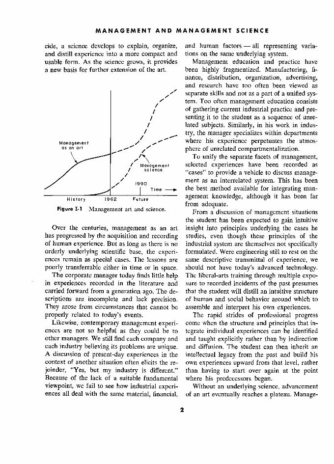
MANAGEMENT AND MANAGEMENT SCIENCE E
cide, a science develops to explain, organize, and human factors - all representing varia- and distill experience into a more compact and tions on the same underlying system. usable form. As the science grows, it provides Management education and practice have a new basis for further extension of the art. been highly fragmentized. Manufacturing, fi-
nance, distribution, organization, advertising, and research have too often been viewed as
separate skills and not as a part of a unified sys- / tem. Too often management education consists
/ of gathering current industrial practice and pre- / senting it to the student as a sequence of unre-
1 lated subjects. Similarly, in his work in indus- / try, the manager specializes within departments
Management where his experience perpetuates the atmos- as an art phere of unrelated compartmentalization.
To unify the separate facets of management, Management selected experiences have been recorded as
/ sc i e nce "cases" to provide a vehicle to discuss manage-
/ 1990 ment as an interrelated system. This has been
T i me - the best method available for integrating man-
Hisrory 1962 Future -
agement knowledge, although it has been far
Figure 1-1 Management art and science. from adequate. Figure 1-1 Management art and ' From a discussion of management situations the student has been expected to gain intuitive
Over the centuries, management as an art insight into principles underlying the cases he has progressed by the acquisition and recording studies, even though these principles of the of human experience. But as long as there is no industrial system are themselves not specifically orderly underlying scientific base, the experi- formulated. Were engineering still to rest on the ences remain as special cases. The lessons are same descriptive transmittal of experience, we
poorly transferrable either in time or in space. should not have today's advanced technology. The corporate manager today finds little help The liberal-arts training through multiple expo- ' in experiences recorded in the literature and sure to recorded incidents of the past presumes
carried forward from a generation ago. The de- that the student will distill an intuitive structure
scriptions are incomplete and lack precision. of human and social behavior around which to
They arose from circumstances that cannot be assemble and interpret his own experiences. properly related to today's events. The rapid strides of professional progress
Likewise, contemporary management experi- come when the structure and principles that in- ences are not so helpful as they could be to tegrate individual experiences can be identified other managers. We still find each company and and taught explicitly rather than by indirection each industry believing its problems are unique. and diffusion. The student can then inherit an A discussion of present-day experiences in the intellectual legacy from the past and build his context of another situation often elicits the re- own experiences upward from that level, rather
joinder, "Yes, but my industry is different." than having to start over again at the point Because of the lack of a suitable fundamental where his predecessors began. viewpoint, we fail to see how industrial experi- Without an underlying science, advancement ences all deal with the same material, financial, of an art eventually reaches a plateau. Manage-
2
§1.2 THE E MANAGER AND MANAGEMENT SCIENCE E
ment has reached such a plateau. If progress is matical economics and management science to continue, an applied science must arise as have often been more closely allied to formal a foundation to support further development of mathematics than to economics and manage- the art. Such a base of applied science would ment. The difference in viewpoint is evident if
permit experiences to be translated into a com- one compares the business literature with publi- mon frame of reference from which they could cations on management science, or descriptive be transferred from the past to the present or economics books with texts on mathematical from one location to another, to be effectively economics. In many professional journal arti-
applied in new situations by other managers. cles the attitude is that of an exercise in formal
logic rather than that of a search for useful solu- 1.2 The Manager and Today's Management tions of real problems. In such an article, as-
Science sumptions having doubtful validity are stated
The search for a scientific base underlying in an introductory paragraph and adopted
management goes back at least to the beginning without justification. On this formal but un-
of this century. It has progressed through work realistic foundation is then constructed an ana-
simplification and statistical quality control. It lytic mathematical solution for the behavior of
has expanded into the "operations research" the assumed system.
activities which followed World War II. With Another evidence of the bias of much of to-
few exceptions, the attempts toward a manage- day's management science toward the mathe-
ment science have dealt with isolated situations matical rather than the managerial motivation
at the bottom of the management structure. is seen in a preoccupation with "optimum"' so-
Thus far, management science still has not lutions. For most of the great management
penetrated the inner circle of top management.1 i problems, mathematical methods fall far short
Partly this is because much of the work in of being able to find the "best" solution. The
operations research has dealt with problems of misleading objective of trying only for an opti-
operating departments - not thé problems of mum solution often results in simplifying the
top management and the board of directors. problem until it is devoid of practical interest.
Partly, as shown in Figure I-1, management The lack of utility does not, however, detract
science is not effective at the top-management from the elegance of the analysis as an exercise
level because the science is still embryonic. in mathematical logic, nor does it prevent the
Management science has not reached a level publication of a paper in a professional journal.
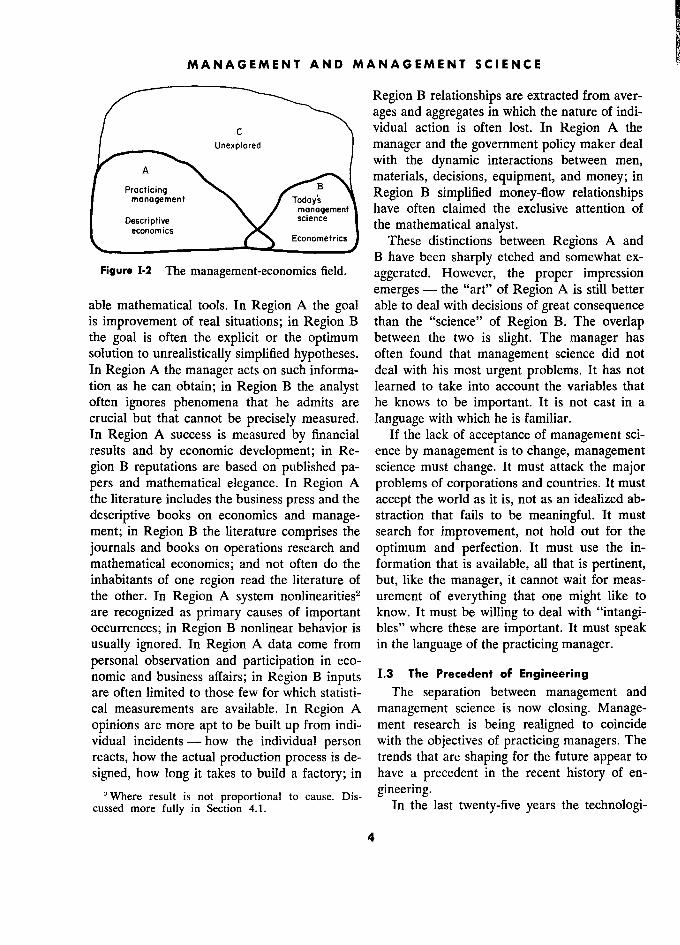
that is effective as a supplement to the skillful Figure 1-2 illustrates the conspicuous di-
practice of top management as an art. Partly it chotomy which has persisted between a Region
is because management science has only begun A: representing practicing managers and econo-
to deal with the time dimension in business - mists, and a Region B, representing the mathe-
the changes and evolution with time that are the matical analyst of business and economic phe-
manager's principal concern. nomena. In business, Region A is inhabited by
But primarily, management science has failed men responsible for decisions and policy, and
to assist top management because the philoso- Region B by staff specialists. In academic cir-
phy and objectives of management science have cles, Region A is the home of the descriptive
often been irrelevant to the manager. Mathe- social scientist whose skill is measured by his ' acuteness in perceiving the motivations and in-
' See Peter Drucker's discussion (Reference 1 ) of terrelationships in economic and managerial the failure of management science to deal thus far affairs; iri contrast, Région B is more apt to in- with the "risk-making and risk-taking decisions of ' 6 r
business enterprise."
' clude those searching for problems to fit avail-
3
MANAGEMENT AND MANAGEMENT SCIENCE E
Region B relationships are extracted from aver-
ages and aggregates in which the nature of indi-
/ c vidual action is often lost. In Region A the
j _ Unexplored manager and the government policy maker deal
with the dynamic interactions between men,
t
A
\. materials, decisions, equipment, and money; in
t Procticing Region B simplified money-flow relationships t management Todoys o r r
) x / management have often claimed the exclusive attention of
§§§i§§(§ the mathematical analyst.
\. economics Econometrics These distinctions between Regions A and
B have been sharply etched and somewhat ex-
Figure 1.2 The management-economics field. aggerated. However, the proper impression
emerges - the "art" of Region A is still better
able mathematical tools. In Region A the goal able to deal with decisions of great consequence is improvement of real situations; in Region B than the "science" of Region B. The overlap the goal is often the explicit or the optimum between the two is slight. The manager has
solution to unrealistically simplified hypotheses. often found that management science did not
In Region A the manager acts on such informa- deal with his most urgent problems. It has not
tion as he can obtain; in Region B the analyst learned to take into account the variables that
often ignores phenomena that he admits are he knows to be important. It is not cast in a
crucial but that cannot be precisely measured. language with which he is familiar.
In Region A success is measured by financial If the lack of acceptance of management sci-
results and by economic development; in Re- ence by management is to change, management
gion B reputations are based on published pa- science must change. It must attack the major
pers and mathematical elegance. In Region A problems of corporations and countries. It must
the literature includes the business press and the accept the world as it is, not as an idealized ab-
descriptive books on economics and manage- straction that fails to be meaningful. It must
ment; in Region B the literature comprises the search for improvement, not hold out for the
journals and books on operations research and optimum and perfection. It must use the in-
mathematical economics; and not often do the formation that is available, all that is pertinent, inhabitants of one region read the literature of but, like the manager, it cannot wait for meas-
the other. In Region A system nonlinearities2 urement of everything that one might like to
are recognized as primary causes of important know. It must be willing to deal with "intangi-
occurrences ; in Region B nonlinear behavior is bles" where these are important. It must speak
usually ignored. In Region A data come from in the language of the practicing manager.
personal observation and participation in eco-
nomic and business affairs; in Region B inputs 1.3 The Precedent of Engineering
are often limited to those few for which statisti- The separation between management and
cal measurements are available. In Region A management science is now closing. Manage-
opinions are more apt to be built up from indi- ment research is being realigned to coincide
vidual incidents - how the individual person with the objectives of practicing managers. The
reacts, how the actual production process is de- trends that are shaping for the future appear to
signed, how long it takes to build a factory; in have a precedent in the recent history of en-
2 Where result is not proportional to cause. Dis- gineering.
cussed more fully in Section 4.1. In the last twenty-five years the technologi-
4

§I.3 3 THE PRECEDENT OF ENGINEERING
cal upsurge in our modern society illustrates the ning in the theory of industrial organizations changes that can be anticipated in management that will bear the same relationship to manage- during the next two or three decades. The ment that physics does to engineering. Both the
changes in the status and world position of en- strengths and weaknesses of this statement are
gineering since 1935 are of the same nature, intended. Physics has provided the foundation and have occurred for the same fundamental for a great upsurge in technology. But it is not
reasons, as the changes we can expect in man- adequate to specify the "best" design of a
agement and economics between now and space vehicle nor to guarantee our ability to 1985. make a roof that does not leak. Physics is a
Over the last twenty years, technology has foundation of principle to explain underlying held the spotlight in the center of the world phenomena but not a substitute for invention,
stage, just as management and economics will perception, and skill in applying the principles. during the remainder of this century. Further- Organization for Research. Twenty years more, the fundamental reasons for great ad- ago the concept of how to organize for scien- vances in management will be essentially the tific research began to change. Before that, re- same as those that have thrust science and en- search was most often a one-man activity. Now
gineering to a dominant international position. team research is recognized as essential if re-
Empirical Practice and Scientific Base. Be- sources are to match the tasks adequately. fore 1935 engineering tended to be an empirical Until recently research in the social sciences art following handbook procedures, precedent, has been largely at the individual level in the and experience. In the same way, management form of doctoral theses and university faculty today is an empirical art. research. (We can scarcely count as research
Before World War II, basic scientific devel- the large group efforts devoted to the collection
opments in the world's universities lacked close of statistical data. These have provided infor- ties to the practice of engineering. There was no mation useful to the practice of management as
strong applied science intermediate between an art, but gathering data is not the creation of basic information and its practical application. an underlying science.) Industrial research laboratories were the excep- The attitude toward management research is tion rather than the rule. In the same way we now changing, and we already see corporations now see a developing body of applicable basic beginning to assign groups for research into the science that has not yet found its way into the underlying fundamentals of management poli- practice of management. cies and decisions. Just as we now expect a
After 1940, the practice of engineering be- percentage of the sales dollar to go to product gan to converge with the underlying science. research, so we may come to expect in the
Engineering advancement was founded more future that a certain fraction of the manage- closely on mathematics, physics, and chemistry. ment and white-collar payroll should be de- The methods, instruments, and attitudes of re- voted to research toward managerial innova- search were no longer foreign to the practical tion. fields of application. Research came to be rec- System Awareness. Over the last two dec-
ognized as an essential part of the technological ades, engineering has developed an articulate
process. Likewise, managers are now beginning recognition of the importance of sy.stems en- to recognize the importance of an applied sci- gineering. Systems engineering is a formal ence foundation underlying the practice of man- awareness of the interactions between the parts agement. of a system. A telephone system is not merely
1 believe that developments are now begin- wire, amplifiers, relays, and telephone sets to
5
MANAGEMENT AND MANAGEMENT SCIENCE
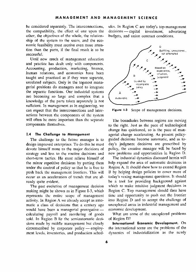
be considered separately. The interconnections, ules. In Region C are today's top-management the compatibility, the effect of one upon the decisions -
capital investment, advertising other, the objectives of the whole, the relation- budgets, and union contract conditions.
ship of the system to the users, and the eco-
nomic feasibility must receive even more atten- D tion than the parts, if the final result is to be Boffiing, unexplored, successful. /
ottempted
Until now much of management education c lx and practice has dealt only with components. 4 Accounting, production, marketing, finance, 'P ,
eosed on '
. T i. / exper.ence. human relations, and economics have been / "/ intuition
taught and practiced as if they were separate, B
". Judgment
unrelated subjects. Only in the topmost mana- incomplete
- -+ ,v incomplete
gerial positions do managers need to integrate policy
the separate functions. Our industrial systems A . -
are becoming so large and complex that a ( Automatic
knowledge of the parts taken separately is not \. a sufficient. In management as in engineering, we
can expect that the interconnections and inter- Figure 1-3 Scope of management decisions.
actions between the components of the system will often be more important than the separate The boundaries between regions are moving
components themselves. to the right. Just as the pace of technological
change has quickened, so is the pace of man-
1.4 The Challenge to Management agerial change accelerating. As present policy-
The challenge to the future manager is to guided decisions become automatic, and as to-
design improved enterprises. To do this he must day's judgment decisions are prescribed by
devote himself more to the major decisions of policy, the creative manager will be faced by
strategy and less to the routine decisions and new problems and opportunities in Region D.
short-term tactics. He must relieve himself of The industrial dynamics discussed herein will
the minor repetitive decisions by putting them help expand the area of automatic decisions in
under the control of policy so that he is free to Region A. It should show how to extend Region
push back the management frontiers. This will B by helping design policies to cover more of
occur as an acceleration of trends that are al- today's vexing management questions. It should
ready quite evident. be a tool for providing background against
The past evolution of management decision which to make intuitive judgment decisions in
making might be shown as in Figure 1-3, which Region C. Top management should then have
represents the entire scope of management time and opportunity to push out the frontier
activity. In Region A we already accept as auto- into Region D and to accept the challenge of
matic a class of decisions that a century ago unexplored areas in industrial management and
would have been a managerial prerogative - economic development.
calculating payroll and reordering of goods What are some of the unexplored problems
sold. In Region B lie the semiautomatic deci- of Region D?
sions made by middle management but closely International Economic Development. On
circumscribed by corporate policy -
employ- the international scene are the problems of the
ment levels, inventories, and production sched- dynamics of industrialization as the newly
6

§I.4 THE CHALLENGE TO MANAGEMENT T
emerging countries of the world move from agri- the individual has become the "organization cultural to industrial economies. man"; and the essence of capitalism, with its
The history of economic development in the competition and its objective basis for reward, Western countries is not directly applicable as has disappeared from the immediate environ- a guide for today's new societies. In the eco- ment of the individual. nomic development of Europe and the United As an estimate, 1 would put this middle-man- States the pace was gradual; education, capital agement lifetime effectiveness as low as a tenth
accumulation, and technological change ad- of the maximum possible. We should not hope vanced together. Other parts of the world are for the maximum; but certainly a manyfold in-
developing in a different environment. Their crease in a 10% effectiveness is possible be-
elementary economies exist in the presence of fore a point of diminishing returns is reached. nations with a high standard of living. Their Our problems of international technological people are impatient to reach the economic competition lie here in the ineffectiveness with level of more advanced countries. Capital for- which we use our human resources of scientists, mation, education, and the aspirations of the engineers, and managers within the corporation people must grow in synchronism if revolution - not in attempts to divert more students into and war are not to overtake economic develop- technology. We cannot, nor could we afford to, ment. attract enough of the population into middle-
The manager of the future must assist in management and technical positions to com- this orderly growth while pursuing his own busi- pensate for such low levels of ability develop- ness. He must avoid policies and investments ment and motivation. in other countries that are incompatible with Long-Range Planning. Another future chal- the development of those countries and hence lenge to management is in the whole realm of with his own long-range welfare. long-range planning. Here we see much lip
The manager will find a world commerce far service but little real action. Plans, where they different from the past. Newly industrialized exist, are apt to be but wishes - goals of countries will compete for markets. The world's greater sales or higher profit without a plausible raw materials will be more in demand. sequence of steps for achieving those goals.
We see already that the international strug- Where long-range plans do exist, they seldom
gle of the 1950's that was based on military have substantial content beyond a five-year technological competition is changing to a span; yet the momentum of our corporations struggle to achieve economic strength and suf- and our economy is such that five years is prac- ficient understanding of economic change to tically the minimum time in which it is possible form a new basis for world leadership. to create any real changes. Past decisions on
Middle Management and Technical Effec- new product research, development of person- tiveness. Closer to home, the corporation has nel, choice of products and markets, and con- a challenge to improve the effective use of its struction of manufacturing facilities have al-
middle-management and technical personnel. In ready determined the essential characteristics of this group, from the 22-year-old college gradu- the corporation for the next five years. The ate to the vice-president, the average lifetime challenge lies in how today's decisions will af- contribution is a small fraction of that which is fect the time interval between five and twenty potentially possible. Individuals are not devel- years hence.
oped to their fullest abilities, and existing abil- Our industrial society has become increas- ities are not challenged to their greatest contri- ingly dependent on decisions that are made bution. A bureaucracy has evolved in which further and further ahead of the period of their
7
MANAGEMENT AND MANAGEMENT SCIENCE E
maximum impact; yet the social pressures on there has been an essential change. The man- the individual have diminished the personal ager of the large, mature corporation is a trus-
emphasis on serious thought about the future. tee. He does not stay more than a few years in The consequences of important decisions that one position nor reap the long-range successes control economic growth once lay inside the and failures that follow his decisions. Emphasis time horizon of the individual's personal plan- is on short-term results; even his own personal ning; now the reverse is more typical. future is assured by retirement plans. His busi-
In a simple agrarian economy, a decision to ness and his position in it are not to be left to
plant and till affected production and the ability his children. As our economy has evolved, the to consume six months or a year later. In personal-interest time horizon has shrunk from
early industrial economies, the essential deci- a lifetime to a few years. sions to construct simple factories affected pro- This modern discrepancy between the distant duction and consumption two or three years consequences of required decisions and the later. As the industrial age emerged, the capital brief tenure of men in the positions where the
equipment industries appeared wherein deci- decisions are made unavoidably reduces re- sions on new tools led to their manufacture, sponsibility and morale. The man is judged on
which, in turn, made new consumer goods fac- results determined by his predecessors and tories possible, which eventually produced con- makes decisions that will affect primarily his sumable products - the interval between pri- successors.
mary decisions and economic results had
lengthened to ten years or more. Now we find 1.5 5 The Manager and Future Management that key decisions relate to research in frontier Science products that will require the development of materials and tools, then of production facili- Managing is the task of designing and con-
ties, then of markets - the span from primary trolling an industrial system. Management sci-
research decision to the full consequences has ence, if it is to be useful, must evolve effective risen to twenty years or more. methods to analyze the principal interactions
As the momentum of the industrial society among all the important components of a com-
has increased, the delays in its response to pany and its external environment. It must be
key decisions have lengthened. By contrast, able to synthesize improved industrial systems. the time span of interest to the individual has Management now stands at a frontier lead- been shortening. ing to a new understanding of industrial growth
In personal planning for the future in an ele- and stability. This new insight into industrial
mentary agricultural economy, the family ex- and economic behavior will come from a better
pects to spend a lifetime on one farm; a person grasp of the time-varying interactions between
looks ahead to building an estate for old age the major facets of our social systems. Manage- and retirement; decisions are made in the light ment education and practice are, 1 believe, on
of their future effect on the decider and his the verge of a major breakthrough in under- children. Likewise, in earlier industrial econo- standing how industrial company success de-
mies, capitalism meant a direct relationship be- pends on the interactions between the flows of
tween success and reward, both financial re- information, orders, materials, money, person- ward and the feeling of accomplishment. The nel, and capital equipment. The way these six
entrepreneur stayed with his business and com- flow systems interlock to amplify one another mitted his own future to the wisdom of his and to cause change and fluctuation will form
management decisions. In our modern economy a basis for anticipating the effects of decisions,
8
§1.5 5 THE MANAGER AND FUTURE MANAGEMENT SCIENCE E
policies, organizational forms, and investment and approaches are more akin to those of the choices. practicing manager than to the management
"Industrial dynamics," as used here, is a science specialist of recent years. From verbal method of systems analysis for management. It description, experience, field observations, and deals with the time-varying interactions between such data as are available will be evolved the the parts of the management system. corresponding mathematical models. I hope to
As a science emerges with the power and show, however, that mathematical notation can
scope to deal with today's practical top-man- be kept close to the vocabulary of business; that
agement problems, the gap between the science each variable and constant in an equation has and today's management art will at first narrow. individual meaning to the practicing manager; The science will develop more rapidly than it that the successful manager of the future can is accepted. As the science reaches maturity, understand, in fact will help originate, the rela- it then becomes a basis for a further develop- tionships described by the equations; that the ment of the art of management. required mathematics is within the reach of
The task of the manager will become more almost anyone who can successfully manage a
challenging. His training will become more modern corporation. rigorous. The new professionalism will not If a management science useful to the top bring automatic success. New tools used with- manager is to be achieved, it must coincide out proper understanding can lead to disaster. with Region A of Figure 1-2, bringing a tool In the hands of those who use them correctly that can enter the circles of responsible line
they become a new competitive advantage to- management. Staff specialization in manage- ward business success. ment science that is apart from the responsible
Management science does not mean auto- manager will in time give way to a professional matic management. It means a platform from level of line management, where the manager which to reach further by the exercise of mana- understands his tools well enough to know their
gerial intelligence and judgment. strengths and their limitations. This imposes The following chapters treat the way in new demands on the manager and his educa-
which the components of the business enter- tion. The answers obtained from using any sci-
prise interact on one another. The approach is entific methods are only as pertinent as the
one of building experimental models of com- questions that are asked. The validity of the re-
panies and industries to determine the influ- sults are only as good as the assumptions on ences of organization and policy. which the study is based. The manager must
Although the methods are quantitative and become able to take the responsibility for the result in a mathematical representation of the questions asked, for the assumptions inserted, business system, the philosophy, objectives, and for the interpretation of results.
9


1
THE MANAGERIAL VIEWPOINT
Part 1 is a nontechnical introduction to the nature and objectives of in- dustrial dynamics. The three chapters are recommended to all readers.
. Chapter 1 defines and describes what we mean by industrial dynamics. It mentions the steps in an industrial dynamics study (which are further developed in Chapter 3), states several premises underlying industrial
dynamics (which are illustrated and supported throughout the book), and review.s the four lines of historical development that make the present book possible. . Chapter 2 provides an illustration, in managerial lerins, of the way the
dynamic responses of an indus trial system can be subjected to experi- mental study. e Chapter 3 discusses the concept of a management laboratory for enter-
prise design and suggests some changes that can be expected in manage- ment practice and education.
11 1

CHAPTER 1
Industrial Dynamics
Industrial dynamics is the investigation of the information-feedback char- acter of industrial systems and the use of models for the design of im-
proved organizational form and guiding policy. Industrial dynamics '
grows out of four lines of earlier development - information-feedback theory, automatizing military tactical decision making, experimental de-
sign of complex systems by use of models, and digital computers for low- cost computation. Each of these is reviewed as part of the background from which this book has evolved.
THIS book treats the time-varying (dynamic) Trace the cause-and-effect information-feedback
behavior of industrial organizations - indus- loops that link decisions to action to resulting trial dynamics. information changes and to new decisions.
Industrial dynamics is the study of the in- e Formulate acceptable formal decision policies formation-feedback characteristics of industrial that describe how decisions result from the
activity to show how organizational structure, , available information streams. _ _
amplification (in policies), and time delays (in e Construct a mathematical model of the decision
decisions and actions) interact to influence the policies, information sources, and interactions
success of the enterprise. It treats the interac- of the system components.
tions between the flows of information, money, Generate the behavior through time of the sys-
orders, materials, personnel, and capital equip- tem as described by the
model (usually with a
ment in a company, an industry, or a national i digital computer to execute the lengthy calcula- ment m a company, an mdustry, or a national
tions). computer to execute the lengthy calcula-
economy. Compare results against all pertinent available
.,r . Compare results against all pertinent available
Industrial dynamics provides a single frame- ' Compare about the actual pertinent available
us na
? vi es a smg e
rame- knowledge about thé actual System. work for integrating the functional areas of f knowledge about the actual system. as a repre-
management - production, ac- * Révise thé mode! until it is acceptable as a repre-
management - marketing, production, ac- sentation of the actual system. as a repre-
sentation of thé actual System. counting, research and development, and capi-
sentation of the actual system. organizational . ° .. - < Re esign withm thé mode!, thé organizationa! tal investment. It is a quantitative and experi- relationships and the model, the organizational mental 1 h for relating organizational 1 relationships and pohcies which can be altered mental approach for relating organizational in the actual system to find the changes which h structure and corporate policy to industrial
improve system behavior. growth and stability. a Alter the real system in the directions that model
Industrial dynamics should provide a basis experimentation has shown will lead to im-
for the design of more effective industrial and proved performance. economic systems. An industrial dynamics ap- proach to enterprise design progresses through Such an approach is based on several prem- several steps : ises:
Identify a problem.. Décisions in management and economics take
. Isolate the factors that appear to interact to cre- place in a framework that belongs to the general ate the observed symptoms. class known as information-feedback systems.
13 3
INDUSTRIAL DYNAMICS
Our intuitive judgment is unreliable about how A knowledge of decision-making processes these systems will change with time, even when . experimental model approach to complex we have good knowledge of the individual
systems parts of the system. , parts of the system. e The digital computer as a means to simulate
. Model experimentation is now possible to fill the realistic mathematical models. gap where our judgment and knowledge are
'
weakest - by showing the way in which the Because of the important part these four known separate system parts can interact to play in making industrial dynamics possible, produce unexpected and troublesome over-all each will be reviewed in some detail.
. system results. . Enough information is available for this experi- j _j Information-Feedback Control Theory
mental model-building approach without great The first and most important foundation for expense and delay in further data gathering.
Thé first and most important foundation for expense and delay m further data
h f and delay in further data gathering. . industrial dynamics is the concept of servo- . The mechanistic view of décision makine The "mechanistic" view of decision making mechanisms (or information-feedback sys- implied by such model experiments is true
tems) as enough so that the main structure of controlling tems)
as evolved during and after World War
policies and decision streams of an organization 11'' Until recently we have been insufficiently
can be represented. aware of the effect of time delays, amplification, . Our industrial systems are constructed internally
and structure on the dynamic behavior of a sys- in such a way that they create for themselves tem. We are coming to realize that the interac-
many of the troubles that are often attributed tions between system components can be more to outside and independent causes. important than the components themselves.
. Policy and structure changes are feasible that The concepts of information-feedback sys- will produce substantial improvement in indus- tems will become a principal basis for an under- trial and economic behavior; and system per- lying structure to integrate the separate facets of formance is often so far from what it can be the management process. What is an informa- that initial system design changes can improve tion-feedback system? 1 should like to give a all factors of interest without a compromise broad definition: that causes losses in one area in exchange for An information-feedback system exists when- gains in another.
ever the environment leads to a decision that re- Why are these premises now a sound basis sults in action which affects the environment
for developing a better understanding of the and thereby influences future decisions. behavior of industrial systems? The approach This is a definition that encompasses every discussed in this book would not have been feas- ible The rieed has long ex- In References 2 and 3 are listed early texts recom- ibie
even a décade
Ihe need has long ex- mended to the beginner as simplified treatments r _ u., mended to the beginner as simplified treatments of
isted for better insights into the problems of the mathematical theory of servomechanisms. Brown
management and economics, but the corner- and Campbell (Reference 4) give a more complete stones for an adequate approach have ??? ? ? treatment
of transient analysis.
In these three books stones or an .a ? PP have ? will be found references to the early papers of the
cently been laid. field. The serious worker in dynamics of industrial Four foundations on which to construct an systems should acquire as background an understand-
improved understanding of the dynamics Of ing of linear servomechanisms analysis. The methods improved understanding
of thé will find little use as such, but they help provide the social organizations have been built m the intuitive "feel" about the way amplification and de- United States since 1940, primarily as a by- lays combine to create total system behavior. The
systems These books in Reference 5 carry the treatment of informa-
product of military systems research. These tion-feedback systems into the effects of noise and four are: intermittent data, give an excellent picture of the
.. scope of linear information-feedback system theory, e 'The theory of information-feedback systems and contain generous references.
14
91.1 INFORMATION-FEEDBACK CONTROL THEORY
conscious and subconscious décision made by fects of making only slight changes in system struc-
people. It also includes those mechanical deci- ture and time delays. Suppose the driver were
sions made by devices called servomechanisms. blindfolded and drove only by instructions from
Systems of information-feedback control are his front-seat companion. The resulting few sec-
fundamental to all life and human endeavor, onds of increased information delay and the
f th 1 f 1 .
1 1. .
t ' slightly greater information distortion caused by from the slow pace of biological évolution to slightly greater information distortion caused eye mserting voice and ear between the observing eye the launching of the latest space satellite. To and the driver's brain would cause erratic driving.
illustrate: Still worse, if the blindfolded driver could ..
. A thermostat receives temperature information get instructions only on where he had been
and décides to start the furnace; this raises the from a companion who could see only through température, and the furnace is stopped.
. from a companion who could sec only through
A '
th h f Il h. thé rear window, ms driving would be even
* A person senses that he may fall, corrects his the
rear window, his driving would be even
balance, and thereby is able to stand erect. more erratic. Yet this is the situation in business.
In business, orders and inventory levels lead d Top executives do not see the salesmen calling
to manufacturing decisions that fill orders, cor- on customers, do not see the prospective buyers
rect inventories, and yield new manufacturing watchmg a télévision commercial. They do not
decisions. attend the board meetings of competitors. They
. A profitable industry attracts competitors until do not have a clear view of the road ahead. The
the profit margin is reduced to equilibrium with only thing they can tell, and that with only par- other economic forces, and competitors cease to tial certainty, is what happened in the past. enter the field. In an information-feedback system it is al-
* The competitive need for a new product leads ways the presently available information about
to research and development expenditure that the past which is being used as a basis for de-
produces technological change. ciding future action.
All of these are information-feedback con- Everything we do as an individual, as an Al of thèse are information-feedback con-
trol loops. The regenerative process is continu- industry, or as a society is done in the context
trol loops. The regenerative process is continu- of an information-feedback system. The denni- .. a an information-feedback system. The defini- ous, .
and new results lead to new décisions tion of such a system is so ail-inclusive as to which keep the system in continuous
motion. seem meaningless at first. Yet we are only now Such systems are not necessarily well behaved.
becoming sulficiently aware of the tremendous In fact, a complex information-feedback system significance of information-feedback system designed by happenstance or in accordance
,t,? ? ??ting thé behavior of thèse designed by happenstance or in accordance parameters in creating the behavior of these
with what may be intuitively obvious will usu- systems.
ally be unstable or ineffective. d eals wlth .
Information-feedback systems, whether they The study of feedback systems deals with be mechanical, biological, or social, owe their the way information is used for the purpose of behavior to three characteristics - structure, con t ro. 1 1 teps h 1 us ta understand how the
behavlOr ta three charactenstlcs - structure, control. It helps us to understand how thé
delays, amplification. The structure of a amount of corrective action and the time delays system tells amplification. are re 1 ate d to of
a
in interconnected components can lead to un- another. Delays always exist in the availability stable fluctuation. Driving an automobile pro- of information, in making décisions based on vides a good example: the information, and in taking action on the de-
The information and control loop extends from cisions. Amplification usually exists throughout
steering wheel, to automobile, to street, to eye, such systems, especially in the decision policies to hand, and back to steering wheel. We accept of our industrial and social systems. Amplifica- this complex system thoughtlessly. Consider the ef- tion is manifested when an action is more force-
15 s
INDUSTRIAL DYNAMICS
ful than might at first seem to be implied by the able mathematics. The problems, the needs, information inputs to the governing decisions. and the tools were adequately matched for two We are only beginning to realize the way in decades of progress in the dynamics of physi- which structure, time lags, and amplification cal systems. combine to determine behavior in our social sys- Our social systems are a great deal more com- tems. plex than the information-feedback systems that
Why has the fundamental nature and the have already been mastered in engineering. Are
importance of information-feedback systems es- we ready to tackle them?
caped notice until the last three decades? 1 Our knowledge of information-feedback sys- think it is because of the peculiar classes into tems has been growing in that exponential man- which these systems fell before 1940. On the ner so characteristic of the early phase of any one hand, we had the biological information- area of human knowledge. The ability to deal feedback systems that regulate body tempera- with information-feedback systems seems to ture, muscular coordination, and other functions. have been progressing by about a factor of 10 These systems had been so ideally perfected per decade. for their purposes, and at the same time In the late 1930's the scientific papers in the we had so completely accepted their shortcom- field dealt with the dynamic characteristics of
ings, that the systems and their information- very simple control systems described by linear feedback character went unnoticed. On the differential equations of two variables. By the other hand, social, economic, and industrial early 1940's the field had developed into the
systems have evolved in recent centuries but on concepts of Laplace transforms, frequency re- so large a scale compared with the individual sponse, and vector diagrams. that the fundamental information-feedback But as usual, the forefront of mathematics characteristics were most difficult to discern. was unable to cope with the problems of major Furthermore, hosts of other explanations have engineering interest. Military necessity exerted been advanced for the behavior that arises di- pressure. Engineers did not long linger waiting rectly from the information-feedback character for analytical solutions to information-feed- of these systems. Explanations have been in back-system behavior. Linear and nonlinear terms of the superficial specific manifestations mathematical models were constructed for solu- of the particular problem rather than in the tion on analog computing machines. By 1945 more fundamental terms of generalized closed- systems of 20 variables were easy to handle -
loop systems. a tenfold increase over 1935. The theory and concepts of information-feed- By the end of the second decade, in 1955,
back systems have developed recently as a re- new methods and new areas were again being sult of trying to build simple self-regulating con- pioneered. The digital computer had appeared, trol systems. As control devices developed be- opening the way to the simulation of systems yond the early steam-engine governor, greater far beyond the capability of analog machines.
precision was needed. The systems to be con- With the new tools, attention began to center trolled became more complex. The dynamic on the information-feedback characteristics of characteristics and system difficulties became military combat systems incorporating both obvious and on a scale small enough for study. equipment and people. Systems of 200 variables
Strong commercial and military incentives en- could be feasibly studied.
couraged attempts to master the theory of The pace has not slackened. We are now en-
information-feedback-system design. Initial sim- tering the 1965 era with another factor of 10
ple problems lay within the reach of the avail- within reach. Models of 2,000 variables, with
16
§ 1 .3 3 EXPERIMENTAL APPROACH TO SYSTEM ANALYSIS S
no restrictions on representing nonlinear phe- man organization to respond. A decade of time
nomena, put us within a vast area of important and thousands of people were involved in this
managerial and economic questions. interpretation of military decision processes and automatizing the operational policies that
1.2 Decision-Making Processes are the basis for tactical military decision mak- The second foundation for industrial dy- ing. It has been amply demonstrated that care-
namics is the better understanding of decision fully selected formal rules can lead to short-
making achieved in the 1950's during the au- term tactical decisions that excel those made by tomatizing of military tactical operations. human judgment under the pressure of time, or
Historically, military necessity has often led with men having irisufficient experience and not only to new devices like aircraft and digital practice, or in the rigidity of large organiza-
computers but also to new organizational forms tions. and to a new understanding of social forces. Men who started to formalize decision-mak- These developments have then been adapted to ing policy in 1950 in the environment of "you civilian usage. can't make a machine substitute for my military
Such innovations have appeared in the mili- training and command experience" have in ten
tary command (or management) function. As years seen the same critics accept as better and the pace of warfare has quickened, there has of as commonplace the automatic execution of
necessity been a shift of emphasis from the tac- front-line military "judgment." The resulting tical decision (moment-by-moment direction of body of practical experience in determining the the battle) to strategic planning (preparing for basis for decisions and the content of "judg- possible eventualities, establishing policy, and ment" is now becoming available to the study determining in advance how tactical decisions of management systems. Many men from mili- will be made). The battle commander can no tary systems research are now moving into the
longer plot the course of his enemy on a chart study of industrial and economic systems. and personally calculate the aiming point. In As in military decisions, we shall see that
fact, with a ballistic missile he would have no there is an orderly basis that prescribes much time even to select his defensive weapon.2 of our present managerial decision making. De-
During World War II, fire-control prediction cisions are not entirely "free will" but are decisions were made automatically by machine, strongly conditioned by the environment. This but before 1950 there was almost no accept- being true, we can set down the policies govern- ance of automatic threat evaluation, weapon ing such decisions and determine how the poli- selection, friend and foe identification, alerting cies are affecting industrial and economic be- of forces, or target assignment. In a mere ten havior.
years these automatic decisions were pioneered, accepted, and put into practice. In so doing, it 1.3. Experimental Approach to System was necessary to interpret the "tactical judg- Analysis .
ment and experience" of military decision mak- The third foundation for industrial dynamics ing into formal rules and procedures. This is the experimental approach to understanding change was forced because the pace of modern system behavior.
military operations exceeded the ability of a hu- Mathematical analysis is not powerful ' There is little useful literature on the subject of enough to yield general analytical solutions to
automatizing of military decisions, not so much be- situations as complex as are encountered in cause of military security classification as because the business. The alternative is the experimental changes in attitudes toward military decision making g have received scant philosophical documentation. approach.
17
,
. , ,. , , . _ . " I NDUSTRIAL dYNAMiCS
A mathemàticàl model of the industrial sys- can be tested to determine their effects on com- tem is constructed. Such a mathematical model pany success. is a detailed desciiption that tells howthe con- Instead of going from the general anàlytical ditions at one point in time lead to subsequent solution to the particular special case, we have conditidns at later points in time. The behavior corne to appreciate the great utility, if not the of the niodel is observed, ànd experimënts are mathematical elegancë, of the empirical ap- coilductèd to answer specific questions about proach. In this we study a number of particular the system that is répresënted by the model. situations, and from these we generalize as far
"Simulation" is a name of2en applied fo this as we dare.
process of conducting experitments on a model Use of simulation methods will not require instead of attempeing the experiments with the great mathematical ability. To be sure, details real System. During the 1950's simulation was of setting up a model need to be monitored by extensively developed in thé design of air de- experts becaùse there are special skills required fense systems" and in'engineering work. For and pitfalls to be avoided. However, )he job example: ,, of chbosing the situations to be explored, judg- '
ing the assumptions, and interpreting the results In planning the a river basin, is within the ability of the type of men we now
numbers in a digital computer represent water see in management schools and executive de- volumes, flow fates, electriè demand, and rainfall.
velopmérit programs. A few seconds computer time can represent a '
whole day of actuat system, opération. Dams can j _4 Digital Computers be located and designed for an adequate compro- The fourth foundation for industrial dy- mise between tne conflicting demands of power
oun ation for mdustrial y
generation, irrigation, navigation, and flood con- namics progress is the electronic digital com-
trol. '
. ' '
puter that became. generally available between " 1955 and 1960. Without it, the vast amourit of
Likewise, sirriple simulation studies of parts work to obtain specific solutions to the charac- of a busiriess have,been common in the last few teristics of 'complex systems would be prohibi- years and are reported in the opérations re- tively expensive. In the last fiffeen years the search , litèrature. Simulation techniques have épst of arithmetic computation has fallen by a a now reàched a statë of devëlopment where they factor of 10,000 or more in thosé aréas where can be àpplied.to thé top-management problems digital computers can be used in their most ef- of indus trial organisations, ficÍent modes of operation. The simulation of
In business, simulation means setting up in information-feedback models of industrial be- a digital computer the conditions thàt describe havior is such an area of high efficie?cy. A cost
company operations. 'On the basis of the de- reduction factor of 10,000 or 100,Ô00 creates
scriptions and assumptions about the company, a totally different research environment than the computer then gerierates the resulting time existed even a decade ago. charts of information cbncerning finance, man- After World War II the advent of computing power, product movement, and so on. Different machines brought the feasibility of dealing with
management policies and market assumptions more complex systems. Analog-type com-
puters, as used in electrical-power-system net-
a Simulation studies of military systems have re- work analyzers and in differential equation ceived tens of thousands of man-years of effort in analyzers, had been developed from 1930 to the last decade, both to study system behavior and 1950. At first, attempts were made to use
system. to provide ways to train men in their duties in the
analog computing devices for the study of eco-
' 18 8
.

§ 1 .4 DIGITAL COMPUTERS S
nomic systems.4 However, these analog com- tor of nearly 10 per year over the decade of the
puters proved inadequate to cope with problems 1950's; in almost every year there was a ten- of practical interest. They do not readily deal fold increase in speed, memory capacity, or re- with nonlinear systems. The upper capacity liability. Over-all, this was a technological limit of such machines barely overlaps the mini- change greater than that effected in going from mum size and complexity that must interest us chemical to atomic explosives. Society cannot in economic and corporate problems. absorb so big a change in a mere ten years. We
The appearance of high-speed electronic have a tremendous untapped backlog of poten- digital computers has removed the practical tial devices and applications. It is now to be
computational barrier. The technical perform- expected that machine progress will stay ahead ance of electronic computers increased by a fac- of conceptual progress in industrial and eco-
' A book by Tustin (Reference 6) discusses the nomic dynamics. Computing machines are now similarities between economic systems and electrome- so widely available, and the cost of computation chanical servomechanisms. In broad concept, the book and machine programming is so low relative to anticipates present simulation studies; in detail, it is L ). , out of date in referring only to analog computers and Other costs, that the former dlfficulties in acti- classical types of simple models of economic behavior. vating a simulation model need no longer de- It is recommended, however, as background on the termine our rate of progress in understanding havior.
view of economic be- system dynamics.
r o o
.
19

CHAPTER 2
An Industrial System
Before starting the discussion in Part Il of the philosophy and methodology of industrial dynamics, it seems best to give the reader a quick exposure to the kinds of results toward which we are working. In this chapter a
simple model of a distribution system will be used to show how the form and the policies of an organization can give rise to characteristic and un- desirable modes of behavior. Indication of ways to improve the system
'
will appear, but the process of system redesign will be illustrated in another context in Chapter 18. We begin with a verbal description of the system. The details of actual model construction are postponed until Chapter 15. But u.sing that model, this chapter proceeds to illustrate the kinds of questions that can be explored. It is the intent of this chapter to provide a motivation for further study of the subject. We shall here examine:
. How small changes in retail sales can lead to large swings in factory production
How reducing clerical delays may fail to improve management deci- sions significantly
How a factory manager may find himself unable to fill orders although at all times able to produce more goods than are being sold to con- sumers
How an advertising policy can have a magnifying effect on production variations
THE general description of industrial dynam- questions to be answered. This initial example ics in the first chapter should become more must be kept simple. It will be wise, for the
meaningful in the context of a simple example. sake of clear explanation, to start with a very How do the concepts of information-feedback limited subsystem of an entire company. To
systems apply to specific business situations? maintain this initial simplicity, the questions we
Or, stated differently, how do the delays and ask must deal with problems whose causes lie
amplifications in the circuital flow of informa- within a restricted part of the industrial enter- tion in a company affect its operations? How prise. Later we can range more broadly over the can we use a model of such a system to discover management field. the way its components affect its over-all be- The central core of many industrial com- havior ? panies is the process of production and distri-
bution. A recurring problem is to match the 2.1 The Approach production rate to the rate of final consumer
The first step in a system study is to identify sales. It is well known that factory production clearly the problem to be explored and the rate often fluctuates more widely than does
21 1
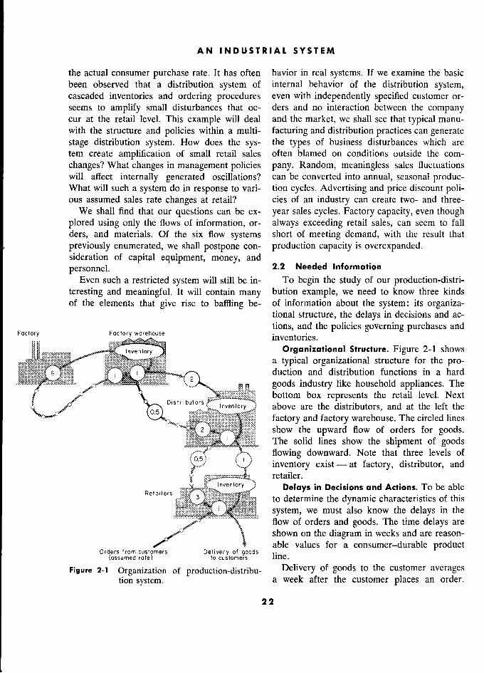
AN INDUSTRIAL SYSTEM
the actual consumer purchase rate. It has often havior in real systems. If we examine the basic been observed that a distribution system of internal behavior of the distribution system, cascaded inventories and ordering procedures even with independently specified customer or- seems to amplify small disturbances that oc- ders and no interaction between the company cur at the retail level. This example will deal and the market, we shall see that typical manu- with the structure and policies within a multi- facturing and distribution practices can generate stage distribution system. How does the sys- the types of business disturbances which are tem create amplification of small retail sales often blamed on conditions outside the com-
changes ? What changes in management policies pany. Random, meaningless sales fluctuations will affect internally generated oscillations? can be converted into annual, seasonal produc- What will such a system do in response to vari- tion cycles. Advertising and price discount poli- ous assumed sales rate changes at retail? cies of an industry can create two- and three-
We shall find that our questions can be ex- year sales cycles. Factory capacity, even though plored using only the flows of information, or- always exceeding retail sales, can seem to fall
ders, and materials. Of the six flow systems short of meeting demand, with the result that
previously enumerated, we shall postpone con- production capacity is overexpanded. sideration of capital equipment, money, and
personnel. 2.2 Needed Information
Even such a restricted system will still be in- To begin the study of our production-distri- teresting and meaningful. It will contain many bution example, we need to know three kinds of the elements that give rise to baffiing be- of information about the system: its organiza-
tional structure, the delays in decisions and ac-
Factory Fcictory worehouse tions, and the policies governing purchases and ?'ory Factory warehouse inventories.
BËEmmsw? jnventory Organizational Structure. Figure 2-1 shows a typical organizational structure for the pro- duction and distribution functions in a hard
gn goods industry like household appliances. The
\ bottom box represents the retail level. Next
Distribulors Invenfory above are the distributors, and at the left the
factory and factory warehouse. The circled lines show the upward flow of orders for goods. The solid lines show the shipment of goods flowing downward. Note that three levels of
inventory exist - at factory, distributor, and retailer.
Inventory Delays in Decisions and Actions. To be able to determine the dynamic characteristics of this
' ;' system, we must also know the delays in the flow of orders and goods. The time delays are
\ shown on the diagram in weeks and are reason-
Orders from customers Delivery of goods able values for a consumer-durable product Orders tram custamers Delivery of goods able
values for a consumer-durable product (assumed rote) fa customers line.
Figure 2-1 Organization of production-distribu- Delivery of goods to the customer averages tion system. a week after the customer places an order.
22
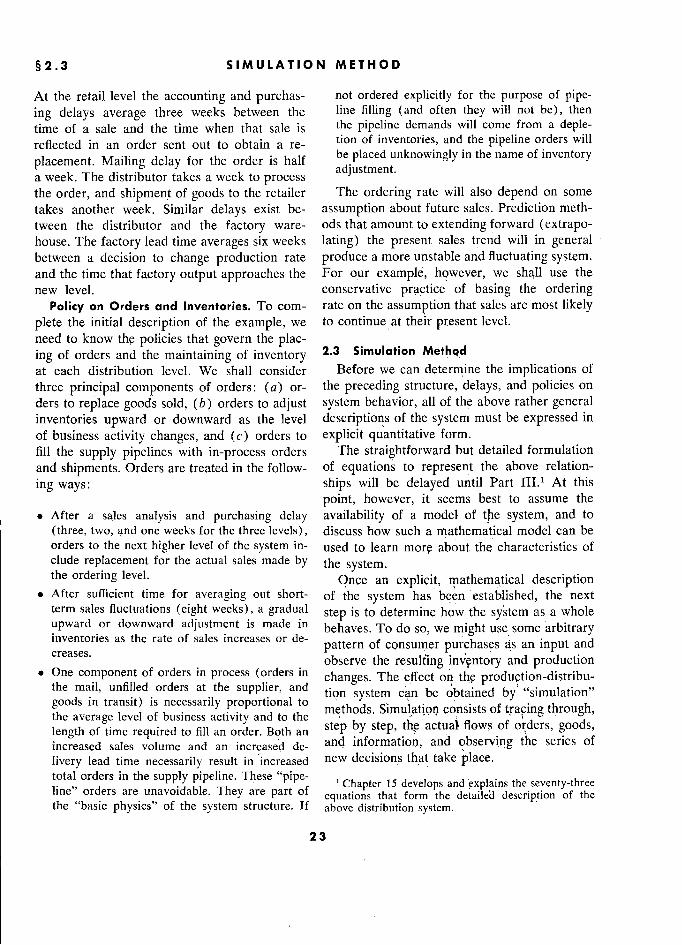
§2.3 SIMULATION METHOD
At the retail level the accounting and purchas- not ordered explicitly for the purpose of pipe-
ing delays average three weeks between the line filling (and often they will not be), then
time of a sale and the time when that sale is the pipeline demands will corne from a deple-
reflected in an order sent out to obtain a re- tion of inventories, and the pipeline orders will
placement. Mailing delay for the order is half be placed unknowingly in the name of inventory
a week. The distributor takes a week to process adjustment.
the order, and shipment of goods to the retailer The ordering rate will also depend on some
takes another week. Similar delays exist be- assumption about future sales. Prediction meth-
tween the distributor and the factory ware- ods that amount to extending forward (extrapo- house. The factory lead time averages six weeks lating) the present sales trend will in general between a decision to change production rate produce a more unstable and fluctuating system. and the time that factory output approaches the For our example, h9wever, we shall use the
new level. conservative practice of basing the ordering Policy on Orders and Inventories. To com- rate on the assumption that sales are most likely
plete the initial description of the example, we to continue at their present level.
need to know the policies that govern the plac- ing of orders and the maintaining of inventory
2.3 Simulation Methq,d
at each distribution level. We shall consider Before we can détermine the implications of
three principal components of orders: (a) or- the preceding structure, delays, and policies on
ders to replace goods sold, (b) orders to adjust system behavior, all of the above rather general inventories upward or downward as the level descriptions of the system must be expressed in
of business activity changes, and (c) orders to explicit quantitative form.
fill the supply pipelines with in-process orders The straightforward but detailed formulation
and shipments. Orders are treated in the follow- of equations to represent the above relation-
ing ways: ships will be delayed until Part IIL1 At this
point, however, it seems best to assume the
After a sales analysis and purchasing delay availability of a model of the system, and to
(three, two, and one weeks for the three levels), discuss how such a mathematical model can be orders to the next higher level of the system in- used to learn morç about the characteristics of clude replacement for the actual sales made by the system. the ordering level. .
Once an explicit, mathematical description After sufficient time for averaging out short- of the system has been established, the next
term sales fluctuations (eight weeks), a gradual step is to determine how the system as a whole upward or downward adjustment is made in behaves. To do so, we might use some arbitrary inventories as the rate of sales increases or de-
pattern of consumer purchases as an input and creases.
.. observe the resulting inventory and production . One component of orders in process (orders in
changes. The effect on thç produçtion-distribu- the mail, unfilled orders at the supplier, and tion system can be obtained by "simulation"
" tion system can be àbtàined by' "simulation" goods in transit) is necessarily proportional
to methods. Simulation consists of tracing through, 1 1 f b. t th SImulatIOn conslsts of traclllg through, thé average level of business activity and to thé , . " ' ;
length of time required to fill an order. Both an step by step, the actual flows of orders, goods,
increased sales volume and an increased de- and information, and observing the series of
livery lead time necessarily result in increased new decisions that take place. total orders in the supply pipeline. Thèse "pipe- ,_, ,,, , . ,.. , ,. total orders
in the supply pipeline.
These "pipe- ' Chapter 1 5 develops and ,explains the seventy-three line" orders are unavoidable. They are part of
equations that form the detailed description of the the "basic physics" of the system structure. If above distribution system.
23 '
I .... I .. , I . , . I , I . I .... I ..
Factory orders
Retail inventory IAR (units)
Factory orders
from distributors RRF
(units/week)
- 4% Manufacturing orders ta factory MOF (units/week)
51% Foctory production output SRF (units/week)
1500 ».. - -
Distributor orders _
from retailersRRD +34% O
Distributor inventory IAD (uriits)
(uniis /week ) £ - - - - - - - - -
/ ,
- -
+'O% +12%
Z) 7- __ / _ - __ _ ·s2
+32% _-_ _
1000
_ . -
- Retail sales RRR
(unifs/week) Factory worehouse 3nventory
[AF (units)
- T....
Foctory warehouse unfilled
00
', orders UOF (units) +56%
500 , ', ..
,' o
T weeks \ -·-·-·-·-·-·-·-· ..
2.4 weeks
°
à , _ £ _ _ .-°-°-°-°-°-°-°-
2-week dela 20% increase U
Factory warehouse
.-8-8-.-.-.-.-8-e-
Factory warehouse
average order-filling
0 10 20
delay DFF (weeks)
, , 10 20 1 60 7p Feb Mur Moy Aug M Sept Dec Feb Apr Jun
Figure 2-2 Response of production-distribution system to a sudden 10% increase in retail sales.
As an example of simulation, our produc- which are represented more precisely by the tion-distribution system might be acted out by equations in Chapter 15. Alternatively, the a group of men around a table, one to repre- whole exercise can be done by one person sent retailers, another the postal service, an- in tabular form on paper. Better still, the en- other transportation, another the factory, and tire sequence can be programmed on a digital so on. Five minutes might represent a computer.a Digital-computer simulation was and in each time interval the proper purchase used to obtain the following results. orders and deliveries would be made according to the policies which were described above and 2.4 System Experiments
It now becomes possible to test how the
= For this kind of laborious, manual simulation, above production-distribution system would re-
- or this kind 0 laborious, manual simulation, larger time steps are usually used than are appropriate spond to any arbitrarily specified lnput. We if a good representation of system detail is to be might think that we should choose some actual generated, as can be done on a computer. The fol- lowing computer-simulated examples were computed ' A description of how these studies are handled each twentieth of a week. See Appendix D on solution with the "DYNAMO" compiler on a digital computer interval. will be found in Appendix A.
24
§2.4 SYSTEM EXPERIMENTS
sales history as a trial input. This can be done cause the incoming-order level at the distributors
later, but any such complex pattern will be persists above retail sales for more than four
unduly confusing at this introductory stage. months and is readily mistaken for an enduring '
It is more informative to take simple, "pure," increase in business volume. The distributors'
sequences for preliminary study purposes. Such orders to the factory, therefore, include not only simple patterns include a step (a sudden change the 18% increase in orders they themselves from one constant level to another), or a receive but also a corresponding increase for sinusoid ( a smoothly fluctuating disturbance). distributor inventories and for orders and goods A more complex artificial pattern would be in transit between distributor and factory. As some random-noise curve of specified statistical a result, orders at the factory warehouse reach, characteristics. at the 14th week, a peak of 34% above the
Step Input. A very informative input is the previous December.
simple step. It provides a single disturbance at Let us turn now to manufacturing orders. the input and allows us to observe how the They are placed on the basis of the increasing
'
internal components of the system respond factory warehouse orders and the falling ware- thereafter. Figure 2-2 shows the result of a house inventory, which drops 15%. Manufac- 10% increase in retail sales introduced in Janu- turing orders rise 51 % at the 15th week. As
ary. The resulting fluctuations are shown in a result, the factory output, delayed by a factory order rates, factory output, factory warehouse lead time of 6 weeks, reaches a peak in the 2 1 st
inventory, and unfilled orders. (Retail orders week, an amount 45% above the previous De- are here given as an input that is independent cember. While retail sales are still at 10%
'
of what happens in the production-distribution above December, the factory increase has be- "
system itself. Retail orders are, of course, not come over four times as great. . actually independent since they are affected by It is important to note that all of these effects
availability of the product and by advertising, are reversible. As retailers satisfy their inven- a point to be discussed later.) tory requirements, they decrease their order
Because of accounting, purchasing, and mail- rate. The distributors find they have built up an
ing delays, the increase in distributors' orders order rate, an inventory, and a supply-line rate from retailers lags about a month in reaching in excess of needs. They take the excess out of the 10% level. It is important to note, how- current orders to the factory, so that at the 32nd
ever, that the rise does not stop at 1 0%l . Instead week this order rate is 6% below retail sales it reaches a peak of 18% at the llth week be- and only 4% above the previous December. cause of the new orders that have been added at In September and October at the 39th week the the retail level (a) to increase inventories some- factory output drops to 3% below the previous what and (b) to raise the level of orders and December and 13 % below current retail sales.
goods in transit in the supply pipeline by 10% As a direct result of the typical organizational to correspond to the 10% increase in sales form shown in Figure 2-1 and of the customary rate. These inventory and pipeline increments inventory and ordering policies described, over occur as "transient" or nonrepeating additions a year is required before all ordering and to the order rate, and when they have been manufacturing rates stabilize to their proper satisfied, the retailers' orders to the distributors levels corresponding to the 10% retail sales in-
drop back to the enduring 10% increase. crease. Ironically, this increase was minor com- The factory warehouse orders from distribu- pared to the fluctuations in company opera-
tors show an even greater swing. This is be- tions.
25
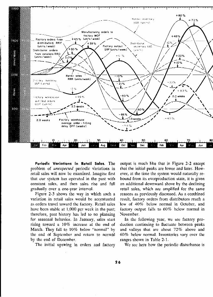
... : 1 1 1 1
+eo % Retail inventory ' IAR (units)
°
MGnufacturing orders Io . _ factory MOF o/
1500 _._ Factory orders from -_ t45 % (units/week) a fl distributors RR F / \ Distributor \ \ (units / week) t / Factory output "
inventory IAD \ '
Distributor orders SRF(units/week)\ (units) / /
/ \ \ / from retailers RRD
+51 % / +22 % N e r
(units /week )
_ ,
/ ,/ '
a v v
/
Retail 'sales ' ,
-10 % .· j\ '' \
Factory inventory
RRR ( unlls/w ee ̀ k 1 -., - .._...--'' /
/ /
/
\ RRR (units/week /
, IAF (units)
21 % 33% /w -12 %
-
/ , / / il 3 */%. %
Factory warehouse ? +49% %
\ /\/ unfllled orders .il
\ '/`
500 UOF
$ 6 0
"
£,'£ç.h.-.,',
60 % °?'Ç
. 2.0weeks' warehouse ???? °
fl;
average order-filling *"*
deloy DFF (weeks) 54
%
.00
0 10 ; i2 10..... 10..510, 60 70 !
Feb Apr Jun Aug S,,t m Dec Feb Apr Jun M
Periodic Variations in Retai) Sales. The output is much like that in Figure 2-2 except problem of unexpected, periodic variations in that the initial peaks are lower and later. How- retail sales will now be examined. Imagine first ever, at the time the system would naturally re- that our system has operated in the past with bound from its overproduction state, it is given constant sales, and then sales rise and fall an additional downward shove by the declining gradually over a one-year interval. retail sales, which are amplified for the same
Figure 2-3 shows the way in which such a reasons as previously discussed. As a combined variation in retail sales would be accentuated result, factory orders from distributors reach a as orders travel toward the factory. Retail sales low of 40% below normal in October, and have been stable at 1,000 per week in the past; factory output falls to 60% below normal in therefore, past history has led to no planning November. for seasonal behavior. In January, sales start In the following year, we see factory pro- rising toward a 10% increase at the end of duction continuing to fluctuate between peaks March. they fall to 10% below "normal" by and valleys that are about 72% above and the end ôf September and return to normal 60% below normal. Inventories vary over the
by the end of December. ranges shown in Table 2-1. The initial upswing in orders and factory We see hère how the periodic disturbance is
26
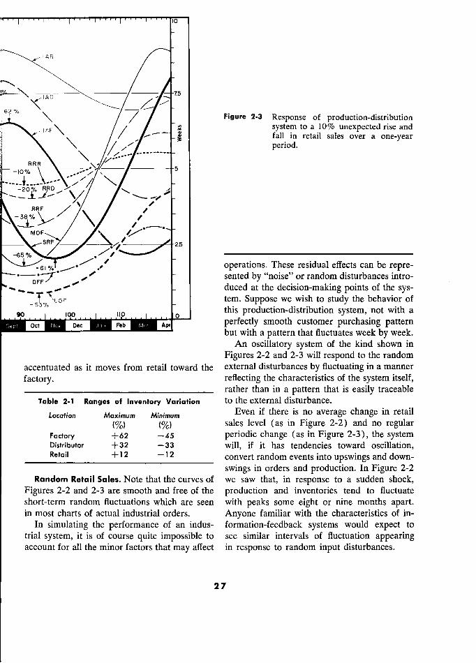
..................j i ... 10
IAR AR /
\
D
/
1° / /
Figure 2-3 Response of production-distribution
IAF\ /
/ system to a 10% unexpected rise and '
/ / fall in retail sales over a one-year
\ period.
RRR
----------
RRR / - -io%
5
RRD . RPF / /. /
MOF /. -
- SRF ode -25
65 % ––––––––––––––––––––––––––––––––––––––––
operations. These residual effects can be repre- '
sented by "noise" or random disturbances intro-
- duced at the decision-making points of the sys-
tem. Suppose we wish to study the behavior of
so .... 1 no 0 this production-distribution system, not with a
Dec Feb Apr
°
perfectly smooth customer purchasing pattern
but with a pattern that fluctuates week by week.
An oscillatory system of the kind shown in
Figures 2-2 and 2-3 will respond to the random
accentuated as it moves from retail toward the external disturbances by fluctuating in a manner
factory. reflecting the characteristics of the system itself,
____________________________ rather than in a pattern that is easily traceable
Table 2-1 Ranges of Inventory Variation to the external disturbance.
Locafion Maximum Minimum Even if there is no average change in retail
(%) (%o) sales level (as in Figure 2-2) and no regular
Factory +62 -45 periodic change (as in Figure 2-3), the system
Distributor +32 -33 will, if it has tendencies toward oscillation,
Retail +12 -12 convert random events into upswings and down-
swings in orders and production. In Figure 2-2
Random Retail Sales. Note that the curves of we saw that, in response to a sudden shock,
Figures 2-2 and 2-3 are smooth and free of the production and inventories tend to fluctuate
short-term random fluctuations which are seen with peaks some eight or nine months apart.
in most charts of actual industrial orders. Anyone familiar with the characteristics of in-
In simulating the performance of an indus- formation-feedback systems would expect to
trial system, it is of course quite impossible to see similar intervals of fluctuation appearing
account for all the minor factors that may affect in response to random input disturbances.
27
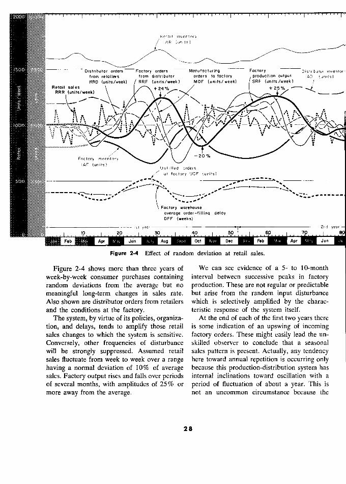
Retail inveritory IAR (units )
1500 Distributor ordersfactory orders Manufacturing Factory Y Distributor invento
jNtN from retailers from distributor orders tofoctory production output IAD (units) RRD (units/week)
RRF (units/week) MOF (units/week) SRF (units/week)
Retail sales +24 % + - RRR (units/week) - -
-
,
_
j , , i ·
y , , .
1000 '. a \ .i : _
î, / ii v \r i '/ ,` y 111
; v . v
-\ W'
i /
.. n .W v
.i n \
Cr Factory inventory 20 ?
IAF (unifs) Untilled orders Unfilled orders
of factory UOF (units)
v v -
Factory Factory warehouse
--
Factory warehouse '
average order-filling deloy DFF (weeks)
Ist year .]4 2nd yeor
10 10 20 Ist 8
Jo? m m(ir m May i,iy M Sept m Nov m ion m M (1, M,?Y Jun M
Figure 2-4 Effect of random deviation at retail sales.
Figure 2-4 shows more than three years of We can see evidence of a 5- to 10-month
week-by-week consumer purchases containing interval between successive peaks in factory random deviations from the average but no production. These are not regular or predictable meaningful long-term changes in sales rate. but arise from the random input disturbance Also shown are distributor orders from retailers which is selectively amplified by the charac- and the conditions at the factory. teristic response of the system itself.
The system, by virtue of its policies, organiza- At the end of each of the first two years there tion, and delays, tends to amplify those retail is some indication of an upswing of incoming sales changes to which the system is sensitive. factory orders. These might easily lead the un-
Conversely, other frequencies of disturbance skilled observer to conclude that a seasonal will be strongly suppressed. Assumed retail sales pattern is present. Actually, any tendency sales fluctuate from week to week over a range here toward annual repetition is occurring only having a normal deviation of 10% of average because this production-distribution system has sales. Factory output rises and falls over periods internal inclinations toward oscillation with a of several months, with amplitudes of 25%l or period of fluctuation of about a year. This is more away from the average. not an uncommon circumstance because the
28
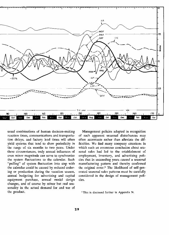
10
IAR
MOF
/ 7.5
o
SRF
fl
% _ / - - ; f,fl
A A -' . 5 '
RRR RRD
- 22% 'AF
2.5
DFF
year
oct Dec 1,0.. , ? . ? 1 ...150 160 1
170
C) j
oct OVL Dec Feb MOLMI-M Apr Jun Auçi Oct Dec Feb
usual combinations of human decision-making Management policies adopted in recognition reaction times, communications and transporta- of such apparent seasonal disturbances may tion delays, and factory lead times will often often accentuate rather than alleviate the dif-
yield systems that tend to show periodicity in ficulties. We find many company situations in the range of six months to two years. Under which such an erroneous conclusion about sea- these circumstances, truly annual influences of sonal sales had led to the establishment of even minor magnitude can serve to synchronize employment, inventory, and advertising poli- the system fluctuations to the calendar. Such cies that in succeeding years caused a seasonal
"pulling" of system fluctuation into step with manufacturing pattern and thereby confirmed the calendar could be caused by reduced order- the original error.4 The likelihood of self-gen- ing or production during the vacation season, erated seasonal sales patterns must be carefully annual budgeting for advertising and capital considered in the design of management poli- equipment purchase, annual model design cies.
changes, and of course by minor but real sea-
sonality in the actual demand for and use of the prodUct. < This is discussed further in Appendix N.
29
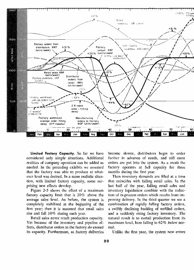
r-I . rT 1
+345% =Z5
v tl2 % prod
Retail I '
inventory 1 AR (units)
+61 /Î
1500
F.cl.,y
_
nvL>,,l lunlsl
#1
.. -
Factory orders from / Distributory
- 13
1## \/
:
tt distributors RRF t31 % ' Factory (units/week)\
output SRF \inventory IAD(units?
/ ' (units /week)
P _ t20 % output SRF , , tt?N
_ +200/. (units/week) +38% = 2?3 /
'
/-20%
\
\ '
p roduction
,,/'
\ \
" -
', , Pr°duction , l' +lo.i
Retail sales RRR
-'
w\ -10 -.
/ ' / (units/week) pistributor
' \ ------ / /
Factory inventory IAF or
\ /
/ (units)
orders from \
i ,,
l /
retail RRD (units/week - 23
\) % /
,'
/
\ / ` , .
))Nt)t)) Factory warehouse .0 + 57 \ /
500 untilled orders UOF *40 ss (units) \ -44%
(un'ts) 2.6-week
-44% -62 % ,
7 order - filling % 2 weeks' deloy , _"§" .roduction , -
,
Factory warehouse Manufacturing ' 0- NNNt average order-filling orders to factory
delay DFF (weeks) MOF (units/week) + 70 2nd
year e 10 ! 20 - 55
%
8
Feb Apr Jun Auq Oct Dec Feb Apr Jun
Limited Factory Capacity. So far we have become slower, distributors begin to order considered only simple situations. Additional further in advance of needs, and still more realities of company operation can be added as orders are put into the system. As a result the needed. In the preceding exhibits we assumed factory operates at full capacity for three that the factory was able to produce at what- months during the first year. ever level was desired. In a more realistic situa- Then inventory demands are filled at a time tion, with limited factory capacity, some sur- that coincides with falling retail sales. In the
prising new effects develop. last half of the year, falling retail sales and
Figure 2-5 shows the effect of a maximum inventory liquidation combine with the reduc-
factory capacity limit that is 20% above the tion of in-process orders which results from im-
average sales level. As before, the system is proving delivery. In the third quarter we see a
completely stabilized at the beginning of the combination of rapidly falling factory orders, first year; then it is assumed that retail sales a swiftly declining backlog of unfilled orders, rise and fall 10% during each year. and a suddenly rising factory inventory. The
Retail sales never reach production capacity. natural result is to curtail production from its Yet because of the inventory and pipeline ef- maximum level, here falling to 62% below nor- fects, distributor orders to the factory do exceed mal. its capacity. Furthermore, as factory deliveries Unlike the first year, the system now enters
30
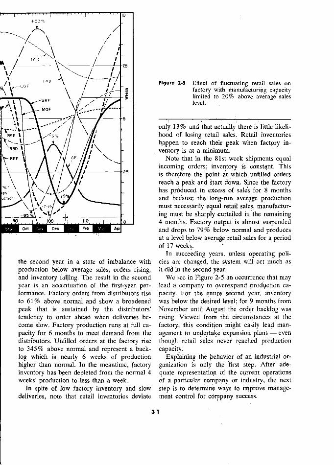
, i 10 , , g .
/ j
/ ' '
IA " .
y \
1 AD
/
/ Figure 2-5 Effect of fluctuating retail sales on
UOF \ factory with manufacturing capacity
\ limited to 20% above average sales SRF
/ --
3 limited
to 20% above average sales
,
1
i ,
/ level.
_ ,
. MOF / -
,i 5 :
,
.
A // - only 13 % and that actually there is little likeli-
RRR t ! //
hood of losing retail sales. Retail inventories
/ happen to reach their peak when factory in- RRD
\ \ / '
ventory is at a minimum.
-RRF A
[AF Note that in the 81st week shipments equal
t / -/ 25
incoming orders; inventory is constant. This
/ is therefore the point at which unfilled orders
N 1, \ jY
' reach a peak and start down. Since the factory
- has produced in excess of sales for 8 months
/ / 79-
and because the long-run average production
–"" \ 74, le
must necessarily equal retail sales, manufactur-
ing must be sharply curtailed in the remaining
1 111.0. 0 4 months. Factory output is almost suspended
and drops to 79% below normal and produces ° . ' '
at a level below average retail sales for a period ' of i 7 week?s.
'
In succeeding years, unless operating poli-
the second year in a state of imbalance with cies are chapged, the system will act much as
production below average sales, orders rising, it did in the second year.
and inventory falling. The result in the second We see in Figure 2-5 àn occurrence that may
year is an accentuation of the first-year per- lead a company to overexpand production ca-
formance. Factory orders from distributors rise pacity. For the entire second year, inventory
to 61 % above normal and show a broadened was below the desired level; for 9 months from
peak that is sustained by the distributors' November until August the order backlog was
tendency to order ahead when deliveries be- rising. Viewed from the circumstances at the
come slow. Factory production runs at full ca- factory, this condition might easily lead man-
pacity for 6 months to meet demand from the agement to undextake expansion plans - even
distributors. Unfilled orders at the factory rise though retail sales never reached production
to 345% above normal and represent a back- capacity.
log which is nearly 6 weeks of production Explaining the behavior of an industrial or-
higher than normal. In the meantime, factory ganization is only the first step. After ade-
inventory has been depleted from the normal 4 quate représentation of the cqrrent operations
weeks' production to less than a week. of a particular company or industry, the next
In spite of low factory inventory and slow step is to determine ways to improve manage-
deliveries, note that retail inventories deviate ment control for company success.
31 1 '
: _
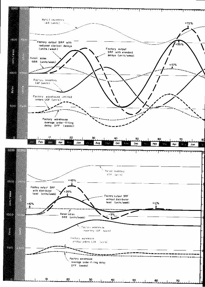
2000 -=- 1 1 1 1 1
r
Retail Inventory IAR (unifs) +72%
. output SRF with
)
1500 FaCtory output SRF with
reduced clerical delays - (units/week) Factory output
SRF with stcindard / - delays (units/week)
Retail sale delays (units/week)
Z) .2 RRR (units/week)
---.
/ /"10%
1000
._ . __._f____
-
Factory inventory - ____,_.
,,,
[AF (units)
;
Factory warehouse unfilled /
,...-...,
orders UOF (units) unlilled
" /':/
" orders UOF (units)
J<
i 'oe ,
··· ' '
< -,-
Factory warehouse .
average order-filling " ,' delay DFF (weeks)
0 e , 10 30 40 50 .7p.... E
Jan M ma, Jun Aug Sept Nov Feb Apr M"y
2000 I .. " I
? Retail inventory IAR (units)
.. +45% 1500
Factory output SRF S F - with
distributor y+26% "'
!C level (units/week) .
Foctory output SRF L. without distributor
+10% level (units/week) +12%
1000 5000 Retail ales RRR (units/week) t,.;;;;;-
'
w.,7eho, se Foctory warehouse
inventory IAF (units)
Factory worehouse unfilled orders UOF (units)
\ average order-fillinq deloy DFF (weeks)
0 0 ........ - 10 .. .... 1 .... 20 .... 1 .. 1 1 1 . "0. 1 .. 1 ...510 60 70 (
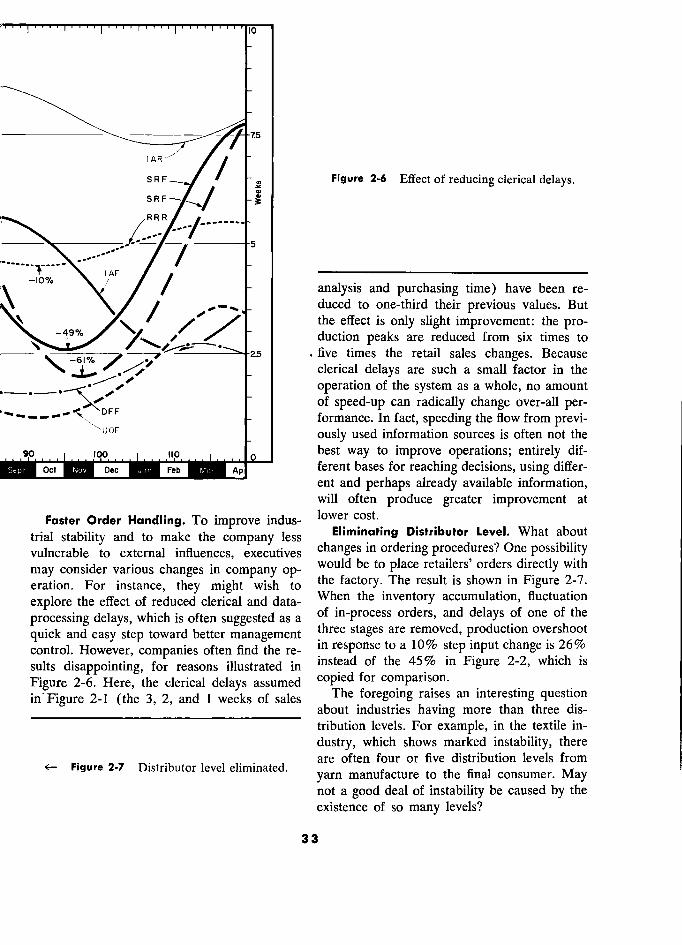
10
75
IAR //
s R F Figure 2-6 Effect of reducing clerical delays.
S R F
RRR
--------
_.. _ °
___ ............... .'
"""
-/
5
analysis and purchasing time) have been re-
IAF / / analysis and purchasing time) have been re-
_ .... -10% / /
- analysis and purchasing time) have been re-
\/ /
duced to one-third their previous values. But S\
-49* / the effect is only slight improvement: the pro-
duction peaks are reduced from six times to .
25. five. times the retail sales changes. Because -
- clerical delays are such a small factor in the
operation of the system as a whole, no amount '
of speed-up can radically change over-all per- - formance. In fact, speeding the flow from previ- ,
UDF - ously used information sources is often not the
'
90 . ?oo no o best way to improve operations; entirely dif-
?ttt?o?tMW??lMtt*?1tBtt*? ferent bases for reaching decisions, using differ-
ent and perhaps already available information, will often produce greater improvement at
Faster Order Handling. To improve indus- lower cost.
trial stability and to make the company less Elimin.ating Distributor Level. What about
vulnerable to external influences, executives changes in ordering procedures? One possibility
may consider various changes in company op- would be to place retailers' orders directly with
eration. For instance, they might wish to the factory. The result is shown in Figure 2-7.
explore the effect of reduced clerical and data- When the inventory accumulation, fluctuation
processing delays, which is often suggested as a of in-process orders, and delays of one of the
quick and easy step toward better management three stages are removed, production overshoot
control. However, companies often find the re- in response to a 10% step input change is 26%
sults disappointing, for reasons illustrated in instead of the 45 % in Figure 2-2, which is
Figure 2-6. Here, the clerical delays assumed copied for comparison.
in Figure 2-1 (thé 3, 2, and 1 weeks of sales The foregoing raises an interesting question
____________________________ about industries having more than three dis-
tribution levels. For example, in the textile in-
dustry, which shows marked instability, there
level are often four or five distribution levels from
Figure 2-7 Distributor level eliminated. yarn manufacture to the final consumer. May not a good deal of instability be caused by the
existence of so many levels?
33
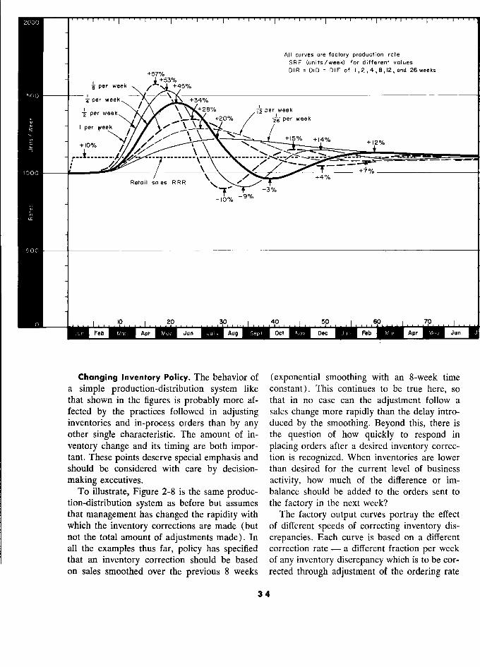
2000
All curves cire factory production rate - SRF (units/week) for différent values
jttt DIR = DID DIF of 1,2,4,8,12, and 26weeks
1500
-6
per 1 per week
J_+53% +45%
+34% § Per +34%
week ,
+2 8 i-2 per
week week
.
per Week à per week
1 per week /
+15% +14% + 1 2 %
-------- ---------- --- .-Ir.
1000 ' _ 100,
-7-/.
etc 1 sales , es R
, _ 7 -3%
+ 4 %
500
io%
Feb Apr Jun Aug Dct Dec Feb Apr Jun
Changing lnventory Policy. The behavior of (exponential smoothing with an 8-week time a simple production-distribution system like constant). This continues to be true here, so that shown in the figures is probably more af- that in no case can the adjustment follow a fected by the practices followed in adjusting sales change more rapidly than the delay intro- inventories and in-process orders than by any duced by the smoothing. Beyond this, there is other single characteristic. The amount of in- the question of how quickly to respond in
ventory change and its timing are both impor- placing orders after a desired inventory correc- tant. These points deserve special emphasis and tion is recognized. When inventories are lower should be considered with care by decision- than desired for the current level of business
making executives. activity, how much of the difference or im- To illustrate, Figure 2-8 is the same produc- balance should be added to the orders sent to
tion-distribution system as before but assumes the factory in the next week? that management has changed the rapidity with The factory output curves portray the effect which the inventory corrections are made (but of different speeds of correcting inventory dis- not the total amount of adjustments made). In crepancies. Each curve is based on a different all the examples thus far, policy has specified correction rate a différent fraction per week that an inventory correction should be based of any inventory discrepancy which is to be cor- on sales smoothed over the previous 8 weeks rected through adjustment of the ordering rate
34
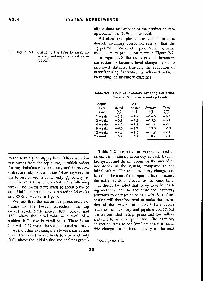
§2.4 SYSTEM EXPERIMENTS S
ally without undershoot as the production rate
approaches the 10% higher level. All other examples in this chapter use the
4-week inventory correction rate so that the
F' 2 8' "4 per week" curve of Figure 2-8 is the same
<- Figure 2-8 Changing the time to make in- as the factory production curve in Figure 2-2. (°Y d P° °° ° In Figure 2-8 the more gradual inventory rections.
correction to business level changes leads to
improved stability. Further, the reduction of
manufacturing fluctuation is achieved without
increasing the inventory extremes.
Table 2-2 Effect of Inventory Ordering Correction Time on Minimum Inventory Levels
Adjust- Dis- . ment Retail tributor Factory Total
Time (%) l%) (%) (%) 1 week -3.6 -9.4 -16.0 -6.6 2 weeks -3.9 -9.8 -15.8 -6.9 4 weeks -4.2 -9.9 -14.8 -7.0 8 weeks -4.6 -9.7 -13.0 -7.0
12 weeks -4.8 -9.6 -11.9 -7.1 26 weeks -5.2 -9.2 -10.2 -7.1
____________________________ Table 2-2 presents, for various correction
to the next higher supply level. This correction stem minimum inventory at each level in rate varies from the top curve, in which orders y minimum for the sum of ail
for any imbalance in inventory and in-process inventories in the system, compared to the
orders are fully placed in the following week, to initial values. The total inventory changes are
the lowest curve, in which only of any re- less than the sum of the separate levels because
maining imbalance is corrected in the following the extremes do not occur at the same time.
week. The lowest curve leads to about 60% of It should be noted that many sales forecast-
an initial imbalance being corrected in 26 weeks lng methods tend to accelerate the inventory
and 85 % corrected in 1 year. reactions to changes in sales levels. Such fore-
We see that the successive production ex- casting will therefore tend to make the opera-
tremes for the 1-week correction (the top tion of the system less stable. This occurs
curve) reach 57% above, 10% below, and because the inventory and pipeline corrections
15 % above the initial value as a result of a are concentrated in high peaks and low valleys
sudden 10% rise in retail sales. There is an and tend to be self-regenerative. The inventory
interval of 27 weeks between successive peaks. correction rates at one level are taken as bona
At the other extreme, the 26-week correction changes in business activity at the next
time (the lowest curve) leads to a peak of only 20 % above the initial value and déclines gradu- 5 See Appendix L. .
35 5
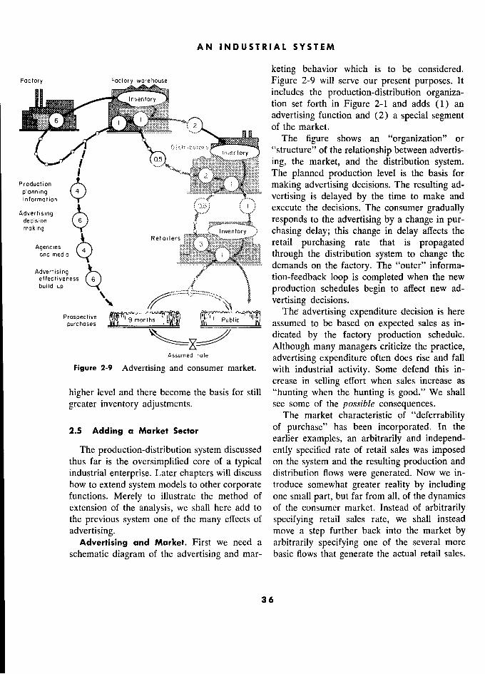
AN INDUSTRIAL SYSTEM
keting behavior which is to be considered. Factory Factory warehouse Figure 2-9 will serve our present purposes. It
M includes the production-distribution organiza- Inventory tion set forth in Figure 2-1 and adds ( 1 ) an
6 advertising function and (2) a special segment 2 of the market.
The figure shows an "organization" or
Distrib tor s Inveritory "structure" of the relationship between advertis-
ing, the market, and the distribution system. 1 ; The planned production level is the basis for
Production \ J< making advertising decisions. The resulting ad- planning J .
d 1 d b h. k d information vertising is delayed by the time to make and
Advertising 0.5 execute the decisions. The consumer gradually decision te) J responds to the advertising by a change in pur- moking
Inventory chasing delay; this change in delay affects the
Agencies d,o
Retoilers retail purchasing rate that is propagated and média 4 through the distribution system to change the
Adverrising
.: demands on the factory. The "outer" informa-
effectiveness s 6 p \ tion-feedback loop is completed when the new build-up
t production schedules begin to affect new ad-
vertising decisions.
Prospective Thé advertising expenditure decision is here
purchases le assumed to be based on expected sales as in- dicated by the factory production schedule.
Although many managers criticize the practice, Assumed rate
advertising expenditure often does rise and fall Figure 2-9 Advertising and consumer market. with industrial activity. Some defend this in-
crease in selling effort when sales increase as
higher level and there become the basis for still "hunting when the hunting is good." We shall
greater inventory adjustments. see some of the po.ssible consequences. The market characteristic of "deferrability
2.5 Adding a Market Sector of purchase" has been incorporated. In the ' earlier examples, an arbitrarily and independ-
The production-distribution system discussed ently specified rate of retail sales was imposed thus far is the oversimplified core of a typical on the system and the resulting production and industrial enterprise. Later chapters will discuss distribution flows were generated. Now we in-
how to extend system models to other corporate troduce somewhat greater reality by including functions. Merely to illustrate the method of one small part, but far from all, of the dynamics extension of the analysis, we shall here add to of the consumer market. Instead of arbitrarily the previous system one of the many effects of specifying retail sales rate, we shall instead
advertising. move a step further back into the market by Advertising and Market. First we need a arbitrarily specifying one of the several more
schematic diagram of the advertising and mar- basic flows that generate the actual retail sales.
36
§2.5 ADDING A MARKET SECTOR
The model has therefore been extended so chase somewhat sooner than they would have
that the independent input is the flow of "pro- with a lower selling effort. ;.
spective purchases." A prospective purchaser Now look more closely at the relationships '
is one who has some awareness of need for the shown in Figure 2-9:
product, who expects to purchase, but has not 0 production planning information is averaged d yet done so. For products like household major over a period of 4 weeks, and the average is appliances, this rate would be determined by the basis for advertising decisions. such factors as the rate of wear-out of existing . A time interval of 6 weeks is assumed for analy- appliances and by new family formation and sis of sales conditions, waiting to be sure of busi- new housing construction. ness trends, and reaching a decision to change
The prospective purchasers are here defined the advertising expenditure rate. as that group who will eventually buy and who. Acting on advertising decisions by agencies and
already have some awareness of their plans media is taken to require 4 weeks. and need to purchase. For a mature, well- . Full buyer awareness of the advertising is as- known, generally accepted product such as sumed to develop over a period of 6 weeks after household refrigerators, much of the market fits the appearance of a new level of advertising. this description. For the industry as a whole, . The average time that prospective buyers con- without yet considering the competitive aspects, template purchase and during which they are
clearly a large fraction of sales is generated subject to advertising influence is assumed to be
independently of advertising and sales efforts. about 9 months in the presence of an "average"
What, then, can be the effect of selling effort level of advertising.
on these prospective customers? It might in- * A 10% change in the advertising level is taken
fluence the average time that the prospective to shorten or lengthen by about 2 weeks the
customer waits between first awareness of need 9-month period during
which the average pro-
and the actual purchase. Could this have any spective buyer considers his purchase. and thé actual purchase. Could tms hâve any spective buyer considers his purchase.
influence on system behavior? How much effect This postpones, to a future model extension, on customer purchasing practices must be the further details of a consumer market - the
created to change the character of the distribu- use of advertising to introduce new products, or
tion system responses as seen in the previous the place of advertising in the competitive rela-
figures ? tionship between companies. The interaction of We are here dealing with a situation where advertising and sales here proposed is most
the purchase is not mandatory at a particular plausible if the production-distribution-adver- moment ; it is deferrable; and presumably the tising system is thought of as representing an actual moment of buying can be somewhat in- entire industry rather than a single company. fluenced by outside persuasion. If advertising The flows are then total industry market, sales, has any effect on the timing of the purchase, and advertising. it should be to shorten the contemplation in- Production Cycle from Advertising Interac- terval as the advertising effort is increased. tions. We can now see what the interaction be-
Customers who are persuaded that prices are tween advertising, sales, and consumer market
now favorable or that the features of new might do to the production-distribution proc- models are desirable, or customers who simply esses already studied. What are some possible have their attention directed toward acting on a implications of gearing the advertising budget
purchase that was already imminent, may pur- to the incoming sales dollar?
37
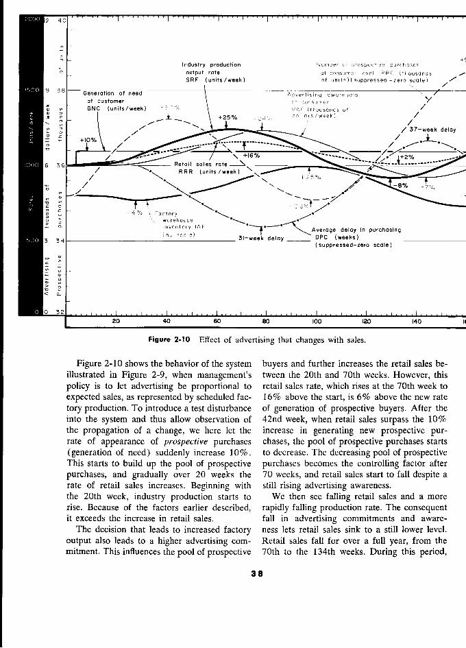
12
!N!N!N!j - Industry production Numberof prospective purchoses
° _ output rate at consumer level PPC (thousands . tNNN) SRF (units/week) of units)(suppressed -zero scale)
Senerat!on Advertising awareness
)N)N)t)j _ otcustomer ) at consumer <* GNC (units/week) +57% \ VAC (thousands of -g
w eek
+25% +241/. dollars/week) /
'" r
,
:> 1 ù
<
/ ,/
, _ _
> , ,
,
+ 2s d 0 1 1 a r s / wee k )
/ 37-week deloy
= - o , F»",»-,« ---------- /
+16 +16% ...... _.i+2*,' .......... 6 36 Retail soles rate
J, -------------
RRR (units /week)
, 2 5
01
14
-8% -7o/, / ' , -70%
g ( 0. 3
u - 4%, F Factor w wore Ouse
inventory IAF
deloy in purchosing (weeks) ___________
t)<OJ)t (suppressed-zero scale)
3 21
20 40 60 80 100 120 140
Figure 2-10 Effect of advertising that changes with sales.
Figure 2-10 shows the behavior of the system buyers and further increases the retail sales be- illustrated in Figure 2-9, when management's tween the 20th and 70th weeks. However, this
policy is to let advertising be proportional to retail sales rate, which rises at the 70th week to
expected sales, as represented by scheduled fac- 16% above the start, is 6% above the new rate
tory production. To introduce a test disturbance of generation of prospective buyers. After the into the system and thus allow observation of 42nd week, when retail sales surpass the 10% the propagation of a change, we here let the increase in generating new prospective pur- rate of appearance of prospective purchases chases, the pool of prospective purchases starts
(génération of need) suddenly increase 10%. to decrease. The decreasing pool of prospective This starts to build up the pool of prospective purchases becomes the controlling factor after
purchases, and gradually over 20 weeks the 70 weeks, and retail sales start to fall despite a rate of retail sales increases. Beginning with still rising advertising awareness. the 20th week, industry production starts to We then see falling retail sales and a more rise. Because of the factors earlier described, rapidly falling production rate. The consequent it exceeds the increase in retail sales. fall in advertising commitments and aware-
The decision that leads to increased factory ness lets retail sales sink to a still lower level.
output also leads to a higher advertising com- Retail sales fall for over a full year, from the mitment. This influences the pool of prospective 70th to the 134th weeks. During this period,
38
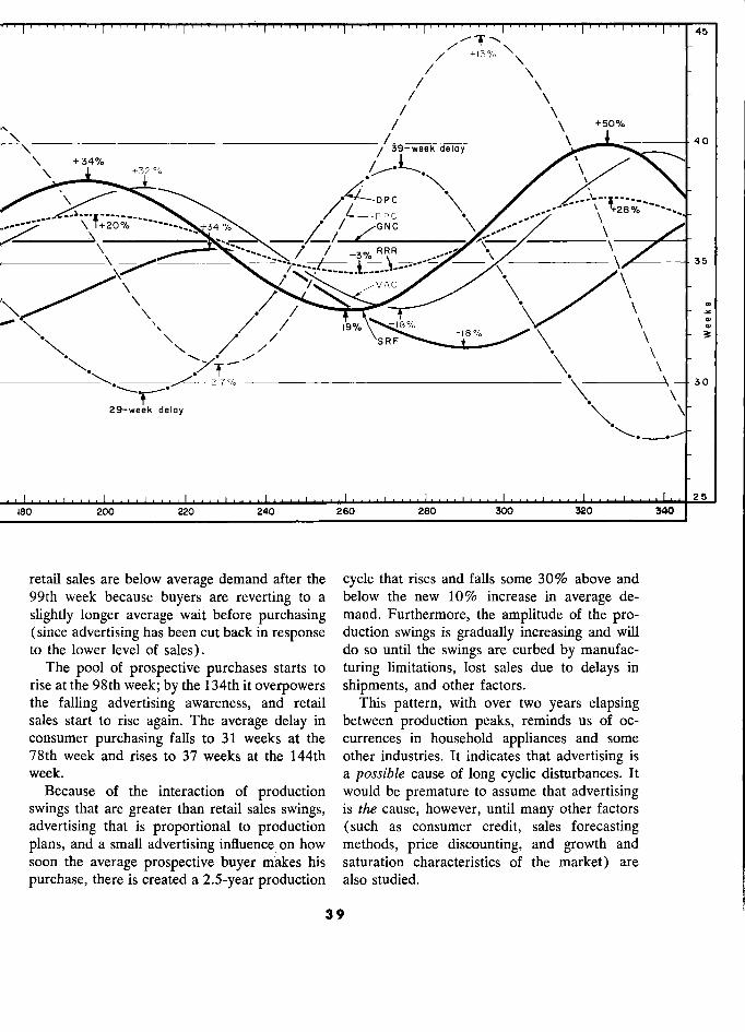
, , , , . 45
.
/ .
/ \ +50%
39-week ,
\ +34% 39-week delay
v \
40
% ,Q.£. ·
"
__ `\1._. ___.- C
j t,
'
N
N - RRR
- 35 /-- wl--____.i_ _
35
, ..
\ \\ ,
% / /
/ 19% VAC -ie %
/°
.
\ N
v ,° CI> CI>
3:
3
30 0 - 2.7 % .
\ 29-week delay \ \'
25
180 200 220 240 260 280 300 320 340
retail sales are below average demand after the cycle that rises and falls some 30% above and 99th week because buyers are reverting to a below the new 10% increase in average de-
slightly longer average wait before purchasing mand. Furthermore, the amplitude of the pro- (since advertising has been cut back in response duction swings is gradually increasing and will to the lower level of sales ). do so until the swings are curbed by manufac-
The pool of prospective purchases starts to turing limitations, lost sales due to delays in rise at the 98th week; by the 134th it overpowers shipments, and other factors. the falling advertising awareness, and retail This pattern, with over two years elapsing sales start to rise again. The average delay in between production peaks, reminds us of oc- . consumer purchasing falls to 31 weeks at the currences in household appliances and some 78th week and rises to 37 weeks at the 144th other industries. It indicates that advertising is week. a possible cause of long cyclic disturbances. It
Because of the interaction of production would be premature to assume that advertising swings that are greater than retail sales swings, is the cause, however, until many other factors
advertising that is proportional to production (such as consumer credit, sales forecasting plans, and a small advertising influence on how methods, price discounting, and growth and soon the average prospective buyer makes his saturation characteristics of the market) are
purchase, there is created a 2.5-year production also studied.
39
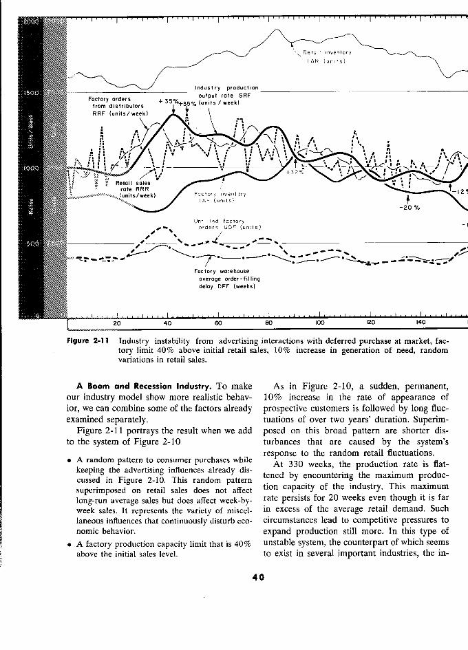
1 ' 1 11
, , . 1 1 1 . 1
1 .
NtttN Retail inventory
I AR t s)
Industry production
NNW
' output rate SRF
from distributors s RRF (uriiis/ week)
n
i ;
, x ;,
.
ÉÀ .
§ £,
%, ;
.. 1, o ( ij
" §
jj ;
fl
32,Y. l, Il
Y Retail sales Retoil sales
rate RRR
Factory irivenfory , I AF (units)
- 20 %a
Unfilied factory orders UOF (units)
,,M- ... - -- "
jNNNj Foc for y wore house NtNt) average order-filling MNt) deloy DFF (weeks)
)'''' 20 40 60 80 100 120 140
Figure 2-11 1 Industry instability from advertising interactions with deferred purchase at market, fac-
tory limit 40% above initial retail sales, 10% increase in generation of need, random
variations in retail sales.
A Boom and Recession lndustry. To make As in Figure 2-10, a sudden, permanent,
our industry model show more realistic behav- 10% increase in the rate of appearance of
ior, we can combine some of the factors already prospective customers is followed by long fluc-
examined separately. tuations of over two years' duration. Superim-
Figure 2-1 1 portrays the result when we add posed on this broad pattern are shorter dis-
to the system of Figure 2-10 turbances that are caused by the system's
, response to the random retail fluctuations. a A random pattern to consumer purchases while
At 330 production ra t. e IS nat- At 330 weeks, the production rate is flat-
keeping thé advertising m uences a rea y is- - '
cussed in Figure 2 10 This random pattern tened by encountering the maximum produc- cussed m Fisure 2-10. This random
uc-
superimposed on retail sales does not affect tion the mdustry. This maximum
long-run average sales but does affect week-by- rate persists for 20 weeks even though it is far
week sales. It represents the variety of miscel- in excess of the average retail demand. Such
laneous influences that continuously disturb eco- circumstances lead to competitive pressures to
nomic behavior. expand production still more. In this type of
. A factory production capacity limit that is 40% unstable system, the counterpart of which seems
above the initial sales level. to exist in several important industries, the in-
40
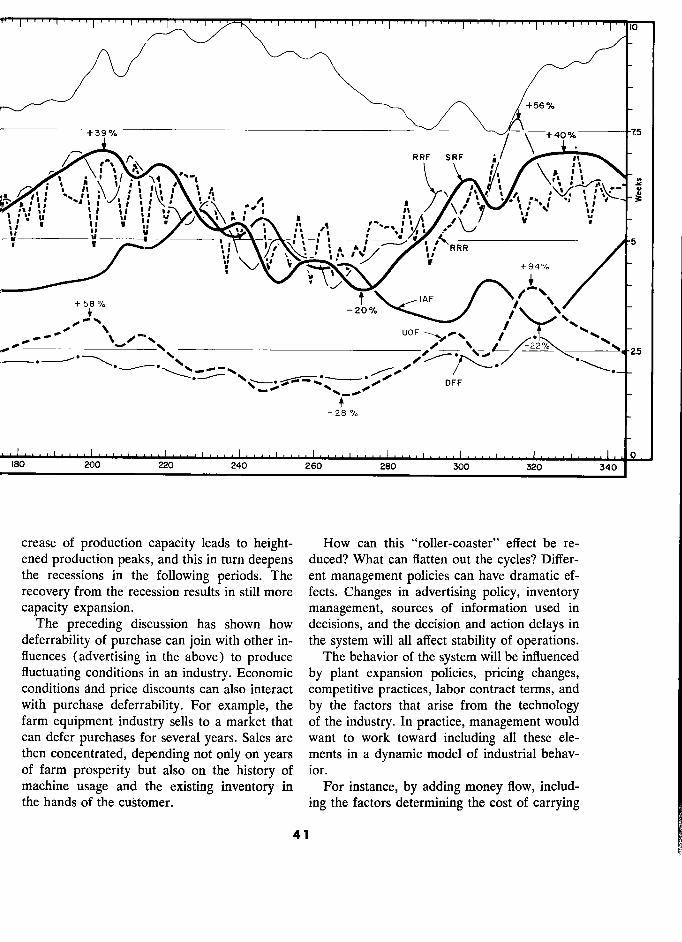
+56 %a
+39%
RRF – RRF SRF ,/ n
, 1
, , 1 %
on
, 1 § j ',,/)
j
fi ) 1
à ) j j
J ; '
, 1 lit
, , / ., j ',' tu 1
1
,
" -RRR
5
'
/
[AF
./ A
\
+
',
_
f
° o / DFF
- 28%
..-. 1 . . 1 . , 1 . .. 1.. 0 180 200 220 MO 260 280 300 320 340
crease of production capacity leads to height- How can this "roller-coaster" effect be re- ened production peaks, and this in turn deepens duced? What can fiatten out the cycles? Differ- the recessions in the following periods. The ent management policies can have dramatic ef-
recovery from the recession results in still more fects. Changes in advertising policy, inventory capacity expansion. management, sources of information used in
The preceding discussion has shown how decisions, and the decision and action delays in
deferrability of purchase can join with other in- the system will all affect stability of operations. fluences (advertising in the above) to produce The behavior of the system will be influenced
fluctuating conditions in an industry. Economic by plant expansion policies, pricing changes, conditions ànd price discounts can also interact competitive practices, labor contract terms, and with purchase deferrability. For example, the by the factors that arise from the technology farm equipment industry sells to a market that of the industry. In practice, management would can defer purchases for several years. Sales are want to work toward including all these ele- then concentrated, depending not only on years ments in a dynamic model of industrial behav- of farm prosperity but also on the history of ior. machine usage and the existing inventory in For instance, by adding money flow, includ- the hands of the customer. ing the factors determining the cost of carrying
41 1

AN INDUSTRIAL SYSTEM
inventory, cost of changing production levels, plants, union contract provisions, and advertis- and losses from special inventory clearance ing policy. These are the same items that we
sales, executives would be able to get direct consider and try to interrelate in the everyday profit comparisons between various methods of management of a business.
operation. The model could include the restric- In an adequately complete company model, tions imposed by available labor supply, maxi- more intangible items must also be specified, mum hiring and training rate, overtime, and such as the likelihood of results from research
policies regarding work-force reduction. expenditures, consumer response to advertising, To set up a dynamic model for simulating and market behavior. Many of these quantities
company or industry behavior, we must ade- will be unknown at first; a few can be measured;
quately describe the real system that it repre- some can be closely estimated; others will be sents. Gathering the information will sometimes guesses. Today these same factors are com- be difficult. However, the kinds of information bined intuitively, and sometimes quite effec- needed involve the essential characteristics of tively, but the systems-analysis approach should the company. We need factory lead time, in- help increase our understanding of the systems ventory policies, construction time for new that we are attempting to manage.
42 2
CHAPTER 3
The Managerial Use of
Industrial Dynamics
The information-feedback concepts of system behavior, mathematical models of dynamic interrelationships, and the digital computer to simulate
system interactions make experimental industrial system design possible. The manager can have a design laboratory to assist him in creating im-
proved control policies and the information flows on which they depend. This will lead to greater depth in management education and to changes in the qualifications of managers. It can be expected to alter the present staff versus line management duties in companies.
I N Chapter 2 the example of an industrial sys- be studied that might seldom be encountered tem has provided an elementary demonstration in the real world. Daring changes that might of a way to study the effect of policy and organi- seem too risky to try with an actual company zational structure. The example has been based can be investigated. The manager, like the on very simplified flows of information, orders, engineer, can now have a laboratory in which he and materials, but even so, realistic and infor- can learn quickly and at low cost the answers mative results have emerged. What then is the that would seldom be obtainable from trials on
place of such analysis in the quest for better real organizations. methods of management? The controlled laboratory experiment is a
It is only through costly experience and er- powerful tool - when used properly. The rors that managers have been able to develop wind-tunnel model of an airplane illustrates the effective intuitive judgment. We need to expe- strengths and dangers of this technique. Today's dite this learning process. Other professions aircraft would be impossible without laboratory in similar circumstances have turned to labo- model experiments; but the erroneous design of
ratory experiments. a model or mistaken interpretation of labora-
tory results can lead to disaster in the final 3.1 The Management Laboratory airplane. In the same way the manager must
Controlled laboratory experiments on indus- come to understand his new tools, their dangers, trial and economic situations are now possible and their effective use. with computers to do the work required by mathematical models that simulate the system 3.2 Steps in Enterprise Design
being studied. Unlike real life, all conditions The management laboratory approach will but one can be held constant and a particular follow the same steps common to other design time-history repeated to see the effect of the one laboratories. These have been mentioned in condition that was changed. Circumstances can Chapter 1. The goals must be defined, the
43 3
THE MANAGE RIAL USE OF INDUSTRIAL DYNAMICS S
significant factors identified, a model con- us to experiment with the implications of the
structed, the model tested, and the results statements already made. Any truly complete interpreted. and unambiguous verbal statement (whether
The Goals. First come the goals and the correct or not is immaterial) can be cast into
questions to be answered. To be productive, mathematical notation. The task here is routine
laboratory design must be addressed to an im- - if the verbal statement was indeed clear. The
portant goal. The questions guide the work that job is essentially no different from the transla- follows. The problems must be worthy and tion from one verbal language to another. In-
significant. This seems obvious, but too often deed, mathematics is but another language form
management research and academic thesis - one with more rigid rules than English for studies have been addressed to questions whose controlling its definitions, syntax, and logic.l answers could have but little significance to the The difficulties that will often arise in this con-
improvement of management. The important version to mathematical language arise because
problems are often no harder to subdue than of ill-conceived questions in the first step above, the trivial ones; the results are more rewarding. or an inadequate and incomplete description in
The Description of the Situation. Next, the the second step. factors that bear on the answers must be visual- This third step gives us a model that con-
ized, interrelated, and described. This should tains the mechanisms of interaction that have not be a formal step of mere statistical proce- been visualized between the parts of the system dure but rather the point where intuition and as described in the second step. In general, this
insight have their greatest opportunity. This is model will constitute a straightforward, under- a step for the philosophical, sensitive, percep- standable description of a managerial situation tive observer. Here, with respect to the past that is, nevertheless, far too complex in detail and present, we deal with what are indeed the to permit "optimum" (best possible) mathe- actual practices - not merely with formal or- matical solutions. It does, however, make pos- ganization charts, or profit-maximizing con- sible the generation of a specific time history of
cepts, or "economic man," but with the social, behavior that would result if the system (as de-
psychological, and organizational forces that scribed) were started with a specified initial influence decisions. state and with any specified behavior of the
Here we need experience, alertness, and a external environment.
strong intuitive feel for the nature of informa- Simulation. This tracing of a specific time tion-feedback systems. We need to look in the history is called .çimulation. The model takes
proper places for the policies, delays, and in- the place of the real system and simulates its formation sources that determine dynamic sys- operation under circumstances that are as real- tem behavior. istic as was the original description of the sys-
This step should result in an unambiguous, tem. This is the counterpart of trying a new
clear, verbal description of the factors and their policy or organizational structure in the real
interrelationships that bear on the questions to system, but here cost is insignificant compared be answered. with the cost of a real-life experiment.2 Further-
The Mathematical Model. Even the best more, a great deal more is learned because the verbal description will lack clarity; the spoken language is notoriously vulnerable to misunder- 1 Part II that follows discusses a mathematical
standing. The next step then is to clarify the language that is adequate for this translation. ° Around $30 per experiment at present commercial
verbal statement by translating it into a less Computing costs. Such economic feasibility has existed
ambiguous form and into a form that will allow only since 1956.
44
§3.3 EFFECT ON THE MANAGER
experimental conditions are fully known, con- 3.3 Effect on the Manager
trollable, and reproducible, so that changes in The ultimate goal of industrial dynamics and
system behavior can be traced directly to their of the management laboratory is "enterprise causes. Examples of such time histories were design." But the effect on the manager often seen in the preceding chapter. becomes evident before the effect on the enter-
The simulation step requires a vast amount prise. of arithmetical drudgery, and here the elec- One of the first effects is to develop in the tronic computer comes into its own. The com- manager a better intuitive feel for the time-
puter can take the mathematical statements varying behavior of industrial and economic from the preceding step, automatically do the systems. The study of particular situations, as detailed computer programming, generate a in the previous chapter, improves his judgment time history showing the implications of the about the factors influencing company success.
system description when combined with the A background in experimental system design input conditions as specified, and prepare the helps the developing manager to enhance the
requested tabular data and graphical curves. benefit from his work experience. His operat- Interpretation. After a simulation run comes ing experience becomes more meaningful when
interpretation of the results. Did it turn out as he better understands how his immediate en-
expected ? If not, why? As the experiment is vironment is related to other company func- examined, new questions arise. Perhaps a tions.
totally implausible result discloses a defect in At the college level, system simulation (simu- the system description of step two, or in the lation as used here does not mean manage- mathematical translation of step three. Perhaps ment games, see Section 20.5) allows the stu- it even becomes evident that the wrong ques- dent to observe the nature of the industrial tions had been asked in the first step. enterprise. He can for the first time experience
System Revision. If the goal is improvement the result of policy changes. He can "establish" of an existing industrial system, the first model controlling policies for "his" company and ob- will usually be built to represent the system as serve the results. He can acquire a better ap- it has been. When the results adequately repre- preciation for the underlying similarities be- sent the important behavior characteristics of tween seemingly diverse kinds of organizations, the past, the next step in search of improve- and begin to sense what makes them appear on ment is the redesign of system structure and the surface to be different.
policies. This is a process of invention and trial What will these changes demand of a man- like the design of a physical system. The skilled ager in training and'ability? designer will obtain better results than the Just as automation requires new skills at the novice or the unimaginative. worker level, so will improved methods require
Repeated Experimentation. At each step in new abilities at the management level. The top the above sequence, the prior steps may need to executive of the future will be concerned less be reviewed and revised. Each simulation result with actual operating decisions and more with
teaches, and it also prompts additional ques- the policy basis that should guide operating tions. The procedure is analogous to the re- decisions.3 He will be concerned not so much
peated design and test of an experimental ma- with day-to-day crises as with the establishment chine until performance has been improved ' See Leavitt and Whisler, "Management in the and the ... See Leavitt and Whisler, "Management in the and the difficulties have been reduced to a 1980's" (Reference 7), for additional views on the point where the resulting design can be put into changing nature of policy making and middle manage- use. ment.
45 5
THE MANAGERIAL USE OF INDUSTRIAL DYNAMICS
of policies and plans that minimize emergencies. time to train a new generation of managers, We can expect changes in various manage- and time for these men to reach positions of
ment responsibilities. There will be a merging responsibility. of many line-and-staff functions. Today the Industrial dynamics is in an early stage of kind of systems studies discussed here would be development. At a few isolated places, in both the province of staff specialists, yet the results companies and universities, research is under
determine the future success of the company. way as an outgrowth of military or operations Therefore the methods of enterprise design must research projects. But the full impact will not in time become well known to the top line be felt for a decade or more.
executive. Progress will come in two stages. It is likely In the past, power has been concentrated at that the five years from 1960 to 1965 will be
the top in order to improve over-all integration devoted to the development of basic analytical and control. We can expect that improved defi- techniques, demonstration by success in spe- nition of objectives and more pertinent stand- cific industrial situations, and establishment of ards for the measurement of managerial success new academic programs for training future will permit managers at the lower levels to take managers.
' on more responsibility in a form which can be After that will come general recognition of more effectively discharged. the advantage enjoyed by the pioneering man-
This will lead to a more decisive separation agements who have been the first to improve of policy making from operations, with the di- their understanding of the interrelationships be-
viding line much lower in the organization than tween separate company functions and between at present. We can expect a reduction in the the company and its markets, its industry, and size of the middle-management hierarchy. The the national economy. Competitive pressures
'i upper levels will become more exclusively con- will then lead other managements to seek the I cerned with the design of policies to integrate same advantage.
the separate functions of the business and less Many companies are already developing the with actual decision making. At the lower man- background skills that will be needed. Comput- agement levels those decisions that impinge on ers that are now being acquired for other pur- other departments and on the outside environ- poses can be used as systems simulators. Op- ment will be removed to a point where the erations research departments can expand into
guiding policy can be set with regard to the the broader activity of studying management system as a whole. Instead, at these lower levels systems. Simulation techniques, feedback-con-
' the responsibilities will become better matched trol-system theory, and analysis of decision to the opportunities and authorities that can processes are now being developed in the engi- there exist. Stress will increase on innovation, neering and product research departments of
efficiency, and personnel morale within a better- many firms. defined local framework. Already some companies are taking the lead.
As with any major social change, a new ap- For them, research on the management process
i I
proach to the management process will take is a part of the long-range planning of company time - time to develop ideas, time to test them, improvement.
46
'. 1 1
DYNAMIC MODELS OF INDUSTRIAL L
AND ECONOMIC ACTIVITY
Part Il is more technical than Part 1. It treats the nature of mathematical' models, the principles of formulating industrial dynamics models, and the specific methodology to be used in Part III.
. Chapter 4 classifies models, to help place the models of this book into the contéxt of môdels as found in engineering, the physical sciences, and the social sciences.
. . Chapter 5 discusses the basis of model formulation, stressing the view that a model is for a purpose. The objective comes Arst to guide the model content.
Chapter 6 gives a simple model structure of alternating levels and flow rates into which can be cast the broad managerial systems investigations outlined in Part 1.
. Chapter 7 describes the system of equations that is used within the model structure of Chapter 6.
. Chapter 8 introduces flow-diagram symbols to illustrate the relation-
ships between system components.
. Chapter 9 discusses the nature and the mathematical representation of delays which exist in all system actions and which are essential to an
understanding of system dynamics. . Chapter 10 on policies and decisions treats the formal nature of deci- sion making. It establishes the basis whereby the policy statements in a model are formulated to generate the system decisions through time.
Chapter 77 gives a basis for aggregating the separate items and events of a system into the essential main channels.
Chapter 12 describes the use of independent (exogenous) variables in
dynamic-model experimentation.
Chapter 13 discusses the several viewpoints from which models must be judged in establishing their validity and in determining their utility.
Chapter 14 summarizes the principal points made in Part Il.
47
In recommending a reading procedure for Part II, we shall recognize three groups of readers:
. Group A includes the manager who is not taking time for the more technical material, nor for the specific model-formulation detail in Part III.
Chapter 4 should be read; unfamiliar terminology can be ignored. The preview paragraphs at the beginning of the other chapters will provide the central thought of each chapter. Chapters 5 and 10 should be ex- amined and read insofar as they are of interest. Chapter 14 gives a
summary of Part II. All managers who can be persuaded to place them- selves in Group B should do so. . Group B includes those who are interested in how models of industrial
systems can be set up but who do not at this reading wish to spend time
I on underlying model-building philosophy. Chapters 4 through 9 should '
be read, but sections that seem obscure can be left after a single reading and can be re-examined as necessary when reading Part III. The first ' part of Chapter 10, the preview paragraphs of Chapters 11 through 13, and all of Chapter 14 should be read.
. Group C includes the serious student of the book who wants to take time to get the most out of it. All of Part II should be read carefully. Experience has shown, however, that this material falls short of its in- tended purpose until after the reader has seen the material applied. The
Group C reader should study Part Il carefully but need not be concerned about those parts that do not seem to fall readily into place. He should then continue to a study of Part III, which contains two complete examples of dynamic models. He will want to refer back to Part II while studying
I Part III. After Part III he should reread Part II. It is only on this reread-
ing, after seeing examples, that most students achieve a good grasp of the intended content of Part II.
48
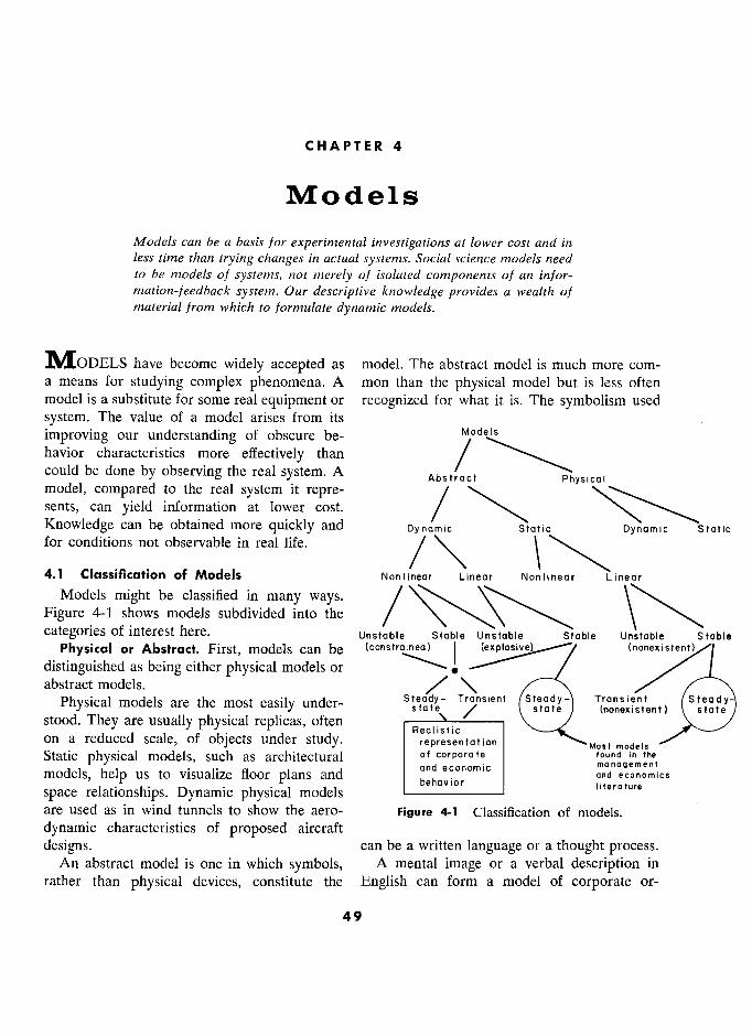
CHAPTER 4
Models
Models can be a basis for experimental investigations at lower cost and in less time than trying changes in actual systems. Social science models need to be models of systems, not merely of isolated components of an infor- mation-feedback system. Our descriptive knowledge provides a wealth of material from which to formulate dynamic models.
MODELS have become widely accepted as model. The abstract model is much more com- a means for studying complex phenomena. A mon than the physical model but is less often model is a substitute for some real equipment or recognized for what it is. The symbolism used
system. The value of a model arises from its .
improving our understanding of obscure be- nnodeis
havior characteristics more effectively than / could be done by observing the real system. A Abstroel r Physical
model, compared to the real system it repre- sents, can yield information at lower cost.
/ Knowledge can be obtained more quickly and Dynamic Static Dynamic sroric . for conditions not observable in real life.
/ \ 4.1 Classifitation of Models Nonlinear Linear Nonlinear Linear
Models might be classified in many ways. / Figure 4-1 shows models subdivided into the
categories Of mterest here. Unstable Stable Unstable Stable Unstable Stable Physical or Abstract. First, models can be
(constrained) 1 (explos (nonexistent) distinguished as being either physical models or , / abstract models.
Physical models are the most easil under- S teady - Transient Steady- Transient Steady-
Physical are usually physical easily often kig§§ state (nonexistent) state
stood. They are usually physical replicas, often Reclistic . " . , ' . Reallstle on a reduced scale, of objects under study. représentation Most models Static physical models, such as architectural of corporate found in the
models, help us to visualize floor plans and and economic management
models, help us to visualize floor plans and behavior and economics
space relationships. Dynamic physical models behavior literature
are used as in wind tunnels to show the aero- Figure 4-1 Classification of models.
dynamic characteristics of proposed aircraft
designs. can be a written language or a thought process. An abstract model is one in which symbols, A mental image or a verbal description in
rather than physical devices, constitute the English can form a model of corporate or-
49

MODELS S
' ganization and its processes. The manager deals Linear or Nonlinear. Systems represented by continuously with these mental and verbal a model may be "linear" or "nonlinear," and models of the corporation. They are not the real the models can be similarly classified.
corporation. They are not necessarily correct. In a linear system, external effects on the
They are models to substitute in our thinking system are purely additive.' A linear repre- for the real system that is being represented. sentation of a factory would be one in which a
A mathematical model is a special subdi- doubling of the incoming-order rate would, at vision of abstract models. The mathematical every future moment of time, produce exactly model is written in the "language" of mathe- ten times the changes that would come from a matical symbols. A mathematical model, like 10% increase in orders. In such a factory other abstract models, is a description of the model, production capacity limits would not
system it represents. Mathematical models are be permissible; man-hour productivity would in common use but are less easy to comprehend not decrease as employment began to crowd than physical models and are less frequent in the available equipment; large changes in ca-
everyday life than verbal models. An equation pacity would take no longer to accomplish than
relating the lengths and weights on each side small changes. Labor, equipment, and mate- of a playground seesaw is a static mathemati- rials would each make its own contribution to cal model. The equations for stress in a structure production rate entirely independently of the make up a static mathematical model of the state of the other two, implying, for example, girders and supports. The equations of motion that labor and equipment could produce a prod- of the planets around the sun form a dynamic uct even if materials were zero. Linear models mathematical model of the solar system. are adequate in much of the work in the physi-
Mathematical notation is a more specific cal sciences but fail to represent essential char-
language than English. It is less ambiguous. A acteristics of industrial and social processes. mathematical model is therefore a description In obtaining explicit mathematical solutions,
having greater clarity than most verbal models. linear models are much simpler than nonlinear. In model building, we start with a verbal model With negligible exceptions, mathematical anal- and then refine it until it can be translated into ysis is unable to deal with the general solu- mathematical language. The translation is not tions to nonlinear systems. As a consequence, inherently difficult. The problems in going from linear models have often been used to approxi- the verbal to mathematical statements arise mate phenomena that are admittedly nonlinear. when the initial verbal model is not an adequate description, and the shortcomings of the verbal
'A linear model is one in which the concept of model are revealed in the attempt to translate. 'A linear model is one in which the concept of model are revealed in the attempt to translate. superposition holds. in a linear system the response The mathematical model is valuable because to every disturbance runs its course independently of
it can be manipulated more easily than verbal preceding or succeeding inputs to the system; the total or physical models. Its logical structure is more result is no
more nor less than the sum of the separate
components of system response. The response to an explicit. It can be more readily used to trace input is independent of when the input occurs in the
assumptions to their resulting consequences. case of a linear system with constant coefficients (not Static or Dynamic. Models may or may not for
a linear system having time-varying coefficients). Y Only damped or sustained oscillations can exist in an
represent situations that change with time. A actual linear system; an oscillation that grows is not static model describes a relationship that does bounded and must become explosively larger. Thèse
not vary with time. A dynamic model deals are not descriptions of real industrial and economic ..... systems. Nonlinear phenomena are the causes of much
with time-varying interactions. of the system behavior that we shall wish to study.
50
§4.1 1 CLASSIFICATION OF MODELS S
As a result, the nonlinear characteristics have whether their behavior is primarily steady-state been lost.-' or transient.
When we no longer insist that we must ob- A steady-state pattern is one that is repetitive tain a general solution that describes, in one with time and in which the behavior in one time
neat package, all possible behavior character- period is of the same nature as any other period. istics of the system, the difference in difficulty (For some purposes, a model of a nongrowing between linear and nonlinear systems vanishes. national economy that shows business-cycle Simulation methods that obtain only a particu- patterns could be considered a steady-state lar solution to each separately specified set of fluctuation, even though never repeating identi-
circumstances can deal as readily with non- cally any particular sequence of events. Like-
linear as with linear systems. wise, the long, mature portion of a product life
Stable or Unstable. Dynamic models, in cycle, as now illustrated by automobiles, might which conditions change with time, can be sub- be considered a steady-state dynamic model
divided into stable and unstable models. Like- for the answering of certain questions.) In busi-
wise, the actual systems they represent are char- ness systems, steady-state behavior is a re-
acterized as being stable or unstable. stricted, special case. (The system discussed in A stable system is one that tends to return to Chapter 2 is a steady-state, dynamic model.)
its initial condition after being disturbed. It Transient behavior describes those changes may overshoot and oscillate (like a simple where the character of the system changes with
pendulum that is set in motion), but the time. A system that exhibits growth would show disturbances decline and die out. transient behavior. Transient responses are
In an unstable system that starts at rest, an "one-time" phenomena that cannot repeat. initial disturbance is amplified, leading to Many of the important management problems growth or to oscillations whose amplitude in- are transient in character - company growth, creases. A nonlinear system that is unstable new plant construction, and market develop- under normal conditions can exhibit fluctua- ment. tions that grow until restrained by the appear- Open or Closed. In addition to the classifica-
ance of nonlinear influences (labor shortage, tion of Figure 4-1, models may be "open" or
production capacity, declining availability of "closed." The distinction is not as sharp as the
materials). The sustained fluctuation might words would indicate. Different degrees of
then be thought of as having reached a sta- "openness" can exist. ble amplitude of peak-and-valley excursion. The closed dynamic model is one that func-
Clearly, in economic systems, upper levels of tions without connection to externally supplied activity are limited by resources, and the lower (exogenous) variables that are generated out- levels are at least bounded by zero activity. side the model. A closed model is one that in-
The indications are that the industrial and ternally generates the values of variables economic systems of greatest interest will often through time by the interaction of the variables, be of this type wherein small disturbances grow one on another. The closed model can exhibit
in an unstable manner until restrained by non- interesting and informative behavior without re-
linearities. ceiving an input variable from an external
Steady-State or Transient. Models (and sys- source.3
tems) can be further subdivided according to Information-feedback systems are essentially 2 For an interesting, descriptive, nonmathematical
discussion of nonlinearity, see Reference 8. 3 See Chapter 12 on exogenous inputs to models.
51 1

MODELS S
closed systems. They are self-regulating, and the tory capacity, labor and credit shortage, and characteristics of principal interest are those the dependence of decisions on complex rela- that arise from the internal structure and inter- tionships between variables, all compellingly in- actions rather than those responses that reflect sist on being included in a usefully realistic
merely the externally supplied inputs. model of the industrial enterprise. Since time The models of interest to us here can be oper- and changes with time are the essence of the
ated as closed systems. The internal dynamic manager's task, a useful model must be dy- interactions are of primary interest. We shall namic and capable of adequately generating its not always choose to study such models in own evolution through time.
completely closed form. It is often informative Consequently, we are speaking here of math- to depart from strictly closed operation enough ematical models that can be used to simulate to permit a test input that serves as excitation the time-sequential operation of dynamic sys- of the internal responses of the system. Im- tems, linear or nonlinear, .çtable or unstable, pulses, steps, sinusoids, trends, and noise (ran- steady-state or transient. The model must be dom disturbances) are common test inputs. able to accept our descriptions of organizational Such external (exogenous) inputs are valid form, policy, and the tangible and intangible only under conditions where we are willing to factors that determine how the system evolves assume that the external inputs are themselves with time. Such models will be far too complex entirely independent of the resulting response (tens, hundreds, or thousands of variables) to within the system. yield analytical solutions. In fact, for nonlinear
Models of Industrial Systems. Most of the systems modern mathematics can achieve ana- mathematical models found thus far in the man- lytical solutions to only the most trivial of prob- agement and economics literature belong in lems. The models considered here are instead one of the two circles in the figure. Nearly all to be used to simulate (that is, to trace through are steady-state, stable, and linear. Some are time) a particular course of action that results static and some dynamic. The practical utility from a specific set of starting conditions coupled of these models in dealing with economic sys- with one specific combination of noise and other tems has not been notable. The models of in- inputs which are introduced. This is an experi- dustrial situations in the field of operations re- mental, empirical approach in search of better search have often repaid their cost manyfold, knowledge, and thereby better results, but not but even so they have not dealt with the major promising "optimum" solutions to any question. problems of corporate top management. In the management science and economics
To deal with practical management and eco- literature, the term "mathematical model" has nomic problems of pressing importance, a customarily been used to mean any mathemati- mathematical model must be able to include all cal relationship between the inputs and the out- of the categories leading to the square in Figure put of a part of a system. In the terminology of 4-1. Corporate management must cope with engineering systems, this output reaction of a the transients of growth and the steady state of system component to one or more inputs is normal business fluctuation and uncertainty. commonly called a "transfer function." The Stable industrial systems may exist in mature transfer function specifies how conditions at the
product lines. Systems that are unstable and input will be transferred to the output. In this are restrained only by their nonlinearities are text, a simple mathematical relationship describ- to be expected in capital goods industries, com- ing the response of a component of the system modities, and probably in our economic system to its immediate environment will not be called as a whole. The nonlinearities of maximum fac- a "model" but instead will be referred to syn-
52 2

§4.2 MODELS IN SCIENCE AND ENGINEERING
onymously as "transfer function," "functional the physical sciences, engineering systems have
relation," "decision equation," or "rate equa- complexity approaching the complexity of social tion." In contrast, a "model" defines a system systems. Both engineering and social systems consisting of an interacting set of "decision have a continuous gradation (from the obvi-
equations." ously important, through the doubtful, into the
negligible) of influences that affect each action 4.2 Models in the Physical Sciences, Engi- and decision; by contrast, the physical science
neering, and the Social Sciences systems have often been different, with a sub- Mathematical models in the social sciences stantial gap in importance between the few fac-
have often been compared with the simple tors that must be included in a model and nearly models in the physical and biological sciences. insignificant ones that can be omitted. Social This may have been misleading. systems are strongly characterized by their
Useful models of the solar system, the atom, closed-loop (information-feedback) structure, Newton's laws of motion, and heredity are much like many engineering systems that have been
simpler than models that will be helpful in in- modeled but unlike most models in the basic dustrial and economic systems. Linear analysis physical sciences. In models of social systems, is much more widely applicable in such physical as in engineering but unlike simple physical sci- science systems. Most physical science systems ence models, we must be interested in transient, that have been represented by successful models noncyclic, nonrepeating phenomena. have contained much smaller amounts of noise Dynamic models have proved indispensable (uncertainty) than in our social systems. Physi- in designing physical systems. They are used cal science models have been deduced to ex- in aircraft engineering, the planning of military plain phenomena that can be observed but command systems, and in studying communica-
usually not altered. Statistical inference methods tions networks. They have included both equip- that succeed in relating unidirectional cause and ment and people; therefore, they take on aspects effect in biological heredity are not necessarily of social systems. Today's advanced technology sound in studying social systems where effect would be impossible without the knowledge that reacts on cause. has resulted from mathematical models.
The attitudes toward the source and purpose The same cannot be said for the impact of of physical science and social science models mathematical models on business and economic have been similar, to the detriment of progress decisions. Economic models have enjoyed a in models of social systems. long history of research but little general ac-
Models in the engineering and military worlds ceptance as a tool to aid top management of a are so different in degree from the physical company or a country. science models that we can fairly say they differ Many of the past failures in economic model in principle. They arise in a different way, to building can be traced to unsound methods and be used for a different purpose. to attempts to reach unachievable objectives.
Models in engineering and military usage We need new attitudes toward the construction
provide a much better precedent for the social and use of models of social systems. sciences than do physical science and biology Objectives. The past contrast in usefulness models. Economics and management, like en- between engineering and economic dynamic gineering, deal with aggregate systems above the models can be partly traced to the way the tools level of the individual elementary events that of model building have been employed. The dif- are the subject of many physical science models. ference between the two uses of models seems Unlike systems that are commonly modeled in to arise from a different emphasis on end objec-
53

MODELS S
tive. In engineering, models have been used for formal data and make better use of our vast
designing new systems; in economics, a common store of descriptive information. use is to explain existing systems. A model that Validity of a Model. The test of the ade- is useful for design must also explain. But it quacy of a model also differs between engineer- appears that models that have been undertaken ing and economic usage. In technical and mili-
only for explanation have often had their goals tary circles, models have been judged by their set so low that they fail not only for design but ability to exhibit the dynamic characteristics of also for their explanatory purposes. systems such as amplification, bandwidth,4 and
Basis for a Model. In engineering systems, transient response. In economics, models have models have been built upward from available often been judged by their ability to predict the
knowledge about the separate components. De- specific state of the system at some future time; signing a system model upward from identifiable and the models have customarily failed to pass and observable pieces is a sound procedure with this prediction test. a history of success. In using a model, we should look less for
In economics, models have often been con- prediction of specific actions in the future and structed working backward from observed total- more for enhancing our understanding of the
system results. Even as a theoretical goal, there inherent characteristics of the system. There is no evident reason to believe that the inverse seem to be good reasons why models cannot be
process of going from total-system behavior to expected to predict specific system condition far the characteristics of the parts is possible in enough into the future to be particularly sig- the kinds of complicated, noisy systems that nificant. If so, prediction of a specific sequence are encountered in business and economics. of actions is not a useful test of a model.5 In-
The attempt merely to reproduce an existing stead a model should be judged by its ability to economic system in a model has led to models reproduce or to predict the behavior charac- that are statistically derived from observed time teristics of the system - stability, oscillation, series of past behavior. It is most unlikely that growth, average periods between peaks, general the internal causal mechanisms of a complex, time relationships between changing variables, nonlinear information-feedback system can be and tendency to amplify or attenuate externally derived from a sequence of external observa- imposed disturbances. tions of its normal performance. By contrast, Similarity of Model and System. In engineer- the use of models for the design of physical ing, mathematical models have shown a greater systems has emphasized models of systems that correspondence to the structural and opera- do not yet exist, models that could not possibly tional details of the real systems they represent be constructed backward from observed results. than appears in the classical economic models. A wind-tunnel model of an airplane is not con- The communications barrier has been nearly structed to reproduce merely observable over- impenetrable between the mathematical models all behavior of a known airplane; it is not de- in the social sciences, and the industrial and
signed merely to match the aggregate average governmental executives. This is accentuated of all airplanes designed in the past. It is de- because models of social systems, unlike models
signed part by part to represent a proposed new of physical systems, have not been cast in the aircraft so that the interaction of the parts and terms commonly employed by the active prac- the performance of the airplane as a whole can be studied. ' An indication of the resistance to disturbance of
In formulating a model of a system, we an6 existing trends and cycles.
should rely less exclusively on statistics and pendix 'See K. Chapter 13 on model validity and also Ap-
54
§4.5 SCOPE OF MODELS
titioners of the art. The difference in terminol- model, the intangibles, and our assumptions ogy may arise from the differing initial view- about them, become tangible and observable.
point. The manager deals with the components We then have a means for tracing the implica- of his organization just as the engineer does with tions of our assumptions. the components of his airplane; the manager does not use abstract coefficients that cannot 4.4 Mechanizing the Model be tied to specific sources in the real system. A dynamic mathematical model is a descrip- The modelmaker, who derives relationships tion of how to generate the actions that are to from statistical analysis, is apt to leave his co- be taken progressively through time. To be use- efficients as abstract, empirical results that are ful, the model must be mechanized by provid- not identified with particular features of the ing some way of carrying out the specified ac- real system. tions.
In the chapters that follow, we shall attempt The actions called for by the model could to make every variable and every constant have be executed by a group of people playing the individual significance in the context of every- separate parts of the real system that is being day managerial practice. It should be possible simulated. Decisions and actions would generate to discuss the individual plausibility of the results that would in turn become the inputs for value of any constant because that constant will, the decisions and actions that follow. Such in its own right, have physical or conceptual simulation, using groups of people, has been
meaning. employed in studies of real systems. It is a good technique for classroom demonstration of basic
4.3 Models for Controlled Experiments principles. For the study of large systems it is The mathematical model makes controlled burdensome and expensive.
experiments possible. The effects of different A digital computer can be instructed to
assumptions and environmental factors can be execute the same procedures that would be fol- tested. In the model system, unlike real systems, lowed by the group. The cost is less than one- the effect of changing one factor can be ob- thousandth of the cost of the same clerical oper- served while all other factors are held un- ations executed by a group of persons. The task
changed. Such experimentation will yield new is ideally suited to the unique characteristics
insights into the characteristics of the system of the electronic digital computer. that the model represents. By using a model of
4.5 Scope of Models a complex system, more can be learned about 4.5 Scope of Models
internal interactions than would ever be possible In recent years it has become possible to
through manipulation of the real system. In- formulate dynamic models of industrial be-
ternally, the model provides complete control havior with sufficient reality to cope with the of the system organizational structure, its poli- interactions of production, distribution, adver-
cies, and its sensitivities to various events. Ex- tising, research, investment, and the consumer
ternally, a wider range of circumstances can be market. Within such a formulation, both physi- generated than are apt to be observable in real cal and psychological factors can be included. life. Model-building technique and computational
In the model, observations can be made of cost no longer limit the systems that can be variables that are unmeasurable in the real sys- studied. Instead, progress will be set by the rate tem. An adequate model must include any "in- at which our knowledge of the industrial world
tangibles" that we believe contribute im- can be sifted, refined, and reorganized into an
portantly to the behavior being studied. In the explicit form.
55
MODELS S
The immediate goal is to take our literature of equipment. The model of a company is justi- and knowledge of "descriptive management" fied to the extent that it will allow us to manage and "descriptive economics" and formalize what the company better. There is no implication that we believe about the separate parts. It then will the results need be perfect to be beneficial. A become possible to improve our understanding model can be useful in determining the degree of how thèse parts interact. In discussing the to which the industrial system is sensitive to formulation of dynamic models, no distinction changes in a policy or in system structure. It is made in this book between corporations, in- can help determine the relative value of infor- dustries, and complete economies. There should mation of differing kind, accuracy, and timeli- be no difference in approach or arbitrary dis- ness. It can show the extent to which the system tinction between microeconomics and macro- amplifies or attenuates disturbances impressed economics. The same principles control. The by the outside environment. It is a tool for de- same theoretical considerations will guide the termining vulnerability to fluctuation, overex-
way in which aggregation can be accomplished. pansion, and collapse. A model can point the The opportunities for improving our under- way to policies that yield more favorable per- standing are similar, with the same restrictions formance. In short, mathematical models should on achievable objectives. The comments in this serve as tools for "enterprise engineering," that book are intended to apply equally at all levels, is, for the design of an industrial organization from dynamic behavior of the individual firm to meet better the desired objectives. to international economics. The preceding comments imply that a useful
model of a real system should be able to repre- 4.6 Objectives in Using Mathematical sent the nature of the system; it should show
Models how changes in policies or structure will pro- A mathematical model of an industrial en- duce better or worse behavior. It should show
terprise should aid in understanding that en- the kinds of external disturbance to which the
terprise. It should be a useful guide to judgment system is vulnérable. It is a guide to improving and intuitive decisions. It should help establish management effectiveness.
desirable policies. Using a model implies the But note especially that quantitative predic-
following: tion of specific events at particular future times has not been included in the objectives of a
. We have some knowledge about the detailed model. It has often been erroneously taken as characteristics of the system. self-evident that a useful dynamic model must
. These known and assumed facts interact to in- forecast the specific condition of the system at
fluence the way in which the system will evolve some future time.s This may be désirable, but with time. the usefulness of models need not rest on their
. Our intuitive ability to visualize the interaction ability to predict a specifie path in the future.
of the parts is less reliable than our knowledge This is fortunate because there is ample reason
of the parts individually. to believe that such a prédiction will not be
v By constructing the model and watching the achieved in the foreseeable future? . By constructmg thé mode! and watching thé e
interplay of the factors within it, we shall come tests of the period-by-period dif- to a better understanding of the system with ferences between model variables and real-system which we are dealing. variables imply such an expectation that the model
should predict the specific future configuration of the Thèse assumptions form thé same basis on system. See Chapter 13 on model validity.. These assumptions form the same basis on 7 See Appendix K for an example of s ystem nature
which we construct models of floor plans and versus future system condition prediction.
56

§4.7 INFORMATION FOR MODELS S
4.7 Sources of Information for Constructing "not vague." The mathematical model is not Models necessarily more "accurate" than the verbal
Many persons discount the potential utility model, where by accuracy we mean the degree of models of industrial operations on the as- of correspondence to the real world. A mathe-
sumption that we lack adequate data on which matical model could "precisely" represent our to base a model. They believe that the first step verbal description and yet be totally "inac- must be extensive collecting of statistical data. curate."
Exactly the reverse is true. Much of the value of the mathematical model We usually start already equipped with comes from its "precision" and not from its "ac-
enough descriptive information to begin the curacy." The act of constructing a mathematical construction of a highly useful model. A model model enforces precision. lt requires a specific should come first. And one of the first uses of statement of what we mean. Constructing a the model should be to determine what forma] model implies nothing one way or the other data need to be collected. We see all around about the accuracy of what is being precisely us the laborious collection of data whose value stated. does not equal the cost. At the same time There seems to be a general misunderstand-
highly crucial and easily available information ing to the effect that a mathematical model is neither sought nor used. cannot be undertaken until every constant and
The routine, clerical collection of numerical functional relationship is known to high ac- data is unlikely to expose new concepts or curacy. This often leads to the omission of
previously unknown but significant variables. admittedly highly significant factors (most of Extensive data collecting is not apt to shed new the "intangible" influences on decisions) be-
light on the general nature of the variables. cause these are unmeasured or unmeasurable. Some of the most important sources for a re- To omit such variables is equivalent to saying alistic dynamic model do not exist as "data" in they have zero effect - probably the only value the usual sense of tabulated statistical informa- that is known to be wrong! tion. Different attitudes toward data and their
What is the relative importance of the many accuracy can be traced to the different goals different variables? How accurately is the in- and objectives of models already discussed. formation needed? What will be the conse- If the only useful and acceptable model is
quences of incorrect data? These questions one that fully explains the real system and pre- should be answered before much time or money dicts its specific future condition, then precision is expended in data gathering. is not sufficient; it must also be accurate. Lack-
Actually we use models of corporate and eco- ing such accuracy, the endeavor flounders. nomic systems continuously with only the data If, on the other hand, our objective is to en- that we have at hand. A word picture or de- hance understanding and to clarify our think-
scription is a model; our mental picture of how ing about the system, a model can be useful if the organization functions is a model. A ver- it represents only what we believe to be the bal model and a mathematical model are close nature of the system under study. Such a model kin. Both are abstract descriptions of the real will impart precision to our thinking; vagueness system. The mathematical model is the more must be eliminated in the process of construct-
orderly ; it tends to dispel the hazy inconsist- ing a mathematical model; we are forced to encies that can exist in a verbal description. The commit ourselves on what we believe is the
mathematical model is more "precise." By pre- relative importance of various factors. We shall cise is meant "specific," "sharply defined," and discover inconsistencies in our basic assump-
57
MODELS S
tions. We shall often find that our assumptions As a model is detailed toward an approxima- about the separate components cannot lead to tion of a real or proposed system, we can use our expected consequences. Our verbal model, the model itself to study the significance of vari- when converted to precise mathematical form, ous assumptions that have gone into it. With
may be inconsistent with the qualitative nature respect to every numerical value that we have of the real world we observe around us. We been forced to estimate arbitrarily, there is some
may find that cherished prejudicies cannot, by range within which we are practically certain
any plausible combination of assumptions, be that the "true" value must fall. It will often shown to have validity. Through any of these happen that the model is relatively insensitive we learn. to changes in value within this range; refining
In these ways we use a model as does the our estimate would then be unjustified.s engineer or military strategist. What would the On the other hand, the entire qualitative be- situation be like if the real system corresponds havior of the system may depend significantly to our basic assumptions? What would a pro- on some different numerical value that has been
posed system be like if we designed it to agree assumed.9 We are then alerted to the critical with the model? What changes in the model nature of this assumption. When the vulnerabil- would give it more nearly the characteristics of ity to an error in numerical value is demon- the existing system that it presumably repre- strated, we must then choose between sents? These are questions that can be asked of . Measuring the value with adequate accuracy a closed, or closable, model and are significant . Controlling the value to a desired range when the system is so complex that the correct
v Redesigning the system and the model to make answers are not évident by inspection. the value less important
A model must start with a "structure," mean-
ing the general nature of the interrelationships A mathematical model should be based on
within it. Assumptions about structure must the best information that is readily available, but
be made before we can collect data from the the design of a model should not be postponed real system. Having a reasonable structure that until all pertinent parameters have been ac-
fits our descriptive knowledge of the system, curately measured. That day will never come.
we can take the next step and assign plausible Values should be estimated where necessary, so
numerical values to coefficients, since the coef- that we can get on with the many things that can
ficients should represent identifiable and de- be learned while data gathering is proceeding. scribable characteristics of the real system. We In gencral sufficient information exists in the
can then proceed to alter the model and the descriptive knowledge possessed by the active
real system to eliminate disagreement and move practitioners of the management and economics
both toward a more desirable level of perform- arts to serve the model builder in all his initial
ance. efforts. He will find that he is more in danger This is the attitude of the manager toward the from being insensitive to and unperceiving of
verbal image that he uses as a model of the important variables than from lack of informa-
company he directs. He strives to grasp the im- tion, once the variables have been exposed and
plications of the separate factors he observes defined. Searching questions, asked at points about him. He attempts to relate individual throughout the organization under study by one
policies and characteristics of the system to the skilled in knowing what is critical in system
conséquences that they imply. He tries to esti- " See Figure 2-6 on the system insensitivity to cleri- mate thé resu!t of chansin? those parts of thé cal
-, o .- ' '.' '.. <- mate the result of changing those parts of the 0 See Figure 2-8 showing sensitivity to rapidity of system over which he has control.
r "
inventory adjustment. sensltIvily to rapl Ity of
58

/
§4.7 INFORMATION FOR MODELS S
dynamics, can divulge far more useful informa- have been collected in the past. We are depend- tion than is apt to exist in recorded data. ent on our insight into the separate parts of the
These comments are not to discourage the system to establish how they would respond to
proper use of the data that are available nor new circumstances. Fortunately, this is usually the making of measurements that are shown possible. In fact, we may be more certain about to be justified; they are to challenge the com- the extreme limiting circumstances of human
mon opinion that measurement cornes first and behavior, the likely decisions, and the techno-
foremost. Lord Kelvin's famed quotation, that logical nature of production and inventories we do not really understand until we can meas- than we are about the "normal" range. These
ure, still stands. But before we measure, we limiting conditions are part of our body of de-
should name the quantity, select a scale of scriptive knowledge. Incorporating the full pos- measurement, and in the interests of efficiency sible range of functional relationships in a
we should have a reason for wanting to know. model makes it feasible to study wider ranges Even in the context of basic research that is of system operation. It also improves the ac-
presumed to seek information for its own sake, curacy of model representation over normal
the world has limited resources, and the re- ranges because incorporating the known ex-
searcher should have conviction that his inves- treme values helps to bound and determine
tigation promises a high probability of impor- many characteristics in the normal ranges. tant results. Useful results can be expected from models
To some, this attitude toward the data on constructed as herein discussed - by building which to base a model will seem highhanded and upward from the characteristics of the separate will be repugnant. To others, it will seem the components and by incorporating and estimat-
practical and necessary avenue along which to ing the values of all factors that our descriptive attack a difficult problem. familiarity with the system tells us are impor-
One important use for a model is to explore tant. Such models will communicate easily with
system behavior outside the normal and his- the practicing manager because they arise from
torical ranges of operation. These ranges will the same sources and in the same terminology be outside the region of any data that could as his own experience.
59
CHAPTER 5
Principles for Formulating
Dynamic System Models
The questions to be answered precede model design. The closed-loop system structure must be reflected in a model. Time delays, amplification, and information distortion must be adequately represented. All constants and variables of the model can and should be counterparts of correspond- ing quantities and concepts in the actual system. Dimensional units of measure of model quantities must be meticulously consistent. The pre- ferred practice is to begin with the continuous (nonstochastic) structure of system decisions and later add randomness and periodic influences. Model formulation methods should not presuppose system linearity or
stability.
B EFORE proceeding with the specific details use a model is tested immediately - his first of equations and a suitable mathematical struc- decision is to ask pertinent questions having ture for a dynamic model, we shall discuss some important answers. Trivial questions can but
general principles that should guide the con- lead to trivial answers. Questions that are too struction of a model of an industrial system. general - such as how to be more successful
- fail to define an area of attack. Questions 5.1 What to Include in a Model that are too restrictive may confine the inves-
In practice there will be no such thing as the tigation to an area that does not contain the model of a social system, any more than there answer. Questions that are impossible to answer is the model of an aircraft. An airplane is repre- can lead only to disappointment. sented by several aerodynamic wind-tunnel Questions to be answered control the con- models for various purposes, plus cockpit ar- tent of a model. But how? Again the perception rangement mock-ups, models for maximum and judgment of the investigator are taxed. He stress loading, etc. In designing a dynamic must select, on the basis of his knowledge of simulation model of a company or economy, the situation, the factors that he believes are the factors that must be included arise directly pertinent. Here skill and practice in working from the questions that are to be answered. with the dynamic behavior of systems are im-
In the absence of an all-inclusive model, portant. What the novice often considers para- which we are unlikely to achieve, there may mount may prove to be insignificant. Some fac- well be different models for different classes of tors that are stressed in static analysis may not
questions about a particular system. And a par- even exist as essential concepts in a dynamic ticular model will be altered and extended as model. Factors that are omitted, both in static each new question is explored. analysis and in ordinary descriptive debates
The skill of the person who undertakes to about a problem, may prove to be crucial.
60

§5.2 2 INFORMATION-FEEDBACK ASPECTS OF MODELS S
Here, "art" re-enters the picture as a guide to tions are converted to information that is a
proper use of the tools of science. For the pres- basis for decisions that control action to alter ent we can do no better than to discuss general the surrounding conditions. The cycle is con-
principles and later supply specific examples tinuous. We cannot properly speak of any be- that will help the beginner to start developing ginning or end of the chain. It is a closed loop. his own skills. This is a broad definition covering most hu-
Since the objective is to include those factors man, social, and technical activities. Economic that influence the answers sought, the basis of fluctuations are one manifestation of the time- model building cannot be limited to any one varying interactions that occur in information- narrow classification of intellectual discipline. feedback loops. At the company level, rising We must feel free to include technical, legal, sales exceed plant capacity, leading to expan- managerial, economic, psychological, organiza- sion plans and construction that restore the
tional, monetary, and historical factors. All balance of demand and output. Falling sales these must find their proper places in our and rising inventories may lead to greater mar- formulation of system component interactions. keting effort to increase sales to equal produc-
In formulating a quantitative model, we must tion. The need for product improvement leads have courage to include all the facets that we to research expenditure, to technological prog- should consider essential to a verbal description ress, to new competition, to the need for still of the phenomena under study. In the past, so newer products, and to more research. These
long as mathematical models were restricted and all other management decisions are made to those which could be solved analytically, the in the framework of an information-feedback models could not accept the wealth of concepts system where the decision ultimately affects the that exist in descriptive knowledge. Simulation environment that caused the decision. models and electronic computers change this The general concepts of information-feed-
picture. back systems are essential because such systems As a generalization, significant models for exhibit behavior as a whole which is not evi-
the answering of top-management questions dent from examination of the parts separately. range in size between 30 and 3,000 variables. The pattern of system interconnection, the am- The lower limit is about the minimum that will plification caused by decisions and policy, the exhibit the kinds of behavior of interest to the delays in actions, and the distortion in informa-
manager ; the upper limit will bound for some tion flows combine to determine stability and time our ability to conceive of a system and its
growth.' meaningful interrelationships. Already there As we have seen in Chapter 2, the intercon- have been several preliminary explorations nection of entirely ordinary corporate actions with both steady-state and transient growth models incorporating up to a few hundred vari- 1 We are not dealing here with the simple concept ables. of the servomechanism which is often treated in engi- '
neering literature as having a single "error function" (difference between actual and desired results) and
5.2 Information-Feedback Aspects of Models a single control mechanism. Instead our economic
Economie and lridustrlal activities are closed- systems have "distributed error functions" represented . , f by the individual goals of many participating persons.
loop, information-feedback systems. Models of The control function is likewise dispersed, so that it such systems must preserve the closed-loop exists in part at each decision point in the system. structure that gives rise to so much of the in- Formal servomechanisms theory is unlikely to find
, behavior. direct use in economic models but is an excellent back-
g behavior. ground to guide the selection of factors that should In an information-feedback system, condi- enter such models.
61 1
PRINCIPLES FOR FORMULATING MODELS S
can lead to production fluctuations, unemploy- equipment reservoirs include plant and ma-
ment, and excess plant capacity. As one action chines, segregated as necessary by age, type, feeds into another and eventually back to the productivity index, and life expectancy. first, it causes instability that is the counterpart Although time delays are important, and of "hunting" in mechanical servomechanisms. without delays our systems would not exhibit
Careful attention must be given to represent their usual characteristics toward instability, it
properly the time delays, information distortion, is far from true that all delays are bad in a and the basis for reaching decisions. system. Nor is it true that the practical solution
Time Relationships. The behavior of infor- to system improvement always lies in reducing mation-feedback systems is intimately asso- delays.3 There are occasions when the introduc- ciated with the time-sequence relationships be- tion of time lags at properly selected points tween the actions in the system. Time delays may be the most economical way to achieve a
arise in every stage of system activity - in desired objective.4
decisions, in transportation, in averaging data, The method of model formulation and the
and in inventories and stocks of all kinds. types of equations used should permit time Variable accumulations of all types must be delays to be represented both in average dura-
carefully noted and must be represented if the tion and in transient characteristics, in close time magnitudes associated with them are agreement with our knowledge of how the de-
judged to be important. Points of accumulation lays are actually created.71 Neither the solution
permit, or intentionally introduce, time delays interval of the model equations nor the intervals between input and output rates of flow. The at which data on the actual system may have fundamental purpose of an inventory is to un- been collected should dictate the way in which
couple somewhat the inflow and outflow rates delays are generated in the model. so that the incoming receipt of goods need not Amplification. Amplification is a most im- match exactly at all times the rate of delivery portant characteristic determining the behavior from the inventory. The level of the inventory of information-feedback systems. "Amplifica- fluctuates to make up the difference in the flow tion" is used here as a nontechnical term imply- rates. ing a response from some part of a system
We must include reservoirs in information which is greater than would at first seem to be and order channels as well as in physical goods. justified by the causes of that response. For ex- Such reservoirs contain unfilled-order backlogs, ample, it is often observed that fluctuations in in-transit orders in the mail, decisions that have factory production rate greatly exceed the mag- been made but not executed, and data that are nitude of retail sales rate changes. being gathered and processed but not yet used. Amplification occurs in many places in our Reservoirs of materials include in-process and social system. Amplification arises, as to be dis- finished inventories and goods in transit. Money cussed later, in the policies that define decisions flow reservoirs include bank balances and that control rates of flow. Policies, and the loans.2 Personnel reservoirs include employees, decisions that result from them, must be care-
various categories of unemployed, and the fully examined, since they are the source of classes of consumers and investors. Capital amplification in social systems.
2 In the context of many situations these will be considered as information rather than money. Ac- ' For instance, in Figure 2-6, reducing the clerical counts payable and receivable and capital equipment delays produces only slight improvement. and depreciation accounts ordinarily are not "money" * See Figure 2-8, where increasing the delay in in the cash flow sense and will usually appear in the invpntory adjustment reduces production fluctuation. information flow channels. s See Chapter 9.
62
§5.3 3 MODEL AND REAL-SYSTEM VARIABLES S
Amplification occurs in many places. Orders Model variables should be measured in the for goods do not merely reproduce the rate of same units as the real variables. At first glance sales; orders are added for inventory accumu- this may seem obvious and elementary, but
lation, to fill supply pipelines, and for specula- this principle has rather consistently been vio- tion. Amplification occurs in many forecasting lated in model building. and predicting procedures, as when growth rates Sufficiently close correspondence of model are extrapolated and lead to overinvestment in and real-system variables is obtained only factory capacity. Amplification arises from the through constant alertness and re-examination
tendency to order ahead when deliveries slow of whether the decision functions adequately down. Ordering ahead during price rises and represent the concepts, social pressures, and
delayed ordering during price declines produce sources of information that control the actual
amplification. All these are of the greatest im- decisions.
portance in representing the factors that con- Flows of goods should be measured in phys- trol industrial growth and stability. ical units, not equivalent dollars. Money flow
Information Distortion. Information is the should be separate. Prices relate the two. Goods
input to decisions, and the decisions are affected cannot be represented in terms of equivalent by all the influences that act on the information dollars, or else we lose the significance of prices flows. Information can be distorted in other and of the fact that dollars do not flow in
ways than by delays and amplification. Infor- synchronism with goods but usually with a de- mation is modified by averaging procedures and layed relationship. Orders for goods are not
by summarizing individual business transactions goods, goods delivered are different from ac- into composite data for executive decision. counts receivable, and accounts receivable are Information is interpreted differently by differ- not money. We sometimes see equation systems ent people and organizations. Prejudices, past built in dollar-equivalent terms, as if refrigera- history, integrity, hope, and the internal politi- tors were made of dollar bills instead of from cal environment of an organization all bias materials, by labor, using only existing capital information flows. Information contains errors equipment. The concentration on money flow and random noise and unknown perturbations using the money equivalent of labor and mate- from external sources. rials (and the complete omission of information
Since information is the raw material of de- as a separate quantity) has obscured the char-
cisions, information distortion must be included acter of the industrial system in many analytical if we are to represent decisions properly. Par- attempts. ticular attention must be given to determining Time-sequential relationships exist between what information is actually available and used the actual variables of the real system. These at each point in the system-much information must be represented by our analysis methods if
is not available, much of what is available is the true dynamic behavior of the information- not actually used, what is used is not neces- feedback system is to be preserved. For exam-
sarily the most effective of that available. ple, demand (information) leads to shortages (material) that lead to construction (flow of
5.3 Correspondence of Model and materials and labor) that increases productive Real-System Variables capacity (capital equipment) that requires pay-
In the proper formulation of a dynamic simu- ment for the capital equipment (money flow). lation model, the model variables should corre- We must distinguish between "actual" and
spond to those in the system being represented. "desired" quantities, and between the "true"
e As seen in Figure 2-5. value of a variable and what our available in-
63
PRINCIPLES FOR FORMULATING MODELS S
formation may give as the "indicated" value. efficients in equations merely to make the di- In an economic system model we should use mensions correct. Each coefficient should ap-
actual money prices, not prices deflated by pear because it has a meaning in its own right; multiplying with a price index. The actual then the units of measure should be checked to
money prices and their changes produce im- see that all terms in the equations are consistent.
portant psychological effects, as in wage negoti- The formulation of the model should be suspect ations. Price changes would not create the same until each coefficient, and its dimensions of illusions if calculated in dollars of constant measure, can be defended as having individual
purchasing power. meaning and reality and has been selected in In many models it will be necessary to deal such terms that its numerical value can be
separately with length of work week, number discussed in the context of the industrial prac- of employees, productivity per man-hour, and tice that it represents. This may at first seem
wages per man-hour, all of which may be sys- easy and obvious, but it is one of the major tem variables that interact. Each has its sepa- pitfalls of the beginner. rate nonlinearities and restrictions that must be
recognized in decisions to change production. 5.5 Continuous Flows
Effort to achieve correspondence between the In formulating a model of an industrial op- model and real-system variables will be re- eration, we suggest that the system be treated, warded in many ways. Important system time at least initially, on the basis of continuous flows
delays often appear at the conversion points be- and interactions of the variables.7 Discreteness tween flows, such as from orders to goods, men of events is entirely compatible with the concept to research results, and plans to factories. As of information-feedback systems, but we must
the model variables correspond more closely be on guard against unnecessarily cluttering our
to life, our vast body of descriptive knowledge formulation with the detail of discrete events
becomes more directly applicable. Clarity in that only obscure the momentum and continuity
identifying the real-system variables will make exhibited by our industrial systems. us more sensitive to the relationships that must In beginning, decisions should be formulated
be incorporated between them. in the model as if they were continuously (but not implying instantaneously) responsive to the
5.4 Dimensional Units of Measure factors on which they are based. This means in Equations that decisions will not be formulated for inter-
In writing equations, meticulous attention mittent reconsideration each week, month, or must be given to the correctness of the dimen- year. For example, factory production capacity sions (units of measure) associated with each would vary continuously, not by discrete addi- term. Dimensional analysis plays an important tions. Ordering would go on continuously, not
part in guiding equation writing in engineering monthly when the stock records are reviewed. and the physical sciences. Inconsistency in di- There are several reasons for recommending mensions often divulges an incorrect equation the initial formulation of a continuous model: formulation. The units of measure of all vari-
Real systems are more nearly continuous than . . Rea! Systems are more near y con inuous than ables and constants should be precisely stated
is commonly are more nearly continuous than ,,,,,,.... ' -'.. IS commonly supposed. There may be an annual and should be checked for consistency in each
is frequently modified by new equation that is written. Carelessness on this
budget, but it is frequently modified by new
point can lead to much needless confusion. 7 Here "continuous" and "discontinuous" do not .
g refer to the common distinction between differential
A speCial Cautlon should be inserted here and difference equations but to the intent of the verbal against the practice of arbitrarily inserting co- description of the phenomena being represented.
64
§5.5 5 CONTINUOUS FLOWS 5
conditions. Even the signing of a particular con- . As a starting point, the dynamics of the con-
tract, which may seem a discontinuous step, is tinuous-flow model are usually easier to under-
usually preceded by a period of negotiation, by stand and should be explored before complica- a continuously rising expectation of completing tions of discontinuities and noise are added. the agreement, and by actions to prepare one- For this reason, it seems better to start with a self for the obligations that it will impose. The continuous representation of the system than
signing is followed by further actions to con- with a stochastic model (one that generates each solidate the plans that have been under way. In decision on a random basis from some con-
factory capacity, an old plant will be pushed to trolled probability distribution). Noise (random new limits while waiting for added facilities; disturbances) can later be added to the decision
temporary expediencies can fill a production functions in the equations. Very often such
gap; and the new facility probably starts pro- noise will adequately generate the effects on the
ducing gradually, and its full capacity may not system that would be created by the discontinu- be needed at first. Even major executive deci- ous generation of decisions at spaced points in sions represent a rather continuous process; time.
they are reached after a period of consideration; . A discontinuous model, which is evaluated at advance actions may be taken in anticipation of infrequent intervals, such as an economic the probable outcome; action is not taken im- model solved for a new set of values annually, mediately after the decision; and the decision is should never be justified by the fact that data in interpreted and "smoothed" and produces grad- the real system have been collected at such in- ual change as it overcomes resistance and the frequent intervals. The model should represent inertia of other persons in the organization. the continuously interacting forces in the system
. There will usually be considerable "aggregation" being studied.8 The frequency with which meas-
(that is, grouping of individual events into urements on the real system may happen to have
classes) in our models. Orders arrive as separate been taken is not relevant to the frequency
pieces of paper, but we represent them as a con- with which internal dynamic performance must
tinuous order flow, and our interest in the be calculated
model, like the executive's interest in the com- These comments must not be construed as pany, is from a viewpoint above the separate
suggesting that the model builder should lack individual transactions. sugges ing t at e mo e m er s ou ac
individual transactions.
'II ff. interest in the microscopic separate events that
. A continuous-flow system is usually an effective occur in a continuous-flow channel. The course
t .. " ..
t occur in a conùnuous- ow channel. The course first approximation even where répétitive but
of the continuous flow is the course of the discrete decisions and events do occur. It pro- of the continuous flow is the course the e
vides a good starting point from which to add separate events in it. By studying individual
later the greater reality of separated actions events we get a picture of how decisions are
where such a representation is necessary. made and how the flows are delayed. The study . There is a natural tendency of mode] builders of individual events is one of our richest sources
and executives to overstress the discontinuities of information about the way the flow chan-
of real situations. This is partially compensated 8 Nor can we safely assume that long- and short- by stressing here the continuously varying na- range phenomena can be separated into different ture of all flows in the system. models that would allow the computation of long-
. A continuous-flow model helps to concentrate term growth factors at widely spaced time intervals.
, P In a nonlinear system the separate phenomena may attention on the central framework of the sys- not be superposable, and the long-term characteristics tem. This framework is more orderly and un- may depend on the nature of the superposed short-
changing than usually expected. Diversion of at- term fluctuations. tention toward separate isolated events tends to 9 The theory of sampled-data servomechanisms deals
, ... , with thé intervals that are permissible between so u- obscure the central structure of the system that tiens, the intervals that are permissible between solu- y tions, relative to the bandwidth characteristics of the we are trying to define. system.
65
PRINCIPLES FOR FORMULATING MODELS 5
nels of the model should be constructed. When economics and industry - the system which is a decision is actually being made regularly on bounded by nonlinear influences and is stable a periodic basis, like once a month, the con- only for large amplitudes of disturbance.
tinuous-flow equivalent channel should contain There is strong indication that among real a delay of half the interval; this represents the systems of importance some are unstable in the
average delay encountered by information in usual mathematical sense. They do not tend the channel. toward a state of static equilibrium (even in
The preceding comments do not imply that the absence of randomness or external disturb- discreteness is difficult to represent, nor that it ance). They are unstable, tending toward in-
should forever be excluded from a model. At creasing amplitudes of oscillation that are con- times it will become significant. For example, it tained by a continuously shifting balance of
may create a disturbance that will cause system forces among the system nonlinearities. Our
fluctuations that can be mistakenly interpreted social systems are highly nonlinear and most as externally generated cycles (such as where of the time are operating against limitations of annual design changes, or summer employee overemployment, politically unacceptable un-
vacations, or yearly budgeting procedures create employment, money shortage, pressures to over- effects that resemble a seasonal demand in con- come inflation or recession, or inadequacy of sumer sales). When a model has progressed to capital equipment. It seems likely that such the point where such refinements are justified, nonlinearities, coupled with the unstable tenden- and there is reason to believe that discreteness cies caused by amplifications and time delays, has a significant influence on system behavior, create the characteristic modes of behavior that discontinuous variables should then be explored we see in free-enterprise economic systems. to determine their effect on the model. "Small-signal" linear analysis is not justified
for nonlinear, unstable systems. Such an analy- 5.6 Stability and Linearity sis of small disturbances from equilibrium neces-
In formulating a model, we should not base sarily assumes a static equilibrium point and a
our work on the assumption that the system system that tends to return to such a point.
being represented will necessarily be stable.'° Instead, results from working with dynamic
Many models that appear in the management models" and the observed behavior of actual
and economics literature have assumed that the systems both suggest that the important mani-
system being represented is linear. It has then festations are often "large-signal" and nonlinear
been necessary, in consequence, to assume a phenomena.
stable system. This excludes the study of a Formulating a model in a way that presup-
class of systems that appears very important in poses stability may exclude from considération some of the most interesting and significant
'° By stable is meant a tendency toward a state of system characteristics. equilibrium, either by following a nonoscillatory or ' a damped-oscillation approach to equilibrium. ' for example, see Figure 2-11.
66
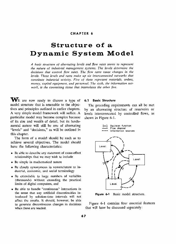
CHAPTER 6
Structure of a Dynamic System Model
A basic structure of alternating levels and flow rates seems to represent the nature of industrial management systems. The levels determine the decisions that control flow rates. The flow rates cause changes in the levels. These levels and rates make up six interconnected networks that constitute industrial activity. Five of these represent materials, orders,
money, capital equipment, and personnel. The sixth, the information net-
work, is the connecting tissue that interrelates the other five.
WE are now ready to discuss a type of 6.1 Basic Structure
model structure that is amenable to the objec- The preceding requirements can all be met tives and principles outlined in earlier chapters. by an alternating structure of reservoirs or A very simple model framework will suffice. A levels interconnected by controlled flows, as
particular model may become complex because shown in Figure 6-1. of its size and wealth of detail, but its funda- mental nature will still be one of alternating p4 ?ecision function "1 1" and "d .. " as .11 b 1. d. in Flow channel "levels" and "decisions," as will be outlined in Information sources this chapter.
The form of a model should be such as to achieve several objectives. The model should \
have the following characteristics: Levei 1 / 1
. Be able to describe any statement of cause-effect
relationships that we may wish to include \ / / \ Level
. Be simple in mathematical nature 'J Level
. Be closely synonymous in nomenclature to in- \ f ;
dustrial, economic, and social terminology 1 / / Be extendable to large numbers of variables t J /
(thousands) without exceeding the practical ! limits of digital computers, and Level /
Be able to handle "continuous" interactions in ––––––y-–– the sense that any artificial discontinuities in-
Figure 6-1 Basic model structure. troduced by solution-time intervals will not
" '
affect the results. It should, however, be able to generate discontinuous changes in decisions Figure 6-1 contains four essential features
when these are needed. that will later be discussed separately:
67
STRUCTURE OF A DYNAMIC SYSTEM MODEL L
. Several levels levels from rates. Some levels have the dimen-
. Flows that transport the contents of one level sion of units over time (as units per week). to another This may cause confusion until the basic distinc-
. Decision functions (drawn as valves) that con- tion between levels and rates is clear. trol the rates of flow between levels A good test to determine whether a variable
. Information channels that connect the decision is a level or a rate is to consider whether or functions to the levels not the variable would continue to exist and
This is the basic structure that be used to have meaning in a system that had been
This is the basic structure that wi be used brought to activity, in the form of
here, even with industrial and economic models flows, were ta cease, the levels would still
that at first glance may seem vastly more com- exist. Stopping the receiving and shipping of plex. If the reader acquires a good grasp of
goods does not affect the continued existence this structure and the basic équations of the
of inventory that is in a warehouse. If all ac- next chapter that go with it, he should have no
tivity in a system is momentarily stopped, rates difficulty with even extensive models. At each tivity in a system is momentarily stopped, rates are unobservable. There is no movement to be separate point the larger systems will still cor-
detected, but the levels continue to exist. The respond to one of the above four features in
levels of physical quantities such as goods, the fundamental structure of Figure 6-1.1 money, and personnel would be countable in
The following sections will discuss each of the stationary system. the four features of the basic model structure. information network as Levels. The levels are the accumulations well as in the physical network of material, etc. well as in the physical network of material, etc.
within the system. They are the inventories, "Awareness levels" exist in the mental attitudes goods in transit, bank balances, factory space, that influence decisions. Levels of satisfaction, and number of employées. Levels are the près- of optimism, and of recollection of a past ent values of those variables that have resulted disastrous depression, all influence economic from the accumulated différence between in- behavior. The level of awareness of inflation flows and outflows.2 Levels exist in all of the trends influences investment. In a more prosaic six networks to be discussed later: information, context the level of recent business activity materials, orders, money, personnel, and capital influences ordering and inventory decisions. All equipment. memory and continuity from the past to the
It is very important to note that the units of future exist in the levels of the system. measure of a variable do not serve to distinguish In the information network especially, we
1 The reader who is already familiar with the are apt to find levels that carry the dimensional mathematical organization of a problem for solution units usually thought of as belongmg to rates. on a differential analyzer will note the identity of
Take, for example, the average sales level for Figure 6-1 to a system of integrators and function '
generators. The equations of the next chapter are a the last year. It may be measured in items per set of first-order difference équations equivalent to the month or dollars per year. It is not a rate. It integrations ordinarily executed by the differential is not a ilow that iridicates the moment-by- analyzer. As already noted in Chapter 1, the analog- -'
type differential analyzer is inadequate because it does moment, présent transfer rate between any two not readily handle problems of the size or degree of levels. In a continuously rising trend, the aver- nonlinearity that we shall deal with in the field of
age sales rate that is computed at any given management. The digital computer can handle the ° sales rate that is computed at ? given
same class of problems to perhaps 100 times the size moment would never be equal to the actual cur- that has been done successfully on analog machines, rent sales rate at that same moment. Average
- Levels are the time integrals of the net flow rates. sales are often j business practice channels. A level
may have any number of inflow or outflow as a level
.. channels. as a eve - t e eve o sa es or t e eve o
68
§6.1 1 BASIC STRUCTURE
business. The average sales level is obtained by and the average transportation delay, a con-
integrating (summing) the moment-by-moment stant). On the other hand, a decision function actual sales rate over some period of time like a may be described by a long and elaborate se-
year ; it is therefore of the same mathematical quence of computations that progresses through equation form that describes the other levels the evaluation of a number of intermediate in the system. By the test of bringing the system concepts (for example, a personnel hiring de- to rest, we see that average sales for the last cision might involve the following levels: pres- year is a level. We can stop all present sales and ent employees, average order rate, employees shipping activity without destroying the con- in training, employee requisitions already initi-
cept and numerical value of average sales for ated, backlog of unfilled orders, present inven- the preceding year. tory levels, available capital equipment, avail-
Flow Rates. From the preceding discussions able materials, etc.). of levels, the nature of flow rates has emerged. Information as a Basis for Decisions. In Rates define the present, instantaneous flows Figure 6-1 it is shown that the decision func- between the levels in the system. The rates cor- tions determining the rates are dependent only respond to activity, while the levels measure the on information about the levels. Rates are not
resulting state to which the system has been determined by other rates. This is always true
brought by the activity. Rates as well as levels in principle.3 exist in all six networks that may constitute a In principle, present, instantaneous rates are
system - materials, orders, money, personnel, not available as inputs to the making of other
capital equipment, and information. decisions. In fact, present rates are in general The rates of flow are determined by the levels unmeasurable. If we shorten sufficiently what
of the system according to rules defined by the we mean by the "present" time, we have no decision functions. In turn the rates determine knowledge of other action rates occurring at the levels. The levels determining a particular the same time. We do not know the sales rate flow rate will usually include the level from of our company at precisely this moment; in which the flow itself comes. fact it would be meaningless to us in view of
Decision Functions. The decision functions the normal short-run fluctuations that occur.
(called rate equations in some later sections) What we usually mean by "present" rates are are the statements of policy that determine how really averages (levels) such as average sales the available information about levels leads to for the week, or the month, or last year. the decisions (current rates). All decisions per- By making the time span sufficiently short, tain to impending action and are expressible as we can in principle establish the impossibility flow rates (generation of orders, construction of having a particular decision dependent on of equipment, hiring of people). As will be some other present decision (or rate) that is discussed in Section 10.4, the decision functions being determined at the same instant in another
pertain both to managerial decisions and to part of the system. (Another decision stream those actions that are inherent results of the might depend on the same input levels.) The
physical state of the system. decision to attempt to hire more employees in A decision function may appear as a simple New York is not conditioned by the corre-
equation that determines, in some elementary sponding decision at the same moment by a
way, a flow in response to the condition of one _ _ or two levels (like the output of a transporta-
3 At times the modelmaker may for simplicity take liberties with this principle by letting a generated a
tion system that may often be adequately repre- instantaneous rate be used instead of a very short sented by the goods in transit, which is a level, run average.
69 .
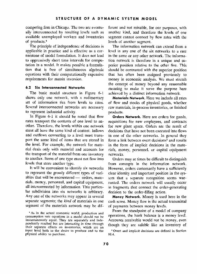
STRUCTURE OF A DYNAMIC SYSTEM MODEL L
competing firm in Chicago. The two are eventu- ferent and not mixable, for our purposes, with
ally interconnected by resulting levels such as another kind, and therefore the levels of one available unemployed workers and inventories segment cannot connect by flow rates with the of products.4 levels of another segment.
The principle of independence of decisions is The information network can extend from a
applicable in practice and is effective as a cor- level in any one of the six networks to a rate nerstone of model formulation. It does not lead in the same or any other network. The informa- to oppressively short time intervals for compu- tion network is therefore in a unique and su- tation in a model. It makes possible a formula- perior position relative to the other five. This tion that is free of simultaneous algebraic should be contrasted with the superior position equations with their computationally expensive that has often been assigned previously to
requirements for matrix inversion. money in economic analysis. We must stretch the concept of money beyond any reasonable
6.2 Six Interconnected Networks meaning to make it serve the purpose here
The basic model structure in Figure 6-1 achieved by a distinct information network. shows only one network, with a rudimentary Materials Network. Here we include all rates set of information ties from levels to rates. of flow and stocks of physical goods, whether Several interconnected networks are necessary raw materials, in-process inventories, or finished to represent industrial activity. products.
In Figure 6-1 it should be noted that flow Orders Network. Here are orders for goods, rates transport the contents of one level to an- requisitions for new employees, and contracts other. Therefore, the levels within one network for new plant space. Orders are the result of must all have the same kind of content. Inflows decisions that have not been executed into flows and outflows connecting to a level must trans- in one of the other networks. In general they port the same kind of items that are stored in form a link between overt decisions5 and results the level. For example, the network for mate- in the form of implicit decisions in the mate- rial deals only with material and accounts for rials, money, personnel, or capital equipment the transport of the material from one inventory networks. to another. Items of one type must not flow into Orders may at times be difficult to distinguish levels that store another type. from concepts in the information network.
It will be convenient to identify six networks However, orders customarily have a sufficiently to represent the grossly different types of vari- clear identity and important position in the sys- ables that will be encountered - orders, mate- tem that a separate recognition seems war- rials, money, personnel, and capital equipment, ranted. The orders network will usually occur all interconnected by information. This particu- in fragments that connect the order-generating lar subdivision into six networks is arbitrary. decision to the order-filling action.
Any one of the networks may appear in several Money Network. Money is used here in the
separate segments; the kind of materials in one cash sense. Money flow is the actual transmittal
segment of the materials network may be dif- of payments between money levels.
' As in the actual economic world, production and From the standpoint of a model of company As in the actual economic world, production 11 consumption rate equations in a model should not be operations, the bank balance is a money level.
instantaneously equal. They are separately and inde- Accounts receivable would not be money, even pendently reached but are interacting in time through thought they are salable like an inventory of their separate effects on inventories, which are an ' '
input level both to the desire to produce and to the 6 Overt and implicit decisions are defined in Section physical ability to purchase. , 10.4.
70

§6.2 SIX INTERCONNECTED NETWORKS 5
goods; they can be carried in the information men multiplied by the length of work week.
network as information telling us our rights to Different considerations control changes in num-
the receipt of payment. Price is also informa- bers of men from those that circumscribe the
tion, and not part of the money network. changes in length of work week. In most situa- At the point of filling orders, three flows are tions we shall need to distinguish men in the
created. First is the flow of completed orders personnel network from the variables that are
out of the unfilled-order backlog. Second is the in the information network, such as length of
flow of physical goods from supplier to cus- work week and the productivity per man-hour.
tomer. Third is the flow of information to ac- Capital Equipment Network. The capital counts receivable, which is the product of price equipment network includes factory space,
multiplied by the goods flow rate. The level of tools, and equipment necessary to the produc- accounts payable at the customer, along with tion of goods. It describes the way that factories invoice payment delay and his ability to pay, and machines come into existence, the stock of determine the rate of money flow from the cus- existing capital equipment, what part (to meas-
tomer's bank account to the supplier. This flow ure the level of productivity) of our capital rate increases the supplier's bank account level, equipment stock is in use at any instant, and and information about the rate decreases the the discard rate of capital equipment. level of accounts receivable. Within a capital goods producing sector, it
Different points of view may lead to different should be noted that the capital equipment out- treatment of information and money. The bank put is a result, among other things, of material
account, treated by the company as a money that flowed into the capital equipment pro- level, is to the bank an account payable. The duction facility. The capital equipment pro- account contains no money but is information ducer has his own stock of equipment used for
concerning the right of the company to make a the production process. withdrawal. Representation of money, credit, Interconnecting Information Network. The and information will require more subtle treat- information network is itself a sequence of alter- ment as the refinements of a banking and na- nating rates and levels. In this book it is raised tional monetary system are incorporated into to a position superior to the other networks more comprehensive dynamic models. because it is the interconnecting tissue between
Personnel Network. Many important dy- all of them. namic effects in the company arise because of In general, the information network starts at the policies and behavior patterns surrounding the levels and rates in the other five networks the acquisition and utilization of people. Com- and ends at the rate-generating decision func-
pany policies, labor union contracts, and avail- tions in those five. It transfers level information
ability of people establish a framework that to decision points, and rate information in the
affects the changing of employment levels. The other networks to the levels in the information
timing of such changes can interact with other network. Levels and rates of flow exist within
parts of the company to produce unexpected the information network itself. For example, results. In Part III, Chapters 17 and 18, is an information about the actual, current rate of
example of the way the interaction of the manu- incoming orders is averaged to produce the
facturer's labor policy with the customers' or- level of average incoming-order rate. This is a
dering policy creates instability in an industry. level in the information network and will usu- In the personnel network we deal with people ally be one of the inputs to an ordering decision
as countable individuals, not as man-hours of in the order network. labor. Man-hours per week is a product of The value of an information variable must
. 7 1

STRUCTURE OF A DYNAMIC SYSTEM MODEL L
not be confused with the true variable it repre- linkage that causes the other five networks to sents. Orders usually go into an unfilled-order act on one another. In many economic models, file; information about the level of average order and in our attitudes toward accounting, there rate and about the level of unfilled orders may is often an effort to visualize money in this
go many places in the company. Information central, interlocking relationship to the other will often be delayed, as will flows in the other parts of industrial activity. The money network
five networks. As discussed in Section 5.2, does not provide adequate inputs for creating information may contain noise and bias. In- actual managerial and economic decisions. The
formation is not necessarily identical in value money network constitutes a summary of past to the "true" variable that it represents. transactions and acts as a restraint on future
The information network will contain the decisions but is not a sufficient guide to the
generation of various "concepts" that are in- making of those decisions.
puts to decision making, such as desired inven- Careful observation of the information net-
tory level, projected size of necessary plant, work of an organization is e?sential to under-
forecast of sales, desired employment level, and standing its true character. Its dynamic behavior
knowledge from research results. cannot be represented without a proper treat-
The major fraction of a model will usually ment of the flows, levels, delays, and distortions
be within the information network. Information that lie in the information channels that inter-
is the essence of decision making. It is the weave the separate organizational components.
72
CHAPTER 7
System of Equations
The rnodel structure described in Chapter 6 leads to a simple system of equations that suffices for representing information-feedback sy.stems. The
equations tell how to generate the system conditions for a new point in time, given the conditions known from the previous point in time. The
equations of the model are evaluated repeatedly to generate a sequence of steps equally spaced in time. Level equations and rate equations gener- ate the levels and rates of the basic model structure. In addition, auxiliary, supplementary, and initial-value equations are used. The interval of time between solutions must be relatively short, determined by the dy- namic characteristics of the real system that is being modeled. Simple first-order integration of level equations is satisfactory.
IN the preceding chapter an arrangement for Basically, the equation system consists of the basic structure of a model was illustrated two types of equations corresponding to the in terms of levels (reservoirs) interconnected by levels and the rates discussed in the preceding rates of flow. To describe this general structure, chapters. In a following section will be intro- we must have a suitable system of equations. duced other incidental types of equations which The equations should be compatible with the add convenience and clarity to complex systems five objectives of a model listed at the beginning but which are not fundamental to the model of Chapter 6. structure. Before doing that, the fundamental
The system of equations should be adequate time sequence of computation can be described to describe the situations, concepts, interac- in terms of levels and rates.
tions, and decision processes that constitute the world of management and economics. The 7.1 Computing Sequence model should be able to fit our concepts of A system of equations is written in the con-
reality rather than requiring violent and unac- text of certain conventions that state how the
ceptable simplifications to bring those concepts equations are to be evaluated. We are dealing into the bounds of a model structure. here with a system of equations that controls the
The equations to be described here form a changing interactions of a set of variables as basic system going with, and elaborating slightly time advances. This system evolution implies on, the model structure already described. that the equations will be computed periodi- Classes of equations are discussed in this chap- cally to yield the successive new states of the ter but not the special forms that particular system. equations of these classes may assume.l At each point in time, there may be a par-
' In particular, this discussion omits various inter- ticular sequence of computation implied by the In partlcu ar, t IS discussion omlts vanous mter- . ) j i
mittent operations like periodic sampling and "box- équation system. The sequence to be used here car" delays that are useful in segregating and saving is shown in Figure 7-1. The continuous advance historical information, as in bringing forward annual pf time ts small intervals of equal sales curves from past years and separating capital . " . equipment by age and productivity. length DT (Standing for "delta time," or time
73
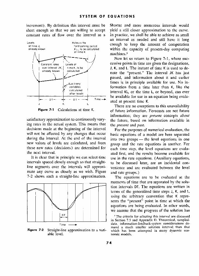
SYSTEM OF EQUATIONS 5
increment). By definition this interval must be Shorter and more numerous intervals would
short enough so that we are willing to accept yield a still closer approximation to the curve.
constant rates of flow over the interval as a In practice, we shall be able to achieve as small
Levels Rates in the an interval as needed and still have it long
at ti me J, Rotes in rhe enough to keep the amount of computation at lime J, larlhcamlng penad alreody knowri KL, la be calculuted within the capacity of present-day computing
A ! cit time K
machines.2
./ Now let us return to Figure 7-1, where suc-
Constant rotes Levels at / cessive points in time are given the designations, over iriterval JK, time K, to be / J, K, and L. The instant of time K is used to de-
\ already known colculoted note the présent. " The interval JK has just passed, and information about it and earlier
" 1 Auxiirary times is in principle available for use. No in-
variables formation from a time later than K, like the cv-o,,culoted interval KL, or the time L, or beyond, can ever if interval KL, or the time L, or beyond, can ever alter levels "
DT DT Tlme- be available for use in an equation being evalu- ated at present time K.
J K L There are no exceptions to this unavailability
Figure 7-1 Calculations at time K. of future information. Forecasts are not future
information; they are present concepts about
satisfactory approximation to continuously vary- the future, based on information available in ing rates in the actual system. This means that the present and past. decisions made at the beginning of the interval For the purposes of numerical evaluation, the will not be affected by any changes that occur basic equations of a model are here separated during the interval. At the end of the interval into two groups - thé level équations in one new values of levels are calculated, and from
group and the rate equations in another. For these new rates (decisions) are determined for each time step, the level equations are evalu- the next interval. ated first, and the results become available for
It is clear that in principle we. can select time use in the rate equations. (Auxiliary equations, intervals spaced closely enough so that straight- to be discussed later, are an incidental con- line segments over the intervals will approxi- venience and are evaluated between the level mate any curve as closely as we wish. Figure and rate groups.) 7-2 shows such a straight-line approximation. The equations are to be evaluated at the
__________________________ moments of time that are separated by the solu- tion intervals DT. The equations are written in
terms of the generalized time steps J, K, and L,
using the arbitrary convention that K repre- sents the "present" point in time at which the
\. // equations are being evaluated. In other words, *==' we assume that the progress of the solution has
DT 2 The criteria for selecting this interval are discussed
_________________________ in Section 7.5 and Appendix D. Theoretical, sampled-
Time data, information-feedback-system considerations de-
mand a much smaller solution interval. than that
Figure 7-2 Straight-line approximation to a vari- which has been attempted in many dynamic eco-
able level. nomic models.
74
§7.3 TIME NOTATION IN EQUATIONS 5
just reached time K, but that the equations have 7.2 Symbols in Equations not yet been solved for levels at time K, nor for
Symbols used to represent quantities in the rates over the interval KL.
equations of the model should be chosen to The level equations show how to obtain levels have as much mnemonic significance as possi-
at time K, based on levels at time J, and on rates ble, that is, to remind us of the commonly used over the interval JK. At the time K, when the
terminology of everyday affairs. Partly to agrée level equations are evaluated, all necessary in- with- common usage, partly to recognize thé formation is available and has been carried restricted choice of characters available on forward from the preceding time step. digital computer output printers, we shall use
The rate equations are evaluated at the pres- only groups of capital English letters and Arabic ent time K after the level equations have been numerals to signify the variables and constants evaluated. The rate equations can, therefore, in a mode!." Thus the number of employees at have available as inputs the present values of Plant A might be represented as EPLTA; the levels at K.3 The values determined by the rate
inventory in warehouse number 5 could be (decision) equations determine the rates that INVW5; the inventory desired at the retail level represent the actions that will be taken over the could be IDR. Manufacturing output rate from forthcoming interval KL. Constant rates imply a the factory could be MOF. constant rate of change in levels during a time Because of the limitations of computer print- interval. The slopes of the straight lines in
ing equipment, no subscripts or superscripts Figure 7-1 are proportional to the rates and will be used. connect the values of the levels at the J, K, and L
points in time. After evaluation of the levels at time K and Time Notation in Equations
the rates for the interval KL, time is "indexed." A convention must be adopted for indicating That is, the J, K, L positions of Figure 7-1 are time notation so that we can specify the mo- moved one time interval to the right. The K ment of time at which a numerical value ap- levels just calculated are relabeled as J levels. plies. Often in the literature, time has been The KL rates become the JK rates. Time K, "the indicated by small subscripts below the line of
present," is thus advanced by one interval of printing; this is not readily accomplished on a time of DT length. The entire computation se- typewriter and not at ai] on many computing, quence can then be repeated to obtain a new machine printers. state of the system at a time that is one DT To designate time, we shall use one or two later than the previous state. The model traces capital letters following a variable and sepa- the course of the system through time as the rated by a period. environment (levels) leads to decisions and ac- Thus in the previous examples, the level of tions (rates) that in turn affect the environ- employees at time J would be EPLTA.J, the level ment. Thus the interactions within the system at time K would be written as EPLTA.K. Note are made to follow the "description" that has that the single letter is used as a time suffix been set down in the equations of the model.4 because the values of levels are calculated at,
The rates from the JK interval are also available and are correct only at, the separate instants
and may sometimes be used as an expediency, but in " . MO principle are not properly or necessarily involved in 5 To agree with the specifications of the DYNAMO the computation of new rates. computing system (see Appendix A), which has been
'In Appendix C will be found an example of the designed especially for this équation system, we shall
computational steps in evaluating a simple set of use groups of five characters or less, of which the first
equations. will be alphabetic.
75 5
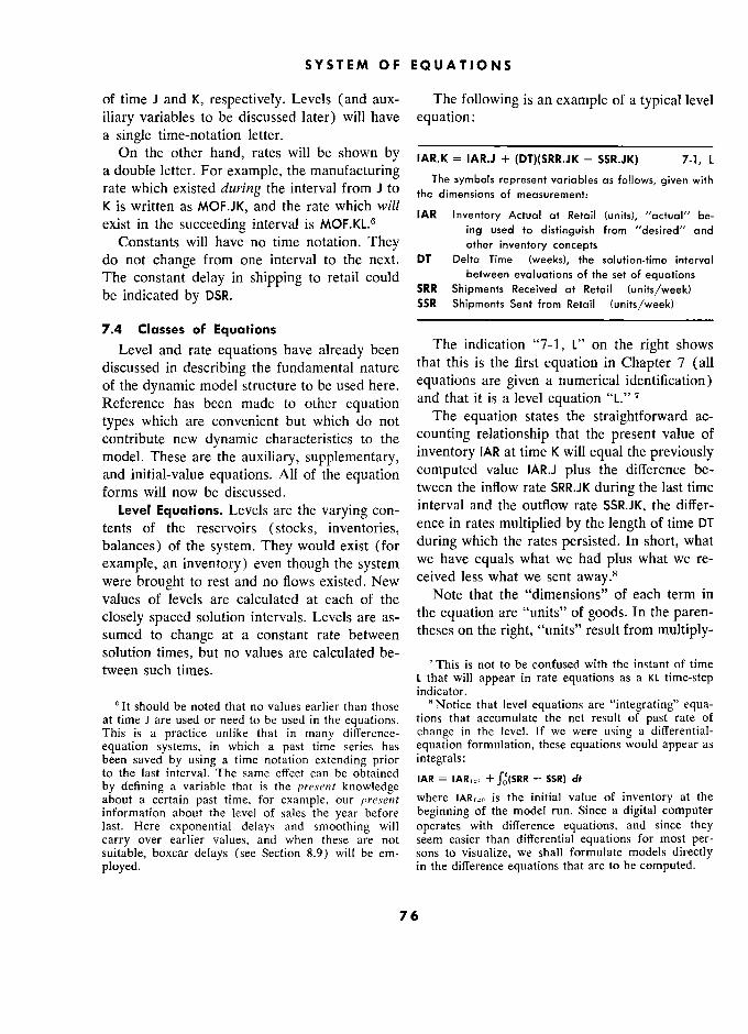
SYSTEM OF EQUATIONS
of time J and K, respectively. Levels (and aux- The following is an example of a typical level iliary variables to be discussed later) will have equation: a single time-notation letter.
On the other hand, rates will be shown by IAR.K = IAR.J + (DT)(SRR.JK - SSR.JK) 7-1, L a double letter. For example, the manufacturing The symbols represent variables as follows, given with rate from ta
sym o represent variables as iollows, given with rate which existed during the interval from J to the dimensions of measurement: K is written as MOF.JK, and the rate which will
IAR Inventory Actual at Retail (units), "actual" be- exist in the succeeding interval is MOF.KL.6
IAR !nventoryActua)atRetai) (units),
exist in the succeeding interval is MOF.KL.6 ing used to distinguish from "desired" and Constants will have no time notation. They other inventory concepts
do not change from one interval to the next. DT Delta Time (weeks), the solution-time interval The constant delay in shipping to retail could between évaluations of the set of equations
be indicated by DSR. SRR Shipments Received at
Retail (units/week) ' SSR Shipments Sent from Retail (units/week)
7.4 Classes of Equations Level and rate equations have already been The indication "7-1, L" on the right shows
discussed in describing the fundamental nature that this is the first equation in Chapter 7 (all
of the dynamic model structure to be used here. equations are given a numerical identification)
Reference has been made to other equation and that it is a level equation "L." 7
types which are convenient but which do not The equation states the straightforward ac-
contribute new dynamic characteristics to the counting relationship that the present value of
model. These are the auxiliary, supplementary, inventory IAR at time K will equal the previously
and initial-value equations. All of the equation computed value IAR.J plus the difference be-
forms will now be discussed. tween the inflow rate SRR.JK during the last time
Level Equations. Levels are the varying con- interval and the outflow rate SSR.JK, the differ-
tents of the reservoirs (stocks, inventories, ence in rates multiplied by the length of time DT
balances) of the system. They would exist (for during which the rates persisted. In short, what
example, an inventory) even though the system we have equals what we had plus what we re-
were brought to rest and no flows existed. New ceived less what we sent away.s
values of levels are calculated at each of the Note that the "dimensions" of each term in
closely spaced solution intervals. Levels are as- the equation are "units" of goods. In the paren- sumed to change at a constant rate between theses on the right, "units" result from multiply- solution times, but no values are calculated be- ' This is not to bc confused with the instant of time tween such times.
7 This is not to be confused with the instant of time tween such times. L that will appear in rate equations as a KL time-step indicator.
° It should be noted that no values earlier than those 8 Notice that level equations are "integrating" equa- at time J are used or need to be used in the equations. tions that accumulate the net result of past rate of This is a practice unlike that in many différence- change in the level. If we were using a differential-
equation systems, in which a past time series has equation formulation, these equations would appear as been saved by using a time notation extending prior integrals: to the last interval. The same effect can be obtained ,.., e SSR .j. by defining a variable that is the présent knowledge about a certain past time, for example, our present where is the initial value of inventory at the information about the level of sales the year before beginning of the model run. Since a digital computer last. Here exponential delays and smoothing will operates with difference equations, and since they carry over earlier values, and when these are not seem easier than differential equations for most per- suitable, boxcar delays (see Section 8.9) will be em- sons to visualize, we shall formulate models directly ployed. in the difference equations that are to be computed.
76

§7.4 CLASSES OF EQUATIONS
ing time in fractions of a week by flow rates in types; there is no structural or evident difference
units/week. in the equations themselves.
The flow rates are always measured in some The rate equations, being decision equations
customary unit of time such as day, week, or in the broad sense to be discussed later, are
month, not in terms of the solution interval DT. best thought of as controlling what is to happen But the time units of the rates and the time units next in the system. A rate equation is evaluated
of DT must be the same, for example, all in at time K to determine the decision governing weeks or months. The equation is valid and the rate of flow over the forthcoming interval
independent of the solution interval DT so long KL. Rate equations in principle depend only on
as the interval does not exceed a maximum the value of levels at time K.1° (In practice, value to be discussed later. The solution interval rates from the last time interval JK may occa-
can be changed without requiring any change sionally be used as a short cut in place of the
in the equation formulation or in any constants level of an average rate where a very short aver-
that may have appeared. By letting the interval aging time would have been used.) DT appear explicitly in the equation, we can Rate equations are evaluated independently follow the procedure of using the normal cus- of one another within any particular time step,
tomary units of measure found in the real sys- just as level equations are. Interaction occurs by tem that is being modeled. their ensuing effect on levels that then influence
Level equations are independent of one an- other rates at later times. A rate equation de-
other. Each depends only on information before termines an immediately forthcoming action.
time K. It does not matter in what order level If this action is sufficiently immediate (that is,
equations are evaluated. At the evaluation time the length of the solution interval DT is suf-
K, no level equation uses information from other ficiently short), it is evident that the decision
level equations at the same time. A level at time cannot itself be affected by other decisions being K depends on its previous value at time J and made at the same time instant in other parts of
on rates of flow during the JK interval. the system.ll The rate equations are therefore
Variables that should be classed as levels may independent of one another and can be eval-
carry units of measure, like "items per week," uated in any sequence. Since they do depend that at first may seem to indicate rates. The on the values of the levels, the group of rate
"stationary-system" test as discussed in Section equations is evaluated after the level equations. 6.1 should be applied. As explained there, An example of a rate equation is provided by
average rates are by nature levels, not rates. the outflow rate of a first-order exponential de-
Rate Equations (Decision Functions). The lay. The justification of the equation will be
rate equations define the rates of flow between given in Chapter 9; its form will be examined
the levels of the system. The rate equations are here.
the "décision functions" that will be discussed , the "decision functions" that will be discussed '° Auxiliary variables appear in rate equations further in Chapter 10. A rate equation is eval-
merely as subdivisions of the rate equation and so uated from the presently existing values of are not a violation of this principle. levels in the system, very often including the "A sufficiently short time interval precludes inter-
level from which the rate Comes communication of information between decisions
level which the rate cornes and the one within one time step. Meeting this requirement does into which it goes. The rates in turn cause the not lead to excessively short solution intervals. A
changes in the levels. The rate equations may decision can depend on as many information inputs as
"OVert" Or "im 9 d .. are thought significant. The value of any one level
e either of thé overt or p décision may be used by several separate decision points at
"See Section 10.4. any one time step.
77
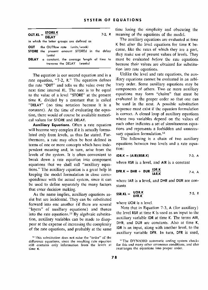
SYSTEM OF EQUATIONS
time losing the simplicity and obscuring the OUT.KL =
STORE.K 7-2, R meaning of the equations of the model.
in which )f groups are defined as The auxiliary equations are evaluated at time
OUT the OUTflow rate (units/week) K but after the level equations for time K be- OUT thé OUT<1ow rate (units/week) cause, like the rates of ,., , the are a art, STORE the présent amount STOREd in the delay cause, like the rates of which they are a part,
(units) they make use of present values of levels. They DELAY Y a constant, the average length of time to must be evaluated before the rate equations
traverse the DELAY (weeks) because their values are obtained for substitu- tion into rate equations.
The equation is our second equation and is a Unlike the level and rate equations, the aux- rate equation, "7-2, R." The equation defines iliary equations cannot be evaluated in an arbi- the rate "OUT" and tells us the value over the trary order. Some auxiliary equations may be next time interval KL. The rate is to be equal components of others. Two or more auxiliary to the value of a level "STORE" at the present equations may form "chains" that must be time K, divided by a constant that is called evaluated in the proper order so that one can "DELAY" (no time notation because it is a be used in the next. A possible substitution
constant). At the time of evaluating the equa- sequence must exist if the equation formulation
tion, there would of course be available numeri- is correct. A closed loop of auxiliary equations cal values for STORE and DELAY. where two variables depend on the values of
Auxiliary Equations. Often a rate equation each other indicates a set of simultaneous equa- will become very complex if it is actually formu- tions and represents a forbidden and unneces- lated only from levels, as thus far stated. Fur- sary equation formulation.'3
thermore, a rate may often be best defined in The following is a chain of two auxiliary terms of one or more concepts which have inde- equations between two levels and a rate equa- pendent meaning and, in turn, arise from the tion: levels of the system. It is often convenient to IDR.K = (AIR)(RSR.K) 7-3, A break down a rate equation into component , . , ... is equations that we shall call "auxiliary equa-
?? ? and ?? ? a constant
tions." The auxiliary equation is a great help in DFR.K = DHR + DUR IDR.K
keeping the model formulation in close corre- IAR.K A
spondence with the actual system, since it can where IAR is a level, and DHR and DUR are con- be used to define separately the many factors stants
'
that enter decision making. UOR.K 7-5, R As the name implies, auxiliary equations as- SSR.KL = 7-5, R sist but are incidental. They can be substituted
wher, UOR is a level. forward into one another (if there are several where UOR is a level.
"layers" of auxiliary equations) and thence Note that in Equation 7-3, A (for auxiliary) into the rate equations.12 By algebraic substitu- the level RSR at time K is used as an input to the
tion, auxiliary variables can be made to disap- auxiliary variable IDR at time K. The terms AIR,
pear at the expense of increasing the complexity DHR, and DUR are constants. Also at time K, of the rate equations, and probably at the same IDR is an input, along with another level, to the
auxiliary variable DFR. In turn, DFR is used, " This substitution does not raise the "order" of the
difference equations, since the resulting rate equation "The DYNAMO automatic coding system checks still contains only information from the levels at for this and many other erroneous conditions, and also time K. rearranges the equations into proper order.
78
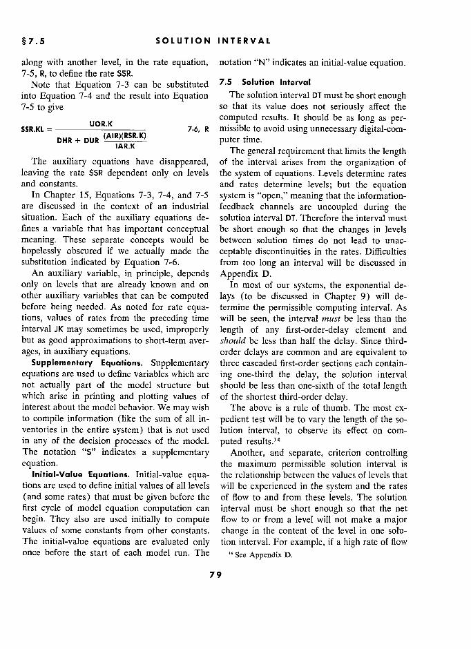
§7.5 SOLUTION INTERVAL
along with another level, in the rate equation, notation "N" indicates an initial-value equation. 7-5, R, to define the rate SSR.
Note that Equation 7-3 can be substituted 7.5 S Solution Interval
into Equation 7-4 and the result into Equation The solution interval DT must be short enough 7-5 to give so that its value does not seriously affect the
UOR.K computed results. It should be as long as per- SSR.KL = 7-6, R missible to avoid using unnecessary digital-com-
DHR + DUR puter time. IAR.K The general requirement that limits the length
The auxiliary equations have disappeared, of the interval arises from the organization of
leaving the rate SSR dependent only on levels the system of equations. Levels determine rates and constants. and rates determine levels; but the equation
In Chapter 15, Equations 7-3, 7-4, and 7-5 system is "open," meaning that the information- are discussed in the context of an industrial feedback channels are uncoupled during the situation. Each of the auxiliary equations de- solution interval DT. Therefore the interval must fines a variable that has important conceptual be short enough so that the changes in levels
meaning. These separate concepts would be between solution times do not lead to unac-
hopelessly obscured if we actually made the ceptable discontinuities in the rates. Difficulties substitution indicated by Equation 7-6. from too long an interval will be discussed in
An auxiliary variable, in principle, depends Appendix D.
only on levels that are already known and on In most of our systems, the exponential de- other auxiliary variables that can be computed lays (to be discussed in Chapter 9) will de- before being needed. As noted for rate equa- termine the permissible computing interval. As tions, values of rates from the preceding time will be seen, the interval must be less than the interval JK may sometimes be used, improperly length of any first-order-delay element and but as good approximations to short-term aver- should be less than half the delay. Since third-
ages, in auxiliary equations. order delays are common and are equivalent to
Supplementary Equations. Supplementary three cascaded first-order sections each contain-
equations are used to define variables which are ing one-third the delay, the solution interval not actually part of the model structure but should be less than one-sixth of the total length which arise in printing and plotting values of of the shortest third-order delay. interest about the model behavior. We may wish The above is a rule of thumb. The most ex- to compile information (like the sum of all in- pedient test will be to vary the length of the so- ventories in the entire system) that is not used lution interval, to observe its effect on com- in
any of the decision processes of the model. puted results.14
The notation "S" indicates a supplementary Another, and separate, criterion controlling equation. the maximum permissible solution interval is
Initial-Value Equations. Initial-value equa- the relationship between the values of levels that tions are used to define initial values of all levels will be experienced in the system and the rates
(and some rates) that must be given before the of flow to and from these levels. The solution first cycle of model equation computation can interval must be short enough so that the net
begin. They also are used initially to compute flow to or from a level will not make a major values of some constants from other constants. change in the content of the level in one solu- The initial-value equations are evaluated only tion interval. For example, if a high rate of flow once before the start of each model run. The 14 See Appendix D.
79 .
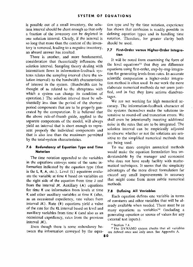
SYSTEM OF EQUATIONS
is possible out of a small inventory, the solu- tion type and by the time notation, experience tion interval should be short enough so that only has shown that confusion is readily possible in a fraction of the inventory can be depleted in defining equation types and in handling time one solution interval. Clearly, if the interval is notation. Therefore, for greater clarity both so long that more than the content of the inven- should be used. tory is removed, leading to a négative inventory, tory is removed, leading to a negative inventory' 7.7 First-Order versus Higher-Order Integra- an absurd answer has resulted.
. irs . r er versus ig er. r er n egra. an absurd answer has resulted. tion There is another, and more fundamental,
consideration that theoretically influences thé lt will be noted from examining thé form of
solution interval. Sampling theory dealing with the level equationsle that they are difference
intermittent flows in information-feedback sys- équations using first-order, step-by-step integra- tems relates the sampling interval (here the so- tion for generating levels from rates. In accurate
lution interval) to the bandwidth characteristics scientific computation a higher-order integra- of interest in the system. (Bandwidth can be tion method is often used. In our work the more
thought of as related to the abruptness with elaborate numerical methods do not seem justi- which a system can change its condition of fied, and in fact they have serious disadvan-
operation.) The solution interval must be sub- ta g es.
stantially less than the period of the shortest- We are not working for high numerical ac-
period components that are to be properly gen- curacy. The information-feedback character of
erated by the computation. It is believed that the systems themselves make the solutions in-
the above rule-of-thumb guide, applied to the sensitive to round-off and truncation errors. We
separate components of the model, will always shall even be intentionally inserting additional
yield an interval that is short enough to repre- noise in the rates that are to be integrated. The
sent properly the individual components and solution interval can be empirically adjusted that is also less than the maximum permitted to
observe whether or not the solutions are sen-
by the total-system characteristics. sitive to the simplified numerical methods that ' are being used.
7.6 Redundancy of Equation Type and Time To use more complex numerical methods Notation would make the equation formulation less un-
The time notation appended to the variables derstandable by the manager and economist in the equations conveys some of the same in- who does not have ready facility with mathe-
formation indicated by the equation type (that matical techniques. It seems that the simplicity is the L, R, A, etc.). Level (L) equations evalu- advantages of the more direct formulation far
ate the variable at time K based on variables on exceed any small improvements in accuracy the right side of the equation from time J and that might corne from more subtle numerical
from the interval JK. Auxiliary (A) equations methods.
for time K use information from levels at time 7,g 8 Defining All Variables K and other auxiliary variables at time K (also, Each équation defines one variable in terms as an occasional expediency, rate values from of constants and other variables that will be al- interval JK). Rate e (R) equations yield a value
ready available when needed. There must be as of the rate for the KL interval based on level and
many equations as nee?ed. Ther? must. be as a auxiliary variables from time K (and also as an
generating equation or source of values for any occasional expediency, rates from the previous generating equation or source of values for any
interval JK). Iency, ra es rom e prevlOus external test inputs).
Even though there is some redundancy be- ,. Section 7.4. system checks that all variables tween the information conveyed by the equa- are defined once and only once. See Appendix A.
80

CHAPTER 8
Symbols for Flow Diagrams
The model structure of Chapter 6 and the interrelationships of the equa- tions of Chapter 7 can be displayed diagrammatically. Such a flow dia-
gram helps to prevent confusion and forms another means of communicat-
ing the nature of the model to those who are not proficient in "reading" mathematical equations. This chapter explains the symbols that will be used in Chapters 15 to 18.
EXPERIENCE from teaching the formula- symbols for flow diagrams of dynamic models.1 tion of industrial dynamics models has demon- Symbolism for diagrammatic presentation is strated that a pictorial representation of an based on arbitrary choices that are selected to
equation system is highly desirable. A diagram emphasize and clarify particular aspects of a that displays the interrelationships between situation.
equations helps to lend clarity to the system The system of symbols used here shows the
formulation. Many people visualize the inter- existence of the interrelationships in the system.
relationships better when these are shown in a It distinguishes levels from rates. It separates flow diagram than they do from a mere listing the six flow systems of information, materials, of equations. A detailed flow diagram supple- orders, money, personnel, and equipment from ments a set of equations. It gives much of the one another. It discloses what factors enter into same information but in a different manner. each decision (rate) function. But the diagram A properly constructed flow diagram is better does not reveal what the functional relation- than a set of equations for communicating the ships are within the decision functions. For the
structure of a system to many practicing man- specific nature of the interactions between the
agers. A diagram represents an intermediate factors entering into a decision, the diagram transition between a verbal description and a carries the equation numbers, and we are
set of equations. thereby referred to the pertinent equation. The
A flow diagram of the system interrelation- diagram corresponds point by point to the
ships should be developed simultaneously with equations. the development of the equations of a system. Many beginners attempt to develop equations 8_1 Levels first and then summarize these later in a dia-
A level shown by a rectangle, - in Figure e gram, if the diagram is used at all. Such neglect level is shown corner is the symbol Figure gram, diagram diagram
is used at aH. the neglect 8-1. In thé upper-left corner is thé symbol group ot a diasram until a later stase loses thé clarity- ing advantage that a later stage can
provide in OAR) that denotes this particular level variable. ing advantage that a diagram can provide in
'
the initial stages of equation formulation. 1 In Chapter 15 these symbols will be applied to a This chapter will describe a set of standard specific situation.
81 1
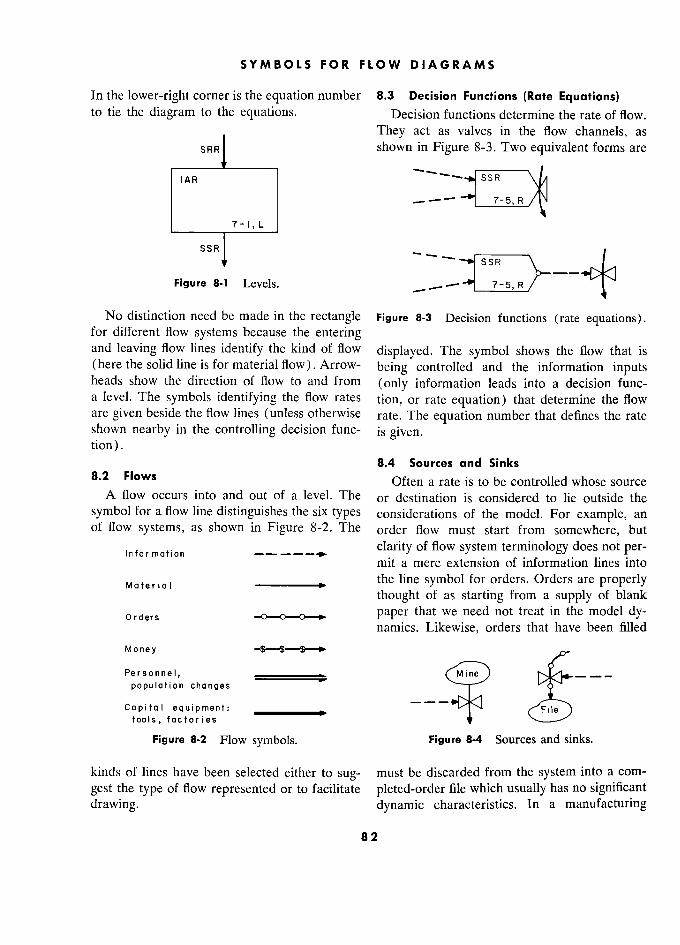
SYMBOLS FOR FLOW DIAGRAMS 5
In the lower-right corner is the equation number 8.3 Decision Functions (Rate Equations) to tie the diagram to the equations. Decision functions determine the rate of flow.
. They act as valves in the flow channels, as
SRR shown in Figure 8-3. Two equivalent forms are
.––––––!––––––.._ ______ < IAR SSR IAR
7 - 1 , L
SSR
1 SSR
Figure 8-1 1 Levels.
_
No distinction need be made in the rectangle Figure 8-3 Decision functions (rate equations). for different flow systems because the entering and leaving flow lines identify the kind of flow
displayed. The symbol shows the flow that is
(here the solid line is for material flow). Arrow- being controlled and the information inputs heads show the direction of flow to and from
(only information leads into a decision func- a level. The symbols identifying the flow rates tion, or rate equation) that determine the flow are given beside the flow lines (unless otherwise rate. The equation number that defines the rate shown nearby in the controlling decision func- is given. tion).
8.4 Sources and Sinks 8.2 Flows
Often a rate is to be controlled whose source A flow occurs into and out of a level. The or destination is considered to lie outside the
symbol for a flow line distinguishes the six types considerations of the model. For example, an of flow systems, as shown in Figure 8-2. The order flow must start from somewhere, but
, clarity of flow system terminology does not per- mit a mere extension of information lines into
i the line symbol for orders. Orders are properly
thought of as starting from a supply of blank
orders paper that we need not treat in the model dy- namics. Likewise, orders that have been filled
Money y .-,
Personnel, 1 , Mine
population changes
-s-5
,"",pm,"', . e Capital equipment: File
tools, factories t
Figure 8-2 Flow symbols. Figure 8-4 Sources and sinks.
kinds of lines have been selected either to sug- must be discarded from the system into a com-
gest the type of flow represented or to facilitate pleted-order file which usually has no significant
drawing. dynamic characteristics. In a manufacturing
82
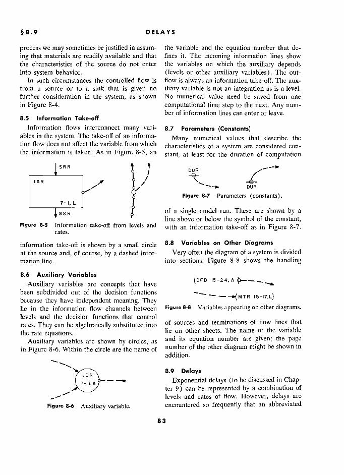
§8.9 DELAYS 5
process we may sometimes be justified in assum- the variable and the équation number that de-
ing that materials are readily available and that fines it. The incoming information lines show
the characteristics of the source do not enter the variables on which the auxiliary depends into system behavior. (levels or other auxiliary variables). The out-
In such circumstances the controlled flow is flow is always an information take-off. The aux-
from a source or to a sink that is given no iliary variable is not an integration as is a level.
further consideration in the system, as shown No numerical value need be saved from one
in Figure 8-4. computational time step to the next. Any num-
ber of information lines can enter or leave. 8.5 Information Take-off
Information flows interconnect many vari- 8.7 Parameters (Constants) ables in the system. The take-off of an informa-
Many numerical values that describe the tion flow does not affect the variable from which characteristics of a system are considered con- the information is taken. As in Figure 8-5, an
stant, at least for the duration of computation
SRR R t SRR & 1
t DUR --.
,–––*––––, t / - e- / IAR /f 1' ', aÀ
& Figure 8-7 Parameters (constants). 7- I, L L J
of a single model run. These are shown by a
line above or below the symbol of the constant, Figure 8-5 Information take-off from levels and with an information take-off as in Figure 8-7.
rates.
information take-off is shown by a small circle 8.8 Variables on Other Diagrams
at the source and, of course, by a dashed infor- Very often the diagram of a system is divided
mation line. into sections. Figure 8-8 shows the handling
8.6 Auxiliary Variables
(DFD 15-24,A Auxiliary variables are concepts that have (DFD
been subdivided out of the decision functions R 15 -17, L)
because they have independent meaning. They because they have independent meaning. They M T R 15 -17, L
lie in the information flow channels between Figure 8-8 Variables appearing on other diagrams.
levels and the decision functions that control
rates. They can be algebraically substituted into of sources and terminations of flow lines that
the rate equations. lie on other sheets. The name of the variable
Auxiliary variables are shown by circles, as and its équation number are given; the page
in Figure 8-6. Within the circle are the name of number of the other diagram might be shown in
addition.
-
Delays DR \
7-3 A Exponential delays (to be discussed in Chap-
, ter 9) can be represented by a combination of
levels and rates of flow. However, delays are
Figure 8-6 Auxiliary variable. encountered so frequently that an abbreviated
83
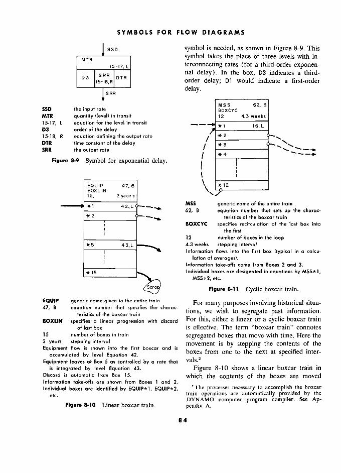
SYMBOLS FOR FLOW DIAGRAMS 5
s s D symbol is needed, as shown in Figure 8-9. This
symbol takes the place of three levels with in-
j 5 - j7, L terconnecting rates (for a third-order exponen-
D 3 s R R tial delay). In the box, D3 indicates a third-
3 order delay; D1 would indicate a first-order
SRR delay. SRR -
SSD the in ut rate M S S 62, B
SSD the input rate BOXCYC MTR quantity (level) in transit 12 2 4.3 weeks
15-17, L équation for the level in transit L
D3 order of the delay
15-18, R équation defining the output rate /
* 2
DTR time constant of the delay .
', SRR the output rate –––––––––––––
* 4 '--––<.
Figure 8-9 Symbol for exponential delay. 1
i
EOUIP P 47, B ` ?12 2 BOXLIN N "- 15, 2 year s
y MSS generic name of the entire train
*1 62, B équation number that sets up the charac- 2
2 teristics of the boxcar train
j BOXCYC spécifies recirculation of the last box into
1 the first
_____________ 12 number of boxes in the loop jE 5 4 3. L 4.3 weeks stepping interval
Information flows into the first box (typical in a calcu- ) lation of averages).
Information toke-offs come from Boxes 2 and 3.
5 Individual boxes are designated in équations by MSS*1,
MSS*2, etc.
scrap . Figure 8-11 t Cyclie boxcar train.
EQUIP generic name given to the entire train For many purposes involving historical situa-
47, B équation number that spécifies the charac- ..§ . . 47, B
teristics of the boxcar train
the charac- tions, we wish to segregate past information.
teristics oi thé oxcar train
BOXLIN spécifies a linear progression with discard For this, either a linear or a cyclic boxcar train
of last box is effective. The term "boxcar train" connotes
15 number of boxes in train segregated boxes that move with time. Here the
2 years stepping interval movement is by stepping the contents of the Equipment flow is shown into the first boxcar and is
boxes rom one ta the next at specified inter- accumulated by level Equation 42. .
boxes from the next at specified mter-
Equipment leaves at Box 5 as controlled by a rate that vais.
is integrated by level Equation 43. Figure 8-10 shows a linear boxcar train in
Discard is automatic from Box 15. which the contents of the boxes are moved Information take-offs are shown from Boxes 1 and 2. Individual boxes are identified by EQUIP*1, EQUIP*2, The processes necessary to accomplish the boxcar
etc. train operations are automatically provided by the ' DYNAMO computer program compiler. See Ap-
Figure 8-10 0 Linear boxcar train. pendix A.
. 84

§8.9 DELAYS 5
down one step at the specified intervals and the Figure 8-11 shows a cyclic boxcar train in contents of the last box are discarded. Each which the contents of the last box are reinserted box has a designation that can be used in equa- into the first box. The example shown might be tions in the same manner as any other variable. used to generate the average seasonal sales The example shown might represent the thirty- month by month by averaging corresponding year life of capital equipment, segregated by months of past years. Such monthly values
two-year age blocks. A parallel information might enter into decisions that are based on sea- boxcar train could hold separate productivity sonal considerations. Appendix N shows a cyclic indices for each age of equipment. boxcar train for seasonal sales analysis.
85 5
CHAPTER 9
Representing Delays
Delays are crucial in creating the dynamic characteristics of information- feedback systems. Delays are themselves composed of the standard level and rate equations of Chapter 7. Some forms of delays - exponential and pipeline - are discussed in the present chapter. Because of the preva- lence of delays, a "shorthand" notation is introduced to stand for the actual level and rate equations that are to be used in representing a delay.
PRECEDING chapters have stressed the resulting flow rate at the output. The outflow
important contribution of delays to creating may differ instant by instant from the inflow the characteristics of an information-feedback rate under dynamic circumstances where the
system. This chapter discusses methods of rep- rates are changing in value. This necessarily resenting in mathematical models the kinds of implies that the delay contains a variable
delays encountered in our industrial and eco- amount of the quantity in transit. The content nomic processes. of the delay increases whenever the inflow ex-
In principle, delays exist in all flow channels. ceeds the outflow, and vice versa.
However, to introduce a time delay in every A delay is a special, simplified category of flow would lead to a vast amount of model de- the general concept of inventories or levels. All tail, much of which would contribute little to levels exist to permit the inflow rates to differ, system behavior. Two kinds of simplifications over limited intervals, from the outflow rates. will always be used to reduce the number of In the general concept of a level, there is no
points at which delays must be introduced into restriction on the factors that might control the a model formulation. First, many system delays outflow. For example, the outflow from an in- will be judged to be so short that their effect ventory can be influenced both by the level of is negligible compared with the other longer or the inventory and by the level of unfilled orders. more significantly located delays that are to be By contrast, a delay is here thought of as a
incorporated. Second, delays that arise from special class of level wherein the outflow is de-
separate, actual processes which are cascaded termined only by the internal level stored in the one after the other can often be combined into delay (and by certain descriptive constants). a single delay representation. In addition, de- For example, a transportation system can often
lays in parallel branches entering a common be adequately represented merely as a delay. If channel may often be combined by shifting so, the internal level of goods in transit is the them into the common channel. only variable. A constant describes the average
delay, and a specified computing process is ap- 9.1 Structure of Delays plied to the internal level to generate the ap- A delay is essentially a conversion process propriate type of transient relationships between
that accepts a given inflow rate and delivers a the internal level and the output rate.
86
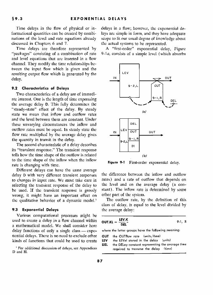
§9.3 EXPONENTIAL DELAYS 5
Time delays in the flow of physical or in- delays in a flow; however, the exponential de- formational quantities can be created by combi- lays are simple in form, and they have adequate nations of the level and rate equations already scope to fit our usual degree of knowledge about discussed in Chapters 6 and 7. the actual systems to be represented.
Time delays are therefore represented by A "first-order" exponential delay, Figure "packages" consisting of a combination of rate 9-la, consists of a simple level (which absorbs and level equations that are inserted in a flow channel. They modify the time relationships be- –––––
tween the input flow which is given and the
resulting output flow which is generated by the V
delay. 1 N OUT r
9.2 Characteristics of Delays 9 L OUT T
Two characteristics of a delay are of immedi- 9r- IUIR
Two characteristics of a delay are of immedi- ate interest. One is the length of time expressing
R DEL
the average delay D. This fully determines the ' - / v
"steady-state" effect of the delay. By steady '
state we mean that inflow and outflow rates and the level between them are constant. Under –– –––
these unvarying circumstances the inflow and DEL L
outflow rates must be equal. In steady state the LEV OUT flow rate multiplied by the average delay gives ––« the quantity in transit in the delay. 9-!.R R
The second characteristic of a delay describes '
D1 its "transient response." The transient response __ ___ tells how the time shape of the outflow is related to the time shape of the inflow when the inflow 1 d 1 to the time shape of the inflow when the inflow
Figure 9-1 First-order exponential delay. . .. Igure - irs -or er exponen ia e ay. rate is changing with time. -
Different delays can have the same average delay D with very different transient responses the difference between the inflow and outflow
to changes in input rate. We must take care in rates) and a rate of outflow that depends on
selecting the transient response of the delay to the level and on the average delay (a con-
be used. If the transient response is grossly stant). The inflow rate is determined by some
wrong, it might have an important effect on other part of the system. the qualitative behavior of a dynamic model.l The outflow rate, by the definition of this
class of delay, is equal to the level divided by 9.3 Exponential Delays the average delay:
Various computational processes might be ––––––––––––––––––––––––––––
used to create a delay in a flow channel within _ = LEV.K
9-1, R a mathematical model. We shall consider here DEL
delay functions of only a single class - expo- where the letter groups have the following meaning:
nential delays. There is no need to exclude other OUT the OUTflow rate (units/time) kinds of functions that could be used to create LEV the LEVeI stored in the delay (units)
DEL the DELay constant representing the average time 1 For additional discussion of delays, see Appendices required to traverse the delay (time)
D and H.
8 7
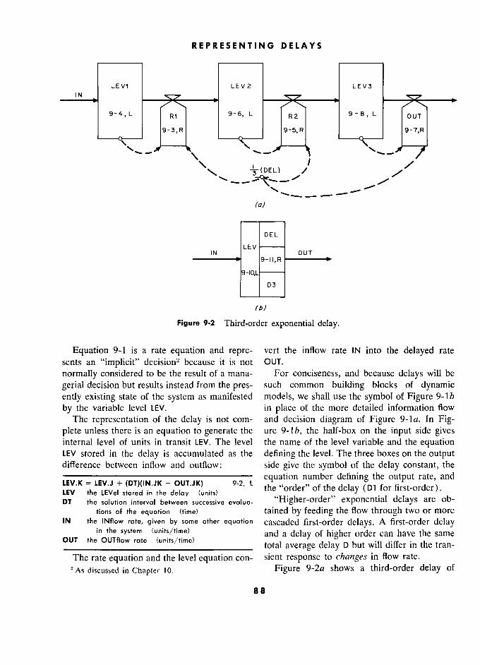
REPRESENTING DELAYS
LEV1 LEV2 2 LEV3 3 l N
.
9-4.L L 9-6, L 9-8, L oui
9-3, R 9-5.R R 9-7,R
, / 1
(0)
DEL
LEV lN OUT
––––––––" 9-II,R
9-!QL ––––
D3
rb)
Figure 9-2 Third-order exponential delay.
Equation 9-1 is a rate equation and repre- vert the inflow rate lN into the delayed rate sents an "implicit" decision? because it is not OUT.
normally considered to be the result of a mana- For conciseness, and because delays will be
gerial decision but results instead from the pres- such common building blocks of dynamic ently existing state of the system as manifested models, we shall use the symbol of Figure 9- 1 6
by the variable level LEV. in place of the more detailed information flow The representation of the delay is not com- and decision diagram of Figure 9-la. In Fig-
plete unless there is an equation to generate the ure the half-box on the input side gives internai level of units in transit LEV. The level the name of the level variable and the equation LEV stored in the delay is accumulated as the defining the level. The three boxes on the output difference between inflow and outflow: side give the symbol of the delay constant, the
LEV.K = LEV.J + (DT)(IN.JK - OUT.JK) 9-2, L equation number defining the output rate, and LEV.K = LEV.J + OUT.JK) 9-2, l
thé "order" of thé delay (m for first-order). LEV thé LEVeI stored in thé delay (units) e e e ay -'" DT the solution interval between successive evalua- "Higher-Order" exponential delays are ob-
tions of the équation (time) tained by feeding the flow through two or more lN thé INflow rate, given by some other équation cascaded first-order delays. A first-order delay
in the system (units/time) and a delay of higher order can have the same
oUT rhe ouTflow rate (units/time) total average delay D but will dîner in thé tran- -
The rate equation and the level equation con- sient response to change.ç in flow rate.
2 As discussed in Chapter JO. Figure 9-2a shows a third-order delay of
88
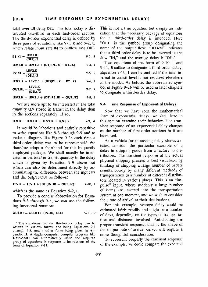
§9.4 TIME RESPONSE OF EXPONENTIAL DELAYS 5
total over-all delay DEL. This total delay is dis- This is not a true equation but simply an indi-
tributed one-third in each first-order section. cation that the necessary package of equations The third-order exponential delay is defined by for a third-order delay is intended. Here three pairs of equations, like 9-1, Rand 9-2, L, "OUT" is the symbol group designating the which relate input rate IN to outflow rate OUT: name of the output flow; "DELAY3" indicates
LEV1.K that a third-order delay is to be inserted in the
R1.KL = (DEL)/3
9-3, R flow "IN," and the average delay is "DEL."
LEV1.K = LEV1.J + (DT)(IN.JK - 9-4, L Two equations of the form of 9-10, L and '
LEV2.K
' ' 9-11, R suffice to designate a third-order delay. LEV2.K E . 9 1 0 b
. d .f h 1 . R2.KL =
(DEL)/3 9-5, R Equation 9-10, L can be omitted if the total in-
(DEL)/3 ternal in-transit level is not required elsewhere LEV2.K = LEV2.J + (DT)(R1.JK - R2.JK) 9-6, L in the model. As before, the abbreviated sym-
OUT.KL = LEV3.K 9 7 R bol in Figure 9-2b will be used in later chapters ' (DEL)/3
' to designate a third-order delay.
LEV3.K = LEV3.J + (DT)(R2.JK - OUT.JK) 9-8, L
We are more apt to be interested in the total 9.4 Time Response of Exponential Delays
quantity LEV stored in transit in the delay than Now that we have seen the mathematical 1 in the sections separately. If so, form of exponential delays, we shall hère in
LEV.K = LEV1.K + LEV2.K + LEV3.K 9-9, A this section examine their behavior. The tran-
It would be laborious and entirely repetitive sient response of an exponential delay changes
to write équations like 9-3 through 9-9 and to as the number of
first-order sections in it are
make a diagram like Figure 9-2a each time a increased. ,
third-order delay was to be represented.3 We e As a vehicle for discussing delay character-
therefore adopt a shorthand for this frequently istics, consider the particular example of a
employed package. We shall usually be inter- delay in shipping goods from a factory to dis-
ested in the total in-transit quantity in the delay tributors. The transient response of the actua)
which is given by Equation 9-9 above but .. physical shipping process is best visualized by
which can also be determined directly by ac- thinking of shipping a large number of orders
cumulating the difference between the input IN simultaneously by many different methods of
and the output OUT as follows : , transportation to a number of different distribu- °
tors located in various places. This is an "im- LEV.K = LEV.J + (DT)(IN.JK - OUT.JK) 9-10, L
pulse" input, where suddenly a large number
which is the same as Equation 9-2, L. of items are inserted into the transportation To provide a concise abbreviation for Equa- system at one moment, and we wish to consider
tions 9-3 through 9-8, we can use the follow- their rate of arrival at their destinations.
ing functional notation: For this example, average delay could be
OUT.KL = DELAY3 (IN.JK, DEL) 9-11, R estimated fairly readily and might be a number
OUT.KL = DELAY3 (.N.JK, DEL) 9-n, R of days, depending on the types of transporta-
'The equations for the third-order delay can be tion and distances involved. Anticipating the
written équations for the third-order delay can be proper transient resporise, that is, the shape of wntten in vanous forms, one being Equations 9-3 r . through 9-8, and another form being given in Ap- the output rate-of-arrival curve, will require a
pendix H. A digital-computer compiler program like more thoughtful consideration. DYNAMO can automatically insert the required To represent properly the transient response group of equations in response to instructions of the . „ , . form of Equation 9-11. of the example, we could compare the expected
89
REPRESENTING DELAYS
_ Figure 9-3 shows a first-order exponential
delay. In Figure 9-3a the maximum rate of out-
' put occurs immediately after an impulse input,
- D Time and the output rate declines exponentially there- ––'. p tjTimc–*? output rate déclines exponentially there-
(0) (b) after. This is clearly not representative of the
Figure 9-3 First-order exponential delay. shipping delay, since Figure 9-3a shows that the
Figure 9.3 First-order exponential delay. f§1[tilf£§' f Figure 9-3 First-order exponential delay. maximum rate of arrival at the destinations oc- -
curs at the instant the multiplicity of shipments
J
is made. Certainly the maximum rate of arrival
/ does not occur at the moment of shipment.
-_---__n- Figure 9-3b represents a step change (solid Time e -
line) in input rate and the resulting exponential (a) (b) rise in output rate from a first-order delay. The
Figure 9-4 Second-order exponential delay. area between the solid and dotted curves is a
measure of the quantity that accumulates in
- --.......... the in-transit level in the delay. So long as there
is a flow through the delay, the total amount
/ delivered at the output is less (by the amount
__D D e _ in transit) than the total amount that has been ––!. D -rime–? Time m transit) than thé total amount that bas been
(o) (b) put
Figure in. 9-4 is the output response of a second- _ _ , Figure 9-4 is thé output response of a second- Figure 9-5 Third-order exponential delay.
order exponential delay. The second-order delay order exponential delay. The second-order delay
il n __________ is the equivalent of two first-order delays cas-
caded one after the other so that the output of
fT Tf 1
the first is the input to the second. In Figure 9-4a
J L - .-... -.- - the initial output rate in response to an impulse -- f4-- D------+I Time -
input is zero, and the output curve has its maxi-
(0) (b) mum slope at the origin. This is also qualita-
Figure 9-6 Discrete or pipeline delay. tively unacceptable as a shipping delay because
we should not expect the rate of arrivals to
behavior of the actual system with the different start rising rapidly at the moment that ship-
exponential delays that might be selected. Fig- ments leave the factory. ures 9-3, 9-4, 9-5, and 9-6 show selections from In Figure 9-5 is a third-order exponential de-
the exponential family. lay. This shape of output response is the first
In the figures the solid line represents the of the sequence that satisfies the more obvi-
input to the delay; the dotted line shows the ous characteristics of the actual shipping proc-
output. Time moves to the right along the hori- ess. In Figure 9-5a the output response to an
zontal axis. In each figure the left-hand diagram impulse input is initially zero. Also the initial
is for an impulse input; that is, a quantity is in- slope of the output curve is zero. The curve
serted into the delay in a negligibly short time, begins to rise slowly, reaches a maximum slope and the dotted line shows the rate of arrival at and then a peak value, and falls off. In Figure
the output. In the right-hand diagram, the input 9-5b is the output following a step change in
is a sudden step increase in input rate, and the the input rate.
dotted line again shows the resulting output The third-order delay satisfies the major in-
rate. tuitive requirements that we should place on the
90
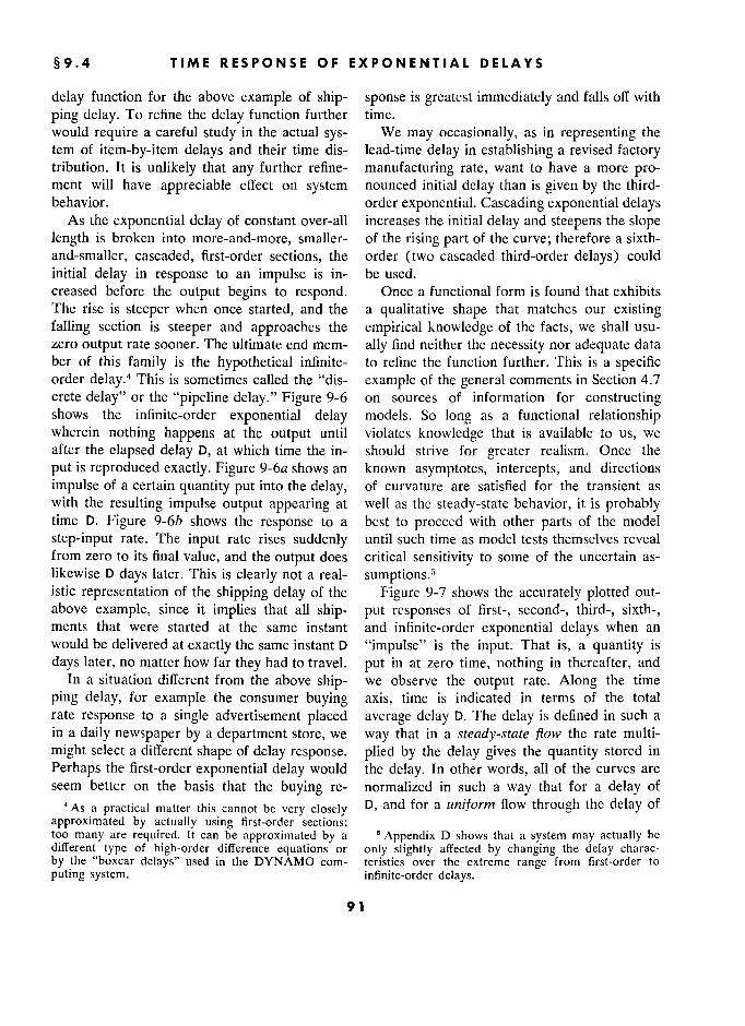
§9.4 TIME RESPONSE OF EXPONENTIAL DELAYS 5
delay function for the above example of ship- sponse is greatest immediately and falls off with
ping delay. To refine the delay function further time. would require a careful study in the actual sys- We may occasionally, as in representing the tem of item-by-item delays and their time dis- lead-time delay in establishing a revised factory tribution. It is unlikely that any further refine- manufacturing rate, want to have a more pro- ment will have appreciable effect on system nounced initial delay than is given by the third- behavior. order exponential. Cascading exponential delays
As the exponential delay of constant over-all increases the initial delay and steepens the slope length is broken into more-and-more, smaller- of the rising part of the curve; therefore a sixth-
and-smaller, cascaded, first-order sections, the order (two cascaded third-order delays) could initial delay in response to an impulse is in- be used. creased before the output begins to respond. Once a functional form is found that exhibits The rise is steeper when once started, and the a qualitative shape that matches our existing falling section is steeper and approaches the empirical knowledge of the facts, we shall usu- zero output rate sooner. The ultimate end mem- ally find neither the necessity nor adequate data ber of this family is the hypothetical infinite- to refine the function further. This is a specific order delay.4 This is sometimes called the "dis- example of the general comments in Section 4.7 crete delay" or the "pipeline delay." Figure 9-6 on sources of information for constructing shows the infinite-order exponential delay models. So long as a functional relationship wherein nothing happens at the output until violates knowledge that is available to us, we after the elapsed delay D, at which time the in- should strive for greater realism. Once the
put is reproduced exactly. Figure 9-6a shows an known asymptotes, intercepts, and directions
impulse of a certain quantity put into the delay, of curvature are satisfied for the transient as with the resulting impulse output appearing at well as the steady-state behavior, it is probably time D. Figure 9-6b shows the response to a best to proceed with other parts of the model
step-input rate. The input rate rises suddenly until such time as model tests themselves reveal from zero to its final value, and the output does critical sensitivity to some of the uncertain as- likewise D days later. This is clearly not a real- sumptions.e istic representation of the shipping delay of the Figure 9-7 shows the accurately plotted out- above example, since it implies that all ship- put responses of first-, second-, third-, sixth-, ments that were started at the same instant and infinite-order exponential delays when an would be delivered at exactly the same instant D "impulse" is the input. That is, a quantity is
days later, no matter how far they had to travel. put in at zero time, nothing in thereafter, and In a situation different from the above ship- we observe the output rate. Along the time
ping delay, for example the consumer buying axis, time is indicated in terms of the total rate response to a single advertisement placed average delay D. The delay is defined in such a in a daily newspaper by a department store, we way that in a .rteady-.state flow the rate multi-
might select a different shape of delay response. plied by the delay gives the quantity stored in
Perhaps the first-order exponential delay would the delay. In other words, all of the curves are seem better on the basis that the buying re- normalized in such a way that for a delay of
'As a practical matter this cannot be very closely D, and for a uniform flow through the delay of
approximated by actually using first-order sections; too many are required. It can be approximated by a 5 Appendix D shows that a system may actually be different type of high-order difference equations or only slightly affected by changing the delay charac- by the "boxcar delays" used in the DYNAMO com- teristics over the extreme range from first-order to puting system. infinite-order delays.
91 1
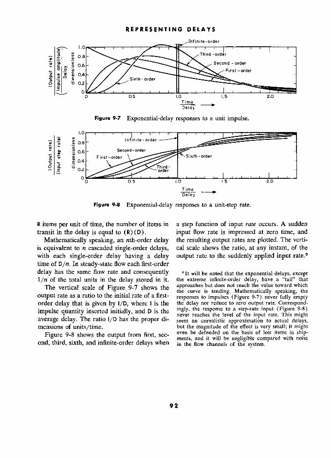
REPRESENTING DELAYS
Infinite-order 1
,
I Thir d - rder
E g Second - order ° ° First-order
'a 'j m E
order
- order
0 m * 02 - \
0 t I i i i I III n i i I I i i i 0 0.5 LO L5 5 2.0
Time Delay
Figure 9-7 Exponential-delay responses to a unit impulse.
i.o
_ z I !X r.Q_ 1 n f i n i t e - orde r
, o â 0.8 Infinite-order
] F 1 r s t -
Second-order
ë 0.4 First-order
ci 0 Z
Third-
order 1 - 1 1 1 1 1 1 1 1 1 1 1 1 1 o o,5 1,o 0 0.5 L0 L5 2.0
Time Delay
Figure 9-8 Exponential-delay responses to a unit-step rate.
R items per unit of time, the number of items in a step function of input rate occurs. A sudden
transit in the delay is equal to (R) (D). input flow rate is impressed at zero time, and
Mathematically speaking, an nth-order delay the resulting output rates are plotted. The verti-
is equivalent to n cascaded single-order delays, cal scale shows the ratio, at any instant, of the
with each single-order delay having a delay output rate to the suddenly applied input rate.,,
time of D/n. In steady-state flow each first-order
delay has the same now rate and consequently It will be noted that the exponential delays, except 1/M of the total units in the delay stored in it. the extreme infinite-order delay, have a "tail" that
The vertical scale of Figure 9-7 shows the approaches but does not reach the value toward which
, ° the curve is tending. Mathematically speaking, the
output rate as a ratio to the initial rate of a first- responses to impulses (Figure 9-7) never fully empty
order delay that is given by I/D, where 1 is the the delay nor reduce to zero output rate. Correspond-
impulse quantity inserted initially, and D is the ingly, the response
to a step-rate input (Figure 9-8) " -'
,_ never reaches the level of the input rate. This might
average delay. The ratio I/D has the proper di- seem an unrealistic approximation to actual delays, mensions of units/time. but the magnitude of the effect is very small; it might
Figure 9-8 shows the output from first, sec- even be defended on the basis of lost items in ship-
' ' ments, and it will be negligible compared with noise
ond, third, sixth, and infinite-order delays when in the flow channels of the system.
92
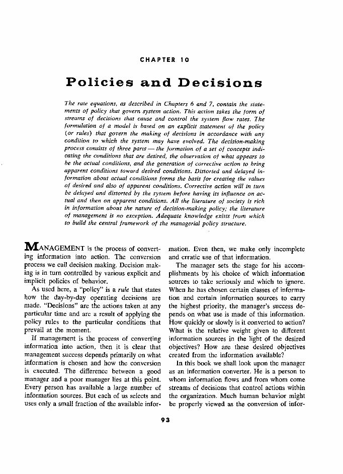
CHAPTER 10
Policies and Decisions
The rate equations, as described in Chapters 6 and 7, contain the state- ments of policy that govern system action. This action takes the form of streams of decisions that cause and control the system flow rates. The formulation of a model is based on an explicit statement of the policy (or rules) that govern the making of decisions in accordance with any condition to which the system may have evolved. The decision-making process consists of three parts- the formation of a set of concepts indi- cating the conditions that are desired, the observation of what appears to be the actual conditions, and the generation of corrective action to bring apparent conditions toward desired conditions. Distorted and delayed in- formation about actual conditions forms the basis for creating the values of desired and also of apparent conditions. Corrective action will in turn be delayed and distorted by the system before having its influence on ac- tual and then on apparent conditions. All the literature of society is rich in information about the nature of decision-making policy; the literature of management is no exception. Adequate knowledge exists from which to build the central framework of the managerial policy structure.
MANAGEMENT is the process of convert- mation. Even then, we make only incomplete ing information into action. The conversion and erratic use of that information.
process we call decision making. Decision mak- The manager sets the stage for his accom-
ing is in turn controlled by various explicit and plishments by his choice of which information
implicit policies of behavior. sources to take seriously and which to ignore. As used here, a "policy" is a rule that states When he has chosen certain classes of informa-
how the day-by-day operating decisions are tion and certain information sources to carry made. "Decisions" are the actions taken at any the highest priority, the manager's success de-
particular time and are a result of applying the pends on what use is made of this information.
policy rules to the particular conditions that How quickly or slowly is it converted to action?
prevail at the moment. What is the relative weight given to different If management is the process of converting information sources in the light of the desired
information into action, then it is clear that objectives? How are these desired objectives management success depends primarily on what created from the information available? information is chosen and how the conversion In this book we shall look upon the manager is executed. The difference between a good as an information converter. He is a person to
manager and a poor manager lies at this point. whom information flows and from whom come
Every person has available a large number of streams of decisions that control actions within information sources. But each of us selects and the organization. Much human behavior might uses only a small fraction of the available infor- be properly viewed as the conversion of infor-
93
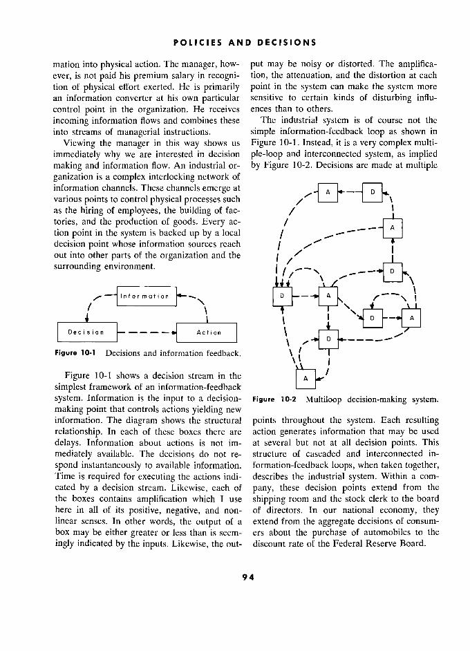
POLICIES AND DECISIONS 5
mation into physical action. The manager, how- put may be noisy or distorted. The amplifica- ever, is not paid his premium salary in recogni- tion, the attenuation, and the distortion at each
tion of physical effort exerted. He is primarily point in the system can make the system more an information converter at his own particular sensitive to certain kinds of disturbing influ-
control point in the organization. He receives ences than to others.
incoming information flows and combines these The industrial system is of course not the
into streams of managerial instructions. simple information-feedback loop as shown in
Viewing the manager in this way shows us Figure 10-1. Instead, it is a very complex multi-
immediately why we are interested in decision ple-loop and interconnected system, as implied making and information flow. An industrial or- by Figure 10-2. Decisions are made at multiple ganization is a complex interlocking network of __ information channels. These channels emerge at A D various points to control physical processes such \ as the hiring of employees, the building of fac- / '
tories, and the production of goods. Every ac- / tion point in the system is backed up by a local / decision point whose information sources reach 1./'" out into other parts of the organization and the
é surrounding environment.
1 1 l - - '\ '
*–--. \
j , ',
D s 1 o n - - - - ) Decision n –––––* Action t
\ '
A
1 Decision ?----1 Action
1 \ "" ./
Figure 10-1 Decisions and information feedback. " , j
Figure 10-1 shows a decision stream in the
simplest framework of an information-feedbac Uk
system. Information is the input to a decision- Figure t0-2 Multiloop decision-making system. making point that controls actions yielding new information. The diagram shows the structural points throughout the system. Each resulting
relationship. In each of these boxes there are action generates information that may be used
delays. Information about actions is not im- at several but not at all decision points. This
mediately available. The decisions do not re- structure of cascaded and interconnected in-
spond instantaneously to available information. formation-feedback loops, when taken together, Time is required for executing the actions indi- describes the industrial system. Within a com- cated by a decision stream. Likewise, each of pany, these decision points extend from the the boxes contains amplification which 1 use shipping room and the stock clerk to the board here in all of its positive, negative, and non- of directors. In our national economy, they y linear senses. In other words, the output of a extend from the aggregate decisions of consum- box may be either greater or less than is seem- ers about the purchase of automobiles to the
ingly indicated by the inputs. Likewise, the out- discount rate of the Federal Reserve Board.
94
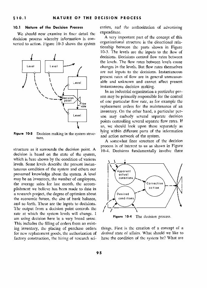
§ 10.1 1 NATURE OF' THE DECISION PROCESS 5
10.1 Nature of the Decision Process entists, and the authorization of advertising
We should now examine in finer detail the expenditure.
decision process whereby information is con- A very important part of the concept of this
verted to action. Figure 10-3 shows the system organizational structure is the directional rela-
tionship between the parts shown in Figure 10-3. The levels are the inputs to the flow of decisions. Decisions control flow rates between the levels. The flow rates between levels cause
Level Level changes in the levels. But flow rates themselves
–.––n– -o–––– / are not inputs to the decisions. Instantaneous ) ' '
present rates of flow are in general unmeasur-
/ l, 1 ! Level able and unknown and cannot affect present
\ instantaneous decision making. i \ < In an industrial organization a particular per-
' , Decision son may be primarily responsible for the control point
F?oW of one particular flow rate, as for example the . ' rate replacement orders for the maintenance of an
inventory. On the other hand, a particular per-
j Leve' son may embody several separate decision
!–––.–– points controlling several separate flow rates. If
so, we should look upon these separately as
Figure 10-3 3 Decision making h system struc- lying within different parts of the information Figure )0-3
ture. making - in thé system ' struc-
and action network of the system. ' A somewhat finer structure of the decision
.... process is of interest to us as shown in Figure structure as it surrounds the decision point. A 10-4. Decisions fundamentally involve three decision is based on the state of the system, which is here shown by the condition of various
. j levels. Some levels describe the present instan- / taneous condition of the system and others our Apparent \ /
presumed knowledge about the system. A level oc tua! \ / may be an inventory, the number of employees, conditions \// the average sales for last month, the accom- Corrective _
plishment we believe has been made to date in action n ; /<\
a research project, the degree of optimism about Desired d ' V
the economic future, the size of bank balance, condirions
and so forth. These are the inputs to decisions. / \. The output from a decision point controls the
j/ 1' rate at
which the system levels
will change. 1
Figure 10-4 Thé décision process. am using decision here in a very broad sense. Figure 10-4 The decision process.
This includes the filling of orders from an exist-
ing inventory, the placing of purchase orders things. First is the creation of a concept of a
for new replacement goods, the authorization of desired state of affairs. What should we like to
factory construction, the hiring of research sci- have the condition of the system be? What are
95 5

POLICIES AND DECISIONS
we striving for? What are the goals and ob- We note that we are viewing the decision
jectives of this particular decision point? Sec- process from a very particular distance. We are ond, there is the apparent state of actual condi- not close enough to be concerned with the tions. In other words, our available information mechanisms of human thought. We are not even leads us to certain observations that we believe close enough to see each separate decision as
represent the present state of the system. These we ordinarily think of decisions. We may not
apparent conditions may be either close or far be close enough to care whether one person or removed from the actual present state, depend- a group action creates the decision. On the
ing on the information flows that are being used other hand, we are not so far away as to be un- and the amount of time lag and distortion in aware of the decision point and its place in the these information sources. The third part of the system. This proper distance and perspective is decision process is the generation of the kinds important to our purposes. We are not the of action that will be taken in accordance with psychologist delving into the nature and sources
any discrepancy which can be detected between of personality and motivation, nor are we the the apparent and the desired conditions. In gen- biophysicist interested in the physical and logi- eral, the greater the discrepancy, the greater the cal structure of the brain. On the other hand, we
resulting action, although this entire process of are not the stockholder who is so far from the
forming a concept of desired conditions, detect- corporation as to be unaware of the internal
ing actual conditions, and creating from these a structure, social pressures, and decision points. course of action is highly nonlinear and noisy. Our viewpoint is more that of the managerial Very small discrepancies between apparent and superior of a particular person who is charged desired conditions may seem of no consequence with certain responsibilities. The superior is and create little action. A mounting discrepancy close enough to know how desired goals are
may lead to more and more decisive attempts established. He is in a position to observe and ' to correct actual conditions toward desired con- probably provide the information sources to be
ditions. However, a level of discrepancy can used by the subordinate to determine his con- be reached where the maximum possible cor- cept of actual conditions. He knows in general rective action is being exerted, and at that point the guiding policies and the manner in which further widening of the gap between desired the subordinate decision maker would respond and actual system state will no longer cause to various kinds of circumstances.
proportionate changes in flow rates. Decision making is being presented here as a 10.2 Policy
continuous process. It is a conversion mecha- We are now led to what is here called policy. nism for changing continuously varying flows of The word "policy" is used as a broad term to information into control signals that determine describe how the decision process converts in- rates of flow in the system. The decision point formation into action. What actions will result is continually yielding to the pressures of the from certain information inputs? What is the environment. It is taking advantage of new conversion relationship between information
developments as they occur. It is always adjust- sources and the stream of resulting decisions?
ing to the state of affairs. It is treading a nar- We shall first define what is here meant by row path between too much action and too policy. We shall later turn our attention to little. It is always attempting to adjust toward whether or not such policy does exist and the desired goals. The amount of action is some whether or not its form can be determined. function of the discrepancy between goals and Policy is a formal statement giving the rela- observed system status. tionship between information sources and re-
96
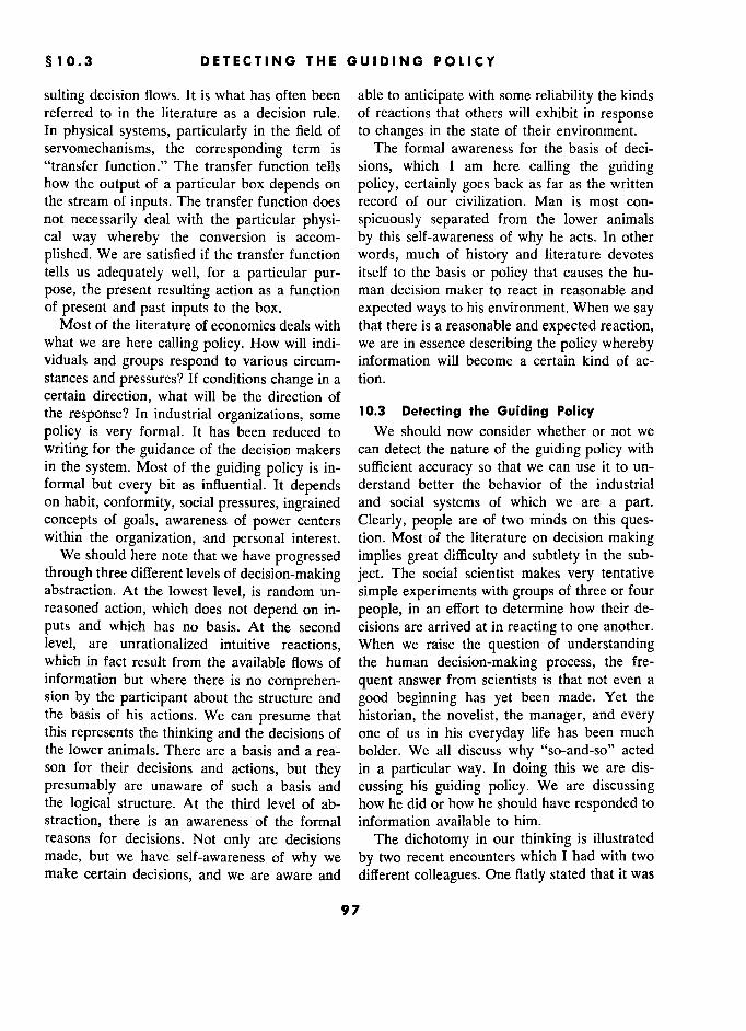
§10.3 DETECTING THE GUIDING POLICY
sulting decision flows. It is what has often been able to anticipate with some reliability the kinds referred to in the literature as a decision rule. of reactions that others will exhibit in response In physical systems, particularly in the field of to changes in the state of their environment.
servomechanisms, the corresponding term is The formal awareness for the basis of deci- "transfer function." The transfer function tells sions, which 1 am here calling the guiding how the output of a particular box depends on policy, certainly goes back as far as the written the stream of inputs. The transfer function does record of our civilization. Man is most con- not necessarily deal with the particular physi- spicuously separated from the lower animals cal way whereby the conversion is accom- by this self-awareness of why he acts. In other
plished. We are satisfied if the transfer function words, much of history and literature devotes tells us adequately well, for a particular pur- itself to the basis or policy that causes the hu-
pose, the present resulting action as a function man decision maker to react in reasonable and of present and past inputs to the box. expected ways to his environment. When we say
Most of the literature of economics deals with that there is a reasonable and expected reaction, what we are here calling policy. How will indi- we are in essence describing the policy whereby viduals and groups respond to various circum- information will become a certain kind of ac- stances and pressures? If conditions change in a tion. certain direction, what will be the direction of the response? In industrial organizations, some 10.3 Detecting the Guiding Policy
policy is very formal. It has been reduced to We should now consider whether or not we
writing for the guidance of the decision makers can detect the nature of the guiding policy with in the system. Most of the guiding policy is in- sufficient accuracy so that we can use it to un- formal but every bit as influential. It depends derstand better the behavior of the industrial on habit, conformity, social pressures, ingrained and social systems of which we are a part. concepts of goals, awareness of power centers Clearly, people are of two minds on this ques- within the organization, and personal interest. tion. Most of the literature on decision making
We should here note that we have progressed implies great difficulty and subtlety in the sub-
through three different levels of decision-making ject. The social scientist makes very tentative abstraction. At the lowest level, is random un- simple experiments with groups of three or four reasoned action, which does not depend on in- people, in an effort to determine how their de-
puts and which has no basis. At the second cisions are arrived at in reacting to one another.
level, are unrationalized intuitive reactions, When we raise the question of understanding which in fact result from the available flows of the human decision-making process, the fre- information but where there is no comprehen- quent answer from scientists is that not even a sion by the participant about the structure and good beginning has yet been made. Yet the the basis of his actions. We can presume that historian, the novelist, the manager, and every this represents the thinking and the decisions of one of us in his everyday life has been much the lower animals. There are a basis and a rea- bolder. We all discuss why "so-and-so" acted son for their decisions and actions, but they in a particular way. In doing this we are dis-
presumably are unaware of such a basis and cussing his guiding policy. We are discussing the logical structure. At the third level of ab- how he did or how he should have responded to
straction, there is an awareness of the formal information available to him. reasons for decisions. Not only are decisions The dichotomy in our thinking is illustrated
made, but we have self-awareness of why we by two recent encounters which 1 had with two make certain decisions, and we are aware and different colleagues. One flatly stated that it was
97
POLICIES AND DECISIONS
clearly impossible to introduce the actions of the specific nature and extent of this guiding the Federal Reserve Board into a formal model policy. of national economic behavior. The impossi- We saw in Figure 1-3 in the Introduction
bility was argued on the basis that we do not how decisions could be classified according to know the process by which such decisions are the form of the controlling policy. Even in the reached. They are too subtle. They are sub- Region C of judgment decisions, there is a
jective, intuitive decisions for which we know strong presumption concerning what constitutes not the guiding policy. The other incident took proper action. ln general, it is well known
place in a doctoral oral examination. Another what the direction of effect of various changes colleague, as a routine matter, casually asked in the system status will do to the resulting de- the candidate to describe the factors that would cisions. The current management press, such as lead the Federal Reserve System to make ad- Business Week, the Wall Street Journal, and
justments in various directions in its discount Forbes, is filled with the rationale for manage- rate and open-market policies. In other words, ment decisions. Much of the printed material the economics doctoral candidate was expected is devoted to a discussion of the pressures of to know the essential nature of the policy that the current state of affairs and the effects these would guide the stream of Federal Reserve will have on decision makers. Board decisions. To be sure, there may be a Many people seem to believe that a sharp high noise content that can cause timing varia- break exists between the automatic decisions tions and uncertainty in the extent of a response. that are completely formal and the other regions However, the broad underlying outlines of guid- of management decisions. Such persons are un-
ing policy were expected to be within the under- willing to accept the possibility of even the
standing and comprehension of the student. existence of formal policies that could describe This contradiction in the opinions we hold the major aspects of management in the other
about the process of decision making is very decision-making regions. There is an interesting similar to that which we observe in our think- contradiction in the attitude of many managers ing about the process of invention. There is toward this matter of understanding the formal
great argument and little agreement in any dis- basis of the decision process. Any manager cussion of how new ideas are generated and must of necessity admit the existence of the how invention and research results are achieved. region of automatic decisions, since these are Yet we are almost in 100% agreement in ac- common practice. The majority of managers knowledging that more intelligent and more will argue that the region of the intuitive-judg- experienced people, and greater research budget ment decision is so subtle that no reasonable
expenditure, and greater motivation, and greater approximation can be made to it through formal need for the results will all enhance the proba- decision rules. Yet those same managers, when
bility of a successful outcome. This agreement faced with a decision that they recognize as on the nature of the conversion function that lying beyond the capabilities of their intuitive
couples financial and manpower inputs to sci- judgment, will once more fall back on formal entific output is the basis for Congressional ac- decision-making procedures. 1 here refer to the tion and military department appropriations. whole field of sales and market and economic
In short, our whole civilization is founded not forecasting when done on the basis of statistical
only on the presumption that a basis exists analysis of past data or by routine procedures for the guidance of human action but also on of collecting and tabulating sales department the conviction that we know a great deal about estimates. Forecasting is essentially a decision-
98 8

§ 10.3 3 DETECTING THE GUIDING POLICY
making process. It consists of taking past and First, there is the matter of perspective, or
presently available information and converting viewing distance, mentioned earlier. The social this into results that indicate a course of action. scientist has tended to look at the individual 1 am not a supporter of the wisdom and validity man with emphasis on psychology and indi- of the majority of this type of forecasting, but vidual motivation. Many of the attempts at 1 simply point out the conflict in attitudes. laboratory experiments have been with small There are those who relegate the simple de- groups assembled in an artificial environment cisions to automatic procedures. They rely, for for brief periods of time. The results have not lack of anything better, on certain formal sta- been conditioned by the strong social forces of tistical decision procedures with respect to some precedent, conformity, and the attempt to be- of the most subtle and difficult decisions. But have as the man believes his superior would
they reserve the middle ground as a region for want him to. Study of the individual man, espe- judgment, which they assert is untouchable by cially over short periods of time in an artificial formal decision rule. environment, tends to accentuate the feeling
It seems to me that there is now ample evi- that decisions are capricious, infrequent, dis- dence to indicate that this middle region is not connected, and isolated. the obscure and subtle jungle that it has so At the other extreme, the economist has often been pictured. Men are not good calcula- viewed the corporation from too great a dis- tors of the dynamic behavior of complicated tance. He has often looked upon the market as
systems. The number of variables that they can maximizing its utility, whether or not it has the in fact properly relate to one another is very information available to do so. He looks upon limited. The intuitive judgment of even a skilled the entrepreneur as a man who maximizes his
investigator is quite unreliable in anticipating profit without asking whether or not he has the the dynamic behavior of a simple information- available information sources and the mental feedback system of perhaps five or six variables. computing capacity to find a maximum. This This is true even when the complete structure viewing from too great a distance tends to over- and all the parameters of the system are fully stress the importance of the top-management known to him. The verbal model and the mental decisions compared to those made in the lower model that we carry around with us to explain and middle structure of the corporation. A the dynamics of industrial and economic system directive from top management does not change behavior probably do not rank in effective dy- the prejudices, habits, and self-interest objec- namic complexity beyond a fourth- or fifth- tives of the middle-level decision makers. For order differential equation. We think that we example, the public press has well documented
give consideration to a much larger number of the futility felt by the successive Secretaries of
variables, but 1 doubt that these are properly Defense who have tried their hands at changing related to one another in groups larger than the character, attitudes, and practices of our five or six at a time. In dealing with the dy- military department. It is a long, slow process. namics of information-feedback systems, the hu- We tend to be misled by various "upheaval" man is not a subtle and powerful problem incidents. A proxy fight followed by a complete solver. change of top management and the firing of
Management science has so far been very half of the middle-management structure will ineffective in dealing with this formulation and indeed change the attitudes and traditions of an use of decision-making policy. The past dif- organization. But this drastic surgery is not ficulties might be gathered into three categories. common.
99
POLICIES AND DECISIONS S
For an understanding of the corporate infor- cedures that our traditions and our manage- mation-feedback system, it is very essential that ment folklore have led us to believe are precisely we look neither at the individual person isolated in the wrong direction. Our understanding of from his environment nor at the exterior of the the dynamics of complicated information-feed-
system. It is at the intermediate viewpoint from back systems is so inadequate that our intuitive which we can know men and groups of men in judgment can often not be trusted to tell us their working environment that we can capture whether improvement or degradation will result the true character of the operation. from a given direction of policy change.
Second, 1 think that the understanding of The third difficulty into which many seem to decision making has been greatly handicapped have fallen in attempting to understand deci-
by the presumption that it is a more subtle and sion-making policy has resulted from trying to more skillful process than it actually is. We skip one of the evolutionary steps in the hier- have been too heavily influenced by the fact archy of decision-making abstraction mentioned that the highest speed computers cannot yet earlier. It was suggested earlier that the lowest
play chess as well as a person. This is not a level of decision making would be that where
typical example. Full and exact information is actions were random and irrational. The sec- available to the man. It is a problem of visual- ond level would be one where actions are rea-
izing spatial relationships, which a man does soned and rational but where there is no self-
quite well and today's machines do poorly. awareness of what the governing policies might There are other situations, such as the time be. Man was characterized in the third level as histories of Chapter 2, where a computing ma- having, throughout recorded history, at least a chine can determine in five minutes what the verbal descriptive model of a rational policy consequences of a set of policies will be and that creates the stream of individual decisions. wherein a group of men could argue inconclu- This is already a major fraction of the step sively for a year about what follows from a toward the ability to formulate explicit, quanti- given set of assumptions. tative, policy-governing decisions. This next
It is my feeling that in a dynamic informa- level would be one in which the art and the tion-feedback system the human decision maker intuitive judgment are applied to the develop- is usually using a great deal less than the total ment of a better understanding of policy. amount of information available to him. Fur- Art, judgment, and intuition are at this new
thermore, the information available to him is level no longer applied to the individual sepa- a great deal less than that commonly presumed. rate decisions but to the definition of a policy In general, his actions with respect to any given that governs the stream of individual decisions. decision stream will be almost entirely condi- This is the level of abstraction that is just tioned by less than ten information inputs. emerging. This is the one wherein we can point What he does with these few information to numerous successful examples but where sources is apt to be rather stereotyped. Some of there is not general agreement on method. At them will be used to create a concept of desired this level of abstraction, there is not a descrip- objectives. Others will serve to form his im- tive literature on what constitutes the practice pressions of the true state of affairs. From the of the art of detecting decision-making policy. difference will result reasonably straightforward In spite of the gap in the art that exists at the and obvious actions. What seems obvious may policy-detection level, many economists have at- not be best. Some of the biggest improvements tempted to skip to the next level of the abstrac- that can be made in the dynamics of our in- tion hierarchy. They have been attempting to dustrial systems will come from following pro- develop statistical methods that can be routinely
100

§ 10.3 DETECTING THE GUIDING POLICY
applied to extract from quantitative data about is and of the significance of the policy that de-
a system the governing decision policies. This scribes the decision process. is still another level of abstraction in which We have the proper structure relating system intuitive art and judgment are applied to setting status to policy, to decisions, and to action.
up rigid rules whereby the formal decision e We realize that the process is noisy and we shall
policies can be derived. 1 feel we are not ready not get and do not need high accuracy of de-
to attempt this last level of abstraction until cision-making representation.
we have achieved acknowledged success in ap- e We use to best advantage the extensive body of
plying art and judgment and intuition to the experience and descriptive information that
extraction of the decision policies themselves. probably contains of the essential infor-
After this process is well understood, it may mation on decision making. The other 2% will
then reduce this method of analy- come from formal statistical and numerical
then be possible to reduce this method a f ana 1 y- from formaI statistical and numerical
sis of an organization ta a rigid and orderly data.
sis of an organization to a
rigid and orderly . §§ realize that a formal quantitative statement
procédure. In general, the precedents seem to of policy carries with it no implications one way indicate that we must take thèse levels of ab- or the other regarding absolute accuracy. We straction one at a time. At each point in time, can make a formal quantitative statement cor- art and judgment are devoted to establishing responding to any statement that can be made the rules whereby the lower levels can be au- in descriptive English. Lack of descriptive ac- tomatized. curacy does not prevent quantifying our ideas
An example has been the history of comput- about decision policy. Assigning a number does
ing-machine programming. Ten years ago one not enhance the accuracy of the original state-
wrote the specific machine code for the solution ment. The common belief that we cannot
of a particular problem. The next level of ab- quantify a decision rule because we do not know it wtth hieh accuracy ts mixms two quite straction was to write a program of logical in- it with high accuracy is mixing two quite
structions to tell the machine h ow to create its s separate considerations. We can quantify re- structions to tell the machine how
to create its gardless of accuracy. After that, we deal with
own running program for a specific problem the question of what is sufficient accuracy. formulation. The hierarchy of abstraction in
problem programming is now deepening. At the 1 feel it has been adequately demonstrated
new level, man develops concepts that allow that these things can be done. We have the
the computer to formulate the specific state- tremendous examples of corresponding accom-
ment of the problem which another computer plishments in the understanding of military con-
program will in turn convert into machine lan- trol systems in the last decade. We have pre-
guage. This is philosophically the equivalent of liminary examples of the application of the
the above hierarchy of orderly rules related to same approaches to industrial systems. decision making. Actual, effective decision functions in a com-
To begin to deal with the dynamic charac- pany or in an economy go much further than
teristics of social systems, we must be able to the formal policy that is set down in executive
represent at least the central essential skeleton memoranda and in laws. The "effective policy" of the decision-making structure. To do this, we is the framework for reaching decisions and is
must be able to approximate the controlling established by the environment, the sources of
policy at each significant decision point in the information that are in fact available, the suc-
system. This understanding of policy can be ac- cess measures and rewards that affect people at
complished if each decision point, the priority order of food
and shelter and luxuries, the mores of the so- e We have the proper concept of what a decision ciety, and the prejudices and habits impressed
101 1

POLICIES AND DECISIONS
by past experience. When decisions are ex- from a transportation system, resulting from the amined in the light of this circumscribing frame- input rates, the goods in transit, and the trans-
work, we find that they are far from the un- port delays, and (3) taxes due as a result of
predictable actions that arc sometimes supposed. profits. Even for a particular individual, we can assume Factory production serves to emphasize the a certain degree of consistency and can mean- distinction between overt and implicit decisions.
ingfully discuss probable effects of various pres- Actual, present production rate is usually the sures on him. For a class of persons in similar result of an implicit decision function that shows
environments, the likely average response to how production rate is a consequence of em-
changes in specific environmental forces can be ployment, available equipment, and materials. estimated with even higher confidence. It is not usually an overt decision; it is not pos-
A principal use of a dynamic model is to sible to décide arbitrarily on a production rate
study the influence of policies on system be- and thereby have that rate exist immediately havior. In formulating a model, we must extend and with certainty. The accompanying overt the concept of policy beyond its usual meaning. managerial decisions are the decisions to at- All decisions in the model come under the com- tempt to hire people and to order equipment plete control of policy. The policy represents and materials. Whether or not people are in the basis for controlling flows at all points in the fact hired as a result of the overt decision de- actual system. We are forced to explore this pends on the implicit decision functions within basis in depth to see how decisions are gen- the "physical" state of the system which recog- erated from the various circumstances that arise. nize such factors as the supply of workers, the The concept of policies governing decisions goes wages being offered, etc. Whether or not mate- well beyond that of the human, managerial de- rials and equipment result from the orders cision. A model must also make "decisions" depends on the available supplies. that are of a physical nature - for example, Overt and implicit decisions need not be how many unfilled orders can be filled depend- distinguished in the manner in which they are
ing on the state of inventories? handled in the model; but thinking of them
separately helps us to avoid omission of im- 10.4 Overt and Implicit Decisions portant steps in the flows of information and
It is sometimes helpful in our thinking to di- the resulting decisions and actions. Including vide decision functions into two categories, both the overt and implicit decisions makes it
depending on whether they are ordinarily con- possible, in the model, to deal with the
scious, "free" human decisions or whether they as well as the actuality. Conditions lead to a arise inexorably from the physical condition of desire for a change; the desire interacts with the system. The dividing line is not sharp. Overt the state and resources of the system to deter- decisions are here defined as the conscious de- mine what, if anything, is to happen. cisions by people as part of the management Introducing the concepts of both overt and and economic process. In the overt decisions implicit decisions is one factor that here elimi- will be found all executive decisions, consumer nates the necessity of simultaneous equations purchase decisions, and all psychological factors that arise in some models, such as in making that are to be included. Implicit decisions are production decisions continuously equal to con- the unavoidable result of the state of the system. sumption decisions, etc. Such decisions are actu- Included here are usually ( 1 ) present ability to ally made separately and independently, and
deliver, depending on the present status of in- are eventually coupled through inventories, ventories, (2) the output rate (goods delivered) prices, and various information flows. The overt
102
§10.6 DETERMINING THE FORM OF DECISION FUNCTIONS S
decisions to want or to attempt are a result of nomic system would continuously generate an
information available to the decision maker. The actual, instantaneous, gross national production
implicit decisions, which create the actions, rate; but this rate should not be available as an
recognize the existing true state of the system as input to any overt decisions (such as planning well as the desires. plant expansions). The available information,
to agree with actual conditions, must be delayed 10.5 Inputs to Decision Functions and should contain a degree of error and un-
In formulating decision functions (the rate certainty even with regard to what the true val-
equations) we must take care that the decisions ues were before the delay. are generated from the variables that would A model, like the real world, must often
actually be available at the decision point. In generate both "true" values of variables and
general, the information available for overt de- also associated variables that represent the
cision making is not identical to the primary values that are measured or conceived for de-
variables that it represents. The information cision-making use.
may be late, biased, and noisy. Here again, a
distinction between implicit and overt decisions 10.6 Determining the Form of Decision may arise. Overt decisions are usually based on Functions information (which may be perturbed) about the primary variables. The more mechanistic A model that can create proper dynamic
implicit decisions control the routine fiows that system behavior requires formal expressions to
depend on the actual state of the system and, indicate how decisions are made. The flow of
therefore, on the true values of the variables in information is continuously converted into de-
the model. cisions and action. No plea about the inade-
The distinction between the true value of a quacy of our understanding of the decision-
variable and the value of information about making process can excuse us from estimating
the variable can be illustrated by an inventory. the decision-making criteria. To omit decision
Ability to deliver an item from an inventory, making is to deny its presence - a mistake of
being dependent on whether or not the item is far greater magnitude than any errors in our
present, can usually be thought of as an implicit best estimate of the process.
decision controlled by the actual, present, true Can estimated decision functions be good
state of the inventory. This present, true in- enough to be useful? In general, it appears that
ventory is one of the variables in the model. they can. Perceptive observation, searching dis-
The overt decision function that controls re- cussions with persons making the decisions,
ordering of material for inventory may depend study of already existing data, and the examina-
on information about the inventory, such infor- tion of specific examples of decisions and ac-
mation being subject to delay and inaccuracy. tions will all illuminate the principal factors that
What the inventory is believed to be may, in influence decisions. In considering a factor influ-
some models for some purposes, need to be in- encing a decision, we progress through four
cluded as a second and different variable. In stages:
addition, we should often deal with the concept , of "desired inventory," which is often different e What factors are significant enough to include?
from either of the preceding; this would then Then for each:
become a third variable with a still different e What is the direction of its effect?
value relating to the same inventory. * What is the magnitude of its effect?
As a second example, a model of an eco- e What nonlinearities should be recognized?
103
POLICIES AND DECISIONS
Factors to Include. In deciding how to formu- than those before it, and the increasing delay late a particular decision function (policy) in a leads to still more advance ordering.2 model, the first step is to list those factors that Direction of Effect. There will usually be little are important influences on the decision. The doubt about the direction in which a decision answer is often obscure. What at first may ap- will be influenced by changes in a particular pear to be a most significant factor will some- factor affecting the decision. However, we must times be found to have little influence on the be alert to represent properly the"worse-before- model behavior or on the actual system. A better" sequences that often arise. The short- factor that is ordinarily overlooked in everyday term and long-term influences on a decision by management practice may turn out to hold the a particular factor are often in opposite direc-
key to important characteristics of the total tions, and the dynamic behavior of a model can
system. be seriously affected if only the long-range ef- The choice of factors that affect a decision fects are included.
must be made from the viewpoint of what af- Several examples will illustrate the kinds of fects the characteristics of an information-feed- factors that can have short-term effect (often back system. Very few persons have a good overlooked) that is opposite to the long-term intuitive judgment about such systems. Work- effects that are ordinarily considered. It is com-
ing with system models helps develop sound monly assumed that higher prices are an incen-
judgment and intuition. The decisive test of the tive to greater output of a product, but in the
significance of a factor in a decision function short run this sometimes will not be true. In in a model is to observe model performance the production of beef the first step in increas- with and without the factor. In this way the ing production is to withhold cattle from market model itself can be used to help determine what to build up breeding herds, thus reducing sales it should contain. for two or three years; also, rising prices mean
The extent of the direct influence of the fac- an appreciation in value of live "inventory," tor on the decision is not the only consideration. which results in lengthening the fattening inter- We must also consider the degree of feedback val in the feed lot and also reduces sales rates or repercussion of the decision on the factor for a period of several months. In some types entering into the decision, and the timing of of mining a rise in prices makes it economically such feedback. Relatively slight influences on feasible to process lower-grade ore; fixed-ton- decisions can be important in "positive feed- nage-rate equipment is then applied to a lower- back" conditions, where the variable factor in- yielding raw material, a procedure which can fluences a decision and the decision affects the result in reduced total output until marginal input factor to create still more change in the mines that were not previously operating can decision.1 This is seen in many places. For ex- be opened. In an expanding research activity ample, when customers order further ahead in more people may be needed to accelerate the
response to increasing delay in the delivery of completion of a project, but the first effect may goods, increased ordering rate increases the be reduced progress while these people are
backlog of unfilled orders, the rising backlog trained and absorbed into the organization. In means that each new order is delayed even more a full-employment national economy, the de-
1 Figure 2-10 is an example where the cumulative 2 This appeared in Figure 2-5. Also, see Chapters 17 cycle of sales increases advertising and advertising and 18 for discussion of a system in which a small increases sales until some other effect (depletion of percentage change in a factor in a policy can be the
, prospective customer pool) terminates the regenerative essential link in creating an unstable market-to-fac- process. tory-to-employment interaction.
104
§10.6 DETERMINING THE FORM OF DECISION FUNCTIONS 5
mand for more goods may require diverting dynamics; the model would readjust or warp workers from producing goods into the manu- internally, as does the real economy, so that a
facture of additional factories and machinery; doser approach to the limit of full employment the first step to achieve more long-term output would counterbalance any built-in tendencies
tends initially to reduce production (this effect to create excessive employing rates. In a model,
may of course be counterbalanced by other fac- too low a consumer propensity to buy auto-
tors such as a longer work week). mobiles would cause the consumer stock of
Magnitude of Effects in Decision Functions. automobiles to decline and progressively de-
The dynamic behavior of information-feedback crease transportation service until the auto-
systems is determined by the way in which mobile purchase rate increases. Changes in the
changes in one variable cause changes in an- level of consumer stocks of automobiles will
other. This might lead one to expect a high sys- help to compensate for an inaccurate purchase- tem sensitivity to the exact values of parame- rate decision function, while still leaving the
ters3 in the decision functions, but such will dynamics of purchase-rate changes qualitatively
usually not be true. correct with respect to other variables in the
If the model is properly constructed to repre- model.
sent the actual information-feedback structure We should be more concerned with what the
of our social systems, it will have the same self- model tells us about the factors that will cause
correcting adaptability that exists in real-life changes in the rates and levels than about the
situations. In the preferred model formulation accuracy in determining the average magnitudes all parameters that must be estimated for deci- of the rates and levels.
sion functions are acted on by the values of A properly constructed model is often sur-
levels to obtain the rates of flow that are con- prisingly unaffected by plausible changes in most
trolled by the decisions. The levels are in turn parameter values - even sometimes changes of
adjusted by the resulting decisions. An inac- severalfold. In a model, the sensitivity to selected
curate decision-function parameter can then values of parameters should be no greater than
lead to compensating readjustments of levels in the sensitivity of the real system to the corre-
the model until the rates of flow are properly sponding factors. It seems obvious that our ac-
related to one another. tual industrial and economic activities must not
Some examples will illustrate this internai be highly sensitive to their fundamental parame-
readjustment. In estimating a parameter deter- ters and that these parameters do not change
mining the delay in repaying accounts receiv- rapidly. This must be true because the signifi-
able, one might choose too high a value; this cant characteristic.ç of our organizations persist would cause the level of accounts receivable to for long times. The successful company tends to
run slightly high, but repayment rate is still remain so for extended periods - a success .
coupled to the rate at which new obligations are that is founded in basic organization and poli-
being incurred. Or too high a labor mobility in cies (including the essential aspects of its leader-
describing a labor market could produce levels ship). Our national economy has exhibited
of unemployment that run lower in the model surprisingly similar economic cycles throughout than in the actual economy, while still retaining its history, in spite of vast changes in technol-
the proper effects of policy changes on model ogy, monetary structure, transportation and
communication speed, relative importance of 3 A parameter is a constant for a given model run industry and agriculture, and magnitude of gov-
, whose value has been assigned in constructing the errimerit aCtlvlty. mode]. It can of course be changed between one simulation run and another. Nonlinear Decision Functions. Nonlinear
105 ,
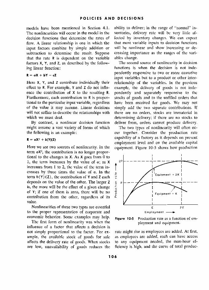
POLICIES AND DECISIONS S
models have been mentioned in Section 4.1. ability to deliver; in the range of "normal" in-
The nonlinearities will occur in the model in the ventories, delivery rate will be very little af-
decision functions that determine the rates of fected by inventory changes. We can expect flow. A linear relationship is one in which the that most variable inputs to decision functions
input factors combine by simple addition or will be nonlinear and show increasing or de-
subtraction to determine the result. Suppose creasing importance as the ranges of the vari-
that the rate R is dependent on the variable ables change. factors X, Y, and Z, as described by the follow- The second source of nonlinearity in decision
ing linear function: functions is when the decision is not inde-
R = X Z pendently responsive to two or more causative " ' input variables but to a product or other inter-
Here X, Y, and Z contribute individually their relationship of the variables. In the previous effect to R. For example, Y and Z do not influ- example, the delivery of goods is not inde- ence the contribution of X to the resulting R. pendently and separately responsive to the
Furthermore, each contribution to R is propor- stocks of goods and to the unfilled orders that tional to the particular input variable, regardless have been received for goods. We may not of the value it may assume. Linear decisions simply add the two separate contributions. If will not suffice to describe the relationships with there are no orders, stocks are immaterial in which we must deal. determining delivery; if there are no stocks to
By contrast, a nonlinear decision function deliver from, orders cannot produce delivery. might assume a vast variety of forms of which The two types of nonlinearity will often oc- the following is an example: cur together. Consider the production rate
R = xX2 + b(Y)(Z) capability of a factory as it depends on present R = ax2 + b(Y)(z) employment level and on the available capital
Here we see two sources of nonlinearity. In the equipment. Figure 10-5 shows how production term the contribution is no longer propor- tional to the changes in X. As X goes from 0 to ! : 1, the term increases by the value of a; as X increases from 1 to 2, the value of the term in-
t 1
w
creases by three times the value of a. In the v )
term bey) (Z), the contribution of Y and Z each S I I Equipment I depends on the value of the other. The larger Z g p --
- - , - - - - is, the more will be the effect of a given change ;, 1 of Y; if one of them is zero, there will be no 1 0 1 Equi pmen! = K contribution from the other, regardless of its 0::
/ :
Equipment = K
/ value. / 1 ___
Nonlinearities of these two types are essential E 2 E to the proper representation of corporate and Empioyment - economic behavior. Some examples may help. p;gure 10-5 Production rate as a function of em-
The first form of nonlinearity was when the ployment and equipment. influence of a factor that affects a decision is not simply proportional to the factor. For ex- rate might rise as employees are added. At first,
ample, the available stock of goods for sale as employees are added, each can have access
affects the delivery rate of goods. When stocks to any equipment needed, the man-hour ef-
are low, unavailability of goods reduces the ficiency is high, and the curve of total produc-
106

§ 10.7 NOISE IN DECISION FUNCTIONS 5
tion rises steeply. As the maximum capacity of extreme limiting conditions of a relationship the equipment is approached, the additional between variables than we do about the normal
production per worker decreases. Still more range of operation. Very often we know the
employees finally result in the maximum possi- value or the slope that a curve relating two ble production from the equipment. Beyond variables must assume as the input variable this level of employment, additional men would approaches zero or some absurdly high value. create only congestion and confusion and loss By selecting functional relationships that match of total production. We see then that for a fixed all our bits of knowledge, we enhance our amount of equipment the production is not chances of obtaining a model that acts properly. proportional to the employment and is a non- In regard to correct representation of deriva- linear relationship. Furthermore, the contribu- tives (slope, rate of change of slope, etc.), the tion to production of any given change of em- danger of using broken-line approximations to
ployment depends on the amount of equipment, functions is apparent. Most actual limiting con- so that the two inputs interact on one another. ditions exert their influence in a progressive way At low employment levels, it is unimportant as the limit is approached. It is poor practice, where the amount of equipment might be in often with serious consequences, to approximate the range of K to 2K. At higher levels of em- such a function by a linear section that is
ployment, the contribution of additional men is "clipped" to stop its travel suddenly. At the
increasingly affected by whether or not equip- clipping point, all derivatives of the function are ment is added. in extreme error.
Linear approximations to these nonlinear re- Correctly curved functional relationships fa-
lationships are usually not satisfactory. Normal cilitate internal self-adjustment as already dis-
operations will vary over ranges wide enough cussed, wherein the model seeks values that so that the nonlinearities are highly significant. balance one another. Realistic behavior is easier
Very often, the approach to one limit becomes to achieve in a nonlinear than in a linear model the input signal to some compensating action because the nonlinear model formulation leads
(in the above example, the lowering man-hour us more quickly to the factors on which actual
efficiency caused by crowding is one of the in- system behavior depends. puts to the decision to order more equipment).
The models we formulate should be valid 10.7 Noise in Decision Functions
over wide ranges of the variables. This is desir- The decision functions of a model will neces- able for several reasons. We shall want to ex- sarily incorporate only the more important of
plore wide ranges of conditions. We may not the factors that influence decisions. Beyond know how far some variables will be called these will be a host of minor influences that will
upon to move. We shall want the model to be unavoidably be omitted. The omissions can useful outside the operating ranges that may represent two quite different categories. have been already encountered by the real sys- In the first category of omission are the slight tem because the design of new systems implies influences from those variables that are a part of
operation outside of historical practices. the system and of the model under considera- In building a model we should use all the tion. These omissions are actually the elimina-
pertinent information that we have about the tion of some of the feedback paths between the
system that is being represented. An indispen- model variables. This will often happen because sable class of information is our knowledge of of the necessity for simplification, but the dan- what to expect under extreme conditions of op- gers are those discussed in Section 10.6. Omit-
eration. Very often we know more about the ting a variable within the model from a decision
107
POLICIES AND DECISIONS
function is the omission of an input that may contribution to all decision points in our actual
be correlated in time with the decisions created social systems. We can approximate these by
by the decision function. We cannot substitute including "noise" variation in the decision func-
for this type of omission by a random variable tions in the model.
incorporated into the decision process of the The theoretical treatment of noise inputs model. and how to design them comprise a complex
A second class of omission from the decision subject to be taken up elsewhere. The practical functions has a very different character. These question of what noise characteristics should
omitted factors are the ones that are not them- be included in a model will, like many other in-
selves affected by each other or by the other puts, be decided primarily by such knowledge variables of the model. Their source is outside as we have of the system being represented.5 of and independent of the real system being Noise inputs to decision functions can be
represented. An example is the uncertain in- used to represent the influence of the above-
fluence of weather4 - not only its obvious in- mentioned second class of omissions from the
fluence on agriculture but also its effect on decision functions in a model, where the omitted
Easter sales, sports equipment, and day-by-day factors are unrelated to the system being mod-
department store business. Also we might clas- eled. Noise cannot substitute for the first class
sify as random the incidents of the local, na- of omissions which constitute a simplification tional, and international political news that may and omission of parts of the information-feed-
not be completely independent of business and back structure of the system. economic affairs but that are often sufficiently It should be noted that neither the "random num- loosely related ta be ????? ? ? ?? as uncorre- It should be noted that neither the "random num- loosely related to be looked upon as uncorre- bers" of statistics nor the "white noise" of the engi- lated happenings. Here also would be the pur- neer can be employed without modification. Due
chasing agent's vacation or the production man- regard must be given to sampling interval, the high
ager's illness and the effect they have on the and low cutoff frequencies contained in the noise illness they hâve on thé , sequence, and to the way the noise is inserted at the
smooth flow of business. This flood of "noise" decision point with respect to the closed-loop channels of a random and unpredictable form adds its of which it becomes a part. In Appendix F is some
discussion of the filtering of the outputs of "pseudo- ° Until such time as weather is controlled as part random" noise generators to obtain a noise form that
of the economic system. meets desired frequency and amplitude specifications.
108 8

CHAPTER 11 1
Aggregation of Variables
Much of the value of a model comes from distinguishing the important factors in a system and setting them apart from the unimportant. Part of this highlighting of the essence of a system is accomplished by com-
bining similar factors into a single aggregate. Aggregation is desirable and /n<o a ag?yegc?e. /4ggrega?oy: M an? essential and yet a hazard. Permissibility of aggregation is determined
largely by examining the decision-making policies of the separate factors that might be aggregated. Items controlled by sufficiently similar policies that depend on sufficiently equivalent information sources may be com- bined into a single channel. Allowable aggregation, as with other aspects of a model, depends on the purpose of the model.
I T is obvious that a model of a company sions, the aggregate flows must still traverse the or of an economy cannot possibly represent same channels followed by individual items. As
every individual decision and transaction tak- an analogy, if we were developing a model of a
ing place in the system. In fact, we should not city water works, we should include individual want to do so, any more than we should want reservoirs, pumping stations, major distribution
equations that account for each molecule of lines, and groups of water consumers segregated water in calculating pressures and flows in a by type and by geographical location. We water supply system. If individual actions are should make no effort to identify a particular properly grouped according to similarity of cir- drop of water, but we should devise a diagram cumstances, the average behavior can be more that would represent the circumstances en-
accurately described than we could hope to countered by an individual drop as it passes do for any individual incident. from wells to reservoir and through piping and
How this grouping, or "aggregating," is done pumps until it is used. is of the greatest importance. If there is insuf- Likewise we must formulate our industrial ficient aggregation, the model will be cluttered system model by examining particular individ-
by unnecessary and confusing detail. If aggrega- ual decisions and the sequences in their execu- tion is too sweeping or accomplished by com- tion.
bining the wrong things, we shall lose elements A flow diagram is first developed to repre- of dynamic behavior that we wish to observe. sent the sequence of individual actions. For ex- Some general guides may help determine the ample, we might trace the path of an order, its basis for aggregation. formation, its clerical delays, its transmittal, its
waiting in a backlog of unfilled orders, the ship- 11.1 Using Individual Events to Formulate ment of goods in response to the order, and
Aggregate Flow the transportation of the goods. Each item in Even though we speak of aggregating large the flow encounters these same circumstances.
groups of individual physical items and deci- The channel is easiest to find and to visualize
109
AGGREGATION OF VARIABLES
in terms of the route of a single item of busi- By aggregating only when decision functions ness. Having established the channel of one are similar, we shall combine only those items
item, we then wish to aggregate into this chan- that have the same time-response characteristics nel as many separate items as possible. to the factors on which they depend. For exam-
ple, in a model of an economic system, con- 11.2 Aggregation on Basis of Similar Deci- sumer purchases would usually be aggregated
sion Functions only into classes of similar time response to in- The decision functions that control rates of come and savings. For many purposes it would
flow provide the best clue to permissible aggre- be possible to aggregate all items of food; and
gation. into another category soft goods, such as cloth- We can aggregate into one channel any two ing; into another hard goods, including appli-
items or classes of items if the following condi- ances and automobiles; and into another hous- tions exist: ing. These major categories must be kept
, separate from each other because they repre- * The items can be assumed to be controlled by y separate from each other because they repre-
the same identical decision-function. sent major dynamic différences in the motiva- tion for purchase, the deferrability of purchase, . The controlled outputs are assumed to be used tion for purchase,
the deferrability
of purchase,
for identical purposes elsewhere in the model. and the life of the inventory of the item held by ' the consumer. Likewise we might aggregate
For example, we can often aggregate even machine tools and industrial factory construc- diverse catalogue items being ordered by dis- tion, on the basis that changes in these occur tributors from a factory. The first condition is with approximately the same timing, and on the met if inventories of the separate items are to be basis of similar decisions. controlled on a similar basis, and if orders are Aggregating only similar decision functions
generated in the same manner with the same will preserve the important nonlinearities of the
delays. The second condition is met if the ques- system which appear in the decision functions. tions of interest at the factory and at the dis- To illustrate, in the previous example of aggre- tributor depend only on the combined aggregate gated factory conditions, one product line may flow of orders. This would be true if there is be near peak production capacity while another
enough production interchangeability so that is lightly loaded. The facilities may not be con-
space, employment, and other factory consider- vertible between products. Consequently, ris- ations are adequately described by the combined ing aggregate sales compared with total aggre- flow ; and if the "mix" proportions of the items gate production capacity will not tell us that one are sufficiently constant that total aggregate in- line may need expansion while there is still ventories describe the average ability to fill spare capacity in the other. The two may need orders. to be handled separately. The resolution of this
Aggregation on the basis of similarity of de- problem is determined in part by the use the cision functions will at various times lead to model builder wishes to make of the model (see different results, depending on the nature of Section 5.1 ) . the particular questions that the model is to answer. Questions of total capital budget re- 11.3 Effect of Aggregation on Time Delays
quirements may need to be based only on total It should be noted that aggregation of diverse
aggregate production, but the specific equip- items into a common flow channel will broaden ment to be bought will depend on product lines the distribution of time intervals taken by items or the sales volume in particular catalogue in traversing delays. A particular letter in the items. mail takes a definite number of hours for de-
110

§ 1 1 . 3 EFFECT OF AGGREGATION ON TIME DELAYS 5
livery. This precise delay should not be used channel, the wider will be the range of indi-
for each and every letter. Some will take longer, vidual delays and the less sharply defined 1 will
some shorter. There will be an average delay be the delay response. and a distribution around that average. The
delays in aggregate flow channels should reflect ' From Section 9.4 on time response of exponential this time distribution of output.
delays, the third-order delay is seen to be less sharply this time distribution of output. _ _ defined in its output response to an input than are The greater the diversity of the items m the higher-order delays.
111 1

CHAPTER 12
Exogenous Variables
Variables that are generated independently (exogenous variables) of the
system described by the model equations can properly be used as test sig- nals for a model. As such, they allow us to see how the internal system of the model reacts to a particular kind of behavior pattern in the environ- ment external to the system. An independent variable is used as if the
response of the system under study had no coupling back to the independ- ent variable; only those questions can be explored for which the assump- tion of independence is sufficiently valid. Seldom will more than a single exogenous variable be justified (other than random-noise variables, which can be considered as internal to the decision policies of the model). Using more than one exogenous variable implies a rather unlikely condi- tion that the exogenous variables are interlocked by control mechanisms between themselves but all are free of interlocking ties with the variables of the system under study. The purpose of an exogenous variable is not to create more realistic model behavior but to set arbitrarily the external conditions under which the system is to be observed.
OPEN and closed models have been men- pendence, the model will fail to exhibit modes tioned in Section 4.1. The closed model repre- of operation that involve closed-loop coupling sents a self-contained system without connection from the model variables to the exogenous vari-
to external (i.e., exogenous, or independent) ables and back into the model system of equa-
inputs. Exogenous variables are those whose tions.2 As discussed in Section 10.6, coupling values arise independently of the internaI vari- that appears very slight can sometimes produce ables of the model. dramatic effects on system performance if the
In exploring the dynamic characteristics of proper time-phase, direction, and amplifying a model of a system, we shall often use an ex- relationships exist.
ogenous input as a test input.' In so doing, we It has sometimes been the practice in formu-
assume that the test input is itself independent lating econometric models3 to use several time
of, and not affected by, what occurs within the 2 For example, in Figures 2-2 . ?i- variables that are -' resented in the model 1 - For example, in Figures 2-2 through 2-8 in Chap- vanables that are represented in the model it- ter 2, we assumed that retail sales were independent
self. In using the model, we can then validly ex- of what might happen within the production-distribu-
plore only those questions for which the assump- tion system. Clearly this assumption is of limited
. -' ., , validity, and the explorations had to be restricted to tion of independence of the test input is correct. eertain of the internal characteristics of the distribu- Where there is assumed but not actual inde- tion chain itself. When in Figures 2-10 and 2-11
retail sales became affected by internal conditions in ' For example, the step function or the seasonal the distribution chain, new modes of system behavior
fluctuation or the noise was used as an assumed test appeared and could be explored. input in the illustrations of Chapter 2. ' See Klein (Reference 9), pages 2, 3, 38.
112
EXOGENOUS VARIABLES
series of values taken from the real economic ables such as profits, price level, and the social world and to insert these into the model. These and political pressures of unemployment. are called "exogenous inputs" and are variables In this kind of situation it appears that we which are used in the model equations but which should fare much better to represent in the are not generated by the equations of the model. model (no matter how poorly) the policies and Such a procedure is fraught with dangers from political forces that we believe are operating in the viewpoint of dynamic behavior. If the the actual system than to try to use actual time
system being modeled is actually sensitive to series of historical or current data from the real the variables that are assumed to be exogenous system as a model input. The assumed decision and in turn affects those variables, then the functions for the governmental sector may, of failure to define the mechanisms of the exog- course, be highly simplified in a model, just as enous variables so that they may become are all the other decision functions. However,
endogenous (that is, as dependent variables including these simplified policies within the created within the model by appropriate equa- model at least would retain the major closed
tions) destroys the feedback linkages that may flow loops that connect governmental expendi- actually exist between the assumed exogenous ture and credit control into the economy of the variables and those of the model. This situation country, so that the dynamic interactions of the is equivalent to assuming that the model has dy- two could be explored. namic meaning independent of the exogenous The use of exogenous inputs seems contrary inputs and that the exogenous inputs are being to sound practice in handling dynamic models taken only as a test input to the model. Further- except where the external input is completely more, the exogenous inputs are being taken "en- independent of and unaffected by any of the semble" as a single test input. It is implicitly be- variables generated in the model.4 As discussed
ing assumed that the time relationships of the in Section 10.7, noise of specified characteristics
exogenous variables to each other are significant can be inserted in decision functions to repre- and interlocked, even though the exogenous sent the independent factors in decisions that variables are as a body all assumed independent are not being generated within the model struc- of the variables being generated in the model. ture. This procedure is apt to be most misleading. In- The inherent incorrectness of interconnecting puts that are improperly assumed to be exogen- real-life variables with model variables in a ous may be so strongly linked into the equations model run is closely related to the discussion in of the model that they force the entire response the next chapter regarding the limitations on the of the model. The model may lack the internal ability of models to predict the values of real-life freedom of action from which arises the be- variables. A model should be considered quali- havior of the real system. If so, the model results tatively excellent if both it and the real world are merely the reflection of the numerous and generated growth and oscillatory modes of ap- fully controlling inputs. The dynamic charac- proximately the same time constants, frequency, ater of the actual system is obscured in the and damping.5 If, however, the frequencies and model. growth rates are not exactly the same, or if they
It seems quite incorrect to use taxes, nioney are excited into changing phase owing to differ-
supply, or government expenditure as exog- enous variables in a model of an economic sys- ? ?§?g?f°°P?°??? (Reference 10), see pages 56 and
' 393-394. tem. These clearly have important coupling 5
Damping refers to the tendency of the oscillation both from and back into other economic vari- to change in amplitude as time progresses.
1 1 3
EXOGENOUS VARIABLES
ent noise in the model and the real systems, the maker probably have negligible effect on the variable from the real system does not possess placing of government contracts for equipment. a plausible relationship to the instantaneous Here it is worth noting that as a practical values of other variables in the model. Its in- matter we are usually limited to one exogenous, clusion can be a completely extraneous act; the nonnoise, test input. It is unlikely that two or "true" value from the real system is irrelevant more exogenous inputs will be totally independ- to the state of the model variables. ent of the variables in the model and still have
Deciding what variables must be internally strong causal coupling between themselves. If
generated in the model and what may be taken the two or more exogenous variables have no as independent (exogenous) is a matter for the cause for interrelationship, then every time- model builder's judgment and depends on the phase combination of the two or more constitute
purpose of the model. Take, for example, an a separate test input to be explored. Given industrial company model of a supplier of com- several exogenous inputs that presumably have
ponents that go into military equipment. Here meaningful nonnoise time sequences, the com- orders for components from equipment manu- binations of these in different time-phase rela- facturers cannot be considered an exogenous tionships to one another soon become prohibi- variable except for some studies of very limited tively numerous. interest on internal interactions at the com- At the other extreme, where there are many ponent maker, such as interrelating inventory, noise inputs,7 we cannot expect to generate
employment, and sales rate. The ordering rate more than an infinitesimal fraction of the time- from equipment manufacturer to the component sequence relationships that might exist amongst maker is actually very sensitive to what happens the noise inputs. However, after a model run within the component-maker sector. It is af- that is several times as long as the period of fected by the ability of the component maker the longest disturbances existing in the system to supply. Inability to supply shifts orders to dynamics, the general qualitative nature of the
competitors; also, delay in supplying causes or- system combined with its noise will become evi-
dering further in advance in anticipation of dent. need. Interactions between component sup- In summary, exogenous inputs in dynamic plier and equipment maker may create the im- models should be thought of as "test inputs." portant dynamic behavior of the industry.6 On They are themselves independent of what hap- the other hand, we probably can assume that pens in the model. They should not be used to
military department ordering from equipment produce greater reality in model behavior; the manufacturers is an exogenous input so far as reverse would usually occur. They are inputs the component maker is concerned. Ordering of from the independent external environment
military equipment will not usually be done used to see how the system under study would with awareness of the supply condition of or- respond to assumed changes in that environ-
dinary components. If our component maker ment. does not meet the demand, other sources will 7 most persons upon noise as be develo ed. The actions ,. the com onent Probabty most persons would look upon noise as be developed. The actions of the component an exogenous input, but we might consider it en-
dogenous (internai) to any decision function, since we 6 See Chapters 17 and 18 for a model of this in- specify its qualitative characteristics and its method of
dustrial system. generation.
114
CHAPTER 13 3
Judging Model Validity
The significance of a model depends on how well it serves its purpose. The purpose of industrial dynamics models is to aid in designing better
management systems. The final test of satisfying this purpose must await the evaluation of the better management. In the meantime the significance of models should be judged by the importance of the objectives to which
they are addressed and their ability to predict the results of system design changes. The eflectiveness of a model will depend first on the system boundaries it encompasses, second on the pertinence of selected variables, and last on the numerical values of parameters. The defense of a model rests primarily on the individual defense of each detail of structure and
policy, all confirmed when the total behavior of the model system shows the performance characteristics associated with the real system. The ability of a model to predict the state of the real system at some specific future time is not a sound test of model usefulness.
THE validity (or significance) of a model a total viewpoint and discipline. The pertinent should be judged by its suitability for a particu- test is that of utility in improving management lar purpose. A model is sound and defendable practice. Any new approach to management if it accomplishes what is expected of it. This problems will be on probation until this test is means that validity, as an abstract concept di- passed. vorced from purpose, has no useful meaning. The evaluation of improved managerial effec- What may be an excellent model for one pur- tiveness will almost certainly rest on a subjec- pose may be misleading and therefore worse tive judgment rendered by managers in regard than useless for another purpose. What then are to the help they have received. Objective, non- the standards for judging the models discussed controversial proof of the effectiveness of an in this book? experimental system design using models is
most difficult to conceive. Who is to say un- 13.1 l Purpose of Models
equivocally that a superior manager is more suc- The purpose of industrial dynamics models cessful because of a methodology and not be-
is to aid in the design of improved industrial cause of the judgment and skill which he must and economic systems. How are we to judge also possess? if the models are suitable for this purpose? The Although industrial dynamics in its entirety ultimate test is whether or not better systems will ultimately be judged by the management result from investigations based on model ex- change it creates, this does not serve the interim
perimentation. By this criterion, the validity of purpose of judging a particular investigation industrial dynamics models is not separable as it progresses. The ultimate test is too remote from the effectiveness of industrial dynamics as to be a guide for current work. We then attempt
1 1 5
JUDGING MODEL VALIDITY
to find ways that can substantiate the work in our effort to design a better industrial system progress. In the early phases we can expect to rests on the investigator's judgment in selecting establish only a degree of confidence that is less a specific objective. Choosing significant objec- than complete. There can be no certain proof tives depends on keen perception of symptoms of final success until after that success has been and ability to relate them to the probable causes. achieved. We must then consider on what our We must then conclude that the first and most interim confidence is to rest. important subsidiary test - the value of the
objectives of a specific industrial dynamics 13.2 Importance of the Specific Objectives study - is still a judgment decision for which
If the purpose of a series of models is to as- there is now no objective criterion. sist in the design of an improved industrial Can we be more specific? Is there a more
system, the first concern should be whether or concrete operational statement of what makes not the particular undertaking is addressed to a useful model?
important questions and problems. The absolute worth of a model can be no greater than the 13.3 Predicting Results of Design Changes worth of its objectives. The operational use of the models discussed
The value of the objective transcends all in this book is to predict the result that will other considerations in determining the utility ensue from a change in organizational form or of a model. An elaborate and accurate model policy. We are most interested in the direction can do little if it relates to questions and be- of the major changes in system performancel havior that are of no consequence to the suc- that will result from altering a structural rela- cess of the organization. On the other hand, a tionship or a policy in the system. Second, we
simple and even inaccurate model may still be wish to know the approximate extent of the
tremendously valuable if it yields only a little system improvements that will follow. Improve- better understanding of the reasons for major ments that are slight in magnitude are apt to be success and failure. Our mental models are ex- less certain and also may not be worth the ef-
amples. The simple and rather inaccurate dy- fort required. namic models in the minds of skilled managers How can we determine the model's ability have been far more effective in carrying our to predict the effect of design changes in the industrial civilization to its present heights than actual system? We can discuss some of the re- have the formal mathematical models thus far quirements. used in management and economic science. If a model is to indicate the effect of real- The manager's working models in the form of system changes, there must be a correspondence verbal descriptions and thought processes are between the parameters and structure that might more attuned to important objectives of the fu- be changed in the model and the actual param- ture and more perceptive of the behavior mech- eters and structure of the system. A proposed anisms of actual organizations than have been model redesign must be meaningful in terms the abstract models developed for explanation of changes that can be accomplished in the real of the past. system. The mechanisms of the model must
How can we determine whether or not solu- represent the mechanisms of actuality. Further- tions to significant problems are being sought? 1
By "performance" we mean here such measures Is there any formal test to show how promising of a system as profitability, employment stability, and how feasible the goals are toward which market penetration, product cost, company growth, we are working? For the présent at least, the price fluctuation, investment required, and cash posi-
. , , ' tion variations - those characteristics that indicate the answer is negative. The ultimate significance of "desirability" of system operation.
116
§ 13.4 MODEL STRUCTURE AND DETAIL L
more, a model must generate the nature of the In the design and justification of a model, we
dynamic characteristics that are of interest; need to call upon the full variety of knowledge otherwise it is not a vehicle for detecting how that is available about the system. Most of our those characteristics can be changed. knowledge is in the experiences and the minds
As before, we lack an objective test of of people who have observed and worked with whether or not the model will predict design the system. Much information is in the descrip- changes. The persuasive test is like that for tive literature. Only occasionally will there be
model purpose - do real-system behavior numerical and statistical evidence sufficient to
changes actually occur as predicted by the settle important model-building questions. model? An actual test is possible only after the Industrial dynamics models are built on the
design change has been made and there is same information and evidence used for the some measurement or observation of the per- manager's usual mental model of the manage- formance changes in the real system. Eventually ment process. The power of industrial dynamics such evidence will accumulate, but in the mean- models does not come from access to better in-
time on what are we to base our faith to sub- formation than the manager has. Their power stantiate work in progress? lies in their ability to use more of the same in-
The presumption of model significance rests formation and to portray more usefully its im-
on two foundations. Primarily, confidence de- plications. pends on how acceptable the model is as a Can we establish objective and noncontro-
representation of the separate organizational versial quantitative tests of whether or not a and decision-making details of the actual sys- model is properly constituted? Validity of a tem. Secondarily, confidence is confirmed by model as a description of a specific system the correspondence of total model behavior to should be examined relative to that of the actual system.. System boundaries
13.4 Model Structure and Detail .1 e Interacting variables
.. * Values ofparameters During the course of an industrial dynamics
Values of parameters
study, the defense of any model rests primarily System Boundaries. The first and most im-
on the defense of the details of its design. This portant question about detailed model design means the evidence and the arguments to justify regards the proper selection of boundaries of not only the form of each equation but also the the system to be represented. Suitable bound- selection of system boundaries, system varia- aries are related to objectives, as discussed in
bles, and assumed system interactions between Section 13.2. If the system chosen for study variables. does not contain the answers being sought, the
The importance of justifying model detail model cannot help. If the boundaries range un- rests on a fundamental working assumption, necessarily far, the model will be distracting and the assumption that if all the necessary compo- may lead to such confusion that the project is
nents are adequately described and properly in- abandoned.
terrelated, the model system cannot do other As with the selection of objectives, the choice than behave as it should. The converse is not of system boundaries is not yet guided by a
true; an endless variety of invalid components definitive theory that can be objectively tested. and structure can exist to give the same ap- The methods and the conceptual background of
parent system behavior, but these incorrect a science must, at the forefront, be applied with
structures usually would not open the way to art and judgment based on successful experi- better system designs. ence.
1 1 7
JUDGING MODEL VALIDITY
Basing decisions on judgment does not mean its importance to the dynamic behavior of the that the choices lack a foundation of fact or system. Time phasing and transient character contact with reality. It means rather that a may far outweigh sheer magnitude in determin- choice is made concerning what part of the ing dynamic performance.2 available knowledge is to be relied upon. For The methods of objective analysis offer no most model-building questions, a wealth of in- guarantee that the proper variables are included formation exists, but with many contradictions, and properly interrelated. However, we do have and these contradictions cannot be resolved by the negative test - a test that is necessary but
objective means that are generally accepted. not sufficient. If the decision stream is demon- One man may resolve a conflict by an "objec- strably incompatible with the decision-making tive" test, but in the eyes of another this begs hypothesis, the test has failed. On the other the question unless the justification and perti- hand, passing the test is no guarantee of a cor- nence of the test itself are acceptable. rect hypothesis. Even the closeness of fit be-
Interacting Variables. The second most im- tween data and a hypothesis is not an adequate portant question of model design is to ask test for choosing between two hypotheses. A if the model contains an effective choice of hypothesis based on the wrong selection of
variables, properly interconnected. In the final variables but with compensating adjustment of
analysis, this will also rest on our working parameters may pass a statistical test outside
knowledge about the system. The most difficult the system context more successfully than a choices will be in the decision functions of the decision function based on a more correct selec- model. These exist largely within the informa- tion of causal variables but with parameter er- tion networks where policies are informal. For rors that degrade the statistical match but not most decision functions, no verifying numerical the dynamic behavior of the model.3 3
data are available. Therefore the model must Failure to include the proper system vari- be constructed from the descriptive information ables in a model can destroy the utility of the on policy. model as a design tool. As the dynamic behavior
However, consider the few exceptions where of systems becomes better understood, we can data do seem to be accessible. Even this does expect that useful principles will emerge to not satisfy the search for an objective, quanti- guide the selection of model content. For now, tative criterion for model design. Data may it is best to acknowledge that the most useful serve to reject a grossly wrong decision-making models will be constructed by those who know
hypothesis, but they can scarcely prove a cor- the actual system and who at the same time rect one. Two or three inputs to a decision point have a background in dynamic system analysis. may account for most of the output, but what Parameter Values. The third and least im- sort of fit is good enough? A positive feedback portant aspect of a model to be considered in
loop whose contribution to a decision stream is judging its validity concerns the values for its well below the noise level in that channel may 2"" _ hold thé key ta system behavior. The feedback 2 This is illustrated in Chapter 18, Figures 18-1 and
18-5, where a feedback signal to customer ordering information will be highly correlated with other due to varying producer delivery delay is one of the variables. In a statistical analysis, the feedback necessary causes of the large producer employment
signal can easily pass unnoticed in the random fluctuation, even though the feedback signal accounts for only a few per cent of the order rate.
noise or as a part of one of the other input examination of Figures 2-10 and 2-11 will variables. show that with carefully chosen coefficients and delays
Further, the simple magnitude of an input any variable could be closely correlated with any
1s ° related t0 other, regardless of actual mechanisms that underly to a decision stream is not closely related to the system operation.
118 8
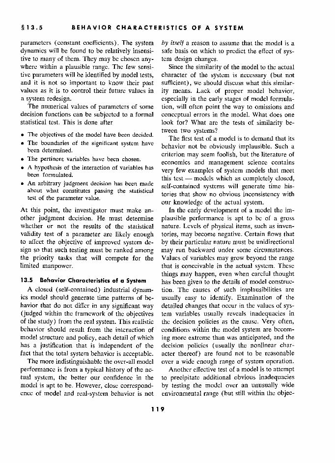
§ 13.5 5 BEHAVIOR CHARACTERISTICS OF A SYSTEM
parameters (constant coefficients). The system by itself a reason to assume that the model is a
dynamics will be found to be relatively insensi- safe basis on which to predict the effect of sys- tive to many of them. They may be chosen any- tem design changes. where within a plausible range. The few sensi- Since the similarity of the model to the actual tive parameters will be identified by model tests, character of the system is necessary (but not and it is not so important to know their past sufficient), we should discuss what this similar- values as it is to control their future values in ity means. Lack of proper model behavior, a system redesign. especially in the early stages of model formula-
The numerical values of parameters of some tion, will often point the way to omissions and decision functions can be subjected to a formal conceptual errors in the model. What does one statistical test. This is done after look for? What are the tests of similarity be-
- The objectives of the model have been decided. tween two systems? . The objectives of the model have been decided.
Th first test a f a model is to demand that its Thé first test of a model is to demand that its s . The boundaries of the significant system have behavior not be obviously implausible. Such a
beendetermmed..... VIOUS y aUSI e. uc a
been determined. criterion may seem foolish, but the literature of _ _ cn enon may seem toolish, but thé i era ure ot
. The pertinent variables have been chosen. economics and management science contains A hypothesis of the interaction of variables has
very few examples of system models that meet been formulated.
this test - models which as completely closed, . An arbitrary judgment decision has been made self-contained systems will generate time his-
about what constitutes passing thé statistical t .
t. h b" - .
about what constitutes passing the statistical
tories that show no obvious inconsistency with test of the parameter value.
our knowledge of the actual system. At this point, the investigator must make an- In the early development of a model the im- other judgment decision. He must determine plausible performance is apt to be of a gross whether or not the results of the statistical nature. Levels of physical items, such as inven-
validity test of a parameter are likely enough tories, may become negative. Certain flows that to affect the objective of improved system de- by their particular nature must be unidirectional
sign so that such testing must be ranked among may run backward under some circumstances. the priority tasks that will compete for the Values of variables may grow beyond the range limited manpower. that is conceivable in the actual system. These
things may happen, even when careful thought 13.5 Behavior Characteristics of a System has been given to the details of model construc-
A closed (self-contained) industrial dynam- tion. The causes of such implausibilities are ics model should generate time patterns of be- usually easy to identify. Examination of the havior that do not differ in any significant way detailed changes that occur in the values of sys- (judged within the framework of the objectives tem variables usually reveals inadequacies in of the study) from the real system. This realistic the decision policies as the cause. Very often, behavior should result from the interaction of conditions within the model system are becom- model structure and policy, each detail of which ing more extreme than was anticipated, and the has a justification that is independent of the decision policies (usually the nonlinear char- fact that the total system behavior is acceptable. acter thereof) are found not to be reasonable
The more indistinguishable the over-all model over a wide enough range of system operation. performance is from a typical history of the ac- Another effective test of a model is to attempt tual system, the better our confidence in the to precipitate additional obvious inadequacies model is apt to be. However, close correspond- by testing the model over an unusually wide ence of model and real-system behavior is not environmental range (but still within the objec-
119
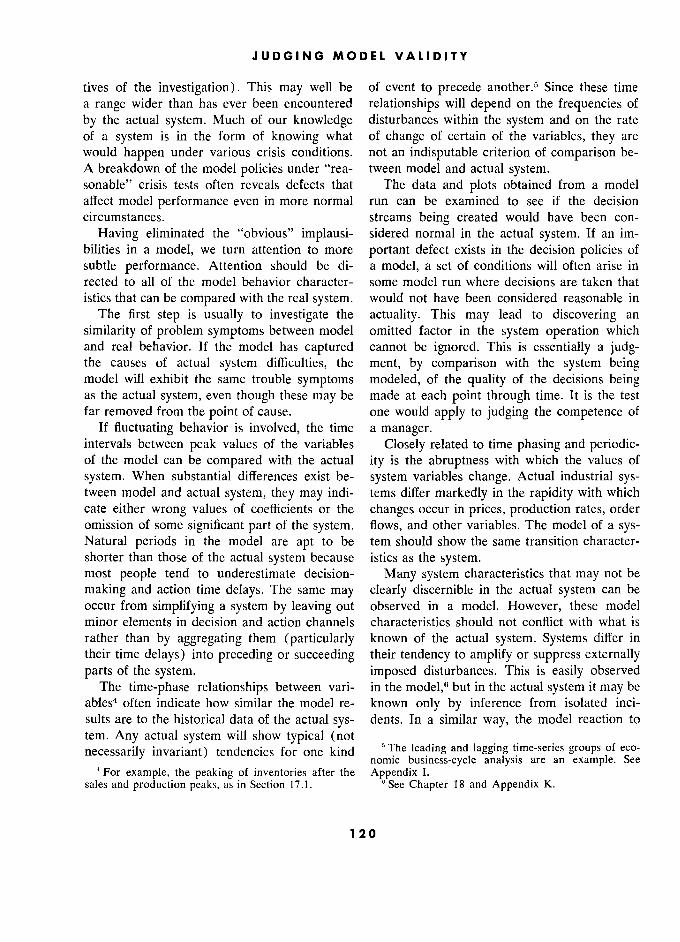
JUDGING MODEL VALIDITY
tives of the investigation). This may well be of event to precede another,.5 Since these time a range wider than has ever been encountered relationships will depend on the frequencies of
by the actual system. Much of our knowledge disturbances within the system and on the rate of a system is in the form of knowing what of change of certain of the variables, they are would happen under various crisis conditions. not an indisputable criterion of comparison be- A breakdown of the model policies under "rea- tween model and actual system. sonable" crisis tests often reveals defects that The data and plots obtained from a model affect model performance even in more normal run can be examined to see if the decision circumstances. streams being created would have been con-
Having eliminated the "obvious" implausi- sidered normal in the actual system. If an im- bilities in a model, we turn attention to more portant defect exists in the decision policies of subtle performance. Attention should be di- a model, a set of conditions will often arise in rected to all of the model behavior character- some model run where decisions are taken that istics that can be compared with the real system. would not have been considered reasonable in
The first step is usually to investigate the actuality. This may lead to discovering an
similarity of problem symptoms between model omitted factor in the system operation which and real behavior. If the model has captured cannot be ignored. This is essentially a judg- the causes of actual system difficulties, the ment, by comparison with the system being model will exhibit the same trouble symptoms modeled, of the quality of the decisions being as the actual system, even though these may be made at each point through time. It is the test far removed from the point of cause. one would apply to judging the competence of
If fluctuating behavior is involved, the time a manager. intervals between peak values of the variables Closely related to time phasing and periodic- of the model can be compared with the actual ity is the abruptness with which the values of
system. When substantial differences exist be- system variables change. Actual industrial sys- tween model and actual system, they may indi- tems differ markedly in the rapidity with which cate either wrong values of coefficients or the changes occur in prices, production rates, order omission of some significant part of the system. flows, and other variables. The model of a sys- Natural periods in the model are apt to be tem should show the same transition character- shorter than those of the actual system because istics as the system. most people tend to underestimate decision- Many system characteristics that may not be
making and action time delays. The same may clearly discernible in the actual system can be occur from simplifying a system by leaving out observed in a model. However, these model minor elements in decision and action channels characteristics should not conflict with what is rather than by aggregating them (particularly known of the actual system. Systems differ in their time delays) into preceding or succeeding their tendency to amplify or suppress externally parts of the system. imposed disturbances. This is easily observed
The time-phase relationships between vari- in the model,6 but in the actual system it may be ables4 often indicate how similar the model re- known only by inference from isolated inci- sults are to the historical data of the actual sys- dents. In a similar way, the model reaction to tem. Any actual system will show typical (not
necessarily invariant) tendencies for one kind 5 The leading and lagging time-series groups of eco- - ' nomic business-cycle analysis are an example. See
* For example, the peaking of inventories after the Appendix I. sales and production peaks, as in Section 17.1. ° See Chapter 18 and Appendix K.
120
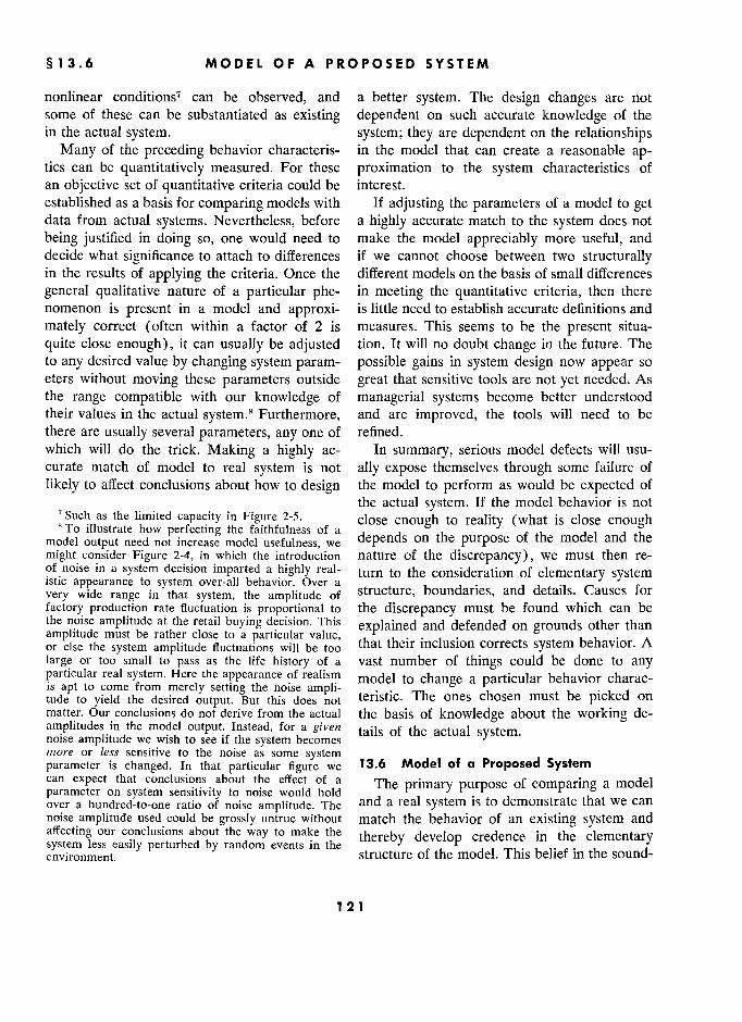
§ 13.6 MODEL OF A PROPOSED SYSTEM
nonlinear conditions7 can be observed, and a better system. The design changes are not some of these can be substantiated as existing dependent on such accurate knowledge of the in the actual system. system; they are dependent on the relationships
Many of the preceding behavior characteris- in the model that can create a reasonable ap- tics can be quantitatively measured. For these proximation to the system characteristics of an objective set of quantitative criteria could be interest. established as a basis for comparing models with If adjusting the parameters of a model to get data from actual systems. Nevertheless, before a highly accurate match to the system does not
being justified in doing so, one would need to make the model appreciably more useful, and decide what significance to attach to differences if we cannot choose between two structurally in the results of applying the criteria. Once the different models on the basis of small differences
general qualitative nature of a particular phe- in meeting the quantitative criteria, then there nomenon is present in a model and approxi- is little need to establish accurate definitions and
mately correct (often within a factor of 2 is measures. This seems to be the present situa-
quite close enough), it can usually be adjusted tion. It will no doubt change in the future. The to any desired value by changing system param- possible gains in system design now appear so eters without moving these parameters outside great that sensitive tools are not yet needed. As the range compatible with our knowledge of managerial systems become better understood their values in the actual system,.8 Furthermore, and are improved, the tools will need to be there are usually several parameters, any one of refined. which will do the trick. Making a highly ac- In summary, serious model defects will usu- curate match of model to real system is not ally expose themselves through some failure of
likely to affect conclusions about how to design the model to perform as would be expected of the actual system. If the model behavior is not
1 §/?????"??l?i limited capacity in Figure 2-5. close enough to reality (what is close enough 8 To illustrate how perfecting the faithfulness of a
model output need not increase model usefulness, we depends on the purpose of the model and the
might consider Figure 2-4, in which the introduction nature of the discrepancy), we must then re- of noise in a system decision imparted a highly real- turn to the consideration of elementary system istic appearance to system over-all behavior. Over a
very wide range in that system, the amplitude of structure, boundaries, and détails. Causes for
factory production rate fluctuation is proportional to the discrepancy must be found which can be the noise amplitude at the retail buying décision. This
explained and defended on grounds other than amplitude must be rather close to a particular value, .., ' . or else the system amplitude fluctuations will be too that their inclusion corrects system behavior. A
large or too small to pass as the life history of a vast number of things could be done to any particular real system. Here the appearance of realism model to change a particular behavior charac- is apt to corne from merely setting the noise ampli- tude to yield the desired output. But this does not teristic. The ones chosen must be picked on matter. Our conclusions do not derive from the actual the basis of knowledge about the working de- amplitudes in the model output. Instead, for a given tails of the actual system. noise amplitude we wish to see if the system becomes ' more or less sensitive to the noise as some system parameter is changed. In that particular figure we 13.6 Model of a Proposed System can expect that conclusions about the effect of a The primary purpose of comparing a model parameter on system sensitivity to noise would hold , r over a hundred-to-one ratio of noise amplitude. The and a real system is to demonstrate that we can noise amplitude used could be grossly untrue without match the behavior of an existing system and affecting our conclusions about the way to make the
thereby develop credence in the elementary system less
easily perturbed by random events in the structure of the model. Thls bellef in the sound- environment. structure of thé model. This beliet m thé sound-
121 1
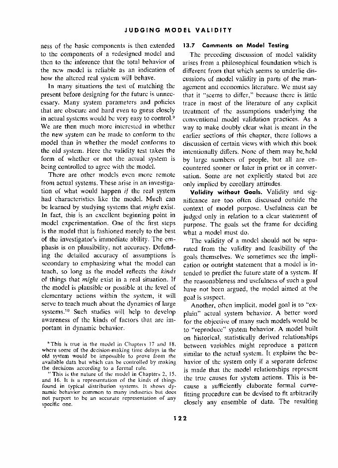
JUDGING MODEL VALIDITY
ness of the basic components is then extended 13.7 Comments on Model Testing to the components of a redesigned model and The preceding discussion of model validity then to the inference that the total behavior of arises from a philosophical foundation which is the new model is reliable as an indication of different from that which seems to underlie dis- how the altered real system will behave. cussions of model validity in parts of the man-
In many situations the test of matching the agement and economics literature. We must say present before designing for the future is unnec- that it "seems to differ," because there is little
essary. Many system parameters and policies trace in most of the literature of any explicit that are obscure and hard even to guess closely treatment of the assumptions underlying the in actual systems would be very easy to contrôla 9 conventional model validation practices. As a We are then much more interested in whether way to make doubly clear what is meant in the the new system can be made to conform to the earlier sections of this chapter, there follows a model than in whether the model conforms to discussion of certain views with which this book the old system. Here the validity test takes the intentionally differs. None of them may be. held form of whether or not the actual system is by large numbers of people, but all are en-
being controlled to agree with the model. countered sooner or later in print or in conver- There are other models even more remote sation. Some are not explicitly stated but are
from actual systems. These arise in an investiga- only implied by corollary attitudes. tion of what would happen if the real system Validity without Goals. Validity and sig- had characteristics like the model. Much can nificance are too often discussed outside the be learned by studying systems that might exist. context of model purpose. Usefulness can be In fact, this is an excellent beginning point in
judged only in relation to a clear statement of model experimentation. One of the first steps purpose. The goals set the frame for deciding is the model that is fashioned merely to the best what a mode] must do. of the investigator's immediate ability. The em- The validity of a model should not be sepa- phasis is on plausibility, not accuracy. Defend- rated from the validity and feasibility of the
ing the detailed accuracy of assumptions is goals themselves. We sometimes see the impli-
secondary to emphasizing what the model can cation or outright statement that a model is in- teach, so long as the model reflects the kinds tended to predict the future state of a system. If of things that might exist in a real situation. If the reasonableness and usefulness of such a goal the model is plausible or possible at the level of have not been argued, the model aimed at the
elementary actions within the system, it will goal is suspect.
'
serve to teach much about the dynamics of large Another, often implicit, model goal is to "ex-
systems.1° Such studies will help to develop plain" actual system behavior. A better word awareness of the kinds of factors that are im- for the objective of many such models would be
portant in dynamic behavior. to "reproduce" system behavior. A model built
on historical, statistically derived relationships 9 This is true in the model in Chapters 17 and 18, between variables might reproduce a pattern where some of the decision-making time delays in the Similar
to the actual s stem. It ex lains
the old system would be impossible to prove from the similar to thé actual y p thé be-
available data but which can be controlled by making havior of the system Orily if a separate defense the decisions according to a formal rule. is made that the model relationships represent '°This is the nature of the model in Chapters 2. 15. , fan and 16. It is a representation of the kinds of things the true causes for system actions. This is be-
found in typical distribution systems. It shows dy- cause a sufficiently elaborate formal curve- namic behavior common to many industries but does
fitting procédure can be devised to fit arbitrarily
specific not purport one. to be an accurate representation of any
closely any ensemble of data. The resulting specific one. closely any ensemble of data. Thé resultmg
122

§ 13.7 COMMENTS ON MODEL TESTING
summary of the data carries with it no implica- will take on an aura of authenticity in its own tion of containing proper causal mechanisms. right. It becomes a pseudoscientific ritual. The It may give no promise whatever of even quali- underlying assumptions based on judgment or tative behavior similar to the actual system merely faith may be forgotten. The objective outside the time period for which the data fitting test, which may have been sound for the original was done. goals and assumptions, may now move by itself
Assumptions Underlying Test Procedure. into new areas where it is useless or actually Any "objective" model-validation procédure misleading. rests eventually at some lower level on a judg- Predicting Future System State. A model is ment or faith that either the procedure or its a statement of a "law of behavior." It thereby goals are acceptable without objective proof.11 purports to unify what would otherwise be un-
In tests of statistical significance it is usually related and perhaps even apparently contradic- taken as self-evident that the "measure of sig- tory information. Within what the "law of be- nificance" is significant. Yet there is often no havior" is supposed to represent, we should answer to the question, "What is good enough?" expect that it predicts future real-life behavior if
because the result of the "objective" test has that behavior is indeed governed by the "law." not been related to a goals.12 At this point we must be most careful in defin-
Many persons will protest at the way the ing and understanding what the "law" repre- earlier sections of this chapter depend on sub- sented by a model is intended to do. We judge jective judgment for model validation. Yet at the validity of a model by comparing its predic- some point the "objective" methods rest on the tions against observations of the system whose same foundation. The objective test is useful behavior it is supposed to represent. But in if the underlying assumptions for it are sound what sense is a specific model expected to pre- and if the judgment criteria are not amenable dict, and how is the comparison of a model to to direct application but must be interpreted the real system to be made?
through an intermediate quantitative procedure. Take the solar system as an example of what The danger is that the quantitative procedure we do not have in social systems. It is a group
of bodies whose motion is governed by a very Churchman, Reference 11, for a discussion of few basic causes (inertial forces and gravita- the philosophy underlying scientific methodology. „ , . - .
12 As an illustration, 1 once attended a seminar It 1S an Open system ; 1t is not an m- conducted by a respected member of the management formation-feedback system in which there are science community, in which a hypothesis was pre- forces that would return a planet to its "orig- sented for the way in which a particular kind of . decision had been made by the people in an actual inal" orbit were it to be disturbed by the passage system. A decision function near the bottom of the of some foreign heavenly body. It is a system management hierarchy had been chosen because in which the forces not explained by the pri- historical data did exist. The hypothesis fitted the data to high accuracy for over 90% of the incidents. The mary laws (inertia and gravitation) are van-
implication was that the hypothesis was excellent. ishingly small compared with the primary But the lecturer had no answer to the question forces. It is a system whose future speclftc state whether the decision function was really good enough, or to the question whether too great an effort had been is of interest to us. It is a System whose future expended to make it as good as that (the research had specific state will not be disturbed by our having been extensive). No goal or purpose existed against advance knowledge of what that state will be. which to measure or judge or even discuss the perti- ° '
nence and validity of the validity test. In fact, he A useful solar system model is one that pre- offered the response that the research merely proved dicts the times of specific future events like sun- that the real-life decision procedure was not a random
rise, winter, a lurlar The usefulness process. 1 believe that no one could have been found ' to defend the proposition that it was random. of the model rests on its ability to make this
123
JUDGING MODEL VALIDITY
prediction, and its accuracy is measured by the and we have not discovered its generating error between model prediction of time and causes. (We may have useful estimates of its
place and the actual observations. magnitude and statistical characteristics.) The Often we find the same test being applied to model acts on the noise components as it acts
a model of a social system without a critical re- on all other flows within the system. The struc- examination of whether the objectives and foun- ture and characteristics of the model determine dations are still valid. Before applying the test the nature of the reaction to the noise. of predicting the system state at specific future Not knowing the instantaneous values of the times to a model of industrial or economic be- noise, we can still study the kind of behavior
havior, we must ask several questions. Is pre- exhibited by the system, including the sensitivity diction of specific events a proper goal of the to the noise inputs. In the model the exact model? Is there reason to believe that the objec- paths of the variables in time depend not only tive is possible? Is it the most useful applica- on the model structure and the. initial values tion of the model? Is the system sufficiently in- of system variables but also on the unknown
dependent of the prediction process itself? noise. The relative determinancy created by the Economic systems are conceptually of a dif- known policies and structure versus the un-
ferent class from the solar system. Economic certainty introduced by noise will determine
systems are characterized by their information- the ability of a model to predict the specific feedback-system behavior, while the solar sys- state of a system at a particular future time. tem is an open-ended system. There is no reason From a consideration of the nature of the to believe that either the nature or purpose of components and structure of social systems, models of the two would be identical. Economic it appears that we should not soon expect mod- behavior occurs in the context of an informa- els that can be useful in predicting specific fu- tion-feedback system in which goal-seeking de- ture system state. This type of prediction of cisions are constantly responding to the state future state is possible only to the extent that of the system itself. An external disturbance in- the correctly known laws of behavior predomi- duces closed-loop reactions within the system nate over the unexplained noise. In the model of toward re-establishing the goals. the solar system the noise components of force
The economic system contains large "noise" on the bodies are vanishingly small compared forces that are not explained by the behavior with those forces which can be explained. In laws that we feel justified in hypothesizing. social systems this is not true. These unknown influences are often comparable The relationship between structure, noise,
(depending on the way in which the compari- and prediction of future system state can be
son is made) with the orderly forces. This im- demonstrated entirely within the realm of model
plies that the system is subject to having its fu- experimentation. Consider that there are two
ture deflected by the unexplained factors. identical models'3 which contain noise at one Even though stable organizational structure, or more decision points in the system. Let these
policies, and human reactions exist and these two models represent, respectively, the "real"
determine the principal dynamic characteristics system and the "model" of the "real" system. of a system, we cannot assume a perfect model The "model" is then known to be identical in
in which every relationship is known exactly. structure and in all its coefficients to the "real"
Therefore, we are committed to models in which system and even has the same statistical charac-
every decision function has, at least in principle, l' Sec Appendix K for this experiment conducted a noise or uncertainty component. By définition, See Appendix K for this experiment conducted a noise or uncertainty comportent. By definition, on the production-distribution system with noise input,
the exact time pattern of this noise is unknown, as aiready seen in Figure 2-4.
124
§ 13.7 COMMENTS ON MODEL TESTtNG
teristics in its noise sources. The instantaneous is an undefined concept in nonlinear systems values of noise are unknown and will differ. As but implies the degree of persistence of exist- time progresses from the initial conditions, the ing trends and cycles and the rapidity with
two models will begin to diverge in the numeri- which these might be altered by random events. cal values of the variables they are generating. The narrower the bandwith around any compo- Soon there will be no evident, instantaneous nent of system behavior, the longer we can ex-
similarity between the quantitative values of pect that component to persist. Actually, it
corresponding variables in the two systems.l4 seems clear that we are dealing with wide-band Over long periods of time, however, they will systems in management and economics, in
both show the same general type of behavior. which the noise components strongly determine
Although the "model" may not be useful for the state of the system even in as short a time
predicting the condition of the identical "real" as a part of one "cycle" of disturbance into the
system at a specific future time, it has the same future. Nonlinear systems probably show dif-
performance nature. It has the same kind and ferent bandwidths at different times, so that
degree of sensitivity to the noise disturbances. vulnerability to change will vary with the state
Furthermore, this nature, in both the "model" of the system. and the "real" systems, is dependent on the The determinancy of a system in projecting structure and coefficients of the system. The the past and present into the future will be re- "model" can be used to predict how a change in lated to the degree of stability of the system. A the "real" system would make it a more de- system with strong, unstable oscillatory tend- sirable system, even in the continued presence encies will be more predictable through the next of noise that excludes prediction of specific fu- cycle of disturbance than an inherently more ture system state. stable system in which the fluctuations are more
A dynamic system model should therefore be dependent on noise whose source is unrelated
expected to represent and to predict the be- to the behavior of the system itself. havior characteristics (like profitability, stabil- The relationship between noise, policy, ob-
ity of employment and prices, growth tenden- servation, system behavior characteristics, and
cies, and typical time-phasing relationships prediction can perhaps be illustrated by an between changes in variables) of the actual sys- absurdly simple analogy to a coin-flipping ex- tem. It should not be expected to predict fu- periment. The unknown and uncontrolled forces ture system state except to the extent that the that determine which side of the coin comes up system has continuity and momentum charac- are usually predominant. We do not expect to teristics that will cause present conditions and predict correctly each separate flipping event. trends to persist for a time in spite of noise The statistical prediction relates to the nature disturbances. of the pattern of behavior. The model of the
Indeed, one of the performance characteris- process deals with the type of long-term out- tics of a system that we might study in its model come, not the individual specific event at each is the inherent limitation on prediction ability. point in time which is, in the usual coin ex-
Using the model, we should be able to study periment, supposed to be controlled by random the counterpart of what the engineer calls events. But suppose that we do not like the be- "bandwidth" in his linear systems. "Bandwidth" havior of this system in which each event is
independent of the past and is a result of un- " For the system of Chapter 2, the divergence be- controlled forces. Are there possible policy
tween the "model" and the "real" system is substantial changes in the system which might affect the
after only a few weeks from the identical starting o u conditions. nature of the results?
125 5
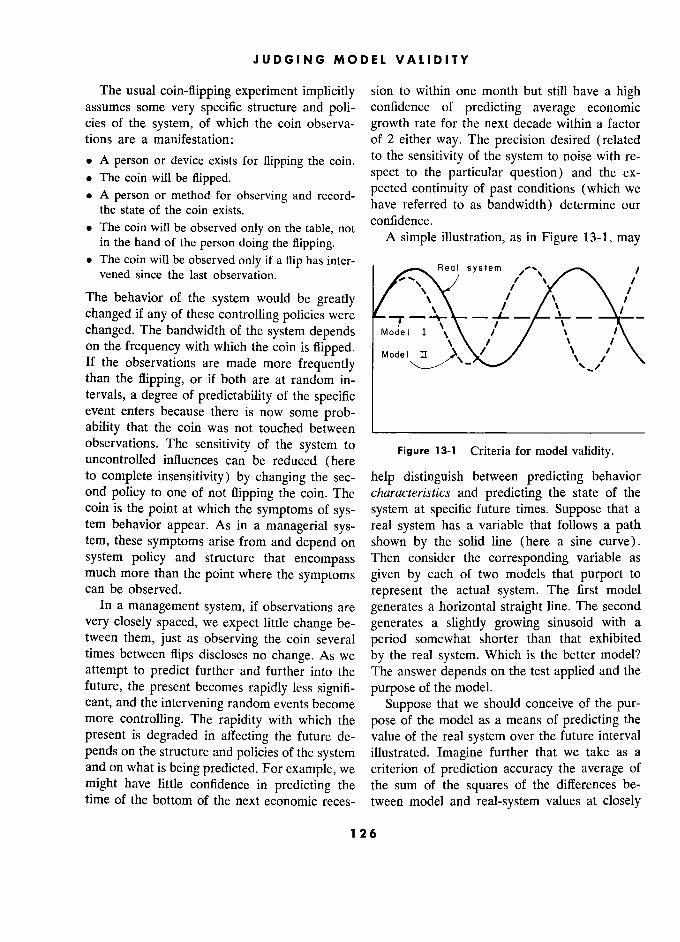
JUDGING MODEL VALIDITY
The usual coin-flipping experiment implicitly sion to within one month but still have a high assumes some very specific structure and poli- confidence of predicting average economic cies of the system, of which the coin observa- growth rate for the next decade within a factor tions are a manifestation: of 2 either way. The precision desired (related
. A person or device exists for flipping the coin. to the sensitivity of the system to noise with re-
The coin will be flipped. spect to the particular question) and the ex-
. A person or method for observing and record- pected continuity of past conditions (which we . A person or method for 0 servmg and record- ' „ .. the state of the coin exists. have referred to as bandwidth) détermine our
? The coin will b observed only on the table, not confidence. . The coin will be observed only on thé table, not
may in the hand of the person doing the flipping. . P illustration, as in Figure 13-1, may
. The coin will be observed only if a flip has inter- Real system vened since the last observation. ,' ", \. ,'
The behavior of the system would be greatly / , \ / i
changed if any of these controlling policies were -7
– A– – –\–– changed. The bandwidth of the system depends
Mode
i I \\ " / /\ on the frequency with which the coin is flipped. \ If the observations are made more frequently than the flipping, or if both are at random in- tervals, a degree of predictability of the specific event enters because there is now some prob- ability that the coin was not touched between ____________________________ observations. The sensitivity of the system to
Figure 13-1 Criteria for model validity. uncontrolled e influences can be reduced (here Critena for mode! vahdlty.
to complete insensitivity) by changing the sec- help distinguish between predicting behavior ond policy to one of not flipping the coin. The characteristics and predicting the state of the coin is the point at which the symptoms of sys- system at specific future times. Suppose that a tem behavior appear. As in a managerial sys- real system has a variable that follows a path tem, these symptoms arise from and depend on shown by the solid line (here a sine curve).
system policy and structure that encompass Then consider the corresponding variable as much more than the point where the symptoms given by each of two models that purport to can be observed. represent the actual system. The first model
In a management system, if observations are generates a horizontal straight line. The second
very closely spaced, we expect little change be- generates a slightly growing sinusoid with a tween them, just as observing the coin several period somewhat shorter than that exhibited times between flips discloses no change. As we by the real system. Which is the better model?
attempt to predict further and further into the The answer depends on the test applied and the
future, the present becomes rapidly less signifi- purpose of the model.
cant, and the intervening random events become Suppose that we should conceive of the pur- more controlling. The rapidity with which the pose of the model as a means of predicting the
present is degraded in affecting the future de- value of the real system over the future interval
pends on the structure and policies of the system illustrated. Imagine further that we take as a and on what is being predicted. For example, we criterion of prediction accuracy the average of
might have little confidence in predicting the the sum of the squares of the differences be- time of the bottom of the next economic reces- tween model and real-system values at closely
126
§13.7 COMMENTS ON MODEL TESTING
spaced points in time. (Such a criterion is com- the causal relationships of the actual system are
mon, usually arbitrarily chosen without justifica- represented in the mechanisms of the model. An tion of its significance as a useful measure, and endless variety of model details having no simi- selected because it is mathematically easy to larity to the actual system could be assembled handle. ) that would create the Model II curve. Our con-
By this test, Model I, which gives the straight fidence in Model II as an experimental tool for line, is the better predictor. The above error studying the effect of structure and policy measure will be smaller and the maximum er- changes in the actual system is based on our ror will be less than for the second model. confidence in the model components separately
In spite of being a better predictor, according and individually and in the fact that in concert to the above arbitrary criterion, of the specific they produce the behavior that interests us in future state of the system, we should not expect the actual system. Model 1 to reveal much about how to redesign One additional point needs to be made re- the actual system to change its performance. gardmg the search for models that will predict Model 1 does not exhibit the characteristic fluc- the state of an actual system at some future
tuating behavior of the actual system. It does point in time. Economic and industrial systems not pass the necessary (but insufficient) test would not, even to a crude first approximation, of having dynamic behavior similar to that of be independent of a process that would really the actual system. We should conclude that any predict the state of the system far into the fu- defense of its component structure and policies ture.15 Predictions are sought as a guide to ac- must be inadequate because it seems incapable tions that would take place within the system of creating the sinusoidal behavior which can being modeled. The actions taken as a result of here be seen and measured in the actual system. a prediction would directly affect the stream of Because the components of the model fail to events whose prediction is being attempted. A create the nature of the behavior of the actual successful model for predicting the future state
system, we should not trust modifications in of a business or economic system cannot these components to show how the system be- remain aloof from that system except to the havior might be changed. extent that the model fails. Should a model of
Consider Model II in Figure 13-1. Suppose proved ability to predict the specific future that the defense of structure and policy are with- course of a social system exist, it would defeat out serious objection. Does it pass the criterion itself if it were put to use. of having a dynamic behavior similar to that A "predicting procedure" can be treated only of the real system? There is a predominant as a decision-making rule, like all other deci- sinusoidal behavior pattern. The period of fluc- sion rules, in its proper place in the system con- tuation in the model is a little shorter than the text. It must be related to the actions that will actual system but only by 25%. Its damping result from the "prediction." The predicting coefficient (indicative of the tendency of the procedure would not, therefore, exist separately. fluctuation to grow or decline) is a small nega- It would become a component of a larger model tive value that is not much different from the of the total system and would contribute to the zero value of the actual system. Because the dynamic behavior character of the system as a model, compared with the actual system, has whole. Limitations on predicting ability arising similar amplitude, period, and damping, we from model incompleteness and noise would should conclude that it may be a close represen- then become the same as for other models, as tation of the actual system. This test is meaning- discussed above. ful only because we believe independently that 15 See Appendix N.
127
JUDGING MODEL VALIDITY
In a longer-term context, the same could be Let us summarize the use of dynamic system argued for industrial dynamics models. As models for prediction: they become generally understood, and if they are highly effective as a basis of system design, e If a model could predict specific events far
they become a part of the arsenal of competitive enough ahead to allow action to be taken as a
methods whose existence affects the systems result of the prédiction, there may be sufficient
they represent. However, a distinction can lie time intervening for random events to alter the
in the immediacy of application. A reliable pre- predicted values.
diction of an event, like a sales upturn, would If random disturbances do not exist, if the
be more easily understood and responses to it model is sufficiently near to perfect, and if the
would be more rapid than the response to a momentum of the system is not strong enough
prediction that a specific change in corporate to inhibit action in anticipation of the predicted
policy would increase the likelihood of higher events, then the
action taken is itself highly
sales. °
likely to affect the predicted outcome. The pre- ' diction procedure would then need to be a sys- Even so, we must never be oblivious to the tem decision function incorporated so that the effect that a system dynamics study may have model recognizes the effect of the prediction on on the system being studied. It has been my other decisions.
experience that a decision hypothesis, in the , pny prédiction procédure is part of a decision-
context of a system model which reveals the making process and is properly viewed as a
implications of the hypothesis, begins to have decision function in its system context, where it an immediate effect on the actual system. The can be studied to see how it affects the behavior
searching questions that must be asked to ex- characteristics of the system of which it is a
pose the information flows and the power cen- part. ters in an organization will cause people to re- . System models should predict and reproduce the examine their action patterns. The investigator behavior character of a system, not specific who develops a system model (if he wants to events or particular, unique sections of actual
compare its behavior, in any of the senses of system time history.
comparison, against the actual system) must be alert to the fact that he has already himself Nonquantitative Model Validation. We
become a part of the system under study. The sometimes encounter the attitude that model
more the people in the actual system know of validity can be treated only in a numerical and
the objectives and possible outcomes of a system quantitative manner. This hardly seems justi-
investigation, the more they may be affected by fiable when such a preponderant amount of
the investigation itself. This does not imply that human knowledge is in nonquantitative form.
the purposes of a system study should be with- A model will be cast in numerical form in
held. It only says that the investigator must order that our statements will be specific and
be alert to the changes in system structure and unambiguous. Such statements, however, often
policies that may occur simply as a result of ex- arise from beliefs about relative magnitudes,
posing those policies. Under some circum- limiting conditions, and probable consequences. stances, the effects might become great enough The numbers that appear in such a model often
to affect substantially the dynamic character- do not derive in any analytical or statistical way istics of the system even before any formal re- from specific numerical data from the operating sults of a policy design study had been imple- system. mented. Quantitative validation of a model should be
128

§ 13.7 COMMENTS ON MODEL TESTING
done when possible and when the anticipated periences, and considered from the viewpoint results are expected to justify the cost and ef- of what they imply under both normal and ex-
fort. However, if most of the content of a model treme circumstances. Knowledge of all forms
is drawn from nonnumerical sources in the can be brought to bear on forming an opinion form of individual personal knowledge and ver- of whether or not a model is suitable to its par- bal and written descriptions, the defense of the ticular purpose. model will usually rest on the same kinds of This means that model building and model
knowledge. The individual expressions in a validation do not stop at the boundary where
model should always have meaning in the con- numerical data fail. It means that both have
text of the real system. All variables and param- full access to the vastly richer sources that lie
eters should have conceptual meaning that can in the nonquantitative areas of business man-
be individually considered with respect to the agement. By hypothesizing quantitatively about
actual system. They can then be examined, these areas, the day may be hastened when
argued, checked against past incidents and ex- firmer facts and measurements are available.
129

CHAPTER 14
Summary of Part II
In Part III that follows are examples of dynamic models based on the
philosophy and general principles that have just been given in Part II. pA!7oMp/!y and prMC;'p/M f/!af Aave &een t'n //. Before going to Part 111, the chapters of Part II will now be briefly sum- marized.
I N Chapter 4, models are classified. Those reached the point where systems of hundreds or that would usefully describe industrial and eco- thousands of linear and nonlinear variables can nomic behavior were identified as mathematical, be readily and economically investigated. The
dynamic and nonlinear models. They need to hurdles are not technical nor financial, but in- treat both stable and unstable as well as steady- tellectual. Success will be paced by the rate of state and transient systems. advancement in our descriptive knowledge and
Industrial dynamics models, in their purpose insight into the industrial, economic, political, and origin, will be more similar to models of educational, and social interactions that sur-
engineering systems than to models in the physi- round us. Models must simultaneously deal with cal, genetic, and agricultural sciences. They all these factors if they are to serve their pur- are models of information-feedback systems, pose. not models of open-ended systems in which re- Dynamic models will be based primarily on sults do not react on causes. our descriptive information already available,
Mathematical models can be constructed not on statistical data alone. Observation of from the bottom upward, based on our descrip- and familiarity with a system will reveal actions, tive knowledge of the elementary parts of the motivations, and information sources that can-
system to be represented (the size of the ele- not be discovered through historically available ments depends on the purpose of the model). A quantitative measures. The "intangibles" must successful dynamic model of nonlinear, noisy, appear quantitatively in a model to the best information-feedback systems probably cannot ability of the model builder; to omit them is a be derived by statistical analysis of the over-all, more serious failing than to have an error in
aggregate, system performance. magnitude. Our real-life systems are not highly Mathematical models make controlled experi- sensitive to changes in the components of which
ments possible and allow us to see the effect of they are constructed, neither are models having the separate parts of the system. A manage- the proper structure. Severalfold changes in ment laboratory then becomes possible for the values of parameters and major changes in
design of improved managerial policies. The the shapes of assumed statistical distributions of
dynamic model is a tool for the design of policy system responses often have but slight influ- and organizational form. ence. Concentration must be on those factors
The understanding of system dynamics and that determine the characteristics of informa- the tools of electronic computation have now tion-feedback systems - structure, amplifica-
130

SUMMARY OF PART Il
tion, and delays. A model itself can be used to kind of flow system to another are the points determine the system sensitivity to a particular at which essential policies and conversion fac-
parameter or structural change. From the model tors are to be found. studies can come an estimate of how much cost As a first step, it is strongly recommended is justified in refining our knowledge of the that systems be formulated in the continuous actual system. form and that discontinuities and periodic re-
Chapter 5 discusses the formulation of a dy- view of decisions be postponed until the funda- namic system model. A model is designed to mentals of the continuous system are under- answer specific classes of questions. The com- stood.
pleteness required in a model depends on the We cannot assume that systems will be either
questions to be explored. Models of industrial stable or linear. Linear analysis over a small
activity usually begin by containing a few hun- range of system operation will often fail to il- dred variables. Just as verbose writing is easier luminate the characteristics of greatest interest than the concise, so is the cluttered and complex to the manager. model easier to formulate than the simple model Chapter 6 describes a basic model structure that still retains the essence of the larger system. that has been found to correspond to the im-
Very often it is more expeditious to include a portant dynamic characteristics of industrial and factor than to determine that it can be omitted. managerial activity. The model consists of an
Economic and industrial activities are closed- alternating system of levels and flows. The flow
loop, information-feedback systems. Models of channels transport the contents of one level to such systems must preserve the closed-loop another, and the flow rates themselves are con- structure that gives rise to the dynamic behavior trolled by the levels. The decision functions are of interest. An information-feedback system ex- the relationships that describe how the levels ists when an environment leads to decisions control the flow rates. Information channels that in turn lead to actions that are intended to connect the levels to the decision functions. alter the original environment and in turn lead This model structure is simple and straight- to new decisions. forward. It permits a one-to-one correspond-
The essential characteristics of information- ence between the model and the system being feedback systems arise from organization struc- represented. It leads to a system of equations ture (including policy), amplification, and de- that can be individually evaluated one by one at
lays. These characteristics must be carefully successive time intervals in tracing the time se-
preserved in going from the real-life system to quence of system operation. No solutions to the model of the system. simultaneous equations are required.
A dynamic model can and should be con- Six interconnected flow systems are used to structed to correspond to identifiable features represent industrial and economic activity. The and policies of the actual system. The terminol- five elementary flow systems handle orders, ma-
ogy should be the same. The units of measure terials, money, personnel, and equipment. These can be identical. The same concepts, objectives, five are interconnected by a superimposed in- and goals should appear in each. formation network that links the levels of the
The dimensional units of measure of variables five flow systems to the rates in the same and in and of constants should be given meticulous different flow systems. The information network care. The money equivalent of variables hav- itself may contain levels and rates.
ing other physical and conceptual meaning Chapter 7 describes the types of equations should not be substituted for measures in more needed for the fundamental model structure. realistic terms. The conversion points from one For the symbols to represent variables, English
131 1
SUMMARY OF PART T 1 1
letters and Arabic numerals are used so that of the behavior in which we are interested arises
they may be readily printed on typewriters and from the nonlinear phenomena within the sys- digital-computer output equipment. A time no- tem. Only if these are incorporated in the model tation indicates the variables as belonging to can the model show us the behavior character- the present, the immediate past, and the im- istics in which we are interested. The rate equa- mediately following moments in time. This time tions, which represent the policies that control notation is for computational purposes and is system decisions, can represent only the pre- independent of representation of delays in the dominant variables and must necessarily omit a
system. Level equations describe the contents vast amount of secondary detail. In an actual of the reservoirs or accumulations within the system that part of the omitted detail which
system. Rate equations (decision functions) arises outside the system and is independent of describe the manner in which the levels control what happens inside the system can be con- the rates of flow. Auxiliary equations are ac- sidered as noise. The estimated statistical char-
tually part of the rate equations, but have been acteristics of this noise should be incorporated algebraically factored out of the rate equations in many of the decision functions in the system. for convenience or because the auxiliary equa- As with the estimates of other parameters of tions define variables of separate interest. The the system, the exact characteristics of the noise
equations constitute a recursive system of first- can often be in substantial error without defeat- order difference equations which can be evalu- ing the purposes of the model. ated individually and which yield the numerical Chapter 11 discusses the aggregation of indi- values necessary for progressing step by step vidual events into continuous flows within the
through time. model. This implies that the model takes the
Chapter 8 describes a system of flow dia- viewpoint not of the individual middle manager grams that pictorially represent the equations within the organization, but rather adopts the and the relationships within the system. It is viewpoint of top corporate officers, wherein
strongly recommended that detailed flow dia- the individual event is not of primary signifi- grams be developed simultaneously with de- cance. Attention is focused on organizational velopment of the equations for a system. Flow form and on the policies that govern the opera- diagrams are often a better means of communi- tion of the system. Aggregate flows will, how- cation than equations. Also they assist in avoid- ever, reflect the sequences of actions that would
ing errors by ensuring that the equation rela- be encountered by any one item in the flow
tionships are as intended. channel.
Chapter 9 discusses the representation of de- Chapter 12 discusses exogenous variables.
lays in all channels. It suggests that first- and These should be used for establishing the ex- third-order exponential delays are simple and ternal environment that is to be assumed en- are adequate for most situations that will be tirely independent of what happens within the encountered. modeled system. Exogenous variables are ordi-
Chapter 10 discusses decision making and narily limited to a single variable and are not the rate equations that describe the policies used to feed real-system data into the model
controlling the system operation. Decisions are with the hope of achieving greater model ac- the day-by-day results of applying these policies curacy. The exogenous inputs serve as assumed to the available information. The dynamic test conditions to allow observation of system model is a tool for studying the influence of reactions. Great care must be exercised to be
policy on system behavior. System nonlinearities sure that the externally supplied conditions are
appear in the decision-making policies. Much indeed independent of what happens within the
132 2

SUMMARY OF PART Il 1
system insofar as the questions being studied ceptability of over-all system behavior. The
are concerned. complete model must be judged on the basis of
Chapter 13 discusses how to judge the use- system behavior - stability, periods of fluctua-
fulness of a model. Since models of noisy sys- tion, timing relationships between variables, and
tems cannot be expected to predict future amplitudes of system fluctuation. These are the
moment-by-moment values of system variables, variables that describe the general character of
the model cannot therefore be tested by how a system. The final judgment of industrial dy- well it predicts specific future system events. namics models will rest on the extent to which
Confidence in a model arises from a twofold test they are helpful to the manager in designing - the defense of the components and the ac- better industrial systems.
133

III '
EXAMPLES OF
DYNAMIC SYSTEM MODELS
Part III, consisting of the next four chapters, contains two system models to illustrate the model-building discussion of the preceding chapters.
The models themselves are but examples. They are not intended to have universal applicability.
The economics literature has often tended to emphasize the uniqueness, individuality, and the durability of models. One sees many references of the form "so-and-so's model of -," as if the designer of the model were irrevocably committed to the particular form that may have ap- peared in a publication. In the system studies that we are discussing here, there is no such thing as "the model." A model will continuously evolve, sometimes a particular form surviving for no longer than a single computer run giving one time history of system operation. Results of studying the model lead to constant change-often extensive change. One phase of a study may center around one model form, while other classes of questions are answered by a different or more extensive model.
The first model, in Chapters I and 16, is the same as the one used in
Chapter 2. It is a simple distribution system involving inventories and flows of orders and goods. It is extended to include a simple aspect of the market and sales effort. The second model, in Chapters 17 and 18, is similar in complexity but deals with a double-loop system in which the customer-supplier loop interacts with the supplier-labor loop. In that model, money flow has been added.
Neither of these two models incorporates the more subtle factors that are often significant in industrial system behavior. Such factors are beyond the scope of this present volume and also would require the presentation of models that have not yet been sufficiently refined to justify their inclu- sion. However, to compensate for the incompleteness of the models of Part III, Chapter 19 of Part IV contains discussions of additional facets of the indus tri al picture that have received partial study in other dynamic system models.
135

With the same reader classification as in the introduction to Part Il
preceding Chapter 4, the following suggestions are made:
e Group A (the manager who is not taking time for study of the more technical material) : Sections 15.1 through 15.4 should be read. Section 15.5 develops the equations of the model. It is strongly recommended that the reader work part way into this section. It looks formidable to some people but is actually understandable, with some effort, by anyone interested in the subject of this book. Studying the model equations is the only way to understand fully what assumptions lead to the system results that are illustrated in the time histories generated by the models. Section 15.5 on model equations illustrates the process of going from the
manager's descriptive knowledge to a formal model of the industrial
enterprise. However, at the point where the reader no longer wishes to
study the details of the equations, he can scan the remainder of the sec- tion, examine the flow diagrams, and proceed to Sections 15.6 and 15.7.
Chapters 16, 17, and I should be treated in a similar way by reading the
parts of interest. Part IV beginning at Chapter 19 is very different in character from Part III and is especially significant for the manager. e Group B (the reader who is interested in how models of industrial
systems can be set up but is not attempting to develop personal skill and
competence) : Read Part 111 and finish with Part IV.
e Group C (the serious student of industrial dynamics who is develop- ing his personal competence to do system analysis) : Study Part III care-
fully, referring to sections of Part Il as necessary. After Part III (or after Part IV), carefully reread all of Part II, which should become more
meaningful after studying the examples of Part III.
136
CHAPTER 15 5
Model of the Production- Distribution System of Chapter 2
This chapter illustrates the process of using a statement of the objectives and a verbal description to create a mathematical model of an industrial
system. It is a simple example, to the extent that few "intangibles" are involved. A total of seventy-three equations represent retail, distributor, and factory sectors and the initial conditions that describe the starting point of the system. The results of the model runs in Chapter 2 are
repeated with details of interpretation and of how the model was altered
for each run.
I N this chapter are derived equations for later chapters the representation of a company the production-distribution system discussed in will be extended outward into more difficult
Chapter 2. This first simple model will illustrate corporate functions. the application of many of the general princi- ples of Chapters 4 through 13. 15.1 1 Objectives
This initial example deals with a few of the In constructing a useful dynamic model of
principal information and material flows in corporate behavior it is essential to have clearly a typical production-distribution system. Al- in mind the purposes of the model. Only by
though the system is general in nature and can knowing the questions to be answered can we
represent many industrial situations, the reader safely judge the pertinence of factors to include
may feel most comfortable if he thinks of the in or omit from the system formulation.
example as applying to the manufacture and Therefore, we shall define our immediate
distribution of consumer durables, such as objective as an examination of possible fluctuat-
household electrical appliances. ing or unstable behavior arising from the prin- We start with a production-distribution sys- cipal organizational relationships and manage-
tem, partly because it is simpler to describe ment policies at the factory, distributor, and than other corporate functions, partly because retailer. We shall explore the way in which the
plausible behavior patterns and the basis for simple, central structure of the system tends to
making the principal decisions are more evident, accentuate or modify the external disturbances
and partly because production and distribution that impinge on the system. are the fundamental economic tasks of most Because of the critical importance of time
corporations. delays in contributing to instability of informa-
Because the production-distribution relation- tion-feedback systems, the analysis should in-
ships are simpler, this first development of clude the principal time delays in the flows of
equations can dwell more on method and tech- orders and material.
nique and less on justifying the assumptions Sources of amplification must be perceived about the corporate operations themselves. In and incorporated, since these will be crucial to
137
MODEL OF THE PRODUCTION-DISTRIBUTION SYSTEM
the dynamic behavior of the whole system. In bare framework and major phenomena; other- this simple example such amplification will be wise, unimportant detail will obscure the prin- found in the factors affecting the generation cipal lessons that can be learned. Extension of of purchase orders. Outgoing orders (for re- the system boundaries and enrichment of the
placing stock) from one stage of the system internal detail can come later as we learn to will not necessarily be equal to incoming orders cope with more complex situations.
(representing sales). Several factors can
amplify changes in the order flow rate. 15.2 Scope The first of these amplifications arises from Industrial activity has been discussed in
the necessity for filling supply pipelines with Chapter 6 in terms of six interacting flow net- orders and goods in proportion to the level of works: business activity. An increased sales rate re- · Materials quires a corresponding increase in the placing 0 d of orders, if inventory is to be
maintained. In
e Money addition, h higher level 1 activity requires addition, thé higher level of activity requires e Personnel more orders in transit in the supply pipeline. * Personne!
Building up these orders and goods in the pipe- " Capital equipment
line requires a short-term, transient, additional e Information
increase in the outgoing-order rate. If these Can some of these be omitted and still retain pipeline-filling orders are not intentionally a system worthy of preliminary study? Produc- placed, inventory will fall correspondingly until tion and distribution would seem to require the in-transit pipeline demands are satisfied. consideration of the flow of materials (physical
The second amplification arises from coin- goods). The materials flow is controlled by
mon inventory policies. We observe that an in- orders representing decisions based on informa- crease in sales level usually creates a desire tion about inventories (material) and about to carry a higher level of inventory. This inven- sales. Therefore, we shall include those parts of tory can be acquired only by ordering, for a the information and order networks that directly time, in excess of the sales rate. relate to the material network.2
Such amplifying factors operate as well in The flow of money represents an accounting the negative direction to cause replacement or- for completed transactions. Money flow, how- ders to fall faster than sales.
ever, is not ordinarily the principal determinant Forecasting and trend extrapolation methods of sales and manufacturing decisions. Only in
can also lead to further amplification and marginal organizations that are operating at a
further instability of the system. This is a ... major subject in its own right; it is an "extra" 2.Some may feel that the omission of economic .-' '
r variables and sales forecasts from the ordering de- that can easily be added later after we have cisions is unrealistic; but these influences on decisions achieved an understanding of the simple struc- seldom take precedence for long if they run contrary ture of our system. Forecasting will therefore to
actual sales and inventory conditions. Forecasting
be Ost Oned uritil 1 i methods can be added once the more basic parts of P P until !ater.' 1
the system are understood. Furthermore, the model For a general approach to this type of study, here developed can be interpreted as the response of
we must start with a System of Suflîcierit scope the system to deviations between actual and forecast
. -' . sales. Some form of forecast is implicit in any de- to contain interestin dynamic problems. In sasisn making. Here, because nothing more elaborate the first step, however, the investigation of a is included, the implicit forecast is for a continuation
system should be restricted to a study of its of present average sales. The effect of a forecast that
' -' is an extrapolation of present trends is shown in ' See Appendix L. Appendix L.
138
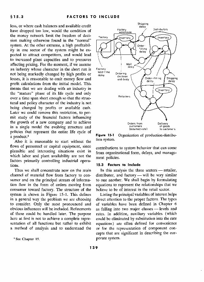
§ 15.3 3 FACTORS TO INCLUDE E
.. Shipping loss, or where cash balances and available credit deloy
have dropped too low, would the condition of wcire ouse /" Distributors the money network limit the freedom of deci-
Foctory Inventory Inventory sion making otherwise found in the "normal"
system. At the other extreme, a high profitabil- i ) (. Order- /
ity in one sector of the system might be ex- r/\ deloy v
g 7
pected to attract competitors, and would lead to increased plant capacities and to pressures \ / / / affecting pricing. For the moment, if we assume \ Mon ./ / / an industry whose character in the short run is Factory
delay / not being markedly changed by high profits or lead-time Ordering
/ deloy decision
losses, it is reasonable to omit money flow and and delay Order-filling Shipping - ' \ de!oy jt de)oy
profit calculations from the initial model. This \ deloy deloy
means that we are dealing with an industry in ) Inventory
the "mature" phase of its life cycle and only Retailers ÏJ i /
over a time span short enough so that the struc- Retailers \ /'
tural and policy character of the industry is not \ / being changed by profits or available cash. Later we could remove this restriction, to per- mit study of the financial factors influencing c the growth of a new company and to achieve orders from Delivery in a single model the evolving structure and customers of goods
c ° (assumed rote) to customers
policies a product.3 that represent the entire life cycle of
Figure 15-1 Organization of production-distribu-
Also it is reasonable to start without the han system.
OrganizaUon of producUon-distribu-
flows of personnel or capital equipment, since contributions to system behavior that can come plausible and interesting situations exist in from organizational form, delays, and manage- which labor and plant availability are not the ment policies.
"
factors primarily controlling industrial opera- tions. 15.3 Factors to Include
Thus we shall concentrate now on the main In this analysis the three sectors - retailer, channel of material flow from factory to con- distributor, and factory - will be very similar sumer and on the principal stream of informa- to one another. We shall begin by formulating tion flow in the form of orders moving from equations to represent the relationships that we
consumer toward factory. The structure of the believe to be of interest in the retail sector.
system is shown in Figure 15-1. This defines Listing the principal variables of interest helps in a general way the problem we are choosing direct attention to the proper factors. The types to consider. Only the most pronounced and of variables have been defined in Chapter 6
obvious influences will be included. Refinements as falling into two major classes - levels and of these could be handled later. The purpose rates. In addition, auxiliary variables (which here at first is not to achieve a complete repre- could be eliminated by substitution into the rate sentation of all functions but rather to exhibit equations) are often defined for convenience a method of analysis and to understand the or for the representation of component con-
cepts that are significant in describing the cor-
g See Chapter 19. porate system.
139
MODEL OF THE PRODUCTION-DISTRIBUTION SYSTEM
Levels represent those variables that measure fines of a book there is not enough space (it
quantities which would be countable if the sys- would also be unduly confusing) to attempt to tem were brought to rest. Levels include inven- trace all of the steps that were actually followed
tories, number of employees, unfilled orders, in evolving the present equations. We shall, stocks of capital equipment, bank balances, or- therefore, take advantage of advance knowledge ders in transit in communication channels, of the outcome and move directly to a listing of
goods in shipment, and unfilled requisitions for the principal variables. new employees. As we shall see later, certain For the retail sector, the levels that are cen- other variables, which might at first glance ap- tral to the distribution and sales task, and that
pear to be rates, are indeed levels. These in- exist in the orders, information, and materials clude smoothed or averaged rates. We speak of flow channels, appear to be the "average level of sales during the last year." e Backlog of orders received from the consumer It is in fact customary to use the word "level" but not yet filled in such a phrase. We shall find later that an Inventory of goods in stock k
sales rate of
similar Average??elin past, used in decid- average sales rate is of .. similar mathematical Average sales in the recent past, used in decid- form to that of the équations for levels. Further-
ing on the desired inventory and supply pipeline more, an average sales rate does not represent levels
e eSlre mven ory an supp y pIpe me
at any time an actual instantaneous flow of .. orders or goods. It is not an actual rate of flow Since money flow, personnel, and capital into or out of any reservoir. In general the "di- equipment are not yet being included (we as-
mensions" or "units of measure" of a variable sume their adequate availability so as not to
are not an adequate indicator of whether the restrict actions in the system), the related levels
quantity is a rate, a level, or an auxiliary vari- need not be listed.
able. Correspondingly, the major rates of flow that
Likewise, we should list all rates of flow that appear pertinent to the objectives cited earlier
we consider significant in the system. By impli- ?'ould be
cation this means that we are listing the impor- . Incoming-order flow from customers tant decisions, both implicit and overt, which . Outgoing-shipping rate to customers are being made. Décisions control the rates of . Outgoing-order rate from retailer to distributor flow, but in obtaining an initial description of . Incoming-shipping rate of goods from the dis- the system it is often more effective to think tributor in terms of the rates than in terms of the cor-
responding décisions. The principal delays in these rates of flow
In addition to levels and rates, we should ini- v'ill be taken as
tially list the important delays that we think a Delay in filling customers' orders at retail
may contribute to system behavior. Mathemati- . Delay in deciding on and preparing outgoing cally, the delays take the form of equations of orders from retailer to distributor levels and rates; but in terms of system struc- . Delay in transmission (mail) of orders from ture, we can proceed most rapidly by identifying retailer to distributor
separately the delays that are to be included.. Delay in shipping goods from distributor to In approaching an actual new situation, many retailer
months may be taken in tentative identification of the pertinent variables, in reducing some of 15.4 Basis for Developing Equations these to equation form, and in selecting the We can now develop equations describing factors that are to be included. Within the con- activity at the retail level. It should be stressed
140
§ 15.5.1 1 EQUATIONS FOR THE RETAIL SECTOR
that these equations are not "right" in any in- the reader can see why they were chosen. Al- trinsic or mathematical way. They merely de- though we believe that these represent the cen- scribe what we have chosen as the most sig- tral framework of the ordinary production- nificant relationships. The equations are akin distribution relationships, the purpose of this to a verbal description of the situation. They chapter is to show a method of system analysis. are correct if our perception of the system is If the reader understands the method, he can correct. They are wrong to the extent that we then substitute for himself his own choice of
wrongly interpret the organization which is principal factors affecting the way the system being described. operates.
We are not yet presuming to incorporate all For this example, we shall let a group of of the important factors. We do hope to select three capital letters represent each variable and the factors that are highest on the priority list parameter under study. In the retail sector the of effects within the specified boundaries of the third letter in each group will be an R. The third
system being studied. Our assumptions about letter D will identify variables at the distributor how the selected factors act on one another level. Likewise, F will identify variables at the should be plausible. They should be of interest factory level. to the investigator. They may represent his It seems best to develop the equations and estimate of the behavior of an existing system, the corresponding flow diagrams simultane- or they may represent the characteristics of a ously. In this chapter the first flow diagram will
proposed or hypothetical system whose be- be evolved in steps corresponding to the de- havior is to be explored. The assumptions im- velopment of the equations. To conserve space plied by the system formulation must be defend- later, flow diagrams will be given in their en- able in the view of the investigator. In general tirety, anticipating the equations that are to fol- the usefulness of the model depends on the low.4
reasonableness and pertinence of the individual
equations. The crucial importance of the valid- 15 5 System Equations
ity of the underlying assumptions, in the con- 15.5 System Equat)ons
text of model testing, has already been dis- 15.5.1 Equations for the Retail Sector. We cussed in Chapter 13. shall begin with two simple equations: one
Where conflicting assumptions about the true representing the level of unfilled orders and the nature of the system exist, the model itself can other the inventory of goods. Figure 15-2 shows be used to study the influence of alternative these two variables in the first step of our
assumptions. Often it will be found that the al- evolving flow diagram. Since IAR is an inventory ternatives lead to essentially the same results, of goods, solid lines representing flows of ma- and consequently the choice does not matter. terial come in and out. Since UOR is the level Some assumptions will be found to affect the of unfilled orders, circled lines enter and leave
system operation critically. After the high im- the rectangular box.
portance of a factor has been demonstrated, The following equation for UOR is of the then is the time to attempt detailed measure- standard type for defining a simple level into ments in a real organization. In this way costly which flows a single input rate and from which data collection and data analysis can be con- flows a single output rate:5 5
centrated where the results will be most useful. In this chapter the particular choice of factors ' The symbols used in the flow diagrams are as
from among the many that exist in real life given in Chapter 8. ..
?ÎY àÉÀ/?lf?level equations has been discussed
will be defended o only to suc an extent that in Chapter 7. of level équations has been dlscussed
141 1
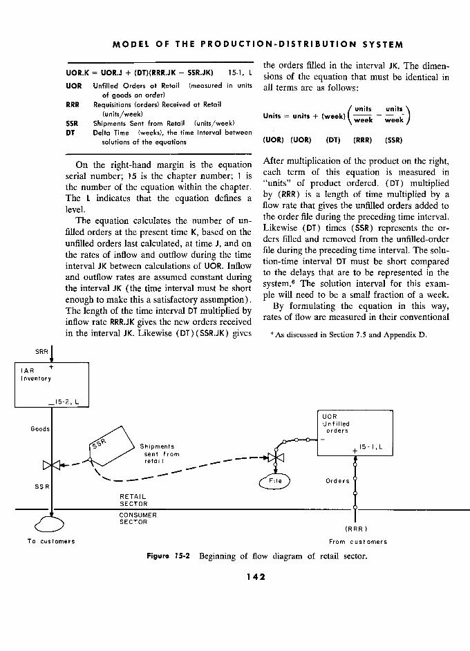
MODEL OF THE PRODUCTION-DISTRIBUTION SYSTEM
UOR.K the orders filled in the interval JK. The dimen-
UOR.K = UOR.J + (DT)(RRR.JK - SSRJK) 15-L L sions of the equation that must be identical in UOR Unfilled Orders at Retail (measured in units all terms are as follows:
of goods on order) RRR Réquisitions (orders) Received at Retail units units \
(units / week) Units = units + (week) units - un)ts \
SSR (unitsjweek) from Retail (units/week) units = units +
(week) week SSR Shipments Sent from Retail (units/week) mts = umts +
\ / DT Delta Time (weeks), the time interval between '
solutions of the equations (UOR) (UOR) (DT) (RRR) (SSR)
On the right-hand margin is the equation After multiplication of the product on the right,
serial number; 15 is the chapter number; 1 is each term of this equation is measured in
the number of the equation within the chapter. "units" of product ordered. (DT) multiplied
The L indicates that the equation defines a by (RRR) is a length of time multiplied by a
level. flow rate that gives the unfilled orders added to
The equation calculâtes the number of un- the order file during the preceding time interval.
filled orders at the present time K, based on the Likewise (DT) times (SSR) represents the or-
unfilled orders last calculated, at time J, and on ders filled and removed from the unfilled-order
thé rates of inflow and outflow during thé time file during the preceding time interval. The solu-
interval JK between calculations of UOR. Inflow tion-time interval DT must be short compared
. interval JK rates are assumed constant during to the
delays that
are to be
represented in the and outflow rates are assumed constant
during system.6 solution interval for this in thé the interval JK (the time interval must be short
sys em. solution m erva or this exam- enough to make this a satisfactory assumption).
ple will need to be a small
fraction of
a week.
The length of the time interval DT multiplied by y formulating the équation in this way,
inflow rate RRR.JK gives the new orders received rates of flow are measured .. g
inflow rate RRR.JK gives thé new orders received in the interval JK. Likewise (DT) (SSR.JK) gives 0 As discussed in Section 7.5 and Appendix D.
SRR IAR R +
Inventory
15-2, L
UOR R Unfilled
Goods orders s
Shipments s L sent from _ + '
- -- retai i 1 --- --- -- -- -
. \.
'- -- --
File Orders SSR R )
RETAIL L T ______ SECTOR
CONSUMER j SECTOR (RPR) ' (R R R )
To customers s From customers s
Figure 15-2 Beginning of flow diagram of retail sector.
142
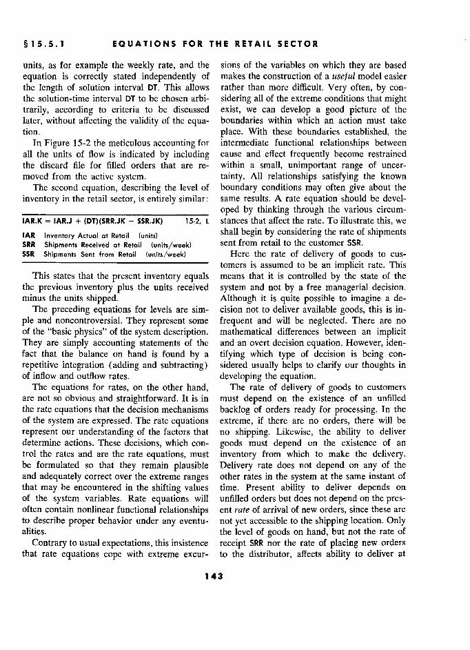
§ 15.5.1 1 EQUATIONS FOR THE RETAIL SECTOR
units, as for example the weekly rate, and the sions of the variables on which they are based
equation is correctly stated independently of makes the construction of a useful model easier the length of solution interval DT. This allows rather than more difficult. Very often, by con- the solution-time interval DT to be chosen arbi- sidering all of the extreme conditions that might trarily, according to criteria to be discussed exist, we can develop a good picture of the
later, without affecting the validity of the equa- boundaries within which an action must take tion. place. With these boundaries established, the
In Figure 15-2 the meticulous accounting for intermediate functional relationships between all the units of flow is indicated by including cause and effect frequently become restrained the discard file for filled orders that are re- within a small, unimportant range of uncer- moved from the active system. tainty. All relationships satisfying the known
The second equation, describing the level of boundary conditions may often give about the
inventory in the retail sector, is entirely similar: same results. A rate equation should be devel-
____________________________ oped by thinking through the various circum- IAR.K = IAR.J + (DT)(SRR.JK - SSR.JK) 15-2, L stances that affect the rate. To illustrate this, we
IAR Inventory Actual ot Retail (units) shall begin by considering the rate of shipments SRR Shipments Received at Retail (units/week) sent from retail to the customer SSR. SSR Shipments Sent from Retail (units/week) Here the rate of delivery of goods to cus- –––––––––––––––––––––––––––– tomers is assumed to be an implicit rate. This
This states that the present inventory equals means that it is controlled by the state of the the previous inventory plus the units received system and not by a free managerial decision. minus the units shipped. Although it is quite possible to imagine a de-
The preceding equations for levels are sim- cision not to deliver available goods, this is in-
ple and noncontroversial. They represent some frequent and will be neglected. There are no of the "basic physics" of the system description. mathematical differences between an implicit They are simply accounting statements of the and an overt decision equation. However, iden- fact that the balance on hand is found by a tifying which type of decision is being con-
repetitive integration (adding and subtracting) sidered usually helps to clarify our thoughts in of inflow and outflow rates. developing the equation.
The equations for rates, on the other hand, The rate of delivery of goods to customers are not so obvious and straightforward. It is in must depend on the existence of an unfilled the rate equations that the decision mechanisms backlog of orders ready for processing. In the of the system are expressed. The rate equations extreme, if there are no orders, there will be
represent our understanding of the factors that no shipping. Likewise, the ability to deliver determine actions. These decisions, which con- goods must depend on the existence of an trol the rates and are the rate equations, must inventory from which to make the delivery. be formulated so that they remain plausible Delivery rate does not depend on any of the and adequately correct over the extreme ranges other rates in the system at the same instant of that may be encountered in the shifting values time. Present ability to deliver depends on of the system variables. Rate equations will unfilled orders but does not depend on the pres- often contain nonlinear functional relationships ent rate of arrival of new orders, since these are to describe proper behavior under any eventu- not yet accessible to the shipping location. Only alities. the level of goods on hand, but not the rate of
Contrary to usual expectations, this insistence receipt SRR nor the rate of placing new orders that rate equations cope with extreme excur- to the distributor, affects ability to deliver at
143 3
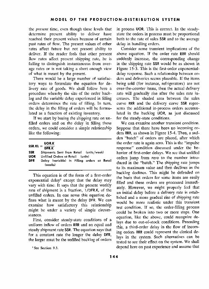
MODEL OF THE PRODUCTION-DISTRIBUTION SYSTEM
the present time, even though these levels that in process UOR. This is correct. In the steady- determine present ability to deliver have state the orders in process must be proportional reached their present values because of certain both to the rate of sales SSR and to the average past rates of flow. The present values of other delay in handling orders. rates affect future but not present ability to Consider some transient implications of the deliver. If the reader feels that other present above equation. If the order rate RRR should flow rates affect present shipping rate, he is suddenly increase, the corresponding change failing to distinguish instantaneous from aver- in the shipping rate SSR would be as shown in
age rates or is not taking a short enough view Figure 15-3. This is the first-order exponential- of what is meant by the present. delay response. Such a relationship between or-
There would be a large number of satisfac- ders and deliveries seems plausible. If the items
tory ways to formulate the equation for de- being sold (for instance, refrigerators) are not
livery rate of goods. We shall follow here a over-the-counter items, then the actual delivery procedure whereby the size of the order back- rate will gradually rise after the sales rate in-
log and the variable delay experienced in filling creases. The shaded area between the sales orders determines the rate of filling. In turn, curve RRR and the delivery curve SSR repre- the delay in the filling of orders will be formu- sents the additional in-process orders accumu- lated as a function of existing inventory. lated in the backlog UOR, as just discussed
If we start by basing the shipping rate on un- for the steady-state conditions. filled orders and on the delay in filling those We can examine another transient condition.
orders, we could consider a simple relationship Suppose that there have been no incoming or- like the following: ders RRR, as shown in Figure 15-4. Then, a sud- –––––––––––––––––––––––––– den "batch" of orders are placed, after which
SSR.KL UOR.K the order rate is again zero. This is the "impulse SSR.KL = pFR.K response" condition discussed under the be-
SSR Shipments Sent from Retail (units/week) havior of first-order delays. We see that unfilled UOR Unfilled Orders at Retail (units) orders jump from zero to the number intro- DFR Delay (variable) in Filling orders at
Retail " i- " - DFR in Filling orders at Retail
duced m the batch. The shipping rate jumps
(weeks) to its maximum value and then declines as the
backlog declines. This might be defended on This équation is of thé orm o a
exponential delay7 except that the delay may the basis that orders for some items are easily
exponential delay7 except that the delay may vary with time. It says that the present weekly filled and these orders are processed immedi- - rate of shipment is a fraction, 1/DFR.K, of the
ately. However, we might properly feel that an initial delay before a delivery rate is es - unfilled orders. In one sense this équation de-
an initial delay before a delivery rate is estab- e fines what is meant by the delay DFR. We can lished and
a more gradual rise of shipping rate
examine how satisfactory this relationship realistic under this transient
test condition. If so, thé or er- mg process might be under a variety of simple circum- test condition. If so, the order-filling process e stances.
r could be broken into two or more steps. One
stances.. like thé above, could recognize de- of a equation, like the above, could recognize de-
uniform inflow of orders RRR and an equal and a
lays due to out-of-stock conditions. Preceding uniform innow of orders RPR and an equal and uniform shipment rate SSR. The equation equal and this, a third-order delay in thé fiow of incom- steady shlpment rate SSR. The equation says that
lllg or d ers RRR could represent the e c 1. enca for a constant rate the longer the delay DFR, 1 ays be the larger must be the unfilled backlog of orders Such alternatives can ° ° tested to see their effect on the system. We shall
7 s Section 9.3. depend here on past experience and assume that
144
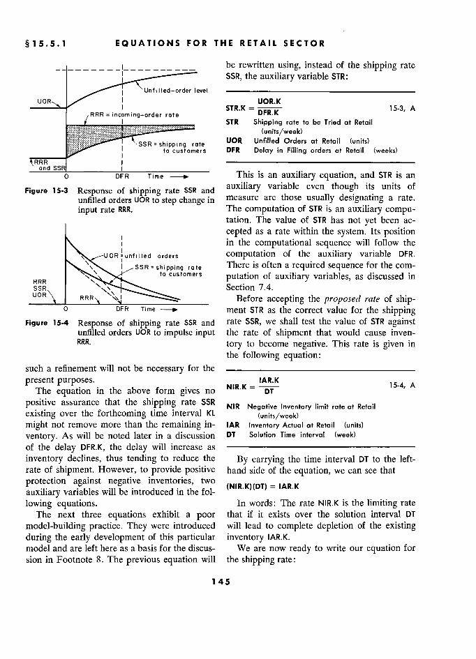
1 EQUATIONS FOR THE RETAII SECTOR
- - - - - - - - L - - - - - - - - - be rewritten using, instead of the shipping rate
SSR, the auxiliary variable STR:
'Unfilled-order level –––––––––––––––––––––––––––––––––––––
uoR I
UOR.K
? RRR = incoming-order rate
STR.K DFR.K 15-3, A
STR Shipping rate to be Tried at Retail
(units/week)
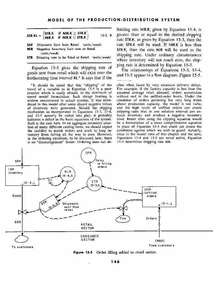
MODEL OF THE PRODUCTION-DISTRIBUTION SYSTEM
limiting rate NIR.K, given by Equation 15-4, is
SSR.KL = if ''
15-5, R greater than or equal to the desired shipping if NIR.K < STR. jK rate STR.K, as given by Equation 15-3, then the e SSR Shipments Sent from Retail (units/week) rate STR.K will be used. If NIR.K is less than NIR Négative Inventory limit rate at Retail STR.K, then the rate NIR will be used as the
(units/week) shipping rate. Under ordinary circumstances STR Shipping rate to be Tried at Retait (units/week) where inventory Under not reach circumstances
Ipplng rate te e ne at etal Unlts wee where inventory will not reach zéro, the ship-
ping rate is determined by Equation 15-3. Equation 15-5 gives the shipping rate of ping
Equation 15-3.
goods sent from retail which will exist over the The relationships of Equations 15-3, 15-4,
? ... ? ? ? ? . ? ? and 15-5 appear in a fiow diagram, Figure 15-5.
Orthcommg time mterva KL.s It says that if thé e 6 ' 6
8 It should be noted that this "clipping" of the cline when faced by very excessive delivery delays. travel of a variable as in Equation 15-5 is a poor For example, if the factory capacity is less than the practice which is easily abused, to the detriment of assumed average retail demand, orders accumulate sound model formulation. Such abrupt limiting is without end in the unfilled-order levels. Under the seldom encountered in actual systems. It was intro- condition of orders persisting for very long times duced in this model after some absurd negative values above production capacity, the model is not valid, of inventory were generated. Should the clipping and the high levels of unfilled orders can create mechanism as incorporated in Equations 15-3, 15-4, shipping rates that in one solution interval can ex- and 15-5 actually be called into play, it probably haust inventory and produce a negative inventory indicates a defect in the basic equations of the system. level. Better than using the clipping equation would Such is the case here. In an aggregate inventory situa- be a formulation of a more comprehensive equation tion of many different catalog items, we should expect in place of Equation 15-3 that could not create the the inability to match orders and stock to keep in- conditions against which we wish to guard. Actually, ventory from falling all the way to zero. However, since in the model runs of this chapter and the next, in the ordering equations, to be discussed later, there Equations 15-4 and 15-5 are never active, Equation is no "discouragement" factor. Ordering does not de- 15-3 determines shipping rate SSR.
DFR
SRR Delay 11 irig
N ' R orders
!AR ' \ orders
1 nventory
+ NIR
\
in9
STR i
-
15-4,A 15- 2, L STR
/ ––––––––––––––! /
/ "..... -––. ----
UOR Unfilled
Goods orders Goods
s rf ,t5-!.L L 1 sent from - re toi 1
-- "?
Orders 1 Y ' - - - - ' File Orders
SSR i RETAIL V SECTOR _____________1____________________
CONSUMER ! SECTOR (RRR)
To customers From customers
Figure 15-5 Order filling added to retail sector.
. , 146
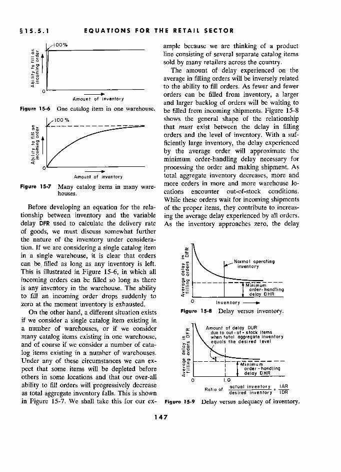
§15.5.1 1 EQUATIONS FOR THE E R E T A 1 SECTOR
ample because we are thinking of a product
f
line consisting of several separate catalog items sold by many retailers across the country.
:ê The amount of delay experienced on the
g average in filling orders will be inversely related
___________________ to the ability to fill orders. As fewer and fewer o - orders can be filled from inventory, a larger Amount ot invenrory
and larger backlog of orders will be waiting to Figure 15-6 One catalog item in one warehouse. be filled from incoming shipments. Figure 15-8
loo io shows the general shape of the relationship that must exist between the delay in filling g orders and the level of inventory. With a suf-
t ficiently large inventory, the delay experienced 1 by the average order will approximate the
minimum order-handling delay necessary for
o processing the order and making shipment. As
Amount of inventory total aggregate inventory decreases, more and
Figure 15 - 7 Many ca t a 1 og items m many ware- more orders in more and more warehouse 10- Ftgure t5-7
houses. catalog items m many ware-
cations encounter out-of-stock conditions.
While these orders wait for incoming shipments Before developing an equation for the rela- of the proper items, they contribute to increas-
tionship between inventory and the variable ing the average delay experienced by ail orders.
delay DFR used to calculate the delivery rate As the inventory approaches zero, the delay of goods, we must discuss somewhat further the nature of the inventory under considera- tion. If we are considering a single catalog item a: \ in a single warehouse, it is clear that orders \ can be. filled as long as any inventory is left. cg Normol operating This is illustrated in Figure 15-6, in which ail
incoming orders can be filled so long as there _______ is any inventory in the warehouse. The ability d- ?o?d'?r'-T)and)!nç to fill an incoming order drops suddenly to delay DHR
zero at the moment inventory is exhausted. ° Inventory y ––
On the other hand, a différent situation exists Figure 1 5-8 Delay versus inventory. if we consider a single catalog item existing in a number of warehouses, or if we consider \ Amount of delay DUR , u- \ dueto out-of-stock (tems many catalog items existing in one Warehouse, jà \ when total aggregate inventory and of course if we consider a number of cata- ô
M equals the desired level
log items existing in a number of warehouses. ë Under any of these circumstances we can ex- *' )tfv))n)mum pect that some items will be depleted before ' order others in some locations and that our over-all "
ability to fill orders will progressively decrease actual inventory IAR as total aggregate inventory falls. This is shown
Ratio ° ° desired inventor = IDR
in Figure 15-7. We shall take this for our ex- Figure 15-9 Delay versus adequacy of inventory.
147
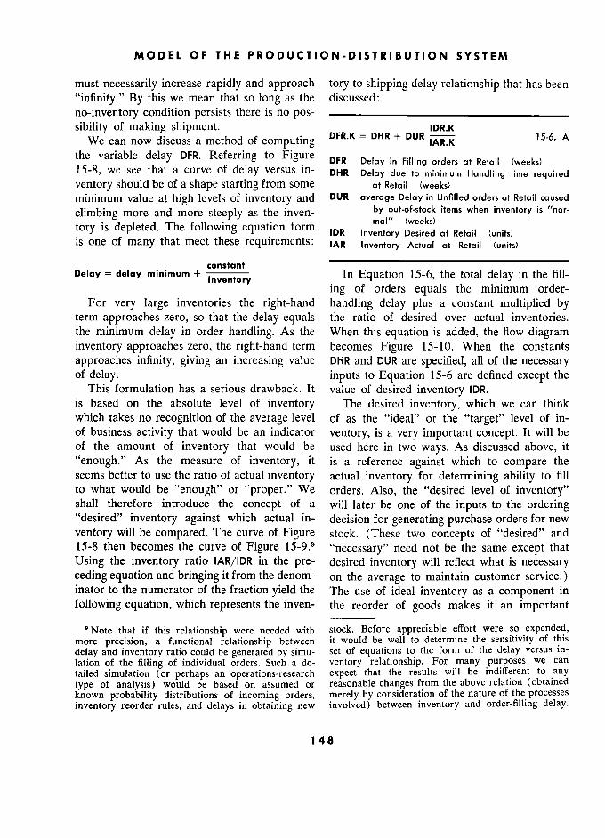
MODEL OF THE PRODUCTION-DISTRIBUTION SYSTEM
must necessarily increase rapidly and approach tory to shipping delay relationship that has been
"infinity." By this we mean that so long as the discussed:
no-inventory condition persists there is no pos- –––________________________
sibility of making shipment. DFR.K = DHR + IDR.K 15-6, A We can now discuss a method of computing DFR.K = DHR + DUR IAR.K 15-6, A
the variable delay DFR. Referring to Figure pFR Delay in Filling orders ar Retail .1 (weeks) s 15-8, we see that a curve of delay versus in- DHR Delay due to minimum Handling time required ventory should be of a shape starting from some at Retail (weeks) minimum value at high levels of inventory and DUR average Delay in Unfilled orders at Retail caused
climbing more and more steeply as the inven- by out-of-stock items when inventory is "nor- climbing more and more steeply as the inven-
bY (weeks) i?ems When invent°rY 15 "n°r-
tory d 1 d The following equation form mal" (weeks)
tory is depleted. The following equation form IDR Inventory Desired ar Retail .1 (units) S is one of many that meet thèse requirements: IAR Invenrory Actual at Retail (units)
constant Delay = delay minimum +
inventory In Equation 15-6, the total delay in the fill-
ing of orders equals the minimum order- For very large inventories the right-hand handling delay plus a constant multiplied by
term approaches zero, so that the delay equals the ratio of desired over actual inventories. the minimum delay in order handling. As the When this equation is added, the flow diagram inventory approaches zero, the right-hand term becomes Figure 15-10. When the constants
approaches infinity, giving an increasing value DHR and DUR are specified, all of the necessary of delay. inputs to Equation 15-6 are defined except the
This formulation has a serious drawback. It value of desired inventory IDR. is based on the absolute level of inventory The desired inventory, which we can think which takes no recognition of the average level of as the "ideal" or the "target" level of in- of business activity that would be an indicator ventory, is a very important concept. It will be of the amount of inventory that would be used here in two ways. As discussed above, it
"enough." As the measure of inventory, it is a reference against which to compare the seems better to use the ratio of actual inventory actual inventory for determining ability to fill to what would be "enough" or "proper." We orders. Also, the "desired level of inventory" shall therefore introduce the concept of a will later be one of the inputs to the ordering "desired" inventory against which actual in- decision for generating purchase orders for new
ventory will be compared. The curve of Figure stock. (These two concepts of "desired" and 15-8 then becomes the curve of Figure 15-9.9 "necessary" need not be the same except that
Using the inventory ratio IAR/IDR in the pre- desired inventory will reflect what is necessary ceding equation and bringing it from the denom- on the average to maintain customer service. ) inator to the numerator of the fraction yield the The use of ideal inventory as a component in
following equation, which represents the inven- the reorder of goods makes it an important
"Note that if this relationship were needed with stock. Before appreciable effort were so expended, more precision, a functional relationship between it would be well to determine the sensitivity of this
delay and inventory ratio could be generated by simu- set of equations to the form of the delay versus in- lation of the filling of individual orders. Such a de- ventory relationship. For many purposes we can tailed simulation (or perhaps an operations-research expect that the results will be indiffèrent to any type of analysis) would be based on assumed or reasonable changes from the above relation (obtained known probability distributions of incoming orders, merely by consideration of the nature of the processes inventory reorder rules, and delays in obtaining new involved) between inventory and order-filling delay.
148
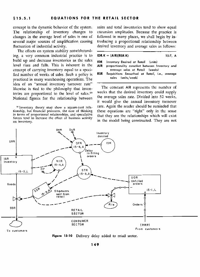
§ 15.5.1 1 EQUATIONS FOR THE RETAIL SECTOR
concept in the dynamic behavior of the system. sales and total inventories tend to show equal The relationship of inventory changes to excursion amplitudes. Because the practice is
changes in the average level of sales is one of followed in many places, we shall begin by in- several major sources of amplification causing troducing a proportional relationship between fluctuation of industrial activity. desired inventory and average sales as follows:
The effects on system stability notwithstand- ––––––––––––––––––––––––––––
ing, a very common industrial practice is to IDR.K = (AIR)(RSR.K) 15-7, A
build up and decrease inventories as the sales IDR Invenrory Desired at Retail (units) level rises and falls. This is inherent in the AIR proportionality constAnt between Inventory and
concept of carrying inventory equal to a speci- average sales at Retail (weeks)
fied number of weeks of sales. Such a policy is RSR Réquisitions Smoothed at Retail, i.e., average
practiced in many warehousing operations. The e sales (units/week)
idea of an "annual inventory turnover rate" likewise is tied to the philosophy that inven- The constant AIR represents the number of
tories are proportional to the level of sales.10 weeks that the desired inventory could supply
National figures for the relationship between the average sales rate. Divided into 52 weeks, it would give the annual inventory turnover
'" Inventory theory may show a square-root rela- rate. Again the reader should be reminded that
tionship, but financial pressures, the ease of thinking these equations are "right" only in the sense in terms of proportional relationships and spéculative that they are the relationships which will exist forces tend to increase thé effect of business actIvlty .
h d 1 b . d on forces inventory. tend to increase the effect of business activity in the model being constructed. They are not
DHR DUR Inventory
\ \ desired '
DFR IDR SRR
_ , 15-6, A - Delay ./
IAR ' N ' R
in filling \ orders
IAR \ \ orders
Invenrory N I R inventory 1 ! \
Inventory 15-2,L DT STR -15-2,L ---- / -- UOR / UOR
/ Unfilled Goods orders Goods
S hipments rr -
L "J.
sent from -- +
retail 1 -- ---
File Orders Y SSR ) RETAIL 0 SECTOR ) ______
CONSUMER ! SECTOR R ( R R R )
To customers From customers
Figure 15-10 Delivery delay added to retail sector.
149
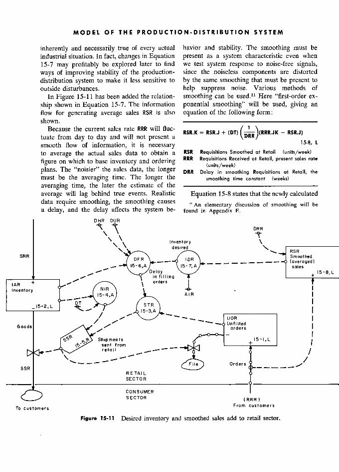
MODEL OF THE PRODUCTION-DISTRIBUTION SYSTEM
inherently and necessarily true of every actual havior and stability. The smoothing must be
industrial situation. In fact, changes in Equation present as a system characteristic even when
15-7 may profitably be explored later to find we test system response to noise-free signals,
ways of improving stability of the production- since the noiseless components are distorted
distribution system to make it less sensitive to by the same smoothing that must be present to
outside disturbances. help suppress noise. Various methods of
In Figure 1 S-11 bas been added the relation- smoothing can be used.11 Here "first-order ex-
ship shown in Equation 15-7. The information ponential smoothing" will be used, giving an
flow for generating average sales RSR is aiso equation of the following form: shown. ––––––––––––––––––––––––––
Because the current sales rate RRR will Hue- (DT) f––\RRRJK - RSR.J)
tuate from day to day and will not present a DRR) tuate from day to day and will not présent a ' '
DRR ' '
smooth flow of information, it is necessary L
to average the actual sales data to obtain a RSR Réquisitions Smoothed at Retail (units/week)
figure on which to base inventory and ordering RRR Réquisitions Received at Retail, présent sales rate
)ans. .....„, . data the lon er (units/week) plans. The noisier the sales data, the longer DRR Delay in smoothing Réquisitions at Retail, the must be the averaging time. The longer the smoothing time constant (weeks)
'
averaging time, the later the estimate of the ––––––––––––––––––––––––––
average will lag behind true events. Realistic Equation 15-8 states that the newlycalculated data require smoothing, the smoothing causes 11 An elementary discussion of smoothing will be a delay, and the delay affects the system be- found in Appendix E.
DHR DUR
DRR
', "' 1 ' Inventory \
\ desired RSR RSR
SRR \ / Smoothed SR R
_ - sales !5-8,L
_______]_______ / i De^ fyl ling n q t + 15-8, L
IAR + i \ orders I
R ' Inventory NIR , !nventory
.5-2.L
! \ AIR R
–-'" ' STR ) / / - _
.. '**'–-(.Unf!)!ed UOR Goods '//
/ ? ? Unfilled UOR Goods orders (
Shipments L . i
from ––––––t–––––– retail /
SSR
_ - - ' File Orders - - -
/
RETAIL L o SECTOR )
CONSUMER ! SECTOR R (RRR)
To customers From customers
Figure 15-11 l Desired inventory and smoothed sales add to retail sector.
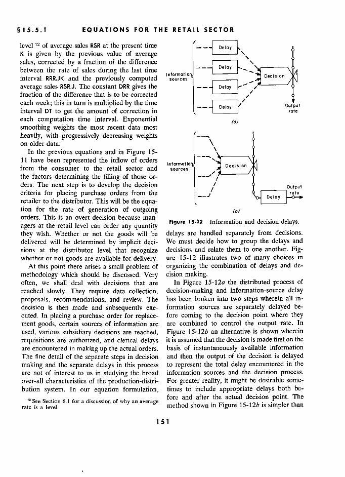
§ 15.5.1 1 EQUATIONS FOR THE RETAIL SECTOR
level l of average sales RSR at the present time - -1 Delay i K is given by the previous value of average j[ sales, corrected by a fraction of the difference \ ) between the rate of sales during the last time
Information - Decision interval RRR.JK and the previously computed sources _____.
average sales RSR.J. The constant DRR gives the y fraction of the difference that is to be corrected i A each week; this in turn is multiplied by the time
-- -1 Delay r/ 1
interval DT to get the amount of correction in rate
each computation time interval. Exponential smoothing weights the most recent data most
heavily, with progressively decreasing weights - 1 on older data. \
In the previous equations and in Figure 15- _ \_____ ) 11 have been represented the inflow of orders Informcitio from the consumer to the retail sector and sources Decision /1\t the factors determining the filling of those or- 1 v
ders. The next step is to develop the decision 1 y Output criteria for placing purchase orders from the
Delay rate retailer to the distributor. This will be the equa- tion for the rate of generation of outgoing orders. This is an overt decision because man-
p;9ure 15-12 Information and decision delays. agers at the retail level can order any quantity y
Figure 15-12 Information and decision delays.
they wish. Whether or not the goods will be delays are handled separately from decisions.
delivered will be determined by implicit deci- We must decide how to group the delays and
sions at the distributor level that recognize decisions and relate them to one another. Fig- whether or not goods are available for delivery. ure 15-12 illustrates two of many choices in
At this point there arises a small problem of organizing the combination of delays and de-
methodology which should be discussed. Very cision making. often, we shall deal with decisions that are In Figure 15-12a the distributed process of
reached slowly. They require data collection, decision-making and information-source delay
proposals, recommendations, and review. The has been broken into two steps wherein all in-
decision is then made and subsequently exe- formation sources are separately delayed be-
cuted. In placing a purchase order for replace- fore coming to the decision point where they ment goods, certain sources of information are are combined to control the output rate. In
used, various subsidiary decisions are reached, Figure 15-12b an alternative is shown wherein
requisitions are authorized, and clerical delays it is assumed that the decision is made first on the
are encountered in making up the actual orders. basis of instantaneously available information
The fine detail of the separate steps in decision and then the output of the decision is delayed
making and the separate delays in this process to represent the total delay encountered in the
are not of interest to us in studying the broad information sources and the decision process. over-all characteristics of the production-distri- For greater reality, it might be desirable some-
bution system. In our equation formulation, times to include appropriate delays both be-
12 See Section 6.1 for a discussion of why an average fore and after the actual decision point. The
rate is a level. 6. 1 for a discussion of why an average method shown in Figure 15-12b is simpler than
151 1
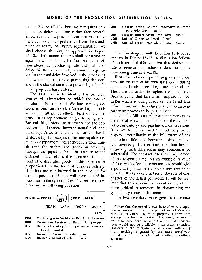
MODEL OF THE PRODUCTION-DISTRIBUTION SYSTEM
that in Figure 15-12a, because it requires only LDR pipeline orders Desired (necessary) in transit
one set of delay equations rather than several. LAR
pipeline orders Actual (units)
Retail (units) for the purposes of our present study, UOR Unfilled orders at Retail (units)
(units)
', P Y' UOR Unfilied Orders ai Retail (units) there is no obvious preference from the stand- UNR Unfilled orders, Normal, at Retail (units)
point of reality of system representation, we
shall choose the simpler approach in Figure The flow diagram with Equation 15-9 added 15-12b. This means that we shall construct an
appears
e
in Figure 15-13. A discussion follows
e
equation which defines the "impending" deci- of each term of this equation that defines the
sion about the purchasing rate and shall then rate of generating purchase orders during the e
delay this tllllelly Î?1lollÎir??ÎΧ/ÎÎ/lr?? forecoming time interval KL.
lent to the total delay involved in the processing First, the retailer's purchasing rate will de-
of raw data, in making a purchasing decision, pend on the rate of his own sales RRR,13 during and in the clerical steps of a purchasing office in the immediately preceding time interval JK.
making up purchase orders. . . , These are the orders to replace the goods sold.
The first task is to identify y the e principal Bear in mind that this is an "impending" ,,
de- sources of information on which the rate of
cision which is being made on the latest true purchasing is to depend. We have already de-
information, with the delays of the information- cided to omit any explicit forecasting methods
s gathering process ta be put in later.
as well as all minor effects. irst on the prl7 The delay DIR is a time constant representing
ority list is replacement of goods being sold. the rate at which the retailers, on the average,
Beyond this, orders are necessary for the cor-
act on inventory- and pipeline-deficit situations. rection of differences between actual and ideal
is not ta be assumed that retailers would in one manner or another it
It is not o e assumed that retailers would
inventory. Also, in one manner or another it respond immediately to the full extent of any
is necessary to recognize the mescapable de- theoretical difference between desired and ac-
mands of pipeline filling. If there in traveling tual inventory. Furthermore, the time lags in
si time for orders and goods s m travehng observing such differences may sometimes be
through the pipeline from the retailer to the e substantial. The constant DIR allows adjustment distributor and return, it is necessary that the of this response time. As an example, a value
total of orders plus goods in this pipeline be of four weeks for the constant DIR would give
proportional to the )evel in business activity. a purchasing rate that corrects any remaining
If orders are not mserted in the out of for deficit in the term in brackets at the rate of one-
ventories in the system. These corne out of
in- quarter of the deficit per week. It will be seen
ventories in the system. These factors
are recog- later that this response constant is one of the e nized in the foIlowing equation: more critical parameters in determining the
system's dynamic performance. PDR.KL = RRR.JK
[The two inventory terms give the difference PDR.KL = RRR.JK +
DIR (IDR.K - IAR.K)
+ (LDR.K - LAR.K) + (UOR.K - UNR.K) ]
13 Note that the use of a rate in another rate equa- +.. tion is contrary to the principles of model structure
15-9, R discussed in Chapter 6. More properly, a short-term
PDR Purchosing rate Decision at Retail (units/week) average rate for the previous day, week, or month
RRR Requisitions Received at Retail (units/week) rates be used here, since in fact the instantaneous
DIR Delay iri Inventory (and pipeline) adjustment at rates would not be available in an actual situation. DIR
Delay in Inventory at
However, as the averaging period becomes sufficiently Retail (weeks) short, nothing is gained by the extra complexity IDR lnventory Desired at Retail (units) caused by the introduction of another smoothing
IAR Inventory Actual at Retail (units) equation.
152
§ 15.5.1 1 EQUATIONS FOR THE RETAIL SECTOR
between desired and actual inventory. If the level of average sales, in the same manner as level of desired inventory is above or below desired inventory. Actually, it may be doubtful actual inventory, a correcting component will that many retail organizations consciously rec- be introduced into the ordering rate. ognize the orders for pipeline filling as part of
The two pipeline terms act like the inventory their ordering procedure. If they do not, the terms. The desired level of orders in the pipe- orders necessary to maintain the required de- line will be defined later as proportional to the livery rate of goods will automatically come out
D 1 R Q Order Q \0rder A ' Or de, PDR decision PDR
( LDR _
_ - - /
i 15- 9, R
- i
Pipeline ) /?P?.ne
/ OHR i U N R
/
, , \ '
WO, desired / DHR ' ' \
'°"""'
Goods
DUR R UNR / / ' t '
content
DUR
/ DRR t DRR
/ / / \
\ \
T
\ \ !nventory /
/ /
t
'
\ DRR 1? . " Inventory
"Î R S R < SRR I 1
,' ' <
15-6, A Delay in filling \
sales + 15-8,L
nventory AR + i orders
\ \ '
nventory T t -è- \ \, ) nventory ? ?
_ + 1 5- 2 ,
AIR
1
\
j
..5-2. L –––!––––
* / _ \
„' / , / UOR \ I j
Goods ? Untilled j Goods - orders 1s '
??Shipments c! L . j senT fram + /
retail 1 / /
' Fi le Ord er s --
/ /
File Orders / SSR -- - -
RETAIL L SECTOR )
CONSUMER E R ) SECTOR R (RRR)
To customers From customers
Figure 15-13 Purchasing decision added to retail sector.
153
MODEL OF THE PRODUCTION-DISTRIBUTION SYSTEM
of their own inventories, and at that time the term LAR, so that the backlog of unfilled orders
attempts to readjust inventory will lead to the is retained at the distributor.
necessary extra orders. The delay time constant The term for unfilled orders normally held DIR allows for varying degrees of intentional at the retail level UNR is included so that under or unintentional delay in making the adjust- steady-state conditions the actual inventory at ments. the retailer will run equal to the desired inven-
The term in the ordering equation for un- tory. Under normal steady-state conditions the filled orders at the retail level UOR is inserted two pipeline terms will cancel one another and as part of the general attempt to make sure we should expect the two inventory terms to that the equations behave reasonably under cancel one another. However, if the unfilled- extreme conditions of operation. In a situation order term UOR were present without the can- where there is no supply of goods coming from celing normal level of unfilled orders UNR, the the factory, and where the backlog of unfilled inventory terms would differ from one another orders at retail is so great as to discourage by enough to equal the unfilled-order term UOR. further incoming customer orders, we find that While proper values of various inventory con- the retail ordering rate RRR is zero. Under stants could be selected to make the actual in- these circumstances the actual inventory would ventory reach the desired amount, it would be fall to zero. According to Equations 15-7 and confusing and contrary to our implied mean- 15-8, the desired level of inventory under these ing of "desired inventory" if actual inventory circumstances would also fall to zero. This did not attempt to equal desired inventory might not appear plausible at first, but under under steady-state operating conditions. the circumstances of no incoming orders and Transient interaction between the inventory, no supply and a backlog of unfilled orders it pipeline, and unfilled-order terms is important. is both unlikely and unnecessary to have an in- Suppose that a deficit exists in actual inventory ventory in stock. Under these circumstances it IAR compared with desired inventory IDR. This will be essential that unfilled orders held at the will cause an ordering rate that places orders retail level be reflected in unfilled orders held in process in the pipeline term LAR. When suf- at the distributor level. Otherwise, there will be ficient orders have been initiated to meet in- no orders on hand at higher points in the system ventory needs, the additional orders in the nega- to reinitiate a flow of goods when a supply be- tive LAR term will cause the total value inside comes available. As we shall see later, the actual the bracket in Equation 15-9 to fall to zero. As
pipeline orders LAR include the backlog of un- the goods ordered for inventory are delivered, filled orders at the distributor level. However, if they will transfer from orders in the pipline LAR the unfilled-order term UOR is not included in to inventory IAR, so that the ordering equa- Equation 15-9, we see that unfilled orders at tion continues in balance. The equation thereby the distributor level will be canceled until they avoids duplicate reordering of inventory in suc- cease to exist. This will happen because all ceeding time periods before the goods are de- other terms in the equation can fall to zero when livered. no supply is available. Then, the negative term We can view in another way the terms in the for pipeline content LAR (which contains only bracket of Equation 15-9 as representing the the backlog of unfilled orders at the distributor "stock-commitment gap." By regrouping, under these circumstances) will lead to a nega- (IDR.K + LDR.K + UOR.K) would represent the tive ordering rate until the backlog is canceled "desired ownership" by the retailer-d?sired in- at the distributor. The positive term UOR bal- ventory plus necessary goods in transit in the ances, under the circumstances, the negative supply line plus product to fill the orders on
154
§15.5.1 1 EQUATIONS FOR THE RETAIL SECTOR
hand. Against this will be offset a negative term filling orders at the distributor DFD depends on
(IAR.K + LAR.K + UNR.K) representing the the availability of inventory at the distributor, commitments that do not need filling-the in- from which orders can be filled. It is therefore
ventory now present plus the goods now in the a variable delay, as it is at retail.
pipeline plus the unfilled orders that are con- The actual content of the supply pipeline sidered normal. consists of the sum of the orders and the goods
Equation 15-9 for purchasing rate depends in the various separate pieces of the supply on values of several variables that have not yet line as follows : been defined. One of these is the desired or –––––––––––––––––––––––––––
necessary level of orders and goods in transit LAR.K = CPR.K + PMR.K + UOD.K + MTR.K
in the supply pipeline from the retailer to the 15-11, A
distributor and return. The necessary orders LAR pipeline orders Actually in transit to Retail and goods in transit in this pipeline will depend (units) on the length of the line (total delay) and on CPR Clerical in-Process orders at Retail (units)
the average level of retail sales that are to be PMR Purchase orders in Mail from Retail (units) .... . UOD Unfilled Orders at Distributor (units)
supplied. This is expressed by the following MTR Material in Transit to Retail (units) equation: ____________________________
––––––––––––––––––––––––––' The actual units in transit in the supply pipe-
LDR.K = (RSR.K)(DCR + DMR + DFD.K + DTR) line are defined here as an auxiliary variable
line are defined here as an auxiliary variable 15-10, A that is the sum of the four levels of orders and
LDR pipeline orders Desired (or necessary) to supply goods existing in the four sections of the pipe- Retail (units) line.
RSR Rell/11/on/llothed
at Retail (average sales) remaining undefined term from Equation j /
Thé remaining undefined term from Equation DCR Delay in Clerical order processing at Retail 15-9 is the normal level of unfilled orders at
(weeks) retail UNR. It is equal to the average sales level DMR Delay in order Mailing from Retail (weeks)
multiplied by the normal delay in the filling of DFD Delay (variable) in Filling orders at the Distribu- ne Il
tor (weeks) or ers as a ows:
DTR Delay in Transportation of goods to Retail (weeks) UNR.K = (RSR.K)(DHR + DUR) 15-12, A
––––––––––––––––––––––––––––––––––– UNR Unfilled Normal level of orders at Retail The total average orders and goods necessary (units)
in transit in the supply line LDR is the product RSR Requisitions Smoothed at Retaü (average sales)
of average retail sales RSR multiplied by the (units/week) _ ,, .. for an order to travel around
. DHR Delay in Handling time ar Retail (weeks) s ime required for an order o travel around DUR Delay in Unfilled orders at Retail from out-of- the supply circuit. The right-hand parentheses stock items at normal inventory (weeks)
give this total delay. Three of the delays are ____________________________ constant-order processing DCR, the mailing The normal delay at retail consists of two delay DMR, and the transportation of goods DTR.
components - that represented by the average It is here assumed these do not vary with the minimum handling time of orders, plus that state of the system under study.14 The delay in
contributed by the normal out-of-stock condi-
Communications delays probably must be con- tiens with thé associated delay in filling orders. sidered a variable in studies of dynamics of the na- The total delay multiplied by average sales gives tional economy when economic activity reaches a the "normal" number of unfilled orders to be level to cause overloading of existing transportation d facilities. expected.
155 5
MODEL OF THE PRODUCTION-DISTRIBUTION SYSTEM
Equations 15-1 through 15-12 complete the PDR Purchasing rate Décision at Retail
definitions at retail of levels, rates, and the aux- (units/week)
.1' .
bl .
h . PSR Purchase orders Sent from Retail
iliary variables necessary in the rate equations. PSR
(units/week) There remain the equations describing delays. DCR Delay in Clerical order placing at Retail Three separate delays will be considered - in (weeks)
placing purchase orders, in mailing orders from DELAY3 not a variable but a function specifying a retailer to distributor, and in shipping goods
set of third-order-delay equationsl7
from distributor to retailer. Figure 15-14 shows ––––––––"––––––––––––––––––
Equations 15-10 through 15-18 (including the Equation 15-13 is the usual level equation delays) added to the flow diagram. The delay in stating that the quantity CPR in transit in the
filling orders at the distributor will be incor- delay equals its former value plus what has gone porated later in the description of the distribu- in minus what has come out. Equation 15-14 tor sector. states how the output rate is to be obtained.
The third-order delay will be used as ade- It should be noted that the expression DELAY3
quately representing our intuitive "feel" for how is not a variable like the other letter groups. It order handling, mailing, and shipping respond is a functional notation (third-order-delay func- to various steady-state and transient inputs.15 tion of the input rate PDR and of the delay Two equations will be written. One equation (a DCR). It indicates what is to be done with the
level) will define the quantity in transit in the quantities. It says that a third-order delay is to
delay. The other equation, in "shorthand" form, be generated, in which the input rate is the will specify the procedure for computing the variable PDR as defined by its own equation, and
output rate. In the computing system being the length of the delay is given by the constant
used,16 this output-rate "functional notation" DCR. will be automatically converted into the neces- The output of the clerical processing delay sary level and rate equations. The equation is the input to the mailing delay. The mail will used hereafter for defining the output rate of also be represented as a third-order exponential a delay is therefore not the actual difference delay: equation that can be evaluated but is merely ____________________________ an indication sufficient to tell the computing PMR.K = PMR.J + (DT)(PSR.JK - RRD.JK) 15-15, L
program what computing method is to be used. RRD.KL = DELAY3(PSR.JK, DMR) 15-16, R The actual equations are supplied in the auto- matic generation of the detailed computer pro-
pMR Purchase orders in Mail from Retail (units)
gram instructions. PSR Purchase orders
Sent from Retail (units/week) The pair of équations defining the third- RRD Réquisitions (orders) Received at Distributor
order delay in making the purchasing decision (units/week) and placing purchase orders from retail to dis- DMR Delay in Mail from Retail to distributor
tributor is as follows: (weeks) DELAY3 spécifies third-order-delay equations
CPR.K = CPR.J + (DT)(PDR.JK - PSR.JK) 15-13, l A b f E . 15 15' h ..
CPR.K (DT)(PDR.JK - PSR.JK) 15-13, L As before, Equation 15-15 gives the units in
PSR.KL = DELAY3(PDR.JK, DCR) 15-14, R transit in the delay. The accompanying special CPR Clerical in-Process orders at Retail (units) function in Equation 15-16 tells how to gen-
° Chapter 9 and Appendix H give the actual equa- 15 Delays are discussed in Chapter 9. tions that are evaluated in each time step to generate
16 See Appendix A on the DYNAMO compiler. a third-order exponential delay.
156
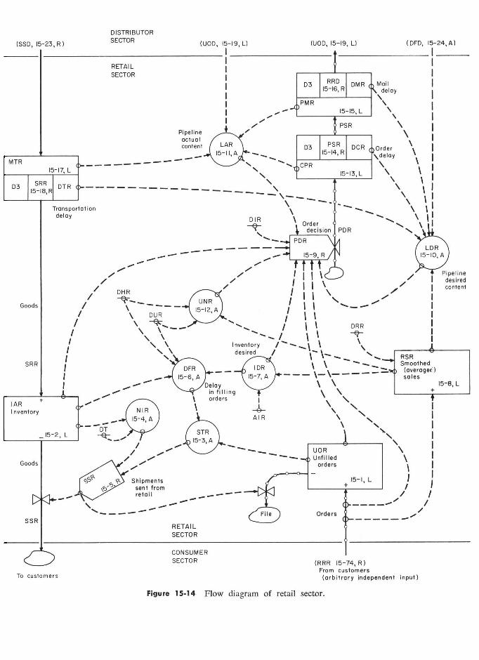
MODEL OF THE PRODUCTION-DISTRIBUTION SYSTEM
erate the output rate of the mailing delay, which tributor. We shall therefore set down eighteen is the rate of actual receipt of orders at the equations identical in form with the previous distributor. eighteen. The constants defining delays and the
We shall define the retail sector to include other parameters of the system need not of the transportation of goods from the distribu- course be the same at the distributor level as tor to the retailer. Therefore we need another at the retail level. If in a particular actual system pair of equations to define the delay in trans- there were clear differences between retail and
portation: distributor decision criteria, there would then
____________________________ be a basis for formulating a different set of
MTR.K = MTR.J + (DT)(SSD.JK - SRR.JK) 15-17, L equations. Even with the same equation forms,
SRR.KL 15-18, R selection of different parameter values can
' ' ' R make allowance for different inventory levels,
MTR Material in Transit to Retail (units) different delay intervals for processing orders SSD Shipments Sent from Distributor inventory and handling goods, and different policies on
(units/week) s rtf't r!'t t speed of inventory adjustment. SRR Shipments Received at Retail inventory Speed of y J '
(units/week) The equations for the distributor sector will DTR Delay in Transportation of goods to Retail follow with a minimum of discussion, since the
(weeks) explanation of the retail equations applies DELAY3 spécifies rhird-order-delay équations equally well here. The equation for unfilled
–––––––––––––––––––––––– orders at the distributor is similar to that given The input to the transportation delay is the in Equation 15-1 for the retail sector:
output rate from the distributor inventory. The ____________________________ output SRR from the shipping delay is the input UOD.K = UOD.J + (DT)(RRD.JK - SSD.JK) 15-19, L to the retail inventory as required in Equation UOD Unfilled Orders at Distributor (units) 15-2. As before, Equation 15-17 defines the
UOD Unfilled Orders at Distributor (units) Distributor . < .- „ . nes
e RRD Réquisitions (orders) R . d at Distributor . RRD equlsllions or ers ecelve at Istn utor goods in transit, and Equation 15-18 gives the e
RRD (units/week)
(orders) Received at Distributor
necessary information for calculating the output SSD Shipments Sent from Oistributor inventory rate according to the characteristics of a third- (units/week) order delay.
DT Time interval between solutions of the equa-
This completes the set of equations that we rions (weeks)
propose to use at present for representing oper- ations in the retail sector. The equations are not This is an accounting equation giving the new
self-contained, since they depend on knowing unfilled-order level in terms of previous un- the values of certain variables (SSD, UOD, filled orders and the orders which have come in
DFD) that exist in the distributor sector. and the orders which have been filled. 15.5.2 Equations for the Distributor Sector. Figure 15-15 shows the flow diagram for
The equations that have already been developed equations in the distributor sector. for the retail sector deal with the general char- The equation for inventory at the distributor acteristics of receiving goods, receiving orders, level corresponds to Equation 15-2 at retail:
shipping goods, and ordering replacements. Be- __________________________ havior patterns at the distributor could of IAD.K = IAD.J + (DT)(SRD.JK - SSD.JK) 15-20, L course be different. In the absence of wanting
' ' ' ' '
to introduce any particular differences between IAD Inventory Actual at Distributor (units)
retail and distributor behavior, we can use a SRD Shipments Received at Distributor (units/week) retail and distnbutor behavior, we can use a similar set of equations to represent the dis- SSD Shipments Sent from Distributor (units/week)
158
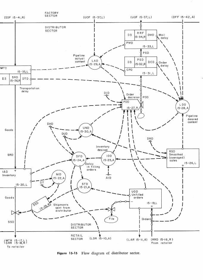
MODEL OF THE PRODUCTION-DISTRIBUTION SYSTEM
As in Equations 15-3, 15-4, and 15-5, the "––––––––––––––––––
shipping rate from the distributor is given by IDD.K = (AID)(RSD.K) 15-25, A
––––––––––––––––––––––––––––––– RSD.K = RSD.J + (DT) (RRD.JK - RSD.J)
STD.K UOD.K 15-21, A DRD
15-26, L STD K = pFD.K 15-21, A 15.26, L
IDD Inventory Desired at Distributor (units) DFD.K
IDD Inventory Desired at Distributor (units) IAD.K AID proportionality constAnt for Inventory at Dis-
NID.K = DT 15-22, A tributor (weeks)
RSD Réquisitions Smoothed at Distributor
if NID.K > STD.K 15-23, R (units/week)
if NID.K Ù STD.K / DRD Delay time constant in smoothing Requisitions at
STD Shipping rate to be Tried at Distributor ,, Distributor (weeks)
(units/week) RRD Requisitions (orders) Received at Distributor
UOD Unfilled Orders at Distributor (units) (units/week) DFD Delay (variable) in Filling orders at the Dis- ____________________________________
tributor (weeks) NID Négative Inventory limit rate at Distributor , , , ,
(units/week) For the purchasing decision equation at the IAD Inventory Actual at Distributor (units) distributor level, we shall use the same form as DT Solution time interval, Delta Time (weeks) in Equation 15-9: t SSD Shipments Sent from Distributor (units/week)
Equation 15-21 gives the tentative shipping PDD.KL = RRD.JK +
1
) F IAD.K) rate from the distributor which is to be tested PDD.KL = RRD.JK
+ DID IAD.K)
against the rate that would cause a negative 1 ] inventory (Equation 15-22). The smaller of f +(LDD.K - LAD.K) + (UOD.K -
the two rates is taken as the actual shipping 15-27, R
rate (Equation 15-23). PDD Purchasing rate Décision at Distributor As in Equation 15-6, the variable delay (units/week)
representing the average delay in filling orders RRD Réquisitions (orders) Received at Distributor
at the distributor is _.
(unit5/week) (and pipeline) adjustment at
e s u DID Delay in Inventory (and pipeline) adjustment at
___________________________________ Distributor (weeks)
IDD.K „ IDD Inventory Desired at Distributor (units) DFD.K = DHD + DUD 15-24, A IAD Inventory Actual at Distributor (units)
IAD.K LDD pipeline orders Desired (necessary) in transit to DFD Delay in Filling orders at Distributor (weeks) Distributor (units)
_ , , , DHD Delay due to minimum Handling time required LAD pipeline orders Actual in transit to Distributor
at Distributor (weeks) (units) , , ,
DUD Delay, average, in Unfilled orders at Distributor UOD Unfilled Orders at the Distributor (units) _
caused by out-of-stock items when inventory UND Unfilled orders, Normal, at Distributor (units) is "normal" (weeks)
IDD Inventory Desired at Distributor (units) IAD Inventory Actual at Distributor (units) [AD Inventory Actual at Distributor (units) The equations for the orders and goods nec-
essary in the supply pipeline between the dis- As in Equations 15-7 and 15-8, the desired tributor and the factory and the corresponding
level of distributor inventory and smoothed in- actual orders and goods in transit in the pipeline coming requisitions are given by are similar to Equations 15-10 and 15-11:
160
§ 15.5.3 EQUATIONS FOR THE FACTORY SECTOR
LDD.K = (RSD.K)(DCD + DMD + DFF.K + DTD) CPD.K = CPD.J + (DT)(PDD.JK - PSD.JK) 15-31, L 15-28, A PSD.KL = DELAY3(PDD.JK, DCD) 15-32, R
LDD pipeline orders Desired (necessary) in transit to (DT)(PSD.JK - RRF.JK) 15-33, L Distributor (units) L
RSD Réquisitions Smoothed at Distributor RRF.KL = DELAY3(PSD.JK, DMD) 15-34, R (units/week)
' '
DCD Delay Clerical at Distributor (weeks) CPD Clerical in-Process orders at Distributor
DMD Delay in order Mailing from Distributor (weeks) (units) DFF Delay (variable) in Filling orders at Factory PDD Purchasing-rate Décision at Distributor
(weeks) (units/week) DTD Delay of goods in Transit to Distributor PSD Purchase orders Sent from Distributor
(weeks) (units/week) DCD Delay in Clerical order processing at Dis-
tributor (weeks) PMD Purchase orders in Mail from Distributor
(units) LAD.K = CPD.K + PMD.K + UOF.K + MTD.K RRF Requisitions (orders) Received at Factory
15-29, A (units/week) LAD pipeline orders Actual in transit to Distributor DMD Delay in Mail from Distributor (weeks)
(units) DELAY3 spécifies third-order-delay equations CPD orders in Clerical Processing at Distributor
(units) PMD Purchase orders in Mail from Distributor (units) UOF Unflled Orders at the Factory (units) The remaining two equations for the distribu- MTD Material in Transit ta the Distributor (units) tor sector describe the shipping delay for goods ____________________________ coming from the factory. These correspond to
As in Equation 15-12, "normal" unfilled or- Equations 15-17 and 15-18 at retail:
ders depend on the normal order-processing delay and the average level of business activity:
MTD.K MIRD.J + (Dlr)(SSF.JK - SRD.JK) 15-35, L MTD.K = MTD.J + (DT)(SSF.JK - SRD.JK) 15-35, L
SRD.KL = DELAY3(SSF.JK, DTD) 15-36, R UND.K = (RSD.K)(DHD + DUD) 15-30, A
MTD Material in Transit ta Distributor (units) MTD Material in Transit to Distributor (units) UND Unfilled orders, Normal, at Distributor (units) SSF Shipments Sent from Factory (units/week) RSD Réquisitions (orders) Smoothed at Distributor SRD Shipments Received at Distributor
(units/week) (units/week) DHD Delay due to minimum Handling time required DTD Delay in Transportation of goods to Distribu-
at Distributor (weeks) tor (weeks) DUD Delay, average, in Unfilled orders at Distributor DELAY3 spécifies third-order-delay equations
caused by out-of-stock items when inventory is "normal" (weeks)
This completes the eighteen equations to The distributor experiences delays in the represent the distributor level.
placing of purchase orders and in mailing these 15.5.3 Equations for the Factory Sector. At orders to the factory in the same way discussed the factory many of the order-filling functions in Equations 15-13 through 15-16. The four are similar to those at retail and the distributor.
equations for the ordering delay and the mail However, some organizational differences exist
delay are at the factory. We shall assume that the factory
161 1

MODEL OF THE PRODUCTION-DISTRIBUTION SYSTEM
warehouse and factory are adjacent. Therefore, NIF Négative Inventory limit rate at Factory
we shall not provide for mail or transportation Ui/Wek
delays between thé warehouse and the factory; IAF Inventory Actual at Factory (units)
delays between t e ware ouse and the factory; DT 1... interval, Delta Time (weeks) " .. -' DT solution time !nterva!, Delta Time (weeks) s on the other hand, there is a production lead SSF Shipments Sent from Factory warehouse time between a decision to change production (units/week) rate and the resulting change in factory output. -___________________________
In developing the equations for the factory, The expressions for the delay in filling orders, we shall start first with those that are similar the ideal inventory, and the smoothed sales to the retail and the distributor sectors. Figure rate can be of the same form as given in Equa- 15-16 gives the flow diagram described by the tions 15-6, 15-7, and 15-8:
following equations. The equations for unfilled ____________________________
orders and actual inventory are similar to Equa- IDF.K tions 15-1 and 15-2: DFF.K = DHF + DUF
IAF.K 15-42, A
IDF.K = (AIF)(RSF.K) 15-43, A UOF.K = UOF.J + (DT)(RRF.JK - SSF.JK) 15-37, L
IDF.K (AIF)(RSF.K) 15-43, A
IAF.K = IAF.J + (DT)(SRF.JK - SSF.JK) 15-38, L RSF.K = RSF.J + DF
RSF.J) RF
UOF Unfilled Orders at the Factory (units) \
15-44, L RRF Réquisitions (orders) Received at Factory
,
(units/week) DFF Delay (variable) in Filling orders at Factory SSF Shipments Sent from Factory warehouse (weeks)
(units/week) DHF Delay due to minimum Handling time required IAF Inventory Actual at Factory warehouse (units) at Factory (weeks)
SRF Shipments Received at Factory warehouse (man- DUF Delay, average, in Unfilled orders at Factory
ufacturing output) (units/week) caused by out-of-stock items when inventory
___________________________________ is "normal" (weeks) IDF Inventory Desired at Factory (units)
We shall assume that the factory warehouse IAF Inventory Actual at Factory (units) is stocking and shipping a number of catalog AIF proportionality constAnt for Inventory at Fac-
items in the product line. This continues to tory (weeks)
imply the concept of a delivery delay that in- RSF Réquisitions Smoothed at Factory (units/week)
creases gradually as the level of inventory de- DRF
Delay in smoothing Réquisitions at Factory
– - .' - (weeks) s creases. Consequently, our representation of RRF Réquisitions (orders) Received at Factory shipping rate will be determined as in Equations (units/week)
15-3, 15-4, and 15-5: _________________________
–––––––––––––––––––––––––– We now come to the manufacturing rate de-
UOF.K cision. In a real situation it might be affected by STF.K 15-39, A various practical considerations determined by y
IAF.K physical manufacturing facilities. Most produc- NIF.K
= - 15-40, A tion lines and equipment can, however, operate
FS'IF.K if NIF.K STF.K) over a substantial range of production capaci-
NIF.K if f 15-41, R ties. Therefore, we assume for this example
lNIF.K )fN)r.K<?STr.KJ that manufacturing rate is continuously variable e
STF Shipping rate to be Tried at Factory from zero up to some maximum rate. (units/week) rr.i.
d . (units/week)
.L E . < The desire to produce more than the maxi- UOF U fill d 0 d h F (. ) UOF Unfilled Orders at the Factory (units) DFF Delay (variable) in Filling orders at Factory
mum rate will lead only to maximum factory (weeks) output. It should be noted that the "overt" de-
162
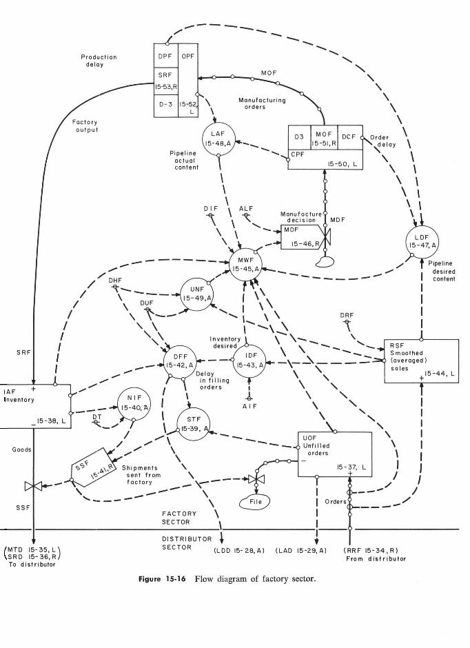
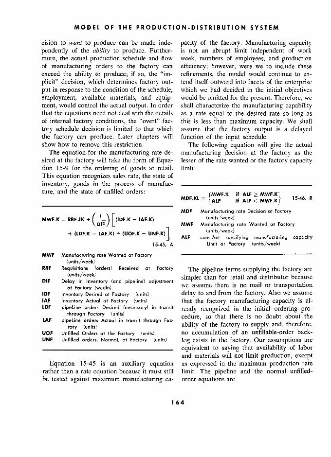
MODEL OF THE PRODUCTION-DISTRIBUTION SYSTEM
cision to want to produce can be made inde- pacity of the factory. Manufacturing capacity pendently of the ability to produce. Further- is not an abrupt limit independent of work
more, the actual production schedule and flow week, numbers of employees, and production of manufacturing orders to the factory can efficiency; however, were we to include these exceed the ability to produce; if so, the "im- refinements, the model would continue to ex-
plicit" decision, which determines factory out- tend itself outward into facets of the enterprise put in response to the condition of the schedule, which we had decided in the initial objectives employment, available materials, and equip- would be omitted for the present. Therefore, we
ment, would control the actual output. In order shall characterize the manufacturing capability that the equations need not deal with the details as a rate equal to the desired rate so long as of internal factory conditions, the "overt" fac- this is less than maximum capacity. We shall
tory schedule decision is limited to that which assume that the factory output is a delayed the factory can produce. Later chapters will function of the input schedule. show how to remove this restriction. The following equation will give the actual
The equation for the manufacturing rate de- manufacturing decision at the factory as the sired at the factory will take the form of Equa- lesser of the rate wanted or the factory capacity tion 15-9 for the ordering of goods at retail. limit: This equation recognizes sales rate, the state of
inventory, goods in the process of manufac- ____________________________
ture, and the state of unfilled orders: MDF.K
if ALF >
MWF.K 15-46, R
_______________________________ MDF.KL =
ALF if ALF < MWF.K / 15-46, R
MWF.K = RRF.JK DIF ) L
(IDF.K - IAF.K) ' MDF Manufacturing rate Décision at Factory
MWF.K = RRF.JK + ( ) [(IDF.K -
IAF.K) MWF
(units/week) rate Wanted at Factory DIF / L MWF Manufacturing rate Wanted at Factory
+ (LDF.K - LAF.K) + (UOF.K - UNF.K) J ALF constAnt (units/week) specifying manufacturing capacity
15-45, A Limit at Factory (units/week)
MWF Manufacturing rate Wanted at Factory –––––––––––––––––––––––––––––––––––
(units/week) RRF Réquisitions (orders) Received at Factory The pipeline terms supplying the factory are
DIF (units/week) . , . simpler than for retail and distributor because
DIF Delay in Inventory (and pipeline) adjustment at Factory (weeks) we assume there is no mail or transportation
IDF Inventory Desired at Factory (units) delay to and from the factory. Also we assume IAF Inventory Actual at Factory (units) that the factory manufacturing capacity is al- LDF pipeLine orders Desired (necessary) in transit
ready recognized in the initial ordering pro- through Factory (units)
cedure, so that there is no doubt about the LAF pipeline orders Actual in transit through Fac-
f f f tory (units) ability of the factory to supply and, therefore, UOF Unfilled Orders at the Factory (units) no accumulation of an unfillable-order back- UNF Unfilled orders, Normal, at Factory (units) log exists in the factory. Our assumptions are
____________________________ equivalent to saying that availability of labor
and materials will not limit production, except Equation 15-45 is an auxiliary equation as expressed in the maximum production rate
rather than a rate equation because it must still limit. The pipeline and the normal unfilled- be tested against maximum manufacturing ca- order equations are
164
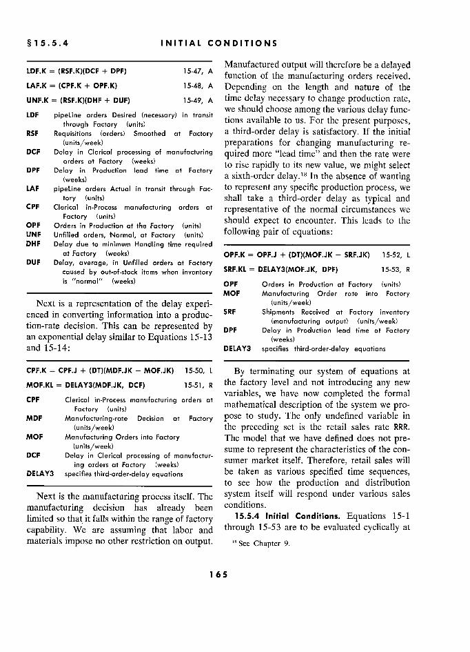
§15.5.4 INITIAL CONDITIONS 5
LDF.K=(RSF.K)(DCF+DPF) 15-47, A Manufactured output will therefore be
a delayed " +
function of the manufacturing orders received. LAF.K = (CPF.K + OPF.K) 15-48, A Depending on the length and nature of the
UNF.K = (RSF.K)(DHF + DUF) 15-49, A time delay necessary to change production rate,
LDF pipeline orders Desired (necessary) in transit _ we should choose among the various delay func- LDF pipeline orders Desired (necessary) in
transit..1 bl F h '
though tions available to us. For the present purposes,
RSF Requisitions (orders) Smoothed at Factory a third-order delay is satisfactory. If the initial
(units/week) preparations for changing manufacturing re- DCF Delay in Clerical processing of manufacturing quired more "lead time" and then the rate were
orders at Factory (weeks) to rise rapidly to its new value, we might select t DPF Delay in Production lead time at Factory . h d 1 18 1 h b' f
se DPF ??§j£?§J?
Production lead time at Factory a sixth-order delay.11 In the absence of wanting (weeks) a Slxt -or er delay. ? In thé absence of want)ng LAF pipeline orders Actual in transit through Fac- to represent any specific production process, we
tory (units) shall take a third-order delay as typical and CPF Clerical in-Process manufacturing orders at
representative of the normal circumstances we
(unirs) . , .. should expect to encounter. This leads to the OPF Orders in Production at the Factory (units) , . '
UNF Unfilled orders, 'Normal, at Factory (units) following pair of équations : DHF Delay due to minimum Handling time required –––––––––––––––––––––––––––––––––––––
at Factory (weeks) OPF.K = OPF.J + (DT)(MOF.JK - SRF.JK) 15-52, L DUF Delay, average, in Unfilled orders at Factory
caused by out-of-stock items when inventory SRF.KL = DELAY3(MOF.JK, DPF) 15-53, R is "normal" (weeks) OPF Orders in Production at Factory (units)
––––––––––––––––––––––––––––––––––––– MOF Manufacturing Order rate into Factory Next is a representation of the delay experi- (units/week)
enced in converting information into a produc- SRF Shipments Received at Factory inventory
, , ,, (manufacturing output) (units/week) tion-rate decision. This can be represented by DPF Delay in Production lead rime ar Factory an exponential delay similar to Equations 15-13 3 (weeks) and 15-14: DELAY3 specifies third-order-delay equations
CPF.K = CPF.J + (DT)(MDF.JK - MOF.JK) 15-50, L By terminating our system of equations at
MOF.KL = DELAY3(MDF.JK, DCF) 15-51, R the factory level and not introducing any new
CPF Clerical in-Process manufacturing orders at variables, we have now completed the formal CPF Clerical in-Process manufacturing orders at
th t. 1 d . t. f th t CPF
Clerical in.Process manufacturing orders ar
mathematical description of the system we pro- Factory (units) ma ema Ica escnp Ion a e sys em :ve
MDF Manufacruring-rare Decision at Factory pose to study. The only undefined variable in
(units/week) the preceding set is the retail sales rate RRR. MOF Manufacturing Orders into Factory The model that we have defined does not pre-
(units/week) sume to represent the characteristics of the con- DCF Delay in Clerical processing of manufactur-
market, Therefore, retail sales ing orders at Factory (weeks) sumer market itself. Therefore, retail sales will ing orders at Factory (weeks) sumer mar e l se. ere ' re al sa es WI
DELAY3 specifies third-order-delay équations be taken as various specified time sequences, ____________________________ to see how the production and distribution
Next is the manufacturing process itself. The system itself will respond under various sales
manufacturing decision has already been conditions.
limited so that it falls within the range of factory 15.5.4 Initial Conditions. Equations 15-1
capability. We are assuming that labor and through 15-53 are to be evaluated cyclically at
materials impose no other restriction on output. '8 See Chapter 9.
165 5
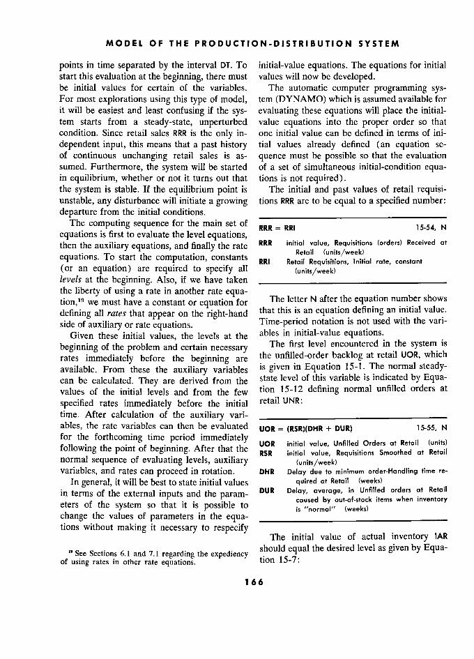
MODEL OF THE PRODUCTION-DISTRIBUTION SYSTEM
points in time separated by the interval DT. To initial-value equations. The equations for initial start this evaluation at the beginning, there must values will now be developed. be initial values for certain of the variables. The automatic computer programming sys- For most explorations using this type of model, tem (DYNAMO) which is assumed available for it will be easiest and least confusing if the sys- evaluating these equations will place the initial- tem starts from a steady-state, unperturbed value equations into the proper order so that condition. Since retail sales RRR is the only in- one initial value can be defined in terms of ini-
dependent input, this means that a past history tial values already defined (an equation se- of continuous unchanging retail sales is as- quence must be possible so that the evaluation sumed. Furthermore, the system will be started of a set of simultaneous initial-condition equa- in equilibrium, whether or not it turns out that tions is not required). the system is stable. If the equilibrium point is The initial and past values of retail requisi- unstable, any disturbance will initiate a growing tions RRR are to be equal to a specified number:
departure from the initial conditions. The computing sequence for the main set of RRR = RRI 15-54, N
equations is first to evaluate the level equations, ,
then the auxiliary équations, and finally the rate RRR initial value, Requisitions (orders) Received at . rr ..... . Retail (unitsjweek)
équations. To start the computation, constants RRI R e t al .1 R equisi ..t' Ions, 1 ni .t' la ... t an e uation are re t to s ecif all
RRI Retail Requisitions, Initial rate, constant (or an equation) are required to specify all (units/week) levels at the beginning. Also, if we have taken the liberty of using a rate in another rate equa- . tion,'9 we must have a constant or equation for The letter N after the équation number shows
defining all rates that appear on the right-hand that this is an équation defining an initial value.
side of auxiliary or rate equations. Time-period notation is not used with the van-
Given these initial values, the levels at the ables in initial-value équations. ,
beginning of the problem and certain necessary The first level encountered in the system is
rates immediately before the beginning are the unfilled-order backlog at retail UOR, which
available. From these the auxiliary variables given in Equation 15-1. The normal steady-
can be calculated. They are derived from the state level of this variable is indicated by Equa-
values of the initial levels and from the few tion 15-12 defining normal unfilled orders at
specified rates immediately before the initial retail UNR:
time. After calculation of the auxiliary vari- __________________________ ables, the rate variables can then be evaluated UOR = (RSR)(DHR + DUR) 15-55, N for the forthcoming time period immediately UOR initial value, Unfilied Orders . , . following the point of beginning. After that the
UOR initial value, Unfilled Orders at Retail (Unlts) following the point of beginning. After that the RSR initial value, Réquisitions Smoothed at Retail normal sequence of evaluating levels, auxiliary (units/week) variables, and rates can proceed in rotation. DHR Delay due to minimum order-Handling time re-
In general, it will be best to state initial values quired at Retail (weeks)
in terms of the external inputs and the param- DUR Delay, average, in Unflled orders at Retail
eters of that it is possible t0 caused by out-of-stock items when inventory
eters of thé System so that lt IS possible to is normal' (weeks) s change the values of parameters in the equa- ___________________________ tions without making it necessary to respecify
The initial value of actual inventory IAR The initial value of actual inventory IAR
'° See Sections 6.1 and 7.1 regarding the expediency should . equal the desired level as given by Equa- "See Sections 6. and 7. 1 regarding thé expediency
of using rates in other rate equations. tion 15-7: "
166
§ 15.5.4 INITIAL CONDITIONS 5
IAR = (AIR)(RSR) 15-56, N PMR = (DMR)(RRR) 15-59, N
IAR initial value, Inventory Actual at Retail (units) MTR = (DTR)(RRR)20 15-60, N
AIR proportionality constAnt for Inventory at Retail CPR initial value, Clerical in-Process orders at Re- (ratio of desired inventory to weekly sales) tail (units) (weeks) DCR Delay in Clerical order placing at Retail
RSR initial value, Requisitions Smoothed at Retail (weeks) (units/week) RRR initial value, Requisitions (orders) Received at
–––––––––––––––––––––––––––––––––– Retail (units/week)
1 f PMR initial value, Purchase orders in Mail from Re-
The next level in the set of equations is that tail ., (units) . for the smoothed retail sales rate that in the DMR Delay in Mail from Retail (weeks) steady state will equal the constant past sales MTR initial value, Material in Transit to Retail rate: (units)
DTR Delay in Transportation of goods to Retail (weeks)
RSR = RRR 15-57, N _______________________________ RSR initial value, Réquisitions Smoothed at Retail With the preceding initial values defined and
,.,,„.. with h thé initial 1 value ofunniled d orders at thé RRR initial (units/week) value, Requisitions ( d ) Received at with the initial value of unfilled orders at the e
Retail (units/week) distributor UOD, which will be available from
__________________________ the specification of initial values in the distribu-
Using the initial values already defined, we tor sector, it becomes possible to evaluate
Usine thé imtial values aiready y defined, d we ? - ? ? ? . possible ta evaluate
can see that the computing program can then Equation 15-9 for the rate of generating pur- can see that thé e computmg program can then ,_ .. chase orders at retail PDR. Under thèse steady- evaluate Equations 15-7, 15-6, 15-3, 15-4, and ehase orders at retail PDR.
Under these steady-
15-5, yielding values of the auxiliary variables state initial conditions, all the terms in the
15 - , 5 yie mg values of thé auxiliary variables e terms . t e
d ..
°.... , f "
.1 SSR bracket of Equation 15-9 total zero, leavlllg and arriving at a shipping rate from retail SSR the order-generation rate equal to retail sales.
that is equal to the specified steady-state con- It is well to test the initial-value retail sales. ..t' ..t' 1 t It is well to test the initial-value équations to
. dition of retail réquisition initial rate RRI. . make is well that test the initial-value equations to
. rr, ..t' 1 1 f d d d.
make sure that they will generate thé antici- The initial values of orders and goods in m make sure that they will generate
the antici-
t .t' e lllI th la
va ues 1 1. a or
t ers 1 an b -Y- j. pated initial values of auxiliary and rate van- transit in the supply line must also be specified.
pated initial values of auxiliary to formulate a In thé steady state the rates of flow in thé supply ables. equations in which the actual steady-state
a
line between retailer and distributor will equal 1 set of equations in which the actual steady-state
the retail sales rate. The product of this rate conditions are not what is desired and not at
thé retail sales rate. Thé product of this rate e conditions are not what is desired and
at . i . nrst slance what they would appear to be. This
multiplied by the length of a delay will give thé first glance what they would appear to be. This
o t or e
point was mentioned earher as one of the rea- quantity stored in the delay. The equations for point was mentioned earlier as one of the rea-
- sons for placing the normal unniled-order term clérical processing, mail, and transportation are sons for placing the normal unfilled-order
term
then processmg, mai , an transportation are
UNR in Equation 15-9 for the purchasing rate. The additional equations for initial values
at the distributor sector follow: CPR = (DCR)(RRR)20 15-58, N
20 ln principle, specifying the initial content of a RRD = RRR 21 15-61, N delay is sufficient to specify steady-state initial condi- tions of the inflow and outflow rates. However, the UOD = (RSD)(DHD + DUD) 15-62, N convention used in the DYNAMO compiler requires ––––– that the initial input rate to a third-order delay be 21 Since RRD would be generated by DYNAMO as given, requiring, in addition to the above, the equa- the initial output rate of the mail delay, this equation tions PDR = RRR and SSD = RRR. DYNAMO generates would not be needed. As before, the ordering and the initial output value of a third-order delay (PSR) shipping delays would require PDD = RRD and SSF so that this will be available to the mail delay. = RRD.
167
MODEL OF THE PRODUCTION-DISTRIBUTION SYSTEM
IAD = (AID)(RSD) 15-63, N RRF initial value, Réquisitions Received at Factory
(units/week) RSD = RRD 15-64, N RRR initial value, Requisitions Received at Retail '1
CPD = (DCD)(RRD) 15-65, N (units/week) UOF initial value, Unfilled Orders at the Factory
PMD = (DMD)(RRD) 15-66, N (units)
MTD = (DTD)(RRD) 15-67, N RSF initial value, Requisitions Smoothed at Factory ' (units/week)
RRD initial value, Requisitions (orders) Received at DHF Delay due to minimum Handling time required Distributor (units/week) at Factory (weeks)
RRR initial value, Requisitions (orders) Received at DUF Delay, average, in Unfilled orders at Factory Retail (units/week) caused by out-of-stock items when inventory
UOD initial value, Unfilled Orders at Distributor is "normal" (weeks) (units) IAF initial value, Inventory Actual at Factory
RSD initial value, Requisitions Smoothed at Distribu- (units) tor (units/week) AIF proportionality constAnt for Inventory at Fac-
DHD Delay due to minimum Handling time required tory (weeks) at Distributor (weeks) CPF initial value, Clerical in-Process manufacturing
DUD Delay, average, in Unfilled orders at Distributor orders at Factory (units) caused by out-of-stock items when inventory DCF Delay in Clerical processing of manufacturing is "normal" (weeks) orders at Factory (weeks)
IAD initial value, Inventory Actual at Distributor OPF initial value, Orders in Production at Factory (units) (units)
AID proportionality constAnt for Inventory at Dis- DPF Delay in Production lead time at Factory tributor (weeks) (weeks)
CPD initial value, Clerical in-Process orders at Dis- _____________________________________ tributor (units) .
DCD D 1 . d .
t D. t .b EquatlOns 15-54 through 15-73 state the DCD Delay in Clerical order processing at Distribu- u- ° 15-54 through 15-73 state the ror (weeks) initial values necessary for starting the compu-
PMD initial value, Purchase orders in Mail from Dis- tationof Equations 15-1 through 15-53.23 tributor (units) 15.5.5 Parameters (Constants) of the Sys- DMD Delay in Mail from Distributor (weeks)
tem. Having completed the equations describ- MTD initial value, Material in Transit to Distributor h (units) ing the system behavior and the equations de-
DTD Delay in Transportation of goods to Distributor fining initial values, we now need a set of nu- (weeks) merical values of the parameters (constants
–––––––––––––––––––––––––––– during any particular solution) of the system. A similar set of initial-value equations ap- The first parameter encountered in the equa-
plies to the factory sector as follows: tions is really a parameter of the solution pro- –––––-––––––––––––––––––––– cedure rather than of the system as such. It is RRF = RRR 22 15-68, N the solution-time interval DT. 24 The solution in-
UOF = (RSF)(DHF + DUF) ) 15-69, N terval should be a small fraction (less than one- , sixth) of the length of time represented in any IAF = (AIF)(RSF) 15-70, N third-order delay in the system. Since we shall
RSF = RRF 15-71, N represent delays as short as a half-week in the
CPF = (DCF)(RRF) . 15-72, N system, we take the solution-time interval as
OPF = (DPF)(RRF) 15-73, N DT = 0.05 week, solution interval
23 All of the equations are tabulated together in 22 The DYNAMO compiler would not require this Appendix B.
equation, but for the ordering delay would need basis for choosing a solution-time interval MDF = RRF. is discussed in Appendix D.
168 8
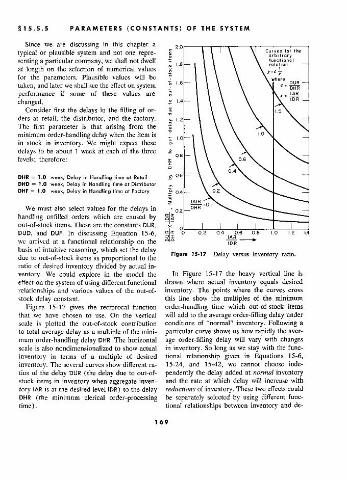
§ 15.5.5 5 PARAMETERS (CONSTANTS) OF THE SYSTEM
Since we are discussing in this chapter a 2.0.
typical or plausible system and not one repre- E t I \ \ Curves tor
the Q) arbl trory
senting a particular company, we shall not dwell functionm , -'" 1.8 relation
at length on the selection of numerical values g \ v=c L for the parameters. Plausible values will be ) t \ \ where
taken, and later we shall see the effect on system 1.6
\ ° - DHR
-
performance if some of these values are 0 t \ \ \ I AR
changed..2 I .4
t \ \ \ 'R Consider first the delays in the filling of or-
t \ \ \ 1.5
ders at retail, the distributor, and the factory. »1.2 \ \ \ –
The first parameter is that arising from the v \ \ minimum order-handling delay when the item is : 1.0. t \ \ 1.0
° \ in stock in inventory. We might expect these t \ \ \ delays to be about 1 week at each of the three °
t \ \ levels; therefore: a::
0.,8 \
\ J: o °
0.4 DHR = 1.0 week, Delay in Handling time at Retail 8 °.6 \ \ DHD = 1.0 week, Delay in Handling time at Distributor » \ DHF = 1.0 week, Delay in Handling time at Factory 0.2
–
i DUR
We must also select values for the delays in 0,2 DHR -on
handling unfilled orders which are caused by ô â out-of-stock items. These are the constants DUR, i 0. I ___' DUD, and DUF. In discussing Equation 15-6, ° 0.2 0.4
IAR 0.6 0.8 MW
1.0 i.2 2 1.4
we arrived at a functional relationship on the 0 0 IDR
basis of intuitive reasoning, which set thé delay the delay Figure 15-17 7 Delay versus inventory ratio. due to out-of-stock items as proportional to the e Figure 15.17 Delay versus inventory ratio.
ratio of desired inventory divided by actual in-
ventory. We could explore in the model the In Figure 15-17 the heavy vertical line is
effect on the system of using different functional drawn where actual inventory equals desired
relationships and various values of the out-of- inventory. The points where the curves cross
stock delay constant. this line show the multiples of the minimum
Figure 15-17 gives the reciprocal function order-handling time which out-of-stock items
that we have chosen to use. On the vertical will add to the average order-filling delay under
scale is plotted the out-of-stock contribution conditions of "normal" inventory. Following a
to total average delay as a multiple of the mini- particular curve shows us how rapidly the aver-
mum order-handling delay DHR. The horizontal age order-filling delay will vary with changes scale is also nondimensionalized to show actual in inventory. So long as we stay with the func-
inventory in terms of a multiple of desired tional relationship given in Equations 15-6,
inventory. The several curves show different ra- 15-24, and 15-42, we cannot choose inde-
tios of the delay DUR (the delay due to out-of- pendently the delay added at normal inventory stock items in inventory when aggregate inven- and the rate at which delay will increase with
tory IAR is at the desired level IDR) to the delay reductions of inventory. These two effects could
DHR (the minimum clerical order-processing be separately selected by using different func-
time). tional relationships between inventory and de-
169
MODEL OF THE PRODUCTION-DISTRIBUTION SYSTEM
lay.25 Let us assume that the curves marked figures are equivalent to an inventory turnover 0.4, 0.6, and 1.0 agree adequately with our of 6.5, 8.7, and 13 times per year at the three estimate of the out-of-stock order-filling delays levels. at retail, distributor, and factory levels. Since The parameters in Equations 15-8, 15-26, these are to be multiplied by the minimum and 15-44 give the exponential smoothing time
order-handling delay, which in each case has constant used for averaging present sales into
already been selected as 1 week, the values of smoothed sales. We shall assume, to start our the constants are also investigation, that an 8-week time constant is
DUR = 0.4 week, Delay due to Unfillable orders at r being used at each of the three levels. There-
Retai! il fore:
DUD = 0.6 week, Delay due to Unfillable orders at 8 weeks, Delay in smoothing Réquisitions at Distributor Retail
DUF = 1.0 week, Delay due to Unfillable orders at DRD = 8 weeks, Delay in smoothing Requisitions at Factory Distributor
1 . h... - DRF = 8 weeks,? Delay in smoothin9 Réquisitions at Thèse values in their respective équations DRF = 8
F ac t ory Delay in smoothing Requisitions at
state, for example, that as retail inventory drops to half the desired amount, the average order-fill- In Equations 15-9, 15-27, and 15-45 are the ing delay at retail will rise from 1.4 to 1.8 of rates of inventory and pipeline correction given the minimum order-handling time. At the dis- by the parameters DIR, DID, and DIF. As we shall tributor, the delay would rise from 1.6 to 2.2 see later, the system performance is sensitive to times the minimum; at the factory from 2.0 to the values of these inventory and pipeline cor- 3.0 times the minimium. Estimates of correct rection rates. These parameters are ones about values, in a particular situation, could be whose values we might lack a basis for esti- reached by examining a sample of orders to mating closely. They might be indicated by his- determine typical order-filling time and the fre- torical ordering data. They are controllable by quency of out-of-stock delays. management. We shall start by selecting values
The next parameters encountered in the that seem plausible and later see the effect of equations are the ones that relate the level of changing these values. Initially, we shall assume desired inventory to the average sales rate. that at each level the ordering rate corrects in- This constant is defined as the number of weeks ventory and pipeline deviations at the rate of of average sales which could be supplied out of one-quarter of the imbalance per week: the "normal" inventory. Let us take these at the
DIR = 4 weeks, Delay in Inventory (and pipeline) ad- retail, distributor, and factory levels as DIR = 4 weeks, Delay in Inventory (and pipeline) ad- retail, distributor, and factory. levels as
justment at Retail AIR = 8 weeks, proportionality constant for Inventory DID = 4 weeks, Delay in Inventory (and pipeline) ad-
at Retail justment at Distributor AID = 6 weeks, proportionality constAnt for Inventory DIF = 4 weeks,27 Delay in Inventory (and pipeline) ad-
at Distributor justment at Factory AIF = 4 weeks, proportionality constAnt for Inventory .. h at Factory Next we must specify the delays in the proc-
essing of purchase orders. We shall assume that If these are divided into 52 weeks, they give this takes longer at retail than at the distributor,
the inventory turnover rate per year. The above " Under some circumstances this is equivalent to
" Or a table of values could be provided with a 16-week moving average. See Appendix E. interpolation for the delay corresponding to any in- n These values are probably smaller than would be ventory ratio. usual.
170
§ 15.6 SELECTING REASONABLE PARAMETER VALUES S
a period which is in turn longer than at the fac- The retail sales rate will be specified differ-
tory, giving ently for different explorations of system be-
DCR = 3 weeks, Delay, Clerical at Retail havior. The specification of this rate will be
DCD = 2 weeks, Delay, Clerical at Distributor given with each of the sets of test conditions DCF = 1 week, Delay, Clerical at Factory to which the system is to be subjected.
For the mailing delay from retailer and dis- tributor we shall use 15.6 Philosophy of Selecting Reasonable
. f n . Parameter Values DMR = 0.5 week, Delay in Mailing from Retail
Parameter Values
DMD = 0.5 week, Delay in Mailing from Distributor The reader may at first object to the arbitrary For the delay in shipping goods we shall use liberties just exhibited in selecting values of
the following from distributor to retailer and parameters. The preceding is inconsistent with
from factory to distributor much of the statistical estimating effort ex-
DTR = 1.0 week, Delay in Transportation to Retail hibited in the management science and eco-
DTR =1.0 week, Delay in Transportation to Retail DTD = 2.0 weeks, Delay in Transportation to Disrribu- nomics literature. However, 1 feel that extensive
tor to
data gathering and analysis should follow the
A th f demonstration of a need for more accuracy in
At the factory a 6-week lead time is assumed a particular parameter. For many purposes between the scheduling of a change in produc- values of parameters anywhere within the plaus- tion rate and the time when the new rate of flow ible range will produce approximately the same of goods is available from the factory: results.
WI pro uce approxlma e y e same
DPF = 6.0 weeks, Delay in Production lead time at It must be true that most industrial and eco- Factory nomic systems are not highly sensitive to small
Equation 15-46 requires a value for the max- changes in parameters; otherwise their whole
imum factory production rate. For our initial qualitative dynamic character would be much
exploration of the system, the factory limitation more changeable than it is. To a first approxi-
is not to be active. Therefore it can be set at a mation, economic fluctuation continues decade
very high multiple of the retail sales level. after decade in similar patterns although many details of the system have been greatly modi-
ALF = (1,000)(RRI) units/week, constAnt, manufactur- fied. In the last two hundred years we have ing capocity Limit at Factory
changed our form of government and our bank-
In the above expression ALF is the manufac- ing system; government expenditure has risen
turing limit at the factory and RRI is the retail to a substantial fraction of our national pro-
requisition initial rate. duction; the country has shifted from largely The initial production and sales rate must be agricultural to largely industrial activity; and
specified at which to have the system operate. transportation and communication speeds have
This can be arbitrarily chosen to some con- increased by a factor of 100. Yet in spite of these
venient scale of operations such as changes our capitalist economic system persists
- .., .... in similar fluctuations and trends in growth and RRI = 1,000 units/week, Retail Réquisitions, Initial rate
monetary fluctuations shall find that the and ' H - monetary inflation. We shall find that thé com-
We now have a complete set of dynamic plexity of the system structure, the existence
equations, initial-value equations, and param- of delays distributed throughout, the decisions
eters, with the exception of a specification of that introduce amplification, and the time con-
the input retail requisition rate RRR that will stants that arise from human memory and ac-
be applied to the system for test purposes. tion and life span all combine to produce sys-
' 171 1
MODEL OF THE PRODUCTION-DISTRIBUTION SYSTEM
tem behavior that is independent of reasonable useful beginning point. A historical time series
changes in most of the parameters. is too complex a pattern for a beginning explo- An information-feedback system is a system ration of system behavior. Simpler test condi-
of counterbalancing influences. An error in one tions are preferable during attempts to under- factor is often balanced within the system by stand the fundamental characteristics of the self-induced changes in other factors. The more system itself. At a later time, we can study re-
complete and realistic the system, the less sensi- sponses to typical historical data or can com- tive we should expect it to be to small changes bine properly selected pure inputs consisting in most of the individual parameters. of growth trends, seasonal and other periodic
Tests on the model itself can be used to de- fluctuations, and noise to create a test input termine model sensitivity to values of param- of known composition which generates the eters. When a peculiarly sensitive parameter statistical characteristics of historical sequences. is identified, we are faced with more problems Figures 2-2 through 2-8 of Chapter 2 will than merely measuring its value. Perhaps we now be repeated and individually discussed. can measure it accurately, but we must have The equations and parameters of Section 15.5 confidence that the value is constant with time. apply except as indicated. Otherwise it may be an important system vari- 15.7.1 Step Increase in Sales. A very in-
able, and if its source of variation cannot be formative, and one of the simplest, test inputs identified, our model behavior may be mislead- for the study of system dynamics is the "step ing. Maybe the parameter is one that can be function." This is a sudden disturbance caused
controlled, once its importance is realized. If by changing an external system input to some the parameter cannot be measured accurately, new value that is then held constant. A step or is not constant, or cannot be controlled, then function is a shock containing, in principle, an
perhaps we can redesign the structure of the infinite band of component frequencies. It can
industrial system so that the system behavior is serve to "excite" any mode of response that no longer vulnerable to the value of and may be inherent in the system model being changes in the parameter. tested. If the system has oscillatory behavior,
the step input gives an immediate indication 15.7 Test Runs of Model of the natural period of oscillation and the ra-
In Chapter 2 were given figures showing the pidity of damping or of growth of the oscilla-
way that a typical distribution organization tion. The step input will usually serve to trigger would react to some simplified retail sales in- any cumulative tendencies toward sustained
puts. In the preceding sections of this chapter growth or decline. have been given the equations that describe the The equations needed for generating a 10%
organization and the management policies of step in retail sales RRR follow: the system of Chapter 2.
In following sections will be given a more detailed description of each of the figures in RRR.KL = RRI + RCR.K " R
etal e ? a eac ° gures III
fO
)ft)me)s)essthan0 th an 0 } Chapter 2, induding the équations used to pro- RCR.K =
0 if time is less than 0 p g q P - { 100 if time is greater than duce the test-input conditions. RRR Réquisitions (orders) Received at Retail
It might at first be assumed that the most (units/week) informative type of system test input would be RRI Retail Réquisitions, Initial rate, constant
a time series of actual sales taken from a real- (units/week) a hme senes a actua sa es ta en rom a rea - RCR Requ!s?on Change at Retad ., (umts/week) life situation. In general, this is not the most RCR Requisition Change at Retail (units/week)
172
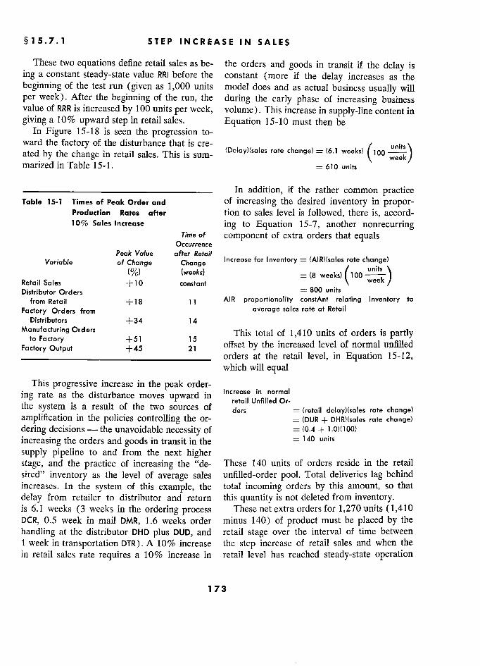
§ 15.7.1 STEP INCREASE IN SALES
These two equations define retail sales as be- the orders and goods in transit if the delay is ing a constant steady-state value RRI before the constant (more if the delay increases as the beginning of the test run (given as 1,000 units model does and as actual business usually will per week). After the beginning of the run, the during the early phase of increasing business value of RRR is increased by 100 units per week, volume). This increase in supply-line content in giving a 10% upward step in retail sales. Equation 15-10 must then be
In Figure 15-18 is seen the progression to- ward the factory of the disturbance that is cre-
(
units \ ated by the change in retail sales. This is sum- (Delay)(sales rate change) = (6.1 weeks)
C100 week J marized in Table 15-1. = 610 units
––––––-––––––––––––––––––––– In addition, if the rather common practice Table 15-1 Times of Peak Order and of increasing the desired inventory in propor-
Production Rates after tion to sales level is followed, there is, accord- 10% Sales ncrease ing to Equation 15-7, another nonrecurring
Time of component of extra orders that equals Occurrence
Peak Value after Retail Variable of Change Change Increase for Inventory = (AIR)(sales rate change)
Retail $oles (0/0) (weeks) = (8 weeks)
C100 units \ J Retail Sales 0 constant = 800 \
week Distributor Orders = SOO units
from Retail + 18 11 AIR proportionality constAnt relating Inventory to
Factory Orders from average sales rate at Retail Distributors +34 14
Manufacturing Orders This total of 1,410 units of orders is partly ta Factory +51 15 .
Factory Output +45 21 offset by the increased level of normal unfilled
____________________________ orders at the retail level, in Equation 15-12, which will equal
This progressive increase in the peak order- Increase in normal
ing rate as the disturbance moves upward in Increase in normal .° , . , .. , . retal nrl e r.
the system is a result of the two sources of ders = (retail delay)(sales rate change) amplification in the policies controlling the or- (DUR + DHR)(sales rate change) dering decisions -the unavoidable necessity of = (0.4 + 1.0)(100)
increasing the orders and goods in transit in the = 140 units
supply pipeline to and from the next higher stage, and the practice of increasing the "de- These 140 units of orders reside in the retail sired" inventory as the level of average sales unfilled-order pool. Total deliveries lag behind
increases. In the system of this example, the total incoming orders by this amount, so that
delay from retailer to distributor and return this quantity is not deleted from inventory. is 6.1 weeks (3 weeks in the ordering process These net extra orders for 1,270 units (1,410
DCR, 0.5 week in mail DMR, 1.6 weeks order minus 140) of product must be placed by the
handling at the distributor DHD plus DUD, and retail stage over the interval of time between 1 week in transportation DTR). A 10% increase the step increase of retail sales and when the
in retail sales rate requires a 10% increase in retail level has reached steady-state operation
173
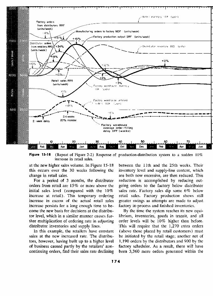
Factory orders Retail inventory IAR (units)
Factory orders from distributors RRF (units/week)
4 orders to factory MOF (units/week)
T 51 % +45% Foctory production output SRF (units/week) 1500 - - -
Distribulor orders _ from relailersRRD +34% O \
Distributor inventory (AD (unils) (units /week 1 ' o £ - - - - - - - - -
%
/< +12% .2 % /
f32% +12 %
1000 +4% .
_ Retail soles RRR -
(units/week) Factory worehouse 3mentor [AF (units)
, Factory worehouse unfilled ', orders UOF (units)
500 / °
, ,
,' .& · 0 2.4 weeks
2-weekTdelay 20% increase Factory warehouse
average order-filling delay DFF (weeks)
0 . 1 .. .... 10 .... 1 .... 20. 10. 60 .7 P .. 1 , . , . Jon Feb Mar Apr Mc;y Jun Aug sept Oct Nov Dec Jon Feb M,I, Apr ma, Jun .1
Figure 15-18 (Repeat of Figure 2-2) Response of production-distribution system to a sudden 10% increase in retail sales.
at the new higher sales volume. In Figure 15-18 8 between the 11 th and the 25th weeks. Their this occurs over the 30 weeks following the inventory level and supply-line content, which
change in retail sales. are both now excessive, are then reduced. This For a period of 3 months, the distributor reduction is accomplished by reducing out-
orders from retail are 15% or more above the going orders to the factory below distributor initial sales level (compared with the 10% sales rate. Factory sales dip some 6% below increase at retail). This temporary ordering retail sales. Factory production shows still increase in excess of the actual retail sales greater swings as attempts are made to adjust increase persists for a long enough time to be- factory in-process and finished inventories. come the new basis for decisions at the distribu- By the time the system reaches its new equi- tor level, which in a similar manner causes fur- librium, inventories, goods in transit, and all ther multiplication of ordering rate in adjusting order levels will be 10% higher than before. distributor inventories and supply lines. This will require that the 1,270 extra orders
In this example, the retailers have constant (above those placed by retail customers) must sales at the new increased rate. The distribu- be initiated by the retail stage; another net of
tors, however, having built up to a higher level 1,190 orders by the distributors and 900 by the of business caused partly by the retailers' non- factory scheduler. As a result, there will have
continuing orders, find their sales rate declining been 3,360 more orders generated within the
174
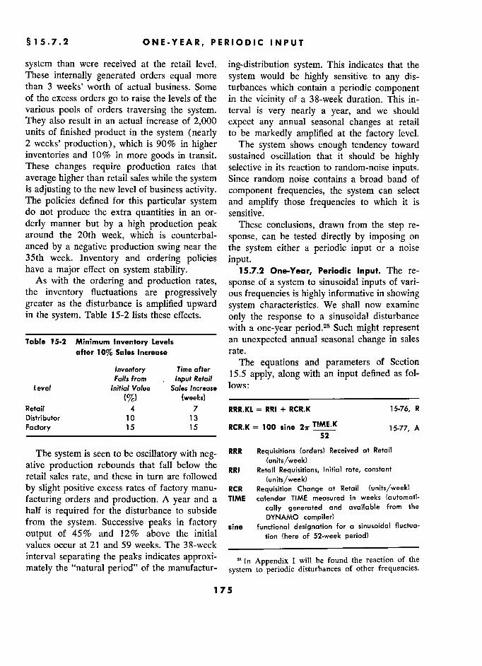
§15.7.2 ONE-YEAR, PERIODIC INPUT T
system than were received at the retail level. ing-distribution system. This indicates that the These internally generated orders equal more system would be highly sensitive to any dis- than 3 weeks' worth of actual business. Some turbances which contain a periodic component of the excess orders go to raise the levels of the in the vicinity of a 38-week duration. This in- various pools of orders traversing the system. terval is very nearly a year, and we should
They also result in an actual increase of 2,000 expect any annual seasonal changes at retail units of finished product in the system (nearly to be markedly amplified at the factory level. 2 weeks' production), which is 90% in higher The system shows enough tendency toward inventories and 10% in more goods in transit. sustained oscillation that it should be highly These changes require production rates that selective in its reaction to random-noise inputs. average higher than retail sales while the system Since random noise contains a broad band of is adjusting to the new level of business activity. component frequencies, the system can select The policies defined for this particular system and amplify those frequencies to which it is do not produce the extra quantities in an or- sensitive.
derly manner but by a high production peak These conclusions, drawn from the step re- .
around the 20th week, which is counterbal- sponse, can be tested directly by imposing on anced by a negative production swing near the the system either a periodic input or a noise 35th week. Inventory and ordering policies input. have a major effect on system stability. 15.7.2 One-Year, Periodic Input. The re-
As with the ordering and production rates, sponse of a system to sinusoidal inputs of vari- the inventory fluctuations are progressively ous frequencies is highly informative in showing greater as the disturbance is amplified upward system characteristics. We shall now examine in the system. Table 15-2 lists these effects. only the response to a sinusoidal disturbance
__________________________ with a one-year period.28 Such might represent Table 15-2 Minimum Inventory Levels an unexpected annual seasonal change in sales
after 10% Sales Increase rate.
lnventory Time after The equations and parameters of Section
Invenfory , Time Retail 5 a ly with an input defined as fol- Falls front . Input Retoil . fr -" b r
Level Initial Value Sales Increase lows: "
(%) (weeks) ––––––––––––––––––––––––––––––––––– Retail 4 7 RRR.KL = RRI + RCR.K 15-76, R Distributor 10 13 Factory 15 15 RCR.K = 100 sine 27r TIME.K
15-77, A ––––––––––––––––––––––––––––––– 52
The system is seen to be oscillatory with neg- RRR Réquisitions (orders) Received at Retail
ative production rebounds that fall below the (units/week) ative production rebounds that fall below thé retail producllon rebounds that are below the
RRI Retail Requisitions, Initial rate, constant retail sales rate, and thèse in turn are followed (units/week)
'
by slight positive excess rates of factory manu- RCR Réquisition Change at Retail (units/week)
facturing orders and production. A year and a TIME calendar TIME measured in weeks (automatic-
half is required for the disturbance to subside e cally generated and available from the „ .. „ .. DYNAMO compiter) er from the system. Successive peaks in factory DYNAMO désignation for ??????j??j fluctua- out ut of 45% and 12% above the iri1t1a1
sine functional designation for a sinusoidal fluctua- output of 45% and 12% above the initial tion (hère of 52-week period) values occur at 21 and 59 weeks. The 38-week ____________________________
interval separating the peaks indicates approxi- In Appendix I will be found the reaction of the
mately the "natural period" of the manufactur- system to periodic disturbances of other frequencies.
175 5
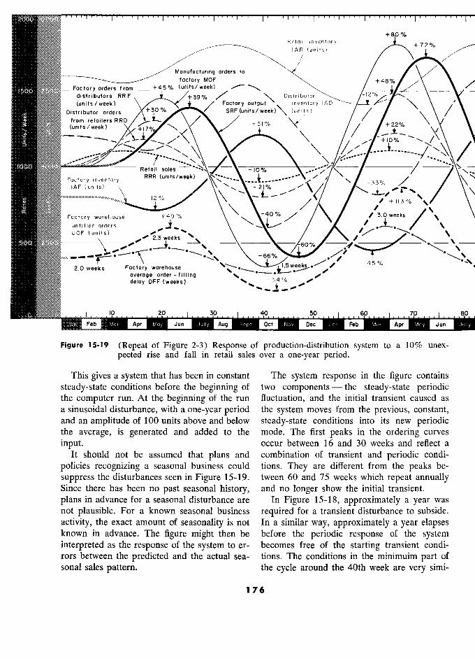
2000 i i I i....,....i...., ...I ...,... i... ,....I
+eo % Retcii inventory y
IAR (units) °
Manufacturinq orde 0 //o
factory MOF
1500 Factory orders from - t45 % (units/week) '
distributors RRF F <
Distributor 12
(units/week) Factory output `
inventory IAD \ .
Distributor orders SRF (units / week) (units) /
/ from retailers RRD
t22 % i (units /week l
,
°
/ +22% ' W
''' '' ............ \
' . / '
/ ------- ' _, \
\ /
1000 b Retail sales -10% -''j/ .
Factory inventory RRR
-- _-"_,__--" ' / , / IAF (units) - 2 1 /
-12 % t il 3
Factory worehouse '
q
40 / /
/ 3.0 weeks
%
1', untilled orders , ' ,
UOF F ( u n 1 t s ) ' , , UOF (units) 3 weeks
- 60 % '
5 0 0 ' 6
0
- -66*. '
2.0 weeks Factory warehouse -45 %
average order-filling *14 , delay DFF (weeks) ? 54
% ,,
C) 10 20 ....... 6p, 70 0
Feb Apr Jun Aug ?Dec?Jun??M
Figure 15-19 (Repeat of Figure 2-3) Response of production-distribution system to a 10% unex-
pected rise and fall in retail sales over a one-year period.
This gives a system that has been in constant The system response in the figure contains
steady-state conditions before the beginning of two components - the steady-state periodic the computer run. At the beginning of the run fluctuation, and the initial transient caused as a sinusoidal disturbance, with a one-year period the system moves from the previous, constant, and an amplitude of 100 units above and below steady-state conditions into its new periodic the average, is generated and added to the mode. The first peaks in the ordering curves
input. occur between 16 and 30 weeks and reflect a It should not be assumed that plans and combination of transient and periodic condi-
policies recognizing a seasonal business could tions. They are different from the peaks be-
suppress the disturbances seen in Figure 15-19. tween 60 and 75 weeks which repeat annually Since there has been no past seasonal history, and no longer show the initial transient.
plans in advance for a seasonal disturbance are In Figure 15-18, approximately a year was not plausible. For a known seasonal business required for a transient disturbance to subside.
activity, the exact amount of seasonality is not In a similar way, approximately a year elapses known in advance. The figure might then be before the periodic response of the system interpreted as the response of the system to er- becomes free of the starting transient condi- rors between the predicted and the actual sea- tions. The conditions in the minimuim part of sonal sales pattern. the cycle around the 40th week are very simi-
176
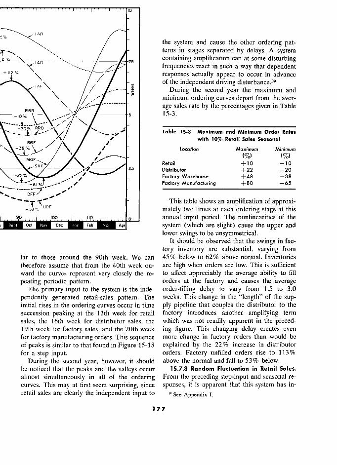
IAR V. [AR the system and cause the other ordering pat-
° /
' the system and cause the other ordering pat-
/ . - terns in stages separated by delays. A system containing amplification can at some disturbing
+62% / frequencies react in such a way that dependent
\ responses actually appear to occur in advance
// / of the independent driving disturbance.29
1 AF "
During the second year the maximum and
\ \ minimum ordering curves depart from the aver-
\ \ age sales rate by the percentages given in Table RRR \ \w F 5 ico 5 15-3.
/ Table 15-3 Maximum and Minimum Order Rates
\ /'/ / with 10% Retail Sales Seasonal
/ \ / Location Maximum Minimum
V?OF / X (%1 (%) MOF
MO SRF ` Retail 0 -10 0 ––––\" 2.5 Distributor +22 -20 65 % Factory Warehouse +48 -38
Factory Manufacturing +80 -65 ,' ––––––––––––––––––––––
, q'
, / ' This table shows an amplification of approxi-
53% _ mately two times at each ordering stage at this
so loo j 110 o annual input period. The nonlinearities of the
oct '.' M(ir 1
Apt 0
system (which are slight) cause the upper and lower swings to be unsymmetrical.
It should be observed that the swings in fac-
tory inventory are substantial, varying from lar to those around the 90th week. We can 45% below to 62% above normal. Inventories therefore assume that from the 40th week on- are high when orders are low. This is sufficient ward the curves represent very closely the re- to affect appreciably the average ability to fill
peating periodic pattern. orders at the factory and causes the average The primary input to the system is the inde- order-filling delay to vary from 1.5 to 3.0
pendently generated retail-sales pattern. The weeks. This change in the "length" of the sup- initial rises in the ordering curves occur in time ply pipeline that couples the distributor to the succession peaking at the 13th week for retail factory introduces another amplifying term
sales, the 16th week for distributor sales, the which was not readily apparent in the preced- 19th week for factory sales, and the 20th week ing figure. This changing delay creates even for factory manufacturing orders. This sequence more change in factory orders than would be of peaks is similar to that found in Figure 15-18 8 explained by the 22% increase in distributor for a step input. orders. Factory unfilled orders rise to 113%
During the second year, however, it should above the normal and fall to 53% below. be noticed that the peaks and the valleys occur 15.7.3 Random Fluctuation in Retail Sales. almost simultaneously in all of the ordering From the preceding step-input and seasonal re- curves. This may at first seem surprising, since sponses, it is apparent that this system has in- retail sales are clearly the independent input to 29 See Appendix I.
' 177
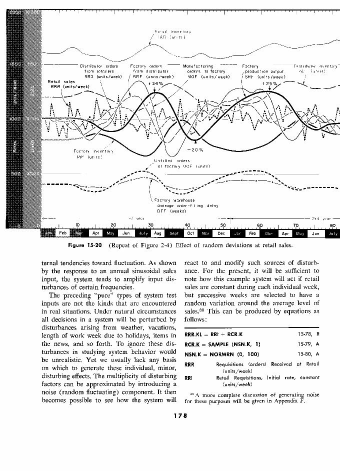
2000 . 1 1 1 1 1 1 1 11 1 1 , 1 , , - , 1 , , 1 1 r=
Retail inventory IAR (units
1500 Distribulor orders-Factory orders Manufocturing Factory Distributor inventor from retailers from distributor orders tofactory production output IAD (units)
Retaii saies RRD (units/week) /RRF (units/week) MOF (units/week) SRF (units/week)
RRR (units/week) , _ -
j2 , - ,
1000 , '
c
a: Fciclory inventory
Unfilied orders Urifilied orders at factory UOF (units)
500 .... --"""----........ ,,
....!....
..
j worehouse !
"
M j 60 j 70 ! 80
Factory warehouse
avercige order-fillinq deloy DFF (weeks)
0 ... 10 ........ 20.
Ist
year 4p, .j* 1 610....... 70 2nd year -
Apr JUIY M Sept m Nov m Jan m Mc., m MCY mi
Figure 15-20 (Repeat of Figure 2-4) Effect of random deviations at retail sales.
ternal tendencies toward fluctuation. As shown react to and modify such sources of disturb-
by the response to an annual sinusoidal sales ance. For the present, it will be sufficient to
input, the system tends to amplify input dis- note how this example system will act if retail
turbances of certain frequencies. sales are constant during each individual week, The preceding "pure" types of system test but successive weeks are selected to have a
inputs are not the kinds that are encountered random variation around the average level of
in real situations. Under natural circumstances sales.10 This can be produced by equations as
all decisions in a system will be perturbed by follows : disturbances arising from weather, vacations, –––––––––––––––––––––––––––-
length of work week due to holidays, items in RRR.KL RRI + RCR.K 15-78, R
the news, and so forth. To ignore these dis- RCR.K SAMPLE (NSN.K, 1) 15-79, A turbances in studying system behavior would (0, 100) 15-80, A be unrealistic. Yet we usually lack any basis
RRR Requisitioris (orders) Received at Retail . RRR Requisitions (orders) Received at Reta!! on which to generate these mdividual, mmor,
disturbing effects. The multiplicity of disturbing RRI Retail Réquisitions, Initial rate, constant
factors can be approximated by introducing a (uriits/week)
noise (random fluctuating) component. It then 30 A complete discussion generating noise
becomes possible to see how the system will for these purposes will be given in Appendix F.
178 8
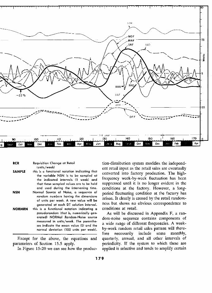
10
IAR
MOF
RRF \//SRF -75
o
fl
',
i -
,; àb SRF
,
A A 4 A .... '
5
,
RRR '£/
22% \. IAF \_y
25
DFF
year
Sept Dec Feb M(ir Jun JUIY Sept m Nov Feb &Pr
RCR Réquisition Change at Retail tion-distribution system modifies the independ- (units/week) ent retail input as the retail sales are eventually SAMPLE this is functionat notation
indicating that t into factory production. Thé thé variable NSN is to be sampled art -'
the indicated intervals (1 week) and frequency week-by-week fluctuation has been
that thèse sampled values are to be held suppressed until it is no longer évident in the and used during the intervening time. conditions at the factory. However, a long-
NSN Normal Source of Noise, a séquence of period fluctuating condition at the factory has
randomnumbershaving the dimensions... random numbers having ..... e arisen. It clearly is caused by the retail random- of units per week. A new value will be Y
generated at each DT solution interval. ness but shows no obvious correspondence to
NORMRN this is a functional notation indicating a conditions at retail. pseudorandom (that is, numerically gen- As will be discussed in Appendix F, a ran- erated) NORMal Random-Noise source dom-noise séquence contains components of measured in units/week. The measured in units/week. The e a wide range of dînèrent frequencies. A week- ses indicate thé mean value (0) and thé
a wi e range o i eren requencies, wee -
normal déviation (100 units per week). by-week random retail sales pattern will there- –––––––––––––––––––––––––––– fore necessarily include some monthly,
Except for the above, the equations and quarterly, annual, and all other intervals of
parameters of Section 15.5 apply. periodicity. If the system to which these are
In Figure 15-20 we can see how the produc- applied is selective and tends to amplify certain
179
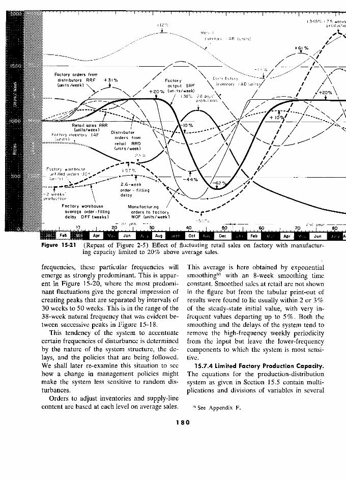
... I I , I "
+345% =75 wee + 12 % produc
Retai I ,1 inventory I AR (units)
''
+31% ??tory
Factory orders from // Distributory
/
d.str.butors RPF F +3!% Faetory ` Distributory /
(units /week) output SRF \ inven/tory I AD (units? / '
/ /
\ / +20% (units/week) +38 % =
/ - /
'+20%
°
`
produCtion
,
+ /
,
', ,
... Retail sales RRR
`
`
-10 % -
+IÔ%q/ /' ·' //
`
\ Retail sciles RRR -10 % , ,
(units/week) Distributor
\ ------- /
Factory inventory IAF orders frorri
`
/ i
\ / /
(units) orders from ` ' '
O 1' / '
`\ (units/week) \ /
/
Factory warehouse
\
+
% \
\ / `
))t)tN) Factory warehouse UOF
/ unfilled orders UOF 500 (units)
.0 * -' -44% (units)
' -44 %
-62 % /
.
, order - filling , =2 weeks' delay
filling % #0
production deloy --- *
production Factory warehouse Manufacturing / 00
overage order-fillinq orders to factory
deloy DFF (weeks) MOF (units/week)
j« 2nd - Ist ye r - - 55 % 2nd year
0 .... 10 .... 20 60 ?0 . 1 1 1 1 01
?Dec???H
Figure 15-21 (Repeat of Figure 2-5) Effect of fluctuating retail sales on factory with manufactur- ing capacity limited to 20% above average sales.
frequencies, these particular frequencies will This average is here obtained by exponential emerge as strongly predominant. This is appar- smoothing,"' with an 8-week smoothing time ent in Figure 15-20, where the most predomi- constant. Smoothed sales at retail are not shown nant fluctuations give the général impression of in the figure but from the tabular print-out of
creating peaks that are separated by intervals of results were found to lie usually within 2 or 3% 30 weeks to 50 weeks. This is in the range of the of the steady-state initial value, with very in- 38-week natural frequency that was evident be- frequent values departing up to 5Yv . Both the tween successive peaks in Figure 15-18. smoothing and the delays of the system tend to
This tendency of the system to accentuate remove the high-frequency weekly periodicity certain frequencies of disturbance is determined from the input but leave the lower-frequency by the nature of the system structure, the de- components to which the system is most sensi-
lays, and the policies that are being followed. tive. We shall later re-examine this situation to see 15.7.4 Limited Factory Production Capacity. how a change in management policies might The equations for the production-distribution make the system less sensitive to random dis- system as given in Section 15.5 contain multi- turbances. plications and divisions of variables in several
Orders to adjust inventories and supply-line content are based at each level on average sales. "'See Appendix E.
180
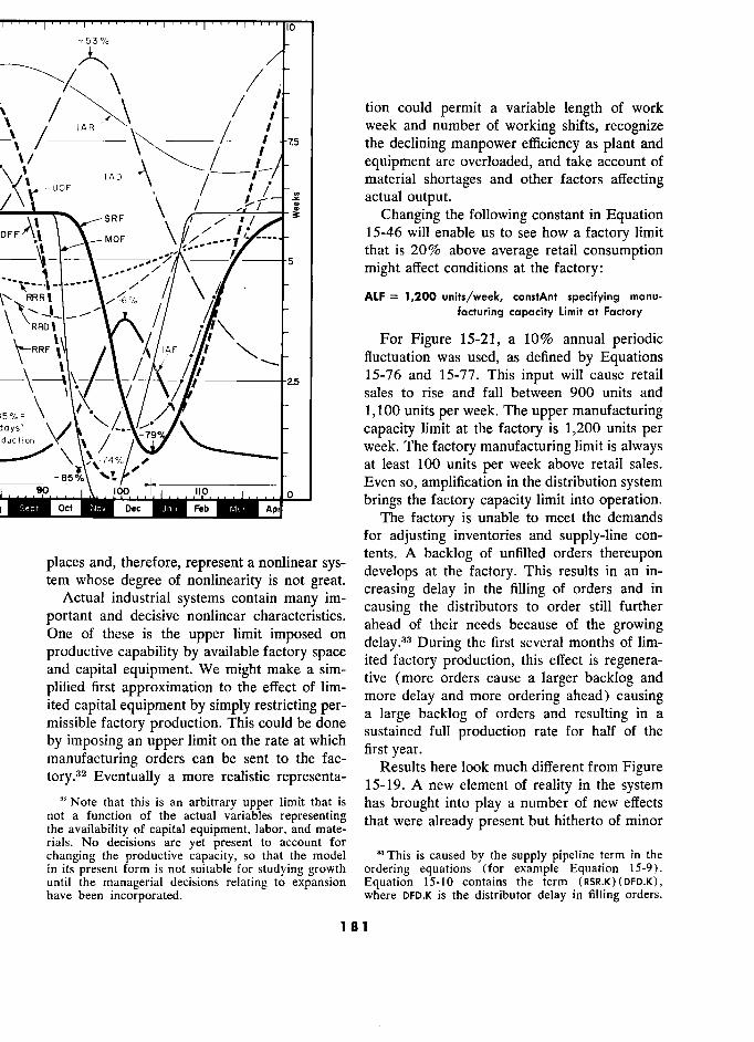
10
/ "
/ / / tion could permit a variable length of work
, /
` / week and number of working shifts, recognize
) , the declining manpower efficiency as plant and / equipment are overloaded, and take account of
t UOF 1 AD ` /
/ material shortages and other factors affecting \ actual output.
SRF 3 Changing the following constant in Equation MoF 15-46 will enable us to see how a factory limit
7 5 that is 20% above average retail consumption
t ./ ''i
/ 5
might affect conditions at the factory:
RRRI I
/j / .
ALF = 1,200 units/week, constAnt specifying manu-
// '
facturing capacity Limit at Factory \ // t iAF
For Figure 15-21, a 10% annual periodic RRF 1 fluctuation was used, as defined by Equations
1 \- \ 15-76 and 15-77. This input will cause retail
\ V sales to rise and fall between 900 units and
,, = ) \'\ 1,100 units per week. The upper manufacturing rs' '
capacity limit at the factory is 1,200 units per -79. week. The factory manufacturing limit is always -
at least 100 units per week above retail sales. Even so, amplification in the distribution system
o o
brings the factory capacity limit into operation. Feb Ap. The factory is unable to meet the demands
for adjusting inventories and supply-line con- , tents. A backlog of unfilled orders thereupon
places and, therefore, represent a nonlinear sys- tents. A backlog tem whose degree of nonlinearity is not great. develops at the
factory. This results in an in- tem whose degree of non inean y is not
1 - . , ° . , - . ° . creasins delay m thé nilins of or ers and m Actual industrial systems contain many im- creasing delay in the filling of orders and in ? c ua ? in ? ? us na .. systems con ain ? many causins thé distributors to order still turther
portant and decisive nonlinear characteristics. causing the distributors to
order still further a ea of eir needs because of thé e growing One of these is the upper limit imposed on aheads of their needs
because of the growing
detay."" Dunns thé hrst several months of Iim- productive capability by available factory space first several months
of lim-
and . equipment. ' . ited factory production, this effect is regenera- and capital equipment. e mig ma e a sim- _, and capital equipment. We might make a 1.
tive (more orders cause a larger backlog and phned rs approximation to thé ect of im- . plified first approximation to the effect of per-
more delay and more ordering ahead) causing g ited capital equipment y simp y res nc ing per- -
missible factory production. This restnctlllg per- a large backlog of orders and resulting in a
missibie factory production. This could be done sustained full production rate for half r on the could at done
sustained full production rate for half of thé e by imposing an upper limit on the rate at which
manufacturing orders can be sent to the fac- first year. i oo u igure manu 32 actunng or ers can
realistic ta t e ac-
Results here look much different from Figure tory. Eventually a more reahshc representa- 15-19. A new élément of reality in thé system
* Note that this is an arbitrary upper limit that is has brought into play a number of new effects not a function of the actual variables representing that were already present but hitherto of minor the availability of capital equipment, labor, and mate- -' rials. No decisions are yet present to account for changing the productive capacity, so that the model 3A This is caused by the supply pipeline term in the in its present form is not suitable for studying growth ordering equations (for example Equation 15-9). until the managerial decisions relating to expansion Equation 15-10 contains the term (RSR,K) (DFD,K), have been incorporated. where DFD.K is the distributor delay in filling orders.
181 1
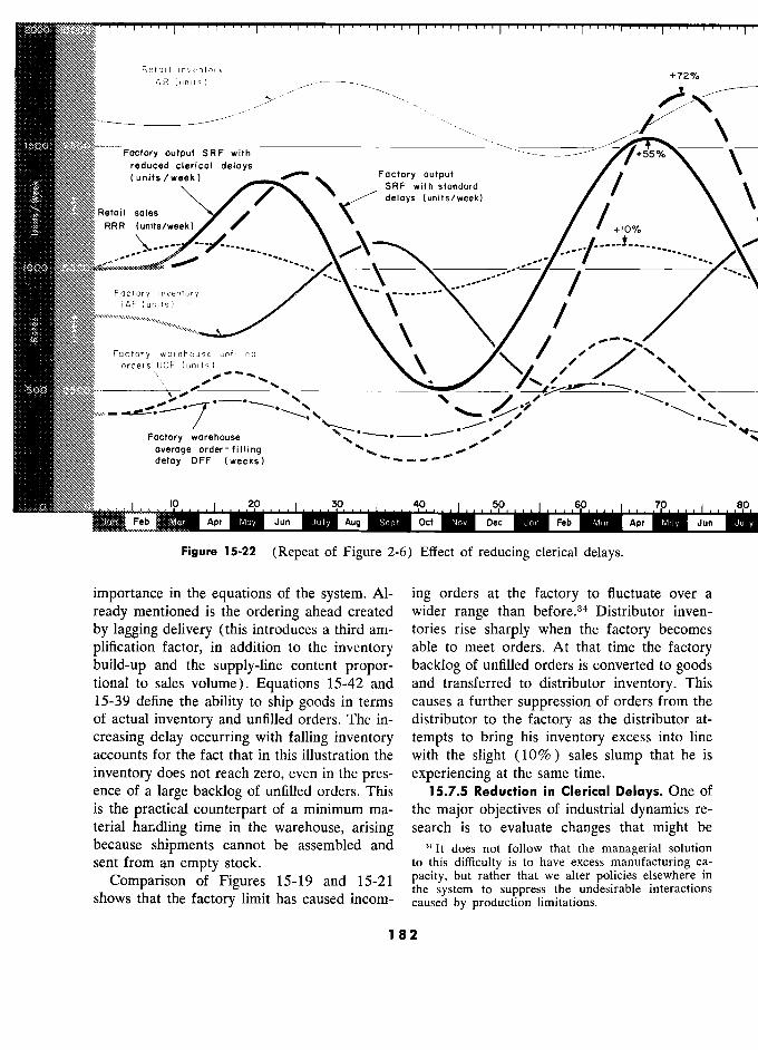
2000 10000 I , I , I
Retail inventory IAR (units) 1
°
1500 7500 Factory output SRF with
( reduced ciericul delays ( units /week ) Factory output
/ SRF with standard
] delays (units/week)
Retail
sales RRR (units/week)
__i ._
............................
.
... .
100019-
Factory inventory 7
[AF (units) 1 &F (units l
, /
/
Factory warehouse unfilled
, '- ', orders UOF (unlls)
l -
"'}
, '
w .. ·
- -=".-
Factory warehouse , ,'
, -,,
average order-filling ',, ,,' delay DFF (weeks)
0 ,. 10 .... 1 20 10.... 40 6p.... 7p.... Jon Mar Jun Aug M Sept Dec Feb m Apr May
Figure 15-22 (Repeat of Figure 2-6) Effect of reducing clerical delays.
importance in the equations of the system. AI- ing orders at the factory to fluctuate over a
ready mentioned is the ordering ahead created wider range than before.34 Distributor inven-
by lagging delivery (this introduces a third am- tories rise sharply when the factory becomes
plification factor, in addition to the inventory able to meet orders. At that time the factory build-up and the supply-line content propor- backlog of unfilled orders is converted to goods tional to sales volume). Equations 15-42 and and transferred to distributor inventory. This 15-39 define the ability to ship goods in terms causes a further suppression of orders from the of actual inventory and unfilled orders. The in- distributor to the factory as the distributor at-
creasing delay occurring with falling inventory tempts to bring his inventory excess into line accounts for the fact that in this illustration the with the slight ( lo 9l ) sales slump that he is
inventory does not reach zero, even in the pres- experiencing at the same time. ence of a large backlog of unfilled orders. This 15.7.5 Reduction in Clerical Delays. One of is the practical counterpart of a minimum ma- the major objectives of industrial dynamics re- terial har.dling time in the warehouse, arising search is to evaluate changes that might be because shipments cannot be assembled and It does not follow that the managerial solution sent from an empty stock. to this difficulty is to have excess manufacturing ca-
Comparison of Figures 15-19 and 15-21 pacity, but rather that we alter policies elsewhere in , , , the system to suppress the undesirable interactions
shows that the factory limit has caused incom- caused by production limitations.
182 2
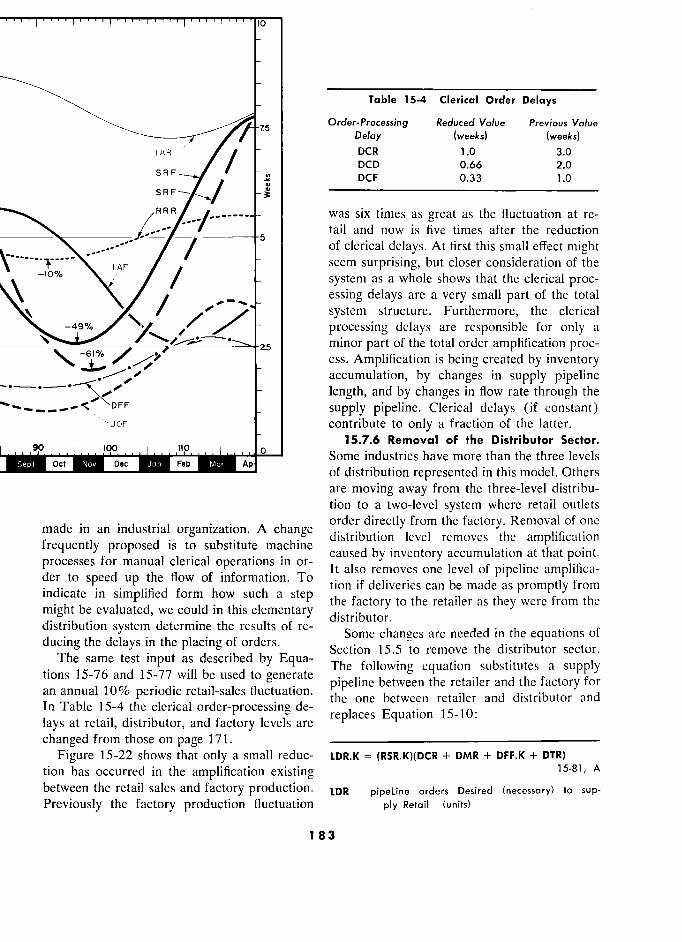
'''
Table 15-4 Clerical Order Delays
Order-Processing Reduced Value Previous Value Delay (weeks) (weeks)
I AR .// '
DCR 1.0 3.0
RF / / DCD 0.66 2.0 2 DCF 0.33 1.0
SRF
–––––––––––
R was six times as gréât as the fluctuation at re- tail and now is five times after the reduction
.._ __ / /
-5 of clerical delays. At first this small effect might
IAF -
seem surprising, but closer consideration of the ' / system as a whole shows that the clerical proc-
_ essing delays are a very small part of the total / system structure. Furthermore, the clerical
-49% processing delays are responsible for only a minor part of the total order amplification proc- ess. Amplification is being created by inventory accumulation, by changes in supply pipeline
' '-' '
length, and by changes in flow rate through the DFF _ supply pipeline. Clerical delays (if constant)
\uoF contribute to only a fraction of the latter. 15.7.6 Removal of the Distributor Sector.
tM?t ' ' 0 Some industries have more than the three levels of distribution represented in this model. Others are moving away from the three-level distribu- tion to a two-level system where retail outlets order directly from thé factory. Rcmoval of onc
made in an industrial organization. A change distribution level removes the amplification frequently proposed is to substitute machine distribution level renioves the amplification t requen propose is o su s i u e mac
inc causedbymventory that
processes for manual clérical operations in or- caused by inventory accumulation at that point. ,. It so removes one cvc of pipc i c a p -
der to speed up the flow of information. To It also removes one level of pipeline amplifica- „ Ion 1 e lvenes can e ma as prompuy from indicate in simplified form how such a step tion if deliveries can
be made
as promptly from c might be evaluated, we could in this elementary
the factory to the retailer as they were from the mig be evaluated, we could m this elementary
'
distribution systein determine the results of f " distributor.
distribution system détermine thé results of re- Some needed in the equations of lstn utlOn System detcrmllle t e resu
ts a re- Some changes are needed in thé équations ot f
ducing the delays in the placing of orders. arc needed in the equations of .
The same test input as described by Equa- Section 15.5 to reniove the distributor sector. tions 15-76 and 15-77 will be used to gencrate The following equation substitutes a supply tions 15-76 and 15-77 ... will be used ta gencrate pipe . 1. me between thé retailer and thé tactory for
an annual 10% periodic retail-sales fluctuation. pipeline between retailer and distributor and
In Table 15-4 the clérical order-processing de- re 1 aces E qua t. Ion 15 - 1 0 and
distributor
lays at retail, distributor, and factory levels are p q 15-10:
changed from those on page 171. ––––––––––––––––––––––––––––
Figure 15-22 shows that only a small reduc- LDR.K = (RSR.K)(DCR + DMR + DFF.K + DTR) tion has occurred in the amplification existing 15-81, A
between the retail sales and factory production. LDR pipeline orders Desired (necessary) to sup-
Previously the factory production fluctuation ply Retail (units)
183 3
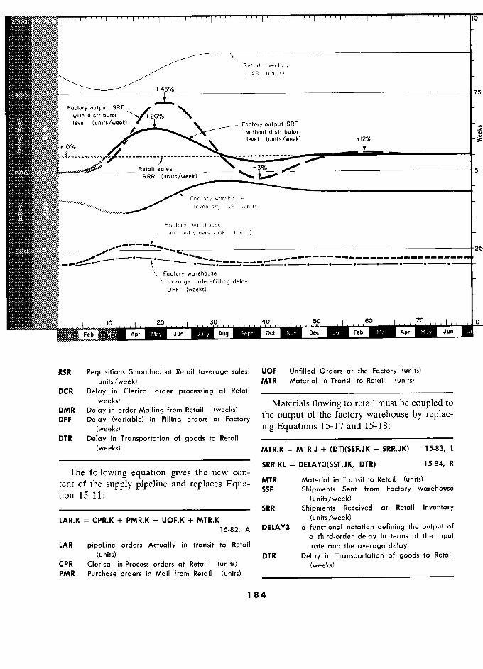
2000 aaa? IC
Relail inventory 1 AR (units)
+45% -7
Factory output SRF ,
-Ï-
7
Factory output SRF with distributor "' level (units/week) '
Foctory output SRF 3: L. _ without distributor
+10% level (units/week) +12%
+10%
` Retail sales j: 1000
ï RRR (units/week) .
\ Factory warehouse
inventory IAF (units)
Factory warehouse filled orders UOF (units)
- y Í
500 00
_
warehouse
- - - - - - - - - - - - - - - - - -
Foctory worehouse
\ average order-filling deloy DFF (weeks)
, 10 1 20 1
30 Aug Sept M 10.....50 .... Jan
.... 7p .... LI
Feb m Mar Jun Aug Oct Nov Feb Apr May
RSR Requisitions Smoothed at Retail (average sales) UOF Unfilled Orders at the Factory (units)
(units/week) MTR Material in Transit to Retail (units)
DCR Delay in Clerical order processing at Retail
(weeks) Materials flowing to retail must be coupled to DMR Delay in order Mailing from Retail (weeks)
DFF Delay (variable) in Filling orders ar Factory the output of the factory warehouse by replac- (weeks) ing Equations 15-17 and 15-18:
DTR Delay in Transportation of goods to Retail
(weeks) MTR.K = MTR.J + (DT)(SSF.JK - SRR.JK) 15-83, L
SRR.KL = DELAY3(SSF.JK, DTR) 1 5-84, R
The following equation gives the new con-
SRR.KL =
DELAY3(SSF.JK, DTR)
15-84, R
tent of the supply pipeline and replaces Equa- MTR Material in Transit to Retail (units)
tion 15 Il' SSF Shipments Sent from Factory warehouse
(units/week)
SRR Shipments Received at Retail inventory
LAR.K = CPR.K + PMR.K + UOF.K + MTR.K (units/week)
15-82, A DELAY3 a functional notation defining the output of '
a third-order delay in terms of the input
LAR pipeline orders Actually in transit to Retail rate and the average delay (units) DTR Delay in Transportation of goods to Retail
CPR Clerical in-Process orders at Retail (units) (weeks)
PMR Purchase orders in Mail from Retail (units)
184
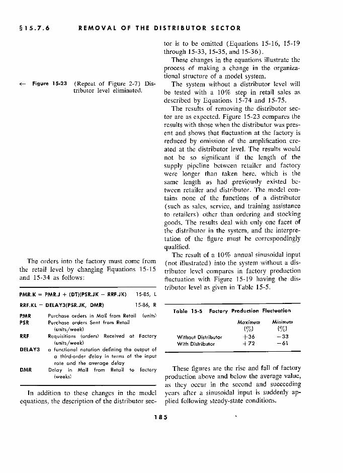
§ 15.7.6 REMOVAL OF THE DISTRIBUTOR SECTOR
tor is to be omitted (Equations 15-16, 15-19
through 15-33, 15-35, and 15-36). These changes in the equations illustrate the
process of making a change in the organiza- tional structure of a model system.
Figure 15-23 (Repeat of Figure 2-7) Dis- The system without a distributor level will tributor level eliminated. be tested with a 10% step in retail sales as
described by Equations 15-74 and 15-75. The results of removing the distributor sec-
tor are as expected. Figure 15-23 compares the
results with those when the distributor was pres- ent and shows that fluctuation at the factory is reduced by omission of the amplification cre-
ated at the distributor level. The results would
not be so significant if the length of the
supply pipeline between retailer and factory were longer than taken here, which is the
same length as had .previously existed be-
tween retailer and distributor. The model con-
tains none of the functions of a distributor
(such as sales, service, and training assistance
to retailers) other than ordering and stocking
goods. The results deal with only one facet of
the distributor in the system, and the interpre- tation of the figure must be correspondingly
qualified. The result of a 10% annual sinusoidal input
The orders into the factory must come from (not illustrated) into the system without a dis- the retail level by changing Equations 15-15 tributor level compares in factory production and 15-34 as follows: fluctuation with Figure 15-19 having the dis- –––––––––––––––––––––––––––– tributor level as given in Table 15-5. PMR.K = PMR.J + (DT)(PSR.JK - RRF.JK) 15-85, L
RRF.KL = DELAY3(PSR.JK, DMR) 15-86, R
PMR Purchase orders in Mail from Retail (units) Table 15-5 Factory Production Fluctuation
PMR Purchase orders Sent from Retail (units)
Maximum Minimum PSR Purchase orders Sent from Retail Maximum Minimum
(units/week) (%) (%) RRF Requisitions (orders) Received at Factory Without Distributor +36 -33
(units/week) With Distributor +72 -61 DELAY3 a functional notation defining the output of
a third-order delay in terms of the input rate and the average delay
DMR Delay in Mail from Retail to factory These figures are the rise and fall of factory (weeks) production above and below the average value,
–––––––––––––––––––––––––––– as they occur in the second and succeeding In addition to these changes in the model years after a sinusoidal input is suddenly ap-
equations, the description of the distributor sec- plied following steady-state conditions.
185 ,
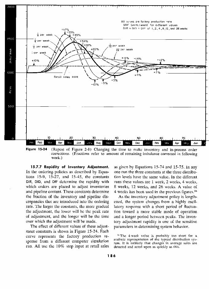
2000
AIl curves are factory production rate
)tt)t) - SRF (units /week) for different values
Ntt? D 1 R = D i O = D i F of 1 , 2 , 4 , 8 , 12 , ùnd 26 wee ks
per week
1500 e
per week +45%
+34% ,
per week \
. v
i§ Per week per week
+281/. per week Z per week \ +28 %
+20 Per 26 week per week
3z 1 per week /
\
+1 \
v \ +15% % +14% %
+12%
+io% %
// //
v
\
\ \
y _
+12 %
. //
__ ____.___`
------ -
1000 /
+7%
Retail sales RRR ',
J' -3%
- io%
%
- 10 % -9 %
500
0 10 20 ! 30 ! 40 ! 50 ! 60 !
&pr 70 ! j
Feb Mar Jun Aug. Sept M Nov
M Jan m Apr M"y
Figure 15-24 (Repeat of Figure 2-8) Changing the time to make inventory and in-process order corrections. (Fractions refer to amount of remaining imbalance corrected in following week.)
15.7.7 Rapidity of Inventory Adjustment. as given by Equations 15-74 and 15-75. In any In the ordering. policies as described by Equa- one run the three constants at the three distribu- tions 15-9, 15-27, and 15-45, the constants tion levels have the same value. In the different
DIR, DID, and DIF determine the rapidity with runs these values are 1 week, 2 weeks, 4 weeks,
, which orders are placed to adjust inventories 8 weeks, 12 weeks, and 26 weeks. A value of and
pipeline content. These constants determine 4 weeks has been used in the
previous figures . 35
the fraction of the inventory and pipeline dis- As the inventory adjustment policy is length- crepancies that are introduced into the ordering ened, the system changes from a highly oscil- rate. The larger the constants, the more gradual latory response with a short period of fluctua- the adjustment, the lower will be the peak rate tion toward a more stable mode of operation of adjustment, and the longer will be the time and a longer period between peaks. The inven- over which the adjustment will be made. tory adjustment rapidity is one of the sensitive
The effect of different values of these adjust- parameters in determining system behavior. ment constants is shown in Figure 15-24. Each curve represents the factory production re- 35 The 4-week value is probably too short for a
sponse from . . . realistic representation of the typical distribution sys-
sponse from a dînèrent tem. It is unlikely that changes in average sales are run. AIl use the 10% step input at retail sales detected and acted upon as quickly as this.
186
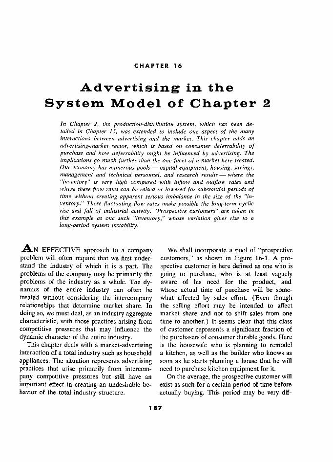
CHAPTER 16
Advertising in the
System Model of Chapter 2
In Chapter 2, the production-distribution system, which has been de- tailed in Chapter 15, was extended to include one aspect of the many interactions between advertising and the market. This chapter adds an
advertising-market sector, which is based on consumer deferrability of purchase and how deferrability might be influenced by advertising. The
implications go much further than the one facet of a market here treated. Our economy has numerous pools - capital equipment, housing, savings, management and technical personnel, and research results - where the
"inventory" 1,ç very high compared with inflow and outflow rates and where these flow rates can be raised or lowered for substantial periods of time without creating apparent serious imbalance in the size of the "in-
ventory." These fluctuating flow rates make possible the long-term cyclic rise and fall of industrial activity. "Prospective customers" are taken in this example as one such "inventory," whose variation gives rise to a
long-period system instability.
AN EFFECTIVE approach to a company We shall incorporate a pool of "prospective problem will often require that we first under- customers," as shown in Figure 16-1. A pro- stand the industry of which it is a part. The spective customer is here defined as one who is
problems of the company may be primarily the going to purchase, who is at least vaguely problems of the industry as a whole. The dy- aware of his need for the product, and namics of the entire industry can often be whose actual time of purchase will be some- treated without considering the intercompany what affected by sales effort. (Even though relationships that determine market share. In the selling effort may be intended to affect
doing so, we must deal, as an industry aggregate market share and not to shift sales from one
characteristic, with those practices arising from time to another. ) It seems clear that this class
competitive pressures that may influence the of customer represents a significant fraction of
dynamic character of the entire industry. the purchasers of consumer durable goods. Here This chapter deals with a market-advertising is the housewife who is planning to remodel
interaction of a total industry such as household a kitchen, as well as the builder who knows as
appliances. The situation represents advertising soon as he starts planning a house that he will
practices that arise primarily from intercom- need to purchase kitchen equipment for it.
pany competitive pressures but still have an On the average, the prospective customer will
important effect in creating an undesirable be- exist as such for a certain period of time before havior of the total industry structure. actually buying. This period may be very dif-
187
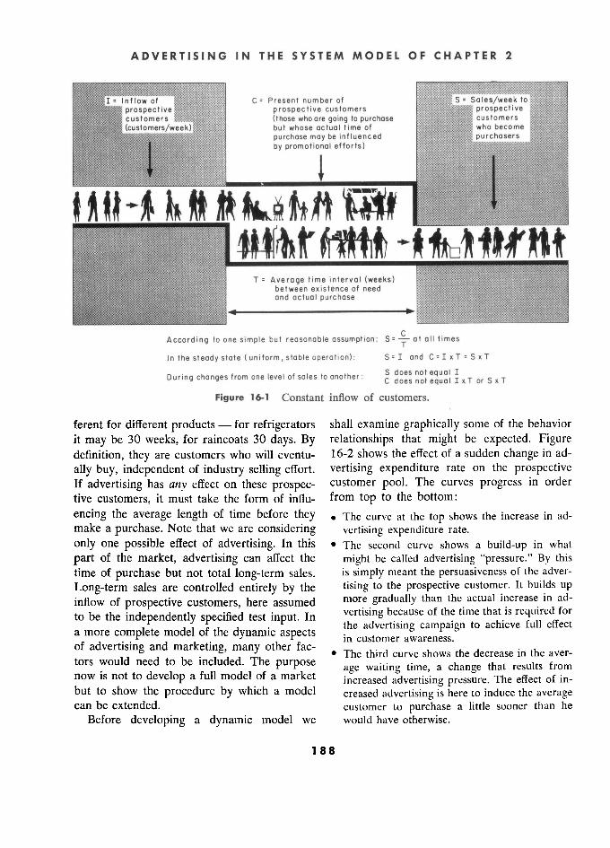
ferent for different products - for refrigerators shall examine graphically some of the behavior it may be 30 weeks, for raincoats 30 days. By relationships that might be expected. Figure definition, they are customers who will eventu- 16-2 shows the effect of a sudden change in ad-
ally buy, independent of industry selling effort. vertising expenditure rate on the prospective If advertising has any effect on these prospec- customer pool. The curves progress in order
tive customers, it must take the form of influ- from top to the bottom:
encing the average length of time before they . The curve at the top shows the increase in ad- make a purchase. Note that we are considering vertising expenditure rate.
only one possible effect of advertising. In this 0 The second curve shows a build-up in what
part of the market, advertising can affect the might be called advertising "pressure." By this time of purchase but not total long-term sales. is simply meant the persuasiveness of the adver-
Long-term sales are controlled entirely by the tising to the prospective customer. It builds up inflow of prospective customers, here assumed more gradually than the actual increase in ad-
to be the independently specified test input. In vertising because of the time that is required for , .. , , - thé advertisms campaisn to achieve tull ettect
a more complète model of the dynamic aspects the advertising campaign to achieve full effect
of advertising and marketing, many other fac- in customer awareness.
e a - tors would need to be included. The purpose
The third curve shows the decrease in the aver- tors would need to be induded. The purpose age waiting time, that results from now is not to develop a full model of a market increased advertising pressure. that effect of in- but to show the procedure by which a model creased advertising is here to induce the average can be extended. customer to purchase a little sooner than he
Before developing a dynamic model we would have otherwise.
188 8
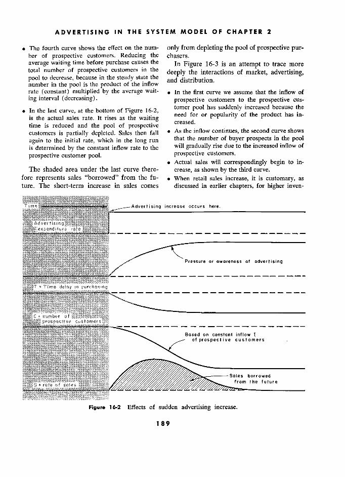
ADVERTISING 1 N THE SYSTEM MODEL OF CHAPTER 2
The fourth curve shows the effect on the num- only from depleting the pool of prospective pur- ber of prospective customers. Reducing the chasers. average waiting time before purchase causes the In Figure 16-3 is an attempt to trace more total number of prospective customers in the
deeply the interactions of market, advertising, pool to decrease, because in the steady state the and distribution.
' ,
number in thé pool is the product of the m ow rate (constant) multiplied by the average wait- « In the first curve we assume that the inflow of inginterval (decreasing). prospective customers to the prospective cus-
ï In the last curve, at the bottom of Figure tomer pool has suddenly increased because thé
. In thé last curve, at thé bottom of Figure 16-2, is the actual sales rate. It rises as the waiting need for or popularity of the product bas in-
is thé actuat sales rate. It nses as thé waiting time is reduced and the pool of prospective customers is partially depleted. Sales then fat! 8 As the inflow continues, the second curve shows
again to the initial rate, which in the long run that the number of buyer prospects in the pool is determined by the constant inflow rate to the will gradually rise due to the increased inflow of
prospective customer pool. prospective customers.
e Actual sales will correspondingly begin to in- The shaded area under the last curve there- crease, as shown by the third curve.
fore represents sales "borrowed" from the fu- 8 When retail sales increase, it is customary, as ture. The short-term increase in sales cornes discussed in earlier chapters, for higher inven-
T i m e Advertising increase occurs here.
t u r e r a t e
Pressure or awareness of advertising
T Ti me delay in purchosing .............
C number of f prospective cu
Based on constant inflow 1 o prospective customers s .
Sales borrowed from the future e
Figure 16.2 Effects of sudden advertising increase.
189
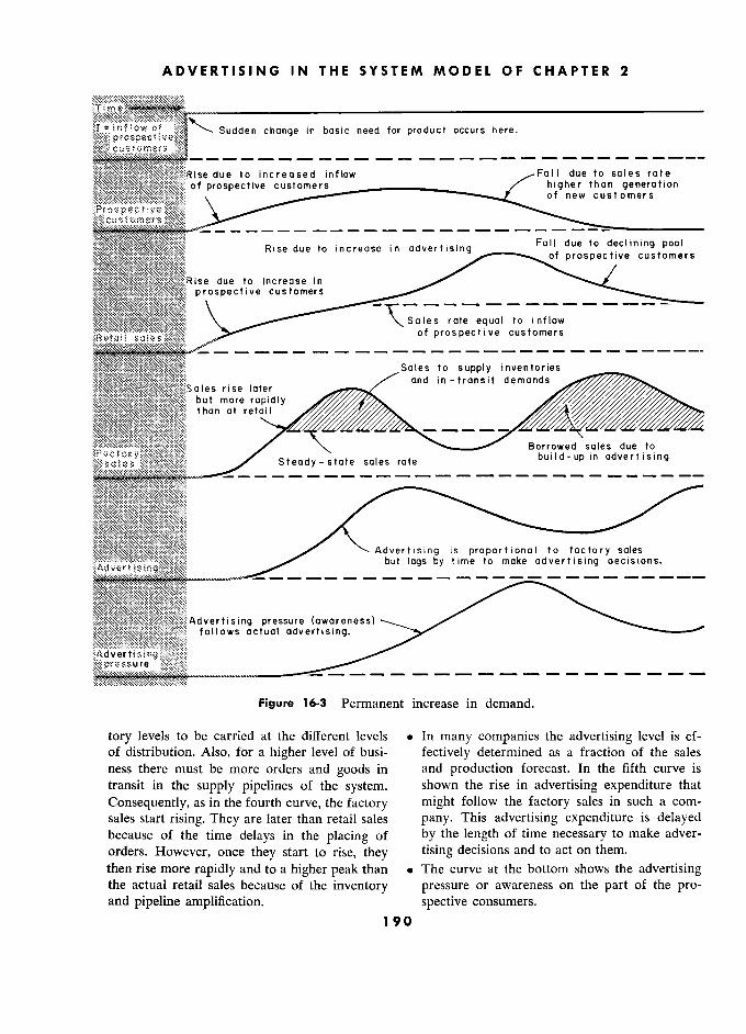
ADVERTISING IN THE SYSTEM MODEL OF CHAPTER 2
?-infiowof Sudden change in basic need for product occurs hère.
customers Î DL14Ï?'R ise due to incre(ised inflow F(i 11due ta sales rate Fall due to sales raIe ofprospective eustomers higher than génération
of new customers
u r
?????????g??????,? of prospective customers
Rise due to increase in p rospe ctive customers
\
-
Saies rate equat to inflow o prospective customers
Sales to supply inventories
es rise later and in-transit i dema ds
Sales rise later but more ropii ly thon at retail
Borrowed sales due ta
Steady-state sales rate build-up in advertising
Advertising is proportional to factory sales but lags by time ta make advertisirig decisions.
?t!t!Z!??t!!!!S!!N?dvertisin9 pressure (awareness) f ollo ws actual advertising.
Figure 16-3 Permanent increase in demand.
tory levels to be carried at the different levels e In many companies the advertising level is ef-
of distribution. Also, for a higher level of busi- fectively determined as a fraction of the sales
ness there must be more orders and goods in and production forecast. In the fifth curve is
transit in the supply pipelines of the system. shown the rise in advertising expenditure that
Consequently, as in the fourth curve, the factory might follow the factory sales in such a com-
sales start rising. They are later than retail sales pany. This advertising expenditure is delayed because of the time delays in the placing of by the length of time necessary to make adver-
orders. However, once they start to rise, they tising decisions and to act on them.
then rise more rapidly and to a higher peak than e The curve at the bottom shows the advertising the actual retail sales because of the inventory pressure or awareness on the part of the pro- and pipeline amplification. spective consumers.
190
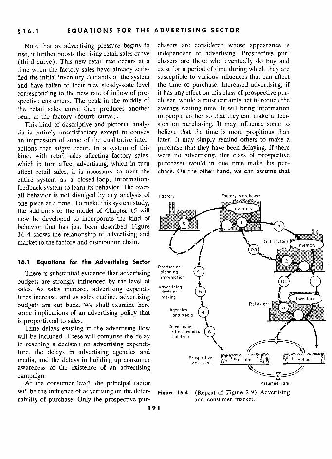
§16.1 1 EQUATIONS FOR THE ADVERTISING SECTOR
Note that as advertising pressure begins to chasers are considered whose appearance is
rise, it further boosts the rising retail sales curve independent of advertising. Prospective pur- (third curve). This new retail rise occurs at a chasers are those who eventually do buy and
time when the factory sales have already satis- exist for a period of time during which they are
fied the initial inventory demands of the system susceptible to various influences that can affect
and have fallen to their new steady-state level the time of purchase. Increased advertising, if
corresponding to the new rate of inflow of pro- it has any effects on this class of prospective pur-
spective customers. The peak in the middle of chaser, would almost certainly act to reduce the
the retail sales curve then produces another average waiting time. It will bring information
peak at the factory (fourth curve). to people earlier so that they can make a deci-
This kind of descriptive and pictorial analy- sion on purchasing. It may influence some to
sis is entirely unsatisfactory except to convey believe that the time is more propitious than
an impression of some of the qualitative inter- later. It may simply remind others to make a
actions that might occur. In a system of this purchase that they have been delaying. If there
kind, with retail sales affecting factory sales, were no advertising, this class of prospective which in turn affect advertising, which in turn purchaser would in due time make his pur- affect retail sales, it is necessary to treat the chase. On the other hand, we can assume that
entire system as a closed-loop, information-
feedback system to learn its behavior. The over-
all behavior is not divulged by any analysis of Fa c tory Factory worehouse
one piece at a time. To make this system study, a a
the additions to the model of Chapter 15 will a, Inventory
now be developed to incorporate the kind of T, behavior that has just been described. Figure
' .
6 ' 2
16-4 shows the relationship of advertising and
market to the factory and distribution chain. D i str i bu tor s
1 R%.. ::
16.1 Equations for the Advertising Sector Production '
: Production i
There is substantial evidence that advertising planning. _
budgets are strongly influenced by the level of information
o.5
sales. As sales increase, advertising expendi- Advertising (e) f, , g P decision
tures increase, and as sales decline, advertising making & Inventory
budgets are cut back. We shall examine here Agencies
Retmlers 3 3
some implications of an advertising policy that ond medio 4
is proportional to sales. Time delays existing in the advertising flow Advertising \
effectivene 6 will be included. These will comprise the delay build-u
in reaching a decision on advertising expendi- v ture, the delays in advertising agencies and ., media, and the delays in building up consumer
Prospective purc oses 9 months . i Public
awareness of the existence of an advertising
purchoses
campaign. At the consumer level, the principal factor Assumed rote
will be the influence of advertising on the defer- Figure 16-4 (Repeat of Figure 2-9) Advertising rability of purchase. Only the prospective pur- and consumer market.
191 1
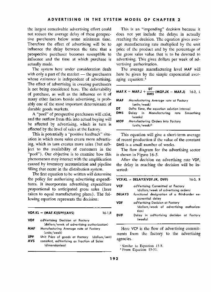
ADVERTISING IN THE SYSTEM MODEL OF CHAPTER 2
the largest conceivable advertising effort could This is an "impending" decision because it not reduce the average delay of these prospec- does not yet include the delays in actually tive purchasers below some minimum time. reaching the decision. The equation gives aver- Therefore the effect of advertising will be to age manufacturing rate multiplied by the unit influence the delay between the time that a price of the product and by the percentage of
prospective purchaser becomes susceptible to the gross sales value that is to be devoted to influence and the time at which purchase is advertising. This gives dollars per week of ad-
actually made. vertising authorization. The system here under consideration deals The average manufacturing level MAF will
with only a part of the market - the purchasers here be given by the simple exponential aver- whose existence is independent of advertising. aging equation:l
1
The effect of advertising in creating purchasers ____________________________ is not being considered here. The deferrability MAF.K = MAF.J + DT (MOF.JK - MAF.J) 16-2, L of purchase, as well as the influence on it of
' ' DMS
'
many other factors beside advertising, is prob- MAF Manufacturing Average rate at Factory ably one of the most important determinants of (units/week) durable goods markets. DT Delta Time, the équation solution interval
: A "pool" of prospective purchasers will exist, DMS Delay in Manufacturing rate Smoothing
d h fl f h.. 1 b..11 (weeks) and the outflow from this into actual buying will
Facrory an t e out ow rom t IS mto actua UYlllg o MOF Manufacturing Orders into Factory be affected by advertising, which in turn is (units/week)2 affected by the level of sales at the factory. ––––––––––––––––––––––––––
This is potentially a "positive feedback" situ- This equation will give a short-term average ation in which more sales create more advertis- of recent production if the value of the constant
ing, which in turn creates more sales (but sub- DMS is a small number of weeks.
ject to the availability of customers in the The flow diagram for the advertising sector
"pool"). Our objective is to examine how this is shown in Figure 16-5.
phenomenon may interact with the amplification After the decision on advertising rate VDF, caused by inventory accumulation and pipeline the delay in reaching the decision will be in-
filling that occur in the distribution system. serted: The first equation to be written will determine ._________________________
the policy for authorizing advertising expendi- VCF.KL = DELAY3(VDF.JK, DVF) 16-3, R tures. It incorporates advertising expenditure VCF advertising Committed at Factory proportional to anticipated gross sales (here (dollars/week of advertising orders) taken to equal manufacturing plans). The fol- DELAY3 functional désignation of a third-order ex-
lowing equation represents the decision: ponential delay VDF adVertising Décision at Factory
–––-_______________________________ (dollars/week of advertising authoriza-
VDF.KL = (MAF.K)(UPF)(AVS) 16-1,R DVF Delay tion) in adVertising decision at Factory DVF e ay ln a ertlslng dec!S!on at Factory VDF adVertising Décision at Factory (weeks)
(dollars/week of advertising authorization) –––––––––––––––––––––––––––––––––––––
MAF Manufacturing Average rate at Factory Here VCF is the flow of advertising commit- (units/week) ments from the factory to the advertising UPF Unit Price of goods at Factory (dollars/unit)
ageriCles. AVS constAnt, adVertising as fraction of Sales e l S.
(dimensionless) 1 Similar to Equation 15-8. _________________________________ 'From Equation 15-51.
' 192
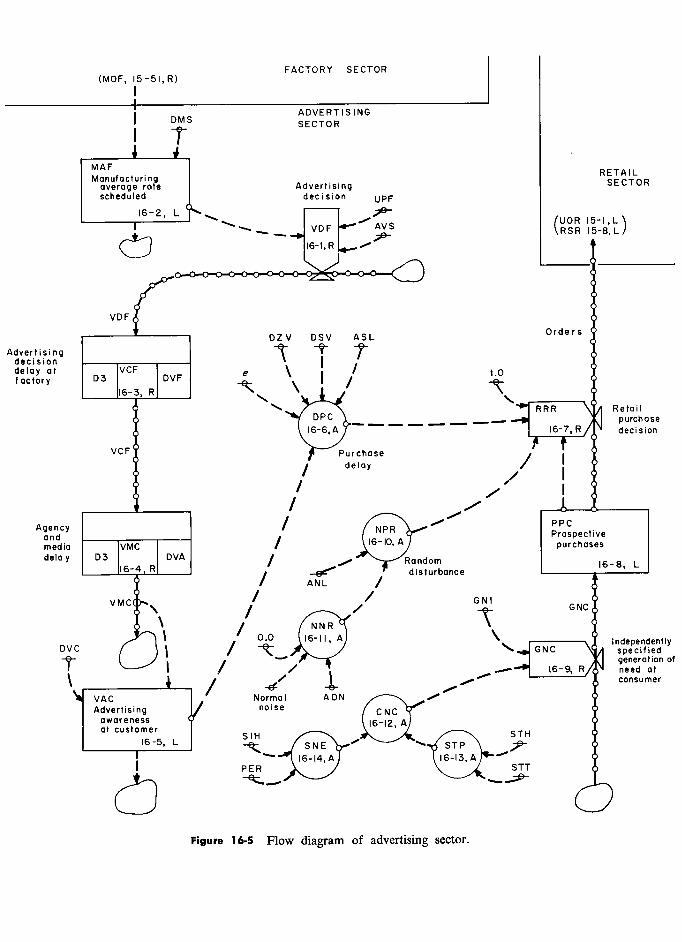
FACTORY SECTOR (MOF, 15-51, R)
FACTOR' "CTOR
1 1
j
1 ADVERTISING
1 SECTOR
MAF . RETAIL Manufacturing RETAIL
average rate Advertising SECTOR
scheduled decision UpF
16-2 L ––––
UOR 15-1, L !
I AVS
(RSR 15-8, L - - VDF R5R 15-B,L L
)
VDFR
0--O--O--O-O-< .
A VDF
DZV DSV ASL Orders
advertising ' j' 0
decision ––––,–––––.–––– '
1 , i delay at
VCF
)VF e \
) / .0 o Y
factory
D3 DVF ! /
&
' 0
RRR
Retail A DPC _ _ _ _ _ _ _
16 X purchase
16-6,A 16-7,R decision
VCF Purchase ' '
?
<
1
1 delay
/ 1
1
1 V
/ /
! /
Agency /
/
// PPC
Agency ____________ 1
NPR Q" Prospective and media ia VMC / purchases
dela y y D3 16-4 vmc DVA
1 Random ,68 , L R
/
' /
' disturbance
, ? / ANL / '
VMC GNI GNC
GNI
S NNR À,
y
/ independent!y DVC
t / t / GNC spect-fied
i- t
y , . '-' A generation ai
Î / / 16-9, R need at 01
\ t / consumer \ /
consumer
VAC Normal ADN / V
Advertising J/ noise
V awareness Y Y at customer
S lH '
STH 16-5 L
51H SNE STP 5TH - SNE
–– ? STP \ 0
Y
PER /
Y
U
""
'"
ô
Figure 16-5 Flow diagram of advertising sector.
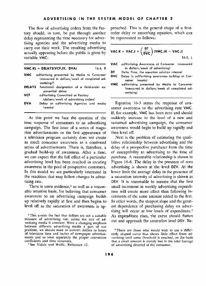
ADVERTISING IN THE SYSTEM MODEL OF CHAPTER 2
The flow of advertising orders from the fac- proached. This is the general shape of a first-
tory should, in turn, be put through another order delay or smoothing equation, which can
delay representing the time necessary for adver- be represented as follows:
tising agencies and the advertising media to ____________________________
carry out their work. The resulting advertising / pT \
actually appearing before the public is given by VAC.K = VAC.J + (VMC.JK - VAC.J)
variable VMC: \
16-5, L
VAC advertising Awareness at Consumer (measured VMC.KL = DELAY3(VCF.JK, DVA) 16-4, R in dollars/week of advertising)
DT Delta Time, the équation solution interval VMC adVertising presented by Média to Consumer pVC Delay in adVertising awareness buildup at Con-
(measured in dollars/week of completed ad- sumer (weeks) vertising)3 VMC adVertising presented by Média to Consumer
DELAY3 functional désignation of a third-order ex- (measured in dollars/week of completed ad- ponential delay vertising)
VCF adVertising Committed at Factory (dollars/week of advertising orders)
DVA Delay at adVertising Agencies and média Equation 16-5 states the response of con- (weeks) sumer awareness to the advertising rate VMC.
–––––––––––––––––––––––––– If, for example, VMC has been zero and should At this point we face the question of the suddenly increase to the level of a new and
time response of consumers to an advertising sustained advertising campaign, the consumer
campaign. The first issue of a series of maga- awareness would begin to build up rapidly and zine advertisements or the first appearance of then level off. a television program certainly does not create Next is the problem of estimating the quali- as much consumer awareness as a continued tative relationship between advertising and the series of advertisements. There is, therefore, a delay of a prospective purchaser from the time
gradual build-up of awareness. After a time, of susceptibility to advertising to the time of we can expect that the full effect of a particular purchase. A reasonable relationship is shown in
advertising level has been reached in creating Figure 16-6. The delay in the presence of zero awareness in the pool of prospective customers. advertising is shown at the level DZV. At the In this model we are particularly interested in lower limit the average delay in the presence of the reactions that may follow changes in adver- a saturation intensity of advertising is shown as
tising rate. DSV. It is reasonable to assume that the first There is some evidence,4 as well as a reason- small increment in weekly advertising expendi-
able intuitive basis, for believing that consumer ture will create more effect than following in- awareness to an advertising campaign builds crements of the same amount added to the first.
up relatively rapidly at first and then begins to In other words, the steepest slope and the great- level off as the saturation of awareness is ap- est dependence of purchasing delay on adver-
tising will occur at low levels of expenditure.5 g This avoids the fact that dollars are not a suitable As expenditure rises, the curve should flatten
measure of advertising rate unless the
mix of ad- out and approach the saturation level DSV. Be- vertising média is constant. Were a changing emphasis between different advertising media a part of our problem, we should need to convert dollars to hours 5 There are those who would wish to use a differ- of television time and inches of newspaper advertise- ently shaped curve that shows little effect from ad- ments and to treat separately the proper conversion vertising until some threshold is reached, on the basis coefficients and time constants. that a small amount is merely lost in the total barrage
See Vidale and Wolfe, Reference 12. of advertising directed at the consumer.
194
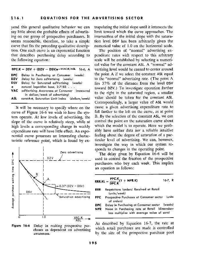
§ 16.1 1 EQUATIONS FOR THE ADVERTISING SECTOR
yond this general qualitative behavior we can trapolating the initial slope until it intersects the
say little about the probable effects of advertis- limit toward which the curve approaches. The
ing on our group of prospective purchasers. It intersection of the initial slope with the satura- seems reasonable, therefore, to take a simple tion level DSV has been arbitrarily given the curve that fits the preceding qualitative descrip- numerical value of 1.0 on the horizontal scale. tion. One such curve is an exponential function The position of "normal" advertising ex- that describes purchasing delay according to penditure rates with respect to this arbitrary the following equation: scale will be established by selecting a numeri- ____________________________ cal value for the constant ASL. A "normal" ad- DPC.K = DSV + (DZV - DSV)e-VAC.K/ASL 16-6, A vertising level would be caused to center around
DPC Delay in Purchasing at Consumer (weeks) the point A if we select the constant ASL equal DZV Delay for Zéro adVertising (weeks) to the "normal" advertising rate. (The point A DSV Delay for Saturated adVertising (weeks) lies 37% of the distance from the level DSV e natural logarithm base, 2.7183 ... toward DZV.) To investigate operation further VAC adVertising Awareness at Consumer (measured
iri the Il in dollars/week of advertising) ) ? ? nght m thé saturated région, a smaller
ASL constAnt, Saturation Limit index (dollars/week) value should be taken for the constant ASL.
____________________________ Correspondingly, a larger value of ASL would
It will be necessary to specify where on the cause a given advertising expenditure rate to
curve of Figure 16-6 we wish to have the sys- fall farther to the left on the curve, as at point tem operate. At low levels of advertising, the B. By the selection of the constant ASL, we can
slope of the curve is relatively steep, while at control the point on the saturation curve about
high levels a corresponding change in weekly which the model is to operate. Here we prob-
expenditure rate will have little effect. An expo- ably have neither data nor a reliable intuitive
nential curve possesses an interesting charac- feeling about the degree of saturation of a par- teristic reference point, which is found by ex- ticular level of advertising. We can, however,
investigate the way in which our system re-
Zero advertising sponds to changes in the operating point.
f zv
Zero cdvertlslng The delay given by Equation 16-6 will be e
u - - - - - used to control the fraction of the prospective :5 \ 7 purchasers who buy each week. This implies
/ an equation as follows:
B B ––––––––––––––––––––––––––––––––––– c
1 A PPC K \\i/ RRR.KL = '(i
+ NPR.K) 16-7, R
\ DSV) DPC.K
DSV ' 1 RRR Requisitions (orders) Received at Retail (units/week) 5. ";7s
- - -:- (units/week) .
<1> .\ adverti sinq PPC Prospective Purchases at Consumer sector (units
go of orders) 1 DPC Delay in Purchasing at Consumer sector (weeks)
a I NPR Noise in Purchasing rate at Retail (dimension-
_________!______________________ less multiplier with average value of zero) a LO VAC. K
ASL - , _
Figure 16-6 6 Delay in making prospective pur- As described by Equation 16-7, the rate at
Figure - Delay in making prospective pur- ..) chases as dependent on advertising
retail purchases are made is controlled
awareness. by the size of the prospective purchase pool
195 5
ADVERTISING IN THE SYSTEM MODEL OF CHAPTER 2
PPC and the average delay before purchasing advertiser and purchase chain and which are
DPC. The noise term NPR is to be used for in- independent inputs. One of these is the noise
troducing uncertainty fluctuations into the pur- input used in Equation 16-7. Weekly sales or-
chase rate. It will be defined later. dinarily fluctuate owing to causes that we do not
The prospective purchases in the pool PPC hope to represent in a system model. These will
is given by a simple level equation based on the be approximated by a noise input that will vary inflow and the outflow: successive weekly purchasing rates. This noise
____________________________ input will be represented by two equations. The
PPC.K = PPC.J + (DT)(GNC.JK - RRR.JK) 16-8, L first of these will sample a noise variable and
PPC Prospective Purchases at Consumer sector will hold that sample available for the duration
PPC Prospective Purchases at Consumer sector (units of , of, for example, 1 week. The second describes
GNC Generation of Need at Consumer sector the noise source that is being sampled. (units/week of prospective purchases)
RRR Requisitions (orders) Received at Retail _ SAMPLE 16-10, A . (units/week) NPR.K SAMPLE , ' ANL) 16-10, ' A
––––––––––––––––––––––––––––––––––––– NPR Noise in Purchasing rate at Retail (dimen-
The inflow the prospective purchase pool 1 sionless multiplier with average value of zero)
is the rate of génération of need for the product SAMPLE a functional notation indicating that the GNC. For the purposes of the present investiga- variable is to be sampled and held until
tion, this will be taken as an arbitrarily specified the next sampling time
input. It takes the place of the arbitrarily speci- NNR Normal Noise at Retail (dimensionless)
- constAnt, Noise samp!e Length (weeks) fied retail sales rate RRR, which was previously y ANL constant, Noise sample length (weeks)
used for testing the production-distribution chain itself. By specifying the generation of The number to be sampled and held by need rather than arbitrarily specifying retail Equation 16-10 is taken from a normal distri-
purchases, we have introduced a further re- bution of random noise as defined by the fol-
finement and a higher degree of reality in the lowing equation:
system that we are studying. The generation of __________________________
prospective purchases will therefore be de- NNR.K = NORMRN (0.0, ADN) 16-11, A scribed by the following equation: NNR Normal Noise at Retail _, (dimensionless) ––––––––––––––––––––––––––––––––––––– NORMRN functional notation indicating NORMal GNC.KL = GNI + CNC.K 16-9, R Random Noise
GNC Generation of Need , at Consumer secror 0.0. mean value of the noise
GNC Need at Consumer sector ... ? .. r ?. - , !. ,-
(units/week of prospective purchases) . ADN constAnt, standard Deviation of Noise (di-
(units/week of prospective purchases) . 1 ) _.„ '. ,...,. , , , .. mens!on!ess) GNI Generation of Need, Initial rate (units/week) mensioniess)
CNC Change in Need at Consumer sector (units/week) For the test input CNC in Equation 16-9, we
–––––––––––––––––––––––––––– may wish to use one or more of several inputs.
The initial rate GNI is the past steady-state One of these might be a step input wherein the level of business activity and is a constant. Any rate of generation of need takes on some new variations on this level which we may wish to value that then continues. A second common use for test purposes can be described by suit- type of test input would be a sine wave used able variations in the change term CNC. to represent seasonal and other fluctuating cir-
There now remain to be defined several cumstances. For convenience, these inputs will variables which are not directly involved in the be combined in the following equation, where
196
§ 16.2 2 INITIAL-CONDITION EQUATIONS S
each input can be controlled by its own generat- steady-state rate of orders at the factory RRF : 6
ing equation: ––––––––––––––––––––––––––––
_______________________________ MAF = RRF 16-15, N
CNC.K = STP.K + SNE.K 16-12, A MAF Manufacturing Average rate at Factory
CNC Change in Need at Consumer sector (units/week)
(units/week) RRF Réquisitions (orders) Received at Factory
„-- .,/ ,. STP STeP, test input (units/week) (units/week)
SNE the SiNE variable used as a test input –––––––––––––––––––––––––––––––––––
(units/week) Since the rate of flow VDF is an input to a ____________________________ delay function, its initial rate must be defined
The step input to be used in Equation 16-12 by an initial-condition equation. This rate will
can be defined in terms of the amplitude of the be determined only by the average manufac-
step and the time at which it occurs as given in turing rate MAF multiplied by unit price and by the following equation: the fraction of gross receipts going to advertis-
____________________________ ing: STP.K = STEP(STH, STT) 16-13, A
VDF = (MAF)(UPF)(AVS) 16-16, N STP STeP, test input (units/week) STEP a functional notation indicating that a STEP VDF adVertising Décision at Factory
change is to be generated (dollars/week of advertising authorization)
STH STep Height, test input (units/week) MAF Manufacturing Average rate at Factory
STT STep Time after beginning of the model run at (units/week)
which the step occurs (weeks) UPF Unit Price of goods at Factory (dollars/unit)
_____________________________________ AVS constAnt, adVertising as fraction of Sales (di-
mension?ess) A sine-wave input for the test function can mensionless)
be provided by the following equation: With the rate VDF given, the initial steady- –––––––––––––––––––––––––––– state outflow rate VCF from the advertising de-
SNE.K = A cision delay is necessarily identical.7 17 Likewise SNE.K =
1 PER 1 16-14, A
VCF, as the input to the agency delay, deter- L J '
VCF, as the input to the agency delay, deter-
SNE the SiNE variable used as a test input mines the output VMC.
(units/week) An initial-condition equation is necessary SIH Slne Height, test input (units/week) for the level of advertising awareness VAC. In S)N
afunct!onai notat!onmd!cat!ng a sme fluctua-
the steady state this will be equal . the constant ' SIN
a tion functlonal
notation indicating a sine fluctua- the steady state this will be equal to the constant
TIME the independent time variable generated by level of advertising expenditure rate VMC:
DYNAMO (weeks) –––––––––––––––––––––––––––––––––––––
PER sine PERiod, test input (weeks) VAC = VMC 16-17, N
.., VAC adVertising Awareness at Consumer (measured This completes the active equations needed in dollars/week of advertising)
to add the advertising sector to the production- VMC adVertising presented by Média to Consumer
distribution model of Chapter 15. (measured in dollars/week of completed ad-
vertising).
16.2 Initial-Condition Equations –––––––––––––––––––––––––––
..... 6 As determined by Equation 15-6R.
Equations are necessary for generating initial ; The DYNAMO computer compiler, which is here
conditions for levels and SOme rates. assumed to be available, will automatically generatc
Under steady-state conditions the average these subsidiary initial conditions arising from the
- ' .. ° outflow from delays and will make them available as level of manufacturing MAF will equal the
necessary to other initial-condition calculations.
197
ADVERTISING IN THE SYSTEM MODEL OF CHAPTER 2
An operating point in steady state must be Finally, it will be necessary to specify a chosen on the curve of Figure 16-6. This will steady-state initial condition for retail sales RRR be accomplished by selecting a value for ASL; for use in the retail sector:8 ASL can be defined by an initial-condition equa- –––––––––––––––––––––––––––– tion in terms of the value of the advertising RRR = GNI 16-21, N
awareness VAC. For initial studies of the sys- RRR Réquisitions (orders) Received at Retail tem, we shall select a "normal" operating point (units/week) at A which is obtained when the following equa-
GNI Génération of Need, Initial rate (units/week) tion holds: –––'––––––––––––––––––––––––
____________________________ This completes the initial-condition equa-
ASL = VAC 16-18, N tions necessary for starting the combined ' production-distribution-advertising system in
ASL constAnt, Saturation Limit index (dollars/week) stead -state operation. VAC adVertising Awareness at Consumer (measured y '
in dollars/week of advertising) 16.3 3 Values 0 f C ons t an t s
In order to determine the steady-state level Numerical values of the constants must be
In order to determine the steady-state level chosen before the model is complete. of prospective purchases PPC, it will be neces- It should be noted that values must be speci- sary to have a value for the steady-state pur- fied for the unit price UPF and for the fraction chasing delay. This value is determined by se- of gross revenue being spent for advertising lecting the steady-state operating delay from AVS. But neither of thèse constants has a direct Figure 16-6. This is best done by writing the effect on the behavior of thé system. The selec- steady-state equivalent of Equation 16-6 as fol-
constant ASL in Equation 16-6 over- lows: rides the numbers selected for UPF and AVS –––––––––––––––––––––––––– and completely determines the relationship be- DPC = DSV + (DZV - DSV)e-VAC/ASL 16-19, N tween steady-state advertising and the point on
DPC Delay in Purchasing at Consumer level (weeks) the advertising saturation curve in Figure 16-6. DZV Delay for Zéro adVertising (weeks) The preceding initial-condition equations that DSV Delay for Saturated adVertising (weeks) set ASL in terms of VAC will cause ASL to com- e natural logarithm base, 2.7183 ...
lri UPF arid AVS. VAC adVertising Awareness at Consumer (measured .
f in dollars/week of advertising) ) followlng arbitrary sélection will therefore suf-
ASL constAnt Saturation Limit index (dollars/week) fice:
'–––––––––––––––––––––––––––––––––––– UPF = 100 dollars, Unit Price of goods at Factory
The steady-state level 1 prospective pur- AVS = 0.06 dimensionless constAnt, advertising as Ihe s ea y-s a e level ot prospective pur- fraction of Sales
c ases e equa to l ow fraction of Saies
chases PPC will be equal to the uniform inflow fraction of Sales
or outüow multiplied by the average delay ex- Delays in the advertising system must now
perienced in the "pool": be specified. The following plausible values will be taken without detailed justification:
PPC = (RRR)(DPC) 16-20, N DMS = 4 weeks, Delay in Manufacturing rate Smooth- ' '
ing PPC Prospective Purchases at Consumer level (units DVF = 6 weeks, Delay in adVertising décision at Fac-
of orders) tory RRR Requisitions (orders) Received at Retail
DVA 4 , ... at ,., .... , d DVA = 4weeks, Delay at adVertising Agencies and (units/week) media DPC Delay in Purchasing at Consumer level (weeks) media
________________________________ 8 This replaces Equation 15-54.
198 8
§ 16.4 BEHAVIOR OF SYSTEM WITH ADVERTISING
The "time constant" for the rate at WhiCh v The pipeline and inventory adjustment times of 4
advertising awareness will respond to a change weeks (DIR, DID, and DIF) in Section 15.5.5 have
. d f' . ht r h b t been changed to 8 weeks as a more likely reaction in advertising might lie somewhere between
been changed ta 8 weeks as a more likely reaction III a ver ISlllg mlg le somew ere e ween time: 4 weeks and 12 weeks. We shall here take DIR = DID = DIF = 8 weeks
DVC = 6 weeks, Delay in adVertising awareness build- . The half-week mail delays DMR and DMD in up at Consumer level
Chapter 15 are the limiting factors in deter-
For consumer durable goods, the length of mining how long the solution interval DT may time taken for a prospective purchase to be- be. Incorporating these delays separately in the
come an actual retail order may vary over a model is easily shown (by observing system
wide time range from almost immédiate pur- performance before and after a change) to
, e
hme range from ? . r make a neshsible différence in system behav-
chase up to several years. Our estimates of a make a negligible difference in system behav- fi?
° ior. In exploring the new modes of behavior normal average time will not be very reliable, with the advertising sector included, we en- nor will our estimates of the maximum value counter manufacturing fluctuations with peri- DZV in Figure 16-6 or the minimum value DSV. ods as long as two years or more. Model runs We can, however, pick some plausible values of several times the natural period of the system and then see what effect changes in these values are of interest. For run lengths of five to ten
would have on system behavior. Therefore we years, a solution interval of 0.05 week begins shall here take the following estimated values to use appréciable computing time." It is there-
for the constants shown in Figure 16-6: fore worth while to combine the mailing delay ' with the clerical order-processing delays at the
DZV = 70 weeks, Delay for Zéro adVertising retail and distributor levels. Such does not
DSV = 15 weeks, Delay for Saturated adVertising change the length of the supply pipelines but
only the number of pieces into which they are As m the study of the production-distribution divided. The retail purchasing delay DCR then
system by itself, we shall take the steady-state becomes 3.5 weeks; and at the distributor, DCD retail sales rate as becomes 2.5 weeks. Equations 15-15, 15-16,
GNI = 1,000 units/week, Génération of Need, Initial 15-33, and 15-34 are omitted. Equation 15-14
rate is altered to define orders flowing to the dis-
.., tributor RRD, and Equation 15-32 to define or- The following constants determine test condi- ders to the factory RRF.
tions for various runs on the model and must With the preceding changes, thé shortest third- 1 the preceding changes, the shortest third- be given values for each study to be made: " order delays in the system are 1 week, and the ADN constAnt, standard Déviation of Noise (dimen- solution interval DT can be extended to 0.1
sionless) week. Further increase in the solution interval ANL constAnt, Noise sample Length (weeks) could be obtained (again with no important PER sine PERiod, test input (weeks) change in dynamic behavior) by changing the SIH Sine Height, test input (units/week) shorter third-order delays in the system to first- STH STep Height, test input (units/week) order delays, but such has not been done for STT STep Time after start of model run (weeks) the following model runs.1°
Sections 16.1 through 16.3 have developed the model description of a very simplified ad- 16.4 Behavior of System with Advertising
vertising and market sector to be added to the The preceding sections have developed the
production-distribution model of Chapter 15. advertising and market additions to the distri-
The équations and constants of Section 15.5 s Some 15 minutes per run on an IBM 704 com-
apply except for the following: puter. 10 ln Appendix B is a tabulation of the equations
, Equation 16-21 replaces 15-54. and constants of this extended model.
199
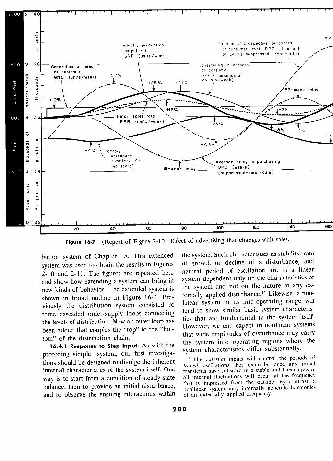
12 12 40 ... , , , . , , ,
c:
-
::J Industry production
Number of prospective purchases +9.
o output rate at consumer level PPC (thousands 1'
SRF (units/week) of units)(suppressed-zero scale) ./ /'
9 38 Generation of need
SRF (units/week)
Advertising awareness r
at customer at consumer
GNC (units/week) 1. ° VAC (thousands of GNC
(un __17 +24% dollars/week)
/37-week
/
delay
./"'"
/37-week delay
É
$
Î
ù À
_l 0_ /
'
6 36
"'"
6 ......... Retail sales
rate - , --.--.-........ -
/ RRR
(units /week):-...; +2 5% % ,1'
-------
......
/"/ 8% -7%
ô ' ----- '......
8% -7% - " ...................- \
--/'.
· _
N /. "
0 # warehouse L a inventory IAF T ?Average delay in purchasing
3 34 delay DPC (weeks) 3 34
(suppressed-zero scale)
0 ' Z
g > g
à
t
D 32
20 40 60 80 100 120 140 16
Figure 16-7 (Repeat of Figure 2-10) Effect of advertising that changes with sales.
bution system of Chapter 15. This extended the system. Such characteristics as stability, rate
system was used to obtain the results in Figures of growth or decline of a disturbance, and
2-10 and 2-11. The figures are repeated here natural period of oscillation are in a linear
and show how extending a system can bring in system dependent only on the characteristics of
new kinds of behavior. The extended system is the system and not on the nature of any ex-
shown in broad outline in Figure 16-4. Pre- ternally applied disturbance.11 Likewise, a non-
viously the distribution system consisted of linear system in its mid-operating range will
three cascaded order-supply loops connecting tend to show similar basic system characteris-
the levels of distribution. Now an outer loop has tics that are fundamental
to the system itself.
been added that couples the "top" to the "bot- However, we can expect in nonlinear systems
tom" of the distribution chain. that wide amplitudes
of disturbance may carry
16.4.1 Response to Step Input. As with the the system into operating regions where the
preceding simpler system, our first investiga- system characteristics differ substantially.
_
tions should be designed to divulge the inherent 11 The external inputs will contre] the
periods of
internaI characteristics of the s stem it lf 0 force? oscillations. For example, once any initial
system itself. One transients have subsided in a stable and linear system,
way is to start from a condition of steady-state ail internal fluctuations will occur at the frequency
balance, then to provide an initial disturbance, that is impressed from the outside. By contrast,
a
d
' ..., _ _
' nonlinear system may internally generate harmonics
and to observe the ensuing interactions within of an externally applied frequency.
200
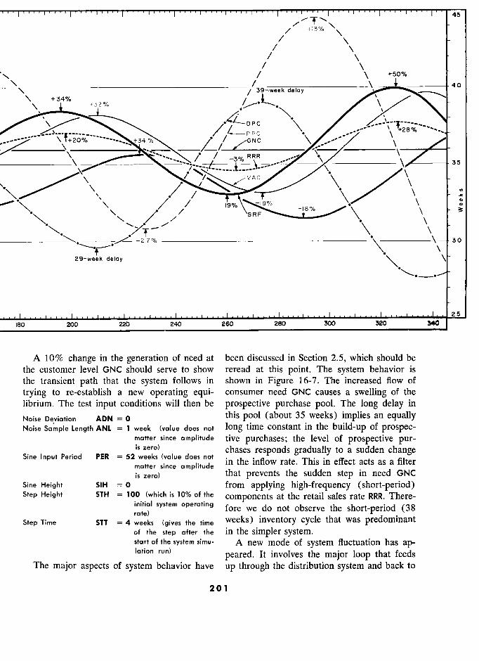
45
, / +50% _\ ____________________________________________/____________________\
', +34%
/ 39-.week deloy 40
"
/ P PC
i N
\ /*
/ p N
C C
3% RRR
35
, VAC
'
'
', ' /
1'
,
1 i CI>
fl
% 18
'"\ /,/
––––––––––––––––––––––––––––––––––––––––––– 30 \
29-week deloy \ \'
25
180 200 22Ô 240 260 280 300 320 340
A 10% change in the generation of need at been discussed in Section 2.5, which should be the customer level GNC should serve to show reread at this point. The system behavior is the transient path that the system follows in shown in Figure 16-7. The increased flow of
trying to re-establish a new operating equi- consumer need GNC causes a swelling of the librium. The test input conditions will then be prospective purchase pool. The long delay in
Noise Déviation ADN = 0 this pool (about 35 weeks) implies an equally Noise Sa'mple Length ANL = 1 week (value does not long time constant in the build-up of prospec-
matter since amplitude tive purchases; the level of prospective pur- ..
is zero) chases responds gradually to a sudden change Sine Input Period PER = 52 weeks (value does not . as matter since amplitude III
m ow is in e ec ac s as a er
js zéro) since amplitude
that prevents the sudden step in need GNC Sine Height SIH = 0 from applying high-frequency (short-period) StepHeight STH = 100 (which is 10% of the
componentsat the retail-sales rate RRR. There-
initial system operating fore we observe thé short-period (38 rate) ..
Step Time STT = 4 weeks (gives the time weeks) inventory cycle that was predominant of the step after the in the simpler system. start of the system simu- A new mode of system fluctuation has ap-
run) peared. It involves the major loop that feeds
The major aspects of system behavior have up through the distribution system and back to
201 1
ADVERTISING IN THE SYSTEM MODEL OF CHAPTER 2
the market through the advertising decision The amplification is frequency sensitive; that chain. It should be realized that the loop called is, it amplifies different periods of oscillation
advertising in this example can be considered by different amounts.12
more broadly as any of the factors that cause a The phase relationships between different
rising factory production rate to increase the parts of the system also depend on the dis-
pressure to purchase at the retail level. In vary- turbance frequency. It may be surprising to
ing degrees the fluctuating availability of con- note that factory production, although it clearly sumer credit, price discounts precipitated by is a result of retail sales, actually is reaching low sales and high inventories, and the flow of its peak value earlier than the peak of retail
rising factory wages into the hands of prospec- sales. Of course it is equally correct to say that tive purchasers can have similar effects. in this example retail sales fluctuate entirely as
The system shows a period of about 2.5 a result of changes in factory production. How-
years, which furthermore is growing in ampli- ever, retail sales do not lag factory production tude of oscillation. We should not attach undue by anywhere near the 20 weeks of delay that
significance to the exact values of either of these exists down through the advertising decision observations. chain. Such characteristics, which may at first
The period of oscillation will be determined be unexpected, are typical of the closed-loop primarily by the time delays around the outer types of systems with which we are dealing. feedback loop. Changing the lengths of the de- Several factors in the system can cause a phase lays will affect the period. Here the longest lead at appropriate disturbance frequencies. and the most significant delay is the one in the This is true in the inventory and pipeline terms
prospective purchase pool. Our economic sys- of the ordering equation, where these compo- tem abounds in these levels that are large com- nents are partially responsive to the rate at
pared with the average inflow and outflow rates. which sales are changing.13 Also, the peak of Such levels constitute, in effect, delays with long retail sales occurs substantially in advance of time constants and are found in money balances the minimum value in purchase delay (because
(especially in savings), capital equipment pool depletion as well as delay controls the out-
pools, inventories of durables (and even tex- flow rate). tiles) in the hands of consumers, deferrable Very often a sharp distinction is drawn be-
housing construction, allocation of land utiliza- tween stable and unstable oscillatory systems, tion, farm commodity storage, the equipment that is, between ones in which a disturbance of transportation systems, and the various diminishes in amplitude versus one in which a
slowly changing categories of labor and popula- disturbance increases. We should not attach any tion. All of these and numerous others interact great significance to the point of neutral stability to create economic fluctuation, and should be separating these two regions. Better, we should
incorporated in future models of economic sys- look upon stability as a continuous matter of tems. degree. The rate of decay of a disturbance is
To exhibit oscillation, a feedback system important, but it is far from sufficient that a must contain amplification. Here amplification disturbance merely decline. A system showing is created by the ordering policies in the distri- a natural period that decays slowly will be a bution system. A variable delay, such as incor-
porated at the point of prospective purchase Appendix G. DPC, could also create amplification if it had 13 The derivative (rate of change) of sales rate leads
the proper functional relationship to its cause the sales curves by a quarter-period. (The maximum
r rate of rise in a sinusoidal fluctuation occurs as the of Varlatl°n. curve passes through zero.)
202 2
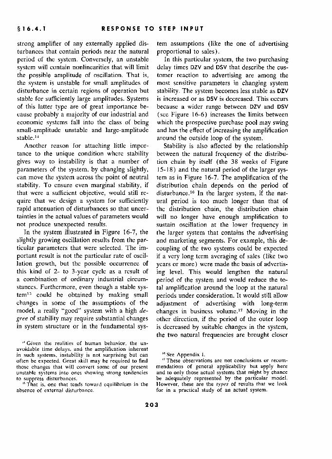
§ 16.4.1 1 RESPONSE TO STEP INPUT T
strong amplifier of any externally applied dis- tem assumptions (like the one of advertising turbances that contain periods near the natural proportional to sales).
period of the system. Conversely, an unstable In this particular system, the two purchasing system will contain nonlinearities that will limit delay times DZV and DSV that describe the cus- the possible amplitude of oscillation. That is, tomer reaction to advertising are among the the system is unstable for small amplitudes of most sensitive parameters in changing system disturbance in certain regions of operation but stability. The system becomes less stable as DZV stable for sufficiently large amplitudes. Systems is increased or as DSV is decreased. This occurs of this latter type are of great importance be- because a wider range between DZV and DSV cause probably a majority of our industrial and (see Figure 16-6) increases the limits between economic systems fall into the class of being which the prospective purchase pool may swing small-amplitude unstable and large-amplitude and has the effect of increasing the amplification sable. 14 around the outside loop of the system.
Another reason for attaching little impor- Stability is also affected by the relationship tance to the unique condition where stability between the natural frequency of the distribu-
gives way to instability is that a number of tion chain by itself (the 38 weeks of Figure parameters of the system, by changing slightly, 15-18) and the natural period of the larger sys- can move the system across the point of neutral tem as in Figure 16-7. The amplification of the
stability. To ensure even marginal stability, if distribution chain depends on the period of that were a sufficient objective, would still re- disturbance.16 In the larger system, if the nat-
quire that we design a system for sufficiently ural period is too much longer than that of
rapid attenuation of disturbances so that uncer- the distribution chain, the distribution chain tainties in the actual values of parameters would will no longer have enough amplification to not produce unexpected results. sustain oscillation at the lower frequency in
In the system illustrated in Figure 16-7, the the larger system that contains the advertising slightly growing oscillation results from the par- and marketing segments. For example, this de- ticular parameters that were selected. The im- coupling of the two systems could be expected portant result is not the particular rate of oscil- if a very long term averaging of sales (like two lation growth, but the possible occurrence of years or more) were made the basis of advertis- this kind of 2- to 3-year cycle as a result of ing level. This would lengthen the natural a combination of ordinary industrial circum- period of the system and would reduce the to- stances. Furthermore, even though a stable sys- tal amplification around the loop at the natural
could be obtained by making small periods under consideration. It would still allow
changes in some of the assumptions of the adjustment of advertising with long-term model, a really "good" system with a high de- changes in business volume.''' Moving in the
gree of stability may require substantial changes other direction, if the period of the outer loop in system structure or in the fundamental sys- is decreased by suitable changes in the system,
the two natural frequencies are brought closer
" Given the realities of human behavior, the un- avoidable time delays, and the amplification inherent in such systems, instability is not surprising but can '° See Appendix I. often be expected. Great skill may be required to find 17 These observations are not conclusions or recom- those changes that will convert some of our present mendations of general applicability but apply here unstable systems into ones showing strong tendencies and to only those actual systems that might by chance to suppress disturbances. be adequately represented by the particular model.
"That is, one that tends toward equilibrium in the However, these are the types of results that we look absence of external disturbance. for in a practical study of an actual system.
203 3
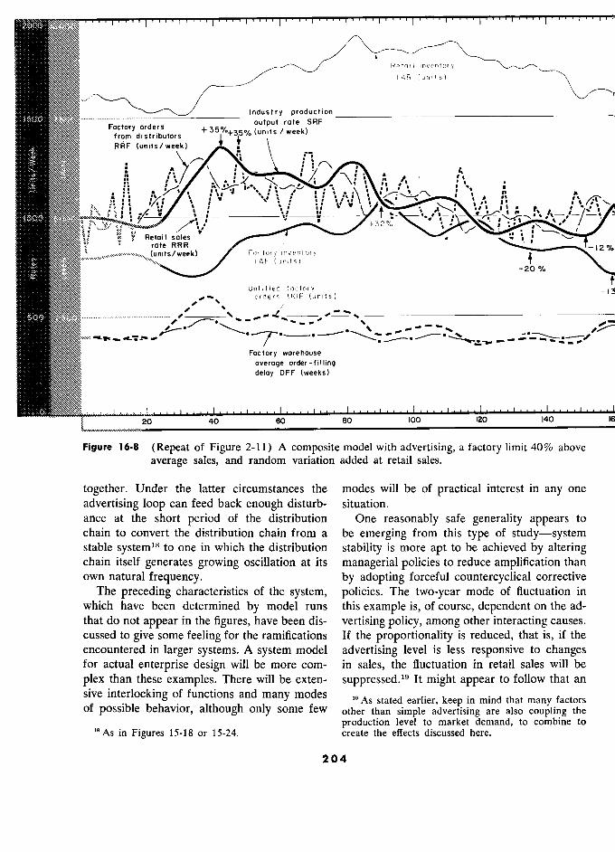
NjjJN
NNtN
Foctoryorders +35'y
IAR (un it s)
Industry production
Factory orders (units
(units week) l
,, ts , , i j
,
,
, 3 2 '
)j .. (
Retail sales R < À 1
j 2 . h!n!)-'!frr!f1 Factory inventory
t I AF (units) - 20 %
tNNN ]tj Unfilled factory _
ord e r s U0 (units)
....... - -- ", -
"
Factory worehouse tNNN average order-filling
deloy DFF (weeks)
20 40 60 80 100 120 140
Figure 16-8 (Repeat of Figure 2-11) A composite model with advertising, a factory limit 40% above
average sales, and random variation added at retail sales.
together. Under the latter circumstances the modes will be of practical interest in any one
advertising loop can feed back enough disturb- situation. ance at the short period of the distribution One reasonably safe generality appears to chain to convert the distribution chain from a be emerging from this type of study-system stable system18 to one in which the distribution stability is more apt to be achieved by altering chain itself generates growing oscillation at its managerial policies to reduce amplification than own natural frequency. by adopting forceful countercyclical corrective
The preceding characteristics of the system, policies. The two-year mode of fluctuation in which have been determined by model runs this example is, of course, dépendent on the ad- that do not appear in the figures, have been dis- vertising policy, among other interacting causes. cussed to give some feeling for the ramifications If the proportionality is reduced, that is, if the encountered in larger systems. A system model advertising level is less responsive to changes for actual enterprise design will be more com- in sales, the fluctuation in retail sales will be
plex than thèse examples. There will be exten- suppressed.19 It might appear to follow that an sive intertockine of functions and many modes " As stated earlier, keep in mind that many factors "As stated earher, keep m mmd that many factors of possible behavior, although only some few other than simple advertising are also coupling the
production level to market demand, to combine to
"As in Figures 15-18 or 15-24. create the effects diseussed here.
204
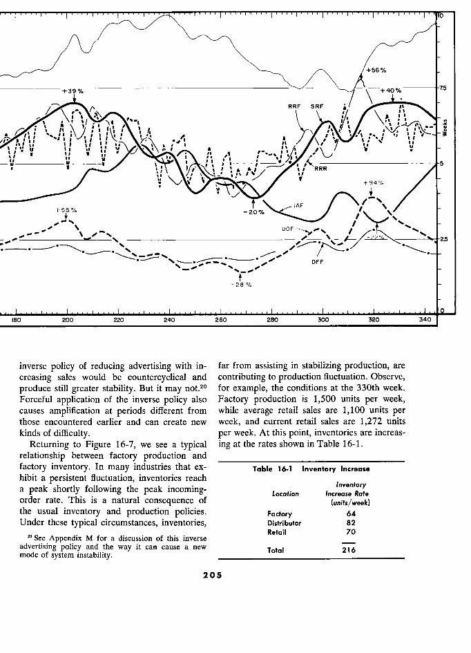
+39%
RRF SRF ' tt 1
% q 1
w
, j j , , ,
j i j
' ( j j
i 1 ,,< i
, jj , / ,
y g',,i 1
y 1
-RRR - i j
5
' +94%
/-
+ 58 % -20% IAF ./ If1
,' ,), _
',
UOF --- 1 .JL
25
- 28%
1 .... 0 180 200 220 240 260 280 300 320 340
inverse policy of reducing advertising with in- far from assisting in stabilizing production, are
creasing sales would be countercyclical and contributing to production fluctuation. Observe,
produce still greater stability. But it may not.20 for ex ample, the conditions at the 330th week. Forceful application of the inverse policy also Factory production is 1,500 units per week, causes amplification at periods différent from while average retail sales are 1,100 units per those encountered earlier and can create new week, and current retail sales are 1,272 units kinds of difficulty. per week. At this point, inventories are increas-
Returning to Figure 16-7, we see a typical ing at the rates shown in Table 16-1.
relationship between factory production and
factory inventory. In many industries that ex- Table 16,i lnventory Incrense
hibit a persistent fluctuation, inventories reach ln%,entory a peak shortiy 1 following thé peak incoming- a peak shortly following the peak incoming- Location lncrease Rate
order rate. This is a natural consequence of
the usual inventory and production policies. Factory 64 Under these typical circumstances, inventories, Distributor 82
, Retait 70 ' Sec Appendix M for a discussion of this inverse
Retail 70
advertising policy and the way it can cause a new 216 mode of system instability.
205 5
ADVERTISING IN THE SYSTEM MODEL OF CHAPTER 2 2
Of the difference between average demand Step Time STT = 4 weeks (gives the time and current production, 55% is going into in- of rhe step after the
ventory. When the production facilities are un- srarr of the
system sim-
der greatest stress, a major part of the excess
production is going into stocks, to heighten the In addition, for this run the factory limit has
production rate above actual retail demand. been brought down to a point where it will
Conversely, at the point of minimum retail de- affect system operation when production rates
mand, rather than by using inventory to ac- above 140% of the initial rates are called for:
cumulate some of the excess production, sales ALF = 1,400 units/week, constAnt specifying manufac-
are being partially filled from inventories, and turing capacity Limit at Factory
production has been cut back to a point lower Figure 16-8 retains the underlying character- than the reduced retail demand. It is not coin- istics of Figure 16-7. The long-period business
cidence, nor the result of random bad luck, that fluctuation is still predominant. In addition, the inventories reach their lowest point just at the noise at the retail sales rate has reintroduced time they are needed to meet a rapidly rising short-term fluctuation in the inventories and
demand; the usual system organization and pipelines of the distribution chain, as we saw in
policies combine to ensure that inventories are Figure 15-20.21 lowest just ahead of peak demand and are high- Factory production still peaks at about the est just as demand approaches a minimum. same time as or before retail sales, and inven-
16.4.2 Random Fluctuations at Retail Sales. tory is rising at the time of maximum produc- Figure 16-7 was examined without random tion and peaks just ahead of the retail sales min-
components in any of the system decisions. In imum. Although not shown in the figure, pur- a noise-free system we were able to see best chasing delay at the prospective purchase pool some of the inherent characteristics. However, varies only about 5 weeks from its initial value we know that smooth, unperturbed flows are of 35 weeks as it did in Figure 16-7, yet this not usually found in actual industrial systems. is sufficient to cause the fluctuating outflow of In principle, we should introduce uncertainty retail orders. at all decision points in the system, but actually In Figure 16-8 the long-period fluctuation of we expect little change in the effect on the sys- something over two years' duration is still very tem after random inputs have been added at a pronounced and regular. The strength and uni- few of the most sensitive points. formity of such a mode of operation will depend
Figure 16-8 shows the effect of a random on both the degree of stability of the system and
component in the retail sales rate. The figure on the amplitude of those external disturbances results from the equations of Chapter 15, as that have components with periods near that modified and extended in Sections 16.1 through of the natural period of the system. Here the
16.3, with the test conditions for Equations model system is slightly unstable and will there- 16-10 through 16-14 as follows: fore be strongly persistent in its natural mode
Noise Déviation ADN = 0.1 of opération. Also the noise input that is ran-
Noise Sample Length ANL = 1.0 domly sampled each week will contain very Sine Input Period PER = 52 weeks (value does little energy in the 2-year to 4-year period oc-
not matter since ampli- tave22 to cause any deviation from the natural
Sine Height SIH = 0 is internal inclinations of the system. With a more
sine Height cru = 0 (which is 10% of the stable system, and with more external disturb- Srep Height STH = 100 (which is 10% of the
initial system operating C'1 See Sections 2.4 and 15.7.3. rate) 22 See Appendix F.
206

§ 16.4.2 RANDOM FLUCTUATIONS AT RETAIL SALES S
ing forces having periods near that of the sys- Chapters 17 and 18. Numerous other industries
tem, we should expect a much less coherent with similar behavior exist in parallel with these, character in the natural frequency of the sys- and still others are cascaded back into capital tem.23 equipment and commodities. Strong coupling
The production-distribution-market system forces existing in the market and in financial cir- of Figure 16-8 shows behavior somewhat like cles draw separate industries into a synchronous the business cycle fluctuations of our national rise and fall of business activity. The national
economy. So does the system that follows in economy can be viewed as a partially inter- locked composite of these separate systems,
23 .. each of which is organized and managed so that - 3 More like the character of the wandering, broad- ç j which contribute band fluctuation of Figure 15-20 but showing longer-
it contains inherent tendencies which
contribute
term components; or like the system in Chapter 18. to national économie mstability.
207
CHAPTER 17
A Customer-Producer-
Employment Case Study
In this chapter will be developed a dynamic model that resulted from a case study of an actual company. It arose from a .çearch for causes of a fluctuating employment level that varied over a ratio of about 2 to 1, with peak-to-peak intervals of about 2 years. There seemed to be no likelihood that the explanation lay in a similar large variation in the final usage rate of the product. The model shows that the observed employ- ment instability can result from interactions between the purchasing prac- tices of the customers' and the inventory, production, and employment practices of the company. The example is of interest here because it is
typical of a substantial fraction of American industry. This chapter de- scribes the industrial situation, gives the reasons for choosing the particu- lar factors that went into the model, and develops the mathematical model. Chapter 18 contains the results of the model studies and methods of improving employment stability.
THE problem and system model discussed ponents that are used by other manufacturers in in this chapter arose from a case study of a their products, and these in turn are sold to in-
company in the electronic components industry. dustrial and governmental customers. The cus- The essential features of the actual study are tomers of the company under consideration are retained here, although the description and the informed buyers purchasing a product in a model have been simplified for clarity of presen- manner that is geared to their own production tation. In some places the model has been gen- demands. eralized to incorporate typical features of other The product is a high-quality electronic com- industrial situations that did not appear im- ponent that is manufactured by a number of
portant in the particular study. Some of the suppliers and is used in military and industrial numerical values have been changed to make equipment. It had been generally considered, the model representative of a wider class of and appears to be true, tlyat the average cus- industrial situations where the particular case tomer is interested first in quality, second in de- was atypical. None of these changes has had any livery, and third in price. Price can be relegated major effect on the nature of the dynamic be- to third position partly because it is indeed havior nor on the kinds of conclusions that can less important to the customer than quality and be drawn. availability, and partly because prices are com-
petitive and differ but little between suppliers 17.1 Description and appear not to be the principal basis for
The situation relates to a supplier of com- selection of a supplier.
208 8
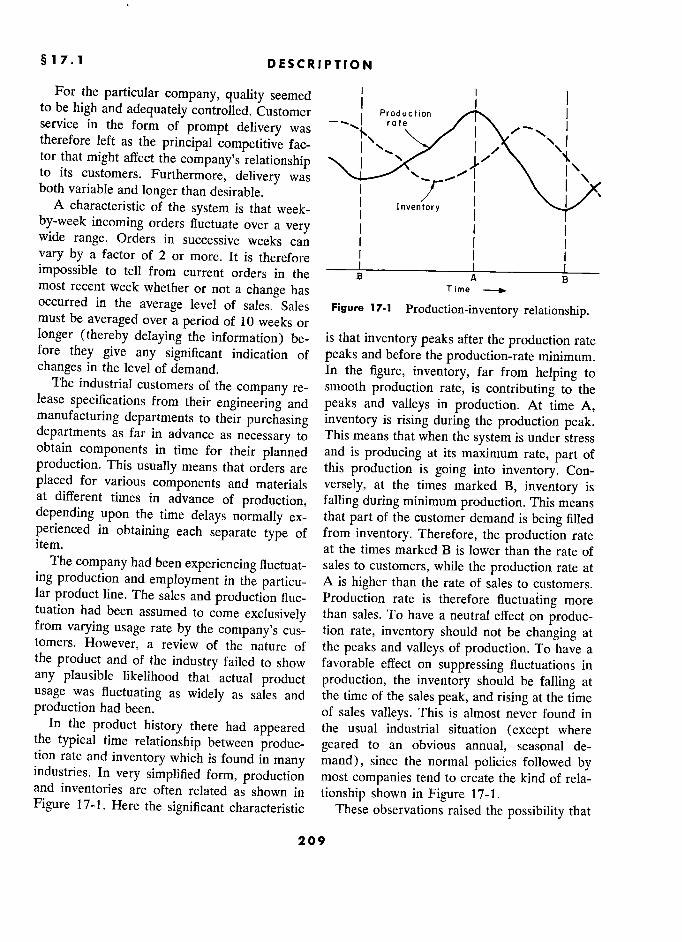
1 DESCRIPTION
For the particular company, quality seemed ) 1 )
to be high and adequately controlled. Customer j
Production
) service in the form of prompt delivery was ./ 1 therefore left as the principal competitive fac- tor that might affect the company's relationship j
' j'
j , to its customers. Furthermore, delivery was i
I \ both variable and longer than desirable.
: fi j 1 A characteristic of the system is that week- Inventory j
by-week incoming orders fluctuate over a very 1 1 wide range. Orders in successive weeks can 1 1 1 vary by a factor of 2 or more. It is therefore I 1
impossible to tell from current orders in the BAB most recent week whether or not a change has Time
occurred in the average level of sales. Sales Figure 17-1 Production-inventory relationship. must be averaged over a period of 10 weeks or
longer (thereby delaying the information) be- is that inventory peaks after the production rate fore they give any significant indication of peaks and before the production-rate minimum. changes in the level of demand. In the figure, inventory, far from helping to
The industrial customers of the company re- smooth production rate, is contributing to the lease specifications from their engineering and peaks and valleys in production. At time A, manufacturing departments to their purchasing inventory is rising during the production peak. departments as far in advance as necessary to This means that when the system is under stress obtain components in time for their planned and is producing at its maximum rate, part of production. This usually means that orders are this production is going into inventory. Con- placed for various components and materials versely, at the times marked B, inventory is at different times in advance of production, falling during minimum production. This means
depending upon the time delays normally ex- that part of the customer demand is being filled perienced in obtaining each separate type of from inventory. Therefore, the production rate item. at the times marked B is lower than the rate of
The company had been experiencing fluctuat- sales to customers, while the production rate at ing production and employment in the particu- A is higher than the rate of sales to
customers. lar product line. The sales and production fluc- Production rate is therefore fluctuating more tuation had been assumed to come exclusively than sales. To have a neutral effect on produc- from varying usage rate by the company's cus- tion rate, inventory should not be changing at tomers. However, a review of the nature of the peaks and valleys of production. To have a the product and of the industry failed to show favorable effect on suppressing fluctuations in any plausible likelihood that actual product production, the inventory should be falling at usage was fluctuating as widely as sales and the time of the sales peak, and rising at the time production had been. of sales valleys. This is almost never found in
In the product history there had appeared the usual industrial situation (except where the typical time relationship between produc- geared to an obvious annual, seasonal de- tion rate and inventory which is found in many mand), since the normal policies followed by industries. In very simplified form, production most companies tend to create the kind of rela- and inventories are often related as shown in tionship shown in Figure 17-1.
Figure 17-1. Here the significant characteristic These observations raised the possibility that
209
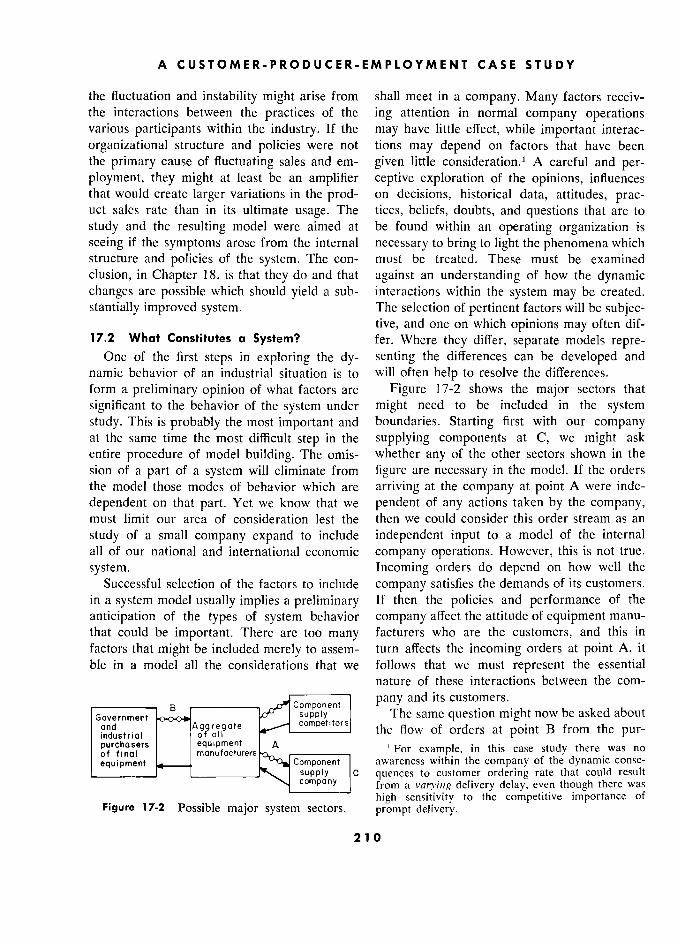
A CUSTOMER-PRODUCER-EMPLOYMENT CASE STUDY
the fluctuation and instability might arise from shall meet in a company. Many factors receiv- the interactions between the practices of the ing attention in normal company operations various participants within the industry. If the may have little effect, while important interac-
organizational structure and policies were not tions may depend on factors that have been the primary cause of fluctuating sales and em- given little consideration.1 A careful and per- ployment, they might at least be an amplifier ceptive exploration of the opinions, influences that would create larger variations in the prod- on decisions, historical data, attitudes, prac- uct sales rate than in its ultimate usage. The tices, beliefs, doubts, and questions that are to
study and the resulting model were aimed at be found within an operating organization is
seeing if the symptoms arose from the internal necessary to bring to light the phenomena which structure and policies of the system. The con- must be treated. These must be examined
clusion, in Chapter 18, is that they do and that against an understanding of how the dynamic changes are possible which should yield a sub- interactions within the system may be created.
stantially improved system. The selection of pertinent factors will be subjec- tive, and one on which opinions may often dif-
17.2 What Constitutes a System? fer. Where they differ, separate models repre- One of the first steps in exploring the dy- senting the differences can be developed and
namic behavior of an industrial situation is to will often help to resolve the differences. form a preliminary opinion of what factors are Figure 17-2 shows the major sectors that
significant to the behavior of the system under might need to be included in the system study. This is probably the most important and boundaries. Starting first with our company at the same time the most difficult step in the supplying components at C, we might ask entire procedure of model building. The omis- whether any of the other sectors shown in the sion of a part of a system will eliminate from figure are necessary in the model. If the orders the model those modes of behavior which are arriving at the company at point A were inde-
dependent on that part. Yet we know that we pendent of any actions taken by the company, must limit our area of consideration lest the then we could consider this order stream as an
study of a small company expand to include independent input to a model of the internal all of our national and international economic company operations. However, this is not true.
system. Incoming orders do depend on how well the Successful selection of the factors to include company satisfies the demands of its customers.
in a system model usually implies a preliminary If then the policies and performance of the
anticipation of the types of system behavior company affect the attitude of equipment manu- that could be important. There are too many facturers who are the customers, and this in
factors that might be included merely to assem- turn affects the incoming orders at point A, it
ble in a model all the considerations that we follows that we must represent the essential
nature of these interactions between the com-
,________ B ––––––––– Component pany and its customers.
Government ooof supply The same question might now be asked about ond Aggregate competitors and 1 ? on the flow of orders at point B from the pur- ?str? g thé pur-
P§§hQS?" manufacturers A _______ 1 For example, in this case study there was no of final mariufacturers , . h f h d
. equipment « Component awareness within the company of the dynamic conse-
_______ supply C quences to customer ordering rate that could resuit company from a var.?,iiig delivery delay, even though there was
high sensitivity to the competitive importance of Figure 17-2 Possible major system sectors. prompt delivery.
210
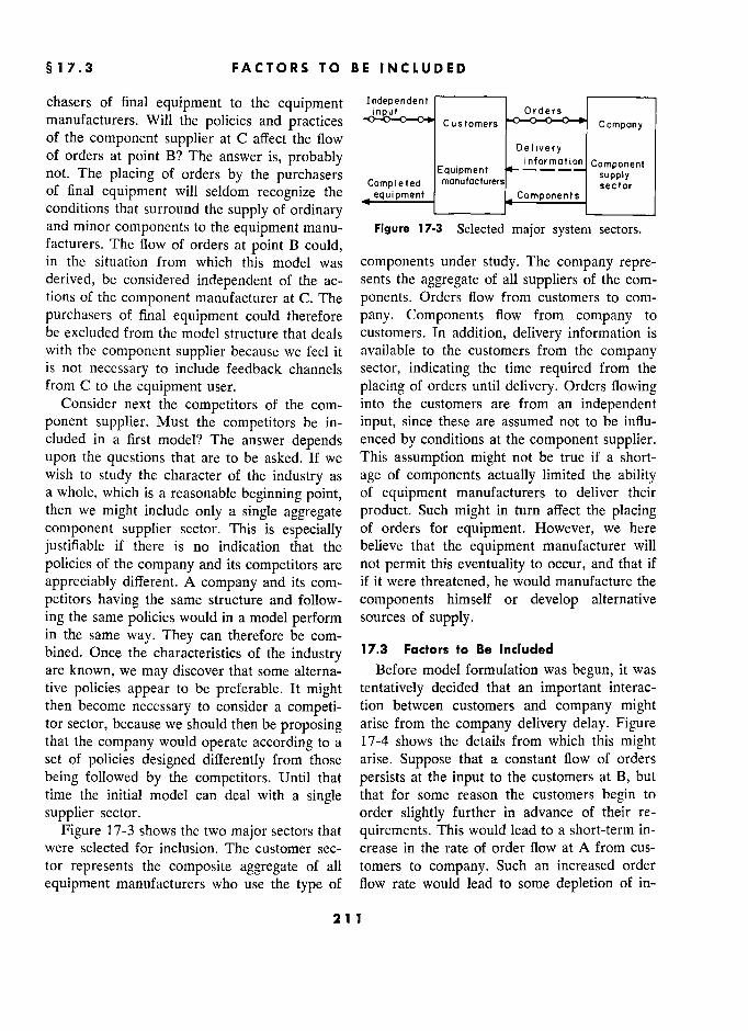
§ 17.3 3 FACTORS TO BE INCLUDED
chasers of final equipment to the equipment Independent
r 1 ,. Orders manufacturers. Will the policies and practices input customers company of the component supplier at C affect the flow
of orders at point B? Thé answer is, probably émotion component a orders at point B? The answer is, probably
Equipment - ' information Component not. The placing of orders by the purchasers Completed nianufacturers --- supply sector rc i ...... . , Completed manufacturers sector of final equipment will seldom recognize the equipment Components conditions that surround the supply of ordinary ______ ______
and minor compononts to the equipment manu- Figure 17-3 Selected major system sectors.
facturers. The flow of orders at point B could, in the situation from which this model was components under study. The company repre-
derived, be considered independent of the ac- sents the aggregate of all suppliers of the com-
tions of the component manufacturer at C. The ponents. Orders flow from customers to com-
purchasers of final equipment could therefore pany. Components flow from company to
be excluded from the model structure that deals customers. In addition, delivery information is
with the component supplier because we feel it available to the customers from the company is not necessary to include feedback channels sector, indicating the time required from the
from C to the equipment user. placing of orders until delivery. Orders flowing Consider next the competitors of the com- into the customers are from an independent
ponent supplier. Must the competitors be in- input, since these are assumed not to be influ-
cluded in a first model? The answer depends enced by conditions at the component supplier.
upon the questions that are to be asked. If we This assumption might not be true if a short-
wish to study the character of the industry as age of components actually limited the ability a whole, which is a reasonable beginning point, of equipment manufacturers to deliver their
then we might include only a single aggregate product. Such might in turn affect the placing
component supplier sector. This is especially of orders for equipment. However, we here
justifiable if there is no indication that the believe that the equipment manufacturer will
policies of the company and its competitors are not permit this eventuality to occur, and that if
appreciably different. A company and its com- if it were threatened, he would manufacture the
petitors having the same structure and follow- components himself or develop alternative
ing the same policies would in a model perform sources of supply. in the same way. They can therefore be com-
bined. Once the characteristics of the industry 17.3 Factors to Be Included
are known, we may discover that some alterna- Before model formulation was begun, it was
tive policies appear to be preferable. It might tentatively decided that an important interac-
then become necessary to consider a competi- tion between customers and company might tor sector, because we should then be proposing arise from the company delivery delay. Figure that the company would operate according to a 17-4 shows the details from which this might set of policies designed differently from those arise. Suppose that a constant flow of orders
being followed by the competitors. Until that persists at the input to the customers at B, but
time the initial model can deal with a single that for some reason the customers begin to
supplier sector. order slightly further in advance of their re-
Figure 17-3 shows the two major sectors that quirements. This would lead to a short-term in-
were selected for inclusion. The customer sec- crease in the rate of order flow at A from cus-
tor represents the composite aggregate of all tomers to company. Such an increased order
equipment manufacturers who use the type of flow rate would lead to some depletion of in-
21 1
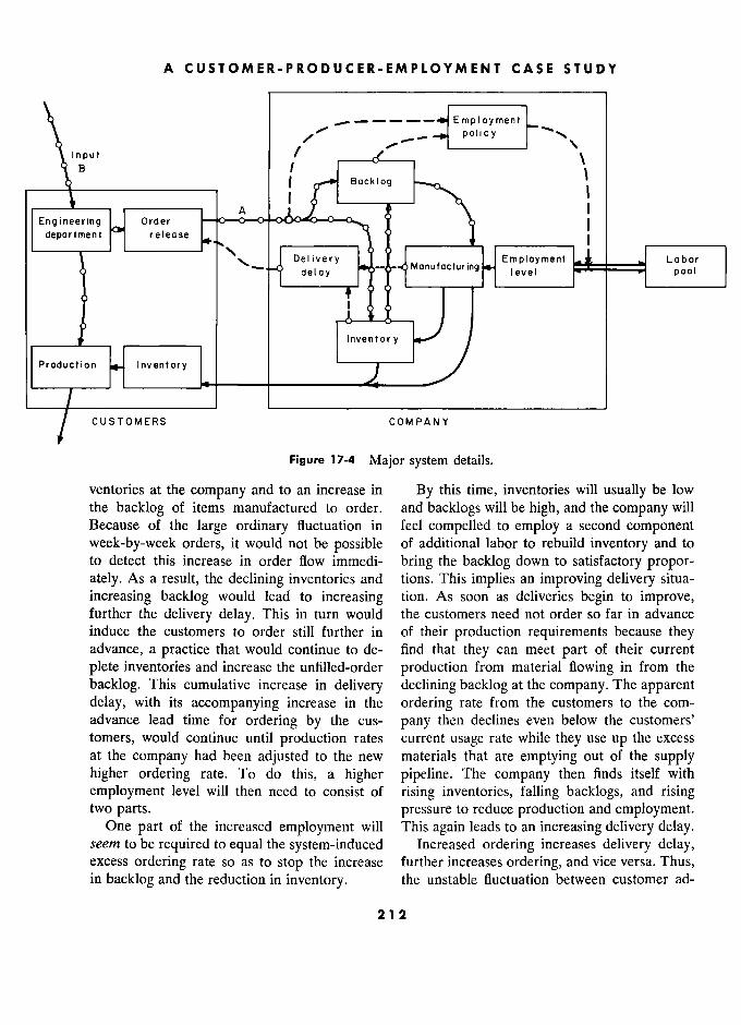
A CUSTOMER-PRODUCER-EMPLOYMENT CASE STUDY
- Employment t \ policy
Input / ,/ _ _ policy Y ',
', Input / ,
________ \ \
H /
/'
'"
-- policy -.......
, \ \ 1 _____0__________________
A f
rT*" Bocklog I I !–––––––! A JL
' V X
. ! \ 1
Engineering q Order r V 1
department release \ Y ) 1 ! . ! A ,–––'-) .––––. \ Delivery y ) )
Manufacturing Employment Labor r -
! deloy y level
el pool 1
1
_____jt___ _________ Inventory y <
Production Inventory ––––)–––– /
/ CUSTOMERS COMPANY Y
Figure 17-4 Major system details.
ventories at the company and to an increase in By this time, inventories will usually be low the backlog of items manufactured to order. and backlogs will be high, and the company will Because of the large ordinary fluctuation in feel compelled to employ a second component week-by-week orders, it would not be possible of additional labor to rebuild inventory and to to detect this increase in order flow immedi- bring the backlog down to satisfactory propor- ately. As a result, the declining inventories and tions. This implies an improving delivery situa-
increasing backlog would lead to increasing tion. As soon as deliveries begin to improve, further the delivery delay. This in turn would the customers need not order so far in advance induce the customers to order still further in of their production requirements because they advance, a practice that would continue to de- find that they can meet part of their current
plete inventories and increase the unfilled-order production from material flowing in from the
backlog. This cumulative increase in delivery declining backlog at the company. The apparent delay, with its accompanying increase in the ordering rate from the customers to the com- advance lead time for ordering by the cus- pany then declines even below the customers'
tomers, would continue until production rates current usage rate while they use up the excess at the company had been adjusted to the new materials that are emptying out of the supply higher ordering rate. To do this, a higher pipeline. The company then finds itself with
employment level will then need to consist of rising inventories, falling backlogs, and rising two parts. pressure to reduce production and employment.
One part of the increased employment will This again leads to an increasing delivery delay. seem to be required to equal the system-induced Increased ordering increases delivery delay, excess ordering rate so as to stop the increase further increases ordering, and vice versa. Thus, in backlog and the reduction in inventory. the unstable fluctuation between customer ad-
212 2
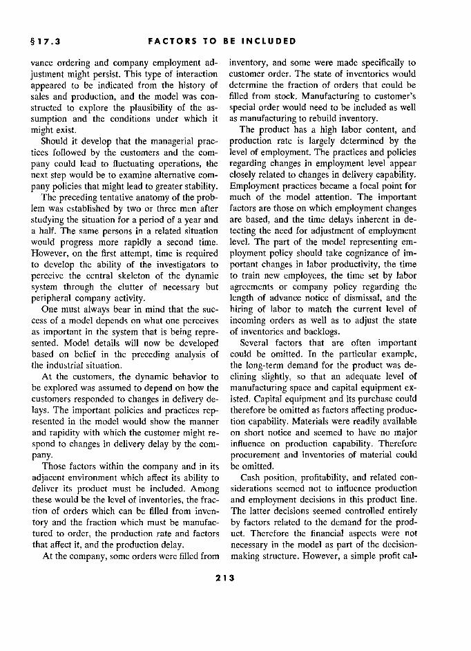
§ 17.3 FACTORS TO BE INCLUDED
vance ordering and company employment ad- inventory, and some were made specifically to
justment might persist. This type of interaction customer order. The state of inventories would
appeared to be indicated from the history of determine the fraction of orders that could be sales and production, and the model was con- filled from stock. Manufacturing to customer's structed to explore the plausibility of the as- special order would need to be included as well
sumption and the conditions under which it as manufacturing to rebuild inventory.
might exist. The product has a high labor content, and
Should it develop that the managerial prac- production rate is largely determined by the tices followed by the customers and the com- level of employment. The practices and policies pany could lead to fluctuating operations, the regarding changes in employment level appear next step would be to examine alternative com- closely related to changes in delivery capability. pany policies that might lead to greater stability. Employment practices became a focal point for
The preceding tentative anatomy of the prob- much of the model attention. The important lem was established by two or three men after factors are those on which employment changes studying the situation for a period of a year and are based, and the time delays inherent in de- a half. The same persons in a related situation tecting the need for adjustment of employment would progress more rapidly a second time. level. The part of the model representing em-
However, on the first attempt, time is required ployment policy should take cognizance of im- to develop the ability of the investigators to portant changes in labor productivity, the time
perceive the central skeleton of the dynamic to train new employees, the time set by labor
system through the clutter of necessary but agreements or company policy regarding the
peripheral company activity. length of advance notice of dismissal, and the One must always bear in mind that the suc- hiring of labor to match the current level of
cess of a model depends on what one perceives incoming orders as well as to adjust the state as important in the system that is being repre- of inventories and backlogs. sented. Model details will now be developed Several factors that are often important based on belief in the preceding analysis of could be omitted. In the particular example, the industrial situation. the long-term demand for the product was de-
At the customers, the dynamic behavior to clining slightly, so that an adequate level of be explored was assumed to depend on how the manufacturing space and capital equipment ex- customers responded to changes in delivery de- isted. Capital equipment and its purchase could
lays. The important policies and practices rep- therefore be omitted as factors affecting produc- resented in the model would show the manner tion capability. Materials were readily available and rapidity with which the customer might re- on short notice and seemed to have no major spond to changes in delivery delay by the com- influence on production capability. Therefore
pany. procurement and inventories of material could
Those factors within the company and in its be omitted.
adjacent environment which affect its ability to Cash position, profitability, and related con- deliver its product must be included. Among siderations seemed not to influence production these would be the level of inventories, the frac- and employment decisions in this product line. tion of orders which can be filled from inven- The latter decisions seemed controlled entirely
tory and the fraction which must be manufac- by factors related to the demand for the prod- tured to order, the production rate and factors uct. Therefore the financial aspects were not that affect it, and the production delay. necessary in the model as part of the decision-
At the company, some orders were filled from making structure. However, a simple profit cal-
213
A CUSTOMER-PRODUCER-EMPLOYMENT CASE STUDY
j Input t t
Section 17.6 Orders \ \
Section !7.6 Orders
- (independent Customer
ordering Section 17.4.7
- ........ ,
, /
/ , / \/ Labor
ae 0,\/Delivery-delay Section 17.4.5 -'y informgtion \
, \
ô \ /' 0 df––'**** / Delivery-delay /
/
/ t \\
\
\.\ \ Y ( quotation ) /%orders Section 17.4.6
/ /
'. ..
/- filled from /m / \ \ 0/ / \ inventory/
/ / Order g
\ --"" /
/ filling il / 1 \
/ Section 174.1 / Profit and x 1 \
j \ / V
dividends Î
/ Prs
Pr
â v /
/
/
0/
,v(eo Sec ti Î j
) \
,'
j
l
1 '" /
/ /
0
/ /
0('\ 1 1-7 ,
1 ;: - 1 t' / j i ,'
1 1
1 ? Manufacturing // l a
1
' 1 t )
-) ) c' a) /
' , -, y Section 174.3 c -, / / ,
t t ' W - i
Section
CIl 1
/ ' /
/
1 CI)
1
\)e \0("'" - :; ::: 1 1 /
1 ,
j \ /
j \ /
cess SS / / , CL
'
1 '
/ Î] ) / < -o -m
/
I
Inventory t Ic \°- / Cash
/ reorder /
C°sh \
' reorder
j J 1 w / Section 174.2
M°terial I lô °
' , Moterial t
Section 174.8
. stock \ /
Average \? stock
, I'°
/ Average , /
sales '-0....
/ Material \
N
,
ordering ) /
\ Section 17.4.4 /
/ / ,
,
Sect'°n '?.4.4
.00, /
/
' -
/
Figure 17-5 Subdivisions of the model, interconnections, and sections where described.
214
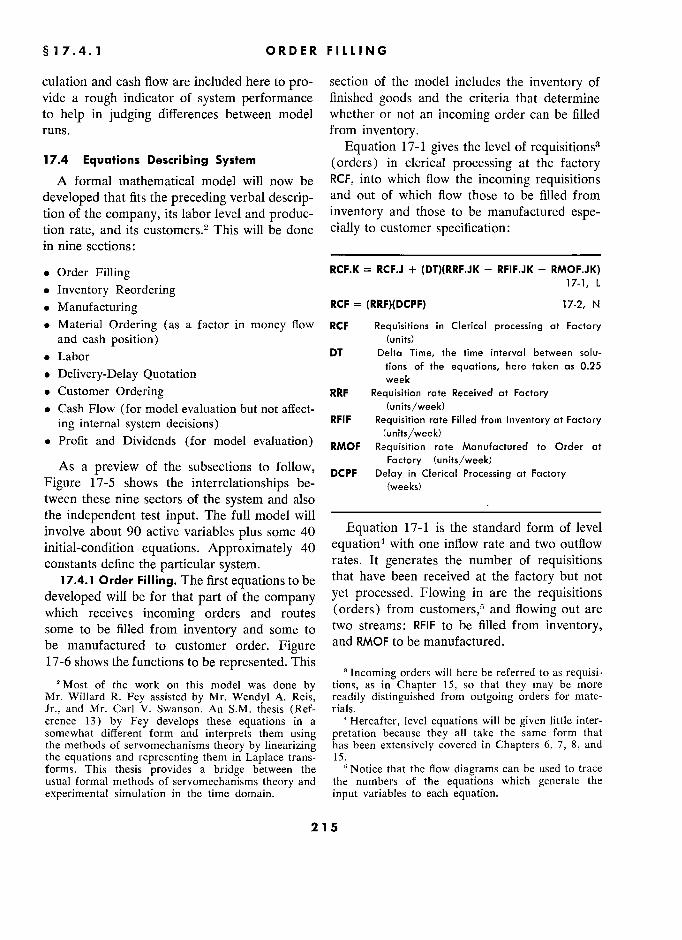
1 7.4, 1 ORDER FILLING
culation and cash flow are included here to pro- section of the model includes the inventory of
vide a rough indicator of system performance fini shed goods and the criteria that determine
to help in judging differences between model whether or not an incoming order can be filled
runs. from inventory.
Equation 17-1 gives the level of requisitions3 17.4 Equations Describing System (orders) in clérical processing at the factory
A formal mathematical model will now be RCF, into which flow the incoming requisitions
developed that fits the preceding verbal descrip- and out of which flow those to be filled from
tion of the company, its labor level and produc- inventory and those to be manufactured espe-
tion rate, and its customers.2 This will be done cially to customer specification:
in nine sections:
Order Filling RCF.K = RCF.J + (DT)(RRF.JK - RFIF.JK - RMOF.JK)
nventory eor enng L
. Manufacturing RCF = (RRF)(DCPF) 17-2, N
. Material Ordering (as a factor in money flow RCF Réquisitions in Clerical processing at Factory and cash position) (units)
. Labor DT Delta Time, thé time interval between solu-
D 1. D 1 Q . tions of the equations, hère taken as 0.25
. DeIivery-Delay Quotation
. Customer Ordering RRF Requisition rate Received at Factory
Cash Flow (for model evaluation but not affect- (units/week)
ing internal system décisions) RFIF Requisition rate Filled from Inventory at Factory
, .. (units/week) . Profit and Dividends (for model évaluation) RMOF Requisition rate Manufactured to Order at t
A .
f h. . Factory (units/week) As a preview of the subsections to follow, DCPF Delay in Clerical Processing ar Facrory
Figure 17-5 shows the interrelationships be-
' DCPF
(weeks>
enca Processing at Factory
tween these nine sectors of the system and also
the independent test input. The full model will .. involve about 90 active variables plus some 40 Equation 17-1 is the standard form of level
initial-condition équations. Approximately 40 equation' with one inflow rate and two outflow
constants define the particular system. rates. It generates the number of requisitions
17.4.1 Order Filling. The first equations to be that have been received at the factory but not
developed will be for that part of the company yet processed. Flowing in are the requisitions
which receives incoming orders and routes (orders) from customers,5 and flowing out are
some to be filled from inventory and some to two streams: RFIF to be filled from inventory,
be manufactured to customer order. Figure and RMOF to be manufactured.
17-6 shows the functions to be represented. This 3
Incoming orders will here be referred to as requisi- _
2 Most of the work on this model was done by tions, as in Chapter 15, so that they may be more Mr. Willard R. Fey assisted by Mr. Wendyl A. Reis, readily distinguished from outgoing orders for mate-
Jr., and Mr. Carl V. Swanson. An S.M. thesis (Ref- rials. erence 13) by Fey develops these equations in a ' Hereafter, level equations will be given little inter- somewhat different form and interprets them using pretation because they all take the same form that the methods of servomechanisms theory by linearizing has been extensively covered in Chapters 6, 7, 8, and the equations and representing them in Laplace trans- 15. forms. This thesis provides a bridge between the ' Notice that the flow diagrams can be used to trace usual formal methods of servomechanisms theory and the numbers of the equations which generate the
experimental simulation in the time domain. input variables to each equation.
215 5
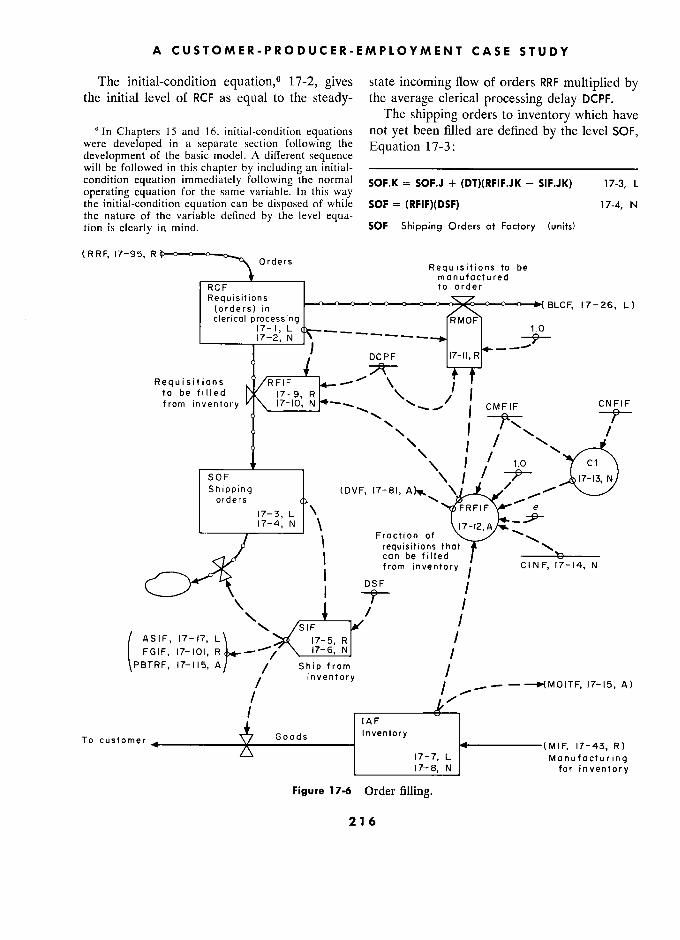
A CUSTOMER-PRODUCER-EMPLOYMENT CASE STUDY
The initial-condition equation,6 17-2, gives state incoming flow of orders RRF multiplied by the initial level of RCF as equal to the steady- the average clerical processing delay DCPF.
The shipping orders to inventory which have 6 ln Chapters 15 and 16, initial-condition equations not yet been filled are defined by the level SOF,
were developed in a separate section following the Equation 17-3:
development of the basic model. A different sequence will be followed in this chapter by including an initial- ––––––––––––––––––––––––––––––––––– condition equation immediately following the normal SOF.K = SOF.J + (DT)(RFIF.JK - SIF.JK) 17-3, L operating equation for the same variable. In this way
'
the initial-condition equation can be disposed of while SOF = (RFIF)(DSF) 17-4, N the nature of the variable defined by the level equa- tion is clearly in mind. SOF Shipping Orders at Factory (units)
(RRF, 17-95, Orders .......
(RRF, 17-95, R
Orders Requisitions to be ______Y______ manufactured
RCF F to order
Requisitions BLCF, 17-26, L) (orders) in -
17-26, L)
clerical processing RMOF 17-I, L
_ 1.0 17-2, N
' i'
DCPF t7-H.R _ _,
._L DCPF 17-11, R _ Ô
Requisitions s '
RFIF j t
to be filled 17-9, R \ / f from inventory 17-10, N
\\
I CMFIF C
I <
"
"
l
§
(
1
/ S 0 F
(DVF, 17-81,
/
Shipping (DVF, 17-81, A)% orders "'",
17-3, L FRFIF e
' 17-3, N \ 1
' Fraction of
' requisitions that \
j can be filled t
?jK '
from inventory j
CINF, 17-14, N
DSF
inventory
1
1
1 CI N F, 17-14, N
\ ) /
1
ASIF, !7-)7, L ,7-5, R /
FGIF, '7-6. N
PBTRF, 17-115, A / Sh!p from 1 PBTRF, 17-115, A / Ship from
/
j
/ inventory
/y / /
17-15, A)
/ . IAF
To customer Goods Inventory
(MIF, 17-43, R)
17-7, L Manufacturing
17-8, N for inventory
Figure 17-6 Order filling.
216
§ 1 7.4.1 1 ORDER FILLING
RFIF Réquisition rate Filled from Inventory at Factory "
(units/week) IAF.K = IAF.J + (DT)(MIF.JK - SIF.JK) 17-7, L SIF Shipments from Inventory at Factory
(units/week) IAF = (CIRF)(RRF) 17-8, N DSF Delay in Shipping at Factory (weeks)
IAF Inventory Actual at Factory (units) MIF Manufacturing rate for Inventory at Factory
In Equation 17-4 the initial steady-state level (units/week) of shipping orders SOF is equal to the steady-
SIF Shipments from Inventory at Factory
state now of orders that b fill from in- -,-. (units/week) state ow a or ers that can e filled rom in- CIRF C oe ffi. IClent f or 1 nventory Ratio at Factory
ventory RFIF multiplied by the average delay in CIRF
(weeks) making shipments DSF. RRF Réquisition rate Received at Factory
The orders shipped per unit of time will be (units/week)
represented as a fixed fraction of the backlog –––––––––––––––––––––––––––– SOF. This is by definition a first-order exponen- In this situation, the target inventory was tial delay,' as given by
In this situation, thé target inventory was tial delay,l as given by authorized in terms of a certain number of weeks of sales; therefore the initial steady-state
SIF.KL = 50F.K p5F 17-5, R level of inventory in Equation 17-8 is propor-
tional 1 the constant initial 1 fl of incoming tional to the constant initial flow of incoming SIF = RFIF 17-6, N orders multiplied by the target ratio CIRF be-
SIF Shipments from Inventory at Factory tween sales rate and inventory level.9 The
(units/week) target ratio CIRF is the number of weeks during SOF Shipping Orders at Factory (units) which the desired level of inventory would be DSF Delay in Shipping at Factory (weeks) able to meet the demands of the steady-state RFIF Réquisition rate Filled from Inventory at Factory d - ( b RFIF
Requisirion rare Filled from Inventory at Factory oraer now rate (assuming all orders could be e
(units/week) filled from inventory).
An average shipping time is here used as Returning now to the flow rate RFIF, which An average shipping time is ere used as stream is that part of the incoming requisition stream
DSF = 1 week, Delay in shipping from Factory that can be filled from inventory, we know that
..... 8 it must depend primarily on three factors - the
Equation 17-6 gives the initial value of the level of unrouted requisitions RCF, the average delivery rate of goods SIF, which in the steady- delay in routing DCPF, and the fraction of the state must equal the fiow of orders RFIF that orders that can be filled from inventory FRFIF are to be filled from inventory. (this fraction will be discussed below). These
The inventory of finished components at the would reasonably be related as in the following factory is given by the usual level equation: equations: .
' See Chapter 9 and Appendix H. e Some initial values for rates are necessary because B This does not imply that the inventory lias to be
they are convenient or necessary for defining still proportional to sales, especially in the short-term busi- other initial conditions. In a few places they are ness fluctuation. In the long-term, many factors do needed in the first time step because other rates or tend to force inventories to rise with increased busi- auxiliary equations depend on them (for example, as ness volume. Inventory may be required by wider inputs to third-order-delay functions, see Appendix geographical coverage that requires more inventory H). In this chapter we anticipate where we shall want locations, by in-process and in-transit inventories that initial conditions for rates (usually discovered as the are proportional to sales rate, by larger individual model formulation is nearing completion) and insert incoming orders that require larger stocks to main- the initial-condition equation while the rate equation tain ability to fill from inventory, and by increased is being discussed. sales that come from additions to the product line.
217
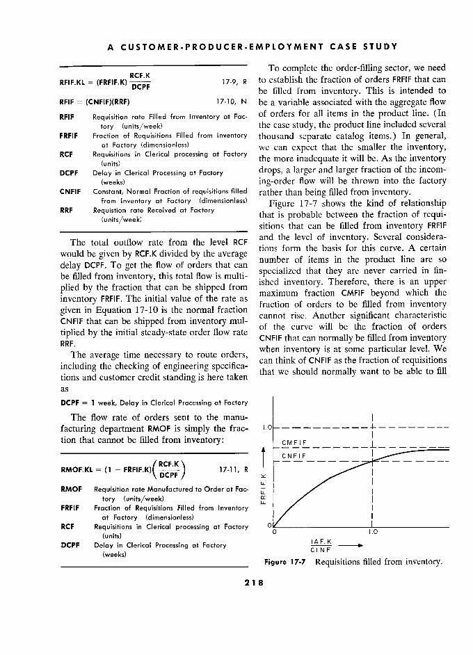
A CUSTOMER-PRODUCER-EMPLOYMENT CASE STUDY
To complete the order-filling sector, we need
RFIF.KL = (FRFIF.K) 17-9, R to establish the fraction of orders FRFIF that can
be filled from inventory. This is intended to
RFIF = (CNFIF)(RRF) 17-10, N be a variable associated with the aggregate flow
RFIF Réquisition rate Filled from Inventory at Fac- of orders for all items in the product line. (In
tory (units/week) the case study, the product line included several
FRFIF Fraction of Requisitions Filled from Inventory thousand separate catalog items.) In general,
RCF
at Factory (dimensioniess) we can expect that the smaller the inventory, PCF Réquisitions in C!erica! processing at Factory
the more inadequate will As inventory RCF
Requisitions ;
in Clerical processing at Factory thé more inadéquate it As thé inventory
DCPF Delay in Clerical Processing at Factory drops, a larger and larger fraction of the incom-
(weeks) ing-order flow will be thrown into the factory CNFIF Constant, Normal Fraction of requisitions flled rather than being filled from inventory.
RRF from Inventory at Factory (dimensionless)
Figure 17-7 shows the kind of relationship RRF Requistion rate Received at Factory
that is probable between the fraction of requi- '"'"'
that is probable between the fraction of requi-
(units/week) sitions that can be filled from inventory FRFIF
The total outflow rate from the level RCF and the level of inventory. Several considera-
would be given by RCF.K divided by the average tions form the basis for this curve. A certain
delay DCPF. To get the flow of orders that can number of items in the product line are so
be filled from inventory, this total flow is multi- specialized that they are never carried in fin-
,....., . ,'' , . ,_.... ished inventory. Therefore, there is an upper plied by the fraction that can be shipped from
ished inventory. Therefore, there is an upper ' maximum fraction CMF)F beyond which thé inventory FRFIF. The initial value of the rate as maximum fraction CMFIF beyond
which the
given in Equation 17-10 is the normal fraction fraction of orders to be filled from inventory
CNFIF that can be shipped from inventory mul- cannot rise. Another significant characteristic
CNFtF that can bc shipped from inventory mul- of the curve will bc the fraction of orders . ,. , ,
a can e
s ro i _, r.
mu - of thé curve will be thé fraction of orders
tiplied by thé initial steady-state order flow rate of the curve wlll be the fraction of orders
RRF. by the initial steady-state order flow rate e
CNFIF that can normally be filled from inventory
The average time necessary to route orders, when inventory is at some particular level. We
The average time necessary to route orders, can think 1 fraction of requisitions . , e average , ime ..,
ss y o rou or
s, as thé fraction of réquisitions
including thé checking of engineering specifica- can think of CNFIF as the fraction of requisitions
including the checking of engineenng speci ca- that we should normally want to be able to fill hons and customer credit standing is here taken
that we should norma want ta be able ta fill tiens and customer credit i standing is hère taken e '
as
DCPF = 1 week, Delay in Clerical Processing at Factory
The flow rate of orders sent to the manu- 1
facturing department RMOF is simply the frac-
tion that cannot be filled from inventory : .
i
j -- __
––––––––––––––––––––––––––––––––––– ! CNFIF
RMOF.KL = (i - FRFIF.K)
17-11, –– –– ––
–– ––
––
–– –– ––
> 17-H.R R
DCPF / v: (
RMOF Requisition rate Manufactured to Order at Fac- ! tory (units/week)
FRFIF Fraction of Requisitions Filled from Inventory LL
) at Factory (dimensionless) /
I
RCF Requisitions in Clerical processing at Factory 0
(units) 0 1.0
DCPF Delay in Clerical Processing at Factory 1 A F. K -
(weeks) C I N F
_____________________________ Figure 17-7 Requisitions filled from inventory.
218 8
§17.4.1 1 ORDER FILLING
from inventory. It will always be less than the will be followed, whereby the split fraction is
maximum fraction CMFIF. Otherwise, inventory determined by the following equation: would be unnecessarily high. The horizontal –––________________________
axis is nondimensionalized in terms of the ratio
17-12, A of actual inventory to the amount of inventory FRFIF.K = (CMFIF)(1 - 17-12, A
CINF that
will yield the desired "normal" split FRFIF Fraction of Réquisitions Filled from Inventory at fraction.
_ Factory (dimensionless) Figure 17-7 implies that as total aggregate CMFIF Constant, Maximum Fraction from Inventory at
inventory rises, the split fraction rises slowly to Factory (dimensionless)
approach the limit CMFIF, which represents the e base of natural logarithms, equals 2.7183 ...
items that might conceivably be found in inven- C i Defined constant selected to fit réquisition split-
tA' t d r „, )-tt f fraction curve to specified initial point
tory. As inventory declines, the split fraction fraction curve specified initial point
ory. s mven ory ec mes, e sp l rac Ion (dimensionless)
falls slowly at first and then more and more IAF Inventory Actual at Factory (units)
rapidly as zero inventory is approached and no CINF Constant, Inventory Necessary at Factory to
requisitions can be filled from inventory. The make FRFIF equal CNFIF (units)
system is set up so that those requisitions that ––––––––––––––––––––––––––––
cannot be filled from inventory will be sent to In Equation 17-12, as IAF approaches zero,
the factory to be made to customer order. the last term becomes e to the zero power, which
It should be noted that Figure 17-7 asserts equals 1. Therefore, the right-hand term be-
that the split fraction depends only on the level comes ( 1 - 1 ), and the split fraction ap- of inventory. It does not for example depend on proaches zero. As IAF becomes very large, the
the rate RRF at which requisitions are arriving. last term approaches zero and FRFIF becomes
This is reasonable under certain plausible con- equal to CMFIF, as it should. An exponential ditions. If we assume a reasonably constant function of this kind has one degree of freedom
inventory proportioning between the various represented by the constant Cl ; Cl should be
catalog items and a certain inventory level, the chosen so that the curve will go through the
probability of filling the next order will be but value CNFIF in Figure 17-7 when inventory little affected by requisitions previously filled. equals the value CINF."
This assumes that the average size of individual ––––––––––––––––––––––––––––
requisitions does not change; that is, business CI = loge
CMFIF 17-13, N
increases because there are more orders, not C1
CMFIF - CNFIF 17.13 ' N
larger orders.10 C1 i Defined constant selected to fit requisition split- . The relationship as shown in Figure 17-7, fraction curve to specifed initial point
giving the split fraction when inventory is (dimensionless)
known, could be provided in either of two ways in the model. A table of values for FRFIF could '1 When IAF equals CINF, Equation 17-12 becomes
be stored for several levels of inventory, and FRFIF = CNFIF = (CMFIF)(1 - e-C1)
then intermediate values could be found by in- By rearrangement,
terpolation. Alternatively, we can choose some CNFIF mathematical relationship that has the form of
** CMFIF
the curve in Figure 17-7. This latter procedure By inversion to clear the negative sign in the exponent,
'o Alternative assumptions, such as that the split e C1 = CMFIF
fraction depends on the ratio of actual to ideal in- CMFIF - CNFIF
ventory as in Chapter 15, can be readily substituted By taking the natural logarithm of each side we get to see if the system is sensitive to such changes. Equation 17-13.
219
A CUSTOMER-PRODUCER-EMPLOYMENT CASE STUDY
loge a notation indicating the natural logarithm of with those who were concerned showed three the following number
, principal factors as influences on inventory re- CMFIF Constant, Maximum Fraction from Inventory i CMFIF
at Factory (dimensionless) from Inventory
plenishment. One was the average rate at atFactory (dimensionless) One was thé average rate
CNFIF Constant, Normal Fraction of réquisitions filled which inventory was being depleted by ship- from Inventory at Factory (dimensionless) ment to customers. A second was the adjust-
–––––––––––––––––––––––––––– ment to bring actual inventory to its desired
Equation 17-13 is an initial-condition equa- level. A third was a recognition of the orders
tion that defines a constant which will cause the for inventory in process in the factory and the
curve of Figure 17-7 to pass through the de- factory lead time for filling inventory orders.
sired point at the specified value of CNFIF; CNFIF F This inventory-reorder decision is set up as
must have a value less than CMFIF. the typical, isolated inventory-management de-
From a consideration of the plans for inven- cision that does not take into account the effect
tory stocking and the fraction of orders that which it may have on total system dynamics. In
might conceivably be filled from inventory, we the next chapter we shall see the implications obtain of this policy and some possible changes in it.
CMFIF = 0.8, dimensionless Constant, Maximum Frac- As formulated here, target inventory rises with
tion from Inventory at Factory a rise in average sales rate. The inventory-or-
From the average past inventory practice and dering decision is further given the inventory
estimates of the requirements for adequate serv- manager's and salesmen's viewpoint by order-
ice for customers, we take ing ahead in response to increases in the factory
. ' .. delivery delay. CNFIF = 0.7, dimensionless Constant, Normal Fraction of delivery delay. équation combines thé pertl- requisitions filled from Iriventory at Factory
The following equation combines the perti- requisitions filled
from Inventory at Factory nent factors in the same way as was used for the e
Figure 17-7 has been established on the as- placement of orders in Equation 15-9:
sumption that in steady-state system operation we expect to operate with IAF equal to CINF F and therefore with a split fraction equal to MOITF.K = ASIF.K + TIAF (IDF.K - IAF.K CNFIF. In fact this is the definition of CNFIF. + OINF.K - OIAF.K) 17-15, A Accordingly, CINF is a constant whose value _
'
should be that of the initial steady-state inven- MOITF Manufacturing Orders for Inventory to be should
be that of the initial ' inven- Tned at Factory (umts/week) therefore ASIF AÉ$ÔÉeàlllls flll/lllry
at the Fac- tory; therefore ASIF Average Shipments from Inventory at the Fac- ––––––––––––––––––––––––––––––––––– tory (units/week) CINF = IAF 17-14, N TIAF Time for Inventory Adjustment at Factory
CINF Constant, Inventory Necessary at Factory, to (weeks)
CINF Constant, Inventory Necessary at Factory, to )nven?ory Desired at Factory (units) s
make FRFIF equal CNFIF (units) IDF Inventory Desired at Factory (units) IAF Inventory Actual at Factory (units) IAF Inventory Actual at Factory (units) at Factory IAF lnventory Actual at factory (units) OINF Orders for Inventory Necessary at Factory ––––––––––––––––––––––––––––––––––––– (units)
This completes that part of the model that OIAF Orders for Inventory Actual at Factory relates incoming orders, shipment from inven- ni
tory, and customer orders sent to the factory. –"–––––––––––––––––––––––––
17.4.2 Inventory Reordering. The inventory The first term in the equation is the average
reordering decision is shown in Figure 17-8. shipment rate from inventory ASIF. Using the
In this situation, inventory-reorder procedure short-term average is the more proper pro- did not exist as a formal written policy. How- cedure and the more realistic, rather than the
ever, examination of records and discussion expediency used in Equation 15-9, where the
220
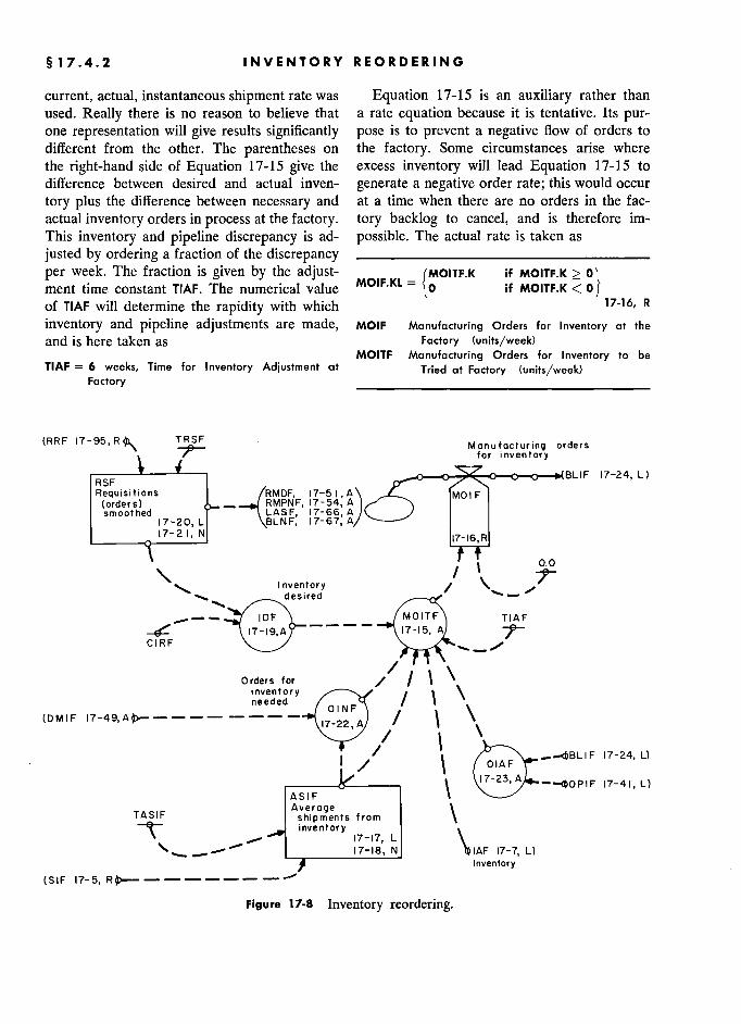
§ 17.4.2 INVENTORY REORDERING
current, actual, instantaneous shipment rate was Equation 17-15 is an auxiliary rather than
used. Really there is no reason to believe that a rate equation because it is tentative. Its pur- one representation will give results significantly pose is to prevent a negative flow of orders to different from the other. The parentheses on the factory. Some circumstances arise where the right-hand side of Equation 17-15 give the excess inventory will lead Equation 17-15 to
difference between desired and actual inven- generate a negative order rate; this would occur
tory plus the difference between necessary and at a time when there are no orders in the fac- actual inventory orders in process at the factory. tory backlog to cancel, and is therefore im- This inventory and pipeline discrepancy is ad- possible. The actual rate is taken as
justed by ordering a fraction of the discrepancy ____________________________
per week. The fraction is given by the adjust- MOIF.KL (MOITF.K
if MOITF.K > o j l ment time constant TIAF. The numerical value MOIF.KL =
f if MOITF.K < 0 f of TIAF will determine the rapidity with which
l 17-16, R
inventory and pipeline adjustments are made, MOIF Manufacturing Orders for Inventory at the and is here taken as Factory (units/week)
MOITF Manufacturing Orders for Inventory to be TIAF = 6 weeks, Time for Inventory Adjustment at Tried at Factory (units/week)
Factory _______________ ____ ____ ________
(RRF 17-95, R 4\ M anufacturing orders s
RSF .
e- for inventory
BLIF 17-24, L) RSF X. BLIF F 17-24, L)
Réquisitions RMDF, 7-5'A MOI F (orders)
RMPNF, 17-54,
A smoothed
1 7 -2 0 , LASF,
17-20, L BLNF, 17-67, A ' ' ' N 17-16, R
t 0.0 \ . Inventory
% desired
IDF MOITF TIAF F # 1 7 - 1 9, A 1 7 - ' 5, A A CIRF , /
Orders for / / 1 \ ' inventory
< t \ needed ./omr? / ' \ (DMIF ----
OINF A ,
/
,
\ '
(DM IF 17-49,Ap.----- ----
/ /
\ \
\ --<bBLIF 17-24, L) · j / t
17-24, L) ' / '
\ 01A F - -ÉB L 1 F 1 7 - 24, L)
A S I F \
TASIF Average \ TASIF shipments from \
inventory inventory
!7-t7,L L N ( IAF 17-7, L) N tp IAF !7-7,L)
Inventory (SIF
Figure 17-8 Inventory reordering.
A CUSTOMER-PRODUCER-EMPLOYMENT CASE STUDY
The standard first-order exponential averag- The target inventory is here taken as equal
ing equation will be used to convert the ship- to 4 weeks of sales, although in many situations
ment rate from inventory into the average ship- a higher level of inventory would be carried.
ment rate that was used in Equation 17-15: CIRF = 4 weeks, Coefficient for Inventory Ratio at t ––––––––––––––––––––––––––––––––––––– Factory
ASIF.K = ASIF.J + DT (SIF.JK - ASIF.J) 17-17, L Equation 17-19 requires an average level of TASIF sales. This is obtained in the same way as dis-
ASIF = RFIF 17-18, N cussed in Equation 15-8:
ASIF Average Shipments from Inventory at the ––––––––––––––––––––––––––––––––––––– Factory (units/week) DT
TASIF Time to Average Shipments from Inventory at RSF.K = RSF.J + TRSF(RRF.JK - RSF.J) 17-20, L the Factory (weeks)
SIF Shipments from Inventory at Factory RSF = RRF 17-21, N
(units/week) RSF Requisition rate Smoothed at Factory RFIF Requisition rate Filled from 1 at Fac- RSF Requisition rate Smoothed at Factory RF)F Requ!S!t!on rate F!!!ed from !nventory at Fac- 7 . / !
\ equlslhon 1 e rom nventory at ac-
(units/week) tory (units/week) TRSF Time for Requisition Smoothing at Factory (weeks)
The average inventory shipping rate is in- RRF Réquisition rate Received at Factory
tended to reflect very recent shipments from (units/week)
inventory. A short averaging time is therefore ––––––––––––––––––––––––––––
appropriate, such as This averaging of the incoming-order rate
2 ? ?_ ? _ From was necessary because week-by-week order flow
TASIF = 2 weeks, Time to Average Shipments From fl t t d 'd 1 M t f h r< rates must
inventory )°§§§§ fluctuated widely. Most of such now rates must
inventory at Factory be averaged before making management deci-
As described in Equation 15-7 and as ex- sions. This averaging may be a formal numeri-
pressed in the preceding discussion of policies, cal process or may be an intuitive or psychologi- the target inventory will be taken as propor- cal averaging of the flow of available informa- tional to average sales: 12 tion. Equation 17-20 shows that each week a
.__________________________ fraction TRSF of the différence between the cur-
IDF.K = (CIRF)(RSF.K) 17-19, A rent and average sales is used to correct the
IDF Inventory Desired at Factory (units) , level of average sales. In the steady-state aver- )DF inventory Des?red at Factory (un?ts) ° , , . ' CIRF Coefficient for Inventory Rario at Factory age, sales will equal the incoming sales rate RRF,
(weeks) as given in Equation 17-21. RSF Réquisition rate Smoothed at Factory The averaging time for incoming orders is
(units/week) here used as
this proportionality is taken because such TRSF weeksl3
was the policy in the case study. In a system redesign, The normal number of items on order for the "desired inventory" concept could give way to a inventory
to be d . in process h fac- "necessary inventory" concept based on a considera- inventory to bc expected in process at the fac-
tion of the relationships between customer service tory would be the average inventory shipping delay and customer order size, production lead time, rate multiplied by the manufacturing delay for manufacturing costs, changing distribution Patterns, and changes in product mix that are a function of y in the factory. changing sales levels. The necessary inventory would probably then lie between the square-root relationship '3 This is an exponential smoothing time and under (of simple inventory theory) and a linear propor- certain conditions is equivalent to a 30-week moving- tionality to sales. average interval. See Appendix E.
222
§ 17.4.3 MANUFACTURING
. BLIF BackLog for Inventory at Factory (units)
OINF.K = (ASIF.K)(DMIF.K) 17-22, A MOIF Manufacturing Orders for Inventory at the
OINF Orders for Inventory Necessary at Factory BLIRF Factory (units/week)
rate at Factory (units) BLIRF BackLog Inventory Reduction rate at Factory
ASIF Average Shipments from Inventory at the Fac- RFIF
(units/week) Filled from Inventory at Fac-
tory (units/week) RFIF Requisition rate Filled from Inventory at Fac-
DMIF Delay (variable) in Manufacturing for Inventory tory (units/week) r- , at Factory (weeks) , DNBLF Delay in Normal BackLog at Factory (weeks)
The actual orders in process in the factory for In Equation 17-25 the initial value for the
inventory will be the sum of two components, backlog of orders for inventory is given by the
the backlog of orders not yet started and the steady-state flow of orders that are filled from
orders in the process of manufacture: inventory RFIF multiplied by the normal length ____________________________ of the backlog DNBLF (value given after Equa- OIAF.K = BLIF.K + OPIF.K 17-23, A tion 17-67).
OIAF Orders for Inventory Actual at Factory (units) The backlog of work in progresS for goods BLIF BackLog for Inventory at Factory (units) being manufactured to customer order is simi- OPIF Orders in Process for Inventory at Factory lar:
(units)
This completes the description of inventory BLCF.K = BLCF.J + (DT)(RMOF.JK - PCOF.JK) This completes the description of inventory 17 26 L
reordering. Next the manufacturing sector of f L
the company will be described. BLCF = (RRF - RFIF)(DNBLF) 17-27, N
17.4.3 Manufacturing. The manufacturing BLCF BackLog for Customer at Factory (units)
operation is here represented by two flows, one RMOF Réquisition rate Manufactured to Order at
for goods that go into inventory and the other Factory (units/week)
for goods made to customer order. In actual PCOF
Production ta Customer Order at Factory
.... (units/week) practice these were intermixed in the same pro- RRF Réquisition rate Received at Factory duction lines, but in the model they will be (units/week) treated separately to provide the necessary RFIF Réquisition rate Filled from Inventory at Fac-
variables representing each of the two flows. tory (units/week)
at Factory (weeks) Consequently, Figure 17-9 shows two backlogs
DNBLF Delay in Normal BackLog at Factory (weeks)
of orders and two production delays. Since in
the process being represented the inventory or- We must now represent the allocation of
ders and the customer backlog orders were manufacturing manpower to each of the order
intermixed, there will be no priority given to flows. In normal operation, the two backlogs either category in this first formulation. were intermixed, giving them approximately the
Chapter 18 discusses some alternative manage- same priority. This implies that manpower was
ment policies including a priority for customer allocated in proportion to each of the backlogs, orders. so this should be the normal mode of operation.
The first equation gives the backlog of orders However, there may be times when the avail-
that are to be manufactured for inventory: able labor can produce more items than are in
____________________________ the backlogs during a period in which work
BLIF.K = BLIF.J + (DT)(MOIF.JK - BLIRF.JK) force is being reduced. At such times the back- 17-24, L logs should not become negative, but instead
BLIF = (RFIF)(DNBLF) 17-25, N the excess labor is devoted to making inventory.
223 3
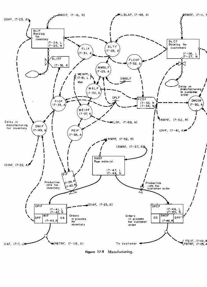
MOIF, 17-16, R) LBLAF, 17-68, A) RMOF, 17-11,
(OIAF, 17-23, A)y / <
BLIF F
/
/ BLIF ' 1
( Bockloq t -- T far --__ " ,
inventory t / inventory 17-24, L L
', BLCF
for Backlog for / N BLTF
customers
/ '–––––––f––––––' BLTF \ customers c
/ V f ) A eustamers 17-26, L ' ) 17-31, A 17 - 28, A 000, 17-26, L
t BLIRF
17-27, N -
1 j_ R MMBLF 17-32,
A
j t ( / \ t
,. y
A
) \
\
\
"–––"
/ / )hr)( DMBLF
\
, 1
/
/
Delay in j ' \ 1
/
t Delay in in t . / t ) manufacturing/
\ j f , t
f ta customer 9/
\ ! _t \ \ / t i / order er
\ ' PIOF 17-30, CPLF PCOF 7- 33, R order DMCOF
\ A
Delay in
17-35, A MEIPF
-) -aLDF '-- 17-69 17-34,
N
lÎ
A
\ /y
A /
'
Delay in \
/ , jt
17-69, AI , 'RMPF, 17-52, R)
/ /
manufacturinq ' '
t for inventory 17-49, ) PEIF
j (DVF, t7-81, A)·'/
17-38, A 17-52, RI 1
, lDVF, 17-81, AI'*'
t 17-52, R) )
,
\ /
/ l' (RMRF, 17-57, R
§
/ / ) 1
\
\ ) 1
1
/ / RMSF /
,' ;
(DINF, 17-22, A ¡, j
) (
/
Î Raw material
/
, / .
' / 17-47, L / /
/
J /
/
/
, 1 - Production --59,
17-48, N
Production . Production \..'Production '
rate for Jf
rate for order /
/
inventory order
.
17-23, A) OPCF ––––! /
1
. OPIF
17-41, L
0 1 A F, 17- 23, A) OPC F 17-44, L /
\ 17-42 N k N /
\ MIF Orders Orders s
SMOF DPF D3 in
process 1 n process
D3 17-46, R
DPF for for customer 17-46, R
j inventory order )
, (IAF, 17-7, L 17-115, A) To customer FG IF, 17-101? liAF, 17- 115, A) To customer PBTRF, 17-lls,
Figure 17-9 Manufacturing.
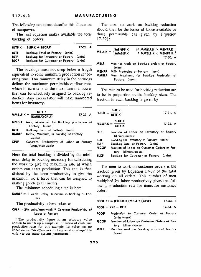
§ 17.4.3 3 MANUFACTURING
The following equations describe this allocation The men to work on backlog reduction
of manpower. should then be the lesser of those available or
The first equation makes available the total those permissible (as given by Equation
backlog of orders: 17-29):
BLTF.K = BLIF.K + BLCF.K 17-28, A
-??.?MBLF.K>MENPF.K1 } BLTF BackLog Total at Factory (units) MBLF.K = MMBLF_K if MMBLF.K <: MENPF.K } BLIF BackLog for Inventory at Factory (units) 17-30, A
BLCF BackLog for Customer at Factory (units) '
_____ MBLF Men for work on BackLog orders at Factory
The backlogs must not drop below a length MENPF MEN (men) Producing at Factory (men) not o MENPF MEN Produc!ng at Factory (men) equivalent to some minimum production sched- MMBLF Men, Maximum, for BackLog Production at uling time. This minimum delay in the backlogs Factory (men) defines the maximum permissible outflow rate, ––––––––––––––––––––––––––
which in turn tells us the maximum manpower The men to be used for backlog reduction are that can be effectively assigned to backlog re- to be in proportion to the backlog sizes. The duction. Any excess labor will make unordered fraction in each backlog is given by items for inventory.
MMBLF.K = 17-29, A F))PX = 17-3 1, A MMBLF.K = (DMBLF)(CPLF) 17-29, A FLIF.K =
gLTF.K 17-31, A
MMBLF Men, Maximum, for BackLog production at BLCF.K , _ A
Factory \ Factory (men) ' BLTF.K '
BLTF BackLog Total at Factory (units) FLIF Fraction of Labor on Inventory at Factory FDF Fraction of Labor on )nventoryat Factory DMBLF Delay, Minimum, in Backlog at Factory (dimensionless) (d!mens!on!ess)
CPLF (weeks) Productivity of Labor c Factory
BLIF BackLog for Inventory at Factory (units) } CPLF Constant, Productivity of Labor at Factory f$ at Factory °§"[ (units/man-week)
BLTF BackLog Total at Factory FLCOF Fraction of Labor on Customer Orders at Fac-
tory (dimensionless) Here the total backlog is divided by the mini- BLCF BackLog for Customer at Factory (units) mum delay in backlog necessary for scheduling ____________________________ the work to give the maximum rate at which
men to on customer is orders can enter production. This rate is then
fraction given work on customer orders is the - , fraction given by Equation 17-32 of thé total divided by thé labor productivity to give thé
fraction given by Equation 17-32 of the total
maximum work labor that can be assigned the e
working on all orders. This number of men maximum work force that can be assigned ta
r < maximum work force that
a can e assigned o multiplied by labor productivity gives
d mu lp le y a or productivity y l e- making goods to .
f making goods to
fill orders. lowing production rate for items for customer The minimum scheduling time is hère
order: produchon rate for Items or customer
° order: DMBLF = 1 week, Delay, Minimum in Backlog at Fac-
tory
The productivity is here taken as PCOF.KL = (FLCOF.K)(MBLF.K)(CPLF) 17-33, R
PCOF = RRF - RFIF 1734, N CPLF = 2% units/man-week,14 Constant Productivity of
Labor at Factory PCOF Production to Customer Order at Factory .. c . L' . (unitsjweek) "The productivity figure is an arbitrary value (units/week) ,-? Fac- chosen to match up a simple set of ratios of costs and FLCOF
Fraction of Labor on Customer Orders at Fac-
production rates for this example. Its value has no tory (dimensionless) effect on system dynamics so long as it is compatible MBLF Men for work on BackLog orders at Factory with various other system parameters. (men)
225
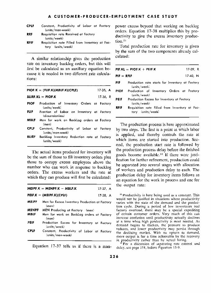
A CUSTOMER-PRODUCER-EMPLOYMENT CASE STUDY
CPLF Constant, Productivity of Labor at Factory power excess beyond that working on backlog (unirs/man-week) orders. Equation 17-38 multiplies this by pro- RRF Requisition rate Received at Factory .
RRF Requisition rate Received at Factory
ductivity to give the excess inventory produc- iw ta gwe the excess inven ory produc- (units/week) . l- RFIF Réquisition rate Filled from Inventory at Fac-
1
tory (units/week) Total production rate for inventory is given ____________________________ by the sum of the two components already cal-
A ..1 1. h.. h culated: A similar relationship gives the production culated:
rate on inventory backlog orders, but this will ____________________________ first be calculated as an auxiliary equation be- PIF.KL = PIOF.K + PEIF.K 17-39, R cause it is needed in two different rate calcula- PIF = RFIF 17-40, N tions:
' '
PIF Production rate starts for Inventory at Factory (units/week)
PIOF.K = (FLIF.K)(MBLF.K)(CPLF) 17-35, A PIOF Production of Inventory Orders at Factory
BLIRF.KL = PIOF.K 17-36, R (units/week) PEIF Production Excess for Inventory at Factory
PIOF Production of Inventory Orders at Factory (units/week) (units/week) RFIF Réquisition rate Filled from Inventory at Fac-
FLIF Fraction of Labor on Inventory at Factory tory (units/week) (dimensionless) _____________________________________
MBLF Men for work on BackLog orders at Factory (men) The production process is here approximated
CPLF Constant, Productivity of Labor at Factory by two steps. The first is a point at which labor
BLIRF (units/man-week)
Reduction rate at Factory <
B,,BE D !.. c applied, and thereby controls thé rate at BLIRF BackLog Invenrory Réduction rate at Factory is applied, an t ere y contro s t e rate at
(units/week) e uctlon rate at actory
which items are started into production. Sec-
____________________________ ond, the production start rate is followed by .. thé production process delay before thé nnished
The actual items produced for inventory will the production process delay before
the finished
. sum of those to fill inventory orders plus goods become available.16 If there were justi- be thé sum of those to fui inventory orders plus fi?atd'?on fo ?further refinement, produc on could to occupy excess employees above the fication for further refinement, production could
those to occupy excess employees above the be separated into several stages with allocation
ll§ # ° ° § °) to backlog of workers and production delay to each. The
which they excess workers and ca 1 cu 1 ate : d production delay for inventory items follows as which they can produce will rst be calculated:
an equation for the work in process and one for
–––––––––––––––––––––––––– the output rate:
MEIPF.K = MENPF.K - MBLF.K 17-37, A
PEIF.K = (MEIPF.K)(CPLF) 17-38, A Productivity is here being used as a constant. This would not be justified in situations where productivity MEIPF Men for Excess Inventory Production at Factory varies with the state of the demand and the produc-
(men) tion cycle. During a period of low inventories and MENPF MEN Producing at Factory (men) factory overload, there may be a special expediting MBLF Men for work on BackLog orders at Factory of certain customer orders. Very much of this can
(men) increase confusion until productivity actually declines PEIF Production Excess for Inventory at Factory at a time when high productivity is most needed. As
(units/week) demand begins to slacken, the pressure to produce
,..,,, , reduces, and lower productivity may persist through CPLF Constant,
Productivity of Labor at Factory the declining market. With an upturn in demand, (units/man-week) more output is for a time achievable by the recovery
––––-–––––––––––––––––––––––––––– in productivity rather than by actual hiring. . "' For a discussion of separating rate control and
Equation 17-37 tells us if there is a man- delay, see page 151, before Equation 15-9.
226
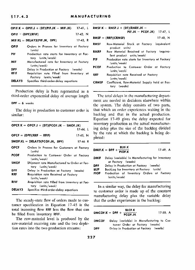
§ 17.4.3 MANUFACTURING
OPIF.K = OPIF.J + (DT)(PIF.JK - MIF.JK) 17-41, L RMSF.K = RMSF.J + (DT)(RMRF.JK -
OPIF = (DPF)(RFIF) 17-42, N PIF.JK - PCOF.JK) 17-47, L
OPIF = (DPF)(RFIF) 17-42, N
MIF.KL = DELAY3(PIF.JK, DPF) 17-43, R RMSF = (RRF)(CRMSF) 17-48, N
MIF.KL = DELAY3(PIF.JK, DPF) 17-43, R
OPIF Orders in Process for Inventory et Factory RMSF Raw-Material Stock at Factory (equivalent
OPIF Orders
in Process for Inventory at Factory product units) s (units) RMRF Raw Material Received at Factory (equiva-
PIF Production rate starts for Inventory at Fac- lent product units/week) tory (units/week) pIF Production rate starts for Inventory at Factory
MIF Manufactured rate for Inventory at Factory (units/week) (units/week) PCOF Production to Customer Order at Factory
DPF Delay in Production at Factory (weeks) (units/week) RFIF Requisition rate Filled from Inventory at RRF Requisition rate Received at Factory
Factory (units/week) (units/week) DELAY3 Specifies third-order-delay equations CRMSF Coefficient, Raw-Material Supply held at Fac- ––––––––––––––––––––––––––––––––––– tory (weeks)
Production delay is here represented as a ––––––––––––––––––––––––––––
third-order exponential delay of average length The total delays in the manufacturing depart- ment are needed in decisions elsewhere within
DPF = 6 weeks the system. The delay consists of two parts,
The delay in production to customer order is that which an order experiences waiting in the
similar: backlog and that in the actual production.
____________________________ Equation 17-49 gives the delay expected for
OPCF.K = OPCF.J + (DT)(PCOF.JK - SMOF.JK) inventory production as the actual manufactur- ' ' 17-44, L ing delay plus the size of the backlog divided
_ (DPF)fRRF - RF.F) ' N by the rate at backlog is being de-
OPCF = (DPF)(RRF - RFIF) 17-45, N bYl th de
rate at which the backlog is being de-
pleted: SMOF.KL = DELAY3(PCOF.JK, DPF) 17-46 R _______________________________
OPCF Orders in Process for Customers at Factory DMIF.K = DPF BLIF.K 17-49, A (units) DMIF.K = DPF + pIOF.K 17-49, A
PCOF Production to Customer Order at Factory (units/week) DMIF Delay (variable) in Manufacturing for Inventory
SMOF Shipment rate Manufactured to Order at Fac- at Factory (weeks)
tory (units/week) DPF Delay in Production at Factory (weeks)
DPF Delay in Production at Factory (weeks) BLIF BackLog for Inventory at Factory (units)
RRF Requisition rate Received et Factory PIOF Production of Inventory Orders at Factory
(units/week) (units/week) RFIF Requisition rate Filled from Inventory at Fac- –––––––––––––––––––––––––––––––––––––
tory (units/week) In a similar way, the delay for manufacturing DELAY3 Spécifies third-order-delay
équations to customer order is made up of the constant –––––––––
manufacturing delay plus the variable delay The steady-state flow of orders made to cus- that the order experiences in the backlog:
tomer specification in Equation 17-45 is the _________________________–– total incoming flow RRF less the flow that can BLCF.K be filled from inventory RFIF. DMCOF.K = DPF + pCOF.JK 17-50, A
The raw-material level is produced by the ln M anu f ac t. unng t 0 Cus-
raw-material receiving rate and the two deple- tomer Order at Factory (weeks) tion rates into the two production streams: l DPF Delay in Production at Factory (weeks)
227
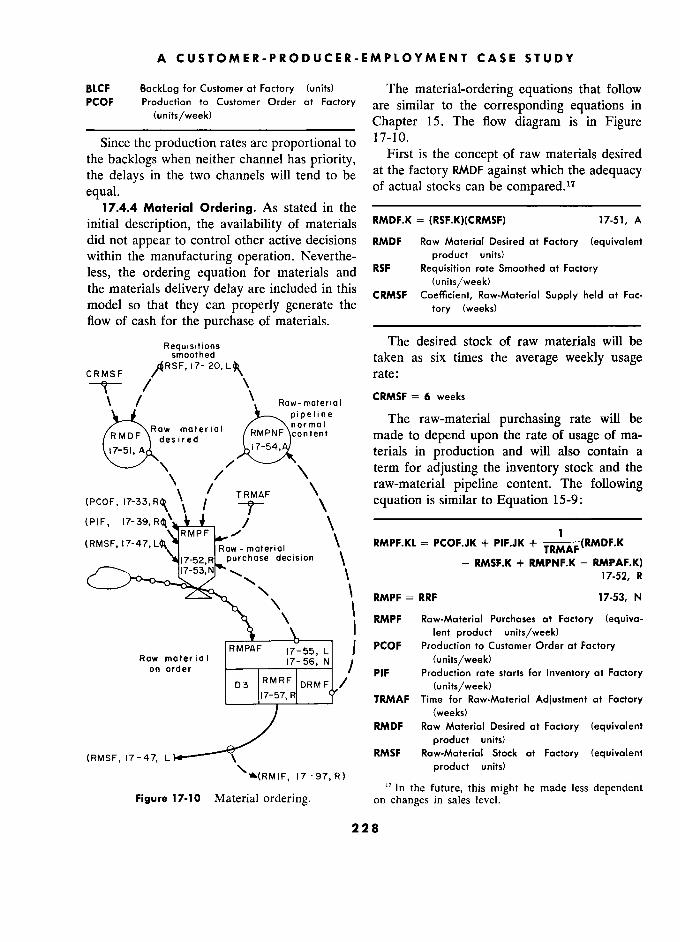
A CUSTOMER-PRODUCER-EMPLOYMENT CASE STUDY
BLCF BackLog for Customer at Factory (units) The material-ordering equations that follow PCOF Production to Customer Order at Factory are similar to the corresponding equations in
(units/week) Chapter 15. The flow diagram is in Figure Since the production rates are proportional to °.
the backlogs when neither channel has priority, First is the concept of raw materials desired
the delays in the two channels will tend to be at the factory RMDF against which the adequacy
equal. . of actual stocks can be compared.17
17.4.4 Material Ordering. As stated in the ––––––––––––––––––––––––––––
initial description, the availability of materials RMDF.K = (RSF.K)(CRMSF) 17-51, A did not appear to control other active decisions RMDF Raw Material Desired at Factory (equivalent within the manufacturing operation. Neverthe- product units) less, the ordering equation for materials and RSF Réquisition rate Smoothed at Factory the materials delivery delay are included in this (units/week) c ! L ? ? e t e matena s e lvery e ay are mc u e III t IS CRMSF Coefficient, Raw-Material Supply held at Fac- model so that they can properly generate the tory (weeks) flow of cash for the purchase of materials. __________________________
Réquisitions The desired stock of raw materials will be smootned taken as six times the average weekly usage
CRMSF F rate. 1 ° J 6
CRMSF F '/' rare: - r- Raw-material
CRMSF = 6 weeks ' / \ , CRMSF = 6 weeks \ / . Raw-matena!
normal e The raw-material purchasing rate will be
RMDF Rdesimederial RMPNF content t made to depend upon the rate of usage of ma-
de 17-54' terials in production and will also contain a 17-51, A 17-54, terials in production and will also contain a '–"
\\ \ term for adjusting the inventory stock and the \
/ TRMAF \ raw-material pipeline content. The following (PCOF, 17-33, equation is similar to Equation 15-9:
(PIF, / N ––––––––––––––––––––––––––––––––––– VRMPF ? \ 1
(RMSF, 17-47, L Row - mciterial \ RMPF.KL = PCOF.JK + PIF.JK + £ (RMDF.K 17-52,R purchase décision \ - RMSF.K + RMPNF.K - RMPAF.K)
\ 17-52, R ) RMPF = RRF 17-53, N
. RMPF Raw-Material Purchases at Factory (equiva-
\ t lent product units/week) RMPAF j_ L J PCOF Production to Customer Order at Factory
Raw material 1 17-56, N 1 (units/week) on order PIF Production rate starts for Inventory at Factory
D3 3 ??DRMF?/ (units/week) 17-57, R TRMAF Time for Raw-Material Adjustment at Factory
/ (weeks) ./ RMDF Raw Material Desired at Factory (equivalent
product units) (RMSF, 17-47, RMSF Raw-Material Stock at Factory (equivalent ' '
17-97,R) product units)
17-97,R) In the future, this might be made less dependent
Figure 17-10 Material ordering. on changes in sales level.
228 8
§ 1 7.4.5 5 LABOR
RMPNF Raw-Material Pipeline Normal content at Fac- tory (units) RMPAF.K = RMPAF.J + (DT)(RMPF.JK - RMRF.JK)
RMPAF Raw-Material Pipeline Actual content at Fac- 17-55, L
tory (units) RRF Requistion rate Received at Factory RMPAF = (RRF)(DRMF) 17-56, N
(units/week) RMRF.KL = DELAY3(RMPF.JK, DRMF) 17-57, R
In Equation 17 52 we again follow the ex- RMPAF Raw-Material Pipeline Actual content at Fac-
In Equation 17-52 we agam fonow thé e ex- Tory (units)
pediency of letting the present raw-material RMPF Raw-Material Purchases at Factory (equiva- purchasing rate depend upon the present raw- lent product units/week) material usage rate even though in principle and RMRF Raw Material Received at Factory (equiva-
in practice thé usage rate should be smoothed ,, lent product units/week)
,... RRF Requisition rate Received at Factory and delayed slightly to create levels as was done (units/week) in Equation 17-17. The parentheses in Equation DRMF Delay in Raw Materials at Factory (weeks) 17-52 give the difference between desired and DELAY3 Specifies third-order-delay equations actual raw-material stock plus the difference __________________________ between necessary and actual raw-material The average delay in procuring raw materials pipeline content. The time constant TRMAF con- is here trols the rate at which inventory and pipeline discrepancies will be corrected. The following
DRMF = 3 weeks
value of 8 weeks means that the correction rate 17.4.5 Labor. The labor supply and the is one-eighth of the remaining discrepancy per policies governing the changes in labor force are week:
important parts of the system under study. The
TRMAF = 8 weeks, Time for Raw-Material 1 Ad' lUS t men t effect under study is the interaction between the
at Factory varying flow of incoming orders from the cus-
. tomers and the resulting manufacturing rate, The necessary raw-materia) orders and ma- which in turn is controlled by the labor force
terial in transit in the material supply pipeline and adjustment. are proportional to the average level of business The labor sector and its governing policies activity and the length of the pipeline: are diagrammed in Figure 17-11. The labor –––––––––––––––––––––––––– loop itself consists of a labor pool, a hiring de- RMPNF.K = (RSF.K)(DRMF) 17-54, A cision, an initial training period, the level of
RMPNF Raw-Material Pipeline Normal content at E manpower available for production, a dismissal
tory (units) decision, and employees who have received RSF Réquisition rate Smoothed at Factory termination notices but have not yet left the
(units/week) payroll. DRMF Delay in Raw Materials at Factory (weeks) Several concepts are developed in a series of ––––––––––––––––––––––––––––
auxiliary equations dealing with the desired Since we are not interested here in the effects number of employees for the average level of
of a variable delay in the supply of materials, business and the number of employees neces- it will suffice to pass the orders through a third- sary for adjusting undesirable levels of order order delay from which the materials return backlogs. to factory raw-material stock. This requires a We shall start with the main labor flow loop level equation, its initial-value equation, and by considering the training delay. This is de- the designation of the delay function: scribed by the following three equations:
229
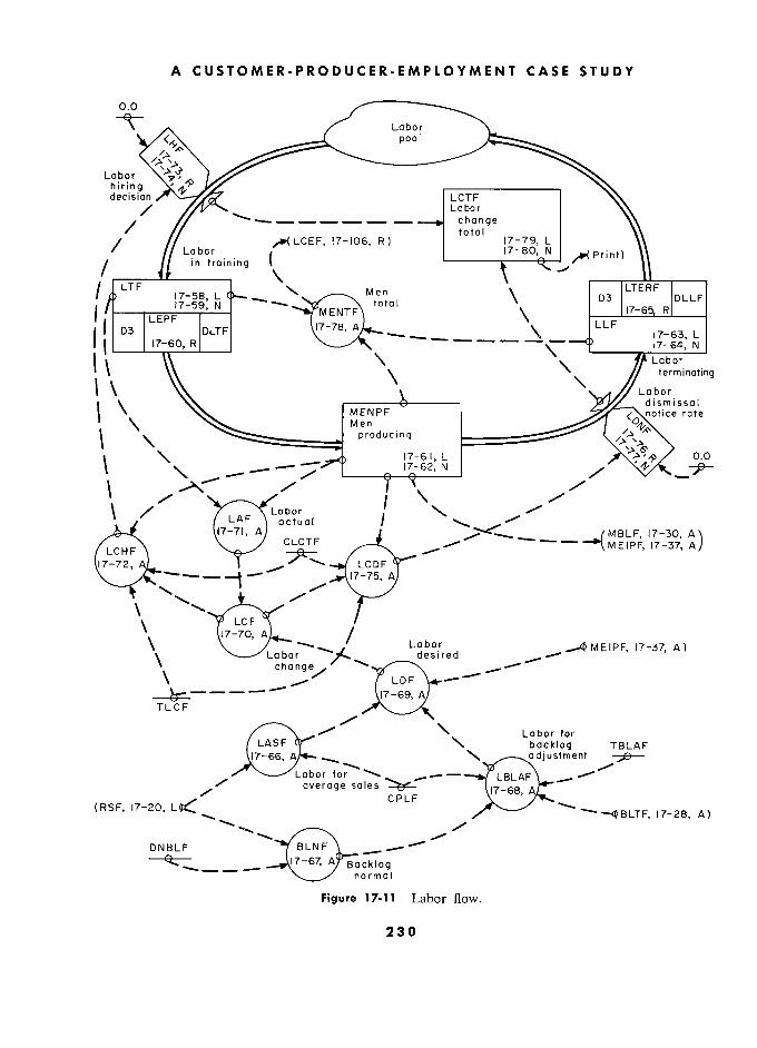
A CUSTOMER-PRODUCER-EMPLOYMENT CASE STUDY
fi Labor '\ < pool
Labor h i r i.n g decision LCTF
/ //''"* Labor \\
/ ° - change
/7 total
)7-79,L \\ /
17-106, R 17-79, L
/
/ Labor in
traininq j
/ LCEF, 17-lo6, R ) 17-80, N
L
sprint) \\
/ « La in bar training (
\ )t
J LTF
7
in training
, ,
LTERF /." .7-58. \ 1 MENTF total
'°'°'
D3 !7-6?R
f D3
LEPF DLTF
LLF L
j ' j
D3 17-60, R
- 17-63, N L
1 \ '\
'\ Labor
Î ) ', terminating
) \ '
Labor ) \ ( \ ?? MENPF Men
producing
t \ 17-6 1, L 0.0
j
17- 6 2, ?KJ
/
'\ \ / Labor \
y" 17-30,
A)
17-71, A CLCTF
< M B L F, 17 -30, A / \ \ / CLCTF *––**
A LCHF n A
- -4
A}
É)
LCHF desired. /
"
' '
17-70, A Labor
- - ,
desired ' '
\ change,?
17-69, A TLCF
/ Labor for ,/ Labor for /LASFqr
'
" backlog TBLAF
17-66, ??.?–?adjustment --fi-
Labor for average sales \!7-68 Ar
(RSF, 17-20,
average oles CPLF \,
17-28, A)
CPLF
DNBLF
17-67, A i3ocklog
Figure 17-H 1 Labor flow.
230
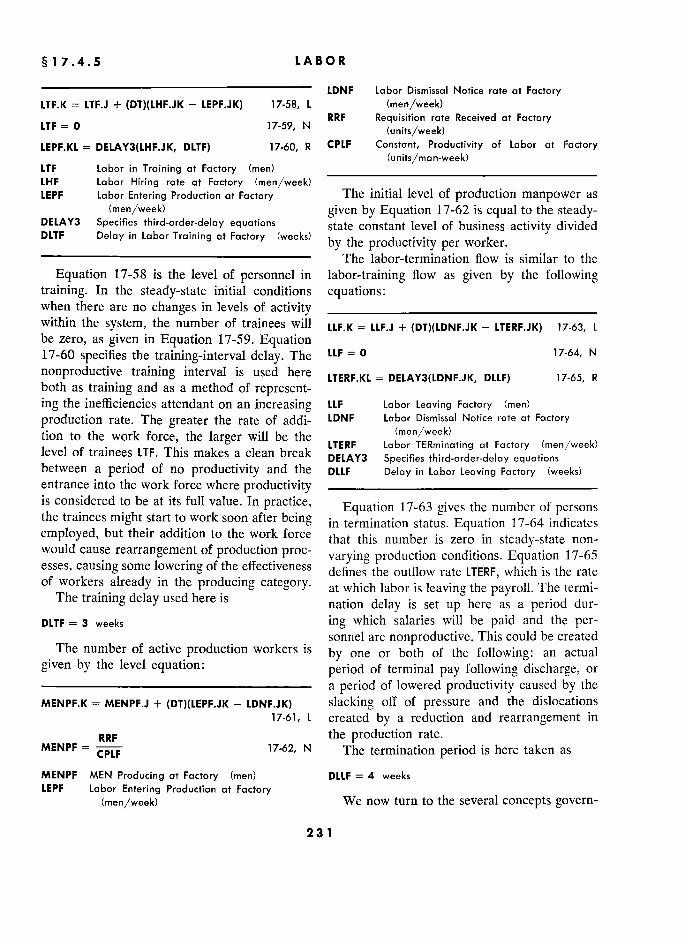
§ 1 7.4.5 5 LABOR
LDNF Labor Dismissal Notice rate at Factory LTF.K = LTF.J + (DT)(LHF.JK - LEPF.JK) 17-58, L (men/week)
LTF = 0 17-59, N RRF Réquisition rate Received at Factory
LTF = 0 17-59, N (units/week)
LEPF.KL = DELAY3(LHF.JK, DLTF) 17-60, R CPLF Constant, Productivity of Labor at Factory
LTF Labor in Training at Factory (men) (units/man-week)
LTF Labor in Training at Factory (men) _____________________________________ LHF Labor Hiring rate at Factory (men/week) LEPF Labor Entering Production at Factory The initial level of production manpower as
(men/week) given by Equation 17-62 is equal to the steady- DELAY3 Specifies third-order-delay equations state constant level of business activity divided DLTF Delay in Labor Training at Factory (weeks)
by the Productivity per worker. –––––––––––––––––––––––––––– The labor-termination flow is similar to the
Equation 17-58 is the level of personnel in labor-training flow as given by the following training. In the steady-state initial conditions equations: when there are no changes in levels of activity ____________________________ within the system, the number of trainees will LLF.K = LLF.J + (DT)(LDNF.JK - LTERF.JK) 17-63, L be zero, as given in Equation 17-59. Equation 17-60 specifies the training-interval delay. The LLF = 0 17-64, N
nonproductive training interval is used here LTERF.KL = DELAY3(LDNF.JK, DLLF) 17-65, R both as training and as a method of represent- ing the inefficiencies attendant on an increasing LLF Labor Leaving Factory (men)
production rate. The greater the rate of addi- LDNF Labor Dismissal Notice rate at Factory
tion to the work force, the larger will be the (men/week)
han clean break LTERF Labor TERminaring at Factory (men/week) level of trainees ' This makes a clean break DELAY3 Specifies third-order-delay equations
between a period of no productivity and the DLLF Delay in Labor Leaving Factory (weeks) entrance into the work force where productivity ____________________________ is considered to be at its full value. In practice, Equation 17-63 gives the number of persons the traînées might start to work soon after being in termination status. Equation 17-64 indicates employed, but their addition to the work force that this number is zero in steady-state non- would cause rearrangement of production proc- varying production conditions. Equation 17-65 esses, causing some lowering of the effectiveness defines the outflow rate LTERF, which is the rate of workers already in the producing category. at which labor is leaving the payroll. The termi-
The training delay used here is nation delay is set up here as a period dur-
DLTF = 3 weeks ing which salaries will be paid and the per- sonnel are nonproductive. This could be created
The number of active production workers is by one or both of the following: an actual
given by the level equation: period of terminal pay following discharge, or –––––––––––––––––––––––––––– a period of lowered productivity caused by the
MENPF.K = MENPF.J + (DT)(LEPF.JK - LDNF.JK) slacking off of pressure and the dislocations
17-61, L created by a reduction and rearrangement in
RRF the production rate. MENPF
CPLF 17-62, N The termination period is here taken as
MENPF MEN Producing at Factory (men) DLLF = 4 weeks LEPF Labor Entering Production at Factory
(men/week) We now turn to the several concepts govern-
231 1
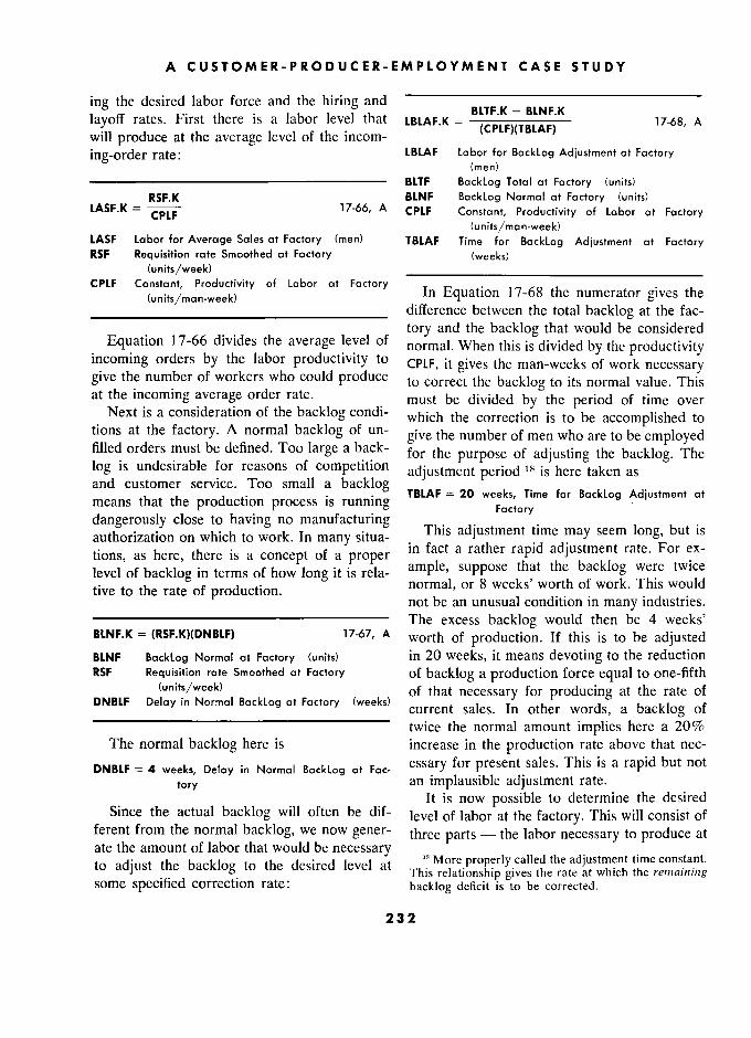
A CUSTOMER-PRODUCER-EMPLOYMENT CASE STUDY
ing the desired labor force and the hiring and BLTF.K - BLNF.K
layoff rates. First there is a labor level that LBLAF.K = j j 17-68, A
will produce at the average level of the incom-
ing-order rate: = LBLAF Labor for BackLog Adjustment at Factory (men)
––––––––––––––––––––––––––––––––––––– BLTF BackLog Total at Factory (units) RSF.K BLNF BackLog Normal at Factory (units)
LASF.K = CpLF 17-66, A CPLF Constant, Productivity of Labor at Factory . CPLF
(units/man-week) LASF Labor for Average Sales at Factory (men) TBLAF Time for BackLog Adjustment at Factory RSF Réquisition rate Smoothed at Factory (weeks)
(units/week) _____________________________________ CPLF Constant, Productivity of Labor at Factory
. , (units/man-week)
In Equation 17-68 the numerator gives the e
____________________________ difference between the total backlog at the fac-
tory and the backlog that would be considered Equation 17-66 divides the average level of normal. When this is divided by the productivity
incoming orders by the labor productivity ta CPLF, it gives the man-weeks of work necessary give the number of workers who could produce to correct the backlog to its normal value. This at the incoming average order rate.
_ must be divided by the period of time over Next is a consideration of the backlog condi- which the correction is to be accomplished to
tions at the factory. A normal backlog of un- give the number of men who are to be employed
filled orders must be defined. Too large a back- for the purpose of adjusting the backlog. The log is undesirable for reasons of competition adjustment period Il is here taken as and customer service. Too small a backlog TBLAF = 20 weeks, Time for BackLog Adjustment at - TBLAF = 20 weeks, Time for BackLog Adjustment at means that the production process is running g
TBLAF = 20
for - Adjusrment at
dangerously close to having no manufacturing Factory
authorization on which to work. In many situa- This adjustment time may seem long, but is
there to a concept many situa- in fact a rather rapid adjustment rate. For ex- -
tions, as here, there is a concept of a proper ample, suppose that adjustment were twice
level of backlog in terms of how long it is rela- ample, suppose that the backlog were twice tive to the rate of production. of
work. industries.
hve ta the rate of productlOn. not be an unusual condition in many industries. –––––––––––––––––––––––––––– The excess backlog would then be 4 weeks' BLNF.K = (RSF.K)(DNBLF) 17-67, A worth of production. If this is to be adjusted BLNF BackLog Normal at Factory (units) in 20 weeks, it means devoting to the reduction RSF Réquisition rate Smoothed at Factory of backlog a production force equal to one-fifth
(units/week) of that necessary for producing at the rate of DNBLF Delay in Normal Backlog at Factory (weeks)
Currerit sales. In other words, a backlog Of DNBLF ' in Normal '' ai ' (wee s)
current sales. In other words, a backlog of twice the normal amount implies here a 20%
The normal backlog here is increase in the production rate above that nec-
DNBLF = 4 weeks, Delay in Normal BackLog at Fac- essary for present sales. This is a rapid but not
tory an implausible adjustment rate. .
h d . d It is now possible to determine the desired Since the actual backlog will often be dif- level of labor at the factory. This will consist of
ferent from the normal backlog, we now gener- three parts - the labor necessary to produce at ate the amount of labor that would be necessary " More properly called the adjustment time constant. to .. level 13 More properly called the adJustm?nt time cons,ta,nt. to adjust the backlog to the desired level at relationship gives the rate at which the rernnining some specified correction rate: backlog deficit is to be corrected.
232
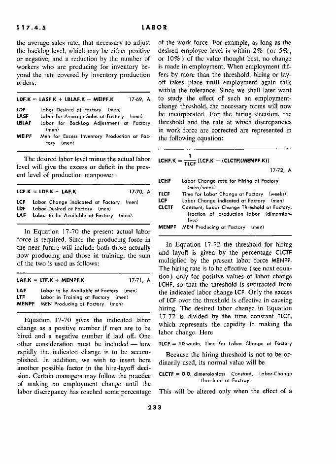
§ 1 7.4.5 5 LABOR
the average sales rate, that necessary to adjust of the work force. For example, as long as the
the backlog level, which may be either positive desired employée level is within 2% (or 5%, or negative, and a reduction by the number of or 10% ) of the value thought best, no change workers who are producing for inventory be- is made in employment. When employment dif-
yond the rate covered by inventory production fers by more than the threshold, hiring or lay- orders : off takes place until employment again falls ____________________________ within the tolerance. Since we shall later want
LDF.K = LASF.K + LBLAF.K - MEIPF.K 17-69, A to study the effect of such an employment-
LDF Labor Desired at Factors (men) change threshold, the necessary terms will now LDF Labor Des!red at Factory (men) ° -' LASF Labor for Average Sales ar Factory (men) be incorporated. For the hiring decision, the
LBLAF Labor for BackLog Adjustment at Factory threshold and the rate at which discrepancies (men) in work force are corrected are represented in
MEIPF Men for Excess Inventory Production at Fac- the following equatiori: tory (men)
'
The desired labor level minus the actual labor LCHF.K = [LCF.K - (CLCTF)(MENPF.K)l level will give the excess or deficit in the pres-
TLCF 17-72, A
ent level of production manpower: ' '
ent level of production manpower: LCHF Labor Change rate for Hiring at Factory
(men/week) LCF.K = LDF.K - LAF.K 17-70, A TLCF Time for Labor Change at Factory (weeks) LCF Labor Change indicated at Factory (men) LCF Labor Change indicated at Factory (men) LDF Labor Desired at Factory (men) CLCTF Constant, Labor Change Threshold at Factory, LAF Labor to be Available at Factory (men). fraction of production labor (dimension-
_____________________________________ less)
In Equation 17-70 the present actual labor MENPF MEN Producing at Factory (men)
force is required. Since the producing force in the near future will include both those actually and Equation .17-72 the threshold for hiring now producing and those in training, the sum and layoff is given by the percentage CLCTF
of the two is used as follows: _ '
multiplied by the present labor force MENPF. ° ° The hiring rate is to be effective (see next equa-
LAF.K = LTF.K + MENPF.K 17-71, A tion) only for positive values of labor change LCHF, so that the threshold is subtracted from
LAF Labor to be Available at Factory (men) the indicated labor change LCF. Only the excess LTF Labor in Training at Factory (men) LTF Labor Producing at Factory (men) of LCF over the threshold is effective in causing
MENPF MEN Producing at Factory (men) hiring. The desired labor change in Equation
Equation the indicated labor 17-72 is divided by the time constant TLCF,
change as a positive number if men are to be which represents the rapidity in making the e
change as a positive number if men are to be r o pOSI Ive . t. b
er -r , ..j r<-
e 1 abor change. Hère
hired and a negative number if laid off. One labor change. Here
other consideration must be included - how TLCF = 10 weeks, Time for Labor Change at Factory
rapidly the indicated change is to be accom- Because the hiring threshold is not to be or- plished. In addition, we wish to insert here
dinarily i normal value will be another possible factor in the hire-layoff deci-
'
sion. Certain managers may follow the practice CLCTF = 0.0, dimensionless Constant, Labor-Change
of making no employment change until the Threshold at Factroy
labor discrepancy has reached some percentage This will be altered only when the effect of a
233 3
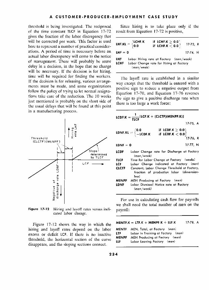
A CUSTOMER-PRODUCER-EMPLOYMENT CASE STUDY
threshold is being investigated. The reciprocal Since hiring is to take place only if the of the time constant TLCF in Equation 17-72 result from Equation 17-72 is positive, gives the fraction of the labor discrepancy that –––––––––––––––––––––––––––– will be corrected per week. This factor is used
LHF.KL LCHF.K if LCHF.K > 0.0 j
R here to represent a number of practical consider- if LCHF.K K < 0.0 JJJ)
" ,
ations. A period of time is necessary before an LHF = 0 17-74, N actual labor discrepancy will come to the notice
LHF Labor Hiring rare ai Facrory (men/week) LHF Labor Hiring rate at Factory (men/week) of management. There will probably be some LCHF Labor Change rate for Hiring at Factory delay in a decision, in the hope that no change (men/week) will be necessary. If the decision is for hiring, ____________________________ time will be required for finding the workers.
The layoff rate is established in a similar If the décision is for releasing, various arrange- way except that the threshold is entered with a ments must be made, and some
organizations positive sign to reduce a negative output from follow the policy of trying to let normal résigna- Equation 17-70, and Equation 17-76 reverses tions take care of the réduction. The 10 weeks s
the sign to give discharge rate when just mentioned is probably on the short side of
there is too large force: the usual delays that will be found at this point
'
in a manufacturing process. LCDF.K + (CLCTF)(MENPF.K)l LCDF.K TLCF
+ (CLCTF)(MENPF.K)]
17-75, A x
0.0 if LCDF.K > 0 0 L ô
LDNF.KL if LCDF.K < Threshold
Tg '' LDNF.KL - if LCDF.K
17-76, R (CLCTF)(MENPF)
LDNF = 0 17-77, N 1
\. [ ??S?ope' LCDF Labor Change rate for Discharge at Factory ! determined (men/week)
TLCF Time for Labor Change at Factory (weeks) L1 I LCF LCF Labor Change indicated at Factory (men)
) CLCTF Constant, Labor Change Threshold at Factory,
-J fraction of production labor (dimension-
less) S MENPF MEN Producing at Factory (men)
LDNF Labor Dismissal Notice rate at Factory
5 h U (men/week)
Î –––––––––––––––––––––––––––––––––––––
z " For use in calculating cash ftow for payrolls
we shall need the total number of men on the Figure 17-12 2 Hiring and layoff rates versus indi- payroll:
cated labor change. ___________________________
Figure 17-12 shows the way in which the MENTF.K = LTF.K + MENPF.K + LLF.K 17-78, A
hiring and layoff rates depend on the labor MENTF MEN, Total, at Factory (men)
excess or deficit LCF. If there is no inactive LTF Labor in Training at Factory (men)
threshold, the horizontal section of the curve MENPF
disappears, and the sloping sections connect. LLF Labor Leaving Factory (men)
234
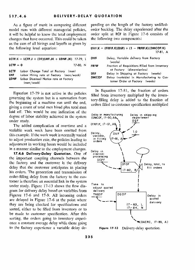
§ 17.4.6 DELIVERY-DELAY QUOTATION
As a figure of merit in comparing different pending on the length of the factory unfilled-
model runs with different managerial policies, order backlog. The delay experienced after the
it will be helpful to know the total employment order split at RCF in Figure 17-6 consists of
changes that have occurred. This could be taken the following two components: as the sum of all hirings and layoffs as given by ––––––––––––––––––––––––––––
the following level equation: DVF.K = (FRFIF.K)(DSF) + (1 - FRFIF.K)(DMCOF.K) 17-81, A
LCTF.K = LCTF.J + (DT)(LHF.JK + LDNF.JK) 17-79, L DVF Delay, Variable delivery from Factory (weeks)
LCTF = 0 17-80, N FRFIF Fraction of Réquisitions Filled from Inventory
LCTF Labor Change Total at Factory (men) at Factory (dimensionless)
LHF Labor Hiring rate at Factory (men/week) DSF Delay in Shipping at Factory (weeks)
LDNF Labor Dismissal Notice rate at Factory DMCOF Delay (variable) in Manufacturing to Cus-
(men/week) tomer Order at Factory (weeks)
? ?, is not active in the policies In Equation 17-81, the fraction of orders
Equation 17-79 is not active in thé policies filled from inventory multiplied by the inven-
governing the system but is a summation from tory-filling delay is added to the fraction of
the beginning of a machine run until thé end, orders filled to customer specification multiplied
gwmg a count of total men hired plus total men laid off. This would be one indication of the
De?ay!nmanufactur!ng Delay in shipping degree of labor stability achieved in the system Deiay in manutact??rin9 Deiay in shippin9 g y y department under study.
' \ DSF F
The added complication of overtime and a (FRFIF, 1 variable work week have been omitted from
Delay, 0 this example. If the work week is normally varied variable to adjust production rate, the policies leading to 17-81, A
adjustment in working hours would be included \ in a manner similar to the employment changes. in \
17.4.6 Delivery-Delay Quotation. One of clerical \ the important coupling channels between the \ the factory and the customer is the delivery DCPF Delay, torai, ro delay that the customer anticipates in placing fi i i' ordels his orders. The generation and transmission of l
order-filling delay from the factory to the cus- 1 tomer is therefore an essential link in the system Time ta
1 under study. Figure 17-13 shows the flow dia-
gram for delivery delay based on variables from delivery _______t
Figures 17-6 and 17-9. All incoming orders TAOD
F DQDF F De I o y i n are delayed in Figure 17-6 at the point where
quoted they are being checked for specifications and 17-83, L
sorted, either to be filled from inventory or to i N
be made to customer specification. After this '
sorting, the orders going to inventory experi- -&(DAERC, 17-89, A) ence a constant average delay while those going
A)
to the factory experience a variable delay de- Figure 17-13 Delivery-delay quotation.
235 5
A CUSTOMER-PRODUCER-EMPLOYMENT CASE STUDY
by the delay that these orders experience in mation delay) into which flows the delivery-
traversing the factory. The sum of these two delay information:
components gives the average delay experienced ––––––––––––––––––––––––––––
by the entire order flow after it divides into the DODF.K = DQDF.J + DT (DFOF.JK - DQDF.J) two channels. TAQDF
'
In addition to the average delay for the two 17-83, L
flow channels, aIl orders experience the delay DQDF =
DCPF + (CNFIF)(DSF) DCPF in Figure 17-6 while they are being
+ (1 - CNFIF)(DPF + ) 17-84, N
separated into the inventory and factory chan- DQDF Delay (variable) in Quoted Delivery at Factory
nels. This delay must be
added to the variable Quoted Delivery at Factory delay from Equation 17-81 as is done in the e
TAQDF (weeks)
Quored Delivery at Factory
following rate equation that controls the pri- DFOF Delay (variable) to Fill Orders at Factory
mary flow of order-filling-delay information (weeks)
within the factory. DCPF Delay in Clerical Processing at Factory " ' (weeks) CNFIF Constant, Normal Fraction of requisitions filled
from Inventory at Factory (dimensionless) DFOF.KL = DCPF + DVF.K 17-82, R DSF Delay in Shipping at Factory (weeks)
DFOF Delay (variable) to Fill Orders at Factory DPF Delay in Production at Factory (weeks)
(weeks) DNBLF F Delay in Normal BackLog at Factory (weeks)
DCPF Delay in Clerical Processing at Factory –––––––––––––––'––––––––––––––––––––––
(weeks) The time delay TAQDF indicates the rapidity DVF Delay, Variable delivery from Factory (weeks) witjl which quoted time delays DQDF approach –––––––––––––––––––––––––––– the value DFOF that is implicit in the state of the
Equation 17-82 gives the present instantane- manufacturing operation. Here we shall use a Equation 17-82 gives thé présent instantané-
1-month lag; therefore ous delivery delay. This value is not necessarily 1-month lag; therefore
known by the sales department for quotation TAQDF = 4 weeks, Time to Adjust Quoted Delivery at
to customers. Awareness of an increasing fac- Factory
tory backlog does not permeate the entire or- The initial-value equation, 17-84, is derived
ganization at once. Quoted delivery delays in by combining Equations 17-81 and 17-82, in
many industries are based more on the delays which the split fraction FRFIF has been replaced which have been experienced by the orders cur- by its normal value CNFIF from Figure 17-7,
rently being delivered rather than the delays and the manufacturing delay DMCOF is replaced which can be anticipated in the future, based on by the steady-state values. considerations of backlog and present produc- 17.4.7 Customer Ordering. The customer tion rate. The delay information given by Equa- ordering section appears in the flow diagram of tion 17-82 should then be delayed, and the Figure 17-14. The independent input INPUT values transmitted to the customer will lag represents the flow of orders to the customer for behind the values that may be indicated by equipment in which will be used the components present instantaneous operating facts within the made by the component supplier. As discussed
organization. The following equation'a is an av- in Section 17.2, this will be considered as an
eraging equation (producing a first-order infor- independent input to the system under study. It " As noted in earlier chapters, the dimensional units equations dealing with average rates and having the
of measure are not an adequate indication of whether same dimensions of measure as a rate of flow. In a variable should be written as a rate or level equa- information channels rates will often have the dimen- tion. We have seen numerous examples of level sions of the information being delayed and averaged.
236
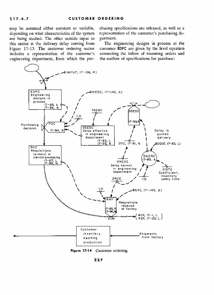
§ 17.4.7 CUSTOMER ORDERING
may be assumed either constant or variable, chasing specifications are released, as well as a
depending on what characteristics of the system representation of the customer's purchasing de-
are being studied. The other outside input to partment.
this sector is the delivery delay coming from The engineering designs in process at the
Figure 17-13. The customer ordering sector customer EDPC are given by the level equation includes a representation of the customer's connecting the inflow of incoming orders and
engineering department, from which the pur- the outflow of specifications for purchase:
––"S.
EDPC C 17-143, A) Engineering /
designs in / __
process 7-85 L process 17-85, L / .)
17-86, N , '
o
TAEDC DDEDC
"-––--
/ / /
1.0 TAEDC /
DDEDC
Purchasing PDC /
17-90, \
decision !/<(. DEEDC C \
decis ion 7-94, R Delay effective Delays in n
j in engineering q /
( quoted d i department i
< delivery y
) 17-92, L '
17-93 N DTC, 17-91, N ' ,»DODF 17-83, L)
RCC ./ Requisitions
. (orders) in clerical processing DAERC û)
7-87 L DNEDC 17-89, '
DNEDC N DNLDC \ /
––––––t–––––– \ Delay normal 1. jL
. in
engineering / CISTC in enginee,,ng CISTC )
\ department Coefficient.
& \ DRCC
„–6– inventory \
\ DRCC 1.0 safety time
'
\ - 1- 10
- ----K:- 1
/ PC,
'
17- 145, A) \.
\
\ ,
, \ /
\. RRF Réquisitions
RRF Requisitions
received 17-95,R R at factory 17-96,N N
RCF, 17- 1, L ) l
RSF, 17-20, L /
Customer
inventory y Shipments s
awaiting q from factory y
production
Figure 17-14 4 Customer ordering.
237
A CUSTOMER-PRODUCER-EMPLOYMENT CASE STUDY
EDPC.K = EDPC.J + (DT)(INPUT.JK - PDC.JK) purchasing department, here assumed to be EDPC.K = EDPC.J + (DT)(INPUT.JK -
PDC.JK) 17-85, L constant, on the average.
EDPC = (INPUT)(DEEDC) 17-86, N The second part of the delay is the time nec-
EDPC = (INPUT)(DEEDC) 17-86, N essary on the average for filling orders at the
EDPC Engineering Designs in Process at Customer component manufacturer; this is the variable (units) quoted delivery time DQDF. The third part of
INPUT INPUT of orders to customer from outside of time that Components system (equivalent units/week) PDC Purchasing Décision at Customer lie in inventory awaiting production at the cus- PDC P h. D.. t C the Produchon PDC Purchasing Decision a Customer
(units/week) tomer plant. We are especially interested in any DEEDC Delay Effective (variable) in Engineering De- variable component in the inventory holding
partment at Customer (weeks) period at the customer, since this can create a –––––––––––––––––––––––––––– variable reservoir that can affect the customer's
The steady-state level of designs in process is ordering rate. It is reasonable to assume that
given by Equation 17-86 as the product of a the customer will protect himself by carrying
steady-state input flow and the initial value of an inventory stock that is related to the length the delay in the engineering department. of time that he finds is needed to procure com-
The next level equation defines the requisi- ponents. As the delivery delay increases, so will
tions in process in the purchasing department the inventory holding period, at least to some RCC: extent. Here the constant CISTC relates the com-
____________________________ ponent procurement delay to the variable part RCC.K = RCC.J + (DT)(PDC.JK - RRF.JK) 17-87, L of the inventory holding period. The total time
RCC = (INPUT)(DRCC) 17-88, N from engineering
release date until the
compo- " nents are assembled into equipment is then
RCC Réquisitions in Clerical processing at Customer given by (units)
PDC Purchasing Décision at Customer (units/week) ****'
RRF Réquisition rate Received at Factory DAERC.K = DRCC + (1 + CISTC)(DQDF.K) (units/week) 17-89, A
INPUT INPUT of orders to customer from outside of DAERC Delay (variable) in procurement After Engi- ( . 1 .
/ k) , DAERC Delay ln procurement After Engl' system (equivaient units/week) neering Release at Customer (weeks) neering Release at Customer (weeks) '
DRCC Delay, average, for Requisitions in Clerical DRCC Delay, average, for Requisitions in Clerical 1 ' , DRCC De!ay, average, for Requ!s?t!ons !n Ciencai processing at Customer (weeks)
e ay, average, Customer (weeks) ln erlca
processing at Customer (weeks) –––––––––––––––––––––––––– CISTC Coefficient for Inventory Safety Time at Cus-
The steady-state level in Equation 17-88 is tomer, fraction of procurement delay that
given by the initial flow rate multiplied by the goods lie in customer inventory (dimension- . , . , .... less)
average e dela the p rocessin g of p urchase DQDF Delay less) (variable) in Quoted Delivery at Fac- . orders DRCC. tory (weeks)
The customer engineering department will be ___________________________-
responsive to the component procurement de- We shall here use lay as one of the factors controlling the release date of design specifications to the purchasing CISTC = 0.5, dimensionless Coefficient for Inventory
department. This delay between engineering Safety Time at Customer, fraction of
release and the time that components are as- procurement delay that goods lie in retease and thé time that components are as- sembled into the equipment produced by the
customer inventory
customer consists of three parts. The first is which means that the customer's inventory the delay in placing orders in the customer's holding period goes up and down by half the
238 8
§17.4.7 CUSTOMER ORDERING
amount of the actual change in procurement DNEDC Delay Normal in Engineering Department at
delay. Customer (weeks)
, .. DRCC De!ay, average, for Réquisitions !nC!erica! As stated in the general description of the
DRCC Delay, average, for Requisitions in Clerical As stated description processing at Customer (weeks)
problem, the customer tends to order critical CISTC Coefficient for Inventory Safety Time at Cus-
components as far ahead as necessary. This tomer, fraction of procurement delay that
means that especially critical components are goods lie in customer inventory (dimension-
given special consideration in the design process , , Delivery at Factory so that they can bc released earlier when cir-
DQDF Delay (variable) Quoted Delivery at Factory so that they can be released earher when cir- (weeks) cumstances make this necessary. If everything (weeks)
required by the customer should be on a long
delivery schedule, his own equipment delivery The normal engineering department design
dates may have to be postponed. However, his time used here is
first attempt will be to maintain his own delivery DNEDC = 30 weeks, Delay Normal in Engineering De-
schedule by accelerating the release date of partment at Customer
special items out of his engineering department .
so that they may be ordered as early as neces- Equation 17-90 gives thé desired time that
so that other words, normal engineering delay the engineering department has available for
plus average procurement delay controls the design before purchase specification release.
customer in promising his own deliveries. Thé However, the change in engineering design
particular delay experienced in each component time cannot be instantaneously responsive to
tends to determine when he places his orders. a change in component-delivery quotations. To
The permissible time that an order may take accelerate the design release of a particular
in the customer's engineering department will component, it may be necessary to start well
now be defined as the total time he has from ahead of the release date to begin making this
incoming equipment order to equipment de- information available ahead of schedule. The
livery, less the time that component procure- following equation represents the lag in the
ment requires: actual delay effective in the engineering depart-
__________________________ ment as it lags behind the changing delivery
DDEDC.KL = DTC - DAERC.K 17-90, R quotations:
DDEDC Delay (variable) Desired in Engineering De-
partment of Customer (weeks) DT DTC Delay Total at Customer (weeks) DEEDC.K DEEDC.J
+ TAEDC ' '
DAERC Delay (variable) in procurement After Engi- 17-92, L
neering Release at Customer (weeks) ,
_______________________________ DEEDC = DTC - (1 + CISTC)(DQDF) - DRCC –––––––––––––––––––––––––––––––
17-93, N
Equation 17-90 gives the flow of desired re- 17-93, N
lease-date information to the engineering de- DEEDC Delay Effective (variable) in Engineering De-
partment. The normal total time taken by the ,.,-.. partment at Customer (weeks)
customer to fill equipment orders DTC is here TAEDC
Time (weeks) to Adjust Engineering Delay at Customer
approximated (omitting details of production DDEDC Delay (variable) Desired in Engineering De-
and equipment test) by the following: partment of Customer (weeks)
_____________________________________ DTC Delay Total at Customer (weeks)
DTC = DNEDC + DRCC + (1 + CISTC)(DQDF) CISTC Coefficient for Inventory Safety Time at Cus-
' tomer, fraction of procurement delay that
goods lie in customer inventory (dimen-
DTC Delay Total at Customer (weeks) sionless)
239
A CUSTOMER-PRODUCER-EMPLOYMENT CASE STUDY
DQDF Delay (variable) Quoted Delivery at Factory pletion. The term in parentheses adds a noise
DRCC Wk) for Requisition in Clerical term that can be used to test the sensitivity of
DRCC De!ay, averaqe, for Réquisition in C!erica! DRCC processing ar Customer cweeks)
in Clerical thé system to a fiuctuating and erratic output pïocessmg at Customer (weeks)
ythe engineering department pool. In
an from the engineering department pool. In an
The time constant of the engineering re- actual situation this noise can come from the
The time constant of the engineering and from sponse delay is here assumed to be e
intermittent release of conditions, changes in sponse delay is hère assumed to be changes in economic conditions, changes in
TAEDC = 15 weeks, Time to Adjust Engineering Delay military budgeting and contracting, and other at Customer factors that may cause customers to accelerate
Equation 17-92 is an equation of the first- or delay their purchasing decisions. The noise
order exponential smoothing type used here to term NEDC will be specified later in the input
delay the information DDEDC before it becomes test functions.
actually effective in controlling engineering de- In a similar way, the release rate of orders
partment releases in the form of DEEDC. The from the purchasing department will be taken
reciprocal of the adjustment time TAEDC gives as a fixed fraction of the orders being proc-
the fraction of the difference between the essed. As in the engineering release rate, this
quoted and the effective delay that is adjusted can be modified by a noise variable to represent
per week within the engineering department the bunching and irregular placing of orders as
scheduling. For example, if DEEDC had been they would come out of customer purchasing 30 weeks and DDEDC is now 25 weeks, the dif- departments: "
ference of 5 weeks divided by the 15-week time ––––––––––––––––––––––––––
constant TAEDC would lead to a shortening of RCC.K the engineering department design schedule by
RRF.KL = NPC.K) 17-95, R
one-third of a week per week. RRF = INPUT 17-96, N The variable delay developed in Equation RRF Requisition rate Received at Factory
'
17-92 is now available to control thé fraction RRF Requisition rate Received at Factory 17-92 is now available to control the fraction (units/week)
per week of the orders in the engineering de- RCC Requisitions in Clerical processing at Customer partment which are released for purchasing: (units) _____________________________________ DRCC Delay, average, for Réquisitions in Clerical
EDPC.K K processing at Customer (weeks)
PDC.KL = (1 + NEDC.K) 17-94, R NPC Noise at output of Purchasing at Customer DEEDC.K ' '
(dimensionless)
PDC Purchasing Décision at Customer INPUT INPUT of orders ta customer from outside of
(units/week) system (equivalent units/week) EDPC Engineering Designs in Process at Customer –––––––––––––––––––––––––––––––––––––
The average delay in placing purchase orders DEEDC Delay (unit5) Effectue (variable) ln Engineering De- . here The
average delay in placing purchase orders
partment 'lÉln$ (weeks) is
NEDC Noise at Engineering Department output of DRCC = 3 weeks Customer (dimensionless) t DRCC = 3 weeks
–––––––––––––––––––––––––––– 17.4.8 Cash Flow. The cash flow sector is
The essential part of the purchasing decision shown in Figure 17-15. As set up here it is for at the customer is the ratio of engineering work the monitoring of operation in the remainder in process to the engineering department delay. of the model. Cash position and the cash flow This gives the outflow rate in terms of the work rates do not enter into any of the essential de- in progress and the time necessary for its com- cisions of the system. However, it is to be ex-
240
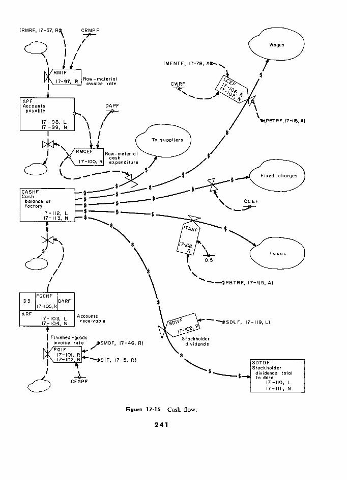
(RMRF, 17-57, R4§ CRMPF
T
'MENTF, '7-78,
Wages
.)
\ // /
RMIF Rùw-mùteriùl
<MENTF '7-78 .
/)\ !7-97 R Raw-materio! / 17- 97, R invoce rate CWRF / )
APF
aw ,"'.", invoice te
/0
\
APF Accounts DAPF / \
payable DA
PF / '
-..¡ PBTRF,17-115, A) payable 17 -98, L ,
r- ____ / 17-99, N \ / /
'\
/
Ta suppliers
/
$
?, Raw-material $ y ?CL cash .ture
.jr-––––– ,! _____ 17-100, R expenditur
1 \ -.-
$ ------
1
Fixed charges
CCEF CASHF balance at
factory at
*"$ ' CCEF
factory 17 -112, L -$
,
17-113, N
$
at $
$
: I ,
\
0.5
\
( Taxes
) '
. 0.5
/ .' 1/
FGCRF \ D3 3
DARF $
17-105, R .
ARF Accounts \ _ A ccount s - 17-119, L} !7-!04N L N
' F_'?'s?ed -Q°°dS \`?Stockholder
I invoice rate QSMOF, 17-46, R) \ dividends
'
'StockhOlddertotal SCTDF
!7-!0!,R R r
$
I 17-5, R) SDTDF
. ' Stockholder / \ „ dividends s total
_
l
-
N
CFGPF date
CFGPF 17-I10, L
Figure 17.15
17-III, N
Figure 17-15 Cash flow.
241
A CUSTOMER-PRODUCER-EMPLOYMENT CASE STUDY
pected that different policies will lead to differ- average delay in paying invoices. Equation ent profitability of operation and to different 17-100 specifies the rate of payment for ma-
degrees of fluctuation in cash position. The cash terial as a fraction of the accounts payable. An
flow sector will be kept simple to serve this average invoice payment interval has been taken
monitoring purpose and to show how the finan- as cial flows can be added to a dynamic model. DAPF = 3 weeks, Delay in Accounts Payable at Factory
The following equations give raw-material invoice rate, the level of accounts payable, and Money received for goods delivered will be
the rate of cash expenditure for raw materials: handled in a slightly different but equivalent __________________________ way to serve as an alternative example. Here
RMIF.KL = (RMRF.JK)(CRMPF) 17-97, R invoices for finished goods will traverse a third-
APF.K = APF.J + (DT)(RMIF.JK - RMCEF.JK)
' order delay (at the customer) before being con-
APF.K = APF.J + (DT)(RMIF.JK - "'_ L verted to a flow of cash receipts:
APF = (RRF)(CRMPF)(DAPF) 17-99, N FGIF.KL = (SIF.JK + SMOF.JK)(CFGPF) 17-101, R
RMCEF.KL = 17-100, R FGIF = (RRF)(CFGPF) 17-102, N . DAPF ' ARF.K = ARF.J + (DT)(FGIF.K - FGCRF.JK)
RMIF Raw-Material Invoice rate at Factory 17-103, L (dollars/week)
RMRF Raw Material Received at Factory (équivalent ARF = (RRF)(CFGPF)(DARF) 17-104, N
product units/week) FGCRF.KL = DELAY3(FGIF.JK, DARF) 17-105, R CRMPF Constant, Raw-Material Price at Factory
(dollars/unit) FGIF Finished-Goods Invoice rate at Factory APF Accounts Payable at Factory (dollars) (dollars/week) RMCEF Raw-Material Cash Expenditure at Factory SIF Shipments from Inventory at Factory
(dollars/week) (units/week) RRF Réquisition rate Received at Factory SMOF Shipment rate Manufactured to Order at
(units/week) Factory (units/week) DAPF Delay in Accounts Payable at Factory CFGPF Constant, Finished-Goods Price at Factory
(weeks) (dollars/unit) _____________________________________ RRF Réquisition rate Received at Factory
17 .
h .. (units/week) Equation 17-97 gives the raw-materiâl in- ARF Accounrs Receivable at Factory (dollars)
voice rate as the product of raw-material receiv- FGCRF Finished-Goods Cash-Receipt rate at Factory
ing rate multiplied by the raw-material price per (dollars/week) unit of product. Prices here are chosen for this DARF Delay in Accounts Receivable at Factory
example as a self-consistent set related by rea- (weeks)
example as a self-consistent set related -' rea- DELAY3 Specifies (weeks) third-order-delay equations
sonable ratios.2° The raw-material cost is __________________________
CRMPF = $20.00 per unit Equation 17-101 multiplies the shipments
Equation 17-98 is the standard level equa- from inventory plus the shipments to customer
tion accumulating the difference between in- specifications by the price per unit of product
voices received and paid. Equation 17-99 gives Here again is the expediency of using flow rates the initial steady-state value of accounts payable on the right-hand side to determine a flow rate on the as the product of the rate of sales multiplied by left. It would, however, avail us nothing to create a
the material cost per unit multiplied by the level of invoices in the process of being mailed, since r the delay can be included m the delay in Equation 17-105, intervening between the generation of in-
They are not the values from the case study. voices and receipt of payment.
242
1 7 . 4 . 8 CASH FLOW
The unit price used in this example is Equation 17-107 is needed because the wage-
CFGPF = $100.00 per unit, Constant, Finished-Goods s rate flow appears on the right-hand side of
Price at Factory Equation 17-115. _ . The basis for taxes and dividends is devel- Equation 17-102 gives the initial value of the
oped in the next section. The corresponding invoice rate as the total sales rate multiplied cash flow is taken here as follows: by the unit price. Equation 17-103 gives the
'
level of accounts receivable; actually this is a ITAXF.KL = (0.5)(PBTRF.K) 17-108, R variable not used elsewhere in the model, and 17.108, R
the equation could be omitted unless its value SDIVF.KL = SDLF.K 17-109, R
is wanted in the output information from the ITAXF Income TAX at Factory (dollars/week) model. Equation 17-104 is the initial level of PBTRF Profit Before Tax Rate at Factory the accounts receivable given by the product (dollars/week) of sales rate, unit price, and average accounts- SDIVF Stockholder DIVidends at Factory
receivable delay. Equation 17-105 represents (dollars/week) receivable delay. Equation 17-105 represents SDLF Stockholder Dividend Level at Factory
the sum of all the delays in the accounts-receiv- able circuit. It includes billing, mailing of in- ____________________________ voices, the time necessary for the customer to
Equation 17-108 gives taxes as a simple 50% initiate payment, and the time to receive a of the profit-before-tax rate. Equation 17-109 check and deposit it. This total all-inclusive de-
gives the rate of payment of dividends as being lay is taken as
equal to the level of dividend payments calcu- DARF = 5 weeks, Delay in Accounts Receivable at lated in the next section.
Factory To provide a basis for comparison between
The next equations give cash flow for the computer runs, the stockholder dividend total
payment of wages: to date can be accumulated as follows:
LCEF.KL = (MENTF.K)(CWRF) 17-106, R SDTDF.K = SDTDF.J + (DT)(SDIVF.JK) 17-110, L
LCEF = (MENPF)(CWRF) 17-107, N SDTDF = 0 17-111, N
LCEF Labor Cash Expenditures at Factory SDTDF Stockholder Dividends To Date at Factory (dollars/week) (dollars)
MENTF MEN, Total, at Factory (men) SDIVF Stockholder DIVidends at Factory CWRF Constant, VVage Rate at Factory (dollars/week)
(dollars/man-week) (dollars/week)
MENPF MEN Producing at Factory (men) ____________________________ All the cash flow rates have already been
Equation 17-106 computes the rate of cash defined, so that the cash balance is given by the
flow for wages as the number of total employees équation : "
multiplied by the weekly wage rate. Overtime ––––––––––––––––––––––––––––
and other forms of variable productivity have CASHF.K = CASHF.J + (DT)(FGCRF.JK - RMCEF.JK
not been incorporated in this example. An ar- -LCEF.JK - CCEF - ITAXF.JK
bitrary wage rate selected to go with the other '' ' L
prices in this example is CASHF = (CNCSF)(CFGPF)(RRF) 17-113, N
CWRF = $80.00 per man-week CASHF CASH balance at Factory (dollars) FGCRF Finished-Goods Cash-Receipt rate at Factory
The initial value of the wage rate given by (dollars/week)
243
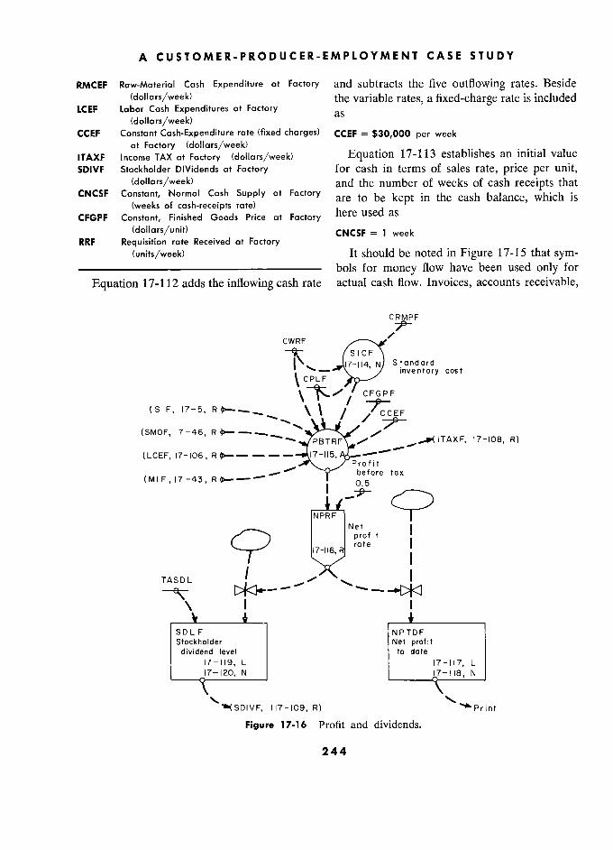
A CUSTOMER-PRODUCER-EMPLOYMENT CASE STUDY
RMCEF Raw-Material Cash Expenditure at Factory and subtracts the five outflowing rates. Beside (dollars/week) . the variable rates, a fixed-charge rate is included
LCEF Labor Cash Expenditures at Factory as (dollars/week)
CCEF Constant Cash-Expenditure rate (fixed charges) CCEF = $30,000 per week at Factory (dollars/week)
ITAXF Income TAX at Factory (dollars/week) Equation 17-113 establishes an initial value
SDIVF Stockholder Dividende at Factory for cash in terms of sales rate, price per unit, (dollars/week) and the number of weeks of cash receipts that
CNCSF Constant, Normal Cash
Supply at Factory are t0 be kept in the cash balance, which is (weeks of cash-receipts rate)
here used as CFGPF Constant, Finished Goods Price at Factory here used as
(dollars/unit) CNCSF = 1 week RRF Réquisition rate Received at Factory
(units/week) It should be noted in Figure 17-15 that sym- –––––––––––––––––––––––––––– bols for money flow have been used only for
Equation 17-112 adds the inflowing cash rate actual cash flow. Invoices, accounts receivable,
CRMPF
CWRF - SICF
j$ / à[ N Standard d
)\
17-114, N Standard
' / inventory cost
\\ / ' CCEF (SMOF.!7-46,R<)–––._
t7-!08. R) (SMOF, 17 -46, R
` PBTRF ./' ./'
ITAXF, 17-108, R)
(LCEF, 17-106, Profit it t
(MIF,17-43, before tax before fax
0.5 5
? NPRF ) Net 1 profit i t
9
rate 1
1 17-I16,
R rate
1
1
TASDL ' 1
- g- \ ' '
SDLF F NPTDF F Stockholder Net profit dividend level to date
17-119, L 17-117, L 17-120, N 17-118, N
'"SDIVF, 117-109, R) ' ' Print
Figure 17-16 Profit and dividends.
244
§ 17.4.9 PROFIT AND DIVIDENDS S
and such are part of the information flow sys- MIF Manufactured rate for Inventory at Factory tem. (units/week)
1749 1 this a CWRF Constant, Wage Rate at Factory 17.4.9 Profit and D)V)dends. In mis model a .. ro 1 an IVI en s. n IS ma e a (dollars/man-week)
simple computation of current profit rate will be CPLF Constant, Productivity of Labor at Factory generated to be used as an indicator of system (units/man-week) performance. It will be based on a most ele- CCEF Constant Cash-Expenditure rate (fixed charges)
mentary view of accounting relationships. The at Factory (dollars/week)
profit calculation is shown in the flow diagram ––––––––––––––––––––––––––––
of Figure 17-16. The first two terms in parentheses give the A standard inventory cost will first be gener- sum of the production for inventory plus the
ated as an initial-condition equation based on production to customer specification. This sum
the constants already incorporated: is multiplied by the cost of goods sold less the –––––––––––––––––––––––––– standard inventory costs. This would yield gross
SICF = CRMPF + CWRF 17-114, N profit if the labor were being employed at full CPLF
" efficiency, and the last term subtracts the fixed
SICF Standard nventory Cost per item at Factory costs. The middle term of the equation subtracts
(dollars/unit) the total wage payment minus the standard CRMPF Constant, Raw-Material Price at Factory labor value in the goods produced. The wage
(dollars/unit) level LCEF will be equal to the labor value in CWRF Constant, Wage Rate at Factory
the goods produced if there are no training or
(dollars/man-week) the goods produced If there are no training or
(dollars/man-week) at Factory CPLF Constant, Productivity of Labor at Factory termination payments being made. This term
(units/man-week) subtracts the excess labor costs represented by –––––––––––––––––––––––––––– the losses incurred by training and layoffs.
Items in inventory are here being valued at Net profit rate will be taken simply as half of
material cost plus the direct labor per unit. the profit before tax rate:
The profit-before-tax rate will be used as the ____________________________
following: NPRF.KL = (0.5)(PBTRF.K) 17-116, R
PBTRF.K = (SIF.JK + SMOF.JK)(CFGPF - SICF) NPTDF.K = NPTDF.J + (DT)(NPRF.JK) 17-117, L
PBTRF.K = (SIF.JK + SMOF.JK)(CFGPF - SICF) NPTDF = 0 17-118, N
- rLCEF.JK - (MIF.JK NPRF Net Profit Rate at Factory (dollars/week)
CWRF)]
PBTRF Profit Before Tax Rate at Factory + SMOF.JK)
- - CCEF (dollars/week)
CPLF NPTDF Net Profit To Date at Factory (dollars) 17-115, A ___________________________________
PBTRF Profit-Before-Tax Rate at Factory (dollars/week) Equation 17-117 is a level equation that
SIF Shipments from Inventory at Factory accumulates net profit to date as one of thé accumulates net profit ta date as one of the (units/week) ..
f Th. 1 l' SMOF Shipment rate Manufactured ta Order at Fac- indicators of system performance. This level is
tory (units/week) set initially to zero by Equation 17-118. CFGPF Constant, Finished-Goods Price at Factory The net profit rate will be averaged over a
(dollars/unir) period of time as the basis for the payment of SICF Standard Inventory Cost per item at Factory stockholder dividends so that dividends will not
(dollars/unit) S oc a er IVI en s sa a
IVI en s WI no
LCEF Labor Cash Expenditures at Factory fluctuate with short-run changes in net profit (dollars/week) rate:
245
A CUSTOMER-PRODUCER-EMPLOYMENT CASE STUDY
DT model itself. Also a variety of test input func-
SDLF.K = SDLF.J + SDLF.J) tions will be needed to determine the system TASDL 17-119, L behavior. These are covered in the next two ' '
sections. r / CWRF
SDLF = 0.S[RRF(CFGPF -
CRMPF - CPLF > L \ " / 17.5 Supplementary Output Information
In the output tabular and plotted information - CCEF 1 17-120, N
it is often to present variables in forms N
it is often desirable to present variables in forms J or combinations that have not been a part of
SDLF Stockholder Dividend Level at Factory the model structure itself. These we here call
TASDL Time (dollars/week) to Adjusr Srockholder Dividend Level supplementary variables. They are calculated TASDL
Time (weeks) to Adjust Stockholder Dividend Level
only Y sa that their values may b recorded for ) oniy so that their values may be recorded tor
NPRF Net Profit Rate at Factory (dollars/week) study. RRF Réquisition rate Received at Factory For an example system model as presented
(units/week) here, the actual numerical values of the vari- CFGPF Constant, Finished-Goods Price at Facrory ables are not of great significance since the
(dollars/unit) , .. ... CRMPF Constant, Raw-Material Price a Factory scale of opérations could be increased or de-
(dollars/unit) creased to represent any size of business. We CWRF Constant, VVage Rate at Factory are more interested in comparing the percentage
(dollars/man-week) changes in most of the variables; therefore for CPLF Constant, Productivity of Labor at Factory the variables r principal importance, we shail CPLF
Producriviry 'thé variables of principal importance, we shall (units/man-week)
e vana es 0 r l p '.. s.. CCEF Consront Cash Expenditure rate (fxed charges) calculate them as percentages of their initial
at Factory (dollars/week) steady-state values :
The exponential averaging time of BLTPC.K = (BLTF.K)(1oo) 17-121, S
TASDL = 52 weeks, Time to Adjust Stockholder Divi- (CINPI)(DNBLF)
'
dend Level CASPC.K =
(CASHF.K)(100) 17-122, S
used here is equivalent, under many conditions, to a longer moving-average période
BLTPC BackLog Total as Per Cent of initial value
Th ...
1 d" E .
17 120' b (per cent) The initial-condition Equation 17-120 is ob- BLTF BackLog Total at Factory (units) e llllha -con lhon quahon - IS a - BLTF BackLog Total at Factory (units)
tained by substituting the initial steady-state CINPI Constant, INPut, Initial value (units/week) values of Equation 17-114 into 17-115, from DNBLF Delay in Normal BackLog at Factory (weeks) which the middle term is zero and can be CASPC CASh balance in Per Cent of initial value
dropped, and 1 d. thé 0.5 factor from ...,.,, , „ „ . factor from CASHF CASH balance at Factory (dollars)
Equation 17-116. CNCSF Constant, Normal Cash Supply at Factory This formulation pays out all profits as divi- (weeks of cash-receipt rate)
dends, since no other use of profits has been in- CFGPF Constant, Finished-Goods Price at Factory cluded in the model. (dollars/unit)
The preceding equations complete the de- ––––––––––––––––––––––––––––
scription of the system under study. In addition, In Equation 17-121, the denominator gives it will be désirable to have certain values re- the initial value of backlog as the initial sales corded for study which are not active in the rate multiplied by the normal length of the
=" See Appendix E. backlog.
246
§ 17.5 5 SUPPLEMENTARY OUTPUT INFORMATION
The fraction of requisitions filled from in- NPRPC Net Profit Rate in Per Cent of initial value
ventory needs only be multiplied by 100 to plot NPRF (per cent)
at Factory (dollars/week) on a per cent scale: NPRF Net Profit Rate at Factory (dollars/week) CFGPF Constant, Finished-Goods Price at Factory
(dollars/unit)
FRFPC.K = (FRFIF.K)(100) 17-123, S SICF Standard Inventory Cost per item at Factory
(dollars/unit) FRFPC Fraction of Réquisitions Filled from inventory CCEF Constant Cash-Expenditure rate (fixed charges)
in Per Cent (per cent) at Factory (dollars/week) FRFIF Fraction of Réquisitions Filled from Inventory RRFPC Réquisitions Received at Factory in Per Cent
at Factory (dimensionless) of initial value (per cent)
_____________________________________ RRF Réquisition rate Received at Factory
(units/week) The following equations are self-explanatory ____________________________
for percentage changes in actual and desired We may wish to know the total shipment
inventory, the input sales rate, the employment rate to the customer, a value that has not thus level, net profit, and orders received at factory: far been calculated:
IAFPC.K = (IAF.K)(100) 17-124, S SCF.K = SIF.JK + SMOF.JK 17-130, S
(CIRF)(CINPI) ,
SCF Shipments to Customer from Factory
(IDF.K)( 1 00) (units/week) IDFPC.K
= - 17-125, S SIF Shipments from Inventory at Factory (CIRF)(CINPI) ' (CIRF)(CINPI)
(units/week)
INPPC.K = INPUT.JK
(100) 17-126, S SMOF Shipment rate Manufactured to Order at
' CINPI
' Factory (units/week)
MENPC.K = (MENPF.K) (CINPI) CPLF
(100) 17-127, S In evaluating the performance of the model
MENPC.K = (1 00) 1 7-1 27, S In evaluating thé performance of the model
(NPRF.JK)(loo) system, we shall sometimes want the kind of NPRPC.K K =
(0.5)[(CINPI)(CFGPF - SICF) - CCEF] financial information ordinarily provided in
17-128, s cash-flow statements and balance sheets. The
RRFPC.K RRF.JK
(100) 17-129 S cash-flow variables for the simple financial
CINPI s
considerations of this model have been defined
IAFPC Inventory Actual at Factory in Per Cent of ini- in Section 17.4.8. In addition, we shall want
tial value (per cent) the balance-sheet information giving inventory IAF Inventory Actual at Factory (units) valuations and the différence between current
CIRF Coefficient for Inventory Ratio at Factory assets (here cash, accounts receivable, and in-
CINPI Constant
lNPut Initial value (units/week) ventories of finished goods, work in process and
CINPI Constant, INPut, Initial value (units/week) material) and current liabilities (here only IDFPC Inventory Desired at Factory in Per Cent of f matenal) ' and current lia 1 ities omy J
initial value (per cent) accounts payable) : "
IDF Inventory Desired at Factory (units) _____________________________________
INPPC INPut Per Cent of initial value (per cent)
VIAF.K = (IAF.K)(SICF) 17-131, S INPUT INPUT of orders to customer from outside of .. 17-1 , S
system (équivalent units/week) VIPIF.K = (OPIF.K + r rCRMPF MÉNPC MEN producing at factory, Per Cent of initial VIPIF.K = (OPIF.K + OPCF.K) CRMPF
value (per cent) /CWRF MENPF MEN Producing at Factory (men) + 17-132, S
CPLF Constant, Productivity of Labor at Factory
(units/man-week) VRMSF.K = (RMSF.K)(CRMPF) 17-133, S
247
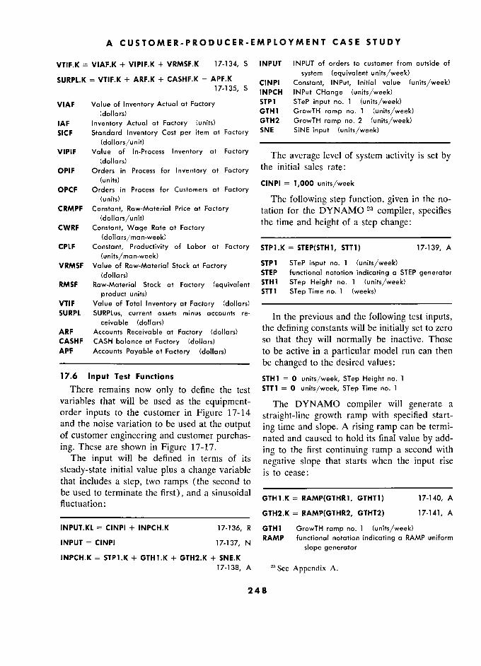
A CUSTOMER-PRODUCER-EMPLOYMENT CASE STUDY
VTIF.K = VIAF.K + VIPIF.K + VRMSF.K 17-134, S INPUT INPUT of orders to customer from outside of
SURPL.K = VTIF.K + ARF.K + CASHF.K - APF.K system (equivalent units/week) SURPL.K T'F'K ARF. C°. °"'
s CINPI Constant, INPut, Initial value (units/week)
17-135, S INPCH INPut CHange (units/week) VIAF Value of Inventory Actual at Factory STP1 STeP input no. 1 (units/week)
(dollars) GTH1 1 GrowTH ramp no. 1 (units/week) IAF Inventory Actual at Factory (units) GTH2 GrowTH ramp no. 2 (units/week) SICF Standard Inventory Cost per item at Factory SNE SiNE input (units/week)
(dollars/unit) ––––––––––––––––––––––––––––––––––––– VIPIF In-Process Inventory at Factory The average level of system activity is set by
(dollars) . t h e lllItla ... 1 sa 1 es rate: OPIF Orders in Process for Inventory at Factory the initial sales rate:
(units) CINPI = 1,000 units/week OPCF Orders in Process for Customers at Factory
(units) The following step function, given in the no- CRMPF Constant, Raw-Material Price at Factory tation for the DYNAMO 23 compiler, specifies (dollars/unit) the time and height of a step change: CWRF Constant, Wage Rate at Factory ° r* &
(dollars/man-week) ––––––––––––––––––––––––––––––––––––– CPLF Constant, Productivity of Labor at Factory STP1.K = STEP(STH1, STT1) 17-139, A
(units/man-week) VRMSF Value of Raw-Material Stock at Factory STP1 1 STeP input no. 1 (units/week)
(dollars) STEP functional notation indicating a STEP generator RMSF Raw-Material Stock at Factory (équivalent STH1 1 STep Height no. 1 (units/week)
product units) ) STT1 1 STep Time no. 1 (weeks)
VTIF Value of Total Inventory at Factory (dollars) ––––––––––––––––––––––––––––––––––– SURPL SURPLus, current assets minus accounts re- In the previous and the following test inputs, ceivable (dollars) . .. ARF ceivable Receivable ai (d Il) the defining constants will be initially set to zero ARF Accounts Receivable at (dollars) t e e ning constants wi e
mitia y set to zero
CASHF CASH balance at Factory (dollars) so that they will normally be inactive. Those APF Accounts Payable at Factory (dollars) to be active in a particular model run can then –––––––––––––––––––––––––––– be changed to the desired values: '
17.6 Input Test Functions STH1 = 0 units/week, STep Height no. 1
There remains now only to define the test STT1 = 0 units/week, STep Time no. 1
variables that will be used as the equipment- The DYNAMO compiler will generate a order inputs to the customer in Figure 17-14
straight-line growth ramp with specified start- and the noise variation to be used at the output ing time and slope. A rising ramp can be termi- of customer engineering and customer purchas- nated and caused to hold its final value by add- ing. These are shown in Figure 17-17.
_ ing to the first continuing ramp a second with The input will be defined in terms of its
negative slope that starts when the input rise steady-state initial value plus a change variable is to cease: that includes a step, two ramps (the second to ________ be used to terminate the first), and a sinusoidal
GTH1.K = RAMP(GTHR1, GTHT1) 17-140, A fluctuation:
' ' '
_______________________________ GTH2.K = RAMP(GTHR2, GTHT2) 17-141, A
INPUT.KL = CINPI + INPCH.K 17-136, R GTH1 GrowTH ramp no. 1 (units/week)
CINPI 17-137, N RAMP functional notation indicating a RAMP uniform
INPUT = CINPI 17.137, N si ope generator
INPCH.K = STP1.K + GTH1.K + GTH2.K + SNE.K 17-138, A =5 See Appendix A.
248
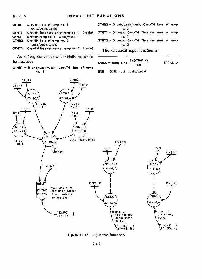
§ 17.6 INPUT TEST FUNCTIONS S
GTHR1 GrowTH Rate of ramp no. 1 GTHR2 = 0 unit/week/week, GrowTH Rate of ramp (units/week/week) no. 2
GTHTI GrowTH Time for start of ramp no. 1 (weeks) GTHT1 = 0 week, GrowTH Time for start of ramp GTH2 GrowTH ramp no. 2 (units/week) no. 1 GTHR2 GrowTH Rate of ramp no. 2 GTHT2 = 0 week, GrowTH Time for start of ramp
(units/week/week) no. 2 GTHT2 GrowTH Time for start of ramp no. 2 (weeks) 'j'he sinusoidal input function is:
As before, the values will initially be set to ––––––––––––––––––––––––––––
be inactive: the values will initially be set to
SNE.K = (SIH) sine 17-142, A
GTHR1 = 0 unit/week/week, GrowTH Rate of ramp no. 1 SNE SiNE input (units/week)
GTHTt GTHR2
GTHR1\ 1 GTHT2
GTH1 GTH2 / (7 -140,A fl
/ f
Growth Growth STTI 1 1
no. 2
PER
',
/ SIH
STP1
/
/ SNE
/
17-139,A U7-!42,A) A
CNAEC Step .)** Sine fluctuation na.1 17-138,A
Sine f luctuation CNAEC no.t
Input 0.0 CNAPC / change –– CNAPC
1 /
NNEDC NNPC / j C 1 NP I ) ) )
17-144,A 17-146,A
INPUT Input orders to
CNSEC C ) '
CNSPC
17-136, Input orders ta D' 1 )7-!36,R customer sector t 1 . 17-137, from outside ' /
of system NPC
t 17-143, A 17-145, A
EDPC l INoise at INoise at
17-85, L / t engineering
purchasing department t output output
\ PDC C \ RRF F '\
RRF )
Figure 17-17 Input test functions.
249
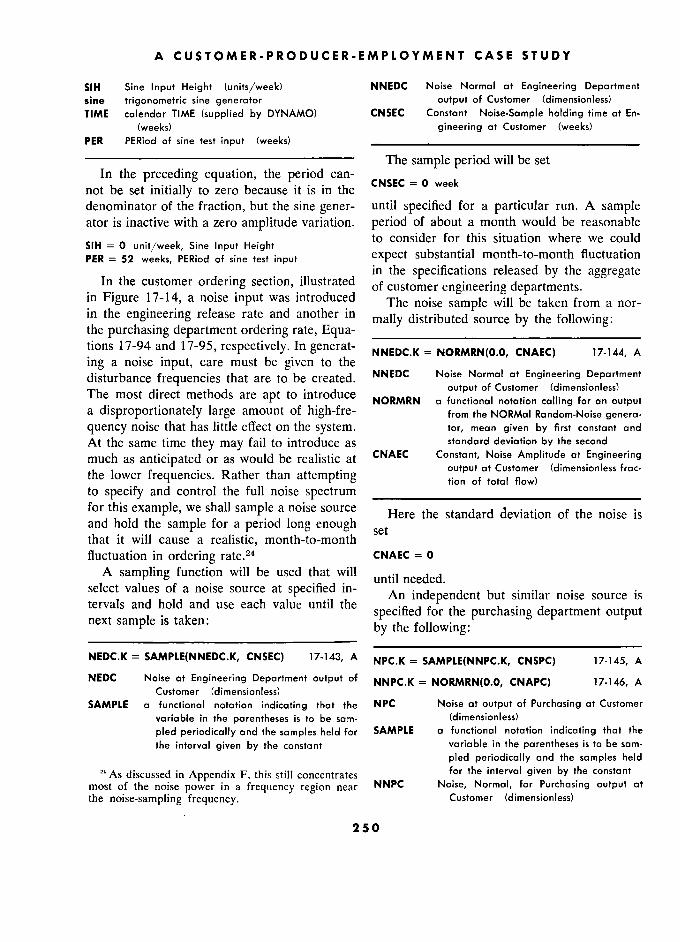
A CUSTOMER-PRODUCER-EMPLOYMENT CASE STUDY
SIH Sine Input Height (units/week) NNEDC Noise Normal at Engineering Department sine trigonometric sine generator output of Customer (dimensionless) TIME calendar TIME (supplied by DYNAMO) CNSEC Constant Noise-Sample holding time at En-
(weeks) gineering at Customer (weeks) PER PERiod of sine test input (weeks) _______._____________________________
––––––––––––––––––––––––––
The sample period will be set In the preceding equation, the period can-
CNSEC = 0 week not be set initially to zero because it is in the e
CNSEC = 0 week
denominator of the fraction, but the sine gener- until specified for a particular run. A sample ator is inactive with a zero amplitude variation. period of about a month would be reasonable
SIH 0 unit/week, Sine , _ t to consider for this situation where we could
PER = 52 weeks, PERiod of sine test input expect substantial month-to-month fluctuation
In the customer ordering section, illustrated in the specifications released by the aggregate
In thé customer ordering section, dlustrated of customer engineering departments.
in Figure 17-14, a noise input was introduced The noise sample wil) be taken from a nor- in the engineering release rate and another in
mally distributed source by the fo)lowing: the purchasing department ordering rate, Equa- ____________________________ tions 17-94 and 17-95, respectively. In generat- NNEDC.K = NORMRN(0.0, CNAEC) 17-144, A ing a noise input, care must be given to the
' ' ' ,
disturbance frequencies that are to be created. NNEDC Noise Normal at Engineering Department .
output of Customer (dimensionless) The most direct methods are apt to introduce outpur of Customer (dimensionless)
.. The ? ta m ro uce NORMRN a functional notation calling for an output t a disproportionately large amount of high-fre- from th NORMal Random-Noise genera- quency noise that has little effect on the system. tor, mean given by first constant and At the same time they may fail to introduce as standard déviation by the second
much as anticipated or as would be realistic at CNAEC Constant, Noise Amplitude at Engineering , . output at Customer (dimensionless frac-
the lower frequencies. Rather than attempting rion of toral flow) (dimensionless frac-
e ower requencies. a er an a emp mg to specify and control the full noise spectrum ____________________________ for this example, we shall sample a noise source rj c the noise is , , , , Hère thé standard déviation of thé noise IS and hold the sample for a period long enough setHere
the standard deviation of the noise is
that it will cause a realistic, month-to-month se
fluctuation in ordering rate.24 CNAEC = 0
A sampling function will be used that will until needed.
. select values of a noise source at specified in- An independent but similar noise source is tervals and , hold . , and , use each , value ? untn ., thé , An -c ? ? independent ? en u Slml ar
noise source IS tervals and
hold and use each value until the
specified for the purchasing department output t next sample is taken: following:
NEDC.K = SAMPLE(NNEDC.K, CNSEC) 17-143, A NPC.K = SAMPLE(NNPC.K, CNSPC) 17-145, A NEDC Noise at Engineering Department output of NNPC.K = NORMRN(O.0, CNAPC) 17-146, A
Customer (dimensionless) ' ' '
SAMPLE a functional notation indicating that the NPC Noise at output of Purchasing at Customer variable in the parenthèses is to be sam- (dimensionless) pled periodically and the samples held for SAMPLE a functional notation indicating that the
, the interval given by the constant variable in the parenthèses is to be sam- pled periodically and the samples held
"' As discussed in Appendix F, this still concentrates for the interval given by the constant most of the noise power in a frequency region near NNPC Noise, Normal, for Purchasing output at the noise-sampling frequency. Customer (dimensionless)
250

§ 17.6 INPUT TEST FUNCTIONS S
CNSPC Constant, Noise-Sample holding time at Where the reservoir of orders in process in Purchasing at Customer (weeks) the purchasing department is short (the average NORMRN a functionai notation calling for an output
delay DRCC equals 3 weeks), a shorter sampling from the NORMal Random-Noise gener- -' equa s wee a s or er r ing
ator, mean given by first constant and period CNSPC of about 1 week would be rea-
standard deviation by the second .
sonable. CNAPC Constant, Noise Amplitude at Purchasing This completes the design of the model that
output at Customer (dimensionless frac- well be used in the next chapter.z5 tion of total flow) '
CNSPC = 0 week 25 Appendix A contains a tabulation of the equations
CNAPC = 0 that have been developed in this chapter.
251 1

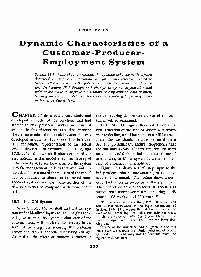
CHAPTER 18 8
Dynamic Characteristics of a
Customer-Producer-
Employment System
Section 18.1 of this chapter examines the dynamic behavior of the system described in Chapter 17. Variations in system parameters are tested in Section 18.2 to determine the policies to which the system i.s most sensi- tive. ln Sections 18.3 through 18.7 changes in system organization and
policies are made to improve the stability of employment, cash position, backlog variation, and delivery delay without requiring larger inventories or inventory fluctuations.
C HAPTER 17 described a case study and the engineering department output of the cus-
developed a model of the practices that had tomer will be examined. seemed to exist previously within an industrial 18.1.1 Step Change in Demand. To obtain a
system. In this chapter we shall first examine first indication of the kind of system with which the characteristics of the model system that was we are dealing, a sudden step input will be used.
developed in Chapter 17, to see if its behavior From this we should be able to see if there is a reasonable representation of the actual are any predominant natural frequencies that
system described in Sections 17.1, 17.2, and die out only slowly. If there are, we can form 17.3. After that we shall alter certain of the an estimate of their period and also of rate of
assumptions in the model that was developed attenuation, or if the system is unstable, their in Section 17.4, to see how sensitive the system rate of expansion in amplitude. is to the management policies that were initially Figure 18-1 shows a 10% step input to the included. Then some of the policies of the model independent ordering rate entering the customer will be modified to obtain an improved man- sector of the modela The system shows a peri- agement system, and the characteristics of the odic fluctuation in response to the step input. new system will be compared with those of the The period of this fluctuation is about 100 old. weeks, with manpower peaks appearing at 68
weeks, 168 weeks, and 266 weeks.2
18.1 The Old System 1 This is obtained by setting STT1 - 8 weeks and . i. 11 ,- t. STH1 - 100 units/week in the input parameters of
As m Chapter 15, we shall first test the sys- Section 17.6. This means that at the 8th week the
tem under idealized inputs for the insights these independent-order input will rise 100 units per week,
will give us into the dynamic character of the which
is a value of Sec Figure 17-14
for the
system. These will first be a step change in the diagram
input, and Figure 17-17 for the input flow
level of ordering rate entering the customer 2 Many of the numerical values given in the text
sector and then a periodic fluctuattng change. have been taken from the tabular print-out of results °
° of model runs and may not be readable from the After that, the effect of random variation at
figures included here.
253
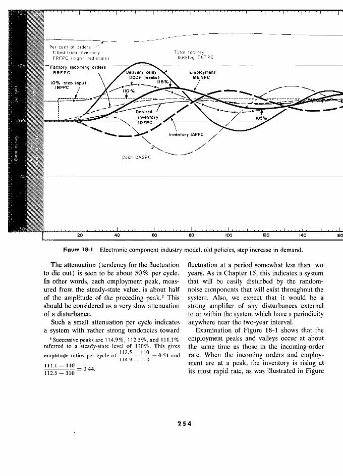
Per cent of orders '
filled from Inventory Total factory . FRFPC (right, red scale) backlog BLTPC
'? -Factory incominq orders RRFPC Delivery deloy Employment
(weeks) MENPC 10% step input 115%
I NPPC
· I10 % - O
' Desired /
inventory / 105%
? '°FP) /
105%
'
Inventory IAFPC
/
Cash CASPC
20 40 60 80 100 120 140 h
Figure 18-1 Electronic component industry model, old policies, step increase in demand.
The attenuation (tendency for the fluctuation fluctuation at a period somewhat less than two to die out) is seen to be about 50% per cycle. years. As in Chapter 15, this indicates a system In other words, each employment peak, meas- that will be easily disturbed by the random- ured from the steady-state value, is about half noise components that will exist throughout the of the amplitude of the preceding peak.3 This system. Also, we expect that it would be a should be considered as a very slow attenuation strong amplifier of any disturbances external of a disturbance. to or within the system which have a periodicity
Such a small attenuation per cycle indicates anywhere near the two-year interval. a system with rather strong tendencies toward Examination of Figure 18-1 shows that the
3 Successive peaks are 114.9%, 112.5%, and 111.1 % employment peaks and valleys occur at about referred to a steady-state level of 110%. This gives the same time as those in the incoming-order
112 5 - 110 Wh h.. d d 1 amplitude ratios per cycle - 0.51 and rate. When the incoming orders and employ-
111.1 - 110 0.44.
110 o ment are at a peak, the inventory is rising at
112.5 - 110 - its most rapid rate, as was illustrated in Figure
254
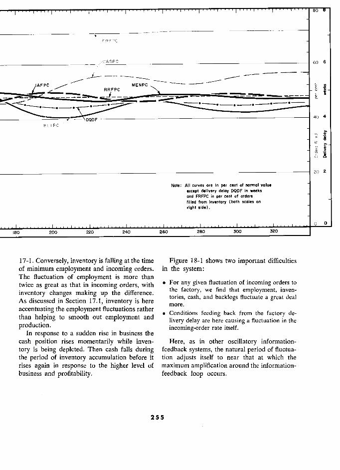
l ' 1 1 1 l' l "1 1 l
' . , " , BO a
FRFPC
60 6
_
RRFPC MENPC
_ -
- £ w
t
4
BLTPC / - DODF
40 4
>- g °' ., .. 0 ;.= >-
., > - 0 :.:
O O
2
Note: All curves are in per cent of normal va lue
except delivery delay DODF in weeks
and FRFPC in per cent of orders
filled from inventory (both scales on
riyht side).
....... 0 0
180 200 220 260
17-1. Conversely, inventory is falling at the time Figure 18-1 shows two important difficulties
of minimum employment and incoming orders. in the system :
The fluctuation of employment is more than _
twice as great as that in incoming orders, with ° For any given fluctuation of incoming orders to
inventory changes making up thé difference. the factory, we find
that employment, inven-
A d' d' S . 17 ..
h tories, cash, and backlogs fluctuate a great deal
As discussed in Section 17.1, inventory is here cash, an ac ogs uc ua e a grea ea
accentuating the employment fluctuations rather r"ore. f e-
than helping ? smooth out employment and * Conditions feedins back from thé factory de-
than helpmg .
ta smooth out employment and l' Ivery d e 1 ay are h ere causmg 'fi a uc t ua t, Ion m 'th e ° livery delay are hère causing a fluctuation in thé
production. incoming-order rate itself. In response to a sudden rise in business the
cash position rises momentarily while inven- Here, as in other oscillatory information-
tory is being depleted. Then cash falls during feedback systems, the natural period of fluctua-
the period of inventory accumulation before it tion adjusts itself to near that at which the
rises again in response to the higher level of maximum amplification around the information-
business and profitability. feedback loop occurs.
255 5
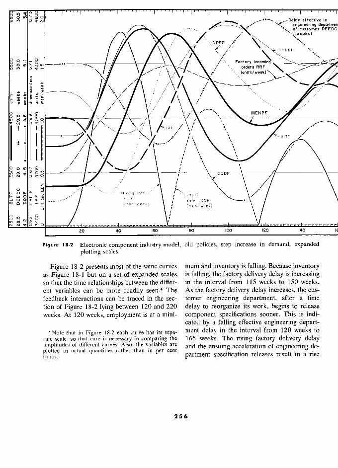
,...,0
3 M, 0 n
. , 1 1 1 1 1
1 , 1 , ..1.... 1 11 1 1
1..
1 , .
effective in engineering departm
------ , of customer DEED
'X (weeks)
/ //\ '/\ / /'' v\ ''\
0 //\
A
,,'
X Factor " O ictory incomin orders RRF
.2 CI)
= / ¡: :.ê J:"C E Cl)E
\ / v/ \ \ \ """--
0 g / \. MENPF W) Co 0
°. Y––––/\––
î' 1AF '' ', x
Io, l 1 1 B LT F
j
1. 1 1: 1 / / , ,,
,: ;
/ j , /
,
, ,, ,
O 0 S D.DF , tC; 0\
rn 0 .
,," " /
i Y
D F i, ,
/ \
ZO ,,' ,,,"
u- -J
„--'"/
,
\ " / LHF t
y8 rateLDNF N F "--––'-t ", / \
/ \ /
W
O?LL aoe
0 ------
(men/week)
rate
LDNF W) 0 / \.' \/ n / \'____________________\/ eu v 0 ,..., 0 -- -- ........ - -
20 40 60 80 100 120 140
Figure 18-2 Electronic component industry model, old policies, step increase in demand, expanded
plotting scales.
Figure 18-2 présents most of the same curves mum and inventory is falling. Because inventory
as Figure 18-1 but on a set of expanded scales is falling, the factory delivery delay is increasing
so that the time relationships between the difier- in the interval from 115 weeks to 150 weeks.
ent variables can be more readily seen.4 The As the factory delivery delay increases, the cus-
feedback interactions can be traced in the sec- tomer engineering department, after a time
tion of Figure 18-2 lying between 120 and 220 delay to reorganize its work, begins to release
weeks. At 120 weeks, employment is at a mini- component specifications sooner. This is indi-
cated by a falling effective engineering depart-
'Note that in Figure 18-2 each curve has its sepa- ment delay in the interval from 120 weeks to
rate scale, so that care is necessary in comparing the 165 weeks. The rising factory delivery delay amplitudes of different curves. Also, the variables are d t ensuing accélération of engineering de- plotted in actual quantities rather than in per cent , . -
partment speci cation releases result in a -rise
256
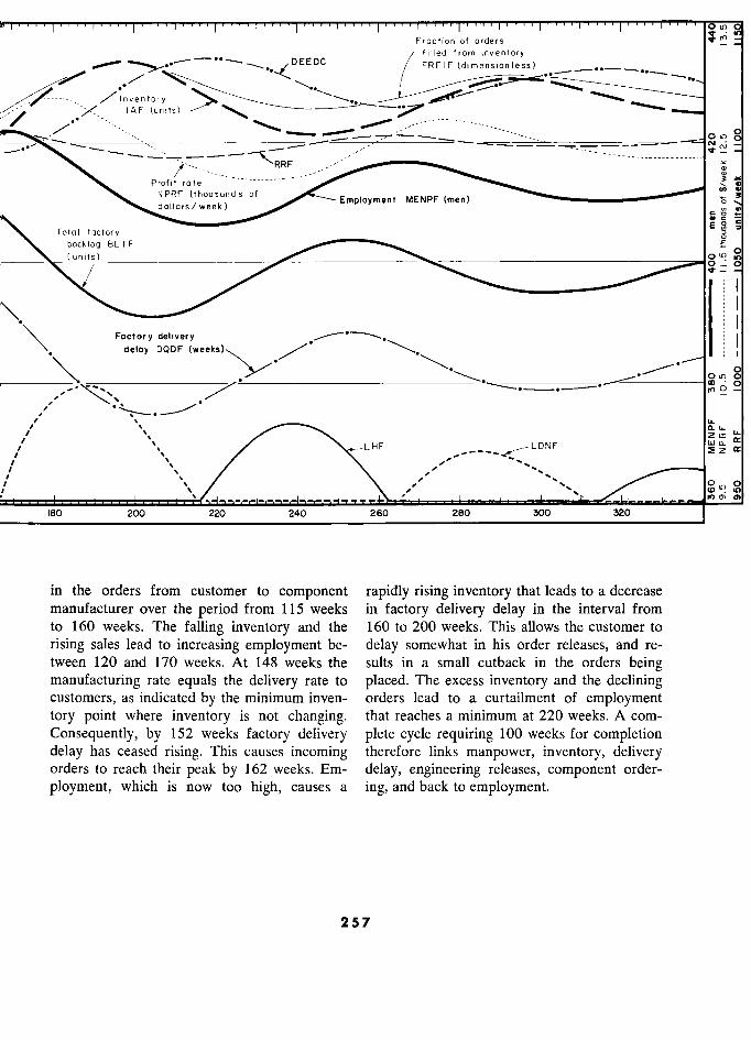
" " , " 0
Fraction of orders
_ DEEDC filled from inventory
- --- -- -00- --- .(DEEDC FRFIF FRFIF (dimensianless) ··--..
DC FRF I F (dimension less) --..--..
./" ../" Inventory
_ -..
?Inventory
% $' __ _ .. X- "
IAF (units)
""""'- ---- -;7 ___h___-
--- - ::.:..:-- - - -
7"
/ Profit rate
NPRF (thousands of 3 3 dollars/week) Employment MENPF (men)
-;;;
Total factory
dollars/ week)
.- '
Total factory e '"
0
c "
Total ::> backlog BLTF backlog BLTF
( units) .0 0 ( units) 0"': 0
Factory delivery ' 1
)
"'-. delay DQDF
(weeks)
. /.
.
0 lD g
1
'D . 0 n 0 0 0
"
''''' . -
, ... , '\ a U-
i
LHF w z a:
gr oe LI-
' ,
v
', ", '\ ,
" - - - -
,,' ,
,".... '....
'- % \ 0 O) 01
180 200 220 260 300 320
in the orders from customer to component rapidly rising inventory that leads to a decrease manufacturer over the period from 115 weeks in factory delivery delay in the interval from to 160 weeks. The falling inventory and the 160 to 200 weeks. This allows the customer to
rising sales lead to increasing employment be- delay somewhat in his order releases, and re- tween 120 and 170 weeks. At 148 weeks the sults in a small cutback in the orders being manufacturing rate equals the delivery rate to placed. The excess inventory and the declining customers, as indicated by the minimum inven- orders lead to a curtailment of employment tory point where inventory is not changing. that reaches a minimum at 220 weeks. A com-
Consequently, by 152 weeks factory delivery plete cycle requiring 100 weeks for completion delay has ceased rising. This causes incoming therefore links manpower, inventory, delivery orders to reach their peak by 162 weeks. Em- delay, engineering releases, component order-
ployment, which is now too high, causes a ing, and back to employment.
257
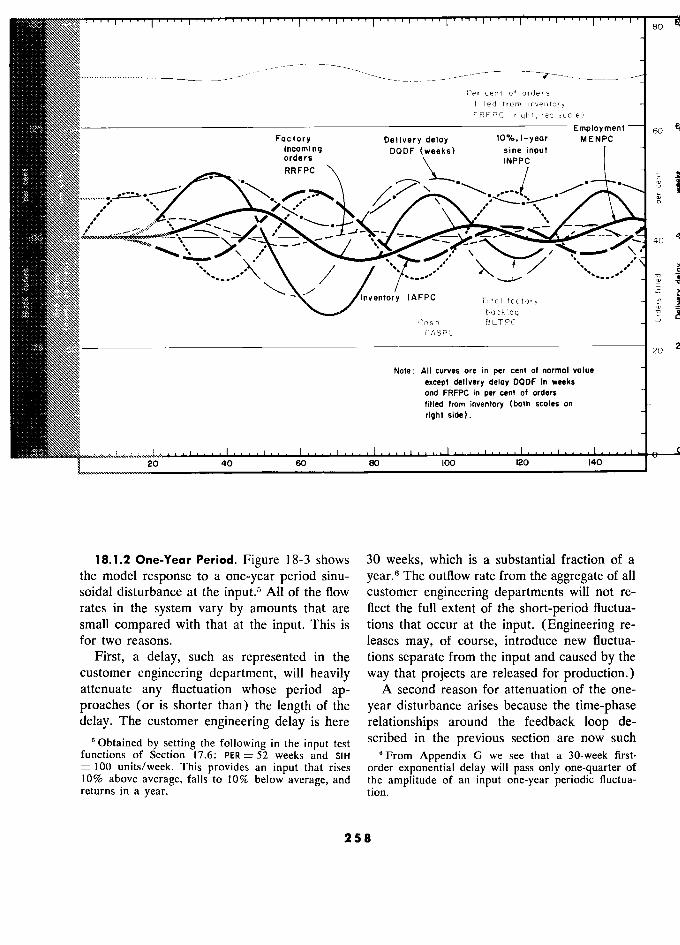
. 80
Per cent of orders filled from inventory FRFPC (riqht, red sccile)
- Employment 60
?NjJt Factory Delivery deloy 10%, 1-year MENPC
! lncominq DODF (weeks) sine input
f
orders INPPC RRFPC _
C>
Il lm
40
Inverit ry Il PC alli t ? /
- c Cash BLTPC °
CASPC
20
Note: Ali curves are in per cent of normal value
except delivery deloy DQDF in weeks and FRFPC in per cent of orders
filled from inventory (both sco!es on
right side).
20 40 60 80 !00 i2o 140
18.1.2 One-Year Period. Figure 18-3 shows 30 weeks, which is a substantial fraction of a the model response to a one-year period sinu- year.s The outflow rate from the aggregate of all soidal disturbance at the input.5 All of the flow customer engineering departments will not re- rates in the system vary by amounts that are flect the full extent of the short-period fluctua- small compared with that at the input. This is tions that occur at the input. (Engineering re- for two reasons. leases may, of course, introduce new fluctua-
First, a delay, such as represented in the tions separate from the input and caused by the customer engineering department, will heavily way that projects are released for production.) attenuate any fluctuation whose period ap- A second reason for attenuation of the one-
proaches (or is shorter than) the length of the year disturbance arises because the time-phase delay. The customer engineering delay is here relationships around the feedback loop de-
o Obtained by setting the following in the input test scribed in the previous section are now such functions of Section 17.6: PER = 52 weeks and SIH From Appendix G we see that a 30-week first- = 100 units/week. This provides an input that rises order exponential delay will pass only one-quarter of 10% above average, falls to 10% below average, and the amplitude of an input one-year periodic fluctua- returns in a year. tion.
258 8
Figure 18-3 Electronic component industry model, old policies, one-year sinusoidal input.
that the variation in delivery delay tends to is falling due to the fluctuating input. These two
suppress the system fluctuation. The natural effects tend to cancel one another to some ex-
period of the system was seen in Figures 18-1 tent and further reduce the amount of the and 18-2 to be about 100 weeks. At that period input disturbance that is transmitted from cus- of oscillation, the flow of delivery delay in- tomer to factory. formation from component supplier to customer For the preceding two reasons, incoming or- tended to reinforce the system fluctuation. We ders to the factory vary only 18% as much as should not expect the same reinforcement for the input to the customer. Even so, employment other oscillation periods imposed upon the sys- at the factory fluctuates 33% as much as the tem. In fact, the reverse is true in the model orders at the customer input. This means that at a one-year period of disturbance. From a employment is still fluctuating more ( 1859% ) curve for engineering department release delay than the actual inflow of orders to the factory, (not shown), we find that the engineering de- so that employment varies almost twice as much
partment is tending to accelerate its design re- as any annual, seasonal component in the fac- leases at the same time that the work load itself tory orders.
259
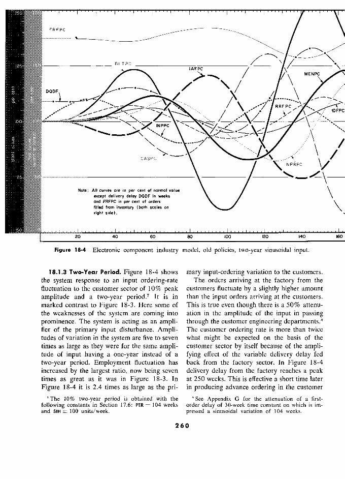
FRFPC
BLTPC l BLTPC IAFPC IAFPC
MENPC
DQDF
> m
DQDF
,
/
, - . 11;
- - _ ,
"" -
_,
_
..,,__ ,,_
/ · -`-`
,,
IDFF '
vv \
/J/
/\ . "',,,
CASPC'.? '-_
` 'NPRPC j /
NPRPC /
)-
Note: All curves are in per cent of normal value
) except delivery deloy DQDF in weeks and FRFPC in per cent of orders
filled from inventory (both scales on
right side).
20 40 60 80 100 120 140 16,
Figure 18-4 Electronic component industry model, old policies, two-year sinusoidal input.
18.1.3 Two-Year Period. Figure 18-4 shows mary input-ordering variation to the customers. the system response to an input ordering-rate The orders arriving at the factory from the fluctuation to the customer sector of 10% peak customers fluctuate by a slightly higher amount
amplitude and a two-year period.7 It is in than the input orders arriving at the customers. marked contrast to Figure 18-3. Here some of This is true even though there is a 50% attenu- the weaknesses of the system are coming into ation in the amplitude of the input in passing prominence. The system is acting as an ampli- through the customer engineering departments.8 fier of the primary input disturbance. Ampli- The customer ordering rate is more than twice tudes of variation in the system are five to seven what might be expected on the basis of the times as large as they were for the same ampli- customer sector by itself because of the ampli- tude of input having a one-year instead of a fying effect of the variable delivery delay fed
two-year period. Employment fluctuation has back from the factory sector. In Figure 18-4 increased by the largest ratio, now being seven delivery delay from the factory reaches a peak times as great as it was in Figure 18-3. In at 250 weeks. This is effective a short time later
Figure 18-4 it is 2.4 times as large as the pri- in producing advance ordering in the customer
? The 10% two-year period is obtained with the " See Appendix G for the attenuation of a first-
following constants in Section 17.6: PER = 104 weeks order delay of 30-week time constant on which is im-
and SIH = 100 units/week. pressed a sinusoidal variation of 104 weeks.
260
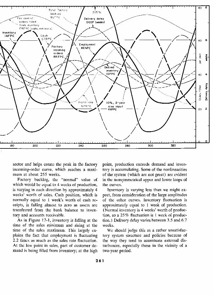
, . , , . , 80 8
Toto) factory \
bocklog /
215%
\ Per cent of BLTPC PC \
Delivery delay \ orders filled DQDF (weeks) \ from inventory \ \ -i FRFPC (right, red scale) /
nventory .' \ IAFPC Cash s h \ \ /
eo 6
- - CASPC oc tory Employment /
-
\ /
60 6
/ Foctory °rY
\
MENPC
, /
y
incomin
\\g \
\/ .- \/
y -.. , orders / C -=
/\ ..
.·:
' .
/ /
/ - '
x
g _
\ / / /
inventory / .\ ./ / _ ' _
. / ,"
_, &, ,, l i nvent D F P C or
"._ / 40 4 / 40 4
',
, /
,:"
, _, '
) ,,.
,,'
/ ',
,
,:" ._
/
"Q .S!
'"
\ \ \
>
\ / rate \X / joola, z-year \ /
"'
;5
ô
\ / / \, NPRPC X sine input \ '
/ ––––– \4- ?-INPPC
––– \––/
- 20 2
_ /
/ e
% a /
/
o
180 200 220 240 260 280 300 320 ___
sector and helps create the peak in the factory point, production exceeds demand and inven-
incoming-order curve, which reaches a maxi- tory is accumulating. Some of the nonlinearities mum at about 255 weeks. of the system (which are not great) are evident
Factory backlog, the "normal" value of in the nonsymmetrical upper and lower loops of which would be equal to 4 weeks of production, the curves. is varying in each direction by approximately 4 Inventory is varying less than we might ex- weeks' worth of sales. Cash position, which is pect, from consideration of the large amplitudes normally equal to 1 week's worth of cash re- of the other curves. Inventory fluctuation is
ceipts, is falling almost to zero as assets are approximately equal to 1 week of production. transferred from the bank balance to inven- (Normal inventory is 4 weeks' worth of produc- tory and accounts receivable. tion, so a 25 % fluctuation is 1 week of produc-
As in Figure 17-1, inventory is falling at the tion.) Delivery delay varies between 3.5 and 6.7 time of the sales minimum and rising at the weeks. time of the sales maximum. This largely ex- We should judge this as a rather unsatisfac-
plains the fact that employment is fluctuating tory system structure and policies because of 2.2 times as much as the sales rate fluctuation. the way they tend to accentuate external dis- At the low point in sales, part of customer de- turbances, especially those in the vicinity of a mand is being filled from inventory; at the high two-year period.
261 1
CUSTOMER-PRODUCER-EMPLOYMENT SYSTEM
18.1.4 Random Releases from Engineering neering department contains the month-by- Department. The preceding figures h'ave been month random fluctuation. taken with pure, idealized test inputs so that The further the random fluctuation pene- we could look at one component of system be- trates into the system, the more it is smoothed, ' havior at a time. The previous curves have been and the more it takes on the characteristics of smooth and have an artificial appearance com- the system itself rather than the original noise.
pared with a real industrial enterprise, because Even in the factory incoming requisitions, a the decisions in the system have all been free certain amount of correlation is evident; that is, of random variations. orders in consecutive weeks vary smoothly from
We are now ready to examine the response one to the next because of the intervening cus- of the system to a more complex environment. tomer purchasing department that causes some For this we introduce a nonuniform design averaging and smoothing of the order flow.10
specification release rate from the aggregate (The reader should here refer to Figure ... , ? ? * aggregate rcaacy .s?oMM! rerer <o F?Mrc customer engineering departments. As set up ,- _
e rea .,. , , , , ° customer engineering departments. As set
page 264, and the explanation beneath.) . c t- 4 7 6
- - t.i 18-5, pa?e 264, ana </!c c?D/ana?on oen6<M/:.) in Sections 17.4.7 and 17.6, a noise variable e r & ' /
is available in the model for insertion in the As we had reason to expect from Figures flow rate between customer engineering depart- 18-1 and 18-4, the system as shown in Figure ment and customer purchasing department. 18-5 responds unfavorably to the presence of This fluctuating signal does not create or de- the unavoidable random disturbances that will
stroy any orders for electronic components. Or- always exist in an industrial system. Because ders are determined in the long run by those the system is highly sensitive to and selective
entering customer engineering from the outside of frequencies near a two-year period, it world. The random output from the engineering chooses frequency components in that periodic- department can affect the time at which orders ity range and amplifies them. Any kind of are released and, therefore, causes a random random-noise disturbance is therefore suffitcient
bunching of the order outflow. Any random to trigger into operation the inherent tendencies
signal contains a very broad band of disturbance of the system to develop unfavorable fluctua-
frequencies and inherently contains excitation tions owing to the interactions between cus- for any modes of behavior to which the indus- tomer ordering, and factory inventories, de- trial system is especially sensitive.9 livery delay, and employment level.
We shall now examine the electronic compo- 18.1.5 Cash Flow and Continuous Balance nent industry model when the order inflow to Sheet. The variables plotted in the preceding the customer engineering department is constant figures are the principal ones that determine and the order outflow from the customer engi- system dynamic performance even though the
financial variables usually receive more atten- 'Thé random disturbance is here obtained by set- tion. The financial data corresponding to Fig- ting CNSEC = 5 weeks and CNAEC = 0.1 in the parame-
tion. The financial data corresponding to Fig- ters of Section 17.6. This means that random numbers having a normal distribution and a mean deviation of '° Section 17.6, Equation 17-145, made available in 10% are added to the customer engineering depart- the model at Equation 17-95 a second noise variable ment output rate. These random numbers are sampled, at the output of the customer purchasing department. and each number is held for 5 weeks before a new Activation of this noise input would have produced a sample is selected. The sampling and holding are here week-by-week random scatter in the orders to the done as a simple expedient, instead of other methods factory, but would have had little effect on the system that might be chosen, to control somewhat the power- since most of the added noise signal would have been density versus frequency characteristic of the noise. in the very high frequency spectrum to which the sys- See Appendix F. tem is only slightly sensitive.
262 2
§ 18.1.6 ADEQUACY OF THE MODEL L
ure 18-5 are shown in Figure 18-6 for cash flow made to move in opposite directions, so that and Figure 18-7 as a continuous balance sheet. current assets flow back and forth between ac-
Figure 18-6 presents the six cash-flow vari- counts receivable and inventory and place less ables from the cash-flow diagram of Figure fluctuating demands on cash. 17-15. The scales are plotted from different 18.1.6 Adequacy of the Model. The results zero points to superimpose the curves on the of Sections 18.1.1 through 18.1.5 show a model same diagram. However, the vertical height of whose behavior is in accord with the available the figure represents a range of $20,000 per knowledge about the actual system. The con- week for each of the curves so that vertical fidence in the model rests primarily on the
changes are comparable for all curves.ll It knowledge we have of the separate parts of the should be noted that all of the expenditure rates system. Nevertheless, this would not be suffi-
begin to rise earlier than the cash-receipts rate cient if the model exhibited system behavior and reach peaks ahead of the peak in cash that was inconsistent with the actual system. receipts. This is clearly evident, for example, There is usually a paucity of dependable rec- in the range from 40 weeks to 80 weeks, and ords that can be compared with a system model. between 120 weeks and 150 weeks. This means The checking consists of examining all aspects that cash drain peaks ahead of cash replenish- of the model behavior about which there is
ment, causing the wide cash fluctuations seen knowledge in the actual system. One examina- in Figure 18-7. tion is to look for any improbable behavior in
In the continuous balance sheet of Figure the decision streams in the model. Phase rela- 18-7 can be seen the interplay between the vari- tionships between variables are important; for ous current assets. In-process inventory rises example, the model in Figures 18-4 and 18-5 and falls approximately in synchronism with shows the inventories peaking after orders and
employment level in Figure 18-5. employment as observed in the actual system, The most important point in Figure 18-7 is and as shown in Figure 17-1. As appears
to observe the way in which the value of total to be true in the actual system, the model shows inventories and the accounts receivable rise production and employment fluctuations that and fall together. This can be seen most clearly are substantially larger than the changes in in the interval between 50 and 100 weeks, and order flow to the customer sector from the cus- between 120 and 180 weeks. The result is that tomers' customers (government and industry both inventory and accounts receivable draw on orders for electronic equipment). Periods of -
cash and return into cash at the same times. about two years had existed in the fluctuations Cash position must be able to supply the simul- of the actual system, and similar behavior is taneous demands of both inventory and ac- evident in the model. Examination, by the man- counts receivable. This accentuates the cash- agers familiar with the actual system, of the
position fluctuation. After making changes in model assumptions and its over-all performance system management policies, we shall see in does not reveal implausible structure or policy Section 18.6 that the short-term fluctuations of assumptions or behavior that is judged to inventories and accounts receivable can be degrade the model for its intended uses.
These are all negative tests. Nothing has " Neither Figure 18-5 nor the financial data dia- been discovered about the model that is be-
grams of 18-6 and 18-7 give the actual shipping rate to invalidate it for the purposes of ex- of finished goods to the customer. This has approxi-
i u
mately the shape of the finished-goods cash-receipts Text Continues on Ci curve if that curve were moved 5 weeks to the left. Text continues on page 268.
263 3
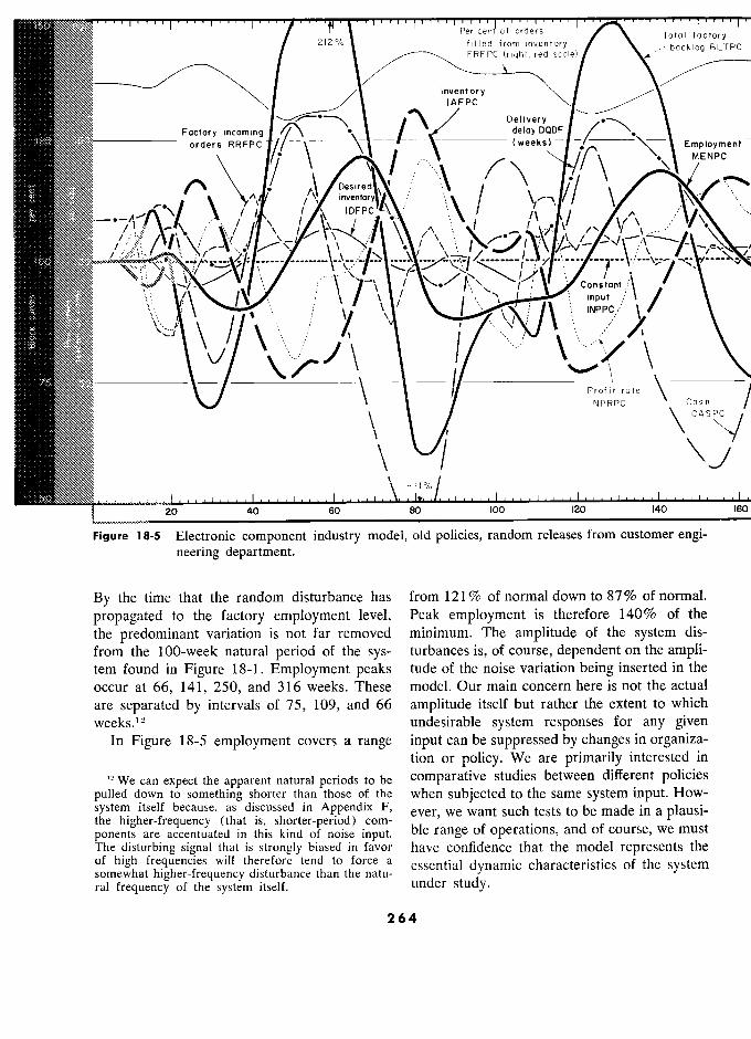
2'2i'o §/lled ÉrorÉ?illlntory 2 12 filied inventory scale)
bocklog BLTPC
lnveritory IAFPC
'§ Delivery
incoming delay DQDF < X \. RRFPC (weeks) Employment t
MENPC
Î
/
Desire
Î
".,£ ) j
) j
K X )
, ,,."
..,, "..,
inven y 1 ID
Cons tant
j / ' Î ".
" ,
/
";, / '
$j /
/ - Profit rate
-, NPRPC
) 1
°°°ov/
20 40 60 80 100 120 140 16
Figure 18-5 Electronic component industry model, old policies, random releases from customer engi- neering department.
By the time that the random disturbance has from 121% of normal downto 87% of normal.
propagated to the factory employment level, Peak employment is therefore 140% of the
the predominant variation is not far removed minimum. The amplitude of the system dis-
from the 100-week natural period of the sys- turbances is, of course, dependent on the ampli- tem found in Figure 18-1. Employment peaks tude of the noise variation being inserted in the
occur at 66, 141, 250, and 316 weeks. These model. Our main concern here is not the actual
are separated by intervals of 75, 109, and 66 amplitude itself but rather the extent to which
weeks.12 undesirable system responses for any given In Figure 18-5 employment covers a range input can be suppressed by changes in organiza-
tion or policy. We are primarily interested in
?We can expect the apparent natural periods to be comparative studies between different policies
pulled down to something shorter than those of the when subjected to the same system input. How-
system itself because, as discussed in Appendix F, ever we made in pj????_ the higher-frequency (that is, shorter-period) com-' , „
ponents are accentuated in this kind of noise input. ble range of opérations, and of course, we must
The disturbing signal that is strongly biased in favor have confidence that the model represents the
of high frequencies will therefore tend to force a
essential dynamic characteristics of thé system somewhat higher-frequency disturbance than the natu- .....) ral frequency of the system itself. under study.
264
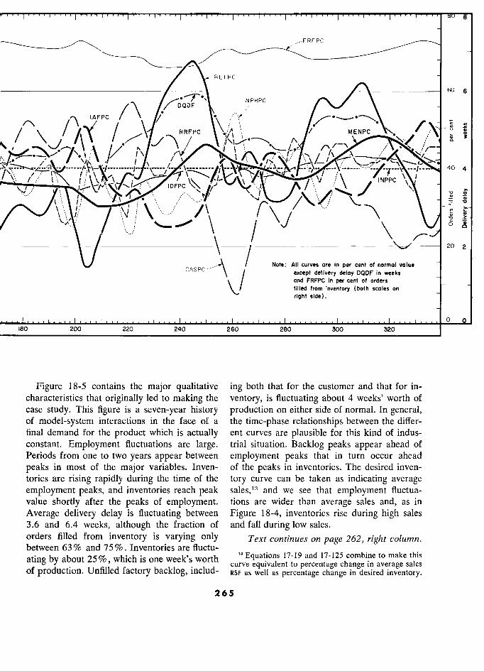
1 8
FRFPC
Y?-BLTPC 60 6
. NPRPC / \
/\
DQDF \
\/ \ /À
/ RRFPC \Vt ' A
'00r s
1-- 40 4 ÷
, INPPC j NPPC
(
––––– 20 2
' Note: All curves are in per cent of normol value CASPC
,
except delivery deloy DODF in weeks < andFRFPCinpercentoforders
filled from inventory (both scales on * right side).
0 180 200 220 240 260 280 300 320
Figure 18-5 contains the major qualitative ing both that for the customer and that for in-
characteristics that originally led to making the ventory, is fluctuating about 4 weeks' worth of
case study. This figure is a seven-year history production on either side of normal. In general, of model-system interactions in the face of a the time-phase relationships between the differ-
final demand for the product which is actually ent curves are plausible for this kind of indus-
constant. Employment fluctuations are large. trial situation. Backlog peaks appear ahead of
Periods from one to two years appear between employment peaks that in turn occur ahead
peaks in most of the major variables. Inven- of the peaks in inventories. The desired inven-
tories are rising rapidly during the time of the tory curve can be taken as indicating average
employment peaks, and inventories reach peak sales,"' and we see that employment fluctua-
value shortly after the peaks of employment. tions are wider than average sales and, as in
Average delivery delay is fluctuating between Figure 18-4, inventories rise during high sales
3.6 and 6.4 weeks, although the fraction of and fall during low sales.
orders filled from inventory is varying only Text continues on page 262, right column. between 63% and 75%. Inventories are fluctu-
ating by about qg which is one week's worth '? Equations 17-19 and 17-125 combine to make this ° -' '
. curve equivalent to percentage change in average sales of production. Unfilled factory backlog, includ- RSF as well as percentage change in desired inventory.
265 5
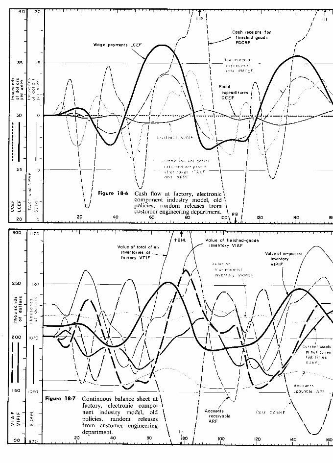
40 20 1 -
/ !'2j Î / III
/ /
/
/ I ) Cash receipts for
/
? finished goods Wage payments LCEF / Wage paymerits LCEF / FGCRF
/ _ Î /
35 15 Raw-material
'
li / / \ expenditure l
/\ /
"
\ /
/ \
\
t
')
rate RMCEF / '
_
/ ,
/ \ Fixed
/ \ / II) 0 3: V') 03: ' '
/ \ I
expenditures ? y; ,- \\ CCEF <lJ
I r
i CCEF " -
'"''''
)
Î
,1 "
;"
30 10 lo
:.
.-i .1·'1'' \1
1 ,
1 , l
j
) 1
)
) /
,
j
i
j j
1
É ( 1
·:\,· )
/
j j
.I I
i
1 j )
'
j
j ) j j j :
É (
Î
) _.' ;.
j
Î
1 ,' '""--'' ' '''--''''' / 1 t ( )
' i
I
j ·
?f?\Income tax obligation
·· _.
I j
Î )"
j /
j
tcix obligation t ' .
\ ' / /
- ' rate and net profit Î
. ' /
5 after taxes ITAXF after taxes ITAXF
j
0:: z
o _
I
I I
Î
j
Î and NPRF
)
j
j
ô § t / F19ure 18-6 Cash How at factory, electronic l ' Figure 18.6
w w \
' component industry mode], old 1
policies, random- releases from 1
1- 2
L 0
1l
40 customer engineering department. 1\ 1
120 140 20 0 O M 40 customer engineering
l
120 !40
300 j j70 300
1170 +614. t 'Value of finished-goods
Value of total of cil / inventory VIAF
inventories at Value of in-process \ factory VTIF inventory factory VT!F
/
/
/
/ t
\ Value of VIPIF / /
/ row-moterial /
/\. / \ inventory VRMSF /
250 I I 2
i
,
0-
.__.___. ._ /
-
,l/ , I ____ 1 ;
' -
0- _. ._
J
_._. __ _. _..__ - / _._/--- =0 ro ^ _
i 1 `
/
200 - -
/ '-
1
Curre t assel
' I,\ 1
/ / minus curre
[
- - liabilities
SURPL
1 -
\ Accounts 150 1020 \-?ble APF 150 jozo
Figure 18-7 Continuous balance sheet
at\
,
1 '
factory, electronic comp /o 1 v. -J nent industry model, old 1
J
Accounts Cash CASHF \ '
i-L policies, random industry model,
receivable N /
- ? policies, random releases \ ' ARF \ /
" from customer engineering
j j
'
100 department. 40 60
\ - 12.
IE 100 970 20 40 1 60 ' E!0 .,0] 0
.. 1 120 140
1 IE
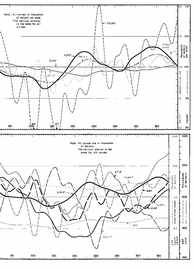
30 110
. ; )
Note : All curves In thousands t '
of dollars per week. per week. t The vertical interval )
. is the some for GII l f FGCRF
curves. wm. W,,"
t
j
/
-
Î
)
,
1 1 ,
" '°' curves. \
105
É \ . ) / \ /
\ /f\
\
1
È , E F
LCEF Î
) '".
/ = %
,,, ., ,." Î ..' ' " ;" 100
à., Î '
1% " Î
É., j 1 '
i j
j ' 1
j )
Î
1
j J ) ) j
"
,/
' 1
SDIVF ,."
:."".. ;"
' J Î
Î '
Î
,.)
à
/
j
1
1
1
1
/
/
ï i !
! < \
-" ,
/
/ < 1 /
t
' ) '
'
!
,'
: /
t ) ' ) t ' f
' LL. IL W II: j
j j j
j j Î
Î j j J 1
u
U
180 20 22Ù 87
24
(r IL
!e0 200) f 220); MO 260 MO
KM 320 Io
160 F '''!'''' i '''''''''!'''''''''!'''' 200 600
Note: All curves ore in thousands of dollars.
The vertical interval Is the same for 011 curves,
150 550
,A / 0
:
/ ) J'\ '/ \ VRMSF
Î
É% g
É
°
'°10 :00
/ï
JI (
'v \ "
// SURPL
100
1 ,
1 - 1 \ .
- ,
j /
SURPL
1 1
1 \
/ \
1 ,0\ 1'\
/ J, VIAF
1 \7
/ \
\
1
1
) 1 1
J
/ '
40°
j
)
50 m'
\
CASHF LL LL
c:r>
\ /
CASHF
11,10, 200 220 240 260
280 300 MO
o 400
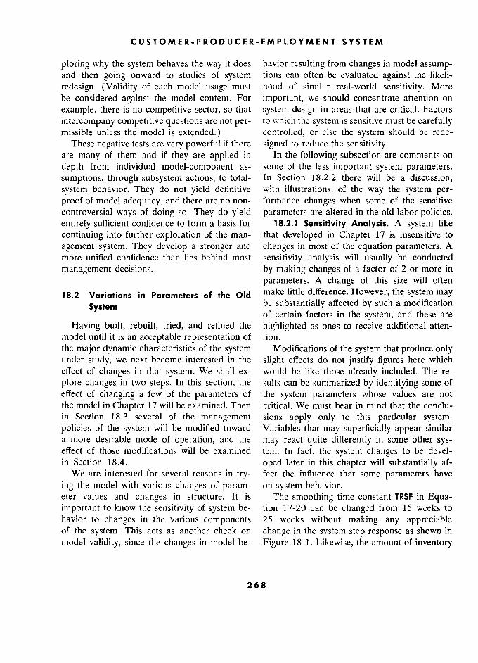
CUSTOMER-PRODUCER-EMPLOYMENT SYSTEM
ploring why the system behaves the way it does havior resulting from changes in model assump- and then going onward to studies of system tions can often be evaluated against the likeli-
redesign. (Validity of each model usage must hood of similar real-world sensitivity. More be considered against the model content. For important, we should concentrate attention on
example, there is no competitive sector, so that system design in areas that are critical. Factors
intercompany competitive questions are not per- to which the system is sensitive must be carefully missible unless the model is extended.) controlled, or else the system should be rede-
These negative tests are very powerful if there signed to reduce the sensitivity. are many of them and if they are applied in In the following subsection are comments on
depth from individual model-component as- some of the less important system parameters. sumptions, through subsystem actions, to total- In Section 18.2.2 there will be a discussion,
system behavior. They do not yield definitive with illustrations, of the way the system per- proof of model adequacy, and there are no non- formance changes when some of the sensitive controversial ways of doing so. They do yield parameters are altered in the old labor policies. entirely sufficient confidence to form a basis for 18.2.1 Sensitivity Analysis. A system like
continuing into further exploration of the man- that developed in Chapter 17 is insensitive to
agement system. They develop a stronger and changes in most of the equation parameters. A
more unified confidence than lies behind most sensitivity analysis will usually be conducted
management decisions. by making changes of a factor of 2 or more in
parameters. A change of this size will often
18.2 Variations in Parameters of the Old make little difference. However, the system may
System be substantially affected by such a modification of certain factors in the system, and these are
Having built, rebuilt, tried, and refined the highlighted as ones to receive additional atten- model until it is an acceptable representation of tion. the major dynamic characteristics of the system Modifications of the system that produce only under study, we next become interested in the slight effects do not justify figures here which effect of changes in that system. We shall ex- would be like those already included. The re-
plore changes in two steps. In this section, the sults can be summarized by identifying some of effect of changing a few of the parameters of the system parameters whose values are not the model in Chapter 17 will be examined. Then critical. We must bear in mind that the conclu- in Section 18.3 several of the management sions apply only to this particular system. policies of the system will be modified toward Variables that may superficially appear similar a more desirable mode of operation, and the may react quite differently in some other sys- effect of those modifications will be examined tem. In fact, the system changes to be devel- in Section 18.4. oped later in this chapter will substantially af-
We are interested for several reasons in try- fect the influence that some parameters have
ing the model with various changes of param- on system behavior. eter values and changes in structure. It is The smoothing time constant TRSF in Equa- important to know the sensitivity of system be- tion 17-20 can be changed from 15 weeks to havior to changes in the various components 25 weeks without making any appreciable of the system. This acts as another check on change in the system step response as shown in model validity, since the changes in model be- Figure 18-1. Likewise, the amount of inventory
268 8
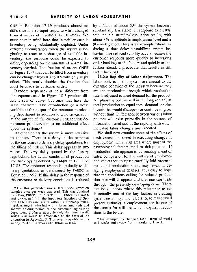
§18.2.2 RAPIDITY OF LABOR ADJUSTMENT T
CIRF in Equation 17-19 produces almost no by a factor of about 3,15 the system becomes difference in step-input response when changed substantially less stable. In response to a 10% from 4 weeks of inventory to 10 weeks. We step input a sustained oscillation results, with must bear in mind here that in neither case is about 8 % amplitude in employment level and a
inventory being substantially depleted. Under 90-week period. Here is an example where re- extreme circumstances when the system is be- ducing a time delay unstabilizes system be-
ginning to react to a shortage of available in- havior. The reduced stability occurs because the
ventory, the response could be expected to customer responds more quickly to increasing differ, depending on the amount of normal in- order backlogs at the factory and quickly orders
ventory carried. The fraction of orders CNFIF further ahead, a procedure that results in still in Figure 17-7 that can be filled from inventory larger backlogs. can be changed from 0.7 to 0.5 with only slight 18.2.2 Rapidity of Labor Adjustment. The effect. This nearly doubles the fraction that labor policies in this system are crucial to the must be made to customer order. dynamic behavior of the industry because they
Random sequences of noise different from are the mechanism through which production the sequence used in Figure 18-5 produce dif- rate is adjusted to meet demand for the product. ferent sets of curves but ones that have the All plausible policies will in the long run adjust same character. The introduction of a noise total production to equal total demand, or else variable at the output of the customer purchas- inventories would disappear or continue to grow ing department in addition to a noise variation without limit. Differences between various labor at the output of the customer engineering de- policies will exist primarily in the sources of
partment produces almost no additional effect information used and in the rapidity with which
upon the system.14 indicated labor changes are executed. At other points the system is more sensitive We shall now examine some of the effects of
to changes. There is a delay in the response decisiveness and speed in executing changes in of the customer to delivery-delay quotations for employment. This is an area where most of the the filling of orders. This delay appears in two psychological factors tend to delay action. If
places. Delivery delay quoted by the factory production rate appears to be running ahead of
lags behind the actual condition of production sales, compassion for the welfare of emplovees and backlogs as defined by TAQDF in Equation and reluctance to upset carefully laid procure- 17-83. The customer responds gradually to de- ment and production plans may result in de-
livery quotations as determined by TAEDC in laying employment changes. It is easy to hope Equation 17-92. If this delay in the response of that the conditions calling for reduced produc- the customer to delivery conditions is reduced tion rate will disappear and that one can "ride
through" the presently developing crisis. There 14 For this particular run a 10% noise deviation ean be situations where this reluctance to act
sampled once per week was used. This was obtained by setting CNSEC = 5, CNAEC = 0.1, CNSPC = 1 week, is Y one of the key factors in g g and CNAPC = 0.1 in the input test functions of Sec- system instability. The reluctance to make small tion 17.6. Likewise, a run without customer-purchas- present cutbacks in employment can be one of ing-department noise but with a larger amplitude and ' shorter holding period at the customer engineering the causes for still greater employment reduc- department produces approximately the same result, tions in the future. which is as would be anticipated on the basis of the discussion in Appendix F. This result was obtained by 15 For example, by changing TAEDC from 15 weeks setting CNSEC = 2 weeks and CNAEC = 0.25. to 5 weeks and TAQDF from 4 weeks to 1 week.
269
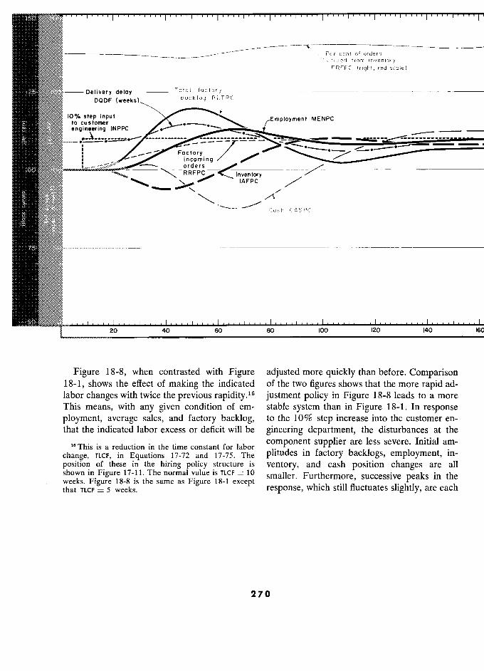
- -- Per cent of orders filled from inventory FRFPC (right, red scale)
Delivery delay Total factory
DQDF (weeks) backlog q B t.T P c
10% step input Employment MENPC to customer ,
Employment MENPC
engineering INPPC - -
- .,--
/ ': ---- Factory -:::::-.-. -_.-",.,,"",.«"'-
s incomm /g
1. -
^ orders w
...'.ro
i' °
E IAFPC /
? Cash CASPC Cash CASPC
20 40 60 80 100 120 140
Figure 18-8, when contrasted with Figure adjusted more quickly than before. Comparison 18-1, shows the effect of making the indicated of the two figures shows that the more rapid ad-
, labor changes with twice the previous rapidity.16 justment policy in Figure 18-8 leads to a more This means, with any given condition of em- stable system than in Figure 18-1. In response ployment, average sales, and factory backlog, to the 10% step increase into the customer en- that the indicated labor excess or deficit will be gineering department, the disturbances at the
"This is a reduction in the time constant for labor component supplier are less severe. Initial am-
change, TtCF, in Equations 17-72 and 17-75. The plitudes in factory backlogs, employment, in- position of these in the hiring policy structure is ventory, and cash position changes are all shown in Figure 17-11. The normal value is TLCF - 10 smaller. Furthermore, successive peaks in the
. weeks. Figure 18-8 is the same as Figure 18-1 except res onse ? ' sli htl are each that TLCF = 5 weeks. response, ? still fluctuates slightly, are each
270
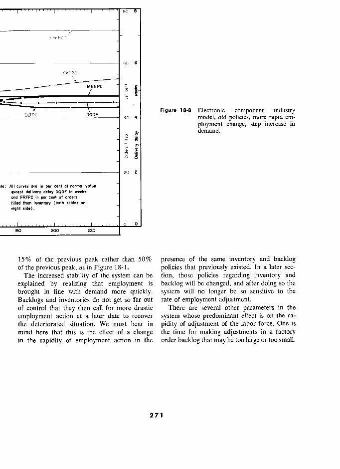
r ''' ! ''' " , " .. r 80 6
FRFPC
60 6
CASPC
MENPC '_S _ -
d
- â *
Figure 18-8 Electronic component industry 40 4 model, old policies, more rapid em-
ployment change, step increase in
j
à demand. - 0 " " 0; = 0
'" >_ " >
:5
20 2
: All curves ore in per cent ot normal volus
except delivery deloy DODF in weeks ond FRFPC in per cent of orders
filled from inventory (both scales on
right side).
Ci 0
IBO 200 220
15% of the previous peak rather than 50% presence of the same inventory and backlog
of the previous peak, as in Figure 18-1. policies that previously existed. In a later sec-
The increased stability of the system can be tion, those policies regarding inventory and
explained by realizing that employment is backlog will be changed, and after doing so the
brought in line with demand more quickly. system will no longer be so sensitive to the
Backlogs and inventories do not get so far out rate of employment adjustment.
of control that they then call for more drastic There are several other parameters in the
employment action at a later date to recover system whose predominant effect is on the ra-
the deteriorated situation. We must bear in pidity of adjustment of the labor force. One is
mind here that this is the effect of a change the time for making adjustments in a factory
in the rapidity of employment action in the order backlog that may be too large or too small.
2 7 1
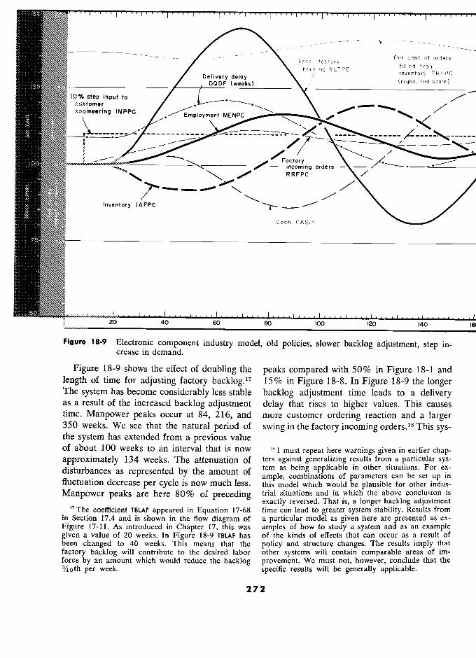
150 . , , . ... _ i .... I .... i .... I . , . " " I , " I " "
- - Total factory
Per cent of orders Total factory filled from
Oelivery deloy bcicklog BLTPC c
(riqht, red FRFPC DODF deloy (right, red scale)
iO°Ja step input to · / customer engineering INPPC / Employment MENPC
·
/ ' , /
-- / -
---
gelez ' Factory , incoming orders -
RRFPC / / R RFPC
/
/
m Inventory IAFPC
?Cash CASPC
v, 20 40 60 80 100 120 140
Figure 18-9 Electronic component industry model, old policies, slower backlog adjustment, step in- crease in demand.
Figure 18-9 shows the effect of doubling the peaks compared with 50% in Figure 18-1 and
length of time for adjusting factory backlog.17 15% in Figure 18-8. In Figure 18-9 the longer The system has become considerably less stable backlog adjustment time leads to a delivery as a result of the increased backlog adjustment delay that rises to higher values. This causes time. Manpower peaks occur at 84, 216, and more customer ordering reaction and a larger 350 weeks. We see that the natural period of swing in the factory incoming orders.18 This sys- the system has extended from a previous value of about 100 weeks to an interval that is now 'x I must repeat here warnings given in earlier chap- approximately 134 weeks. The attenuation of ters against generalizing results from a particular sys-
disturbances as represented by the amount of tem as being applicable in other can be For ex- , _ ample, combinations of parameters can bc set up in
fluctuation decrease per cycle is now much less. this model which would be plausible for other indus-
Manpower peaks are here 80% of preceding trial situations and in which the above conclusion is
exactly reversed. That is, a longer backlog adjustment 17 The coefficient TBLAF appeared in Equation 17-68 time can lead to greater system stability. Results from in Section 17.4 and is shown in the flow diagram of a particular model as given here are presented as ex- Figure 17-11. As introduced in Chapter 17, this was amples of how to study a system and as an example given a value of 20 weeks. In Figure 18-9 TBLAF has of the kinds of effects that can occur as a result of been changed to 40 weeks. This means that the policy and structure changes. The results imply that
factory backlog will contribute to the desired labor other systems will contain comparable areas of im- force by an amount which would reduce the backlog provement. We must not, however, conclude that the ;4oth per week. specific results will be generally applicable.
272
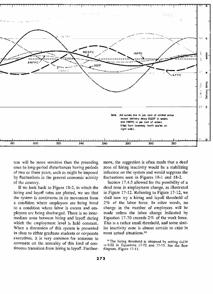
tH.) 8
FRFPC
BLTPC 60 6 TPC
' fl -
/ ` - MENPC
fl INPPC
~ ..
RRFPC?? / / ----_` ,w - n
0. , - s
D DF
_ ' 'CASPC W
?IAFPC l A F PC
.. "g
N ô à
2
Note: All curves ore in per cent of normal value
except delivery deloy DODF in weeks and FRFPC in per cent of orders filled from inventory (both scales on
_ right side).
180 200 220 260 2BO 300 320
tem will be more sensitive than the preceding more, the suggestion is often made that a dead ones to long-period disturbances having periods zone of hiring inactivity would be a stabilizing of two or three years, such as might be imposed influence on the system and would suppress the
by fluctuations in the general economic activity fluctuations seen in Figures 18-1 and 18-2. of the country. Section 17.4.5 allowed for the possibility of a
If we look back to Figure 18-2, in which the dead zone in employment change, as illustrated
hiring and layoff rates are plotted, we see that in Figure 17-12. Referring to Figure 17-12, we the system is continuous in its movement from shall now try a hiring and layoff threshold of a condition where employees are being hired 2% of the labor force. In other words, no to a condition where labor is excess and em- change in the number of employees will be
ployees are being discharged. There is no inter- made unless the labor change indicated by mediate zone between hiring and layoff during Equation 17-70 exceeds 2% of the work force. which the employment level is held constant. This is a rather small threshold, and some simi- When a discussion of this system is presented lar inactivity zone is almost certain to exist in in class to either graduate students or corporate most actual situations.19 executives, it is very common for someone to
The hiring threshold is obtained by setting CLCTF comment on the unreality of this kind of con- = p,02 in Equations 17-72 and 17-75. See the flow tinuous transition from hiring to layoff. Further- diagram, Figure 1 7-1 1 .
. 273 3
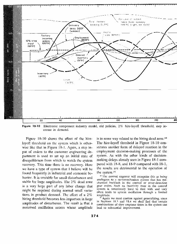
- --- Per cent of orders Total factory filled from inventory
Delivery backlog BLTPC FRFPC (right, red scale)
delay DQDF
Factory
( w eeks ) Profit NPRPC / : Factory
_- /_
rate NPRPC
/ i incoming Employm rit il/ 10 % step orders N PC ._
/ , /
input RRFPC
INPPC __:.' · "
t De i r e> d7 1000
_ ".. _.,
l ` _: inventory y 11-e
·
·
·/ `
___. "'
e ,
Inveritory > - - ', IAFPC
Cas h _£ S - '
/
Cash \ CASPC
20 40 60 80 100 120 140
Figure 18-10 Electronic component industry model, old policies, 2% hire-layoff threshold, step in- crease in demand.
Figure 18-10 shows the effect of the hire- is in some way related to the hiring dead zone.2o
layoff threshold on the system which is other- The hire-layoff threshold in Figure 18-10 con-
wise like that in Figure 18-1. Again, a step in- stitutes another form of delayed reaction in the
put of orders to the customer engineering de- employment decision-making processes of the
partment is used to set up an initial state of system. As with the other kinds of decision-
disequilibrium from which to watch the system making delays already seen in Figure 18-1 com-
recovery. This time there is no recovery. Here pared with 18-8, and 18-9 compared with 18-1,
we have a type of system that 1 believe will be the results are detrimental to the operation of
found frequently in industrial and economic be- the system.21
havior. It is unstable for small disturbances and '0 The control engineer will recognize this as being
analogous to a servomechanism system that has me- stable for large amplitudes. The ° dead zone chanical backlash in the control or error-detection
is a very large part of any labor change that gear trains. Such an inactivity zone in the control
might be required during normal small varia- system is notoriously hard to deal with and very
_ , often leads to system oscillation through a limited tions in product demand. The effect of a 2% amplitude.
hiring threshold becomes less important in large 21
Again we must caution against generalizing, since in Sections 18.3 and 18.4 we shall find that certain
amplitudes of disturbance. The result is that a combinations of slow response times in the system can P _ S lS S
IS. a combinations of slow response times III the system can
sustained oscillation occurs whose amplitude lead to substantial improvement.
274
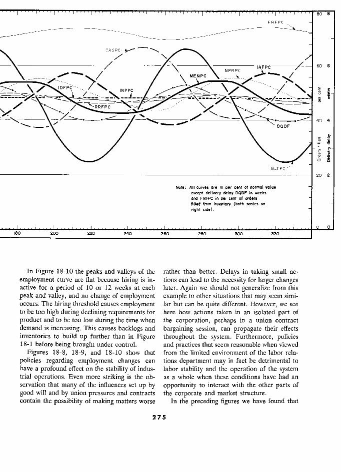
1 1 1 1 , . 1 , , . Bo 8
FRFPC
\ 110,
6
-------- ---
/
/ \
MENPC NPRPC ------- ---- ---- IAFPC - - - - -
- -71
60 6
IDFPC' / s
?fl , 40
4
DODF "0 0
i
'"
'" >
BLTPC - 20 2
Note: All curves ore in per cent of normal volume
except delivery deloy DODF in weeks and FRFPC in per cent of orders
filled from inventory (both scales on riqht side) .
o 0 j 180 200 220 240 260 280 300 320
In Figure 18-10 the peaks and valleys of the rather than better. Delays in taking small ac-
employment curve are flat because hiring is in- tions can lead to the necessity for larger changes active for a period of 10 or 12 weeks at each later. Again we should not generalize from this
peak and valley, and no change of employment example to other situations that may seem simi- occurs. The hiring threshold causes employment lar but can be quite différent. However, we see to be too high during declining requirements for here how actions taken in an isolated part of
product and to be too low during the time when the corporation, perhaps in a union contract demand is increasing. This causes backlogs and bargaining session, can propagate their effects inventories to build up further than in Figure throughout the system. Furthermore, policies 18-1 before being brought under control. and practices that seem reasonable when viewed
Figures 18-8, 18-9, and 18-10 show that from the limitedenvironmentof the labor rela-
policies regarding employment changes can tions department may in fact be detrimental to have a profound effect on the stability of indus- labor stability and the operation of the system trial operations. Even more striking is the ob- as a whole when thèse conditions have had an servation that many of the influences set up by opportunity to interact with the other parts of
good will and by union pressures and contracts the corporate and market structure. contain the possibility of making matters worse In the preceding figures we have found that
275 5
CUSTOMER-PRODUCER-EMPLOYMENT SYSTEM
the old system is sensitive to delays in the em- gained in this direction. Furthermore, we should
ployment decisions. These delays are not ordi- not expect that the major improvements in
narily subject to careful consideration or close system behavior will result merely from chang- control. System dynamics are at the mercy of ing the values of those parameters which had
capricious decisions. If the sensitivity to these already been included in the model. More ef-
factors is to remain, the important parameters fective changes are often possible. The initial
should be closely controlled. If the system can structure of the model was that which had been be redesigned to make it insensitive, that will be judged to represent the old mode of operation. even better. The structure is subject to change in many
places. Not only can the parameters in decision 18.3 New Policies policies be changed, but those policies can be
In the preceding sections we have examined changed in form as well. Decisions can often the dynamic characteristics of the model that be based on different and more effective sources was developed in Chapter 17. The model was of information.
designed to represent the operating character- We shall try to find a redesigned management istics of a real case study. The model behavior structure and policies which are achievable in showed the same problems and difficulties as practice and which lead to more favorable oper- did the actual system and that originally led to ation. The objective is to attain greater labor the study. The model passed as a reasonable stability, less tendency for the system to amplify representation of the system, both in the de- certain critical frequencies of external disturb- tailed equations of which it was constructed ance, and less tendency for the system to be and also in its over-all performance. The per- perturbed by internal or external random varia- formance of the model was judged by such tions. This must be done without imposing re- criteria as natural period and degree of stability, quirements for unacceptable levels of inven- and also by the time-phase relationships that tories and without requiring financial resources were developed between the internal variables. which are unavailable or which would cost
Changes in the parameters of the model some- more than the value of the improvements. Since times led to unexpected changes in results. But most industrial systems seem to operate so far these changes, when understood, could be from a hypothetical ideal, it is reasonable to traced back to a reasonable likelihood that the hope that system improvements can first be effects would be similar in the real system.22 obtained without requiring any compromise.
At this point, we begin to feel sufficient con- Improving one factor may not require paying fidence to believe that the model is an adequate a penalty elsewhere. That is the situation here. basis for exploring ways to improve the system. With changes in the model that can easily be Section 18.2.2 has shown that a more respon- made in the real system, we can simultaneously sive hiring policy that acts more quickly pro- hope to reduce labor fluctuation, reduce peak duces some improvement. Practical considera- cash demands, improve the uniformity of de-
tions, however, limit the amount that can be livery delay, reduce the fluctuation in order
22 This study of the company and the development backlogs, and hold inventory excursions to ap-
and interpretation of the model were made over a proximately their present satisfactory value.
two-year period by three or four people. In this section, changes for achieving some
276
§18.3 NEW POLICIES S
of these improvements will be evolved. The im- low the flow of information from inventory in
provements to be discussed lie in the manage- Figure 17-6 to inventory reordering in Figure ment of inventory and of employment changes.
17-8 to manufacturing backlogs in Figure 17-9
Several points about the old system should be and to employment changes in Figure 17-11,
especially noted: we see that three sets of decision-making and ' decision-executing delays lie between factory in-
. Inventory changes are not effective in absorb- ventory and work force. This is not an unusual
ing fluctuations in sales; the reverse holds, so situation within most companies, in view of all that employment varies more than the usage of the steps that couple primary information to
rate of the product. production-rate changes.
. As shown in Figure 17-8, inventory and inven- All of the preceding points suggest revision tory reordering are managed relatively inde- of the information flows controlling inventory , pendently of the remainder of the system. and employment changes. Information about
. Authorized inventory is geared to the average inventories should enter directly into employ- level of sales. If sales rise, more inventory is
ment-change decisions without going through permissible and considered desirable. If average the intervening step of appearing as factory- sales fall, inventories corne in for intensive
manufacturing backlog. Inventory orders need sales . fall, inventories come in for
. intensive manufactunng backlog. lnventory orders nee ? scrutmy and must be reduced. If inventories , ? .. scrutiny and must be reduced. If inventories not enter the factory in such a way that they mix fall in a period of nsmg business, there is con- i " °Y fall that customer service will be impaired. All orders being manufactured to customer
of these viewpoints seem reasonable and are spécification. If customer orders are given ex-
common industrial practice. An upturn in sales peditious scheduling and priority, they will not
depletes inventory while at the same time mak- be delayed so long in factory backlog and
ing more inventory permissible and presumably should contribute less to the variability of de- desirable. livery delay.
. The system is set up as if inventory were a di- Doing these things implies that production rectly controllable variable. An inventory re- for inventory is, as it should be, simply the way ordering policy exists for the control of inven- to occupy efficiently that fraction of the work tory levels. Desired inventory changes are force not manufacturing items to customer discussed as such. The system organization and
specification. The factory needs a priority list management discussions tend to contradict what of the particular catalog items that are most everyone knows - that inventory is not a di-
needed in inventory, but this is different from rectly controllable e quan t't 1 y. Inventory is thé e needed
m lllventory, .. but , . dlfferent from -
accumulated difference between what is pro- the concept of inventory production orders that accumulated différence between what is pro- i?ntory production orders that -
duced and what is delivered to the customer. are binding on the factory to deliver. The fac-
Assuming that we sell and deliver what we can, tory produces for inventory the amount that its
inventory is controllable only by control of employment level will permit. Adjusting the
production rate. flow of goods into inventory is done by adjust- . Employment changes in Figure 17-11 are made ing the employment level. This changes the
primarily as a result of the average level of number of employees in excess of those making sales and the state of factory-order backlogs. special orders for customers.
. Before inventory adjustments influence employ- In the following three subsections are the
ment changes, the inventory orders must find necessary changes to the equations and flow di-
their way into the factory backlog. If we fol- agrams of Chapter 17.
277
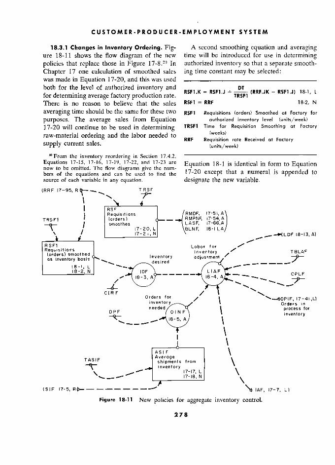
CUSTOMER-PRODUCER-EMPLOYMENT SYSTEM
18.3.1 Changes in Inventory Ordering. Fig- A second smoothing equation and averaging ure 18-11 shows the flow diagram of the new time will be introduced for use in determining policies that replace those in Figure In authorized inventory so that a separate smooth- Chapter 17 one calculation of smoothed sales ing time constant may be selected: was made in Equation 17-20, and this was used –––––––––––––––––––––––––––– both for the level of authorized inventory and
RSF1.K = RSF1.J + DT
(RRF.JK - RSF1.J) 18-1, L for determining average factory production rate.
' ' TRSFI ' ' '/ There is no reason to believe that the sales RSF1 = RRF 18-2, N
;. averaging time should be the same for these two RSF1 Réquisitions (orders) Smoothed at Factory for " purposes. The average sales from Equation authorized inventory level (units/week)
17-20 will continue to be used in determining TRSF1 Time for Réquisition Smoothing at Factory
raw-material ordering and the labor needed to RRF Requisitionweeks) rate Received at Factory 1 1 ° RRF Réquisition rate Receive at Factory
supply current sales. (units/week) 'From the inventory reordering in Section 17.4.2, –––––––––––––––––––––––––––––––––
Equations 17-15, 17-16, 17-19, 17-22, and 17-23 are Equation 18-1 is identical jr form to Equation now to be omitted. The flow diagrams give the num- bers of the equations and can be used to find the 17-20 exCept that a numéral is appended to source of each variable in any equation. designate the new variable.
(RRF 17-95, TRSF
Î '
1 RSF . , . ) Réquisitions
RMDF, 17-51 A
TRSFI 1 ' (orders) - RMPNF, 17-54,A A - f smoothed $LASF, 17-66,A
\ ' ' 17-20,L L BLNF, 18-1 1, A
\ Î N F, A
RSF1 Labor for Requisitions inventory TBLAF (orders) smoothed inventory TBLAF as inventory basis / , Inventory Y adjustment t desired B(ISI'S
18-I, L L ' ' - N "_y IDF ____
as Inventory basls
17-41,L)
18-1 L
- - C-I 6R-F F /
Orders for / 1 inventorv–,? t Orders in needed t process for DPF F 0 I N F \ inventory
\
1 \ \
ASIF F \ TASIF Average . TASIF shipments from \
...- - inventory
17-17, L \ inventory
17-17, L \ 17-18, N \
(SIF 17-7, L)
Figure 18-11 1 New policies for aggregate inventory control.
278
§ 18.3.1 1 CHANGES IN INVENTORY ORDERING
Desired inventory is determined as in Equa- necessary and actual in-process inventory. The tion 17-19 but uses the new value of smoothed sum of these differences gives the inventory sales: adjustment which is desired. This is divided
by labor productivity to give the man-weeks of work necessary for inventory adjustment. The
IDF.K = (CIRF)(RSFl.K) 18-3, A result is further divided by a time period over
IDF Inventory Desired at Factory (units) which the adjustment is to be accomplished, IDF inventory Desired at Factory (units)
CIRF Coefficienr for Inventory Ratio at Factory yielding the number of men needed to adjust (weeks) inventory. Since inventory and factory backlog
RSF1 Réquisitions (orders) Smoothed at Factory for are in many senses the inverse of one another, authorized inventory level (units/week) the same adjustment time constant will be used
_____________________________ here as previously for the correction of back-
logs. Information from Equation 18-4 flows di- The important change to be made is that ag- rectly to the labor decision in Equation 18-13.
gregate inventory is no longer to be controlled In the manufacturing sector there will no by the separate independent inventory orders longer be a formal backlog of orders destined for individual catalog items. A control of total for inventory, so that the former Equation aggregate inventory is to be established by con- 17-22 must be modified: trol of employment, and within this framework
priorities will indicate to the factory the prefer- ––––––––––––––––––––––––––––
ences for various catalog items. The policy OINF.K = (ASIF.K)(DPF) 18-5, A therefore becomes a statement of how
many ' pINF Orders for Inventory Necessary at Factory employees are necessary for adjusting an im- ,, proper lc'Vel of inventory: ASIF Average Shipments from Inventory at the Fac-
tory (units/week) ––––––––––––––––––––––––––––––––––– DPF Delay in Production at Factory (weeks)
LIAF.K IAF.K . \TBLAF/\CPL /F
(IDF.K - IAF.K
+ OINF.K - OPIF.K) 18-4, A Equation 18-5 gives the normal work in
LIAF Labor for Inventory Adjustment at Factory process in the factory for inventory as the prod- LIAF
(men) Inventory Adjustment at Factory uct of the average usage rate from inventory
TBLAF Time for BackLog Adjustment at Factory multiplied by the factory-production delay. (weeks) Actually the new equations in Figure 18-11 1
CPLF Constant, Productivity of Labor at Factory no longer represent inventory ordering in the (units/man-week) usual sense. They become one of the considera-
IAF Inventory ?Î'§ ar Factory (units) tions entering into the new employment policies. IAF Inventory Actual at Factory (units) , °._.. , ' ' .*
OINF Orders for Inventory Necessary at , The responsibility for total aggregate inventory (units) would now rest at the point in the organization
OPIF Orders in Process for Inventory at Factory where central system control is being exercised. <its> At the stock room, the responsibility becomes
one of establishing priorities based on stock
levels and usage rates. The stock room controls The last term in parentheses in Equation 18-4 preferences for the sequence of goods to be
gives the difference between desired and actual manufactured but not the total amourit to be finished inventory and the difference between manufactured for inventory.
279
CUSTOMER-PRODUCER-EMPLOYMENT SYSTEM
18.3.2 Changes in Manufacturing Départ- 18-7 checks this against the number of men
ment. The essential information and control in available, and the lesser of those needed or those
the part of the model that represents the manu- available are taken to work on customer orders.
facturing department are now to be simplified The production rate on customer orders is
as shown in Figure 1 8- 1 2.4 In the revised oper- therefore
ation a normal amount of time will be taken
for the planning and scheduling of special or- PCOF.KL = (LCOF.K)(CPLF) 18-8, R
ders for customers, and then the full resources '
of the factory are first available for making PCOF Production to Customer Order at Factory
these orders. The excess labor remaining is then (units/week)
- . t a - . mg e d d s LCOF Labor for Customer Order at Factory (men)
applied to making product for finished-goods CPLF Constant, Productivity of Labor at Factory inventory. The factory is no longer obligated to (units/man-week) deliver the full amount ordered for inventory ____________________________
but rather determines the production for inven-
tory by the labor available after production The remainder of the labor force not work-
obligations for special customer orders have ing on customer orders is available to manufac-
been met. ture for inventory:
BLCF.K LIF.K = MENPF.K - LCOF.K 18-9, A
LDCOF.K = (DNBLF)(CPLF)
18-6, A PIF.KL = (LIF.K)(CPLF) 18-10, R
_ LDCOF.K if MENPF.K ::::>: LDCOF.K1 LIF Labor for Inventory at Factory (men) '
MENPF,K if MENPF.K [ LDCOF.K f MENPF MEN Producing at Factory (men)
18-7, A LCOF Labor for Customer Order at Factory (men)
PIF Production rate starts for Inventory at Factory LDCOF Labor Desired for Customer Orders at Factory (units/week)
(men) CPLF Constant, Productivity of Labor at Factory BLCF BackLog for Customer at Factory (units)
(units/man-week) DNBLF Delay in Normal BackLog at Factory (weeks)
(units/man-week)
CPLF Constant, Productivity of Labor at Factory ****
(units/man-week) Figure 18-12 does not show the flow of in- LCOF Labor for Cusromer Order at Factory (men) Figure
does not show the flow of
MENPF MEN Producing at Factory (men) structions for determining what items will be
manufactured for inventory with the available
labor. The manner of determining the actual
The objective of Equation 18-6 is to apply items to be made will not affect the dynamic
to the customer backlog of orders a work force behavior of the system. It is assumed that items
in proportion to the size of that backlog so that will be chosen to keep the material in the aggre-
the backlog delay will be held constant. The gate inventory as useful as possible in filling
backlog is divided by the labor productivity customer orders. The relationship in Figure
giving the man-hours of labor represented in 1 7-7 continues to control the fraction of cus-
the backlog. This in turn divided by the normal tomer orders that can be filled from inventory.
scheduling interval for backlog orders gives the Total employment level is determined at the
number of men that should be used. Equation point where the over-all system dynamics are
" ... being controlled. The responsibility of the fac-
following equations from Section 17.4.3 are tory management is for efficient production us-
to be omitted: 17-24, 17-25, 17-28 through 17-33, , -' _,
17-35 through 17-39, and 17-49. ing the authorized people.
280
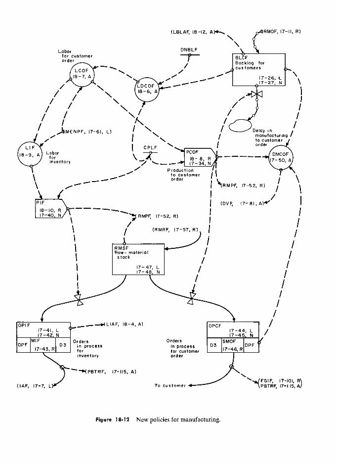
(LBLAF, 18-12, RMOF, 17-II, R)
Labor DNBLF \ \______ for customer
––P–– BLCF order
' Backlog for customers
L
/ -" g
.
/
\
,
, /
j
Î
/ /
/ /
/
1
/ 1
E NPF 17-61 LI Delay i n / /
1
F
/
)
/
/
/ Î
) \ ' to customer
t CPLF I order
"
` PCOF
1 monufaeturing 1 - , for for ` ----- DMCOF
\ / 'o'' A y
I
A
1
\ 1'
- "
Production
, 17-52, R) \ \
t
\ ––-"" to customer
/t
Y /
' \ \ order
?RMPF, 17-52, R) '
__ j (DVF, / 1
) < !7-40, N 1 '?RMPF !7-52.R) R)
'
17-40 N
j / / (RMRF, R)
j
. /
) /
(RMRF, 17-57, R)
j
1
RMSIF /
t RMSF /
' ' Raw- material 1 /
/ '
) stock . /
t
S °C
17- 47, L / /
) !7-48, 'N /
I '
/ 1
'
1
1
/
OPIF !7-4).L
OPCF !7-44,L / L 17-44, L
/ !7-42.N N !7-45.N N '
M!F Orders Orders SMOF ,/ DPF
17-43, D3 in process
in process D3
17-46, DPF for for customer \. inventory order j
, i7-!!5. A)
(IAF, 17-7, To customer R1 (IAF, !7-7. Lr To customer
Figure 1 8-1 2 New policies for manufacturing.
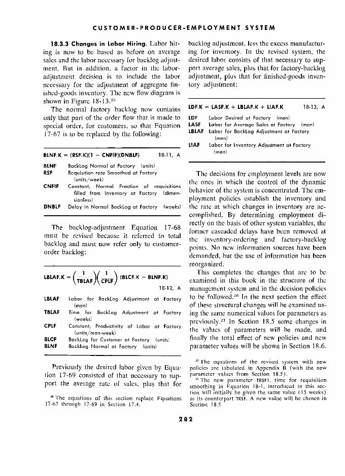
CUSTOMER-PRODUCER-EMPLOYMENT SYSTEM
18.3.3 Changes in Labor Hiring. Labor hir- backlog adjustment, less the excess manufactur-
ing is now to be based as before on average ing for inventory. In the revised system, the
sales and the labor necessary for backlog adjust- desired labor consists of that necessary to sup- ment. But in addition, a factor in the labor- port average sales, plus that for factory-backlog
adjustment decision is to include the labor adjustment, plus that for finished-goods inven-
necessary for the adjustment of aggregate fin- tory adjustment:
ished-goods inventory. The new flow diagram is
shown in Figure 1 8- 1 3 .2Ô LDF.K = LASF.K + LBLAF.K + LIAF.K 18-13, A The normal factory backlog now contains LDF.K = LASF.K + LBLAF.K + LIAF.K 18-13, A
only that part of the order flow that is made to LDF Labor Desired at Factory (men)
special order, for customers, so that Equation LASF Labor for Average Sales at Factory (men)
17-67 is to be replaced by the following: LBLAF Labor for BackLog Adjustment at Factory
' (men) _____________________________________ LIAF Labor for Inventory Adjustment at Factory
BLNF.K = (RSF.K)(1 - CNFIF)(DNBLF) 18-11, A (men)
BLNF BackLog Normal at Factory (units) RSF Réquisition rate Smoothed at Factory The decisions for employment levels are now
§'/i _ , the ones in which the control of the dynamic CNFIF Constant, Normal Fraction of requisitions . rr.. filled from Inventory at Factory (dimen- behavior of the system is concentrated. The em-
sionless) ployment policies establish the inventory and DNBLF Delay in Normal BackLog at Factory (weeks) the rate at which changes in inventory are ac- –––––––––––––––––––––––––––– complished. By determining employment di-
The backlog-adjustment Equation 17-68 rectly on the basis of other system variables, the
must bc it referred to total , former cascaded delays have been removed at
must be revised because it referred to total
must be and must now refer only to customer- thé e inventory-ordering and factory-backlog
backlog d b and kl must ta
points. No new information sources have been order ° demanded, but the use of information has been ____________________________ reorganized.
LBLAF.K )(
1 (BLCF.K - BLNF.K) This completes the changes that are to be
examined in this book in the structure of the 18-12, A management system and in the decision policies
LBLAF Labor for BackLog Adjustment at Factory to be fo11owed.:w In the next section the effect
(men) of these structural changes will be examined us- TBLAF Time for BackLog Adjustment at Factory ing the same numerical values for parameters as
(weeks) previously.=7 In Section 18.5 some changes in
CPLF Constant, Productivity of Labor at Factory the values of parameters will L made, and thé vaiues ot parameters wul e ma e, and (units/man-week)
BLCF BackLog for Customer at Factory (units) finally the total effect of new policies and new BLNF BackLog Normal at Factory (units) parameter values will be shown in Section 18.6.
. " equations of the revised system with new Previously the desired labor given by Equa- policies are tabulated in Appendix B (with the new
tion 17-69 consisted of that necessary to sup- parameter values from Section 18.5).
j 1 " new parameter TRSF1, time for requisition
port the average rate of sales, plus that for smoothing in Equation 18-1, introduced in this sec- tion will initially be given the same value ( 1 weeks)
' The equations of this section replace Equations as its counterpart TRSF. A new value will be chosen in 17-67 through 17-69 in Section 17.4. Section 18.5.
282 2
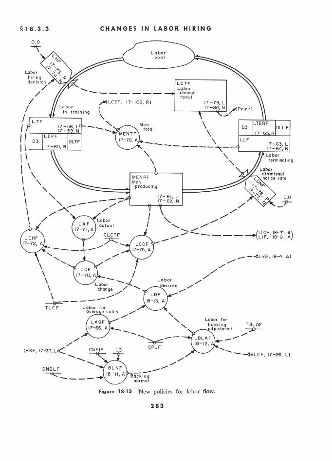
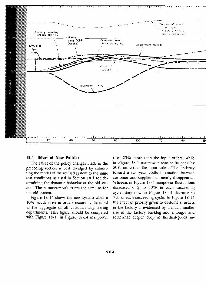
Per cent of orders filled from
NNNN N Factory incoming inventory FRFPC
comin (right, red scale) ttNt jN orders RRFPC trtqht.redsca)e) .. Delivery
\ deloy DQDF Customer-order
la% step \
weeks backlog BLCPC Employment MENPC
input _ INPPC
_ - .....
· _
·
Cosh
-. -
C.sh
y . CASPC
jtgtjt Inventory IAFPC
/
` /
j 20 40 60 80 100 120 140
18.4 Effect of New Policies rises 25% more than the input orders, while
The effect of the policy changes made in the in Figure 18-1 manpower rose at its peak by
preceding section is best divulged by submit- 50% more than the input orders. The tendency
ting the model of the revised system to the same toward a two-year cyclic interaction between
test conditions as used in Section 18.1 for de- customer and supplier has nearly disappeared. termining the dynamic behavior of the old sys- Whereas in Figure 18-1 manpower fluctuations
tem. The parameter values are the same as for decreased only to 50% in each succeeding the old system. cycle, they now in Figure 18-14 decrease to
Figure 18-14 shows the new system when a 7% in each succeeding cycle. In Figure 18-14
10% sudden rise in orders occurs at the input the effect of priority given to customers' orders to the aggregate of all customer engineering in the factory is evidenced by a much smaller
departments. This figure should be compared rise in the factory backlog and a longer and with Figure 18-1. In Figure 18-14 manpower somewhat deeper drop in finished-goods in-
284
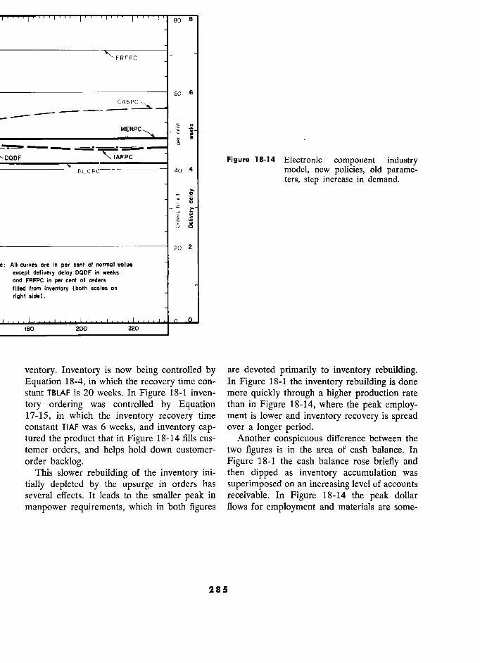
, ç>,= 8 8 v,
FRFPC
60 6 '
, - _ _ CASPÇ?
..
.
,
MENPC _ v d d ;
.
DQDF -71-AF PC Figure 18-14 4 Electronic component industry
. '
4 nlodel, new policies, old parame- :
ters, step increase in demand.
g '
v v
" .: ' "
20 2
All curves ore in per cent of normal value except delivery deloy DQDF in weeks . and FRFPC in per cent of orders "
filled from inventory (both scoles on _ r!9hts!de).
- () 01
-'
, 180 ' 200 220
ventory. Inventory is now being controlled by are devoted primarily to inventory rebuilding.
Equation 18-4, in which the recovery time con- In Figure 18-1 the inventory rebuilding is done
stant TBLAF is 20 weeks. In Figure 18-1 inven- more quickly through a higher production rate
tory ordering was controlled by Equation than in Figure 18-14, where the peak employ-
17-15, in which the inventory recovery time ment is lower and inventory recovery is spread constant TIAF was 6 weeks, and inventory cap- over a longer period. tured the product that in Figure 18-14 fills cus- Another conspicuous difference between the
tomer orders, and helps hold down customer- two figures is in the area of cash balance. In
order backlog. Figure 18-1 the cash balance rose briefly and
This slower rebuilding of the inventory ini- then dipped as inventory accumulation was
tially depleted by the upsurge in orders has superimposed on an increasing level of accounts
several effects. It leads to the smaller peak in receivable. In Figure 18-14 the peak dollar
manpower requirements, which in both figures flows for employment and materials are some-
285 5
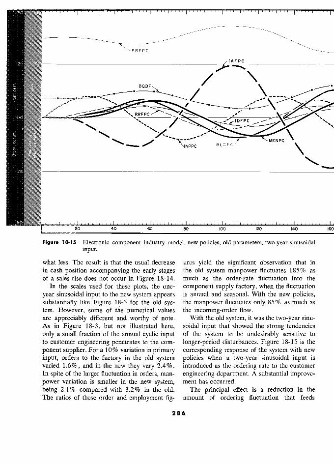
..., .I.. 1 1 . 1 1 1 1 1 1 1 1 1
1 1
1 1 1 1
R FPC
/ IAFPC
DODF
W , W ?y RRFPC ? \ ' ,
IDFPC _ P
N %"%,.00.01
` / ?INPPC' BLCPC
MENPC '
v
20 40 60 80 100 120 140 I?
Figure 18-15 5 Electronic component industry model, new policies, old parameters, two-year sinusoidal
input.
what less. The result is that the usual decrease ures yield the significant observation that in
in cash position accompanying the early stages
the old system manpower fluctua tes 185 % as
of a sales rise does not occur in Figure
18-14. much as the order-rate fluctuation into the
In the scales used for these plots, the one- component supply factory, when the fluctuation
year sinusoidal input
to the new system appears
is annual and seasonal. With the new policies,
substantially like Figure 18-3 for the old sys-
the manpower
fluctuates only 85 9% as much as
tem. However, some of the numerical values the incoming-order flow.
are appreciably different and
worthy of note. With the old system,
it was the two-year sinu-
As in Figure 18-3, but not illustrated here, soidal input
that showed the strong tendencies
only a small fraction of the annual cyclic input of the system to be undesirably sensitive to
to customer engineering penetrates
to the com- longer-period disturbances. Figure 18-15 is the
ponent supplier. For a 10% variation in primary corresponding response
of the system
with new
input, orders to the factory
in the old system policies
when a two-year sinusoidal input
is
varied 1 .6 % , and in the new they vary 2.49% . introduced as the ordering rate to the customer
In spite
of the larger fluctuation in orders, man- engineering department. A substantial
improve-
power variation is smaller in the new system, ment has occurred.
being 2.1% compared
with 3.2% in the old. The principal
effect is a reduction in the
The ratios of these order and employment fig-
amount of ordering fluctuation that feeds
286
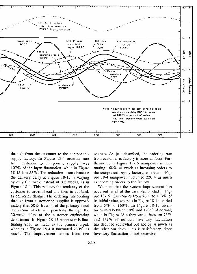
I , I 80 B
Per cent of orders
filled from inventory FRFPC (right, red scale)
60 6
Iriventory ^
la%, 2-yeor Delivery Customer-order [AFPC sinusoidal delay backlo
'/ Input INPPC DODF / BLCPC 9
- ·\
Factory
lnput INPPC
/? '/ U> Ÿ
\ \· /
Factory d 3 incoming orderi
°
,· RRFPC w
·
À
W ``y Desired
\\
i 4
w _ `` Inventory y ` _ i .-.
' y - v ô
Cash h Employment '
"",, /
___"" r Cash
Em loyment CASPC m NPC ? cu
,
CASPC MENPC
% /
cu _- °'
. 0
20 2
Note: All curves are in per cent of normol value
except dellvery delay DQDF in weeks and FRFPC in per cent of orders
filled from inventory (both scales on
right side).
0 oj 180 200 220 240 260 280 300 320
through from the customer to the component- sources. As just described, the ordering rate
supply factory. In Figure 18-4 ordering rate from customer to factory is more uniform. Fur- from customer to component supplier was thermore, in Figure 18-15 manpower is fluc- 107% of the input fluctuation, while in Figure tuating 160% as much as incoming orders to 18-15 it is 53 9% . The reduction occurs because the component-supply factory, whereas in Fig- the delivery delay in Figure 18-15 is varying ure 18-4 manpower fluctuated 220% as much
by only 0.8 week instead of 3.2 weeks, as in as incoming orders to the factory. Figure 18-4. This reduces the tendency of the We note that the system improvement has customer to order ahead and then to cut back occurred in all of the variables plotted in Fig- as deliveries change. The ordering rate feeding ure 18-15. Cash varies from 76% to 113% of
through from customer to supplier is approxi- its initial value, whereas in Figure 18-4 it varied
mately that 50% fraction of the primary input from 5% to 160%. In Figure 18-15 inven- fluctuation which will penetrate through the tories vary between 78% and 120% of normal, 30-week delay of the customer engineering while in Figure 18-4 they varied between 73%
department. In Figure 18-IS manpower is fluc- and 132% of normal. Inventory fluctuation
tuating 85% as much as the primary input, has declined somewhat but not by as much as whereas in Figure 18-4 it fluctuated 230% as the other variables. This is satisfactory, since much. The improvement comes from two inventory fluctuation is not excessive.
287
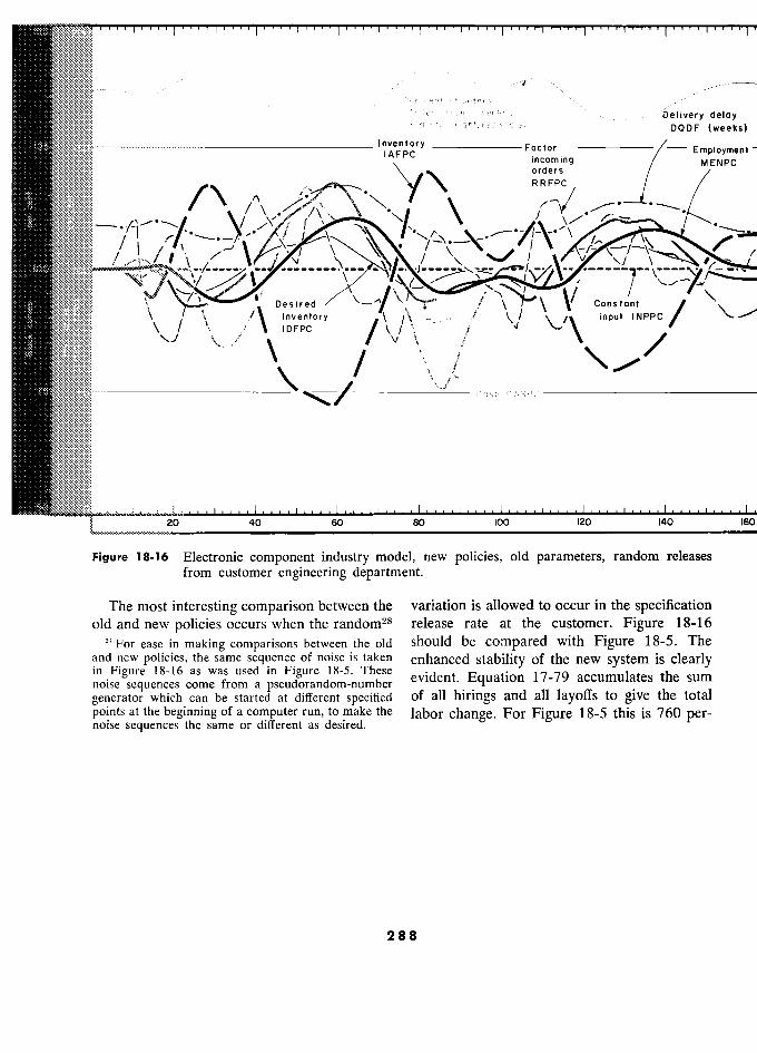
;a
Per cent l' orders
/* fi 1 led from m !nt/entory de?ay ;. filled from inventory Delivery delay FRFPC (right,redscale) DODF (weeks)
^' Inventory IAFPC Factor - Employmenl IAFPC
incoming MENPC
'
]
orders
ll
RRFPC
" _ ,
/ ) p' / ' m ; /
, "
, l '
.. ' 1
., \
·
_.
I
\
j'
\ l..
W/ v
N Desired Constant n
t C / tBttmMB \ / \ /\
inventory \ BLCPC \/\ input
INPPC
\J/ ` IDFPC
/ /
`
/
JJH)
fl-/
IV (
(
s CASPC PC
/
Cash CASPC
20 40 60 80 100 120 140 IE
Figure 18-16 Electronic component industry model, new policies, old parameters, random releases from customer engineering department.
The most interesting comparison between the variation is allowed to occur in the specification old and new policies occurs when the random28 release rate at the customer. Figure 18-16 6
* For ease in making comparisons between the old should be compared with Figure 18-5. The and new policies, the same sequence of noise is taken enhanced stability of the new system is clearly in Figure 18-16 as was used in Figure 18-5.
These evident. E uation 17-79 accumulates the sum noise sequences come from a pseudorandom-number . ?quahon
17 -79 accumul?tes
the sum
generator which can be started at different specified of aIl hirings and all layoffs to give the total
points at the beginning of a computer run, to make the labor change. For Figure 18-5 this is 760 per- noise sequences the same or different as desired.
288
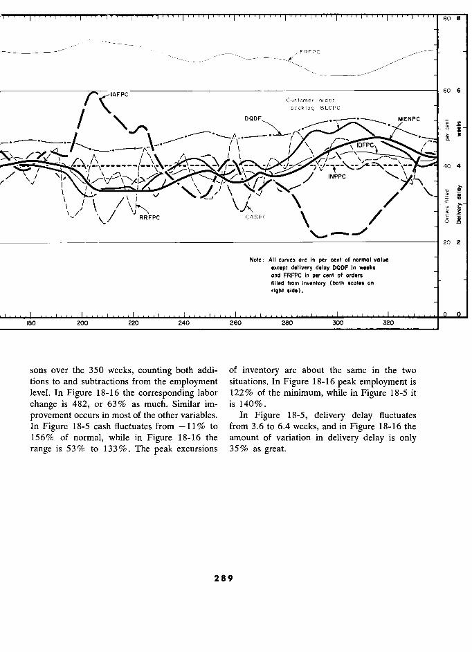
80 8
FRFPC
6
Customer-order
/
DQDF MENPC -
/ i -- l '
< ,
a.
40
4
/ /
" Il " /
\./ CASPC
>
20 2
Note: All curves ore in per cent oi normal valu.
except delivery deloy DQDF in weeks
and FRFPC ln per cent 01 orders _ filled from inventory (both sectes on
right side).
180 200 220 240 260 280 300 320
0 0
sons over the 350 weeks, counting both addi- of inventory are about the same in the two tions to and subtractions from the employment situations. In Figure 18-16 peak employment is level. In Figure 18-16 the corresponding labor 122% of the minimum, while in Figure 18-5 it
change is 482, or 63% as much. Similar im- is 140%.
provement occurs in most of the other variables. In Figure 18-5, delivery delay fluctuates In Figure 18-5 cash fluctuates from - 11 % to from 3.6 to 6.4 weeks, and in Figure 18-16 the 156% of normal, while in Figure 18-16 the amount of variation in delivery delay is only range is 53% to 133%. The peak excursions 35% as great.
289

CUSTOMER-PRODUCER-EMPLOYMENT SYSTEM
18.5 Improvements in New Policies other words, a constant level of employment We have seen that the system containing the would cause no more inventory fluctuation than
new inventory and employment policies as is already here present. The incoming-order
represented in Figures 18-14, 18-15, and 18-16 curve to the factory rises to a peak of about
is more stable and less sensitive to disturbing 5% above the average sales rate. This repre- forces than the old policies represented in sents a peak of 50 units per week in excess
Figures 18-1, 18-4, and 18-5. However, we of the average level of sales. The inventory have not necessarily arrived at the best solution curve shown in Figure 18-15 is falling at the
that we can find. rate of 50 units per week at its steepest point,
Figure 17-1 in Section 17.1 discusses the way and if that point coincided with the peak sales, in which inventory fluctuations so often ac- the inventory could supply all of the excess de-
centuate employment changes compared with mand at the peak and absorb the excess produc- the sales curve. In Figure 18-4, the old system tion at the sales minimum. We can work toward
was one in which inventories had begun to rise this, but there is no reason to believe that we
before the peak of the sales curve. This means can fully achieve the ideal inventory relation-
that production rate is exceeding sales rate at ship over all of the fluctuation frequencies of
some time before peak sales, and that the peak interest.
of production rate must necessarily be higher One way to make better use of the inventory than the peak of the sales curve. The policies fluctuation is to adopt policies that will hold
that lead to an inventory upturn before peak a more uniform employment and production sales are reached account for much of the rate. This in itself will cause the sales and
system tendency to amplify disturbances in the production excesses to flow in and out of in-
region of a two-year period. Figure 18-15 ventory. In both Figure 18-4 and Figure 18-15
shows that the new policies have alleviated this the large amount of employment fluctuation
situation somewhat. The point of minimum in- is caused by the rapidity with which employ-
ventory is at the time of the peak incoming ment is being adjusted to equal sales rate and
factory orders. This means that the manpower also the rapidity with which inventory correc-
curve, representing production capacity, still tions are being demanded. In the system policies crosses the top of the incoming-order curve three time constants predominantly influence
and must necessarily have its own peak later at the responsiveness of employment to changes some higher value. The situation here is better in sales and inventory. than for Figure 18-4 in that inventories are The smoothing constant TRSF in Equation doing less harm. They are, however, contribut- 17-20 determines how quickly the average ing nothing to the reduction of employment sales RSF will follow changes in the incoming- fluctuations. The greatest amount of good would order rate. The average sales RSF determine be obtained if the maximum rate of fall of in- the work force to be employed for meeting sales ventories were to coincide with the peak of demands. the incoming-order curve. The constant TRSF1 in Equation 18-1 de-
It is interesting to note that in Figure 18-15 5 termines the rapidity with which the average the amount of inventory fluctuation which is sales RSFI follow the changes in incoming present would be entirely sufficient to carry all factory orders. This value of average sales de- of the incoming-order fluctuation if the timing termines the authorized level of desired inven- of the inventory fluctuation were correct. In tory. It is clear that the desired level of inven-
290
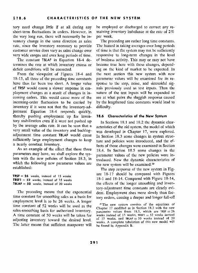
§ 18.6 CHARACTERISTICS OF THE NEW SYSTEM
tory need change little if at all during any be employed or discharged to correct any re- short-term fluctuations in orders. However, in maining inventory imbalance at the rate of 2% the very long run, there will necessarily be in- per week.
ventory change in the same direction as sales The preceding are rather long time constants.
rate, since the inventory necessary to provide The hazard in taking averages over long periods customer service does vary as sales change over of time is that the system may not be sufficiently very wide ranges and over long periods of time. responsive to long-term changes in the level
The constant TBLAF in Equation 18-4 de- of business activity. This may or may not have
termines the rate at which inventory excess or become true here with these changes, depend- deficit conditions will be corrected. ing on the kind of market to be expected. In
From the viewpoint of Figures 18-4 and the next section this new system with new
18-15, all three of the preceding time constants parameter values will be examined for its re- have thus far been too short. A longer value sponse to the step, noise, and sinusoidal sig- of TRSF would cause a slower response in em- nals previously used as test inputs. Then the
ployment changes as a result of changes in in- nature of the test inputs will be expanded to
coming orders. This would cause more of the see at what point the sluggish response caused
incoming-order fluctuation to be carried by by the lengthened time constants would lead to
inventory if it were not that the inventory-ad- difficulty. justment Equation 18-4 responds quickly, thereby pushing employment up for inven- 18.6 Characteristics of the New System
tory stabilization even if it were not pushed up In Sections 18.1 and 18.2 the dynamic char- by the average sales rate. It can be seen that a acteristics of the old system, the model of which very small value of the inventory and backlog- was developed in Chapter 17, were explored. adjustment time constant TBLAF would cause In Section 18.3 some changes in system struc- sufficiently large employment changes to keep ture and policies were introduced, and the ef- a nearly constant inventory. fects of those changes were examined in Section
As an example of the effect that these three 1 g.4. In Section 18.5 some changes in the parameters may have, we shall explore the sys- parameter values of the new policies were in- tem with the new policies of Section 18.3, in troduced. Now the dynamic characteristics of which the following new parameter values are the new system will be examined.29 established: " The step response of the new system in Fig-
TRSF = 26 weeks, instead of weeks s ure 18-17 should be compared with Figures TRSF1 = 5llÎ,'lll§d°li 15 weeks 18-1 and 18-14. Compared with Figure 18-14, TBLAF = 50 weeks, instead of 20 weeks the effects of the longer smoothing and inven-
tory-adjustment time constants are clearly evi- The preceding means that the exponential dent. Employment rises more slowly than fac-
time constant for smoothing sales as a basis for tory orders, causing a deeper and longer fall-off
employment level is to be 26 weeks. A longer 29 ' . time constant of 52 weeks will be used as the The new
system consists of the equations of
" .. Chapter 17 modified as in Section 18.3 wlth the new sales-smoothing basis for authorized inventory. parameter values from 18.5, which are TRSF =26 A time constant of 50 weeks will be taken for weeks instead of 15 weeks, TRSFI = 52 weeks instead
adjusting inventory toward the desired level. of IS weeks, and TBLAF = 50 weeks instead of 20 The latter means that ..
weeks. A complete tabulation of this new model will The latter means that sufficient manpower will be found in Appendix B.
291 1
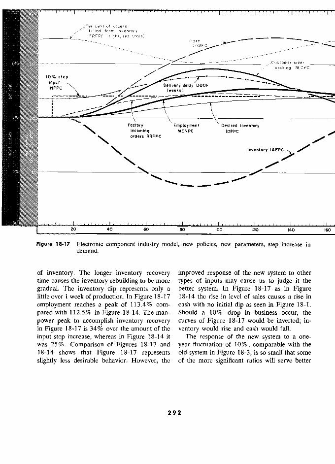
150
:1 cent of orders ,1 filled from inventory y
FRFPC (right, red scale) Cash -_
1
.1 FRFPC (flght, red scole) -
---...;;::: C AS P
1 . Customer-order - Cus tomer-order r
/' backlog BLCPC
10 % step /
_.-.-0-0- input INPPC Delivery deloy DODF
0--0
(weeks ) . --,
1 , 1 .,_ 1 ! .,. ..
-.... i Factory Employment Desired inventory
l " incoming MENPC IDFPC ; orders RRFPC .0
,1" J '
Inventory
IAFPC
/ '
,,, , / ./'
i
loi 20 40 60 80 100 120 140 160
Figure 18-17 Electronic component industry model, new policies, new parameters, step increase in demand.
of inventory. The longer inventory recovery improved response of the new system to other
time causes the inventory rebuilding to be more types of inputs may cause us to judge it the
gradual. The inventory dip represents only a better system. In Figure 18-17 as in Figure little over 1 week of production. In Figure 18-17 18-14 the rise in level of sales causes a rise in
employment reaches a peak of 113.4% com- cash with no initial dip as seen in Figure 18-1.
pared with 112.5% in Figure 18-14. The man- Should a 10% drop in business occur, the
power peak to accomplish inventory recovery curves of Figure 18-17 would be inverted; in-
in Figure 18-17 is 34% over the amount of the ventory would rise and cash would fall.
input step increase, whereas in Figure 18-14 it The response of the new system to a one-
was 25% . Comparison of Figures 18-17 and year fluctuation of 10%, comparable with the
18-14 shows that Figure 18-17 represents old system in Figure 18-3, is so small that some
slightly less desirable behavior. However, the of the more significant ratios will serve better
292 2
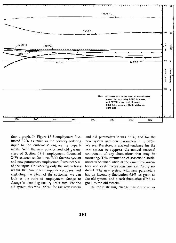
FRFPC
__________"""––––-____ CASPC 606 6
?MENPC ?ppC - S js MENPC INPPC û x y
– 3 ' ....
BLCPC
4
i2 y
N
-S
20 z
Note: All curves are in per cent of normal value
except delivery deloy DQDF in weeks
and FRFPC in per cent of orders filled from inventory (both scales on
rtghtside).
0 0 180 200 220 240 260 280 300 320
than a graph. In Figure 18-3 employment fluc- and old parameters it was 86%, and for the tuated 32% as much as the primary ordering new system and new parameters it is 38%. input to the customers' engineering depart- We see, therefore, a marked tendency for the ments. With the new policies and old param- new system to suppress the annual seasonal eters of Section 18.3 employment fluctuated component of any fluctuations that may be 24% as much as the input. With the new system occurring. This attenuation of seasonal disturb- and new parameters employment fluctuates 9% ances is obtained while at the same time inven- of the input. Considering only the interactions tory and cash fluctuations are also being re- within the component supplier company and duced. The new system with new parameters neglecting the effect of the customer, we can has an inventory fluctuation 63% as great as look at the ratio of employment change to the old system, and a cash fluctuation 67% as change in incoming factory-order rate. For the great as the old system. old system this was 1 85 % , for the new system The most striking change has occurred in
293 3
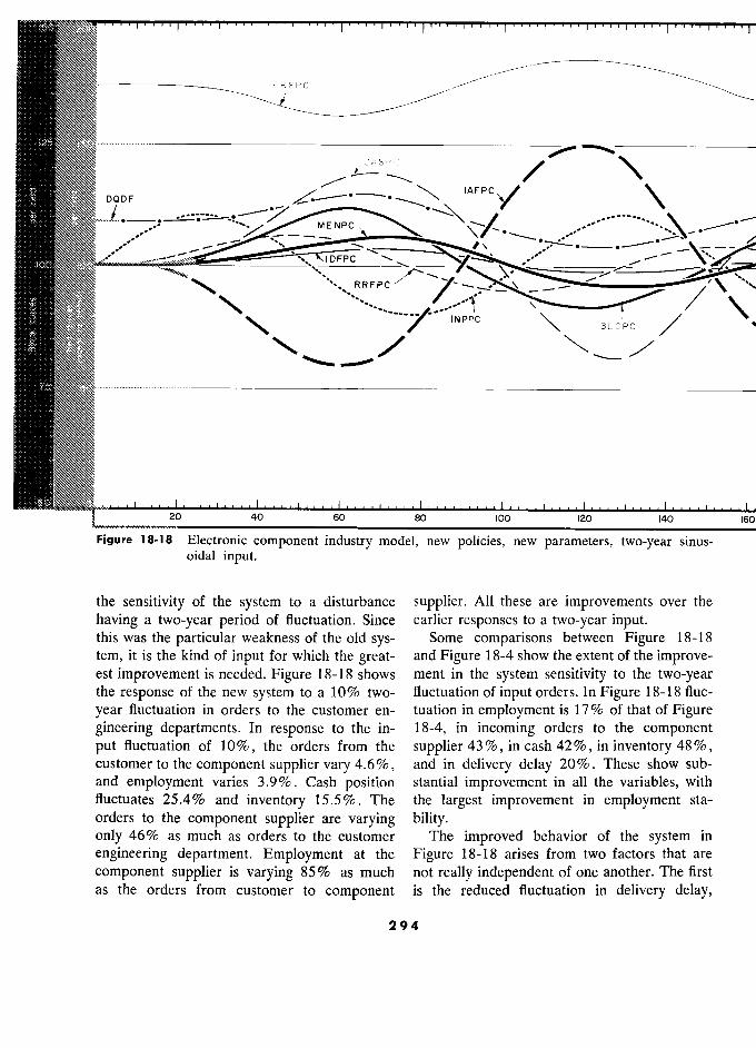
50 1· , 1 - , . 1 ,.. 1
. 1
, . , 1 , , 'T""
FRFPC C
125 '
CASPC C
/
/ F
% IAFPC P C
DQDF D°°F
' MENPC
·
/°'
' ,w - IDFPC ,,' , -
RF PC _\ _ '
/ , -
/ INPPC \ BLCPC
l N PPC P C
/
fl /
20 40 60 80 100 120 140 1£
Figure 18-18 Electronic component industry model, new policies, new parameters, two-year sinus- oidal input.
the sensitivity of the system to a disturbance supplier. All these are improvements over the
having a two-year period of fluctuation. Since earlier responses to a two-year input. this was the particular weakness of the old sys- Some comparisons between Figure 18-18 8
tem, it is the kind of input for which the great- and Figure 18-4 show the extent of the improve- est improvement is needed. Figure 18-18 shows ment in the system sensitivity to the two-year the response of the new system to a 10% two- fluctuation of input orders. In Figure 18-18 fluc-
year fluctuation in orders to the customer en- tuation in employment is 17% of that of Figure gineering departments. In response to the in- 18-4, in incoming orders to the component put fluctuation of 10%, the orders from the supplier 43 %, in cash 42 %, in inventory 48 %, customer to the component supplier vary 4.6%, and in delivery delay 20%. These show sub- and employment varies 3.9%. Cash position stantial improvement in all the variables, with fluctuates 25.4% and inventory 15.5%. The the largest improvement in employment sta- orders to the component supplier are varying bility. only 46% as much as orders to the customer The improved behavior of the system in
engineering department. Employment at the Figure 18-18 arises from two factors that are
component supplier is varying 85% as much not really independent of one another. The first as the orders from customer to component is the reduced fluctuation in delivery delay,
294
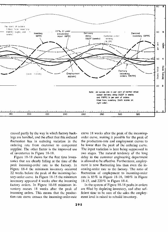
, .I , I , ..I , ,.I.... " ... 80 8
Per cent of orders _ filied from inventory
10%, 2-year - FRFPC (right, red 60 6 scale) Inventory sinusoidal Delivery Desired
IAFPC Input INPPC deloy Customer-order inventory IDFPC
- ,
/ DQDF (weeks) backlog
? t
._
·
BLCPC
v Ÿ .
\
· \
\ - B
,,,,--
*-.
§
°
° "-
w ` 40 4 - '
' ____/-' Factory __v a - ° d ô
Factory >. Cash CASPC Employment 011, incoming
MENPC orders RRFPC MENPC orders RRFPC
20 2
Note: All curves are in per cent of normal value
except delivery deloy DQDF in weeks and FRFPC in per cent of orders
filled from inventory (both scales on
right side).
180 200 220 240 260 280 300 320
caused partly by the way in which factory back- curve 18 weeks after the peak of the incoming- logs are handled, and the effect that this reduced order curve, making it possible for the peak of fluctuation has in reducing variation in the the production-rate and employment curves to
ordering rate from customer to component be lower than the peak of the ordering curve.
supplier. The other factor is the improved use The input variation is here being suppressed in of inventories in Figure 18-18. two stages. The natural tendency of the long
Figure 18-18 shows for the first time inven- delay in the customer engineering department tories that are clearly falling at the time of the is allowed to be effective. Furthermore, employ- peak incoming-order rate to the factory. In ment is now fluctuating less than even the in-
Figure 18-4 the minimum inventory occurred coming-order rate to the factory. The ratio of 22 weeks before the peak of the incoming-fac- fluctuation of employment to incoming-order tory-order curve. In Figure 18-15 the minimum rate is 85% in Figure 18-18, 160% in Figure inventory appeared 4 weeks after the incoming 18-15, and 220% in Figure 18-4.
factory orders. In Figure 18-18 minimum in- In the system of Figure 18-18 peaks in orders
ventory occurs 18 weeks after the peak of are filled by depleting inventory, and after suf-
incoming orders. This means that the produc- ficient time to be sure of the sales the employ- tion-rate curve crosses the incoming-order-rate ment level is raised to rebuild inventory.
295
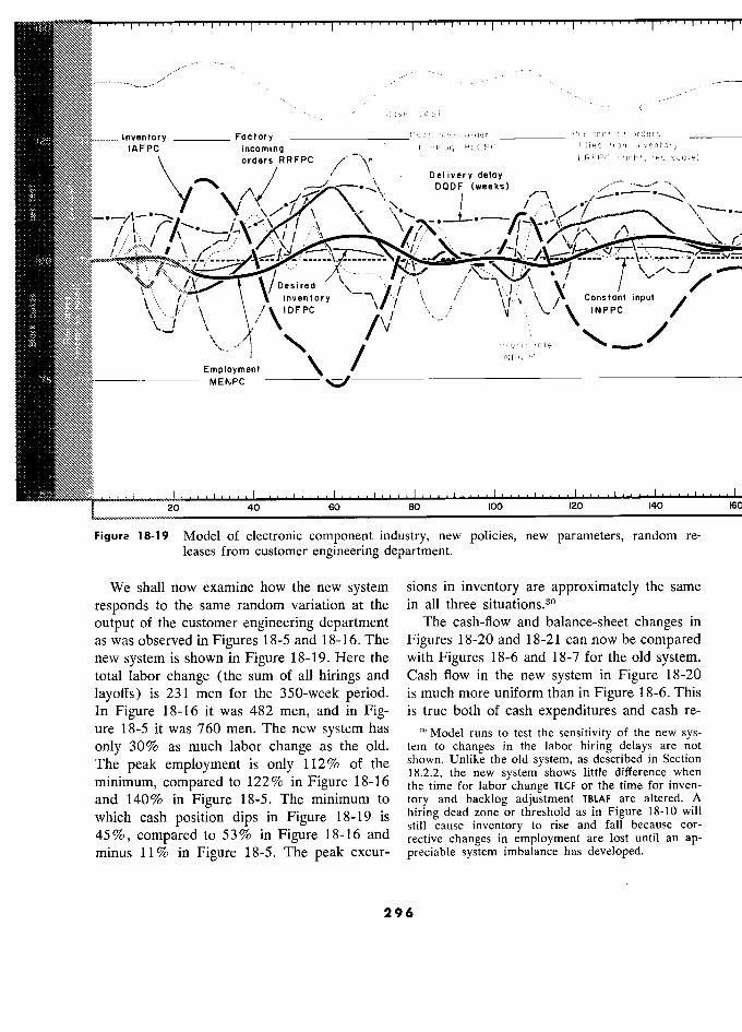
___)n«entory _______Foctory cash Customer-order _________ Percent oforders ––––– Inventory Factory Cus tome r -order Per cent of orders
?NBa ., IAFPC incoming / bocklog BLCPC filled from inventory
\ ders RRFPC /"*Y / ivery deloy
FRFPC(ri9ht,redsca!e)
,
DQDF D F (wee ks )
/J ,"
/ +'
f .
j j ,
Desired
ttNNN?? ... /.t \ \ inventory \
( \F\ \
Constant input p u t /
P
N ' (
/
Profit f i .te te ' - '
Employment , / NPRPC
MENPC 9
20 40 60 80 100 120 140 1
Figure 18-19 Model of electronic component industry, new policies, new parameters, random re-
leases from customer engineering department.
We shall now examine how the new system sions in inventory are approximately the same
responds to the same random variation at the in all three situations.30
output of the customer engineering department The cash-flow and balance-sheet changes in
as was observed in Figures 18-5 and 18-16. The Figures 18-20 and 18-21 can now be compared
new system is shown in Figure 18-19. Hère the with Figures 18-6 and 18-7 for the old system.
total labor change (the sum of all hirings and Cash flow in the new system in Figure 18-20
layoffs) is 231 men for the 350-week period. ismuch more uniformthan in Figure 18-6. This
In Figure 18-16 it was 482 men, and in Fig- is true both of cash expenditures and cash re-
ure 18-5 it was 760 men. The new system has " Model runs to test the sensitivity of the new sys-
only 30% as much labor change as the old. tem to changes in the labor hiring delays are not
The peak employment is only 112% of the shown. Unlike the old system, as described in Section
18.2.2, the new system shows little difference when
minimum, compared to 122% m lgUX the time for labor change TLCF or the time for inven-
and 140% in Figure 18-5. The minimum to tory and backlog adjustment TBLAF are altered. A
which cash position dips in Figure 18-19 is hiring dead zone or threshold as in Figure 18-10 will
till cause inventory to rise and fall because cor-
45%, compared to 53% in Figure 18-16 and rective changes in employment are lost until an ap-
minus 11% in Figure 18-5. The peak excur- preciable system imbalance has developed.
296
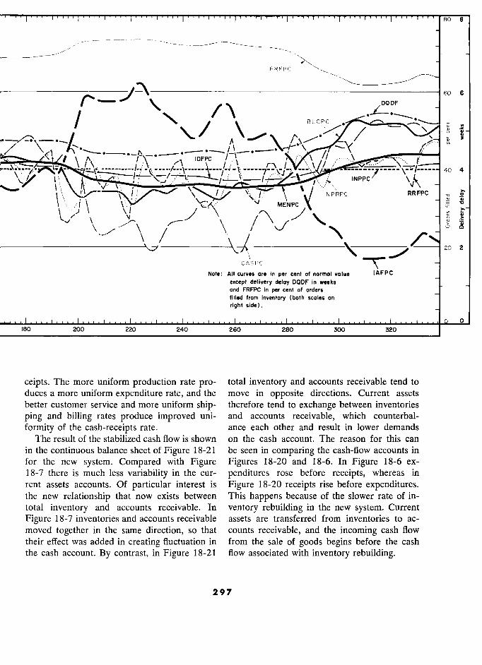
.... i .. " , , . i , 8
-
/ ,
FRFPC????
6
DODF 60
6
/ BLCPC d
-
*_ j /
, / \ P en ;0
<1 _..-._
IDFPC ; :
t\ t\
i'
'(
v.,\\
ÉPC j ]
\ f INPPC
__ /:__ no 4
v. \...,
_.= w' MENPC
R J
PC 0
ô ;;J, ME PC
NPRPC RRFPC ., Ci
t ' /f\ ''-' Mc-NrC \ '"
\ \' /"\ \v
., > \ \ ô2 i
20 Î 2
CASPC ` rC
Note : Ail curves ore in per cent of normal value IAFPC
except delivery deloy DODF in weeks and FRFPC in per cent of orders filled from inventory (both scales on righi side).
1 .. i 1 ... 1 . .. 1 .... i . .. 1 1 0 180 200 220 240 260 260 300 320
ceipts. The more uniform production rate pro- total inventory and accounts receivable tend to duces a more uniform expenditure rate, and the move in opposite directions. Current assets better customer service and more uniform ship- therefore tend to exchange between inventories
ping and billing rates produce improved uni- and accounts receivable, which counterbal-
formity of the cash-receipts rate. ance each other and result in lower demands The result of the stabilized cash flow is shown on the cash account. The reason for this can
in the continuous balance sheet of Figure 18-21 1 be seen in comparing the cash-flow accounts in for the new system. Compared with Figure Figures 18-20 and 18-6. In Figure 18-6 ex- 18-7 there is much less variability in the cur- penditures rose before receipts, whereas in rent assets accounts. Of particular interest is Figure 18-20 receipts rise before expenditures. the new relationship that now exists between This happens because of the slower rate of in- total inventory and accounts receivable. In ventory rebuilding in the new system. Current
Figure 18-7 inventories and accounts receivable assets are transferred from inventories to ac- moved together in the same direction, so that counts receivable, and the incoming cash flow their effect was added in creating fluctuation in from the sale of goods begins before the cash the cash account. By contrast, in Figure 18-21 flow associated with inventory rebuilding.
297
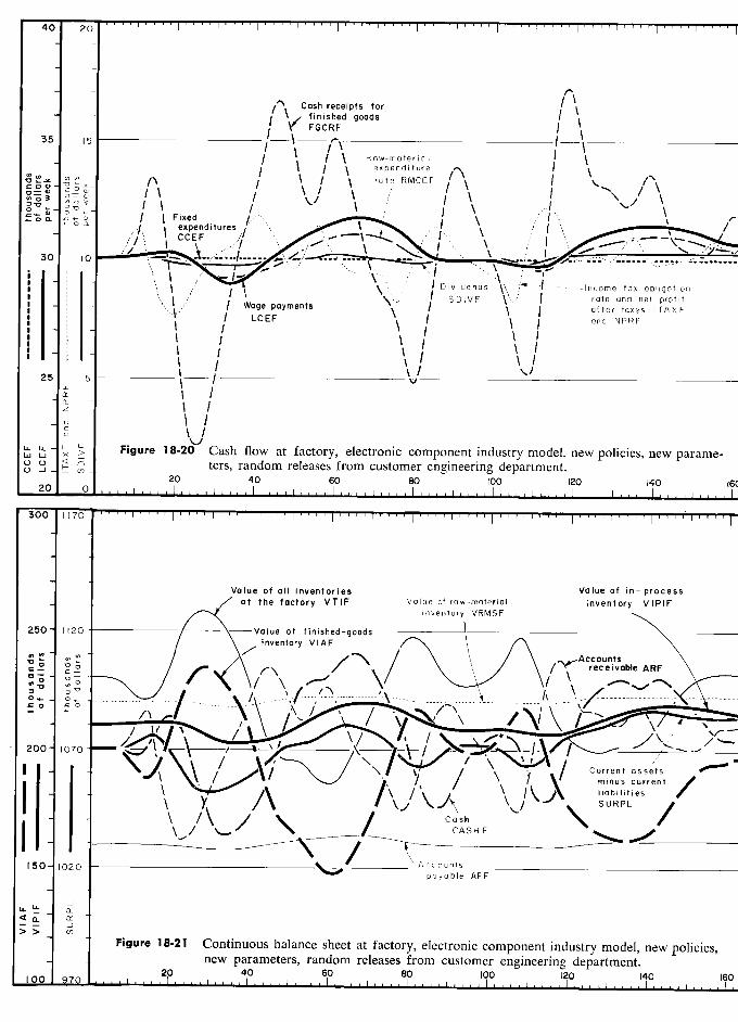
40 20 , r ''''!'''' t
¡"" C ash receipts for \ t finished goods /
\ /
FGCRF7 ) '
/ \
/ \ Raw-material 1 ' \
/ \ / \ expenditure f
/\ I\ / \
rate RMCEF /1 _ / \ /
1 \ \ 1
1
\ \ ";
RMCEF
/\ \ f /"\ \
) ?àtnd i tu res ? ",, ', ,:
"
' /
.m '
- / / ; \ ,..' l .... \ oa v
3
/
' 1 1 Fixed
' I
\ '.-1 '
- a 0.
"- //'. ,
C e pen Fd itures '
)- ".,,
\ .'' ' ., /
.',,: \ CCEF
'-
:%v ; ` \
.' .., ., L
30 10 //
" ,/ ..., ... -......:.:: " \
\ i
...' " "
30 10 ., -....,--.../..--.. " .."....,."""':'::;¡¡:;;--",,,,,,-,,,--,_uu' .u..-..".......
l i \
'.., "\ ...
:' /r
"'".,,,\.,. ,\...
,,¡
.
lax obligation "..-"- ( / ''. ) /' ?\Dividends :4*--f--Iricome tax obligation
: '· 1 · / /
Wage payments \\-' SDIVF F f rate and net profit : / '--.'./
J Wage
payments
\` /
i
after taxes ITAXF
:
1 :
:
' j ( ) '
;
) '
'' , j
' /
LCEF
\ \ /
/
) \
\ \ \"J
'
1 1 1
and NPRF
r 2 5
I
5
?
5
1 '
J V
z \ '
/ \ /
w > ,
Figure 18-2à"/ Cash flow at factory, electronic component industry model, new policies, new parame- wLux - ..
g % 3 ters, random releases from customer engineering department.
20 0 20
1 40 60 80 100 120 140 1
?20 ! t t ! ! !
300 1170
Value of all inventories Value of in- process - at the factory VTIF Value of raw-moleriol inventory VIPIF
inventory VRMSF
250 1120 Volue of finished-goods -
/ \ inventory V!AF t \
/ A
inventory VIAF
/*\
/
\ \ / \ Accounts \
c [ 1 / \/ \ \ ?? receivoble ARF \
'" 0. 0 , \ /
\ o #
::J"U ---------------
\-
fl -----
°
'`
-.
\
_.____ _-
„ %
2 oo
l070 7
/ / /
/ Current assets ! - \ / \
/ \ .1- /
Current as sels
) \ ' / X
minus current
/
1
\
A /\ \\Jl t \ \
liabilities 's \
\ / \ / \
/ \. 1 Cash
"'
1
, - -
CASHF F /
'50- _s 150 102 (D payable APF
LL I.L.. a= u- a a. Q_ Q:
' – – r) > > (f)
Figure 18-21 1 Continuous balance sheet at factory, electronic component industry model, new policies, new parameters, random releases from customer engineering department.
100 970 20
40 60 1 80 100
1 140
. , .. i .. 16 1
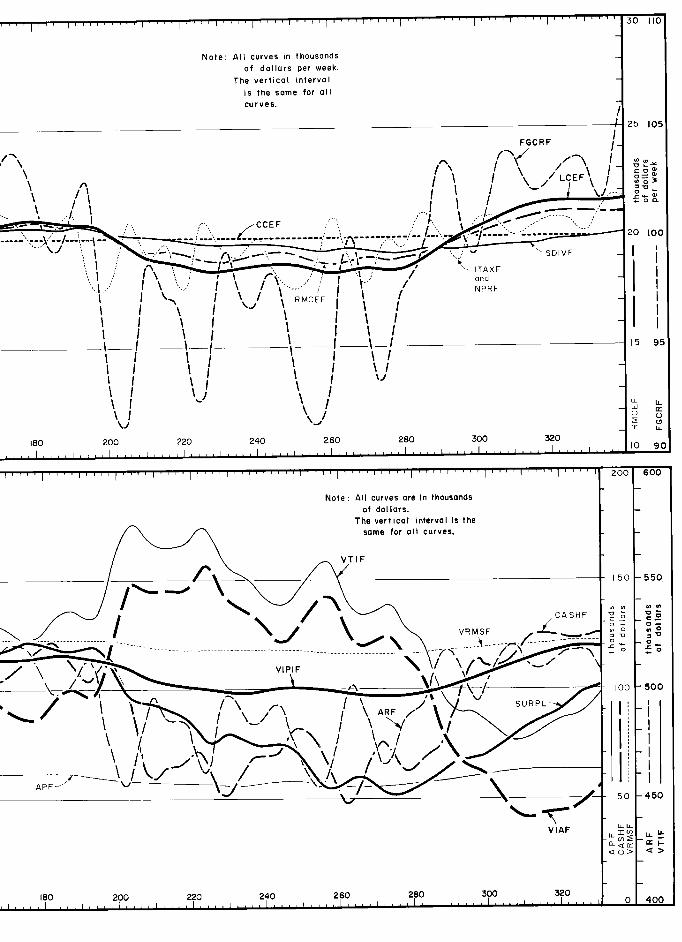
1 1 -1
.... 1 1 1 , 1 , , 1 1
1 1
1 Il 1 ' ' ' ' 30 110
Note: All curves in thousands –
of dollars per week.
The vertical interval
is the same for all i
curves. "
25 105
FGCRF
,
', ) )
/
'
CCEF
... _.\`__/..:._.'.. _:·,
\, __... 20 100
..- \J 1
I ;
t l'
.' `' \
v SDIVF I j
1
ITAXF r 1 ·.1 : / and
'"i ' ·,,,i;i. I
I \
\`·.
.. ·
I
I \ I
1 I
I
I I
NPRF
'. ;
/
"',, 1 ;
/ 'i,'
'<,
RMCEF ' ' j
/
)
', ; ', ; 15 95
'<
' ) ;
Î
j \ 1
. / \ \ <
<'
'
j "
\ I I LLJ U \J (->
S \l '" Ir LL
180 200 220 240 260 280 300 320 10 0
200 600
Note : Ali curves are in thousands
of dollars. The vertical interna! is the
/*\ same for all curves.
/ \ VTIF
- 1 50 550
/< - CASHF
'"""
'
/ . \ CASHF ô ç / u
/ \ VRMSF
- _ ___/ `
\ 0 0 O
/ \ VIPIF
'-'
- l00
/
A
I
i
- /
'1,,
)
ij ?
k 1 '
"
/ ,-/"' ,
ARF
/
) )
i
)
Î
i APF -
50 450
VIAF VIAF
X w CU> < >
180 200 220 240 260 280
300 320 ?0400
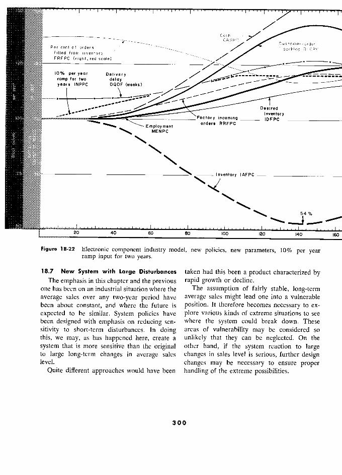
150 I . , .... I .... , " , " , I I , ,
Cash CASPC /
Customer-order Per cent of orders bocklog BLCPC
filled from invenfory / FRFPC (right, red scale)
10 % per year Delivery / _ ___ romp for two deloy _ - _ _ yeors INPPC DQDF (weeks) -
.. /
Desired " Inventory
.. · Factory incoming IDFPC
? Employment orders RRFPC
IDFPC
\` MENPC
EO
-75 I nvenrory I AFPC
541/. M
° -ù 5
4
- ' % -fil
) 20 40 60 80 100 120 140 16(
Figure 18-22 Electronic component industry model, new policies, new parameters, 10% per year ramp input for two years.
18.7 New System with Large Disturbances taken had this been a product characterized by The emphasis in this chapter and the previous rapid growth or decline.
one has been on an industrial situation where the The assumption of fairly stable, long-term
average sales over any two-year period have average sales might lead one into a vulnérable
been about constant, and where the future is position. It therefore becomes necessary to ex-
expected to be similar. System policies have plore various kinds of extreme situations to see been designed with emphasis on reducing sen- where the system could break down. These
sitivity to short-term disturbances. In doing areas of vulnerability may be considered so
this, we may, as has happened here, create a unlikely that they can be neglected. On the
system that is more sensitive than the original other hand, if the system reaction to large to large long-term changes in average sales changes in sales level is serious, further design level. changes may be necessary to ensure proper
Quite différent approaches would have been handling of the extreme possibilities.
300
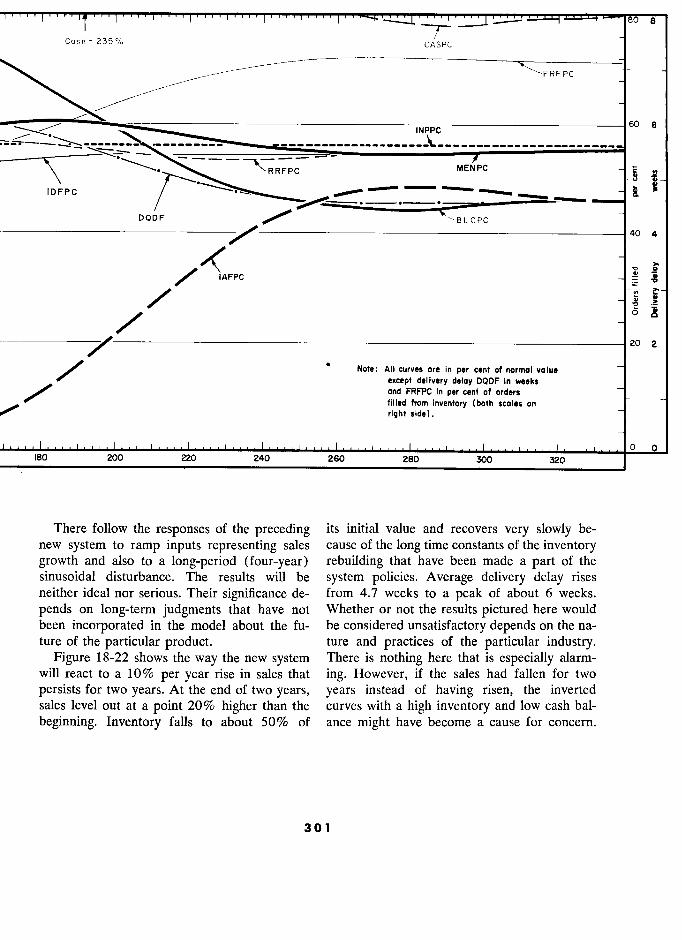
I .... , .... I .... , .... I .... , .... I .... , J o e
Cash = 235 % C
'"''
INPPC
60 6
\
- :::s:::::-. --
MENPC
.fi IDFPC --
DQDF BLCPC
/ 40 4
v ô
elooe
2 2
/
. Note: All curves ore ln per cent of normal value
le-le except delivery delay DQDF ln weeks
/' and FRFPC in per cent of orders filled from inventory (both scales on
right side). ..
o 0 180 200 220 240 260 280 300 320
There follow the responses of the preceding its initial value and recovers very slowly be- new system to ramp inputs representing sales cause of the long time constants of the inventory growth and also to a long-period (four-year) rebuilding that have been made a part of the sinusoidal disturbance. The results will be system policies. Average delivery delay rises neither ideal nor serious. Their significance de- from 4.7 weeks to a peak of about 6 weeks.
pends on long-term judgments that have not Whether or not the results pictured here would been incorporated in the model about the fu- be considered unsatisfactory depends on the na- ture of the particular product. ture and practices of the particular industry.
Figure 18-22 shows the way the new system There is nothing here that is especially alarm- will react to a 10% per year rise in sales that ing. However, if the sales had fallen for two
persists for two years. At the end of two years, years instead of having risen, the inverted sales level out at a point 20% higher than the curves with a high inventory and low cash bal-
beginning. Inventory falls to about 50% of ance might have become a cause for concern.
301 1
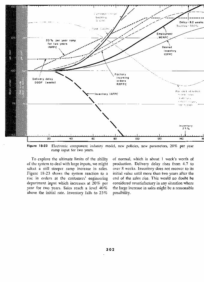
Customer-order / ,_ - j backlog __ - - - - - - - - - - - - - - -
BLCPC ' .
i Deloy " 8.2 week
,/
mployment
Bocklog = 330% Cash CASPC
/
· /
\j//
. '·
/ /
/ /
Employment MFNPCI.
20 % per year ramp . / //
MENPC-
for two yeors j/ INPPC Deslred
Inventory /
IDFPC
Factory
Delivery delay ........ incoming Delivery delciy "' incoming
DODF (weeks) RRFPC RRFPC
Per cent of orders
Inventory IAFPC filled from
'-
inventory ,-
, "' FRFPC (right,
"
red scale) -
Inventory 23 %
20 40 60 80 100 120 140
Figure 18-23 Electronic component industry model, new policies, new parameters, 20% per year ramp input for two years.
To explore the ultimate limits of the ability of normal, which is about 1 week's worth of of the system to deal with large inputs, we might production. Delivery delay rises from 4.7 to select a still steeper ramp increase in sales. over 8 weeks. Inventory does not recover to its
Figure 18-23 shows the system reaction to a initial value until more than two years after the rise in orders at the customers' engineering end of the sales rise. This would no doubt be
department input which increases at 20% per considered unsatisfactory in any situation where
year for two years. Sales reach a level 40% the large increase in sales might be a reasonable above the initial rate. Inventory falls to 23% possibility.
302
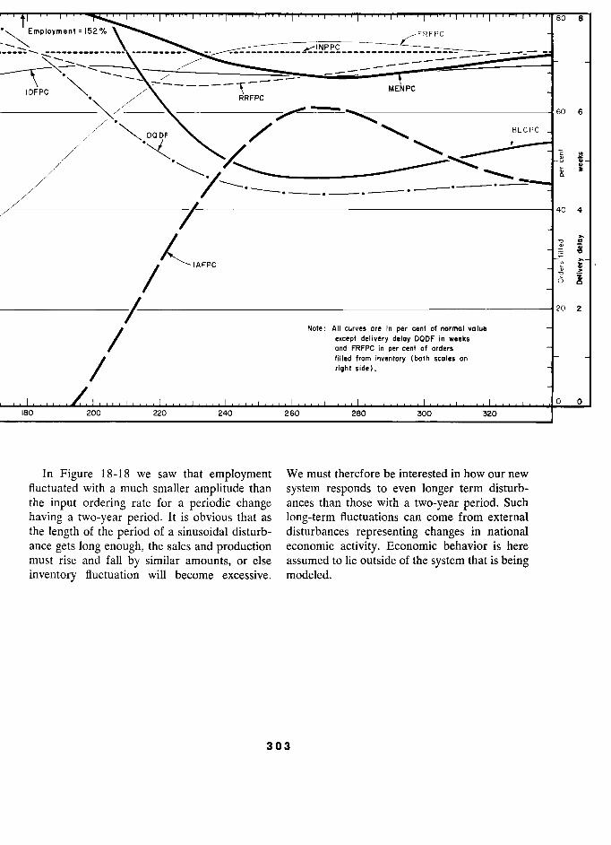
.... , i " " .. i . , " " , " 1 1 1 1 1 1 1 , . , , 1 , go 8
Employment = 152% FRFPC
Ào _ _________ ________ _ -
IDFPC - /-'- / RRFPC
_
_ - - -
60 6
/ ? BLCPC
.
fl , .. u '"
g3 "
y.-...-.
40 4
>- / 0
IAFPC d d >
<
1 A F P C
/
20 2
Note: All curves are in per cent of normal value except delivery deloy DQDF in weeks and FRFPC in per cent of orders filled from inventory (both scales on -
/ right side).
0 0 180 200 220 240 260 280 300 320
In Figure 18-18 we saw that employment We must therefore be interested in how our new fluctuated with a much smaller amplitude than system responds to even longer term disturb- the input ordering rate for a periodic change ances than those with a two-year period. Such
having a two-year period. It is obvious that as long-term fluctuations can come from external the length of the period of a sinusoidal disturb- disturbances representing changes in national ance gets long enough, the sales and production economic activity. Economic behavior is here must rise and fall by similar amounts, or else assumed to lie outside of the system that is being inventory fluctuation will become excessive. modeled.
303
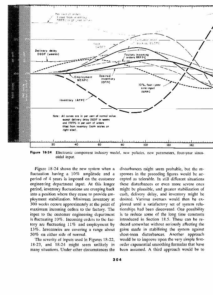
150 I , I , I , .
Per cent of orders filled from inventory , FRFPC (right,red scale)
/ VÀ .1 / -
Customer-order er-order -
Cosh ·/
/ backlog BLCPC Cash /' backl09 BLCPC
/ CASPC /
"
Delivery delay ° DODF (weeks) _ Factory incoming DODF (w.eks)
01 ders RRFPC c ;:---.....
"\1 \
i - Lorders RRFPC
gelez
E mp Y
D .. w
.."
I DF PC
"'..
..........
--- ....... MENPC inventory ""..--- ' ..
Ô IDFPC
10°/ , four-yeor r ' "
sine inpuf
1.:
'IDFPC
INPPC 7'7"-"'\
.......... Inventory
-......----
...
000
Note : All curves are ln per cent of normal value
except dellvery delay DODF ln weeks and FRFPC in per cent of orders
filled from inventory (both scales on
rlght side).
20 40 60 80 ioo 120 140
Figure 18-24 Electronic component industry model, new policies, new parameters, four-year sinus- oidal input.
Figure 18-24 shows the new system when a disturbances might seem probable, but the re- fluctuation having a 10% amplitude and a sponses in the preceding figures would be ac-
period of 4 years is imposed on the customer cepted as tolerable. In still different situations
engineering department input. At this longer these disturbances or even more severe ones
period, inventory fluctuations are creeping back might be plausible, and greater stabilization of into a position where they cease to provide em- cash, delivery delay, and inventory might be
ployment stabilization. Minimum inventory at desired. Various avenues would then be ex- 300 weeks occurs approximately at the point of plored until a satisfactory set of system rela- maximum incoming orders to the factory. The tionships had been discovered. One possibility input to the customer engineering department is to reduce some of the long time constants is fluctuating 10%. Incoming orders to the fac- introduced in Section 18.5. These can be re-
tory are fluctuating 1 1 % and employment by duced somewhat without seriously affecting the 13 %. Inventories are covering a range about gains made in stabilizing the system against 50% on either side of normal. short-term disturbances. Another approach
The severity of inputs used in Figures 18-22, would be to improve upon the very simple first-
18-23, and 18-24 might seem unlikely in order exponential smoothing formulas that have
many situations. Under other circumstances the been assumed. A third approach would be to
304
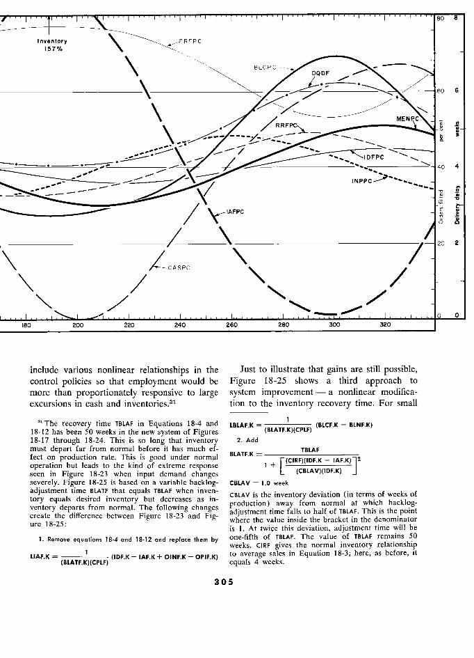
" i " , i I " " i " i 8
Inventory ?FRFPC 157%
\ BLCPC
D F /
\
/'
60 6
\ -
_
\
/RRFPC'3.. - MENP.C S -- -- .
, " - ' O _
ii -;
;;-- ;....----. -.......,
IDFPC '
fl - .- . - . F 40 4
'.....
40 4
,,, INPPC ..,,-
/
INPPC/
a . ,,, - - - , é
- -- - = '1:1
---
`?IAFPC n, §
> '/ \
M 2
\ .-/-CASPC /
"/
/
\
0 i .. 1 i 1, .. i . ... 1 ...... o
180 200 220 240 260 280 300 320
include various nonlinear relationships in the Just to illustrate that gains are still possible, control policies so that employment would be Figure 18-25 shows a third approach to more than proportionately responsive to large system improvement - a nonlinear modifica- excursions in cash and inventories.31 tion to the inventory recovery time. For small
31 The recovery time TBLAF in Equations 18-4 and LBLAF.K = 1
(BLCF.K - BLNF.K) 18-12 has been 50 weeks in the new system of Figures
(BtATF.K)(CtF
18-17 through 18-24. This is so long that inventory 2. Add
must depart far from normal before it has much ef- _ TBLAF fect on production rate. This is good under normal
,,_ _
£
operation but leads to the kind of extreme response 1 + ] seen in Figure 18-23 when input demand changes
L ' J
severely. Figure 18-25 is based on a variable backlog- CBLAV = 1.0 week
adjustment time BLATF that equals TBLAF when inven- inventory déviation (in terms of weeks of
tory equals desired inventory but decreases as in- inventory deviation terms of j_
ventory departs from
normal. The following changes falls t half of TBLAF. This is thé point create the difference between Figure 18-23 and Fig- where the value inside the bracket in the denominator 18.25'
° ° where thé value mSlde thé bracket in thé denommator ure 18-25: .
is 1. At twice this deviation, adjustment time will be
1. Remove équations 18-4 and 18-12 and replace them by one-fifth of TBLAF. The value of TBLAF remains 50
weeks. CIRF gives the normal inventory relationship
LIAF.K = (IDF.K - IAF.K + OINF.K - OPIF.K) to average sales in Equation 18-3; here, as before, it
(BLATF.K)(CPLF) equals 4 weeks.
305 5
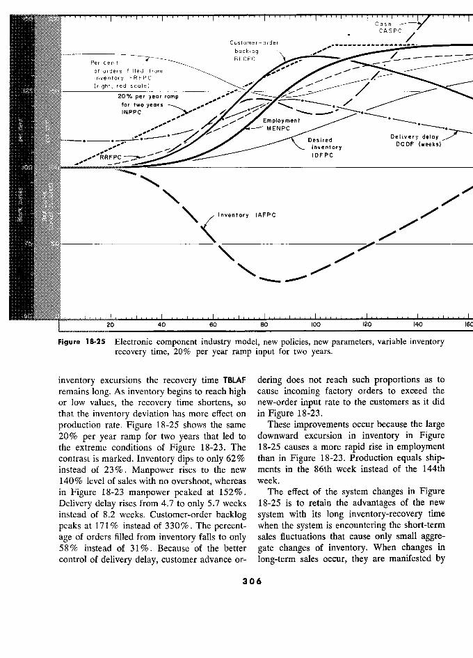
11 ..-I... , I . , I , ,
Cash CASPC,
Customer-order '
_ _ backlog
Per c en t BLCPC '
of orders filled from , inventory FRFPC C , / (right, red scale) "
20 % per yeur romp W , for two yeors fl INPPC
y
, Employrnent ' " M EN PC
.. / / MENPC
Desired DDODF?·(weeks)
...... \ Inventory IDFPC
, / ,
Inventory
IAFPC P C
./"
/
/
" " - -- /
7'
20 40 60 80 100 120 140 1
Figure 18-25 Electronic component industry model, new policies, new parameters, variable inventory recovery time, 20% per year ramp input for two years.
inventory excursions the recovery time TBLAF dering does not reach such proportions as to
remains long. As inventory begins to reach high cause incoming factory orders to exceed the
or low values, the recovery time shortens, so new-order input rate to the customers as it did
that the inventory deviation has more effect on in Figure 18-23.
production rate. Figure 18-25 shows the same These improvements occur because the large 20% per year ramp for two years that led to downward excursion in inventory in Figure the extreme conditions of Figure 18-23. The 18-25 causes a more rapid rise in employment contrast is marked. Inventory dips to only 62% than in Figure 18-23. Production equals ship- instead of 23io . Manpower rises to the new ments in the 86th week instead of the 144th
140% level of sales with no overshoot, whereas week.
in Figure 18-23 manpower peaked at 152%. The effect of the system changes in Figure
Delivery delay rises from 4.7 to only 5.7 weeks 18-25 is to retain the advantages of the new
instead of 8.2 weeks. Customer-order backlog system with its long inventory-recovery time
peaks at 1 7 1 % instead of 330%. The percent- when the system is encountering the short-term
age of orders filled from inventory falls to only sales fluctuations that cause only small aggre- 58% instead of 31 %. Because of the better gate changes of inventory. When changes in
control of delivery delay, customer advance or- long-term sales occur, they are manifested by
306
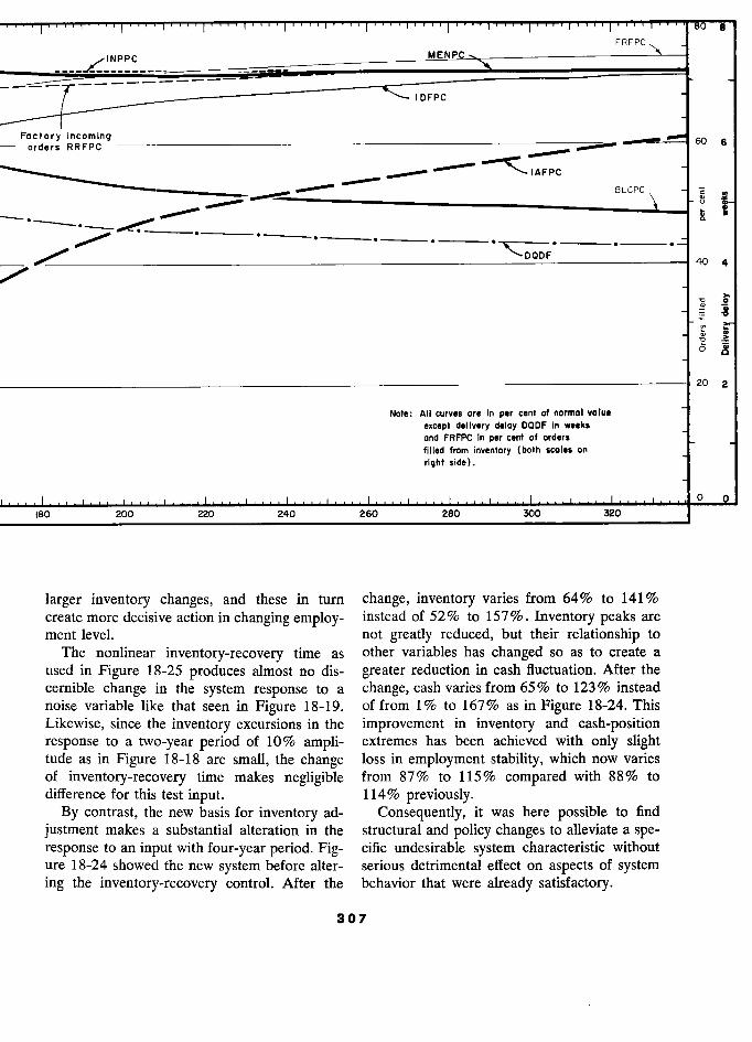
, L., ., . 8
FRFPC
INPPC MENPC FRFPC?
"'–––
- ----
/ IDFPC
Factory incoming - orders RRFPC – 60 6
BLCPC g
BLCPC
- . --- ----
-- BLCPC
3 u
" i
F 40 4 >
4
... "0 0 - - '" 0 ' C
. v
è5 !
20 2
Note: All curves are In per cent of normal value
except dellvery deloy DQDF In weeks
and FRFPC in per cent of orders
filled from inventory (both scoles on
rlght side).
0 0
180 200 220 240 260 280 300 320
larger inventory changes, and these in turn change, inventory varies from 64% to 1419% create more decisive action in changing employ- instead of 52% to 157%. Inventory peaks are ment level. not greatly reduced, but their relationship to
The nonlinear inventory-recovery time as other variables has changed so as to create a used in Figure 18-25 produces almost no dis- greater reduction in cash fluctuation. After the cernible change in the system response to a change, cash varies from 65 % to 123 % instead noise variable like that seen in Figure 18-19. of from 1 % to 167% as in Figure 18-24. This Likewise, since the inventory excursions in the improvement in inventory and cash-position response to a two-year period of 10% ampli- extremes has been achieved with only slight tude as in Figure 18-18 are small, the change loss in employment stability, which now varies of inventory-recovery time makes negligible from 87% to 115% compared with 88% to difference for this test input. 114% previously.
By contrast, the new basis for inventory ad- Consequently, it was here possible to find
justment makes a substantial alteration in the structural and policy changes to alleviate a spe- response to an input with four-year period. Fig- cific undesirable system characteristic without ure 18-24 showed the new system before alter- serious detrimental effect on aspects of system ing the inventory-recovery control. After the behavior that were already satisfactory.
307
CUSTOMER-PRODUCER-EMPLOYMENT SYSTEM
18.8 Summary changed. This brought substantially better sys-
In Chapter 17 a model was designed to repre- ment. tem stability but still left room for improve-
sent the organization and policies in a particu- ment. Sections 18.4 and 18.5, the equations and In Sections 1 8 .4 and 1 8 .5, the equations and
lar case study. parameters controlling inventory were changed
In Section 18-1 the dynamic characteristics to make inventory variations assist in provid-
of this "old" system were studied. The model ing employment stability instead of contributing showed the kinds of behavior that had been ta the instability as before.
experienced in the actual system. The charac- These changes led to a system, as explored in
teristics of the closed, self-contained model Section 18.7, that was somewhat unresponsive
seemed reasonable compared with the actual to large, enduring changes in sales level. Figure
of component parts and agreed with the exten- 18-25 indicated the way that long-term, large-
sive descriptive knowledge of the separate facets amplitude inputs could be controlled without sive descriptive knowledge of the e separate acets
giving up the improvements which had been of the company and of customer motivation. achieved in random and short-period system When these acceptable pieces were assembled,
sensitivity.
in random and ? system
they interacted in agreement with past knowl- We might weIl assume that improvements
edge of the total system. The model was there- over the policies studied in this chapter are still
upon judged sufficiently reliable to be a basis possible. Nevertheless, we should not make the
for system redesign. mistake of expecting perfection not set of sys- was indicated by the strong mistake of expecting perfection in a set of sys- Need for redesign was indicated by the strong tem Neither should we delay j
tendency of the system to amplify disturbances the policies. Neither should we delay unduly having a periodicity near two years. The unde-
suing some illusive optimum sirable responsiveness to such periods made the All illusive made in design. model system susceptible to being badly perturbed by All chapter are ones the system readily short-period random effects of even small in the actual system. Their implementa-
made Îl§uirl ÎhÎfor?1alizing of criticll policies amplitude.... tion requires the formalizing of critical policies In Section 18.2 the sensitivity of the old sys- tion system control to ensure critical policies tem was explored to determine what parts were
sistently control to executed. they are con- most crucial in determining the undesirable be-
mation flows are required which had not infor- havior. Delays in the hiring policies, which had viously flows required which readily pre-
not been subjected to careful managerial con- viously
d but which can readily be
trol, were found to be of great importance. made '
_ In Section 18.3 the sources . .
32 A report on the experiences in implementing these In Section 18.3 the sources of information
changes in the actual system is not yet timely and and the policies for controlling labor level were will be left to other authors at a later date.
308
IV
FUTURE OF INDUSTRIAL L DYNAMICS
Part IV completes the book with a discussion of the future of industrial dynamics.
a Chapter 19 summarizes the high points of industrial dynamics models that have been developed for a variety of industrial situations. These are included to illustrate how the methods discussed in this book can go beyond the examples given in Part III. Dynamic models of market, growth, commodities, and research and development have been explored. e Chapter 20 relates industrial dynamics to management education as
providing a central system structure around which to integrate the separate functional subdivisions of management. e Chapter 21 discusses the organization, staffing, and use of industrial dynamics within the corporation.
Part IV is suggested for all readers.
309

CHAPTER 19
Broader Applications of Dynamic Models
The purpose of this chapter is to indicate how aspects of the industrial enterprise beyond the functions treated in Part III can be represented in dynamic models. Examples are drawn from thesis and staff research at M.I.T. A model of an automobile market has related design decisions to market penetration. A model of product growth represents a transient dynamic situation that continuously changes in character, as distinguished from the models of Part III, which are "steady-state dynamic" systems in which any five- or ten-year period is similar in general character to any other period. Studies on commodity markets show unexpected ways in which price stability may be improved. The process of military research and development management is being formulated into a system involving characteristics of the product, the development organization, the military contracting office, and the government budget cycle. Long-range-planning models can be u,sed to integrate present facts and assumptions to see the ways they might interact in the future.
THE two models presented in Part III treat been developed have not been explored and
very restricted aspects of the total industrial revised to the point where they yet justify formal
picture. Capital equipment, one of the six flow presentation in their entirety. However, in as-
systems in Section 6.2, was not used. Money sociated work done to date in other models of flow has appeared in the model of Chapters industrial activity, many interesting points have 17 and 18 but only in an incidental, reporting arisen and tentative conclusions formulated.
capacity. Of the major functional subdivisions This chapter will try to round out the descrip- of management we have given some attention tion of the models given in Part III by discuss- to production and distribution, have barely ing the high lights arising from studies of other touched the market area, and have entirely industrial situations that have followed the omitted research, capital investment, long-range methods outlined in this book.
corporate planning, and many others. These omissions do not occur because they
19.1 Market Dynamics
represent areas of less importance or because There seems to be a common inclination to
they are less amenable to study by dynamic assume that the mechanisms of the market are model methods, or because excursions are obscure, that psychological factors predominate lacking into these somewhat more elusive to the exclusion of tangible factors, and that
aspects of corporate life. Rather, the more ad- there is little possibility of useful modeling of vanced models fall beyond the work to be un- the market interactions. 1 hold the opposite dertaken in this volume, and the ones that have view. To be sure, many of the market charac-
311 1
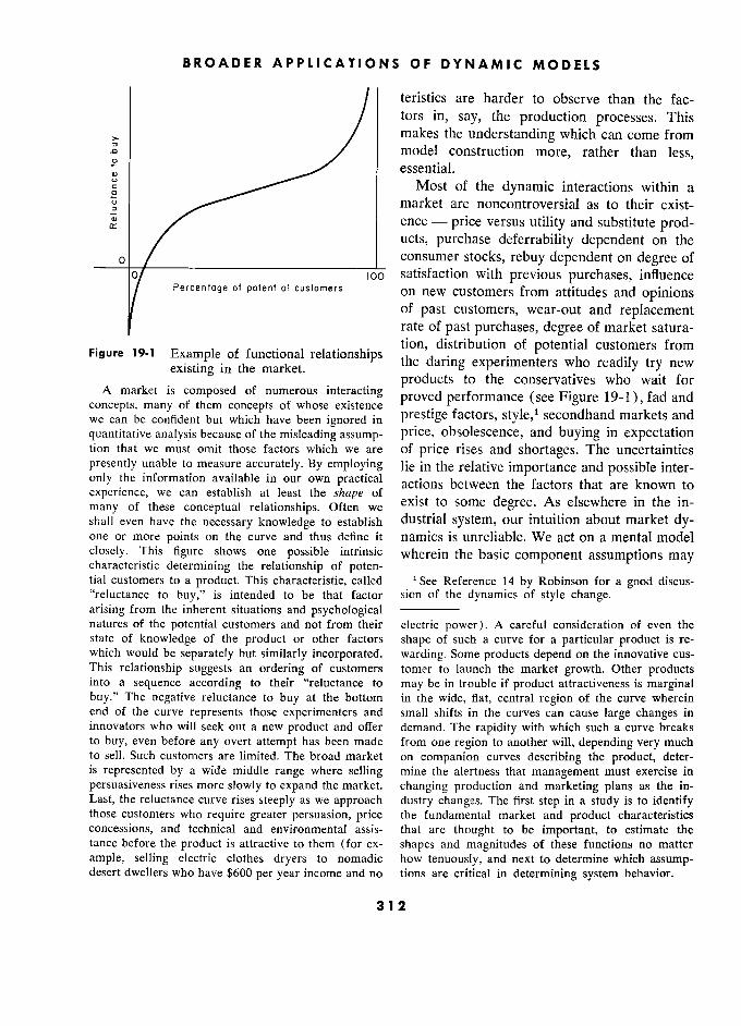
BROADER APPLICATIONS OF DYNAMIC MODELS
/ teristics are harder to observe than the fac-
/ tors in, say, the production processes. This
/ makes the understanding which can come from ./ model construction more, rather than less,
essential. '" Most of the dynamic interactions within a
market are noncontroversial as to their exist- ence - price versus utility and substitute prod- ucts, purchase deferrability dependent on the
o / L consumer stocks, rebuy dependent on degree of
o ioo satisfaction with previous purchases, influence / Percentage of potentiol customers on new customers from attitudes and opinions
of past customers, wear-out and replacement ) rate of past purchases, degree of market satura-
, ... - . , ....... tion, distribution of potential customers from Figure 19-1 Example of functional relationships
tion, distribution of potential customers from existing in thé
market. products to the conservatives who wait new ... products to the conservatives who wait for A market is composed of numerous interacting proved performance (see Figure 19-1 ) fad and
concepts, many of them concepts of whose existence factors, 1 secondhand markets and we can be confident but which have been ignored in Fustige factors, style,l secon an markets an
quantitative analysis because of the misleading assump- price, obsolescence, and buying in expectation tion that we must omit those factors which we are of price rises and shortages. The uncertainties presently unable to measure accurately. By employing lie in the relative importance and possible inter- only the information available in our own practical betweerl the factors that are known to experience, we can establish at least the shape of many of these conceptual relationships. Often we exlst to some degree. As elsewhere in the m-
shall even have the necessary knowledge to establish dustrial system, our intuition about market dy- one or more points on the curve and thus define it namics is unreliable. We act on a mental model closely. This figure shows one possible intrinsic wherein the basic component assumptions may characteristic determining the relationship of poten- tial customers to a product. This characteristic, called ' See Reference 14 by Robinson for a good discus- "reluctance to buy," is intended to be that factor sion of the dynamics of style change. arising from the inherent situations and psychological –––––– natures of the potential customers and not from their electric power). A careful consideration of even the state of knowledge of the product or other factors shape of such a curve for a particular product is re- which would be separately but similarly incorporated. warding. Some products depend on the innovative cus- This relationship suggests an ordering of customers tomer to launch the market growth. Other products into a sequence according to their "reluctance to may be in trouble if product attractiveness is marginal buy." The negative reluctance to buy at the bottom in the wide, flat, central region of the curve wherein end of the curve represents those experimenters and small shifts in the curves can cause large changes in innovators who will seek out a new product and offer demand. The rapidity with which such a curve breaks to buy, even before any overt attempt has been made from one region to another will, depending very much to sell. Such customers are limited. The broad market on companion curves describing the product, deter- is represented by a wide middle range where selling mine the alertness that management must exercise in persuasiveness rises more slowly to expand the market. changing production and marketing plans as the in- Last, the reluctance curve rises steeply as we approach dustry changes. The first step in a study is to identify those customers who require greater persuasion, price the fundamental market and product characteristics concessions, and technical and environmental assis- that are thought to be important, to estimate the tance before the product is attractive to them (for ex- shapes and magnitudes of these functions no matter ample, selling electric clothes dryers to nomadic how tenuously, and next to determine which assump- desert dwellers who have $600 per year income and no tions are critical in determining system behavior.
312
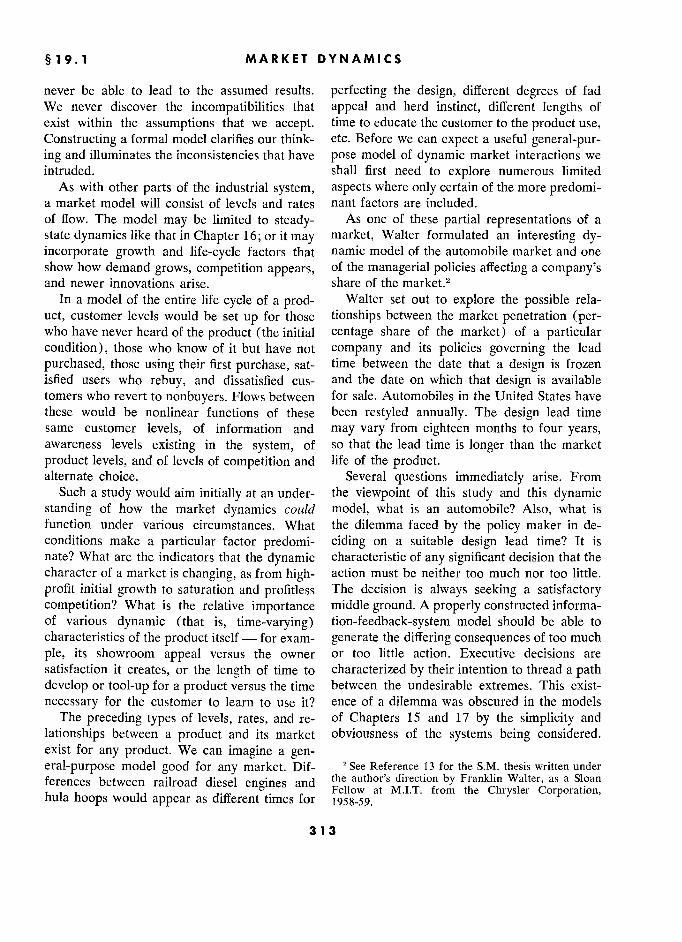
§ 19.1 1 MARKET DYNAMICS S
never be able to lead to the assumed results. perfecting the design, different degrees of fad We never discover the incompatibilities that appeal and herd instinct, different lengths of exist within the assumptions that we accept. time to educate the customer to the product use,
Constructing a formal model clarifies our think- etc. Before we can expect a useful general-pur- ing and illuminates the inconsistencies that have pose model of dynamic market interactions we intruded. shall first need to explore numerous limited
As with other parts of the industrial system, aspects where only certain of the more predomi- a market model will consist of levels and rates nant factors are included. of flow. The model may be limited to steady- As one of these partial representations of a state dynamics like that in Chapter 16; or it may market, Walter formulated an interesting dy- incorporate growth and life-cycle factors that namic model of the automobile market and one show how demand grows, competition appears, of the managerial policies affecting a company's and newer innovations arise. share of the market.? 2
In a model of the entire life cycle of a prod- Walter set out to explore the possible rela-
uct, customer levels would be set up for those tionships between the market penetration (per- who have never heard of the product (the initial centage share of the market) of a particular condition), those who know of it but have not company and its policies governing the lead
purchased, those using their first purchase, sat- time between the date that a design is frozen isfied users who rebuy, and dissatisfied cus- and the date on which that design is available tomers who revert to nonbuyers. Flows between for sale. Automobiles in the United States have these would be nonlinear functions of these been restyled annually. The design lead time same customer levels, of information and may vary from eighteen months to four years, awareness levels existing in the system, of so that the lead time is longer than the market
product levels, and of levels of competition and life of the product. alternate choice. Several questions immediately arise. From
Such a study would aim initially at an under- the viewpoint of this study and this dynamic standing of how the market dynamics could model, what is an automobile? Also, what is function under various circumstances. What the dilemma faced by the policy maker in de- conditions make a particular factor predomi- ciding on a suitable design lead time? It is nate? What are the indicators that the dynamic characteristic of any significant decision that the character of a market is changing, as from high- action must be neither too much nor too little.
profit initial growth to saturation and profitless The decision is always seeking a satisfactory competition? What is the relative importance middle ground. A properly constructed informa- of various dynamic (that is, time-varying) tion-feedback-system model should be able to characteristics of the product itself - for exam- generate the differing consequences of too much
ple, its showroom appeal versus the owner or too little action. Executive decisions are satisfaction it creates, or the length of time to characterized by their intention to thread a path develop or tool-up for a product versus the time between the undesirable extremes. This exist-
necessary for the customer to learn to use it? ence of a dilemma was obscured in the models The preceding types of levels, rates, and re- of Chapters 15 and 17 by the simplicity and
lationships between a product and its market obviousness of the systems being considered. exist for any product. We can imagine a gen- eral-purpose model good for any market. Dif- 2 See Reference 13 for the S.M. thesis written under ferences between railroad diesel engines and the
author's direction by Franklin Walter, as a Sloan
1 h Id Fellow at M.LT. from the Chrysler Corporation, hula hoops would appear as different times for 1958-59.
' ' ' '
313

BROADER APPLICATIONS OF DYNAMIC MODELS S
In Chapter 15 the major decision was that of time-dependent behavior of the market? In this
ordering goods from a supplier. An incorrect study the question of system formulation was
ordering rate would result in a level of inven- resolved by defining two characteristics of an
tory that was too high or too low, and this automobile - showroom appeal and ownership would become an indicator of necessary correc- satisfaction. These two characteristics can relate tion in future ordering decisions. In Chapter 17 7 design lead time to market reactions. one of the important decisions was the employ- Showroom appeal combines all those charac- ment level, and too high a level would lead to teristics of the product which affect its sales at- excess inventory, and too low a level to a tractiveness to a potential customer who has had deficient inventory. What then is to be the di- no prior personal expérience with the product. lemma representing the consequences of a too This may be thought of as primarily style but
long or a too short design lead time in also includes advertising, existing prevalence the automobile production-marketing system? of the product and consequent awareness of it,
Many answers might be given depending on the reputation regarding operating characteristics,
particular facet of the industry being studied. and so forth. There is no pretense that the particular study On the other hand, ownership satisfaction related here deals with all of the important deals with those characteristics of the product facets of the automobile industry, but only that which affect the opinion of the person who has it deals with one of the top-priority sets of inter- purchased it and which ultimately affect his actions. inclination to rebuy the same brand of product.
As developed by Walter, a shorter design It is clear that a particular physical charac- lead time would permit a company to be more teristic of the product may not lie exclusively cognizant of recent customer preferences and in one or the other of these categories. Yet,
design and styling trends. New innovations and given a particular characteristic, it is usually market fads could be recognized and incorpo- clear whether the characteristic is more persua- rated before they had run their courses and ex- sive at the point of sale or exerts its strongest
pired as market factors. However, shortening influence on the person who has already pur- of the design lead time means a shorter interval chased and is an owner. For example, style will
in which to build experimental models, to find affect primarily the showroom appeal; but door
design defects, and to perfect the multitude of handles that fall off will affect ownership satis- small details. Conversely, a longer design lead faction. time should, within limits, lead to greater physi- Figure 19-2 shows reasonable shapes for cal perfection while at the same time introduc- these two curves as a function of the design lead
ing the hazard of designs that are out of step time. Within a certain short lead-time interval, with current market trends. Here then is the further shortening of design lead time would not dilemma faced by the executive who must de- be expected to increase appreciably the show- cide when to freeze designs and proceed with room appeal, because market trends would not the long sequence of construction, testing, and be perceptible and significant over such brief
tooling steps. periods of observation. The curve must there- In this context, what is the dynamic descrip- fore be horizontal as it approaches the intro-
tion of an automobile? The obvious physical duction date. On the other hand, showroom ap- attributes such as gasoline mileage, height of peal may decline rather rapidly as the design tail fins, and colors, do not seem to lend them- lead time is lengthened into the three-year inter- selves to direct incorporation. How does the val that characterizes the life of short-term style result of the lead-time decision enter into the fads. Beyond four years of lead time, the prod-
314
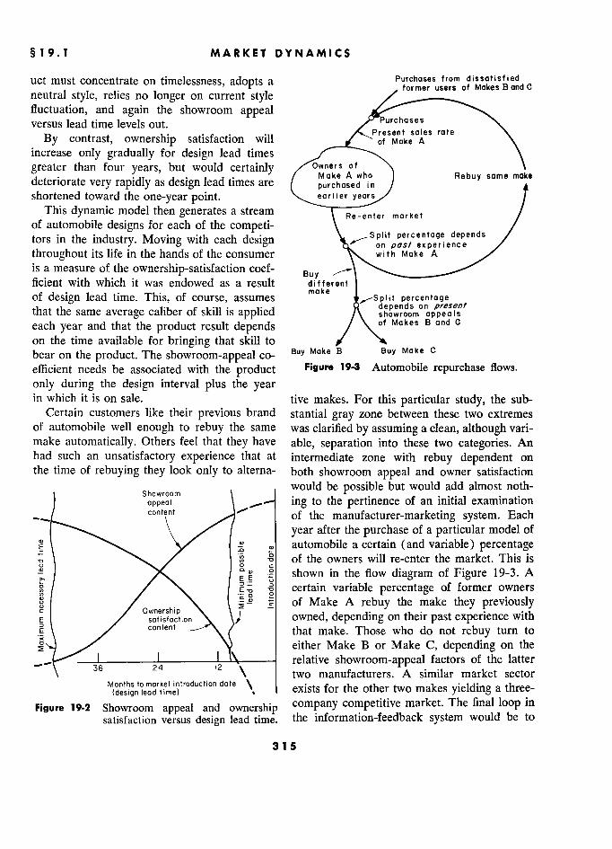
1 MARKET DYNAMICS S
uct must concentrate on timelessness, adopts a P§rch°S?S?J§e§? dissatisfied , r former users of Makes Band C neutral style, relies no longer on current style former users
of Makes B and C
fluctuation, and again the showroom appeal versus lead time levels out. Purchases
By contrast, ownership satisfaction will PotsMakeoAs rare
\ increase only gradually for design lead times \ greater than four years, but would certainly owners of \.
deteriorate ver ra idl as desi n lead times are / Moke A wno Rebuy same make deteriorate very rapidly as design lead times are f purchased in / shortened toward the one-year point. eorlier years?/ f
This dynamic model then generates a stream market / of automobile designs for each of the competi- \ / tors in the industry. Moving with each design / throughout its life in the hands of the consumer with Make A is a measure of the ownership-satisfaction coef- ficient with which it was endowed as a result différent ) of design lead time. This, of course, assumes ?Split percenfoge
that the same average caliber of skill is applied A °(#IÉÎÎ' J
each year and that the product result depends / °
on the time available for bringing that skill to bear on the product. The showroom-appeal co- Suy Make B Buy Make c
efficient needs be associated with the product Figure 19-3 Automobile repurchase flows.
only during the design interval plus the year in which it is on sale. tive makes. For this particular study, the sub-
Certain customers like their previous brand stantial gray zone between thèse two extremes of automobile well enough to rebuy the same was clarified by assuming a clean, although vari- make automatically. Others feel that they have able, separation into these two categories. An had such an unsatisfactory experience that at intermediate zone with rebuy dependent on the time of rebuying they look only to alterna- both showroom appeal and owner satisfaction
Showroom \ would be possible but would add almost noth-
j appeo? \ ing to the pertinence of an initial examination - content of the manufacturer-marketing system. Each
\. year after the purchase of a particular model of
Q) automobile a certain ( and variable) percentage of the owners will re-enter the market. This is o 0 c
s shown in the flow diagram of Figure 19-3. A
S t / / / \. ° certain variable percentage of former owners
Ownership \ of Make A rebuy the make they previously satisfocfion owned, depending on their past experience with
j \ content that make. Those who do not rebuy turn to
y either Make B or Make C, depending on the
relative showroom-appeal factors of the latter \ \ two manufacturers. A similar market sector
exists for the other two makes yielding a three-
Figure 19-2 Showroom appeal and ownership ?l?Î?r??r?l?ÎÎr?Î?ÎÔb?Î??St???l? final loop in
satisfaction versus design lead time. the information-feedback system would be to
315 5
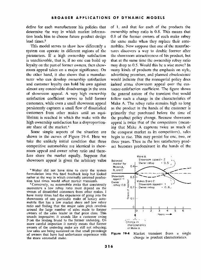
B R O A D E R APPLICATIONS OF DYNAMIC MODELS S
define for each manufacturer his policies that of 1, and that for each of the products the determine the way in which market informa- ownership rebuy ratio is 0.8. This means that tion leads him to choose future product design 0.8 of the former owners of each make rebuy lead times.3 the same make when they replace their auto-
This model serves to show how differently a mobiles. Now suppose that one of the manufac-
system can operate in different regions of the tures discovers a way to double forever after
parameters. If a high ownership satisfaction the showroom attractiveness of his product, but is unachievable, that is, if no one can build up that at the same time the ownership rebuy ratio
loyalty on the part of former owners, then show- may drop to 0.5. Would this be a wise move? In room appeal takes on a major significance. On many kinds of products the emphasis on style, the other hand, it also shows that a manufac- advertising promises, and planned obsolescence turer who can develop ownership satisfaction would indicate that the managerial policy does and customer loyalty can hold his own against indeed stress showroom appeal over the cus- almost any conceivable disadvantage in the area a tomer-satisfaction coefficient. The figure shows of showroom appeal. A very high ownership the general nature of the transient that would satisfaction coefficient serves to hold former follow such a change in the characteristics of
customers, while even a small showroom appeal Make A. The rebuy ratio remains high so long persistently captures a small flow of dissatisfied as the product in the hands of the customer is customers from other makes until an equi- primarily that purchased before the time of librium is reached in which the make with the the product policy change. Because showroom
high ownership satisfaction has a disproportion- appeal is twice that of the competitors (mean- ate share of the market.4 ing that Make A captures twice as much of
Some simple aspects of the situation are the conquest market as its competitors), sales shown in the curves of Figure 19-4. Here we begin to rise. This may persist for one, two, or take the unlikely initial condition that three three years. Then as the less satisfactory prod- competitive automobiles are identical in show- uct becomes predominant in the hands of the room appeal and owner rebuy ratio and there- fore share the market equally. Suppose that MokeA showroom appeal is given the arbitrary value salonced Showroom appeal =
} - '
market for tor Owner rebuy UY = 0.5
MokesA, 0.4 __
9 Walter did not have time to carry the system B, ci ri d C
formulation into this final feedback loop but looked
rather at the way in which externally assumed produc- Showroom o.3 - - --
tion 1 d ' 1 If k. appea-
Mokes B and C tion lead times would affect market transients. Owner Makes B and C
C
'Conversely, an automobile make that consistently rebuy=0.8 à Showroom appear 1 1
encounters a low rebuy ratio must depend on the E o.2 Owner rebuy
stream of dissatisfied customers from other makes. 1
have many times had the experience of going into the j' showrooms of one particular make of luxury auto- en o. i
mobile that has a low market share and low rebuy ratio and finding that the major sales pitch revolves
0 ) ! ! ! ! around the large number of sales made to former
0 1 2 3 4 5 6
owners of the sales leader in that price class. This ...
Yeors il sounds impressive; it sounds like a customer swing t
from the leading brand to the former underdog. On
more careful inspection it merely means that former characteristics owners of the underdog make are still not rebuying; of Make A low sales are being sustained on that small percentage ,
of owners that have had unfortunate experience with '9Ure 19-4 Market transient from a single e
the more successful make. change in product characteristics.
316
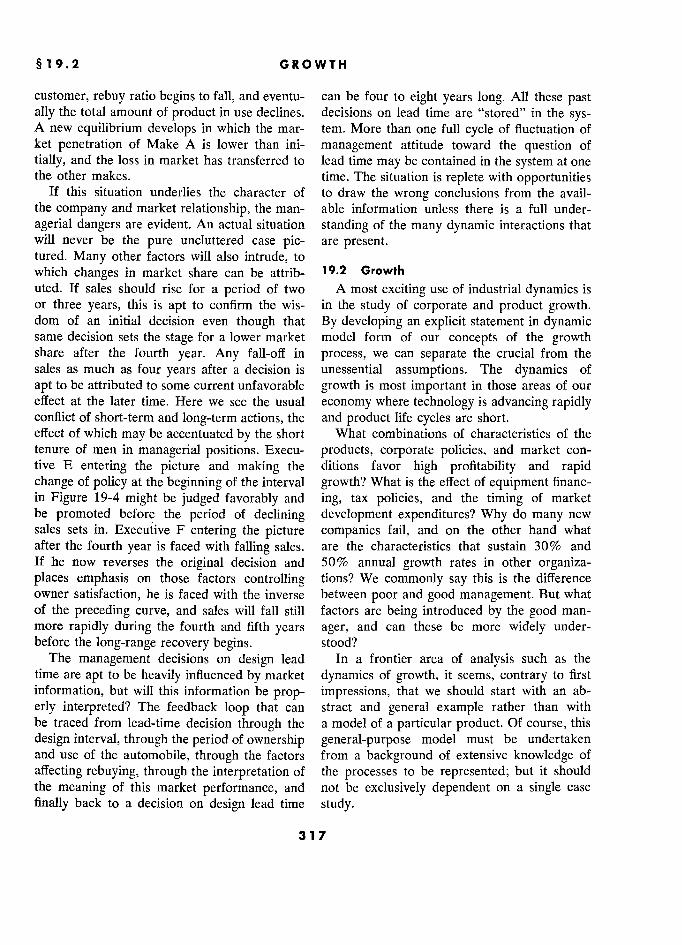
§ 19.2 GROWTH
customer, rebuy ratio begins to fall, and eventu- can be four to eight years long. All these past ally the total amount of product in use declines. decisions on lead time are "stored" in the sys- A new equilibrium develops in which the mar- tem. More than one full cycle of fluctuation of ket penetration of Make A is lower than ini- management attitude toward the question of
tially, and the loss in market has transferred to lead time may be contained in the system at one the other makes. time. The situation is replete with opportunities
If this situation underlies the character of to draw the wrong conclusions from the avail- the company and market relationship, the man- able information unless there is a full under-
agerial dangers are evident. An actual situation standing of the many dynamic interactions that will never be the pure uncluttered case pic- are present. tured. Many other factors will also intrude, to which changes in market share can be attrib- 19.2 Growth
uted. If sales should rise for a period of two A most exciting use of industrial dynamics is or three years, this is apt to confirm the wis- in the study of corporate and product growth. dom of an initial decision even though that By developing an explicit statement in dynamic same decision sets the stage for a lower market model form of our concepts of the growth share after the fourth year. Any fall-off in process, we can separate the crucial from the sales as much as four years after a decision is unessential assumptions. The dynamics of
apt to be attributed to some current unfavorable growth is most important in those areas of our effect at the later time. Here we see the usual economy where technology is advancing rapidly conflict of short-term and long-term actions, the and product life cycles are short. effect of which may be accentuated by the short What combinations of characteristics of the tenure of men in managerial positions. Execu- products, corporate policies, and market con- tive E entering the picture and making the ditions favor high profitability and rapid change of policy at the beginning of the interval growth? What is the effect of equipment financ- in Figure 19-4 might be judged favorably and ing, tax policies, and the timing of market be promoted before the period of declining development expenditures? Why do many new sales sets in. Executive F entering the picture companies fail, and on the other hand what after the fourth year is faced with falling sales. are the characteristics that sustain 30% and If he now reverses the original decision and 50% annual growth rates in other organiza- places emphasis on those factors controlling tions? We commonly say this is the difference owner satisfaction, he is faced with the inverse between poor and good management. But what of the preceding curve, and sales will fall still factors are being introduced by the good man- more rapidly during the fourth and fifth years ager, and can these be more widely under- before the long-range recovery begins. stood?
The management decisions on design lead In a frontier area of analysis such as the time are apt to be heavily influenced by market dynamics of growth, it seems, contrary to first
information, but will this information be prop- impressions, that we should start with an ab-
erly interpreted? The feedback loop that can stract and general example rather than with be traced from lead-time decision through the a model of a particular product. Of course, this
design interval, through the period of ownership general-purpose model must be undertaken and use of the automobile, through the factors from a background of extensive knowledge of
affecting rebuying, through the interpretation of the processes to be represented; but it should the meaning of this market performance, and not be exclusively dependent on a single case
finally back to a decision on design lead time study.
317
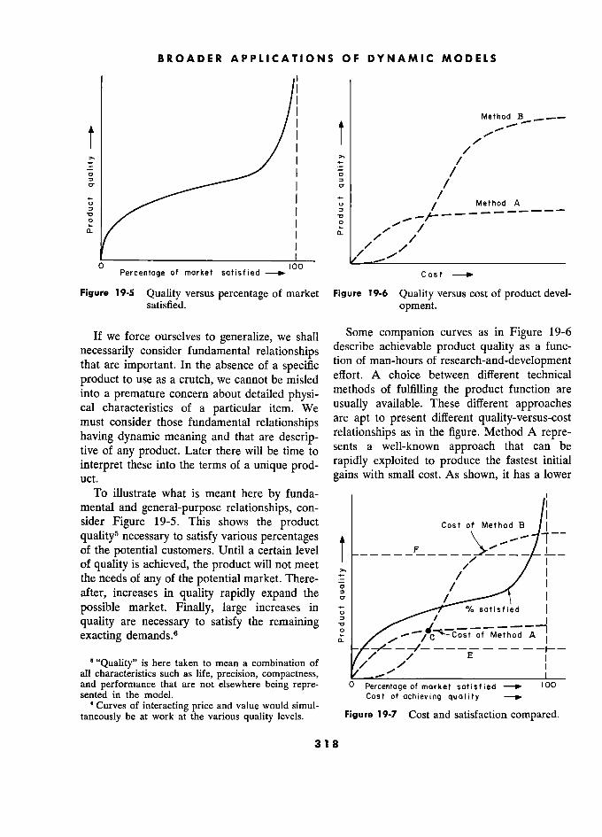
BROADER APPLICATIONS OF DYNAMIC MODELS S
1
/
- 1
Method B
Î j
j
, /
/ " - -
É 1 D / ,
-
z j /
j 1 /
- #
j - v 1
Method A
2
j /
? 7
/ 1 '
-
A
(l. '- 0
/' ,
a o_ /
j /
/ /
/
0 Percentage of market satisfied
100 Cost t -
Figure 19-5 Quality versus percentage of market Figure 19-6 Quality versus cost of product devel- satisfied. opment.
If we force ourselves to generalize, we shall Some companion curves as in Figure 19-6
necessarily consider fundamental relationships describe achievable product quality as a func-
that are important. In the absence of a specific tion of man-hours of research-and-development
product to use as a crutch, we cannot be misled effort. A choice between different technical
into a premature concern about detailed physi- methods of fulfilling the product function are
cal characteristics of a particular item. We usually available. These different approaches
must consider those fundamental relationships are apt to present different quality-versus-cost
having dynamic meaning and that are descrip- relationships as in the figure. Method A repre-
tive of any product. Later there will be time to sents a well-known approach that can be
interpret these into the terms of a unique prod- rapidly exploited to produce the fastest initial
uct. gains with small cost. As shown, it has a lower
To illustrate what is meant here by funda- 1
mental and general-purpose relationships, con- 1
sider Figure 19-5. This shows the p roduct Cost of Method B 1
1
quahty" necessary ta satisfy various percentages 0 t of the necessary to satisfy Until a certain level
( _ _ - _ 1 _
of quality is achieved, the product will not meet 1
the needs of any of the potential market. There- := / 1
after, increases in quality rapidly expand the
possible market. Finally, large increases in /
d 1 u 1 sie éd
quality are necessary to satisfy the remaining 1 0 t of te eth. d A7 exacting demands.6
"Quality" is here taken to mean a combination of / 1' i 6 "Quality" is here taken to mean a combination of / / all characteristics such as life, precision, compactness, -....
1
and performance that are not elsewhere being repre- 0 Î/5?Îllà/.£°§§?§ satisfied 100
sented in the model. Cost of achieving quality 00 ? Curves of interacting price and value would simul- urves of interacting price and value would simul-
taneously be at work at the various quality levels. Figure 19-7 Cost and satisfaction compared.
318
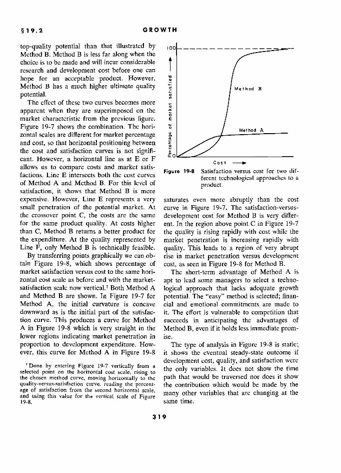
§ 19.2 GROWTH
top-quality potential than that illustrated by Method B. Method B is less far along when the choice is to be made and will incur considerable
i research and development cost before one can !
hope for an acceptable product. However, Y Method B has a much higher ultimate quality / Method B
potential. g N The effect of these two curves becomes more - / cu t
apparent when they are superimposed on the - < market characteristic from the previous figure. E
/
Figure 19-7 shows the combination. The hori- ô / Mernod A zontal scales are different for market percentage and cost, so that horizontal positioning between the cost and satisfaction curves is not signifi- cant. However, a horizontal line as at E or F a.. 0
est - allows us to compare costs and market satis-
Cost ' f ..... – .? both market satis-
Figure 19-8 Satisfaction versus cost for two dif-
of Method A E Method both For cost curves ferent technological approaches to a
of Method A and Method B. For this level of product. satisfaction, it shows that Method B is more expensive. However, Line E represents a very saturates even more abruptly than the cost small penetration of the potential market. At curve in Figure 19-7. The satisfaction-versus- the crossover point C, the costs are the same development cost for Method B is very differ- for the same product quality. At costs higher ent. In the region above point C in Figure 19-7 than C, Method B returns a better product for the quality is rising rapidly with cost while the the expenditure. At the quality represented by market penetration is increasing rapidly with Line F, only Method B is technically feasible. quality. This leads to a region of very abrupt
By transferring points graphically we can ob- rise in market penetration versus development tain Figure 19-8, which shows percentage of cost, as seen in Figure 19-8 for Method B. market satisfaction versus cost to the same hori- The short-term advantage of Method A is zontal cost scale as before and with the market- apt to lead some managers to select a techno- satisfaction scale now vertical.' Both Method A logical approach that lacks adequate growth and Method B are shown. In Figure 19-7 for potential. The "easy" method is selected; finan- Method A, the initial curvature is concave cial and emotional commitments are made to downward as is the initial part of the satisfac- it. The effort is vulnerable to competition that tion curve. This produces a curve for Method succeeds in anticipating the advantages of A in Figure 19-8 which is very straight in the Method B, even if it holds less immediate prom- lower regions indicating market penetration in ise. proportion to development expenditure. How- The type of analysis in Figure 19-8 is static; ever, this curve for Method A in Figure 19-8 it shows the eventual steady-state outcome if
7 by entering Figure 19-7 vertically from a development cost, quality, and satisfaction were
selected point on the only variables. It does not show the time the chosen method curve, moving horizontally to the path that would be traversed nor does it show quality-versus-satisfaction curve, reading the p2rcent- the contribution which would be made by the age of satisfaction from the second horizontal scale,
many other variables that are changing at the and the many other variables that are changing at the and ustng this value for the vertical scale of Figure -' o & 19-8. same time.
319

BROADER APPLICATIONS OF DYNAMIC MODELS
Curves such as in Figure 19-5 and 19-6 are in a larger company or as the growth factors
typical of the nonlinear functions that would in the early life of a small company while it
be used to describe the general character of a is still dependent on an initial product concept. market and of a product.s Many other charac- This mathematical model describing the life
teristics would also be involved to define the cycle of a product includes a preliminary treat-
various dimensions pertinent to the product, ment of six sectors internal to the company the market, the manufacturer, and the competi- (manufacturing, personnel, capital equipment, tion. money, marketing, and research and develop-
An application of the methods in this book ment) and two external sectors (the market, was made to product and company growth by and pricing and competition). Kinsley.9 Kinsley developed a dynamic model Speaking of the typical but hypothetical of 160 variables illustrating the interrelation- company represented by the model, Kinsley
ships that his experience had shown him to be says, "It can be broadly defined as a research-
of importance in the development and market- based company with no other identifiable char-
ing of a new product. The model might be acteristics. This definition is purposely vague. looked upon either as the model of one product ... The characteristics assigned to the ABC
company in the course of building the mathe- e We often see comparative situations like Method matical model can be typically found in many
A and Method B in new, rapidly evolving technologi- companies." In discussing the nature of the cal areas. Method A illustrates the approach which j is initially easier and which people attempt to exploit new product process one is apt to be diverted
beyond its inherent capabilities. Programs become by the peculiarities of a particular product and committed to such improvement and can involve large trapped into a treatment of its superficial char- expenditures. An entirely différent approach aimed at much higher goals can often be the least costly in the acteristics. In the previous section on the d1s-
long run because it requires embarking upon an ap- cussion of the automobile market, we saw how proach of much greater inherent potential. Each in- the physical characteristics of the product could dustry can find its examples, especially during the early period of rapid technological change. An ex- be converted into a more fundamental view-
ample from the last decade is the high-speed internal point dealing with product concepts as they y memory for digital computing £)§f§i§§j Method A affect various phases in the life of the product. in the period around 1950 was represented by the use , r of beam-deflection electrostatic storage tubes. These Here, ln discussing the typical life cycle of a
represented only a small step beyond the cathode- new product, Kinsley avoids the dangers of ray-tube art, and yielded very promising results for
prematurely concentrating on a spécial case. small amounts of effort. However, the method was inherently limited by the short life and unreliability The model is built around a nonSpeC1fiC de- of vacuum tubes and secondary-emission surfaces. scription of the general class of situations that Method B was at that time represented by the random- he is exploring. To succeed in this approach access coincident-current magnetic-core storage. This r & rr held the promise of indefinite life and superior per- requires intimate familiarity with the actual formance but required much preliminary effort in the problems, processes, and factors that are in- development of materials before it could be competi- volved. TheSe are in gerieral accessible Orily to tive. At the time of crossover of the two technologies ° -' (about 1953), as at point C in Figure 19-7, the rate the person with keen insight into the type of of rise of performance of the magnetic-core storage endeavor being represented. However, in draw- was so rapid that within a period of two or three
ing Ori specific personal expérience it is neces- years it had superseded all competitive methods of ° r r r high-speed internai storage in digital computers. sary to distill out the underlying fundamentals
' See Reference 13 for the S.M. thesis written under in order that the resulting dynamic model is the author's direction by Edward R. Kinsley, as a suitable to any member of the entire class of Sloan Fellow at M.I.T. from the Texas Instruments 7
Company, 1958-59. products being represented. In this example,
320
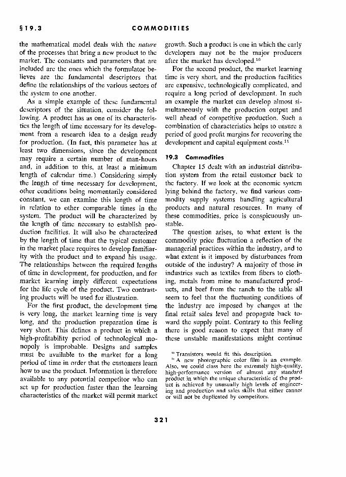
§ 19.3 3 COMMODITIES S
the mathematical model deals with the nature growth. Such a product is one in which the early of the processes that bring a new product to the developers may not be the major producers market. The constants and parameters that are after the market has developed.lo included are the ones which the formulator be- For the second product, the market learning lieves are the fundamental descriptors that time is very short, and the production facilities define the relationships of the various sectors of are expensive, technologically complicated, and the system to one another. require a long period of development. In such
As a simple example of these fundamental an example the market can develop almost si-
descriptors of the situation, consider the fol- multaneously with the production output and
lowing. A product has as one of its characteris- well ahead of competitive production. Such a tics the length of time necessary for its develop- combination of characteristics helps to ensure a ment from a research idea to a design ready period of good profit margins for recovering the for production. (In fact, this parameter has at development and capital equipment costs.l least two dimensions, since the development may require a certain number of man-hours 19.3 Commodities
and, in addition to this, at least a minimum Chapter 15 dealt with an industrial distribu-
length of calendar time.) Considering simply tion system from the retail customer back to the length of time necessary for development, the factory. If we look at the economic system other conditions being momentarily considered lying behind the factory, we find various com- constant, we can examine this length of time modity supply systems handling agricultural in relation to other comparable times in the products and natural resources. In many of
system. The product will be characterized by these commodities, price is conspicuously un- the length of time necessary to establish pro- stable. duction facilities. It will also be characterized The question arises, to what extent is the
by the length of time that the typical customer commodity price fluctuation a reflection of the in the market place requires to develop familiar- managerial practices within the industry, and to
ity with the product and to expand his usage. what extent is it imposed by disturbances from The relationships between the required lengths outside of the industry? A majority of those in of time in development, for production, and for industries such as textiles from fibers to cloth- market learning imply different expectations ing, metals from mine to manufactured prod- for the life cycle of the product. Two contrast- ucts, and beef from the ranch to the table all
ing products will be used for illustration. seem to feel that the fluctuating conditions of For the first product, the development time the industry are imposed by changes at the
is very long, the market learning time is very final retail sales level and propagate back to-
long, and the production preparation time is ward the supply point. Contrary to this feeling very short. This defines a product in which a there is good reason to expect that many of
high-profitability period of technological mo- these unstable manifestations might continue
nopoly is improbable. Designs and samples must be available to the market for a long i? Transistors
would fit this description. period of time in order that the customers learn A new photographie color film is an example. period of time in order that thé customers Icarn
the extremely high-quality, how to use the product. Information is therefore high-performance version of almost any standard available to any potential competitor who can product in which the unique characteristic of the prod- set up for production faster than the learning
uct is achieved by unusually high levels of engineer- .... ing and production and sales skills that either cannot
characteristics of the market will permit market or will production and by competitors. either cannot
characteristics of thé market p market or will not be dupticated by competitors.
321 1
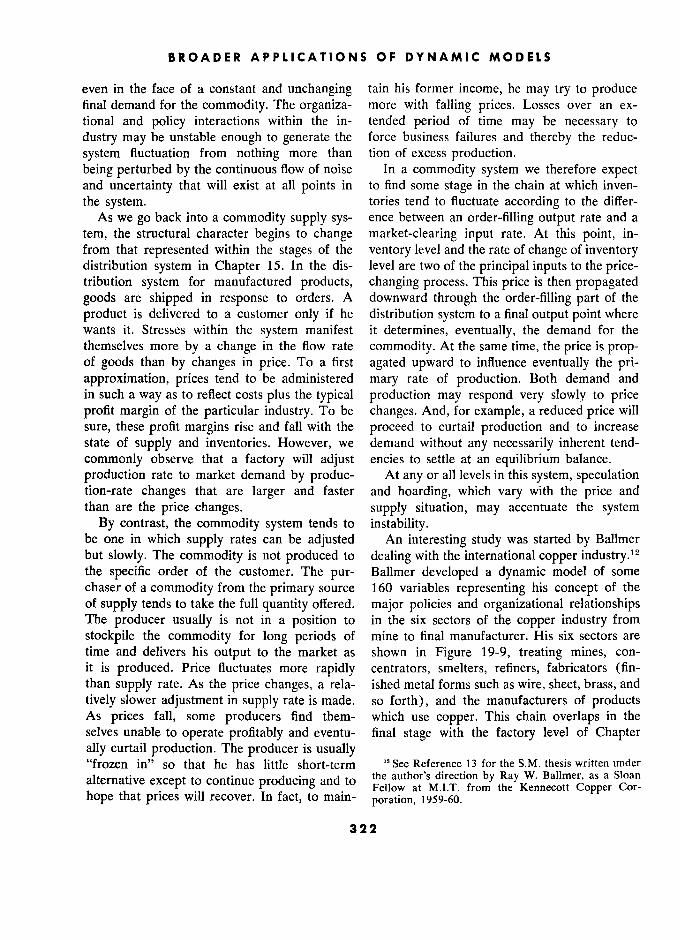
BROADER APPLICATIONS OF DYNAMIC MODELS
even in the face of a constant and unchanging tain his former income, he may try to produce final demand for the commodity. The organiza- more with falling prices. Losses over an ex- tional and policy interactions within the in- tended period of time may be necessary to
dustry may be unstable enough to generate the force business failures and thereby the reduc-
system fluctuation from nothing more than tion of excess production. being perturbed by the continuous flow of noise In a commodity system we therefore expect and uncertainty that will exist at all points in to find some stage in the chain at which inven- the system. tories tend to fluctuate according to the differ-
As we go back into a commodity supply sys- ence between an order-filling output rate and a
tem, the structural character begins to change market-clearing input rate. At this point, in- from that represented within the stages of the ventory level and the rate of change of inventory distribution system in Chapter 15. In the dis- level are two of the principal inputs to the price- tribution system for manufactured products, changing process. This price is then propagated goods are shipped in response to orders. A downward through the order-filling part of the
product is delivered to a customer only if he distribution system to a final output point where wants it. Stresses within the system manifest it determines, eventually, the demand for the themselves more by a change in the flow rate commodity. At the same time, the price is prop- of goods than by changes in price. To a first agated upward to influence eventually the pri- approximation, prices tend to be administered mary rate of production. Both demand and in such a way as to reflect costs plus the typical production may respond very slowly to price profit margin of the particular industry. To be changes. And, for example, a reduced price will
sure, these profit margins rise and fall with the proceed to curtail production and to increase state of supply and inventories. However, we demand without any necessarily inherent tend-
commonly observe that a factory will adjust encies to settle at an equilibrium balance.
production rate to market demand by produc- At any or all levels in this system, speculation tion-rate changes that are larger and faster and hoarding, which vary with the price and than are the price changes. supply situation, may accentuate the system
By contrast, the commodity system tends to instability. be one in which supply rates can be adjusted An interesting study was started by Balimer but slowly. The commodity is not produced to dealing with the international copper industry.11 the specific order of the customer. The pur- Ballmer developed a dynamic model of some chaser of a commodity from the primary source 160 variables representing his concept of the of supply tends to take the full quantity offered. major policies and organizational relationships The producer usually is not in a position to in the six sectors of the copper industry from
stockpile the commodity for long periods of mine to final manufacturer. His six sectors are time and delivers his output to the market as shown in Figure 19-9, treating mines, con- it is produced. Price fluctuates more rapidly centrators, smelters, refiners, fabricators (fin- than supply rate. As the price changes, a rela- ished metal forms such as wire, sheet, brass, and
tively slower adjustment in supply rate is made. so forth), and the manufacturers of products As prices fall, some producers find them- which use copper. This chain overlaps in the selves unable to operate profitably and eventu- final stage with the factory level of Chapter ally curtail production. The producer is usually "frozen in" so that he has little short-term 12 sexe Reference 13 for the S.M. thesis written under
alternative except to continue producing and to the author's direction by Ray W. Ballmer, as a Sloan
' fact to malll- Fellow at M.LT. from thé Kennecott Copper Cor-
hope that prices will recover. In fact, to main- poration, 1959-60. from the Kennecott Copper Cor.
322
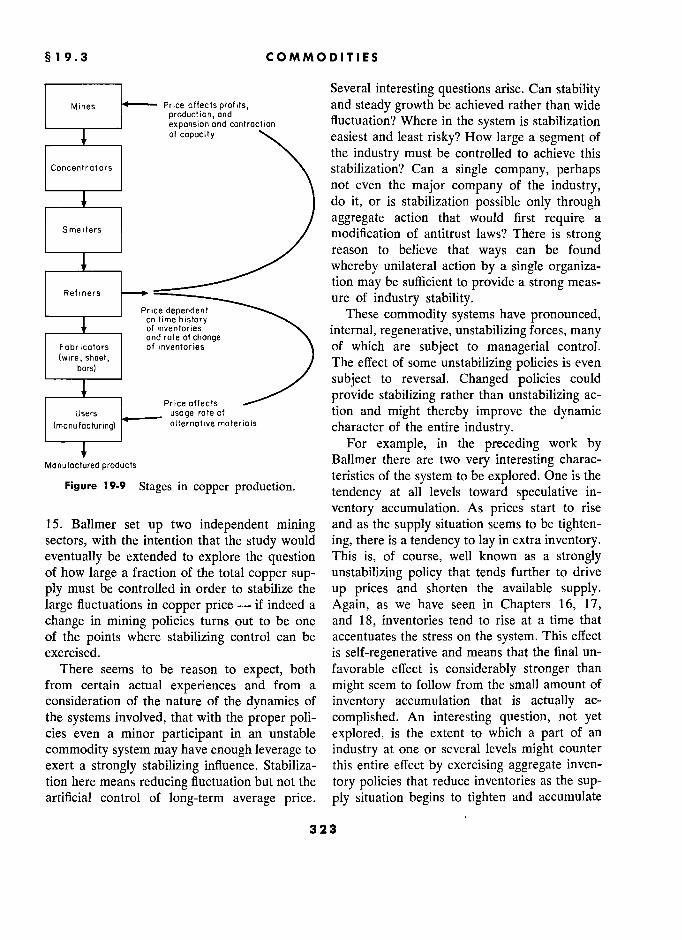
§ 19.3 COMMODITIES S
Several interesting questions arise. Can stability Mines Price affects profits, and steady growth be achieved rather than wide
production,and „ . ,. h
. b'l'
. expansion and contraction fluctuation? Where in the s stem is stabilization of copocity easiest and least risky? How large a segment of
the industry must be controlled to achieve this Concentrators \. stabilization? Can a single company, perhaps
______ not even the major company of the industry, ___t___ j do it, or is stabilization possible only through
/ aggregate action that would first require a Smelters modification of antitrust laws? There is strong
–––.––– ./ reason to believe that ways can be found
whereby unilateral action by a single organiza- . tion may be sufficient to provide a strong meas-
Refiners ure of industry stability. –––)––– Price dependent These commodity systems have pronounced, on lime history ,___:___, of inventories "\. internal, regenerative, unstabilizing forces, many and rate of chonge \ " o ' o , -'
Fabricators of inventories \ of which are subject to managerial control.
bars) ,
/ The effect of some unstabilizing policies is even –––)––– ./ subject to reversai. Changed policies could .–––!–––, Price affects provide stabilizing rather than unstabilizing ac-
Users usage rote of . tion and might thereby improve the dynamic (manufocturing) alternative moterlols character of the entire industry.
–––T––– For example, in the preceding work by Monufoctured products Ballmer there are two very interesting charac-
, _ teristics of the system to be explored. One is the Figure 19-9 Stages in copper production. tendency at the levels toward speculative in-
ventory accumulation. As prices start to rise 15. Ballmer set up two independent mining and as the supply situation seems to be tighten- sectors, with the intention that the study would ing, there is a tendency to lay in extra inventory. eventually be extended to explore the question This is, of course, well known as a strongly of how large a fraction of the total copper sup- unstabilizing policy that tends further to drive
ply must be controlled in order to stabilize the up prices and shorten the available supply. large fluctuations in copper price - if indeed a Again, as we have seen in Chapters 16, 17, change in mining policies turns out to be one and 18, inventories tend to rise at a time that of the points where stabilizing control can be accentuates the stress on the system. This effect exercised. is self-regenerative and means that the final un-
There seems to be reason to expect, both favorable effect is considerably stronger than from certain actual experiences and from a might seem to follow from the small amount of consideration of the nature of the dynamics of inventory accumulation that is actually ac- the systems involved, that with the proper poli- complished. An interesting question, not yet cies even a minor participant in an unstable explored, is the extent to which a part of an
commodity system may have enough leverage to industry at one or several levels might counter exert a strongly stabilizing influence. Stabiliza- this entire effect by exercising aggregate inven- tion here means reducing fluctuation but not the tory policies that reduce inventories as the sup- artificial control of long-term average price. ply situation begins to tighten and accumulate
323 3
BROADER APPLICATIONS OF DYNAMIC MODELS S
inventories in the slack periods. This would not equipment is being operated at maximum ton-
necessarily imply any larger swings in inventory nage capacity, this means that the same amount than are current at the present time, and would, of ore, yielding less final copper, would be if it is possible to do so, actually make inven- mined. The result of a rising price can then be tories available at the time they are most a continuation of the same profit levels and a needed. reduction in the mine output. Whether or not
Another control point for management policy this factor is predominant, any tendency in this to affect system stability may exist at the min- direction may, if it exists to a significant extent,
ing level. There is some reason to believe that contribute to reducing the industry stability. the pressures on the mine manager may lead to Ballmer found the system stability to be actions which further help to accentuate sys- considerably influenced by both of the preced- tem fluctuation, although this point needs fur- ing factors, but the study has not yet been car- ther exploration. The question arises concern- ried far enough to be conclusive, nor has any ing how mine production rate varies with price, consideration been given to the risks that might both in the short run and the long run. In the be encountered by anyone attempting such
long run, and this may represent two years or policy changes. The risks would no doubt be
more, a rising price will no doubt lead to greater strongly influenced by the size of the industry production as additional marginal mines are sector whose policies could be changed. Such
opened for operation. In the short run there explorations show great promise of successful are factors tending to suppress an increase in managerial results, but a large number of ques- production with an increase in price and may tions would need to be explored before defini-
actually create a reduced output as price rises. tive recommendations would emerge. Such ex- This could result from the following combina- plorations would not be unduly lengthy or costly tion of circumstances: in comparison with the possible importance of
- ...... d 1. 1 1 the outcome.13
The mining, concentrating, and smelting levels s the outcome.13 , a fixed tonnage capacity of raw Other promising areas of exploration exist in
ore. toward a nxed tonnage capacity of raw
agricultural products. Perhaps the most promis-
Th available ore at a mine varies in yield per ing for initial exploration are those in which o The available ore a a mine varies in yield per ton, and therefore in the copper output per
there are individual suppliers or users con-
hour of machine operation, depending on what trolling at least 10% of the market and in
part of the property is mined. which governmental politically inspired con-
. The mine manager attempts not to make the trols are not an overriding market factor.
maximum possible profit at every moment but rather is under pressure to meet the profit levels 19.4 Research and Development
expected within the industry and, if he can ac- Management
complish this, is further expected to maintain The management of research and develop- stability of profitable operations and is also ment is a new facet of corporate life that has expected to use eventually both the high-grade grown to its present importance during the last and the low-grade ores available to him. two decades. Because of this newness, research
Under the foregoing circumstances, as the "The study begun by Ballmer was continued in ..t. b "Thé study begun by BaHmer was continued in
price rises, it becomes possible to maintain the J, Schlager, was Sloan Fellow
accepted level of profitability while mining from the AC Spark Plug Division of General Motors lower grade ores and thereby using up those Corporation. He also developed a dynamic model of
mineral resources which might not be profitably the aluminum industry to make
a comparison with
m?nera resources w IC . mlg t eratiOns.
pro ta y copper and further examined the factors influencing
mined under lower-price opérations. If the price and supply. See Reference 13.
324

§ 19.4 RESEARCH AND DEVELOPMENT MANAGEMENT T
management is fraught with more uncertainty advised to think first of a typical project rather
than most other parts of the management pic- than a particular one. In Section 19.2 we dealt
ture. It might seem that any attempt at formal with the general factors in the growth of a
dynamic analysis of the research management product. We concentrated on the characteristics
process would be foolhardy. Yet because the that had significance in the time sequence of
need is so great, this may indeed be one of the events under study. Likewise, here we should
points of major payoff even though it is a concentrate on those fundamental character-
frontier for analysis and one filled with in- istics of the process that are independent of the
tangible factors. The first result of such an at- particular research project but are representa-
tempt is a clarification of one's thinking about tive of all. What are those common and funda-
the importance of various factors and how they mental descriptors which will define any project are related to one another. From such a study, and which will separate one from the other
the combinations of circumstances leading to when suitable numerical values have been as-
success or failure become clearer. signed to the parameters of the system? As with
An initial approach to a dynamic model of the dynamic models already discussed, the re-
military research-and-development management search-and-development activity will consist of
was begun by Katz.14 This work is being carried several interacting sectors. Depending on the
forward by Roberts.l5 objectives of the study, these might be Research and development is commonly con-
nected in our thinking with invention and in- e The end product including size, complexity,
novation, an area of human endeavor sur- novelty, and stringency of performance require- ments, a!l relative to thé présent standard prac- rounded by much controversy. On thé one hand ments, all
relative to the present standard prac-
we argue the unpredictability of invention, tice of the art
for whom the research is done. o Thé customer for whom thé research is done. while on the other recognize certain orderly
9 The customer for whom the research is done.
relationships in the expectations of probable This may be a military contracting office with
relationships m thé expectations of probable e a company has a contract, or in other success. The size of a group that we assign to circumstances it might be the management of a research project is always a function of our the company for whom the research department need for the result, our estimate of the magni- is engaging in projects. tude of the undertaking, and the uncertainty a 'l'he characteristics of the research organization that we feel in the outcome. In other words, we and its management usually operate on an assumption that a larger . The characteristics of the need that the results effort will either shorten the time or increase of the research are to fill the probability of success. Throughout the pic- ture there are similar recognitions of acknowl- This latter item - the nature of the need be-
edged orderly relationships between the vari- ing filled - brings into the open a characteristic
ables. of the information-feedback model which may In approaching a representation of the re- have been obscured by the simplicity of the
search-and-development process, we are well models in Chapters 15 and 17. What is the
measure of system success? What is the system " See Reference 13 for the S.M. thesis written under attempting to accomplish? What are the criteria
the author's direction by Abraham Katz, as a Sloan by adjusts itself toward an at-
Fellow at M.I.T. from the Radio Corporation of America, 1957-58. tempted better meeting of the objectives ? In
'6 As a doctoral thesis and staff research in the both of the models in Chapters 15 and 17 the Industrial Dynamics Project at M.LT. by Edward B.
system was attempting to provide the flow of Roberts on the staff of the School of Industrial Man- agement. goods called for by an externally supplied de-
325 5
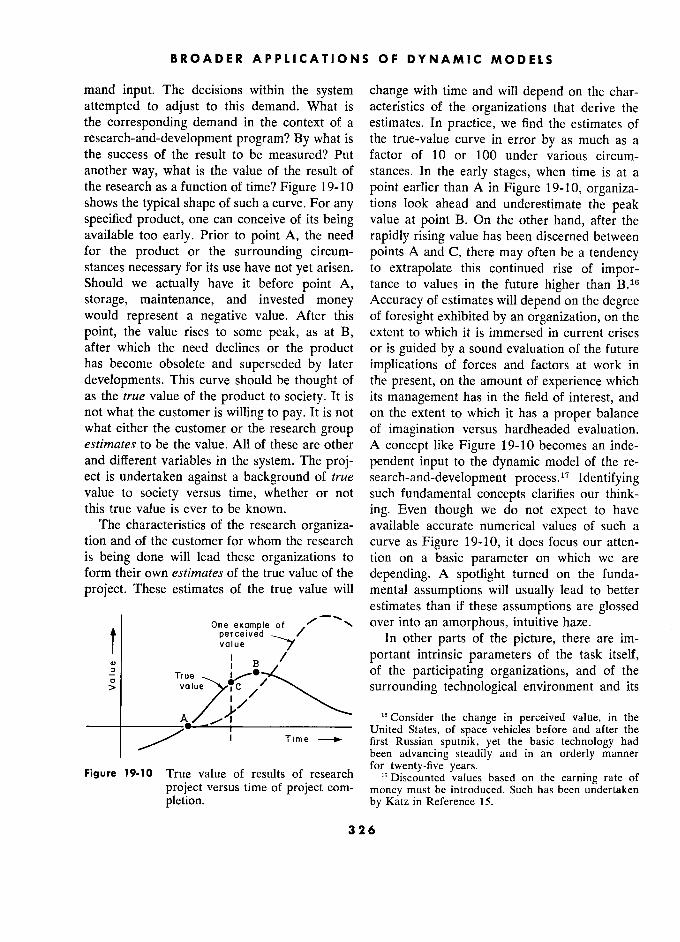
BROADER APPLICATIONS OF DYNAMIC MODELS S
mand input. The decisions within the system change with time and will depend on the char-
attempted to adjust to this demand. What is acteristics of the organizations that derive the the corresponding demand in the context of a estimates. In practice, we find the estimâtes of
research-and-development program? By what is the true-value curve in error by as much as a the success of the result to be measured? Put factor of 10 or 100 under various circum- another way, what is the value of the result of stances. In the early stages, when time is at a the research as a function of time? Figure 19-10 point earlier than A in Figure 19-10, organiza- shows the typical shape of such a curve. For any tions look ahead and underestimate the peak specified product, one can conceive of its being value at point B. On the other hand, after the available too early. Prior to point A, the need rapidly rising value has been discerned between for the product or the surrounding circum- points A and C, there may often be a tendency stances necessary for its use have not yet arisen. to extrapolate this continued rise of impor- Should we actually have it before point A, tance to values in the future higher than B.16
storage, maintenance, and invested money Accuracy of estimates will depend on the degree would represent a negative value. After this of foresight exhibited by an organization, on the
point, the value rises to some peak, as at B, extent to which it is immersed in current crises after which the need déclines or the product or is guided by a sound evaluation of the future has become obsolete and superseded by later implications of forces and factors at work in
developments. This curve should be thought of the present, on the amount of experience which as the true value of the product to society. It is its management has in the field of interest, and not what the customer is willing to pay. It is not on the extent to which it has a proper balance what either the customer or the research group of imagination versus hardheaded evaluation. estimates to be the value. All of these are other A concept like Figure 19-10 becomes an inde- and different variables in the system. The proj- pendent input to the dynamic model of the re- ect is undertaken against a background of true search-and-development process. 17 Identifying value to society versus time, whether or not such fundamental concepts clarifies our think- this true value is ever to be known. ing. Even though we do not expect to have
The characteristics of the research organiza- available accurate numerical values of such a tion and of the customer for whom the research curve as Figure 19-10, it does focus our atten- is being done will lead these organizations to tion on a basic parameter on which we are form their own estimates of the true value of the depending. A spotlight turned on the funda-
project. These estimates of the true value will mental assumptions will usually lead to better estimates than if thèse assumptions are glossed
One example of / ' , over into an amorphous, intuitive haze.
Î perceived In other parts of the picture, there are im- value / '
i B / portant intrinsic parameters of the task itself, - ' of the participating organizatibns, and of the
surrounding technological environment and its
A '8 Consider the change in perceived value, in the ol
°8 Consider the change in perceived value, in the United States, of space vehicles before and after the
1 Time first Russian sputnik, yet the basic technology had been advancing steadily and in an orderly manner
Figure 19-10 True value of results of research for twenty-five years. Figure 19.10 True value of results of research Discounted values based on the earning rate of project versus time of project com- money must be introduced. Such has been undertaken pletion. by Katz in Reference 15.
326
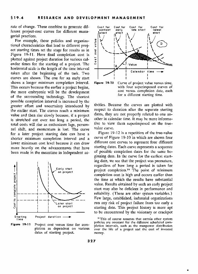
§ 19.4 RESEARCH AND DEVELOPMENT MANAGEMENT T
rate of change. These combine to generate dif- cos ror Cost for Cost for Cost for ferent project-cost curves for différent mana- earliest stort
lote start latest
gerial practices. \/ stort For example, those policies and organiza- 1
\ tional characteristics that lead to different proj- \ : 1 1 ect starting times set the stage for results as in \
Figure 19-11. Here final completion cost is ° T- 1
plotted against project duration for various cal- ° C 1 1
endar times for the starting of a project. The " Value 1 horizontal scale is the length of the time interval –
taken after the beginning of the task. Two I c a i e n d a
time e
curves are shown. The one for an early start i 1 1 shows a longer minimum completion interval. Figure 19-12 2 Curve of project value versus time, This occurs because the earlier a project begins, with four superimposed curves of
the more embryonic will be the development cost versus completion date, each
of the surrounding technology. The shortest for a different starting time.
possible completion interval is increased by the _ greater effort and uncertainty introduced by
tivities. Because the curves are plotted with
the earlier start. The curves reach a minimum respect to duration after the separate starting value and then rise slowly because, if a project dates, they are not properly related to one an-
is stretched out over too long a period, the other in calendar time. It may be more informa-
total costs will rise as enthusiasm lags, person- tive to view them superimposed on the true-
nel shift, and momentum is lost. The curve value curve.
for a later project starting date can have a Figure 19-12 is a répétition of the true-value
shorter minimum completion interval and a curve of Figure 19-10 in which are shown four
lower minimum cost level because it can draw différent cost curves to represent four different
more heavily on the advancements that have starting dates. Each curve represents a sequence been made in the meantime in independent ac- of possible completion dates for the same be-
ginning date. In the curve for the earliest start-
j ing date, we see that the project was premature,
j i i
\ Early stcirt regardless of how long a period is taken for ! 1 on project project completion.18 The point of minimum
il j 1 on project
completion cost is high and occurs earlier than
1 \ the time at which the results have substantial
) \ value. Results obtained by such an early project
j I start may also be deficient in performance and
- - - reliability. (Thèse are other system variables.) 2 Few large, established, industrial organizations
i Later srorr t run any risk of project failure from too early a
) on project
starting date. This project history is more apt –––––––––––– to be encountered by the visionary or crackpot
Starting Project duration t i m e
n q Project duration "Thts of course assumes that certain other system
,.. .. Pro ect cost versus time for com- policies are constant for the different scheduled com- Project cost versus time for corn- pletion intervals, such as the manpower distribution pletion as dependent on various over the life of a project and the cost of invested dates of starting project. money.
327
.

BROADER APPLICATIONS OF DYNAMIC MODELS
who undertakes to reach a sound objective but can lead to initial budgeting plans influenced
long before the society has come to the point more by the available funds than by a realistic where it can use and appreciate the results. estimate of the task to be undertaken. By the
The second cost curve for an early start has time that the full magnitude of the job is ap- a substantial area of overlap with the value parent and its cost implications have become curve, as shown by the shaded region. Fur- unavoidable, it may already be too late to re- thermore, we see that the maximum margin of organize the effort for completion at a time and the value curve above the cost curve is not very cost that fall under the true-value curve. How- sensitive to the horizontal position of the cost ever, this does not necessarily mean that the curve in time nor to the length of project com- project will be terminated. The momentum of
pletion interval. In other words, a misjudgment the organizations involved, the unwillingness to of proper start and completion dates is less recognize an error in judgment, wishful think- serious than it would be if operations are shifted ing, and the obscurity of the true-value concept into the region of the third curve, labeled as a can easily lead to actions based on an assump- late start. The third curve, as shown, has a tion of value in the region marked D in Figure substantial maximum point for value in excess 19-12. As the cost rises and as the estimated of cost, but this value diminishes very rapidly cost exceeds by greater and greater margins the if conditions shift the curve to the right. Here true value to society, the probability increases the late start increases the risk. The fourth that a collapse will occur in the emotionally cost curve for the latest start has the lowest created value structure. The internal system will minimum cost but again is a curve in which be under stress and on an unfirm foundation, cost always is in excess of project completion making it an easy target for penetrating inquiry value. and criticism from outsiders who have become
The preceding cost curves are not input func- unsympathetic. tions to the model like the true-value curve but Here we see the crucial importance of so- are in the nature of the kind of results to be called "intangibles" in a model of system dy- derived from a sufficient number of model runs. namics. Anyone intimately familiar with re- Their discussion brings forth the kinds of fac- search and development recognizes the crucial tors that underlie the research and development importance of factors such as courage, imagina- processes. tion, foresight, integrity, hope, optimism, and
An important factor in research and develop- emotional defense of past decisions. The rela- ment management is apt to be the nature of the tive ranking of several organizations with re- financial approvals and budget cycle involved. spect to any of these characteristics will usually This is especially pertinent in large military be noncontroversial if the selected organiza- projects in which several years may be involved tions cover the wide range encountered among in preparing military estimates, getting these actual organizations. approved, defending and securing the appropri- Some organizations are conspicuously and ations from Congress, and writing contracts for continuously successful in the projects they the work. undertake. To a considerable extent this arises
In the budget cycle, the managerial charac- through the initial selection of projects that can teristics of the contractor and contracting of- succeed, coupled with the foresight to generate fice enter heavily into the probability of success. an early enough start even if it may mean the
Competence, foresight, courage, and integrity risk of spending their own internal funds before exert a major influence on the realism of esti- the value of the undertaking is recognized by mates. A low level of courage and integrity financial sponsors. Such organizations have the
328 8
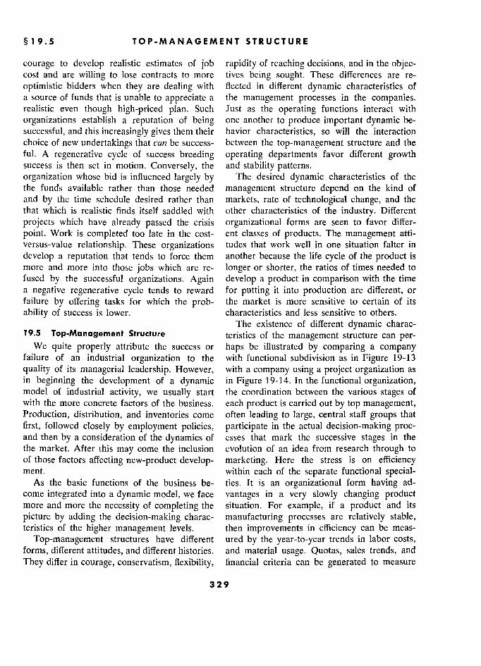
§ 19.5 5 TOP-MANAGEMENT STRUCTURE E
courage to develop realistic estimates of job rapidity of reaching decisions, and in the objec- cost and are willing to lose contracts to more tives being sought. These differences are re-
optimistic bidders when they are dealing with flected in different dynamic characteristics of a source of funds that is unable to appreciate a the management processes in the companies. realistic even though high-priced plan. Such Just as the operating functions interact with
organizations establish a reputation of being one another to produce important dynamic be-
successful, and this increasingly gives them their havior characteristics, so will the interaction choice of new undertakings that can be success- between the top-management structure and the ful. A regenerative cycle of success breeding operating departments favor different growth success is then set in motion. Conversely, the and stability patterns. organization whose bid is influenced largely by The desired dynamic characteristics of the the funds available rather than those needed management structure depend on the kind of and by the time schedule desired rather than markets, rate of technological change, and the that which is realistic finds itself saddled with other characteristics of the industry. Different
projects which have already passed the crisis organizational forms are seen to favor differ-
point. Work is completed too late in the cost- ent classes of products. The management atti- versus-value relationship. These organizations tudes that work well in one situation falter in
develop a reputation that tends to force them another because the life cycle of the product is more and more into those jobs which are re- longer or shorter, the ratios of times needed to fused by the successful organizations. Again develop a product in comparison with the time a negative regenerative cycle tends to reward for putting it into production are différent, or failure by offering tasks for which the prob- the market is more sensitive to certain of its
ability of success is lower. characteristics and less sensitive to others. The existence of different dynamic charac-
19.5 Top-Management Structure teristics of the management structure can per- We quite properly attribute the success or haps be illustrated by comparing a company
failure of an industrial organization to the with functional subdivision as in Figure 19-13
quality of its managerial leadership. However, with a company using a project organization as in beginning the development of a dynamic in Figure 19-14. In the functional organization, model of industrial activity, we usually start the coordination between the various stages of with the more concrete factors of the business. each product is carried out by top management, Production, distribution, and inventories come often leading to large, central staff groups that
first, followed closely by employment policies, participate in the actual decision-making proc- and then by a consideration of the dynamics of esses that mark the successive stages in the the market. After this may come the inclusion evolution of an idea from research through to of those factors affecting new-product develop- marketing. Here the stress is on efficiency ment. within each of the separate functional special-
As the basic functions of the business be- ties. It is an organizational form having ad- come integrated into a dynamic model, we face vantages in a very slowly changing product more and more the necessity of completing the situation. For example, if a product and its
picture by adding the decision-making charac- manufacturing processes are relatively stable, teristics of the higher management levels. then improvements in efficiency can be meas-
Top-management structures have different ured by the year-to-year trends in labor costs,
forms, different attitudes, and different histories. and material usage. Quotas, sales trends, and
They differ in courage, conservatism, flexibility, financial criteria can be generated to measure
329
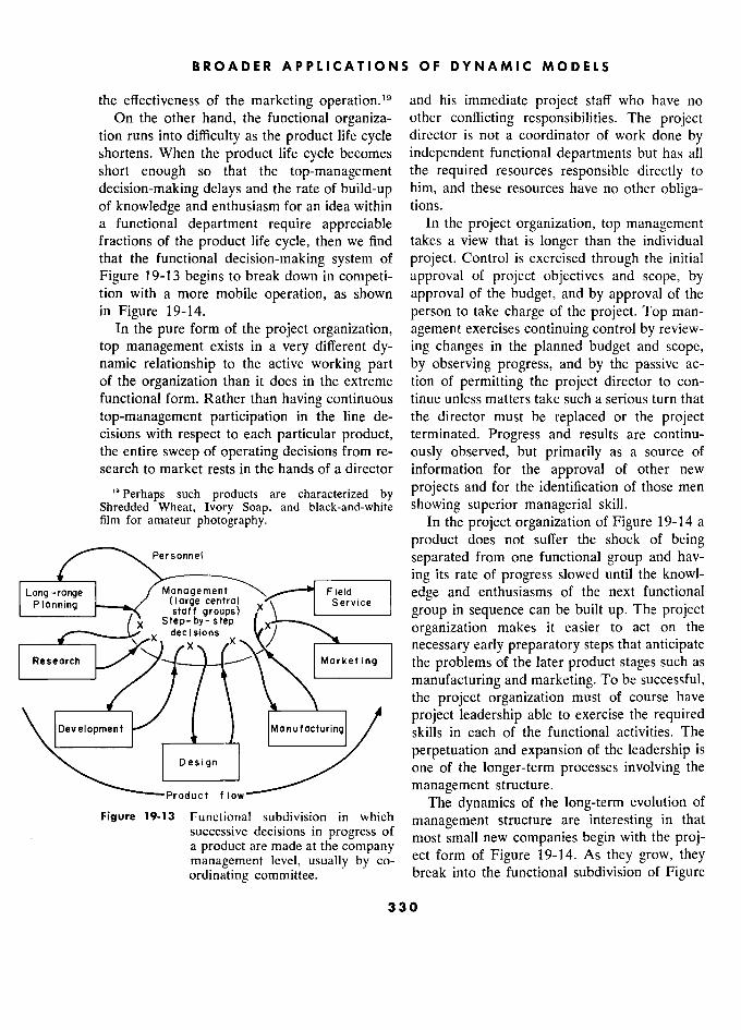
BROADER APPLICATIONS OF DYNAMIC MODELS S
the effectiveness of the marketing operation.l? and his immediate project staff who have no On the other hand, the functional organiza- other conflicting responsibilities. The project
tion runs into difficulty as the product life cycle director is not a coordinator of work done by shortens. When the product life cycle becomes independent functional departments but has all short enough so that the top-management the required resources responsible directly to
decision-making delays and the rate of build-up him, and these resources have no other obliga- of knowledge and enthusiasm for an idea within tions. a functional department require appreciable In the project organization, top management fractions of the product life cycle, then we find takes a view that is longer than the individual that the functional decision-making system of project. Control is exercised through the initial
Figure 19-13 begins to break down in competi- approval of project objectives and scope, by tion with a more mobile operation, as shown approval of the budget, and by approval of the in Figure 19-14. person to take charge of the project. Top man-
In the pure form of the project organization, agement exercises continuing control by review-
top management exists in a very different dy- ing changes in the planned budget and scope, namic relationship to the active working part by observing progress, and by the passive ac- of the organization than it does in the extreme tion of permitting the project director to con- functional form. Rather than having continuous tinue unless matters take such a serious turn that
top-management participation in the line de- the director must be replaced or the project cisions with respect to each particular product, terminated. Progress and results are continu- the entire sweep of operating decisions from re- ously observed, but primarily as a source of search to market rests in the hands of a director information for the approval of other new
'9 Perhaps such products are characterized by y projects and for the identification of those men
Shredded Wheat, Ivory Soap, and black-and-white showing superior managerial skill. film for amateur photography. In the project organization of Figure 19-14 a a
__ product does not suffer the shock of being Personnel separated from one functional group and hav-
_______ ing its rate of progress slowed until the knowl-
Long-range Management Field
1 edge and enthusiasms of the next functional
pjannina large central Service .. Plonning staff groups) group in sequence can be built up. The project
x organization makes it easier to act on the e
x x necessary early preparatory steps that anticipate Research Marketing the problems of the later product stages such as
––––––– / / \ \
––––––– manufacturing and marketing. To be successful,
/ / \ \. \ the project organization must of course have \ ( project leadership able to exercise the required
\ Development J
Manufacturing / skills in each of the functional activities. The \––––––– perpetuation and expansion of the leadership is
Design one of the longer-term processes involving the
Product flow management structure. The dynamics of the long-term evolution of
Figure 19-13 Functionai subdivision in which management structure are interesting in that
_ successive decisions in progress of most small new companies begin with the proj- a product are made at the company . management level, usually by co-
ect form of Figure 19-14. As they grow, they
ordinating committee. break into the functional subdivision of Figure
330
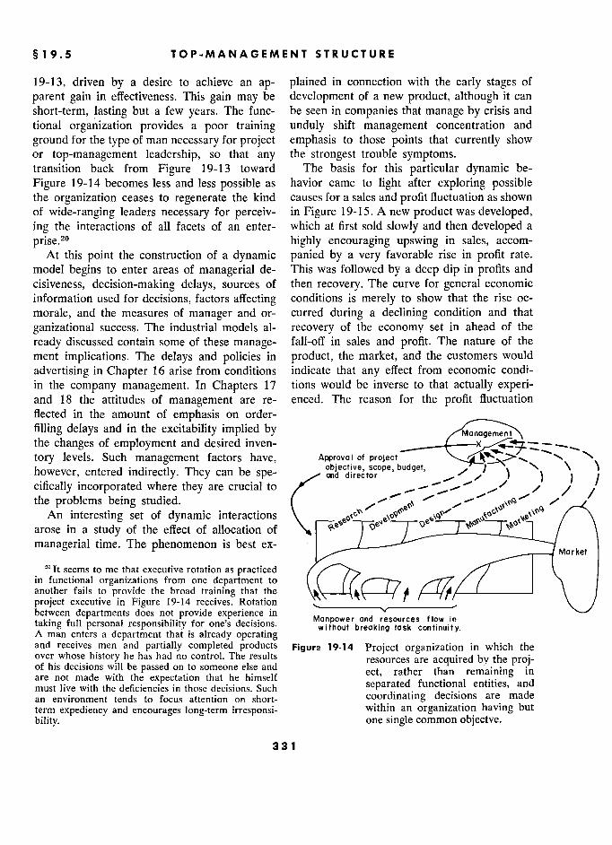
§ 19.5 5 TOP-MANAGEMENT STRUCTURE E
19-13, driven by a desire to achieve an ap- plained in connection with the early stages of
parent gain in effectiveness. This gain may be development of a new product, although it can
short-term, lasting but a few years. The func- be seen in companies that manage by crisis and tional organization provides a poor training unduly shift management concentration and
ground for the type of man necessary for project emphasis to those points that currently show or top-management leadership, so that any the strongest trouble symptoms. transition back from Figure 19-13 toward The basis for this particular dynamic be-
Figure 19-14 becomes less and less possible as havior came to light after exploring possible the organization ceases to regenerate the kind causes for a sales and profit fluctuation as shown of wide-ranging leaders necessary for perceiv- in Figure 19-15. A new product was developed, ing the interactions of aIl facets of an enter- which at first sold slowly and then developed a
prise.20 highly encouraging upswing in sales, accom- At this point the construction of a dynamic panied by a very favorable rise in profit rate.
model begins to enter areas of managerial de- This was followed by a deep dip in profits and
cisiveness, decision-making delays, sources of then recovery. The curve for general economic information used for decisions, factors affecting conditions is merely to show that the rise oc-
morale, and the measures of manager and or- curred during a declining condition and that
ganizational success. The industrial models al- recovery of the economy set in ahead of the
ready discussed contain some of these manage- fall-off in sales and profit. The nature of the
ment implications. The delays and policies in product, the market, and the customers would
advertising in Chapter 16 arise from conditions indicate that any effect from economic condi-
in the company management. In Chapters 17 tions would be inverse to that actually experi- and 18 the attitudes of management are re- enced. The reason for the profit fluctuation
flected in the amount of emphasis on order-
filling delays and in the excitability implied by Management the changes of employment and desired inven-
tory levels. Such management factors have, Approval of project objective, scope, budget, however, entered indirectly. They can be spe- ond director j 'j j
cifically incorporated where they are crucial to _ - / / the problems being studied. (
An interesting set of dynamic interactions arose in a study of the effect of allocation of / "II?LJ / \ managerial time. The phenomenon is best ex- /
Mar ket
seems to me that executive rotation as practiced \ in functional organizations from one department to ( ( / / \ another fails to provide the broad training that the / '_______ \ project executive in Figure 19-14 receives. Rotation '. \. y between departments does not provide experience in
Monpower and resources flow in taking full personal responsibility for one's decisions. without breaking tosk continuity. A man enters a department that is already operating
wlthout breoklng tosk contlnully,
and receives men and partially completed products Figure 19-14 Project organization in which the over whose history he has had no control. The results resources are acquired by the proj- of his decisions will be passed on to someone else and
ect, rather than remaining in are not made with the expectation that he himself and must live with the deficiencies in those decisions. Such P§Î _ functional entities, and
an environment tends to focus attention on short- coordinating decisions are made term expediency and encourages long-term irresponsi- within an organization having but
bility. one single common objectve.
331 1
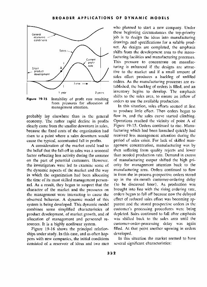
BROADER APPLICATIONS OF DYNAMIC MODELS S
who planned to start a new company. Under
General these beginning circumstances the top-priority economic job is to design the ideas into manufacturing conditions "*-.
drawings and specifications for a salable prod-
Sales uct. As designs are completed, the emphasis shifts from the development area to the manu-
/ / Current facturing facilities and manufacturing processes.
/ profit This pressure to concentrate on manufac-
Stort a / rare turing is enhanced if the designs are attrac-
product / \ / tive to the market and if a small amount of development. /
/ / \
\ / / sales effort produces a backlog of unfilled
orders. As the manufacturing processes are es- ime 1- tablished, the backlog of orders is filled, and an
1 yeor z inventory begins to develop. The emphasis
Figure 19-15 1 nsta b')' 1 Ity 0 profit rate resulting shifts to the sales area, to ensure an inflow of
Ftgure Instabt!)ty of profit rate resuttine orders to use the available roduction. from pressures for allocation of orders to use the available production.
management attention. In this situation, sales efforts seemed at first to produce little effect. Then orders began to
probably lay elsewhere than in the general flow in, and the sales curve started climbing. economy. The rather rapid decline in profits Operations reached the vicinity of point A of
clearly came from the smaller downturn in sales, Figure 19-15. Orders continued to rise. Manu-
because the fixed costs of the organization had facturing which had been launched quickly had
risen to a point where a sales downturn would received less management attention during the
cause the typical, accentuated fall in profits. period of sales crisis. For lack of skilled man-
A consideration of the market could lead to agement concentration, manufacturing was by the belief that the fall-off in sales was a seasonal then suffering from quality rejects and lower
factor reflecting less activity during the summer than needed production rate. Demand in excess
on the part of potential customers. However, of manufacturing output shifted the high pri- the investigators were led to examine some of ority for management attention back to the
the dynamic aspects of the market and the way manufacturing area. Orders continued to flow
in which the organization had been allocating in from the in-process prospective orders stored
the time of its most skilled management person- up in the six-month customer-ordering delay nel. As a result, they began to suspect that the (to be discussed later). As production was
character of the market and the pressures on brought into line with the rising ordering rate, the management were interacting to cause the orders began to fall off because now the delayed observed behavior. A dynamic model of this effect of reduced sales effort was becoming ap-
system is being developed. This dynamic model parent and the stored prospective orders in the
combines some simplified characteristics of customer's processing procedures were being
product development, of market growth, and of depleted. Sales continued to fall after emphasis allocation of management and personnel re- was shifted back to the sales area until the
sources. It is a highly nonlinear system. customer-order-processing delay was again
Figure 19-16 shows the principal relation- filled. At that point another upswing in orders
ships under study. In this case, and as often hap- developed.
pens with new companies, the initial conditions In this situation the market seemed to have
consisted of a reservoir of ideas and two men several significant characteristics:
332
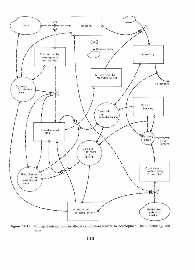

BROADER APPLICATIONS OF DYNAMIC MODELS
For all practical purposes, the size of the mar- \ :
ket was unlimited in comparison with the size Ë \ 1 of the company and its potential production \ j ability. o
\ 1
The product was capital equipment in which 1
an individual order might run several thousands -° à \ 1 or a few tens of thousands of dollars. Such S E \ 1
equipment has been traditionally made to order. à \ 1 Skilled technical salesmanship plus effective de- N E \. 1
signs, sample equipment, and demonstrations 0
were sufficient to initiate discussion of a CllS- Percentage of manager's total tomer order. week unallocated d
Because it was an item of capital equipment, Figure 19-17 Resistance to time allocation ver- several levels of management approval within sus percentage of unallocated time. the customer organization were necessary to , place an order, and under some circumstances to the allocation of more of the unallocated
approval of the purchase was required from a time as a function of the percentage of total
military contracting officer if the product was time unallocated. This is presented as a per- to be used in connection with military projects. centage of a full 168-hour week. The resistance These approvals, the answering of inquiries, the to allocation of additional time is approximately demonstration to various superiors of the per- neutral in the vicinity of a 35- or 40-hour work son actually desiring the equipment, and the week. At a larger amount of unallocated time preparation by the customer of specifications the coefficient is shown as negative, indicating and an order require about six months on the an actual desire to be more active. As unallo- average. Orders become ready for placement a
cated time falls, the résistance to the allocation of substanttaf penod of time after the initial 1
cated , ta ?
substantial period of time
after the initial any more time rises steeply as the limit of
demonstrations and selling. ' human endurance is approached. Thé field )s so compétitive that orders, when ., ..n... 1..j -n 1.
they are 15 So competltlve t at orders, lost if Quite differently shaped curves will be gen- they are ready for placing, can be lost if , deliveries are too slow. The state of the order erated for the "pressure" for allocation to the de1iverieS are too s!ow. Thé state of thé order
§, £ backlog and the shipping rate are indicative of areas. Thèse pressures will dépend on
the delivery delays, and in the model thèse con- 'need for work in those areas. For example, an
trol the split of order flow between those placed ?verage order level higher than production rate and those lost. and a falling and low inventory would create
pressures for allocation of more time in the The allocation of managerial and personnel production sector. Pressure to allocate to the
time consist in this model, as shown in Figure sales area would rise as the rate of orders de-
19-16, of a system of needs and priorities that clines, as the backlog of unfilled orders declines, balance themselves by causing flows of time al- and as inventories become excessive. In addi- location by way of the pool of unallocated time. tion, relative priorities between sectors would A pressure, or allocation priority, is generated be assigned to represent various managerial for each of the four levels, including the unal- policies. A short-sighted organization is apt to
. located level. Differences in allocation pressure have a low-priority coefficient on the conver- cause a flow of time allocation from one part of sion of ideas to designs if there is stress in the the system to the other. Figure 19-17 illustrates manufacturing area. Likewise, trouble in the one of these functions as it applies to the pool sales area is apt to take precedence over either of unallocated time. This shows the resistance of the other two. As would be expected, the
334
§ 19.6 MONEY AND ACCOUNTING
behavior of the system is highly dependent on more weeks of delay matter, added to a year the priority coefficients, the allocation func- or more?
tions, and the time constants with which al- To the extent that accounting information location changes are made. The model becomes actually is used in making management deci- a basis for studying the results of various man- sions, it must be represented within a model.
agement attitudes in different product and mar- The peculiar characteristics of accounting in- ket situations. formation can impart important dynamic char-
acteristics to a business. If this information, 19.6 Money and Accounting which is so long delayed after the primary deci-
In view of the central position held by ac- sions on which it is based, is an important counting information and money flow in most influence in the managerial decisions, then those discussions of business operation, the reader delays and the amplification caused by them
may feel that financial variables have been have serious implications for system stability. slighted in this book. At first thought, money When a business has gotten itself into such
may appear to constitute the network which a serious condition that its operations are jeop- ties together the parts of a business. In this ardized by low cash position and unavailable
book, the coordinating position has been taken credit, then the financial inputs may be the
by the information flow network. Furthermore, principal controllers of the operating decisions. most information flow has been presented as Such a state is, however, usually the result of a nonfinancial in form. 1 believe this change in long earlier history in which the implications emphasis is proper, although money flow and of other kinds of information have gone un- the generation of accounting-type information heeded. cannot be ignored in the construction of more Barring these drastic marginal situations, ac-
complete models. A beginning to the inclusion counting information does not seem to find its of money and accounting data was introduced way directly into operating decisions in the in Chapter 17. In that chapter, however, the same tangible way that sales become one of the financial information does not form an integral ingredients in the orders for replacement goods. part of the decision-making functions in the Instead, the profit-and-loss statement may have model. Rather it is a reporting system to indi- an important effect in setting the general tone cate to the investigator how the system has be- of optimism and care surrounding the making haved. of decisions. As current profitability increases,
Is not reporting of performance the principal there is apt to be a relaxing of careful, disci- use commonly made of accounting informà- plined consideration of new expenditures. Flim- tion ? It measures past success of the organi- sier arguments will suffice for hiring additional .
zation. It performs a policing action to ensure personnel into service and staff groups where
honesty. It acts as a basis for rewards - both they become a fixed cost to the organization, to managers and to stockholders. which persists well into a later time of financial
To be sure, accounting information is held in difficulty. On the other hand, unfavorable indi-
great esteem as data for current operating de- cators from the accounting system may serve cisions. But is this justified? Does it matter to delay seriously and perhaps prevent those whether the profit-and-loss statement and the expenditures that alone hold the key to financial balance sheet for the last month are available improvement. In this manner we can anticipate on the fifth or twenty-fifth of this month, since that the psychological attitudes deriving from both reflect the results of decisions taken six the financial information have the potential for
months, a year, or five years ago? Does three influencing decisions in such a way as to rein-
335
BROADER APPLICATIONS OF DYNAMiC MODELS S
force other difficulties to which the organization start a study of dynamic characteristics with the
may be subject. industry as a whole. This was done in Chapter The skeleton framework of primary effects 17. It presumes that the company of immediate
within the organization can often be represented interest is similar to others in the industry and without financial and accounting information. that the problems of the industry are the prob- On the other hand, as models become more lems of the company. After the dynamic char- subtle and begin to deal with the very important acteristics of the industry are better understood,
aspect of top-management decision making, the then company differentiation can be studied.
accounting system becomes an essential part lf substantially different policies would be de- of internal information loops affecting attitudes sirable for the industry, there then arises the and decisions. question of what will happen should one com-
However, we must not lose sight of the fact pany unilaterally adopt these policies. We can that financial information is but one small part expect that there will be circumstances where of the total information within the organization. unilateral adoption of different policies is feasi-
Usually it measures symptoms, not causes. It ble, and on the other hand situations wherein is dangerous because it is easier to derive than the risk will be too great. Once the nature of other more important kinds of information. We the industry is adequately understood, the study have a tendency to gather easily available in- of different policies between companies be-
formation, whether or not that information is comes important. the most efficient and effective. The policies of a company can control not
only its share of the total market but also that 19.7 Competition part of the market to which the company
In the conduct of a business, the competitive caters. We are accustomed to thinking of mar-
aspects of product and market seem to take ket differentiation on the basis of product per-
precedence in management thinking. Yet many formance, price, quality, and other physical of the problems which a business faces are characteristics. There is also another dimension
characteristic of the entire industry. Companies of possible differentiation, and that is in the
are often sufficiently alike and the factors inter- dynamic characteristics of the market. In some
locking their behavior are sufficiently strong so industries we find one company whose policies that the ups and downs in the fortunes of the attract the fluctuating part of the market de-
industry are usually reflected in the welfare of mand, whereas another company has policies each company within the industry. The coupling that attract a stable underlying continuity of
forces between companies within an industry demand. The company that follows the policy serve to impress upon each a similar timing of of pursuing every possible sale and having environmental circumstances. If one company product available to push into the hands of the
has a better delivery capability than another, customer even in peak periods of demand may sufficient business can shift to provide equal find it is unknowingly selecting the peaks of
loading during times of production stress. La- demand as its share of the market. This will be
bor union demands tend to equalize costs. A especially true if the intrinsic value of the
rising demand will tend to stimulate concurrent product in the eyes of the customer is less than
expansion of production capability throughout that of competitors and if the company is taking the industry. advantage of sales that come to it because of the
If the industry has conspicuous characteris- unavailability of preferred competitive products. tics whose changes with time affect all the com- On the other hand, a contrasting company
, panies within the industry, then it seems wise to policy could be to establish a preferred position
' 336
§ 19.8 8 THE FUTURE IN DECISION MAKING
in design, quality, and sales effectiveness so for trends and seasonal behavior. Long-rangé that all production is salable in the periods of planning implies a time period beyond that of lowered market demand. This company might forecasting, and rests more on the manager's forgo possible higher sales in periods of in- interpretation of the way present factors will creased demand in the interest of greater con- interact to shape the future. Interpreted in this
tinuity of operations and to prevent dilution of way, forecasting and long-range planning are its quality and skill. In this situation the first related in quite different ways to dynamic model
company has a much higher percentage fluctua- building. tion in its operations than has the industry as Forecasting. Forecasting, as referred to in a whole. business and especially in sales practice, usually
Differences in policy that tend to differentiate depends heavily on the analysis of past data a company on the basis of its dynamic charac- in an attempt to detect patterns of growth, fluc- teristics will be an important aspect of com- tuation, and changes in trends. The results are
petitive models. In Section 19.1 the study of used as predictions of the future on which to
design lead time and market penetration are base operating decisions.
examples. In Section 19.3 the discussion of a It should hardly be necessary to point out model of the copper industry illustrates the that there is no such thing as information avail-
process of starting first with the industry as a able from the future. Yet the aura of mystery whole and then distinguishing policies between surrounding sales forecasting in many com-
competitive companies. panies seems to give it an esoteric character The dynamics of early growth discussed in setting it apart from the straightforward con-
Section 19.5 shows, on the other hand, a study cept of converting presently available informa- where the industry is amorphous and poorly tion from one form into another. defined and has no conspicuous characteristics The forecasting process fits into the concept other than growth and wide opportunity. The of the decision equations discussed in earlier
challenge there tended to be not the competitive chapters. These equations take the available interactions between companies, but rather the sources of present information and combine
matching of company characteristics to the dy- them to generate present decisions and actions. namic characteristics of a field of rapid techno- The possible complexity of the process does
logical advancement. not change its fundamental character. If a fore- Other types of questions deal primarily with casting procedure is used, we must be sure to
competitive behavior. The life cycle of a new represent it in the decision equations of a
product such as discussed in Section 19.2 is model. This is especially true if we believe that
strongly influenced by the factors which give the forecasting affects the behavior of the in-
rise to competition and which control chang- dustrial system - either for better or worse.
ing profit rates throughout the life cycle of the More folklore seems to surround the process product. of forecasting than in any other part of the
corporation. The high esteem that the results 19.8 The Future in Decision Making enjoy often belie a comparison between fore-
Forecasting and long-range planning are cast and actual happenings. Be the accuracy terms arising from the manager's concern about as it may, the implications of forecasting go the future effect of his decisions. Forecasting still deeper. Nearly all of the statistical and
usually implies a search for decision-making mathematical treatment of forecasting implicitly help in the near future, and often rests heavily assumes that the time series that is being fore- on a statistical analysis of past data in a search cast is independent of actions based on the fore-
337

BROADER APPLICATIONS OF DYNAMIC MODELS S
cast.21 We have seen in the behavior of the Most attempts at forecasting turn out to be
systems modeled in Chapters 15 and 17 how heavily dependent on extrapolation into the
easy it is for actions of the company to affect future of the course of events in the rather market behavior. In fact, aIl of marketing and recent past. Many other factors presumably go salesmanship is aimed in that direction. If the into forecasts, but usually these other factors
past pattern of sales is the basis for a forecast do not carry enough weight to override extrapo- and if the forecast leads to actions that can lation as the major forecasting component. affect future sales, we have a closed-loop in- Sales departments see orders increasing and formation-feedback system. The assumption estimate still greater rises to encourage the pro- that the input time series is independent of duction department to meet any possible fu- the actions based on analysis of that time series ture demands. Delivery delays are increasing, no longer holds. The forecasting procedure be- so that we accelerate ordering in anticipation cornes a part of the system in which it is set. of still tighter delivery. Prices are falling so that The forecasting procedure has then the poten- orders are cut back in the hope of still lower tial for creating amplification and a shift in future prices. the time responses of the system. The results The forecasting process can affect not only may be far from those expected. In fact, it is the series of events being forecast but also can
quite reasonable to expect that forecasting affect the future forecasting procedures them- methods will often be one of the factors creat- selves. A forecast which is too high leads to
ing system instability and that they can accen- certain production and inventory crises which tuate the very problems they are presumed to create greater forecasting caution in the next alleviate. year. This conservatism can bias future fore-
It is well to note that any decision-making casts downward with the result that they under-
process implicitly contains some type of fore- shoot. cast. Very often, whether recognized or not, Analysis methods that derive seasonal be- the psychological factors include extrapolation havior patterns are also potentially dangerous. of recent business changes. Even the apparent A sequence of events can be set up in a closed-
complete ignoring of a forecast as in the pur- loop feedback system in which the detection of
chasing decision of Equation 15-9, implies some a seasonal pattern can lead to actions that pre- simple attitude like the future being a continua- sumably anticipate the seasonality, but that tion of the present. Major system effects'=`- can can feed back to the market system in such a be created by even so simple a change in fore- way as to strengthen and accentuate the ap- casting attitude as there is between parent seasonality.23 . Continuation of the présent level of activity In summary, forecasting methods that predict
and from past and present data are a mixed bless-
. Continuation of the present rate of change of ing. They may be good or bad, depending on
the level of activity how they interact with the remainder of the
For example, as discussed by Robert G. Brown in company. On the whole, 1 am incliried to be- Reference 16 and by Peter R. Winters in Reference lieve that present industrial forecasting attempts 17.
? See Appendix L. There a simple extrapolation of f do more harm than good. Either way, they will
"See Appendix L. There a simple extrapolation of £° changes in recent sales has been used to guide the have a pOwerful effect on the system and must
inventory and pipeline terms in the ordering equa- tions. This anticipation of a continuation of present " See Appendix N for an illustration of seasonal direction and rate of change in business activity in forecasting in the production-distribution-market-ad- the near future markedly reduces system stability. vertising model of Chapter 16.
338
\
§19.8 8 THE FUTURE IN DECISION MAKING
be included in any realistic model of industrial forewarned about the latter crucial assump- behavior. tions.
Long-Range Planning. There is another use An interesting formulation of such a planning of models about the future which is different in model was undertaken by Hurford.24 The dy- principle from the analysis of the statistical namic model developed by Hurford interrelates
components of a past time series. This we shall 140 variables affecting the transition of the call the long-range-planning model that repre- electric utility industry from generation from sents the interdependencies which are thought to thermal power to generation from nuclear be significant between the factors that affect a power. It deals in particular with the manufac- future course of events. In a broad sense, all of ture of nuclear fuel for both initial installation the models discussed in this book belong in and replacement. the category of long-range planning. The models This model is primarily one of the learning are based on the fundamental factors that are processes involved in the transition of an in-
thought to be of importance, and from these dustry to a new type of technology. One of the one develops an understanding of the system primary inputs is the present distribution of and how its future general behavior depends on utilities from low-cost to high-cost fuel areas. the component assumptions and management Against this are set those factors that will con-
policies. Such a model is used to anticipate how tribute to the reduction in cost of nuclear power a system will be affected by changing its generation. These include the rate at which
organizational form or its policies. technical knowledge might be acquired as a A model to aid in planning will deal with the function of the number of plants built, the cost
generation of future time sequences that have of atomic plants as it declines with manufac not existed in the past. The planning model turing experience, the construction delays shows how those present factors about which versus design and manufacturing experience, we have information and confidence can com- and the rate at which the confidence of the bine in shaping the future. This is like the customer can be developed as a function of the mental model on which good intuitive judg- number of successful plants already established. ment is based. We have experience in how Figure 19-18 shows the general shape of the various types of factors will evolve. Visualizing cost curve in terms of the percentage of utilities the development of a field gives us our esti- that could economically use power generation mate of its future potential and how rapidly at various costs. A new technology is very de- it will grow. A formal mathematical model for pendent on the shape of the tail of the curve on the purpose of planning acts as a check on our the right-hand side. Initially a high-cost new estimates and to refine the assumptions on technology may be economically usable only which the future plan is based. Like the other by a very small number of customers. The ques- dynamic models discussed in this book, it helps tion then arises whether the technical knowledge to clarify our thinking and will often divulge gained from these first installations will ac- inconsistencies in the basic assumptions and cumulate rapidly enough so that costs will fall will also show unexpected degrees of sensitivity quickly enough to open the way to still more to the various input factors. Some assumptions penetration of the market. A fortuitous relation- will be less important than initially assumed, while others of apparently minor significance 21 See Reference 13 for the S.M. thesis written under
may turn out to be highly sensitive in their the author's direction by Walter J. Hurford, as a
- ' Sloan Fellow at M.LT. from the Westinghouse Elec- effects on the results. We become alerted and tric Corporation, 1959-60.
339
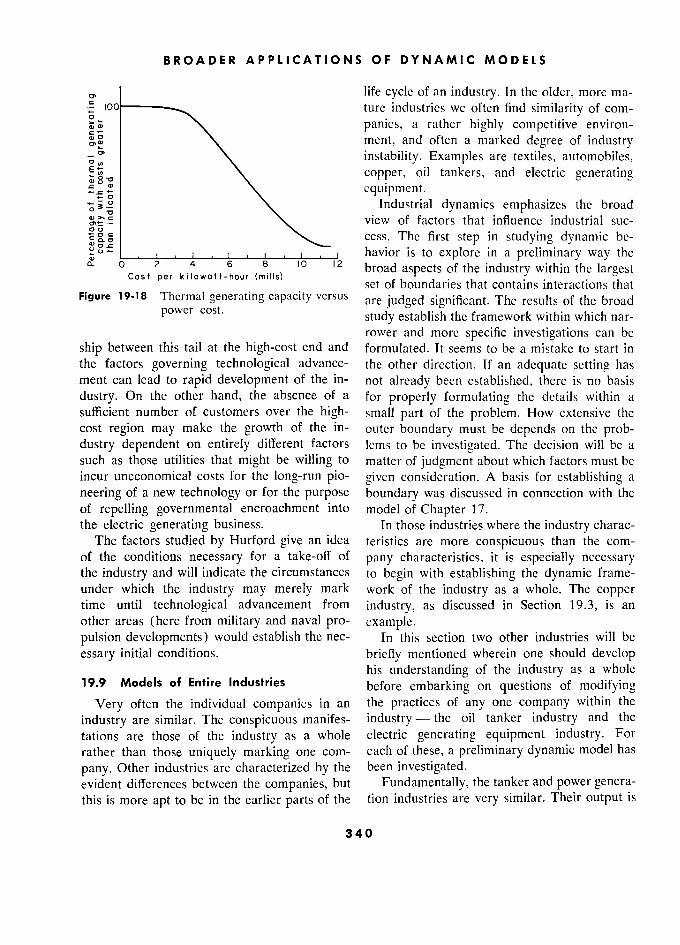
BROADER APPLICATIONS OF DYNAMIC MODELS S
life cycle of an industry. In the older, more ma-
ture industries we often find similarity of com-
S panies, a rather highly competitive environ-
S.3 \. ment, and often a marked degree of industry
- g°* instability. Examples are textiles, automobiles,
Er \. copper, oil tankers, and electric generating
\ equipment.
0 Industrial dynamics emphasizes the broad
\. view of factors that influence industrial suc-
g cess. The first step in studying dynamic be-
VOL ,___,_____. , havior is to explore in a preliminary way the 8 10 12 broad aspects of the industry within the largest Cost per kilowatt-hour (mills)
_ set of boundaries that contains interactions that Figure 19-18 Thermal generating capacity versus are judged significant. The results of the broad
power cost. study establish the framework within which nar-
rower and more specific investigations can be
ship between this tail at the high-cost end and formulated. It seems to be a mistake to start in
the factors governing technological advance- the other direction. If an adequate setting has
ment can lead to rapid development of the in- not already been established, there is no basis
dustry. On the other hand, the absence of a for properly formulating the details within a
sufficient number of customers over the high- small part of the problem. How extensive the
cost region may make the growth of the in- outer boundary must be depends on the prob-
dustry dependent on entirely different factors lems to be investigated. The decision will be a
such as those utilities that might be willing to matter of judgment about which factors must be
incur uneconomical costs for the long-run pio- given consideration. A basis for establishing a
neering of a new technology or for the purpose boundary was discussed in connection with the
of repelling governmental encroachment into model of Chapter 17.
the electric generating business. In those industries where the industry charac-
The factors studied by Hurford give an idea teristics are more conspicuous than the com-
of the conditions necessary for a take-off of pany characteristics, it is especially necessary the industry and will indicate the circumstances to begin with establishing the dynamic frame-
under which the industry may merely mark work of the industry as a whole. The copper time until technological advancement from industry, as discussed in Section 19.3, is an
other areas (here from military and naval pro- example.
pulsion developments) would establish the nec- In this section two other industries will be
essary initial conditions. briefly mentioned wherein one should develop his understanding of the industry as a whole
19.9 Models of Entire Industries before embarking on questions of modifying
Very often the individual companies in an the practices of any one company within the
industry are similar. The conspicuous manifes- industry - the oil tanker industry and the
tations are those of the industry as a whole electric generating equipment industry. For
rather than those uniquely marking one com- each of these, a preliminary dynamic model has
pany. Other industries are characterized by the been investigated.
evident differences between the companies, but Fundamentally, the tanker and power genera-
this is more apt to be in the earlier parts of the tion industries are very similar. Their output is
340
§ 19.9 MODELS OF ENTIRE INDUSTRIES
to perform a continuing service, in one case Electric Generating Equipment. At first ton-miles of oil transportation per year and in glance the ordering and production of electric the other kilowatt-hours of electric power per generating equipment presents a striking anom-
year. In both, the cost of the service is a small aly. The curve of electric power consumption part of the cost of the products into which it in this country is one of the smoothest and best-
goes. Both involve the construction of capital behaved time series in our economic life. At
equipment. They differ markedly in the stability the same time the placing of orders for electric of price of the final service - electric power generating equipment and the manufacturing of costs being very stable and tanker charter rates this equipment represent a classic case of one
fluctuating widely. Even so, they are similar in of our most unstable industries. Ordering rates
showing a wide cyclic fluctuation in the orders for new generators vary by a ratio as high as
placed for new tankers and new electric gen- 10 to 1, with a typical interval between peaks erating equipment. In both cases, the instability of five or six years. Manufacturing rates may seems clearly to arise out of the interacting vary over a ratio of 4 to 1. This fluctuation has characteristics of the participants in the industry existed for several decades. rather than from any factors that are imposed Such a high degree of fluctuation of industrial
by the final demands of society upon the indus- activity increases the cost of the product. On tries. the average, factory capacity is far from fully
Oil Tanker Industry. Two recent studies bear employed. Wage rates must be high enough to on the dynamic nature of the oil tanker charter compensate at least partially for the periods rates and shipbuilding fluctuations. One of these of unemployment. Expenses are incurred in
by Zannetos deals with the economic factors shifting production rates and finding and train- and the market expectations bearing on oil ing employees.28 These added costs must appear tankship rates.-5 His study develops an exten- in the price of the equipment and eventually in sive descriptive picture of the industry, derives the cost of electricity. The social cost to the numerical values for descriptive parameters, community and to the companies can be high and interprets industry behavior from the view- in poor labor relations and disruption of com-
point of traditional static and dynamic economic munity well-being. models. The dynamic study of such an industry shows
A coordinated dynamic model of the tank- how a combination of commonly accepted fac-
ship industry following the procedures outlined tors can interact to create a persisting instabil- in this book has been done by Raff.-6 Raff uses ity.23 some 230 variables to interrelate four activities It is characteristic in such an industry that within the oil companies (supply department, each participant blames the undesirable phe- chartering department, coordination depart- nomena on the practices of others. Here for
ment, and operating department) and three ex- example, the equipment companies feel that terior activities (tankship brokers, independent the trouble arises primarily from the manner
owners, and shipyards).27 in which the utilities place orders for equip- Sec Reference 18. Zg I have received informal estimates from indi- Sec Reference 13 for the S.M. thesis written viduals within the industry that equipment costs are
under the author's direction by Alfred I. Raff, gradu- increased some 20% by the inefficiencies of fluctuat- ate student at M.I.T. in the Department of Naval ing activity. Architecture and Marine Engineering, 1960. 29 A study of the dynamic characteristics of the
This study was carried to the point of a complete electric generating equipment industry is being car- operable dynamic model, the behavior of which was ried out as a research project by Alexander L. Pugh, generally reasonable, but not to the point of incor- III, in the Industrial Dynamics Group of the School of porating revisions resulting from analysis. Industrial Management, M.I.T.
341 1
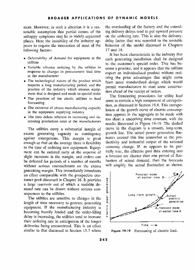
BROADER APPLICATIONS OF DYNAMIC MODELS S
ment. However, in such a situation it is a rea- the overloading of the factory and the extend-
sonable assumption that partial causes of the ing delivery delays tend to put upward pressure
unhappy symptoms may lie in widely separated on the ordering rate. This is also the delivery-
places. Here the instability of the industry ap- delay factor that was essential to the unstable
pears to require the interaction of most of the behavior of the model discussed in Chapters
following factors: 17 and 18.
... It has been characteristic in the industry that . Deferrability of demand for equipment at the each generating installation shall be designed
utilities , .... to the customer's special order. This has be-
. Variable advance ordering by the utilities in come a practice, and it appears that the utilities response to changes in procurement lead time
expect an individualized product without real- at the manufacturer
izing the price advantages that might come . The technological nature of the product which from more standardized design which would
requires a long manufacturing period, and the permit manufacturers to start some construc-
practice of the industry which stresses equip- tion receipts ? tion ahead ot thé receipt ot orders. ment that is designed and made to special order
The forecasting procedures for utility load · The practices of the electic utilities in load Thé forecastms procédures for utility Ioad * Thé practices of thé e ectlc utl Itles m toad .. ri... r .. i
forecasting
load seem to contain a high component of extrapola-
forecasting _ tion, as discussed in Section 19.8. This extrapo- . Thé existence of excess manufacturing capacity 1. .. f h h f 1 . -
in the equipment supplying industry capacity lation of the growth curve of electric consump- tn thé equipment supplying 10 us ry . ? , _, . L
?? . ? ?? inherent in increasing and de- tion appears in the aggregate to be made with
. Thé time delays 10 erent 10 mcreasing and de- . , ...
? The time ??ÎYS.???????? ?? ?Z??"??????? ??? too short a smoothing time constant, with the
creasing production rates at thé manufacturers . , creasing production rates ai the manufacturers
results illustrated in Figure 19-19. The dashed
The utilities carry a substantial margin of curve in the diagram is a smooth, long-term, excess generating capacity as contingency growth line. The actual power generation fluc-
against emergencies. This margin is great tuates around this line somewhat as the pro-
enough so that on the average there is flexibility ductivity and industrial output of the national
in the time of ordering new equipment. Equip- economy change. If, as appears to be par- ment can be ordered early at the expense of tially true, the effective past data entering into
slight increases in the margin, and orders can a forecast are shorter than one period of fluc-
be deferred for periods of a number of months tuation of actual demand, then the forecasts
without serious encroachment on the excess will amplify the actual fluctuation as shown.
generating margin. This immediately introduces an effect comparable with the prospective cus- Forecast made
,. „, <- at earlier time B tomer pool discussed in Chapter 16. It provides
° /./"
a large reservoir out of which a variable de- B , mand rate can be drawn without serious con- CI>
sequences to the utilities. Long-term growth Actual The .1.... h in the - Actual Thé utilities are sensitive to changes in the eiectric
length of time necessary to procure generating 0-- génération
equipment. If the manufacturing industry is forecast made
becoming heavily loaded and the order-filling 0 at earlier time A
delay is increasing, the utilities tend to increase W
their ordering rate in anticipation of the longer ––––––––––––––––––––––––––
deliveries being encountered. This is an effect Time
similar to that discussed in Section 15.7 where Figure 19-19 Forecasting of electric load.
342
§19.9 MODELS OF ENTIRE INDUSTRIES S
Extension of the period of slower growth as at pany may make a speech on the condition of
point A leads to a forecast of the future at his industry and cite the favorable near-term
point A'. A forecast made during the period of prospects and state or imply that order books more rapid increase in demand as at point B are beginning to fill up. The presidents of elec- leads to a forecast at point B'. Not only does tric utilities take note of these comments and
point B' lie above the actual demand curve, but encourage their engineering and operating de- in the interval from A' to B' the deficit repre- partments to advance their ordering dates ahead sented by the amount that point A' lies below of the rush on manufacturing facilities. This the actual demand curve must be made up in leads to a still more optimistic environment new equipment orders. Formal forecasting pro- within the manufacturing sales departments. cedures will usually recognize a longer base Surprisingly small amounts of this kind of posi- period from which to derive the prediction; tive feedback can produce substantial amplifica- but the shorter-range components of forecast- tion in an already oscillatory system. ing are apt to be introduced by psychological Another secondary factor affecting this par- variables applied in the managerial and finan- ticular industry is a repetitive pattern of price cial decision-making phases of placing an order. softening as the period of very low manufactur-
The existence of excess capacity for the man- ing backlogs develops. This likewise is a self-
ufacturing of generating equipment is an essen- perpetuating factor in which utilities come to '
tial component of the industry instability. If expect a period of price discounting. Some util-
capacity existed only for the long-term growth ities withhold and delay orders in anticipation rate, higher rates of equipment installation of a period of more favorable prices. By that would not be possible to create peak periods, time they may have deferred new equipment and the minimum periods would not be neces- ordering as long as they can, so that the price sary for recovery from the preceding excess discounting arrives along with a mandatory re- rate of installation. Excess capacity develops entry of the utilities into the equipment market. from the desire of each company to be in a posi- These combine and cause an accentuated order- tion to capture a maximum possible fraction ing rate. of the business during the upswing in ordering An even broader outside loop exists here if rates. Yet this motivation leads to a condition we should conclude that the manufactures of that accentuates the upswings that each com- electric generating equipment represent a large pany is attempting to capture. enough piece of the national economy so that
Other less tangible factors also appear to be the actual variable rate of manufacturing would involved and to accentuate the difficulties that contribute to the fluctuation of electric power would be created by the preceding combination generation. Certainly in the initial study of the of six industry characteristics. A strong psycho- behavior of such an industry, we should be
logical and speculative undercurrent seems to likely to take the country's use of electricitv as circulate within the industry. This can be exem- separable from the industry and to assume that
plified by the following sequence. A few addi- the connection is sufficiently slight not to inter- tional orders may be placed by utilities as part act from one sector of the industry out through of the upswing in cyclic business variation or the general economy and back into some other as a combination of random circumstances. sector of the industry being studied. However, These lead to sales optimism and to increasing the possibility of this type of interaction must
expectations within the manufacturing com- come up for consideration in dealing with the
pany. The president of a manufacturing com- larger industries.
343

CHAPTER 20
Industrial Dynamics and Management Education
Industrial dynamics views business as an integrated system. As such, it can provide an academic framework on which to assemble the other management subjects. Mathematical models provide a case method of interrelating as much richness of detail as necessary. Models make this detail specific and show how the system that has been described will evolve through time. Industrial dynamics can be taught as a brief exposure to introduce system concepts or can be extended to a major field with a thread running throughout an undergraduate and graduate academic program. Industrial history (of a kind dealing with the reasons for de- cisions and the life histories of industries, companies, and products) and also linear information-feedback theory are especially important support- ing fields for industrial dynamics. Management games have several points of methodology in common with industrial dynamics but fail to treat structure and policy in the business enterprise; they combine the shortcomings of both complete dynamic model research and real-life experience without the advantages of either. New challenges face aca- demic research in finding new management approaches to modern tech-
nology and economic development.
THIS chapter will relate system dynamics both teachers and students, than has been cus- to management education. The study of systems tomary in management schools. The impact on can provide a framework to unite subjects in academic research in management can be vast, the separate management functions. It can in- moving research away from mere data collection troduce the time dimension into what has pre- and explanation and into a position of leader-
viously been too static a treatment of the man- ship toward the design of more effective enter-
agement process. prises. Certain principles can be evolved that have A fundamental view of system dynamics does
general usefulness, but these should not be mis- not require the characterization of a system by understood by attempting a close analogy with the size of the institution - macro- and micro- the isolated laws of open systems as they are economics merge, and the growth of the small known in a field like physics. corporation fits a transient dynamic mold simi-
An academic program built around system lar to the development of a new national econ-
dynamics can be dramatic, challenging, and in- omy. The more successful we are in identifying tellectually demanding. It requires a different truly fundamental factors, the more universally emphasis in the selection and goals of people, they are applicable, whether in research man-
344
§20.1 1 INDUSTRIAL L DYNAMICS S AS S AN INTEGRATING STRUCTURE E
agement, production, or market dynamics, in taught in the colleges, it becomes the basis for transient or cyclical change, in management or future practice of the art, and returns as the economics. voice of experience to support future teaching.
Emphasis on system behavior removes exces- A comprehensive dynamic model can form sive attention from the particular business deci- a bridge between the case approach to manage- sion and places needed emphasis on the con- ment policy and the teaching of principles, trolling policy - policy as affected by both analysis, and functions. The case approach, formal rules and informal understandings, by based on discussion and argument, has the ad- organization, and by tradition, habit, past ex- vantage of broad perspective and integration; perience, and accepted practice. but it lacks precision, it may easily rest on
wrong intuitive estimates of the sources of dim- 20.1 l Industrial Dynamics as an Integrating culty, it is unreliable in tracing the consequences
Structure of policy changes, and it can perpetuate past ! One of the conspicuous weaknesses of man- misunderstandings. On the other hand, the
agement education has been that "the subject teaching of separate principles and corporate lacks a well-defined base or well-knit internai functions is necessarily done in isolation from structure." 1 This lack of integration appears the interactions with other functions; the prin- in the universities2 as a separation of educa- ciples and analysis methods tend to be static tional courses into functional areas. These frag- and fail to account for the paramount impor- ments are drawn together only in "business tance of the time variable; the managerial goals policy" courses or by case-method discussions. to integrate action and to lead advancement are
Attempts at integration by discussion of only lost, and for them are substituted description business cases can easily fail to perceive the and the mathematical goals of optimum solu- consequences of feedback interactions between tions to artificial problems. the separate facets of business. Misconceptions In a very real sense, the dynamic model is can persist because there is no experimental a business case. It can have as much richness or objective test of the opinions rendered. Class- of detail as one needs or has the patience to room situations are "solved" by using as a provide. It can handle any concepts and inter- guide the commonly accepted practices from the relationships that can be propounded in descrip- real-life management art. Here is another of tive language. But it can go further than the our information-feedback loops - the art is language. It can show the consequences of
_ , interlinking thé components of thé system that 1 Page ix of Reference t9 by Pierson. interlinking
the components of the
system that
2 And even the professional societies of manage- have been described. It can show how changes ment science tend to move away from an integrated in organization and policy will lead to a differ- concept of the management process. For example. The ent system character. It Can discipline diseus- Institute of Management Sciences has divided its ac- - - tivities into "colleges" (professional subgroups) that sion of the case by showmg w et er proposed disperse the membership into Managerial Economics, changes in management methods lead to im- Business Computer and Data Systems, Organization provement, are of no conséquence, or in fact Theory, Management Communications, Management
' Control Systems, Decision Processes, Simulation, make matters worse. Management Games, Planning, Research and De- The objection that a dynamic model cannot velopment Management, Management Psychology, incorporate the required subtlety and complete- and Measurements in Management. This compart- . - 1 mentalization is a caricature of the tendency to sub- ness must be dismissed. It has been amply
§ divide and specialize the subject until the manager's demonstrated by expérience in the use of reason for being, that is to integrate and coordinate, models in teaching that a dynamic model can
has search. been lost from management education and re-
encompass more system factors than can be held
345 5
INDUSTRIAL DYNAMICS AND MANAGEMENT EDUCATION
in proper perspective during a verbal discus- policy can be defined after knowing how sion. Whatever the shortcomings, they are in- broadly it affects the system and what informa-
herently less severe than doing without an or- tion it should recognize.3 derly structure for interrelating the parts of the The duties of the line manager and the staff
system that is under consideration. advisor will lose their présent conflicting objec- We can begin to integrate the separate tives as policy is more carefully distinguished
aspects of management when a common lan- from the resulting decisions. Now the line man-
guage and structure have been found that ager is presumably responsible for policy but
equally well fit the circumstances of produc- is too busy with day-by-day decisions to study tion, marketing, corporate policy, research and personally the nature of a wise guiding policy. development, investment, or human relations. The staff man is an advisor on decisions, but A language and structure are required that can he is the only one with time to consider policy, relate hypothesis to implications, and cause to yet he does not have the authority and responsi- effect. This seems to be provided in the meth- bility to put policy into effect. Clarification will
odology of Part II, Chapters 4 to 14: come with realization that policy and structure are thé principal déterminants of success. Thé
Levels (of inventory, knowledge, need, confi- are the principal determinants of success.
The
l' )§ § architect of the corporation's olicies and or-
momentary state to which the system has ar- ganization is the most influential person in de-
rived. termining growth, stability, and profitability. . Information about the state of the system is It is with him that leadership, authority, and
the ingrédient from which décisions are gen- responsibility should réside. He must have time
erated. and the ability to design the corporation. He
. Policy describes the procédure by which infor- will have the authority and the willingness °
mation is converted into décisions. Policy may takc risks that characterize today's line manager be formal or informal. It may rest on inescap- but will need the training and a detachment able physical characteristics of the system or from day-by-day problems that are now com- on habit, precedent, and folklore. monly associated with staff advisors. Décisions control the rates of flows to and from Historical experiences and present activity the levels. The evolution of the system through can be brought into a common frame of refer- time is created. This évolution shows the conse- ence. This will corne as rapidly as we succeed quences of the structure and polices that have in identifying those physical and human factors been used to describe the system. which tend to be constant but which cause the
The dynamic model represents a system as superficial and erratic symptoms that are dis-
broad as one chooses to describe. It gives tractingly apparent. For example, much is writ-
quantitative system results that follow from the ten on the acceleration of technological obso-
input assumptions. It allows a study of policy. lescence - how entirely new problems are
It therefore becomes a vehicle for integrating :' For example, in Chapter 18 it is suggested that h descriptive, h quantitative, and h case- "For example, in Chapter 18 it is suggested that the descriptive, thé quantitative, an thé case-
employment level must be controlled by over-all sys- discussion methods of management education. tem policy which recognizes sales rate, nature of the
The distinction between policy making and customer, inventories, and backlogs. The information
operations fades away when we realize that all sources and the policy-generating considerations are operations fades away when we broader than the scope of the production manager. décisions arise from some method (policy) of On the other hand, production efficiency (with pres- converting information into action. Policy can ently available plant equipment) has its sources pri- be studied at arly level from the k room to marily within the production department, and policy be studied at any level from thé stock room to the board of directors. The proper scope of a manager.
be established at the level of the production
346
§20.2 2 PRINCIPLES OF SYSTEM STRUCTURE E
created by the pace of new scientific develop- A common approach to levels, policy, deci- ment and its effect on the rapid revision of de- sions, and flow rates should erase the artificial
signs and products. This is often interpreted as distinctions that have grown up between studies
requiring a short-range view, justified by the of the company versus an industry, or between observation that today's product is obsolete the teaching of microeconomics versus macro- tomorrow. Whether or not there really is rapid economics. The same fundamental kinds of de-
change depends on our viewpoint and on the cisions, the same importance of structure, the level of abstraction of our thinking. Two or same need for some amount of aggregation ac- three decades ago product design may indeed cording to the same principles, the same pres- have been more constant. The required man- ence of uncertainty, the same perturbations agement policies were those governing the flow from "noise" in decisions and flow rates are all of materials and manpower into the continuous to be found, whether one considers the corner creation of the physical product. Planning drug store or international trade. These may needed to reach ahead only to the creation of differ in scope, in controversy, and in obscurity, plants and marketing organizations. Now prod- but they all fit the same conceptual structure. uct designs in many industries have a short .. life.4 Policies must have a somewhat différent 20.2 Principles of System Structure
emphasis. Rather than dealing primarily with Many places in this book have referred to the
the conversion of material into product, we deal "orderly underlying principles" from which sys- more with the conversion of men, ideas, money, tem behavior derives. It is too early in the study and laboratory space into designs. The continu- of system dynamics to attempt a comprehen- ous output of this system is a stream of new sive specific treatment of these principles, but
designs. Conceptually, this is still a conversion their nature is beginning to emerge.
process with inputs flowing into output. At this The principles to be discussed here all arise
level of abstraction, where our attention is in the context of information-feedback systems. focused on the conversion of resources into new They are systems principles. They are not the
designs, the time span of interest has actually principles of the management art such as have
lengthened, not shortened, compared with that been taught in organization, production, and
for the production line. Whereas in the "good human relations courses.
old days" the manager needed policies that phasis that has carried us from an agricultural so-
governed the planning of factory capacity, he ciety (where men grew their own food), to a craft now needs policies that govern the creation and trade society (where men worked on special products O a L directly for the consumer), to an early industrial so- p of a research g a much
ciety (where men used machines to make products longer process. The horizon has receded, not for unknown men), to our late industrial society approached. The continuous output was prod- (where men made machines to be operated by other
- men to make consumer goods), to automation (where uct, now it is new designs. Tlle difference is men design machines for others to make, which with- only a slight change in emphasis in system out men make products for men to consume), to an structure and policies. We had new designs "artificial intelligence" society (where men will lay
before, roduction sys- out the concepts that will be followed by machines, we still p now. e sys- to make machines, to make products that men will
tem is the same but with a shift in some param- consume). Economic evolution has followed a con- eters.5 tinuously deepening hierarchy of abstraction where
human endeavor is more and more distant from the end goal of satisfying human needs. When the process
. Perhaps artificially short to the detriment of finally bears fruit, a man-hour of effort produces an company success. ever-increasing standard of living by having been
' In fact, this apparent technological acceleration multiplied through the intervening sectors that lie is a continuation of the slowly changing system em- between human effort and consumption.
347
INDUSTRIAL DYNAMICS AND MANAGEMENT EDUCATION
Because the principles apply to systems be- sired levels. This process whereby decisions at-
havior, they do not fall into neat separate pack- tempt to adjust actual conditions toward desired
ages. We do not find here the equivalent of the conditions defines an information-feedback sys-
separate laws of thermodynamics, or of New- tem and sets the framework for model con-
ton's laws of motion, or Einstein's relativity. Of struction. A décision function is déficient un-
course, even those t... i ? and unre- less it is working toward some objective.7 This
course, even those are but incomplete and unre- does not working toward some
objective.7 This does not impiy that thé System must reach thé lated fragments of some broader future unify- equilibrium that is sought. The interacting r
ing concept.
- equilibrium that is sought. The interacting ef-
ing concept. . " . forts toward goals may keep the system con- The concept of a system implies interaction tinuously off balance.
and interdependence. In attempting to identify ? Many "worse-before-better" sequences are to be o Many "worse-before-better" . sequences are to be
factors that are common to all systems, we found where corrective forces first cause action must keep the essential indivisibility in mind.
opposite from the desired direction.s These can In certain contexts, the principles discussed be highly unstabilizing. They arise as part of the below are separable, at other times they may frequent conflict between short- and long-term better be interpreted as different views of over- considerations.
lapping phenomena. Amplification occurs at points where policies An information-feedback system dérives its attempt to adjust levels in the system to values
behavior from that change with varying flow rates associated
, s with those levels. This was seen in the inven-
D 1 tories proportional to sales rates in Chapters . 15 and 17.
o Amplification e Delays can create amplification by requiring It is a principle of dealing with such systems that input flow rates exceed the output flow for that we must look for the actual effective or- an interval long enough so that the delay ac-
ganizational structure and information sources, cumulates an internal content equal to the
not merely those that appear in formal charts product of the rate of flow multiplied by the
and operating procedures. We must watch delay interval.9
closely for the presence of delays, especially e Variability of delay can create amplification. A
those overlooked in informal information chan- variable delay can induce a variable inflow rate
nels and in the higher levels of management de- in an attempt to control the outflow.111 Also, a
cision making. Amplification is inherent in variable delay can cause amplification by vary-
many of the system policies, especially in the ing the outflow rate from a reservoir.Il
overt6 decisions.. Averaging or smoothing of data inherently
To point the way toward the kinds of princi- The outflow decision of a transportation system . ples of system structure that will émerge, 1 shall
delay is working decision of a transportation system delay is working to adjust outflow rate to inflow rate. list some of those that have been illustrated by after taking into account (implicitly) the required the two dynamic models in Part III, Chapters level of goods in transit. A purchasing decision is
15 thmitoh 1S-
' working (usually explicitly) to adjust inventories to
15 through 10. a desired level. The hiring action of a personnel of-
. All system decisions implicitly or explicitly con- fice is adjusting employment to the authorized level
tain the conce t of a desired state of affairs. of a factory work force. tain the concept of a desired state of affairs. Sections 10.6 and 19.3. Rates of flow in a system are determined by ° See Section 15.7.1. decisions, which are created by policies that '° As in the variable-delay supply pipelines in Sec-
ultimately rest on some attempt to bring actual tion 15.7.4. purchaser pool of Chapter r ...
" As in thé prospective purchaser pool of Chapter system levels into agreement with a set of de- 16 or in the release rate from the engineering depart-
° See Section 10.4. ment in Chapters 17 and 18.
348 8
§20.2 PRINCIPLES OF SYSTEM STRUCTURE E
causes a delay in the information.l2 Averaging behind changes in another. In those level and is necessary to remove meaningless noise fluctu- rate combinations that are herein called delays, ations from the data (as for example, sales in- changes in an outflow rate lag behind changes formation). The greater the noise in proportion in an inflow rate. It is typical of the other levels to the desired information, the longer must be that changes in the inflow rates lag behind the time over which an average is taken; the changes in the outflow rates.
longer the averaging time, the longer the infor- . Delays and policies are frequency-sensitive. mation is delayed. That is, they may amplify disturbances having When forecasting includes extrapolating past a certain interval of periodicity and attenuate trends and cyclic fluctuations (as it usually disturbances outside this rangea Also the phase does), it introduces a potential source of sys- shift and time delay between input and output tem amplification.l3 This amplification caused will depend on the frequencies of the dis- by an effort to anticipate the future can help turbance,16 produce a more undesirable future. Curves -. , . , , , ,. produce a more undesirable
future. .. Curves ? Delays are not inherently "bad." The effect of f be ?? and ?? ? ? order
o Delays are not inherently "bad." The efieet of need to be smooth and we - e ave in order , th a t th ey may b e ex t rapo 1 a t e d. mto th future. a delay depends on where it is in the system.l7 that they may be extrapolated into thé future.
e ay epen S on
w i
e em.
But the may are often derived from noisy Delays may produce either amplification or at-
But thé curves are 0 ten denved from noisy But the curves are often derived from noisy tenuation of disturbances depending on where d t The data are d t get th
tenuatlOn of dlsturbances depending on where data. The data are average get smooth
the appear.
is ur anees * - on w ere
curves, but this averaging introduces a delay. appear.
The further into the future that the curve is The preceding principles identify some of the to be extrapolated, the smoother it must be; factors of consequence in system behavior. but the more the data are averaged, the later is
principles for the formulation of models were the result. Because of the erratic nature of
re- o f th e aval n e m . ? 1 d b a bl e discussed in Chapter 5. General principles re- of the available industrial data, it is probable to specific that only a few curves can be meaningfully lating component structure ta speclfic over-all
extrapolated to the present, to say nothing of system behavior are ruled out at present by our
the future. inability to generalize about the nature of com-
. All levels (inventories, bank balances, skil, plex, nonlinear systems. Principles like the pre-
levels, etc.) are very similar in character to ceding can tell us what may be important. For
what we have otherwise isolated and called the present, the discrimination between those
delays. As we have used "delay," it consists of factors that may be and those that are impor- a level or levelsl4 whose input flow rate is con- tant must be obtained by putting the compo- trolled but whose output flow is uncontrolled nents into the context of the system and then de- and is generated by the internal structure of the termining the composite behavior and how that delay. The other nondelay system levels have outflow rates that ordinarily are directly con- 15 section 15.7.3 discusses how the distribution sys- trolled and where only indirect control exists tem of Chapter 15 selects and amplifies from a noise '
over inflow (as in the ordering of goods to input those frequencies that are near the natural
replenish inventory). The policies for system period of the system. See also Appendix G.
control are usually designed to attempt to '° Appendix 1 shows how the output of a system can - ' ° .. , ' , lag the input at some input periods and actually lead
maintain some specified quantity in the level. thg input at other pà periods and actually lead
All levels, whether in what we have called de- 17 ln Section 15.7.7 increasing the delay in the
lays or elsewhere, serve to uncouple one rate adjustment of inventory was one of the most power- of flow from another and thereby cause (or ful parameters for reducing system fluctuation. In
in one rate to lag Chapter 18 the new policies for improved stability make it possible for) changes m one rate to !ag were based on longer rather than shorter delays in adjusting employment and inventories (in spite of the
l2 See Appendix E. fact that in the original system the system was less i2 See Appendix L. Also see Section 19.8. stable as the delay in changing employment was in- 14 See Section 9.3. creased).
349
INDUSTRIAL DYNAMICS AND MANAGEMENT EDUCATION
over-all behavior depends on the separate com- sophomore year through the doctoral thesis
ponents. level.
Enterprise design, through the use of dy- 20.3 Academic Programs in Industrial namic models, provides an opportunity for a
Dynomics new kind of laboratory work in organizational The treatment of industrial management as theory and management policy. To a certain
the organization and control of a system, and extent, the student can begin in his academic the use of models to permit experiments in program to gain experience in the management system behavior, can provide an integrating of industrial systems.1° structure for the teaching of management. This System dynamics and the associated models can create motivation and effective "synthetic provide information feedback in the educational
experience" in policy making. The study of process itself. An idea can be developed, it can
system dynamics can be introduced at the be- be set up as an experiment, the results can be
ginning of an undergraduate academic program evaluated, and the idea can be revised. This and continue through the doctoral and Execu- sequence of invention, experiment, evaluation, tive Development Programs. At the Master's and review has been illustrated in connection and doctoral thesis levels it provides a means with the models of Chapters 15 through 18. for experimenting with new hypotheses and Such work provides an environment in which
concepts of management organization and pol- it is possible to observe and evaluate certain of
icy. the personal characteristics of students which
Pu'rpose. Industrial dynamics in the manage- do not show up clearly in courses where ma- ment curriculum should unify y the other subject terial is studied and examinations test primarily matter of management. It should tie together the memory of facts. In converting descriptive functional areas and should add the time di- knowledge to a dynamic model, the student is mension. It should create an understanding of faced with a need to identify a problem, to visu-
growth and of system-created change in indus- alize the dynamic concepts which are at work, trial operations. to show initiative and judgment in selecting the
Gordon and Howell stress the importance of factors to be incorporated, to cope with un- an integrating course in business policy.l8 They certainty and incomplete information, and to
suggest that such a course must be of the case- supply inventiveness in seeking system improve- study variety and must come in the senior year ments. of an undergraduate curriculum. Section 20.1 A sequence of systems courses should at- discusses how the dynamic model can give tempt to instill in the student several attitudes:
rigor and precision to the discussion of a case. e That there are f un d amen t a 1 c h arac t, ens t. lCS of f o That there are fundamenta) charactenstics of
It seems clear, however, that such an approach systems which apply whether these systems be should not be limited to a single term or even electrical, mechanical, chemical, biological, cor- year. The student does not assimilate the feeling porate, or économie for systems behavior quickly. For full effect, . That there are important interactions between the student must be steeped in a combination the parts of a system and that thèse systems of theory, analysis, laboratory work, and design _ _ _ _ over a considerable period of time. There is '° In fact, 1 have seen this type of artificial experi- over a considerable ? of time. There is
ence carry a research team of graduate students so certainly material here to be developed well far into the understanding of the problems of one
beyond that which would be required to carry corporation that an executive of the company made
a continuous thread from the beginning of the the succinct comment, "It is clear that you already '-' ° know more about the way this product is managed
18 Pages 206-208 of Reference 20. than anyone in the company."
350
§20.3 3 ACADEMIC PROGRAMS IN INDUSTRIAL DYNAMICS S
interactions are often of greater consequence study of more complicated systems by using than the individual characteristics of the com- digital computer simulation if a suitable ma-
ponents chine is available, and individual and group . That static analysis is an inadequate tool in projects in formulating models of industrial
dealing with the managerial environment situations.
e That our intuition is unreliable in anticipating a Classroom simulation, with students playing the the behavior of complicated information-feed- part of various components of the system, can back systems be used to demonstrate the principles discussed
. That the experimental model-building approach in Section 20.2. Group simulation shows in a
is a powerful tool for handling situations that more personal and dramatic way than mere
are beyond the grasp of intuitive or analytical computed curves the behavior of larger systems. mathematical solution It can also show convincingly that the environ-
_ ment is a strong determinant of the "free-will" Teaching Procedure. Management, like en- decisions and that the "obvious" best action is
gineering and medicine and architecture, is a often so powerfully dictated by available infor-
practical profession dedicated to achieving spe- mation that intuitive decisions by different peo- cific goals. The successful practitioner must be ple are surprisingly alike.
highly motivated toward accomplishment. The Even if a digital computer and automatic pro- end justifies the effort necessary. It therefore gram compiler are available, emphasis should seems inappropriate to spend long years devel- be placed on hand computation of simple dy- oping foundation subjects before giving the namic sequences. A well-chosen example is student an opportunity to view the objective. highly informative. Furthermore, the time re-
The experimental study of system dynamics quired to do the computation gives the student
does not rest on any mathematics that cannot an opportunity to watch the progress of a dis-
be taught in a few days any time after the high- turbance as it is propagated through the system.
school level. An education in industrial man- Simple effects such as a step-function input to a
agement could therefore begin with a study of supply pipeline are highly informative. By con- agement cou!d therefore begm with a study to °
verting some of the delays from exponential to quantitative system dynamics closely coordi- discrete delays, and by lengthening the solution nated with verbal industrial dynamics, in the interval to approximately a week, one of the form of history and the reading and interpréta- stages of the distribution system of Chapter 15 5 tion of the current daily and weekly business cornes within the range of practical hand com-
press. Such an approach would bring forth putation. With proper coaching, the student both the underlying fundamentals of business can study the way in which rates integrate
activity as well as the superficial manifestations into levels, the way in which delays cause
of its problems. Such would then become a mo- amplification, and the ways in which differ-
tivation for the study of science, engineering, ent décision policies affect the system. As an
finance, human relations, economic develop- fl example of the latter, he can experiment with
ment, politics, and the other facets of manage- various omissions and additions in the pur- ment, pohtIcs, and thé other facets of manage- h.. f d..b' t
. . ment.
po i ics, an e o er ace s o manage- chasing équation of one distribution stage in
ment. Chapter 15. Based on some three years of teaching of
15. , ,
industrial dynamics, several suggestions have In teaching industrial dynamics the instructor
developed: dynamics, " several sUgges hâve
must be careful to concentrate on the concepts s °
of business and how to express and interrelate a The subject is effectively taught as lecture and the business factors rather than to be carried
discussion combined with various forms of labo- away by the techniques and the methodology. ratory work. This laboratory work can include There seems to be a tendency to elaborate the hand computation on simple examples, the mathematics and the methodology beyond that
. , 351 1

INDUSTRIAL DYNAMICS AND MANAGEMENT EDUCATION
justified by any real effect on the qualitative tion arising from both within and without the nature of the results. In so doing, the goal of functional specialty. An understanding of the business behavior can be easily submerged by separate functional areas is obviously essential the unnecessary refinement of technique.2° to their inclusion in an over-all system. Some
. A number of new staff members of manage- academic subjects whose pertinence to system ment S'h°°'S now have training in engineering. dynamics is not so obvious justify special men- Some of these men show a strong tendency to tion.
cast management problems into the vocabulary Goods history of economic systems, of indus- of the engineering field. There is no more reason y
of the engineering should There dealt with in terms tries, of companies, and of special projects can why management shoutd be deatt with in terms compames, and of spécial projects can
of capacitors, resistors, vacuum-tube circuits, or serve as the descriptive raw material for the e
hydraulic flows than there would be for teach- construction of dynamic models. Such history ing engineering in terms of inventories, average must of course contain the descriptive material
sales, and accounts receivable. The subject must relating to the important factors. Such history not be handicapped by the insistence on an is hard to obtain. Often the reasons for deci- artificial conversion of vocabulary. sions, which may have been evident at the time
e The availability of a modern, large-scale digital within the committee meeting or the board of computer lends drama, vitality, and scope to directors meeting, are not recorded in the min- the teaching of experimental system dynamics. utes and not available to the historian who The teacher of such a course should have had cornes on the scene late. The recollections and experience in the building of models of rather
even many of the contemporary documents are complex systems and their simulation on a
apt to be biased in favor of the way the system digital computer. However, for an instrtictor should operated decisions should who bas had this expérience and who has justi- should have operated and the decisions s ou who 0 as had this experience and who 0 as JUs 1- $
. fied confidence in what he is doing, 1 believe have been made, rather than the way in which
that a very effective course can be taught on they were. History does not often enough treat
the basis of hand-computed and group-simu- the interacting forces of organizational stresses, lated examples. The unavailability of a modern personal interest, technological factors, reluc-
digital computer is to be regretted but need not tance to reach decisions, conflicting objectives, prevent the teaching of industrial dynamics. and the multitude of circumstances that eventu-
Related Subjects. The functional subjects in ally resolve themselves into a course of action.
thé separate management areas should treat the e Likewise, history does not adequately record
forces at work within the individual areas and the alternative courses of action that might have
show how decisions are influenced by informa- been taken in an attempt to analyze what the
ensuing consequences might have been. 2° Students at M.I.T., even those having no previous A perceptive history of past managerial situa-
experience with a digital computer, receive but one tions is one of the inputs to the better under- or two hours of lecture and description on the DYNAMO compiler described in Appendix A. Beyond standing of system dynamics. The ability to this they are able and are expected to use the modern build models of complex systems and to study digital computer as a research tool by reading an their behavior should make historians more instruction pamphlet and receiving some coaching .. , . from a laboratory assistant. Here is an example of a sensitive to the important system variables.
place where the instructor might be tempted to insert They should try better to search out and record a lengthy interlude on digital computers and com- the "policies" that tell how actions and pres- puter programming. This is not necessary. With rea- sonably adequate written material, it can be left to the sures influence décision making. _ student, just as is learning to use a slide rule. The In a quite different area, the courses taught in class presentation should concentrate on management servomechanisms in many engineering depart- staff systems advisor. from
the viewpoint of the manager, not the ments provide an excellent background for the e
352
§20.3 3 ACADEMIC PROGRAMS IN INDUSTRIAL DYNAMICS S
study of industrial systems. A good foundation available, making a full academic year as op- in linear systems analysis develops an intuitive tional subjects. To the Sloan Fellows (men be-
understanding and keen perception of the kinds tween 30 and 40 years old sent for a full cal- of factors that give information-feedback sys- endar year by their companies to M.I.T. ) the tems their typical behavior characteristics. subject was taught for three class hours per However, the problems of industrial dynamics week over a period of seven weeks, in addition are too complex for analytical treatment. to which there were nine hours of guided labo-
Although the fundamental principles of or- ratory work. The Senior Executive Program (a dinary information-feedback systems are ap- ten-week series for industrial executives in the
plicable, the quantitative nature of industrial age bracket of 40 to 50 years) contained an and economic systems can be quite different introduction to the subject consisting of six from what the engineer ordinarily encounters. lecture hours. We do not have here the simple, single-loop In addition to the academic work, theses at control systems in which there is one point of the undergraduate senior, the Master's, and the error detection and one place where error-cor- Ph.D. levels have been based on models of dy- recting control is exercised. Error detection and namic behavior. Several of these have been dis- control are both distributed throughout the cussed in Chapter 19.
system. Every decision point constitutes both. Future extension of the present two courses
Many of the practical design procedures devised at the graduate level might take the form of four for engineering systems are not applicable to consecutive one-term courses (the typical social systems. Many of the methods that have M.I.T. Master's degree graduate program in been useful in engineering systems work be- management is of two years' duration). The cause of the special characteristics of those sys- first of these, as at present, would follow the tems. Engineering systems tend to be designed subject matter of this book along with labora- and used in such ways that the normal operat- tory and classroom exercises as discussed
ing frequencies, the natural frequencies of the above. The second term, as at present, would
system, and the impressed noise frequencies continue to be on advanced industrial applica- tend to fall into different frequency bands. This tions, with experience in interpreting new situ- does not seem to be true in our industrial sys- ations into a mathematical model structure. A tems. The disturbing noise, the natural fre- third course (now available as a series of sub-
quencies of the systems, and the frequencies to jects in the M.I.T. Department of Electrical which they are expected to respond all fall Engineering and taken by staff members and within the same frequency band. It is my belieL doctoral students in industrial dynamics) would that the formal theory of servomechanisms will deal with Laplace transforms, transient re- continue to be an important part of the educa- sponse, frequency response, quantized-data sys- tional background of those taking leadership tems, smoothing, data filtering, and random in the field of industrial dynamics, but that signals. A fourth subject might build on the first servomechanisms theory will not be directly three, plus courses in economics, to treat the used as an experimental and operating tool. dynamics of economic systems.
M.I.T. in 1961. In 1961 industrial dynamics As has been typical in other subjects in the was included in each of the four programs of past,21 the material in industrial dynamics, as the School of Industrial Management at the Massachusetts Institute of Technology. At the n For example, courses on digital computers that
undergraduate senior and the graduate student were taught in the M.I.T. graduate school in 1949
levels, two consécutive Orie-term courses were high and 1950 schools. are a decade later available in a number of
353
INDUSTRIAL DYNAMICS AND MANAGEMENT EDUCATION
developed first in the graduate school, is being 0 Selecting the factors to be dealt with
adapted into the undergraduate teaching of a Constructing a formal model of the preceding management. Throughout the undergraduate. Using the model to simulate system interactions program, systems studies could provide an inte- under selected conditions
grating vehicle for the functional subjects and . Interpreting the significance of the simulation also bring in continuously the nature of indus- results trial behavior, its problems, its managerial chal- . Inventing system improvements lenges, its history, and its current press.. Repeating all of these steps to move doser and
closer to the true problems and to better man- 20.4 People agement policies.
In discussing how the characteristics of peo- ple fit them to make use of the methods of in- Starting the student on the techniques of the
dustrial dynamics discussed in this book, we seventh and eighth items (constructing a model
must distinguish between two levels of interest and using it) can be a very effective initial in-
and intent - for general student background troduction to the subject of industrial dynamics. and intent - for general student background
on the one hand and on the other, for research, It gives an opportunity for the student to pre-
management, and educational leaders who ex- view the more tangible aspects of the subject
pect to use the subject seriously. and to sample the nature of the goals. The real
For the ordinary student of management, managerial content, however, lies in the first
industrial dynamics can be included in the cur- five items on problem definition and in the last
riculum to almost any extent from a few lec- three items on interpretation of results and sys-
tures upward. At any level of intensity it will tem improvements. ,
give some enhancement of the concept of busi- This brings us to the second type of person ness as an integrated system. If properly taught
man who is preparing himself to be a
in relationship to the backgrounds of the stu- leader on either the academic or the industrial
dents, it can be fitted to almost any level of front. ,
previous mathematical preparation. Herein lies The teacher or the enterprise designer, unless
a danger. The techniques and the methodology he is also an experienced and competent man-
appear very simple. It is too easy to create the ager, may concentrate overly long on the tech-
impression that a single graduate course or one niques of the seventh and eighth items. Con-
academic year of study can cover the ground structing a model and operating it are the most
and can produce students who are expert in sys- tangible of the steps and also the easiest. Unless
tems analysis. great diligence is exercised, some simple and
The difficult part of industrial dynamics lies arbitrary assumptions will be made to substitute
in the question of what problems to attack, and for the difficult perceptual and conceptual steps what factors to include as pertinent. The steps
of the first six items. Furthermore, after a model
in an industrial dynamics study are is constructed and simulated, simple observa-
... tion of results is likely to take the place of . Defining the objectives of the system under thoughtful interpretation of the reasons for the
study , results. Invention of system improvements
. Observing symptoms based on promising hypotheses that are then
. Detecting the real problem explored in the model may give way to mere
. Visualizing the system at issue trials of randomly chosen parameter variations.
. Estimating the boundaries within which lie the The teacher or the corporate staff research causes of the trouble man who is narrowly oriented toward methods
354

§20.4 PEOPLE E
can here fall into the same practices that were velop some impressions of the kind of training criticized in the Introduction with regard to that a man needs to become an effective leader
operations research in business - the emphasis in industrial dynamics. He must of course be on the methodology may replace the emphasis interested in the subject. He must be interested on management. To maintain the proper per- not merely in gathering information and under-
spective with regard to systems dynamics and standing systems, but he must also wish to move the managerial objectives requires a man with into system redesign and improvement. He breadth of viewpoint. He must be interested in needs high integrity. He should have the per- the objective of improved systems, not in merely sonality that makes it possible for him to delve the method of analysis. Yet he must at the same into sensitive and embarrassing corporate cir- time guard against breadth without depth, an cumstances and deficiencies without alienating approach that leads to a superficial treatment people. of subtle and complex problems. Regardless of his background he should work
So far, we are finding two types of men to be his way up through the formal theory of linear the most successful in this work. One type is and sampled-data systems to the level of two or the man whose interests are centering on the three graduate courses in the subject. If he lacks area of business management but who has had a background in differential equations and formal training in the analysis of information- engineering, this may involve three or more feedback systems (obtained in the study of preparatory undergraduate courses before he
mechanical, electrical, or hydraulic equipment), reaches the graduate-school level of systems and preferably has also had laboratory work study .22 Such a sequence of courses in dynamic and first-hand experience with such Systems. -2 A sample sequence of related courses selected d samp)e séquence of re)ated courses setected The second type of successful man is the un- from the M.I.T. catalogue follows. Most students usually compétent and perceptive indus trial undertaking a study in depth of industrial dynamics
manager. He also has dealt with complex in- will have at least part of the following material, and _ P others may find it possible to abbreviate the sequence formation-feedback systems in the true-life en- in various ways. This intensity of training in systems
vironment. Even better, there are many men theory is appropriate for the doctoral candidate whose now becoming available with both kinds of emphasis
is in industrial dynamics. Courses in Elec-
Ca abilitles. ° uL trical Engineering are indicated by the number 6;
p courses in Mathematics by the number 18. There is To be successful, a man needs a good feeling no reason why the subject matter of these courses
for system dynamic, and also he must under- might not be taught in the economics and business -' context, but so far it has not seemed necessary to stand the factors that go into managerial deci- duplicate material of the same underlying philosophy sion making. He needs a strong motivation merely to get a change of vocabulary (so long as the
toward deeper insight into better management. more complex business systems are taught in the busi- ness vocabulary). In time, the systems theory repre- By contrast, we have had much less success in sented in these courses could be adapted and some- the industrial dynamics work at M.LT. with what shortened into a theory sequence for students those trained primarily in mathematics, in con-
of management.
ventional operations research, and in mathe- 6.01 lntroductory Circuit Theory ,.. .. , ..., , Two-term sequence for students majoring in
matical economics. Men who are narrowly in- electrical engineering. Network topology and terested in these latter areas seem often to lack topological aspects of duality, Kirchhoff's one or all of the essential qualifications of laws, volt-ampere relations
for the elements, , " and sources of excitation. Equilibrium equa-
dynamic systems intuition, motivation, and un- tions and methods for their solution. Step derstanding of the real-life business processes. function and impulse response of simple cir-
After trying various shortcuts without nota- Sinusoidal their complex natural frequencies. ., , Sinusoidal steady-state behavior. Impedance as ble success, we have at M.LT. begun to de- a function of applied and natural frequencies
355 5
INDUSTRIAL DYNAMICS AND MANAGEMENT EDUCATION
theory can be studied in parallel with material study to the Ph.D. degree is usually thought of such as presented in this book. This book does as preparation for teaching. Such was the atti- not depend directly on such material, and yet a tude toward advanced graduate study in engi- proper interpretation and understanding of the neering twenty-five years ago, but now, doctoral material discussed herein will be greatly en- study is a common step in the route to top in- hanced by an understanding of the subject mat- dustrial technical positions. As the professional ter of linear dynamic theory. challenge in management becomes more de-
Along with the preceding material, the stu- manding, the need will grow for greater depth dent can study functional subjects of manage- of training in the academic program for man-
ment, economic and industrial history, and read agement. The trends that we have seen in the
regularly the daily and weekly business press. other professions can be expected to develop As the nature of management education in management. Advanced study will initially
changes, the place of doctoral level study in prepare men for teaching. But as the manage- business will also change. At the present time ment profession evolves, advanced study will
and its geometrical interpretation in the com- solution of classical equations of mathematical plex frequency plane. Resonance phenomena, physics. Sokolnikoff and Redheffer, Mathe- amplitude and frequency scaling, vector dia- matics of Physics and Modern Engineering. grams, reciprocal and complementary im- 6.601 Feedback Control Theory Prerequisite: 6.05 pedances. Energy storage and dissipation; active and 18.05. Graduate Subject. and reactive power. Mutual inductive coupling. Models for physical systems, block diagrams, Polyphasé circuits. Usefulness of the duality Laplace and Fourier transforms, stability cri- principle given prominence throughout the dis- teria, transient response, frequency response, cussions. Closely correlated laboratory work performance indices, and compensation schemes accompanying lectures and recitations. leading to trial-and-error design procedure for
6.02 Electronic Devices and Circuits Prerequisite: linear control systems. Properties and effects of 6.01 stochastic signals. Introduction to nonlinear sys- Basic subject for students majoring in elec- tems, sampled and quantized-data systems, trical engineering. Circuit models for electronic and optimization theory. Newton, Gould, and devices such as transistors, vacuum tubes, gas Kaiser, Analytical Design of Linear Feedback tubes, etc. Analysis of basic electronic circuits Controls. using nonlinear curves or piecewise-linear ap- 6.54 Sampled and Quantized Systems Prerequisite: proximation for nonlinear operation and in- 6.601. Graduate Subject. cremental models for linear operation. Asso-
Development and application of linear analysis ciated laboratory. techniques to design of discrete systems and to 6.05 Electronic Circuits and Signals Prerequisite: related problems. z-transform methods. Proc-
6.02 .... esses of sampling continuous data and of Basic subject for students majoring in elec- smoothing sampled data. Feedback systems em- trical engineering. Fourier representation of ploying sampled-error data, including stability signals. Modulation, amplification, and genera- studies of such systems. Study of continuous tion of electrical signals. Limitations on signal systems by numerical methods. Digital com- transmission imposed by inherent energy stor- puter operations as data filtering, analysis and age, noise, and saturation in electronic systems. synthesis of linear digital computer programs in Associated laboratory. frequency domain. Development of a circuit
18.05 Advanced Calculus for Engineers Prerequisite: theory for sampled and mixed systems making Differential Equations. Graduate Subject. use of flow graphs. Comparison between tech- Vector analysis; orthogonal curvilinear coordi- niques of numerical analysis and control sys- nates. Functions of a complex variable; calculus tem design. Response of sampled-data systems of residues; conformal mapping; ordinary dif- to random inputs. Study of quantization and ferential equations; integration by power series; round-off noise in numerical solution and real- Bessel and Legendre functions. Characteristic- time control. Analysis of errors in computation. value problems; expansions in series of or- Study of random Markov processes by sampled- thogonal functions, including Fourier series. data analogs. Design of statistically optimum Partial differential equations; characteristics; discrete systems and adaptive systems.
356
§20.5 5 MANAGEMENT GAMES S
become a normal channel to the higher mana- proper faculty guidance, take a responsible part gerial positions.23 in the growth of industrial dynamics. He can
The development of a stronger foundation of help develop underlying methods and tech-
management science will not change the fact niques. He can interpret industrial problems that management is an art. The better managers into systems structure. If he has the proper will still be the ones who have the judgment to personality characteristics, he can work within use their tools in the proper places. There is an industrial organization to delve into the not soon to be in management, any more than mode of operation and to interview the several in engineering, law, or medicine, an orderly management levels until the factors influencing
procedure for identifying the worthwhile goals decisions begin to clarify. The better of such
or the road to them. Therefore, the full develop- men often come out of full-time research as- ment of an expert in the field of industrial dy- sistantships (after three or four years, or more namics requires an opportunity for him to gain if they have earned both S.M. and Ph.D. de-
experience, to test judgment, and to build self- grées) with published papers and a national or confidence. This seems to require some form international reputation for their pioneering of internship. work. After a combination of study and prac-
An effective internship has been provided at tice, the man becomes capable of taking leader- M.LT. in the form of the full-time research as- ship in new academic programs or in setting
sistantship for the graduate student. In the up a new activity within an industrial company. School of Industrial Management this is pat- terned after the program which has been highly
20.5 Management Games
effective in M.I.T. engineering departments Management games have received much at-
during the last three decades. The full-time re- tention, both in academic circles and as a cor-
search assistant works at a new frontier of porate tool for executive training. Because of
knowledge in an atmosphere of serious, timely the publicity that management games have re-
importance. The work usually takes the form ceived, it is necessary to comment on them
of developing and applying new methods to the here. This is especially so because they super- solution of problems that are of intense interest ficially appear very similar to the dynamic to an outside cooperating organization. He models in this book, and yet educationally they works on new concepts and methods and on move almost in the opposite direction.
their conversion into use. The man is expected As used here the term management game to be a responsible member of his research means a situation in which part of the industrial
project, devoting full time to it except for the system is represented by a dynamic model, but
time actually in class. His graduate thesis is certain of the information flows are presented
usually closely related to his staff work, so that to a person who makes decisions and inserts
the two mutually support each other. He can his decisions into the system as the simulation
progress in his graduate study at a rate about progresses. Most often there are a number of
half that of a full-time student. people involved who, along with the simulation
A carefully selected full-time research as- carried out by a computer or a referee, make
sistant at the graduate school level can, with up the entire business process being repre-
? See Leavitt and Whisler, Reference 7, for addi- sented. tional discussion of how the future entry point to There are some close similarities between the
upper-management positions will more and more be business game and the full dynamic model. In through special training rather than by working up the dynamic model, as discussed in this book, through the lower administrative levels of the cor- ' ' '
poration. all parts of the system and all policies are
357
INDUSTRIAL DYNAMICS AND MANAGEMENT EDUCATION
represented by decision rules that are mecha- already believes them to be, can do nothing but nized by a digital computer. In the business accentuate already existing misconceptions. For
game most of the system is represented by example, at least one of the very popular early formal policies within a computer, but a few management games involved a research-and- of the decisions are made by the human par- development expenditure in which the profitable ticipants as the game progresses. In both there pay-off from research and development occurred is a mathematical model, usually there is a within two or three quarter-years after the
computer, both concentrate on the business expenditure. This is so untypical as to be
system, and both aspire to enhance understand- seriously misleading, especially to the partici- ing of the broader business scope. Here the pant who already underestimates the time similarities end. required to achieve research results. In this par-
The management game has the combined ticular case, the defense of the short time con-
shortcomings of both the full mathematical stant by the designer of the game was merely dynamic model and also the learning process that longer time constants would take so long from real-life experience in an operating com- to react that the effects would not be visible
pany. At the same time, it lacks the principal within the one day of playing available to the
advantages of either of the other two. Like the participants. real-life business system, the participant in the The management game, if it teaches any- game views the remainder of the system as a thing, is usually defended as illustrating good black box that he attempts to poke and prod decision-making practice. This means good with his decisions to see how it responds. In a practice as viewed by the designer of the game. complex nonlinear system this is disappoint- Game designers have not ordinarily been great ingly unrewarding. Even if the model in the managers skilled in innovative advancement of black box were a good one, and truly repre- the management art. The game then becomes a sented the particular business of interest, he vehicle for perpetuating the past clichés about still would not be able to fathom its complexi- what constitutes good management. The game ties by this type of external teasing. is designed to reward the kinds of decisions
The emphasis in the business game is on the that the game designer thinks are proper. The external manifestations, not on the internal player is therefore being trained in the patterns structure and its implications. In fact, the in- that the game designer intuitively believes to ternal structure gets relatively inadequate at- be preferable. Any manager who plays the tention. The design emphasis is on achieving a management game for the sake of learning better
superficial external appearance of reality, highly management should examine carefully whether
tempered by pressures to enhance the theatrical or not the game judges his decisions in a way effect. We need only observe typical examples that is significantly related to the way his deci- of such games to immediately detect misleading sions react in his own company. compromises that have been introduced in the The management game has often been com- interest of showmanship. pared with devices like the Link cockpit trainer
The most conspicuous warping of reality in for the training of aircraft pilots. This is a good game design is in the direction of shortening analogy and immediately shows up the short- the pertinent time constants of the system. Most comings of the method. The Link Trainer is
managers think they can get systems responses designed to enhance and ingrain automatic re- much faster than in fact can be accomplished. sponses in the trainee. The kinds of situations The management game, by shortening these to which he is to respond are designed in ad- time constants even more than the manager vance. The relationships are relatively simple
358
§20.5 5 MANAGEMENT GAMES S
from the standpoint of the system designer. The the interacting parts of the management system. information to be presented to the trainee is This is Before, the player may have had
predetermined. In fact, it is no great intellectual only an intellectual belief in the importance of
step to set down the precise formal rules that interactions between parts of the system. He the trainee should follow to get the best pos- may come away from the game with a deeper sible response out of the system. This has been done in fully automatic autopilots for aircraft.
In connection with industrial dynamics studies, we In a sensé, the pilot trainee is being processed have connection with one day dynamics studies, we g ,P , 8 have often devoted one day to a hand-computed through the Link Traïner because he is the game that is a simplification of the model described most available and least expensive machine to in Chapter 17. The game consists of putting the
carry out a predetermined set of policies regard- student in the position of the production manager of
_ r b the company supplying components. He has but one ing data analysls and décision making. By con- decision to make: the number of people to be hired trast, the Link Trainer is of practically no or released from the production work force each
value in designing a new, différent, and im- regarding is told the général structure of the system ° . ° ' ' regardmg the delays m the transit of orders from the
proved type of aircraft. The cockpit trainer has customer to the production department. He is given been designed and adjusted until it reacts the union contract conditions regarding termination
sufficiently like a particular known actual air- notice to employees, and is told how long the training S l y l.
e m aii period is for new employees before they can become
craft so that it serves the purposes of obtaining productive. He is also given an unusual piece of in- emotional involvement from the pilot, presents formation not normally available to the production to him the typical kinds of information, and manager, to the effect that the customer is rigidly to
him thé typical kmds information, and
following a formal decision process for generating recelves and acts plausibly well on his reac- his orders for components. The forcefulness of the tions. It need not, however, contain any true environment in predetermining the participant's de-
cisions can be adjusted by changing such things as appreciation for the underlying causal factors
the length of the employee termination notice, the " the length of the employee termination notice, the that make the behavior what it is. The aircraft training delay, and the constant CISTC in Equation designer goes instead to his wind-tunnel model, 17-89 that determines the extent to which customer
his mathematical r inventory varies with delivery delay. The production his mathematical models of aircraft behavior manager makes one hiring or layoff decision each
to be solved on a computer, and his considéra- week (represented by perhaps 5 minutes of real time). tions of performance objectives in order to bring By proper selection of coefficients, all within a reason-
i able range, it is possible to create a situation wherein out a new p design. In this analogy, the almost every participant, whether he is a student or
manager of the future should be more in the experienced corporate manager, will find himself
position of a man seeking a new improved air- tracing a highly unstable employment and sales pat-
transport of tern even when the customer is using the product at
transport system than in the position of the an absolutely constant rate in his own production man being trained as a robot operator of a process. Furthermore, this is true even when the
piece of equipment. participant has a monopoly (without knowing it) sup- there are certain 1 - plying the entire market demand. (As in Figures 18-5
On thé s1 e, there are certain thm gs and 18-19.) As soon as this history hegins to unfold, that a management game can do well. Game the manager begins to see what he believes to be a
designers stress the extent to which the man- seasonal pattern, and proceeds to make allowances , for it in the future. This only makes matters worse,
agement game achieves intensity of participa- since the seasonal pattern is merely a reflection from tion and emotional involvement from the play- the customer of the supplier's own varying delivery ers. This is certainly true but also applies to delay. The exercise drives home two points. First,
oker arid football. T emotional irivolvement that the interactions between the parts of the system
poker and football. Is emotional involvement can be tremendously powerful. Second, the assumed the proper state of mind for objective, créative free-will managerial decision is strongly conditioned
management? The management game usually by the environment, and at least in the more unstable
leaves the player with a much stronger impres- system structures it is highly predictable because it
leaves the player wlth a much stronger lmpres- is so heavily forced by the available information sion than he had before of the importance of sources.
359
INDUSTRIAL DYNAMICS AND MANAGEMENT EDUCATION
conviction that the systems interactions are stresses the short-range crisis and the imme- indeed of great importance. In general, he will diate decision rather than the long-range plan- not know what the nature of the interactions is, ning of policies and organizations to avoid but he will be convinced that they are signifi- crises. If the management game tries to improve cant. The management game therefore can intuitive decision making, it runs the risk in- serve as an effective opening wedge into a true herent in nonlinear systems of training for the
study of system dynamics wherein the manager particular combination of circumstances exist-
goes behind the scenes and deals with the actual ing in the game but giving no basis for knowing concepts of how the parts of the system relate when those conditions may cease. In short, the to one another. One or two days of game play- management game is a game. ing are usually sufficient for this purpose.
The emphasis in the management game tends 20.6 Management Research
to endorse many of the actual weaknesses of Management Researeh
present managerial practice. For example, the Much of academic research in management game emphasizes the short-term decision of has been following the tradition of the liberal the moment, rather than the importance of arts and the social sciences - gathering data sound policy. It does not allow the experimental about the past and seeking explanations of the
approach in which a given situation can be present. The present can use more than expla- repeated with known changes in policy or struc- nation. It needs more effective concepts for in- ture to see what effect those changes would dustrial management and economic leadership. have. It emphasizes management by crisis de- University research in management has the cisions. It puts emphasis on outguessing com- same opportunity to assume aggressive, inno-
petitors rather than on developing a plan for vative leadership that we have seen in the great a strong independent course of action. schools of medicine, science, and engineering.
We see then the difference between indus- Breaking out of the old patterns must be based trial dynamics and management games. In- on new hypotheses supported by experimental dustrial dynamics emphasizes the basis for verification. Daring experiments are necessary reaching decisions. It emphasizes the study and to find new concepts for enterprise design. finding of policies that should be used for Experiments with actual organizations are
guiding decisions. The attention is on the in- too costly, too time consuming, and too difficult ternal processes of the industrial system and to interpret to be used as a routine experimental how they interact. It is a study of the internal research method. Mathematical models can structure of cause-and-effect relationships. The carry the principal burden of experiments in
goal is the design of a more successful system management systems. A limited number of that may involve a new structure, new policies, real-life trials can be arranged to keep the and different sources of information. model experiments attuned to reality.
On the other hand, the management game Management is a profession of action. Man- follows the pattern of the business world, with agement research should be attempting to de-
emphasis on intuitive decisions without formal velop new management viewpoints and new attention to the consequences of various ways types of organizations and policies. Manage- of reaching those decisions. Management games ment research has the opportunity to lead the
perpetuate the black-box nature of the business way in putting new ideas into practice. To do world. The game has a causal structure for its this, cooperative programs between university behind-the-scenes operation, but this structure research and industrial organizations can pro- is not itself the subject of study. The game vide contact with important problems, and also
360

§20.6 MANAGEMENT RESEARCH
the opportunity to test the results of experi- tional, and the technological to obtain a better ments with models by carrying recommenda- understanding of the dynamics of stable, rapid tions into revisions of operating organizations. growth. What are to be the stages of economic
Research opportunities exist all the way from development? What kinds of people will be
inventory and production rate policies, as dis- required? Where are they to come from, and cussed in Part III of this book, to the problems who will train them? The United States asserts of international trade and finance and economic to new countries the advantages of building in
development. In this latter area in particular, the democratic tradition, yet these countries do the world has much to learn. The newly emerg- not have the foundation of an educated public ing countries present a great challenge to the that the United States had at its establishment.
leadership of the Western democracies. Our We hold ourselves up as an example of eco- record is not impressive in showing the way by nomic development, but we present no clear which a primitive society can move rapidly to and coordinated plan through which others can
the level of the more advanced economies. harness education and political and economic Must they go through all of the stages through forces for the common good. We have no which we have gone? Or knowing now the plan because we lack an adequate understand-
forthcoming age of automation, can their so- ing of the dynamics of growth. This is but one cieties perhaps skip the stage of large manual- of the opportunities for management research. labor and white-collar worker forces that are The experimental approach should take the now on the decline in the more advanced coun- place of observation alone. Mathematical tries? The successes of history have been in- models should incorporate all the factors that
frequent, and furthermore there is grave doubt our judgment tells us are essential to the solu- that countries today want to follow the patterns tion of the problem at hand. No longer should of development of those countries which have we limit our attention to oversimplified analysis been successful in history. What then is the simply to achieve analytical solutions. We
structure, the policy, the allocation of resources, should abandon the quest for optimum solu- the timing, the goals, and the aspirations that tions in the interest of attacking significant can lead to success? Here is an area for in- problems. More is to be gained by improving novative model building. We need to combine areas of major opportunity than by optimizing the economic factors, the political, the educa- areas of minor importance.
361 1
CHAPTER 21 1
Industrial Dynamics in Business
Industrial dynamics studies of the corporation should be started as a long-term program at an activity level low enough to avoid pressure for immediate results. Selection of proper men with the managerial view- point and the necessary technical skills is crucial. They must be given time to develop their understanding of the company's problems and of system dynamic behavior. Suitable men will be those also in demand to fill management positions in the company.
A frequently asked question regards the the company and market factors on which the procedure for making industrial dynamics an indicated courses of action may depend. After effective tool in the management of a company. this, a first experiment in applying results to There are at least two important considerations. an actual operating situation may require two First a company must begin with the proper or three years or more to inaugurate and to intent of continuity of effort and with plans evaluate. The whole undertaking can well re- for long-term, gradual development. Second, quire a decade before the approach is gen- it must select suitable men who will undertake erally accepted as valid and powerful by the to analyze the major corporate problems and responsible managers of the company. During the factors on which improvement depends. this decade, men who have acquired personal
The rapidity with which results can be ob- experience in corporation design will move tained in a particular company will depend into managerial positions and they can accel- greatly on the kind of people available for as- erate the acceptance of new methods of man- signment to the industrial dynamics work and agement. also on the environment within the company. If this interval seems unduly long, under- Even under the most favorable circumstances standing corporate dynamics should be com- where the proper kinds of men are initially pared with other much simpler undertakings available, a period of three or four years would that have required at least as long. Electronic usually elapse before the industrial dynamics digital computers for the routine clerical proc- studies have reached a point where definite essing of information have been known for over managerial recommendations begin to emerge. a decade, and yet we really should regard most This period of time is needed to establish the of the computer installations in 1961 as provid- proper perspective and attitudes on the part ing experimental evaluation of things to come. of the study group, to allow them time to in- A new product may take ten years from the still some confidence for their work in the op- beginning of research and development until erating managers of the company, to identify it is successful in the market. In the use of in- the truly important problems, and to clarify dustrial dynamics as a managerial tool, we are
362
1
INDUSTRIAL DYNAMICS IN BUSINESS
speaking of a process that will be inherently tions for the future. This initial enthusiasm is slower than the acceptance of isolated tech- apt to suffer when in spite of all warnings re-
niques of management science and slower than sults do not come as rapidly as was hoped. In
new-product development. We have come to starting an industrial dynamics study, initial
accept the need for new-product development. corporate models and their results will point It does not meet with emotional resistance. the way toward what is needed in future models There is belief in its importance. New products rather than toward immediately useful new are assisted by favorable management attitudes. concepts of management. The initial planning On the other hand, new management methods of an industrial dynamics study should recog- may at first be viewed suspiciously, for a time nize the probability that it must live through they may be hindered rather than helped. the typical secondary reaction of disappoint-
Industrial dynamics in the company will not ment which so often accompanies new enter- evolve fast enough to bear on today's crisis. prises of any type. The hazard here may be It should not be started with the expectation of greater than it is in the corresponding enthusi-
showing the way out of a specific present dif- asm profile of a new product, because there is
ficulty, although of course it should help avoid no history of success in other similar situations similar difficulties at a future time. Industrial to support confidence. At this point the selec-
dynamics should not be undertaken as a method tion of an unsuitable leader of the industrial of forecasting specific future events or of guar- dynamics group may make its appearance. If
anteeing the correctness of any specific deci- so, the valley of despair will be greatly length- sion. Instead it should be aimed at a better un- ened while a group reorganization takes place. derstanding of the management process and at It is important, then, to avoid starting work
improving the frequency of successful decisions in the area of industrial dynamics at a level of rather than ensuring a particular decision.1 activity that cannot be sustained. It is much
The executive ought also to bear in mind the better to begin at a low level of activity, with
typical enthusiasm profile of a new undertaking. plans for gradual growth, than to start with a At the time an activity is established, enthusi- larger program that from its very size must be asm will be high, along with optimistic expecta- committed to early success.
1 The desire to treat the specific decision is usually innovation. Does company strength in the market stronger than the interest in the proper policy. This really arise from innovation and being first with is a manifestation of the short-term view taking design changes? Or is the long-term position built on precedence over the long-term. An illustrative example quality, performance, and trouble-free operation? occurred at a talk on industrial dynamics which 1 Must the innovation be exploited rapidly, thereby gave to executives of one company. During the en- making significant the original question of trying to suing discussion the executive in charge of a con- establish production in anticipation of demand? Or sumer-durable product line commented, "Very inter- is the risk primarily in the dissatisfied customers that esting. But how does industrial dynamics tell me how might result from flooding the market prematurely many to manufacture of our newly announced abc with an unproved design? The policy that should design?" The abc design was a convenience improve- govern production depends on the character and the ment in an otherwise mature and long-accepted kind time responses of the market. What kind of business of product. The question was whether or not to rush are we in? Can production decisions be taken as de- into full-scale production on the basis of initially mand develops and as sales information becomes promising sales to distributors. Some similar situations available through normal channels, or does success in the past had developed successfully, others had not depend on information not normally available? If the supported at retail the initial enthusiasms of the dis- latter, are we justified in the cost of unusual informa- tributors. Industrial dynamics should not be expected tion sources that can be timely in guiding the pro- to enter at this late stage to answer the specific ques- duction decisions? These are questions that must be tion. Instead, it could have been used to understand considered in advance; they cannot be answered soon better the nature of this particular kind of product enough after a crisis has developed.
363
INDUSTRIAL DYNAMICS IN BUSINESS S
The process of illuminating and improving suited to this kind of understanding are now the nature of the business system is not expen- emerging into managerial positions in many sive. It does not require a large group. It is companies. It is no doubt going to be easier for more dependent on quality than on quantity the companies who have had military systems of personnel. In fact, a surprising amount can and chemical-process and electrical aircraft be done by one person given a period of three control-system work in their technical depart- or four years. A one-man group is not advisable ments to find qualified men for working in the because it is of unstable size. Should the one dynamics of industrial organizations. Business man decide to leave the company or to take on schools will in time turn out qualified leaders. some different responsibilities, the momentum It will take them time, however, to develop and continuity of his work will be lost. There- their teaching programs and to provide the fore a group of at least three persons seems to several years' sequence of training necessary be indicated so that they can work with one to make experts. Until such an educational another and act as an inspiration to each other process has begun to be effective, the best- and as a check on each other's work. A three- qualified people will come from within those man group may be large enough so that new industrial organizations that already have a members can be fitted in to replace ones who tradition of working with dynamic systems. leave, without a resulting break in momentum. The suitable candidate must have as his goal
It has been stressed throughout this book the building of a better company. He is not the that industrial dynamics is a tool for the profes- mathematician interested in the analytical proc- sional, responsible, creative manager. There- esses for their own sake. He is not the opera- fore the kind of man who undertakes the intro- tions research specialist who looks upon himself duction of industrial dynamics into a company as a scientist and an advisor instead of a leader should be the kind of man who is qualified, or with a personal responsibility for the success of at least will be qualified, for an important the organization. He must have the courage to
managerial position. Because it is a long-term delve into the areas which are important, not
process, the company may start with a group merely the ones which lack political strength in of younger men, but they should be men who the company.2 have the capability to develop into top-level The man described here will be in great de- executives. Their judgment, courage, integrity, mand for other assignments in the company. and understanding of the business problems and Industrial dynamics is premature in a company objectives are paramount. Next, they must have, until it is viewed with sufficient regard that it or they must develop, a real insight into the can compete for the most capable men. It may dynamic behavior of complicated systems. A be as well to do nothing as casually to delegate desirable foundation of formal training is given the subject to a staff study just as a way to in Footnote 22 on page 355. They should be create the feeling of having done something men in whom the management has confidence,
I know one corporate group engaged in industrial and men with whom thé management enjoys ' I know one corporate group engaged in industrial
and men with
b. J-' dynamics research which seems to be extremely well- workmg. They should be men wlth whom the e qualified technically but which at times appears to innermost secrets and hopes of the organization stumble on this point of courage. It has been their
can be discussed. frank personal opinion, as well as mine, that the xyz _ area is crucial to the processes being studied. Yet they
Men of these qualifications may seem very have shown great reluctance to delve into how that rare, but they are not. A large number of men area is operated, how the decisions are arrived at, and
between the ages of 25 and 40 who have a how it ought to be represented in a system model
back round ° ex . that makes them well- because "it is not politically expedient in our company
background of p that makes them well- to question that department."
364

INDUSTRIAL DYNAMICS IN BUSINESS
and to get the subject off the executive's desk. be little immediate support for this conclusion. The man who takes up industrial dynamics In the largcst organizations, the functional
primarily to further his own personal cause compartmentalization is apt to be stronger than within the company is apt to be foredoomed to in smaller companies, making it very much failure. He may be looking for a gimmick to more difficult for any person actually to cut which to attach his own career. His competence across all activities from research to market- and integrity are apt to be such that he is al- ing. It is beginning to appear that the aggres- ready under a cloud and not apt to enjoy the sive, rapidly growing, medium- and small-size full confidence of his associates. It is of course organizations may be the places where the essential that the man who undertakes such a methods discussed in this book will have their new development be enthusiastic about it. Yet first important impact. Such organizations are he must have qualifications well beyond that often more flexible. They may be more respon- of enthusiasm. sive to the wishes of the company officers, so
There are no doubt exceptions, but industrial that if the officers want to explore a new man-
dynamics will not often fit happily into the agement tool, the organization will indeed do conventional computer applications department so. In the newer companies, the management nor into the usual staff advisory group of op- is often younger, expects to hold office longer, erations research experts. The former is busy and takes a longer-range view of developing with an overwhelming load of immediate de- company strength than in more mature com- tailed work; it is apt to approach industrial panies. The smaller organizations may be more
dynamics as a computer application rather fluid, so that the rigidities of functional sub- than from a viewpoint of top management. The divisions are not so much of a handicap. The latter is often oriented more toward science costs of management systems research are low and mathematics than toward management. enough so that they present no great difficulty
It appears that the most successful use of in an organization as small as one million industrial dynamics will occur when it is under- dollars per year of business. taken on a long-term basis and placed in the Because of the organizational hazards and hands of the line manager type of personality the uncertainties of picking a suitably qualified who approaches the subject as an opportunity man, there is no certainty of initial success in for him to learn new management methods that any particular industrial dynamics program. he himself will have the future opportunity However, similar risks are taken in many other of applying as a responsible company executive. places where the potential gains are not as
Last, there is the question of the size of great. One is playing here for stakes compara- company to which industrial dynamics is most ble with the normally expected profit margins of suitable. There is a common first presumption the industry. The risks and the time and effort that industrial dynamics is a tool of use pri- must be assessed against the possibility of
marily to the largest corporations. As the field solving some of today's most vexing problems has thus far been developing, there seems to of management.
365


APPENDICES

APPENDIX A
DYNAMO
DYNAMO is a special-purpose compiler for gen- If the model passes the logical checks, the
erating the running code to simulate the type of DYNAMO compiler then creates a computer run- models discussed in this book on an IBM 704, 709, ning code. This code is run and the desired data or 7090 digital computer.1 tabulated and the desired graphical plots gener-
The DYNAMO compiler takes equations in the ated. form that has been used in Part III of this book. The DYNAMO compiler itself consists of about It checks the equations for the kinds of logical er- 10,000 instructions that guide the checking, run- rors that represent inconsistencies within the equa- ning code generation, model simulation, and out- tion set itself, improper details in equation struc- put data preparation. The DYNAMO compiler ture, and card-punching errors that represent with a 32,000-word internal-memory IBM 709
impossible situations. An example of such an er- computer can accept a dynamic model of some ror response is shown in Figure A-1. Here a set 1,500 variables. of equations containing numerous logical errors DYNAMO generates various special functions was submitted to the 709 computer under the and groups of equations in response to functional control of the DYNAMO compiler. Instead of re- instructions such as STEP, DELAY3 and RAMP, that
turning a simulation run of the model, an analysis were seen in Chapters 15 through 18 as well as of the inconsistencies in the equations was printed others not used in this book.2 out. It should be noted that the equation system
specified in this book and mechanized by
1 . DYNAMO is suitable for the simulation of any 'DYNAMO was created over a period of three information-feedback system, be it biological, years with an investment of some six man-years of . skilled design by several of the country's experts in chemical process, river basin control, economic,
digital computer programming. A forerunner to the or industrial. DYNAMO system was written by Mr. Richard K. Figures A-2 through A-12 are photographie Bennett, who developed the version used to produce reproductions of selected pages of the computer the data for the computer runs that appeared in Refer- run that produced Figure 18-5. The separate pages ence 21 in July, 1958. DYNAMO itself was created ''"" ?
P'-oduced Figure Thé separate pages
by Dr. Phyllis Fox (Mrs. George Sternlieb) and Mr. of the run are given separate figure numbers for Alexander L. Pugh, III, assisted by Mrs. Grace Duren identification. Explanations are in the figure cap- and Mr. David J. Howard. The automatic curve-plot- tions. ting features were designed primarily by Mr. Edward B. Roberts. DYNAMO was converted from the 704 to ? See Reference 22 for the user's handbook for the 709 and 7090 computers by Mr. Pugh. DYNAMO.
369
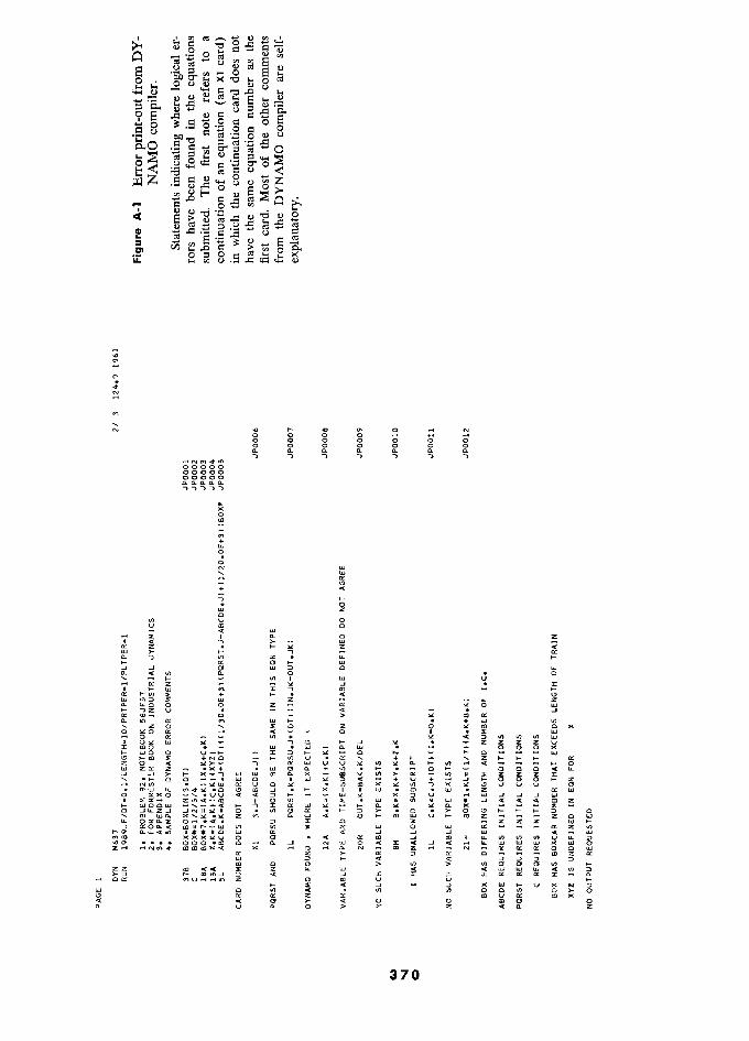
1
s U
?g ° U
...
Li \1) ..c:: b Sgëx c 0 ="g ...... en c*
< s cG
IL Or
.. o' ..... Q à fl ¡;..¡ m
< F O OE O - « N m 0 N 0000000 à à § 0 000 § 0000000 O a -t a n a n , Î Î Î Î , Î
00000 00000 00000 c..o.o..Q.,c..
& >< o .. fl + ? 0 É W N W ..... LIJ K - a + Î > W ë o fl u 0 u m W 0 - c W
.-4::E £ 1 < 1 n. a z
ta Y n"7 a. a If) Z L.I...... 1- Î " à a # LU J J a LU n 0 IL ù <0( fl ù 0 o 1 lu . 0 à X ...... LU IL '7 ro ..... t- 0::: Ffl Z + f-. <1: LU = £ W z..... <_ - L.I.. Z V'
a. à É Z 1 É LU ' 1- 7 U V ......... et J Î Î 1 1 À é É Î a r,{\ m (f'\ LU 1- > . + LU w K If) O xo 5 m p K É Î tY à Î à Î fl fl fl ....... 0 -... \1) + <0( J \1) \1) \1) LU Il O? LU m CI E ""'...J J !It o - z z z z W à IDO o O Ô-I - w. À 1 LL.J É w à 1 - 0 0 0 x l:) + NO q VI 0:: Z 0 <0( YY- . 0:: W U U ..... - - .... 0 LU eX+ . LU a a... V') +- - a a 0 cc
1 b 8 à z ...... N'" '::>L NmxYNOXYt7UVV U a C"lU U. «'\4" '::>L.O \.9 aJ ..J J . 1- X 1 Il IL . o;¡ . w . Z a:::: W o O - . V < < 1- Y X J U M W J ..J z Y2x £ à %8#5 5àiÛÎ 0 . '" a à . 1- J ù .0 . % É à 1 a , «'\ 0.. I.LJ 00( 0 W U 1- co oZ ............... z a UJ Î Î É É É W l- É OKOnQmlll?-.ILJI '" '" Z W 0 w a::::............... Œ Z '" Il...0 W 41 C..J..J..J J W 00( ..... W 0 a Œ IJJ À
É ro É '" '"
É ..0 0' .... OOO.aJ £:) .-t a...J N LU IJJ lU X IJJ 0 ?lJJmXoI/( x x ...... a ...... N ..... 00 Z ........... N ..... 0:: a IJJ a m W 1- < < J => J 7
ùÔ '
fi a > > 1- ZZ Z IJJ G Y Z W 00( 00( IL IL W 01/( '" Y7 ? oom..J => 01/( J III = a. EOE Z 0 co u U l-
W E à 01/( 7 7 à ° U Î N => W a c ..... '" '" 0 0 '" 0 >- 0 ? Z 0:: aJ a:::: aJ)( x $ 1 C ù à o a 0 Ô o a Z Z 01/( ù z
370
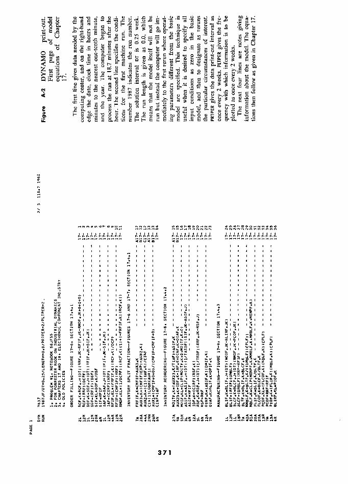
0 Q) cj. ;
0 CI cd
e w 0
C
I a)
.a 3
op
io pn
,,C"
C a)
° c.
*- zi
a ° w
x G 1. CD ° ·3 .3 C) > ° . p . U
u
S S
B
tY -3=3 O
;!
ou =u -ô ° ô on ô. ô c ?
o ô
P
' «
NNNmm.t N11(lvDrmPO.-INm "" --«--««««« NNNNNNmmmmmmm 1 1 1 1 1 1 1 I I I 1 1 1 1 1 1 1 ,,, 1 1 1 1 1 1 1 1 I 1 1 1 1 1 I I 1 I """""' ""'£ ?" ' "' rrrrrrrrrrrrr
I 1 1 1 1 I I 1 I 1 1 1 1 1 1 I I 1 1 1 1 I I 1 " 1 1 1 1 1 I I 1 1 1 1 I 1 1 1 1 I I I ' 1 1 I I 1 I 1 1 1 I 1 1 I I 1 1 1 1 1 I I 1 1 1 1 1 1 1 1 v I 1 1 1 1 1 I
WI 1 1 1 1 1 1 1 1 1 1 1 1 1 1
1 1 1 I 1 z 1 1 1 1 1 1 I 1 I 1 1 1 I 1 ° 1 1 1 I I ' I 1 1 1 1 I 1 1 I 1 I 1 1 1 > I 1 I 1 1 V I 1 1 1 I 1 I 1 1 1 I 1 I I
) ) ) t t 1 t ) t
1 ) ( t ) , ' t ) ) t 1 1 I I 1 I I 1 I 1 1 I 1 1 1 I 1 1 1 o r a I 1 1 1 1 ' ' 1 I 1 1 1 I 1 1 , 1 I 1 1 O rl 1 I I 11C r ̂ 1 1 I r -a 1 I I I 1 I 1 1^1 1 1
, Y ..Z + 1 1 I 1 I O I 1 1 2 I I ̂ 1 1 1 I I . I I 1 O + I 1 I I a Z 1 I 1 I ' 7 · I I ' 1 1 I I 1 ' % ' I ° ' ' Z W
' I I 1 1 r I I 1 1 I # 1
1 1 1 1 I 11 K
=1 1 1 1 1 N
1 I 1
( 2'
1 _O 1 1
In. il 1 1
i Y – IL 2' 0 In. f0
00
:I
lu ?101
1
V ·^ ? 1 H - % 1 J Y V J ' N I 1 - '
§ Y I Y 1 Y I o.. I a
1 O ZZZ 1
* · IL V I 1 -
- t- I
- · V
v " I O
O 1- v
Y Ô
fi O -
J 1L
£ : i fi
li V V VY<\£
V' <+Y.w
? Z ?tay v C £
N p 1 -f0·O.'m\2W
O OOO^Y iy 1i
c 71L...1L [ ?
" °°"" V' 4 " -.r 7 J`.J(OJIOJJm-1 41 N II
'? C 2 I?v .HNII Z 4m .i .H.11 Iv " 4
mm O IW Iit?44.1?IW ? > IiX7( x z > Z ^^V VHIDJ?VO00?
K V VOO·?«1?4? Z K?7r?7? Z ] § J
£.H .-nNm.t O .. 4«V <V E £ maNmmmiE W a.2GGm
zz z ? zaza aazz a ««OE < '
<eD.tP?OZ r<<aJZNJZ?< J?JaO^NNOON1Z?1OC .
W
p
371
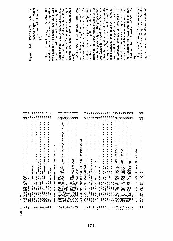
N 8 r.
mc g +.I v w 0.... O ^ _ d In q w 'C, ·
.6 .... a ..c::u ê .... cz u G =' ' m '" ê
CI0 0 <e: s:: u 0 1::;S",-g..s."l::u -bl:: CD
E 0 O N '"
0:1 ..Iod . ...: < U 0 1::
'" 0:1 '" E
'" 8 '" .;::: 6,D ." u 'O ,Ÿ E '" .... ¡¡.¡ C"::; 1:: '<t
'" ." 0:1.2 r::
r:: ....
r. '" z - U *,Z .- r, x un..0 w Cr 0 r. x Cr ci ()::3. '.¡::j 8 .- ez ";j u =,",:::""" u c:: ...... Q) ...... (/') do) « tJ,:I 0""" - 0 0"'1'-
'" '" '" Ô O .... o
...... CI) Q) - ." C iS Q.. E- ..c:: 0'" r. .-; 1:: 15 0:1; .5 m M -5 Q) 'E S.9 ......c:: ....
0 8 1::
l'a . e ..: 0 Q) z fi) cC
Q) 1) r. <c"C
II; Ô
=' M u 0 "'o..¡L;o d OJ «1) 0:: cd .5 Co) C tfj tfj -t-I uzu cd OJ tfj
-- ?????????? mm Il 111111111111 1 1111111111 1 111111111111111111111111 I I
-- 1 1 1 1 j 1 1 1 d 1 1 1 1 1 1 1 11 1 1 1 1 1 1 1 1 1 >< 1 j 1 1 1 i 1 1 1 1 1 < 1 1 1 1 1 1 I l '1 1 ' oC j j 1 1 1 1 r III 1 1 1 1 1 1 1 1 1 1 1 1 I 1 1 < 1 1 1 1 1 1 1 1 1 + 1 1 1 1 1 1 1 1 1 1 1 1 1 1 1 1 1 1 1 1 l 1 < < 1 ? 1 1 1 1 ' ' 1 1 1 1 < 1 1 1 ' 1 1 j 1 1 1 j 1 1 1 < 1 1 i i 1 1 1 i 1 1 1 1 1 1 1 Z j j 1 1 < 1 < 111. 1 < 1 1 < r 1 1 1 1 1 1 1 1 1 ' ' ::[ 1 j j 1 < 1 1 ? 1 1 1 1 1 1 1 1 1 < 1 1 1 1 1 1 ' 1 1 1 1 1 ' 1 < l..;t f 1 r < 1 < < 1 1 1 l I 1 ' ... 1 1 1 1 1 - ' 1 .1 1 1 1"'" h 1 < < 1 1 1 i 1 1 1 1 1 1 1 1 j 1 ù ' 1 . i 1 1 1 1 1 1 I 1 - 1 1 1 1 o .. z - 1 1 1 1 1 + 1 . 1 ..c: 1 1 1 I 0 1 1 1 I 1 < 1 I l)t 1 < 1..0 " ' o --...... I.L.. 1 1 1 1 $ , 1 £ 1+1 lit- 1 1 I 1 l 1 II.i..I 1 1" f < - u Z Q j 1 1 < -, < o 1 1 1 UI w < 1 1 < 1 LU 1 Z 1 1 1"'" h I 1 1 1 1 O_ 1 V) W I 1 1 I I W 1 1 1 < 1 1 1 1 u.. 1 - 1 LL. 1 1 1 1 1 1 1 1 - 12:1 1 1 1 , , , o fl , il - - ' - 1 1 ' ' - Z Z ' 1 1 1 1 U 1 u 1::1:1 I 1 1 NI::.::: Y 1 1 1 1 u.. 1 1 1 0 1 , , lu ... ' m- t- 1 ' 1 1 I 1 1 1""1 I 1 . 1 1 1 . - 1 1 1 1 u 1....1 1 I- 1 - -, ..... W Y J U V l ':w:: Y .1"") % - Y 1 1 a:: .r 1 z O ' 1 1 U IJ- · '")1 W - , 0 . X :w:: 0 . 1 UO O . 1 1 . 01 LL. - -4" à a:: CI ""'11 I J 1-1 1 I.L. h ÀÔ 1 YX I Z 1' 1 2 - Z - 1 1 - V) 1 n. li -:;) 1 1 l ':J. - LI.. 1 )0£ lU 1 LL. 1 :,¿ 1 ....... 1 ...... al ('t'\ ic 1..... 1 I < -, LI.. 0.. -, t- J < 010l OLL.::.lJ J ...-- 1 1 f %1 I I Z « 1 u.. - à J 1 ·I ·p l ':./..:.i "" w ::> - LI... cr: - ..J t- I.L 1 0 t:D Q. ':./.. 1'- .. 1 l , u..... 1 o. a:: c( + 1 1 1 1 I..JQ. 1 .J, 1 4. - a..u. -u.. +v.;:) +- X" lU -u -- J- -- Y ·4. - lu ao :.la::: I.!) V_' -W Y v '1 J O Z 1 ::Iot:...J:.l::.l "-1 I.LI.L a.. ..... II. I.L-I.L I.L-. tJJ u.. """)- Z I.L Li....O 1.Lu.. -...J ::> Li....1.L J f! J Y W1 a Y a - · 4. Iv · d' · N. v O v p li m h 4. d' IU 1u i 7 - · Z p Z li J 1 2 J Y v Y · Y 1 V O w V li p t7 > · 4
N 1 I 3 3 ? ?8 £· ?Q.? 1:- - -J 1W I.L- 1 1 jhÔ
t ' É 1 ÉéÎÉ 1 mQ·\
1(5Ô Z- ' O = 1 0.0. - .et:)- .VI.LU a p d' JY -:,¿ 1 +J- J6 ...J:Iot:O IX Vla-J 0 '") JZ V1 -':./..::.:::+-o.. u..1.L "-1 -u N1NJ0 t- -......- ........J +-f- oz il Il .1 Do UJ t- nua:::J II IJ >::>- < IIJIIU.I?::Iot:1ol-.J U') J ....J::..t:a:::...J 1ol11&:ltIJ..J..J1I1I Il...J ?II cr <1 - Y Il :Iot:-Utl N vYY ·Y N p N YJ YYO ·YO o W Il:./. ., 2 > Y v UJ 0 O î œ X e « W
£Ap40OZOOV1N-'fpp £ 0.'f< <ffftY2' J JJJZ£JJJJfOJaJJJJJJJJJfJJ p p<
cc J2PJOJZPONNaaQaN.?l2N.-12<JZ N N 1?1 .O .1
W
...
372
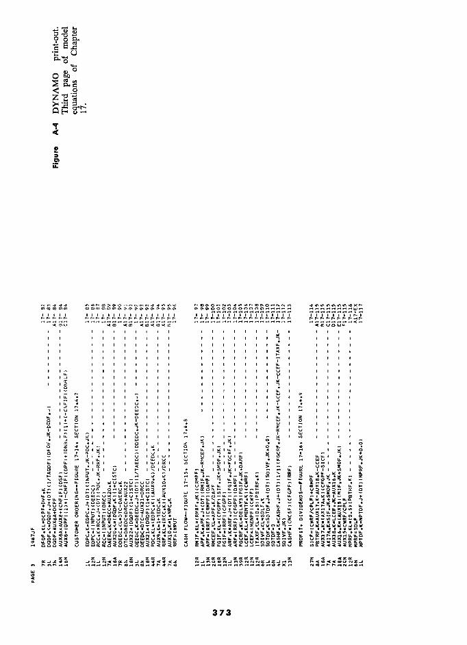
''- 1-< ' 000..
ce . .
0 w
0 ,
CI
¡::: .
- ( 0
zbr .
é
le ::t m
iE
N?444 moomooro oomwrowm??????????? ???OOOOOOOOOOrl_?rl- --------w-
- -------------- --------1- ^ ' ' ' ' ' 11111 [ 1 11111 fil 1 1 ' ' ' ii7Viiii77iiii7 11111111 r-.
r-r-r-r-r- IIIIILLLL2ILLL2DÎI
- ---- ..
' 1 ' 1 ' ' ' ' 1 ' ' 1 ' 1 1 1 ' ' ' ' ' ' '
' ' ' ' ' ' ' ' ' ' ' ' ' ' ' ' ' # '
' ' ' ' 1 1 I 1 1 1 1 I 1 1 1 1 I 1 1 1 1 1
1 1 1 1 1
' 1 1 1 ' 1 1 ' 1 ' ' ' 1 1 1 1 ' 1 ' 1 ' ' ' 1
' 1 ' ' ' ' ' ' ' 1 ' 1 1 1 1 1 ' < 1 1 ' ' '
' ' 1 1 1 1 ' ' ' ' 1 1 ' ' 1 ' 1 1 1 ' 1 1 '
1
1 1 1 1 ' 1 ' 1 1 ' ' 1 1 1 ' ' 1 1 1 1 1 '
1 '- - 1 ' ' 1 1 1 ' 1 1 ' ' 1 1 ' 1 V 1 1 1 ' ' U
' 1 J 1 1 1 ' ' ' 1 1 ' 1 I 1 ' ' 1 1 ' 1 1 1 ' 1 00 ""
1 '# Z 1 1 1 1 ' 1 1 ' ' 1 ' 1 ' 1 1 7 1 ' 1 ' ' o .
1 1 1 1 1 ' ' 1 1 ' 1 ' ' 1 u.. 1 1 1 1 ' - r- - ?
1 1 1 1 ' 1 1 1 u 1. 1 - 4'...J 4"
'I Li.. 1 1 I 1 U 1 1 1 ' 1 I 1 ' lit 1 1 . 1 1 ' 1 - Z r CI lot' r O 1 U..-.¡ ^ ' 1 ' 1 UJ 1 1 1 1 1 1 1 1 1 ' 1 I 1 ' ' 1 . 1 t.IJ .
- 1 Z 1 1 1 1 CI 1 1 1 1 1 1 1 1 ' u. 1 0 1 ' ' 1 a ' 0
' ' ' ' 1 co
' ' ' ' ' I.IJ 0
' ' ' ' CI p
1........ F-
1 1 1 1 1 1 1 1 -
1 1 1 1 1 VI....
1 1 1 1 o Î 4 I 1 - viii 1 - 1 1 1 * 1 I 1 I ' 11:: fU V I I 1 '
- w - £' ' ' '
v - '
1 à ' t.IJ ' ' ' ' - 1 –t)–f')–i I V) 1 1 I
. J W lot' 0"1 7 - U. m v I 1 1 a 1 1 1 Z I .... . ' ' 0 o Z4"V- ^ Y 08-8 .0 ..... 8 U. p 1 1 1 ..... u. 1:..::1u..1 I 2 d' l:.l Y à 0 a .... 1 "1 ..... V t.IJ U 1 -"1 +
7 I ' U I p I V 1 V V 1 "1 ,.. 1 8 )l
- LL
' CI lu V LU ::E U. O 11:: U..,
7 1 1 Il IUJIO::I I 1/) 4' 1 O 1 Ia_ 1 < u.. - U-I 0 O 1 8 a D..
liJ 8 ex:
- c:( CI CI
" I:E 1 0
LLJ k VV)
X .....
" CI 0:: 1 1 1 U 1 t- 1"'" 1 ...... 1 1 .. -'" 1 V) 1 :..:: 1 K 1 1 t 1/) 1 < - lot'
Y F- \
- - £ u.., +"1:"::- - CI ......
7 loto.. lIt+ D..
t- u..- CI Q.' 1/) ...... ')L:Io! .... a....- z: \ v 5
-8. 1 :f:Ll..LL.,
..... - -.... I LL - V ')LU?NV-VVC' 0 ..... Ct:-CI.- LL - - - u..
::û:î 7C ri 2 1 p 8t- 11.V V' 7 LLJ .... u.o -1 1 Z c:( + + IL CI -llItv>l- - fL + .... J ., U Z , n + 'V - - UJ
+7 V V^ UJ -VlotV V I-M IL ^ a .......a..- u. 0 .JO :I: u...... CI O 1 H
n,3 O D.J vHppp+p411 ppZV + 1 ·p£a-Np ^ O a v-z 0
0 ...J1I::)c(0 UJ J
t- e.I<1I 0 ^ 11U.r-c:(<O>DIl\.JlLL.
t- UV-IIa:::NQIINOON.O'-.-4I' :I: 0.. 0.. co 000 tI) ddV VUJXIy VX4llu% V xl?%4 N 0 0' lac et Œ
v U
ZZ Z Z C z za ? CIl: x z z 4 CZa:: JNJN.œa::Z??ZG4"<.<Z NJ?O?N.J?O'NNNŒJZ...J-? ,...<COC<COONZ.J
? .H .O N
W
S < IL
373
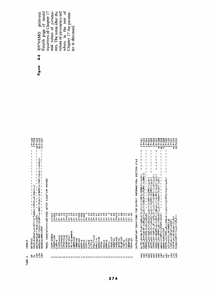
É
É .5 &. u M o. cC w
+.J x
'Ô
M
on <
d 3 01 ¡¡:
m?ooo NNNNNNNNNNNPIInlnl?l 11111 I I 111'111' l' , 1 l' 1 1
<mu cm 1 ' ' ' 1 ' ' ' ' 1 1 ' ' ' ' ' ' ' 1 1 1 1 1 1 1 1 1 1 f In I I I 1 I t 1 1)( t ) J N ' 1 et 1 I I I 1 1 1 1 Z ' "' 1 2 1 1 1 1 1 1 1 1 t- 1 1 ' 1 1 101 t lu – – 1
. 1 1-1 .... 1 IQ:I lai 0 ' a.: ID O - i 1 1 - 1 I I - -- 1 1 I ......
Z .... . U. E COQ- 0 z ex . XO 0 ...... O_ r u V I I t- < Z -- -
11111 et - I J > a 0.. IÎI-I" NI O .... 1 Z LU 1 :::; 0 Œ uv,,- - " z - 0 ......- --00- , Li. a 0- 0 I IXI 0 -0 - o - z' O .... +1 I W c-- .. Z -- - ........" .... Z o----ou..-V O -- \IJG 111111111111111111..1111111111111 0 -OOOOO...Jo-. UJ - v? OO.-iOO-UNI G - -v le
""o-oo---u.. -u..--- - ."'IL It N ltJ 1rIl- .-- - ."'LL O !- 2 0 à .--v c a J In 0 t Œ -eto' Z 00 0 Z 0 00 .0 Il\ N 0 W
W V MM .?SNrvrv OOJI 1¥c(1I11 II ?11.;t"lnIiIINIIIIG;I(C'\"'?'4'(C'\1I1I11 w iL v N n1 rv N J V V V V V V V V H 11 V Y . U. 11 . w Q, a Q, Q,ao?? 0 7 .... % uuuvuvuvvUUvoaao£)oooooaal-l-l-???I-?? ?
ZZZ N N?IZ ZJ'4'?O t uvvuuvvvuuuvuuuvuvvuuvuuuvvvuvvuu ... a
374
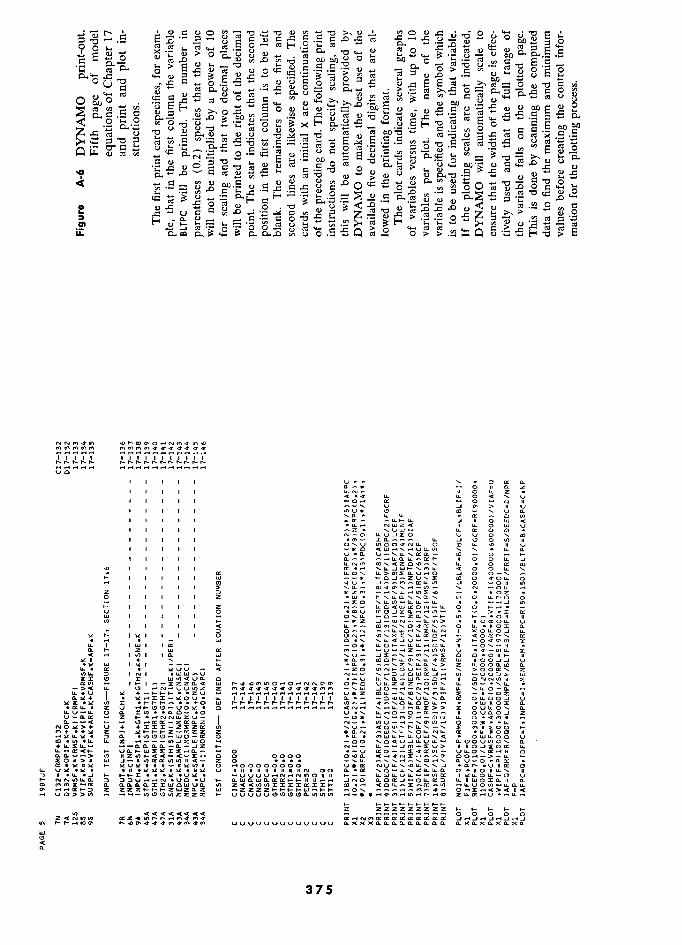
.G 1
1 cu ... "2 0;"" 00 ? p....- .5
.¡:: p". ..0 Q)
c;¡ <) o 0 <:::: ,;: ::s ,;:
OJ) 0.0"'0 ';; <) cd c;¡ Q ,Un c:::::: Cul c:::::: Õ G c::::::
::s oS .- +-' c::::::o -:S
cd "t:I 'E
J-. en
o
ro +-4
Q) u u U c::::::
cd ;>-.,...c:: CI) ......, ci u u 0
8
en
C <Ji
CD u- x c'à..-2 - E on u .G 'JO ,;: - 0 zi "0 Q) .-
Q U '" 0
<) 0
8 cd
.Û '° <) ..... 0 "0
"? v; G G Q "Tj
0 -5 <) '"
cc p r- c:::::: -E lu
-0 CD .8 ¡....
co ? r
cli ¡..... Q 0..';:):-::; .... M z> ci M '" U 0
0
.2' ci := ,ô. ua: ?
ô --;;
11111 , 1 1 1 1111111 ô .' ..1 .,
1 1 1 1 1 Q.. Q.. -lOI - 0 Il a.. z 1 1 ' 1 ' 4. N - W Il 0 1.1.. 0 < , U 1 1 ' Il - -....... V > Il I U ' ' 1 1 1 * w n a.. n 1 1 1 ' 1 * C - 4 J Il 0 C N?ZC Il 0 ? u , 1 1 1 1 .. lI.. 0::: a a .. , , ' ' ' WÔiÉÙ 0 U U m 1 1 1 1 1 Il O.......U a O ro lI.. Il U 1 1 1 1 1 -Il100 u7 ,........ Q.. v-a.. 00 - 1 1 1 1 1 a..-- Il 0 a LI... J , , ' ' ' lI.. co ' 1 1 1 1 . u.o....... J 0 0-""'" .... l ' '1 ' i 0 r
Z I I 1 I 1 £ .p -. IIOZ . o ' 1 1 1 1 É a - -::£0 .J It't 1 1 1 1 z W 1 1 < 1 1 2 Il v 1 1 1 Ô Q. - - O-N 1 LI... À 1 0 ac:: ." . - w Z ac:: 1 1 ILl 1 la::: !r ... ù z W ac:: u :L < - .w 1 la.. n ILl lx Il W:I 1 .a..t"'\ W IIOO...J...J U V 8)t UJ Q. . C -zo z Z V)LI..;:) > INI I .liJILI-U ü1 XI ? w I 0 x oefl - w - Z -\1.1 ...
§$j ) U 2-ÎliààÉô .-I II f 7777771771777 V ::.£X.:.l \1") J: -- u. z o Q Z 1 «oM>+ U + \1) e- Z "
":w:u...)(. > 0 U Z · -00 a ' F- ° IL t- Va..f-ILI:!::!:I;:£""a..- - 0 .-v I 0 V1 0 0 0000 LU z 0 .... O .w00000000 0 0.. U IIUIIIIIIUIiIIIIN 00 · U 2ÀÎ?à ? à m IL 11410Sn II 0- ro 0.. o.o.o.o.IIWCLUUa.. v') 00."" OE ......"cr::t-::) z < .... z II) Q 0
?
W
< ..
375
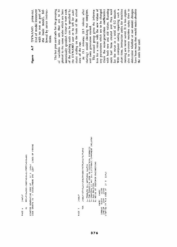
s ' t)
N ° t-G, ",OJ)¡::¡:: p C
1.U" C Û a U CI t: ë Il) rn 0
ci -5 L.; ro E J3.E.a'Ü:3 U ro ..c=
.- c:: Q.) =' U 0 .5 > N 6 - lU
0
s V'J
i
0 ci g
cI1 Ci ...... i 0
;; ' 0
p
"
:8 U 0
en
>
ü
" '" Z z
C N Uf- o Il X U 0: X LJ
w otZ _ zo 0 - 0 ... >-a.. o J 0::£ ë a.
. 4J J U
o Z N
a V
N J D::: t- Z
.. nl
.. w z .-. Z
U r-4 0. Il\V)O ... 0... 1- a::: ? h 10, w IL cr:: 0.. ,zu UJ 41
O , z Z , " u1 J - zw C) 7 co f"\ O z . .. W Il 0 .. W '" o K x m - cr: a "
o vl C) W
0 o
W Il W z w LI. 1..
cr: a
W Q
1- o m
a x , 10 , a <1- N - . "'LU V 00..0 .O 0 1- oo? 1- o n'1 " XOCOCJC vooe Q N Uf"\ H1 1- 010 O Il O .. 0 <?ow
oC) LI.. - Z, v 0 ""') - O W YOxJO u
Il co co OZ Z co U <tz Z co co ooz Z '" a a::- P 0' .n
Z 1/) N .v .-n N m ?
\1) .. · UJ )- Z 0 C) cr: u ....
ot Z o Q t- tt- ta. 0 )( UJ \1) r cr"IU 4l
1- W âw ILl W 001)D a;
ao a e 1- o et r Il.. V'} U D..
376
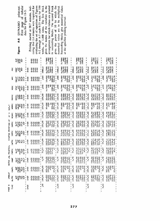
li 1 In .
iÉ .- 00
0..>'- H "0 .- -
i0
< ::::s 0.. 0:1 uÕ <!)
;> et! ..:::
;> 0:1"<:: f-<
(ù 0
<!)
c:: ::s"" ,5
CJ) CL) c
É 1 1 l Ù
°
% <!)
1 .5 'E ::1 (1) ]
en 0..
à
1 i 0000 1 0000 1 0000 1 i ('1"10"'0'> i 0000 000 · 000 · 000 · 1 É888 ' 1 00-01 I 00-01 1 00.01 I oO...-t' 1 NO.CO 1
OOUD:: ++++ "".00 "".00 "".00 "".00 JQ. 1 ÎÎÎÎ ' 1 00 i 00 1 ÎÀ2 ' 1 00 1 ÎÔÉ ' 1
t"'I.... C""I..-t t"'I ('1"1"" t"'I C""I..-t ' ' ' '
,,,, '
', gg,, ', og,, ', gg,, lN
Oama Im
e: n.OmP 1
v LLLLl.LtL 00000 .00...00-..00... °""... f'"\U"I-. C OClZO:: tr
10 0000 + +
1p O 0-00
O lo 8.oo O
10 0-00 o
.oIt 0.""0 d
o '4' O-C04'
1 a 0 1
++++ 0 """'00 0 N o 0 IUJ I4JUJUJUJ 1 -?oo 10 10 1
' 1 1 1 1 1 1 1 1 00.0. 0000010 0000010 1 0 10 Io
u a 88Ô8Ôlà 0 000-0 0 0 000-0 0 0 Q.. 0 1 0.00. 10 0-00-10 0-00-10 0-00-10 0-00-1 1 Z + .00 .. .00 · .00 . .000
%-IOO::>IUJ ààÎÎÎ' i à r-O?I 1 0 r-O«"I 1 à I 0 ""'ONI I à ""'ONI 1
1 ' ' '
,,,,,' 'o OgQOo'o ooOOO'O OOOOOI? F4OOo'OE MWm«o' U 0 oo?o? 0 00..0 0 00-.0 0 00--0 tt"I Of'O"l.-o tt"I o OUOtrl/) 10 00000IO 0- Ôfl'8 Àflààfl'8 É2àà2'2 N-OO-I UJ ItJrii + +++++ 1 00 ...... ?OO ...... mm00 z 0 o.a::O::IUJ UJI1JILJILJILJI 1 . ONI 1 - ONI 1 . ONI I - ONI I - ONI 1
' '
' I , 1 1 1 1 1
, r 10 0000010 0000010
0oooola O?..o?OI
u 0 BÔÔ2Ô'£ 0 2ÀÀàfl'fl a 22Ààfl'fl 22ÀÉfl'2 0 8ÙôÀfl' a OLUtra..-IO 000001- 0000-1- 0000.1. 0000-1. oooo.t- OOtrDN.' 1 LI.. UJuo.xa. + +++++ 0 .00 0 .00 0 a .--00 co .00 œ IL UJI.LJUJI.LJILJIO 0000""10 ààà8i'À O 0000.-? 1 1 0000.-n 1 OOOO?I I
, 1 1000.0010 00-0010 00-001t"'! 1 m Oa ·NP 1 I
u UlLU?? 0 oooo? 1 00000 O 00000 O 00000 r O<ll(Q.Oc(IO 8À8ÀÔ'fl I - a:: + +++++ + . 0 -% 00 0-.00 O 00 a .O -. am o a. o£o a::>IUJ WWI.LJWWIO 0 0010 0 0010 0 0010 0100-100- NO-l N 01
1 .... '" m m
trlN"" tri m m tt"I.....
- N N
I ..... 1
' 10 0000010 0000010 0000010 1 1 '" U 0 «"OO<"lf'O"l a 0000 . 0 0000 . 0 0000 . 0 0 ·
a I.I/)QWa. 1 ÔÀBÔÔ'£ £fl8Àà'£ -000 1...000 1...0-001- - fl2É8à' 1 ...... + +++++ a a oll\o-t- 0 0,,",0."'" 0 Oll'ltt"l-"'" 0 o-COt"'!."'" N 1 w
wwwwwi?? I o orooo I O orooo 1 0,...00010 1 $#2éÔ' I
f- " N
< 1 ooooola ooooola o..0.10 U 0 omooo 0 -0.00 0 -0 -00 a -0.00 0 0
C) 0 0000o I 1 000.-1.000.-1. à@à2fl'2 1 + +++++ a 0-000 0 0-000 0 0-000 0 0 - Z I 4141411u11 I ÀàflÀÀ'À oot-oOlo oot-OOIO oot-oolo Éà2Ék' 1
- t-t- .... r--t- - t-"'" ..... t-t- - t-t- 1 ' "i
,_ 1 la 0000010 0000010 000001..........04r-OIo- 000t-"""'1
Q. ° 00000
0 0..-0 c 1o 0..-0 1o ·O m Q, ??.JVOIO ÀÉ888'2 2ÀéÀ2'2 -000-1. 2ÀÀà2'ô flààÀ2'fl -0t-\f\.1 I
+ +++++ O 00000 O OOU00 0 00000 0 0-00""0 0 000"""..00 W 0 JZ::E ?IILJ wWl.LJwlLJlO 00?0010 001l'l0010 0011'10010 1. o. 1. 0'01l'l001 1 oc
- W-% £ I 1 1 1 1 1 1 1
.... 1 10 Oooooto 0000010 0000010 1/) V 000000 0.-0.0 0--0-00 --0-00 --0-""
a. 000001 . 00 -0 - 1 00 -0 - 1 I +++++ O OOOOO 0 00000 O OOOOO 0 OOON- 0- m
m Iw WWWWILJIO ?oOOOIO COOOOOlo 00000010 0000""'010'> roOO'NNI I -
. 1 1 1 1 1 1 1
,,,, ' 10 0000010 0000010 0000010 OOWWO' I
.-- 1 0000,", 1 0
--00. O ·00 1 m c · o 0. a 00000 1 - 00 - - ,- 00 - -0 1 - 00 - -a 1 àà2flà'fl NIl\ -.01 1
11. J-Z- 1 + +++++ a Oo?o 0 OO?ON
0 001l'l04
a 0' N??WOO 0:: à W?#iÔ'à ILJWWUJWI"'" £'..10""'0 1"'" 1 a. LI... ::E
1 ' ' J M , , ' 10 0000010 0000010 0000010 ..00'0""'010 I . 000.?'
..... 00000 ? 00000 r 00000
1; OOEOWO r nr000
o ·^a^J 1 ooooo 1 .0-.01- . -0--01- -0--01- . ."'--01- . .00-.01 I 0 u)l.Lza.o ÉÉÉÉÉI' 4" 00"'0 - 4" 001l'l0. 4" 00\1\0 - "'O'>o.noo.
a C:C;O::UJ WWILJWUJI 1 1 I orroo 0 1 1 1 .... r -f'O"Ir-.-4 r-- .f'O"I""'"" ..... -(0"1""'- r -f<'\..o- <:( 1 1 1 1 1 1 1 '"
,, 1 'O OOOOO'O OOOOO'O OOOOO'O OOOOO'4
U a tt"I?OOf'O"l a 00000 0 00000 0 00000 0 00000 Il'I rooooo Q. ÔÔ88Ô'i 228fl8'2 22É2É'2 -0 -0 1 2fl828'2 fl2À2À' 1
O gg-
· ;Ig
U gg.
· ;18 gg.
· O gg-
· P ·
j UYwam wwwww i 00 À'8 ?É À'É ÉÉ 0l0 oo olm 1 ÔÉ À'
V °' l
.r .r ..n 1 I
- ,
, ' 'o ooooo'o OooQo'o OOOOOIN Of'O"lll\N"""CO
CIO V 0 mm000 ci cl .0 -. 0 000 - - 1 000 -. 0 Oo()r<'I. - · 0' a.Q.J:ou 10 00000 1. 888éÀ'2 - 00000 1 - 000001- 1 ... + +++++ a ·000 o .-000 O O .... -.r<'\NN
lU °'à ààààà'À ÀÀ2ÉÉ'À 1o ÀÀfI@É'É àà22É'Ô àà21Ù' m
41
I
I 41 -
1
I --
......of'O"l -- _.-4
......oN N
1
I -- ~
1
1
1 ' I O la O I O la O la O 1
Ql)W 1?1 0 0 a 0 a O X 10 O 1- . '2 · 1- · 'ù 1- · 1
W ....
+ w +
4 1 W
c 1 I.JJ ' 1 1 1 1 1
Q. 1 1 1 1 1 1 1
377
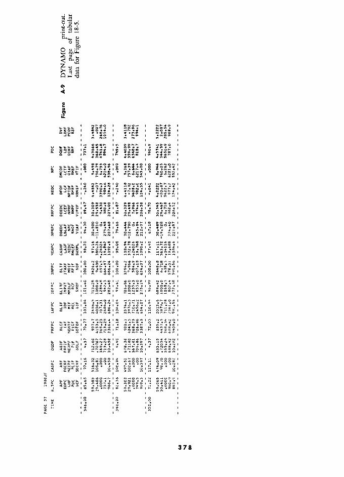
ù ..!...c 1 C M 0° ...
5 o M 2 n
0 o
os <
Ë >_ 1:1'1 ¡¡:
1 rvrmo 1 1 1 >ZOO1 1 «.10."'- 1 1 NO-OI 1
OQUΠ1 1 0 0 0
04>0 1 rP 1 eNCOa- 1 mN N mN N
1 1 1 '
1.-4 1 U"I 0\01"""" 10....0'>010 1
a coz« I O.COCO 10 "'.0"" 1 Q.
p moe
1 O O .,prm Ir .hlnm IP /
1 1 1 1
1
V 4 1? 4 lu I? O O O
z 1. 1 ZJOd'' 1 ? PY?.ONm I · PN?ONd 1 I
o m r m
1
1 1 1
10 o rvrm.om I Q)NOOII'\I"'" N""I'-NNI I U CIl OUOa:II)'N m.0i.llv --CON-IO N8N"".'
""""OQ)", . NON""'. Z 01
o.Ck:a:11 1
. fl'\O'oNII 1
-,,,,Q\Ntl I 1
Z > olt .... r 1 1 1
1"" Q\COO?OI"" I V Q. QUJcr;:a..-I. rt\"'o......- f"'t"'''''N-. 1
00 iD ..O.o Πm OPPPO 1 m OPrPO 1 1
CIl > 1
fl'\N N 1
N 1
fl'\N N 1
1 0 OO 1 l ?o
iO f l
40
Pm
.Or
l 10 U .?oœo ? Q. .." 4'C"o ..' 0::: ... - mr 0'0 II'\N â.-1 Q. cm o- ?Ol? ON 00'0 NNI o OJ
I NN 1 NN
I NN
1 1 1 1 1 1 1 1
10 I u IL li V 4. N a
..-04' t
Z CD CD W ?CDNO'oOI? O?NO'oOI? 1 X Ul
1 1 I 1 i r-n
1 I 1 1
la O NONri 1 O N.OPmr 1 I U a .C"'\ .CDN O O ......011'1 0. -.1"0\""-.1- 1
0 N.O'o..o..o 0 0 Z 10 N?II'\OC"'lIO I - - ..... C"'I C"'I m 00 N rv
1 1 1 1
la O m O m m m 1 ? ?O O m O P I 1 U 4" N.-.4" 4" m P ..,....(0"1
-04"N.I- .Ofl"lt'"\-I- -OooN-1 I u.. P ..oOC"'lll'\fl"I 0 CDO..oON CI ?ZX £ m I P O O N m r 1 CDOoro?1 I - m-x ..... N
I I 0-- N
1 1 1 1 1
1 1 v 00 m ..<")-N 0 '" P --N-fl"I N 6 . m.0 .dv I . mP .-v . 1 u.. ('"1 COfl"l?CD..o 0 14 O m m I O dOO.Om 1 (O"IO'M4"('"I''''' 1 1 - .....
' 1 1 1
.....",C'\..oC"'lIC"'l N"'4"NOI I U 0 ..C"'I4'. Q,. U«I-OOI. '--'''''....01. "'''''..001 u.. J-Z-I- 0 C"'III'IO'C"'I>O ..... N4'CO..ooo N C"'IC"'ICOCOO
m Wa..CI? CJ'N..oOt'"\I? 004'>000"'" 1 X V') 4"C"'I >0 (0"1
1 1 1 1
W r orr m I II'I""""NNI 1
..o..oNNII'I ..,. C"'ICOooCOO' C'\ r-8C"'1N4'CO m o 1 C) 4' 4" ff'lNII'I!.O. O <eœw V') 1 ""'''''..0''''01 I I C"'I?..oCOOI
-0.1'<\..0"'" 1 1 ' 1
1..0 POOOrv 1 U CJ' ?-oOOO' ..... O?OOCD à 1 V') r co ..00.. <e o?.01 v N
I ~ I d
I 1 1 1 1 .., 00 ?rlO??1 I
U .0 m00 . Orv0 . CJ' a o..a..:I:QU 1. . mPOPP I . OdOOm 1
'" ..0C"'l.o N ..04'0 J UJ ICO ro ?N rv m
' 1 1 1
F 'o 'O 'O ' C'\ UJ 0 0 0
I * I . 1 . 1 UJ 0 00 0
> '4 4' '4 ..,. 1 11'1 ' « r<\ C"'I r<\ 2 1
" 1
'** 1
" 1
378
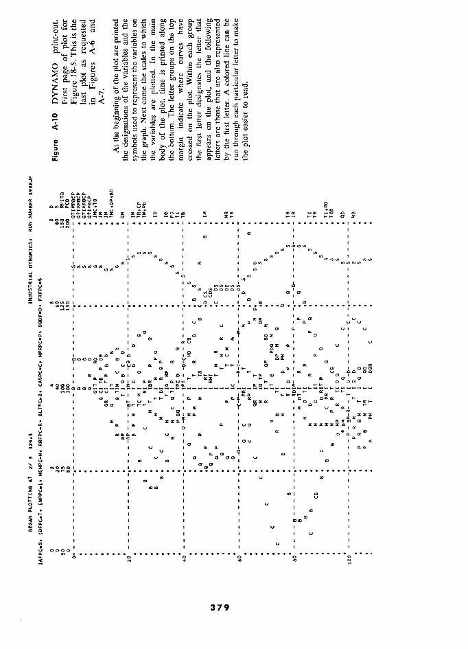
cd 8
d
O
o. O
1-4 cu
'" - .- J-¡ ..c::
11) J-¡ 2 si N
cC
-
CI p) N
O.
"" ;¡ ? c a OEOEù n CD .... vuua... j -maJmaJuaJ à UJ ::I:uo::.:o::.:œa:u-" o 0.0 CI en fl uo- n:: :¡: u .... -Q J à CI ac-CD :E oco:: à % Z 0 .-. Xt- ....- ................ 0 ? Z 0)000 Z .... ::> ""N N CI:: 1 1 1 co ' 1 CD S ' 1 co ' ' ' À J 1 1 1 1 1 U v1 1 l ' l ' 1 Cil V" m V) 1 1 V) N 1 tJ) t VI 1 W 1 UI >- 1 1 V) 1 CD 1 CQUJ U7 1 N ln V) N Q N 1 N 1 1 1 1 1 J ««fl< l
< l / '
, 00:( OE
à o
1 '
S (
N 'w
1 tn 1
'
1 ' :!
N V 1 . tl)tJ)IJ)lI).h
h Ó I 1
1/) Cl. 1 . 1 11)0.000 CI 1 1 É LL ' ' ' ?CI " ' Z LL co CI Î
o 1 1 lia 1 1 1 i 1 1 i 1 o Q X X CL a v o t i IV W Ixo a <CL ù U W CI ' i ' a ù W' W 1 ' 1 0 1 n 1 I V
É ' ' Cf ' o f aX ' ' A. 1 1 Cf 1 Q 1 OX Z 1" O 1 1 o m o: X tu V I ) 0E8 1 1 1 V O OF n V . 1 co CI a Cf 0 1
£ ' nom CI ' XV 1 1 1 000000 co V 00.. à 1 z o a X 1 a 1 OE 0 f OE 1 0.. ?yQ ° o 000 à U o ? r a u Oo?ô2 A. ' a::: Q. IDI a: QI 1 m et: 1 ? ?x 0.." o " 00:( 1 01 1 a' a 00 . OU v .... a:: ........ CO 1 I OWW .... a_> , 1 a f et: ....
' 0 ........ 0 1 m Z 0.. 0.. ce ex: 1 O o a a CI 0.. a:: cr:: 1""""
f A 1 1 O r U 1
I E y 1 I O K K K
Q v et: 1 r
- f i iOE X 2'Zù ' mOE ' 0.. 5 zZZ i:O 1 1 X co 1 XCL , coa::: 1 i 1 :EX::E . j ce j *xjif ::E i OE 1 Q. ... 1 a::: 1 ::EX% lia::: n' 1 Q.::£ aJ CD « 0.. 0.. 0.. va xxxxxxm )t 1 1 u CI 1 tn 0.. 1 Knnm Q:I v 1 0.. 1 1 aJ Q. a::: . LI.. ma a::: m a. d 1 1 ) c* u 1 1 œ N [K 0 m
u 0.. a. 1 ' 0..0.. n XII ' ° 1 0.. a 1 1 [J) 1 ° 1 en Il ' U "00' u U 1 1 ID ID 1 1 1 cc 1 É N Z NO"'O 1 1 1 ()I 1 1 1 1 I :z: 1 1 1 1 1 1 .... % ' '
@ m ' ' u , ' cc '
' .0:( .: 1 1 mil t 1
 ' ' mm a) 1 1 1 1 Z U .. 0.. 1 1 1 1 cc 1 m 1 .... Q. U Z 1 1 1 1 1 1 I ' , i 1 U . i Î £ 1 1 1 1 1 1 Q.. CD 1 ' ' 1 1 m ' Z . CD a w 1 1 1 1 mm 1 'V n
:s 1 1 1 U i 1 - j j i i 1 u 1 " i 1 1 i 1 1 a u 18 t 1 lit . 1 à 0000
O O O O O O O O O O O . N 0 co
379
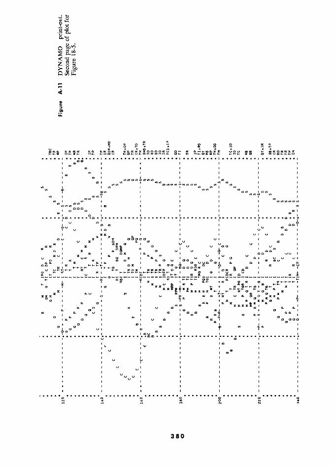
....
..... ;:3..... 0 O
.É 0..."'" O
. o
n Î
A Ù
5
! 3
CI
a n "- x o r - 0 c CI KQ- a w . 0 1-.. à a o § - l- V et: .. -0 a .......- m?? ?X«Q: ?? Q:?Q:«?%OQCQQ:u Q- Œ vau mm 1- m«Q«Q:%% rrz -t-%I- --r 1--0- 0........ zo o --m............-
..................-1........-, .......... I ?mm ? 1 IJ) 1 1 1 1 l ' CD 1 [JJ 1 l I 1 1 1 1 m I 1 1 1 1 1 tu 1 1 1 1 l 1 1 l V) V) II) ' ' IJ) ' ' U') N 1 II) f 1 tJ) m O< ' ' V) ' '« ' 1 cou) 1 1 1 U) 1/) 1 II) V') 1 1/) V)tJ)V) V) V) 1 1 ' 1 ' '
V) 1 lit 1 1 ICD m ' t 1 1 m 000 1 a Q 1 1 I 1 1 CD 1 CD CD I o 1 1 1 1 I 1
1 / 1 1 i 1 i 1 i 1 i 1 u O i i 1 1 <> 1 0 mit ) 1 ) cal t o u m 9 u 'a () 1 1 1 u 1 1 :EX ' 1 ' U W VOl 1 >: >: "- ou 1 OCJOOO 1 VIII / V::E z a 0 v m
m 1 mx 0 o V V vii na X a u v 00 u rc 1
1 F 1 1 0.5 ox 1 Q.. u 0
J. 00 1 00° VU 1
1
W 0 l W V V a W u 1 ua:: 1 a x 1 Q.. 1 u 1 0 al u u ul o ae m a n.ou v 00 O K m V '"' aa z I a K QÈ 0.. 1 cr:.2: 0. OX X 1 a. 00 a Ó 0 Û Ct b Q. a 1 0:
OEOEOEOEù OClooaocr: 1 Q. 01 i a rr CI a: 0« 0 0 a .... 0:: 0::: 1 1 0 QI 1 V U ' 1 %
l 'f x ?? 0 cr CD a:..................t¡" .... ::1: % n a a. CD........ o 1 10 1 2:% CI: t- 1 1 t:XX.EÏ:Tï: X t-t-t-t- t- n XIII I Q. 2: 1 a ID ' W m ........ W Œ Ô O ' xxx:t 1 0 1 0:: Z t m ' ' ' n- o- ' Z o z 0. 0. a 1 1 1 1 1 2: Q. %% QI 1 0. (] a. 1 ' 1 1 II) II) 1 0. QI m v (1) 0: 0. 0.
m a Î ' 1 1 1 eu O m f 1 0 1 ID 0. U m ID ID a 0.0.. o 1 1 1 (1) a::. (Z) 0.0::: ' a ' W m ' Q. ' aaa ta- o t m 1 a 1 1 0 000 "- (J 1" o f ID 1 1 ' 1 1
o o " t m (1) t m aJ an ) ulm 1 1 CCV CD 1
1 1 1
1 1 1 1 t I
1 u V · 1 1 1 f0 1 1 1 1 1 1 1 m f 1 ' V V I 1 I ' t V <
'" t '
! ? ' ) '
t 1 1 1 1 (Z) 1 1 1 I I
1 lit
( 1 1 u Y 1 1 1 1 u 1 1 1 1 1 u i 1 / 1 1 i u I / V V 1 1 1 1 1 u 1 1 i 1 / / 1 1 1 1 1 1 1 1 1 ' 1 ' ' 1 1
,........................................................... O o 0 O 0 O 0 a g co 0 N .. ·W N N ?
380
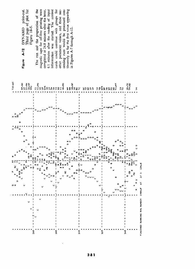
§à ° ° 'g a.S-5° o.
ÙrÀ
V;
**M)00
cz QHtj,
C4
<
l
-
2
2 O Wù O O ù ù OO m mp n â O F
il fl ££O T W fi ? OE £ tC - --ùù-Iù%%OEQ-W ùOEXOEWW Wùùùù ùOE>ùW%OW- XO OEù Z >
OEOEOE-OE !
v V&&2;2;
rrp£rpaKr t
-> >
.........>........" .........> .........> .........j .....
> ' > > '
' ' ' > '
> ' ' ' '
i 1 1 1 1
1 1 1 1 W???Wi W
Wlu>flfl N fl??flflfl N ' ??flfl?
fl fl Wfl W WW
W ?W WW?WWWWW? W fl ' ' flflw 1 1 1
@W2 1 1 1 1 1
1 1 1 1 1
m ) t ) 1 1
*QQ O
' **
' l Wm 1 W 1 1
) ) f0 t (0 l )
àù ? OOÎ 00o I
l 1 1 1 0 0 0
m ) l m0 1 0) a o t a m a T 1 1
X 0 tL 0 0 . I OOQ O ' OE 1 1
% OE? 1 OE? OEOEOE Q?%ÉOE ù OEù £ 1 rc KKK F a n pa £ £ m V S On rcKa
i W 0E82??2?Î 020 poa a
sa a pn rrrr£ r a tCa r rcFrro r
- -----OE--f££1£à-----£-L--1-LL-£---fi£h-£---Q-L>£-----L-- t-
" OE >W » t- OEZ OE > f OE OE ZZ W>
>?OEOE £
1 O 2 r0 r o '°
.
Y ùà?wà I
W mOE OE À Q: o.fK'?cûtD m m0 a: '
W OE ' OOE O OE OE 1 OE 1 ' - p a
à
000
m a n i i m V I p p I i m
m W OE OE p
pal W OE?
â '
O I V I O 1 V V V I m I rv OE
'
' W
'
' OE
' WWW
'
' W
'
'
W
«
) ' ) t ) m "
' 'W ' f? ù > I I V I I I a r W <
OEOE W ' W' ' W' W' OE V V m
' Y 1 ' W V VV 7
' ' 1 1 1 aD 2 V V m
É t ' ) ·1 u )
' W ' ' 1 1 OE
W ' I ' 1 ' ' t0
' ' 1 ' ' O
' ' 1 ' '
W ! ! !
1 ' ' ' ' _
W ' ' ' 1 £
' l ' 1 §
à ' ' ' ' '
1 ' ' ' ' 2
à
S 2 À £ £ N N « m m m
y
381


APPENDIX B
Model Tabulations
FOR convenient reference, the models that were in Figures B-4 through B-7.
developed in Chapters 15 through 18 are here The model of the electronic component industry tabulated to give a consolidation of the applicable of Chapters 17 and 18 with old policies was used
equations and parameters. in the example in Appendix A and appears in The production-distribution system of Chapters Figures A-2 through A-7.
2 and 15 follows in Figures B-1 through B-3. The model of the electronic component industry The advertising addition and the production- with new policies of Chapter 18 is given in Figures
distribution system of Chapters 2 and 16 are given B-8 through B-12.
383
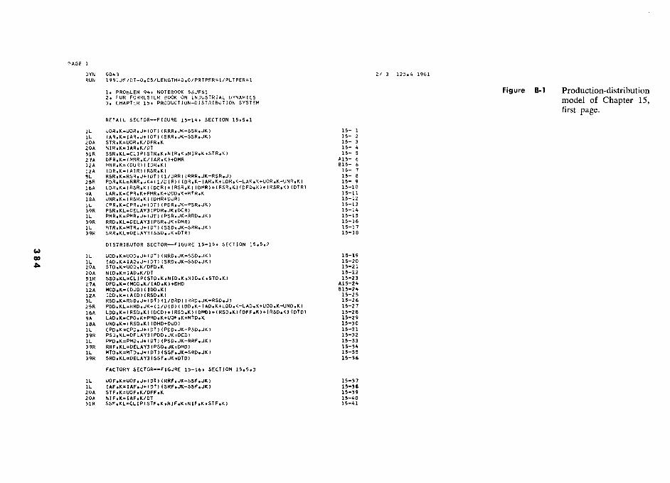
= . 0\1) r,, .Y
::3 ... .0
<U
'H ce e;
' U
0:1
ea
N
3 ."
- 0' d t on
N
,,,, 1
1 11111 I Nv
m
.a .a
.r ...-w
..wa
.. m
.a .+
.r
- à – o
H
1- - C
i -0 0
ae- Q
- t£ Y
Y
1 .
1 . Y
tt Y
O
aeae a?
0 – N
0 –
g +
* g +
+ + -
Y
. :W
:)l y
m
1/) 11J ...n
.. li
V m
1-
. C
u.. u p
u li
OE
:::E
>- '" 0
Z
0 w
C
V)
> .
1 -- - -. p
0 2 1 - - O
'" 0..
tn ::.l-
- ::.l.
- -
/ ÎÔ
- à
- J
00 ·
V
-o-z 2.
........JI- r 0
e...J1/) Ip
Ut::.l.
Y
8...JV)
N
!"-( .-4
<1::::)"" .
G
. 0+0::""
8 II
H
. a
&IJ....
W
1-0::: K
W
--
V)
^ - - -
É
1/) 1/)
· w
w
m
Jm
'17 Y
1^·£
Y
'1 7 7
77 Y
W
·iY
7 7
7"7 Y
p.'
.-. 1
v1 a::: ul K
CI::
U:
a 00
N
O_
2' OY
-p v 1 v O -
F- v u.. O
- N
4,
Z
1 Z
z
z .
zo U
'\ Il I ..
-0.+ ·+
Il
1 I ..
·+ Il 1
... a
?O
Y
Il H
71 v=
e:::-V) .-""')0,0""')0
...." 7O
.J: w
77
. 1: O
::W:V
IJ a
IL
CIO
et
.. o
4100 J
1 Z
^ z
Z
a:: 1
W 0
a:: 0
Y
1 zoeoe
I II..éÉ
v v-.+V
>
II..à..IÎV.rlololo j
II. ·
v t
V
u a
II) 0
. .-n
0 w
- o
0:: .,«(,,,,,:,e{
IX
.,«,c(,,,,,: u
,,?ZIlo.
Il v
0 ....-aao.oo.a....J....J....J
W
....- ? W
QW
ppppJO
?^pd'UIO
NC
711p1U041 II)
o II)
Oc(O
cc:v ,
m a.
w
> W
«
J W
U Il...J Il Il Il Il...J Il...J "..J
n W Il Il...J 1:1 Il Il U
...J Il . Il n...J Il ...J U...J
11 4 II U
J O
=
-
IX
0 Y
v7 00000000000000001?00
u ...
w
cc: 0""
m
Q
u... V
7
z? oc
«0:: O
OC
W
O
<
a.
384
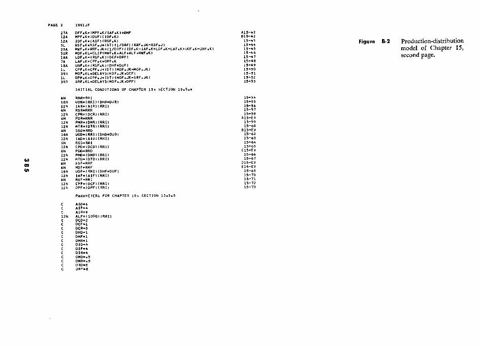
i s O
E o
CM
04,
OE
O
? à
3 s D
0f <
E :rsaffafafInInN
,N
Inlnmlnlnw
ln?ôl:um.o.o.ol.um
olalu.ôl??r=I=
I I I W W
I I 1 I
1 1 1 1 I I 1 1 W W
W W
I
Inmm
wlnlnlnm
Y,m
lnlnln InN
,pvInInNm
nmInN
,InmInw
N,InInm
u,NV
lnmln
,
§ 4 z '
1 ©
+ . h
%
fl
s t < 3
_
!.t t-
. - .
V
N
IL
w
- p
ul o
li J Z
£+ +
" o
f Y -
- - m
1
Iv i Y
.
v .`.n 3 i
Ul
N
Z
H.
> K
O
pG
2
4' vlu Z
-N-
< À
li J
1 1
- %
IW
W
Ô
'O
U
a p-J?
741CI??L
O
O
QtO
' Î
- -
- 1
O
7 7
7 U
e- É
I
I II
+- É
un
- ,
p a
za iz
a
. 1Y
4.IL v
^4. vJ
YJ
O
-- - --
-- - --
-- p
47.?IW
V
O
i0 <N
?UK
d?Apdp
° r.2'
2' p
?p ...IL
I?It
IO
O
- N
-V
p0 p
J ..O
C^K
V
d H
O
li
p N N
N
IIJ H N
II II J IJ
ü1 fl
mm
? N
n N
N
N
P IL
W W
ItiL141L
41?ILIL
1? .?. 2K
fKfp:O
CK
ppppppppl >_IL
1?1 W ?
p4Kl
plL?pltfpIL
KppC
pl N
.a ovisOp<
Zaoad'
z K
o<UlnozH
Vloa V
IapFF-U)po<vlaa
a
aaca a
Q;
ZZ
z
zz zz
z zz
zz z?
z «
1? Ilt..lOp?m
JPJP zz
N
W
<
385
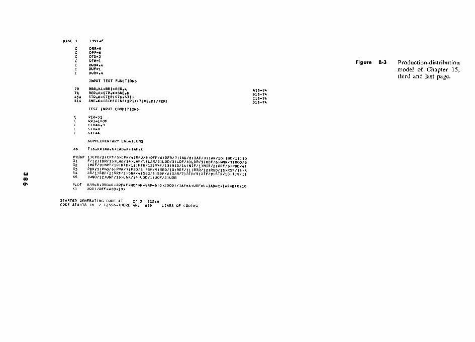
i ë
Ù
ÉÔ
ù
41 C
-
O
<
g ce
3d
m
m S 3
w
4*ee nnnn
à111
$$ÛÔ
=
Ô
2 m
pr-N..
– X
2£X
?OÔ
à f Ô
1
2 OE
'm-'fl
N
N
à O
b
S
à 0
((££$ [
8
I83àà 1
É
ë
£XN

Ô
fl
2 S
- «
-
à à
# vN
3-NO
- Z
2
N
- J.aN
p\ %
.
0 T
OE
-m
W
W
fi
s s
a e--O
oel Ô
W
s £ 0 -
£ Q
«< W
... p
Z - )§1§ W
>N
>
§ 1
D
OE
8 s
v
H
f O
u1
S â
S p
3X
W
41 À
5
%%
E%
>
tC
22f d
É
p-wn-
%'
I ·
· p
1 p
· ·
,je,;,z v
1- 9.9
p 1
0 )
- z O
N
P ZI pC
pIW p 2C
Ot41
h àIàÔÀ
ÀÀ
£ àY
#5 h
k§Xà#
d àÀ
- 52
« 5
H
o J..
~ < Z
?u????. À
À2X
V
vuVV
S
2à tU
t-
%
lÉ > o
386
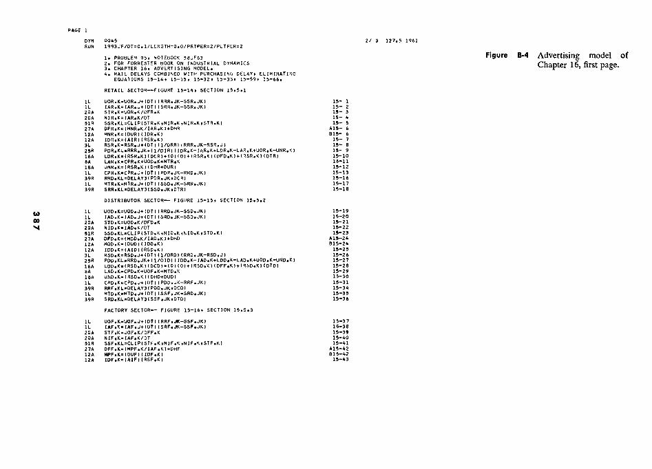
W
O à aD
O
E
O+/
É 4
- B
'-!
- N
4-<
>
OE
q ça
2! D
I iE
o' ., . N - m
.... N
1111111' 111111111 1
11111111111111111 1
11111111 1 Y
1 111
rr .ml
.n .y .n .n .r .r ,r N .n
.n .n .n .n .n .a .u .,
r-1 ^
.w .n .n .n
m .n
- œ
0 C
. o
z v
Tae
2 ÎO
ZI 1
r m
-0
N
Q-
0 0-.
. o-
. - 0-
+.. +.
Jv M
OE
2'
fl ocr 1 .11)""
- el/) W
.
U
rl?« oO
E
N
- W
« . . z
<- °
I1 0
+ 0
a g
<
Q_ ,
j+ - £
-- ......
k ù
Z
a. â
>-
m m
I W .-1 - K
1( 1L
ô u W
v
li Y
z z Q
o
J Z
Z
-
IL
? -
- -
OE
0
Y
- t-
....... « 1:""'" -
. + -
« o
0+- + -
u .
N
t- O
E
m
O
W
Il U
V
c:r::: .:W
:: Y
ri
Y
II) O
E
l¡J II)
v - -
1 --
tJ) 10- - -
-- V
) II) U
U
. m
UU
. M
.
a.. O
'7 -1
J7 ï
D
DD
U
'-1/) JI
U
CI::" ......10::
o . « o. o
4 O
EO
E OE
O
EU
- C
I OE
W 00
CI
OU
- L
I... CI ' W
W
LI...
d' r
a 0:::1,/)1/)""
O
a p Ù
Î
É
^ 1
?? Z
o
Z""'..-III'III"
-co I a 1 tt V
' I 1 -00
1010 p Il''
" o
UO
W
o
0 I
.a » Y
Y
lu ^ 7'7 Y
Y
Y .2 O
Q
lal Y 7'1
Y
y ._ W
ùù àÀ
aa
0::-000....::> Ô
?ù l1..0
p ??
> WO
WW
. n ad'
Z-
'-+zOO
%fl%
O
EO
E
Z-
'-+zOO
%fl%
- O
EO
E Z
- 1..'1
w
CI:: /I
u.. .Y
--- z
0 co-
0 ·Y
Y .Y
Y
J V
I
' /
IJ O
E O
QW
»-Ofl
..-1 cr
0 --001/)'-0:::
a à
2 llÙÙ
i%rllù%
lÉÀ
àlà a:::
u ,"""')::t.l:lolQ
..-- Il
U
O
....-OO
C .0C
.O ...J...J
W ....-lJ..U
-u.. oe 00
m
> ::>-::>-n---
/ II11
% O
Eo
<a - U
UM
UM
UM
UU
UU
UM
MM
MM
O
E U
UU
UM
MU
UU
UU
UU
UM
MU
o
UU
MM
MU
MM
Y
It\rrI
o..U.U
::EIJJ
oC(
a ........
ààààààààààààààéàà à
O?
C O
CI--I/)u..o.o
0..-1 0
W ::>-I/)Z
I/)O%
-
ZZ
a
a ««Œ
<CC
<c >::>
7
..-1 OOC
U
J W
ù
387
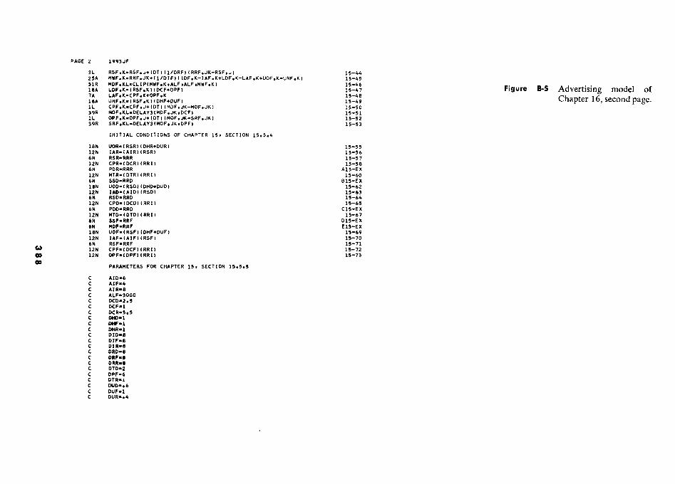
?
'° 0 c
I: S ci
CL
, >
M
aU
H
s s 3 0) E
aN.orm
o.o.rNm
n.nnm
?coxNm
onxrxxao.-.Nn
aee.teennu,n ul.nw
.oo.o.ol,mol,m
.orrrr nnnnn
wnnnm
mnm
nnnnnnnn
)i. # IoL
§
.! +
.
t S
£ < g
J O
O
I
f h
h u In
lu ..
·O 0
fl U
- J .
Z
N C
+ K
Y -
- - 111
1 1 . Y
.a
h W
C
Y
y ->
a IL
.. I Z
s
le r
K Y
? O
d' 1
à tX
*b. <
Y1
- J
I It 1 =
r1 Y
VY
d "
Î o-Ja
' ô t
£ a -
z a
é 7
D
V
1- =
a o
rw
ce ce
xo ce
ce xw
m
m
m
Z
M
Oa
oCs
p
d'K
d- -U
10 I
J N??V
2'F-ON
??VO
HI?I?N
?1? Q
f O
n n
.. ? P
KZ
Z
JJ7 V
ZO
N
0<0&
0 00 â
««Ô??G
OC
OO
OO
OD
OG
O?G
G
s
a a
a m
u
x
ZD
m
uo z
zz
ù ««O
OO
O
oconnaa
Jn?m<
mJPJP
mN
ZN
ZN
ZaY
NZ
NZ
NZ
Zm
NZ
NN
N
A
.·
V V
V V
V V
V V
V V
V V
V V
V V
V V
V V
V
V
W
<
388
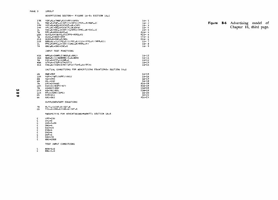
41
nï
–. n<
N
rob
K
t 2
v d.
- °-S
0ô
S 3 rn
w
- NM
4m0000F?O
E
P O
-NM
4 m
OF?O
EO
EO
EO
EO
-M
àààààààààààà 1
1 ààààà
1 1
ààààààààààà 1
1 .O
.O .o
.o .O
.O
.O N
.O
.p
.O
.O .O
.O
.O
.D
.O
<O
WO
<W
VO
<
« w
o 0
1 w
M
M
- - -
s x
ë 9
1 -
- g
5 V
Z
O
4!
Î G
i
à
J £
W
. In
< <
< a
. z Z
' '
' ù-
W
W
w
Y
... ? q
Ô -
0-' f
0: o
M
. 0
>
z--> . -O
E
W
O
£
É àIÉ
#I %
#$
-£ à
<
fl Q
$
W
>fIO
OW
D
o%
Jp
OE
z
o -
<z"">
<
a 1
Wo V
Z
< -
o O
o H
a
W
I(l
) É
az
Z
– S
à O
E
W
fl < U
+ >
- O
O
E-W
W-
* --
- o
> D
oM
O
>
O--M
>
O
<
a W
o <
«
à É
..
m
- ce
fl fl
M-M
M_*
.fl'W-o
D
W
<
W
> o
.+»+D
-OU
OE
+W
W
W
OE
+flfl o
OE
'
OE
O
E
U+
IL
.W V
W
W%
«D<
M'
.OD
+
10 o
- Q
<
.Il Z
> O
EZ
.ùr o
- M
OE
>O-
> W
. fl
> fl
W
_ Z
O
E
lm
fl 1É
ùfl#Éiùù7à2
1 àcàà?
X
# Q
É
O
8 à
OO
X
"XO
t' IUM
UO
fIO J
<" < l t' fl
<
W
W
O
o m
O
O - ·
o. O
E U
UM
UM
M..O
UM
M ?
MU
UU
M -
X
J .M
X
O
- W
o o o ...
M - « o ..
> ....
o <t
ù - o
< 1 fl 1< « <t « t< fl 1 ù fl «
> W
WW
WW
WX
fIMO
EW
W
ù O
EO
EW
ùW - W
WW
OW
<tl ù
OE
w
£ Q
C-
D
J· W
Oz
< zzw
flfl - fl
OE
>«OO
OQ
QO
W ?
«
ÀO
SàO<À
<àÀ
OO
E
là<ÀÀ
zÀ
zZZ
#Zà#Z
Z
flfl rJO
?PJamaoN
Ja m
a«n.-I zm
zzzmzoN
ZZ
w
ln m
- M
MM
MF«F««PP
4MFO
M
FW
WV
WW
WW
WW
WW
V
W
W
n
389
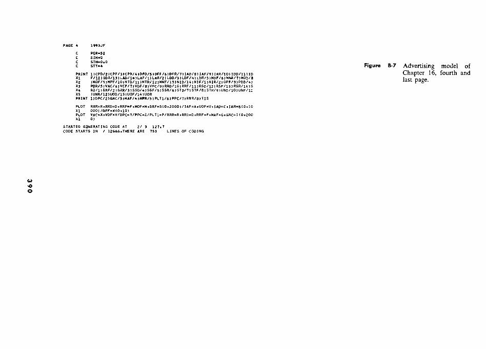
C
ça
0 a
oe
W
"
go
s 3
Q
O
* M
.-I a\
4 O
N
X
0 à
m -
2txPz Z
O
\mC
0 II
< u à
u
%È
%aà
Q
à <
4\2'P <
r%£âà
z 1
- £-N
a f
fl Q
Ê
kitÔx
r à
O
> fl0
a' 0
# à
ù Ô
à
n a
o
j g
W
- x
r à
C
t
Ù
Ô
W
o ce
à 0-Q
, ·
- S
i à
(Y
z '
O '
v r t
J N
r
à à
r %
M
gj (
f "n
· O
\
J T
%
N
IL
4i\t-n N
II
4! n.
V
%
2 X
n
à k
\ >
Y
' ùàe K
w0
·N\\
wO
V
U.m
W
Ou
p?0 e
V\n
VvJl9
p I
IL
V
N
-
q(g
Q
O
NO
->d'NN
K
n> t7
n N
w
pw
2\
T?2f
1 r
m
mm
um N
1
nNIL
\.w2'n
11-II !-
S 5i£5
L8%
- 1£
P IU
H1?H
K
v -
ùflwfl
ln ..
u - --
0
> "
20 N
t- I- 0
o oc
4 W
WW
W T
â2fi£22 0 0
8à d
V
V
&. X
XX
X&
&
X&
X
IJN
s K
41
S 18
£à «
.0 0
G
? u
390
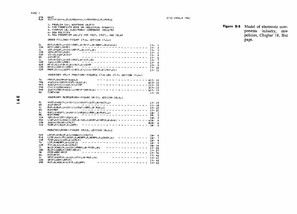
U
00 .
<u
'"
,
.
Qj
<U
0 <
U
0 00
S 2
L6
*Ét
S
W
- e
N
« T
\ «
Nf?tnd
rmO
.H.rN
Tddm
?O
rmP G
.Ord O
?N1.1
«« N
.. N
N T
d d d d
1 1
I 1
I I
I I
1 1
I 1
1 1
1 I
1 1
1 1
1 1
1 I
1 1
I I
1 1
I 1
1 1
( 1
1 1
1
rrrrrrrrrrr rrrrr
rrrrmm
mm
mm
m
mm
mm
rrrrrrr Îm
V<
m~
I I
1 1
I I
I I
I I
1 I
I 1
1 1
1 I
1
1 I
1 I
1 1
1 1
1 1
1 I
1 1
1 1
1 I
1
1 1
1 I
1 1 1
1 1
1 1
1 1
1 1
I I
I 1
' '
' '
' d
' '
' '
' '
' '
' '
' I
1 1
1 I
1 I
I I
1 1
1 1
I I
1 1
1 1
r 1
1 I
1 I
1 I
1 1
1 I
I I
1 1
1 1
I I
I I
1 Z
I 1 I
1 1
1 I
1 1
I 1
I I
I o
1 I
I I
1 1
1 1
1 I
I 1
1 I
I 1
I
I I
1 1
1 V
1 I I
1 1
1 I
1 1
1 1
1 I
1
4 1
I I
I 1
N I 1
I -
1 I
I I
1 1
1 I
I I
I
J 1
I I
I 1
1 '
1 1
M
1 1
I 1
1 1
1 I
1 1
' r
o -' ' ' '
I '- ' ' ' '
1 m
'
' '
- ' '
' '
' '
C
r F
.r O
O
E>
C
+I 1 1
I 1
I 1
I +
1 I 1 1 1
1 «
VK
Z
C
o
Z
O
« Y
"
.y +
I I 1 1
I 4 C
1 t I
O
^ 1
1 - I
+ I
o I
' 1
1 '
L-
4 '
) 1
t*) *)
1 T
0' ' '
1 '
a Y
M
-
V
4 -
4 m
V
>
Z
4 I
I - .O
1 1 1
IU
C
1 I
1 O
Q
- fl
- o
M '
/ /
%
< ù
&
â K
VI
1 z
J '
) !
à r
Z
O
I 1 4
1 1
O
aC
Û '
' <
Z
O
£ I
I I
I I
.. 1
1 1
Y
1 U
N 1
1f 1
I I
Y
1 I
« ..,
lu o
K
OE
4
'7. C
7
o 4
O
- a
– U
Y
4
O
Y
4J Y
1C
-
4 O
E
C
m
4 1C
4
Z
41 Z
4
7 2
rNp
K
lu tY
l I 1
J +
.. 1
N
^4! I O
I
o r
V;
o o
O
4 .-
17 4
N
K
OE
O
-
£ V
4
C
'7 C
O
4 I 4 1 -
lu I
+ 1
4 v
1 C I
4 m
ZV
4' O
E
. - -
W
4 2'-K
- -
NJaf
I £
C
T
~ V
O
4 I v 1
I I I
- £ V
l7
1 1
' «
4 V '
I W
iC I
1 l ^
r I IaL
I I I I-I-
Z
É
I N
I^INI
< 1
m
1 1
7 4
CO
OZ
V
'.· O
D
Y
YY
O
o 4
W
4<4K
O
E
- 4
Q
ù "
O
O
4 7
o '7
o o
- V
1 1
4 4 - O
^
4 C
Z
m
aLK
W
L
w
4
4 n-
7^ 4
1 K
v
, Y
41
J£4 £4
41 J
K
4 U
V
V
H
< V
£
tY
m
· a
1L
V'
rOV
<JK4
W
KC
<
<
.lvV
Ù
Y44JZ
1CG
·4?4 O
D
d'
C
T
2ZÛ
1
§ 1
1 V
' O
·V
4J-K
X
t &
O
EW
O
E
W - -
W -
UW
- 1M
'o-- w
L
- &
W
-&-
- O
-VV
04 p^..
' U
,IV
I -2-
1 -4a
CH
1 04C
4C
C44K
2 ·- 1 -<X
+ x
+
a +
C
+
I atC
. 1 ^+2 G
V
.m.-.tu
17 J
= . O
7 -
7 -<-
o V
£ Z
+
V+O
X
IU
+ +
-<-4 Z
·a>
£d'KJC
J
xx-z- 4
Kv« ?
4104J0< J
4^440 > V
V V
t?4 >
V
744 N
m
J 1 G
441 é
J4 Haa
N
K 4 -0£4
a a^N
n
N V
N
4?mZ
440QC
2
A
OE
4
O
Y 011 JV
< e
1142?4 Y??.Y
rN
V
Y
NJ£ N
NC
K..N
OI
4 O
K<
33 n
Y4'N
aYC
YY
?-Y
< .Y
YIJfL
?-K4aL
?-J O
C
02414 K
Z
4
· 2
o N
YC
.N
Y .11 .
4 4
..YY
·N N
K · N
1L
rr d4V
Z2
IL
o« o<
t o<t
11444 IU
IU
44.N
>
044..444N44.
O
p 44444444..r0
> 4 X
XN
XZ
>
Z
V0044 V
V04m
-·4 o.
o o
K
V
1 o z
Z
< O
V
X«
O
^ 4«V <V
£
JJaJ4msaaoo£
zz z
zz zrcza
«££ aaza
«OE
O
E
£ £O
E
JNJN
OZ
JNdN
N
JZJZ
JZN
dNN
N
<NJm
ZZ
JNP
- C
G'
4 tB
6
391
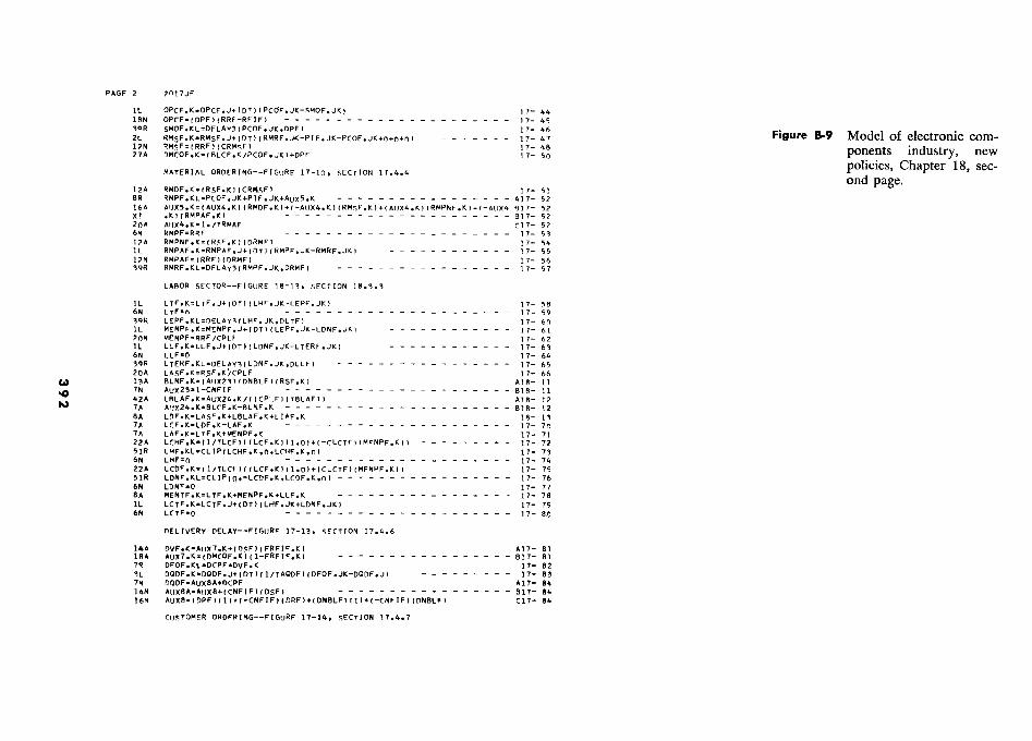
H 3 Û à v
0 p
U
00
N
u< h
N
41 U U
. y
°
- - a C
;...
^O
0 m
Ô
0 a
0? S 3
0) iE
dN.,orm
c m
aln.or ..N
mada
aaaad?n ?n?nInInN
?uwnlnum
n m
mm
mm
mm
? ? II
I I I I I I II ? ? ^
rl ^ I 1 1 I 1 I I I 1 1 I I I 1 I 1 1 1 1 I 1 1
I I I I 1 I
1 1
'.âmm
i,..........., âm
^"âmu
<imÈ
<m
<m
<m
<mW
I I
I d I I 1 I
I I
I I
I I
I I
I I
1 I
I I
I I
I I
I I
I 1
I 1
1 I
I 1
1 I
1 a
I I
I I
I I
I I
n I
1 I
I I
I I
I I
I I
I 1
I I
I +
I I
1 I
I I
I I
I I
I 1
I 1
I I
1 I
I 1
1 Y
1 1
I 1
I I
I 1
I I
I 1
1 I
1 I
I 1
I
1 1
I 4 1 I I 1
I I
I 1
1 1
1 I
I i
I 1
I 1
1
I I
n I
I I
I I
I I
I I
I I
I 1
I 1
1 -
) !
I
! '
! !
I I
1 1
I I
I 1
I m
u
I I -
I I
n I
I I
I I
I I
I I
I I
I z
' -
Y
J '
' '
' '
' J
' J
' '
' '
' 1
I ·
I I
I 1
I 1
I 1
I I
I I
I 1
I I
I
I p +C
d ·
I I
I I
I 1
I I
1 I
Y
I - 1 I 1
I I
li d
1 +
1 I i
1 I
I I
I I
I I
I I
· I Y
I I I
I I
u ·
I + c
I +
n
n I
I I
n n u
I a
I 1
I a
I - 7
I r
Y
- o
z a
· .
1
I I 7
z
1 I Y
I I
I 1
I I o
I I
I I
I i I
I I £
4
I I
f z
I I
I 1
I I ~ r
I I
o Q
I 1
^ + ô
I C
V
I£I IY
1~ -
IY
I 1
I 1uI^I
1 IO
z
I o I
Y
I I
v. I
I O
I
1 I
1 I
V
I H
I I ^
I 5
1 7
1 4 ,
7 Y
-
4 -
4 Y
J
V
Y
V
o J
w
. 7
-- IW
ti-
m
4 o
O
o £
V
Y
C
o -
1 V
C
o
N
O
2 d
0 1
4 -
«' I
J O
E
IL
'7 I
4 I ^ 1
I ^ I -
4 I
4
v I
4 4
r I
I 4
I Y
IU
4 ^ I < I
1 C
I
à +
r I
-14.w
- In<
·a^
< <
14YC
Q
11 J
I ·£
TIU
14 JJ
O
Iml
1 I
0 +1
I 1L
Y4
%
b >
- 4K
.-nJh4 1
01? à'
u r
mp
a a4.'
b
É
. 4
Y
" +
^ £
w
Y :
4u 7
d' ^
li ^ v J
-- >
Ù
V
7£ -O
·
O
o 4
JY+
: Y
= K
K
Z
IO4
· 2^W
'444·4 4^
.y147-Z442·Y
4
44. ·J
W
.- 4 4
I v. 1
C
£ n
4 C
= .
r C
Z
J V
4 v Y
V
V
C 4
.- .-
I -
O^
V
I i^£
?O
a C
J
4C
J C
m
.-Z
4 ·JO
L
JV
C^
·- ^ Y-
^Z
I -
4 V H
-a m
aaa
o-^£ t7
J4Z
· .-J Z
>
4- ·H
4V
CC
Q04?
Z
V+-
J+ Iu0
1 Y
.^4p Z
Y
v
-- Y
^ 4
11 É
Y
I m 4 Z
-- i -
w
£ ...
I N
'W
>OK
4 ' Y
· .
I z
·4G>
I V
^ Y
7 +4+7V
V-
4.
C
· d^2' V
Q-J
z +
aaa+
J ?N
.. 4 Y?+J
^ Fd . ·
J C
-
J C
' 0
x .a-
O
O
JZ
\O
IaW
(li V
. Y
\2 ^
IL
mV
24++^ 2'
V ^4l U
7^m
O
K£ 4lal
h ·
4141 · p4-Z
7J4 ·
m-
u C
O
G
4C£4.-
Kd<li
· 4
C£4u
n N.4V
Qm
Vnli4.-IJ
J V
xC
Cpm
X4
02 2CH
J
nKJ
H N
<ph^V
J >
CX
O
E C
' 11 C
J IIKY
<
U7
J JY
KJ
Y 11 .?Y
YJJJn
11 ·
J Y
N
K
4: 4
YY
Y£Y
K ..IIY
H
Y
·H
·Y1C
H
· n N N
YJ
YY
O ·Y
O
4u Y
YY
< N-
£ %
o«
IIIr_ 2'
·2' . I 444 ·
(r Y C
·44YO
U . 4d Y
YY
·Y C
· 114 ·
> Y
.. N <
N
O
r IW
niNU
O
u uuln-duz«u
o ·114na·IIm
?IeNaN
.··4.nulu?-4u - rliuum
m
h vu 0
v oax?-xaaaa2'
s uuazzu44l ;Z
J%444Z
U40Z
?ZZ
fh J
4xOC
Cx
v, 4 2 Z
££ Q
Ii JY
£££££ Iu1a141JJrQ
J 7m'C
VQ
V S=V
Op41 JU
^
O
O a C
C
£ K
K G
· Q Q
K ? C
? J
J J Z £ J J J J m
< J < J J J J J J J J J i
J C
C < O
p O
< <
V
' za
za a
a a
a zz
a z
OE
« <
<OE
aa
zz Jm
O? JN
r N
K vp? C
ZN
JNP
dmK
JZd?O
«
N
.O
'n
HJ
l7 <
392
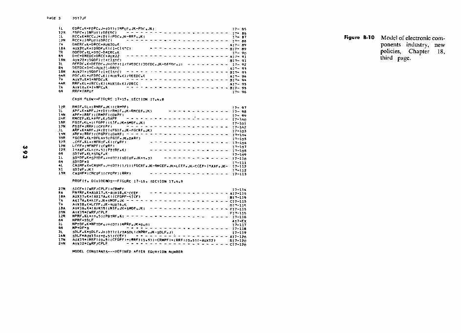
< U
. O
- C
L, aD
Ù
ao °
M- C
L,
'0 U
U -Q
0
n 'S
0 s S 3
In?prmPP 0.-?.-?N
TT
ddlnln.0 dN
llvNInInIW
pXrm
P CO
O
mC
GaD
mm
aDPPPPPPPPPPP
i i ' i i i i i i i i i i i i i ' i i iil?iliilllillii
1 ? ? 11111111111111111
111111111111111111 Illlllllrllllll
rrrrrrrrrrrrrrrrr rrrrrrrr-rrrrrrrrrr
rrrrrrrr.?rrrrrr ?<m
vôluli '
' '
' '
' '
' '
' '
' '
' '
' '
' '
' '
' '
' '
' '
' '
' '
' '
' '
' ,
' '
7 1
' '
' '
' '
' '
' '
' '
' '
' '
' '
' '
' '
4 I
1 n
I I
I I
' '
' '
' '
' '
' '
' '
' '
' '
< 1
1 I
1 1
1 1 N
1 ' '
' ' ' '
' ' ' '
' ' ' '
' ' ' '
' ' ' '
' ' ' '
' ' ' '
' ' I '
' ' I l
I ' I X
1
, T
7
I I
I I
I 1
I I
1 I
I I
I I
I 4
I I
I I
I 1
I < 1 '
' '
' '
' '
' '
' '
' I
' '
V
I 1
1 I
I 1
1 '
' '
' '
' '
' '
, ' '
' '
, '
v , ' '
' '
' '
'm' -
I 1
I 1
1 1
I 1
1 I
1 1
1 1
1 1
1 1
I 1
1 I
1 O 1
' '
' '
' '
' '
' '
' '
' '
' -7
I I
1 I
I 1
I O 1
' '
' '
1 I
I I
1 I
I I
1 I
I I
I I
I 1
1 -
41 P
IL
OE
'
' '
' %
' ' ' 1
' '
' '
' '
' V
I
o 1
I 1
1 1
I K I
41 '
' '
' é ' ' '
' '
' '
' '
' J
d '
' '
' '
m
I 1 1 1 1 I 1 I I 1
t)t) 1
I .I - 1 I
' '
' '
C
' '
' '
' '
' r
' '
' '
I I
1 I
Ic I
1 I
I I
1 1
1 I
I 1
1 I
I I
1 1 ̂ 1
Z
W
o o
W
I Z
£
1 1 I I
ZO
£
1 I
I I
Y 1 I
1 o
1 I
I I
I V
I 1 I 1 1
I p 1 Q 1
' '
' '
O o
' '
' o
' '
' ,
' Z
, v
' '
' '
V1 U
v ' '
t- I
I I
I I
I 1
1 I
I I
I 6'
I V
1
I I
1 I I I 1 I
< V
1
lu 1L
- t
) )
–)
w
O
7 W
C
N
C
C 7
- o m
IU
· I 1 I O
1 I 1 Z
7 I
I o o
. I
I C I 1?
1 · I c v - I Y
1
I 1 u . n
I 1e I 1f I le
I + c Im
o K
1 1C I
1 n1 a
2 O
- V
lu O
C ^
Y V
I
- 7
+ I 1 · I
1 V 1 C
1 U
I V
V
1 · 1 V I
7 'V
r 1 I '
Y 1 - 1 4
1 Iv '7 Y
1 K
I I O
I lu IU I
K
V 1
lu V7 G' F 1
t? 4 I K
<
li - .w
V ? lu
V I O
lu I '1 · 1 2 Q' 1 <
r l K 1
I V I I
C \ 1 O
\ I
- aC
1
p · _> - 4 ? 4n
I Z V
J 1
C - N
+ I IU
p
Y
' - -
+ 7 Y^
p \ C 7
aC4 Y+
G 4^^
Z
G 1
OE
« 1C
Y 2
· - 1L
- 7 4 Y U
! ? 4' 47 lu · Q
aC · 1L
^
z o
- --
-o o
i .a
o _ _ u -
wua W
V
Y W
GN
U-V
VP
O
r 2..G ..m
4 3 lu · lu
o .-nVO
7 lu ^p
·+ «
V£<lu4
2 I C
xVliX
4 O
- va o-.vxlnercm
? x
_-a_pa.. e p a 1
a p_ --v 1
ro-^ -alr,-
In 1
r^- I
plu-Vx.-lu<V
+ < K
+ + 4
m + pln^ 1
> O
\. Z 1uY
·+Y-41 W
- YvIL
< V
7 ·p6YW
4'pd >4V^
o 41 J +C
·J F.
lu O
4rr7 4 O
I 06 Z ^+
OV
K
^p J-Vp .p
Z+K
W
V'
·JC =
Vln p
< li ·7-V
O ?-O
t?1u44441VZ
1 Z
OV
21?-'7V111414 G
C
V N
N
H 4+^ \ H
A
-·1-!L'p0+
041100ZV
+ 1
< A
JInI?IW
7 O
aVJp-11V
OO
VO
IU+C
.y f - .-IW
- -ZIIIIN
pr-iK
2' Z
N
7 O 1121iJ nIrK
I?J 114JJ II nYV
Z
N 1 N
N 311 J N
%K
3 O
Y
YY
41-Yp-n N
Yp J J<K
YJd'<2'Y
JiYY
YO
YO
- U
YY
Ya(Y
V
JpHO
N V
4. Y
- .Z
N II JY
J .Z IY
Y IIK .a(-H
K
v1l- . N ·
P N 1C
Vi .N
1L<N
N
7
· Nt?lu4l?ln.lu4
N 41? . N
I?N
J r
V V
· n !r N p n N
p O N
. P · .-I
n 2
.a Ul
- ad V
VIL
X41V
x4:4lXV
X1? X
1? O
V·X
?Xx)(try?ffJJ%
X
G
O
p O
N
V
?«p44«IU
JJ-N V
IU1V
hV
2 JE
i
z z
<
z za
rc a
zaaz zzazrc
z z
< aza
Z.z
N J N
< m
K Z
m J Z
m d < d <
Z
C
t7
4
393
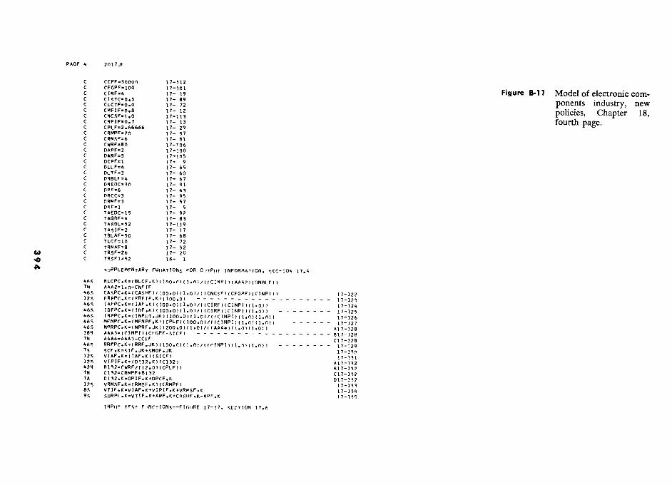
' 0ô
? U
£££ N
<K
'-' pp
W
OE
s 1Q
o
iZ .T
mdN
VO
rmm
aJP G.?N
NN
Nm
dIl? N
NN
NN
NN
NN
N m
m
1 I I 1 1 I 1 1 I I I 1 I I I I I I 1
rrrrrr rr I
1 '
1 I
I I
I 1
I I
1 I
1 1
' I
' ;
t t
' '
f )
! '
' '
! o
I I
I I
I I
I I
I IW
V
- I
- I
V J
n I - - C
C - I
.O
m 2
^ --oo- -
* Z
Z
G
h
§ Z
<
N
Q
a a
1 t
I t? G
Z
- - V
U a n -
- -I--2Z
d1 2
I 2
< F
- - K
K---G
-
o -
_ I I
i a â -.
r I
\ -oc- 1
YI
à ?
c - O
I o
Y · a lu
O . O
o
I 5
U'
.O.C
.OPdPY
VN
Pm.-??.O
rW N
V7
- ...C-- ^04 -
- ->Q
4
«P «
««« «
Z
C
^ - C 4 W
i C
--
4. + V
I r 1 r I r I r 1 r I r I r 1 I I I I I r 1 r 1 r 1 r I r I r 1 I 1 I 1 1 I I r 1 r 1 r I r 1 r I I
1 O
e O
· C O
O ..rn O
O J O
O -
V O
Y ^ m
N
4 J Y n f . Y
Y
+ V I
c o
.. c ô _ u. N I
z â
-. o-00---4 o
-ôln-- r
4. Y
.O
lu V
Z
>
1 ,O
a
Vn V
llululCn2?-?V
ICY
.m-m
W ) ·u ?
W
.o a
C
.p f
OG
·.pC
C
O
«
Q
« Iv. 11 C
N I ?..< N
- IIZ£04 >
N
OO
C.H
C vN
v00 dm
£
f y.
N d H
H IIm
mN
.wdm
H
MM
11N
H IL
-< · N
Y .V
UY
.Y .
O
H 1? N
V 1? 4 1? 1? H
1? lu H N
II H II lu V
.0 11 H .r V
IL. J 4 1? 11 li N
J V
H V
V V
V V
U V
II II V Y
. lu II I . lu · J
F F
ICnIC
Hf.. V
;-Iin Y,41C
IC1u1C
4 JG Y
lilC II pC
G·alr_alC
lu a aN
anaanaamda .?.-.N
NN
V)1C
n S
« Ia. V
^ C V
: V IC
V IC
J f f n n a n J H m
l.l 4 V f 4 1u O
V, V
) J V £ V
) V
I n V < V
W li l n Z
K a G
4 1i i n t? F m f ^ ? n
C
V IC
- - J f Z Z
n K K
; Q < V
J J Z Z
n Q C
I! Q 6 Q
i m J K
K
K
O
Z
N
V V
UV
V V
V V
V1:U
VC
CC
CpC
CC
CC
GFFH
fHfFH
r V
C
QU
4....-£Za<K
UN
»2UC
» V:
.-
OE
V:U
7V,V
?NZ
V
' V
.Z
O
4 W
ww
ww
wvvvvvvvvvv@
VV
VV
VV
WW
WW
WW
WW
W
.C Z
.ON
.O.O
.O?pvpaD
Z?O
V'N
NZ
QN
V7
V:
d V
VV
VV
VU
VU
VV
VV
VV
VV
VV
VV
VV
VV
VV
UV
VV
V
drd.rddddd.?rdr.-m?drr.?m
P
n
394
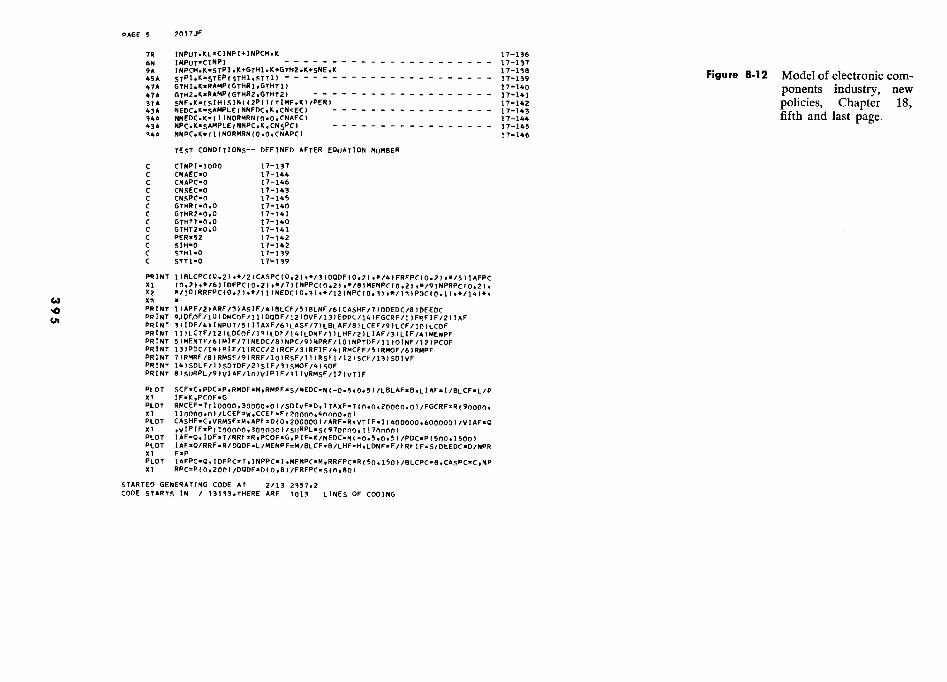
S°" u
Sa _
. V
fl .
a " -
"S
('01
ta 2 1» iE
a , 1 Iii 1 1 1 III
1 1 '-
1 r
1 1
1 v..
a a a
£Ir::: Q. '
' '
' '
..... C
Il a
Z
1 1
1 1
1 0
LI..
v '
' '
' '
cc .q Il
C
c( -....
U
1 1
1 1
1 L
I.. C - 00
Il - -.....
U
0< > 011
U
V
' '
j '
1 \p. H
` V
1 cc
Q yl
' '
' '
' -
WW
m
Œ
- ....0 1
1 1
1 1
*Œ'- ̂
- lL
.LL
....... 0
O
-w
et - 0..-
.w
N lu a O
.... L
I.. 0 O
? V
'
1 '
1 '
-2. u""O
ZU
Il
O
0 co . N
-O
OL
L.U
?? L
I.. V
0 m
I
1 '
' '
cc ?
0 n
0""1...1 L
I.. 6
Li
V
' '
l 1
1 Z
Q
.. '
' 1
1 '
m
0 0
ou. J
, ,
Il. 0 Q
..Œ
m
.1 1
m
et:' ..... ..
V_
ar::: L
LO
"" c(
0 0--"" -
1 '
1 '
1 ?
--. J
0 ?C
?LL
. 0 O
m
m
0 m
2
' 1
1 '
' Z
J
N
- *Z
ff' IIC
-Z.
0 1
1 1
1 1
Z
.W.
- C
o
- c v d V
J p v 11'\. ---....J
1('1 u
1 1
1 1
1 C
C
«Q. -
o -«lU
:I:'-N
Q..W
V)
..... 0 - >-1:1: ce
I.L.
' 1
1 1
I -
o.....a.. n-
0 ....
C[o.......u...-:l:N
> '"
noo::czu... ua
' '
l '
' 2m
IJ')
=
O-N
N
0
><ou...OU
..J u.... 41
1 1
1 1
0 1
O::C
Z
4/
O .\
m
- 1
10:: -C
· w
-C
"""-ZM
H
Z
lu "
é 1\1)1
4 U
J V
o.O
":!I.lU
IIV
N
N
+ ......
.00fI"'
CI
Il CO
-lII...J va... o
1:!I.lI ---
UJ
. ca:
O
z \
Z K
IN
I N
-- -co=:c...:I:
1¡Ju... X
L
L'V
ez:Vo. C
.-u O
NN
V¡.II
:E""" N
- --Z
ZZ
A
I¡J 0""0
N
z (W
'Iq4'44'4'444'4.?? n
V1Z
Q
- Il.....w
L
I.. 111111111111.10..- Z
Olup0041
Z
UJ
a:: n CV
U
-I-C
lCI-uC
:.,{. C
I """-<O
(I;f"OV
u...V»
. ouu..co....... 0.0 p
Q..
u.""" ::E
CU
o.O....J
Zn n
w
£ 1 I
-1.&..
O
cr: fr
+ +r.r.r.-Z
::EZ
O::
CI)
......u- 0
?":EO
I.LO
x Z
.00N
-C......v..................O
u.. Z
u C
2 M
O
n- 0
.1.1.... 0:: O
UJI,L
CO
::O U""" \
. Z
-00
<Z-- L
&Jf'"'I
1- r
o.C)O
..J:EO
I-O:: u..C
O('r'
- 0
O::-Z
I'\I--O::--
00 0-
CI 0
0000 ^
T
..J-NV
.'or::o::v,l,/')nC[- Z
0 ....
-"""u... ......
:¡¿v:¡¿nlll-n),{.V)1I
a ""O
OO
OC
OO
O
v.cr o.u""'.un-o::
OC
O
7 U
V
N
00 2 ·K
r .V
r Q
4141·16K4'1-r n N
H.n
JNO
m
wL
xwoez;>
Y Y
41Cx4
2 m
,< - -
Y
ZC
<V:U
',r.r.r.Xor:::r.r.1- m
.- V
< Z
c
22Z rf r24nZ
Q Z
(K
'- N
1-
UJ V
I Z
1- r
< "
vvvvvvvvvvww
w
000 00 0 < 1
UU
VU
UU
UU
UU
UV
U
Q.><
><><
Q.Q
.Q.Q
.Q.Q
.Q.Q
.Q..
0.><0.><11.><0.0..><0..>< W
V)
>- 4i ,
G IU
W
a §
< >-0
O
w
395
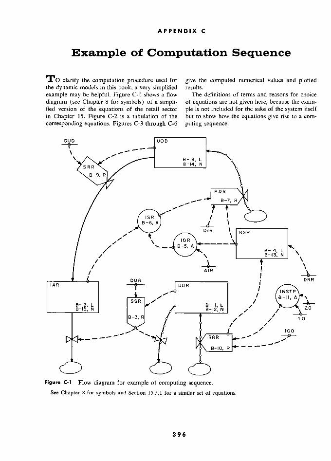
APPENDIX C
Example of Computation Sequence
TO clarify the computation procedure used for give the computed numerical values and plotted the dynamic models in this book, a very simplified results.
example may be helpful. Figure C-1 shows a flow The definitions of terms and reasons for choice
diagram (see Chapter 8 for symbols) of a simpli- of equations are not given here, because the exam- fied version of the equations of the retail sector ple is not included for the sake of the system itself in Chapter 15. Figure C-2 is a tabulation of the but to show how the equations give rise to a com-
corresponding equations. Figures C-3 through C-6 puting sequence.
DUD D UOD D
_ P ' B- 8, L
S RR B-14, N
8-9, R
PDR R
B-7, -R/ V
, / T fi
ISR / ' B-6, A Î
DIR RSR RSR
/ B- 4, L
1'
/ B- 1 3, N ,
' / \
1 I \ 1 j
IAR DUR R
UOR j DRR
fl? J INSTP / B-11, 1 1, A
L SSR R /
/
I, L
/
IAR N
/""
É-121 L
, ' 1' 20
B-2,L N B-I': 2 N / B-15, N
_ B-12,
N
/
/ / oo
B-3, R / /
/ / 1.0
/ / "., // 100
- --- -- """ RRR "",--¡¡r- - -- '
RRR
.... "'"
R
Figure C-1 Flow diagram for example of computing sequence. See Chapter 8 for symbols and Section 15.5.1 for a similar set of equations.
396
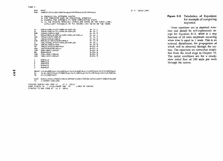
h y t-I
S
- S g
23-2='
s N
O
N
N
– . o
NO
O
àOE
d
O d'
* ·
Q
0 1?1 O
K C
Z
K
7
2' *
II $
11 p
* *
O
0: 1 *
S t*
4~ >
m'
a 11
2 &
XO
E/«O
EX
OE
OE
<0000 À
i p
410 JJ2'J«K
JKK
<Z
ZZ
Z
N
m
<? r
............ m
a
I- vl L
n -z o -
u O
1-Z
H
K
U7
1 N
O
<
1 1
1 à
1 1
1 I 1 1 1 1 1 1
10 O
.. <
Z
!L'
m
!Y
m
· 1
Ô
a IL
-owp V
Z Z
0
0 p H
E
.. >
Z
\
P II
V
? K
Î
" >
p ? amz W
p
ô ?z<
O
o w
4
V V
1 NI V
N
2
0. p 0
_Z
41 C
J N
T
É
1 J
a!-3ui I
M
ù .
° -
lal Y
Y
Y
Y
K
W 7=
u1=
77 '1
7 ù
À
tl I?pu7J1-
..m
fi U
1 C
NV
) 2'
d' C
4.'
' M
' C
K
à H
NO
N
N
OC
N
'«
K
I- 1
XIO
Y
Y
· ?Y
?O
p
M
Î II
O
-D.
IL
i 7
K
K '1
O
11 IW
n =
ozm
J
o? Q
M
ô
K
v K
N
luol.ma
za 0 C
r az
12 W
'
J 2a<
1J< --
ce) IL
'
IL »
Hyh-K
2'pF-J200 00
\.. ?O
H
2\ O
n
p.· Q
H N
W
N
4
PIJt?K?
++Y+
· 1 R
+YO
dO
00 410
ô aa
i 2 0-1
R
· ?K
W ' vN
RpO
F-· 11.?
I- ILO
JN1J
0.'I-p ? 1 V
N
p
JW p=
J O
<O
m<p-O
7.w 11 ? vp?
KN
O
N·
m
FF-.-. >r
N2'-v
Ii Y Y
707? 00000
UIZ
? V
1Z O
7 O
X
12, "0 7
KO
XZ
7 .-n m
NN
1 w
N
V
1?0 21v41?<
II 11 N N
11 1111 H 1
IIN
I- m
P 4.'2K
2'p *
<ZZ
.O
P 2À
ÀS
O<
m?Ipm
pO*-'?Z
ON
O<
JK··O
JW
m
??Z
SD
0 ...
a .0
0 1-
41 1- O
2 l7 d' 1-
ZZ
?«2'<Z
ZZ
O
É
- <
Y7
JJOJN
iI?JO?N
NZ
NN
2'.H
N
JN
ph-p N
p d'
.? V V
V V
V W
C X
A
X N
l N IU
0
H
r 41
K IJ K
0
apa 1- o
A
N V
N
397
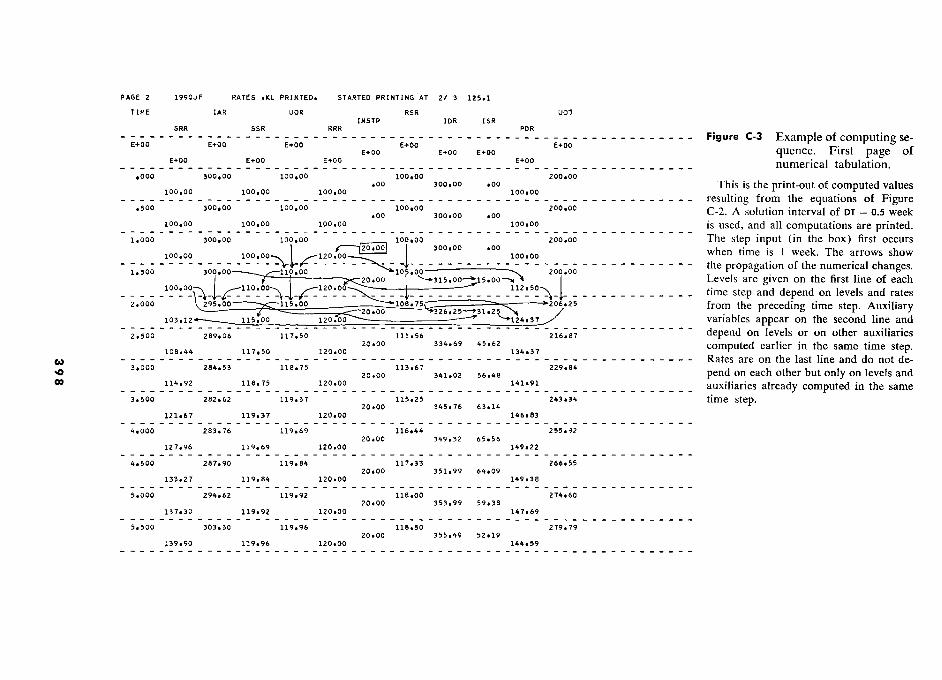
'" e0
a
b.Q 0)
CI
Q)
C'-!
w C
) ":
e
c <U
o "s
'"" D
13 '5
0 a 0
O
QJa
1-<
¡:¡
M, W
Q' C
. N
C 'd
cC
p.' h C .. rV
ccf
¡; C
D
'"
V,)
- F É
1 1
1 1
1 1
1 1
1 1
1 1
1 1
1 1
t 1
1 1
1 1
1 1
1 1
1 1
1 1
1 1
1 1
1 1
1 1
1 1
1 1
1 1
1 l
, 1
1 1
1 1
1 1
1 1
1 1
1 1
1 1
1 r
1 1
1 1
1 1
1 1
1 1
1 1
1 1
1 lit
I 1
1 1
1 1
1 1
1 1
1 1
1 1
1 1
1 1
l ,
1 1
1 1
1 1
1 1
1 1
1 1
1 1
1 1
1 1
1 1
1 1
1 1
1 1
1 1
1 1
1 1
1 1
1 1
1 1
1 1
1 1
1 1
1 1
1 1
1 1
1 1
1 1
1 1
1 1
1 1
1 1
1 1
1 1
1 1
O
O
O
O
IN
I? I?
« I?
O
I? 1
0 0
0 0
O
N
o 10 O
2 . 2 .
2 . 2 .
1 . 2
2 . ,e .
1 . 2 .
1- . 1. .
1 J
Î 41 +
000
À
O
I o o
2 .· 'O
N
P ? tn a
? .O
.0
À
r d r P
I la
la la
lN
,. 1
1
l I , IN
1 IN
I 1 1 IN
O IN
I 'O
r I IN
1 1 IN
1 I IN
1 IN
1 1 I I N
1 I N
1 1 IN
0. 1 1 1
1 O
01
01 1
- M
N
I O
JI 0-1
0-1 p 1
a O 1
0 . I fl . 1
0 . 1 2 I
tn . 1
T I
. 1 2 . 1
N . I
T 1
. I . I
aloI 0 1
-1 -1
-1 À
d
-1 Ù
-1
-1 -1
-1 -\
+ 1
UJI 1
;:1 i 1
1 .a 1
N I
I I
:!;I I 1
1 I
I l
, 1
1 1
I 1
1 1
1 1
1 1
1 1101010 ,
O
O
I N
rv 1
d 0
1 0-
1 ro
1 1
- Œ
À
2 2
0 fl
1 fl
1 "1/)101-'-1-'
I 1
-1-'- 1
-1-1-1- I
À
" +
à à
0- 2
ln 1
w
1 1
1 1
..:t 11"1 1
.0 1
.0 1
.0 1
IC\ 1
11"1 1 N
41
I I
I I
I tn
I d
I P
1 'O
I
.O
I I
I in
I N
1
1 ; 1 :
1 1
1 0
1 0
1 0
1 O
I
N
0- P
1 1
1 .0 1
N
1 0-
1 0-
1 1
IX.
0 fl fl
fl .
0 0-
0- ..:t
ClIO
I-I-I-1 1
I 1
1 1
-1-1-'-1-1 1
à -
+ 000
À
À
'D
2 0-
N
I lal 1 O I O
I O
1 N
I
N
I
1 1
1 1
1 1
1 1
1 l
, ,
1 1
H
e 1e
10 <
1
10 10
l..:t 10
la 1
W
à ü.' u1
0
I O
O
0
1 O
O .
0 1 O
O
. I O
O
. I O
/ O
. I 1 h .
2 I .
?
I 1- 'O
.
N
I .n N
. f
I d S . 1 ·
0
1 O
O ·
?
I .
I I
Z
Œ
+
0 0
o---j.n m
.0
00 O
J 1 ltJ
À
1 I o
1 o I o
Î 1::: .m-n
1 1;:::
.n D
fl .·
1::: .n 1
:: 1
1 1
I I
I I
1 1
1 1
1 1
1 et::
, 1010
0 1
0 tj
0 0
o 010
0 1 0 1 0 1 a 1 0
o 1
0 a
0 0
0 0
000 0
a 000
0
? o
I C
I +
000
a 000
lIJ Z
iwi
I 1
1 N
I
N
I N
N
ININ
ININ
ININ
I I
.... 0::
l ,
l ,
1 1
1 1
1 1
1 1
1 1
« 1- 1
1 01
I 01
I O
I
I O
1
01 I 01 1
01 1 01 1
01 I
01 1 01 I
et:: 000
O
O
O
O
0 0
0 0
000 O
1
Î
1
8
I
-1
À
1
1
-1
I
-1
1
-1
1
-1
I
-1
I
'
1
-1
I et::
+ 0
0 0
0 0
a 0
0 0
1 U
JI 01
01 N
I N
I N
I N
I N
I N
I N
I N
I N
I N
I . -
1 1
1 1
1 1
1 1
1 1
1 C
I 1
1 I
1 I
I /
I 1
I I
I 1
I w
1
10 la 10 110 II"- 1C7' 14
lN
1.0 1
et:: 000
10 O
J Z
O
Ô
O
d' 10 O
O
+
1- O
O
2 O
O
2 O
O
O
YO
1 . 1- r .
D O
:
1- P 1- P
2 P . D
P : 1 P P
1 '
à À
À
À
?
C7'
C7'
fl IX
. Iw
IU
10 O
10 O 1 O
1" .w
a
1 lM
rn 1 M
lM
.w
I 1
lit 1
r 1
1 1
1 1
1 J
1 1
c,!" O
4
1 1
01 I
0 I
O
1 O
1
O
I 01 I
11\1 I I
1 ..:tl I
NI I
I -
à 0
1 2
0 ,
O
O
2 2
.0 co
C7'
0" II} 1
01 I -1 I
-1 I .
1 ·
1 .
1 -1 1
-1 I -1 I
-1 i -1 1
-1 1 -1 I
1/) +
0
0 À
À
U
1 O
J 0-
fl U
J 1
ltJl 1 01
1 0
1 O
I
I I
I "1
i "1
1 "1
I "1
I I
MI 1
à g Q
1 1
1 1
1 1
1 1
1 1
1 1
10 10
10 lN
1.0
10 lN
10
1 a:::
000 O
O
a O
O
1 O
O
\ \1Y
10 1 O
1 O
ln Pt
..0 'D
,... r 'O
C7' O
P
.0 N
m
1 cC
10 0
2 .
1- . fl
. fl
. I
. 2
. 1- .
1- . 1- .
1- . 1- .
2 .
1 ..... ·
+
0 a
0 À
N
2
1 w
10 o 10 o
10 o I
o I P
I ¡C
O
w
100 aD
IC
O
mm
1 co
1C7'
P 10 ô
1 W
1
1 1 1
1 1
N 1
J
1 , à
1 1
O
I O
I
O
I O
1
N
1 4
I N
I 1 I
.01 I "'""1 I
O
I O
I
à P à C
I
01 1 -1
I -1
I -1
I . ·
1 1
-1 I
-1 1
.1 I
D
i 1
2 1
-1 I
+
0 a
a À
Ù
fl
2 1
1 tul I
O
I 01 I
01 1 1
01 1 01 I
I
N
I N
I 1 In
1 1
(t'Il I
1 1
1 1
1 1
1 1
1 go
1 1
1
1
1 10 O
10 O
10 O
10 O
10 O
la O
10 O
10 O
la O
10 O
10 O 10 O
1 N
ltJ
000 À
0
0 0
0 0
0 0
0 a
0 x
10 O
10 O
10 O 1
10 O lin N
10 O
.n la O
1 ln
10 O N
1
w-
-. +
-
- -
- .
- .
- -
- -
- I
IW I
1 1
1 1
lN N
lN
N
À ('<1
I? M
d 1 4
N
111"1 1
« Q.
1 1
1 1
1 1
1 1
1 1
1 1
1 1
398

IW o ao M
e
M e
i! ÔÎÎ
"
.U.
.
cd N
S n ë
iG
a C
' c
C7
S
Of
1 '
' '
' '
' '
' '
' '
' '
) )
t t
t )
t t
) t
) t
t t
1 '
' '
' '
' '
' '
' '
' '
1 '
' '
' '
' '
' '
' '
' '
1 '
' '
' '
' '
' '
' '
' '
1 '
' '
' '
' '
' '
' '
' '
1 '
' '
' '
' '
' '
' '
' '
1 '
' '
' '
' '
' '
' '
' '
1 '
' '
' '
' '
' '
' '
' '
1 1
1 1
1 1
1 1
' '
' '
1 '
1 '
' '
' '
' '
' '
' '
' '
' '
' '
' '
' '
' '
' '
' '
'fl d 'M
m jO
o 'Q
P '<
'4 d 'O
o 'm
n '« N
'm n
'W m
'O o
'W
m
' Ô
o
'< : '2 ro
. '<
: '<
: '1 r .
'a ,o .
't : '< :
'< ,n . 'a .o
. '2 ,o
. '1 :
'Q .o .
' '2 m
N
'Ô
® 'R
r P 'ù r
'S P 'à A
'2 m
r
'« In 'à d
'S O
· 'X
In .0
'2 m
'S '
N
N
N
N
N
N
N
N
N
' '
' m
' I
W'
I h'
I 0'
I +
' I
0' I
1 I
N
9 «'
1 O
' I
h' I
«' I
4' I
à' T
' t'
i' 1'
2' <
' 2'
T'
?' t'
e' 2'
O
1 .
I ·
I ·
I v
1 ·
I 1
1 ·
1 n
1 ·
I .
1 .
I n
1 .
1 ù
O
m
- <
« O
E
<
4 M
«
« «
M
' I
4' 1
M'
I M
' 1
I N
' 1
-' I
-' 1
-' I
-' 1
-' 1
-' I
I -'
1
' ' m
m
Î
- Î
M '
OE
P
Î W
' O
E
P '
h Î
4 1
e 1
e 1
e 1
m
Î
à ' t '
a Î
2 ' 1
1 £
1 < '
fl '
2 1
1 1
2 ' < '
2 ' N
I
I 1
I 1
I I
I 1
1 I
I 1
1
S ' 2 '
à ' i '
n ' 2 ' 2 '
1 ' 2 '
1 d
I en
I N
I
I I
1 I
1 1
I I
.r I
I I
.r 1
' '
' '
'
0
1 0
1 1
1 1
' 1
I 1
I I
I 1
1 I
I 1
I I
1
' « '
h 1
O '
F ' M
' O
' O
' m
' 0
1 m
1
- 1
0 1
OE
1
à ' 2 '
£
r a 1 < '
2 ' t '
I I
1 ' 1 '
2 ' Z
' %
' %
' %
'
1 I
# ' N
' N
' N
' K
' K
' 2 '
K '
K '
K '
K '
K '
I N
I
n 1
I rt1
I N
I
h I
N
I m
I
N
I I
M
I N
I
In I
M
M
M
M
M
M
M
M
m
cn n
M
M
' '
' '
' '
' '
' '
' '
' '
'F r '0
'F r '« N
'4 d
'M In
'O o
'm m
'O
E P
'« rv '4 d
'm O
'0
' m
.O
r
m
m
m
P P
P P
f '%
. '<
.
't .
'T
. 'a
. 'Z
.
'% .
'% .
'% .
'< .
'ù .
'1 .
'1 .
' 2'
m
P P
P P
P P
P P
P P
P P
1 '£ N
'£
'£ '£
'£ '£
'£ rl '£ .n
'£ '£
'£ '£
' '
' O
' I
O '
O '
O '
O '
O '
O '
I O
' O
' O
' O
' O
' O
' I
à ' o 0
0 0 0
0 o
0 0
0 0
0 0
H
1 I
I I
I I
I I
I I
I I
I I
N
O
O
O
O
O
O
O
O
O
O
O
O
B '
Z
I N
I
N
I rv
1 N
1
rv 1
N
I N
I
N
I rv
I N
I
N
1 N
I
N
I
' '
' '
' '
' '
' '
' '
'
' O
' O
' O
' O
' O
' O
' O
' O
' 0
1 01
0 1
0 1
O'
O
e1 0
1 01
01 0
1 01
0 1
0 1
01 1
1
O
à' I
2' 1
2' 1
2' I
2' t
2' I
2' I
21 I
1' I
2' I
?' 1
2' 1
2' 1
1' I
£' 2'
£' £'
£' £'
£' £'
2' £'
£' £'
£' I
NI
NI
NI
NI
NI
NI
NI
NI
NI
NI
NI
NI
NI
1 iO
'Q
10 'O
'O
'O
'O
'O
'O
'O
'O
'O
'O
'
2' P
P O
O
O
O
O
O
O
O
O
O
O
à
'D
. '£
. '2
. '2
. '2
. '2
. '2
. '?
. '2
. '2
. '?
. '2
. '?
. '
'£ '£
'£ '£
'£ '2
'£ '2
1£ '£
'£ '2
'£ '
1 i-1
I I
N
1 N
I
N
1 N
I
N
I N
I
N
I N
I
N
I N
I
N
I '
' W
' I
Q'
I O
' I
O'
I O
' I
O'
I O
' I
O'
1 O
' I
O'
1 O
' I
O'
I O
' I
à' D
' £'
2' ?'
2' 2'
2' 2'
2' 2'
2' 2'
2' m
I
. I
. I
. 1
. I
. I
. 1
. I
. I
. I
. I
. I
. I
. I
£' £'
£' £'
B'
£' £'
£' £'
B'
£' £'
£' 1
.H
1 .-I
1 N
I
N
1 N
1
N
I N
1
N
I N
1
N
1 N
1
N
1 N
I
' 'F 1«
iOE
'4
'4 'W
'O
E
'N
'O
'O
'm
'« '4
1
%
K
'1 : '2 m
. '1 N
. '<
. '%
P e 't
m .
'i N
. 'Q
·
'1 d · 'Z
. '£ P .
'< . '2 :
'
'n 'à N
m
'£ d n
'S d d 'ù P N
'2 o
e .G
0
r o '©
r m
'f r a
'£ r d '£ r d
'm r N
'
W
' i
1 I
I 1
I I
I 1
I 1
I 1
I I
à '
F' 1
4' 1
O
I P
I m
I
Ni
I N
I
m
I .1
1 N
1
4' 1
m'
1 4'
I
à P I
2' I
D'
I t'
I I
e' I
2' I
I T
' 1
Z'
1 t'
1 2'
I 2'
1 fl'
1 -
W
- O
O
E
F 4
- W
m
«
O
W
m
' 4'
1 4'
1 M
' I
M'
1 M
' I
M'
1 «'
1 «'
I «'
I «'
I -'
I -'
1 1
' 'O O
'O
O
10 O
1 O
1 O
1
O
'O O
0
O
1 O
'O
O
'O O
'O
O
'Q O
'
? IL
'2
'2 '0
'2 '2
'2 'À
'2
'à '2
'8 '2
'2 '
Z
1 O
1
m
I O
1
P 1 O
I
P I
O
I W
1
O
1 h
1 O
1
W
I O
1
lyl ..
H
r '4 ·o
'4 .o '£ r
'£ r '# m
'# m
'à P
'à P 'à O
'J O
'1
'1 '£ N
'
f '
' '
' '
' '
' '
' 399
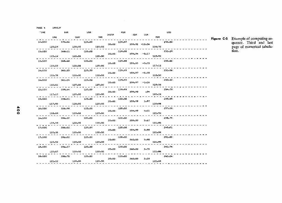
1 Y
I
? CQ
s ?H
g
0-. M
o
S ë ? - 3 o g
'
H
U o
LL
. ' '
' '
' '
' '
' '
' '
' '
' '
' '
' '
' '
' '
' '
' '
' '
' '
' '
' '
' '
' '
' '
' '
' '
' '
' '
' '
' '
' '
' '
' '
' '
' '
' '
' '
' '
' '
' '
' '
' '
' '
' '
' '
' '
' '
' '
' '
' '
' '
' '
' '
' '
' '
' '
' '
' '
' '
' '
' '
' '
' '
' '
' '
' '
' '
' '
' '
' '
' '
' '
' '
' '
' '
' '
' '
' '
' '
' '
<
<
< t
) <
< t
) t
t <
) )
'w m
'Q
P '<
'< 'm
' iO
E
P 'm
n 'w
m
'Q P
'- 'O
O
'4 d '4 a
'
Ô
'2 '1
'1 '1
'fl '2
'1 '£
'£ '1
'7 '
O
1 · 1
· I
· 1
· I
· 1
1 · 1
· 1
· I
· 1
· I
· 1
· 1
'À m
O
'À
m
O
'À m
O
'X
en 'ù m
N
'À
M
a '2 M
'# r
'À m
'$ t O
'Û
· '$ r
'1 t N
' ' I
1 I
I I
I 1
I I
1 I
1 1
I
' O
' O
' «'
O'
<' W
' O
' M
' O
E'
OE
' m
'
É'
Î' ?'
<' ô'
à' Î'
?' 2'
2' ù'
ù' 2'
' O
1
. I
· 1
· 1
. I
· I
· 1
· 1
· 1
· 1
· 1
· 1
· 1
· 1
OE
+
m
P
W
OE
O
O
-
- -
- -
- '
-' N
' N
' N
' N
' N
' N
' N
' «'
' "
' 4 '
P ' M
' W
' I
< ' 4 '
P ' - ' I
P ' W
' I
W '
OE
P '
à ' 2 '
1 ' 1 '
1 ' 1 '
2 ' 1 '
2 ' 1 '
1 ' 1 '
1 ' - m
1 I )
I I m
I m
t
1 1 m
I -
) I 1
·
I I ..
I I t
1 1 M
1 I
m
t I M
n
m
) I
) '
) t
t <
< t
t t
t t
; ;
) i
« ' 4 '
m '
F ' P
1 w
1
OE
'
OE
1
OE
'
OE
1
O '
O '
O
o 1
É '
1 1
1 1
? ' 1 ' ? ' ? ' ?
P i
? i
2 ' 1 '
2 ' 2 '
2 ' 1
1 I
1 I
I I
1 1
1 1
I I
I -
OE
Q
O
E
OE
O
E
OE
Q
O
E
OE
O
E
O
O
O
2 ' 2 '
2 ' 2 '
2 ' 2 '
I I
m
m
m
m
m
m
en m
m
m
m
m
m
'
' '
' '
' '
' '
' '
1 '
'
'P r 'w
m
'W m
'OE
P
'OE
P
1 P Io O
10 O
1 0
10 O 1 O
'O
O
'O O
'
, à
'2 '2
'2 '2
'2 '2
'£ '2
'2 '£
'£ '2
'f '
OE
O
E
OE
O
E
Q
OE
Q
O
O
O
O
O
O
O
'- .w
'- .w
'-
'- '- .w
'-
'« N
'« N
'« N
'« N
'« N
'« N
'« N
'
) [
) t
f )
) t
) t
t )
)
' O
' O
1
O '
O '
O '
O
O
1 O
' O
1
1 O
' O
O
1
O
1 O
1
o 1
t 0)
0) 0)
0) 0)
0
1
0) 0)
0 0)
0) 0
0
1 ô
I 0
1 0
1 0
1 0
1 0
1 0
I 0
1 0
I ô
I 0
1 0
1 ô
I
É '
À
N
1 À
' £ '
À '
£ ' À
' À
' I
À '
1 À
' À
' 1
£ ' À
' À
' I
' '
' '
' '
' '
' '
' '
'
' O
' I
o' 1
o' 1
O'
I O
' I
O'
I O
' I
O'
I O
' I
O'
1 O
' 1
O'
1 O
' I
-
10 10
10 1
10 O
10
10 1
£'
0 10
10
£' 2'
d' 1
· 1
· I
· I
· I
· I
· I
· 1
· I
· 1
· I
· I
· 1
· 1
OE
O
O
O
O
O
O
O
O
O
O
O
O
O
'
«' N
' N
' «'
N'
«' N
' «'
«' N
' «'
«1 «'
' 'O O
'O
O
'O O
'O
O
'O O
'O
O
'O O
'O
O
'O O
'o O
'o O
'O
O
'O O
'
C
O
O
O
O
O
O
O
O
O
O
O
O
O
0 '2 ·
'2 · '2
· '2 ·
'2 ·
'2 ·
'2 · '2
· ·
1 Ci
1 %
1 0 1
· '
O
O
O
O
O
O
O
O
O
O
O
O
O
'£ '£
'£ 'À
'£
'£ '£
lÀ
'£ '£
'£ 'À
'£
' '
' 0
1 0
1 0
1 1
01 0
1 01
0 1
1 0
1 0
1 0
1 O
'
à' £' £' £' 2' £' 2' £' £' £' £' £' £' £'
N
I ·
I ·
I ·
1 ·
I ·
1 ·
I ·
I ·
I ·
1 ·
I ·
1 ·
I ·
I m
O
O
O
O
O
O
O
O
O
O
O
O
O
£'
À'
À'
£' £'
£' £'
À'
£' £'
À'
£' £'
' '0 '-
'W m
'm
'4 d
'4 d I
1 m
1 N
1 N
1 N
1 r 9 O
'
[ 'j .f ·
'i : '£
· '£ In ·
'£ N ·
'j d · '£ O
· '§ P .
'§ : '£ O
. 'Q
O ·
') N ·
'£ r · '
O
m
M
P m
.O
.0
N
.O
.O
.0 '# h
'À
'À O
'À
t
.O
'2 W
?2 ?2 n
'2 ?2 O
'2 W
'2 W
'
·1 M
A
W
'
' '
' '
' '
' '
' '
' '
'
ù '
Q'
4' M
' k'
-' m
' M
' O
E'
OE
' O
' O
' F'
«' O
1
I 41 1
mi 1
mi 1
I I
mi I
I I
QI I
01 I I
"J 1
à P §'
1 I
Î' I
1 1'
1 1'
I 1
I I
2' I
2' 1
2' 1
2' I
<' 1
.· V
W
11 n11
O1
r m
P
O
O
O
2i I
I 1
1 1
Î' I
I 1
1 £'
1 £'
1 £1 I
à' I
' 10 O 'O
O
'O O
'O
O
'O O
'o D
'o O
'O
O
'O O
'O
O
'O O
'O
O
'O O
'
a w
0
0 0
0 0
0 0
0 0
0 0
0 0
É
1 'À
o 'À
n 1 %
'À
'À
o '1 P
'À o
'1 h 'À
0 '1 N
'À
o 'À
P '
r ..
'£ N
'À en
'À n
'à N
'à a
'À
'À n
'À
'À
'( 'é I-
'À m
'à
' 1
400
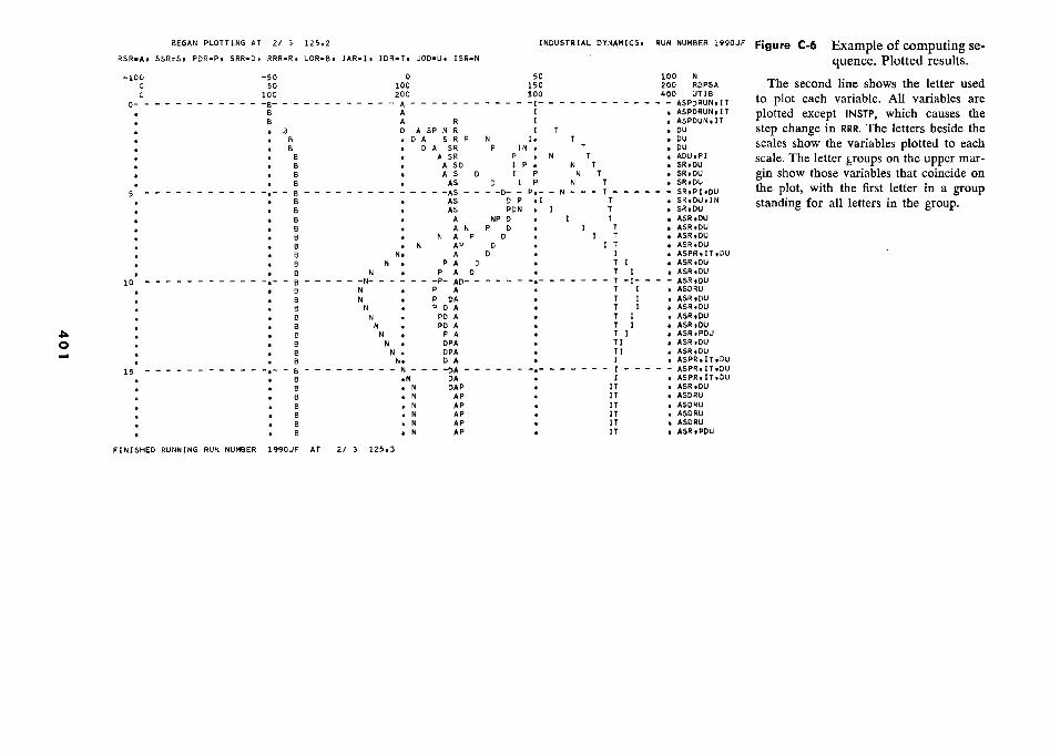
àf à Ô
m
&
si .
Se N
N
Î
d
C À
À
3 à ç," <1)
u Î %
H?
.... »
> D
» a
ooa --1-
1- >z z
CI
Q ca
p
et: z · 7
p J J 7 a n p 7
à 1 ; z «
z 000
........" ........"
........" .......
0:: >
1 ' 1
1 1
1 1
f '
V
/ 1
-- I
« '
t 1
' '
1 '
i t
a .... 1
1 .....
1 1
i i >
i 1
' 1 ,
- I
r z
1 I
1 :
t W
x
z t )
t fl
1 ' >
z i 1
' ' II)
1 Z
1
1 g
1 z
i !
Q
1 z
1""" ..
1 1
z 1"'" 1 1
1 a
el. 1
1 Z
D
- I
z p 1
1 1
1 cn. 00 1
1 1 1
z OE
1 '
Q. O
E o O
1 1
1 ' 0..
CI
Z
0 z
1 O
1
0. a
1 1
z 1
CI 1
CI 1
1 É
1
0.. '
z I
1 0
el. C
I 1
flfl ««
.. 1
Z?
« 1
a 1
OO
Qa.Q
OO
I J
' < ,«
' a.
a. U
'
Q. <
1
1 a. 0. a.
1 C
> "'
à 1
..;(0 Q
1
1 1
Z
ail )
1 zzzzzz Z
.. 000
...o...o.z5...... '
" - «
Z ·
Z
Q:
[ 1
1 Z
1
a Z
Z
.
' '
1 Z
1
. '
' o '
Z
' N
..
1 1
z 1 1 z Z
l
"'" -
Z
Z
'! t
1 ) Z
Z:
( œ
<
1 i ) '
i t l 1 '
1 1 '
M
.. 1
1 1
J N
r:;
t 1
1 1
a: t
) t
1 t-
N o # à
' 1 1 '
1 i 1 i
Q
- =)
1 1
1 1
1 m
m m
mm
mm
mm
mm
mm
mm
mm
mm
mm
mm
mm
mm
mm
mm
mm
m
W
Il i I m
'
' 1
P o N
a:: 0001 1 1 1 ".
f- .. '
-' 1 1
1 1
ail '
1 1
S $ à W
fl § Ô
' ' '
' i '
i i '
i ' '
o fl a::
1 1
.... lI) 1
1 1
1 ;:) Z
1-" a
1 t
i ?
Il J
1 1
1 :)
D- ce:
OC
o à 1'
i ' ' i i 1
1 ' 1 ' 1 1
_ Q
«, )
1 1
1 Z
l.L
J lI) 1
1 1
1 Z
. et::: à à À
' ' '
' ' ' 1 i i
' ' ' Q
§ , "'
' t ' t
) 'S !
s o "
1 1
1 1
, <
000 I I
I 1
x .0
N
a:: - 0
ti'\ 11\
.... fl O
E 1 '
O
m
- r"I m
y
œ
-
401

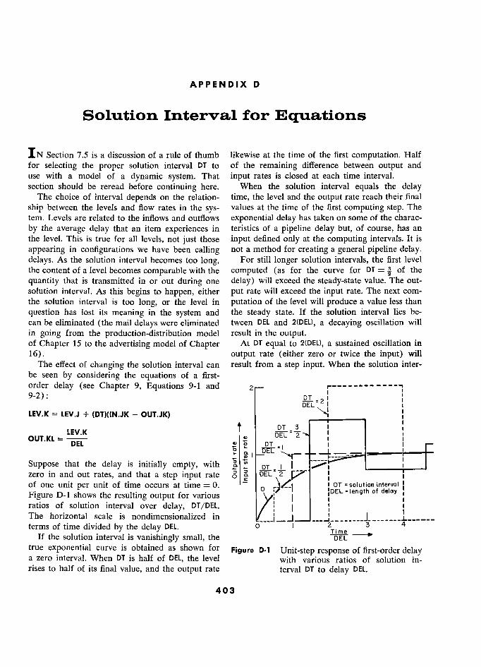
APPENDIX D
Solution Interval for Equations
I N Section 7.5 is a discussion of a rule of thumb likewise at the time of the first computation. Half for selecting the proper solution interval DT to of the remaining difference between output and use with a model of a dynamic system. That input rates is closed at each time interval. section should be reread before continuing here. When the solution interval equals the delay
The choice of interval depends on the relation- time, the level and the output rate reach their final
ship between the levels and flow rates in the sys- values at the time of the first computing step. The tem. Levels are related to the inflows and outflows exponential delay has taken on some of the charac-
by the average delay that an item experiences in teristics of a pipeline delay but, of course, has an the level. This is true for all levels, not just those input defined only at the computing intervals. It is
appearing in configurations we have been calling not a method for creating a general pipeline delay. delays. As the solution interval becomes too long, For still longer solution intervals, the first level the content of a level becomes comparable with the computed (as for the curve for DT = Í of the
quantity that is transmitted in or out during one delay) will exceed the steady-state value. The out- solution interval. As this begins to happen, either put rate will exceed the input rate. The next com- the solution interval is too long, or the level in putation of the level will produce a value less than
question has lost its meaning in the system and the steady state. If the solution interval lies be- can be eliminated (the mail delays were eliminated tween DEL and 2(DEL), a decaying oscillation will in going from the production-distribution model result in the output. of Chapter 15 to the advertising model of Chapter At DT equal to 2(DEL), a sustained oscillation in
16). output rate (either zero or twice the input) will The effect of changing the solution interval can result from a step input. When the solution inter-
be seen by considering the equations of a first- order delay (see Chapter 9, Equations 9-1 and 2 r-------- M
9-2) : " 1 -=21 1 :
LEV.K = LEV.J + (DT)(IN.JK - OUT.JK) i i 1
OUT.KL = LEV.K t 3
2 1
1 1 1
1 1
OUT.KL = DEL ô 5ÊL i i DEL
DT 1 1 1 -L---- 1
Suppose that the delay is initially empty, with É ( DT 1 1 : ___t zero in and out rates, and that a step input rate O 2 ) 1 of one unit per unit of time occurs at time = 0. 0 i DT =solution interval : Figure D-1 shows the resulting output for various
,) j
length delay (
ratios of solution interval over delay, DT/DEL. ' '
1: 1 i
The horizontal scale is nondimensionalized in terms of time divided by the delay DEL. 0 1
2 Time 3 0-
4
If the solution interval is vanishingly small, the Q true exponential curve is obtained as shown for Figure D-1 Unit-step response of first-order delay a zero interval. When DT is half of DEL, the level with various ratios of solution in- rises to half of its final value, and the output rate terval DT to delay DEL.
403
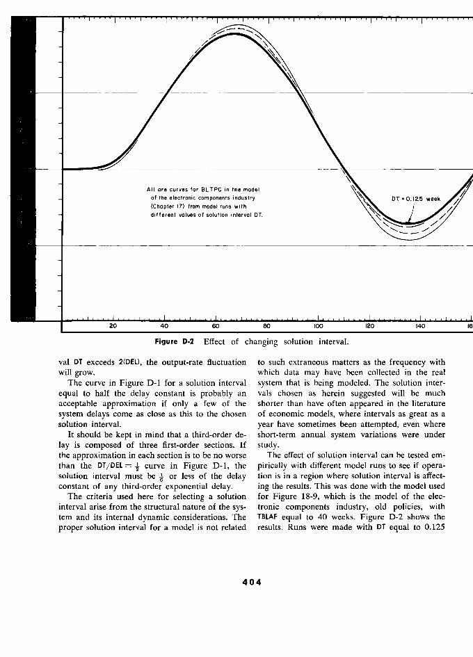
All are curves for BLTPC in the model
- of the electronic components industry DT 0. 125 week
(Chapter 17) from model runs with / - différent values of solution interval DT.
Y
20 40 60 80 100 120 140
Figure D-2 Effect of changing solution interval.
val DT exceeds 2(DEL), the output-rate fluctuation to such extraneous matters as the frequency with will grow. which data may have been collected in the real
The curve in Figure D-1 for a solution interval system that is being modeled. The solution inter-
equal to half the delay constant is probably an vals chosen as herein suggested will be much
acceptable approximation if only a few of the shorter than have often appeared in the literature
system delays corne as close as this to the chosen of economic models, where intervals as great as a solution interval. year have sometimes been attempted, even where
It should be kept in mind that a third-order de- short-term annual system variations were under
lay is composed of three first-order sections. If study. the approximation in each section is to be no worse The effect of solution interval can be tested em- than the DT/DEL curve in Figure D-1, the pirically with different model runs to see if opera- solution interval must be i or less of the delay tion is in a region where solution interval is affect- constant of any third-order exponential delay. ing the results. This was done with the model used
The criteria used here for selecting a solution for Figure 18-9, which is the model of the elec- interval arise from the structural nature of the sys- tronic components industry, old policies, with tem and its internal dynamic considerations. The TBLAF equal to 40 weeks. Figure D-2 shows the
proper solution interval for a model is not related results. Runs were made with DT equal to 0.125
404
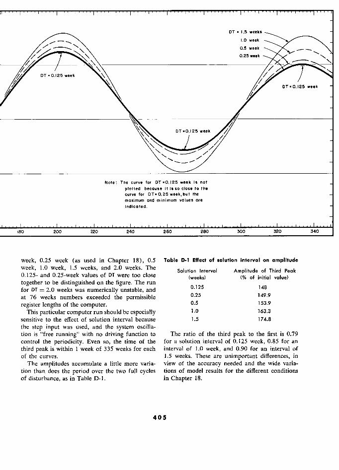
DT = 1.5 weeks
1.0 week
- ' , 0.5 week - - ,
\
0.25 week
DT?O.)25week / DT = 0.125 week /
DT 0. 125 week
DT'0.)25week
Note : The curve for DT =0,125 week is not plotted because it is so close to the curve for DT- 0. 25 week, but the maximum and minimum values are Indlcated.
180 200 220 240 260 280 300 320 340
week, 0.25 week (as used in Chapter 18), 0.5 Table D-1 Effect of solution interval on amplitude week, 1.0 week, 1.5 weeks, and 2.0 weeks. The 1 nterva 1 of Third k 0.125- and 0.25-week values of DT were too close , (% of j__j value) together to be distinguished on the figure. The run
0.125 148 for DT = 2.0 weeks was numerically unstable, and 0. 5
at 76 weeks numbers exceeded the permissible 0.25 149.9
register lengths of the computer. °.5 153.9
This particular computer run should be especially 1.0 163.3
sensitive to the effect of solution interval because 1.5 174.8 the step input was used, and the system oscilla- tion is "free running" with no driving function to The ratio of the third peak to the first is 0.79 control the periodicity. Even so, the time of the for a solution interval of 0.125 week, 0.85 for an third peak is within 1 week of 335 weeks for each interval of 1.0 week, and 0.90 for an interval of of the curves. 1.5 weeks. These are unimportant differences, in
The amplitudes accumulate a little more varia- view of the accuracy needed and the wide varia- tion than does the period over the two full cycles tions of model results for the different conditions of disturbance, as in Table D-1. in Chapter 18.
405
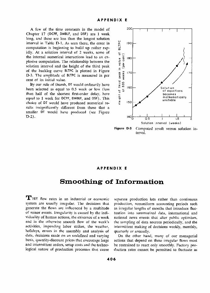
APPENDIX E
A few of the time constants in the model of 200 ––'–––––––––––––––––– Chapter 17 (DCPF, DMBLF, and DSF) are 1 week
long, and these are less than the longest solution interval in Table D-1. As seen there, the error in f i9o –
computation is beginning to build up rather rap- idly. At a solution interval of 2 weeks, some of the internal numerical interactions lead to an ex- m –
plosive computation. The relationship between the Î / . solution interval and the height of the third peak é / of the backlog curve BLTPC is plotted in Figure ? 170 / / _ D-3. The amplitude of BLTPC is measured in per g / cent of its initial value.
-2
* /
By our rule of thumb, DT would ordinarily have i so /. Solution ri been selected as equal to 0.5 week or less (less s
than half of the shortest first-order delay, here f becomes s
equal to 1 week for DCPF, DMBLF, and DSF). This unstable choice of DT would have produced numerical re- x .g 150 unsta ble
sults insignificantly different from those that a smaller DT would have produced (see Figure D-2). 140? 0 0.5 1 1.5 2
Solution interval (weeks)
Figure D-3 Computed result versus solution in- terval.
APPENDIX E
Smoothing of Information
T HE flow rates in an industrial or economic separate production lots rather than continuous system are usually irregular. The decisions that production, nonuniform accounting periods such generate the flows are influenced by a multitude as irregular lengths of months that introduce fluc- of minor events. Irregularity is caused by the indi- tuation into summarized data, international and viduality of human actions, the existence of a week national news events that alter public optimism, end in the otherwise smooth flow of the week's the sampling of data sources periodically, and the activities, impending labor strikes, the weather, intermittent making of decisions weekly, monthly, holidays, errors in the assembly and analysis of quarterly or annually. data, decisions made on an undefined and varying On the other hand, many of our managerial basis, quantity-discount prices that encourage large actions that depend on these irregular flows must and intermittent orders, setup costs and the techno- be restrained to react only smoothly. Factory pro- logical nature of production processes that cause duction rates cannot be permitted to fluctuate as
406

SMOOTHING OF INFORMATION
rapidly as do the day-by-day incoming orders. This is its purpose. Consequently, smoothing dis- Inventories are built up and decreased slowly. The torts for better or worse the information flows in
manager is in the position of trying to filter out a system. and ignore the fluctuations introduced by other Smoothing is always a compromise. One is decision makers, while at the same time trying to caught in the dilemma between more smoothing to detect as soon as possible any enduring change to reduce meaningless noise and less smoothing to re- which he wants to respond. duce the time delay in extracting the desired, mean-
The effort to detect underlying, significant ingful information. Smoothing is characterized by changes in data, while ignoring the superimposed, these two effects - the attenuation of rapid fluctu-
meaningless fluctuations, is called smoothing or ations, and the creation of a time delay. These
averaging. Smoothing of incoming information oc- will be examined after discussing two common curs to some extent at every decision-making point kinds of smoothing. in the system. In turn, each of these same deci- A discussion of smoothing methods can become sions also contributes its source of noise to the a complex subject in its own right. We shall deal rates being controlled. here with only the simple concepts.
We should recognize two separate kinds of Smoothing is a process of taking a series of mechanisms for data smoothing. The most obvious, past information values and attempting to form but the least frequent, is the format, numerical an estimate of the present value of the underlying processing of data into averages. The more fre- significant content of the data. Smoothing methods
quent, although more illusive, is the intuitive can vary widely in the weight (or importance) smoothing introduced by a wait-and-see attitude in attached to various ages of the past data. We shall
reaching decisions. discuss two smoothing methods - the moving The existence of a formal, mathematical average and exponential smoothing.
smoothing procedure is easy to locate in a system. The moving average attaches the same weight or It is a practice based on an established policy. importance to each past value of a time series
Weekly, monthly, quarterly, and annual summaries back to a cutoff time before which no data are of sales, or production, or costs are averages for included. "Average sales for the last 8 weeks" is the periods specified. These formal averaging a moving average. Sales for 8 weeks are added
processes are found in many information flow together (equal importance) and the total divided channels. by 8. The average would be computed as fo)lows:
In addition, further smoothing is usually in- troduced at the decision
points in a
system. We
Moving average = + S2 + S3 + S4 + S5
might refer to this as
"psychological smoothing."
Full and immediate action is seldom taken on 6 ? 7 8
a change of incoming information, even though where Si is the most recent full week, S2 is the
that information may already be the result of nu- next earlier week, etc. For the general case of a
merical averaging processes applied to the raw moving average taken over T periods data. This tendency to delay action until the
change in information is insistent and until many Moving average
=
q(Si + S2 + + ST)
indicators point in the same direction is smooth-
ing introduced by judgment, or procrastination, or The moving average is customarily found in
indecisiveness. business where formal, numerical averages are
Smoothing processes are fundamental to a obtained. It is simple to explain. The process lends
proper treatment of system dynamics. Smoothing itself easily to the form in which data have usually is essential for filtering out short-period noise. been kept manually and to the manual clérical
But smoothing inherently introduces delays in in- computing methods. Weekly, monthly, and annual
formation channels and in decisions. Smoothing levels of average activity are moving averages in
changes the sensitivity of the system to different the sense that they give equal weight to all the data
periodicities that may exist in data fluctuations. within the interval, but they create additional in-
407
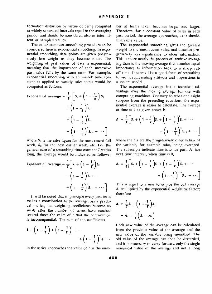
APPENDIX E
formation distortion by virtue of being computed ber of terms taken becomes larger and larger. at widely separated intervals equal to the averaging Therefore, for a constant value of sales in each period, and should be considered also as intermit- past period, the average approaches, as it should, tent or sampled values. that same value.
The other common smoothing procedure to be The exponential smoothing gives the greatest considered here is exponential smoothing. In expo- weight to the most recent value and attaches pro- nential smoothing, data points are given progres- gressively less significance to older information. sively less weight as they become older. The This is more nearly the process of intuitive averag- weighting of past values of data is exponential, ing than is the moving average that attaches equal meaning that the importance of each successive importance to information back to a sharp cut- past value falls by the same ratio. For example, off time. It seems like a good form of smoothing exponential smoothing with an 8-week time con- to use in representing attitudes and impressions in stant as applied to weekly sales totals would be a system model.
computed as follows: The exponential average has a technical ad-
Exponential average 1 r- / . vantage over the moving average for use with
Exponential average = 8 Si
+ ( 1 - computing machines. Contrary to what one might 8 8 suppose from the preceding equations, the expo-
( 1
S3
nential average is easier to calculate. The average + 1 - at time = 1 as given above is
]
where SI is the sales figure
for the most recent -fJull where the S's are the progressively
older values of
week, 52 for the next earlier week, etc. For the the variable, for example sales, being averaged
gencral case of a smoothing
time constant T weeks The subscripts indicate time into the past. At the
long, the average would be indicated as follows: next time interval, when time = 0,
Exponential average +
I 1 - T I S.=
A.
= T SI
+
( 1 - y 1 JS?
+ + ... ·
]
(
n
j
This is equal
to a new term plus
the old average
T SO+l
J Ai multiplied by the
exponential weighting factor;
therefore
It will be noted that in principle every past
term
makes a contribution to the average.
As a practi-
1
1
\ cal matter, the
weighting coefficients become so A° =
T Al
small after the number of terms have reached \
several times the value of T that the contribution = A, +
A, ) is inconsequential.
The sum of the coefficients T (
, /
Each new value of the average
can be calculated
1 + C 1 - T T +---
· from the previous
value of the average and the
new value of the variable being smoothed. The
+
( ï - – ) + . - -
old value of the average
can then be discarded,
T and it is
necessary to
carry forward
only the single
in the series approaches the value of T as the num- numerical value of the
average and not a
long
408 8
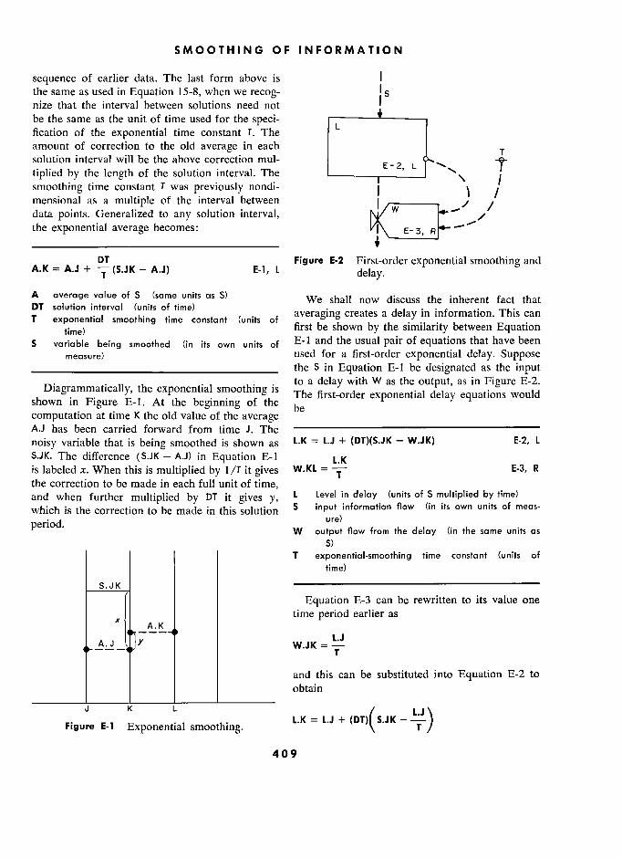
SMOOTHING OF INFORMATION
sequence of earlier data. The last form above is 1
the same as used in Equation 15-8, when we
recog- 1 S
nize that the interval between solutions need not
be the same as the unit of time used for the speci-
fication of the exponential time constant T. The L
amount of correction to the old average
in each
solution interval will be the above correction mul-
E-2, L
tiplied by the
length of the solution interval. The ' LI j
smoothing time constant T was
previously nondi-
1 , / mensional as a multiple
of the interval between j
data points.
Generalized to any
solution interval, W ' /
the exponential average becomes: /j\ - R
_____________________________ t
DT Figure E-2 First-order exponential smoothing
and
A.K = A.J + T
(S.JK - A.J) E-1, L
delay.
A average value of S (same units as S) We shall now discuss the inherent fact that
DT solution interval (units of time)
averaging creates a delay in information. This can
constant , ,, f averasins
creates a delay
in information. This can T exponential smoothing time constant (units of
first be shown b
the similarity
between Equation time)
°
first be shown by the similarity
between Equation
S variable being smoothed (in its own units of E-1 and the usual
pair of equations that have been
measure) used for a first-order exponential delay. Suppose
._____________________________ the S in Equation
E-1 be designated as the input
.. , .. is
to a delay
with W as the output,
as in Figure E-2.
Diagrammatically,
the exponential smoothing
is The first-order
exponential delay equations would
shown m Figure
E-1. At the beginning
of the e
first-order exponential delay equations
would
computation at time K the old value of the average
e
A.J has been carried forward from time J. The –––––––––––––––––––––––––––––
noisy variable that is
being smoothed is shown as L.J + (DT)(S.JK - W.JK) E-2, L
S.JK. The différence (S.JK - A.J) in Equation
E-1 L.K
is labeled x. When this is multiplied by 1/T it
gives W.KL =
T E-3, R
the correction to be made in each full unit of time,
and when further multiplied by
DT it gives y, L Level in delay (units of S multiplied by time)
which is the correction to be made in this solution S input information flow (in its own units of meas-
period. W
ure)
flow from the delay (in the same . as W output flow from the delay (in the same units as
S)
T exponential-smoothing time constant (units of
time)
S.JK K –––––––––––––––––––––––––––––––––––––
Equation E-3 can be rewritten to its value one
X
A,K
time period
earlier as
A . K '
T
and this can be substituted into Equation
E-2 to
obtain
L /
J E-i K
L
smoothing. F<gure E-) Exponential smoothing.
L.K = +
\ T /
409
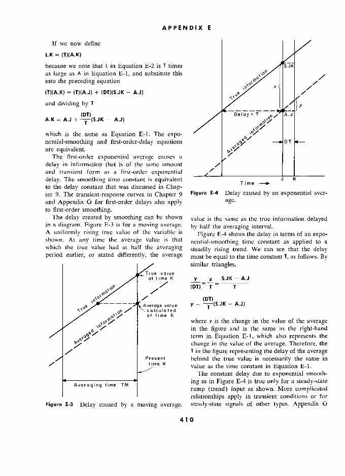
APPENDIX E
If we now define
L.K = (T)(A.K)
because we note that L in Equation
E-2 is T times
as large
as A in Equation E-1, and substitute this
./ into the
preceding equation 01, /
, x
/
(T)(A.K) = (T)(A.J) + (DT)(S.JK - A.J) /
.tt /
and dividing by
T
/1 y „
(DT) J
A.K = A.J + A.J)
A.J
T
,,0/
which is the same as Equation
E-1. The expo-
/
nential-smoothing and
first-order-delay equations DT T «--
are équivalent.
The first-order exponential average
causes a ;/
delay in information that is of the same amount /
and transient form as a first-order exponential /
delay. The
smoothing time constant is
equivalent Time 10
J K
to the delay constant that was discussed in
Chap-
ter 9. The transient-response
curves in Chapter 9 Figura E-4
Delay caused
by an
exponential aver-
and Appendix
G for first-order delays
also apply
age.
to first-order smoothing.
The delay created
by smoothing can be shown
value is the same as the true information delayed
in a diagram. Figure
E-3 is for a moving average.
by half the
averaging interval.
A uniformly rising true value of the variable- is
Figure E-4 shows the delay
in terms of an expo-
shown. At any time the average
value is that nential-smoothing
time constant as applied
to a
which the true value had at half the averaging steadily rising
trend. We can see that the delay
period earlier, or stated differently,
the average must be equal to
the time constant T, as follows. By
similar triangles,
True value
at t ime K y x S.JK - A.J
T
./ (DT)
e ---_ _ Average value Y =
A.J)
a lc u 1 a t e d
=
T A.J)
ai time K
where y is the change
in the value of the average
à in the figure
and is the same as the right-hand
term in Equation E-1, which also
represents the
change in the value of the average. Therefore, the
T in the figure representing the delay of the average
Présent behind the true value is necessarily
the same in
.10, t ime K value as the time constant in
Equation E-1.
The constant delay
due to exponential smooth-
, , ing
as in Figure
E-4 is true only
for a steady-state
Averaging t!me TM
ramp (trend) input as shown. More
complicated
,
relationships apply in transient conditions or for
Figure E-3 Delay
caused by
a moving average. steady-state signals
of other types. Appendix G
410

SMOOTHING OF INFORMATION
shows that for a sinusoidal input
the delay
never sions. Delays
and amplification (here the fre-
exceeds a quarter
of a period
of the input
fluctua- quency-sensitive reduction in
amplitude) are
tion. caused by smoothing,
and as we have seen in
A flow of information is distorted in both ampli-
Part III, these have important
effects on the
tude and time by being smoothed. The nature of dynamic
behavior of systems.
the distortion depends
on the character of the Even in noise-free runs of a model (such as
changes that occur in the
input information, the many of the figures
in Part III) the smoothing
kind of smoothing,
and the amount of smoothing processes must be represented
in the model. The
that is required by
the kind and degree
of un- smoothing,
which the noise imposes, unavoidably
wanted disturbances that exist in the information. acts as a filter to distort the desired information;
Almost all information flows are smoothed by
the smoothing
distortion must be present
even in
formal mathematical processes,
or by psychologi-
the noise-free runs if the system
is to be properly
cal processes,
or both before being
used in deci- represented.
411 1
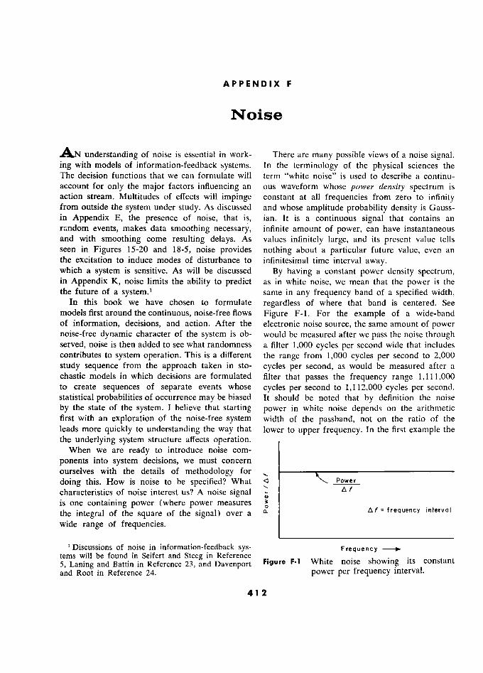
APPENDIX F
Noise
AN understanding of noise is essential in work- There are many possible views of a noise signal. ing with models of information-feedback systems. In the terminology of the physical sciences the The decision functions that we can formulate will term "white noise" is used to describe a continu- account for only the major factors influencing an ous waveform whose power density spectrum is action stream. Multitudes of effects will impinge constant at all frequencies from zero to infinity from outside the system under study. As discussed and whose amplitude probability density is Gauss- in Appendix E, the presence of noise, that is, ian. It is a continuous signal that contains an random events, makes data smoothing necessary, infinite amount of power, can have instantaneous and with smoothing come resulting delays. As values infinitely large, and its present value tells seen in Figures 15-20 and 18-5, noise provides nothing about a particular future value, even an the excitation to induce modes of disturbance to infinitesimal time interval away. which a system is sensitive. As will be discussed By having a constant power density spectrum, in Appendix K, noise limits the ability to predict as in white noise, we mean that the power is the the future of a system.l same in any frequency band of a specified width,
In this book we have chosen to formulate regardless of where that band is centered. See models first around the continuous, noise-free flows Figure F-1. For the example of a wide-band of information, decisions, and action. After the electronic noise source, the same amount of power noise-free dynamic character of the system is ob- would be measured after we pass the noise through served, noise is then added to see what randomness a filter 1,000 cycles per second wide that includes contributes to system operation. This is a different the range from 1,000 cycles per second to 2,000 study sequence from the approach taken in sto- cycles per second, as would be measured after a chastic models in which decisions are formulated filter that passes the frequency range 1,111,000 to create sequences of separate events whose cycles per second to 1,112,000 cycles per second. statistical probabilities of occurrence may be biased It should be noted that by définition the noise
by the state of the system. 1 believe that starting power in white noise depends on the arithmetic first with an exploration of the noise-free system width of the passband, not on the ratio of the leads more quickly to understanding the way that lower to upper frequency. In the first example the the underlying system structure affects operation.
When we are ready to introduce noise com-
ponents into system decisions, we must concern ourselves with the details of methodology for –––––r–––––––––––––––––––––
doing this. How is noise to be specified? What a Power characteristics of noise interest us? A noise signal
f
is one containing power (where power measures 30 Af frequency interval the intégral of the square of the signal) over a Il- 1::.( = frequency interval
wide range of frequencies.
1 Discussions of noise in information-feedback sys- Frequency tems will be found in Seifert and Steeg in Reference _ 5, Laning and Battin in Reference 23, and Davenport Figure F-1 White noise showing its constant
and Root in Reference 24. power per frequency interval.
412
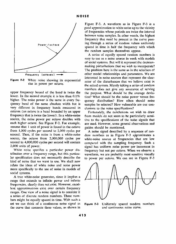
NOISE E
/ Figure F-3. A waveform as in Figure F-3 is a
/ good approximation to white noise up to the vicinity / of frequencies whose periods are twice the interval
/ between noise samples. In other words, the highest / frequency that need be present in the curve pass-
e / ing through a series of random values uniformly e spaced in time is half the frequency with which h
the random samples themselves appear. A series of equally spaced random numbers is
easy to use as a noise source in work with models of social systems. But will it represent the decision-
making perturbations that we wish to incorporate? , . , The problem here is the same as in the selection of
Frequency (octaves ) other model relationships and parameters. We are
, interested in noise sources that represent the char- Figure F-2 White noise showing its exponential acter of the disturbances that we believe exist in
rise in power per octave. the actual system. Merely taking a series of random numbers does not give any assurance of serving
upper frequency bound of the band is twice the the purpose. What should be the average devia- lower. In the second example it is less than 0. 1 9l tion? What should be the noise power versus fre- higher. The noise power is the same in every fre- quency distribution? How often should noise quency band of the same absolute width but is samples be selected? How vulnerable are our con- very different in frequency bands measured in clusions to the noise specifications? octaves (an octave is a band bounded by an upper Fortunately, the conclusions we wish to draw frequency that is twice the lower). In a white-noise from models do not seem to be particularly sensi- source, the noise power per octave doubles with tive to the specifications of the noise signais that each higher octave. See Figure F-2. For example, are used. However, some general observations and assume that 1 unit of power is found in the octave guides should be mentioned. from 1,000 cycles per second to 2,000 cycles per A noise signal described by a sequence of ran- second. Then, if the noise is from a white-noise dom numbers as in Figure F-3 approximates a source, the octave from 2,000,000 cycles per white-noise source at frequencies that are low second to 4,000,000 cycles per second will contain compared with the sampling frequency. Such a 2,000 units of power. signal has uniform noise power per increment in
White noise specifies a particular power dis- frequency but not per octave. When we observe a tribution over a frequency range, but this particu- waveform, we are probably most sensitive visually lar specification does not necessarily describe the to power per octave. We can see in Figure F-3 kind of noise that we want to use. We shall now relate the ideas of white noise and noise power more specifically to the use of noise in models of / /\ social systems. / \ \ /
A true white-noise generator, since it implies a / \ range that extends to infinite power and infinite Ty\ ! / )\ji/ frequencies, clearly does not exist. However, excel- t lent approximations exist over certain frequency y ranges. One view of a noise signal is to consider it f y a series of discrete random numbers. These num- y bers might be equally spaced in time. With such a "'
set we can think of a continuous noise signal as Figure F-3 Uniformly spaced random numbers the curve that connects these values, as shown in and continuous noise curve.
413
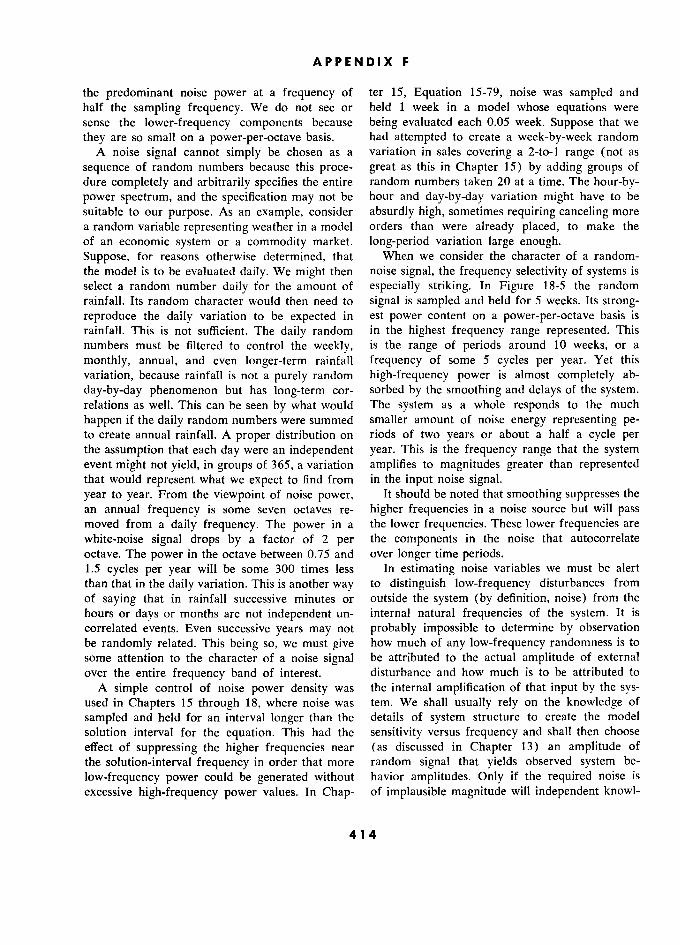
APPENDIX F
the predominant noise power at a frequency of ter 15, Equation 15-79, noise was sampled and half the sampling frequency. We do not see or held 1 week in a model whose equations were sense the lower-frequency components because being evaluated each 0.05 week. Suppose that we
they are so small on a power-per-octave basis. had attempted to create a week-by-week random A noise signal cannot simply be chosen as a variation in sales covering a 2-to-1 range (not as
sequence of random numbers because this proce- great as this in Chapter 15) by adding groups of dure completely and arbitrarily specifies the entire random numbers taken 20 at a time. The hour-by- power spectrum, and the specification may not be hour and day-by-day variation might have to be suitable to our purpose. As an example, consider absurdly high, sometimes requiring canceling more a random variable representing weather in a model orders than were already placed, to make the of an economic system or a commodity market. long-period variation large enough. Suppose, for reasons otherwise determined, that When we consider the character of a random- the model is to be evaluated daily. We might then noise signal, the frequency selectivity of systems is select a random number daily for the amount of especially striking. In Figure 18-5 the random rainfall. Its random character would then need to signal is sampled and held for 5 weeks. Its strong- reproduce the daily variation to be expected in est power content on a power-per-octave basis is rainfall. This is not sufficient. The daily random in the highest frequency range represented. This numbers must be filtered to control the weekly, is the range of periods around 10 weeks, or a
monthly, annual, and even longer-term rainfall frequency of some 5 cycles per year. Yet this
variation, because rainfall is not a purely random high-frequency power is almost completely ab-
day-by-day phenomenon but has long-term cor- sorbed by the smoothing and delays of the system. relations as well. This can be seen by what would The system as a whole responds to the much
happen if the daily random numbers were summed smaller amount of noise energy representing pe- to create annual rainfall. A proper distribution on riods of two years or about a half a cycle per the assumption that each day were an independent year. This is the frequency range that the system event might not yield, in groups of 365, a variation amplifies to magnitudes greater than represented that would represent what we expect to find from in the input noise signal. year to year. From the viewpoint of noise power, It should be noted that smoothing suppresses the an annual frequency is some seven octaves re- higher frequencies in a noise source but will pass moved from a daily frequency. The power in a the lower frequencies. These lower frequencies are white-noise signal drops by a factor of 2 per the components in the noise that autocorrelate octave. The power in the octave between 0.75 and over longer time periods. 1.5 cycles per year will be some 300 times less In estimating noise variables we must be alert than that in the daily variation. This is another way to distinguish low-frequency disturbances from of saying that in rainfall successive minutes or outside the system (by definition, noise) from the hours or days or months are not independent un- internal natural frequencies of the system. It is correlated events. Even successive years may not probably impossible to determine by observation be randomly related. This being so, we must give how much of any low-frequency randomness is to some attention to the character of a noise signal be attributed to the actual amplitude of external over the entire frequency band of interest. disturbance and how much is to be attributed to
A simple control of noise power density was the internal amplification of that input by the sys- used in Chapters 15 through 18, where noise was tem. We shall usually rely on the knowledge of
sampled and held for an interval longer than the details of system structure to create the model solution interval for the equation. This had the sensitivity versus frequency and shall then choose effect of suppressing the higher frequencies near (as discussed in Chapter 13) an amplitude of the solution-interval frequency in order that more random signal that yields observed system be-
low-frequency power could be generated without havior amplitudes. Only if the required noise is
excessive high-frequency power values. In Chap- of implausible magnitude will independent knowl-
414
PHASE AND GAIN RELATIONSHIPS S
edge of real-system noise be useful in determining sion. Were we to try to introduce long-term noise model validity. at some pool in the system where the delay is
One should observe that the selection of the short, the pool would décline at a rapid rate com- noise power spectrum should be related to the pared with the period of the noise component and time constants of the part of the system with which would attenuate the noise effect. Noise at large the noise is associated. In Figure 17-14 and Equa- pools is of special importance. The large pools tions 17-94 and 17-95 noise signals were intro- can support varying flows that have periods which duced in two places - the output flow of the are comparable with those of the system itself.
engineering design pool EDPC and the output of The prospective purchaser pool PPC of Figures the orders in process in customer purchasing RCC. 16-1 and 16-5 is also an example. These are points The noise at the engineering department output where long-period noise can affect the system. acts on a pool of much longer time constant (the They are the points that in actual systems are apt average value of transit time through engineering to be affected by long-period external disturbances. DEEDC is about 30 weeks). This is a large pool in The use of noise in dynamic models needs much terms of the flow rate through it. It can support more study. This appendix has attempted to point long-term noise components in the outflow deci- out some of the important considerations.
'
APPENDIX G
Phase and Gain Relationships
EARLIER sections have commented on the way This is for a steady-state continuing sinusoidal in which data smoothing and the delays in flow signal. The transient, sudden beginning of such a channels cause amplitude and timing distortions in signal may, like a step function, contain com- the flow rates. Chapter 9 discussed the transient ponents of other frequencies. A linear filter does characteristics of exponential delays in response to not cause new frequencies to be generated within
step and impulse inputs. We also are often inter- the filter system. On the other hand, a nonlinear ested in what smoothing and delays will do to filter can create harmonics of an input variation.
sinusoidally varying signals that pass through In dealing with simple exponential filters, we them. are interested in how the output is related to the
A sinusoidal signal passing through any kind of input both in phase and in amplitude. Both of
passive filter such as the exponential smoothing these relationships will depend on the way in and the delays that have been used in this book which the period of the sinusoidal input is related will of course emerge with the same frequency. to the delay time constant of the filter.
415 5
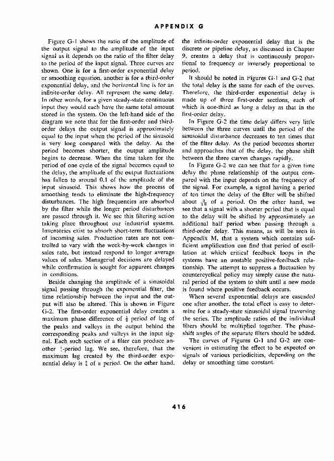
APPENDIX G
Figure G-1 shows the ratio of the amplitude of the infinite-order exponential delay that is the the output signal to the amplitude of the input discrete or pipeline delay, as discussed in Chapter signal as it depends on the ratio of the filter delay 9, creates a delay that is continuously propor- to the period of the input signal. Three curves are tional to frequency or inversely proportional to shown. One is for a first-order exponential delay period. or smoothing equation, another is for a third-order It should be noted in Figures G-1 and G-2 that
exponential delay, and the horizontal line is for an the total delay is the same for each of the curves. infinite-order delay. All represent the same delay. Therefore, the third-order exponential delay is In other words, for a given steady-state continuous made up of three first-order sections, each of
input they would each have the same total amount which is one-third as long a delay as that in the stored in the system. On the left-hand side of the first-order delay. diagram we note that for the first-order and third- In Figure G-2 the time delay differs very little order delays the output signal is approximately between the three curves until the period of the
equal to the input when the period of the sinusoid sinusoidal disturbance decreases to ten times that is very long compared with the delay. As the of the filter delay. As the period becomes shorter
period becomes shorter, the output amplitude and approaches that of the delay, the phase shift
begins to decrease. When the time taken for the between the three curves changes rapidly. period of one cycle of the signal becomes equal to In Figure G-2 we can see that for a given time the delay, the amplitude of the output fluctuations delay the phase relationship of the output com- has fallen to around 0.1 of the amplitude of the pared with the input depends on the frequency of
input sinusoid. This shows how the process of the signal. For example, a signal having a period smoothing tends to eliminate the high-frequency of ten times the delay of the filter will be shifted disturbances. The high frequencies are absorbed about -, 3. of a period. On the other hand, we
by the filter while the longer period disturbances see that a signal with a shorter period that is equal are passed through it. We see this filtering action to the delay will be shifted by approximately an
taking place throughout our industrial systems. additional half period when passing through a Inventories exist to absorb short-term fluctuations third-order delay. This means, as will be seen in of incoming sales. Production rates are not con- Appendix M, that a system which contains suf- trolled to vary with the week-by-week changes in ficient amplification can find that period of oscil- sales rate, but instead respond to longer average lation at which critical feedback loops in the values of sales. Managerial decisions are delayed systems have an unstable positive-feedback rela- while confirmation is sought for apparent changes tionship. The attempt to suppress a fluctuation by in conditions. countercyclical policy may simply cause the natu-
Beside changing the amplitude of a sinusoidal ral period of the system to shift until a new mode
signal passing through the exponential filter, the is found where positive feedback occurs. time relationship between the input and the out- When several exponential delays are cascaded
put will also be altered. This is shown in Figure one after another, the total effect is easy to deter- G-2. The first-order exponential delay creates a mine for a steady-state sinusoidal signal traversing maximum phase difference of 4 period of lag of the series. The amplitude ratios of the individual the peaks and valleys in the output behind the filters should be multiplied together. The phase- corresponding peaks and valleys in the input sig- shift angles of the separate filters should be added. nal. Each such section of a filter can produce an- The curves of Figures G-1 and G-2 are con-
other 4-period lag. We see, therefore, that the venient in estimating the effect to be expected on
maximum lag created by the third-order expo- signals of various periodicities, depending on the
nential delay is ? of a period. On the other hand, delay or smoothing time constant.
416
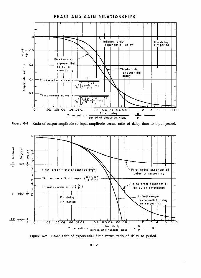
PHASE AND GAIN RELATIONSHIPS
1.0 1.0
lnfinite - order D = delay \. exponentiol deloy P = period
–––––
0.8 First -order x \ \
0,6 exponentiol \ o delay or or \ \ = smoothing \
Third -order 2 , ' !
1 \ \ exponentiol
_ -order )
? = ) deloy
First -order curve = ––––––––––– ' –– – –––––– ––– –– ––– –– –
?
0.4 FI,,,
rï Tï
)' +, \\
deley
- D \ E
p p
0.2 1 Third-order curve = ––' ! "*.
0 /r/2Tr 3
\ p
3
.01 .02 .03.04 .06.080.1 0.2 O.3 O.4 O.6 O.8 1 2 3 4 6 8 10
Time ratio = filter deloy = -L 10 period of sinusoidal signal P
Figure G-1 Ratio of output amplitude to input amplitude versus ratio of delay time to input period.
o
1 1 1 1 1 ' '
-
(JI
i ;
° o en
1.
ir 90....!... 24-
First-order = arctangent (2Tr)(-p-) ?First-order exponentiol
0 Third-order = 3 arctangent
2
P
P)
deloy or smoothing = 3 arctangent ––\-\-–––––––––––––––––––––––
.. Third-order exponentiol
? Infinite-order = 2 D p \ delay or smoothing M \ \
" D =del lay
=period X. ponentiol deloy -
\ smoothing
2 4 4 3
.0! l .02 .03.04 .06 .080.1 0.2 0304 Q6 0.8 1 2 3 4 6 8 1 10
Time ratio filter deloy D
period of sinusoidal
Figure G-2 Phase shift of exponential filter versus ratio of delay to period.
417
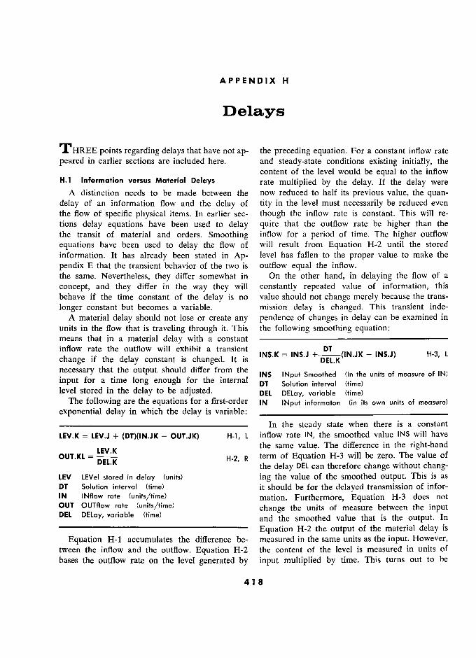
APPENDIX H
Delays
THREE points regarding delays that have not ap- the preceding equation. For a constant inflow rate
peared in earlier sections are included here. and steady-state conditions existing initially, the content of the level would be equal to the inflow
H.1 1 Information versus Material Delays rate multiplied by the delay. If the delay were A distinction needs to be made between the now reduced to half its previous value, the quan-
delay of an information flow and the delay of tity in the level must necessarily be reduced even the flow of specific physical items. In earlier sec- though the inflow rate is constant. This will re- tions delay equations have been used to delay quire that the outflow rate be higher than the the transit of material and orders. Smoothing inflow for a period of time. The higher outflow
equations have been used to delay the flow of will result from Equation H-2 until the stored information. It has already been stated in Ap- level has fallen to the proper value to make the
pendix E that the transient behavior of the two is outflow equal the inflow. the same. Nevertheless, they differ somewhat in On the other hand, in delaying the flow of a
concept, and they differ in the way they will constantly repeated value of information, this behave if the time constant of the delay is no value should not change merely because the trans-
longer constant but becomes a variable. mission delay is changed. This transient inde- A material delay should not lose or create any pendence of changes in delay can be examined in
units in the flow that is traveling through it. This the following smoothing equation: means that in a material delay with a constant –––––––––––––––––––––––––––-–––
inflow rate the outflow will exhibit a transient DT INS.J) H-3, L
change if the delay constant is changed. It is !NS.K = )NS.J
+––––()N.JK – tNb.J) n-j, L
necessary that the output should differ from the INput d (in the units 0 measure 0
input for a time long enough for the internal )NS !Nput Smoothed (m thé units of measure of )N)
input for a time long enough for the internal DT Solution interval (time) level stored in the delay to be adjusted. DEL DELay, variable (time)
The following are the equations for a first-order IN INput informaton (in its own units of measure) exponential delay in which the delay is variable: _______________________________ ––––––––––––––––––––––––––––––– In the steady state when there is a constant
LEV.K = LEV.J + (DT)(IN.JK - OUT.JK) H-1, L inflow rate IN, the smoothed value INS will have
LEV.K the same value. The difference in the right-hand
OUT.KL = H-2 R term of Equation H-3 will be zero. The value of DEL.K '
the delay DEL can therefore change without chang- LEV LEVeI stored in delay (units) ing the value of the smoothed output. This is as DT Solution interval (time) it should be for the delayed transmission of infor- IN [Nflow rate (units/time) mation. Furthermore, Equation H-3 does not OUT OUTflow rate (units/time) change the units of measure between the input DEL DELay, variable (time) and the smoothed value that is the output. In –––––––––––––––––––––––––––––
Equation H-2 the output of the material delay is
Equation H-1 accumulates the difference be- measured in the same units as the input. However, tween the inflow and the outflow. Equation H-2 the content of the level is measured in units of bases the outflow rate on the level generated by input multiplied by time. This turns out to be
418
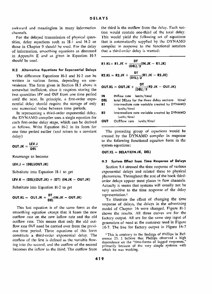
DELAYS S
awkward and meaningless in many information the third is the outflow from the delay. Each sec- channels. tion would contain one-third of the total delay.
For the delayed transmission of physical quan- This would yield the following set of equations tities, delay equations such as H-1 and H-2 or that is automatically supplied by the DYNAMO
those in Chapter 9 should be used. For the delay compiler in response to the functional notation
of information, smoothing equations as discussed that a third-order delay is wanted: in Appendix E and as given in Equation H-3 ––––––––––––––––––––––––––––– should be used. DT
R1.KL= R1.JK + R1.JK) L)/3([N.JK
H.2 Alternative Equations for Exponential Delays DT
The difference Equations H-1 and H-2 can be R2.KL = R2.JK + Z(Rl .JK -
R2.JK) written in various forms, depending on con- (DEL)/3
venience. The form given in Section H.1 above is pUT.KL = OUT.JK + OUT.JK) somewhat inefficient, since it requires storing the
' ' (DEL)/3
' '
two quantities LEV and OUT from one time period IN INflow rate (units/time) until the next. In principle, a first-order expo- DEL total DELay for the three delay sections (time) nential delay should require the storage of only Rl intermediate rate variable created by DYNAMO one numerical value between time periods. (units/time)
In representing a third-order exponential delay, R2 intermediate rate variable created by DYNAMO
the DYNAMO compiler uses a single equation for (units/time) each first-order delay stage, which can be derived OUT OUTflow rate (units/time) as follows. Write Equation H-2 in its form for ––––––––––––––––––––––––*––––––
one time period earlier (and return to a constant The preceding group of equations would be
delay) created by the DYNAMO compiler in response
LEV.J to the following functional equation form in the
OUT.JK = [)EL
system equations : DEL
OUT.KL = DELAY3(IN.JK, DEL) Rearrange to become
LEV.J = (DEL)(OUT.JK) H.3 System Effect from Time Response of Delays
LEV.J = (DEL)(OUT.JK) Section 9.4 stressed the time response of various
Substitute into Equation H-1 to get exponential delays and related these to physical phenomena. Throughout the rest of the book third-
LEV.K = (DEL)(OUT.JK) + (DT) (IN.JK - OUT.JK) order delays appear most places in flow channels.
Substitute into Equation H-2 to get Actually it seems that systems will usually not be
very sensitive to the time response of the delay
OUT.KL = OUT.JK + DT OUT.JK) representation.l ., OUT.KL = OUT.JK ' To illustrate the effect of changing the time
... response of delays, the delays in the advertising This last equation is of the same form as the model of Chapter 16 were changed. Figure H-1
smoothing equation except that it bases the new shows the results. All three curves are for the outflow rate on the new inflow rate and the old
factory output. All are for the same step input of outflow rate. This means that only the old out-
generation of need at the customer used in Figure flow rate OUT need be carried over from the previ- 16-7. The line for factory output in Figure 16-7 ous time period. Three equations of this form constitute a third-order exponential delay. The ' This is contrary to the findings of Phillips in Ref-
outfiow of the first is defined as the variable fiow- erence 25. 1 believe that Phillips observed a high outflow of thé nrst is denned as thé variable How- dependence
ing into the second, and the outfiow of the second dependence on thé time-forms ?Lmagged responses, mg into the second, and the outflow of the second primarily because of the very simple systems with
becomes the inflow to the third. The outflow from which he was working. y p y
419
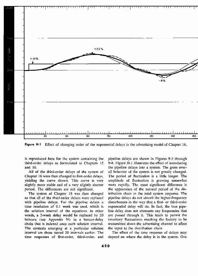
+25%
+la% `\\
- 8%
20 40 60 80 t00 120 140 16(
Figure H-1 Effect of changing order of the exponential delays in the advertising model of Chapter 16.
is reproduced here for the system containing the pipeline delays are shown in Figures 9-3 through third-order delays as formulated in Chapters 15 9-8. Figure H-1 illustrates the effect of introducing
. and 16. the pipeline delays into a system. The gross over- All of the third-order delays of the system of all behavior of the system is not greatly changed.
Chapter 16 were then changed to first-order delays, The period of fluctuation is a little longer. The
yielding the curve shown. This curve is very amplitude of fluctuation is growing somewhat
slightly more stable and of a very slightly shorter more rapidly. The most significant difference is
period. The differences are not significant. the appearance of the natural period of the dis- The system of Chapter 16 was then changed tribution chain in the total system response. The
so that all of the third-order delays were replaced pipeline delays do not absorb the higher-frequency with pipeline delays. For the pipeline delays a disturbances in the way that a first- or third-order time resolution of 0.1 week was used, which is exponential delay will do. In fact, the true pipe- the solution interval of the equations. In other line delay does not attenuate any frequencies that
words, a 2-week delay would be replaced by 20 are passed through it. This tends to permit the boxcars (see Appendix N) in a boxcar-delay inventory fluctuations reaching the factory to be chain that is indexed once each solution interval. transmitted down the advertising channel to affect The contents emerging at a particular solution the input to the distribution chain. interval are those stored 20 intervals earlier. The The effect of the time response of delays may time responses of first-order, third-order, and depend on where the delay is in the system. One
420
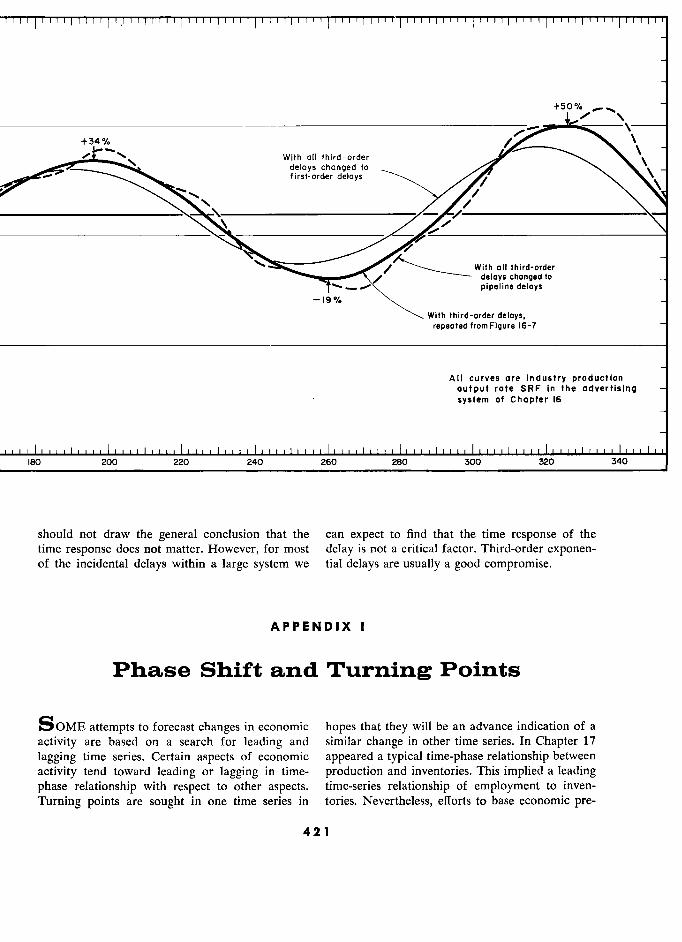
1 ! 1 Il 11111 ! 1 Il \ ,III! 1 1 1 1 l' III Il! Il Il 111111'1 Il 11111111
+50%
\____
+34% \ - _ With ail third-order
delays changed to \ tirst-order delays
\
With all third-order delays chonged ta _ pipeline delays
- 19%
With third-order delays, repeated fromfigure 16-7 _
All curves are industry production output rate SRF in the advertisinq -
. system of Chapter 16 16
180 MO 220 240 260 280 300 320 340
should not draw the general conclusion that the can expect to find that the time response of the time response does not matter. However, for most delay is not a critical factor. Third-order exponen- of the incidental delays within a large system we tial delays are usually a good compromise.
APPENDIX 1
Phase Shift and Turning Points
SOME attempts to forecast changes in economic hopes that they will be an advance indication of a
activity are based on a search for leading and similar change in other time series. In Chapter 17
lagging time series. Certain aspects of economic appeared a typical time-phase relationship between
activity tend toward leading or lagging in time- production and inventories. This implied a leading phase relationship with respect to other aspects. time-series relationship of employment to inven-
Turning points are sought in one time series in tories. Nevertheless, efforts to base economic pre-
421 1
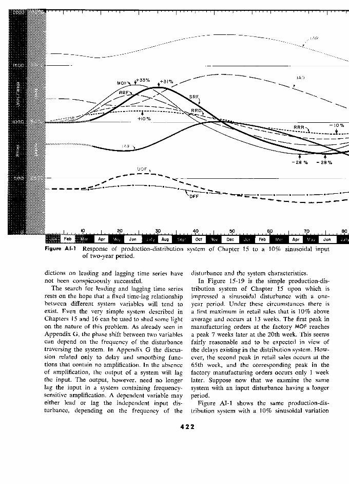
2000 ... " I
" " , I
" , I , , I
i " " I
" " I i " , I
" " I " , I
, , i I
IAR
ev c,:-_ :.. :;oe
MOF ,.....- O ¡
(AD
3: e RRF
- - F SRF - a
,
__ RRD
1000 ï% +la +10%
-110%
IAF
- 28 % - 28 %a
UOF,
..,..""'" °
- . - . - .
DFF
0 0 10 .... 2 10. 6p, 8
j') Feb Mc],
Apr Jun J?IY Aug Sept Oct Nov Dec Feb Mc), Apr MCY Jun .0
Figure AI-1 Response of production-distribution system of Chapter 15 to a 10% sinusoidal input of two-year period.
dictions on leading and lagging time series have disturbance and the system characteristics. not been conspicuously successful. In Figure 15-19 is the simple production-dis-
The search for leading and lagging time series tribution system of Chapter 15 upon which is rests on the hope that a fixed time-lag relationship impressed a sinusoidal disturbance with a one- between different system variables will tend to year period. Under these circumstances there is exist. Even the very simple system described in a first maximum in retail sales that is 10% above
Chapters 15 and 16 can be used to shed some light average and occurs at 13 weeks. The first peak in on the nature of this problem. As already seen in manufacturing orders at the factory MOF reaches
Appendix G, the phase shift between two variables a peak 7 weeks later at the 20th week. This seems can depend on the frequency of the disturbance fairly reasonable and to be expected in view of
traversing the system. In Appendix G the discus- the delays existing in the distribution system. How- sion related only to delay and smoothing func- ever, the second peak in retail sales occurs at the tions that contain no amplification. In the absence 65th week, and the corresponding peak in the of amplification, the output of a system will lag factory manufacturing orders occurs only 1 week the input. The output, however, need no longer later. Suppose now that we examine the same
lag the input in a system containing frequency- system with an input disturbance having a longer sensitive amplification. A dependent variable may period. either lead or lag the independent input dis- Figure AI-1 shows the same production-dis- turbance, depending on the frequency of the tribution system with a 10% sinusoidal variation
422 2
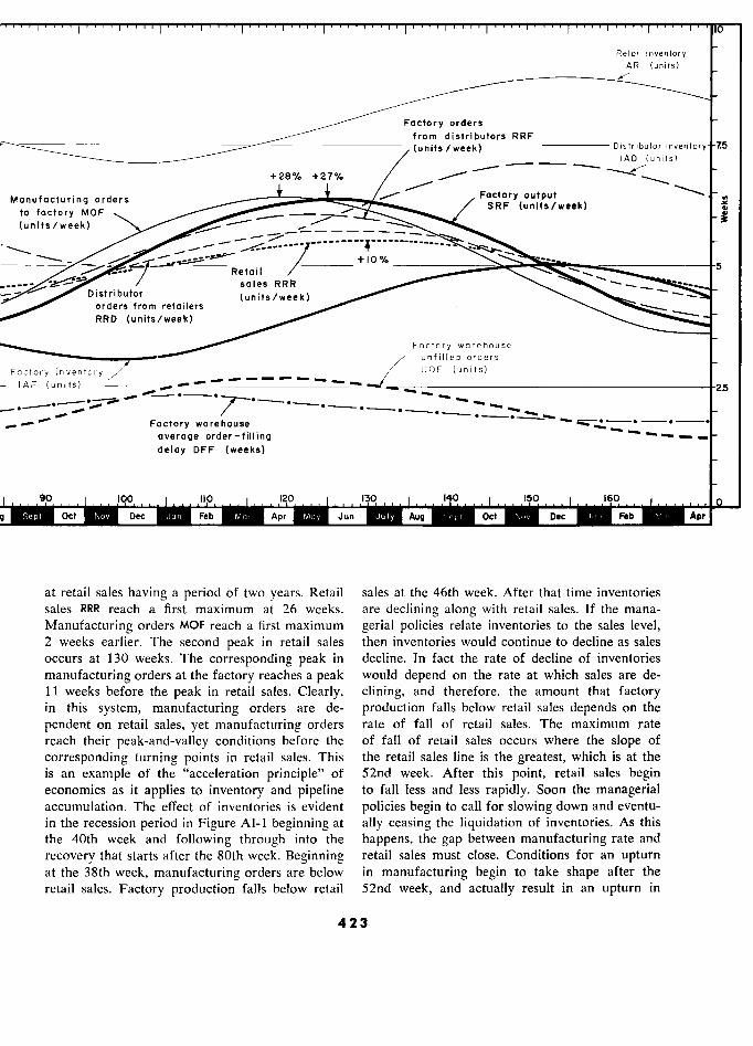
" i , " " I " " I " " " t " " " t T . ) " " , " " , , t . " , i " 10
Retai! inventory IAR (units)
Factory orders
from distributors RRF
- --- /week) Distributorinventory 75
IAD (units)
- -- +28% +27% /
Manufacturing orders s
+28% +27%
/ / Factory output , o '" SRF (units/week)
to factory MOF _ -- SRF (units/week) '"
(units/week)
Retail +10% i.._._..
__._
W 5
sales RRR _ sales RRR - - _ _ Distributor (units/week) -
orders from retailers _
RRO (units/week)
Factory warehouse
L
unfilled orders
Factory inventory _ UOF (units)
IAF (units) - 23
- .... -- ."",. Factory warehouse -.-.
average order-filling
delay DFF (weeks)
90 !qo.... '110, '13 140 150 ... 160
Sept ? Dec ? Jan ?pr M., Auq M Oct Dec Feb Apr ?
at retail sales having a period of two years. Retail sales at the 46th week. After that time inventories sales RRR reach a first maximum at 26 weeks. are declining along with retail sales. If the mana-
Manufacturing orders MOF reach a first maximum gerial policies relate inventories to the sales level, 2 weeks earlier. The second peak in retail sales then inventories would continue to decline as sales occurs at 130 weeks. The corresponding peak in decline. In fact the rate of decline of inventories
manufacturing orders at the factory reaches a peak would depend on the rate at which sales are de- Il weeks before the peak in retail sales. Clearly, clining, and therefore, the amount that factory in this system, manufacturing orders are de- production falls below retail sales depends on the
pendent on retail sales, yet manufacturing orders rate of fall of retail sales. The maximum rate reach their peak-and-valley conditions before the of fall of retail sales occurs where the slope of
corresponding turning points in retail sales. This the retail sales line is the greatest, which is at the is an example of the "acceleration principle" of 52nd week. After this point, retail sales begin economics as it applies to inventory and pipeline to fall less and less rapidly. Soon the managerial accumulation. The effect of inventories is evident policies begin to call for slowing down and eventu- in the recession period in Figure AI-1 beginning at ally ceasing the liquidation of inventories. As this the 40th week and following through into the happens, the gap between manufacturing rate and
recovery that starts after the 80th week. Beginning retail sales must close. Conditions for an upturn at the 38th week, manufacturing orders are below in manufacturing begin to take shape after the retail sales. Factory production falls below retail 52nd week, and actually result in an upturn in
423
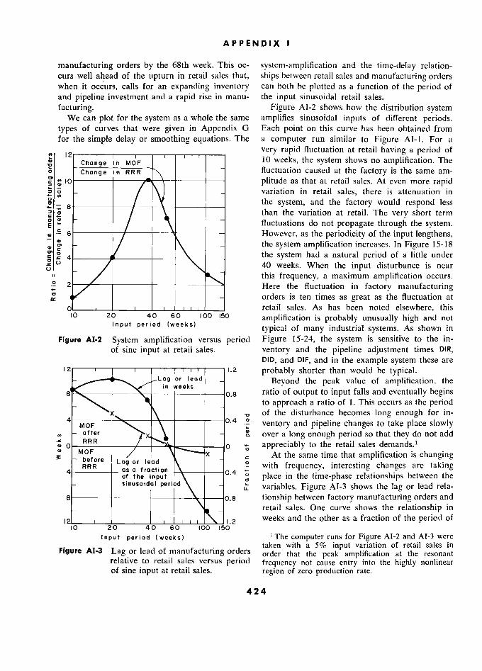
APPENDIX 1
manufacturing orders by the 68th week. This oc- system-amplification and the time-delay relation-
curs well ahead of the upturn in retail sales that, ships between retail sales and manufacturing orders
when it occurs, calls for an expanding inventory can both be plotted as a function of the period of
and pipeline investment and a rapid rise in manu- the input sinusoidal retail sales.
facturing. Figure AI-2 shows how the distribution system We can plot for the system as a whole the same amplifies sinusoidal inputs of different periods.
types of curves that were given in Appendix G Each point on this curve has been obtained from
for the simple delay or smoothing equations. The a computer run similar to Figure AI-1. For a
very rapid fluctuation at retail having a period of 12 2
Change 'in MOF 10 weeks, the system shows no amplification. The
0 Cnange in RRR '
fluctuation caused at the factory is the same am-
- 5 d 10 ––––––––––7*T)––––––– plitude as that at retail sales. At even more rapid
N g -
/ \J - variation in retail sales, there is attenuation in
8 8 Y______ the system, and the factory would respond less
than the variation at retail. The very short term
1 ' / \ "
fluctuations do not propagate through the system. , .> 6 However, as the periodicity of the input lengthens,
S. - / \
- the system amplification increases. In Figure 15-18 8
ô L 4 the system had a natural period of a little under
" ./ 40 weeks. When the input disturbance is near " ./ this frequency, a maximum amplification occurs. .2 2 Here the fluctuation in factory manufacturing
9 F - orders is ten times as great as the fluctuation at
p retail sales. As has been noted elsewhere, this 10 20 40 60 100 150
amplification is probably unusually high and not '' '° (week)
typical of many industrial systems. As shown in
Figure AI-2 System amplification versus period Figure 15-24, the system is sensitive to the in-
of sine input at retail sales. ventory and the pipeline adjustment times DIR,
DID, and DIF, and in the example system these are
i.2 probably shorter than would be typical. -
°r lead -
Beyond the peak value of amplification, the
8' ln weeks 0.8 g ratio of output to input falls and eventually begins to approach a ratio of 1. This occurs as the period
i: \ * of the disturbance becomes long enough for in-
4 MOF 0'4 °
ventory and pipeline changes to take place slowly VI
after \
- â over a long enough period so that they do not add
0 RRR 0 Õ appreciably to the retail sales demands.l
°' MOF \ X At the same time that amplification is changing
RRR or lecid \ °_ with frequency, interesting changes are taking
4 RRR
ore
as a fraction 0 with frequency, interesting changes are taking 4
of the mput \°'? ? place in the time-phase relationships between the - sinusoidal period t variables. Figure AI-3 shows the lag or lead rela-
8 p,g tionship between factory manufacturing orders and
- - retail sales. One curve shows the relationship in
I2 11.2 weeks and the other as a fraction of the period of
10 20 40 0 60 100 150
Input period (weeks) The computer runs for Figure AI-2 and AI-3 were
? taken with a 5% input variation of retail sales in
Figure AI-3 Lag or lead of g orders order that the peak amplification at the resonant relative to retail sales versus period frequency not cause entry into the highly nonlinear of sine input at retail sales. region of zero production rate.
424

PHASE SHIFT AND TURNING POINTS S
the input sinusoidal disturbance. For the very lie in a periodicity range comparable to that ex- short period inputs, the time delay is in the 8- to hibited by business cycle fluctuation. Small varia- 10-week interval, with manufacturing orders tions in the rate of change of system variables can
lagging behind changes in retail sales. In fact in cause the lag or lead relationships to shift rather this region a complete phase reversal can occur rapidly as indicated by Figure AI-3. The multitude with factory manufacturing orders at a peak at of noise sources containing periodicities in this the same time that retail sales are at a minimum. range will create similar effects. The lag or lead As the periodicities of the input become longer, relationships are dependent in a very complicated the inventory and pipeline accumulation effects way on the past history of the pertinent variables can take place to create a phase displacement that and their rates of change. It is hardly to be ex- causes manufacturing orders first to approach pected that decisive indicators of future events retail sales in time and then actually to occur in can be found in these relationships. Certain vari- advance of retail sales. The most rapid rate of ables will tend, however, to be related in specific change in the lag or lead relationship occurs near ways, and on the average certain directions of the peak in Figure AI-2. In Figure AI-3 manu- time relationship will predominate over the reverse
facturing orders lag behind retail sales by about directions. 7 weeks, when the input disturbance has a 38- The problem of the leading and lagging series week period. By the time the input disturbance can be examined in Figure 18-5. In that system of has reached a period of 55 weeks, which is only Chapters 17 and 18 the situation is very simple, slightly more than a year, the manufacturing and the cause-and-effect relationships are free of orders are occurring simultaneously with retail the complicated interlocking loops that would be sales. By the time the disturbance to which the found in a complete economic system. As a result
system is being subjected has reached a period that we should expect in Figure 18-5 that the leading is 2 years long, the manufacturing orders are and lagging phase relationships would be more
leading some 10 weeks ahead of retail sales. consistent and have more decisiveness than they Much more investigation of this phenomenon would in a system of greater complication. By
is called for. However, I believe that many of our inspection, it appears that the backlog curve leads industrial systems will be found to be operating the employment curve and the employment curve
generally in a region comparable with the zone leads the inventory curve most of the time. This between 40 weeks and 100 weeks in Figure AI-3. is especially true for the large and long-period , A fuller development of a model with the inclusion disturbances. The lead-lag relationship begins to of factors not appearing in this simplified example break down, however, for the smaller disturbances. will tend to lengthen the natural period of the We should expect the time relationships to be-
system. This means that the region of rapidly come less decisive in a complex system with more
changing lag or lead relationships will probably interlocking relationships between many industries.
425 5


APPENDIX J
Value of Information
INFORMATION is the substance from which conviction that better information means better
managerial decisions are made. As with other management. Machine processing of business data
products the quality of the raw material partially is usually justified on the basis of machine-proc- determines the quality of the output. The manager essing costs relative to costs in the previously is well aware that information sources are impor- existing system. For lack of any real measure of tant. But does he know with any assurance the the value of information, this justification is al- measures of information quality? most never made on the basis of the relationships
Information sources, like other flows in the between information cost and information value. industrial system, are subject to being distorted. It is my belief, based on experiences with in- The distortion can occur in amplitude and in dustrial organizations, that some of the most im-
timing. The distortion will depend on the time- portant and useful information is going unused
varying character of the information. Amplifica- and untouched. At the same time, great efforts are tion can exist in information channels. The kinds devoted to attempting to acquire information that of distortions seen in Appendices E, G, and 1 even were it available would do little for the occur in the information flows. success of the organization. As an example, some
The manager is interested in more useful in- organizations have succeeded in speeding up the formation on which to base decisions. Greater flow of sales information and production sched-
utility can be obtained both by improving existing uling to the point where the random-noise varia- information sources and by basing decisions on tions in the market can now be directly imposed new and different sources that have not been used on the production process. This tends to ignore in the past. The cost of obtaining improved infor- the proper use of inventories for absorbing such mation can usually be estimated with fair ac- variations. Carried to an extreme, the result of
curacy. But what is better information worth? more timely information can be harmful. The This is not so easily answered. Better information effect can be to cause the manager to put more is worth the value that we attach to the improved and more stress on short-range decisions. In Chap- industrial performance which results when the ter 18 the system improvements did not result so better information is available. Unless we can much from changing the type of information determine the change in system performance that available or its quality nearly so much as from will result from a changed information flow, we changing the sources of information used and the cannot determine its value. nature of the decision based on the information.
The value of information has usually been A system model can be used to see how changed determined by highly subjective means that neces- information flows will affect the system. Doing sarily include an estimate of what the information this requires a firm hypothesis about how the in- will do to the dynamic behavior of the system. formation affects decisions. Herein would be the Our ability to estimate the characteristics of in- first test of much of the information generated in formation-feedback systems is poor. It is to be industrial organizations. For much of the informa-
expected that one of the weakest areas of mana- tion selected, it would be nearly impossible to
gerial judgment is in placing a dollar value on suggest a hypothesis about the way such informa- an information source. tion affects the flow of business activity. Inability
The United States has a tremendous data- to suggest a use for an information source raises
processing industry that caters to the managerial the possibility that it is not useful. Given the as-
427
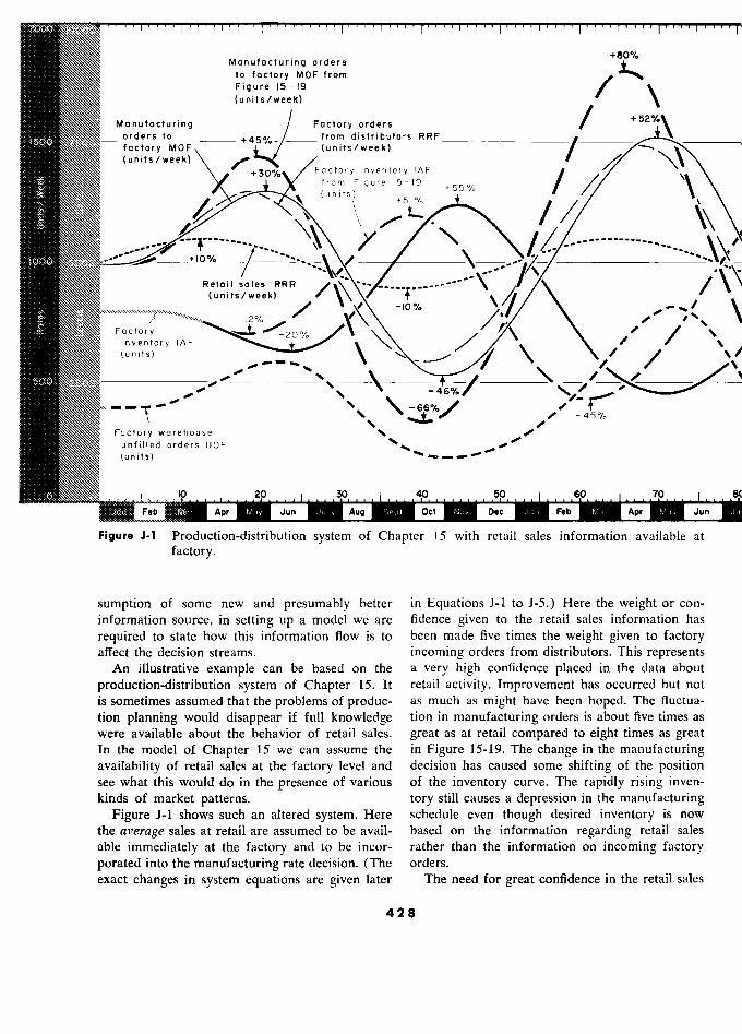
2000 ... , .... , .... I
.... i , .... i .. , , .... , 1 1 1
" " i " "
. +80% Manufacturing orders
to factory MOF from
/-..... Figure 15-19
(u nits /week)
Manufacturing
J
Factory orders / +52%`
_ orders 10 +45'/.- from distributors RRF
\`F
1500 factory MOF (units/week)
/ -
\ (units /week) (units/week)
+30% Factory inventory IAF
/
// .Ó "" \
from Figure 15-19 IÍ \ 3: (units) lu n its)
+51%
%
b
+51 %
'
/ /
______
\
1000
'-" -
-i
{.-. ----
-----"- -....
.,_.. ..-
les RRR
/- \-_--.7- -, 1-
Retail sales RRR / \ _. _f -
/ Retail sales
RRR
-
/\,---- '-\V' 10 ._---------"
----
J. IV\
\
/ ','"
Factory ?20 % `·
.
Factory
N
-lo% 40
,
(units) IAF
\
"
\ 40 ,
500 i · -\ _1
- fi
- -T-' "-66%/
/'/-r"
Factory warehouse
-45-/. 4
Foctory worehouse , ," unfilled orders UOF '....,;
(units) ' - - -"
0 .... 10 .... 1 .... 20 .... 1 .... 4p.....50..7p ....
Feb Me, Jun Aug Oct M N.v Feb Apr M,] y
Figure J-1 Production-distribution system of Chapter 15 with retail sales information available at factory.
sumption of some new and presumably better in Equations J-1 to J-5.) Here the weight or con- information source, in setting up a model we are fidence given to the retail sales information has
required to state how this information flow is to been made five times the weight given to factory affect the decision streams. incoming orders from distributors. This represents
An illustrative example can be based on the a very high confidence placed in the data about
production-distribution system of Chapter 15. It retail activity. Improvement has occurred but not is sometimes assumed that the problems of produc- as much as might have been hoped. The fluctua- tion planning would disappear if full knowledge tion in manufacturing orders is about five times as were available about the behavior of retail sales. great as at retail compared to eight times as great In the model of Chapter 15 we can assume the in Figure 15-19. The change in the manufacturing availability of retail sales at the factory level and decision has caused some shifting of the position see what this would do in the presence of various of the inventory curve. The rapidly rising inven- kinds of market patterns. tory still causes a depression in the manufacturing
Figure J-1 shows such an altered system. Here schedule even though desired inventory is now the average sales at retail are assumed to be avail- based on the information regarding retail sales able immediately at the factory and to be incor- rather than the information on incoming factory porated into the manufacturing rate decision. (The orders. exact changes in system equations are given later The need for great confidence in the retail sales
428 8
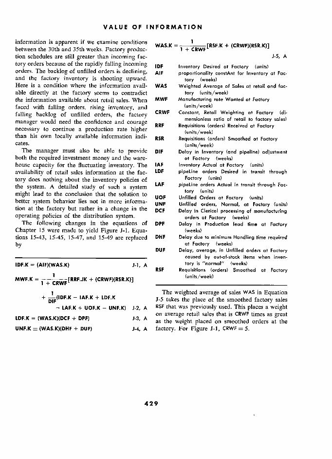
VALUE OF INFORMATION
information is apparent if we examine conditions
(CRWF)(RSR.K)] between the 30th and 35th weeks. Factory produc- '
1 + CRWF ' '
tion schedules are still greater than incoming fac- J-5, A
tory orders because of the rapidly falling incoming IDF Inventory Desired at Factory (units) orders. The backlog of unfilled orders is declining, AIF proportionality constAnt for Inventory at Fac- and the factory inventory is shooting upward. tory (weeks) Here is a condition where the information avail- WAS Weighted Average of Sales at retail and fac- .
able directly at the factory seems to contradict tory (units/week) the information available about retail sales. When MWF Manufacturing rate Wanted at Factory faced with falling orders, rising inventory, and (units/week)
falling backlog of unfilled orders, the factory CRWF Constant, Retail Weighting at Factory (di-
mensionless ratio of retail to factory sales) manager would need the confidence and courage RRF Requisirions ( d ) of refait ar Factory
saies)
necessary to continue a production rate higher RRF Requisitions (orders) Received at Factory
necessary to continue a production rate higher (units/week) than his own locally available information indi- RSR Requisitions (orders) Smoothed at Factory cates. (units/week)
The manager must also be able to provide DIF Delay in Inventory (and pipeline) adjustment both the required investment money and the ware- at Factory (weeks) house capacity for the fluctuating inventory. The IAF Inventory Actual at Factory (units)
availability of retail sales information at the fac- LDF pipeline orders Desired in transit through
tory does nothing about the inventory policies of Factory (units)
the system. A detailed study of such a system LAF pipeline orders Actual in transit through Fac-
might lead to the conclusion that the solution to tory (units) '
mlg t ea
to t e
c?nc to UOF Unfilled Orders at Factory (units) better system behavior lies not in more informa- UNF Unflled orders, Normal, at Factory (units) tion at the factory but rather in a change in the DCF Delay in Clerical processing of manufacturing ". operating policies of the distribution system. orders at Factory (weeks)
The following changes in the equations of DPF Delay in Production lead time at Factory Chapter 15 were made to yield Figure J-1. Equa- (weeks) tions 15-43, 15-45, 15-47, and 15-49 are replaced DHF Delay due to minimum Handling time required by at Factory (weeks)
DUF Delay, average, in Unfilled orders at Factory caused by out-of-stock items when inven-
IDF.K = (AIF)(WAS.K) J-1, A tory is "normal" (weeks) RSF Réquisitions (orders) Smoothed at Factory
MWF.K = (CRWF)(RSR.K)] (units/week)
1 The weighted average of sales WAS in Equation + w'F.K
IAF.K + LDF.K J-5 takes the place of the smoothed factory sales - LAF.K + UOF.K - UNF.K) J-2, A RSF that was previously used. This places a weight
LDF.K (WAS.K)(DCF + DPF) J-3, A on average retail sales that is CRWF times as great LDF.K = (WAS.K)(DCF + DPF) J-3, A as the weight placed on smoothed orders at the
UNF.K = (WAS.K)(DHF + DUF) J-4, A factory. For Figure J-1, CRWF = 5.
429
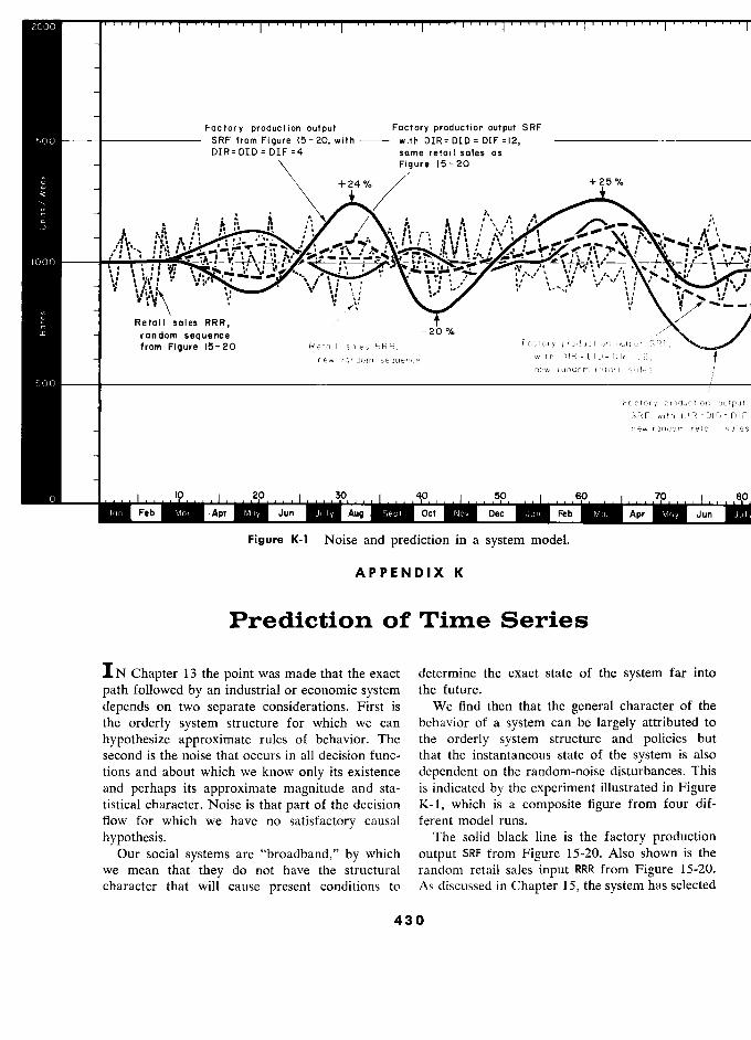
2000
NNNN Factory production output Factory production output SRF
SRF from Figure 15-20, with––– wilh DIR=DID=DIF=12, 1 2, –––––––––––––––––––––––
))t)t)))J) DIR=DID=DIF=4 4 same retail sales as Figure 15-20
+ 24 % + 2 5 %
-k 8%, 1000
, ,, ,:;
Retail sales RRR, rcindom sequence
20%
jtjtt) from Figure 15-20 Retail sales RRR, Factary production output SRF,
riew random sequence with
new random retai 1 sales
500
Factary production outpu
SRF, with DIR?DID=DL l
new random retait 9019
?Dec?M
Figure K-1 Noise and prediction in a system model.
APPENDIX K
Prediction of Time Series
IN Chapter 13 the point was made that the exact determine the exact state of the system far into
path followed by an industrial or economic system the future.
depends on two separate considerations. First is We find then that the general character of the
the orderly system structure for which we can behavior of a system can be largely attributed to
hypothesize approximate rules of behavior. The the orderly system structure and policies but
second is the noise that occurs in all decision func- that the instantaneous state of the system is also
tions and about which we know only its existence dependent on the random-noise disturbances. This
and perhaps its approximate magnitude and sta- is indicated by the experiment illustrated in Figure
tistical character. Noise is that part of the decision K-1, which is a composite figure from four dif-
flow for which we have no satisfactory causal ferent model runs.
hypothesis. The solid black line is the factory production
Our social systems are "broadband," by which output SRF from Figure 15-20. Also shown is the
we mean that they do not have the structural random retail sales input RRR from Figure 15-20.
character that will cause present conditions to As discussed in Chapter 15, the system has selected
430
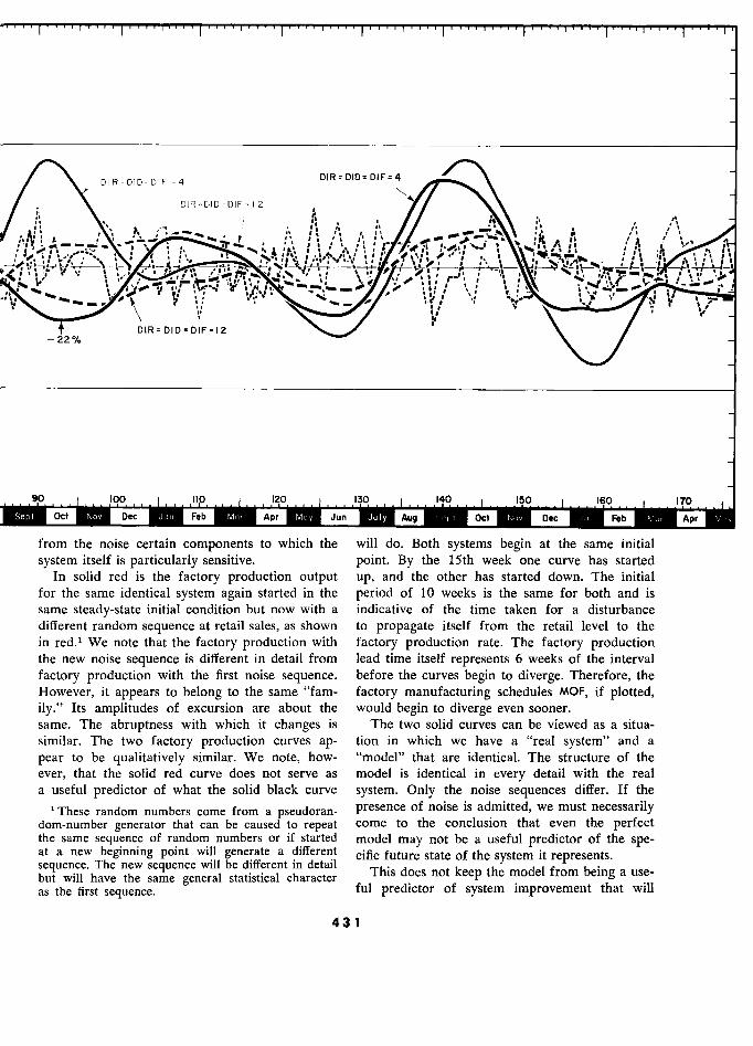
DIR=DID=DIF=4 = 4
DIR= DID=DIF=12 12 2
' ,., ' . ' ' ,, '
j, Î /
,, Î 1 ' jj , j"
,; 0-010
, , r ;
DIR=DID=D[F=12 2 \ / - 22%a
Sept Nov Jon Apr Jun M July 1 lo?Itm Feb Ma,
from the noise certain components to which the will do. Both systems begin at the same initial
system itself is particularly sensitive. point. By the 15th week one curve has started In solid red is the factory production output up, and the other has started down. The initial
for the same identical system again started in the period of 10 weeks is the same for both and is same steady-state initial condition but now with a indicative of the time taken for a disturbance different random sequence at retail sales, as shown to propagate itself from the retail level to the in red.1 We note that the factory production with factory production rate. The factory production
'
the new noise sequence is different in detail from lead time itself represents 6 weeks of the interval
factory production with the first noise sequence. before the curves begin to diverge. Therefore, the However, it appears to belong to the same "fam- factory manufacturing schedules MOF, if plotted, ily." Its amplitudes of excursion are about the would begin to diverge even sooner. same. The abruptness with which it changes is The two solid curves can be viewed as a situa- similar. The two factory production curves ap- tion in which we have a "real system" and a
pear to be qualitatively similar. We note, how- "model" that are identical. The structure of the ever, that the solid red curve does not serve as model is identical in every détail with the real a useful predictor of what the solid black curve system. Only the noise sequences differ. If the
i These random numbers corne from a pseudoran- présence of noise is admitted, we must necessarily dom-number generator that can be caused to repeat corne to the conclusion that even the perfect the same sequence of random numbers or if started model may not be a useful predictor of the spe- at a new beginning point will generate a différent cific future state of the system it represents. sequence. The new sequence will be different in détail but will have thé same général statistical character ?'s does not keep thé model from bemg a use-
as thé first séquence, general statistical character
ful predictor of system improvement that will
'
431 1
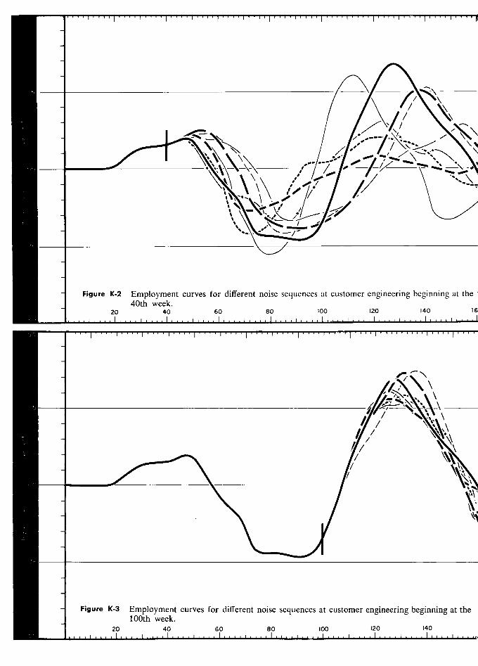
%%
' Figure K-2 Employment curves for different noise sequences at customer engineering beginning at thE
40th week. ttt?
' 20 40 60 80 100 120 140
- Figure K-3 Employment curves for different noise sequences at customer engineering beginning at the 100th week.
tt)jt 20 40 60 80 100 120 140
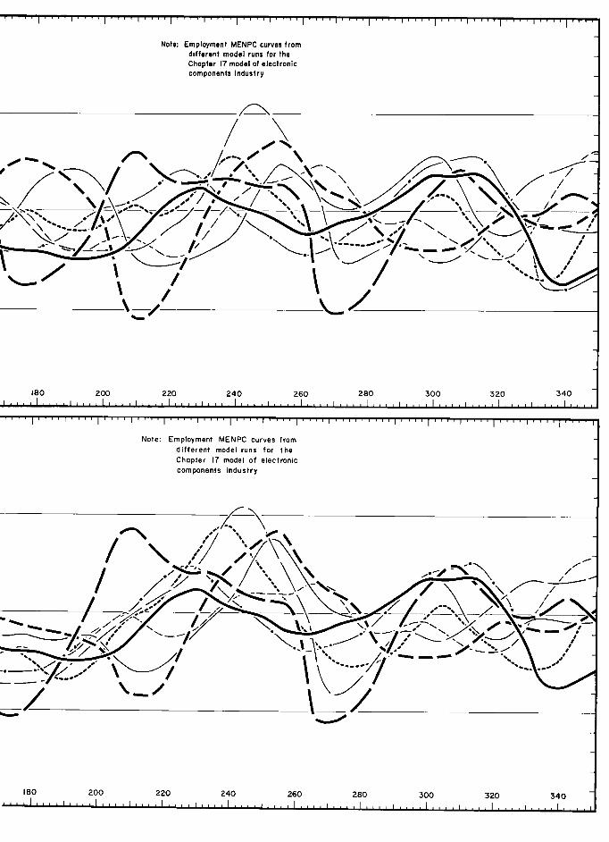
Note: Employment MENPC curves from different model runs for the Chopter 17 model of e lectronic components industry
'
-
/ , '
\- "0 (,-
V"
\,
\
.00/
oe"
"",
180 200 220 240 260 280 300 320 340
Note: Employment MENPC curves from différent model runs for the Chopter 17 model of electronic componentsindustry
180 200 220 240 260 280 300 320 340
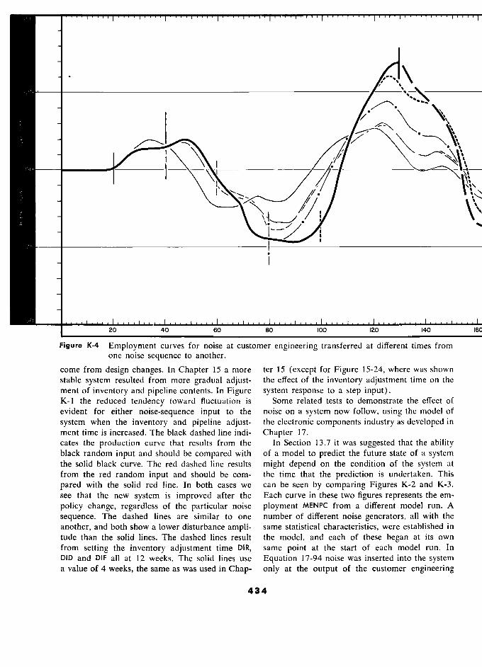
20 40 60 80 IOO 120 140 1.
Figure K-4 Employment curves for noise at customer engineering transferred at different times from
one noise sequence to another.
corne from design changes. In Chapter 15 a more ter 15 (except for Figure 15-24, where was shown
stable system resulted from more gradual adjust- the effect of the inventory adjustment time on the
ment of inventory and pipeline contents. In Figure system response to a step input). K-l the reduced tendency toward fluctuation is Some related tests to demonstrate the effect of
evident for either noise-sequence input to the noise on a system now follow, using the model of
system when the inventory and pipeline adjust- the electronic components industry as developed in
ment time is increased. The black dashed line indi- Chapter 17.
cates the production curve that results from the In Section 13.7 it was suggested that the ability black random input and should be compared with of a mode ! to predict the future state of a system the solid black curve. The red dashed line results might depend on the condition of the system at
from the red random input and should be com- the time that the prediction is undertaken. This
pared with the solid red line. In both cases we can be seen by comparing Figures K-2 and K-3.
see that the new system is improved after the Each curve in these two figures represents the em-
policy change, regardless of the particular noise ployment MENPC from a different model run. A
sequence. The dashed lines are similar to one number of different noise generators, all with the
another, and both show a lower disturbance ampli- same statistical characteristics, were established in
tude than the solid lines. The dashed lines result the model, and each of thèse began at its own
from setting the inventory adjustment time DIR, same point at the start of each model run. In
DID and DIF all at 12 weeks. The solid lines use Equation 17-94 noise was inserted into the system a value of 4 weeks, the same as was used in Chap- only at the output of the customer engineering
434
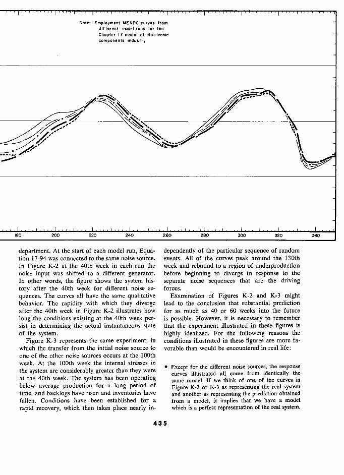
Note: Employment MENPC curves from dlfferent model runs for the
Chapter 17 model of electronic
com ponents industry
, v
;
\
- ..
i
. ,
¿)jT ,
;
i
180 200 220 260 300 320 340
department. At the start of each model run, Equa- dependently of the particular sequence of random tion 17-94 was connected to the same noise source. events. All of the curves peak around the 130th In Figure K-2 at the 40th week in each run the week and rebound to a region of underproduction noise input was shifted to a different generator. before beginning to diverge in response to the In other words, the figure shows the system his- separate noise sequences that are the driving tory after the 40th week for different noise se- forces.
quences. The curves all have the same qualitative Examination of Figures K-2 and K-3 might behavior. The rapidity with which they diverge lead to the conclusion that substantial prediction after the 40th week in Figure K-2 illustrates how for as much as 40 or 60 weeks into the future
long the conditions existing at the 40th week per- is possible. However, it is necessary to remember sist in determining the actual instantaneous state that the experiment illustrated in these figures is of the system. highly idealized. For the following reasons the
Figure K-3 represents the same experiment, in conditions illustrated in these figures are more fa- which the transfer from the initial noise source to vorable than would be encountered in real life: one of the other noise sources occurs at the 100th week. At the t00th week the internai stresses in . week. At the
100th week the internal stresses in Except for the different noise sources, the response the system are considerably greater than they were Ulustrated all corne from 1 .d en t. Ica Ily the at the 40th week. The system has been operating curves illustrated all from of the curves the at thé 40th week. Thé system has been operating same model. If we think of one of the curves in
below average production for a long period of Figure K-2 or K-3 as representing the real system time, and backlogs have risen and inventories have and another as representing the prediction obtained
fallen. Conditions have been established for a from a model, it implies that we have a model
rapid recovery, which then takes place nearly in- which is a perfect representation of the real system.
435
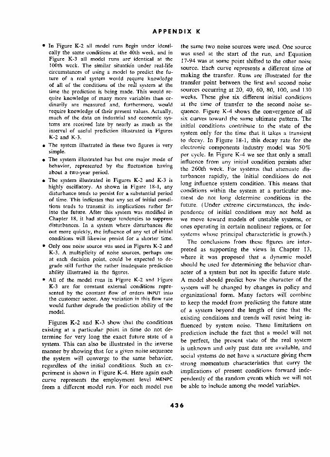
APPENDIX K
In Figure K-2 all model runs Begin under identi- the same two noise sources were used. One source cally the same conditions at the 40th week, and in was used at the start of the run, and Equation Figure K-3 all model runs are identical at the 1 7-94 was at some point shifted to the other noise 100th week. The similar situatiôn under real-life source. Each curve represents a different time of f circumstances of using a model to predict the fu-
making the transfer. Runs are illustrated for the ' makms thé transfer. Runs are iHustrated for thé e ture of a real system would require knowledge . of all of the conditions of the real system at the transfer point between the first and second noise
time the prediction is being made. This would re- sources occurring at 20, 40, 60, 80, 100, and 130
quire knowledge of many more variables than or- weeks. These give six different initial conditions
dinarily are measured and, furthermore, would at the time of transfer to the second noise se- require knowledge of their present values. Actually, quence. Figure K-4 shows the convergence of all much of the data on industrial and economic sys- six curves toward the same ultimate pattern. The tems are received late by nearly as much as the initial conditions contribute to the state of the interval of useful prediction illustrated in Figures system only for the time that it takes a transient K-2 and K-3.
... to decay. In Figure 18-1, this decay rate for the e . The system illustrated in these two figures is very electronic components industry model was 50%
simple. mode of per cycle. In Figure K-4 we see that only a small . Thé system Illustrated bas but one major mode of influence from any initial condition persists after r
behavior, represented by thé fluctuation having the 260th week. For systems that t tt t dis- about a two-year period. -' ° thé 260th week. For systems that attenuate dis- about a two-year eriod. e .. or a.a,
enua e IS-
is turbances rapidly, the initial conditions do not
. The system iHustrated in Figures K-2 and K-3 is , · The system illustrated in Figures Figure and K-3
any long influence system condition. This means that highly oscillatory. As shown in Figure 18-1, any
that
disturbance tends to persist for a substantial period 1 conditions within the system at a particular mo-
of time. This indicates that any set of initial condi- ment do not long determine conditions in the
tions tends to transmit its implications rather far future. (Under extreme circumstances, the inde- into the future. After this system was modified in pendence of initial conditions may not hold as Chapter 18, it had stronger tendencies to suppress we move toward models of unstable systems, or disturbances. In a system where disturbances die ones operating in certain nonlinear regions, or for out more quickly, the influence of any set of initial systems whose principal characteristic is growth.) conditions will likewise persist for a shorter time.
The conclusions from these figures are inter- conditions will likewise persist for a shorter time.
Thé conclusions from thèse ngures are mter- one noise source was used in Figures K-2 and
pretel lÎ?/upporting the views 3 K-3. A noise source was used in Figures K-2 one preted as supporting the views in Chapter 13, K-3. A multiplicity of noise sources, perhaps one as rr b vlews m r 13,
at each decision point, could be expected to de- where it was proposed that a dynamic mode !
grade still further the rather inadequate prediction should be used for determining the behavior char-
ability illustrated in the figures. acter of a system but not its specific future state. All of the model runs in Figure K-2 and Figure A model should predict how the character of the K-3 are for constant external conditions repre- system will be changed by changes in policy and sented by the constant flow of orders INPUT into
organizational form. Many factors will combine the customer sector. Any variation in this flow rate
to keep the rnodel from predicting the future state
would further dégrade the prédiction ability of the e
to keep the beyond the predicting the future state of a system beyond the length of time that the
Figures K-2 and K-3 show that the conditions existing conditions and trends will resist being in- Figures K-2 and K-3 show that thé conditions
fluenced by system limitations on existing at a particular point in time do not de- fluenced by system noise. These limitations on
eX"?Ing at a PartlcUtar pomt In tlllle do not
pr?diction mc 1 u d the fact that a modet 1 WI .11 not t termine for very long the exact future state of a prediction include the fact that a model will not
system. This can also be illustrated in the inverse be perfect, the present state of the
real system manner by showing that for a given noise sequence
is unknown and only past data are available, and
the system will converge to the same behavior, social systems do not have a structure giving them
regardless of the initial conditions. Such an ex- strong momentum characteristics that carry the
periment is shown in Figure K-4. Here again each implications of present conditions forward inde-
curve represents the employment level MENPC pendently of the random events which we will not
from a different model run. For each model run be able to include among the model variables.
436

APPENDIX L
___ , f
Forecasting
I N Appendix K prediction was used as meaning We cannot avoid taking actions that imply some the employment of formal models for predicting assumption about the future. However, the form the specific future values of time series of inter- of this assumption can be one of the very im- est. Forecasting is distinguished in this appendix portant decision-making policies in determining as meaning any of the more informal processes total system behavior. In many situations fore-
by which estimates are made about the future. In casts can be either self-validating or self-defeat-
particular, as used here, forecasting applies to ing. such activities as the short-range sales forecast. An example of a self-validating forecast arises
Forecasting is especially subject to misunder- in some situations involving the growth of new
standing when considered outside the context of products, where sales growth is erroneously as- the system of which it is a part. In most organiza- sumed to reflect growth in market demand, tions that take sales forecasting seriously, the whereas in fact it reflects growth in production process is highly subjective and is based on skill, capacity. This can happen in a situation where
experience, and judgment. If any evaluation of the demand continuously exceeds supply, where a per- forecasting results is attempted, it is to view in sistent backlog of unfilled orders exists, and where
retrospect the similarity between forecast and ac- this delay in the filling of orders is sufficiently long tual events. Almost never is it studied for its influ- to depress the natural ordering rate. Under these ence on the dynamics of the total industrial sys- circumstances exponential growth can often persist tem. for several years, with demand consistently run-
Forecasters always stress the wide scope of fac- ning ahead of supply and with market growth rate tors that they take into account in arriving at determined primarily by supply growth rate. their forecast. However, an examination of the Another form of self-validating forecast arises entire forecasting procedure will usually reveal where seasonal sales are forecast, followed by that extrapolation is one of the strongest basic managerial actions that tend to create seasonality. processes in a forecast. The forecast is based very This is the mechanism illustrated in Appendix N.
largely on an assumption of persistence. This In the example that follows, the self-defeating may include a belief in the persistence of present type of forecast is illustrated, where the forecast values of variables, and a belief in the persistence can actually accentuate the difficulty that it is in- of a recent trend, and a belief in the persistence tended to alleviate. This example takes the produc- of past cyclical fluctuation. tion-distribution system of Chapter 15 and adds to
In Chapters 15 through 18 no explicit forecast- the ordering decision a forecast that assumes the
ing procedures were incorporated, and therefore persistence of recent trends. the system might be interpreted as one in which A sales forecasting procedure based on trend the decision makers merely anticipated the con- extrapolation has been added at the retail, distribu- tinuation of the present state of affairs. Appendix tor, and factory manufacturing order stages. It is N deals with a forecast that assumes the continu- assumed, as would usually be true, that the cur- ation of a past cyclical seasonal behavior. The rent actual sales figures are fluctuating from ran-
present appendix is intended to raise questions dom events by such an amount that they must be about that component of forecasting which as- smoothed before being meaningful. Sales smooth- sumes a continuation of recent trends. ing has already been provided in Chapter 15.
437
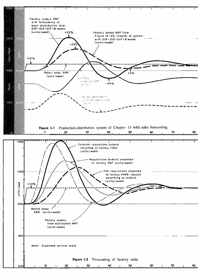
2000
Factory output SRF with forecosting at
euch distribution level . DIR=DID=DIF=8 weeks
)NNNNttB (units/week) +53% Foctory output SRF from Figure 15-24, Chapter 15 system
15()0 with DIR = DID = DIF= 8 weeks
+34*/. (units/week)
1000 Retail sales RRR +4%
(units /week) Factory
inventory IAF 4 4 (u n i t s)
Factory worehouse
500 '" unfilled orders UOF
- ... %
I%b -% , , , . - - -
Figure L-1 Production-distribution system of Chapter 15 with sales forecasting. M w ,
1400 Forecost réquisitions (orders)
smoothed ot factory FRSF
/ (units/week)
\. Requisitions (orders) smoothed
/ at foctory RSF (units/week)
?? Past requisitions smoothed –––––––––––––––––––––– '
/ / \\ at foctory PRSR (double
; y / \ smoothingof orders)
(
/ / / \ \ \ (units/week)
a ï
RetaUsates -' ./ - RRR (units/week) ,/
- Factory orders
from distributors RRF
- (units/week)
800 –––––––––––––––––––––––––––––––––––––––––––––––––––––––––––––––––––––––––––––––––––––––
Note: Exponded verticol scole
Figure L-2 Forecasting of factory sales.
____ 600 la j 20 1 , , 40 j . , 7p M
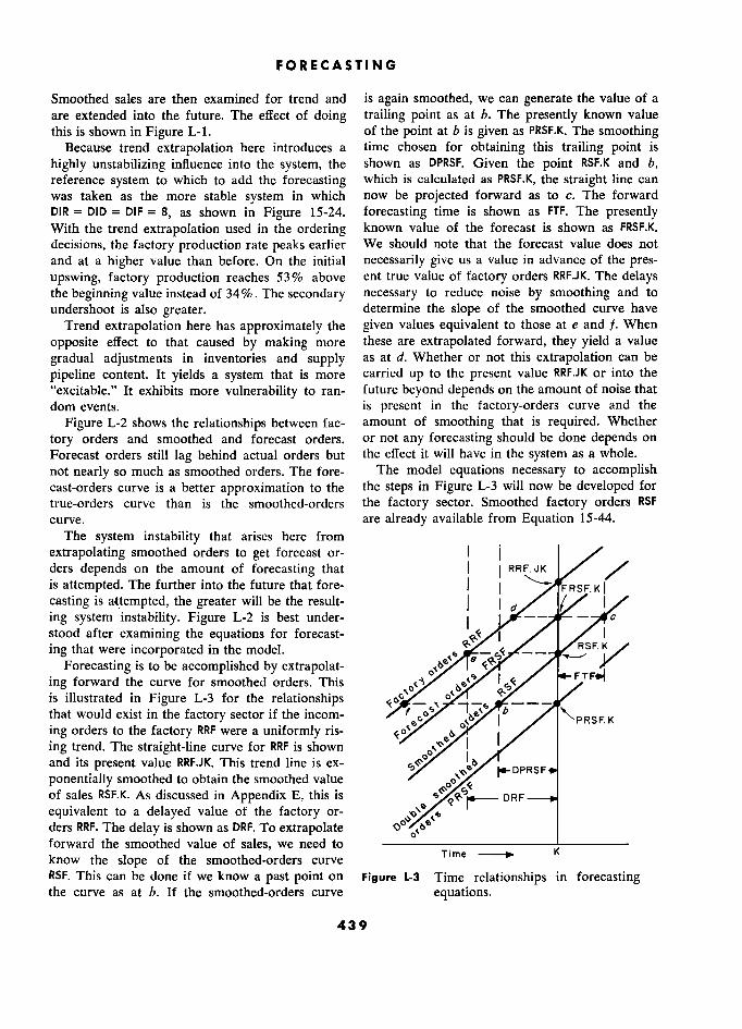
FORECASTING
Smoothed sales are then examined for trend and is again smoothed, we can generate the value of a are extended into the future. The effect of doing trailing point as at b. The presently known value this is shown in Figure L-1. of the point at b is given as PRSF.K. The smoothing
Because trend extrapolation here introduces a time chosen for obtaining this trailing point is
highly unstabilizing influence into the system, the shown as DPRSF. Given the point RSF.K and b, reference system to which to add the forecasting which is calculated as PRSF.K, the straight line can was taken as the more stable system in which now be projected forward as to c. The forward DIR = DID = DIF = 8, as shown in Figure 15-24. forecasting time is shown as FTF. The presently With the trend extrapolation used in the ordering known value of the forecast is shown as FRSF.K.
decisions, the factory production rate peaks earlier We should note that the forecast value does not and at a higher value than before. On the initial necessarily give us a value in advance of the pres- upswing, factory production reaches 53% above ent true value of factory orders RRF.JK. The delays the beginning value instead of 34%. The secondary necessary to reduce noise by smoothing and to undershoot is also greater. determine the slope of the smoothed curve have
Trend extrapolation here has approximately the given values equivalent to those at e and f. When
opposite effect to that caused by making more these are extrapolated forward, they yield a value
gradual adjustments in inventories and supply as at d. Whether or not this extrapolation can be
pipeline content. It yields a system that is more carried up to the present value RRF.JK or into the "excitable." It exhibits more vulnerability to ran- future beyond depends on the amount of noise that dom events. is present in the factory-orders curve and the
Figure L-2 shows the relationships between fac- amount of smoothing that is required. Whether
tory orders and smoothed and forecast orders. or not any forecasting should be done depends on Forecast orders still lag behind actual orders but the effect it will have in the system as a whole. not nearly so much as smoothed orders. The fore- The model equations necessary to accomplish cast-orders curve is a better approximation to the the steps in Figure L-3 will now be developed for true-orders curve than is the smoothed-orders the factory sector. Smoothed factory orders RSF
curve. are already available from Equation 15-44. The system instability that arises here from
extrapolating smoothed orders to get forecast or- 1 ders depends on the amount of forecasting that RRF. JK is attempted. The further into the future that fore- t casting is attempted, the greater will be the result- j .
ing system instability. Figure L-2 is best under- c c stood after examining the equations for forecast- 1
ing that were incorporated in the model. RSF. Forecasting is to be accomplished by extrapolat-
ing forward the curve for smoothed orders. This is illustrated in Figure L-3 for the relationships that would exist in the factory sector if the incom- f b
x ing orders to the factory RRF were a uniformly ris-
PRSF. K
ing trend. The straight-line curve for RRF is shown and its present value RRF.JK. This trend line is ex-
ponentially smoothed to obtain the smoothed value E M-DPRSF-O
of sales RSF.K. As discussed in Appendix E, this is oRF equivalent to a delayed value of the factory or- ders RRF. The delay is shown as DRF. To extrapolate forward the smoothed value of sales, we need to K know the slope of the smoothed-orders curve
K
RSF. This can be done if we know a past point on Figure L-3 Time relationships in forecasting the curve as at b. If the smoothed-orders curve equations.
439
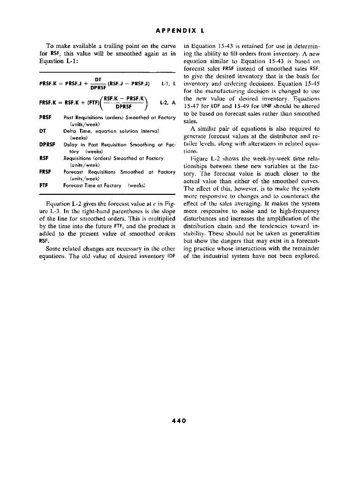
APPENDIX L
To make available a trailing point on the curve in Equation 15-43 is retained for use in determin- for RSF, this value will be smoothed again as in ing the ability to fill orders from inventory. A new
Equation L-1: equation similar to Equation 15-43 is based on
_______________________________ forecast sales FRSF instead of smoothed sales RSF,
DT to give the desired inventory that is the basis for PRSF.K = PRSF.J +
DPRSF (RSF.J - PRSF.J) L-1, L inventory and ordering decisions. Equation 15-45 for the manufacturing decision is changed to use
FRSF.K = RSF.K + /RSF.K - PRSF.K1 L.2, A the new value of desired inventory. Equations
) DPRSF I 15.47 for LDF and 15-49 for UNF should be altered ' '
\ DPRSF / ' ' 15-47 for LDF and 15-49 for UNF should be altered
PRSF Past Requisitions (orders) smoothed at Factory to be based on forecast sales rather than smoothed
rRSr est .equlsltlons
(orders) Smoothed at Factory sales. (units/week)
sales. (umts/week) _
DT Delta Time, équation solution interval A similar pair of équations is also required to
(weeks) generate forecast values at the distributor and re- DPRSF Delay in Past Réquisition Smoothing at Fac- tailer levels, along with alterations in related equa-
tory (weeks) tions. RSF Réquisitions (orders) Smoothed at Factory Figure L-2 shows the week-by-week time rela-
(units/week) tionships between these new variables at the fac- FRSF Forecast Réquisitions Smoothed at Factory tory. The forecast value is much doser to the
(units/week) actual value than either of the smoothed curves. FTF Forecast Time at Factory (weeks) The effect of this, however, is to make the system
more responsive to changes and to counteract the
Equation L-2 gives the forecast value at c in Fig- effect of the sales averaging. It makes the system ure L-3. In the right-hand parentheses is the slope more responsive to noise and to high-frequency of the line for smoothed orders. This is multiplied disturbances and increases the amplification of the
by the time into the future FTF, and the product is distribution chain and the tendencies toward in- added to the present value of smoothed orders stability. These should not be taken as generalities RSF. but show the dangers that may exist in a forecast-
Some related changes are necessary in the other ing practice whose interactions with the remainder
equations. The old value of desired inventory IDF of the industrial system have not been explored.
440
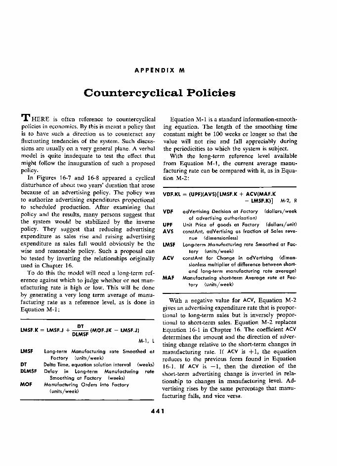
APPENDIX M
Countercyclical Policies
T HERE is often reference to countercyclical Equation M-1 is a standard information-smooth-
policies in economics. By this is meant a policy that ing equation. The length of the smoothing time is to have such a direction as to counteract any constant might be 100 weeks or longer so that the
fluctuating tendencies of the system. Such discus- value will not rise and fall appreciably during sions are usually on a very general plane. A verbal the periodicities to which the system is subject. model is quite inadequate to test the effect that With the long-term reference level available
might follow the inauguration of such a proposed from Equation M-1, the current average manu-
policy. facturing rate can be compared with it, as in Equa- In Figures 16-7 and 16-8 appeared a cyclical tion M-2:
disturbance of about two years' duration that arose _______________________________ because of an advertising policy. The policy was VDF.KL = (UPF)(AVS)[LMSF.K + ACV(MAF.K to authorize advertising expenditures proportional - LMSF.K)] M-2, R to scheduled production. After examining that
VDF advertisirig Decision at Factory (dollars/week tu VDF adVertising Décision at Factory (doi!ars/week policy and the results, many persons suggest that VDF
adVertising Decision at Facrory ) (dallars/week
the system would be the inverse of advertising aurhorizarion)
thé system would be stabilized by thé inverse UPF Unit Price of goods at Factory (dollars/unit) policy. They suggest that reducing advertising AVS constAnt, advertising as fraction of Sales reve- expenditure as sales rise and raising advertising nue (dimensionless) expenditure as sales fall would obviously be the LMSF Long-term Manufacturing rate Smoothed at Fac- wise and reasonable policy. Such a proposal can tory (units/week) be tested by inverting the relationships originally ACV constAnt for Change in advertising (dimen- used in Chapter 16. sionless multiplier of différence between short-
To do this the model will need a long-term ref- and long-term manufacturing rate average)
erence against which to judge whether or not man- MAF Manufacturing short-term Average rate at Fac-
ufacturing rate is high or low. This will be done tory
by generating a very long term average of manu- ., . facturing rate as a reference level, as is done in With a négative value for ACV, Equation M-2
Equation M-1: = gives an advertising expenditure rate that is propor- _____________________________ tional to long-term sales but is inversely propor-
DT tional to short-term sales. Equation M-2 replaces
LMSF.K = LMSF.J + (MOF.JK - LMSF.J) Equation 16-1 in Chapter 16. The coefficient ACV DLMSF
L determines the amount and the direction of adver- M-1, l
tising change relative to the short-term changes in .
LMSF Long-term Manufacturing rate Smoothed at manufacturing rate. If ACV is +1, the equation Factory (units/week) reduces to the previous form found in Equation
DT Delta Time, équation solution interval (weeks) 16-1. If ACV is -1, then the direction of the DLMSF
Delay in Long-term Manufacturing rate short-term advertising change is inverted in rela-
Smoothing at Factory (weeks) in MOF Manufacturing Orders into Factory tlOnship to changes 1ll manufacturing level. Ad- MOF Manufacturing Orders into Factory r ' '
(unirs/week) vertising rises by the same percentage that manu-
_______________________________ facturing falls, and vice versa.
441 1
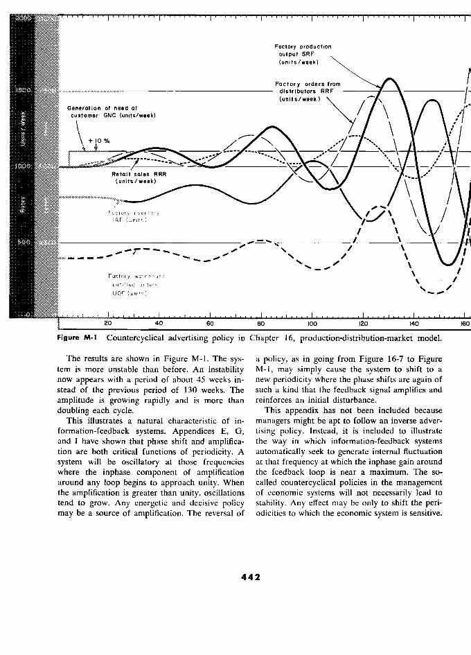
Factory production output SRF (unifs/week) .
Factory orders from distributors RRF (units/week)
Generation of need at (Un"S/Weekl
/ ) j
<
customer GNC (units/week) ,'
f -
- --- ------ -
i :
· -
Retall sales RRR - - 'y -
__ -;- -
(units/week) RRR
_
Factory inventory j / IAF (units)
/ ' v w
, - - - , , '
/ '
_
Factory warehouse · /
l
unfilied orders % I' .
/
UOF (units) ' '
20 40 E?0 80 100 120 140 IE
Figure M-1 Countercyclical advertising policy in Chapter 16, production-distribution-market model.
The results are shown in Figure M-1. The sys- a policy, as in going from Figure 16-7 to Figure tem is more unstable than before. An instability M-1, may simply cause the system to shift to a now appears with a period of about 45 weeks in- new periodicity where the phase shifts are again of stead of the previous period of 130 weeks. The such a kind that the feedback signal amplifies and
amplitude is growing rapidly and is more than reinforces an initial disturbance.
doubling each cycle. This appendix has not been included because This illustrates a natural characteristic of in- managers might be apt to follow an inverse adver-
formation-feedback systems. Appendices E, G, tising policy. Instead, it is included to illustrate and 1 have shown that phase shift and amplifica- the way in which information-feedback systems tion are both critical functions of periodicity. A automatically seek to generate internal fluctuation
system will be oscillatory at those frequencies at that frequency at which the inphase gain around
where the inphase component of amplification the feedback loop is near a maximum. The so-
around any loop begins to approach unity. When called countercyclical policies in the management the amplification is greater than unity, oscillations of economic systems will not necessarily lead to tend to grow. Any energetic and decisive policy stability. Any effect may be only to shift the peri-
may be a source of amplification. The reversal of odicities to which the economic system is sensitive.
442

APPENDIX N
Self-generated Seasonal Cycles
INDUSTRIAL policies adopted in recognition of tends to concentrate its sales at this particular time seasonal sales patterns may often accentuate the of year. very seasonality from which they arise. A seasonal Other kinds of seasonality are much less clear.
forecast can lead to action that may cause fulfill- Almost always when seasonality is expected, ex-
ment of the forecast. In closed-loop systems this is planations can be found to justify whatever one
a likely possibility. The analysis of sales data in believes to be true. A tradition can be established
search of seasonality is fraught with many dangers. that a particular item sells better at a certain time
As discussed in Appendix F, random-noise dis- of year. As this "fact" becomes more and more
turbances contain a broad band of component fre- widely believed, it may tend to concentrate sales
quencies. This means that any effort toward sta- effort at the time when the customers are believed
tistical isolation of a seasonal sales component will n to wish to buy. This in turn still further heightens tistical isolation of a seasonat sales component wilt thé e sa es at t at particu ar time.
find some seasonality in the random disturbances. the sales at that particular time. e
Should the seasonality An example is shown in Figure N-1. Hère the
ou thé seasonahty so oca e lead to décisions System that create actual scasonality, the process can be-
come self-regenerative. of Chapter 16 has been modified to include an
corne setf-regenerative. analysis of seasonal sales. Advertising is based on
Self-induced seasonality appears to occur many the forecast level of seasonal sales and is initiated places in American industry. Sometimes it is obvi- in time to become effective at the market at the ous and clearly recognized, and perhaps little can time of the forecasted sales level. The year is di- be done about it. An example of the obvious is the vided into 2-week intervals. The sales during cor-
strong seasonality in items such as cameras sold in responding 2-week intervals from preceding years the Christmas trade. By bringing out new models are exponentially averaged. These averages form and by advertising and other sales promotion in the estimates of future sales during corresponding anticipation of Christmas purchases, the industry intervals.
443
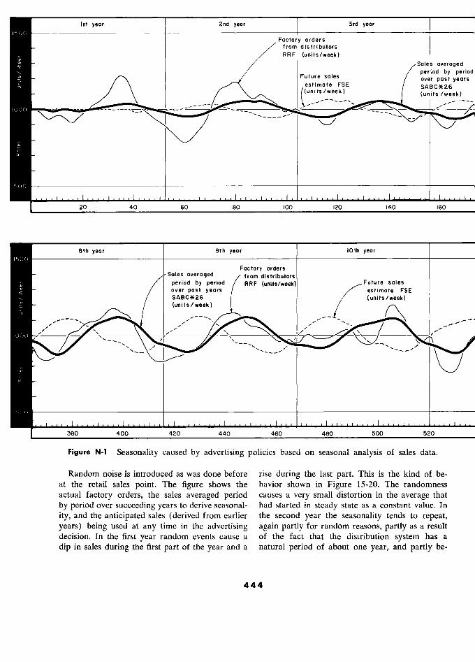
NNN! 151 yeor 2ndyeor 77
3rd yeor
NNN!! Factory orders from distributors
/' RRF (units/week) Sales averaged
j 20 40 M 80 !20 period by
perie Future sales over past years estimole FSE SABC*26
(units /week)
\-- , (uni ts
/week ) _ off '" ;;
20 40 60 80 100 120 140 160
jttj 8thyeor 9th yeor )0thyear
Factory orders -Sales averaged from distributors
/ period by period RRF (units/week) Future sales
/ overpastyears < estimate FSE ttjjt) / SABC*26 / (units /week)
(units/week)
j 380 400 420 440 4M 480 500 520
Figure N-1 Seasonality caused by advertising policies based on seasonal analysis of sales data.
Random noise is introduced as was done before rise during the last part. This is the kind of be- at the retail sales point. The figure shows the havior shown in Figure 15-20. The randomness actual factory orders, the sales averaged period causes a very small distortion in the average that
by period over succeeding years to derive seasonal- had started in steady state as a constant value. In
ity, and the anticipated sales (derived from earlier the second year the seasonality tends to repeat, years) being used at any time in the advertising again partly for random reasons, partly as a result decision. In the first year random events cause a of the fact that the distribution system has a
dip in sales during the first part of the year and a natural period of about one year, and partly be-
444
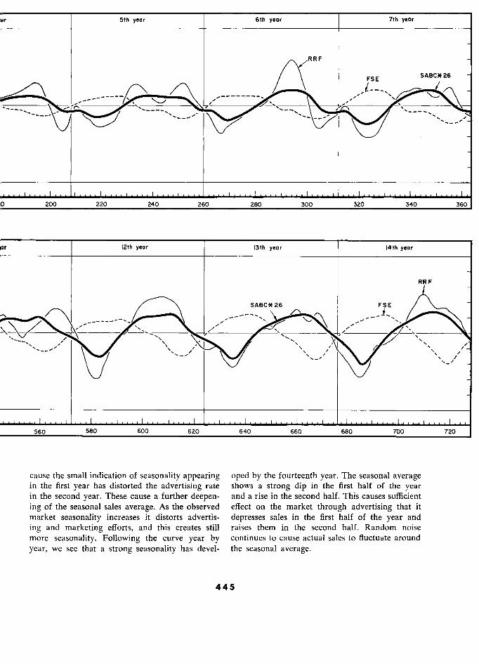
Sthyeor 6th yeor 7thyeor
RRF
/ \
FSE SABC*26 26 -
200 220 240 260 280 300 320 340 360
12th yeor 13th yeor 14th year
RRF
SABC*26 FSE ./
u
'V
\,__,,/'
,
', ',_,
\7
,
560 580 600 620 640 660 680 700 720
cause the smail indication of seasonality appearing oped by the fourteenth year. The seasonal average in the first year has distorted the advertising rate shows a strong dip in the first half of the year in the second year. These cause a further deepen- and a rise in the second half. This causes sufficient
ing of the seasonal sales average. As the observed effect on the market through advertising that it market seasonality increases it distorts advertis- depresses sales in the first half of the year and
ing and marketing efforts, and this creates still raises them in the second half. Random noise more seasonality. Following the curve year by continues to cause actual sales to fluctuate around
year, we see that a strong seasonality has devel- the seasonal average.
445
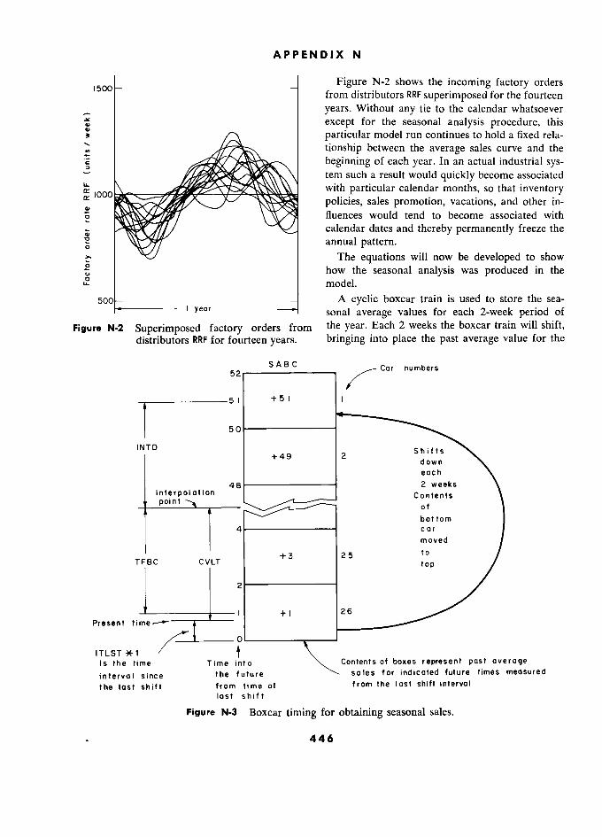
APPENDIX N
_ _ Figure N-2 shows the incoming factory orders l50o from distributors RRF superimposed for the fourteen
years. Without any tie to the calendar whatsoever
except for the seasonal analysis procedure, this /*\ particular model run continues to hold a fixed rela-
b tionship between the average sales curve and the
g beginning of each year. In an actual industrial sys- - tem such a result would quickly become associated LL 0-1 \_
with particular calendar months, so that inventory CI> policies, sales promotion, vacations, and other in-
ô fluences would tend to become associated with
m calendar dates and thereby permanently freeze the annual pattern.
r The equations will now be developed to show how the seasonal analysis was produced in the model.
500 1 year
A cyclic boxcar train is used to store the sea- 1 yeor sonal average values for each 2-week period of
Figure N-2 Superimposed factory orders from the year. Each 2 weeks the boxcar train will shift, distributors RRF for fourteen years. bringing into place the past average value for the
52 S A B C Car numbers
- 51 1 +5 1 I
l 50 –––––––––––––
+5' ,
INTD t49 2 Shifts
s down x each \
48 2 weeks Interpolation
48 ––––––––––––– Contents
\ \ point of t
"' bottom t 4 ––––––––––––– car r t
moved t
+3 to TFBC CVLT +3 25
top / /
2 ––––––––––––– y
- I tl 1 26
Present time-
ITLST *, 1 r 0 ––––––––,.––––
ITLST ?E 1 Time f 1\1-1 Contents of boxes represent past average is thé time Time into 0 Contents of boxes represent past average
interval since the future "- sales for indicated future times measured
the last shift from time of from the last shift interval last shift
Figure N-3 Boxcar timing for obtaining seasonal sales.
. 446
SELF-GENERATED SEASONAL CYCLES
current period. Into this old average new sales The flow diagram for the new equations appears are averaged. in Figure N-4.
Figure N-3 will help to clarify the timing of For interpolation purposes, it will be necessary the cyclic boxcar, the averaging, and the interpola- to know at any given time how much of the tion for a future value in the table of averages. 2-week interval has already passed. This can be The following equation is used to designate a accomplished by accumulating time during the
cyclic boxcar: 2-week interval and then discarding the accumu-
_______________________________ lated value at the same time that the boxcar train
BOXCYC (26, 2) N-1, a is shifted. This can be done with a linear boxcar SABC=BOXt;YC (2&,2) N-!,b train, the last value of which is discarded each ,.
SABC Seasonal Average Boxcar Cyde, the desig- shifting interval. Equation N-3 sets up a one-car nation of this particular boxcar train, boxcar train for this purpose: any one car of which is designated by adding an asterisk and the number of –––––––––––––––––––––––––––––––––––––
the car in the train ITLST = BOXLIN (1, 2) N-3, B BOXCYC a functional désignation instructing the
ITLST Interpolation Time Linear Sh'f T' used to DYNAMO compiler that box- )TLST !nterpo!at!onT!meLmear5h!ftTra!nusedto DYNAMO compiler that a cychc box-
accumulate the time elapsed since the last car train be set up accumulate
the trme elapsed sm ce the last
26 the number of cars in the train sh)tt t
... h thé number ° cars in thé train BOXLIN functional notation instructing the 2 the time interval between shifts of the train
BOXDN funct!ona! notation instructing thé DYNAMO 2 thé time interva! betweensh?ftsof thé tram
BOXLlN compiler linear boxcar train
(weeks) , comp' er to estab!?sh a mea: boxear train (weeks) 1 ) the number of cars in the train
––––––––––––––––––––––––––––––––––– 2 the shift interval (weeks)
In Figure N-3 the bottom (or 26th) box will be ––––––––––––––––––––––––––––**
designated as the one representing the current Equation N-4 accumulates time in the boxcar,
2-week time period. Equation N-2 averages pres- set up by Equation N-3, during any one 2-week ent factory orders RRF into the previous value of interval:
'
this box. The time constant TSD (here taken as four years) is the exponential-smoothing time con- stant controlling the influence of the current sales 'LS* .K " 'LS* 1.J + DT N-4, L
in changing the year-to-year average. ITLST* 1 the variable in the first box of train ITLST, the amount of time since the last shift of the boxcar trains (weeks)
SABC*26.K = SABC*26.J + DT
(RRF.JK DT Delta Time, the equation solution interval 2(TSD) (weeks) - SABC*26.J) N-2, L _______________________________
SABC*26 the variable content of car No. 26 in the It is now possible to interpolate in the table of cyclic train SABC,
sales in
the current seasonal values for the future sales estimate that 2-week period averaged over past years eas na a ues r e u ure sa es es ima e
a
(units/week). (A car désignation permirs is to be used in the advertising decision. In Figure (units/week). car designation permits .
the asterisk and car number beyond the N-3 the constant CVLT represents the interval of
standard five symbols normally allowed time required to act on advertising decisions. It is in naming a variable.) here taken as 18 weeks. Immediately after a box-
DT Delta Time, équation solution interval car shift, time can be thought of as rising from the (weeks) bottom up to the 2-week level, at which time the
2 the weeks per year that this box is active entire boxcar train is shifted down again. The in- in the averaging process (weeks/year) terpolation point in the table rises gradually over
TSD Time constant for Seasonal Detector for a 2-week period, drops with the shifting of the averaging sales data (years)
..ne averaging sales data n t boxcar train so that it retains its relative position RRF equisi ,ons or ers ece,ve a ac ory _ 3
RRF j, /
Received at Factory in the table, and continues to progress smoothly y
_______________________________ through the table. Since the interpolation process
447
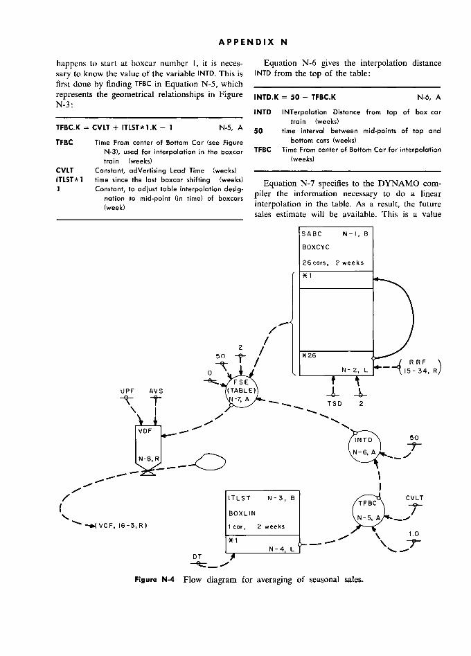
APPENDIX N
happens to start at boxcar number 1, it is neces- Equation N-6 gives the interpolation distance
sary to know the value of the variable INTD. This is INTD from the top of the table: first done by finding TFBC in Equation N-5, which _______________________________ represents the geometrical relationships in Figure INTD.K = 50 - TFBC.K K N-6, A N-3:
INTD INTerpolation Distance from top of box car train (weeks)
TFBC.K = CVLT + ITLST* 1.K - 1 N-5, A 50 time interval between mid-points of top and
TFBC Time From center of Bottom Car (see Figure bottom cars (weeks)
N-3), used for interpolation in the boxcar TFBC Time From center of Bottom Car for interpolation train (weeks) (weeks)
CVLT Constant, adVertising Lead Time (weeks) ––––––––––––––––––––––––––––––––––– ITLST*1 1
time since the last boxcar shifting (weeks)
Equation N-7 specifies to the DYNAMO com- 1 Constant, to adjust table interpolation desig-
piler necessary 1. nation ro mid-poinr piler thé information necessary to do a mear nation to mid-point (in time) of boxcars result, (week)
to ml -pOint un tmie) ot boxcars interpolation in the table. As a result, thé future
_____________________________ sales estimate will be available. This is a value
SABC N-I, B B
BOXCYC
26cars, 2 weeks s
*1 1
_ -
0
50 2
/
X26 6
N- N-2 2, LD L 15 15 - R R R
34 F R)
/
- / / * 26
N - 2, RRF 3 F \ R ) L _ N-2 L
FSE UPF AVS S (TABLE) 1 T A TSD D 2
\
- 7, A SD 2
VDF - ' , /
./
VDF
INTD 50
N-8, - - R
ITLST T N-3, B TFBC
CVLT
f ¡- ' _
BOXLIN
R) 1 car, 2 weeks
Ù
––––––––––––– \ 1.0 1 *1
% L T DT
Figure N-4 Flow diagram for averaging of seasonal sales.

BEGINNERS' DIFFICULTIES S
CVLT (18 weeks in this example) in advance of Equation N-8 replaces Equation 16-1 and bases
the current date taken from the average seasonal advertising on the estimate of future seasonal sales: sales analysis.
FSE.K = TABLE(SABC, INTD.K, 0, 50, 2) N-7, A VDF.KL = (UPF)(AVS)(FSE.K) N-8, R
FSE Future Sales Estimate (units/week) . TABLE functional désignation instructing DYNAMO VDF adVertising Décision at Factory (dollars/week
to interpolate linearly for a value in a table of advertising authorization)
SABC the name designating the table from which UPF Unit Price of goods at Factory (dollars/unit) interpolated value is to be drawn, a boxcar AVS constAnt, adVertising as fraction of Sales reve- train can be used as a table nue (dimensionless)
INTD the interpolating variable (weeks) FSE Future Sales Estimate
Q the first value of the interpolating variable for FSE Future Sales Estimate (units/week) 0 thé first va?ue of thé jnterpoiat!ng variable for which a number is stored (weeks)
50 the last value of the interpolating variable '
for which a number is stored (weeks) _, .. , 2 the which berween stored values (weeks) These eight equations generate a seasonal aver- 2 the interval between stored values (weeks)
_______________ age and a seasonal sales forecast based on it.
APPENDIX 0
Beginners' Difficulties
I T seems that a discussion of what should be done important problems are but little more difficult to in a new activity does not constitute adequate in- handle than the unimportant. Many men prede- struction. The positive approach alone does not termine mediocre results by setting initial goals provide forwarning against the pitfalls that lie too low. The attitude must be one of enterprise along the road. Therefore, 1 shall try in this sec- design. The expectation should be for major im- tion to explain some of the difficulties experienced provement in the systems. The attitude that the
by students and staff members who have under- goal is to explain behavior, which is fairly common
taken the kinds of systems studies discussed in this in academic circles, is not sufficient. The goal book. should be to find management policies and organ-
The following are arranged as a collection of izational structures that lead to greater success. isolated topics somewhat in the sequence in which
Defining the Questions they arise in a systems analysis.
Defining the Questions
A model should be designed to answer specific Courage questions. A systems study must be for a purpose Industrial dynamics is an approach that should if it is to be productive. The questions must be
help in important top-management problems. Very meaningful and tangible and specific if they are to few workers in the area of management science serve to guide a program. Determining the prob- havë had their aspirations conditioned to the ex- lems and the goals is the most critical part of al-
pectation of major successes in the more difficult most any undertaking. The beginner tends to forge and challenging fields. The solutions to small prob- ahead into detailed construction of a model before lems yield small rewards. Very often the most its purpose has been adequately defined.
449
APPENDIX 0
Scope of System Hypothesis about Dynamic Behavior
An important decision is to determine the boun- The beginner usually fails to realize the impor- daries of the system under study. The beginner can tance of an initial hypothesis about dynamic be-
easily err on either side. On the one hand, he may havior. There is often a feeling that to propose lack boldness to be comprehensive enough and modes of dynamic behavior before a system model
thereby limit his attentions to a subsystem within is constructed is to prejudge the answers. In a which the answers to the questions do not lie. On sense this is exactly what is needed. We start the other hand, he may define questions so vaguely with a hypothesis for behavior. We build a model that the objectives cannot be used to limit the to see if the mode of behavior could exist and
scope of what must be included initially. The key whether or not it can result from the initial as- to success will lie in clear questions which are sumptions. The experimental work is designed to broad enough to encompass matters of major con- prove or disprove the initial hypothesis. sequence but which initially limit a system to pro- The initial hypothesis is part of the establish-
portions that fit the skill, time, and experience of ment of the initial questions and goals for the the investigator. study. Without this initial mental and verbal model
of the dynamic behavior being studied, there is Automatic Formulation and Evaluation no basis for deciding what factors might be im-
Many beginners in the study of system dynamics portant and which ones could be neglected. It is seem to feel that there must be a "scientific very unlikely that a meaningful model will result method" that will ensure their ability to create a from wandering through an organization and in-
proper model. They look for statistical procedures corporating into the model whatever happens to that can be applied to the scanty data ordinarily come to one's attention. available, in the hope of having an orderly pro- A model of a chemical pilot plant serves as an cedure that will create a system model by objec- analogy to what we are attempting here. It is made tive methods. They seem unwilling to express a after a very tangible hypothesis about the plant's professional opinion and to take risks on the basis probable method of operation and the product it of personal knowledge and judgment about the is to make. A pilot plant is designed and built to character of the system being improved. For the see if the hypothesis is correct and to see what
present, there seem to be no such objective new problems and insights are developed as one methods that are effective. The attitude of requir- goes from a proposed method of operation to the
ing such safety and assurance of accepted experimental testing of the ideas. This is the way methodology is not the attitude of the risk-taking we use our dynamic model of an enterprise. A
manager. One does not achieve innovation and pilot plant is not constructed before a statement of
creativity by being timid. objectives and probable mode of operation. We do Similar attitudes arise with respect to model not build a plant at random and then wait to see
evalution. The insecure system designer looks for what kind of product it might produce. "objective" criteria for the evaluation of the per- tinence of a model. The compulsion to use such Verbal Descriptive Model
objective measures is sometimes so strong that Following closely after the hypothesis about
refuge is taken in procedures that lack a sound dynamic behavior is the verbal model or verbal foundation. description of the system with which one is deal-
The world has thus far been run on the basis of ing. In general, the verbal model should come
judgment applied to the making of individual de- before the mathematical model. The verbal model cisions. We are now on the threshold of moving should treat the description of how the parts be- the decision-making procedure back by one level have and how they interact with one another. of abstraction. When this has been done, judgment The verbal model is the support and the rationale must cope with policy detection and policy design. for the hypothesis about dynamic behavior. If
450

BEGINNERS' DIFFICULTIES S
the verbal model is sufficiently complete, the plications about accuracy. Once the system has mathematical model will follow as a consequence. been cast in the terms of formal equations and The beginner is apt to fail to recognize the es- numerical values of parameters, one can then sential importance of the descriptive model as a determine much about the required accuracy. step toward the creation of the equivalent formal Creating a quantitative description of a system is mathematical model. The latter is a translation a separate matter from achieving accuracy. These and clarification from the initial verbal language. two different considerations are often confused by
the person who does not think of mathematical System Perspective and numerical notation as being merely another
It is easy to view the system under consideration language for expressing ideas.
from the wrong distance. Students of economics Our descriptive knowledge is rich in informa-
tend to view from too great a distance, and they tion about the probable form of decision functions
fail to see the essential decision points, non- under extreme limiting conditions. The use of the
linearities, and interconnections of the system. full nonlinear breadth of all the information that
Managers and those having personal, intimate, we have available makes the task of successfully first-hand knowledge of the system tend to view it describing system components much easier.
from too close a distance. They want to put in Crecting Definitions too much detail. Separate, individual decisions Creating Définitions
take on too much importance. Apparent excep- A companion to the reluctance to use the avail-
tions, which can be treated as noise disturbances, able descriptive information is the reluctance to
blind them to average behavior. create precise definitions and arbitrary scales of
Each decision point should be represented as it measurement for the quantities that exist in the
might be seen by the next higher or the second descriptive knowledge. Many of the concepts and
higher administrative level. Very often the proper the so-called intangibles do not have generally
viewpoint from which to model a corporation is recognized scales of measurement. This does not
that of the perceptive banker or the skilled man- keep the investigator from creating his own precise
agement consultant. At the levels of these men, definitions and his own arbitrary scale of measure-
it is the broad sweep of the system that catches ment. It does require that he crystallize and clarify the attention. They are aware of technical progress, what he means by the terms which he uses. Here
of managerial and employee skills, of system ob- again, courage becomes important. The man must
jectives, and of markets. Yet, these viewpoints do take the leadership in creating a field of knowl-
not get enmeshed in the hour-by-hour and day-by- edge, a vocabulary, a precision in descriptive
day details of the separate parts of the system. terms, and a method of ranking and measurement. He must be willing to accept criticism that can be
Use of Descriptive Knowledge leveled only at the person who steps forward with
The beginner usually neglects information that a proposal. He must decide whether to defend
is in descriptive form and is inclined to look too himself against the criticism as being unwarranted
long and futilely for sufficient information in the or to use it to strengthen further the structure that
form of numerical data. He fails to appreciate he is building. that the overwhelming preponderance of our in-
Insensitivity to Cause-and-Effect Mechanisms formation about social systems is now in descrip- Insensitivity to °'° ' " Mechanisms
tive form. There is often an unwillingness to trans- The beginner may often fail to look at the sys- late this descriptive knowledge into quantitative tem closely enough to observe the factors that form. Descriptive information almost always im- create the dynamic behavior in which he is inter-
plies relative magnitudes and differing importance ested. of factors and assumptions. Attaching arbitrary There is often a tendency to want to disaggre- scales and quantitative values to these concepts gate into too fine a structure within any given flow can provide orderliness without carrying any im- channel, and at the same time to neglect to sepa-
451 1

APPENDIX 0
rate the flow channels well enough from each thought to be present or which he wished were other. present. The man with no experience with actual
In very many places, as discussed in earlier organizations may come with a strong idealized chapters, the "worse-before-better" sequences oc- but unrealistic concept of their behavior acquired cur. These can often be very important to system through academic study of simplified abstractions. dynamics but can be overlooked if one is unper- On the other hand, the man who has been im- ceptive of system interactions. For example, the mersed in a particular system too long may be expansion and training of an engineering depart- unable to distinguish the actual system from what ment does not just happen. It requires the diver- he wishes it were. A system model is apt to be- sion of managerial and technical time that might come a reflection of how the participants hope the otherwise be put to different purposes. The whole system operates rather than a picture of how it structure of skills and the development of people does operate. Both of these, of course, are prob- and organizations must take place before they can ably different from how it should operate. Wishful
produce an output. Many of the actual practical thinking and strongly formed past prejudices are
working mechanisms of a system tend to create both hazards to successful dynamic analysis. the conflict between short-term and long-term re- sults. Décision Points in System Context
The aggregate flow channels must represent the The novice at system modeling may underesti-
sequences that are traversed by individual items mate the importance of extensive, detailed, first-
following the channels. Very often a single event hand observation of the system with which he is must be traced in order to discover the informa- dealing. He may rely too much on what he is tion channels of the system. But one must not told are the factors and objectives at a certain let this study of the individual event trap him into place in the system. He may not take the time to an unduly close view of the system and a desire discover that the pressures on people at that point to model separate decisions rather than policy. come from quite unexpected places in the organi-
In all of these warnings against the hazards of zation. He may not observe that the sources of
system analysis we see that the investigator is information that are assumed to be necessary may faced by the usual form of decision wherein he simply not exist. He may not discover the extent must not do too much or too little of any of the to which the goals and objectives are purely local
things that are a part of success. As in the systems ones designed to keep the participants out of dif- he is modeling, his own decisions are balancing ficulty rather than goals that constructively pro- the amount of his action against the goal which mote the welfare of the whole organization. A he has set. model of system behavior depends on an adequate
representation of the decision-making policies Perceived versus Actual within the system. The beginner usually does not We have said earlier that the decision maker in realize the depth to which he must probe to dis-
a system acts on what he perceives to be the state tinguish the superficial veneer of rationalization of affairs. This perception is usually not identical from the deeper effective motivations. with the actual state of affairs but depends on the sources of information used and the amount of Model Permanence
prejudice and distortion with which the informa- The beginner often looks upon a model as tion is viewed. The system analyst faces the same something that he should build to last. He thinks
problem. He comes with ideas already formed of the model that can be constructed and then about the system with which he is to deal. If he used to answer all questions. As he progresses in does not have sufficient firmness in his approach, his understanding of enterprise design, he comes he may never reach decisions and effective action. to realize that each new question may carry with If his prejudices lead to blindness, the system he it an extension and a variation of the system analyzes may be merely the one that he initially previously defined. A model evolves with one's
452
BEGINNERS' DIFFICULTIES S
understanding of the system with which he is Underestimating Time Constants
dealing. It can start with a very simple structure The beginner almost invariably underestimates aimed at the essence of one particular phenome- the lengths of delays and time constants that will non. It can then be extended to bring in new facets exist in our social systems. He overlooks the long and to study new questions. The typical life of a educational delays. He fails to appreciate the model may be but a day or week before new persistence of prejudice and past personal experi- extensions give it new form and meaning. ence. He fails to examine the sequential steps
_ through which an action must go, and may esti- Decisions versus Policy mate a total over-all time so short that it is a
Management and management education have physical impossibility in the actual system. Time
given such emphasis to decision making that the estimâtes by students are often so short that they inexperienced systems analyst usually has a hard do not even fall within the limits of plausibility, time grasping the full significance of dealing in- once there has been a thorough discussion of the stead with the policy that creates the flow of actual real-life mechanisms involved. decisions. A new orientation in attitude must take
place. Time is required to develop an understand- Discontinuous Functions
ing of the full meaning of policy. It takes time to The beginner tends to be carried away by his
gain confidence that our existing knowledge of knowledge of the discreteness of various decisions
policy is sufficient for at least a major start in and actions. This arises partly from viewing the
understanding system behavior. system from too close a range. He wants budgets _ established once a year, production quotas each
Excessive Detail quarter, inventories reported each month, indi-
The beginner typically includes too much detail vidual model years of product handled separately, in model formulation. This is a natural result of and so forth. These are all factors that may be the fact that it is easier in the kinds of models important in some of the more subtle questions discussed in this book to include a factor than it that may be asked as a study progresses. However, is to present a convincing argument that a factor they seldom involve the broad interactions that does not matter. Junk is added in the model lead to conspicuous success or failure. structure to avoid discriminating thinking about System dynamics can best be visualized if cast whether or not various factors are necessary. This first in terms of continuous flows until the interac- is understandable and probably will always hap- tions of the major time constants, decisions, and
pen. Again it is a matter of degree. The beginner levels can be understood. is more conspicuously vulnerable to including too Another amateur tendency in the area of dis- much than he will be after some experience in continuous functions comes from carelessness in
building models and after the discovery of how thinking about the nonlinear forms of decision much simplification is possible. functions. There is a tendency to make up deci-
Some detail, even when it does not affect system sion functions from a straight-line linear section
performance, is justified in order to provide ap- that is abruptly terminated when some limiting parent reality and easier communication with threshold is reached. In general, decision functions others less skilled in model building. For this are not discontinuous. Much of the essential char- reason the models in Part III of this book are more acter of our industrial organizations arises because detailed than would be necessary to capture the of the changes that begin to occur progressively essence of the dynamic performance exhibited as various limiting conditions are approached. In in the various figures of Chapters 15 through 18. actual systems, pressures build up gradually, lead-
The clarity of the initial dynamic hypothesis ing progressively over a period of time to aware- and the initial verbal description of the system ness and action. Spurious system behavior is very will largely determine one's vulnerability to wan- apt to be introduced by artificial breaks and dis-
dering off into unnecessary complexity and detail. continuities in decision functions. One can very
453

APPENDIX 0
seldom argue that life continues as normal up to patible with at least the obvious tests and chal- some very particular point at which the entire lenges. The most powerful defense of a dynamic character of an organization changes. model lies in the extent to which all of the com-
ponents are acceptable. The complex information- Coefficients without Meaning feedback behavior is usually not subject to strong The beginner may not take the time to be cer- intuitive argument. To depend on the information-
tain that every parameter and variable in his sys- feedback network in order to avoid a state of
tem has a solidly defined meaning that can be affairs wherein defective décision functions would
related to the actual system with which he is have the opportunity to create unexpected dif-
working. Coefficients are often inserted to make ficulty is to compromise in that region where
dimensional units correct without thinking through soundness can be achieved and confidence can
whether or not thèse coefficients arise out of the be greatest. One's trust is relegated to that area
actual structure and practices of the system. I of the model about which he knows the least.
believe it is possible to make every variable and The dynamic behavior is what we are trying to
every coefficient relate directly to its counterpart learn about the system. We want to know the
in the real system and be discussable with and dynamic behavior that will result from the best
understandable by the practical operating people knowledge we have about the component parts .
in the organization. Forcing this degree of reality and how they must contribute to the total system.
in equations and parameters helps to clarify think-
ing and d t 0 1 ea d t 0 grea t er model validity. Simultaneous Initial-Condition Equations
ing and to lead to greater mode! validity. The beginner usually has a great deal of dif-
Dimensional Units of Parameters and Variables ficulty in the establishment of initial-condition
The careless analyst may fait to define the eq°ations for a model and very often finds himself <
dimensional units of measure of variables m the position of having to solve a system of
dimensionai units s of measure of variables es and simuitaneous atsebraic équations to get a con-
parameters. This is apt to merge into a lack of a a simultaneous algebraic equations to get a con-
clear understanding of their meaning, and from sistent set
° £.§ [§§§/§§ often
arises this there rapidly follows a departure of the model
from a poor choice of what is to be independently this there rapidty foitows a departure of thé mode) specified and ;. t. necessarily
system from the relationships of real life and from have values which parameters may necessarily " , have values dépendent on others already picked. those intended e in thé initiât la verbal a description. It is my feeling that a skillful handling of the ose in en
e in e -
ia ver
a escnp ion. is that ??qj??j thé
The units of measure of every factor should be ., IS my feeling that a skillful handling of the
carefully defined, preferably in terms that are as way in which parameters are defined and numeri- carefuHy denned, preferably in terms that are as parameters
1 .bl t th th t h .. h cal values are chosen can always lead to a direct
close as possible to those that have meaning in the cal values are chosen can always lead to a direct ose a
ave r?r
m e détermination solution
verbal description and practical use of that factor. determination of initial conditions without solution
ver a escrip ion an prac ica use o a of simultaneous équations for the initial condition
Defective Decision Functions of the system. This was true in the models of
Deteettve Dec!S)on unctlons Chapters 15 through 18, although it must be recog-
Very often the beginner develops decision func- nized that those systems are not complex. A tions which he recognizes as having major defects thorough treatment of the methodology for han- but which he defends on the basis that the infor- dling initial conditions is beyond the scope of this mation-feedback loops threaded through the re- book, and the matter will be left at present simply mainder of the system will prevent the occurrence with the assertion that I have always found it of those circumstances under which the particular possible to achieve a straightforward determination decision function would be wrong. This is a of initial conditions. This, however, is not the dangerous practice. One is now dealing with a sys- usual experience of the person first undertaking tem that fails to pass the test of "not being obvi- mode ! construction. ously wrong." It contains relationships that can be established as wrong on the basis of a logical
Infinite Ratios
argument. In general this is unnecessary. A little Sooner or later the model builder usually en-
thought and care can make the relationships com- counters a situation where he has set up a func-
454
BEGINNERS' DIFFICULTIES S
tional relationship as the ratio of two variables the systems analyst and those in the actual busi- where the denominator can take on a small or ness system. It is also a handicap because the zero value. Since real life does not contain infinite engineering systems are not well equipped with values for significant variables, this can be looked examples of highly nonlinear phenomena. This on as a defect in the equation formulation. In conversion to, for example, an electrical network fact, some of these do exist in Chapters 15 5 tends to initiate a very inappropriate line of think-
through 18, and the difficulties would become ap- ing that restricts consideration to linear systems. parent were the model called upon to create Those coming from the field of servomecha-
properly system activity all the way from zero nisms may have difficulty in distinguishing funda- sales rate upward. The difficulty is especially likely mental concepts from the practical art of the in transient growth models, where ail of the vari- engineering field. The fundamental concepts of ables may have initial values of zero. In general, information-feedback systems are universally ap- the difficulty is surmounted by an adequately plicable. The practical art is apt to depend on the realistic and wide-ranging statement of decision particular classes of systems that are encountered. functions that cannot under any circumstances Most especially, the physical systems are usually take on impossible values. characterized by having their own internal natural
periods well separated from the frequencies that Loops without Levels are imposed upon them in their ordinary opera- In the discussion of model structure in Chapter tion. This leads to certain practical design proce-
6, it was pointed out that rates create levels and dures that may not carry over into nonlinear sys- that levels are the only proper inputs to the deter- tems in which the noise frequencies, the natural mination of rates. It was, however, further noted frequencies of the system, and the frequencies to that as a practical matter one sometimes uses a which the system should respond all lie within rate instead of a short-term average as an input to approximately the same frequency band. another rate. This must be watched very carefully, The engineer is more accustomed to thinking because it is rather easy to create a loop whereby in terms of differential equations than he is in a chain of auxiliary equations may arise from one terms of integral equations. The difference equa- rate to control another rate that may eventually tions used in this book are all essentially integra- lead to a third which appears as an input to one tions of rates. It is common in engineering to of the first equations. In the flow diagram of the speak of velocity as the derivative of position and
system this leads to a loop in which no level equa- acceleration as the derivative of velocity. How- tion exists. Such a situation is contrary to the ever, nature does not usually take derivatives.
concepts on which the model structure was built. Actually the inverse sequence is a more natural This kind of erroneous structure can lead to a viewpoint. Forces create acceleration. Acceleration
high-frequency numerical instability in the model is integrated to get velocity, and velocity is inte-
structure, where the instability is a characteristic of grated to get position. Mathematically these are the model defect and not of the system being equivalent. Conceptually they give one a some- modeled. what different viewpoint of the system and its
structure. Engineers A number of the people entering the field of
dynamic analysis of business systems have a back- "?? ?? ?
ground in engineering. They may wish to carry Students coming in from the areas of science, over familiar methodology which may not be ap- whether it be physics, mathematics, or the social
propriate in the industrial context. They may have sciences, are apt to have their attention focused
strong tendencies to want to convert the structure too exclusively on methodology and technique. and the terminology of the business system into an They are accustomed to looking for analytic solu- electrical or a hydraulic network. This greatly tions to problems. This habit has in turn forced
increases the communications difficulty between them to the consideration of only linear systems.
455 5

APPENDIX 0
They may have been trained so exclusively in volve around the selection of a solution interval linear systems and linear approximations to sys- DT. He may become involved in trying to deter- tems that they lack an awareness of the extent to mine how large this interval can be made, rather which our life and our world depend for their than merely making sure that it is small enough very existence on nonlinear behavior. to raise no questions.
A fascination with methodology is apt to lead The science student may lack any first-hand to a quite disproportionate amount of attention to awareness of the political factors that enter into
peripheral questions of technique. The mathe- even the so-called scientific and technical deci- matician may want to substitute some more elegant sions. He is apt to feel that rigorous and objective methodology for the first-order integration such methods must of necessity be found for the con- as used in this book, even though there can struction of models, even though in his home field
probably be no objective demonstration of the there are no rigorous and objective methods that
necessity. He may become involved in the discon- ensure the success of the design of engineering tinuities and the computing phenomena that re- systems and models of engineering devices.
456

REFERENCES S
[Including place in this book where cited]
1. Drucker, Peter F., "Thinking Ahead: Potentials 12. Vidale, M. L., and Wolfe, H. B., "An Operations- of Management Science," Harvard Business Re- Research Study of Sales Response to Advertising," view, Vol. 37, No. 1, pp. 25-30, 146-150 (January- Operations Research, Vol. 5, No. 3, pp. 370-381 February 1959). [Section 1.2.] (June 1957). [Section 16.1.] .]
2. Porter, A., An Introduction to Servomechanisms, 13. The following S.M. theses have been completed Methuen & Co., London, and John Wiley & Sons, at the M.I.T. School of Industrial Management New York, 1950. [Section 1.1.] under the supervision of the author. Being S.M.
3. MacMillan, R. H., An Introduction to the Theory theses, only part time for some six months was of Control in Mechanical Engineering, The Uni- available to the students for their completion. versity Press, Cambridge, 1951. [Section 1.1.] Time did not permit as many revised drafts as
4. Brown, Gordon S., and Campbell, Donald P., may have been desirable, nor was there time for
Principles of Servomechanisms, John Wiley & the student to interpret and take full advantage Sons, New York, 1948. [Section 1.1.] of the system model that he formulated. However,
5. S amp 1 e - d D ata C ontro 1 S ystems, each of the following has made a substantial con-
John Wiley tribution in opening new facets of the field of in- John Wiley & Sons, New York, 1958. [Section 1.1.] dustrial dynamics. Ph.D. thèses and staff research ° ' . dustnal dynamics. Ph.D. theses and staff research Ragazzini, John R., and Franklin, Gene F., Sam- are now under way to exploit interesting areas pled-Data Control Systems, McGraw-Hill Book opened by several of the following theses. Micro- Company, New York, 1958. [Section 1.1.] film or photocopies of theses can be purchased Seifert, William W., and Steeg, Carl W., Jr., Edi- from the Library, Massachusetts Institute of Tech- tors, Control Systems Engineering, McGraw-Hill nology, Cambridge, Mass. Book Company, New York, 1960. [Section 1.1, Ballmer, Ray W., Sloan Fellow at M.I.T., Appendix F.] 1959-1960, from the Kennecott Copper Corpora-
6. Tustin, Arnold, The Mechanism of Economic Sys- tion, S.M. Thesis, School of Industrial Manage- tems, Harvard University Press, Cambridge, ment, Copper Market Fluctuations: An Industrial Mass., 1953. [Section 1.4.] Dynamics Study, 1960, i-ix plus 125 pages.
7. Leavitt, Harold J., and Whisler, Thomas L., "Man- [Section 19.3.] agement in the 1980's," Harvard Business Review, Fey, Willard R., The Stability and Transient Re- Vol. 36, No. 6, pp. 41-48 (November-December sponse of Industrial Organizations, S.M. Thesis, 1958). [Sections 3.3, 20.4.] Department of Electrical Engineering, 1961,
8. Kovach, Ladis D., "Life Can Be So Nonlinear," M.I.T., 8 unnumbered front pages, 132 pages plus American Scientist, Vol. 48, No. 2, pp. 218-225 appendix of 22 pages. [Section 17.4.] (June 1960), published by the Society of the Hurford, Walter J., Sloan Fellow at M.I.T., Sigma Xi. [Section 4.1.] 1959-60, from the Westinghouse Electric Cor-
9. Klein, Lawrence R., Economic Fluctuations in the poration, S.M. Thesis, School of Industrial Man- United States 1921-1941, Cowles Commission agement, Application of Industrial Dynamics to
Monograph No. 11, John Wiley & Sons, New the Growth of the Fuel Manufacturing Industry York, 1950. [Chapter 12.] for Nuclear Thermal Electric Power Plants, 1960,
10. Koopmans, Tjalling C., Editor, Statistical Infer- i-vii plus 123 pages. [Section 19.8.]
ence in Dynamic Economic Models, Cowles Com- Katz, Abraham, Sloan Fellow at M.I.T., 1957-58, mission Monograph No. 10, John Wiley & Sons, from the Radio Corporation of America, S.M. New York, 1950, Third Printing, July 1958. Thesis, School of Industrial Management, An
[Chapter 12.] Operations Analysis of an Electronic Systems
11. Churchman, C. West, Theory of Experimental Finn, 1958, 7 front plus 109 pages. [Section 19.4.1
Inference, The Macmillan Company, New York, Kinsley, Edward R., Sloan Fellow at M.I.T., 1948. [Section 13.7.] 1958-59, from the Texas Instruments Company,
457 .
REFERENCES S
S.M. Thesis, School of Industrial Management, tially Weighted Moving Averages," Managernent The Managerial Use of Industrial Dynamics as Science, Vol. 6, No. 3, pp. 324-342 (April 1960). Illilstrated by a Company Growth Model, 1959, [Section 19.8.] i-vii plus 180 pages. [Section 19.2.] 18. Zannetos, Zenon S., The Theory of Oil Tankship Raff, Alfred I., Dynamics of the Tankship Indus- Rates, Ph.D. Thesis, Department of Economics try, S.M. Thesis, Department of Naval Architec- and Social Science, Massachusetts Institute of ture and Marine Engineering, M.I.T., 1960, 5 un- Technology, September 1959, 12 unumbered front numbered front pages and 100 pages. [Section pages plus 299 pages. [Section 19.9.] 19.9.] 19. Pierson, Frank C., and others, The Education of Schlager, Kenneth J., Sloan Fellow at M.I.T., American Bllsinessmen, The Carnegie Series in 1960-61, from the AC Spark Plug Division of American Education, McGraw-Hill Book Com- General Motors Corporation, S.M. Thesis, School pany, New York, 1959. [Section 20.1.] .] of Industrial Management, Systems Analysis of 20. Gordon. Robert Aaron, and Howell. James Ed- the Copper and Aluminum Industries: An Indus- win, Higher Education for Business, Columbia trial Dynamics Study, 1961, i-vüi plus 264 pages. University Press, New York, 1959. [Section 20.3]. [Section 19.3.1 21. Forrester, Jay W., "lndustrial Dynamics - A Walter, Franklin, Sloan Fellow at M.I.T., 1958-59 Major Breakthrough for Decision Makers," Har- from the Chrysler Corporation, S.M. Thesis, vard Business Review, Vol. 36, No. 4, pp. 37-66 School of Industrial Management, An Analysis July-August 1958). [Appendix A.] Relating Lead
Time and Market Penetration in 22. Pugh, Alexander L., Ill, DYNAMO User's Man- the Auto Industry,
1959, i-vn plus 125 pages. ual, M.I.T. Press, Cambridge, Mass., 1961. [Section 19.1.1 Available through The Technology Store, 40
14. Robinson, Dwight E., "Fashion Theory and Prod- Massachusetts Avenue, Cambridge, Mass. [Ap- uct Design," Harvard Business Review, Vol. 36, pendix A.] No. 6, pp. 126-138 (November-December 1958). 23. Laning, J. Halcombe, Jr., and Battin, Richard H., [Section 19.1.] Random Processes in Automatic Control, Mc-
15. Katz, Abraham, "An Industrial Dynamic Ap- Graw-Hill Book Company, New York, 1956. proach to the Management of Research and De- [Appendix F.] velopment," IRE Transactions on Engineering 24. Davenport, Wilbur B., Jr., and Root, William L., Management, Vol. EM-6, No. 3, pp. 75-80 (Sep- An Introduction to the Theory of Random Signals tember 1959), Institute of Radio Engineers, New and Noise, McGraw-Hill Book Company, New York. [Section 19.4.] York, 1958. [Appendix F.]
'
16. Brown, Robert G., Statistical Forecasting for In- 25. Phillips, A. W., "Stabilisation Policy and the Time- ventory Control, McGraw-Hill Book Company, Forms of Lagged Responses," Economic Journal New York, 1959. [Section 19.8.] (London), Vol. 67, No. 266, pp. 265-277 (June
17. Winters, Peter R., Forecasting Sales by Exponen- 1957). [Appendix H.]
458

Index Académie program, for freshman, vii Battin, Richard H., 412, 458 Dead-zone instability, 233-234, 274
in industrial dynamics, 350-354 Beef, production dynamics, 104 Decision functions, to control rates, 69 at M.I.T., 353-354 Bennett, Richard K., ix, 369 determining form, 103-107
Accounting information, 335-336 Boundaries of models, see Models, factors to include, 104 Accuracy, defined, 57 scope inputs to, 103 AC Spark Plug Division, 324, 458 Bowles, Edward L., viii noise in, 107-108 Adequacy, see Validity Bowman, Edward H., ix nonlinearity in, 106-107 Advertising, added to production-dis- Boxcar train, flow-diagram symbols, omission of feedback paths, 107
tribution system, 36-42, 187-207 84-85 parameters, model correction of in- causing production instability, 36- see also Delays, boxcar train accuracy, 105
42, 187-207 Boyd, Constance D., ix as policy statement, 69 proportional to sales, 36, 190-192 Brooks, E. P., viii positive feedback, 104 time response to, 194-195 Brown, Gordon S., viii, 14,457 short-term vs. long-term effects, 104
Aggregation, into continuous flows, 65 Brown, Robert G., ix, 338, 458 see also Decision making, Equa- of whole industry, 187, 211, 340-341 Bryant, Lynwood S., ix tions, rate, Flows, Information, see also Delays, aggregation, and Buoncristiani, John F., ix for constructing models, Policy,
Variables, aggregation Bursk, Edward C., ix Rates Alfred P. Sloan Foundation, ix Business games, see Management Decision making, as continuous proc- Amplification, from adjusting levels, games ess, 96
348 Business Week, 98 controlling flows, 95 affected by decay rate, 202-203 delays in, 151 1 as characteristic of information- Campbell, Donald P., 14, 457 determining basis of, 17
feedback system, 62-63 Capital equipment, flow symbol for, discussion of, 93-108 from delays, 348 82 as foundation for industrial dynam- from forecasting, 138, 349 flow system, described, 71 ics, 17 frequency-sensitive, 202, 349, 442 introduced, 13 implicit, 102, 151, 164 from inventory policies, 138, 173, Carlson, Bruce R., ix information-feedback context, 94
209 Cash flow, 240-245, 263, 296 levels as input, 95 from ordering procedures, 22, 173- Chapman, John F., ix in military tactics, 17 7
175 Chrysler Corporation, 313,458 nature of process, 95-96 in pipelines, 138, 173 Churchman, C. West, 123,457 overt, 102, 151, 162-164 stability by reducing, 204 Combining variables, see Variables, three parts, 95 of system, 254, 260, 424 aggregation action 96 from variable delay, 182, 202, 212, Commodity dynamics, 321-324 apparent state, 96, 452
348 , _ _ inventories, 322 desired state, 95-96, 148, 348 see also Delays, Noise, amplification price changes, 322 threshold in, 233-234, 274
of, Smoothing Competition, 336-337 .. viewing distance, 96 Analog computer, 18-19, 68 Computer, see Analog computer, Digi- see a/sa Decision functions, Policy Assumptions, see Models, assumptions tal computers Deferrability of purchase, 36, 187-189
about system Computing, sequence, 73-75, 396-40 Delays, 86-92, 418-421 1 ' '
Atomic fuel, 339 time required, see Digital computers, in advertising response, 194-195 Automobile, see Market . time required aggregation, effect of, 110-111 Auxiliary equations, see Equations, Constants, see Parameters boxcar train, examples, 447
auxiliary, Flow diagram, aux- Controlled experiments, 43 flow-diagram symbols, 84-85 iliary-variable symbol models for, 55 5 as characteristic of information-
Averagmg of data, see Smoothing, Correlated data, 118 feedback-system, 15 .. Equations, smoothing Countercyclical policy, see Policy, characteristics, length determining countercyclical steady-state, 87
Balance sheet, continuous, 263, 296 Cycles created by forecasts, 443-449 transient response, 87, 89-92 Ballmer, Ray W., 322, 457
' communications, 155
Bandwidth, 54 Damping, defined, 113 3 at conversion points, 64 described 54 125 Data, collection of, 141 decision-making, representation, 151 1 in nonlinear system, 125 see also Information for construct- equations for, 87-89, 418-419 prediction related to, 125, 126, 430 ing models, data, Parameters, exponential, equations for third-or- solution interval related to, 80 Statistical estimation der, 89, 419 9 as system characteristic, 54 Davenport, Wilbur B., Jr., 412, 458 higher-order, 88
459

INDEX
Delays, frequency-sensitive, 415-417 DYNAMO computer compiler, order- Exogenous variables, see Input to importance in models, 62 ing initial-value equations, 166 model, exogenous variable as, impulse response, 90-92, 144 teaching of, 352 Variables, exogenous information, 418 8 Exponential averaging, see Smoothing, initial value, 167 Economic development, academic re- exponential inventory, see Inventory, delivery search, 361 Exponential delays, see Delays, ex-
delay as challenge to management, 6 ponential material, 418 dynamics of, viii, 361 Extreme conditions, see Models, non- period of oscillation related to, 202 Education, liberal-arts, 2 linear in production-distribution example, see also Management education
22-23, 140 Electric generating industry, 341-343 Feedback, see Information-feedback quantity in transit, 86, 89 Engineering, precedent for manage- systems representation of, 86-92 ment, 4-6 Fey, Willard R., ix, 215, 457 smoothing, equivalence to, 418 8 see also Men, engineers Flow diagram, auxiliary variable sym- smoothing as cause, see Smoothing, Enterprise design, goals, 44, 449 bol, 83
creating delay steps in, 13, 43-45 delay symbols, boxcar, 84 step response, 90-92 Equations, auxiliary, dependent on exponential, 84 structure of, 86-87 evaluation sequence, 78 described, 81-85 system effect of, changing value, described, 78-79 flow symbols, 82
32-33, 182-183, 268-276, 349 example, 78 level symbol, 81-82 time response, 419-421 as subdivision of rate equation, parameter symbol, 83
transient response, curves for, 90, 78 rate symbol, 82 92 basis for, 140-141 1 source-and-sink symbol, 82
transportation, 155 classes of, 76 variable on other diagrams, symbols, underestimating, 453 constants, see Parameters 83 see also Amplification, from vari- initial-value, for delays, 167 Flows, capital equipment, 71 1
able delay, Flow diagram, de- described, 79 continuous treatment, 64-66 lay symbols ordered by DYNAMO, 166 defined, 69
Descriptive information, see Informa- production-distribution model, determined by levels, 69 tion, for constructing models, 165-168 flow-diagram symbols, 82 descriptive for rates, 217 information, 71-72
Design of enterprises, see Enterprise simultaneous, 454 material, 70 design steady-state start, 166 money, 70-71 1
Diagrams, see Flow diagram level, described, 76-77 orders, 70 Differential analyzer, 68 example, 76 personnel, 71 1 Digital computers, 369 independence of evaluation se- six, described, 70-72
capacity, 68 quence, 77 introduced, 13 3 cost reduction, 18 independent of solution interval, see also Decision functions, Flow as foundation for industrial dynam- 77 diagram, Rates
ics, 18-19 as integrations, 68, 76 Forbes Magazine, 98 technical advancement, 19 loops without, 455 Forced oscillation, 200 time required, 199, 381 1 parameters, see Parameters Forecasting, 437-440
see also Simulation, cost rate, auxiliary as subdivisions of, amplification from, 138, 349, 437 Digital Equipment Corporation, ix 77-78 as decision equations, 337 Dimensions of measure, see Units of described, 77-78 defined, 437
measure example, 78 discussion of, 337-339 Discrete events, 64-66 formulation of, 143 in electric generating industry, 342 Distribution system, 21-42, 137-186 independence of evaluation se- extrapolation in, 337, 437 Douty, Arthur L., ix quence, 77 in ordering decisions, 138 Drucker, Peter F., 3, 457 smoothing, 150-151 1 self-defeating, 437 DT, defined, 73-74 see also Smoothing self-validating, 437
see also Solution interval symbols for variables in, 75 system independence of, 337 Durand, David, ix system of, 73-80 see also Prediction Duren, Grace, ix, 369 computing sequence, 73-75, 396- Ford Foundation, ix Dynamics, see Commodity dynamics, 401 1 Forrester, Ethel W., viii
Growth dynamics, Market, dy- supplementary, described, 79 Forrester, Jay W., 369, 458 namics of, Mining, Research examples, 246-248 Forrester, M. M., viii and development tabulation of, 383-395 Foundations for industrial dynamics,
DYNAMO computer compiler, 369- test input generation, 248-251 1 14-19 9 381 1 see also Decision functions, Delays, Fox, Phyllis (Mrs. George Sternlieb),
checking defined variables, 80 equations for, Information for ix, 369 creating sets of delay equations, 89 constructing models, Integra- Franklin, Gene F., 14, 457 delay equations used in, 419 tion, Levels, Rates, Solution Frequency-sensitive amplication, see error print-out, 370 interval Amplification, frequency-sensi- growth ramp, 248 Equilibrium, see Equations, initial- tive, Delays, frequency-sensi- initial conditions for delays, 197 value tive, Smoothing, frequency se- ordering auxiliary equations, 78 Error function, 61 lectivity
460

INDEX
Future, see Industrial dynamics, inter- Information.feedback systems, delays Jury, Eliahu 1., 14, 457 val to develop as characteristic of, 14-15
history, 16 K, as present time step, defined, 74 Gain, see Amplification, Delays, information in, 94 Katz, Abraham, 325, 326, 457, 458
Smoothing progress in understanding, 1 6 Kennecott Copper Corporation, 322, General Motors Corporation, 324, 458 social systems as, 15 53, 61-63 457
Copper CorporatIon, 322,
Goals of enterprise design, 44, 449 structure, as characteristic of, 14-15 Kinsley, Edward R., 320, 457 Goetz, Billy E., ix theory, as foundation of Industrial as following time interval, defined, Gordon, Robert Aaron, 350, 458 dynamics, 14-17, 455
KL, 74
tIme mterval, defined,
Growth dynamics, viii, 317-321, 331- Initial conditions, see Equations, in- Klein, Lawrence R., 112, 457 334 itial-value em, awrece.., 12,457 Initial-value équations, see Equations, Kovach, Ladis D., 51, 457
Haberstroh, Chadwick J., ix initial-value , , Kovach, Ladls D., 51, 457
Harvard Business Review, ix Input to model, equations to generate, as next time step, defined, 74 History, importance, 352 248-251 1
Labor, see Personnel defined, 74
Howard, David J., ix, 369 exogenous variable as, 112-114 Lagging time series, see Leading-lag- Howell, James Edwin, 350, 458 historical time séries, 172
Lagging time series, ??"°S lâg- "
Hunting in servomechanisms, 61 1 periodic, one-year, to electronic series
Hurford, Walter J., 339, 457 component model, 258-259, Lags, see Delays 286, 292 Laning, J. Halcombe, Jr., 412, 458
Implicit d see Décision makin one-year, to production-distri- Laplace transforms, 215
Implicit decision, see Decision making, bution system, 26-27, 175-177 Leading-lagging time series, 421-425 bution system, 26-27, 175-177 Leading-Iagging time series,
42 "425
implicit Delays, impulse two-year, to electronic component 202 Impulse response, see Delays, impulse model, 260-261, 294
component variability, 425 response
, > model, 260-261, 294 vana i i y, 425
p Me Variables, random, to advertising-market sys- Leavitt, Harold J., 45, 457
Independent variable, see Variables, tem, 40-41 Level equations, see Equations, level
exogenous to electronic component model, Levels, average rates as, 68, 140
Infinite values, 454-455 Sciences 345 262, 264-265, 296 defined, 68-69
Institute of Management Sciences, 345 to production-distribution system, of distribution, 32-33, 183-185 Internship, 357
' to production-distribution system, of dist!ibution, 32-33, 183-185 Industrial dynamics, approach to a 27.29, 177-180 g y 81-82
roblem, 21 approach to a related to exogenous variables, in six flow networks, 68
114 test for, 68 defined, 13
45-46 see also Noise to uncouple rates, 349 effect on manager, 45-46 step, to advertising-market system, variables in distribution system, 140 foundations, 14-19
program 35C: 38-41, 200-203 see also Equations, level integrating academic program, to electronic component model, Life cycle, growth phase, 317-321
interval to develop, 46, 362-363 253-257, 291-293 mature phase, 139
premises, 13-14 for, 365 frequency content, 172 Limiting conditions, see Models, non-
of company for, 365 to production-distribution system, linear of management, 46 steps, required
to study system 213 25 172-175 .. Line functions of management, 46 time required to study System, 213, Instability caused by advertising, 37-41 Linear model, defined, 50 time required to study system, 213, Instability caused by advertising, 37-41 see model, defined, 50
Systems, lin- 276, 362 Intangibles in model, 328 see also Models, linear, Systems, lin- to study system, 213, 276, 362 Integration, first-order vs. higher-or- ear
Information, as basis for décisions, 69 . der, 80 Long-range planning, see Planning
for constructing models, 54, 57-59, in level equations, 68 101 59 l o l 1 17 1 1 8 14
international Business Machines C,r- Macmillan, R. H,, 14, 457 data, 57, 59, lOI 117. 118, 141 poration, ix Machines Cor- M M'II R H 14 457
data, d .. 'funcÉions 118,
141 poration, ix d j jt Management, as an art, 1-3, 357 for décision functIons 103 Interpretation of model results, 45 Management as an
' ' 357 for decision functions, 103 Interpretation
of model 45 challenge to, 6-8 8 ' ,
descriptive, 218' , , Inventory, adjustment rapidity of, 34- converting information to action, 93 example of, 218-219 °§§' ?/]lf/£'°' convertmg information to action, 93
see also Equations, basis for amplification from, 138, 173-175 effectiveness, 7
'
IS ortIon, 63 in commodity systems, 322 frontIer 1 distortion, 63 conditions 107
in commodity systems, 322 labomtorv43 about extrême conditions, 107 delivery delay, (à#Î$'8fl19 laboratory, 43 46 How symbol for, 82, 83 delivery delay, 222 169
line functions 46 2 flow ystem, described, 71-72 demed 148.149 222 p flow system, described,
71-72 sales related to, 217, 1 222 rofessional status, 2
m ro uce , th 149' , staff funetions, 46 introduced, 13 427
149 see also Management science
harmful results, 427 ?i?? Ç?j??i?? to production 205- see also Management science interconnecting other Hows, 71-72
time relation to production, Management education, case study, 2, interconnecting other flows, 71-72 206, 209, 254-255, 290 Management education, case study, 2
retail, at factory, 428 turnover 149, 170 ' ,
unavailable about future, 74, 3 37 urno/verp" I? fragments, 2
value of, 427-429 future,
74, 337 see also Pipelines history, basis of models, 352
value of, Variables true vs. indicated industrial dynamics in, 45, 344-361 see also Variables, true vs. indicated ., industrial dynamics iil, 45, 352, 355- Information-feedback systems, am- J, as previous time step, defined, 74 servomechanisms courses, 352, 355-
plification in, 14-15, 62-63, 442 JK, as past time interval, defined, 74 356 characteristics, source of, 15-16 6 Jarmain, W. Edwin, ix unifying, 350 -,--,-. closed, 51-52 Johnson, Howard W., viii Management games, 357-360 counterbalancing influences, 172 Judgment in selecting model objective, defined, 357 defined, 14
' 116 dynamic models related to, 357-358
461 1

INDEX
Management science, art vs., 1-4 Models, mathematical, 44 Operations research, 3, 148 policy detection in, 99 for clarity, 44 see also Management science see also Operations research term distinguished from economic Orders, flow symbol for, 82
Manager, development, 45-46 usage, 52 flow system, described, 70 effect of industrial dynamics on, 45- translation from English, 44, 50 introduced, 13 3
46 mechanizing,55 policy governing, 152-156, 220-222 his task, 1 nonlinear, 50 Organization, functional, 329 related to management science, 8-9 formulation easier than linear, project, 330
Market, added to production-distribu- 107, 143 see also Structure tion system, 36-42, 187-207 objectives, 53, 56, 137, 213 3 Oscillation, forced, 200
advertising, 36-42, 187-191 open, 51 1 Overt decision, see Decision making, automobile, 313-317 physical, 49-50 overt differentiation by dynamic charac- results, interpretation, 45
ter, 336 in science, 53 dynamics of, 311-317 scope, 55-56, 138, 210-211, 450
Massachusetts Institute of Technology, significance, see Validity Parameters, flow-diagram symbol, 83 academic program, 353 of solar system, 123 model insensitivity to values, 105,
Computation Center, ix stable, S 1 171, 268 Lincoln Laboratory, viii static, 50 plausible range, estimate, 171 1 Servomechanisms Laboratory, viii steady-state, defined, S1 1 selecting values, 171-172
Materials, flow symbols for, 82 structure, 67-70 sensitivity, test in model, 172, 268- flow system, described, 70 as system description, 18 8 276
introduced, 13 3 testing, see Validity see also Information Mathematical models, see Models time relationships in, 62 Performance of system, defined, 116 6 Mathematical training for simulation, transient, defined, 51 Period, natural, maximum amplifica-
18 unstable, 5 1 tion related to, 255 5 Mathematics, in experimental dynam- validity of, see Validity of production-distribution system,
ics, 35 1 see also Model building, Systems 175 linear analysis, 50 Money, balance sheet, continuous, of oscillation related to delays, 202 optimum solutions, 3 263, 296 Periodic input, see Input, periodic
Men, engineers, 455 cash flow, 263, 296 Personnel, flow symbol for, 82 qualifications for industrial dynam- flow symbol for, 82 flow system, described, 71 1
ics, 364-365, 449 flow system, described, 70-71 introduced, 13 scientists, 455-456 effect on decisions, 138-139 policies, effect, 269-276
Mental models, see Models, abstract example, 240-246 representation in model, 229-235 Mining, 104, 322-324 vs. information flow, 335 Phase, see Leading-lagging time series Minute Maid Corporation, ix introduced, 13 3 Phase shift in delays, 415-417 Model building, hypothesis, impor- Moving average, see Smoothing, mov- Ph.D. degree, as training for manage-
tanee, 450 ing-average ment, 356 poor practices, 145, 146, 449-456 Phillips, A. W., 419, 458 see also Models, nonlinear Natural period, see Period Pierson, Frank C., 345, 458
Models, 49-59 Networks, 70-72 Pipelines, amplification in, 138, 173 abstract, 49-50 Noise, 412-415 content adjustment, 152
mental, 49-50, 116, 117 amplification of, 175, 180, 414 in-transit quantity, 152, 155,173 verbal, 49-50, 450 converted to annual cycles, 22, 27- Planning, long-range, models for, 339-
accuracy vs. precision, 57 29, 443-449 340 assumptions about system, 141 1 in decision functions, 107-108 challenge to management, 7 basic structure, 67-70 in economic systems, 124 Policy, consistency in, 102 as business cases, 345 forecasting, effect on, 443 countercyclical, instability from, boundaries, see Models, scope frequency spectrum, 108, 179, 262, 205, 441-442 characteristics to represent indus- 264, 269, 4 1 2-4 1 5 defined, 93, 96-97
trial systems, 52 control of, 250, 262, 414 detection of, 97-102 classification, 49-52 power in, 412 discussion of, 93-108 closed, 51 1 prediction, effect on, 124, 430-436 frequency-sensitive, 349 complexity for industrial represen- random numbers related to, 413 3 intuitive judgment vs., 98
tation, 52, 61 white, 108 dynamic variables in, 99 content, 60-61 defined, 412 knowledge of, basis of civilization, continuous flows in, 64-66 see also Smoothing 98 correspondence to real system, 54, Nonlinear models, see Models, nonlin- nonlinearity in, 305-307, 45 3
63-64 ear infinite ratios, 454-455 delays in, 62 Nonlinear policies, see Policy, nonlin- ordering, 152-156, 220-222 dynamics, 50 earity in three levels of abstraction, 97, 100 in engineering, 53 Nonlinear systems, see Systems, non- as transfer function, 97 information feedback in, 61 1 linearity in see also Amplification, Decision information for, see Information Nord, Ole C., ix making as "law of behavior," 123 Notation, see Symbols Porter, A., 14, 457 linear, defined, 50 Nuclear fuel, 339 Precision, defined, 57
462

INDEX
Prédiction, as decision-making rule, Seasonality, self-induced, 29, 443-449 Supplementary equations, see Equa- 127 Seifert, William W., 14, 412, 457 tions, supplementary
dependence on system condition, Sensitivity tests, see Parameters, sen- Supply pipelines, see Pipelines 434 sitivity, test in model Swanson, Carl V., ix, 215 5
by leading-lagàing series, 421-422 Sequence, computing, 73-75, 396-401 Symbols, for terms in equations, 75 noise effect on, 430-436 Servomechanisms, see Information- for time notation, 75-76 system independence of, 127 feedback systems Systems, experimental analysis as time series, 430-436 6 Servomechanisms courses, background foundation of industrial dy- unstable system related to, 125 for industrial dynamics, 352- namics, 17-18 8 see also Forecasting, Validity 353, 355-356 frequency selectivity, 28-29
Price, in commodities, 322 Shapiro, Eli, viii improvement, as step in enterprise Procedure, see Model building Significance of a model, see Validity design, 45, 276-277 Product growth, see Growth dynamics Simulation, applied to management instability in, 66 Production, capacity formulation, 164 problems, 18 linear, defined, 50
limit, effect of, 30-31, 40-41, 181, cost, 44, see also Digital computers, linearity in, 66 204-206 time required nonlinearity in, 66, 318 8
fluctuation, 21-22 defined, 18, 23 parameters, insensitivity to, 171 1 representation of, 162-164, 223-228 mathematical training for, 18 8 performance, defined, 116 6 see also Inventory, time relation to in military systems, 18 stability, by reducing amplification,
production procedure, 24 204 Production-distribution system dynam- using digital computer, 45 significance of, 202-203
ics, 21-42 Sinusoidal input, see Input, periodic stable, 51 1 Pugh, Alexander L., III, ix, 341, 369, Sloan Foundation, Alfred P., ix study effect on, 128
458 Smoothing, 406-411 1 unstable, 51, 203 Purpose of model, see Models, objec- creating delay, 150, 348-349, 407, see also Amplification, of system,
tives 409-411 1 Models equation, see Equations, smoothing Systems engineering, as precedent for
Radio Corporation of America, 325, exponential, 408-411 1 management science, 5-6 457 formal, 407
Raff, Alfred 1., 341, 458 frequency selectivity, 414, 415-416 Ragazzini, John R., 14, 457 intuitive, 407 Tabulation of model equations, 383- Random input, see Input, random, moving-average, 407 395
Noise noisy data, 150, 406 Tanker, oil shipping, 341 1 Random numbers, characteristics of, by system, 262 Testing, see Validity
108, 412-415 5 Solution interval, 403-406 Texas Instruments Company, 320, 457 modification of, 108 data unrelated to, 62, 404 Time delays, see Delays
pseudorandom generator, 431 1 defined, 73-74 Time notation, 75-76 see also Input, random, Noise delays related to, 79, 403-404 Time-phase relationships, see Amplifi-
Rate equations, see Decision functions, empirical test, 404-406 cation, Delays, Leading-lagging Equations, rate, Rates length of, 79-80, 168, 199, 403-406 time series, Smoothing, Systems
Rates, defined, 69 levels related to, 403 Time required, see Digital computers, determined by levels, 69 rule of thumb for, 79-80, 406 time required, Industrial dy- in distribution system, 140, 143 symbol for, 73 namics, time required equations for, 77-78 see also Equations, level, independ- Time series, see Input to model, Pre- flow-diagram symbol, 82 ent of solution interval diction, time series used in other rate equations, 69, 77, Sprague, Robert C., ix Top management, decision-making,
152 Sprague Electric Company, ix 329 see also Decision functions, Equa- Stability, see Models, stable, Sys- functional, 329
_ tiqns, rate, Flows tems, stable project organization, 330 Reading instructions, 11, 48, 136, 309 Staff management, 46 time allocation, 332-335 Reis, Wendyl A., Jr., ix, 215 5 Statistical estimation, after need dem- Transfer function, defined, 52 Research, organization for, 5 onstrated, 171 Transient model, see Models, tran- Research and development, dynamic Statistics, forecasting by, 337-338 sient
analysis of, 324-329 not to measure policy, 100-101 1 Transient response, see Delays, tran- Richards, Faith, ix see also Information, for construct- sient response Roberts, Edward B., ix, 325, 369 ing models Transportation delays, 155 R°binson, Dwight E., 312, 458 Steady state, see Models, steady-state Turning points, see Leading-lagging Root, William L., 412, 458 Steeg, Carl W., Jr., 14, 412, 457 time series
Step input, see Input, step Tustin, Arnold, 19, 457 SAGE air defense system, viii Sternlieb, Mrs. George, ix, 369 Sage, Nathaniel McL., Sr., viii Structure, as characteristic of informa- Schlager, Kenneth J., 324, 458 tion-feedback systems, 14-15 5 Units of measure, 451, 454 Scientific method, 450 see also Information-feedback sys- dimensional correctness, 64, 142 Scope of models, see Models, scope tem, structure, Organization not equivalent dollars, 63 Seasonality, created by forecasts, 338, Sum of the squares, see Validity, judg- Unstable models, see Models, unstable
443-449 ing, by least-squares tests Unstable systems, see Systems, insta- from random disturbances, 28 Superposition, 50 bility in
463

. INDEX
Validity, behavior of model related to, Validity, in predicting behavior char- Variables, exogenous, destruction of 119, 120 acteristics, 125, 126 feedback paths, 113
boundaries of system, 117 7 in predicting change, 116 6 independence of, 112 2 by controlling system to model, 122 prediction related to, 54, 56, 123- noise inputs contrasted, 114 correspondence of detailed param- 128 as single test input, 113 3
eters and structure, 116 6 limitation on, 125 as test input, 112 2 defense of model details, 117, 263 related to purpose, 115-122 see also Input to model differing views, 122-129 similarity of problem symptoms, independent, see Variables, exoge- engineering and economic models 120 nous
contrasted, 53-54 statistical analysis, vs. noise, 118 true vs. indicated, 63-64, 103 formal test, lack of, 116 6 significance tests, 123 see also Equations, Flow diagram foundations, two, 117 7 subjective evaluation, 115-116, 123 Verbal models, 49-50 judging, 115-129 test over wide range, 119 9 Vidale, M. L., 194, 457
as applied to managers, 120 value of objectives, related to, 116 6 by leading-lagging time series, variables, choice of, determines, Wall Street Journal, 98
120, 263 118 Walter, Franklin, 313, 458 by least-squares tests, 56, 126-127 see also Prediction Ward, Ernest L., ix by qualitative results, 121, 263- Variables, aggregation, 109-111 Westinghouse Electric Corporation,
268 same channels as individual items, 339,457 by real-system results, 115 5 109 Weymar, Helmut, ix
noise, related to prediction, 124 of similar decision functions, 110 Whisler, Thomas L., 45, 357, 457 nonquantitative, 128-129 correspondence in model and Winters, Peter R., 338, 458 not-implausible test, 119-120, 263 system, 63-64 Wolfe, H. B., 194, 457 objective tests, 117, 118, 123, 450 defining all, 80 Worse-before-better sequences, 348
basis, 123 exogenous, 112-114 parameter values, influence on, 118- dangers in use, 113 3 Zannetos, Zenon S., 341, 458
119, 121 defined, 112 Zero denominators, 455
464

Top Related
Copyright © 2022 FDOKUMEN

