


Bahasa
Halaman
Hukum


Washington University in St. LouisWashington University Open Scholarship
All Theses and Dissertations (ETDs)
5-24-2012
Improved Designs for Application VirtualizationChung-Ping HungWashington University in St. Louis
Follow this and additional works at: http://openscholarship.wustl.edu/etd
This Dissertation is brought to you for free and open access by Washington University Open Scholarship. It has been accepted for inclusion in AllTheses and Dissertations (ETDs) by an authorized administrator of Washington University Open Scholarship. For more information, please [email protected].
Recommended CitationHung, Chung-Ping, "Improved Designs for Application Virtualization" (2012). All Theses and Dissertations (ETDs). Paper 698.

WASHINGTON UNIVERSITY IN ST. LOUIS
School of Engineering and Applied Science
Department of Electrical and Systems Engineering
Dissertation Examination Committee:Paul S. Min, ChairRoger Chamberlain
Arye NehoraiJoseph O’SullivanAmmar Rayes
Jung-Tsung Shen
Improved Designs for Application Virtualization
by
Chung-Ping Hung
A dissertation presented to theGraduate School of Arts and Sciences of
Washington University in partial fulfillment of therequirements of the degree of
DOCTOR OF PHILOSOPHY
May 2012Saint Louis, Missouri

ABSTRACT OF THE DISSERTATION
Improved Designs for Application Virtualization
by
Chung-Ping Hung
Doctor of Philosophy in Electrical Engineering
Washington University in St. Louis, 2012
Research Advisor: Professor Paul S. Min
We propose solutions for application virtualization to mitigate the performance
loss in streaming and browser-based applications. For the application streaming, we
propose a solution which keeps operating system components and application software
at the server and streams them to the client side for execution. This architecture
minimizes the components managed at the clients and improves the platform-level
incompatibility.
The runtime performance of application streaming is significantly reduced when
the required code is not properly available on the client side. To mitigate this issue and
boost the runtime performance, we propose prefetching, i.e., speculatively delivering
code blocks to the clients in advance.
The probability model on which our prefetch method is based may be very large.
To manage such a probability model and the associated hardware resources, we per-
form an information gain analysis. We draw two lower bounds of the information
gain brought by an attribute set required to achieve a prefetch hit rate.
We organize the probability model as a look-up table (LUT). Similar to the mem-
ii

ory hierarchy which is widely used in the computing field, we separate the single
LUT into two-level, hierarchical LUTs. To separate the entries without sorting all
entries, we propose an entropy-based fast LUT separation algorithm which utilizes
the entropy as an indicator.
Since the domain of the attribute can be much larger than the addressable space
of a virtual memory system, we need an efficient way to allocate each LUT’s entry
in a limited memory address space. Instead of using expensive CAM, we use a hash
function to convert the attribute values into addresses. We propose an improved
version of the Pearson hashing to reduce the collision rate with little extra complexity.
Long interactive delays due to network delays are a significant drawback for the
browser-based application virtualization. To address this, we propose a distributed
infrastructure arrangement for browser-based application virtualization which reduces
the average communication distance among servers and clients.
We investigate a hand-off protocol to deal with the user mobility in the browser-
based application virtualization. Analyses and simulations for information-based
prefetching and for mobile applications are provided to quantify the benefits of the
proposed solutions.
iii

Acknowledgments
My deepest gratitude goes to my advisor, Prof. Paul S. Min. Prof. Min is always
open-minded and supportive to every idea I come up with. He not only overlooks my
research progress and provides directions but also helps tremendously to initiate my
career. Beyond research works, Professor Min also generously gives me many advices
on working and living in America. I couldn’t imagine how my years at Washington
University and my future could be without his generous help.
I am also grateful for other five dissertation examination committee members:
Prof. Arye Nehorai, Prof. Joseph O’Sullivan, Prof. Jung-Tsung Shen, Prof. Roger
Chamberlain from CSE department, and Dr. Ammar Rayes from Cisco Systems. All
of them have spent significant time and efforts on reviewing my research and gave me
constructive comments, which help me improve my final thesis. I specially thank Dr.
Rayes, who not only helped me in working with Cisco System during the summer of
2011, from where I learned from the industrial perspective, but also flew all the way
from San Jose, CA to St. Louis to serve as my committee member.
Last but not the least, I would like to thank all of my friends, especially Ho-Chou
Tu, William Tu and Chiao-wen Yang, who help me settle down and get through
iv

homesickness when I first came to study at Washington University.
Finally, I would like offer my most sincere thanks to my family, who is always
supportive and encourages me to pursuit the doctoral degree. My father and mother,
Cheng-Hsing Hung and Mei-Fon Hsu, and my sister, Yu-Ning, always share my hap-
piness and sadness and try everything to help me concentrate on my research.
Thank you all.
Chung-Ping Hung
Washington University in Saint Louis
May 2012
v

Glossary
ASCII American Standard Code for Information Interchange
BS BaseStation
CAM Content-Addressable Memory
CPU Central Processing Unit
ETSI European Telecommunications Standards Institute
I/O Input/Output
ISA Instruction Set Architecture
ISP Internet Service Provider
LSA Local Service Area
LSG Local Service Group
LUT Look-Up Table
IT Information Technology
MS Mobile Station
MVP Mobile Virtualization Platform
vi

NATO North Atlantic Treaty Organization
PDA Personal Digital Assistant
PDF Probability Distribution Function
RAM Random-Access Memory
SDK Software Development Kit
UMTS Universal Mobile Telecommunications System
VDI Virtual Desktop Infrastructure
VM Virtual Memory or Virtual Machine
WAN Wide-Area Network
XOR eXclusive OR
vii

Contents
Abstract ii
Acknowledgments iv
Glossary vi
List of Figures xiii
1 Introduction 1
1.1 Background . . . . . . . . . . . . . . . . . . . . . . . . . . . . . . . . 1
1.2 Virtualization . . . . . . . . . . . . . . . . . . . . . . . . . . . . . . . 2
1.3 Main Goal of This Thesis . . . . . . . . . . . . . . . . . . . . . . . . 5
1.4 Organization . . . . . . . . . . . . . . . . . . . . . . . . . . . . . . . 6
2 Optimization of Application Streaming Virtualization 9
2.1 Related Work . . . . . . . . . . . . . . . . . . . . . . . . . . . . . . . 11
2.2 Proposed Architecture . . . . . . . . . . . . . . . . . . . . . . . . . . 13
2.3 Prefetch in the Proposed Application Streaming Architecture . . . . . 16
2.3.1 Observation . . . . . . . . . . . . . . . . . . . . . . . . . . . . 16
viii

2.3.2 Profiling . . . . . . . . . . . . . . . . . . . . . . . . . . . . . . 17
2.3.3 Algorithm . . . . . . . . . . . . . . . . . . . . . . . . . . . . . 17
2.3.4 Probability Model Management . . . . . . . . . . . . . . . . . 18
2.4 The Lower Bounds of Information Gain for Prefetch Systems . . . . . 19
2.4.1 Decision Tree Learning and Prefetch . . . . . . . . . . . . . . 20
2.4.2 Lower Bounds of Information Gain for Prefetch Systems . . . 22
2.4.2.1 Minimum Hit Rate . . . . . . . . . . . . . . . . . . . 22
2.4.2.2 Hit Rate Versus Information Gain . . . . . . . . . . 23
2.4.2.3 Minimum Information Gain of Attributes to Achieve
an Expected Hit Rate . . . . . . . . . . . . . . . . . 24
2.4.2.4 Minimum Information Gain of Attributes Eligible to
Guarantee an Expected Hit Rate . . . . . . . . . . . 29
2.4.3 Learning from Climbing Profiles . . . . . . . . . . . . . . . . . 32
2.4.4 Attribute set Compression . . . . . . . . . . . . . . . . . . . . 34
2.4.5 Feasibility of the Proposed Prefetch Application . . . . . . . . 34
2.5 Management of the Probability Model . . . . . . . . . . . . . . . . . 35
2.5.1 Hierarchical LUT . . . . . . . . . . . . . . . . . . . . . . . . . 35
2.5.1.1 LUT Separation Algorithm . . . . . . . . . . . . . . 37
2.5.1.2 Comparison . . . . . . . . . . . . . . . . . . . . . . . 37
2.5.1.3 Analyzing the Probability Distribution . . . . . . . . 38
2.5.2 Access LUT without CAM - Improved Pearson Hashing for
Collision Reduction . . . . . . . . . . . . . . . . . . . . . . . . 48
2.5.2.1 Hashing Basics . . . . . . . . . . . . . . . . . . . . . 50
ix

2.5.2.2 Algorithm of Pearson Hashing . . . . . . . . . . . . . 52
2.5.2.3 Collision Elimination or Reduction in Pearson Hashing 53
2.5.2.4 Improved Pearson Hashing to Reduce Collision . . . 53
2.5.2.5 Properties of the Proposed Hash Algorithm . . . . . 56
2.5.2.6 Technical Details . . . . . . . . . . . . . . . . . . . . 56
2.5.2.7 Experimental Results . . . . . . . . . . . . . . . . . 57
2.5.2.8 Implications . . . . . . . . . . . . . . . . . . . . . . . 60
2.6 Summary . . . . . . . . . . . . . . . . . . . . . . . . . . . . . . . . . 60
3 Optimization of Browser-Based Application Virtualization 63
3.1 Related Work . . . . . . . . . . . . . . . . . . . . . . . . . . . . . . . 66
3.2 Distributed Application Virtualization Service Configuration . . . . . 66
3.3 Hand-off Protocol . . . . . . . . . . . . . . . . . . . . . . . . . . . . . 68
3.4 Performance Evaluation Using Free Particle Mobility Model . . . . . 70
3.4.1 Continuous Service Area Approach . . . . . . . . . . . . . . . 72
3.4.1.1 Average Transmission Distance . . . . . . . . . . . . 73
3.4.1.2 Probability of Transactions Relevant to Hand-off . . 75
3.4.1.3 Average Response Time Comparison of the Three Con-
figurations . . . . . . . . . . . . . . . . . . . . . . . . 81
3.4.1.4 The Actual Rate of Leaving Hand-off State . . . . . 84
3.4.2 Optimal Arranged Base Stations Approach . . . . . . . . . . . 85
3.4.2.1 Average Transmission Distance . . . . . . . . . . . . 88
3.4.2.2 Probability of Transactions Relevant to Hand-offs . . 89
x
3.4.2.3 Average Response Time Comparison of the Two Con-
figurations . . . . . . . . . . . . . . . . . . . . . . . . 91
3.4.3 Simulation Result . . . . . . . . . . . . . . . . . . . . . . . . . 92
3.5 Performance Evaluation Using the UMTS Urban Mobility Model . . . 97
3.5.1 UMTS Urban Mobility Model . . . . . . . . . . . . . . . . . . 98
3.5.2 Mobius City . . . . . . . . . . . . . . . . . . . . . . . . . . . . 100
3.5.3 Configuration of Backhaul Network . . . . . . . . . . . . . . . 103
3.5.4 Traverse Delay . . . . . . . . . . . . . . . . . . . . . . . . . . 103
3.5.5 Hand-off Duration . . . . . . . . . . . . . . . . . . . . . . . . 104
3.5.6 Update Time Points and Cost Charging . . . . . . . . . . . . 105
3.5.7 Traverse Time Accounting . . . . . . . . . . . . . . . . . . . . 107
3.5.8 Simulation Results . . . . . . . . . . . . . . . . . . . . . . . . 107
3.5.8.1 Effect of Trl . . . . . . . . . . . . . . . . . . . . . . . 108
3.5.8.2 Effect of Trt . . . . . . . . . . . . . . . . . . . . . . . 109
3.5.8.3 Effect of Tx . . . . . . . . . . . . . . . . . . . . . . . 110
3.5.8.4 Effect of λ . . . . . . . . . . . . . . . . . . . . . . . . 111
3.6 Performance Evaluation Using the UMTS Rural Mobility Model . . . 112
3.6.1 UMTS Vehicular Mobility Model . . . . . . . . . . . . . . . . 113
3.6.2 Mobius County . . . . . . . . . . . . . . . . . . . . . . . . . . 115
3.6.3 Configuration of Backhaul Network . . . . . . . . . . . . . . . 118
3.6.4 Performance Metricand Hand-off Duration . . . . . . . . . . . 118
3.6.5 Update Time Points and Cost Charging . . . . . . . . . . . . 119
3.6.6 Traverse Time Accounting . . . . . . . . . . . . . . . . . . . . 119
xi

3.6.7 Simulation Results . . . . . . . . . . . . . . . . . . . . . . . . 119
3.6.7.1 Effect of Trl . . . . . . . . . . . . . . . . . . . . . . . 121
3.6.7.2 Effect of Trt . . . . . . . . . . . . . . . . . . . . . . . 122
3.6.7.3 Effect of Tx . . . . . . . . . . . . . . . . . . . . . . . 123
3.6.7.4 Effect of λ . . . . . . . . . . . . . . . . . . . . . . . . 123
3.7 Summary . . . . . . . . . . . . . . . . . . . . . . . . . . . . . . . . . 124
4 Conclusion and Future Work 127
4.1 Summary . . . . . . . . . . . . . . . . . . . . . . . . . . . . . . . . . 127
4.2 Future Work . . . . . . . . . . . . . . . . . . . . . . . . . . . . . . . . 130
Bibliography 137
xii

List of Figures
1.1 Two common architectures of virtual computing . . . . . . . . . . . . 4
2.1 High-level depiction of the proposed architecture. . . . . . . . . . . . 14
2.2 On-demand page delivery scheme. . . . . . . . . . . . . . . . . . . . . 17
2.3 Page delivery scheme with prefetch. . . . . . . . . . . . . . . . . . . . 18
2.4 Comparison of the key equation and 2nd-order regression. . . . . . . . 27
2.5 The climbing profile visualizes the relation between h and r. . . . . . 28
2.6 The climbing profile illustrates the relation between h and r eligible to
guarantee an expected hit rate. . . . . . . . . . . . . . . . . . . . . . 31
2.7 Constrains of a climbing profile . . . . . . . . . . . . . . . . . . . . . 33
2.8 An example distribution of Model A. . . . . . . . . . . . . . . . . . . 39
2.9 An example distribution of Model B. . . . . . . . . . . . . . . . . . . 40
2.10 The first example distribution of Model C. . . . . . . . . . . . . . . . 41
2.11 The second example distribution of Model C . . . . . . . . . . . . . . 41
2.12 Differences between estimated and real threshold points given the uni-
form test set. . . . . . . . . . . . . . . . . . . . . . . . . . . . . . . . 44
xiii

2.13 Differences between estimated and real threshold points given the Gaus-
sian test set. . . . . . . . . . . . . . . . . . . . . . . . . . . . . . . . . 45
2.14 Coverage rate errors generated by estimated threshold points given the
uniform test set. . . . . . . . . . . . . . . . . . . . . . . . . . . . . . . 46
2.15 Coverage rate errors generated by estimated threshold points given the
Gaussian test set. . . . . . . . . . . . . . . . . . . . . . . . . . . . . . 47
2.16 Test key set complied from NATO reporting names. . . . . . . . . . . 58
2.17 Comparison of collision counts distributions generated by Pearson and
the proposed hashings. . . . . . . . . . . . . . . . . . . . . . . . . . . 59
3.1 Protocol timeline for a mobile station moving from Server A to Server
B. . . . . . . . . . . . . . . . . . . . . . . . . . . . . . . . . . . . . . 70
3.2 Service area of 7-server configuration compares with of single-server one. 73
3.3 Service area of 12-server configuration compares with of single-server
one. . . . . . . . . . . . . . . . . . . . . . . . . . . . . . . . . . . . . 74
3.4 30-60-90 triangle as part of hexagon with edge length L, used to esti-
mate average distance to the lower right vertex. . . . . . . . . . . . . 75
3.5 The Markov chain of a moving MS’s status. . . . . . . . . . . . . . . 75
3.6 For an MS close to the borderline who can freely choose it direction,
the probability of crossing the borderline in the next time instance is 2θ2π. 77
3.7 Users at the singular area (dark area) have higher Pcross; the above
equation can only apply in the normal areas (light areas). . . . . . . . 78
3.8 The actual average hand-off duration. . . . . . . . . . . . . . . . . . . 85
xiv

3.9 The value of α given different Tcomplete. . . . . . . . . . . . . . . . . . 86
3.10 Service area of single-server configuration with m = 3. . . . . . . . . . 87
3.11 Service areas of 7-server configuration, each with m = 1, covering the
same amount of area. . . . . . . . . . . . . . . . . . . . . . . . . . . . 88
3.12 Comparison of average transmission distances of different approaches
covering approximately equal service area. . . . . . . . . . . . . . . . 89
3.13 Comparison of estimations and simulation result with R = 0.25 and
m = 40. . . . . . . . . . . . . . . . . . . . . . . . . . . . . . . . . . . 93
3.14 Comparison of estimation errors with R = 0.25 and m = 40. . . . . . 94
3.15 Comparison of estimations and simulation result with R = 2.0 and
m = 5. . . . . . . . . . . . . . . . . . . . . . . . . . . . . . . . . . . . 95
3.16 Comparison of estimation errors with R = 2.0 and m = 5. . . . . . . 96
3.17 UMTS outdoor to Indoor and Pedestrian test environment and LSA
arrangement. . . . . . . . . . . . . . . . . . . . . . . . . . . . . . . . 99
3.18 Mobius City map with teleporting directions. . . . . . . . . . . . . . . 101
3.19 Simulation result of different N given Trl = 0.5s Trt = 20ms, and
Tx = 600s, λ = 1.0. . . . . . . . . . . . . . . . . . . . . . . . . . . . . 108
3.20 Simulated Ttv given Trl = 0.2s, 0.5s, 0.8s, 1.1s and Trt = 20ms, Tx =
600s, λ = 1.0. . . . . . . . . . . . . . . . . . . . . . . . . . . . . . . . 109
3.21 Simulated Ttv given Trt = 20ms, 40ms, 60ms and Trl = 500ms, Tx =
600s, λ = 1.0. . . . . . . . . . . . . . . . . . . . . . . . . . . . . . . . 110
3.22 Simulated Ttv given Tx = 300s, 600s, 900s, 1200s and Trt = 20ms,
Trl = 0.5s, λ = 1.0. . . . . . . . . . . . . . . . . . . . . . . . . . . . . 111
xv

3.23 Normalized simulation results given λ = 0.33, 0.5, 1.0 and Trt = 20ms,
Trl = 0.5s, Tx = 600s. . . . . . . . . . . . . . . . . . . . . . . . . . . . 112
3.24 The UMTS rural vehicular test environment with LSA arrangement. . 114
3.25 Mobius County map with teleporting directions. . . . . . . . . . . . . 116
3.26 Simulation results of different N of both cell configurations given Trl =
0.5s Trt = 20ms, and Tx = 600s, λ = 1.0. . . . . . . . . . . . . . . . . 120
3.27 Simulated Ttv’s of both cell configurations given Trl = 0.2s, 0.5s, 0.8s,
1.1s and Trt = 20ms, Tx = 600s, λ = 1.0. . . . . . . . . . . . . . . . . 121
3.28 Simulated Ttv’s of both cell configurations given Trt = 20ms, 40ms,
60ms and Trl = 500ms, Tx = 600s, λ = 1.0. . . . . . . . . . . . . . . 122
3.29 Simulated Ttv of both cell configurations given Tx = 300s, 600s, 900s,
1, 200s and Trt = 20ms, Trl = 0.5s, λ = 1.0. . . . . . . . . . . . . . . 123
xvi

Chapter 1
Introduction
1.1 Background
Today, software is an essential aspect of everyone’s life. Any computing device, such
as laptops, PDAs, or even wireless phones, is useless unless it is equipped with proper
software that provides the necessary utilities (e.g., email, web browsing, media player).
While the hardware cost has been steadily declining over the past decade, the cost of
software, which includes the support and maintenance, has not followed such a trend
over the years.
Depending on the environments, software programs are used in very different
manners. For example, companies use software programs as part of information
technology (IT) infrastructure. A company may have an internal IT department or
contracted third parties to provide software installation, training, maintenance, and
upgrade. On the other hand, individuals users are themselves responsible to set up,
learn, maintain, upgrade, and troubleshoot the software programs.
1

Development of software is a sophisticated art, which has evolved over many
years. Advanced software development kits (SDKs) have made it easy to implement
an innovative idea into a software program. The .NET framework from Microsoft
Corporation made the input/output (I/O) from software programs and manipula-
tion of memory a straightforward task. Today, there are abundant skilled software
engineers, who can develop software programs with ease.
We note, however, the success of software products does not rely solely on the
software code itself. Other factors such as friendly licensing terms, 24/7 reliability,
high performance, and convenient user interface are just as important as the potential
utility of the software programs that rises from the underlying ideas. Moreover, use
of software programs is highly personalized (e.g., web browsers with personal history,
readers with personalized filing schemes). The users may access the software pro-
grams anywhere from the Internet while they are traveling. The users may utilize
computing hardware with different operating systems. In order for a software pro-
gram to maximize its potential utility, a new paradigm for developing, using, and
maintaining software programs is sought.
1.2 Virtualization
We believe that virtualization is a key technique that can aid to achieve this goal.
The computing industry has been incorporating the concept of virtualization for many
years. From swapping relays and wires to run stored programs in the past, today’s
computers are based on logic circuits, which virtualize stored programs into an in-
2
struction set architecture (ISA). From directly addressing registers in the past, to-
day’s computers use virtual memory, system calls, and device drivers, which virtualize
physical resources in a computer into logical ones.
There are two main reasons for virtualization. First, virtualization allows “divide-
and-conquer” in computing. Different elements of a computing system, e.g., memory,
CPU, software program, etc. may interact with others based virtual interface (e.g.,
logical memory address instead of physical memory address), thus the overall system
is divided and solved individually. Second, virtualization increases compatibilities.
When the resources in a computing system are virtualized, they become more portable
and reusable, thus increasing the compatibility.
This thesis focuses on a specific type of virtualization, i.e., virtualization of ap-
plication programs. Virtualized software programs can be developed without specific
knowledge for the hardware architecture of computing device.
There are two common approaches to application virtualization, as shown in Fig-
ure 1.1. The concept shown on the left in Figure 1.1 corresponds to the traditional
terminal architecture wherein the client machine’s main job is performing the I/O
functions. Based on the inputs received from the client machine, the server runs
software programs and sends the outputs back to the client machine for display or
other forms of output (e.g., audio). This concept reaps the benefits of traditional
server-client architecture such as the ease of management and cost reduction. The
drawback of this architecture is the large amount of data that needs to be exchanged
between the client machine and the server across the communication link, which may
take long time if the client is geographically far away from the server. This results in
3

Figure 1.1: Two common architectures of virtual computing
potentially slow and unpredictable interactions between the client machine and the
server. Today, most of the browser-based applications in the Internet use the concept
shown in the left in Figure 1.1.
The concept depicted in the right in Figure 1.1 is known as the application stream-
ing. When a user chooses to run an application program in a server, the server delivers
the selected application program as small binary blocks over the communication link
and the application program is run on the client machine using the local processor(s).
This concept improves interaction time for the users since the application software
is run locally. A drawback for this architecture is that a significant portion (40% or
more in current implementations) of the application software must be first uploaded,
which delays the start-up process significantly. Depending on the performance of the
communication link, there may be substantial delay before the application software
is downloaded to the client machine. Another drawback is that since the application
software is run on the client machine, it might be sensitive to the operating system’s
4

configuration and stability of the client machine, which leaves the responsibility of
operating system maintenance to the users.
Application virtualization presents substantial opportunities for high performance
computing and ease of IT management. Currently, however, there is no method of
application virtualization that provides the necessary performance, reliability, and
convenience that are expected from the users. The resulting architecture must have
the look and feel of the computers that today’s users are accustomed to. Without
this, wide spread acceptance of application virtualization may remain elusive.
1.3 Main Goal of This Thesis
The main goal of this dissertation is to mitigate the drawbacks in both application
virtualization approaches as stated previously. For the application streaming concept,
we propose an architecture which encapsulates components of an operating system
and application software as downloadable blocks. Furthermore, a prefetch mechanism
is applied in the architecture which enables downloading binary blocks for future
use based on speculations, rather than merely downloading them on-demand. Since
communication cost is high in wide area network (WAN), we propose lower bounds
of information gains to achieve an expected hit rate with certain confidences.
The prediction model in the proposed architecture is managed by a look-up table
(LUT). We propose an algorithm to divide a monolithic LUT into two-level hierar-
chical LUTs to optimize the performance and with lower implementation cost based
on the characteristics of the probability model itself. To achieve high speed look up
5

within the LUT without using content-addressable memory (CAM), we also propose
a hash algorithm to manage the address space of the LUT.
For the browser-based concept, we propose a distributed service infrastructure
to address the drawback. The proposed configurations should significantly reduce
propagation delay since each server is geographically closer to its user. Considering
that mobile computing devices become widely used, the proposed configuration has
to handle hand-off cases, i.e., mobile computing devices in use moving from one
service area to another. We also propose a hand-off protocol offering seamless user
experience.
The proposed configuration comes with a price, such as inducing longer response
latency during hand-off periods, in addition to higher overall system complexity. We
propose analytical and empirical performance estimations, based on Universal Mobile
Telecommunications System (UMTS) mobility models, to determine the condition at
which the proposed configuration with the hand-off protocol outperforms the conven-
tional one.
1.4 Organization
This dissertation is divided in two parts, which address the above-mentioned two main
approaches of application virtualization. In Part 1, we propose an architecture which
mitigates the compatibility between operating systems and application software. We
propose the concept of prefetching to boost the performance of application streaming.
With the help of decision tree learning, we derive the lower bounds of the information
6

gain to achieve an expected hit rate, which outline the specification and capability of
the prefetch system for this application.
The proposed architecture relies on the probability model. To manage the poten-
tially large memory requirements for the LUT, we propose an algorithm to divide one
large LUT into two-level hierarchical LUTs which can achieve better performance or
lower implementation cost.
Finding an entry in a large LUT requires expensive content addressable mem-
ory (CAM). We propose a hash algorithm to encode the content in each entry into
numerical address with relatively fewer hash collisions.
In Part 2, we propose a distributed infrastructure configuration to address the
drawbacks in the browser-based application virtualization. We propose a hand-off
protocol to provide seamless user experience on mobile computing devices. The ana-
lytical and empirical performance evaluations are presented.
7

8
Chapter 2
Optimization of Application
Streaming Virtualization
Different approaches of application virtualization have respective advantages and dis-
advantages. These advantages and disadvantages depend on the conditions under
which a program is executed and managed. We aim to mitigate the disadvantages,
while preserving the advantages.
The main aim of this chapter is to develop a novel method of desktop virtualization
that improves the performance, reliability, and convenience. At the same time, we
address the challenges stemming from diverse hardware and software. In this chapter,
we focus on the following three objectives for the desktop virtualization method to
be developed..
Objective 1: Software applications and general operating system components should
reside centrally at the server, which enables skilled IT professionals to manage
9

them efficiently.
Objective 2: Since some users would feel more comfortable storing their personal
files locally in their own machines rather than in remote servers controlled by
somebody they don’t know. Some other users would prefer cloud-based storage
for convenience and mobility, personal files can be opted to store in either side.
We support both modes of data storage.
Objective 3: Software applications are run in the client machines, where computa-
tional resources are dedicated for them without incurring long interaction delay.
In this chapter, we propose an architecture based on the application streaming
concept which fulfills the three objectives of application virtualization [1]. We also
suggest allowing servers to deliver pages before they are actually needed by clients to
optimize the propose architecture.
There are many issues needed to be addressed to apply the prefetch algorithm to
the proposed architecture. First of all, accurately selecting the exact page that the
processor needs next, out of the virtual memory (VM) space, is not easy. We derive
two information boundaries which indicate the feasibility of implementing a prefetch
system given arbitrary memory access models. We utilize the concept of decision tree
learning.
Furthermore, the probability model is a key of the proposed algorithm. How to
efficiently manage and access the potentially huge memory that describes the proba-
bility model is a challenge. In this chapter, we use LUT to organize the probability
model and propose an algorithm to separate single large LUT into two-level, hierar-
10

chical LUTs to increase efficiency and reduce implementation cost. We also propose
a simple hash algorithm to implement LUTs without expensive CAM.
2.1 Related Work
The early days of virtual computing was based on mainframe computers [2]. Us-
ing a centralized mainframe computer, a number of remote terminals emulate the
mainframe remotely. In this method, the remote terminals are connected directly to
the mainframe using dedicated cables. The computing resource in the mainframe is
simply shared among the remote terminals by time-division multiplexing.
As the Internet proliferated in 1990s, network-based approaches to virtual com-
puting emerged [3]–[12]. In this method, the remote terminals are not connected
directly to the computing resource. By using the network connection available to the
remote terminals, any computing resources in the Internet can be accessed and used.
For example, using network browsers, users can access computing resources located
anywhere in the Internet. However, as anyone who has surfed the Internet can testify,
the performance of Internet browser can be highly unpredictable [5], [7].
In [3], [11], authors discuss a new problem of security arising from virtual com-
puting. In [4], [9], [13], authors describe issues related to application streaming.
In [13], authors propose a novel virtual web service architecture which integrates
web services without user awareness. The users can access the web services with
the same experience they are used to without manually switching around the service
providers.
11

In [14], authors take the advantages of virtualization and further integrate the
Java Virtual Machine technology into the operating system. We believe it is the
future of virtualization computing.
While virtual computing is touted as the solution to manage extreme complexity
in today’s computing, there is no clear approach reported to date that address the
performance, convenience and cost involved in virtual computing.
When discussing prefetch algorithms, sophisticated ones have been studied in
many papers. For high level computing, Jiang and Kleinrock proposed an adaptive
network prefetch scheme, which is based on conditional probabilities, to improve web
surfing experience in [15]. Palpanas and Mendelzon proposed a prefetching algorithm
based on partial match prediction for the similar purpose [16]. For low level computing
such as instruction and data prefetching systems embedded deep inside processors,
on the other hand, the researchers focused on how to manage record history and
make predictions efficiently. Joseph and Grunwald used Markov chain to manage
record history for the proposed prefetch system [17]. Nesbit and Smith proposed
an architecture to improve the efficiency of Markov-based prefetching [18]. For disk
prefetching, which is closest to our application, Lin et al. [19] proposed a prediction
based prefetch algorithm to work with a SRAM cache which increases the perfor-
mance of NAND flash memory and enables it to replace more expensive NOR flash
memory. Many research works have been done on integrating prefetchers with task
schedulers of embedded systems [20][21][22] and results are very promising. Microsoft
proposed Superfetch [23] to prevent pages frequently used by users from swapped out
by background processes in Windows Vista based on a usage model. However, those
12

approaches are empirical and lack the heuristic perspective of designing a prefect
system.
The proposed feasibility analysis of the prefetch system is based on decision tree
learning. J.R. Quinlan has made many critical contributions on information-based
decision learning [24][25], although these works focused on artificial intelligent ap-
plications. Quinlan proposed that information gain, which is equivalent to mutual
information between attributes and outcome classes, is the most important param-
eter in selecting critical attributes and reducing decision trees’ sizes. Although not
being theoretically proved, putting the test of the attribute generating the highest
information gain first can result a simpler decision tree.
2.2 Proposed Architecture
Based on the above-stated objectives, Figure 2.1 reflects the high-level depiction of
the proposed method. The proposed architecture employs a server wherein software
applications and operating systems reside. The client machines are enabled to store
personal files, and have limited device system functions such as boot loader, file
management, and I/O.
When a process is initialized on any computer (real or virtual), the operating sys-
tem assigns a memory structure with which the processor(s) interacts. This memory
structure is known as the virtual memory (VM). From the VM, the processor fetches
the instructions and data, responses to the inputs, writes intermediate results, invokes
output routines etc. All the tasks done by the processor is based on the VM. For 32-bit
13

Figure 2.1: High-level depiction of the proposed architecture.
Windows XP, the VM is defined over the address range of 0x00000000–0xFFFFFFFF,
of which 0x00000000–0xFFFFFFF is the user space and 0x80000000–0xFFFFFFFF is
the kernel space. There are a total of 4GB VM space defined for each 32-bit Windows
XP process.
The VM is organized in terms of page. For example, for Windows XP, each
page corresponds to 4KB of data. For each application, some pages of the VM
are specific to individual users, some are populated by the operating system, some
are populated during the run time, and some are never accessed. Once an ISA-
compatible machine has the same VM image and limited system level compatibility
(e.g., providing device drivers in case of the application software performing low-
level access), it can execute the same application software and get expected results
regardless of who creates the VM space. In other words, the VM space is an instance
which represents the major information about running a process. Therefore, the
proposed virtualization architecture becomes the matter of how VM space is created,
14

transferred, and accessed.
In the proposed architecture, the VM space should be created by the server since
memory management is handled by the operating system, which should be managed
by IT personnel centrally based on Objective 1. Similar to the VM space in a stan-
dalone computer, some of the pages are mapped to components that belong to the
operating systems and the application software originally stored in the server while
some other pages are mapped to the user’s personal files, which can be physically
stored in the client machine or the server side to satisfy Objective 2.
In order to achieve Objective 3, the context in the VM space, or at least the pages
required immediately to continue execution, should be made available at the client’s
machine. In other words, there might be more pages of data transferred from the
server to the client machine over the Internet compared to conventional application
streaming architectures.
Furthermore, the client’s machine would request the pages from the VM space in
various orders during the runtime. If the server delivers every page found physically
unavailable at the client’s machine, which is similar to the on-demand paging we
apply on current memory management, the performance would be intolerably low
since the transmission latency over the Internet is hundreds of times slower than that
of the local hard drive bus. Therefore, we suggest speculatively delivering pages before
they are actually needed in runtime, i.e., prefetching pages, to reduce the chance of
on-demand transmission and thus improve runtime performance.
15

2.3 Prefetch in the Proposed Application Stream-
ing Architecture
2.3.1 Observation
A typical VM space in 32-bit Windows XP (i.e., 4GB space consisted of 4KB pages)
can hold 1M pages. Theoretically there will be 220! possible page access sequences
within the VM space, which is difficult, if not impossible, to manage.
However, we can significantly reduce the possible page access sequences by re-
ferring to certain information. The information can be either implicit, such as the
dynamic history, or as explicit as manually added vectors attached with the execution
flow.
Referring to the dynamic history, which is the way widely utilized in current
prefetch systems of different applications, is based on the fact that some pages tend
to be followed by or follow particular ones, while others might never or very unlikely
be accessed before or after particular ones.
The page access history is considered the most essential reference information
in the proposed prefetch application. To introduce the dynamic history as part of
the reference information in the proposed prefetch application, we have to profile the
memory usage behavior and establish its probability model of the application software
first.
16

Figure 2.2: On-demand page delivery scheme.
2.3.2 Profiling
Fortunately, Oracle provides truss, which is a powerful tracing facility, integrated in
Solaris family operating systems. We can get page access sequences from a program
starts, with runtime user interactions, till it ends, by tracking and recording the page
fault addresses (since Solaris is a pure on-demand paging operating system.) If we
keep track of enough of these page access sequences, we can characterize and establish
the probabilistic model of memory usage per application software and user.
2.3.3 Algorithm
Figure 2.2 illustrates the traditional on-demand page delivery scheme applied to net-
work based desktop virtualization. As we can see, the server only sends the page
requested by the client each time, which leaves vast idle periods due to the round-trip
delay of the network.
In order to utilize the idle periods, we propose an algorithm illustrated in Figure
2.3. Once the client machine tries to access a page that is currently unavailable locally,
it sends a request for the page to the server. The server does not only reply with the
17

Figure 2.3: Page delivery scheme with prefetch.
page, but also delivers a series of other pages, which are considered the most likely
ones to be accessed thereafter according to the probability model. If the prefetch
hits, the client machine can continue the execution without the delay involved in
requesting the next page. If the prefetch misses, the client machine sends the request
for the next page, just as it does using the conventional on-demand paging, and stores
the incoming pages for potential future use.
Based on the proposed prefetch algorithm described above, the prefetch accuracy
is very important. A low prefetch hit rate not only increases waiting time but also
the cost on unnecessary data transfers. Therefore, we will take the prefetch hit rate
as the key specification in the next section.
2.3.4 Probability Model Management
In the proposed architecture, the probability model is managed by a special look-up
table (LUT). Each entry of the LUT comprises a set of attribute values and indices of
a page series which are the most probable to be requested given the set of attribute
values. Once the server gets a client machine’s request, including the current required
18

page number and other attributes, it looks through the entries, finds the one matches
the client’s request, and then sends the requested page and the following ones in that
entry, i.e., the most probable page series that the client might need at the time.
Managing and searching from the LUT, however, is not going to be easy due to
the huge number of entries, even if the number of potential page access sequences
has been significantly reduced from the worst case. The richer the information we
refer to, the more diverse the probability model is and the larger LUT we need to
accommodate it. Therefore, we need to investigate the required specification of the
reference information, which includes the page access history and maybe explicitly
added vectors in the proposed application, to find the minimum set of it and thus
generate the minimum sized LUT given an expected performance gain.
2.4 The Lower Bounds of Information Gain for
Prefetch Systems
Prefetching is basically accessing a memory space and loading it into a faster storage
device before it is actually needed according to spatial, temporal, or other informa-
tion available at the time. Simple prefetching algorithms, which exploit spatial and
temporal localities, are already widely utilized from processors to web services. The
effectiveness of these prefetching algorithms, however, varies by the data access model.
Prefetching for low level computing, such as instruction and data prefetch down
into the heart of a processor, requires to be implemented with very low complexity
19

to reduce overhead. However, for some high level applications whose data transmis-
sion costs significantly more time than computation does, a more complex prefetch
algorithm which can provide a more accurate result is allowed and expected.
Many research works have been done to improve prefetching accuracy or overhead.
The solutions, however, only address issues in specific domains or even specific data
access models. To our best knowledge, there is no heuristic design guideline, or
even rule-of-thumb, about how complex a prefetch algorithm should be, or what
characteristics the reference information should have, to achieve some expectations if
there is no limitation on its complexity to date.
In this section, we first calculate two lower bounds of information gain to enable
and guarantee to achieve a given hit rate in a prefetch system. To better outline
the quantitative system requirement, we borrow the concept of information-based
decision tree learning. We do not, however, imply either decision tree learning is
preferable to prefetch system designs, or the information bounds are only applicable
to decision tree learning designs.
2.4.1 Decision Tree Learning and Prefetch
A decision tree is a data structure which represents the relationship between attributes
and consequences in a tree-like graph. Each node in a decision tree can either represent
a test of one or more attributes in a given condition, or a consequence of the last test.
Decision tree learning is an implementation of machine learning, which is supported
by a decision tree as a predictive model to decide which consequence class is best
20

associated by given attributes. The decision tree is generated from a training set,
which is a small subset of all attribute-class combinations adequate to exemplify how
the predictor or classifier should work.
At the first glance, we can take the history record or other helpful indicators as the
attributes set and the memory block indices to be accessed next as the classes, which
makes prefetching merely another application of decision tree learning. Decision tree
learning, however, cannot be directly applied on the prefetch system of the proposed
application. In machine learning’s perspective, a tree structure utilized to predict the
next page to read based on the operational experience is not strictly a decision tree,
since:
1. There is no training set which represents a small subset of all possible attribute-
class combinations. The prefetch system should learn to improve prediction
quality on the fly during the operation.
2. The uncertainty in the proposed application is impossible to be eliminated at
the time of a prediction in general. Interrupts and user interventions at the last
moment can affect the outcome beyond any attribute available before, i.e., an
exhausted and perfectly accurate decision tree would never exist.
Furthermore, formal decision tree learning does not discriminate any instance
when generating the decision tree from the training set since the actual occurrence
rate of each instance is unknown at the time. Consequently, the probability of each
class used to estimate the information gain is merely the fraction of the number of
the instances in the class out of the number of all instances in the same set, i.e.,
21

each instance branched by a test is assumed to have equal chance to be selected.
In contrast, the actual occurrence rate of each attribute value is not uniformly dis-
tributed in the proposed prefetch application. Therefore, the probability distribution
of each attribute should be taken into consideration to estimate the hit rate in actual
operation.
Selecting the attributes is a challenge in applying decision tree learning to prefetch-
ing since it is difficult to sort out whether an attribute is likely to matter or not by
intuition. In order to keep the prefetch decision tree from being too large to man-
age, we can only install some well-known indicators as the attributes in the prefetch
decision tree while unintentionally dropping some potential helpful indicators is in-
evitable.
Roughly speaking, the decision tree in proposed prefetch application is a decision
tree which is pruned so far that the uncertainty of the outcomes is very significant. We
will estimate the minimum requirements of the attributes to achieve and guarantee
an expected hit rate in the next subsection.
2.4.2 Lower Bounds of Information Gain for Prefetch Sys-
tems
2.4.2.1 Minimum Hit Rate
Assume Sh and Sm are the speedup ratios when a hit and a miss occur, respectively,
where Sh > 1 and Sm ≤ 1. Assume r is the hit rate of the prefetch system. Then, for
22

a successful prefetch system
r
Sh
+1− r
Sm
< 1
⇒ r >Sh(1− Sm)
Sh − Sm
(2.1)
In conclusion, in order to compensate the performance penalty brought by miss
prefetching, the hit rate r must higher than Sh(1−Sm)Sh−Sm
. Otherwise applying the prefetch
system only brings performance loss. Also, higher Sh and/or lower Sm can lower the
threshold of r.
2.4.2.2 Hit Rate Versus Information Gain
As we can see in the previous subsection, the overall speedup a prefetch system can
provide only directly depends on the hit rate and both performance changes when hit
and miss. Information characteristics, however, are still more helpful tools to analyze
the statistical relationship between the observable variables and predictive outcome
while the hit rate is an empirical variable which is left unknown until the very last
stage of a simulation.
Assume we are trying to implement a prefetch system with decision tree learning,
the first thing we have to decide is which attributes the system has to keep track of
in order to meet the expected hit rate and achieve performance gain. We will outline
in the next section the requirement on the attributes’ properties in terms of the hit
rate.
23

2.4.2.3 Minimum Information Gain of Attributes to Achieve an Expected
Hit Rate
Assume X = {x0, x1, · · · , xn−1} are n possible memory blocks, A = {a0, a1, · · · , ak−1}
are k possible values of an attribute at the time of prediction. Then the hit rate given
A can be derived as
r = E{max
xP (x|a)
}=∑a∈A
{P (a) ·max
xP (x|a)
}(2.2)
If additional information ∆A is available for reference, the new hit rate is updated
as
r =∑
∆a∈∆A
∑a∈A
{max
xP (x, a,∆a)
}≥∑a∈A
{max
xP (x|a)
}= r (2.3)
Therefore, by referring more attribute, the prefetch system can achieve an equal
or higher hit rate.
The uncertainty of X given A and ∆A is also equal or less than the uncertainty
of X given A only, i.e.,
H(X|A,∆A) ≤ H(X|A) (2.4)
Now assume the priori (i.e., zero-order) probability distribution function (PDF)
P (X) is known, ra is the hit rate given A = a, P (A) is the PDF of A. The overall
hit rate should be
r =∑a∈A
P (a) · ra (2.5)
Given ra, the maximum H(X|A = a) occurs when the following two conditions
24

are all satisfied:
1. maxx P (X|A = a) = ra.
2. the other (n− 1) outcomes with equal probabilities:
P (X|A) = 1− ran− 1
. . . ∀x ∈ X except argmaxx
P (X|A = a) (2.6)
Therefore,
maxHA(X|A = a)|ra = ra · ln(1
ra
)+ (1− ra) · ln
(n− 1
1− ra
)(2.7)
For an arbitrary discrete random variable X which also has n possible outcomes,
the highest occurrence probability of its outcomes, i.e., maxx P(X|A = a
), can never
exceed ra if H(X|A = a
)> maxHA(X|A = a)|ra .
Define the mutual information between X and A, which is equivalent to the infor-
mation gain brought by A in decision tree learning’s terminology, as I(X;A). Then,
IA(X;A) = H(X)−∑a∈A
{P (a) ·H(X|A = a)} (2.8)
The minimum I(X;A) we can find in the following derivation:
min IA(X;A) = min
{H(x)−
∑a∈A
{P (a) ·H(X|A = a)}}
≥ H(X)−∑a∈A
{P (a) ·maxHA(X|A = a)|ra}
= H(X)−∑a∈A
{P (a) ·
{ra · ln
(1
ra
)+ (1− ra) · ln
(n− 1
1− ra
)}}
25

= H(X)−∑a∈A
{P (a) ·
{ra · ln
(1
ra
)+ (1− ra) · ln
(1
1− ra
)}}−
∑a∈A
{P (a) · (1− ra) · ln(n− 1)}
= H(X)−∑a∈A
{P (a) ·
{ra · ln
(1
ra
)+ (1− ra) · ln
(1
1− ra
)}}− (1− r) ln(n− 1)
≥ H(X)− k · h− (1− r) ln (n− 1) (2.9)
where k is the total number of a ∈ A and h is the constant satisfies both
ra · ln
(1ra
)+ (1− ra) · ln
(1
1−ra
)= h
P (a)∑a∈A P (a) · ra = r
(2.10)
for all a ∈ A.
In summary,
k · h = maxHA(X|A)− (1− r) ln(n− 1) (2.11)
There is, however, no solution of finite terms for ra in terms of h and P (A).
To gain facility with this expression, we use 2nd-order regression to approximate the
equation to approximate the key equation hP (a)
= ra · ln(
1ra
)+ (1− ra) · ln
(1
1−ra
),
which is very close to a parabola for ra ∈ [0 1] as shown in Figure 2.4.
Now we can use hP (a)
= c1ra2 + c2ra + c3 to approximate h
P (a)= ra · ln
(1ra
)+
(1− ra) · ln(
11−ra
)and solve ra in terms of h and P (a) as below:
ra =−c2 ±
√c22 − 4c1
(c3 − h
P (a)
)2c1
(2.12)
26

Figure 2.4: Comparison of the key equation and 2nd-order regression.
where c1 ≈ −2.4975, c2 ≈ 2.4975, c3 ≈ 0.0838.
Therefore,
r =∑a∈A
{P (a)ra} =1
2c1
∑a∈A
{−c2P (a)±
√c22P
2(a)− 4c1(c3P 2(a)− hP (a))}
=1
2c1
{−c2 ±
∑a∈A
√(c22 − 4c1c3)P 2(a) + 4c1hP (a)
}
= − c22c1
± 1
2c1
∑a∈A
√(c22 − 4c1c3)P 2(a) + 4c1hP (a)
⇒ 2c1
(r +
c22c1
)= ±
∑a∈A
√(c22 − 4c1c3)P 2(a) + 4c1hP (a)
⇒ 2c1r + c2√c22 − 4c1c3
= ±∑a∈A
√√√√P 2(a) +4c1hP (a)
c22 − 4c1c3
= ±∑a∈A
√√√√(P (a) +2c1h
c22 − 4c1c3
)2
−(
2c1h
c22 − 4c1c3
)2
(2.13)
27

Figure 2.5: The climbing profile visualizes the relation between h and r.
Since c1 < 0 and c1 = −c2 as the parabola is symmetric at ra =12,
|2c1r + c2|√c22 − 4c1c3
=∑a∈A
√√√√(P (a) +2c1h
c22 − 4c1c3
)2
−(
−2c1h
c22 − 4c1c3
)2
(2.14)
We can visualize the solution above with Pythagorean Theorem as a climbing
profile to better illustrate the relationship between h and r as shown in Figure 2.5.
As we can see in Figure 2.5, the climbing profile is basically k right triangles cas-
cade together. Each right triangle, which represents a possible value of the attribute,
is −2c1hc22−4c1c3
in height with P (ai)+2c1h
c22−4c1c3as hypotenuse. The hypotenuses of these cas-
caded triangles form a rough mountain ridge which is 1+ 2c1{maxHA(X|A)|r−(1−r) ln (n−1)}c22−4c1c3
in length while the width of the bottom is |2c1r+c2|√c22−4c1c3
and the summit is
−2c1{maxHA(X|A)|r−(1−r) ln (n−1)}c22−4c1c3
high.
28

Once r and P (A) is given, a prefetch system designer can find the approximate
maxHA(X|A)|r and thus the minimum I(X;A), i.e., the information gain, through
the climbing profile. These parameters will help the prefetch system designer to
decide whether an attribute set provides enough information gain, or searching for
some other potential helpful attributes is required, to at least get a chance to achieve
expected hit rate.
2.4.2.4 Minimum Information Gain of Attributes Eligible to Guarantee
an Expected Hit Rate
The lower bound of the information gain derived in the previous section is based on
very loose assumptions. We can only ensure that a prefetch system is impossible to
achieve the expected hit rate if its attribute set provides information gain less than
the lower bound. However, acquiring an attribute set with information gain higher
than the lower bound does not mean the prefetch system can achieve the expected
hit rate. In this section, we are going to derive a more rigorous lower bound on
information gain given an expected hit rate using an approach similar to the one we
used in the previous section.
Again, assume P (X) is the priori PDF of X, ra is the hit rate given A = a, P (A)
is the PDF of A, and∑
a∈A P (a)ra = r. In this case, we have to assume ra ≥ 12in
order to simplify the problem. To guarantee ra, the maximum H(X|A = a) should
occur when
1. maxx P (X|A = a) = ra,
29

2. only one other possible outcome x ∈ X where P (x|A = a) = 1− ra.
Therefore,
maxHG(X|A = a)|ra = ra · ln(1
ra
)+ (1− ra) · ln
(1
1− ra
)(2.15)
The intuition here is that for an arbitrary discrete random variable X, the high-
est occurrence probability of its outcomes, maxx P(X|A = a
)can never be lower
than ra if H(X|A = a
)< maxHG(X|A = a)|ra . In other words, the hit rate ra
given A = a is not guaranteed if the entropy of the conditional PDF is higher than
maxHG(X|A = a)|ra .
The derivation of the lower bound of the information gain eligible to guarantee
expected hit rate is very similar to the counterpart in the previous section:
min IG(X;A) = min
{H(X)−
∑a∈A
{P (a) ·H(X|A = a)}}
≥ H(X)−∑a∈A
{P (a) ·max
xHG(X|A)|ra
}
= H(X)−∑a∈A
{P (a) · ra · ln
(1
ra
)+ (1− ra) · ln
(1
1− ra
)}≥ H(X)− k · h− (1− r) ln (n− 1) (2.16)
where k is the total number of a ∈ A and h is the constant satisfies both
ra · ln
(1ra
)+ (1− ra) · ln
(1
1−ra
)= h
P (a)∑a∈A P (a) · ra = r
(2.17)
for all a ∈ A and k · h = maxHG(X|A)|r.
30

Figure 2.6: The climbing profile illustrates the relation between h and r eligible toguarantee an expected hit rate.
The approximate solution is identical to the one in the previous section given
r ≥ 12as well:
−2c1r − c2√c22 − 4c1c3
=∑a∈A
√√√√(P (a) +2c1h
c22 − 4c1c3
)2
−(
−2c1h
c22 − 4c1c3
)2
(2.18)
Once again, we use Pythagorean Theorem to visualize the relation between h and
r as a climbing profile shown in Figure 2.6.
As we can see in Figure 2.6, the climbing profile comprises k right triangles cascade
together. Each right triangle, which represents a possible value of the attribute, is
−2c1hc22−4c1c3
in height with P (ai) +2c1h
c22−4c1c3as hypotenuse. The hypotenuses of these
31

cascaded triangles form a rough mountain ridge which is 1+ 2c1maxHG(X|A)|rc22−4c1c3
in length
while the width of the bottom is −2c1r−c2√c22−4c1c3
and the summit is −2c1maxHG(X|A)|rc22−4c1c3
high.
Once r and P (A) is given, a prefetch system designer can find the approximate
maxHG(X|A)|r and thus the minimum IG(X;A), i.e., the information gain eligible
to guarantee an expected hit rate r, through the climbing profile in Figure 2.6. These
parameters will help a prefetch system designer to decide whether an attribute set is
eligible to fulfill a rigorous hit rate requirement. If an attribute set provides infor-
mation gain less than IG(X;A), we can not eliminate the chance that the prefetch
decision tree works below expectation.
2.4.3 Learning from Climbing Profiles
Climbing profiles have three important properties. First of all, its bottom width
is only a function of r. Once expected hit rate is given, the bottom width is fixed.
Secondly, the shape of the ridgeline depends on the uniformity of P (A). A lower P (a)
results a steeper ridgeline segment while a higher P (a) results a moderate one. If
P (A) is a uniform distribution function, the climbing profile becomes a right triangle.
Finally, the total length of the ridgeline and the height Hs is 1.
Consequently, we can imagine a rope with length equal to 1 and both ends attach
to the two ends of a bottom line whose length is |2c1r+c2|√c22−4c1c3
(≈ 0.9390|2r − 1|). If we
keep the right portion of the rope upright and the left portion monotonically departed
from the bottom in any shape as shown in Figure 7, we can observe that
1. the highest Hs we can form is when the rope is tightly pulled to form a right
32

Figure 2.7: Constrains of a climbing profile
triangle with the bottom. Any change in incline rate along the ridgeline results
a lower Hs,
2. widening the bottom results a lower Hs.
Both climbing profile are identical in shape given the same P (A). However, Hs
represents either −2c1{maxHA(X|A)|r−(1−r) ln (n−1)}c22−4c1c3
to achieve the expected hit rate r, or
−2c1maxHG(X|A)|rc22−4c1c3
to be eligible to guarantee the expected hit rate r. According to the
geometric observations above, we can conclude that
1. Given r, if A becomes more uniformly distributed, both lower bounds of the
information gain decrease due to the higher Hs,
2. the higher the expected hit rate r is, the lower the conditional entropy H(X|A)
should be and thus the higher the information gain IA(X;A) and IG(X;A) the
33

attribute set should provide. The lower bound of IA(X;A) rises even higher
since maxHA(X|A)|r = c22−4c1c3−2c1
·Hs + (1− r) ln(n− 1).
2.4.4 Attribute set Compression
As we can experience in the previous sections, the unknown and unevenly distributed
A brings difficulty and uncertainty in our boundary estimation. What would happen if
we compress the attribute set using entropy coding and design the prefetch decision
tree to test the now approximately evenly distributed values? The answer is very
obvious through the climbing profile illustration.
If we compress A into A with any entropy coding scheme, P(A)should become
more close to a uniform distribution function. As we can observe in the previous
section, the climbing profile of X and A should become more close to a right triangle
and push Hs higher. Consequently, both lower bounds of the information gain are
decreased as well.
The information gain provided by A, however, is unchanged by the entropy coding
scheme. Therefore, encoding A into A loosens the constraints in information gain and
thus might increases the chance to achieve expected hit rate.
2.4.5 Feasibility of the Proposed Prefetch Application
Both lower bounds of IA(X;A) and IG(X;A) are the starting points in searching
for potential helpful attributes for a prefetch decision tree. If a prefetch system is
only designed to provide some performance boost with minimum cost, we may start
34

from IA(X;A). On the other hand, when designing a prefetch system which is very
sensitive to the hit rate, such as one for application streaming where every activity
over the network is very expensive, we may consider the lower bound of IG(X;A) as
the starting point in searching for attributes and the reference to outline the system
capacity. For example, we can first search within the page access history and decide
how long the history we should keep track of. If the dynamic history cannot efficiently
provide the information gain to achieve the performance specification, we can consider
attaching additional vectors to increase the information gain.
Our research work in this section, however, only outlines a range of information
gain rather than discovers any solid quantitative relation from information gain to
hit rate values. We can expect an algorithm quantitatively searches and discards
attributes to select a minimum set which can provide sufficient information gain from
the proposed starting points.
Furthermore, we also show that applying entropy coding schemes on the attribute
set and testing in terms of the encoded attribute values could help increase the chance
to achieve the expected hit rate of a prefetch decision tree.
2.5 Management of the Probability Model
2.5.1 Hierarchical LUT
After we establish the probability model with minimum number of entries as the result
of carefully select the reference information to be tracked, we may find that preserving
35

all of the information in a single LUT is still not feasible within the given memory
technology. We now consider separating one LUT into multiple LUTs in hierarchy,
i.e., storing the LUT in multiple levels of storage elements which are different in
speed and capacity. In this chapter, we simplify the problem by separating one LUT
into only two levels. One is the fast portion, which may be implemented by fast
and expensive technology (e.g., semiconductor memory), and the other is the slow
portion, which may be implemented in bulk storage devices (e.g., hard drives).
Let Tav be the average transaction time:
Tav = Pfast · Tfast + (1− Pfast) · Tslow (2.19)
where Pfast is the probability of accessing the fast portion and Tfast (Tslow) is the
transaction time for the fast (slow) portion.
Intuitively, the optimal algorithm would be first sorting the entire entries in the
LUT by the occurrence probabilities from high to low. Then, the entries with high
occurrence probabilities are put in the fast portion, and the other entries are put in
the slow portion. We can, therefore, minimize Tav by maximizing Pfast. However,
we have to sort the entire LUT by occurrence probabilities in the beginning, and
again whenever the probabilities change, which is an unsustainable overhead for the
LUT, in this approach. In order to reduce the complexity, we propose an alternative
algorithm to partition the LUT.
36

2.5.1.1 LUT Separation Algorithm
Assume we already map the probability model into a decision tree and attach the
occurrence probability of each leaf node, we can store the full probability model in
fast and slow LUTs accordingly. The proposed algorithm is described below:
1. Assume all states are stored in the fast LUT.
2. Analyze the probability distribution of the outgoing paths from the root node.
3. Remove all the subtrees which are rooted from the outgoing paths with relatively
low probabilities, to the slow LUT.
4. Redo steps 2 and 3 for each next level node, which is remain in the fast LUT,
until reaching the leaf nodes.
2.5.1.2 Comparison
Comparing to the optimal approach, the proposed algorithm has some pros and cons:
Pros: 1. Assume we have total N attributes {A0, A1, A2, · · · , AN−1} are monitored
in our model where attribute Ai has mi possible values. Instead of sorting
∏N−1i=0 mi entries in the worst case, the proposed approach only needs to
sort mj−1 entries∏j−1
i=0 mi times at the jth level, which significantly reduce
the computational complexity.
2. Each sorting can be done independently, i.e., we can significantly speed up
the process by utilizing parallel computing technologies.
37

3. We can limit the portion that needs to be updated in case of minor prob-
ability changes instead of processing the whole LUT again.
Cons: 1. The proposed algorithm is not optimal; we cannot guarantee that all
entries in the slow portion have lower probabilities than any entry in the
fast portion.
2. We have to develop a fast analyzing algorithm to keep the computational
complexity low.
3. We cannot know the coverage rate and the entry number of each portion
from any preset coefficient before we run the first pass.
2.5.1.3 Analyzing the Probability Distribution
We introduce three standardized models which can characterize the unknown proba-
bility distributions with some degree of accuracy in the proposed algorithm’s step 2
and help us to determine whether its element has relatively low probability or not.
Model A:
The first model is illustrated in Figure 2.8. As we can see, of the possible n
points, some points have the same nonzero probabilities while the others have
zero probabilities. The probability distribution function is given by:
P1(x) =1
nfor x = 1, 2, . . . n (2.20)
where n is the number of points with nonzero probabilities. In Model A, the
38

Figure 2.8: An example distribution of Model A.
entropy provided by the same n is maximized:
H(P1(x)) = −n∑
x=1
{1
n· ln
(1
n
)}= ln(n) (2.21)
Model B:
In this model, the probability of each element is exponential decreasing within
a limited range. The distribution function is given by:
P2(x) = arx−1 for x = 1, 2, . . . n (2.22)
where
a =(1− r
1− rn
)0 ≤ r < 1 (2.23)
Parameter r represents the degree of concentration for all Model B’s. Model B
with n = 7 and r = 0.5 is illustrated in Figure 2.9.
39

Figure 2.9: An example distribution of Model B.
The entropy of model B is
H(P2(x)) = −n∑
x=1
{arx−1 · ln
(arx−1
)}= ln(1− rn)− ln(1− r)
− (n− 1)rn−1 − nrn + r
(1− r)(1− rn)· ln(r) (2.24)
Model C:
In this model, the probability of each element is linearly decreasing within a
range. The distribution function of Model C is given by
P3(x) =
a− k · (x− 1) for x = {1, 2, . . . , n}
0 otherwise
(2.25)
where
a =1
n+
k · (n− 1)
2
40
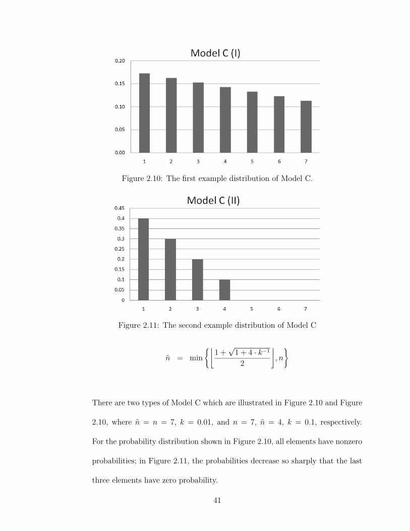
Figure 2.10: The first example distribution of Model C.
Figure 2.11: The second example distribution of Model C
n = min
{⌊1 +
√1 + 4 · k−1
2
⌋, n
}
There are two types of Model C which are illustrated in Figure 2.10 and Figure
2.10, where n = n = 7, k = 0.01, and n = 7, n = 4, k = 0.1, respectively.
For the probability distribution shown in Figure 2.10, all elements have nonzero
probabilities; in Figure 2.11, the probabilities decrease so sharply that the last
three elements have zero probability.
41

The entropy of Model C is
H(P3(x)) = −n∑
x=1
(a− k · (x− 1)) · ln (a− k · (x− 1)) (2.26)
Unfortunately, there is no way to further simplify the entropy of Model C as in
the previous two cases.
As we can see, the entropy of Model B is the function of parameters r and n, the
entropy of Model C is the function of parameters k and n, while the entropy of
Model A is only the function of n. We can model every non-increasing probability
distribution function by the three standardized models with equal entropy based on
this observation. Therefore, we can establish an approximate relationship between
the coverage rate and the number of selected elements.
The threshold point k for an arbitrary non-increasing probability function is de-
fined by the following equation:
k = argmini∈N
{i∑
x=1
P (x) ≥ α
}(2.27)
where α is the coverage rate between zero and one.
We can solve k2 for Model B by
k2∑x=1
P2(x) = ak2∑x=1
rx−1 =1− rk2
1− rn≥ α
⇒k2 = ⌈logr {1− α(1− rn)}⌉ (2.28)
42

We can calculate k1 for Model A as well:
k1∑x=1
P1(x) =k1∑x=1
1
n=
k1n
≥ α ⇒ k1 = ⌈nα⌉ (2.29)
The threshold point k3 for Model C is solved by geometry similarity of right
triangle and trapezoid:
k3 =
2n+nk−
√2n+nk
2−8α·k2·k
for 0 ≤ k < 2n2
⌈(1−
√1− α) ·
√2k
⌉for k ≥ 2
n2
(2.30)
Then we expect for an arbitrary non-increasing probability distribution function
f(x), the threshold point kf(x) would be close to k1, k2, and k3, which come from the
standardized models with the same entropy and total points as of f(x). We verify
it by two test sets; each includes 99 randomly generated non-increasing probability
distributions, whose probabilities are assigned by uniform and Gaussian distributions.
Figure 2.12 and Figure 2.13 show the simulation results of the two test sets. The
differences of the 90% threshold points among the three standardized models and the
real distributions generated by uniform distribution are shown in Figure 2.12. As
we can see, k2’s are closest to the actual threshold points while k1’s are also very
accurate. The simulation result of the Gaussian counterpart is shown in Figure 2.13.
As we can see, k1 and k2 are good references for the actual threshold point.
The errors in coverage rate of the uniform and Gaussian test sets are shown in
Figure 2.14 and Figure 2.15, respectively. As we can see, the coverage rate’s errors
43

Figure 2.12: Differences between estimated and real threshold points given the uni-form test set.
44

Figure 2.13: Differences between estimated and real threshold points given the Gaus-sian test set.
45

Figure 2.14: Coverage rate errors generated by estimated threshold points given theuniform test set.
are acceptable for each standardized model in both test sets, i.e., the idea that using
these standardized models with the same entropy to estimate the threshold point of
an unknown probability distribution, even before they are sorted, is sustainable.
Since the conversion from the entropy to the threshold point based on Model A
has the lowest computational complexity among the three standardized models and
also provides pretty good accuracy, we believe that Model A has higher potential to
be applied to the proposed algorithm.
In the real world, we expect the LUT’s separation to be efficient, i.e., the fast
LUT saves much in capacity without losing too much information. If we found the
estimated threshold point is close to 0.9n, i.e., this probability model is very uniform,
46
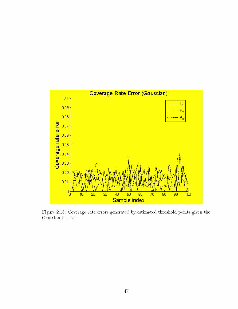
Figure 2.15: Coverage rate errors generated by estimated threshold points given theGaussian test set.
47

we can conclude that applying separation for this probability model is inefficient thus
we keep all the data in the fast portion.
Since we cannot get exact partitioning until completing the first pass, further ad-
justing is required. Since we assume our probability model to be a tree-like structure,
it naturally provides multiple granularities in probability adjustment. For example,
if we observe that the coverage rate of the fast portion is far less than the expected
value after the first pass, we can relax the criteria for the root levels. On the other
hand, if we observe that the coverage rate of the fast portion exceeds the capacity a
little bit, we can tighten the criteria for the leaf levels. By controlling the criteria for
each level, we can achieve successive adjusting of the coverage rate to full utilize the
fast portion capacity.
2.5.2 Access LUT without CAM - Improved Pearson Hash-
ing for Collision Reduction
Although LUT is a very intuitive abstraction, its underlying implementation is very
complex or time-consuming. If we directly store all the entries of an LUT in traditional
numerically addressed RAM, we have to compare every key field to a key until we
find the match one in order to retrieve the value associate to it. Special hardware
designs, such as Content-Addressable Memory (CAM), are capable of fast retrieving
values by keys by performing comparisons in parallel. However, it is too expensive
to implement large scale LUTs. Therefore, we need to develop an efficient way to
implement LUTs without large scale key comparing.
48

A hash table is a data structure which uses a hash function to translate keys into
numerical indices where their corresponding values to be stored and retrieved in one
mathematical step in most case. This data structure totally fulfills the requirement of
implementing LUTs, which is retrieving values by keys instead of numerical addresses
with a low time complexity.
Although a good hash function can evenly distribute the output values in the hash
table’s index space from natural data set in probability, the birthday paradox virtually
guarantees the occurrences of collision, i.e., multiple different keys are mapped into
single address. If all keys are known before organizing a hash table, we can carefully
develop a perfect hash function to completely eliminate collisions and place every key
and corresponding value in a unique memory address. However, in most case, where
the data has to be dynamically arranged, the perfect hash is unachievable.
In order to handle the collisions, most hash tables have to work with collision
resolution strategies. Consequentially, most hash tables are actually maintained by
hybrid addressing models. When an entry does not collide to others, its index is simply
equal to its key’s hash value. Should collision occur, an auxiliary data structure, in
most case is linked list, is introduced to associate the collide entries with their index.
Intuitively, the more collisions occur, the larger portion of our data is organized
in linked lists, and the fewer entries can be directly located by the hash function.
Therefore, the best way to improve the performance of a hash table is to develop a
hash function which can reduce the chance of collisions in the first place.
In this section, we proposed an improved hashing scheme based on Pearson Hash-
ing [26]. Pearson hashing has extremely low computational complexity (only bit-
49

wise arithmetic is utilized), which makes it an ideal hash function to manage large
LUT. Although Pearson hashing was originally developed to encode and manage text
strings, it is applicable to any data type since we can treat each 8-bit segment in
the binary input data stream as a character. We add another permutation table
to “dodge” incoming collision at the last step rather than using single permutation
table and carefully tweaking it to avoid collisions by some rule-of-thumb. The pro-
posed improvement does not only reduce the collision probability, but also enhance
the priority property of the result data structure.
2.5.2.1 Hashing Basics
Hashing itself is a process mapping any data which can be numerically represented
into a limited and discrete number domain. Any function capable for this purpose
can be defined as a hash function.
Assume we have a data set, which each entry in it has two fields, which are the
key and the value associates to the key. What we need is organizing the data set
into a manageable form, i.e., data structure, to enable adding, deleting, and accessing
arbitrary entries according to their key in limited time.
Since the key domain can be very large or even indefinite, it is difficult to use the
keys themselves as the entries’ indices. Therefore, using hash function to map the
keys into a predetermined index space to fit the entries in a limited memory space
is a reasonable solution. A data structure whose entries are mainly indexed by their
keys’ hash values is called a hash table.
Once we organize our data set as a hash table, we can locate an entry by calculate
50

its key’s hash value as index, without scanning through many entries. Then we can
insert, delete, read, or write the entry in the hash table.
Since hash functions map large or indefinite key space into a smaller and limited
index space, there exists a chance that multiple completely different keys generate
identical hash values, which is defined as collisions. Collisions in hash tables, if not
handled properly, can cause problem since entries may be overwritten by others and
lost forever.
We expect a good hash function can evenly distribute output values among the
index space in probability unless a specially designed key set is given. There are many
hash functions designed to process natural text data do achieve this expectation.
However, the birthday paradox guarantees we cannot eliminate collisions no matter
how well the hash function is.
The schemes used to handle hash collisions are collision resolution strategies.
There are varies collision resolution strategies such as using linked lists to chain
collided entries together, i.e., separate chaining, or just leaping forward along the
index space until finding an empty slot to fit in, i.e., open addressing. Both separate
chaining and open addressing strategies require linearly searching in a subset of the
hash table. A hash table’s performance differs by the collision resolution strategy it
uses and its load factor, which defined by the number of entries divided by the total
number of indices provided by the hash function.
In general, applying separate chaining would have average search time higher than
applying open addressing when load factor is low. However, the average search time
using separate chaining would be less sensitive to load factor increasing. Applying
51

separate chaining would outperform open addressing in high load factor conditions.
If the data set is prioritized, i.e., some keys should have lower search time than
others due to their higher occurrence probabilities, we can reorder the entries and
start with the entry with highest occurrence probability while building the hash ta-
ble. Therefore, an entry with higher priority can have better chance to be directly
addressed by hashing its key rather than searched along the linked list or hash table.
Should a higher priority entry collide, it can still be allocated closer to the head of the
linked list (using separate chaining) or to the original address calculated by hashing
(using open addressing), which also means shorter scanning distance along the linear
structure before reaching the goal.
2.5.2.2 Algorithm of Pearson Hashing
The algorithm of Pearson hash function comprises the following steps:
1. Assume we have an n-character long string as our input data, which is encoded
as A0A1A2 · · ·An−1 in ASCII.
2. Create a permutation table, which consists of 256 8-bit codes in random order.
3. Initialize the hash value h = 0 and character index k = 0.
4. Get the new index i = Ak ⊕ h.
5. Find the ith codeword from the permutation table as the new h, and then
increase k by one.
52

6. Repeat Step 4 and 5 using following input characters till the end of the string,
then the final h is the hash value of the string.
As we can see, Pearson hashing uses simple bitwise arithmetic to calculate hash
values. Although the simplicity of Pearson hashing compromises its security, it is
very efficient for text search and any other purposes wherever security is not an issue.
Original Pearson hashing only generates 8-bit hash values. One can, however,
execute an additional Pearson hashing with the first character numerically added one
and combine these two hash values to expand the output range to 16-bit. The pseudo
random nature of Pearson hashing should generate two uncorrelated hash values in
16-bit calculation.
2.5.2.3 Collision Elimination or Reduction in Pearson Hashing
Since the calculation in Pearson hashing is quite straightforward, the only thing we
can do to avoid collision is manipulating the permutation table. The author provided
some guidelines to create a permutation table enabling perfect hashing. However,
those are only rule-of-thumbs and rely on manual try-and-error, which are impractical
to be implemented on autonomous systems.
2.5.2.4 Improved Pearson Hashing to Reduce Collision
The major difficulty to suppress collision rate in Pearson hashing is due to its single
permutation table design, which makes each tweak in the permutation table could
change almost every key’s hash value. Here we propose an improved hash algorithm
based on Pearson hashing by introducing an additional permutation table. By replac-
53

ing the permutation table used while processing the last character in the string with
another permutation table, i.e., the auxiliary permutation table, which is generated
during creating the hash table, a significant number of collisions can be avoid by our
well defined algorithm.
The proposed algorithm to create the hash table and the corresponding auxiliary
permutation table is described below:
1. Assume we have an n-character long string as our input data, which is encoded
as A0A1A2 · · ·An−1 in ASCII.
2. Create a permutation table, which consists of 256 8-bit codes in random order.
3. Create an empty table, i.e., the auxiliary permutation table, which has 256
slots.
4. Initialize the hash index set H = {0, 1, 2, · · · , 254, 255}.
5. For each key, initialize the hash value h = 0, character index k = 0, hash index
j = 0.
6. Get the new index i = Ak ⊕ h.
7. Find the ith codeword from the primary permutation table as the new h, and
then increase k by one.
8. Repeat step 6 and 7 until k = n− 3.
9. Get the new index i = An−2 ⊕ h.
10. There could be four possible cases:
54

(a) If the ith slot in the auxiliary permutation table is empty, and (An−1 ⊕ j)
does not equal to any codeword in the auxiliary permutation table where
j ∈ H, put (An−1 ⊕ j) in the ith slot of the auxiliary permutation ta-
ble, remove j from H, and update h as the jth codeword in the primary
permutation table.
(b) If the ith slot in the auxiliary permutation table is empty, but either
(An−1 ⊕ j) equal to another codeword in the auxiliary permutation table
or j /∈ H, increase j by one and check again.
(c) If the ith slot in the auxiliary permutation table is occupied by codeword
R, and j = (An−1 ⊕R) ∈ H, remove j from H, and update h as the jth
codeword in the primary permutation table.
(d) If the ith slot in the auxiliary permutation table is occupied by codeword
R, and j = (An−1 ⊕R) /∈ H, update h as the jth codeword on the primary
permutation table; there is nothing we can do to avoid this collision.
11. Repeat Step 5 through 10 until all the keys are processed.
12. Fill the empty slots in the auxiliary permutation table with unused codewords,
which make it a legitimate permutation table.
Once we create both permutation tables, we can calculate any key’s hash value
by using the codeword from the auxiliary permutation table, instead of the primary
permutation table, to XOR with the second last character in the key string.
55

2.5.2.5 Properties of the Proposed Hash Algorithm
In the proposed hash algorithm, j represents the last index to select the final hash
value from the primary permutation table for each key. If a key is assigned to a unique
index, it should not collide with others. If we can assign every key a unique index,
we can achieve perfect hashing. The assignment of indices, however, is restricted by
the existed codeword in the auxiliary permutation table, such as condition (b), (c),
and (d) in Step 10. Therefore, we cannot arbitrarily assign index for each key as our
wish and achieve perfect hashing.
When the first few keys are processed, there are still many indices can be picked up
from the hash index set and many codewords can be filled in the auxiliary permutation
table, which enable them to easily get their unique indices. Consequentially, the first
few keys are very unlikely to collide with each other. While the remaining codewords
and available indices getting fewer, the latter keys would have higher chance colliding
with previous keys. In contrast, in the original Pearson hashing, every two keys
colliding together has equal probability. That is, if the data set is prioritized, the
proposed hash algorithm could enhance the advantage of the higher priority keys
over lower priority ones more significantly than the original Pearson hashing does
while building the hash table.
2.5.2.6 Technical Details
The proposed hash algorithm can be implemented in autonomous systems without
human intervene. We allocate two 256 entries memory blocks, one stores the hash
56

table while the other stores collided entries temporarily. Each entry has five fields,
which are entry type, key, length of key, previous address, and next address. The
entry type field represents the entry’s current state; it can either be empty, the body
of a linked list, the head of a linked list, pure hash addressable, or the tail of a linked
list, which is important for collision resolution. The key and its length fields are used
to match in searching. The previous and next address fields are only useful when the
entry is a part of a linked list.
When a collision occurs, we first put the new entry to the temporary block in
sequence and link them. The entries in the temporary block are inserted back to the
empty spaces left in the hash table (and the links should be maintained of course) after
all entries are processed. The hash table should not use any space in the temporary
block at the end.
There are some auxiliary variables inserted to count linked lists’ lengths and colli-
sion occurrences while building the hash tables. The experiment results are presented
in the next subsection.
2.5.2.7 Experimental Results
We implement both Pearson hashing and the proposed hash algorithm in C, feed them
with identical text data set, execute 1M iterations, and then compare the average
linked list lengths and collision counts of each key.
As shown in Figure 2.16, the text data set is list of 256 NATO reporting names,
which are used to identify Soviet, Russian, and Chinese military equipments including
aircraft, missiles, and submarines. All keys are in upper case. The list is not in
57

Figure 2.16: Test key set complied from NATO reporting names.
alphabetical order though the reporting names for aircraft and missiles with the
same initials are put together. The compilation of this data set is not based on
any meaningful idea; just like how the NATO officials picked up those nouns from a
dictionary.
The average linked list length in the hash table generated by the proposed hash
algorithm is 1.280576, while it is 1.586192 by original Pearson hashing. The proposed
hash algorithm reduces the average linked list length by 19.27%, which also means
lowering the average search time.
The collision counts versus each key’s processing sequence of both hash algorithms
are shown in Figure 2.17.
As we can see, the proposed hash algorithm enhances the advantage of the former
58

Figure 2.17: Comparison of collision counts distributions generated by Pearson andthe proposed hashings.
59

keys over latter ones with lower collision rate in most case. Note the 6 peaks in the
graph of the proposed hash algorithm. They are generated by the keys who share most
of the characters except the last one with previous keys as the keys in bold typeface in
Figure 2.16. However, the proposed hash algorithm outperforms the original Pearson
hashing in general.
2.5.2.8 Implications
We can significantly lower the collision rate and thus the average search time of a hash
table by applying the proposed hash algorithm. Since the proposed hash algorithm
retains the arithmetic simplicity of Pearson hashing in searching, we can achieve even
faster content searching in the much more efficient hash table. The only extra costs
are 256 bytes memory space for the auxiliary permutation table, and more complex
scheme for hash table building. However, we do searching much more frequently than
setup data structures.
2.6 Summary
In this chapter, we propose an architecture to improve the compatibility of virtualiza-
tion based on the application streaming concept. We further propose prefetching VM
pages to reduce the waiting. We also discuss the feasibility of applying prefetch based
on decision tree learning and information theory which also outlines the requirement
of the probability model.
To apply prefetch in the proposed application, we use LUT to mange the proba-
60

bility model. We then propose an algorithm to separate a single LUT into two-level
hierarchical LUTs to improve efficiency.
Since implementing LUTs requires retrieving certain value associate to a key, we
propose using a hash tables to implement instead of expensive CAM. We propose an
improved hashing scheme based on Pearson hashing. The proposed hashing signifi-
cantly reduces the collision rate with a very little extra cost on complexity comparing
to Pearson hashing, which help us to efficiently access the probability model to realize
the proposed prefetch application.
61

62

Chapter 3
Optimization of Browser-Based
Application Virtualization
As computing devices get smaller, lighter, and more portable, computing becomes
more focused on mobile applications. We expect this trend to continue for years to
come.
Deploying application software on mobile computing devices can be a challenge
for several reasons. First of all, various mobile operating systems exist and none is
expected to dominate and set the standards for the mobile computing in ways the
Windows operating systems have done for the desktop computing. Making a software
program to be compatible with different mobile operating systems requires extra cost
and effort – for example, developing multiple SDKs.
Although compatibility across application-platforms also exist on typical desk-
top computers, it is far more difficult for mobile computing devices because of the
additional constraints such as limited compute cycles in the mobile devices. Un-
63

like operating systems for desktop computers, mobile operating systems are highly
customized per product and secured against unauthorized user access. Generally, or-
dinary end-users cannot upgrade or patch their mobile operating systems to address
application-platform compatibility issues, as can be done for the desktop computers.
It is thus hinged upon software developers to provide compatibility across mobile
platforms.
Virtualization can address the compatibility in deploying mobile application soft-
ware on various mobile platforms. Theoretically, we can either use application stream-
ing to deploy application software over the Internet and run the application software
on top of a preinstalled runtime environment, i.e., virtual machine, or run the appli-
cation software on a managed server while each client device deals with user inputs,
such as keystrokes, and outputs, such as display updates from the server [4] [9] [13].
We generally refer to the latter paradigm as the browser-based approach since web
browsers provide an ideal framework for it.
Although technically plausible, deploying a virtual machine running on top of a
mobile operating system requires the distribution of applications violates the “Non-
Compete” policy [27] [28] by marketplace operators1. Consequently, the browser-
based approach becomes the only practical way to provide application virtualization
on mobile computing devices.
1VMware’s Mobile Virtualization Platform (MVP) [29], which implements this paradigm, is notavailable in Android Marketplace. To install MVP on an Android phone requires sideloading, andonly Android platform leaves this loophole to install apps outside the marketplace, which is at themercy of Google and wireless service providers. In fact, some wireless providers do block sideloadingon some Android phones. Furthermore, among the major mobile device players, only Android issupported by MVP. Therefore, even VMware starts their own app store for MVP, it does not helpcross-platform software deployment anyway.
64

The conventional solution of web-based application virtualization involves setting
up a server or a group of servers at a co-location center (or data center) provided by
an Internet service provider (ISP). From the co-location center, application virtual-
ization services are provided through the Internet. This configuration typically incurs
long response latency and significantly reduces the user experience since every input
must travel through a series of routers and bridges to the co-location center and the
corresponding response has to traverse backward through a similar route. Each node
along the route introduces processing delay, queuing delay, and transmission delay.
To alleviate this issue, we propose an alternative configuration which partitions a
service area into multiple smaller service areas with own server(s) [30]. The proposed
configurations can significantly reduce delays since each server is closer to its user.
The proposed configuration, however, has to handle hand-off, i.e., mobile stations
moving from one service area to another. We also propose a hand-off protocol offering
seamless user experience in Section 3.3.
The proposed configuration comes with a price, such as introducing longer re-
sponse latency during hand-offs. We use an analytical approach to evaluate the
performance as a result of infrastructure arrangement [30].
We further set up a simulation environment based on the UMTS urban pedestrian
model and vehicular mobility model, and use the empirical approach to establish the
correlations between the performance and the size of local service areas [31][32].
65

3.1 Related Work
There are several papers proposed to optimize service migration though for different
applications. Bienkowski et al. proposed competitive analysis for service migration
in optimizing the server allocation in VNets in [33]. Arora et al. proposed some
strategies for flexible server allocation in [34] following the previous work [33]. Al-
though these works were not specifically for mobile application virtualization, they
provide a precious insight on the performance evaluation for dynamic service alloca-
tion considering both user experience and operational cost. However, the analytical
approach used in these works is topological and does not focus on the user mobility
and interaction models. Furthermore, the authors of [33] and [34] allow services being
temporarily interrupted during migrations, which is not feasible for application vir-
tualization services. In the proposed configuration, application services are available
to users with reduced performance during hand-offs.
3.2 Distributed Application Virtualization Service
Configuration
Running application software on a remote server is conceptually similar to the usage
model of time-sharing mainframe computers in the 1960s [2]. Although the commu-
nication bandwidth between terminals and mainframe servers at that time was low
by the recent standards, it did not affect the user experience thanks to the text-only
display and short traverse distance. However, in recent application virtualization
66

technologies such as Virtual Desktop Infrastructure (VDI) proposed by VMware [35],
much more complex and bloated content must be exchanged over much longer dis-
tances between clients and servers, especially for mobile users.
An infrastructure ready to offer mobile users application virtualization services
includes base stations (BSs) covering the whole service area, a core network connecting
base stations and servers together, and a server hosting the services. A command sent
by a mobile station (MS) has to travel over the wireless channel to the BS, go through
the backhaul network to the server, and then make some changes on the server. Should
any update corresponding to the command be sent to the MS, the information has
to travel all the way backward. In order to reduce the network delay generated by
long transmission distances among the backhaul network, we deploy multiple servers
among a wide area to serve their nearby MSs in the proposed configuration, instead
of setting up a group of servers located at one data center serving all MSs.
In the proposed configuration, each server connects to several nearby BSs which
form a local service group (LSG). The area covered by the BSs of the same LSG is
defined as the local service area (LSA). Every BS belongs to one LSG in order to
provide the service over the wireless network’s coverage area. When a user demands
a virtual application program, the server of the LSG, based on VDI [35] paradigm,
starts a virtual machine (VM) dedicated to the user and launches the application
software on top of it. The MS only handles inputs and outputs that interact with the
VM at the server.
As long as the MS stays in the same LSA, the user can enjoy using application
software with low response latency. If the MS moves from the original LSA to a
67

nearby one, a hand-off at the VM level, which transfers the runtime environment to
the server of the next LSG, is triggered. The detail of the hand-off protocol will be
proposed in the next section.
3.3 Hand-off Protocol
The purpose of the proposed hand-off protocol is to transfer minimum information
required to recreate the runtime environment on a remote server, i.e., the snapshot,
without interrupting the service. No matter how small the snapshot is, it still takes
a period of time before the next server receives the complete snapshot and is ready
to take over the service. In order to provide a seamless user experience during this
period, the next server has to record all inputs from the MS, relay all inputs to the
previous server, and relay all output from the previous server to the MS, until the
runtime environment resumes locally. The proposed hand-off protocol is described as
below:
1. When an MS moves from Server A’s to Server B’s LSA and sends an input
command, Server B notices a newcomer within its LSA.
2. Server B broadcasts the newcomer’s identification to all geographically nearby
servers.
3. Server A, which hosts the MS’s runtime environment, i.e., its VM server, re-
sponds Server B’s inquiry. Now Server B knows the newcomer’s VM server is
Server A.
68

4. Server B records and relays the user’s input commands to Server A, signals
Server A to transfer the runtime environment, and relays display updates from
Server A to the newcomer.
5. Once Server A is signaled to transfer the runtime environment, it takes a snap-
shot.
6. Besides continually responding to the input commands relayed from Server B
as the MS is still in its LSA, Server A also sends the snapshot to Server B in
the background.
7. Once Server B receives the complete snapshot and recreates the runtime envi-
ronment from the snapshot and base data, it internally feeds the input queue,
which was recorded during the transition period, to the runtime environment.
Therefore, the runtime environment state on Server B is synchronous with that
on Server A after the snapshot was transferred.
8. Server A completely stops serving the MS, the MS’s VM server is now Server
B instead.
The timeline of the proposed hand-off protocol is illustrated in Figure 3.1.
If the MS turns around and reenters Server A’s LSA before the hand-off is com-
pleted, Server A can preempt the snapshot transmission and resume serving the MS
as if the hand-off never happened. Since Server B relays all inputs to Server A while
the MS is absent from Server A’s LSA, aborting the hand-off procedure would not
generate any glitch noticed by the user. This hand-off abortion mechanism can pre-
69

Figure 3.1: Protocol timeline for a mobile station moving from Server A to Server B.
vent unnecessary data transmission from moving VM servers back and forth if an MS
were moving around the edge of an LSA. On the other hand, if the MS moves to
Server C’s LSA before the hand-off is completed, Server C initializes another hand-off
procedure with Server B. In addition to the snapshot, Server B has to transfer the in-
put record before Server C joins the hand-off chain. We allow pipelining transmission
to reduce hand-off periods and shorten subsequent hand-off chains in this scenario.
3.4 Performance Evaluation Using Free Particle
Mobility Model
We define the response time as the average time interval between a user sends an input
and gets an expected output update. The proposed server configuration is meant to
70

improve the response time by reducing propagation delay along the communication
route between each base station to the server which is hosting the service. Factors
other than the propagation delay, such as wireless communication technologies and
computational capabilities provided by servers, would affect the user experience and
the quality of our service. Most of them, however, either affect both configurations
equally, or can be overcome with reasonable cost.
The proposed configuration reduces the propagation delay and thus provides more
responsive user experiences when uses are standing still. When a hand-off occurs,
however, the user may experience longer response time waiting for the information
to be exchanged between two servers before the runtime environment is successfully
taken over by the new server. The smaller each local service area is, the higher
occurrence probability of hand-offs the user may experience. Therefore, we have to
quantitatively estimate and compare the propagation delays of the conventional and
the proposed server configurations.
The precise propagation delay analysis depends on a wireless service provider’s
core network topology and its users’ moving pattern record. Instead of acquiring
those field data, we focus on the intrinsic properties of the two configurations. There
are two approaches to estimate the average response time due to propagation delay;
one assumes continuous service areas, the other is based on the optimal arrangement
of base stations. The details are presented in the following subsections.
71

3.4.1 Continuous Service Area Approach
In this approach, we simplify the communication model between mobile stations and
servers. Here are our assumptions:
1. The whole service area can be covered by a single server, or proximately by
multiple servers, each having a regular hexagon shaped service area seamlessly
tiled together as a service array.
2. A mobile station can directly communicate with the server everywhere in its
(local) service area.
3. Users are uniformly distributed geographically in the beginning. Users can
either move a certain distance in any direction, or stay at the same location for
a while.
4. The propagation delay of each link is proportional to its length.
5. Each server’s allocation is geographically optimized, that is, each server is lo-
cated at the center of its (local) service area to reduce the average propagation
delay.
The traverse time in our case is defined by:
Ttraverse = 2 · (1− PHO) · (Tr + Tl) + 2 · PHO · THO (3.1)
where PHO is the probability of transactions which either trigger hand-offs or occur
during each handoff, Tr is the radio propagation delay, Tl is the line propagation
72

Figure 3.2: Service area of 7-server configuration compares with of single-server one.
delay, and THO is the prolonged traverse time during each hand-off according to the
proposed protocol. To simplify the problem, we only compare the following three
configurations covering the same amount of area:
A A single server covering a regular hexagon service area of edge length L.
B 7 servers, each covering a regular hexagon service area of edge length L√7, as shown
in Figure 3.2.
C 12 servers, each covering a regular hexagon service area of edge length L√12, as
shown in Figure 3.3.
3.4.1.1 Average Transmission Distance
We can calculate the distance from an arbitrary point within each hexagon-shaped
service area to the center of the area, where the optimal server is. Since we assume
73

Figure 3.3: Service area of 12-server configuration compares with of single-server one.
that our users’ locations are uniformly distributed geographically in our service area,
we can estimate the average transmission distance for each user in terms of edge
length of the service area. Due to the symmetry of hexagons, the average distance
from an arbitrary point within a hexagon to its center is equivalent to the average
distance from an arbitrary point within a 30-60-90 triangle to the 30-degree vertex
as shown in Figure 3.4.
By integrating√r2 + h2 along h and r, as shown below:
∫ √3L2
0
∫ r√3
0
{√r2 + h2
}dhdr
=∫ √
3L2
0
{h
2
√r2 + h2 +
r2
2ln∣∣∣h+
√r2 + h2
∣∣∣}∣∣∣∣∣0
r√3
dr
=∫ √
3L2
0r2dr ·
{1
3+
ln(3)
4
}
=
√3L3
8·{1
3+
ln(3)
4
}(3.2)
74

Figure 3.4: 30-60-90 triangle as part of hexagon with edge length L, used to estimateaverage distance to the lower right vertex.
Figure 3.5: The Markov chain of a moving MS’s status.
By averaging the result above by the whole triangle area, the average transmission
distance for each user in terms of the edge length of the service area is:
√3L3
8·{13+ ln(3)
4
}√3L2
8
=
{1
3+
ln(3)
4
}· L ≈ 0.60799L (3.3)
3.4.1.2 Probability of Transactions Relevant to Hand-off
The transition between normal and hand-off mode of each moving MS can be repre-
sented by a simple two-state Markov chain as shown in Figure 3.5.
As we can see in Figure 3.5, a moving MS in the normal state gets into the
75

hand-off state when it moves across the border of its current local service area with
probability Pcross. On the other hand, a moving MS in the hand-off state can go back
to the normal state either by completing the hand-off procedure with probability
Pcomplete, or by returning to the previous local service area and preempting the hand-
off procedure with probability Pabort. The summation of Pcomplete and Pabort is Pr,
which represents the total probability for a moving MS in the hand-off state to return
to the normal state.
By steady-state analysis, we can derive the probability of transactions relevant to
hand-offs, i.e., PHO, as below:
[ 1− PHO PHO ]
1− Pcross Pcross
Pr 1− Pr
= [ 1− PHO PHO ]
PHO =Pcross
Pcross + Pr
≤ Pcross
Pcross + Pcomplete
(3.4)
As we can see, the two factors Pcross and Pr affect PHO. Both factors depend on
e users’ mobility and the dimension of the service areas. Assume the average moving
speed of an MS is s∆t. To make it possible to trigger a hand-off in the following time
instance ∆t, the MS has to be within s from the current service area’s borderline.
Furthermore, the probability of an MS satisfying this prerequisite actually crossing
the borderline and thus triggers a hand-off depends on how close to the borderline it
is as shown in Figure 3.6.
Therefore, the probability of an MS which is located d from the borderline with
76
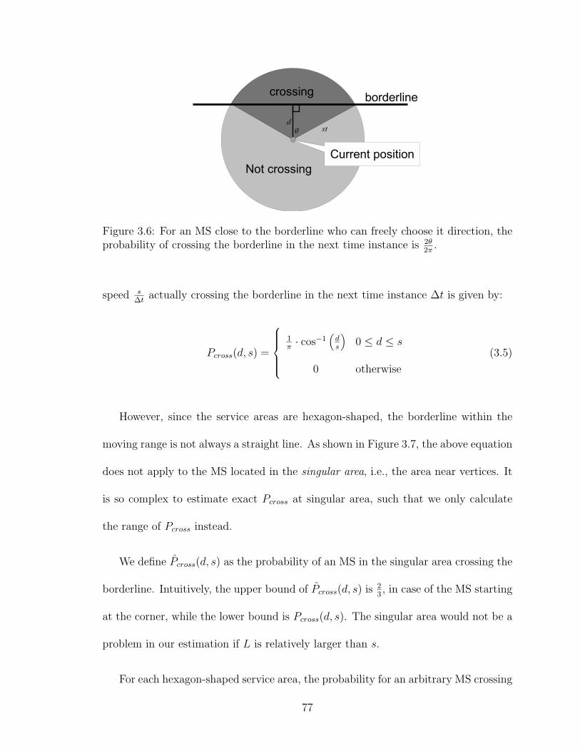
Figure 3.6: For an MS close to the borderline who can freely choose it direction, theprobability of crossing the borderline in the next time instance is 2θ
2π.
speed s∆t
actually crossing the borderline in the next time instance ∆t is given by:
Pcross(d, s) =
1π· cos−1
(ds
)0 ≤ d ≤ s
0 otherwise
(3.5)
However, since the service areas are hexagon-shaped, the borderline within the
moving range is not always a straight line. As shown in Figure 3.7, the above equation
does not apply to the MS located in the singular area, i.e., the area near vertices. It
is so complex to estimate exact Pcross at singular area, such that we only calculate
the range of Pcross instead.
We define Pcross(d, s) as the probability of an MS in the singular area crossing the
borderline. Intuitively, the upper bound of Pcross(d, s) is23, in case of the MS starting
at the corner, while the lower bound is Pcross(d, s). The singular area would not be a
problem in our estimation if L is relatively larger than s.
For each hexagon-shaped service area, the probability for an arbitrary MS crossing
77

Figure 3.7: Users at the singular area (dark area) have higher Pcross; the aboveequation can only apply in the normal areas (light areas).
the borderline and triggering a hand-off is:
Pcross(L, s, n) =2
3√3L2
∫ s
0{n(L− 2s) · Pcross(d, s)} dd+ ns2
(2− 1√
3
)· 2
¯P cross
3√3L2
=2
3π√3L2
∫ s
0
{n(L− 2s) · cos−1
(d
s
)}dd+
2ns2(2√3− 1) · ¯P cross
9L2
=2ns(L− 2s)
3π√3L2
∫ 1
0cos−1(k)dk +
2ns2(2√3− 1) · ¯P cross
9L2
=2ns(L− 2s)
3π√3L2
·{k cos−1(k)−
√1− k2
}∣∣∣10+
2ns2(2√3− 1) · ¯P cross
9L2
=2ns(L− 2s)
3π√3L2
+2ns2(2
√3− 1) · ¯P cross
9L2(3.6)
where¯P cross is the average probability of an MS in the singular area crossing the
borderline, and n is the number of edges which border another service area.
78

Since¯P cross ≤ 2
3,
Pcross(L, s, n) ≤ 2ns(L− 2s)
3π√3L2
+2ns2(2
√3− 1) · 2
3
9L2
=2ns{3
√3L+ 2(2
√3π − 2π − 3
√3)s}
27πL2
=2√3n
9π·(s
L
)+
4(2√3π − 2π − 3
√3)n
27π·(s
L
)2
(3.7)
For s ≪ L,
Pcross(L, s, n) ≈2√3n
9π·(s
L
)(3.8)
In the proposed design, the hand-off procedure takes a period of time while the
MS can continue sending requests. The duration of a complete hand-off Tcomplete, as
a result of the total amount of data which are transferred for each hand-off Dsync, the
transmission bandwidth provided by the link between the two adjacent servers BW s,
and the transmission latency of the link Tls, all affect the fraction of transactions
relevant to hand-offs. The equation is given by:
Tcomplete =Dsync
BW s
+ Tls (3.9)
Once a user triggers a hand-off, the subsequent requests within Tcomplete are cate-
gorized as hand-off related transactions. In other word, there are at least Pcomplete =
1Tcomplete
of MSs which are performing the hand-off procedure return to the normal
status in average. The actual rate of leaving the hand-off status Pr should be substan-
tially higher since some MSs preempt the hand-off. However, the hand-off abortion
79

rate Pabort is very difficult to be derived with analytical approaches. Consequently,
we take Pcomplete as a reference of Pr first and discuss the relation between them later.
Now we can derive PHO by the following equation:
PHO =Pcross
Pcross +α
Tcomplete
=Pcross
Pcross +α
DsyncBWs
+Tls
=
2√3E(n)9π
·(
sL
)2√3E(n)9π
·(
sL
)+ α
DsyncBWs
+Tls
=2√3E(n)
(sL
)·{Dsync
BW s+ Tls
}2√3E(n)
(sL
)·{Dsync
BW s+ Tls
}+ 9πα
(3.10)
where α = Pr
Pcomplete> 1 is the average hand-off duration, and E(n) is the average num-
ber of edges which border another service area, which is 0, 247, and 4 for Configuration
A, B, and C, respectively.
We can roughly conclude that PHO can be increased by higher MS mobility, a
larger volume of the data required for the synchronization, and a longer transmission
latency between the servers. On the other hand, it will be reduced by a wider service
area, a higher bandwidth between the servers, and a higher rate of hand-off abortion.
However, the transmission latency between the two adjacent servers is proportional
to the service range. We will see how the service range affects the average response
time in the following subsection.
80

3.4.1.3 Average Response Time Comparison of the Three Configurations
In Configuration A, there is only one server thus no hand-off mechanism. The average
traverse time of Configuration A is quite straightforward:
TAtraverse = 2 · (Tr + TA
l ) (3.11)
Now we have to consider hand-offs in Configuration B. Its average traverse time
is:
TBtraverse = 2 · (1− PB
HO) · (Tr + TBl ) + 2 · PB
HO · TBHO
= 2 · (1− PBHO) · (Tr +
Tl√7) + 2 · PB
HO · (Tr + Tlmax + Tls)
= 2
Tr +Tl√7− PB
HOTl√7
+
{12+ 3 ln(3)
4+√3}PBHOTl
√7(13+ ln(3)
4
)
= 2
{Tr +
Tl√7
{1 + PB
HO
{12√3 + 2 + 6 ln(3)
4 + 3 ln(3)
}}}(3.12)
where Tlmax is the propagation delay between the MS and the new server during
hand-offs, which is{
12√3+ 3 ln(3)
8√3
}Tls, since we assume that the MSs are still located
around the borderline at the time.
Therefore, if we expect that Configuration B would outperform Configuration A,
i.e., TBtraverse < TA
traverse, we can estimate the upper bound of PBHO as below:
1 + PBHO
{12√3 + 2 + 6 ln(3)
4 + 3 ln(3)
}<
√7
81

PBHO <
(√7− 1)(4 + 3 ln(3))
12√3 + 2 + 6 ln(3)
≈ 0.4087356087 (3.13)
This constrain is generally considered very slack.
Similarly, the average traverse time for Configuration C is:
TCtraverse = 2
{Tr +
Tl√12
{1 + PB
HO
{12√3 + 2 + 6 ln(3)
4 + 3 ln(3)
}}}(3.14)
And the upper bound of PCHO to outperform Configuration A is:
1 + PCHO
{12√3 + 2 + 6 ln(3)
4 + 3 ln(3)
}<
√12
PCHO <
(√12− 1)(4 + 3 ln(3))
12√3 + 2 + 6 ln(3)
≈ 0.6119795056 (3.15)
Furthermore, to outperform Configuration B given the same BW s, the criteria
are estimated below:
Tl√12
{1 + PC
HO
{12
√3+2+6 ln(3)4+3 ln(3)
}}< Tl√
7
{1 + PB
HO
{12
√3+2+6 ln(3)4+3 ln(3)
}}√7{1 + PC
HO · k} <√12{1 + PB
HO · k}
k{√7PC
HO −√12PB
HO} <√12−
√7
k
√7 ·2√3EC(n)
(√12sL
)·{
DsyncBWs
+TCls
}2√3EC(n)
(√12sL
)·{
DsyncBWs
+TCls
}+9παC
−√12 ·
2√3EB(n)
(√7sL
)·{
DsyncBWs
+TBls
}2√3EB(n)
(√7sL
)·{
DsyncBWs
+TBls
}+9παB
<
√12−
√7
8√21
(√12sL
)·{
DsyncBWs
+√
712
TBls
}8√3
(√12sL
)·{
DsyncBWs
+√
712
TBls
}+9παC
−967
(√7sL
)·{
DsyncBWs
+TBls
}16
√3
7
(√7sL
)·{
DsyncBWs
+TBls
}+3παB
< (√12−
√7)(4+3 ln(3))
12√3+2+6 ln(3)
(3.16)
82

The inequality above provides an accurate bound of the function of sL, Dsync
BW s, TB
ls ,
αB, and αC . It is, however, too complex to help us to determine which configuration
is better given a set of system parameters. Fortunately, we can discover the benefit
brought by a more distributed infrastructure arrangement by simplify the inequality
above based on sensible approximations. First of all, in most case Tls is negligible
comparing to Dsync
BW s. Therefore, we can replace all Tcomplete by Dsync
BW s. Secondly, as
s ≪ L, Pabort’s in both configurations are approximately the same. In consequence,
αB ≈ αC . Therefore, we can further set αPr = βPBcross where β > 0 to simplify the
inequality.
Since
Pcross(L, s) ≈2√3E(n)
9π·(s
L
)(3.17)
Therefore,
PCcross
PBcross
=
2√3·4
9π·(√
12sL
)2√3· 24
7
9π·√7sL
⇒ PCcross =
√7
3PBcross (3.18)
Now we can represent PBHO and PC
HO only in terms of PBcross and β:
PBHO =
PBcross
PBcross + αPr
=PBcross
PBcross + βPB
cross
=1
1 + β
PCHO =
PCcross
PCcross + αPr
=
√73PCcross√
73PCcross + βPB
cross
=
√7√
7 +√3β
(3.19)
83

And then rewrite the inequality in terms of β:
√7PC
HO −√12PB
HO <(√12−
√7)(4 + 3 ln(3))
12√3 + 2 + 6 ln(3)
7√7 +
√3β
− 2√3
1 + β<
(√12−
√7)(4 + 3 ln(3))
12√3 + 2 + 6 ln(3)
(7− 2√21) + β√
7 + (√7 +
√3)β +
√3β2
<(√12−
√7)(4 + 3 ln(3))
12√3 + 2 + 6 ln(3)
⇒ 0.352β2 − 0.110β + 2.703 > 0 (3.20)
which is true for all β.
Therefore, we can conclude that if s ≪ L, Dsync
BW s≫ Tls, and αB ≈ αC , Configura-
tion C can always outperform Configuration B in terms of traverse delay.
3.4.1.4 The Actual Rate of Leaving Hand-off State
To better understand Pr and its relation to Tcomplete, we wrote a simple simulation
program to empirically measure the average time an MS stays in the hand-off status.
The program simulates an MS originally located close to a borderline, whose distance
to it is uniformly distributed from 0 to s. Before it cross the borderline and triggers
a hand-off, it randomly choose a direction from −π to π and step forward s, which
ensures it either crosses, or approaches to, the borderline. Once it triggers a hand-off,
it can randomly choose any direction to step forward until the predetermined Tcomplete
runs out or it moves back to the other side of the borderline. The time each MS stays
in the hand-off status is gauged and averaged in the end of the program.
The average time MSs stay in the hand-off status given different Tcomplete is shown
in Figure 3.8.
84

Figure 3.8: The actual average hand-off duration.
The value of α, which varies in a similar curve as in Figure 3.8 is shown in Figure
3.9.
As we can see in Figure 3.8 and Figure 3.9, the actual rate of leaving hand-off state
Pr, which is the inverse of actual average hand-off duration, only fluctuates slightly
in response to Tcomplete. Therefore, we can assure that ignoring Tls and subsequently
assuming that Tcomplete’s are identical for both configurations are sensible.
3.4.2 Optimal Arranged Base Stations Approach
In this approach, the service area is covered by a group of base stations, each con-
nected to a server. Unlike the continuous service area approach which assumes each
service area is a perfect regular hexagon, in this model the service areas are shaped
by overlapping disks, each covered by a base station with omni-directional antenna.
85

Figure 3.9: The value of α given different Tcomplete.
Consequently, each (local) service area is similar to a regular hexagon but with some
“ripples” around the edges, which make it very difficult to estimate the hand-off prob-
ability. We can, however, proximately estimate it in certain conditions. Here are the
assumptions, which are slightly different from those of the other approach:
1. The whole service area is covered by minimum number of base stations with
omni-directional antennae. In other words, base stations are located at unit
points of a two-dimensional Synergetics coordinates [36].
2. We can either connect all base stations to one server, or separate base stations
into several groups and connect them to the server of each group. The optimal
service area of each group is approximately a regular hexagon.
3. Users are uniformly distributed geographically in the beginning. Users can
86

Figure 3.10: Service area of single-server configuration with m = 3.
either move a certain distance in any direction, or stay at the same location for
a while.
4. The propagation delay of each link is proportional to its length.
5. Each server’s allocation is geographically optimized, that is, each server is lo-
cated in the center of its (local) service area to reduce average propagation
delay. The traverse time in our service is defined by (3.1) as well.
Again, we compare the following two configurations covering the same area.
A: (3m2 + 3m + 1) base stations are placed like a regular hexagon, where m is the
number of the base stations’ intervals along one of the hexagon’s edges. Each
interval is√3R long, where R is the effective communication range of each base
station. An example is illustrated in Figure 3.10.
B: 7 servers, each connected to (3⌈m3⌉2 + 3⌈m
3⌉ + 1) base stations as a local service
area. The base stations in each local service area are placed like a regular
87

Figure 3.11: Service areas of 7-server configuration, each with m = 1, covering thesame amount of area.
hexagon with ⌈m3⌉ intervals along one of its edge, as shown in Figure 3.11.
3.4.2.1 Average Transmission Distance
The average transmission distance in this approach is the discrete version of the
continuous service area’s counterpart. However, it is very difficult to represent in
terms of m, as shown below:
3r∑m−1
t=0
∑m−tk=1
√3(2k + t)2 + 9t2
3m2 + 3m+ 1(3.21)
Fortunately, we find out that the average transmission distance in this approach
is approximately linear and gets closer to its continuous counterpart as m increases
according to the computer calculation, as shown in Figure 3.12.
88

Figure 3.12: Comparison of average transmission distances of different approachescovering approximately equal service area.
In other words, we can estimate the average transmission distance by either (3.21),
or the continuous counterpart (3.3) with comparable parameters. In the later sections,
we will use the latter one to focus on the quantitative relationships between the
parameters and the performance rather than the exact value.
3.4.2.2 Probability of Transactions Relevant to Hand-offs
Due to the irregular shape of each local service area, it is difficult to estimate the exact
probability of an arbitrary user around the border moving out of the service area by
equations. However, if users’ moving distances in each time instance are relatively
short compared to a base station’s effective communication range, the perimeter of
each local service area at any point is near a straight line from a user’s point of view.
Therefore, we can borrow the results from the continuous counterpart (3.6) to
89

estimate the probability of a user crossing the borderline. The average probability of
a user crossing the borderline along an arbitrary line which is perpendicular to the
assumed straight borderline is:
δPcross(s) =∫ s
0
{1
πcos−1
(d
s
)}dd
=s
π
∫ 1
0cos−1(k)dk
=s
π
{k cos−1(k)−
√1− k2
}∣∣∣10=
s
π
(3.22)
The perimeter of the service area has to be recalculated as 6(m−1) one-third arcs
and 6 half circles of radius R:
6Ledge = 6(m− 1) ·(2πR
3
)+ 6 ·
(2πR
2
)= 2πR(2m+ 1) (3.23)
For a local service area with n edges bordering another one, the length of borderline
eligible to invoke hand-offs is:
nLedge =nπR(2m+ 1)
3(3.24)
And we recalculate the service area as well. The area is basically a hexagon with
some “decorations” around the perimeter:
A =3√3
2
(√3mR +
R√3
)2
+ 6
{πR2
2− R2
√3+ (m− 1)
(πR2
2−
√3R2
4
)}
90

= R2
{9√3m2
2+
(2π +
3√3
2
)m+ π
}(3.25)
By accumulating the ¯δP cross along the perimeter and averaging with total area,
the probability of a user crosses the borderline for mobile stations located in the
service area for s ≪ R is:
Pcross =nπR(2m+ 1)s
3πR2{9√3m2
2+(2π + 3
√3
2
)m+ π
}=
n(2m+ 1)s
3R{9√3m2
2+(2π + 3
√3
2
)m+ π
} (3.26)
Similar to the continuous counterpart, PHO is given by the following equation:
PHO =Pcross
Pcross + Pr
=
E(n)(2m+1)s
3R
{9√
3m2
2+
(2π+ 3
√3
2
)+π
}E(n)(2m+1)s
3R
{9√
3m2
2+
(2π+ 3
√3
2
)+π
} + αDsyncBWs
+Tls
(3.27)
for s ≪ R, where E(n) is the average number of edges bordering another local service
area as well, which is 0 and 247in Configuration A and B, respectively.
3.4.2.3 Average Response Time Comparison of the Two Configurations
The average response time of configuration A TAresponse is still 2(Tr +TA
l ).The average
traverse time of Configuration B is equal to its continuous counterpart (3.12) as well.
If we expect that Configuration B would bring a shorter average response time over
Configuration A, the upper bound of PBHO is unchanged:
PBHO <
(√7− 1)(4 + 3 ln(3))
12√3 + 2 + 6 ln(3)
≈ 0.4087356087
91

Therefore, the constraints for m, s, R, Dsync
BWs, α, Tls, and Tu are represented in the
equation below:
8(2m+1)s
R
{9√
3m2
2+
(2π+ 3
√3
2
)+π
}8(2m+1)s
R
{9√
3m2
2+
(2π+ 3
√3
2
)+π
} + 7αDsyncBWs
+Tls
< 0.051091951 (3.28)
3.4.3 Simulation Result
To verify the estimations of Pcross, we use the Monte Carlo method by running a
simulation program which sets up base stations of given R at optimal locations,
randomly puts a large number of mobile stations, moves them away from their original
location a fixed distance in any direction, and measures the number of the mobile
stations escaping from the service area.
To compare the errors of the two different approaches, we set two environments
with short R and large m, and long R with small m, and adjustable s. In the former
environment, we set R = 0.25, m = 40, s varies from 0.1 to 2.0 with 0.01 steps, and
place 107 mobile stations. The PHO derived by the estimators and measured in the
simulation are compared in Figure 3.13.
As we can see, the continuous service area approach is a better estimator since the
shape of the service area is very close to a perfect regular hexagon in this environment.
Furthermore, we compare the error rate of both estimators and compare them in
Figure 3.14.
We can see in this series of simulations, the optimal arranged base stations ap-
proach only works well with very low s. However, when we set R = 2.0 and m = 5
92

Figure 3.13: Comparison of estimations and simulation result with R = 0.25 andm = 40.
93

Figure 3.14: Comparison of estimation errors with R = 0.25 and m = 40.
94

Figure 3.15: Comparison of estimations and simulation result with R = 2.0 andm = 5.
and run the same simulations, it becomes a different story as shown in Figure 3.15.
Since the base stations are far less dense than in the previous setting, the “ripples”
around the service area get larger and distort the shape away from a perfect regular
hexagon. As we can see in Figure 3.15, the optimal arranged base stations approach
is a very accurate PHO estimator for s ≤ 0.5 (s ≤ R4), and the continuous service area
approach gets more and more accurate PHO in response to increasing user mobility.
By comparing the estimation errors of both approaches in Figure 3.16, we can see
the accuracies of the two estimators significantly depend on user mobility.
95

Figure 3.16: Comparison of estimation errors with R = 2.0 and m = 5.
96

3.5 Performance Evaluation Using the UMTS Ur-
ban Mobility Model
Although the free particle analysis in the previous section relates the overall perfor-
mance to the MS’s mobility and the infrastructure’s geographical parameters, the
arbitrary mobility model is too arbitrary to preview the performance of the proposed
configuration and hand-off protocol in real world. Since each MS moves without in-
ertia and any intelligent intent, it is able to suddenly turn to an opposite direction in
the free particle mobility model. This moving characteristic only makes sense for an
application virtualization service specific for a bunch of drunks wondering on a rural
plain. In the proposed distributed service configuration, the free particle model does
increase the chance an MS triggers and aborts a hand-off procedure in a short period.
Therefore, we need to further evaluate the performance of the proposed configuration
and hand-off protocol in more realistic mobility models.
Of course the most realistic mobility model comes from the field record of a mobile
phone carrier. The data is extremely difficult to be obtained for several reasons. For
instance, carriers may record the users’ moving pattern along with other behaviors
and store them in a huge database in general. In most case, they do not do any
data mining or organization except for their internal research projects. If an outsider
requests a data set about user mobility from a mobile phone carrier, they do not
know where the data is even if they are willing to help. Furthermore, those records
may involve sensitive user privacy. Mobile phone carriers would reluctant to allow
any outsider to get access to the databases to prevent from potential legal issues.
97

Fortunately, European Telecommunication Standards Institute (ETSI) published
a document [37] which described three test environments and user mobility models,
which are Indoor Office, Outdoor to Indoor and Pedestrian, and Vehicular ones, as
common benchmarks to evaluate potential wireless technologies to develop Universal
Mobile Telecommunication System (UMTS). Although the reality of the models is
never explicitly justified and Jugl and Boche [38] have extended the mobility model to
improve the reality, the original UMTS models still provide a fair reference for mobility
related performance evaluation. If more realistic mobility models are available, we
can replace the UMTS ones and obtain more accurate configuration parameters.
In this section, we set up a simulation environment referring to the UMTS’s Out-
door to Indoor and Pedestrian mobility model, also known as the UMTS urban mo-
bility model, and use the empirical approach to establish the correlations between the
performance and the size of each local service area and the capabilities of the network
infrastructure. With our proposed modification, we enable the simulation to run for
an indefinite period of time without presuming any boundary condition.
3.5.1 UMTS Urban Mobility Model
As shown in Figure 3.17, The UMTS Outdoor to Indoor and Pedestrian test environ-
ment is basically a Manhattan-like street structure where MSs move along 30 meters
wide streets and are only allowed to change directions with half chance at the inter-
sections, which are 200 meters apart. Each MS’s moving speed can be updated every
5 meters with 20% chance, and the new speed is generated by a truncated Gaussian
98

Figure 3.17: UMTS outdoor to Indoor and Pedestrian test environment and LSAarrangement.
distribution whose mean equals 3 km/h, standard deviation equals 0.3 km/h, and
minimum speed equals 0 km/h. All MSs are initially uniformly distributed on the
Manhattan-like streets.
The UMTS document, however, does not explicitly specify where an MS turns
within the intersection area. Therefore we make a reasonable assumption to overcome
the ambiguity. If an MS is supposed to turn in an intersection, it has six points, which
are 5 meters apart along the crosswalk, to change its direction before reaching the
other side. We assume an MS picks one out of the six points with equal chances as
its turning point, which keeps MSs uniformly distributed on the streets rather than
be concentrated on a certain part of the streets over time.
The BSs in the UMTS Outdoor to Indoor and Pedestrian test environment are
99

located at the dark grey dots in Figure 3.17. Although the placement of the BSs is
not optimal, it is not far from that. Considering an actual city could be preoccupied
by tall private buildings on each block, deploying BSs along the streets makes sense
both technically and politically.
One of the shortcomings of the UMTS mobility model is the bounded test area
which generates ambiguities on setting boundary conditions. We consequently add
some special traffic rules, known as portals, to eliminate the boundary discontinuities
and allow the interaction among LSAs to be simulated and observed for indefinite
period of time. These portals will be described in the next subsection.
3.5.2 Mobius City
What interests us is the geographical relation between the service facilities and the
MSs’ moving space. Once we group the BSs in Figure 3.17 to form hexagon-shaped
LSAs that optimize in both coverage and average transmission distance by deploying
servers at the centers, we can find a regular repetitive pattern of streets and service
groups, which depends on N , the number of the BSs per LSA’s edge. If we align the
origin to a BS, the parallelogram ABCD surrounded by four straight lines, which are:
1. (3N − 1)x+ (9N + 5)y = 920(6N2 + 6N + 2) on the north,
2. (3N − 1)x+ (9N + 5)y = −920(6N2 + 6N + 2) on the south,
3. (5N + 3)x− (N − 1)y = −920(3N2 + 3N + 1) on the west,
4. and (5N + 3)x− (N − 1)y = 920(3N2 + 3N + 1) on the east,
100

Figure 3.18: Mobius City map with teleporting directions.
can be regarded as the element of the repetitive pattern and represent sufficient
geographical information we need. We can, therefore, crop out parallelogram ABCD
in Figure 3.17 as our new test area, where we call Mobius City as shown in Figure
3.18, to represent every identical piece comprises the indefinite large test area.
Mobius City only has four LSGs. The center one is the only complete LSA. The
north half (N) and the south half (S), the northwest half (NW) and the southeast half
(SE), and the northeast half (NE) and the southwest half (SW), comprise the three
other LSAs. The latter three LSAs’ allocation emulates six complete LSAs around
the center one in the original test area. Since we are only interested in when, where,
and how frequently an MS moves from one LSA to another rather than specifically
identifying which one it moves from and to, assigning only four LSGs is sufficient for
our work.
Mobius City is comprised by the area cropped from the original street structure
and portals at the boundaries. Just like moving through the tunnels in Pac-Man’s
101

maze, whenever an MS moving among the streets reaches a boundary and is about to
escape from Mobius City, the portal teleports it to a proper location at the opposite
side and reenter Mobius City. The rules of the portals are:
1. For MSs about crossing north boundary, teleport them to
(−230(N − 1),−230(5N + 3)) from their current locations.
2. For MSs about crossing south boundary, teleport them to
(230(N − 1), 230(5N + 3)) from their current locations.
3. For MSs about crossing west boundary and their current locations satisfy 3(N−
1)x+ (9N +5)y > 0, teleport them to (230(4N + 3),−230(4N + 1)) from their
current locations.
4. For MSs about crossing west boundary and their current locations satisfy 3(N−
1)x + (9N + 5)y ≤ 0, teleport them to (230(5N + 2), 230(N + 2)) from their
current locations.
5. For MSs about crossing east boundary, and their current locations satisfy 3(N−
1)x+(9N +5)y > 0, teleport them to (−230(5N + 2),−230(N + 2)) from their
current locations.
6. For MSs about crossing east boundary, and their current locations satisfy 3(N−
1)x+ (9N +5)y ≤ 0, teleport them to (−230(4N + 3), 230(4N + 1)) from their
current locations.
The teleport directions are shown in Figure 3.18 as well.
102

An MS moving through a portal doesn’t encounter any discontinuity except its
coordinates: its direction and speed are the same, it associates with the same LSG,
and the geographical parameters relative to the service group’s facilities remain. Thus,
everything interests us is equivalent as the MS moving into an adjacent parallelogram
area in an indefinite large test area.
3.5.3 Configuration of Backhaul Network
Although connecting every BS to the corresponding server through a line-of-sight
and high-speed direct link offers the lowest transmission latency, constructing such
a backhaul network is impractically expensive. Therefore, we assume each BS only
has direct connections to its six neighboring BSs to form a mesh network as the core
network. In mesh-styled backhaul network, network latency between a BS and the
server depends on the number of nodes along the shortest path, the total length of
the path, and the relay latency per node. The former two factors are related to the
coordinates of the BS and the server, which will be simulated as well.
3.5.4 Traverse Delay
We define the response time as the average time interval between when a user sends
an input and gets an expected output update. The proposed server configuration is
meant to improve the response time by reducing traverse delay along the commu-
nication route between each BS to the server which is hosting the service. Factors
other than the traverse delay, such as computational capabilities provided by servers,
103

would affect the user experience and the quality of our service. Most of them, how-
ever, either affect different configurations equally, or can be overcome with reasonable
cost.
Traverse delay is defined as:
Ttv = 2 ·{Lr
Vr
+Ll
Vl
+Nrt · Trt +Nrl · Trl
}(3.29)
where Lr is the distance of radio transmission, which is the distance between the MS
and the BS it currently uses, Vr is the propagation speed of radio, which equals to the
speed of light, Ll is the total length of wireline transmission in the mesh network, Vl
is the propagation speed in wireline, which is approximately two thirds of the speed
of light, Nrt is the number of nodes along the transmission path in the mesh network,
Trt is the average waiting time per node in the mesh network, which includes nodal
processing delay, queuing delay, and transmission delay, Nrl is the number of servers
which are receiving the snapshot and relaying data to/from the VM server, and Trl
is the processing and relay time per server in the hand-off chain.
3.5.5 Hand-off Duration
Whenever a VM-level hand-off occurs, i.e., an MS detects that it’s out of the range of
the original BS and the nearest BS belongs to another LSG at the latest update, we
set up an anticipated hand-off end time by adding hand-off duration to the current
104

time. The hand-off duration is given by the following equation:
Tho = Tx +Ls
Vl
+Ns · Trt (3.30)
where Tx is the total time to deliver every bit of a snapshot to media, which is the
summation of queuing delay, processing delay, and transmission delay of the snapshot,
which is proportional to the size of the snapshot, Ls is the total transmission distance
between the current and the next VM servers, and Ns is the number of nodes between
two neighboring servers, which always equals to 2N + 1 in this case.
3.5.6 Update Time Points and Cost Charging
Updates occur for two reasons: a hand-off is completed, or an MS reaches an up-
date position. At each update time point, Ttv and transaction counts are updated
concurrently.
Whenever a position update comes at Tnow, all hand-off end times registered in
queue earlier than Tnow have to be treated as update time points according to the
algorithm described below:
1. Define Tn as the nth earliest hand-off end time in queue, Lsn as the total trans-
mission distance between servers corresponding to the nth earliest hand-off in
queue, Lr, Ll, Nrt, and Nrl are the current cost parameters calculated by the
MS’s current position and hand-off status, and Tlast as the previous update
time.
105

2. If Tnow > T0, insert an update time point at T0, calculate the transaction counts
by the Poisson process given user input rate λ and time duration (T0−Tlast), set
Tlast = T0, subtract Nrl by one, subtract Nrt by {2N + 1}, subtract Ll by Ls0,
update Ttv according to the new parameters, and remove T0 and corresponding
Ls0 from the queues.
3. Redo step 2 until Tnow < T0 or the queue is emptied.
4. Calculate the transaction counts by the Poisson process given λ and time du-
ration (Tnow − Tlast), update Ttv according to the new parameters, and set new
Tlast = Tnow.
As specified in UMTS urban mobility model, we update the MSs’ positions every
5 meters. Since a hand-off may occur at the same time, we have to handle the extra
cost brought by it as well. When a new hand-off occurs with a position update at
current time Tnow while the previous update time is Tlast, and every hand-off end
time earlier than Tnow is already treated with the above algorithm, we use another
algorithm to update cost parameters, which is described below:
1. Register the new hand-off end time and the corresponding Ls in the queue.
2. Increment Nrl by one.
3. Nrt is recalculated by the MS’s current position and added by {Nrl · (2N +1)}.
4. Let Ll equals to the summation of all Ls’s in queue.
5. Ttv is then updated accordingly.
106

6. The transaction counts are calculated by the Poisson process given λ and time
duration (Tnow − Tlast), and then set new Tlast = Tnow for the next update.
Every transaction in an update interval is charged with identical Ttv. Note that
Ttv updated at a time point T is applied to the transactions occur after T , while
transaction counts calculated at T are placed in the time interval ended at T . Al-
though technically we can create a continuous Ttv function and integrate it in each
update interval to derive a slightly more accurate Ttv, it is unnecessarily complex
since Ttv variation is negligible within the 5 meters (or less) long path.
3.5.7 Traverse Time Accounting
The average Ttv per transaction is calculated at the end of 100,000 independent sim-
ulations, each lasts 86,400 seconds (one day). The simulation results of variable N ,
Trt, Trl, Tx, and λ, are presented in the following section.
3.5.8 Simulation Results
We first simulate how the size of LSAs affects Ttv given nominal parameters, which
are Trt = 20ms, Trl = 500ms, Tx = 600s, and λ = 1.0. The simulation result is shown
in Figure 3.19.
As we can see in Figure 3.19, Ttv is high in small LSA configurations due to
the higher hand-off occurrence rate. As N increases, Ttv first descends, levels for a
range of N ’s, and then linearly ascends. The descending for low N ’s is due to the
reduction of hand-off occurrence. The smooth ascending for higher N ’s is caused by
107

Figure 3.19: Simulation result of different N given Trl = 0.5s Trt = 20ms, andTx = 600s, λ = 1.0.
the higher average number of the nodes along the backhaul route and longer average
transmission distance while the hand-off occurrence rate is too low to matter. The
flat bottom in between is the result of the two effects competing with each other. We
can conclude that setting N = 10 in this case is optimal in reducing average Ttv and
keeping the total number of the servers low, which also means lower deployment and
maintenance cost.
Since the above conclusion is only applicable in this set of parameters, we adjust
each parameter in the nominal set to see how it affects Ttv as a function of N in the
following subsections.
3.5.8.1 Effect of Trl
Trl is the cost that only applies in hand-offs. We set Trl to 200ms, 800ms, and
1, 100ms, to see how it affects Ttv. The simulated Ttv as a function of N and Trl given
108

Figure 3.20: Simulated Ttv given Trl = 0.2s, 0.5s, 0.8s, 1.1s and Trt = 20ms, Tx =600s, λ = 1.0.
Trt = 20ms, Tx = 600s, λ = 1.0 is shown in Figure 3.20.
As we can see in Figure 3.20, higher Trl significantly increases Ttv in small LSA
configurations. As N increases, Ttv given different Trl’s has a tendency to converge
together since the hand-off occurrence rate is dramatically reduced and thus renders
the effect of Trl insignificant.
3.5.8.2 Effect of Trt
Unlike Trl, Trt affects both hand-offs and normal transactions since higher Trt amplifies
the influence of transmission distance. The simulated Ttv as a function of N and Trt
given Trl = 0.5s, Tx = 600s, λ = 1.0 are shown in Figure 3.21.
Figure 3.21 shows the comparison of Ttv’s as functions of N given Trt = 20ms,
40ms, and 60ms. We can easily figure out that as Trt increases, not only Ttv increases,
but it also increases more sharply for higher N and thus compresses the optimal range
of N since higher Trt increases the communication cost per transmission distance in
109

Figure 3.21: Simulated Ttv given Trt = 20ms, 40ms, 60ms and Trl = 500ms, Tx =600s, λ = 1.0.
the mesh network. In larger LSA configurations, although hand-offs rarely occurs
and thus related cost is minimized, the inner-LSA transmission cost increases more
significantly due to the higher nodal cost Trt.
3.5.8.3 Effect of Tx
Tx affects the cost only in hand-offs. Higher Tx may mean larger synchronization
data, longer hand-off initialization time, or longer queuing delay. How Tx affects Ttv
is represented in Figure 3.22.
Since Tx is the dominant factor of each hand-off’s duration, increasing Tx fairly
increases the proportion of the transactions occurred during hand-offs for every N . It
is why Ttv’s as functions of N given different Tx’s are virtually parallel to each other
and show little tendency to converge as N increases.
110

Figure 3.22: Simulated Ttv given Tx = 300s, 600s, 900s, 1200s and Trt = 20ms,Trl = 0.5s, λ = 1.0.
3.5.8.4 Effect of λ
Although not being an intuitive factor, we still simulate Ttv’s as functions of N given
different user input rates λ. The simulated Ttv’s given λ = 0.33, 0.5, and 1.0 inputs per
second are almost identical. To visualize the differences, the normalized simulation
results are compared in Figure 3.23.
As we can see in Figure 3.23, there is no difference induces by adjusting λ per se
in statistical view. We should keep in mind, however, that the user experience and
the maximum tolerable response delay depend on the interactivity of the application
software.
111

Figure 3.23: Normalized simulation results given λ = 0.33, 0.5, 1.0 and Trt = 20ms,Trl = 0.5s, Tx = 600s.
3.6 Performance Evaluation Using the UMTS Ru-
ral Mobility Model
In the previous section, we used UMTS’s urban mobility model to empirically es-
tablish the correlations between the performance and the size of each local service
area and the capabilities of the network infrastructure. In this section, we employ
the Vehicular test environment, also known as the rural vehicular mobility model, of
the UMTS document [37] to complete the performance evaluation of the proposed
configuration and protocol. The other test environment, that is, the Indoor Office en-
vironment described in the UMTS document, will not be discussed in this dissertation
since the communication distance varies relatively small. The Indoor Office environ-
ment is more relevant to the radio and baseband design, which is out of our scope.
In the UMTS rural vehicular mobility model, BSs are sparsely but optimally placed,
112

MSs move faster and more freely, and the hand-off behavior among base stations
is different as well. Although the simulation program in the UMTS rural vehicular
model is significantly different from the one presented in the previous section, the
concept of the indefinite simulation is retained.
3.6.1 UMTS Vehicular Mobility Model
As shown in Figure 3.24, the UMTS rural vehicular test environment is a plain with no
physical obstacle. Each MS’s speed is fixed at 120 km/h. Each MS’s moving direction
is allowed to change up to 45◦ left or right every 20 meters with 20% chance. All MSs
are initially uniformly distributed on the plain.
The BSs in the UMTS rural vehicular test environment are located at the dark
grey dots in Figure 3.24. Each BS has three directional antennae to serve tri-sectored
cells. Each cell is assumed to be a hexagon and seamlessly tiles with each other. Each
cell’s radius R is either 2,000 meters (for services up to 144kbit/s) or 500 meters (for
services above 144kbit/s). Therefore, the minimum distance between two BSs can be
6 km or 1.5 km, respectively.
The original UMTS mobility model generates discontinuities on the boundaries of
the test area. We consequently add some special traffic rules, known as portals, to
eliminate the boundary discontinuities and allow the interaction among LSAs to be
simulated and observed for an indefinite period of time. The characteristics of the
portals will be detailed in the next section.
113

Figure 3.24: The UMTS rural vehicular test environment with LSA arrangement.
114

3.6.2 Mobius County
What interests us is the geographical relation between the service facilities and the
MSs’ moving space. As the method we conducted in the previous section, the first
step is to define a sample area which can represent all the geographical characteristics
of service infrastructure we need. We first group the BSs in Figure 3.24 to form ap-
proximately hexagon-shaped LSAs which are optimized in both coverage and average
transmission distance by deploying servers at the centers. As the urban counterpart,
i.e., Mobius City, in the previous section, the sample area should include one complete
LSA in the center and six neighboring halves. Given R and N, the number of the BS
intervals per LSA’s edge, if we align the origin to the server of an LSG, we define the
Parallelogram ABCD surrounded by four straight lines, which are:
1.√3x− 3(2N + 1)y = −6
√3R(3N2 + 3N + 1) on the north,
2.√3x− 3(2N + 1)y = 6
√3R(3N2 + 3N + 1) on the south,
3.√3(2N + 1)x+ y = −3
√3R(3N2 + 3N + 1) on the west,
4. and√3(2N + 1)x+ y = 3
√3R(3N2 + 3N + 1) on the east.
as the sample area of our best interest. We can, therefore, crop out Parallelogram
ABCD in Figure 3.24 as our test area, where we call Mobius County as shown in
Figure 3.25, to represent every identical piece comprises the indefinite large test area.
Like Mobius City, assigning four logical LSGs in Mobius County is sufficient to
figure out when, where, and how frequently an MS moves from one LSA to another.
115

Figure 3.25: Mobius County map with teleporting directions.
116

However, to apply the hand-off aborting mechanism, which was disabled in the previ-
ous section, we need to distinguish whether an MS is coming back to the LSA it just
left or entering the LSA on the opposite side of the one it just crossed. Therefore, we
have to assign an additional unique identification for each LSG.
The portals around Mobius County are also similar to those around Mobius City.
Whenever an MS is about escaping from Mobius County, the portal teleports it to
a proper location at the opposite side so that it reenters Mobius County. Therefore
Mobius County can emulate a limitless test area. Since there is no street structure to
align in Mobius County, the rules of the portals are much more simple and straight-
forward than of Mobius City:
1. For MSs about crossing the north boundary, teleport them to(3R,−3
√3R(2N + 1)
)from their current locations.
2. For MSs about crossing the south boundary, teleport them to(−3R, 3
√3R(2N + 1)
)from their current locations.
3. For MSs about crossing the west boundary, teleport them to(−9R(2N+1)
2,−3
√3R2
)from their current locations.
4. For MSs about crossing the east boundary, teleport them to(9R(2N+1)
2, 3
√3R2
)from their current locations.
The teleport directions are shown in Figure 3.25 as well.
The purpose of the portals is to eliminate all discontinuities except the MS’s
coordinates when it is moving out of the boundary: it keeps the same direction
117
and speed, it associates with the same logical LSG, and preserves the geographical
parameters relative to the service group’s facilities. Thus, everything interests us is
equivalent as the MS moving into an adjacent parallelogram area in a limitless test
area.
3.6.3 Configuration of Backhaul Network
We assume a mesh-styled backhaul network as we did in the previous section. There-
fore, each BS only has direct links to its six neighboring BSs. In the mesh-styled
backhaul network, network latency between a BS and the server depends on the
number of nodes along the shortest path, the total length of the path, and the relay
latency per node. The former two factors are related to the coordinates of the BS
and the server, while the last one is varied to simulate different nodal transmission
capabilities.
3.6.4 Performance Metricand Hand-off Duration
The definition of the traverse delay is identical to the counterpart in the previous
section:
Ttv = 2 ·{Lr
Vr
+Ll
Vl
+Nrt · Trt +Nrl · Trl
}
The hand-off duration is also the same as in the previous section:
Tho = Tx +Ls
Vl
+Ns · Trt
118

3.6.5 Update Time Points and Cost Charging
This part of our simulation program is virtually identical to the counterpart in the
previous section. The only differences are: 1) the position update interval is 20
meters instead of 5 meters, 2) the time increment is fixed at 0.6 seconds since each
MS’s moving speed is always 120 km/h.
3.6.6 Traverse Time Accounting
The average Ttv per transaction is calculated at the end of 100,000 independent sim-
ulations, each lasting 86,400 seconds. The simulation results of variable N , Trt, Trl,
Tx, and λ for both R = 2, 000m or 500m, are presented in the following section.
3.6.7 Simulation Results
We first simulate how the size of LSAs affects Ttv given nominal parameters, which
are Trt = 20ms, Trl = 500ms, Tx = 600s, and λ = 1.0. The simulation results of both
R settings are shown in Figure 3.26.
As we can see in Figure 3.26, both Ttv’s bear a strong resemblance in shape to the
counterpart in the previous section despite the significantly different mobility models.
Ttv’s are high in small LSA configurations due to the higher hand-off occurrence rate.
As N increases, Ttv’s first descend, level for several N ’s, and then linearly ascend. The
descending for low N ’s is due to the reduction of hand-off occurrences. The smooth
ascending for higher N ’s is caused by the higher average number of the nodes along
the backhaul route and the longer average transmission distance while the hand-off
119

Figure 3.26: Simulation results of different N of both cell configurations given Trl =0.5s Trt = 20ms, and Tx = 600s, λ = 1.0.
occurrence rate is too low to matter. The flat bottom in between is the result of the
two effects competing with each other.
Note although we compare two cell configurations, R = 2, 000m and R = 500m,
in the same figure, each LSA of the former one is in fact 4 times larger than of
the latter one. Therefore, each MS encounters much fewer hand-offs in the large cell
configuration than in the small cell one. We can also observe slightly steeper ascending
for higher N ’s in the large cell configuration than in the small cell one due to the
higher propagation delay brought by the longer wireline and wireless transmission
distances.
We can conclude that in this case, setting N = 4 for the large cell configuration,
and N = 8 for the small cell one, are optimal in reducing average Ttv and keeping the
total number of the servers low, which also means lower deployment and maintenance
cost.
120
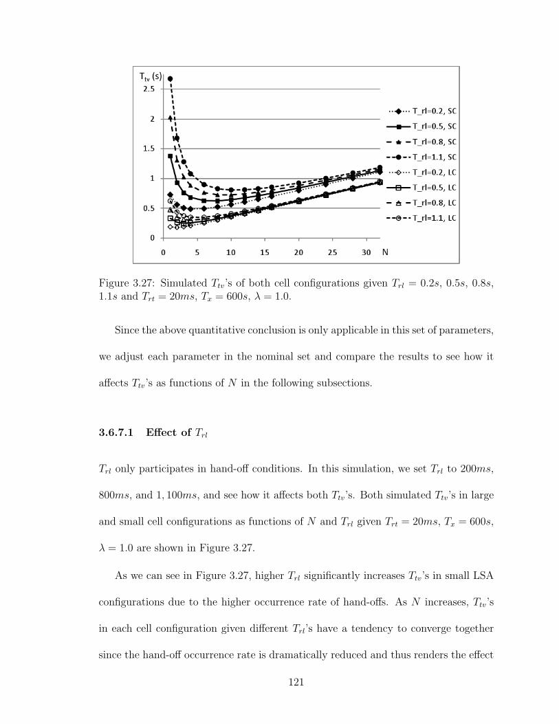
Figure 3.27: Simulated Ttv’s of both cell configurations given Trl = 0.2s, 0.5s, 0.8s,1.1s and Trt = 20ms, Tx = 600s, λ = 1.0.
Since the above quantitative conclusion is only applicable in this set of parameters,
we adjust each parameter in the nominal set and compare the results to see how it
affects Ttv’s as functions of N in the following subsections.
3.6.7.1 Effect of Trl
Trl only participates in hand-off conditions. In this simulation, we set Trl to 200ms,
800ms, and 1, 100ms, and see how it affects both Ttv’s. Both simulated Ttv’s in large
and small cell configurations as functions of N and Trl given Trt = 20ms, Tx = 600s,
λ = 1.0 are shown in Figure 3.27.
As we can see in Figure 3.27, higher Trl significantly increases Ttv’s in small LSA
configurations due to the higher occurrence rate of hand-offs. As N increases, Ttv’s
in each cell configuration given different Trl’s have a tendency to converge together
since the hand-off occurrence rate is dramatically reduced and thus renders the effect
121

Figure 3.28: Simulated Ttv’s of both cell configurations given Trt = 20ms, 40ms,60ms and Trl = 500ms, Tx = 600s, λ = 1.0.
of Trl insignificant. In the large cell configuration, Ttv’s converge more significantly
and earlier due to the extremely low hand-off occurrence rate.
3.6.7.2 Effect of Trt
Higher Trt amplifies the influence of transmission distance. The simulated Ttv’s in
both cell configurations as functions of N and Trt given Trl = 0.5s, Tx = 600s,
λ = 1.0 are shown in Figure 3.28.
Figure 3.28 shows the comparison of Ttv’s of both cell configurations as functions
of N given Trt = 20ms, 40ms, and 60ms. Besides the resemblance in shape to
the counterpart in the previous section, we can also notice that Trt is a more decisive
factor for the large cell configuration’s performance due to the low hand-off occurrence
rate and the long average communication distance in each LSA. Even N = 1 can be
preferable if Trt is greater than 60ms in the large cell configuration.
122

Figure 3.29: Simulated Ttv of both cell configurations given Tx = 300s, 600s, 900s,1, 200s and Trt = 20ms, Trl = 0.5s, λ = 1.0.
3.6.7.3 Effect of Tx
Tx only affects the cost brought by hand-offs. A higher Tx may mean a larger snapshot
file, a longer hand-off initialization time, or a longer queuing delay. How Tx affects
Ttv is represented in Figure 3.29.
Similar to the counterpart in the previous section, Ttv’s of each cell configuration
as functions of N given different Tx’s are virtually parallel for high N to each other
and show very little tendency to converge as N increases. However, slightly higher
optimal N brought by higher Tx in both configurations is still observable.
3.6.7.4 Effect of λ
Although we have shown that user input rate λ was not a relevant parameter in the
previous section, we still simulate Ttv’s as functions of N given different user input
rates λ in Mobius County. We again confirm that the property doesn’t change in the
123

UMTS rural vehicular mobility model.
However, we should keep in mind that the user experience depends more on the
interactivity of the application software than on the absolute response latency.
3.7 Summary
In this chapter, we have first proposed a geographically distributed server arrange-
ment and a hand-off protocol for application virtualization services for mobile users.
We have also proposed two analyses to evaluate the impact and the benefit of uti-
lizing the proposed hand-off protocol. And we verify the estimators of probability
of a user crossing the borderline by the Monte Carlo experiments and evaluate the
accuracies and limitations of both approaches. After going through the quantitative
approaches to compare different server-user configurations, we find out the factors
which should be taken into consideration when a service provider plans to launch
virtual application services or even virtual desktop services on mobile devices. If they
analyze the user behaviors and the application’s runtime properties and conclude that
their users rarely move, or only move at a low speed, or the data volume required to
recreate the runtime environment is relatively small, it is more likely to improve the
performance by geographically deploying more servers to cover the whole service area
and implement the proposed hand-off protocol. On the other hand, should one or
more factors induce a very high hand-off count or overhead, the conventional single
server configuration would be preferred. In the following two chapters, we proposed
Mobius City and Mobius County, which are based on the original UMTS urban and
124
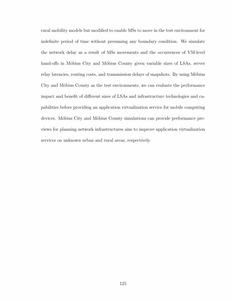
rural mobility models but modified to enable MSs to move in the test environment for
indefinite period of time without presuming any boundary condition. We simulate
the network delay as a result of MSs movements and the occurrences of VM-level
hand-offs in Mobius City and Mobius County given variable sizes of LSAs, server
relay latencies, routing costs, and transmission delays of snapshots. By using Mobius
City and Mobius County as the test environments, we can evaluate the performance
impact and benefit of different sizes of LSAs and infrastructure technologies and ca-
pabilities before providing an application virtualization service for mobile computing
devices. Mobius City and Mobius County simulations can provide performance pre-
views for planning network infrastructures aim to improve application virtualization
services on unknown urban and rural areas, respectively.
125

126

Chapter 4
Conclusion and Future Work
4.1 Summary
Virtualization technologies have significantly reshaped our computing paradigm. We
used to have to manage, execute, and interact with an application program physically
at the same place. Now we can manage, execute, and interact with them wherever it
is convenient by introducing application virtualization.
However, geographical separation is always playing an important role with regard
to the performance. Application virtualization technologies only make the geograph-
ical separation of software management, execution, and usage possible rather than
guarantee the user experience. In spite of the proliferation of high-speed commu-
nication technologies, exchanging information over the Internet still takes hundreds
or thousands times more than it does in a local bus. Therefore, efficiently dealing
with information exchange between remote and local ends is one of the keys to bring
virtualization technologies to the users who have been used to the responsive and
127

high-performance computers for long.
In this dissertation, we proposed several architectures and algorithms to improve
the current application virtualization technologies in performance. Therefore, we
can enjoy the benefits of application virtualization, such as better serviceability and
compatibility, without compromising too much in performance.
Application virtualization technologies can be implemented based on two con-
cepts. Both implementation concepts are completing each other in different scenarios
and applications, rather than competing with each other. The application streaming
concept is more feasible to introduce virtualization technologies for highly interactive
application software running on high performance client machine, such as contem-
porary personal computers, while the browser based concept can help bringing the
benefits of compatibility and centralized management to handheld mobile computing
devices with lower processing power. We proposed architectures and algorithms to
improve application virtualizations of both concepts.
We developed a novel architecture for virtual computing based on the applica-
tion streaming concept. The proposed architecture combines the merits of the known
methods: (1) storing application software and general operating system components
at the server side to reduce the platform incompatibility and inconsistency, (2) pro-
viding an option to store personal data at the client or server side, which allows the
users who concern about the security and privacy to maintain the control of own data
and files, (3) running the application software on the client side locally to optimize
the performance, (4) prefetching VM pages based on a probability model to mini-
mize the startup and on-demand page delivery delays. We also proposed a feasibility
128
analysis to outline the information required by the prefetch system, an algorithm to
efficiently build a 2-level hierarchical LUT to better manage the probability model,
and an improved hash scheme based on Pearson hashing to implement efficient lookup
without using expensive CAM.
For the browser based concept virtualization, the most prominent challenge is the
long interaction delay between the client and the server sides due to the long commu-
nication distance. We proposed a distributed infrastructure configuration to mitigate
this problem and a hand-off protocol to deal with the user mobility. To figure out
the condition where the performance gain brought by the proposed configuration out-
weighs the loss introduced by the proposed hand-off protocol, we proposed analytical
and empirical performance estimations, where the latter ones are based on the UMTS
mobility model.
The optimal framework of application virtualization has not been thoroughly in-
vestigated yet and performance is merely one of the many concerns raised when shift-
ing an IT environment from a traditional to a virtualized paradigm. For example,
with an application streaming architecture, sooner or later a user can obtain a full
copy of the executable of the software he/she subscribes to in the local storage. If we
do not explore a way to prevent it, the application streaming service will be an easy
subject of piracy and abuse. Therefore, efficiently delivering and making VM pages
available on the client side is only one half of the solution with regard to a real world,
pay-per-use SaaS. We also have to make the VM pages unavailable on the client side
at some time to encourage the subscribers to keep paying for the service.
Availability is another dimension of application virtualization frameworks. The
129

proposed distributed infrastructure configuration in fact has a great potential on
service availability. Although modern data centers have some capability to sustain
short power outages, they are still very vulnerable to long term ones. Since most
outages and failures only take place locally, the distributed nature of the proposed
configuration enables the nearby healthy servers to take over the workload of a failed
one and continue providing application virtualization services with a proper designed
mechanism.
Furthermore, the feasibility analysis prefetch is not only applicable in our appli-
cation virtualization framework. The derivation can also help design any prefetch
systems in terms of information theory. The proposed hash scheme can be used on
any kind of fast data lookup application as well.
4.2 Future Work
In Part 1, we improved the performance of application streaming using the prob-
abilistic characteristics of page usage. While the proposed approach improves the
start-up delay and the performance, we have not addressed the issue of controlling
the code block sequence, when the user behaviors change in real-time generating an
unacceptable rate of misses. In the future, we will investigate the use of information
associated with the misses to adapt the code block sequence in real-time.
The proposed architecture is the foundation of an application virtualization frame-
work. Many other components still need to be designed in the future to make it avail-
able as a software design framework. Furthermore, the impact on power consumption
130

on both server and client sides is currently not considered and will be investigated in
the future.
The proposed information gain analysis can also be applied on prefetch systems in
different level of general computing. If we design a separate data stream supplied as
reference to boost prefetch hit rate, the compilation of the reference data stream can
be compiled according to a static information analysis algorithm following a similar
concept.
As other hashing schemes, the proposed improvement on Pearson hashing can be
applied on many fields other than data structure management. For example, since
the proposed hashing scheme uses two tables instead of one and has lower collision
rate, it could be more helpful in computer security than the original Pearson hashing.
This is also an opportunity for us to investigate in the future.
In Part 2, we employ deterministic infrastructure delay parameters and a simple
usage model to evaluate the performance. We will introduce more sophisticated usage
and infrastructure delay model to facilitate more precise mobile application virtual-
ization service simulations. Furthermore, besides the benefit of lowering the average
response latency, the distributed application virtualization service configuration and
the hand-off protocol can also be applied to load balancing and fault tolerance for bet-
ter resource management and service robustness. We will investigate these potential
applications in the future as well.
131

Bibliography
[1] Chung-Ping Hung and Paul S. Min, “Probabilistic Approach to Network-
based Virtual Computing”, The 9th International Information and
Telecommunication Technologies Symposium (I2TS 2010), Dec. 2010, pp.
117-124.
[2] L. Peter Deutsch and B. W. Lampson, SDS 930 Time-sharing System
Preliminary Reference Manual, Doc. 30.10.10, Project Genie, Univ. Cal.
at Berkeley, April 1965.
[3] Michael Price, “The Paradox of Security in Virtual Environments”, Com-
puter Magazine, Vol. 41, Issue 11, Nov. 2008, pp. 22-28.
[4] Joeng Kim et al., “An Application Streaming Service for Mobile Handheld
Devices”, SCC’06 IEEE International Conference on Services Computing,
Sept. 2006, pp. 323-326.
[5] Philip Winslow et al., “Desktop Virtualization Comes Of Age”, Credit
Suisse, Nov. 26, 2007.
132
[6] Mendel Rosenblum and Tal Garfinkel, “Virtual Machine Monitors: Cur-
rent Technology and Future Trends”, Computer Magazine, Volume 38,
Issue 5, May 2005, pp. 39-47.
[7] Rich Uhlig et al., “Intel Virtualization Technology”, Computer Magazine,
Volume 38, Issue 5, May 2005, pp. 48-56.
[8] S.J. Vaughan-Nichols, “New Approach to Virtualization Is a Lightweight”,
Computer Magazine, Volume 39, Issue 11, November 2006, pp. 12-14.
[9] VMware Inc., “VMware ThinApp Agentless Application Virtualization
Overview,”.
[10] EMA Report: “AppStream: Transforming On-Premise Software for SaaS
Delivery - without Reengineering”
[11] Peter M. Chen and Brian D. Noble, “When Virtual Is Better Than Real”,
Proceedings 8th Workshop Hot Topics in Operating Systems, IEEE CS
Press, 20-22 May 2001, pp. 133-138.
[12] Sunwook Kim et al., “On-demand Software Streaming System for Embed-
ded System”, WiCOM 2006 International Conference on Wireless Com-
munications, Networking and Mobile Computing, 22-24 Sept. 2006, pp.
1-4.
[13] Ana Fernandez Vilas et al., “Providing Web Services over DVB-H: Mobile
Web Services”, IEEE Transactions on Consumer Electronics, Vol. 53, No,
2, May 2007, pp. 644-652.
133

[14] Godmar Back and Wilson C. Hsieh, “The KaffeOS Java Runtime System”,
ACM Transactions on Programming Languages and Systems (TOPLAS),
Volume 27, Issue 4, July 2005, pp. 583-630.
[15] Zhimei Jiang and Leonard Kleinrock, “An Adaptive Network Prefetch
Scheme”, IEEE Journal on Selected Areas in Communications, Vol. 16,
No. 3, April 1998, pp. 358-368.
[16] Themistoklis Palpanas and Alberto Mendelzon, “Web Prefetching Us-
ing Partial Match Prediction”, Proceedings of the 4th International Web
Caching Workshop (WCW99), San Diego, CA, 1999.
[17] Doug Joseph and Dirk Grunwald, “Prefetching using Markov Predictors”,
Proceedings of the 24th Annual International Symposium on Computer
Architecture (ISCA’97), Denver, CO, 1997, pp. 252-263.
[18] Kyle J. Nesbit and James E. Smith, “Data Cahe Prefetching Using a
Global History Buffer”, Proceedings of the 10th International Symposium
on High Performance Computer Architecture (HPCA’04), 2004, pp. 96-
105.
[19] Jian-Hong Lin et al., “A NOR Emulation Strategy over NAND Flash
Memory”, 13th IEEE International Conference on Embedded and Real-
Time Computing Systems and Applications (RTCSA 2007), 2007, pp. 95-
102.
134

[20] G. Edward Suh et al., “Job-Speculative Prefetching: Eliminating Page
Faults From Context Switches in Time-Sharing Systems”, Computation
Structure Group, Massachusetts Institute of Technology, 2001.
[21] Derek Chiou et al., “Scheduler-Based Prefetching for Multilevel Memo-
ries”, Computation Structures Group, Massachusetts Institute of Tech-
nology, 2001.
[22] Stanislav A. Belogolov et al., “Scheduler-Assisted Prefetching: Efficient
Demand Paging for Embedded Systems”, The 14th IEEE International
Conference on Embedded and Real-Time Computing Systems and Appli-
cations (RTCSA 2008), 2008, pp. 111-119.
[23] Mark Russinovich, “Inside the Windows Vista Kernel: Part 2”, TechNet
Magazine, March 2007, pp. 24-32.
[24] J.R Quinlan, “Induction of Decision Trees”, Machine Learning, No. 1,
1986, pp. 81-106.
[25] J.R. Quinlan, “Decision Trees and Instance-Based Classifiers”, The Com-
puter Science and Engineering Handbook, 1997, pp. 521-535.
[26] Peter K. Pearson, “Fast Hashing of Variable-length Text Strings”, Com-
munications of the ACM, Vol. 33, No. 6, June 1990, pp. 677-680.
[27] Apple Inc., “App Store Review Guidelines for iOS apps”, 2.7 and 2.8,
http://developer.apple.com/appstore/guidelines.html, Retrieved 9 Sep.
2010.
135

[28] Google Inc., “Android Market Developer Distribution Agreement”, 4.5,
http://www.android.com/us/developer-distribution-agreement.html, Re-
trieved 22 Feb. 2011.
[29] VMware Inc., “VMware MVP (Mobile Virtualization Platform)”,
http://www.vmware.com/products/mobile/overview.html, Retreived 7
Aug. 2011.
[30] Chung-Ping Hung and Paul S. Min, “Infrastructure Arrangement for Ap-
plication Virtualization Services”, The 9th International Information and
Telecommunication Technologies Symposium (I2TS 2010), 2010, pp. 78-
85.
[31] Chung-Ping Hung and Paul S. Min, “Service area optimization for applica-
tion virtualization using UMTS mobility model”, International Conference
on Internet Computing (ICOMP 2011), 2011, pp. 128-134.
[32] Chung-Ping Hung and Paul S. Min, “Performance evaluation of dis-
tributed application virtualization services using the UMTS mobility
model”, The First International Conference on Mobile Services, Re-
sources, and Users (MOBILITY 2011), 2011, pp. 83-89.
[33] Marcin Bienkowski et al., “Competitive Analysis for Service Migration in
VNets”, in Proc. 2nd ACM SIGCOMM Workshop on Virtualized Infras-
tructure Systems and Architectures, 2010, pp. 17-24.
136

[34] Dushyant Arora et al., “On the benefit of virtualization: strategies for
flexible server allocation”, Hot-ICE’11 Proceedings of the 11th USENIX
conference on Hot topics in management of internet, cloud, and enterprise
networks and services, 2011.
[35] VMware Inc., “Virtual Desktop Infrastructure”.
[36] R. Buckminster Fuller, Synergetics: explorations in the geometry of think-
ing, Macmillan Publishing Company, 1975.
[37] ETSI. “Universal Mobile Telecommunications System (UMTS); selection
procedures for the choice of radio transmission technologies of the UMTS
(UMTS 30.03, version 3.2.0)”. Technical report, European Telecomminca-
tion Standards Institute, Apr. 1998.
[38] H. Boche and E. Jugl, “Extension of ETSI’s Mobility Models for UMTS in
Order to Get More Realistic Results”, Proc. UMTS Workshop, Gunzburg,
Germany, Nov. 1998.
137
Top Related
Copyright © 2022 FDOKUMEN

