www.elsevier.com/locate/agee

Agriculture, Ecosystems and Environment 122 (2007) 233–242

Impact of elevated CO2 and temperature on rice yield and methods

of adaptation as evaluated by crop simulation studies

P. Krishnan a,*, D.K. Swain b, B. Chandra Bhaskar b, S.K. Nayak a, R.N. Dash b

a Division of Biochemistry, Plant Physiology and Environmental Sciences, Central Rice Research Institute, Cuttack 753006, Indiab Division of Soil Science and Microbiology, Central Rice Research Institute, Cuttack 753006, India

Received 7 February 2006; received in revised form 20 December 2006; accepted 19 January 2007

Available online 6 March 2007

Abstract

Impact of elevated CO2 and temperature on rice yield in eastern India was simulated by using the ORYZA1 and the INFOCROP rice

models. The crop and weather data from 10 different sites, viz., Bhubaneswar, Chinsurah, Cuttack, Faizabad, Jabalpur, Jorhat, Kalyani, Pusa,

Raipur and Ranchi, which differed significantly in their geographical and climatological factors, were used in these two models. For every

1 8C increase in temperature, ORYZA1 and INFOCROP rice models predicted average yield changes of �7.20 and �6.66%, respectively, at

the current level of CO2 (380 ppm). But increases in the CO2 concentration up to 700 ppm led to the average yield increases of about 30.73%

by ORYZA1 and 56.37% by INFOCROP rice. When temperature was increased by about +4 8C above the ambient level, the differences in the

responses by the two models became remarkably small. For the GDFL, GISS and UKMO scenarios, ORYZA1 predicted the yield changes of

�7.63, �9.38 and �15.86%, respectively, while INFOCROP predicted changes of �9.02, �11.30 and �21.35%. There were considerable

differences in the yield predictions for individual sites, with declining trend for Cuttack and Bhubaneswar but an increasing trend for Jorhat.

These differences in yield predictions were mainly attributed to the sterility of rice spikelets at higher temperatures. Results suggest that the

limitations on rice yield imposed by high CO2 and temperature can be mitigated, at least in part, by altering the sowing time and the selection

of genotypes that possess higher fertility of spikelets at high temperatures.

# 2007 Elsevier B.V. All rights reserved.

Keywords: Climate change; CO2; INFOCROP; ORYZA; Oryza sativa L.; Simulation; Temperature; Yield

1. Introduction

The climatic variability and the predicted climatic changes

are of major concern to the rice crop scientists because of

Abbreviations: BVP, Basic Vegetative Phase; DLAI, Death Rate of

Leaf Area Index; FACE, Free Air Concentration Enrichment; GCMs,

General Circulation Models; GFDL, General Fluid Dynamics Laboratory;

GFP, Grain Filling Phase; GISS, Goddard Institute of Space Studies; GLAI,

Leaf Area Growth Rate; IPCC, Intergovernmental Panel on Climate

Change; LAI, Leaf Area Index; NATP, National Agricultural Technology

Project; PFP, Panicle Formation Phase; PLTR, Net loss of LAI due to

transplanting; PSP, Photoperiod-Sensitive Phase; RLAI, Net Leaf Area

Growth Rate; RUE, Radiation Use Efficiency; RWLVG, Increment in Leaf

Weight; SLA, Specific Leaf Area; SUBLAI, LAI is simulated in the

subroutine SUBLAI; UKMO, United Kingdom Meteorological Office

* Corresponding author.

E-mail address: prameelakrishnan@yahoo.com (P. Krishnan).

0167-8809/$ – see front matter # 2007 Elsevier B.V. All rights reserved.

doi:10.1016/j.agee.2007.01.019

their potential threat to rice productivity and the associated

impact on the socioeconomic structure of many rice-growing

countries. Among the global atmospheric changes, the incre-

asing concentrations of greenhouse gases such as CO2 may

have significant effect on rice productivity due to increase in

both the average surface temperature and the amount of CO2

available for photosynthesis (Aggarwal, 2003). In the absence

of temperature increase, many studies have shown that the net

effect of doubling of CO2 was increase in the yield of rice

(Kim et al., 2003). It becomes necessary to assess the effects of

potential interactive changes of CO2 and temperature in order

to determine the future agricultural strategies that would

maintain higher rice productivity.

The simulations by different models and many field

experiments have shown the potential impact of climatic

change and the variability in rice productivity (Baker et al.,

P. Krishnan et al. / Agriculture, Ecosystems and Environment 122 (2007) 233–242234

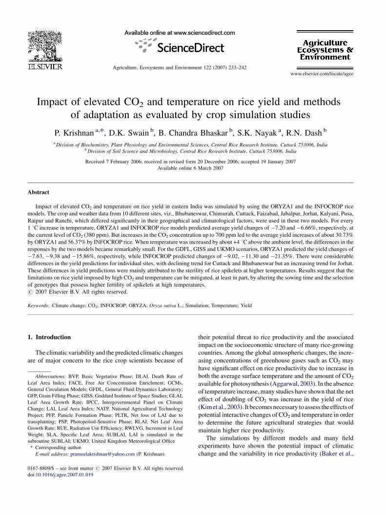
Fig. 1. Comparison of yield simulated by ORYZA1 and INFOCROP rice.

1992b; Peng et al., 2004; Kim et al., 2003). The modeling

studies from Bangladesh (Karim et al., 1994), Japan (Horie

et al., 2000), China (Bachelet et al., 1995) and India (Mall

and Aggarwal, 2002) reported the country-wise variations in

rice production, anticipated due to the climatic changes. The

simulated yields increased when temperature increases were

small, but declined when the decadal temperature increase

was more than 0.8 8C, with the greatest decline in crop

yields occurring between the latitudes of 108 and 358N.

Similar results were obtained by Penning de Vries (1993).

Many uncertainties exist in modeling studies, partly due

to the quality of the predictions by the models, from the use

of limited sites for which historical weather data are

available, due to the quality of the crop simulation models,

especially when applied under the rain-fed conditions

(Bachelet et al., 1995), and due to the quality of the climate

models used to predict future weather scenarios. These

uncertainties may be reduced only when a large number of

scenarios for different locations are compared and evaluated.

In order to overcome the predicted limitations for rice

production in the future, there is also a need to identify and

evaluate the suitable agronomic practices such as altered

sowing date and selection of improved varieties with

increased spikelet fertility at high temperature and other

useful traits.

Attempts have been made earlier to assess the general

effects of global environmental changes on rice yield using

simulation models, but little attention has been given to the

potential interactive effects between high temperature and

increasing CO2 levels. Lal et al. (1998) used the CERES rice

and predicted a 20% decline in rice yields in the

northwestern India due to elevated CO2 and temperature.

Eastern India accounts for about 63% (26.5 million ha) of

the total rice-growing area in India. The rice ecosystems in

these regions show characteristic differences with respect to

the environmental factors as well as the cultural practices.

There is an urgent need to characterize the impact of future

climatic changes on rice yield in these regions for sustaining

the productivity. The present paper discusses the outcomes

of two rice growth simulation models, ORYZA and

INFOCROP rice, when applied to different rice-growing

sites in the eastern India for studying the potential interactive

effects between high temperature and increasing CO2 levels

and for the different thermal climate change scenarios.

2. Materials and methods

Two popular models of rice growth ORYZA1 (Kropff

et al., 1994) and INFOCROP rice (Aggarwal et al., 2006) are

used in this study. Prior to their use, both were evaluated

and compared (Fig. 1) and then these crop models were

calibrated for the indica variety IR 36 at all sites. In general,

the two models differ in the manner in which dry matter

production and partition, leaf area development, and pheno-

logical development are calculated. ORYZA1 calculates dry

matter production as a function of light, CO2 and temperature

by considering photosynthetic processes at the leaf level and

integrating these over the canopy to obtain crop-level values.

Respiration is also modeled explicitly as a function of

temperature and partitioning of dry matter is according to

phenology-dependent functions. Thus, ORYZA calculates

dry matter production as a function of gross canopy

photosynthesis, depending on the detailed calculations of

the distribution of light within the canopies, the radiation

absorbed by the canopy and photosynthesis light response

curve of leaves. Growth and maintenance respiration are

calculated as a function of tissue N content, temperature

and crop-specific coefficients. This methodology, although

yields very accurate results, poses practical difficulties

because of its requirement for detailed and careful measure-

ments (Kropff et al., 1994). The INFOCROP model, however,

uses a simpler radiation use efficiency (RUE) relationship

between intercepted solar radiation and growth, in which

respiration is implicit. CO2 effects are accounted for by using

a curvilinear function relating RUE to CO2 concentration.

Temperature is assumed not to affect RUE. More or less

similar results can be obtained under normal radiation

situations by calculating the net dry matter production as a

function of RUE. Pre-determined values of RUE were input in

the model as a function of crop/cultivar (RUEMAX), and

RUE was further modified by the development stage

(Aggarwal et al., 2004).

The rice-growing regions included for the present study lie

in eastern India, and these sites (Bhubaneswar, Chinsurah,

Cuttack, Faizabad, Jabalpur, Jorhat, Kalyani, Pusa, Raipur

and Ranchi), which are geographically apart at varied

altitudes ranging from 7.8 to 86.56 m above mean sea level,

show characteristic features with respect to the weather and

crop factors. The crop parameters included in the study were

obtained from the field experiments conducted at these sites

under National Agricultural Technology Project (NATP)

RRPS 25 during 2001–2003 (Table 1).

The input parameters used for the two models are given in

Table 2a (parameters such as varietal data, soil data and

weather data), Table 2b (physical and chemical properties of

P. Krishnan et al. / Agriculture, Ecosystems and Environment 122 (2007) 233–242 235

Table 1

Sites and institutes where the field observation and weather data were

collected

Sites Institutes

Bhubaneswar Orissa University of Agriculture & Technology (OUAT)

Chinsurah Rice Research Station (RRS)

Cuttack Central Rice Research Institute (CRRI)

Faizabad Narendra Deva University of Agriculture &

Technology (NDUAT)

Jabalpur Jawaharlal Nehru Krishi Vishwa Vidyalaya (JNKVV)

Jorhat Assam Agricultural University (AAU)

Kalyani Bidan Chandra Krishi Viswa Vidyalaya (BCKV)

Pusa Rajendra Agricultural University (RAU)

Raipur Indira Gandhi Agricultural University (IGAU)

Ranchi Birsa Agricultural University (BAU)

Indian Meteorological Department (IMD),

Pune (weather data)

soils) and Table 2c (geographical information). The weather

data containing measurements of sunshine hours, tempera-

ture and rainfall from all these sites were used as the baseline

data for input into these crop models. Later, the simulations

Table 2a

Combined input parameters for both the models used

Varietal data S

1. Base temperature for sowing to germination 1

2. Thermal time for sowing to germination 2

3. Base temperature for germination to 50% flowering 3

4. Thermal time for germination to 50% flowering 4

5. Base temperature for 50% flowering to physiological maturity 5

6. Thermal time for 50% flowering to physiological maturity 6

7. Optimal temperature 7

8. Maximum temperature 8

9. Sensitivity to photoperiod 9

10. Relative growth rate of leaf area 1

11. Specific Leaf Area 1

12. Extinction coefficient of leaves at flowering 1

13. Radiation Use Efficiency 1

14. Root growth rate

15. Index of greenness of leaves

16. Sensitivity of crop to flooding

17. Index of N fixation

18. Slope of storage organ number/m2 to dry matter during storage

organ formation stage

19. Potential storage organ weight at maximum temperature

20. Nitrogen content of storage organ

21. Sensitivity of storage organ setting to low temperature

22. Sensitivity of storage organ setting to high temperature

Table 2b

Model inputs of physical and chemical properties of soil at different locations

Soil properties Bhubaneswar Kalyani Faizabad Ranchi

Texture Sandy clay loam Sandy clay loam Loam Loam

B.D.a (g/cc) 1.35 1.45 1.3 1.41

O.C.b (%) 0.73 0.51 0.3 0.68

Total N (%) 0.07 0.04

Available N (kg/ha) 128.4 355

a B.D., bulk density.b O.C., organic carbon.

were made for the main rice-growing season for each of

these sites. Generally, the dates of sowing and transplanting

were supplied along with the weather data.

2.1. Climate change scenarios

For each of these rice-growing regions, the potential yield

of rice was simulated under 30 different combinations of

CO2 and temperature, including with the ‘fixed increment’

changes in CO2 (380, 400, 500, 600 and 700 ppm) and

temperature (ambient, +1, +2, +3, +4 and +5 8C) individu-

ally, and with all the combinations of these levels of CO2 and

temperature. The actual daily weather data, collected for

three consecutive years from each of these sites were used

for simulation. For temperature changes, the daily weather

data from each site were exported to Excel spread sheets and

then the daily maximum and minimum temperatures were

increased by 1–5 8C individually. Later, the modified

weather data were used as the inputs for ORYZA1. In case

of INFOCROP, for a given daily weather data, the climate

oil data Weather data (daily data)

. Soil type 1. Maximum and minimum

temperatures

. Soil texture 2. Relative humidity

. pH of soil 3. Sun shine hours

. EC 4. Precipitation

. Sand %

. Silt %

. Clay %

. Saturation fraction

. Field capacity

0. Wilting point

1. Saturated hydraulic conductivity

2. Bulk density

3. Organic carbon

Pusa Raipur Jabalpur Jorhat Cuttack

Sandy clay loam Silt Clayey Sandy clay loam Sandy loam

1.3 1.23 1.34 1.48 1.4

0.57 0.54 0.69 0.67 0.47

– 0.07

258.6 – 267 265.8

P. Krishnan et al. / Agriculture, Ecosystems and Environment 122 (2007) 233–242236

Table 2c

Model inputs of geographical information of different locations

Soil properties Bhubaneswar Kalyani Faizabad Ranchi Pusa Raipur Jabalpur Jorhat Cuttack

Latitude 208140N 228570N 228870N 238170N 22850N 258590N 238090N 26880N 208300NLongitude 858520E 888210E 88840E 858190E 868E 85840E 798580E 95850 E 868EAltitude (m) 25.9 7.8 8.62 625 23 51.84 411 86.56 23

change scenarios were specified as +1 to +5 8C for

temperatures and the percent changes in precipitation.

The inbuilt weather generator of that model generated the

modified daily weather data accordingly, and these data were

used as the daily weather inputs. The climate change

scenarios under different levels of CO2 were applied by

changing the ambient CO2 concentration parameter in these

two models.

Besides, the outputs from the climate models were used

in combination with these crop models. The coarse grid from

each GCM was interpolated using a four point inverse-

distance-squared algorithm to a 0.58 latitude � 0.58 long-

itude grid using a raster-based Geographical Information

Systems (GIS) software package. Scenarios were produced

by applying ratios of precipitation or differences in tempe-

rature predicted for the 2 � CO2 and 1 � CO2 simulation to

the baseline present climate data set for different sites

(Mathews and Wassmann, 2003). The important features of

three General Circulation Models (GCMs) used such as

the General Fluid Dynamics Laboratory (GFDL) Model,

Goddard Institute of Space Studies (GISS) model and the

United Kingdom Meteorological Office (UKMO) model are

provided in Table 3.

The GCM scenarios were produced by applying the ratios

of precipitation or differences in temperature predicted for

the 1 � CO2 (380 ppm) and 2 � CO2 (760 ppm) simulations

to the baseline daily weather data set. The changes between

1 � CO2 and 2 � CO2 conditions were representative of the

differences between the present and the future climate

scenarios following an equivalent doubling of CO2.

2.2. Simulation

For the simulation analysis, only runs that terminated

normally or by crop deaths as a result of temperature were

included. The relative yield changes under the scenarios,

referred to yields predicted for the current climate, were

used in the analysis rather than absolute yields. To provide

an estimate of the overall effect of climate change on rice

production under the three GCMs scenarios, the average

Table 3

The major features of the General Circulation Models used in this study

GFDL

Source laboratory Geophysical Fluid Dynamics

Laboratory

Base 1 � CO2 (ppm) 380

Change in global temperature (8C) +4.0

Change in global precipitation (%) 8

relative increase predicted for each site was weighed by its

current production observed in the field trials of an earlier

study (Annual Report of NATP RRPS 25, 2002–2003). The

differences in the production capacities among these sites

were evaluated.

3. Results

3.1. Effect of temperature and CO2 levels at fixed

increments on yields

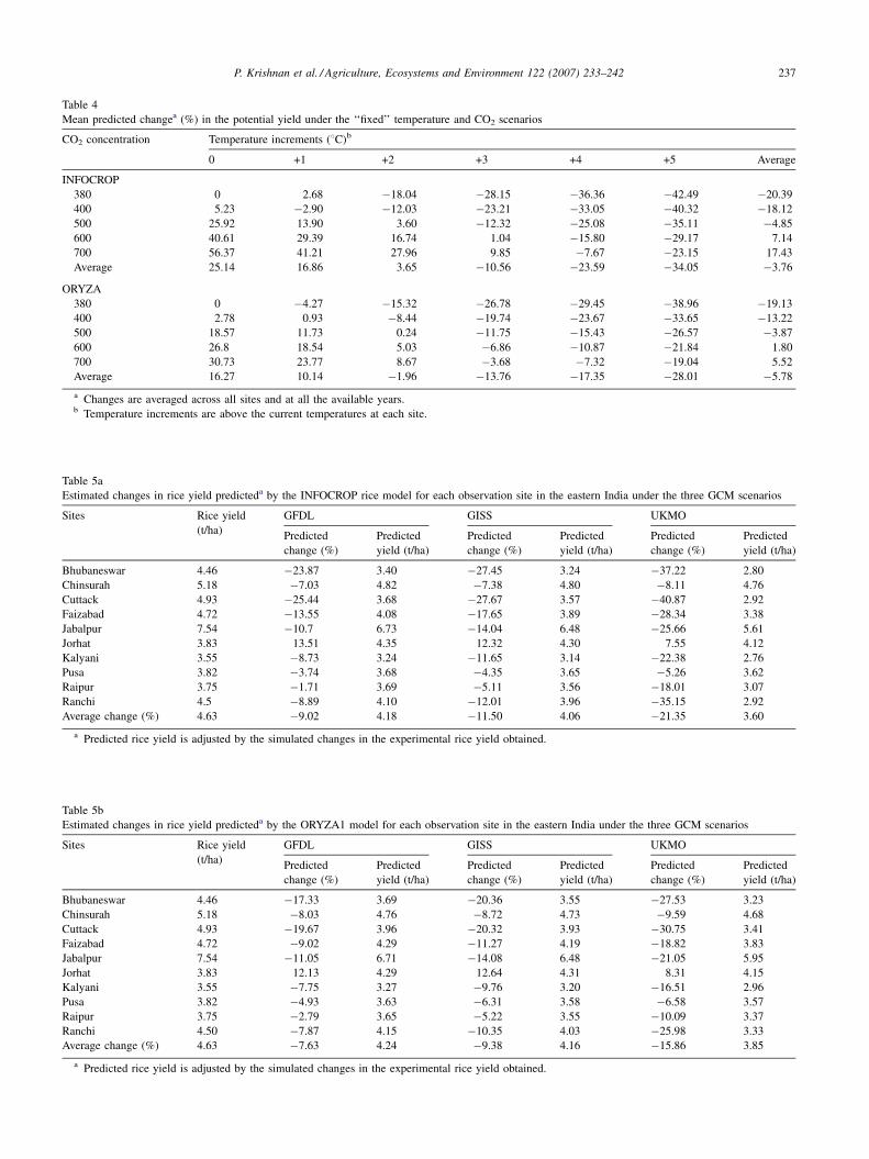
At all the CO2 levels tested (380, 400, 500, 600 and

700 ppm), both the models predicted the declining yields of

rice due to an increase in temperature. On the contrary, an

increase in CO2 level at any particular temperature increased

the rice yields (Table 4). At the current level of CO2

(considered at 380 ppm), ORYZA predicted a mean change

of �7.20% in yields for every 1 8C increase in temperature,

while INFOCROP predicted �6.66%. But increasing CO2

concentration (700 ppm) resulted in increases of 30.37 and

56.37% in yield by ORYZA and INFOCROP, respectively.

However, with temperature increase of +4 8C above

ambient, the differences in the yield predictions by the

two models became remarkably small (Table 4).

3.2. Effect of predicted GCM scenarios on rice yields

The predicted changes in overall production for each site

under different climate scenarios using the two crop models

are provided in Tables 5a and 5b. In general, the ORYZA

model suggested the decreases of �7.63, �9.38 and

�15.86% in yield for the GDFL, GISS and UKMO

scenarios, respectively. For the corresponding scenarios,

INFOCROP indicated larger reductions at �9.02, �11.30

and �21.35%, respectively. When each site was analysed

individually under three GISS and UKMO scenarios, almost

all the sites except one showed the declining trend in yields.

The decreases in the yield of rice, when the mean of the

corresponding values in Tables 5a and 5b were considered,

GISS UKMO

Goddard Institute for

Space Studies

United Kingdom

Meteorological Office

380 380

+4.2 +5.2

11 15

P. Krishnan et al. / Agriculture, Ecosystems and Environment 122 (2007) 233–242 237

Table 4

Mean predicted changea (%) in the potential yield under the ‘‘fixed’’ temperature and CO2 scenarios

CO2 concentration Temperature increments (8C)b

0 +1 +2 +3 +4 +5 Average

INFOCROP

380 0 2.68 �18.04 �28.15 �36.36 �42.49 �20.39

400 5.23 �2.90 �12.03 �23.21 �33.05 �40.32 �18.12

500 25.92 13.90 3.60 �12.32 �25.08 �35.11 �4.85

600 40.61 29.39 16.74 1.04 �15.80 �29.17 7.14

700 56.37 41.21 27.96 9.85 �7.67 �23.15 17.43

Average 25.14 16.86 3.65 �10.56 �23.59 �34.05 �3.76

ORYZA

380 0 �4.27 �15.32 �26.78 �29.45 �38.96 �19.13

400 2.78 0.93 �8.44 �19.74 �23.67 �33.65 �13.22

500 18.57 11.73 0.24 �11.75 �15.43 �26.57 �3.87

600 26.8 18.54 5.03 �6.86 �10.87 �21.84 1.80

700 30.73 23.77 8.67 �3.68 �7.32 �19.04 5.52

Average 16.27 10.14 �1.96 �13.76 �17.35 �28.01 �5.78

a Changes are averaged across all sites and at all the available years.b Temperature increments are above the current temperatures at each site.

Table 5a

Estimated changes in rice yield predicteda by the INFOCROP rice model for each observation site in the eastern India under the three GCM scenarios

Sites Rice yield

(t/ha)

GFDL GISS UKMO

Predicted

change (%)

Predicted

yield (t/ha)

Predicted

change (%)

Predicted

yield (t/ha)

Predicted

change (%)

Predicted

yield (t/ha)

Bhubaneswar 4.46 �23.87 3.40 �27.45 3.24 �37.22 2.80

Chinsurah 5.18 �7.03 4.82 �7.38 4.80 �8.11 4.76

Cuttack 4.93 �25.44 3.68 �27.67 3.57 �40.87 2.92

Faizabad 4.72 �13.55 4.08 �17.65 3.89 �28.34 3.38

Jabalpur 7.54 �10.7 6.73 �14.04 6.48 �25.66 5.61

Jorhat 3.83 13.51 4.35 12.32 4.30 7.55 4.12

Kalyani 3.55 �8.73 3.24 �11.65 3.14 �22.38 2.76

Pusa 3.82 �3.74 3.68 �4.35 3.65 �5.26 3.62

Raipur 3.75 �1.71 3.69 �5.11 3.56 �18.01 3.07

Ranchi 4.5 �8.89 4.10 �12.01 3.96 �35.15 2.92

Average change (%) 4.63 �9.02 4.18 �11.50 4.06 �21.35 3.60

a Predicted rice yield is adjusted by the simulated changes in the experimental rice yield obtained.

Table 5b

Estimated changes in rice yield predicteda by the ORYZA1 model for each observation site in the eastern India under the three GCM scenarios

Sites Rice yield

(t/ha)

GFDL GISS UKMO

Predicted

change (%)

Predicted

yield (t/ha)

Predicted

change (%)

Predicted

yield (t/ha)

Predicted

change (%)

Predicted

yield (t/ha)

Bhubaneswar 4.46 �17.33 3.69 �20.36 3.55 �27.53 3.23

Chinsurah 5.18 �8.03 4.76 �8.72 4.73 �9.59 4.68

Cuttack 4.93 �19.67 3.96 �20.32 3.93 �30.75 3.41

Faizabad 4.72 �9.02 4.29 �11.27 4.19 �18.82 3.83

Jabalpur 7.54 �11.05 6.71 �14.08 6.48 �21.05 5.95

Jorhat 3.83 12.13 4.29 12.64 4.31 8.31 4.15

Kalyani 3.55 �7.75 3.27 �9.76 3.20 �16.51 2.96

Pusa 3.82 �4.93 3.63 �6.31 3.58 �6.58 3.57

Raipur 3.75 �2.79 3.65 �5.22 3.55 �10.09 3.37

Ranchi 4.50 �7.87 4.15 �10.35 4.03 �25.98 3.33

Average change (%) 4.63 �7.63 4.24 �9.38 4.16 �15.86 3.85

a Predicted rice yield is adjusted by the simulated changes in the experimental rice yield obtained.

P. Krishnan et al. / Agriculture, Ecosystems and Environment 122 (2007) 233–242238

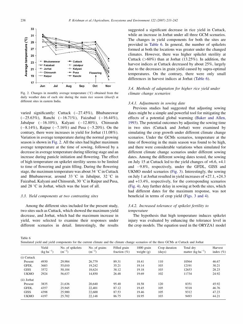
Fig. 2. Changes in monthly average temperature (8C) obtained from the

daily weather data of each site during the main rice season (kharif) at

different sites in eastern India.

varied significantly: Cuttack (�27.45%), Bhubaneswar

(�25.63%), Ranchi (�16.71%), Faizabad (�16.44%),

Jabalpur (�16.10%), Kalyani (�12.80%), Chinsurah

(�8.14%), Raipur (�7.16%) and Pusa (�5.20%). On the

contrary, there were increases in yield for Jorhat (11.08%).

Variation in average temperature during the normal growing

season is shown in Fig. 2. All the sites had higher maximum

average temperature at the time of sowing, followed by a

decrease in average temperature during tillering stage and an

increase during panicle initiation and flowering. The effect

of high temperature on spikelet sterility seems to be limited

to time of flowering and grain filling. During the flowering

stage, the maximum temperature was about 34 8C in Cuttack

and Bhubaneswar, around 33 8C in Jabalpur, 32 8C in

Faizabad, Kalyani and Chinsurah, 30 8C in Raipur and Pusa,

and 28 8C in Jorhat, which was the least of all.

3.3. Yield components at two contrasting sites

Among the different sites included for the present study,

two sites such as Cuttack, which showed the maximum yield

decrease, and Jorhat, which had the maximum increase in

yield, were selected to examine their responses under

different scenarios in detail. Interestingly, the results

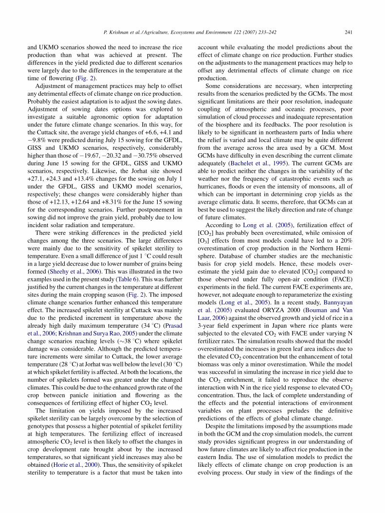
Table 6

Simulated yield and yield components for the current climate and the climate ch

Yield

(kg ha�1)

No. of spikelets

(m�2)

No. of grains

(m�2)

Filled grai

fraction (%

(i) Cuttack

Present 4930 29,984 26,779 89.31

GFDL 3683 55,010 19,242 35.21

GISS 3572 50,104 18,624 38.12

UKMO 2924 56,637 14,850 26.48

(ii) Jorhat

Present 3835 21,636 20,640 95.40

GFDL 4357 25,945 22,401 87.12

GISS 4398 25,900 22,600 87.53

UKMO 4197 25,702 22,148 86.75

suggested a significant decrease in rice yield in Cuttack,

while an increase in Jorhat under all three GCM scenarios.

The changes in yield components for both the sites are

provided in Table 6. In general, the number of spikelets

formed at both the locations was greater under the changed

climates. However, there was higher spikelet sterility at

Cuttack (>60%) than at Jorhat (13.25%). In addition, the

harvest indices at Cuttack decreased by about 25%, largely

due to the decreases in grain yield caused by supra-optimal

temperatures. On the contrary, there were only small

differences in harvest indices at Jorhat (Table 6).

3.4. Methods of adaptation for higher rice yield under

climate change scenarios

3.4.1. Adjustments in sowing date

Previous studies had suggested that adjusting sowing

dates might be a simple and powerful tool for mitigating the

effects of a potential global warming (Baker and Allen,

1993). The potential outcomes by adjusting the sowing time

in two sites (Cuttack and Jorhat) were examined by

simulating the crop growth under different climate change

scenarios. Under the GCMs scenarios, temperature at the

time of flowering in the main season was found to be high,

and there were considerable variations when simulated for

different climate change scenarios under different sowing

dates. Among the different sowing dates tested, the sowing

on July 15 at Cuttack led to the yield changes of +6.6, +4.1

and �9.8%, respectively, under the GFDL, GISS and

UKMO model scenarios (Fig. 3). Interestingly, the sowing

on July 1 at Jorhat resulted in yield increases of +27.1, +24.3

and +13.4%, respectively, for the corresponding scenarios

(Fig. 4). Any further delay in sowing at both the sites, which

had different dates for the maximum response, was not

beneficial in terms of crop yield (Figs. 3 and 4).

3.4.2. Increased tolerance of spikelet fertility to

temperature

The hypothesis that high temperature induces spikelet

injury was evaluated by enhancing the tolerance level in

the crop models. The equation used in the ORYZA1 model

ange scenarios of the three GCMs at Cuttack and Jorhat

n

)

1000 grain

weight (g)

Crop duration

(days)

Total dry

matter (kg ha�1)

Harvest

index (%)

18.41 110 10564 46.67

19.14 103 12191 30.21

19.18 103 12653 28.23

19.69 102 11734 24.92

18.58 120 8351 45.92

19.45 105 9318 46.76

19.46 105 9312 47.23

18.95 103 9493 44.21

P. Krishnan et al. / Agriculture, Ecosystems and Environment 122 (2007) 233–242 239

Fig. 3. Changes in yield (%) under the GCMs scenarios of the rice variety

IR 36 under different sowing dates grown during the kharif season at

Cuttack.

Fig. 5. Changes in yield (%) under the GCMs scenarios of the rice variety

IR 36 and IR 36 with improved temperature tolerance grown during the

kharif season at Cuttack.

to describe the response of spikelet fertility to temperature

is

d ¼ 100

½1þ e0:853ðTmax�TmpÞ�

where d is the fertility percentage, Tmax the average daily

maximum temperature (8C) during the flowering period and

Tmp the average daily maximum temperature (8C) at which

50% of the spikelets are fertile. For the indica variety, Tmp

had a value of 36.5. To simulate the possible effect of an

increase in tolerance of spikelet to high temperatures, it was

assumed that this response was shifted by 2 8C by increasing

the value of Tmp to 38.5 8C. This adaptation in the spikelet

trait was examined in Cuttack site. With the available

weather data for this site, and with a constant sowing date

of June 15, a comparative study using the ORYZA1 model

was made for the current climate and other GCM scenarios

as obtained by the GFDL, GISS and UKMO (Fig. 5). Under

the GCMs scenarios, temperature at the time of flowering for

the main season was already high. Without any temperature

Fig. 4. Changes in yield (%) under the GCMs scenarios of the rice variety

IR 36 under different sowing dates grown during the kharif season at Jorhat.

tolerance of the variety by not adjusting the value of Tmp,

large decreases in yield due to spikelet sterility were pre-

dicted. But with the adaptation of variety by improved

temperature tolerance of the spikelet, the yield increased

higher than that of the current scenario level, at about +10.7,

+13.6 and �8.4, respectively, under the GFDL, GISS and

UKMO model scenarios (Fig. 5).

4. Discussion

Both the crop simulation models predicted that any

increase in temperature at all the CO2 levels tested would

cause declines in yields but an increase in CO2 level at each

temperature increment would increase yields. These results

corroborated with that of Bachelet et al. (1995). Summariz-

ing the data from several experimental studies on different

agricultural crops, Kimbal et al. (2002) found a 30%

increase in growth rate with a doubling of CO2 levels, which

was midway between the predicted values of the two models

in the present study. Nevertheless, the experimental findings

from the growth chamber studies (Baker et al., 1992a,b)

showed a 32% increase in rice grain yield due to doubling of

the CO2 concentration from 330 to 660 mmol CO2 mol�1 air

(ppm). The increased growth response with increasing CO2

concentration was attributed to greater tillering and more

grain-bearing panicles. The net assimilation rate and canopy

net photosynthesis also increased with increasing CO2

concentration. The elevated CO2 concentration was found to

accelerate the development but shorten the total growth

duration of rice.

There are many indirect influences of elevated CO2 on

rice growth and development. When photosynthesis is

enhanced by increased CO2, the C/N ratio also increases in

the plants, which can reduce the nutritional quality of leaves

and increase feeding by the herbivorous insects (Johnson

and Lincoln, 1990). There can be considerable changes in

the nutrient-cycling processes in soils also (Strain, 1985).

Since the current crop growth simulation models have not

P. Krishnan et al. / Agriculture, Ecosystems and Environment 122 (2007) 233–242240

taken these factors into account, there are still limitations on

their predictive value.

The average yield changes of �8.23 and �7.31% by

ORYZA and INFOCROP, respectively, due to the effect of

temperature when simulated on per degree Celsius basis,

were comparable with that of �10% measured in the

controlled environment experiments (Baker and Allen,

1993). The low responses at 400 ppm and 1 8C in both the

models ORYZA (0.93%) and INFOCROP (�2.90%) clearly

show the positive effects of temperature increase, simulated

by step-wise 1 8C increase with corresponding rise in CO2 to

400 ppm from the present ambient condition. However, the

CO2 concentration of 700 ppm resulted in increases of about

30.73 and 56.37% by ORYZA and INFOCROP, respectively.

In the light of recent experimental evidence (Kim et al.,

2003), these values appeared to be very high, probably

because the simulation models predicted the crop yield

mathematically from either RUE or net photosynthesis. In

ORYZA1, the hyperbolic relationship between the max-

imum rate of leaf photosynthesis at 1 g N/m2, and the

external CO2 concentration during rice growth has been

used. The rate of photosynthesis increased from

34 kg CO2 ha�1 h�1 at the 350 ppm CO2 concentration to

47 kg CO2 ha�1 h�1 at the 700 ppm CO2 concentration. The

CO2 fertilization factor is applied in INFOCROP to reflect

the direct physiological stimulation by elevated CO2

concentration. When compared with the results from the

FACE experiments (Kim et al., 2003), the fertilization

effects used in these two models are probably overestimated.

When simulated for the climate change scenarios, the

ORYZA model predicted changes of �7.63, �9.38 and

�15.86% for the GDFL, GISS and UKMO scenarios,

respectively, and INFOCROP predicted changes of �9.02,

�11.30 and �21.35%, respectively (Tables 5b and 5a). The

main cause for the differences in the predictions of the two

crop models was the way in which the leaf area development

and crop growth rate were calculated, and in the routines

describing phenological events in the crop. In ORYZA1, the

leaf area is calculated from leaf dry matter using the Specific

Leaf Area (SLA). LAI is simulated in the subroutine

SUBLAI. For a closed canopy, the LAI is calculated from

the leaf dry weight using SLA. When the canopy is not

closed, the plants grow exponentially as a function of the

temperature sum. The temperature sum is calculated using

the same procedure used to calculate the heat units for the

phenological development. The relative death rate of leaves

is applied to the leaf weight to calculate the weight loss of

leaves. The reduction in leaf area is calculated from the loss

of leaf weight using SLA (Kropff et al., 1994). In

INFOCROP, the Leaf Area Index changes proportionally

with Leaf Area Growth Rate (GLAI); its value is obtained by

multiplying the Increment in Leaf Weight (RWLVG) by the

SLA. The Net Leaf Area Growth Rate (RLAI) was

calculated based on the Initial Leaf Area Index (LAII),

GLAI, death rate of LAI (DLAI) and net loss of LAI due to

transplanting (PLTR) (Aggarwal et al., 2004).

In both the models, the phenological phases are

characterized by the thermal time and day length. In the

ORYZA1 model, the phenological development of the rice

crop is divided into four main phases, namely Basic

Vegetative Phase (BVP), Photoperiod-Sensitive Phase

(PSP), Panicle Formation Phase (PFP) and Grain Filling

Phase (GFP) (Kropff et al., 1994). In INFOCROP model, the

phenological development is divided into three main phases,

namely sowing to seedling emergence, seedling emergence

to anthesis and storage organ filling phase. The seedling

emergence to anthesis phase is further subdivided into three

major sub-phases depending on the environmental factors

affecting them and the organs formed, namely basic juvenile

phase, PSP and storage organ formation phase (Aggarwal

et al., 2004, 2006).

For each crop model, the GFDL scenario was the most

benign and the UKMO the most severe, corresponding to

the severity of temperature increases predicted by each GCM.

The predictions across both crop models and the three GCM

scenarios indicated a�12.45% decline in the overall regional

rice yield. Averaged across all three GCM scenarios, the mean

change in yield predicted by INFOCROP to be�13.95% and

by ORYZA to be �10.96%. Nevertheless, these values were

lesser than the average values for the scenarios in which

temperature and CO2 were varied at the fixed increments,

independently or in combination, above the current tempera-

ture for each site. It is likely that the GCM scenarios have

appropriate temperature corrections associated with the

elevated CO2 concentration, resulting in a better predictive

value compared to that of the scenarios with arbitrary

combinations of elevated CO2 and temperatures.

Among the different sites tested, both the models pre-

dicted the maximum loss in yield at Cuttack (�27.45%),

while the maximum gain in yield was at Jorhat (+11.08%).

These differences in yield predictions were mainly due to the

rice spikelet sterility at high temperature. The temperature at

the time of flowering affects the spikelet fertility and hence

the yield (Krishnan and Surya Rao, 2005). The rice-growing

sites such as Cuttack and Bhubaneswar (hot, moist

subhumid climate type) had high maximum temperature

of about 34 8C and minimum temperature of 25 8C during

the flowering period. Other sites such as Jabalpur, Faizabad

and Ranchi (hot dry and moist subhumid type) had a high

maximum temperature of about 31 8C and the minimum

temperature of about 21 8C, which were lower than that of

Bhubaneswar and Cuttack. The low minimum temperature

probably helps to reduce the respiration at night. Likewise,

the rice-growing sites such as Kalyani, Pusa, Raipur and

Chinsurah (hot subhumid type) had a maximum temperature

of 30 8C and a minimum temperature of 20 8C during the

flowering period. But Jorhat (warm moist perhumid type)

had the maximum temperature of about 28 8C and a

minimum temperature of 19 8C only, which probably

contributed to the benefits from the predicted effects of

climate change scenarios. The predicted declines in the

overall rice yield by both cop models for the GFDL, GISS

P. Krishnan et al. / Agriculture, Ecosystems and Environment 122 (2007) 233–242 241

and UKMO scenarios showed the need to increase the rice

production than what was achieved at present. The

differences in the yield predicted due to different scenarios

were largely due to the differences in the temperature at the

time of flowering (Fig. 2).

Adjustment of management practices may help to offset

any detrimental effects of climate change on rice production.

Probably the easiest adaptation is to adjust the sowing dates.

Adjustment of sowing dates options was explored to

investigate a suitable agronomic option for adaptation

under the future climate change scenarios. In this way, for

the Cuttack site, the average yield changes of +6.6, +4.1 and

�9.8% were predicted during July 15 sowing for the GFDL,

GISS and UKMO scenarios, respectively, considerably

higher than those of�19.67,�20.32 and�30.75% observed

during June 15 sowing for the GFDL, GISS and UKMO

scenarios, respectively. Likewise, the Jorhat site showed

+27.1, +24.3 and +13.4% changes for the sowing on July 1

under the GFDL, GISS and UKMO model scenarios,

respectively; these changes were considerably higher than

those of +12.13, +12.64 and +8.31% for the June 15 sowing

for the corresponding scenarios. Further postponement in

sowing did not improve the grain yield, probably due to low

incident solar radiation and temperature.

There were striking differences in the predicted yield

changes among the three scenarios. The large differences

were mainly due to the sensitivity of spikelet sterility to

temperature. Even a small difference of just 1 8C could result

in a large yield decrease due to lower number of grains being

formed (Sheehy et al., 2006). This was illustrated in the two

examples used in the present study (Table 6). This was further

justified by the current changes in the temperature at different

sites during the main cropping season (Fig. 2). The imposed

climate change scenarios further enhanced this temperature

effect. The increased spikelet sterility at Cuttack was mainly

due to the predicted increment in temperature above the

already high daily maximum temperature (34 8C) (Prasad

et al., 2006; Krishnan and Surya Rao, 2005) under the climate

change scenarios reaching levels (�38 8C) where spikelet

damage was considerable. Although the predicted tempera-

ture increments were similar to Cuttack, the lower average

temperature (28 8C) at Jorhat was well below the level (30 8C)

at which spikelet fertility is affected. At both the locations, the

number of spikelets formed was greater under the changed

climates. This could be due to the enhanced growth rate of the

crop between panicle initiation and flowering as the

consequences of fertilizing effect of higher CO2 level.

The limitation on yields imposed by the increased

spikelet sterility can be largely overcome by the selection of

genotypes that possess a higher potential of spikelet fertility

at high temperatures. The fertilizing effect of increased

atmospheric CO2 level is then likely to offset the changes in

crop development rate brought about by the increased

temperatures, so that significant yield increases may also be

obtained (Horie et al., 2000). Thus, the sensitivity of spikelet

sterility to temperature is a factor that must be taken into

account while evaluating the model predictions about the

effect of climate change on rice production. Further studies

on the adjustments to the management practices may help to

offset any detrimental effects of climate change on rice

production.

Some considerations are necessary, when interpreting

results from the scenarios predicted by the GCMs. The most

significant limitations are their poor resolution, inadequate

coupling of atmospheric and oceanic processes, poor

simulation of cloud processes and inadequate representation

of the biosphere and its feedbacks. The poor resolution is

likely to be significant in northeastern parts of India where

the relief is varied and local climate may be quite different

from the average across the area used by a GCM. Most

GCMs have difficulty in even describing the current climate

adequately (Bachelet et al., 1995). The current GCMs are

able to predict neither the changes in the variability of the

weather nor the frequency of catastrophic events such as

hurricanes, floods or even the intensity of monsoons, all of

which can be important in determining crop yields as the

average climatic data. It seems, therefore, that GCMs can at

best be used to suggest the likely direction and rate of change

of future climates.

According to Long et al. (2005), fertilization effect of

[CO2] has probably been overestimated, while omission of

[O3] effects from most models could have led to a 20%

overestimation of crop production in the Northern Hemi-

sphere. Database of chamber studies are the mechanistic

basis for crop yield models. Hence, these models over-

estimate the yield gain due to elevated [CO2] compared to

those observed under fully open-air condition (FACE)

experiments in the field. The current FACE experiments are,

however, not adequate enough to reparameterize the existing

models (Long et al., 2005). In a recent study, Bannyayan

et al. (2005) evaluated ORYZA 2000 (Bouman and Van

Laar, 2006) against the observed growth and yield of rice in a

3-year field experiment in Japan where rice plants were

subjected to the elevated CO2 with FACE under varying N

fertilizer rates. The simulation results showed that the model

overestimated the increases in green leaf area indices due to

the elevated CO2 concentration but the enhancement of total

biomass was only a minor overestimation. While the model

was successful in simulating the increase in rice yield due to

the CO2 enrichment, it failed to reproduce the observe

interaction with N in the rice yield response to elevated CO2

concentration. Thus, the lack of complete understanding of

the effects and the potential interactions of environment

variables on plant processes preludes the definitive

predictions of the effects of global climate change.

Despite the limitations imposed by the assumptions made

in both the GCM and the crop simulation models, the current

study provides significant progress in our understanding of

how future climates are likely to affect rice production in the

eastern India. The use of simulation models to predict the

likely effects of climate change on crop production is an

evolving process. Our study in view of the findings of the

P. Krishnan et al. / Agriculture, Ecosystems and Environment 122 (2007) 233–242242

recent FACE studies clearly shows the need for modification

of the existing models. Other levels of production such as the

influences of water, nutrients and pests, and diseases due to

climate change are to be included in the refined models.

Some of these limitations in the use of present models can be

addressed so that increasingly more accurate predictions can

be made in future.

Acknowledgement

Our acknowledgements are to the collaborating members

from Orissa University of Agriculture & Technology

(OUAT), Bhubaneswar; Rice research Station (RRS),

Chinsurah; Narendra Deva University of Agriculture &

Technology (NDUAT), Faizabad; Jawaharlal Nehru Krishi

Vishwa Vidyalaaya (JNKVV), Jabalpur; Assam Agricultural

University (AAU), Jorhat; Bidan Chandra Krishi Viswa

Vidyalaya (BCKV), Kalyani, Rajendra Agricultural Uni-

versity (RAU), Pusa; Indira Gandhi Agricultural University

(IGAU), Raipur; Birsa Agricultural University (BAU),

Ranchi; for providing the crop parameter and weather data

under the NATP RRPS 25 and Indian Meteorological

Department (IMD), Pune, for weather data.

References

Aggarwal, P.K., 2003. Impact of climate change on Indian agriculture. J.

Plant Biol. 30, 189–198.

Aggarwal, P.K., Kalra, N., Chander, S., Pathak, H., 2004. INFOCROP A

Generic Simulation model for annual crops in tropical environments.

IARI, New Delhi, p. 132.

Aggarwal, P.K., Kalra, N., Chander, S., Pathak, H., 2006. InfoCrop: A

dynamic simulation model for the assessment of crop yields, losses due

to pests, and environmental impact of agro-ecosystems in tropical

environments. I. Model description. Agric. Syst. 89 (1), 1–25.

Bachelet, D., Kern, J., Tolg, M., 1995. Balancing the rice carbon budget in

China using spatially-distributed data. Ecol. Model 79 (1/3), 167–177.

Baker, J.T., Allen Jr., L.H., 1993. Effects of CO2 and temperature on rice: A

summary of five growing seasons. J. Agric. Meterol. 48 (5), 575–582.

Baker, J.T., Allen Jr., L.H., Boote, K.J., 1992a. Effects of CO2 and

temperature on growth and yield of rice. J. Exp. Bot. 43, 959–964.

Baker, J.T., Allen Jr., L.H., Boote, K.J., 1992b. Response of rice to carbon

dioxide and temperature. Agr. Forest Meteorol. 60, 153–166.

Bannyayan, M., Kobayashi, K., Kim, H., Lieffering, M., Okada, M., Mirza,

S., 2005. Modelling the interactive effects of atmospheric CO2 and N on

rice growth and yield. Field Crops Res. 93, 237–251.

Bouman, B.A.M., Van Laar, H.H., 2006. Description and evaluation of rice

growth model ORYZA 2000 under nitrogen limited conditions. Agric.

Syst. 87, 249–273.

Horie, T., Baskar, J.T., Nakagawa, H., 2000. Crop ecosystem responses to

climate change: Rice. In: Reddy, K.R., Hodges, H.F. (Eds.), Climate

change and Global crop productivity. CABI Publishing, Wallingford,

Oxon, pp. 81–106.

Johnson, R.H., Lincoln, D.E., 1990. Sagebrush and grasshopper responses

to atmospheric carbon dioxide concentration. Oecologia 84, 103–110.

Karim, Z., Ahmed, M., Hussain, S.G., Rashid, Kh.B., 1994. Impact of

climate change on the production of modern rice in Bangladesh.

Bangladesh Agricultural Research Council, Dhaka, Bangladesh.

Kim, H.Y., Lieffering, M., Kobayashi, K., Okada, M., Miura, S., 2003.

Seasonal changes in the effects of elevated CO2 on rice at three levels of

nitrogen supply: A free air CO2 enrichment (FACE) experiment. Global

Change Biol. 9, 826–837.

Kimbal, B.A., Kobayashi, K., Bindi, M., 2002. Responses of agricultural

crops to free air CO2 enrichment. Adv. Agron. 77, 293–368.

Krishnan, P., Surya Rao, A.V., 2005. Effects of genotypic and environmental

on seed yield and quality of rice. J. Agric. Sci. 143, 283–292.

Kropff, M.J., Van Laar, H.H., Mathews, R.B., 1994. ORYZA1: An eco-

physiological model for irrigated rice production. In: SARP Research

Proceedings, IRRI, Wagningen.

Lal, M., Singh, K.K., Rathore, L., Srinivasan, G., Saseendran, S.A., 1998.

Vulnerability of rice and wheat yields in NW India to future changes in

climate. Agric. Forest Meterol. 89, 101–114.

Long, S.P., Ainsworth, E.A., Leakey, A.D.B., Morgan, P.B., 2005. Global

food insecurity. Treatment of major food crops with elevated carbon

dioxide or ozone under large-scale fully open-air conditions suggests

recent models may have over estimated future yields. Phil. Trans. R.

Soc. B 360, 2011–2020.

Mall, R.K., Aggarwal, P.K., 2002. Climate change and rice yields in diverse

agro-environments of India. I. Evaluation of impact assessment models.

Clim. Change 52, 315–330.

Mathews, R., Wassmann, R., 2003. Modeling the impacts of climate change

and methane emission reductions on rice production: A review. Eur. J.

Agron. 19, 573–598.

Peng, S.B., Huang, J.L., Sheehy, J.E., Laza, R.C., Visperas, R.M., Zhong,

X., Centeno, G.S., Khush, G.S., Cassman, K.G., 2004. Rice yield

decline with higher night temperature from global warming. Proc. Natl.

Acad. Sci. U.S.A. 101, 9971–9975.

Penning de Vries, F.W.T., 1993. Rice production and climate change. In:

Penning de Vries, F.W.T., Teng, P., Metselaar, K. (Eds.), Systems

Approaches for Agricultural Development. Kluwer Academic Publish-

ers, Dordrecht, The Netherlands, pp. 175–189.

Prasad, P.V.V., Boote, K.J., Allen Jr., L.H., Sheehy, J.E., Thomas, J.M.G.,

2006. Species, ecotype and cultivar differences in spikelet fertility and

harvest index of rice in response to high temperature stress. Field Crops

Res. 95 (2/3), 398–411.

Sheehy, J.E., Mitchell, P.L., Ferrer, A.B., 2006. Decline in rice grain yields

with temperature: Models and correlations can give different estimates.

Field Crops Res. 98, 151–156.

Strain, B.R., 1985. Physiological and ecological controls on carbon seques-

tering in terrestrial ecosystems. Biogeochemistry 1, 219–232.