


Bahasa
Halaman
Hukum

Fundamental Storage Mechanismsfor Location-based Services in
Mobile Ad-hoc Networks
Von der Fakultat Informatik, Elektrotechnik und Informationstechnik der
Universitat Stuttgart zur Erlangung der Wurde eines Doktors der
Naturwissenschaften (Dr. rer. nat.) genehmigte Abhandlung
Vorgelegt von
Dominique Dudkowski
aus Ruit auf den Fildern
Hauptberichter: Prof. Dr. rer. nat. Dr. h. c. Kurt Rothermel
Mitberichter: Prof. Dr. rer. nat. habil. Pedro Jose Marron
Tag der mundlichen Prufung: 15. September 2009
Institut fur Parallele und Verteilte Systeme (IPVS)
der Universitat Stuttgart
2009


To my parents and the memory of my beloved Oma,
with love and gratitude

Abstract
The proliferation of mobile wireless communication technology has reached a considerable mag-nitude. As of 2009, a large fraction of the people in most industrial and emerging nations isequipped with mobile phones and other types of portable devices. Supported by trends inminiaturization and price decline of electronic components, devices become enhanced with lo-calization technology, which delivers, via the Global Positioning System, the geographic positionto the user. The combination of both trends enables location-based services, bringing informa-tion and services to users based on their whereabouts in the physical world, for instance, in theform of navigation systems, city information systems, and friend locators.
A growing number of wireless communication technologies, such as Wireless Local Area Net-works, Bluetooth, and ZigBee, enable mobile devices to communicate in a purely peer-to-peerfashion, thereby forming mobile ad-hoc networks. Together with localization technology, thesecommunication technologies make it feasible, in principle, to implement distributed location-based services without relying on any support by infrastructure components. However, thespecific characteristics of mobile ad-hoc networks, especially the significant mobility of userdevices and the highly dynamic topology of the network, make the implementation of location-based services extremely challenging. Current research does not provide an adequate answer tohow such services can be supported. Efficient, robust, and scalable fundamental mechanismsthat allow for generic and accurate services are lacking.
This dissertation presents a solution to the fundamental support of location-based services inmobile ad-hoc networks. A conceptual framework is outlined that implements mechanisms onthe levels of routing, data storage, location updating, and query processing to support anddemonstrate the feasibility of location-based services in mobile ad-hoc networks.
The first contribution is the concept of location-centric storage and the implementation ofrobust routing and data storage mechanisms in accordance with this concept. This part of theframework provides a solution to the problems of data storage that stem from device mobilityand dynamic network topology. The second contribution is a comprehensive set of algorithmsfor location updating and the processing of spatial queries, such as nearest neighbor queries.To address more realistic location-based application scenarios, we consider the inaccuracy ofposition information of objects in the physical world in these algorithms.
Extensive analytical and numerical analyses show that the proposed framework of algorithmspossesses the necessary performance characteristics to allow the deployment of location-basedservices in purely infrastructureless networks. A corollary from these results is that currentlyfeasible location-based services in infrastructure-based networks may be extended to the infra-structureless case, opening up new business opportunities for service providers.
5

Zusammenfassung
Die Verbreitung mobiler drahtloser Kommunikationstechnologie hat ein betrachtliches Aus-maß erreicht: Im Jahre 2009 ist bereits ein großer Teil der Menschen in den Industrie- undSchwellenlandern mit Mobiltelefonen sowie einer Vielzahl weiterer Arten von tragbaren Geratenausgestattet. Unterstutzt durch die technologischen Entwicklungen in der Miniaturisierungsowie dem Preisverfall elektronischer Komponenten werden Gerate zunehmend mit Lokali-sierungstechnologien ausgerustet, mit deren Hilfe die geographische Position von Benutzernermittelt werden kann. Zu diesen Technologien zahlen beispielsweise leistungsfahige inte-grierte Schaltungen, die mit Hilfe des satellitengestutzten Global Positioning System (GPS)die geographische Position eines Benutzers mit hoher Genauigkeit ermitteln konnen. Durchdie Verknupfung dieser beiden Entwicklungen werden lokationsbasierte Dienste ermoglicht, dieBenutzern Informationen und Dienste in Abhangigkeit von ihrem Ort in der physischen Weltzur Verfugung stellen konnen. Beispiele solcher Anwendungen sind Navigations- und Stadtin-formationsysteme sowie Systeme zur gegenseitigen Lokalisierung von Personen.
Eine wachsende Zahl drahtloser Kommunikationstechnologien, darunter drahtlose lokale Netze(WLANs), Bluetooth und ZigBee, ermoglichen den mobilen Geraten eine Kommunikation nachdem Peer-to-Peer-Schema, wonach Gerate so genannte mobile Ad-hoc-Netze bilden. Gemein-sam mit den Lokalisierungstechnologien wird dadurch grundsatzlich die Umsetzung verteilterlokationsbasierter Dienste moglich, ohne dabei auf infrastrukturbasierte Netze zuruckzugreifen.Die spezifischen Merkmale mobiler Ad-hoc-Netze, vor allem die betrachtliche Mobilitat vonGeraten und die hochdynamische Topologie dieser Netze, machen jedoch die Implementierunglokationsbasierter Dienste zu einer Herausforderung. Die aktuelle Forschung gibt keine hin-reichende Antwort auf die Frage, wie solche Dienste in mobilen Ad-hoc-Netzen unterstutztwerden konnen. Effiziente, robuste und zugleich skalierbare Grundverfahren, welche die Imple-mentierung leistungsfahiger lokationsbasierter Dienste ermoglichen, fehlen ganzlich.
Die vorliegende Dissertation befasst sich mit dem Entwurf, der Implementierung und der Bewer-tung eines Rahmenwerkes, das grundlegende Verfahren fur die Speicherung und Verwaltung vonDaten in mobilen Ad-hoc-Netzen bereitstellt. Das Rahmenwerk tragt dabei insbesondere denMerkmalen mobiler Ad-hoc-Netze Rechnung, indem es Strategien und Mechanismen definiert,die diesen Merkmalen wirksam begegnen. Die Dissertation zeigt ferner, wie unter Ausnutzungder vorgestellten Grundverfahren solche Funktionalitat bereitgestellt werden kann, die fur loka-tionsbasierte Dienste von Bedeutung ist. Dies wird beispielhaft anhand raumlicher Anfragengezeigt, wobei insbesondere die Ungenauigkeit der geographischen Positionen von Benutzernin der physischen Welt berucksichtigt wird. Ausfuhrliche Messergebnisse zeigen, dass die be-trachteten Verfahren als Grundlage fur die Umsetzung einer Vielzahl von lokationsbasiertenDiensten in mobilen Ad-hoc-Netzen geeignet sind.
7

8
Eigenschaften mobiler Ad-hoc-Netze
Die vorliegende Arbeit grenzt sich vom Stand der Forschung ab durch die Betrachtung vonGrundverfahren der Datenspeicherung in reinen mobilen Ad-hoc-Netzen. Im Gegensatz zuden klassischen mobilen Netzen besitzen diese Netze eine Reihe spezifischer Merkmale, die denEntwurf von Verfahren fur die Datenspeicherung besonders schwierig gestalten. Diese Eigen-schaften umfassen die beschrankten Rechen-, Speicher- und Energiekapazitaten von Geraten,einer im Vergleich zu Festnetzen geringeren Bandbreite und der sich stets andernden Qualitatdes Kommunikationskanals, sowie der Geratemobilitat und -dichte.
In Abhangigkeit von der zu losenden Aufgabe beeinflussen diese Merkmale die Gestaltung vonVerfahren in mobilen Ad-hoc-Netzen unterschiedlich stark. Aus diesen Grund ist zunachst zuuntersuchen, welche der Eigenschaften fur den Entwurf von Speicherverfahren besonders zuberucksichtigen sind. Hierbei zeigt sich, dass Geratemobilitat und -dichte den großten Einflussausuben, da die Dynamik dieser Großen unmittelbar zu Anderungen in der Netztopologie fuhrenkann, wodurch die Datenubertragung uber mehrere benachbarte Gerate erschwert wird.
Insbesondere kann die Mobilitat bei einer geringen Geratedichte zur Entstehung von Netzparti-tionen fuhren, da die Kommunikationsreichweite von Geraten (im Folgenden Netzknoten oderKnoten genannt) nicht mehr ausreicht, um einen zusammenhangenden Netzgraphen zu bilden.Hingegen fuhrt der nichtdeterministische Charakter mobiler Ad-hoc-Netze, die z.B. durch dieGerate von Personen in Stadtgebieten gebildet werden, auch zu der vorteilhaften Situation, beider sich zuvor getrennte Netzpartitionen wieder vereinigen.
Grundsatzlich konnen Netzpartitionen die Datenspeicherung stark beeintrachtigen, da zwischenPartitionen naturgemaß weder Daten ausgetauscht noch Anfragen verarbeitet werden konnen.Aus diesem Grund ist ein Verstandnis des Partitionierungsverhaltens mobiler Ad-hoc-Netze furden Entwurf moglichst robuster Speicherverfahren von grundlegender Bedeutung. Zu diesemZweck stellt die Dissertation eine Menge von Partitionsmetriken vor, die in der Lage sind,verschiedene Eigenschaften der Netzpartitionierung geeignet zu beschreiben.
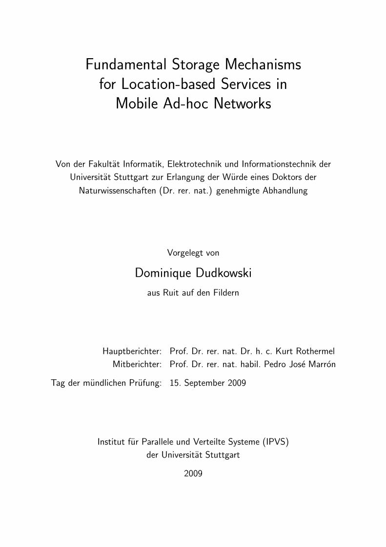
Im Folgenden wird dies beispielhaft anhand zweier Partitionsmetriken gezeigt. Um die Rele-vanz der Netzpartitionierung hervorzuheben wird zunachst die Partitionsanzahl in einem be-stimmten Netzszenario betrachtet. Bei dieser Metrik handelt es sich um eine so genanntenetzzentrische Metrik, da sie das Partitionsverhalten eines mobilen Ad-hoc-Netzes als Ganzesbeschreibt. Abbildung 1.a zeigt die mittlere Partitionsanzahl in einem typischen Innenstadt-szenario am Beispiel von Manhattan. Zunachst steigt die mittlere zu erwartende Anzahl derPartitionen stark an, da mehr und mehr einzelne Knoten isoliert voneinander existieren. NachDurchschreiten eines Maximums vermindert sich mit steigender Dichte die Partitionsanzahl,was durch die allmahliche Verschmelzung kleinerer zu immer großeren Partitionen zu erklarenist. Insbesondere zeigt Abbildung 1.a, dass auch bei der hochsten gemessenen Dichte nochimmer eine signifikante Anzahl von Netzpartitionen auftritt.
Zur Verdeutlichung der moglichen Dynamik des Partitionierungsverhaltens mobiler Ad-hoc-Netze wird anhand der Partitionsanderungsrate gezeigt, wie haufig ein einzelner Netzknotenseine eigene Partition wechselt. Da hierbei die Sicht eines einzelnen Knotens im Vordergrundsteht, handelt es sich bei dieser Metrik um eine so genannte knotenzentrische Partitionsmetrik.Abbildung 1.b zeigt den Verlauf der mittleren knotenzentrischen Partitionsanderungsrate in
9
0
10
20
30
40
50
60
70
80
0 400 800 1200 1600 2000 2400
Mitt
lere
Par
titio
nsan
zahl
Knotenanzahl
0
0.1
0.2
0.3
0.4
0.5
0.6
0.7
0.8
0 400 800 1200 1600 2000 2400
Mitt
lere
Par
titio
nsän
deru
ngsr
ate
[1/s
]
Knotenanzahl
a. Mittlere Partitionsanzahl b. Mittlere Partitionsänderungsrate
Abbildung 1: Mittlere Partitionsanzahl und knotenzentrische Partitionsanderungsrate inAbhangigkeit von der Knotenanzahl im Stadtgebiet von Manhattan.
Abhangigkeit von der Knotendichte. Wahrend bei sehr geringen Dichten aufgrund der weitvoneinander entfernten Knoten Anderungen der Partitionszugehorigkeit nur selten stattfinden,treten diese Anderungen bei mittleren Dichten haufig auf. Dieses Verhalten zeigt insbesondere,dass ein einzelner Knoten durchaus in der Lage ist, auch Knoten in anderen Partitionen bereitsnach einer relativ kurzen Zeit erneut zu kontaktieren.
Die Ergebnisse im Hauptteil der Dissertation fuhren zu zwei Schlussfolgerungen. Einerseits istdas Auftreten von Netzpartitionen von den Verfahren der Datenspeicherung als haufig auftre-tender Normalfall anzusehen. Andererseits zeigt sich bei einer zumindest fur eine Kommunika-tion sinnvollen Mindestknotendichte eine Dynamik, die zu einer endlichen Dauer von Parti-tionierungssituationen fuhrt. Das bedeutet, dass Speicherverfahren eine Partitionierung zwarberucksichtigen mussen, den durch eine Partitionierung entstehenden moglichen Inkonsistenzenin der Datenverwaltung jedoch mit Hilfe geeigneter Maßnahmen entgegenwirken konnen.
Grundverfahren der Datenspeicherung
Um den Eigenschaften mobiler Ad-hoc-Netze wirksam entgegenzutreten, definiert die vor-liegende Arbeit das Paradigma der lokationszentrischen Speicherung, das Ausgangspunkt furdie Grundverfahren der Datenspeicherung ist. Bei diesem Ansatz werden raumliche Daten, alsoDaten mit einer zugehorigen raumlichen Position, auf denjenigen Knoten eines mobilen Ad-hoc-Netzes gespeichert, die sich in der Nahe einer geographischen Referenzposition befinden. DiesePosition befindet sich ihrerseits in der Nahe derjenigen geographischen Position, die durch dasDatum selbst definiert ist. Beide Nahebegriffe lassen sich nun so flexibel gestalten, dass geringeKnotendichten, hohe Mobilitat und Netzpartitionierungen zeitweise toleriert werden konnen.Grundlegend ist hierbei auch der Begriff der raumlichen Koharenz, welche definiert ist als diemittlere geographische Entfernung zwischen einem Datum und der zugehorigen Referenzposi-tion. Diese Metrik ist fur die Bewertung von Speicherverfahren grundlegend, und ein Verfahrenist umso effizienter, desto geringer diese Entfernung ist.
10
a. Verwerfung bei unidirektionaler Paketweiterleitung
cr
upus
.........
>> 3
verwerfen
b. Konvergenz bei bidirektionaler Paketweiterleitung
cr up
us
...
......>> 3
Startknoten
(1)
(2)
(3)
(4)
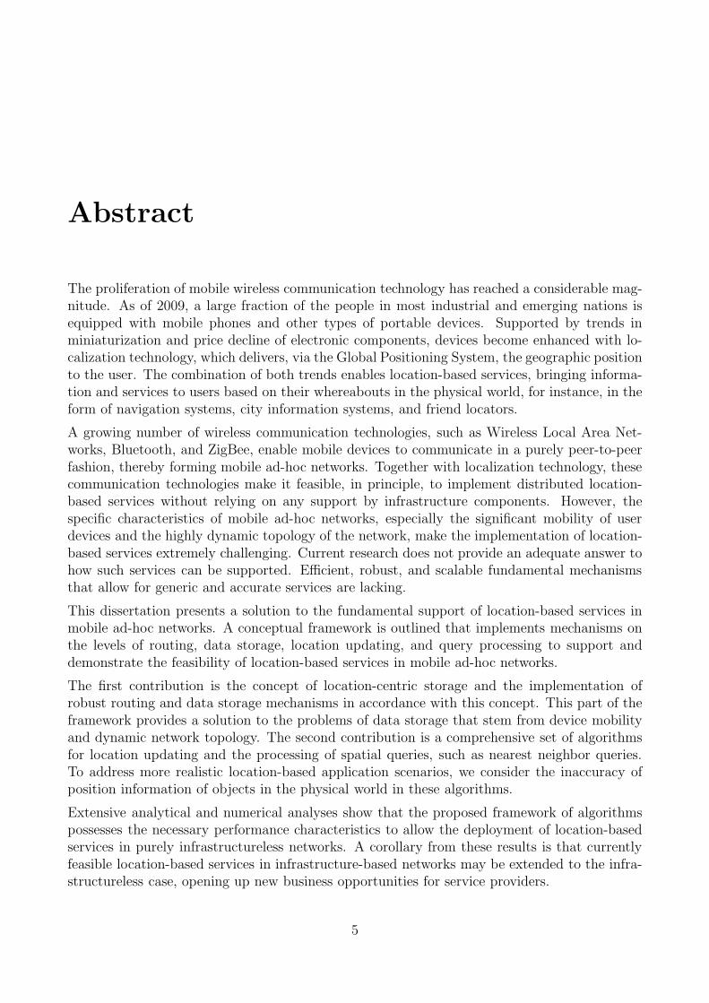
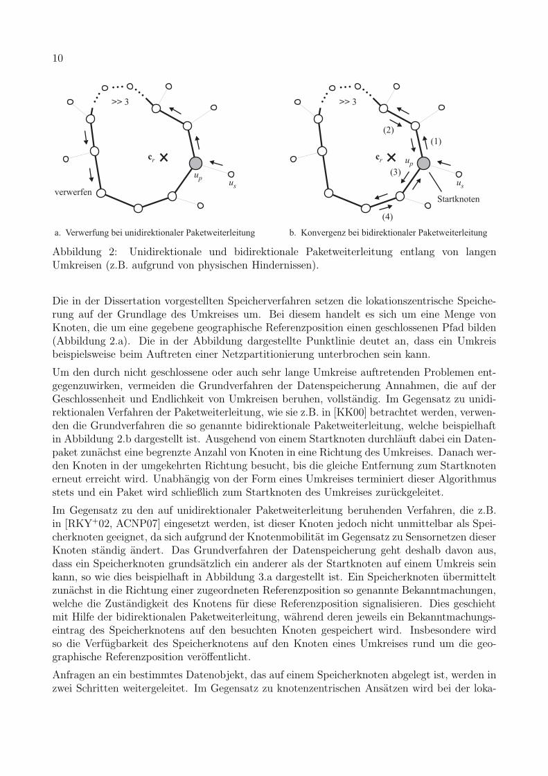
Abbildung 2: Unidirektionale und bidirektionale Paketweiterleitung entlang von langenUmkreisen (z.B. aufgrund von physischen Hindernissen).
Die in der Dissertation vorgestellten Speicherverfahren setzen die lokationszentrische Speiche-rung auf der Grundlage des Umkreises um. Bei diesem handelt es sich um eine Menge vonKnoten, die um eine gegebene geographische Referenzposition einen geschlossenen Pfad bilden(Abbildung 2.a). Die in der Abbildung dargestellte Punktlinie deutet an, dass ein Umkreisbeispielsweise beim Auftreten einer Netzpartitionierung unterbrochen sein kann.
Um den durch nicht geschlossene oder auch sehr lange Umkreise auftretenden Problemen ent-gegenzuwirken, vermeiden die Grundverfahren der Datenspeicherung Annahmen, die auf derGeschlossenheit und Endlichkeit von Umkreisen beruhen, vollstandig. Im Gegensatz zu unidi-rektionalen Verfahren der Paketweiterleitung, wie sie z.B. in [KK00] betrachtet werden, verwen-den die Grundverfahren die so genannte bidirektionale Paketweiterleitung, welche beispielhaftin Abbildung 2.b dargestellt ist. Ausgehend von einem Startknoten durchlauft dabei ein Daten-paket zunachst eine begrenzte Anzahl von Knoten in eine Richtung des Umkreises. Danach wer-den Knoten in der umgekehrten Richtung besucht, bis die gleiche Entfernung zum Startknotenerneut erreicht wird. Unabhangig von der Form eines Umkreises terminiert dieser Algorithmusstets und ein Paket wird schließlich zum Startknoten des Umkreises zuruckgeleitet.
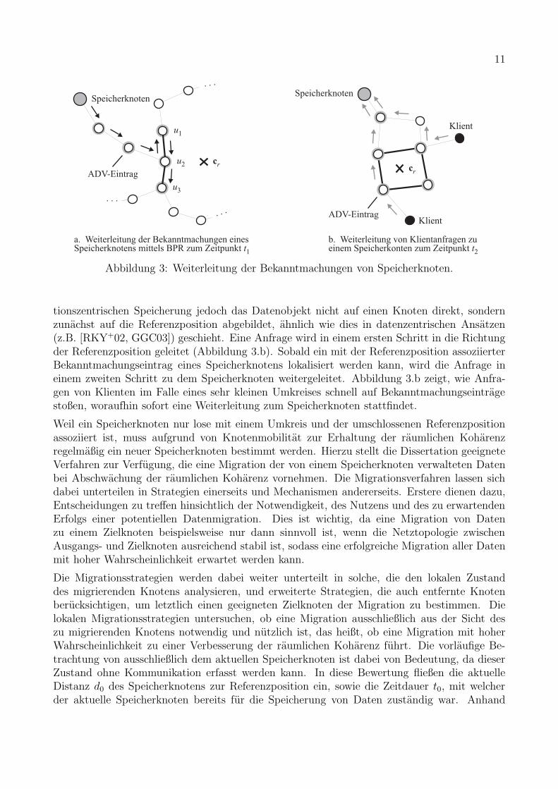
Im Gegensatz zu den auf unidirektionaler Paketweiterleitung beruhenden Verfahren, die z.B.in [RKY+02, ACNP07] eingesetzt werden, ist dieser Knoten jedoch nicht unmittelbar als Spei-cherknoten geeignet, da sich aufgrund der Knotenmobilitat im Gegensatz zu Sensornetzen dieserKnoten standig andert. Das Grundverfahren der Datenspeicherung geht deshalb davon aus,dass ein Speicherknoten grundsatzlich ein anderer als der Startknoten auf einem Umkreis seinkann, so wie dies beispielhaft in Abbildung 3.a dargestellt ist. Ein Speicherknoten ubermitteltzunachst in die Richtung einer zugeordneten Referenzposition so genannte Bekanntmachungen,welche die Zustandigkeit des Knotens fur diese Referenzposition signalisieren. Dies geschiehtmit Hilfe der bidirektionalen Paketweiterleitung, wahrend deren jeweils ein Bekanntmachungs-eintrag des Speicherknotens auf den besuchten Knoten gespeichert wird. Insbesondere wirdso die Verfugbarkeit des Speicherknotens auf den Knoten eines Umkreises rund um die geo-graphische Referenzposition veroffentlicht.
Anfragen an ein bestimmtes Datenobjekt, das auf einem Speicherknoten abgelegt ist, werden inzwei Schritten weitergeleitet. Im Gegensatz zu knotenzentrischen Ansatzen wird bei der loka-
11
...
...
...
cr
a. Weiterleitung der Bekanntmachungen einesSpeicherknotens mittels BPR zum Zeitpunkt t1
Speicherknoten
ADV-Eintrag
u1
u2
u3
b. Weiterleitung von Klientanfragen zueinem Speicherkonten zum Zeitpunkt t2
Speicherknoten
cr
Klient
Klient
ADV-Eintrag
Abbildung 3: Weiterleitung der Bekanntmachungen von Speicherknoten.
tionszentrischen Speicherung jedoch das Datenobjekt nicht auf einen Knoten direkt, sondernzunachst auf die Referenzposition abgebildet, ahnlich wie dies in datenzentrischen Ansatzen(z.B. [RKY+02, GGC03]) geschieht. Eine Anfrage wird in einem ersten Schritt in die Richtungder Referenzposition geleitet (Abbildung 3.b). Sobald ein mit der Referenzposition assoziierterBekanntmachungseintrag eines Speicherknotens lokalisiert werden kann, wird die Anfrage ineinem zweiten Schritt zu dem Speicherknoten weitergeleitet. Abbildung 3.b zeigt, wie Anfra-gen von Klienten im Falle eines sehr kleinen Umkreises schnell auf Bekanntmachungseintragestoßen, woraufhin sofort eine Weiterleitung zum Speicherknoten stattfindet.
Weil ein Speicherknoten nur lose mit einem Umkreis und der umschlossenen Referenzpositionassoziiert ist, muss aufgrund von Knotenmobilitat zur Erhaltung der raumlichen Koharenzregelmaßig ein neuer Speicherknoten bestimmt werden. Hierzu stellt die Dissertation geeigneteVerfahren zur Verfugung, die eine Migration der von einem Speicherknoten verwalteten Datenbei Abschwachung der raumlichen Koharenz vornehmen. Die Migrationsverfahren lassen sichdabei unterteilen in Strategien einerseits und Mechanismen andererseits. Erstere dienen dazu,Entscheidungen zu treffen hinsichtlich der Notwendigkeit, des Nutzens und des zu erwartendenErfolgs einer potentiellen Datenmigration. Dies ist wichtig, da eine Migration von Datenzu einem Zielknoten beispielsweise nur dann sinnvoll ist, wenn die Netztopologie zwischenAusgangs- und Zielknoten ausreichend stabil ist, sodass eine erfolgreiche Migration aller Datenmit hoher Wahrscheinlichkeit erwartet werden kann.
Die Migrationsstrategien werden dabei weiter unterteilt in solche, die den lokalen Zustanddes migrierenden Knotens analysieren, und erweiterte Strategien, die auch entfernte Knotenberucksichtigen, um letztlich einen geeigneten Zielknoten der Migration zu bestimmen. Dielokalen Migrationsstrategien untersuchen, ob eine Migration ausschließlich aus der Sicht deszu migrierenden Knotens notwendig und nutzlich ist, das heißt, ob eine Migration mit hoherWahrscheinlichkeit zu einer Verbesserung der raumlichen Koharenz fuhrt. Die vorlaufige Be-trachtung von ausschließlich dem aktuellen Speicherknoten ist dabei von Bedeutung, da dieserZustand ohne Kommunikation erfasst werden kann. In diese Bewertung fließen die aktuelleDistanz d0 des Speicherknotens zur Referenzposition ein, sowie die Zeitdauer t0, mit welcherder aktuelle Speicherknoten bereits fur die Speicherung von Daten zustandig war. Anhand
12
dieser Großen wird das Pradikat PMRP bestimmt, das die notwendige Bedingung einer Migra-tion definiert und genau dann wahr ist, wenn d0 oder t0 einen durch dthresh und tthresh gegebenenraumlichen bzw. zeitlichen Grenzwert uberschreitet:
PMRP := d0 > dthresh ∨ t0 > tthresh (1)
Nur bei einem wahren Pradikat wird in einem zweiten Schritt eine Menge entfernter Knotenbetrachtet, um einen Zielknoten zu bestimmen, der fur den Empfang der zu migrierendenDaten geeignet ist (im anderen Fall wird nach Ablauf eines Zeitintervalls eine erneute Prufungdes Pradikats in (1) vorgenommen). Grundsatzlich sind in diesem Schritt solche Knoten zubevorzugen, die sich naher an der Referenzposition aufhalten. Ebenfalls zu berucksichtigen istdie Geschwindigkeit von Knoten, da sich Knoten mit hoher Geschwindigkeit schneller von derReferenzposition entfernen als langsame Knoten, und somit bereits nach kurzer Zeit erneut eineMigration erforderlich ist. Ferner spielt die Zeitdauer eine Rolle, mit der ein Knoten bereits inder Vergangenheit als Speicherknoten fungierte. Dies ist vor allem fur die Lastverteilung zwi-schen moglichst allen Knoten eines mobilen Ad-hoc-Netzes von Bedeutung. Zusammenfassendlasst sich aus diesen Betrachtungen die Gesamteignung eines Knotens bestimmen. Diese setztsich multiplikativ aus den individuellen Eignungen εd
i , εδti und εΔt
i zusammen, welche die zuvorbeschriebenen Eigenschaften modellieren:
εi := εdi · εδt
i · εΔti (2)
Neben der Bestimmung der Eignungswerte εi einer Menge von Knoten ist die Stabilitat dermoglichen Netzpfade zu diesen Knoten eine wichtige Große, da die Eignung der Knoten alleinnicht fur die Bewertung einer erfolgreichen Migration ausreicht. Die Dissertation stellt hierfureinen Algorithmus zur Verfugung, der effizient moglichst stabile Pfade zwischen dem aktuellenSpeicherknoten und der Menge moglicher Zielknoten einer Migration bestimmt. Gemeinsammit den Eignungswerten εi wird am Ende des zweiten Bewertungsschrittes ein Knoten als Migra-tionsziel endgultig festgelegt. Wird kein geeigneter, uber einen ausreichend stabilen Netzpfaderreichbarer Knoten gefunden, so beginnt die Auswertung der Strategien nach Ablauf eineszweiten Zeitintervalls von Neuem.
Fur die anschließende Migration vom Ausgangs- zum Zielknoten uber den gewahlten Netzpfadstellt die Dissertation einen Mechanismus vor, der Migrationen moglichst effizient ausfuhrtund das Auftreten von Migrationsfehlern vermeidet. Bei diesem Mechanismus wird insbeson-dere die Distanz zwischen Ausgangs- und Zielknoten berucksichtigt, um den Datentransfer auf-grund von Eigenschaften des gemeinsamen drahtlosen Kommunikationsmediums zu optimieren.Nach erfolgter Migration aller Daten wird der ursprungliche Speicherknoten deaktiviert und derZielknoten ubernimmt dessen Aufgabe. Wahrend dieser Ubergabe wird auch die Versendungvon Bekanntmachungen konsistent vom ursprunglichen auf den zukunftigen Speicherknotenubertragen, sodass dieser seine Zustandigkeit im Netz so mitteilt, dass Anfragen von Klientennun an diesen neuen Knoten geleitet werden.
Aufgrund der Problematik der Netzpartitionierung wird der Migrationsmechanismus von einemKonsolidierungsmechanismus erganzt, der in der Lage ist, auftretende Redundanzen von Spei-cherknoten aufzulosen. Aufgrund kommunikationstheoretischer Eigenschaften und unter be-stimmten Fehlermodellen kann ein Migrationsprozess in einer solchen Art fehlschlagen, dass
13
a. Vor Partitionsvereinigung zum Zeitpunkt t1 b. Nach Partitionsvereinigung zum Zeitpunkt >t t2 1
ADV-Eintrag
u1
cr
u2
cr
u1ADV-
Eintragu2
ADV-Eintrag
u1
u1
u2
u3
u3
ADV-Eintrag
u2
Redundanz-erkennung
RED RED
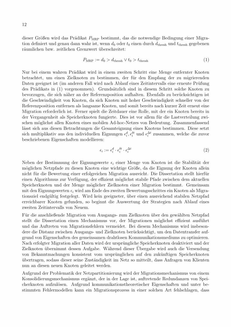
Abbildung 4: Erkennung von redundanten Speicherknoten.
eine Entscheidung, welcher Speicherknoten die Datenspeicherung fortfuhrt, nicht moglich ist.Dieser Sachverhalt ist fur den Fall einer Netzpartitionierung in Abbildung 4.a dargestellt. Injeder Partition existiert nach einer fehlgeschlagenen Migration jeweils ein Speicherknoten. BeideSpeicherknoten sind in dieser Situation dazu bestimmt, ihre eigenen Bekanntmachungen in dieRichtung der geographischen Referenzposition zu senden.
Der Konsolidierungsmechanismus ist in solchen Situationen in der Lage, Redundanzen ohnezusatzliche Kommunikation zu erkennen, sobald eine Wiedervereinigung von Partitionen statt-findet. Abbildung 4.b zeigt die Vereinigung der zuvor dargestellten Partitionen. Da nunein einziger Umkreis die Referenzposition umschließt, fuhrt das Bekanntmachungsverfahrendazu, dass Bekanntmachungen beider Speicherknoten schließlich in einem Knoten (Knoten u3
in Abbildung 4.b) zusammentreffen. Dieser Knoten kann somit unmittelbar eine Redundanzfeststellen, die er sodann an die beteiligten Speicherknoten signalisiert. Die Speicherknotenihrerseits stoßen daraufhin einen Konsolidierungsprozess an, der nach einem ahnlichen Ver-fahren wie dem der Migration verfahrt. Nachdem einer der Speicherknoten seinen Datenbestandzum anderen ubermittelt hat, werden beide Datenbestande verschmolzen und anschließend derubermittelnde Speicherknoten, ahnlich wie im Falle der Migration, abgelost. Im Ergebnis ex-istiert somit nach einer Konsolidierung lediglich ein Speicherknoten.
Hinsichtlich der Grundverfahren stellt die Dissertation ausfuhrliche analytische und simulativeErgebnisse zur Verfugung. Ein Auszug aus der simulativen Leistungsbewertung zeigt, dass dieGrundverfahren der Datenspeicherung effizient, robust und skalierbar sind. Fur die Bewertungwird eine Gesamtflache von 600 · 600 m2 angenommen, in deren Zentrum eine Zelle der Große200 · 200 m2 platziert ist. Insgesamt bewegen sich 150 Knoten nach dem Random-Waypoint-Mobilitatsmodell mit einer Geschwindigkeit von 1,5 m/s und Verweilzeit von 30 s innerhalb desSimulationsgebiets. Die Kommunikationsreichweite der Knoten ist 100 m.
Zunachst wird die Leistungsfahigkeit der Grundverfahren anhand der Erfolgsrate von Klient-anfragen dargelegt. Die Erfolgsrate von Anfragen ist definiert als derjenige Bruchteil von An-fragen, die erfolgreich zu einem Speicherknoten ubermittelt werden konnen. Als Vergleichs-verfahren wurde die datenzentrische Speicherung (DCS/GPSR) nach [RKY+02] gewahlt, umdie Vorteile des lokationszentrischen Ansatzes dieser Dissertation zu zeigen. Fur das daten-zentrische Verfahren ist die Erfolgsrate derjenige Bruchteil von Anfragen, die erfolgreich amStartknoten des Umkreises (Abbildung 2), der den Speicherknoten definiert, eintreffen.
14
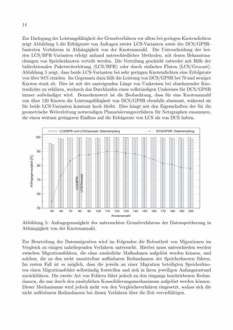
Zur Darlegung der Leistungsfahigkeit der Grundverfahren vor allem bei geringen Knotendichtenzeigt Abbildung 5 die Erfolgsrate von Anfragen zweier LCS-Varianten sowie des DCS/GPSR-basierten Verfahrens in Abhangigkeit von der Knotenanzahl. Die Unterscheidung der bei-den LCS/BPR-Varianten erfolgt anhand unterschiedlicher Methoden, mit denen Bekanntma-chungen von Speicherknoten verteilt werden. Die Verteilung geschieht entweder mit Hilfe derbidirektionalen Paketweiterleitung (LCS/BPR) oder durch einfaches Fluten (LCS/Geocast).Abbildung 5 zeigt, dass beide LCS-Varianten bei sehr geringen Knotendichten eine Erfolgsratevon uber 94% erzielen. Im Gegensatz dazu fallt die Leistung von DCS/GPSR bei 70 und wenigerKnoten stark ab. Dies ist mit der ansteigenden Lange von Umkreisen bei abnehmender Kno-tendichte zu erklaren, wodurch das Durchlaufen eines vollstandigen Umkreises fur DCS/GPSRimmer aufwandiger wird. Bemerkenswert ist die Beobachtung, dass fur eine Knotenanzahlvon uber 120 Knoten die Leistungsfahigkeit von DCS/GPSR ebenfalls abnimmt, wahrend siefur beide LCS-Varianten konstant hoch bleibt. Dies hangt mit den Eigenschaften der fur diegeometrische Weiterleitung notwendigen Planarisierungsverfahren fur Netzgraphen zusammen,die einen weitaus geringeren Einfluss auf die Erfolgsrate von LCS als von DCS haben.
50
60
70
80
90
100
50 60 70 80 90 100 110 120 130 140 150 160 170 180 190 200
Anfr
agegenauig
keit
[%]
Knotenanzahl
LCS/BPR und LCS/Geocast: Datenempfang DCS/GPSR: Datenempfang
LC
S/B
PR
LC
S/G
eocast
Abbildung 5: Anfragegenauigkeit des untersuchten Grundverfahrens der Datenspeicherung inAbhangigkeit von der Knotenanzahl.
Zur Beurteilung der Datenmigration wird im Folgenden die Robustheit von Migrationen imVergleich zu einigen naheliegenden Verfahren untersucht. Hierbei muss unterschieden werdenzwischen Migrationsfehlern, die ohne zusatzliche Maßnahmen aufgelost werden konnen, undsolchen, die zu den nicht unmittelbar auflosbaren Redundanzen der Speicherknoten fuhren.Im ersten Fall ist es moglich, dass die jeweils an einer Migration beteiligten Speicherkno-ten einen Migrationsfehler selbstandig feststellen und sich in ihren jeweiligen Anfangszustandzuruckfuhren. Die zweite Art von Fehlern fuhrt jedoch zu den eingangs beschriebenen Redun-danzen, die nur durch den zusatzlichen Konsolidierungsmechanismus aufgelost werden konnen.Dieser Mechanismus wird jedoch nicht von den Vergleichsverfahren eingesetzt, sodass sich dienicht auflosbaren Redundanzen bei diesen Verfahren uber die Zeit vervielfaltigen.
15
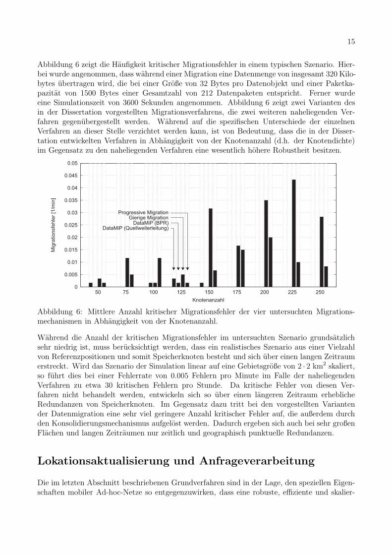
Abbildung 6 zeigt die Haufigkeit kritischer Migrationsfehler in einem typischen Szenario. Hier-bei wurde angenommen, dass wahrend einer Migration eine Datenmenge von insgesamt 320 Kilo-bytes ubertragen wird, die bei einer Große von 32 Bytes pro Datenobjekt und einer Paketka-pazitat von 1500 Bytes einer Gesamtzahl von 212 Datenpaketen entspricht. Ferner wurdeeine Simulationszeit von 3600 Sekunden angenommen. Abbildung 6 zeigt zwei Varianten desin der Dissertation vorgestellten Migrationsverfahrens, die zwei weiteren naheliegenden Ver-fahren gegenubergestellt werden. Wahrend auf die spezifischen Unterschiede der einzelnenVerfahren an dieser Stelle verzichtet werden kann, ist von Bedeutung, dass die in der Disser-tation entwickelten Verfahren in Abhangigkeit von der Knotenanzahl (d.h. der Knotendichte)im Gegensatz zu den naheliegenden Verfahren eine wesentlich hohere Robustheit besitzen.
0
0.005
0.01
0.015
0.02
0.025
0.03
0.035
0.04
0.045
0.05
50 75 100 125 150 175 200 225 250
Mig
rationsfe
hle
r[1
/min
]
Knotenanzahl
Progressive MigrationGierige Migration
DataMiP (BPR)DataMiP (Quellweiterleitung)
Abbildung 6: Mittlere Anzahl kritischer Migrationsfehler der vier untersuchten Migrations-mechanismen in Abhangigkeit von der Knotenanzahl.
Wahrend die Anzahl der kritischen Migrationsfehler im untersuchten Szenario grundsatzlichsehr niedrig ist, muss berucksichtigt werden, dass ein realistisches Szenario aus einer Vielzahlvon Referenzpositionen und somit Speicherknoten besteht und sich uber einen langen Zeitraumerstreckt. Wird das Szenario der Simulation linear auf eine Gebietsgroße von 2 · 2 km2 skaliert,so fuhrt dies bei einer Fehlerrate von 0.005 Fehlern pro Minute im Falle der naheliegendenVerfahren zu etwa 30 kritischen Fehlern pro Stunde. Da kritische Fehler von diesen Ver-fahren nicht behandelt werden, entwickeln sich so uber einen langeren Zeitraum erheblicheRedundanzen von Speicherknoten. Im Gegensatz dazu tritt bei den vorgestellten Variantender Datenmigration eine sehr viel geringere Anzahl kritischer Fehler auf, die außerdem durchden Konsolidierungsmechanismus aufgelost werden. Dadurch ergeben sich auch bei sehr großenFlachen und langen Zeitraumen nur zeitlich und geographisch punktuelle Redundanzen.
Lokationsaktualisierung und Anfrageverarbeitung
Die im letzten Abschnitt beschriebenen Grundverfahren sind in der Lage, den speziellen Eigen-schaften mobiler Ad-hoc-Netze so entgegenzuwirken, dass eine robuste, effiziente und skalier-
16
bare Datenspeicherung ermoglicht wird. Fur lokations- und kontextbasierte Dienste und An-wendungen sind diese Verfahren jedoch nicht von unmittelbarer Bedeutung, da nur einzelneDatenobjekte ohne Berucksichtigung ihrer Semantik aktualisiert und angefragt werden konnen.Das in der Dissertation vorgestellte Rahmenwerk umfasst deshalb zusatzlich Dienste, die erwei-terte Funktionalitat bereitstellen. Im Folgenden wird gezeigt, wie Verfahren zur Lokationsaktu-alisierung einerseits und zur Verarbeitung raumlicher Anfragen andererseits durch Ausnutzungder grundlegenden Speicherverfahren umgesetzt werden konnen.
Wichtig fur die Entwicklung von Verfahren zur Lokationsaktualisierung ist die Erkenntnis, dassjedes Modell der physischen Welt mit Hilfe von Sensorik nur innerhalb bestimmter Genauigkeits-grenzen erfasst werden kann. Insbesondere gilt dies fur die Position physischer Objekte,denen stets eine Ungenauigkeit anhaftet. Positionsungenauigkeiten konnen mit Hilfe einerWahrscheinlichkeitsdichte und einem zugehorigen kreisformigen Gebiet beschrieben werden, in-nerhalb dessen sich das Objekt mit einer gewissen Wahrscheinlichkeit aufhalt. Die Lokation Leines Objektes lasst sich formal wie folgt darstellen:
L := (�(X), CEPY ) (3)
In (3) bezeichnet �(X) die Wahrscheinlichkeitsdichte und CEPY das so genannte circular errorprobable (CEP) fur die Wahrscheinlichkeit Y , mit der ein Objekt innerhalb des durch CEPY
definierten kreisformigen Gebietes lokalisiert werden kann.
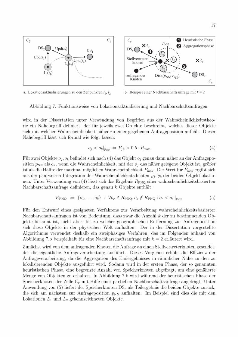
Auf der Grundlage der durch (3) gegebenen Semantik von Lokationen eines Objekts definiertdie Dissertation einen Algorithmus zur Lokationsaktualisierung, dessen Funktionsweise im Fol-genden anhand von Abbildung 7 erlautert wird. Das geographische Gebiet, innerhalb dessensich das mobile Ad-hoc-Netz befindet, ist dabei in Zellen unterteilt, fur die jeweils ein Spei-cherknoten (DS) zustandig ist. Jeder Knoten ist in der Lage, die Lokation eines Objekts mitHilfe seiner eigenen Sensorik zur Positionsbestimmung zu erfassen und eine Lokationsinforma-tion nach (3) zu erzeugen. Sodann wird diejenige Menge von Zellen bestimmt, die mit demdurch CEPY definierten kreisformigen Lokationsgebiet uberlappen. In Abbildung 7.a uberlapptbeispielsweise Lokationsgebiet Li(t1) mit Zelle C2, Li(t2) mit den Zellen C2 und C1.
Im nachsten Schritt wird jeweils eine Kopie der Lokationsinformation an die fur die zuvorbestimmten Zellen zustandigen Speicherknoten gesendet. An dieser Stelle greift das Verfahrender Lokationsaktualisierung auf die indirekte Paketweiterleitung des Grundverfahrens zuruck,das die Lokationsinformationen in zwei Schritten an die zuvor bestimmten Zellen und danachan die Speicherknoten DS2 und DS1 weiterleitet. Die empfangenen Lokationsinformationen desaktualisierten Objekts werden sodann in der lokalen Datenbank des jeweiligen Speicherknotensaktualisiert, in der sie fur die weitere Verarbeitung von Anfragen zur Verfugung stehen.
Das Verfahren zur Lokationsaktualisierung stellt ferner Methoden bereit, die Kopien einesDatenobjekts auf mehreren Speicherknoten loscht, wenn diese nach einer erneuten Lokations-aktualisierung nicht mehr auf die entsprechenden Zellen abbilden. Damit wird stets einemoglichst hohe Konsistenz von Datenobjekten erzielt, wodurch insbesondere die Genauigkeitvon den im Folgenden betrachteten raumlichen Anfragen erhoht wird.
Am Beispiel von Nachbarschaftsanfragen soll nun gezeigt werden, wie effiziente Algorithmenfur die Verarbeitung von raumlichen Anfragen in mobilen Ad-hoc-Netzen effizient gestaltetwerden konnen. Dabei ist zu beachten, dass Positionsungenauigkeiten auch bei der Defini-tion einer geeigneten Semantik fur Nachbarschaftsanfragen zu berucksichtigen sind. Hierzu
17
DS2
C2 C1
Cs
Upd( )t1
Li( )t1
Upd( )t2
Li( )t2Upd( )t2
DS1
a. Lokationsaktualisierungen zu den Zeitpunkten t1, t2
anfragenderKnoten
Stellvertreter-knoten
Cr
b. Beispiel einer Nachbarschaftsanfrage mit = 2k
crDSr
DSs
cs
pNN
L1
L2
L3
2
1
Heuristische Phase
Aggregationsphase
Disk( , )p rNN agg
1
2
Abbildung 7: Funktionsweise von Lokationsaktualisierung und Nachbarschaftsanfragen.
wird in der Dissertation unter Verwendung von Begriffen aus der Wahrscheinlichkeitstheo-rie ein Nahebegriff definiert, der fur jeweils zwei Objekte beschreibt, welches dieser Objektesich mit welcher Wahrscheinlichkeit naher zu einer gegebenen Anfrageposition aufhalt. DieserNahebegriff lasst sich formal wie folgt fassen:
oj < ok|pNN⇔ Pjk > 0.5 · Pmax (4)
Fur zwei Objekte oj , ok befindet sich nach (4) das Objekt oj genau dann naher an der Anfragepo-sition pNN als ok, wenn die Wahrscheinlichkeit, mit der oj das naher gelegene Objekt ist, großerist als die Halfte der maximal moglichen Wahrscheinlichkeit Pmax. Der Wert fur Pmax ergibt sichaus der paarweisen Integration der Wahrscheinlichkeitsdichten �j , �k der beiden Objektlokatio-nen. Unter Verwendung von (4) lasst sich das Ergebnis RPNQ einer wahrscheinlichkeitsbasiertenNachbarschaftsanfrage definieren, das genau k Objekte enthalt:
RPNQ := {o1, . . . , ok} : ∀or ∈ RPNQ, os �∈ RPNQ : or < os |pNN(5)
Fur den Entwurf eines geeigneten Verfahrens zur Verarbeitung wahrscheinlichkeitsbasierterNachbarschaftsanfragen ist von Bedeutung, dass zwar die Anzahl k der zu bestimmenden Ob-jekte bekannt ist, nicht aber, bis zu welcher geographischen Entfernung zur Anfragepositionsich diese Objekte in der physischen Welt aufhalten. Der in der Dissertation vorgestellteAlgorithmus verwendet deshalb ein zweiphasiges Verfahren, das im Folgenden anhand vonAbbildung 7.b beispielhaft fur eine Nachbarschaftsanfrage mit k = 2 erlautert wird.
Zunachst wird von dem anfragenden Knoten die Anfrage an einen Stellvertreterknoten gesendet,der die eigentliche Anfrageverarbeitung ausfuhrt. Dieses Vorgehen erhoht die Effizienz derAnfrageverarbeitung, da die Aggregation des Endergebnisses in raumlicher Nahe zu den zulokalisierenden Objekte ausgefuhrt wird. Sodann wird in der ersten Phase, der so genanntenheuristischen Phase, eine begrenzte Anzahl von Speicherknoten abgefragt, um eine genaherteMenge von Objekten zu erhalten. In Abbildung 7.b wird wahrend der heuristischen Phase derSpeicherknoten der Zelle Cr mit Hilfe einer partiellen Nachbarschaftsanfrage angefragt. UnterAnwendung von (5) liefert der Speicherknoten DSr als Teilergebnis die beiden Objekte zuruck,die sich am nachsten zur Anfrageposition pNN aufhalten. Im Beispiel sind dies die mit denLokationen L1 und L2 gekennzeichneten Objekte.

18
Nach der Bestimmung der Naherungsmenge von Datenobjekten werden in der anschließendenAggregationsphase diejenigen Objekte festgestellt, die sich raumlich naher an der Referenzpo-sition befinden als die zuvor bestimmten. Dazu wird ein Kreis mit Mittelpunkt pNN konstru-iert, der die Lokationsgebiete der zuvor bestimmten Objekte enthalt (Abbildung 7.b). Anhanddieses Kreises lasst sich durch Uberlapp mit weiteren Zellen bestimmen, welche SpeicherknotenObjekte verwalten, die noch naher an der Anfrageposition liegen als die bereits bestimmtenObjekte. Im Beispiel existiert ein solches Objekt auf DSs, dargestellt durch LokationsgebietL3. Wahrend der Aggregationsphase werden schließlich weitere partielle Nachbarschaftsanfra-gen versendet, um die verbleibenden Speicherknoten zu kontaktieren. Im Beispiel ist dies DSs,der daraufhin das Objekt mit der Lokation L3 an den Stellvertreterknoten zuruckliefert. DerStellvertreterknoten fuhrt die durch partielle Anfragen erhaltenen Objekte schließlich mittels(4) so zusammen, dass nur die tatsachlich nachsten k Objekte im Endergebnis der Anfrage ent-halten sind. In Abbildung 7.b sind dies L3 und L1, wahrend L2 nach Aggregation nicht mehrBestandteil des Ergebnisses ist. Am Ende wird das Endergebnis der Nachbarschaftsanfrage anden anfragenden Knoten zuruckgesendet.
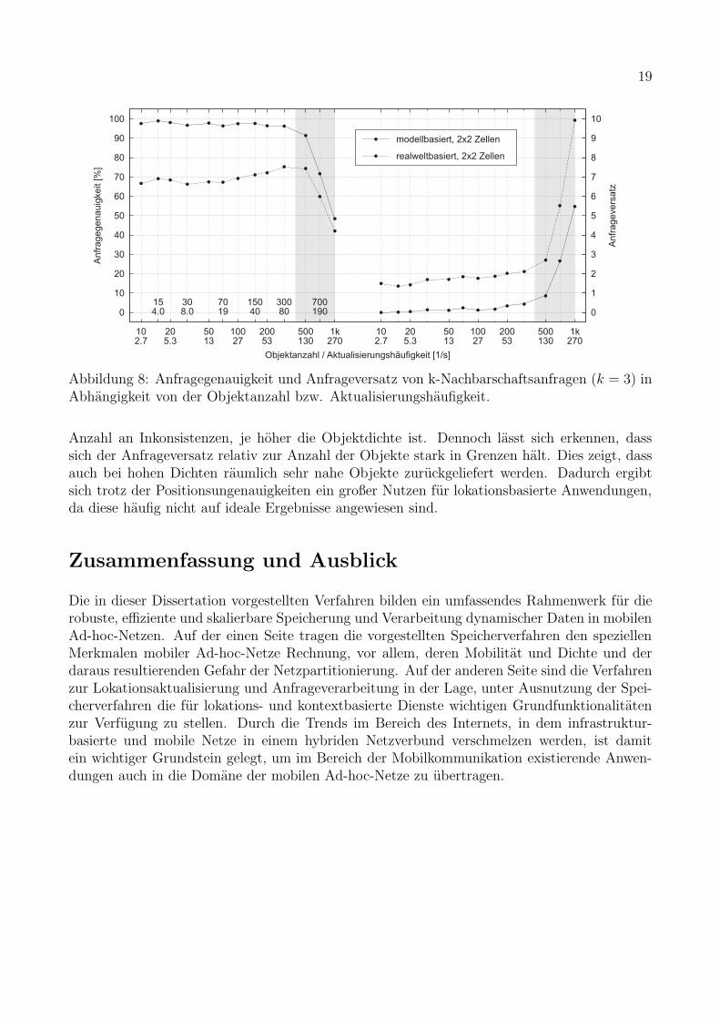
Im Folgenden wird die Leistungsfahigkeit der Verarbeitung von Nachbarschaftsanfragen anhandeiner Beispielmessung aus dem Hauptteil der Dissertation aufgezeigt. Das durch das mobileAd-hoc-Netz abgedeckte geographische Gebiet hat eine Flache von 600 · 600 m2, welches invier Zellen der Große 300 · 300 m2 unterteilt ist. Die Bewegung der Knoten wird wie imFalle der Speicherverfahren mit Hilfe des Random-Waypoint-Mobilitatsmodells beschrieben,das mit einer Knotengeschwindigkeit von 1.5 m/s und einer Verweilzeit von 30 s parametrisiertist. Ferner wird eine Positionsungenauigkeit von 5 m angenommen, was den Eigenschaftenmoderner GPS-Empfanger entspricht. Der Anfrageparameter ist k = 3.
Zur Qualitatsbewertung von Anfrageergebnissen werden zwei Metriken verwendet. Einerseitswird durch die Anfragegenauigkeit definiert, welcher Bruchteil der zuruckgelieferten Objektemit einer idealen Ergebnismenge ubereinstimmt. Die ideale Ergebnismenge ist dabei definiertals das Resultat der Ausfuhrung des Anfragealgorithmus unter idealen Bedingungen, bei dereine zentrale Datenbank sowie eine verzogerungsfreie Lokationsaktualisierung und Anfragever-arbeitung angenommen werden. Andererseits beschreibt der Anfrageversatz, um welche Anzahlvon Objekten ein Anfrageergebnis vom idealen Anfrageresultat entfernt ist. Beispielsweise istder Anfrageversatz genau eins, falls die zuruckgelieferten Objekte einer 3-Nachbarschaftsanfragevollstandig in der Ergebnismenge einer idealen 4-Nachbarschaftsanfrage liegen.
Abbildung 8 zeigt die Ergebnisse der Anfragegenauigkeit und des Anfrageversatzes als Funk-tion der Anzahl der Objekte, die mit der Aktualisierungshaufigkeit korreliert, fur drei unter-schiedliche Zellgroßen. Die Ergebnisse zeigen, dass in einem Bereich von bis zu 300 Datenob-jekten, d.h. bis zu einer Aktualisierungshaufigkeit von 80/s, die Anfragegenauigkeit und derAnfrageversatz knapp unterhalb der maximal moglichen Werte liegen. Ab einer Anzahl von 300Datenobjekten zeigt sich ein starker Abfall der Anfragegenauigkeit. Dies hangt mit dem Ein-fluss der Positionsungenauigkeiten bei hohen Objektdichten zusammen. Wird die Objektdichteerhoht, so erhoht sich ebenso die Wahrscheinlichkeit von sich uberlappenden Lokationsgebietenunterschiedlicher Objekte. Aufgrund von diskreten Aktualisierungsereignissen ergeben sichstandig Anderungen in der Art und Weise, wie sich Objektlokationen uberlappen. Aufgrundder Tatsache, dass Anfragen zu ihrer Bearbeitung eine gewisse Zeit in Anspruch nehmen, fuhrendie wahrend dieser Bearbeitungszeit auftretenden Aktualisierungsereignisse zu einer großeren
19
0
10
20
30
40
50
60
70
80
90
100
102.7
154.0
205.3
308.0
5013
7019
10027
15040
20053
30080
500130
700190
1k270
102.7
205.3
5013
10027
20053
500130
1k270
0
1
2
3
4
5
6
7
8
9
10
Anfr
agegenauig
keit
[%]
Anfr
agevers
atz
Objektanzahl / Aktualisierungshäufigkeit [1/s]
modellbasiert, 2x2 Zellen
realweltbasiert, 2x2 Zellen
Abbildung 8: Anfragegenauigkeit und Anfrageversatz von k-Nachbarschaftsanfragen (k = 3) inAbhangigkeit von der Objektanzahl bzw. Aktualisierungshaufigkeit.
Anzahl an Inkonsistenzen, je hoher die Objektdichte ist. Dennoch lasst sich erkennen, dasssich der Anfrageversatz relativ zur Anzahl der Objekte stark in Grenzen halt. Dies zeigt, dassauch bei hohen Dichten raumlich sehr nahe Objekte zuruckgeliefert werden. Dadurch ergibtsich trotz der Positionsungenauigkeiten ein großer Nutzen fur lokationsbasierte Anwendungen,da diese haufig nicht auf ideale Ergebnisse angewiesen sind.
Zusammenfassung und Ausblick
Die in dieser Dissertation vorgestellten Verfahren bilden ein umfassendes Rahmenwerk fur dierobuste, effiziente und skalierbare Speicherung und Verarbeitung dynamischer Daten in mobilenAd-hoc-Netzen. Auf der einen Seite tragen die vorgestellten Speicherverfahren den speziellenMerkmalen mobiler Ad-hoc-Netze Rechnung, vor allem, deren Mobilitat und Dichte und derdaraus resultierenden Gefahr der Netzpartitionierung. Auf der anderen Seite sind die Verfahrenzur Lokationsaktualisierung und Anfrageverarbeitung in der Lage, unter Ausnutzung der Spei-cherverfahren die fur lokations- und kontextbasierte Dienste wichtigen Grundfunktionalitatenzur Verfugung zu stellen. Durch die Trends im Bereich des Internets, in dem infrastruktur-basierte und mobile Netze in einem hybriden Netzverbund verschmelzen werden, ist damitein wichtiger Grundstein gelegt, um im Bereich der Mobilkommunikation existierende Anwen-dungen auch in die Domane der mobilen Ad-hoc-Netze zu ubertragen.


Acknowledgements
Publishing my work would not have been possible without a great deal of help at every stagealong the journey from conception to its realization in this final form.
This dissertation has been developing in my mind for several years, and I would like to thankmy advisor, Professor Kurt Rothermel, for guiding me through this intriguing and challengingtopic. I am also thankful to my co-advisor, Professor Pedro Jose Marron, for the support andfeedback while being my colleague and my friend at the Distributed Systems Group.
Many colleagues helped me shape my ideas over the years, and I must thank them for theirfellowship and priceless comments on my work. I am fortunate to have worked with wonderfulpeople, such as Martin Bauer, Christian Becker, Susanne Burklen, Frank Durr, Tobias Farrell,Lars Geiger, Jorg Hahner, Boris Koldehofe, Ralf Lange, Steffen Maier, Annemarie Rosler,Harald Weinschrott, and many others, to whom I offer my heartfelt thanks.
During my time at the Distributed Systems Group, I had the opportunity to work with somebright and talented students who greatly inspired my work and with whom I shared some goodtimes. Many thanks to you guys.
Last but not least, I would like to thank the German Research Foundation for their financialsupport through the Nexus project, which enabled my research in the first place.
In writing this dissertation, as in all else, I am specially indebted to my parents Stan and Anita,my grandmother Maminka, my aunt Brigitte, my best friend Holger, and my partner Elena, fortheir patience and sustained moral support, and for granting me in the past years the privilegeof worrying about nothing else but my work.
21

Contents
1 Introduction 351.1 Motivation . . . . . . . . . . . . . . . . . . . . . . . . . . . . . . . . . . . . . . . 351.2 Technological and Paradigmatic Trends . . . . . . . . . . . . . . . . . . . . . . . 36
1.2.1 Computing . . . . . . . . . . . . . . . . . . . . . . . . . . . . . . . . . . 371.2.2 Communication . . . . . . . . . . . . . . . . . . . . . . . . . . . . . . . . 381.2.3 Sensing . . . . . . . . . . . . . . . . . . . . . . . . . . . . . . . . . . . . 38
1.3 Background . . . . . . . . . . . . . . . . . . . . . . . . . . . . . . . . . . . . . . 391.3.1 Explicit Context Models . . . . . . . . . . . . . . . . . . . . . . . . . . . 391.3.2 SFB 627 (Nexus) . . . . . . . . . . . . . . . . . . . . . . . . . . . . . . . 40
1.4 Focus and Contributions . . . . . . . . . . . . . . . . . . . . . . . . . . . . . . . 411.4.1 Focus . . . . . . . . . . . . . . . . . . . . . . . . . . . . . . . . . . . . . 411.4.2 Contributions . . . . . . . . . . . . . . . . . . . . . . . . . . . . . . . . . 43
1.5 Structure of the Dissertation . . . . . . . . . . . . . . . . . . . . . . . . . . . . . 44
2 Fundamentals 452.1 Mobile Ad-hoc Networks (MANETs) . . . . . . . . . . . . . . . . . . . . . . . . 45
2.1.1 Network Model . . . . . . . . . . . . . . . . . . . . . . . . . . . . . . . . 452.1.2 Discussion of Network Characteristics . . . . . . . . . . . . . . . . . . . . 47
2.2 Partitioning in Mobile Ad-hoc Networks . . . . . . . . . . . . . . . . . . . . . . 492.2.1 Related Work . . . . . . . . . . . . . . . . . . . . . . . . . . . . . . . . . 502.2.2 Simulation Model . . . . . . . . . . . . . . . . . . . . . . . . . . . . . . . 512.2.3 Preliminary Notations . . . . . . . . . . . . . . . . . . . . . . . . . . . . 512.2.4 Definition of Partition Metrics . . . . . . . . . . . . . . . . . . . . . . . . 522.2.5 Simulation Study . . . . . . . . . . . . . . . . . . . . . . . . . . . . . . . 582.2.6 Conclusions: Network Partitioning . . . . . . . . . . . . . . . . . . . . . 72
2.3 Location-centric Storage (LCS) . . . . . . . . . . . . . . . . . . . . . . . . . . . 722.4 Requirements and Reference Model . . . . . . . . . . . . . . . . . . . . . . . . . 742.5 Related Work . . . . . . . . . . . . . . . . . . . . . . . . . . . . . . . . . . . . . 77
2.5.1 Context-aware Systems and Middlewares . . . . . . . . . . . . . . . . . . 782.5.2 Core Data Storage and Data Migration . . . . . . . . . . . . . . . . . . . 812.5.3 Location Updating and Query Processing . . . . . . . . . . . . . . . . . . 852.5.4 Summary of Related Work . . . . . . . . . . . . . . . . . . . . . . . . . . 90
3 Core Data Storage 913.1 System Model . . . . . . . . . . . . . . . . . . . . . . . . . . . . . . . . . . . . . 91
23
24 CONTENTS
3.2 Bidirectional Perimeter Routing . . . . . . . . . . . . . . . . . . . . . . . . . . . 923.3 Core Data Storage Algorithms . . . . . . . . . . . . . . . . . . . . . . . . . . . . 95
3.3.1 Server Advertisement . . . . . . . . . . . . . . . . . . . . . . . . . . . . . 963.3.2 Request Forwarding . . . . . . . . . . . . . . . . . . . . . . . . . . . . . . 97
3.4 Analytical Study . . . . . . . . . . . . . . . . . . . . . . . . . . . . . . . . . . . 993.4.1 Examined Approaches . . . . . . . . . . . . . . . . . . . . . . . . . . . . 993.4.2 Analytical Model . . . . . . . . . . . . . . . . . . . . . . . . . . . . . . . 1003.4.3 Analytical Derivations . . . . . . . . . . . . . . . . . . . . . . . . . . . . 1013.4.4 Discussion . . . . . . . . . . . . . . . . . . . . . . . . . . . . . . . . . . . 1123.4.5 Analytical Study: Summary . . . . . . . . . . . . . . . . . . . . . . . . . 122
3.5 Performance Analysis . . . . . . . . . . . . . . . . . . . . . . . . . . . . . . . . . 1223.5.1 Generic Methodology . . . . . . . . . . . . . . . . . . . . . . . . . . . . . 1233.5.2 Core Data Storage: Methodology . . . . . . . . . . . . . . . . . . . . . . 1243.5.3 Performance Metrics . . . . . . . . . . . . . . . . . . . . . . . . . . . . . 1263.5.4 Request Accuracy . . . . . . . . . . . . . . . . . . . . . . . . . . . . . . . 1263.5.5 Request Latency . . . . . . . . . . . . . . . . . . . . . . . . . . . . . . . 1313.5.6 Request Cost . . . . . . . . . . . . . . . . . . . . . . . . . . . . . . . . . 1353.5.7 Evaluation Summary: Core Storage . . . . . . . . . . . . . . . . . . . . . 140
4 Data Migration 1414.1 Migration Framework Overview . . . . . . . . . . . . . . . . . . . . . . . . . . . 1414.2 Migration Recommendation Policy . . . . . . . . . . . . . . . . . . . . . . . . . 1424.3 Network Topology Exploration . . . . . . . . . . . . . . . . . . . . . . . . . . . . 1454.4 Migration Decision Policy . . . . . . . . . . . . . . . . . . . . . . . . . . . . . . 146
4.4.1 Node Eligibility . . . . . . . . . . . . . . . . . . . . . . . . . . . . . . . . 1474.4.2 Path Stability . . . . . . . . . . . . . . . . . . . . . . . . . . . . . . . . . 1514.4.3 Output of the Migration Decision Policy . . . . . . . . . . . . . . . . . . 156
4.5 Migration Mechanism . . . . . . . . . . . . . . . . . . . . . . . . . . . . . . . . . 1574.5.1 Data Migration . . . . . . . . . . . . . . . . . . . . . . . . . . . . . . . . 1574.5.2 Data Consolidation . . . . . . . . . . . . . . . . . . . . . . . . . . . . . . 162
4.6 Performance Analysis . . . . . . . . . . . . . . . . . . . . . . . . . . . . . . . . . 1674.6.1 Performance Metrics . . . . . . . . . . . . . . . . . . . . . . . . . . . . . 1684.6.2 Spatial Coherence . . . . . . . . . . . . . . . . . . . . . . . . . . . . . . . 1694.6.3 Migration Efficiency and Duration . . . . . . . . . . . . . . . . . . . . . . 1734.6.4 Migration Robustness . . . . . . . . . . . . . . . . . . . . . . . . . . . . 1774.6.5 Evaluation Summary: Data Migration . . . . . . . . . . . . . . . . . . . 180
5 Service Tier 1815.1 Semantics of Inaccurate Locations . . . . . . . . . . . . . . . . . . . . . . . . . . 1815.2 System Model Extensions . . . . . . . . . . . . . . . . . . . . . . . . . . . . . . 1835.3 Location Updating . . . . . . . . . . . . . . . . . . . . . . . . . . . . . . . . . . 1845.4 Query Processing . . . . . . . . . . . . . . . . . . . . . . . . . . . . . . . . . . . 190
5.4.1 Semantics of Probabilistic Spatial Queries . . . . . . . . . . . . . . . . . 1905.4.2 Probabilistic Query Algorithms . . . . . . . . . . . . . . . . . . . . . . . 194
5.5 Performance Analysis . . . . . . . . . . . . . . . . . . . . . . . . . . . . . . . . . 1995.5.1 Performance Metrics . . . . . . . . . . . . . . . . . . . . . . . . . . . . . 201
CONTENTS 25
5.5.2 Query Accuracy and Query Offset . . . . . . . . . . . . . . . . . . . . . . 2025.5.3 Query Latency and Query Cost . . . . . . . . . . . . . . . . . . . . . . . 2055.5.4 Evaluation Summary: Service Tier . . . . . . . . . . . . . . . . . . . . . 209
6 Conclusion 2116.1 Summary and Conclusions . . . . . . . . . . . . . . . . . . . . . . . . . . . . . . 211
6.1.1 Network Characteristics and Network Partitioning . . . . . . . . . . . . . 2126.1.2 Location-centric Storage Paradigm and Framework . . . . . . . . . . . . 2136.1.3 Core Data Storage and Data Migration . . . . . . . . . . . . . . . . . . . 2136.1.4 Probabilistic Location Updating and Query Processing . . . . . . . . . . 2146.1.5 Analytical and Simulative Performance Evaluation . . . . . . . . . . . . 215
6.2 Promising Research Directions . . . . . . . . . . . . . . . . . . . . . . . . . . . . 2156.2.1 Data Replication . . . . . . . . . . . . . . . . . . . . . . . . . . . . . . . 2166.2.2 Extensions of Data and Model Characteristics . . . . . . . . . . . . . . . 2166.2.3 Extension of Service Functionality . . . . . . . . . . . . . . . . . . . . . . 2186.2.4 Hybrid System Structures . . . . . . . . . . . . . . . . . . . . . . . . . . 218
A List of Abbreviations 221
B Network Partitioning: Addendum 225
C Preliminaries 231C.1 LCS Core Mechanism . . . . . . . . . . . . . . . . . . . . . . . . . . . . . . . . . 231
C.1.1 Correlation between Topology and Geometry . . . . . . . . . . . . . . . . 231C.1.2 Derivation of Traversal Distances . . . . . . . . . . . . . . . . . . . . . . 232
C.2 Derivation of the Location PDF . . . . . . . . . . . . . . . . . . . . . . . . . . . 235
D Network Topology Exploration Region 237D.1 Area Restriction on the NTE Region . . . . . . . . . . . . . . . . . . . . . . . . 237D.2 NTE Region Base Shapes . . . . . . . . . . . . . . . . . . . . . . . . . . . . . . 238
D.2.1 Special Case . . . . . . . . . . . . . . . . . . . . . . . . . . . . . . . . . . 238D.2.2 Circular Case . . . . . . . . . . . . . . . . . . . . . . . . . . . . . . . . . 238D.2.3 Elliptical Case 1: Curvature Subcase . . . . . . . . . . . . . . . . . . . . 239D.2.4 Elliptical Case 2: Tangent Subcase . . . . . . . . . . . . . . . . . . . . . 240D.2.5 Summary of Cases . . . . . . . . . . . . . . . . . . . . . . . . . . . . . . 242
D.3 NTE Region Specification . . . . . . . . . . . . . . . . . . . . . . . . . . . . . . 242D.3.1 Special Case . . . . . . . . . . . . . . . . . . . . . . . . . . . . . . . . . . 242D.3.2 Circular Case . . . . . . . . . . . . . . . . . . . . . . . . . . . . . . . . . 243D.3.3 Elliptical Case 1: Curvature Subcase . . . . . . . . . . . . . . . . . . . . 243D.3.4 Elliptical Case 2: Tangent Subcase . . . . . . . . . . . . . . . . . . . . . 246D.3.5 Summary of Cases . . . . . . . . . . . . . . . . . . . . . . . . . . . . . . 248
Refereed Publications 249
Bibliography 251

List of Figures
1.1 FutureNet 21: Mobile Ad-hoc Network Scenario in the Year 2015 . . . . . . . . 351.2 Enabling Technologies for Mobile, Ubiquitous, and Context-aware Computing . 371.3 Computing Paradigms, Explicit Context Models, and the SFB 627 (Nexus) . . . 391.4 High-level Architecture of the Nexus Platform . . . . . . . . . . . . . . . . . . . 411.5 Design Space: System Structure, Location Model, and Data Characteristics . . . 42
2.1 Taxonomy of Network Partition Metrics in Mobile Ad-hoc Networks . . . . . . . 532.2 Input Graphs to the Graph Mobility Model . . . . . . . . . . . . . . . . . . . . 592.3 Average Number of Partitions . . . . . . . . . . . . . . . . . . . . . . . . . . . . 602.4 Frequency Distribution of the Number of Partitions (1) . . . . . . . . . . . . . . 602.5 Frequency Distribution of the Number of Partitions (2) . . . . . . . . . . . . . . 612.6 Average Size of Partitions . . . . . . . . . . . . . . . . . . . . . . . . . . . . . . 622.7 Frequency Distribution of the Partition Size (1) . . . . . . . . . . . . . . . . . . 622.8 Frequency Distribution of the Partition Size (2) . . . . . . . . . . . . . . . . . . 632.9 Average Partition Change Rate . . . . . . . . . . . . . . . . . . . . . . . . . . . 642.10 Average Partition Size Ratio . . . . . . . . . . . . . . . . . . . . . . . . . . . . . 642.11 Frequency Distribution of the Partition Size Ratio . . . . . . . . . . . . . . . . . 652.12 Average Node Partition Change Rate . . . . . . . . . . . . . . . . . . . . . . . . 662.13 Frequency Distribution of the Node Partition Change Rate (1) . . . . . . . . . . 662.14 Frequency Distribution of the Node Partition Change Rate (2) . . . . . . . . . . 672.15 Average over the Sum of Node Separation Times . . . . . . . . . . . . . . . . . . 682.16 Sum of Node Separation Times . . . . . . . . . . . . . . . . . . . . . . . . . . . 682.17 Number of Node Separations . . . . . . . . . . . . . . . . . . . . . . . . . . . . . 692.18 Frequency Distribution of Node Separation Times . . . . . . . . . . . . . . . . . 692.19 Cumulative Frequency Distribution of Node Separation Times . . . . . . . . . . 702.20 Average Size of Continuous Node Visibility Sets . . . . . . . . . . . . . . . . . . 712.21 Average Size of Accumulative Node Visibility Sets . . . . . . . . . . . . . . . . . 712.22 Conceptual Architecture of the Location-centric Storage Framework . . . . . . . 762.23 Reference Models for Context Management in the Literature . . . . . . . . . . . 782.24 Classification of Mechanisms for Data-centric Storage . . . . . . . . . . . . . . . 822.25 Position-based and Cell-based Data-centric Storage . . . . . . . . . . . . . . . . 83
3.1 Unidirectional Perimeter Routing in the Case of Malformed Perimeters . . . . . 933.2 Bidirectional Perimeter Routing in the Case of Malformed Perimeters . . . . . . 943.3 Bidirectional Perimeter Routing: Perimeter Radius and Length . . . . . . . . . . 963.4 Core Data Storage: Server Advertisement . . . . . . . . . . . . . . . . . . . . . . 97
27

28 LIST OF FIGURES
3.5 Core Data Storage: Request Forwarding in the Case of Closed Perimeters . . . . 983.6 Core Data Storage: Request Forwarding in the Case of Network Partitions . . . 983.7 Analytical Study: Classification of Considered Approaches . . . . . . . . . . . . 1003.8 Analytical Study: Fraction of Malformed Perimeters . . . . . . . . . . . . . . . . 1023.9 Analytical Study: Mean Route Length and Distance Between Nodes . . . . . . . 1033.10 DCS/GPSR: Fraction of Occurrences of Unidirectional Perimeters . . . . . . . . 1103.11 Global Approaches: Variation of the Update Frequency . . . . . . . . . . . . . . 1133.12 Global Approaches: Variation of the Query Frequency . . . . . . . . . . . . . . . 1133.13 Cell-based Approaches: Variation of the Update Frequency . . . . . . . . . . . . 1143.14 Cell-based Approaches: Variation of the Query Frequency . . . . . . . . . . . . . 1153.15 Cell-based Approaches: Idle Mode (1) . . . . . . . . . . . . . . . . . . . . . . . . 1163.16 Cell-based Approaches: Idle Mode (2) . . . . . . . . . . . . . . . . . . . . . . . . 1163.17 Global Approaches: Variation of the Number of Data Items (1) . . . . . . . . . 1173.18 Cell-based Approaches: Variation of the Number of Data Items (1) . . . . . . . 1183.19 Global Approaches: Variation of the Number of Data Items (2) . . . . . . . . . 1183.20 Cell-based Approaches: Variation of the Number of Data Items (2) . . . . . . . 1193.21 Cell-based Approaches: Variation of the Cell Size (1) . . . . . . . . . . . . . . . 1193.22 Cell-based Approaches: Variation of the Cell Size (2) . . . . . . . . . . . . . . . 1203.23 Cell-based Approaches: Variation of the Cell Size (3) . . . . . . . . . . . . . . . 1213.24 Cell-based Approaches: Variation of the Cell Size (4) . . . . . . . . . . . . . . . 1213.25 Request Accuracy as a Function of the Cell Size . . . . . . . . . . . . . . . . . . 1273.26 Request Accuracy as a Function of the Number of Nodes . . . . . . . . . . . . . 1283.27 Request Accuracy as a Function of the Node Speed (1) . . . . . . . . . . . . . . 1293.28 Request Accuracy as a Function of the Node Speed (2) . . . . . . . . . . . . . . 1303.29 Request Accuracy as a Function of the Number of Data Items . . . . . . . . . . 1303.30 Request Accuracy as a Function of the Number of Requests . . . . . . . . . . . 1313.31 Request Latency as a Function of the Cell Size . . . . . . . . . . . . . . . . . . . 1323.32 Request Latency as a Function of the Number of Data Items (1) . . . . . . . . . 1333.33 Request Latency as a Function of the Number of Data Items (2) . . . . . . . . . 1333.34 Request Latency as a Function of the Node Speed (1) . . . . . . . . . . . . . . . 1343.35 Request Latency as a Function of the Node Speed (2) . . . . . . . . . . . . . . . 1353.36 Communication Cost as a Function of the Cell Size . . . . . . . . . . . . . . . . 1363.37 Request Cost as a Function of the Cell Size . . . . . . . . . . . . . . . . . . . . . 1363.38 Communication Cost as a Function of the Number of Nodes . . . . . . . . . . . 1373.39 Communication Cost as a Function of the Node Speed . . . . . . . . . . . . . . 1383.40 Communication Cost as a Function of the Number of Data Items . . . . . . . . 1393.41 Communication Cost as a Function of the Number of Requests . . . . . . . . . . 140
4.1 Overview of the Data Migration Framework . . . . . . . . . . . . . . . . . . . . 1434.2 Migration Recommendation Predicate . . . . . . . . . . . . . . . . . . . . . . . . 1444.3 Topology Exploration Region: Example Shapes . . . . . . . . . . . . . . . . . . 1464.4 Migration Decision Policy: Distance-based Eligibility . . . . . . . . . . . . . . . 1474.5 Migration Decision Policy: Combined Node Eligibility . . . . . . . . . . . . . . . 1514.6 Data Migration: Occurrence and Detection of a Server Redundancy . . . . . . . 1624.7 Data Consolidation . . . . . . . . . . . . . . . . . . . . . . . . . . . . . . . . . . 1654.8 Concurrent Data Subset Consolidation . . . . . . . . . . . . . . . . . . . . . . . 166

LIST OF FIGURES 29
4.9 Spatial Coherence as a Function of the Threshold Distance . . . . . . . . . . . . 1704.10 Spatial Coherence as a Function of the Number of Nodes . . . . . . . . . . . . . 1714.11 Spatial Coherence as a Function of the Number of Data Items (1) . . . . . . . . 1724.12 Spatial Coherence as a Function of the Number of Data Items (2) . . . . . . . . 1724.13 Migration Efficiency and Duration as a Function of the Threshold Distance . . . 1734.14 Migration Efficiency and Duration as a Function of the Number of Nodes . . . . 1744.15 Migration Efficiency as a Function of the Number of Nodes . . . . . . . . . . . . 1754.16 Migration Efficiency and Duration as a Function of the N. of Data Items (1) . . 1754.17 Migration Efficiency and Duration as a Function of the Speed Ratio (1) . . . . . 1764.18 Migration Efficiency and Duration as a Function of the Speed Ratio (2) . . . . . 1764.19 Number of Migration Failures as a Function of the Number of Nodes . . . . . . 1784.20 Number of Fatal Migration Failures as a Function of the Number of Nodes . . . 1784.21 N. of Recoverable Migration Failures as a Function of the N. of Data Items . . . 1794.22 Number of Fatal Migration Failures as a Function of the N. of Data Items . . . . 180
5.1 Example: Location Update Algorithm . . . . . . . . . . . . . . . . . . . . . . . 1895.2 Example: Probabilistic Range Queries . . . . . . . . . . . . . . . . . . . . . . . 1925.3 Semantics of Probabilistic k-Nearest Neighbor Queries . . . . . . . . . . . . . . . 1935.4 Probabilistic Range Query Algorithm . . . . . . . . . . . . . . . . . . . . . . . . 1955.5 Probabilistic k-Nearest Neighbor Query Algorithm . . . . . . . . . . . . . . . . . 1985.6 Query Accuracy and Offset as a Function of the Number of Objects . . . . . . . 2025.7 Query Accuracy and Offset as a Function of the Query Frequency . . . . . . . . 2045.8 Query Accuracy and Offset as a Function of the Query Parameter k . . . . . . . 2055.9 Query Latency as a Function of the Number of Objects . . . . . . . . . . . . . . 2065.10 Query Cost as a Function of the Number of Objects . . . . . . . . . . . . . . . . 2065.11 Query Latency as a Function of the Query Frequency . . . . . . . . . . . . . . . 2075.12 Query Cost as a Function of the Query Frequency . . . . . . . . . . . . . . . . . 2085.13 Query Latency as a Function of the Query Parameter k . . . . . . . . . . . . . . 2085.14 Query Cost as a Function of the Query Parameter k . . . . . . . . . . . . . . . . 209
6.1 Hybrid System Structure . . . . . . . . . . . . . . . . . . . . . . . . . . . . . . . 219
B.1 Average Number of Partitions . . . . . . . . . . . . . . . . . . . . . . . . . . . . 226B.2 Average Size of Partitions . . . . . . . . . . . . . . . . . . . . . . . . . . . . . . 226B.3 Average Partition Change Rate . . . . . . . . . . . . . . . . . . . . . . . . . . . 227B.4 Average Node Partition Change Rate . . . . . . . . . . . . . . . . . . . . . . . . 227B.5 Average Partition Size Ratio . . . . . . . . . . . . . . . . . . . . . . . . . . . . . 228B.6 Average over the Sum of Node Separation Times . . . . . . . . . . . . . . . . . . 228B.7 Average Size of Continuous Node Visibility Sets . . . . . . . . . . . . . . . . . . 229B.8 Average Size of Accumulative Node Visibility Sets . . . . . . . . . . . . . . . . . 229
C.1 Mean Route Length Functions (1) . . . . . . . . . . . . . . . . . . . . . . . . . . 231C.2 Mean Route Length Functions (2) . . . . . . . . . . . . . . . . . . . . . . . . . . 232C.3 Mean Route Length Functions (3) . . . . . . . . . . . . . . . . . . . . . . . . . . 232C.4 Mean Route Length Functions (4) . . . . . . . . . . . . . . . . . . . . . . . . . . 233C.5 Derivation of Square/Circle Traversal Distances . . . . . . . . . . . . . . . . . . 233

30 LIST OF FIGURES
D.1 Base Shapes of the Network Topology Exploration Region . . . . . . . . . . . . 238D.2 Elliptical Case: Curvature and Tangent Subcases . . . . . . . . . . . . . . . . . 239D.3 Elliptical Case 1: Curvature Subcase Variants . . . . . . . . . . . . . . . . . . . 243D.4 Elliptical Case 2: Tangent Subcase Variants . . . . . . . . . . . . . . . . . . . . 246
List of Tables
2.1 Characteristics of Mobile Ad-hoc Networks . . . . . . . . . . . . . . . . . . . . . 472.2 Network Partitioning: Notations . . . . . . . . . . . . . . . . . . . . . . . . . . . 522.3 Classification of Related Work in the Field of Update and Query Processing . . 862.4 Classification of Related Work in the Field of Probabilistic Query Processing . . 89
3.1 Analytical Model: Notations . . . . . . . . . . . . . . . . . . . . . . . . . . . . . 1013.2 Analytical Model: Individual Communication Cost Terms . . . . . . . . . . . . . 1023.3 General System Parameters for All Experiments . . . . . . . . . . . . . . . . . . 1243.4 Core Data Storage: System Parameters . . . . . . . . . . . . . . . . . . . . . . . 125
4.1 Data Migration: System Parameters . . . . . . . . . . . . . . . . . . . . . . . . 168
5.1 Relation between Location Area Radius and Circular Error Probable . . . . . . 1835.2 Query Processing: System Parameters . . . . . . . . . . . . . . . . . . . . . . . 200
31

Listings
4.1 Computation of Network Paths . . . . . . . . . . . . . . . . . . . . . . . . . . . 1534.2 Data Migration . . . . . . . . . . . . . . . . . . . . . . . . . . . . . . . . . . . . 1584.3 Data Consolidation . . . . . . . . . . . . . . . . . . . . . . . . . . . . . . . . . . 163
5.1 Location Updating . . . . . . . . . . . . . . . . . . . . . . . . . . . . . . . . . . 1855.2 Processing of Probabilistic k-Nearest Neighbor Queries . . . . . . . . . . . . . . 196
33


Chapter 1
Introduction
1.1 Motivation
Paris, rush hour, Saturday, September 12, 2015 - Crowds of people populate the city’s avenues,from La Villette to Montparnasse, from Bercy to La Defense, in their hundreds of thousandsthey surge the streets. Equipped with invisible, unobtrusive technology, each individual seam-lessly becomes part of a vast pervasive and ambient interconnection network, which extendsacross hundreds of intermediate participants in every direction. Running at previously unimag-inable end-to-end rates beyond the 1 Gbit/s, terabits of information are transferred in eachsecond through the complement of devices in the network. While everyone is on the move, thedynamic network organizes itself to sustain continuous and uninterrupted operation, makingeach and everyone to become a part of “FutureNet 21” (Figure 1.1).
Figure 1.1: FutureNet 21: mobile ad-hoc network scenario in the year 2015.
35
36 CHAPTER 1. INTRODUCTION
Alice, who is new to the city, carries some of the most advanced mobile equipment on her,branched into FutureNet 21 in an autonomous way. Through her devices, she gains access toan abundance of services dispersed throughout the network, which continuously collect andprocess information across the city, adjusted to her personal profile and her whereabouts.Supported by sophisticated visual displays, she perceives her environment in an augmentedway, delivering to her familiarity with the city from the very first moment.
Scenarios of this kind will become possible by the amalgamation of trends in computing andcommunication technology and the paradigms of mobile, ubiquitous, and context-aware com-puting. In contrast to current location-based services, which operate through the support ofservice and information infrastructures implemented in the fixed part of communication net-works, the previous scenario foregoes the use of any infrastructure-based support and relies onthe collaborative utilization of user devices only.
Such a radically different system structure would allow to exploit the vast storage and commu-nication capacity available in wireless ad-hoc networks, in addition to existing infrastructure-based networks, for the purpose of realizing location-based services. Not only would coreand radio access networks be relieved of large loads that inevitably come with the delivery oflocation-based services to a large number of users, but service and information coverage could,in general, be significantly extended by the ad-hoc communication paradigm.
However, a missing link in enabling large-scale location-based application scenarios are sophisti-cated mechanisms that operate at the basis of the information and service infrastructure, whichare able to defy the harsh characteristics of infrastructureless networks. Only by providing alevel of efficiency, robustness, and scalability that qualitatively matches the characteristics offixed networks to the best possible extent, will it be possible to build accurate location-basedservices in a generic way also in infrastructureless networks.
This dissertation targets at the development of such a set of fundamental mechanisms thatwill enable scenarios as the one described in the first place. In this chapter, we provide thebackground for and develop the specific objectives addressed by this dissertation.
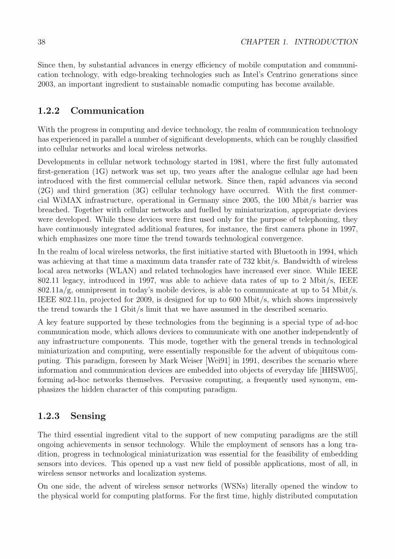
We first require to highlight in more detail the essential technological and parallel paradigmatictrends in Section 1.2, which enable, in principle, scenarios of the described kind. In Section 1.3,we embed our work into the Nexus Center of Excellence, in whose context this dissertation waspursued. We will ultimately frame the specific focus and contributions of this dissertation inSection 1.4, in relation to the objectives addressed by Nexus. In Section 1.5 we outline thestructure that we will pursue in the chapters to follow.
1.2 Technological and Paradigmatic Trends
During the past three decades, some significant technological revolutions have occurred that actas enablers for the realization of scenarios based on the paradigms of mobile, ubiquitous, andcontext-aware computing. Some of the most influential leaps in technological advancementsare depicted in Figure 1.2, annotated with key paradigms presented in parallel. The depictionallows us to identify three main branches, which become manifest in the realms of computing,communication, and sensing technology. The grey-shaded funnel indicates the degree of tech-
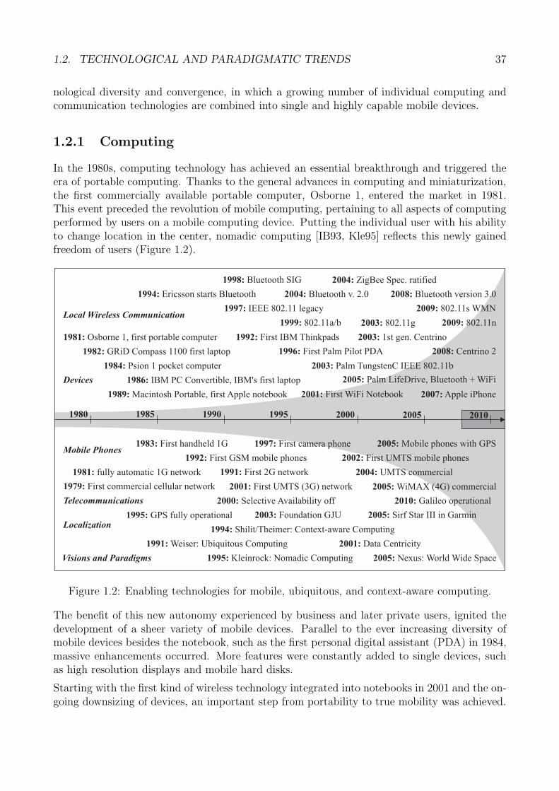
1.2. TECHNOLOGICAL AND PARADIGMATIC TRENDS 37
nological diversity and convergence, in which a growing number of individual computing andcommunication technologies are combined into single and highly capable mobile devices.
1.2.1 Computing
In the 1980s, computing technology has achieved an essential breakthrough and triggered theera of portable computing. Thanks to the general advances in computing and miniaturization,the first commercially available portable computer, Osborne 1, entered the market in 1981.This event preceded the revolution of mobile computing, pertaining to all aspects of computingperformed by users on a mobile computing device. Putting the individual user with his abilityto change location in the center, nomadic computing [IB93, Kle95] reflects this newly gainedfreedom of users (Figure 1.2).
200520001995199019851980
1981: Osborne 1, first portable computer
1984: Psion 1 pocket computer
1992: First IBM Thinkpads
1996: First Palm Pilot PDA
2001: First WiFi Notebook
2003: 1st gen. Centrino
2008: Centrino 2
2005: Palm LifeDrive, Bluetooth + WiFi
2003: Palm TungstenC IEEE 802.11b
1982: GRiD Compass 1100 first laptop
1986: IBM PC Convertible, IBM's first laptop
1989: Macintosh Portable, first Apple notebook 2007: Apple iPhone
1997: IEEE 802.11 legacy
1994: Ericsson starts Bluetooth
1998: Bluetooth SIG
2004: Bluetooth v. 2.0 2008: Bluetooth version 3.0
1999: 802.11a/b 2003: 802.11g 2009: 802.11n
2004: ZigBee Spec. ratified
2009: 802.11s WMN
1983: First handheld 1G
1992: First GSM mobile phones
1997: First camera phone
2002: First UMTS mobile phones
2005: Mobile phones with GPS
1979: First commercial cellular network
1981: fully automatic 1G network 1991: First 2G network
2001: First UMTS (3G) network
2004: UMTS commercial
2005: WiMAX (4G) commercial
Mobile Phones
1995: GPS fully operational
2000: Selective Availability off
2003: Foundation GJU 2005: Sirf Star III in Garmin
2010: Galileo operational
1991: Weiser: Ubiquitous Computing
1994: Shilit/Theimer: Context-aware Computing
2001: Data Centricity
2005: Nexus: World Wide Space
Local Wireless Communication
Devices
Visions and Paradigms
Localization
Telecommunications
1995: Kleinrock: Nomadic Computing
2010
Figure 1.2: Enabling technologies for mobile, ubiquitous, and context-aware computing.
The benefit of this new autonomy experienced by business and later private users, ignited thedevelopment of a sheer variety of mobile devices. Parallel to the ever increasing diversity ofmobile devices besides the notebook, such as the first personal digital assistant (PDA) in 1984,massive enhancements occurred. More features were constantly added to single devices, suchas high resolution displays and mobile hard disks.
Starting with the first kind of wireless technology integrated into notebooks in 2001 and the on-going downsizing of devices, an important step from portability to true mobility was achieved.
38 CHAPTER 1. INTRODUCTION
Since then, by substantial advances in energy efficiency of mobile computation and communi-cation technology, with edge-breaking technologies such as Intel’s Centrino generations since2003, an important ingredient to sustainable nomadic computing has become available.
1.2.2 Communication
With the progress in computing and device technology, the realm of communication technologyhas experienced in parallel a number of significant developments, which can be roughly classifiedinto cellular networks and local wireless networks.
Developments in cellular network technology started in 1981, where the first fully automatedfirst-generation (1G) network was set up, two years after the analogue cellular age had beenintroduced with the first commercial cellular network. Since then, rapid advances via second(2G) and third generation (3G) cellular technology have occurred. With the first commer-cial WiMAX infrastructure, operational in Germany since 2005, the 100 Mbit/s barrier wasbreached. Together with cellular networks and fuelled by miniaturization, appropriate deviceswere developed. While these devices were first used only for the purpose of telephoning, theyhave continuously integrated additional features, for instance, the first camera phone in 1997,which emphasizes one more time the trend towards technological convergence.
In the realm of local wireless networks, the first initiative started with Bluetooth in 1994, whichwas achieving at that time a maximum data transfer rate of 732 kbit/s. Bandwidth of wirelesslocal area networks (WLAN) and related technologies have increased ever since. While IEEE802.11 legacy, introduced in 1997, was able to achieve data rates of up to 2 Mbit/s, IEEE802.11a/g, omnipresent in today’s mobile devices, is able to communicate at up to 54 Mbit/s.IEEE 802.11n, projected for 2009, is designed for up to 600 Mbit/s, which shows impressivelythe trend towards the 1 Gbit/s limit that we have assumed in the described scenario.
A key feature supported by these technologies from the beginning is a special type of ad-hoccommunication mode, which allows devices to communicate with one another independently ofany infrastructure components. This mode, together with the general trends in technologicalminiaturization and computing, were essentially responsible for the advent of ubiquitous com-puting. This paradigm, foreseen by Mark Weiser [Wei91] in 1991, describes the scenario whereinformation and communication devices are embedded into objects of everyday life [HHSW05],forming ad-hoc networks themselves. Pervasive computing, a frequently used synonym, em-phasizes the hidden character of this computing paradigm.
1.2.3 Sensing
The third essential ingredient vital to the support of new computing paradigms are the stillongoing achievements in sensor technology. While the employment of sensors has a long tra-dition, progress in technological miniaturization was essential for the feasibility of embeddingsensors into devices. This opened up a vast new field of possible applications, most of all, inwireless sensor networks and localization systems.
On one side, the advent of wireless sensor networks (WSNs) literally opened the window tothe physical world for computing platforms. For the first time, highly distributed computation
1.3. BACKGROUND 39
and communication infrastructures were able to gather and process information about thephysical world for specific applications. On the other side, localization systems, such as theGlobal Positioning System (GPS) [EM99], operational since 1995, were able to deliver accurateposition information to the user’s end device. With the high-performance SiRFstar III chipset,first incorporated in Garmin handheld devices in 2005, highly accurate position acquisitions inthe range of only a few meters became possible.
These developments allowed for a whole new class of applications in mobile communicationnetworks, based on the paradigm of context-aware computing, a term presumably first coinedin [ST94]. Also referred to as sentient computing, this paradigm incorporates information that isrelevant for a user’s current situation in order to adapt the services and information accordingly.The special case of location-based computing puts the position as a specific type of context inthe center, enabling the delivery of services and information to the user in dependence of hiscurrent position in the physical world.
1.3 Background
1.3.1 Explicit Context Models
In a broader sense, context can be defined according to [RBB03, RDD+03] and based on [DA99]as “the information which can be used to characterize the situation of an entity”. In thisdefinition, entities may refer to “persons, locations, or objects which are considered to berelevant for the behavior of an application.”
When dealing with a large number of users with similar but also different needs regarding theirpersonal context, it is of great value to provide structured context information in the form ofexplicit context models. Appropriately implemented, such models can provide each user withhis particular subset of relevant information. Research related to all aspects of explicit contextmodels can be positioned, based on the analysis provided in [HHSW05], in the intersectionsof mobile, ubiquitous, and context-aware computing according to Figure 1.3, with the backingenabling technologies discussed in the previous section.
Explicit Context Models
Center of Excellence627 (Nexus)
Nomadic ComputingMobile Computing
Ubiquitous ComputingPervasive Computing
Context-aware ComputingSentient Computing
Figure 1.3: Computing paradigms, explicit context models, and the SFB 627 (Nexus).
40 CHAPTER 1. INTRODUCTION
Regarding the collection of large quantities of context information, an essential distinctionbetween primary and secondary context according to [RBB03, RDD+03] is useful. Primarycontext, shared by virtually all possible types of entities, encompasses identity, location, andtime, which designate the most essential properties of an entity. Secondary context, comprisingany other conceivable context information, e.g., a car’s current speed and direction of movement,may model other relevant aspects of individual entities.
Besides the mere provisioning of context information in a generic form, the specific way ofhow context is used is a key indicator for selecting methods that provide context informationefficiently. For example, if the location information of a user is not required distant from him,it makes no sense to set up a distributed index structure that materializes the information atdistant storage locations, which would require constant maintenance with no benefit.
For our convenience, the authors of [RBB03, RDD+03] have identified three basic ways in whichapplications make use of context information: context-based selection, presentation, and action.These functionalities provide essential hints to more basic required services. For instance, inorder to select information relevant to a user’s current location, that location needs to becontinuously available. Another example is the presentation of information in the vicinity of auser’s current location, which implies the usage of spatial queries that retrieve information suchas a defined number of nearest objects of a specific type relative to the user’s current location.Yet another example is to perform certain functions when defined spatial constellation betweenthe user and other entities in the world occur (spatial events), such as the popping up of amessage based on the user reaching a certain geographic region (e.g., a building).
1.3.2 SFB 627 (Nexus)
The provisioning of explicit context models for context-based applications has been addressedby a large number of efforts in the research community. In a nutshell, the majority of theseattempts provide context models for a specific purpose only [BCQ+07].
Dealing with a broad range of issues related to the provisioning of context models on a large scalehas been addressed by the Center of Excellence 627 (Nexus)1 [HKL+99, GBH+05, REF+06].The project deals with many objectives related to the modelling, acquisition, processing, andprovisioning of context to context-aware applications. Figure 1.3 shows the location of theCenter’s research scope relative to mobile, ubiquitous, and context-aware computing.
Central to the Nexus project is the architecture of the Nexus platform, depicted in Figure 1.4and based on an adaptation of [REF+06]. It provides not only an extensive context model of thereal world, but also the basic services to accomplish the context-based interactions selection,presentation, and action), which we have described in the previous section.
The Nexus platform architecture can be divided into three main tiers: the client, federation,and service tier [FV03]. Each server in the service tier stores the context information of aspecific geometric region in the physical world. This is due to the fact that context informationis frequently queried by referring to a geometric location, which emphasizes the importance ofcontext models to location-based applications in particular.
1German: Sonderforschungsbereich (SFB) 627
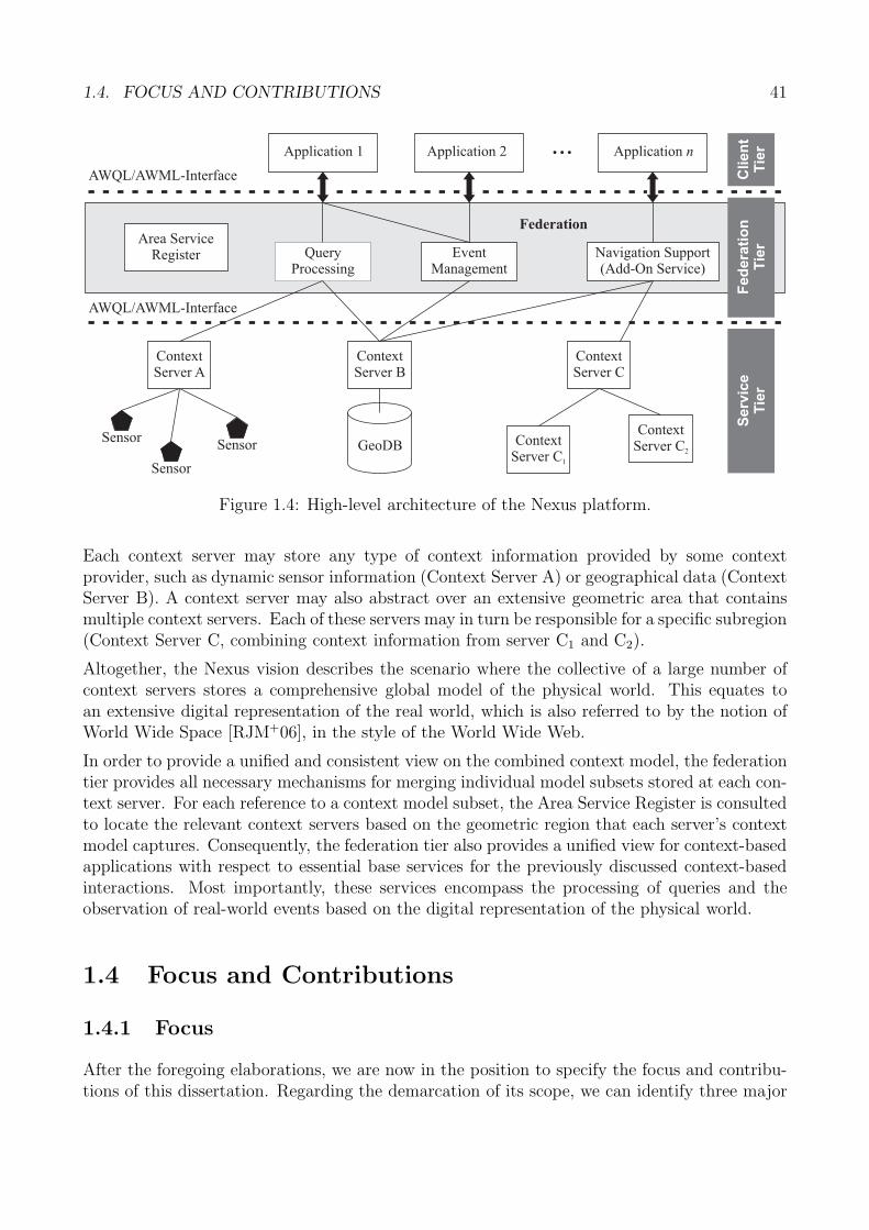
1.4. FOCUS AND CONTRIBUTIONS 41
SensorSensor
Sensor
Area ServiceRegister
Federation
QueryProcessing
EventManagement
Navigation Support(Add-On Service)
AWQL/AWML-Interface
Application 1 ...Application 2 Application n
AWQL/AWML-Interface
ContextServer B
GeoDB
ContextServer C
ContextServer C1
ContextServer C2
ContextServer A
Clien
tT
ier
Fed
era
tio
nT
ier
Serv
ice
Tie
r
Figure 1.4: High-level architecture of the Nexus platform.
Each context server may store any type of context information provided by some contextprovider, such as dynamic sensor information (Context Server A) or geographical data (ContextServer B). A context server may also abstract over an extensive geometric area that containsmultiple context servers. Each of these servers may in turn be responsible for a specific subregion(Context Server C, combining context information from server C1 and C2).
Altogether, the Nexus vision describes the scenario where the collective of a large number ofcontext servers stores a comprehensive global model of the physical world. This equates toan extensive digital representation of the real world, which is also referred to by the notion ofWorld Wide Space [RJM+06], in the style of the World Wide Web.
In order to provide a unified and consistent view on the combined context model, the federationtier provides all necessary mechanisms for merging individual model subsets stored at each con-text server. For each reference to a context model subset, the Area Service Register is consultedto locate the relevant context servers based on the geometric region that each server’s contextmodel captures. Consequently, the federation tier also provides a unified view for context-basedapplications with respect to essential base services for the previously discussed context-basedinteractions. Most importantly, these services encompass the processing of queries and theobservation of real-world events based on the digital representation of the physical world.
1.4 Focus and Contributions
1.4.1 Focus
After the foregoing elaborations, we are now in the position to specify the focus and contribu-tions of this dissertation. Regarding the demarcation of its scope, we can identify three major
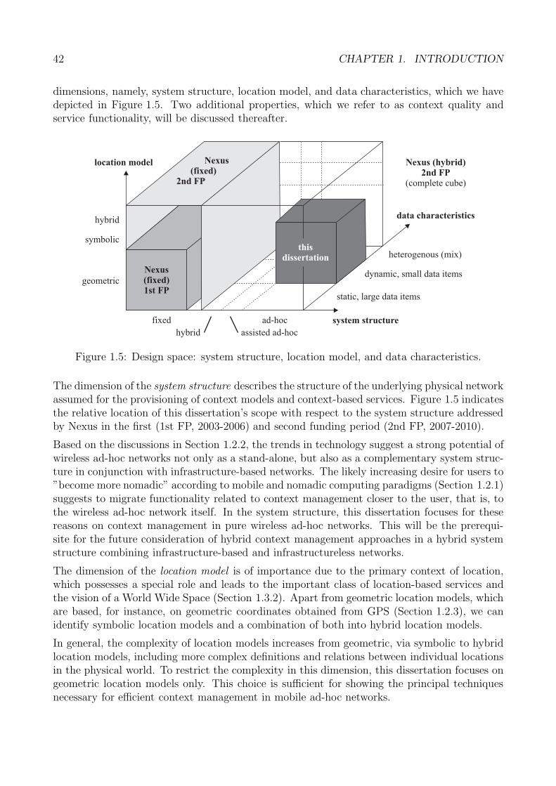
42 CHAPTER 1. INTRODUCTION
dimensions, namely, system structure, location model, and data characteristics, which we havedepicted in Figure 1.5. Two additional properties, which we refer to as context quality andservice functionality, will be discussed thereafter.
system structurefixed ad-hoc
assisted ad-hochybrid
data characteristics
location model
symbolic
hybrid
geometric
static, large data items
dynamic, small data items
heterogenous (mix)
Nexus(fixed)1st FP
Nexus (hybrid)2nd FP
(complete cube)
thisdissertation
Nexus(fixed)
2nd FP
Figure 1.5: Design space: system structure, location model, and data characteristics.
The dimension of the system structure describes the structure of the underlying physical networkassumed for the provisioning of context models and context-based services. Figure 1.5 indicatesthe relative location of this dissertation’s scope with respect to the system structure addressedby Nexus in the first (1st FP, 2003-2006) and second funding period (2nd FP, 2007-2010).
Based on the discussions in Section 1.2.2, the trends in technology suggest a strong potential ofwireless ad-hoc networks not only as a stand-alone, but also as a complementary system struc-ture in conjunction with infrastructure-based networks. The likely increasing desire for users to”become more nomadic” according to mobile and nomadic computing paradigms (Section 1.2.1)suggests to migrate functionality related to context management closer to the user, that is, tothe wireless ad-hoc network itself. In the system structure, this dissertation focuses for thesereasons on context management in pure wireless ad-hoc networks. This will be the prerequi-site for the future consideration of hybrid context management approaches in a hybrid systemstructure combining infrastructure-based and infrastructureless networks.
The dimension of the location model is of importance due to the primary context of location,which possesses a special role and leads to the important class of location-based services andthe vision of a World Wide Space (Section 1.3.2). Apart from geometric location models, whichare based, for instance, on geometric coordinates obtained from GPS (Section 1.2.3), we canidentify symbolic location models and a combination of both into hybrid location models.
In general, the complexity of location models increases from geometric, via symbolic to hybridlocation models, including more complex definitions and relations between individual locationsin the physical world. To restrict the complexity in this dimension, this dissertation focuses ongeometric location models only. This choice is sufficient for showing the principal techniquesnecessary for efficient context management in mobile ad-hoc networks.
1.4. FOCUS AND CONTRIBUTIONS 43
The dimension of the data characteristics describes general properties of the data items to bemanaged. Apart from many different characteristics that can be consulted for classificationpurposes, the dynamics and the size of data items can be regarded as the most influencingones. This is due to the fact that the product of dynamics and size directly correlates to anincrease in the cost of keeping data items in the system up to date.
A key observation is that the dynamics and size of data items generally exhibit a strong corre-lation. For example, city maps, constituting large amounts of data, are mostly static, whereasthe rather small items of location information are likely to be highly dynamic in a scenario ofmobile users. Therefore it is valid and absolutely sufficient for our purposes to arrange bothcharacteristics in a combined form in Figure 1.5.
From the discussion about the importance of the primary context of location for location-basedapplications in particular (Section 1.3.1), this dissertation focuses on dynamic and small dataitems. In addition, straightforward solutions are conceivable for rather static data items inmobile ad-hoc networks, e.g., their replication on a predefined subset of network nodes.
An additional fact that complicates the provisioning of model data and the implementation offunctionality on top of it is that a model of the physical world can be captured in the systemonly within certain limits of accuracy. This is due to technological limitations in the acquisitionof data pertaining to physical objects, as discussed in Section 1.2.3 for the case of GPS.
In general, the imperfections in any observation of the physical world can be subsumed by theterm data quality, or context quality when referring to the management of context information.In this dissertation, we will address the issue of data quality by taking into consideration theinaccuracy of geometric locations of objects of the real world and its impact on the mechanismsfor the management of dynamic location information.
Besides the provisioning of context models, it is important to demonstrate the applicabilityand practicability of the concepts developed in this dissertation. To this end, we make use ofselected base service functionality that builds on the previously discussed items and which isessential in the support of the diverse types of context-based applications.
During our discussion on forms of interaction in Section 1.3.1 and the base service functionalityprovided by the Nexus platform (Figure 1.4), we can identify queries and events as two ofthe most fundamental services required for context-based and location-based services. In thisdissertation, we will take up the processing of spatial queries, which are centered around theprimary context of location and constitute a fundamental type of query especially for location-based services. We will briefly discuss events in the outlook Section 6.2.
1.4.2 Contributions
The objectives of this dissertation are the design, implementation, and evaluation of a frame-work for fundamental strategies and mechanisms for context management in mobile ad-hocnetworks. The dissertation lays the foundation for enabling the development and deploymentof location-based and context-based services in these networks.
The individual contributions within this framework follow from the derivation of the focus inthe previous section and can be concisely stated as follows:
44 CHAPTER 1. INTRODUCTION
(1) We present a quantitative analysis of the topological characteristics of mobile ad-hocnetworks by looking at the partitioning behavior of these networks;
(2) We derive a compact framework comprising the essential components for dynamic datastorage in mobile ad-hoc networks and discuss in detail the related literature;
(3) We introduce a fundamental set of algorithms for the management of dynamic data, whichis robust against the specific characteristics of mobile ad-hoc networks;
(4) We devise an analytical model for the assessment of storage costs in mobile ad-hoc net-works and present a taxonomy and comparison of fundamental storage approaches;
(5) We define a formal accuracy model for the semantics of location information and spatialqueries, the latter including geometric range and nearest neighbor queries;
(6) We introduce algorithms for the updating of dynamic and inaccurate location informationand probabilistic spatial queries based on the defined formal accuracy model;
(7) We provide an extensive simulative performance analysis to validate the algorithms forfundamental storage and query processing in mobile ad-hoc networks.
1.5 Structure of the Dissertation
The main part of the dissertation is structured as follows. In Chapter 2 we introduce funda-mental notions regarding mobile ad-hoc networks and data storage relevant for the scope ofthis dissertation. This chapter also presents the analysis of the partitioning behavior of mobilead-hoc networks, and derives the principal structure of the storage framework. The chapterconcludes with an extensive discussion of the related literature.
Chapter 3 introduces a resilient core approach to the storage of dynamic data items in mobilead-hoc networks based on the paradigm of location-centric storage. This chapter presents theanalytical comparison of our own storage approach with other fundamental approaches, and asimulative performance analysis of a set of key performance metrics.
In Chapter 4, we complement the core storage approach with comprehensive strategies andmechanisms of data migration to address the impact of node mobility on data storage. Addi-tional simulative performance results compare our own migration approach with a number ofother conceivable approaches and demonstrate its superiority over these approaches.
Chapter 5 defines the formal accuracy models for location information and spatial queries. Thischapter also introduces the algorithms for location updating and query processing in mobile ad-hoc networks and provides a simulative analysis to point out the impact of imperfect locationinformation on the performance of these algorithms.
The dissertation is concluded in Chapter 6 by summarizing key results and stating some impor-tant implications for future considerations. Finally, a repertory of promising research directionsdeduced from the work in this dissertation is highlighted to stimulate future efforts in the fieldof data and context management in mobile ad-hoc networks.
Chapter 2
Fundamentals
In this chapter we specify the fundamental constraints, assumptions, and requirements thatunderly the algorithms developed in the remainder of this dissertation. The key differentiationto other work is the model of mobile ad-hoc networks and its unique characteristics, whichmake the design of fundamental algorithms a highly challenging task and which we describe indetail in Section 2.1. To emphasize the importance of MANET characteristics, we present adetailed analysis of the partitioning behavior in these networks in Section 2.2.
In Section 2.3 we develop the notion of location-centric storage, the fundamental paradigmthat follows from arguments based on the important role the primary context of location playsfor context-based applications, and which underlies our algorithms. Based on the constraintsand assumptions of Section 2.1 through 2.3, we derive the key requirements that the storagealgorithms must take into account and derive our reference model for context management inMANETs based on these requirements in Section 2.4. Finally, we discuss related work that isrelevant in the scope of our reference model in Section 2.5.
2.1 Mobile Ad-hoc Networks (MANETs)
2.1.1 Network Model
Mobile ad-hoc networks (MANETs, e.g. [LC04]) are a class of communication networks formedby portable devices that communicate with one another over wireless communication (radio)links. Devices may comprise any of the equipment described in Section 1.2 and Figure 1.2, suchas mobile phones, personal digital assistants (PDAs), and notebooks.
Due to the limited radio range of wireless communication technologies, such as IEEE 802.11and Bluetooth (Section 1.2.2), any device is able to communicate directly only with a subsetof other devices at any time. Due to the ability of devices to move about freely while be-ing carried by users, however, devices continuously discover new devices by moving into oneanother’s communication range. Thus, communication links between mobile devices are estab-lished and severed in a spontaneous manner. Viewed across the whole network, mobility leadsto a constantly changing topology of the physical network.
45
46 CHAPTER 2. FUNDAMENTALS
Another type of wireless multihop networks are wireless sensor networks (WSNs). In contrastto MANETs, the devices in WSNs possess significantly less capabilities in terms of batterylifetime, processing, storage, and communication. Typical WSNs furthermore exhibit muchlower degrees of device mobility than MANETs. A further important differentiator is thatWSNs are designed for specific applications based on the processing of sensor informationgathered from their environment, and, in contrast to MANETs, they do generally not allow formore general services due to their limited capabilities.
A second type of wireless multihop networks are wireless mesh networks (WMNs). Differentfrom MANETs, nodes of WMNs consist of stationary devices, forming a relatively stable ”mesh”of nodes through wireless radio links. Furthermore, the nodes in WMNs are powered externallyand have significantly more capabilities with respect to processing and storage. WSNs aresometimes also considered to be more general and to comprise not only wireless mesh routers,but also MANETs as a complementary network structure [AWW05]. In this view, MANETscan be regarded as a special case of WMNs.
In MANETs, in order to coordinate access to the shared medium when devices attempt totransmit at the same time, protocols for medium access control (MAC) that are specific towireless media are employed. Such protocols are designed to minimize the number of collisionson the medium to avoid frequent retransmissions and congestions. Due to the limited com-munication range of devices, configurations such as the hidden and exposed terminal situationmay occur where collision detection schemes cannot be applied. Therefore, protocols employalternative methods, for instance, the CSMA/CA with RTS/CTS mechanism in IEEE 802.11,which builds on collision avoidance instead by negotiating which device is to transmit next. Inthis dissertation, we will assume the aforementioned protocol, without limiting the generalityof our approaches to be developed in the remainder of this dissertation.
To function as a network, an essential property is that communication between two nodes gener-ally occurs over multiple hops of intermediary nodes, since communication range strongly limitsdirect communication between nodes. While routing is also essential in infrastructure-basednetworks, for instance the Internet, the constantly changing network topology make routingone of the major challenges in MANETs. For this reason, a large number of routing protocolshave been devised that attempt to establish efficient routes on-demand, for instance AODV,rather than pre-computing routes beforehand. While these protocols are able to significantlyminimize the overhead for route establishment, route failures are still critical because they re-quire costly route discoveries. For this reason, geometric routing protocols, such as GPSR, arepreferred over topological routing protocols, like AODV, when the geometric position is knownto network nodes. In this protocol class, routing is virtually stateless in the sense that explicitroute maintenance and discovery are not required. Instead, routing is accomplished based ondecisions that are taken from the viewpoint of a single node.
In this dissertation, we will assume that the nodes in MANETs are able to acquire their positioninformation, for example, based on an embedded GPS receiver (Section 1.2.3). Therefore, geo-metric routing protocols may be employed for packet routing. We will investigate in Chapter 3in more detail additional routing mechanisms required for our purposes.
Besides routing, the transport of messages that exceed the size of single packets is an importantmechanism also in MANETs. While TCP’s faulty assumptions of its congestion control mech-anism in wireless networks is a well-known problem, additional properties further complicate
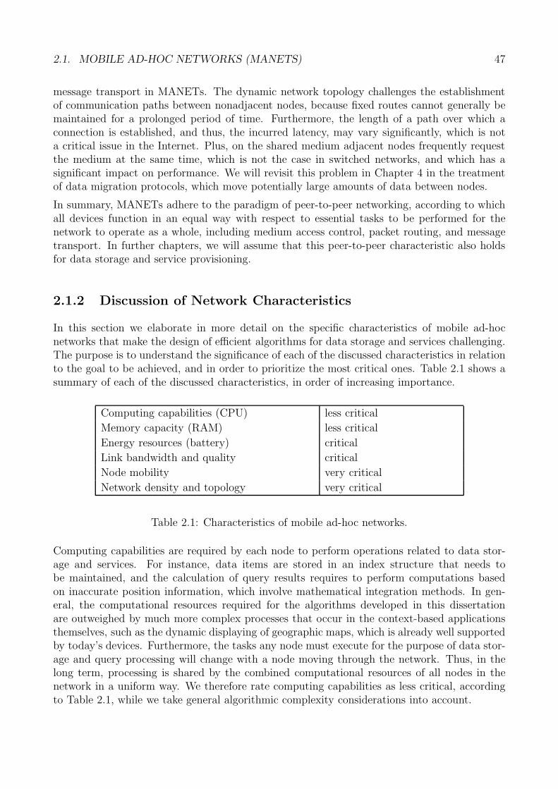
2.1. MOBILE AD-HOC NETWORKS (MANETS) 47
message transport in MANETs. The dynamic network topology challenges the establishmentof communication paths between nonadjacent nodes, because fixed routes cannot generally bemaintained for a prolonged period of time. Furthermore, the length of a path over which aconnection is established, and thus, the incurred latency, may vary significantly, which is nota critical issue in the Internet. Plus, on the shared medium adjacent nodes frequently requestthe medium at the same time, which is not the case in switched networks, and which has asignificant impact on performance. We will revisit this problem in Chapter 4 in the treatmentof data migration protocols, which move potentially large amounts of data between nodes.
In summary, MANETs adhere to the paradigm of peer-to-peer networking, according to whichall devices function in an equal way with respect to essential tasks to be performed for thenetwork to operate as a whole, including medium access control, packet routing, and messagetransport. In further chapters, we will assume that this peer-to-peer characteristic also holdsfor data storage and service provisioning.
2.1.2 Discussion of Network Characteristics
In this section we elaborate in more detail on the specific characteristics of mobile ad-hocnetworks that make the design of efficient algorithms for data storage and services challenging.The purpose is to understand the significance of each of the discussed characteristics in relationto the goal to be achieved, and in order to prioritize the most critical ones. Table 2.1 shows asummary of each of the discussed characteristics, in order of increasing importance.
Computing capabilities (CPU) less critical
Memory capacity (RAM) less critical
Energy resources (battery) critical
Link bandwidth and quality critical
Node mobility very critical
Network density and topology very critical
Table 2.1: Characteristics of mobile ad-hoc networks.
Computing capabilities are required by each node to perform operations related to data stor-age and services. For instance, data items are stored in an index structure that needs tobe maintained, and the calculation of query results requires to perform computations basedon inaccurate position information, which involve mathematical integration methods. In gen-eral, the computational resources required for the algorithms developed in this dissertationare outweighed by much more complex processes that occur in the context-based applicationsthemselves, such as the dynamic displaying of geographic maps, which is already well supportedby today’s devices. Furthermore, the tasks any node must execute for the purpose of data stor-age and query processing will change with a node moving through the network. Thus, in thelong term, processing is shared by the combined computational resources of all nodes in thenetwork in a uniform way. We therefore rate computing capabilities as less critical, accordingto Table 2.1, while we take general algorithmic complexity considerations into account.
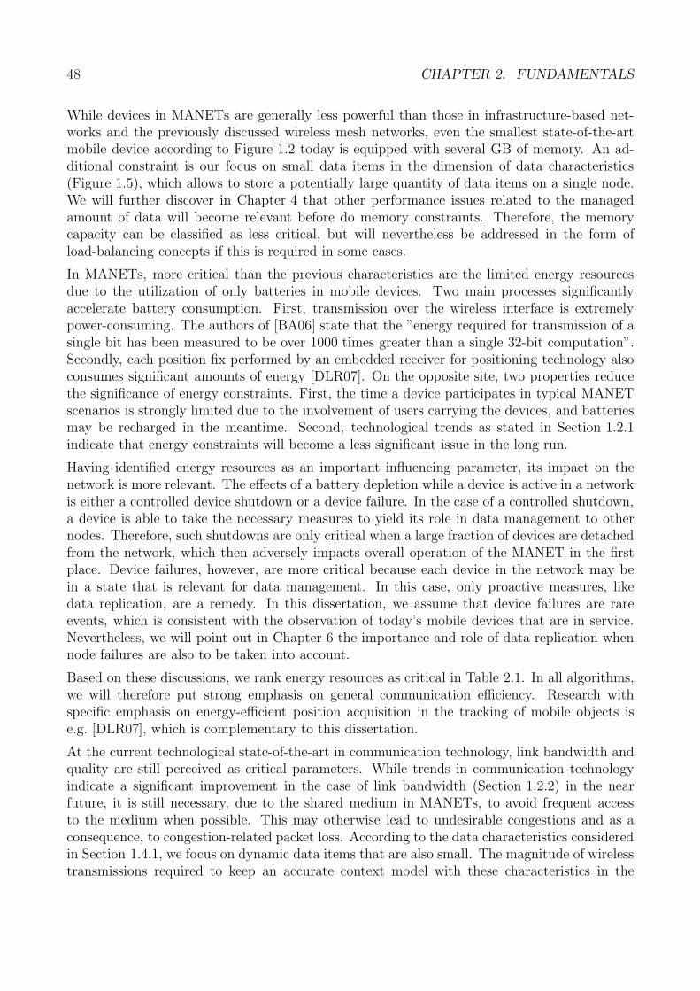
48 CHAPTER 2. FUNDAMENTALS
While devices in MANETs are generally less powerful than those in infrastructure-based net-works and the previously discussed wireless mesh networks, even the smallest state-of-the-artmobile device according to Figure 1.2 today is equipped with several GB of memory. An ad-ditional constraint is our focus on small data items in the dimension of data characteristics(Figure 1.5), which allows to store a potentially large quantity of data items on a single node.We will further discover in Chapter 4 that other performance issues related to the managedamount of data will become relevant before do memory constraints. Therefore, the memorycapacity can be classified as less critical, but will nevertheless be addressed in the form ofload-balancing concepts if this is required in some cases.
In MANETs, more critical than the previous characteristics are the limited energy resourcesdue to the utilization of only batteries in mobile devices. Two main processes significantlyaccelerate battery consumption. First, transmission over the wireless interface is extremelypower-consuming. The authors of [BA06] state that the ”energy required for transmission of asingle bit has been measured to be over 1000 times greater than a single 32-bit computation”.Secondly, each position fix performed by an embedded receiver for positioning technology alsoconsumes significant amounts of energy [DLR07]. On the opposite site, two properties reducethe significance of energy constraints. First, the time a device participates in typical MANETscenarios is strongly limited due to the involvement of users carrying the devices, and batteriesmay be recharged in the meantime. Second, technological trends as stated in Section 1.2.1indicate that energy constraints will become a less significant issue in the long run.
Having identified energy resources as an important influencing parameter, its impact on thenetwork is more relevant. The effects of a battery depletion while a device is active in a networkis either a controlled device shutdown or a device failure. In the case of a controlled shutdown,a device is able to take the necessary measures to yield its role in data management to othernodes. Therefore, such shutdowns are only critical when a large fraction of devices are detachedfrom the network, which then adversely impacts overall operation of the MANET in the firstplace. Device failures, however, are more critical because each device in the network may bein a state that is relevant for data management. In this case, only proactive measures, likedata replication, are a remedy. In this dissertation, we assume that device failures are rareevents, which is consistent with the observation of today’s mobile devices that are in service.Nevertheless, we will point out in Chapter 6 the importance and role of data replication whennode failures are also to be taken into account.
Based on these discussions, we rank energy resources as critical in Table 2.1. In all algorithms,we will therefore put strong emphasis on general communication efficiency. Research withspecific emphasis on energy-efficient position acquisition in the tracking of mobile objects ise.g. [DLR07], which is complementary to this dissertation.
At the current technological state-of-the-art in communication technology, link bandwidth andquality are still perceived as critical parameters. While trends in communication technologyindicate a significant improvement in the case of link bandwidth (Section 1.2.2) in the nearfuture, it is still necessary, due to the shared medium in MANETs, to avoid frequent accessto the medium when possible. This may otherwise lead to undesirable congestions and as aconsequence, to congestion-related packet loss. According to the data characteristics consideredin Section 1.4.1, we focus on dynamic data items that are also small. The magnitude of wirelesstransmissions required to keep an accurate context model with these characteristics in the
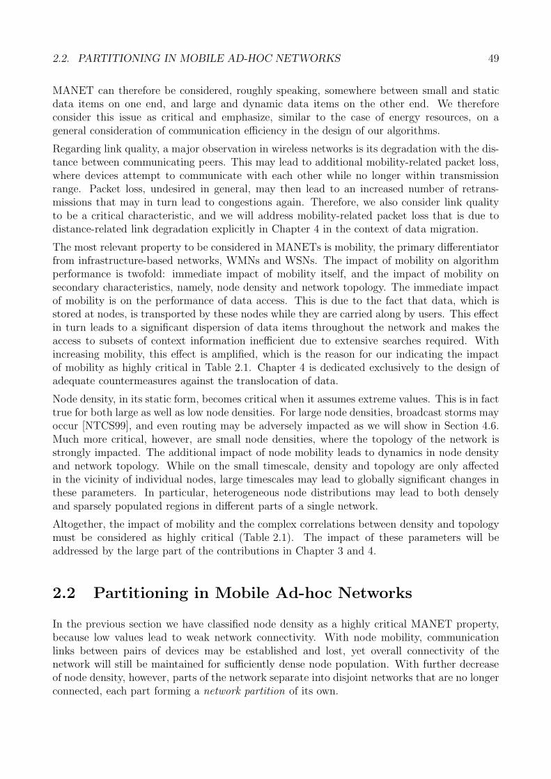
2.2. PARTITIONING IN MOBILE AD-HOC NETWORKS 49
MANET can therefore be considered, roughly speaking, somewhere between small and staticdata items on one end, and large and dynamic data items on the other end. We thereforeconsider this issue as critical and emphasize, similar to the case of energy resources, on ageneral consideration of communication efficiency in the design of our algorithms.
Regarding link quality, a major observation in wireless networks is its degradation with the dis-tance between communicating peers. This may lead to additional mobility-related packet loss,where devices attempt to communicate with each other while no longer within transmissionrange. Packet loss, undesired in general, may then lead to an increased number of retrans-missions that may in turn lead to congestions again. Therefore, we also consider link qualityto be a critical characteristic, and we will address mobility-related packet loss that is due todistance-related link degradation explicitly in Chapter 4 in the context of data migration.
The most relevant property to be considered in MANETs is mobility, the primary differentiatorfrom infrastructure-based networks, WMNs and WSNs. The impact of mobility on algorithmperformance is twofold: immediate impact of mobility itself, and the impact of mobility onsecondary characteristics, namely, node density and network topology. The immediate impactof mobility is on the performance of data access. This is due to the fact that data, which isstored at nodes, is transported by these nodes while they are carried along by users. This effectin turn leads to a significant dispersion of data items throughout the network and makes theaccess to subsets of context information inefficient due to extensive searches required. Withincreasing mobility, this effect is amplified, which is the reason for our indicating the impactof mobility as highly critical in Table 2.1. Chapter 4 is dedicated exclusively to the design ofadequate countermeasures against the translocation of data.
Node density, in its static form, becomes critical when it assumes extreme values. This is in facttrue for both large as well as low node densities. For large node densities, broadcast storms mayoccur [NTCS99], and even routing may be adversely impacted as we will show in Section 4.6.Much more critical, however, are small node densities, where the topology of the network isstrongly impacted. The additional impact of node mobility leads to dynamics in node densityand network topology. While on the small timescale, density and topology are only affectedin the vicinity of individual nodes, large timescales may lead to globally significant changes inthese parameters. In particular, heterogeneous node distributions may lead to both denselyand sparsely populated regions in different parts of a single network.
Altogether, the impact of mobility and the complex correlations between density and topologymust be considered as highly critical (Table 2.1). The impact of these parameters will beaddressed by the large part of the contributions in Chapter 3 and 4.
2.2 Partitioning in Mobile Ad-hoc Networks
In the previous section we have classified node density as a highly critical MANET property,because low values lead to weak network connectivity. With node mobility, communicationlinks between pairs of devices may be established and lost, yet overall connectivity of thenetwork will still be maintained for sufficiently dense node population. With further decreaseof node density, however, parts of the network separate into disjoint networks that are no longerconnected, each part forming a network partition of its own.
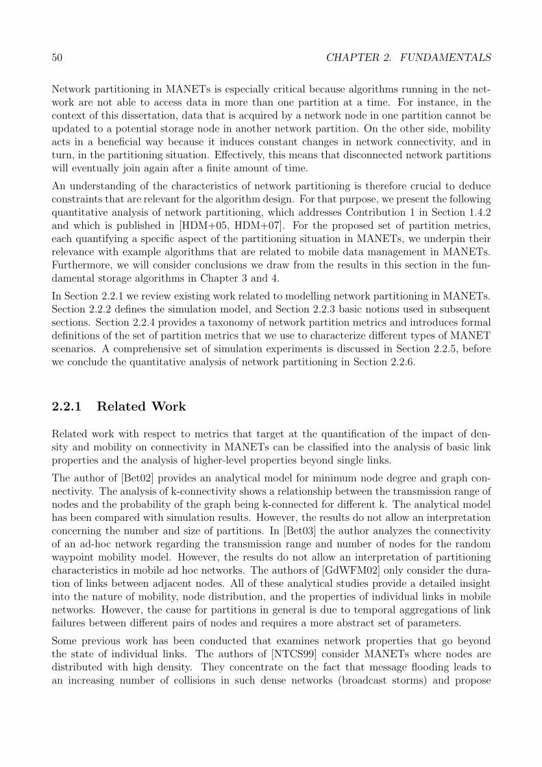
50 CHAPTER 2. FUNDAMENTALS
Network partitioning in MANETs is especially critical because algorithms running in the net-work are not able to access data in more than one partition at a time. For instance, in thecontext of this dissertation, data that is acquired by a network node in one partition cannot beupdated to a potential storage node in another network partition. On the other side, mobilityacts in a beneficial way because it induces constant changes in network connectivity, and inturn, in the partitioning situation. Effectively, this means that disconnected network partitionswill eventually join again after a finite amount of time.
An understanding of the characteristics of network partitioning is therefore crucial to deduceconstraints that are relevant for the algorithm design. For that purpose, we present the followingquantitative analysis of network partitioning, which addresses Contribution 1 in Section 1.4.2and which is published in [HDM+05, HDM+07]. For the proposed set of partition metrics,each quantifying a specific aspect of the partitioning situation in MANETs, we underpin theirrelevance with example algorithms that are related to mobile data management in MANETs.Furthermore, we will consider conclusions we draw from the results in this section in the fun-damental storage algorithms in Chapter 3 and 4.
In Section 2.2.1 we review existing work related to modelling network partitioning in MANETs.Section 2.2.2 defines the simulation model, and Section 2.2.3 basic notions used in subsequentsections. Section 2.2.4 provides a taxonomy of network partition metrics and introduces formaldefinitions of the set of partition metrics that we use to characterize different types of MANETscenarios. A comprehensive set of simulation experiments is discussed in Section 2.2.5, beforewe conclude the quantitative analysis of network partitioning in Section 2.2.6.
2.2.1 Related Work
Related work with respect to metrics that target at the quantification of the impact of den-sity and mobility on connectivity in MANETs can be classified into the analysis of basic linkproperties and the analysis of higher-level properties beyond single links.
The author of [Bet02] provides an analytical model for minimum node degree and graph con-nectivity. The analysis of k-connectivity shows a relationship between the transmission range ofnodes and the probability of the graph being k-connected for different k. The analytical modelhas been compared with simulation results. However, the results do not allow an interpretationconcerning the number and size of partitions. In [Bet03] the author analyzes the connectivityof an ad-hoc network regarding the transmission range and number of nodes for the randomwaypoint mobility model. However, the results do not allow an interpretation of partitioningcharacteristics in mobile ad hoc networks. The authors of [GdWFM02] only consider the dura-tion of links between adjacent nodes. All of these analytical studies provide a detailed insightinto the nature of mobility, node distribution, and the properties of individual links in mobilenetworks. However, the cause for partitions in general is due to temporal aggregations of linkfailures between different pairs of nodes and requires a more abstract set of parameters.
Some previous work has been conducted that examines network properties that go beyondthe state of individual links. The authors of [NTCS99] consider MANETs where nodes aredistributed with high density. They concentrate on the fact that message flooding leads toan increasing number of collisions in such dense networks (broadcast storms) and propose
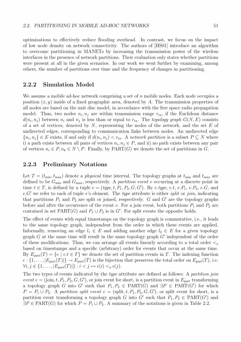
2.2. PARTITIONING IN MOBILE AD-HOC NETWORKS 51
optimizations to effectively reduce flooding overhead. In contrast, we focus on the impactof low node density on network connectivity. The authors of [HS01] introduce an algorithmto overcome partitioning in MANETs by increasing the transmission power of the wirelessinterfaces in the presence of network partitions. Their evaluation only states whether partitionswere present at all in the given scenarios. In our work we went further by examining, amongothers, the number of partitions over time and the frequency of changes in partitioning.
2.2.2 Simulation Model
We assume a mobile ad-hoc network comprising a set of n mobile nodes. Each node occupies aposition (x, y) inside of a fixed geographic area, denoted by A. The transmission properties ofall nodes are based on the unit disc model, in accordance with the free space radio propagationmodel. Thus, two nodes ni, nj are within transmission range rtx, if the Euclidean distanced(ni, nj) between ni and nj is less than or equal to rtx. The topology graph G(N, E) consistsof a set of vertices, denoted by N , representing the nodes of the network, and the set E ofundirected edges, corresponding to communication links between nodes. An undirected edge{ni, nj} ∈ E exists, if and only if d(ni, nj) < rtx. A network partition is a subset P ⊆ N wherei) a path exists between all pairs of vertices ni, nj ∈ P , and ii) no path exists between any pairof vertices ni ∈ P, nk ∈ N \ P . Finally, by PART(G) we denote the set of partitions in G.
2.2.3 Preliminary Notations
Let T = (tmin, tmax) denote a physical time interval. The topology graphs at tmin and tmax aredefined to be Gmin and Gmax, respectively. A partition event e occurring at a discrete point intime t ∈ T , is defined by a tuple e = (type, t, P1, P2, G, G′). By e.type, e.t, e.P1, e.P2, e.G, ande.G′ we refer to each of tuple e’s element. The type attribute is either split or join, indicatingthat partitions P1 and P2 are split or joined, respectively. G and G′ are the topology graphsbefore and after the occurrence of the event e. For a join event, both partitions P1 and P2 arecontained in set PART(G) and P1 ∪ P2 is in G′. For split events the opposite holds.
The effect of events with equal timestamps on the topology graph is commutative, i.e., it leadsto the same topology graph, independent from the order in which these events are applied.Informally, removing an edge l1 ∈ E and adding another edge l2 ∈ E for a given topologygraph G at the same time will result in the same topology graph G′ independent of the orderof these modifications. Thus, we can arrange all events linearly according to a total order <o
based on timestamps and a specific (arbitrary) order for events that occur at the same time.By Epart(T ) = {e | e.t ∈ T} we denote the set of partition events in T . The indexing functionε : {1, . . . , |Epart(T )|} → Epart(T ) is the bijection that preserves the total order on Epart(T ), i.e.∀i, j ∈ {1, . . . , |Epart(T )|} : i < j ↔ ε(i) <o ε(j).
The two types of events indicated by the type attribute are defined as follows: A partition joinevent e = (join, t, P1, P2, G, G′), or join event for short, is a partition event in Epart transforminga topology graph G into G′ such that P1, P2 ∈ PART(G) and ∃P ∈ PART(G′) for whichP = P1 ∪ P2. A partition split event e = (split, t, P1, P2, G, G′), or split event for short, is apartition event transforming a topology graph G into G′ such that P1, P2 ∈ PART(G′) and∃P ∈ PART(G) for which P = P1 ∪ P2. A summary of the notations is given in Table 2.2.
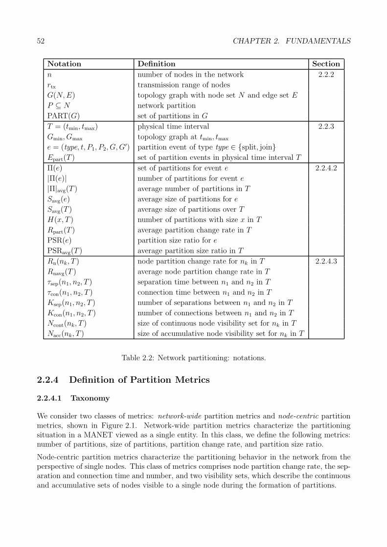
52 CHAPTER 2. FUNDAMENTALS
Notation Definition Section
n number of nodes in the network 2.2.2
rtx transmission range of nodes
G(N, E) topology graph with node set N and edge set E
P ⊆ N network partition
PART(G) set of partitions in G
T = (tmin, tmax) physical time interval 2.2.3
Gmin, Gmax topology graph at tmin, tmax
e = (type, t, P1, P2, G, G′) partition event of type type ∈ {split, join}Epart(T ) set of partition events in physical time interval T
Π(e) set of partitions for event e 2.2.4.2
|Π(e)| number of partitions for event e
|Π|avg(T ) average number of partitions in T
Savg(e) average size of partitions for e
Savg(T ) average size of partitions over T
H(x, T ) number of partitions with size x in T
Rpart(T ) average partition change rate in T
PSR(e) partition size ratio for e
PSRavg(T ) average partition size ratio in T
Rn(nk, T ) node partition change rate for nk in T 2.2.4.3
Rnavg(T ) average node partition change rate in T
τsep(n1, n2, T ) separation time between n1 and n2 in T
τcon(n1, n2, T ) connection time between n1 and n2 in T
Ksep(n1, n2, T ) number of separations between n1 and n2 in T
Kcon(n1, n2, T ) number of connections between n1 and n2 in T
Ncont(nk, T ) size of continuous node visibility set for nk in T
Nacc(nk, T ) size of accumulative node visibility set for nk in T
Table 2.2: Network partitioning: notations.
2.2.4 Definition of Partition Metrics
2.2.4.1 Taxonomy
We consider two classes of metrics: network-wide partition metrics and node-centric partitionmetrics, shown in Figure 2.1. Network-wide partition metrics characterize the partitioningsituation in a MANET viewed as a single entity. In this class, we define the following metrics:number of partitions, size of partitions, partition change rate, and partition size ratio.
Node-centric partition metrics characterize the partitioning behavior in the network from theperspective of single nodes. This class of metrics comprises node partition change rate, the sep-aration and connection time and number, and two visibility sets, which describe the continuousand accumulative sets of nodes visible to a single node during the formation of partitions.
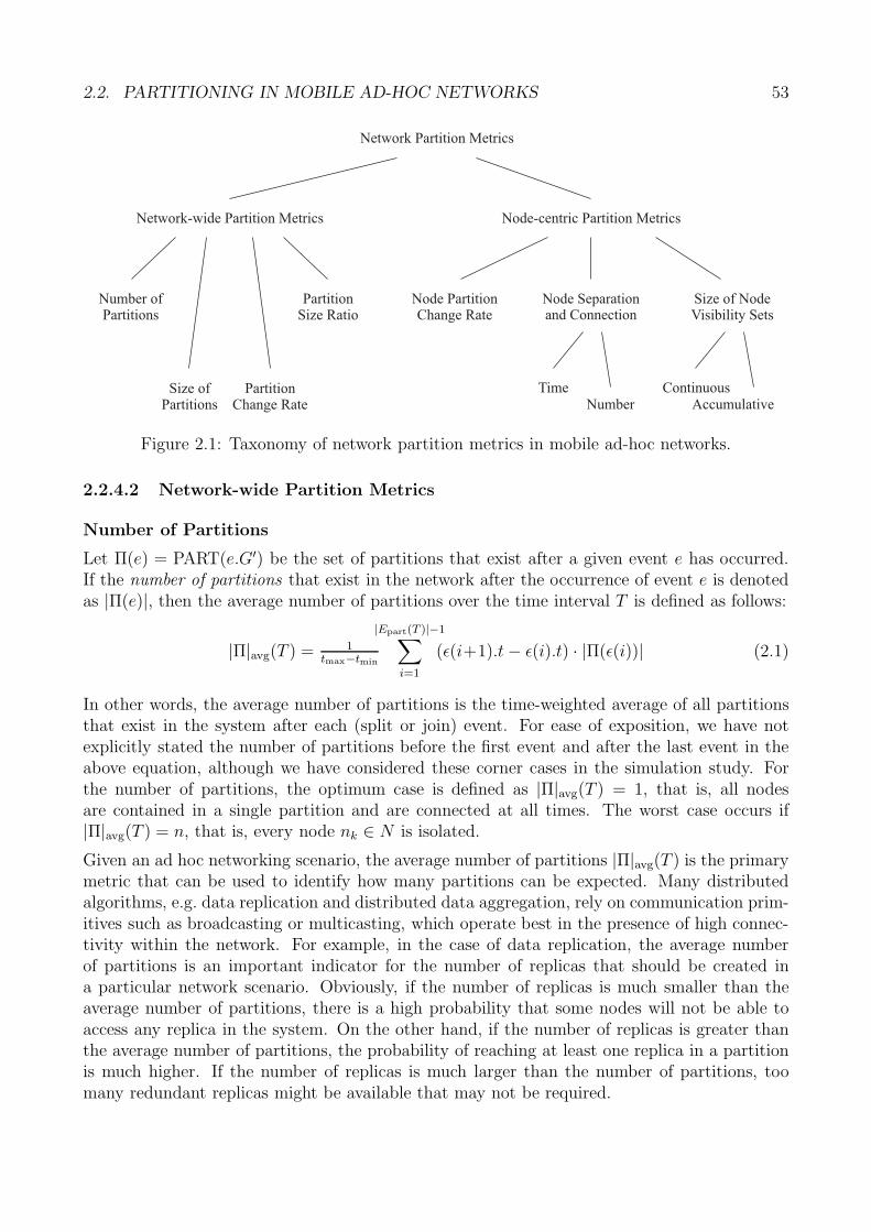
2.2. PARTITIONING IN MOBILE AD-HOC NETWORKS 53
Network Partition Metrics
Network-wide Partition Metrics Node-centric Partition Metrics
Number ofPartitions
Size ofPartitions
PartitionSize Ratio
Node PartitionChange Rate
Node Separationand Connection
Size of NodeVisibility Sets
PartitionChange Rate Number
Time ContinuousAccumulative
Figure 2.1: Taxonomy of network partition metrics in mobile ad-hoc networks.
2.2.4.2 Network-wide Partition Metrics
Number of Partitions
Let Π(e) = PART(e.G′) be the set of partitions that exist after a given event e has occurred.If the number of partitions that exist in the network after the occurrence of event e is denotedas |Π(e)|, then the average number of partitions over the time interval T is defined as follows:
|Π|avg(T ) = 1tmax−tmin
|Epart(T )|−1∑i=1
(ε(i+1).t − ε(i).t) · |Π(ε(i))| (2.1)
In other words, the average number of partitions is the time-weighted average of all partitionsthat exist in the system after each (split or join) event. For ease of exposition, we have notexplicitly stated the number of partitions before the first event and after the last event in theabove equation, although we have considered these corner cases in the simulation study. Forthe number of partitions, the optimum case is defined as |Π|avg(T ) = 1, that is, all nodesare contained in a single partition and are connected at all times. The worst case occurs if|Π|avg(T ) = n, that is, every node nk ∈ N is isolated.
Given an ad hoc networking scenario, the average number of partitions |Π|avg(T ) is the primarymetric that can be used to identify how many partitions can be expected. Many distributedalgorithms, e.g. data replication and distributed data aggregation, rely on communication prim-itives such as broadcasting or multicasting, which operate best in the presence of high connec-tivity within the network. For example, in the case of data replication, the average numberof partitions is an important indicator for the number of replicas that should be created ina particular network scenario. Obviously, if the number of replicas is much smaller than theaverage number of partitions, there is a high probability that some nodes will not be able toaccess any replica in the system. On the other hand, if the number of replicas is greater thanthe average number of partitions, the probability of reaching at least one replica in a partitionis much higher. If the number of replicas is much larger than the number of partitions, toomany redundant replicas might be available that may not be required.
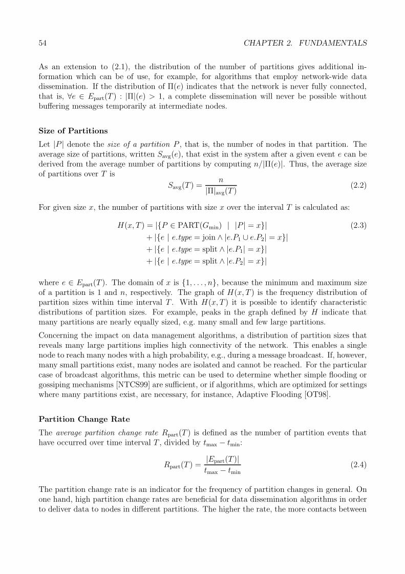
54 CHAPTER 2. FUNDAMENTALS
As an extension to (2.1), the distribution of the number of partitions gives additional in-formation which can be of use, for example, for algorithms that employ network-wide datadissemination. If the distribution of Π(e) indicates that the network is never fully connected,that is, ∀e ∈ Epart(T ) : |Π|(e) > 1, a complete dissemination will never be possible withoutbuffering messages temporarily at intermediate nodes.
Size of Partitions
Let |P | denote the size of a partition P , that is, the number of nodes in that partition. Theaverage size of partitions, written Savg(e), that exist in the system after a given event e can bederived from the average number of partitions by computing n/|Π(e)|. Thus, the average sizeof partitions over T is
Savg(T ) =n
|Π|avg(T )(2.2)
For given size x, the number of partitions with size x over the interval T is calculated as:
H(x, T ) = |{P ∈ PART(Gmin) | |P | = x}| (2.3)
+ |{e | e.type = join ∧ |e.P1 ∪ e.P2| = x}|+ |{e | e.type = split ∧ |e.P1| = x}|+ |{e | e.type = split ∧ |e.P2| = x}|
where e ∈ Epart(T ). The domain of x is {1, . . . , n}, because the minimum and maximum sizeof a partition is 1 and n, respectively. The graph of H(x, T ) is the frequency distribution ofpartition sizes within time interval T . With H(x, T ) it is possible to identify characteristicdistributions of partition sizes. For example, peaks in the graph defined by H indicate thatmany partitions are nearly equally sized, e.g. many small and few large partitions.
Concerning the impact on data management algorithms, a distribution of partition sizes thatreveals many large partitions implies high connectivity of the network. This enables a singlenode to reach many nodes with a high probability, e.g., during a message broadcast. If, however,many small partitions exist, many nodes are isolated and cannot be reached. For the particularcase of broadcast algorithms, this metric can be used to determine whether simple flooding orgossiping mechanisms [NTCS99] are sufficient, or if algorithms, which are optimized for settingswhere many partitions exist, are necessary, for instance, Adaptive Flooding [OT98].
Partition Change Rate
The average partition change rate Rpart(T ) is defined as the number of partition events thathave occurred over time interval T , divided by tmax − tmin:
Rpart(T ) =|Epart(T )|tmax − tmin
(2.4)
The partition change rate is an indicator for the frequency of partition changes in general. Onone hand, high partition change rates are beneficial for data dissemination algorithms in orderto deliver data to nodes in different partitions. The higher the rate, the more contacts between
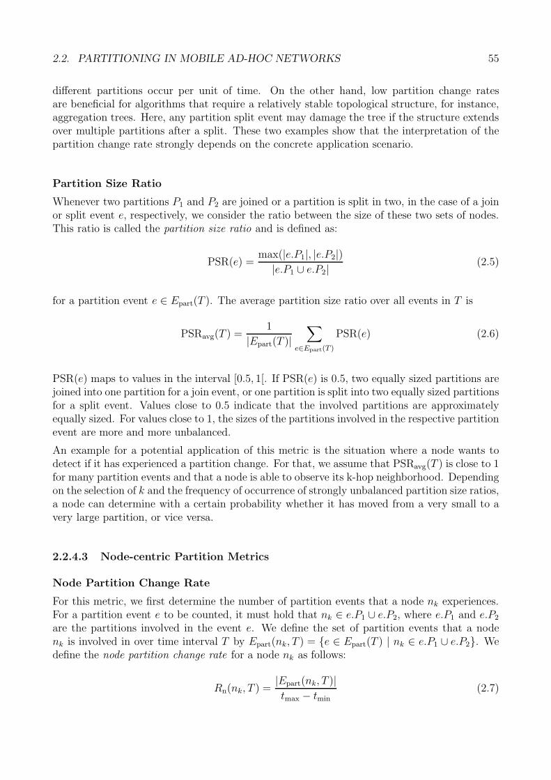
2.2. PARTITIONING IN MOBILE AD-HOC NETWORKS 55
different partitions occur per unit of time. On the other hand, low partition change ratesare beneficial for algorithms that require a relatively stable topological structure, for instance,aggregation trees. Here, any partition split event may damage the tree if the structure extendsover multiple partitions after a split. These two examples show that the interpretation of thepartition change rate strongly depends on the concrete application scenario.
Partition Size Ratio
Whenever two partitions P1 and P2 are joined or a partition is split in two, in the case of a joinor split event e, respectively, we consider the ratio between the size of these two sets of nodes.This ratio is called the partition size ratio and is defined as:
PSR(e) =max(|e.P1|, |e.P2|)
|e.P1 ∪ e.P2| (2.5)
for a partition event e ∈ Epart(T ). The average partition size ratio over all events in T is
PSRavg(T ) =1
|Epart(T )|∑
e∈Epart(T )
PSR(e) (2.6)
PSR(e) maps to values in the interval [0.5, 1[. If PSR(e) is 0.5, two equally sized partitions arejoined into one partition for a join event, or one partition is split into two equally sized partitionsfor a split event. Values close to 0.5 indicate that the involved partitions are approximatelyequally sized. For values close to 1, the sizes of the partitions involved in the respective partitionevent are more and more unbalanced.
An example for a potential application of this metric is the situation where a node wants todetect if it has experienced a partition change. For that, we assume that PSRavg(T ) is close to 1for many partition events and that a node is able to observe its k-hop neighborhood. Dependingon the selection of k and the frequency of occurrence of strongly unbalanced partition size ratios,a node can determine with a certain probability whether it has moved from a very small to avery large partition, or vice versa.
2.2.4.3 Node-centric Partition Metrics
Node Partition Change Rate
For this metric, we first determine the number of partition events that a node nk experiences.For a partition event e to be counted, it must hold that nk ∈ e.P1 ∪ e.P2, where e.P1 and e.P2
are the partitions involved in the event e. We define the set of partition events that a nodenk is involved in over time interval T by Epart(nk, T ) = {e ∈ Epart(T ) | nk ∈ e.P1 ∪ e.P2}. Wedefine the node partition change rate for a node nk as follows:
Rn(nk, T ) =|Epart(nk, T )|tmax − tmin
(2.7)
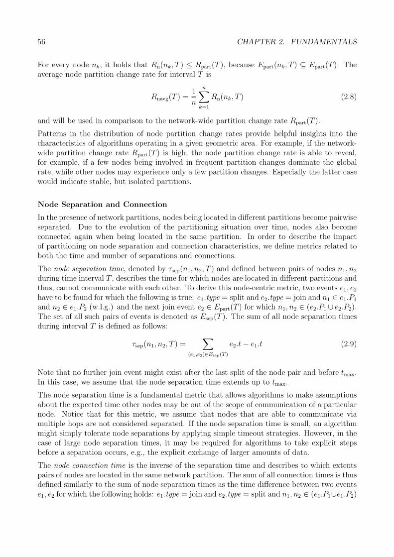
56 CHAPTER 2. FUNDAMENTALS
For every node nk, it holds that Rn(nk, T ) ≤ Rpart(T ), because Epart(nk, T ) ⊆ Epart(T ). Theaverage node partition change rate for interval T is
Rnavg(T ) =1
n
n∑k=1
Rn(nk, T ) (2.8)
and will be used in comparison to the network-wide partition change rate Rpart(T ).
Patterns in the distribution of node partition change rates provide helpful insights into thecharacteristics of algorithms operating in a given geometric area. For example, if the network-wide partition change rate Rpart(T ) is high, the node partition change rate is able to reveal,for example, if a few nodes being involved in frequent partition changes dominate the globalrate, while other nodes may experience only a few partition changes. Especially the latter casewould indicate stable, but isolated partitions.
Node Separation and Connection
In the presence of network partitions, nodes being located in different partitions become pairwiseseparated. Due to the evolution of the partitioning situation over time, nodes also becomeconnected again when being located in the same partition. In order to describe the impactof partitioning on node separation and connection characteristics, we define metrics related toboth the time and number of separations and connections.
The node separation time, denoted by τsep(n1, n2, T ) and defined between pairs of nodes n1, n2
during time interval T , describes the time for which nodes are located in different partitions andthus, cannot communicate with each other. To derive this node-centric metric, two events e1, e2
have to be found for which the following is true: e1.type = split and e2.type = join and n1 ∈ e1.P1
and n2 ∈ e1.P2 (w.l.g.) and the next join event e2 ∈ Epart(T ) for which n1, n2 ∈ (e2.P1 ∪ e2.P2).The set of all such pairs of events is denoted as Esep(T ). The sum of all node separation timesduring interval T is defined as follows:
τsep(n1, n2, T ) =∑
(e1,e2)∈Esep(T )
e2.t − e1.t (2.9)
Note that no further join event might exist after the last split of the node pair and before tmax.In this case, we assume that the node separation time extends up to tmax.
The node separation time is a fundamental metric that allows algorithms to make assumptionsabout the expected time other nodes may be out of the scope of communication of a particularnode. Notice that for this metric, we assume that nodes that are able to communicate viamultiple hops are not considered separated. If the node separation time is small, an algorithmmight simply tolerate node separations by applying simple timeout strategies. However, in thecase of large node separation times, it may be required for algorithms to take explicit stepsbefore a separation occurs, e.g., the explicit exchange of larger amounts of data.
The node connection time is the inverse of the separation time and describes to which extentspairs of nodes are located in the same network partition. The sum of all connection times is thusdefined similarly to the sum of node separation times as the time difference between two eventse1, e2 for which the following holds: e1.type = join and e2.type = split and n1, n2 ∈ (e1.P1∪e1.P2)
2.2. PARTITIONING IN MOBILE AD-HOC NETWORKS 57
and the next split event e2 ∈ Epart for which n1 ∈ e2.P1 and n2 ∈ e2.P2 (w.l.g.). The sum of allconnection times of n1 and n2 over T is denoted as τcon(n1, n2, T ).
The node connection time is crucial because it determines how much data can potentially beexchanged between nodes. For example, if the network characteristics are such that sufficientlylarge connection times never exist, an algorithm may explicitly perform remote operations inmultiple steps in the first place.
While the node separation and connection time give a picture of the aggregated time thatcan be expected for nodes to be separated or connected, it does not specify the frequency ofseparations and connections that occur. In other words, each of the separation and connectiontime do not state whether the expressed sum is due to a small number of large intervals, or,vice versa, to a large number of small intervals. Therefore, we also examine the number ofnode separations Ksep(n1, n2, T ) and connections Kcon(n1, n2, T ) per node pairs, which definethe number of separations and connections that occur during time interval T , respectively.
The relevance of this further specification of node separation and connection behavior is shownby the following example. Consider the transmission of a large message between two nodescurrently located in the same partition, and for which it is known that both nodes are connectedin the same partition during 90 % of the time. However, if the number of connections indicatehigh frequency in the separation and reconnection of the two nodes, it is not likely that atransmission between both nodes can be maintained for a prolonged period of time. This is duea node separation that may follow shortly after a reconnection, and which is due to a recurringpartition split. Such situations may require additional precautions to optimize transmissionprotocols, depending on the magnitude of node separation and connection frequencies.
Node Visibility Sets
We define two metrics related to the set of nodes visible to a specific node nk during the splittingand joining of partitions: the continuous and accumulative node visibility set.
The continuous node visibility set Econt(nk, T ) ⊆ Epart(T ) is the subset of nk’s split events withinthe time interval T defined as Econt(nk, T ) = {e ∈ Epart(T ) | nk ∈ e.P1∧e.type = split∧e.t ∈ T}.1The size of this set is defined as
Ncont(nk, T ) =∣∣ ⋂
e∈Econt(nk,T )
e.P1
∣∣ (2.10)
Ncont(nk, T ) gives information about how many nodes are located in the same partition as nk
during the time interval T . The gradient of Ncont(nk, T ) based on a variation of T is an indicatorof how fast the individual nodes in nk’s partition are separated into other partitions.
Data management algorithms that fragment information across multiple nodes are only suitablefor systems with a reasonably small gradient, because only a slowly decreasing continuous nodevisibility set ensures a sufficiently long availability of information stored on remote nodes.The value of the gradient tolerable for algorithms depends on how long remote data has tobe available. In the area of distributed query processing, for example, this includes the timebetween sending a query and receiving all answers from remote nodes.
1Without loss of generality, we assume that nk is always contained in the first partition P1 of e.
58 CHAPTER 2. FUNDAMENTALS
The accumulative node visibility set Eacc(nk, T ) is the subset of nk’s join events within T definedas Eacc(nk, T ) = {e ∈ Epart(T ) | nk ∈ (e.P1 ∪ e.P2) ∧ e.type = join ∧ e.t ∈ T}. Its size is
Nacc(nk, T ) =∣∣ ⋃
e∈Eacc(nk,T )
e.P1 ∪ e.P2
∣∣ (2.11)
Nacc(nk, T ) increases monotonically as partitions with new nodes are joined with nk’s partitionand converges towards the set of all nodes; it will be N , if nk has been in the same partitionwith all nodes over the time interval T at least once. In the context of data dissemination thegradient of Nacc(nk, T ) is an upper bound for how fast an individual node can access all othernodes throughout the network.
2.2.5 Simulation Study
To conduct our experiments, we have used an event-based simulator which, given a mobilitytrace, constructs and alters the topology graph over time. The event-based approach is ableto capture every occurring state of the topology graph over time. The mobility traces wereobtained using the simulation environment presented in [SHB+03]. The random waypoint modeloperates on an area of 2 × 2 km2. For the graph-based random walk mobility model, we havemodelled two graphs, representing a typical Central European city (Figure 2.2.a) and MidtownManhattan (Figure 2.2.b). Each graph spans a total area of approximately 2.5× 1.8 km2. Thesimilar areas of the mobility models allow us to compare the simulation results for differentmobility patterns with one another. The speed of nodes was randomly chosen from the interval[0.5, 2.0] m/s. The total simulation time was 3600 s.
The key parameters for performance evaluation of algorithms in MANETs are the spatial areain which the mobile nodes may move, the number of nodes in the network, the mobility modelthe nodes follow, and the transmission range of the wireless communication technology. Thespatial node density is defined by the size of the spatial area and the number of nodes. In thefollowing simulations, we provide detailed results for the various metrics and focus on nodedensity and a discussion of the impact of each of the mobility models. A discussion of theimpact of the transmission range is provided in Appendix B.
We assume that all network nodes are mobile, thus inducing changes in the topology graph overtime. We use two mobility models in our experiments: the random waypoint mobility model[BMJ+98] and the graph-based mobility model [THB+02], which model typical scenarios in anopen field and urban area, respectively. In the random waypoint model, nodes move on straightlines inside of the simulation area by repetitively selecting a random destination and randomspeed. Because this model has the property of a steadily decreasing average node speed overtime [YLN03], we choose the random speed from an interval [vmin, vmax], with vmin > 0. In thegraph-based model, the mobility of nodes is spatially constrained by a graph. Each vertex inthe graph represents a particular location (x, y) within a geographic region, such as points ofinterest or road intersections. Graph edges connect these locations, and represent routes in theregion, such as streets. Each node chooses a vertex of the graph as its destination and a speedfrom a given interval randomly and moves to that destination on the shortest path of the graphat the chosen speed. In contrast to the random waypoint mobility model, the graph-basedrandom walk mobility model is more restrictive and prohibits completely arbitrary movement,reflecting more closely scenarios in urban areas.
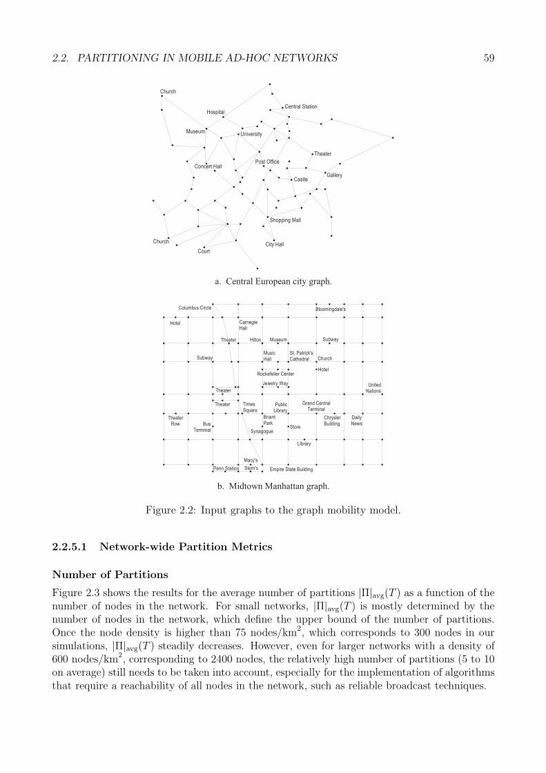
2.2. PARTITIONING IN MOBILE AD-HOC NETWORKS 59
Church
Hospital
Museum
Concert Hall
Court
City Hall
Shopping Mall
GalleryCastle
Theater
Post Office
University
Central Station
Church
a. Central European city graph.
TheaterRow Bus
Terminal
Penn Station
Macy's
Empire State Building
Bloomingdale's
UnitedNations
Subway
MusicHall
HiltonTheater
Subway
Rockefeller Center
St. Patrick'sCathedral Church
BriantPark
PublicLibrary
DailyNews
ChryslerBuilding
Grand CentralTerminal
Museum
TimesSquare
Theater
Theater
CarnegieHall
Columbus Circle
Library
Hotel
Store
Stern's
Jewelry Way
Synagogue
Hotel
b. Midtown Manhattan graph.
Figure 2.2: Input graphs to the graph mobility model.
2.2.5.1 Network-wide Partition Metrics
Number of Partitions
Figure 2.3 shows the results for the average number of partitions |Π|avg(T ) as a function of thenumber of nodes in the network. For small networks, |Π|avg(T ) is mostly determined by thenumber of nodes in the network, which define the upper bound of the number of partitions.Once the node density is higher than 75 nodes/km2, which corresponds to 300 nodes in oursimulations, |Π|avg(T ) steadily decreases. However, even for larger networks with a density of600 nodes/km2, corresponding to 2400 nodes, the relatively high number of partitions (5 to 10on average) still needs to be taken into account, especially for the implementation of algorithmsthat require a reachability of all nodes in the network, such as reliable broadcast techniques.
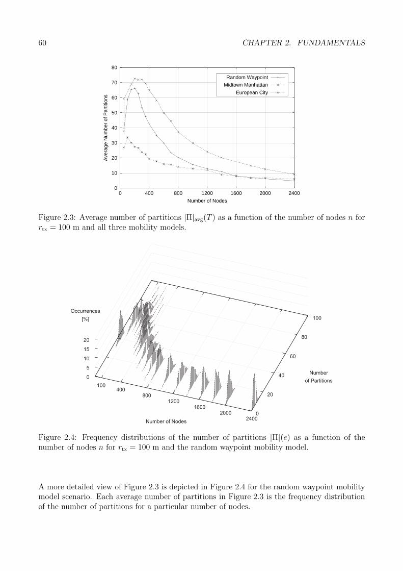
60 CHAPTER 2. FUNDAMENTALS
0
10
20
30
40
50
60
70
80
0 400 800 1200 1600 2000 2400
Ave
rage
Num
ber
of P
artit
ions
Number of Nodes
Random Waypoint
Midtown Manhattan
European City
Figure 2.3: Average number of partitions |Π|avg(T ) as a function of the number of nodes n forrtx = 100 m and all three mobility models.
100400
8001200
16002000
2400Number of Nodes
0
20
40
60
80
100
Number
of Partitions0
5
10
15
20
Occurrences
[%]
Figure 2.4: Frequency distributions of the number of partitions |Π|(e) as a function of thenumber of nodes n for rtx = 100 m and the random waypoint mobility model.
A more detailed view of Figure 2.3 is depicted in Figure 2.4 for the random waypoint mobilitymodel scenario. Each average number of partitions in Figure 2.3 is the frequency distributionof the number of partitions for a particular number of nodes.
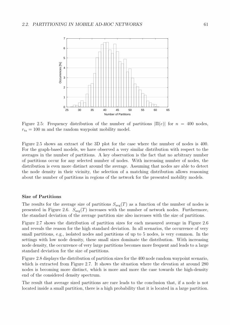
2.2. PARTITIONING IN MOBILE AD-HOC NETWORKS 61
0
1
2
3
4
5
6
7
25 30 35 40 45 50 55 60 65
Occ
urre
nces
[%]
Number of Partitions
Figure 2.5: Frequency distribution of the number of partitions |Π(e)| for n = 400 nodes,rtx = 100 m and the random waypoint mobility model.
Figure 2.5 shows an extract of the 3D plot for the case where the number of nodes is 400.For the graph-based models, we have observed a very similar distribution with respect to theaverages in the number of partitions. A key observation is the fact that no arbitrary numberof partitions occur for any selected number of nodes. With increasing number of nodes, thedistribution is even more distinct around the average. Assuming that nodes are able to detectthe node density in their vicinity, the selection of a matching distribution allows reasoningabout the number of partitions in regions of the network for the presented mobility models.
Size of Partitions
The results for the average size of partitions Savg(T ) as a function of the number of nodes ispresented in Figure 2.6. Savg(T ) increases with the number of network nodes. Furthermore,the standard deviation of the average partition size also increases with the size of partitions.
Figure 2.7 shows the distribution of partition sizes for each measured average in Figure 2.6and reveals the reason for the high standard deviation. In all scenarios, the occurrence of verysmall partitions, e.g., isolated nodes and partitions of up to 5 nodes, is very common. In thesettings with low node density, these small sizes dominate the distribution. With increasingnode density, the occurrence of very large partitions becomes more frequent and leads to a largestandard deviation for the size of partitions.
Figure 2.8 displays the distribution of partition sizes for the 400 node random waypoint scenario,which is extracted from Figure 2.7. It shows the situation where the elevation at around 280nodes is becoming more distinct, which is more and more the case towards the high-densityend of the considered density spectrum.
The result that average sized partitions are rare leads to the conclusion that, if a node is notlocated inside a small partition, there is a high probability that it is located in a large partition.
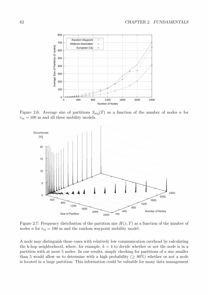
62 CHAPTER 2. FUNDAMENTALS
0
100
200
300
400
500
600
700
800
0 400 800 1200 1600 2000 2400
Ave
rage
Siz
e of
Par
titio
ns [#
nod
es]
Number of Nodes
Random Waypoint
Midtown Manhattan
European City
Figure 2.6: Average size of partitions Savg(T ) as a function of the number of nodes n forrtx = 100 m and all three mobility models.
400800
12001600
20002400Size of Partition 100
400
800
1200
1600
2000
2400
Number of Nodes
0
5
10
15
20
Occurrences
[%]
Figure 2.7: Frequency distribution of the partition size H(x, T ) as a function of the number ofnodes n for rtx = 100 m and the random waypoint mobility model.
A node may distinguish these cases with relatively low communication overhead by calculatingthe k-hop neighborhood, where, for example, k = 4 to decide whether or not the node is in apartition with at most 5 nodes. In our results, simply checking for partitions of a size smallerthan 5 would allow us to determine with a high probability (≥ 80%) whether or not a nodeis located in a large partition. This information could be valuable for many data management
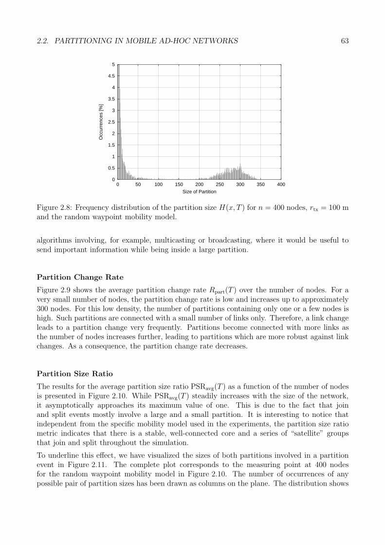
2.2. PARTITIONING IN MOBILE AD-HOC NETWORKS 63
0
0.5
1
1.5
2
2.5
3
3.5
4
4.5
5
0 50 100 150 200 250 300 350 400
Occ
urre
nces
[%]
Size of Partition
Figure 2.8: Frequency distribution of the partition size H(x, T ) for n = 400 nodes, rtx = 100 mand the random waypoint mobility model.
algorithms involving, for example, multicasting or broadcasting, where it would be useful tosend important information while being inside a large partition.
Partition Change Rate
Figure 2.9 shows the average partition change rate Rpart(T ) over the number of nodes. For avery small number of nodes, the partition change rate is low and increases up to approximately300 nodes. For this low density, the number of partitions containing only one or a few nodes ishigh. Such partitions are connected with a small number of links only. Therefore, a link changeleads to a partition change very frequently. Partitions become connected with more links asthe number of nodes increases further, leading to partitions which are more robust against linkchanges. As a consequence, the partition change rate decreases.
Partition Size Ratio
The results for the average partition size ratio PSRavg(T ) as a function of the number of nodesis presented in Figure 2.10. While PSRavg(T ) steadily increases with the size of the network,it asymptotically approaches its maximum value of one. This is due to the fact that joinand split events mostly involve a large and a small partition. It is interesting to notice thatindependent from the specific mobility model used in the experiments, the partition size ratiometric indicates that there is a stable, well-connected core and a series of “satellite” groupsthat join and split throughout the simulation.
To underline this effect, we have visualized the sizes of both partitions involved in a partitionevent in Figure 2.11. The complete plot corresponds to the measuring point at 400 nodesfor the random waypoint mobility model in Figure 2.10. The number of occurrences of anypossible pair of partition sizes has been drawn as columns on the plane. The distribution shows
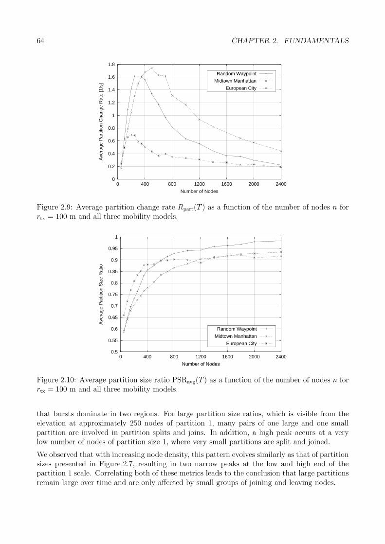
64 CHAPTER 2. FUNDAMENTALS
0
0.2
0.4
0.6
0.8
1
1.2
1.4
1.6
1.8
0 400 800 1200 1600 2000 2400
Ave
rage
Par
titio
n C
hang
e R
ate
[1/s
]
Number of Nodes
Random Waypoint
Midtown Manhattan
European City
Figure 2.9: Average partition change rate Rpart(T ) as a function of the number of nodes n forrtx = 100 m and all three mobility models.
0.5
0.55
0.6
0.65
0.7
0.75
0.8
0.85
0.9
0.95
1
0 400 800 1200 1600 2000 2400
Ave
rage
Par
titio
n S
ize
Rat
io
Number of Nodes
Random Waypoint
Midtown Manhattan
European City
Figure 2.10: Average partition size ratio PSRavg(T ) as a function of the number of nodes n forrtx = 100 m and all three mobility models.
that bursts dominate in two regions. For large partition size ratios, which is visible from theelevation at approximately 250 nodes of partition 1, many pairs of one large and one smallpartition are involved in partition splits and joins. In addition, a high peak occurs at a verylow number of nodes of partition size 1, where very small partitions are split and joined.
We observed that with increasing node density, this pattern evolves similarly as that of partitionsizes presented in Figure 2.7, resulting in two narrow peaks at the low and high end of thepartition 1 scale. Correlating both of these metrics leads to the conclusion that large partitionsremain large over time and are only affected by small groups of joining and leaving nodes.
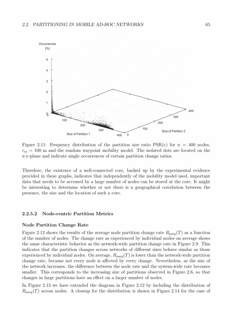
2.2. PARTITIONING IN MOBILE AD-HOC NETWORKS 65
0
100
200
300
400Size of Partition 1 0
100
200
300
400
Size of Partition 2
0
1
2
3
4
5
Occurrences
[%]
Figure 2.11: Frequency distribution of the partition size ratio PSR(e) for n = 400 nodes,rtx = 100 m and the random waypoint mobility model. The isolated dots are located on thex-y-plane and indicate single occurrences of certain partition change ratios.
Therefore, the existence of a well-connected core, backed up by the experimental evidenceprovided in these graphs, indicates that independently of the mobility model used, importantdata that needs to be accessed by a large number of nodes can be stored at the core. It mightbe interesting to determine whether or not there is a geographical correlation between thepresence, the size and the location of such a core.
2.2.5.2 Node-centric Partition Metrics
Node Partition Change Rate
Figure 2.12 shows the results of the average node partition change rate Rnavg(T ) as a functionof the number of nodes. The change rate as experienced by individual nodes on average showsthe same characteristic behavior as the network-wide partition change rate in Figure 2.9. Thisindicates that the partition changes across networks of different sizes behave similar as thoseexperienced by individual nodes. On average, Rnavg(T ) is lower than the network-wide partitionchange rate, because not every node is affected by every change. Nevertheless, as the size ofthe network increases, the difference between the node rate and the system-wide rate becomessmaller. This corresponds to the increasing size of partitions observed in Figure 2.6, so thatchanges in large partitions have an effect on a larger number of nodes.
In Figure 2.13 we have extended the diagram in Figure 2.12 by including the distribution ofRnavg(T ) across nodes. A closeup for the distribution is shown in Figure 2.14 for the case of
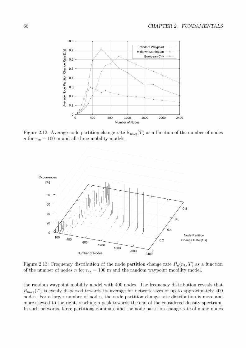
66 CHAPTER 2. FUNDAMENTALS
0
0.1
0.2
0.3
0.4
0.5
0.6
0.7
0.8
0 400 800 1200 1600 2000 2400
Ave
rage
Nod
e P
artit
ion
Cha
nge
Rat
e [1
/s]
Number of Nodes
Random Waypoint
Midtown Manhattan
European City
Figure 2.12: Average node partition change rate Rnavg(T ) as a function of the number of nodesn for rtx = 100 m and all three mobility models.
100400
8001200
16002000
2400Number of Nodes0
0.2
0.4
0.6
0.8
Node Partition
Change Rate [1/s]
0
20
40
60
80
Occurrences
[%]
Figure 2.13: Frequency distribution of the node partition change rate Rn(nk, T ) as a functionof the number of nodes n for rtx = 100 m and the random waypoint mobility model.
the random waypoint mobility model with 400 nodes. The frequency distribution reveals thatRnavg(T ) is evenly dispersed towards its average for network sizes of up to approximately 400nodes. For a larger number of nodes, the node partition change rate distribution is more andmore skewed to the right, reaching a peak towards the end of the considered density spectrum.In such networks, large partitions dominate and the node partition change rate of many nodes
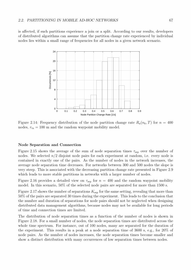
2.2. PARTITIONING IN MOBILE AD-HOC NETWORKS 67
is affected, if such partitions experience a join or a split. According to our results, developersof distributed algorithms can assume that the partition change rate experienced by individualnodes lies within a small range of frequencies for all nodes in a given network scenario.
0
4
8
12
16
20
24
0 0.1 0.2 0.3 0.4 0.5 0.6 0.7 0.8 0.9
Occ
urre
nces
[%]
Node Partition Change Rate [1/s]
Figure 2.14: Frequency distribution of the node partition change rate Rn(nk, T ) for n = 400nodes, rtx = 100 m and the random waypoint mobility model.
Node Separation and Connection
Figure 2.15 shows the average of the sum of node separation times τsep over the number ofnodes. We selected n/2 disjoint node pairs for each experiment at random, i.e. every node iscontained in exactly one of the pairs. As the number of nodes in the network increases, theaverage node separation time decreases. For networks between 300 and 500 nodes the slope isvery steep. This is associated with the decreasing partition change rate presented in Figure 2.9which leads to more stable partitions in networks with a larger number of nodes.
Figure 2.16 provides a detailed view on τsep for n = 400 and the random waypoint mobilitymodel. In this scenario, 50% of the selected node pairs are separated for more than 1500 s.
Figure 2.17 shows the number of separations Ksep for the same setting, revealing that more than50% of the pairs are separated 30 times during the experiment. This leads to the conclusion thatthe number and duration of separations for node pairs should not be neglected when designingdistributed data management algorithms, because nodes may not be available for long periodsof time and connection times are limited.
The distribution of node separation times as a function of the number of nodes is shown inFigure 2.18. For a small number of nodes, the node separation times are distributed across thewhole time spectrum. For instance, out of 100 nodes, many are separated for the duration ofthe experiment. This results in a peak at a node separation time of 3600 s, e.g., for 20% ofnode pairs. As the number of nodes increases, the node separation times become smaller andshow a distinct distribution with many occurrences of low separation times between nodes.
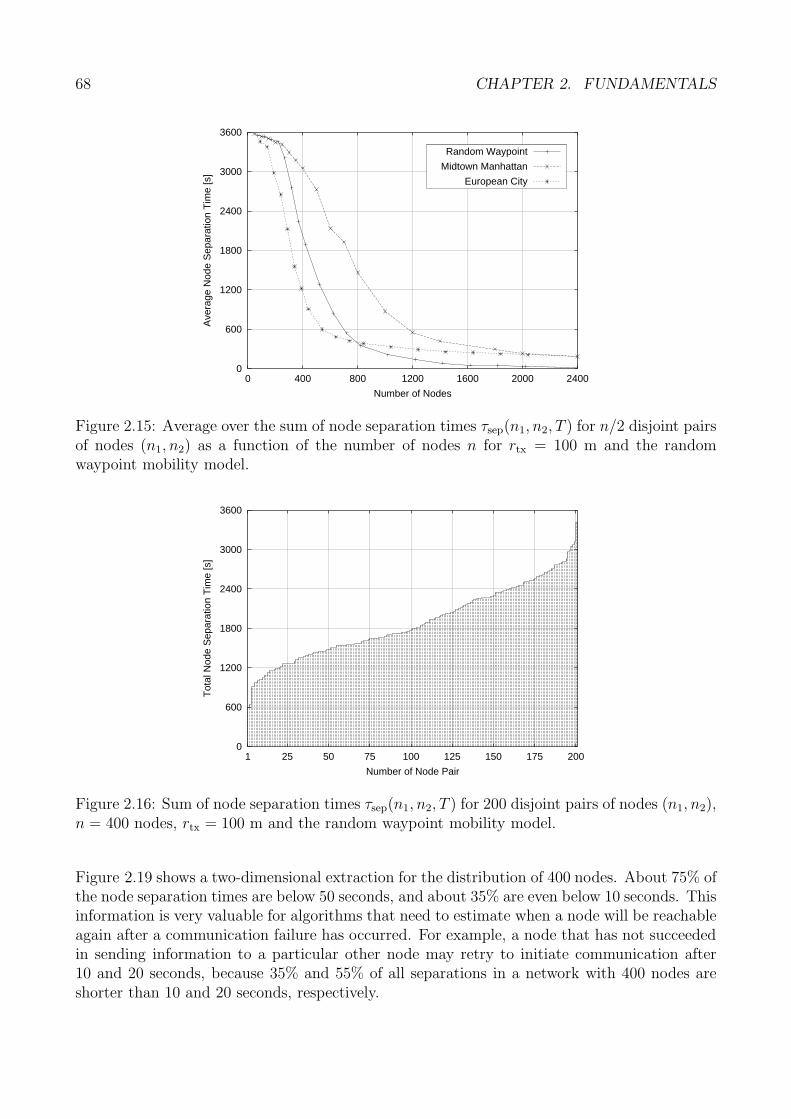
68 CHAPTER 2. FUNDAMENTALS
0
600
1200
1800
2400
3000
3600
0 400 800 1200 1600 2000 2400
Ave
rage
Nod
e S
epar
atio
n T
ime
[s]
Number of Nodes
Random Waypoint
Midtown Manhattan
European City
Figure 2.15: Average over the sum of node separation times τsep(n1, n2, T ) for n/2 disjoint pairsof nodes (n1, n2) as a function of the number of nodes n for rtx = 100 m and the randomwaypoint mobility model.
0
600
1200
1800
2400
3000
3600
1 25 50 75 100 125 150 175 200
Tot
al N
ode
Sep
arat
ion
Tim
e [s
]
Number of Node Pair
Figure 2.16: Sum of node separation times τsep(n1, n2, T ) for 200 disjoint pairs of nodes (n1, n2),n = 400 nodes, rtx = 100 m and the random waypoint mobility model.
Figure 2.19 shows a two-dimensional extraction for the distribution of 400 nodes. About 75% ofthe node separation times are below 50 seconds, and about 35% are even below 10 seconds. Thisinformation is very valuable for algorithms that need to estimate when a node will be reachableagain after a communication failure has occurred. For example, a node that has not succeededin sending information to a particular other node may retry to initiate communication after10 and 20 seconds, because 35% and 55% of all separations in a network with 400 nodes areshorter than 10 and 20 seconds, respectively.
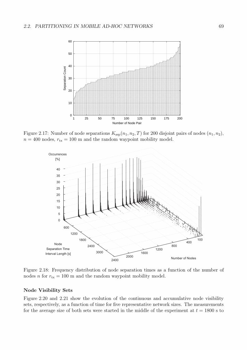
2.2. PARTITIONING IN MOBILE AD-HOC NETWORKS 69
0
10
20
30
40
50
60
1 25 50 75 100 125 150 175 200
Sep
arat
ion
Cou
nt
Number of Node Pair
Figure 2.17: Number of node separations Ksep(n1, n2, T ) for 200 disjoint pairs of nodes (n1, n2),n = 400 nodes, rtx = 100 m and the random waypoint mobility model.
100400
8001200
16002000
2400Number of Nodes
600
1200
1800
2400
3000
Node
Separation Time
Interval Length [s]
0
5
10
15
20
25
30
35
40
Occurrences
[%]
Figure 2.18: Frequency distribution of node separation times as a function of the number ofnodes n for rtx = 100 m and the random waypoint mobility model.
Node Visibility Sets
Figure 2.20 and 2.21 show the evolution of the continuous and accumulative node visibilitysets, respectively, as a function of time for five representative network sizes. The measurementsfor the average size of both sets were started in the middle of the experiment at t = 1800 s to
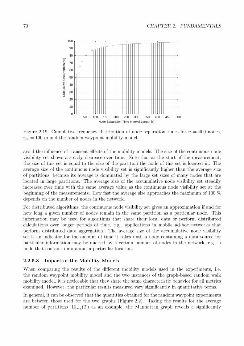
70 CHAPTER 2. FUNDAMENTALS
0
10
20
30
40
50
60
70
80
90
100
0 50 100 150 200 250 300 350 400 450 500
Cum
ulat
ive
Occ
urre
nces
[%]
Node Separation Time Interval Length [s]
Figure 2.19: Cumulative frequency distribution of node separation times for n = 400 nodes,rtx = 100 m and the random waypoint mobility model.
avoid the influence of transient effects of the mobility models. The size of the continuous nodevisibility set shows a steady decrease over time. Note that at the start of the measurement,the size of this set is equal to the size of the partition the node of this set is located in. Theaverage size of the continuous node visibility set is significantly higher than the average sizeof partitions, because its average is dominated by the large set sizes of many nodes that arelocated in large partitions. The average size of the accumulative node visibility set steadilyincreases over time with the same average value as the continuous node visibility set at thebeginning of the measurements. How fast the average size approaches the maximum of 100 %depends on the number of nodes in the network.
For distributed algorithms, the continuous node visibility set gives an approximation if and forhow long a given number of nodes remain in the same partition as a particular node. Thisinformation may be used for algorithms that share their local data or perform distributedcalculations over longer periods of time, e.g., applications in mobile ad-hoc networks thatperform distributed data aggregation. The average size of the accumulative node visibilityset is an indicator for the amount of time it takes until a node containing a data source forparticular information may be queried by a certain number of nodes in the network, e.g., anode that contains data about a particular location.
2.2.5.3 Impact of the Mobility Models
When comparing the results of the different mobility models used in the experiments, i.e.the random waypoint mobility model and the two instances of the graph-based random walkmobility model, it is noticeable that they share the same characteristic behavior for all metricsexamined. However, the particular results measured vary significantly in quantitative terms.
In general, it can be observed that the quantities obtained for the random waypoint experimentsare between those used for the two graphs (Figure 2.2). Taking the results for the averagenumber of partitions |Π|avg(T ) as an example, the Manhattan graph reveals a significantly
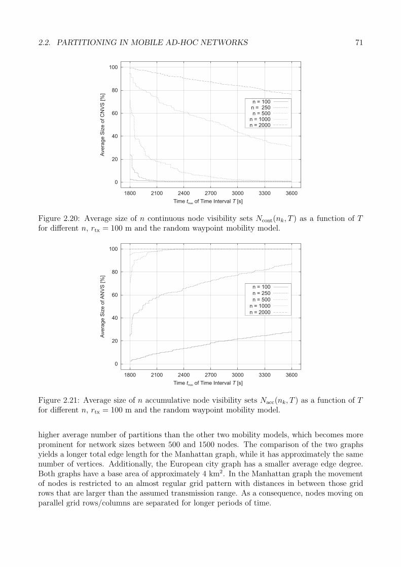
2.2. PARTITIONING IN MOBILE AD-HOC NETWORKS 71
0
20
40
60
80
100
1800 2100 2400 2700 3000 3300 3600
Avera
ge
Siz
eof
CN
VS
[%]
Time of Time Interval [s]t Tmax
n = 100n = 250n = 500
n = 1000n = 2000
Figure 2.20: Average size of n continuous node visibility sets Ncont(nk, T ) as a function of Tfor different n, rtx = 100 m and the random waypoint mobility model.
0
20
40
60
80
100
1800 2100 2400 2700 3000 3300 3600
Avera
ge
Siz
eofA
NV
S[%
]
Time of Time Interval [s]t Tmax
n = 100
n = 250
n = 500
n = 1000
n = 2000
Figure 2.21: Average size of n accumulative node visibility sets Nacc(nk, T ) as a function of Tfor different n, rtx = 100 m and the random waypoint mobility model.
higher average number of partitions than the other two mobility models, which becomes moreprominent for network sizes between 500 and 1500 nodes. The comparison of the two graphsyields a longer total edge length for the Manhattan graph, while it has approximately the samenumber of vertices. Additionally, the European city graph has a smaller average edge degree.Both graphs have a base area of approximately 4 km2. In the Manhattan graph the movementof nodes is restricted to an almost regular grid pattern with distances in between those gridrows that are larger than the assumed transmission range. As a consequence, nodes moving onparallel grid rows/columns are separated for longer periods of time.
72 CHAPTER 2. FUNDAMENTALS
The results obtained with the two different city graphs underline that the partitioning behaviordepends especially on the spatial structure of the system’s environment. The analysis of thisdimension is out of the scope of this dissertation and left to future work.
2.2.6 Conclusions: Network Partitioning
The analysis of partitioning has shown that network partitions occur frequently even in networkswith reasonably high node densities. For example, in a network containing 800 nodes on a 4 km2
area and a transmission range of 100 m, we found more than 20 partitions on average. For suchscenarios, the partitioning situation should not be neglected in the design of distributed datamanagement algorithms in mobile ad-hoc networks.
For the scope of this dissertation, we can draw two main conclusions. First, the fundamentalalgorithms to be developed shall consider the occurrence of partitioning as a common case thatis likely to occur. While the situation of a partitioned network implies that communicationis not possible between partitions while they exist, algorithms must still be designed in a waythat partitioning does not lead to unresolvable failures in the algorithms’ operation. We willaddress this issue in particular in the design of the core storage approach in Chapter 3.
The second important result is the fact that the mobility of mobile ad-hoc networks leads to thesituation where different network partitions eventually join again, assuming some sensible nodedensity that allows the general operation of the network in the first place. This observationhas the key implication that the duration of partitions is finite in general. After a partitionjoin, therefore, measures shall be taken to also unify potential temporary inconsistencies in theoperation of the algorithms. We will consider this observation specifically in the design of thedata migration approach, which we introduce in Chapter 4.
2.3 Location-centric Storage (LCS)
Location-centric storage is a fundamental paradigm in the field of mobile data management(MDM) that lies at the basis of our algorithms. The general goal of MDM is to provide mobileclients (network nodes) with the data they need, when they need it, and where they needit [PJC06]. With respect to these three aspects, MDM addresses all problems related to howdata can be obtained, stored, processed, and delivered to the mobile clients.
In its original form, MDM means data management in mobile (nomadic) computing [IB93, IB94](Section 1.2.1), where mobile clients are connected to the infrastructure via a direct radiouplink. Due to the mobility of clients, many new challenges related to MDM arise, such asthe general impact of mobility on data management, disconnected operation (e.g. prefetching,hoarding), energy-efficient data access, and wireless data broadcasting. These issues have beenconsidered by a large body of related work (see, for example, [PS97, Bar99, GS02, Kum06])and are orthogonal to the scope of this dissertation.
In mobile ad-hoc networks, not only is the data delivered to mobile devices, it is also man-aged by the mobile devices themselves, according to the peer-to-peer networking paradigm(Section 2.1.1). Intuitively, this is much more challenging due to the characteristics of MANETsas discussed in Section 2.1.2 and the potential occurrence of network partitioning as shown inSection 2.2. For these reasons, besides the requirement of new protocols on link, routing, and
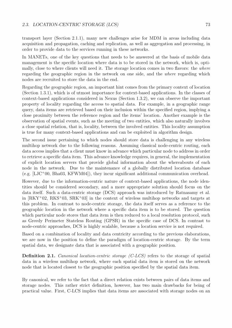
2.3. LOCATION-CENTRIC STORAGE (LCS) 73
transport layer (Section 2.1.1), many new challenges arise for MDM in areas including dataacquisition and propagation, caching and replication, as well as aggregation and processing, inorder to provide data to the services running in these networks.
In MANETs, one of the key questions that needs to be answered at the basis of mobile datamanagement is the specific location where data is to be stored in the network, which is, opti-mally, close to where clients will need it. The storage location comes in two flavors: the whereregarding the geographic region in the network on one side, and the where regarding whichnodes are recruited to store the data in the end.
Regarding the geographic region, an important hint comes from the primary context of location(Section 1.3.1), which is of utmost importance for context-based applications. In the classes ofcontext-based applications considered in Nexus (Section 1.3.2), we can observe the importantproperty of locality regarding the access to spatial data. For example, in a geographic rangequery, data items are retrieved based on their inclusion within the specified region, implying aclose proximity between the reference region and the items’ location. Another example is theobservation of spatial events, such as the meeting of two entities, which also naturally involvesa close spatial relation, that is, locality, between the involved entities. This locality assumptionis true for many context-based applications and can be exploited in algorithm design.
The second issue pertaining to which nodes should store data is challenging in any wirelessmultihop network due to the following reasons. Assuming classical node-centric routing, eachdata access implies that a client must know in advance which particular node to address in orderto retrieve a specific data item. This advance knowledge requires, in general, the implementationof explicit location servers that provide global information about the whereabouts of eachnode in the network. Due to the maintenance of a globally distributed location database(e.g. [LJC+00, Bha03, KFWM04]), they incur significant additional communication overhead.
However, due to the information-centric nature of context-based applications, the node iden-tities should be considered secondary, and a more appropriate solution should focus on thedata itself. Such a data-centric storage (DCS) approach was introduced by Ratnasamy et al.in [RKY+02, RKS+03, SRK+03] in the context of wireless multihop networks and targets atthis problem. In contrast to node-centric storage, the data itself serves as a reference to thegeographic location in the network where a specific data item is to be stored. The questionwhich particular node stores that data item is then reduced to a local resolution protocol, suchas Greedy Perimeter Stateless Routing (GPSR) in the specific case of DCS. In contrast tonode-centric approaches, DCS is highly scalable, because a location service is not required.
Based on a combination of locality and data centricity according to the previous elaborations,we are now in the position to define the paradigm of location-centric storage. By the termspatial data, we designate data that is associated with a geographic position.
Definition 2.1. Canonical location-centric storage (C-LCS) refers to the storage of spatialdata in a wireless multihop network, where each spatial data item is stored on the networknode that is located closest to the geographic position specified by the spatial data item.
By canonical, we refer to the fact that a direct relation exists between pairs of data items andstorage nodes. This rather strict definition, however, has two main drawbacks for being ofpractical value. First, C-LCS implies that data items are associated with storage nodes on an
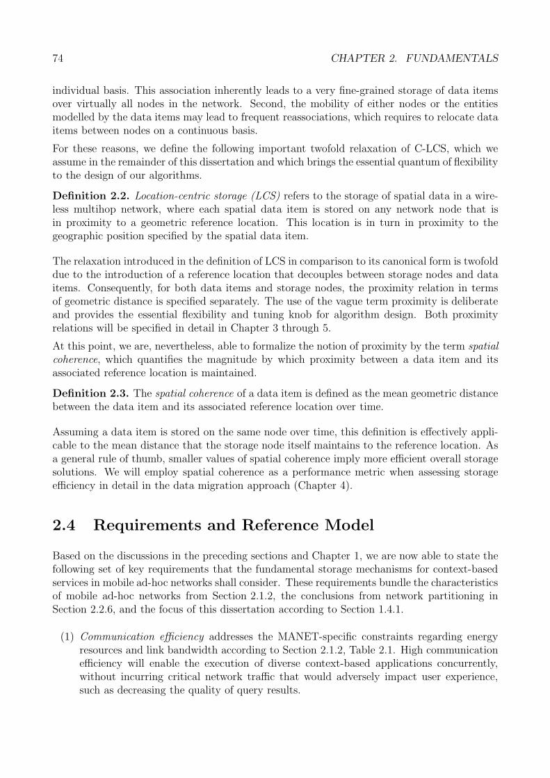
74 CHAPTER 2. FUNDAMENTALS
individual basis. This association inherently leads to a very fine-grained storage of data itemsover virtually all nodes in the network. Second, the mobility of either nodes or the entitiesmodelled by the data items may lead to frequent reassociations, which requires to relocate dataitems between nodes on a continuous basis.
For these reasons, we define the following important twofold relaxation of C-LCS, which weassume in the remainder of this dissertation and which brings the essential quantum of flexibilityto the design of our algorithms.
Definition 2.2. Location-centric storage (LCS) refers to the storage of spatial data in a wire-less multihop network, where each spatial data item is stored on any network node that isin proximity to a geometric reference location. This location is in turn in proximity to thegeographic position specified by the spatial data item.
The relaxation introduced in the definition of LCS in comparison to its canonical form is twofolddue to the introduction of a reference location that decouples between storage nodes and dataitems. Consequently, for both data items and storage nodes, the proximity relation in termsof geometric distance is specified separately. The use of the vague term proximity is deliberateand provides the essential flexibility and tuning knob for algorithm design. Both proximityrelations will be specified in detail in Chapter 3 through 5.
At this point, we are, nevertheless, able to formalize the notion of proximity by the term spatialcoherence, which quantifies the magnitude by which proximity between a data item and itsassociated reference location is maintained.
Definition 2.3. The spatial coherence of a data item is defined as the mean geometric distancebetween the data item and its associated reference location over time.
Assuming a data item is stored on the same node over time, this definition is effectively appli-cable to the mean distance that the storage node itself maintains to the reference location. Asa general rule of thumb, smaller values of spatial coherence imply more efficient overall storagesolutions. We will employ spatial coherence as a performance metric when assessing storageefficiency in detail in the data migration approach (Chapter 4).
2.4 Requirements and Reference Model
Based on the discussions in the preceding sections and Chapter 1, we are now able to state thefollowing set of key requirements that the fundamental storage mechanisms for context-basedservices in mobile ad-hoc networks shall consider. These requirements bundle the characteristicsof mobile ad-hoc networks from Section 2.1.2, the conclusions from network partitioning inSection 2.2.6, and the focus of this dissertation according to Section 1.4.1.
(1) Communication efficiency addresses the MANET-specific constraints regarding energyresources and link bandwidth according to Section 2.1.2, Table 2.1. High communicationefficiency will enable the execution of diverse context-based applications concurrently,without incurring critical network traffic that would adversely impact user experience,such as decreasing the quality of query results.
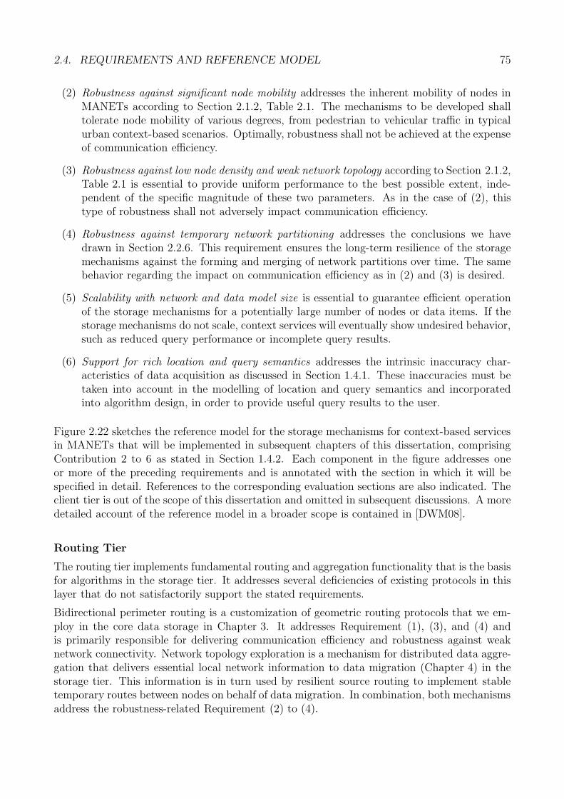
2.4. REQUIREMENTS AND REFERENCE MODEL 75
(2) Robustness against significant node mobility addresses the inherent mobility of nodes inMANETs according to Section 2.1.2, Table 2.1. The mechanisms to be developed shalltolerate node mobility of various degrees, from pedestrian to vehicular traffic in typicalurban context-based scenarios. Optimally, robustness shall not be achieved at the expenseof communication efficiency.
(3) Robustness against low node density and weak network topology according to Section 2.1.2,Table 2.1 is essential to provide uniform performance to the best possible extent, inde-pendent of the specific magnitude of these two parameters. As in the case of (2), thistype of robustness shall not adversely impact communication efficiency.
(4) Robustness against temporary network partitioning addresses the conclusions we havedrawn in Section 2.2.6. This requirement ensures the long-term resilience of the storagemechanisms against the forming and merging of network partitions over time. The samebehavior regarding the impact on communication efficiency as in (2) and (3) is desired.
(5) Scalability with network and data model size is essential to guarantee efficient operationof the storage mechanisms for a potentially large number of nodes or data items. If thestorage mechanisms do not scale, context services will eventually show undesired behavior,such as reduced query performance or incomplete query results.
(6) Support for rich location and query semantics addresses the intrinsic inaccuracy char-acteristics of data acquisition as discussed in Section 1.4.1. These inaccuracies must betaken into account in the modelling of location and query semantics and incorporatedinto algorithm design, in order to provide useful query results to the user.
Figure 2.22 sketches the reference model for the storage mechanisms for context-based servicesin MANETs that will be implemented in subsequent chapters of this dissertation, comprisingContribution 2 to 6 as stated in Section 1.4.2. Each component in the figure addresses oneor more of the preceding requirements and is annotated with the section in which it will bespecified in detail. References to the corresponding evaluation sections are also indicated. Theclient tier is out of the scope of this dissertation and omitted in subsequent discussions. A moredetailed account of the reference model in a broader scope is contained in [DWM08].
Routing Tier
The routing tier implements fundamental routing and aggregation functionality that is the basisfor algorithms in the storage tier. It addresses several deficiencies of existing protocols in thislayer that do not satisfactorily support the stated requirements.
Bidirectional perimeter routing is a customization of geometric routing protocols that we em-ploy in the core data storage in Chapter 3. It addresses Requirement (1), (3), and (4) andis primarily responsible for delivering communication efficiency and robustness against weaknetwork connectivity. Network topology exploration is a mechanism for distributed data aggre-gation that delivers essential local network information to data migration (Chapter 4) in thestorage tier. This information is in turn used by resilient source routing to implement stabletemporary routes between nodes on behalf of data migration. In combination, both mechanismsaddress the robustness-related Requirement (2) to (4).
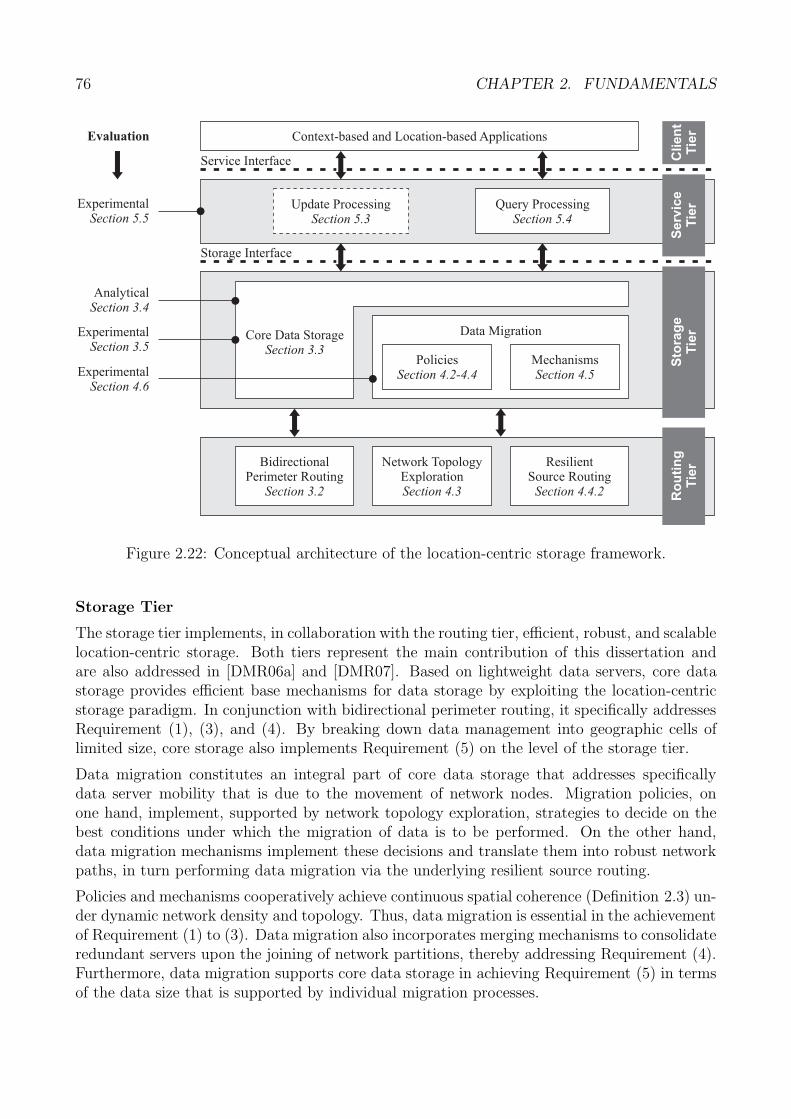
76 CHAPTER 2. FUNDAMENTALS
BidirectionalPerimeter Routing
Section 3.2
Network TopologyExplorationSection 4.3
ResilientSource Routing
Section 4.4.2
AnalyticalSection 3.4
PoliciesSection 4.2-4.4
MechanismsSection 4.5
Data MigrationCore Data StorageSection 3.3
Update ProcessingSection 5.3
Query ProcessingSection 5.4
ExperimentalSection 5.5
Context-based and Location-based Applications
Sto
rag
eT
ier
Ro
uti
ng
Tie
r
Evaluation
Serv
ice
Tie
rC
lien
tT
ier
ExperimentalSection 3.5
ExperimentalSection 4.6
Service Interface
Storage Interface
Figure 2.22: Conceptual architecture of the location-centric storage framework.
Storage Tier
The storage tier implements, in collaboration with the routing tier, efficient, robust, and scalablelocation-centric storage. Both tiers represent the main contribution of this dissertation andare also addressed in [DMR06a] and [DMR07]. Based on lightweight data servers, core datastorage provides efficient base mechanisms for data storage by exploiting the location-centricstorage paradigm. In conjunction with bidirectional perimeter routing, it specifically addressesRequirement (1), (3), and (4). By breaking down data management into geographic cells oflimited size, core storage also implements Requirement (5) on the level of the storage tier.
Data migration constitutes an integral part of core data storage that addresses specificallydata server mobility that is due to the movement of network nodes. Migration policies, onone hand, implement, supported by network topology exploration, strategies to decide on thebest conditions under which the migration of data is to be performed. On the other hand,data migration mechanisms implement these decisions and translate them into robust networkpaths, in turn performing data migration via the underlying resilient source routing.
Policies and mechanisms cooperatively achieve continuous spatial coherence (Definition 2.3) un-der dynamic network density and topology. Thus, data migration is essential in the achievementof Requirement (1) to (3). Data migration also incorporates merging mechanisms to consolidateredundant servers upon the joining of network partitions, thereby addressing Requirement (4).Furthermore, data migration supports core data storage in achieving Requirement (5) in termsof the data size that is supported by individual migration processes.
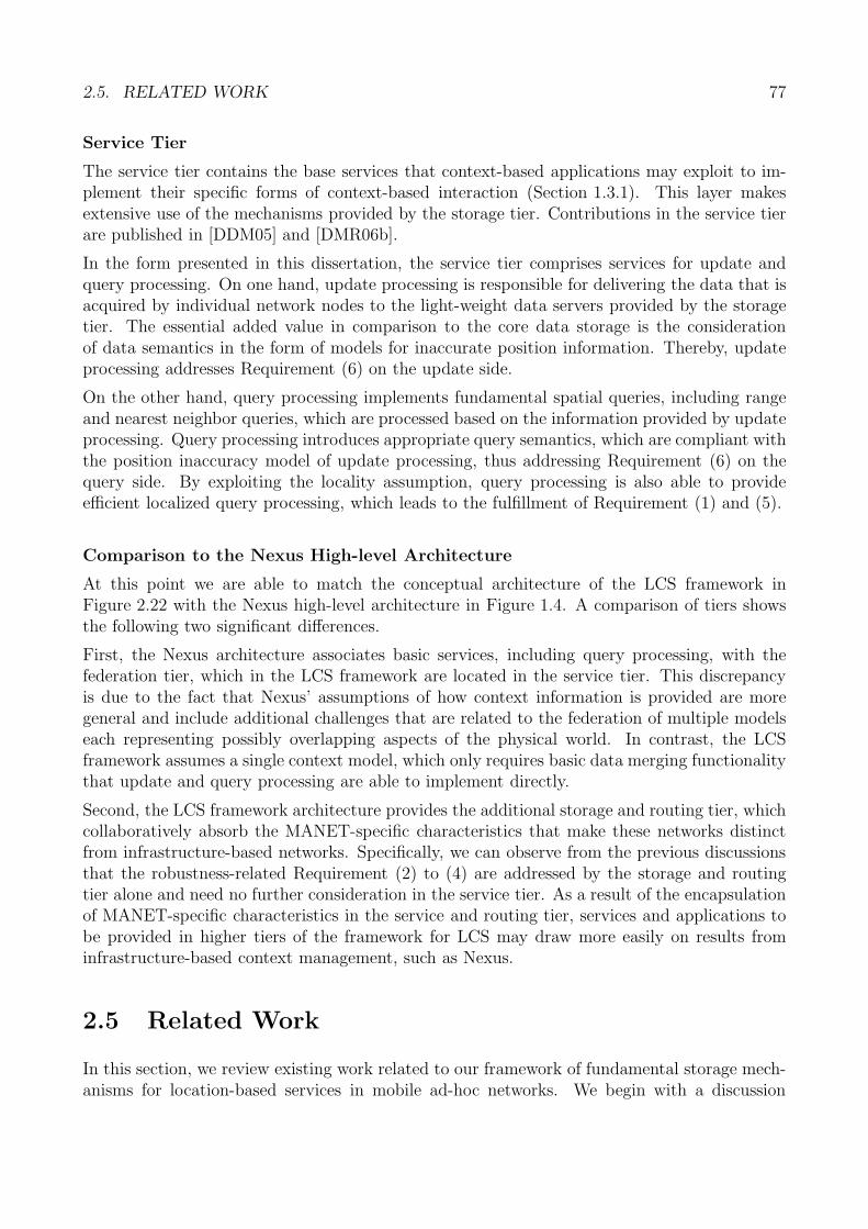
2.5. RELATED WORK 77
Service Tier
The service tier contains the base services that context-based applications may exploit to im-plement their specific forms of context-based interaction (Section 1.3.1). This layer makesextensive use of the mechanisms provided by the storage tier. Contributions in the service tierare published in [DDM05] and [DMR06b].
In the form presented in this dissertation, the service tier comprises services for update andquery processing. On one hand, update processing is responsible for delivering the data that isacquired by individual network nodes to the light-weight data servers provided by the storagetier. The essential added value in comparison to the core data storage is the considerationof data semantics in the form of models for inaccurate position information. Thereby, updateprocessing addresses Requirement (6) on the update side.
On the other hand, query processing implements fundamental spatial queries, including rangeand nearest neighbor queries, which are processed based on the information provided by updateprocessing. Query processing introduces appropriate query semantics, which are compliant withthe position inaccuracy model of update processing, thus addressing Requirement (6) on thequery side. By exploiting the locality assumption, query processing is also able to provideefficient localized query processing, which leads to the fulfillment of Requirement (1) and (5).
Comparison to the Nexus High-level Architecture
At this point we are able to match the conceptual architecture of the LCS framework inFigure 2.22 with the Nexus high-level architecture in Figure 1.4. A comparison of tiers showsthe following two significant differences.
First, the Nexus architecture associates basic services, including query processing, with thefederation tier, which in the LCS framework are located in the service tier. This discrepancyis due to the fact that Nexus’ assumptions of how context information is provided are moregeneral and include additional challenges that are related to the federation of multiple modelseach representing possibly overlapping aspects of the physical world. In contrast, the LCSframework assumes a single context model, which only requires basic data merging functionalitythat update and query processing are able to implement directly.
Second, the LCS framework architecture provides the additional storage and routing tier, whichcollaboratively absorb the MANET-specific characteristics that make these networks distinctfrom infrastructure-based networks. Specifically, we can observe from the previous discussionsthat the robustness-related Requirement (2) to (4) are addressed by the storage and routingtier alone and need no further consideration in the service tier. As a result of the encapsulationof MANET-specific characteristics in the service and routing tier, services and applications tobe provided in higher tiers of the framework for LCS may draw more easily on results frominfrastructure-based context management, such as Nexus.
2.5 Related Work
In this section, we review existing work related to our framework of fundamental storage mech-anisms for location-based services in mobile ad-hoc networks. We begin with a discussion
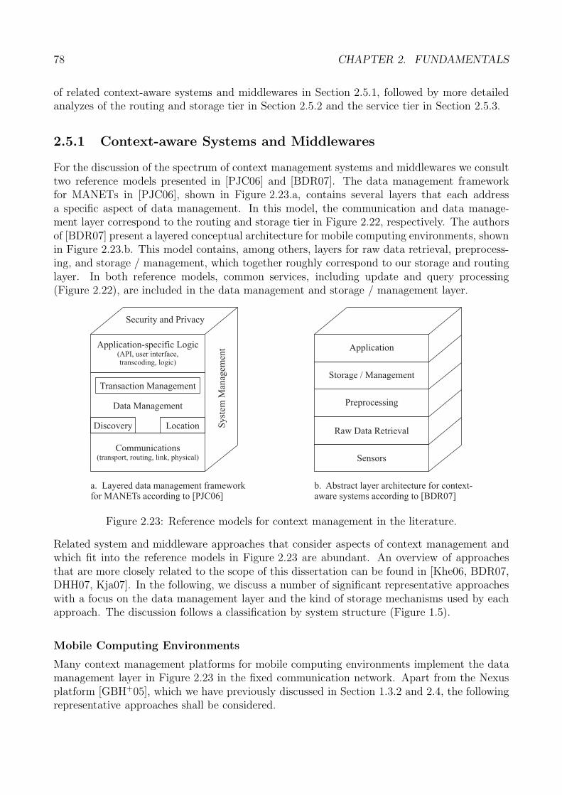
78 CHAPTER 2. FUNDAMENTALS
of related context-aware systems and middlewares in Section 2.5.1, followed by more detailedanalyzes of the routing and storage tier in Section 2.5.2 and the service tier in Section 2.5.3.
2.5.1 Context-aware Systems and Middlewares
For the discussion of the spectrum of context management systems and middlewares we consulttwo reference models presented in [PJC06] and [BDR07]. The data management frameworkfor MANETs in [PJC06], shown in Figure 2.23.a, contains several layers that each addressa specific aspect of data management. In this model, the communication and data manage-ment layer correspond to the routing and storage tier in Figure 2.22, respectively. The authorsof [BDR07] present a layered conceptual architecture for mobile computing environments, shownin Figure 2.23.b. This model contains, among others, layers for raw data retrieval, preprocess-ing, and storage / management, which together roughly correspond to our storage and routinglayer. In both reference models, common services, including update and query processing(Figure 2.22), are included in the data management and storage / management layer.
Sensors
Raw Data Retrieval
Preprocessing
Storage / Management
Application
Transaction Management
Data Management
Discovery Location
Communications(transport, routing, link, physical)
Application-specific Logic(API, user interface,transcoding, logic)
Security and Privacy
Syst
emM
anag
emen
t
a. Layered data management frameworkfor MANETs according to [PJC06]
b. Abstract layer architecture for context-aware systems according to [BDR07]
Figure 2.23: Reference models for context management in the literature.
Related system and middleware approaches that consider aspects of context management andwhich fit into the reference models in Figure 2.23 are abundant. An overview of approachesthat are more closely related to the scope of this dissertation can be found in [Khe06, BDR07,DHH07, Kja07]. In the following, we discuss a number of significant representative approacheswith a focus on the data management layer and the kind of storage mechanisms used by eachapproach. The discussion follows a classification by system structure (Figure 1.5).
Mobile Computing Environments
Many context management platforms for mobile computing environments implement the datamanagement layer in Figure 2.23 in the fixed communication network. Apart from the Nexusplatform [GBH+05], which we have previously discussed in Section 1.3.2 and 2.4, the followingrepresentative approaches shall be considered.
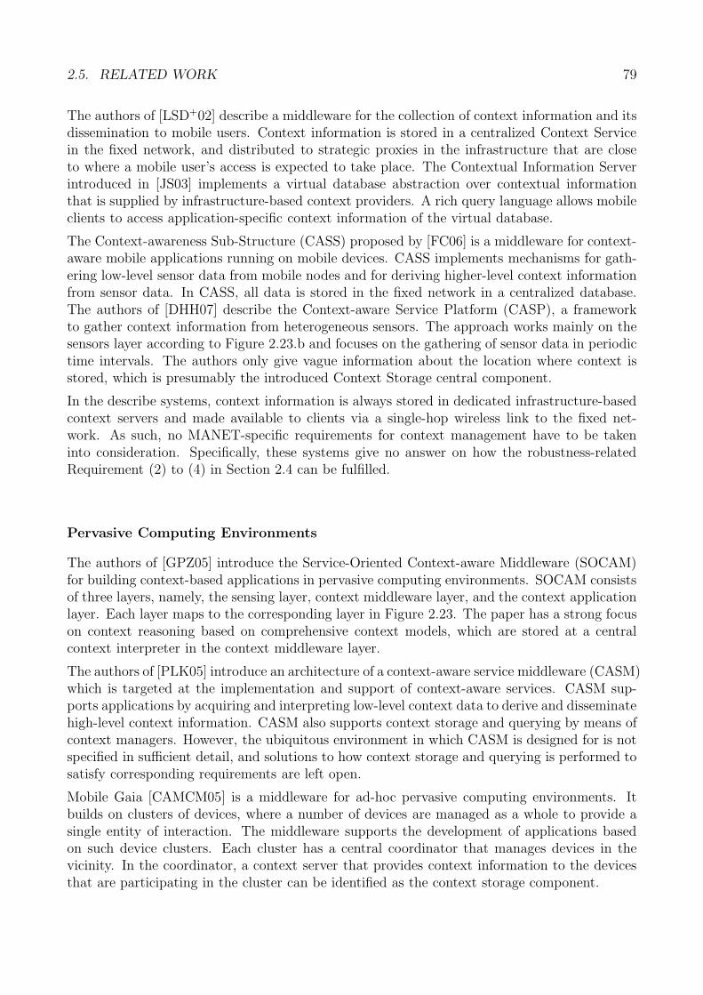
2.5. RELATED WORK 79
The authors of [LSD+02] describe a middleware for the collection of context information and itsdissemination to mobile users. Context information is stored in a centralized Context Servicein the fixed network, and distributed to strategic proxies in the infrastructure that are closeto where a mobile user’s access is expected to take place. The Contextual Information Serverintroduced in [JS03] implements a virtual database abstraction over contextual informationthat is supplied by infrastructure-based context providers. A rich query language allows mobileclients to access application-specific context information of the virtual database.
The Context-awareness Sub-Structure (CASS) proposed by [FC06] is a middleware for context-aware mobile applications running on mobile devices. CASS implements mechanisms for gath-ering low-level sensor data from mobile nodes and for deriving higher-level context informationfrom sensor data. In CASS, all data is stored in the fixed network in a centralized database.The authors of [DHH07] describe the Context-aware Service Platform (CASP), a frameworkto gather context information from heterogeneous sensors. The approach works mainly on thesensors layer according to Figure 2.23.b and focuses on the gathering of sensor data in periodictime intervals. The authors only give vague information about the location where context isstored, which is presumably the introduced Context Storage central component.
In the describe systems, context information is always stored in dedicated infrastructure-basedcontext servers and made available to clients via a single-hop wireless link to the fixed net-work. As such, no MANET-specific requirements for context management have to be takeninto consideration. Specifically, these systems give no answer on how the robustness-relatedRequirement (2) to (4) in Section 2.4 can be fulfilled.
Pervasive Computing Environments
The authors of [GPZ05] introduce the Service-Oriented Context-aware Middleware (SOCAM)for building context-based applications in pervasive computing environments. SOCAM consistsof three layers, namely, the sensing layer, context middleware layer, and the context applicationlayer. Each layer maps to the corresponding layer in Figure 2.23. The paper has a strong focuson context reasoning based on comprehensive context models, which are stored at a centralcontext interpreter in the context middleware layer.
The authors of [PLK05] introduce an architecture of a context-aware service middleware (CASM)which is targeted at the implementation and support of context-aware services. CASM sup-ports applications by acquiring and interpreting low-level context data to derive and disseminatehigh-level context information. CASM also supports context storage and querying by means ofcontext managers. However, the ubiquitous environment in which CASM is designed for is notspecified in sufficient detail, and solutions to how context storage and querying is performed tosatisfy corresponding requirements are left open.
Mobile Gaia [CAMCM05] is a middleware for ad-hoc pervasive computing environments. Itbuilds on clusters of devices, where a number of devices are managed as a whole to provide asingle entity of interaction. The middleware supports the development of applications basedon such device clusters. Each cluster has a central coordinator that manages devices in thevicinity. In the coordinator, a context server that provides context information to the devicesthat are participating in the cluster can be identified as the context storage component.
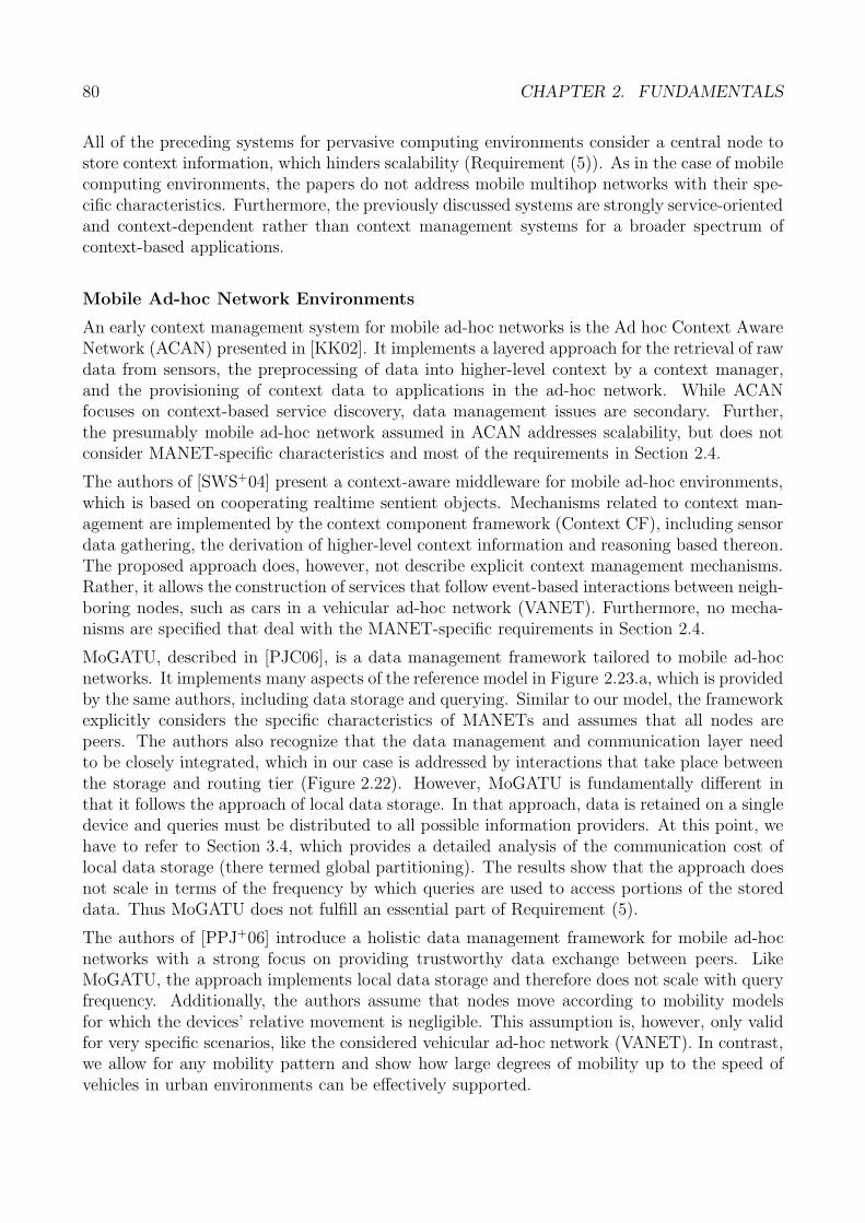
80 CHAPTER 2. FUNDAMENTALS
All of the preceding systems for pervasive computing environments consider a central node tostore context information, which hinders scalability (Requirement (5)). As in the case of mobilecomputing environments, the papers do not address mobile multihop networks with their spe-cific characteristics. Furthermore, the previously discussed systems are strongly service-orientedand context-dependent rather than context management systems for a broader spectrum ofcontext-based applications.
Mobile Ad-hoc Network Environments
An early context management system for mobile ad-hoc networks is the Ad hoc Context AwareNetwork (ACAN) presented in [KK02]. It implements a layered approach for the retrieval of rawdata from sensors, the preprocessing of data into higher-level context by a context manager,and the provisioning of context data to applications in the ad-hoc network. While ACANfocuses on context-based service discovery, data management issues are secondary. Further,the presumably mobile ad-hoc network assumed in ACAN addresses scalability, but does notconsider MANET-specific characteristics and most of the requirements in Section 2.4.
The authors of [SWS+04] present a context-aware middleware for mobile ad-hoc environments,which is based on cooperating realtime sentient objects. Mechanisms related to context man-agement are implemented by the context component framework (Context CF), including sensordata gathering, the derivation of higher-level context information and reasoning based thereon.The proposed approach does, however, not describe explicit context management mechanisms.Rather, it allows the construction of services that follow event-based interactions between neigh-boring nodes, such as cars in a vehicular ad-hoc network (VANET). Furthermore, no mecha-nisms are specified that deal with the MANET-specific requirements in Section 2.4.
MoGATU, described in [PJC06], is a data management framework tailored to mobile ad-hocnetworks. It implements many aspects of the reference model in Figure 2.23.a, which is providedby the same authors, including data storage and querying. Similar to our model, the frameworkexplicitly considers the specific characteristics of MANETs and assumes that all nodes arepeers. The authors also recognize that the data management and communication layer needto be closely integrated, which in our case is addressed by interactions that take place betweenthe storage and routing tier (Figure 2.22). However, MoGATU is fundamentally different inthat it follows the approach of local data storage. In that approach, data is retained on a singledevice and queries must be distributed to all possible information providers. At this point, wehave to refer to Section 3.4, which provides a detailed analysis of the communication cost oflocal data storage (there termed global partitioning). The results show that the approach doesnot scale in terms of the frequency by which queries are used to access portions of the storeddata. Thus MoGATU does not fulfill an essential part of Requirement (5).
The authors of [PPJ+06] introduce a holistic data management framework for mobile ad-hocnetworks with a strong focus on providing trustworthy data exchange between peers. LikeMoGATU, the approach implements local data storage and therefore does not scale with queryfrequency. Additionally, the authors assume that nodes move according to mobility modelsfor which the devices’ relative movement is negligible. This assumption is, however, only validfor very specific scenarios, like the considered vehicular ad-hoc network (VANET). In contrast,we allow for any mobility pattern and show how large degrees of mobility up to the speed ofvehicles in urban environments can be effectively supported.
2.5. RELATED WORK 81
Finally, the authors of [CYC07] present a framework for context management to support con-text applications in mobile ad-hoc networks. The proposed framework builds on clusters ofnodes, each containing a single mobile context manager that stores context information thatit obtains from context providers located in close vicinity. Multiple clusters are interconnectedby constructing an explicit topological structure, referred to as Segment-Tree Virtual Network(STVN). This structure is then used to route queries to those context managers that containrelevant data for each query issued by the context-aware applications.
Due to the mobility of nodes, however, the proposed STVN requires explicit reconstructionand maintenance. The authors provide measurement results that confirm the significant over-head which is even greater than a straightforward publish/subscribe approach based on Ad-hocOn-Demand Distance Vector Routing (AODV) that the authors present for comparison. Incontrast, the proposed framework in this dissertation does not require any maintenance ofstructures, since it relies on a rendezvous-based approach between data updates and queries.This is vital also for achieving robustness against low node density and weak topological struc-tures (Requirement (3)) and temporary network partitioning (Requirement (4)).
2.5.2 Core Data Storage and Data Migration
Let us now discuss previous approaches that relate to the storage tier of our framework inFigure 2.22 with respect to the requirements in Section 2.4. Figure 2.24 presents a classificationof related data-centric storage approaches. The close relation to LCS is based on the fact thatall DCS mechanisms implement fundamental mechanisms in order to store data at particularlocations in the network. Based on this classification, we can distinguish between position-basedDCS, cell-based DCS, and miscellaneous DCS approaches.
Position-based DCS
Approaches that can be associated with position-based data-centric storage employ geometricrouting to determine individual storage nodes. A reference position is circumscribed by a packetthat visits subsequent nodes located close to that position until a node is visited twice. Bydefinition, this node is deemed to be the storage node (Figure 2.25.a).
Data-centric Storage (DCS) was proposed for wireless sensor networks in [RKY+02, RKS+03,SRK+03]. DCS uses the Greedy Perimeter Stateless Routing (GPSR) [KK00] protocol to locatea storage node, termed home node in DCS, responsible for storing data. The authors extendedDCS by Structured Replication (SR-DCS) to load-balance data associated with the same keyto multiple home nodes at different locations. To achieve data consistency in the presence oflimited node mobility and node failures, DCS employs the Perimeter Refresh Protocol (PRP)to replicate data around a perimeter in addition to the home node.
The authors of [GGC03] propose an extension to DCS which they call Resilient Data-centricStorage (R-DCS). Using replica and monitoring nodes, they optimize knowledge about dataavailability in different regions and the exchange of data between different cells to provide acertain degree of replication. Similar to DCS, the authors apply GPSR to locate storage nodesand optionally support PRP to partially recover data from departing or failing nodes.
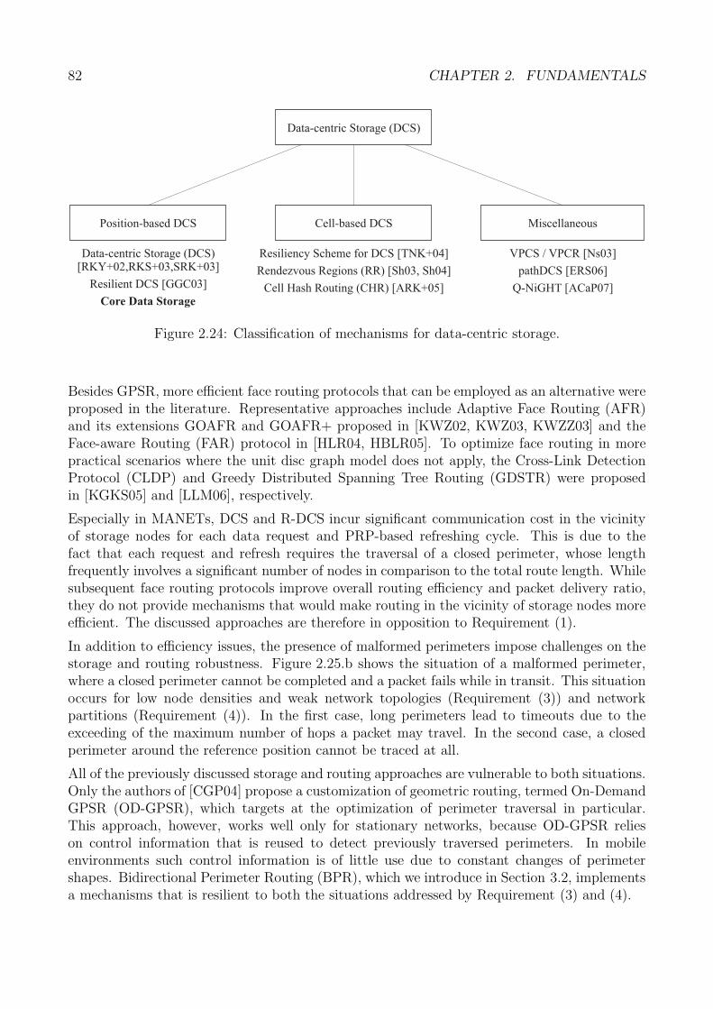
82 CHAPTER 2. FUNDAMENTALS
Data-centric Storage (DCS)
Position-based DCS Cell-based DCS
Data-centric Storage (DCS)[RKY+02,RKS+03,SRK+03]
Resilient DCS [GGC03]
Core Data Storage
Resiliency Scheme for DCS [TNK+04]
Rendezvous Regions (RR) [Sh03, Sh04]
Cell Hash Routing (CHR) [ARK+05]
Miscellaneous
VPCS / VPCR [Ns03]
pathDCS [ERS06]
Q-NiGHT [ACaP07]
Figure 2.24: Classification of mechanisms for data-centric storage.
Besides GPSR, more efficient face routing protocols that can be employed as an alternative wereproposed in the literature. Representative approaches include Adaptive Face Routing (AFR)and its extensions GOAFR and GOAFR+ proposed in [KWZ02, KWZ03, KWZZ03] and theFace-aware Routing (FAR) protocol in [HLR04, HBLR05]. To optimize face routing in morepractical scenarios where the unit disc graph model does not apply, the Cross-Link DetectionProtocol (CLDP) and Greedy Distributed Spanning Tree Routing (GDSTR) were proposedin [KGKS05] and [LLM06], respectively.
Especially in MANETs, DCS and R-DCS incur significant communication cost in the vicinityof storage nodes for each data request and PRP-based refreshing cycle. This is due to thefact that each request and refresh requires the traversal of a closed perimeter, whose lengthfrequently involves a significant number of nodes in comparison to the total route length. Whilesubsequent face routing protocols improve overall routing efficiency and packet delivery ratio,they do not provide mechanisms that would make routing in the vicinity of storage nodes moreefficient. The discussed approaches are therefore in opposition to Requirement (1).
In addition to efficiency issues, the presence of malformed perimeters impose challenges on thestorage and routing robustness. Figure 2.25.b shows the situation of a malformed perimeter,where a closed perimeter cannot be completed and a packet fails while in transit. This situationoccurs for low node densities and weak network topologies (Requirement (3)) and networkpartitions (Requirement (4)). In the first case, long perimeters lead to timeouts due to theexceeding of the maximum number of hops a packet may travel. In the second case, a closedperimeter around the reference position cannot be traced at all.
All of the previously discussed storage and routing approaches are vulnerable to both situations.Only the authors of [CGP04] propose a customization of geometric routing, termed On-DemandGPSR (OD-GPSR), which targets at the optimization of perimeter traversal in particular.This approach, however, works well only for stationary networks, because OD-GPSR relieson control information that is reused to detect previously traversed perimeters. In mobileenvironments such control information is of little use due to constant changes of perimetershapes. Bidirectional Perimeter Routing (BPR), which we introduce in Section 3.2, implementsa mechanisms that is resilient to both the situations addressed by Requirement (3) and (4).
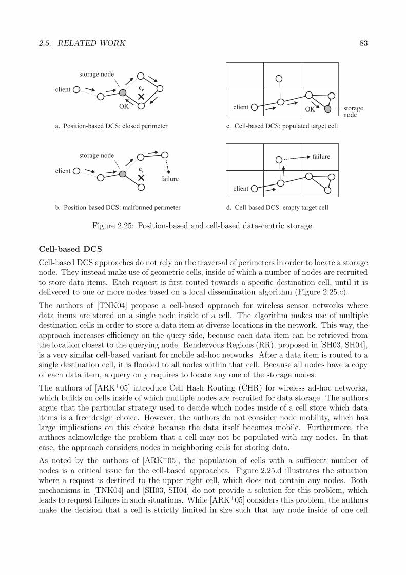
2.5. RELATED WORK 83
OKclient storagenode
failure
client
OK
cr
failure
cr
client
storage node
storage node
a. Position-based DCS: closed perimeter
b. Position-based DCS: malformed perimeter
c. Cell-based DCS: populated target cell
d. Cell-based DCS: empty target cell
client
Figure 2.25: Position-based and cell-based data-centric storage.
Cell-based DCS
Cell-based DCS approaches do not rely on the traversal of perimeters in order to locate a storagenode. They instead make use of geometric cells, inside of which a number of nodes are recruitedto store data items. Each request is first routed towards a specific destination cell, until it isdelivered to one or more nodes based on a local dissemination algorithm (Figure 2.25.c).
The authors of [TNK04] propose a cell-based approach for wireless sensor networks wheredata items are stored on a single node inside of a cell. The algorithm makes use of multipledestination cells in order to store a data item at diverse locations in the network. This way, theapproach increases efficiency on the query side, because each data item can be retrieved fromthe location closest to the querying node. Rendezvous Regions (RR), proposed in [SH03, SH04],is a very similar cell-based variant for mobile ad-hoc networks. After a data item is routed to asingle destination cell, it is flooded to all nodes within that cell. Because all nodes have a copyof each data item, a query only requires to locate any one of the storage nodes.
The authors of [ARK+05] introduce Cell Hash Routing (CHR) for wireless ad-hoc networks,which builds on cells inside of which multiple nodes are recruited for data storage. The authorsargue that the particular strategy used to decide which nodes inside of a cell store which dataitems is a free design choice. However, the authors do not consider node mobility, which haslarge implications on this choice because the data itself becomes mobile. Furthermore, theauthors acknowledge the problem that a cell may not be populated with any nodes. In thatcase, the approach considers nodes in neighboring cells for storing data.
As noted by the authors of [ARK+05], the population of cells with a sufficient number ofnodes is a critical issue for the cell-based approaches. Figure 2.25.d illustrates the situationwhere a request is destined to the upper right cell, which does not contain any nodes. Bothmechanisms in [TNK04] and [SH03, SH04] do not provide a solution for this problem, whichleads to request failures in such situations. While [ARK+05] considers this problem, the authorsmake the decision that a cell is strictly limited in size such that any node inside of one cell
84 CHAPTER 2. FUNDAMENTALS
can communicate directly with all other nodes in adjacent cells. This is a particularly strongassumption, which works only for the idealized unit disc graph model and the absence of nodemobility. Thus, under the conditions of mobile ad-hoc networks, Requirement (3) in Section 2.4cannot be supported by the aforementioned approaches.
Miscellaneous DCS Approaches
Besides the discussed position-based and cell-based DCS variants, a number of approaches wereproposed that apply entirely different strategies in achieving data-centric storage.
The authors of [NS03] introduce a DCS variant for wireless sensor networks that is based on thenotion of a Virtual Polar Coordinate Space (VPCS). Different from all other DCS approaches,network nodes are not aware of their physical location. Instead, a virtual polar coordinatesystem is constructed as an overlay to the network. Virtual Polar Coordinate Routing (VPCR)is then used to route requests to specific nodes that occupy a well-defined location in theVPCS. Similar to [ARK+05], if a node is not available in the supposed location, a more distantalternative node is selected for storing the data item. While the approach also provides recoverymechanisms in case of node failures, the authors acknowledge that it is inefficient for networkswith significant node mobility. Hence, VPCS/VPCR is clearly designed for stationary wirelesssensor networks and not practical in mobile ad-hoc networks.
An approach to DCS that builds on the abstraction of paths is introduced in [ERS06] andnamed pathDCS. In this approach, a number of trees are constructed in the network that eachroot at one of several well-known landmark nodes. Each request is then routed to a specificlandmark and then forwarded on a sequence of segments along multiple trees. Similar to PRPin [RKY+02], pathDCS incurs significant overhead in refreshing data in the presence of mobilenodes. Furthermore, pathDCS requires the maintenance of a number of network-wide trees,which incurs significant overhead for dynamic network topologies. The maintenance of suchstructures, is, in general, not feasible in MANETs, due to potentially low node densities andthe risk of network partitioning. In summary, pathDCS is not suitable for MANETs.
The authors of [ACNP07] introduce Q-NiGHT, a DCS mechanism which focuses on QoS controland load balancing. To increase data availability, the approach is based on the concept of aball. A ball is defined as the circular region around a node that contains a specific number ofadditional nodes. The center node corresponds to the home node as defined in [RKY+02]. Adispersal protocol distributes each data item to the nodes located within this ball. Furthermore,the authors address the issue that perimeter routing according to [KK00] traverses perimetersonly in one direction. Q-NiGHT instead dynamically chooses between left-hand and right-handtraversal in dependence of the destination location. The main drawback of Q-NiGHT is thatit lacks a suitable protocol to maintain data within a ball in the presence of node mobility.Furthermore, the decision in which direction a parameter is to be traversed is taken beforeeach request and does not solve the problems related to long and open perimeters, as discussedpreviously. Therefore, Q-NiGHT is unsuitable for mobile ad-hoc networks.
Specific Approaches to Data Migration
In order to maintain spatial coherence according to Definition 2.3, a number of approaches existthat implement explicit approaches to data migration. From the discussed DCS mechanisms,Rendezvous Regions (RR) [SH03, SH04] is the only approach that explicitly maintains data
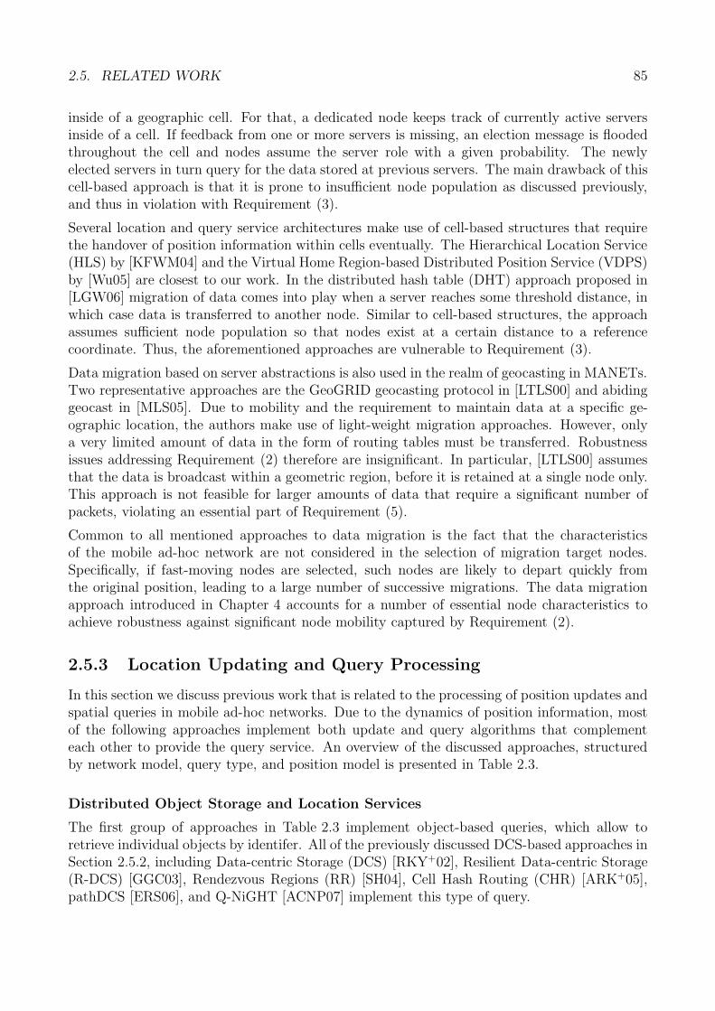
2.5. RELATED WORK 85
inside of a geographic cell. For that, a dedicated node keeps track of currently active serversinside of a cell. If feedback from one or more servers is missing, an election message is floodedthroughout the cell and nodes assume the server role with a given probability. The newlyelected servers in turn query for the data stored at previous servers. The main drawback of thiscell-based approach is that it is prone to insufficient node population as discussed previously,and thus in violation with Requirement (3).
Several location and query service architectures make use of cell-based structures that requirethe handover of position information within cells eventually. The Hierarchical Location Service(HLS) by [KFWM04] and the Virtual Home Region-based Distributed Position Service (VDPS)by [Wu05] are closest to our work. In the distributed hash table (DHT) approach proposed in[LGW06] migration of data comes into play when a server reaches some threshold distance, inwhich case data is transferred to another node. Similar to cell-based structures, the approachassumes sufficient node population so that nodes exist at a certain distance to a referencecoordinate. Thus, the aforementioned approaches are vulnerable to Requirement (3).
Data migration based on server abstractions is also used in the realm of geocasting in MANETs.Two representative approaches are the GeoGRID geocasting protocol in [LTLS00] and abidinggeocast in [MLS05]. Due to mobility and the requirement to maintain data at a specific ge-ographic location, the authors make use of light-weight migration approaches. However, onlya very limited amount of data in the form of routing tables must be transferred. Robustnessissues addressing Requirement (2) therefore are insignificant. In particular, [LTLS00] assumesthat the data is broadcast within a geometric region, before it is retained at a single node only.This approach is not feasible for larger amounts of data that require a significant number ofpackets, violating an essential part of Requirement (5).
Common to all mentioned approaches to data migration is the fact that the characteristicsof the mobile ad-hoc network are not considered in the selection of migration target nodes.Specifically, if fast-moving nodes are selected, such nodes are likely to depart quickly fromthe original position, leading to a large number of successive migrations. The data migrationapproach introduced in Chapter 4 accounts for a number of essential node characteristics toachieve robustness against significant node mobility captured by Requirement (2).
2.5.3 Location Updating and Query Processing
In this section we discuss previous work that is related to the processing of position updates andspatial queries in mobile ad-hoc networks. Due to the dynamics of position information, mostof the following approaches implement both update and query algorithms that complementeach other to provide the query service. An overview of the discussed approaches, structuredby network model, query type, and position model is presented in Table 2.3.
Distributed Object Storage and Location Services
The first group of approaches in Table 2.3 implement object-based queries, which allow toretrieve individual objects by identifer. All of the previously discussed DCS-based approaches inSection 2.5.2, including Data-centric Storage (DCS) [RKY+02], Resilient Data-centric Storage(R-DCS) [GGC03], Rendezvous Regions (RR) [SH04], Cell Hash Routing (CHR) [ARK+05],pathDCS [ERS06], and Q-NiGHT [ACNP07] implement this type of query.
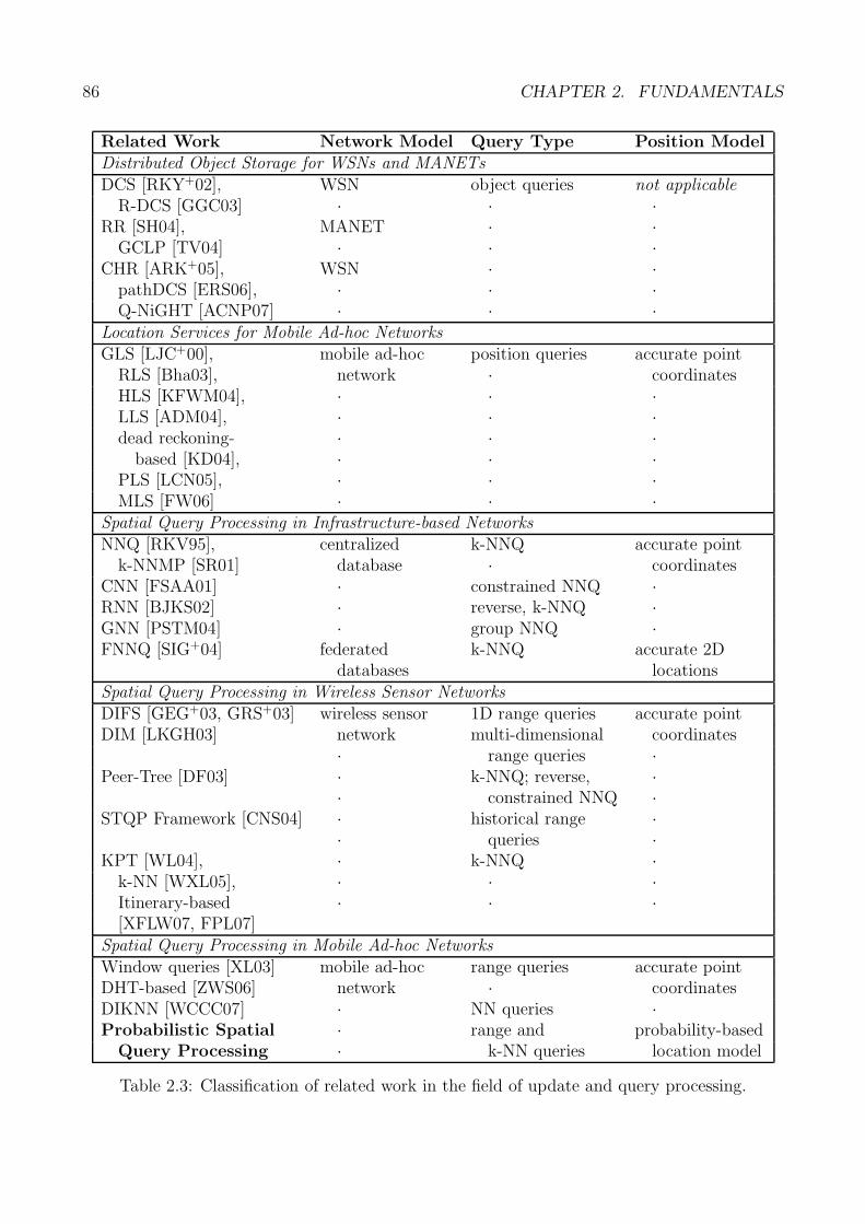
86 CHAPTER 2. FUNDAMENTALS
Related Work Network Model Query Type Position ModelDistributed Object Storage for WSNs and MANETsDCS [RKY+02], WSN object queries not applicable
R-DCS [GGC03] · · ·RR [SH04], MANET · ·
GCLP [TV04] · · ·CHR [ARK+05], WSN · ·
pathDCS [ERS06], · · ·Q-NiGHT [ACNP07] · · ·
Location Services for Mobile Ad-hoc NetworksGLS [LJC+00], mobile ad-hoc position queries accurate point
RLS [Bha03], network · coordinatesHLS [KFWM04], · · ·LLS [ADM04], · · ·dead reckoning- · · ·
based [KD04], · · ·PLS [LCN05], · · ·MLS [FW06] · · ·
Spatial Query Processing in Infrastructure-based NetworksNNQ [RKV95], centralized k-NNQ accurate point
k-NNMP [SR01] database · coordinatesCNN [FSAA01] · constrained NNQ ·RNN [BJKS02] · reverse, k-NNQ ·GNN [PSTM04] · group NNQ ·FNNQ [SIG+04] federated k-NNQ accurate 2D
databases locationsSpatial Query Processing in Wireless Sensor NetworksDIFS [GEG+03, GRS+03] wireless sensor 1D range queries accurate pointDIM [LKGH03] network multi-dimensional coordinates
· range queries ·Peer-Tree [DF03] · k-NNQ; reverse, ·
· constrained NNQ ·STQP Framework [CNS04] · historical range ·
· queries ·KPT [WL04], · k-NNQ ·
k-NN [WXL05], · · ·Itinerary-based · · ·[XFLW07, FPL07]
Spatial Query Processing in Mobile Ad-hoc NetworksWindow queries [XL03] mobile ad-hoc range queries accurate pointDHT-based [ZWS06] network · coordinatesDIKNN [WCCC07] · NN queries ·Probabilistic Spatial · range and probability-based
Query Processing · k-NN queries location model
Table 2.3: Classification of related work in the field of update and query processing.
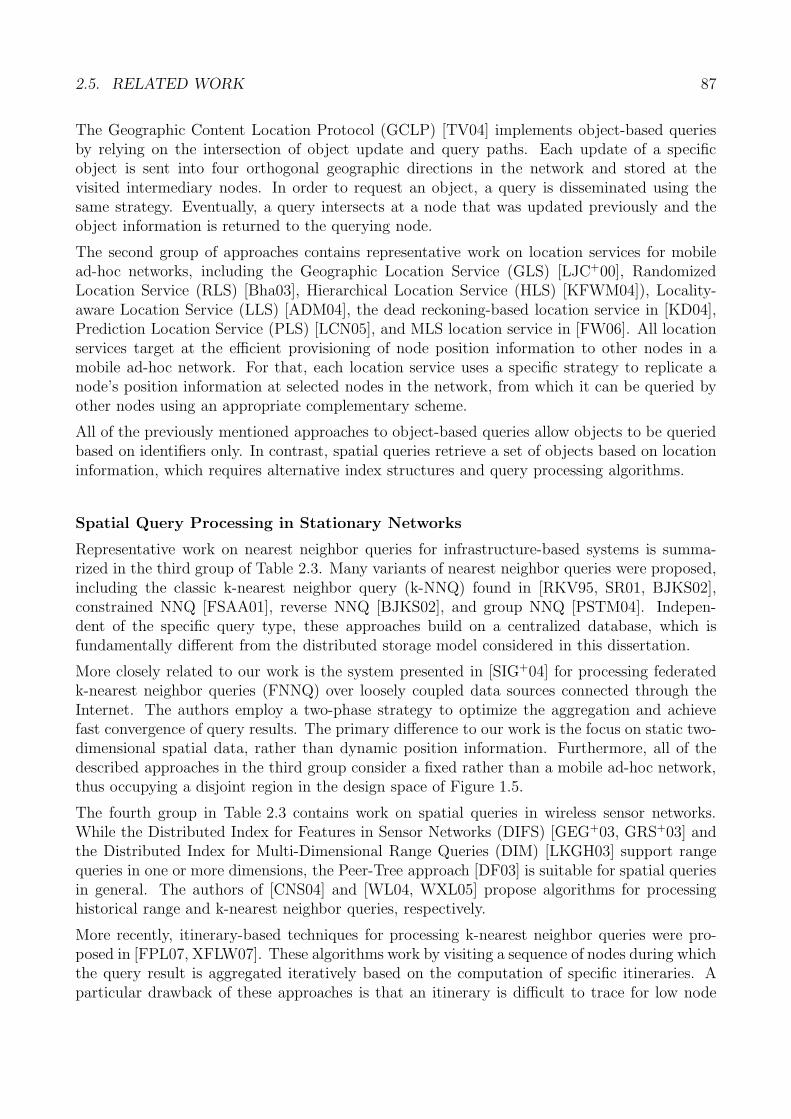
2.5. RELATED WORK 87
The Geographic Content Location Protocol (GCLP) [TV04] implements object-based queriesby relying on the intersection of object update and query paths. Each update of a specificobject is sent into four orthogonal geographic directions in the network and stored at thevisited intermediary nodes. In order to request an object, a query is disseminated using thesame strategy. Eventually, a query intersects at a node that was updated previously and theobject information is returned to the querying node.
The second group of approaches contains representative work on location services for mobilead-hoc networks, including the Geographic Location Service (GLS) [LJC+00], RandomizedLocation Service (RLS) [Bha03], Hierarchical Location Service (HLS) [KFWM04]), Locality-aware Location Service (LLS) [ADM04], the dead reckoning-based location service in [KD04],Prediction Location Service (PLS) [LCN05], and MLS location service in [FW06]. All locationservices target at the efficient provisioning of node position information to other nodes in amobile ad-hoc network. For that, each location service uses a specific strategy to replicate anode’s position information at selected nodes in the network, from which it can be queried byother nodes using an appropriate complementary scheme.
All of the previously mentioned approaches to object-based queries allow objects to be queriedbased on identifiers only. In contrast, spatial queries retrieve a set of objects based on locationinformation, which requires alternative index structures and query processing algorithms.
Spatial Query Processing in Stationary Networks
Representative work on nearest neighbor queries for infrastructure-based systems is summa-rized in the third group of Table 2.3. Many variants of nearest neighbor queries were proposed,including the classic k-nearest neighbor query (k-NNQ) found in [RKV95, SR01, BJKS02],constrained NNQ [FSAA01], reverse NNQ [BJKS02], and group NNQ [PSTM04]. Indepen-dent of the specific query type, these approaches build on a centralized database, which isfundamentally different from the distributed storage model considered in this dissertation.
More closely related to our work is the system presented in [SIG+04] for processing federatedk-nearest neighbor queries (FNNQ) over loosely coupled data sources connected through theInternet. The authors employ a two-phase strategy to optimize the aggregation and achievefast convergence of query results. The primary difference to our work is the focus on static two-dimensional spatial data, rather than dynamic position information. Furthermore, all of thedescribed approaches in the third group consider a fixed rather than a mobile ad-hoc network,thus occupying a disjoint region in the design space of Figure 1.5.
The fourth group in Table 2.3 contains work on spatial queries in wireless sensor networks.While the Distributed Index for Features in Sensor Networks (DIFS) [GEG+03, GRS+03] andthe Distributed Index for Multi-Dimensional Range Queries (DIM) [LKGH03] support rangequeries in one or more dimensions, the Peer-Tree approach [DF03] is suitable for spatial queriesin general. The authors of [CNS04] and [WL04, WXL05] propose algorithms for processinghistorical range and k-nearest neighbor queries, respectively.
More recently, itinerary-based techniques for processing k-nearest neighbor queries were pro-posed in [FPL07, XFLW07]. These algorithms work by visiting a sequence of nodes during whichthe query result is aggregated iteratively based on the computation of specific itineraries. Aparticular drawback of these approaches is that an itinerary is difficult to trace for low node
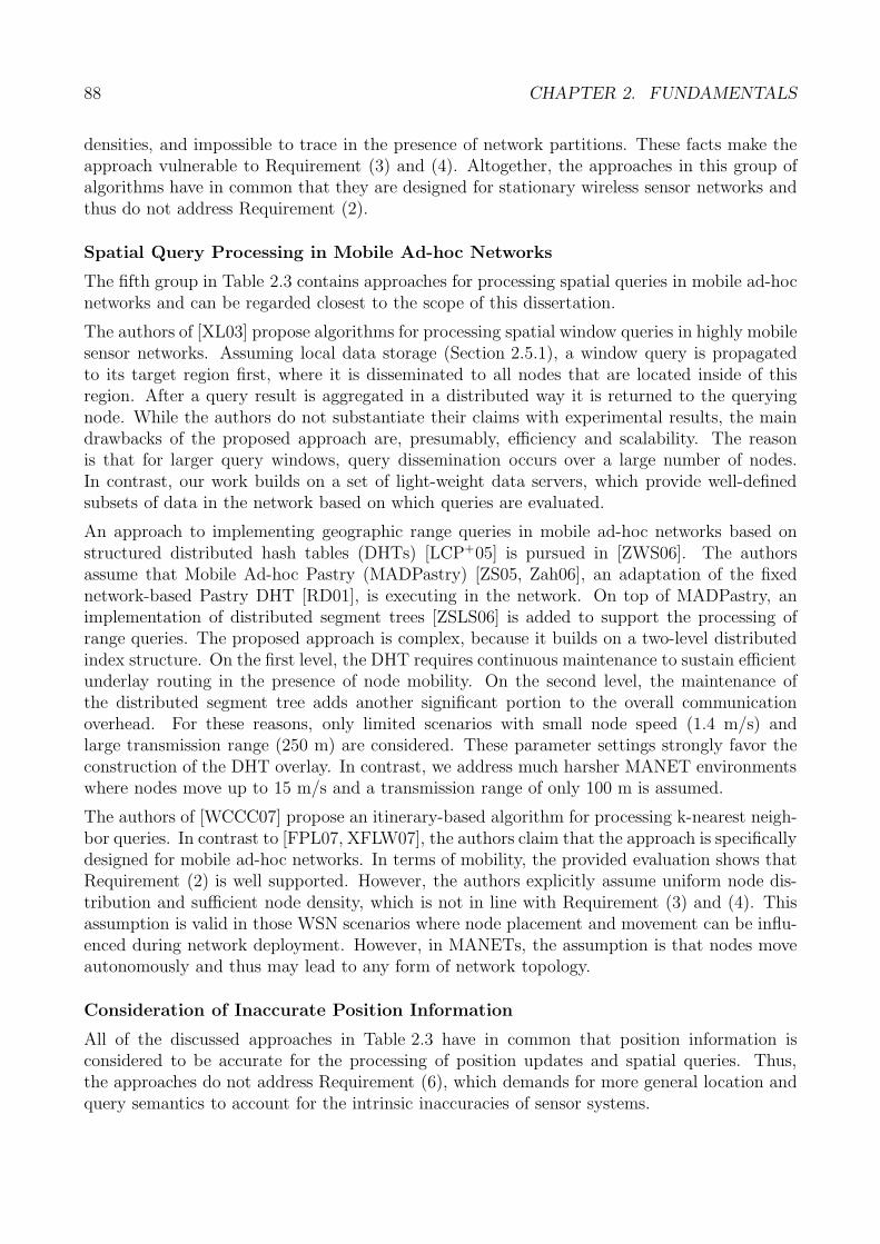
88 CHAPTER 2. FUNDAMENTALS
densities, and impossible to trace in the presence of network partitions. These facts make theapproach vulnerable to Requirement (3) and (4). Altogether, the approaches in this group ofalgorithms have in common that they are designed for stationary wireless sensor networks andthus do not address Requirement (2).
Spatial Query Processing in Mobile Ad-hoc Networks
The fifth group in Table 2.3 contains approaches for processing spatial queries in mobile ad-hocnetworks and can be regarded closest to the scope of this dissertation.
The authors of [XL03] propose algorithms for processing spatial window queries in highly mobilesensor networks. Assuming local data storage (Section 2.5.1), a window query is propagatedto its target region first, where it is disseminated to all nodes that are located inside of thisregion. After a query result is aggregated in a distributed way it is returned to the queryingnode. While the authors do not substantiate their claims with experimental results, the maindrawbacks of the proposed approach are, presumably, efficiency and scalability. The reasonis that for larger query windows, query dissemination occurs over a large number of nodes.In contrast, our work builds on a set of light-weight data servers, which provide well-definedsubsets of data in the network based on which queries are evaluated.
An approach to implementing geographic range queries in mobile ad-hoc networks based onstructured distributed hash tables (DHTs) [LCP+05] is pursued in [ZWS06]. The authorsassume that Mobile Ad-hoc Pastry (MADPastry) [ZS05, Zah06], an adaptation of the fixednetwork-based Pastry DHT [RD01], is executing in the network. On top of MADPastry, animplementation of distributed segment trees [ZSLS06] is added to support the processing ofrange queries. The proposed approach is complex, because it builds on a two-level distributedindex structure. On the first level, the DHT requires continuous maintenance to sustain efficientunderlay routing in the presence of node mobility. On the second level, the maintenance ofthe distributed segment tree adds another significant portion to the overall communicationoverhead. For these reasons, only limited scenarios with small node speed (1.4 m/s) andlarge transmission range (250 m) are considered. These parameter settings strongly favor theconstruction of the DHT overlay. In contrast, we address much harsher MANET environmentswhere nodes move up to 15 m/s and a transmission range of only 100 m is assumed.
The authors of [WCCC07] propose an itinerary-based algorithm for processing k-nearest neigh-bor queries. In contrast to [FPL07, XFLW07], the authors claim that the approach is specificallydesigned for mobile ad-hoc networks. In terms of mobility, the provided evaluation shows thatRequirement (2) is well supported. However, the authors explicitly assume uniform node dis-tribution and sufficient node density, which is not in line with Requirement (3) and (4). Thisassumption is valid in those WSN scenarios where node placement and movement can be influ-enced during network deployment. However, in MANETs, the assumption is that nodes moveautonomously and thus may lead to any form of network topology.
Consideration of Inaccurate Position Information
All of the discussed approaches in Table 2.3 have in common that position information isconsidered to be accurate for the processing of position updates and spatial queries. Thus,the approaches do not address Requirement (6), which demands for more general location andquery semantics to account for the intrinsic inaccuracies of sensor systems.
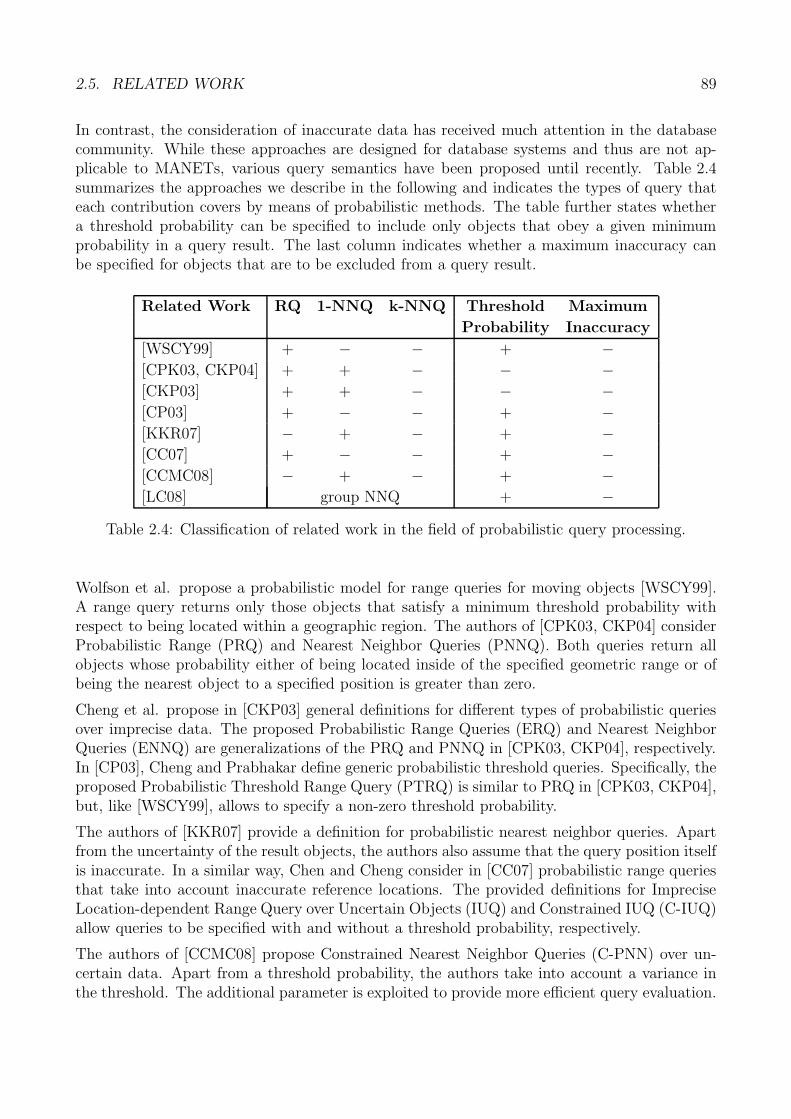
2.5. RELATED WORK 89
In contrast, the consideration of inaccurate data has received much attention in the databasecommunity. While these approaches are designed for database systems and thus are not ap-plicable to MANETs, various query semantics have been proposed until recently. Table 2.4summarizes the approaches we describe in the following and indicates the types of query thateach contribution covers by means of probabilistic methods. The table further states whethera threshold probability can be specified to include only objects that obey a given minimumprobability in a query result. The last column indicates whether a maximum inaccuracy canbe specified for objects that are to be excluded from a query result.
Related Work RQ 1-NNQ k-NNQ Threshold Maximum
Probability Inaccuracy
[WSCY99] + − − + −[CPK03, CKP04] + + − − −[CKP03] + + − − −[CP03] + − − + −[KKR07] − + − + −[CC07] + − − + −[CCMC08] − + − + −[LC08] group NNQ + −
Table 2.4: Classification of related work in the field of probabilistic query processing.
Wolfson et al. propose a probabilistic model for range queries for moving objects [WSCY99].A range query returns only those objects that satisfy a minimum threshold probability withrespect to being located within a geographic region. The authors of [CPK03, CKP04] considerProbabilistic Range (PRQ) and Nearest Neighbor Queries (PNNQ). Both queries return allobjects whose probability either of being located inside of the specified geometric range or ofbeing the nearest object to a specified position is greater than zero.
Cheng et al. propose in [CKP03] general definitions for different types of probabilistic queriesover imprecise data. The proposed Probabilistic Range Queries (ERQ) and Nearest NeighborQueries (ENNQ) are generalizations of the PRQ and PNNQ in [CPK03, CKP04], respectively.In [CP03], Cheng and Prabhakar define generic probabilistic threshold queries. Specifically, theproposed Probabilistic Threshold Range Query (PTRQ) is similar to PRQ in [CPK03, CKP04],but, like [WSCY99], allows to specify a non-zero threshold probability.
The authors of [KKR07] provide a definition for probabilistic nearest neighbor queries. Apartfrom the uncertainty of the result objects, the authors also assume that the query position itselfis inaccurate. In a similar way, Chen and Cheng consider in [CC07] probabilistic range queriesthat take into account inaccurate reference locations. The provided definitions for ImpreciseLocation-dependent Range Query over Uncertain Objects (IUQ) and Constrained IUQ (C-IUQ)allow queries to be specified with and without a threshold probability, respectively.
The authors of [CCMC08] propose Constrained Nearest Neighbor Queries (C-PNN) over un-certain data. Apart from a threshold probability, the authors take into account a variance inthe threshold. The additional parameter is exploited to provide more efficient query evaluation.
90 CHAPTER 2. FUNDAMENTALS
Finally, Probabilistic Group Nearest Neighbor Queries (PGNN) are proposed in [LC08]. Thework extends the query definition in [PSTM04] by taking into account position inaccuracies.This query type is, however, different from the ones considered in this dissertation.
In summary, Table 2.4 reveals that none of the proposed definitions supports probabilistic k-nearest neighbor queries. Furthermore, none of the approaches considers that objects shallbe filtered out from query results due to their exceeding a specified maximum inaccuracy.This feature is, however, essential for many practical scenarios, because objects with largeinaccuracies might not be of any value to the querying user.
2.5.4 Summary of Related Work
In the previous sections, we have analyzed in detail a representative number of approaches thatrelate to each of the tiers presented in the reference model in Figure 2.22. The assessment inSection 2.5.1 and 2.5.2 show that mobility (Requirement (2)) and robustness (Requirement (3)and (4)) are not sufficiently addressed in combination. Chapter 3 and 4 will introduce in detailthe storage tier that addresses these requirements in a combined way.
Section 2.5.3 discussed a large number of approaches that address update and query processingin various system structures. In summary, the approaches for mobile ad-hoc networks are sparseand violate efficiency and scalability (Requirement (1) and (5)). In particular, probabilisticconcepts are unavailable for k-nearest neighbor queries, thus Requirement (6) needs furtherconsideration. We will address these issues in Chapter 5.
Chapter 3
Core Data Storage
This chapter elaborates the algorithms that implement the core data storage component ac-cording to the storage tier in Figure 2.22. In Section 3.1 we describe more formally the systemmodel that we assume in this chapter and also in Chapter 4. Section 3.2 introduces Bidirec-tional Perimeter Routing (BPR) that is situated in the routing tier according to Figure 2.22.The core data storage algorithms are presented in Section 3.3.
To analyze the performance of the devised algorithms, we adopt a twofold methodology. In orderto understand the performance of core data storage in a broader scope, Section 3.4 presents ananalytical study of its communication cost in comparison to a number of more straightforwardapproaches. A detailed analysis of supplementary performance metrics is presented in theexperimental performance analysis of Section 3.5.
3.1 System Model
We consider a mobile ad-hoc network (MANET) deployed inside of a Euclidean 2-space. Let ui
denote network nodes communicating via wireless links, characterized by the nominal transmis-sion range rtx. We assume no specific propagation model, hence the effective transmission rangeof nodes may vary from rtx with time. Let ri(t) denote the trajectory of node ui. We put norestrictions on how coordinates are obtained, both physical (e.g. WGS84 through GPS [EM99])or virtual coordinates (e.g. [RPSS03]) are supported by our model.
Let D denote a set of data items oi ∈ D stored in the network. Let C denote a set of referencecoordinates cr ∈ C. By R ∈ D × C we denote a relation between data items and referencecoordinates, known to all nodes. Relation R induces data subsets D(cr) ⊆ D, containing dataitems related to the same reference coordinate. A network node ui is said to be the data serverfor data subset D(cr) if it is responsible for storing all data items of that subset. A data servermay manage several data subsets at the same time.
According to our discussions in Section 2.1.2 we assume that nodes do not fail nor leave thenetwork without explicit notice. Specifically, this allows a data server to take the necessaryactions regarding the migration of any stored data prior to logging off the network. We furtherassume that network partitions may occur at any time, but that the duration of a partition is
91
92 CHAPTER 3. CORE DATA STORAGE
finite. We assume further that the forming of partitions follows a nondeterministic pattern. Inconjunction with finite partition durations, this property implies that any two nodes are even-tually able to communicate with each other in the same partition. Finally, we allow messagesto be lost, arbitrarily delayed or reordered by the communication system.
Two types of requests are used to access data items that are stored at data servers: updatesand queries. Updates are performed by clients with respect to a single data item oi. An updateon data item oi is considered successful when it is reflected in a write operation on oi at least atone data server. An update may be lost while being propagated to a data server (best effort),e.g. due to a routing failure, in which case it is considered to have not occurred. Queries arecomplex requests by clients that lead to read operations on multiple data items at one or moredata servers. Processes that update never query data items, and vice versa.
According to the CAP Theorem [Bre00], at most two of the properties of data consistency, sys-tem availability, and tolerance to network partitioning can be achieved at any given time [GL02].Because we explicitly take into account network partitioning, we must therefore decide on atradeoff between consistency and availability. Under consideration of the many types of con-ceivable context-based applications that do not require strict data consistency, we decide torelax consistency in favor of availability. Formally, we assume that the storage system obeyseventual consistency, defined according to [TDP+94, GA02, TS06]:
Definition 3.1. A storage system provides eventual consistency when it guarantees that if noupdates on the data items take place for a long time, any access to any data item will eventuallyreturn the most recently updated value of that data item.
Apart from eventual consistency, no further guarantees are given. More concretely, eventualconsistency allows that for two consecutive queries for the same data item, the read associatedwith the first query may occur on a more recent value of the data item than the read that isdue to the second query. It is further possible that successive queries that involve the readingof the same data item may not see all updated values of that data item. However, it is notpossible that a data item which is successfully updated to a data server is lost at a later pointin time, which would otherwise be in violation with Definition 3.1
3.2 Bidirectional Perimeter Routing
In Section 2.5.2 we have discussed how existing approaches to data-centric storage (DCS) areunable to sufficiently support the robustness-related requirements in Section 2.4. We havespecifically shown in Figure 2.25 how position-based and cell-based DCS are deemed to fail insituations of low node density and network partitions.
To tackle these shortcomings, we introduce Bidirectional Perimeter Routing (BPR), a cus-tomization of geometric routing protocols (Section 2.5.2) that apply face routing while relayingpackets towards their destination. BPR adapts perimeter routing in such a way that it allowsto deterministically locate practical data servers even in the presence of malformed perimeters.While BPR may be applied to any geometric routing protocol that uses face routing, we takeGPSR as an example throughout this chapter and Chapter 4.
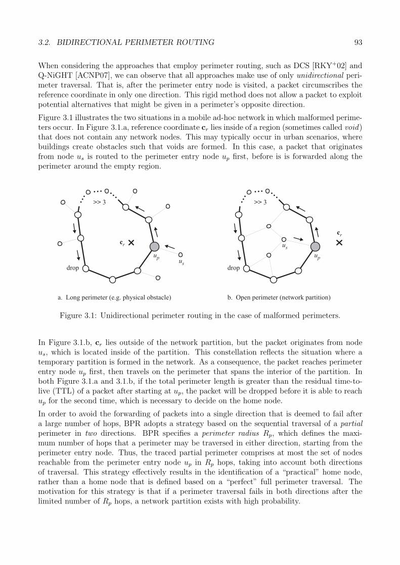
3.2. BIDIRECTIONAL PERIMETER ROUTING 93
When considering the approaches that employ perimeter routing, such as DCS [RKY+02] andQ-NiGHT [ACNP07], we can observe that all approaches make use of only unidirectional peri-meter traversal. That is, after the perimeter entry node is visited, a packet circumscribes thereference coordinate in only one direction. This rigid method does not allow a packet to exploitpotential alternatives that might be given in a perimeter’s opposite direction.
Figure 3.1 illustrates the two situations in a mobile ad-hoc network in which malformed perime-ters occur. In Figure 3.1.a, reference coordinate cr lies inside of a region (sometimes called void)that does not contain any network nodes. This may typically occur in urban scenarios, wherebuildings create obstacles such that voids are formed. In this case, a packet that originatesfrom node us is routed to the perimeter entry node up first, before is is forwarded along theperimeter around the empty region.
a. Long perimeter (e.g. physical obstacle) b. Open perimeter (network partition)
cr
upus
...
......>> 3
drop
cr
up
us
...
......>> 3
drop
Figure 3.1: Unidirectional perimeter routing in the case of malformed perimeters.
In Figure 3.1.b, cr lies outside of the network partition, but the packet originates from nodeus, which is located inside of the partition. This constellation reflects the situation where atemporary partition is formed in the network. As a consequence, the packet reaches perimeterentry node up first, then travels on the perimeter that spans the interior of the partition. Inboth Figure 3.1.a and 3.1.b, if the total perimeter length is greater than the residual time-to-live (TTL) of a packet after starting at up, the packet will be dropped before it is able to reachup for the second time, which is necessary to decide on the home node.
In order to avoid the forwarding of packets into a single direction that is deemed to fail aftera large number of hops, BPR adopts a strategy based on the sequential traversal of a partialperimeter in two directions. BPR specifies a perimeter radius Rp, which defines the maxi-mum number of hops that a perimeter may be traversed in either direction, starting from theperimeter entry node. Thus, the traced partial perimeter comprises at most the set of nodesreachable from the perimeter entry node up in Rp hops, taking into account both directionsof traversal. This strategy effectively results in the identification of a “practical” home node,rather than a home node that is defined based on a “perfect” full perimeter traversal. Themotivation for this strategy is that if a perimeter traversal fails in both directions after thelimited number of Rp hops, a network partition exists with high probability.
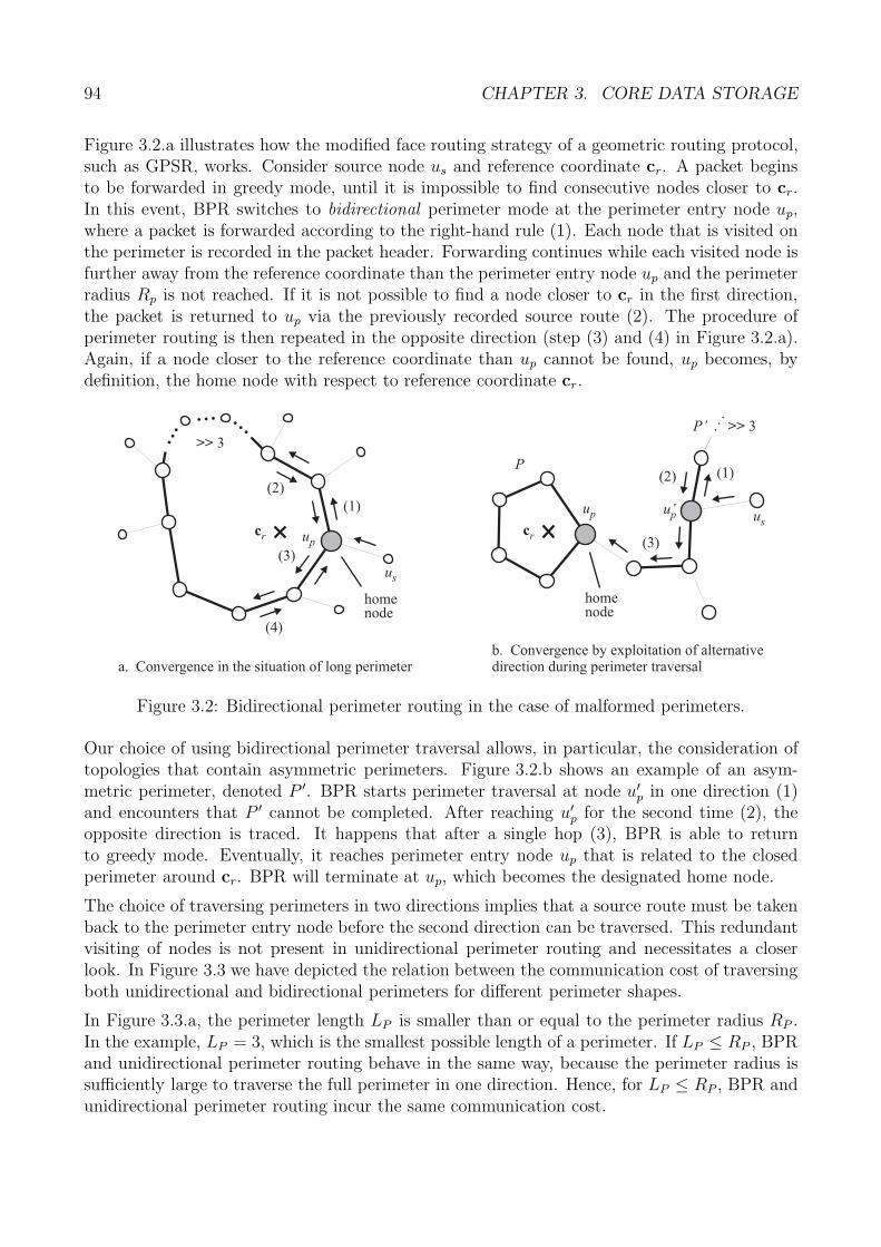
94 CHAPTER 3. CORE DATA STORAGE
Figure 3.2.a illustrates how the modified face routing strategy of a geometric routing protocol,such as GPSR, works. Consider source node us and reference coordinate cr. A packet beginsto be forwarded in greedy mode, until it is impossible to find consecutive nodes closer to cr.In this event, BPR switches to bidirectional perimeter mode at the perimeter entry node up,where a packet is forwarded according to the right-hand rule (1). Each node that is visited onthe perimeter is recorded in the packet header. Forwarding continues while each visited node isfurther away from the reference coordinate than the perimeter entry node up and the perimeterradius Rp is not reached. If it is not possible to find a node closer to cr in the first direction,the packet is returned to up via the previously recorded source route (2). The procedure ofperimeter routing is then repeated in the opposite direction (step (3) and (4) in Figure 3.2.a).Again, if a node closer to the reference coordinate than up cannot be found, up becomes, bydefinition, the home node with respect to reference coordinate cr.
a. Convergence in the situation of long perimeterb. Convergence by exploitation of alternativedirection during perimeter traversal
cr up
us
...
......>> 3
homenode
(1)
(2)
(3)
(4)
cr
us
homenode
up
(1)(2)
(3)
P
... >> 3P’
Figure 3.2: Bidirectional perimeter routing in the case of malformed perimeters.
Our choice of using bidirectional perimeter traversal allows, in particular, the consideration oftopologies that contain asymmetric perimeters. Figure 3.2.b shows an example of an asym-metric perimeter, denoted P ′. BPR starts perimeter traversal at node u′
p in one direction (1)and encounters that P ′ cannot be completed. After reaching u′
p for the second time (2), theopposite direction is traced. It happens that after a single hop (3), BPR is able to returnto greedy mode. Eventually, it reaches perimeter entry node up that is related to the closedperimeter around cr. BPR will terminate at up, which becomes the designated home node.
The choice of traversing perimeters in two directions implies that a source route must be takenback to the perimeter entry node before the second direction can be traversed. This redundantvisiting of nodes is not present in unidirectional perimeter routing and necessitates a closerlook. In Figure 3.3 we have depicted the relation between the communication cost of traversingboth unidirectional and bidirectional perimeters for different perimeter shapes.
In Figure 3.3.a, the perimeter length LP is smaller than or equal to the perimeter radius RP .In the example, LP = 3, which is the smallest possible length of a perimeter. If LP ≤ RP , BPRand unidirectional perimeter routing behave in the same way, because the perimeter radius issufficiently large to traverse the full perimeter in one direction. Hence, for LP ≤ RP , BPR andunidirectional perimeter routing incur the same communication cost.
3.3. CORE DATA STORAGE ALGORITHMS 95
In Figure 3.3.b, LP is larger than RP , but smaller than or equal to 2 · RP . In this case, theperimeter is traversed in one direction up to the perimeter radius RP , then travelled back untilthe perimeter entry node is reached for the second time. In the second direction, BPR musttraverse the perimeter only up to the node that terminated the partial perimeter in the oppositedirection. The same number of hops must be travelled back to the perimeter entry node. Incomparison to unidirectional perimeter routing, BPR incurs significantly larger overhead forRP < LP ≤ 2 · RP . The total number of hops is H = 2 · RP + 2 · (LP − RP ) = 2 · LP , namely,twice as large as for unidirectional perimeter traversal.
In Figure 3.3.c, LP is larger than 2 ·RP , thus, BPR must traverse a perimeter in both directionsup to the full perimeter radius. In this case, BPR requires the constant overhead of 4 ·RP hops,whereas unidirectional perimeter traversal requires LP hops. Assuming that a perimeter isalways closed, the advantage of unidirectional versus bidirectional traversal diminishes withincreasing LP by the difference of 4 · RP − LP . For LP = 4 · RP , the overhead of BPR andunidirectional perimeter routing breaks even.
The aforementioned considerations indicate that BPR incurs significantly larger overhead thanunidirectional perimeter routing for LP > RP . However, two additional aspects need to be takeninto account. Firstly, the arguments regarding Figure 3.3 only apply to closed perimeters. Insituations where node density is low, the traversal of a large number of hops may indicate along or open perimeter. For a malformed perimeter, the effective number of hops traversedby unidirectional perimeter routing is limited only by the packet’s TTL, which may be large.In contrast, BPR’s overhead is limited by the upper bound 4 · RP , which is assumed to besignificantly smaller than the TTL.
The second aspect pertains to the specific purpose for which BPR is used. In the discussed DCSapproaches in Section 2.5.2, every request implies the application of unidirectional perimeterrouting in order to determine a home node. In contrast, we will show in the next sectionhow BPR’s use of bidirectional perimeter traversal can be strongly reduced by completelydecoupling it from request forwarding. We will furthermore revisit BPR’s communication costin Section 3.4, where we will analyze it within the scope of core data storage.
3.3 Core Data Storage Algorithms
Core data storage comprises the mechanisms that allow clients to forward requests to dataservers according to the location-centric storage paradigm. In this section, we will discuss thestatic aspect of location-centric storage. With the mobility of nodes, data migration becomesnecessary, which is discussed in detail in Chapter 4.
In order to forward requests, the common strategy in the position-based DCS approaches dis-cussed in Section 2.5.2 is to use a local routing scheme to deterministically select a storage node.For instance, in DCS [RKY+02], GPSR’s customized perimeter routing is used to consistentlylocate a home node. Hence, the identification of a storage node takes place implicitly, withoutthe need of node-centric routing. The robustness of node selection, however, depends stronglyon the schemes’ ability to cope with the characteristics of mobile ad-hoc networks that areaddressed by Requirement (3) and (4) in Section 2.4. If a storage node cannot be determined,request accuracy will in turn be adversely affected.
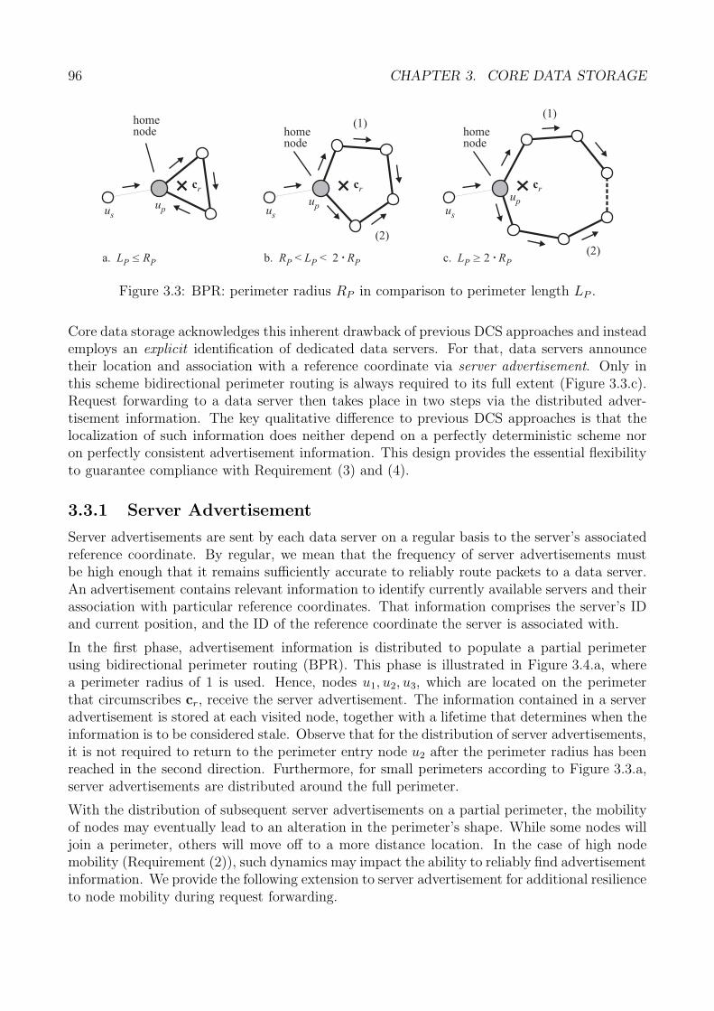
96 CHAPTER 3. CORE DATA STORAGE
cr
us
homenode
up
(1)
(2)
b. < 2 · RPR LP P < c. 2 · RPL >P
cr
homenode
up
(1)
(2)
cr
homenode
upus us
a. RPL <P
Figure 3.3: BPR: perimeter radius RP in comparison to perimeter length LP .
Core data storage acknowledges this inherent drawback of previous DCS approaches and insteademploys an explicit identification of dedicated data servers. For that, data servers announcetheir location and association with a reference coordinate via server advertisement. Only inthis scheme bidirectional perimeter routing is always required to its full extent (Figure 3.3.c).Request forwarding to a data server then takes place in two steps via the distributed adver-tisement information. The key qualitative difference to previous DCS approaches is that thelocalization of such information does neither depend on a perfectly deterministic scheme noron perfectly consistent advertisement information. This design provides the essential flexibilityto guarantee compliance with Requirement (3) and (4).
3.3.1 Server Advertisement
Server advertisements are sent by each data server on a regular basis to the server’s associatedreference coordinate. By regular, we mean that the frequency of server advertisements mustbe high enough that it remains sufficiently accurate to reliably route packets to a data server.An advertisement contains relevant information to identify currently available servers and theirassociation with particular reference coordinates. That information comprises the server’s IDand current position, and the ID of the reference coordinate the server is associated with.
In the first phase, advertisement information is distributed to populate a partial perimeterusing bidirectional perimeter routing (BPR). This phase is illustrated in Figure 3.4.a, wherea perimeter radius of 1 is used. Hence, nodes u1, u2, u3, which are located on the perimeterthat circumscribes cr, receive the server advertisement. The information contained in a serveradvertisement is stored at each visited node, together with a lifetime that determines when theinformation is to be considered stale. Observe that for the distribution of server advertisements,it is not required to return to the perimeter entry node u2 after the perimeter radius has beenreached in the second direction. Furthermore, for small perimeters according to Figure 3.3.a,server advertisements are distributed around the full perimeter.
With the distribution of subsequent server advertisements on a partial perimeter, the mobilityof nodes may eventually lead to an alteration in the perimeter’s shape. While some nodes willjoin a perimeter, others will move off to a more distance location. In the case of high nodemobility (Requirement (2)), such dynamics may impact the ability to reliably find advertisementinformation. We provide the following extension to server advertisement for additional resilienceto node mobility during request forwarding.
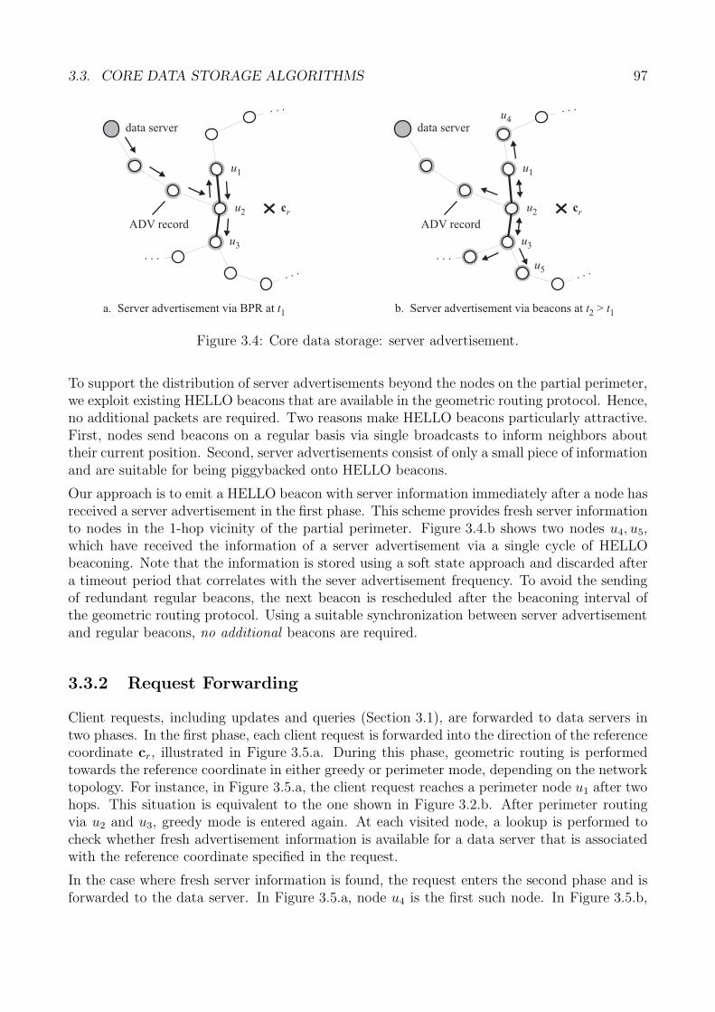
3.3. CORE DATA STORAGE ALGORITHMS 97
...
...
...
cr
a. Server advertisement via BPR at t1
data server
ADV record
b. Server advertisement via beacons at >t t2 1
cr
data server
ADV record
u1
u2
u3
u1
u2
u3
u4
u5
...
...
...
Figure 3.4: Core data storage: server advertisement.
To support the distribution of server advertisements beyond the nodes on the partial perimeter,we exploit existing HELLO beacons that are available in the geometric routing protocol. Hence,no additional packets are required. Two reasons make HELLO beacons particularly attractive.First, nodes send beacons on a regular basis via single broadcasts to inform neighbors abouttheir current position. Second, server advertisements consist of only a small piece of informationand are suitable for being piggybacked onto HELLO beacons.
Our approach is to emit a HELLO beacon with server information immediately after a node hasreceived a server advertisement in the first phase. This scheme provides fresh server informationto nodes in the 1-hop vicinity of the partial perimeter. Figure 3.4.b shows two nodes u4, u5,which have received the information of a server advertisement via a single cycle of HELLObeaconing. Note that the information is stored using a soft state approach and discarded aftera timeout period that correlates with the sever advertisement frequency. To avoid the sendingof redundant regular beacons, the next beacon is rescheduled after the beaconing interval ofthe geometric routing protocol. Using a suitable synchronization between server advertisementand regular beacons, no additional beacons are required.
3.3.2 Request Forwarding
Client requests, including updates and queries (Section 3.1), are forwarded to data servers intwo phases. In the first phase, each client request is forwarded into the direction of the referencecoordinate cr, illustrated in Figure 3.5.a. During this phase, geometric routing is performedtowards the reference coordinate in either greedy or perimeter mode, depending on the networktopology. For instance, in Figure 3.5.a, the client request reaches a perimeter node u1 after twohops. This situation is equivalent to the one shown in Figure 3.2.b. After perimeter routingvia u2 and u3, greedy mode is entered again. At each visited node, a lookup is performed tocheck whether fresh advertisement information is available for a data server that is associatedwith the reference coordinate specified in the request.
In the case where fresh server information is found, the request enters the second phase and isforwarded to the data server. In Figure 3.5.a, node u4 is the first such node. In Figure 3.5.b,
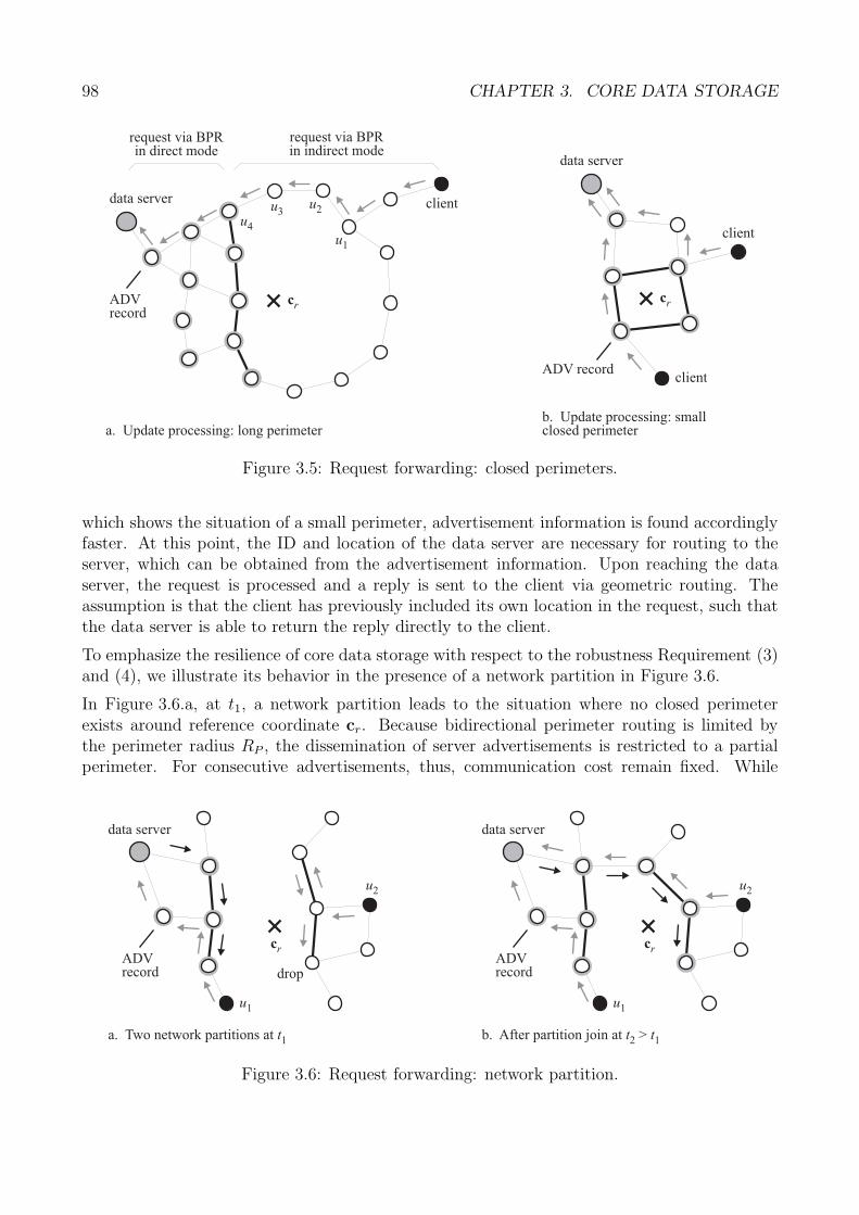
98 CHAPTER 3. CORE DATA STORAGE
cr
client
request via BPRin indirect mode
data server
request via BPRin direct mode
a. Update processing: long perimeterb. Update processing: smallclosed perimeter
data server
cr
client
client
ADVrecord
ADV record
u1
u2u3u4
Figure 3.5: Request forwarding: closed perimeters.
which shows the situation of a small perimeter, advertisement information is found accordinglyfaster. At this point, the ID and location of the data server are necessary for routing to theserver, which can be obtained from the advertisement information. Upon reaching the dataserver, the request is processed and a reply is sent to the client via geometric routing. Theassumption is that the client has previously included its own location in the request, such thatthe data server is able to return the reply directly to the client.
To emphasize the resilience of core data storage with respect to the robustness Requirement (3)and (4), we illustrate its behavior in the presence of a network partition in Figure 3.6.
In Figure 3.6.a, at t1, a network partition leads to the situation where no closed perimeterexists around reference coordinate cr. Because bidirectional perimeter routing is limited bythe perimeter radius RP , the dissemination of server advertisements is restricted to a partialperimeter. For consecutive advertisements, thus, communication cost remain fixed. While
a. Two network partitions at t1 b. After partition join at >t t2 1
ADVrecord
data server
cr
u1
u2
dropADVrecord
data server
cr
u1
u2
Figure 3.6: Request forwarding: network partition.
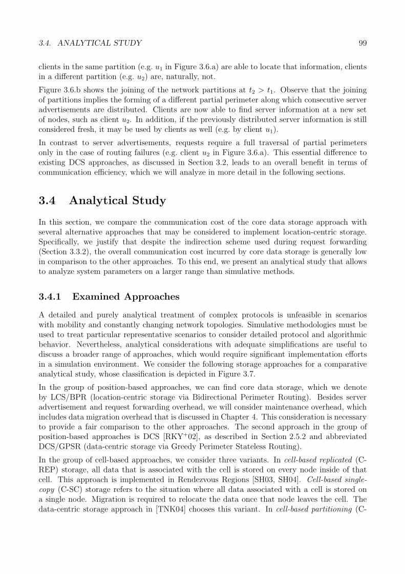
3.4. ANALYTICAL STUDY 99
clients in the same partition (e.g. u1 in Figure 3.6.a) are able to locate that information, clientsin a different partition (e.g. u2) are, naturally, not.
Figure 3.6.b shows the joining of the network partitions at t2 > t1. Observe that the joiningof partitions implies the forming of a different partial perimeter along which consecutive serveradvertisements are distributed. Clients are now able to find server information at a new setof nodes, such as client u2. In addition, if the previously distributed server information is stillconsidered fresh, it may be used by clients as well (e.g. by client u1).
In contrast to server advertisements, requests require a full traversal of partial perimetersonly in the case of routing failures (e.g. client u2 in Figure 3.6.a). This essential difference toexisting DCS approaches, as discussed in Section 3.2, leads to an overall benefit in terms ofcommunication efficiency, which we will analyze in more detail in the following sections.
3.4 Analytical Study
In this section, we compare the communication cost of the core data storage approach withseveral alternative approaches that may be considered to implement location-centric storage.Specifically, we justify that despite the indirection scheme used during request forwarding(Section 3.3.2), the overall communication cost incurred by core data storage is generally lowin comparison to the other approaches. To this end, we present an analytical study that allowsto analyze system parameters on a larger range than simulative methods.
3.4.1 Examined Approaches
A detailed and purely analytical treatment of complex protocols is unfeasible in scenarioswith mobility and constantly changing network topologies. Simulative methodologies must beused to treat particular representative scenarios to consider detailed protocol and algorithmicbehavior. Nevertheless, analytical considerations with adequate simplifications are useful todiscuss a broader range of approaches, which would require significant implementation effortsin a simulation environment. We consider the following storage approaches for a comparativeanalytical study, whose classification is depicted in Figure 3.7.
In the group of position-based approaches, we can find core data storage, which we denoteby LCS/BPR (location-centric storage via Bidirectional Perimeter Routing). Besides serveradvertisement and request forwarding overhead, we will consider maintenance overhead, whichincludes data migration overhead that is discussed in Chapter 4. This consideration is necessaryto provide a fair comparison to the other approaches. The second approach in the group ofposition-based approaches is DCS [RKY+02], as described in Section 2.5.2 and abbreviatedDCS/GPSR (data-centric storage via Greedy Perimeter Stateless Routing).
In the group of cell-based approaches, we consider three variants. In cell-based replicated (C-REP) storage, all data that is associated with the cell is stored on every node inside of thatcell. This approach is implemented in Rendezvous Regions [SH03, SH04]. Cell-based single-copy (C-SC) storage refers to the situation where all data associated with a cell is stored ona single node. Migration is required to relocate the data once that node leaves the cell. Thedata-centric storage approach in [TNK04] chooses this variant. In cell-based partitioning (C-
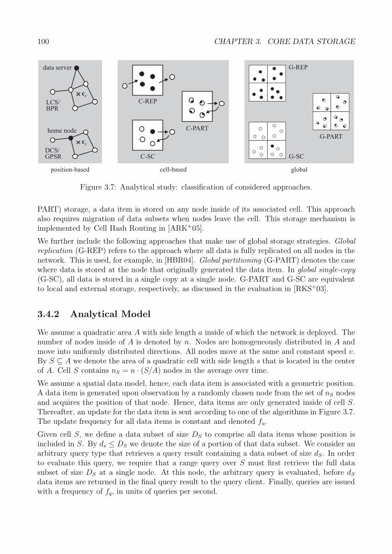
100 CHAPTER 3. CORE DATA STORAGE
G-REP
G-SC
G-PART
global
LCS/BPR
DCS/GPSR
cr
position-based
cr
data server
home node
C-REP
C-SC
C-PART
cell-based
Figure 3.7: Analytical study: classification of considered approaches.
PART) storage, a data item is stored on any node inside of its associated cell. This approachalso requires migration of data subsets when nodes leave the cell. This storage mechanism isimplemented by Cell Hash Routing in [ARK+05].
We further include the following approaches that make use of global storage strategies. Globalreplication (G-REP) refers to the approach where all data is fully replicated on all nodes in thenetwork. This is used, for example, in [HBR04]. Global partitioning (G-PART) denotes the casewhere data is stored at the node that originally generated the data item. In global single-copy(G-SC), all data is stored in a single copy at a single node. G-PART and G-SC are equivalentto local and external storage, respectively, as discussed in the evaluation in [RKS+03].
3.4.2 Analytical Model
We assume a quadratic area A with side length a inside of which the network is deployed. Thenumber of nodes inside of A is denoted by n. Nodes are homogeneously distributed in A andmove into uniformly distributed directions. All nodes move at the same and constant speed v.By S ⊆ A we denote the area of a quadratic cell with side length s that is located in the centerof A. Cell S contains nS = n · (S/A) nodes in the average over time.
We assume a spatial data model, hence, each data item is associated with a geometric position.A data item is generated upon observation by a randomly chosen node from the set of nS nodesand acquires the position of that node. Hence, data items are only generated inside of cell S.Thereafter, an update for the data item is sent according to one of the algorithms in Figure 3.7.The update frequency for all data items is constant and denoted fu.
Given cell S, we define a data subset of size DS to comprise all data items whose position isincluded in S. By ds ≤ DS we denote the size of a portion of that data subset. We consider anarbitrary query type that retrieves a query result containing a data subset of size dS. In orderto evaluate this query, we require that a range query over S must first retrieve the full datasubset of size DS at a single node. At this node, the arbitrary query is evaluated, before dS
data items are returned in the final query result to the query client. Finally, queries are issuedwith a frequency of fq, in units of queries per second.
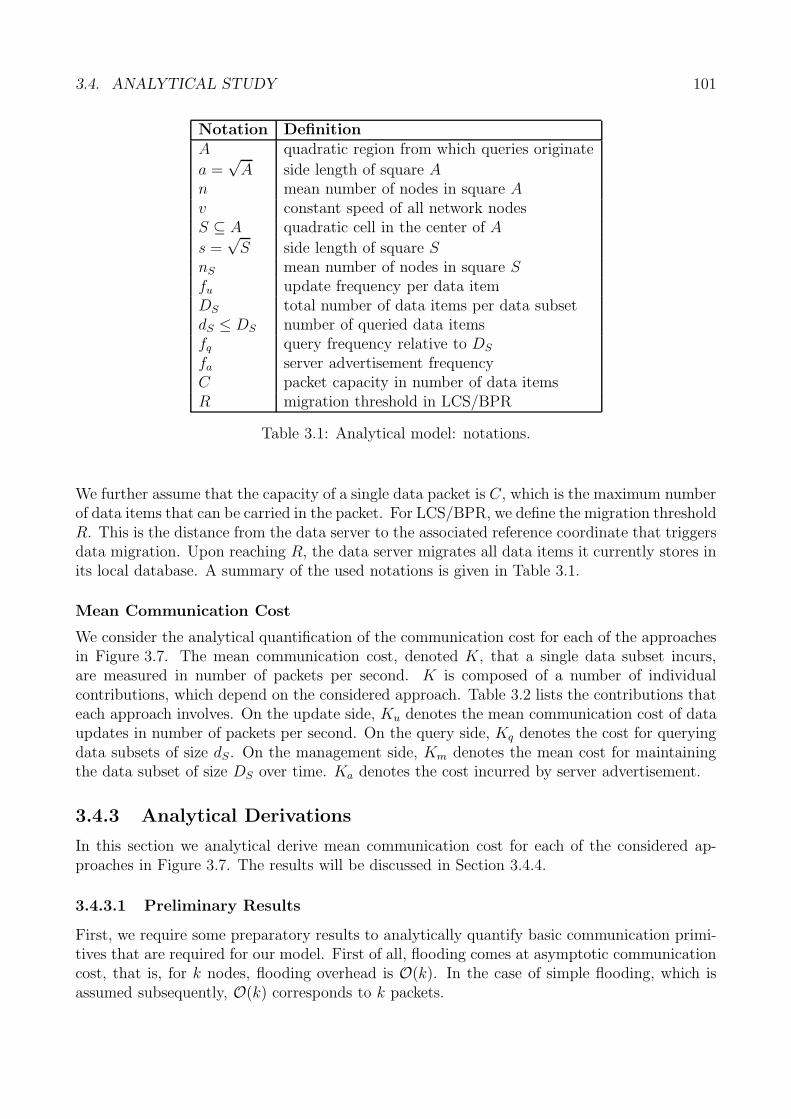
3.4. ANALYTICAL STUDY 101
Notation DefinitionA quadratic region from which queries originate
a =√
A side length of square An mean number of nodes in square Av constant speed of all network nodesS ⊆ A quadratic cell in the center of A
s =√
S side length of square SnS mean number of nodes in square Sfu update frequency per data itemDS total number of data items per data subsetdS ≤ DS number of queried data itemsfq query frequency relative to DS
fa server advertisement frequencyC packet capacity in number of data itemsR migration threshold in LCS/BPR
Table 3.1: Analytical model: notations.
We further assume that the capacity of a single data packet is C, which is the maximum numberof data items that can be carried in the packet. For LCS/BPR, we define the migration thresholdR. This is the distance from the data server to the associated reference coordinate that triggersdata migration. Upon reaching R, the data server migrates all data items it currently stores inits local database. A summary of the used notations is given in Table 3.1.
Mean Communication Cost
We consider the analytical quantification of the communication cost for each of the approachesin Figure 3.7. The mean communication cost, denoted K, that a single data subset incurs,are measured in number of packets per second. K is composed of a number of individualcontributions, which depend on the considered approach. Table 3.2 lists the contributions thateach approach involves. On the update side, Ku denotes the mean communication cost of dataupdates in number of packets per second. On the query side, Kq denotes the cost for queryingdata subsets of size dS. On the management side, Km denotes the mean cost for maintainingthe data subset of size DS over time. Ka denotes the cost incurred by server advertisement.
3.4.3 Analytical Derivations
In this section we analytical derive mean communication cost for each of the considered ap-proaches in Figure 3.7. The results will be discussed in Section 3.4.4.
3.4.3.1 Preliminary Results
First, we require some preparatory results to analytically quantify basic communication primi-tives that are required for our model. First of all, flooding comes at asymptotic communicationcost, that is, for k nodes, flooding overhead is O(k). In the case of simple flooding, which isassumed subsequently, O(k) corresponds to k packets.
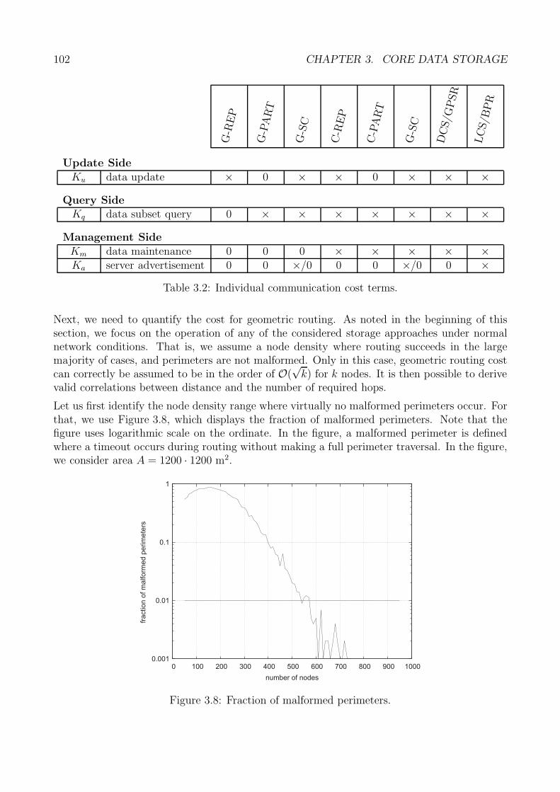
102 CHAPTER 3. CORE DATA STORAGE
G-R
EP
G-P
ART
G-S
C
C-R
EP
C-P
ART
G-S
C
DC
S/G
PSR
LC
S/B
PR
Update SideKu data update × 0 × × 0 × × ×
Query SideKq data subset query 0 × × × × × × ×
Management SideKm data maintenance 0 0 0 × × × × ×Ka server advertisement 0 0 ×/0 0 0 ×/0 0 ×
Table 3.2: Individual communication cost terms.
Next, we need to quantify the cost for geometric routing. As noted in the beginning of thissection, we focus on the operation of any of the considered storage approaches under normalnetwork conditions. That is, we assume a node density where routing succeeds in the largemajority of cases, and perimeters are not malformed. Only in this case, geometric routing costcan correctly be assumed to be in the order of O(
√k) for k nodes. It is then possible to derive
valid correlations between distance and the number of required hops.
Let us first identify the node density range where virtually no malformed perimeters occur. Forthat, we use Figure 3.8, which displays the fraction of malformed perimeters. Note that thefigure uses logarithmic scale on the ordinate. In the figure, a malformed perimeter is definedwhere a timeout occurs during routing without making a full perimeter traversal. In the figure,we consider area A = 1200 · 1200 m2.
0.001
0.01
0.1
1
0 100 200 300 400 500 600 700 800 900 1000
fra
ctio
no
fm
alfo
rme
dp
erim
ete
rs
number of nodes
Figure 3.8: Fraction of malformed perimeters.
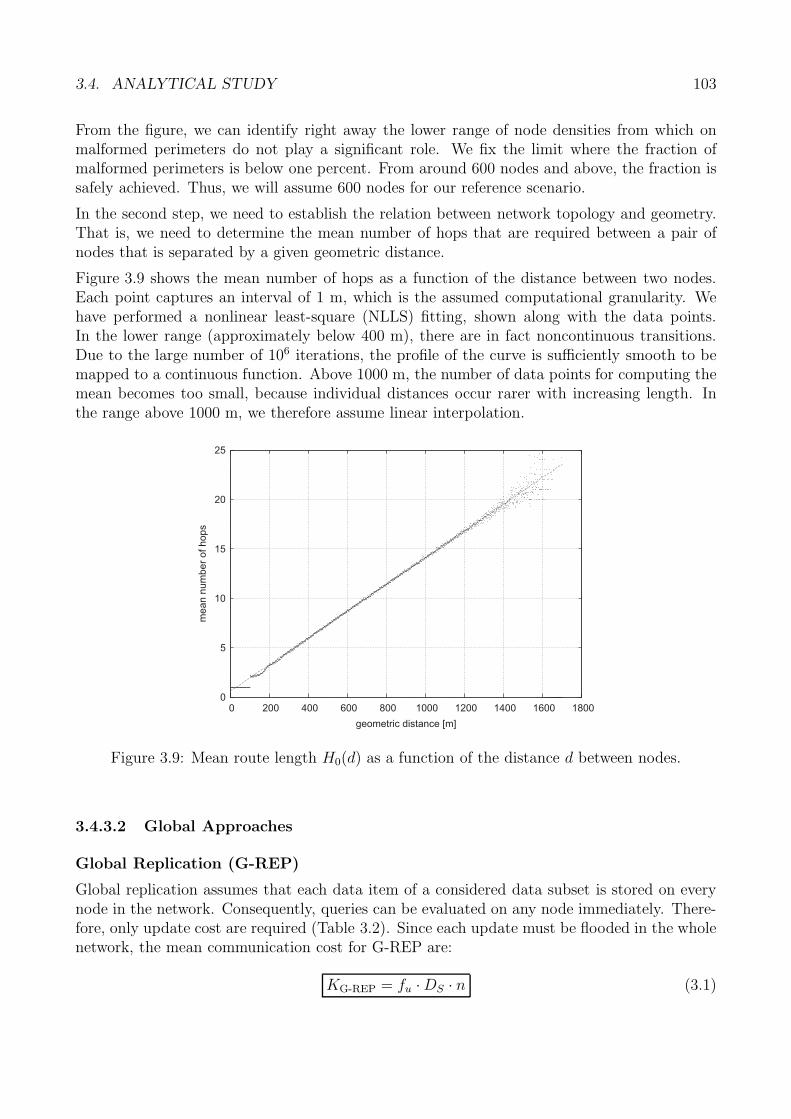
3.4. ANALYTICAL STUDY 103
From the figure, we can identify right away the lower range of node densities from which onmalformed perimeters do not play a significant role. We fix the limit where the fraction ofmalformed perimeters is below one percent. From around 600 nodes and above, the fraction issafely achieved. Thus, we will assume 600 nodes for our reference scenario.
In the second step, we need to establish the relation between network topology and geometry.That is, we need to determine the mean number of hops that are required between a pair ofnodes that is separated by a given geometric distance.
Figure 3.9 shows the mean number of hops as a function of the distance between two nodes.Each point captures an interval of 1 m, which is the assumed computational granularity. Wehave performed a nonlinear least-square (NLLS) fitting, shown along with the data points.In the lower range (approximately below 400 m), there are in fact noncontinuous transitions.Due to the large number of 106 iterations, the profile of the curve is sufficiently smooth to bemapped to a continuous function. Above 1000 m, the number of data points for computing themean becomes too small, because individual distances occur rarer with increasing length. Inthe range above 1000 m, we therefore assume linear interpolation.
0
5
10
15
20
25
0 200 400 600 800 1000 1200 1400 1600 1800
meannumberofhops
geometric distance [m]
Figure 3.9: Mean route length H0(d) as a function of the distance d between nodes.
3.4.3.2 Global Approaches
Global Replication (G-REP)
Global replication assumes that each data item of a considered data subset is stored on everynode in the network. Consequently, queries can be evaluated on any node immediately. There-fore, only update cost are required (Table 3.2). Since each update must be flooded in the wholenetwork, the mean communication cost for G-REP are:
KG-REP = fu · DS · n (3.1)
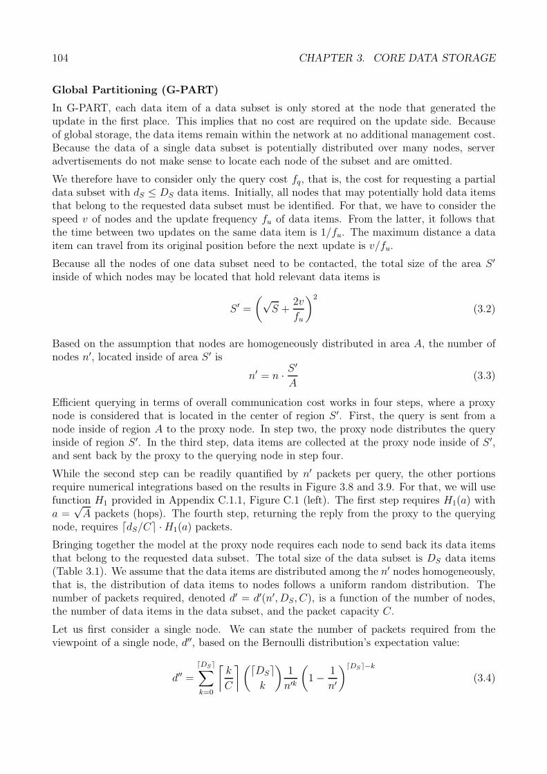
104 CHAPTER 3. CORE DATA STORAGE
Global Partitioning (G-PART)
In G-PART, each data item of a data subset is only stored at the node that generated theupdate in the first place. This implies that no cost are required on the update side. Becauseof global storage, the data items remain within the network at no additional management cost.Because the data of a single data subset is potentially distributed over many nodes, serveradvertisements do not make sense to locate each node of the subset and are omitted.
We therefore have to consider only the query cost fq, that is, the cost for requesting a partialdata subset with dS ≤ DS data items. Initially, all nodes that may potentially hold data itemsthat belong to the requested data subset must be identified. For that, we have to consider thespeed v of nodes and the update frequency fu of data items. From the latter, it follows thatthe time between two updates on the same data item is 1/fu. The maximum distance a dataitem can travel from its original position before the next update is v/fu.
Because all the nodes of one data subset need to be contacted, the total size of the area S ′
inside of which nodes may be located that hold relevant data items is
S ′ =
(√S +
2v
fu
)2
(3.2)
Based on the assumption that nodes are homogeneously distributed in area A, the number ofnodes n′, located inside of area S ′ is
n′ = n · S ′
A(3.3)
Efficient querying in terms of overall communication cost works in four steps, where a proxynode is considered that is located in the center of region S ′. First, the query is sent from anode inside of region A to the proxy node. In step two, the proxy node distributes the queryinside of region S ′. In the third step, data items are collected at the proxy node inside of S ′,and sent back by the proxy to the querying node in step four.
While the second step can be readily quantified by n′ packets per query, the other portionsrequire numerical integrations based on the results in Figure 3.8 and 3.9. For that, we will usefunction H1 provided in Appendix C.1.1, Figure C.1 (left). The first step requires H1(a) witha =
√A packets (hops). The fourth step, returning the reply from the proxy to the querying
node, requires �dS/C� · H1(a) packets.
Bringing together the model at the proxy node requires each node to send back its data itemsthat belong to the requested data subset. The total size of the data subset is DS data items(Table 3.1). We assume that the data items are distributed among the n′ nodes homogeneously,that is, the distribution of data items to nodes follows a uniform random distribution. Thenumber of packets required, denoted d′ = d′(n′, DS, C), is a function of the number of nodes,the number of data items in the data subset, and the packet capacity C.
Let us first consider a single node. We can state the number of packets required from theviewpoint of a single node, d′′, based on the Bernoulli distribution’s expectation value:
d′′ =
�DS�∑k=0
⌈k
C
⌉(�DS�k
)1
n′k
(1 − 1
n′
)�DS�−k
(3.4)
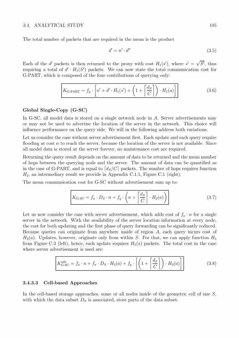
3.4. ANALYTICAL STUDY 105
The total number of packets that are required in the mean is the product
d′ = n′ · d′′ (3.5)
Each of the d′ packets is then returned to the proxy with cost H1(s′), where s′ =
√S ′, thus
requiring a total of d′ · H1(S′) packets. We can now state the total communication cost for
G-PART, which is composed of the four contributions of querying only:
KG-PART = fq ·[n′ + d′ · H1(s
′) +
(1 +
⌈dS
C
⌉)· H1(a)
](3.6)
Global Single-Copy (G-SC)
In G-SC, all model data is stored on a single network node in A. Server advertisements mayor may not be used to advertise the location of the server in the network. This choice willinfluence performance on the query side. We will in the following address both variations.
Let us consider the case without server advertisement first. Each update and each query requireflooding at cost n to reach the server, because the location of the server is not available. Sinceall model data is stored at the server forever, no maintenance cost are required.
Returning the query result depends on the amount of data to be returned and the mean numberof hops between the querying node and the server. The amount of data can be quantified asin the case of G-PART, and is equal to �dS/C� packets. The number of hops requires functionH2, an intermediary result we provide in Appendix C.1.1, Figure C.1 (right).
The mean communication cost for G-SC without advertisement sum up to:
KG-SC = fu · DS · n + fq ·(
n +
⌈dS
C
⌉· H2(a)
)(3.7)
Let us now consider the case with server advertisement, which adds cost of fa · n for a singleserver in the network. With the availability of the server location information at every node,the cost for both updating and the first phase of query forwarding can be significantly reduced.Because queries can originate from anywhere inside of region A, each query incurs cost ofH2(a). Updates, however, originate only from within S. For that, we can apply function H5
from Figure C.3 (left), hence, each update requires H5(s) packets. The total cost in the casewhere server advertisement is used are:
KadvG-SC = fa · n + fu · DS · H5(a) + fq ·
[(1 +
⌈dS
C
⌉)· H2(a)
](3.8)
3.4.3.3 Cell-based Approaches
In the cell-based storage approaches, some or all nodes inside of the geometric cell of size S,with which the data subset DS is associated, store parts of the data subset.
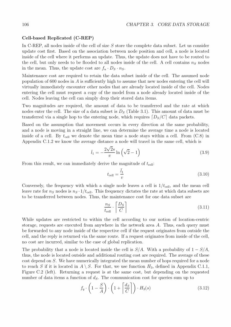
106 CHAPTER 3. CORE DATA STORAGE
Cell-based Replicated (C-REP)
In C-REP, all nodes inside of the cell of size S store the complete data subset. Let us considerupdate cost first. Based on the association between node position and cell, a node is locatedinside of the cell where it performs an update. Thus, the update does not have to be routed tothe cell, but only needs to be flooded to all nodes inside of the cell. A cell contains nS nodesin the mean. Thus, the update cost are fu · DS · nS.
Maintenance cost are required to retain the data subset inside of the cell. The assumed nodepopulation of 600 nodes in A is sufficiently high to assume that new nodes entering the cell willvirtually immediately encounter other nodes that are already located inside of the cell. Nodesentering the cell must request a copy of the model from a node already located inside of thecell. Nodes leaving the cell can simply drop their stored data items.
Two magnitudes are required, the amount of data to be transferred and the rate at whichnodes enter the cell. The size of a data subset is DS (Table 3.1). This amount of data must betransferred via a single hop to the entering node, which requires �DS/C� data packets.
Based on the assumption that movement occurs in every direction at the same probability,and a node is moving in a straight line, we can determine the average time a node is locatedinside of a cell. By tcell we denote the mean time a node stays within a cell. From (C.8) inAppendix C.1.2 we know the average distance a node will travel in the same cell, which is
l1 = −2√
2s
πln(√
2 − 1)
(3.9)
From this result, we can immediately derive the magnitude of tcell:
tcell =l1v
(3.10)
Conversely, the frequency with which a single node leaves a cell is 1/tcell, and the mean cellleave rate for nS nodes is nS · 1/tcell. This frequency dictates the rate at which data subsets areto be transferred between nodes. Thus, the maintenance cost for one data subset are
nS
tcell·⌈
DS
C
⌉(3.11)
While updates are restricted to within the cell according to our notion of location-centricstorage, requests are executed from anywhere in the network area A. Thus, each query mustbe forwarded to any node inside of the respective cell if the request originates from outside thecell, and the reply is returned via the same route. If a request originates from inside of the cell,no cost are incurred, similar to the case of global replication.
The probability that a node is located inside the cell is S/A. With a probability of 1 − S/A,thus, the node is located outside and additional routing cost are required. The average of thesecost depend on S. We have numerically integrated the mean number of hops required for a nodeto reach S if it is located in A \ S. For that, we use function H3, defined in Appendix C.1.1,Figure C.2 (left). Returning a request is at the same cost, but depending on the requestednumber of data items a function of dS. The communication cost for queries sum up to
fq ·(
1 − S
A
)·(
1 +
⌈dS
C
⌉)· H3(s) (3.12)
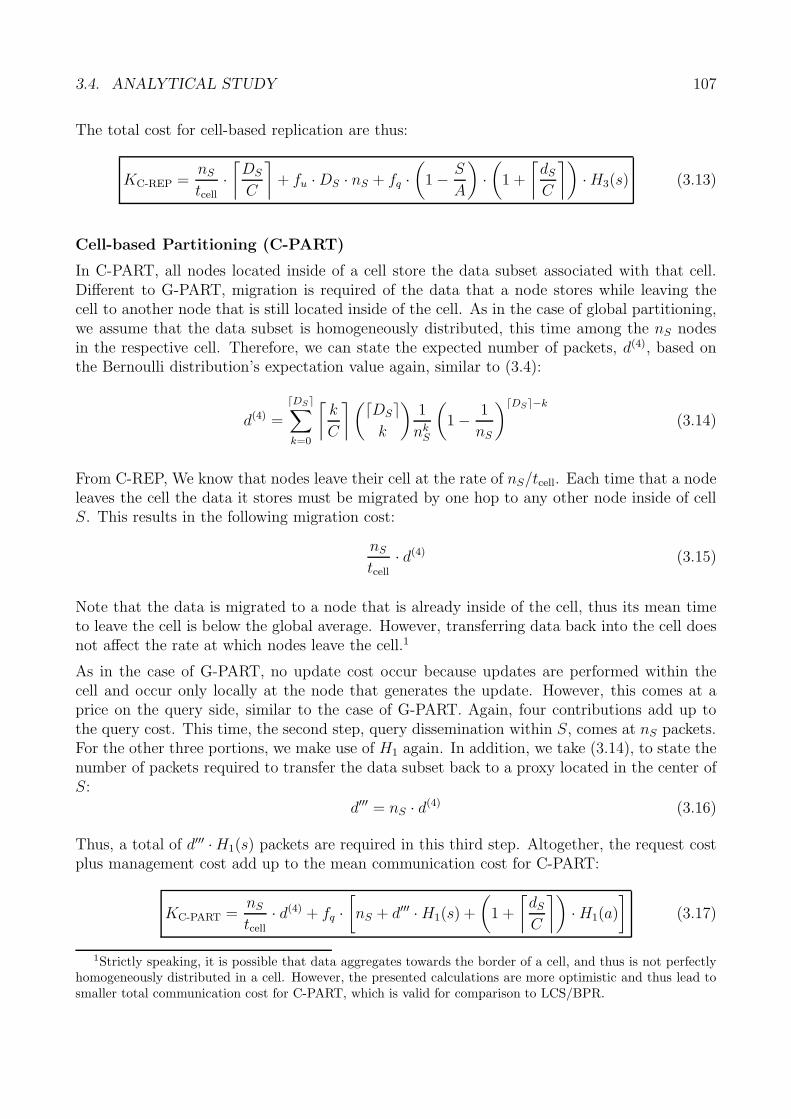
3.4. ANALYTICAL STUDY 107
The total cost for cell-based replication are thus:
KC-REP =nS
tcell·⌈
DS
C
⌉+ fu · DS · nS + fq ·
(1 − S
A
)·(
1 +
⌈dS
C
⌉)· H3(s) (3.13)
Cell-based Partitioning (C-PART)
In C-PART, all nodes located inside of a cell store the data subset associated with that cell.Different to G-PART, migration is required of the data that a node stores while leaving thecell to another node that is still located inside of the cell. As in the case of global partitioning,we assume that the data subset is homogeneously distributed, this time among the nS nodesin the respective cell. Therefore, we can state the expected number of packets, d(4), based onthe Bernoulli distribution’s expectation value again, similar to (3.4):
d(4) =
�DS�∑k=0
⌈k
C
⌉(�DS�k
)1
nkS
(1 − 1
nS
)�DS�−k
(3.14)
From C-REP, We know that nodes leave their cell at the rate of nS/tcell. Each time that a nodeleaves the cell the data it stores must be migrated by one hop to any other node inside of cellS. This results in the following migration cost:
nS
tcell· d(4) (3.15)
Note that the data is migrated to a node that is already inside of the cell, thus its mean timeto leave the cell is below the global average. However, transferring data back into the cell doesnot affect the rate at which nodes leave the cell.1
As in the case of G-PART, no update cost occur because updates are performed within thecell and occur only locally at the node that generates the update. However, this comes at aprice on the query side, similar to the case of G-PART. Again, four contributions add up tothe query cost. This time, the second step, query dissemination within S, comes at nS packets.For the other three portions, we make use of H1 again. In addition, we take (3.14), to state thenumber of packets required to transfer the data subset back to a proxy located in the center ofS:
d′′′ = nS · d(4) (3.16)
Thus, a total of d′′′ ·H1(s) packets are required in this third step. Altogether, the request costplus management cost add up to the mean communication cost for C-PART:
KC-PART =nS
tcell· d(4) + fq ·
[nS + d′′′ · H1(s) +
(1 +
⌈dS
C
⌉)· H1(a)
](3.17)
1Strictly speaking, it is possible that data aggregates towards the border of a cell, and thus is not perfectlyhomogeneously distributed in a cell. However, the presented calculations are more optimistic and thus lead tosmaller total communication cost for C-PART, which is valid for comparison to LCS/BPR.
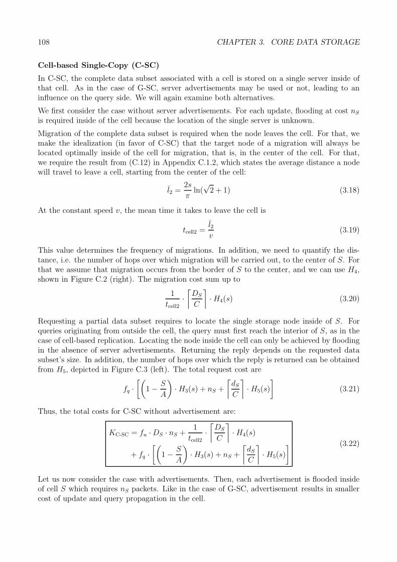
108 CHAPTER 3. CORE DATA STORAGE
Cell-based Single-Copy (C-SC)
In C-SC, the complete data subset associated with a cell is stored on a single server inside ofthat cell. As in the case of G-SC, server advertisements may be used or not, leading to aninfluence on the query side. We will again examine both alternatives.
We first consider the case without server advertisements. For each update, flooding at cost nS
is required inside of the cell because the location of the single server is unknown.
Migration of the complete data subset is required when the node leaves the cell. For that, wemake the idealization (in favor of C-SC) that the target node of a migration will always belocated optimally inside of the cell for migration, that is, in the center of the cell. For that,we require the result from (C.12) in Appendix C.1.2, which states the average distance a nodewill travel to leave a cell, starting from the center of the cell:
l2 =2s
πln(
√2 + 1) (3.18)
At the constant speed v, the mean time it takes to leave the cell is
tcell2 =l2v
(3.19)
This value determines the frequency of migrations. In addition, we need to quantify the dis-tance, i.e. the number of hops over which migration will be carried out, to the center of S. Forthat we assume that migration occurs from the border of S to the center, and we can use H4,shown in Figure C.2 (right). The migration cost sum up to
1
tcell2·⌈
DS
C
⌉· H4(s) (3.20)
Requesting a partial data subset requires to locate the single storage node inside of S. Forqueries originating from outside the cell, the query must first reach the interior of S, as in thecase of cell-based replication. Locating the node inside the cell can only be achieved by floodingin the absence of server advertisements. Returning the reply depends on the requested datasubset’s size. In addition, the number of hops over which the reply is returned can be obtainedfrom H5, depicted in Figure C.3 (left). The total request cost are
fq ·[(
1 − S
A
)· H3(s) + nS +
⌈dS
C
⌉· H5(s)
](3.21)
Thus, the total costs for C-SC without advertisement are:
KC-SC = fu · DS · nS +1
tcell2·⌈
DS
C
⌉· H4(s)
+ fq ·[(
1 − S
A
)· H3(s) + nS +
⌈dS
C
⌉· H5(s)
] (3.22)
Let us now consider the case with advertisements. Then, each advertisement is flooded insideof cell S which requires nS packets. Like in the case of G-SC, advertisement results in smallercost of update and query propagation in the cell.
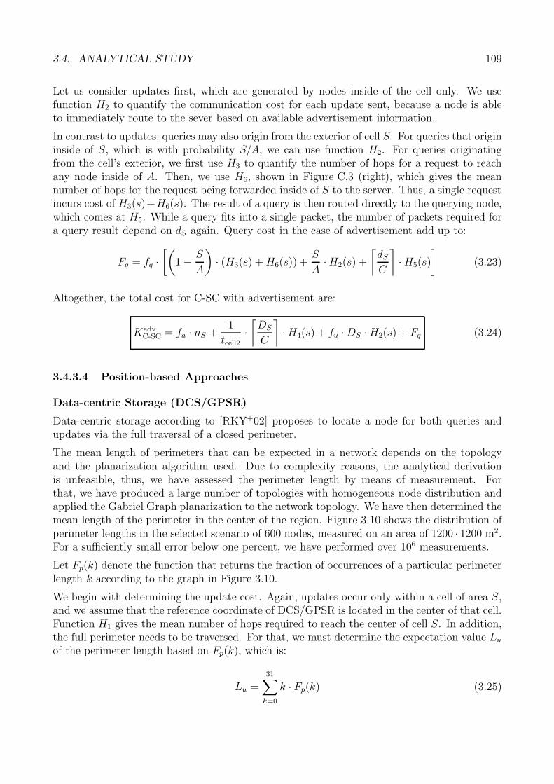
3.4. ANALYTICAL STUDY 109
Let us consider updates first, which are generated by nodes inside of the cell only. We usefunction H2 to quantify the communication cost for each update sent, because a node is ableto immediately route to the sever based on available advertisement information.
In contrast to updates, queries may also origin from the exterior of cell S. For queries that origininside of S, which is with probability S/A, we can use function H2. For queries originatingfrom the cell’s exterior, we first use H3 to quantify the number of hops for a request to reachany node inside of A. Then, we use H6, shown in Figure C.3 (right), which gives the meannumber of hops for the request being forwarded inside of S to the server. Thus, a single requestincurs cost of H3(s)+H6(s). The result of a query is then routed directly to the querying node,which comes at H5. While a query fits into a single packet, the number of packets required fora query result depend on dS again. Query cost in the case of advertisement add up to:
Fq = fq ·[(
1 − S
A
)· (H3(s) + H6(s)) +
S
A· H2(s) +
⌈dS
C
⌉· H5(s)
](3.23)
Altogether, the total cost for C-SC with advertisement are:
KadvC-SC = fa · nS +
1
tcell2·⌈
DS
C
⌉· H4(s) + fu · DS · H2(s) + Fq (3.24)
3.4.3.4 Position-based Approaches
Data-centric Storage (DCS/GPSR)
Data-centric storage according to [RKY+02] proposes to locate a node for both queries andupdates via the full traversal of a closed perimeter.
The mean length of perimeters that can be expected in a network depends on the topologyand the planarization algorithm used. Due to complexity reasons, the analytical derivationis unfeasible, thus, we have assessed the perimeter length by means of measurement. Forthat, we have produced a large number of topologies with homogeneous node distribution andapplied the Gabriel Graph planarization to the network topology. We have then determined themean length of the perimeter in the center of the region. Figure 3.10 shows the distribution ofperimeter lengths in the selected scenario of 600 nodes, measured on an area of 1200 · 1200 m2.For a sufficiently small error below one percent, we have performed over 106 measurements.
Let Fp(k) denote the function that returns the fraction of occurrences of a particular perimeterlength k according to the graph in Figure 3.10.
We begin with determining the update cost. Again, updates occur only within a cell of area S,and we assume that the reference coordinate of DCS/GPSR is located in the center of that cell.Function H1 gives the mean number of hops required to reach the center of cell S. In addition,the full perimeter needs to be traversed. For that, we must determine the expectation value Lu
of the perimeter length based on Fp(k), which is:
Lu =31∑
k=0
k · Fp(k) (3.25)
110 CHAPTER 3. CORE DATA STORAGE
0
0.05
0.1
0.15
0.2
0.25
0 4 8 12 16 20 24 28 32
fra
ctio
no
fo
ccu
rre
nce
s
perimeter length
Figure 3.10: Fraction of occurrences of unidirectional perimeters for DCS/GPSR.
The cost for updating thus sums up to
Ku = fu · DS · (H1(s) + Lu) (3.26)
Queries may originate from anywhere within A. In addition to updates, a reply must also besent to the querying node, for which H1 applies as well. Thus, the total query cost sum up to:
Kq = fq ·[(
1 +
⌈dS
C
⌉)· H1(a) + Lu
](3.27)
On the management side, DCS/GPSR implements the perimeter refresh protocol to retaindata in case of movement of individual nodes. For that, a home node periodically sends refreshmessages around the perimeter. According to [RKY+02], a refresh message must contain alldata associated with the key, which means in our case the complete data subset. Therefore,management cost occur at the following magnitude:
Km = fa · Lu ·⌈
DS
C
⌉(3.28)
Note that we have used the advertisement frequency for the frequency of the perimeter refreshprotocol, because advertisement and refresh messages both relate to the mobility in the network.The total cost for DCS/GPSR are thus
KDCS/GPSR = fu · DS · (H1(s) + Lu)
+ fq ·[(
1 +
⌈dS
C
⌉)· H1(a) + Lu
]+ fa · Lu ·
⌈DS
C
⌉(3.29)
3.4. ANALYTICAL STUDY 111
Location-centric Storage (LCS/BPR)
LCS/BPR has four contributions to the overall communication cost. We will start by updatecost again, and we assume that no additional distribution by HELLO beacons is used. There-fore, any node on a perimeter must be located first to find information about the location ofthe server. This phase can be quantified with H1 again. Next, geometric routing to the serveris required. Because a server will be located within a circle, we can use function H7 given inFigure C.4 (left) in Appendix C.1.1. Assuming radius R, the number of hops required for asingle packet to reach a server from the circle’s center is H7(R). The update cost are
Ku = fu · DS · (H1(s) + H7(R)) (3.30)
Next, we consider the cost for a single query, originating in A. We need function H8 shownin Figure C.4 (right), which quantifies the mean distance between nodes located inside of thecircle and square A. Query cost sum up to
Kq = fq ·(
H1(a) + H7(R) + H8(R) ·⌈
dS
C
⌉)(3.31)
Regarding the cost for server advertisement, each advertisement is distributed using bidirec-tional perimeter routing. The cost for a single advertisement depend on the length of theperimeter, as shown in Figure 3.10. Instead of unidirectional traversal, bidirectional perimetertraversal is used. Let RP denote the perimeter radius setting of BPR. The number of hopsrequired for a particular perimeter length k is given by the following equations:
Hb(k, RP ) =
⎧⎨⎩
k if k ≤ RP
2 · RP + (k − RP ) = k + RP if RP < k ≤ 2 · RP
3 · RP if k > 2 · RP
(3.32)
Note that a perimeter is never traced back in the second direction, which is sufficient for a serveradvertisement. Thus, the expectation value Lb(RP ), which gives the expected mean number ofhops for bidirectional perimeter routing for a perimeter radius of RP , is
Lb(RP ) =
31∑k=0
Hb(k, RP ) · Fp(k) (3.33)
In addition to Lu, each advertisement requires to be sent from the server to the perimeter,which we already quantified by H7(R). Altogether, server advertisement cost are
Ka = fa · (H7(R) + Lb(RP )) (3.34)
Finally, we derive the migration cost. For that, we assume that a server is initially located atthe center of the circle, thus, using (C.13), the time required for it to leave the circle is
tcell3 =R
v(3.35)
112 CHAPTER 3. CORE DATA STORAGE
Further, the number of hops required for the migration of the data is determined by the radiusonly, and we can use the graph from Figure 3.9, whose function we have denoted by H0(d) withdistance d. Migration incurs the following cost:
Km =1
tcell3·⌈
DS
C
⌉· H0(R) (3.36)
Written in an abbreviated form, the total cost for LCS/BPR are
KLCS/BPR = Ku + Kq + Ka + Km (3.37)
3.4.4 Discussion
Based on the analytical derivations we now discuss the performance of LCS/BPR in relationto the other approaches from Figure 3.7. We use the following default parameter settings:Let A = 1200 · 1200 m2, S = 400 · 400 m2, n = 600, and v = 1.5 m/s, which correspondsto typical pedestrian speed. Let DS = 67, which results in one data item per node with theaforementioned setting of S. Let C = 32, which corresponds to approximately 50 bytes perdata item for a packet payload of 1600 bytes. This setting allows to include all necessaryinformation in the data packet, like object identifier and position, and the time of observation.For the migration radius of LCS/BPR, we assume the default value R = 100 m.
We further assume the update frequency fu = 0.3, that is, an update on an object occurs every3.3 seconds. This case reflects an accuracy of 5 m in the position of pedestrians moving at thespeed of 1.5 m/s, using a time-based update protocol. The query frequency is fq = 10, whichcorresponds to one query every 60 seconds per node. The number of data items requested bydefault corresponds to the size of the data subset, that is dS = DS. This reflects the case wherethe complete data subset is requested by a client for further processing.
3.4.4.1 Update and Query Performance Relative to Global Approaches
We begin by examining the relation of LCS/BPR with respect to the global approaches. Wewill use the default settings and vary the update and query frequency individually. Figure 3.11and 3.12 display the variation of fu and fq, respectively. Note the use of a logarithmic scale,because our analytical model allows us to evaluate the approaches over a wide range of valuesettings. We also indicate in the following four figures the parameter range where core datastorage operates best in comparison to all other approaches.
Both diagrams show the extremal cases where global replication and partitioning have theiradvantage. In Figure 3.11, the performance of global replication is best when the updatefrequency is low. However, performance quickly degrades. Based on our analytical model,the intersection with LCS/BPR occurs at about fu = 0.007, which corresponds to about oneupdate every 2.5 minutes. This is well below the degree of dynamics we are interested in.
Figure 3.12 reveals the strength of global partitioning for small values of the query frequencyfq. Above approximately fq = 0.5, LCS/BPR performs better than global partitioning. Notethat fq = 0.5 corresponds to one query every two seconds, that is, for 600 nodes, one query
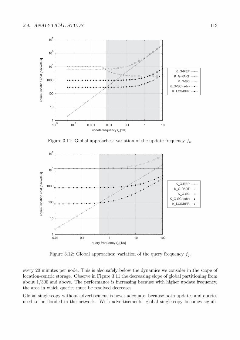
3.4. ANALYTICAL STUDY 113
1
10
100
1000
104
105
106
10-5
10-4
0.001 0.01 0.1 1 10
update frequency [1/s]fu
K_G-REP
K_G-PART
K_G-SC
K_G-SC (adv)
K_LCS/BPR
co
mm
un
ica
tio
nco
st
[pa
cke
ts/s
]
Figure 3.11: Global approaches: variation of the update frequency fu.
1
10
100
1000
104
105
0.01 0.1 1 10 100
query frequency [1/s]fq
K_G-REP
K_G-PART
K_G-SC
K_G-SC (adv)
K_LCS/BPR
co
mm
un
ica
tio
nco
st
[pa
cke
ts/s
]
Figure 3.12: Global approaches: variation of the query frequency fq.
every 20 minutes per node. This is also safely below the dynamics we consider in the scope oflocation-centric storage. Observe in Figure 3.11 the decreasing slope of global partitioning fromabout 1/300 and above. The performance is increasing because with higher update frequency,the area in which queries must be resolved decreases.
Global single-copy without advertisement is never adequate, because both updates and queriesneed to be flooded in the network. With advertisements, global single-copy becomes signifi-
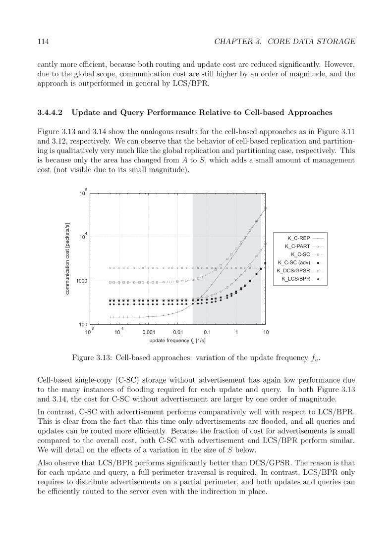
114 CHAPTER 3. CORE DATA STORAGE
cantly more efficient, because both routing and update cost are reduced significantly. However,due to the global scope, communication cost are still higher by an order of magnitude, and theapproach is outperformed in general by LCS/BPR.
3.4.4.2 Update and Query Performance Relative to Cell-based Approaches
Figure 3.13 and 3.14 show the analogous results for the cell-based approaches as in Figure 3.11and 3.12, respectively. We can observe that the behavior of cell-based replication and partition-ing is qualitatively very much like the global replication and partitioning case, respectively. Thisis because only the area has changed from A to S, which adds a small amount of managementcost (not visible due to its small magnitude).
100
1000
104
105
10-5
10-4
0.001 0.01 0.1 1 10
update frequency [1/s]fu
K_C-REP
K_C-PART
K_C-SC
K_C-SC (adv)
K_DCS/GPSR
K_LCS/BPR
co
mm
un
ica
tio
nco
st
[pa
cke
ts/s
]
Figure 3.13: Cell-based approaches: variation of the update frequency fu.
Cell-based single-copy (C-SC) storage without advertisement has again low performance dueto the many instances of flooding required for each update and query. In both Figure 3.13and 3.14, the cost for C-SC without advertisement are larger by one order of magnitude.
In contrast, C-SC with advertisement performs comparatively well with respect to LCS/BPR.This is clear from the fact that this time only advertisements are flooded, and all queries andupdates can be routed more efficiently. Because the fraction of cost for advertisements is smallcompared to the overall cost, both C-SC with advertisement and LCS/BPR perform similar.We will detail on the effects of a variation in the size of S below.
Also observe that LCS/BPR performs significantly better than DCS/GPSR. The reason is thatfor each update and query, a full perimeter traversal is required. In contrast, LCS/BPR onlyrequires to distribute advertisements on a partial perimeter, and both updates and queries canbe efficiently routed to the server even with the indirection in place.
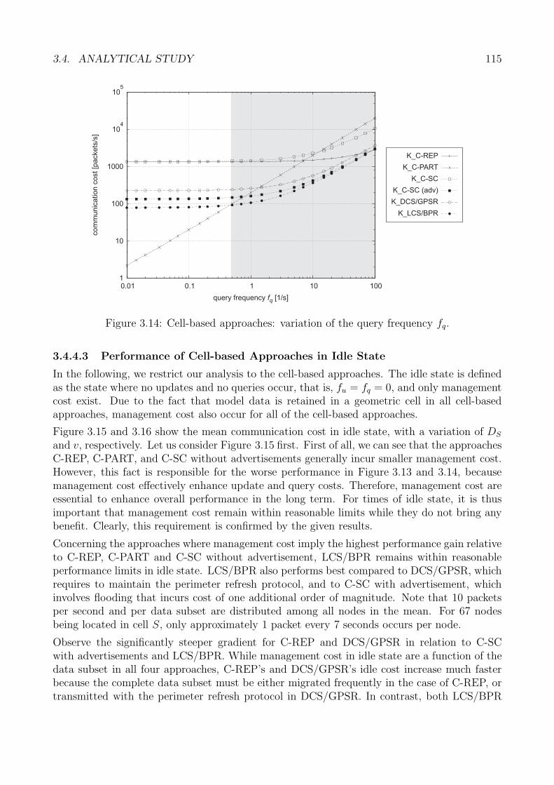
3.4. ANALYTICAL STUDY 115
1
10
100
1000
104
105
0.01 0.1 1 10 100
query frequency [1/s]fq
K_C-REP
K_C-PART
K_C-SC
K_C-SC (adv)
K_DCS/GPSR
K_LCS/BPR
co
mm
un
ica
tio
nco
st
[pa
cke
ts/s
]
Figure 3.14: Cell-based approaches: variation of the query frequency fq.
3.4.4.3 Performance of Cell-based Approaches in Idle State
In the following, we restrict our analysis to the cell-based approaches. The idle state is definedas the state where no updates and no queries occur, that is, fu = fq = 0, and only managementcost exist. Due to the fact that model data is retained in a geometric cell in all cell-basedapproaches, management cost also occur for all of the cell-based approaches.
Figure 3.15 and 3.16 show the mean communication cost in idle state, with a variation of DS
and v, respectively. Let us consider Figure 3.15 first. First of all, we can see that the approachesC-REP, C-PART, and C-SC without advertisements generally incur smaller management cost.However, this fact is responsible for the worse performance in Figure 3.13 and 3.14, becausemanagement cost effectively enhance update and query costs. Therefore, management cost areessential to enhance overall performance in the long term. For times of idle state, it is thusimportant that management cost remain within reasonable limits while they do not bring anybenefit. Clearly, this requirement is confirmed by the given results.
Concerning the approaches where management cost imply the highest performance gain relativeto C-REP, C-PART and C-SC without advertisement, LCS/BPR remains within reasonableperformance limits in idle state. LCS/BPR also performs best compared to DCS/GPSR, whichrequires to maintain the perimeter refresh protocol, and to C-SC with advertisement, whichinvolves flooding that incurs cost of one additional order of magnitude. Note that 10 packetsper second and per data subset are distributed among all nodes in the mean. For 67 nodesbeing located in cell S, only approximately 1 packet every 7 seconds occurs per node.
Observe the significantly steeper gradient for C-REP and DCS/GPSR in relation to C-SCwith advertisements and LCS/BPR. While management cost in idle state are a function of thedata subset in all four approaches, C-REP’s and DCS/GPSR’s idle cost increase much fasterbecause the complete data subset must be either migrated frequently in the case of C-REP, ortransmitted with the perimeter refresh protocol in DCS/GPSR. In contrast, both LCS/BPR
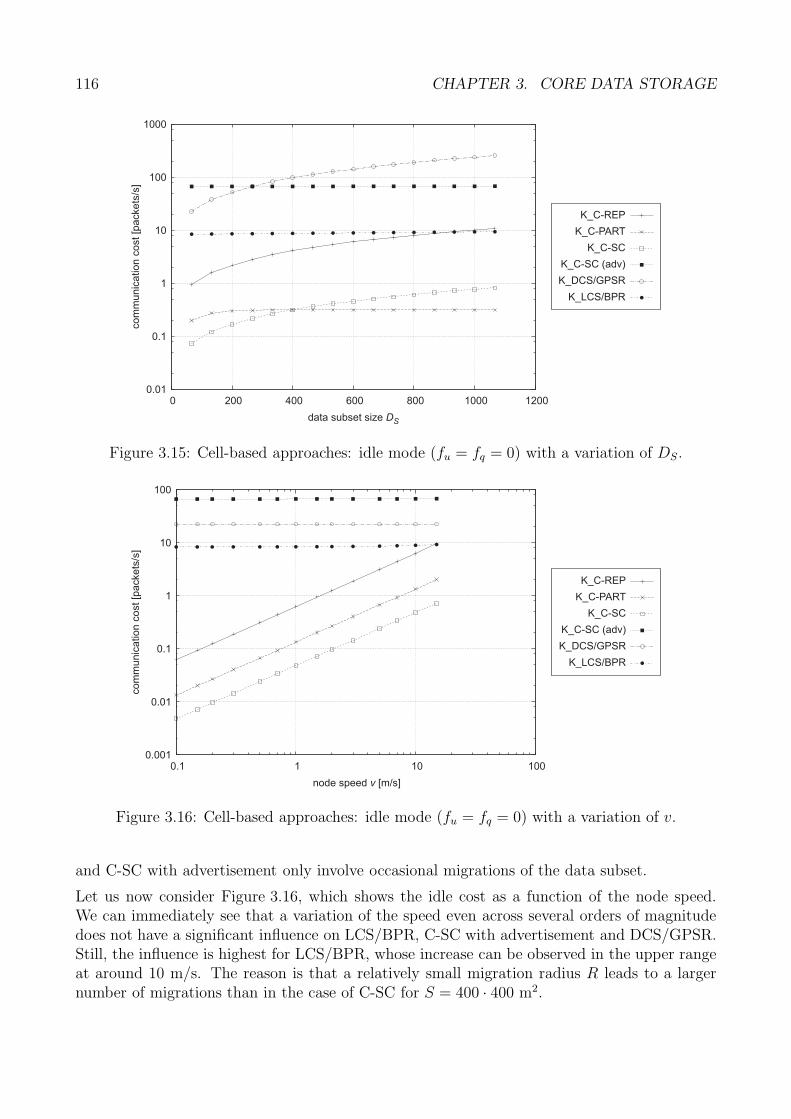
116 CHAPTER 3. CORE DATA STORAGE
0.01
0.1
1
10
100
1000
0 200 400 600 800 1000 1200
data subset size DS
K_C-REP
K_C-PART
K_C-SC
K_C-SC (adv)
K_DCS/GPSR
K_LCS/BPR
co
mm
un
ica
tio
nco
st
[pa
cke
ts/s
]
Figure 3.15: Cell-based approaches: idle mode (fu = fq = 0) with a variation of DS.
0.001
0.01
0.1
1
10
100
0.1 1 10 100
node speed [m/s]v
K_C-REP
K_C-PART
K_C-SC
K_C-SC (adv)
K_DCS/GPSR
K_LCS/BPR
co
mm
un
ica
tio
nco
st
[pa
cke
ts/s
]
Figure 3.16: Cell-based approaches: idle mode (fu = fq = 0) with a variation of v.
and C-SC with advertisement only involve occasional migrations of the data subset.
Let us now consider Figure 3.16, which shows the idle cost as a function of the node speed.We can immediately see that a variation of the speed even across several orders of magnitudedoes not have a significant influence on LCS/BPR, C-SC with advertisement and DCS/GPSR.Still, the influence is highest for LCS/BPR, whose increase can be observed in the upper rangeat around 10 m/s. The reason is that a relatively small migration radius R leads to a largernumber of migrations than in the case of C-SC for S = 400 · 400 m2.
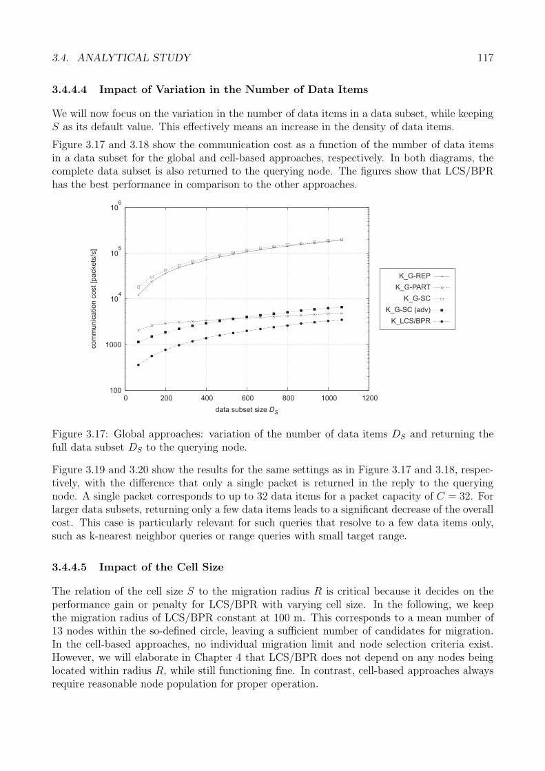
3.4. ANALYTICAL STUDY 117
3.4.4.4 Impact of Variation in the Number of Data Items
We will now focus on the variation in the number of data items in a data subset, while keepingS as its default value. This effectively means an increase in the density of data items.
Figure 3.17 and 3.18 show the communication cost as a function of the number of data itemsin a data subset for the global and cell-based approaches, respectively. In both diagrams, thecomplete data subset is also returned to the querying node. The figures show that LCS/BPRhas the best performance in comparison to the other approaches.
100
1000
104
105
106
0 200 400 600 800 1000 1200
data subset size DS
K_G-REP
K_G-PART
K_G-SC
K_G-SC (adv)
K_LCS/BPR
co
mm
un
ica
tio
nco
st
[pa
cke
ts/s
]
Figure 3.17: Global approaches: variation of the number of data items DS and returning thefull data subset DS to the querying node.
Figure 3.19 and 3.20 show the results for the same settings as in Figure 3.17 and 3.18, respec-tively, with the difference that only a single packet is returned in the reply to the queryingnode. A single packet corresponds to up to 32 data items for a packet capacity of C = 32. Forlarger data subsets, returning only a few data items leads to a significant decrease of the overallcost. This case is particularly relevant for such queries that resolve to a few data items only,such as k-nearest neighbor queries or range queries with small target range.
3.4.4.5 Impact of the Cell Size
The relation of the cell size S to the migration radius R is critical because it decides on theperformance gain or penalty for LCS/BPR with varying cell size. In the following, we keepthe migration radius of LCS/BPR constant at 100 m. This corresponds to a mean number of13 nodes within the so-defined circle, leaving a sufficient number of candidates for migration.In the cell-based approaches, no individual migration limit and node selection criteria exist.However, we will elaborate in Chapter 4 that LCS/BPR does not depend on any nodes beinglocated within radius R, while still functioning fine. In contrast, cell-based approaches alwaysrequire reasonable node population for proper operation.
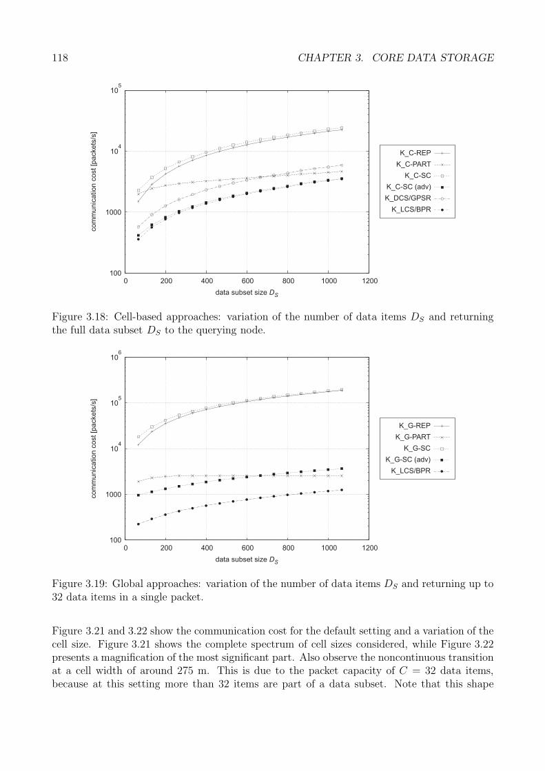
118 CHAPTER 3. CORE DATA STORAGE
100
1000
104
105
0 200 400 600 800 1000 1200
data subset size DS
K_C-REP
K_C-PART
K_C-SC
K_C-SC (adv)
K_DCS/GPSR
K_LCS/BPR
co
mm
un
ica
tio
nco
st
[pa
cke
ts/s
]
Figure 3.18: Cell-based approaches: variation of the number of data items DS and returningthe full data subset DS to the querying node.
100
1000
104
105
106
0 200 400 600 800 1000 1200
K_G-REP
K_G-PART
K_G-SC
K_G-SC (adv)
K_LCS/BPR
data subset size DS
co
mm
un
ica
tio
nco
st
[pa
cke
ts/s
]
Figure 3.19: Global approaches: variation of the number of data items DS and returning up to32 data items in a single packet.
Figure 3.21 and 3.22 show the communication cost for the default setting and a variation of thecell size. Figure 3.21 shows the complete spectrum of cell sizes considered, while Figure 3.22presents a magnification of the most significant part. Also observe the noncontinuous transitionat a cell width of around 275 m. This is due to the packet capacity of C = 32 data items,because at this setting more than 32 items are part of a data subset. Note that this shape
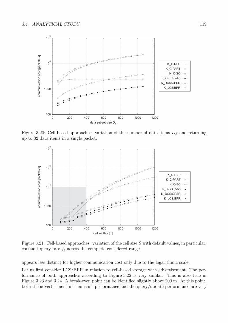
3.4. ANALYTICAL STUDY 119
100
1000
104
105
0 200 400 600 800 1000 1200
K_C-REP
K_C-PART
K_C-SC
K_C-SC (adv)
K_DCS/GPSR
K_LCS/BPR
data subset size DS
co
mm
un
ica
tio
nco
st
[pa
cke
ts/s
]
Figure 3.20: Cell-based approaches: variation of the number of data items DS and returningup to 32 data items in a single packet.
100
1000
104
105
106
0 200 400 600 800 1000 1200
cell width [m]s
K_C-REP
K_C-PART
K_C-SC
K_C-SC (adv)
K_DCS/GPSR
K_LCS/BPR
co
mm
un
ica
tio
nco
st
[pa
cke
ts/s
]
Figure 3.21: Cell-based approaches: variation of the cell size S with default values, in particular,constant query rate fq across the complete considered range.
appears less distinct for higher communication cost only due to the logarithmic scale.
Let us first consider LCS/BPR in relation to cell-based storage with advertisement. The per-formance of both approaches according to Figure 3.22 is very similar. This is also true inFigure 3.23 and 3.24. A break-even point can be identified slightly above 200 m. At this point,both the advertisement mechanism’s performance and the query/update performance are very
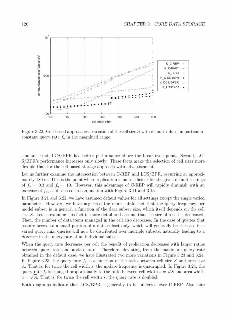
120 CHAPTER 3. CORE DATA STORAGE
100
1000
104
100 150 200 250 300 350 400
cell width [m]s
K_C-REP
K_C-PART
K_C-SC
K_C-SC (adv)
K_DCS/GPSR
K_LCS/BPR
co
mm
un
ica
tio
nco
st
[pa
cke
ts/s
]
Figure 3.22: Cell-based approaches: variation of the cell size S with default values, in particular,constant query rate fq in the magnified range.
similar. First, LCS/BPR has better performance above the break-even point. Second, LC-S/BPR’s performance increases only slowly. These facts make the selection of cell sizes moreflexible than for the cell-based storage approach with advertisement.
Let us further examine the intersection between C-REP and LCS/BPR, occurring at approxi-mately 180 m. This is the point where replication is more efficient for the given default settingsof fu = 0.3 and fq = 10. However, this advantage of C-REP will rapidly diminish with anincrease of fu, as discussed in conjunction with Figure 3.11 and 3.13.
In Figure 3.21 and 3.22, we have assumed default values for all settings except the single variedparameter. However, we have neglected the more subtle fact that the query frequency permodel subset is in general a function of the data subset size, which itself depends on the cellsize S. Let us examine this fact in more detail and assume that the size of a cell is decreased.Then, the number of data items managed in the cell also decreases. In the case of queries thatrequire access to a small portion of a data subset only, which will generally be the case in avaried query mix, queries will now be distributed over multiple subsets, naturally leading to adecrease in the query rate at an individual subset.
When the query rate decreases per cell the benefit of replication decreases with larger ratiosbetween query rate and update rate. Therefore, deviating from the maximum query rateobtained in the default case, we have illustrated two more variations in Figure 3.23 and 3.24.In Figure 3.23, the query rate fq is a function of the ratio between cell size S and area sizeA. That is, for twice the cell width s, the update frequency is quadrupled. In Figure 3.24, thequery rate fq is changed proportionally to the ratio between cell width s =
√S and area width
a =√
A. That is, for twice the cell width s, the query rate is doubled.
Both diagrams indicate that LCS/BPR is generally to be preferred over C-REP. Also note
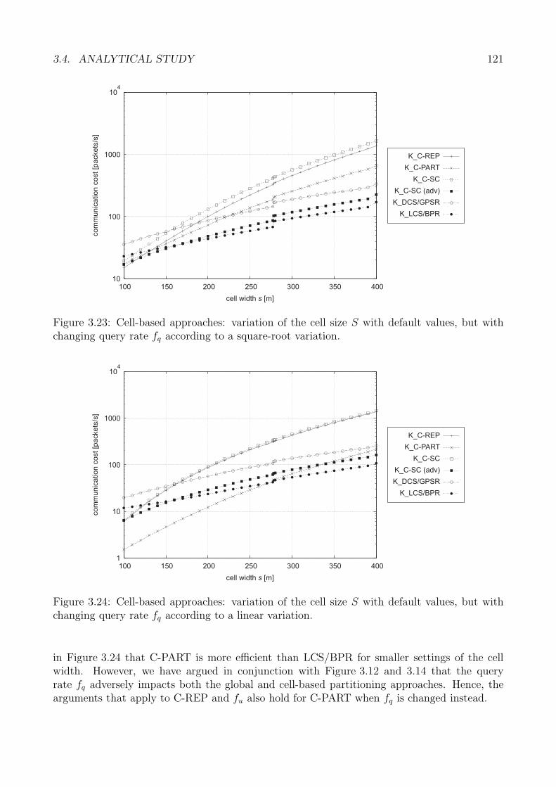
3.4. ANALYTICAL STUDY 121
10
100
1000
104
100 150 200 250 300 350 400
cell width [m]s
K_C-REP
K_C-PART
K_C-SC
K_C-SC (adv)
K_DCS/GPSR
K_LCS/BPR
co
mm
un
ica
tio
nco
st
[pa
cke
ts/s
]
Figure 3.23: Cell-based approaches: variation of the cell size S with default values, but withchanging query rate fq according to a square-root variation.
1
10
100
1000
104
100 150 200 250 300 350 400
cell width [m]s
K_C-REP
K_C-PART
K_C-SC
K_C-SC (adv)
K_DCS/GPSR
K_LCS/BPR
co
mm
un
ica
tio
nco
st
[pa
cke
ts/s
]
Figure 3.24: Cell-based approaches: variation of the cell size S with default values, but withchanging query rate fq according to a linear variation.
in Figure 3.24 that C-PART is more efficient than LCS/BPR for smaller settings of the cellwidth. However, we have argued in conjunction with Figure 3.12 and 3.14 that the queryrate fq adversely impacts both the global and cell-based partitioning approaches. Hence, thearguments that apply to C-REP and fu also hold for C-PART when fq is changed instead.
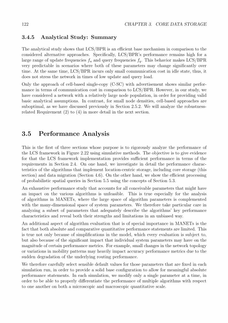
122 CHAPTER 3. CORE DATA STORAGE
3.4.5 Analytical Study: Summary
The analytical study shows that LCS/BPR is an efficient base mechanism in comparison to theconsidered alternative approaches. Specifically, LCS/BPR’s performance remains high for alarge range of update frequencies fu and query frequencies fq. This behavior makes LCS/BPRvery predictable in scenarios where both of these parameters may change significantly overtime. At the same time, LCS/BPR incurs only small communication cost in idle state, thus, itdoes not stress the network in times of low update and query load.
Only the approach of cell-based single-copy (C-SC) with advertisement shows similar perfor-mance in terms of communication cost in comparison to LCS/BPR. However, in our study, wehave considered a network with a relatively large node population, in order for providing validbasic analytical assumptions. In contrast, for small node densities, cell-based approaches aresuboptimal, as we have discussed previously in Section 2.5.2. We will analyze the robustness-related Requirement (2) to (4) in more detail in the next section.
3.5 Performance Analysis
This is the first of three sections whose purpose is to rigorously analyze the performance ofthe LCS framework in Figure 2.22 using simulative methods. The objective is to give evidencefor that the LCS framework implementation provides sufficient performance in terms of therequirements in Section 2.4. On one hand, we investigate in detail the performance charac-teristics of the algorithms that implement location-centric storage, including core storage (thissection) and data migration (Section 4.6). On the other hand, we show the efficient processingof probabilistic spatial queries in Section 5.5 using the concepts of Section 5.3.
An exhaustive performance study that accounts for all conceivable parameters that might havean impact on the various algorithms is unfeasible. This is true especially for the analysisof algorithms in MANETs, where the large space of algorithm parameters is complementedwith the many-dimensional space of system parameters. We therefore take particular care inanalyzing a subset of parameters that adequately describe the algorithms’ key performancecharacteristics and reveal both their strengths and limitations in an unbiased way.
An additional aspect of algorithm evaluation that is of special importance in MANETs is thefact that both absolute and comparative quantitative performance statements are limited. Thisis true not only because of simplifications in the model, which every evaluation is subject to,but also because of the significant impact that individual system parameters may have on themagnitude of certain performance metrics. For example, small changes in the network topologyor variations in mobility patterns may heavily impact accuracy performance metrics due to thesudden degradation of the underlying routing performance.
We therefore carefully select sensible default values for those parameters that are fixed in eachsimulation run, in order to provide a solid base configuration to allow for meaningful absoluteperformance statements. In each simulation, we modify only a single parameter at a time, inorder to be able to properly differentiate the performance of multiple algorithms with respectto one another on both a microscopic and macroscopic quantitative scale.
3.5. PERFORMANCE ANALYSIS 123
The overall performance analysis is preluded with an overview and justification of the genericevaluation methodology in Section 3.5.1. This generic part of the evaluation will be assumedin the remainder of this section and also in Section 4.6 and 5.5. In Section 3.5.2 and 3.5.3,we discuss the core data storage-specific evaluation methodology and performance metrics,respectively. Section 3.5.4 through 3.5.6 discuss the detailed evaluation results for core datastorage. We conclude the evaluation with a brief summary in Section 3.5.7.
3.5.1 Generic Methodology
The analysis of algorithms can be principally accomplished by any of the four methods of realsystem-based evaluation, emulation, simulation, and mathematical analysis. While we haveapplied the latter in Section 3.4 to the detailed analysis of communication cost, we have chosena simulation-based methodology in this section due to the following desired properties.
In order to obtain statistically useful and deterministic evaluation results, a sufficiently largegeographic area and number of nodes need to be considered, while at the same time a largenumber of evaluation runs need to be performed. With respect to these facts real systems areimpractical, since they require large setup efforts and runtime overhead, sequential executionof individual evaluation trials, and thus lead to a significant expenditure of time. Real sys-tems furthermore make it virtually impossible to repeat the same experiment under similarconditions, which naturally may lead to inconclusive results.
In order to be able to approximate the performance behavior that algorithms would exhibitin a real system, a comprehensive protocol stack implementation that mimics its real systemcounterpart is indispensable. Due to the shared nature of wireless media and the extremelyhigh timing requirements in the emulation of shared medium access protocols, emulation en-vironments provide only simplified versions of the MAC sublayer. This fact makes currentemulation systems unsuitable for our purposes.
Network topology and node mobility are two of the fundamental system parameters that willsignificantly impact algorithm performance and therefore must be considered in any mobilead-hoc network-based evaluation. While real systems and emulation are able to support theseparameters, analytical approaches become overwhelmingly complex when attempting to capturethese parameters by the analytical model. They may, therefore, only be used to provide apicture under specific constraints and individual performance metrics, which was our goal inthe analytical study of the storage tier in Section 3.4.
For these reasons, we have chosen a simulation-based methodology. All evaluations were basedon version 2.29 of the ns-2 simulator, using the wireless extensions introduced by Broch etal. in [BMJ+98]. These extensions provide an adequate implementation of the CSMA/CA2
protocol with the RTS/CTS3 mechanism according to the IEEE 802.11 standard.
A total of three experiments, corresponding to core data storage, data migration (Section 4.6)and query processing (Section 5.5) were conducted. Each experiment comprises a number ofsimulations, which depends on the number of system parameters (e.g. node speed, number ofnodes) that were modified. All simulations were set up with the following general parametersand their default values, also listed in Table 3.3.
2Carrier Sense Multiple Access / Collision Avoidance3Request to Send / Clear to Send
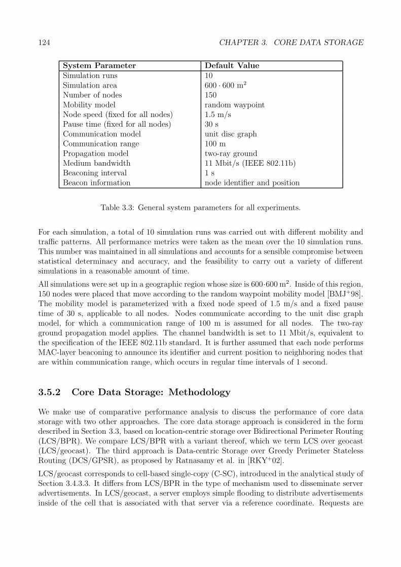
124 CHAPTER 3. CORE DATA STORAGE
System Parameter Default ValueSimulation runs 10Simulation area 600 · 600 m2
Number of nodes 150Mobility model random waypointNode speed (fixed for all nodes) 1.5 m/sPause time (fixed for all nodes) 30 sCommunication model unit disc graphCommunication range 100 mPropagation model two-ray groundMedium bandwidth 11 Mbit/s (IEEE 802.11b)Beaconing interval 1 sBeacon information node identifier and position
Table 3.3: General system parameters for all experiments.
For each simulation, a total of 10 simulation runs was carried out with different mobility andtraffic patterns. All performance metrics were taken as the mean over the 10 simulation runs.This number was maintained in all simulations and accounts for a sensible compromise betweenstatistical determinacy and accuracy, and the feasibility to carry out a variety of differentsimulations in a reasonable amount of time.
All simulations were set up in a geographic region whose size is 600·600 m2. Inside of this region,150 nodes were placed that move according to the random waypoint mobility model [BMJ+98].The mobility model is parameterized with a fixed node speed of 1.5 m/s and a fixed pausetime of 30 s, applicable to all nodes. Nodes communicate according to the unit disc graphmodel, for which a communication range of 100 m is assumed for all nodes. The two-rayground propagation model applies. The channel bandwidth is set to 11 Mbit/s, equivalent tothe specification of the IEEE 802.11b standard. It is further assumed that each node performsMAC-layer beaconing to announce its identifier and current position to neighboring nodes thatare within communication range, which occurs in regular time intervals of 1 second.
3.5.2 Core Data Storage: Methodology
We make use of comparative performance analysis to discuss the performance of core datastorage with two other approaches. The core data storage approach is considered in the formdescribed in Section 3.3, based on location-centric storage over Bidirectional Perimeter Routing(LCS/BPR). We compare LCS/BPR with a variant thereof, which we term LCS over geocast(LCS/geocast). The third approach is Data-centric Storage over Greedy Perimeter StatelessRouting (DCS/GPSR), as proposed by Ratnasamy et al. in [RKY+02].
LCS/geocast corresponds to cell-based single-copy (C-SC), introduced in the analytical study ofSection 3.4.3.3. It differs from LCS/BPR in the type of mechanism used to disseminate serveradvertisements. In LCS/geocast, a server employs simple flooding to distribute advertisementsinside of the cell that is associated with that server via a reference coordinate. Requests are
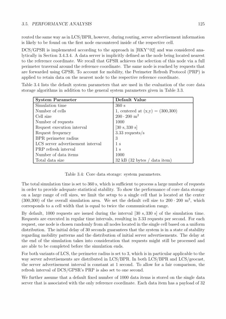
3.5. PERFORMANCE ANALYSIS 125
routed the same way as in LCS/BPR, however, during routing, server advertisement informationis likely to be found on the first node encountered inside of the respective cell.
DCS/GPSR is implemented according to the approach in [RKY+02] and was considered ana-lytically in Section 3.4.3.4. A data server is implicitly defined as the node being located nearestto the reference coordinate. We recall that GPSR achieves the selection of this node via a fullperimeter traversal around the reference coordinate. The same node is reached by requests thatare forwarded using GPSR. To account for mobility, the Perimeter Refresh Protocol (PRP) isapplied to retain data on the nearest node to the respective reference coordinate.
Table 3.4 lists the default system parameters that are used in the evaluation of the core datastorage algorithms in addition to the general system parameters given in Table 3.3.
System Parameter Default ValueSimulation time 360 sNumber of cells 1, centered at (x,y) = (300,300)Cell size 200 · 200 m2
Number of requests 1000Request execution interval [30 s, 330 s]Request frequency 3.33 requests/sBPR perimeter radius 3LCS server advertisement interval 1 sPRP refresh interval 1 sNumber of data items 1000Total data size 32 kB (32 bytes / data item)
Table 3.4: Core data storage: system parameters.
The total simulation time is set to 360 s, which is sufficient to process a large number of requestsin order to provide adequate statistical stability. To show the performance of core data storageon a large range of cell sizes, we limit the setup to a single cell that is located at the center(300,300) of the overall simulation area. We set the default cell size to 200 · 200 m2, whichcorresponds to a cell width that is equal to twice the communication range.
By default, 1000 requests are issued during the interval [30 s, 330 s] of the simulation time.Requests are executed in regular time intervals, resulting in 3.33 requests per second. For eachrequest, one node is chosen randomly from all nodes located in the single cell based on a uniformdistribution. The initial delay of 30 seconds guarantees that the system is in a state of stabilityregarding mobility patterns and the distribution of initial server advertisements. The delay atthe end of the simulation takes into consideration that requests might still be processed andare able to be completed before the simulation ends.
For both variants of LCS, the perimeter radius is set to 3, which is in particular applicable to theway server advertisements are distributed in LCS/BPR. In both LCS/BPR and LCS/geocast,the server advertisement interval is constant at 1 second. To allow for a fair comparison, therefresh interval of DCS/GPSR’s PRP is also set to one second.
We further assume that a default fixed number of 1000 data items is stored on the single dataserver that is associated with the only reference coordinate. Each data item has a payload of 32
126 CHAPTER 3. CORE DATA STORAGE
bytes, resulting in a total of 32 kB of data. This parameter is relevant due to the fact that coredata storage must run with data migration in place. Thus, this amount of data correspondsto the data that is transferred during a migration process. A precise analysis of the impact ofdata size on migration performance follows in Section 4.6.
3.5.3 Performance Metrics
The performance metrics considered in the evaluation of the core data storage approach arerequest accuracy, request latency, and request cost.
Request Accuracy
For LCS/BPR and LCS/geocast, request accuracy is defined as the fraction of requests suc-cessfully delivered from the node that issued the request to the current data server. In the caseof a migration in progress, it is not essential whether the migrating node or the target node isreached by the requests, since this situation is handled by the migration process.
For DCS/GPSR, request accuracy is defined as the fraction of requests successfully delivered tothe perimeter entry node of the perimeter that encloses the reference coordinate. We assume itis sufficient that a closed perimeter around the reference coordinate can be traced, independentof whether the respective perimeter entry node is up to date according to the PRP. Thissimplification is in favor of DCS/GPSR and provides an upper bound for its performance, thus,it can validly be assumed in the comparative performance analysis.
Request Latency
Request latency is defined as the mean time between the sending of a request at the requestingnode and the reception of that request at the target node, taken over all successful requests.More specifically, for both LCS variants, only requests that are delivered to the current dataserver are considered. For DCS/GPSR, only those requests that are delivered to the perimeterentry node after the successful traversal of a closed perimeter are considered.
Request Cost
Request cost are defined as the mean number of packets sent per second over all requests of thesimulation, including both successful and unsuccessful requests.
In addition to the request cost, we also state the cost incurred by server management (datamigration, perimeter refresh protocol, topology exploration) and server advertisement. Thesecost will be further elaborated in the evaluation of data migration in Section 4.6.
3.5.4 Request Accuracy
Figure 3.25 through 3.30 show the simulation results for the request accuracy as a function ofdifferent system parameters. Let us start by considering Figure 3.25, which shows the requestaccuracy as a function of the cell width. The default cell width is 200 m. Depicted are two barsfor LCS/BPR (left bar) and LCS/geocast (right bar), overlayed with a graph for DCS/GPSR.For the LCS variants, two colors indicate whether a request is received while a data server isin active or receiving state (cf. Section 4.5 for a discussion of these states).
We firstly observe that the request accuracy of all approaches drops gently and with a similarslope with increasing cell size. The cause for this behavior is that requests are only performed
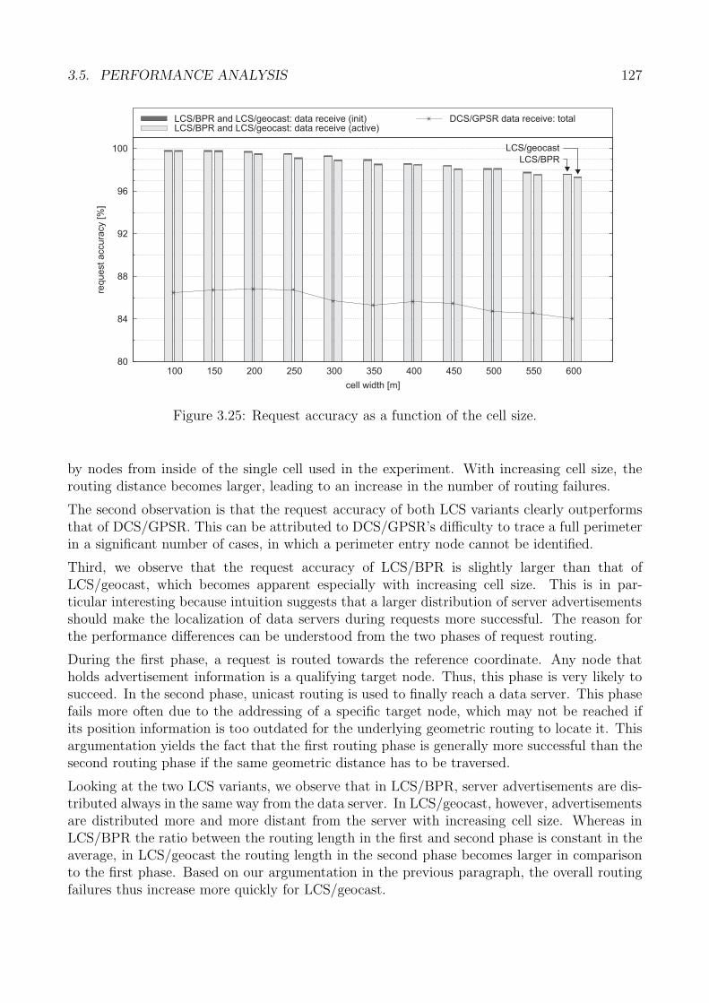
3.5. PERFORMANCE ANALYSIS 127
80
84
88
92
96
100
100 150 200 250 300 350 400 450 500 550 600
requestaccura
cy
[%]
cell width [m]
LCS/BPR and LCS/geocast: data receive (init)LCS/BPR and LCS/geocast: data receive (active)
DCS/GPSR data receive: total
LCS/BPR
LCS/geocast
Figure 3.25: Request accuracy as a function of the cell size.
by nodes from inside of the single cell used in the experiment. With increasing cell size, therouting distance becomes larger, leading to an increase in the number of routing failures.
The second observation is that the request accuracy of both LCS variants clearly outperformsthat of DCS/GPSR. This can be attributed to DCS/GPSR’s difficulty to trace a full perimeterin a significant number of cases, in which a perimeter entry node cannot be identified.
Third, we observe that the request accuracy of LCS/BPR is slightly larger than that ofLCS/geocast, which becomes apparent especially with increasing cell size. This is in par-ticular interesting because intuition suggests that a larger distribution of server advertisementsshould make the localization of data servers during requests more successful. The reason forthe performance differences can be understood from the two phases of request routing.
During the first phase, a request is routed towards the reference coordinate. Any node thatholds advertisement information is a qualifying target node. Thus, this phase is very likely tosucceed. In the second phase, unicast routing is used to finally reach a data server. This phasefails more often due to the addressing of a specific target node, which may not be reached ifits position information is too outdated for the underlying geometric routing to locate it. Thisargumentation yields the fact that the first routing phase is generally more successful than thesecond routing phase if the same geometric distance has to be traversed.
Looking at the two LCS variants, we observe that in LCS/BPR, server advertisements are dis-tributed always in the same way from the data server. In LCS/geocast, however, advertisementsare distributed more and more distant from the server with increasing cell size. Whereas inLCS/BPR the ratio between the routing length in the first and second phase is constant in theaverage, in LCS/geocast the routing length in the second phase becomes larger in comparisonto the first phase. Based on our argumentation in the previous paragraph, the overall routingfailures thus increase more quickly for LCS/geocast.
128 CHAPTER 3. CORE DATA STORAGE
Figure 3.26 shows request accuracy as a function of the number of nodes. Note that 150 nodesis the default value. In this figure, we have decreased the number of nodes down to 50. Thisis very low concerning the transmission range of only 100 m, where partitions begin to form(Section 2.2). We observe that even in the lowest density range, both LCS variants achievea greater than 94% request accuracy. We also observe a small advantage of LCS/BPR overLCS/geocast which is due to the same reasons discussed in the previous figure.
50
60
70
80
90
100
50 60 70 80 90 100 110 120 130 140 150 160 170 180 190 200
requestaccura
cy
[%]
number of nodes
LCS/BPR and LCS/geocast: data receive (init)LCS/BPR and LCS/geocast: data receive (active)
DCS/GPSR data receive: totalLC
S/B
PR
LC
S/g
eocast
Figure 3.26: Request accuracy as a function of the number of nodes.
In contrast, DCS/GPSR’s performance drops sharply starting at around 70 nodes and below.This is because the length of perimeters increases significantly with lower node density, and itbecomes more difficult for DCS/GPSR to trace a closed perimeter. Mobility complicates thissituation, where a small change of a node’s position will lead to many inconsistencies betweenthe planarized graph used for perimeter routing and the actual physical network topology.
With increasing node density, once the request accuracy of the LCS variants has reached itsmaximum at around 80 nodes already, it remains virtually constant. An additional observationis that starting at around 120 nodes, the performance of DCS/GPSR begins to drop again. Thisbehavior is due to the graph planarization required by GPSR that is the basis for perimeterrouting ([KK00]). With increasing node density, the number of nodes eliminated from a node’sneighbor list to build its view of a planarized graph also increases. At the same time, mobilityleads to the situation where each node’s neighbor set fluctuates more strongly. Thus, withincreasing node density, the inconsistencies increase between a node’s planarized view on thegraph and the physical graph, as well as between the planarized views on the graph of differentnodes. In turn, perimeter routing is operating on a more inconsistent overall planarized graphwith increasing node density, making it more difficult to terminate on a closed perimeter.
Figure 3.27 depicts request accuracy as a function of node speed. The first observation is thestrong performance of both LCS variants up to the maximum tested speed of 15 m/s. Atthis speed, LCS/BPR is roughly 1% better than LCS/geocast due to the reasons discussed
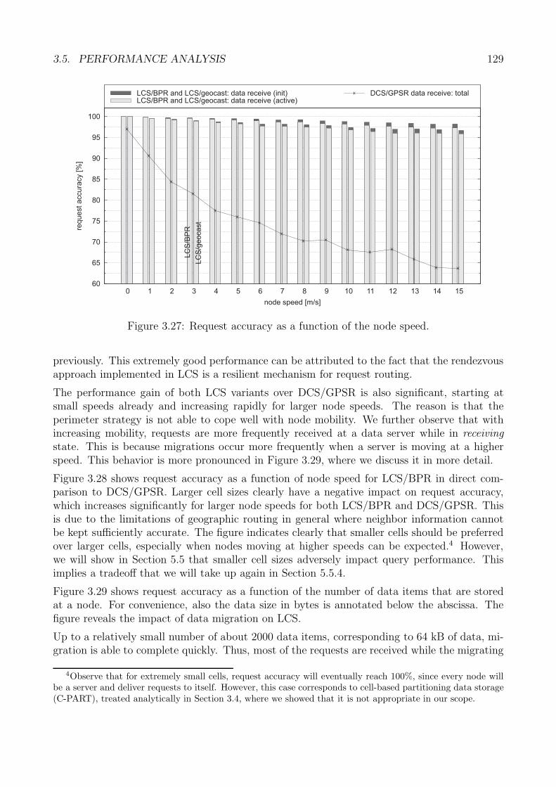
3.5. PERFORMANCE ANALYSIS 129
60
65
70
75
80
85
90
95
100
0 1 2 3 4 5 6 7 8 9 10 11 12 13 14 15
requestaccura
cy
[%]
node speed [m/s]
LCS/BPR and LCS/geocast: data receive (init)LCS/BPR and LCS/geocast: data receive (active)
DCS/GPSR data receive: total
LC
S/B
PR
LC
S/g
eocast
Figure 3.27: Request accuracy as a function of the node speed.
previously. This extremely good performance can be attributed to the fact that the rendezvousapproach implemented in LCS is a resilient mechanism for request routing.
The performance gain of both LCS variants over DCS/GPSR is also significant, starting atsmall speeds already and increasing rapidly for larger node speeds. The reason is that theperimeter strategy is not able to cope well with node mobility. We further observe that withincreasing mobility, requests are more frequently received at a data server while in receivingstate. This is because migrations occur more frequently when a server is moving at a higherspeed. This behavior is more pronounced in Figure 3.29, where we discuss it in more detail.
Figure 3.28 shows request accuracy as a function of node speed for LCS/BPR in direct com-parison to DCS/GPSR. Larger cell sizes clearly have a negative impact on request accuracy,which increases significantly for larger node speeds for both LCS/BPR and DCS/GPSR. Thisis due to the limitations of geographic routing in general where neighbor information cannotbe kept sufficiently accurate. The figure indicates clearly that smaller cells should be preferredover larger cells, especially when nodes moving at higher speeds can be expected.4 However,we will show in Section 5.5 that smaller cell sizes adversely impact query performance. Thisimplies a tradeoff that we will take up again in Section 5.5.4.
Figure 3.29 shows request accuracy as a function of the number of data items that are storedat a node. For convenience, also the data size in bytes is annotated below the abscissa. Thefigure reveals the impact of data migration on LCS.
Up to a relatively small number of about 2000 data items, corresponding to 64 kB of data, mi-gration is able to complete quickly. Thus, most of the requests are received while the migrating
4Observe that for extremely small cells, request accuracy will eventually reach 100%, since every node willbe a server and deliver requests to itself. However, this case corresponds to cell-based partitioning data storage(C-PART), treated analytically in Section 3.4, where we showed that it is not appropriate in our scope.
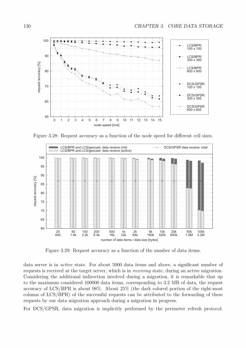
130 CHAPTER 3. CORE DATA STORAGE
50
60
70
80
90
100
0 1 2 3 4 5 6 7 8 9 10 11 12 13 14 15
req
ue
sta
ccu
racy
[%]
node speed [m/s]
LCS/BPR:100 x 100
LCS/BPR:300 x 300
LCS/BPR:600 x 600
DCS/GPSR:100 x 100
DCS/GPSR:300 x 300
DCS/GPSR:600 x 600
Figure 3.28: Request accuracy as a function of the node speed for different cell sizes.
60
65
70
75
80
85
90
95
100
20640
501.6k
1003.2k
2006.4k
50016k
1k32k
2k64k
5k160k
10k320k
20k640k
50k1.6M
100k3.2M
requestaccura
cy
[%]
number of data items / data size [bytes]
LCS/BPR and LCS/geocast: data receive (init)LCS/BPR and LCS/geocast: data receive (active)
DCS/GPSR data receive: total
Figure 3.29: Request accuracy as a function of the number of data items.
data server is in active state. For about 5000 data items and above, a significant number ofrequests is received at the target server, which is in receiving state, during an active migration.Considering the additional indirection involved during a migration, it is remarkable that upto the maximum considered 100000 data items, corresponding to 3.2 MB of data, the requestaccuracy of LCS/BPR is about 98%. About 25% (the dark colored portion of the right-mostcolumn of LCS/BPR) of the successful requests can be attributed to the forwarding of theserequests by our data migration approach during a migration in progress.
For DCS/GPSR, data migration is implicitly performed by the perimeter refresh protocol.
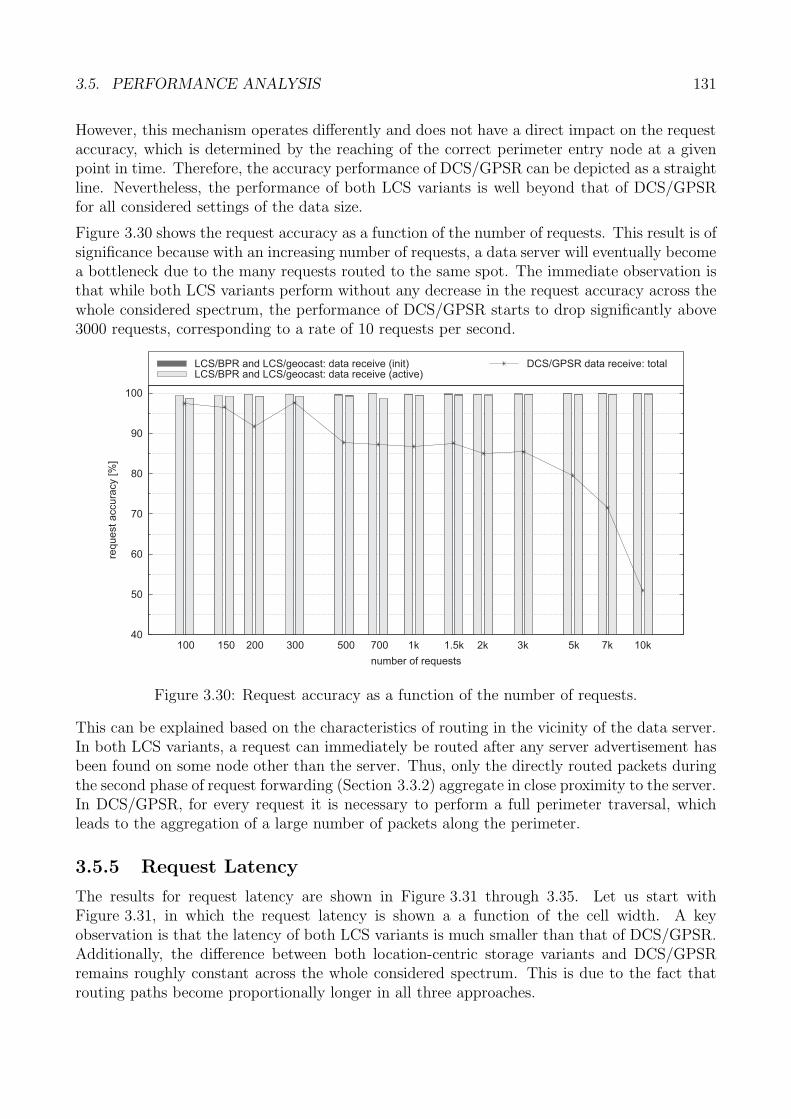
3.5. PERFORMANCE ANALYSIS 131
However, this mechanism operates differently and does not have a direct impact on the requestaccuracy, which is determined by the reaching of the correct perimeter entry node at a givenpoint in time. Therefore, the accuracy performance of DCS/GPSR can be depicted as a straightline. Nevertheless, the performance of both LCS variants is well beyond that of DCS/GPSRfor all considered settings of the data size.
Figure 3.30 shows the request accuracy as a function of the number of requests. This result is ofsignificance because with an increasing number of requests, a data server will eventually becomea bottleneck due to the many requests routed to the same spot. The immediate observation isthat while both LCS variants perform without any decrease in the request accuracy across thewhole considered spectrum, the performance of DCS/GPSR starts to drop significantly above3000 requests, corresponding to a rate of 10 requests per second.
40
50
60
70
80
90
100
100 150 200 300 500 700 1k 1.5k 2k 3k 5k 7k 10k
requestaccura
cy
[%]
number of requests
LCS/BPR and LCS/geocast: data receive (init)LCS/BPR and LCS/geocast: data receive (active)
DCS/GPSR data receive: total
Figure 3.30: Request accuracy as a function of the number of requests.
This can be explained based on the characteristics of routing in the vicinity of the data server.In both LCS variants, a request can immediately be routed after any server advertisement hasbeen found on some node other than the server. Thus, only the directly routed packets duringthe second phase of request forwarding (Section 3.3.2) aggregate in close proximity to the server.In DCS/GPSR, for every request it is necessary to perform a full perimeter traversal, whichleads to the aggregation of a large number of packets along the perimeter.
3.5.5 Request Latency
The results for request latency are shown in Figure 3.31 through 3.35. Let us start withFigure 3.31, in which the request latency is shown a a function of the cell width. A keyobservation is that the latency of both LCS variants is much smaller than that of DCS/GPSR.Additionally, the difference between both location-centric storage variants and DCS/GPSRremains roughly constant across the whole considered spectrum. This is due to the fact thatrouting paths become proportionally longer in all three approaches.
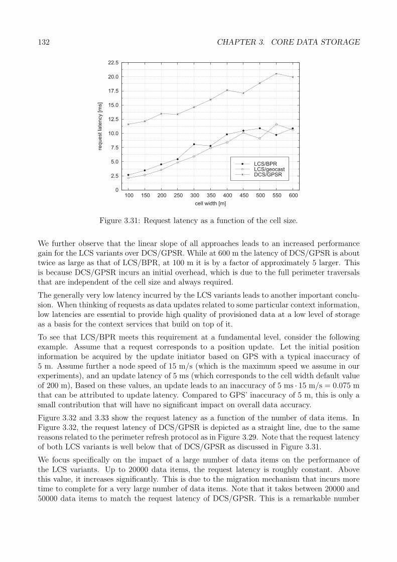
132 CHAPTER 3. CORE DATA STORAGE
0
2.5
5.0
7.5
10.0
12.5
15.0
17.5
20.0
22.5
100 150 200 250 300 350 400 450 500 550 600
req
ue
st
late
ncy
[ms]
cell width [m]
LCS/BPRLCS/geocastDCS/GPSR
Figure 3.31: Request latency as a function of the cell size.
We further observe that the linear slope of all approaches leads to an increased performancegain for the LCS variants over DCS/GPSR. While at 600 m the latency of DCS/GPSR is abouttwice as large as that of LCS/BPR, at 100 m it is by a factor of approximately 5 larger. Thisis because DCS/GPSR incurs an initial overhead, which is due to the full perimeter traversalsthat are independent of the cell size and always required.
The generally very low latency incurred by the LCS variants leads to another important conclu-sion. When thinking of requests as data updates related to some particular context information,low latencies are essential to provide high quality of provisioned data at a low level of storageas a basis for the context services that build on top of it.
To see that LCS/BPR meets this requirement at a fundamental level, consider the followingexample. Assume that a request corresponds to a position update. Let the initial positioninformation be acquired by the update initiator based on GPS with a typical inaccuracy of5 m. Assume further a node speed of 15 m/s (which is the maximum speed we assume in ourexperiments), and an update latency of 5 ms (which corresponds to the cell width default valueof 200 m), Based on these values, an update leads to an inaccuracy of 5 ms · 15 m/s = 0.075 mthat can be attributed to update latency. Compared to GPS’ inaccuracy of 5 m, this is only asmall contribution that will have no significant impact on overall data accuracy.
Figure 3.32 and 3.33 show the request latency as a function of the number of data items. InFigure 3.32, the request latency of DCS/GPSR is depicted as a straight line, due to the samereasons related to the perimeter refresh protocol as in Figure 3.29. Note that the request latencyof both LCS variants is well below that of DCS/GPSR as discussed in Figure 3.31.
We focus specifically on the impact of a large number of data items on the performance ofthe LCS variants. Up to 20000 data items, the request latency is roughly constant. Abovethis value, it increases significantly. This is due to the migration mechanism that incurs moretime to complete for a very large number of data items. Note that it takes between 20000 and50000 data items to match the request latency of DCS/GPSR. This is a remarkable number
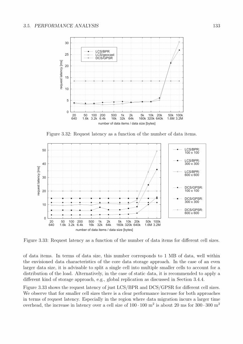
3.5. PERFORMANCE ANALYSIS 133
0
5
10
15
20
25
30
20640
501.6k
1003.2k
2006.4k
50016k
1k32k
2k64k
5k160k
10k320k
20k640k
50k1.6M
100k3.2M
req
ue
st
late
ncy
[ms]
number of data items / data size [bytes]
LCS/BPRLCS/geocastDCS/GPSR
Figure 3.32: Request latency as a function of the number of data items.
0
10
20
30
40
50
20640
501.6k
1003.2k
2006.4k
50016k
1k32k
2k64k
5k160k
10k320k
20k640k
50k1.6M
100k3.2M
req
ue
st
late
ncy
[ms]
number of data items / data size [bytes]
LCS/BPR:100 x 100
LCS/BPR:300 x 300
LCS/BPR:600 x 600
DCS/GPSR:100 x 100
DCS/GPSR:300 x 300
DCS/GPSR:600 x 600
Figure 3.33: Request latency as a function of the number of data items for different cell sizes.
of data items. In terms of data size, this number corresponds to 1 MB of data, well withinthe envisioned data characteristics of the core data storage approach. In the case of an evenlarger data size, it is advisable to split a single cell into multiple smaller cells to account for adistribution of the load. Alternatively, in the case of static data, it is recommended to apply adifferent kind of storage approach, e.g., global replication as discussed in Section 3.4.4.
Figure 3.33 shows the request latency of just LCS/BPR and DCS/GPSR for different cell sizes.We observe that for smaller cell sizes there is a clear performance increase for both approachesin terms of request latency. Especially in the region where data migration incurs a larger timeoverhead, the increase in latency over a cell size of 100 · 100 m2 is about 20 ms for 300 · 300 m2
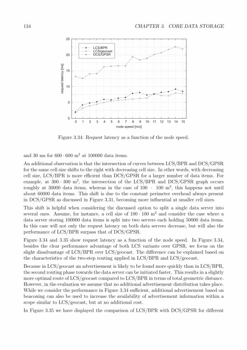
134 CHAPTER 3. CORE DATA STORAGE
0
5
10
15
20
25
0 1 2 3 4 5 6 7 8 9 10 11 12 13 14 15
req
ue
st
late
ncy
[ms]
node speed [m/s]
LCS/BPRLCS/geocastDCS/GPSR
Figure 3.34: Request latency as a function of the node speed.
and 30 ms for 600 · 600 m2 at 100000 data items.
An additional observation is that the intersection of curves between LCS/BPR and DCS/GPSRfor the same cell size shifts to the right with decreasing cell size. In other words, with decreasingcell size, LCS/BPR is more efficient than DCS/GPSR for a larger number of data items. Forexample, at 300 · 300 m2, the intersection of the LCS/BPR and DCS/GPSR graph occursroughly at 30000 data items, whereas in the case of 100 · 100 m2, this happens not untilabout 60000 data items. This shift is due to the constant perimeter overhead always presentin DCS/GPSR as discussed in Figure 3.31, becoming more influential at smaller cell sizes.
This shift is helpful when considering the discussed option to split a single data server intoseveral ones. Assume, for instance, a cell size of 100 · 100 m2 and consider the case where adata server storing 100000 data items is split into two servers each holding 50000 data items.In this case will not only the request latency on both data servers decrease, but will also theperformance of LCS/BPR surpass that of DCS/GPSR.
Figure 3.34 and 3.35 show request latency as a function of the node speed. In Figure 3.34,besides the clear performance advantage of both LCS variants over GPSR, we focus on theslight disadvantage of LCS/BPR over LCS/geocast. The difference can be explained based onthe characteristics of the two-step routing applied in LCS/BPR and LCS/geocast.
Because in LCS/geocast an advertisement is likely to be found more quickly than in LCS/BPR,the second routing phase towards the data server can be initiated faster. This results in a slightlymore optimal route of LCS/geocast compared to LCS/BPR in terms of total geometric distance.However, in the evaluation we assume that no additional advertisement distribution takes place.While we consider the performance in Figure 3.34 sufficient, additional advertisement based onbeaconing can also be used to increase the availability of advertisement information within ascope similar to LCS/geocast, but at no additional cost.
In Figure 3.35 we have displayed the comparison of LCS/BPR with DCS/GPSR for different
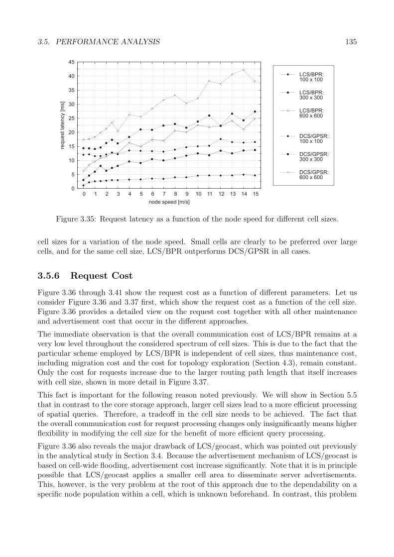
3.5. PERFORMANCE ANALYSIS 135
0
5
10
15
20
25
30
35
40
45
0 1 2 3 4 5 6 7 8 9 10 11 12 13 14 15
req
ue
st
late
ncy
[ms]
node speed [m/s]
LCS/BPR:100 x 100
LCS/BPR:300 x 300
LCS/BPR:600 x 600
DCS/GPSR:100 x 100
DCS/GPSR:300 x 300
DCS/GPSR:600 x 600
Figure 3.35: Request latency as a function of the node speed for different cell sizes.
cell sizes for a variation of the node speed. Small cells are clearly to be preferred over largecells, and for the same cell size, LCS/BPR outperforms DCS/GPSR in all cases.
3.5.6 Request Cost
Figure 3.36 through 3.41 show the request cost as a function of different parameters. Let usconsider Figure 3.36 and 3.37 first, which show the request cost as a function of the cell size.Figure 3.36 provides a detailed view on the request cost together with all other maintenanceand advertisement cost that occur in the different approaches.
The immediate observation is that the overall communication cost of LCS/BPR remains at avery low level throughout the considered spectrum of cell sizes. This is due to the fact that theparticular scheme employed by LCS/BPR is independent of cell sizes, thus maintenance cost,including migration cost and the cost for topology exploration (Section 4.3), remain constant.Only the cost for requests increase due to the larger routing path length that itself increaseswith cell size, shown in more detail in Figure 3.37.
This fact is important for the following reason noted previously. We will show in Section 5.5that in contrast to the core storage approach, larger cell sizes lead to a more efficient processingof spatial queries. Therefore, a tradeoff in the cell size needs to be achieved. The fact thatthe overall communication cost for request processing changes only insignificantly means higherflexibility in modifying the cell size for the benefit of more efficient query processing.
Figure 3.36 also reveals the major drawback of LCS/geocast, which was pointed out previouslyin the analytical study in Section 3.4. Because the advertisement mechanism of LCS/geocast isbased on cell-wide flooding, advertisement cost increase significantly. Note that it is in principlepossible that LCS/geocast applies a smaller cell area to disseminate server advertisements.This, however, is the very problem at the root of this approach due to the dependability on aspecific node population within a cell, which is unknown beforehand. In contrast, this problem
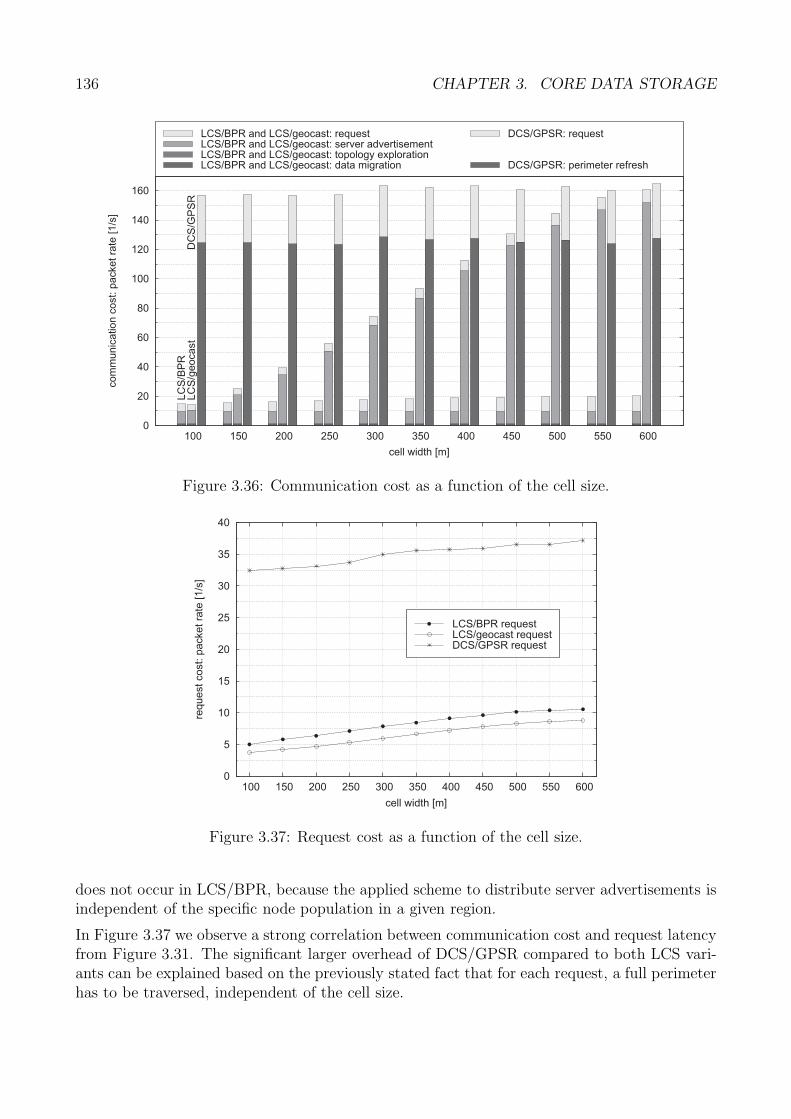
136 CHAPTER 3. CORE DATA STORAGE
0
20
40
60
80
100
120
140
160
100 150 200 250 300 350 400 450 500 550 600
com
munic
ation
cost:
packetra
te[1
/s]
cell width [m]
LCS/BPR and LCS/geocast: requestLCS/BPR and LCS/geocast: server advertisementLCS/BPR and LCS/geocast: topology explorationLCS/BPR and LCS/geocast: data migration
DCS/GPSR: request
DCS/GPSR: perimeter refresh
LC
S/B
PR
LC
S/g
eocast
DC
S/G
PS
R
Figure 3.36: Communication cost as a function of the cell size.
0
5
10
15
20
25
30
35
40
100 150 200 250 300 350 400 450 500 550 600
req
ue
st
co
st:
pa
cke
tra
te[1
/s]
cell width [m]
LCS/BPR requestLCS/geocast requestDCS/GPSR request
Figure 3.37: Request cost as a function of the cell size.
does not occur in LCS/BPR, because the applied scheme to distribute server advertisements isindependent of the specific node population in a given region.
In Figure 3.37 we observe a strong correlation between communication cost and request latencyfrom Figure 3.31. The significant larger overhead of DCS/GPSR compared to both LCS vari-ants can be explained based on the previously stated fact that for each request, a full perimeterhas to be traversed, independent of the cell size.
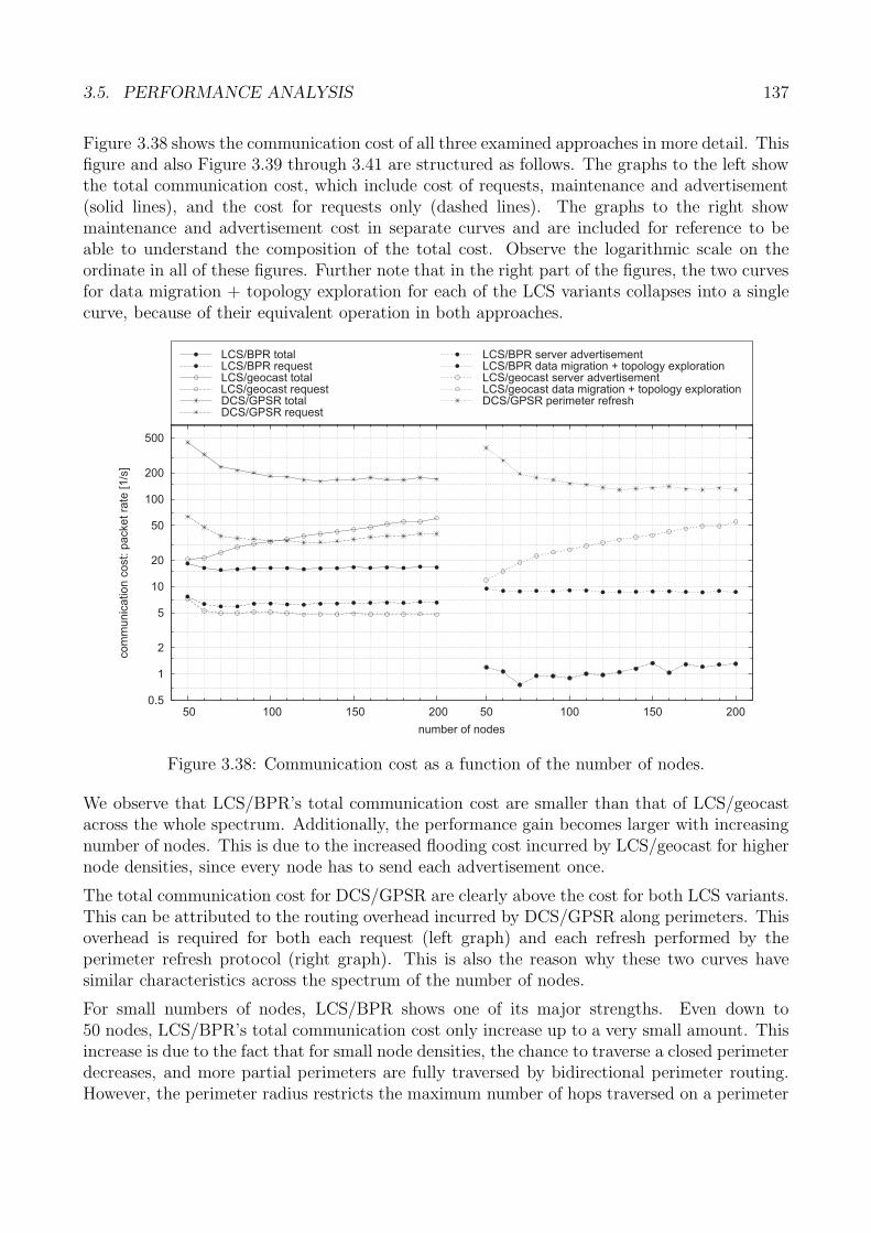
3.5. PERFORMANCE ANALYSIS 137
Figure 3.38 shows the communication cost of all three examined approaches in more detail. Thisfigure and also Figure 3.39 through 3.41 are structured as follows. The graphs to the left showthe total communication cost, which include cost of requests, maintenance and advertisement(solid lines), and the cost for requests only (dashed lines). The graphs to the right showmaintenance and advertisement cost in separate curves and are included for reference to beable to understand the composition of the total cost. Observe the logarithmic scale on theordinate in all of these figures. Further note that in the right part of the figures, the two curvesfor data migration + topology exploration for each of the LCS variants collapses into a singlecurve, because of their equivalent operation in both approaches.
0.5
1
2
5
10
20
50
100
200
500
50 100 150 200 50 100 150 200
com
munic
ation
cost:
packetra
te[1
/s]
number of nodes
LCS/BPR totalLCS/BPR requestLCS/geocast totalLCS/geocast requestDCS/GPSR totalDCS/GPSR request
LCS/BPR server advertisementLCS/BPR data migration + topology explorationLCS/geocast server advertisementLCS/geocast data migration + topology explorationDCS/GPSR perimeter refresh
Figure 3.38: Communication cost as a function of the number of nodes.
We observe that LCS/BPR’s total communication cost are smaller than that of LCS/geocastacross the whole spectrum. Additionally, the performance gain becomes larger with increasingnumber of nodes. This is due to the increased flooding cost incurred by LCS/geocast for highernode densities, since every node has to send each advertisement once.
The total communication cost for DCS/GPSR are clearly above the cost for both LCS variants.This can be attributed to the routing overhead incurred by DCS/GPSR along perimeters. Thisoverhead is required for both each request (left graph) and each refresh performed by theperimeter refresh protocol (right graph). This is also the reason why these two curves havesimilar characteristics across the spectrum of the number of nodes.
For small numbers of nodes, LCS/BPR shows one of its major strengths. Even down to50 nodes, LCS/BPR’s total communication cost only increase up to a very small amount. Thisincrease is due to the fact that for small node densities, the chance to traverse a closed perimeterdecreases, and more partial perimeters are fully traversed by bidirectional perimeter routing.However, the perimeter radius restricts the maximum number of hops traversed on a perimeter
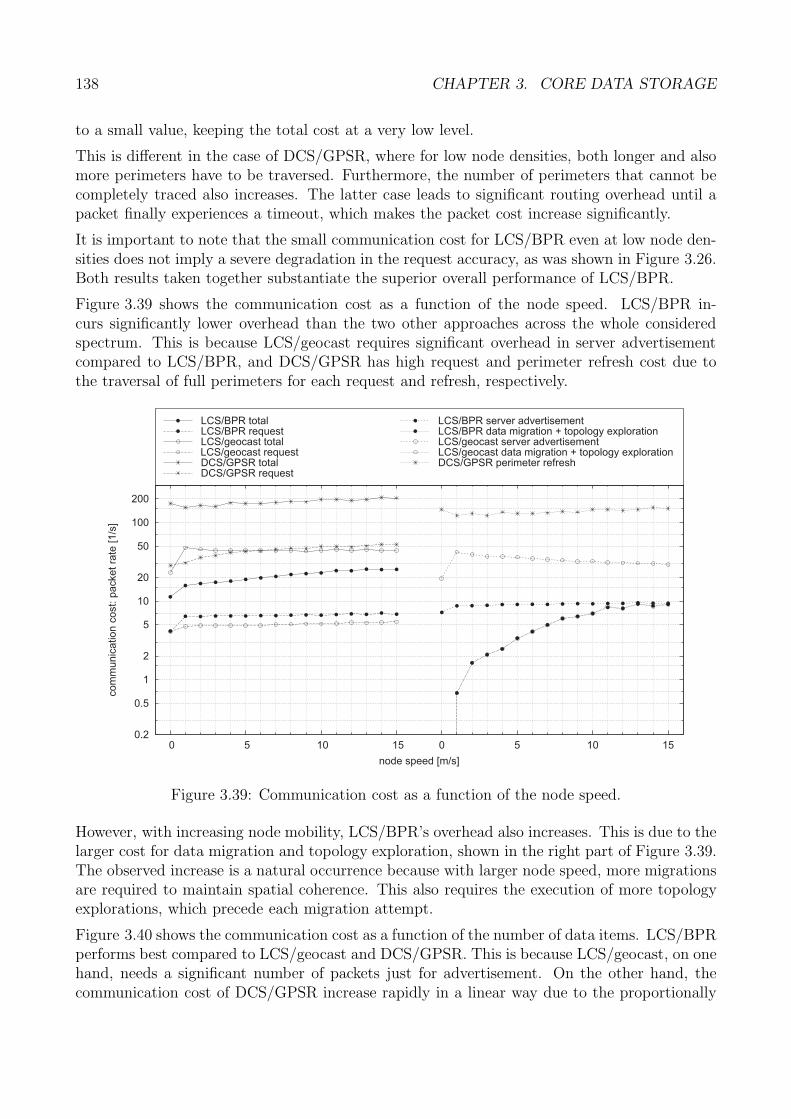
138 CHAPTER 3. CORE DATA STORAGE
to a small value, keeping the total cost at a very low level.
This is different in the case of DCS/GPSR, where for low node densities, both longer and alsomore perimeters have to be traversed. Furthermore, the number of perimeters that cannot becompletely traced also increases. The latter case leads to significant routing overhead until apacket finally experiences a timeout, which makes the packet cost increase significantly.
It is important to note that the small communication cost for LCS/BPR even at low node den-sities does not imply a severe degradation in the request accuracy, as was shown in Figure 3.26.Both results taken together substantiate the superior overall performance of LCS/BPR.
Figure 3.39 shows the communication cost as a function of the node speed. LCS/BPR in-curs significantly lower overhead than the two other approaches across the whole consideredspectrum. This is because LCS/geocast requires significant overhead in server advertisementcompared to LCS/BPR, and DCS/GPSR has high request and perimeter refresh cost due tothe traversal of full perimeters for each request and refresh, respectively.
0.2
0.5
1
2
5
10
20
50
100
200
0 5 10 15 0 5 10 15
com
munic
ation
cost:
packetra
te[1
/s]
node speed [m/s]
LCS/BPR totalLCS/BPR requestLCS/geocast totalLCS/geocast requestDCS/GPSR totalDCS/GPSR request
LCS/BPR server advertisementLCS/BPR data migration + topology explorationLCS/geocast server advertisementLCS/geocast data migration + topology explorationDCS/GPSR perimeter refresh
Figure 3.39: Communication cost as a function of the node speed.
However, with increasing node mobility, LCS/BPR’s overhead also increases. This is due to thelarger cost for data migration and topology exploration, shown in the right part of Figure 3.39.The observed increase is a natural occurrence because with larger node speed, more migrationsare required to maintain spatial coherence. This also requires the execution of more topologyexplorations, which precede each migration attempt.
Figure 3.40 shows the communication cost as a function of the number of data items. LCS/BPRperforms best compared to LCS/geocast and DCS/GPSR. This is because LCS/geocast, on onehand, needs a significant number of packets just for advertisement. On the other hand, thecommunication cost of DCS/GPSR increase rapidly in a linear way due to the proportionally
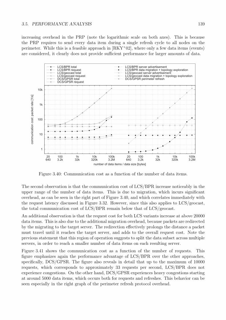
3.5. PERFORMANCE ANALYSIS 139
increasing overhead in the PRP (note the logarithmic scale on both axes). This is becausethe PRP requires to send every data item during a single refresh cycle to all nodes on theperimeter. While this is a feasible approach in [RKY+02], where only a few data items (events)are considered, it clearly does not provide sufficient performance for larger amounts of data.
1
10
100
1k
10k
20640
1003.2k
1k32k
10k320k
100k3.2M
20640
1003.2k
1k32k
10k320k
100k3.2M
com
munic
ation
cost:
packetra
te[1
/s]
number of data items / data size [bytes]
LCS/BPR totalLCS/BPR requestLCS/geocast totalLCS/geocast requestDCS/GPSR totalDCS/GPSR request
LCS/BPR server advertisementLCS/BPR data migration + topology explorationLCS/geocast server advertisementLCS/geocast data migration + topology explorationDCS/GPSR perimeter refresh
Figure 3.40: Communication cost as a function of the number of data items.
The second observation is that the communication cost of LCS/BPR increase noticeably in theupper range of the number of data items. This is due to migration, which incurs significantoverhead, as can be seen in the right part of Figure 3.40, and which correlates immediately withthe request latency discussed in Figure 3.32. However, since this also applies to LCS/geocast,the total communication cost of LCS/BPR remain below that of LCS/geocast.
An additional observation is that the request cost for both LCS variants increase at above 20000data items. This is also due to the additional migration overhead, because packets are redirectedby the migrating to the target server. The redirection effectively prolongs the distance a packetmust travel until it reaches the target server, and adds to the overall request cost. Note theprevious statement that this region of operation suggests to split the data subset across multipleservers, in order to reach a smaller number of data items on each resulting server.
Figure 3.41 shows the communication cost as a function of the number of requests. Thisfigure emphasizes again the performance advantage of LCS/BPR over the other approaches,specifically, DCS/GPSR. The figure also reveals in detail that up to the maximum of 10000requests, which corresponds to approximately 33 requests per second, LCS/BPR does notexperience congestions. On the other hand, DCS/GPSR experiences heavy congestions startingat around 5000 data items, which occurs both for requests and refreshes. This behavior can beseen especially in the right graph of the perimeter refresh protocol overhead.
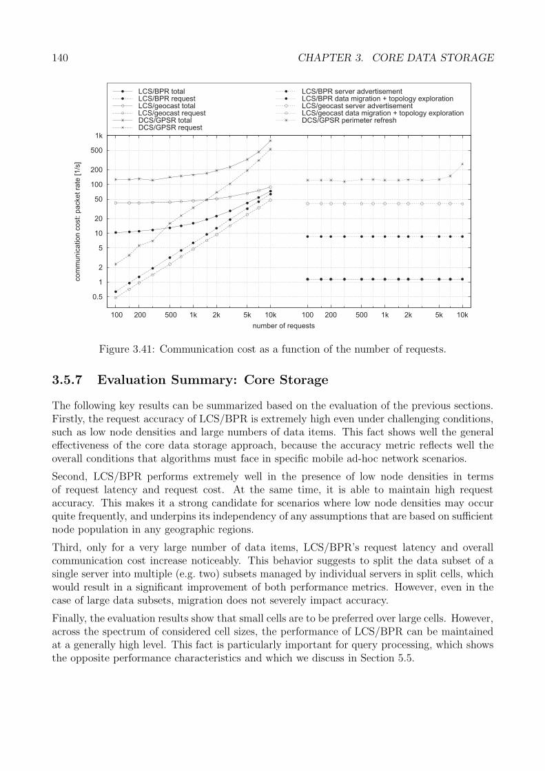
140 CHAPTER 3. CORE DATA STORAGE
0.5
1
2
5
10
20
50
100
200
500
1k
100 200 500 1k 2k 5k 10k 100 200 500 1k 2k 5k 10k
com
munic
ation
cost:
packetra
te[1
/s]
number of requests
LCS/BPR totalLCS/BPR requestLCS/geocast totalLCS/geocast requestDCS/GPSR totalDCS/GPSR request
LCS/BPR server advertisementLCS/BPR data migration + topology explorationLCS/geocast server advertisementLCS/geocast data migration + topology explorationDCS/GPSR perimeter refresh
Figure 3.41: Communication cost as a function of the number of requests.
3.5.7 Evaluation Summary: Core Storage
The following key results can be summarized based on the evaluation of the previous sections.Firstly, the request accuracy of LCS/BPR is extremely high even under challenging conditions,such as low node densities and large numbers of data items. This fact shows well the generaleffectiveness of the core data storage approach, because the accuracy metric reflects well theoverall conditions that algorithms must face in specific mobile ad-hoc network scenarios.
Second, LCS/BPR performs extremely well in the presence of low node densities in termsof request latency and request cost. At the same time, it is able to maintain high requestaccuracy. This makes it a strong candidate for scenarios where low node densities may occurquite frequently, and underpins its independency of any assumptions that are based on sufficientnode population in any geographic regions.
Third, only for a very large number of data items, LCS/BPR’s request latency and overallcommunication cost increase noticeably. This behavior suggests to split the data subset of asingle server into multiple (e.g. two) subsets managed by individual servers in split cells, whichwould result in a significant improvement of both performance metrics. However, even in thecase of large data subsets, migration does not severely impact accuracy.
Finally, the evaluation results show that small cells are to be preferred over large cells. However,across the spectrum of considered cell sizes, the performance of LCS/BPR can be maintainedat a generally high level. This fact is particularly important for query processing, which showsthe opposite performance characteristics and which we discuss in Section 5.5.
Chapter 4
Data Migration
In the previous chapter we have introduced core data storage, which provides the base mecha-nisms for data storage according to the location-centric storage paradigm (Definition 2.2). Themain objective of core data storage was to address Requirement (1), (3), and (4) in Section 2.4,which capture storage efficiency and robustness. In the presence of node mobility, however,core data storage does not enforce spatial coherence according to Definition 2.2 between a dataserver’s stored data and its associated reference coordinate.
To this end, we present the data migration component, which complements the core data storagecomponent in the storage tier of the LCS framework of Figure 2.22. Data migration providesthe strategies and mechanisms to maintain spatial coherence by migrating data subsets betweendata servers and thereby addresses specifically Requirement (2) in Section 2.4.
We begin with an overview of the migration framework in Section 4.1. In Section 4.2 through 4.4,we detail on migration policies, followed by a description of the migration mechanisms inSection 4.5. The evaluation of data migration will follow in Section 4.6.
4.1 Migration Framework Overview
Figure 4.1 presents the high-level structure of the framework for data migration. In the storagetier (Figure 2.22), the framework contains two components: migration policies and migrationmechanisms. In the routing tier, these are supported by components that implement networktopology exploration and resilient source routing.
The migration policies’ task is to estimate the necessity, benefit, and success that a potentialmigration will bring in terms of achieving strong and continuous spatial coherence. Our ap-proach works by splitting the migration policies in two parts: the migration recommendationand the migration decision. The migration recommendation policy (MRP, Section 4.2) uses thelocal state of the current data server to determine whether migration is needed and beneficial,that is, whether it leads to an increase in spatial coherence and thus storage efficiency. Forthat, it evaluates the migration recommendation predicate (PMRP).
Only when PMRP is true, that is, a migration is recommended, the migration decision policy(MDP, Section 4.4) is invoked to refine the recommendation in order to bring about a decision.The MDP examines the remote state of a set of possible candidate target nodes and attempts
141
142 CHAPTER 4. DATA MIGRATION
to find the most eligible one. In order to do so, the MDP is supported by the network topologyexploration component (Section 4.3), which provides efficient distributed aggregation of theremote state. The MDP also considers the network stability of the current topology to determinewhether a sufficiently stable path exists to perform a successful migration. A migration is onlyperformed if the migration decision predicate (PMDP) and the MRP agree to do so. In thatcase, a selected target server, an initial source route, and the priority value Π indicating theurgency of the migration, are handed to the data migration component (Figure 4.1).
The migration mechanisms are composed of two components: data migration and data consol-idation. The data migration component is responsible for carrying out individual migrationsbased on the initial target server and source route provided by the migration policy. This com-ponent makes extensive use of resilient source routing (Section 4.5), which takes as input theprovided source route and supports the transport of data between remote servers. The datamigration component also relies on network topology exploration to update the source routeduring the migration of large quantities of data. Furthermore, the data migration provides asmuch transparency as possible for requests, both updates and queries.
Data consolidation is invoked asynchronously to the rest of the described processes in theevent of migration failures. Such failures cannot be avoided in the system model we assume inSection 3.1 and require the consolidation of data stored at several servers. In close collaborationwith core data storage, data consolidation is, however, able to detect server redundancies andinitiate the merging of multiple servers, and thus, data subsets, into a single one.
4.2 Migration Recommendation Policy
The migration recommendation policy (MRP) is the initial step in the process of checking forwhether or not a migration makes sense under the current network conditions. Each data serverin the network monitors in regular time intervals ΔtMRP if the MRP ought to be invoked fora particular data subset. After each ΔtMRP, the MRP examines the server’s local state andevaluates the migration recommendation predicate, denoted PMRP.
If PMRP = true, local state indicates that migration is necessary from the point of view of thecurrent data server, and that it will likely increase spatial coherence between the respective datasubset and its associated reference coordinate (Section 3.1). If PMRP = false, the evaluationof the MRP is deferred to the next migration cycle after ΔtMRP. The length of the migrationcycle is determined by the application and is a configurable parameter.
Besides this predicate, we introduce the notion of migration priority Π ∈ [0, 1]. This priorityvalue dictates the strictness by which the subsequent MDP must determine a target server(Figure 4.1). If Π = 0 (minimum priority), the MDP has full freedom on choosing a candidateto receive the data to migrate. If Π = 1 (maximum priority), the MDP is forced to find a targetnode at any cost, even if the most eligible node may not be an optimal choice.
Let us first consider predicate PMRP, which is composed of several partial predicates, eachmodelling a relevant aspect of a server’s local state. The spatial predicate, denoted Pspatial,ensures that a data server will migrate upon moving too far away from its associated referencecoordinate. Thus, it is the primary indicator for weak spatial coherence. Let t0 denote thecurrent time, r0(t0) the position of the server at t0, and d0 = d0(t0) = |r0(t0) − cr|.
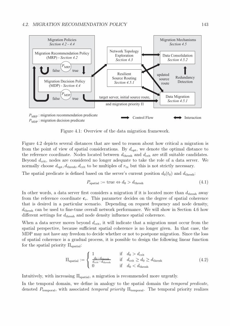
4.2. MIGRATION RECOMMENDATION POLICY 143
Migration MechanismsSection 4.5
Network TopologyExplorationSection 4.3
ResilientSource Routing
Section 4.5.1Migration Decision Policy(MDP) - Section 4.4
Migration Recommendation Policy(MRP) - Section 4.2
Migration PoliciesSection 4.2 - 4.4
Data MigrationSection 4.5.1
Data ConsolidationSection 4.5.2
true
target server, initial source route,
and migration priority Π
Control Flow Interaction
RedundancyDetection
false
PMDP
PMRP
truefalse
PMRP : migration recommendation predicate
PMDP : migration decision predicate
updatedsource
route
Figure 4.1: Overview of the data migration framework.
Figure 4.2 depicts several distances that are used to reason about how critical a migration isfrom the point of view of spatial considerations. By dopt, we denote the optimal distance tothe reference coordinate. Nodes located between dthresh and dcrit are still suitable candidates.Beyond dcrit, nodes are considered no longer adequate to take the role of a data server. Wenormally choose dopt, dthresh, dcrit to be multiples of rtx but this is not strictly necessary.
The spatial predicate is defined based on the server’s current position d0(t0) and dthresh:
Pspatial := true ⇔ d0 > dthresh (4.1)
In other words, a data server first considers a migration if it is located more than dthresh awayfrom the reference coordinate cr. This parameter decides on the degree of spatial coherencethat is desired in a particular scenario. Depending on request frequency and node density,dthresh can be used to fine-tune overall network performance. We will show in Section 4.6 howdifferent settings for dthresh and node density influence spatial coherence.
When a data server moves beyond dcrit, it will indicate that a migration must occur from thespatial perspective, because sufficient spatial coherence is no longer given. In that case, theMDP may not have any freedom to decide whether or not to postpone migration. Since the lossof spatial coherence is a gradual process, it is possible to design the following linear functionfor the spatial priority Πspatial:
Πspatial :=
⎧⎨⎩
1 if d0 > dcritd0−dthresh
dcrit−dthreshif dcrit ≥ d0 ≥ dthresh
0 if d0 < dthresh
(4.2)
Intuitively, with increasing Πspatial, a migration is recommended more urgently.
In the temporal domain, we define in analogy to the spatial domain the temporal predicate,denoted Ptemporal, with associated temporal priority Πtemporal. The temporal priority realizes
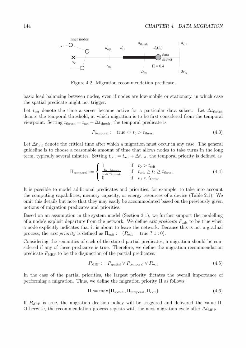
144 CHAPTER 4. DATA MIGRATION
cr
...
...
inner nodes
rtx
2rtx 3rtx
dthresh dcrit
dopt dΠ
Π = 0.4
d t0 0( )
dataserver
Figure 4.2: Migration recommendation predicate.
basic load balancing between nodes, even if nodes are low-mobile or stationary, in which casethe spatial predicate might not trigger.
Let tact denote the time a server became active for a particular data subset. Let Δtthresh
denote the temporal threshold, at which migration is to be first considered from the temporalviewpoint. Setting tthresh = tact + Δtthresh, the temporal predicate is
Ptemporal := true ⇔ t0 > tthresh (4.3)
Let Δtcrit denote the critical time after which a migration must occur in any case. The generalguideline is to choose a reasonable amount of time that allows nodes to take turns in the longterm, typically several minutes. Setting tcrit = tact + Δtcrit, the temporal priority is defined as
Πtemporal :=
⎧⎨⎩
1 if t0 > tcritt0−tthresh
tcrit−tthreshif tcrit ≥ t0 ≥ tthresh
0 if t0 < tthresh
(4.4)
It is possible to model additional predicates and priorities, for example, to take into accountthe computing capabilities, memory capacity, or energy resources of a device (Table 2.1). Weomit this details but note that they may easily be accommodated based on the previously givennotions of migration predicates and priorities.
Based on an assumption in the system model (Section 3.1), we further support the modellingof a node’s explicit departure from the network. We define exit predicate Pexit to be true whena node explicitly indicates that it is about to leave the network. Because this is not a gradualprocess, the exit priority is defined as Πexit := (Pexit = true ? 1 : 0).
Considering the semantics of each of the stated partial predicates, a migration should be con-sidered if any of these predicates is true. Therefore, we define the migration recommendationpredicate PMRP to be the disjunction of the partial predicates:
PMRP := Pspatial ∨ Ptemporal ∨ Pexit (4.5)
In the case of the partial priorities, the largest priority dictates the overall importance ofperforming a migration. Thus, we define the migration priority Π as follows:
Π := max{Πspatial, Πtemporal, Πexit} (4.6)
If PMRP is true, the migration decision policy will be triggered and delivered the value Π.Otherwise, the recommendation process repeats with the next migration cycle after ΔtMRP.
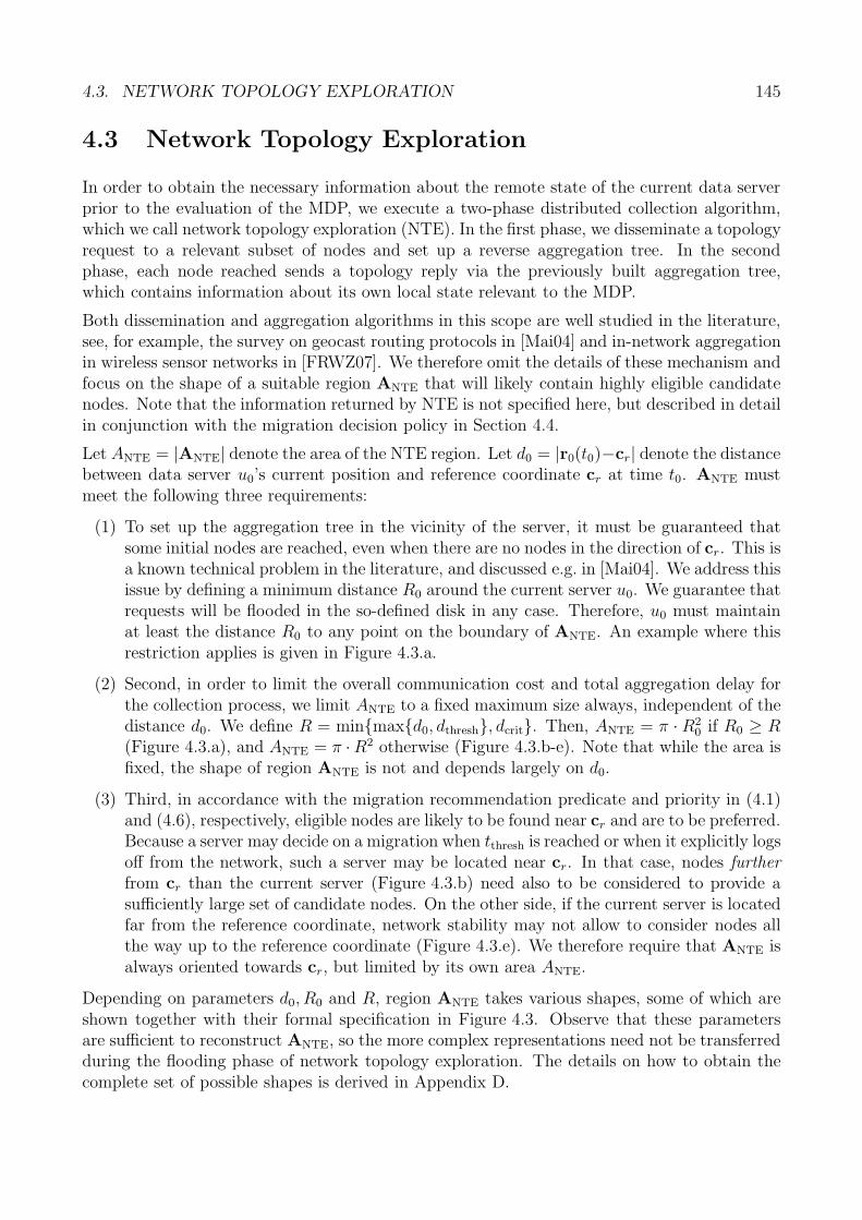
4.3. NETWORK TOPOLOGY EXPLORATION 145
4.3 Network Topology Exploration
In order to obtain the necessary information about the remote state of the current data serverprior to the evaluation of the MDP, we execute a two-phase distributed collection algorithm,which we call network topology exploration (NTE). In the first phase, we disseminate a topologyrequest to a relevant subset of nodes and set up a reverse aggregation tree. In the secondphase, each node reached sends a topology reply via the previously built aggregation tree,which contains information about its own local state relevant to the MDP.
Both dissemination and aggregation algorithms in this scope are well studied in the literature,see, for example, the survey on geocast routing protocols in [Mai04] and in-network aggregationin wireless sensor networks in [FRWZ07]. We therefore omit the details of these mechanism andfocus on the shape of a suitable region ANTE that will likely contain highly eligible candidatenodes. Note that the information returned by NTE is not specified here, but described in detailin conjunction with the migration decision policy in Section 4.4.
Let ANTE = |ANTE| denote the area of the NTE region. Let d0 = |r0(t0)−cr| denote the distancebetween data server u0’s current position and reference coordinate cr at time t0. ANTE mustmeet the following three requirements:
(1) To set up the aggregation tree in the vicinity of the server, it must be guaranteed thatsome initial nodes are reached, even when there are no nodes in the direction of cr. This isa known technical problem in the literature, and discussed e.g. in [Mai04]. We address thisissue by defining a minimum distance R0 around the current server u0. We guarantee thatrequests will be flooded in the so-defined disk in any case. Therefore, u0 must maintainat least the distance R0 to any point on the boundary of ANTE. An example where thisrestriction applies is given in Figure 4.3.a.
(2) Second, in order to limit the overall communication cost and total aggregation delay forthe collection process, we limit ANTE to a fixed maximum size always, independent of thedistance d0. We define R = min{max{d0, dthresh}, dcrit}. Then, ANTE = π · R2
0 if R0 ≥ R(Figure 4.3.a), and ANTE = π ·R2 otherwise (Figure 4.3.b-e). Note that while the area isfixed, the shape of region ANTE is not and depends largely on d0.
(3) Third, in accordance with the migration recommendation predicate and priority in (4.1)and (4.6), respectively, eligible nodes are likely to be found near cr and are to be preferred.Because a server may decide on a migration when tthresh is reached or when it explicitly logsoff from the network, such a server may be located near cr. In that case, nodes furtherfrom cr than the current server (Figure 4.3.b) need also to be considered to provide asufficiently large set of candidate nodes. On the other side, if the current server is locatedfar from the reference coordinate, network stability may not allow to consider nodes allthe way up to the reference coordinate (Figure 4.3.e). We therefore require that ANTE isalways oriented towards cr, but limited by its own area ANTE.
Depending on parameters d0, R0 and R, region ANTE takes various shapes, some of which areshown together with their formal specification in Figure 4.3. Observe that these parametersare sufficient to reconstruct ANTE, so the more complex representations need not be transferredduring the flooding phase of network topology exploration. The details on how to obtain thecomplete set of possible shapes is derived in Appendix D.
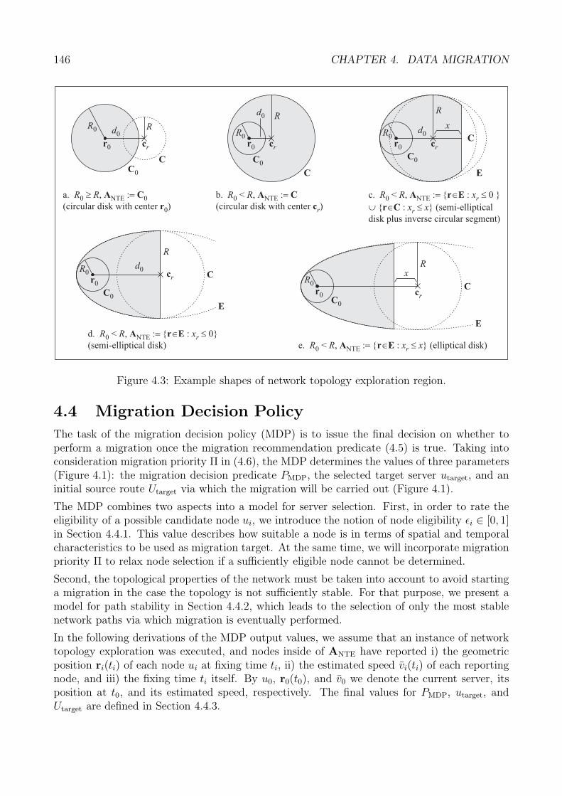
146 CHAPTER 4. DATA MIGRATION
a. ,
(circular disk with center )
R R0 NTE 0
0
� ��A C
r
cr
R0 d0R
E
C
E
E
r0
C0
xR0
d0 R
r0 cr
C0
C
b. < ,
(circular disk with center )
R R0 NTEA C
c
��
r
c. R R x
x x0 NTE< , : 0 }
{ : } (semi-elliptical
disk plus inverse circular segment)
A r E
r C
���� � �
� �r
r
r0
R0d0
C0
cr
R
C
d. R R x0 NTE< , : 0}
(semi-elliptical disk)
A r E���� � �r
R0
r0
C0
d0
R
cr C
e. R R x x0 NTE< , : } (elliptical disk)A r E���� � �r
R0
C0
x
cr
r0
R
C
Figure 4.3: Example shapes of network topology exploration region.
4.4 Migration Decision Policy
The task of the migration decision policy (MDP) is to issue the final decision on whether toperform a migration once the migration recommendation predicate (4.5) is true. Taking intoconsideration migration priority Π in (4.6), the MDP determines the values of three parameters(Figure 4.1): the migration decision predicate PMDP, the selected target server utarget, and aninitial source route Utarget via which the migration will be carried out (Figure 4.1).
The MDP combines two aspects into a model for server selection. First, in order to rate theeligibility of a possible candidate node ui, we introduce the notion of node eligibility εi ∈ [0, 1]in Section 4.4.1. This value describes how suitable a node is in terms of spatial and temporalcharacteristics to be used as migration target. At the same time, we will incorporate migrationpriority Π to relax node selection if a sufficiently eligible node cannot be determined.
Second, the topological properties of the network must be taken into account to avoid startinga migration in the case the topology is not sufficiently stable. For that purpose, we present amodel for path stability in Section 4.4.2, which leads to the selection of only the most stablenetwork paths via which migration is eventually performed.
In the following derivations of the MDP output values, we assume that an instance of networktopology exploration was executed, and nodes inside of ANTE have reported i) the geometricposition ri(ti) of each node ui at fixing time ti, ii) the estimated speed vi(ti) of each reportingnode, and iii) the fixing time ti itself. By u0, r0(t0), and v0 we denote the current server, itsposition at t0, and its estimated speed, respectively. The final values for PMDP, utarget, andUtarget are defined in Section 4.4.3.
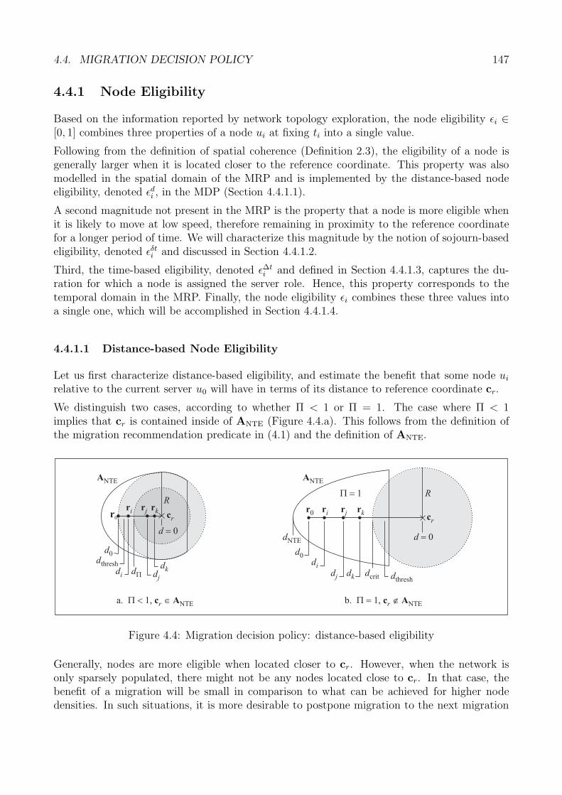
4.4. MIGRATION DECISION POLICY 147
4.4.1 Node Eligibility
Based on the information reported by network topology exploration, the node eligibility εi ∈[0, 1] combines three properties of a node ui at fixing ti into a single value.
Following from the definition of spatial coherence (Definition 2.3), the eligibility of a node isgenerally larger when it is located closer to the reference coordinate. This property was alsomodelled in the spatial domain of the MRP and is implemented by the distance-based nodeeligibility, denoted εd
i , in the MDP (Section 4.4.1.1).
A second magnitude not present in the MRP is the property that a node is more eligible whenit is likely to move at low speed, therefore remaining in proximity to the reference coordinatefor a longer period of time. We will characterize this magnitude by the notion of sojourn-basedeligibility, denoted εδt
i and discussed in Section 4.4.1.2.
Third, the time-based eligibility, denoted εΔti and defined in Section 4.4.1.3, captures the du-
ration for which a node is assigned the server role. Hence, this property corresponds to thetemporal domain in the MRP. Finally, the node eligibility εi combines these three values intoa single one, which will be accomplished in Section 4.4.1.4.
4.4.1.1 Distance-based Node Eligibility
Let us first characterize distance-based eligibility, and estimate the benefit that some node ui
relative to the current server u0 will have in terms of its distance to reference coordinate cr.
We distinguish two cases, according to whether Π < 1 or Π = 1. The case where Π < 1implies that cr is contained inside of ANTE (Figure 4.4.a). This follows from the definition ofthe migration recommendation predicate in (4.1) and the definition of ANTE.
R
r0 cr
d
d 0�
ri
dj
dk
rj rk
di
d0di
R
r0cr
d 0�
ri rj rk
�� 1
ANTE
d0dthresh
dj dk dthreshdcrit
dNTE
a. 1,�� �c Ar NTE b. �� �1, c Ar NTE
ANTE
Figure 4.4: Migration decision policy: distance-based eligibility
Generally, nodes are more eligible when located closer to cr. However, when the network isonly sparsely populated, there might not be any nodes located close to cr. In that case, thebenefit of a migration will be small in comparison to what can be achieved for higher nodedensities. In such situations, it is more desirable to postpone migration to the next migration
148 CHAPTER 4. DATA MIGRATION
cycle until more suitable candidates become available. This is exactly the purpose of priorityΠ, which we apply to implement a deferral of a migration in such situations as follows.
Using the migration priority Π from (4.6), we are able to define a distance limit dΠ (Figure 4.4.a)that any candidate node must not exceed. Nodes located further from cr than dΠ will not beconsidered as valid candidates. For Π < 1, we define:
dΠ = 0.5 · (1 + Π) · dthresh (4.7)
The interpretation of (4.7) is as follows: Consider Π = 0, which by definition leaves maximumfreedom to the MDP to decide on a target server. In spatial terms, if cr ∈ ANTE, a nodemust gain at least 0.5 times the distance dthresh in order to be considered eligible. Choosingdthresh instead of d0 in (4.7) makes sure that progress is always relative to the threshold. This isimportant if u0 is almost co-located with the reference coordinate, in which case no candidatenodes may exist in a very small region. For larger values of Π, distance dΠ increases, whicheffectively increases the set of nodes that will be considered in the selection process.
The choice of the factor 0.5 can be understood from Figure 4.2. In the example, the distance ofthe current server to the reference coordinate is d0(t0). According to (4.6), Π = 0.4. Then, (4.7)yields dΠ = 0.7 · dthresh, indicated in Figure 4.2. We can see that now not only nodes locatedup to dopt are considered in the selection process, but also nodes located up to dΠ. That is,once the current server moves beyond dthresh, priority Π together with the factor 0.5 effectivelyassures that migration will only occur over a distance of at least rtx.
In the second case where Π = 1, migration must occur according to the MRP’s recommendation,which effectively turns into a decision in this case. Therefore, we set dΠ = dNTE, where dNTE
is the maximum distance between the NTE region, ANTE, and the reference coordinate cr
(Figure 4.4.b). That is, any node located inside of ANTE is considered, even if it is locatedfurther away from the reference coordinate than u0 itself.
We are ready now to define the distance-based eligibility εdi of every node ui. It is always defined
relative to dthresh to be compatible with the MRP. Let di(t0) = di(ti) + vi · (t0 − ti), then
εdi =
{1 − di(t0)
dthreshif Π < 1
1 − di(t0)dNTE
if Π = 1(4.8)
In the previous equation, we set εdi = 0 if di(t0) > dthresh.
We further require the notion of the minimum distance-based eligibility, denoted εΠd , which
denotes the eligibility that a node must satisfy in order to be a valid candidate:
εΠd =
{1 − dΠ
dthreshif Π < 1
0 if Π = 1(4.9)
4.4.1.2 Sojourn-based Node Eligibility
The sojourn-based node eligibility, denoted εδti , is related to the expected speed that a node
ui takes relative to the considered reference coordinate cr. We define the notion of estimated
4.4. MIGRATION DECISION POLICY 149
residual sojourn time, based on notions in [TDC01, MMM05], in such a way that it can beadopted for the definition of the sojourn-based eligibility.
Using the assumption that a data migration will occur after Δtthresh if the spatial migrationpredicate in (4.1) does not trigger, we can define Δtthresh as the maximum residual sojourntime. We first consider the case where Π < 1 ⇒ cr ∈ ANTE. We define the sojourn time δti ofnode ui relative to the current time t0 as follows:
δti = min
{dthresh − di(t0)
vi, Δtthresh
}(4.10)
If di(t0) > dthresh, we set δti = 0. If vi = 0 for some i, we set δti = Δtthresh. For Π = 1, we takethe distance dNTE as the reference:
δti = min
{dNTE − di(t0)
vi
, Δtthresh
}(4.11)
If di(t0) > dNTE, we set δti = 0.
In contrast to the distance-based node eligibility, an absolute reference for the sojourn-basedeligibility does not make sense. This is because the sojourn time distribution of nodes canpotentially be arbitrary, depending on the mobility of network nodes. We thus divide the setof nodes into two partitions, each having a size that is a function of migration priority Π.
Let us first consider Π < 1. Let δt′0, . . . , δt′n denote the estimated residual sojourn time values
in increasing order, with equal values in arbitrary order. If δt′n > 0, we define k′ ∈ {0, . . . , n/2}to be k′ = �(1 − Π) · (n/2)�. Then we define k = k′ if δt′k′ > 0, and if δt′k′ = 0, we setk = min{k′′ : Δt′k′′ > 0}. Then we set the minimum residual sojourn time to δtΠ = δtk. Ifδt′n = 0, we set δtΠ = δtthresh. In the case where Π = 1 we immediately set δtΠ = δt′0.
The set of nodes to be considered is defined as all nodes whose sojourn time is equal to or greaterthan the sojourn time δt′k. In particular, value Π = 0 corresponds to the case where only nodeswhose sojourn time is above or equal to δtn/2 are considered (in the case where δtn/2 > 0). IfΠ � 1, then k = 0 and all nodes (for which δti > 0) are considered as valid candidates. Thus,for smaller Π, the requirements regarding the residual sojourn time are relaxed in the sensethat also nodes with larger sojourn time are considered in the selection process.
We can now define the sojourn-based eligibility of a node ui as follows. For that, we defineδtlim = δt′n if δt′n > 0 and δtlim = Δtthresh otherwise. We obtain:
εδti =
δtiδtlim
(4.12)
The minimum sojourn-based node eligibility is defined as
εδtΠ =
δtΠδtlim
(4.13)
Observe that if δt′n = 0, which implies that all δti = 0, then εδti = 0 for all i, and εδt
Π = 1. Notethat this special case implies that there are no nodes within threshold distance dthresh to cr att0, and thus εd
i = 0 for all i also holds.
150 CHAPTER 4. DATA MIGRATION
4.4.1.3 Time-based Node Eligibility
While the MRP uses the temporal predicate to share load from the viewpoint of the currentserver, the MDP generalizes the notion to a set of nodes such that the management of datasubsets is more evenly balanced and migration oscillations between a few nodes are avoided.
Let us first define the load factor Li ∈ [0, 1] of a node ui. Let Δtbusyi denote the total time node
ui was server for any number of data subsets. Let Δtupi denote the up time of a node since its
joining the network (e.g. by being turned on). The load factor is
Li =Δtbusy
i
Δtupi
(4.14)
Li assumes its minimum if a node has never served, and the upper bound 1 if a node was alwaysserver for some data subset. Note that the load factor is already computed at remote nodesbased on busy and up times, and the single value Li is returned during topology exploration.
Relaxation by priority Π is implemented similar to the sojourn-based node eligibility. We usethe reported subset of nodes from network topology exploration as the reference, because thegoal is to distribute load evenly among these nodes. This time, we assume that L′
0, . . . , L′n
denote load factors in decreasing order. The load limit is LΠ = L′k with value k being defined
based on the procedure in the sojourn-based node eligibility. The set of considered nodes isagain split into two partitions according to Π. This time, only nodes with a sufficiently smallload factor are considered. A node’s time-based eligibility is
εΔti = 1 − Li (4.15)
The maximum time-based node eligibility is defined as follows:
εΔtΠ = 1 − LΠ (4.16)
4.4.1.4 Combined Node Eligibility
We will now combine the individual notions of eligibility into a single eligibility value εi foreach node ui. First, a sensible combination requires that each of the individual eligibilityvalues obey their own limit. Second, compensation for one dimension may be allowed if oneor both of the other dimensions dominate. For example, this may occur when a fast-movingnode is almost co-located with the reference coordinate, in which case the distance-based nodeeligibility dominates over the sojourn-based eligibility.
We therefore choose a multiplicative approach that we illustrate in Figure 4.5. We have putthe distance-based and sojourn-based eligibility magnitudes on the vertical and horizontal axis,respectively. The time-based node eligibility extends into the third dimension. For ease ofexposition, we have not detailed it in the figure.
The combined eligibility εi of a node ui is defined as follows:
εi := εdi · εδt
i · εΔti (4.17)
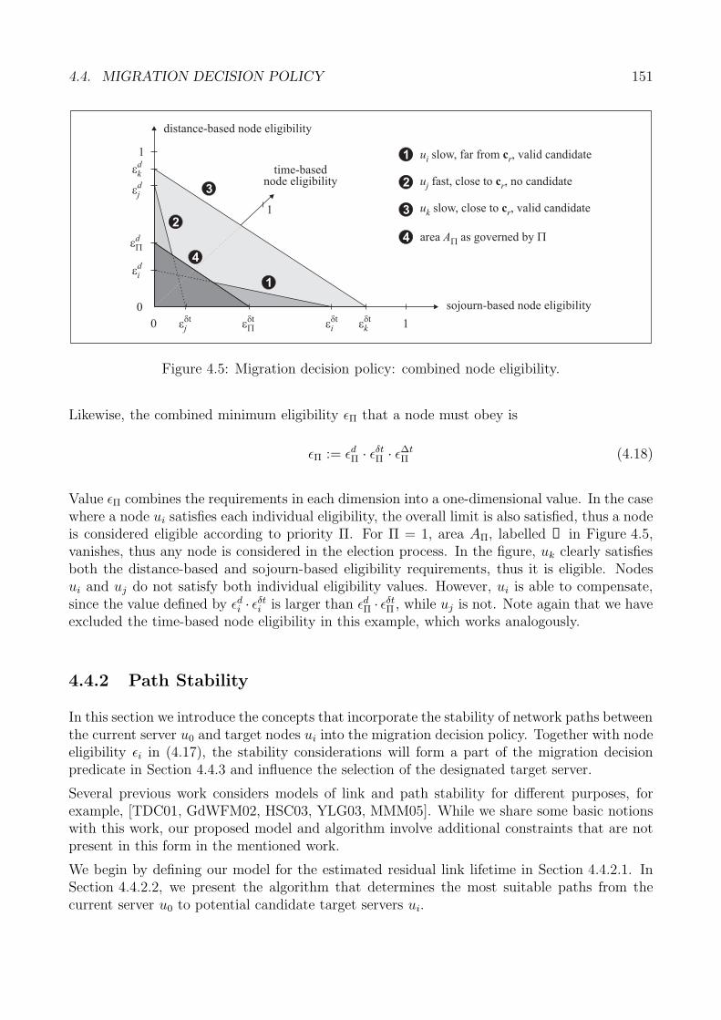
4.4. MIGRATION DECISION POLICY 151
1
2
3
4
1
0
1
2
1
3
4
u
u
u
A
i r
j r
k r
slow, far from , valid candidate
fast, close to , no candidate
slow, close to , valid candidate
area as governed by
c
c
c
d
k
d
j
d
d
i
distance-based node eligibility
time-basednode eligibility
0 �t
j �t
�t
i �t
k
sojourn-based node eligibility
1
Figure 4.5: Migration decision policy: combined node eligibility.
Likewise, the combined minimum eligibility εΠ that a node must obey is
εΠ := εdΠ · εδt
Π · εΔtΠ (4.18)
Value εΠ combines the requirements in each dimension into a one-dimensional value. In the casewhere a node ui satisfies each individual eligibility, the overall limit is also satisfied, thus a nodeis considered eligible according to priority Π. For Π = 1, area AΠ, labelled ➍ in Figure 4.5,vanishes, thus any node is considered in the election process. In the figure, uk clearly satisfiesboth the distance-based and sojourn-based eligibility requirements, thus it is eligible. Nodesui and uj do not satisfy both individual eligibility values. However, ui is able to compensate,since the value defined by εd
i · εδti is larger than εd
Π · εδtΠ , while uj is not. Note again that we have
excluded the time-based node eligibility in this example, which works analogously.
4.4.2 Path Stability
In this section we introduce the concepts that incorporate the stability of network paths betweenthe current server u0 and target nodes ui into the migration decision policy. Together with nodeeligibility εi in (4.17), the stability considerations will form a part of the migration decisionpredicate in Section 4.4.3 and influence the selection of the designated target server.
Several previous work considers models of link and path stability for different purposes, forexample, [TDC01, GdWFM02, HSC03, YLG03, MMM05]. While we share some basic notionswith this work, our proposed model and algorithm involve additional constraints that are notpresent in this form in the mentioned work.
We begin by defining our model for the estimated residual link lifetime in Section 4.4.2.1. InSection 4.4.2.2, we present the algorithm that determines the most suitable paths from thecurrent server u0 to potential candidate target servers ui.
152 CHAPTER 4. DATA MIGRATION
4.4.2.1 Estimated Residual Link Lifetime
Let us first consider the following model of link quality, which is based on geometric informationthat includes node positions ri(ti) and node speeds vi(ti), as returned from network topologyexploration. We assume that the quality of a link connecting nodes ui, uj is modelled by avariable qi,j(t) ∈ [0, 1] that describes the packet loss probability on that link. Let di,j(t0)denote the Euclidean distance between nodes ui and uj at time t0. We define:
qi,j(t) =
{1 if di,j(t0) ≤ rtx
0 otherwise(4.19)
The given model is an idealization in that it considers a link to be perfect up to the nominaltransmission range rtx. Instead of modelling the imperfection of a wireless link at all times, weaddress this issue implicitly by assuming a decreased available bandwidth for migration. Wewill come back to this aspect in Section 4.4.2.2.
Let t0 denote the current time and observe that ∀i : t0 ≥ ti. Assume further, w.l.g., that ti ≥ tj .The distance di,j(t0) between any two nodes ui, uj at t0 is defined as follows:
di,j(t0) := |ri(ti) − rj(tj)| + vj · (ti − tj) + (vi + vj) · (t0 − ti) (4.20)
The distance di,j(t) between ui, uj at any future time t ≥ t0 is
di,j(t) = di,j(t0) + (vi + vj)(t − t0) (4.21)
Excluding special cases, the residual link lifetime is described by the difference t− t0 in (4.21).Reorganizing the equation yields
t − t0 =di,j(t) − di,j(t0)
vi + vj(4.22)
Substituting rtx for di,j(t) in (4.22) yields the residual link lifetime τi,j between nodes ui, uj:
τi,j =
⎧⎪⎪⎨⎪⎪⎩
min
{Δτmax,
rtx − di,j(t0)
vi + vj
}if di,j(t0) ≤ rtx ∧ vi + vj > 0
Δτmax if di,j(t0) ≤ rtx ∧ vi + vj = 00 if di,j(t0) > rtx
(4.23)
In (4.23), we assume τmax to be a sensible upper bound, which is for numerical reasons only. Ifboth vi and vj are zero, there is no relative movement between ui and uj and we also choosethis value. If the distance between two nodes is larger than the nominal transmission range rtx
at the current time t0, the residual link lifetime is, naturally, zero.
4.4.2.2 Algorithm for Path Computation
We now present the algorithm for determining appropriate paths from the current serveru0 to candidate nodes ui via a sequence of intermediary nodes. The algorithm, shown inListing 4.1, is executed by u0 once the residual link lifetimes τi,j have been calculated according
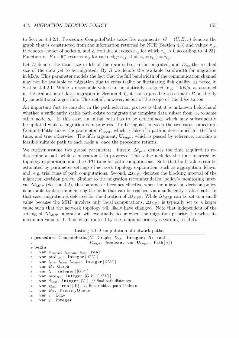
4.4. MIGRATION DECISION POLICY 153
to Section 4.4.2.1. Procedure ComputePaths takes five arguments: G = (U, E, τ) denotes thegraph that is constructed from the information returned by NTE (Section 4.3) and values τi,j.U denotes the set of nodes ui and E contains all edges ei,j for which τi,j > 0 according to (4.23).Function τ : E �→ R+
0 returns τi,j for each edge ei,j, that is, τ(ei,j) = τi,j .
Let D denote the total size in kB of the data subset to be migrated, and Dres the residualsize of the data yet to be migrated. By B we denote the available bandwidth for migrationin kB/s. This parameter models the fact that the full bandwidth of the communication channelmay not be available to migration due to cross traffic or fluctuating link quality, as noted inSection 4.4.2.1. While a reasonable value can be statically assigned (e.g. 1 kB/s, as assumedin the evaluation of data migration in Section 4.6), it is also possible to estimate B on the flyby an additional algorithm. This detail, however, is out of the scope of this dissertation.
An important fact to consider in the path selection process is that it is unknown beforehandwhether a sufficiently stable path exists to migrate the complete data subset from u0 to someother node ui. In this case, an initial path has to be determined, which may subsequentlybe updated while a migration is in progress. To distinguish between the two cases, procedureComputePaths takes the parameter Ptarget, which is false if a path is determined for the firsttime, and true otherwise. The fifth argument, Utarget, which is passed by reference, contains afeasible suitable path to each node ui once the procedure returns.
We further assume two global parameters. Firstly, Δtpath denotes the time required to re-determine a path while a migration is in progress. This value includes the time incurred bytopology exploration, and the CPU time for path computations. Note that both values can beestimated by parameter settings of network topology exploration, such as aggregation delays,and, e.g. trial runs of path computations. Second, ΔtMDP denotes the blocking interval of themigration decision policy. Similar to the migration recommendation policy’s monitoring inter-val ΔtMRP (Section 4.2), this parameter becomes effective when the migration decision policyis not able to determine an eligible node that can be reached via a sufficiently stable path. Inthat case, migration is deferred for the duration of ΔtMDP. While ΔtMRP can be set to a smallvalue because the MRP involves only local computations, ΔtMDP is typically set to a largervalue such that the network topology will likely have changed. Note that independent of thesetting of ΔtMDP, migration will eventually occur when the migration priority Π reaches itsmaximum value of 1. This is guaranteed by the temporal priority according to (4.4).
Listing 4.1: Computation of network paths.
1 procedure ComputePaths (G : Graph ; Dres : integer ; B : real ;2 Ptarget : boolean ; var Utarget : Path [n ] )3 begin4 var τreqmax, τreqmin, τreq : real5 var predBFS : integer [ |G.V | ]6 var lmin, lmax, lstretch : integer [ |G.V | ]7 var H : Graph8 var lH : integer [ |G.V | ]9 var predH2 : integer [ |G.V | ] [ |G.V | ]
10 var dfinal : integer [ |V | ] // final path distances11 var τfinal : real [ |V | ] // final residual path lifetimes12 var EG : Pr ior ityQueue13 var e : Edge14 var j : integer
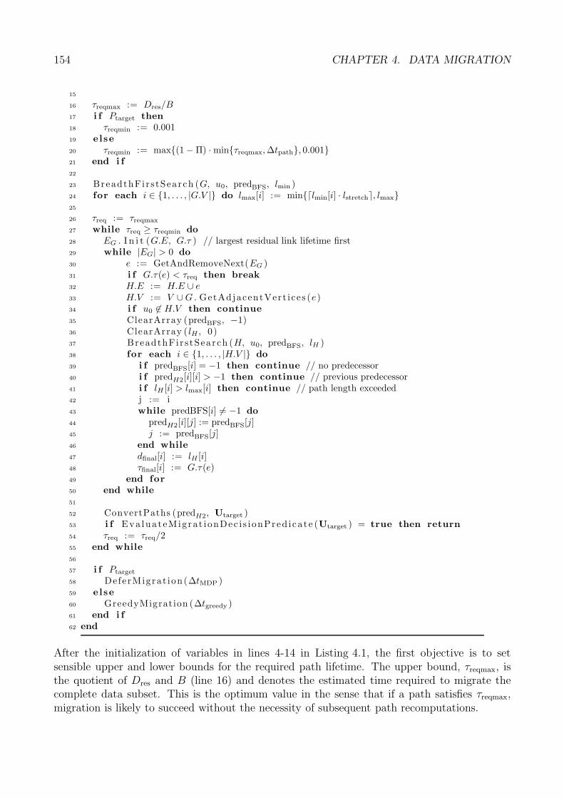
154 CHAPTER 4. DATA MIGRATION
15
16 τreqmax := Dres/B17 i f Ptarget then18 τreqmin := 0.00119 else20 τreqmin := max{(1 − Π) · min{τreqmax, Δtpath}, 0.001}21 end i f22
23 BreadthFir s tSearch (G, u0, predBFS, lmin )24 for each i ∈ {1, . . . , |G.V |} do lmax[i] := min{�lmin[i] · lstretch�, lmax}25
26 τreq := τreqmax
27 while τreq ≥ τreqmin do28 EG . I n i t (G.E, G.τ ) // largest residual link lifetime first29 while |EG| > 0 do30 e := GetAndRemoveNext(EG )31 i f G.τ(e) < τreq then break32 H.E := H.E ∪ e33 H.V := V ∪ G . GetAdjacentVert i ces (e)34 i f u0 �∈ H.V then continue35 ClearArray (predBFS, −1)36 ClearArray ( lH , 0)37 BreadthFir s tSearch (H, u0, predBFS, lH )38 for each i ∈ {1, . . . , |H.V |} do39 i f predBFS[i] = −1 then continue // no predecessor40 i f predH2[i][i] > −1 then continue // previous predecessor41 i f lH [i] > lmax[i] then continue // path length exceeded42 j := i43 while predBFS[i] �= −1 do44 predH2[i][j] := predBFS[j]45 j := predBFS[j]46 end while47 dfinal[i] := lH [i]48 τfinal[i] := G.τ(e)49 end for50 end while51
52 ConvertPaths (predH2, Utarget )53 i f Eva lua teMigrat ionDec i s ionPred icate (Utarget ) = true then return54 τreq := τreq/255 end while56
57 i f Ptarget
58 DeferMigrat ion (ΔtMDP )59 else60 GreedyMigration (Δtgreedy )61 end i f62 end
After the initialization of variables in lines 4-14 in Listing 4.1, the first objective is to setsensible upper and lower bounds for the required path lifetime. The upper bound, τreqmax, isthe quotient of Dres and B (line 16) and denotes the estimated time required to migrate thecomplete data subset. This is the optimum value in the sense that if a path satisfies τreqmax,migration is likely to succeed without the necessity of subsequent path recomputations.
4.4. MIGRATION DECISION POLICY 155
The lower bound, denoted τreqmin, depends on whether a migration is already in progress orthe designated target server is yet to be determined. In the former case, no other option thanfinding the most stable alternative path to the already selected designated target server exists.In this case, we set the minimum required lifetime to a value that is close to but larger thanzero in order for the following while loop to terminate eventually. In the procedure, we havearbitrarily set this value to 0.001, that is, one millisecond (line 18).
In the latter case, all options to determine a designated target server are still open and it isnot mandatory to tolerate situations in which only unstable paths exist. In this case, τreqmin
designates the minimum lifetime that a path must satisfy, otherwise, migration is deferred tothe next blocking interval ΔtMDP. At this point, we are able to incorporate migration priorityΠ from (4.6) one more time, which quantifies the urgency of a migration and which we haveused previously to describe sufficiently eligible nodes ((4.18)).
Let us first consider the expression min{τreqmax, Δtpath} in the assignment of τreqmin as shownin line 20 of Listing 4.1. The rationale behind this term is that it is desirable to find a networkpath that lasts for at least the time it takes to redetermine a subsequent path. This means thatsubsequent path recomputations can be initiated sufficiently in advance so that a new pathis available in time for a transparent switch of paths during migration (Section 4.5). Whenτreqmax < Δtpath, however, only a small number of data items are to be transferred, and a pathwith smaller lifetime is already sufficient.
Let us now assume a small value for the migration priority Π, in which case τreqmin is set toa value close to the expression min{τreqmax, Δtpath}. This reflects the semantics of Π in thatΠ ≈ 0 corresponds to the strongest restrictions on τreqmin. However, for larger Π, indicating amore urgent migration, the value of the expression is relaxed. Eventually, Δtreqmin assumes itsminimum value, which represents virtually no requirements on the path lifetime.
The purpose of lines 23-24 is to determine the maximum length that shall be allowed for aspecific path. The motivation for this restriction is due to the following property of path lengths.Because the link lifetime model in Section 4.4.2.1 is based on the geometric distance betweennodes, more stable paths imply a larger number of hops. However, with every additional hopcommunication cost increase.
For that reason, we restrict the maximum length of paths as follows. In line 23, the breadthfirst search (BFS) initially determines the shortest path from u0 to all other target nodes ui
without considering the stability of links. Procedure BreadthFirstSearch returns, apart fromthe predecessor list that is not required here, the array lmin, which contains the length of theshortest path to each node ui. In line 24, the minimum path length between u0 and each ui isstretched by the factor lstretch, which gives the maximum allowed path length lmax between u0
and ui. This allows to specify a sensible degree of flexibility in the subsequent path selectionprocess. To avoid arbitrarily long paths, we limit the length of any path to the maximum valuelmax. Considering the dimensions of typical network topology exploration regions (Section 4.3),this value can typically be set in the range of a few hops.
Lines 26-50 perform the actual computation of the most stable paths from u0 to each nodeui based on the restrictions on path lifetime and path length in the intervals [τreqmin, τreqmax]and each [lmin[i], lmax[i]], respectively. The outer while loop (lines 27-50) is initialized in line 26with the required path lifetime τreq. This value initially takes the most optimistic value τreqmax
156 CHAPTER 4. DATA MIGRATION
to seek out highly stable paths first, before less stable paths are explored. Next, the priorityqueue EG is initialized in line 28 with the set of edges E of graph G in descending order ofthe residual link lifetimes τi,j . Right after entering the inner while loop (lines 29-49), edge ewith the next largest residual link lifetime is retrieved from EG (line 30). While the lifetimesof retrieved edges obey the required lifetime τreq (line 31), edge e and its adjacent vertices areadded to graph H (lines 32 and 33). If the start vertex u0 has not yet been added to H.V(line 34), no path exists that originates at u0 and the while loop is continued. Otherwise, thepredecessors and path lengths of the following BFS are reset (lines 35 and 36).
At this point, graph H contains only edges whose lifetime is at least τreq, and a breadth firstsearch is run on H in line 37. The task of lines 38-49 is to determine the paths between u0 andeach ui such that each path’s length falls within the valid interval [lmin[i], lmax[i]]. Lines 39-41test various conditions under which a path cannot be updated. Firstly, in line 39, BFS couldnot determine a predecessor, in which case no path from u0 to the considered node ui exists.Second, in line 40, a previous predecessor was already determined, hence, a valid path witha larger residual path lifetime was already found in a previous iteration. Third, line 41 teststhe length restriction, and no path larger than the restriction is allowed. If all restrictions aresatisfied, the newly found path from u0 to some ui is updated in lines 42-46. Finally, the lengthand residual path lifetime of this path are set in lines 47 and 48, respectively.
The inner while loop eventually terminates due to the inability to find additional edges thatsatisfy the required lifetime (line 31). After leaving the while loop, the helper procedure inline 52 converts the predecessor list of each path from u0 to ui to the array of paths Utarget.Note that only paths that satisfy the stability requirements are present, hence, a path to everyui does not necessarily have to exist. Observe also that lmin[i] ≤ dfinal[i] ≤ lmax[i]. Next, themigration decision predicate is evaluated via a call to EvaluateMigrationDecisionPredicate inline 53, taking Utarget as argument. Note that we have omitted node eligibility εi for ease ofexposition (Section 4.4.3). If the MDP returns true, it was able to determine an eligible nodethat is also reachable via a sufficiently stable path. In this case, the procedure returns andthe migration mechanism is subsequently fed with the designated target server and the path toit. If the migration decision is negative, then τreq is relaxed according to an exponential decayfunction (line 54), and the process of finding sufficiently stable paths is repeated.
Eventually, τreq drops below τmin, in which case the outer while loop is exited. If the migrationwas just initiated and the target server was not yet selected, the migration is deferred to thenext migration cycle, which occurs after ΔtMDP (line 58). In the case where a migration isalready in progress and a source route is not available, geometric routing is used instead. Thisdecision is motivated by the fact that migration should continue in the hope that it will succeedwithout specific robustness measures. We will investigate both source routing and geometricrouting with respect to the impact on migration performance in Section 4.6.
4.4.3 Output of the Migration Decision Policy
We now define the migration decision predicate PMDP, which decides on whether or not amigration is to be carried out. The input to the MDP comprises the node eligibility valuesεi and εΠ from (4.17) and (4.18), respectively, and the set of paths Utarget as returned fromprocedure EvaluateMigrationDecisionPredicate(Utarget) in Listing 4.1.
4.5. MIGRATION MECHANISM 157
Let us first construct the auxiliary set I containing only indexes for target nodes that aresufficiently eligible and to which a sufficiently stable path from u0 exists:
I = {i | εi ≥ εΠ ∧ ∃ path Utarget[i] to ui} (4.24)
The migration decision predicate can be directly stated as follows:
PMDP := |I| > 0 or, alternatively, PMPD := ∃i ∈ I (4.25)
Hence, migration will occur if a node exists that has at least the eligibility that priority Πdictates, and a sufficiently stable target path exists to that node. Observe that an eligible nodemay not be reachable because no sufficiently stable path exists and vice versa.
The target node utarget and the target path Utarget to that node are defined as follows:
(utarget, Utarget) := (ui,Utarget[i]) : i ∈ I ∧ ∀j �= i : j ∈ I ⇒ (εi, i) > (εj , j) (4.26)
In the previous equation, we have established a total order of tuples (a, b) with component-wisecomparison, where the first element beats the second element in a comparison.
If the migration decision predicate in (4.25) is true, the most eligible target node reachable viaa sufficiently stable path is input to the migration mechanism. Otherwise, the policy is deferredto the next migration cycle after the blocking interval ΔtMDP (Section 4.4.2.2).
4.5 Migration Mechanism
This section describes the mechanism of the data migration component, shown in Figure 4.1and 2.22. The task of the mechanisms is to implement the robust and efficient transfer of adata subset from its current (source) server u0 to the designated target server utarget.
The objective of the mechanisms is twofold. Firstly, data migration is carried out upon thetriggering of the migration decision policy. We describe this process in Section 4.5.1. Second,data consolidation is required when two servers are handling the same data subset concurrentlydue to a previous migration failure. This process is described in Section 4.5.2.
4.5.1 Data Migration
The migration process is initiated by the source server u0 after the positive evaluation ofthe migration decision predicate in (4.25). The algorithm shown in Listing 4.2 specifies theinteractions between u0 and utarget that take place during a migration. The interactions aregoverned by the following states. A data server operating in active state receives and processesupdates and queries on the data subset, which it receives based on the core data storagemechanism in Section 3.3.2. The migrating and receiving states denote the condition wheresource and target server, respectively, are involved in a running migration process. Duringthese states, a data subset is transferred from the source server u0 to the target server utarget.By retired we denote the state where the source server has completed its migration and thetarget server has fully taken over, that is, assumed the active state.
158 CHAPTER 4. DATA MIGRATION
The entry point of the data migration process is procedure InitMigration in Listing 4.2 (line 11),which takes target server utarget and path Utarget from (4.26) as input. Every migration is set upby an explicit migration request that u0 sends to utarget (line 15). The request contains Utarget
so that both nodes will communicate via that path. When utarget receives the migration request(line 18) and if it is able to accept a migration, it assumes the receiving state (line 22) andreplies with a migration acknowledgement (line 23). However, if, for example, utarget is alreadyinvolved in the processing of another migration, it may decline the request to avoid becominga communication bottleneck (not shown in Listing 4.2).
When the migration acknowledgement is received from the target server (line 26), u0 assumesthe migrating state (line 28). The subsequent transfer of the serialized data subset from u0 toutarget is initiated by an asynchronous call to InitSendDataSubset (line 29). During the completetransfer, a customized transport/routing layer protocol is used, optimized for the source routeUtarget that is used between both nodes. On the transport layer, any transport protocol suitablefor mobile environments may be used. However, we optimize flow control by using a slidingwindow-based mechanism that is tuned to wireless ad-hoc networks. In this approach, windowsizes are determined as a function of the number of hops between u0 and utarget. In order toachieve maximum throughput, the window size is selected based on the results obtained in[CXSN04]. The rationale is to consider the special nature of the wireless medium. In contrastto a switched network, where the full bandwidth on both the inbound and outbound line of aswitch/router is concurrently available, this does not hold in MANETs. Instead, a router, i.e.any network node, must share the medium for inbound and outbound traffic.
On the routing tier, resilient source routing is used, which takes the initially determined pathUtarget as input. The path’s validity is determined by the residual path lifetime τ(Utarget). Thetimer in line 30 controls when path recomputation is due, such that a new path is available fora transparent switch before the previous path becomes stale. For that, the timer is initializedwith the difference between τ(Utarget) and Δtpath, where the latter denotes the time to redeter-mine a path (Section 4.4.2.2). Observe that if the path’s residual lifetime was already belowΔtpath, the timer will immediately expire. Upon expiration, procedure TimerExpired (line 33)initiates the recomputation of a new path (line 35). While data migration continuous to usethe current path Utarget, network topology exploration according to Section 4.3 and procedureComputePaths in Listing 4.1 are run in the background to redetermine a new path. Once de-termined, procedure PathChangeNotification is invoked (line 38) and the migration mechanismtransparently switches from the current path to this new path (line 40). The timer is initiatedagain in line 41 for subsequent path computations.
Every data item received at the target server (line 44) is stored locally (line 46) and acknowl-edged (line 47). When the last data item is received by the target server (line 48), it immedi-ately moves into active state (line 49). Then it begins sending server advertisements (line 50,Section 3.3.1), becoming known to other nodes in the vicinity of its associated reference co-ordinate and accepting incoming requests. Upon the reception of a data acknowledgementat the source server (line 54), u0 checks whether all data items of the subset to be migratedwere acknowledged, that is, whether the data transfer is complete (line 56). In that case, thesource server becomes aware that utarget has taken over. It stops sending server advertisements(line 57), goes to retired state (line 58), and migration terminates. At this point, the targetserver has fully taken over the data subset and is the only one that is now in active state.

4.5. MIGRATION MECHANISM 159
Listing 4.2: Data migration.
1 module DataMigration2 begin3 var utarget : Node // used by u0
4 var u0 : Node // used by utarget
5 var Utarget : Path // used by u0 and utarget
6 var pathRecomputationTimer : Timer // used by u0
7 var s t a t e : Migrat ionState := a c t i v e // used by u0 and utarget
8 var s to rage : Set of Object // used by u0 and utarget
9 var bu f f e r : Set of Object // used by u0
10
11 procedure In i tMig ra t i on (utarget : Node ; Utarget : Path )12 begin // executed by u0
13 this .utarget := utarget
14 this .Utarget := Utarget
15 SendMigrationRequest (utarget , Utarget , u0 )16 end17
18 procedure ReceiveMigrat ionRequest (u0 : Node ; Utarget : Path)19 begin // executed by utarget
20 this .u0 = u0
21 this .Utarget := Utarget
22 s t a t e = r e c e i v i n g23 SendMigrationAck (u0 )24 end25
26 procedure ReceiveMigrationAck ( )27 begin // executed by u0
28 s t a t e := migrat ing29 InitSendDataSubset (utarget , Utarget )30 SetTimer ( pathRecomputationTimer , max{0, τ(Utarget) − Δtpath})31 end32
33 procedure TimerExpired ( )34 begin // executed by u0
35 RecomputePaths ( )36 end37
38 procedure PathChangeNoti f i cat ion (Utarget : Path)39 begin // executed by u0
40 this .Utarget := Utarget
41 SetTimer ( pathRecomputationTimer , max{0, τ(Utarget) − Δtpath})42 end43
44 procedure ReceiveData (oi : Object )45 begin // executed by utarget
46 ExecuteUpdate( s to rage , oi ) // executed while utarget is in r e c e i v i n g state47 SendDataAck (u0, oi )48 i f DataComplete ( ) then49 s t a t e := a c t i v e50 In i tSe rve rAdver t i s ement ( )51 end i f52 end
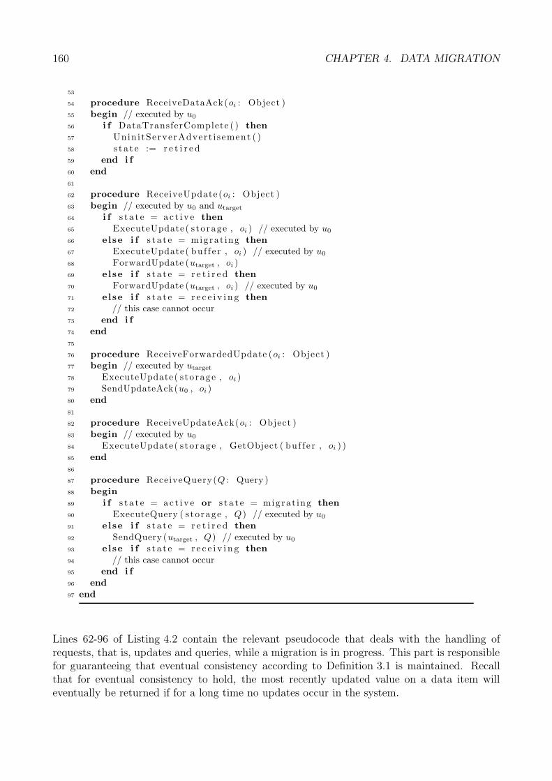
160 CHAPTER 4. DATA MIGRATION
53
54 procedure ReceiveDataAck(oi : Object )55 begin // executed by u0
56 i f DataTransferComplete ( ) then57 Unin i tServerAdver t i sement ( )58 s t a t e := r e t i r e d59 end i f60 end61
62 procedure ReceiveUpdate (oi : Object )63 begin // executed by u0 and utarget
64 i f s t a t e = ac t i v e then65 ExecuteUpdate ( s to rage , oi ) // executed by u0
66 else i f s t a t e = migrat ing then67 ExecuteUpdate ( bu f f e r , oi ) // executed by u0
68 ForwardUpdate (utarget , oi )69 else i f s t a t e = r e t i r e d then70 ForwardUpdate (utarget , oi ) // executed by u0
71 else i f s t a t e = r e c e i v i n g then72 // this case cannot occur73 end i f74 end75
76 procedure ReceiveForwardedUpdate (oi : Object )77 begin // executed by utarget
78 ExecuteUpdate( s to rage , oi )79 SendUpdateAck(u0 , oi )80 end81
82 procedure ReceiveUpdateAck(oi : Object )83 begin // executed by u0
84 ExecuteUpdate( s to rage , GetObject ( bu f f e r , oi ) )85 end86
87 procedure ReceiveQuery(Q : Query )88 begin89 i f s t a t e = ac t i v e or s t a t e = migrat ing then90 ExecuteQuery ( s torage , Q) // executed by u0
91 else i f s t a t e = r e t i r e d then92 SendQuery (utarget , Q) // executed by u0
93 else i f s t a t e = r e c e i v i n g then94 // this case cannot occur95 end i f96 end97 end
Lines 62-96 of Listing 4.2 contain the relevant pseudocode that deals with the handling ofrequests, that is, updates and queries, while a migration is in progress. This part is responsiblefor guaranteeing that eventual consistency according to Definition 3.1 is maintained. Recallthat for eventual consistency to hold, the most recently updated value on a data item willeventually be returned if for a long time no updates occur in the system.
4.5. MIGRATION MECHANISM 161
The way requests are handled essentially depends on the current state that the source andtarget server are in while receiving updates (line 62) and queries (line 87). Let us first considerthe handling of updates. While u0 is in active state (line 64), it accepts any incoming updatesfrom remote nodes and processes them locally (line 65). When an update occurs on a dataitem that is received while u0 is in migrating state (line 66), then that update is put in a localbuffer (line 67) and forwarded to the target server as well (line 68). Note that the data itemis not updated on the local storage of the source server. Any data update received by utarget
is immediately written to the local data storage (line 78) of that server. After that, the targetserver sends an acknowledgement for that data item back to the source server (line 79). Oncean acknowledgement of a data item is received at the source server (line 82), the update canbe moved from the buffer to the persistent storage (line 84).
From the point where the source server is in retired state (line 69), it forwards updates immedi-ately to the target server without further processing (line 70). Finally, note that while utarget isin receiving state (line 72), it does not receive any requests other than those forwarded from u0.This is because it does not yet disseminate advertisements (Section 3.3.1), which are requiredfor client requests to locate utarget in the first place.
Queries, on the other hand, are received through the ReceiveQuery procedure in line 87. Inboth active and migrating state (line 89) a query received at the source server u0 is immediatelyevaluated based on the local storage (line 90). In retired state (line 91), queries are forwardedby the retired server to the now current server (line 92). Note that as in the case of updates,no queries are received during receiving state (line 93).
With respect to eventual consistency, the handling of updates in lines 62-85 guarantees that noupdate is lost once made persistent in the local storage of any data server. While it is trivialto achieve eventual consistency when a server is in active or retired state, the situation is morecomplicated while a migration is in progress. The following problem occurs in the event wherea data update that is forwarded from the source to the target server is lost.
Assume that a data update is received at u0 while a migration is in progress (line 66). Assumefurther that instead of executing the update on the buffer of u0, as shown in line 67, it isimmediately written to the local storage instead. Next, let us assume that the data item,which is forwarded in line 68, is lost on the way to the target server utarget while migration is inprogress. Note that this is allowed according to the system model we stated in Section 3.1. Letus finally assume that the migration of the data subset eventually succeeds, that is, the targetserver transits to active state, while the source server drops the data subset and goes to retiredstate. In this event, the original update on the data item is lost. If no further updates on thisobject occur, this update was the most recent one, hence, eventual consistency is violated.
To avoid this situation, data migration first updates a request in an intermediary buffer inline 67. Only when the source server has received the update’s corresponding acknowledgementin line 82 from the target server, it makes the update persistent in its local storage (line 84).In case a forwarded data update is lost between the source and the target server, that updateis never made persistent due to the absence of a corresponding acknowledgement.
Observe that for the above arguments to hold, node failures must not occur, which is what wehave assumed in the system model in Section 3.1. The handling of node failures in conjunctionwith data replication will be discussed briefly in the outlook in Section 6.2.1.
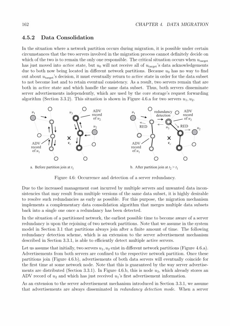
162 CHAPTER 4. DATA MIGRATION
4.5.2 Data Consolidation
In the situation where a network partition occurs during migration, it is possible under certaincircumstances that the two servers involved in the migration process cannot definitely decide onwhich of the two is to remain the only one responsible. The critical situation occurs when utarget
has just moved into active state, but u0 will not receive all of utarget’s data acknowledgementsdue to both now being located in different network partitions. Because u0 has no way to findout about utarget’s decision, it must eventually return to active state in order for the data subsetto not become lost and to retain eventual consistency. As a result, two servers remain that areboth in active state and which handle the same data subset. Thus, both servers disseminateserver advertisements independently, which are used by the core storage’s request forwardingalgorithm (Section 3.3.2). This situation is shown in Figure 4.6.a for two servers u1, u2.
a. Before partition join at t1 b. After partition join at >t t2 1
ADVrecordof u1
cr
u2
cr
u1ADVrecordof u2
ADVrecordof u1
u1
u2
u3
u3
ADVrecordof u2
redundancydetection
RED RED
Figure 4.6: Occurrence and detection of a server redundancy.
Due to the increased management cost incurred by multiple servers and unwanted data incon-sistencies that may result from multiple versions of the same data subset, it is highly desirableto resolve such redundancies as early as possible. For this purpose, the migration mechanismimplements a complementary data consolidation algorithm that merges multiple data subsetsback into a single one once a redundancy has been detected.
In the situation of a partitioned network, the earliest possible time to become aware of a serverredundancy is upon the rejoining of two network partitions. Note that we assume in the systemmodel in Section 3.1 that partitions always join after a finite amount of time. The followingredundancy detection scheme, which is an extension to the server advertisement mechanismdescribed in Section 3.3.1, is able to efficiently detect multiple active servers.
Let us assume that initially, two servers u1, u2 exist in different network partitions (Figure 4.6.a).Advertisements from both servers are confined to the respective network partition. Once thesepartitions join (Figure 4.6.b), advertisements of both data servers will eventually coincide forthe first time at some network node. Note that this is guaranteed by the way server advertise-ments are distributed (Section 3.3.1). In Figure 4.6.b, this is node u3, which already stores anADV record of u2 and which has just received u1’s first advertisement information.
As an extension to the server advertisement mechanism introduced in Section 3.3.1, we assumethat advertisements are always disseminated in redundancy detection mode. When a server
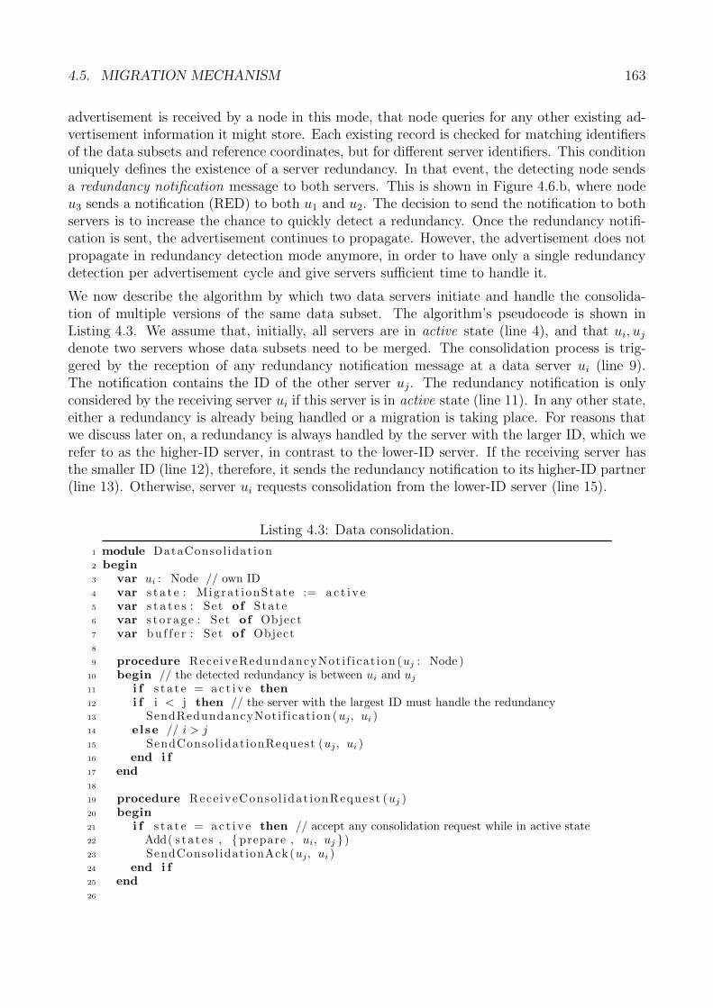
4.5. MIGRATION MECHANISM 163
advertisement is received by a node in this mode, that node queries for any other existing ad-vertisement information it might store. Each existing record is checked for matching identifiersof the data subsets and reference coordinates, but for different server identifiers. This conditionuniquely defines the existence of a server redundancy. In that event, the detecting node sendsa redundancy notification message to both servers. This is shown in Figure 4.6.b, where nodeu3 sends a notification (RED) to both u1 and u2. The decision to send the notification to bothservers is to increase the chance to quickly detect a redundancy. Once the redundancy notifi-cation is sent, the advertisement continues to propagate. However, the advertisement does notpropagate in redundancy detection mode anymore, in order to have only a single redundancydetection per advertisement cycle and give servers sufficient time to handle it.
We now describe the algorithm by which two data servers initiate and handle the consolida-tion of multiple versions of the same data subset. The algorithm’s pseudocode is shown inListing 4.3. We assume that, initially, all servers are in active state (line 4), and that ui, uj
denote two servers whose data subsets need to be merged. The consolidation process is trig-gered by the reception of any redundancy notification message at a data server ui (line 9).The notification contains the ID of the other server uj. The redundancy notification is onlyconsidered by the receiving server ui if this server is in active state (line 11). In any other state,either a redundancy is already being handled or a migration is taking place. For reasons thatwe discuss later on, a redundancy is always handled by the server with the larger ID, which werefer to as the higher-ID server, in contrast to the lower-ID server. If the receiving server hasthe smaller ID (line 12), therefore, it sends the redundancy notification to its higher-ID partner(line 13). Otherwise, server ui requests consolidation from the lower-ID server (line 15).
Listing 4.3: Data consolidation.
1 module DataConsol idation2 begin3 var ui : Node // own ID4 var s t a t e : Migrat ionState := a c t i v e5 var s t a t e s : Set of State6 var s to rage : Set of Object7 var bu f f e r : Set of Object8
9 procedure Rece iveRedundancyNot i f i cat ion (uj : Node )10 begin // the detected redundancy is between ui and uj
11 i f s t a t e = ac t i v e then12 i f i < j then // the server with the largest ID must handle the redundancy13 SendRedundancyNoti f icat ion (uj, ui )14 else // i > j15 SendConsol idationRequest (uj, ui )16 end i f17 end18
19 procedure Rece iveConso l idat ionRequest (uj )20 begin21 i f s t a t e = ac t i v e then // accept any consolidation request while in active state22 Add( s ta te s , {prepare , ui, uj })23 SendConsol idat ionAck (uj, ui )24 end i f25 end26
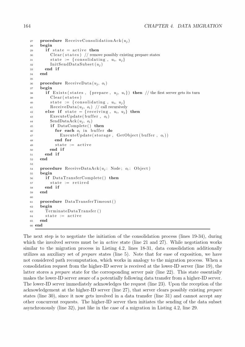
164 CHAPTER 4. DATA MIGRATION
27 procedure Rece iveConsol idationAck (uj )28 begin29 i f s t a t e = ac t i v e then30 Clear ( s t a t e s ) // remove possibly existing prepare states31 s t a t e := { conso l ida t ing , ui, uj}32 InitSendDataSubset (uj )33 end i f34 end35
36 procedure ReceiveData (uj , oi )37 begin38 i f Ex i s t s ( s ta t e s , {prepare , uj, ui }) then // the first server gets its turn39 Clear ( s t a t e s )40 s t a t e := { conso l ida t ing , ui, uj}41 ReceiveData (uj , oi ) // call recursively42 else i f s t a t e = { r e c e i v i n g , ui, uj} then43 ExecuteUpdate ( bu f f e r , oi )44 SendDataAck (uj , oi )45 i f DataComplete ( ) then46 for each oi in bu f f e r do47 ExecuteUpdate ( s to rage , GetObject ( bu f f e r , oi ) )48 end for49 s t a t e := a c t i v e50 end i f51 end i f52 end53
54 procedure ReceiveDataAck(uj : Node ; oi : Object )55 begin56 i f DataTransferComplete ( ) then57 s t a t e := r e t i r e d58 end i f59 end60
61 procedure DataTransferTimeout ( )62 begin63 TerminateDataTransfer ( )64 s t a t e := a c t i v e65 end66 end
The next step is to negotiate the initiation of the consolidation process (lines 19-34), duringwhich the involved servers must be in active state (line 21 and 27). While negotiation workssimilar to the migration process in Listing 4.2, lines 18-31, data consolidation additionallyutilizes an auxiliary set of prepare states (line 5). Note that for ease of exposition, we havenot considered path recomputation, which works in analogy to the migration process. When aconsolidation request from the higher-ID server is received at the lower-ID server (line 19), thelatter stores a prepare state for the corresponding server pair (line 22). This state essentiallymakes the lower-ID server aware of a potentially following data transfer from a higher-ID server.The lower-ID server immediately acknowledges the request (line 23). Upon the reception of theacknowledgement at the higher-ID server (line 27), that server clears possibly existing preparestates (line 30), since it now gets involved in a data transfer (line 31) and cannot accept anyother concurrent requests. The higher-ID server then initiates the sending of the data subsetasynchronously (line 32), just like in the case of a migration in Listing 4.2, line 29.
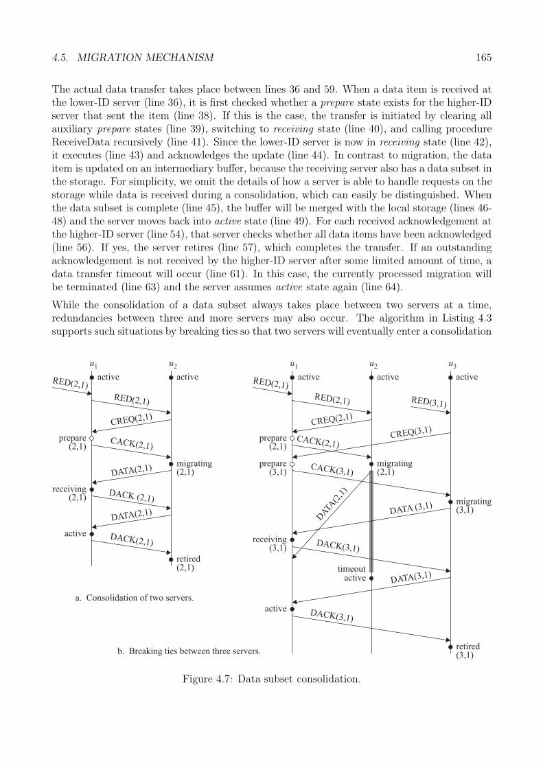
4.5. MIGRATION MECHANISM 165
The actual data transfer takes place between lines 36 and 59. When a data item is received atthe lower-ID server (line 36), it is first checked whether a prepare state exists for the higher-IDserver that sent the item (line 38). If this is the case, the transfer is initiated by clearing allauxiliary prepare states (line 39), switching to receiving state (line 40), and calling procedureReceiveData recursively (line 41). Since the lower-ID server is now in receiving state (line 42),it executes (line 43) and acknowledges the update (line 44). In contrast to migration, the dataitem is updated on an intermediary buffer, because the receiving server also has a data subset inthe storage. For simplicity, we omit the details of how a server is able to handle requests on thestorage while data is received during a consolidation, which can easily be distinguished. Whenthe data subset is complete (line 45), the buffer will be merged with the local storage (lines 46-48) and the server moves back into active state (line 49). For each received acknowledgement atthe higher-ID server (line 54), that server checks whether all data items have been acknowledged(line 56). If yes, the server retires (line 57), which completes the transfer. If an outstandingacknowledgement is not received by the higher-ID server after some limited amount of time, adata transfer timeout will occur (line 61). In this case, the currently processed migration willbe terminated (line 63) and the server assumes active state again (line 64).
While the consolidation of a data subset always takes place between two servers at a time,redundancies between three and more servers may also occur. The algorithm in Listing 4.3supports such situations by breaking ties so that two servers will eventually enter a consolidation
u1 u2
active
RED(2,1)
CREQ(2,1)
prepare(2,1)
migrating(2,1)
CACK(2,1)
DATA(2,1)
DACK (2,1)
retired(2,1)
receiving(2,1)
DATA(2,1)
DACK(2,1)active
RED(2,1)
a. Consolidation of two servers.
u1 u2
active
RED(2,1)
CREQ(2,1)
prepare(2,1)
migrating(2,1)
CACK(2,1)
DATA
(2,1
)
DACK(3,1)
retired(3,1)
u3
active
RED(3,1)
prepare(3,1)
CACK(3,1)
CREQ(3,1)
receiving(3,1)
DATA (3,1)
DATA(3,1)
active DACK(3,1)
timeout
b. Breaking ties between three servers.
active
migrating(3,1)
RED(2,1)active active
Figure 4.7: Data subset consolidation.
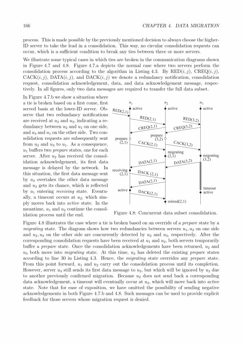
166 CHAPTER 4. DATA MIGRATION
process. This is made possible by the previously mentioned decision to always choose the higher-ID server to take the lead in a consolidation. This way, no circular consolidation requests canoccur, which is a sufficient condition to break any ties between three or more servers.
We illustrate some typical cases in which ties are broken in the communication diagrams shownin Figure 4.7 and 4.8. Figure 4.7.a depicts the normal case where two servers perform theconsolidation process according to the algorithm in Listing 4.3. By RED(i, j), CREQ(i, j),CACK(i, j), DATA(i, j), and DACK(i, j) we denote a redundancy notification, consolidationrequest, consolidation acknowledgement, data, and data acknowledgement message, respec-tively. In all figures, only two data messages are required to transfer the full data subset.
u1 u2
active
u3
active
timeoutactive
active
prepare(3,2)
RED(2,1)
migrating(3,2)
DACK (2,1)
retired(2,1)
DATA(2,1)
DACK(2,1)active
RED(2,1)
CREQ(2,1)CREQ(3,2)
RED(3,2)
prepare(2,1) CACK(3,2)
migrating(2,1)
CACK(2,1)
DATA(2,1)
receiving(2,1)
DATA(3,2)
Figure 4.8: Concurrent data subset consolidation.
In Figure 4.7.b we show a situation wherea tie is broken based on a first come, firstserved basis at the lower-ID server. Ob-serve that two redundancy notificationsare received at u2 and u3, indicating a re-dundancy between u2 and u1 on one side,and u3 and u1 on the other side. Two con-solidation requests are subsequently sentfrom u2 and u3 to u1. As a consequence,u1 buffers two prepare states, one for eachserver. After u2 has received the consol-idation acknowledgement, its first datamessage is delayed by the network. Inthis situation, the first data message sentby u3 overtakes the other data messageand u3 gets its chance, which is reflectedby u1 entering receiving state. Eventu-ally, a timeout occurs at u2, which sim-ply moves back into active state. In themeantime, u1 and u2 continue the consol-idation process until the end.
Figure 4.8 illustrates the case where a tie is broken based on an override of a prepare state by amigrating state. The diagram shows how two redundancies between servers u1, u2 on one sideand u2, u3 on the other side are concurrently detected by u2 and u3, respectively. After thecorresponding consolidation requests have been received at u1 and u2, both servers temporarilybuffer a prepare state. Once the consolidation acknowledgements have been returned, u2 andu3 both move into migrating state. At this time, u2 has deleted the existing prepare statesaccording to line 30 in Listing 4.3. Hence, the migrating state overrides any prepare state.From this point forward, u1 and u2 carry out the consolidation process until its completion.However, server u3 still sends its first data message to u2, but which will be ignored by u2 dueto another previously confirmed migration. Because u2 does not send back a correspondingdata acknowledgement, a timeout will eventually occur at u3, which will move back into activestate. Note that for ease of exposition, we have omitted the possibility of sending negativeacknowledgements in both Figure 4.7.b and 4.8. Such messages can be used to provide explicitfeedback for those servers whose migration request is denied.
4.6. PERFORMANCE ANALYSIS 167
4.6 Performance Analysis
In this section we examine in detail the performance of the data migration approach by meansof a comparative experimental analysis. We have implemented two variants of data migration,which employ source routing and geometric routing, and which we denote by DataMiP (sourcerouting) and DataMiP (BPR), respectively.1 In addition, we have implemented two furtherapproaches, termed greedy migration and progressive migration.
DataMiP (source routing) designates the migration approach that relies on network paths thatare computed by the algorithm in Listing 4.1. According to this approach, a source routeis updated during a migration process whenever the previous one is about to weaken. Thismigration approach is shown in Listing 4.2. In the DataMiP (BPR) variant, the stabilityanalysis in Section 4.4.2 is also performed during the determination of a target node. Thedifference to DataMiP (source routing) is that the output path of the algorithm in Listing 4.1 isomitted during migration. Instead, geometric routing based on bidirectional perimeter routing(BPR, Section 3.2) is used for the migration of the data subset.
In greedy migration, once the current server reaches the threshold distance dthresh, greedy routingis used as the means for network topology exploration to find a suitable target node. A requestis sent by the current server into the direction of the reference coordinate until a node is reachedat which greedy routing fails. BPR is then used as the underlying routing protocol to migratedata to the selected target node. Progressive migration is also initiated upon reaching dthresh. Incontrast to greedy migration, the selection of a target server is based solely on the set of knownneighbors of the current server. From this set, the neighbor is chosen that is located closest tothe reference coordinate, but only if a node exists that is nearer to the reference coordinate thanthe current server. Upon completion of migration to the selected node, subsequent iterations ofprogressive migration follow where data is migrated to nodes located even closer to the referencecoordinate. This procedure continues until no further node can be determined. Both greedyand progressive migration are re-initiated once dthresh is reached again.
The following system parameters, which are also shown in Table 4.1, are applicable in theevaluation of the migration approaches. The general system parameters that are assumed inall experiments presented in this dissertation are listed in Table 3.3.
A total simulation time of 3600 seconds was chosen, corresponding to an increase by a factor of10 compared to the evaluation of core data storage (Section 3.5.2). This is necessary to achievegood statistical values, because migrations occur at a much lower frequency than requests inmost of the simulations. As in the case of core data storage, only a single reference coordinateis placed in the center of the simulation area, with a default size of 200 ·200 m2. No requests areprocessed in order to avoid possible side effects on the migration performance. Furthermore,server advertisements are sent with a rate of 1/second.
The default number of data items is increased also by a factor of 10 compared to core datastorage and set to 10000. This value corresponds to 320 kB of data for each migration, assuming32 bytes per data item. We assume a data packet capacity of 1500 bytes, thus approximately47 data items can be carried in a single data packet. The threshold distance dthresh, which isapplicable in all four discussed approaches, is set to 100 m. The critical distance dcrit, which isonly applicable in the two DataMiP variants, is set to 150 m.
1DataMiP standing for Data Migration Protocol.
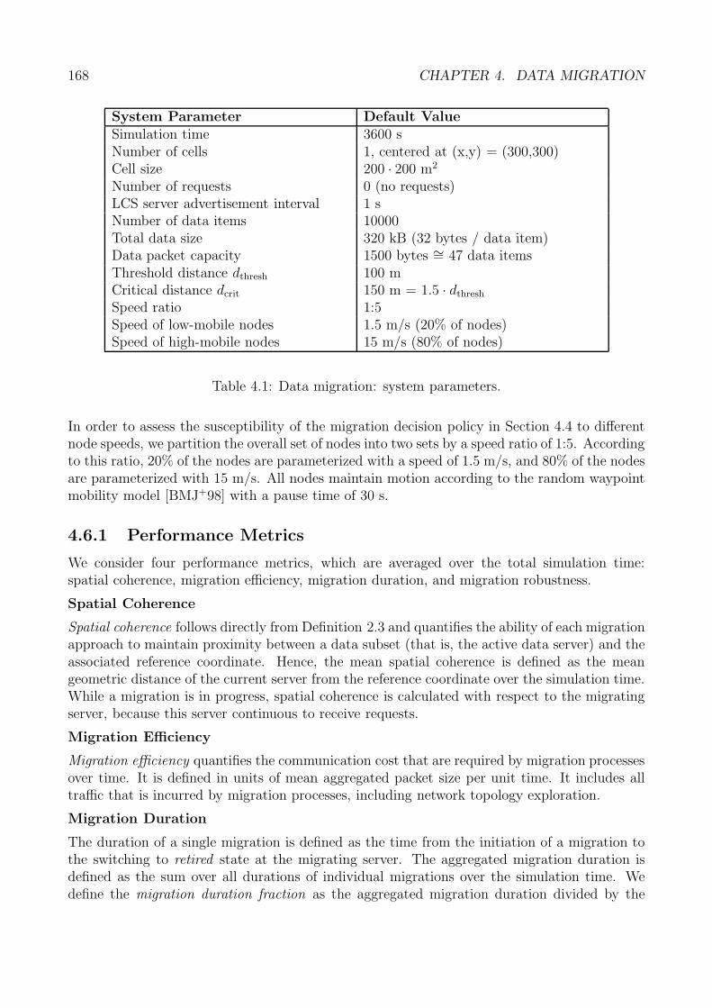
168 CHAPTER 4. DATA MIGRATION
System Parameter Default ValueSimulation time 3600 sNumber of cells 1, centered at (x,y) = (300,300)Cell size 200 · 200 m2
Number of requests 0 (no requests)LCS server advertisement interval 1 sNumber of data items 10000Total data size 320 kB (32 bytes / data item)Data packet capacity 1500 bytes ∼= 47 data itemsThreshold distance dthresh 100 mCritical distance dcrit 150 m = 1.5 · dthresh
Speed ratio 1:5Speed of low-mobile nodes 1.5 m/s (20% of nodes)Speed of high-mobile nodes 15 m/s (80% of nodes)
Table 4.1: Data migration: system parameters.
In order to assess the susceptibility of the migration decision policy in Section 4.4 to differentnode speeds, we partition the overall set of nodes into two sets by a speed ratio of 1:5. Accordingto this ratio, 20% of the nodes are parameterized with a speed of 1.5 m/s, and 80% of the nodesare parameterized with 15 m/s. All nodes maintain motion according to the random waypointmobility model [BMJ+98] with a pause time of 30 s.
4.6.1 Performance Metrics
We consider four performance metrics, which are averaged over the total simulation time:spatial coherence, migration efficiency, migration duration, and migration robustness.
Spatial Coherence
Spatial coherence follows directly from Definition 2.3 and quantifies the ability of each migrationapproach to maintain proximity between a data subset (that is, the active data server) and theassociated reference coordinate. Hence, the mean spatial coherence is defined as the meangeometric distance of the current server from the reference coordinate over the simulation time.While a migration is in progress, spatial coherence is calculated with respect to the migratingserver, because this server continuous to receive requests.
Migration Efficiency
Migration efficiency quantifies the communication cost that are required by migration processesover time. It is defined in units of mean aggregated packet size per unit time. It includes alltraffic that is incurred by migration processes, including network topology exploration.
Migration Duration
The duration of a single migration is defined as the time from the initiation of a migration tothe switching to retired state at the migrating server. The aggregated migration duration isdefined as the sum over all durations of individual migrations over the simulation time. Wedefine the migration duration fraction as the aggregated migration duration divided by the
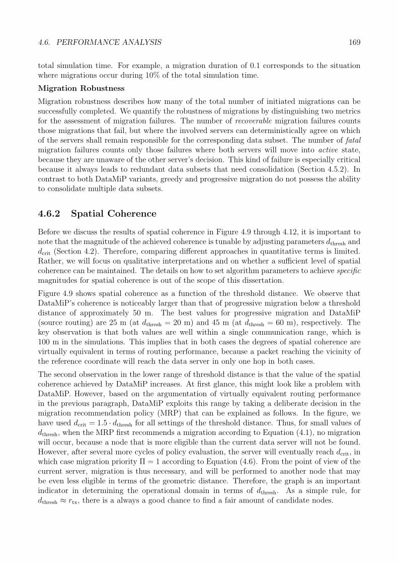
4.6. PERFORMANCE ANALYSIS 169
total simulation time. For example, a migration duration of 0.1 corresponds to the situationwhere migrations occur during 10% of the total simulation time.
Migration Robustness
Migration robustness describes how many of the total number of initiated migrations can besuccessfully completed. We quantify the robustness of migrations by distinguishing two metricsfor the assessment of migration failures. The number of recoverable migration failures countsthose migrations that fail, but where the involved servers can deterministically agree on whichof the servers shall remain responsible for the corresponding data subset. The number of fatalmigration failures counts only those failures where both servers will move into active state,because they are unaware of the other server’s decision. This kind of failure is especially criticalbecause it always leads to redundant data subsets that need consolidation (Section 4.5.2). Incontrast to both DataMiP variants, greedy and progressive migration do not possess the abilityto consolidate multiple data subsets.
4.6.2 Spatial Coherence
Before we discuss the results of spatial coherence in Figure 4.9 through 4.12, it is important tonote that the magnitude of the achieved coherence is tunable by adjusting parameters dthresh anddcrit (Section 4.2). Therefore, comparing different approaches in quantitative terms is limited.Rather, we will focus on qualitative interpretations and on whether a sufficient level of spatialcoherence can be maintained. The details on how to set algorithm parameters to achieve specificmagnitudes for spatial coherence is out of the scope of this dissertation.
Figure 4.9 shows spatial coherence as a function of the threshold distance. We observe thatDataMiP’s coherence is noticeably larger than that of progressive migration below a thresholddistance of approximately 50 m. The best values for progressive migration and DataMiP(source routing) are 25 m (at dthresh = 20 m) and 45 m (at dthresh = 60 m), respectively. Thekey observation is that both values are well within a single communication range, which is100 m in the simulations. This implies that in both cases the degrees of spatial coherence arevirtually equivalent in terms of routing performance, because a packet reaching the vicinity ofthe reference coordinate will reach the data server in only one hop in both cases.
The second observation in the lower range of threshold distance is that the value of the spatialcoherence achieved by DataMiP increases. At first glance, this might look like a problem withDataMiP. However, based on the argumentation of virtually equivalent routing performancein the previous paragraph, DataMiP exploits this range by taking a deliberate decision in themigration recommendation policy (MRP) that can be explained as follows. In the figure, wehave used dcrit = 1.5 · dthresh for all settings of the threshold distance. Thus, for small values ofdthresh, when the MRP first recommends a migration according to Equation (4.1), no migrationwill occur, because a node that is more eligible than the current data server will not be found.However, after several more cycles of policy evaluation, the server will eventually reach dcrit, inwhich case migration priority Π = 1 according to Equation (4.6). From the point of view of thecurrent server, migration is thus necessary, and will be performed to another node that maybe even less eligible in terms of the geometric distance. Therefore, the graph is an importantindicator in determining the operational domain in terms of dthresh. As a simple rule, fordthresh ≈ rtx, there is a always a good chance to find a fair amount of candidate nodes.
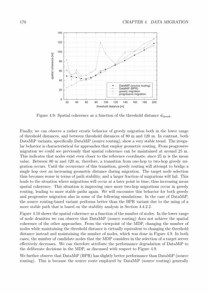
170 CHAPTER 4. DATA MIGRATION
0
20
40
60
80
100
120
140
20 40 60 80 100 120 140 160 180 200
sp
atia
lco
he
ren
ce
[m]
threshold distance [m]
DataMiP (source routing)DataMiP (BPR)greedy migrationprogressive migration
Figure 4.9: Spatial coherence as a function of the threshold distance dthresh.
Finally, we can observe a rather erratic behavior of greedy migration both in the lower rangeof threshold distances, and between threshold distances of 80 m and 120 m. In contrast, bothDataMiP variants, specifically DataMiP (source routing), show a very stable trend. The irregu-lar behavior is characteristical for approaches that employ geometric routing. From progressivemigration we could see previously that spatial coherence can be maintained at around 25 m.This indicates that nodes exist even closer to the reference coordinate, since 25 m is the meanvalue. Between 80 m and 120 m, therefore, a transition from one-hop to two-hop greedy mi-gration occurs. Until the occurrence of this transition, greedy routing will attempt to bridge asingle hop over an increasing geometric distance during migration. The target node selectionthus becomes worse in terms of path stability, and a larger fraction of migrations will fail. Thisleads to the situation where migrations will occur at a later point in time, thus increasing meanspatial coherence. This situation is improving once more two-hop migrations occur in greedyrouting, leading to more stable paths again. We will encounter this behavior for both greedyand progressive migration also in some of the following simulations. In the case of DataMiP,the source routing-based variant performs better than the BPR variant due to the using of amore stable path that is based on the stability analysis in Section 4.4.2.2.
Figure 4.10 shows the spatial coherence as a function of the number of nodes. In the lower rangeof node densities we can observe that DataMiP (source routing) does not achieve the spatialcoherence of the other approaches. From the viewpoint of the MDP, changing the number ofnodes while maintaining the threshold distance is virtually equivalent to changing the thresholddistance instead and maintaining the number of nodes, which was done in Figure 4.9. In bothcases, the number of candidate nodes that the MDP considers in the selection of a target servereffectively decreases. We can therefore attribute the performance degradation of DataMiP tothe deliberate decisions in the MDP, as discussed with respect to Figure 4.9.
We further observe that DataMiP (BPR) has slightly better performance than DataMiP (sourcerouting). This is because the source route employed by DataMiP (source routing) generally
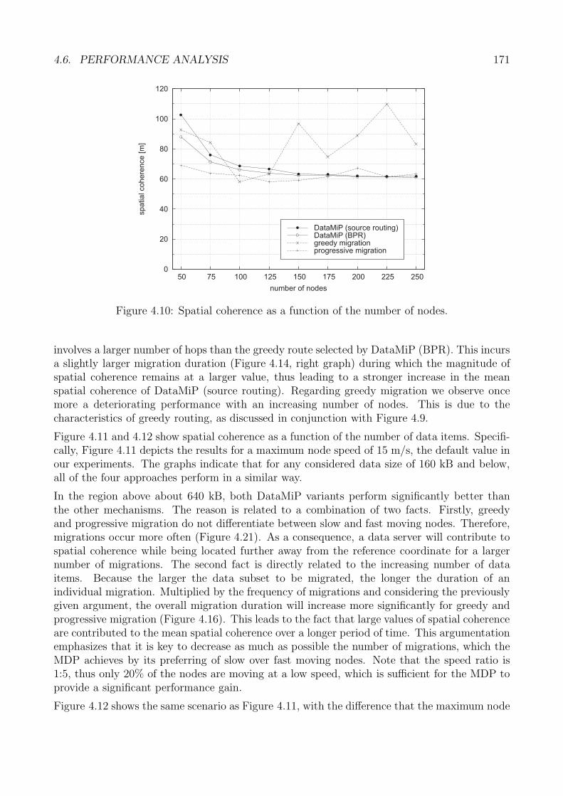
4.6. PERFORMANCE ANALYSIS 171
0
20
40
60
80
100
120
50 75 100 125 150 175 200 225 250
sp
atia
lco
he
ren
ce
[m]
number of nodes
DataMiP (source routing)DataMiP (BPR)greedy migrationprogressive migration
Figure 4.10: Spatial coherence as a function of the number of nodes.
involves a larger number of hops than the greedy route selected by DataMiP (BPR). This incursa slightly larger migration duration (Figure 4.14, right graph) during which the magnitude ofspatial coherence remains at a larger value, thus leading to a stronger increase in the meanspatial coherence of DataMiP (source routing). Regarding greedy migration we observe oncemore a deteriorating performance with an increasing number of nodes. This is due to thecharacteristics of greedy routing, as discussed in conjunction with Figure 4.9.
Figure 4.11 and 4.12 show spatial coherence as a function of the number of data items. Specifi-cally, Figure 4.11 depicts the results for a maximum node speed of 15 m/s, the default value inour experiments. The graphs indicate that for any considered data size of 160 kB and below,all of the four approaches perform in a similar way.
In the region above about 640 kB, both DataMiP variants perform significantly better thanthe other mechanisms. The reason is related to a combination of two facts. Firstly, greedyand progressive migration do not differentiate between slow and fast moving nodes. Therefore,migrations occur more often (Figure 4.21). As a consequence, a data server will contribute tospatial coherence while being located further away from the reference coordinate for a largernumber of migrations. The second fact is directly related to the increasing number of dataitems. Because the larger the data subset to be migrated, the longer the duration of anindividual migration. Multiplied by the frequency of migrations and considering the previouslygiven argument, the overall migration duration will increase more significantly for greedy andprogressive migration (Figure 4.16). This leads to the fact that large values of spatial coherenceare contributed to the mean spatial coherence over a longer period of time. This argumentationemphasizes that it is key to decrease as much as possible the number of migrations, which theMDP achieves by its preferring of slow over fast moving nodes. Note that the speed ratio is1:5, thus only 20% of the nodes are moving at a low speed, which is sufficient for the MDP toprovide a significant performance gain.
Figure 4.12 shows the same scenario as Figure 4.11, with the difference that the maximum node
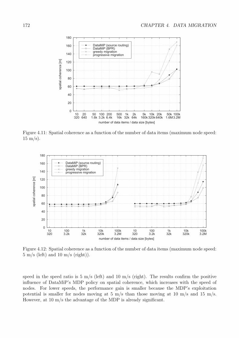
172 CHAPTER 4. DATA MIGRATION
0
20
40
60
80
100
120
140
160
180
10320
20640
501.6k
1003.2k
2006.4k
50016k
1k32k
2k64k
5k160k
10k320k
20k640k
50k1.6M
100k3.2M
sp
atia
lco
he
ren
ce
[m]
number of data items / data size [bytes]
DataMiP (source routing)DataMiP (BPR)greedy migrationprogressive migration
Figure 4.11: Spatial coherence as a function of the number of data items (maximum node speed:15 m/s).
0
20
40
60
80
100
120
140
160
180
10320
1003.2k
1k32k
10k320k
100k3.2M
10320
1003.2k
1k32k
10k320k
100k3.2M
sp
atia
lco
he
ren
ce
[m]
number of data items / data size [bytes]
DataMiP (source routing)DataMiP (BPR)greedy migrationprogressive migration
Figure 4.12: Spatial coherence as a function of the number of data items (maximum node speed:5 m/s (left) and 10 m/s (right)).
speed in the speed ratio is 5 m/s (left) and 10 m/s (right). The results confirm the positiveinfluence of DataMiP’s MDP policy on spatial coherence, which increases with the speed ofnodes. For lower speeds, the performance gain is smaller because the MDP’s exploitationpotential is smaller for nodes moving at 5 m/s than those moving at 10 m/s and 15 m/s.However, at 10 m/s the advantage of the MDP is already significant.
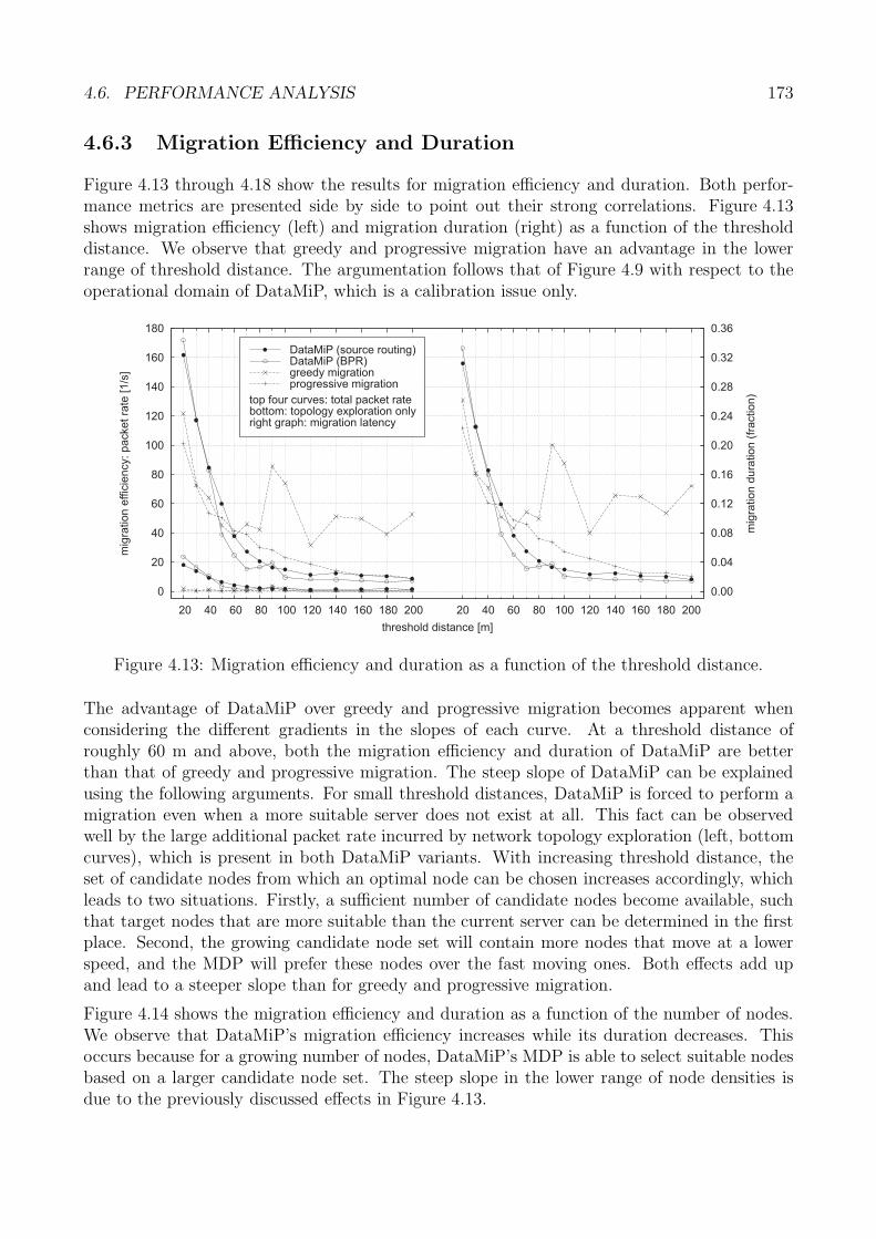
4.6. PERFORMANCE ANALYSIS 173
4.6.3 Migration Efficiency and Duration
Figure 4.13 through 4.18 show the results for migration efficiency and duration. Both perfor-mance metrics are presented side by side to point out their strong correlations. Figure 4.13shows migration efficiency (left) and migration duration (right) as a function of the thresholddistance. We observe that greedy and progressive migration have an advantage in the lowerrange of threshold distance. The argumentation follows that of Figure 4.9 with respect to theoperational domain of DataMiP, which is a calibration issue only.
0
20
40
60
80
100
120
140
160
180
20 40 60 80 100 120 140 160 180 200 20 40 60 80 100 120 140 160 180 200
0.00
0.04
0.08
0.12
0.16
0.20
0.24
0.28
0.32
0.36
mig
ration
effic
iency:packetra
te[1
/s]
mig
ration
dura
tion
(fra
ction)
threshold distance [m]
DataMiP (source routing)DataMiP (BPR)greedy migrationprogressive migration
top four curves: total packet ratebottom: topology exploration onlyright graph: migration latency
Figure 4.13: Migration efficiency and duration as a function of the threshold distance.
The advantage of DataMiP over greedy and progressive migration becomes apparent whenconsidering the different gradients in the slopes of each curve. At a threshold distance ofroughly 60 m and above, both the migration efficiency and duration of DataMiP are betterthan that of greedy and progressive migration. The steep slope of DataMiP can be explainedusing the following arguments. For small threshold distances, DataMiP is forced to perform amigration even when a more suitable server does not exist at all. This fact can be observedwell by the large additional packet rate incurred by network topology exploration (left, bottomcurves), which is present in both DataMiP variants. With increasing threshold distance, theset of candidate nodes from which an optimal node can be chosen increases accordingly, whichleads to two situations. Firstly, a sufficient number of candidate nodes become available, suchthat target nodes that are more suitable than the current server can be determined in the firstplace. Second, the growing candidate node set will contain more nodes that move at a lowerspeed, and the MDP will prefer these nodes over the fast moving ones. Both effects add upand lead to a steeper slope than for greedy and progressive migration.
Figure 4.14 shows the migration efficiency and duration as a function of the number of nodes.We observe that DataMiP’s migration efficiency increases while its duration decreases. Thisoccurs because for a growing number of nodes, DataMiP’s MDP is able to select suitable nodesbased on a larger candidate node set. The steep slope in the lower range of node densities isdue to the previously discussed effects in Figure 4.13.
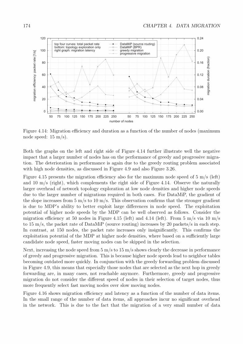
174 CHAPTER 4. DATA MIGRATION
0
20
40
60
80
100
120
50 75 100 125 150 175 200 225 250 50 75 100 125 150 175 200 225 250
0.00
0.04
0.08
0.12
0.16
0.20
0.24
mig
ration
effic
iency:packetra
te[1
/s]
mig
ration
dura
tion
(fra
ction)
number of nodes
DataMiP (source routing)DataMiP (BPR)greedy migrationprogressive migration
top four curves: total packet ratebottom: topology exploration onlyright graph: migration latency
Figure 4.14: Migration efficiency and duration as a function of the number of nodes (maximumnode speed: 15 m/s).
Both the graphs on the left and right side of Figure 4.14 further illustrate well the negativeimpact that a larger number of nodes has on the performance of greedy and progressive migra-tion. The deterioration in performance is again due to the greedy routing problem associatedwith high node densities, as discussed in Figure 4.9 and also Figure 3.26.
Figure 4.15 presents the migration efficiency also for the maximum node speed of 5 m/s (left)and 10 m/s (right), which complements the right side of Figure 4.14. Observe the naturallylarger overhead of network topology exploration at low node densities and higher node speedsdue to the larger number of migrations required in both cases. For DataMiP, the gradient ofthe slope increases from 5 m/s to 10 m/s. This observation confirms that the stronger gradientis due to MDP’s ability to better exploit large differences in node speed. The exploitationpotential of higher node speeds by the MDP can be well observed as follows. Consider themigration efficiency at 50 nodes in Figure 4.15 (left) and 4.14 (left). From 5 m/s via 10 m/sto 15 m/s, the packet rate of DataMiP (source routing) increases by 20 packets/s in each step.In contrast, at 150 nodes, the packet rate increases only insignificantly. This confirms theexploitation potential of the MDP at higher node densities, where based on a sufficiently largecandidate node speed, faster moving nodes can be skipped in the selection.
Next, increasing the node speed from 5 m/s to 15 m/s shows clearly the decrease in performanceof greedy and progressive migration. This is because higher node speeds lead to neighbor tablesbecoming outdated more quickly. In conjunction with the greedy forwarding problem discussedin Figure 4.9, this means that especially those nodes that are selected as the next hop in greedyforwarding are, in many cases, not reachable anymore. Furthermore, greedy and progressivemigration do not consider the different speed of nodes in their selection of target nodes, thusmore frequently select fast moving nodes over slow moving nodes.
Figure 4.16 shows migration efficiency and latency as a function of the number of data items.In the small range of the number of data items, all approaches incur no significant overheadin the network. This is due to the fact that the migration of a very small number of data
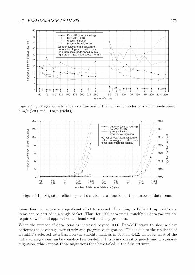
4.6. PERFORMANCE ANALYSIS 175
0
5
10
15
20
25
30
35
40
45
50
50 75 100 125 150 175 200 225 250 50 75 100 125 150 175 200 225 250
mig
ratio
ne
ffic
ien
cy:p
acke
tra
te[1
/s]
number of nodes
top four curves: total packet ratebottom: topology exploration onlyleft graph: max. node speed: 5 m/sright graph: max. node speed: 10 m/s
DataMiP (source routing)DataMiP (BPR)greedy migrationprogressive migration
Figure 4.15: Migration efficiency as a function of the number of nodes (maximum node speed:5 m/s (left) and 10 m/s (right)).
0
40
80
120
160
200
240
280
10320
1003.2k
1k32k
10k320k
100k3.2M
10320
1003.2k
1k32k
10k320k
100k3.2M
0.00
0.08
0.16
0.24
0.32
0.40
0.48
0.56
mig
ration
effic
iency:packetra
te[1
/s]
mig
ration
dura
tion
(fra
ction)
number of data items / data size [bytes]
DataMiP (source routing)DataMiP (BPR)greedy migrationprogressive migration
top four curves: total packet ratebottom: topology exploration onlyright graph: migration latency
Figure 4.16: Migration efficiency and duration as a function of the number of data items.
items does not require any significant effort to succeed. According to Table 4.1, up to 47 dataitems can be carried in a single packet. Thus, for 1000 data items, roughly 21 data packets arerequired, which all approaches can handle without any problems.
When the number of data items is increased beyond 1000, DataMiP starts to show a clearperformance advantage over greedy and progressive migration. This is due to the resilience ofDataMiP’s selected path based on the stability analysis in Section 4.4.2. Thereby, most of theinitiated migrations can be completed successfully. This is in contrast to greedy and progressivemigration, which repeat those migrations that have failed in the first attempt.
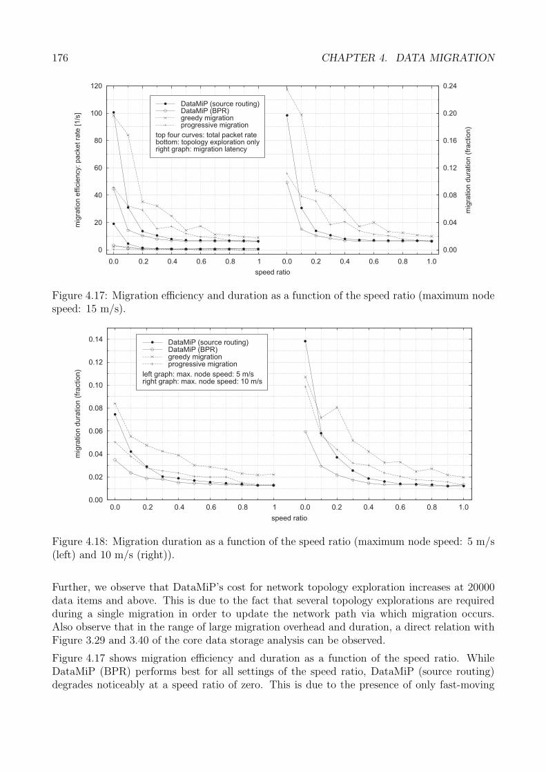
176 CHAPTER 4. DATA MIGRATION
0
20
40
60
80
100
120
0.0 0.2 0.4 0.6 0.8 1 0.0 0.2 0.4 0.6 0.8 1.0
0.00
0.04
0.08
0.12
0.16
0.20
0.24
mig
ration
effic
iency:packetra
te[1
/s]
mig
ration
dura
tion
(fra
ction)
speed ratio
DataMiP (source routing)DataMiP (BPR)greedy migrationprogressive migration
top four curves: total packet ratebottom: topology exploration onlyright graph: migration latency
Figure 4.17: Migration efficiency and duration as a function of the speed ratio (maximum nodespeed: 15 m/s).
0.00
0.02
0.04
0.06
0.08
0.10
0.12
0.14
0.0 0.2 0.4 0.6 0.8 1 0.0 0.2 0.4 0.6 0.8 1.0
mig
ratio
nd
ura
tio
n(f
ractio
n)
speed ratio
left graph: max. node speed: 5 m/sright graph: max. node speed: 10 m/s
DataMiP (source routing)DataMiP (BPR)greedy migrationprogressive migration
Figure 4.18: Migration duration as a function of the speed ratio (maximum node speed: 5 m/s(left) and 10 m/s (right)).
Further, we observe that DataMiP’s cost for network topology exploration increases at 20000data items and above. This is due to the fact that several topology explorations are requiredduring a single migration in order to update the network path via which migration occurs.Also observe that in the range of large migration overhead and duration, a direct relation withFigure 3.29 and 3.40 of the core data storage analysis can be observed.
Figure 4.17 shows migration efficiency and duration as a function of the speed ratio. WhileDataMiP (BPR) performs best for all settings of the speed ratio, DataMiP (source routing)degrades noticeably at a speed ratio of zero. This is due to the presence of only fast-moving
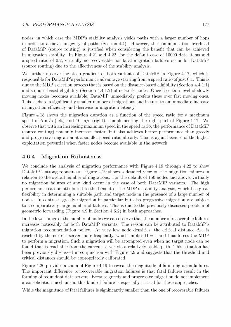
4.6. PERFORMANCE ANALYSIS 177
nodes, in which case the MDP’s stability analysis yields paths with a larger number of hopsin order to achieve longevity of paths (Section 4.4). However, the communication overheadof DataMiP (source routing) is justified when considering the benefit that can be achievedin migration stability. In Figure 4.21 and 4.22, for the default case of 10000 data items anda speed ratio of 0.2, virtually no recoverable nor fatal migration failures occur for DataMiP(source routing) due to the affectiveness of the stability analysis.
We further observe the steep gradient of both variants of DataMiP in Figure 4.17, which isresponsible for DataMiP’s performance advantage starting from a speed ratio of just 0.1. This isdue to the MDP’s election process that is based on the distance-based eligibility (Section 4.4.1.1)and sojourn-based eligibility (Section 4.4.1.2) of network nodes. Once a certain level of slowlymoving nodes becomes available, DataMiP immediately prefers these over fast moving ones.This leads to a significantly smaller number of migrations and in turn to an immediate increasein migration efficiency and decrease in migration latency.
Figure 4.18 shows the migration duration as a function of the speed ratio for a maximumspeed of 5 m/s (left) and 10 m/s (right), complementing the right part of Figure 4.17. Weobserve that with an increasing maximum speed in the speed ratio, the performance of DataMiP(source routing) not only increases faster, but also achieves better performance than greedyand progressive migration at a smaller speed ratio already. This is again because of the higherexploitation potential when faster nodes become available in the network.
4.6.4 Migration Robustness
We conclude the analysis of migration performance with Figure 4.19 through 4.22 to showDataMiP’s strong robustness. Figure 4.19 shows a detailed view on the migration failures inrelation to the overall number of migrations. For the default of 150 nodes and above, virtuallyno migration failures of any kind occur in the case of both DataMiP variants. The highperformance can be attributed to the benefit of the MDP’s stability analysis, which has greatflexibility in determining a suitable path and target node in the presence of a large number ofnodes. In contrast, greedy migration in particular but also progressive migration are subjectto a comparatively large number of failures. This is due to the previously discussed problem ofgeometric forwarding (Figure 4.9 in Section 4.6.2) in both approaches.
In the lower range of the number of nodes we can observe that the number of recoverable failuresincreases noticeably for both DataMiP variants. The reason can be attributed to DataMiP’smigration recommendation policy. At very low node densities, the critical distance dcrit isreached by the current server more frequently, which implies Π = 1 and thus forces the MDPto perform a migration. Such a migration will be attempted even when no target node can befound that is reachable from the current server via a relatively stable path. This situation hasbeen previously discussed in conjunction with Figure 4.9 and suggests that the threshold andcritical distances should be appropriately calibrated.
Figure 4.20 provides a zoom of Figure 4.19 to reveal the magnitude of fatal migration failures.The important difference to recoverable migration failures is that fatal failures result in theforming of redundant data servers. Because greedy and progressive migration do not implementa consolidation mechanism, this kind of failure is especially critical for these approaches.
While the magnitude of fatal failures is significantly smaller than the one of recoverable failures
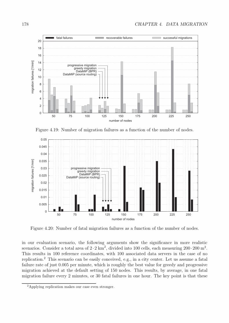
178 CHAPTER 4. DATA MIGRATION
0
2
4
6
8
10
12
14
16
18
20
50 75 100 125 150 175 200 225 250
mig
ration
failu
res
[1/m
in]
number of nodes
successful migrationsrecoverable failuresfatal failures
progressive migrationgreedy migration
DataMiP (BPR)DataMiP (source routing)
Figure 4.19: Number of migration failures as a function of the number of nodes.
0
0.005
0.01
0.015
0.02
0.025
0.03
0.035
0.04
0.045
0.05
50 75 100 125 150 175 200 225 250
mig
ratio
nfa
ilure
s[1
/min
]
number of nodes
progressive migrationgreedy migration
DataMiP (BPR)DataMiP (source routing)
Figure 4.20: Number of fatal migration failures as a function of the number of nodes.
in our evaluation scenario, the following arguments show the significance in more realisticscenarios. Consider a total area of 2 ·2 km2, divided into 100 cells, each measuring 200 ·200 m2.This results in 100 reference coordinates, with 100 associated data servers in the case of noreplication.2 This scenario can be easily conceived, e.g., in a city center. Let us assume a fatalfailure rate of just 0.005 per minute, which is roughly the best value for greedy and progressivemigration achieved at the default setting of 150 nodes. This results, by average, in one fatalmigration failure every 2 minutes, or 30 fatal failures in one hour. The key point is that these
2Applying replication makes our case even stronger.
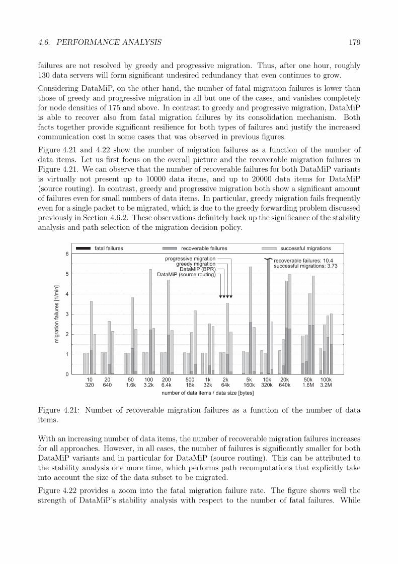
4.6. PERFORMANCE ANALYSIS 179
failures are not resolved by greedy and progressive migration. Thus, after one hour, roughly130 data servers will form significant undesired redundancy that even continues to grow.
Considering DataMiP, on the other hand, the number of fatal migration failures is lower thanthose of greedy and progressive migration in all but one of the cases, and vanishes completelyfor node densities of 175 and above. In contrast to greedy and progressive migration, DataMiPis able to recover also from fatal migration failures by its consolidation mechanism. Bothfacts together provide significant resilience for both types of failures and justify the increasedcommunication cost in some cases that was observed in previous figures.
Figure 4.21 and 4.22 show the number of migration failures as a function of the number ofdata items. Let us first focus on the overall picture and the recoverable migration failures inFigure 4.21. We can observe that the number of recoverable failures for both DataMiP variantsis virtually not present up to 10000 data items, and up to 20000 data items for DataMiP(source routing). In contrast, greedy and progressive migration both show a significant amountof failures even for small numbers of data items. In particular, greedy migration fails frequentlyeven for a single packet to be migrated, which is due to the greedy forwarding problem discussedpreviously in Section 4.6.2. These observations definitely back up the significance of the stabilityanalysis and path selection of the migration decision policy.
0
1
2
3
4
5
6
10320
20640
501.6k
1003.2k
2006.4k
50016k
1k32k
2k64k
5k160k
10k320k
20k640k
50k1.6M
100k3.2M
mig
ration
failu
res
[1/m
in]
number of data items / data size [bytes]
successful migrationsrecoverable failuresfatal failures
progressive migrationgreedy migration
DataMiP (BPR)DataMiP (source routing)
recoverable failures: 10.4successful migrations: 3.73
Figure 4.21: Number of recoverable migration failures as a function of the number of dataitems.
With an increasing number of data items, the number of recoverable migration failures increasesfor all approaches. However, in all cases, the number of failures is significantly smaller for bothDataMiP variants and in particular for DataMiP (source routing). This can be attributed tothe stability analysis one more time, which performs path recomputations that explicitly takeinto account the size of the data subset to be migrated.
Figure 4.22 provides a zoom into the fatal migration failure rate. The figure shows well thestrength of DataMiP’s stability analysis with respect to the number of fatal failures. While
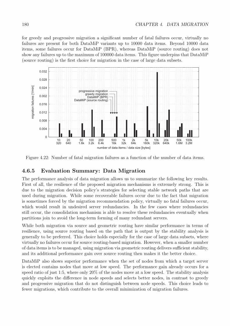
180 CHAPTER 4. DATA MIGRATION
for greedy and progressive migration a significant number of fatal failures occur, virtually nofailures are present for both DataMiP variants up to 10000 data items. Beyond 10000 dataitems, some failures occur for DataMiP (BPR), whereas DataMiP (source routing) does notshow any failures up to the maximum of 100000 data items. This figure underpins that DataMiP(source routing) is the first choice for migration in the case of large data subsets.
0
0.004
0.008
0.012
0.016
0.002
0.024
0.028
0.032
10320
20640
501.6k
1003.2k
2006.4k
50016k
1k32k
2k64k
5k160k
10k320k
20k640k
50k1.6M
100k3.2M
mig
ratio
nfa
ilure
s[1
/min
]
number of data items / data size [bytes]
progressive migrationgreedy migration
DataMiP (BPR)DataMiP (source routing)
Figure 4.22: Number of fatal migration failures as a function of the number of data items.
4.6.5 Evaluation Summary: Data Migration
The performance analysis of data migration allows us to summarize the following key results.First of all, the resilience of the proposed migration mechanisms is extremely strong. This isdue to the migration decision policy’s strategies for selecting stable network paths that areused during migration. While some recoverable failures occur due to the fact that migrationis sometimes forced by the migration recommendation policy, virtually no fatal failures occur,which would result in undesired server redundancies. In the few cases where redundanciesstill occur, the consolidation mechanism is able to resolve these redundancies eventually whenpartitions join to avoid the long-term forming of many redundant servers.
While both migration via source and geometric routing have similar performance in terms ofresilience, using source routing based on the path that is output by the stability analysis isgenerally to be preferred. This choice holds especially for the case of large data subsets, wherevirtually no failures occur for source routing-based migration. However, when a smaller numberof data items is to be managed, using migration via geometric routing delivers sufficient stability,and its additional performance gain over source routing then makes it the better choice.
DataMiP also shows superior performance when the set of nodes from which a target serveris elected contains nodes that move at low speed. The performance gain already occurs for aspeed ratio of just 1:5, where only 20% of the nodes move at a low speed. The stability analysisquickly exploits the difference in node speeds and selects better nodes, in contrast to greedyand progressive migration that do not distinguish between node speeds. This choice leads tofewer migrations, which contribute to the overall minimization of migration failures.
Chapter 5
Service Tier
The previous two chapters described the main contribution of this dissertation, consisting ofthe algorithms of the storage and routing tier according to the LCS framework in Figure 2.22.In close collaboration, both tiers provide robust, efficient, and scalable data storage based onthe location-centric storage paradigm of Definition 2.2.
In this chapter, we show how the storage tier can be exploited by concrete services of theLCS framework’s service tier, in order to deliver suitable base functionality to a variety oflocation-based applications. We begin by addressing Requirement (6) from Section 2.4 andintroduce suitable location semantics in Section 5.1 that incorporate the natural imperfectionof localization technology. In Section 5.2 we extend the system model from Section 3.1 assumedso far to also capture these semantics and to provide a storage structure on top of core datastorage that is tailored to the extended location semantics.
Section 5.3 introduces a location updating algorithm that builds on the location semanticsand the extended system model. The service tier of the LCS framework is complemented inSection 5.4 with the presentation of the semantics and algorithms for the processing of proba-bilistic spatial queries, including range and k-nearest neighbor queries. Evaluation results arediscussed in Section 5.5 to show the performance of the proposed update and query algorithms.
5.1 Semantics of Inaccurate Locations
Let us now formalize the notion of location in the presence of sensor measurements that lead toinaccurate location information. We apply concepts of two-dimensional (bivariate) probabilitydistributions, which are able to model inaccurate locations in a general way.
Definition 5.1. The location probability density function (location pdf) �(X) with X = (x, y) ∈R2 is any two-dimensional pdf in the Euclidean plane R2 that satisfies∫
X∈R2
�(X)dX = 1 (5.1)
In many cases, the technical means by which position information is gathered lead to an in-definite area where the location pdf is greater than zero at any point X of that area. For
181
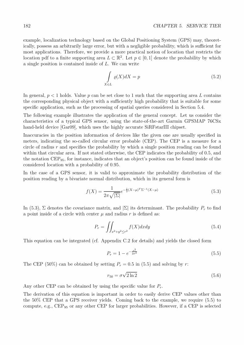
182 CHAPTER 5. SERVICE TIER
example, localization technology based on the Global Positioning System (GPS) may, theoret-ically, possess an arbitrarily large error, but with a negligible probability, which is sufficient formost applications. Therefore, we provide a more practical notion of location that restricts thelocation pdf to a finite supporting area L ⊂ R2. Let p ∈ [0, 1] denote the probability by whicha single position is contained inside of L. We can write∫
X∈L
�(X)dX = p (5.2)
In general, p < 1 holds. Value p can be set close to 1 such that the supporting area L containsthe corresponding physical object with a sufficiently high probability that is suitable for somespecific application, such as the processing of spatial queries considered in Section 5.4.
The following example illustrates the application of the general concept. Let us consider thecharacteristics of a typical GPS sensor, using the state-of-the-art Garmin GPSMAP 76CSxhand-held device [Gar09], which uses the highly accurate SiRFstarIII chipset.
Inaccuracies in the position information of devices like the given one are usually specified inmeters, indicating the so-called circular error probable (CEP). The CEP is a measure for acircle of radius r and specifies the probability by which a single position reading can be foundwithin that circular area. If not stated otherwise, the CEP indicates the probability of 0.5, andthe notation CEP95, for instance, indicates that an object’s position can be found inside of theconsidered location with a probability of 0.95.
In the case of a GPS sensor, it is valid to approximate the probability distribution of theposition reading by a bivariate normal distribution, which in its general form is
f(X) =1
2π√|Σ|e
− 12(X−μ)T Σ−1(X−μ) (5.3)
In (5.3), Σ denotes the covariance matrix, and |Σ| its determinant. The probability Pr to finda point inside of a circle with center μ and radius r is defined as:
Pr =
∫∫x2+y2≤r2
f(X)dxdy (5.4)
This equation can be integrated (cf. Appendix C.2 for details) and yields the closed form
Pr = 1 − e−r2
2σ2 (5.5)
The CEP (50%) can be obtained by setting Pr = 0.5 in (5.5) and solving by r:
r50 = σ√
2 ln 2 (5.6)
Any other CEP can be obtained by using the specific value for Pr.
The derivation of this equation is important in order to easily derive CEP values other thanthe 50% CEP that a GPS receiver yields. Coming back to the example, we require (5.5) tocompute, e.g., CEP95 or any other CEP for larger probabilities. However, if a CEP is selected
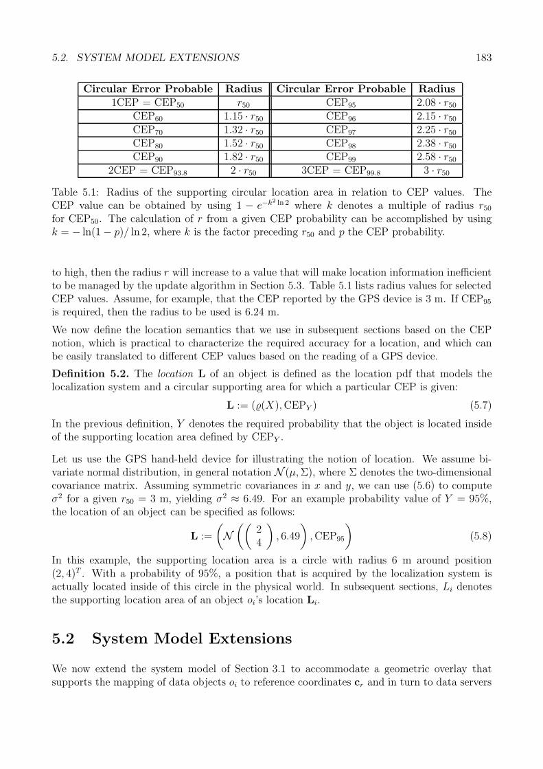
5.2. SYSTEM MODEL EXTENSIONS 183
Circular Error Probable Radius Circular Error Probable Radius1CEP = CEP50 r50 CEP95 2.08 · r50
CEP60 1.15 · r50 CEP96 2.15 · r50
CEP70 1.32 · r50 CEP97 2.25 · r50
CEP80 1.52 · r50 CEP98 2.38 · r50
CEP90 1.82 · r50 CEP99 2.58 · r50
2CEP = CEP93.8 2 · r50 3CEP = CEP99.8 3 · r50
Table 5.1: Radius of the supporting circular location area in relation to CEP values. TheCEP value can be obtained by using 1 − e−k2 ln 2 where k denotes a multiple of radius r50
for CEP50. The calculation of r from a given CEP probability can be accomplished by usingk = − ln(1 − p)/ ln 2, where k is the factor preceding r50 and p the CEP probability.
to high, then the radius r will increase to a value that will make location information inefficientto be managed by the update algorithm in Section 5.3. Table 5.1 lists radius values for selectedCEP values. Assume, for example, that the CEP reported by the GPS device is 3 m. If CEP95
is required, then the radius to be used is 6.24 m.
We now define the location semantics that we use in subsequent sections based on the CEPnotion, which is practical to characterize the required accuracy for a location, and which canbe easily translated to different CEP values based on the reading of a GPS device.
Definition 5.2. The location L of an object is defined as the location pdf that models thelocalization system and a circular supporting area for which a particular CEP is given:
L := (�(X), CEPY ) (5.7)
In the previous definition, Y denotes the required probability that the object is located insideof the supporting location area defined by CEPY .
Let us use the GPS hand-held device for illustrating the notion of location. We assume bi-variate normal distribution, in general notation N (μ, Σ), where Σ denotes the two-dimensionalcovariance matrix. Assuming symmetric covariances in x and y, we can use (5.6) to computeσ2 for a given r50 = 3 m, yielding σ2 ≈ 6.49. For an example probability value of Y = 95%,the location of an object can be specified as follows:
L :=
(N((
24
), 6.49
), CEP95
)(5.8)
In this example, the supporting location area is a circle with radius 6 m around position(2, 4)T . With a probability of 95%, a position that is acquired by the localization system isactually located inside of this circle in the physical world. In subsequent sections, Li denotesthe supporting location area of an object oi’s location Li.
5.2 System Model Extensions
We now extend the system model of Section 3.1 to accommodate a geometric overlay thatsupports the mapping of data objects oi to reference coordinates cr and in turn to data servers
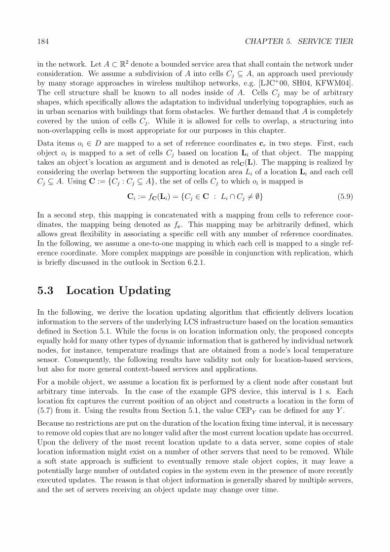
184 CHAPTER 5. SERVICE TIER
in the network. Let A ⊂ R2 denote a bounded service area that shall contain the network underconsideration. We assume a subdivision of A into cells Cj ⊆ A, an approach used previouslyby many storage approaches in wireless multihop networks, e.g. [LJC+00, SH04, KFWM04].The cell structure shall be known to all nodes inside of A. Cells Cj may be of arbitraryshapes, which specifically allows the adaptation to individual underlying topographies, such asin urban scenarios with buildings that form obstacles. We further demand that A is completelycovered by the union of cells Cj. While it is allowed for cells to overlap, a structuring intonon-overlapping cells is most appropriate for our purposes in this chapter.
Data items oi ∈ D are mapped to a set of reference coordinates cr in two steps. First, eachobject oi is mapped to a set of cells Cj based on location Li of that object. The mappingtakes an object’s location as argument and is denoted as relC(L). The mapping is realized byconsidering the overlap between the supporting location area Li of a location Li and each cellCj ⊆ A. Using C := {Cj : Cj ⊆ A}, the set of cells Cj to which oi is mapped is
Ci := fC(Li) = {Cj ∈ C : Li ∩ Cj �= ∅} (5.9)
In a second step, this mapping is concatenated with a mapping from cells to reference coor-dinates, the mapping being denoted as fc. This mapping may be arbitrarily defined, whichallows great flexibility in associating a specific cell with any number of reference coordinates.In the following, we assume a one-to-one mapping in which each cell is mapped to a single ref-erence coordinate. More complex mappings are possible in conjunction with replication, whichis briefly discussed in the outlook in Section 6.2.1.
5.3 Location Updating
In the following, we derive the location updating algorithm that efficiently delivers locationinformation to the servers of the underlying LCS infrastructure based on the location semanticsdefined in Section 5.1. While the focus is on location information only, the proposed conceptsequally hold for many other types of dynamic information that is gathered by individual networknodes, for instance, temperature readings that are obtained from a node’s local temperaturesensor. Consequently, the following results have validity not only for location-based services,but also for more general context-based services and applications.
For a mobile object, we assume a location fix is performed by a client node after constant butarbitrary time intervals. In the case of the example GPS device, this interval is 1 s. Eachlocation fix captures the current position of an object and constructs a location in the form of(5.7) from it. Using the results from Section 5.1, the value CEPY can be defined for any Y .
Because no restrictions are put on the duration of the location fixing time interval, it is necessaryto remove old copies that are no longer valid after the most current location update has occurred.Upon the delivery of the most recent location update to a data server, some copies of stalelocation information might exist on a number of other servers that need to be removed. Whilea soft state approach is sufficient to eventually remove stale object copies, it may leave apotentially large number of outdated copies in the system even in the presence of more recentlyexecuted updates. The reason is that object information is generally shared by multiple servers,and the set of servers receiving an object update may change over time.
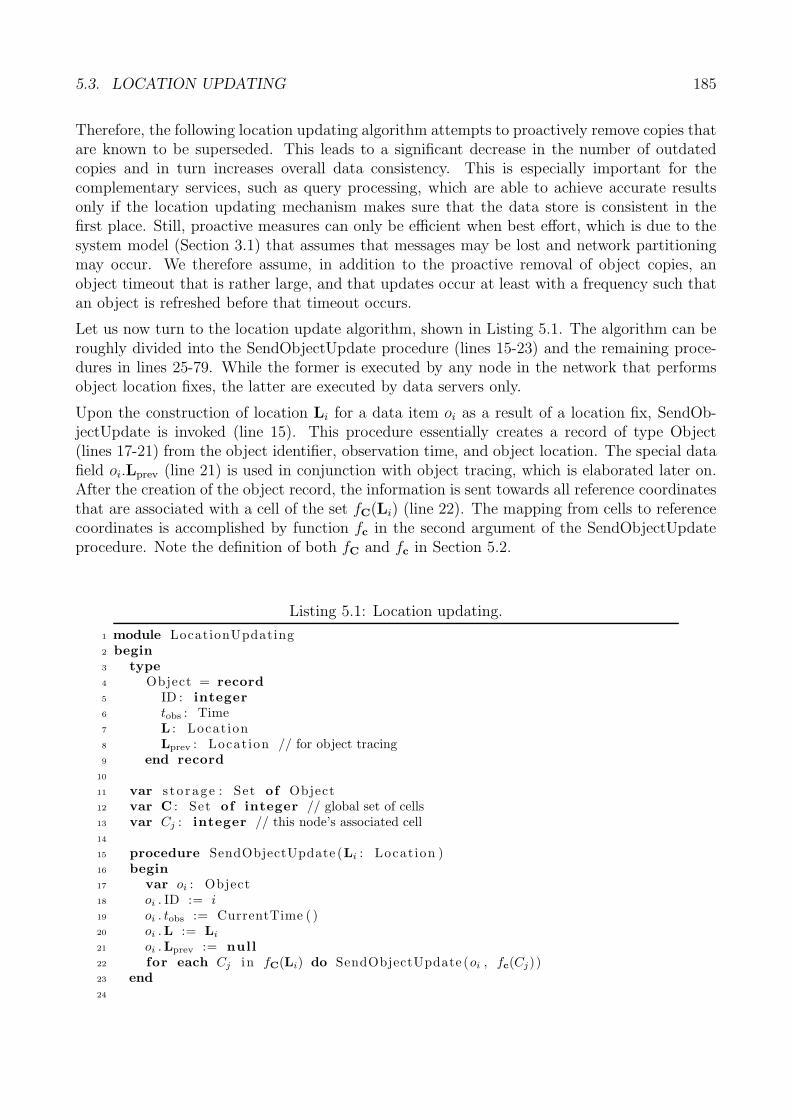
5.3. LOCATION UPDATING 185
Therefore, the following location updating algorithm attempts to proactively remove copies thatare known to be superseded. This leads to a significant decrease in the number of outdatedcopies and in turn increases overall data consistency. This is especially important for thecomplementary services, such as query processing, which are able to achieve accurate resultsonly if the location updating mechanism makes sure that the data store is consistent in thefirst place. Still, proactive measures can only be efficient when best effort, which is due to thesystem model (Section 3.1) that assumes that messages may be lost and network partitioningmay occur. We therefore assume, in addition to the proactive removal of object copies, anobject timeout that is rather large, and that updates occur at least with a frequency such thatan object is refreshed before that timeout occurs.
Let us now turn to the location update algorithm, shown in Listing 5.1. The algorithm can beroughly divided into the SendObjectUpdate procedure (lines 15-23) and the remaining proce-dures in lines 25-79. While the former is executed by any node in the network that performsobject location fixes, the latter are executed by data servers only.
Upon the construction of location Li for a data item oi as a result of a location fix, SendOb-jectUpdate is invoked (line 15). This procedure essentially creates a record of type Object(lines 17-21) from the object identifier, observation time, and object location. The special datafield oi.Lprev (line 21) is used in conjunction with object tracing, which is elaborated later on.After the creation of the object record, the information is sent towards all reference coordinatesthat are associated with a cell of the set fC(Li) (line 22). The mapping from cells to referencecoordinates is accomplished by function fc in the second argument of the SendObjectUpdateprocedure. Note the definition of both fC and fc in Section 5.2.
Listing 5.1: Location updating.
1 module LocationUpdating2 begin3 type4 Object = record5 ID : integer6 tobs : Time7 L : Location8 Lprev : Location // for object tracing9 end record
10
11 var s to rage : Set of Object12 var C : Set of integer // global set of cells13 var Cj : integer // this node’s associated cell14
15 procedure SendObjectUpdate (Li : Location )16 begin17 var oi : Object18 oi . ID := i19 oi . tobs := CurrentTime ( )20 oi .L := Li
21 oi .Lprev := null22 for each Cj in fC(Li) do SendObjectUpdate (oi , fc(Cj))23 end24
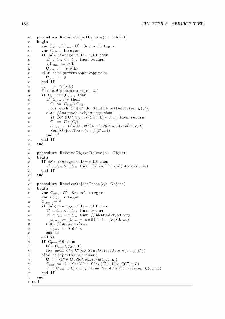
186 CHAPTER 5. SERVICE TIER
25 procedure ReceiveObjectUpdate (oi : Object )26 begin27 var Ccurr, Cprev, C′ : Set of integer28 var Cnext : integer29 i f ∃o′ ∈ s to rage : o′.ID = oi.ID then30 i f oi.tobs < o′.tobs then return31 oi.Lprev := o′.L32 Cprev := fC(o′.L)33 else // no previous object copy exists34 Cprev := ∅35 end i f36 Ccurr := fC(oi.L)37 ExecuteUpdate( s to rage , oi )38 i f Cj = min(Ccurr) then39 i f Cprev �= ∅ then40 C′ := Cprev \ Ccurr
41 for each C′ ∈ C′ do SendObjectDelete (oi, fc(C′))42 else // no previous object copy exists43 i f �C′ ∈ C \ Ccurr : d(C′, oi.L) < dtrace then return44 C′ := C \ {Cj}45 Cnext := C′ ∈ C′ : ∀C′′ ∈ C′ : d(C′, oi.L) < d(C′′, oi.L)46 SendObjectTrace(oi, fc(Cnext))47 end i f48 end i f49 end50
51 procedure Rece iveObjectDe lete (oi : Object )52 begin53 i f ∃o′ ∈ s to rage : o′.ID = oi.ID then54 i f oi.tobs > o′.tobs then ExecuteDelete ( s to rage , oi )55 end i f56 end57
58 procedure ReceiveObjectTrace (oi : Object )59 begin60 var Cprev, C′ : Set of integer61 var Cnext : integer62 Cprev := ∅63 i f ∃o′ ∈ s to rage : o′.ID = oi.ID then64 i f oi.tobs < o′.tobs then return65 i f oi.tobs = o′.tobs then // identical object copy66 Cprev := (Lprev = null) ? ∅ : fC(o′.Lprev)67 else // oi.tobs > o′.tobs
68 Cprev := fC(o′.L)69 end i f70 end i f71 i f Cprev �= ∅ then72 C′ = Cprev \ fC(oi.L)73 for each C′ ∈ C′ do SendObjectDelete (oi, fc(C′))74 else // object tracing continues75 C′ := {C′ ∈ C : d(C′, oi.L) > d(Cj , oi.L)}76 Cnext := C′ ∈ C′ : ∀C′′ ∈ C′ : d(C′, oi.L) < d(C′′, oi.L)77 i f d(Cnext, oi.L) ≤ dtrace then SendObjectTrace (oi, fc(Cnext))78 end i f79 end80 end
5.3. LOCATION UPDATING 187
After a data server has received an object update (line 25), it checks whether a copy of thatobject, denoted o′, with the same ID already exists in the server’s local storage (line 29). If yes,it is further checked whether the observation time of o′ is more current than that of the receivedobject oi (line 30). If this is the case, no further actions are taken and the procedure returns.Otherwise, o′ is a less current object copy whose location is buffered in the current objectfor future object tracing purposes (line 31). The set of cells with which the object’s locationoverlaps is calculated by fC(o′.L) and stored in the previous list variable Cprev (line 32). If nocopy of the received object exists, the previous list is initialized with the empty set (line 34).In line 36 the current set of cells, Ccurr, is assigned the set of cells with which the location ofthe updated object oi overlaps. Both lists are used for the subsequent proactive object removalprocess. The object update is finally executed on the local storage (line 37).
The proactive object removal process is handled in lines 38-48. Because an object’s locationmay overlap with multiple cells, multiple servers may receive an update for the same object.It is therefore necessary to assure that only a single server takes responsibility in handling theremoval of previous object copies. This selection is accomplished in line 38, where the serverhaving the smallest associated cell ID is deemed responsible. If a previous object copy exists,which is indicated by a nonempty previous cell set (line 39), one object delete message is sent toeach data server that is responsible for a cell contained in the set of cells denoted C′ (line 40).This set contains all cells of the previous cell set, but not the cells of the current cell set, becausethe latter contains cells that are associated with servers that receive the current object copy.Object delete messages relating to each cell in C′ are eventually received in line 51. Each deleteis performed on the receiving server’s local storage only if the object exists and that object’sobservation time is smaller than that of the received object.
The case where no previous object copy exists, indicated by an empty previous cell set (line 42),can be due to one of two reasons. Firstly, the location update on the object may be the firstone that has ever occurred due to the object being observed for the first time. Second, thelocation update may have occurred on an object that has entered a new cell, in which case aprevious object copy may still exist at a server that is responsible for another cell. Because thetwo cases cannot be distinguished, a tracing process is considered in the following lines of code.The condition in line 43 checks whether a cell exists that satisfies a specific tracing distancedtrace, but which is not one of the cells that overlaps the object’s location. By setting dtrace to avalue larger than the maximum distance an object may travel between two consecutive locationupdates, it is guaranteed that all cells with which the location of a potential previously updatedobject overlaps are considered. If no such object exists, the procedure returns. Otherwise, a setof cells, denoted C′, is constructed, which contains all cells in the considered network exceptthe current cell (line 44). From this set, the cell that is closest to the supporting location areaof the current object oi is selected (line 45). This cell is the one with the highest probability tofind a previous object copy after an object has entered a new cell. The procedure terminateswith the sending of an object trace message towards the reference coordinate that is associatedwith this cell (line 46). Note that based on the check in line 43 this cell is guaranteed to havea distance to oi’s location area that is smaller than dtrace.
After the reception of an object trace message at a data server (line 58), a previous cell setis first initialized with the empty set (line 62). Next, it is checked whether the object to betraced exists in the local storage of the server (line 63). If a matching object copy exists but its
188 CHAPTER 5. SERVICE TIER
observation time is more current, the procedure returns (line 64). Otherwise, either an identicalcopy of the object exists (line 65) or a less current one (line 67). In the former case, the previouscell set is initialized with the set of cells with which the previous location of object o′ overlaps(line 66). This set is empty if no previous location is available. In the latter case, the set isinitialized with the set of cells with which the existing object’s location overlaps (line 68). Thesubsequent program code (lines 71-78) determines whether the object can be deleted or is to befurther traced. A non-empty previous cell set (line 71) indicates that the trace was successful,that is, a previous object was found and its deletion can be initiated. Just like in line 41 ofprocedure ReceiveObjectUpdate, one delete message is sent towards each reference coordinate(line 73) that is associated with each cell of the set of cells denoted C′ (line 72).
In the case where the previous cell set is empty, a previous object copy could not be foundand the tracing process is continued (line 74). For that, the set of candidate cells is assignedonly those cells that are located further from the current object’s location than the current cell(line 75). This implies a total order of cells in a sequence of increasing distance that is followedfor subsequent tracing attempts, consecutively selecting more distant cells. After choosing thenext cell (line 76), the tracing process continues by sending an object trace message to thereference coordinate that is associated with this cell (line 77). Note that the tracing processeventually terminates when dtrace is no longer satisfied.
The following example, depicted in Figure 5.1, illustrates the operation of the location updatealgorithm. Note that the depiction is not to scale and cell borders are generally crossed muchrarer than shown. Let t1, . . . , t4 denote the time of a location fix, with ti+1 > ti. We write Li(ti)for the supporting location area of an object oi at time ti, and dtrace for the tracing distance. LetDSi and Ci denote data servers and cells, respectively. Let further Upd(t), Del(t), and Trc(t)denote an object update, delete, and trace, respectively, sent to one or more data servers.
Figure 5.1.a and 5.1.b show a sequence of location fixes along the physical path of the objectoi, indicated by the dotted line. In Figure 5.1.a, at t1, object oi is observed by a mobile nodefor the first time and an update is sent to DS2. Upon the reception of the update at DS2,the update is inserted into the server’s local storage. Because no previous object copy existsat DS2, an object trace process is considered (line 42 et sqq.). However, because the tracingdistance spans a circle that is completely located inside of cell C2, no tracing is performed.Recall that from the setting of this distance, it is guaranteed that no other cell exists that mayhave a previous copy of the object if the object had been observed previously.
At t2, the second location fix occurs, which results in a supporting location area that overlapswith both C2 and C1. As a consequence, two updates are sent to DS2 and DS1 (line 22). Bydefinition, the server that is associated with the lowest-ID cell, which is DS1 in the example,handles the object removal process. Because DS1 has not received an object update before,it considers to perform an object trace to find out about possibly existing previous objectcopies (line 42 et sqq.). According to the tracing distance, cell C2 needs to be considered, butno other cell. However, the location associated with the update at t2 also overlaps with C2.Hence, according to line 43, there is no other cell within the tracing distance that can possiblystore a previous object copy, and thus, no object tracing process occurs.
Continuing in Figure 5.1.b, the location fix at t3 results in a single update that is sent to DS1.This time, DS1 stores a previous object copy (line 29). Because cell C2 is not covered by themost recent update’s supporting location area, the server associated with cell C2 is the one from
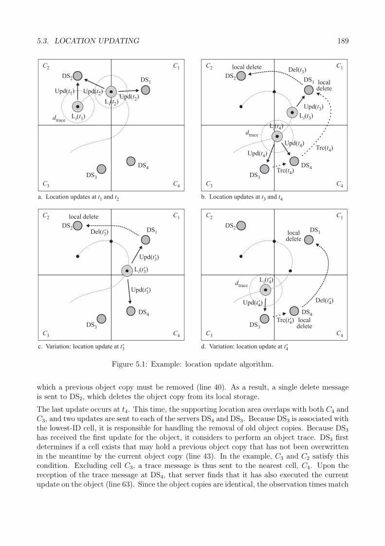
5.3. LOCATION UPDATING 189
DS2
C2 C1
C3 C4
Upd( )t1
dtraceLi( )t1
Upd( )t2
Li( )t2
C2 C1
C3 C4
Upd( )t4
Li( )t4dtrace
DS2 DS1
Trc( )t4
DS4
Del( )t4
DS4
Upd( )t2
DS1
localdelete
DS2
C2 C1
C3 C4
Upd( )t3
Upd( )t4
Li( )t3
Li( )t4dtrace
DS4
DS1
Trc( )t4
Trc( )t4
localdelete
C2 C1
C3 C4
Upd( )t3
Li( )t3
DS2 DS1
DS3
Upd( )t3
Del( )t3
DS4
DS3
DS3DS3
Upd( )t4
a. Location updates at t1 and t2 b. Location updates at andt t3 4
c. Variation: location update at t3 d. Variation: location update at t4
Del( )t3local delete
local delete
localdelete
'
'
'
'
'
' '
'
' '
Figure 5.1: Example: location update algorithm.
which a previous object copy must be removed (line 40). As a result, a single delete messageis sent to DS2, which deletes the object copy from its local storage.
The last update occurs at t4. This time, the supporting location area overlaps with both C4 andC3, and two updates are sent to each of the servers DS4 and DS3. Because DS3 is associated withthe lowest-ID cell, it is responsible for handling the removal of old object copies. Because DS3
has received the first update for the object, it considers to perform an object trace. DS3 firstdetermines if a cell exists that may hold a previous object copy that has not been overwrittenin the meantime by the current object copy (line 43). In the example, C3 and C2 satisfy thiscondition. Excluding cell C3, a trace message is thus sent to the nearest cell, C4. Upon thereception of the trace message at DS4, that server finds that it has also executed the currentupdate on the object (line 63). Since the object copies are identical, the observation times match
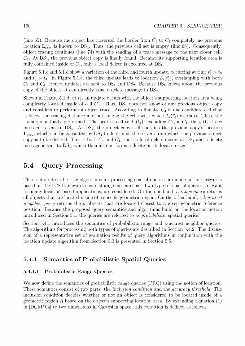
190 CHAPTER 5. SERVICE TIER
(line 65). Because the object has traversed the border from C1 to C4 completely, no previouslocation Lprev is known to DS4. Thus, the previous cell set is empty (line 66). Consequently,object tracing continues (line 74) with the sending of a trace message to the next closer cell,C1. At DS1, the previous object copy is finally found. Because its supporting location area isfully contained inside of C1, only a local delete is executed at DS1.
Figure 5.1.c and 5.1.d show a variation of the third and fourth update, occurring at time t′3 > t3and t′4 > t4. In Figure 5.1.c, the third update leads to location Li(t
′3), overlapping with both
C1 and C4. Hence, updates are sent to DS1 and DS2. Because DS1 knows about the previouscopy of the object, it can directly issue a delete message to DS2.
Shown in Figure 5.1.d, at t′4, an update occurs with the object’s supporting location area beingcompletely located inside of cell C3. Thus, DS3 does not know of any previous object copyand considers to perform an object trace. According to line 43, C4 is one candidate cell thatis below the tracing distance and not among the cells with which Li(t
′4) overlaps. Thus, the
tracing is actually performed. The nearest cell to Li(t′4), excluding C3, is C4, thus, the trace
message is sent to DS4. At DS4, the object copy still contains the previous copy’s locationLprev, which can be consulted by DS4 to determine the servers from which the previous objectcopy is to be deleted. This is both C4 and C1, thus, a local delete occurs at DS4 and a deletemessage is sent to DS1, which then also performs a delete on its local storage.
5.4 Query Processing
This section describes the algorithms for processing spatial queries in mobile ad-hoc networksbased on the LCS framework’s core storage mechanisms. Two types of spatial queries, relevantfor many location-based applications, are considered: On the one hand, a range query returnsall objects that are located inside of a specific geometric region. On the other hand, a k-nearestneighbor query returns the k objects that are located closest to a given geometric referenceposition. Because the proposed query semantics and algorithms build on the location notionintroduced in Section 5.1, the queries are referred to as probabilistic spatial queries.
Section 5.4.1 introduces the semantics of probabilistic range and k-nearest neighbor queries.The algorithms for processing both types of queries are described in Section 5.4.2. The discus-sion of a representative set of evaluation results of query algorithms in conjunction with thelocation update algorithm from Section 5.3 is presented in Section 5.5.
5.4.1 Semantics of Probabilistic Spatial Queries
5.4.1.1 Probabilistic Range Queries
We now define the semantics of probabilistic range queries (PRQ) using the notion of location.These semantics consist of two parts: the inclusion condition and the accuracy threshold. Theinclusion condition decides whether or not an object is considered to be located inside of ageometric region R based on the object’s supporting location area. By extending Equation (1)in [DGM+04] to two dimensions in Cartesian space, this condition is defined as follows:
5.4. QUERY PROCESSING 191
Definition 5.3. The inclusion condition for an object oi is satisfied if and only if the probabilitythat oi is located inside of a geometric region R is greater than or equal to the inclusion threshold0 < PPRQ ≤ 1. Having X denote any position inside of the supporting location area Li, and �i
the pdf of location Li, the inclusion condition is formally given by
P (X ∈ R) =
∫R∩Li
�i(X)dX ≥ PPRQ (5.10)
An important fact not considered in previous work (Table 2.4 in Section 2.5) is that the positionof some objects might be too inaccurate to be of use for some types of application. For example,in an application where the objects returned are to be located in the physical world, such asin the streets of a city center, a location too inaccurate might render it impossible for the userto find the object. To consider this fact, we introduce an additional query parameter thatallows us to omit data objects from query processing if the degree of inaccuracy in the positioninformation of these objects is too large.
Definition 5.4. The accuracy threshold defines the maximum degree of inaccuracy allowedfor an object to take part in the evaluation of a probabilistic spatial query in general, and aprobabilistic range query in particular. It is formally defined as a pair of values, (χ, υ)1, whereχ ≥ 0 and υ ≥ 0 denote the maximum circular error probable (CEP) index and maximumradius, respectively, that the supporting location area’s CEP is allowed to have.
The combination of both parameters is essential, because the supporting location area of anobject’s location can have a small CEP radius with a very small CEP index, or vice versa.
Based on the aforementioned notions, we now define the probabilistic range query:
Definition 5.5. Let R denote the range query’s target geometric region. Let CEPY,i and Yi
denote the circular error probable and probability of an object oi’s location, respectively. Theprobabilistic range query result, denoted RPRQ, is defined as:
RPRQ = {oi | P (Xi ∈ R) ≥ PPRQ ∧ CEPY,i ≤ χ ∧ Yi ≤ υ} (5.11)
In the following example, let L = (�(X), CEPY ) denote an object’s location, with
�(X) =
{Y/(100π · CEP2
Y ) if (X − M)2 ≤ CEP2Y
0 otherwise(5.12)
specifying a uniform distribution over a circular location area with center M and radius CEPY .Let further R denote a rectangular region, the argument of the range query. Further assumethe inclusion threshold PPRQ = 0.75, and (χ, υ) = (3 m, 80).
Figure 5.2 illustrates the location of a number of objects. Object o1 is included in the queryresult, because all restrictions in Definition 5.5 are satisfied. Object o2 and o3 do not satisfy
1χ and υ denote the greek letters Chi and Upsilon.
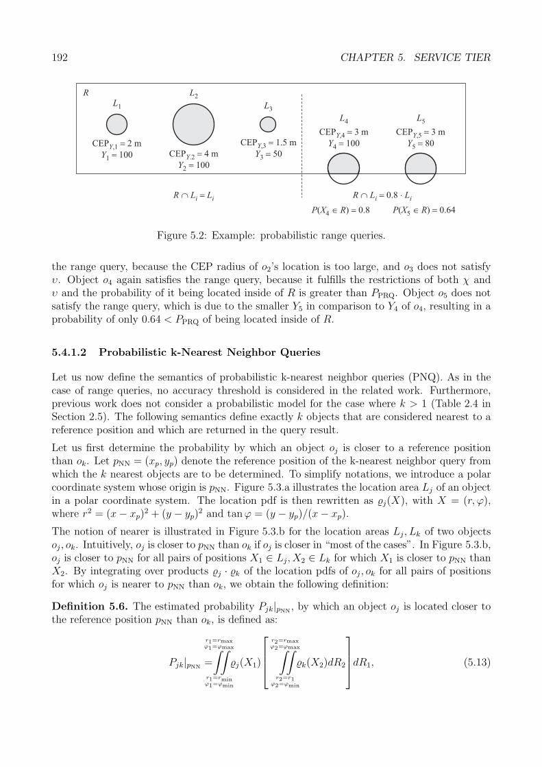
192 CHAPTER 5. SERVICE TIER
R L2
L3
CEP 1.5 mY,3 �
Y3 50�CEP 4 mY.2 �
Y2 100�
L1
CEP 2 mY,1 �
Y1 100�
L4
CEP 3 mY,4 �
Y4 100�
L5
CEP 3 mY,5 �
Y5 80�
R L� �i Li R L� � �i 0.8 Li
P X R( ) 0.645 � �P X R( ) 0.84 � �
Figure 5.2: Example: probabilistic range queries.
the range query, because the CEP radius of o2’s location is too large, and o3 does not satisfyυ. Object o4 again satisfies the range query, because it fulfills the restrictions of both χ andυ and the probability of it being located inside of R is greater than PPRQ. Object o5 does notsatisfy the range query, which is due to the smaller Y5 in comparison to Y4 of o4, resulting in aprobability of only 0.64 < PPRQ of being located inside of R.
5.4.1.2 Probabilistic k-Nearest Neighbor Queries
Let us now define the semantics of probabilistic k-nearest neighbor queries (PNQ). As in thecase of range queries, no accuracy threshold is considered in the related work. Furthermore,previous work does not consider a probabilistic model for the case where k > 1 (Table 2.4 inSection 2.5). The following semantics define exactly k objects that are considered nearest to areference position and which are returned in the query result.
Let us first determine the probability by which an object oj is closer to a reference positionthan ok. Let pNN = (xp, yp) denote the reference position of the k-nearest neighbor query fromwhich the k nearest objects are to be determined. To simplify notations, we introduce a polarcoordinate system whose origin is pNN. Figure 5.3.a illustrates the location area Lj of an objectin a polar coordinate system. The location pdf is then rewritten as �j(X), with X = (r, ϕ),where r2 = (x − xp)
2 + (y − yp)2 and tanϕ = (y − yp)/(x − xp).
The notion of nearer is illustrated in Figure 5.3.b for the location areas Lj , Lk of two objectsoj , ok. Intuitively, oj is closer to pNN than ok if oj is closer in “most of the cases”. In Figure 5.3.b,oj is closer to pNN for all pairs of positions X1 ∈ Lj, X2 ∈ Lk for which X1 is closer to pNN thanX2. By integrating over products �j · �k of the location pdfs of oj , ok for all pairs of positionsfor which oj is nearer to pNN than ok, we obtain the following definition:
Definition 5.6. The estimated probability Pjk|pNN, by which an object oj is located closer to
the reference position pNN than ok, is defined as:
Pjk|pNN=
r1=rmaxϕ1=ϕmax∫∫r1=rminϕ1=ϕmin
�j(X1)
⎡⎢⎢⎣
r2=rmaxϕ2=ϕmax∫∫
r2=r1ϕ2=ϕmin
�k(X2)dR2
⎤⎥⎥⎦dR1, (5.13)
5.4. QUERY PROCESSING 193
�max
�min
rmin
rmax
r1
r2
pNN
Lj
LkX1
X2
Lj
( )r,�
y
p x yNN � ( , )p p
x
y'
x'
( , )x y0 0
a. Polar coordinate transformation. b. Nearer relation between objects.
Figure 5.3: Semantics of probabilistic k-nearest neighbor queries.
where X1 = (r1, ϕ1) and X2 = (r2, ϕ2), as well as dR1 = r1dr1dϕ1 and dR2 = r2dr2dϕ2.
The term estimated indicates that the probability computations might not be complete in thefollowing sense. Recall that the location semantics defined in (5.2) in Section 5.1 may lead top < 1. This implies that the sum of the probabilities by which two objects are mutually closerto each other is not necessarily 1, but assumes the maximum value
Pmax = Pjk|pNN+ Pkj|pNN
(5.14)
Using (5.13) and (5.14) we can now define the nearer relation between two objects.
Definition 5.7. For two objects oj , ok, object oj is nearer than ok to the reference position pNN
if and only if the probability that oj is nearer than ok is greater than one half of the maximumpossible probability. Written formally:
oj < ok|pNN⇐⇒ Pjk > 0.5 · Pmax (5.15)
Based on Definition 5.7, it is also possible that oj and ok have equal distance to pNN:
Definition 5.8. Two objects oj, ok, have equal distance to pNN if the following holds:
oj = ok|pNN⇐⇒ Pjk|pNN
= Pkj|pNN(5.16)
The definition of the k-nearest neighbor query result RPNQ is based on Definition 5.7 and 5.8.In addition, we use the accuracy threshold (χ, υ) of Definition 5.4 to only include objects inthe query processing whose location satisfies that threshold.
Definition 5.9. The probabilistic k-nearest neighbor query result, denoted RPNQ, is defined as:
RPNQ = {o1, . . . , ok} : ∀or ∈ RPNQ : CEPY,r ≤ χ ∧ Yr ≤ υ ∧∀or ∈ RPNQ, os �∈ RPNQ : CEPY,s ≤ χ ∧ Ys ≤ υ ⇒ or ≤ os |pNN
(5.17)
Note that if property (5.16) in Definition 5.8 holds for two objects o′k, o′′k that are both k’th
distant objects to pNN, then the query result is non-unique.
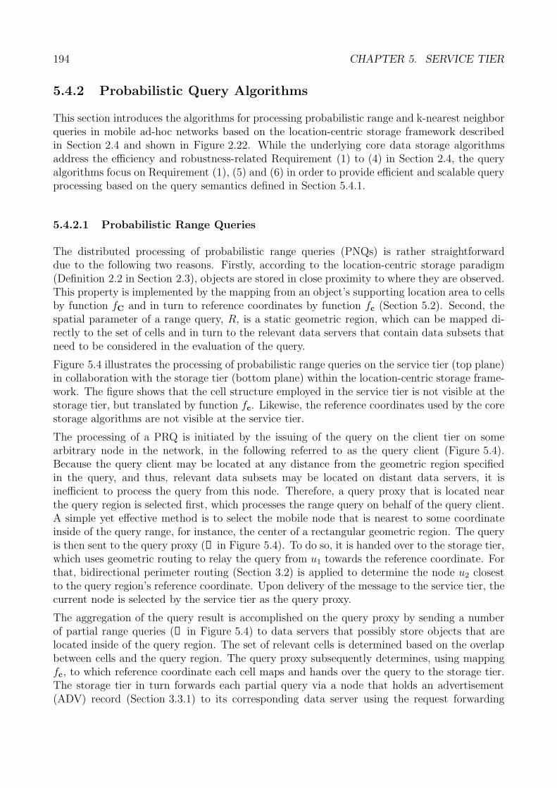
194 CHAPTER 5. SERVICE TIER
5.4.2 Probabilistic Query Algorithms
This section introduces the algorithms for processing probabilistic range and k-nearest neighborqueries in mobile ad-hoc networks based on the location-centric storage framework describedin Section 2.4 and shown in Figure 2.22. While the underlying core data storage algorithmsaddress the efficiency and robustness-related Requirement (1) to (4) in Section 2.4, the queryalgorithms focus on Requirement (1), (5) and (6) in order to provide efficient and scalable queryprocessing based on the query semantics defined in Section 5.4.1.
5.4.2.1 Probabilistic Range Queries
The distributed processing of probabilistic range queries (PNQs) is rather straightforwarddue to the following two reasons. Firstly, according to the location-centric storage paradigm(Definition 2.2 in Section 2.3), objects are stored in close proximity to where they are observed.This property is implemented by the mapping from an object’s supporting location area to cellsby function fC and in turn to reference coordinates by function fc (Section 5.2). Second, thespatial parameter of a range query, R, is a static geometric region, which can be mapped di-rectly to the set of cells and in turn to the relevant data servers that contain data subsets thatneed to be considered in the evaluation of the query.
Figure 5.4 illustrates the processing of probabilistic range queries on the service tier (top plane)in collaboration with the storage tier (bottom plane) within the location-centric storage frame-work. The figure shows that the cell structure employed in the service tier is not visible at thestorage tier, but translated by function fc. Likewise, the reference coordinates used by the corestorage algorithms are not visible at the service tier.
The processing of a PRQ is initiated by the issuing of the query on the client tier on somearbitrary node in the network, in the following referred to as the query client (Figure 5.4).Because the query client may be located at any distance from the geometric region specifiedin the query, and thus, relevant data subsets may be located on distant data servers, it isinefficient to process the query from this node. Therefore, a query proxy that is located nearthe query region is selected first, which processes the range query on behalf of the query client.A simple yet effective method is to select the mobile node that is nearest to some coordinateinside of the query range, for instance, the center of a rectangular geometric region. The queryis then sent to the query proxy (➊ in Figure 5.4). To do so, it is handed over to the storage tier,which uses geometric routing to relay the query from u1 towards the reference coordinate. Forthat, bidirectional perimeter routing (Section 3.2) is applied to determine the node u2 closestto the query region’s reference coordinate. Upon delivery of the message to the service tier, thecurrent node is selected by the service tier as the query proxy.
The aggregation of the query result is accomplished on the query proxy by sending a numberof partial range queries (➋ in Figure 5.4) to data servers that possibly store objects that arelocated inside of the query region. The set of relevant cells is determined based on the overlapbetween cells and the query region. The query proxy subsequently determines, using mappingfc, to which reference coordinate each cell maps and hands over the query to the storage tier.The storage tier in turn forwards each partial query via a node that holds an advertisement(ADV) record (Section 3.3.1) to its corresponding data server using the request forwarding
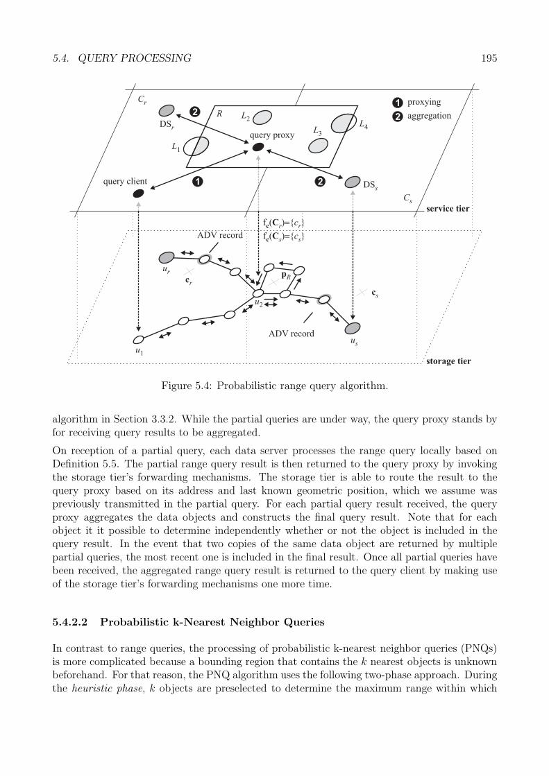
5.4. QUERY PROCESSING 195
L2
L3
L1
L4
cr
ADV record
storage tier
service tier
cs
DSs
DSr
ur
query client
Cr
Cs
query proxy
R
us
f ( ) { }
f ( ) { }
c
c
C
C
r r
s s
�
�
c
c
pR
ADV record
u1
u2
1
2
2
1 proxying
2 aggregation
Figure 5.4: Probabilistic range query algorithm.
algorithm in Section 3.3.2. While the partial queries are under way, the query proxy stands byfor receiving query results to be aggregated.
On reception of a partial query, each data server processes the range query locally based onDefinition 5.5. The partial range query result is then returned to the query proxy by invokingthe storage tier’s forwarding mechanisms. The storage tier is able to route the result to thequery proxy based on its address and last known geometric position, which we assume waspreviously transmitted in the partial query. For each partial query result received, the queryproxy aggregates the data objects and constructs the final query result. Note that for eachobject it it possible to determine independently whether or not the object is included in thequery result. In the event that two copies of the same data object are returned by multiplepartial queries, the most recent one is included in the final result. Once all partial queries havebeen received, the aggregated range query result is returned to the query client by making useof the storage tier’s forwarding mechanisms one more time.
5.4.2.2 Probabilistic k-Nearest Neighbor Queries
In contrast to range queries, the processing of probabilistic k-nearest neighbor queries (PNQs)is more complicated because a bounding region that contains the k nearest objects is unknownbeforehand. For that reason, the PNQ algorithm uses the following two-phase approach. Duringthe heuristic phase, k objects are preselected to determine the maximum range within which
196 CHAPTER 5. SERVICE TIER
additional objects must be considered to compute the final query result. The selection strategyis realized by using partial k-nearest neighbor queries executed in a sequence that allows to findk candidate objects quickly and whose distance to the real k nearest neighbors is small. Thisstep is essential to minimize additional communication cost required to complete the queryduring the aggregation phase. In this phase, all data servers that may contain objects thatare closer to pNN than any of the objects determined during the heuristic phase are queried bymeans of additional partial k-nearest neighbor queries. The final query result is then aggregatedby using the nearer relation in Definition 5.7 and 5.8.
The principal operation of the algorithm for processing probabilistic k-nearest neighbor queriesis shown in Listing 5.2 and Figure 5.5 on page 198. For simplicity, we assume that the queryclient is also the query proxy and derives the query position pNN from its own location. In thecase where a query client is located anywhere in the network and uses a query reference positionpNN that is not its own position, routing between query client and proxy is accomplished justas in the case of range query processing in Section 5.4.2.1 (➊ in Figure 5.5). In the case of ak-nearest neighbor query, the proxy is the node closest to the query position pNN.
Listing 5.2: Processing of probabilistic k-nearest neighbor queries.
1 module QueryProcess ing2 begin3 var s to rage : Set of Object4 var C : Set of integer // global set of cells5 var Cj : integer // this node’s associated cell6 var RPNQ : Set of Object // final query result, Object structure see Listing 5.17 var C′ : Pr ior ityQueue // remaining set of cells ordered by distance to pNN
8 var phase : ( h e u r i s t i c , a gg r ega t i on )9 var aggregationTimer : Timer
10 var rlim : real11
12 procedure ProcessPNQ(k : integer ; pNN : Point ; χ : real ; υ : real )13 begin14 RPNQ := ∅15 phase := h e u r i s t i c16 C′ := SortByDistanceTo(C, pNN )17 SendPart ia lQuery (k, pNN, χ, υ, fC(GetAndRemoveNext(C′ ) ) )18 end19
20 procedure Rece ivePar t i a lRe su l t (RpartPNQ : Set of Object )
21 begin22 // all objects in partial result satisfy the accuracy threshold23 for each oi in Rpart
PNQ do24 i f not Contains (RPNQ, oi ) then25 i f |RPNQ| < k then26 RPNQ := RPNQ ∪ oi
27 else // |RPNQ| = k
28 i f ∃oj ∈ RPNQ : oi < oj |pNN ∧ ∀ok ∈ RpartPNQ : oi ≤ ok|pNN then
29 Replace (RPNQ, oj , Remove(RpartPNQ, oi ) )
30 end i f31 end i f32 end i f33 end for
5.4. QUERY PROCESSING 197
34 i f phase = h eu r i s t i c then35 i f |RPNQ| < k then36 i f d(GetNext(C′), pNN) < rlim then37 SendPart ia lQuery (k, pNN, χ, υ, GetAndRemoveNext(C′ ) )38 else39 De l ive rResu l t (RPNQ ) // no more cells to aggregate from40 end i f41 else // |RPNQ| = k42 phase = agg r ega t i on43 AggregateResult (k, pNN, χ, υ )44 end i f45 else // phase = agg r ega t i on46 i f AggregationComplete ( ) then47 De l ive rResu l t (RPNQ ) // deliver result to client tier48 end i f49 end i f50 end51
52 procedure AggregateResult (k : integer ; pNN : Point ; χ : real ; υ : real )53 begin54 var Cagg : Disk (pNN, 0)55 var ragg, dmax : real56 ragg := 057 for each oi ∈ RPNQ do58 dmax := Maxp∈Li{d(p, pNN)}59 ragg := Min{Max{ragg, dmax}, rlim}60 end for61 i f not Overlaps (GetNext (C′ ) , Disk (pNN, ragg ) ) then62 De l ive rResu l t (RPNQ ) // no more cells to aggregate from63 else64 while Overlaps (GetNext (C′ ) , Disk (pNN, ragg ) ) do65 SendPart ia lQuery (k, pNN, χ, υ, GetAndRemoveNext(C′ ) )66 end while67 SetTimer ( aggregationTimer , tagg )68 end i f69 end70
71 procedure TimerExpired ( )72 begin73 De l ive rResu l t (RPNQ ) // deliver result to client tier74 end75 end
The processing of a PNQ starts at the query proxy by a call to procedure ProcessPNQ (line 12).After initializing the final query result, RPNQ, with the empty set (line 14), the heuristic phaseis entered (line 15) and a copy of the global cell set, C′, is created (line 16). This set is apriority queue that contains cells in ascending order of distance to the query reference positionpNN. The first partial query is sent towards the reference coordinate that is associated with thenearest cell (line 17, ➋ in Figure 5.5). This is the point where the partial query is handed fromthe service to the storage tier, as was shown previously in Figure 5.4.
After the processing of a partial query at a data server in accordance with Definition 5.9, thecorresponding partial query result is received by the query proxy and handled in procedure
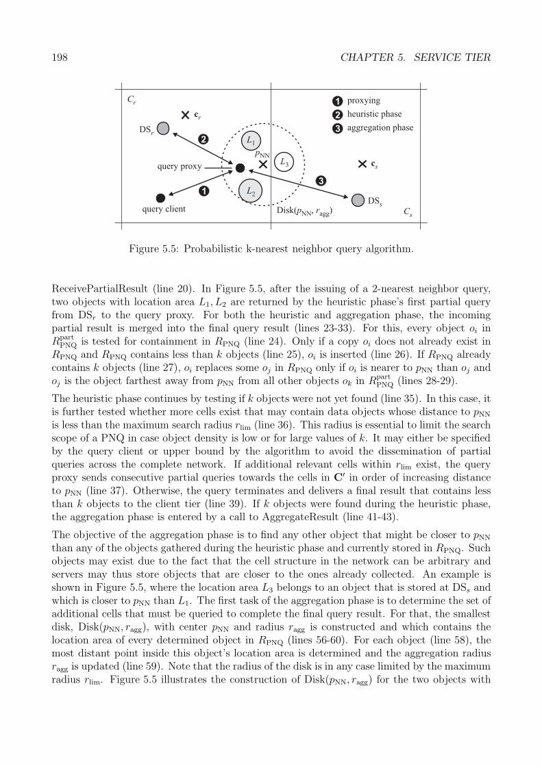
198 CHAPTER 5. SERVICE TIER
Cr
Cs
DSr
DSsquery client
query proxy
13
cr
cs
2
pNN
Disk( , )p rNN agg
L1
L2
L3
1 proxying
2
3
heuristic phase
aggregation phase
Figure 5.5: Probabilistic k-nearest neighbor query algorithm.
ReceivePartialResult (line 20). In Figure 5.5, after the issuing of a 2-nearest neighbor query,two objects with location area L1, L2 are returned by the heuristic phase’s first partial queryfrom DSr to the query proxy. For both the heuristic and aggregation phase, the incomingpartial result is merged into the final query result (lines 23-33). For this, every object oi inRpart
PNQ is tested for containment in RPNQ (line 24). Only if a copy oi does not already exist inRPNQ and RPNQ contains less than k objects (line 25), oi is inserted (line 26). If RPNQ alreadycontains k objects (line 27), oi replaces some oj in RPNQ only if oi is nearer to pNN than oj andoj is the object farthest away from pNN from all other objects ok in Rpart
PNQ (lines 28-29).
The heuristic phase continues by testing if k objects were not yet found (line 35). In this case, itis further tested whether more cells exist that may contain data objects whose distance to pNN
is less than the maximum search radius rlim (line 36). This radius is essential to limit the searchscope of a PNQ in case object density is low or for large values of k. It may either be specifiedby the query client or upper bound by the algorithm to avoid the dissemination of partialqueries across the complete network. If additional relevant cells within rlim exist, the queryproxy sends consecutive partial queries towards the cells in C′ in order of increasing distanceto pNN (line 37). Otherwise, the query terminates and delivers a final result that contains lessthan k objects to the client tier (line 39). If k objects were found during the heuristic phase,the aggregation phase is entered by a call to AggregateResult (line 41-43).
The objective of the aggregation phase is to find any other object that might be closer to pNN
than any of the objects gathered during the heuristic phase and currently stored in RPNQ. Suchobjects may exist due to the fact that the cell structure in the network can be arbitrary andservers may thus store objects that are closer to the ones already collected. An example isshown in Figure 5.5, where the location area L3 belongs to an object that is stored at DSs andwhich is closer to pNN than L1. The first task of the aggregation phase is to determine the set ofadditional cells that must be queried to complete the final query result. For that, the smallestdisk, Disk(pNN, ragg), with center pNN and radius ragg is constructed and which contains thelocation area of every determined object in RPNQ (lines 56-60). For each object (line 58), themost distant point inside this object’s location area is determined and the aggregation radiusragg is updated (line 59). Note that the radius of the disk is in any case limited by the maximumradius rlim. Figure 5.5 illustrates the construction of Disk(pNN, ragg) for the two objects with
5.5. PERFORMANCE ANALYSIS 199
location areas L1 and L2. In the example, the disk contains the location area L3 of anotherobject that is stored on DSs and thus, was not retrieved during the heuristic phase.
Based on the determined radius ragg, the next potential cell from the priority queue is checkedfor overlap with Disk(pNN, ragg) (line 61). Note that all cells that were already queried in theheuristic phase are left out in the aggregation phase, which is guaranteed by the fact that foreach partial query sent during the heuristic phase, the corresponding cell is removed from thepriority queue (line 17 and also 37). If no overlap occurs, the query result is already completeand is delivered to the client tier (line 62). Note that because the priority queue containscells in increasing order to pNN, it is not possible that another cell exists that overlaps withDisk(pNN, ragg). In the case where the disk overlaps with at least the next cell in the priorityqueue (line 63), one partial query is sent for each overlapping cell to the server that is associatedwith this cell. In Figure 5.5, only cell Cs overlaps with Disk(pNN, ragg) and thus, the associateddata server DSs is queried (➌). The sending of a partial query to this server makes sure that thecorresponding object is eventually retrieved and merged into the final query result according tolines 23-33. After the sending of the partial queries, the aggregation timer is set to guaranteethat the aggregation phase terminates eventually (line 67).
Once the partial queries of the aggregation phase are being propagated and processed at thecorresponding server(s), the aggregation phase completes in either one of two cases. The reg-ular case occurs in procedure ReceivePartialResult, lines 45-49. With the reception of eachpartial query result, it is checked whether the aggregation is complete (line 46). This can beaccomplished by matching the number of received partial query results with the number ofpartial queries sent during the aggregation phase. If the result is complete, the query resultis delivered to the client tier (line 47). Otherwise, the procedure finishes and the query proxywaits for the outstanding partial query results.
In the second case, aggregation is terminated due to the expiration of the aggregation timer,which was set in line 67 and which occurs prior to the reception of all outstanding partial queryresults. Upon expiration, procedure TimerExpired is invoked (line 71). In Listing 5.2, thequery result, which may be suboptimal, is immediately delivered to the client tier (line 73). Inthe presented algorithm, only best-effort delivery of query messages is supported. It is straight-forward to extend the algorithm by any level of additional robustness to increase accuracy, alsoin collaboration with the storage tier. However, these details are omitted in this dissertation.Instead, it is shown in Section 5.5 that even under best-effort delivery, a large degree of queryaccuracy can be achieved in typical mobile ad-hoc network scenarios.
5.5 Performance Analysis
This section discusses a representative set of evaluation results of the service tier. We will showthat the service functionality provided for context-based applications can be supported in anefficient way based on the storage tier introduced in Chapter 3 and 4 and in conjunction withthe location updating mechanism elaborated in Section 5.3.
When considering the algorithms for probabilistic range and k-nearest neighbor queries inSection 5.4, we can observe that both types of queries are decomposed into a number of partialqueries that process the overall query result. While the individual strategy of each query
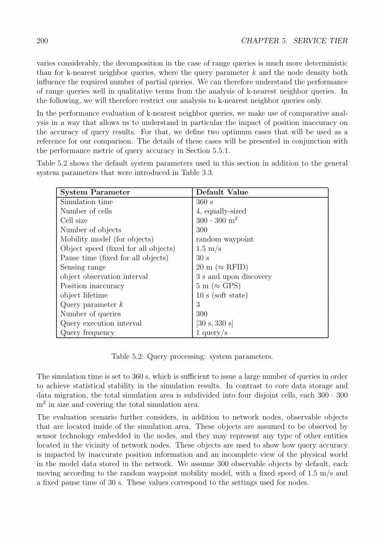
200 CHAPTER 5. SERVICE TIER
varies considerably, the decomposition in the case of range queries is much more deterministicthan for k-nearest neighbor queries, where the query parameter k and the node density bothinfluence the required number of partial queries. We can therefore understand the performanceof range queries well in qualitative terms from the analysis of k-nearest neighbor queries. Inthe following, we will therefore restrict our analysis to k-nearest neighbor queries only.
In the performance evaluation of k-nearest neighbor queries, we make use of comparative anal-ysis in a way that allows us to understand in particular the impact of position inaccuracy onthe accuracy of query results. For that, we define two optimum cases that will be used as areference for our comparison. The details of these cases will be presented in conjunction withthe performance metric of query accuracy in Section 5.5.1.
Table 5.2 shows the default system parameters used in this section in addition to the generalsystem parameters that were introduced in Table 3.3.
System Parameter Default ValueSimulation time 360 sNumber of cells 4, equally-sizedCell size 300 · 300 m2
Number of objects 300Mobility model (for objects) random waypointObject speed (fixed for all objects) 1.5 m/sPause time (fixed for all objects) 30 sSensing range 20 m (≈ RFID)object observation interval 3 s and upon discoveryPosition inaccuracy 5 m (≈ GPS)object lifetime 10 s (soft state)Query parameter k 3Number of queries 300Query execution interval [30 s, 330 s]Query frequency 1 query/s
Table 5.2: Query processing: system parameters.
The simulation time is set to 360 s, which is sufficient to issue a large number of queries in orderto achieve statistical stability in the simulation results. In contrast to core data storage anddata migration, the total simulation area is subdivided into four disjoint cells, each 300 · 300m2 in size and covering the total simulation area.
The evaluation scenario further considers, in addition to network nodes, observable objectsthat are located inside of the simulation area. These objects are assumed to be observed bysensor technology embedded in the nodes, and they may represent any type of other entitieslocated in the vicinity of network nodes. These objects are used to show how query accuracyis impacted by inaccurate position information and an incomplete view of the physical worldin the model data stored in the network. We assume 300 observable objects by default, eachmoving according to the random waypoint mobility model, with a fixed speed of 1.5 m/s anda fixed pause time of 30 s. These values correspond to the settings used for nodes.
5.5. PERFORMANCE ANALYSIS 201
We assume that the sensing range of embedded sensors is 20 m. Any observable object locatedwithin the sensing range of a node is observed by that node. An object is observed for the firsttime when it enters the sensing range of a node and is thereby discovered by that node, thenin regular time intervals of 3 seconds until it leaves the sensing range of the node again.
We assume that a node determines the position of an object upon observation and is able todo so with a position inaccuracy of 5 m, which corresponds to values that can be obtainedfrom typical GPS receivers. After each observation, a data object is created and sent to theserver that is located in those cells whose area overlaps with the location area of the object’sdetermined location according to Listing 5.2. Any object that is not updated within at most10 seconds at a server is removed from that server by a soft state approach.
5.5.1 Performance Metrics
We define three key performance metrics to assess the performance of k-nearest neighbor queries:query accuracy and query offset, query latency, and query cost.
Query Accuracy and Query Offset
Query accuracy and query offset are two related performance metrics that describe the qualityof the result returned by a k-nearest neighbor query. We express both metrics with respect totwo optimum cases, which we term model-based optimum and real world-based optimum.
The purpose of comparing the k-nearest neighbor query result to the model-based optimumresult is to assess the pure performance of the query algorithm, that is, which level of accuracyit is able to achieve with respect to a perfect reference implementation. Such an implementa-tion assumes that a query is processed instantaneously, based on the most recently observedinformation that is stored at a single server at query time. This reflects the best possible casethat is, in theory, achievable in a mobile ad-hoc network at all.
Let Rmod = {o1, . . . , os} and R = {o1, . . . , ot} denote the model-based optimum result and theresult returned by the k-nearest neighbor query implementation, respectively. The accuracyof a single k-nearest neighbor query with respect to the model-based optimum result, denotedAmod, is defined as Amod = |R ∩ Rmod| / |Rmod|.The query offset is a second intuitive way to assess the quality of a k-nearest neighbor queryresult and it expresses by how much the objects returned in the result are “off” from thereference result. Assume, for instance, that in a 3-nearest neighbor query, a single object ismissed and the fourth-nearest instead of the third-nearest object is returned. The query offsetin this case is one. The important property is that for highly inaccurate query results, the queryoffset can still have a small value and indicates how “far”, literally, the returned objects arefrom the reference result. In other words, even if the query accuracy is very low, the offset mayindicate that the result is still useful for specific applications. The offset of a single k-nearestneighbor query with respect to the model-based optimum result is defined as follows.
Let w.l.g. ∀i : d(ri, cr) < d(ri+1, cr) for a reference coordinate cr. Let further R′mod =
{o1, . . . , o′s} denote the smallest set of objects for which R ⊆ R′
mod. The offset of a singlek-nearest neighbor query with respect to the model-based optimum result, denoted Omod, isdefined as Omod = |R′
mod| − |R| ≥ 0. Note that Omod = 0 ⇔ Amod = 1.
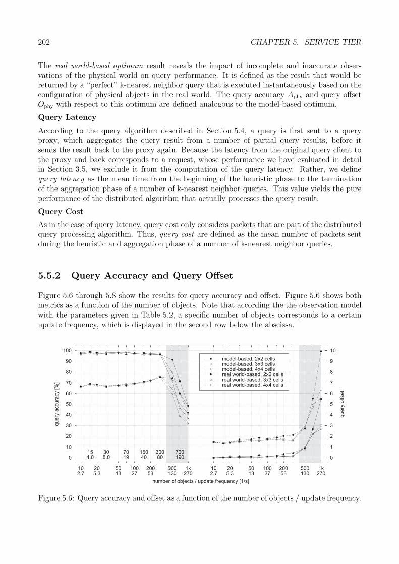
202 CHAPTER 5. SERVICE TIER
The real world-based optimum result reveals the impact of incomplete and inaccurate obser-vations of the physical world on query performance. It is defined as the result that would bereturned by a “perfect” k-nearest neighbor query that is executed instantaneously based on theconfiguration of physical objects in the real world. The query accuracy Aphy and query offsetOphy with respect to this optimum are defined analogous to the model-based optimum.
Query Latency
According to the query algorithm described in Section 5.4, a query is first sent to a queryproxy, which aggregates the query result from a number of partial query results, before itsends the result back to the proxy again. Because the latency from the original query client tothe proxy and back corresponds to a request, whose performance we have evaluated in detailin Section 3.5, we exclude it from the computation of the query latency. Rather, we definequery latency as the mean time from the beginning of the heuristic phase to the terminationof the aggregation phase of a number of k-nearest neighbor queries. This value yields the pureperformance of the distributed algorithm that actually processes the query result.
Query Cost
As in the case of query latency, query cost only considers packets that are part of the distributedquery processing algorithm. Thus, query cost are defined as the mean number of packets sentduring the heuristic and aggregation phase of a number of k-nearest neighbor queries.
5.5.2 Query Accuracy and Query Offset
Figure 5.6 through 5.8 show the results for query accuracy and offset. Figure 5.6 shows bothmetrics as a function of the number of objects. Note that according the the observation modelwith the parameters given in Table 5.2, a specific number of objects corresponds to a certainupdate frequency, which is displayed in the second row below the abscissa.
0
10
20
30
40
50
60
70
80
90
100
102.7
154.0
205.3
308.0
5013
7019
10027
15040
20053
30080
500130
700190
1k270
102.7
205.3
5013
10027
20053
500130
1k270
0
1
2
3
4
5
6
7
8
9
10
query
accura
cy
[%]
query
offset
number of objects / update frequency [1/s]
model-based, 2x2 cells
real world-based, 2x2 cells
model-based, 3x3 cells
real world-based, 3x3 cells
model-based, 4x4 cells
real world-based, 4x4 cells
Figure 5.6: Query accuracy and offset as a function of the number of objects / update frequency.
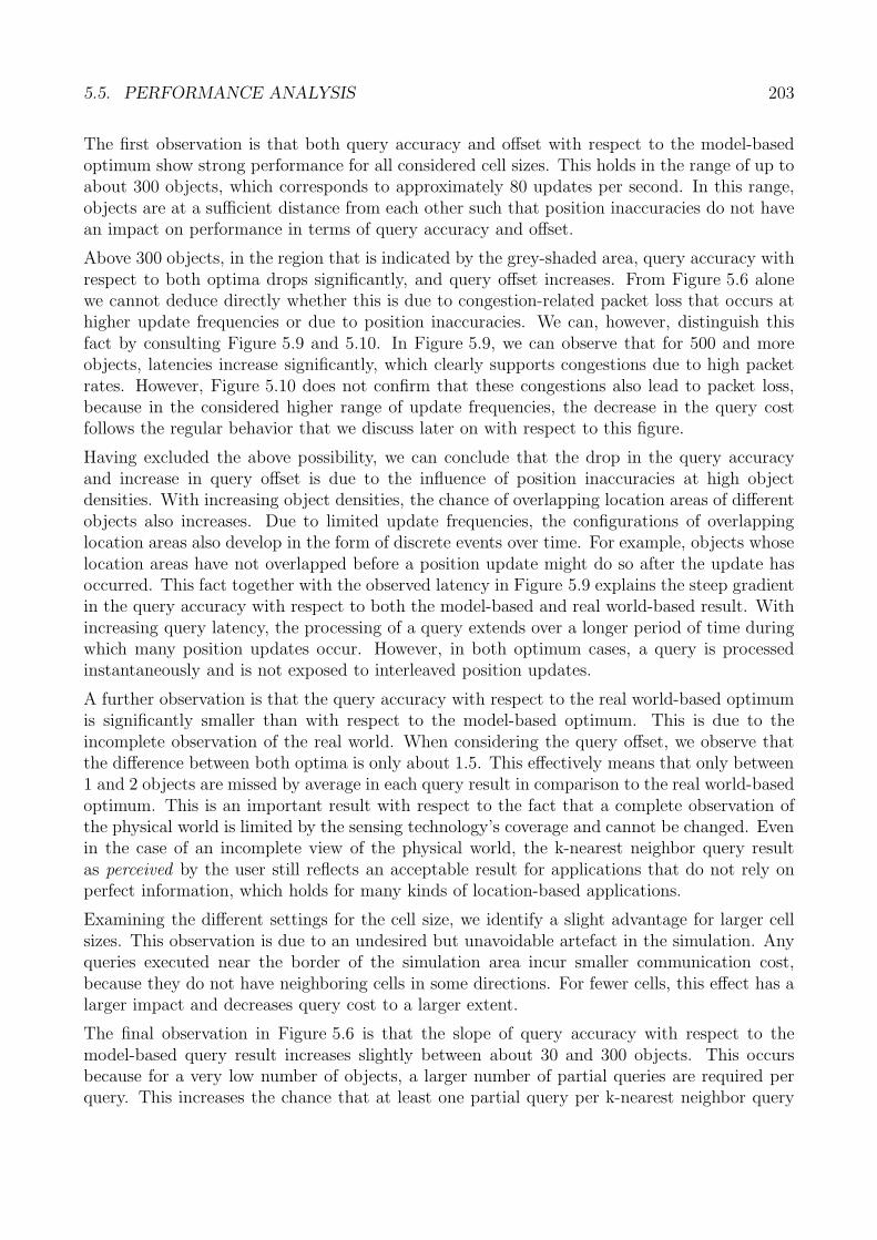
5.5. PERFORMANCE ANALYSIS 203
The first observation is that both query accuracy and offset with respect to the model-basedoptimum show strong performance for all considered cell sizes. This holds in the range of up toabout 300 objects, which corresponds to approximately 80 updates per second. In this range,objects are at a sufficient distance from each other such that position inaccuracies do not havean impact on performance in terms of query accuracy and offset.
Above 300 objects, in the region that is indicated by the grey-shaded area, query accuracy withrespect to both optima drops significantly, and query offset increases. From Figure 5.6 alonewe cannot deduce directly whether this is due to congestion-related packet loss that occurs athigher update frequencies or due to position inaccuracies. We can, however, distinguish thisfact by consulting Figure 5.9 and 5.10. In Figure 5.9, we can observe that for 500 and moreobjects, latencies increase significantly, which clearly supports congestions due to high packetrates. However, Figure 5.10 does not confirm that these congestions also lead to packet loss,because in the considered higher range of update frequencies, the decrease in the query costfollows the regular behavior that we discuss later on with respect to this figure.
Having excluded the above possibility, we can conclude that the drop in the query accuracyand increase in query offset is due to the influence of position inaccuracies at high objectdensities. With increasing object densities, the chance of overlapping location areas of differentobjects also increases. Due to limited update frequencies, the configurations of overlappinglocation areas also develop in the form of discrete events over time. For example, objects whoselocation areas have not overlapped before a position update might do so after the update hasoccurred. This fact together with the observed latency in Figure 5.9 explains the steep gradientin the query accuracy with respect to both the model-based and real world-based result. Withincreasing query latency, the processing of a query extends over a longer period of time duringwhich many position updates occur. However, in both optimum cases, a query is processedinstantaneously and is not exposed to interleaved position updates.
A further observation is that the query accuracy with respect to the real world-based optimumis significantly smaller than with respect to the model-based optimum. This is due to theincomplete observation of the real world. When considering the query offset, we observe thatthe difference between both optima is only about 1.5. This effectively means that only between1 and 2 objects are missed by average in each query result in comparison to the real world-basedoptimum. This is an important result with respect to the fact that a complete observation ofthe physical world is limited by the sensing technology’s coverage and cannot be changed. Evenin the case of an incomplete view of the physical world, the k-nearest neighbor query resultas perceived by the user still reflects an acceptable result for applications that do not rely onperfect information, which holds for many kinds of location-based applications.
Examining the different settings for the cell size, we identify a slight advantage for larger cellsizes. This observation is due to an undesired but unavoidable artefact in the simulation. Anyqueries executed near the border of the simulation area incur smaller communication cost,because they do not have neighboring cells in some directions. For fewer cells, this effect has alarger impact and decreases query cost to a larger extent.
The final observation in Figure 5.6 is that the slope of query accuracy with respect to themodel-based query result increases slightly between about 30 and 300 objects. This occursbecause for a very low number of objects, a larger number of partial queries are required perquery. This increases the chance that at least one partial query per k-nearest neighbor query
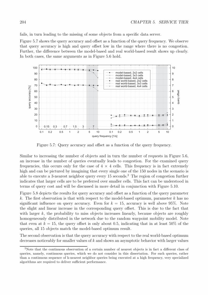
204 CHAPTER 5. SERVICE TIER
fails, in turn leading to the missing of some objects from a specific data server.
Figure 5.7 shows the query accuracy and offset as a function of the query frequency. We observethat query accuracy is high and query offset low in the range where there is no congestion.Further, the difference between the model-based and real world-based result shows up clearly.In both cases, the same arguments as in Figure 5.6 hold.
0
10
20
30
40
50
60
70
80
90
100
0.1
0.15
0.2
0.3
0.5
0.7
1
1.5
2
3
5
7
10 0.1 0.2 0.5 1 2 5 10
0
1
2
3
4
5
6
7
8
9
10
query
accura
cy
[%]
query
offset
query frequency [1/s]
model-based, 2x2 cells
real world-based, 2x2 cells
model-based, 3x3 cells
real world-based, 3x3 cells
model-based, 4x4 cells
real world-based, 4x4 cells
Figure 5.7: Query accuracy and offset as a function of the query frequency.
Similar to increasing the number of objects and in turn the number of requests in Figure 5.6,an increase in the number of queries eventually leads to congestion. For the examined queryfrequencies, this occurs only for the case of 4 × 4 cells. This frequency is in fact extremelyhigh and can be pictured by imagining that every single one of the 150 nodes in the scenario isable to execute a 3-nearest neighbor query every 15 seconds.2 The region of congestion furtherindicates that larger cells are to be preferred over smaller cells. This fact can be understood interms of query cost and will be discussed in more detail in conjunction with Figure 5.10.
Figure 5.8 depicts the results for query accuracy and offset as a function of the query parameterk. The first observation is that with respect to the model-based optimum, parameter k has nosignificant influence on query accuracy. Even for k = 15, accuracy is well above 95%. Notethe slight and linear increase in the corresponding query offset. This is due to the fact thatwith larger k, the probability to miss objects increases linearly, because objects are roughlyhomogeneously distributed in the network due to the random waypoint mobility model. Notethat even at k = 15, the query offset is only about 0.5, indicating that in at least 50% of thequeries, all 15 objects match the model-based optimum result.
The second observation is that the query accuracy with respect to the real world-based optimumdecreases noticeably for smaller values of k and shows an asymptotic behavior with larger values
2Note that the continuous observation of a certain number of nearest objects is in fact a different class ofqueries, namely, continuous queries, which we do not consider in this dissertation. For such queries, ratherthan a continuous sequence of k-nearest neighbor queries being executed at a high frequency, very specializedalgorithms are required to deliver sufficient performance.
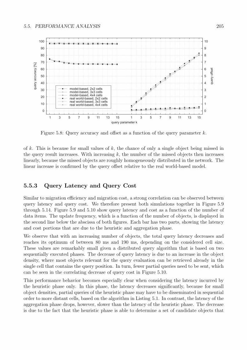
5.5. PERFORMANCE ANALYSIS 205
0
10
20
30
40
50
60
70
80
90
100
1 3 5 7 9 11 13 15 1 3 5 7 9 11 13 15
0
1
2
3
4
5
6
7
8
9
10
query
accura
cy
[%]
query
offset
query parameter k
model-based, 2x2 cells
real world-based, 2x2 cells
model-based, 3x3 cells
real world-based, 3x3 cells
model-based, 4x4 cells
real world-based, 4x4 cells
Figure 5.8: Query accuracy and offset as a function of the query parameter k.
of k. This is because for small values of k, the chance of only a single object being missed inthe query result increases. With increasing k, the number of the missed objects then increaseslinearly, because the missed objects are roughly homogeneously distributed in the network. Thelinear increase is confirmed by the query offset relative to the real world-based model.
5.5.3 Query Latency and Query Cost
Similar to migration efficiency and migration cost, a strong correlation can be observed betweenquery latency and query cost. We therefore present both simulations together in Figure 5.9through 5.14. Figure 5.9 and 5.10 show query latency and cost as a function of the number ofdata items. The update frequency, which is a function of the number of objects, is displayed inthe second line below the abscissa of both figures. Each bar has two parts, showing the latencyand cost portions that are due to the heuristic and aggregation phase.
We observe that with an increasing number of objects, the total query latency decreases andreaches its optimum of between 80 ms and 190 ms, depending on the considered cell size.These values are remarkably small given a distributed query algorithm that is based on twosequentially executed phases. The decrease of query latency is due to an increase in the objectdensity, where most objects relevant for the query evaluation can be retrieved already in thesingle cell that contains the query position. In turn, fewer partial queries need to be sent, whichcan be seen in the correlating decrease of query cost in Figure 5.10.
This performance behavior becomes especially clear when considering the latency incurred bythe heuristic phase only. In this phase, the latency decreases significantly, because for smallobject densities, partial queries of the heuristic phase may have to be disseminated in sequentialorder to more distant cells, based on the algorithm in Listing 5.1. In contrast, the latency of theaggregation phase drops, however, slower than the latency of the heuristic phase. The decreaseis due to the fact that the heuristic phase is able to determine a set of candidate objects that
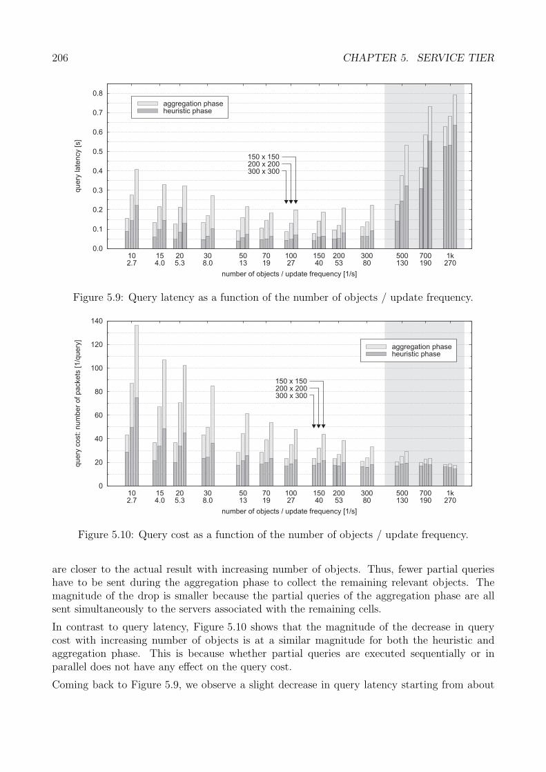
206 CHAPTER 5. SERVICE TIER
0.0
0.1
0.2
0.3
0.4
0.5
0.6
0.7
0.8
102.7
154.0
205.3
308.0
5013
7019
10027
15040
20053
30080
500130
700190
1k270
query
late
ncy
[s]
number of objects / update frequency [1/s]
150 x 150200 x 200300 x 300
aggregation phaseheuristic phase
Figure 5.9: Query latency as a function of the number of objects / update frequency.
0
20
40
60
80
100
120
140
102.7
154.0
205.3
308.0
5013
7019
10027
15040
20053
30080
500130
700190
1k270
query
cost:
num
ber
ofpackets
[1/q
uery
]
number of objects / update frequency [1/s]
150 x 150200 x 200300 x 300
aggregation phaseheuristic phase
Figure 5.10: Query cost as a function of the number of objects / update frequency.
are closer to the actual result with increasing number of objects. Thus, fewer partial querieshave to be sent during the aggregation phase to collect the remaining relevant objects. Themagnitude of the drop is smaller because the partial queries of the aggregation phase are allsent simultaneously to the servers associated with the remaining cells.
In contrast to query latency, Figure 5.10 shows that the magnitude of the decrease in querycost with increasing number of objects is at a similar magnitude for both the heuristic andaggregation phase. This is because whether partial queries are executed sequentially or inparallel does not have any effect on the query cost.
Coming back to Figure 5.9, we observe a slight decrease in query latency starting from about
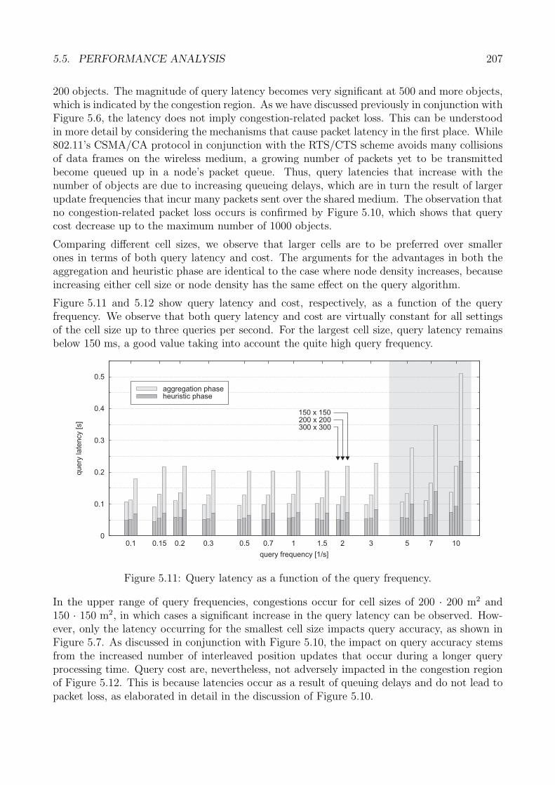
5.5. PERFORMANCE ANALYSIS 207
200 objects. The magnitude of query latency becomes very significant at 500 and more objects,which is indicated by the congestion region. As we have discussed previously in conjunction withFigure 5.6, the latency does not imply congestion-related packet loss. This can be understoodin more detail by considering the mechanisms that cause packet latency in the first place. While802.11’s CSMA/CA protocol in conjunction with the RTS/CTS scheme avoids many collisionsof data frames on the wireless medium, a growing number of packets yet to be transmittedbecome queued up in a node’s packet queue. Thus, query latencies that increase with thenumber of objects are due to increasing queueing delays, which are in turn the result of largerupdate frequencies that incur many packets sent over the shared medium. The observation thatno congestion-related packet loss occurs is confirmed by Figure 5.10, which shows that querycost decrease up to the maximum number of 1000 objects.
Comparing different cell sizes, we observe that larger cells are to be preferred over smallerones in terms of both query latency and cost. The arguments for the advantages in both theaggregation and heuristic phase are identical to the case where node density increases, becauseincreasing either cell size or node density has the same effect on the query algorithm.
Figure 5.11 and 5.12 show query latency and cost, respectively, as a function of the queryfrequency. We observe that both query latency and cost are virtually constant for all settingsof the cell size up to three queries per second. For the largest cell size, query latency remainsbelow 150 ms, a good value taking into account the quite high query frequency.
0
0.1
0.2
0.3
0.4
0.5
0.1 0.15 0.2 0.3 0.5 0.7 1 1.5 2 3 5 7 10
query
late
ncy
[s]
query frequency [1/s]
150 x 150200 x 200300 x 300
aggregation phaseheuristic phase
Figure 5.11: Query latency as a function of the query frequency.
In the upper range of query frequencies, congestions occur for cell sizes of 200 · 200 m2 and150 · 150 m2, in which cases a significant increase in the query latency can be observed. How-ever, only the latency occurring for the smallest cell size impacts query accuracy, as shown inFigure 5.7. As discussed in conjunction with Figure 5.10, the impact on query accuracy stemsfrom the increased number of interleaved position updates that occur during a longer queryprocessing time. Query cost are, nevertheless, not adversely impacted in the congestion regionof Figure 5.12. This is because latencies occur as a result of queuing delays and do not lead topacket loss, as elaborated in detail in the discussion of Figure 5.10.
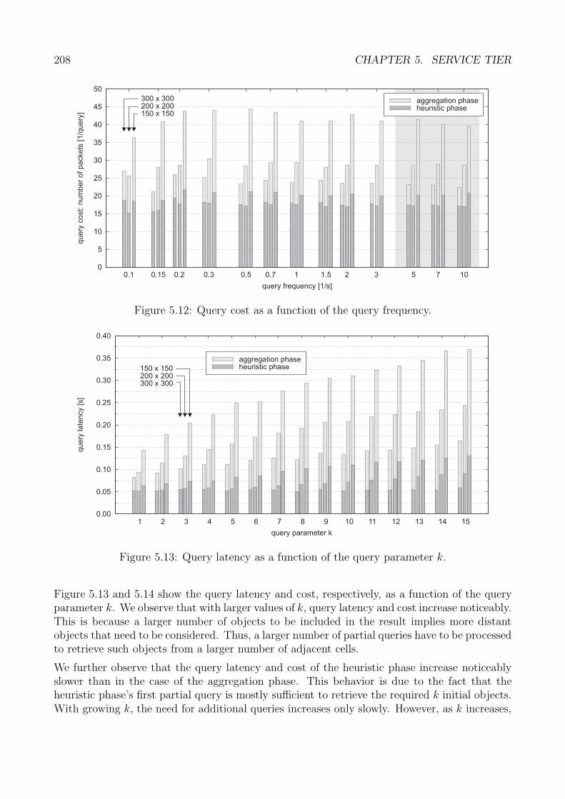
208 CHAPTER 5. SERVICE TIER
0
5
10
15
20
25
30
35
40
45
50
0.1 0.15 0.2 0.3 0.5 0.7 1 1.5 2 3 5 7 10
query
cost:
num
ber
ofpackets
[1/q
uery
]
query frequency [1/s]
300 x 300200 x 200150 x 150
aggregation phaseheuristic phase
Figure 5.12: Query cost as a function of the query frequency.
0.00
0.05
0.10
0.15
0.20
0.25
0.30
0.35
0.40
1 2 3 4 5 6 7 8 9 10 11 12 13 14 15
query
late
ncy
[s]
query parameter k
150 x 150200 x 200300 x 300
aggregation phaseheuristic phase
Figure 5.13: Query latency as a function of the query parameter k.
Figure 5.13 and 5.14 show the query latency and cost, respectively, as a function of the queryparameter k. We observe that with larger values of k, query latency and cost increase noticeably.This is because a larger number of objects to be included in the result implies more distantobjects that need to be considered. Thus, a larger number of partial queries have to be processedto retrieve such objects from a larger number of adjacent cells.
We further observe that the query latency and cost of the heuristic phase increase noticeablyslower than in the case of the aggregation phase. This behavior is due to the fact that theheuristic phase’s first partial query is mostly sufficient to retrieve the required k initial objects.With growing k, the need for additional queries increases only slowly. However, as k increases,
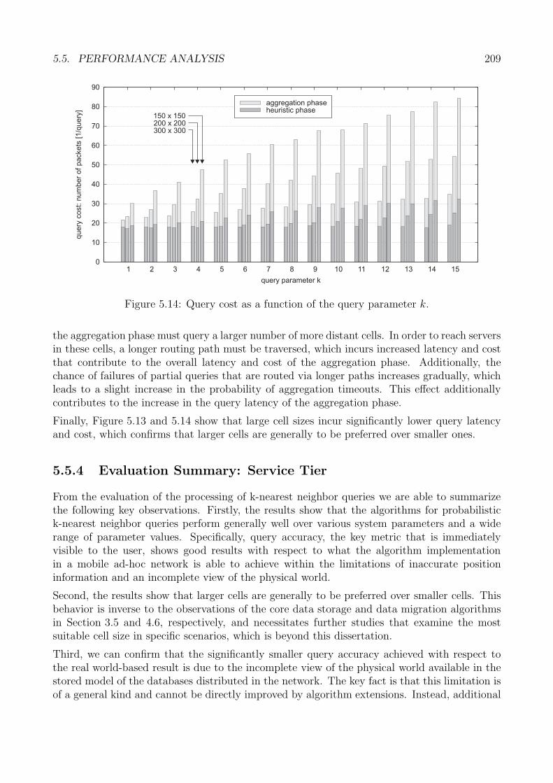
5.5. PERFORMANCE ANALYSIS 209
0
10
20
30
40
50
60
70
80
90
1 2 3 4 5 6 7 8 9 10 11 12 13 14 15
query
cost:
num
ber
ofpackets
[1/q
uery
]
query parameter k
aggregation phaseheuristic phase
150 x 150200 x 200300 x 300
Figure 5.14: Query cost as a function of the query parameter k.
the aggregation phase must query a larger number of more distant cells. In order to reach serversin these cells, a longer routing path must be traversed, which incurs increased latency and costthat contribute to the overall latency and cost of the aggregation phase. Additionally, thechance of failures of partial queries that are routed via longer paths increases gradually, whichleads to a slight increase in the probability of aggregation timeouts. This effect additionallycontributes to the increase in the query latency of the aggregation phase.
Finally, Figure 5.13 and 5.14 show that large cell sizes incur significantly lower query latencyand cost, which confirms that larger cells are generally to be preferred over smaller ones.
5.5.4 Evaluation Summary: Service Tier
From the evaluation of the processing of k-nearest neighbor queries we are able to summarizethe following key observations. Firstly, the results show that the algorithms for probabilistick-nearest neighbor queries perform generally well over various system parameters and a widerange of parameter values. Specifically, query accuracy, the key metric that is immediatelyvisible to the user, shows good results with respect to what the algorithm implementationin a mobile ad-hoc network is able to achieve within the limitations of inaccurate positioninformation and an incomplete view of the physical world.
Second, the results show that larger cells are generally to be preferred over smaller cells. Thisbehavior is inverse to the observations of the core data storage and data migration algorithmsin Section 3.5 and 4.6, respectively, and necessitates further studies that examine the mostsuitable cell size in specific scenarios, which is beyond this dissertation.
Third, we can confirm that the significantly smaller query accuracy achieved with respect tothe real world-based result is due to the incomplete view of the physical world available in thestored model of the databases distributed in the network. The key fact is that this limitation isof a general kind and cannot be directly improved by algorithm extensions. Instead, additional
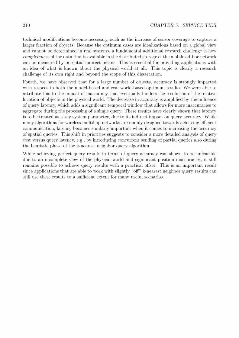
210 CHAPTER 5. SERVICE TIER
technical modifications become necessary, such as the increase of sensor coverage to capture alarger fraction of objects. Because the optimum cases are idealizations based on a global viewand cannot be determined in real systems, a fundamental additional research challenge is howcompleteness of the data that is available in the distributed storage of the mobile ad-hoc networkcan be measured by potential indirect means. This is essential for providing applications withan idea of what is known about the physical world at all. This topic is clearly a researchchallenge of its own right and beyond the scope of this dissertation.
Fourth, we have observed that for a large number of objects, accuracy is strongly impactedwith respect to both the model-based and real world-based optimum results. We were able toattribute this to the impact of inaccuracy that eventually hinders the resolution of the relativelocation of objects in the physical world. The decrease in accuracy is amplified by the influenceof query latency, which adds a significant temporal window that allows for more inaccuracies toaggregate during the processing of a single query. These results have clearly shown that latencyis to be treated as a key system parameter, due to its indirect impact on query accuracy. Whilemany algorithms for wireless multihop networks are mainly designed towards achieving efficientcommunication, latency becomes similarly important when it comes to increasing the accuracyof spatial queries. This shift in priorities suggests to consider a more detailed analysis of querycost versus query latency, e.g., by introducing concurrent sending of partial queries also duringthe heuristic phase of the k-nearest neighbor query algorithm.
While achieving perfect query results in terms of query accuracy was shown to be unfeasibledue to an incomplete view of the physical world and significant position inaccuracies, it stillremains possible to achieve query results with a practical offset. This is an important resultsince applications that are able to work with slightly “off” k-nearest neighbor query results canstill use these results to a sufficient extent for many useful scenarios.
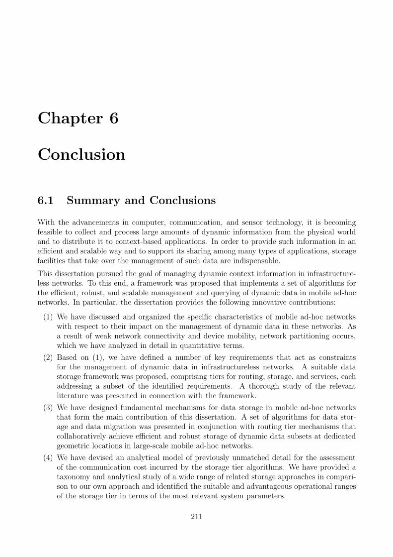
Chapter 6
Conclusion
6.1 Summary and Conclusions
With the advancements in computer, communication, and sensor technology, it is becomingfeasible to collect and process large amounts of dynamic information from the physical worldand to distribute it to context-based applications. In order to provide such information in anefficient and scalable way and to support its sharing among many types of applications, storagefacilities that take over the management of such data are indispensable.
This dissertation pursued the goal of managing dynamic context information in infrastructure-less networks. To this end, a framework was proposed that implements a set of algorithms forthe efficient, robust, and scalable management and querying of dynamic data in mobile ad-hocnetworks. In particular, the dissertation provides the following innovative contributions:
(1) We have discussed and organized the specific characteristics of mobile ad-hoc networkswith respect to their impact on the management of dynamic data in these networks. Asa result of weak network connectivity and device mobility, network partitioning occurs,which we have analyzed in detail in quantitative terms.
(2) Based on (1), we have defined a number of key requirements that act as constraintsfor the management of dynamic data in infrastructureless networks. A suitable datastorage framework was proposed, comprising tiers for routing, storage, and services, eachaddressing a subset of the identified requirements. A thorough study of the relevantliterature was presented in connection with the framework.
(3) We have designed fundamental mechanisms for data storage in mobile ad-hoc networksthat form the main contribution of this dissertation. A set of algorithms for data stor-age and data migration was presented in conjunction with routing tier mechanisms thatcollaboratively achieve efficient and robust storage of dynamic data subsets at dedicatedgeometric locations in large-scale mobile ad-hoc networks.
(4) We have devised an analytical model of previously unmatched detail for the assessmentof the communication cost incurred by the storage tier algorithms. We have provided ataxonomy and analytical study of a wide range of related storage approaches in compari-son to our own approach and identified the suitable and advantageous operational rangesof the storage tier in terms of the most relevant system parameters.
211
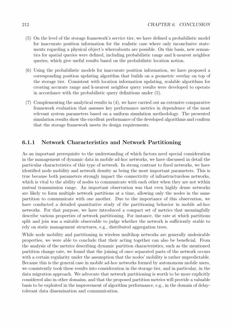
212 CHAPTER 6. CONCLUSION
(5) On the level of the storage framework’s service tier, we have defined a probabilistic modelfor inaccurate position information for the realistic case where only inconclusive state-ments regarding a physical object’s whereabouts are possible. On this basis, new seman-tics for spatial queries were defined, including probabilistic range and k-nearest neighborqueries, which give useful results based on the probabilistic location notion.
(6) Using the probabilistic models for inaccurate position information, we have proposed acorresponding position updating algorithm that builds on a geometric overlay on top ofthe storage tier. Consistent with location information updating, scalable algorithms forcreating accurate range and k-nearest neighbor query results were developed to operatein accordance with the probabilistic query definitions under (5).
(7) Complementing the analytical results in (4), we have carried out an extensive comparativeframework evaluation that assesses key performance metrics in dependence of the mostrelevant system parameters based on a uniform simulation methodology. The presentedsimulation results show the excellent performance of the developed algorithms and confirmthat the storage framework meets its design requirements.
6.1.1 Network Characteristics and Network Partitioning
As an important prerequisite to the understanding of which factors need special considerationin the management of dynamic data in mobile ad-hoc networks, we have discussed in detail theparticular characteristics of this type of network. In strong contrast to fixed networks, we haveidentified node mobility and network density as being the most important parameters. This istrue because both parameters strongly impact the connectivity of infrastructureless networks,which is vital to the ability of nodes to communicate with each other when they are not withinmutual transmission range. An important observation was that even highly dense networksare likely to form multiple network partitions at a time, allowing only the nodes in the samepartition to communicate with one another. Due to the importance of this observation, wehave conducted a detailed quantitative study of the partitioning behavior in mobile ad-hocnetworks. For that purpose, we have introduced a compact set of metrics that meaningfullydescribe various properties of network partitioning. For instance, the rate at which partitionssplit and join was a suitable observable to judge whether the network is sufficiently stable torely on static management structures, e.g., distributed aggregation trees.
While node mobility and partitioning in wireless multihop networks are generally undesirableproperties, we were able to conclude that their acting together can also be beneficial. Fromthe analysis of the metrics describing dynamic partition characteristics, such as the mentionedpartition change rate, we found that the joining of once separated parts of the network occurswith a certain regularity under the assumption that the nodes’ mobility is rather unpredictable.Because this is the general case in mobile ad-hoc networks formed by autonomous mobile users,we consistently took these results into consideration in the storage tier, and in particular, in thedata migration approach. We advocate that network partitioning is worth to be more explicitlyconsidered also in other domains, and that the proposed partition metrics will provide a valuablebasis to be exploited in the improvement of algorithm performance, e.g., in the domain of delay-tolerant data dissemination and communication.
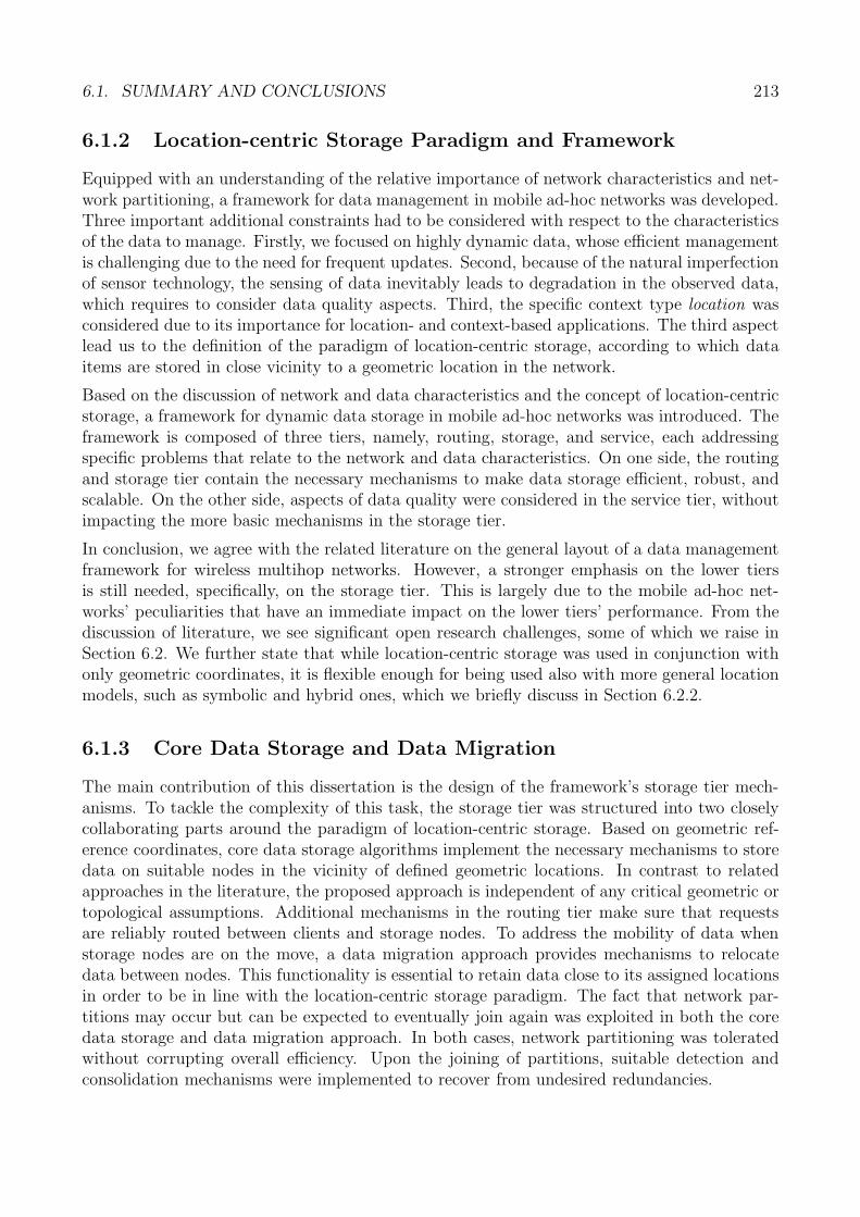
6.1. SUMMARY AND CONCLUSIONS 213
6.1.2 Location-centric Storage Paradigm and Framework
Equipped with an understanding of the relative importance of network characteristics and net-work partitioning, a framework for data management in mobile ad-hoc networks was developed.Three important additional constraints had to be considered with respect to the characteristicsof the data to manage. Firstly, we focused on highly dynamic data, whose efficient managementis challenging due to the need for frequent updates. Second, because of the natural imperfectionof sensor technology, the sensing of data inevitably leads to degradation in the observed data,which requires to consider data quality aspects. Third, the specific context type location wasconsidered due to its importance for location- and context-based applications. The third aspectlead us to the definition of the paradigm of location-centric storage, according to which dataitems are stored in close vicinity to a geometric location in the network.
Based on the discussion of network and data characteristics and the concept of location-centricstorage, a framework for dynamic data storage in mobile ad-hoc networks was introduced. Theframework is composed of three tiers, namely, routing, storage, and service, each addressingspecific problems that relate to the network and data characteristics. On one side, the routingand storage tier contain the necessary mechanisms to make data storage efficient, robust, andscalable. On the other side, aspects of data quality were considered in the service tier, withoutimpacting the more basic mechanisms in the storage tier.
In conclusion, we agree with the related literature on the general layout of a data managementframework for wireless multihop networks. However, a stronger emphasis on the lower tiersis still needed, specifically, on the storage tier. This is largely due to the mobile ad-hoc net-works’ peculiarities that have an immediate impact on the lower tiers’ performance. From thediscussion of literature, we see significant open research challenges, some of which we raise inSection 6.2. We further state that while location-centric storage was used in conjunction withonly geometric coordinates, it is flexible enough for being used also with more general locationmodels, such as symbolic and hybrid ones, which we briefly discuss in Section 6.2.2.
6.1.3 Core Data Storage and Data Migration
The main contribution of this dissertation is the design of the framework’s storage tier mech-anisms. To tackle the complexity of this task, the storage tier was structured into two closelycollaborating parts around the paradigm of location-centric storage. Based on geometric ref-erence coordinates, core data storage algorithms implement the necessary mechanisms to storedata on suitable nodes in the vicinity of defined geometric locations. In contrast to relatedapproaches in the literature, the proposed approach is independent of any critical geometric ortopological assumptions. Additional mechanisms in the routing tier make sure that requestsare reliably routed between clients and storage nodes. To address the mobility of data whenstorage nodes are on the move, a data migration approach provides mechanisms to relocatedata between nodes. This functionality is essential to retain data close to its assigned locationsin order to be in line with the location-centric storage paradigm. The fact that network par-titions may occur but can be expected to eventually join again was exploited in both the coredata storage and data migration approach. In both cases, network partitioning was toleratedwithout corrupting overall efficiency. Upon the joining of partitions, suitable detection andconsolidation mechanisms were implemented to recover from undesired redundancies.
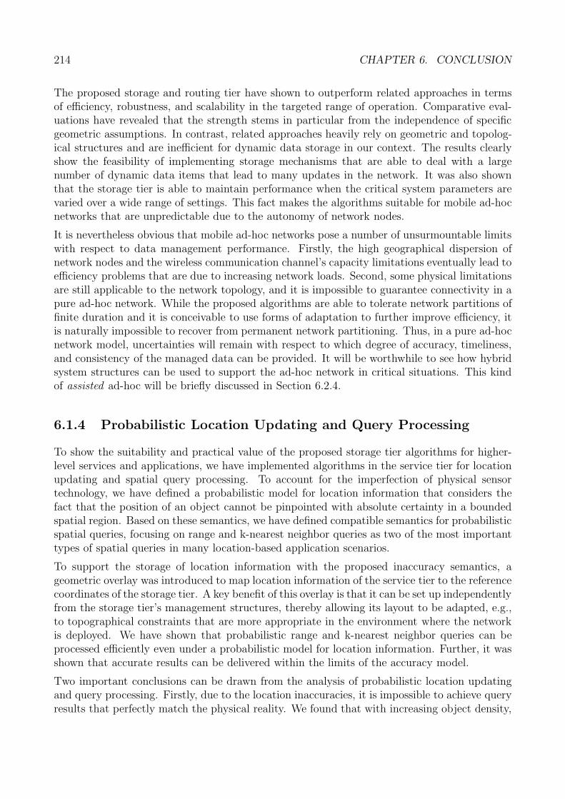
214 CHAPTER 6. CONCLUSION
The proposed storage and routing tier have shown to outperform related approaches in termsof efficiency, robustness, and scalability in the targeted range of operation. Comparative eval-uations have revealed that the strength stems in particular from the independence of specificgeometric assumptions. In contrast, related approaches heavily rely on geometric and topolog-ical structures and are inefficient for dynamic data storage in our context. The results clearlyshow the feasibility of implementing storage mechanisms that are able to deal with a largenumber of dynamic data items that lead to many updates in the network. It was also shownthat the storage tier is able to maintain performance when the critical system parameters arevaried over a wide range of settings. This fact makes the algorithms suitable for mobile ad-hocnetworks that are unpredictable due to the autonomy of network nodes.
It is nevertheless obvious that mobile ad-hoc networks pose a number of unsurmountable limitswith respect to data management performance. Firstly, the high geographical dispersion ofnetwork nodes and the wireless communication channel’s capacity limitations eventually lead toefficiency problems that are due to increasing network loads. Second, some physical limitationsare still applicable to the network topology, and it is impossible to guarantee connectivity in apure ad-hoc network. While the proposed algorithms are able to tolerate network partitions offinite duration and it is conceivable to use forms of adaptation to further improve efficiency, itis naturally impossible to recover from permanent network partitioning. Thus, in a pure ad-hocnetwork model, uncertainties will remain with respect to which degree of accuracy, timeliness,and consistency of the managed data can be provided. It will be worthwhile to see how hybridsystem structures can be used to support the ad-hoc network in critical situations. This kindof assisted ad-hoc will be briefly discussed in Section 6.2.4.
6.1.4 Probabilistic Location Updating and Query Processing
To show the suitability and practical value of the proposed storage tier algorithms for higher-level services and applications, we have implemented algorithms in the service tier for locationupdating and spatial query processing. To account for the imperfection of physical sensortechnology, we have defined a probabilistic model for location information that considers thefact that the position of an object cannot be pinpointed with absolute certainty in a boundedspatial region. Based on these semantics, we have defined compatible semantics for probabilisticspatial queries, focusing on range and k-nearest neighbor queries as two of the most importanttypes of spatial queries in many location-based application scenarios.
To support the storage of location information with the proposed inaccuracy semantics, ageometric overlay was introduced to map location information of the service tier to the referencecoordinates of the storage tier. A key benefit of this overlay is that it can be set up independentlyfrom the storage tier’s management structures, thereby allowing its layout to be adapted, e.g.,to topographical constraints that are more appropriate in the environment where the networkis deployed. We have shown that probabilistic range and k-nearest neighbor queries can beprocessed efficiently even under a probabilistic model for location information. Further, it wasshown that accurate results can be delivered within the limits of the accuracy model.
Two important conclusions can be drawn from the analysis of probabilistic location updatingand query processing. Firstly, due to the location inaccuracies, it is impossible to achieve queryresults that perfectly match the physical reality. We found that with increasing object density,
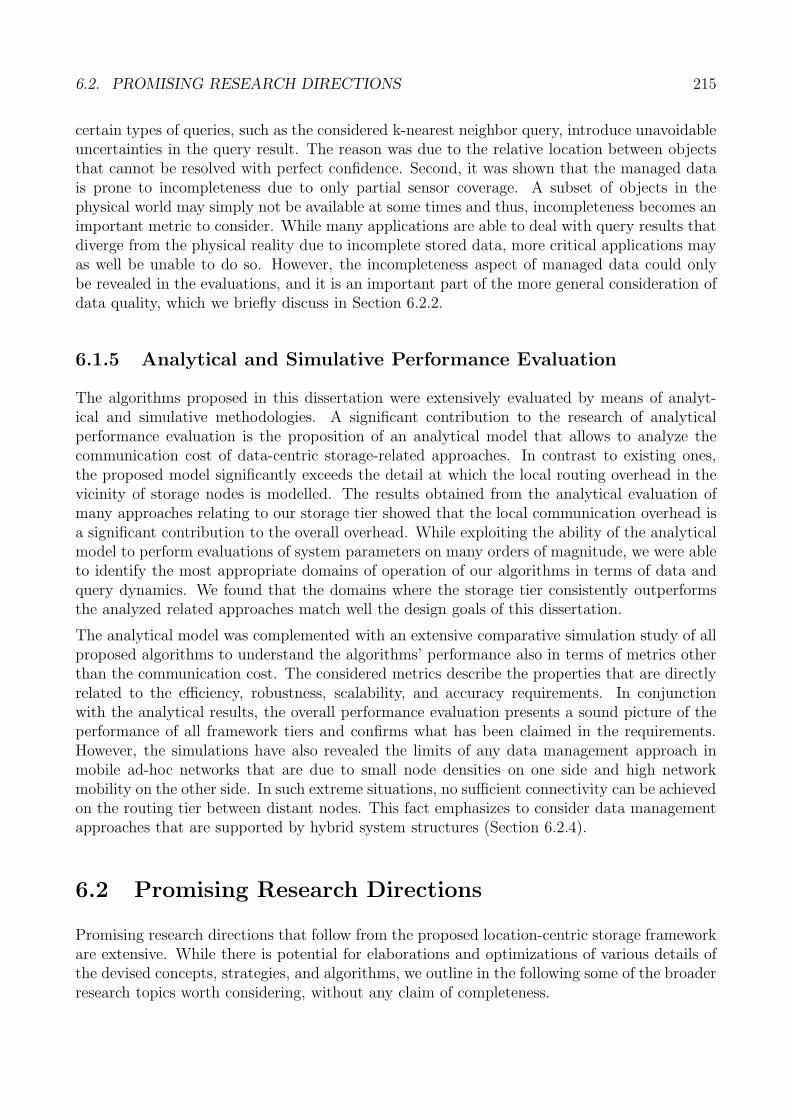
6.2. PROMISING RESEARCH DIRECTIONS 215
certain types of queries, such as the considered k-nearest neighbor query, introduce unavoidableuncertainties in the query result. The reason was due to the relative location between objectsthat cannot be resolved with perfect confidence. Second, it was shown that the managed datais prone to incompleteness due to only partial sensor coverage. A subset of objects in thephysical world may simply not be available at some times and thus, incompleteness becomes animportant metric to consider. While many applications are able to deal with query results thatdiverge from the physical reality due to incomplete stored data, more critical applications mayas well be unable to do so. However, the incompleteness aspect of managed data could onlybe revealed in the evaluations, and it is an important part of the more general consideration ofdata quality, which we briefly discuss in Section 6.2.2.
6.1.5 Analytical and Simulative Performance Evaluation
The algorithms proposed in this dissertation were extensively evaluated by means of analyt-ical and simulative methodologies. A significant contribution to the research of analyticalperformance evaluation is the proposition of an analytical model that allows to analyze thecommunication cost of data-centric storage-related approaches. In contrast to existing ones,the proposed model significantly exceeds the detail at which the local routing overhead in thevicinity of storage nodes is modelled. The results obtained from the analytical evaluation ofmany approaches relating to our storage tier showed that the local communication overhead isa significant contribution to the overall overhead. While exploiting the ability of the analyticalmodel to perform evaluations of system parameters on many orders of magnitude, we were ableto identify the most appropriate domains of operation of our algorithms in terms of data andquery dynamics. We found that the domains where the storage tier consistently outperformsthe analyzed related approaches match well the design goals of this dissertation.
The analytical model was complemented with an extensive comparative simulation study of allproposed algorithms to understand the algorithms’ performance also in terms of metrics otherthan the communication cost. The considered metrics describe the properties that are directlyrelated to the efficiency, robustness, scalability, and accuracy requirements. In conjunctionwith the analytical results, the overall performance evaluation presents a sound picture of theperformance of all framework tiers and confirms what has been claimed in the requirements.However, the simulations have also revealed the limits of any data management approach inmobile ad-hoc networks that are due to small node densities on one side and high networkmobility on the other side. In such extreme situations, no sufficient connectivity can be achievedon the routing tier between distant nodes. This fact emphasizes to consider data managementapproaches that are supported by hybrid system structures (Section 6.2.4).
6.2 Promising Research Directions
Promising research directions that follow from the proposed location-centric storage frameworkare extensive. While there is potential for elaborations and optimizations of various details ofthe devised concepts, strategies, and algorithms, we outline in the following some of the broaderresearch topics worth considering, without any claim of completeness.
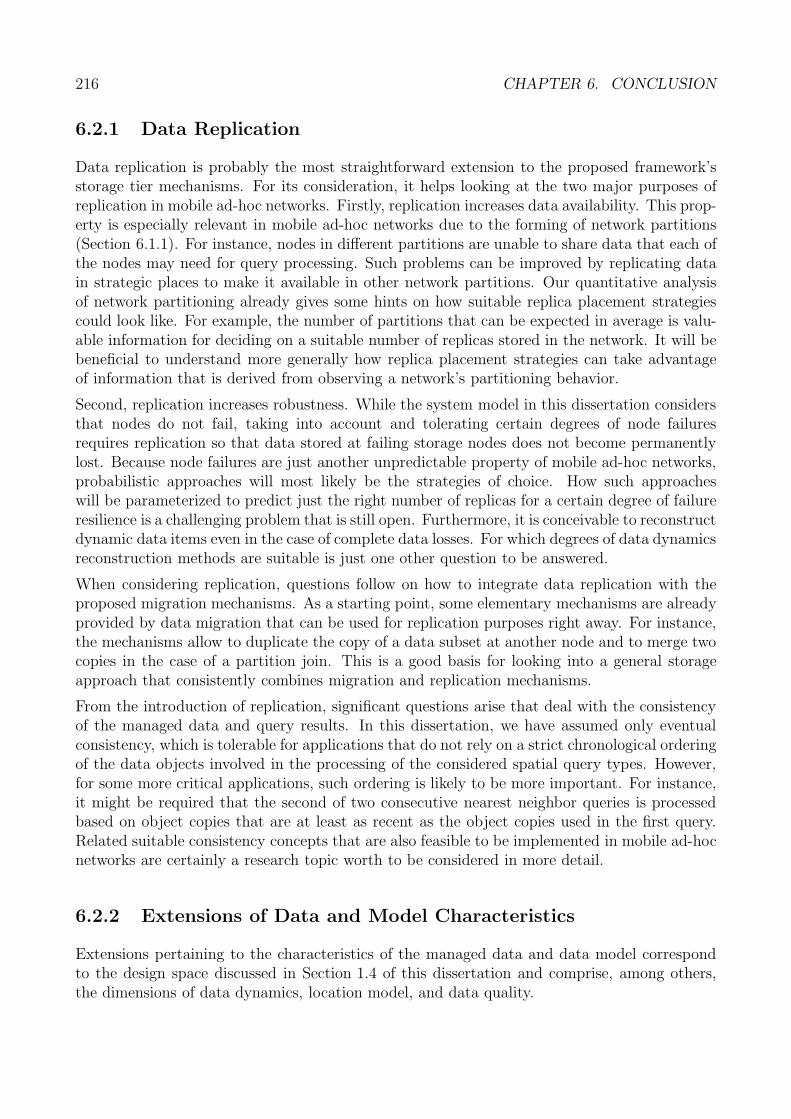
216 CHAPTER 6. CONCLUSION
6.2.1 Data Replication
Data replication is probably the most straightforward extension to the proposed framework’sstorage tier mechanisms. For its consideration, it helps looking at the two major purposes ofreplication in mobile ad-hoc networks. Firstly, replication increases data availability. This prop-erty is especially relevant in mobile ad-hoc networks due to the forming of network partitions(Section 6.1.1). For instance, nodes in different partitions are unable to share data that each ofthe nodes may need for query processing. Such problems can be improved by replicating datain strategic places to make it available in other network partitions. Our quantitative analysisof network partitioning already gives some hints on how suitable replica placement strategiescould look like. For example, the number of partitions that can be expected in average is valu-able information for deciding on a suitable number of replicas stored in the network. It will bebeneficial to understand more generally how replica placement strategies can take advantageof information that is derived from observing a network’s partitioning behavior.
Second, replication increases robustness. While the system model in this dissertation considersthat nodes do not fail, taking into account and tolerating certain degrees of node failuresrequires replication so that data stored at failing storage nodes does not become permanentlylost. Because node failures are just another unpredictable property of mobile ad-hoc networks,probabilistic approaches will most likely be the strategies of choice. How such approacheswill be parameterized to predict just the right number of replicas for a certain degree of failureresilience is a challenging problem that is still open. Furthermore, it is conceivable to reconstructdynamic data items even in the case of complete data losses. For which degrees of data dynamicsreconstruction methods are suitable is just one other question to be answered.
When considering replication, questions follow on how to integrate data replication with theproposed migration mechanisms. As a starting point, some elementary mechanisms are alreadyprovided by data migration that can be used for replication purposes right away. For instance,the mechanisms allow to duplicate the copy of a data subset at another node and to merge twocopies in the case of a partition join. This is a good basis for looking into a general storageapproach that consistently combines migration and replication mechanisms.
From the introduction of replication, significant questions arise that deal with the consistencyof the managed data and query results. In this dissertation, we have assumed only eventualconsistency, which is tolerable for applications that do not rely on a strict chronological orderingof the data objects involved in the processing of the considered spatial query types. However,for some more critical applications, such ordering is likely to be more important. For instance,it might be required that the second of two consecutive nearest neighbor queries is processedbased on object copies that are at least as recent as the object copies used in the first query.Related suitable consistency concepts that are also feasible to be implemented in mobile ad-hocnetworks are certainly a research topic worth to be considered in more detail.
6.2.2 Extensions of Data and Model Characteristics
Extensions pertaining to the characteristics of the managed data and data model correspondto the design space discussed in Section 1.4 of this dissertation and comprise, among others,the dimensions of data dynamics, location model, and data quality.
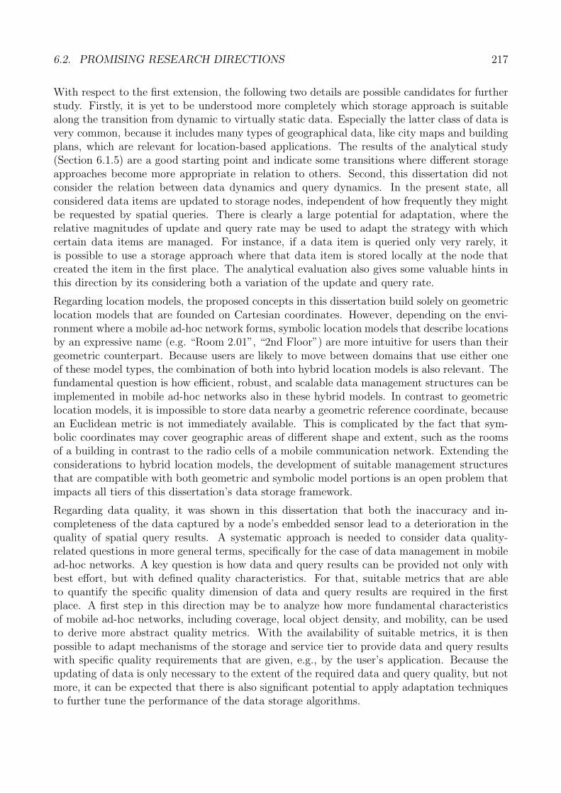
6.2. PROMISING RESEARCH DIRECTIONS 217
With respect to the first extension, the following two details are possible candidates for furtherstudy. Firstly, it is yet to be understood more completely which storage approach is suitablealong the transition from dynamic to virtually static data. Especially the latter class of data isvery common, because it includes many types of geographical data, like city maps and buildingplans, which are relevant for location-based applications. The results of the analytical study(Section 6.1.5) are a good starting point and indicate some transitions where different storageapproaches become more appropriate in relation to others. Second, this dissertation did notconsider the relation between data dynamics and query dynamics. In the present state, allconsidered data items are updated to storage nodes, independent of how frequently they mightbe requested by spatial queries. There is clearly a large potential for adaptation, where therelative magnitudes of update and query rate may be used to adapt the strategy with whichcertain data items are managed. For instance, if a data item is queried only very rarely, itis possible to use a storage approach where that data item is stored locally at the node thatcreated the item in the first place. The analytical evaluation also gives some valuable hints inthis direction by its considering both a variation of the update and query rate.
Regarding location models, the proposed concepts in this dissertation build solely on geometriclocation models that are founded on Cartesian coordinates. However, depending on the envi-ronment where a mobile ad-hoc network forms, symbolic location models that describe locationsby an expressive name (e.g. “Room 2.01”, “2nd Floor”) are more intuitive for users than theirgeometric counterpart. Because users are likely to move between domains that use either oneof these model types, the combination of both into hybrid location models is also relevant. Thefundamental question is how efficient, robust, and scalable data management structures can beimplemented in mobile ad-hoc networks also in these hybrid models. In contrast to geometriclocation models, it is impossible to store data nearby a geometric reference coordinate, becausean Euclidean metric is not immediately available. This is complicated by the fact that sym-bolic coordinates may cover geographic areas of different shape and extent, such as the roomsof a building in contrast to the radio cells of a mobile communication network. Extending theconsiderations to hybrid location models, the development of suitable management structuresthat are compatible with both geometric and symbolic model portions is an open problem thatimpacts all tiers of this dissertation’s data storage framework.
Regarding data quality, it was shown in this dissertation that both the inaccuracy and in-completeness of the data captured by a node’s embedded sensor lead to a deterioration in thequality of spatial query results. A systematic approach is needed to consider data quality-related questions in more general terms, specifically for the case of data management in mobilead-hoc networks. A key question is how data and query results can be provided not only withbest effort, but with defined quality characteristics. For that, suitable metrics that are ableto quantify the specific quality dimension of data and query results are required in the firstplace. A first step in this direction may be to analyze how more fundamental characteristicsof mobile ad-hoc networks, including coverage, local object density, and mobility, can be usedto derive more abstract quality metrics. With the availability of suitable metrics, it is thenpossible to adapt mechanisms of the storage and service tier to provide data and query resultswith specific quality requirements that are given, e.g., by the user’s application. Because theupdating of data is only necessary to the extent of the required data and query quality, but notmore, it can be expected that there is also significant potential to apply adaptation techniquesto further tune the performance of the data storage algorithms.
218 CHAPTER 6. CONCLUSION
6.2.3 Extension of Service Functionality
In this dissertation, we have considered two types of spatial queries: range and k-nearest neigh-bor queries. It is straightforward to consider several other types of spatial queries, for instance,group and reverse nearest neighbor queries. The importance of such query types is supportedby the large body of related literature, which considers implementations for processing thesequeries mainly based on centralized index structures (Section 2.5.3). However, it is unexploredhow such queries can be processed in mobile ad-hoc networks in conjunction with probabilis-tic location semantics. Further generalizations of supported query types eventually lead toapproaches where spatial or even more general queries are expressed by a dedicated query lan-guage. The design of a suitable query processing framework for mobile ad-hoc networks thatsupports such a general approach is a largely open research challenge.
While queries are synchronous operations that are immediately processed by the query system,the consideration of asynchronous services is also of interest. Spatial event management is oneimportant instance of such services and describes, by means of event predicates, when objectsin the real world assume certain spatial constellations. In contrast to query processing, eventobservation works entirely different and introduces many additional questions to the storageand service tier. For instance, the suitable strategy of how to observe the predicate of an eventthat triggers when two objects meet at a given distance depends on the current distance the twoobjects maintain to each other. For small distances, a single storage node may be able to observethe predicate alone because it stores information about both objects. With increasing distance,two objects are likely to be known to different servers and their information must be broughttogether in order to detect possible occurrences of the event. With further increasing objectdistance, also this approach becomes impractical due to updates that need to be propagatedover many network hops. In this latter case, it might be more appropriate to make use of deadreckoning-based approaches. This example illustrates the bandwidth of possible approachesto observe just a single type of event under different object constellations. In mobile ad-hocnetworks, the observation of events is a challenging and still open task.
In Section 6.2.1, data replication was proposed as an extension of the storage tier in order toincrease the robustness of the data store. Due to the fact that event observation is stateful, itmakes sense to consider the replication of the event observation functionality itself to make itmore robust against node failures in wireless multihop networks. In the situation of an eventoccurring in the real world, it is then possible to observe the occurrence of the event even if anode that contains essential observation state has failed. While applying replication to eventobservation sounds promising, it is absolutely unclear how to guarantee that event observationis always consistent. For example, it is possible that based on inconsistent data, observationstaking place in parallel at different servers lead to predicate evaluations that contradict eachother. A framework of algorithms for the scalable and consistent observation of spatial eventsin mobile ad-hoc networks is a complex research field worth further consideration.
6.2.4 Hybrid System Structures
In this dissertation we have focused on the design and implementation of a framework forlocation-centric storage in mobile ad-hoc networks. In Section 6.1.3 and 6.1.5 we have con-
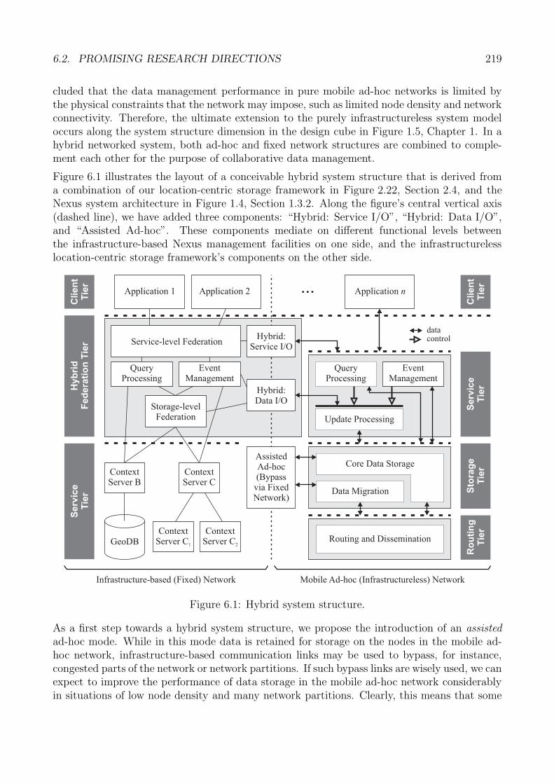
6.2. PROMISING RESEARCH DIRECTIONS 219
cluded that the data management performance in pure mobile ad-hoc networks is limited bythe physical constraints that the network may impose, such as limited node density and networkconnectivity. Therefore, the ultimate extension to the purely infrastructureless system modeloccurs along the system structure dimension in the design cube in Figure 1.5, Chapter 1. In ahybrid networked system, both ad-hoc and fixed network structures are combined to comple-ment each other for the purpose of collaborative data management.
Figure 6.1 illustrates the layout of a conceivable hybrid system structure that is derived froma combination of our location-centric storage framework in Figure 2.22, Section 2.4, and theNexus system architecture in Figure 1.4, Section 1.3.2. Along the figure’s central vertical axis(dashed line), we have added three components: “Hybrid: Service I/O”, “Hybrid: Data I/O”,and “Assisted Ad-hoc”. These components mediate on different functional levels betweenthe infrastructure-based Nexus management facilities on one side, and the infrastructurelesslocation-centric storage framework’s components on the other side.
Hybrid:Service I/O
Routing and Dissemination
Data Migration
EventManagement
QueryProcessing
Update Processing
Hybrid:Data I/O
datacontrol
Hyb
rid
Fed
era
tio
nT
ier
Serv
ice
Tie
r Sto
rag
eT
ier
Ro
uti
ng
Tie
rS
erv
ice
Tie
r
EventManagement
QueryProcessing
Infrastructure-based (Fixed) Network
GeoDBContext
Server C1
ContextServer C2
Application 1 ...Application 2
Clien
tT
ier
Mobile Ad-hoc (Infrastructureless) Network
Service-level Federation
Core Data StorageAssistedAd-hoc(Bypass
via FixedNetwork)
Storage-levelFederation
ContextServer C
ContextServer B
Application n
Clien
tT
ier
Figure 6.1: Hybrid system structure.
As a first step towards a hybrid system structure, we propose the introduction of an assistedad-hoc mode. While in this mode data is retained for storage on the nodes in the mobile ad-hoc network, infrastructure-based communication links may be used to bypass, for instance,congested parts of the network or network partitions. If such bypass links are wisely used, we canexpect to improve the performance of data storage in the mobile ad-hoc network considerablyin situations of low node density and many network partitions. Clearly, this means that some
220 CHAPTER 6. CONCLUSION
mobile devices must support networking technology that allows to setup a wireless uplink to theinfrastructure. Many handheld devices today indeed support different wireless communicationtechnologies, as we have illustrated in our brief survey on technological trends in Section 1.2.This fact makes the assisted ad-hoc mode feasible from a technological point of view. However,many issues remain open on the algorithmic side. For instance, it is unclear how to locatesuitable downlink nodes that are close to the geographic region to which some data or queryis to be delivered. A first idea may be to randomly select a set of beaconing nodes in thead-hoc network, which announce to the infrastructure their presence in a geometric region andoptionally, additional information about their neighboring nodes.
In the hybrid management case, both infrastructureless and infrastructure-based network com-ponents are interconnected to collaboratively manage data and provide service functionality.Two levels can be considered at which integration may take place (Figure 6.1). “Hybrid: DataI/O” refers to all functions required for interconnecting both system structures on the level ofdata storage. For instance, a mobile ad-hoc network could be regarded as just another type ofcontext server that is accessed via its update processing interface. A node in the mobile ad-hocnetwork may take the role of a federation proxy that mediates updates between the infrastruc-ture and ad-hoc network in both directions. “Hybrid: Service I/O” refers to functionality thatallows for collaboration on the level of services. For example, a spatial query may be split intopartial queries that are independently processed in the infrastructure and ad-hoc network untiltheir results are joined in the infrastructure again. The partial query processing mechanismsproposed in this dissertation may be a valuable starting point in this direction. Splitting tech-niques are also conceivable for event management. For example, the observation of the partsof a more complex event predicate (Section 6.2.3) may be delegated to either infrastructure-based or infrastructureless observation nodes. Finally, to provide a uniform view on the hybridstorage and service facility to location- and context-based applications, additional componentsfor both storage- and service-level federation are likely to be required.
In conclusion, the open research challenges discussed in this section could only scratch thesurface of the complexity and may raise even more questions towards hybrid data managementsystems. Until the fixed mobile convergence will have reached a point where the deploymentof full-fledged context-based services would be technically feasible, many efforts to attain richfunctionality, sound performance, and maximum user experience are yet required.

Appendix A
List of Abbreviations
Abbreviation Description
1G First Generation (in telecommunications)2G Second Generation (in telecommunications)3G Third Generation (in telecommunications)4G Fourth Generation (in telecommunications)ACAN Ad hoc Context Aware NetworkADV, adv (server) advertisementAFR Adaptive Face RoutingANVS accumulative node visibility setAODV Ad hoc On-Demand Distance Vector (Routing)AWML Augmented World Modelling LanguageAWQL Augmented World Query LanguageBPR Bidirectional Perimeter RoutingBFS Breadth First SearchCACK consolidation acknowledgementCAP Consistency, Availability and Partition ToleranceCASM context-aware service middlewareCASP Context-Aware Service PlatformCASS Context-Awareness Sub-StructureCEP circular error probableCHR Cell Hash RoutingC-IUQ Constrained Imprecise Location-dependent Range
Query over Uncertain ObjectsC-LCS canonical location-centric storageCLDP Cross-Link Detection ProtocolCNN(Q) constrained nearest neighbor (query)CNVS continuous node visibility setContext CF context component frameworkC-PART cell-based partitioningC-PNN Constrained Probabilistic Nearest Neighbor Query
221

222 APPENDIX A. LIST OF ABBREVIATIONS
Abbreviation Description
CPU Central Processing UnitC-REP cell-based replicationCREQ consolidation requestC-SC cell-based single-copyCSMA/CA Carrier Sense Multiple Access/Collision AvoidanceDACK data acknowledgementDataMiP data migration protocolDCS data-centric storageDCS/GPSR data-centric storage via Greedy Perimeter Stateless
RoutingDHT distributed hash tableDIFS Distributed Index for Features in Sensor NetworksDIKNN Density-aware Itinerary KNN query processingDIM Distributed Index for Multi-Dimensional Range QueriesENNQ (Entity-based) Probabilistic Nearest Neighbor QueryERQ (Entity-based) Probabilistic Range QueryFAR Face-aware RoutingFNNQ federated k-nearest neighbor queryFP funding periodGB gigabyteGbit/s gigabit per secondGCLP Geographic Content Location ProtocolGDSTR Greedy Distributed Spanning Tree RoutingGeoDB Geographic DatabaseGJU Galileo Joint UndertakingGLS Geographic Location ServiceGNN(Q) group nearest neighbor (query)GOAFR Greedy Other Adaptive Face Routing (“gopher”)G-PART global partitioningGPS Global Positioning SystemGPSR Greedy Perimeter Stateless RoutingG-REP global replicationG-SC global single-copyGSM Global System for Mobile CommunicationsHLS Hierarchical Location ServiceIBM International Business Machines CorporationIEEE Institute of Electrical and Electronics EngineersI/O input/outputIUQ Imprecise Location-dependent Range Query over
Uncertain ObjectskB kilobytekB/s kilobyte per second

223
Abbreviation Description
kbit/s kilobit per secondk-NNMP k nearest neighbors for moving query pointk-NN(Q) k-nearest neighbor (query)LCS location-centric storageLLS Locality-aware Location ServiceMAC medium access controlMANET mobile ad-hoc networkMB megabyteMbit/s megabit per secondMDM mobile data managementMDP migration decision policyMRP migration recommendation policyNLLS nonlinear least-squareNN(Q) nearest neighbor (query)NTE network topology explorationOD-GPSR On-Demand Greedy Perimeter Stateless RoutingPC personal computerPDA personal digital assistantpdf probability density functionPGNN Probabilistic Group Nearest Neighbor QueryPLS Prediction Location ServicePNNQ probabilistic Nearest Neighbor QueryPNQ probabilistic k-nearest neighbor queryPRP Perimeter Refresh ProtocolPRQ probabilistic range queryPTRQ Probabilistic Threshold Range QueryQoS Quality of ServiceRAM Random Access MemoryR-DCS Resilient Data-centric StorageRED redundancy notificationRFID Radio Frequency Identification TagRLS Randomized Location ServiceRNN(Q) reverse nearest neighbor (query)RQ range queryRR Rendezvous RegionsRTS/CTS Request to Send/Clear to SendSFB Sonderforschungsbereich (German)SIG Special Interest GroupSOCAM Service-Oriented Context-Aware MiddlewareSR-DCS Structured Replication-Data-centric StorageSTQP spatiotemporal query processingSTVN Segment-Tree Virtual Network

224 APPENDIX A. LIST OF ABBREVIATIONS
Abbreviation Description
TCP Transmission Control ProtocolTTL time-to-liveUMTS Universal Mobile Telecommunications SystemVANET vehicular ad-hoc networkVDPS Virtual Home Region-based Distributed Position ServiceVPCR Virtual Polar Coordinate RoutingVPCS Virtual Polar Coordinate SpaceWGS84 World Geodetic System 1984WiFi Wireless FidelityWiMAX Worldwide Interoperability for Microwave AccessWLAN wireless local area networkWMN wireless mesh networkWSN wireless sensor network
Appendix B
Network Partitioning: Addendum
In this appendix we provide additional results for the simulation study of network partitioningin Section 2.2. In the following, we examine the impact of different values for the transmissionrange rtx on each of the partition metrics for the random waypoint mobility model. In qualita-tive terms, the results show similar behavior independent of the transmission range. However,in quantitative terms, the results of most of the metrics vary significantly across several ordersof magnitude, even for the variation of rtx being only linear. This general observation has astrong influence on the performance of many kinds of algorithms.
Figure B.1 and B.2 show the results for the average number |Π|avg(T ) and average size Savg(T )of partitions, respectively, as a function of the number of nodes in the network. For rtx = 250 m,the largest considered transmission range in our experiments, |Π|avg(T ) decreases sharply and isbelow 2 for networks with more than 200 nodes inside a 4 km2 area. As a consequence, Savg(T )increases almost linearly for more than 200 nodes. On the other side of the spectrum, i.e. forrtx = 50 m, |Π|avg(T ) is virtually equal to the number of nodes in the network for about up to100 nodes and remains above 100 even for as many as 2400 nodes. This observation directlyrelates to Savg(T ), which grows slower for smaller transmission ranges. This large number ofpartitions for an already large network with 600 nodes/km2 and five times the transmissionrange of standard Bluetooth seems considerably high.
Figure B.3 and B.4 show the results for the average partition change rate Rpart(T ) and theaverage node partition change rate Rpart(nk, T ), respectively, as a function of the number ofnodes. The results of Rpart(T ) show a large discrepancy between transmission ranges. Forexample, networks with 1000 nodes experience one partition change on average every 1000seconds for a transmission range of 250 m. On the other hand, the same number of nodesin a network with 50 m transmission range is affected by more than 10 changes per second.This is a difference of 4 orders of magnitude for the rate while using a transmission range thatis only five times higher. The average partition change rates from the perspective of a givennode, Rpart(nk, T ), are significantly smaller for both, low transmission ranges over the completespectrum of the number of nodes and the higher transmission ranges with low node count.This matches the observation that in these cases many small partitions exist where only asmall number of nodes is affected by each change at a time. Whenever the number of partitionsis low, the average node partition change rate comes close to the network-wide rate.
225
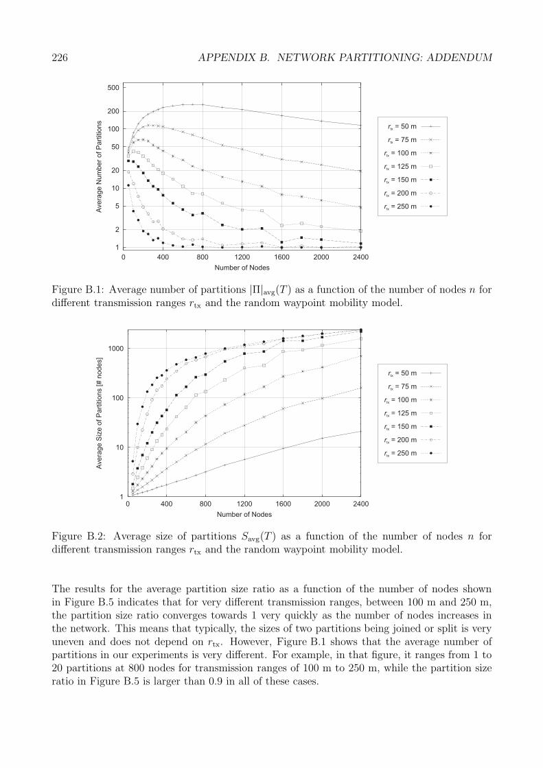
226 APPENDIX B. NETWORK PARTITIONING: ADDENDUM
1
2
5
10
20
50
100
200
500
0 400 800 1200 1600 2000 2400
Ave
rag
eN
um
be
ro
fP
art
itio
ns
Number of Nodes
rtx = 50 m
rtx = 75 m
rtx = 100 m
rtx = 125 m
rtx = 150 m
rtx = 200 m
rtx = 250 m
Figure B.1: Average number of partitions |Π|avg(T ) as a function of the number of nodes n fordifferent transmission ranges rtx and the random waypoint mobility model.
1
10
100
1000
0 400 800 1200 1600 2000 2400
Ave
rag
eS
ize
of
Pa
rtitio
ns
[#n
od
es]
Number of Nodes
rtx = 50 m
rtx = 75 m
rtx = 100 m
rtx = 125 m
rtx = 150 m
rtx = 200 m
rtx = 250 m
Figure B.2: Average size of partitions Savg(T ) as a function of the number of nodes n fordifferent transmission ranges rtx and the random waypoint mobility model.
The results for the average partition size ratio as a function of the number of nodes shownin Figure B.5 indicates that for very different transmission ranges, between 100 m and 250 m,the partition size ratio converges towards 1 very quickly as the number of nodes increases inthe network. This means that typically, the sizes of two partitions being joined or split is veryuneven and does not depend on rtx. However, Figure B.1 shows that the average number ofpartitions in our experiments is very different. For example, in that figure, it ranges from 1 to20 partitions at 800 nodes for transmission ranges of 100 m to 250 m, while the partition sizeratio in Figure B.5 is larger than 0.9 in all of these cases.
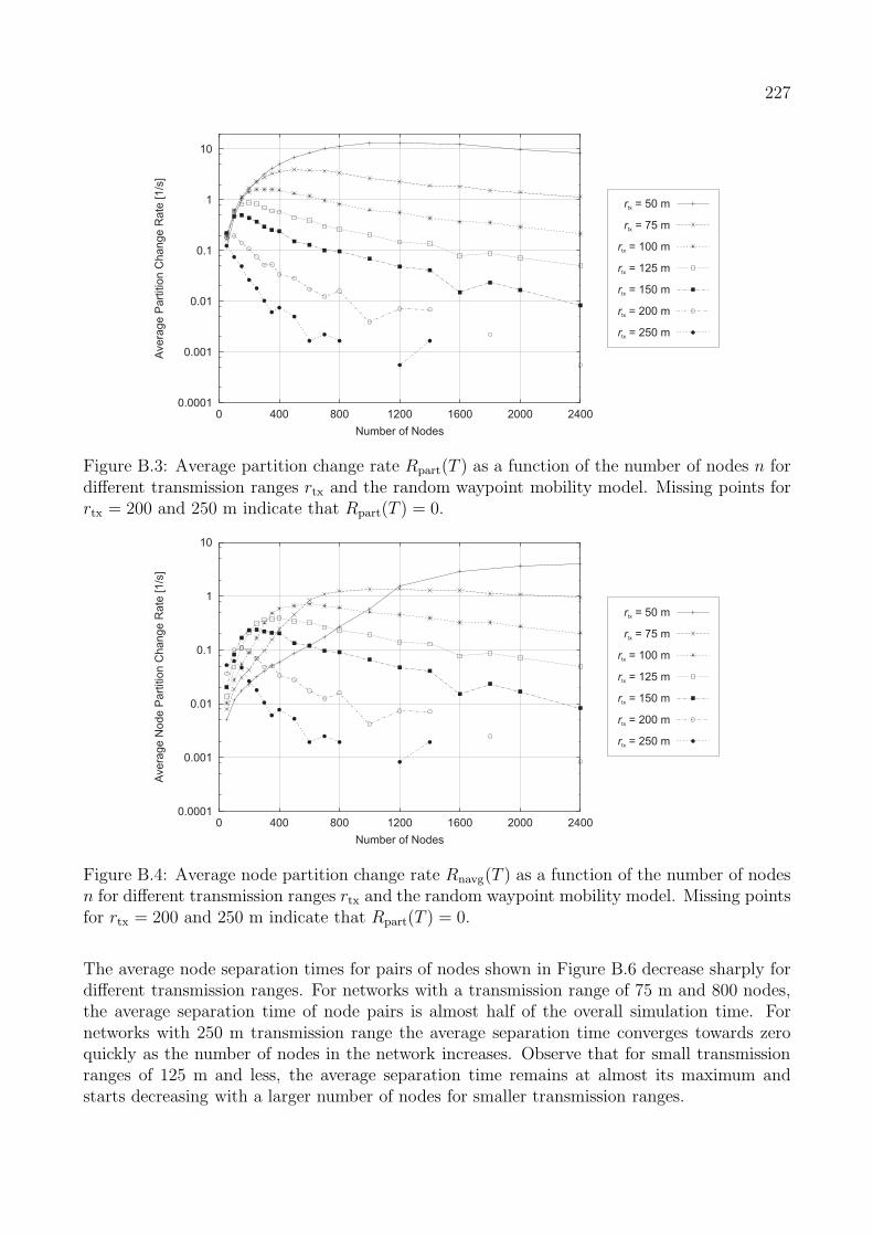
227
0.0001
0.001
0.01
0.1
1
10
0 400 800 1200 1600 2000 2400
Ave
rag
eP
art
itio
nC
ha
ng
eR
ate
[1/s
]
Number of Nodes
rtx = 50 m
rtx = 75 m
rtx = 100 m
rtx = 125 m
rtx = 150 m
rtx = 200 m
rtx = 250 m
Figure B.3: Average partition change rate Rpart(T ) as a function of the number of nodes n fordifferent transmission ranges rtx and the random waypoint mobility model. Missing points forrtx = 200 and 250 m indicate that Rpart(T ) = 0.
0.0001
0.001
0.01
0.1
1
10
0 400 800 1200 1600 2000 2400
Ave
rag
eN
od
eP
art
itio
nC
ha
ng
eR
ate
[1/s
]
Number of Nodes
rtx = 50 m
rtx = 75 m
rtx = 100 m
rtx = 125 m
rtx = 150 m
rtx = 200 m
rtx = 250 m
Figure B.4: Average node partition change rate Rnavg(T ) as a function of the number of nodesn for different transmission ranges rtx and the random waypoint mobility model. Missing pointsfor rtx = 200 and 250 m indicate that Rpart(T ) = 0.
The average node separation times for pairs of nodes shown in Figure B.6 decrease sharply fordifferent transmission ranges. For networks with a transmission range of 75 m and 800 nodes,the average separation time of node pairs is almost half of the overall simulation time. Fornetworks with 250 m transmission range the average separation time converges towards zeroquickly as the number of nodes in the network increases. Observe that for small transmissionranges of 125 m and less, the average separation time remains at almost its maximum andstarts decreasing with a larger number of nodes for smaller transmission ranges.
228 APPENDIX B. NETWORK PARTITIONING: ADDENDUM
0.5
0.6
0.7
0.8
0.9
1
0 400 800 1200 1600 2000 2400
Ave
rag
eP
art
itio
nS
ize
Ra
tio
Number of Nodes
rtx = 50 m
rtx = 75 m
rtx = 100 m
rtx = 125 m
rtx = 150 m
rtx = 200 m
rtx = 250 m
Figure B.5: Average partition size ratio PSRavg(T ) as a function of the number of nodes n fordifferent transmission ranges rtx and the random waypoint mobility model.
0
600
1200
1800
2400
3000
3600
0 400 800 1200 1600 2000 2400
Ave
rag
eN
od
eS
epa
ratio
nT
ime
Number of Nodes
rtx = 50 m
rtx = 75 m
rtx = 100 m
rtx = 125 m
rtx = 150 m
rtx = 200 m
rtx = 250 m
Figure B.6: Average over the sum of node separation times τsep(n1, n2, T ) for n/2 disjoint pairsof nodes (n1, n2) as a function of the number of nodes n for different transmission ranges rtx
and the random waypoint mobility model.
Figure B.7 shows the results for the average size of the continuous node visibility set Ncont(nk, T )over time for 400 nodes. The gradient of the individual functions describes how fast the groupof nodes found permanently in the same partition decays. The general observation for alltransmission ranges is the extreme slope at the beginning of the considered time interval. Thisis an artifact of the random waypoint mobility model, where small groups of nodes break apartfrom the main group of nodes in the center. At first, the average is very high, because allindividual visibility sets of each node are the size of the single large partition. When smallgroups of nodes are separated from the large partition, the value of Ncont(nk, T ) for the nodes
229
0
20
40
60
80
100
1800 2100 2400 2700 3000 3300 3600
Avera
ge
Siz
eof
CN
VS
[%]
Time [s]
rtx = 50 m
rtx = 75 m
rtx = 100 m
rtx = 125 m
rtx = 150 m
rtx = 200 m
rtx = 250 m
Figure B.7: Average size of n continuous node visibility sets Ncont(nk, T ) as a function of T forn = 400 nodes, different transmission ranges rtx and the random waypoint mobility model.
0
20
40
60
80
100
1800 2100 2400 2700 3000 3300 3600
Avera
ge
Siz
eofA
NV
S[%
]
Time [s]
rtx = 50 m
rtx = 75 m
rtx = 100 m
rtx = 125 m
rtx = 150 m
rtx = 200, 250 m
Figure B.8: Average size of n accumulative node visibility sets Nacc(nk, T ) as a function of Tfor n = 400 nodes, different transmission ranges rtx and the random waypoint mobility model.
of these groups drops to a very small number, which strongly pushes the average size of the nodevisibility set towards smaller values. At later times, many small visibility sets already exist,and additional separations of nodes have little influence on the average size of the metric. Thesteep gradient of the continuous node visibility set for the lower transmission ranges indicatesthat reasonably stable groups of nodes are small and can be assumed to be available only forsmall time spans of 100 seconds or less. For higher transmission ranges the speed of decay slowsdown significantly and the size of the stable groups grows.
230 APPENDIX B. NETWORK PARTITIONING: ADDENDUM
Figure B.8 shows the average size of the accumulative node visibility set over time for networkswith 400 nodes at different transmission ranges. Obviously, the accumulative node visibilityset grows faster for larger transmission ranges. For rtx = 50 m, the results show that evenafter 30 minutes of simulation time, only 20 percent of the nodes have been contained in anode’s same partition. This is due to the small average number of partitions (Figure B.1).While moving, nodes encounter only a small number of other nodes in the same partition.Because the partitions are small with respect to their geographical extent, they provide a smallcontact area, so that the fusion of individual partitions occurs only rarely. Also note the stronginitial growth for higher transmission ranges. The reason is similar to the Ncont(nk, T ) case inFigure B.7. At the point of initialization of the accumulative node visibility set, a few isolatednodes or very small groups of nodes exist. At the same time, one large partition exists, in whichall nodes have a large accumulative node visibility set consisting of the nodes in that partition.The average size is relatively small because of the small visibility sets. After the addition of thesmall groups of nodes to the large partition, their individual accumulative visibility sets growrapidly, resulting in a large increase of the average during the first seconds. These phenomenaare observed independent of a variation in the transmission range (Figure B.7) or in the numberof nodes for a given transmission range (Figure 2.21 in Section 2.2.5).
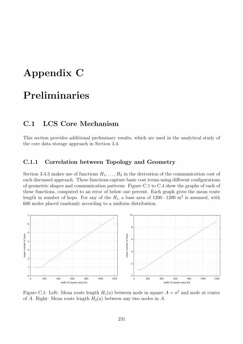
Appendix C
Preliminaries
C.1 LCS Core Mechanism
This section provides additional preliminary results, which are used in the analytical study ofthe core data storage approach in Section 3.4.
C.1.1 Correlation between Topology and Geometry
Section 3.4.3 makes use of functions H1, . . . , H8 in the derivation of the communication cost ofeach discussed approach. These functions capture basic cost terms using different configurationsof geometric shapes and communication patterns. Figure C.1 to C.4 show the graphs of each ofthese functions, computed to an error of below one percent. Each graph gives the mean routelength in number of hops. For any of the Hi, a base area of 1200 · 1200 m2 is assumed, with600 nodes placed randomly according to a uniform distribution.
0
1
2
3
4
5
6
7
0 200 400 600 800 1000 1200
meannumberofhops
width of square area [m]
0
2
4
6
8
10
0 200 400 600 800 1000 1200
meannumberofhops
width of square area [m]
Figure C.1: Left: Mean route length H1(a) between node in square A = a2 and node at centerof A. Right: Mean route length H2(a) between any two nodes in A.
231
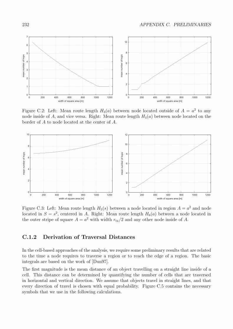
232 APPENDIX C. PRELIMINARIES
0
1
2
3
4
5
6
7
0 200 400 600 800 1000 1200
meannumberofhops
width of square area [m]
0
2
4
6
8
10
0 200 400 600 800 1000 1200
meannumberofhops
width of square area [m]
Figure C.2: Left: Mean route length H3(a) between node located outside of A = a2 to anynode inside of A, and vice versa. Right: Mean route length H4(a) between node located on theborder of A to node located at the center of A.
0
2
4
6
8
10
0 200 400 600 800 1000 1200
meannumberofhops
width of square area [m]
0
2
4
6
8
10
12
0 200 400 600 800 1000 1200
meannumberofhops
width of square area [m]
Figure C.3: Left: Mean route length H5(s) between a node located in region A = a2 and nodelocated in S = s2, centered in A. Right: Mean route length H6(a) between a node located inthe outer stripe of square A = a2 with width rtx/2 and any other node inside of A.
C.1.2 Derivation of Traversal Distances
In the cell-based approaches of the analysis, we require some preliminary results that are relatedto the time a node requires to traverse a region or to reach the edge of a region. The basicintegrals are based on the work of [Dun97].
The first magnitude is the mean distance of an object travelling on a straight line inside of acell. This distance can be determined by quantifying the number of cells that are traversedin horizontal and vertical direction. We assume that objects travel in straight lines, and thatevery direction of travel is chosen with equal probability. Figure C.5 contains the necessarysymbols that we use in the following calculations.
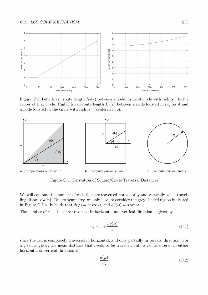
C.1. LCS CORE MECHANISM 233
0
1
2
3
4
5
6
7
0 100 200 300 400 500 600
meannumberofhops
radius of circle [m]
0
1
2
3
4
5
6
7
8
9
0 100 200 300 400 500 600
meannumberofhops
radius of circle [m]
Figure C.4: Left: Mean route length H7(r) between a node inside of circle with radius r to thecenter of that circle. Right: Mean route length H8(r) between a node located in region A anda node located in the circle with radius r, centered in A.
a
dy( )�
d( )�
a
x
y
�
a. Computations on square A
R
c. Computations on circle C
�
y
x
s/2
s/2
b. Computations on square S
d( )�
Figure C.5: Derivation of Square/Circle Traversal Distances
We will compute the number of cells that are traversed horizontally and vertically when travel-ling distance d(ϕ). Due to symmetry, we only have to consider the grey-shaded region indicatedin Figure C.5.a. It holds that d(ϕ) = s/ cos ϕ, and dy(ϕ) = s tanϕ.
The number of cells that are traversed in horizontal and vertical direction is given by
ns = 1 +dy(ϕ)
s(C.1)
since the cell is completely traversed in horizontal, and only partially in vertical direction. Fora given angle ϕ, the mean distance that needs to be travelled until a cell is entered in eitherhorizontal or vertical direction is
d(ϕ)
ns
(C.2)
234 APPENDIX C. PRELIMINARIES
We then determine the mean of such distances for all angles 0 ≤ ϕ ≤ π/4:
l1 =4
π
π4∫
ϕ=0
d(ϕ)
nsdϕ =
4
π
π4∫
ϕ=0
acos ϕ
1 + a tan ϕs
dϕ =4s
π
π4∫
ϕ=0
1
cos ϕ + sin ϕdϕ (C.3)
In order to integrate this intermediate result, we make use of the following trigonometric identityabout linear combination of the sine:
a sin α + b cos α =√
a2 + b2 · sin(
α + arctanb
a
)(C.4)
Applying this identity yields
l1 =4s
π
π4∫
ϕ=0
1√2 sin
(ϕ + π
4
)dϕ (C.5)
Because the argument of the sine contains only the variable of integration and a constant value,it can immediately be integrated using the following identity:∫
csc xdx = ln | csc x − cot x| + C (C.6)
The result after integration is
l1 =2√
2s
π
[ln
∣∣∣∣∣ 1
sin(ϕ + π
4
) − 1
tan(ϕ + π
4
)∣∣∣∣∣]π
4
ϕ=0
(C.7)
Evaluating and simplifying to the end yields
l1 = −2√
2s
πln(√
2 − 1)
(C.8)
The second result we require is the mean distance an object travels from the center of a square oflength s to its border. Again, every direction is assumed equally probable. Symmetry propertiesof the square allow us to integrate over an angle of only ϕ/4. It holds that d(ϕ) = (s/2)/ cosϕ(Figure C.5.b). We can then set up the following integral and simplify:
l2 =4
π
∫ π4
ϕ=0
d(ϕ)dϕ =4
π
∫ π4
ϕ=0
s
2 cos ϕdϕ =
2s
π
∫ π4
ϕ=0
1
cos ϕdϕ (C.9)
This time we can use the following integration rule:∫sec xdx = ln | sec x + tanx| + C (C.10)
C.2. DERIVATION OF THE LOCATION PDF 235
Integrating by this rule yields
l2 =2s
π
[ln
∣∣∣∣ 1
cos ϕ+ tan ϕ
∣∣∣∣]π
4
ϕ=0
(C.11)
After simplifying we have the final result
l2 =2s
πln(
√2 + 1) (C.12)
In the case of a circle, shown in Figure C.5.c, the distance required from the center of the circleC to the border is always the circle’s radius, independent of direction. Thus:
l3 = R (C.13)
C.2 Derivation of the Location PDF
In this section we derive the closed form of the bivariate location probability density function(location pdf), which we use in (5.5) of Section 5.1.
We first restate the full equation in integral form, based on (5.1) and (5.2):
Pr =1
2π√|Σ|
∫∫(x−μx)2+(y−μy)2≤r2
e−12(X−M)T Σ−1(X−M)dxdy (C.14)
In the previous equation, we have used M = (μx, μy)T to denote the center of the circle, and Σ
to denote the covariance matrix.
The random variables x and y are independent, and we assume that they are equal for boththe x and y dimension, which is a reasonable assumption in case of a positioning system that isapproximately isotropic with respect to position inaccuracy. Thus, we set σ = σx = σy, and thecovariance matrix assumes the form σ2E where E denotes the unit matrix. Thus, the inverse ofΣ is Σ−1 = E as well. Further, the determinant is |Σ| = σ4. We can now simplify the argumentof the exponential function:
−1
2(X − M)T Σ−1(X − M) (C.15)
= − 1
2σ2(x − μx, y − μy)
(1 00 1
)(x − μx
y − μy
)(C.16)
= − 1
2σ2
[(x − μx)
2 + (y − μy)2]
(C.17)
We plug this result and the determinant into (C.14) and we have
Pr =1
2πσ2
∫∫(x−μx)2+(y−μy)2≤r2
e−1
2σ2 [(x−μx)2+(y−μy)2]dxdy (C.18)

236 APPENDIX C. PRELIMINARIES
Next, we substitute x′ = x − μx, which gives dx′ = dx and likewise, y′ = y − μy, which givesdy′ = dy. Then
Pr =1
2πσ2
∫∫x′2+y′2≤r
e−1
2σ2 (x′2+y′2)dx′dy′ (C.19)
We now substitute polar coordinates, using the identity
∫∫C
f(x, y)dxdy =
∫ ϕ′=2π
ϕ′=0
∫ r′=r
r′=0
f(r cos ϕ, r sin ϕ)rdrdϕ (C.20)
Applying the substitution yields
Pr =1
2πσ2
∫ ϕ′=2π
ϕ′=0
∫ r′=r
r′=0
r′e−1
2σ2 r′2dr′dϕ′ (C.21)
We now use the integral identity ∫xeax2
dx =1
2aeax2
+ C (C.22)
with a = − 12σ2 to solve the integral in (C.21) by first integrating via r′:
Pr =1
2πσ2
∫ ϕ′=2π
ϕ′=0
[−σ2e−
12σ2 r′2
]r′=r
r′=0dϕ′ (C.23)
= − 1
2π
∫ ϕ′=2π
ϕ′=0
(e−
12σ2 r2 − 1
)dϕ′ (C.24)
Integration by ϕ′ yields
Pr = − 1
2π
[ϕ(e−
12σ2 r2 − 1
)]ϕ′=2π
ϕ′=0(C.25)
= −(e−
1σ2 r2 − 1
)(C.26)
Hence, the final result is
Pr = 1 − e−1
σ2 r2
(C.27)
Appendix D
Network Topology Exploration Region
This appendix provides the step-by-step derivation of the network topology exploration region(NTE region) that was introduced in Section 4.3.
The starting point are the Requirement (1) to (3), stated in Section 4.3. The following basicnotations are assumed: By ANTE and ANTE = |ANTE| we denote the NTE region and itscorresponding area, respectively. The reference coordinate is denoted by cr. Let r0 denote thecurrent position of data server u0, and d = |r0 − cr| the distance between r0 and cr.
D.1 Area Restriction on the NTE Region
The first objective is to satisfy Requirement (1), which dictates a circular region around positionr0 of the current server u0. This region must always be included in the NTE region, which musttherefore satisfy the following minimum area:
A′NTE = π · R2
0 (D.1)
Parameter R0 can be understood as a real multiple of the nominal transmission range rtx
(Section 3.1), that is, R0 = ν · rtx for some ν ≥ 0.
The second objective is to satisfy Requirement (2), stating that the NTE region must obey anupper limit, independent of its shape. For that, we let us guide by the spatial domain of themigration recommendation policy (Section 4.2) and Requirement (3). First of all, the thresholddistance dthresh determines the outcome of the spatial predicate of the MDP (Equation (4.1)).Thus, nodes inside of the circle defined by dthresh and cr are potentially eligible and shouldbe considered, independent of the server’s current position r0 (note that the overall migrationrecommendation predicate may be true, but the spatial predicate may not).
If the server is located further away than dthresh, any node closer to cr than the server is moreeligible when only considering the geometric distance. In this case, r0 and cr define the shapeof the NTE region. However, when the server is located beyond the critical distance dcrit, regionANTE must be restricted in order to prevent the forming of an increasingly large scope. Thisrestriction shall be defined based on the circle that is formed around cr with radius dcrit.
237
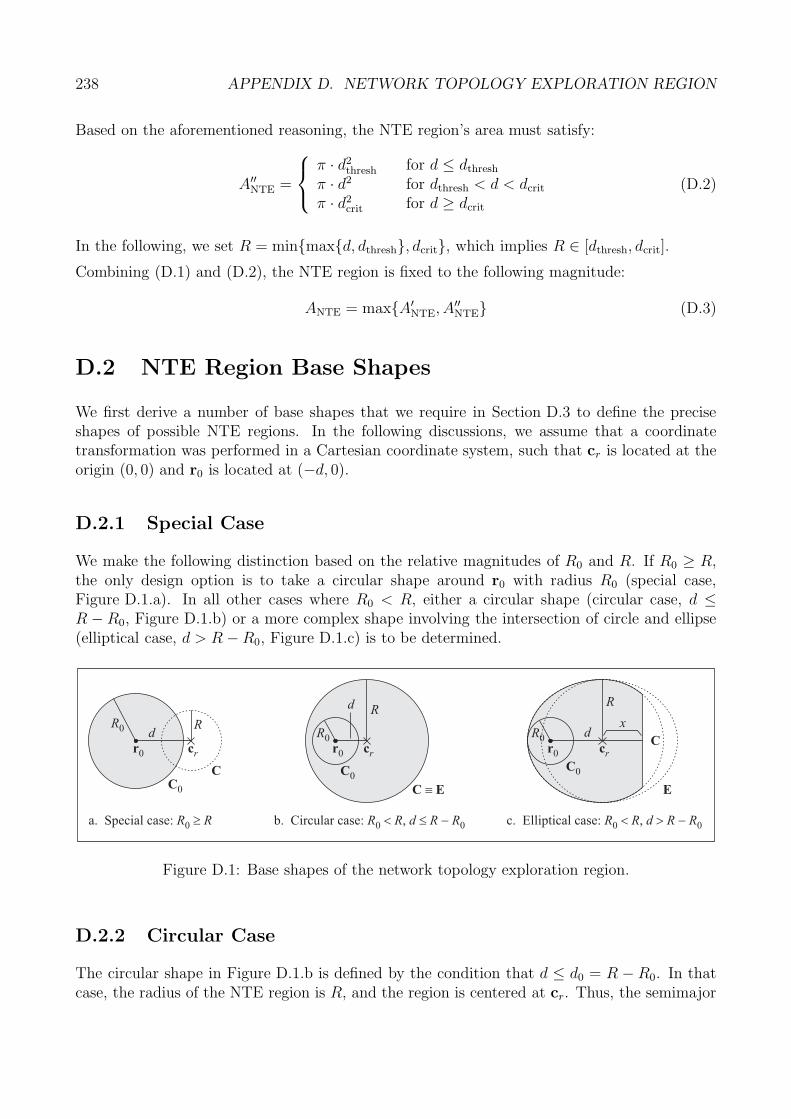
238 APPENDIX D. NETWORK TOPOLOGY EXPLORATION REGION
Based on the aforementioned reasoning, the NTE region’s area must satisfy:
A′′NTE =
⎧⎨⎩
π · d2thresh for d ≤ dthresh
π · d2 for dthresh < d < dcrit
π · d2crit for d ≥ dcrit
(D.2)
In the following, we set R = min{max{d, dthresh}, dcrit}, which implies R ∈ [dthresh, dcrit].
Combining (D.1) and (D.2), the NTE region is fixed to the following magnitude:
ANTE = max{A′NTE, A′′
NTE} (D.3)
D.2 NTE Region Base Shapes
We first derive a number of base shapes that we require in Section D.3 to define the preciseshapes of possible NTE regions. In the following discussions, we assume that a coordinatetransformation was performed in a Cartesian coordinate system, such that cr is located at theorigin (0, 0) and r0 is located at (−d, 0).
D.2.1 Special Case
We make the following distinction based on the relative magnitudes of R0 and R. If R0 ≥ R,the only design option is to take a circular shape around r0 with radius R0 (special case,Figure D.1.a). In all other cases where R0 < R, either a circular shape (circular case, d ≤R − R0, Figure D.1.b) or a more complex shape involving the intersection of circle and ellipse(elliptical case, d > R − R0, Figure D.1.c) is to be determined.
a. Special case: R R0 �
cr
R0 dR
E
C
r0
C0
xR0
d R
r0 cr
C0
C E�
b. Circular case: ,R R d R0 � � � R0 c. Elliptical case: R R d R R0 0,� � �
R0 d
C0
cr
R
Cr0
Figure D.1: Base shapes of the network topology exploration region.
D.2.2 Circular Case
The circular shape in Figure D.1.b is defined by the condition that d ≤ d0 = R − R0. In thatcase, the radius of the NTE region is R, and the region is centered at cr. Thus, the semimajor

D.2. NTE REGION BASE SHAPES 239
axis a of ellipse E (which in the circular case simply takes the form of a circle and is equivalentto C) in the circular case is given by
a = R for d ≤ d0 (D.4)
D.2.3 Elliptical Case 1: Curvature Subcase
When the distance d between r0 and cr reaches d0, circle C0 around r0 touches circle C aroundcr. To guarantee that r0 maintains at least a distance d to any point on the NTE region, circleC is stretched into an ellipse E with increasing distance d > d0. An ellipse is suitable becauseit allows the smooth stretching with increasing distances and provides both, good directionalityand propagation characteristics (Requirement (1) in Section 4.3).
The ellipse E may first stretch until the curvature of the ellipse in its vertex V is equal to thecurvature of the circle C0. This extremal case is shown in Figure D.2.a.
r0V
E
R0
C0
d1
a1
R
crCcr
R
d
a
C0T2
T1
V
R0
(0,0)( ,0)�d
r0
E
a. Elliptical case 1: curvature subcase. b. Elliptical case 2: tangent subcase.
C
Figure D.2: Elliptical case: curvature and tangent subcases.
While the curvature of E is greater than the curvature of C0, there is always a single point ofintersection (tangent point) at V between E and C0. Thus, the second critical distance d1 isdefined as the situation where E and C0 have equal curvature. The curvature radius of E invertex V of the major axis is defined as follows:
rV =b2
a(D.5)
The curvature radius of circle C is simply its radius R0. The problem is to find the ellipse withlength of the semiminor axis b = R and rV = R0. Thus, we solve (D.5) for extremal a1:
R0 =R2
a1(D.6)
a1 =R2
R0(D.7)

240 APPENDIX D. NETWORK TOPOLOGY EXPLORATION REGION
We obtain the critical distance d1 as follows:
d1 = a1 − R0 (D.8)
d1 =R2
R0− R0 (D.9)
d1 =1
R0
(R2 − R2
0
)(D.10)
Because (D.8) always holds (Figure D.2.a) it can be used to calculate a in general:
a = R0 + d for d0 < d ≤ d1 (D.11)
Observe that for d = d0 = R − R0, (D.4) and (D.11) take the same form.
D.2.4 Elliptical Case 2: Tangent Subcase
If ellipse E is stretched further, that is, distance d exceeds d1, the curvature of E becomessmaller than that of C0. To maintain radius R0 (Requirement (1) in Section 4.3), E must beplaced tangent to C0 in two tangent points T1 and T2, as illustrated in Figure D.2.b. Thiscase is applicable for all d > d1.
The procedure to determine a as a function of d in the tangent subcase is to solve the equationsfor E and C0 under the constraints that i) there exists exactly two points of tangency T1,T2
between E and C0 and ii) that the length of the semiminor axis of E is b = R.
The general equation of a circle is
(x − xm)2 + (y − ym)2 = r2 (D.12)
where (xm, ym) denotes the center of the circle. In our particular case, the special equation forthe circle located at (xm, ym) = (−d, 0) with radius r = R0 is
C0 : (x + d)2 + y2 = R20 (D.13)
The general equation of an ellipse is
(x − x0)2
a2+
(y − y0)2
b2= 1 (D.14)
where (x0, y0) denotes the center of the ellipse. In our case, we have (x0, y0) = (0, 0) and b = R.Thus, the special form of the ellipse equation takes the form
E :x2
a2+
y2
R2= 1 (D.15)
The problem is to solve the set of equations (D.13) and (D.15) for a under the constraint thatC0 and E intersect at tangent points T1,T2 for d > d2. We first transform (D.13) and get
y2 = R20 − (x + d)2 (D.16)

D.2. NTE REGION BASE SHAPES 241
Then, we substitute y2 in (D.15) with (D.16) and solve for x:
1 =x2
a2+
R20 − (x + d)2
R2(D.17)
1 =x2
a2+
R20 − (x2 + 2dx + d2)
R2(D.18)
1 =x2
a2+
R20 − x2 − 2dx − d2
R2(D.19)
0 =x2
a2− x2
R2− 2dx
R2+
R20 − d2
R2− 1 (D.20)
0 =
(1
a2− 1
R2
)x2 − 2d
R2x +
R20 − d2
R2− 1 (D.21)
We can state the solutions of the quadratic equation in general form as follows:
x1,2 =−β ±√
β2 − 4αγ
2α(D.22)
where
α =1
a2− 1
R2(D.23)
β = − 2d
R2(D.24)
γ =R2
0 − d2
R2− 1 (D.25)
We are interested in the solutions where x1 = x2, which mark the tangent points T1,T2. Thus,we solve the discriminant such that
β2 − 4αγ = 0 (D.26)
Plugging (D.23), (D.24), and (D.25) into (D.26) and solving for a yields:
0 =
(− 2d
R2
)2
− 4
(1
a2− 1
R2
)(R2
0 − d2
R2− 1
)(D.27)
0 =4d2
R4− 4
(1
a2− 1
R2
)(R2
0 − d2
R2− 1
)(D.28)
d2
R4=
(1
a2− 1
R2
)(R2
0 − d2
R2− 1
)(D.29)
d2
R4=
(1
a2− 1
R2
)(R2
0 − d2 − R2
R2
)(D.30)
1
a2− 1
R2=
d2R2
R4(R20 − d2 − R2)
(D.31)
1
a2=
d2
R2(R20 − d2 − R2)
+1
R2(D.32)
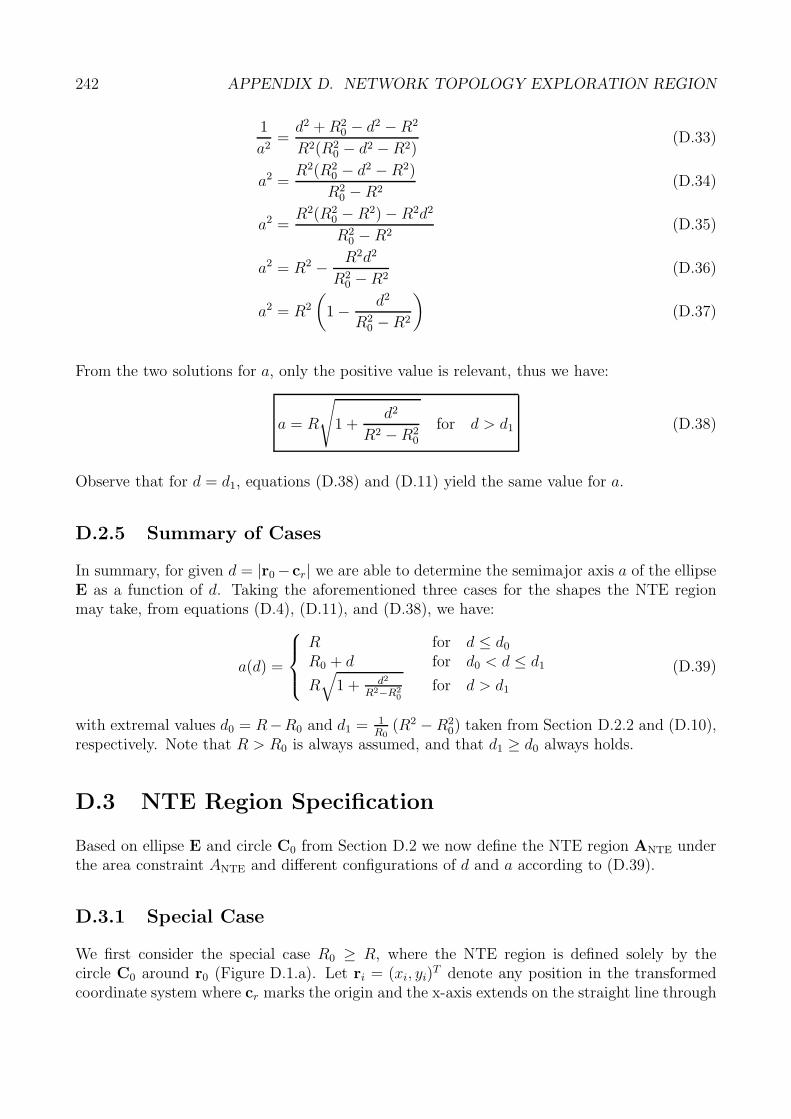
242 APPENDIX D. NETWORK TOPOLOGY EXPLORATION REGION
1
a2=
d2 + R20 − d2 − R2
R2(R20 − d2 − R2)
(D.33)
a2 =R2(R2
0 − d2 − R2)
R20 − R2
(D.34)
a2 =R2(R2
0 − R2) − R2d2
R20 − R2
(D.35)
a2 = R2 − R2d2
R20 − R2
(D.36)
a2 = R2
(1 − d2
R20 − R2
)(D.37)
From the two solutions for a, only the positive value is relevant, thus we have:
a = R
√1 +
d2
R2 − R20
for d > d1 (D.38)
Observe that for d = d1, equations (D.38) and (D.11) yield the same value for a.
D.2.5 Summary of Cases
In summary, for given d = |r0 −cr| we are able to determine the semimajor axis a of the ellipseE as a function of d. Taking the aforementioned three cases for the shapes the NTE regionmay take, from equations (D.4), (D.11), and (D.38), we have:
a(d) =
⎧⎪⎨⎪⎩
R for d ≤ d0
R0 + d for d0 < d ≤ d1
R√
1 + d2
R2−R20
for d > d1
(D.39)
with extremal values d0 = R−R0 and d1 = 1R0
(R2 − R20) taken from Section D.2.2 and (D.10),
respectively. Note that R > R0 is always assumed, and that d1 ≥ d0 always holds.
D.3 NTE Region Specification
Based on ellipse E and circle C0 from Section D.2 we now define the NTE region ANTE underthe area constraint ANTE and different configurations of d and a according to (D.39).
D.3.1 Special Case
We first consider the special case R0 ≥ R, where the NTE region is defined solely by thecircle C0 around r0 (Figure D.1.a). Let ri = (xi, yi)
T denote any position in the transformedcoordinate system where cr marks the origin and the x-axis extends on the straight line through
D.3. NTE REGION SPECIFICATION 243
r0 and cr. Then, r0 = (−d, 0)T , and C0 : (x + d)2 + y2 ≤ R20 denotes the circle around r0. The
NTE region is defined as follows in the transformed coordinate system:
ANTE := {ri ∈ C0} for R0 ≥ R (D.40)
D.3.2 Circular Case
In the circular case, where R0 < R, the NTE region is the disk that is formed by circle C(Figure D.1.b) and becomes C : x2 + y2 ≤ R2 in the transformed coordinate system. Thedefinition of the NTE region can be stated immediately:
ANTE := {ri ∈ C} for R0 < R ∧ d ≤ d0 (D.41)
D.3.3 Elliptical Case 1: Curvature Subcase
When d > d1 the ellipse E forms and the elliptical case occurs. For the curvature subcase, adistinction in two different subcase variants is necessary, shown in Figure D.3.
r0a
V
d
aV
d�C
t
�E
a
t
ANTE � 0.5A A AE C C0.5� � seg
ADseg
ANTE � AEseg
ACseg
r0
E
R R
C
cr
R
cr
C
E
a. Curvature subcase: 2R a R� � � b. Curvature subcase: 2a R� �
Figure D.3: Elliptical case 1: curvature subcase variants.
The distinction is made based on the condition that the NTE region is either completelylocated on the left or right side of the minor axis b. First, the area of the trivial ellipse (circle)is Aa=b
E = πb2. If a = 2b, then Aa=2bE = πab = π2bb = 2πb2 = 2Aa=b
E . Thus, for b < a ≤ 2b,the area of the ellipse is extending beyond the minor axis, where for a > 2b the area is located

244 APPENDIX D. NETWORK TOPOLOGY EXPLORATION REGION
completely on the left side of the minor axis b. Note that this distinction is independent of thepreviously determined limit d1 and that the possible cases depend on the proportion R/R0.
First, (D.7) defines limit a1 = R2/R0. Second, the critical distance for the area switch isa′ = 2b = 2R. Thus, if the area switch’ critical distance a′ is beyond a1, it will never berelevant, that is, when a′ > a1 ⇔ 2R > R2R0 ⇔ 2 > R/R0 ⇔ R > 2R0. In other words,if R is at least two times R0, there will never be the case where the area is located onlyon the left side. For example, if R = 1.5R0, then a = 2b = 2R and according to (D.7),a1 = R2/R0 = R2 · 1.5/R = 1.5R, in which case both possibilities exist, i.e., the NTE may belocated on the left side or on both sides of the semiminor axis.
Case R < a ≤ 2 · R (Figure D.3.a)
In this case, area ANTE consists of one half of the area AE, plus half the area of circle C, whichis denoted AC, minus the circular segment ACseg:
ANTE =1
2AE +
1
2AC − ACseg (D.42)
Applying the formula for the area of ellipse, circle, and circular segment, (D.42) becomes:
ANTE =πaR
2+
πR2
2− R2
2(ϕC − sin ϕC) (D.43)
Solving (D.43) for ϕC requires numerical methods because the angle appears both by itselfand as the argument of the sine. In our situation, an approximation is sufficient because theNTE region is used for flooding topology requests. Thus, we achieve efficient approximationby specifying some ΔAerr � ANTE, the maximum areal error that we will tolerate. This valueis at the same time the exit condition of the following iterative algorithm to determine ϕC.Observe that ϕC may run from > 0 up to π and that the area increases strongly monotonicwith decreasing ϕC (Figure D.3.a).
Initially, we set t = Δt = R/2. Note that t ∈ [0, R]. Observe that the maximum deviationfrom the actual area ANTE is upper bound by Δt · R. We execute the following procedure:
(1) compute angle ϕ′ = 2 · arccos(t/R)
(2) compute A′NTE using (D.43) with ϕC = ϕ′
(3) if Δt · R < ΔAerr or A′NTE = ANTE then exit
(4) set Δt := Δt/2
(5) if A′NTE > ANTE then set t := t − Δt and goto (1)
(6) if A′NTE < ANTE then set t := t + Δt and goto (1)
The result A′NTE is an approximation that is within the bounds specified by ΔAerr. At the same
time, the algorithm outputs value t that fixes the extension of ANTE to the right-side.
D.3. NTE REGION SPECIFICATION 245
The full specification of the NTE region is as follows. Let ri = (xi, yi)T . Then, E : x2
a2 + y2
R2 ≤ 1.The NTE region is defined as follows in the transformed coordinate system:
ANTE := ri ∈ E ∧ xi ≤ 0 ∨ ri ∈ C ∧ xi ≤ t
for R0 < R ∧ d0 < d ≤ d2 ∧ R < a ≤ 2 · R (D.44)
Case a > 2 · R (Figure D.3.b)
In the case where the NTE region does not extend beyond the semiminor axis R of ellipse E,area ANTE consists only of a single elliptical segment:
ANTE = AEseg =b
aADseg (D.45)
Note that the identity used in (D.45) between ellipse and circle holds, because if we write the
y coordinate as a function of x in the general ellipse equation, ye = b√
1 − x2
a2 , and that of a
circle for which r = a, yc = a√
1 − x2
a2 , then ye/yc = b/a.
Applying the formula for the area of a circular segment, (D.45) becomes:
ANTE =b
a
a2
2(ϕE − sin ϕE) =
ab
2(ϕE − sin ϕE) (D.46)
We use again numerical approximation with an error bound ΔAerr � ANTE. Observe thatϕE may run from > 0 up to < π. This time, ANTE increases strongly monotonic with ϕE
(Figure D.3.b). Setting t = Δt = a/2 with t ∈ [0, a], the following procedure is executed:
(1) Compute angle ϕ′ = 2 · arccos(t/a)
(2) Compute ANTE using (D.46) with ϕE = ϕ′
(3) if Δt · R < ΔAerr or A′NTE = ANTE then exit
(4) set Δt := Δt/2
(5) If A′NTE > ANTE then set t := t + Δt and goto (1)
(6) if A′NTE < ANTE then set t := t − Δt and goto (1)
Again the algorithm outputs value t that determines the dimensions of ANTE on the x-axis.
Let ri = (xi, yi)T , E and C as before. With a modified restriction in xi, the NTE region is
defined as follows in the transformed coordinate system:
ANTE := ri ∈ E ∧ xi ≤ −t
for R0 < R ∧ d0 < d ≤ d2 ∧ a > 2 · R (D.47)
246 APPENDIX D. NETWORK TOPOLOGY EXPLORATION REGION
D.3.4 Elliptical Case 2: Tangent Subcase
In the tangent subcase, the NTE region is composed of elliptical and circular segments, illus-trated in Figure D.4. Depending on distance d and values R, R0, area ANTE may or may notextend beyond the semiminor axis R of ellipse E. However, note that it is not possible thatANTE extends only up to the line connecting T1 and T2, because AC0 < AC always holds dueto R > R0. Also, it is not possible that the NTE region extends beyond circle C, becauseANTE = AC in the ideal case without approximation.
r0
C0
aV
d
T1
T2
�E1
�C0
a
A1 � 0.5A A AE E C� �seg1 0seg
A A A ANTE seg seg1 0seg� � �E E C t
t
A A A ANTE 1 0.5� � �C Cseg
AEseg1
AEseg
ACseg
�E
�C
RR
cr
C
AC0seg
R0
Figure D.4: Elliptical case 2: tangent subcase variants.
We begin by determining the critical area A1 that extends up to the semiminor axis R of E:
A1 =1
2AE − AEseg1 + AC0seg (D.48)
=π
2ab − b
aACseg1 + AC0seg (D.49)
=π
2ab − b
a
a2
2(ϕE1 − sin ϕE1) +
R20
2(ϕC0 − sin ϕC0) (D.50)
=π
2ab − ab
2(ϕE1 − sin ϕE1) +
R20
2(ϕC0 − sin ϕC0) (D.51)
Area A1 can be calculated for known ϕE1, ϕC0, which are given by the following identities:
cos(ϕE1
2
)=
|xT1 |a
and cos(ϕC0
2
)=
|xT1| − d
R0
(D.52)

D.3. NTE REGION SPECIFICATION 247
Value |xT1 | can be obtained from (D.22) under the assumption that β2 − 4αγ = 0, thus:
|xT1 | =
∣∣∣∣−β
2α
∣∣∣∣ (D.53)
Plugging in α and β from equations (D.23) and (D.24), respectively, we obtain:
|xT1| =
∣∣∣∣∣ − (− 2dR2
)2(
1a2 − 1
R2
)∣∣∣∣∣ =
∣∣∣∣∣ d
R2(
1a2 − 1
R2
)∣∣∣∣∣ =
∣∣∣∣∣ dR2
a2 − 1
∣∣∣∣∣ =
∣∣∣∣ da2
R2 − a2
∣∣∣∣ (D.54)
Based on the critical area A1, we make the following distinction to determine ANTE.
Case ANTE ≤ A1 (Figure D.4, Upper Shaded Region)
In this case, we obtain from Figure D.4 the following equation:
ANTE = AEseg − AEseg1 + AC0seg (D.55)
We use the following intermediary result that is a transformation of (D.48):
− AEseg1 + AC0seg = A1 − 1
2AE (D.56)
We can substitute the right side of (D.56) for the rightmost two terms in (D.55) and obtain
ANTE = AEseg + A1 − 1
2AE =
ab
2(ϕE − sin ϕE) + A1 − π
2ab (D.57)
which leaves only ϕE variable. Note that the first term is obtained from (D.46).
Like in the previous calculations we use numerical approximation with an error bound ΔAerr �ANTE. (D.57) is applicable for ϕE between ϕE1 to π. Initially, we set t = Δt = 1
2|xT1|. We then
execute the following iterative algorithm:
(1) Compute angle ϕ′ = 2 · arccos(t/a)
(2) Compute A′NTE using (D.57), with ϕE = ϕ′
(3) if Δt · R < ΔAerr or A′NTE = ANTE then exit
(4) set Δt := Δt/2
(5) if A′NTE > ANTE then set t := t + Δt and goto (1)
(6) if A′NTE < ANTE then set t := t − Δt and goto (1)
The algorithm outputs A′NTE within bounds ΔAerr and t that fixes the dimensions of ANTE.
Let ri = (xi, yi)T and r0 = (−d, 0)T in the transformed coordinate system. Then, C0 : (x +
d)2 + y2 ≤ R20 and E : x2
a2 + y2
R2 ≤ 1 with a = R√
1 + d2
R2+R20
according to (D.38). The NTE
region is defined as follows for A ≤ A1:
ANTE := ri ∈ C0 ∧ xi ≤ xT1
∨ ri ∈ E ∧ xT1 < xi ≤ −t
for R0 < R ∧ d > d1 ∧ ANTE ≤ A1
(D.58)
248 APPENDIX D. NETWORK TOPOLOGY EXPLORATION REGION
Case ANTE > A1 (Figure D.4, Lower Shaded Region)
In this case, Figure D.4 yields the following equation:
ANTE = A1 +1
2AC − ACseg = A1 +
π
2R2 − R2
2(ϕC − sin ϕC) (D.59)
The following algorithm yields t, where ϕC runs from π to > 0. Initially, t = Δt = R/2.
(1) Compute angle ϕ′ = 2 · arccos(t/R)
(2) Compute A′NTE using (D.59) with ϕC = ϕ′.
(3) if Δt · R < ΔAerr or A′NTE = ANTE then exit
(4) set Δt := Δt/2
(5) if A′NTE > ANTE then set t := t − Δt and goto (1)
(6) if A′NTE < ANTE then set t := t + Δt and goto (1)
Let ri = (xi, yi)T and C0, E, and a be defined as above, and let C : x2 + y2 ≤ R2 in the
transformed coordinate system. Then, for ANTE > A1, the NTE region is defined as follows:
ANTE : ri ∈ C0 ∧ xi ≤ xT1
∨ ri ∈ E ∧ xT1 < xi ≤ 0
∨ ri ∈ C ∧ 0 < xi ≤ t
for R0 < R ∧ d > d1 ∧ ANTE > A1
(D.60)
D.3.5 Summary of Cases
The set of equations, (D.40), (D.41), (D.44), (D.47), (D.58), and (D.60), defines all possibleshapes and thus completely the NTE region. The full set of definitions is implemented by theprototype in the evaluation of data migration in Section 4.6.
Refereed Publications
[DWM08] Dominique Dudkowski, Harald Weinschrott, and Pedro Jose Marron. Design andImplementation of a Reference Model for Context Management in Mobile Ad-HocNetworks. In Proceedings of the 22nd International Conference on Advanced Infor-mation Networking and Applications - Workshops (AINAW 2008), pages 832–837,Gino-wan, Okinawa, Japan, March, 2008. IEEE Computer Society.
[DMR07] Dominique Dudkowski, Pedro Jose Marron, and Kurt Rothermel. Migration Poli-cies for Location-Centric Storage in Mobile Ad-Hoc Networks. In Proceedings ofthe 3rd International Conference on Mobile Ad-hoc and Sensor Networks (MSN2007), pages 197–208, Beijing, China, December 2007. Lecture Notes in ComputerScience, Volume 4864/2007, Springer Berlin / Heidelberg.
[HDM+07] Jorg Hahner, Dominique Dudkowski, Pedro Jose Marron, and Kurt Rothermel.Quantifying Network Partitioning in Mobile Ad Hoc Networks. In Proceedingsof the 8th International Conference on Mobile Data Management (MDM 2007),pages 174–181, Mannheim, Germany, May 2007. IEEE.
[DMR06b] Dominique Dudkowski, Pedro Jose Marron, and Kurt Rothermel. Efficient Algo-rithms for Probabilistic Spatial Queries in Mobile Ad Hoc Networks. In Proceed-ings of the First International Conference on Communication System Softwareand Middleware (COMSWARE 2006), New Delhi, India, January 2006. IEEE.
[DMR06a] Dominique Dudkowski, Pedro Jose Marron, and Kurt Rothermel. An Efficient Re-silience Mechanism for Data Centric Storage in Mobile Ad Hoc Networks. In Pro-ceedings of the 7th International Conference on Mobile Data Management (MDM2006), Nara, Japan, May 2006. IEEE Computer Society.
[DDM05] Dominique Dudkowski, Tobias Drosdol, and Pedro Jose Marron. Towards Scalableand Efficient Processing of Probabilistic Spatial Queries in Mobile Ad Hoc andSensor Networks. In Mobile Datenbanken: heute, morgen und in 20 Jahren. 8.Workshop des GI-Arbeitskreises “Mobile Datenbanken und Informationssysteme”,Karlsruhe, February/March, 2005.
[HDM+05] Jorg Hahner, Dominique Dudkowski, Pedro Jose Marron, and Kurt Rothermel.A Quantitative Analysis of Partitioning in Mobile Ad Hoc Networks. ExtendedAbstract in Proceedings of the Joint International Conference on Measurement andModeling of Computer Systems (SIGMETRICS 2004/Performance 2004), pages400–401, New York, NY, USA, June 2004. ACM Press.
249

Bibliography
[ACNP07] Michele Albano, Stefano Chessa, Francesco Nidito, and Susanna Pelagatti. Q-NiGHT: Adding QoS to data centric storage in non-uniform sensor networks.In Proceedings of the 8th International Conference on Mobile Data Management(MDM’07), pages 100–107, Mannheim, Germany, May 2007. 10, 84, 85, 86, 93
[ADM04] Ittai Abraham, Danny Dolev, and Dahlia Malkhi. LLS: a locality aware locationservice for mobile ad hoc networks. In Proceedings of the 2004 Joint Workshopon Foundations of Mobile Computing, pages 75–84, Philadelphia, Pennsylvania,USA, October 2004. 86, 87
[ARK+05] Filipe Araujo, Luıs Rodrigues, Jorg Kaiser, Changling Liu, and Carlos Mitidieri.CHR: a distributed hash table for wireless ad hoc networks. In Proceedings of the25th IEEE International Conference on Distributed Computing Systems Work-shops (ICDCSW’05), pages 407–413, Columbus, Ohio, USA, June 2005. 83, 84,85, 86, 100
[AWW05] Ian F. Akyildiz, Xudong Wang, and Weilin Wang. Wireless mesh networks: Asurvey. Computer Networks, 47(4):445–487, March 2005. 46
[BA06] Kenneth C. Barr and Krste Asanovic. Energy-aware lossless data compression.ACM Transactions on Computer Systems (TOCS), 24(3):250–291, August 2006.48
[Bar99] Daniel Barbara. Mobile computing and databases - a survey. IEEE Transactionson Knowledge and Data Engineering, 11(1):108–117, January 1999. 72
[BCQ+07] Cristiana Bolchini, Carlo A. Curino, Elisa Quintarelli, Fabio A. Schreiber, andLetizia Tanca. A data-oriented survey of context models. ACM SIGMOD Record,36(4):19–26, December 2007. 40
[BDR07] Matthias Baldauf, Schahram Dustdar, and Florian Rosenberg. A survey oncontext-aware systems. International Journal of Ad Hoc and Ubiquitous Com-puting, 2(4):263–277, 2007. 78
[Bet02] Christian Bettstetter. On the minimum node degree and connectivity of a wirelessmultihop network. In Proceedings of the 3rd ACM International Symposium onMobile Ad Hoc Networking and Computing (MobiHoc’02), pages 80–91, Lausanne,Switzerland, June 2002. 50
251
252 BIBLIOGRAPHY
[Bet03] Christian Bettstetter. Topology properties of ad hoc networks with random way-point mobility model. ACM SIGMOBILE Mobile Computing and Communica-tions Review, 7(3):50–52, July 2003. 50
[Bha03] Sangeeta Bhattacharya. Randomized location service in mobile ad hoc networks.In Proceedings of the 6th International Workshop on Modeling Analysis and Sim-ulation of Wireless and Mobile Systems (MSWiM’03), pages 66–73, San Diego,California, USA, September 2003. 73, 86, 87
[BJKS02] Rimantas Benetis, Christian S. Jensen, Gytis Karciauskas, and Simonas Saltenis.Nearest neighbor and reverse nearest neighbor queries for moving objects. In Pro-ceedings of the International Database Engineering and Applications Symposium(IDEAS’02), pages 44–53, Edmonton, Canada, July 2002. 86, 87
[BMJ+98] Josh Broch, David A. Maltz, David B. Johnson, Yih-Chun Hu, and JorjetaJetcheva. A performance comparison of multi-hop wireless ad hoc network rout-ing protocols. In Proceedings of the Fourth Annual ACM/IEEE InternationalConference on Mobile Computing and Networking, pages 85–97, Dallas, Texas,USA, October 1998. 58, 123, 124, 168
[Bre00] Eric A. Brewer. Towards robust distributed systems (invited talk). In Proceedingsof the Nineteenth Annual ACM Symposium on Principles of Distributed Comput-ing, page 7, Portland, Oregon, USA, July 2000. ACM New York, NY, USA. 92
[CAMCM05] Shiva Chetan, Jalal Al-Muhtadi, Roy Campbell, and M. Dennis Mickunas. MobileGaia: A middleware for ad-hoc pervasive computing. In Second IEEE ConsumerCommunications and Networking Conference (CCNC’05), pages 223–228, LasVegas, Nevada, USA, January 2005. 79
[CC07] Jinchuan Chen and Reynold Cheng. Efficient evaluation of imprecise location-dependent queries. In Proceedings of the IEEE 23rd International Conference onData Engineering (ICDE’07), pages 586–595, Istanbul, Turkey, April 2007. 89
[CCMC08] Reynold Cheng, Jinchuan Chen, Mohamed Mokbel, and Chi-Yin Chow. Proba-bilistic verifiers: Evaluating constrained nearest-neighbor queries over uncertaindata. In Proceedings of the IEEE 24th International Conference on Data Engi-neering (ICDE’08), pages 973–982, Cancun, Mexico, April 2008. 89
[CGP04] Jian Chen, Yong Guan, and U. Pooch. Customizing GPSR for wireless sensornetworks. In Proceedings of the 2004 IEEE International Conference on Mo-bile Ad-hoc and Sensor Systems, pages 549–551, Fort Lauderdale, Florida, USA,October 2004. 82
[CKP03] Reynold Cheng, Dmitri V. Kalashnikov, and Sunil Prabhakar. Evaluating prob-abilistic queries over imprecise data. In Proceedings of the 2003 ACM SIGMODInternational Conference on Management of Data, pages 551–562, San Diego,California, USA, June 2003. 89
BIBLIOGRAPHY 253
[CKP04] Reynold Cheng, Dmitri V. Kalashnikov, and Sunil Prabhakar. Querying imprecisedata in moving object environments. IEEE Transactions on Knowledge and DataEngineering, 16(9):1112–1127, September 2004. 89
[CNS04] Alexandru Coman, Mario A. Nascimento, and Jorg Sander. A framework forspatio-temporal query processing over wireless sensor networks. In Proceedingsof the First Workshop on Data Management for Sensor Networks (DMSN’04),Toronto, Canada, August 2004. 86, 87
[CP03] Reynold Cheng and Sunil Prabhakar. Managing uncertainty in sensor databases.ACM SIGMOD Record. Special Issue: Special Section on Sensor Network Tech-nology and Sensor Data Managment, 32(4):41–46, December 2003. 89
[CPK03] Reynold Cheng, Sunil Prabhakar, and Dmitri V. Kalashnikov. Querying imprecisedata in moving object environments. In Proceedings of the 19th InternationalConference on Data Engineering (ICDE’03), pages 723–725, Bangalore, India,March 2003. 89
[CXSN04] Kai Chen, Yuan Xue, Samarth H. Shah, and Klara Nahrstedt. Understandingbandwidth-delay product in mobile ad hoc networks. Computer Communications,27(10):923–934, June 2004. 158
[CYC07] Tzung-Shi Chen, Gwo-Jong Yu, and Hsin-Ju Chen. A framework of mobilecontext management for supporting context-aware environments in mobile adhoc networks. In International Wireless Communications and Mobile ComputingConference 2007 (IWCMC’07), pages 647–652, Honolulu, Hawaii, USA, August2007. 81
[DA99] Anind K. Dey and Gregory D. Abowd. Towards a better understanding of contextand context-awareness. Technical Report GIT-GVU-99-22, Georgia Institute ofTechnology, Atlanta, Georgia, USA, 1999. 39
[DF03] Murat Demirbas and Hakan Ferhatosmanoglu. Peer-to-peer spatial queries insensor networks. In Proceedings of the Third International Conference on Peer-to-Peer Computing (P2P’03), pages 32–39, Linkoping, Sweden, September 2003.86, 87
[DGM+04] Amol Deshpande, Carlos Guestrin, Samuel R. Madden, Joseph M. Hellerstein,and Wei Hong. Model-driven data acquisition in sensor networks. In Proceedingsof the 30th VLDB Conference, pages 588–599, Toronto, Canada, August 2004.190
[DHH07] Anusuriya Devaraju, Simon Hoh, and Michael Hartley. A context gatheringframework for context-aware mobile solutions. In Proceedings of the 4th Interna-tional Conference on Mobile Technology, Applications, and Systems and the 1stInternational Symposium on Computer Human Interaction in Mobile Technology,pages 39–46, Singapore, September 2007. 78, 79
254 BIBLIOGRAPHY
[DLR07] Tobias Drosdol, Ralph Lange, and Kurt Rothermel. Energy-efficient tracking ofmobile objects with early distance-based reporting. In Proceedings of the FourthAnnual International Conference on Mobile and Ubiquitous Systems: Networkingand Services (MobiQuitous’07), Philadelphia, PA, USA, August 2007. 48
[Dun97] Steven R. Dunbar. The average distance between points in geometric figures. TheCollege Mathematics Journal, 28(3):187–197, May 1997. 232
[EM99] P. Enge and P. Misra. Scanning the issue/technology - special issue on globalpositioning system. Proceedings of the IEEE, 87(1):3–15, 1999. 39, 91
[ERS06] Cheng Tien Ee, Sylvia Ratnasamy, and Scott Shenker. Practical data-centricstorage. In Proceedings of the 3rd Symposium on Networked Systems Design andImplementation (NSDI’06), pages 325–338, San Jose, California, USA, May 2006.84, 85, 86
[FC06] Patrick Fahy and Siobhan Clarke. CASS: Middleware for mobile, context-awareapplications. In MobiSys 2004 Workshop on Context Awareness, Boston, Mas-sachusetts, USA, June 2006. 79
[FPL07] Tao-Young Fu, Wen-Chih Peng, and Wang-Chien Lee. Optimizing parallelitineraries for KNN query processing in wireless sensor networks. In Proceedingsof the Sixteenth ACM Conference on Information and Knowledge Management,pages 391–400, Lisboa, Portugal, November 2007. 86, 87, 88
[FRWZ07] Elena Fasolo, Michele Rossi, Jorg Widmer, and Michele Zorzi. In-network aggre-gation techniques for wireless sensor networks: A survey. IEEE Wireless Com-munications, 14(2):70–87, April 2007. 145
[FSAA01] Hakan Ferhatosmanoglu, Ioanna Stanoi, Divyakant Agrawal, and Amr El Abbadi.Constrained nearest neighbor queries. In Proceedings of the 7th InternationalSymposium on Advances in Spatial and Temporal Databases (SSTD’01), pages257–278, Redondo Beach, California, USA, January 2001. 86, 87
[FV03] Dieter Fritsch and Steffen Volz. Nexus - the mobile GIS-environment. In Proceed-ings of the Joint First Workshop on Mobile Future and Symposium on Trends inCommunications (SympoTIC’03), pages 1–4, Bratislava, Slovak Republic, Octo-ber 2003. 40
[FW06] Roland Flury and Roger Wattenhofer. MLS: An efficient location service formobile ad hoc networks. In Proceedings of the Seventh ACM International Sym-posium on Mobile Ad Hoc Networking and Computing (MobiHoc’06), pages 226–237, Florence, Italy, May 2006. 86, 87
[GA02] Sanny Gustavsson and Sten F. Andler. Self-stabilization and eventual consistencyin replicated real-time databases. In Proceedings of the First Workshop on Self-healing Systems (WOSS’02), pages 105–107, Charleston, South Carolina, USA,November 2002. 92
BIBLIOGRAPHY 255
[Gar09] Garmin GPSMAP 76CSx. http://www.garmin.com/, September 2009. 182
[GBH+05] Matthias Grossmann, Martin Bauer, Nicola Honle, Uwe-Philipp Kappeler,Daniela Nicklas, and Thomas Schwarz. Efficiently managing context informationfor large-scale scenarios. In Proceedings of the 3rd IEEE International Confer-ence on Pervasive Computing and Communications (PerCom’05), pages 331–340,Kauai, Hawaii, USA, March 2005. 40, 78
[GdWFM02] Michael Gerharz, Christian de Waal, Matthias Frank, and Peter Martini. Linkstability in mobile wireless ad hoc networks. In Proceedings of the 27th AnnualIEEE Conference on Local Computer Networks (LCN’02), pages 30–39, Tampa,Florida, USA, November 2002. 50, 151
[GEG+03] Benjamin Greenstein, Deborah Estrin, Ramesh Govindan, Sylvia Ratnasamy,and Scott Shenker. DIFS: A distributed index for features in sensor networks.In Proceedings of the First IEEE International Workshop on Sensor NetworkProtocols and Applications (SNPA’03), pages 163–173, Anchorage, Alaska, USA,May 2003. 86, 87
[GGC03] Abhishek Ghose, Jens Grossklags, and John Chuang. Resilient data-centric stor-age in wireless ad-hoc sensor networks. In Proceedings of the 4th InternationalConference on Mobile Data Management (MDM’03), pages 45–62, Melbourne,Australia, January 2003. 11, 81, 85, 86
[GL02] Seth Gilbert and Nancy Lynch. Brewer’s conjecture and the feasibility of consis-tent, available, partition-tolerant web services. ACM SIGACT News, 33(2):51–59,June 2002. 92
[GPZ05] Tao Gu, Hung Keng Pung, and Da Qing Zhang. A service-oriented middleware forbuilding context-aware services. Journal of Network and Computer Applications,28:1–18, 2005. 79
[GRS+03] Benjamin Greenstein, Sylvia Ratnasamy, Scott Shenker, Ramesh Govindan, andDeborah Estrin. DIFS: A distributed index for features in sensor networks. AdHoc Networks, 1(2-3):333–349, September 2003. 86, 87
[GS02] Sandeep K. S. Gupta and Pradip K. Srimani. Handbook of Wireless Networks andMobile Computing, chapter Data Management in Wireless Mobile Environments,pages 553–579. Wiley & Sons, February 2002. 72
[HBLR05] Qingfeng Huand, Sangeeta Bhattacharya, Chenyang Lu, and Gruia-Catalin Ro-man. FAR: Face-aware routing for mobicast in large-scale sensor networks. ACMTransactions on Sensor Networks, 1(2):240–271, November 2005. 82
[HBR04] Jorg Hahner, Christian Becker, and Kurt Rothermel. Update-linearizability: Aconsistency concept for the chronological ordering of events in MANETs. InProceedings of the 2004 IEEE International Conference on Mobile Ad-hoc andSensor Systems, pages 1–10, Fort Lauderdale, Florida, USA, October 2004. 100
256 BIBLIOGRAPHY
[HHSW05] Jessica Heesen, Christoph Hubig, Oliver Siemoneit, and Klaus Wiegerling. Lebenin einer vernetzten und informatisierten Welt. Context-Awareness im Schnittfeldvon Mobile und Ubiquitous Computing. SFB 627 Bericht 2005/05, Center ofExcellence 627, Universitat Stuttgart, March 2005. 38, 39
[HKL+99] Fritz Hohl, Uwe Kubach, Alexander Leonhardi, Kurt Rothermel, and MarkusSchwehm. Next century challenges: Nexus - an open global infrastructure forspatial-aware applications. In Proceedings of the 5th Annual ACM/IEEE Inter-national Conference on Mobile Computing and Networking (MobiCom’99), pages249–255, Seattle, Washington, USA, August 1999. 40
[HLR04] Qingfeng Huang, Chenyang Lu, and Gruia-Catalin Roman. Reliable mobicast viaface-aware routing. In Proceedings of the Twenty-third Annual Joint Conferenceof the IEEE Computer and Communications Societies (INFOCOM’04), volume 3,pages 2108–2118, Hong Kong, China, March 2004. 82
[HS01] Hung-Yun Hsieh and Raghupathy Sivakumar. Performance comparison of cel-lular and multi-hop wireless networks: A quantitative study. In Proceedingsof the 2001 ACM SIGMETRICS International Conference on Measurement andModeling of Computer Systems (SIGMETRICS’01), pages 113–122, Cambridge,Massachusetts, USA, June 2001. 51
[HSC03] Michail Hauspie, David Simplot, and Jean Carle. Partition detection in mobilead-hoc networks using multiple disjoint paths set. In Proceedings of the 1st In-ternational Workshop on Objects Models and Multimedia Technologies, Geneva,Switzerland, September 2003. 151
[IB93] Tomasz Imielinski and B. R. Badrinath. Data management for mobile computing.ACM SIGMOD Record, 22(1):34–39, March 1993. 37, 72
[IB94] Tomasz Imielinski and B. R. Badrinath. Mobile wireless computing: Challengesin data management. Communications of the ACM, 37(10):18–28, October 1994.72
[JS03] Glenn Judd and Peter Steenkiste. Providing contextual information to pervasivecomputing applications. In Proceedings of the First IEEE International Con-ference on Pervasive Computing and Communications (PerCom’03), page 133,Dallas-Fort Worth, Texas, USA, March 2003. 79
[KD04] Vijay Kumar and Samir R. Das. Performance of dead reckoning-based locationservice for mobile ad hoc networks. Wireless Communications and Mobile Com-puting, 4(2):189–202, 2004. 86, 87
[KFWM04] Wolfgang Kieß, Holger Fußler, Jorg Widmer, and Martin Mauve. Hierarchicallocation service for mobile ad-hoc networks. Mobile Computing and Communi-cations Review, 1(2):47–58, October 2004. 73, 85, 86, 87, 184
[KGKS05] Young-Jin Kim, Ramesh Govindan, Brad Karp, and Scott Shenker. Geographicrouting made practical. In Proceedings of the 2nd Symposium on Networked
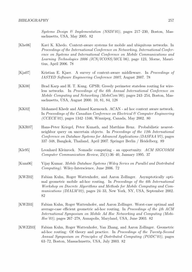
BIBLIOGRAPHY 257
Systems Design & Implementation (NSDI’05), pages 217–230, Boston, Mas-sachusetts, USA, May 2005. 82
[Khe06] Kavi K. Khedo. Context-aware systems for mobile and ubiquitous networks. InProceedings of the International Conference on Networking, International Confer-ence on Systems and International Conference on Mobile Communications andLearning Technologies 2006 (ICN/ICONS/MCL’06), page 123, Morne, Mauri-tius, April 2006. 78
[Kja07] Kristian E. Kjaer. A survey of context-aware middleware. In Proceedings ofIASTED Software Engineering Conference 2007, August 2007. 78
[KK00] Brad Karp and H. T. Kung. GPSR: Greedy perimeter stateless routing for wire-less networks. In Proceedings of the 6th Annual International Conference onMobile Computing and Networking (MobiCom’00), pages 243–254, Boston, Mas-sachusetts, USA, August 2000. 10, 81, 84, 128
[KK02] Mohamed Khedr and Ahmed Karmouch. ACAN - ad hoc context aware network.In Proceedings of the Canadian Conference on Electrical & Computer Engineering(CCECE’02), pages 1342–1346, Winnipeg, Canada, May 2002. 80
[KKR07] Hans-Peter Kriegel, Peter Kunath, and Matthias Renz. Probabilistic nearest-neighbor query on uncertain objects. In Proceedings of the 12th InternationalConference on Database Systems for Advanced Applications (DASFAA’07), pages337–348, Bangkok, Thailand, April 2007. Springer Berlin / Heidelberg. 89
[Kle95] Leonhard Kleinrock. Nomadic computing - an opportunity. ACM SIGCOMMComputer Communication Review, 25(1):36–40, January 1995. 37
[Kum06] Vijay Kumar. Mobile Database Systems (Wiley Series on Parallel and DistributedComputing). Wiley-Interscience, June 2006. 72
[KWZ02] Fabian Kuhn, Roger Wattenhofer, and Aaron Zollinger. Asymptotically opti-mal geometric mobile ad-hoc routing. In Proceedings of the 6th InternationalWorkshop on Discrete Algorithms and Methods for Mobile Computing and Com-munications (DIALM’02), pages 24–33, New York, NY, USA, September 2002.82
[KWZ03] Fabian Kuhn, Roger Wattenhofer, and Aaron Zollinger. Worst-case optimal andaverage-case efficient geometric ad-hoc routing. In Proceedings of the 4th ACMInternational Symposium on Mobile Ad Hoc Networking and Computing (Mobi-Hoc’03), pages 267–278, Annapolis, Maryland, USA, June 2003. 82
[KWZZ03] Fabian Kuhn, Roger Wattenhofer, Yan Zhang, and Aaron Zollinger. Geometricad-hoc routing: Of theory and practice. In Proceedings of the Twenty-SecondAnnual Symposium on Principles of Distributed Computing (PODC’03), pages63–72, Boston, Massachusetts, USA, July 2003. 82
258 BIBLIOGRAPHY
[LC04] Jennifer J.-N. Liu and Imrich Chlamtac. Mobile Ad Hoc Networking, chapter Mo-bile Ad-Hoc Networking with a View of 4G Wireless: Imperatives and Challenges,pages 1–46. Wiley-Interscience, 2004. 45
[LC08] Xiang Lian and Lei Chen. Probabilistic group nearest neighbor queries in un-certain databases. IEEE Transactions on Knowledge and Data Engineering,20(6):809–824, June 2008. 89, 90
[LCN05] Xinwei Luo, Tracy Camp, and William Navidi. Predictive methods for locationservices in mobile ad hoc networks. In Proceedings of the 19th IEEE InternationalParallel and Distributed Processing Symposium (IPDPS’05), page 6, Denver, Col-orado, USA, April 2005. 86, 87
[LCP+05] Eng K. Lua, Jon Crowcroft, Marcelo Pias, Ravi Sharma, and Steven Lim. Asurvey and comparison of peer-to-peer overlay network schemes. IEEE Commu-nications Surveys & Tutorials, 7(2):72–93, 2005. 88
[LGW06] Olaf Landsiegel, Stefan Gotz, and Klaus Wehrle. Towards scalable mobility indistributed hash tables. In Proceedings of the Sixth IEEE International Con-ference on Peer-to-Peer Computing (P2P’06), pages 203–209, Cambridge, UK,September 2006. 85
[LJC+00] Jinyang Li, John Jannotti, Douglas S. J. De Couto, David R. Karger, and RobertMorris. A scalable location service for geographic ad hoc routing. In Proceedings ofthe Sixth Annual International Conference on Mobile Computing and Networking(MobiCom’00), pages 120–130, Boston, Massachusetts, USA, August 2000. 73,86, 87, 184
[LKGH03] Xin Li, Young-Jin Kim, Ramesh Govindan, and Wei Hong. Multi-dimensionalrange queries in sensor networks. In Proceedings of the ACM Conference onEmbedded Networked Sensor Systems (SenSys’03), Los Angeles, California, USA,November 2003. ACM Press. 86, 87
[LLM06] Ben Leong, Barbara Liskov, and Robert Morris. Geographic routing withoutplanarization. In Proceedings of the 3rd Symposium on Networked Systems Designand Implementation (NSDI’06), pages 339–352, San Jose, California, USA, May2006. 82
[LSD+02] Hui Lei, Daby M. Sow, John S. Davis, Guruduth Banavar, and Maria R. Ebling.The design and applications of a context service. ACM SIGMOBILE MobileComputing and Communications Review, 6(4):45–55, October 2002. 79
[LTLS00] Wen-Hwa Liao, Yu-Chee Tseng, Kuo-Lun Lo, and Jang-Ping Sheu. GeoGRID:a geocasting protocol for mobile ad hoc networks based on GRID. Journal ofInternet Technology, 1(2):23–32, December 2000. 85
[Mai04] Christian Maihofer. A survey of geocast routing protocols. IEEE CommunicationsSurveys and Tutorials, 6(2):32–42, 2004. 145
BIBLIOGRAPHY 259
[MLS05] Christian Maihofer, Tim Leinmuller, and Elmar Schoch. Abiding geocast: Time-stable geocast for ad hoc networks. In Proceedings of the 2nd ACM InternationalWorkshop on Vehicular Ad Hoc Networks (VANET’05), pages 20–29, Cologne,Germany, September 2005. 85
[MMM05] Bratislav Milic, Nikola Milanovic, and Miroslaw Malek. Prediction of partitioningin location-aware mobile ad hoc networks. In Proceedings of the 38th Hawaii Inter-national Conference on System Sciences (HICSS’05), page 306c, Hilton WaikoloaVillage, HI, USA, January 2005. 149, 151
[NS03] James Newsome and Dawn Song. GEM: Graph EMbedding for routing anddata-centric storage in sensor networks without geographic information. In Pro-ceedings of the First ACM Conference on Embedded Networked Sensor Systems(SenSys’03), pages 76–88, Redwood, California, USA, November 2003. 84
[NTCS99] Sze-Yao Ni, Yu-Chee Tseng, Yuh-Shyan Chen, and Jang-Ping Sheu. The broad-cast storm problem in a mobile ad hoc network. In Proceedings of the 5th An-nual ACM/IEEE International Conference on Mobile Computing and Networking(MobiCom’99), pages 151–162, Seattle, Washington, USA, August 1999. 49, 50,54
[OT98] Katia Obraczka and Gene Tsudik. Multicast routing issues in ad hoc networks.In Proceedings of the 1998 International Conference on Universal Personal Com-munications, pages 751–756, Florence, Italy, October 1998. 54
[PJC06] Filip Perich, Anupam Joshi, and Rada Chirkova. Enabling Technologies for Wire-less E-Business, chapter Data Management for Mobile Ad-Hoc Networks, pages132–176. Springer-Verlag, 2006. 72, 78, 80
[PLK05] Nam-Shik Park, Kang-Woo Lee, and Hyun Kim. A middleware for supportingcontext-aware services in mobile and ubiquitous environment. In Proceedingsof the International Conference on Mobile Business (ICMB’05), pages 694–697,Sydney, Australia, July 2005. 79
[PPJ+06] Anand Patwardhan, Filip Perich, Anupam Joshi, Tim Finin, and Yelena Yesha.Querying in packs: Trustworthy data management in ad hoc networks. Interna-tional Journal of Wireless Information Networks, 13(4):263–274, October 2006.80
[PS97] Evaggelia Pitoura and George Samaras. Data Management for Mobile Computing(Advances in Database Systems). Springer, 1997. 72
[PSTM04] Dimitris Papadias, Qiongmao Shen, Yufei Tao, and Kyriakos Mouratidis. Groupnearest neighbor queries. In Proceedings of the 20th International Conferenceon Data Engineering (ICDE’04), pages 301–312, Boston, Massachusetts, USA,March 2004. 86, 87, 90
[RBB03] Kurt Rothermel, Martin Bauer, and Christian Becker. Digitale Weltmodelle -Grundlage kontextbezogener Systeme, chapter 5, pages 123–141. Springer-Verlag,Berlin, Heidelberg, New York, May 2003. German. 39, 40
260 BIBLIOGRAPHY
[RD01] Antony I. T. Rowstron and Peter Druschel. Pastry: Scalable, decentralized objectlocation, and routing for large-scale peer-to-peer systems. In Proceedings of theIFIP/ACM International Conference on Distributed Systems Platforms, pages329 – 350, Heidelberg, Germany, November 2001. Springer-Verlag. 88
[RDD+03] Kurt Rothermel, Dominique Dudkowski, Frank Durr, Martin Bauer, and Chris-tian Becker. Ubiquitous computing - more than computing anytime anyplace?In Dieter Fritsch, editor, Proceedings of Photogrammetric Week ’03, pages 1–9,Stuttgart, 2003. 39, 40
[REF+06] Kurt Rothermel, Thomas Ertl, Dieter Fritsch, Paul J. Kuhn, BernhardMitschang, Engelbert Westkamper, Christian Becker, Dominique Dudkowski,Andreas Gutscher, Christian Hauser, Lamine Jendoubi, Daniela Nicklas, SteffenVolz, and Matthias Wieland. SFB 627 - Umgebungsmodelle fur mobile kontextbe-zogene Systeme. Informatik Forschung und Entwicklung, 21:105–113, June 2006.German. 40
[RJM+06] Alexander Roßnagel, Silke Jandt, Jurgen Muller, Andreas Gutscher, and JessicaHeesen. Datenschutzfragen mobiler kontextbezogener Systeme. DuD-Fachbeitrage.Deutscher Universitats-Verlag, Wiesbaden, October 2006. German. 41
[RKS+03] Sylvia Ratnasamy, Brad Karp, Scott Shenker, Deborah Estrin, Ramesh Govin-dan, Li Yin, and Fang Yu. Data-centric storage in sensornets with GHT, ageographic hash table. Mobile Networks and Applications, 8(4):427–442, August2003. 73, 81, 100
[RKV95] Nick Roussopoulos, Stephen Kelley, and Frederic Vincent. Nearest neighborqueries. In Proceedings of the 1995 ACM SIGMOD International Conferenceon Management of Data (SIGMOD’95), pages 71–79, San Jose, California, USA,May 1995. 86, 87
[RKY+02] Sylvia Ratnasamy, Brad Karp, Li Yin, Fang Yu, Deborah Estrin, Ramesh Govin-dan, and Scott Shenker. GHT: a geographic hash table for data-centric storage. InProceedings of the 1st ACM International Workshop on Wireless Sensor Networksand Applications (WSNA’02), pages 78–87, Atlanta, Georgia, USA, September2002. 10, 11, 13, 73, 81, 84, 85, 86, 93, 95, 99, 109, 110, 124, 125, 139
[RPSS03] Ananth Rao, Christos Papadimitriou, Scott Shenker, and Ion Stoica. Geographicrouting without location information. In Proceedings of the 9th Annual Inter-national Conference on Mobile Computing and Networking, pages 96–108, SanDiego, California, USA, September 2003. ACM Press. 91
[SH03] Karim Seada and Ahmed Helmy. Rendezvous regions: A scalable architecture forservice location and data-centric storage in large-scale wireless networks. Techni-cal report, University of Southern California, Los Angeles, California, USA, July2003. 83, 84, 99
[SH04] Karim Seada and Ahmed Helmy. Rendezvous regions: A scalable architecturefor service location and data-centric storage in large-scale wireless networks. In
BIBLIOGRAPHY 261
Proceedings of the 18th International Parallel and Distributed Processing Sympo-sium (IPDPS’04), page 218a, Santa Fe, New Mexico, USA, April 2004. 83, 84,85, 86, 99, 184
[SHB+03] Illya Stepanov, Jorg Hahner, Christian Becker, Jing Tian, and Kurt Rothermel. Ameta-model and framework for user mobility in mobile networks. In Proceedingsof the 11th IEEE International Conference on Networks (ICON’03), pages 231–238, Sydney, Australia, September 2003. 58
[SIG+04] Thomas Schwarz, Markus Iofcea, Matthias Grossmann, Nicola Honle, DanielaNicklas, and Bernhard Mitschang. On efficiently processing nearest neighborqueries in a loosely coupled set of data sources. In Proceedings of the 12th An-nual ACM International Workshop on Geographic Information Systems (GIS’04),pages 184–193, Washington, DC, USA, November 2004. 86, 87
[SR01] Zhexuan Song and Nick Roussopoulos. K-nearest neighbor search for movingquery point. In Proceedings of the 7th International Symposium on Advancesin Spatial and Temporal Databases (SSTD’01), pages 79–96, Redondo Beach,California, USA, July 2001. 86, 87
[SRK+03] Scott Shenker, Sylvia Ratnasamy, Brad Karp, Ramesh Govindan, and DeborahEstrin. Data-centric storage in sensornets. Computer Communication Review,33(1):137–142, January 2003. 73, 81
[ST94] Bill N. Schilit and Marvin M. Theimer. Disseminating active map informationto mobile hosts. IEEE Network, 8(5):22–32, 1994. 39
[SWS+04] Carl-Fredrik Sørensen, Maomao Wu, Thirunavukkarasu Sivaharan, Gordon S.Blair, Paul Okanda, Adrian Friday, and Hector Duran-Limon. A context-awaremiddleware for applications in mobile ad hoc environments. In Proceedings of the2nd Workshop on Middleware for Pervasive and Ad-Hoc Computing (MPAC’04),pages 107–110, Toronto, Canada, October 2004. 80
[TDC01] Damla Turgut, Sajal K. Das, and Mainak Chatterjee. Longevity of routes inmobile ad hoc networks. In Proceedings of the IEEE Semiannual Vehicular Tech-nology Conference (VTC Spring’01), volume 4, pages 2833–2837, Rhodes, Greece,May 2001. 149, 151
[TDP+94] Douglas B. Terry, Alan J. Demers, Karin Petersen, Mike J. Spreitzer, Marvin M.Theimer, and Brent B. Welch. Session guarantees for weakly consistent repli-cated data. In Proceedings of the Third International Conference on Parallel andDistributed Information Systems (PDIS’94), pages 140–149, Austin, Texas, USA,September 1994. 92
[THB+02] Jing Tian, Jorg Hahner, Christian Becker, Illya Stepanov, and Kurt Rothermel.Graph-based mobility model for mobile ad hoc network simulation. In Proceedingsof the 35th Annual Simulation Symposium (ANSS’02), pages 337–344, San Diego,California, USA, April 2002. 58
262 BIBLIOGRAPHY
[TNK04] Ravinder Tamishetty, Lek Heng Ngoh, and Pung Hung Keng. An efficient re-siliency scheme for data centric storage in wireless sensor networks. In Proceed-ings of the IEEE 60th Vehicular Technology Conference (VTC Fall’04), volume 4,pages 2936–2940, Los Angeles, California, USA, September 2004. 83, 99
[TS06] Andrew S. Tanenbaum and Maarten Van Steen. Distributed Systems Principlesand Paradigms. Prentice Hall, second edition, October 2006. 92
[TV04] Jivodar B. Tchakarov and Nitin H. Vaidya. Efficient content location in wirelessad hoc networks. In Proceedings of the 2004 IEEE International Conference onMobile Data Management (MDM’04), pages 74–85, Berkeley, California, USA,January 2004. 86, 87
[WCCC07] Shan-Hung Wu, Kun-Ta Chuang, Chung-Min Chen, and Ming-Syan Chen.DIKNN: An itinerary-based KNN query processing algorithm for mobile sen-sor networks. In IEEE 23rd International Conference on Data Engineering(ICDE’07), pages 456–465, Istanbul, Turkey, April 2007. 86, 88
[Wei91] Mark Weiser. The computer for the twenty-first century. Scientific American Spe-cial Issue on Communications, Computers, and Networks, pages 94–104, Septem-ber 1991. 38
[WL04] Julian Winter and Wang-Chien Lee. KPT: A dynamic KNN query processingalgorithm for location-aware sensor networks. In Proceedings of the First Work-shop on Data Management for Sensor Networks (DMSN’04), Toronto, Canada,August 2004. 86, 87
[WSCY99] Ouri Wolfson, A. Prasad Sistla, Sam Chamberlain, and Yelena Yesha. Updat-ing and querying databases that track mobile units. Distributed and ParallelDatabases, 7(3):257–387, July 1999. 89
[Wu05] Xiaoxin Wu. VPDS: Virtual home region based distributed position service inmobile ad hoc networks. In Proceedings of the 25th IEEE International Confer-ence on Distributed Computing Systems (ICDCS’05), pages 113–122, Columbus,Ohio, USA, June 2005. 85
[WXL05] Julian Winter, Yingqi Xu, and Wang-Chien Lee. Energy efficient processing ofK nearest neighbor queries in location-aware sensor networks. In Proceedings ofthe Second Annual International Conference on Mobile and Ubiquitous Systems:Networking and Services (MobiQuitous’05), pages 281–292, San Diego, California,USA, July 2005. 86, 87
[XFLW07] Yingqi Xu, Tao-Yang Fu, Wang-Chien Lee, and Julian Winter. Itinerary-basedtechniques for processing K nearest neighbor queries in location-aware sensornetworks. Signal Processing, 87(12):2861–2881, December 2007. 86, 87, 88
[XL03] Yingqi Xu and Wang-Chien Lee. Window query processing in highly dynamicgeo-sensor networks: Issues and solutions. In Proceedings of NSF Workshop GeoSensor Networks (GSN’03), Portland, Maine, USA, October 2003. 86, 88
BIBLIOGRAPHY 263
[YLG03] Dan Yu, Hui Li, and Ingo Gruber. Path availability in ad hoc network. In Pro-ceedings of the 10th International Conference on Telecommunications (ICT’03),volume 1, pages 383–387, Papeete, French Polynesia, February 2003. 151
[YLN03] Jungkeun Yoon, Mingyan Liu, and Brian Noble. Random waypoint consideredharmful. In Proceedings of the 22nd Annual Joint Conference of the IEEE Com-puter and Communications Societies (INFOCOM’03), San Francisco, California,USA, March 2003. 58
[Zah06] Thomas Christian Zahn. Structured Peer-to-Peer Services for Mobile Ad HocNetworks. Dissertation, Freie Universitat Berlin, Berlin, Germany, July 2006. 88
[ZS05] Thomas Zahn and Jochen Schiller. MADPastry: A DHT substrate for practicablysized MANETs. In Proceedings of the 5th Workshop on Applications and Servicesin Wireless Networks (ASWN’05), Paris, France, June 2005. 88
[ZSLS06] Changxi Zheng, Guobin Shen, Shipeng Li, and Scott Shenker. Distributed seg-ment tree: Support of range query and cover query over DHT. In Proceedingsof the 5th International Workshop on Peer-to-Peer Systems (IPTPS’06), SantaBarbara, California, USA, February 2006. 88
[ZWS06] Thomas Zahn, Georg Wittenburg, and Jochen Schiller. Towards efficient rangequeries in mobile ad hoc networks using DHTs. In Proceedings of the 1st Inter-national Workshop on Decentralized Resource Sharing in Mobile Computing andNetworking, pages 72–74, Los Angeles, California, USA, September 2006. 86, 88
Index
Aaccumulative node visibility set . . . . . . . . 52, 55
size . . . . . . . . . . . . . . . . . . . . . . . . . . . . . . . . . . . .58accuracy
data accuracy. . . . . . . . . . . . . . . . . . . . .43, 217location accuracy . . . . 43, 75, 132, 182-183,
200-201, 214query accuracy . . . . . . . . . . . . . . 201-202, 210request accuracy . . . . . . . . . . . . . . . . . . . . . 126
accuracy threshold . . . . . . . . . 190, 191, 192-193active state . . . . . . . . . . . . . . . . 157, 158, 161-166Adaptive Flooding . . . . . . . . . . . . . . . . . . . . . . . . 54ad-hoc communication. . . . . . . . . . . . . . . . . . . . .36Ad hoc On-Demand Distance Vector Routing
46, 81aggregation phase. . . . . . . . . . . . . . .196, 198-199aggregation radius . . . . . . . . . . . . . . . . . . 198, 199AODV . . . . . see Ad hoc On-Demand Distance
Vector Routingassisted ad-hoc . . . . . . . . . . . . . 42, 214, 219, 220
Bbandwidth
link bandwidth . . . . . . . . . . . . . . . . . . . . 47, 48battery . . . . . . . . . . . . . . . . . . . . . . . . . . . . . . . . . 47-48battery consumption . . . . . . . . . . . . . . . . . . . . . . 48battery depletion . . . . . . . . . . . . . . . . . . . . . . . . . . 48Bernoulli distribution. . . . . . . . . . . . . . . . 104, 107
expectation value . . . . . . . . . . . . . . . . 104, 107best effort
data update . . . . . . . . . . . . . . . . . . . . . . 92, 185query processing . . . . . . . . . . . . . . . . . 199, 217
bidirectional perimeter mode . . . . . . . . . . . . . . 94Bidirectional Perimeter Routing . . . . . . . 75, 82,
92-95, 111routing convergence . . . . . . . . . . . . . . . . . . . 94source route . . . . . . . . . . . . . . . . . . . . . . . . . . . 94
bidirectional perimeter traversal . . . . . . . . . . 111
bivariate covariance matrix . . . . . . . . . . . . . . . 235bivariate normal distribution . . . . . . . . . 182-183
covariance matrix . . . . . . . . . . . . . . . . 182-183determinant . . . . . . . . . . . . . . . . . . . . . . . . . . 182
bivariate probability distribution . . . . . 181-183bivariate uniform distribution . . . . . . . . . . . . 191blocking interval . . . . . . . . . . . . . . . . 153, 155, 157BPR. . . . . see Bidirectional Perimeter Routingbreadth first search . . . . . . . . . . . . . . . . . . 155-156broadcast storms . . . . . . . . . . . . . . . . . . . . . . 49, 50
Ccanonical location-centric storage . . . . . . . 73-74capacity
memory capacity . . . . . . . . . . . . . . 47-48, 144packet capacity . . . . . . . . . . . . . . . . . . 101, 104
CAP Theorem. . . . . . . . . . . . . . . . . . . . . . . . . . . . .92Carrier Sense Multiple Access. . . . . . . . . . . . .see
CSMA/CAcell
lowest-ID cell . . . . . . . . . . . . . . . . . . . . 188-189mapping of data items. . . . . . . . . . . . . . . .184mapping to reference coordinate . . . . .184,
185cell-based data-centric storage . . . . . . . . . . 83-84cell-based DCS . . . . see cell-based data-centric
storagecell-based partitioning . . . . . . . . . . . 99-100, 107cell-based replicated . . . . . . . . . . . . . 99, 106-107cell-based single-copy. . . . . . . . . . . . 99, 108-109cell-based storage . . . . . . . . . . . 99-100, 105-109
cell-based partitioning. . . . . . . .99-100, 107cell-based replicated . . . . . . . . . 99, 106-107cell-based single-copy . . . . . . . . 99, 108-109
Cell Hash Routing . . . . . . . . . . . . . . . . 83, 85, 100cell structure . . . . . . . . . . . . . . . . . . .184, 194, 198CEP . . . . . . . . . . . . . . see circular error probableChi . . . . . . . . . . . . . . . . . . . . . . . . . . . . . . . . . . . . . . 191
264
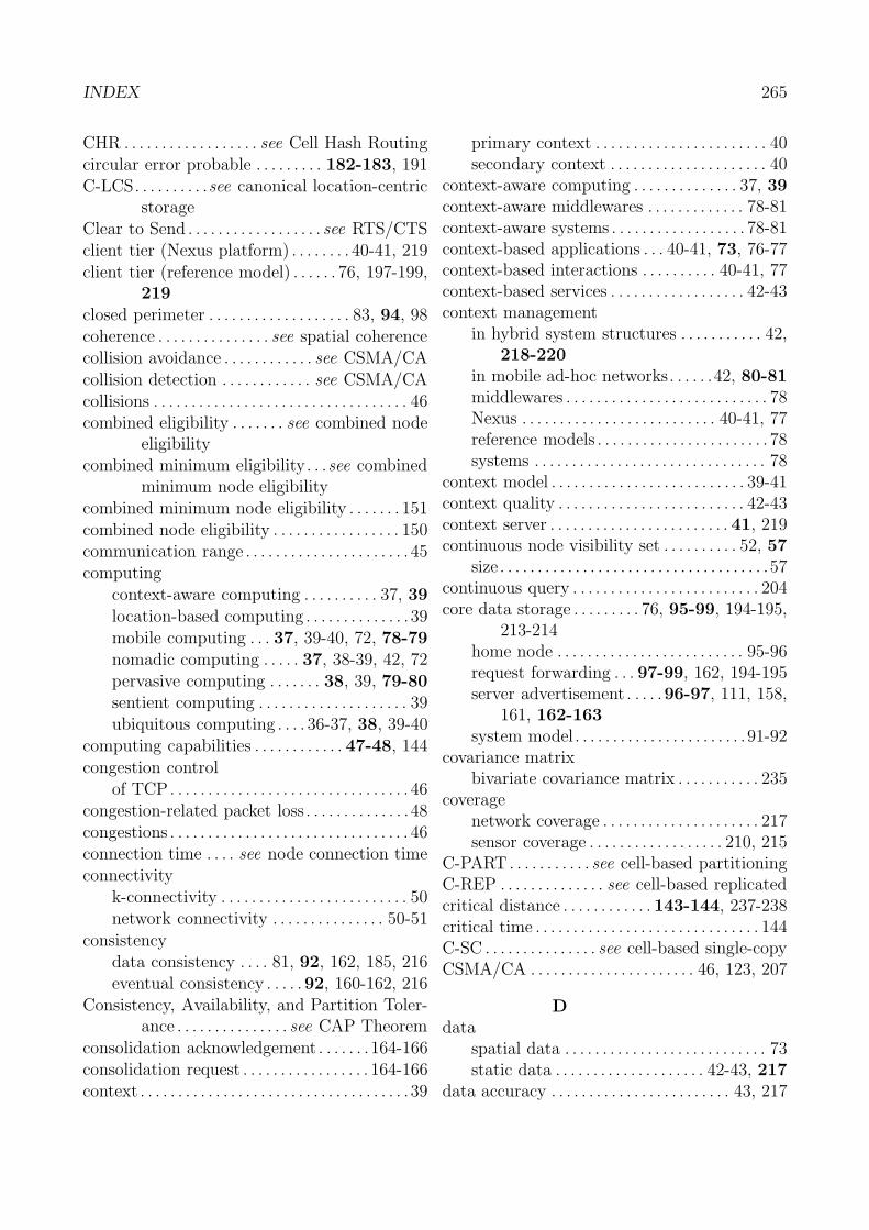
INDEX 265
CHR . . . . . . . . . . . . . . . . . . see Cell Hash Routingcircular error probable . . . . . . . . . 182-183, 191C-LCS. . . . . . . . . .see canonical location-centric
storageClear to Send . . . . . . . . . . . . . . . . . . see RTS/CTSclient tier (Nexus platform) . . . . . . . . 40-41, 219client tier (reference model) . . . . . . 76, 197-199,
219closed perimeter . . . . . . . . . . . . . . . . . . . 83, 94, 98coherence . . . . . . . . . . . . . . . see spatial coherencecollision avoidance . . . . . . . . . . . . see CSMA/CAcollision detection . . . . . . . . . . . . see CSMA/CAcollisions . . . . . . . . . . . . . . . . . . . . . . . . . . . . . . . . . . 46combined eligibility . . . . . . . see combined node
eligibilitycombined minimum eligibility. . .see combined
minimum node eligibilitycombined minimum node eligibility . . . . . . . 151combined node eligibility . . . . . . . . . . . . . . . . . 150communication range . . . . . . . . . . . . . . . . . . . . . . 45computing
context-aware computing . . . . . . . . . . 37, 39location-based computing . . . . . . . . . . . . . . 39mobile computing . . . 37, 39-40, 72, 78-79nomadic computing . . . . . 37, 38-39, 42, 72pervasive computing . . . . . . . 38, 39, 79-80sentient computing . . . . . . . . . . . . . . . . . . . . 39ubiquitous computing . . . . 36-37, 38, 39-40
computing capabilities . . . . . . . . . . . . 47-48, 144congestion control
of TCP. . . . . . . . . . . . . . . . . . . . . . . . . . . . . . . . 46congestion-related packet loss . . . . . . . . . . . . . .48congestions . . . . . . . . . . . . . . . . . . . . . . . . . . . . . . . . 46connection time . . . . see node connection timeconnectivity
k-connectivity . . . . . . . . . . . . . . . . . . . . . . . . . 50network connectivity . . . . . . . . . . . . . . . 50-51
consistencydata consistency . . . . 81, 92, 162, 185, 216eventual consistency . . . . .92, 160-162, 216
Consistency, Availability, and Partition Toler-ance . . . . . . . . . . . . . . . see CAP Theorem
consolidation acknowledgement . . . . . . . 164-166consolidation request . . . . . . . . . . . . . . . . . 164-166context . . . . . . . . . . . . . . . . . . . . . . . . . . . . . . . . . . . . 39
primary context . . . . . . . . . . . . . . . . . . . . . . . 40secondary context . . . . . . . . . . . . . . . . . . . . . 40
context-aware computing . . . . . . . . . . . . . . 37, 39context-aware middlewares . . . . . . . . . . . . . 78-81context-aware systems . . . . . . . . . . . . . . . . . . 78-81context-based applications . . . 40-41, 73, 76-77context-based interactions . . . . . . . . . . 40-41, 77context-based services . . . . . . . . . . . . . . . . . . 42-43context management
in hybrid system structures . . . . . . . . . . . 42,218-220
in mobile ad-hoc networks. . . . . .42, 80-81middlewares . . . . . . . . . . . . . . . . . . . . . . . . . . . 78Nexus . . . . . . . . . . . . . . . . . . . . . . . . . . 40-41, 77reference models . . . . . . . . . . . . . . . . . . . . . . . 78systems . . . . . . . . . . . . . . . . . . . . . . . . . . . . . . . 78
context model . . . . . . . . . . . . . . . . . . . . . . . . . . 39-41context quality . . . . . . . . . . . . . . . . . . . . . . . . . 42-43context server . . . . . . . . . . . . . . . . . . . . . . . . 41, 219continuous node visibility set . . . . . . . . . . 52, 57
size . . . . . . . . . . . . . . . . . . . . . . . . . . . . . . . . . . . .57continuous query . . . . . . . . . . . . . . . . . . . . . . . . . 204core data storage . . . . . . . . . 76, 95-99, 194-195,
213-214home node . . . . . . . . . . . . . . . . . . . . . . . . . 95-96request forwarding . . . 97-99, 162, 194-195server advertisement . . . . .96-97, 111, 158,
161, 162-163system model . . . . . . . . . . . . . . . . . . . . . . .91-92
covariance matrixbivariate covariance matrix . . . . . . . . . . . 235
coveragenetwork coverage . . . . . . . . . . . . . . . . . . . . . 217sensor coverage . . . . . . . . . . . . . . . . . . 210, 215
C-PART. . . . . . . . . . . see cell-based partitioningC-REP . . . . . . . . . . . . . . see cell-based replicatedcritical distance . . . . . . . . . . . . 143-144, 237-238critical time . . . . . . . . . . . . . . . . . . . . . . . . . . . . . . 144C-SC . . . . . . . . . . . . . . . see cell-based single-copyCSMA/CA . . . . . . . . . . . . . . . . . . . . . . 46, 123, 207
Ddata
spatial data . . . . . . . . . . . . . . . . . . . . . . . . . . . 73static data . . . . . . . . . . . . . . . . . . . . 42-43, 217
data accuracy . . . . . . . . . . . . . . . . . . . . . . . . 43, 217
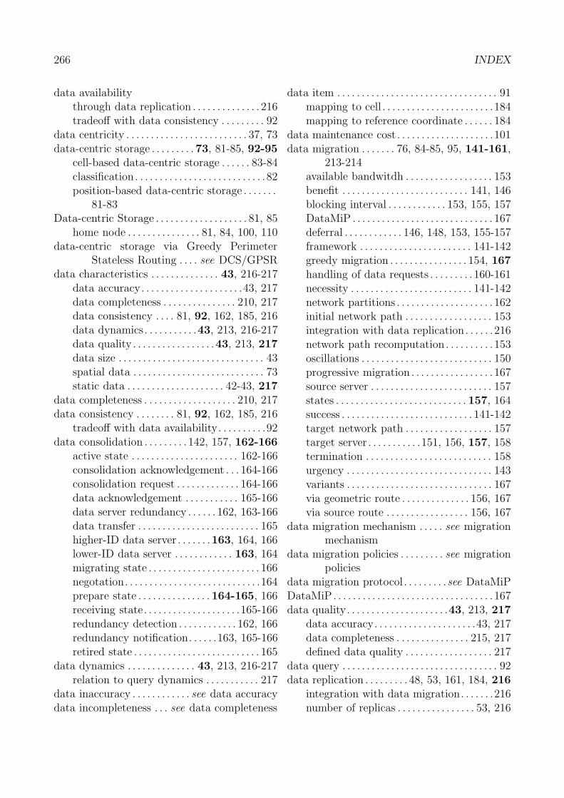
266 INDEX
data availabilitythrough data replication . . . . . . . . . . . . . . 216tradeoff with data consistency . . . . . . . . . 92
data centricity . . . . . . . . . . . . . . . . . . . . . . . . . 37, 73data-centric storage . . . . . . . . .73, 81-85, 92-95
cell-based data-centric storage . . . . . . 83-84classification. . . . . . . . . . . . . . . . . . . . . . . . . . .82position-based data-centric storage . . . . . . .
81-83Data-centric Storage . . . . . . . . . . . . . . . . . . . 81, 85
home node . . . . . . . . . . . . . . . 81, 84, 100, 110data-centric storage via Greedy Perimeter
Stateless Routing . . . . see DCS/GPSRdata characteristics . . . . . . . . . . . . . . 43, 216-217
data accuracy. . . . . . . . . . . . . . . . . . . . .43, 217data completeness . . . . . . . . . . . . . . . 210, 217data consistency . . . . 81, 92, 162, 185, 216data dynamics. . . . . . . . . . .43, 213, 216-217data quality . . . . . . . . . . . . . . . . .43, 213, 217data size . . . . . . . . . . . . . . . . . . . . . . . . . . . . . . 43spatial data . . . . . . . . . . . . . . . . . . . . . . . . . . . 73static data . . . . . . . . . . . . . . . . . . . . 42-43, 217
data completeness . . . . . . . . . . . . . . . . . . . 210, 217data consistency . . . . . . . . 81, 92, 162, 185, 216
tradeoff with data availability. . . . . . . . . .92data consolidation . . . . . . . . . 142, 157, 162-166
active state . . . . . . . . . . . . . . . . . . . . . . 162-166consolidation acknowledgement . . . 164-166consolidation request . . . . . . . . . . . . . 164-166data acknowledgement . . . . . . . . . . . 165-166data server redundancy . . . . . . 162, 163-166data transfer . . . . . . . . . . . . . . . . . . . . . . . . . 165higher-ID data server . . . . . . .163, 164, 166lower-ID data server . . . . . . . . . . . . 163, 164migrating state . . . . . . . . . . . . . . . . . . . . . . . 166negotation. . . . . . . . . . . . . . . . . . . . . . . . . . . .164prepare state . . . . . . . . . . . . . . . 164-165, 166receiving state. . . . . . . . . . . . . . . . . . . .165-166redundancy detection . . . . . . . . . . . . 162, 166redundancy notification. . . . . .163, 165-166retired state . . . . . . . . . . . . . . . . . . . . . . . . . . 165
data dynamics . . . . . . . . . . . . . . 43, 213, 216-217relation to query dynamics . . . . . . . . . . . 217
data inaccuracy . . . . . . . . . . . . see data accuracydata incompleteness . . . see data completeness
data item . . . . . . . . . . . . . . . . . . . . . . . . . . . . . . . . . 91mapping to cell . . . . . . . . . . . . . . . . . . . . . . .184mapping to reference coordinate . . . . . . 184
data maintenance cost. . . . . . . . . . . . . . . . . . . .101data migration . . . . . . . 76, 84-85, 95, 141-161,
213-214available bandwitdh . . . . . . . . . . . . . . . . . . 153benefit . . . . . . . . . . . . . . . . . . . . . . . . . . 141, 146blocking interval . . . . . . . . . . . . 153, 155, 157DataMiP . . . . . . . . . . . . . . . . . . . . . . . . . . . . . 167deferral . . . . . . . . . . . . 146, 148, 153, 155-157framework . . . . . . . . . . . . . . . . . . . . . . . 141-142greedy migration . . . . . . . . . . . . . . . . 154, 167handling of data requests . . . . . . . . . 160-161necessity . . . . . . . . . . . . . . . . . . . . . . . . . 141-142network partitions . . . . . . . . . . . . . . . . . . . . 162initial network path . . . . . . . . . . . . . . . . . . 153integration with data replication. . . . . .216network path recomputation . . . . . . . . . . 153oscillations . . . . . . . . . . . . . . . . . . . . . . . . . . . 150progressive migration . . . . . . . . . . . . . . . . . 167source server . . . . . . . . . . . . . . . . . . . . . . . . . 157states . . . . . . . . . . . . . . . . . . . . . . . . . . . 157, 164success . . . . . . . . . . . . . . . . . . . . . . . . . . . 141-142target network path . . . . . . . . . . . . . . . . . . 157target server . . . . . . . . . . .151, 156, 157, 158termination . . . . . . . . . . . . . . . . . . . . . . . . . . 158urgency . . . . . . . . . . . . . . . . . . . . . . . . . . . . . . 143variants . . . . . . . . . . . . . . . . . . . . . . . . . . . . . . 167via geometric route . . . . . . . . . . . . . . 156, 167via source route . . . . . . . . . . . . . . . . . 156, 167
data migration mechanism . . . . . see migrationmechanism
data migration policies . . . . . . . . . see migrationpolicies
data migration protocol . . . . . . . . .see DataMiPDataMiP. . . . . . . . . . . . . . . . . . . . . . . . . . . . . . . . . 167data quality. . . . . . . . . . . . . . . . . . . . .43, 213, 217
data accuracy. . . . . . . . . . . . . . . . . . . . .43, 217data completeness . . . . . . . . . . . . . . . 215, 217defined data quality . . . . . . . . . . . . . . . . . . 217
data query . . . . . . . . . . . . . . . . . . . . . . . . . . . . . . . . 92data replication . . . . . . . . . 48, 53, 161, 184, 216
integration with data migration. . . . . . .216number of replicas . . . . . . . . . . . . . . . . 53, 216
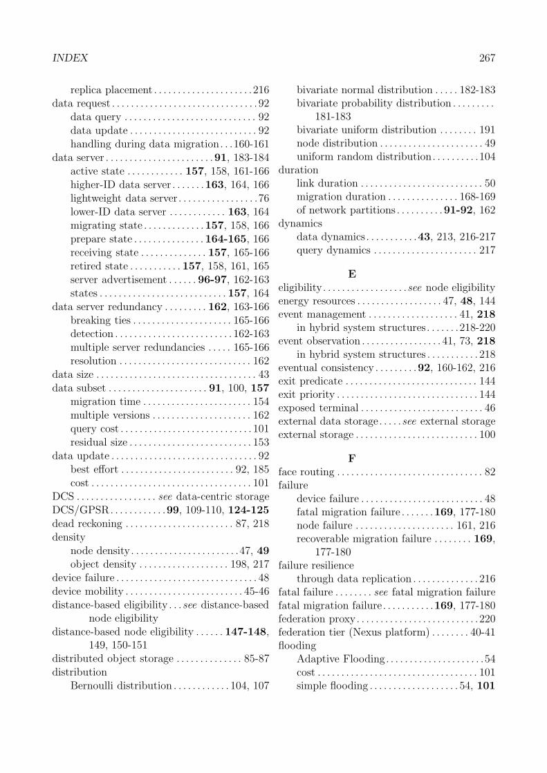
INDEX 267
replica placement . . . . . . . . . . . . . . . . . . . . .216data request . . . . . . . . . . . . . . . . . . . . . . . . . . . . . . . 92
data query . . . . . . . . . . . . . . . . . . . . . . . . . . . . 92data update . . . . . . . . . . . . . . . . . . . . . . . . . . . 92handling during data migration. . .160-161
data server . . . . . . . . . . . . . . . . . . . . . . .91, 183-184active state . . . . . . . . . . . . 157, 158, 161-166higher-ID data server . . . . . . .163, 164, 166lightweight data server. . . . . . . . . . . . . . . . .76lower-ID data server . . . . . . . . . . . . 163, 164migrating state . . . . . . . . . . . . .157, 158, 166prepare state . . . . . . . . . . . . . . . 164-165, 166receiving state . . . . . . . . . . . . . . 157, 165-166retired state . . . . . . . . . . . 157, 158, 161, 165server advertisement . . . . . . 96-97, 162-163states . . . . . . . . . . . . . . . . . . . . . . . . . . . 157, 164
data server redundancy . . . . . . . . . 162, 163-166breaking ties . . . . . . . . . . . . . . . . . . . . . 165-166detection . . . . . . . . . . . . . . . . . . . . . . . . . 162-163multiple server redundancies . . . . . 165-166resolution . . . . . . . . . . . . . . . . . . . . . . . . . . . . 162
data size . . . . . . . . . . . . . . . . . . . . . . . . . . . . . . . . . . 43data subset . . . . . . . . . . . . . . . . . . . . . 91, 100, 157
migration time . . . . . . . . . . . . . . . . . . . . . . . 154multiple versions . . . . . . . . . . . . . . . . . . . . . 162query cost . . . . . . . . . . . . . . . . . . . . . . . . . . . . 101residual size . . . . . . . . . . . . . . . . . . . . . . . . . . 153
data update . . . . . . . . . . . . . . . . . . . . . . . . . . . . . . . 92best effort . . . . . . . . . . . . . . . . . . . . . . . . 92, 185cost . . . . . . . . . . . . . . . . . . . . . . . . . . . . . . . . . . 101
DCS . . . . . . . . . . . . . . . . . see data-centric storageDCS/GPSR. . . . . . . . . . . .99, 109-110, 124-125dead reckoning . . . . . . . . . . . . . . . . . . . . . . . 87, 218density
node density. . . . . . . . . . . . . . . . . . . . . . .47, 49object density . . . . . . . . . . . . . . . . . . . 198, 217
device failure . . . . . . . . . . . . . . . . . . . . . . . . . . . . . . 48device mobility . . . . . . . . . . . . . . . . . . . . . . . . . 45-46distance-based eligibility . . .see distance-based
node eligibilitydistance-based node eligibility . . . . . . 147-148,
149, 150-151distributed object storage . . . . . . . . . . . . . . 85-87distribution
Bernoulli distribution . . . . . . . . . . . . 104, 107
bivariate normal distribution . . . . . 182-183bivariate probability distribution . . . . . . . . .
181-183bivariate uniform distribution . . . . . . . . 191node distribution . . . . . . . . . . . . . . . . . . . . . . 49uniform random distribution. . . . . . . . . .104
durationlink duration . . . . . . . . . . . . . . . . . . . . . . . . . . 50migration duration . . . . . . . . . . . . . . . 168-169of network partitions . . . . . . . . . .91-92, 162
dynamicsdata dynamics. . . . . . . . . . .43, 213, 216-217query dynamics . . . . . . . . . . . . . . . . . . . . . . 217
Eeligibility. . . . . . . . . . . . . . . . . .see node eligibilityenergy resources . . . . . . . . . . . . . . . . . . 47, 48, 144event management . . . . . . . . . . . . . . . . . . . 41, 218
in hybrid system structures. . . . . . .218-220event observation . . . . . . . . . . . . . . . . . 41, 73, 218
in hybrid system structures . . . . . . . . . . . 218eventual consistency . . . . . . . . .92, 160-162, 216exit predicate . . . . . . . . . . . . . . . . . . . . . . . . . . . . 144exit priority . . . . . . . . . . . . . . . . . . . . . . . . . . . . . . 144exposed terminal . . . . . . . . . . . . . . . . . . . . . . . . . . 46external data storage. . . . .see external storageexternal storage . . . . . . . . . . . . . . . . . . . . . . . . . . 100
Fface routing . . . . . . . . . . . . . . . . . . . . . . . . . . . . . . . 82failure
device failure . . . . . . . . . . . . . . . . . . . . . . . . . . 48fatal migration failure . . . . . . .169, 177-180node failure . . . . . . . . . . . . . . . . . . . . . 161, 216recoverable migration failure . . . . . . . . 169,
177-180failure resilience
through data replication . . . . . . . . . . . . . . 216fatal failure . . . . . . . . see fatal migration failurefatal migration failure. . . . . . . . . . .169, 177-180federation proxy. . . . . . . . . . . . . . . . . . . . . . . . . .220federation tier (Nexus platform) . . . . . . . . 40-41flooding
Adaptive Flooding. . . . . . . . . . . . . . . . . . . . .54cost . . . . . . . . . . . . . . . . . . . . . . . . . . . . . . . . . . 101simple flooding . . . . . . . . . . . . . . . . . . . 54, 101
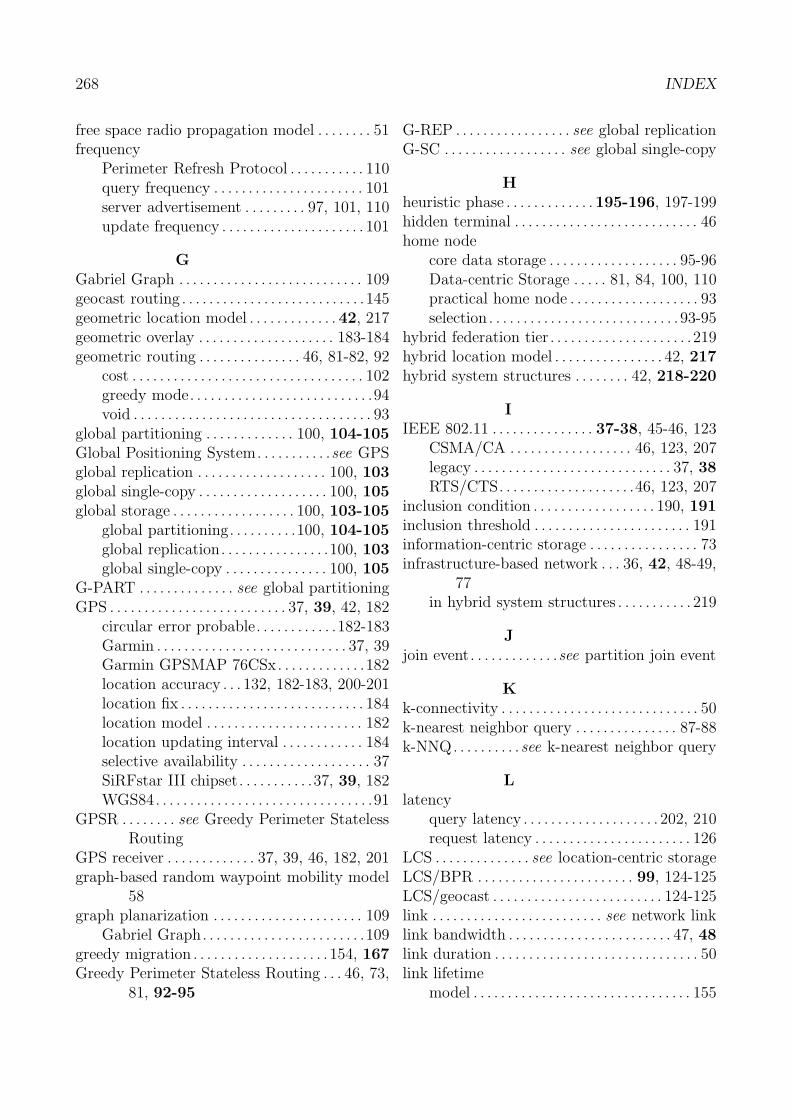
268 INDEX
free space radio propagation model . . . . . . . . 51frequency
Perimeter Refresh Protocol . . . . . . . . . . . 110query frequency . . . . . . . . . . . . . . . . . . . . . . 101server advertisement . . . . . . . . . 97, 101, 110update frequency . . . . . . . . . . . . . . . . . . . . . 101
GGabriel Graph . . . . . . . . . . . . . . . . . . . . . . . . . . . 109geocast routing . . . . . . . . . . . . . . . . . . . . . . . . . . .145geometric location model . . . . . . . . . . . . .42, 217geometric overlay . . . . . . . . . . . . . . . . . . . . 183-184geometric routing . . . . . . . . . . . . . . . 46, 81-82, 92
cost . . . . . . . . . . . . . . . . . . . . . . . . . . . . . . . . . . 102greedy mode. . . . . . . . . . . . . . . . . . . . . . . . . . .94void . . . . . . . . . . . . . . . . . . . . . . . . . . . . . . . . . . . 93
global partitioning . . . . . . . . . . . . . 100, 104-105Global Positioning System. . . . . . . . . . .see GPSglobal replication . . . . . . . . . . . . . . . . . . . 100, 103global single-copy . . . . . . . . . . . . . . . . . . . 100, 105global storage . . . . . . . . . . . . . . . . . . 100, 103-105
global partitioning. . . . . . . . . .100, 104-105global replication. . . . . . . . . . . . . . . .100, 103global single-copy . . . . . . . . . . . . . . . 100, 105
G-PART . . . . . . . . . . . . . . see global partitioningGPS . . . . . . . . . . . . . . . . . . . . . . . . . . 37, 39, 42, 182
circular error probable. . . . . . . . . . . .182-183Garmin . . . . . . . . . . . . . . . . . . . . . . . . . . . . 37, 39Garmin GPSMAP 76CSx. . . . . . . . . . . . .182location accuracy . . . 132, 182-183, 200-201location fix . . . . . . . . . . . . . . . . . . . . . . . . . . . 184location model . . . . . . . . . . . . . . . . . . . . . . . 182location updating interval . . . . . . . . . . . . 184selective availability . . . . . . . . . . . . . . . . . . . 37SiRFstar III chipset. . . . . . . . . . .37, 39, 182WGS84. . . . . . . . . . . . . . . . . . . . . . . . . . . . . . . .91
GPSR . . . . . . . . see Greedy Perimeter StatelessRouting
GPS receiver . . . . . . . . . . . . . 37, 39, 46, 182, 201graph-based random waypoint mobility model
58graph planarization . . . . . . . . . . . . . . . . . . . . . . 109
Gabriel Graph. . . . . . . . . . . . . . . . . . . . . . . .109greedy migration . . . . . . . . . . . . . . . . . . . . 154, 167Greedy Perimeter Stateless Routing . . . 46, 73,
81, 92-95
G-REP . . . . . . . . . . . . . . . . . see global replicationG-SC . . . . . . . . . . . . . . . . . . see global single-copy
Hheuristic phase . . . . . . . . . . . . .195-196, 197-199hidden terminal . . . . . . . . . . . . . . . . . . . . . . . . . . . 46home node
core data storage . . . . . . . . . . . . . . . . . . . 95-96Data-centric Storage . . . . . 81, 84, 100, 110practical home node . . . . . . . . . . . . . . . . . . . 93selection . . . . . . . . . . . . . . . . . . . . . . . . . . . . 93-95
hybrid federation tier . . . . . . . . . . . . . . . . . . . . .219hybrid location model . . . . . . . . . . . . . . . . 42, 217hybrid system structures . . . . . . . . 42, 218-220
IIEEE 802.11 . . . . . . . . . . . . . . . 37-38, 45-46, 123
CSMA/CA . . . . . . . . . . . . . . . . . . 46, 123, 207legacy . . . . . . . . . . . . . . . . . . . . . . . . . . . . . 37, 38RTS/CTS. . . . . . . . . . . . . . . . . . . .46, 123, 207
inclusion condition . . . . . . . . . . . . . . . . . . 190, 191inclusion threshold . . . . . . . . . . . . . . . . . . . . . . . 191information-centric storage . . . . . . . . . . . . . . . . 73infrastructure-based network . . . 36, 42, 48-49,
77in hybrid system structures . . . . . . . . . . . 219
Jjoin event. . . . . . . . . . . . .see partition join event
Kk-connectivity . . . . . . . . . . . . . . . . . . . . . . . . . . . . . 50k-nearest neighbor query . . . . . . . . . . . . . . . 87-88k-NNQ. . . . . . . . . .see k-nearest neighbor query
Llatency
query latency . . . . . . . . . . . . . . . . . . . . 202, 210request latency . . . . . . . . . . . . . . . . . . . . . . . 126
LCS . . . . . . . . . . . . . . see location-centric storageLCS/BPR . . . . . . . . . . . . . . . . . . . . . . . 99, 124-125LCS/geocast . . . . . . . . . . . . . . . . . . . . . . . . . 124-125link . . . . . . . . . . . . . . . . . . . . . . . . . see network linklink bandwidth . . . . . . . . . . . . . . . . . . . . . . . . 47, 48link duration . . . . . . . . . . . . . . . . . . . . . . . . . . . . . . 50link lifetime
model . . . . . . . . . . . . . . . . . . . . . . . . . . . . . . . . 155
INDEX 269
residual link lifetime . . . . . . . . . . . . 152, 156link quality . . . . . . . . . . . . . . . . . . . . . . . 47, 48, 153link stability . . . . . . . . . . . . . . . . . . . . . . . . . . . . . 155
models . . . . . . . . . . . . . . . . . . . . . . . . . . . . . . . 151load factor . . . . . . . . . . . . . . . . . . . . . . . . . . . . . . . 150local data storage . . . . . . . . . . . see local storagelocality . . . . . . . . . . . . . . . . . . . . . . . . . . . . . . . . . . . . 73local storage . . . . . . . . . . . . . . . . . . . . . . 80, 88, 100location
accuracy model . . . . . 44, 77, 181-183, 212practical notion . . . . . . . . . . . . . . . . . . . . . . 182reference location . . . . . . . . . . . . . . . . . . . . . . 74storage location . . . . . . . . . . . . . . . . . . . . . . . 73
location accuracy . . . . . . . . 43, 75, 132, 182-183,200-201, 214
location area. . . . . . . . . . . . . . . . . . . .183, 187-192in polar coordinates . . . . . . . . . . . . . . . . . . 192
location-based computing . . . . . . . . . . . . . . . . . . . .location-based services . . . . . . . . . . . . . . . . . 36, 42location-centric storage . . .72-74, 95, 194, 213
canonical location-centric storage . . . 73-74reference location . . . . . . . . . . . . . . . . . . . . . . 74reference model . . . . . . . . . . . . . . . 74-77, 219
location-centric storage via Bidirectional Peri-meter Routing . . . . . . . . . see LCS/BPR
location-centric storage via geocast. . . . . . . .seeLCS/geocast
location error . . . . . . . . . . . see location accuracylocation fix. . . . . . . . . . . . . . . . . . . . .184, 185, 188location model . . . . . . . . . . . . . . . . . . . . . . . . . . . 217
complexity . . . . . . . . . . . . . . . . . . . . . . . . . . . . 42geometric location model . . . . . . . . . 42, 217hybrid location model . . . . . . . . . . . . 42, 217symbolic location model . . . . . . . . . . 42, 217
location pdf . . . . . . . . . . . . . . . . . . . . . . . . . . . . . . 181derivation . . . . . . . . . . . . . . . . . . . . . . . . . . . . 235in polar coordinates . . . . . . . . . . . . . . . . . . 192supporting area . . . . . . . . . . . . . . . . . . . . . . 182
location probability density function . . . . . . seelocation pdf
location semantics . . . . . . 75, 77, 181-183, 218location servers . . . . . . . . . . . . . . . . . . . . . . . . . . . .73location services . . . . . . . . . . . . . . . . . . . . . . . 85, 87location updating . . . 85-90, 184-190, 214-215
data consistency. . . . . . . . . . . . . . . . . . . . . .185
lowest-ID cell . . . . . . . . . . . . . . . . . . . . 188-189object delete . . . . . . . . . . . . . . . . . . . . . 187-188object record . . . . . . . . . . . . . . . . . . . . . . . . . 185object tracing . . . . . . . . . . 187-188, 189-190object update . . . . . . . . . . . . . . . . . . . . 187-188outdated location information . . . . . . . . 184previous cell set . . . . . . . . . . . . 187-188, 190proactive copy removal . . . . . . . . . . . . . . . 185proactive object removal . . . . 187, 188-189soft state . . . . . . . . . . . . . . . . . . . . . . . . . . . . . 184tracing distance . . . . . . . . . . . . 187, 188, 190
MMAC. . . . . . . . . . . . . . see medium access controlmalformed perimeter . . . . . . . . . . . . . . . 82, 92-95
fraction of malformed perimeters . . . . . 102Mark Weiser. . . . . . . . . . . . . . . .see Weiser, Markmaximum inaccuracy. . . . . . . . . . . . . .89-90, 191MDM. . . . . . . . . . .see mobile data managementMDP . . . . . . . . . . . see migration decision policymedium . . . . . . . . . . . . . . . . . . see shared mediummedium access control . . . . . . . . . . . . . . . . . . 46-47memory capacity . . . . . . . . . . . . . . . . . . 47-48, 144mesh network . . . . . .see wireless mesh networkmigrating state . . . . . . . . . . . . . . . . .157, 158, 166migration acknowledgement . . . . . . . . . . . . . . 158migration cycle . . . . . . . . . . . . . 142, 144, 156-157migration decision. . . . . . . . . . . . . .141, 156-157migration decision policy . . . . . . . 141-142, 145,
146-157combined node eligibility . . . . . . . . . 150-151distance-based node eligibility. . . . . . . . . . . .
147-148, 149, 150-151estimated migration time . . . . . . . . . . . . . 154migration decision predicate. . . . .142, 151,
156, 157network topology exploration . . . . . 145-146node eligibility . . . . 146, 147-151, 156-157path stability . . . . . . . . . . . . . . . . . . . . 151-156remote state . . . . . . . . . . . . . . . . 141-142, 145residual sojourn time . . . . . . . . . . . . . . . . . 149sojourn-based node eligibility . . . . . . . . 147,
148-149, 150-151stretch factor . . . . . . . . . . . . . . . . . . . . . . . . . 155time-based node eligibility . . . . . . 147, 150,
151
270 INDEX
triggering . . . . . . . . . . . . . . . . . . . . . . . . . . . . 144migration decision predicate . . . .142, 151, 156,
157migration duration . . . . . . . . . . . . . . . . . . . 168-169migration duration fraction. . . . . . . . . . .168-169migration efficiency. . . . . . . . . . . . . . . . . . . . . . .168migration failure . . . . . . 142, 157, 169, 177-180
fatal migration failure . . . . . . .169, 177-180recoverable migration failure . . . . . . . . 169,
177-180migration mechanism. . .76, 141-142, 157-166
active state. . . . . . . . . . . . . . . . .157, 158, 161geometric routing . . . . . . . . . . . . . . . . . . . . 167migrating state. . . . . . . . . . . . . . . . . .157, 158migration acknowledgement . . . . . . . . . . 158migration request . . . . . . . . . . . . . . . 158, 166receiving state . . . . . . . . . . . . . . . . . . . . . . . . 157retired state . . . . . . . . . . . . . . . .157, 158, 161source routing . . . . . . . . . . . . . . . . . . . . . . . . 167transport protocol . . . . . . . . . . . . . . . . . . . . 158
migration policies. . . . . . . . . . .76, 141, 142-157blocking interval . . . . . . . . . . . . 153, 155, 157eligible nodes . . . . . . . . . . . . . . . . . . . . . . . . . 142local state . . . . . . . . . . . . . . . . . . 141, 142, 145migration cycle . . . . . . . . . 142, 144, 156-157migration decision policy . . . . . . . . . 146-157migration recommendation policy . . . . . . . .
142-144tasks . . . . . . . . . . . . . . . . . . . . . . . . . . . . . . . . . 141
migration priority . . . . 142-144, 147-151, 153,155, 157
migration recommendation . . . . . . . . . . . . . . . 141migration recommendation policy . . . . . . . . 141,
142-144, 237computing capabilities . . . . . . . . . . . . . . . .144critical distance . . . . . . . . . . . . . . . . . . 143-144critical time . . . . . . . . . . . . . . . . . . . . . . . . . . 144deferral. . . . . . . . . . . . . . . . . . . . . . . . . . . . . . .142energy resources . . . . . . . . . . . . . . . . . . . . . . 144exit predicate . . . . . . . . . . . . . . . . . . . . . . . . 144exit priority . . . . . . . . . . . . . . . . . . . . . . . . . . 144local state . . . . . . . . . . . . . . . . . . . . . . . . . . . . 141memory capacity . . . . . . . . . . . . . . . . . . . . . 144migration cycle . . . . . . . . . . . . . . . . . . 142, 144migration priority . . . . . . . . . . . . . . . . 142-144
migration recommendation predicate . . . . .141, 142-144
optimal distance . . . . . . . . . . . . . . . . . 143-144spatial predicate. . . . . . . . . . . .142, 143, 144spatial priority . . . . . . . . . . . . . . . . . .143, 144temporal predicate . . . . . . . . . 143, 144, 145temporal priority . . . . . . . . . . . . 143144, 145temporal threshold . . . . . . . . . . . . . . . . . . . 144threshold distance . . . . . . . . . . . . . . . . 143-144
migration recommendation predicate . . . . . 141,142-144, 237
migration request . . . . . . . . . . . . . . . . . . . . . . . . 158denial . . . . . . . . . . . . . . . . . . . . . . . . . . . . . . . . 166
migration robustness . . . . . . . . . . . . . . . . . . . . . 169migration threshold . . . . . . . . . . . . . . . . . . . . . . 101minimum required path lifetime . . . . . . 155-156mobile ad-hoc network . . . . . . . . . . . . . . . . . 45-49
as context server . . . . . . . . . . . . . . . . . . . . . 220characteristics . . . . . . . . . . . . . . . . . . . . . . 47-49context management . . . . . . . . . . . 42, 80-81federation proxy . . . . . . . . . . . . . . . . . . . . . . 220in hybrid system structures . . . . . . . . . . . 219mean route length . . . . . . . . . . . . . . . . 231-232medium access control . . . . . . . . . . . . . . 46-47network model . . . . . . . . . . . . . . . . . . . . . 45-47routing layer . . . . . . . . . . . . . . . . . . . . . . . . . . 46spatial query processing . . . . . . . . . . . . . . . 88system model . . . . . . . . . . . . .91-92, 183-184transport layer . . . . . . . . . . . . . . . . . . . . . 46-47
mobile computing . . . . . . . 37, 39-40, 72, 78-79mobile data management . . . . . . . . . . . . . . . . . . 72
frameworks . . . . . . . . . . . . . . . . . . . . . . . . . . . . 78mobility
device mobility . . . . . . . . . . . . . . . . . . . . . 45-46node mobility . . . 45, 47, 49, 123, 149, 217
mobility modelgraph-based random waypoint mobility
model . . . . . . . . . . . . . . . . . . . . . . . . . . . . . 58random waypoint mobility model . . . . . 58,
124mobility-related packet loss . . . . . . . . . . . . . . . . 49mode
bidirectional perimeter mode . . . . . . . . . . 94greedy mode. . . . . . . . . . . . . . . . . . . . . . . . . . .94redundacy detection mode. . . . . . . .162-163
INDEX 271
model-based optimum result . . . . . . . . 201, 210MRP. . .see migration recommendation policy
Nnearer relation . . . . . . . . . . . . . . . . . . . . . . . . . . . 193nearest neighbor query . . . . . . . . . . . . . . . . . . . . 87network
infrastructure-based network . . . . . . 36, 42,48-49, 77, 219
mobile ad-hoc network . . . . . . 45-49, 91-92switched network . . . . . . . . . . . . . . . . . 47, 158vehicular ad-hoc network . . . . . . . . . . . . . . 80wireless mesh network . . . . . . . . . 37, 46, 49wireless sensor network . . . . . . . . 38, 46, 49
network characteristics . . . . . . . . . . . .47-49, 212computing capabilities . . . . . . . . 47-48, 144energy resources . . . . . . . . . . . . . . 47, 48, 144link bandwidth . . . . . . . . . . . . . . . . . . . . 47, 48link quality . . . . . . . . . . . . . . . . . . . 47, 48, 153memory capacity . . . . . . . . . . . . . . 47-48, 144network connectivity . . . . . . . . . . . . . . . 50-51network coverage . . . . . . . . . . . . . . . . . . . . . 217network topology . . . . . . . . . . . . . . . . . . . . . . 47node density. . . . . . . . . . . . . . . . . . . . . . .47, 49node mobility . . . 45, 47, 49, 123, 149, 217
network connectivity . . . . . . . . . . . . . . . . . . . 50-51network coverage . . . . . . . . . . . . . . . . . . . . . . . . . 217network density . . . . . . . . . . . . . see node densitynetwork geometry
correlation with network topology. . . .103,231-232
network linkbandwidth. . . . . . . . . . . . . . . . . . . . . . . . .47, 48duration . . . . . . . . . . . . . . . . . . . . . . . . . . . . . . . 50lifetime . . . . . . . . . . . . . . . . . . . . . . . . . 152, 156lifetime model . . . . . . . . . . . . . . . . . . . . . . . . 155quality . . . . . . . . . . . . . . . . . . . . . . . 47, 48, 153stability . . . . . . . . . . . . . . . . . . . . . . . . . . . . . . 155stability models . . . . . . . . . . . . . . . . . . . . . . 151
network mobility . . . . . . . . . . . see node mobilitynetwork partition . . . . . 49, 51, 91-92, 162, 216
duration . . . . . . . . . . . . . . . . . . . . . . 91-92, 162during data migration . . . . . . . . . . . . . . . . 162during request forwarding . . . . . . . . . . . . . 98exterior. . . . . . . . . . . . . . . . . . . . . . . . . . . . . . . .93forming . . . . . . . . . . . . . . . . . . . . 49, 91-92, 162
interior . . . . . . . . . . . . . . . . . . . . . . . . . . . . . . . . 93joining of network partitions . . . . . . 99, 162set of network partitions . . . . . . . . . . . . . . . 52
network partition change rate . . . see partitionchange rate
network partition event . . . see partition eventnetwork partitioning . . . . . . . . . . 49-58, 92, 212network partition metrics . . . . . . . see partition
metricsnetwork partition size . . . . . . . see partition sizenetwork partition size ratio . . . . . .see partition
size rationetwork path
computation . . . . . . . . . . . . . . . . . . . . . 152-156initial network path for data migration . . .
153length . . . . . . . . . . . . . . . . . . . . . . . . . . . . . . . . 155length restriction . . . . . . . . . . . . . . . . . 155-156lifetime . . . . . . . . . . . . . . . . . . . . . . . . . . 154-155maximum length for data migration. . . . . .
155minimum length . . . . . . . . . . . . . . . . . . . . . . 155minimum required lifetime . . . . . . . 155-156recomputation. . . . . . . . . . . . . . . . . . . . . . . .155recomputation due time . . . . . . . . . . . . . . 158residual lifetime . . . . . . . . . . . . . . . . . 156, 158selection of network path . . . . . . . . . . . . . 155stability . . . . . . . . . . . . . . . . . . . . 142, 151-156sufficiently stable network path . . . . . . 153,
156target network path for data migration. . .
157transparent switching. . . . . . . . . . . . . . . . .155
network topology . . . . . . . . . . . . . . . . . . . . . 47, 123correlation with network geometry . . . 103,
231-232network topology exploration . . . . . . . . . . 75-76,
141-142, 145-146, 152-153, 158aggregation delay . . . . . . . . . . . . . . . . 145, 153aggregation tree . . . . . . . . . . . . . . . . . . . . . . 145geocast routing . . . . . . . . . . . . . . . . . . . . . . . 145reverse aggregation tree . . . . . . . . . . . . . . 145topology reply . . . . . . . . . . . . . . . . . . . . . . . . 145topology request. . . . . . . . . . . . . . . . . . . . . .145
network topology exploration region . . . . . . . . .
272 INDEX
145-146, 155, 237-248area restrictions . . . . . . . . . . . . . . . . . . 237-238base shapes . . . . . . . . . . . . . . . . . . . . . . 238-242circular case . . . . . . . . . . . . . . . . 238-239, 243curvature subcase . . . . . . 239-240, 243-245elliptical cases. . . . . . . . . .239-242, 243-248special case . . . . . . . . . . . . . . . . 238, 242-243summary of cases . . . . . . . . . . . . . . . 242, 248summary of shapes . . . . . . . . . . . . . . . . . . . 146tangent subcase . . . . . . . . 240-242, 246-248
network topology graph . . . . . . . . . . . . . . . 51, 52network-wide partition metrics . . . . . 52, 53-55Nexus . . . . . . . . . . . . . . . . . . . . . . . . . . 39, 40-41, 42
context server . . . . . . . . . . . . . . . . . . . . 41, 219platform . . . . . . . . . . . . . . . . . . . . . . . 40-41, 77World Wide Space . . . . . . . . . . . . . 37, 41, 42
NLLS . . . . . . . see nonlinear least-square fittingNNQ. . . . . . . . . . . . . .see nearest neighbor querynode
home node . . . . . . . . 81, 84, 93-96, 100, 110perimeter entry node . . . . . . . . . . .93-95, 96proxy node . . . . . . . . . . . . . . . . . . 104-105, 107
node-centric partition metrics . . . . . . 52, 55-58node-centric routing . . . . . . . . . . . . . . . . . . . . . . . 95node-centric storage . . . . . . . . . . . . . . . . . . . . . . . 73node connections . . . . . . . . . see number of node
connectionsnode connection time . . . . . . . . . . . . . . . . . . 52, 56node density . . . . . . . . . . . . . . . . . . . . . . . . . . 47, 49node distribution . . . . . . . . . . . . . . . . . . . . . . . . . . 49node eligibility . . . . . . . . 146, 147-151, 156-157
combined minimum node eligiblity. . . .151combined node eligibility . . . . . . . . . . . . . 150distance-based node eligibility. . . . . . . . . . . .
147-148, 149, 150-151sojourn-based node eligibility . . . . . . . . 147,
148-149, 150-151time-based node eligibility . . . 147150, 151
node failure . . . . . . . . . . . . . . . . . . . . . . . . . 161, 216node mobility . . . . . . . 45, 47, 49, 123, 149, 217node partition change rate . . . . . . . . . 52, 55-56node separations . . . . . . . . . see number of node
separationsnode separation time. . . . . . . . . . . . . . .52, 56-57node visibility set
accumulative node visibility set . . . . 52, 58continuous node visibility set . . . . . . 52, 57
node visibility sets . . . . . . . . . . . . . . . . . 52, 57-58nomadic computing . . . . . . . . . 37, 38-39, 42, 72nonlinear least-square fitting . . . . . . . . . . . . . 103normal distribution
bivariate normal distribution . . . . . 182-183NTE . . . . . . . see network topology explorationNTE region. . . . . . . . . . . . .see network topology
exploration regionnumber of node connections . . . . . . . . . . . 52, 57number of node separations. . . . . . . . . . . .52, 57number of partitions . . . . . . . . . . . . . . . 52, 53-54
frequency distribution . . . . . . . . . . . . . . . . . 54
Oobject density . . . . . . . . . . . . . . . . . . . . . . . 198, 217object query. . . . . . . . . . . . . . . . . . . . . . . . . . . .85-87open perimeter . . . . . . . . . . . . . . . . . . . . . . . . 83, 93optimal distance . . . . . . . . . . . . . . . . . . . . 143-144
Ppacket capacity . . . . . . . . . . . . . . . . . . . . . . 101, 104packet loss . . . . . . . . . . . . . . . . . . . . . . . . . . . . . 48-49
congestion-related packet loss . . . . . . . . . . 48mobility-related packet loss . . . . . . . . . . . . 49
packet loss probability. . . . . . . . . . . . . . . . . . . .152partial perimeter . . . . . . . . . . . . 93-95, 96, 98-99partial query. . . . . . . . . . .194-195, 196, 197-199partition change rate . . . . . . . . . . . . . . . 52, 54-55
node partition change rate . . . . . 52, 55-56partition event . . . . . . . . . . . . . . . . . . . . . . . . . . . . 51
partition join event . . . . . . . . . . . . . . . . . . . . 51partition split event . . . . . . . . . . . . . . . . . . . 51total order of partition events. . . . . . . . . .51
partition join event . . . . . . . . . . . . . . . . . . . . . . . . 51partition metrics . . . . . . . . . . . . . . . . . . . . . . . 52-58
accumulative node visibility set . . . . 52, 58continuous node visibility set . . . . . . 52, 57network-wide partition metrics . . . . . . . . . . .
52, 53-55node-centric partition metrics . . . . . . . . . . . .
52, 55-58node connection time . . . . . . . . . . . . . . 52, 56node partition change rate . . . . . 52, 55-56node separation time . . . . . . . . . . . 52, 56-57
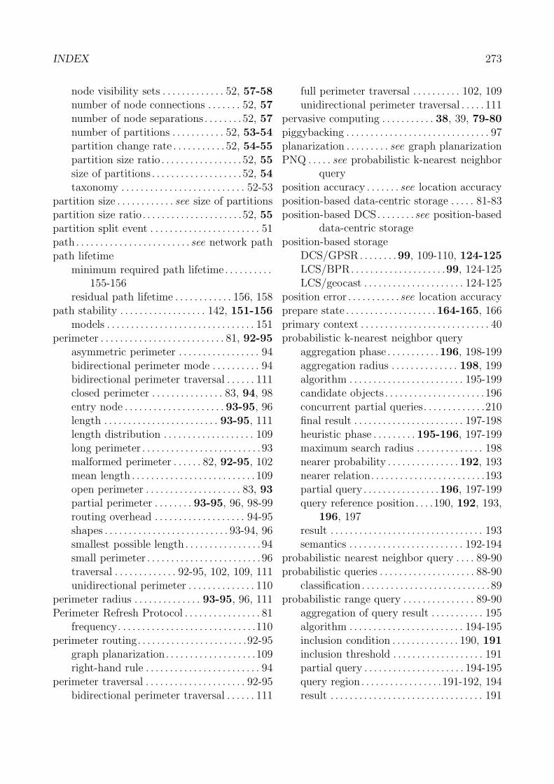
INDEX 273
node visibility sets . . . . . . . . . . . . . 52, 57-58number of node connections . . . . . . . 52, 57number of node separations . . . . . . . . 52, 57number of partitions . . . . . . . . . . . 52, 53-54partition change rate . . . . . . . . . . . 52, 54-55partition size ratio . . . . . . . . . . . . . . . . . 52, 55size of partitions . . . . . . . . . . . . . . . . . . . 52, 54taxonomy . . . . . . . . . . . . . . . . . . . . . . . . . . 52-53
partition size . . . . . . . . . . . . see size of partitionspartition size ratio. . . . . . . . . . . . . . . . . . . . .52, 55partition split event . . . . . . . . . . . . . . . . . . . . . . . 51path . . . . . . . . . . . . . . . . . . . . . . . . see network pathpath lifetime
minimum required path lifetime . . . . . . . . . .155-156
residual path lifetime . . . . . . . . . . . . 156, 158path stability . . . . . . . . . . . . . . . . . . 142, 151-156
models . . . . . . . . . . . . . . . . . . . . . . . . . . . . . . . 151perimeter . . . . . . . . . . . . . . . . . . . . . . . . . . 81, 92-95
asymmetric perimeter . . . . . . . . . . . . . . . . . 94bidirectional perimeter mode . . . . . . . . . . 94bidirectional perimeter traversal . . . . . . 111closed perimeter . . . . . . . . . . . . . . . 83, 94, 98entry node . . . . . . . . . . . . . . . . . . . . . 93-95, 96length . . . . . . . . . . . . . . . . . . . . . . . . 93-95, 111length distribution . . . . . . . . . . . . . . . . . . . 109long perimeter . . . . . . . . . . . . . . . . . . . . . . . . . 93malformed perimeter . . . . . . 82, 92-95, 102mean length . . . . . . . . . . . . . . . . . . . . . . . . . . 109open perimeter . . . . . . . . . . . . . . . . . . . . 83, 93partial perimeter . . . . . . . . 93-95, 96, 98-99routing overhead . . . . . . . . . . . . . . . . . . . 94-95shapes . . . . . . . . . . . . . . . . . . . . . . . . . . 93-94, 96smallest possible length . . . . . . . . . . . . . . . . 94small perimeter . . . . . . . . . . . . . . . . . . . . . . . . 96traversal . . . . . . . . . . . . . 92-95, 102, 109, 111unidirectional perimeter . . . . . . . . . . . . . . 110
perimeter radius . . . . . . . . . . . . . . 93-95, 96, 111Perimeter Refresh Protocol . . . . . . . . . . . . . . . . 81
frequency. . . . . . . . . . . . . . . . . . . . . . . . . . . . .110perimeter routing. . . . . . . . . . . . . . . . . . . . . . .92-95
graph planarization. . . . . . . . . . . . . . . . . . .109right-hand rule . . . . . . . . . . . . . . . . . . . . . . . . 94
perimeter traversal . . . . . . . . . . . . . . . . . . . . . 92-95bidirectional perimeter traversal . . . . . . 111
full perimeter traversal . . . . . . . . . . 102, 109unidirectional perimeter traversal . . . . . 111
pervasive computing . . . . . . . . . . . 38, 39, 79-80piggybacking . . . . . . . . . . . . . . . . . . . . . . . . . . . . . . 97planarization . . . . . . . . . see graph planarizationPNQ . . . . . see probabilistic k-nearest neighbor
queryposition accuracy . . . . . . . see location accuracyposition-based data-centric storage . . . . . 81-83position-based DCS. . . . . . . .see position-based
data-centric storageposition-based storage
DCS/GPSR. . . . . . . .99, 109-110, 124-125LCS/BPR. . . . . . . . . . . . . . . . . . . .99, 124-125LCS/geocast . . . . . . . . . . . . . . . . . . . . . 124-125
position error . . . . . . . . . . .see location accuracyprepare state . . . . . . . . . . . . . . . . . . .164-165, 166primary context . . . . . . . . . . . . . . . . . . . . . . . . . . . 40probabilistic k-nearest neighbor query
aggregation phase . . . . . . . . . . .196, 198-199aggregation radius . . . . . . . . . . . . . . 198, 199algorithm . . . . . . . . . . . . . . . . . . . . . . . . 195-199candidate objects . . . . . . . . . . . . . . . . . . . . . 196concurrent partial queries. . . . . . . . . . . . .210final result . . . . . . . . . . . . . . . . . . . . . . . 197-198heuristic phase . . . . . . . . . 195-196, 197-199maximum search radius . . . . . . . . . . . . . . 198nearer probability . . . . . . . . . . . . . . . 192, 193nearer relation. . . . . . . . . . . . . . . . . . . . . . . .193partial query . . . . . . . . . . . . . . . .196, 197-199query reference position. . . .190, 192, 193,
196, 197result . . . . . . . . . . . . . . . . . . . . . . . . . . . . . . . . 193semantics . . . . . . . . . . . . . . . . . . . . . . . . 192-194
probabilistic nearest neighbor query . . . . 89-90probabilistic queries . . . . . . . . . . . . . . . . . . . . 88-90
classification. . . . . . . . . . . . . . . . . . . . . . . . . . .89probabilistic range query . . . . . . . . . . . . . . . 89-90
aggregation of query result . . . . . . . . . . . 195algorithm . . . . . . . . . . . . . . . . . . . . . . . . 194-195inclusion condition . . . . . . . . . . . . . . 190, 191inclusion threshold . . . . . . . . . . . . . . . . . . . 191partial query . . . . . . . . . . . . . . . . . . . . . 194-195query region . . . . . . . . . . . . . . . . . 191-192, 194result . . . . . . . . . . . . . . . . . . . . . . . . . . . . . . . . 191
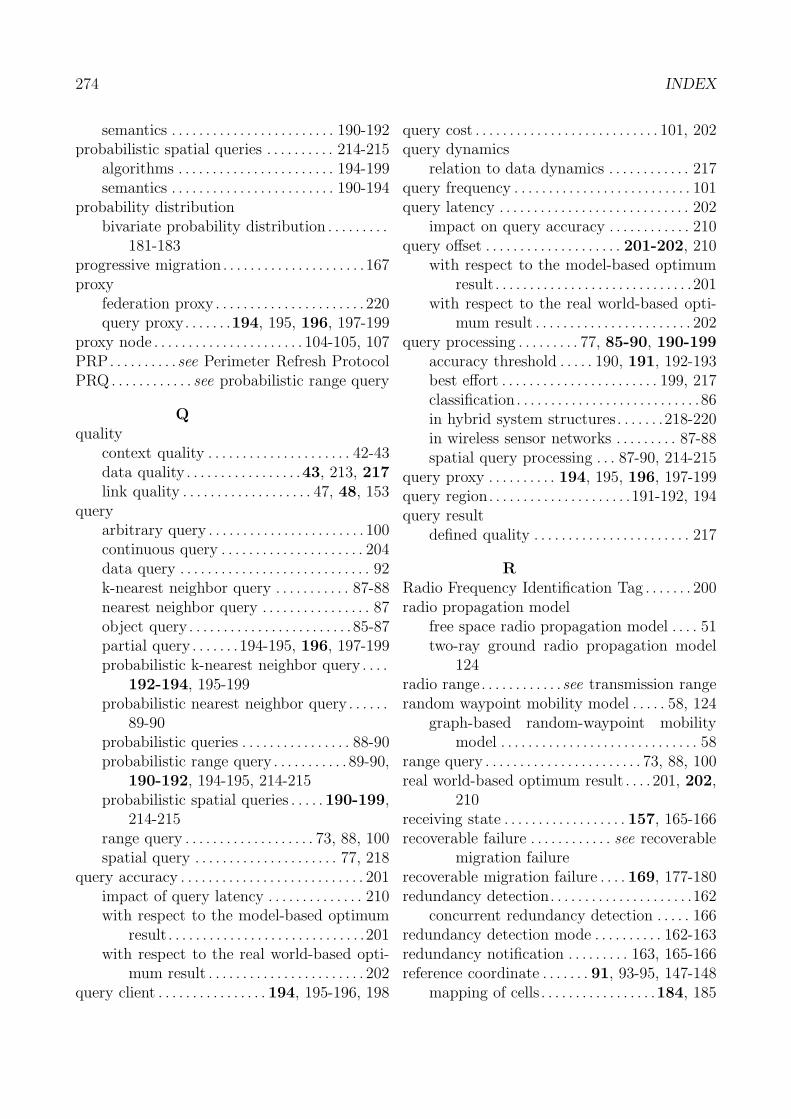
274 INDEX
semantics . . . . . . . . . . . . . . . . . . . . . . . . 190-192probabilistic spatial queries . . . . . . . . . . 214-215
algorithms . . . . . . . . . . . . . . . . . . . . . . . 194-199semantics . . . . . . . . . . . . . . . . . . . . . . . . 190-194
probability distributionbivariate probability distribution . . . . . . . . .
181-183progressive migration . . . . . . . . . . . . . . . . . . . . .167proxy
federation proxy . . . . . . . . . . . . . . . . . . . . . . 220query proxy. . . . . . .194, 195, 196, 197-199
proxy node . . . . . . . . . . . . . . . . . . . . . . 104-105, 107PRP. . . . . . . . . .see Perimeter Refresh ProtocolPRQ. . . . . . . . . . . . see probabilistic range query
Qquality
context quality . . . . . . . . . . . . . . . . . . . . . 42-43data quality . . . . . . . . . . . . . . . . .43, 213, 217link quality . . . . . . . . . . . . . . . . . . . 47, 48, 153
queryarbitrary query . . . . . . . . . . . . . . . . . . . . . . . 100continuous query . . . . . . . . . . . . . . . . . . . . . 204data query . . . . . . . . . . . . . . . . . . . . . . . . . . . . 92k-nearest neighbor query . . . . . . . . . . . 87-88nearest neighbor query . . . . . . . . . . . . . . . . 87object query . . . . . . . . . . . . . . . . . . . . . . . . 85-87partial query . . . . . . . 194-195, 196, 197-199probabilistic k-nearest neighbor query . . . .
192-194, 195-199probabilistic nearest neighbor query . . . . . .
89-90probabilistic queries . . . . . . . . . . . . . . . . 88-90probabilistic range query . . . . . . . . . . . 89-90,
190-192, 194-195, 214-215probabilistic spatial queries . . . . .190-199,
214-215range query . . . . . . . . . . . . . . . . . . . 73, 88, 100spatial query . . . . . . . . . . . . . . . . . . . . . 77, 218
query accuracy . . . . . . . . . . . . . . . . . . . . . . . . . . . 201impact of query latency . . . . . . . . . . . . . . 210with respect to the model-based optimum
result . . . . . . . . . . . . . . . . . . . . . . . . . . . . .201with respect to the real world-based opti-
mum result . . . . . . . . . . . . . . . . . . . . . . . 202query client . . . . . . . . . . . . . . . . 194, 195-196, 198
query cost . . . . . . . . . . . . . . . . . . . . . . . . . . . 101, 202query dynamics
relation to data dynamics . . . . . . . . . . . . 217query frequency . . . . . . . . . . . . . . . . . . . . . . . . . . 101query latency . . . . . . . . . . . . . . . . . . . . . . . . . . . . 202
impact on query accuracy . . . . . . . . . . . . 210query offset . . . . . . . . . . . . . . . . . . . . 201-202, 210
with respect to the model-based optimumresult . . . . . . . . . . . . . . . . . . . . . . . . . . . . .201
with respect to the real world-based opti-mum result . . . . . . . . . . . . . . . . . . . . . . . 202
query processing . . . . . . . . . 77, 85-90, 190-199accuracy threshold . . . . . 190, 191, 192-193best effort . . . . . . . . . . . . . . . . . . . . . . . 199, 217classification. . . . . . . . . . . . . . . . . . . . . . . . . . .86in hybrid system structures. . . . . . .218-220in wireless sensor networks . . . . . . . . . 87-88spatial query processing . . . 87-90, 214-215
query proxy . . . . . . . . . . 194, 195, 196, 197-199query region. . . . . . . . . . . . . . . . . . . . .191-192, 194query result
defined quality . . . . . . . . . . . . . . . . . . . . . . . 217
RRadio Frequency Identification Tag . . . . . . . 200radio propagation model
free space radio propagation model . . . . 51two-ray ground radio propagation model
124radio range. . . . . . . . . . . .see transmission rangerandom waypoint mobility model . . . . . 58, 124
graph-based random-waypoint mobilitymodel . . . . . . . . . . . . . . . . . . . . . . . . . . . . . 58
range query . . . . . . . . . . . . . . . . . . . . . . . 73, 88, 100real world-based optimum result . . . . 201, 202,
210receiving state . . . . . . . . . . . . . . . . . . 157, 165-166recoverable failure . . . . . . . . . . . . see recoverable
migration failurerecoverable migration failure . . . . 169, 177-180redundancy detection. . . . . . . . . . . . . . . . . . . . .162
concurrent redundancy detection . . . . . 166redundancy detection mode . . . . . . . . . . 162-163redundancy notification . . . . . . . . . 163, 165-166reference coordinate . . . . . . . 91, 93-95, 147-148
mapping of cells . . . . . . . . . . . . . . . . .184, 185
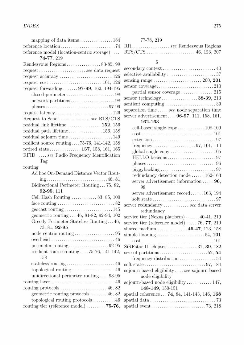
INDEX 275
mapping of data items. . . . . . . . . . . . . . . .184reference location. . . . . . . . . . . . . . . . . . . . . . . . . .74reference model (location-centric storage) . . . .
74-77, 219Rendezvous Regions . . . . . . . . . . . . . . . . 83-85, 99request . . . . . . . . . . . . . . . . . . . . . . see data requestrequest accuracy . . . . . . . . . . . . . . . . . . . . . . . . . 126request cost . . . . . . . . . . . . . . . . . . . . . . . . . 101, 126request forwarding . . . . . . . 97-99, 162, 194-195
closed perimeter . . . . . . . . . . . . . . . . . . . . . . . 98network partitions . . . . . . . . . . . . . . . . . . . . . 98phases . . . . . . . . . . . . . . . . . . . . . . . . . . . . . . 97-99
request latency . . . . . . . . . . . . . . . . . . . . . . . . . . . 126Request to Send . . . . . . . . . . . . . . . see RTS/CTSresidual link lifetime . . . . . . . . . . . . . . . . 152, 156residual path lifetime . . . . . . . . . . . . . . . . 156, 158residual sojourn time . . . . . . . . . . . . . . . . . . . . . 149resilient source routing. . . .75-76, 141-142, 158retired state . . . . . . . . . . . . . . .157, 158, 161, 165RFID . . . . . see Radio Frequency Identification
Tagrouting
Ad hoc On-Demand Distance Vector Rout-ing. . . . . . . . . . . . . . . . . . . . . . . . . . . . .46, 81
Bidirectional Perimeter Routing . . . 75, 82,92-95, 111
Cell Hash Routing . . . . . . . . . . . . 83, 85, 100face routing . . . . . . . . . . . . . . . . . . . . . . . . . . . 82geocast routing . . . . . . . . . . . . . . . . . . . . . . . 145geometric routing . . . 46, 81-82, 92-94, 102Greedy Perimeter Stateless Routing . . . 46,
73, 81, 92-95node-centric routing . . . . . . . . . . . . . . . . . . . 95overhead . . . . . . . . . . . . . . . . . . . . . . . . . . . . . . 46perimeter routing . . . . . . . . . . . . . . . . . . .92-95resilient source routing . . . . 75-76, 141-142,
158stateless routing . . . . . . . . . . . . . . . . . . . . . . . 46topological routing . . . . . . . . . . . . . . . . . . . . 46unidirectional perimeter routing . . . . 93-95
routing layer . . . . . . . . . . . . . . . . . . . . . . . . . . . . . . 46routing protocols . . . . . . . . . . . . . . . . . . . . . . 46, 82
geometric routing protocols . . . . . . . . 46, 82topological routing protocols . . . . . . . . . . .46
routing tier (reference model) . . . . . . . . . 75-76,
77-78, 219RR . . . . . . . . . . . . . . . . . . see Rendezvous RegionsRTS/CTS . . . . . . . . . . . . . . . . . . . . . . . 46, 123, 207
Ssecondary context . . . . . . . . . . . . . . . . . . . . . . . . . 40selective availability . . . . . . . . . . . . . . . . . . . . . . . 37sensing range . . . . . . . . . . . . . . . . . . . . . . . 200, 201sensor coverage . . . . . . . . . . . . . . . . . . . . . . . . . . . 210
partial sensor coverage . . . . . . . . . . . . . . . 215sensor technology . . . . . . . . . . . . . . . . . 38-39, 213sentient computing . . . . . . . . . . . . . . . . . . . . . . . . 39separation time . . . . . see node separation timeserver advertisement . . . .96-97, 111, 158, 161,
162-163cell-based single-copy. . . . . . . . . . . . .108-109cost . . . . . . . . . . . . . . . . . . . . . . . . . . . . . . . . . . 101extension . . . . . . . . . . . . . . . . . . . . . . . . . . . . . . 97frequency . . . . . . . . . . . . . . . . . . . . 97, 101, 110global single-copy . . . . . . . . . . . . . . . . . . . . 105HELLO beacons . . . . . . . . . . . . . . . . . . . . . . . 97phases . . . . . . . . . . . . . . . . . . . . . . . . . . . . . . . . . 96piggybacking . . . . . . . . . . . . . . . . . . . . . . . . . . 97redundancy detection mode . . . . . . 162-163server advertisement information . . . . . 96,
98server advertisement record . . . . . . 163, 194soft state . . . . . . . . . . . . . . . . . . . . . . . . . . . . . . 97
server redundancy . . . . . . . . . . . . see data serverredundancy
service tier (Nexus platform). . . . . . .40-41, 219service tier (reference model) . . . . . 76, 77, 219shared medium . . . . . . . . . . . . . . 46-47, 123, 158simple flooding . . . . . . . . . . . . . . . . . . . . . . . 54, 101
cost . . . . . . . . . . . . . . . . . . . . . . . . . . . . . . . . . . 101SiRFstar III chipset . . . . . . . . . . . . . . 37, 39, 182size of partitions. . . . . . . . . . . . . . . . . . . . . . .52, 54
frequency distribution . . . . . . . . . . . . . . . . . 54soft state . . . . . . . . . . . . . . . . . . . . . . . . . . . . . 97, 184sojourn-based eligibility . . . . see sojourn-based
node eligibilitysojourn-based node eligibility . . . . . . . . . . . . 147,
148-149, 150-151spatial coherence . . . 74, 84, 141-143, 146, 168spatial data . . . . . . . . . . . . . . . . . . . . . . . . . . . . . . . 73spatial event . . . . . . . . . . . . . . . . . . . . . . . . . . 73, 218
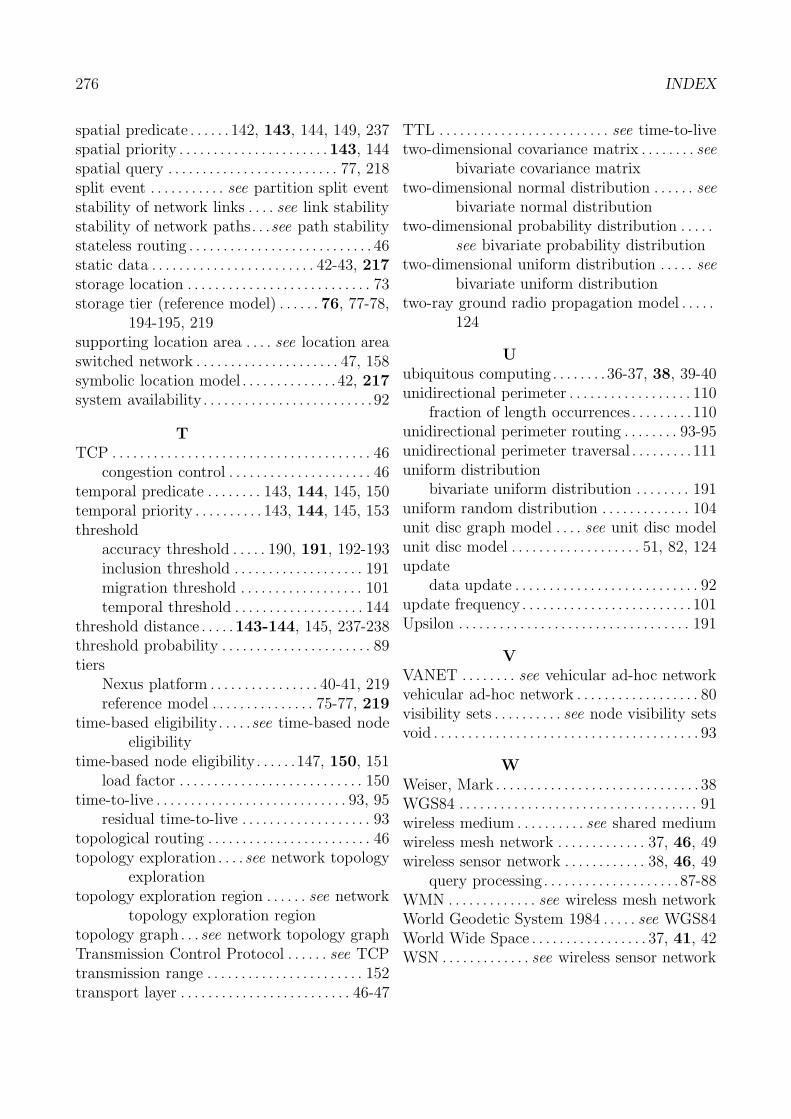
276 INDEX
spatial predicate . . . . . . 142, 143, 144, 149, 237spatial priority . . . . . . . . . . . . . . . . . . . . . .143, 144spatial query . . . . . . . . . . . . . . . . . . . . . . . . . 77, 218split event . . . . . . . . . . . see partition split eventstability of network links . . . . see link stabilitystability of network paths. . .see path stabilitystateless routing . . . . . . . . . . . . . . . . . . . . . . . . . . . 46static data . . . . . . . . . . . . . . . . . . . . . . . . 42-43, 217storage location . . . . . . . . . . . . . . . . . . . . . . . . . . . 73storage tier (reference model) . . . . . . 76, 77-78,
194-195, 219supporting location area . . . . see location areaswitched network . . . . . . . . . . . . . . . . . . . . . 47, 158symbolic location model . . . . . . . . . . . . . . 42, 217system availability . . . . . . . . . . . . . . . . . . . . . . . . .92
TTCP . . . . . . . . . . . . . . . . . . . . . . . . . . . . . . . . . . . . . . 46
congestion control . . . . . . . . . . . . . . . . . . . . . 46temporal predicate . . . . . . . . 143, 144, 145, 150temporal priority . . . . . . . . . . 143, 144, 145, 153threshold
accuracy threshold . . . . . 190, 191, 192-193inclusion threshold . . . . . . . . . . . . . . . . . . . 191migration threshold . . . . . . . . . . . . . . . . . . 101temporal threshold . . . . . . . . . . . . . . . . . . . 144
threshold distance . . . . .143-144, 145, 237-238threshold probability . . . . . . . . . . . . . . . . . . . . . . 89tiers
Nexus platform . . . . . . . . . . . . . . . . 40-41, 219reference model . . . . . . . . . . . . . . . 75-77, 219
time-based eligibility. . . . .see time-based nodeeligibility
time-based node eligibility. . . . . .147, 150, 151load factor . . . . . . . . . . . . . . . . . . . . . . . . . . . 150
time-to-live . . . . . . . . . . . . . . . . . . . . . . . . . . . . 93, 95residual time-to-live . . . . . . . . . . . . . . . . . . . 93
topological routing . . . . . . . . . . . . . . . . . . . . . . . . 46topology exploration . . . . see network topology
explorationtopology exploration region . . . . . . see network
topology exploration regiontopology graph . . . see network topology graphTransmission Control Protocol . . . . . . see TCPtransmission range . . . . . . . . . . . . . . . . . . . . . . . 152transport layer . . . . . . . . . . . . . . . . . . . . . . . . . 46-47
TTL . . . . . . . . . . . . . . . . . . . . . . . . . see time-to-livetwo-dimensional covariance matrix . . . . . . . . see
bivariate covariance matrixtwo-dimensional normal distribution . . . . . . see
bivariate normal distributiontwo-dimensional probability distribution . . . . .
see bivariate probability distributiontwo-dimensional uniform distribution . . . . . see
bivariate uniform distributiontwo-ray ground radio propagation model . . . . .
124
Uubiquitous computing . . . . . . . . 36-37, 38, 39-40unidirectional perimeter . . . . . . . . . . . . . . . . . . 110
fraction of length occurrences . . . . . . . . . 110unidirectional perimeter routing . . . . . . . . 93-95unidirectional perimeter traversal . . . . . . . . . 111uniform distribution
bivariate uniform distribution . . . . . . . . 191uniform random distribution . . . . . . . . . . . . . 104unit disc graph model . . . . see unit disc modelunit disc model . . . . . . . . . . . . . . . . . . . 51, 82, 124update
data update . . . . . . . . . . . . . . . . . . . . . . . . . . . 92update frequency . . . . . . . . . . . . . . . . . . . . . . . . . 101Upsilon . . . . . . . . . . . . . . . . . . . . . . . . . . . . . . . . . . 191
VVANET . . . . . . . . see vehicular ad-hoc networkvehicular ad-hoc network . . . . . . . . . . . . . . . . . . 80visibility sets . . . . . . . . . . see node visibility setsvoid . . . . . . . . . . . . . . . . . . . . . . . . . . . . . . . . . . . . . . . 93
WWeiser, Mark . . . . . . . . . . . . . . . . . . . . . . . . . . . . . . 38WGS84 . . . . . . . . . . . . . . . . . . . . . . . . . . . . . . . . . . . 91wireless medium . . . . . . . . . . see shared mediumwireless mesh network . . . . . . . . . . . . . 37, 46, 49wireless sensor network . . . . . . . . . . . . 38, 46, 49
query processing . . . . . . . . . . . . . . . . . . . .87-88WMN . . . . . . . . . . . . . see wireless mesh networkWorld Geodetic System 1984 . . . . . see WGS84World Wide Space . . . . . . . . . . . . . . . . . 37, 41, 42WSN . . . . . . . . . . . . . see wireless sensor network
Copyright © 2022 FDOKUMEN

