From Static to Dynamic Representations of Probability Concepts

Nenad Radakovic, Ontario Institute for Studies in Education, University of Toronto

Douglas McDougall, Ontario Institute for Studies in Education, University of Toronto

Abstract

In this chapter, we explore the nature and the importance of dynamic visualizations for teaching and learning probability. The chapter begins with a discussion of importance of probability as one of the key elements of risk literacy. We identify, in a literature review, the features of dynamic visualizations that make them more suitable for learning mathematics and what differentiates them from static representations. Through the case study of learning conditional probability in the classroom, we describe how students use and transform representations from inert static to kinesthetic/aesthetic representations. We also discuss limitations of static representations and illustrate how those limitations could be resolved using dynamic representations.

Background

This chapter explores the ways in which dynamic visualizations can be used in learning probability. Our first goal is to identify the features of dynamic visualizations that make them appropriate for learning probability. The second goal is to present our research on the use of dynamic area proportional Venn diagrams in order to illustrate the first goal.

Importance of learning probability

Gal (2005) describes internal and external reasons for learning probability. Internal reasons are related to the importance of probability within the broader discipline of mathematics. Consistent with the internal reasons, learning probability is important because it serves as foundations for other mathematical disciplines such as statistics and decision theory. This is because probability is connected to other mathematical concepts such as rational numbers (e.g. theoretical probability is defined as a ratio of favorable outcomes to the total number of outcomes), equations (e.g. many probability problems can be reduced to linear and quadratic equations), and integrals ( e.g. cumulative distribution function of a continuous random variable is defined as a definite integral of the probability density function). It

2

follows that solving problems in probability provides opportunity for further mastery of mathematics. External reasons are connected with the fact that probability could be used to explain many natural and social phenomena. Probability models are at the core of many disciplines, theories, and models, including the quantum-theoretic model of the atom, kinetic gas theory, and genetics. For example, in the quantum-theoretic model of the atom, the position of an electron is defined by a probability density function. In addition, many socio-economic issues are approached by using sophisticated probabilistic models. They include interpreting crime rates, determining chance of a new recession, and finding evidence for racial discrimination.

Another external reason for studying probability is that probability is an element of risk literacy, which is gaining momentum in the educational community (Pratt et al., 2011). Decisions that involve the understanding of risk are made in all aspects of life including health (e.g. whether to continue with the course of medication), finances (paying for extra insurance) and politics (preemptive strikes versus political dialogue). These decisions are not only common, but they are also critical for individual and societal health and well-being. Some studies have shown that people are routinely exposed to medical risk information (e.g. prevalence rates of diseases) and that their understanding of this information can have serious implications on their health (Rothman et al., 2008). Despite its importance, most people are unable to adequately interpret and communicate risk (Reyna et al., 2009).

Understanding conditional probability

Conditional probability is a mathematical concept describing the likelihood of an event given that another event has occurred . Algebraically, the conditional probability of an event A occurring given that the event B has occurred can be written as

;

where is a probability that both events A and B have occurred. In the following discussion, the formula above will be referred to as the conditional probability formula.

3

The concept plays an important role in understanding of risk because in everyday situations, probability of one event is often contingent on the probability of another. For example, the probability of getting a flu is contingent on many factors (e.g. the strength of one’s immune system, whether or not a person has received a vaccine, etc.)

Historically, research on understanding of probability in general and the conditional probability in particular, concentrated on describing people’s misconceptions of probability. For example, a very influential work by Kahneman and Tversky provided evidence that individuals tend to make errors in reasoning about conditional probability because of ignoring base rates ( Kahneman, Slovic, and Tversky, 1982). In addition, Koehler (1996) describes and provides empirical evidence for inverse fallacy in which the conditional probability of the event A given the event B is taken to be equivalent to the conditional probability of the event B given the event A.

The nature of dynamic visualizations

The use of technology and visualizations in mathematics has been widely discussed (Arcavi, 1999; Duval, 1999; Hitt, 1999; Hoyles, 2008; Kaput & Hegedus, 2000; McDougall, 1999; Moreno-Armella, 1999; Presmeg, 1999; Santos-Trigo, 1999; Thompson, 1999). Extending on this research, recently there has been a focus on dynamic learning environments, such as GeoGebra, which allow users to create mathematical objects and explore them both visually and dynamically.

Moreno-Armella, Hegedus and Kaput (2008) describe learning environment in which students can visualize, construct, and manipulate mathematical concepts. The dynamic learning environments can enable students to act mathematically and to seek relationships between mathematical objects that would not be as intuitive within a static environment of paper and pencil. The authors outline the evolutionary transition from static to dynamic representations by dividing them into five stages: static inert, static kinesthetic/aesthetic, static computational, discrete dynamic, and continuous dynamic. While the authors use the term ‘inscriptions’, we will use the term ‘representation’, to illustrate the same concept.

In the static inert stage, the representation is inseparable from the media it is presented in. One example would be textbook pages. The main feature of the second stage, static kinesthetic/aesthetic, is

4

erasibility. One example would be writing on the whiteboard and the chalkboard. The writings could be erased over time. The two main features are that the writings are kinesthetic- it is easy to move within the medium (e.g., by adding comments or erasing them on the chalkboard). The second feature is that creation and altering of the writing is an aesthetic process (e.g., using differently coloured markers). The third stage is static computational in which presentations are “artifacts of a computational response to a human’s action” (Moreno-Armella, Hegedus, & Kaput, 2008, p. 103). One is working with such representations when using a graphing calculator.

Unlike static stages, in dynamic stages, there is a “co-action between the user and the environment” (p. 103). Discrete dynamic representations can be changed through parametric inputs (i.e., the use of spinners and sliders). For example, a parabola could be moved up or down from the use of a slider that represents a vertical shift. In the continuous dynamic stage, there is an “interaction through space and time” (p. 103) between the user and the representation. For example, there are programs that allow users to explore mathematics through a continuous action of the mouse or in the case of the hand held devices, through the gesture on the touch screen.

Transition from static to dynamic representations: An example from probability

In this section, we use a well-known breast cancer problem (Eddy, 1982) to describe how it can be represented by the Moreno-Armella et al.’s (2008) stages; starting from a static representation and culminating with a continuous dynamic representation we use dynamic area proportional Venn diagrams.

Breast cancer problem

A well-known breast cancer problem from Eddy (1982) is an exemplar used for assessing individuals’ understanding of conditional probability (Gigerenzer, 2002) Recently, Eliezer Yudkowsky, an artificial intelligence theorist and a blogger, has re-introduced the breast cancer problem on line formulizing it as follows:

1% of women at age forty who participate in routine screening have breast cancer. 80% of women with breast cancer will get positive mammograms. 9.6% of women without breast cancer will also get positive mammograms. A woman in this age group

5

had a positive mammogram in a routine screening. What is the probability that she actually has breast cancer?

(Yudkowsky, 2003)

The problem as stated by Yudkowsky was also used in our research and the solution to the problem is given in the Appendix A.

Static representations. The problem, when presented on paper, is an inert static representation. The move from the inert static inscription to the kinetic/aesthetic static inscription can be done in many ways. One of the ways or representing the problem is to draw a Venn diagram representing the population with and without breast cancer as presented in the Figure 1 a). The second way is to draw a tree diagram representing the situation which will be described later in the article. There is also a symbolic way to represent the problem by introducing the Bayes’ formula and matching various probabilities with the context of the problem as it is done in the Appendix A.

Computational stage: Area proportional Venn diagrams. There are many ways to illustrate the computational stage. We suggest that the use of area proportional Venn diagrams, generated by a computer program, can help explain and solve the problem. Venn diagrams were first used to describe qualitative relationships between sets. Researchers have only begun to investigate geometric properties of Venn diagrams (see Ruskey & Weston, 2005).

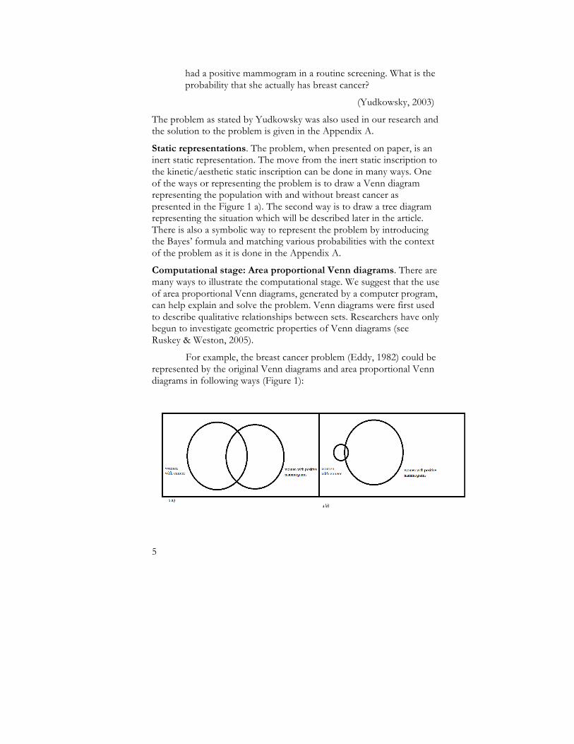
For example, the breast cancer problem (Eddy, 1982) could be represented by the original Venn diagrams and area proportional Venn diagrams in following ways (Figure 1):

6

Figure 1. Original and area proportional Venn diagrams.

The key feature of the area proportional Venn diagram is that the probability of each event matches the area of the region within the diagram. For example, in Figure 1(b), the area of the circle representing the proportion of women with breast cancer (1%) is equal to 1% of the area of the diagram.

The area proportional Venn diagram presented in the Figure 1 a) is still a static inert representation. To make it static computational, we can use a software to draw the diagrams given the specific probabilities (for a detailed description of the construction of area proportional Venn diagrams, see Radakovic & McDougall, 2011).

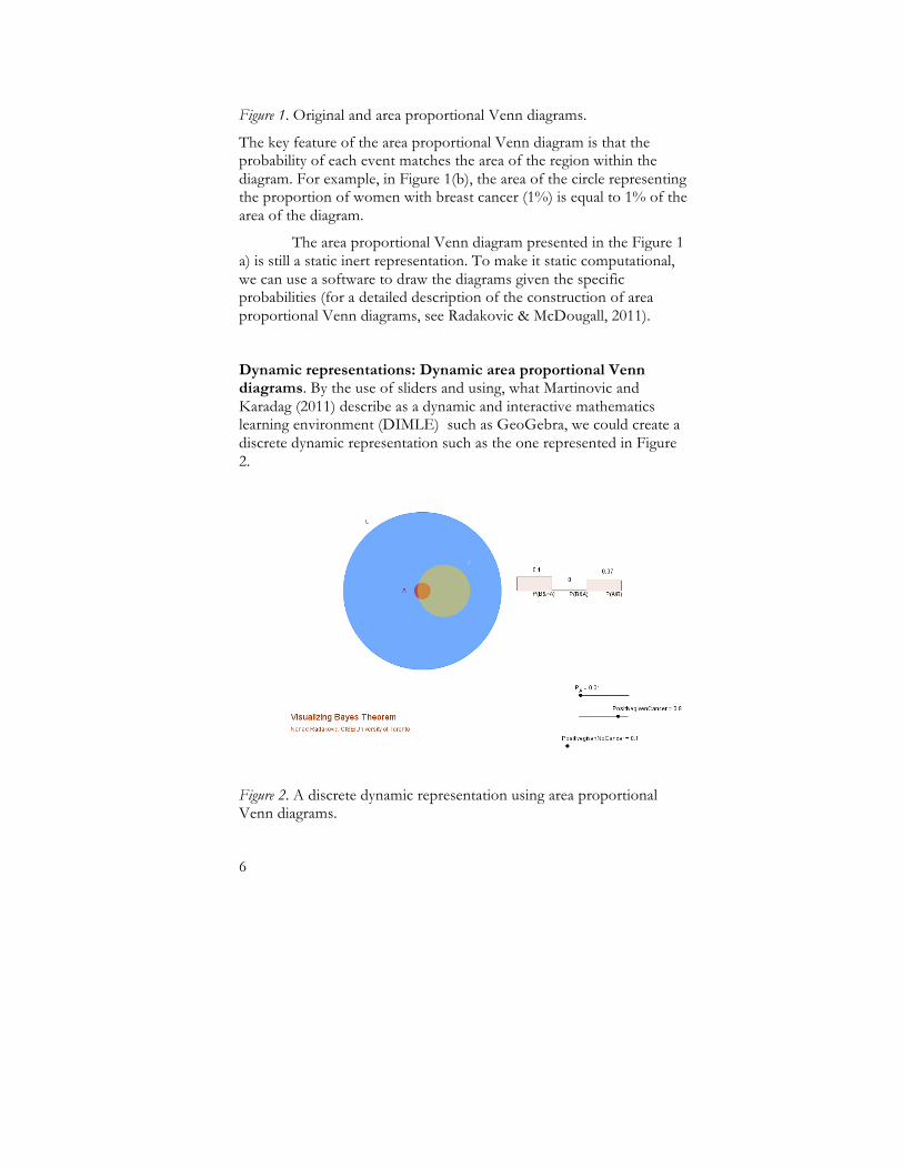
Dynamic representations: Dynamic area proportional Venn diagrams. By the use of sliders and using, what Martinovic and Karadag (2011) describe as a dynamic and interactive mathematics learning environment (DIMLE) such as GeoGebra, we could create a discrete dynamic representation such as the one represented in Figure 2.

Figure 2. A discrete dynamic representation using area proportional Venn diagrams.            

7

  The applet consists of two circles representing the set of all women with cancer and the set of all women tested positive. There are three variables that can be manipulated by the users. They are the base rate (probability that a woman over forty has cancer), the conditional probability of testing positive given that one has breast cancer, and the conditional probability of testing positive given that one does not have breast cancer. These variables can be manipulated with the sliders on the right from the Venn diagrams.

There are two ways in which the conditional probability of a female having breast cancer given that she tested positive is visualized by the applet. First, the conditional probability is displayed in the bar graph. Second, the user can estimate the probability by estimating the size of the intersection in relation to the size of the set corresponding to the women that tested positive. For example, in Figure 1, the base rate, given by the area of the circle A, is 0.01. The conditional probability of P(A|B) is represented by the ratio of the intersection of the circle A and circle B. The value of the conditional probability is given in the bar graph (P(B|A)=0.07).

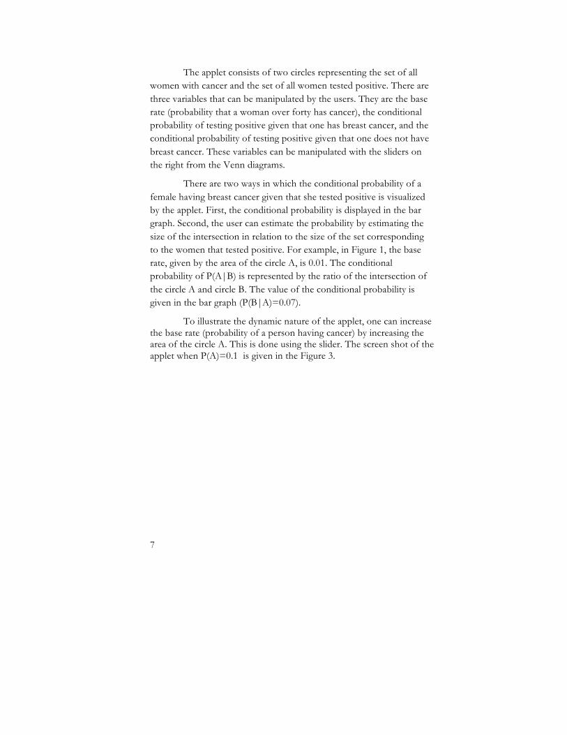
To illustrate the dynamic nature of the applet, one can increase the base rate (probability of a person having cancer) by increasing the area of the circle A. This is done using the slider. The screen shot of the applet when P(A)=0.1 is given in the Figure 3.

8

Figure 3. A discrete dynamic representation using area proportional Venn diagrams with the base rate of 0.1.

One can see that the conditional probability, which is the ratio of the area of the intersection to the area of the circle A is now greater than in the Figure 2. Furthermore, the probability P(A|B) is given on the bar graph as 0.47.

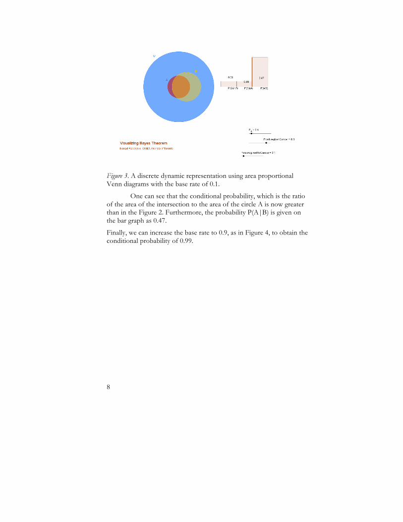
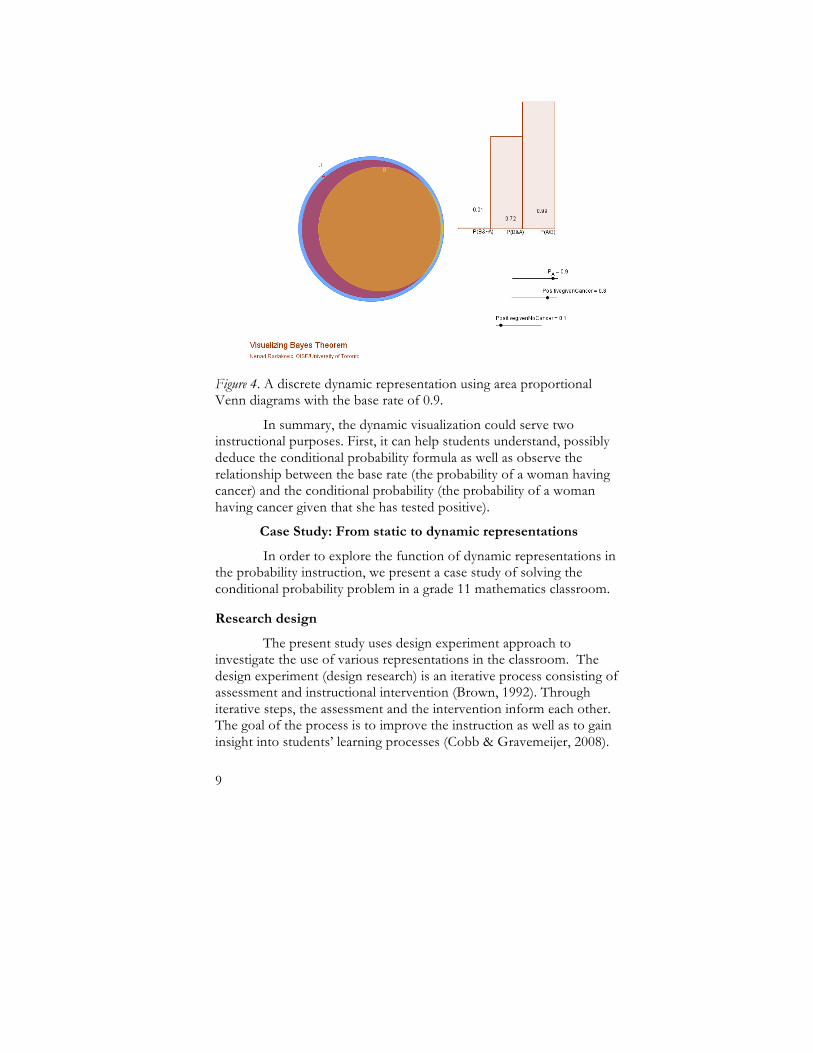
Finally, we can increase the base rate to 0.9, as in Figure 4, to obtain the conditional probability of 0.99.

9

Figure 4. A discrete dynamic representation using area proportional Venn diagrams with the base rate of 0.9.

In summary, the dynamic visualization could serve two instructional purposes. First, it can help students understand, possibly deduce the conditional probability formula as well as observe the relationship between the base rate (the probability of a woman having cancer) and the conditional probability (the probability of a woman having cancer given that she has tested positive).

Case Study: From static to dynamic representations

In order to explore the function of dynamic representations in the probability instruction, we present a case study of solving the conditional probability problem in a grade 11 mathematics classroom.

Research design

The present study uses design experiment approach to investigate the use of various representations in the classroom. The design experiment (design research) is an iterative process consisting of assessment and instructional intervention (Brown, 1992). Through iterative steps, the assessment and the intervention inform each other. The goal of the process is to improve the instruction as well as to gain insight into students’ learning processes (Cobb & Gravemeijer, 2008).

10

Specific phases of the design experiment depend on the unique contextual features of a research. According to Cobb and Gravemeijer, the phases of the design experiment are (a) the preparation for the experiment, (b) experiment to support learning, and (c) conducting retrospective analyses. On the other hand, Middleton et al. (2008) present the design experiment consisting of seven phases. These phases are construction of grounded models, development of artefact, feasibility study, prototyping and trials, field study, definitive tests, and dissemination and impact (p. 33).

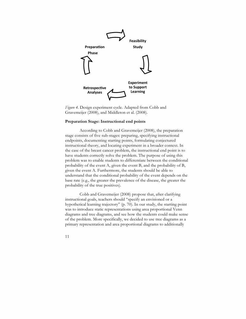
We found Cobb and Gravemeijer’s (2008) phases suitable for our context. However, we also thought that feasibility study, which includes negotiations with teachers and school administrators on the specific features of research. This is why we also added the feasibility study stage from Middleton et al.’s (2008) description of the design experiment. In other words, we have arrived at at four stages appropriate for the context of the research. These stages are 1) preparing for the experiment, 2) feasibility study, 3) experimenting to support learning, and 4) conducting retrospective analyses of the data.

The phases of the design research are given in the Figure 3. The design experiment research we are conducting consists of two cycles (phases) of the design experiment. The first cycle took place in a Grade 11 mathematics classroom at an all-boy private secondary school in Ontario during the probability and statistics unit. There were 23 participants in the study, all of them male. This chapter only focuses on the first, third, and the fourth stage of the cycle since the description of the feasibility study is not relevant for the purpose of this article. After completing the first cycle, the second design experiment will be conducted in a different educational setting, i.e., a co-educational independent school in Ontario in a Grade 11 classroom during the probability and statistics unit.

11

Figure 4. Design experiment cycle. Adapted from Cobb and Gravemeijer (2008), and Middleton et al. (2008).  

Preparation Stage: Instructional end points

According to Cobb and Gravemeijer (2008), the preparation stage consists of five sub-stages: preparing, specifying instructional endpoints, documenting starting points, formulating conjectured instructional theory, and locating experiment in a broader context. In the case of the breast cancer problem, the instructional end point is to have students correctly solve the problem. The purpose of using this problem was to enable students to differentiate between the conditional probability of the event A, given the event B, and the probability of B, given the event A. Furthermore, the students should be able to understand that the conditional probability of the event depends on the base rate (e.g., the greater the prevalence of the disease, the greater the probability of the true positives).

Cobb and Gravemeijer (2008) propose that, after clarifying instructional goals, teachers should “specify an envisioned or a hypothetical learning trajectory” (p. 70). In our study, the starting point was to introduce static representations using area proportional Venn diagrams and tree diagrams, and see how the students could make sense of the problem. More specifically, we decided to use tree diagrams as a primary representation and area proportional diagrams to additionally

Feasibility  

Study  

Experiment      to  Support  Learning  

Retrospec9ve  Analyses  

Prepara9on    

           Phase  

12

illustrate the problem. Prior to the research, we developed the area-proportional Venn diagrams applet in GeoGebra.

The experiment to support learning

The purpose of the experiment to support learning is to improve and test the envisioned trajectory from the preparation stage (Cobb & Gravemeijer, 2008). In this phase, the classroom data collection effectively begins. The experiment to support learning is a phase in which documenting students’ shifts in reasoning is crucial. For this purpos we used three types of data: classroom observations, interviews, and assessments (written as well as oral). We also audio taped meetings with the teacher. After each session, there was debriefing with both students and the teacher to discuss the outcomes of the sessions. As a part of the initial assessment, students were presented with the breast cancer problem. Only two students out of 20 who participated in the initial assessment were able to give the correct answer to the question. After the initial assessment, followed by individual interview with students and a debriefing with the teacher, it became apparent that students found the context of the breast cancer problem as well as the issue of false positive results alien. We decided to change the context while still addressing the same underlying concept. The new problem was restated as follows:

In May of 2009, Security Vendor Symantec released a report that 90.4 % of ALL email is spam. Let’s assume that the number of spam messages is high, say 80% (this is consistent with the number of spam messages I am getting). Suppose, further that 85% of spam messages are correctly identified as spam (end up in spam folder). Also, 5% of messages that are not spam also end up in spam folder.

There were five parts to this question: a) what is the probability that a message (any message) will end up in a spam folder; b) what is the probability that the actual spam message will end up in the spam folder; c) what is the probability that a message that is in spam folder is actually spam; d) What is the probability that a message is not spam; and

13

e) How would the answer change if only 10% of all messages were spam.

From Inert to the Kinesthetic/Aesthetic representations

The students, who were divided into groups of four or five, were instructed to picture the problem using tree diagrams, which were introduced in previous lectures. In this part, we use video data to report on one of the groups of four students as they proceed to solve the problem. The data were analyzed with a specific focus on the way they created and transformed representations and used representations to support their problem solving and to communicate with the others. We also paid close attention to the gestures the students were using in their arguments.

The Group. The group consisted of four Grade 11 students, Ray, Samir, David, and Blair. Based on the grades and the teacher’s perception, Ray could be labeled a weak mathematics learner, Samir as medium, whereas David and Blair could be considered strong students. Samir was designated by the teacher to be the recorder, which means that he was responsible for drawing the diagram and recording answers to all parts of the question given above. The answers were recorded on the construction paper.

Solving the problem: Transforming the representations. Throughout the activity, students were transforming the representations from inert static to kinesthetic aesthetic representations by adding the features that enabled them to move within the representation and solve the problem. The process of transforming representations started with the handout containing the text of the problem and all of the sub-questions. As it is, the problem was represented by the static inert representation. Students started exploring the problem by drawing a tree diagram (i.e., using the kinesthetic/aesthetic representation). David instructed Samir how to draw the tree diagram by gesturing with his fingers how it should branch out. Based on this explanation, Samir proceeded to draw the diagram, mapping out the complete sample space for the situation described in the problem. The nodes students labeled as S and S’

14

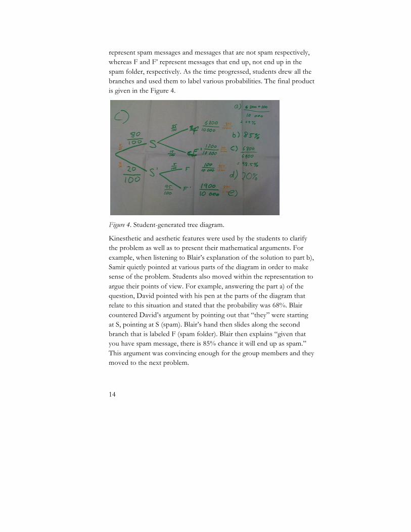
represent spam messages and messages that are not spam respectively, whereas F and F’ represent messages that end up, not end up in the spam folder, respectively. As the time progressed, students drew all the branches and used them to label various probabilities. The final product is given in the Figure 4.

 

Figure 4. Student-generated tree diagram.

Kinesthetic and aesthetic features were used by the students to clarify the problem as well as to present their mathematical arguments. For example, when listening to Blair’s explanation of the solution to part b), Samir quietly pointed at various parts of the diagram in order to make sense of the problem. Students also moved within the representation to argue their points of view. For example, answering the part a) of the question, David pointed with his pen at the parts of the diagram that relate to this situation and stated that the probability was 68%. Blair countered David’s argument by pointing out that “they” were starting at S, pointing at S (spam). Blair’s hand then slides along the second branch that is labeled F (spam folder). Blair then explains “given that you have spam message, there is 85% chance it will end up as spam.” This argument was convincing enough for the group members and they moved to the next problem.

15

The students also used the aesthetic features of the representation. For example, in order to solve the last part of the problem, Samir wrote the new probabilities in orange color to contrast them with the old ones that were in green.

Limits of Static Kinesthetic/Aesthetic representations. The last part of the problem, namely, finding how the answer would change the probability of the message being spam was 80%, tested the limits of tree diagram as a tool for solving this problem. The fact that the probability depends on the base rate was not obvious to students since they responded to the question by calling the teacher and asking whether they had to re-calculate the answer. Seeing that they did not know how to estimate the probability, the teacher and one of the researchers suggested that students re-calculate the probabilities and write them next to the “old” probabilities. The teacher tried to get the members of the group estimate the new probability based on comparing by how much the base rate changed. However, the students did not seem to understand the teacher’s line of reasoning.

Toward dynamic representations

The objective of the part “e” was for students to grasp the relationship between the base rates and the conditional probability. As explained above, the static features of the tree diagram did not allow for an intuitive way to describe the relationship. One way to approach the problem would be to create a computer or a calculator program that would return the values for the conditional probability, given the base rates. This would introduce the static computational representation into the activity.

Our approach was to introduce students to the GeoGebra applet scribed above consisting of the area proportional Venn diagrams in order to offer the alternative representation of the breast cancer problem. The representation contains dynamic features that could assist students in exploring the relationship between the base rate and the conditional probability. The applet was projected on an Interactive Smart Board and manipulated by the teacher. The teacher was

16

effectively modeling the manipulation with the applet. The students were able to see how the size of the set A (base rate) influences the conditional probability.

In order to gather more evidence that dynamic representations were beneficial for solving the problem, one of the authors conducted two separate one-on-one interviews with the students in the class. The students were presented the breast cancer problem (since they have already seen the spam problem and since they were at that point more familiar with the structure of the problem). They were then shown the applet and through Socratic dialogue encouraged to come up with a way to calculate the conditional probability of getting cancer, given positive test results. Similar to the group activity described above, the students did not work with the applet. Instead, the researcher used the applet to explain how to find the probabilities needed to solve the problem. Furthermore, by using the slider to change the base rate, the researcher demonstrated how the change in base rate changes the conditional probability.

Final assessment

Towards the end of the project, each student was given a test that contained the following problem which is equivalent to the breast cancer problem as well as the spam problem.

About 5% of hard discs have a computer virus. A company makes a computer software that detects 95% of infected programs. However, it also falsely identifies 10% of non-infected hard disks as infected. What is the probability that the computer program will identify any hard disk as infected?

Out of 21 students who took the test, 11 (52%) students solved this problem correctly. There were two students who solved the pre-test question correctly and one of them took the post-test. That means that 10 students who solved the pre-test question incorrectly solved the post-test question correctly. More specifically, most of the students were able to calculate the overall probability of being identified as

17

defective, as well as the probability of being defective and being identified as defective. What they failed to do is put the two pieces of information together and divide the latter by the former thus calculating the conditional probability.

Conclusion

In this chapter, we illustrated the transformation from the inert static representations to discrete dynamic representations on an example from teaching probability in a secondary school mathematics classroom. The study contributes to the field by giving examples outside of geometry and algebra, originally presented in Moreno-Armella, Hegedus, and Kaput (2008) article. As it can be seen from the results presented, the dynamic representations above were not used extensively, rather only as the secondary resource to the static representations. We described students’ use of static representations, as well as their limitations, thus indirectly identifying features of representations necessary for identifying base rates. More specifically, the episode in which Samir writes the new probabilities next to the old one in order to induce the relationship between the base rate and the conditional probability, shows the need for “co-action between the user and the environment” (Moreno-Armella, Hegedus, & Kaput, 2008, p. 103). This “co-action” could be provided by the dynamic visualization in which the user instead of recalculating the values could simply increase the size of the set. This would enable the user to directly observe the cause and effect of changing the conditional probability by changing the base rate.

However, as the results show, there is only limited evidence that students improved their ability to solve the breast cancer type problems while using dynamic visualizations. After all, although 52% of the students solved the post-correctly compared to the 10% who solved the pre-test incorrectly, 48% did not solve the question correctly. This could be because dynamic visualizations were only used for a brief period of time and they were not used directly by students, thus not

18

allowing the students to participate themselves in the “co-action” with the technology as described in the above mentioned article.

In the second design cycle, we intend to enable each student to use the applet and freely explore the relationship between various parts of the area proportional Venn diagrams. In addition, the researcher used the GeoGebra applet as a dynamic representation ( i.e., to manipulate objects (Venn diagrams) through sliders). For the second phase of the design experiment, we intend to create an applet that will allow students to change the base rate by clicking directly on the circles rather than doing it indirectly via sliders or inputting the values. This would create more of a continuous dynamic representation in which there is a direct interaction between the user and the machine.

Although there needs to be more empirical evidence of the usefulness of dynamic visualizations, the case study illustrates the range of representations of conditional probability used in the classroom and what each one of them brings to the instruction. It also sheds more light on the nature of dynamic area proportional Venn diagrams and their possible pedagogical role.

 

 

 

 

 

 

 

19

References

Arcavi, A. (1999). The role of visual representations in the learning of mathematics. In F. Hitt & M. Santos (Eds.), Proceedings of the Twenty First Annual Meeting of the North American Chapter of the International Group for the Psychology of Mathematics Education, 55-80.

Cobb, P., Confrey, J., diSessa, A., Lehrer, R., & Schauble, L. (2003). Design experiments in educational research. Educational Researcher, 32(1), 9-13, 35-37.

Cobb, P., & Gravemeijer, K. (2008). Experimenting to Support and Understand Learning rocess. In Kelly, A. E., Lesh, R. A., & Baek, J. Y. (Eds.). Handbook of design research methods in education. (pp. 68-95). New York: Routledge.

Duval, R. (1999). Representation, vision and visualization: Cognitive functions in mathematical thinking: Basic issues for learning. In F. Hitt & M. Santos (Eds.), Proceedings of the Twenty First Annual Meeting of the North American Chapter of the International Group for the Psychology of Mathematics Education, 3-26.

Eddy, D.M. (1982). Probabilistic Reasoning in Clinical Medicine: Problems and Opportunities. In D. Kahneman, P. Slovic & A. Tversky (Eds.), Judgment Under Uncertainty: Heuristics and Biases. Cambridge University Press. (pp. 249-267)

Gal, I. (2005). Towards “probability literacy” for all citizens: Building blocks and instructional dilemmas. In Jones, G. A. (Ed.), Exploring probability in school: Challenges for teaching and learning (pp. 39-63). New York: Springer.

Gigerenzer, G. (2002). Calculated risks: How to know when numbers deceive you. New York: Simon & Schuster.

Hitt, F. (1999). Representations and mathematics visualization. In F. Hitt & M. Santos (Eds.), Proceedings of the Twenty First Annual Meeting of the North American Chapter of the International Group for the Psychology of Mathematics Education, 137-138.

Hoyles, C. (2008). Transforming the mathematical practices of learners and teachers through digital technology. 11th International Congress on Mathematical Education. Monterrey, Nuevo Leon, Mexico.

20

Kahneman, D., Slovic, P., & Tversky, A. (Eds.). (1982). Judgment under uncertainty: Heuristics and biases. New York: Cambridge University Press.

Koehler, J. J. (1996). The base rate fallacy reconsidered: Descriptive normative and methodological challenges. Behavioral & Brain Sciences, 19, 1-53. Kaput, J. J., & Hegedus, S. J. (2000). An introduction to the profound potential of connected algebra activities: Issues of representation, engagement and pedagogy. Proceedings of the 28th International Conference of the International Group for the Psychology of Mathematics Education, 3, 129-136.

McDougall, D. (1999). Geometry and technology. In F. Hitt & M. Santos (Eds.), Proceedings of the Twenty First Annual Meeting of the North American Chapter of the International Group for the Psychology of Mathematics Education, 135-136.

Moreno-Armella, L. (1999). On representations and situated tools. In F. Hitt & M. Santos (Eds.), Proceedings of the Twenty First Annual Meeting of the North American Chapter of the International Group for the Psychology of Mathematics Education, 99-104.

L. Moreno-Armella, S. Hegedus, & J. Kaput. (2008). Static to dynamic mathematics: Historical and representational perspectives. Special issue of Educational Studies in Mathematics: Democratizing Access to Mathematics through Technology— Issues of Design and Implementation, 68(2), 99–111.

Martinovic, D., & Karadag, Z. (2011). Dynamic and Interactive Mathematics Learning Environments (DIMLE). The Tenth International Conference on Technology in Mathematics Teaching, July 5-8, 2011, University of Portsmouth, England.

Pratt, D., Ainley, J., Kent, P., Levinson, R., Yougi, C., & Kapadia, R. (2011). Role of context in risk-based reasoning. Mathematical Thinking and Learning, 13, 322-345.

Presmerg, N. C. (1999). On Visualization and Generalization in Mathematics. In F. Hitt & M. Santos (Eds.), Proceedings of the Twenty First Annual Meeting of the North American Chapter of the International Group for the Psychology of Mathematics Education, 1.

Radakovic, N., & McDougall, D. (2011). Using dynamic geometry software for teaching conditional probability with area proportional

21

Venn diagrams. International Journal of Mathematical Education in Science and Technology. DOI: 10.1080/0020739X.2011.633628.

Reyna, V. F., Nelson, W., Han, P., & Dieckmann, N. F. (2009). How numeracy influences risk comprehension and medical decision making. Psychological Bulletin, 135, 943-973.

Rothman, R. L., Montori, V. M., Cherrington, A., & Pigone, M. P. (2008). Perspective: The role of numeracy in healthcare. Journal of Health Communication, 13, 583–595.

Santos-Trigo, M. S. (1999). The use of technology as a means to explore mathematics: Qualities in proposed problems. In F. Hitt & M. Santos (Eds.), Proceedings of the Twenty First Annual Meeting of the North American Chapter of the International Group for the Psychology of Mathematics Education, 139-146.

Thompson, P. (1999). Representation and evolution: A discussion of Duval’s and Kaput’s papers. In F. Hitt & M. Santos (Eds.), Proceedings of the 21st Annual Meeting of the North American Chapter of the International Group for the Psychology of Mathematics Education, 1, 49-54.

Yudkowsky, E. (2003). An intuitive explanation of Bayes’ theorem. Retrieved from: www.yudkowsky.net/rational/bayes.

 

 

 

 

 

 

 

 

 

 

22

Appendix A: Solution to the breast cancer problem by Eddy (1982)

To solve the following problem,

1% of women at age forty who participate in routine screening have breast cancer. 80% of women with breast cancer will get positive mammograms. 9.6% of women without breast cancer will also get positive mammograms. A woman in this age group had a positive mammogram in a routine screening. What is the probability that she actually has breast cancer?

Let A represent the event of having breast cancer

B the event of testing positive

We are given: P(A)= 0.01

0.8

0.096

We can calculate P(B) as follows:

We then substitute this value into the conditional probability formula: