


Bahasa
Halaman
Hukum

VIA EXAMPLES AND SOLUTIONSFLUID DYNAMICS
SERGEY NAZARENKO
FLUID DYNAMICS N
AZA
REN
KO
ISBN: 978-1-4398-8882-7
9 781439 888827
90000
K14078
Fluid Dynamics via Examples and Solutions provides a substantial set of example problems and detailed model solutions covering various phenomena and effects in fluids. The book is ideal as a supplement or exam review for undergraduate and graduate courses in fluid dynamics, continuum mechanics, turbulence, ocean and atmospheric sciences, and related areas. It is also suitable as a main text for fluid dynamics courses with an emphasis on learning by example and as a self-study resource for practicing scientists who need to learn the basics of fluid dynamics.
The author covers several sub-areas of fluid dynamics, types of flows, and applications. He also includes supplementary theoretical material when necessary. Each chapter presents the background, an extended list of references for further reading, numerous problems, and a complete set of model solutions.
Features • Describes many examples dealing with various phenomena and
effects in fluids • Promotes effective hands-on study of fluid dynamics through physically
motivated exercises • Provides instructors with a wealth of possible exam questions from
which to choose • Contains model solutions and suggestions for further reading in
each chapter
Sergey Nazarenko is a professor at the University of Warwick. His research focuses on fluid dynamics, turbulence, and waves, including wave turbulence, magneto-hydrodynamic turbulence, superfluid turbulence, water waves, Rossby waves, vortices and jets in geophysical fluids, drift waves and zonal jets in plasmas, optical vortices and turbulence, and turbulence in Bose-Einstein condensates.
Physics
K14078_COVER_final.indd 1 10/27/14 1:14 PM
FLUID DYNAMICS VIA EXAMPLES AND SOLUTIONS
K140778_FM.indd 1 10/27/14 1:07 PM

This page intentionally left blankThis page intentionally left blank
FLUID DYNAMICS VIA EXAMPLES AND SOLUTIONS
SERGEY NAZARENKOUniversity of Warwick, UK
Boca Raton London New York
CRC Press is an imprint of theTaylor & Francis Group, an informa business
K140778_FM.indd 3 10/27/14 1:07 PM
CRC PressTaylor & Francis Group6000 Broken Sound Parkway NW, Suite 300Boca Raton, FL 33487-2742
© 2015 by Taylor & Francis Group, LLCCRC Press is an imprint of Taylor & Francis Group, an Informa business
No claim to original U.S. Government worksVersion Date: 20141216
International Standard Book Number-13: 978-1-4398-8890-2 (eBook - PDF)
This book contains information obtained from authentic and highly regarded sources. Reasonable efforts have been made to publish reliable data and information, but the author and publisher cannot assume responsibility for the validity of all materials or the consequences of their use. The authors and publishers have attempted to trace the copyright holders of all material reproduced in this publication and apologize to copyright holders if permission to publish in this form has not been obtained. If any copyright material has not been acknowledged please write and let us know so we may rectify in any future reprint.
Except as permitted under U.S. Copyright Law, no part of this book may be reprinted, reproduced, transmitted, or utilized in any form by any electronic, mechanical, or other means, now known or hereafter invented, including photocopying, microfilming, and recording, or in any information stor-age or retrieval system, without written permission from the publishers.
For permission to photocopy or use material electronically from this work, please access www.copy-right.com (http://www.copyright.com/) or contact the Copyright Clearance Center, Inc. (CCC), 222 Rosewood Drive, Danvers, MA 01923, 978-750-8400. CCC is a not-for-profit organization that pro-vides licenses and registration for a variety of users. For organizations that have been granted a photo-copy license by the CCC, a separate system of payment has been arranged.
Trademark Notice: Product or corporate names may be trademarks or registered trademarks, and are used only for identification and explanation without intent to infringe.
Visit the Taylor & Francis Web site athttp://www.taylorandfrancis.com
and the CRC Press Web site athttp://www.crcpress.com
Contents
Preface xiii
Acknowledgements xv
List of Figures xvii
Author Biography xxi
1 Fluid equations and different regimes of fluid flows 1
1.1 Background theory . . . . . . . . . . . . . . . . . . . . . . . 11.1.1 Incompressible flows . . . . . . . . . . . . . . . . . . . 11.1.2 Inviscid flows . . . . . . . . . . . . . . . . . . . . . . . 21.1.3 Rotating flows . . . . . . . . . . . . . . . . . . . . . . 3
1.2 Further reading . . . . . . . . . . . . . . . . . . . . . . . . . 31.3 Problems . . . . . . . . . . . . . . . . . . . . . . . . . . . . . 3
1.3.1 Reynolds number . . . . . . . . . . . . . . . . . . . . . 41.3.2 Mach number . . . . . . . . . . . . . . . . . . . . . . . 41.3.3 Rossby number . . . . . . . . . . . . . . . . . . . . . . 41.3.4 Richardson number . . . . . . . . . . . . . . . . . . . . 51.3.5 Prandtl number . . . . . . . . . . . . . . . . . . . . . . 51.3.6 Stokes number . . . . . . . . . . . . . . . . . . . . . . 6
1.4 Solutions . . . . . . . . . . . . . . . . . . . . . . . . . . . . . 71.4.1 Model solution to question 1.3.1 . . . . . . . . . . . . 71.4.2 Model solution to question 1.3.2 . . . . . . . . . . . . 71.4.3 Model solution to question 1.3.3 . . . . . . . . . . . . 81.4.4 Model solution to question 1.3.4 . . . . . . . . . . . . 81.4.5 Model solution to question 1.3.5 . . . . . . . . . . . . 91.4.6 Model solution to question 1.3.6 . . . . . . . . . . . . 10
2 Conservation laws in incompressible fluid flows 11
2.1 Background theory . . . . . . . . . . . . . . . . . . . . . . . 112.1.1 Velocity-vorticity form of the Navier-Stokes equation . 112.1.2 Bernoulli theorems . . . . . . . . . . . . . . . . . . . . 122.1.3 The vorticity form of the flow equation . . . . . . . . 12
v

vi Contents
2.1.4 Energy balance and energy conservation . . . . . . . . 132.1.5 Momentum balance and momentum conservation . . . 142.1.6 Circulation: Kelvin’s theorem . . . . . . . . . . . . . . 152.1.7 Vorticity invariants in 2D flows . . . . . . . . . . . . . 15
2.2 Further reading . . . . . . . . . . . . . . . . . . . . . . . . . 162.3 Problems . . . . . . . . . . . . . . . . . . . . . . . . . . . . . 17
2.3.1 Conservation of potential vorticity . . . . . . . . . . . 172.3.2 Tap water . . . . . . . . . . . . . . . . . . . . . . . . . 172.3.3 Discharge into a drainage pipe . . . . . . . . . . . . . 182.3.4 Oscillations in a U-tube . . . . . . . . . . . . . . . . . 192.3.5 Force on a bent garden hose . . . . . . . . . . . . . . . 202.3.6 Firehose flow . . . . . . . . . . . . . . . . . . . . . . . 202.3.7 Shear flow in a strain field . . . . . . . . . . . . . . . . 212.3.8 Rankine vortex in a strain field . . . . . . . . . . . . . 222.3.9 Forces produced by a vortex dipole . . . . . . . . . . . 232.3.10 Torque produced by a vortex . . . . . . . . . . . . . . 242.3.11 Jammed garden hose . . . . . . . . . . . . . . . . . . . 242.3.12 Flow through a Borda mouthpiece . . . . . . . . . . . 262.3.13 Water barrel on wheels . . . . . . . . . . . . . . . . . 272.3.14 Vortex lift . . . . . . . . . . . . . . . . . . . . . . . . . 282.3.15 Water clock . . . . . . . . . . . . . . . . . . . . . . . . 292.3.16 Reservoir with regulated water level . . . . . . . . . . 292.3.17 Energy of ideal irrotational flows . . . . . . . . . . . . 30
2.4 Solutions . . . . . . . . . . . . . . . . . . . . . . . . . . . . . 312.4.1 Model solution to question 2.3.1 . . . . . . . . . . . . 312.4.2 Model solution to question 2.3.2 . . . . . . . . . . . . 322.4.3 Model solution to question 2.3.3 . . . . . . . . . . . . 322.4.4 Model solution to question 2.3.4 . . . . . . . . . . . . 332.4.5 Model solution to question 2.3.5 . . . . . . . . . . . . 342.4.6 Model solution to question 2.3.6 . . . . . . . . . . . . 352.4.7 Model solution to question 2.3.7 . . . . . . . . . . . . 352.4.8 Model solution to question 2.3.8 . . . . . . . . . . . . 372.4.9 Model solution to question 2.3.9 . . . . . . . . . . . . 382.4.10 Model solution to question 2.3.10 . . . . . . . . . . . . 392.4.11 Model solution to question 2.3.11 . . . . . . . . . . . . 412.4.12 Model solution to question 2.3.12 . . . . . . . . . . . . 422.4.13 Model solution to question 2.3.13 . . . . . . . . . . . . 422.4.14 Model solution to question 2.3.14 . . . . . . . . . . . . 432.4.15 Model solution to question 2.3.15 . . . . . . . . . . . . 442.4.16 Model solution to question 2.3.16 . . . . . . . . . . . . 442.4.17 Model solution to question 2.3.17 . . . . . . . . . . . . 45
Contents vii
3 Fluid with free surface 47
3.1 Background theory . . . . . . . . . . . . . . . . . . . . . . . 473.1.1 Pressure boundary condition . . . . . . . . . . . . . . 473.1.2 Kinematic boundary condition . . . . . . . . . . . . . 483.1.3 Axially and spherically symmetric flows . . . . . . . . 48
3.2 Further reading . . . . . . . . . . . . . . . . . . . . . . . . . 493.3 Problems . . . . . . . . . . . . . . . . . . . . . . . . . . . . . 49
3.3.1 Water surface distortion due to vortex . . . . . . . . . 493.3.2 Free surface shape of water in an annular flow . . . . . 503.3.3 Water-filled turntable . . . . . . . . . . . . . . . . . . 513.3.4 Cavity implosion . . . . . . . . . . . . . . . . . . . . . 523.3.5 Flow in an expanding air bubble . . . . . . . . . . . . 533.3.6 Flow in wire coating die . . . . . . . . . . . . . . . . . 54
3.4 Solutions . . . . . . . . . . . . . . . . . . . . . . . . . . . . . 543.4.1 Model solution to question 3.3.1 . . . . . . . . . . . . 543.4.2 Model solution to question 3.3.2 . . . . . . . . . . . . 563.4.3 Model solution to question 3.3.3 . . . . . . . . . . . . 573.4.4 Model solution to question 3.3.4 . . . . . . . . . . . . 583.4.5 Model solution to question 3.3.5 . . . . . . . . . . . . 603.4.6 Model solution to question 3.3.6 . . . . . . . . . . . . 60
4 Waves and instabilities 63
4.1 Background theory . . . . . . . . . . . . . . . . . . . . . . . 634.1.1 Waves . . . . . . . . . . . . . . . . . . . . . . . . . . . 634.1.2 Instabilities . . . . . . . . . . . . . . . . . . . . . . . . 65
4.2 Further reading . . . . . . . . . . . . . . . . . . . . . . . . . 684.3 Problems . . . . . . . . . . . . . . . . . . . . . . . . . . . . . 68
4.3.1 Motion of a wave packet . . . . . . . . . . . . . . . . . 684.3.2 Gravity waves on the water surface . . . . . . . . . . . 694.3.3 Gravity and capillary waves: dimensional analysis . . . 704.3.4 Inertial waves in rotating fluids . . . . . . . . . . . . . 714.3.5 Internal waves in stratified fluids . . . . . . . . . . . . 724.3.6 Sound waves in compressible fluids . . . . . . . . . . . 734.3.7 Sound rays in shear flows: acoustic mirage . . . . . . . 744.3.8 Sound rays in stratified flows: wave guides, Snell’s law 754.3.9 Sound rays in a vortex flow: a black hole effect . . . . 764.3.10 Kelvin-Helmholtz instability . . . . . . . . . . . . . . . 764.3.11 Rayleigh-Taylor instability . . . . . . . . . . . . . . . . 774.3.12 Rapid distortion theory . . . . . . . . . . . . . . . . . 78
4.4 Solutions . . . . . . . . . . . . . . . . . . . . . . . . . . . . . 804.4.1 Model solution to question 4.3.1 . . . . . . . . . . . . 804.4.2 Model solution to question 4.3.2 . . . . . . . . . . . . 814.4.3 Model solution to question 4.3.3 . . . . . . . . . . . . 83
viii Contents
4.4.4 Model solution to question 4.3.4 . . . . . . . . . . . . 844.4.5 Model solution to question 4.3.5 . . . . . . . . . . . . 854.4.6 Model solution to question 4.3.6 . . . . . . . . . . . . 864.4.7 Model solution to question 4.3.7 . . . . . . . . . . . . 874.4.8 Model solution to question 4.3.8 . . . . . . . . . . . . 884.4.9 Model solution to question 4.3.9 . . . . . . . . . . . . 904.4.10 Model solution to question 4.3.10 . . . . . . . . . . . . 914.4.11 Model solution to question 4.3.11 . . . . . . . . . . . . 934.4.12 Model solution to question 4.3.12 . . . . . . . . . . . . 95
5 Boundary layers 99
5.1 Background theory . . . . . . . . . . . . . . . . . . . . . . . 995.2 Problems . . . . . . . . . . . . . . . . . . . . . . . . . . . . . 100
5.2.1 The boundary layer equations . . . . . . . . . . . . . . 1005.2.2 A boundary layer over a semi-infinite plate . . . . . . 1015.2.3 Boundary layer produced by a pure strain flow . . . . 1025.2.4 A flow near an oscillating wall . . . . . . . . . . . . . 1045.2.5 A boundary layer in a rotating fluid . . . . . . . . . . 104
5.3 Solutions . . . . . . . . . . . . . . . . . . . . . . . . . . . . . 1065.3.1 Model solution to question 5.2.1 . . . . . . . . . . . . 1065.3.2 Model solution to question 5.2.2 . . . . . . . . . . . . 1075.3.3 Model solution to question 5.2.3 . . . . . . . . . . . . 1095.3.4 Model solution to question 5.2.4 . . . . . . . . . . . . 1105.3.5 Model solution to question 5.2.5 . . . . . . . . . . . . 111
6 Two-dimensional flows 115
6.1 Background theory . . . . . . . . . . . . . . . . . . . . . . . 1156.2 Problems . . . . . . . . . . . . . . . . . . . . . . . . . . . . . 118
6.2.1 Pure strain flow . . . . . . . . . . . . . . . . . . . . . . 1186.2.2 Couette flow . . . . . . . . . . . . . . . . . . . . . . . 1186.2.3 Poiseuille flow . . . . . . . . . . . . . . . . . . . . . . . 1196.2.4 “Turbulent” shear flows . . . . . . . . . . . . . . . . . 1196.2.5 Jet flow . . . . . . . . . . . . . . . . . . . . . . . . . . 1216.2.6 Mixing layer . . . . . . . . . . . . . . . . . . . . . . . 1216.2.7 Stream function for a 2D flow . . . . . . . . . . . . . . 1226.2.8 Round vortices: Rankine vortex and a point vortex . . 1236.2.9 Flow bounded by two intersecting planes . . . . . . . 1236.2.10 “Binary star system” . . . . . . . . . . . . . . . . . . . 1246.2.11 Complex potential for the gravity water waves . . . . 1256.2.12 Aeroplane lift and trailing vortices . . . . . . . . . . . 1256.2.13 Finding drag and lift using dimensional analysis . . . 1256.2.14 A laminar jet flow . . . . . . . . . . . . . . . . . . . . 1266.2.15 Flow in a cylinder with an elliptical cross-section . . . 127
Contents ix
6.2.16 Rain flow over an inclined roof . . . . . . . . . . . . . 1276.2.17 Flow over an inclined plane . . . . . . . . . . . . . . . 128
6.3 Solutions . . . . . . . . . . . . . . . . . . . . . . . . . . . . . 1296.3.1 Model solution to question 6.2.1 . . . . . . . . . . . . 1296.3.2 Model solution to question 6.2.2 . . . . . . . . . . . . 1296.3.3 Model solution to question 6.2.3 . . . . . . . . . . . . 1306.3.4 Model solution to question 6.2.4 . . . . . . . . . . . . 1316.3.5 Model solution to question 6.2.5 . . . . . . . . . . . . 1336.3.6 Model solution to question 6.2.6 . . . . . . . . . . . . 1346.3.7 Model solution to question 6.2.7 . . . . . . . . . . . . 1356.3.8 Model solution to question 6.2.8 . . . . . . . . . . . . 1366.3.9 Model solution to question 6.2.9 . . . . . . . . . . . . 1376.3.10 Model solution to question 6.2.10 . . . . . . . . . . . . 1396.3.11 Model solution to question 6.2.11 . . . . . . . . . . . . 1416.3.12 Model solution to question 6.2.12 . . . . . . . . . . . . 1426.3.13 Model solution to question 6.2.13 . . . . . . . . . . . . 1426.3.14 Model solution to question 6.2.14 . . . . . . . . . . . . 1436.3.15 Model solution to question 6.2.15 . . . . . . . . . . . . 1446.3.16 Model solution to question 6.2.16 . . . . . . . . . . . . 1456.3.17 Model solution to question 6.2.17 . . . . . . . . . . . . 146
7 Point vortices and point sources 149
7.1 Background theory . . . . . . . . . . . . . . . . . . . . . . . 1497.2 Further reading . . . . . . . . . . . . . . . . . . . . . . . . . 1527.3 Problems . . . . . . . . . . . . . . . . . . . . . . . . . . . . . 152
7.3.1 Energy, momentum, and angular momentum of a pointvortex set . . . . . . . . . . . . . . . . . . . . . . . . . 152
7.3.2 Motion of two point vortices . . . . . . . . . . . . . . 1537.3.3 Vortex “molecules” . . . . . . . . . . . . . . . . . . . . 1537.3.4 Motion of three point vortices . . . . . . . . . . . . . . 1557.3.5 Point vortex in a channel . . . . . . . . . . . . . . . . 1557.3.6 Point vortices and their images . . . . . . . . . . . . . 1577.3.7 Clustering in the gas of point vortices . . . . . . . . . 1577.3.8 Discharge through a hole . . . . . . . . . . . . . . . . 1597.3.9 Submerged pump near a wall . . . . . . . . . . . . . . 1597.3.10 Flows past a zeppelin and a balloon . . . . . . . . . . 159
7.4 Solutions . . . . . . . . . . . . . . . . . . . . . . . . . . . . . 1617.4.1 Model solution to question 7.3.1 . . . . . . . . . . . . 1617.4.2 Model solution to question 7.3.2 . . . . . . . . . . . . 1627.4.3 Model solution to question 7.3.3 . . . . . . . . . . . . 1637.4.4 Model solution to question 7.3.4 . . . . . . . . . . . . 1657.4.5 Model solution to question 7.3.5 . . . . . . . . . . . . 1677.4.6 Model solution to question 7.3.6 . . . . . . . . . . . . 1677.4.7 Model solution to question 7.3.7 . . . . . . . . . . . . 168
x Contents
7.4.8 Model solution to question 7.3.8 . . . . . . . . . . . . 1697.4.9 Model solution to question 7.3.9 . . . . . . . . . . . . 1707.4.10 Model solution to question 7.3.10 . . . . . . . . . . . . 171
8 Turbulence 173
8.1 Background theory . . . . . . . . . . . . . . . . . . . . . . . 1738.2 Further reading . . . . . . . . . . . . . . . . . . . . . . . . . 1768.3 Problems . . . . . . . . . . . . . . . . . . . . . . . . . . . . . 176
8.3.1 Kolmogorov spectrum of turbulence . . . . . . . . . . 1768.3.2 Dual cascade in steady two-dimensional turbulence . . 1778.3.3 Dual cascade in evolving two-dimensional turbulence . 1788.3.4 Spectra of two-dimensional turbulence . . . . . . . . . 1798.3.5 Dispersion of particles in turbulence . . . . . . . . . . 1798.3.6 Near-wall turbulence . . . . . . . . . . . . . . . . . . . 1808.3.7 Dissipative anomaly in turbulence . . . . . . . . . . . 181
8.4 Solutions . . . . . . . . . . . . . . . . . . . . . . . . . . . . . 1828.4.1 Model solution to question 8.3.1 . . . . . . . . . . . . 1828.4.2 Model solution to question 8.3.2 . . . . . . . . . . . . 1828.4.3 Model solution to question 8.3.3 . . . . . . . . . . . . 1838.4.4 Model solution to question 8.3.4 . . . . . . . . . . . . 1838.4.5 Model solution to question 8.3.5 . . . . . . . . . . . . 1848.4.6 Model solution to question 8.3.6 . . . . . . . . . . . . 1858.4.7 Model solution to question 8.3.7 . . . . . . . . . . . . 186
9 Compressible flow 187
9.1 Background theory . . . . . . . . . . . . . . . . . . . . . . . 1879.1.1 One-dimensional gas dynamics . . . . . . . . . . . . . 1879.1.2 Two-dimensional gas dynamics . . . . . . . . . . . . . 190
9.1.2.1 Irrotational isentropic flows . . . . . . . . . . 1909.1.2.2 Steady hypersonic flow past a slender body . 191
9.2 Further reading . . . . . . . . . . . . . . . . . . . . . . . . . 1939.3 Problems . . . . . . . . . . . . . . . . . . . . . . . . . . . . . 193
9.3.1 Characteristic equations . . . . . . . . . . . . . . . . . 1939.3.2 Flow due to a piston withdrawal . . . . . . . . . . . . 1949.3.3 Gas expansion into vacuum . . . . . . . . . . . . . . . 1959.3.4 Dam break flow . . . . . . . . . . . . . . . . . . . . . . 1959.3.5 Momentum conservation in a viscous compressible flow 1959.3.6 Energy conservation in compressible flow . . . . . . . 1959.3.7 Rankine-Hugoniot conditions for jumps across shocks 1969.3.8 Hypersonic collision of two gas masses . . . . . . . . . 1969.3.9 Zhukovskiy’s theorem for the subsonic flow . . . . . . 1989.3.10 Flow around a cone-nosed rocket . . . . . . . . . . . . 1999.3.11 Flow around a wedge . . . . . . . . . . . . . . . . . . . 200
Contents xi
9.3.12 Lift force on a hypersonic wing . . . . . . . . . . . . . 2029.3.13 Formation of a blast wave by a very intense explosion 2039.3.14 Balloon in polytropic atmosphere . . . . . . . . . . . . 203
9.4 Solutions . . . . . . . . . . . . . . . . . . . . . . . . . . . . . 2049.4.1 Model solution to question 9.3.1 . . . . . . . . . . . . 2049.4.2 Model solution to question 9.3.2 . . . . . . . . . . . . 2049.4.3 Model solution to question 9.3.3 . . . . . . . . . . . . 2079.4.4 Model solution to question 9.3.4 . . . . . . . . . . . . 2079.4.5 Model solution to question 9.3.5 . . . . . . . . . . . . 2079.4.6 Model solution to question 9.3.6 . . . . . . . . . . . . 2089.4.7 Model solution to question 9.3.7 . . . . . . . . . . . . 2099.4.8 Model solution to question 9.3.8 . . . . . . . . . . . . 2109.4.9 Model solution to question 9.3.9 . . . . . . . . . . . . 2119.4.10 Model solution to question 9.3.10 . . . . . . . . . . . . 2129.4.11 Model solution to question 9.3.11 . . . . . . . . . . . . 2149.4.12 Model solution to question 9.3.12 . . . . . . . . . . . . 2169.4.13 Model solution to question 9.3.13 . . . . . . . . . . . . 2179.4.14 Model solution to question 9.3.14 . . . . . . . . . . . . 218
Bibliography 219
Index 223

This page intentionally left blankThis page intentionally left blank
Preface
As an applied subject, fluid dynamics is best studied via considering specificexamples and solving problems dealing with various phenomena and effectsin fluids. This is well recognised in most Fluid Dynamics courses, which oftenhave support classes devoted to considering physically motivated exercises.Also, such Fluid Dynamics courses are typically assessed via solution of specificproblems more often than via reproducing mathematical proofs or generalabstract constructions. However, original Fluid Dynamics problems are ratherhard to invent, and the Fluid Dynamics lecturers are often “on their own”having to reinvent successful ideas, tricks and representative examples. Thepresent book addresses these issues by systematically providing such ideas andmodel examples.
A distinct feature of the present book is that it is problem oriented. Ofcourse, there are many wonderful fluid dynamics textbooks, classical and morerecent, which contain exercises and examples, to name just a few: Hydrody-namics by H. Lamb [13], Essentials of Fluid Dynamics L. Prandtl [21], AnIntroduction to Fluid Dynamics by G.K. Batchelor [4], Fluid Dynamics byL.D. Landau and E.M. Lifshitz [14], Prandtl-Essentials of Fluid Mechanics byOertel et al. [17], Elementary Fluid Dynamics by D.J. Acheson [1], Fluid Me-chanics by P.K. Kundu and I.M. Cohen [12], Physical Fluid Dynamics by D.J.Tritton [28], A First Course in Fluid Dynamics by A.R. Paterson [19], Ele-mentary Fluid Mechanics by T. Kambe [9], Fluid Mechanics: A Short Coursefor Physicists by G. Falkovich [6], Fundamentals of Geophysical Fluid Dynam-ics by J.C. McWilliams [16] and Waves in Fluids by J. Lighthill [15]. However,most of the existing books make an accent on the theory or expositions. Therehas been a clear lack of a text which would contain a sizeable set of exam-ple problems and detailed model solutions. The present book is intended tofill this gap by presenting a number of fluid dynamics problems organised inchapters dealing with several sub-areas, types of flows and applications. Theproblems form a “skeleton” of the book structure. Throughout this book, weinclude supplementary theoretical material when necessary, with an extendedlist of references for suggested further reading material at the end of eachchapter. We also provide a complete set of model solutions.
The book is designed to be used in problem solving support classes and forexam revision in undergraduate and graduate fluid dynamics courses. Also,the book will aid lecturers by offering a pool of possible exam questions forsuch fluid dynamics courses. It is my hope that the book could be useful also
xiii
xiv Preface
to students and lecturers in related subjects, such as continuum mechanics,turbulence, ocean and atmospheric sciences, etc. More broadly, the providedset of example problems should help an effective hands-on study of fluid dy-namics, within or outside of a university course, including an independentstudy by specialists in other scientific areas who would like to learn basics offluid dynamics.
Acknowledgements
I am grateful to Jason Laurie for a thorough proofreading of the manuscript.I thank Davide Faranda, Denis Kuzzay, Vadim Nikolaev, and Miguel Onoratofor their comments that allowed to improve the presentation. The book waspartially written during my sabbatical leave spent at the Institute of Com-putational Technologies in Novosibirsk, Russia, in 2012–13 and at the SPEClaboratory at the Commissariat a l’Energie Atomique in Saclay, France, in2013–14. I am grateful to both of these organisations for their genuine hospi-tality.
xv

This page intentionally left blankThis page intentionally left blank
List of Figures
2.1 Tap water. . . . . . . . . . . . . . . . . . . . . . . . . . . . . 182.2 Drain pipe. . . . . . . . . . . . . . . . . . . . . . . . . . . . 192.3 U-tube. . . . . . . . . . . . . . . . . . . . . . . . . . . . . . . 202.4 Bent garden hose. . . . . . . . . . . . . . . . . . . . . . . . . 212.5 Water flow in firehose. . . . . . . . . . . . . . . . . . . . . . 222.6 Vortex pair in a cylindrical container. . . . . . . . . . . . . . 242.7 Vortex in a cylindrical container. . . . . . . . . . . . . . . . 252.8 Sudden change of a pipe cross-section. . . . . . . . . . . . . 252.9 Flow through a Borda mouthpiece. . . . . . . . . . . . . . . 272.10 Flow from a moving barrel. . . . . . . . . . . . . . . . . . . 282.11 Vortices over sharply swept plane wings. . . . . . . . . . . . 282.12 Vortex over an infinite flat plate located at y = 0. The image
vortex is below the plate (dashed line). . . . . . . . . . . . . 292.13 Water clock. . . . . . . . . . . . . . . . . . . . . . . . . . . . 302.14 Reservoir with a sluice gate. . . . . . . . . . . . . . . . . . . 30
3.1 Vortex in a layer of fluid with free surface. . . . . . . . . . . 503.2 Water in an annular flow. . . . . . . . . . . . . . . . . . . . 513.3 Rotating tank of water. . . . . . . . . . . . . . . . . . . . . . 523.4 Cavity implosion. . . . . . . . . . . . . . . . . . . . . . . . . 533.5 Expanding air bubble. . . . . . . . . . . . . . . . . . . . . . 543.6 Flow in a wire coating die. . . . . . . . . . . . . . . . . . . . 55
4.1 Wave packet. . . . . . . . . . . . . . . . . . . . . . . . . . . 644.2 Stable (left) and unstable (right) fixed points. . . . . . . . . 664.3 Plane-parallel shear flow. . . . . . . . . . . . . . . . . . . . . 674.4 Fourier distribution in a wave packet. . . . . . . . . . . . . . 694.5 Sound propagation in a shear flow. . . . . . . . . . . . . . . 744.6 Kelvin-Helmholtz instability setup: piecewise constant shear
flow with a tangential discontinuity. . . . . . . . . . . . . . . 774.7 Constant-shear flow. . . . . . . . . . . . . . . . . . . . . . . 794.8 Sound rays in a shear flow. . . . . . . . . . . . . . . . . . . . 884.9 Sound rays in a stratified flow. . . . . . . . . . . . . . . . . . 894.10 Sound rays in a stratified flow. . . . . . . . . . . . . . . . . . 904.11 Sound rays in a point vortex flow. . . . . . . . . . . . . . . . 92
xvii
xviii List of Figures
5.1 Boundary layer profile. . . . . . . . . . . . . . . . . . . . . . 1005.2 Boundary layer over a semi-infinite plate. . . . . . . . . . . . 1025.3 Boundary layer near a stagnation point. . . . . . . . . . . . 1035.4 Boundary layer near an oscillating wall. . . . . . . . . . . . 1045.5 Boundary layer in a rotating fluid. . . . . . . . . . . . . . . 105
6.1 Couette flow. . . . . . . . . . . . . . . . . . . . . . . . . . . 1186.2 Poiseuille flow. . . . . . . . . . . . . . . . . . . . . . . . . . . 1196.3 Jet flow. . . . . . . . . . . . . . . . . . . . . . . . . . . . . . 1216.4 Mixing layer. . . . . . . . . . . . . . . . . . . . . . . . . . . 1226.5 Flow down a roof. . . . . . . . . . . . . . . . . . . . . . . . . 1276.6 Flow down a slope. . . . . . . . . . . . . . . . . . . . . . . . 1286.7 “Turbulent” Couette flow. . . . . . . . . . . . . . . . . . . . 1326.8 “Turbulent” Poiseuille flow. . . . . . . . . . . . . . . . . . . 1336.9 Calculation of the mass flux. . . . . . . . . . . . . . . . . . . 1366.10 Point vortex. . . . . . . . . . . . . . . . . . . . . . . . . . . 1366.11 Case n = 4. . . . . . . . . . . . . . . . . . . . . . . . . . . . 1386.12 Case n = 4/3. . . . . . . . . . . . . . . . . . . . . . . . . . . 1386.13 Case n = 2/3. . . . . . . . . . . . . . . . . . . . . . . . . . . 1396.14 Case n = 1/2. . . . . . . . . . . . . . . . . . . . . . . . . . . 1396.15 “Binary star system”. . . . . . . . . . . . . . . . . . . . . . . 140
7.1 “Gas” of point vortices. Counter-clockwise and clockwisepointing arrows mark vortices with positive and negative cir-culations respectively. . . . . . . . . . . . . . . . . . . . . . . 150
7.2 A point source flow. . . . . . . . . . . . . . . . . . . . . . . . 1517.3 Three-vortex of molecule. . . . . . . . . . . . . . . . . . . . 1537.4 Four-vortex of molecule. . . . . . . . . . . . . . . . . . . . . 1547.5 N -vortex of molecule for N = 6. . . . . . . . . . . . . . . . 1547.6 Scattering of a point vortex dipole at an isolated vortex. . . 1567.7 Vortex in channel. . . . . . . . . . . . . . . . . . . . . . . . . 1577.8 Infinite chain of image vortices. . . . . . . . . . . . . . . . . 1587.9 Water discharging through a hole at the bottom. . . . . . . 1597.10 Submerged pump near a wall. . . . . . . . . . . . . . . . . . 1607.11 Flow around a zeppelin. . . . . . . . . . . . . . . . . . . . . 1607.12 Motion of two like-signed point vortices. Both vortices are
counter-clockwise in this figure, i.e. they have positive circu-lations Γ1 > 0 and Γ2 > 0. . . . . . . . . . . . . . . . . . . . 163
7.13 Motion of two opposite-signed point vortices. Counter-clockwise and clockwise pointing arrows mark vortices withpositive and negative circulations respectively. In this exam-ple Γ1 > 0 and Γ2 < 0. . . . . . . . . . . . . . . . . . . . . . 164
7.14 Dipole of point vortices. Counter-clockwise and clockwisepointing arrows mark vortices with positive and negative cir-culations respectively. . . . . . . . . . . . . . . . . . . . . . . 165
List of Figures xix
7.15 Three-vortex of molecule. . . . . . . . . . . . . . . . . . . . 166
8.1 Richardson cascade in the physical space. . . . . . . . . . . 1748.2 Richardson’s cascade in the k-space. . . . . . . . . . . . . . 1758.3 2D turbulence: dual cascade in the k-space space. . . . . . . 175
9.1 Hypersonic flow past a slender body (“hypersonic plane”).The bold solid line is a shock, dashed lines indicate an expan-sion fan. . . . . . . . . . . . . . . . . . . . . . . . . . . . . . 192
9.2 Gas motion after a collision of two clouds. The dashed linesmark positions of the three jumps: two shocks (on the rightand on the left) and a contact discontinuity (in the middle).The solid line is the density profile. The pressure profile is sim-ilar, except that there is no pressure jump across the contactdiscontinuity. . . . . . . . . . . . . . . . . . . . . . . . . . . 197
9.3 Flow past a thin rocket. . . . . . . . . . . . . . . . . . . . . 1999.4 Flow past a wedge. . . . . . . . . . . . . . . . . . . . . . . . 2019.5 Hypersonic flow past a flat wing. . . . . . . . . . . . . . . . 2029.6 Characteristics in a piston-generated flow. C0 – solid lines,
C− – dashed lines, C+ – dash-dotted lines. The bold straightline passing through (0, 0) is separating the C+-characteristicsoriginating on the x-axis and the ones originating at the pis-ton’s trajectory x = X(t). . . . . . . . . . . . . . . . . . . . 205
9.7 C+-characteristics in a piston-generated flow in the case whenthe piston’s speed is constant and negative, X(t) = −V < 0. 207
9.8 Flow past a thin rocket. . . . . . . . . . . . . . . . . . . . . 2129.9 Flow past a wedge. . . . . . . . . . . . . . . . . . . . . . . . 2149.10 Hypersonic flow past a flat wing. The wing is shown by the
very bold line. The bold line marks the shocks, and the dashedlines mark the expansion fans. The streamlines are marked bythe thin solid lines. . . . . . . . . . . . . . . . . . . . . . . . 216

This page intentionally left blankThis page intentionally left blank
Author Biography
Sergey Nazarenko’s research is in the areas of fluid dynamics, turbu-lence and waves arising in different applications. This includes wave turbu-lence, magneto-hydrodynamic turbulence, superfluid turbulence, water waves,Rossby waves, vortices and jets in geophysical fluids, drift waves and zonaljets in plasmas, optical vortices and turbulence, turbulence in Bose-Einsteincondensates.
Sergey Nazarenko has been working at the University of Warwick since1996, where presently he holds a position of full professor. Prior to Warwick,Sergey Nazarenko worked as visiting assistant professor at the Department ofMathematics, University of Arizona in 1993–1996, postdoc at the Departmentof Mechanical and Aerospace Engineering, Rutgers University, New Jersey in1992–1993, and researcher at the Landau Institute for Theoretical Physics,Moscow in 1991–1992.
Sergey Nazarenko wrote Wave Turbulence published by Springer in 2011.He was a co-editor of the books Non-equilibrium Statistical Mechanics andTurbulence, CUP 2008, and Advances in Wave Turbulence, World Scientific,2013. Sergey Nazarenko has organised twelve international scientific confer-ences and workshops in fluid dynamics and turbulence.
xxi
This page intentionally left blankThis page intentionally left blank
Chapter 1
Fluid equations and differentregimes of fluid flows
1.1 Background theory
A fluid is a continuous medium whose state is characterised by its velocityfield, u = u(x, t), pressure and density fields, p = p(x, t) and ρ = ρ(x, t)respectively, and possibly other relevant fields (e.g. temperature). Here, t istime and x ∈ Rd is the physical coordinate in the d-dimensional space, d = 1, 2or 3. Respectively, u ∈ Rd, although in some special flows the dimensions ofx and u may be different from each other.
Most of the fluid dynamics results have been obtained starting fromthe Navier-Stokes equations. These equations have many variations depend-ing on the forces acting on the fluid, as well as the properties of thefluid itself—compressibility, thermoconductivity, viscosity, density homogene-ity/inhomogeneity, chemical composition, etc. We will consider a relativelysmall but important subset of idealised cases.
1.1.1 Incompressible flows
The Navier-Stokes equation for incompressible flow is given by
Dtu = −1
ρ∇p+ ν∇2u + f , (1.1)
which is a momentum balance equation for fluid particles (a continuousmedium version of Newton’s second law). We introduced notation for thefluid particle acceleration,
Dtu ≡ ∂tu + (u · ∇)u. (1.2)
Operator Dt ≡ ∂t + (u · ∇) is a time derivative along the fluid particletrajectory—a Lagrangian time derivative. Possible external forces acting onthe fluid (per unit mass) are denoted by term f in the right-hand side ofequation (1.1); these could be gravity, electrostatic force, etc.
The momentum balance equation (1.1) has to be complemented by a mass
1
2 Fluid Dynamics via Examples and Solutions
balance equation, which for an incompressible fluid is
∇ · u = 0, (1.3)
and is usually called the incompressibility condition.Note that fluids can be incompressible and yet the density of the fluid
particles may vary in physical space. In this case we need an extra equationdescribing the conservation of ρ along the fluid particle trajectories,
Dtρ = 0. (1.4)
1.1.2 Inviscid flows
When the Reynolds number is large one can ignore viscosity (see problem1.3.1), and the momentum balance equation (1.1) reduces to
Dtu = −1
ρ∇p+ f , (1.5)
which is known as the Euler equation. It is valid for both compressible andincompressible fluids. However, for compressible fluids, the mass balance equa-tion is now different:
∂tρ+∇ · (ρu) = 0. (1.6)
(This equation remains the same in presence of viscosity). Also, since thereis an extra unknown field, ρ(x, t), we need an extra evolution equation forthe model to be complete. Generally, such an equation is provided by theenergy balance relation. In particular, assuming that different fluid particlesare thermally insulated from each other, one can write the additional equationin the form of conservation of entropy S ≡ S(x, t) along the fluid paths,
DtS = 0. (1.7)
For the polytropic gas model
S = Cv lnp
ργ, (1.8)
where constants Cv and γ are called the specific heat constant and the adi-abatic index respectively. Obviously, Cv drops out of the equation (1.8) andtherefore it is irrelevant in this case. For monatomic ideal gas (e.g. helium,neon, argon) γ = 5/3; for diatomic gas γ = 7/5 (e.g. oxygen, nitrogen).
In the simplest case of isentropic gas, S =const, i.e.
p ∝ ργ . (1.9)
In incompressible fluids the equation (1.7) implies conservation of temper-ature T along the fluid paths,
DtT = 0. (1.10)
Fluid equations and different regimes of fluid flows 3
Moreover, in this case the flow velocity field is not affected by the temperaturedistribution, i.e. the temperature is passively advected by the flow.
In presence of thermal conductivity, the fluid particles are no longer insu-lated from each other and equation (1.10) (for an incompressible flow) shouldbe replaced by
DtT = κ∇2T, (1.11)
where κ is the thermal conductivity coefficient. In presence of viscosity onemust also add a heat production term due to the internal viscous friction, butthis contribution can be neglected if the temperature is high and the velocitygradients are small.
1.1.3 Rotating flows
In rotating fluids, it is convenient to write the Navier-Stokes equations in arotating (rather than the inertial/laboratory) frame of reference. In the framerotating with an angular velocity Ω the Navier-Stokes equations become
Dtu = −1
ρ∇pR − 2 Ω× u + ν∇2u + f , (1.12)
where pR = p−Ω2r2/2 is the so-called reduced pressure and r is the distancefrom x to the rotation axis. Term −2 Ω× u is called Coriolis acceleration.
1.2 Further reading
Discussions of various dynamical regimes in fluids can be found in mostFluid Dynamics textbooks, e.g. in the books Elementary Fluid Dynamics byD.J. Acheson [1], Fluid Dynamics by L.D. Landau and E.M. Lifshitz [14] andElementary Fluid Mechanics by T. Kambe [9]. More advanced discussions ofregimes with rotation and stratification relevant to the geophysical flows canbe found in the book Fundamentals of Geophysical Fluid Dynamics by J.C.McWilliams [16].
1.3 Problems
The determination of the regime a fluid is in, and the choice of whichsimplifications of the full set of equations can be made, are based on a fewnon-dimensional numbers characterising a particular flow. The problems belowconsider a few examples of such numbers: the Reynolds number, the Mach
4 Fluid Dynamics via Examples and Solutions
number, the Rossby number, the Richardson number, the Prandtl numberand the Stokes number.
1.3.1 Reynolds number
Consider a flow with a typical scale of variation of its velocity field Land typical velocity magnitude U . For what values of L, U and the viscositycoefficient ν can one neglect the influence of viscosity? For what values ofthese parameters can one ignore the fluid particle acceleration? Express bothanswers in terms of the conditions on the Reynolds number
Re =UL
ν. (1.13)
1.3.2 Mach number
Consider a compressible isentropic flow with a typical velocity magnitudeU . For what values of U can the compressibility of the fluid be neglected?Express your answer in terms of the Mach number,
M =U
cs, (1.14)
where
cs =
öp
∂ρ(1.15)
is the speed of sound.
1.3.3 Rossby number
Consider an incompressible flow with a typical velocity U and typicallength scale L in a uniformly rotating (with angular velocity Ω) frame ofreference.
1. For what values of U , L and Ω = |Ω| can one neglect the nonlinear term(u · ∇)u? Express your answer in terms of the Rossby number,
Ro =U
ΩL. (1.16)
2. Taylor-Proudman theorem. Consider a steady incompressible inviscidflow in a uniformly rotating frame of reference with Ro 1. Show thatin the leading order in small Ro, the velocity and the pressure fields areindependent of the coordinate projection to the rotation axis.
Fluid equations and different regimes of fluid flows 5
1.3.4 Richardson number
Consider a fluid flow in a gravity field whose density is stratified with amean profile ρ(z) and a typical size in the vertical direction h. If the kineticenergy of fluid particles in such a flow exceeds the work done by the buoyancyforce when it is moved a distance ∼ h in the vertical direction, then thebuoyancy effect may be neglected and the fluid will quickly homogenise. Inthe opposite case, when the stratification is stable, ∂zρ(z) < 0, and whenthe negative work needed to be done by the buoyancy force to move a fluidelement vertically a distance ∼ h is greater than the kinetic energy, the fluidelement will not be able to move over distance ∼ h and the stratification willpersist with the same mean profile ρ(z). When the stratification is unstable,∂zρ(z) > 0, then the flow will be buoyancy driven, i.e. it will gain the kineticenergy due to the positive work done by the buoyancy force.
The Richardson number Ri is a dimensionless number, the value of whichdetermines whether the buoyancy force is an important factor governing thedynamics of a flow. Namely, this number is a measure for the typical ratio ofthe absolute value of work done by the buoyancy force on a fluid particle tothe kinetic energy of this particle.
1. Find the buoyancy (Archimedes) force on a fluid element with infinites-imal volume V and density ρ1 which is surrounded by fluid of densityρ2.
2. Find the work done by the buoyancy force on a fluid element when it ismoved vertically a distance h.
3. Define the Richardson number Ri as the typical ratio of the absolutevalue of work done by the buoyancy force on a fluid particle to thekinetic energy of this particle and express it in terms of the typicalvertical length h, typical gradient of the density gradient ρ′ = ∂zρ(z),typical velocity U and the gravity acceleration g.
4. Describe the character of the fluid motion when the initial Richardsonnumber is much greater than unity both in the case of the stable andthe unstable stratifications. Will the Richardson number remain muchgreater than unity? Estimate the characteristic time constants in therespective cases.
1.3.5 Prandtl number
The Prandtl number Pr is a dimensionless number defined as
Pr =ν
κ,
where ν is the kinematic viscosity coefficient, and κ is the thermal conductivitycoefficient.
6 Fluid Dynamics via Examples and Solutions
Typical values are: Pr 1 for liquid metals (thermal diffusivity domi-nates), Pr 1 for motor oil (momentum diffusivity dominates), Pr ∼ 1 forair and Pr ∼ 10 for water.
1. Consider a flow of viscous heat-conducting fluid over a semi-infinite flatplate; see figure 5.2. The plate is hotter than the ambient flow. Twolayers will form at the plate: a thermal boundary layer defined by thedistance from the plate at which the temperature relaxes to the ambienttemperature and a velocity boundary layer defined by the distance atwhich the flow velocity relaxes to the velocity value at infinity. Which ofthe two layers will be thicker if the fluid is mercury? Air? Water? Motoroil? Assume that the heat production due to viscosity is significantlyless than the heat supplied by the plate.
2. Apart from the temperature, the Prandtl number is also used to quantifypassive advection-diffusion of material substances, e.g. pollutant parti-cles. In this case κ is the pollutant’s diffusion coefficient. In turbulentflows, due to random mixing, the pollutant concentration acquires small-scale structure.
How does the smallest scale in the pollutant concentration field comparewith the size of the smallest vortices in turbulence for Pr 1? ForPr ∼ 1? For Pr 1? Explain your answers.
3. Estimate the ratio of the smallest scale in the pollutant concentrationfield, `p, to the size of the smallest vortices in turbulence, `u, as a func-tion of Pr for Pr 1 (the so-called Batchelor’s regime of the passivescalar turbulence). Hint: the leading contribution to the pollutant’s ad-vection in this regime comes from the velocity gradients produced bythe smallest turbulent vortices.
1.3.6 Stokes number
The Stokes number St is a dimensionless number quantifying the behaviourof particles suspended in a fluid flow. It is defined as
St = στ,
where τ is the particle’s relaxation time to the velocity of the fluid flow (dueto a drag), and σ is a typical velocity gradient in the flow (shear or strain).Note that 1/σ is a typical variation time of the flow velocity field in the frameco-moving with a fluid particle. Particles with a low Stokes number closelyfollow the fluid elements. This is used in the particle image velocimetry (PIV)experimental technique to measure the flow velocity field. For a large Stokesnumber, the particle’s inertia dominates so that the particle will continuemoving with its initial velocity along a nearly straight line (think e.g. of alarge rain droplet).
Fluid equations and different regimes of fluid flows 7
1. When the Reynolds number based on the particle size d is low, e.g. whenthe particle is small, the flow around it will be laminar and with a singlelength scale ∼ d. Moreover, when the particle is neutrally buoyant (i.e.with the same density as the flow) the relaxation time cannot dependon the density. Use a dimensional argument to find an estimate for therelaxation time τ in terms of d and the kinematic viscosity coefficient ν.Write the Stokes number in terms of the same quantities and σ.
2. Suppose that the Stokes number is low, St 1. Consider a movingparticle in a 2D vortex with circular streamlines and a particle near astagnation point where the streamlines are nearly hyperbolic. Describequalitatively the particle motion in each of the two cases. Use theseexamples and generalise your conclusions to the particle in a flow whichinvolves many vortices and stagnation points in between them.
3. Suppose now that the Stokes number is high, St 1. Consider a particlethat moves with velocity U through turbulent air with characteristicstrain s and typical size of vortices L. Find the mean distance to whichthe particle deviates in the transverse to its main motion direction attime t. Hint: consider a simplified model in which the particle makesone random step in the transverse plain each time it travels through onefluid vortex.
1.4 Solutions
1.4.1 Model solution to question 1.3.1
Typical value of the fluid particle acceleration is
|(u · ∇)u| ∼ U2/L,
whereas the typical value of the viscous term is
|ν∇2u| ∼ νU/L2.
The ratio of these two typical values makes the Reynolds number Re = ULν .
Thus, one can neglect viscosity if Re 1, whereas the fluid particle acceler-ation term can be ignored if Re 1.
1.4.2 Model solution to question 1.3.2
Balancing the inertia term (u · ∇)u with the pressure force term in theEuler equation (1.5), we obtain an estimate for relative changes in density, δρ:
(u · ∇)u ∼ ∇pρ
→ U2/L ∼ ∂p
∂ρ
δρ
ρL→ δρ
ρ∼ U2
c2s= M2.

8 Fluid Dynamics via Examples and Solutions
Therefore, the fluid compressibility is negligible (δρ ρ) when the Machnumber is small, M 1.
1.4.3 Model solution to question 1.3.3
1. In the equation (1.12), let us estimate the nonlinear inertial term as|(u · ∇)u| ∼ U2/L and the Coriolis term as | − 2 Ω × u| ∼ ΩU . Thus,the nonlinear inertial term is much less than the Coriolis term when
Ro =U
ΩL 1. (1.17)
2. The equation (1.12) with ν = f = 0 becomes:
2ρΩ× u = −∇pR (1.18)
(here one could also add a potential force which would only redefine pR).From the z-component (parallel to Ω) to of this equation we get
∂zpR = 0.
Applying the curl operator to equation (1.18) and taking into accountthat ∇ · u = 0, we arrive at
(Ω · ∇)u = 0, or ∂zu = 0.
Both the pressure and the velocity fields are independent of the coordi-nate projection to the rotation axis. Thus we have proven the Taylor-Proudman theorem.
1.4.4 Model solution to question 1.3.4
1. According to the Archimedes law, the buoyancy force F on a fluid ele-ment with infinitesimal volume V and density ρ1 which is surroundedby fluid of density ρ2 is
F = (ρ2 − ρ1)gV.
2. The work done by the buoyancy force F on a fluid element when it ismoved vertically a distance h is
A =
∫ h
0
F (z) dz = gV
∫ h
0
[ρ(z)− ρ(0)] dz ∼ gV ρ′h2.
3. The Richardson number defined as the typical ratio of the absolute valueof work done by the buoyancy force on a fluid particle to the kineticenergy of this particle is:
Ri =gV ρ′h2
ρV u2=gρ′h2
ρu2.
Fluid equations and different regimes of fluid flows 9
4. In the case of the stable stratification, the particles will oscillate aroundtheir equilibrium positions. The Richardson number in this case willremain much greater than unity and the characteristic time τ will simplybe the wave period, which can be found from the equation of motion ofthe fluid particle:
ρV z(t) = F = gV ρ′z(t),
i.e.
τ =2π
ω=
2π√g|ρ′|/ρ
.
In the unstable stratification case (heavy fluid on top of a light one),the instability will result in the light particles rising to the top andaccelerating. The available potential energy will get converted into thekinetic energy. Thus, the Richardson number in this case will be lower, avalue around unity. The characteristic time constant will be the inversegrowth rate of the instability
τ =1
γ=
1√g|ρ′|/ρ
.
1.4.5 Model solution to question 1.3.5
1. For mercury, Pr 1, so the heat diffusion is faster than the momentumdiffusion. Hence the thermal boundary layer will be thicker than the ve-locity boundary layer. For air Pr ∼ 1, i.e. the heat diffusion occurs ata similar rate as the momentum diffusion. Hence the thermal boundarylayer will be of approximately the same thickness as the velocity bound-ary layer. For water and motor oil Pr 1, so the heat diffusion is slowerthan the momentum diffusion. Hence the thermal boundary layer willbe thinner than the velocity boundary layer (a lot thinner in the case ofthe motor oil).
2. The smallest vortex scale in turbulence, `u, (Kolmogorov scale) will bedetermined by the balance of the advection time-scale and the viscoustime-scale. The smallest scale in the pollutant concentration field, `p,will be determined by the balance of the advection time-scale and thediffusion time-scale. Thus, the smallest scale in the pollutant concentra-tion field `p will be much greater than the smallest vortex size `u forPr 1, of the same order for Pr ∼ 1, and much less for Pr 1.
3. In Batchelor’s regime of the passive scalar turbulence, when Pr 1,the typical advection time-scale is the same for both the smallest tur-bulent vortex and for the scalar field at the scales smaller than `u. Thistypical advection time-scale is τu = 1/u′, where u′ is the typical velocitygradient produced by the smallest turbulent vortices. The smallest scalein the pollutant concentration field is determined by the balance of τu
10 Fluid Dynamics via Examples and Solutions
and the scalar diffusion time `2p/κ. The size of the smallest vortices inturbulence is determined by the balance of τu and the viscous diffusiontime `2u/ν. Indeed, the smaller pollutant structures would quickly diffuseand become bigger. Therefore `2p/κ ∼ `2u/ν, or finally,
`u`p
=√Pr.
1.4.6 Model solution to question 1.3.6
1. When the Reynolds number based on the particle size d is low, e.g. whenthe particle is small, the flow around it will be laminar and with a singlelength scale ∼ d. Moreover, when the particle is neutrally buoyant (i.e.with the same density as the flow) the relaxation time cannot dependon the density. Using the dimensional argument we find
τ =Cd2
ν,
where C is a dimensionless constant (which is, based on a more rigorousanalysis, equal to 1/18).
Respectively, the Stokes number is
St =Cd2σ
ν.
2. Due to a finite relaxation time, there is some delay in adjusting theparticle’s velocity to the one of the flow, in particular in adjusting itsdirection. Because of this, the particle’s velocity is not tangential tothe flow—it has a finite (small if St 1) negative normal componentwith respect to the streamline. For a particle moving in a 2D vortexwith circular streamlines, it means spiralling away of the vortex cen-tre, and for a particle near a stagnation point it means moving closerto the separatrices (streamlines passing through the stagnation point).Generalising, the particle in a flow which involves many vortices andstagnation points tends to be pushed away from the vortices into thein-between space adjacent to the separatrices.
3. When the Stokes number is high, St 1, the particle moves mostly inone direction with small deviations in the transverse plane because ofthe fluid vortices. Passing one such vortex would take time τp = L/Uand it would result in a transverse deviation δ ∼ Lστp/St. Assumingthat each of the deviations caused by different vortices are random andstatistically independent, for a mean transverse distance ∆(t) we havea random-walk result:
∆(t)2 ∼ δ2
τpt ∼ σ2L3
U St2t.
Chapter 2
Conservation laws in incompressiblefluid flows
2.1 Background theory
Many properties of fluid flows can be understood based on very generalconservation laws. Some of these laws are universal in physics, such as theenergy and the momentum conservation laws. Each of them represents a globalconservation property, i.e. the total amount of energy and momentum remainunchanged in the system. The other type of conservation laws in fluids arelocal or Lagrangian: they refer to conservation of a field along fluid trajectories(e.g. the vorticity in 2D) or conservation over a selected set of moving fluidparticles (e.g. the velocity circulation over contours made out of moving fluidparticles).
2.1.1 Velocity-vorticity form of the Navier-Stokes equation
Let us consider the Navier-Stokes equation for incompressible flow (1.1)under gravity forcing,
(∂t + (u · ∇))u = −1
ρ∇p− g z + ν∇2u. (2.1)
Let us define the vorticity ω as
ω = ∇× u (2.2)
and use vector identity
(u · ∇)u = ω × u +∇(u2
2
),
which is valid for incompressible flows, i.e. ∇ · u = 0.Then equation (2.1) can be rewritten as
∂tu + ω × u = −∇B + ν∇2u, (2.3)
where we have introduced the Bernoulli potential:
B =p
ρ+u2
2+ gz. (2.4)
11
12 Fluid Dynamics via Examples and Solutions
2.1.2 Bernoulli theorems
Irrotational flows are defined as the flows with zero vorticity field, ω = 0.For the irrotational flows, the velocity field can be represented as a gradientof a velocity potential, u = ∇φ. For irrotational flow, the second term on theleft-hand side of equation (2.3) is zero, and the viscous term is zero too bythe incompressibility condition, ∇2φ = ∇ · u = 0. (Another way to see this isto realise that for incompressible fields, ∇2u = −∇×ω). Thus, this equationcan be integrated once over a path in x. This gives Bernoulli theorem fortime-dependent irrotational flow:
∂tφ+B = C, (2.5)
where C is a constant.For a stationary irrotational flow, when all the fields are time independent
at each fixed point x, Bernoulli theorem becomes,
B ≡ p
ρ+u2
2+ gz = C. (2.6)
Note that C is the same constant throughout the irrotational flow volume.There is yet another form of the Bernoulli theorem: the one for a steady in-
viscid flow with non-zero vorticity. Considering the dot product of the inviscid(ν = 0) stationary (∂tu = 0) version of equation (2.3) with u we have,
(u ·B) = 0.
But (u · B) is just a steady-state version of the time derivative of B along afluid path. Thus:
In steady ideal flow, the Bernoulli potential B is constant along the flowstreamlines.
Note that for flows with non-zero vorticity field this constant is generallydifferent for different streamlines, whereas for irrotational flows the constant isthe same throughout the flow, i.e. it is the same for all streamlines as expressedin equation (2.6).
2.1.3 The vorticity form of the flow equation
Taking the curl of the equation (2.3), assuming ρ = const or p ≡ p(ρ)(barotropic flow), we have
∂tω +∇× (ω × u) = +ν∇2ω. (2.7)
Note that this equation is also valid for compressible isentropic fluids, i.e.when the pressure is also a function of the density only. In question 2.3.1 wewill consider a generalisation of this equation to baroclinic (non-barotropic)flows and will derive Ertel’s theorem.

Conservation laws in incompressible fluid flows 13
Using the vector identity
∇× (ω × u) = (u · ∇))ω − (ω · ∇)u,
(which is valid for incompressible flows, ∇ · u = 0) we have the followingvorticity form of the flow equation,
Dtω ≡ (∂t + (u · ∇))ω = (ω · ∇)u + ν∇2ω. (2.8)
The left-hand side of this equation describes the time derivative of the vorticityalong a fluid path; hence the notation Dtω. The first term on the right-handside is the so-called vortex stretching (it is absent in 2D), whereas the last termon the right-hand side is the term associated with the diffusion of vorticity.
2.1.4 Energy balance and energy conservation
Let us suppose that the fluid is contained in a finite volume whose wallsare impenetrable and stationary, so that the normal component of velocity uis zero at the boundary. For finite viscosity ν, the parallel component of u isalso zero at the boundary—this is the no-slip boundary condition: u = 0|∂V ,where ∂V denotes the bounding surface for the volume V occupied by thefluid. However, we will also include the case with zero ν, in which case onedoes not have a condition on the parallel velocity at the boundary—this is thefree-slip boundary condition: (u · n) = 0|∂V , where n is a unit vector normalto the boundary.
Dot multiply equation (2.3) by u (the second term on the left-hand sidewill vanish) and integrate over the containing volume:
∂t
∫V
1
2u2 dx = −
∫V
u · ∇B dx + ν
∫V
u · ∇2u dx. (2.9)
Using the incompressibility condition ∇ · u = 0 in the first term on the right-hand side of this equation, and integrating by parts the last term on the right,we get
∂t
∫V
1
2u2 dx +
∫V
∇ · (uB) dx = −ν3∑
i,j=1
∫V
(∇iuj)2 dx. (2.10)
While integrating by parts in the viscous term, we have dropped the boundaryterms because they are zero by virtue of the no-slip boundary conditions (inthe case when ν = 0, this boundary condition is incorrect, but then there isno viscous term to start with).
Now, using Gauss’s theorem one can write∫V
∇ · (uB) dx =
∫∂V
B (u · ds), (2.11)
which gives zero, because the normal to the boundary velocity is zero in both
14 Fluid Dynamics via Examples and Solutions
the no-slip and the free-slip boundary conditions, u · ds = 0. (Here, ds is theoriented infinitesimal surface element whose absolute value is the area of thiselement and the direction is along the normal to the surface).
Defining the total kinetic energy as
E =ρ
2
∫V
u2 dx, (2.12)
we arrive at the energy balance equation
E = −νρ3∑
i,j=1
(∇iuj)2 dx. (2.13)
In the inviscid case, this becomes the energy conservation law
E = 0. (2.14)
It is interesting that in the incompressible inviscid fluid, it is the kinetic energywhich is conserved, and not only the total energy, which includes both thekinetic and the potential energies. This is because in incompressible fluidsthe total potential energy is also conserved separately: a fluid parcel movingupwards and gaining potential energy will always be accompanied by someother parcel of equal volume moving down and loosing the same amount ofpotential energy.
2.1.5 Momentum balance and momentum conservation
First of all, recall that equation (2.1) is already the momentum balanceequation: it was obtained by applying Newton’s second law to a moving in-finitesimal fluid parcel. For an arbitrary fixed volume V occupied by the fluid,we can get a balance equation for the total momentum,
M =
∫V
ρu dx,
by integrating equation (2.1) over this volume.
∂tMi = −ρ∫V
u · ∇ui dx−∫V
∇i(p+ gρz) dx + νρ
∫V
∇2ui dx. (2.15)
Using the incompressibility condition and Gauss’s theorem, we have for thei-component
∂tMi = −ρ∫∂V
uui ds−∫∂V
(p+ gρz) dsi + νρ
∫∂V
(∇ui) ds, (2.16)
where ∂V denotes the bounding surface for the volume V and dsi is the i-component of the oriented surface element.
Conservation laws in incompressible fluid flows 15
For steady inviscid flows, equation (2.16) reduces to
ρ
∫∂V
uui ds = −∫∂V
(p+ gρz) dsi, (2.17)
a relation which will be used in several problems below.If V is the entire volume of the fluid, then obviously M = 0 and the first
term on the right-hand side of equation 2.16 is zero by the (no-slip or free-slip)boundary conditions. Then we find that the net effect of the pressure force,the gravity force, and the viscous stress at the boundary must be zero,
−∫∂V
(p+ gρz) dsi + νρ
∫∂V
(∇ui) ds = 0. (2.18)
2.1.6 Circulation: Kelvin’s theorem
Let us define the velocity circulation Γ over a closed contour C via thefollowing contour integral,
Γ =
∮C
u · d` = 0. (2.19)
By Stokes theorem, one can rewrite expression (2.19) as a surface integral ofthe vorticity over the surface S spanned by the contour C,
Γ =
∫S
ω · ds = 0. (2.20)
Consider a material contour C, the points of which move together with thefluid particles. Now without proof (which can be found in any fluid dynamicstextbook) we present Kelvin’s circulation theorem: In an ideal fluid flow(i.e. inviscid and incompressible), circulation Γ over any material contour Cis conserved, i.e. Γ = 0.
2.1.7 Vorticity invariants in 2D flows
Let us consider a 2D flow: u = (u(x, y, t), v(x, y, t), 0), ω = (0, 0, ω(x, y, t)).Then the vortex stretching term in the vorticity equation (2.8) is zero. Thez-component of this equation becomes:
(∂t + (u · ∇))ω = ν∇2ω. (2.21)
For inviscid flow, this equation becomes
(∂t + (u · ∇))ω = 0, (2.22)
which describes the conservation of vorticity along fluid trajectories.Such a conservation for each fluid particle results in an infinite number of
16 Fluid Dynamics via Examples and Solutions
conservation laws. For example, for any function f(ω) the following quantitywill be conserved, ∫
f(ω) dx, (2.23)
(provided that this integral converges).In particular, we can choose f(ω) = |ω|n, (n = 1, 2, 3, ...), in which case
we get so-called enstrophy series of invariants:
In =
∫|ω|n dx. (2.24)
The most important of these, in particular for the theory of 2D turbulence, isthe invariant for n = 2, which is called the enstrophy:
Z ≡ I2 =
∫ω2 dx. (2.25)
Later in the chapter we will mostly consider 3D flows, but we will use theresults for the conservation laws in 2D later in the chapters devoted to 2Dflows, point vortices and turbulence (in the part considering 2D turbulence).
2.2 Further reading
Discussions and derivations of the conservation laws in fluids, including theKelvin circulation theorem (the derivation of which we have omitted) can befound, e.g., in the following textbooks: Hydrodynamics by H. Lamb [13], VortexDynamics by P.G. Saffman [23], Elementary Fluid Dynamics by D.J. Acheson[1], Fluid Dynamics by L.D. Landau and E.M. Lifshitz [14], and ElementaryFluid Mechanics by T. Kambe [9]. Also highly recommended complementaryreading for this part is the book Prandtl’s Essentials of Fluid Mechanics byOertel et al. [17].
Conservation laws in incompressible fluid flows 17
2.3 Problems
2.3.1 Conservation of potential vorticity
Given information:
• The following relation is valid for any scalar field s and solenoidal(divergence-free) vector fields a and b,
∇s · (∇× (a× b)) = b · ∇(a · ∇s)− a · ∇(b · ∇s). (2.26)
• The Euler equation describing dynamics of inviscid fluids can bewritten in a mixed velocity-vorticity form as follows,
∂tu + ω × u = −1
ρ∇p−∇u
2
2. (2.27)
Consider an incompressible inviscid fluid. Consider also a “passive” scalarfield s(x, t), that is, such a field that does not change along the trajectories ofthe fluid particles.
1. Write down the incompressibility condition in terms of the velocity field.Why does the vorticity field satisfy the same equation?
2. Express mathematically the fact of conservation of a field s(x, t) alongthe trajectories of fluid particles.
3. In barotropic flows, the pressure depends only on the density via a givenfunction p = p(ρ). Flows that are not barotropic are called baroclinic.Starting from the Euler equation (2.27), derive the vorticity evolutionequation for a baroclinic flow (c.f. the vorticity equation (2.7) for thebarotropic flow).
4. Suppose that the passive scalar s(x, t) depends on x and t only via pand ρ, s = s(p, ρ) (for example, s could be temperature or entropy).Show that for both barotropic and baroclinic fluids
∇s · (∇ρ×∇p) = 0.
5. Prove that the field λ = ∇s ·ω is conserved along the trajectories of thefluid particles (this theorem was first proven by Ertel in 1942 [24]).
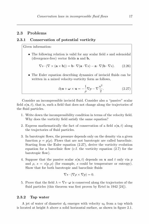
2.3.2 Tap water
A jet of water of diameter d0 emerges with velocity u0 from a tap whichis located at height h above a solid horizontal surface, as shown in figure 2.1.
18 Fluid Dynamics via Examples and Solutions
For simplicity, one can assume that water is inviscid and its velocity profile atthe tap is flat, i.e. velocity of the emerging jet is independent of the distancefrom its centre.
FIGURE 2.1: Tap water.
1. Consider the part of the jet which is of sufficient distance away fromthe point of impact with the solid surface, where we can assume thatvelocity remains independent of the distance from the jet’s centre. Findthe jet velocity u and its diameter d as function of the distance z fromthe tap.
2. Now consider the impact part of the flow in the vicinity of the solidplane. Find the pressure p at the impact point with the solid surface atthe centre of the jet; see figure 2.1.
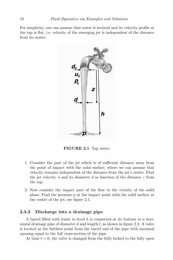
2.3.3 Discharge into a drainage pipe
A barrel filled with water to level h is connected at its bottom to a hori-zontal drainage pipe of diameter d and length l, as shown in figure 2.2. A valveis located at the farthest point from the barrel end of the pipe with maximalopening equal to the full cross-section of the pipe.
At time t = 0, the valve is changed from the fully locked to the fully open
Conservation laws in incompressible fluid flows 19
position. For simplicity, we will ignore viscosity and assume that the pipe flowvelocity is uniform (independent of the distance from the centre of the pipe).
h
`
u
d x0
FIGURE 2.2: Drain pipe.
1. Will velocity u depend on the distance x along the pipe?
2. Find the steady-state velocity in the pipe which forms at large time,u∞ = limt→∞ u.
3. Find an expression for the change of velocity u in the pipe as a functionof time.
4. Find the pressure p in the pipe as a function of t and x.
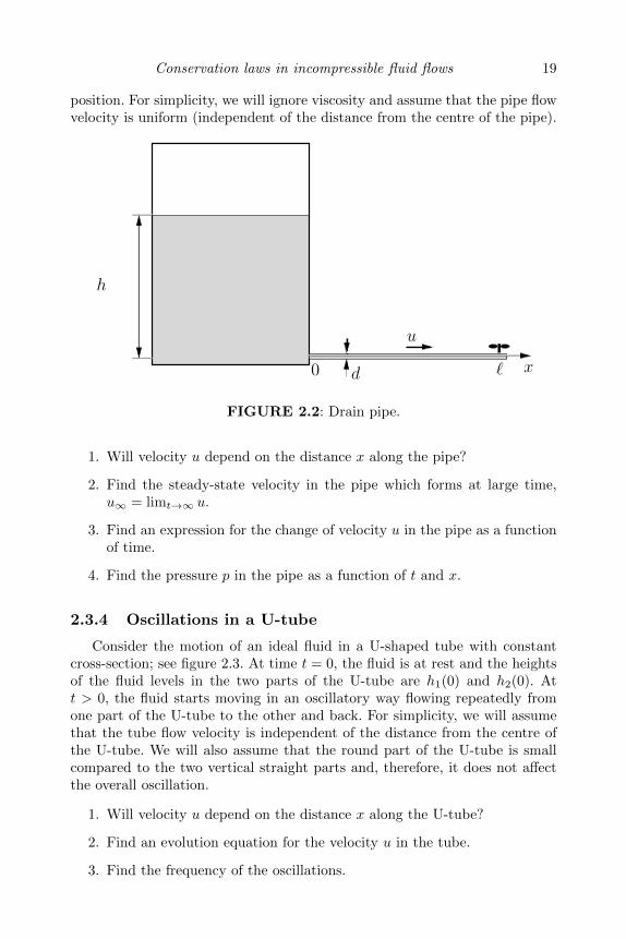
2.3.4 Oscillations in a U-tube
Consider the motion of an ideal fluid in a U-shaped tube with constantcross-section; see figure 2.3. At time t = 0, the fluid is at rest and the heightsof the fluid levels in the two parts of the U-tube are h1(0) and h2(0). Att > 0, the fluid starts moving in an oscillatory way flowing repeatedly fromone part of the U-tube to the other and back. For simplicity, we will assumethat the tube flow velocity is independent of the distance from the centre ofthe U-tube. We will also assume that the round part of the U-tube is smallcompared to the two vertical straight parts and, therefore, it does not affectthe overall oscillation.
1. Will velocity u depend on the distance x along the U-tube?
2. Find an evolution equation for the velocity u in the tube.
3. Find the frequency of the oscillations.
20 Fluid Dynamics via Examples and Solutions
2h
h1
FIGURE 2.3: U-tube.
4. Find the pressure p in the tube as a function of t and x.
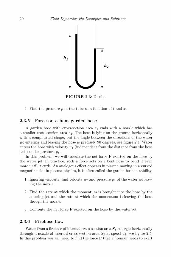
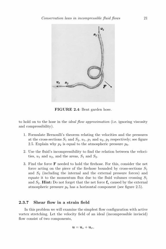
2.3.5 Force on a bent garden hose
A garden hose with cross-section area s1 ends with a nozzle which hasa smaller cross-section area s2. The hose is lying on the ground horizontallywith a complicated shape, but the angle between the directions of the waterjet entering and leaving the hose is precisely 90 degrees; see figure 2.4. Waterenters the hose with velocity u1 (independent from the distance from the hoseaxis) under pressure p1.
In this problem, we will calculate the net force F exerted on the hose bythe water jet. In practice, such a force acts on a bent hose to bend it evenmore until it curls. An analogous effect appears in plasma moving in a curvedmagnetic field: in plasma physics, it is often called the garden hose instability.
1. Ignoring viscosity, find velocity u2 and pressure p2 of the water jet leav-ing the nozzle.
2. Find the rate at which the momentum is brought into the hose by theentering jet and the rate at which the momentum is leaving the hosethough the nozzle.
3. Compute the net force F exerted on the hose by the water jet.
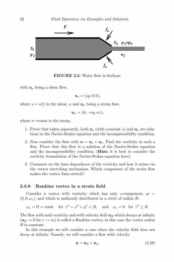
2.3.6 Firehose flow
Water from a firehose of internal cross-section area S1 emerges horizontallythrough a nozzle of internal cross-section area S2 at speed u2; see figure 2.5.In this problem you will need to find the force F that a fireman needs to exert
Conservation laws in incompressible fluid flows 21
FIGURE 2.4: Bent garden hose.
to hold on to the hose in the ideal flow approximation (i.e. ignoring viscosityand compressibility).
1. Formulate Bernoulli’s theorem relating the velocities and the pressuresat the cross-sections S1 and S2, u1, p1 and u2, p2 respectively; see figure2.5. Explain why p2 is equal to the atmospheric pressure p0.
2. Use the fluid’s incompressibility to find the relation between the veloci-ties, u1 and u2, and the areas, S1 and S2.
3. Find the force F needed to hold the firehose. For this, consider the netforce acting on the piece of the firehose bounded by cross-sections S1
and S2 (including the internal and the external pressure forces) andequate it to the momentum flux due to the fluid volumes crossing S1
and S2. Hint: Do not forget that the net force fa caused by the externalatmospheric pressure p0 has a horizontal component (see figure 2.5).
2.3.7 Shear flow in a strain field
In this problem we will examine the simplest flow configuration with activevortex stretching. Let the velocity field of an ideal (incompressible inviscid)flow consist of two components,
u = us + uσ,
22 Fluid Dynamics via Examples and Solutions
o
u1 u2
S
S2
1
Ffa
fa
p1
p =p2
FIGURE 2.5: Water flow in firehose.
with us being a shear flow,
us = (sy, 0, 0),
where s = s(t) is the shear, a and uσ being a strain flow,
uσ = (0,−σy, σz),
where σ =const is the strain.
1. Prove that taken separately, both us (with constant s) and uσ are solu-tions to the Navier-Stokes equation and the incompressibility condition.
2. Now consider the flow with u = us + uσ. Find the vorticity in such aflow. Prove that this flow is a solution of the Navier-Stokes equationand the incompressibility condition. (Hint: it is best to consider thevorticity formulation of the Navier-Stokes equation here).
3. Comment on the time dependence of the vorticity and how it arises viathe vortex stretching mechanism. Which component of the strain flowmakes the vortex lines stretch?
2.3.8 Rankine vortex in a strain field
Consider a vortex with vorticity which has only z-component, ω =(0, 0, ωz), and which is uniformly distributed in a circle of radius R:
ωz = Ω = const for r2 = x2 + y2 < R, and ωz = 0 for r2 ≥ R.
The flow with such vorticity and with velocity field uR which decays at infinity(uR → 0 for r →∞) is called a Rankine vortex; in this case the vortex radiusR is constant.
In this example we will consider a case when the velocity field does notdecay at infinity. Namely, we will consider a flow with velocity
u = uR + uσ, (2.28)
Conservation laws in incompressible fluid flows 23
where uR is the Rankine vortex and uσ is a uniform strain field of the form
uσ = (−σx,−σy, 2σz). (2.29)
In this case the vortex radius R and the vorticity Ω will be time dependent,R = R(t),Ω = Ω(t), because of the vortex stretching produced by the strain.
1. Prove that the Rankine vortex is a solution to the Euler equation for aninviscid fluid. Find the incompressible velocity field uR of the Rankinevortex.
2. Prove that the uniform strain field uσ given by expression (2.29) satisfiesthe ideal flow equations.
3. Now consider the combination of the Rankine vortex and the strain fieldas in expression (2.28) and prove that it satisfies the ideal flow equations.Find dependencies R(t) and Ω(t). Interpret your results in terms of thevortex stretching mechanism.
4. The Burgers vortex is a generalisation of the considered solution to vis-cous flows. This solution is stationary because the vortex stretching isstabilised by the vorticity diffusion due to viscosity. The stain field inthis vortex is the same as in (2.29), but the vorticity profile now is
ωz = Ω0 e−λr2 ,
where Ω0 =const.
Find λ in terms of σ and the viscosity coefficient ν.
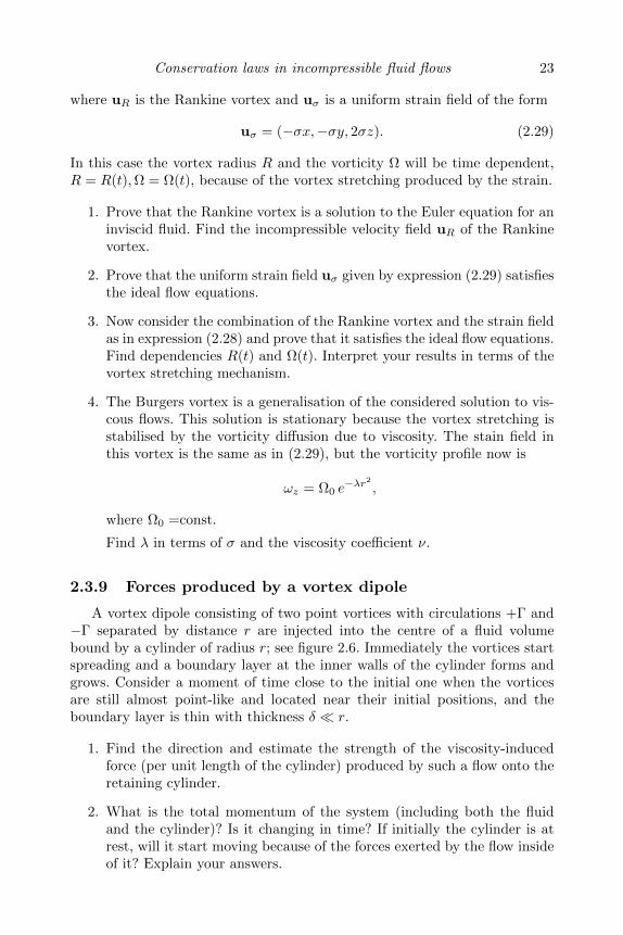
2.3.9 Forces produced by a vortex dipole
A vortex dipole consisting of two point vortices with circulations +Γ and−Γ separated by distance r are injected into the centre of a fluid volumebound by a cylinder of radius r; see figure 2.6. Immediately the vortices startspreading and a boundary layer at the inner walls of the cylinder forms andgrows. Consider a moment of time close to the initial one when the vorticesare still almost point-like and located near their initial positions, and theboundary layer is thin with thickness δ r.
1. Find the direction and estimate the strength of the viscosity-inducedforce (per unit length of the cylinder) produced by such a flow onto theretaining cylinder.
2. What is the total momentum of the system (including both the fluidand the cylinder)? Is it changing in time? If initially the cylinder is atrest, will it start moving because of the forces exerted by the flow insideof it? Explain your answers.
24 Fluid Dynamics via Examples and Solutions
3. Estimate the difference of the pressures at the leftmost and the rightmostparts of the flow. Comment on the difference of this result with the onefor the inviscid flow (obtained e.g. from Bernoulli’s theorem).
Γ
−Γ
r
x
y
FIGURE 2.6: Vortex pair in a cylindrical container.
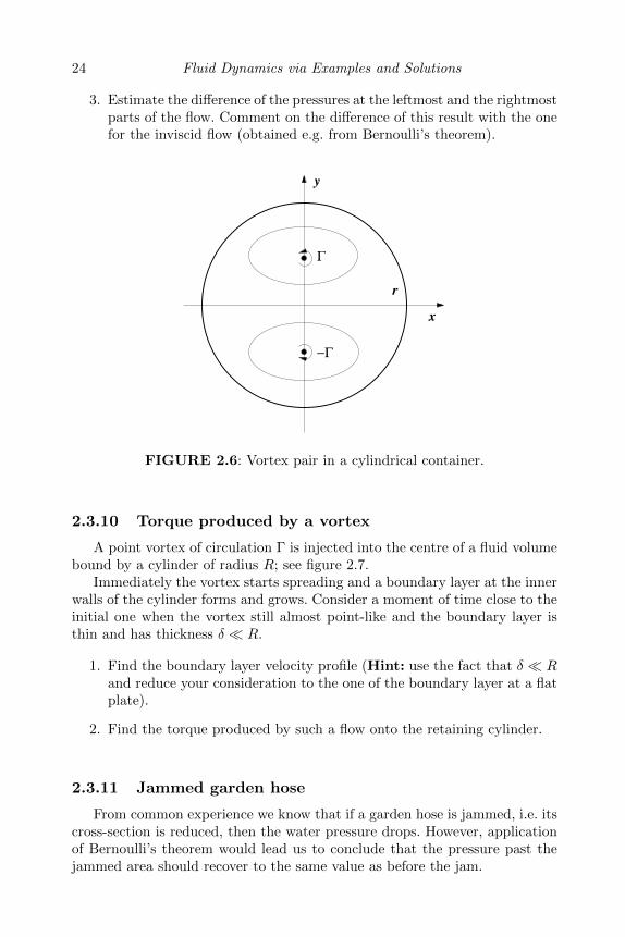
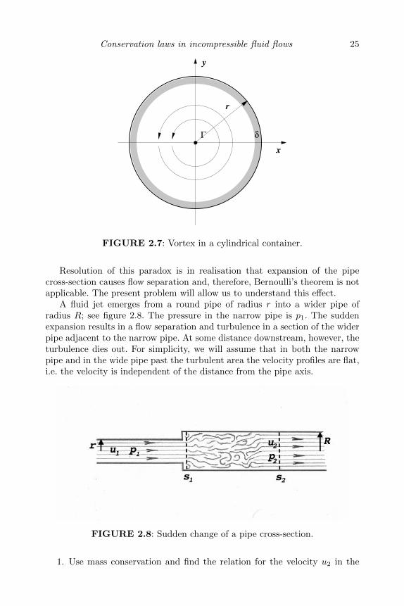
2.3.10 Torque produced by a vortex
A point vortex of circulation Γ is injected into the centre of a fluid volumebound by a cylinder of radius R; see figure 2.7.
Immediately the vortex starts spreading and a boundary layer at the innerwalls of the cylinder forms and grows. Consider a moment of time close to theinitial one when the vortex still almost point-like and the boundary layer isthin and has thickness δ R.
1. Find the boundary layer velocity profile (Hint: use the fact that δ Rand reduce your consideration to the one of the boundary layer at a flatplate).
2. Find the torque produced by such a flow onto the retaining cylinder.
2.3.11 Jammed garden hose
From common experience we know that if a garden hose is jammed, i.e. itscross-section is reduced, then the water pressure drops. However, applicationof Bernoulli’s theorem would lead us to conclude that the pressure past thejammed area should recover to the same value as before the jam.
Conservation laws in incompressible fluid flows 25
x
y
Γ
r
δ
FIGURE 2.7: Vortex in a cylindrical container.
Resolution of this paradox is in realisation that expansion of the pipecross-section causes flow separation and, therefore, Bernoulli’s theorem is notapplicable. The present problem will allow us to understand this effect.
A fluid jet emerges from a round pipe of radius r into a wider pipe ofradius R; see figure 2.8. The pressure in the narrow pipe is p1. The suddenexpansion results in a flow separation and turbulence in a section of the widerpipe adjacent to the narrow pipe. At some distance downstream, however, theturbulence dies out. For simplicity, we will assume that in both the narrowpipe and in the wide pipe past the turbulent area the velocity profiles are flat,i.e. the velocity is independent of the distance from the pipe axis.
FIGURE 2.8: Sudden change of a pipe cross-section.
1. Use mass conservation and find the relation for the velocity u2 in the
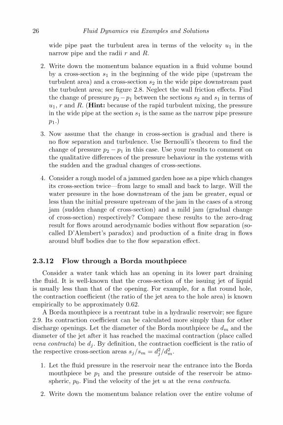
26 Fluid Dynamics via Examples and Solutions
wide pipe past the turbulent area in terms of the velocity u1 in thenarrow pipe and the radii r and R.
2. Write down the momentum balance equation in a fluid volume boundby a cross-section s1 in the beginning of the wide pipe (upstream theturbulent area) and a cross-section s2 in the wide pipe downstream pastthe turbulent area; see figure 2.8. Neglect the wall friction effects. Findthe change of pressure p2−p1 between the sections s2 and s1 in terms ofu1, r and R. (Hint: because of the rapid turbulent mixing, the pressurein the wide pipe at the section s1 is the same as the narrow pipe pressurep1.)
3. Now assume that the change in cross-section is gradual and there isno flow separation and turbulence. Use Bernoulli’s theorem to find thechange of pressure p2 − p1 in this case. Use your results to comment onthe qualitative differences of the pressure behaviour in the systems withthe sudden and the gradual changes of cross-sections.
4. Consider a rough model of a jammed garden hose as a pipe which changesits cross-section twice—from large to small and back to large. Will thewater pressure in the hose downstream of the jam be greater, equal orless than the initial pressure upstream of the jam in the cases of a strongjam (sudden change of cross-section) and a mild jam (gradual changeof cross-section) respectively? Compare these results to the zero-dragresult for flows around aerodynamic bodies without flow separation (so-called D’Alembert’s paradox) and production of a finite drag in flowsaround bluff bodies due to the flow separation effect.
2.3.12 Flow through a Borda mouthpiece
Consider a water tank which has an opening in its lower part drainingthe fluid. It is well-known that the cross-section of the issuing jet of liquidis usually less than that of the opening. For example, for a flat round hole,the contraction coefficient (the ratio of the jet area to the hole area) is knownempirically to be approximately 0.62.
A Borda mouthpiece is a reentrant tube in a hydraulic reservoir; see figure2.9. Its contraction coefficient can be calculated more simply than for otherdischarge openings. Let the diameter of the Borda mouthpiece be dm and thediameter of the jet after it has reached the maximal contraction (place calledvena contracta) be dj . By definition, the contraction coefficient is the ratio ofthe respective cross-section areas sj/sm = d2
j/d2m.
1. Let the fluid pressure in the reservoir near the entrance into the Bordamouthpiece be p1 and the pressure outside of the reservoir be atmo-spheric, p0. Find the velocity of the jet u at the vena contracta.
2. Write down the momentum balance relation over the entire volume of
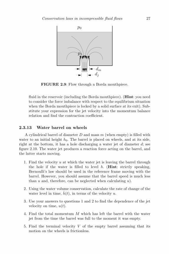
Conservation laws in incompressible fluid flows 27
dj
p0
dm
p1
FIGURE 2.9: Flow through a Borda mouthpiece.
fluid in the reservoir (including the Borda mouthpiece). (Hint: you needto consider the force imbalance with respect to the equilibrium situationwhen the Borda mouthpiece is locked by a solid surface at its exit). Sub-stitute your expression for the jet velocity into the momentum balancerelation and find the contraction coefficient.
2.3.13 Water barrel on wheels
A cylindrical barrel of diameter D and mass m (when empty) is filled withwater to an initial height h0. The barrel is placed on wheels, and at its side,right at the bottom, it has a hole discharging a water jet of diameter d; seefigure 2.10. The water jet produces a reaction force acting on the barrel, andthe latter starts moving.
1. Find the velocity u at which the water jet is leaving the barrel throughthe hole if the water is filled to level h. (Hint: strictly speaking,Bernoulli’s law should be used in the reference frame moving with thebarrel. However, you should assume that the barrel speed is much lessthan u and, therefore, can be neglected when calculating u).
2. Using the water volume conservation, calculate the rate of change of thewater level in time, h(t), in terms of the velocity u.
3. Use your answers to questions 1 and 2 to find the dependence of the jetvelocity on time, u(t).
4. Find the total momentum M which has left the barrel with the waterjet from the time the barrel was full to the moment it was empty.
5. Find the terminal velocity V of the empty barrel assuming that itsmotion on the wheels is frictionless.
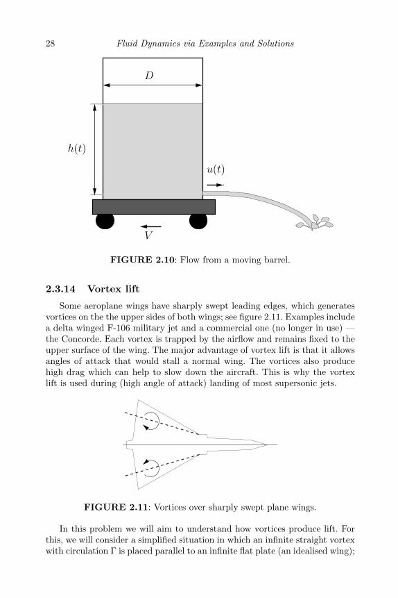
28 Fluid Dynamics via Examples and Solutions
D
h(t)
u(t)
V
FIGURE 2.10: Flow from a moving barrel.
2.3.14 Vortex lift
Some aeroplane wings have sharply swept leading edges, which generatesvortices on the the upper sides of both wings; see figure 2.11. Examples includea delta winged F-106 military jet and a commercial one (no longer in use) —the Concorde. Each vortex is trapped by the airflow and remains fixed to theupper surface of the wing. The major advantage of vortex lift is that it allowsangles of attack that would stall a normal wing. The vortices also producehigh drag which can help to slow down the aircraft. This is why the vortexlift is used during (high angle of attack) landing of most supersonic jets.
FIGURE 2.11: Vortices over sharply swept plane wings.
In this problem we will aim to understand how vortices produce lift. Forthis, we will consider a simplified situation in which an infinite straight vortexwith circulation Γ is placed parallel to an infinite flat plate (an idealised wing);
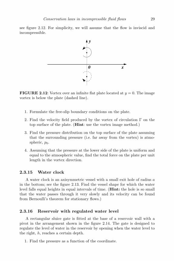
Conservation laws in incompressible fluid flows 29
see figure 2.12. For simplicity, we will assume that the flow is inviscid andincompressible.
y
0 x
FIGURE 2.12: Vortex over an infinite flat plate located at y = 0. The imagevortex is below the plate (dashed line).
1. Formulate the free-slip boundary conditions on the plate.
2. Find the velocity field produced by the vortex of circulation Γ on thetop surface of the plate. (Hint: use the vortex image method.)
3. Find the pressure distribution on the top surface of the plate assumingthat the surrounding pressure (i.e. far away from the vortex) is atmo-spheric, p0.
4. Assuming that the pressure at the lower side of the plate is uniform andequal to the atmospheric value, find the total force on the plate per unitlength in the vortex direction.
2.3.15 Water clock
A water clock is an axisymmetric vessel with a small exit hole of radius ain the bottom; see the figure 2.13. Find the vessel shape for which the waterlevel falls equal heights in equal intervals of time. (Hint: the hole is so smallthat the water passes through it very slowly and its velocity can be foundfrom Bernoulli’s theorem for stationary flows.)
2.3.16 Reservoir with regulated water level
A rectangular sluice gate is fitted at the base of a reservoir wall with apivot in the arrangement shown in the figure 2.14. The gate is designed toregulate the level of water in the reservoir by opening when the water level tothe right, h, reaches a certain depth.
1. Find the pressure as a function of the coordinate.
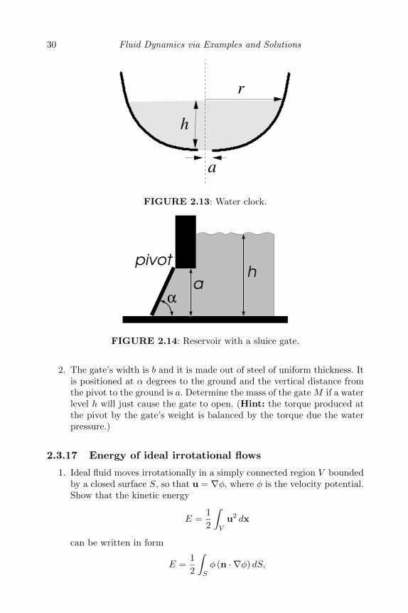
30 Fluid Dynamics via Examples and Solutions
a
h
r
FIGURE 2.13: Water clock.
ah
pivot
α
FIGURE 2.14: Reservoir with a sluice gate.
2. The gate’s width is b and it is made out of steel of uniform thickness. Itis positioned at α degrees to the ground and the vertical distance fromthe pivot to the ground is a. Determine the mass of the gate M if a waterlevel h will just cause the gate to open. (Hint: the torque produced atthe pivot by the gate’s weight is balanced by the torque due the waterpressure.)
2.3.17 Energy of ideal irrotational flows
1. Ideal fluid moves irrotationally in a simply connected region V boundedby a closed surface S, so that u = ∇φ, where φ is the velocity potential.Show that the kinetic energy
E =1
2
∫V
u2 dx
can be written in form
E =1
2
∫S
φ (n · ∇φ) dS,
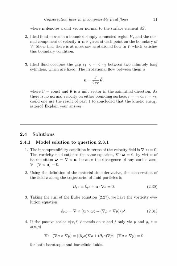
Conservation laws in incompressible fluid flows 31
where n denotes a unit vector normal to the surface element dS.
2. Ideal fluid moves in a bounded simply connected region V , and the nor-mal component of velocity u·n is given at each point on the boundary ofV . Show that there is at most one irrotational flow in V which satisfiesthis boundary condition.
3. Ideal fluid occupies the gap r1 < r < r2 between two infinitely longcylinders, which are fixed. The irrotational flow between them is
u =Γ
2πrθ,
where Γ = const and θ is a unit vector in the azimuthal direction. Asthere is no normal velocity on either bounding surface, r = r1 or r = r2,could one use the result of part 1 to concluded that the kinetic energyis zero? Explain your answer.
2.4 Solutions
2.4.1 Model solution to question 2.3.1
1. The incompressibility condition in terms of the velocity field is ∇·u = 0.The vorticity field satisfies the same equation, ∇ · ω = 0, by virtue ofits definition ω = ∇ × u: because the divergence of any curl is zero,∇ · (∇× u) = 0.
2. Using the definition of the material time derivative, the conservation ofthe field s along the trajectories of fluid particles is
Dts ≡ ∂ts+ u · ∇s = 0. (2.30)
3. Taking the curl of the Euler equation (2.27), we have the vorticity evo-lution equation:
∂tω = ∇× (u× ω) + (∇ρ×∇p)/ρ2. (2.31)
4. If the passive scalar s(x, t) depends on x and t only via p and ρ, s =s(p, ρ)
∇s · (∇ρ×∇p) = [(∂ρs)∇ρ+ (∂ps)∇p] · (∇ρ×∇p) = 0
for both barotropic and baroclinic fluids.
32 Fluid Dynamics via Examples and Solutions
5. Taking the partial time derivative of λ = ∇s ·ω and using the equations(2.31) and (2.30) and the vector identity (2.26), as well as the identity∇s · (∇ρ×∇p) = 0, we have:
∂t(∇s ·ω) = (∇∂ts) ·ω+∇s ·∂tω = ∇s · (∇× (u×ω))−ω ·∇(u ·∇s) =
−u · ∇(ω · ∇s).
Thus,Dtλ ≡ ∂tλ+ u · ∇λ = 0. (2.32)
2.4.2 Model solution to question 2.3.2
1. The pressure in this part of the jet remains atmospheric, p0. Thus, usingBernoulli’s theorem we have
u2
2=u2
0
2+ gz.
Therefore, u =√u2
0 + 2gz.
From the mass conservation we have ud2 = u0d20. So, d = d0
√u0/u =
d0(1 + 2gz/u20)−1/4.
2. At the impact point with the solid surface at the centre of the jet thefluid velocity is zero. Thus,
p = p0 +ρu2
0
2+ ρgh.
2.4.3 Model solution to question 2.3.3
1. Because u is independent of the distance from the centre of the pipe, itmust also be independent from the distance along the pipe x by incom-pressibility. Thus, u is a function of time only, u = u(t).
2. The terminal velocity can be found from the Bernoulli’s theorem, whichgives u∞ =
√2gh.
3. Now, we are dealing with a non-stationary flow and, therefore, we needto use the time-dependent version of the Bernoulli’s theorem. Takinginto account that for the uniform velocity directed along x the velocitypotential is φ = ux, and that the pressure at the far end of the pipe isatmospheric (p0), we have
ul +u2
2+p0
ρ= C, (2.33)
where C is a constant.
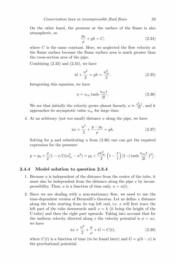
Conservation laws in incompressible fluid flows 33
On the other hand, the pressure at the surface of the flume is alsoatmospheric, so
p0
ρ+ gh = C, (2.34)
where C is the same constant. Here, we neglected the flow velocity atthe flume surface because the flume surface area is much greater thanthe cross-section area of the pipe.
Combining (2.33) and (2.34), we have
ul +u2
2= gh =
u2∞2. (2.35)
Integrating this equation, we have
u = u∞ tanhu∞t
2l. (2.36)
We see that initially the velocity grows almost linearly, u ≈ u2∞t2l , and it
approaches its asymptotic value u∞ for large time.
4. At an arbitrary (not too small) distance x along the pipe, we have
ux+u2
2+p− p0
ρ= gh. (2.37)
Solving for p and substituting u from (2.36) one can get the requiredexpression for the pressure:
p = p0 +ρ
2(1− x/l)(u2
∞ − u2) = p0 +ρu2∞
2
(1− x
l
)[1−( tanh
u∞t
2l
)2].
2.4.4 Model solution to question 2.3.4
1. Because u is independent of the distance from the centre of the tube, itmust also be independent from the distance along the pipe x by incom-pressibility. Thus, u is a function of time only, u = u(t).
2. Since we are dealing with a non-stationary flow, we need to use thetime-dependent version of Bernoulli’s theorem. Let us define x distancealong the tube starting from its top left end, i.e. x will first trace theleft part of the tube downwards until x = h (h being the height of theU-tube) and then the right part upwards. Taking into account that forthe uniform velocity directed along x the velocity potential is φ = ux,we have
ux+u2
2+p
ρ+G = C(t), (2.38)
where C(t) is a function of time (to be found later) and G = g(h− x) isthe gravitational potential.
34 Fluid Dynamics via Examples and Solutions
3. Taking the difference of this equation at the two ends of the tube andtaking into account that the pressure at the ends of the tube is atmo-spheric (p0), we have
ul − g(h1 − h2) = 0, (2.39)
where l = h1+h2 = h1(0)+h2(0) = const is the total length occupied bythe fluid. Taking into account that u = h2 = −h1 we have for s = h2−h1:
sl + 2gs = 0. (2.40)
Solving this equation we have
s(t) = A cos(ωt), (2.41)
where A = h2(0)− h1(0) is the oscillation amplitude and the oscillationfrequency is given by
ω =
√2g
l. (2.42)
Interestingly, this expression coincides with the frequency formula for apendulum which consists of a point mass suspended on a massless stringof length l/2.
4. Differentiating expression (2.41), we get the following solution for thevelocity
u(t) = U sin(ωt), (2.43)
where U = ω2 [h1(0)− h2(0)]. Note that the oscillation phase is chosen in
(2.41) and (2.43) to ensure that the initial condition u(0) = 0 is satisfied.
Similarly, for h1 we have
h1(t) = (h1(0)− l/2) cos(ωt) + l/2, (2.44)
From (2.38), we find for the pressure:
p
ρ= −Uω(x− h1(t)) cos(ωt) + g(x− h1(t)) +
p0
ρ, (2.45)
where C(t) is chosen to satisfy condition p = p0 at x = h1(t).
2.4.5 Model solution to question 2.3.5
1. From mass conservation,
u2 =u1s1
s2. (2.46)
From Bernoulli’s theorem we have
p2 − p1 =ρ
2(u2
1 − u22) =
ρ
2u2
1
(1− s2
1
s22
). (2.47)
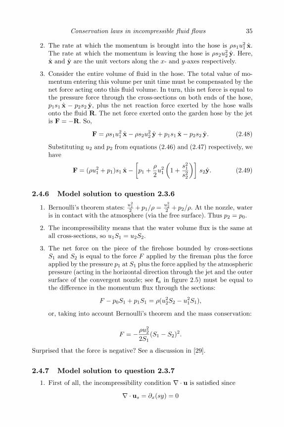
Conservation laws in incompressible fluid flows 35
2. The rate at which the momentum is brought into the hose is ρs1u21 x.
The rate at which the momentum is leaving the hose is ρs2u22 y. Here,
x and y are the unit vectors along the x- and y-axes respectively.
3. Consider the entire volume of fluid in the hose. The total value of mo-mentum entering this volume per unit time must be compensated by thenet force acting onto this fluid volume. In turn, this net force is equal tothe pressure force through the cross-sections on both ends of the hose,p1s1 x − p2s2 y, plus the net reaction force exerted by the hose wallsonto the fluid R. The net force exerted onto the garden hose by the jetis F = −R. So,
F = ρs1u21 x− ρs2u
22 y + p1s1 x− p2s2 y. (2.48)
Substituting u2 and p2 from equations (2.46) and (2.47) respectively, wehave
F = (ρu21 + p1)s1 x−
[p1 +
ρ
2u2
1
(1 +
s21
s22
)]s2y. (2.49)
2.4.6 Model solution to question 2.3.6
1. Bernoulli’s theorem states:u21
2 + p1/ρ =u22
2 + p2/ρ. At the nozzle, wateris in contact with the atmosphere (via the free surface). Thus p2 = p0.
2. The incompressibility means that the water volume flux is the same atall cross-sections, so u1S1 = u2S2.
3. The net force on the piece of the firehose bounded by cross-sectionsS1 and S2 is equal to the force F applied by the fireman plus the forceapplied by the pressure p1 at S1 plus the force applied by the atmosphericpressure (acting in the horizontal direction through the jet and the outersurface of the convergent nozzle; see fa in figure 2.5) must be equal tothe difference in the momentum flux through the sections:
F − p0S1 + p1S1 = ρ(u22S2 − u2
1S1),
or, taking into account Bernoulli’s theorem and the mass conservation:
F = −ρu22
2S1(S1 − S2)2.
Surprised that the force is negative? See a discussion in [29].
2.4.7 Model solution to question 2.3.7
1. First of all, the incompressibility condition ∇ · u is satisfied since
∇ · us = ∂x(sy) = 0
36 Fluid Dynamics via Examples and Solutions
and∇ · uσ = −∂y(σy) + ∂z(σz) = 0.
Both us and uσ are linear functions of x and, therefore, the viscous termis zero. Since s and σ are constant, ∂tus = 0 and ∂tuσ = 0.
Now,(us · ∇)us = sy ∂x(sy) x = 0
and
(uσ · ∇)uσ = σy ∂y(σy) y + σz ∂z(σz) z = σ2(y y + z z).
Thus, us solves the Navier-Stokes equation with pressure p =const anduσ solves the Navier-Stokes equation with pressure
p = const− 1
2ρσ2(y2 + z2).
2. For the vorticity we have:
ω = ∇× u = ∇× us +∇× uσ = s z
(because ∇× uσ = 0).
Since there is only one non-zero component of the vorticity, ω = (0, 0, ω),(ω = s), we will only need to consider the z-component of the vorticityequation. Because ω is uniform in space, the viscous term is zero. Forthe same reason, u · ∇ω = 0.
For the vortex stretching term we have
(ω · ∇)u = s ∂z(σz z) = sσ z.
Thus, the vorticity equation in our case is
∂ts = sσ,
which has the following solution
s(t) = s0 eσt,
where s0 is the initial value of the shear at t = 0.
3. As we can see, the vorticity is growing exponentially in time, ω(t) =s(t) = s0 e
σt. This is due to the z-component of the strain flow whichpulls the fluid particles apart in the z-direction exponentially in time.At the same time, due to volume conservation, the fluid particles arepushed closer to each other in the y-direction making the density of thevortex lines greater—hence the vorticity amplification.
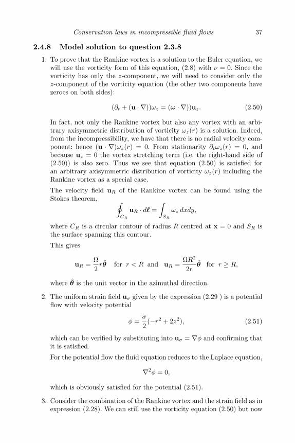
Conservation laws in incompressible fluid flows 37
2.4.8 Model solution to question 2.3.8
1. To prove that the Rankine vortex is a solution to the Euler equation, wewill use the vorticity form of this equation, (2.8) with ν = 0. Since thevorticity has only the z-component, we will need to consider only thez-component of the vorticity equation (the other two components havezeroes on both sides):
(∂t + (u · ∇))ωz = (ω · ∇))uz. (2.50)
In fact, not only the Rankine vortex but also any vortex with an arbi-trary axisymmetric distribution of vorticity ωz(r) is a solution. Indeed,from the incompressibility, we have that there is no radial velocity com-ponent: hence (u · ∇)ωz(r) = 0. From stationarity ∂tωz(r) = 0, andbecause uz = 0 the vortex stretching term (i.e. the right-hand side of(2.50)) is also zero. Thus we see that equation (2.50) is satisfied foran arbitrary axisymmetric distribution of vorticity ωz(r) including theRankine vortex as a special case.
The velocity field uR of the Rankine vortex can be found using theStokes theorem, ∮
CR
uR · d` =
∫SR
ωz dxdy,
where CR is a circular contour of radius R centred at x = 0 and SR isthe surface spanning this contour.
This gives
uR =Ω
2rθ for r < R and uR =
ΩR2
2rθ for r ≥ R,
where θ is the unit vector in the azimuthal direction.
2. The uniform strain field uσ given by the expression (2.29 ) is a potentialflow with velocity potential
φ =σ
2(−r2 + 2z2), (2.51)
which can be verified by substituting into uσ = ∇φ and confirming thatit is satisfied.
For the potential flow the fluid equation reduces to the Laplace equation,
∇2φ = 0,
which is obviously satisfied for the potential (2.51).
3. Consider the combination of the Rankine vortex and the strain field as inexpression (2.28). We can still use the vorticity equation (2.50) but now

38 Fluid Dynamics via Examples and Solutions
with non-zero stretching term. The vortex advection term (the secondterm on the left-hand side) is zero both inside and the outside of theRankine vortex because in both places ∇ωz = 0. Outside of the vortexall terms in the vorticity equation are zero and it is obviously satisfied.Inside the vortex we have
∂tΩ = Ω∂zuz = 2Ωσ, (2.52)
soΩ = Ω(0)e2σt.
Dependence R(t) can be obtained from the Kelvin’s theorem for conser-vation of the circulation. Conservation of the circulation over CR, thecircular contour of radius R, means ΩR2 = const, i.e.
R = R(0)e−σt.
The vorticity amplification is produced by the vortex stretching mecha-nism activated by the z-component of the strain field.
4. Let us substitute the Burgers vortex, ωz = Ω0 e−λr2 , into a steady-state
version of the z-component of the vorticity equation (2.8), but now withfinite ν.
(uσ · ∇)e−λr2
= e−λr2
∂zuσz + ν∇2e−λr2
. (2.53)
Substituting for uσ and differentiating, we have
−σ(−2λr2)e−λr2
= 2σe−λr2
+ ν(−4λ+ 4λ2r2)e−λr2
. (2.54)
This equation is satisfied if
λ =σ
2ν.
2.4.9 Model solution to question 2.3.9
1. From figure 2.6 it is clear that the viscosity induces a force along the x-axis in the negative direction. This is because the negative x-momentumwill be transferred (in equal proportions) to the top and at the bottomparts of the cylinder via the viscous stress in the boundary layer. Therewill be no y-component of the force because, due to symmetry, the y-momentum transfers at the top and at the bottom parts will sum up tozero.
The velocity field produced by the vortex dipole at the walls can beestimated as u ∼ Γ/r. Correspondingly, the viscous stress is σxy ∼ρνu/δ ∼ ρνΓ/(δr). This gives the following estimate for the viscousforce on the cylinder per unit length in the z-direction,
F = (Fx, 0) ∼ (−2πρνΓ/δ, 0).
Notice that this force is independent of the radius of the cylinder r!
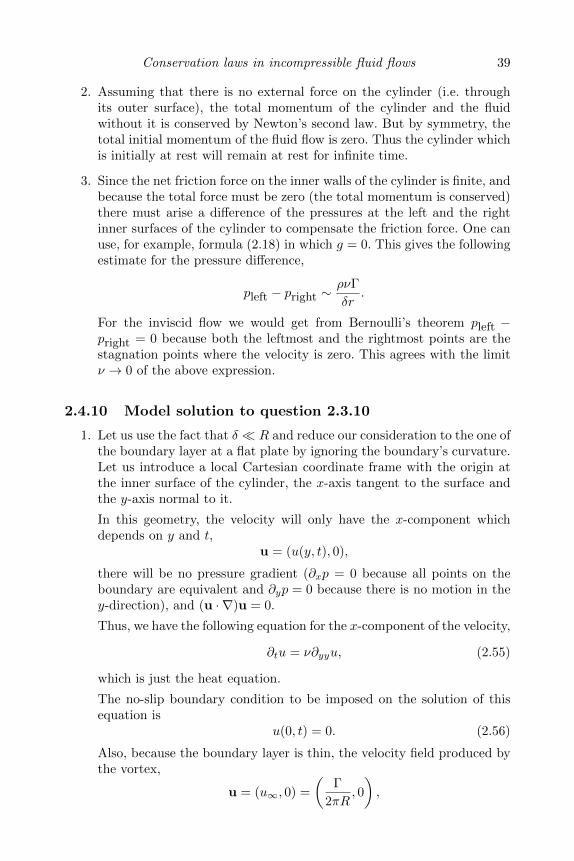
Conservation laws in incompressible fluid flows 39
2. Assuming that there is no external force on the cylinder (i.e. throughits outer surface), the total momentum of the cylinder and the fluidwithout it is conserved by Newton’s second law. But by symmetry, thetotal initial momentum of the fluid flow is zero. Thus the cylinder whichis initially at rest will remain at rest for infinite time.
3. Since the net friction force on the inner walls of the cylinder is finite, andbecause the total force must be zero (the total momentum is conserved)there must arise a difference of the pressures at the left and the rightinner surfaces of the cylinder to compensate the friction force. One canuse, for example, formula (2.18) in which g = 0. This gives the followingestimate for the pressure difference,
pleft − pright ∼ρνΓ
δr.
For the inviscid flow we would get from Bernoulli’s theorem pleft −pright = 0 because both the leftmost and the rightmost points are thestagnation points where the velocity is zero. This agrees with the limitν → 0 of the above expression.
2.4.10 Model solution to question 2.3.10
1. Let us use the fact that δ R and reduce our consideration to the one ofthe boundary layer at a flat plate by ignoring the boundary’s curvature.Let us introduce a local Cartesian coordinate frame with the origin atthe inner surface of the cylinder, the x-axis tangent to the surface andthe y-axis normal to it.
In this geometry, the velocity will only have the x-component whichdepends on y and t,
u = (u(y, t), 0),
there will be no pressure gradient (∂xp = 0 because all points on theboundary are equivalent and ∂yp = 0 because there is no motion in they-direction), and (u · ∇)u = 0.
Thus, we have the following equation for the x-component of the velocity,
∂tu = ν∂yyu, (2.55)
which is just the heat equation.
The no-slip boundary condition to be imposed on the solution of thisequation is
u(0, t) = 0. (2.56)
Also, because the boundary layer is thin, the velocity field produced bythe vortex,
u = (u∞, 0) =
(Γ
2πR, 0
),
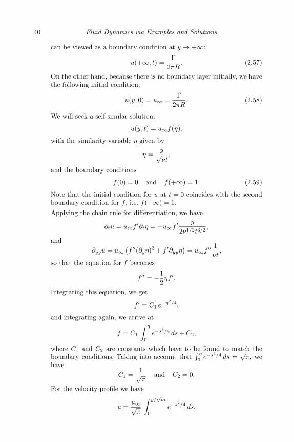
40 Fluid Dynamics via Examples and Solutions
can be viewed as a boundary condition at y → +∞:
u(+∞, t) =Γ
2πR. (2.57)
On the other hand, because there is no boundary layer initially, we havethe following initial condition,
u(y, 0) = u∞ =Γ
2πR. (2.58)
We will seek a self-similar solution,
u(y, t) = u∞f(η),
with the similarity variable η given by
η =y√νt,
and the boundary conditions
f(0) = 0 and f(+∞) = 1. (2.59)
Note that the initial condition for u at t = 0 coincides with the secondboundary condition for f , i.e. f(+∞) = 1.
Applying the chain rule for differentiation, we have
∂tu = u∞f′∂tη = −u∞f ′
y
2ν1/2t3/2,
and
∂yyu = u∞(f ′′(∂yη)2 + f ′∂yyη
)= u∞f
′′ 1
νt,
so that the equation for f becomes
f ′′ = −1
2ηf ′.
Integrating this equation, we get
f ′ = C1 e−η2/4,
and integrating again, we arrive at
f = C1
∫ η
0
e−s2/4 ds+ C2,
where C1 and C2 are constants which have to be found to match theboundary conditions. Taking into account that
∫ η0e−s
2/4 ds =√π, we
have
C1 =1√π
and C2 = 0.
For the velocity profile we have
u =u∞√π
∫ y/√νt
0
e−s2/4 ds.
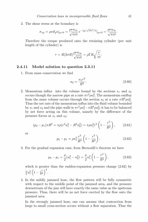
Conservation laws in incompressible fluid flows 41
2. The shear stress at the boundary is
σxy = ρν∂yu|y=0 =ρνu∞√πνt
e−(y/√νt)2/4|y=0 =
ρνu∞√πνt
.
Therefore the torque produced onto the retaining cylinder (per unitlength of the cylinder) is
τ = R(2πR)ρνu∞√πνt
= ρΓR
√ν
πt.
2.4.11 Model solution to question 2.3.11
1. From mass conservation we find
u2 =u1r
2
R2. (2.60)
2. Momentum influx into the volume bound by the sections s1 and s2
occurs though the narrow pipe at a rate πr2ρu21. The momentum outflux
from the same volume occurs through the section s2 at a rate πR2ρu22.
Thus the net rate of the momentum influx into the fluid volume boundedby s1 and s2 and the pipe walls is πr2ρu2
1−πR2ρu22; it has to be balanced
by net force acting on this volume, namely by the difference of thepressure forces at s1 and s2:
(p2 − p1)πR2 = πρ(r2u21 −R2u2
2) = πρu21r
2
(1− r2
R2
), (2.61)
or
p2 − p1 = ρu21
r2
R2
(1− r2
R2
). (2.62)
3. For the gradual expansion case, from Bernoulli’s theorem we have
p2 − p1 =ρ
2(u2
1 − u22) =
ρ
2u2
1
(1− r4
R4
), (2.63)
which is greater than the sudden-expansion pressure change (2.62) by
ρ2u
21
(1− r2
R2
)2
.
4. In the mildly jammed hose, the flow pattern will be fully symmetricwith respect to the middle point of the jammed area, and the pressuredownstream of the jam will have exactly the same value as the upstreampressure. Thus, there will be no net force exerted by the flow onto thejammed area.
In the strongly jammed hose, one can assume that contraction fromlarge to small cross-section occurs without a flow separation. Thus the
42 Fluid Dynamics via Examples and Solutions
pressure difference between the upstream and the jammed parts will bethe same as in the mild jam case and could be found from Bernoulli’stheorem. However, the downstream flow will be separated and the pres-sure will be less that the one predicted by Bernoulli’s theorem, as weestablished in the previous part of this problem. Thus, there will be anet force onto the jammed area in the direction along the flow.
There is a direct analogy with flows past solid bodies. Namely, if there isno flow separation (i.e. the body shape is aerodynamic) there will be nodrag force—result known as d’Alembert’s paradox. On the other hand,if there is separation (bluff body shape), then the pressure behind thebody will not recover to the levels of the upstream flow as would beprescribed by Bernoulli’s theorem. This disbalance of the upstream andthe downstream pressures would cause a finite drag.
2.4.12 Model solution to question 2.3.12
1. By Bernoulli’s theorem,
p1 − p0 =ρ
2u2. (2.64)
2. Force imbalance with respect to the equilibrium situation when theBorda mouthpiece is locked by a solid surface is equal to the (removed)reaction force of such a solid surface, i.e. (p1− p0)sm. It has to be equalto the rate at which momentum is carried away by the jet, i.e. ρu2sj :
(p1 − p0)sm = ρu2sj . (2.65)
Combining (2.64) and (2.65), we finally have
sj/sm = 0.5.
2.4.13 Model solution to question 2.3.13
1. The pressure at the water surface and the one at the jet are both equalto the atmospheric pressure. Thus, ignoring the fluid velocity at thesurface (h) and the barrel velocity, from Bernoulli’s theorem we have
u2
2= gh. (2.66)
2. From mass conservation we have h = −u(d/D)2.
3. Substituting this formula into the time-differentiated equation (2.66),we have: uu = gh = −ug(d/D)2. Integrating, we get:
u =√
2gh0 − g(d/D)2 t. (2.67)
Conservation laws in incompressible fluid flows 43
4. The momentum M which has left the barrel with the water jet from thetime t = 0 when the barrel was full to the moment t = t∗ when it wasempty is
M =
∫ t∗
0
(ρu)(πd2)u dt.
Substituting in here from (2.67) and integrating, we have M =2πρD2
3
√2gh3
0. Here, we took into account that u(t∗) = 0.
Note that d is usually smaller than the hole diameter due to a transientjet contraction right near the hole. However, the jet diameter d dropsout of the answer for M . Can you explain why?
5. The total momentum is conserved. Therefore, the total momentum car-ried away by the water jet will be equal in magnitude and opposite insign to the momentum acquired by the empty barrel, mV = M . So,
V = −2πρD2
3m
√2gh3
0.
2.4.14 Model solution to question 2.3.14
1. The free-slip boundary condition means that the tangential velocity isnot imposed and only the non-penetration condition is enforced, i.e. atthe plate there is no normal component, uy = 0 at y = 0.
2. Suppose the vortex of circulation Γ is at distance d from the plate, i.e.at (x, y) = (0, d). To satisfy the free-slip boundary condition, the imagevortex of circulation −Γ has to be placed at (x, y) = (0,−d). Then aty = 0 we have uy = 0 and the x-component of velocity at y = 0 is thedouble x-velocity produced by the vortex Γ, i.e.
ux(x, 0) =2Γd
2π(x2 + d2).
3. The pressure is to be calculated from Bernoulli’s theorem,
p(x, 0) = p0 −ρ[ux(x, 0)]2
2= p0 −
Γ2d2
π2(x2 + d2)2.
4. Thus the force on the plate (per unit length in the vortex direction) is
F =
∫ ∞−∞
Γ2d2
π2(x2 + d2)2dx.
This integral can be computed as
−Γ2d2
π2
∂
∂(d2)
∫ ∞−∞
1
(x2 + d2)dx = −Γ2d2
π2
∂
∂(d2)
[1
darctan(x/d)
]∞−∞
=Γ2
2πd.
44 Fluid Dynamics via Examples and Solutions
2.4.15 Model solution to question 2.3.15
Since the pressures at the water surface and at the bottom hole are thesame, from Bernoulli’s theorem for stationary flows we have gh = u2/2 i.e.u =√
2gh; see figure 2.13.From the water volume conservation we have:
hr2 = −ua2.
Thus,hr2 = −a2
√2gh,
and from the condition that the water level is reduced at a constant rate,h = C = const, we have
h(r) =C2
2ga4r4.
2.4.16 Model solution to question 2.3.16
1. An expression for the pressure as a function of the coordinate can befound from the Bernoulli’s theorem applied for the case when the velocityis zero:
p = p0 + ρgz,
there ρ is the water density, p0 is the atmospheric pressure, g is thegravity constant and z is the depth measured from the water surface.
2. The torque produced on the gate by its own gravity is
Mga
2cosα.
Since the pressure forces are normal to the gate, their torque at the pivotis: ∫ a/ sinα
0
(p− p0)bs ds = b
∫ a/ sinα
0
ρg(h− a+ s sinα)s ds =
bρg
[(h− a)
a2
2 sin2 α+
a3
3 sin2 α
].
Thus,
M =baρ
sin2 α cosα
[h− a
3
].
Conservation laws in incompressible fluid flows 45
2.4.17 Model solution to question 2.3.17
1. Integrating by parts we can write the kinetic energy as:
E =1
2
∫V
(∇φ)2dx =
1
2
∫V
[∇ · (φ∇φ)− φ∇2φ] dx.
The second term here is zero by the incompressibility condition, ∇·u =∇2φ = 0. Using Gauss’s theorem, the first term gives:
E =1
2
∫S
φ (n · ∇φ) dS,
where n denotes a unit vector normal to the surface element dS.
2. Let u1 = ∇φ1 and u2 = ∇φ2 be two different solutions. Then u =u1 − u2 is also a solution which satisfies u · n = 0 at the boundary.Then, by part 1 E = 0 i.e. u(x) ≡ 0. Hence we arrive at a contradiction:u1 and u2 cannot be different solutions.
3. No, because the specified volume is not simply connected.

This page intentionally left blankThis page intentionally left blank
Chapter 3
Fluid with free surface
3.1 Background theory
Fluids often have a free surface, for example, an upper surface in systemsunder gravity, as commonly seen in everyday life when we pour water ina glass or when we look at the sea. As with solid surfaces, the role of themoving boundary will be in imposing boundary conditions on the fluid motion.However, in this case the boundary conditions will be different. Below we willconsider the boundary conditions which are specific for the free-surface flows.
3.1.1 Pressure boundary condition
One condition is that the pressure of the fluid at the surface is the same asthe pressure of the surrounding air—else the surface particles would experienceinfinite forces. The second condition is that the fluid particles, once at thesurface, remain on the surface for indefinite time; it is called the kinematicboundary condition.
Let the gravity acceleration vector be in the negative z direction, g = gz.Let the free fluid surface elevation be described by a function h marking theheight at which the surface is z = h(x, y, t). Then the pressure boundarycondition will be
p(x, y, h(x, y, t)) = p0, (3.1)
where p0 is the atmospheric pressure. For example, for irrotational flow onecan use the time-dependent Bernoulli equation (2.5) and thus the pressureboundary condition becomes:[
∂tφ+(∇φ)2
2
]z=h
+ gh = 0, (3.2)
where we have chosen the constant C = p0ρ , which corresponds to a calibration
condition that φ = 0 in the motionless state.Note that the pressure boundary condition is relevant to the cases where
the fluid (or gas) beyond the free surface has much smaller density than theone of the main fluid and not-too-high velocity or then viscosity is unimpor-tant. In both of these cases the pressure is the only important component
47
48 Fluid Dynamics via Examples and Solutions
of the stress tensor at the surface. If these conditions are not satisfied, thepressure boundary condition has to be replaced by a more general conditionof continuity at the surface of all the stress tensor components.
3.1.2 Kinematic boundary condition
To obtain the kinematic boundary condition, let us introduce the functionf = h(x, y, t) − z. The level set f = 0 marks the free surface. The state-ment that the surface particles remain on the surface can be formulated asconservation of function f along the fluid paths of the surface particles, i.e.
[∂t + (u · ∇)]f(x, y, z, t) = 0, (3.3)
or, after substituting for f , we finally get
∂th− uz + (u⊥ · ∇)h = 0, (3.4)
where u⊥ is the horizontal velocity projection, u⊥ = (ux, uy).In the problems below we will only consider steady flows without a vertical
velocity component. For these flows the kinematic boundary condition (3.4)is reduced to
(u⊥ · ∇)h = 0, (3.5)
i.e. the level sets of h coincide with the streamlines.However, in the chapters devoted to waves and instabilities we will use the
full unsteady version of the kinematic boundary condition (3.4).It is worth mentioning that the boundary conditions on solid boundaries of
the containing volume remain the same as for the cases without a free surface,namely they are the no-slip or the free-slip boundary conditions depending onwhether we deal with a viscous or an inviscid fluid.
3.1.3 Axially and spherically symmetric flows
In all of the problems considered in the present chapter, there is eitheraxial or spherical symmetry present. For axially symmetric 3D flows it is oftenuseful to use the following expressions for the Laplacian and the divergenceoperators in cylindrical coordinates:
∆f =1
r
∂
∂r
(r∂f
∂r
)+
1
r2
∂2f
∂θ2+∂2f
∂z2,
∇ · u =1
r
∂(rur)
∂r+
1
r
∂uθ∂θ
+∂uz∂z
.
The radial component of (u · ∇)u is
ur∂ur∂r
+uθr
∂ur∂θ
+ uz∂ur∂z− u2
θ
r.
Fluid with free surface 49
The spherically symmetric flows considered in this chapter will only havethe radial velocity component. For considering these flows, it will be useful touse the equation for the radial component of velocity, v, which in this case is,
∂tv + v∂rv = −1
ρ∂rp. (3.6)
The incompressibility condition in this case is
∂r(r2v) = 0. (3.7)
3.2 Further reading
Discussions of the kinematic and the pressure boundary conditions at thefree surface are frequently found in the context of the water wave theory and,therefore, we refer the reader to the specialised books about waves Waves inFluids by J. Lighthill [15] and Linear and Nonlinear Waves by G.B. Whitham[31], as well as more general books Elementary Fluid Dynamics by D.J. Ache-son [1], Prandtl’s Essentials of Fluid Mechanics by Oertel et al [17] and FluidDynamics by L.D. Landau and E.M. Lifshitz [14].
3.3 Problems
3.3.1 Water surface distortion due to vortex
On a sunny day, vortices can be seen in a shallow creek as round dark spotsat the creek’s bottom. This is because vortices produce concave distortions onthe water surface, which act to spread light rays apart. In this problem, youare asked to find the shape of the free surface of an ideal fluid in the presenceof a Rankine vortex; see figure 3.1. Far from the vortex, the surface tends toits undisturbed shape, h→ h∞ for r →∞. You are reminded that a Rankinevortex has uniform vorticity ω = (0, 0,Ω) (Ω =const) inside a vertical cylinder
of radius a (i.e. for r =√x2 + y2 < a) and zero vorticity ω = (0, 0, 0) outside
of this cylinder (for r ≥ a).Hint: You may find it useful to keep in mind that the uniformly rotating
fluid also has constant vorticity distribution, so you should expect the Rankinevortex solution for r < a to be the same as in a rotating bucket of water. Alsoremember that the surface must be continuous at r = a.
1. Derive the velocity field for this Rankine vortex for both r < a andr ≥ a.
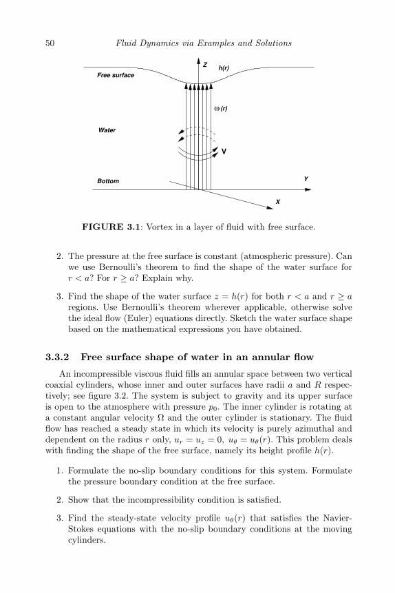
50 Fluid Dynamics via Examples and Solutions
V
ω (r)
h(r)Z
X
YBottom
Water
Free surface
FIGURE 3.1: Vortex in a layer of fluid with free surface.
2. The pressure at the free surface is constant (atmospheric pressure). Canwe use Bernoulli’s theorem to find the shape of the water surface forr < a? For r ≥ a? Explain why.
3. Find the shape of the water surface z = h(r) for both r < a and r ≥ aregions. Use Bernoulli’s theorem wherever applicable, otherwise solvethe ideal flow (Euler) equations directly. Sketch the water surface shapebased on the mathematical expressions you have obtained.
3.3.2 Free surface shape of water in an annular flow
An incompressible viscous fluid fills an annular space between two verticalcoaxial cylinders, whose inner and outer surfaces have radii a and R respec-tively; see figure 3.2. The system is subject to gravity and its upper surfaceis open to the atmosphere with pressure p0. The inner cylinder is rotating ata constant angular velocity Ω and the outer cylinder is stationary. The fluidflow has reached a steady state in which its velocity is purely azimuthal anddependent on the radius r only, ur = uz = 0, uθ = uθ(r). This problem dealswith finding the shape of the free surface, namely its height profile h(r).
1. Formulate the no-slip boundary conditions for this system. Formulatethe pressure boundary condition at the free surface.
2. Show that the incompressibility condition is satisfied.
3. Find the steady-state velocity profile uθ(r) that satisfies the Navier-Stokes equations with the no-slip boundary conditions at the movingcylinders.
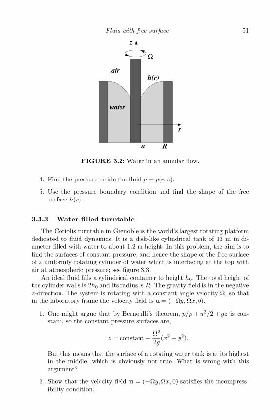
Fluid with free surface 51
air
r
h(r)
a R
z
Ω
water
FIGURE 3.2: Water in an annular flow.
4. Find the pressure inside the fluid p = p(r, z).
5. Use the pressure boundary condition and find the shape of the freesurface h(r).
3.3.3 Water-filled turntable
The Coriolis turntable in Grenoble is the world’s largest rotating platformdedicated to fluid dynamics. It is a disk-like cylindrical tank of 13 m in di-ameter filled with water to about 1.2 m height. In this problem, the aim is tofind the surfaces of constant pressure, and hence the shape of the free surfaceof a uniformly rotating cylinder of water which is interfacing at the top withair at atmospheric pressure; see figure 3.3.
An ideal fluid fills a cylindrical container to height h0. The total height ofthe cylinder walls is 2h0 and its radius is R. The gravity field is in the negativez-direction. The system is rotating with a constant angle velocity Ω, so thatin the laboratory frame the velocity field is u = (−Ωy,Ωx, 0).
1. One might argue that by Bernoulli’s theorem, p/ρ+ u2/2 + gz is con-stant, so the constant pressure surfaces are,
z = constant− Ω2
2g(x2 + y2).
But this means that the surface of a rotating water tank is at its highestin the middle, which is obviously not true. What is wrong with thisargument?
2. Show that the velocity field u = (−Ωy,Ωx, 0) satisfies the incompress-ibility condition.
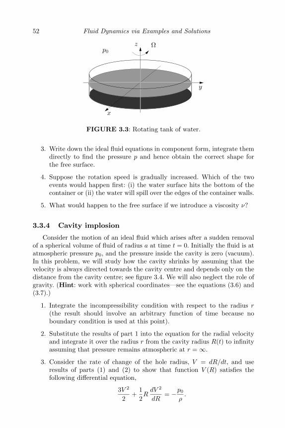
52 Fluid Dynamics via Examples and Solutions
p0
x
y
z Ω
FIGURE 3.3: Rotating tank of water.
3. Write down the ideal fluid equations in component form, integrate themdirectly to find the pressure p and hence obtain the correct shape forthe free surface.
4. Suppose the rotation speed is gradually increased. Which of the twoevents would happen first: (i) the water surface hits the bottom of thecontainer or (ii) the water will spill over the edges of the container walls.
5. What would happen to the free surface if we introduce a viscosity ν?
3.3.4 Cavity implosion
Consider the motion of an ideal fluid which arises after a sudden removalof a spherical volume of fluid of radius a at time t = 0. Initially the fluid is atatmospheric pressure p0, and the pressure inside the cavity is zero (vacuum).In this problem, we will study how the cavity shrinks by assuming that thevelocity is always directed towards the cavity centre and depends only on thedistance from the cavity centre; see figure 3.4. We will also neglect the role ofgravity. (Hint: work with spherical coordinates—see the equations (3.6) and(3.7).)
1. Integrate the incompressibility condition with respect to the radius r(the result should involve an arbitrary function of time because noboundary condition is used at this point).
2. Substitute the results of part 1 into the equation for the radial velocityand integrate it over the radius r from the cavity radius R(t) to infinityassuming that pressure remains atmospheric at r =∞.
3. Consider the rate of change of the hole radius, V = dR/dt, and useresults of parts (1) and (2) to show that function V (R) satisfies thefollowing differential equation,
3V 2
2+
1
2RdV 2
dR= −p0
ρ.
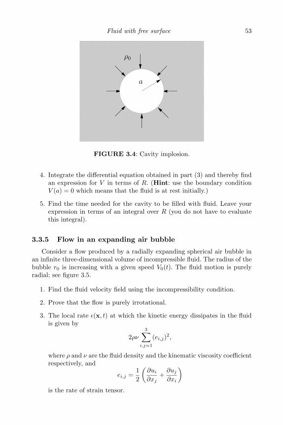
Fluid with free surface 53
ρ0
a
FIGURE 3.4: Cavity implosion.
4. Integrate the differential equation obtained in part (3) and thereby findan expression for V in terms of R. (Hint: use the boundary conditionV (a) = 0 which means that the fluid is at rest initially.)
5. Find the time needed for the cavity to be filled with fluid. Leave yourexpression in terms of an integral over R (you do not have to evaluatethis integral).
3.3.5 Flow in an expanding air bubble
Consider a flow produced by a radially expanding spherical air bubble inan infinite three-dimensional volume of incompressible fluid. The radius of thebubble r0 is increasing with a given speed V0(t). The fluid motion is purelyradial; see figure 3.5.
1. Find the fluid velocity field using the incompressibility condition.
2. Prove that the flow is purely irrotational.
3. The local rate ε(x, t) at which the kinetic energy dissipates in the fluidis given by
2ρν
3∑i,j=1
(ei,j)2,
where ρ and ν are the fluid density and the kinematic viscosity coefficientrespectively, and
ei,j =1
2
(∂ui∂xj
+∂uj∂xi
)is the rate of strain tensor.
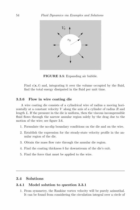
54 Fluid Dynamics via Examples and Solutions
V0
r0
FIGURE 3.5: Expanding air bubble.
Find ε(x, t) and, integrating it over the volume occupied by the fluid,find the total energy dissipated in the fluid per unit time.
3.3.6 Flow in wire coating die
A wire coating die consists of a cylindrical wire of radius a moving hori-zontally at a constant velocity V along the axis of a cylinder of radius R andlength L. If the pressure in the die is uniform, then the viscous incompressiblefluid flows through the narrow annular region solely by the drag due to themotion of the wire; see figure 3.6.
1. Formulate the no-slip boundary conditions on the die and on the wire.
2. Establish the expression for the steady-state velocity profile in the an-nular region of the die.
3. Obtain the mass flow rate through the annular die region.
4. Find the coating thickness b far downstream of the die’s exit.
5. Find the force that must be applied to the wire.
3.4 Solutions
3.4.1 Model solution to question 3.3.1
1. From symmetry, the Rankine vortex velocity will be purely azimuthal.It can be found from considering the circulation integral over a circle of

Fluid with free surface 55
L
V
x
R
a
r
u(r)
die
wire
air
b
FIGURE 3.6: Flow in a wire coating die.
radius r centred at the vortex centre;∮Cr
uφ dl =
∫Dr
ω(r) d2x,
where Dr is the disc bounded by circle Cr with radius r.
The left-hand side here is equal to 2πruφ (because uφ is constant on Cr),and the right-hand side is to be found using cylindrical coordinates. Thisgives:
uφ =Ωr
2for r < a,
uφ =Ωa2
2rfor r ≥ a.
2. Bernoulli’s theorem can be used for r > a because this region is irrota-tional (ω = 0). Region r ≤ a is not irrotational, and Bernoulli’s theoremsays that Bernoulli’s potential is constant along streamlines, but it canhave different value on different streamlines. This information is uselessfor finding the solution for the surface shape at r ≤ a.
3. First we find a solution for r > a from the Bernoulli’s theorem at thefluid surface taking into account that the pressure at the surface z = h(r)is constant equal to the atmospheric pressure p0:
u2
2+p
ρ+ gh(r) = const.
Substituting u we have:
h(r) = h∞ −Ω2a4
8gr2for r ≥ a,
56 Fluid Dynamics via Examples and Solutions
where h∞ is the height of undisturbed water surface.
To find solution for r ≤ a, we write the steady-state Euler equation incomponents,
(u · ∇)u = −∂xp/ρ,(u · ∇)v = −∂yp/ρ,
0 = −∂zp/ρ− g;
or
xΩ2 = −∂xp/ρ,yΩ2 = −∂yp/ρ,
0 = −∂zp/ρ− g.
Integrating, we have
p
ρ=
Ω2
2(x2 + y2)− gz + const.
On the surface we have
h(r) =Ω2r2
2g+ h0 for r < a.
By matching at r = a we find h0 = h∞ − 5Ω2a2
8g .
3.4.2 Model solution to question 3.3.2
1. No-slip boundary conditions: fluid velocity at the boundaries coincideswith the one of the boundaries
uθ(a) = Ωa, uθ(R) = 0.
At the free surfacep(r, h(r)) = p0.
2.
∇ · u =1
r
∂(rur)
∂r+
1
r
∂uθ∂θ
+∂uz∂z
.
Now, ur = uz = 0 and uθ is independent of θ, so ∇ · u = 0.
3. Note that uθ is constant along the streamlines in this flow, Dtuθ = 0.Pressure is independent of θ. Thus, the steady-state Navier-Stokes forthe azimuthal component is
0 = ν1
r∂r (r∂ruθ) .
Fluid with free surface 57
Solving this equation we have
uθ =C1
r+ C2r.
Matching to the boundary condition gives
uθ =Ωa2R
R2 − a2
(R
r− r
R
).
4. The steady-state Navier-Stokes equation in the radial component is
u2θ
r=
1
ρ∂rp.
Substituting here the solution for uθ and integrating, we get
p =ρΩ2a4R2
(R2 − a2)2
(−R
2
2r2− 2 ln r +
r2
2R2
)+ f1(z).
For the z-component:
0 = −1
ρ∂zp− g,
or p = −ρgz + f2(r). Combining, we have
p =ρΩ2a4R2
(R2 − a2)2
(−R
2
2r2− 2 ln r +
r2
2R2
)− ρgz + C3.
5. Using the free-surface pressure condition,
h(r) = h(R) +Ω2a4R2
g(R2 − a2)2
(−R
2
2r2− 2 ln
r
R+
r2
2R2
).
3.4.3 Model solution to question 3.3.3
1. This version of the Bernoulli’s theorem would only be valid for irrota-tional flows. Our flow is not irrotational because it has finite vorticity,|ω| = 2Ω.
2. We have ∇ · u = −Ω∂xy + Ω∂yx = 0.
3. The steady-state Euler equation in components:
(u · ∇)u = −∂xp/ρ,(u · ∇)v = −∂yp/ρ,
0 = −∂zp/ρ− g;

58 Fluid Dynamics via Examples and Solutions
or
xΩ2 = −∂xp/ρ,yΩ2 = −∂yp/ρ,
0 = −∂zp/ρ− g.
Integrating, we have
p
ρ=
Ω2
2(x2 + y2)− gz + C,
where C = const. On the surface we have
h(r) = C1 +Ω2r2
2g
with C1 = C − p0ρ . The fluid volume is conserved,
V = 2π
∫ R
0
h(r) r dr = 2π
∫ R
0
[C +
Ω2r2
2g
]r dr =
πR2C1 +πΩ2R4
4g= const = πR2h0,
so
C1 = h0 −Ω2R2
4g,
and finally
h(r) = h0 +Ω2(2r2 −R2)
4g.
4. We have to compare h(0) and h(R):
h(0) = h0 −Ω2R2
4gand h(R) = h0 +
Ω2R2
2g.
Thus, the surface drop in the centre is exactly twice less than the surfacerise at the edges, which means that in our case the spill should occurbefore touching the bottom.
5. Viscosity would not change the results because the velocity field is linearin x and, therefore, its Laplacian is zero.
3.4.4 Model solution to question 3.3.4
1. From the incompressibility condition ∂r(r2v) = 0. Integrating this equa-
tion we have r2v = f(t), where f is an arbitrary function.
Fluid with free surface 59
2. The radial component of the Euler equation is
∂tv + v∂rv = −1
ρ∂rp.
Substituting in here for v, we have:
f ′
r2+
1
2∂rv
2 = −∂r(p/ρ).
Integrating over r from R to infinity, we have:
−f′
R+
1
2V 2 = p0/ρ.
We have used the boundary conditions v(R) = V, v(∞) = 0, p(R) = 0and p(∞) = p0.
3. For the function f we have f = vr2 = V R2 differentiating which weobtain:
f ′ = V ′(R)R2R′ + V 2RR′ = V ′V R2 + 2V 2R.
Substituting this into part 2, we have:
−3
2V 2 − V ′R2
RV = p0/ρ
or
3V 2 +RdV 2
dR= −2p0/ρ.
4. Separating variables V 2 and R,
dV 2
2p03ρ + V 2
= −3dR
R,
and integrating, we have:
2p0
3ρ+ V 2 =
C
R3.
where constant C is to be found from V (a) = 0. This gives C = 2p0a3
3ρ ,so that
V 2 =2p0
3ρ(a3/R3 − 1).
We choose V < 0, therefore
V = −√
2p0
3ρ(a3/R3 − 1).
5. Integrating, we find for the implosion time:
τ =
∫ a
0
dR
V=
√2p0
3ρ
∫ a
0
dR√a3/R3 − 1
.
60 Fluid Dynamics via Examples and Solutions
3.4.5 Model solution to question 3.3.5
1. Because of the incompressibility condition, the volume flux through thespheres of different radii is the same. Hence:
ur = V0r20/r
2.
2. In Cartesian frame
u = (u, v, w) =
(V0r
20x
r3,V0r
20y
r3,V0r
20z
r3
).
The flow is purely irrotational:
ωz = (∇× u)z = ∂xv − ∂yy = −3V0r20x2y
2r5+
3V0r20y2x
2r5= 0
and the same for ωx and ωy.
3. Since ∇× u = 0, we have ∂iuj = ∂jui. Therefore
eij =1
2
(∂ui∂xj
+∂uj∂xi
)=∂ui∂xj
=V0r
20
r3
(δij − 3
xixjr2
).
Thus, for the kinetic energy density dissipation rate we have:
ε(x, t) = 2ρν
3∑i,j=1
(ei,j)2 = 2ρν
3∑i,j=1
V 20 r
40
r6
(δijδij − 6δij
xixjr2
+ 9x2ix
2j
r4
)=
12ρνV 2
0 r40
r6.
Integrating it over the volume occupied by the fluid, we find the totalenergy dissipated in the fluid per unit time:
E = 4π
∫ ∞r0
r2ε(x, t) dr = 16πρνV 20 r0.
3.4.6 Model solution to question 3.3.6
1. The no-slip boundary conditions are ux(R) = 0, ux(a) = V.
2. The flow is stationary and it is not pressure driven, ∇p = 0. Then thex-component of Navier-Stokes equation becomes:
ν1
r∂r(r∂rux) = 0.
Integrating twice we find:
ux = C1 ln r + C2.
Fluid with free surface 61
Using the no-slip boundary conditions we have:
ux = Vln r
R
ln aR
.
3. We have for the mass flux:
Q = ρ
∫ R
a
ux2πrdr =2πρV
ln aR
∫ R
a
r lnr
Rdr =
πρV R2
2 ln Ra
[1 +
a2
R2
(2 ln
a
R− 1)].
4. Q = ρV π(b2 − a2), so b =√a2 −Q/(πρV ).
5. Force = stress × area, so
F = ρν|∂rux|r=a(2πaL) =2πρνV L
ln Ra
.

This page intentionally left blankThis page intentionally left blank
Chapter 4
Waves and instabilities
4.1 Background theory
4.1.1 Waves
Waves represent one of the most common types of fluid motion: sea waveson water surface, internal waves in stratified oceans and atmospheres (oftenseen in cloud patterns), inertial waves in rotating fluids, Rossby waves ofplanetary scales important for the weather and climate dynamics, sound wavesin air and many more important examples.
The basic element of the wave dynamics in most applications is the simplesttype of wave, monochromatic wave: it is a fluid motion in which all relevantphysical fields a(x, t) behave like
a(x, t) = A cos (k · x− ωt+ ϕ) , (4.1)
where A ∈ R+ is the wave amplitude, k ∈ Rd is the wave vector in a d-dimensional space (e.g. d = 2 for the water surface waves, d = 3 for the soundwaves in air, etc.), ϕ ∈ R is the wave phase and ω ∈ R is the angular wavefrequency (measured in radians per second), which thereafter will be calledsimply the frequency. The frequency is related to k via a dispersion relation,
ω = ω(k), (4.2)
the form of which depends on the particular type of waves. For isotropicsystems ω depends only on the magnitude of the wave vector, k = |k|, andnot on its direction. If for isotropic systems ω is a linear function of k = |k|(like e.g. for sound waves), the waves are called non-dispersive. For anisotropicsystems, the waves are called non-dispersive if ω is a linear function of k timesan arbitrary function of the unit vector along k (orientation). Otherwise thewaves are called dispersive. The origin of this name will become clear whenwe solve question 4.3.1.
Note that different fluid quantities, such as the pressure, density and dif-ferent velocity components, will have their own interrelated amplitudes A andphases ϕ. This is where one finds a possibility of various wave polarisations—plane, circular, elliptic—which refers to the shape of the curve traced in timeby the tip of the velocity vector at a fixed point x in the course of one wave
63
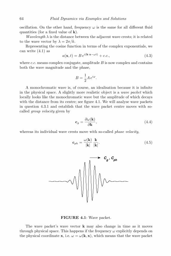
64 Fluid Dynamics via Examples and Solutions
oscillation. On the other hand, frequency ω is the same for all different fluidquantities (for a fixed value of k).
Wavelength λ is the distance between the adjacent wave crests; it is relatedto the wave vector by λ = 2π/k.
Representing the cosine function in terms of the complex exponentials, wecan write (4.1) as
a(x, t) = B ei(k·x−ωt) + c.c., (4.3)
where c.c.means complex conjugate, amplitudeB is now complex and containsboth the wave magnitude and the phase,
B =1
2Aeiϕ.
A monochromatic wave is, of course, an idealisation because it is infinitein the physical space. A slightly more realistic object is a wave packet whichlocally looks like the monochromatic wave but the amplitude of which decayswith the distance from its centre; see figure 4.1. We will analyse wave packetsin question 4.3.1 and establish that the wave packet centre moves with so-called group velocity given by
cg =∂ω(k)
∂k, (4.4)
whereas its individual wave crests move with so-called phase velocity,
cph =ω(k)
|k|k
|k|. (4.5)
Cg , C
ph
FIGURE 4.1: Wave packet.
The wave packet’s wave vector k may also change in time as it movesthrough physical space. This happens if the frequency ω explicitly depends onthe physical coordinate x, i.e. ω = ω(k,x), which means that the wave packet
Waves and instabilities 65
is moving in a non-uniform background, e.g. a medium with inhomogeneousdensity and/or velocity field.
In physical space, one can represent the wave packet as:
a(x, t) = A(εx, εt) eiεψ(εx,εt) + c.c., (4.6)
where A ∈ C is a slowly varying wave amplitude and 1εψ ∈ R is the wave
phase. The formal small parameter ε is introduced here to make the space-timedependence in A slow and to make the phase values large (so that the phasederivatives are order one). Without loss of generality one can take ψ(0, 0) = 0.Indeed, to remove a non-zero value of ψ(0, 0) one could simply redefine A sothat in the leading (ε0) order the phase is a linear function of x and t. Then, inthe leading order we recover the monochromatic wave (4.3) and the dispersionrelation (4.2), in which
k =1
ε∇ψ(εx, εt) and ω =
1
ε∂tψ(εx, εt). (4.7)
But relations (4.7) imply that for the wave packet
∂tk = −∇ω. (4.8)
In the next (ε1) order one gets the so-called transport equation governingthe evolution of the amplitude A, but we will not consider it here.
Changes in k would in turn lead to changes in the group velocity cg: thewave packet may slow down or accelerate or change direction of its propagationup to turning back (reflection). Finding the wave packet trajectory in the(x,k)-space is called ray tracing. It is done by solving the ray tracing equationswhich follow from equations (4.5) and (4.8):
x(t) =∂ω(k,x)
∂k, (4.9)
k(t) = −∇ω(k,x), (4.10)
where the dot means the time derivative. Note that here x(t) and k(t) aretime-dependent vectors and not an independent coordinate x and a vectorfield k(x, t) as before.
4.1.2 Instabilities
The concept of stability of an equilibrium state is very natural in oureveryday life, and it can be most easily illustrated by an example given infigure 4.2. On the left we see a ball at the bottom of a dimple. If we pushthe ball slightly out of equilibrium, it will experience a restoring force actingtoward the equilibrium point: this equilibrium is stable. On the right we see aball on the top of a hill. Slight disturbance will set this ball in a motion thatwill take it away from the equilibrium point: this equilibrium is unstable.
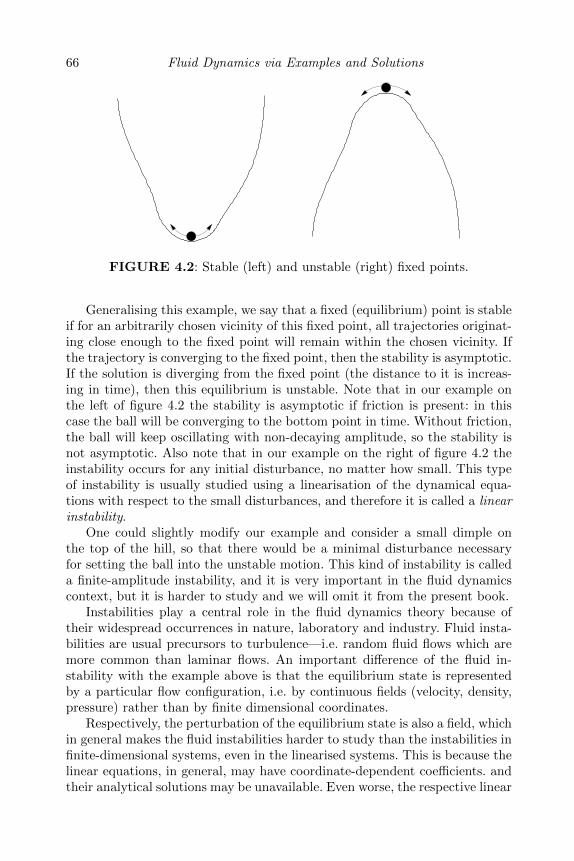
66 Fluid Dynamics via Examples and Solutions
FIGURE 4.2: Stable (left) and unstable (right) fixed points.
Generalising this example, we say that a fixed (equilibrium) point is stableif for an arbitrarily chosen vicinity of this fixed point, all trajectories originat-ing close enough to the fixed point will remain within the chosen vicinity. Ifthe trajectory is converging to the fixed point, then the stability is asymptotic.If the solution is diverging from the fixed point (the distance to it is increas-ing in time), then this equilibrium is unstable. Note that in our example onthe left of figure 4.2 the stability is asymptotic if friction is present: in thiscase the ball will be converging to the bottom point in time. Without friction,the ball will keep oscillating with non-decaying amplitude, so the stability isnot asymptotic. Also note that in our example on the right of figure 4.2 theinstability occurs for any initial disturbance, no matter how small. This typeof instability is usually studied using a linearisation of the dynamical equa-tions with respect to the small disturbances, and therefore it is called a linearinstability.
One could slightly modify our example and consider a small dimple onthe top of the hill, so that there would be a minimal disturbance necessaryfor setting the ball into the unstable motion. This kind of instability is calleda finite-amplitude instability, and it is very important in the fluid dynamicscontext, but it is harder to study and we will omit it from the present book.
Instabilities play a central role in the fluid dynamics theory because oftheir widespread occurrences in nature, laboratory and industry. Fluid insta-bilities are usual precursors to turbulence—i.e. random fluid flows which aremore common than laminar flows. An important difference of the fluid in-stability with the example above is that the equilibrium state is representedby a particular flow configuration, i.e. by continuous fields (velocity, density,pressure) rather than by finite dimensional coordinates.
Respectively, the perturbation of the equilibrium state is also a field, whichin general makes the fluid instabilities harder to study than the instabilities infinite-dimensional systems, even in the linearised systems. This is because thelinear equations, in general, may have coordinate-dependent coefficients. andtheir analytical solutions may be unavailable. Even worse, the respective linear
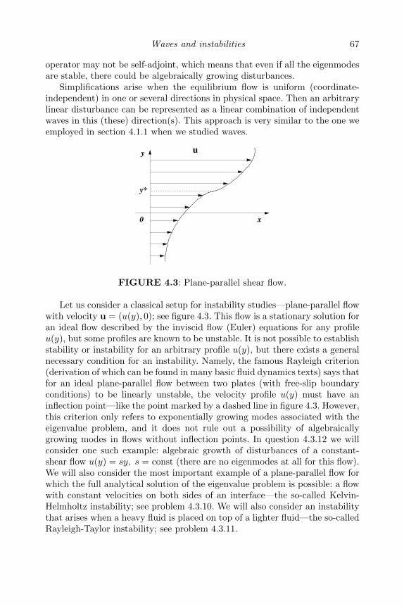
Waves and instabilities 67
operator may not be self-adjoint, which means that even if all the eigenmodesare stable, there could be algebraically growing disturbances.
Simplifications arise when the equilibrium flow is uniform (coordinate-independent) in one or several directions in physical space. Then an arbitrarylinear disturbance can be represented as a linear combination of independentwaves in this (these) direction(s). This approach is very similar to the one weemployed in section 4.1.1 when we studied waves.
u
x0
y*
y
FIGURE 4.3: Plane-parallel shear flow.
Let us consider a classical setup for instability studies—plane-parallel flowwith velocity u = (u(y), 0); see figure 4.3. This flow is a stationary solution foran ideal flow described by the inviscid flow (Euler) equations for any profileu(y), but some profiles are known to be unstable. It is not possible to establishstability or instability for an arbitrary profile u(y), but there exists a generalnecessary condition for an instability. Namely, the famous Rayleigh criterion(derivation of which can be found in many basic fluid dynamics texts) says thatfor an ideal plane-parallel flow between two plates (with free-slip boundaryconditions) to be linearly unstable, the velocity profile u(y) must have aninflection point—like the point marked by a dashed line in figure 4.3. However,this criterion only refers to exponentially growing modes associated with theeigenvalue problem, and it does not rule out a possibility of algebraicallygrowing modes in flows without inflection points. In question 4.3.12 we willconsider one such example: algebraic growth of disturbances of a constant-shear flow u(y) = sy, s = const (there are no eigenmodes at all for this flow).We will also consider the most important example of a plane-parallel flow forwhich the full analytical solution of the eigenvalue problem is possible: a flowwith constant velocities on both sides of an interface—the so-called Kelvin-Helmholtz instability; see problem 4.3.10. We will also consider an instabilitythat arises when a heavy fluid is placed on top of a lighter fluid—the so-calledRayleigh-Taylor instability; see problem 4.3.11.
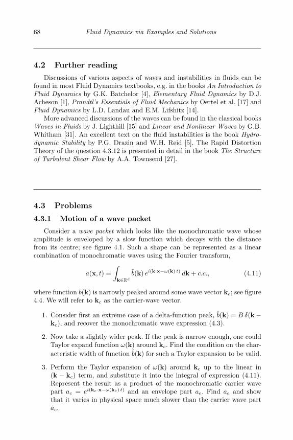
68 Fluid Dynamics via Examples and Solutions
4.2 Further reading
Discussions of various aspects of waves and instabilities in fluids can befound in most Fluid Dynamics textbooks, e.g. in the books An Introduction toFluid Dynamics by G.K. Batchelor [4], Elementary Fluid Dynamics by D.J.Acheson [1], Prandtl’s Essentials of Fluid Mechanics by Oertel et al. [17] andFluid Dynamics by L.D. Landau and E.M. Lifshitz [14].
More advanced discussions of the waves can be found in the classical booksWaves in Fluids by J. Lighthill [15] and Linear and Nonlinear Waves by G.B.Whitham [31]. An excellent text on the fluid instabilities is the book Hydro-dynamic Stability by P.G. Drazin and W.H. Reid [5]. The Rapid DistortionTheory of the question 4.3.12 is presented in detail in the book The Structureof Turbulent Shear Flow by A.A. Townsend [27].
4.3 Problems
4.3.1 Motion of a wave packet
Consider a wave packet which looks like the monochromatic wave whoseamplitude is enveloped by a slow function which decays with the distancefrom its centre; see figure 4.1. Such a shape can be represented as a linearcombination of monochromatic waves using the Fourier transform,
a(x, t) =
∫k∈Rd
b(k) ei(k·x−ω(k) t) dk + c.c., (4.11)
where function b(k) is narrowly peaked around some wave vector kc; see figure4.4. We will refer to kc as the carrier-wave vector.
1. Consider first an extreme case of a delta-function peak, b(k) = B δ(k−kc), and recover the monochromatic wave expression (4.3).
2. Now take a slightly wider peak. If the peak is narrow enough, one couldTaylor expand function ω(k) around kc. Find the condition on the char-
acteristic width of function b(k) for such a Taylor expansion to be valid.
3. Perform the Taylor expansion of ω(k) around kc up to the linear in(k − kc) term, and substitute it into the integral of expression (4.11).Represent the result as a product of the monochromatic carrier wavepart ac = ei(kc·x−ω(kc) t) and an envelope part ae. Find ae and showthat it varies in physical space much slower than the carrier wave partac.
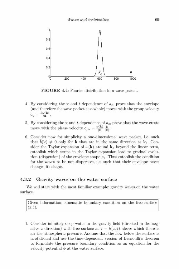
Waves and instabilities 69
0 200 400 600 800 10000
0.2
0.4
0.6
0.8
1
kk0
FIGURE 4.4: Fourier distribution in a wave packet.
4. By considering the x and t dependence of ae, prove that the envelope(and therefore the wave packet as a whole) moves with the group velocity
cg = ∂ω(k)∂k .
5. By considering the x and t dependence of ac, prove that the wave crests
move with the phase velocity cph = ω(k)|k|
k|k| .
6. Consider now for simplicity a one-dimensional wave packet, i.e. suchthat b(k) 6= 0 only for k that are in the same direction as kc. Con-sider the Taylor expansion of ω(k) around kc beyond the linear term,establish which terms in the Taylor expansion lead to gradual evolu-tion (dispersion) of the envelope shape ae. Thus establish the conditionfor the waves to be non-dispersive, i.e. such that their envelope neverchanges its shape.
4.3.2 Gravity waves on the water surface
We will start with the most familiar example: gravity waves on the watersurface.
Given information: kinematic boundary condition on the free surface(3.4).
1. Consider infinitely deep water in the gravity field (directed in the neg-ative z direction) with free surface at z = h(x, t) above which there isair the atmospheric pressure. Assume that the flow below the surface isirrotational and use the time-dependent version of Bernoulli’s theoremto formulate the pressure boundary condition as an equation for thevelocity potential φ at the water surface.

70 Fluid Dynamics via Examples and Solutions
2. Consider a plane wave solution
h(x, t) =H
2ei(kx−ωt) + c.c., φ(x, z, t) = B(z) ei(kx−ωt) + c.c., (4.12)
where H is a real constant (wave amplitude) and B(z) is a complexfunction.
From the incompressibility condition and the condition that the velocityfield must vanish as z → −∞, find the shape of the function B(z).
3. Substitute (4.12) into the equations expressing the pressure and thekinematic boundary conditions and, assuming that the wave is weak,linearise these equations. Find the expressions of the frequency ω as afunction of k and g, and the function B(z) in terms of H, k and g (gbeing the gravity acceleration constant).
4. Find a condition on the wave amplitude H under which the linearisationprocedure is justified. What does it mean in terms of the water surfaceinclination?
5. Find the phase and the group velocities of the gravity wave. What is theratio of these velocities?
6. Find the shape of the fluid paths under the water surface.
4.3.3 Gravity and capillary waves: dimensional analysis
In this problem we will study waves on the water surface: gravity waveswhich appear at larger scales and capillary waves at smaller scales. We will notsolve the fluid equations with free surface in presence of gravity and surfacetension, but we will take a short-cut by postulating that the wave propertiesin the respective situations may only be determined by relevant dimensionalphysical constants: the gravity acceleration in the case of the gravity wavesand the surface tension coefficient and the water density in the case of thecapillary waves.
1. Consider water in the gravity field with free surface above which thereis air the atmospheric pressure. Argue why the pressure of air above thefree surface cannot enter the force balance of the moving fluid particlesand, therefore, they will not enter into the characteristics of the waterwaves.
2. Consider a monochromatic wave on the free surface of infinitely deepwater in presence of gravity (ignore the surface tension for now). Sincethe air pressure is irrelevant, and because there is no characteristic lengthscale in the infinite depth ocean at rest, the only other physical quantitiesthat could determine the properties of the linear waves are the gravityconstant g, the wave vector magnitude k and the water density ρ.
Waves and instabilities 71
Find the physical dimensions of g, k and the wave frequency ω. Find theonly possible combination of g, ρ and k which would have the dimensionof ω and, therefore, find the dispersion relation ω = ω(k) for the gravitywaves. (As usual, such a dimensional method leaves uncertainty up toan order of one dimensionless constant, which in our case appears to beabsent).
Does this relation depend on ρ? Why?
3. Now consider a monochromatic capillary wave on the free surface ofinfinitely deep water whose oscillations are due to the surface tensionforces (ignore gravity). Find the physical dimension of the surface ten-sion coefficient σ, based on its definition as a force per unit length (thinkof a force produced by a soap film onto a wire to which it is attached).
4. Find the unique combination of σ, ρ and k which would have the di-mension of ω and, therefore, find the dispersion relation ω = ω(k) forthe capillary waves. (Again, the undetermined dimensionless constant,in this case appears to be absent).
5. Now consider a system in which both gravity and surface tension arepresent. Find the crossover wave length at which the capillary effect be-comes more important than the gravity effect. Surface tension coefficientat room temperature is about 0.072 Newton per meter, and the gravityconstant is 9.8 m/s2. Use these values to find the crossover wave length.
4.3.4 Inertial waves in rotating fluids
Given information: Euler equation in a uniformly rotating frame of ref-erence (1.12) (with ν = f = 0).
This problem concerns the dynamics of inertial waves, i.e. small perturba-tions to the state of uniform rotation.
1. Write down an expression for the velocity field corresponding to uniformrotation. Find the vorticity corresponding to this flow.
2. Consider a small perturbation u to the state of uniform rotation (withan angular velocity Ω) which has the form of a harmonic wave
u = A ei(k·x−ωt) + A∗ e−i(k·x−ωt),
where k is the wave vector, ω is the frequency, A is the complex am-plitude and A∗ is the complex conjugate of A. How small does theamplitude A need to be for the nonlinear (with respect to A) terms tobe much smaller than the linear ones in the fluid equations?
72 Fluid Dynamics via Examples and Solutions
3. Consider the linearised equations of motion and derive the dispersionrelation ω = ω(k). (Hint: Take the curl of the Euler equation (1.12)and use the identity ∇× (Ω× u) = −(Ω · ∇)u).
4. What is the polarisation of the inertial waves?
5. Are these waves dispersive or non-dispersive? Isotropic or anisotropic?Explain why.
Find the group velocity for the inertial waves and comment on its relativedirection with respect to the wave number.
4.3.5 Internal waves in stratified fluids
In this problem we will study waves that arise due to stratification of thefluid density: the so-called internal waves. They play important roles in bothatmospheric and ocean dynamics. In particular, in the oceans they provide theprincipal mechanism for bringing the global conveyor belt currents from theocean’s bottom to the surface, and as such they are one of the key ingredientsin climate dynamics.
Equations for inviscid incompressible fluid in the presence of a densitystratification are (1.5), (1.3) and (1.4). In the presence of gravity f = −g z,these equations become
∂tu + (u · ∇)u = −1
ρ∇p− g z, (4.13)
∇ · u = 0 (4.14)
and∂tρ+ u · ∇ρ = 0. (4.15)
Consider an incompressible fluid subject to gravity, which at rest has anexponential density profile,
ρ = ρ0(z) = ρ0(0) e−z/h.
1. Find the equilibrium pressure profile p0(z).
2. Consider perturbations around the equilibrium state,
ρ = ρ0(z) + ρ, u = u,
and linearise the fluid equations (4.13) and (4.15).
Consider perturbations in the form of a harmonic wave
u =A√ρ0(z)
ei(k·x−ωt) + c.c., (4.16)
ρ = R√ρ0(z) ei(k·x−ωt) + c.c., (4.17)
p = P√ρ0(z) ei(k·x−ωt) + c.c., (4.18)
Waves and instabilities 73
where k ∈ R3 is the wave vector, ω ∈ R is the frequency, A ∈ C3 is aconstant vector and R ∈ C and P ∈ C are constant scalars; c.c. standsfor “complex conjugate”.
Substituting (4.16), (4.17) and (4.18) into the linearised equations, findthe wave dispersion relation, ω = ω(k).
3. Are these waves dispersive or non-dispersive? Isotropic or anisotropic?Explain why.
Consider the short-wave limit kh 1. Find the group velocity for theinertial waves and comment on its relative direction with respect to thewave vector.
4.3.6 Sound waves in compressible fluids
Equations for inviscid compressible flow are (1.5), (1.6) and (1.7). In ab-sence of forcing (f = 0) for isentropic motions (S = const) of polytropic gas,these equations become
∂tu + (u · ∇)u = −1
ρ∇p, (4.19)
∂tρ+∇ · (ρu) = 0 (4.20)
withp
ργ= const, (4.21)
where γ = const is the adiabatic index.Consider a uniform gas at rest with ρ = ρ0 = const, p = p0 = const and
u = 0. Small perturbations of such a state (ρ, p and u respectively) propagateas acoustic waves (sound) which will be studied in the present problem.
1. Substitute the disturbed fields ρ = ρ0 + ρ, p = p0 + p and u = u intothe equations (4.19), (4.20) and (4.21) and, assuming the perturbationsto be small, linearise these equations.
2. Consider perturbations of the form of a harmonic wave
u = A ei(k·x−ωt) + A∗ e−i(k·x−ωt), (4.22)
ρ = B ei(k·x−ωt) +B∗ e−i(k·x−ωt), (4.23)
where k is the wave vector, ω is the frequency, A and B are the com-plex amplitude vector and scalar respectively, and A∗ and B∗ are theircomplex conjugates.
Substituting (4.22) and (4.23) into the linearised equations, find thesound-wave dispersion relation, ω = ω(k), as well as the relation betweenA and B.
3. How small does the amplitude A need to be for the linearisation of thefluid equations to be valid?
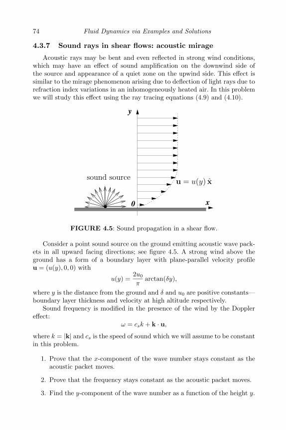
74 Fluid Dynamics via Examples and Solutions
4.3.7 Sound rays in shear flows: acoustic mirage
Acoustic rays may be bent and even reflected in strong wind conditions,which may have an effect of sound amplification on the downwind side ofthe source and appearance of a quiet zone on the upwind side. This effect issimilar to the mirage phenomenon arising due to deflection of light rays due torefraction index variations in an inhomogeneously heated air. In this problemwe will study this effect using the ray tracing equations (4.9) and (4.10).
y
0 x
sound sourceu = u(y) x
FIGURE 4.5: Sound propagation in a shear flow.
Consider a point sound source on the ground emitting acoustic wave pack-ets in all upward facing directions; see figure 4.5. A strong wind above theground has a form of a boundary layer with plane-parallel velocity profileu = (u(y), 0, 0) with
u(y) =2u0
πarctan(δy),
where y is the distance from the ground and δ and u0 are positive constants—boundary layer thickness and velocity at high altitude respectively.
Sound frequency is modified in the presence of the wind by the Dopplereffect:
ω = csk + k · u,
where k = |k| and cs is the speed of sound which we will assume to be constantin this problem.
1. Prove that the x-component of the wave number stays constant as theacoustic packet moves.
2. Prove that the frequency stays constant as the acoustic packet moves.
3. Find the y-component of the wave number as a function of the height y.
Waves and instabilities 75
4. Find the condition for wave packet’s reflection, i.e. for turning its tra-jectory back towards the ground. Find the height of the reflection layery = yr.
5. Sketch the acoustic rays. Explain the amplification of sound on the down-wind side of the source and appearance of a quiet zone upwind of thesource.
4.3.8 Sound rays in stratified flows: wave guides, Snell’s law
When sound rays propagate in a medium with inhomogeneous pressureor/and temperature they deviate from straight lines and may reflect off layerswith higher speed of sound. A quote from Wikipedia:
“The SOFAR channel (short for Sound Fixing and Ranging channel), ordeep sound channel (DSC), is a horizontal layer of water in the ocean at whichdepth the speed of sound is at its minimum. The SOFAR channel acts as awaveguide for sound, and low frequency sound waves within the channel maytravel thousands of miles before dissipating. This phenomenon is an importantfactor in submarine warfare.”
This effect is similar to the refraction and reflection of light rays at theinterfaces of changing refraction index. The relation between the angles ofincidence and refraction is known in optics as Snell’s law. Consequently, asimilar Snell’s law can be found for the angles of incidence and refraction ofthe acoustic rays, which will be the subject of the present problem.
Consider a stratified medium with the speed of sound being amonotonously increasing function of one space coordinate, e.g. height y:cs ≡ cs(y). A sound wave packet is emitted at y = 0 with a positive y-component of the wave number.
1. Prove that the wave number component perpendicular to the y-axisstays constant as the acoustic packet moves.
2. Prove that the frequency stays constant as the acoustic packet moves.
3. Find the y-component of the wave number as a function of the height y.
4. At which position y = yr will the wave packet reflection occur?
5. Sketch the acoustic rays. Also sketch rays in a system which has a speedof sound minimum around some layer ym and discuss this system interms of its wave guiding properties.
6. Suppose now that the speed of sound changes abruptly at a sharp inter-face: cs(y) = c1 for y < y0 and cs(y) = c2 for y > y0, where y0, c1 andc2 are positive constants and c2 > c1.
Find the condition of reflection for a sound ray approaching the interfacefrom y < y0, as well as the relation between the angles of incidence andrefraction (Snell’s law).
76 Fluid Dynamics via Examples and Solutions
4.3.9 Sound rays in a vortex flow: a black hole effect
Consider an acoustic wave packet propagating on background of a velocityfield u(x) produced by a point vortex with circulation Γ:
u(x) =Γ
2πrθ,
where r is the distance from the vortex and θ is a unit vector in the azimuthaldirection.
Interaction with the vortex field will bend the acoustic rays, which may beinterpreted as a scattering process. Remarkably, under certain conditions therays spiral in and fall onto the vortex, which is a fluid dynamics analogy forthe black hole system. Below we will study this effect using the ray tracingequations (4.9) and (4.10).
Sound frequency is modified in presence of a velocity field by the Dopplershift:
ω = csk + k · u,
where k = |k| and cs is the speed of sound which we will assume to be constantin this problem.
1. Prove that the packet’s angular momentum M = kθr stays constant asthe acoustic packet moves. Here kθ is the azimuthal component of thewave number k.
2. Prove that the frequency stays constant as the acoustic packet moves.
3. Find the radial component of the wave number as a function of theradius r.
4. Find the “reflection” condition, i.e. a condition for the wave packetsapproaching the vortex from infinity to turn and to start moving awayfrom the vortex.
5. What happens when the reflection condition is violated? Sketch exam-ples of acoustic rays satisfying and violating the reflection condition.
4.3.10 Kelvin-Helmholtz instability
Consider a plane-parallel shear flow with profile
u = U x for y ≥ 0 and u = −U x for y < 0,
where U = const > 0; see figure 4.6.This flow is a stationary solution of the Euler equation. We will study
evolution of irrotational perturbations of the specified shear flow.
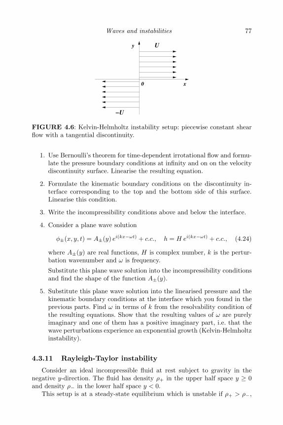
Waves and instabilities 77
−U
0
y
x
U
FIGURE 4.6: Kelvin-Helmholtz instability setup: piecewise constant shearflow with a tangential discontinuity.
1. Use Bernoulli’s theorem for time-dependent irrotational flow and formu-late the pressure boundary conditions at infinity and on on the velocitydiscontinuity surface. Linearise the resulting equation.
2. Formulate the kinematic boundary conditions on the discontinuity in-terface corresponding to the top and the bottom side of this surface.Linearise this condition.
3. Write the incompressibility conditions above and below the interface.
4. Consider a plane wave solution
φ±(x, y, t) = A±(y) ei(kx−ωt) + c.c., h = H ei(kx−ωt) + c.c., (4.24)
where A±(y) are real functions, H is complex number, k is the pertur-bation wavenumber and ω is frequency.
Substitute this plane wave solution into the incompressibility conditionsand find the shape of the function A±(y).
5. Substitute this plane wave solution into the linearised pressure and thekinematic boundary conditions at the interface which you found in theprevious parts. Find ω in terms of k from the resolvability condition ofthe resulting equations. Show that the resulting values of ω are purelyimaginary and one of them has a positive imaginary part, i.e. that thewave perturbations experience an exponential growth (Kelvin-Helmholtzinstability).
4.3.11 Rayleigh-Taylor instability
Consider an ideal incompressible fluid at rest subject to gravity in thenegative y-direction. The fluid has density ρ+ in the upper half space y ≥ 0and density ρ− in the lower half space y < 0.
This setup is at a steady-state equilibrium which is unstable if ρ+ > ρ−,
78 Fluid Dynamics via Examples and Solutions
i.e. when the upper fluid is heavier than the lower one (e.g. water above oil).We will study such an instability by considering evolution of small irrotationalperturbations of the specified configuration.
1. Use Bernoulli’s theorem for time-dependent irrotational flow and for-mulate the pressure boundary condition on the density discontinuitysurface. Linearise the resulting equation.
2. Formulate the kinematic boundary conditions on the discontinuity in-terface corresponding to the top and the bottom side of this surface.Linearise this condition.
3. Write the incompressibility conditions above and below the interface.
4. Consider a plane wave solution
φ±(x, y, t) = A±(y) ei(kx−ωt) + c.c., h = H ei(kx−ωt) + c.c., (4.25)
where A±(y) are real functions, H is a complex number, k is the per-turbation wavenumber and ω is the frequency.
Substitute this plane wave solution into the incompressibility conditionsand find the shape of the function A±(y).
5. Substitute the plane wave solution into the linearised pressure and thekinematic boundary conditions at the interface which you found in theprevious parts. Find ω in terms of k from the resolvability conditionof the resulting equations. Find the condition under which the valuesof ω are purely imaginary and one of them has a positive imaginarypart, i.e. that the wave perturbations experience an exponential growth(Rayleigh-Taylor instability).
4.3.12 Rapid distortion theory
Consider a plane-parallel shear flow with profile
U = s y x, (4.26)
where x is the unit vector along the x-axis, s = const > 0 is the shear rate;see figure 4.7.
This flow is a stationary solution of the Euler equation (1.5) (withoutexternal forcing, f = 0). We will study the evolution of three-dimensionalwave-like perturbations of the specified shear flow. The crucial difference withthe above examples of the Kelvin-Helmholtz and the Rayleigh-Taylor insta-bilities is that in the present case the evolution is “non-modal”, i.e. the wavenumber of the perturbations will no longer be constant, and their growth willnot be exponential but algebraic.
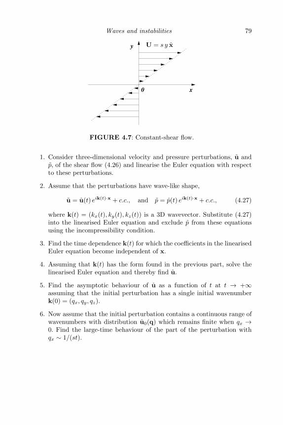
Waves and instabilities 79
0
y
x
U = s y x
FIGURE 4.7: Constant-shear flow.
1. Consider three-dimensional velocity and pressure perturbations, u andp, of the shear flow (4.26) and linearise the Euler equation with respectto these perturbations.
2. Assume that the perturbations have wave-like shape,
u = u(t) eik(t)·x + c.c., and p = p(t) eik(t)·x + c.c., (4.27)
where k(t) = (kx(t), ky(t), kz(t)) is a 3D wavevector. Substitute (4.27)into the linearised Euler equation and exclude p from these equationsusing the incompressibility condition.
3. Find the time dependence k(t) for which the coefficients in the linearisedEuler equation become independent of x.
4. Assuming that k(t) has the form found in the previous part, solve thelinearised Euler equation and thereby find u.
5. Find the asymptotic behaviour of u as a function of t at t → +∞assuming that the initial perturbation has a single initial wavenumberk(0) = (qx, qy, qz).
6. Now assume that the initial perturbation contains a continuous range ofwavenumbers with distribution u0(q) which remains finite when qx →0. Find the large-time behaviour of the part of the perturbation withqx ∼ 1/(st).
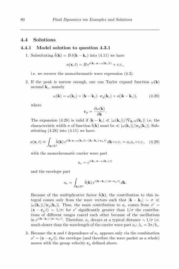
80 Fluid Dynamics via Examples and Solutions
4.4 Solutions
4.4.1 Model solution to question 4.3.1
1. Substituting b(k) = B δ(k− kc) into (4.11) we have
a(x, t) = B ei(kc·x−ω(kc)t) + c.c.,
i.e. we recover the monochromatic wave expression (4.3).
2. If the peak is narrow enough, one can Taylor expand function ω(k)around kc, namely
ω(k) = ω(kc) + (k− kc) · cg(kc) + o(|k− kc|), (4.28)
where
cg =∂ω(k)
∂k.
The expansion (4.28) is valid if |k − kc| |ω(kc)|/|∇kcω(kc)| i.e. the
characteristic width σ of function b(k) must be |ω(kc)|/|cg(kc)|. Sub-stituting (4.28) into (4.11) we have:
a(x, t) ≈∫k∈Rd
b(k) ei(k·x−ω(kc)t−(k−kc)·cg t) dk+c.c. = acae+c.c., (4.29)
with the monochromatic carrier wave part
ac = ei(kc·x−ω(kc) t)
and the envelope part
ae =
∫k∈Rd
b(k) ei(k−kc)·(x−cg t) dk.
Because of the multiplicative factor b(k), the contribution to this in-tegral comes only from the wave vectors such that |k − kc| ∼ σ |ω(kc)|/|cg(kc)|. Thus, the main contribution to ae comes from x′ =(x − cg t) ∼ 1/σ: for x′ significantly greater than 1/σ the contribu-tions of different ranges cancel each other because of the oscillationsin ei(k−kc)·(x−cg t). Therefore, ae decays at a typical distance ∼ 1/σ i.e.much slower than the wavelength of the carrier wave part ac: λc = 2π/kc.
3. Because the x and t dependence of ae appears only via the combinationx′ = (x− cg t), the envelope (and therefore the wave packet as a whole)moves with the group velocity cg defined above.
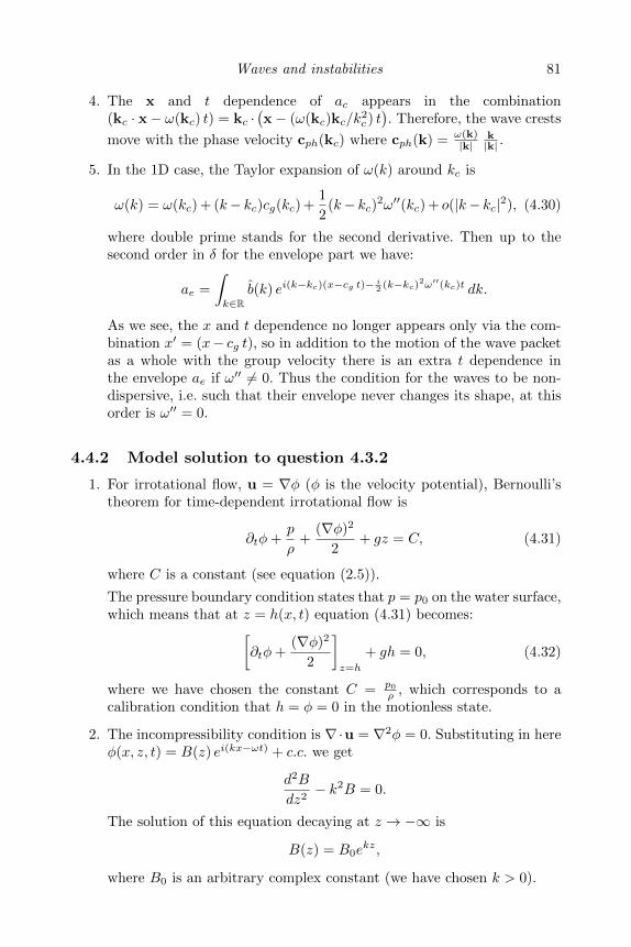
Waves and instabilities 81
4. The x and t dependence of ac appears in the combination(kc · x− ω(kc) t) = kc ·
(x− (ω(kc)kc/k
2c ) t). Therefore, the wave crests
move with the phase velocity cph(kc) where cph(k) = ω(k)|k|
k|k| .
5. In the 1D case, the Taylor expansion of ω(k) around kc is
ω(k) = ω(kc) + (k− kc)cg(kc) +1
2(k− kc)2ω′′(kc) + o(|k− kc|2), (4.30)
where double prime stands for the second derivative. Then up to thesecond order in δ for the envelope part we have:
ae =
∫k∈R
b(k) ei(k−kc)(x−cg t)−i2 (k−kc)2ω′′(kc)t dk.
As we see, the x and t dependence no longer appears only via the com-bination x′ = (x− cg t), so in addition to the motion of the wave packetas a whole with the group velocity there is an extra t dependence inthe envelope ae if ω′′ 6= 0. Thus the condition for the waves to be non-dispersive, i.e. such that their envelope never changes its shape, at thisorder is ω′′ = 0.
4.4.2 Model solution to question 4.3.2
1. For irrotational flow, u = ∇φ (φ is the velocity potential), Bernoulli’stheorem for time-dependent irrotational flow is
∂tφ+p
ρ+
(∇φ)2
2+ gz = C, (4.31)
where C is a constant (see equation (2.5)).
The pressure boundary condition states that p = p0 on the water surface,which means that at z = h(x, t) equation (4.31) becomes:[
∂tφ+(∇φ)2
2
]z=h
+ gh = 0, (4.32)
where we have chosen the constant C = p0ρ , which corresponds to a
calibration condition that h = φ = 0 in the motionless state.
2. The incompressibility condition is ∇·u = ∇2φ = 0. Substituting in hereφ(x, z, t) = B(z) ei(kx−ωt) + c.c. we get
d2B
dz2− k2B = 0.
The solution of this equation decaying at z → −∞ is
B(z) = B0ekz,
where B0 is an arbitrary complex constant (we have chosen k > 0).
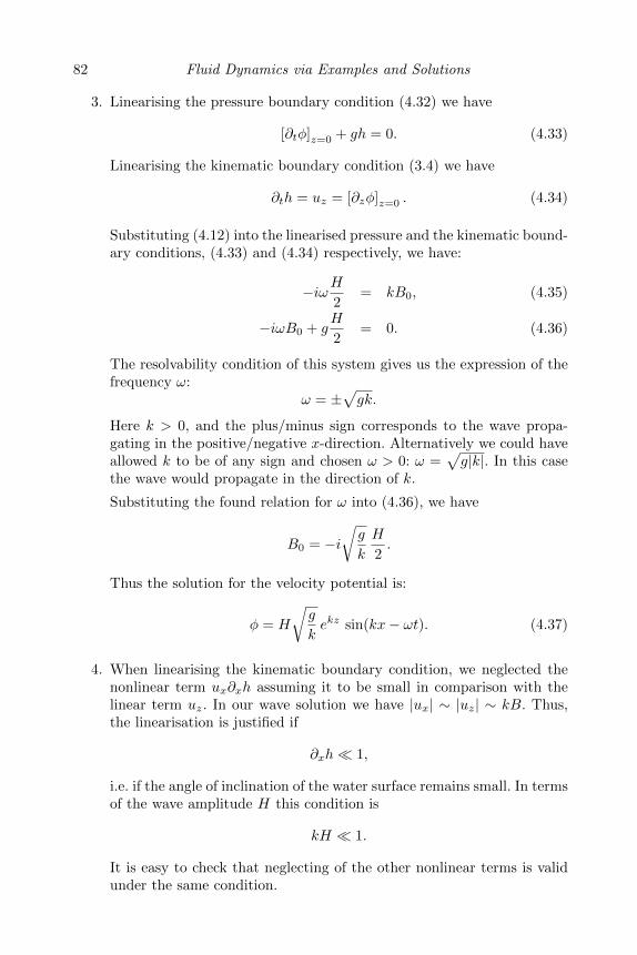
82 Fluid Dynamics via Examples and Solutions
3. Linearising the pressure boundary condition (4.32) we have
[∂tφ]z=0 + gh = 0. (4.33)
Linearising the kinematic boundary condition (3.4) we have
∂th = uz = [∂zφ]z=0 . (4.34)
Substituting (4.12) into the linearised pressure and the kinematic bound-ary conditions, (4.33) and (4.34) respectively, we have:
−iωH2
= kB0, (4.35)
−iωB0 + gH
2= 0. (4.36)
The resolvability condition of this system gives us the expression of thefrequency ω:
ω = ±√gk.
Here k > 0, and the plus/minus sign corresponds to the wave propa-gating in the positive/negative x-direction. Alternatively we could haveallowed k to be of any sign and chosen ω > 0: ω =
√g|k|. In this case
the wave would propagate in the direction of k.
Substituting the found relation for ω into (4.36), we have
B0 = −i√g
k
H
2.
Thus the solution for the velocity potential is:
φ = H
√g
kekz sin(kx− ωt). (4.37)
4. When linearising the kinematic boundary condition, we neglected thenonlinear term ux∂xh assuming it to be small in comparison with thelinear term uz. In our wave solution we have |ux| ∼ |uz| ∼ kB. Thus,the linearisation is justified if
∂xh 1,
i.e. if the angle of inclination of the water surface remains small. In termsof the wave amplitude H this condition is
kH 1.
It is easy to check that neglecting of the other nonlinear terms is validunder the same condition.
Waves and instabilities 83
5. A particle which in the motionless fluid is located at the Eulerian posi-tion (x, z) will move along a Lagrangian path around (x, z):
(x(t), z(t)) = (x, z) + (x(t), z(t)).
For the particle trajectories ˙x(t) = ux, ˙z(t) = uz we have
˙x(t) = ∂xφ = Hω ekz cos(kx− ωt), (4.38)
˙z(t) = ∂zφ = Hω ekz sin(kx− ωt), (4.39)
where we have neglected the deviation of the particle from it equilibriumposition (x, z) in the right-hand sides of the above equations assumingthem to be small (which is valid under the same condition as the lin-earisation procedure).
Equations (4.38) and (4.39) describe motion along the circles
x2 + z2 = r2, where r = Hekz.
4.4.3 Model solution to question 4.3.3
1. Only pressure gradients and not the pressure itself contribute to theforce on a fluid particle. If we added to an existing pressure field aconstant at each point of the physical space, then fluid motion would notchange. Thus the pressure of air above the free surface cannot influencethe dynamical characteristics of the water waves such as, e.g. the wavefrequency.
2. The physical dimension of g is L/T 2—as for any acceleration. The phys-ical dimension of k is 1/L and the physical dimension of the wave fre-quency ω is 1/T . The only possible combination of g, ρ and k whichwould have the dimension of ω is
ω = ω(k) = C√gk,
where C to an order one dimensionless constant (which in this caseappears to be 1).
This expression is independent of the density because the latter containsthe mass dimension (kg) whereas the rest of the quantities, ω, g and kdo not contain the dimension of the mass.
3. The physical dimension of the surface tension coefficient σ, based on itsdefinition as a force per unit length per unit density, is:
[σ] = [mass][acceleration]/L = [kg]/T 2.
4. The unique combination of σ, k and density ρ which would have thedimension of ω is
ω = ω(k) = C
(σ
ρ
)1/2
k3/2,
84 Fluid Dynamics via Examples and Solutions
where C to an order one dimensionless constant (which, again, appearsto be 1).
5. The crossover wave number kc at which the capillary effect become moreimportant than the gravity effects may be estimated from balancing therespective expressions for the gravity and the capillary wave frequencies:
√gk ∼
(σ
ρ
)1/2
k3/2 → kc =
√gρ
σ.
Using the numbers σ = 0.072 N/m, ρ = 1000 kg/m3 and 9.8 m/s2, forthe crossover wave length λc we have:
λc =2π
kc= 2π
√σ
gρ= 0.017 m = 1.7 cm.
4.4.4 Model solution to question 4.3.4
1. The rigid body rotation velocity is U = (Ω× r), so the vorticity is 2Ω.
2. Comparing (u·∇)u and 2(Ω·u): nonlinear term (u·∇)u can be neglectedif u Ω/k.
3. Taking curl of the Euler equation (1.5) (without external forcing, f = 0),we have
∂t∇× u = 2Ω∂zu.
Substituting the plane wave expression, we have
ω(k×A) = 2iΩkzA. (4.40)
After cross multiplication of both sides by k:
−ωk2A = 2iΩkz(k×A). (4.41)
Comparing the equations (4.40) and (4.41) we have
ω = ±2Ωkzk.
4. Substituting the above expression for the frequency into the equation(4.40), we have
A‖ = 0,1
k(k×A⊥) = ±iA⊥, (4.42)
where A‖ and A⊥ are the parallel and the perpendicular to k the pro-jections of A respectively. Thus, the perpendicular to k componentsof A oscillate with the same amplitude and with phase difference π/2with respect to each other (since i = eπ/2), which means that the wavepolarisation is circular.

Waves and instabilities 85
5. For the group velocity we have
cg = ∂kω = ±2Ω
k3(−kzkx,−kzky, k2
⊥). (4.43)
The waves are dispersive: the group velocity depends on k = |k| forany fixed direction of k. The waves are anisotropic: ω depends on thedirection of k for any fixed k = |k|.
From the equation (4.43) we have cg · k = 0. Thus the group velocity isperpendicular to the phase velocity, i.e. the inertial wave packets propagatealong their wave crests (rather than perpendicular to them an in the isotropicwave cases); c.f. similar result for the internal waves.
4.4.5 Model solution to question 4.3.5
1. Integrating the equation (4.13) at rest we have
p0(z) = ghρ0(z).
2. Linearising the equations (4.13) and (4.15) we have
∂tu = − 1
ρ0∇p+
ρ
ρ20
p′0z, (4.44)
and∂tρ+ uzρ
′0 = 0. (4.45)
For the incompressibility condition we have
∇ · u = 0. (4.46)
Substituting (4.16), (4.17) and (4.18) and the profiles ρ0(z) and p0(z)into the above equations, we have
−iωA⊥ = −ik⊥P , (4.47)
−iωAz = (−ikz +1
2h)P − gR , (4.48)
(4.49)
−iωR =1
hAz (4.50)
and
(ikz +1
2h)Az + ik⊥ ·A⊥ = 0. (4.51)
Here ⊥ denotes the vector projection on the horizontal plane (x, y).
Then we obtain the dispersion relation by reducing this system in thefollowing sequence:
86 Fluid Dynamics via Examples and Solutions
• Scalar-multiply equation (4.47) by k⊥ and solve it for P .
• Use the resulting expression for P and (4.51) to obtain an expres-sion for P in terms of Az and substitute it into equation (4.48).
• Solve equation (4.50) for R and substitute the result into equation(4.47).
• The only remaining variable Az will cancel out from the resultingequation, which yields the systems solvability condition, i.e. thedispersion relation:
ω = ω(k) =Nk⊥√k2 + 1
4h
, (4.52)
where N =√g/h is the buoyancy frequency.
3. In the limit kh 1 we have ω(k) = Nk⊥/k. For the group velocity wefind
cg = ∂kω =N
k3k⊥(kxk
2z , kyk
2z ,−kzk2
⊥). (4.53)
The waves are dispersive as the group velocity depends on k. The wavesare anisotropic as ω depends on the direction of k (i.e. not only onk = |k|).From equation (4.53) we have cg · k = 0. Thus the group velocity isperpendicular to the phase velocity, i.e. the inertial wave packets prop-agate along their wave crests (rather than perpendicular to them as inthe isotropic wave cases); c.f. similar result for the inertial waves.
4.4.6 Model solution to question 4.3.6
1. Substituting ρ = ρ0 + ρ, p = p0 + p and u = u into equations (4.19),(4.20) and (4.21) and linearising, we have
∂tu = − 1
ρ0∇p = − c
2s
ρ0∇ρ, (4.54)
where cs =√∂ρ0p0 =
√γp0/ρ0 is the speed of sound, and
∂tρ+ ρ0∇ · u = 0. (4.55)
2. Substituting the harmonic wave perturbations (4.22) and (4.23) into thelinearised equations, we have:
−ωA = − c2s
ρ0kB, (4.56)
Waves and instabilities 87
and−ωB + ρ0 k ·A = 0. (4.57)
From the solvability condition of these equations we find the sound-wavedispersion relation,
ω = ω(k) = ±csk,
where k = |k|. Using this expression, we get the relation between A andB:
A =csk
ρ0kB.
3. In the linear approximation we have assumed smallness of the nonlinearterm (u · ∇)u with respect to ∂tu. In terms of the amplitude A thismeans |A| cs. Easy to check that the other nonlinear terms are smallunder the same condition.
4.4.7 Model solution to question 4.3.7
1. From the x-component of the ray tracing equation (4.10) we have
kx = −∂xω = 0.
Therefore kx stays constant as the acoustic packet moves.
2. The time derivative of the frequency along the wave packet’s trajectoryis
Dtω = ∂tω + x(t) · ∇ω + k(t) · ∂kω.
Taking into account that ∂tω = 0 and substituting x and k from the raytracing equations (4.9) and (4.10), we have
Dtω = 0,
i.e. the frequency stays constant as the acoustic packet moves.
3. We have
ω = csk + k · u = cs
√k2x + k2
y + kxu(y).
Solving for ky, we have
ky = ±
√(ω − kxu(y))2
c2s− k2
x .
4. According to the equation (4.9) the y-component of the packet’s velocityis csky/k, so reflections occur when this velocity component is zero, i.e.when ky = 0. This happens at y = yr where
u(yr) = ur =ω
kx− cs,

88 Fluid Dynamics via Examples and Solutions
which gives
yr =1
δtan
πur2u0
=1
δtan
π(ω/kx − cs)2u0
.
Since yr must be positive, the wave packet’s reflection may only occurif kx > 0. The second condition for the wave packet’s reflection is thatur < maxu(y) = u0, which gives
k0
kx− 1 <
u0
cs,
where k0 =√k2x − k2
0y is the absolute value of the initial wave number.
5. A sketch of the acoustic rays is given in figure 4.8. Rays directed alongthe wind are bent toward the ground and the most oblique of them getreflected. This explains amplification of sound on the downwind sideof the source. Rays directed against the wind are bent away from theground including the ray with k0y = 0; hence appearance of a quiet zoneupwind of the source.
x
y
rays
u
FIGURE 4.8: Sound rays in a shear flow.
4.4.8 Model solution to question 4.3.8
1. From the x-component of the ray tracing equation (4.10) we have
kx = −∂xω = 0.
Therefore kx stays constant as the acoustic packet moves. The same istrue for the z-component of the wave vector. (Actually, one can choosethe y- and z-axes so that the initial kz is zero, in which case it willremain zero at all time).
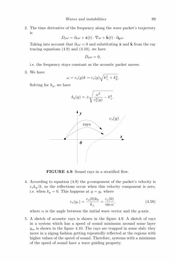
Waves and instabilities 89
2. The time derivative of the frequency along the wave packet’s trajectoryis
Dtω = ∂tω + x(t) · ∇ω + k(t) · ∂kω.Taking into account that ∂tω = 0 and substituting x and k from the raytracing equations (4.9) and (4.10), we have
Dtω = 0,
i.e. the frequency stays constant as the acoustic packet moves.
3. We have
ω = cs(y)k = cs(y)√k2⊥ + k2
y.
Solving for ky, we have
ky(y) = ±
√ω2
c2s(y)− k2⊥.
0
x
y
cs(y)
rays
FIGURE 4.9: Sound rays in a stratified flow.
4. According to equation (4.9) the y-component of the packet’s velocity iscsky/k, so the reflections occur when this velocity component is zero,i.e. when ky = 0. This happens at y = yr where
cs(yr) =cs(0)k0
k⊥=cs(0)
sinα, (4.58)
where α is the angle between the initial wave vector and the y-axis.
5. A sketch of acoustic rays is shown in the figure 4.9. A sketch of raysin a system which has a speed of sound minimum around some layerym is shown in the figure 4.10. The rays are trapped in some slab: theymove in a zigzag fashion getting repeatedly reflected at the regions withhigher values of the speed of sound. Therefore, systems with a minimumof the speed of sound have a wave guiding property.
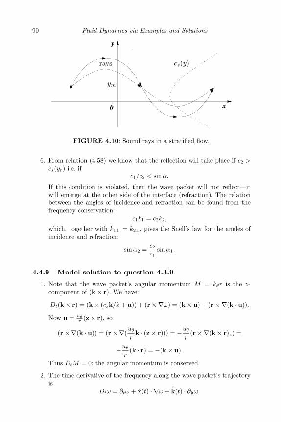
90 Fluid Dynamics via Examples and Solutions
y
0 x
ym
rays cs(y)
FIGURE 4.10: Sound rays in a stratified flow.
6. From relation (4.58) we know that the reflection will take place if c2 >cs(yr) i.e. if
c1/c2 < sinα.
If this condition is violated, then the wave packet will not reflect—itwill emerge at the other side of the interface (refraction). The relationbetween the angles of incidence and refraction can be found from thefrequency conservation:
c1k1 = c2k2,
which, together with k1⊥ = k2⊥, gives the Snell’s law for the angles ofincidence and refraction:
sinα2 =c2c1
sinα1.
4.4.9 Model solution to question 4.3.9
1. Note that the wave packet’s angular momentum M = kθr is the z-component of (k× r). We have:
Dt(k× r) = (k× (csk/k + u)) + (r×∇ω) = (k× u) + (r×∇(k · u)).
Now u = uθr (z× r), so
(r×∇(k · u)) = (r×∇(uθr
k · (z× r))) = −uθr
(r×∇(k× r)z) =
−uθr
(k · r) = −(k× u).
Thus DtM = 0: the angular momentum is conserved.
2. The time derivative of the frequency along the wave packet’s trajectoryis
Dtω = ∂tω + x(t) · ∇ω + k(t) · ∂kω.
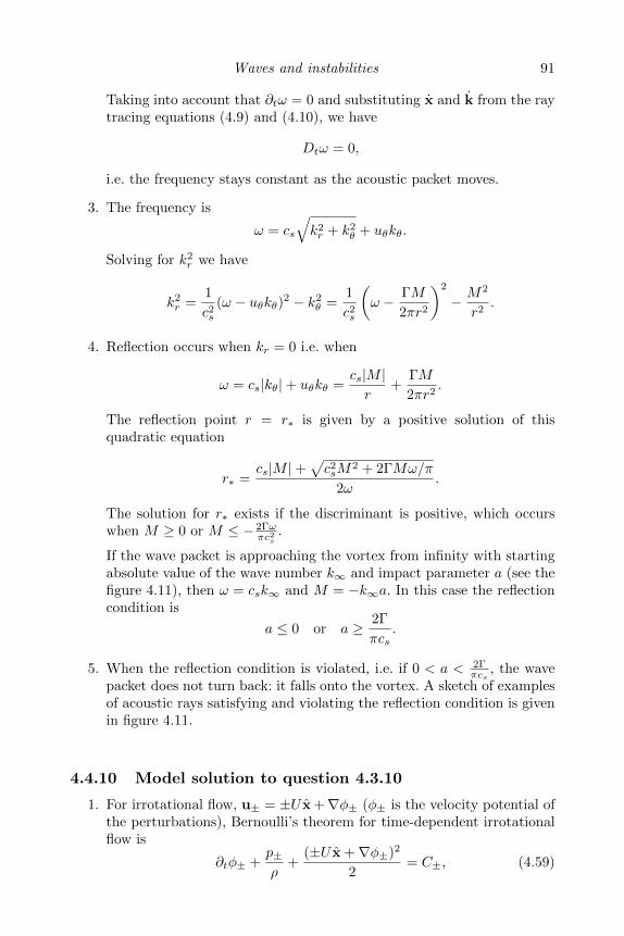
Waves and instabilities 91
Taking into account that ∂tω = 0 and substituting x and k from the raytracing equations (4.9) and (4.10), we have
Dtω = 0,
i.e. the frequency stays constant as the acoustic packet moves.
3. The frequency is
ω = cs
√k2r + k2
θ + uθkθ.
Solving for k2r we have
k2r =
1
c2s(ω − uθkθ)2 − k2
θ =1
c2s
(ω − ΓM
2πr2
)2
− M2
r2.
4. Reflection occurs when kr = 0 i.e. when
ω = cs|kθ|+ uθkθ =cs|M |r
+ΓM
2πr2.
The reflection point r = r∗ is given by a positive solution of thisquadratic equation
r∗ =cs|M |+
√c2sM
2 + 2ΓMω/π
2ω.
The solution for r∗ exists if the discriminant is positive, which occurswhen M ≥ 0 or M ≤ − 2Γω
πc2s.
If the wave packet is approaching the vortex from infinity with startingabsolute value of the wave number k∞ and impact parameter a (see thefigure 4.11), then ω = csk∞ and M = −k∞a. In this case the reflectioncondition is
a ≤ 0 or a ≥ 2Γ
πcs.
5. When the reflection condition is violated, i.e. if 0 < a < 2Γπcs
, the wavepacket does not turn back: it falls onto the vortex. A sketch of examplesof acoustic rays satisfying and violating the reflection condition is givenin figure 4.11.
4.4.10 Model solution to question 4.3.10
1. For irrotational flow, u± = ±U x +∇φ± (φ± is the velocity potential ofthe perturbations), Bernoulli’s theorem for time-dependent irrotationalflow is
∂tφ± +p±ρ
+(±U x +∇φ±)2
2= C±, (4.59)
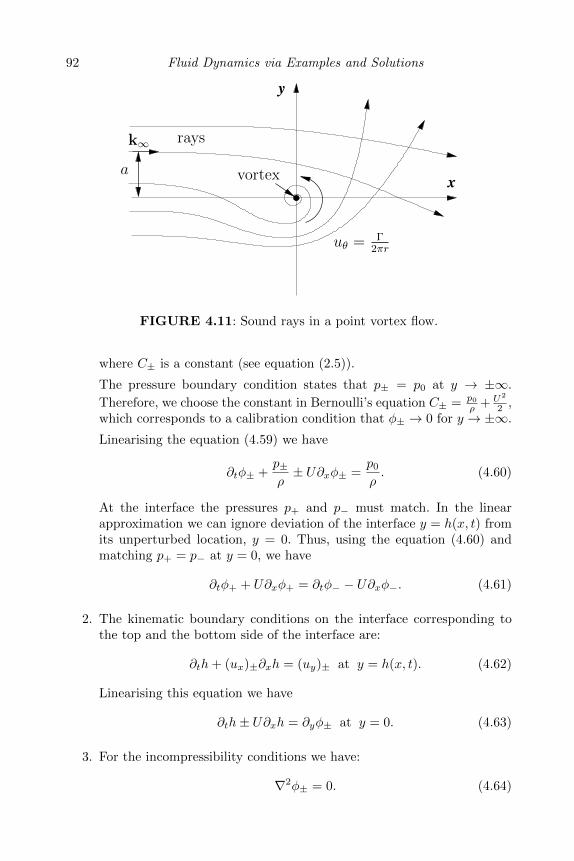
92 Fluid Dynamics via Examples and Solutions
y
x
k∞
vortex
rays
uθ = Γ2πr
a
FIGURE 4.11: Sound rays in a point vortex flow.
where C± is a constant (see equation (2.5)).
The pressure boundary condition states that p± = p0 at y → ±∞.
Therefore, we choose the constant in Bernoulli’s equation C± = p0ρ + U2
2 ,which corresponds to a calibration condition that φ± → 0 for y → ±∞.
Linearising the equation (4.59) we have
∂tφ± +p±ρ± U∂xφ± =
p0
ρ. (4.60)
At the interface the pressures p+ and p− must match. In the linearapproximation we can ignore deviation of the interface y = h(x, t) fromits unperturbed location, y = 0. Thus, using the equation (4.60) andmatching p+ = p− at y = 0, we have
∂tφ+ + U∂xφ+ = ∂tφ− − U∂xφ−. (4.61)
2. The kinematic boundary conditions on the interface corresponding tothe top and the bottom side of the interface are:
∂th+ (ux)±∂xh = (uy)± at y = h(x, t). (4.62)
Linearising this equation we have
∂th± U∂xh = ∂yφ± at y = 0. (4.63)
3. For the incompressibility conditions we have:
∇2φ± = 0. (4.64)
Waves and instabilities 93
4. Substituting the plane wave solution (4.24) into the equation (4.75) wehave
A±(y) = B±e∓ky,
where B± are real constants. Here we assume that k > 0 and choose thesolution that decays at y → ±∞.
5. Substituting the plane wave solution (4.24) into the equation (4.61) wehave
−ωB+ + UkB+ = −ωB− − UkB−, (4.65)
and from the linearised kinematic boundary conditions (4.63) we have:
−iωH = −UikH − kB+ = UikH + kB−. (4.66)
H =kB−
i(−ω − Uk)=
kB+
i(ω − Uk). (4.67)
From the equations (4.65) and (4.67) we have the following resolvabilitycondition:
(ω + Uk)2 = −(ω − Uk)2. (4.68)
orω = iγ, γ = ±Uk. (4.69)
Thus we see that there are two modes with purely imaginary frequencies,one with a positive and another with a negative imaginary parts. Wehave
e−iωt = eγt,
i.e. the mode with positive γ is unstable.
4.4.11 Model solution to question 4.3.11
1. For irrotational flow, u± = ∇φ± (φ± is the velocity potential of theperturbations), Bernoulli’s theorem for time-dependent irrotational flowis
∂tφ± +p±ρ±
+(∇φ±)2
2− gy = C±, (4.70)
where C± is a constant (see equation (2.5)).
We choose the constant in Bernoulli’s equation to be C± = p0ρ±
, where
p0 is a reference pressure at the density discontinuity surface when thelatter is at rest.
The pressure boundary condition states that p+ = p− at the movingdensity discontinuity interface h = y(x, t).
94 Fluid Dynamics via Examples and Solutions
Linearising the equation (4.70) we have
∂tφ± +p± − p0
ρ±− gy = 0. (4.71)
At the interface the pressures p+ and p− must match. In the linearapproximation we can ignore deviation of the interface y = h(x, t) fromits unperturbed location, y = 0, in all terms except for gy = gh(x, t).Thus, using the equation (4.71) and matching p+ = p− at y = 0, wehave
ρ+(∂tφ+ − gh) = ρ−(∂tφ− − gh). (4.72)
2. The kinematic boundary conditions on the interface corresponding tothe top and the bottom side of the interface are:
∂th+ (ux)±∂xh = (uy)± at y = h(x, t). (4.73)
Linearising this equation we have
∂th = ∂yφ± at y = 0. (4.74)
3. For the incompressibility conditions we have:
∇2φ± = 0. (4.75)
4. Substituting the plane wave solution (4.25) into the equation (4.75) wehave
A±(y) = B±e∓ky,
where B± are real constants. He we assume that k > 0 and choose thesolution that decays at y → ±∞.
5. Substituting the plane wave solution (4.25) into the equation (4.72) wehave
ρ+(−iωB+ − gH) = ρ−(−iωB− − gH), (4.76)
and from the linearised kinematic boundary conditions (4.74) we have:
−iωH = −kB+ = kB−. (4.77)
From the equations (4.76) and (4.77) we have the following resolvabilitycondition:
ρ+(ω2/k − g) = ρ−(−ω2/k − g), (4.78)
or
ω =
√(ρ− − ρ+)gk
ρ− + ρ+. (4.79)
Waves and instabilities 95
Thus we see that in the case ρ− > ρ+ we have a real frequency whichcorresponds to a propagating wave. This is a generalisation of the surfacegravity wave considered in question 4.3.2.
In the case ρ− < ρ+ there are two modes with purely imaginary frequen-cies, ω = iγ, one with a positive and another with a negative imaginaryparts:
γ = ±
√(ρ+ − ρ−)gk
ρ− + ρ+. (4.80)
We haveeiωt = eγt,
i.e. the mode with positive γ is unstable.
4.4.12 Model solution to question 4.3.12
(a) Consider the three-dimensional velocity and pressure perturba-tions, u and p, of the shear flow (4.26). The linearised Euler equa-tion is
∂tu + (U · ∇)u + (u · ∇)U = −1
ρ∇p, (4.81)
or, substituting for U,
∂tu + sy ∂xu + suy x = −1
ρ∇p. (4.82)
Taking divergence of this equation and taking into account theincompressibility condition ∇ · u = 0, we have
−1
ρ∇2p = 2s ∂xuy. (4.83)
(b) Assuming that the perturbations have wave-like shape (4.27), equa-tions (4.82) and (4.83) become:
∂tu + i(k · x)u + sy ikxu + suy x = −1
ρikp. (4.84)
and
k2 p
ρ= 2si kx uy.
Solving the latter expression for p and substituting the result in(4.84) we have
∂tu + i(k · x)u + sy ikxu + suy
(x− k
2kxk2
)= 0. (4.85)
96 Fluid Dynamics via Examples and Solutions
(c) For the coefficients in the linearised Euler equation (4.85) to becomeindependent of x we must have
(k · x) = −sy kx,
orkx = kz = 0 and ky = −s kx.
Solving these equations, we have
kx = qx, kz = qz and ky = qy − sqxt,
where q = k(0) is the initial wave number.
(d) Substituting these expressions into (4.85) we have
∂tux + suy
(1− 2q2
x
q2x + (qy − sqxt)2 + q2
z
)= 0, (4.86)
∂tuy − 2suyqx(qy − sqxt)
q2x + (qy − sqxt)2 + q2
z
= 0, (4.87)
∂tuz − 2suyqxqz
q2x + (qy − sqxt)2 + q2
z
= 0. (4.88)
Integrating the equation (4.87) we have
uy(t) = uy(0)q2
q2x + (qy − sqxt)2 + q2
z
, (4.89)
where q2 = q2x + q2
y + q2z . Substituting (4.89) into (4.86) and (4.88)
and integrating, we have
ux(t) = uy(0)q2
q2x + q2
z
[−q2
zλ+q2x
q2µ
]+ ux(0), (4.90)
uz(t) = uy(0)qxqzq2x + q2
z
[q2λ+ µ
]+ uz(0), (4.91)
where
λ =1
qx(q2x + q2
z)1/2arctan
stqx(q2x + q2
z)1/2
q2 − stqxqy, (4.92)
µ =st(q2 − 2q2
y + stqxqy)
q2x + (qy − sqxt)2 + q2
z
. (4.93)
(e) At large time, t → +∞, we have uy → 0. Also, λ and µ tendto some constant values, and so do ux and uz. Thus, there is noinstability if only a single wave was chosen as an initial condition.
Waves and instabilities 97
(f) If the initial perturbation contains a continuous range of wavenum-bers with distribution u0(q) which remains finite when qx → 0,then at large t the part of the perturbation with qx ∼ 1/(st) willbehave as
ux ∼ st, uy ∼ const, uz ∼ const.
Thus we see that such perturbations of the constant shear flowgrow algebraically (linearly in time). One can show that the totalenergy of the perturbations will also grow algebraically,
E =1
2
∫u2(k) dk ≈ 1
2
∫u2x(k) dk ∼ t.
This is because the k-space volume contributing to the integral isproportional to the range of contributing kx = qx which shrinks intime as ∼ 1/(st).

This page intentionally left blankThis page intentionally left blank
Chapter 5
Boundary layers
5.1 Background theory
Boundary layers are flows formed in the close vicinity of solid boundaries.Their properties significantly differ from the properties of the flows furtheraway from the boundaries; see figure 5.1. Boundary layers are most clearlydefined for laminar flows with high Reynolds numbers, because in this casethis will be the only part of the flow where viscosity is important, whereasthe flow in the exterior is nearly ideal. One could roughly think that suchan ideal flow is slowly varying (often irrotational) and satisfying the free-slipboundary conditions on the solid surface. In the other words, when findingthe exterior flow, presence of the boundary layer can be ignored because itis much thinner than the typical length scale L in the exterior flow, δ L;see figure 5.1. On the other hand, the value of the velocity slip serves as aboundary condition at the top side of the thin boundary layer. The role ofthe viscosity here is to eliminate the free slip by slowing the velocity down tozero rapidly within a thin layer so that the no-slip boundary condition couldbe satisfied at the bottom side of the boundary layer. Since the viscositycoefficient is small, the velocity gradient in the boundary layer must be largeso that the viscosity term would become sufficient to balance the other termsin the Navier-Stokes equation. For this reason the boundary layer is thin—thinner than the curvature radius of the solid surface–and it can be locallythought as a plane-parallel shear flow. These ideas were originally presented inPrandtl’s 1905 paper [20] and they remain a conceptual basis for the modernboundary layer theory in laminar flows. Very good detailed presentation of thelaminar boundary layer theory can be found in the Acheson’s book ElementaryFluid Dynamics [1] as well as in Essentials of Fluid Dynamics by L. Prandtl[21].
If the flow far from the boundary is turbulent then the structure of theboundary layer is more complicated, and it cannot be defined as a layer be-yond which the flow is ideal (and in some cases irrotational). Indeed, turbu-lent motions span over a wide range of scales including such small scales atwhich viscosity is important. Also, turbulent flows are never irrotational. Inthe present chapter we will only consider laminar flows. We will study the
99
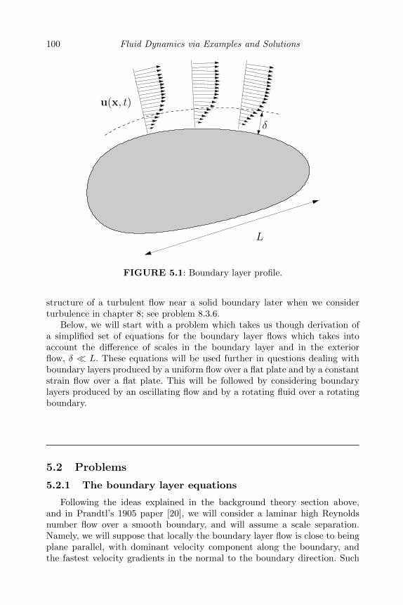
100 Fluid Dynamics via Examples and Solutions
L
δ
u(x, t)
FIGURE 5.1: Boundary layer profile.
structure of a turbulent flow near a solid boundary later when we considerturbulence in chapter 8; see problem 8.3.6.
Below, we will start with a problem which takes us though derivation ofa simplified set of equations for the boundary layer flows which takes intoaccount the difference of scales in the boundary layer and in the exteriorflow, δ L. These equations will be used further in questions dealing withboundary layers produced by a uniform flow over a flat plate and by a constantstrain flow over a flat plate. This will be followed by considering boundarylayers produced by an oscillating flow and by a rotating fluid over a rotatingboundary.
5.2 Problems
5.2.1 The boundary layer equations
Following the ideas explained in the background theory section above,and in Prandtl’s 1905 paper [20], we will consider a laminar high Reynoldsnumber flow over a smooth boundary, and will assume a scale separation.Namely, we will suppose that locally the boundary layer flow is close to beingplane parallel, with dominant velocity component along the boundary, andthe fastest velocity gradients in the normal to the boundary direction. Such
Boundary layers 101
a scale separation will allow us (following Prandtl’s 1905 paper) to derive asimplified set of the boundary layer equations.
Consider a flow with a typical velocity U near a bluff body with a charac-teristic length scale L as in figure 5.1. The flow is laminar and the Reynoldsnumber is high, Re = UL/ν 1, where ν is the viscosity coefficient. Theboundary layer is thin with characteristic thickness δ L and it is attachedto the surface, i.e. there are no streamlines originating at the surface andpenetrating to distances ∼ L away from the surface.
1. Taking into account that the boundary layer flow is locally almost plane-parallel, write a physical estimate for the boundary layer thickness δfrom balancing the inertial and the viscous forces within the boundarylayer (so that the flow could be slowed down to satisfy the no-slip bound-ary condition at the solid surface). Express your answer in terms of Land Re.
2. Rewrite the two-dimensional Navier-Stokes equations in terms of thenon-dimensional scaled variables
x′ =x
L, y′ =
y
δ, u′ =
u
U, v′ =
v
(Uδ/L), p′ =
p
ρU2,
where u, v and x, y are the parallel and the perpendicular to the bound-ary velocity and coordinate components respectively.
3. By taking the limit Re→∞ with all primed functions and their deriva-tives with respect to the primed coordinates kept O(1) with respect to1/Re, derive the boundary layer equations:
u′∂u′
∂x′+ v′
∂u′
∂y′= −∂p
′
∂x′+∂2u′
∂y′2, (5.1)
∂p′
∂y′= 0, (5.2)
∂u′
∂x′+∂v′
∂y′= 0. (5.3)
4. Rewrite the boundary layer equations in terms of the original (unprimed)variables.
5. Formulate the boundary conditions for the obtained equations at y = 0and at y =∞.
5.2.2 A boundary layer over a semi-infinite plate
Consider a boundary layer at a semi-infinite flat plate at y = 0, x ≥ 0produced by the flow which is in the inviscid exterior (i.e. outside of theboundary layer) has uniform velocity with magnitude U and directed parallelto the plate along the x-axis; see figure 5.2.
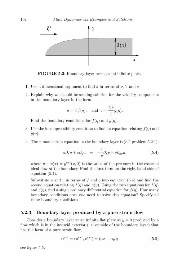
102 Fluid Dynamics via Examples and Solutions
x
δ(x)
U y
FIGURE 5.2: Boundary layer over a semi-infinite plate.
1. Use a dimensional argument to find δ in terms of ν, U and x.
2. Explain why we should be seeking solution for the velocity componentsin the boundary layer in the form
u = Uf(η), and v =Uδ
xg(η).
Find the boundary conditions for f(η) and g(η).
3. Use the incompressibility condition to find an equation relating f(η) andg(η).
4. The x-momentum equation in the boundary layer is (c.f. problem 5.2.1):
u∂xu+ v∂yu = −1
ρ∂xp+ ν∂yyu, (5.4)
where p ≡ p(x) = pext(x, 0) is the value of the pressure in the externalideal flow at the boundary. Find the first term on the right-hand side ofequation (5.4).
Substitute u and v in terms of f and g into equation (5.4) and find thesecond equation relating f(η) and g(η). Using the two equations for f(η)and g(η), find a single ordinary differential equation for f(η). How manyboundary conditions does one need to solve this equation? Specify allthese boundary conditions.
5.2.3 Boundary layer produced by a pure strain flow
Consider a boundary layer at an infinite flat plate at y = 0 produced by aflow which is in the inviscid exterior (i.e. outside of the boundary layer) thathas the form of a pure strain flow,
uext = (uext, vext) = (αx,−αy); (5.5)
see figure 5.5.
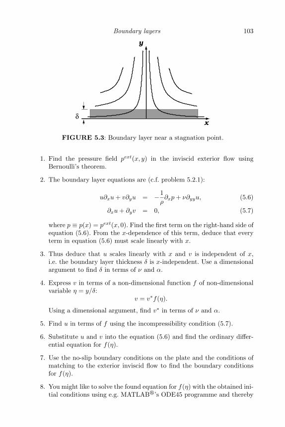
Boundary layers 103
δ
x
y
FIGURE 5.3: Boundary layer near a stagnation point.
1. Find the pressure field pext(x, y) in the inviscid exterior flow usingBernoulli’s theorem.
2. The boundary layer equations are (c.f. problem 5.2.1):
u∂xu+ v∂yu = −1
ρ∂xp+ ν∂yyu, (5.6)
∂xu+ ∂yv = 0, (5.7)
where p ≡ p(x) = pext(x, 0). Find the first term on the right-hand side ofequation (5.6). From the x-dependence of this term, deduce that everyterm in equation (5.6) must scale linearly with x.
3. Thus deduce that u scales linearly with x and v is independent of x,i.e. the boundary layer thickness δ is x-independent. Use a dimensionalargument to find δ in terms of ν and α.
4. Express v in terms of a non-dimensional function f of non-dimensionalvariable η = y/δ:
v = v∗f(η).
Using a dimensional argument, find v∗ in terms of ν and α.
5. Find u in terms of f using the incompressibility condition (5.7).
6. Substitute u and v into the equation (5.6) and find the ordinary differ-ential equation for f(η).
7. Use the no-slip boundary conditions on the plate and the conditions ofmatching to the exterior inviscid flow to find the boundary conditionsfor f(η).
8. You might like to solve the found equation for f(η) with the obtained ini-tial conditions using e.g. MATLABr’s ODE45 programme and thereby
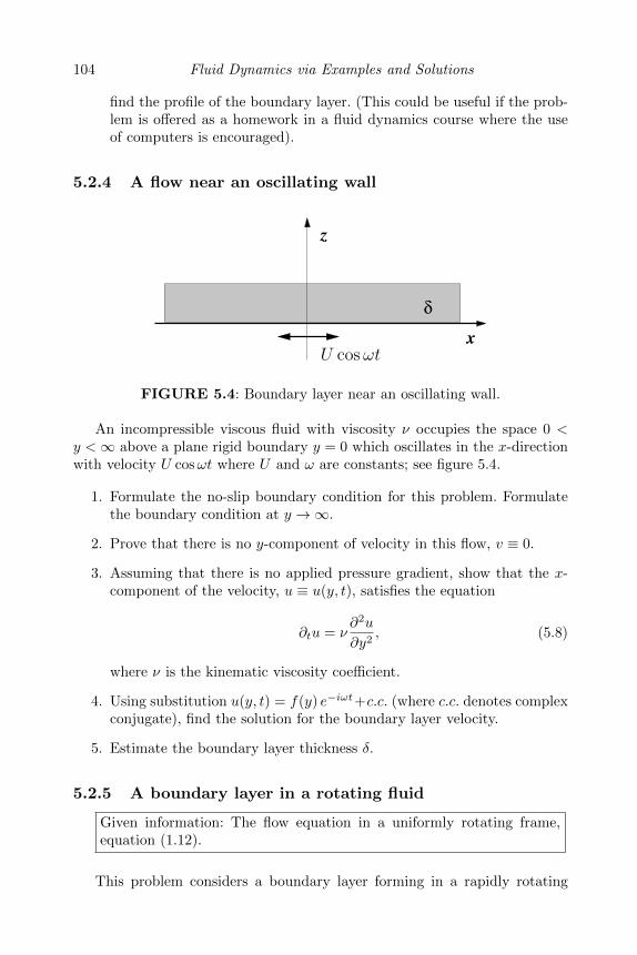
104 Fluid Dynamics via Examples and Solutions
find the profile of the boundary layer. (This could be useful if the prob-lem is offered as a homework in a fluid dynamics course where the useof computers is encouraged).
5.2.4 A flow near an oscillating wall
x
δ
z
U cosωt
FIGURE 5.4: Boundary layer near an oscillating wall.
An incompressible viscous fluid with viscosity ν occupies the space 0 <y <∞ above a plane rigid boundary y = 0 which oscillates in the x-directionwith velocity U cosωt where U and ω are constants; see figure 5.4.
1. Formulate the no-slip boundary condition for this problem. Formulatethe boundary condition at y →∞.
2. Prove that there is no y-component of velocity in this flow, v ≡ 0.
3. Assuming that there is no applied pressure gradient, show that the x-component of the velocity, u ≡ u(y, t), satisfies the equation
∂tu = ν∂2u
∂y2, (5.8)
where ν is the kinematic viscosity coefficient.
4. Using substitution u(y, t) = f(y) e−iωt+c.c. (where c.c. denotes complexconjugate), find the solution for the boundary layer velocity.
5. Estimate the boundary layer thickness δ.
5.2.5 A boundary layer in a rotating fluid
Given information: The flow equation in a uniformly rotating frame,equation (1.12).
This problem considers a boundary layer forming in a rapidly rotating
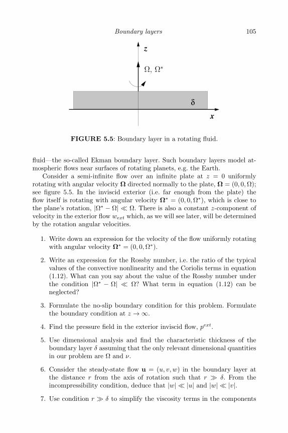
Boundary layers 105
x
δ
z
Ω, Ω∗
FIGURE 5.5: Boundary layer in a rotating fluid.
fluid—the so-called Ekman boundary layer. Such boundary layers model at-mospheric flows near surfaces of rotating planets, e.g. the Earth.
Consider a semi-infinite flow over an infinite plate at z = 0 uniformlyrotating with angular velocity Ω directed normally to the plate, Ω = (0, 0,Ω);see figure 5.5. In the inviscid exterior (i.e. far enough from the plate) theflow itself is rotating with angular velocity Ω∗ = (0, 0,Ω∗), which is close tothe plane’s rotation, |Ω∗ − Ω| Ω. There is also a constant z-component ofvelocity in the exterior flow wext which, as we will see later, will be determinedby the rotation angular velocities.
1. Write down an expression for the velocity of the flow uniformly rotatingwith angular velocity Ω∗ = (0, 0,Ω∗).
2. Write an expression for the Rossby number, i.e. the ratio of the typicalvalues of the convective nonlinearity and the Coriolis terms in equation(1.12). What can you say about the value of the Rossby number underthe condition |Ω∗ − Ω| Ω? What term in equation (1.12) can beneglected?
3. Formulate the no-slip boundary condition for this problem. Formulatethe boundary condition at z →∞.
4. Find the pressure field in the exterior inviscid flow, pext.
5. Use dimensional analysis and find the characteristic thickness of theboundary layer δ assuming that the only relevant dimensional quantitiesin our problem are Ω and ν.
6. Consider the steady-state flow u = (u, v, w) in the boundary layer atthe distance r from the axis of rotation such that r δ. From theincompressibility condition, deduce that |w| |u| and |w| |v|.
7. Use condition r δ to simplify the viscosity terms in the components
106 Fluid Dynamics via Examples and Solutions
of the momentum equations. Argue that the viscosity term can be ne-glected in the z-momentum equation and, therefore, pressure p is ap-proximately independent of z and equal to its exterior value pext.
8. Substitute p = pext into the x- and y-momentum equations and theboundary conditions you found before and solve for u and v.
9. Use the incompressibility condition and the solution for u and v and findw. Using the boundary conditions find the relation for wext in terms ofΩ,Ω∗ and ν.
5.3 Solutions
5.3.1 Model solution to question 5.2.1
1. The viscous term is important in the boundary layer if it is of the sameorder as the inertial term:
|ν∇2u| ∼ |(u · ∇)u|.
Considering the fact that the boundary layer flow is nearly plane-parallelwith u ∼ U and v ∼ uδ/L u (the latter follows from the incompress-ibility condition), we have
νU/δ2 ∼ U2/L ∼ vU/δ.
Thusδ ∼ L/Re1/2.
This relation confirms that δ L when Re 1.
2. The stationary two-dimensional Navier-Stokes equations written in com-ponents are
u∂u
∂x+ v
∂u
∂y= −∂p
∂x+ ν
∂2u
∂x2+ ν
∂2u
∂y2, (5.9)
u∂v
∂x+ v
∂v
∂y= −∂p
∂y+ ν
∂2v
∂x2+ ν
∂2v
∂y2, (5.10)
∂u
∂x+∂v
∂y= 0. (5.11)
Boundary layers 107
In terms of the non-dimensional and scaled variables we have
u′∂u′
∂x′+ v′
∂u′
∂y′= −∂p
′
∂x′+
1
Re
∂2u′
∂x′2+∂2u′
∂y′2,
1
Re1/2
[u′∂v′
∂x′+ v′
∂v′
∂y′
]= −Re1/2 ∂p
′
∂y′+
1
Re3/2
∂2v′
∂x′2+
1
Re1/2
∂2v′
∂y′2,
∂u′
∂x′+∂v′
∂y′= 0.
From this system in the limit Re → ∞ in the leading order we obtainthe reduced system (5.1), (5.2) and (5.3).
3. Integrating equation (5.2) and writing the equations in terms of theoriginal variables we have:
u∂u
∂x+ v
∂u
∂y= −∂p
∂x+ ν
∂2u
∂y2, (5.12)
p ≡ p(x) – independent of y, (5.13)
∂u
∂x+∂v
∂y= 0. (5.14)
4. First of all, we have the no-slip boundary conditions at the solid surface:
u ≡ (u, v) = 0 at y = 0.
The conditions at y → ∞ correspond to matching to the ideal exteriorflow. Note that because of the scale separation the matching range canbe considered as y → ∞ for the boundary layer solution and as y → 0for the exterior flow. Thus u must be matched to the velocity slip of theexterior flow at the boundary, and p ≡ p(x) must be matched to thepressure of the exterior flow at the boundary:
[u]y→∞ =[uext
]y→0
, p(x) =[pext
]y→0
.
5.3.2 Model solution to question 5.2.2
1. Because the semi-infinite flat plate does not have a length scale L, theonly remaining relevant quantity having the dimension of length is thedistance from the plate’s edge x. Thus,
Re =Ux
ν, and δ =
x
Re1/2=
√νx
U.
2. Thus the similarity variable is η = y/δ = y√U/νx.
The fact that u must match U at y → ∞ suggests that we should beseeking solution in the form
u = Uf(η)
108 Fluid Dynamics via Examples and Solutions
with boundary conditions
f(η) = 0 at η = 0, and f(η) = 1 at η →∞, (5.15)
which follow from the no-slip condition at y = 0 and matching to theexterior ideal flow respectively. On the other hand, from the incom-pressibility condition ∂xu = −∂yv, we have v ∼ uδ/x u (c.f. problem5.2.1). This suggests that for v we should take
v =Uδ
xg(η) =
√νU
xg(η),
with boundary conditions
g(η) = 0 at η = 0, and g(η)→ 0 at η →∞, (5.16)
which follow from the no-slip condition at y = 0 and matching to theexterior ideal flow respectively.
3. From the incompressibility condition we have:
η
2f ′(η) = g′(η). (5.17)
4. Because the external ideal flow is uniform, it has a constant pressurewhich is imposed through the boundary layer. Thus the pressure gradientterm in the boundary layer equation is zero. Substituting for u and v interms of f and g into (5.4), we have
−η2ff ′ + gf ′ = f ′′. (5.18)
Combining equations (5.17) and (5.18), we have a single equation forthe profile f :
−f2
=
(f ′′
f ′
)′, (5.19)
which must be solved with three boundary conditions: two conditions(5.15) and a third one arising from (5.16). To find the latter we writefrom (5.17)
g(η) =1
2
∫ η
0
ηf ′(η) dη.
This automatically gives g(0) = 0, whereas the condition g(∞) = 0implies ∫ ∞
0
ηf ′(η) dη = 0,
which is the required third condition on f .
Boundary layers 109
5.3.3 Model solution to question 5.2.3
1. From Bernoulli’s theorem we have
pext = const− ρ
2(α2x2 + α2y2).
2. For the first term on the right-hand side of equation (5.6) we have
−1
ρ∂xp = α2x.
The linear x-dependence of this term implies that every term in equa-tion (5.6) must be ∝ x. This can be realised when u ∝ x and v isx-independent.
3. The only combination of ν and α with the dimension of the length is(ν/α)1/2, so
δ ∼√ν
α.
4. The only combination of ν and α with the dimension of the velocity is(να)1/2, so
v∗ ∼√να = αδ.
5. Thus we consider a self-similar solution
v = −αδf(η),
where the minus sign is chosen so that f > 0.
6. From the expression for v and the incompressibility condition we have
∂yv = −∂xu = −αf ′(η).
Thusu = αxf ′(η).
The integration constant here is set to zero to allow matching to theinviscid exterior (see below).
7. Substituting u, v and the previously found pressure term into equation(5.6), we have
αxf ′αf ′ − αδfαx1
δf ′′ = α2x+ ν
αx
δ2f ′′′,
or(f ′)2 − ff ′′ = 1 + f ′′′.
110 Fluid Dynamics via Examples and Solutions
8. The no-slip boundary conditions are u(0) = v(0) = 0 at y = 0. Fromu(x, 0) = 0 we have
f ′(0) = 0.
From v(x, 0) = 0 we havef(0) = 0.
Matching to the external inviscid flow gives
limy/δ→∞
= αx,
sof ′(∞) = 1.
5.3.4 Model solution to question 5.2.4
1. The no-slip boundary condition for the velocity field u(x, y, t) is as fol-lows:
u(x, 0, t) = U cosωt. (5.20)
The boundary condition at infinity is
u(x, y, t)→ 0 at y →∞. (5.21)
2. Our system is invariant with respect to x-shifts, so u is independent ofx, and using the incompressibility condition, we get v ≡ 0.
3. For the solution see the derivation of the equation (6.14) in section 6.1.In our case there is no pressure gradient, so we have to put f = 0 in thisequation.
4. Substituting u(y, t) = f(y) e−iωt + c.c. into equation (5.8) we get:
−iωf = νf ′′,
where the double prime stands for the second derivative with respect toy. The solution of this equation decaying at y →∞ is
f(y) = C e(i−1)√
ω2ν y,
where C is a constant. Substituting this expression into u(y, t) =f(y) e−iωt + c.c. and using the boundary condition (5.21), we get thesolution for the boundary layer velocity:
u(y, t) = U e−√
ω2ν y cos
(√ω
2νy − ωt
).
5. The boundary layer thickness is determined by the decay distance of theexponential function in the above expression:
δ ∼√
2ν
ω.
Boundary layers 111
5.3.5 Model solution to question 5.2.5
1. The velocity of the flow uniformly rotating with angular velocity Ω∗ =(0, 0,Ω∗) (measured in the frame rotating with angular velocity Ω =(0, 0,Ω)) is
uext⊥ = (Ω∗ −Ω)× x. (5.22)
2. The Rossby number is considered in question 1.3.3. It is defined byexpression (1.16). Using the expression (5.22), we can rewrite expression(1.16) as:
Ro = |Ω∗ − Ω|/|Ω|. (5.23)
Thus, the Rossby number is small, Ro 1, if |Ω∗ − Ω| Ω. Underthis condition the nonlinear term (u · ∇)u in equation (1.12) can beneglected:
∂tu = −1
ρ∇pR − 2 Ω× u + ν∇2u, (5.24)
where pR = p− Ω2r2/2.
3. Since equation (1.12) is for the frame rotating with the angular velocityΩ, the no-slip boundary condition is simply
u = 0 at z = 0. (5.25)
The boundary condition at z →∞ amounts to matching to the inviscidexterior flow:
u→ uext⊥ + wext z at z →∞. (5.26)
4. Neglecting the viscosity term in the stationary version of equation (5.24),for the x- and y-components we have:
−2Ωvext = −2Ω(Ω∗ − Ω)x = −1
ρ∂xp
extR . (5.27)
2Ωuext = −2Ω(Ω∗ − Ω)y = −1
ρ∂yp
extR . (5.28)
Integrating these equations we have:
pext = pextR + Ω2r2/2 = p0 + Ω(Ω∗ − Ω/2)r2 ≈ p0 + Ω2r2/2,
where p0 is a constant.
5. The physical dimension of Ω is 1/T and the physical dimension of ν isL2/T . The only combination of Ω and ν having the dimension of lengthis√ν/Ω, so
δ ∼√ν/Ω.
6. We have ∂xu ∼ u/r, ∂yv ∼ v/r and ∂zw ∼ w/δ w/r. From theincompressibility condition we get ∂xu ∼ ∂yv ∼ ∂zw, so we concludethat |w| |u| and |w| |v|.

112 Fluid Dynamics via Examples and Solutions
7. Using the condition r δ, we can estimate
∂zzu ∼ u/δ2 u/r2 ∼ ∂xxu ∼ ∂yyu
and∂zzv ∼ v/δ2 v/r2 ∼ ∂xxv ∼ ∂yyv.
Therefore, only z-derivative terms can be retained in the viscosity termsin the momentum equations:
−2Ωv = −1
ρ∂xpR + ν∂zzu, (5.29)
2Ωu = = −1
ρ∂ypR + ν∂zzv, (5.30)
0 = = −1
ρ∂zpR + ν∂zzw. (5.31)
Because w u, v, the viscosity term in the z-momentum equation ismuch less than the viscosity terms in the x- and y-momentum equationsand, therefore, can be neglected. Therefore, the reduced pressure pR isapproximately independent of z and equal to its exterior value pextR .
8. Thus, the pressure terms can be substituted from the exterior equations(5.27) and (5.28):
−2Ω(v − vext) = ν∂zzu, (5.32)
2Ω(u− uext) = = ν∂zzv. (5.33)
Introducing a complex variable
f = u− uext + i(v − vext),
we have the following complex equation:
ν∂zzf = 2Ωif.
Since the velocity must match the exterior velocity value at large z, wehave to choose a solution for f which is decaying at z →∞:
f = Ae−(1+i)z/δ,
where A is an arbitrary function of x and y which has to be fixed by theno-slip boundary condition u = v = 0 at z = 0, i.e. f = −uext− ivext atz = 0. Thus
A = −uext − ivextand for the velocity components we have:
u = uext − e−z/δ(uext cos(z/δ) + vext sin(z/δ)), (5.34)
v = vext − e−z/δ(vext cos(z/δ)− uext sin(z/δ)). (5.35)
Boundary layers 113
9. Using the incompressibility condition we have:
w = −∫ z
0
(∂xu(x, y, z′) + ∂yv(x, y, z′)) dz′.
Substituting here the solution for u and v and integrating to z =∞ usingthe matching condition w|z=∞ = wext, we get the following relation,
wext = δ(∂xvext − ∂yuext)/2 = (Ω∗ − Ω)δ.
Note that this expression is positive for cyclones, Ω∗ > Ω, and negativefor anticyclones, Ω∗ < Ω. This effect is called Ekman pumping.

This page intentionally left blankThis page intentionally left blank
Chapter 6
Two-dimensional flows
6.1 Background theory
In this chapter, we will consider the most basic two-dimensional (2D) flowsin ideal and viscous incompressible fluids. In 2D flows, the velocity field hastwo components which depend on two physical space coordinates and time,u = (u(x, y, t), v(x, y, t), 0). Respectively, the vorticity field has only one non-zero component, ω = (0, 0, ω(x, y, t)). This component satisfies the equation(2.21), which we will reproduce here for convenience:
Dtω ≡ (∂t + (u · ∇))ω = ν∇2ω. (6.1)
For 2D incompressible flows, one can introduce a representation of thevelocity field in terms of stream function ψ(x, y, t) as follows,
u = ∇ψ × z, (6.2)
or in component formu = ∂yψ, v = −∂xψ. (6.3)
In terms of the stream function the vorticity is:
ω = −∇2ψ. (6.4)
If the 2D flow is irrotational, then we also have a representation in terms ofthe velocity potential u = ∇φ, or
u = ∂xφ, v = ∂yφ, (6.5)
and the viscous term is automatically zero, ν∇2u = ν∇∇2φ = 0.Combining expressions (6.3) and (6.5) we have
∂xφ = ∂yψ, ∂yφ = −∂xψ. (6.6)
These relations are nothing but the Cauchy-Riemann conditions, i.e. necessaryand sufficient conditions for a complex function w(z) = φ + iψ (where z =x+ iy) to be complex differentiable, that is, holomorphic. The function w(z)
115
116 Fluid Dynamics via Examples and Solutions
is called the complex potential. Both real and imaginary parts of it satisfyLaplace’s equation,
∇ · u = ∇2φ = 0, ∇× u = ∇2ψ = 0. (6.7)
For the velocity u = (u, v) in terms of the complex potential we have
u− iv = ∂zw, (6.8)
so that|u| =
√u2 + v2 = |∂zw|. (6.9)
The identification of the complex potential of a 2D ideal irrotational flowwith a holomorphic function had profound consequences for the rapid devel-opment of both aerodynamic theory and complex analysis, notably utilisingconformal maps to obtain new fluid flow solutions out of already known andoften simpler ones. This approach culminated in 1906 in Zhukovskiy’s lifttheorem, stating the following.
A steady ideal flow past a 2D body and having a uniform velocity U x farfrom the body (i) produces no force component along x, i.e. Fx = 0, and (ii)produces a y-component of the force (per unit length along in the transverseto the 2D plane direction, i.e. z) equal to
Fy = −ρUΓ, (6.10)
where Γ is the velocity circulation around a contour embracing the 2D body(e.g. the 2D body’s boundary). Part (i) asserts the absence of a drag force andis often referred to as D’Alembert’s paradox. Part (ii) is a statement aboutthe lift force.
A proof of this theorem, as well as a detailed discussion of the complexanalysis application to aerodynamics and the aerofoil theory can be found inAcheson’s book [1].
Let us now consider viscous flows. The most basic 2D flows have plane-parallel configuration in which the velocity field is everywhere in the samedirection and constant along that direction, i.e.
u(x, t) = (u(y, t), 0, 0). (6.11)
The incompressibility condition for such a velocity field is automatically sat-isfied, ∇ · u = 0, and the nonlinear term (u · ∇)u is automatically zero,which greatly simplifies finding solutions. Writing the Navier-Stokes equationin components, we have
∂tu = −1
ρ∂xp+ ν∂yyu, (6.12)
0 = −1
ρ∂yp. (6.13)
Two-dimensional flows 117
From the second equation we see that the pressure is independent of y andfrom the first one, that its dependence on x is linear, i.e. the pressure force isuniform and in the x-direction, −∇p/ρ = f x where f = const. Thus we havethe following equation
∂tu = f + ν∂yyu. (6.14)
Introducing a new variable
u = u− fy2
2ν(6.15)
we get the 1D linear diffusion equation
∂tu = ν∂yyu, (6.16)
which is a classical and a very well studied equation with many solution-findingtechniques developed for it.
One can also rewrite equation (6.14) as a continuity equation correspond-ing to the x-momentum conservation:
∂t(ρu) +∇ · F = 0, (6.17)
where F is the x-momentum flux:
F = −fρx x− νρ(∂yu) y. (6.18)
The first part of the flux is due to the pressure forces and the second partcorresponds to the x-momentum transfer between the moving fluid layers dueto the internal friction. As such, the latter part determines the wall frictionper unit area, i.e. the drag:
D = νρ|∂yu|boundary. (6.19)
Similarly, one can consider velocity profiles having only an azimuthal com-ponent independent of the polar angle, which represent various round vortexsolutions. Here, too, the simplification comes from the fact that the nonlinearterm is automatically zero.
In the problems below, we will start with the most basic 2D flows, such asthe constant-strain and the plane-parallel flows, as well as round vortices. Thiswill be followed by considering some irrotational 2D flows given by a prescribedcomplex potential. We will also consider some applications of Zhukovskiy’stheorem. We will consider more general theoretical questions about the be-haviour of vorticity and stream function in 2D flows. Finally, we will considerslightly more complicated flows down inclined slopes.
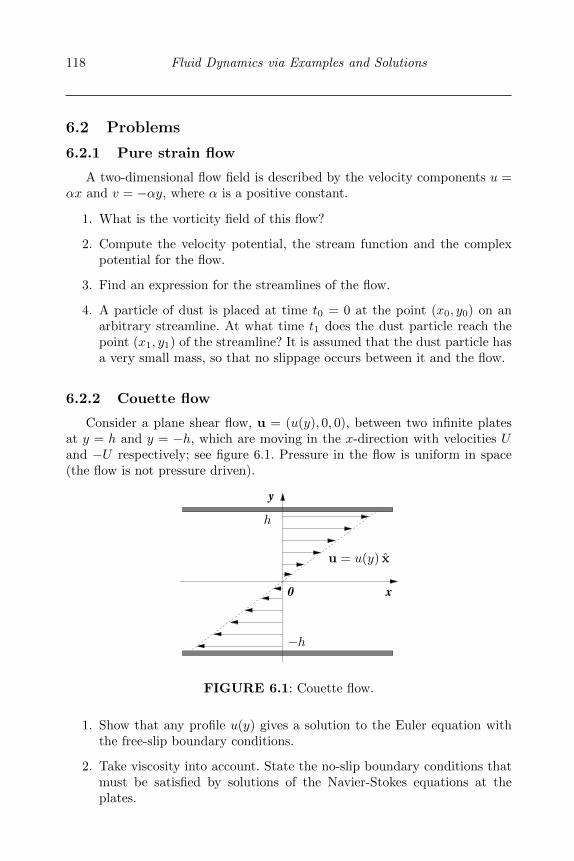
118 Fluid Dynamics via Examples and Solutions
6.2 Problems
6.2.1 Pure strain flow
A two-dimensional flow field is described by the velocity components u =αx and v = −αy, where α is a positive constant.
1. What is the vorticity field of this flow?
2. Compute the velocity potential, the stream function and the complexpotential for the flow.
3. Find an expression for the streamlines of the flow.
4. A particle of dust is placed at time t0 = 0 at the point (x0, y0) on anarbitrary streamline. At what time t1 does the dust particle reach thepoint (x1, y1) of the streamline? It is assumed that the dust particle hasa very small mass, so that no slippage occurs between it and the flow.
6.2.2 Couette flow
Consider a plane shear flow, u = (u(y), 0, 0), between two infinite platesat y = h and y = −h, which are moving in the x-direction with velocities Uand −U respectively; see figure 6.1. Pressure in the flow is uniform in space(the flow is not pressure driven).
0 x
y
u = u(y) x
h
−h
FIGURE 6.1: Couette flow.
1. Show that any profile u(y) gives a solution to the Euler equation withthe free-slip boundary conditions.
2. Take viscosity into account. State the no-slip boundary conditions thatmust be satisfied by solutions of the Navier-Stokes equations at theplates.
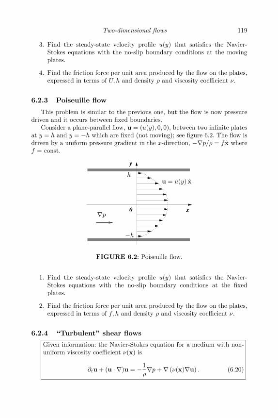
Two-dimensional flows 119
3. Find the steady-state velocity profile u(y) that satisfies the Navier-Stokes equations with the no-slip boundary conditions at the movingplates.
4. Find the friction force per unit area produced by the flow on the plates,expressed in terms of U, h and density ρ and viscosity coefficient ν.
6.2.3 Poiseuille flow
This problem is similar to the previous one, but the flow is now pressuredriven and it occurs between fixed boundaries.
Consider a plane-parallel flow, u = (u(y), 0, 0), between two infinite platesat y = h and y = −h which are fixed (not moving); see figure 6.2. The flow isdriven by a uniform pressure gradient in the x-direction, −∇p/ρ = f x wheref = const.
x
y
0
u = u(y) xh
−h
∇p
FIGURE 6.2: Poiseuille flow.
1. Find the steady-state velocity profile u(y) that satisfies the Navier-Stokes equations with the no-slip boundary conditions at the fixedplates.
2. Find the friction force per unit area produced by the flow on the plates,expressed in terms of f, h and density ρ and viscosity coefficient ν.
6.2.4 “Turbulent” shear flows
Given information: the Navier-Stokes equation for a medium with non-uniform viscosity coefficient ν(x) is
∂tu + (u · ∇)u = −1
ρ∇p+∇ (ν(x)∇u) . (6.20)
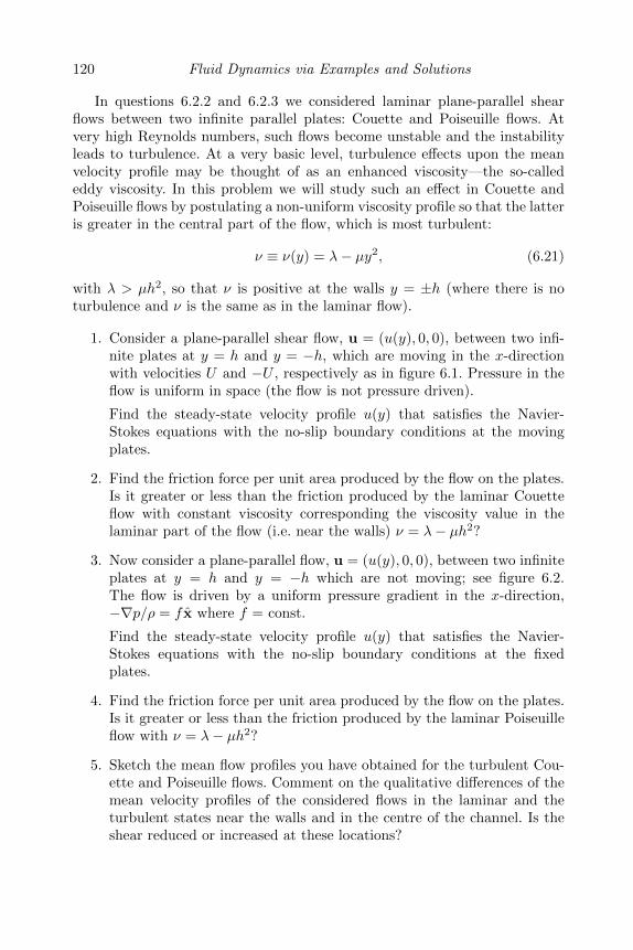
120 Fluid Dynamics via Examples and Solutions
In questions 6.2.2 and 6.2.3 we considered laminar plane-parallel shearflows between two infinite parallel plates: Couette and Poiseuille flows. Atvery high Reynolds numbers, such flows become unstable and the instabilityleads to turbulence. At a very basic level, turbulence effects upon the meanvelocity profile may be thought of as an enhanced viscosity—the so-callededdy viscosity. In this problem we will study such an effect in Couette andPoiseuille flows by postulating a non-uniform viscosity profile so that the latteris greater in the central part of the flow, which is most turbulent:
ν ≡ ν(y) = λ− µy2, (6.21)
with λ > µh2, so that ν is positive at the walls y = ±h (where there is noturbulence and ν is the same as in the laminar flow).
1. Consider a plane-parallel shear flow, u = (u(y), 0, 0), between two infi-nite plates at y = h and y = −h, which are moving in the x-directionwith velocities U and −U , respectively as in figure 6.1. Pressure in theflow is uniform in space (the flow is not pressure driven).
Find the steady-state velocity profile u(y) that satisfies the Navier-Stokes equations with the no-slip boundary conditions at the movingplates.
2. Find the friction force per unit area produced by the flow on the plates.Is it greater or less than the friction produced by the laminar Couetteflow with constant viscosity corresponding the viscosity value in thelaminar part of the flow (i.e. near the walls) ν = λ− µh2?
3. Now consider a plane-parallel flow, u = (u(y), 0, 0), between two infiniteplates at y = h and y = −h which are not moving; see figure 6.2.The flow is driven by a uniform pressure gradient in the x-direction,−∇p/ρ = f x where f = const.
Find the steady-state velocity profile u(y) that satisfies the Navier-Stokes equations with the no-slip boundary conditions at the fixedplates.
4. Find the friction force per unit area produced by the flow on the plates.Is it greater or less than the friction produced by the laminar Poiseuilleflow with ν = λ− µh2?
5. Sketch the mean flow profiles you have obtained for the turbulent Cou-ette and Poiseuille flows. Comment on the qualitative differences of themean velocity profiles of the considered flows in the laminar and theturbulent states near the walls and in the centre of the channel. Is theshear reduced or increased at these locations?
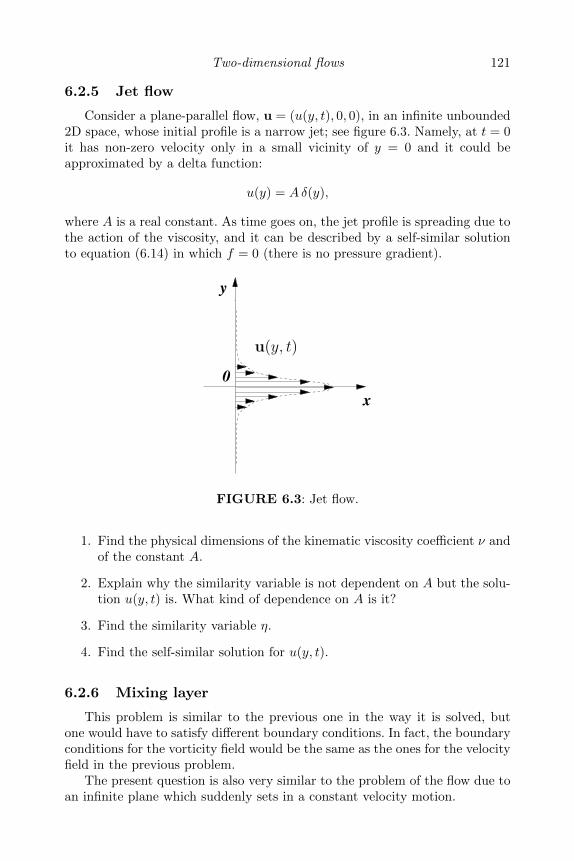
Two-dimensional flows 121
6.2.5 Jet flow
Consider a plane-parallel flow, u = (u(y, t), 0, 0), in an infinite unbounded2D space, whose initial profile is a narrow jet; see figure 6.3. Namely, at t = 0it has non-zero velocity only in a small vicinity of y = 0 and it could beapproximated by a delta function:
u(y) = Aδ(y),
where A is a real constant. As time goes on, the jet profile is spreading due tothe action of the viscosity, and it can be described by a self-similar solutionto equation (6.14) in which f = 0 (there is no pressure gradient).
y
x
0
u(y, t)
FIGURE 6.3: Jet flow.
1. Find the physical dimensions of the kinematic viscosity coefficient ν andof the constant A.
2. Explain why the similarity variable is not dependent on A but the solu-tion u(y, t) is. What kind of dependence on A is it?
3. Find the similarity variable η.
4. Find the self-similar solution for u(y, t).
6.2.6 Mixing layer
This problem is similar to the previous one in the way it is solved, butone would have to satisfy different boundary conditions. In fact, the boundaryconditions for the vorticity field would be the same as the ones for the velocityfield in the previous problem.
The present question is also very similar to the problem of the flow due toan infinite plane which suddenly sets in a constant velocity motion.
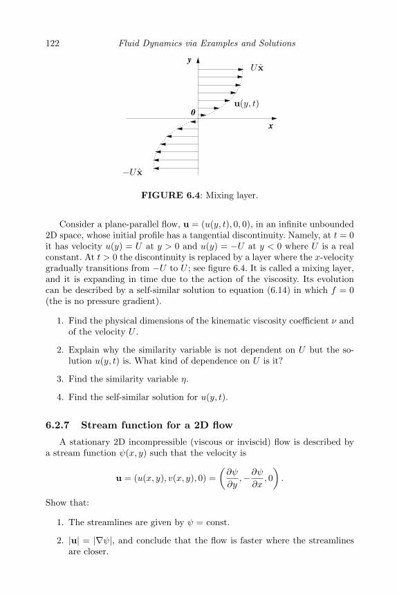
122 Fluid Dynamics via Examples and Solutions
0
x
y
u(y, t)
U x
−U x
FIGURE 6.4: Mixing layer.
Consider a plane-parallel flow, u = (u(y, t), 0, 0), in an infinite unbounded2D space, whose initial profile has a tangential discontinuity. Namely, at t = 0it has velocity u(y) = U at y > 0 and u(y) = −U at y < 0 where U is a realconstant. At t > 0 the discontinuity is replaced by a layer where the x-velocitygradually transitions from −U to U ; see figure 6.4. It is called a mixing layer,and it is expanding in time due to the action of the viscosity. Its evolutioncan be described by a self-similar solution to equation (6.14) in which f = 0(the is no pressure gradient).
1. Find the physical dimensions of the kinematic viscosity coefficient ν andof the velocity U .
2. Explain why the similarity variable is not dependent on U but the so-lution u(y, t) is. What kind of dependence on U is it?
3. Find the similarity variable η.
4. Find the self-similar solution for u(y, t).
6.2.7 Stream function for a 2D flow
A stationary 2D incompressible (viscous or inviscid) flow is described bya stream function ψ(x, y) such that the velocity is
u = (u(x, y), v(x, y), 0) =
(∂ψ
∂y,−∂ψ
∂x, 0
).
Show that:
1. The streamlines are given by ψ = const.
2. |u| = |∇ψ|, and conclude that the flow is faster where the streamlinesare closer.
Two-dimensional flows 123
3. The volume flux (per unit length in z) crossing any curve from (x1, y1)to (x2, y2) is given by ψ(x2, y2)− ψ(x1, y1).
4. ψ = const on any fixed (i.e. stationary) boundary.
5. Find the stream function for the flow with the following velocity field,
u =y
x2 + y2, v = − x
x2 + y2.
Sketch the streamlines and describe the properties of this flow.
6.2.8 Round vortices: Rankine vortex and a point vortex
This problem deals with round 2D vortices, i.e. vortices whose vorticitydistributions depend only on the distance from the vortex centre and not onthe polar angle.
1. Consider a vorticity field of a 2D flow, ω = (0, 0, ω), such that in polarcoordinates ω depend only on the radius and not on the polar angle,ω ≡ ω(r) where r =
√x2 + y2.
Prove that such a vorticity distribution represents a steady-state solutionof the ideal flow equations for any profile ω(r). (This may not necessarilybe a stable, i.e. a realisable solution).
2. Rankine vortex. Consider a vortex profile ω(r) such that ω(r) =κ = const for r ≤ a (a = const) and ω(r) = 0 for r > a. Find thevelocity and the pressure fields for such a vortex.
3. Take the limit a → 0 while keeping the combination Γ = κa2 constant(vortex circulation). This limit corresponds to the so-called point vortex.Find the velocity and the pressure fields for such a vortex.
6.2.9 Flow bounded by two intersecting planes
Consider a 2D potential flow described by the complex potential
w(z) = Czn,
where C and n are real positive numbers.
1. Suppose that n = 1. Describe the resulting flow and the meaning of theconstant C.
2. Suppose now that n = 2. Describe the resulting flow and the meaningof the constant C.
124 Fluid Dynamics via Examples and Solutions
3. Now consider the case where n is an arbitrary rational number which isgreater or equal to 1/2. Write down expressions for the velocity potentialφ and the stream function ψ in terms of the polar coordinates r and θ onthe complex plane, z = reiθ. Find the smallest and the second-smallestpositive angles, θ = θ1 and θ = θ2, for which the stream function ψ iszero for any r. Consider the flow in the sector θ1 < θ < θ2, i.e. betweenthe two intersecting (at z = 0) planes θ = θ1 and θ = θ2. Explain whythe flow with the complex potential w(z) = Czn satisfies the free-slipboundary conditions at these planes.
4. Sketch the flows arising in the cases n = 4, n = 4/3, n = 2/3 andn = 1/2.
5. Describe the qualitative difference in behaviour of the velocity field nearr = 0 for cases n < 1 and n > 1.
6.2.10 “Binary star system”
The setup of this problem could be considered a simplified 2D analogue ofthe flow arising in a binary star system in which one of the stars is a rotatingblack hole. The reader is recommended to search the web for Cygnus X-1images for illustration.
1. Consider a 2D potential flow described by the complex potential
w(z) = C ln z,
where C is a complex constant. Describe the flows when C is real andwhen C is purely imaginary.
2. Consider a 2D potential flow described by the complex potential
w(z) = ln z − (1 + ia) ln(z − 1),
where a is a real positive constant.
Find the stagnation point in this flow.
3. Describe how this flow behaves at r = |z| → ∞.
4. Sketch the streamlines and describe the general features of the flow.
5. Assume now that the “black hole is not rotating”, a = 0. Find theshortest lifetime of the fluid particles, i.e. the shortest time between theemergence of a fluid particle at the source at (x, y) = (0, 0) and itsdisappearance into the “black hole” at (x, y) = (1, 0).
Two-dimensional flows 125
6.2.11 Complex potential for the gravity water waves
The velocity potential corresponding to the gravity wave on deep water is(c.f. question 4.3.2):
φ = Ceky cos(kx− ωt), y < 0, (6.22)
where the water surface is at y = 0, and C, k and ω are real positive constantshaving the meaning of the wave amplitude, wave number and frequency.
1. Find the velocity field under the water surface.
2. Find the stream function and the complex potential.
3. Find the trajectories of the fluid particles and the streamlines. Commenton the differences of these two types of curves.
6.2.12 Aeroplane lift and trailing vortices
This problem deals with the lift force on a flying aeroplane, its relation tothe velocity circulation around the aerofoil and the trailing vortices originatingat the airplane wingtips.
1. Explain why the vortex lines near the wing surface (responsible forthe circulation round the aerofoil) must continue into a trailing vor-tex through the wingtip. What is the relation between the circulationaround the wing and circulation round its trailing vortex?
2. An aeroplane of mass M is flying at speed V through air of density ρ.Each wing of this plane is L meters long. Find the circulation aroundeach of its trailing vortices. (Hint: use Zhukovskiy’s lift theorem.)
3. Assume that the trailing vortices originating at both wings are parallelto each other and that their vorticity is concentrated in thin tubes sep-arated by a distance D = 2L. Find the downdraft velocity produced bythese trailing vortices at the midpoint between them.
6.2.13 Finding drag and lift using dimensional analysis
Consider a 2D incompressible flow with incident velocity U around a solidbody with typical length scale L.
1. Find the physical dimensional unit for the drag and lift forces (per unitlength in the direction transverse to the motion plane).
2. Use the dimensional analysis to find the lift force assuming that therelevant dimensional quantities determining this quantity are U, ρ andL (this will be famous Kutta’s condition).
Find the lift force in terms of U, ρ and Γ (this will be famous Zhukovskiy’sforce).
126 Fluid Dynamics via Examples and Solutions
3. Find the drag force assuming that the relevant dimensional quantitiesdetermining this quantity are U, ρ and L. This regime may be realisedfor some blunt bodies with separated flow and turbulence in its wake.
4. What is the most general expression for the drag force assuming thatthe relevant dimensional quantities determining this quantity are U, ρ, νand L? (Hint: you may use the result of the previous question anduse Re instead of ν.) Note: the drag dependence on Re will be Re−1/2
for a flat plate. What other dependencies are possible? (Hint: think ofd’Alembert’s paradox.)
6.2.14 A laminar jet flow
A 2D jet emerges from a narrow slit in a wall into fluid which is at rest.If the jet is thin, so that velocity u = (u, v) varies much more rapidly acrossthe jet than along it, the fluid equation becomes
u∂u
∂x+ v
∂u
∂y= ν
∂2u
∂y2, (6.23)
where constant ν is the viscosity coefficient. The boundary conditions arethat the velocity and its derivatives tend to zero as we leave the jet (that isas |y| → ∞) and ∂u/∂y = 0 at y = 0, as the motion is symmetrical about thex-axis.
1. By integrating equation (6.23) across the jet and using the incompress-ibility condition, show that the integral
M =
∫ ∞−∞
u2 dy (6.24)
is independent of x.
2. Assuming that the stream function is of a self-similar form,
ψ = xa f(η), where η = yxb, (6.25)
find the relation between the constants a and b using part (1).
3. Substitute the similarity solution (6.25) into equation (6.23) and findthe second relation between a and b. Thus, find a and b.
4. Show that jet equation (6.23) and the velocity boundary conditions leadto the following equation for f(η),
(f ′)2 + ff ′ + 3ν f ′′′ = 0
subject to the conditions
f(0) = f ′′(0) = 0, f ′(∞) = 0,
where prime means differentiation. (It is possible to find an exact solu-tion of this equation but you do not have to do it here.)
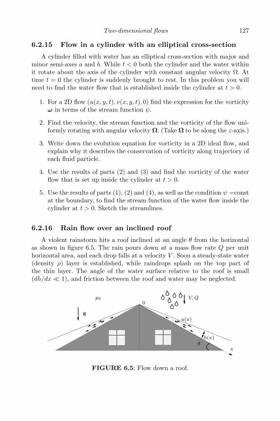
Two-dimensional flows 127
6.2.15 Flow in a cylinder with an elliptical cross-section
A cylinder filled with water has an elliptical cross-section with major andminor semi-axes a and b. While t < 0 both the cylinder and the water withinit rotate about the axis of the cylinder with constant angular velocity Ω. Attime t = 0 the cylinder is suddenly brought to rest. In this problem you willneed to find the water flow that is established inside the cylinder at t > 0.
1. For a 2D flow (u(x, y, t), v(x, y, t), 0) find the expression for the vorticityω in terms of the stream function ψ.
2. Find the velocity, the stream function and the vorticity of the flow uni-formly rotating with angular velocity Ω. (Take Ω to be along the z-axis.)
3. Write down the evolution equation for vorticity in a 2D ideal flow, andexplain why it describes the conservation of vorticity along trajectory ofeach fluid particle.
4. Use the results of parts (2) and (3) and find the vorticity of the waterflow that is set up inside the cylinder at t > 0.
5. Use the results of parts (1), (2) and (4), as well as the condition ψ =constat the boundary, to find the stream function of the water flow inside thecylinder at t > 0. Sketch the streamlines.
6.2.16 Rain flow over an inclined roof
A violent rainstorm hits a roof inclined at an angle θ from the horizontalas shown in figure 6.5. The rain pours down at a mass flow rate Q per unithorizontal area, and each drop falls at a velocity V . Soon a steady-state water(density ρ) layer is established, while raindrops splash on the top part ofthe thin layer. The angle of the water surface relative to the roof is small(dh/dx 1), and friction between the roof and water may be neglected.
xθ
0V,Q
u(x)
h(x)
p0
g
FIGURE 6.5: Flow down a roof.
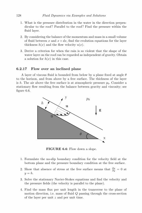
128 Fluid Dynamics via Examples and Solutions
1. What is the pressure distribution in the water in the direction perpen-dicular to the roof? Parallel to the roof? Find the pressure within thefluid layer.
2. By considering the balance of the momentum and mass in a small volumeof fluid between x and x+ dx, find the evolution equations for the layerthickness h(x) and the flow velocity u(x).
3. Derive a criterion for when the rain is so violent that the shape of thewater layer on the roof can be regarded as independent of gravity. Obtaina solution for h(x) in this case.
6.2.17 Flow over an inclined plane
A layer of viscous fluid is bounded from below by a plane fixed at angle θto the horizon, and from above by a free surface. The thickness of the layeris h. The air above the free surface is at atmospheric pressure p0. Consider astationary flow resulting from the balance between gravity and viscosity; seefigure 6.6.
u
y
x
g
0
p0
h
θ
FIGURE 6.6: Flow down a slope.
1. Formulate the no-slip boundary condition for the velocity field at thebottom plane and the pressure boundary condition at the free surface.
2. Show that absence of stress at the free surface means that ∂u∂y = 0 at
y = h.
3. Solve the stationary Navier-Stokes equations and find the velocity andthe pressure fields (the velocity is parallel to the plane).
4. Find the mass flux per unit length in the transverse to the plane ofmotion direction, i.e. mass of fluid Q passing through the cross-sectionof the layer per unit z and per unit time.
Two-dimensional flows 129
6.3 Solutions
6.3.1 Model solution to question 6.2.1
1. The vorticity in 2D flows has only a z-component, Ω = ∂xv − ∂yu.Substituting u and v, we have Ω ≡ 0.
2. From u = ∇φ, we have for the velocity potential φ = 12α(x2−y2). From
u = (∂yψ,−∂yψ), we have the steamfunction ψ = αxy. From w = φ+iψ,we have the complex potential w(z) = 1
2z2.
3. Equation for the streamlines:
dx
u=dy
v.
Substituting u and v:dx
x= −dy
y.
Solving for x and y, we get y = C/x, where C is an arbitrary constant(parametrising the streamlines).
4.dx
dt= αx,
sox = x0e
αt.
Therefore
t1 =1
αlnx1
x0.
6.3.2 Model solution to question 6.2.2
1. Let us start with the Euler equation:
∂tu + (u · ∇)u = −1
ρ∇p.
Consider a steady plane-parallel shear flow: u = (u(y), 0, 0). The flow istime independent,
∂tu = 0,
and x-independent,(u · ∇)u = u∂xu = 0.
Therefore, the x-component of the Euler equation is satisfied if ∂xp = 0,i.e. p is independent of x.
130 Fluid Dynamics via Examples and Solutions
For the y-component of the Euler equation we have: 0 = − 1ρ∂yp, i.e.
p is y-independent. Same for the z-component of the Euler equation:0 = − 1
ρ∂zp, i.e. p is z-independent.
Therefore u = (u(y), 0, 0) is a solution for any profile u(y) and p = const.
2. The no-slip boundary conditions are: u(h) = U, u(−h) = −U.
3. Let us write the Navier-Stokes equation:
∂tu + (u · ∇)u = −1
ρ∇p+ ν∇2u.
The left-hand side of this equation and ∇p are zero as before on u =(u(y), 0, 0). Therefore we have:
∇2u = ∂yyu(y) = 0.
The solution of this equation is
u(y) = Ay +B.
The boundary conditions give B = 0 and A = U/h, i.e.
u(y) =U
hy.
4. The friction per unit area at the bottom plate is equal to the x-momentum flux in the y-direction σxy:
σxy = νρ[∂yu]y=−h =Uνρ
h.
The friction at the top plate is equal in strength and opposite in sign.
6.3.3 Model solution to question 6.2.3
1. The right-hand side of the Navier-Stokes equation is zero on any plane-parallel flow u = (u(y), 0, 0), i.e. ∂tu + (u · ∇)u = 0; see solution 6.3.2.
Therefore∂xp/ρ = −f = ν∂yyu(y).
The solution of this equation is
u(y) = − f
2νy2 +By + C.
The no-slip boundary conditions to be satisfied are u(h) = u(−h) = 0.Thus B = 0 and C = f
2νh2, i.e.
u(y) =f
2ν(h2 − y2).
Two-dimensional flows 131
2. The friction per unit area at the bottom plate is equal to the x-momentum flux in the y-direction σxy:
σxy = [νρ∂yu]y=−h = ρfh.
The friction at the top plate is the same.
6.3.4 Model solution to question 6.2.4
1. For the plane-parallel shear flow, u = (u(y), 0, 0), which has a uniformpressure, ∇p = 0, the Navier-Stokes equation (6.20) becomes:
∂y(ν∂yu(y)) = ∂y((λ− µy2)∂yu) = 0. (6.26)
Integrating this equation once, we have:
(λ− µy2)∂yu = A,
where A is a constant. Solving this equation, we have:
u(y) =
∫A
λ− µy2dy =
A√λµ
arctanh
√µy√λ
+B, (6.27)
where B is a constant. Matching to the no-slip conditions u(h) = U and
u(−h) = −U we have B = 0 and A = U√λµ/arctanh
√µh√λ. Thus,
u(y) =U
arctanh√µh√λ
arctanh
√µy√λ. (6.28)
2. The friction per unit area at the bottom plate is equal to the x-momentum flux in the y-direction σxy (it is convenient here to use ex-pression (6.27)):
σxy = [νρ∂yu]y=−h = ρA =Uρ√λµ
arctanh√µh√λ
.
The friction force at the top plate has the same absolute value and theopposite sign.
This friction force is greater (in the absolute value) than the frictionUρ(λ−µh2)/h produced by the laminar Couette flow with ν = λ−µh2
because λ− µh2 < λ and arctanh√µh√λ<√µh√λ
.
3. Now consider a plane-parallel flow between two parallel plates, which isdriven by a uniform pressure gradient, −∇p/ρ = f x, where f = const.The Navier-Stokes equation (6.20) becomes:
∂y(ν∂yu(y)) = ∂y((λ− µy2)∂yu) = −f. (6.29)
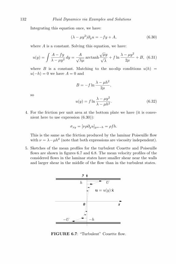
132 Fluid Dynamics via Examples and Solutions
Integrating this equation once, we have:
(λ− µy2)∂yu = −fy +A, (6.30)
where A is a constant. Solving this equation, we have:
u(y) =
∫A− fyλ− µy2
dy =A√λµ
arctanh
√µy√λ
+ f lnλ− µy2
2µ+B, (6.31)
where B is a constant. Matching to the no-slip conditions u(h) =u(−h) = 0 we have A = 0 and
B = −f lnλ− µh2
2µ,
so
u(y) = f lnλ− µy2
λ− µh2. (6.32)
4. For the friction per unit area at the bottom plate we have (it is conve-nient here to use expression (6.30)):
σxy = [νρ∂yu]y=−h = ρfh.
This is the same as the friction produced by the laminar Poiseuille flowwith ν = λ−µh2 (note that both expressions are viscosity independent).
5. Sketches of the mean profiles for the turbulent Couette and Poiseuilleflows are shown in figures 6.7 and 6.8. The mean velocity profiles of theconsidered flows in the laminar states have smaller shear near the wallsand larger shear in the middle of the flow than in the turbulent states.
x
y
0
−U
h
−h
u = u(y) x
U
FIGURE 6.7: “Turbulent” Couette flow.
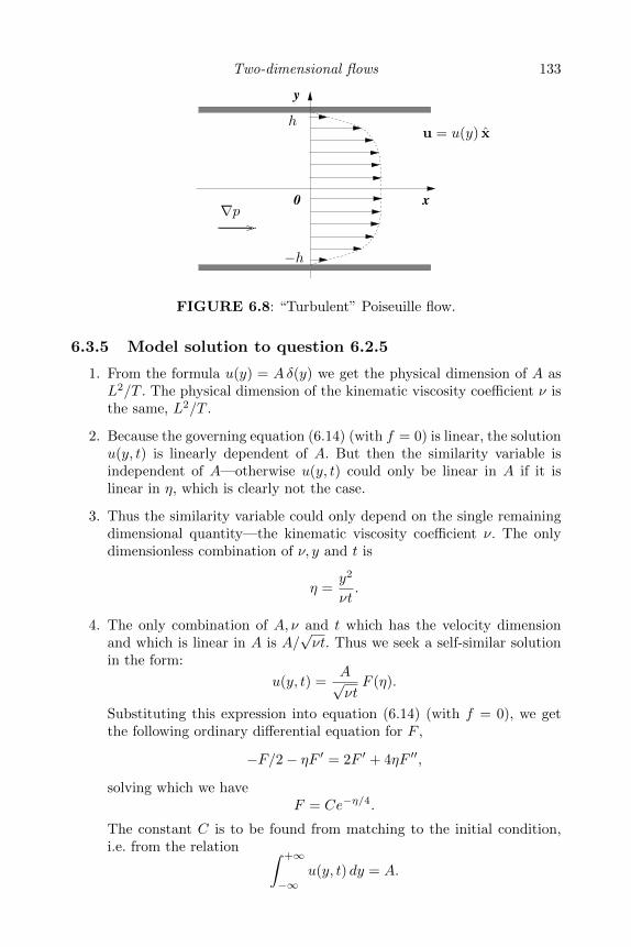
Two-dimensional flows 133
x
y
0
u = u(y) xh
−h
∇p
FIGURE 6.8: “Turbulent” Poiseuille flow.
6.3.5 Model solution to question 6.2.5
1. From the formula u(y) = Aδ(y) we get the physical dimension of A asL2/T . The physical dimension of the kinematic viscosity coefficient ν isthe same, L2/T .
2. Because the governing equation (6.14) (with f = 0) is linear, the solutionu(y, t) is linearly dependent of A. But then the similarity variable isindependent of A—otherwise u(y, t) could only be linear in A if it islinear in η, which is clearly not the case.
3. Thus the similarity variable could only depend on the single remainingdimensional quantity—the kinematic viscosity coefficient ν. The onlydimensionless combination of ν, y and t is
η =y2
νt.
4. The only combination of A, ν and t which has the velocity dimensionand which is linear in A is A/
√νt. Thus we seek a self-similar solution
in the form:
u(y, t) =A√νtF (η).
Substituting this expression into equation (6.14) (with f = 0), we getthe following ordinary differential equation for F ,
−F/2− ηF ′ = 2F ′ + 4ηF ′′,
solving which we haveF = Ce−η/4.
The constant C is to be found from matching to the initial condition,i.e. from the relation ∫ +∞
−∞u(y, t) dy = A.
134 Fluid Dynamics via Examples and Solutions
Here we have used the fact that the integral∫ +∞−∞ u(y, t) dy is conserved
in time.
The easiest way to use this condition is to consider time t = 1/ν so thatνt = 1. Then we have
C
∫ +∞
−∞e−y
2/4 dy = 1,
or C = 12√π
. Finally, we have
u(y, t) =A
2√πνt
ey2
4νt .
6.3.6 Model solution to question 6.2.6
This problem is similar to the previous one in the way it is solved, but onewould have to satisfy different boundary conditions. The boundary conditionsfor the vorticity field will be the same as the ones for the velocity field in theprevious problem.
1. The physical dimension [ν] of the kinematic viscosity coefficient ν can befound from comparing the viscous term in the Navier-Stokes equation,ν∇2u, with the time derivative term ∂tu (obviously they must have thesame physical dimension). Thus [ν] = L2/T . The physical dimension ofthe velocity U is L/T .
2. Because the governing equation (6.14) (with f = 0) is linear, the solutionu(y, t) is linearly dependent on U . But then the similarity variable isindependent of U—otherwise u(y, t) could only be linear in U if it islinear in η, which is clearly not the case.
3. Thus the similarity variable could only depend on the single remainingdimensional quantity—the kinematic viscosity coefficient ν. The onlydimensionless combination of ν, y and t is
η =y2
νt.
4. We seek a self-similar solution in the form:
u(y, t) = U F (η).
Substituting this expression into equation (6.14) (with f = 0), we getthe following ordinary differential equation for F ,
−ηF ′ = 2F ′ + 4ηF ′′.
Two-dimensional flows 135
5. The above equation can be rearranged as:
F ′′/F ′ = − 1
2η− 1
4.
Subsequently integrating, we have:
F ′ = Cη−1/2e−η4 ,
where C is a constant. Integrating one more time, we have:
F = C
∫η−1/2e−
η4 dη = 4C
∫e−ξ
2
dξ = 2C√π erf(ξ) +B,
where ξ = η1/2/2, erf(ξ) is the error function and B is a constant.
Now we need to use the boundary condition that u(0, t) = 0 for t > 0,which translates to F (0) = 0. This gives B = 0. Finally, we need touse the initial condition that u(y, 0) = U for y > 0, which translates toF (∞) = 1, and therefore C = 1/(2
√π). Substituting these constants,
we have the answer for the velocity field:
u(y, t) = U erf(ξ),
where ξ = 12 (y
2
νt )1/2.
6.3.7 Model solution to question 6.2.7
1. In steady flow
Dtψ = ∂tψ + (u · ∇)ψ = ∂yψ∂xψ − ∂xψ∂yψ = 0,
so ψ is constant along streamlines.
2. For the absolute value of velocity we have:
u =√u2x + u2
y =√
(∂yψ)2 + (∂xψ)2 = |∇ψ|.
3. By splitting the curve into n small sub-intervals and finding the massflux Si on each sub-interval i as ui × dli we have (see figure 6.9):
S = limn→∞
n∑i=1
Si =
∫ x2
x1
u× dl =
∫ x2
x1
(∇ψ × ez)× dl =
∫ x2
x1
∇ψ · dl = ψ(x2)− ψ(x1).
4. The normal velocity component is zero at the boundary, (u · n) = 0.Therefore (∇ψ)‖ = 0.
5. For this flow ψ = 12 ln(x2+y2). The streamlines ψ = const are concentric
circles: they are shown in figure 6.10. This is a point vortex flow. It isirrotational everywhere except at the origin x = 0.
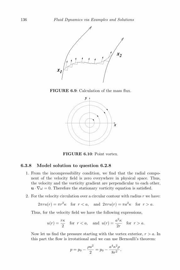
136 Fluid Dynamics via Examples and Solutions
2
x
x
1
FIGURE 6.9: Calculation of the mass flux.
y
x
FIGURE 6.10: Point vortex.
6.3.8 Model solution to question 6.2.8
1. From the incompressibility condition, we find that the radial compo-nent of the velocity field is zero everywhere in physical space. Thus,the velocity and the vorticity gradient are perpendicular to each other,u · ∇ω = 0. Therefore the stationary vorticity equation is satisfied.
2. For the velocity circulation over a circular contour with radius r we have:
2πru(r) = πr2κ for r < a, and 2πru(r) = πa2κ for r > a.
Thus, for the velocity field we have the following expressions,
u(r) =rκ
2for r < a, and u(r) =
a2κ
2rfor r > a.
Now let us find the pressure starting with the vortex exterior, r > a. Inthis part the flow is irrotational and we can use Bernoulli’s theorem:
p = p0 −ρu2
2= p0 −
a4κ2ρ
8r2,
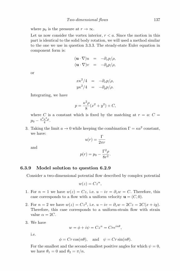
Two-dimensional flows 137
where p0 is the pressure at r →∞.
Let us now consider the vortex interior, r < a. Since the motion in thispart is identical to the solid body rotation, we will used a method similarto the one we use in question 3.3.3. The steady-state Euler equation incomponent form is:
(u · ∇)u = −∂xp/ρ,(u · ∇)v = −∂yp/ρ,
or
xκ2/4 = −∂xp/ρ,yκ2/4 = −∂yp/ρ.
Integrating, we have
p =κ2ρ
8(x2 + y2) + C,
where C is a constant which is fixed by the matching at r = a: C =
p0 − a2κ2ρ4 .
3. Taking the limit a→ 0 while keeping the combination Γ = κa2 constant,we have:
u(r) =Γ
2πrand
p(r) = p0 −Γ2ρ
8r2.
6.3.9 Model solution to question 6.2.9
Consider a two-dimensional potential flow described by complex potential
w(z) = Czn,
1. For n = 1 we have w(z) = Cz, i.e. u − iv = ∂zw = C. Therefore, thiscase corresponds to a flow with a uniform velocity u = (C, 0).
2. For n = 2 we have w(z) = Cz2, i.e. u− iv = ∂zw = 2Cz = 2C(x+ iy).Therefore, this case corresponds to a uniform-strain flow with strainvalue α = 2C.
3. We havew = φ+ iψ = Czn = Creinθ,
i.e.φ = Cr cos(nθ), and ψ = Cr sin(nθ).
For the smallest and the second-smallest positive angles for which ψ = 0,we have θ1 = 0 and θ2 = π/n.
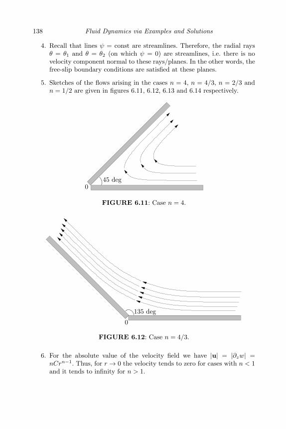
138 Fluid Dynamics via Examples and Solutions
4. Recall that lines ψ = const are streamlines. Therefore, the radial raysθ = θ1 and θ = θ2 (on which ψ = 0) are streamlines, i.e. there is novelocity component normal to these rays/planes. In the other words, thefree-slip boundary conditions are satisfied at these planes.
5. Sketches of the flows arising in the cases n = 4, n = 4/3, n = 2/3 andn = 1/2 are given in figures 6.11, 6.12, 6.13 and 6.14 respectively.
045 deg
FIGURE 6.11: Case n = 4.
135 deg
0
FIGURE 6.12: Case n = 4/3.
6. For the absolute value of the velocity field we have |u| = |∂zw| =nCrn−1. Thus, for r → 0 the velocity tends to zero for cases with n < 1and it tends to infinity for n > 1.
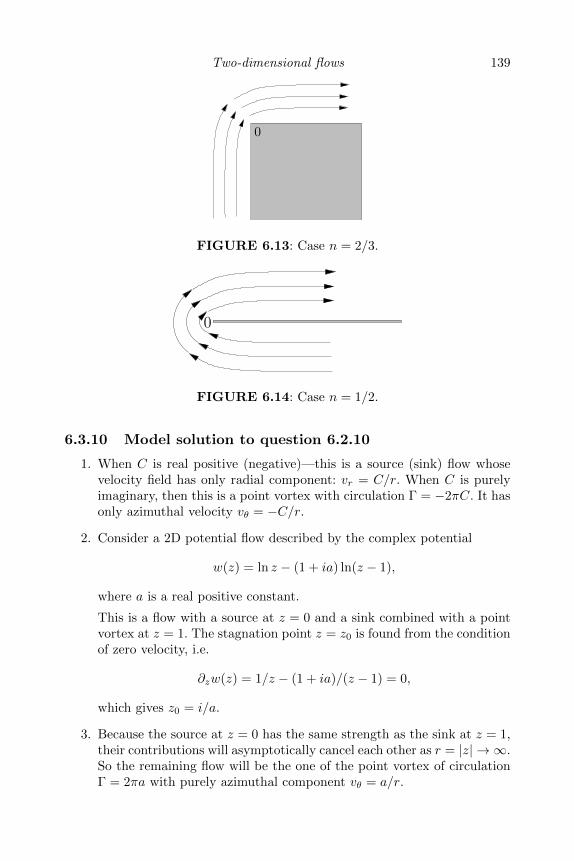
Two-dimensional flows 139
0
FIGURE 6.13: Case n = 2/3.
0
FIGURE 6.14: Case n = 1/2.
6.3.10 Model solution to question 6.2.10
1. When C is real positive (negative)—this is a source (sink) flow whosevelocity field has only radial component: vr = C/r. When C is purelyimaginary, then this is a point vortex with circulation Γ = −2πC. It hasonly azimuthal velocity vθ = −C/r.
2. Consider a 2D potential flow described by the complex potential
w(z) = ln z − (1 + ia) ln(z − 1),
where a is a real positive constant.
This is a flow with a source at z = 0 and a sink combined with a pointvortex at z = 1. The stagnation point z = z0 is found from the conditionof zero velocity, i.e.
∂zw(z) = 1/z − (1 + ia)/(z − 1) = 0,
which gives z0 = i/a.
3. Because the source at z = 0 has the same strength as the sink at z = 1,their contributions will asymptotically cancel each other as r = |z| → ∞.So the remaining flow will be the one of the point vortex of circulationΓ = 2πa with purely azimuthal component vθ = a/r.
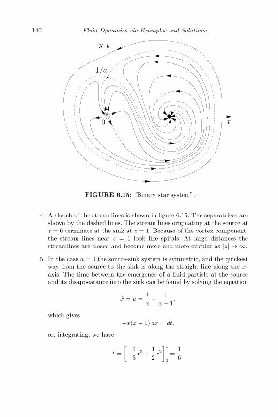
140 Fluid Dynamics via Examples and Solutions
1/a
y
x0
FIGURE 6.15: “Binary star system”.
4. A sketch of the streamlines is shown in figure 6.15. The separatrices areshown by the dashed lines. The stream lines originating at the source atz = 0 terminate at the sink at z = 1. Because of the vortex component,the stream lines near z = 1 look like spirals. At large distances thestreamlines are closed and become more and more circular as |z| → ∞.
5. In the case a = 0 the source-sink system is symmetric, and the quickestway from the source to the sink is along the straight line along the x-axis. The time between the emergence of a fluid particle at the sourceand its disappearance into the sink can be found by solving the equation
x = u =1
x− 1
x− 1,
which gives−x(x− 1) dx = dt,
or, integrating, we have
t =
[−1
3x3 +
1
2x2
]1
0
=1
6.
Two-dimensional flows 141
6.3.11 Model solution to question 6.2.11
1. Taking the gradient of the potential (6.22) we have:
ux = ∂xφ = −Ckeky sin(kx− ωt), uy = ∂yφ = Ckeky cos(kx− ωt).
2. The stream function ψ is defined via
ux = ∂yψ = −Ckeky sin(kx− ωt), uy = −∂xψ = Ckeky cos(kx− ωt).
Integrating we have:
ψ = −Ceky sin(kx− ωt).
The complex potential is then:
ξ = φ+ iψ = Ceky [cos(kx− ωt)− i sin(kx− ωt)] =
Ceky−i(kx−ωt) = Ce−i(kz−ωt),
wherez = x+ iy.
3. A particle which in the still fluid was at position (x, y), in presence ofthe wave will move along a trajectory around (x, y):
(x(t), y(t)) = (x, y) + (x(t), y(t)).
For the particle trajectories we have
˙x(t) = ux = −Ckeky sin(kx− ωt), (6.33)
˙y(t) = uy = Ckeky cos(kx− ωt). (6.34)
Integrating these equations we have:
x(t) = −Ckωeky cos(kx− ωt), (6.35)
y(t) = −Ckωeky sin(kx− ωt). (6.36)
Thus these trajectories are circles:
x2 + y2 = R2,
where
R =Ck
ωeky.
The streamlines are given by the equation
ψ = −Ceky sin(kx− ωt) = const.
They are infinite periodic curves with parts going to y → ±∞. Theparticle trajectories are different from the streamlines, which is naturalfor a non-stationary motion.
142 Fluid Dynamics via Examples and Solutions
6.3.12 Model solution to question 6.2.12
1. Near the wing surface, velocity is nearly tangential to the surface andits variation is in the normal direction. Therefore the vorticity is parallelto the wing. The vorticity field is solenoidal i.e. vortex lines cannot endwithin the fluid. Therefore they must continue beyond the wing tips, sothat the vorticity flux remains the same.
Therefore, the circulation of the trailing vortices is the same as thecirculation around the wing.
2. To keep the plane flying, the gravity force must be balanced by the lift,so
Mg = ρV Γ(2L)
or
Γ =Mg
2ρV L.
3. If the vortices are thin and straight, then each of them produces velocitylike a point vortex in 2D, namely Γ
2πr where r is the distance from thevortex. In the middle point, the velocities produced by the two vorticesadd up: U = Γ
2π(D/2) · 2. Thus,
U =Γ
πL.
6.3.13 Model solution to question 6.2.13
1. The physical unit for force, e.g. the drag and lift forces, is the Newton,which is equal to kg ∗ m/s2. Therefore, force per unit length has thephysical dimension of [ρ]L3/T 2.
2. The only dimensional combination of U, ρ and L having the dimensionof the force per unit length is
F = c1ρU2L,
where c1 is a dimensionless constant.
The only dimensional combination of U, ρ and L having the dimensionof the velocity circulation is
Γ = c2UL,
where c2 is a dimensionless constant.
From the above two expressions we find Zhukovskiy’s lift force:
F = cρUΓ,
where c is a dimensionless constant. More rigorous analysis (Zhukovskiy’stheorem) yields c = 1.
Two-dimensional flows 143
3. For the drag force per unit length D (similarly to the lift force) assumingthat the relevant dimensional quantities determining this quantity areU, ρ and L, we find
D = cρU2L,
where c is a dimensionless constant (which, in this case is not necessarilyequal to one: it is called the drag coefficient and it strongly dependenton the body shape).
4. The most general expression for the drag force assuming that the rele-vant dimensional quantities determining this quantity are U, ρ, ν and L(using the result of the previous question and using Re instead of ν) is
D = cρU2Lf(Re),
where c is dimensionless constant and f is a dimensionless function.
Since, according to D’Alembert’s paradox, the drag must vanish in thelimit ν → 0, we conclude that f(Re) must be a decreasing function ofRe for laminar flows. For turbulent flows the situation is more difficult,because of the flow separation such flows do not tend to the ideal flowsolutions in the limit ν → 0.
6.3.14 Model solution to question 6.2.14
1. Integrating equation (6.23) over y, we have for the individual terms:∫ +∞
−∞uux dy =
1
2∂x
∫ +∞
−∞u2 dy,
∫ +∞
−∞vuy dy = −
∫ +∞
−∞vyu dy =
∫ +∞
−∞uxu dy =
1
2∂x
∫ +∞
−∞u2 dy,
and
ν
∫ +∞
−∞∂yyu dy = uy|+∞−∞ = 0.
Therefore we find:
M =
∫ +∞
−∞u2 dy = C,
where C is an independent of x constant.
2. Substituting the self-similar solution into the expression for M we have:
M =
∫ +∞
−∞u2 dy = x2a+b
∫ +∞
−∞(f ′)2 dη .
But M must be independent of x, so
b = −2a.
144 Fluid Dynamics via Examples and Solutions
3. This leads to the following expressions for the velocity components andtheir derivatives:
u = ψy = x−af ′,
v = −ψx = axa−1(−f + 2ηf ′),
ux = −ax−a−1(f ′ + 2ηf ′′),
uy = x−3af ′′,
uyy = x−5af ′′′.
Substituting these expressions into equation (6.23) we have:
−x−af ′ax−a−1(f ′ + 2ηf ′′) + axa−1(−f + 2ηf ′)x−3af ′′ = νx−5af ′′′.
This equation must be independent of x, so
a = 1/3 and b = −2/3.
4. The required equation immediately follows from the above equationupon substituting a = 1/3.
The boundary conditions are:
• y = 0 is a streamline, therefore f(0) = 0.
• u(−y) = u(y) =⇒ uy = 0 at y = 0, therefore f ′′(0) = 0.
• u|y=∞ = 0, therefore f ′(∞) = 0.
6.3.15 Model solution to question 6.2.15
1. For the vorticity we have ω = (0, 0, ω), where ω = −∇2ψ.
2. The velocity, the stream function and the vorticity of the flow uniformlyrotating with angular velocity Ω are:
u = Ω × x, ψ = −Ω2 (x2 + y2), ω = 2 Ω.
3. We have the following equation for the vorticity:
∂tω + u · ∇ω = 0.
The left-hand side here is the time derivative of vorticity along the fluidpaths, Dt ω, therefore this equation describes conservation of vorticityalong trajectory of each fluid particle.
4. The vorticity field will remain constant, as in the uniformly rotatingflow, ω = 2 Ω = (0, 0, 2Ω).
Two-dimensional flows 145
5. The fact that the vorticity is constant, together with equation ω =−∇2ψ, suggests that ψ will be a quadratic function of x and y: like inpart 2, but now with ψ = const at the elliptic boundary. Therefore, att > 0 we have:
ψ = − Ωa2b2
a2 + b2[(x/a)2 + (y/b)2],
where we found the pre-factor so that −∇2ψ = 2Ω.
6.3.16 Model solution to question 6.2.16
1. For a thin layer, ∂xh 1, the flow is mostly in the x-direction. Thus,from the y-component of the momentum equation we have ∂yp = 0, i.e. pis independent of y. But at the water surface the pressure is atmospheric,p = p0, so p = p0 everywhere in the fluid (it is independent of x and y).
2. Consider a small volume of fluid between x and x+ dx and with a unitlength in the transverse to x direction: dx × h(x) × 1. Let F (x) be themomentum flux,
F = ρhu2.
The gravity force onto the volume element is:
Fg = mg = ρh dxg.
The momentum input per unit time by the rain is:
M = mVx = (Qdx cos θ)(V sin θ).
(We have the x-momentum only because the y-momentum is completelydissipated by the roof).
Thus, the momentum balance for the considered small volume is:
F (x+ dx)− F (x) ≈ dx ∂xF = Fgx +M,
orρ∂x(hu2) = ρgh sin θ +QV sin θ cos θ.
For the mass balance we have:
dx∂x(ρhu) = rain input = Qdx cos θ,
orρ∂x(hu) = Q cos θ.
Integrating this equation we have:
ρhu = Qx cos θ.
146 Fluid Dynamics via Examples and Solutions
3. The gravity force can be ignored if
ρgh sin θ QV sin θ cos θ,
orρgh QV. (6.37)
In this case, integrating the momentum balance equation we have:
ρhu2 = QV x sin θ cos θ + C,
where C is a constant. Combining this result with the mass equation,we get:
u = V sin θ and h =Q cos θ
ρV sin θx,
where we put C = 0 since u must be finite at x = 0. Using this solutionone can rewrite the condition (6.37) as
V 2 gx.
6.3.17 Model solution to question 6.2.17
1. It is clear from figure 6.6 that the flow is plane parallel:
u(x, y) = (u(y), 0), (6.38)
where function u(y) is to be found.
The no-slip boundary condition in this case is
u(0) = 0, (6.39)
and the pressure boundary condition at the free surface is
p(x, h) = p0. (6.40)
2. Stress at the free surface is given by the tangential to the surface com-ponent of the viscous stress tensor,
σij = ρν(∂xiuj + ∂xjui),
namely by σxy = ρν∂yu(y). Absence of the stress at the free surfacetherefore means that
∂yu = 0 at y = h.
Two-dimensional flows 147
3. It is clear that the pressure field in this problem is independent of x.Thus, the stationary Navier-Stokes equations written in components are:
1
ρ∂yp+ g cos θ = 0, (6.41)
ν∂yyu+ g sin θ = 0. (6.42)
Integrating equation (6.41) and using the pressure boundary condition(6.40), we have
p = p0 + ρg(h− y) cos θ. (6.43)
Integrating equation (6.42) twice, and using the no-slip boundary con-dition (6.39) and the condition ∂yu = 0 at y = h, we have
u =g sin θ
2νy(2h− y). (6.44)
4. The mass of fluid passing through the cross-section of the layer, per unitlength in the transverse direction, per unit time is∫ h
0
ρu dy =ρgh3 sin θ
3ν. (6.45)

This page intentionally left blankThis page intentionally left blank
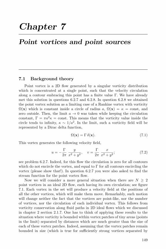
Chapter 7
Point vortices and point sources
7.1 Background theory
Point vortex is a 2D flow generated by a singular vorticity distributionwhich is concentrated at a single point, such that the velocity circulationalong a contour embracing this point has a finite value Γ. We have alreadymet this solution in questions 6.2.7 and 6.2.8. In question 6.2.8 we obtainedthe point vortex solution as a limiting case of a Rankine vortex with vorticityΩ(x) which is constant inside a circle of radius a, Ω(x) = κ = const, andzero outside. Then, the limit a → 0 was taken while keeping the circulationconstant, Γ = πa2κ = const. This means that the vorticity value inside thecircle tends to infinity, κ ∼ 1/a2. In the limit, such a vorticity field will berepresented by a Dirac delta function,
Ω(x) = Γ δ(x). (7.1)
This vortex generates the following velocity field,
u = − Γ
2π
y
x2 + y2, v =
Γ
2π
x
x2 + y2; (7.2)
see problem 6.2.7. Indeed, for this flow the circulation is zero for all contourswhich do not encircle the vortex, and equal to Γ for all contours encircling thevortex (please show that!). In question 6.2.7 you were also asked to find thestream function for the point vortex flow.
Now we will consider a more general situation when there are N ≥ 2point vortices in an ideal 2D flow, each having its own circulation; see figure7.1. Each vortex in the set will produce a velocity field at the positions ofall the other vortices, which will make them move. Remarkably, such motionwill change neither the fact that the vortices are point-like, nor the numberof vortices, nor the circulation of each individual vortex. This follows fromvorticity conservation along fluid paths in 2D ideal flows which we discussedin chapter 2 section 2.1.7. One has to think of applying these results to thesituation where vorticity is bounded within vortex patches of tiny areas (pointsin the limit) separated by distances which are much greater than the size ofeach of these vortex patches. Indeed, assuming that the vortex patches remainbounded in size (which is true for sufficiently strong vortices separated by
149
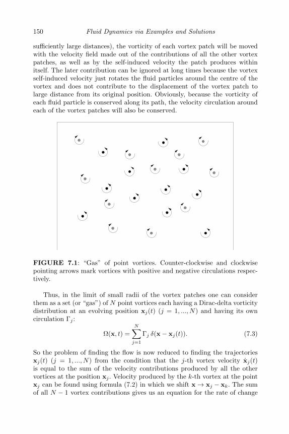
150 Fluid Dynamics via Examples and Solutions
sufficiently large distances), the vorticity of each vortex patch will be movedwith the velocity field made out of the contributions of all the other vortexpatches, as well as by the self-induced velocity the patch produces withinitself. The later contribution can be ignored at long times because the vortexself-induced velocity just rotates the fluid particles around the centre of thevortex and does not contribute to the displacement of the vortex patch tolarge distance from its original position. Obviously, because the vorticity ofeach fluid particle is conserved along its path, the velocity circulation aroundeach of the vortex patches will also be conserved.
FIGURE 7.1: “Gas” of point vortices. Counter-clockwise and clockwisepointing arrows mark vortices with positive and negative circulations respec-tively.
Thus, in the limit of small radii of the vortex patches one can considerthem as a set (or “gas”) of N point vortices each having a Dirac-delta vorticitydistribution at an evolving position xj(t) (j = 1, ..., N) and having its owncirculation Γj :
Ω(x, t) =N∑j=1
Γj δ(x− xj(t)). (7.3)
So the problem of finding the flow is now reduced to finding the trajectoriesxj(t) (j = 1, ..., N) from the condition that the j-th vortex velocity xj(t)is equal to the sum of the velocity contributions produced by all the othervortices at the position xj . Velocity produced by the k-th vortex at the pointxj can be found using formula (7.2) in which we shift x→ xj − xk. The sumof all N − 1 vortex contributions gives us an equation for the rate of change

Point vortices and point sources 151
of xj :
xj =
N∑k=1,k 6=j
Γk2π
z× (xj − xk)
|xj − xk|2, (7.4)
where z is the unit vector normal to the plane of motion, and sign × standsfor the cross product (prove this formula!).
Introducing a complex coordinate for the vortex labelled j as zj(t) =xj(t) + iyj(t), we can rewrite equation (7.4) in a complex form:
dz∗jdt
= − i
2π
N∑k=1,k 6=k
Γkzj − zk
, (7.5)
where star * means complex conjugation.Another kind of point object arising in the study of ideal fluid flows are
point sources or sinks. They have only a radial (with respect to the positionof the source/sink) component of velocity, v(r), which is independent of theangular coordinates:
u = rv(r), (7.6)
where r is a unit vector pointing away from the source/sink in the radialdirection; see figure 7.2.
κ
u = rv(r)
FIGURE 7.2: A point source flow.
From incompressibility we have rd−1v(r) = const, where d is the dimensionof the system (which is 2 or 3) and r is the distance from the source/sink.Therefore
v(r) =κ
rd−1, (7.7)
where constant κ is called the source strength when it is positive and the sinkstrength when it is negative. The constant κ is proportional to the mass fluxout of the source or into the sink respectively.
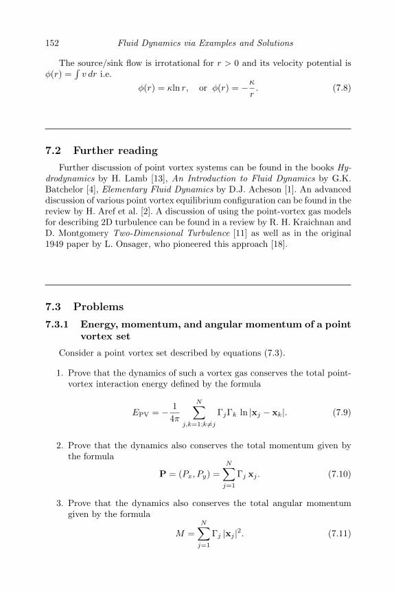
152 Fluid Dynamics via Examples and Solutions
The source/sink flow is irrotational for r > 0 and its velocity potential isφ(r) =
∫v dr i.e.
φ(r) = κln r, or φ(r) = −κr. (7.8)
7.2 Further reading
Further discussion of point vortex systems can be found in the books Hy-drodynamics by H. Lamb [13], An Introduction to Fluid Dynamics by G.K.Batchelor [4], Elementary Fluid Dynamics by D.J. Acheson [1]. An advanceddiscussion of various point vortex equilibrium configuration can be found in thereview by H. Aref et al. [2]. A discussion of using the point-vortex gas modelsfor describing 2D turbulence can be found in a review by R. H. Kraichnan andD. Montgomery Two-Dimensional Turbulence [11] as well as in the original1949 paper by L. Onsager, who pioneered this approach [18].
7.3 Problems
7.3.1 Energy, momentum, and angular momentum of a pointvortex set
Consider a point vortex set described by equations (7.3).
1. Prove that the dynamics of such a vortex gas conserves the total point-vortex interaction energy defined by the formula
EPV = − 1
4π
N∑j,k=1;k 6=j
ΓjΓk ln |xj − xk|. (7.9)
2. Prove that the dynamics also conserves the total momentum given bythe formula
P = (Px, Py) =
N∑j=1
Γj xj . (7.10)
3. Prove that the dynamics also conserves the total angular momentumgiven by the formula
M =
N∑j=1
Γj |xj |2. (7.11)
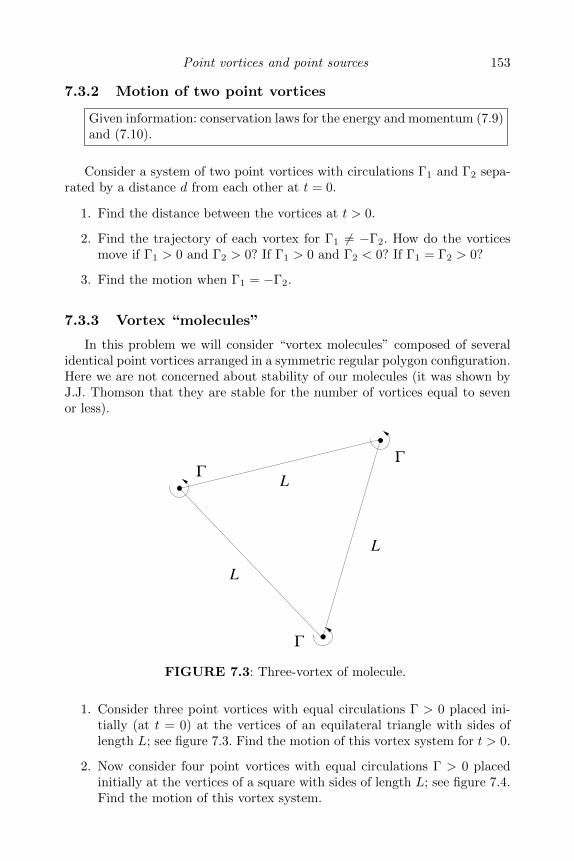
Point vortices and point sources 153
7.3.2 Motion of two point vortices
Given information: conservation laws for the energy and momentum (7.9)and (7.10).
Consider a system of two point vortices with circulations Γ1 and Γ2 sepa-rated by a distance d from each other at t = 0.
1. Find the distance between the vortices at t > 0.
2. Find the trajectory of each vortex for Γ1 6= −Γ2. How do the vorticesmove if Γ1 > 0 and Γ2 > 0? If Γ1 > 0 and Γ2 < 0? If Γ1 = Γ2 > 0?
3. Find the motion when Γ1 = −Γ2.
7.3.3 Vortex “molecules”
In this problem we will consider “vortex molecules” composed of severalidentical point vortices arranged in a symmetric regular polygon configuration.Here we are not concerned about stability of our molecules (it was shown byJ.J. Thomson that they are stable for the number of vortices equal to sevenor less).
L
Γ
Γ
Γ
L
L
FIGURE 7.3: Three-vortex of molecule.
1. Consider three point vortices with equal circulations Γ > 0 placed ini-tially (at t = 0) at the vertices of an equilateral triangle with sides oflength L; see figure 7.3. Find the motion of this vortex system for t > 0.
2. Now consider four point vortices with equal circulations Γ > 0 placedinitially at the vertices of a square with sides of length L; see figure 7.4.Find the motion of this vortex system.
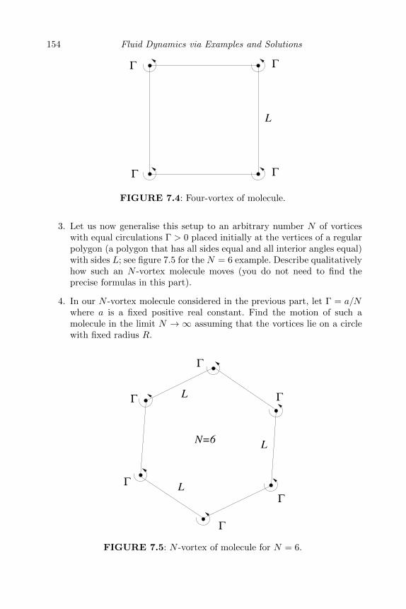
154 Fluid Dynamics via Examples and Solutions
Γ Γ
L
ΓΓ
FIGURE 7.4: Four-vortex of molecule.
3. Let us now generalise this setup to an arbitrary number N of vorticeswith equal circulations Γ > 0 placed initially at the vertices of a regularpolygon (a polygon that has all sides equal and all interior angles equal)with sides L; see figure 7.5 for the N = 6 example. Describe qualitativelyhow such an N -vortex molecule moves (you do not need to find theprecise formulas in this part).
4. In our N -vortex molecule considered in the previous part, let Γ = a/Nwhere a is a fixed positive real constant. Find the motion of such amolecule in the limit N → ∞ assuming that the vortices lie on a circlewith fixed radius R.
N=6
L
Γ
Γ
Γ
L
L
Γ
Γ
Γ
FIGURE 7.5: N -vortex of molecule for N = 6.
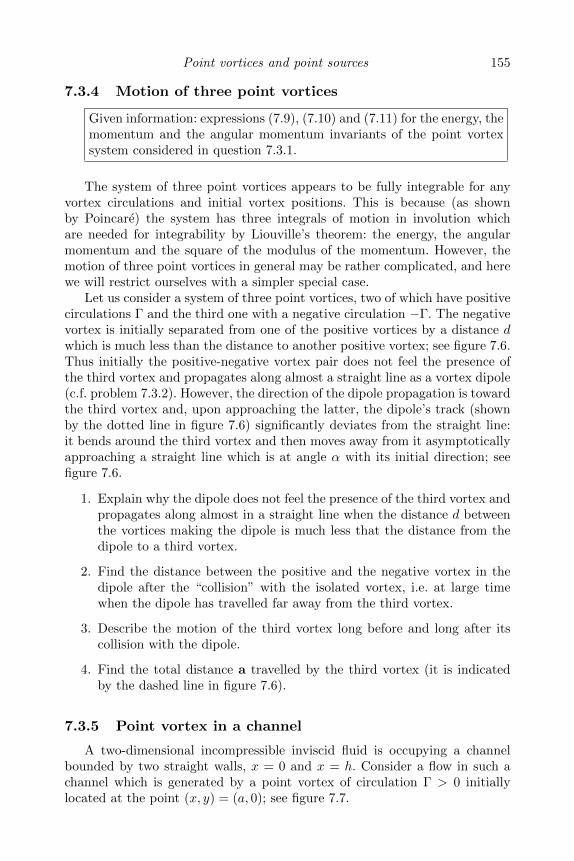
Point vortices and point sources 155
7.3.4 Motion of three point vortices
Given information: expressions (7.9), (7.10) and (7.11) for the energy, themomentum and the angular momentum invariants of the point vortexsystem considered in question 7.3.1.
The system of three point vortices appears to be fully integrable for anyvortex circulations and initial vortex positions. This is because (as shownby Poincare) the system has three integrals of motion in involution whichare needed for integrability by Liouville’s theorem: the energy, the angularmomentum and the square of the modulus of the momentum. However, themotion of three point vortices in general may be rather complicated, and herewe will restrict ourselves with a simpler special case.
Let us consider a system of three point vortices, two of which have positivecirculations Γ and the third one with a negative circulation −Γ. The negativevortex is initially separated from one of the positive vortices by a distance dwhich is much less than the distance to another positive vortex; see figure 7.6.Thus initially the positive-negative vortex pair does not feel the presence ofthe third vortex and propagates along almost a straight line as a vortex dipole(c.f. problem 7.3.2). However, the direction of the dipole propagation is towardthe third vortex and, upon approaching the latter, the dipole’s track (shownby the dotted line in figure 7.6) significantly deviates from the straight line:it bends around the third vortex and then moves away from it asymptoticallyapproaching a straight line which is at angle α with its initial direction; seefigure 7.6.
1. Explain why the dipole does not feel the presence of the third vortex andpropagates along almost in a straight line when the distance d betweenthe vortices making the dipole is much less that the distance from thedipole to a third vortex.
2. Find the distance between the positive and the negative vortex in thedipole after the “collision” with the isolated vortex, i.e. at large timewhen the dipole has travelled far away from the third vortex.
3. Describe the motion of the third vortex long before and long after itscollision with the dipole.
4. Find the total distance a travelled by the third vortex (it is indicatedby the dashed line in figure 7.6).
7.3.5 Point vortex in a channel
A two-dimensional incompressible inviscid fluid is occupying a channelbounded by two straight walls, x = 0 and x = h. Consider a flow in such achannel which is generated by a point vortex of circulation Γ > 0 initiallylocated at the point (x, y) = (a, 0); see figure 7.7.
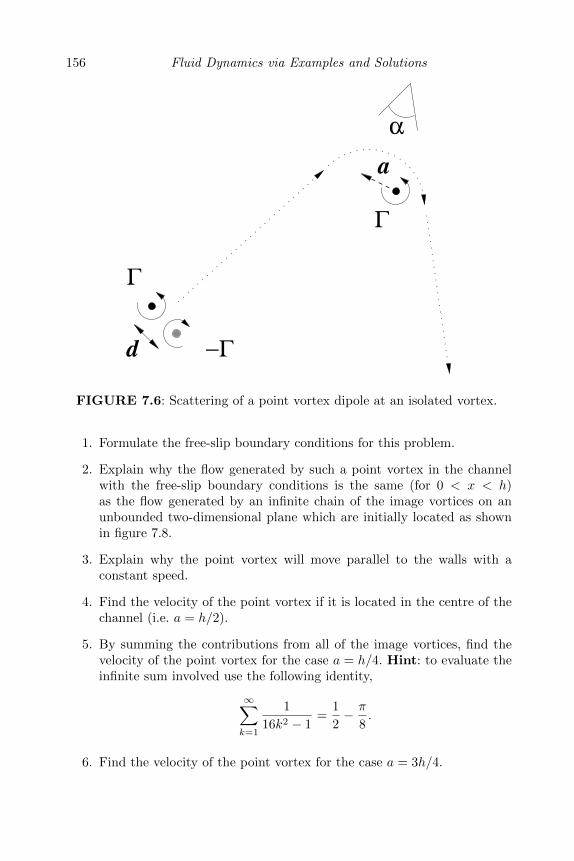
156 Fluid Dynamics via Examples and Solutions
a
Γ
−Γ
Γ
α
d
FIGURE 7.6: Scattering of a point vortex dipole at an isolated vortex.
1. Formulate the free-slip boundary conditions for this problem.
2. Explain why the flow generated by such a point vortex in the channelwith the free-slip boundary conditions is the same (for 0 < x < h)as the flow generated by an infinite chain of the image vortices on anunbounded two-dimensional plane which are initially located as shownin figure 7.8.
3. Explain why the point vortex will move parallel to the walls with aconstant speed.
4. Find the velocity of the point vortex if it is located in the centre of thechannel (i.e. a = h/2).
5. By summing the contributions from all of the image vortices, find thevelocity of the point vortex for the case a = h/4. Hint: to evaluate theinfinite sum involved use the following identity,
∞∑k=1
1
16k2 − 1=
1
2− π
8.
6. Find the velocity of the point vortex for the case a = 3h/4.
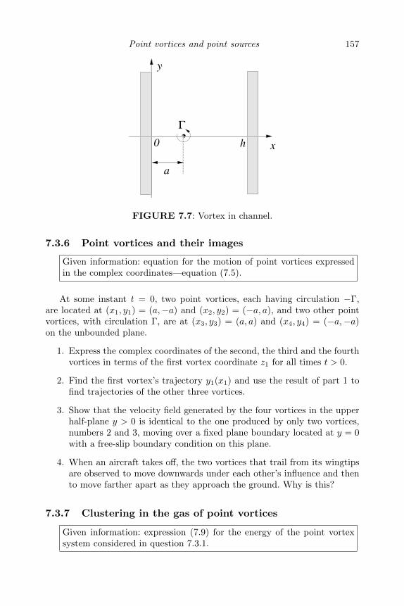
Point vortices and point sources 157
a
Γ
y
xh0
FIGURE 7.7: Vortex in channel.
7.3.6 Point vortices and their images
Given information: equation for the motion of point vortices expressedin the complex coordinates—equation (7.5).
At some instant t = 0, two point vortices, each having circulation −Γ,are located at (x1, y1) = (a,−a) and (x2, y2) = (−a, a), and two other pointvortices, with circulation Γ, are at (x3, y3) = (a, a) and (x4, y4) = (−a,−a)on the unbounded plane.
1. Express the complex coordinates of the second, the third and the fourthvortices in terms of the first vortex coordinate z1 for all times t > 0.
2. Find the first vortex’s trajectory y1(x1) and use the result of part 1 tofind trajectories of the other three vortices.
3. Show that the velocity field generated by the four vortices in the upperhalf-plane y > 0 is identical to the one produced by only two vortices,numbers 2 and 3, moving over a fixed plane boundary located at y = 0with a free-slip boundary condition on this plane.
4. When an aircraft takes off, the two vortices that trail from its wingtipsare observed to move downwards under each other’s influence and thento move farther apart as they approach the ground. Why is this?
7.3.7 Clustering in the gas of point vortices
Given information: expression (7.9) for the energy of the point vortexsystem considered in question 7.3.1.
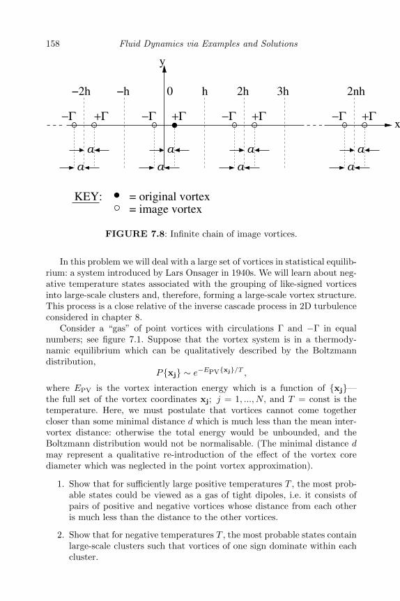
158 Fluid Dynamics via Examples and Solutions
−Γ −Γ −Γ+Γ +Γ+Γ −Γ +Γx
−2h −h 0 h 2h 2nh3h
y
a
a a a a
a a a
= image vortex= original vortexKEY:
FIGURE 7.8: Infinite chain of image vortices.
In this problem we will deal with a large set of vortices in statistical equilib-rium: a system introduced by Lars Onsager in 1940s. We will learn about neg-ative temperature states associated with the grouping of like-signed vorticesinto large-scale clusters and, therefore, forming a large-scale vortex structure.This process is a close relative of the inverse cascade process in 2D turbulenceconsidered in chapter 8.
Consider a “gas” of point vortices with circulations Γ and −Γ in equalnumbers; see figure 7.1. Suppose that the vortex system is in a thermody-namic equilibrium which can be qualitatively described by the Boltzmanndistribution,
Pxj ∼ e−EPVxj/T ,
where EPV is the vortex interaction energy which is a function of xj—the full set of the vortex coordinates xj; j = 1, ..., N, and T = const is thetemperature. Here, we must postulate that vortices cannot come togethercloser than some minimal distance d which is much less than the mean inter-vortex distance: otherwise the total energy would be unbounded, and theBoltzmann distribution would not be normalisable. (The minimal distance dmay represent a qualitative re-introduction of the effect of the vortex corediameter which was neglected in the point vortex approximation).
1. Show that for sufficiently large positive temperatures T , the most prob-able states could be viewed as a gas of tight dipoles, i.e. it consists ofpairs of positive and negative vortices whose distance from each otheris much less than the distance to the other vortices.
2. Show that for negative temperatures T , the most probable states containlarge-scale clusters such that vortices of one sign dominate within eachcluster.
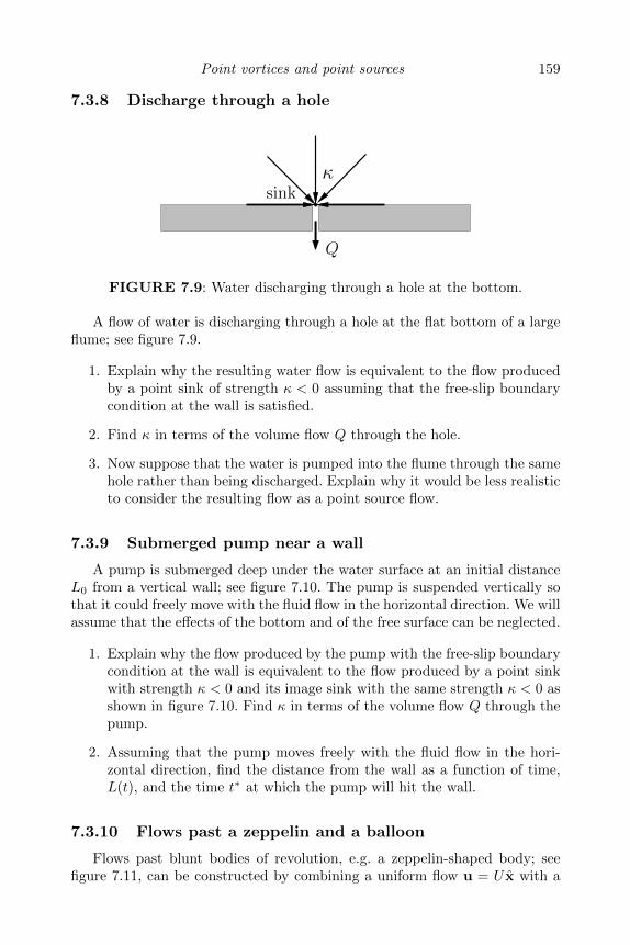
Point vortices and point sources 159
7.3.8 Discharge through a hole
Q
sinkκ
FIGURE 7.9: Water discharging through a hole at the bottom.
A flow of water is discharging through a hole at the flat bottom of a largeflume; see figure 7.9.
1. Explain why the resulting water flow is equivalent to the flow producedby a point sink of strength κ < 0 assuming that the free-slip boundarycondition at the wall is satisfied.
2. Find κ in terms of the volume flow Q through the hole.
3. Now suppose that the water is pumped into the flume through the samehole rather than being discharged. Explain why it would be less realisticto consider the resulting flow as a point source flow.
7.3.9 Submerged pump near a wall
A pump is submerged deep under the water surface at an initial distanceL0 from a vertical wall; see figure 7.10. The pump is suspended vertically sothat it could freely move with the fluid flow in the horizontal direction. We willassume that the effects of the bottom and of the free surface can be neglected.
1. Explain why the flow produced by the pump with the free-slip boundarycondition at the wall is equivalent to the flow produced by a point sinkwith strength κ < 0 and its image sink with the same strength κ < 0 asshown in figure 7.10. Find κ in terms of the volume flow Q through thepump.
2. Assuming that the pump moves freely with the fluid flow in the hori-zontal direction, find the distance from the wall as a function of time,L(t), and the time t∗ at which the pump will hit the wall.
7.3.10 Flows past a zeppelin and a balloon
Flows past blunt bodies of revolution, e.g. a zeppelin-shaped body; seefigure 7.11, can be constructed by combining a uniform flow u = U x with a
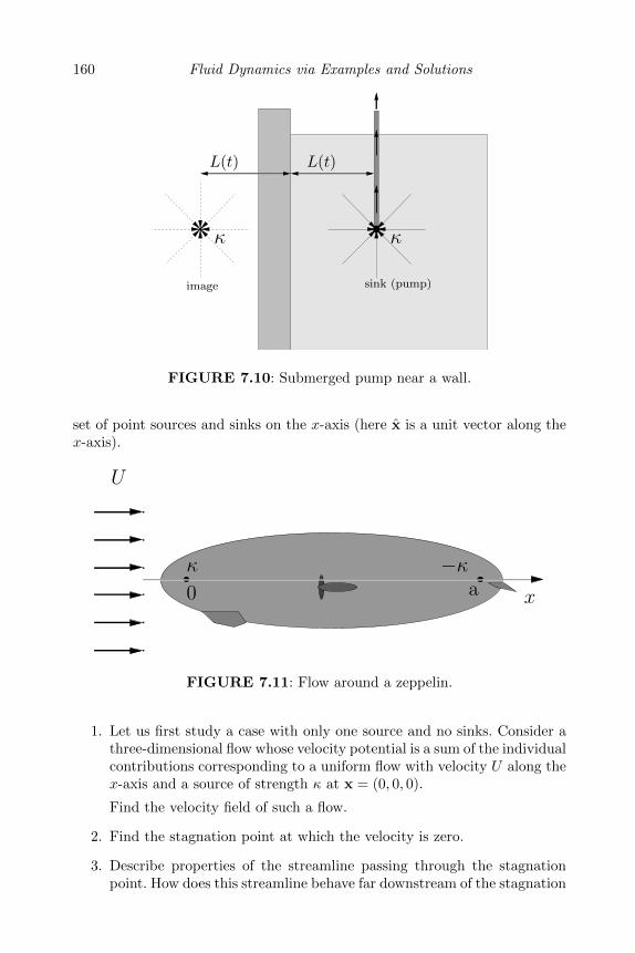
160 Fluid Dynamics via Examples and Solutions
κ κ
image
L(t) L(t)
sink (pump)
FIGURE 7.10: Submerged pump near a wall.
set of point sources and sinks on the x-axis (here x is a unit vector along thex-axis).
x
−κ
U
a0
κ
FIGURE 7.11: Flow around a zeppelin.
1. Let us first study a case with only one source and no sinks. Consider athree-dimensional flow whose velocity potential is a sum of the individualcontributions corresponding to a uniform flow with velocity U along thex-axis and a source of strength κ at x = (0, 0, 0).
Find the velocity field of such a flow.
2. Find the stagnation point at which the velocity is zero.
3. Describe properties of the streamline passing through the stagnationpoint. How does this streamline behave far downstream of the stagnation
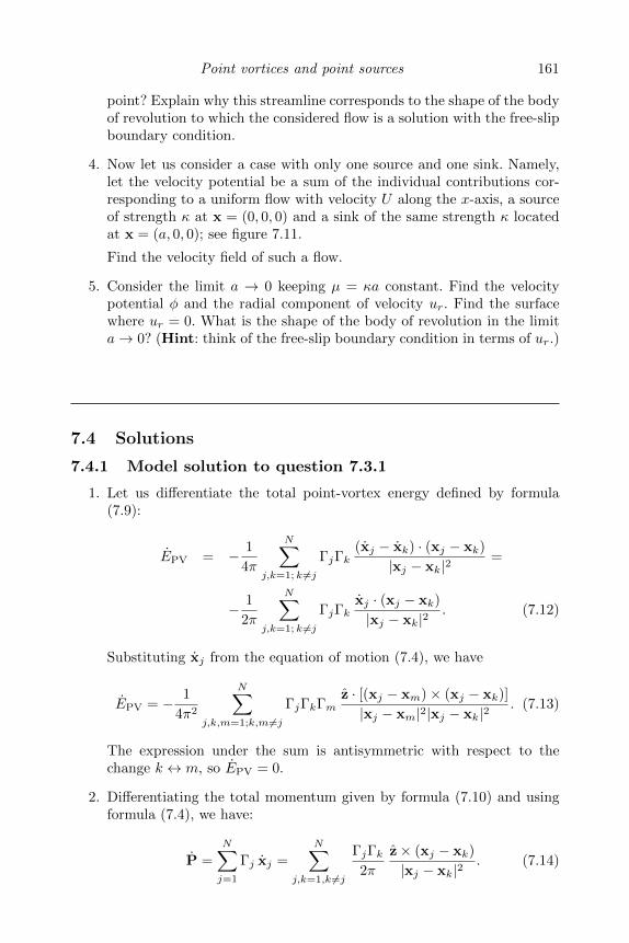
Point vortices and point sources 161
point? Explain why this streamline corresponds to the shape of the bodyof revolution to which the considered flow is a solution with the free-slipboundary condition.
4. Now let us consider a case with only one source and one sink. Namely,let the velocity potential be a sum of the individual contributions cor-responding to a uniform flow with velocity U along the x-axis, a sourceof strength κ at x = (0, 0, 0) and a sink of the same strength κ locatedat x = (a, 0, 0); see figure 7.11.
Find the velocity field of such a flow.
5. Consider the limit a → 0 keeping µ = κa constant. Find the velocitypotential φ and the radial component of velocity ur. Find the surfacewhere ur = 0. What is the shape of the body of revolution in the limita→ 0? (Hint: think of the free-slip boundary condition in terms of ur.)
7.4 Solutions
7.4.1 Model solution to question 7.3.1
1. Let us differentiate the total point-vortex energy defined by formula(7.9):
EPV = − 1
4π
N∑j,k=1; k 6=j
ΓjΓk(xj − xk) · (xj − xk)
|xj − xk|2=
− 1
2π
N∑j,k=1; k 6=j
ΓjΓkxj · (xj − xk)
|xj − xk|2. (7.12)
Substituting xj from the equation of motion (7.4), we have
EPV = − 1
4π2
N∑j,k,m=1;k,m 6=j
ΓjΓkΓmz · [(xj − xm)× (xj − xk)]
|xj − xm|2|xj − xk|2. (7.13)
The expression under the sum is antisymmetric with respect to thechange k ↔ m, so EPV = 0.
2. Differentiating the total momentum given by formula (7.10) and usingformula (7.4), we have:
P =
N∑j=1
Γj xj =
N∑j,k=1,k 6=j
ΓjΓk2π
z× (xj − xk)
|xj − xk|2. (7.14)
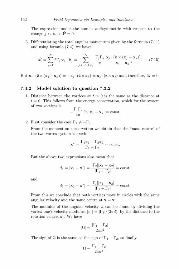
162 Fluid Dynamics via Examples and Solutions
The expression under the sum is antisymmetric with respect to thechange j ↔ k, so P = 0.
3. Differentiating the total angular momentum given by the formula (7.11)and using formula (7.4), we have:
M =
N∑j=1
2Γj xj · xj =
N∑j,k=1,k 6=j
ΓjΓkπ
xj · (z× (xj − xk))
|xj − xk|2. (7.15)
But xj · (z× (xj −xk)) = −xj · (z×xk) = xk · (z×xj) and, therefore, M = 0.
7.4.2 Model solution to question 7.3.2
1. Distance between the vortices at t > 0 is the same as the distance att = 0. This follows from the energy conservation, which for the systemof two vortices is
−Γ1Γ2
4πln |x1 − x2| = const.
2. First consider the case Γ1 6= −Γ2.
From the momentum conservation we obtain that the “mass centre” ofthe two-vortex system is fixed:
x∗ =Γ1x1 + Γ2x2
Γ1 + Γ2= const.
But the above two expressions also mean that
d1 = |x1 − x∗| = |Γ2||x1 − x2||Γ1 + Γ2|
= const.
and
d2 = |x2 − x∗| = |Γ1||x1 − x2||Γ1 + Γ2|
= const.
From this we conclude that both vortices move in circles with the sameangular velocity and the same centre at x = x∗.
The modulus of the angular velocity Ω can be found by dividing thevortex one’s velocity modulus, |v1| = |Γ2|/(2πd), by the distance to therotation centre, d1. We have
|Ω| = |Γ1 + Γ2|2πd2
.
The sign of Ω is the same as the sign of Γ1 + Γ2, so finally
Ω =Γ1 + Γ2
2πd2.
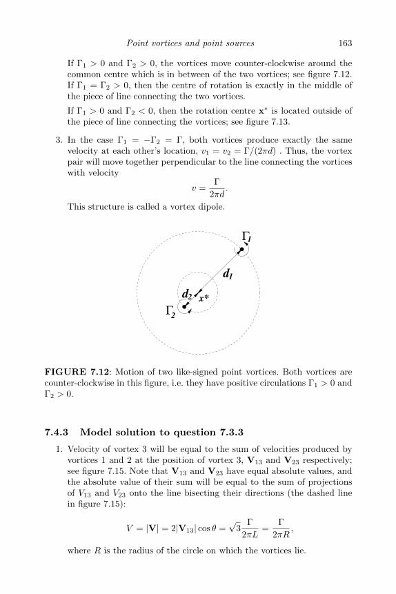
Point vortices and point sources 163
If Γ1 > 0 and Γ2 > 0, the vortices move counter-clockwise around thecommon centre which is in between of the two vortices; see figure 7.12.If Γ1 = Γ2 > 0, then the centre of rotation is exactly in the middle ofthe piece of line connecting the two vortices.
If Γ1 > 0 and Γ2 < 0, then the rotation centre x∗ is located outside ofthe piece of line connecting the vortices; see figure 7.13.
3. In the case Γ1 = −Γ2 = Γ, both vortices produce exactly the samevelocity at each other’s location, v1 = v2 = Γ/(2πd) . Thus, the vortexpair will move together perpendicular to the line connecting the vorticeswith velocity
v =Γ
2πd.
This structure is called a vortex dipole.
x*
Γ1
2
2d
d1
Γ
FIGURE 7.12: Motion of two like-signed point vortices. Both vortices arecounter-clockwise in this figure, i.e. they have positive circulations Γ1 > 0 andΓ2 > 0.
7.4.3 Model solution to question 7.3.3
1. Velocity of vortex 3 will be equal to the sum of velocities produced byvortices 1 and 2 at the position of vortex 3, V13 and V23 respectively;see figure 7.15. Note that V13 and V23 have equal absolute values, andthe absolute value of their sum will be equal to the sum of projectionsof V13 and V23 onto the line bisecting their directions (the dashed linein figure 7.15):
V = |V| = 2|V13| cos θ =√
3Γ
2πL=
Γ
2πR,
where R is the radius of the circle on which the vortices lie.
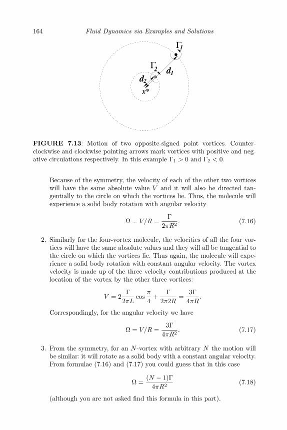
164 Fluid Dynamics via Examples and Solutions
x*
Γ1
d2
d
Γ
2
1
FIGURE 7.13: Motion of two opposite-signed point vortices. Counter-clockwise and clockwise pointing arrows mark vortices with positive and neg-ative circulations respectively. In this example Γ1 > 0 and Γ2 < 0.
Because of the symmetry, the velocity of each of the other two vorticeswill have the same absolute value V and it will also be directed tan-gentially to the circle on which the vortices lie. Thus, the molecule willexperience a solid body rotation with angular velocity
Ω = V/R =Γ
2πR2. (7.16)
2. Similarly for the four-vortex molecule, the velocities of all the four vor-tices will have the same absolute values and they will all be tangential tothe circle on which the vortices lie. Thus again, the molecule will expe-rience a solid body rotation with constant angular velocity. The vortexvelocity is made up of the three velocity contributions produced at thelocation of the vortex by the other three vortices:
V = 2Γ
2πLcos
π
4+
Γ
2π2R=
3Γ
4πR.
Correspondingly, for the angular velocity we have
Ω = V/R =3Γ
4πR2. (7.17)
3. From the symmetry, for an N -vortex with arbitrary N the motion willbe similar: it will rotate as a solid body with a constant angular velocity.From formulae (7.16) and (7.17) you could guess that in this case
Ω =(N − 1)Γ
4πR2(7.18)
(although you are not asked find this formula in this part).
Point vortices and point sources 165
x
−Γ
Γ
d
y
FIGURE 7.14: Dipole of point vortices. Counter-clockwise and clockwisepointing arrows mark vortices with positive and negative circulations respec-tively.
4. In the N -vortex molecule let Γ = a/N and take the limit N →∞ withradius R fixed. Easy to see that this limit corresponds to a uniformdistribution of vorticity on the circle and, therefore, to an axially sym-metric flow without radial component of velocity. The azimuthal velocityin such a flow changes from zero at r < R to
Vr>R =NΓ
2πr=
a
2πr
for r > R.
For the vortices on the circle r = R, velocity is equal to the middle ofthe jump value,
V =Vr=R+0 − Vr=R−0
2=
a
4πR,
andΩ = V/R =
a
4πR2.
7.4.4 Model solution to question 7.3.4
1. The pair of vortices separated by distance d produce, at each other’spositions, velocities which are equal to each other and much greater(by factor r/d) than the velocity induced by the third vortex separatedfrom the dipole vortices by distance r d. Thus the vortex dipole movesalong almost a straight line with velocity Γ/(2πd).
2. After the collision with the isolated vortex, i.e. at large time when thedipole has travelled far away from the third vortex, the distance betweenthe positive and the negative vortex in the dipole will return to its initial
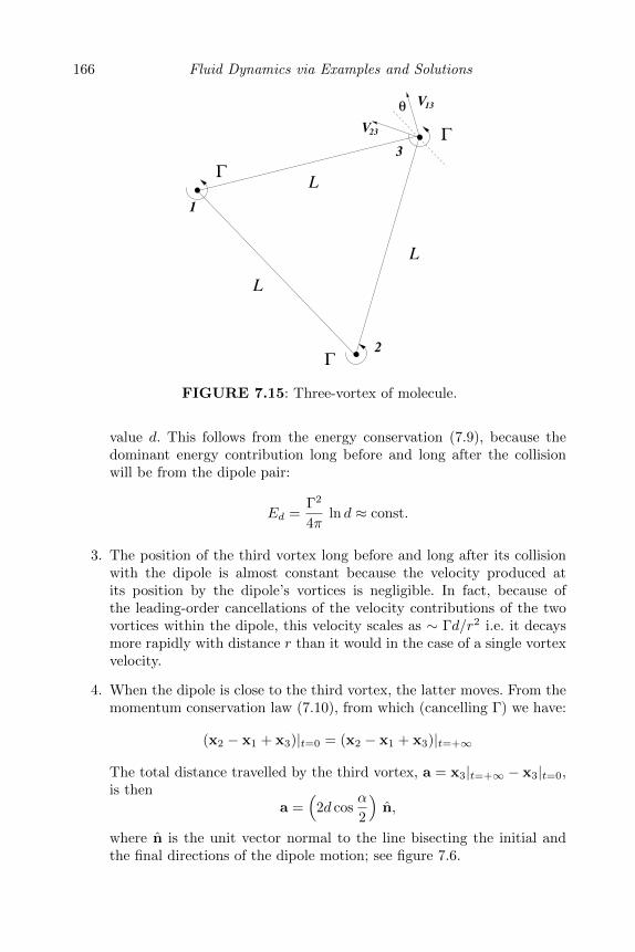
166 Fluid Dynamics via Examples and Solutions
θ
Γ
Γ
L
L
L
1
2
3
Γ
V
V
13
23
FIGURE 7.15: Three-vortex of molecule.
value d. This follows from the energy conservation (7.9), because thedominant energy contribution long before and long after the collisionwill be from the dipole pair:
Ed =Γ2
4πln d ≈ const.
3. The position of the third vortex long before and long after its collisionwith the dipole is almost constant because the velocity produced atits position by the dipole’s vortices is negligible. In fact, because ofthe leading-order cancellations of the velocity contributions of the twovortices within the dipole, this velocity scales as ∼ Γd/r2 i.e. it decaysmore rapidly with distance r than it would in the case of a single vortexvelocity.
4. When the dipole is close to the third vortex, the latter moves. From themomentum conservation law (7.10), from which (cancelling Γ) we have:
(x2 − x1 + x3)|t=0 = (x2 − x1 + x3)|t=+∞
The total distance travelled by the third vortex, a = x3|t=+∞ − x3|t=0,is then
a =(
2d cosα
2
)n,
where n is the unit vector normal to the line bisecting the initial andthe final directions of the dipole motion; see figure 7.6.
Point vortices and point sources 167
7.4.5 Model solution to question 7.3.5
1. Let the velocity field be u = (u(x, y, t), v(x, y, t)). The free-slip boundaryconditions for this problem are:
u(x, 0, t) = u(x, h, t) = 0; v(x, 0, t) & v(x, h, t) —arbitrary.
2. From symmetry, the flow generated by an infinite chain of the imagevortices on an unbounded two-dimensional plane which are located asshown in figure 7.8 will have u(x, 0, t) = u(x, h, t) = 0, as required by thefree-slip boundary conditions of the original problem. Thus, the rest ofthe flow for 0 < x < h will also be the same, because it contains the samepoint vortex inside this interval and it satisfies the fluid equations (ba-sically the Laplace equation for the velocity potential of an irrotationalincompressible flow) outside of the point vortex.
3. The point vortex and its images will remain on the same line for anyt > 0. Thus, they will not produce any x-component of the velocity ateach other’s positions. Because the x-positions of the vortices do notchange, they produce the same y-component of the velocity at eachother’s positions for any t > 0. Therefore, the point vortex (and itsimages) will move parallel to the walls with a constant speed.
4. From the symmetry, the velocity of the point vortex located in the centreof the channel (when a = h/2) is zero.
5. Here we have to refer to figure 7.8. By summing the contributions fromall of the image vortices for the case a = h/4, we have for the vortexvelocity V :
V =Γ
2πh
k=+∞∑k=−∞
[1
2k − 1/2− 1
2k + 1/2
]=
− Γ
πh+
4Γ
πh
k=+∞∑k=1
1
16k2 − 1=
Γ
πh(1− π/2).
6. From the symmetry, the velocity of the point vortex for the case a =3h/4 is just the negative of the velocity found for the case a = h/4,
V = − Γ
πh(1− π/2).
7.4.6 Model solution to question 7.3.6
1. From the symmetry of the problem for t ≥ 0 we have
x1 = x2 = −x3 = −x4; y1 = −y2 = −y3 = y4.
168 Fluid Dynamics via Examples and Solutions
Thus, we have the following expressions for the complex coordinates ofthe 2nd, 3rd and the 4th vortices in terms of the 1st vortex coordinatez1: From the symmetry of the problem for t ≥ 0 we have
z1 = −z2 = z∗3 = −z∗4 ,
where star * stands for complex conjugate.
2. From the equation for the motion (7.5), after substituting the aboverelations, we have the following equation for the coordinate of the firstvortex,
z∗1 ≡ x1 − iy1 =iΓ
2π
[1
2z1− 1
z1 − z∗1− 1
z1 + z∗1
]=
iΓ
2π
[x1 − iy1
2(x21 + y2
1)− 1
2iy1− 1
2x1
].
Taking the ratio of the real and imaginary parts of this equation we have
y1
x1= −y
31
x31
.
Integrating this equation we obtain the trajectories of the 1st vortex
1
y21
− 1
x21
= C = const. (7.19)
For each fixed constant C, this equation describes four disconnectedbranches (in the different quadrants of the (x, y)-plane), each corre-sponding to a trajectory of one of the four vortices. The 1st vortex willmove in the lower-right quadrant.
3. By the symmetry, the vertical velocity of the four-vortex flow is zero aty = 0, which means that the free-slip boundary condition on this planeis satisfied for the two-vortex system. For the latter flow the other twovortices at y < 0 become the image vortices.
4. The aircraft’s trailing vortices move downward as a vortex dipole, andupon approaching closer to the ground they behave like the 2nd andthe 3rd vortices in our problem. According to our solution (7.19), thiscorresponds to decreasing y and increasing x, i.e. the vortices move apartas they approach the ground.
7.4.7 Model solution to question 7.3.7
For the purposes of this problem, we shift expression (7.9) for the energyof the point vortex system by a constant reference energy:
EPV = − 1
4π
N∑j,k=1;k 6=j
ΓjΓk ln|xj − xk|
`, (7.20)
Point vortices and point sources 169
where ` is a typical inter-vortex distance, ` = 1/√n, n being the number
vortices per unit area. This shift does not change the form of the Boltzmanndistribution,
Pxj ∼ e−EPVxj/T ,
since the proportionality constant would have to be normalised anyway.
1. According to expression (7.20), the energy of the point vortex systemconsists of a sum of pairwise contributions: pairs of like-signed and oppo-sitely signed vortices make positive and negative contributions respec-tively when they are tight, |xj − xk| < `, and vice versa if they aredistant, |xj − xk| > `.
For the vortex system with Boltzmann distribution the negative energystates are more probable for positive temperatures T . For large tem-peratures, the most probable states are those that correspond to thevortex configurations with largest possible energies, i.e. such that theyconsist of tight vortex dipoles with sizes `, namely opposite-signedpairs with distance between the vortices of the order of the minimalallowed inter-vortex distance d.
2. For negative temperatures T , the most probable states are configura-tions with like-signed vortex pairs that have on average smaller inter-vortex distances than the opposite-signed pairs. Such distributions canbe viewed as large-scale clusters such that vortices of one sign dominatewithin each cluster. For very large negative temperatures T the mostprobable state consists of just two such clusters: a positive and a nega-tive, each being tight, with distances between the vortices within eachcluster of the order of the minimal distance d.
7.4.8 Model solution to question 7.3.8
1. The velocity field produced by a sink located at the wall will be tan-gential to this wall, i.e. the free-slip boundary condition at the wall issatisfied.
2. The radial component of the velocity field produced by the sink ofstrength κ in the 3D case is
v(r) =κ
r2, (7.21)
and the inward volume flux through a sphere of radius r surroundingthe sink is −4πr2v(r) = −4πκ. However, in the problem only half of thesink flow is realised in the fluid volume and, therefore, the volume flowthrough the hole is Q = −2πκ. Thus, for κ in terms of the volume flowthrough the pump Q we have:
κ = − Q2π. (7.22)
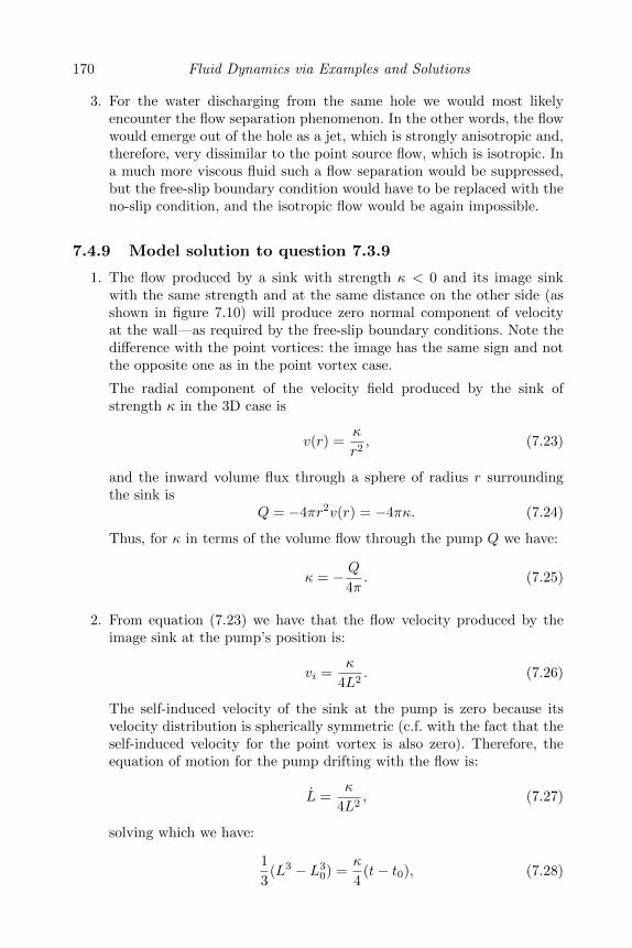
170 Fluid Dynamics via Examples and Solutions
3. For the water discharging from the same hole we would most likelyencounter the flow separation phenomenon. In the other words, the flowwould emerge out of the hole as a jet, which is strongly anisotropic and,therefore, very dissimilar to the point source flow, which is isotropic. Ina much more viscous fluid such a flow separation would be suppressed,but the free-slip boundary condition would have to be replaced with theno-slip condition, and the isotropic flow would be again impossible.
7.4.9 Model solution to question 7.3.9
1. The flow produced by a sink with strength κ < 0 and its image sinkwith the same strength and at the same distance on the other side (asshown in figure 7.10) will produce zero normal component of velocityat the wall—as required by the free-slip boundary conditions. Note thedifference with the point vortices: the image has the same sign and notthe opposite one as in the point vortex case.
The radial component of the velocity field produced by the sink ofstrength κ in the 3D case is
v(r) =κ
r2, (7.23)
and the inward volume flux through a sphere of radius r surroundingthe sink is
Q = −4πr2v(r) = −4πκ. (7.24)
Thus, for κ in terms of the volume flow through the pump Q we have:
κ = − Q4π. (7.25)
2. From equation (7.23) we have that the flow velocity produced by theimage sink at the pump’s position is:
vi =κ
4L2. (7.26)
The self-induced velocity of the sink at the pump is zero because itsvelocity distribution is spherically symmetric (c.f. with the fact that theself-induced velocity for the point vortex is also zero). Therefore, theequation of motion for the pump drifting with the flow is:
L =κ
4L2, (7.27)
solving which we have:
1
3(L3 − L3
0) =κ
4(t− t0), (7.28)
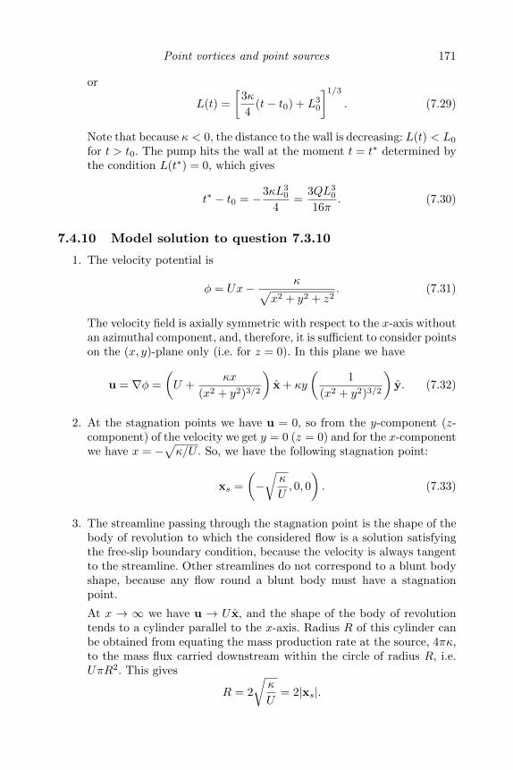
Point vortices and point sources 171
or
L(t) =
[3κ
4(t− t0) + L3
0
]1/3
. (7.29)
Note that because κ < 0, the distance to the wall is decreasing: L(t) < L0
for t > t0. The pump hits the wall at the moment t = t∗ determined bythe condition L(t∗) = 0, which gives
t∗ − t0 = −3κL30
4=
3QL30
16π. (7.30)
7.4.10 Model solution to question 7.3.10
1. The velocity potential is
φ = Ux− κ√x2 + y2 + z2
. (7.31)
The velocity field is axially symmetric with respect to the x-axis withoutan azimuthal component, and, therefore, it is sufficient to consider pointson the (x, y)-plane only (i.e. for z = 0). In this plane we have
u = ∇φ =
(U +
κx
(x2 + y2)3/2
)x + κy
(1
(x2 + y2)3/2
)y. (7.32)
2. At the stagnation points we have u = 0, so from the y-component (z-component) of the velocity we get y = 0 (z = 0) and for the x-componentwe have x = −
√κ/U . So, we have the following stagnation point:
xs =
(−√κ
U, 0, 0
). (7.33)
3. The streamline passing through the stagnation point is the shape of thebody of revolution to which the considered flow is a solution satisfyingthe free-slip boundary condition, because the velocity is always tangentto the streamline. Other streamlines do not correspond to a blunt bodyshape, because any flow round a blunt body must have a stagnationpoint.
At x → ∞ we have u → U x, and the shape of the body of revolutiontends to a cylinder parallel to the x-axis. Radius R of this cylinder canbe obtained from equating the mass production rate at the source, 4πκ,to the mass flux carried downstream within the circle of radius R, i.e.UπR2. This gives
R = 2
√κ
U= 2|xs|.
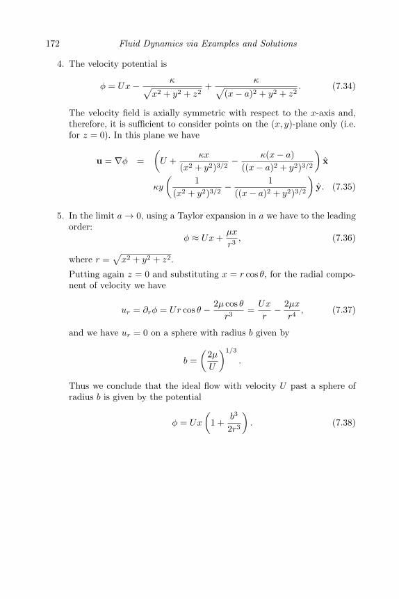
172 Fluid Dynamics via Examples and Solutions
4. The velocity potential is
φ = Ux− κ√x2 + y2 + z2
+κ√
(x− a)2 + y2 + z2. (7.34)
The velocity field is axially symmetric with respect to the x-axis and,therefore, it is sufficient to consider points on the (x, y)-plane only (i.e.for z = 0). In this plane we have
u = ∇φ =
(U +
κx
(x2 + y2)3/2− κ(x− a)
((x− a)2 + y2)3/2
)x
κy
(1
(x2 + y2)3/2− 1
((x− a)2 + y2)3/2
)y. (7.35)
5. In the limit a→ 0, using a Taylor expansion in a we have to the leadingorder:
φ ≈ Ux+µx
r3, (7.36)
where r =√x2 + y2 + z2.
Putting again z = 0 and substituting x = r cos θ, for the radial compo-nent of velocity we have
ur = ∂rφ = Ur cos θ − 2µ cos θ
r3=Ux
r− 2µx
r4, (7.37)
and we have ur = 0 on a sphere with radius b given by
b =
(2µ
U
)1/3
.
Thus we conclude that the ideal flow with velocity U past a sphere ofradius b is given by the potential
φ = Ux
(1 +
b3
2r3
). (7.38)
Chapter 8
Turbulence
8.1 Background theory
Turbulence is a state in which fluid particles move chaotically. Even thoughthe fluid equations are deterministic, turbulent motion of individual fluid par-ticles is unpredictable due to an intrinsic instability of such a motion, i.e.great sensitivity of the fluid paths to slight disturbances. In this, turbulenceis similar to a gas of molecules: even if one uses deterministic laws of classicalmechanics to describe the motion and collisions of the molecules, their individ-ual tracks are impossible to predict. However, in both the turbulence theoryand the kinetic theory of gases one deals with averaged quantities which arepossible to describe and predict, such as the mean concentration of moleculesin gas, or a mean velocity profile distribution (in both gas and turbulence),or the mean velocity distribution of gas molecules, or a mean distribution ofenergy over the turbulent eddies.
The latter is quantified by the energy spectrum which is the central objectin the turbulence theory. The one-dimensional kinetic energy spectrum ofthree-dimensional turbulence is defined via the Fourier transform of a velocitycorrelator as
E =k2
(2π)2
∫〈u(x) · u(x + r)〉eik·r dr, (8.1)
where k is the wave vector and k = |k| and 〈〉 means the ensemble average.The spectrum E(k) describes distribution of the energy over the length scalesl = 2π/k (roughly, over the eddies with diameters l).
Important idealisations in the turbulence theory are assumptions of tur-bulence homogeneity and isotropy, respectively, when all positions and alldirections in the physical space are statistically equivalent. Obviously, to obeythese properties turbulent motion must occupy an infinite space, which mayonly be an approximation to real turbulent flows. In homogeneous turbulencespectrum E is independent of the position x; in isotropic turbulence E isindependent of the direction of k, i.e. E ≡ E(k).
Previously we mentioned an analogy between turbulence and a gas of par-ticles referring to the unpredictability of individual particle trajectories inboth cases. However, there is a crucial difference between these two systems:gases are often found in states close to thermodynamic equilibrium described
173
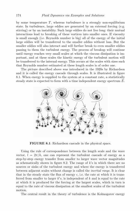
174 Fluid Dynamics via Examples and Solutions
by some temperature T , whereas turbulence is a strongly non-equilibriumstate. In turbulence, large eddies are generated by an external forcing (e.g.stirring) or by an instability. Such large eddies do not live long: their mutualinteractions lead to breaking of these vortices into smaller ones. If viscosityis small enough (i.e. Reynolds number is big) all of the energy of the initiallarge eddies will be transferred to the smaller eddies without loss. But thesmaller eddies will also interact and will further break to even smaller eddiespassing to them the turbulent energy. The process of breakup will continueuntil energy reaches very small scales at which the viscous dissipation is im-portant, and at these scales the kinetic energy of the turbulent motion willbe transferred to the internal energy. This occurs at the scales with sizes suchthat Reynolds number estimated at these length scales is of order one.
The picture described above was introduced in the 1920s by Richardsonand it is called the energy cascade through scales. It is illustrated in figure8.1. When energy is supplied to the system at a constant rate, a statisticallysteady state is expected to form with a time independent energy spectrum E.
FIGURE 8.1: Richardson cascade in the physical space.
Using the rule of correspondence between the length scale and the wavevector, l = 2π/k, one can represent the turbulent cascade of energy as astep-by-step energy transfer from smaller to larger wave vector magnitudesas schematically shown in figure 8.2. The range of k’s in which there are nosources or sinks of the turbulent energy and where the energy is transferredbetween adjacent scales without change is called the inertial range. It is clearthat in the steady state the flux of energy ε, i.e. the rate at which it is trans-ferred from smaller to larger k′s, is independent of k and is equal to the rateat which it is produced for the forcing at the largest scales, which in turn isequal to the rate of viscous dissipation at the smallest scales of the turbulentmotion.
The central result in the theory of turbulence is the Kolmogorov energy
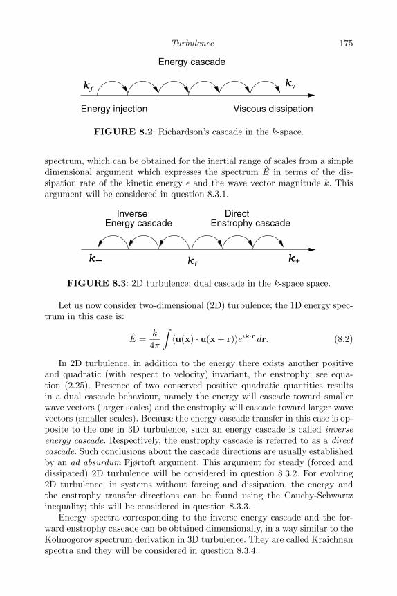
Turbulence 175
νk kf
Energy cascade
Energy injection Viscous dissipation
FIGURE 8.2: Richardson’s cascade in the k-space.
spectrum, which can be obtained for the inertial range of scales from a simpledimensional argument which expresses the spectrum E in terms of the dis-sipation rate of the kinetic energy ε and the wave vector magnitude k. Thisargument will be considered in question 8.3.1.
kf
Energy cascade Enstrophy cascade
kk kk+−
DirectInverse
FIGURE 8.3: 2D turbulence: dual cascade in the k-space space.
Let us now consider two-dimensional (2D) turbulence; the 1D energy spec-trum in this case is:
E =k
4π
∫〈u(x) · u(x + r)〉eik·r dr. (8.2)
In 2D turbulence, in addition to the energy there exists another positiveand quadratic (with respect to velocity) invariant, the enstrophy; see equa-tion (2.25). Presence of two conserved positive quadratic quantities resultsin a dual cascade behaviour, namely the energy will cascade toward smallerwave vectors (larger scales) and the enstrophy will cascade toward larger wavevectors (smaller scales). Because the energy cascade transfer in this case is op-posite to the one in 3D turbulence, such an energy cascade is called inverseenergy cascade. Respectively, the enstrophy cascade is referred to as a directcascade. Such conclusions about the cascade directions are usually establishedby an ad absurdum Fjørtoft argument. This argument for steady (forced anddissipated) 2D turbulence will be considered in question 8.3.2. For evolving2D turbulence, in systems without forcing and dissipation, the energy andthe enstrophy transfer directions can be found using the Cauchy-Schwartzinequality; this will be considered in question 8.3.3.
Energy spectra corresponding to the inverse energy cascade and the for-ward enstrophy cascade can be obtained dimensionally, in a way similar to theKolmogorov spectrum derivation in 3D turbulence. They are called Kraichnanspectra and they will be considered in question 8.3.4.
176 Fluid Dynamics via Examples and Solutions
Interestingly, a Kolmogorov-type scaling was obtained in turbulence theorylong before Kolmogorov found it in his spectrum. Richardson discovered it in1920s by considering experimental data and finding a law of separation of twotracer particles in 3D turbulence, which will be considered in question 8.3.5.
Finally, we will consider turbulence which arises in a fluid flow close to asolid boundary in question 8.3.6. Such near-wall turbulence is inhomogeneousand anisotropic, and we will, following von Karman, aim to find the meanvelocity profile using dimensional considerations.
8.2 Further reading
A detailed account of the turbulence theory is given in the books Turbu-lence: The Legacy of A.N. Kolmogorov by U. Frisch [8] and The Theory ofHomogeneous Turbulence by G.K. Batchelor [3]. Some facts and approachesin turbulence are described in the books Fluid Dynamics by L.D. Landauand E.M. Lifshitz [14] and Elementary Fluid Mechanics by T. Kambe [9].An excellent source of information on the 2D turbulence is a review by R. H.Kraichnan and D. Montgomery Two-Dimensional Turbulence [11]. The readeris also recommended to see the original 1941 paper by A.N. Kolmogorov [10],which is very clearly written and accessible to non-specialists.
8.3 Problems
8.3.1 Kolmogorov spectrum of turbulence
1. Find the physical dimensions of the energy spectrum E(k) and of thedissipation rate of the kinetic energy ε.
2. Use a dimensional argument to find the kinetic energy spectrum assum-ing that the only dimensional quantities it can depend on are ε andk.
Turbulence 177
8.3.2 Dual cascade in steady two-dimensional turbulence
Given information: the energy and the enstrophy densities in the two-dimensional plane, E and Z respectively, are expressed in terms of theone-dimensional energy spectrum E(k) as follows:
E =
∫ ∞0
E(k) dk, and Z =
∫ ∞0
k2 E(k) dk,
where k = |k| is the wavevector length.
In this problem we will consider a statistically steady state of forced anddissipated 2D turbulence and, following Fjørtoft an ad absurdum argument [7]resulting in the dual cascade picture illustrated in figure 8.3.
Consider 2D turbulence which is forced at wave numbers kf and dissipatedin two regions, k < k− and k > k+ such that k− kf k+.
1. Find the relation between the energy production rate ε and the enstro-phy production rate η.
2. Suppose by contradiction that in steady-state conditions energy is dis-sipated at wave numbers k > k+ at a rate comparable to the energyproduction rate ε. Find a lower bound for the enstrophy dissipation ratein this case, and show that this bound is greater than the enstrophyproduction rate η. Thus conclude that this is impossible in steady-stateconditions and, therefore, most of the energy has to be dissipated atk < k−.
3. Find a similar contradiction argument to show that most of the enstro-phy has to be dissipated at k > k+.
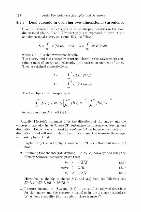
178 Fluid Dynamics via Examples and Solutions
8.3.3 Dual cascade in evolving two-dimensional turbulence
Given information: the energy and the enstrophy densities in the two-dimensional plane, E and Z respectively, are expressed in term of theone-dimensional energy spectrum E(k) as follows:
E =
∫ ∞0
E(k) dk, and Z =
∫ ∞0
k2 E(k) dk,
where k = |k| is the wavevector length.The energy and the enstrophy centroids describe the wavevectors con-taining most of energy and enstrophy (at a particular moment of time).They are defined respectively as
kE =
∫ ∞0
k E(k) dk/E,
kZ =
∫ ∞0
k3 E(k) dk/Z.
The Cauchy-Schwarz inequality is∣∣∣∣∫ ∞0
f(k)g(k) dk
∣∣∣∣ ≤ ∣∣∣∣∫ ∞0
f2(k) dk
∣∣∣∣1/2 ∣∣∣∣∫ ∞0
g2(k) dk
∣∣∣∣1/2for any functions f(k), g(k) ∈ L2.
Usually, Fjørtoft’s argument finds the directions of the energy and theenstrophy cascades in stationary 2D turbulence in presence of forcing anddissipation. Below, we will consider evolving 2D turbulence (no forcing ordissipation), and will re-formulate Fjørtoft’s argument in terms of the energyand enstrophy centroids.
1. Explain why the enstrophy is conserved in 2D ideal flows but not in 3Dflows.
2. Assuming that the integrals defining E,Z, kE , kZ converge and using theCauchy-Schwarz inequality, prove that:
kE ≤√Z/E, (8.3)
kEkZ ≥ Z/E, (8.4)
kZ ≥√Z/E. (8.5)
Hint: You might like to choose f(k) and g(k) from the following list:E1/2, k1/2E1/2, kE1/2, k3/2E1/2.
3. Interpret inequalities (8.3) and (8.5) in terms of the allowed directionsfor the energy and the enstrophy transfers in the k-space (cascades).What does inequality (8.4) say about these transfers?
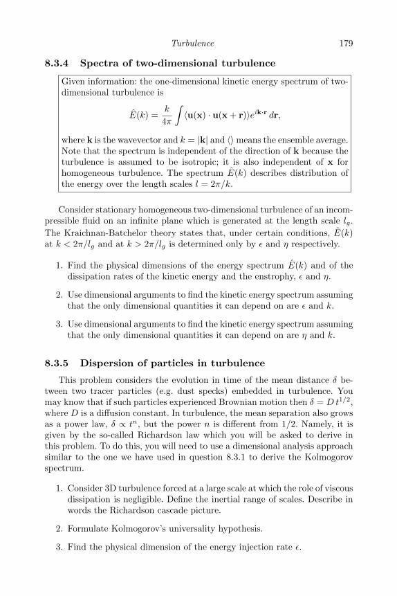
Turbulence 179
8.3.4 Spectra of two-dimensional turbulence
Given information: the one-dimensional kinetic energy spectrum of two-dimensional turbulence is
E(k) =k
4π
∫〈u(x) · u(x + r)〉eik·r dr,
where k is the wavevector and k = |k| and 〈〉means the ensemble average.Note that the spectrum is independent of the direction of k because theturbulence is assumed to be isotropic; it is also independent of x forhomogeneous turbulence. The spectrum E(k) describes distribution ofthe energy over the length scales l = 2π/k.
Consider stationary homogeneous two-dimensional turbulence of an incom-pressible fluid on an infinite plane which is generated at the length scale lg.
The Kraichnan-Batchelor theory states that, under certain conditions, E(k)at k < 2π/lg and at k > 2π/lg is determined only by ε and η respectively.
1. Find the physical dimensions of the energy spectrum E(k) and of thedissipation rates of the kinetic energy and the enstrophy, ε and η.
2. Use dimensional arguments to find the kinetic energy spectrum assumingthat the only dimensional quantities it can depend on are ε and k.
3. Use dimensional arguments to find the kinetic energy spectrum assumingthat the only dimensional quantities it can depend on are η and k.
8.3.5 Dispersion of particles in turbulence
This problem considers the evolution in time of the mean distance δ be-tween two tracer particles (e.g. dust specks) embedded in turbulence. Youmay know that if such particles experienced Brownian motion then δ = D t1/2,where D is a diffusion constant. In turbulence, the mean separation also growsas a power law, δ ∝ tn, but the power n is different from 1/2. Namely, it isgiven by the so-called Richardson law which you will be asked to derive inthis problem. To do this, you will need to use a dimensional analysis approachsimilar to the one we have used in question 8.3.1 to derive the Kolmogorovspectrum.
1. Consider 3D turbulence forced at a large scale at which the role of viscousdissipation is negligible. Define the inertial range of scales. Describe inwords the Richardson cascade picture.
2. Formulate Kolmogorov’s universality hypothesis.
3. Find the physical dimension of the energy injection rate ε.
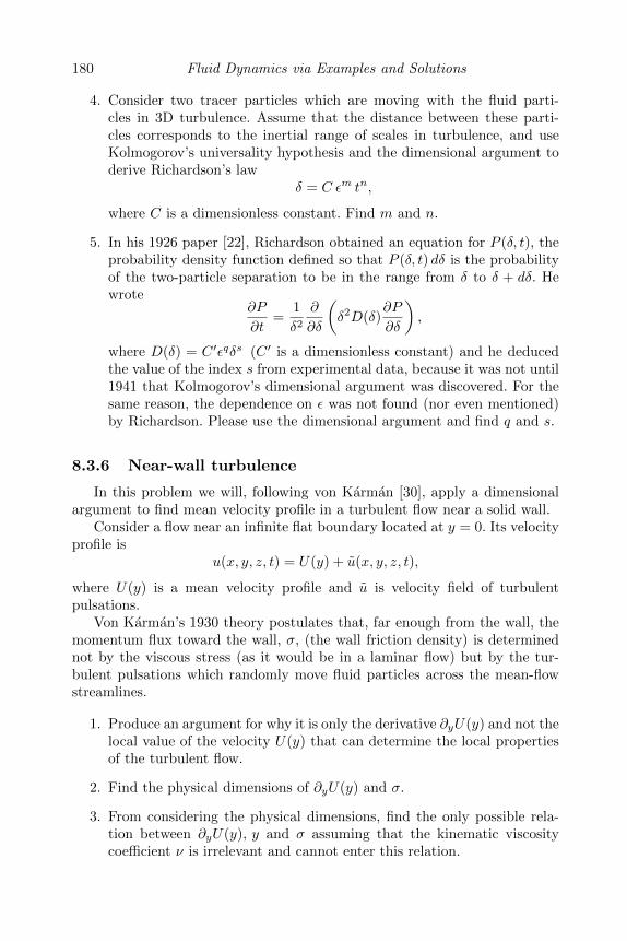
180 Fluid Dynamics via Examples and Solutions
4. Consider two tracer particles which are moving with the fluid parti-cles in 3D turbulence. Assume that the distance between these parti-cles corresponds to the inertial range of scales in turbulence, and useKolmogorov’s universality hypothesis and the dimensional argument toderive Richardson’s law
δ = C εm tn,
where C is a dimensionless constant. Find m and n.
5. In his 1926 paper [22], Richardson obtained an equation for P (δ, t), theprobability density function defined so that P (δ, t) dδ is the probabilityof the two-particle separation to be in the range from δ to δ + dδ. Hewrote
∂P
∂t=
1
δ2
∂
∂δ
(δ2D(δ)
∂P
∂δ
),
where D(δ) = C ′εqδs (C ′ is a dimensionless constant) and he deducedthe value of the index s from experimental data, because it was not until1941 that Kolmogorov’s dimensional argument was discovered. For thesame reason, the dependence on ε was not found (nor even mentioned)by Richardson. Please use the dimensional argument and find q and s.
8.3.6 Near-wall turbulence
In this problem we will, following von Karman [30], apply a dimensionalargument to find mean velocity profile in a turbulent flow near a solid wall.
Consider a flow near an infinite flat boundary located at y = 0. Its velocityprofile is
u(x, y, z, t) = U(y) + u(x, y, z, t),
where U(y) is a mean velocity profile and u is velocity field of turbulentpulsations.
Von Karman’s 1930 theory postulates that, far enough from the wall, themomentum flux toward the wall, σ, (the wall friction density) is determinednot by the viscous stress (as it would be in a laminar flow) but by the tur-bulent pulsations which randomly move fluid particles across the mean-flowstreamlines.
1. Produce an argument for why it is only the derivative ∂yU(y) and not thelocal value of the velocity U(y) that can determine the local propertiesof the turbulent flow.
2. Find the physical dimensions of ∂yU(y) and σ.
3. From considering the physical dimensions, find the only possible rela-tion between ∂yU(y), y and σ assuming that the kinematic viscositycoefficient ν is irrelevant and cannot enter this relation.
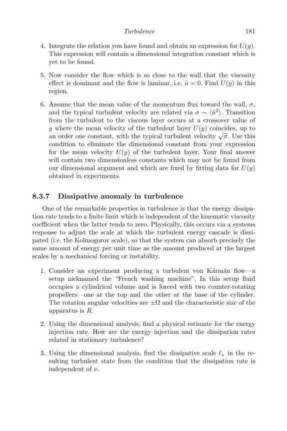
Turbulence 181
4. Integrate the relation you have found and obtain an expression for U(y).This expression will contain a dimensional integration constant which isyet to be found.
5. Now consider the flow which is so close to the wall that the viscosityeffect is dominant and the flow is laminar, i.e. u = 0. Find U(y) in thisregion.
6. Assume that the mean value of the momentum flux toward the wall, σ,and the typical turbulent velocity are related via σ ∼ 〈u2〉. Transitionfrom the turbulent to the viscous layer occurs at a crossover value ofy where the mean velocity of the turbulent layer U(y) coincides, up toan order one constant, with the typical turbulent velocity
√σ. Use this
condition to eliminate the dimensional constant from your expressionfor the mean velocity U(y) of the turbulent layer. Your final answerwill contain two dimensionless constants which may not be found fromour dimensional argument and which are fixed by fitting data for U(y)obtained in experiments.
8.3.7 Dissipative anomaly in turbulence
One of the remarkable properties in turbulence is that the energy dissipa-tion rate tends to a finite limit which is independent of the kinematic viscositycoefficient when the latter tends to zero. Physically, this occurs via a systemsresponse to adjust the scale at which the turbulent energy cascade is dissi-pated (i.e. the Kolmogorov scale), so that the system can absorb precisely thesame amount of energy per unit time as the amount produced at the largestscales by a mechanical forcing or instability.
1. Consider an experiment producing a turbulent von Karman flow—asetup nicknamed the “French washing machine”. In this setup fluidoccupies a cylindrical volume and is forced with two counter-rotatingpropellers—one at the top and the other at the base of the cylinder.The rotation angular velocities are ±Ω and the characteristic size of theapparatus is R.
2. Using the dimensional analysis, find a physical estimate for the energyinjection rate. How are the energy injection and the dissipation ratesrelated in stationary turbulence?
3. Using the dimensional analysis, find the dissipative scale `ν in the re-sulting turbulent state from the condition that the dissipation rate isindependent of ν.
182 Fluid Dynamics via Examples and Solutions
8.4 Solutions
8.4.1 Model solution to question 8.3.1
1. The physical dimensions of the energy spectrum E(k) can be found fromthe formula relating it to the kinetic energy density in the physical space:
1
2〈u2〉 =
∫E(k) dk,
where k is the absolute value of the wave vector. From this formula wefind that the physical dimension of the energy spectrum E(k) is L3/T 2.
The dissipation rate of the kinetic energy ε is, by definition, the energydissipated per unit time per unit volume. Thus, the physical dimensionof ε is L2/T 3.
2. The only dimensional combination of ε and k which has the dimensionof the kinetic energy E(k) is
E(k) = CKε2/3k−5/3,
which is the famous Kolmogorov spectrum [10]. Here CK is a dimen-sionless constant which is called the Kolmogorov constant. Experimentsindicate that CK ≈ 0.5.
8.4.2 Model solution to question 8.3.2
1. The relation between the energy production rate ε and the enstrophyproduction rate η follows from the relation between the k-space densitiesof the energy and the enstrophy (see the given information). Thus,
ε = k2f η.
2. Suppose by contradiction that in steady state energy is dissipated atwave numbers k > k+ at a rate ε+ comparable to the energy productionrate ε. Then we have a lower bound for the enstrophy dissipation in thesame region:
η+ ≥ ε+k2+ ε+k
2f ∼ εk2
f = η.
But it is impossible to dissipate in a steady-state condition more en-strophy per unit time than the amount produced by the forcing. Thusconclude that most of the energy has to be dissipated at k < k−.
3. Similar contradiction argument to show that most of the enstrophy hasto be dissipated at k > k+ is left to the reader.
Turbulence 183
8.4.3 Model solution to question 8.3.3
1. This is because in 2D the vortex stretching term is zero (but not in3D!), hence the vorticity is conserved along the fluid paths, hence theintegrated square vorticity (enstrophy) is conserved.
2. In the Cauchy-Schwartz inequality, we will only deal with positive func-tions, so the absolute value brackets may be omitted. Being in L2 in ourcase means that all the relevant integrals converge, as suggested in thestatement of the problem.
First, let us consider integral∫kE dk and apply the Cauchy-Schwartz
inequality as follows,∫ ∞0
kE dk =
∫(kE1/2)(E1/2) dk ≤
(∫ ∞0
k2E dk
)1/2(∫ ∞0
E dk
)1/2
,
which immediately yields (8.3).
Second, let us consider Ω =∫k2E dk and split it as,∫ ∞
0
k2E dk =
∫ ∞0
(k3/2E1/2)(k1/2E1/2) dk ≤
(∫ ∞0
k3E dk
)1/2(∫ ∞0
kE dk
)1/2
,
which immediately yields (8.4).
Combining (8.4) with (8.3) gives (8.5).
3. Inequalities (8.3) and (8.5) mean that the energy is not allowed to moveto high k’s and the enstrophy is not allowed to move to low k’s. Thus,the energy may move only to low k’s—this is the inverse energy cascade,and the enstrophy may move only to high k’s—this is the direct enstro-phy cascade. However, these inequalities do not oblige the energy andthe enstrophy to move in scale—they may remain at the scales wherethey were put initially (as it is the case e.g. for time-independent 2Dsolutions).
On the other hand, condition (8.4) means that if the energy happenedto move to low k’s, the enstrophy must move to high k’s.
8.4.4 Model solution to question 8.3.4
1. The physical dimensions of the energy spectrum E(k) can be found fromits defining formula: [E(k)] = L−1[u]2L2 = L3/T 2 (this dimension is thesame as in the 3D case).
The dissipation rate of the kinetic energy, ε, is, by definition, the energy

184 Fluid Dynamics via Examples and Solutions
dissipated per unit time per unit volume. Thus, its physical dimensionis [ε] = [u]2/T = L2/T 3.
The dissipation rate of the enstrophy, η, is, by definition, the enstrophydissipated per unit time per unit volume. Thus, its physical dimensionis [η] = [ω]2/T = 1/T 3.
2. The only dimensional combination of ε and k which has the dimensionof the kinetic energy E(k) is
E(k) = C1ε2/3k−5/3,
where C1 is a dimensionless constant. Although this expression is veryclose to the Kolmogorov energy spectrum, the constant C1 does not haveto coincide with the Kolmogorov constant CK (indeed, from experimentit appears to be different, C1 ≈ 7 and CK ≈ 0.5).
3. The only dimensional combination of η and k which has the dimensionof the kinetic energy E(k) is
E(k) = C2ε2/3k−3,
where C2 is a dimensionless constant. This is the Kraichnan spectrum.From numerical experiments C2 ≈ 2.
8.4.5 Model solution to question 8.3.5
1. For 3D turbulence forced at a large scale at which the role of viscousdissipation is negligible, energy dissipation by viscosity occurs at a muchsmaller scale. Starting at the forcing scale, the energy cascades step-by-step from larger to smaller (but comparable in size) scales until it reachesthe viscous dissipation scale: this is the Richardson cascade picture. Therange of scales in between of the energy injection and the energy dissi-pation scales, and where the energy balance is determined purely by theenergy flux through scales (and not its external injection or dissipation)is called the inertial range.
2. Kolmogorov’s universality hypothesis states that all statistical proper-ties of turbulence at any scale within the inertial range are determinedby the energy flux only, and independent of the details of the energyinjection or dissipation mechanisms (turbulence locality). In stationaryturbulence, the energy flux is equal to the injection rate of the kineticenergy density, ε.
3. By definition, the energy injection rate ε is the kinetic energy densityinjected into the system in unit time. Thus,
[ε] = [u2]/T = L2/T 3.
Turbulence 185
4. Letδ = C εm tn,
where C is a dimensionless constant. The only values of m and n whichmake this formula dimensionally correct are m = 1/2 and n = 3/2. Thisis the famous Richardson 3/2-law of turbulent dispersion.
5. From the PDF equation, [D] = L2/T , so the dimensional analysis givesD = C ′ε1/3δ4/3, where C ′ is a dimensionless constant. So, q = 1/3 ands = 4/3.
8.4.6 Model solution to question 8.3.6
1. The laws of physics, including the ones of fluid dynamics, are the samein all inertial frames, i.e. the motion will be the same in any two flowswhose initial conditions are different by a constant velocity field (up totransformation into the moving frame). Thus, the properties of the tur-bulent flow, such as the turbulent transport (including the momentumflux across the streamlines) cannot depend on the mean velocity U(y)but only on its derivative ∂yU(y).
2. The physical dimension of ∂yU(y) is 1/T . By the definition of themomentum flux as the amount of the momentum passing through aunit area per unit time, we find the physical dimension of σ to be[ρ][V ][u]/(L2T ) = L2/T 2. Here we choose the system where ρ = 1 takinginto account the fluid’s incompressibility.
Note that the dimension of σ is the same as the one of squared velocity,which is consistent with the assumption to be made below that σ ∼ 〈u2〉,where u the typical turbulent velocity.
3. The only possible dimensionally correct relation between ∂yU(y), y andσ (independent from the kinematic viscosity coefficient ν) is:
∂yU(y) =
√σ
κy,
where κ is a dimensionless number called the Von Karman constant (itis traditional to define it as a constant in the denominator rather thanin the numerator). Integrating this relation, we obtain the followingexpression for U(y):
U(y) =
√σ
κln y +A,
where A is a dimensional integration constant which is yet to be found.
4. Since there is no stream-wise pressure gradient, U(y) will be a solutionof the x-momentum equation
ν∂yyU = 0,
186 Fluid Dynamics via Examples and Solutions
i.e.U(y) = By,
where B =const (we have taken into account the no-slip boundary con-dition U(0) = 0).
There must be the same amount of the x-momentum flux toward thewall through the laminar sub-layer as through the turbulent one, so
ν∂yU = νB = σ.
5. Assuming that the transition from the turbulent to the viscous layer oc-curs at a crossover value y = y† where the mean velocity of the turbulentlayer U(y) matches, up to an order one constant, the typical turbulentvelocity
√σ, we have
U(y†) =σ
νy† =
√σ i.e. y† =
ν√σ,
(this is just a definition of y†) and
U(y) =√σ
(1
κln
y
y†+ C
),
where C is an order one constant which remains undetermined by ourapproximate matching procedure. Together with κ, C is fixed by fittingdata for U(y) obtained in experiments, which results in κ ≈ 0.4 andC ≈ 5.
8.4.7 Model solution to question 8.3.7
1. In stationary turbulence, the energy injection and the dissipation ratesare equal on average. By definition, the energy injection (dissipation)rate ε is the energy produced (dissipated) in a unit volume per unittime. Thus, the physical dimension of ε is [u2]/T = L2/T 3. The onlycombination of Ω and R that agrees with this dimension is R2Ω3, so
ε ∼ R2Ω3.
2. The physical dimension of the kinematic viscosity coefficient is L2/T .To absorb the energy flux ε by viscosity, we find (using the dimensionalanalysis) that
`ν =ν3/4
ε1/4.
Chapter 9
Compressible flow
9.1 Background theory
The compressibility of the fluid becomes essential when the flow velocityis of the same order or greater than the speed of sound (see question 1.3.2)or when the fluid (or gas) is subject to changing external pressure on thecontaining volume like in an air pump or in a balloon rising through a stratifiedatmosphere.
In this chapter we will deal with compressible flows described by the invis-cid equations of a polytropic gas (1.5), (1.6), (1.7) and (1.8). We will considerboth strong and weak solutions of these equations. The latter contain jumps inthe fluid density, pressure and velocity fields (shocks, contact discontinuities)which are smoothed when viscosity is taken into account. However, the jumpconditions follow from some general conservation laws and they are insensitiveto the detailed structure of the transition region.
9.1.1 One-dimensional gas dynamics
We will start by considering classical results for 1D flows for which equa-tions (1.5), (1.6) and (1.7) become:
∂tu+ u∂xu = −1
ρ∂xp, (9.1)
∂tρ+ ∂x(ρu) = 0, (9.2)
∂tS + u∂xS = 0. (9.3)
A powerful tool for solving the 1D gas equations is the method of char-acteristics. To use this method one needs to rewrite these equations in thecharacteristic form:
D+t p+ ρcsD
+t u = 0, (9.4)
D−t p− ρcsD−t u = 0, (9.5)
D0tS = 0, (9.6)
where cs =√
(∂ρp)S is the speed of sound, ((∂ρ·)S means the ρ-derivative
187

188 Fluid Dynamics via Examples and Solutions
with S kept constant), and D+t , D−t and D0
t are the time derivatives alongthe characteristic curves C+, C− and C0 respectively defined by:
C+ : x(t) = u(x(t), t) + cs(x(t), t), (9.7)
C− : x(t) = u(x(t), t)− cs(x(t), t), (9.8)
C0 : x(t) = u(x(t), t). (9.9)
Obviously, D0t ≡ Dt and the entropy conservation equation (9.3) is already
in the characteristic form. For derivation of the remaining two characteristicequations see problem 9.3.1.
For isentropic flow, S = const, we have D±t p = (∂ρp)SD±t ρ = c2sD
±t ρ. In
this case one can rewrite equations (9.4) and (9.5) as conservation along thecharacteristics laws:
D+t R
+ = 0, (9.10)
D−t R− = 0, (9.11)
where quantities
R+ =
∫cs(ρ)
ρdρ+ u, (9.12)
R− =
∫cs(ρ)
ρdρ− u (9.13)
are called Riemann invariants. For polytropic gases, p = const ργ , hence wehave
R± =2csγ − 1
± u, (9.14)
Crossing characteristics of the same family indicates the moment at whichthe solution with single-valued fields ceases to exist. This happens when dis-turbances travelling at higher speeds catch up with slower disturbances, andthis process is called wave breaking. An example of such breaking solutions isconsidered in question 9.3.2.
After the wave breaking, viscosity becomes important due to high gradientsof the field at the wave breaking location. Sharp transition regions arise andstart moving—they are called shock waves or simply shocks. Even thoughthe viscosity is essential in the sharp transition region, the jump conditionsrelating the flow fields on the two sides of the shock can be determined basedon the inviscid conservation laws written in the continuity equation form.
One such continuity equation is (9.2): it describes the mass conservation.Combining equations (9.1) and (9.2), one can also write a continuity equationdescribing the momentum conservation:
∂t(ρu) + ∂x(ρu2 + p) = 0. (9.15)
Note that the entropy equation (9.3), when combined with the equation (9.2),can also be written as a continuity equation,
∂t(ρS) + ∂x(ρuS) = 0. (9.16)
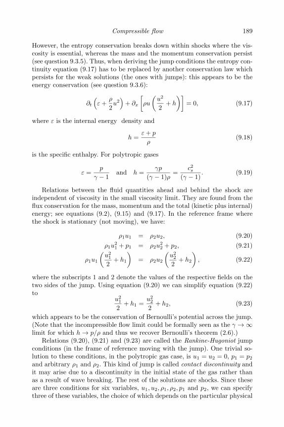
Compressible flow 189
However, the entropy conservation breaks down within shocks where the vis-cosity is essential, whereas the mass and the momentum conservation persist(see question 9.3.5). Thus, when deriving the jump conditions the entropy con-tinuity equation (9.17) has to be replaced by another conservation law whichpersists for the weak solutions (the ones with jumps): this appears to be theenergy conservation (see question 9.3.6):
∂t
(ε+
ρ
2u2)
+ ∂x
[ρu
(u2
2+ h
)]= 0, (9.17)
where ε is the internal energy density and
h =ε+ p
ρ(9.18)
is the specific enthalpy. For polytropic gases
ε =p
γ − 1and h =
γp
(γ − 1)ρ=
c2s(γ − 1)
. (9.19)
Relations between the fluid quantities ahead and behind the shock areindependent of viscosity in the small viscosity limit. They are found from theflux conservation for the mass, momentum and the total (kinetic plus internal)energy; see equations (9.2), (9.15) and (9.17). In the reference frame wherethe shock is stationary (not moving), we have:
ρ1u1 = ρ2u2, (9.20)
ρ1u21 + p1 = ρ2u
22 + p2, (9.21)
ρ1u1
(u2
1
2+ h1
)= ρ2u2
(u2
2
2+ h2
), (9.22)
where the subscripts 1 and 2 denote the values of the respective fields on thetwo sides of the jump. Using equation (9.20) we can simplify equation (9.22)to
u21
2+ h1 =
u22
2+ h2, (9.23)
which appears to be the conservation of Bernoulli’s potential across the jump.(Note that the incompressible flow limit could be formally seen as the γ →∞limit for which h→ p/ρ and thus we recover Bernoulli’s theorem (2.6).)
Relations (9.20), (9.21) and (9.23) are called the Rankine-Hugoniot jumpconditions (in the frame of reference moving with the jump). One trivial so-lution to these conditions, in the polytropic gas case, is u1 = u2 = 0, p1 = p2
and arbitrary ρ1 and ρ2. This kind of jump is called contact discontinuity andit may arise due to a discontinuity in the initial state of the gas rather thanas a result of wave breaking. The rest of the solutions are shocks. Since theseare three conditions for six variables, u1, u2, ρ1, ρ2, p1 and p2, we can specifythree of these variables, the choice of which depends on the particular physical
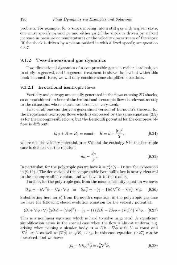
190 Fluid Dynamics via Examples and Solutions
problem. For example, for a shock moving into a still gas with a given state,one must specify ρ1 and p1 and either p2 (if the shock is driven by a fixedincrease in pressure or temperature) or the velocity downstream of the shock(if the shock is driven by a piston pushed in with a fixed speed); see question9.3.7.
9.1.2 Two-dimensional gas dynamics
Two-dimensional dynamics of a compressible gas is a rather hard subjectto study in general, and its general treatment is above the level at which thisbook is aimed. Here, we will only consider some simplified situations.
9.1.2.1 Irrotational isentropic flows
Vorticity and entropy are usually generated in the flows crossing 2D shocks,so our consideration here of the irrotational isentropic flows is relevant mostlyto the situations where shocks are absent or very weak.
First of all one can derive a generalised version of Bernoulli’s theorem forthe irrotational isentropic flows which is expressed by the same equation (2.5)as for the incompressible flows, but the Bernoulli potential for the compressibleflow is different:
∂tφ+B = B0 = const, B = h+|u|2
2, (9.24)
where φ is the velocity potential, u = ∇φ and the enthalpy h in the isentropiccase is defined via the relation:
dh =dp
ρ. (9.25)
In particular, for the polytropic gas we have h = c2s/(γ−1); see the expressionin (9.19). (The derivation of the compressible Bernoulli’s law is nearly identicalto the incompressible version, and we leave it to the reader.)
Further, for the polytropic gas, from the mass continuity equation we have:
∂tρ = −ρ∇2φ−∇ρ · ∇φ or ∂tc2s = −(γ − 1)c2s∇2φ−∇c2s · ∇φ. (9.26)
Substituting here for c2s from Bernoulli’s equation, in the polytropic gas casewe have the following closed evolution equation for the velocity potential:
(∂t +∇φ · ∇)(2∂tφ+ (∇φ)2
)= (γ − 1)
(2B0 − 2∂tφ− (∇φ)2
)∇2φ. (9.27)
This is a nonlinear equation which is hard to solve in general. A significantsimplification arises in the special case when the flow is almost uniform, e.g.arising when passing a slender body, u = U x + ∇φ with U = const and|∇φ| U as well as |∇φ|
√B0 ∼ cs. In this case equation (9.27) can be
linearised, and we have:
(∂t + U∂x)2φ = c20∇2φ, (9.28)
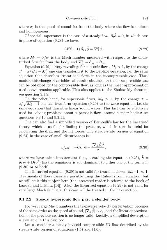
Compressible flow 191
where c0 is the speed of sound far from the body where the flow is uniformand homogeneous.
Of special importance is the case of a steady flow, ∂tφ = 0, in which casein place of equation (9.28) we have:(
M20 − 1
)∂xxφ = ∇2
⊥φ, (9.29)
where M0 = U/c0 is the Mach number measured with respect to the undis-turbed flow far from the body and ∇2
⊥ = ∂yy + ∂zz.Equation (9.29) is very revealing: for subsonic flows, M0 < 1, by the change
x′ = x/√
1−M20 one can transform it to the Laplace equation, i.e. the same
equation that describes irrotational flows in the incompressible case. Thus,modulo this change of variables, all results obtained for the incompressible casecan be obtained for the compressible flow, as long as the linear approximationused above remains applicable. This also applies to the Zhukovskiy theorem;see question 9.3.9.
On the other hand, for supersonic flows, M0 > 1, by the change τ =x/√M2
0 − 1 one can transform equation (9.29) to the wave equation, i.e. thesame equation that describes linear sound waves. This fact can be effectivelyused for solving problems about supersonic flows around slender bodies: seequestions 9.3.10 and 9.3.11.
One can also find a simplified version of Bernoulli’s law for the linearisedtheory, which is useful for finding the pressure, which in turn is useful forcalculating the drag and the lift forces. The steady-state version of equation(9.24) in the case of small disturbances is:
p/ρ0 = −U∂xφ−(∇⊥φ)2
2, (9.30)
where we have taken into account that, according the equation (9.25), h =p/ρ0 +O(p2) (so the remainder is sub-dominant to either one of the terms in(9.30) or to both).
The linearised equation (9.29) is not valid for transonic flows, |M0−1| 1.Treatments of these cases are possible using the Euler-Tricomi equation, butwe will omit this subject here (the interested reader is referred to the book ofLandau and Lifshitz [14]). Also, the linearised equation (9.29) is not valid forvery large Mach numbers: this case will be treated in the next section.
9.1.2.2 Steady hypersonic flow past a slender body
For very large Mach numbers the transverse velocity perturbation becomesof the same order as the speed of sound, |∇⊥φ| ∼ cs, and the linear approxima-tion of the previous section is no longer valid. Luckily, a simplified descriptionis available in this case too.
Let us consider a steady inviscid compressible 2D flow described by thesteady-state version of equations (1.5) and (1.6):
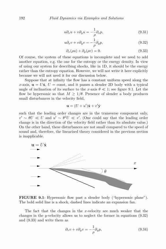
192 Fluid Dynamics via Examples and Solutions
u∂xu+ v∂yu = −1
ρ∂xp, (9.31)
u∂xv + v∂yv = −1
ρ∂yp, (9.32)
∂x(ρu) + ∂y(ρv) = 0. (9.33)
Of course, the system of these equations is incomplete and we need to addanother equation, e.g. the one for the entropy or the energy density. In viewof using our system for describing shocks, like in 1D, it should be the energyrather than the entropy equation. However, we will not write it here explicitlybecause we will not need it for our discussion below.
Suppose that at infinity the flow has a constant uniform speed along thex-axis, u = U x, U = const, and it passes a slender 2D body with a typicalangle of inclination of its surface to the x-axis θ 1; see figure 9.1. Let theflow be hypersonic so that M ≥ 1/θ. Presence of slender a body producessmall disturbances in the velocity field,
u = (U + u′)x + v′y
such that the leading order changes are in the transverse component only,v′ ∼ θU U and u′ ∼ θ2U v′. (One could say that the leading orderchange is in the direction of the velocity field rather than its absolute value.)On the other hand, these disturbances are not small compared to the speed ofsound and, therefore, the linearised theory considered in the previous sectionis inapplicable.
u = U x
θ
x
FIGURE 9.1: Hypersonic flow past a slender body (“hypersonic plane”).The bold solid line is a shock, dashed lines indicate an expansion fan.
The fact that the changes in the x-velocity are much weaker that thechanges in the y-velocity allows us to neglect the former in equations (9.32)and (9.33) and write them as
∂τv + v∂yv = −1
ρ∂yp, (9.34)
Compressible flow 193
∂τρ+ ∂y(ρv) = 0, (9.35)
where τ = x/U is an effective time. We have arrived at equations whichare formally identical to equations (9.1) and (9.2) for an unsteady 1D flow.Without derivation we mention that the same equivalence also applies to theenergy balance equation which we have omitted in this section.
Thus, solving a steady 2D problem of hypersonic flow about a slender bodyreduces to solving an unsteady 1D problem with an effective time τ = x/U . Inthis analogy, the free-slip boundary condition on the solid surface y = Y (x) be-comes a boundary condition corresponding to a moving piston: v = ∂τY (x(τ))on y = Y (x(τ)) where x(τ) = Uτ . Because of this formal correspondence, thedescribed approach is called the piston analogy. For example, in figure 9.1, thepiston moves “into the gas” on the windward (bottom) part of the body and,therefore, a shock wave forms; see question 9.3.7. On the leeward (upper) sideof the body the piston “withdraws from the gas” and, therefore, a rarefactionwave with its typical expansion fan of characteristics forms; see question 9.3.2.
Question 9.3.12 will exploit the piston analogy to find a lift force on aplane hypersonic wing.
9.2 Further reading
Detailed discussions of various aspects of the compressible gas dynamicscan be found in the books Fluid Dynamics by L.D. Landau and E.M. Lifshitz[14], Linear and Nonlinear Waves by G.B. Whitham [31], “Waves in Fluids”by J. Lighthill [15] and Prandtl’s Essentials of Fluid Mechanics by Oertel etal [17].
9.3 Problems
9.3.1 Characteristic equations
Derive the equations for a 1D gas in their characteristic form (9.4) and(9.5) with the characteristic curves defined by equations (9.7) and (9.8).
194 Fluid Dynamics via Examples and Solutions
9.3.2 Flow due to a piston withdrawal
Given information: the equations for a 1D gas in the characteristic form(9.4), (9.5) and (9.6) with the characteristic curves defined by equa-tions (9.7), (9.8) and (9.9). Characteristic equations for the isentropicgas (9.10) and (9.11) with the polytropic-gas expressions for the Rie-mann invariants (9.14).
If a flow is isentropic and one of the Riemann invariants is uniform in thephysical space, the solution for it can be found analytically. This kind of flowis called the simple wave, and in the linear limit it corresponds to sound wavespropagating in a single direction (i.e. either only to the right or only to theleft). In the present problem we will encounter such a simple wave motion.
A piston suddenly starts moving on trajectory x = X(t) withdrawing froma tube filled with gas which is initially still and has uniform initial pressurep0 and density ρ0. Our aim is to find the solution for the gas motion after thepiston starts moving. (Note that the case where the piston is pushed into thegas is analysed in question 9.3.5.)
1. Consider the C0-characteristics (i.e. the fluid paths) on the (x, t)-planebounded by the piston’s trajectory x = X(t) placing the origin so thatX(0) = 0. What entropy has the gas initially (i.e. on the x-axis atx > 0)? How does this value propagate along the C0-characteristics?Will the C0-characteristics originating on the x-axis cover the entirespace occupied by the gas for any time t > 0? By answering thesequestions, find the entropy field for any time t > 0.
2. What is the initial value of the Riemann invariant R−? Will the C−-characteristics originating on the x-axis cover the entire space occupiedby the gas for t > 0? What is the initial value of the Riemann invariantR−. Find R− for all t > 0 and all x > X(t).
3. Explain why the C+-characteristics originating on the x-axis do notcover the entire space occupied by the gas at t > 0. What are the valuesof the Riemann invariant R+ on the x-axis and on the piston’s trajectoryx = X(t)? Find R+ for all t > 0 and all x > X(t) considering separatelythe C+-characteristics originating on the x-axis and on x = X(t).
4. Put together the results of the previous parts and find an implicit so-lution for u and cs in terms of a time parameter τ parametrising thepiston’s position (i.e. when t = τ the piston is at x = X(τ)).
5. Find the explicit solution for u and cs for the case when for t > 0 thepiston has a constant speed X = −V < 0. What is the limiting pistonwithdrawal speed above which a vacuum bubble forms?
Compressible flow 195
9.3.3 Gas expansion into vacuum
A still gas with uniform pressure p0 and density ρ0 occupies the half-space x > 0 limited by a solid plate at x = 0. The second half-space, x < 0, isoccupied by vacuum. At time t = 0 the solid plate is instantaneously removed.Find the gas motion for t > 0.
9.3.4 Dam break flow
Given information: the 1D shallow water equations:
∂tu+ u∂xu = −g∂xh, (9.36)
∂th+ ∂x(hu) = 0, (9.37)
where u(x, t) and h(x, t) are the fluid velocity and the surface heightrespectively and g is the gravity acceleration constant.
Still shallow water with height h = h0 occupies the half-space x > 0 limitedby a gate at x = 0. The second half-space, x < 0, is dry, h = 0. At time t = 0the gate is instantaneously opened. Find the water motion for t > 0.
Hint: You may find it helpful to use the fact that the 1D shallow waterequations are formally identical to the equations for 1D polytropic gases (9.1)and (9.2). What would be the adiabatic index γ in this case?
9.3.5 Momentum conservation in a viscous compressibleflow
Compressible viscous 1D flow is described by the mass continuity equation(1.6) and by the Navier-Stokes equation
ρ(∂tu+ u∂xu) = −∂xp+ λ∂yyu, λ = ξ + 4µ/3, (9.38)
where µ and ξ are the first and the second viscosity coefficients respectively.Derive the continuity equation for the momentum density in a 1D com-
pressible viscous flow.
9.3.6 Energy conservation in compressible flow
1. Using the 1D compressible inviscid flow equations (9.1), (9.2), and (9.3)prove the energy continuity equation (9.17) for a 1D polytropic flow,in which the internal energy and the enthalpy are given by expressions(9.19).
2. Without derivation, present a general qualitative argument on the roleof viscosity in the energy conservation law.
196 Fluid Dynamics via Examples and Solutions
9.3.7 Rankine-Hugoniot conditions for jumps across shocks
1. Consider a 1D shock wave with a still gas ahead of it with pressure p1
and density ρ1. The pressure behind the shock is p2. Using the Rankine-Hugoniot conditions (9.20), (9.21) and (9.23), and the polytropic gasexpression for the enthalpy (9.19), find the gas density and velocitybehind the shock, as well as the shock’s speed.
2. Consider the limit of very strong shocks, p2/p1 →∞. Find the limitingdensity ratio ρ2/ρ1 for an ideal monatomic gas (γ = 5/3) and for an idealdiatomic gas (γ = 1.4). What limiting density ratio should we expectfor air?
3. A piston is suddenly pushed with constant speed V into a tube filledwith a gas which is initially still and which has initial pressure p1 anddensity ρ1. Describe the gas motion after the piston starts moving.
9.3.8 Hypersonic collision of two gas masses
Given information: jump conditions across the shocks are (c.f. question9.3.7):
(u1 − U1)2 =ρ3
ρ1
(p3 − p1)
(ρ3 − ρ1), (9.39)
ρ3 = ρ1
p3p1
(γ + 1) + (γ − 1)
(γ + 1) + p3p1
(γ − 1), (9.40)
where u1, p1 and ρ1 are the velocity, the pressure and the density aheadof the shock, U1 is the shock speed and p3 and ρ3 are the pressure and thedensity behind of the shock. (Here we have chosen the same notationsas for the right shock in figure 9.2.)
Consider two polytropic gas clouds with initial uniform pressures and den-sities, p1, ρ1 and p2, ρ2, moving toward each other with velocities u1 < 0 andu2 > 0 respectively (gas 1 is on the right and gas 2 is on the left). At someinstant of time the clouds collide, and our goal is to describe their subse-quent dynamics assuming that the collision is hypersonic: the relative velocityu = u2 − u1 is much greater than the initial speed of sound in both clouds.
1. Explain why, in general, three jumps will form: two shocks running awayfrom the collision point in the opposite directions an a contact disconti-nuity in between the shocks; see figure 9.2.
2. The shock waves that form as a result of a hypersonic collision are strong:the pressure behind the shock is much greater than the pressure aheadof the shock. Find the limiting expressions for the ratio of the density

Compressible flow 197
behind the shock to the density ahead of the shock when the pressureratio tends to infinity (c.f. question 9.3.7). Find the densities on the twosides of the contact discontinuity.
3. In the strong shock limit, using the mass flow continuity, find the shockspeeds U1 and U2 in terms of the gas velocities u1 and u2 in the referenceframe of stationary contact discontinuity.
4. Using (9.39), find the pressures behind the shocks in terms of the flowparameters ahead of the shocks and the shock speeds in the strong shocklimit. Equating pressures on the two sides of the contact discontinuity,find another condition on the velocities and, using this condition, findU1 and U2 in terms of the relative velocity u = u2 − u1 in the referenceframe of stationary contact discontinuity. Find the pressure between theshocks in terms of ρ1, ρ2, α and u.
xu2
U2
p1, ρ1
u1p4, ρ4
p3, ρ3
p2, ρ2
U1
FIGURE 9.2: Gas motion after a collision of two clouds. The dashed linesmark positions of the three jumps: two shocks (on the right and on the left)and a contact discontinuity (in the middle). The solid line is the density profile.The pressure profile is similar, except that there is no pressure jump acrossthe contact discontinuity.
198 Fluid Dynamics via Examples and Solutions
9.3.9 Zhukovskiy’s theorem for the subsonic flow
Given information:
• Zhukovskiy’s theorem for the lift force F onto a wing in asteady inviscid incompressible 2D flow which is uniform at infinity,u(x, y)→ U x for |x| → ∞:
F = −ρUΓ,
where Γ is the velocity circulation around the wing (see equation(6.10)).
• The linearised equation for the velocity potential perturbation forthe uniform compressible subsonic 2D flow with velocity U x pasta thin wing of uniform cross-section is (c.f. equation (9.29)):
β2∂xxφ+ ∂yyφ = 0, (9.41)
where β =√
1−M20 and M0 = U/c0 is the Mach number mea-
sured with respect to the undisturbed flow far from the wing.
1. Formulate the free-slip boundary condition on the wing’s surface andlinearise this condition taking into account that both the deviation ofthe velocity field from the uniform field U x and the deviation of the unitnormal to the surface from y are small.
2. Find a scaling transformation to reduce the equation (9.41) and the re-spective boundary condition to an effective incompressible flow problem.
3. Find the relation between the circulations and the flow velocities aroundthe wing in the compressible flow and in the effective incompressible flow.By applying Zhukovskiy’s lift theorem to the effective incompressibleflow (assuming that the force in the compressible case will be the sameas for the respective effective flow), find the lift force for the subsoniccompressible flow over the thin wing.
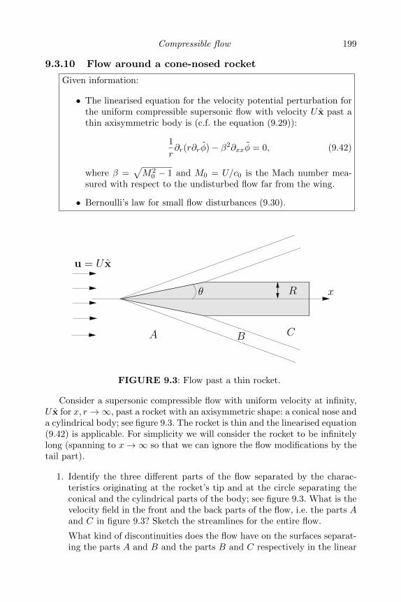
Compressible flow 199
9.3.10 Flow around a cone-nosed rocket
Given information:
• The linearised equation for the velocity potential perturbation forthe uniform compressible supersonic flow with velocity U x past athin axisymmetric body is (c.f. the equation (9.29)):
1
r∂r(r∂rφ)− β2∂xxφ = 0, (9.42)
where β =√M2
0 − 1 and M0 = U/c0 is the Mach number mea-sured with respect to the undisturbed flow far from the wing.
• Bernoulli’s law for small flow disturbances (9.30).
x
CB
u = U x
A
θ R
FIGURE 9.3: Flow past a thin rocket.
Consider a supersonic compressible flow with uniform velocity at infinity,U x for x, r →∞, past a rocket with an axisymmetric shape: a conical nose anda cylindrical body; see figure 9.3. The rocket is thin and the linearised equation(9.42) is applicable. For simplicity we will consider the rocket to be infinitelylong (spanning to x→∞ so that we can ignore the flow modifications by thetail part).
1. Identify the three different parts of the flow separated by the charac-teristics originating at the rocket’s tip and at the circle separating theconical and the cylindrical parts of the body; see figure 9.3. What is thevelocity field in the front and the back parts of the flow, i.e. the parts Aand C in figure 9.3? Sketch the streamlines for the entire flow.
What kind of discontinuities does the flow have on the surfaces separat-ing the parts A and B and the parts B and C respectively in the linear
200 Fluid Dynamics via Examples and Solutions
approximation? In the more general case when the linear approximationis removed?
2. Consider the middle part of the flow (part B in figure 9.3). Seek a self-similar solution for the velocity potential perturbation in the form
φ(r, x) = xf(η) with η = r/x.
By substituting this expression into equation (9.42), derive an ordinarydifferential equation (ODE) for the function f(η).
3. Write down the free-slip boundary condition for the cone (nose) surface.Express this boundary condition in terms of a condition on the functionf(η).
4. Solve the ODE for the function f(η) with the boundary condition andthereby find the flow for part B of the flow.
5. Using the small-disturbance Bernoulli law, find the pressure field on therocket’s surface and use the result to find the wave drag on the rocket.
9.3.11 Flow around a wedge
Given information:
• The linearised equation for the velocity potential perturbation forthe uniform compressible supersonic 2D flow with velocity U x pasta thin wing of uniform cross-section is (c.f. equation (9.29)):
β2∂xxφ− ∂yyφ = 0, (9.43)
where β =√M2
0 − 1 and M0 = U/c0 is the Mach number mea-sured with respect to the undisturbed flow far from the wing.
• The Bernoulli law for small flow disturbances (9.30).
• The following relations hold for the shock created by a piston push-ing with a constant velocity V into a 1D polytropic gas with densityρ0 and pressure p0 (see equations (9.69) and (9.70)):
p = p0 + ρ0UsV, (9.44)
−UsV2
(γ + 1) + U2s − c20 = 0, (9.45)
where Us is the shock speed, p is the pressure behind the shockand c0 =
√γp0/ρ0 is the speed of sound ahead of the shock.
Consider a supersonic compressible 2D flow with uniform velocity U x at
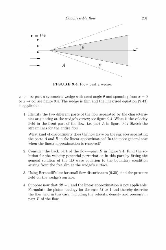
Compressible flow 201
x
B
u = U x
A
θ
FIGURE 9.4: Flow past a wedge.
x→ −∞ past a symmetric wedge with semi-angle θ and spanning from x = 0to x→∞; see figure 9.4. The wedge is thin and the linearised equation (9.43)is applicable.
1. Identify the two different parts of the flow separated by the characteris-tics originating at the wedge’s vertex; see figure 9.4. What is the velocityfield in the front part of the flow, i.e. part A in figure 9.4? Sketch thestreamlines for the entire flow.
What kind of discontinuity does the flow have on the surfaces separatingthe parts A and B in the linear approximation? In the more general casewhen the linear approximation is removed?
2. Consider the back part of the flow—part B in figure 9.4. Find the so-lution for the velocity potential perturbation in this part by fitting thegeneral solution of the 1D wave equation to the boundary conditionarising from the free slip at the wedge’s surface.
3. Using Bernoulli’s law for small flow disturbances (9.30), find the pressurefield on the wedge’s surface.
4. Suppose now that βθ ∼ 1 and the linear approximation is not applicable.Formulate the piston analogy for the case M 1 and thereby describethe flow field in this case, including the velocity, density and pressure inpart B of the flow.
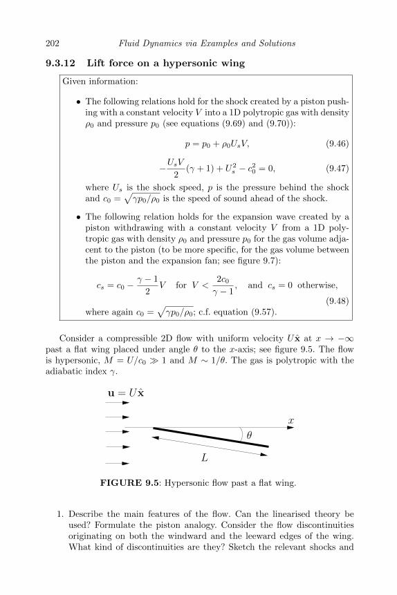
202 Fluid Dynamics via Examples and Solutions
9.3.12 Lift force on a hypersonic wing
Given information:
• The following relations hold for the shock created by a piston push-ing with a constant velocity V into a 1D polytropic gas with densityρ0 and pressure p0 (see equations (9.69) and (9.70)):
p = p0 + ρ0UsV, (9.46)
−UsV2
(γ + 1) + U2s − c20 = 0, (9.47)
where Us is the shock speed, p is the pressure behind the shockand c0 =
√γp0/ρ0 is the speed of sound ahead of the shock.
• The following relation holds for the expansion wave created by apiston withdrawing with a constant velocity V from a 1D poly-tropic gas with density ρ0 and pressure p0 for the gas volume adja-cent to the piston (to be more specific, for the gas volume betweenthe piston and the expansion fan; see figure 9.7):
cs = c0 −γ − 1
2V for V <
2c0γ − 1
, and cs = 0 otherwise,
(9.48)where again c0 =
√γp0/ρ0; c.f. equation (9.57).
Consider a compressible 2D flow with uniform velocity U x at x → −∞past a flat wing placed under angle θ to the x-axis; see figure 9.5. The flowis hypersonic, M = U/c0 1 and M ∼ 1/θ. The gas is polytropic with theadiabatic index γ.
L
θ
u = U x
x
FIGURE 9.5: Hypersonic flow past a flat wing.
1. Describe the main features of the flow. Can the linearised theory beused? Formulate the piston analogy. Consider the flow discontinuitiesoriginating on both the windward and the leeward edges of the wing.What kind of discontinuities are they? Sketch the relevant shocks and
Compressible flow 203
characteristics associated with these discontinuities. Sketch the stream-lines for the flow.
2. Using the piston analogy and the given information, find the pressureon both the upper and the lower parts of the wing. Use these results tofind the lift force on the wing.
9.3.13 Formation of a blast wave by a very intense explosion
The name of this problem was exactly the title of two papers in 1950 byG.I. Taylor who used a simple formula to calculate the power of the world’sfirst nuclear explosion which had previously been classified [25, 26]. Naturally,this revelation had a great impact on the military and its public relations.
A nuclear explosion in atmosphere of density ρ0 deposits energy E andthereby produces a spherical blast shock wave whose distance from the explo-sion point r grows with time t. Assume that the explosion is so strong that theonly dimensional parameters determining the shock motion are E, ρ0 and t.In particular, the ambient atmospheric pressure is unimportant (c.f. question9.3.7). Use dimensional analysis to find G.I. Taylor’s relation between r, E, ρ0
and t.
9.3.14 Balloon in polytropic atmosphere
A stratospheric balloon is partially filled with the buoyant gas hydrogenon the ground. As the balloon rises, it inflates and increases in volume. Thisleads to an additional lift. On the ground, the balloon has volume V0, while itsmaximum volume is V1. The atmospheric pressure and density at the groundlevel are p0 and ρ0 respectively. The hydrogen density at the ground level isρH2 .
1. Assume that the state of the gas in the atmosphere changes polytropi-cally,
p = p0
(ρ
ρ0
)γ,
where γ is constant. Determine the dependence of the density of theatmosphere on the height z.
2. What is the greatest possible weight of the load Gmax that can be lifted?(The balloon itself is part of the weight, but the buoyant gas is not).
3. What is the largest height to which weight G can be lifted? Assume thatat this height the maximal volume V1 is reached.
204 Fluid Dynamics via Examples and Solutions
9.4 Solutions
9.4.1 Model solution to question 9.3.1
Differentiating the pressure and taking into account the equation (9.3), wehave
∂tp+ u∂xp = (∂ρp)S(∂tρ+ u∂xρ) + (∂Sp)ρ(∂tS + u∂xS) = c2s(∂tρ+ u∂xρ).(9.49)
Here, (∂ρ·)S means the ρ-derivative with S kept constant and, respectively,(∂S ·)ρ means the S-derivative with ρ kept constant.
Multiplying the momentum equation (9.1) by ±ρcs, continuity equation(9.2) by c2s and adding the results to the pressure equation (9.49), we see thatthe derivatives of ρ cancel and we get
±ρcs∂tu± ρcsu∂xu+ c2sρ∂xu+ ∂tp+ u∂xp = ∓cs∂xp. (9.50)
By grouping the terms in this equation, we finally rewrite them as
[∂t + (u± cs)∂x]p± ρcs[∂t + (u± cs)∂x]u = 0. (9.51)
These equations are the equations (9.4) and (9.5) with the characteristic curvesdefined by equations (9.7) and (9.8).
9.4.2 Model solution to question 9.3.2
1. The C0-characteristics are the fluid paths. Let us first assume that thepiston’s withdrawal speed is not too fast for a vacuum bubble to form(the opposite case will be discussed in the end of the solution). Thenone of the fluid paths belongs to the particle adjacent to the piston and,therefore, tracing its trajectory x = X(t). The fluid particles at largedistances from the piston are not affected by its motion: they are notmoving i.e. their paths on the (x, t)-plane are straight vertical lines. Inbetween these faraway paths and the piston the fluid paths continuouslyfill the whole space x > X(t) for all t > 0; see figure 9.6. Initially, onthe semi-line t = 0, x > 0, the entropy is uniform: S = S0 = ln(p0/ρ
γ0).
This value is propagated along the C0-characteristics covering the entirespace occupied by the gas for any time t > 0, i.e. S = S0 for any t > 0and all x > X(t).
2. The initial value of the Riemann invariant R− is R−0 = 2c0γ−1 , where
c0 = cs(p0, ρ0) =√γp0/ρ0. The C−-characteristics move with velocities
less (by cs) than the fluid paths and, therefore, the C−-characteristicsoriginating on the x-axis cover the entire space occupied by the gas fort > 0; see figure 9.6. Thus, the initial value of the Riemann invariant R−
will propagate over the entire gas and R− for all t > 0 and all x > X(t).
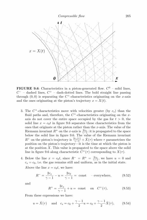
Compressible flow 205
0 x
t
x = X(t)
FIGURE 9.6: Characteristics in a piston-generated flow. C0 – solid lines,C− – dashed lines, C+ – dash-dotted lines. The bold straight line passingthrough (0, 0) is separating the C+-characteristics originating on the x-axisand the ones originating at the piston’s trajectory x = X(t).
3. The C+-characteristics move with velocities greater (by cs) than thefluid paths and, therefore, the C+-characteristics originating on the x-axis do not cover the entire space occupied by the gas for t > 0, thesolid line x = c0t in figure 9.6 separates these characteristics from theones that originate at the piston rather than the x-axis. The value of theRiemann invariant R+ on the x-axis is 2c0
γ−1 : it is propagated to the spacebelow the solid line in figure 9.6. The value of the Riemann invariant
R+ on the piston’s trajectory is 2cs(τ)γ−1 + X(τ) where τ parametrises the
position on the piston’s trajectory—it is the time at which the piston isat the position X. This value is propagated to the space above the solidline in figure 9.6 along characteristic C+(τ) corresponding to X(τ).
4. Below the line x = c0t, since R− = R+ = 2c0γ−1 , we have u = 0 and
cs = c0, i.e. the gas remains still and uniform, as in the initial state.
Above the line x = c0t, we have:
R− =2csγ − 1
− u =2c0γ − 1
= const – everywhere, (9.52)
and
R+ =2csγ − 1
+ u = const on C+(τ), (9.53)
From these expressions we have:
u = X(τ) and cs = c0 +γ − 1
2u = c0 +
γ − 1
2X(τ), (9.54)

206 Fluid Dynamics via Examples and Solutions
i.e. u and cs are constant along the C+-characteristics and these char-acteristics are are straight lines:
x(t) = u+ cs = c0 +γ + 1
2X(τ). (9.55)
Integrating this equation with condition x(τ) = X(τ), we have
x(t) = X(τ) +
[c0 +
γ + 1
2X(τ)
](t− τ). (9.56)
The implicit solution for u and cs is given by (9.54) with the parameterτ = τ(x, t) implicitly defined in (9.56).
5. For a constant speed X = −V < 0, we have to distinguish three zoneson the (x, t)-plane:
(a) The zone of the C+-characteristics originating on the x-axis atx > 0. This zone lies below the line x = c0t and, as before, inthis zone the gas remains still and uniform with the initial valuesof the pressure and the density.
(b) The zone of the C+-characteristics originating on the piston’s tra-jectory at t > 0. This zone lies above the line x = (c0 − V )t. Herefrom (9.54) we have:
u = −V and cs = c0 −γ − 1
2V. (9.57)
(c) The zone of the C+-characteristics originating at (0, 0). The char-acteristics in this zone are straight lines with all possible slopesbetween 1/c0 and 1/(c0 − V ). This is the so-called expansion fan;see figure 9.7. (Think of this zone as arising in a limiting case ofgradual but vanishingly small acceleration of the piston from zerovelocity to −V ). Here u+ cs = x/t and from (9.52) we have:
u =2c0γ + 1
(x
c0t− 1
), and cs =
c0γ + 1
((γ − 1)
x
c0t+ 2
).
Obviously, cs cannot become negative. Thus, from (9.57) we have acritical speed of the piston,
V∗ =2c0γ − 1
,
above which there is a vacuum region between the piston and the pointx = V∗t.
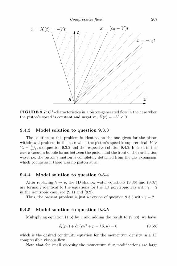
Compressible flow 207
0 x
tx = X(t) = −V t x = (c0 − V )t
x = −c0t
FIGURE 9.7: C+-characteristics in a piston-generated flow in the case whenthe piston’s speed is constant and negative, X(t) = −V < 0.
9.4.3 Model solution to question 9.3.3
The solution to this problem is identical to the one given for the pistonwithdrawal problem in the case when the piston’s speed is supercritical, V >V∗ = 2c0
γ−1 ; see question 9.3.2 and the respective solution 9.4.2. Indeed, in thiscase a vacuum bubble forms between the piston and the front of the rarefactionwave, i.e. the piston’s motion is completely detached from the gas expansion,which occurs as if there was no piston at all.
9.4.4 Model solution to question 9.3.4
After replacing h → ρ, the 1D shallow water equations (9.36) and (9.37)are formally identical to the equations for the 1D polytropic gas with γ = 2in the isentropic case; see (9.1) and (9.2).
Thus, the present problem is just a version of question 9.3.3 with γ = 2.
9.4.5 Model solution to question 9.3.5
Multiplying equation (1.6) by u and adding the result to (9.38), we have
∂t(ρu) + ∂x(ρu2 + p− λ∂xu) = 0. (9.58)
which is the desired continuity equation for the momentum density in a 1Dcompressible viscous flow.
Note that for small viscosity the momentum flux modifications are large
208 Fluid Dynamics via Examples and Solutions
within the jump (shock) regions only, and, therefore, the inviscid version ofthe momentum equation (equation (9.15)) can be used for finding the jumpconditions.
9.4.6 Model solution to question 9.3.6
1. Substituting expressions (9.19) into equation (9.17) and rearranging theterms we obtain:
∂t
(p
γ − 1+ρ
2u2
)= −∂x
[ρu3
2+ u
γp
(γ − 1)
]. (9.59)
From the equations (9.2) and (9.15) we have
∂t(ρu2) = ρu∂tu+ u∂t(ρu) = −ρu2∂xu− u∂xp
−u∂x(ρu2 + p) = −∂x(ρu3)− 2u∂xp. (9.60)
On the other hand, using (9.2) and (9.3) we have
∂tp = (∂ρp)S ∂tρ+ (∂Sp)ρ ∂tS = − (∂ρp)S ∂x(ρu)− (∂Sp)ρ u∂xS (9.61)
and∂xp = (∂ρp)S ∂xρ+ (∂Sp)ρ ∂xS. (9.62)
Here, (∂Sp)ρ and (∂ρp)S denote the derivative of p with respect to ρ withS fixed and the derivative of p with respect to S with ρ fixed. Combiningthe last two equations and using (∂ρp)S = γp/ρ we have
∂tp+ u∂xp = − (∂ρp)S ∂x(ρu)− (∂Sp)ρ u∂xS + u (∂ρp)S ∂xρ+
u (∂Sp)ρ ∂xS = −ρ (∂ρp)S ∂xu = −γp∂xu. (9.63)
Substituting this and (9.60) into (9.59) we have
−γ p∂xuγ − 1
− u∂xp = −∂x(pu)− p∂xu
(γ − 1)= 0, (9.64)
from which it is clear that the equality is identically satisfied, i.e. theenergy continuity equation (9.17) is valid.
2. The energy conservation follows from the first principles of physics andas such it is the most fundamental in fluid dynamics, with or withoutdissipation, and even if additional processes are involved: thermoconduc-tivity, ionisation, electromagnetic interactions. Of course, adding suchadditional effects would modify the expression for the internal energyand could also lead to further contributions to the energy expression(e.g. electro-magnetic energy, energy of interaction of the fluid with anexternal field). The role of viscosity is to transfer the kinetic equationinto the internal one while leaving the total energy unchanged. On theother hand, such increase of the internal energy leads to an increase ofthe entropy.
Compressible flow 209
9.4.7 Model solution to question 9.3.7
1. From equations (9.20) and (9.21) we get for u1 and u2:
u21 =
ρ2
ρ1
(p2 − p1)
(ρ2 − ρ1), (9.65)
u22 =
ρ1
ρ2
(p2 − p1)
(ρ2 − ρ1). (9.66)
Substituting these expressions into equation (9.23) yields the followingrelationship:
2 (h2 − h1) = (p2 − p1)
(1
ρ1+
1
ρ2
).
Using the polytropic gas expression for the entalpy (9.19), we get
ρ2 = ρ1
p2p1
(γ + 1) + (γ − 1)
(γ + 1) + p2p1
(γ − 1). (9.67)
Thus, given ρ1, p1 and p2, one can find ρ2 from (9.67) and then find u1
and u2 using (9.65) and (9.66) respectively. After that we move to theframe where the gas ahead of the shock is stationary, by shifting thevelocity field by −u1. Thus in this frame the shock’s speed will be −u1
and the downstream gas velocity will be u2 − u1 (where u2 and u1 arestill the velocities measured in the frame of the stationary shock).
2. As the shock’s strength increases, there is an increase in the downstreamgas pressure p2, but the density ratio ρ2/ρ1 approaches a finite limit.From equation (9.67) we get for the upper limit on the density ratio:
ρ2/ρ1 = (γ + 1)/(γ − 1) . (9.68)
It is equal to 4 for an ideal monatomic gas (γ = 5/3) and equal to 6for an ideal diatomic gas (γ = 1.4). Since air is comprised mostly ofdiatomic molecules (nitrogen and oxygen), the limiting density ratio forshocks in air is approximately equal to 6.
3. The piston’s motion will create a shock wave. In this case, the piston’svelocity will be equal the gas velocity downstream of the shock, i.e.V = u2 − u1, whereas before u1 and u2 are measured in the stationaryshock frame. In the laboratory frame, the shock’s speed is U = −u1.
From equations (9.20) and (9.21) we have:
p2 = ρ1u21 + p1 − ρ1u1u2 = p1 + ρ1UV. (9.69)
Using this in equation (9.23) yields:
u21
2+
γp1
(γ − 1)ρ1=u2
2
2+
γp2
(γ − 1)ρ2=
(V − U)2
2− γ(p1 + ρ1UV )(V − U)
(γ − 1)ρ1U.
210 Fluid Dynamics via Examples and Solutions
Cancelling on both sidesu21
2 = U2
2 and γp1(γ−1)ρ1
and multiplying the
resulting equation by (γ − 1)U/V , we have
−UV2
(γ + 1) + U2 − c21 = 0. (9.70)
The positive solution of this quadratic equation for U gives the shockspeed. Substituting U into (9.69) gives the pressure behind the shock.
9.4.8 Model solution to question 9.3.8
1. In general, it would be impossible to find a two-shock solution withouta contact discontinuity which would satisfy the boundary conditions,i.e. matching to the velocities, pressures and densities of the flows atx→ ±∞: the system would be overdefined as it would contain one moreequation to satisfy compared to the number of available variables. Hencein general there must be three jumps: two shocks running away from thecollision point in the opposite directions and a contact discontinuity inbetween the shocks as in figure 9.2. The contact discontinuity removesone equation that has to be satisfied, namely the condition that thedensities behind the two shocks must coincide.
2. According to equation (9.40), the limiting density ratio realised in strongshocks, when the pressure ratio tends to infinity is
α =γ + 1
γ − 1
(c.f. question (9.3.7)). Thus, for the densities on the two sides of thecontact discontinuity we have
ρ3 = αρ1 and ρ4 = αρ2.
3. The mass flow continuity across the two shocks yields respectively:
ρ3U1 = ρ1(U1 − u1) and ρ4U2 = ρ2(U2 − u2),
where the velocities are measured in the reference frame of the stationarycontact discontinuity, u3 = u4 = 0.
Thus in the strong shock limit we have:
U1 = − u1
α− 1and U2 = − u2
α− 1(9.71)
(in the reference frame of the stationary contact discontinuity).
4. Using (9.39), we have for the pressures behind the shocks in the strong
Compressible flow 211
shock limit (i.e. neglecting p1 and p2 compared to p3 an p4 and takingthe limiting density ratio α):
p3 =α− 1
αρ1(U1 − u1)2 and p4 =
α− 1
αρ2(U2 − u2)2. (9.72)
From these expressions, equating pressures on the two sides of the con-tact discontinuity, p3 = p4, we find:
ρ1(U1 − u1)2 = ρ2(U2 − u2)2.
Substituting u = u2 − u1 and using the equations (9.71) we get:
u1 = − u
1 +√ρ1/ρ2
and u2 =u
1 +√ρ2/ρ1
, (9.73)
so that
U1 =u
(α− 1)(1 +√ρ1/ρ2)
and U2 = − u
(α− 1)(1 +√ρ2/ρ1)
. (9.74)
The pressure between the shocks can be found from (9.72):
p3 = p4 =αu2
(α− 1)(√
1/ρ1 +√
1/ρ2)2. (9.75)
9.4.9 Model solution to question 9.3.9
1. The free-slip boundary condition on the wing surface y = Y±(x) saysthat the normal to the boundary component of velocity is zero (signsplus and minus correspond to the top and the bottom of the wing re-spectively). This is the same as to say that the vector product of thevelocity and the tangential vector is zero. Since the ratio of the y- andthe x-components of the tangential vector is ∂xY (x), we have:
(U + ∂xφ)∂xY± − ∂yφ = 0 on y = Y±(x).
Linearising this condition taking into account that |∂xφ| U and∂xY±(x) 1, we have:
U∂xY± − ∂yφ = 0 on y = Y±(x). (9.76)
2. By using a scaling transformation φ(x) = φ′(x′)/β and Y±(x) = Y ′±(x′)with x′ = x/β, we reduce equation (9.41) and the boundary condition(9.76) to an effective incompressible flow problem:
∂x′x′φ′ + ∂yyφ
′ = 0, (9.77)
(this is the 2D Laplace equation) and
U∂x′Y′± − ∂yφ′ = 0 on y = Y ′±(x′). (9.78)
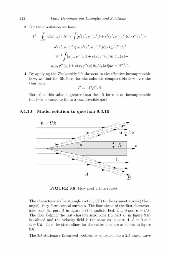
212 Fluid Dynamics via Examples and Solutions
3. For the circulation we have:
Γ′ =
∮C′
u(x′, y) · ds′ ≈∫
[u′(x′, y−(x′)) + v′(x′, y−(x′))∂x′Y′−(x′)−
u′(x′, y+(x′)) + v′(x′, y+(x′))∂x′Y′+(x′)]dx′
= β−1
∫[u(x, y−(x)) + v(x, y−(x))∂xY−(x)−
u(x, y+(x)) + v(x, y+(x))∂xY+(x)]dx = β−1Γ.
4. By applying the Zhukovskiy lift theorem to the effective incompressibleflow, we find the lift force for the subsonic compressible flow over thethin wing:
F = −UρΓ/β.
Note that this value is greater than the lift force in an incompressiblefluid—it is easier to fly in a compressible gas!
9.4.10 Model solution to question 9.3.10
u = U x
B
C
A
u = U x
xθ R
FIGURE 9.8: Flow past a thin rocket.
1. The characteristics lie at angle arctan(1/β) to the symmetry axis (Machangle); they form conical surfaces. The flow ahead of the first character-istic cone (in part A in figure 9.8) is undisturbed, φ ≡ 0 and u = U x.The flow behind the last characteristic cone (in part C in figure 9.8)is calmed and the velocity field is the same as in part A, φ ≡ 0 andu = U x. Thus the streamlines for the entire flow are as shown in figure9.8).
The 3D stationary linearised problem is equivalent to a 2D linear wave
Compressible flow 213
propagation problem with effective time τ = x/β. The changing cross-section of the body then plays the role of a moving piston. Since thevelocity of such a piston changes suddenly at the vertex of the cone (tip ofthe rocket) and the cone’s base (boundary between the conical nose andthe cylindrical body), the velocity field will have discontinuous gradientsat the respective characteristic cones, i.e. on the surfaces separatingparts A and B and parts B and C respectively. In the more generalcase, when the linear approximation is removed, the front discontinuitybecomes a (weak) shock wave and the trailing discontinuity becomesa (weak) rarefaction wave (with an expansion fan concentrated in thenarrow sector of angles).
2. For the middle part of the flow (part B in figure 9.8) we seek a self-similarsolution for the velocity potential perturbation in the form φ(r, x) =xf(η) with η = r/x. By substituting this expression into equation(9.42), we get the following ODE for the function f(η),
η(1− β2η2)∂ηηf + ∂ηf = 0. (9.79)
3. The free-slip boundary condition for the cone surface is
u⊥/(U + u‖) ≈ u⊥/U = tan θ ≈ θ on r = x tan θ ≈ xθ. (9.80)
This boundary condition in terms of a condition on the function f(η)reads:
∂ηf = Uθ at η = θ. (9.81)
4. The ODE has a trivial solution f = const which corresponds to φ =constx and which can be discarded because it corresponds to a finiteuniform x-velocity perturbation at infinity (the latter must be zero).The second fundamental solution is found by solving equation (9.79)with respect to ∂ηf , which, taking into account the boundary condition(9.81), gives:
∂ηf = ∂rψ = ur =θ2βU√1− β2θ2
√1
β2η2− 1 = θ2βU
√x2
β2r2− 1. (9.82)
Here we took into account that βθ 1 because only for such valuesthe linear approach we are using is valid; see section 9.1.2.2. Obviously,expression (9.82) is valid only for r < x/β (recall that for r > x/β wehave part A of the flow where the velocity disturbance is zero).
Integrating equation (9.82) gives:
f = θ2U
[√1− β2η2 − arccosh
1
βη
]. (9.83)
For the x-velocity disturbance we have:
ux = ∂xφ = f − η∂ηf = −θ2Uarccoshx
βr. (9.84)
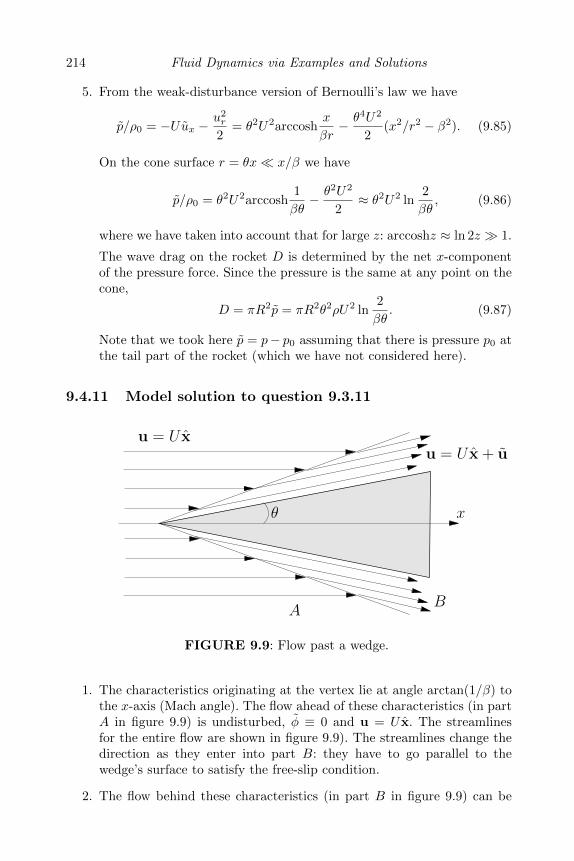
214 Fluid Dynamics via Examples and Solutions
5. From the weak-disturbance version of Bernoulli’s law we have
p/ρ0 = −Uux −u2r
2= θ2U2arccosh
x
βr− θ4U2
2(x2/r2 − β2). (9.85)
On the cone surface r = θx x/β we have
p/ρ0 = θ2U2arccosh1
βθ− θ2U2
2≈ θ2U2 ln
2
βθ, (9.86)
where we have taken into account that for large z: arccoshz ≈ ln 2z 1.
The wave drag on the rocket D is determined by the net x-componentof the pressure force. Since the pressure is the same at any point on thecone,
D = πR2p = πR2θ2ρU2 ln2
βθ. (9.87)
Note that we took here p = p− p0 assuming that there is pressure p0 atthe tail part of the rocket (which we have not considered here).
9.4.11 Model solution to question 9.3.11
u = U x + uu = U x
B
x
A
θ
FIGURE 9.9: Flow past a wedge.
1. The characteristics originating at the vertex lie at angle arctan(1/β) tothe x-axis (Mach angle). The flow ahead of these characteristics (in partA in figure 9.9) is undisturbed, φ ≡ 0 and u = U x. The streamlinesfor the entire flow are shown in figure 9.9). The streamlines change thedirection as they enter into part B: they have to go parallel to thewedge’s surface to satisfy the free-slip condition.
2. The flow behind these characteristics (in part B in figure 9.9) can be
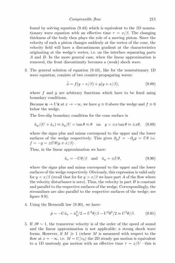
Compressible flow 215
found by solving equation (9.43) which is equivalent to the 1D nonsta-tionary wave equation with an effective time τ = x/β. The changingthickness of the body then plays the role of a moving piston. Since thevelocity of such a piston changes suddenly at the vertex of the cone, thevelocity field will have a discontinuous gradient at the characteristicsoriginating at the wedge’s vertex, i.e. on the interface separating partsA and B. In the more general case, when the linear approximation isremoved, the front discontinuity becomes a (weak) shock wave.
3. The general solution of equation (9.43), like for the nonstationary 1Dwave equation, consists of two counter-propagating waves:
φ = f(y − x/β) + g(y + x/β), (9.88)
where f and g are arbitrary functions which have to be fixed usingboundary conditions.
Because u→ U x at x→ −∞, we have g ≡ 0 above the wedge and f ≡ 0below the wedge.
The free-slip boundary condition for the cone surface is
uy/(U + ux) ≈ uy/U = tan θ ≈ θ on y = ±x tan θ ≈ ±xθ, (9.89)
where the signs plus and minus correspond to the upper and the lowersurfaces of the wedge respectively. This gives ∂yf = −∂yg = Uθ i.e.f = −g = ±Uθ(y ∓ x/β) .
Thus, in the linear approximation we have:
ux = −Uθ/β and uy = ±Uθ, (9.90)
where the signs plus and minus correspond to the upper and the lowersurfaces of the wedge respectively. Obviously, this expression is valid onlyfor y < x/β (recall that for for y > x/β we have part A of the flow wherethe velocity disturbance is zero). Thus, the velocity in part B is constantand parallel to the respective surfaces of the wedge. Correspondingly, thestreamlines are also parallel to the respective surfaces of the wedge; seefigure 9.9).
4. Using the Bernoulli law (9.30), we have:
p = −Uux − u2y/2 = U2θ/β − U2θ2/2 ≈ U2θ/β. (9.91)
5. If βθ ∼ 1, the transverse velocity is of the order of the speed of soundand the linear approximation is not applicable: a strong shock waveforms. However, if M 1 (where M is measured with respect to theflow at x = −∞, i.e. M = U/c0) the 2D steady gas motion is equivalentto a 1D unsteady gas motion with an effective time τ = x/U—this is
216 Fluid Dynamics via Examples and Solutions
the piston analogy. Thus the flow is equivalent to the 1D gas motioncaused by a piston which suddenly starts pushing into the gas with aconstant velocity V = ±U tan θ ≈ ±Uθ (plus for the upper and minusfor the lower sides of the wedge). The shock speed Us in the 1D problemis related to angle α at which the 2D shock is oriented with respect tothe x-axis via tanα = Us/U . Part B of the flow corresponds to the flowbehind such a 1D shock, and its parameters can be found from solvingequations (9.44) and (9.45), which gives:
tanα = ±(γ + 1)θ/4±√θ2(γ + 1)2/16 + 1/M2 (9.92)
and
p = p0 + ρ0U2θ(θ(γ + 1)/4 +
√θ2(γ + 1)2/16 + 1/M2
). (9.93)
Obviously, the y-velocity in part B is still as in (9.90) (i.e. in the re-spective 1D problem the velocity behind the shock is the same as thepiston’s velocity).
Note that expression (9.93) agrees with (9.91) in the limit 1M 1/θ,i.e. when the applicability ranges of both approaches overlap.
9.4.12 Model solution to question 9.3.12
xθ
u = U x
FIGURE 9.10: Hypersonic flow past a flat wing. The wing is shown by thevery bold line. The bold line marks the shocks, and the dashed lines mark theexpansion fans. The streamlines are marked by the thin solid lines.
1. When Mθ ∼ 1 the transverse velocity is of the order of the speed ofsound and the linear approximation is not applicable: strong shocks andnonlinear rarefaction waves form. However, if M 1, the 2D steady gasmotion is equivalent to a 1D unsteady gas motion with an effective timeτ = x/U—this is the piston analogy. Thus the flow below the wing isequivalent to the 1D gas motion caused by a piston which suddenly startspushing into the gas with a constant velocity V = −U tan θ ≈ −Uθ,whereas the flow above the wing is equivalent to the 1D gas motion
Compressible flow 217
caused by a piston which suddenly starts withdrawing from the gaswith a constant velocity V = −U tan θ ≈ −Uθ. Respectively, the flowforms a shock discontinuity originating at the windward edge of thewing and extending below it, and an expansion fan of characteristicsalso originating at the windward edge and extending above the wing(there are velocity gradient discontinuities at the both boundaries of theexpansion fan). At the leeward edge, the picture of the discontinuitiesis symmetric with respect to the windward edge, and behind downwindfrom these discontinuities the flow restores the original shape, u = U x;see figure 9.10. This figure also shows a sketch of the streamlines.
2. By the piston analogy, for the flow below the wing we can use the resultfor the flow behind a 1D shock, equations (9.46) and (9.47). The shockspeed Us in the 1D problem is related to angle α < 0 at which the 2Dshock is oriented with respect to the x-axis via tanα = Us/U . Solving(9.47) for Us and substituting the result into (9.46), we have for thepressure below the wing:
p− = p0 + ρ0U2θ(θ(γ + 1)/4 +
√θ2(γ + 1)2/16 + 1/M2
); (9.94)
c.f. equation (9.93).
Also by the piston analogy, for the flow above the wing we can use theresult for the flow the 1D expansion wave created by a piston withdraw-ing with a constant velocity V = Uθ from a 1D polytropic gas, namelyequation (9.48). Taking into account that the rarefaction wave flow isisentropic, cs/c0 = (p/p0)(γ−1)/2γ , we have for the pressure above thewing:
p+ = p0
[1− γ − 1
2Mθ
]2γ/(γ−1)
for Mθ <2
γ − 1, (9.95)
and p = 0 otherwise (vacuum).
The lift force on the wing (per unit length of the wing) is
F = (p− − p+)L cos θ ≈ (p− − p+)L.
9.4.13 Model solution to question 9.3.13
The unit of energy is erg which is g cm2/s2 (just think of the kinetic energyexpression E = mu2/2). The unit of density ρ is g/cm3 and the units of r andt are cm and s respectively. The only dimensional combination of E, ρ0 and tthat gives the correct dimension of r is:
r(t) = Cρ
1/50
E1/5t2/5,
where C is a dimensionless constant (in polytropic gases it depends on theadiabatic index γ). This is G.I. Taylor’s relation [26].
218 Fluid Dynamics via Examples and Solutions
9.4.14 Model solution to question 9.3.14
1. The vertical component of the Euler equation is:
1
ρ
∂p
∂z= −g.
Substituting the polytropic law, we have:
γp0ργ−2
ργ0
∂ρ
∂z= −g.
Integrating this, we find:
γ
γ − 1
p0
ργ0ργ−1 = −gz + C,
and matching to the boundary condition at the ground, ρ(0) = ρ0,
ρ = ρ0(1− z/H)1/(γ−1), (9.96)
where H = p0γρ0g(γ−1) .
2. Balancing the load weight and the buoyancy force at the ground level,we have:
Gmax = gV0(ρ0 − ρH2).
3. At height zmax, from (9.96) we have the following air density:
ρ1 = ρ0(1− zmax/H)1/(γ−1). (9.97)
So,zmax = H −H(ρ1/ρ0)(γ−1). (9.98)
The force balance at zmax is:
G = gV1(ρ1 − ρ′H2), (9.99)
where ρ′H2is the hydrogen density at height zmax, which can be obtained
from the mass conservation ρ′H2= V0 ρH2/V1. So, ρ1 = V0 ρH2/V1 +
G/gV1.
Finally,
zmax = H −H[V0 ρH2
+G/g
V1ρ0
](γ−1)
.
Bibliography
[1] D.J. Acheson. Elementary Fluid Dynamics. Oxford Applied Mathematicsand Computing Science Series. Clarendon Press, 1990.
[2] Hassan Aref, Paul K. Newton, Mark A. Stremler, Tadashi Tokieda, andDmitri L. Vainchtein. Vortex Crystals. In Advances in Applied Mechanics,volume 39, pages 1–79. Elsevier, 2003.
[3] G.K. Batchelor. The Theory of Homogeneous Turbulence. CambridgeScience Classics. Cambridge University Press, 1953.
[4] G.K. Batchelor. An Introduction to Fluid Dynamics. Cambridge Mathe-matical Library. Cambridge University Press, 2000.
[5] P.G. Drazin and W.H. Reid. Hydrodynamic Stability. Cambridge Math-ematical Library. Cambridge University Press, 2004.
[6] G. Falkovich. Fluid Mechanics: A Short Course for Physicists. CambridgeUniversity Press, 2011.
[7] R. Fjørtoft. On the changes in the spectral distribution of kinetic energyfor two-dimensional nondivergent flow. Tellus, 5(5):225, 1953.
[8] U. Frisch. Turbulence: The Legacy of A. N. Kolmogorov. CambridgeUniversity Press, 1995.
[9] T. Kambe. Elementary Fluid Mechanics. World Scientific, 2007.
[10] A.N. Kolmogorov. The local structure of turbulence in incompressibleviscous fluid for very large Reynolds numbers. Proc. R. Soc. Lond. A,434:9–13, 1991.
[11] R.H. Kraichnan and D. Montgomery. Two-dimensional turbulence. Re-ports on Progress in Physics, 43(5):547, 1980.
[12] P.K. Kundu and I.M. Cohen. Fluid Mechanics. Elsevier Science, 2010.
[13] H. Lamb. Hydrodynamics. Dover Publications, 1945.
[14] L.D. Landau and E.M. Lifshitz. Fluid Dynamics. Theoretical Physics.Butterworth-Heinemann, 1995.
219
220 Bibliography
[15] J. Lighthill. Waves in Fluids. Cambridge Mathematical Library. Cam-bridge University Press, 2001.
[16] J.C. McWilliams. Fundamentals of Geophysical Fluid Dynamics. Cam-bridge University Press, 2006.
[17] H. Oertel, P. Erhard, K. Asfaw, D. Etling, U. Muller, U. Riedel, K.R.Sreenivasan, and J. Warnatz. Prandtl’s Essentials of Fluid Mechanics.Applied Mathematical Sciences. Springer, 2010.
[18] L. Onsager. Statistical hydrodynamics. Nuovo Cimento, 6(2):279–287,1949.
[19] A.R. Paterson. A First Course in Fluid Dynamics. Cambridge UniversityPress, 1983.
[20] L. Prandtl. Verhandlungen des dritten internationalen Mathematiker-Kongresses (Heidelberg 1904). Leipzig, 1905.
[21] L. Prandtl. Essentials of Fluid Dynamics: With Applications to Hy-draulics, Aeronautics, Meteorology, and Other Subjects. Hafner Pub. Co.,1952.
[22] Lewis F. Richardson. Atmospheric diffusion shown on a distance-neighbour graph. Proceedings of the Royal Society of London. SeriesA, 110(756):709–737, 1926.
[23] P.G. Saffman. Vortex Dynamics. Cambridge Monographs on Mechanics.Cambridge University Press, 1992.
[24] Wayne Schubert, Eberhard Ruprecht, Rolf Hertenstein, Rosana NietoFerreira, Richard Taft, Christopher Rozoff, Paul Ciesielski, and Hung-ChiKuo. English translations of twenty-one of Ertel’s papers on geophysicalfluid dynamics (see the first four papers). Meteorologische Zeitschrift,13(6):527–576, 2004-12-01T00:00:00.
[25] Geoffrey Taylor. The formation of a blast wave by a very intense explo-sion. i. theoretical discussion. Proceedings of the Royal Society of London.Series A, Mathematical and Physical Sciences, 201:159–174, 1950.
[26] Geoffrey Taylor. The formation of a blast wave by a very intense explo-sion. ii. the atomic explosion of 1945. Proceedings of the Royal Societyof London. Series A, Mathematical and Physical Sciences, 201:175–186,1950.
[27] A.A. Townsend. The Structure of Turbulent Shear Flow. CambridgeMonographs on Mechanics. Cambridge University Press, 1980.
[28] D.J. Tritton. Physical Fluid Dynamics. Oxford Science Publications.Clarendon Press, 1988.
Bibliography 221
[29] Francisco Vera, Rodrigo Rivera, and Cesar Nunez. Backward reactionforce on a fire hose, myth or reality? Fire Technology, pages 1–5, 2014.
[30] Th. Von Karman. Mechanische Ahnlichkeit und turbulenz. Nachrichtenvon der Gesellschaft der Wissenschaften zu Gottingen, 5:58–76, 1930.
[31] G.B. Whitham. Linear and Nonlinear Waves. Pure and Applied Math-ematics: A Wiley Series of Texts, Monographs and Tracts. Wiley, 2011.

This page intentionally left blankThis page intentionally left blank
VIA EXAMPLES AND SOLUTIONSFLUID DYNAMICS
SERGEY NAZARENKO
ISBN: 978-1-4398-8882-7
9 781439 888827
90000
K14078
Fluid Dynamics via Examples and Solutions provides a substantial set of example problems and detailed model solutions covering various phenomena and effects in fluids. The book is ideal as a supplement or exam review for undergraduate and graduate courses in fluid dynamics, continuum mechanics, turbulence, ocean and atmospheric sciences, and related areas. It is also suitable as a main text for fluid dynamics courses with an emphasis on learning by example and as a self-study resource for practicing scientists who need to learn the basics of fluid dynamics.
The author covers several sub-areas of fluid dynamics, types of flows, and applications. He also includes supplementary theoretical material when necessary. Each chapter presents the background, an extended list of references for further reading, numerous problems, and a complete set of model solutions.
Features • Describes many examples dealing with various phenomena and
effects in fluids • Promotes effective hands-on study of fluid dynamics through physically
motivated exercises • Provides instructors with a wealth of possible exam questions from
which to choose • Contains model solutions and suggestions for further reading in
each chapter
Sergey Nazarenko is a professor at the University of Warwick. His research focuses on fluid dynamics, turbulence, and waves, including wave turbulence, magneto-hydrodynamic turbulence, superfluid turbulence, water waves, Rossby waves, vortices and jets in geophysical fluids, drift waves and zonal jets in plasmas, optical vortices and turbulence, and turbulence in Bose-Einstein condensates.
Physics
K14078_COVER_final.indd 1 10/27/14 1:14 PM
Top Related
Copyright © 2022 FDOKUMEN

