


Bahasa
Halaman
Hukum

FISH AND COMPLEXITY: FAUNAL ANALYSIS AT THE SHELL MIDDEN COMPONENT
OF SITE DGRV-006, GALIANO ISLAND, B.C.
By
JUSTIN RAY HOPT
A thesis submitted in partial fulfillment of
the requirements for the degree of
MASTER OF ARTS IN ANTHROPOLOGY
WASHINGTON STATE UNIVERSITY
Department of Anthropology
DECEMBER 2014
© Copyright by JUSTIN RAY HOPT, 2014
All Rights Reserved

© Copyright by JUSTIN RAY HOPT, 2014
All Rights Reserved
ii
To the Faculty of Washington State University:
The members of the Committee appointed to examine the thesis of JUSTIN RAY
HOPT find it satisfactory and recommend that it be accepted.
_______________________________________
Colin Grier, Ph.D., Chair
_______________________________________
Andrew Duff, Ph.D.
_______________________________________
Brian Kemp, Ph.D.

iii
ACKNOWLEDGMENT
As with any large undertaking, the completion of this thesis was only possible through
the help of others. First and foremost, I must thank my advisor, Colin Grier. This entire project
and thesis would not have been possible without his guidance and support. I also must thank the
other members of my committee: Andrew Duff and Brian Kemp. Their comments on earlier
drafts of this thesis made the finished project a much better piece of writing.
I would also like to thank the field crews from both the 2012 and 2013 excavations for
their hard work in the collection of the faunal material utilized in this thesis. Thanks goes to
everyone in the WSU Northwest Coast lab as well. I would also like to especially thank Patrick
Dolan and Matt Marino, whom have directly helped me think through several aspects of this
thesis.
Finally, I would like to thank my friends and family for their support. My brothers for
keeping me grounded and my parents for both their financial and (more importantly) emotional
support. And lastly, I would like to thank my partner, Vanessa, for always being there for me.
iv
FISH AND COMPLEXITY: FAUNAL ANALYSIS AT THE SHELL MIDDEN COMPONENT
OF SITE DGRV-006, GALIANO ISLAND, B.C.
Abstract
By Justin Ray Hopt, M.A.
Washington State University
December 2014
Chair: Colin Grier
Studies of the development of social complexity and inequality on the Northwest Coast
have focused on the inter-connectedness of subsistence practices and social changes. Several
early studies proposed a linear model for the development of complexity, where increasingly
complex social relations were accompanied by shifts in subsistence activities. These models
hypothesize that a peak in complex social relationships was paired with a specialized salmon
economy in the Marpole Period (2500-1000 BP), with a change in social relationships
accompanied by a more diverse fishing strategy in the Late Period (1000 BP-contact).
Close scrutiny of the empirical data used to support this linear complexity model has
prompted calls for a more nuanced approach to understanding the basis for Northwest Coast
complexity. For example, many of the originally perceived changes in subsistence may actually
be attributed to changes in environmental productivity. Despite such critiques, these models offer
a frame of reference against which patterning in faunal assemblages can be evaluated,
illuminating the ways in which we might better explore the relationships between socio-cultural
shifts and subsistence strategies.
v
In this study, faunal remains from the shell midden component of site DgRv-006 are
examined. Radiocarbon dates indicate that the age of the midden deposits overlap with both a
Late Period plankhouse at DgRv-006, and site DgRv-003, a nearby Marpole-age plankhouse
village. The shift in subsistence posited to occur between the Marpole and Late Period in the
linear model should be evident within the midden deposits, allowing us to directly address the
connection between social and subsistence changes for this important location over the long
term.
Results of the analyses undertaken in this study do not support salmon specialization in
the Marpole faunal assemblage, and fish remains overall show a consistent diverse pattern in
both time periods, indicating that social changes and subsistence shifts may not be as closely
correlated as past models have posited. This study also explores several methodological issues
related to faunal analyses from shell midden contexts, including the use of bulk samples for
correcting sample counts, emphasizing proper quantification techniques, and the use of
correspondence analysis to address shell midden life histories.
vi
TABLE OF CONTENTS
Page
ACKNOWLEDGEMENT............................................................................................... iii
ABSTRACT................................................................................................................. iv-v
LIST OF TABLES..................................................................................................... xi-xii
LIST OF FIGURES ............................................................................................... xiii-xvii
CHAPTER
1. INTRODUCTION.......................................................................................... 1
a. Objectives of the thesis....................................................................... 3
b. Conclusions of the thesis.................................................................... 7
c. Organization of the thesis................................................................... 8
2. FISH AND COMPLEXITY IN NORTHWEST COAST STUDIES ...........10
a. Linear Complexity Model Critiques .................................................16
b. Thesis Analysis .................................................................................19
3. CULTURE HISTORY OF THE GULF OF GEORGIA REGION.............. 23
a. Old Cordilleran (9000-4500 BP)...................................................... 23
b. Charles (4500-3500 BP) ...................................................................24
c. Locarno Beach (3500-2500 BP) .......................................................26
d. Marpole (2500-1000 BP) ..................................................................27
e. Late Period (1000 BP-Contact) .........................................................30
f. Ethnographic Record ........................................................................32
i. Social Organization ...............................................................32

vii
ii. Settlement .............................................................................35
iii. Subsistence ............................................................................35
4. SITE DGRV-006 INFORMATION: ENVIRONMENT, BIOLOGY, AND
ARCHAEOLOGY ........................................................................................39
a. Marine Transgression........................................................................41
b. Geology and Soils of Galiano Island ................................................42
c. Climate/Biology ................................................................................42
d. Archaeology of the Dionisio Point Locality .....................................43
5. QUANTIFYING A MIDDEN ......................................................................52
a. Faunal Analysis Procedure ...............................................................52
b. Quantification of Remains ................................................................55
i. NISP ......................................................................................55
ii. MNI .......................................................................................57
iii. Meat Weights ........................................................................60
iv. Ubiquity ................................................................................62
v. Diversity ................................................................................63
6. TEMPORAL AND DEPOSITIONAL BREAK-DOWN OF MIDDEN
CONTEXTS ..................................................................................................65
a. Radiocarbon Dates and Stratigraphy ................................................65
b. Depositional Unit 1: Mound .............................................................66
c. Depositional Unit 2: Marpole Deposits ............................................66
d. Depositional Unit 3: Later Deposits .................................................67

viii
e. Depositional Unit 4: Shell Dump ......................................................67
f. Temporal Area 1: Dated Marpole .....................................................68
g. Temporal Area 2: Inferred Marpole ..................................................68
h. Temporal Area 3: Dated Late ...........................................................68
i. Temporal Area 4: Inferred Late ........................................................73
j. Correspondence Analysis: Depositional Units .................................73
7. TEMPORAL COMPARISON ......................................................................79
a. Full Midden Assemblage Summary..................................................80
i. Fish Vertebrae .......................................................................81
ii. Terrestrial Mammal ..............................................................84
iii. Sea Mammal .........................................................................86
iv. Bird .......................................................................................86
v. Full Midden Summary ..........................................................87
b. Marpole Assemblage ........................................................................88
i. Fish Vertebrae .......................................................................89
ii. Terrestrial Mammal ..............................................................95
iii. Sea Mammal .........................................................................97
iv. Bird .......................................................................................97
v. Shellfish ................................................................................98
vi. Conclusion: Marpole Assemblage ........................................99
c. Late Period Assemblage .................................................................103
i. Fish Vertebrae .....................................................................104

ix
ii. Terrestrial Mammal ............................................................109
iii. Sea Mammal .......................................................................111
iv. Bird .....................................................................................111
v. Shellfish ..............................................................................112
vi. Conclusion: Late Period Assemblage .................................112
d. Temporal Comparison of Linear Complexity Models ....................114
i. Richness ..............................................................................115
ii. Evenness .............................................................................118
iii. Importance of Salmon .........................................................121
iv. Conclusion ..........................................................................122
8. BULK SAMPLES AND BIAS TESTING .................................................124
a. Screen Size Analysis .......................................................................125
b. Marpole Correction .........................................................................130
c. Late Period Correction ....................................................................132
d. Conclusion ......................................................................................136
9. CONCLUSIONS.........................................................................................139
a. Method-based Conclusions .............................................................139
b. Site-specific Conclusions ................................................................141
c. Linear Complexity Models .............................................................142
BIBLIOGRAPHY .........................................................................................................144
APPENDICES ..............................................................................................................158
A. Fish Vertebrae Raw Counts ........................................................................158
x
B. Fish Vertebrae Raw Data ............................................................................173
C. Terrestrial Mammal Raw Counts ................................................................192
D. Terrestrial Mammal Raw Data....................................................................195
E. Sea Mammal Raw Counts ...........................................................................198
F. Sea Mammal Raw Data ..............................................................................198
G. Bird Raw Counts .........................................................................................199
H. Bird Raw Data.............................................................................................208
I. Fish Elements Raw Data .............................................................................210
J. “No ID” Raw Data ......................................................................................213
K. Temporal and Depositional Unit Level Designation ..................................216
L. Stata Correspondence Analysis Output ......................................................219
xi
LIST OF TABLES
1. Southern Gulf of Georgia Culture History ........................................................................3
2. Ethnographic catchment, seasonality, and processing info. on select fish species .........38
3. AMS dates from Parry Lagoon Midden..........................................................................40
4. Fish biology information on species present in the Parry Lagoon Midden ....................44
5. Shellfish biology information on species present in the Parry Lagoon Midden .............45
6. Vertebrae numbers and fish weights for species present in the Parry Lagoon Midden ..58
7. Parry Lagoon Midden burials and burial location ..........................................................71
8. Input values for depositional unit correspondence analysis ...........................................75
9. Chi-Squared analysis on depositional units ....................................................................77
10. NISP, MNI, and Ubiquity for fish vertebrae – overall Parry Lagoon Midden ...............82
11. Meat weight analysis – overall Parry Lagoon Midden ...................................................84
12. NISP, MNI, and Ubiquity for mammal – overall Parry Lagoon Midden .......................85
13. NISP, MNI, and Ubiquity for bird – overall Parry Lagoon Midden...............................87
14. Marpole assemblage fish NISP and MNI counts ............................................................90
15. Meat weight calculations – Marpole assemblage ...........................................................93
16. Late Period assemblage fish NISP and MNI counts .....................................................105
17. Meat weight analysis – Late Period assemblage...........................................................108
18. Comparison of species presence – Marpole and Late Period .......................................117
19. Comparison of meat weights by time period ................................................................121
20. Matrix sample counts – dry screened............................................................................126
21. Matrix sample counts – wet screened ...........................................................................127

xii
22. NISP count totals for all matrix material ......................................................................129
23. Chi-Squared input values for dry screened bulk samples .............................................129
24. Chi-Squared input values for wet screened bulk samples ............................................129
25. Matrix sample counts – Marpole assemblage ...............................................................130
26. Thomas 1969 correction factor calculation – Marpole assemblage..............................131
27. Thomas 1969 correction factor applied to excavation levels: 15B1, 16B6, 16B8 .......131
28. Meat weight analysis on corrected values – Marpole assemblage ...............................133
29. %NISP of Marpole excavation levels, corrected, and smelt corrected assemblages ....133
30. Matrix sample counts – Late Period .............................................................................134
31. Thomas 1969 correction factor calculation – Late Period assemblage.........................134
32. Thomas 1969 correction factor applied to excavation levels: 12B2, 14B1, 19B2 .......135
33. Meat weight analysis on corrected values – Late Period assemblage ..........................135
34. %NISP of Late Period excavation levels, corrected, and smelt corrected assemblages137
xiii
LIST OF FIGURES
1. Figure 1; Southern Gulf of Georgia Islands ................................................................2
2. Figure 2a; Parry Lagoon Midden with temporal distinction – 2012 excavations.
Redline separates the Marpole from the Late Period. Earliest Marpole portion is
below the blue line. Figure 2b; Parry Lagoon Midden with temporal distinction –
2013 excavations .......................................................................................................21
3. Figure 3; Suttles’ inverted pear of Coast Salish social organization ........................33
4. Figure 4; Dionisio Point archaeological locality. Parry Lagoon Midden indicated in
red. Modified from Grier 2014 .................................................................................40
5. Figure 5; Unit 13 - eroding burial cairn. From Grier, McLay, and Richards 2012 ..47
6. Figure 6; Example of midden undercut during the 2013 excavations ......................48
7. Figure 7; Excavation units 10-19. Photograph taken following excavation of these
units (2012), looking west from Parry Lagoon .........................................................48
8. Figure 8; Parry Lagoon Midden before 2012 excavation - Southern portion. Parry
Lagoon is to the photographer’s back .......................................................................49
9. Figure 9; Parry Lagoon Midden before 2012 excavation - Middle portion. Parry
Lagoon is to the photographer’s back .......................................................................49
10. Figure 10; Parry Lagoon Midden before 2012 excavation - Northern portion. Parry
Lagoon is to the photographer’s back .......................................................................50
11. Figure 11; Parry Lagoon Midden after 2013 excavation. Image on right includes unit
designations...............................................................................................................50

xiv
12. Figure 12; Parry Lagoon Midden before 2013 excavation. Image on right includes
unit designations .......................................................................................................51
13. Figure 13a; Radiocarbon date locations on the midden – 2012 excavations. Dates are
in cal BP. Late Period dates are in blue, Marpole dates in red. Corresponding Table 3
ID letter is located below dates. Figure 13b; Radiocarbon date location on midden –
2013 excavations. Late Period date is in cal BP Corresponding Table 3 ID letter is
located below date.....................................................................................................69
14. Figure 14a; Deposition units of the midden – 2012 excavations. Figure 14b;
Depositional units of the midden – 2013 excavations ..............................................70
15. Figure 15a; Temporal areas of the midden – 2012 excavations. TA-1 and TA-2
combine to make up the Marpole portion. Red line designates the temporal distinction
from Marpole and Late Period. Figure 15b; Temporal areas of the midden – 2013
excavation .................................................................................................................71
16. Figure 17; Stratigraphy view 1 .................................................................................72
17. Figure 18; Stratigraphy view 2 .................................................................................72
18. Figure 18; Deposition unit correspondence analysis biplot ......................................77
19. Figure 19; Parry Lagoon Midden overall counts %NSP. Category, Count, Proportion.
NSP = 18,312. An additional 1,397 specimens were unidentifiable ........................80
20. Figure 20; Parry Lagoon Midden overall counts %NISP. Category, Count, Proportion.
NISP = 13,301 ...........................................................................................................81
21. Figure 21; %MNI for overall Parry Lagoon Midden assemblage. Exact MNI is
presented on top of each respective bar ....................................................................83

xv
22. Figure 22; Pie chart of NSP proportions – Marpole assemblage. Category, Count,
Proportion. NSP = 9,927. An additional 933 specimens were unidentifiable ..........88
23. Figure 23; %NISP and %Ubiquity fish vertebrae – Marpole assemblage ................91
24. Figure 24; %NISP fish vertebrae by family – Marpole assemblage. Inset graph is
%NISP fish vertebrae with “other fish” category. Counts are presented on top of each
respective bar. ...........................................................................................................91
25. Figure 25; %MNI fish vertebrae by family – Marpole assemblage. Inset graph is
%MNI fish vertebrae with “other fish” category. Exact MNI is presented on top of
each respective bar ....................................................................................................92
26. Figure 26; %NISP terrestrial mammal – Marpole assemblage. Counts are presented
on top of each respective bar ....................................................................................95
27. Figure 27; %NISP and %Ubiquity terrestrial mammal – Marpole assemblage .......96
28. Figure 28; %NISP bird – Marpole assemblage. Counts are presented on top of each
bar .............................................................................................................................97
29. Figure 29; %NISP and %Ubiquity bird – Marpole assemblage ...............................98
30. Figure 30; %MNI bird – Marpole assemblage. Exact MNI is presented on top of each
bar .............................................................................................................................99
31. Figure 31; %MNI shellfish – Marpole assemblage. Exact MNI is presnet on top of
each respective bar ....................................................................................................99
32. Figure 32; Canoe travel buffer analysis from site DgRv-006. Both areas contain
distances that a canoe crew could travel to a resource gatherering area, gather
resources, and travel back in a single day as argued by Ames 2002 ......................101

xvi
33. Figure 33; Pie chart of NSP remains – Late Period assemblage. Category, Count,
Proportion. NSP = 6829 ..........................................................................................104
34. Figure 34; %NISP fish vertebrae by family – Late Period assemblage. Inset graph is
%NISP fish vertebrae with “ other fish” category. Exact counts are presented on top
of each respecteive bar ............................................................................................106
35. Figure 35; %NISP and %Ubiquity fish vertebrae – Late Period assemblage .........106
36. Figure 36; %MNI fish vertebrae by family – Late Period assemblage. Inset graph is
%MNI fish vertebrae with “other fish” category. Exact MNI is presented on top of
each respective bar ..................................................................................................107
37. Figure 37; %NISP terrestrial mammal – Late Period assemblage. Counts are
presented on top of each respective bar ..................................................................109
38. Figure 38; %NISP and %Ubiquity terrestrial mammal – Late Period assemblage 110
39. Figure 39; %NISP bird – Late Period assemblage. Counts are presented on top of
each respective bar ..................................................................................................111
40. Figure 40; %MNI bird – Late Period assemblage. Exact MNI is presented on top of
each respective bar ..................................................................................................112
41. Figure 41; %MNI shellfish – Late Period assemblage. Exact MNI is presented on top
of each respective bar..............................................................................................113
42. Figure 42a; Sampling to redundancy for richness – Marpole assemblage. Samples
(excavation levels) were randomly added. Figure 42b; Sampling to redundancy for
richness – Late Period assemblage. Samples (excavation levels) were randomly added
.................................................................................................................................116

xvii
43. Figure 43a; Sampling to redundancy for evenness – Marpole assemblage. Samples
(excavation levels) were randomly added. Figure 43b; Sampling to redundancy for
evenness – Late Period assemblage. Samples (excavation levels) were randomly
added .......................................................................................................................118
44. Figure 44; Comparison of %NISP by time period ..................................................120
45. Figure 45; Comparison of %NISP with “other fish” category by time period .......120
46. Figure 46; Comparison of %MNI with “other fish” category by time period ........121
47. Figure 47; Segmented bar graph: matrix sample fish vertebrae remains. Broken apart
by different screening methods ...............................................................................129
48. Figure 48; %NISP of excavation levels 15B1, 16B6, 16B8 compared with corrected
values ......................................................................................................................133
49. Figure 49; %NISP of excavation levels 12B2, 14B1, 19B2 compared with corrected
values ......................................................................................................................136

1
CHAPTER ONE
INTRODUCTION
Archaeological investigations within the southern Gulf of Georgia region have focused on
explaining social change within these complex hunter-gatherer societies. These efforts have
increasingly involved detailed faunal analysis, with many temporal changes hypothesized to be
reflected within subsistence remains deposited at archaeological sites throughout the region.
Key studies in Gulf of Georgia archaeology have posited that fishing practices shifted in
concert with sociocultural changes such as the emergence of social inequality, sedentary village
life, and multi-family houses (Croes and Hackenberger 1988; Matson and Coupland 1995). This
assumes that economic and social changes are interrelated. Exemplifying this view, the Marpole
period (2500-1000 BP) has been argued to represent the “peak” of complex social relationships,
hypothesized to be the result of a shift from a diversified hunting/fishing strategy to the
specialized intensive fishing of salmon. Recent studies evaluating this trend have shown the
picture to be more complex, and have questioned the use of an overarching, linear, regional
model when the area contains a diversity of environments and cultural practices, both spatially
and temporally. This has led to calls for a better understanding of localized historical contexts
(Grier 2014; Moss 2011, 2012).
In addition, methodological issues related to zooarchaeological quantification and the
complexities of large shell middens have become increasingly important in Northwest Coast
archaeology. Concerns about screen size biasing faunal representation and the use of differing
quantification methods have lead researchers to re-evaluate the role that smaller fishes (most
importantly herring) play in coastal economies (Cannon 1999; Cannon 2000; Casteel 1972,
2
1976a,b; Grayson 1984:168-172; Hanson 1991, 1995; McKechnie 2005, 2012). Finer-grained
analysis of shell middens have also revealed these depositional environments to be more than
trash dumps, but conclusions on the other purposes they served and proper methodologies to
explore them with are few.
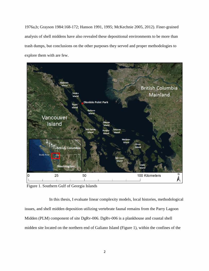
Figure 1. Southern Gulf of Georgia Islands
In this thesis, I evaluate linear complexity models, local histories, methodological
issues, and shell midden deposition utilizing vertebrate faunal remains from the Parry Lagoon
Midden (PLM) component of site DgRv-006. DgRv-006 is a plankhouse and coastal shell
midden site located on the northern end of Galiano Island (Figure 1), within the confines of the
3
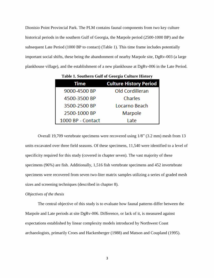
Dionisio Point Provincial Park. The PLM contains faunal components from two key culture
historical periods in the southern Gulf of Georgia, the Marpole period (2500-1000 BP) and the
subsequent Late Period (1000 BP to contact) (Table 1). This time frame includes potentially
important social shifts, these being the abandonment of nearby Marpole site, DgRv-003 (a large
plankhouse village), and the establishment of a new plankhouse at DgRv-006 in the Late Period.
Table 1. Southern Gulf of Georgia Culture History
Overall 19,709 vertebrate specimens were recovered using 1/8” (3.2 mm) mesh from 13
units excavated over three field seasons. Of these specimens, 11,540 were identified to a level of
specificity required for this study (covered in chapter seven). The vast majority of these
specimens (96%) are fish. Additionally, 1,516 fish vertebrate specimens and 452 invertebrate
specimens were recovered from seven two-liter matrix samples utilizing a series of graded mesh
sizes and screening techniques (described in chapter 8).
Objectives of the thesis
The central objective of this study is to evaluate how faunal patterns differ between the
Marpole and Late periods at site DgRv-006. Difference, or lack of it, is measured against
expectations established by linear complexity models introduced by Northwest Coast
archaeologists, primarily Croes and Hackenberger (1988) and Matson and Coupland (1995).
4
According to these models, the Marpole portion of the midden is expected to be dominated by
salmon remains, indicating specialization. In comparison, the Late Period material is expected to
contain a diverse assemblage of fish remains.
Specialization involves a focus on one or a few resources, often with one species
dominating faunal counts (Betts and Friesen 2004:358). Specialization of salmon is indicated by
the abundance of their bones in an assemblage relative to all other fish taxa. However, what
constitutes specialization can vary. For example, Coupland et al. (2010) argue for specialized
assemblages at five sites in Prince Rupert Harbour, all with salmon proportions at (or above)
90% of all fish remains. In comparison, Gulf of Georgia sites interpreted as salmon-specialized
have overall lower proportions of salmon. For example, the Crescent Beach site has component
proportions of 74.2% and 56.8%, which were interpreted as reflecting specialization (Coupland
et al. 2010:202, Matson 1992:408-415). For this study, I set a cut-off point for specialization at
50% of the assemblage. Thus, a taxon over 50% across all quantification techniques will be
considered specialized. This 50% cut-off represents the lower value of what has been accepted as
specialization within the Gulf of Georgia region, which typically ranges between 50% and 80%
of an assemblage.
According to the linear complexity models, Late Period sites are expected to contain a
diverse assemblage of fish remains, rather than a focus on salmon. Diversity consists of two
components, richness (the number of taxa, the more taxa the richer the assemblage) and evenness
(an assemblage is more even when taxa contain similar counts) (Lyman 2008:172-178). A
diversification of resources would be established in this analysis if both the richness and
evenness increase from the Marpole to the Late Period.
5
Given these expectations, in this study I evaluate a null hypothesis of no difference
between the Marpole and Late assemblages at site DgRv-006. If the null hypothesis cannot be
rejected, meaning no difference is evident between the diversity of the Marpole and Late
assemblages, then linear complexity model predictions are not supported. The null hypothesis is
rejected if there are significant differences between the two assemblages in terms of diversity.
Importantly, the linear complexity model predicts that change should be towards increased rather
than decreased diversity. Consequently, any change other than an increase in diversity fails to
support expectations derived from the linear complexity models.
Several implications for the connection between economic and social change can be
drawn whether the null hypothesis is accepted or rejected. At the Dionisio Point locality, a shift
in social organization appears to take place between the Marpole and Late Period, including the
abandonment of the large Marpole village at DgRv-003 around 1300 BP, and the establishment
of a single, large plankhouse at DgRv-006 in the Late Period. Given this apparent shift in
household organization, we should expect some change in the types of economic practices
between these two periods if social and economic changes are linked. Therefore, if no economic
change is observed between the Marpole and Late Period deposits, support for a decoupling of
the social and economic spheres is generated.
Another important implication is that linear models of complexity posit region-wide
changes in economic and social practices. If the DgRv-006 data do not match the linear
complexity models developed based on data from other sites analyzed in the region, then it
stands in contradiction to the posited region-wide pattern. This result would further undermine
such models and support the need for a more historical and local understanding of social change.

6
In recent years, most studies have pointed to more variability in the archaeological record than
can be encompassed by linear complexity models, and this study represents an effort to explore
and recognize that variability (Bilton 2013; Butler and Campbell 2004; Coupland et al. 2010;
Hanson 2008; Moss 2011, 2012).
Due to the nature of zooarchaeological data recovered in midden sites (discussed in
chapter five) the evaluation of the null hypothesis will involve a mostly qualitative, rather than
strictly statistical, assessment of difference between the temporal assemblages.
In addition to this central research objective, several methodological issues are pursued.
First, the development of an appropriate approach to properly quantify faunal remains from the
midden is pursued. The goal is to develop a quantification approach that can address the relative
importance of different taxa within the midden and address larger issues of economic and social
change.
Second, an exploratory data analysis approach using correspondence analysis (CA) is
used to characterize midden depositional patterns. The CA utilizes log (base 10) fish specimen
counts to evaluate how similar or dissimilar faunal patterns are in different depositional areas of
the midden. This offers a methodological technique to address depositional changes over the life
history of a large shell midden.
Third, an understanding of the potential biasing of screen size used in excavation is
needed to test whether significant loss of small fish specimens may have occurred in the larger
excavation sample. In order to address this, matrix sample remains were analyzed using several
different screen sizes and screening techniques, including screens matching the size used in
excavation (1/8”) as well as finer mesh (1/16”). Potential screen size biasing of the temporal

7
assemblages is addressed by comparing excavation level counts corrected for screen size bias
with uncorrected counts.
Conclusions of the thesis
Conclusions from this thesis can be broken into three categories: those that are method-
based, those that relate to site specific history, and those resulting from an evaluation of linear
complexity models. Methods-based conclusions are that increased recovery of fish remains
occurs with both the use of a smaller screen size (1/16”) as well as the use of wet-screening.
However, conclusions also indicate that 1/8” dry-screened material was consistent with those
corrected for screen size bias. Correspondence analysis of fish faunal data is deemed a useful
technique for evaluating intra-midden differences, which helps illuminate changing midden
depositional practices through time. Lastly, the use of multiple different quantification
techniques is deemed necessary for proper quantification of midden contents.
Site-specific results include the identification of overall similarity between the Marpole
and Late Period components and, thus, economic behaviors as well. Fish remains dominate both
assemblages, with herring, salmon, dogfish, and an “other fish” category indicating a diversified
fishing pattern in both periods. This similarity indicates a temporal stability of fishing patterns.
Additionally, other taxa remains indicate continuity in hunting and shellfish gathering practices.
This similarity extends into the local microenvironments utilized and seasonality of occupation
(late-winter/early spring to summer).
On the applicability of linear complexity models for explaining economic and social
change, data from the PLM support rejection of their expectations. This includes an acceptance
of the null hypothesis of no difference between time periods. There was continuity in fishing

8
patterns overtime, with no evidence for salmon specialization. This indicates that we need to
consider social and economic changes separately. While there is evidence for social changes at
DgRv-006, little evidence exists for these being accompanied by subsistence change.
Organization of the thesis
Following this introductory chapter, chapter two offers a more detailed discussion of the
issues and background for this study, with a primary focus on the connection of faunal studies
and complexity on the Northwest Coast, along with some discussion of midden depositional
pressures. Chapter three provides coverage of the general culture history of the Northwest Coast,
with specific focus on the Gulf of Georgia region. Chapter four provides background information
on the specific site under study here, DgRv-006. This chapter includes an exploration of the local
marine transgression record, geology, biology, and a brief history of archaeological studies
within Dionisio Point Provincial Park. Chapter five presents a detailed discussion of excavation
methods used for the collection of this assemblage, as well as quantification methods utilized in
this study. Chapter six contains a stratigraphic breakdown of temporal and depositional midden
categories, and the correspondence analysis of depositional midden categories. Chapter seven
presents the bulk of the analysis of Marpole and Late Period faunal remains, as well as an
exploration of environments utilized, hunting/fishing behaviors, and site seasonality.
Additionally, this chapter includes temporal comparisons and an evaluation of the linear
complexity models. Chapter eight explores potential screen size biasing issues within the midden
assemblage. Chapter nine, the final chapter, offers an in-depth discussion of the three major
conclusions that this study offers.

9
Appendices A through J provide the raw data and identifications utilized in this study.
Appendix K presents the temporal and depositional categorization of individual excavation
levels, and Appendix L contains the raw statistical output of the correspondence analysis (from
the Stata program).
10
CHAPTER TWO
FISH AND COMPLEXITY IN NORTHWEST COAST STUDIES
The Northwest Coast of North America has often been considered a key area for the study of the
development of social complexity and inequality. This is largely due to the ethnographically
observed existence of social hierarchies within a non-agricultural economic system. Beyond the
Northwest Coast (and more recently recognized areas with similar “complex hunter-gatherers”),
this was thought to be atypical, as the control and production of agricultural products was
deemed a necessary prerequisite (or cause) for the deconstruction of egalitarian systems (Ames
and Maschner 1999:13-14).
Although the dismantling of this agricentric model has occurred, the general premise of a
linear progression of social change had remained in studies of Northwest Coast complexity.
Many models covering the development of cultural complexity on the Northwest Coast assume
constantly increasing socioeconomic inequalities, with the ethnographic class system being the
end-point. These models mostly relied on the idea that the control of spatially/temporally
circumscribed, mass-harvested and stored resources (specifically a specialization in anadromous
salmonids) was the key factor in what led to the rise of social classes and substantial wealth
differences within societies (Croes and Hackenberger 1988; Matson 1992; Matson and Coupland
1995; Mitchell 1971; Schalk 1977).
Temporally these models have posited a linear trend, (most systematically described in
Matson and Coupland [1995]), where the “Developed Northwest Coast Cultural Pattern” – a
phenomena which contains ethnographically-noted patterns of ascribed and inherited statuses,

11
class stratification with a large class of elites, large plankhouses, a distinct art style, and stored
winter resources – emerged starting with the Locarno Beach Period (3500-2500 BP). This
pattern, according to Matson and Coupland (1995), was fully expressed in the following Marpole
Period (2500-1000 BP). The Marpole Period is seen as the pinnacle of sociocultural complexity.
Thom (1995) argues that theses elite individuals were organized into a competitive rank-based
system. Ascribed status and the restriction of resources are important in this system, but the
maintenance of social responsibilities to lower ranking individuals (achieved status) determines
the success of individual elite (Thom 1995:3-5).
The following Late Period (also known as the Gulf of Georgia Period) is seen as a
general continuation of this pattern in most aspects (Matson and Coupland 1995:247). However,
an important change in status differences has been argued as emerging in this period, with the
ethnographic pattern of formal social classes emerging, a shift from the argued achieved status in
the Marpole Period. Thom (1995) finds that this shift from a competitive rank-based society to
class stratification occurred due to a restriction of sources of wealth and power through a pattern
of elite marriage ties and extra-local connections. This is reflected in changing mortuary patterns
between the Marpole and Late Periods, with new mortuary symbols establishing the elite’s new
social position (Thom 1995:45). Grier (2003) argues that these extra-local social connections
were already present in the Marpole Period. Angelbeck and Grier (2012) offer a different
hypothesis for how this pattern of elite social class emerged. They argue that increasing
centralization of power was met with active commoner resistance, who utilized the need for their
labor to elevate themselves into the elite class, as a “nouveau riche” (Angelbeck and Grier
2012:563-564).

12
It is within the Locarno Beach/Marpole Periods that key changes emerged that formed
the basis for southern Northwest Coast complexity. However, Northwest Coast archaeologists
differ in explaining how an elite class of individuals would have emerged. Ames (1995) sees
these arguments as falling into two broad categories: “elites as managers” and “elites as thugs.”
The “elites as managers” models see inequalities emerging because certain individuals are
needed to ensure efficient coordination of complex tasks, and these managers work themselves
into positions of authority (Ames 1995:155). The “elites as thugs” view, in comparison, posits
that individuals actively campaigned for control over resources for their own benefit, rather than
a specific societal need (Ames 1995:156; Hayden 1995).
Both Schalk (1977) and Ames (1981) present models of complexity that fall under the
“elites as managers” category (Ames 1995:156). Schalk places importance on the creation of a
storage based salmon economy, arguing that the time and effort it takes to process salmon for
storage, along with the relatively short procurement opportunity, would lead to the rise of a
managerial leader to deal with the complexity of the task. Salmon runs are generally consistent
from year to year. Schalk argues that this reliability lead to a larger population, less mobility,
greater sedentism, and an overall reconstruction of society, where the managers of these
resources get preferential treatment (1977:220-232). Ames’ (1981) model directly follows this
same pattern with institutional leaders (and inequality) emerging because of the need for efficient
management in the procurement and storage of salmon. In an expansion of his ideas, Ames
(1994), added that his view contends that inequality emerged from the “interplay” of
circumscribed resources (temporal and spatial), resource ownership, sedentism, resource
13
specialization (including but not limited to salmon), population growth, and ritual promotion by
individuals (Ames 1994:212-213).
Matson presents an “elites as thugs” model (1983, 1985, 1992) that was evaluated at the
Crescent Beach site, located at the mouth of the Nicomekl River (near the U.S./Canadian
border). The Crescent Beach site contains St. Mungo, Locarno Beach, and Marpole deposits
(Matson 1992:389). Matson’s model hypothesizes that social complexity and inequality emerges
from the control of resource patches that contain differential economic worth (Matson and
Coupland 1995:152). Matson contends that only resources that are reliable, abundant,
predictable, and localized would be beneficial for groups smaller than the community (i.e.,
individuals and families) to attempt to control (Matson 1983:138; Matson 1985; Matson and
Coupland 1995:152). Additionally, this combination of factors would also lead towards
technological innovation to better utilize the controlled resource (Matson 1983:138). Once this
process started, the differences in productivity of the resource patches would lead to inequality
(Matson and Coupland 1995:152). Groups taking less desirable resources and individuals
without a controlled resource patch would be left to join other households, exchanging their
labor for access to the controlled resource (Matson 1985:248; Matson and Coupland 1995:152).
This idea gains some support from the ethnographic work of Suttles (1987c:26-44), who noted
that the Coast Salish environmental region is “neither uniformly rich and dependable within any
tribal area nor precisely the same from area to area” (Suttles 1987c:43).
Matson has argued that shellfish and salmon resources were the initial resource patches
of importance, essentially kick-starting the entire process towards the “Developed Northwest
Coast Pattern” (Matson 1983:136-137; Matson and Coupland 1995:152). Of these two resources,

14
salmon was the resource that was intensified further, because shellfish resources can be
“overcollected and difficult to obtain in dark, stormy winters” (Matson 1983:136). Matson’s
model contains an interconnection between the intensified use of salmon, social ranking, and
sedentary living conditions (Matson 1983:142). He notes that once this pattern has been
achieved, variations that do not contain all three aspects (intensified use of salmon, social
ranking, and sedentary living) would occur (Matson 1983:142). Noting this, Matson makes the
prediction that the Marpole Period in the Gulf of Georgia region, as the first representation of the
complete “Developed Northwest Coast Pattern”, will contain a larger proportion of salmon
remains than subsequent temporal stages (Matson 1983:143). Thom (1995:46-47) more directly
connects this to social changes, noting that in the Late Period, subsistence shifts to include more
broad scale adaptations. He notes that these changes are consistent with what one would expect
from a social shift from ranked to class societies (Thom 1995:46-47).
Croes and Hackenberger (1988) offer an economic explanation for the emergence of the
“Developed Northwest Coast Pattern.” At the core of Croes and Hackenberger’s model is the
idea that economic decision making can be affected by population growth. Shifts in subsistence
economics are driven by two goals: “to attain a secure food and nonfood income” and “to realize
low-cost maintenance of human population aggregations” (Croes and Hackenberger 1988:30).
Important to this idea is the use of an optimal-foraging type explanation for which resources
should be utilized first. To establish population growth and aggregation at a minimum expense, a
resource would be considered important if its yield can be large and spatially sedentary (Croes
and Hackenberger 1988:30). Using computer simulations for both a pre-storage and storage
economy, Croes and Hackenberger develop a model for the Hoko River ecosystem, and test the
15
models assumptions with faunal data from the Hoko River site. With this model and
archaeological evaluation, the authors develop six conclusions with implications for the entire
southern Northwest Coast. First, the authors predict that exponential population growth and
spatial circumscription are important factors affecting subsistence and settlement practices.
Especially important is the advent of a storage economy around 5000-4000 BP which caused an
explosion in population. Second, as populations increase the growth curve would become
logarithmic. Third, as smaller groups expanded and spatial circumscription occurred, population
growth would stabilize in the St. Mungo phase (4000-3000 BP). A storage economy based on
halibut and other flatfish is predicted, with the overuse of shellfish the controlling factor in
population stabilization. Fourth, as human populations continued to slowly grow, shellfish
populations would be shrinking, and thus an emphasis on late spring/fall/winter stored resources
would have to emerge. This is predicted to occur in the Locarno Beach Period with the intense
storage of flatfish. It is here that Croes and Hackenberger see inequality developing, as the
ownership of circumscribed resources would develop (cf. Matson 1985). Fifth, as the storage
economy became more important, a switch to a specialization of salmon would occur. This is
predicted to happen within the Marpole period. Sixth, as populations continued to grow an
intensification of offshore fisheries would occur, explaining the diversification shift seen in the
Late Period by Hanson (1991, 1995) and connected to the social shift argued by Thom (1995)
and Angelbeck and Grier (2012).
Of critical importance to each of the complexity/inequality models presented above is the
development of an economy dominated by salmon specialization. This is hypothesized as
facilitating the development of social inequalities, based on specialization having emerged in the
16
Locarno Beach Period, reaching complete specialization in the Marpole Period, and diversifying
in the Late Period (Croes and Hackenberger 1988; Matson and Coupland 1995; Mitchell 1971).
This focus on the importance of the subsistence economy allows us to evaluate these models
with zooarchaeological data.
Linear Complexity Model Critiques
Critiques of these linear models have focused on how the importance placed on salmon
resources may have prevented researchers from recognizing the importance of other taxa in
Northwest Coast subsistence (Monks 1987). Evaluation of zooarchaelogical data in comparison
to the linear complexity models has mostly taken a broad regional approach (Bilton 2013; Butler
and Campbell 2004; Hanson 2008). The results of these regional studies have generally not
supported a single regional pattern. For example, using abundance and evenness indexes, Butler
and Campbell (2004), find that from 7000 to 150 BP salmon use did increase, but not to the
detriment of other species. Salmon is the most abundant and wide-spread taxa, but does not
increase in importance over time relative to all other fishes, thus contradicting the pattern of
specialization that is predicted by the linear models of complexity. Echoing these results,
Coupland et al. (2010) find that the Gulf of Georgia faunal record contains no evidence for
extreme salmon specialization at any time, including the Marpole Period (Coupland et al.
2010:203-204). They conclude that the development of cultural complexity and inequality
“seems to have occurred without any notable increase in salmon production” (Coupland et al.
2010:205). Bilton (2013) also finds a similar trend regionally. Using principal coordinates
analysis, Bilton evaluated 46 faunal components from the Gulf of Georgia and found no

17
evidence for salmon dominance, instead the data suggest a diversified subsistence pattern (Bilton
2013:298).
This importance of resources other than salmon continues to gain traction in these recent
studies. Additional analyses have also postulated that elements of the “Developed Northwest
Coast Pattern” may have emerged earlier, with the archaeological expressions undiscovered due
to the effects of marine transgression (Fedje and Christianson 1999; Moss 2011:56-72; Punke
and Davis 2006). For example, Cannon and Yang (2006) present evidence for early salmon use
and potentially year-round villages at Namu around 7,000 years ago without evidence for large
population growth and inequality (although Monks and Orchard [2011)] disagree on the
importance of salmon in earlier deposits). The authors also argue that changing fish faunal
patterns at Namu were related to local environmental factors (a collapse in the salmon fishery)
rather than broader social changes along the coast. The potential for different portions of the
“Developed Northwest Coast Pattern” to have arisen earlier suggests that continual evaluation of
data at more local scales is necessary to explain the development of cultural complexity and
inequality on the Northwest Coast.
In the most recent regional volume addressing the Northwest Coast culture area, Moss
(2011), suggests that no regional “master narrative” can be developed. Rather, she suggests that
we look for more localized historical processes (citing Pauketat 2007:185). Moss readily accepts
that some patterns are seen region-wide (population growth, circumscription of territories,
intensification of resource use/storage leading to cooperation and/or competition) but notes that
rather than a step-wise progressive and regional pattern of change, we see different trends
emerging in local areas (Moss 2011:96; also see Moss 2012; Moss and Erlandson 1995).

18
A good example of this can be seen in differences in the hierarchical organization of
houses across the Northwest Coast. Coupland et al. (2009) note a north-to-south cline for the
presence of hierarchical house organization, finding the northern houses to have more strict
hierarchies, whereas the houses of the southern Coast Salish societies (including the Gulf
Islands) appear to maintain less rigid house hierarchies, a notion that is supported by Angelbeck
and Grier (2012). Differences in organization of houses demonstrate the existence of local
historical trajectories on the coast. This has also been demonstrated by Clark’s (2010, 2013)
analysis of the Locarno Beach/Marpole Periods. Clark finds local variation within these time
periods. This variation suggests that local groups “complexity” relies on many different factors,
such as resource availability, the agency of specific individuals, and the innovation of different
technologies. These occur in different areas at different times, and leads to an “uneven” regional
development of complexity (Clark 2010:3). The evaluation of many different forms of
archaeological data (including faunal remains) can help us decipher whether there is a uniform
regional pattern, or more localized historical trajectories. This idea of localized historical
trajectories, as well as an analysis of human actors with agency and agendas, is the direction that
explorations of coastal complexity are currently emphasizing (Grier 2006a, 2014; Moss 2012).
Additionally, we must be open to several different possibilities. If we conclude that
localized historical processes are how complexity should be examined, we still need to evaluate
the unquestionably regional connections that do emerge in the Locarno Beach/Marpole Periods
(Grier 2003). Also, we may need to reevaluate how we view ideas of “complexity” and
“inequality” – undeniably archaeologists (and anthropologists in general) have preferenced
Western viewpoints over aboriginal perspectives on these and other concepts, viewpoints that

19
may not have existed within the indigenous ontological realm (Ewonus 2011b:29; Gosden
1999:185-186). Recent analyses have confirmed the importance and usefulness of an indigenous
knowledge-base archaeologically (Crowell and Howell 2013; Losey 2010; Martindale and
Marsden 2003; Vanpool and Newsome 2012). An in-depth use of this knowledge base will also
prove beneficial for addressing issues of cultural complexity and inequality.
Thesis Analysis
Differing from the regional studies noted above, this study focuses on one site (DgRv-
006). This site contains material with dates spanning the occupation of a Marpole Period
plankhouse village (DgRv-003) as well as the occupation of a Late Period plankhouse (DgRv-
006). This will allow a direct comparison of the two periods without the biases that can emerge
from differing excavation techniques and spatial locations. Given the time periods represented in
this midden, a direct evaluation of faunal changes present during a major sociopolitical change
(abandonment of a village and a later plankhouse occupation) can be reviewed. Although the
evaluation of complexity models is best served by the use of multiple data sets (Clark 2013:3),
this in-depth look at faunal data provides a critical perspective on how subsistence patterns
match or do not match the linear complexity models. Important to note, is that my usage of these
linear models is not because they are the necessarily the most illuminating way to think about
complexity in the Gulf of Georgia (as noted by the studies above), but they present a useful and
explicit frame of reference and a way to set up hypotheses for the faunal material.
Some definitions for the overly broad and often vague conceptual language in use here
are needed before analysis can proceed. First, when the term “social complexity” is used, the
specific focus is on the different social connections made in sedentary villages and if these
20
connections were shaped by resource intensification. The idea of “social complexity” focuses on
the presence of social interactions beyond what is seen in more typical (mobile) foraging
societies. Additionally important to this study are the terms “specialization” and
“diversification.” Specialization indicates an extreme focus on one or two key species, while
diversification involves the use of a wide range of species (Betts and Friesen 2004:358-359).
Diversification is often noted as consisting of two trends in the data: richness (the number of
taxa, the more taxa the richer the assemblage) and evenness (an assemblage is more even when
taxa contain a similar count) (Lyman 2008:172-178).
Also important in this analysis is the correct identification of the depositional context of
this midden, as it is clear middens are not simply trash heaps (Grier et al. 2009; Hayden and
Cannon 1983). The inclusion of both human and dog burials in the midden requires that we not
assume the depositional context to be solely domestic trash. We must consider other possibilities
that account for the non-trash that is included in coastal shell middens. Two ideas may be
relevant for explaining the presence of burials and the highly visible nature of the midden on the
Parry Lagoon shoreline. First is the idea that the midden may have acted as “food for the dead”,
given the presence of both human burials as well as more typical food remains (e.g. Carlson
1999; Cybulski 1992). Secondly, taking cues from landscape-based archaeological approaches
(Ingold 1993), we can also consider how a large shell midden becomes part of the built
environment, projecting a multitude of social messages to groups passing by in canoes. It
becomes a cultural feature that can convey ownership and social identity (Moss 2011:124).
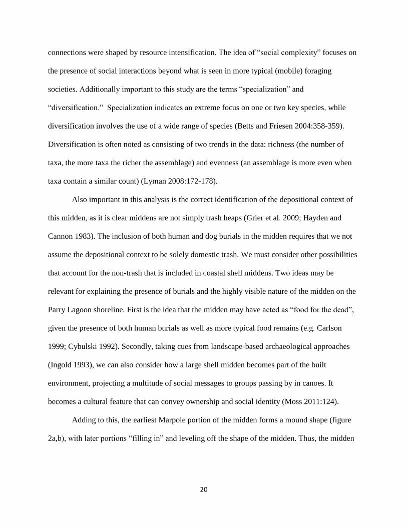
Adding to this, the earliest Marpole portion of the midden forms a mound shape (figure
2a,b), with later portions “filling in” and leveling off the shape of the midden. Thus, the midden
21
may have served different depositional purposes through time. Potentially interesting is the
prospect that this midden started out as a special mortuary feature for the earlier village (DgRv-
003), with its purpose shifting after the abandonment of that village. Faunal remains can be used
to investigate these types of relationships by noting if faunal deposition changes when
stratigraphic aspects of the midden change. Final conclusions on what these different
depositional areas represent will not be reached here. A complete identification of these areas
would need additional coverage of other aspects of the midden (most importantly the burials),
which are outside the scope of this study.
Before these analyses can be presented, additional background information is necessary
to give appropriate context to this study. This contextual information will be addressed in the
following two chapters with specific culture history of the southern Northwest Coast in the
following chapter, and site/island information in chapter four.
Figure 2a. Parry Lagoon Midden with temporal distinction – 2012 excavations.
Red line separates the Marpole from the Late Period. Earliest Marpole portion is
below the blue line

22
Figure 2b. Parry Lagoon Midden with temporal distinction – 2013 excavations.

23
CHAPTER THREE:
CULTURE HISTORY OF THE GULF OF GEORGIA REGION
The Gulf of Georgia is the most intensely studied region within the larger Northwest Coast
culture area, and because of this, a detailed historical framework has been developed. Several
different sequences have been advanced over the years to organize these data, including the
broad syntheses presented in volumes by Matson and Coupland (1995) and Ames and Maschner
(1999). Matson and Coupland’s framework largely focuses on the Gulf of Georgia region and
thus it is the framework that will be used (Table 1). Culture history coverage will begin with the
Old Cordilleran and extend to the ethnographic record. It should be noted that current research
suggests that an even earlier habitation than the Old Cordilleran may be found on the coast, but
this issue is not addressed here (Erlandson et al 2007; Jenkins et al 2012; Punke and Davis 2006).
Old Cordilleran (9000-4500BP)
The earliest well-defined Northwest Coast archaeological culture is the Old Cordilleran,
dated from 9000-4500 BP (Matson and Coupland 1995). This unit was originally developed in
the Gulf of Georgia area by information obtained from the Glenrose Cannery site (DgRr-006),
located in the Delta of the Fraser River (Matson 1976; Matson and Coupland 1995: 69).
Additional sites from outside of the Gulf of Georgia region including, Namu, Bear Cove,
Milliken, Five Miles Rapids, and Tahkenitch Landing, were also considered in the development
of this cultural component. The Saltery Bay site (DkSb-30) represents another well-excavated
site (Bilton 2013:75).
24
The Old Cordilleran was characterized by Matson and Coupland as a terrestrial mammal
subsistence system, with use of some “smaller resources,” including shellfish and a variety of
fish (1995:81). They note that this is a widespread coastal adaptation, which may represent an
early seasonal round (Matson and Coupland 1995:81). Glenrose Cannery offers a good example
of this, as both mammalian resources (wapiti, deer, beaver, and harbor seal) as well as fish
remains (salmon, flatfish, eulachon, stickleback, and peamouth) were deemed important
resources (Matson and Coupland 1995:73-74). Artifacts include leaf-shaped bifaces, cobble and
flake tools, and antler wedges (Ames and Maschner 1999:72). At the time of Matson and
Coupland’s writings, there were no large site components like those seen in the later cultural
components and nothing to suggest a group larger than the family (Matson and Coupland
1995:96).
Matson and Coupland considered there to be no evidence for sedentism or social
inequalities at this time (Matson and Coupland 1995:81). This is now being debated with the
work done at the Namu site in central British Columbia, where researchers argue for the
existence of a large salmon fishery (Cannon and Yang 2006; Moss 2011:78). Cannon and Yang
have also argued for the presence of a large sedentary village at this time, although this argument
has proven more controversial (Cannon and Yang 2006, 2011; Monks and Orchard 2011). Other
fish-heavy faunal assemblages have been noted at the Cohoe Creek site on Haida Gwaii, Bear
Cove on Vancouver Island, and Tahkenitch Landing on the Oregon Coast (Moss 2011:79-82).
Charles (4500-3500BP)
Next in the sequence is the Charles Period, which has been dated from 4500-3500 BP.
The Charles Period is composed of two sub-periods, St. Mungo and Mayne, which overlap in

25
time (Matson and Coupland 1995:98). The St. Mungo Period has been described from three sites
located on the Fraser River: St. Mungo, Glenrose Cannery, and Crescent Beach (Matson and
Coupland 1995:98). Important artifact changes include the increase of bone and ground stone
tools, which are seen as important components of the Developed Northwest Coast pattern.
Carved antler and anthropomorphic/zoomorphic figures have also been found in this time period
(Bilton 2013:83; Matson and Coupland 1995:107). The use of shellfish and fish becomes a more
important component of the diet, although shellfish type and abundance varies by location (Moss
2011:85). The increase in shellfish and fish lead Matson and Coupland to consider this a
subsistence pattern focused on a diverse coastal/riverine forager adaptation (1995:109, 114).
Additionally, the increased presence of milling stones shows a larger importance of plant
resources (Ames and Maschner 1999:138-139).
The Mayne Period has direct temporal overlap with the St. Mungo Period, but occurs in
different areas. Mayne Period sites are exclusively located on the Gulf Islands, causing some to
distinguish this as a purely island adaptation (Bilton 2013:80, 243-244). Overall there is a
general similarity between the St. Mungo and Mayne Periods, with most distinctions being made
in the presence of labrets (stone lip plugs often associated as status markers) in Mayne
components. Overall, Matson and Coupland see this time period as a period of local groups
“settling in” to the resource bases (1995:142). Perhaps because of this, we see a generally broad
subsistence economy at this time (Ames and Maschner 1999:138). The “Developed Northwest
Coast Pattern” is not seen in these phases, as there is no evidence for large houses or ascribed
status differences (Matson and Coupland 1995:143). However, this is not a universally accepted
26
notion. Looking at the Pender Canal site (DeRt-1 and DeRt-2), Carlson and Hobler (1993) argue
that the full “Developed Northwest Coast Pattern” can be seen in this earlier time period.
Locarno Beach (3500-2500BP)
The Locarno Beach Period witnesses the “development of cultural complexity” and the
start of the most important economic aspects of the “Developed Northwest Coast Pattern” are
attributed to this period (Matson and Coupland 1995:145-146).
The type site of Locarno Beach, dated from 3500 to 2500 BP, is located in present day
Vancouver (Matson and Coupland 1995:154). Most of the Locarno Beach artifact components
are based on Mitchell’s early 1970s report on Montague Harbour (Matson and Coupland
1995:156). Common artifacts include unilaterally barbed points, ground slate tools, bird-bone
needles, labrets, celts, stemmed chipped points, microliths and functionally questionable ground
stone known as the “Gulf Island Complex” (Matson and Coupland 1995:156; Moss 2011:98).
Additionally high proportions of both ground stone and faunal tools are found in Locarno Beach
assemblages (Moss 2011:88). Ames and Maschner find that the presence of microblade cores
and blades, toggling harpoons, and ground-stone tools are what set the Locarno Beach Period
apart (1999:104). Locarno Beach sites are also known for clay depressions, rock slab features,
and the presence of exclusively midden burials (Moss 2011:98).
Faunal patterns indicate an increased importance of fish remains, particularly salmon,
flatfish, and herring, moving away from the “broad-scale” pattern noted in the previous time
periods (Matson and Coupland 1995:177). Of note is an increase in the amount of salmon
vertebral remains, in comparison to cranial elements. This matches an ethnographic pattern for
the removal of salmon heads as preparation for storage of trunk elements, and has been used by
27
researchers to infer salmon storage (Boehm 1973; Butler and Chatters 1994:413; Matson and
Coupland 1995:166-167). Butler and Chatters (1994) evaluate if this pattern is related to
differences in bone densities between elements, rather than being a cultural phenomenon. They
found that salmon cranial elements are less dense and degrade faster than vertebral elements,
arguing that this must be taken into account before storage is inferred from proportions of cranial
versus vertebral elements. Thus, although there is a noted increase in salmon cranial elements in
the Locarno Beach Period, this does not necessarily mean widespread storage emerged.
It is within the Locarno Beach phase that many aspects of the “Developed Northwest
Coast Pattern” start to emerge including: bone, antler, and ground stone tools, woodworking,
multifamily houses, labrets, and a fish storage economy argued to be driving increasing
complexity (Matson and Coupland 1995:197-198). Missing from the Locarno Beach Period are
the important social changes, including a shift to large villages and ascribed status differences
(Matson and Coupland 1995:198).
Marpole (2500-1000BP)
The Marpole Period (2500-1000 BP) is when the “Developed Northwest Coast Pattern” is
fully realized according to Matson and Coupland (1995:199). The Marpole Period is considered
to be the most complex period in the Gulf of Georgia area, where large multi-family plankhouse
villages, subsistence based on stored salmon, and institutionalized status and inequality were
widely expressed as a complex (Matson and Coupland 1995:255).
The Marpole Period was initially recognized by Borden in the 1950s from his work at the
Point Grey site, as well as observations on materials from the Great Eburne Midden, now known
as the Marpole type site (Matson and Coupland 1995:200-201). This initial categorization was

28
soon strengthened by work from Mitchell (1971) and Burley (Matson and Coupland 1995:201).
The entire ethnographically observed pattern of complex cultural behavior is seen within this
period.
Burial analyses indicate that ascribed social statuses were present, inferred from large
amounts of ethnographically noted wealth and status items interred with juveniles in cairn burials
(Matson and Coupland 1995:209-210). Among these burial analyses is Burley’s (1989) work at
the midden component of the False Narrows site on Gabriola Island. This midden contained a
population of at least 86 individuals from 50 internments (Burley 1989:51). Both males and
females are present, as well as adults and juveniles (Burley 1989:51). Of the 86 individuals
identified only 19 had any grave goods associated with them (Burley 1989:59). Individuals with
grave goods differed in the amount and types of grave goods present (Burley 1989:60). From
this, Burley inferred a stratified social order of haves and have-nots. Below ground burials with
status differentiation are present throughout the Marpole Period (Thom 1995).
Matson and Coupland claim that common artifact types remain unchanged from the
Locarno Beach Period, Moss however notes that leaf-shaped and triangular shaped slate points,
nipple topped mauls, and stone and shell beads are diagnostic artifacts for this period (Moss
2011:98). Labrets disappear from the record around 2000 years ago (Moss 2011:103). A
continued shift away from chipped stone and towards ground stone and bone/antler technologies
is also observed (Matson and Coupand 1995:218). Chipped stone was never completely replaced,
which has lead Moss to the conclusion of cultural continuity with cumulative cultural
innovations being seen in the use of ground stone and faunal tools (2011:89). Types of personal
29
status items increased, including shell beads and stone bowl sculptures (Ames and Maschner
1999:104; Bilton 2013:86).
Large village sites are also seen, from the presence of house platforms (seen at the Beach
Grove, Whalen Farm, False Narrows and Dionisio Point sites), as well as inferred evidence of
storage from large amounts of salmon vertebral elements (e.g., Glenrose Cannery) (Burley 1989;
Grier 2001; Matson and Coupland 1995:223). Subsistence data also indicate the “Developed
Northwest Coast Pattern” dependence on salmon storage emerged, corresponding with increases
in inequality and cultural nodes of complexity. It is important to note that when Matson and
Coupland’s model was generated subsistence data was “rather limited” (1995:222). Marpole
subsistence information that Matson and Coupland utilized comes mainly from five sites:
Glenrose Cannery, Crescent Beach, Beach Grove, Deep Bay, and Point Grey. Of these sites,
three (Glenrose Cannery, Crecent Beach, and Beach Grove) are noted for the abundance of
salmon vertebral remains, Glenrose Cannery being interpreted as a winter village subsisting on
stored salmon (Matson and Coupland 1995:223). From these sites, Matson and Coupland infer a
pattern of large winter base camps occupied until spring, subsisting on a specialized storage of
salmon. Other sites (Deep Bay, Point Grey) represent limited activity sites that were utilized at
different parts of the year, as part of a seasonal round. This pattern of salmon importance has had
some recent support by Clark (2010, 2013), but other researchers are questioning this notion, as
noted above (e.g., Bilton 2013; Butler and Cambell 2004; Coupland et al. 2010).
Clark (2010, 2013) has presented a different notion of what the Locarno Beach and
Marpole Periods represent. Rather than finding Locarno “evolving” into Marpole, Clark argues
that these cultural periods are not simply temporal differences but represent two different culture
30
types that were spatially separated. Clark argues that the Locarno culture was present in the
southern Gulf Islands and southern Vancouver Island at the same time that the Marpole culture
was present in the Fraser River valley and northern Gulf Islands. Through time, connections
developed and both cultures emerged in the Late Period, as one distinct culture type.
Late Period (1000 BP-Contact)
The Late Period is the most recent cultural period prior to the historic period, and is
generally seen as a continuation from the Marpole Period. The Late Period is often considered as
the archaeological representation of the ethnographic record, with many interpretations using the
record to explain phenomena in the Late Period, largely ignoring the changes that would emerge
with European intrusion (Codere 1950; Moss and Erlandson 1995:29, 34). Artifact patterns in the
Gulf of Georgia region are considered to have “evolve[ed] in a seamless manner from the
Marpole phase” (Matson and Coupland 1995:268). Bone, antler, and ground stone tools
dominate assemblages (Matson and Coupland 1995:268). Composite toggling harpoons, flat top
mauls, and bone bipoints are common, but a general reduction in the diversity of tools is noted
(Ames and Maschner 1999:106-107; Matson and Coupland 1995:268). Additionally,
anthropomorphic stone bowls disappear from the record (Ames and Maschner 1999:107).
A shift to an elite dominated (numerically) social class system is present within this time
period (Angelbeck and Grier 2012). A change from below ground burial practices to above
ground burials has been argued as representing this shift (Thom 1995). Thom states that this shift
in mortuary symbols represents elite leaders changing the symbol utilized to represent higher
status (1995:43). Above-ground burials typically involved the need for elaborate boxes and/or
poles, which would restrict these burials to those that could hire skilled artisans, restricting the

31
expression of class status to those with the proper wealth and connections (Thom 1995:43-44).
Angelbeck and Grier (2012) offer a different explanation for this large elite class emergence,
arguing that it emerged due to commoner resistance to outright rule. They argue that this can be
seen in the increase in the proportion of individuals with cranial deformation, a marker of high
status at birth, but one that could be adopted by individuals to express autonomy (Angelbeck and
Grier 2012:557-564). The proportions of cranial deformation are low in the Marpole Period
(which would be expected for a marker of high status when that status is rare), but are in a
majority of the population in the Late Period (Angelbeck and Grier 2012:559).
Matson and Coupland present few thoughts on the subsistence of this time period,
mostly noting its similarity to the ethnographic record. This includes a north to south trend of
environmental differences which affects the resources utilized (also well noted in Schalk 1981).
Also noted are differences between inner sandy coasts and outer rocky coast resource use, and
that sites near large rivers tend to be dominated by salmon remains (Matson and Coupland
1995:295-296). Late Period faunal analyses have noted a diversity of fishing resources, a notion
supported by Croes and Hackenberger’s (1988) model (Matson and Coupland 1995:296). This
broadening of the resource base is a result of an increased focus on offshore resources (Croes and
Hackenberger 1988:78-79). Additional support for this subsistence change can be seen in the
work of Hanson (1991, 1995). Hanson looked at several Late Period sites in the southern Gulf of
Georgia and found that a diversity of fish species were more important than the ethnographic
record indicated. Although salmon was important to the diet, fish species like cods, sculpins,
herring, and perches proved to be more important than the ethnographic record indicated. Given
these results, the question should be if this pattern in the subsistence of the Late Period actually

32
represents a shift in subsistence strategy, or if it is the pattern that had persisted before, and was
missed due to excavation methodology (Hanson 1991, 1995). This would then have an important
effect on how models of complexity and inequality are developed and evaluated.
Ethnographic Record
The ethnographic record has had an important impact on interpretations of Northwest
Coast prehistory, largely because of the vast amount of ethnographic data available on coastal
peoples. This record has greatly influenced archaeological interpretations, as evidenced by the
existence of the “Developed Northwest Coast Pattern” concept. An uncritical connection of the
archaeological record and the ethnographic record is often provided, with interpretations only
being accepted when they agree with the ethnographic record (Grier 2007). This has hindered
interpretations of the past, as only what was observed in the ethnographic present has been
considered viable. This can be problematic when we consider that the ethnographic record is not
perfect and the indigenous people observed were already greatly influenced by Europeans
(Codere 1950; Drucker and Heizal 1967). With this said, the ethnographic record does offer us a
great source for hypotheses against which to test the archaeological record against (Grier 2007).
Because of this notion, a brief review of the ethnographic record is needed. Ethnographic
information on the Coast Salish of the southern Gulf of Georgia is presented below, broken into
three important categories: social organization, settlement, and subsistence.
Social Organization
Coast Salish social organization is noted for its flexibility (Suttles 1987a:16-17). Coast
Salish groupings consisted of families living in plankhouses (typically made of cedar), with at
least one individual claiming right to resources (Suttles 1987a:16-17). This plank-household
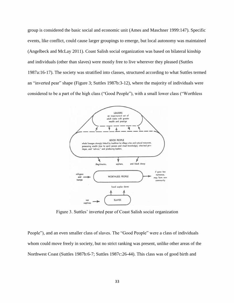
33
group is considered the basic social and economic unit (Ames and Maschner 1999:147). Specific
events, like conflict, could cause larger groupings to emerge, but local autonomy was maintained
(Angelbeck and McLay 2011). Coast Salish social organization was based on bilateral kinship
and individuals (other than slaves) were mostly free to live wherever they pleased (Suttles
1987a:16-17). The society was stratified into classes, structured according to what Suttles termed
an “inverted pear” shape (Figure 3; Suttles 1987b:3-12), where the majority of individuals were
considered to be a part of the high class (“Good People”), with a small lower class (“Worthless
Figure 3. Suttles’ inverted pear of Coast Salish social organization
People”), and an even smaller class of slaves. The “Good People” were a class of individuals
whom could move freely in society, but no strict ranking was present, unlike other areas of the
Northwest Coast (Suttles 1987b:6-7; Suttles 1987c:26-44). This class was of good birth and
34
could obtain wealth, something the others could not (Suttles 1987b:3-14). Leaders were drawn
from this class as they had the potential to own important resources. This included both material
resources, such as houses and subsistence locations, as well as cultural resources, like ritual
knowledge (Suttles 1987b:8). These leaders did not have oppressive or coercive power
(excluding over slaves), and their power base revolved around their influence and importance in
gaining access to resources and their reputation in the prestige economy (Ames 1995). An
example of this can be seen in the way that owned resources were managed. Although resources
were owned, use of these resources was not restricted (Suttles 1987a:21).
Social prestige systems were considered to be integrated with the subsistence economy,
and it is hypothesized that this integration allowed populations to adapt to variable
environmental conditions present in the Gulf of Georgia region. Variability took four different
forms: variety of foods, local variability, seasonal variability, and year-to-year fluctuations in
productivity (Suttles 1987a,c). Food was not directly considered wealth, but it could be
exchanged for status items, which could be given away to increase prestige of both the individual
and the household. Suttles identified two forms of exchange related to the upper classes of Coast
Salish society, which he hypothesized, allowed them to live in an environment defined by
variability. The first exchange network involved connections between upper class families. This
involves the exchange of food for different forms of wealth, which could happen when one
family’s controlled resource patch failed. This exchange network had an important impact on the
socioeconomic reality of the region, ensuring that the rich maintain prestige by allowing
individuals to directly turn food into wealth, something the other classes could not do (Suttles
1987a: 17-20). The second system of exchange was the potlatch. The potlatch offered a way for

35
individuals, whom obtain a surplus of wealth, to give it away in a large gathering to obtain status
and prestige. At the same time, this giving away of wealth allows other groups to “restore their
purchasing power,” thus enabling the entire system to continue (Suttles 1987a: 23-24).
Settlement
The Coast Salish settlement pattern consisted of seasonal movements with an aggregation
of multiple families into large plankhouse villages during the winter and early spring months
(Matson and Coupland 1995:2-8). These more permanent winter dwellings were of the “shed
roof” type in the Gulf Islands, in comparison to the “gable roof” structures present in other areas
of the coast (Barnett 1955:35-58; Suttles 1974:256).
Shed roof plankhouses consisted of a framework of large posts with removable cedar
planks covering the sides and roof of the structure (Suttles 1974:256). Planks were removed
when the structure was not in use, the larger posts being left at site. Plankhouses were large, up
to 200 feet or longer, and could be partitioned into separate sections. Sectioning of the house in
this way created several households within one structure (Suttles 1974:260). Winter houses also
acted as both workshops and storage centers. Fall-caught fish were smoked in the house with
storage boxes placed under sleeping platforms (Suttles 1974:256-260). Interesting inferences on
how houses reflect social structure have been made archaeologically (see Grier 2006b and
Coupland et al 2009).
Subsistence
Coast Salish populations consisted of individuals who hunted, gathered, and fished. Many
food gathering activities were also communal. Drawing from Suttles’ (1974) and Barnett’s
(1955) work, we can reconstruct some of the ways that Coast Salish individuals obtained these
36
different foods. Plant foods were also extremely important to Coast Salish individuals, but given
the scope of this study, will not be reviewed here.
Shellfish were typically obtained by hand or with a digging stick (Suttles 1974:57). This
was done at low tide throughout the year, but was at its greatest in the summer (Suttles 1974:65-
69). Shellfish were steamed in an earth oven, roasted, or eaten raw (Suttles 1974:65-69; Barnett
1955:60-61). Urchins were also collected with the gonads eaten both raw and cooked (Suttles
1974:66).
Deer and wapiti (elk) were the primary terrestrial animals hunted. Deer bucks were
predominantly taken in late spring/early summer as bucks were fattest at this time (Suttles
1974:82-92). Ungulate hunting techniques varied, but typically involved bow and arrow
technology, although nets and pit falls were also utilized (Suttles 1974:138-147). Hunting
occurred alone or in pairs, sometimes dogs were utilized, and some hunting also occurred at
night in canoes (Suttles 1974:82-92). Meat was typically steamed for storage and dried bones
were often cracked for marrow. The lower leg bones (metapodial) of deer were commonly used
as tool making material for arrow and duck spear points (Suttles 1974:91). Land mammals could
be roasted, steamed, or boiled (Barnett 1955: 63). Hunting of birds also occurred with techniques
ranging from raised nets over migratory paths, submerged nets, slings, snares, and bow and
arrow hunting (Suttles 1974:70-81).
Sea mammals were also hunted by the Coast Salish, with Porlier Pass being well-known
as a productive area (Suttles 1987d:233-247). Seals and sea lions were hunted by canoe with
harpoons and nets, while beached individuals could be clubbed (Suttles 1974:162-166). Sea
mammals were an important source of oil (Barnett 1955:61).
37
Fishing techniques could vary by fish type and location; ethnographic information on
fishing techniques is presented in Table 2. Techniques include: harpooning of larger fish, use of
spears, hook and line, clubbing, and nets. Suttles (1974) offers a very detailed explanation of the
large reef-net salmon fisheries seen in the Straits area, which consisted of multiple canoes
working in tandem to catch large amounts of salmon before they reached the Fraser River.
Additionally, the use of weirs made of both wood and stones were common to corral fish both in
marine environments and riverine settings. Fish were often dried or smoked with salmon being
the primary species preserved for winter subsistence, although this may be the result of European
intrusion and not representative in deep time. The act of fishing was considered a sacred activity
and men often sought supernatural help and guidance for success (Barnett 1955:77). Other
ceremonial duties were often observed before fishing could commence, the most famous being
the “first salmon rite” (Barnett 1955).
Ethnographic descriptions present a diversity of different activities and resources as being
important to the Coast Salish subsistence pattern. This stands in direct contrast to the extreme
focus on salmon seen in many scholarly treatments of Coast Salish subsistence.
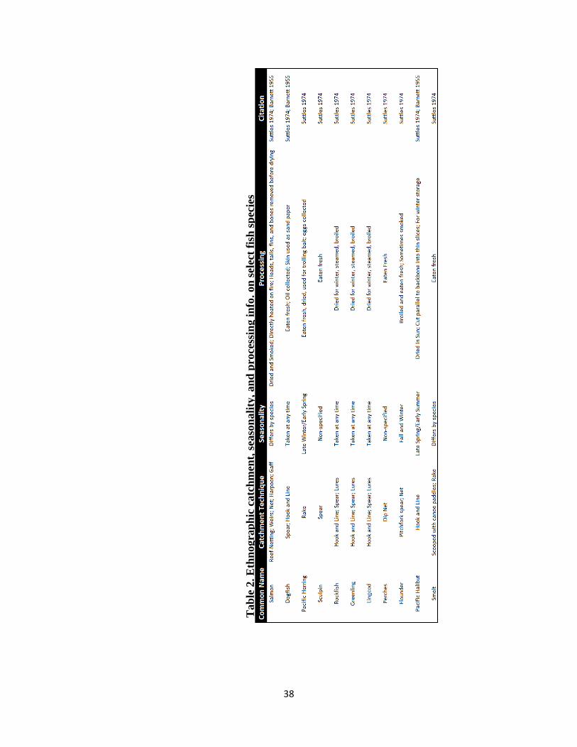
38
Tab
le 2
. E
thn
ogra
ph
ic c
atc
hm
ent,
sea
son
ali
ty, an
d p
roce
ssin
g i
nfo
. on
sel
ect
fish
sp
ecie
s
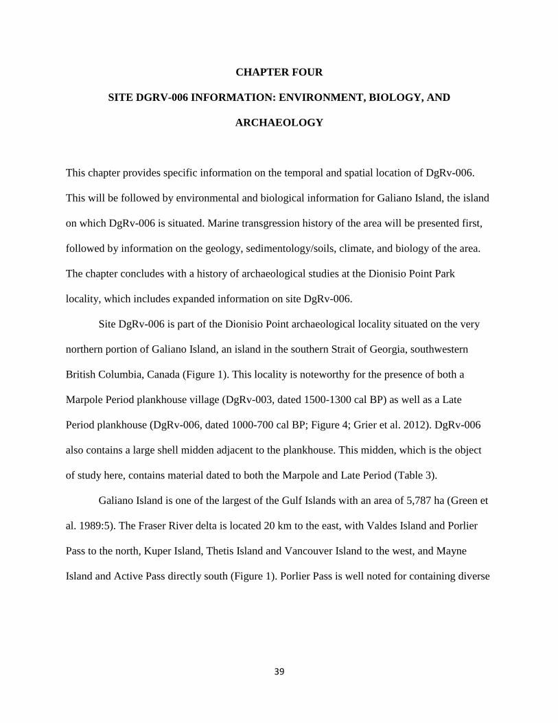
39
CHAPTER FOUR
SITE DGRV-006 INFORMATION: ENVIRONMENT, BIOLOGY, AND
ARCHAEOLOGY
This chapter provides specific information on the temporal and spatial location of DgRv-006.
This will be followed by environmental and biological information for Galiano Island, the island
on which DgRv-006 is situated. Marine transgression history of the area will be presented first,
followed by information on the geology, sedimentology/soils, climate, and biology of the area.
The chapter concludes with a history of archaeological studies at the Dionisio Point Park
locality, which includes expanded information on site DgRv-006.
Site DgRv-006 is part of the Dionisio Point archaeological locality situated on the very
northern portion of Galiano Island, an island in the southern Strait of Georgia, southwestern
British Columbia, Canada (Figure 1). This locality is noteworthy for the presence of both a
Marpole Period plankhouse village (DgRv-003, dated 1500-1300 cal BP) as well as a Late
Period plankhouse (DgRv-006, dated 1000-700 cal BP; Figure 4; Grier et al. 2012). DgRv-006
also contains a large shell midden adjacent to the plankhouse. This midden, which is the object
of study here, contains material dated to both the Marpole and Late Period (Table 3).
Galiano Island is one of the largest of the Gulf Islands with an area of 5,787 ha (Green et
al. 1989:5). The Fraser River delta is located 20 km to the east, with Valdes Island and Porlier
Pass to the north, Kuper Island, Thetis Island and Vancouver Island to the west, and Mayne
Island and Active Pass directly south (Figure 1). Porlier Pass is well noted for containing diverse

40
marine environments, while also being an important travel corridor (Matson et al. 1999:12-13;
Suttles 1987d).
Figure 4. Dionisio Point archaeological locality. Parry Lagoon
Midden indicated in red. Modified from Grier 2014.
Table 3. AMS dates from Parry Lagoon Midden
All samples processed by University of Arizona AMS Laboratory, *Direct AMS, or **Curt-Engelhorn-Centre for
Archaeometry, Manneim, Germany aConv Age is the lab-reported radiocarbon conventional age before application of marine correction
bAll calibrations complete with Calib 7.0 Terrestrial material calibrated with intcall3.14c. Marine shell calibrated
with Marine 04 (global correction) using Delta R (local correction) of 400 ± 40 years, derived from Queen’s
University Belfast 14Chrono marine database cCalibrated median calendar ages rounded to the nearest decade
41
The Gulf of Georgia region is delineated as a distinct area both culturally and
environmentally (Mitchell 1971). This region consists of the northern half of the Georgia
Depression, which includes the Strait of Georgia and the Puget Sound (Clark 2013:5; Mitchell
1971:2). The region is bordered by the Insular Mountains of Vancouver Island to the West, the
Cascade and Coast Range mountains to the East, the Olympic Mountains/Puget Sound to the
South, and the Johnstone Strait in the North (Clark 2013:5; Mitchell 1971:2-5). The Strait of
Juan de Fuca provides access to the Pacific Ocean in the southern Strait of Georgia, while
Johnstone Strait provides access from the north. The coastline includes many bays and inlets in
comparison to the straight beaches of Oregon and Washington (Ames and Maschner 1999:16-17;
Clark 2013:6).
This coastline pattern is seen in microcosm at the Dionisio Point locality, where a lagoon,
coastal spit, and several bays are located within a few km of the sites (Figure 4). Tidal patterns in
the southern Gulf of Georgia are driven by oscillating movements of water between the inner
Strait waters and the Strait of Juan de Fuca/Pacific Ocean. When tides are low in the Gulf of
Georgia, they are high at the Strait of Juan de Fuca and vice-versa (Mitchell 1971:4-5 citing the
Canadian Hydrographic Service 1966:1).
Marine Transgression
The Northwest Coast culture area is well-noted for having a complex marine
transgression history (Aikens et al. 2011:217-219; Punke and Davis 2006). Three factors play
into post-glacial Northwest Coast sea level change: eustatic, isostatic, and geotectonism (Clauge
et al 1982:598; Fedje and Christiansan 1999:637; Fladmark 1975:144). These factors interact in

42
their influence on marine transgression in the Gulf of Georgia and are important for evaluating
how sea level change can impact coastal shell middens.
Recent research on sea level rise is presented by Fedje et al. (2009) and elaborated in a
locally-relevant context by Grier et al. (2009). Both these studies specifically look at sea level
changes within the past 5,000 years in the Gulf Islands area. Utilizing shovel test pits and auger
samples to find past shorelines (with datable material) in present-day intertidal zones, both
studies indicate a sea level rise of only 1.5-2.0 m since the middle Holocene (Fedje et al.
2009:243; Grier et al. 2009:272).
Geology and Soils of Galiano Island
Galiano Island’s underlying geology consists of the Naniamo Formation, which dates to
the Cretaceous period (90-65 mya) (Johnstone 2006). The Naniamo Formation consists of
sedimentary deposits of sandstone, siltstone, and mudstone. These deposits are marine based in
origin (Johnstone 2006:67). Glacial till deposited by receding glaciers is also present on many
southern Gulf Islands (Green et al. 1989:22). Most soils on the southern Gulf Islands are
moderate to well drained, although some poorly drained silts and clays do lead to the formation
of lakes and bogs (Green et al. 1989:20).
Climate/Biology
Galiano Island is located within the rain-shadow of the mountains of Vancouver Island.
This leads to warm, dry summers and mild, wet winters in comparison to mainland British
Columbia and Vancouver Island, both of which are subjected to wetter conditions (Meidinger
and Pojar 1991:82). Annual temperatures range from 9.2 to 10.5oC, with annual precipitation
ranging from 647 to 1,263 mm (Meidinger and Pojar 1991:82). Because of these conditions,
43
Galiano Island contains the ecosystem designation of “Coastal Douglas-fir zone” (Meidinger and
Pojar 1991:81). Most important for this designation are the types of large trees that grow in the
area: Douglas-fir, Western Redcedar, Grand fir, and Arbutus (Meidinger and Pojar 1991:82). A
multitude of different species of fish and shellfish are present given the diversity of marine
microenvironments present on the island. Tables 4 and 5 present information on important fish
and shellfish species that are present in the midden.
Archaeology of the Dionisio Point Locality
The earliest excavations within the Dionisio Point archaeological locality were
undertaken by Mitchell (1971) at site DgRv-003. DgRv-003 consists of five large house
depressions located between sandstone bedrock bluffs, with a gravel beach-lined bay directly to
the north. Large-scale excavation was undertaken at site DgRv-006 by Colin Grier in 1997 and
1998, and these mark the most extensive excavations within the Dionisio Point locality to date
(Grier 2001, 2003). In 1997, Grier tested two house depressions (House 2 and House 5), while in
1998 about 40% of one house (House 2) was excavated (Grier 2001). Radiocarbon dates place
this house within the Marpole period (House 2: 1500-1300 cal BP). Grier described the five
houses at DgRv-003 as a winter village, based on the substantial architectural remains and
overall plan of the village (Grier 2001, 2006c). An additional layer representing Late Period
shellfish (mostly urchin) resource acquisition overlies the Marpole deposits. Grier’s excavations
tested the hypothesis that House 2 was internally separated into different socioeconomic
groupings, effectively showing that social differntiation was evident within large plankhouses of
this age (Grier 2001, 2006a, 2006c). Data from this site has been used to argue for household
transmission (Grier 2006c) and regional interactions (Grier 2006a). Dolan (2009) conducted

44
Tab
le 4
. F
ish
bio
logy i
nfo
rmati
on
on
sp
ecie
s p
res
ent
in t
he
Parr
y L
ag
oon
Mid
den

45
Table 5. Shellfish biology information on species present in the Parry Lagoon Midden
* All information from Ricketts et al. 1968
a geoarchaeological evaluation of sediments collected from Houses 2 and 5 in his MA thesis.
Additional research at the site was undertaken by Grier in 2002 as part of a UBC field school and
further unpublished excavations have occurred since 2008.
Zooarchaeological work completed since these initial analyses has called the seasonality
of the site into question. Ewonus (2011a,b), identifying 15,968 vertebrate remains from House 2,
concluded that due to a strong dominance of herring bone counts and an overall richness of taxa
present, that the site should be considered an aggregate village focused on seasonal herring
fishing. Additionally, aDNA was successfully obtained by Ewonus and colleagues (2011) which
indicated the presence of ten sockeye salmon and one pink salmon in a sample of the salmon
assemblage. Ewonus et al. (2011) argued that these salmon represent locally caught migrating
salmon that were available at Dionisio Point during summer. In response, Grier reiterated his
original interpretation, noting that the use of bone counts can be misleading when considering
mass caught fish with variable weights, such as herring and salmon. Alternatively, Grier and
Lukowski (2012) argue that salmon represents a larger proportion of the diet when considering
the actual meat that each fish represents. Ewonus (2012) in turn re-asserted his interpretation,
noting issues with the use of meat weight based analyses. Grier and colleagues (2013) further
support their stance by obtaining aDNA from a larger sample of salmon at the site (72 successful

46
extractions) finding a more diverse sample of salmon species, predominantly fall and winter
spawning salmon. They conclude that this diversity of salmon species supports a winter
occupation. Regional connections are inferred, as the diversity of salmon species is most likely
not obtainable locally (Grier 2003; Grier et al. 2013:10).
More important to the current study is site DgRv-006, a plankhouse and midden site
located to the east of DgRv-003 and directly west of Parry Lagoon (Figure 4). DgRv-006 was
first recorded as a shell midden in 1963 by provincial archaeologists Donald Abbott and John
Sendey (Grier and McLay 2007:14-15). In 1974, the site was mapped for the first time and
estimated to be 200 m by 30 m with a depth of 0.5 m (Grier and McLay 2007:15). In the late-
1980s, several instances of human burial recovery occurred. In 1987, a minimum of 11
individuals were recovered, one burial was excavated consisting of a young adult male buried in
sands covered by sandstone boulders (Grier and McLay 2007:15-16). In 1988 another burial was
excavated, a young adult female in a shallow pit (Grier and McLay 2007:16-18).
Re-survey of Dionisio Point Park occurred in 1991 and new dimensions of 200 m by 75
m were designated for DgRv-006 (Grier and McLay 2007:18). In 2002, a human cranium was
found eroding from the shoreline which led to four 1 x 1 m excavation units being placed in the
site to ensure collection of all remains (Grier and McLay 2007:19). During these excavations the
plankhouse was first noted as a depression measuring 60 m by 15 m (Grier and McLay 2007:20).
Summer 2010 excavations partially removed another eroding burial cairn (Figure 5). This area
would later be designated as Unit 13, and the remainder of this burial was removed in 2012.
Also in the summer of 2010, several dog burials in association with a child burial were removed
from the midden.
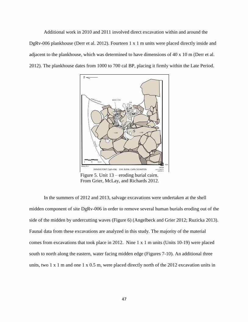
47
Additional work in 2010 and 2011 involved direct excavation within and around the
DgRv-006 plankhouse (Derr et al. 2012). Fourteen 1 x 1 m units were placed directly inside and
adjacent to the plankhouse, which was determined to have dimensions of 40 x 10 m (Derr et al.
2012). The plankhouse dates from 1000 to 700 cal BP, placing it firmly within the Late Period.
Figure 5. Unit 13 – eroding burial cairn.
From Grier, McLay, and Richards 2012.
In the summers of 2012 and 2013, salvage excavations were undertaken at the shell
midden component of site DgRv-006 in order to remove several human burials eroding out of the
side of the midden by undercutting waves (Figure 6) (Angelbeck and Grier 2012; Ruzicka 2013).
Faunal data from these excavations are analyzed in this study. The majority of the material
comes from excavations that took place in 2012. Nine 1 x 1 m units (Units 10-19) were placed
south to north along the eastern, water facing midden edge (Figures 7-10). An additional three
units, two 1 x 1 m and one 1 x 0.5 m, were placed directly north of the 2012 excavation units in

48
the summer of 2013, in order to remove another eroding burial and further stabilize the midden
bank (Figures 11 and 12).
Figure 6. Example of midden undercut during the 2013 excavations.
Figure 7. Excavation units 10-19. Photograph taken following excavation of these units (2012),
looking west from Parry Lagoon.
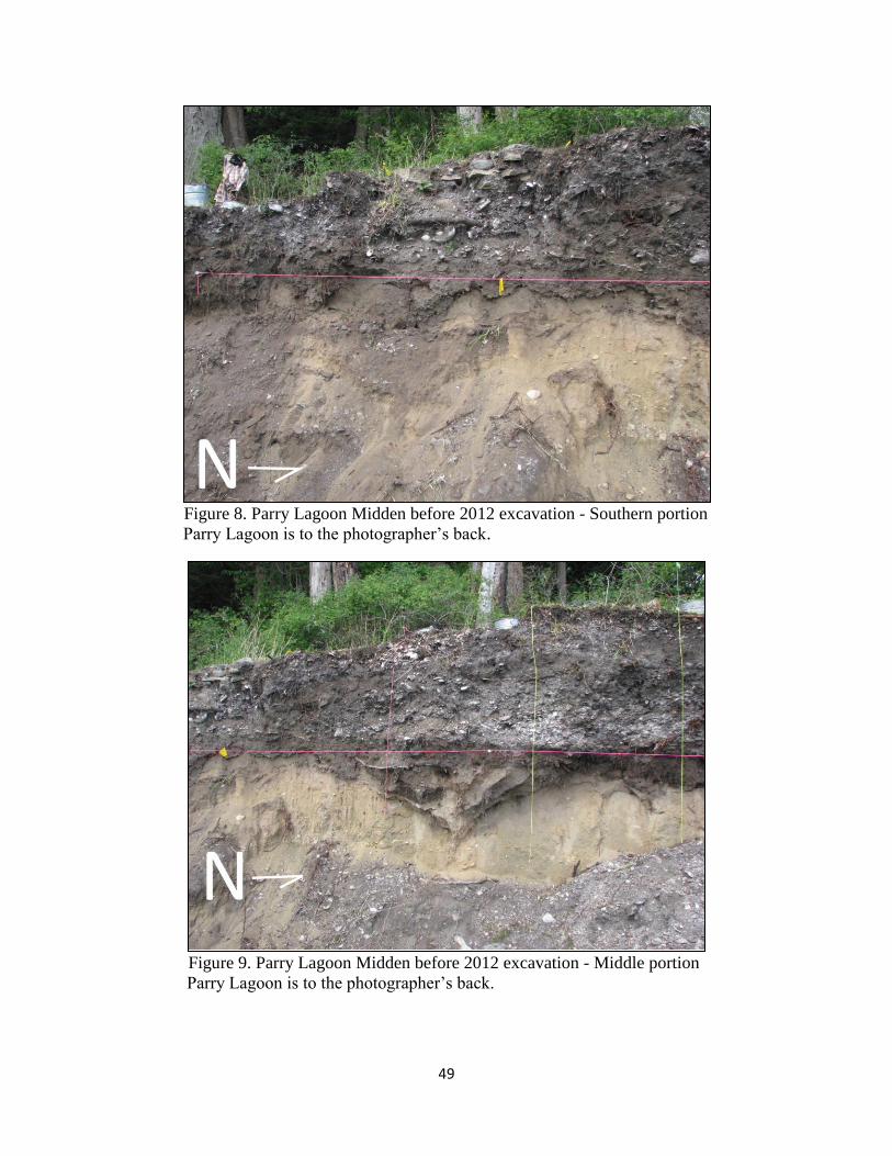
49
Figure 8. Parry Lagoon Midden before 2012 excavation - Southern portion
Parry Lagoon is to the photographer’s back.
Figure 9. Parry Lagoon Midden before 2012 excavation - Middle portion
Parry Lagoon is to the photographer’s back.

50
Figure 10. Parry Lagoon Midden before 2012 excavation - Northern portion.
Parry Lagoon is to the photographer’s back.
Figure 11. Parry Lagoon Midden after 2013 excavation. Image on right includes unit
designations.

51
Figure 12. Parry Lagoon Midden before 2013 excavation. Image on right includes unit
designations.
Initially the midden was assumed to date to the Late Period, consistent with the age of the
plankhouse to the north (Hopt and Grier 2013). However, radiocarbon dates (Table 3) indicate
that an earlier Marpole component is also contained within the midden. Based on these dates and
stratigraphic relationships within the midden, a hypothetical temporal line separating these two
components was designated (Hopt 2014; Marino and Hopt 2014).
There are several potential areas of natural bias present in the midden that could affect
cultural interpretations (Schiffer 1983). Most notably the midden is actively being eroded by
intense winter storms, indicating a general loss of archaeological material, but likely leaving
uneroded material in primary context. Root casts, and both active rodent burrows and krotovina
are present throughout the midden. This indicates some movement of material has occurred, but
they are not significant enough to consider disturbance as extensive, as stratigraphic boundaries
can still be deciphered. Additionally, given the broad context of temporal and depositional
distinctions, a low level of disturbance will not affect the results of this study.
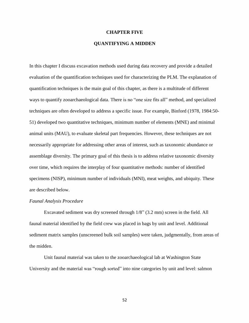
52
CHAPTER FIVE
QUANTIFYING A MIDDEN
In this chapter I discuss excavation methods used during data recovery and provide a detailed
evaluation of the quantification techniques used for characterizing the PLM. The explanation of
quantification techniques is the main goal of this chapter, as there is a multitude of different
ways to quantify zooarchaeological data. There is no “one size fits all” method, and specialized
techniques are often developed to address a specific issue. For example, Binford (1978, 1984:50-
51) developed two quantitative techniques, minimum number of elements (MNE) and minimal
animal units (MAU), to evaluate skeletal part frequencies. However, these techniques are not
necessarily appropriate for addressing other areas of interest, such as taxonomic abundance or
assemblage diversity. The primary goal of this thesis is to address relative taxonomic diversity
over time, which requires the interplay of four quantitative methods: number of identified
specimens (NISP), minimum number of individuals (MNI), meat weights, and ubiquity. These
are described below.
Faunal Analysis Procedure
Excavated sediment was dry screened through 1/8” (3.2 mm) screen in the field. All
faunal material identified by the field crew was placed in bags by unit and level. Additional
sediment matrix samples (unscreened bulk soil samples) were taken, judgmentally, from areas of
the midden.
Unit faunal material was taken to the zooarchaeological lab at Washington State
University and the material was “rough sorted” into nine categories by unit and level: salmon

53
vertebrae, herring vertebrae, dogfish vertebrae, “other fish” vertebrae, fish elements (rays,
spines, cranial elements, etc.), bird, terrestrial mammal, and sea mammal. All vertebrate fauna
material was initially processed in this manner.
All remains were further identified with the aid of a 10x hand lens. The faunal collection
at Washington State University and several manuals (Brown and Gustafson 1990; Gilbert 1990;
Gilbert et al 1996; Olsen 1964; Post 2004, 2012; Schmid 1972) were used for identification of
the terrestrial mammal, sea mammal, and bird collections. Fish identification aid was obtained
from multiple sources including the Washington State University faunal collection, the Virtual
Zooarchaeology of the Arctic Project (Betts et al 2011: http://vzap.iri.isu.edu/), Cannon’s (1987)
marine fish manual, the Portland State University faunal collection (photographs were taken of
relevant fish elements, courtesy of Virginia Butler), as well as a digital photo archive created by
the author. Faunal identification data is provided in Appendices A-J.
Species level of identification was attempted for all terrestrial mammal specimens, sea
mammal specimens, bird specimens, and fish vertebrae. Salmon vertebrae were identified to
genus (Oncorhynchus spp.) rather than species. Species level of identification for salmon
requires additional analyses that were not attempted, such as aDNA or osteometric analysis
(Cannon and Yang 2006; Grier et al. 2013; Huber et al. 2011; Orchard and Szpak 2011).
Terrestrial mammal and bird elements taxonomically unidentifiable were given a size class
designation (small, medium, large), with deer and duck being considered the medium category
within their respective categories (following Ewonus 2011a,b). All other fish elements (cranial
elements, rays, spines, and fin elements) were only identified into these broad categories. Further
identification of fish cranial elements was not attempted for three reasons: First, the lack of a
54
comprehensive comparative fish collection, paired with author inexperience, could have caused
varying degrees of identification (Lyman 2002). Second, different species contain different
amounts of elements within the skull. Identification of all remains could bias representation of
fishes that naturally contain more elements. Lastly, the density of specific elements and their
likelihood of preservation are related, thus, the identification of elements with different densities
could potentially introduce biases related to deferential preservation. Several studies have
demonstrated that element density varies between fish species and within an individual fish
(Butler and Chatters 1994, Smith 2008, Smith et al. 2011). Although few studies on bone density
for Pacific Northwest fish have been attempted (only salmon, Pacific cod, and halibut), vertebral
elements are consistently among the densest elements (Smith 2008:46-73). An identification
focus on vertebral elements should help mitigate the role that taphonomic factors play on
specimen representation. Without quantitative knowledge of the role of bone density in other
fishes, the inclusion of potentially less dense cranial elements could introduce an unknown
amount of bias into the specimen counts. Additionally, identifying differential element
representation is not a goal of this analysis, thus, identification of every element is not
specifically needed.
Shellfish remains were collected from seven two-liter bulk sediment samples.
Identification of shellfish remains was accomplished with the use of a comparative collection at
Washington State University. Sea urchin remains were not quantified, but were abundant in each
matrix sample.

55
Quantification of Remains
Multiple quantification methods were utilized to properly analyze the faunal remains.
Different techniques were required, as each method of quantification contains potentially
problematic issues associated with its application, especially with the analysis of fish bones.
These quantification techniques are detailed below in an effort to highlight their strengths and
weaknesses, and their specific application in this study.
NISP
Considered “the most fundamental unit by which faunal remains are tallied” (Lyman
2008: 27), Number of Identified Specimens (NISP), involves simply counting every skeletal
specimen and fragments of elements that have been identified to the order, family, genus, or
species level (Lyman 2008:27). Relative proportions (%NISP) are often utilized, allowing a
comparison of contexts with different sample sizes. A more general categorization, Number of
Specimens (NSP), is also used here to express broader element identifications, such as
“terrestrial mammal” or “fish vertebrae.”
The main advantage of NISP is its ease of quantification; simply identify remains and
tally the numbers. Additionally, NISP counts can be considered an observed value rather than a
derived one, and thus counts are not affected by choices made by the analyst (Lyman 2008:28).
Disadvantages of the use of NISP counts have been well described and an exhaustive list can be
found in Lyman (2008: 29-30). Here, it is beneficial to highlight one of these issues specifically;
NISP is a poor measure of diet (Lyman 2008:30). Because NISP is a “counts only” measure,
smaller, mass-caught animals (e.g., herring) are often given an increased importance in the diet
in comparison to taxa that are obtained in fewer numbers, but contribute more weight per animal
56
(e.g., salmon). Thus, NISP counts may be dominated by the smaller individuals, however, these
smaller individuals are not contributing as much dietary sustenance as the less represented taxa.
Because of this, the strict use of NISP can cause erroneous interpretations when used as a
measure of diet and as a measure of overall taxa importance (Grier and Lukowski 2012; Monks
and Orchard 2011). To deal with this issue, meat weights are taken into account with a specific
meat weight analysis that is explained below.
Dogfish NISP counts deserve a special mention. Dogfish vertebral elements take an hour-
glass type form that are mostly found broken in half in archaeological assemblages. In order to
maintain consistency in NISP counts, half vertebrae were considered one “NISP.” Thus, each full
vertebrae is considered two “NISP.” This highlights another issue with NISP; interdependence of
specimens. With NISP the same individual can be counted multiple times. Thus, one individual
animal will be counted an unknown number of times. This can be problematic when using NISP
as a measure of abundance, as bone densities and amount of elements can vary between species.
This is particularly problematic with fish remains (Wheeler and Jones 1989:152). Because of this
issue of interdependence, NISP data presents a theoretical maximum and can be considered
ordinal scale data (Lyman 2008:71-78).
NISP will be used in this study as the primary view of taxa abundance within the PLM.
NISP presents the only non-derived, directly observable measure available to faunal analysis,
and can be considered a maximum value. The main issues with NISP involve the
interdependence of the data generated and the treatment of all taxa as equally weighted. These
issues are solved by the use of additional quantification methods, explained below.

57
MNI
Standing for “Minimum Number of Individuals,” MNI can be defined as the most
commonly occurring, non-repetitive element of a specific taxon (Lyman 2008:38), although
there are many other definitions (Lyman 2008:40). Because these specific elements are non-
repeating, this gives the minimum individuals required to account for an assemblage. To
calculate MNI for terrestrial mammals and bird, I counted the most commonly occurring, non-
repetitive, left or right element. For fish, of which only vertebral elements have been identified, a
technique developed by White (1953) and expanded on by Casteel (1976a) is utilized.
Calculation consists of taking the identified vertebrae in a context and dividing by the average
number of vertebrae in the specific fish (presented in Table 6). Although not the only way to
calculate fish MNIs, it does offer us the quickest way when cranial elements are not identified
(for a different technique see Orchard 2005). This MNI technique presents us with fairly
conservative estimates for numbers of individuals, as it takes a full set of vertebrae to equal one
individual. Because of this, fish species with large NISP counts (representing more than one
individual) will be underrepresented more so than fish species with smaller (less than a complete
vertebrae column) NISPs.
Shellfish quantification is in MNI form rather than shell weights given the small amount
of sediment analyzed (see Mason et al. 1998 for a larger breakdown of this issue; also see
Claasen 2000). Shellfish MNIs were calculated by dividing NISP counts of hinge fragments by
two for clams, while barnacle, chiton, whelk and limpet MNI values are the same as their NISP.

58
Tab
le 6
. V
erte
bra
e n
um
ber
s an
d f
ish
wei
gh
ts f
or
spec
ies
pre
sen
t in
th
e P
arr
y L
ag
oon
Mid
den

59
The use of MNI does have disadvantages; Lyman (2008:45-46) identified seven specific
issues, three of which deserve special attention. First, MNI can be derived by many different
methods, thus comparability between studies can be problematic. This becomes a less of an issue
if researchers are clear about how MNIs are calculated, and make the raw data easily accessible.
The second major issue with the use of MNI is that they often exaggerate rarer taxa. For
example, a taxon with an NISP count of “1” may have the same MNI as a taxon with a much
higher NISP count. This is especially an issue with the fish vertebrae calculation presented
above. The last issue is that MNI counts change based on how contexts are aggregated. Do we
count everything in the excavation level as a context and determine MNI based on each
excavation level? Is so, this MNI will differ from an MNI calculated with a site-wide aggregation
of faunal remains. Because of these issues, MNI is best considered an ordinal scale measure
(Lyman 2008:71). An additional fragmentation issue not covered by Lyman (2008) is also
important to note. While NISP counts will over represent fragmented taxa, MNI does the exact
opposite. As noted by Marshall and Pilgrim (1993), extremely fragmented assemblages will
under represent individuals due to issues with taxonomic identification.
Although these issues are problematic, MNI remains a useful measure and overcomes
some of the issues present in NISP counts. In particular, it allows a measure of relative
abundance that is more intuitive (actual animals) and more comparable across species
(McKechnie 2012:159). In conjunction with other methods, MNI offers another useful way to
frame the data. In this study MNI will be used as an alternative measure of taxa abundance. In
comparison to the maximum value provided by NISP, MNI is a minimum value for taxa
representation. The primary issue with MNI in this study is how fish MNI calculations will under
60
represent taxa with large NISPs relative to taxa with small NISP values. Additionally, similar to
NISP, MNI does not take weight of taxa into account.
Meat Weights
NISP and MNI are the two most widely used methods for quantifying faunal data from
archaeological sites. However, both NISP and MNI are not well suited for dealing with
assemblages that contain fauna that vary in size. This is particularly problematic in an
assemblage dominated by fish. Both NISP and MNI do not take weight into consideration, thus
one small fish, like a herring, is given the same dietary importance as one large fish, like a
salmon or a halibut. However one herring on average weighs 156 g, while one coho salmon on
average weighs 4050 g, and one halibut on average weighs 6000 g (Haist and Stocker 1985:140,
Hart 1973:116, Olsen et al. 2009). Because of these wide differences, NISP and MNI do not
completely capture the actual realities of what a taxon contributed to diet. Given this issue, meat
weights will be used in this analysis. Being a derived measure based on MNI, meat weight
calculations suffer from the same issues as MNI, and, since it moves beyond MNI, additional
issues arise depending on the specific technique used. However, it does present us with a way to
account for differently sized animals.
In this study, meat weights will be calculated on fish vertebrae. I will only be using fish
weights on select fish species where reliable averages are available, specifically herring, salmon,
dogfish, codfish, and flatfish. The specific technique follows Monks and Orchard (2011) and
Grier and Lukowski (2012). Earlier studies by Guthrie (1968) and White (1953) present a similar
approach. This technique involves calculating the MNI by taking the NISP counts from a context
in the midden and dividing by the vertebrae found in one specimen (this is the same as MNI
61
above). This MNI is then multiplied by the average adult weight of the fish type, which gives us
the relative amount of fish weight.
Average fish weights were obtained from published sources and are presented Table 6.
Salmon weights deserve explanation. Average weights of salmon were calculated from an
average of three species: Pink, Chum, and Sockeye. These three species made up 91% of salmon
remains identified with aDNA by Grier et al. (2013) for site DgRv-003. Given the proximity of
both sites, as well as temporal overlap, it is reasonable to assume similarities in salmon species
for DgRv-006.
Meat weight calculations were calculated by species when applicable, but also by genus
and family when species level of identification could not be established. These weights are then
standardized to the salmon weight, which is done by dividing each total weight category by the
total weight of salmon. This is done to provide a simple way to compare relative importance of
these taxa, as anything greater than “1” would show that taxon as contributing more meat weight
than salmon, thus illuminating the contribution of salmon relative to other species (see Grier and
Lukowski 2012).
Salient critiques of this style of meat weight calculation have emerged (Cannon and Yang
2011; Ewonus 2012). One major issue with this technique is variability of fish weight. The use of
average weights for fish does not take into account sources of variability that will be present in
the archaeological fish such as age, sex, health status, historical differences, and even simple
individual difference. Thus, exact biomass for the midden population cannot be achieved with
this method. However, my interest is not in obtaining an exact population biomass but rather in

62
ascertaining the relative importance of each taxa, so that we can better understand human
behavior as it pertains to temporal components found in the midden.
It is impossible that any quantification method utilized will be able to correctly identify
exact numbers of individuals or grams of meat consumed by a population. However, by using
many different approaches, we can address and potentially correct issues that each technique has.
Using this multi-technique approach, we should be able to identify when specific techniques are
under or overestimating taxa importance. Meat weight analyses that involve several assumptions
should not be used as the sole basis for an argument. But, it can be used as one way to
demonstrate how dominant NISP or MNI values for any species may not actually result in
dietary dominance. Although presented in more quantitative terms, the use of meat weight can
be considered an ordinal measure. More accurate fish weights would be derived through the use
of regression formulae (see Casteel 1974, 1976; Orchard 2001), but that level of data resolution
is not the objective here, nor is it necessary to understand the major patterns in the assemblages.
Ubiquity
Another way to measure a taxon’s abundance is by using the measure of ubiquity and
percent ubiquity. Ubiquity describes the presence/absence of a taxon across archaeological
contexts, while percent ubiquity is simply the proportion of these contexts that contain the taxon
expressed as a percent. For example, if there are 10 different contexts, such as arbitrary 10 cm
excavation levels, and salmon were found in 8 of these 10 contexts we would have a ubiquity of
8 and a percent ubiquity of 80%. Exact numbers of specific taxa are not taken into account with
this approach. Ubiquity is noted as being useful for fish remains, given the issues of differential
element representation and bone density (Wheeler and Jones 1989:152). Additionally, it is useful
63
to address abundance of taxa when an assemblage contains large amounts of smaller fauna that
may not be contributing as much to the overall diet as the counts would suggest. Here, ubiquity
will be calculated using arbitrary excavation levels and features (120 different contexts total).
The use of ubiquity in this study will mainly address the spread and dispersion of taxa within the
midden, with the baseline expectation that the most abundant taxa should also appear in the most
contexts. Deviation from this pattern could be indicating an increased abundance of taxa from
what NISP values express.
Diversity
The concept of diversity and how it is measured deserves discussion to better
contextualize how the previous measures will be utilized to address the issue of diversity, which
is central to the very discussion of changing temporal faunal trends in this study. I utilize the
term “diversity” in the same way that others have used the term “heterogeniety” (Lyman
2008:176). Here, diversity refers to the “structure and composition” of a faunal data set,
incorporating both assemblage richness and assemblage evenness (Lyman 2008:174-178).
Richness involves the number of different types of taxa within an assemblage (NTAXA).
Evenness is a measure of the proportions across taxa, where the more similar the proportions the
more “even” an assemblage. For example, if an assemblage consists of two taxa, both equaling
50% of the assemblage, this would be an “even” assemblage. In comparison if one taxon made
up 98% of the assemblage, this would be considered an “uneven” assemblage.
Diversity studies often consider both of these measures together with the use of simple
mathematical indices, the Shannon-Wiener index being the most common (Lyman 2008:192).
These indices are useful for an evaluation of multiple different assemblages at once, however,

64
given the smaller scope of this study I prefer to evaluate diversity by looking at richness and
evenness separately. This allows for a more in-depth evaluation of each component and their
influences on the expression of diversity. Richness will be evaluated simply by tallying the
amount of taxa identified in each assemblage. Evenness will be evaluated by the comparison of
taxa NISP, MNI, and meat weight proportions.
A combination of four different quantification methods, NISP, MNI, meat weights, and
ubiquity, will be utilized in this study. This multi-technique approach facilitates a better
understanding of faunal importance by presenting multiple lines of evidence: counts, individuals,
weights, and range of spatial location. Additionally, this allows an exploration of the data that
mitigates the downfalls of any single technique. With methodology and quantification techniques
sufficiently covered, I now turn to an exploration of the PLM’s temporal and depositional
stratigraphy.
65
CHAPTER SIX
TEMPORAL AND DEPOSITIONAL BREAKDOWN OF MIDDEN CONTEXTS
The PLM is a complex depositional environment consisting of multiple depositional episodes of
variable material. In this chapter, I divide the midden into two kinds of units: 1.) those that
reflect differences in deposition, and 2.) those that reflect deposition over time (aka
chronostratigraphy). These divisions are based on stratigraphic observations and the results of
radiocarbon dating (presented by excavation level in Appendix K). I then undertake exploratory
data analysis, in the form of correspondence analysis, on the faunal composition of the
depositional units (DU) in order to identify patterning in faunal representation across the midden.
I posit that support for changing depositional uses in the midden will be established if there are
distinct differences in faunal deposition that are consistent with the stratigraphic divisions.
Temporal depositional trends are explored in chapter seven. Overall the midden contains a
three-strata pattern common in sites in the region: A: topsoil (historic disturbance), B: midden
material, C: sterile beach sands (Stein 1992: 79). The temporal and depositional stratigraphic
units differences are all contained within the B strata.
Radiocarbon Dates and Stratigraphy
Nine radiocarbon dates have been obtained for the PLM (Table 3), revealing a fairly long
time range for the use of this midden. Seven date to the Marpole Period and overlap with the
occupation of the adjacent (150 m away) Marpole village, DgRv-003, providing evidence for use
of this midden by these occupants. Two dates post-date the abandonment of the village providing
evidence for continued use of the midden into the Late Period.

66
Figure 13 presents the radiocarbon dates with their spatial locations within the midden.
Pairing these with stratigraphic differences evident through changing proportions of shell and
sediments differences there appear to be four depositional areas (Figure 14) and four temporal
areas (Figure 15).
Depositional Unit 1: Mound
Depositional Unit 1 (DU-1) consists of the lowest portion of the midden. This area
includes underlying basal sands and a mound of shell that extends through units 15, 16, and 17
(see Figure 7). Five burials are located within this portion of the midden (Table 7), with four of
them located within or directly on top of the basal sands (BR-2, BR-5, BR-7, and BR-8). Dates
from this portion of the midden (2012-16b, 2012-17a, 2012-21, 2012-24) place it as the earliest
area of use, meeting expectations of the law of superposition. Maximum date range is 1400-1730
cal BP. Using just charcoal dates, this section of the midden dates to 1556-1730 cal BP.
Depositionally, it appears that a prepared burial surface on a sandy beach environment may have
been the original deposition, as a prepared floor surface was found, with the earliest burials both
placed on top of and dug into this surface. It then appears that additional shell deposits were
placed on top. These burials are currently being analyzed and will be described fully in a
subsequent publication.
Depositional Unit 2: Marpole Deposits
Depositional Unit 2 (DU-2) sits directly on top of DU-1 and is bounded on top by
Depositional Areas 3 and 4. DU-2 is characterized as a deposit containing less shell material than
all other depositional areas. This area is interspersed with some sandy matrix material (Figure
16-17). One burial has been identified as a pit burial dug into the DU-2 matrix later in the
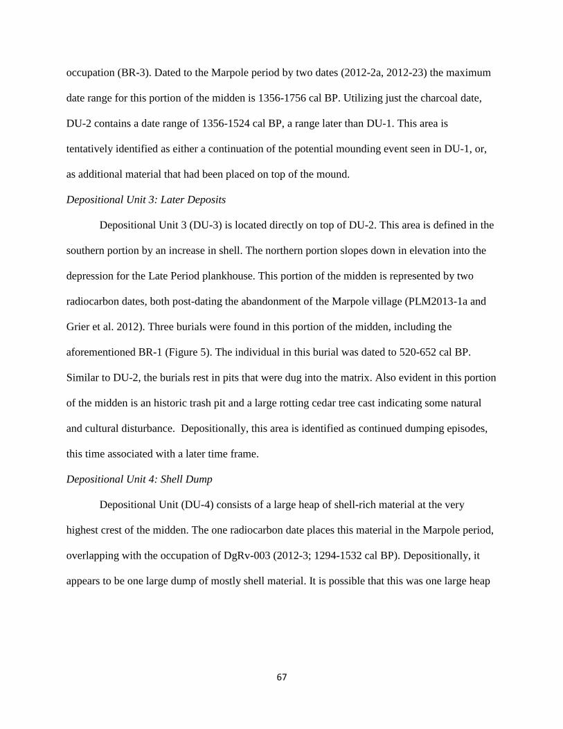
67
occupation (BR-3). Dated to the Marpole period by two dates (2012-2a, 2012-23) the maximum
date range for this portion of the midden is 1356-1756 cal BP. Utilizing just the charcoal date,
DU-2 contains a date range of 1356-1524 cal BP, a range later than DU-1. This area is
tentatively identified as either a continuation of the potential mounding event seen in DU-1, or,
as additional material that had been placed on top of the mound.
Depositional Unit 3: Later Deposits
Depositional Unit 3 (DU-3) is located directly on top of DU-2. This area is defined in the
southern portion by an increase in shell. The northern portion slopes down in elevation into the
depression for the Late Period plankhouse. This portion of the midden is represented by two
radiocarbon dates, both post-dating the abandonment of the Marpole village (PLM2013-1a and
Grier et al. 2012). Three burials were found in this portion of the midden, including the
aforementioned BR-1 (Figure 5). The individual in this burial was dated to 520-652 cal BP.
Similar to DU-2, the burials rest in pits that were dug into the matrix. Also evident in this portion
of the midden is an historic trash pit and a large rotting cedar tree cast indicating some natural
and cultural disturbance. Depositionally, this area is identified as continued dumping episodes,
this time associated with a later time frame.
Depositional Unit 4: Shell Dump
Depositional Unit (DU-4) consists of a large heap of shell-rich material at the very
highest crest of the midden. The one radiocarbon date places this material in the Marpole period,
overlapping with the occupation of DgRv-003 (2012-3; 1294-1532 cal BP). Depositionally, it
appears to be one large dump of mostly shell material. It is possible that this was one large heap
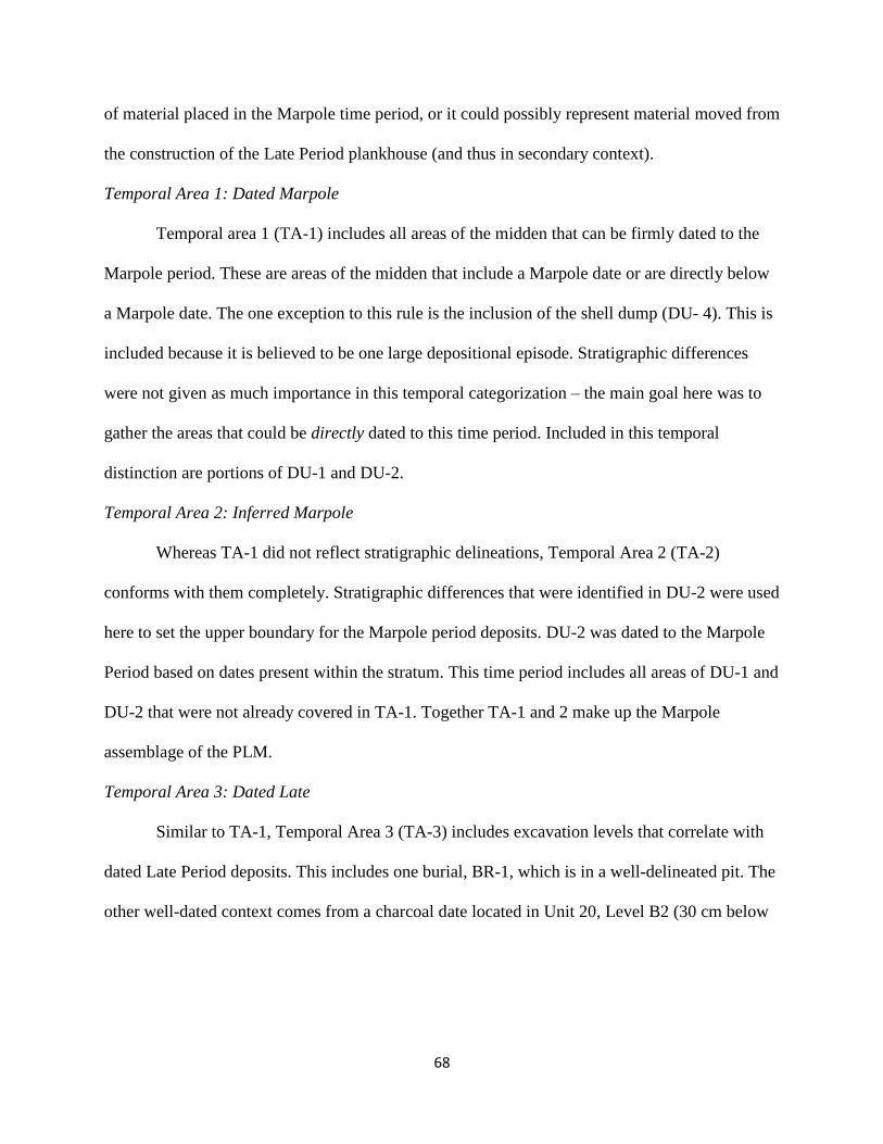
68
of material placed in the Marpole time period, or it could possibly represent material moved from
the construction of the Late Period plankhouse (and thus in secondary context).
Temporal Area 1: Dated Marpole
Temporal area 1 (TA-1) includes all areas of the midden that can be firmly dated to the
Marpole period. These are areas of the midden that include a Marpole date or are directly below
a Marpole date. The one exception to this rule is the inclusion of the shell dump (DU- 4). This is
included because it is believed to be one large depositional episode. Stratigraphic differences
were not given as much importance in this temporal categorization – the main goal here was to
gather the areas that could be directly dated to this time period. Included in this temporal
distinction are portions of DU-1 and DU-2.
Temporal Area 2: Inferred Marpole
Whereas TA-1 did not reflect stratigraphic delineations, Temporal Area 2 (TA-2)
conforms with them completely. Stratigraphic differences that were identified in DU-2 were used
here to set the upper boundary for the Marpole period deposits. DU-2 was dated to the Marpole
Period based on dates present within the stratum. This time period includes all areas of DU-1 and
DU-2 that were not already covered in TA-1. Together TA-1 and 2 make up the Marpole
assemblage of the PLM.
Temporal Area 3: Dated Late
Similar to TA-1, Temporal Area 3 (TA-3) includes excavation levels that correlate with
dated Late Period deposits. This includes one burial, BR-1, which is in a well-delineated pit. The
other well-dated context comes from a charcoal date located in Unit 20, Level B2 (30 cm below
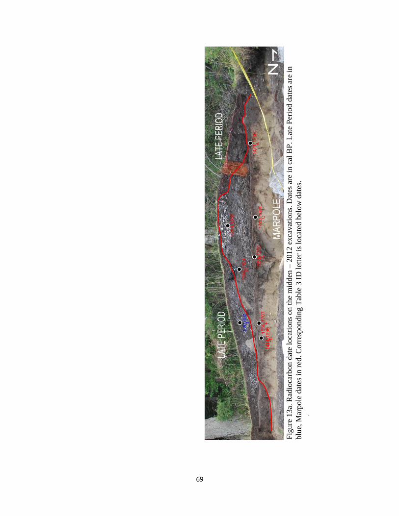
69
Fig
ure
13
a. R
adio
carb
on d
ate
loca
tions
on t
he
mid
den
– 2
012 e
xca
vat
ions.
Dat
es a
re i
n c
al B
P. L
ate
Per
iod d
ates
are
in
blu
e, M
arpole
dat
es i
n r
ed. C
orr
espondin
g T
able
3 I
D l
ette
r is
loca
ted b
elo
w d
ates
. .
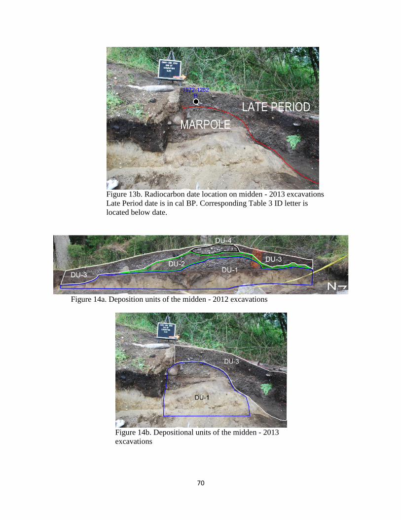
70
Figure 13b. Radiocarbon date location on midden - 2013 excavations
Late Period date is in cal BP. Corresponding Table 3 ID letter is
located below date.
Figure 14a. Deposition units of the midden - 2012 excavations
Figure 14b. Depositional units of the midden - 2013
excavations
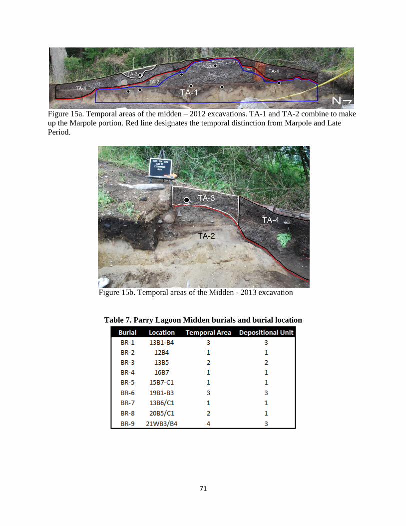
71
Figure 15a. Temporal areas of the midden – 2012 excavations. TA-1 and TA-2 combine to make
up the Marpole portion. Red line designates the temporal distinction from Marpole and Late
Period.
Figure 15b. Temporal areas of the Midden - 2013 excavation
Table 7. Parry Lagoon Midden burials and burial location
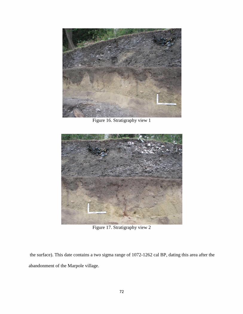
72
Figure 16. Stratigraphy view 1
Figure 17. Stratigraphy view 2
the surface). This date contains a two sigma range of 1072-1262 cal BP, dating this area after the
abandonment of the Marpole village.
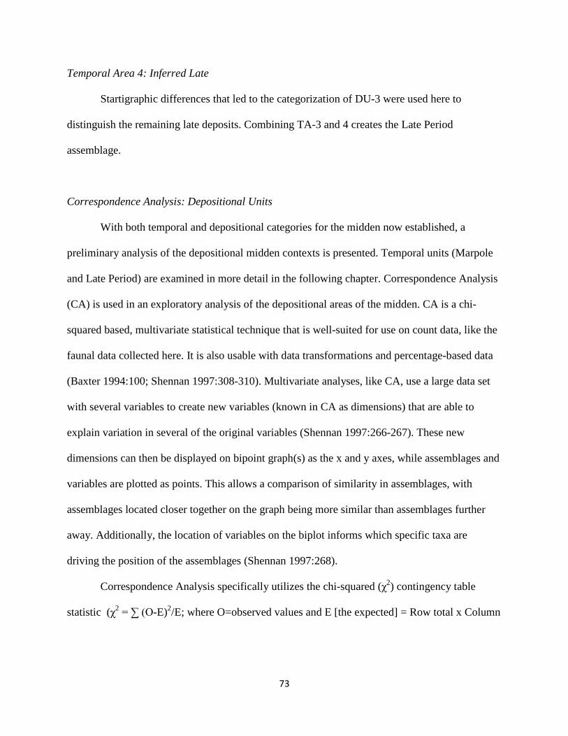
73
Temporal Area 4: Inferred Late
Startigraphic differences that led to the categorization of DU-3 were used here to
distinguish the remaining late deposits. Combining TA-3 and 4 creates the Late Period
assemblage.
Correspondence Analysis: Depositional Units
With both temporal and depositional categories for the midden now established, a
preliminary analysis of the depositional midden contexts is presented. Temporal units (Marpole
and Late Period) are examined in more detail in the following chapter. Correspondence Analysis
(CA) is used in an exploratory analysis of the depositional areas of the midden. CA is a chi-
squared based, multivariate statistical technique that is well-suited for use on count data, like the
faunal data collected here. It is also usable with data transformations and percentage-based data
(Baxter 1994:100; Shennan 1997:308-310). Multivariate analyses, like CA, use a large data set
with several variables to create new variables (known in CA as dimensions) that are able to
explain variation in several of the original variables (Shennan 1997:266-267). These new
dimensions can then be displayed on bipoint graph(s) as the x and y axes, while assemblages and
variables are plotted as points. This allows a comparison of similarity in assemblages, with
assemblages located closer together on the graph being more similar than assemblages further
away. Additionally, the location of variables on the biplot informs which specific taxa are
driving the position of the assemblages (Shennan 1997:268).
Correspondence Analysis specifically utilizes the chi-squared (χ2) contingency table
statistic (χ2 = ∑ (O-E)
2/E; where O=observed values and E [the expected] = Row total x Column
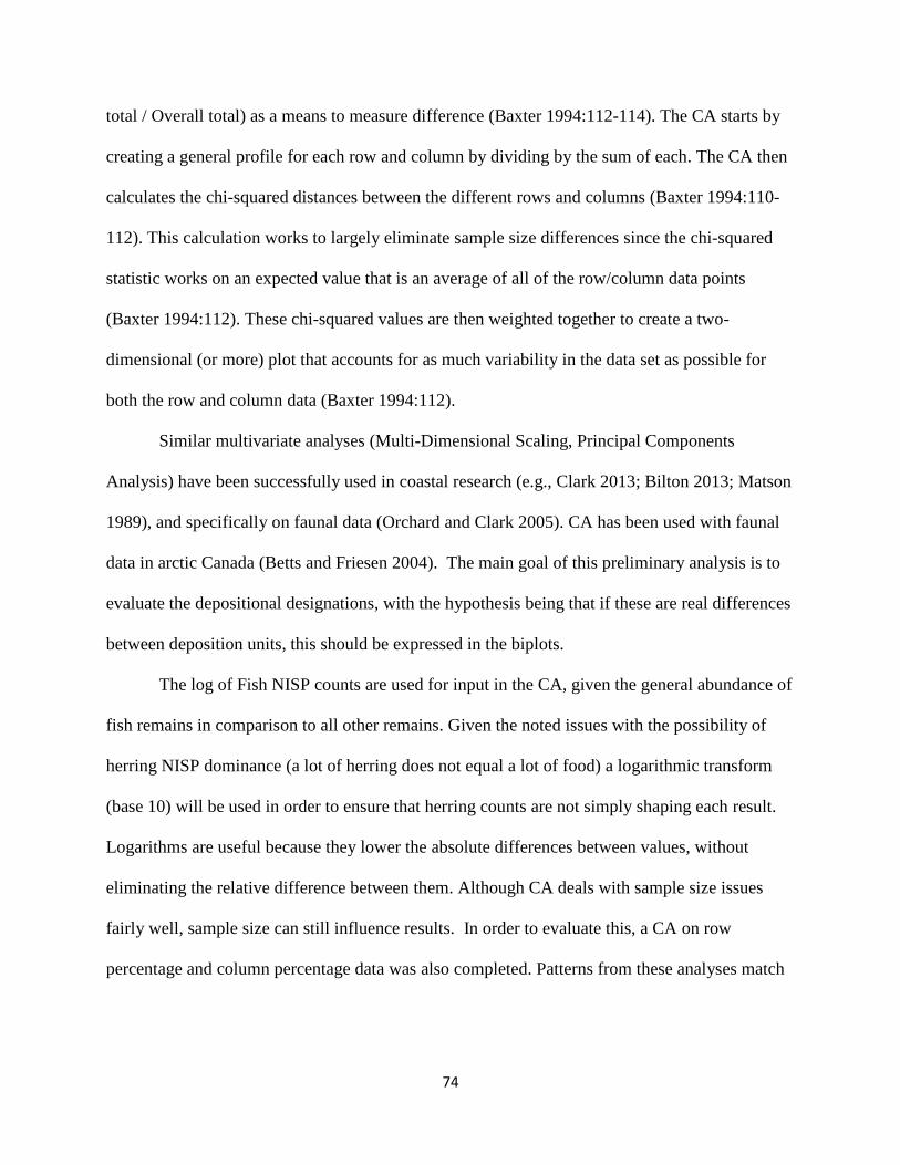
74
total / Overall total) as a means to measure difference (Baxter 1994:112-114). The CA starts by
creating a general profile for each row and column by dividing by the sum of each. The CA then
calculates the chi-squared distances between the different rows and columns (Baxter 1994:110-
112). This calculation works to largely eliminate sample size differences since the chi-squared
statistic works on an expected value that is an average of all of the row/column data points
(Baxter 1994:112). These chi-squared values are then weighted together to create a two-
dimensional (or more) plot that accounts for as much variability in the data set as possible for
both the row and column data (Baxter 1994:112).
Similar multivariate analyses (Multi-Dimensional Scaling, Principal Components
Analysis) have been successfully used in coastal research (e.g., Clark 2013; Bilton 2013; Matson
1989), and specifically on faunal data (Orchard and Clark 2005). CA has been used with faunal
data in arctic Canada (Betts and Friesen 2004). The main goal of this preliminary analysis is to
evaluate the depositional designations, with the hypothesis being that if these are real differences
between deposition units, this should be expressed in the biplots.
The log of Fish NISP counts are used for input in the CA, given the general abundance of
fish remains in comparison to all other remains. Given the noted issues with the possibility of
herring NISP dominance (a lot of herring does not equal a lot of food) a logarithmic transform
(base 10) will be used in order to ensure that herring counts are not simply shaping each result.
Logarithms are useful because they lower the absolute differences between values, without
eliminating the relative difference between them. Although CA deals with sample size issues
fairly well, sample size can still influence results. In order to evaluate this, a CA on row
percentage and column percentage data was also completed. Patterns from these analyses match
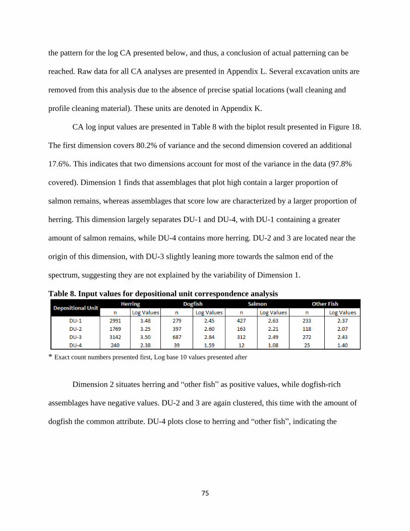
75
the pattern for the log CA presented below, and thus, a conclusion of actual patterning can be
reached. Raw data for all CA analyses are presented in Appendix L. Several excavation units are
removed from this analysis due to the absence of precise spatial locations (wall cleaning and
profile cleaning material). These units are denoted in Appendix K.
CA log input values are presented in Table 8 with the biplot result presented in Figure 18.
The first dimension covers 80.2% of variance and the second dimension covered an additional
17.6%. This indicates that two dimensions account for most of the variance in the data (97.8%
covered). Dimension 1 finds that assemblages that plot high contain a larger proportion of
salmon remains, whereas assemblages that score low are characterized by a larger proportion of
herring. This dimension largely separates DU-1 and DU-4, with DU-1 containing a greater
amount of salmon remains, while DU-4 contains more herring. DU-2 and 3 are located near the
origin of this dimension, with DU-3 slightly leaning more towards the salmon end of the
spectrum, suggesting they are not explained by the variability of Dimension 1.
Table 8. Input values for depositional unit correspondence analysis
* Exact count numbers presented first, Log base 10 values presented after
Dimension 2 situates herring and “other fish” as positive values, while dogfish-rich
assemblages have negative values. DU-2 and 3 are again clustered, this time with the amount of
dogfish the common attribute. DU-4 plots close to herring and “other fish”, indicating the
76
importance of these taxa to the assemblage. DU-1 plots highest indicating that herring and “other
fish” are also important to this assemblage.
Taking both dimensions into consideration the four assemblages can be seen as falling
into three groups. DU-1 and DU-4 can be considered their own respective patterns, which
support the distinctions that were made with stratigraphic differences. DU-2 and 3 cluster
together in both dimensions, indicating a general similarity between the two. This stands in
contrast to the stratigraphic difference, and indicates perhaps a similar depositional use for these
two areas despite their difference in time. Given that DU-1 may be a special burial environment,
DU-2 and 3 may represent a shift to more conventional depositional practices. These three
different deposition patterns are supported by traditional chi-squared analyses presented in Table
9. DU-1 and DU-4 are significantly different from all other depositional environments (p-value <
0.001). The comparison of DU-2 and DU-3 failed to reject the null hypothesis of no difference
(p-value = 0.109), indicating a similar depositional pattern.
Overall this analysis provides a useful exploration of the midden depositional contexts
and illuminates the differences and similarities between them. For example, the separation of
DU-1 and DU-2 in the CA plot indicates a depositional shift and reflects the differentiation of the
two areas established by stratigraphy. Interestingly, this also indicates that deposition does
change within the same time period (Marpole). In comparison, the clustering of the faunal
compositions of DU-2 and DU-3 indicates that the stratigraphic boundary denoted here does not
indicate a significant depositional shift. This indicates, in terms of fish material, temporal change
is not always associated with changes in deposition.

77
Figure 18. Depositional unit correspondence analysis biplot.
Table 9. Chi-Squared analysis on depositional units
* Null hypothesis states that there is no difference between the two compared. Significance is
established at an α of 0.05. Null hypothesis is only rejected for the comparison of DU-2 and 3
In sum, this analysis has utilized both stratigraphic realities and radiocarbon dates to
establish specific temporal and depositional areas of the PLM. Depositional units were presented
first with four specific areas noted: DU-1: Mound, DU-2: Marpole Deposits, DU-3: Late
78
Deposits, and DU-4: Shell Dump. Utilizing these findings, four temporal areas were then
presented: TA-1: Dated Marpole, TA-2: Inferred Marple, TA-3: Dated Late, and TA-4: Inferred
Late. TA-1 and TA-2 are combined to make up the overall Marpole assemblage, while TA-3 and
TA-4 combined make up the Late Period assemblage. These will be presented and evaluated in
the following chapter.
Following this, a correspondence analysis was utilized to preliminarily evaluate
depositional contexts. The hypothesis for this analysis was that if midden depositional practices
actually shifted in this manner, than this would be reflected taxonomically along the stratigraphic
boundaries. Results from the CA found that DU-1 and DU-4 are both distinct areas, while DU-2
and DU-3 appear taxonomically similar. This strengthens the idea that DU-1 may be a distinct
burial and mound event (or series of events), with a shift to a more temporally constant
deposition behavior.
With temporal midden distinctions established, this study now turns to the bulk of the
analysis. Both Marpole and Late Period assemblages are evaluated below, with coverage of all
faunal remains presented for each temporal period. Each assemblage coverage will be followed
by an explanation of environmental and behavioral patterns that are evident, given the taxonomic
compositions. This is followed with the main goal of this thesis, a comparison of the temporal
assemblages and how they relate to the larger regional patterns covered in chapter two. These
regional, linear, complexity patterns state that salmon specialization is expected to be present in
the Marpole assemblage, with a diversification of fishing practices emerging in the Late Period.
79
CHAPTER SEVEN
TEMPORAL COMPARISON
Using the temporal distinctions established in the last chapter, a comparison of the Marpole and
Late Period faunal remains can now be made. Amounts and proportions of faunal material from
the overall midden assemblage (regardless of time) will be presented first. Temporal assemblage
analysis will follow, with direct comparison of the two presented at the end of the chapter. This
comparison is driven by the null hypothesis (of no expected difference) outlined in Chapter one.
Drawing on linear complexity models, the Marpole assemblage is expected to contain a
specialization of salmon, while a diversification of fish is expected in the Late Period. But if
there is no difference we reject these expectations. Consequently, deviations from this model
would suggest that reevaluation on the interconnection of subsistence and social change is
needed, as has been argued in recent Northwest Coast literature (Grier 2014; Moss 2011, 2012).
Analysis of the entire midden includes all excavated material, while the temporal
comparison leaves out some excavation contexts. These contexts mainly consist of profile/wall
cleaning material, and are noted in Appendix K. Additionally, three arbitrary excavation levels
(13B3, 13B4, 19B3) are split by the line separating the Marpole from the Late Period deposits.
The majority of each level was located within the Marpole section. The entire level will therefore
be considered Marpole. Analysis excluding these levels does not change the overall results, thus,
there is no reason to completely exclude them from the analysis.
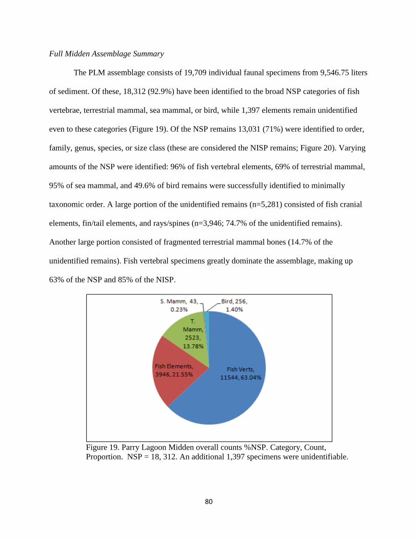
80
Full Midden Assemblage Summary
The PLM assemblage consists of 19,709 individual faunal specimens from 9,546.75 liters
of sediment. Of these, 18,312 (92.9%) have been identified to the broad NSP categories of fish
vertebrae, terrestrial mammal, sea mammal, or bird, while 1,397 elements remain unidentified
even to these categories (Figure 19). Of the NSP remains 13,031 (71%) were identified to order,
family, genus, species, or size class (these are considered the NISP remains; Figure 20). Varying
amounts of the NSP were identified: 96% of fish vertebral elements, 69% of terrestrial mammal,
95% of sea mammal, and 49.6% of bird remains were successfully identified to minimally
taxonomic order. A large portion of the unidentified remains (n=5,281) consisted of fish cranial
elements, fin/tail elements, and rays/spines (n=3,946; 74.7% of the unidentified remains).
Another large portion consisted of fragmented terrestrial mammal bones (14.7% of the
unidentified remains). Fish vertebral specimens greatly dominate the assemblage, making up
63% of the NSP and 85% of the NISP.
Figure 19. Parry Lagoon Midden overall counts %NSP. Category, Count,
Proportion. NSP = 18, 312. An additional 1,397 specimens were unidentifiable.
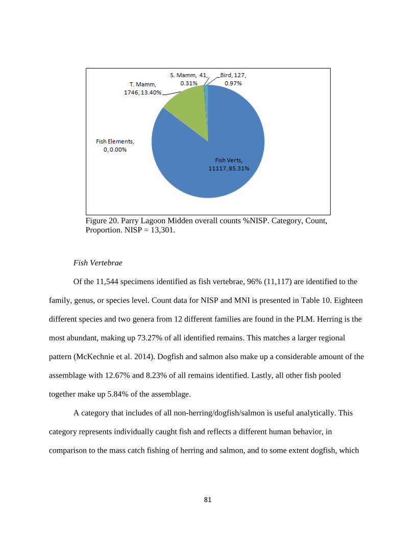
81
Figure 20. Parry Lagoon Midden overall counts %NISP. Category, Count,
Proportion. NISP = 13,301.
Fish Vertebrae
Of the 11,544 specimens identified as fish vertebrae, 96% (11,117) are identified to the
family, genus, or species level. Count data for NISP and MNI is presented in Table 10. Eighteen
different species and two genera from 12 different families are found in the PLM. Herring is the
most abundant, making up 73.27% of all identified remains. This matches a larger regional
pattern (McKechnie et al. 2014). Dogfish and salmon also make up a considerable amount of the
assemblage with 12.67% and 8.23% of all remains identified. Lastly, all other fish pooled
together make up 5.84% of the assemblage.
A category that includes of all non-herring/dogfish/salmon is useful analytically. This
category represents individually caught fish and reflects a different human behavior, in
comparison to the mass catch fishing of herring and salmon, and to some extent dogfish, which

82
are likely caught while feeding on schooling fish such as smelts and/or herring. Dogfish were
also an important source of non-food materials in ethnographic times, as sand paper and oil,
which would indicate that they should be given their own taxonomic category (Suttles 1974:130-
131).
Table 10. NISP, MNI, and Ubiquity for fish vertebrae - overall Parry Lagoon Midden
MNI values reveal an increased representation of the combined “other fish” category in
comparison to their NISP value, moving from fourth to second in rank order of abundance

83
(Figure 21). It is only when combined that these other fish species become numerically
important, as no individual species of “other fish” approach more than 4% of the accumulated
MNI, and most contain an MNI of 1. This would suggest that none of these fish individually
were important to the diet, but does suggest that behaviorally, mass-catch fishing is not the only
important fishing technique. Other important shifts in the rank order from the NISP counts
indicate an increased frequency for salmon and rockfish, while dogfish decrease in frequency.
Ubiquity percentages are presented in Table 10. The relative proportions of NISP are
generally reflected in the rank order of percent ubiquity, the more abundant species are also
found within more of the contexts. One important difference is the high ubiquity of salmon,
dogfish, and rockfish, which are in more contexts than their NISP values would suggest.
Figure 21. %MNI for overall Parry Lagoon Midden assemblage. Exact MNI
is presented on top of each respective bar.
Meat weights were also calculated for six families: Clupeidae (herring), Salmonidae
(salmon), Squalidae (dogfish), Scorpaenidae (rockfish), Gadidae (cods), and Pleuronectidae
(flatfish) (Table 11). This meat weight analysis reveals a very different rank of these taxa then
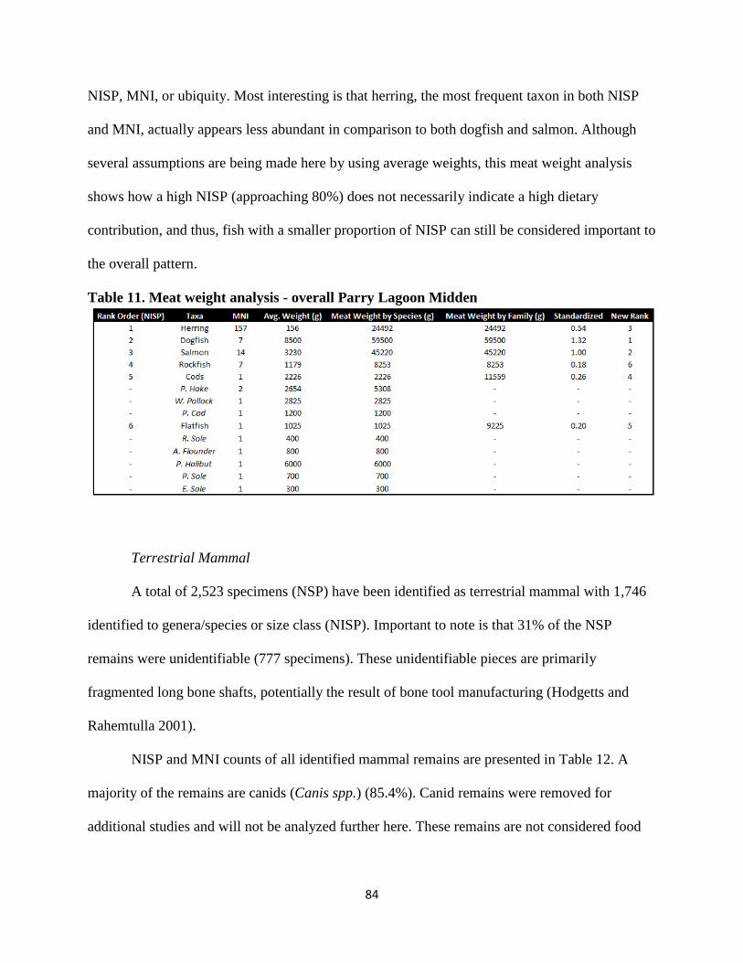
84
NISP, MNI, or ubiquity. Most interesting is that herring, the most frequent taxon in both NISP
and MNI, actually appears less abundant in comparison to both dogfish and salmon. Although
several assumptions are being made here by using average weights, this meat weight analysis
shows how a high NISP (approaching 80%) does not necessarily indicate a high dietary
contribution, and thus, fish with a smaller proportion of NISP can still be considered important to
the overall pattern.
Table 11. Meat weight analysis - overall Parry Lagoon Midden
Terrestrial Mammal
A total of 2,523 specimens (NSP) have been identified as terrestrial mammal with 1,746
identified to genera/species or size class (NISP). Important to note is that 31% of the NSP
remains were unidentifiable (777 specimens). These unidentifiable pieces are primarily
fragmented long bone shafts, potentially the result of bone tool manufacturing (Hodgetts and
Rahemtulla 2001).
NISP and MNI counts of all identified mammal remains are presented in Table 12. A
majority of the remains are canids (Canis spp.) (85.4%). Canid remains were removed for
additional studies and will not be analyzed further here. These remains are not considered food
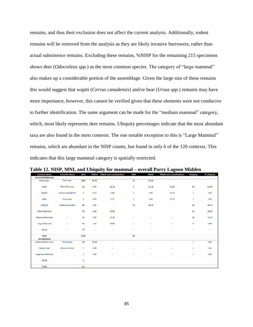
85
remains, and thus their exclusion does not affect the current analysis. Additionally, rodent
remains will be removed from the analysis as they are likely invasive burrowers, rather than
actual subsistence remains. Excluding these remains, %NISP for the remaining 215 specimens
shows deer (Odocoileus spp.) as the most common species. The category of “large mammal”
also makes up a considerable portion of the assemblage. Given the large size of these remains
this would suggest that wapiti (Cervus canadensis) and/or bear (Ursus spp.) remains may have
more importance, however, this cannot be verified given that these elements were not conducive
to further identification. The same argument can be made for the “medium mammal” category,
which, most likely represents deer remains. Ubiquity percentages indicate that the most abundant
taxa are also found in the most contexts. The one notable exception to this is “Large Mammal”
remains, which are abundant in the NISP counts, but found in only 6 of the 120 contexts. This
indicates that this large mammal category is spatially restricted.
Table 12. NISP, MNI, and Ubiquity for mammal – overall Parry Lagoon Midden

86
MNIs were generated by counting the most commonly occurring, non-repeating element
for each taxa (deer = left mandible, wapiti = femur, bear = left humerus, and rodent = left
mandible). Table 12 presents the results of the MNI calculation, which largely reflect the NISP
counts. Deer is most likely underrepresented here due to the fragmentary nature of most of the
remains, which was detrimental for siding bones. In comparison, rodents were relatively intact,
which allowed for identification of element and side, which in turn helped increase the MNI
count for this taxon. This also supports the intrusive nature of these remains, as all other remains
had a higher degree of fragmentation.
Sea Mammal
The sea mammal component of the PLM consists of only 43 elements, 41 of which were
identified. Most elements were identified as Pinnipedia (92.68% of remains), with two
specimens identified as Harbor Seal (Phoca vitulina), and one specimen indentified as a “large
sea mammal” (Table 12). The fragmentary nature of these remains prevents meaningful MNI
calculations.
Bird
Of the 256 bird specimens present in the PLM, 127 (49.61%) were identified to order or a
greater precision. Specimens were identified to six species, one genus, three families, and eight
orders. Three orders of birds make up the majority of the identified remains (60.63%):
Charadriiformes (sea birds), Passeriformes (perching/song birds), and Anseriformes (waterfowl)
(Table 13). All other remains were identified to five other orders contributing a minimal amount
of the overall NISP (6.3% when consolidated). Bird NISP rank order for ubiquity shows a
general agreement with the rank order of NISP. What this suggests is that the most abundant

87
birds are also most commonly found across the midden. MNI calculations largely mirror NISP
results.
Table 13. NISP, MNI, and Ubiquity for bird – overall Parry Lagoon Midden
Full Midden Summary
The PLM consists largely of fish vertebral specimens with terrestrial mammal, bird, and
sea mammal remains providing a much smaller proportion of the assemblage. Looking strictly at
NISP counts, herring specimens make up a large majority of the fish remains. However, when
measured by MNI and meat weight, other taxa, especially dogfish and salmon, increase in
frequency. This is largely because of the vast difference in meat weights. Herring is numerically
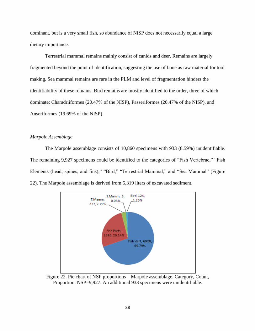
88
dominant, but is a very small fish, so abundance of NISP does not necessarily equal a large
dietary importance.
Terrestrial mammal remains mainly consist of canids and deer. Remains are largely
fragmented beyond the point of identification, suggesting the use of bone as raw material for tool
making. Sea mammal remains are rare in the PLM and level of fragmentation hinders the
identifiability of these remains. Bird remains are mostly identified to the order, three of which
dominate: Charadriiformes (20.47% of the NISP), Passeriformes (20.47% of the NISP), and
Anseriformes (19.69% of the NISP).
Marpole Assemblage
The Marpole assemblage consists of 10,860 specimens with 933 (8.59%) unidentifiable.
The remaining 9,927 specimens could be identified to the categories of “Fish Vertebrae,” “Fish
Elements (head, spines, and fins),” “Bird,” “Terrestrial Mammal,” and “Sea Mammal” (Figure
22). The Marpole assemblage is derived from 5,319 liters of excavated sediment.
Figure 22. Pie chart of NSP proportions – Marpole assemblage. Category, Count,
Proportion. NSP=9,927. An additional 933 specimens were unidentifiable.
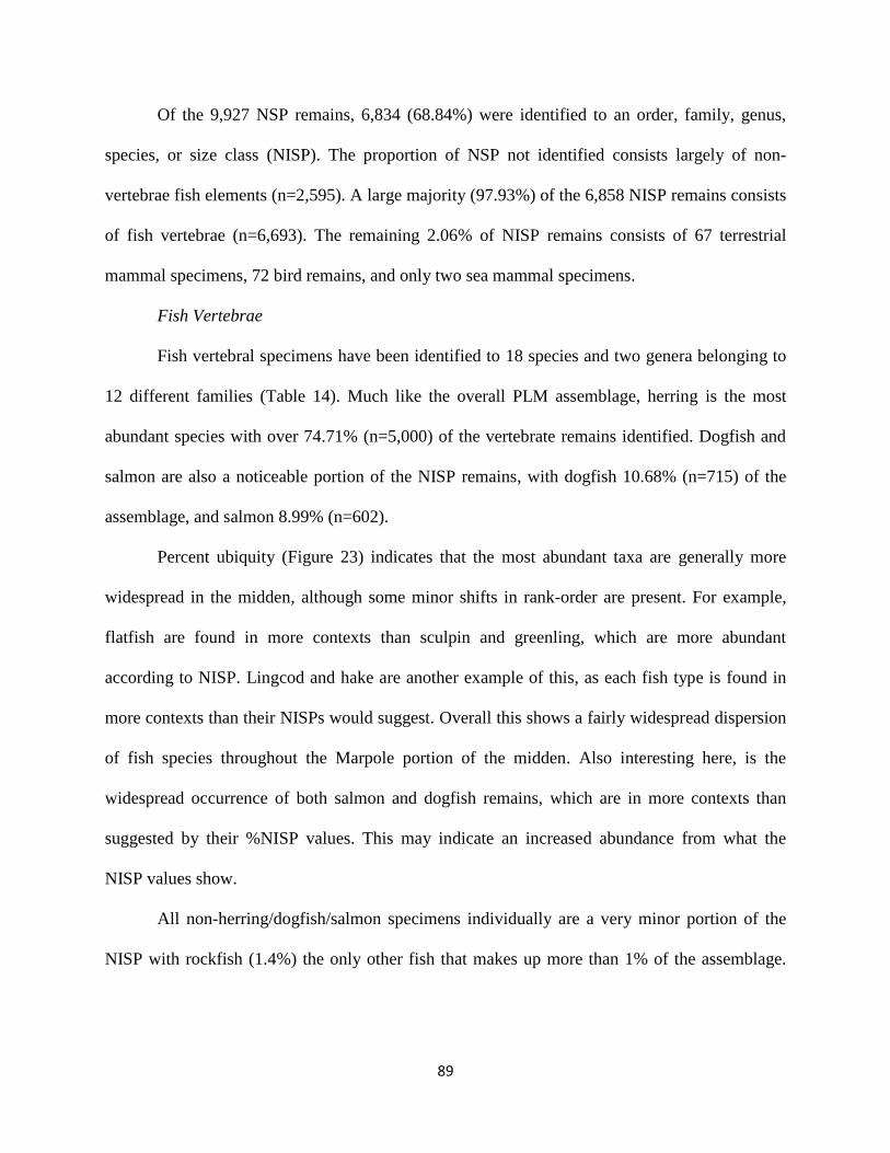
89
Of the 9,927 NSP remains, 6,834 (68.84%) were identified to an order, family, genus,
species, or size class (NISP). The proportion of NSP not identified consists largely of non-
vertebrae fish elements (n=2,595). A large majority (97.93%) of the 6,858 NISP remains consists
of fish vertebrae (n=6,693). The remaining 2.06% of NISP remains consists of 67 terrestrial
mammal specimens, 72 bird remains, and only two sea mammal specimens.
Fish Vertebrae
Fish vertebral specimens have been identified to 18 species and two genera belonging to
12 different families (Table 14). Much like the overall PLM assemblage, herring is the most
abundant species with over 74.71% (n=5,000) of the vertebrate remains identified. Dogfish and
salmon are also a noticeable portion of the NISP remains, with dogfish 10.68% (n=715) of the
assemblage, and salmon 8.99% (n=602).
Percent ubiquity (Figure 23) indicates that the most abundant taxa are generally more
widespread in the midden, although some minor shifts in rank-order are present. For example,
flatfish are found in more contexts than sculpin and greenling, which are more abundant
according to NISP. Lingcod and hake are another example of this, as each fish type is found in
more contexts than their NISPs would suggest. Overall this shows a fairly widespread dispersion
of fish species throughout the Marpole portion of the midden. Also interesting here, is the
widespread occurrence of both salmon and dogfish remains, which are in more contexts than
suggested by their %NISP values. This may indicate an increased abundance from what the
NISP values show.
All non-herring/dogfish/salmon specimens individually are a very minor portion of the
NISP with rockfish (1.4%) the only other fish that makes up more than 1% of the assemblage.
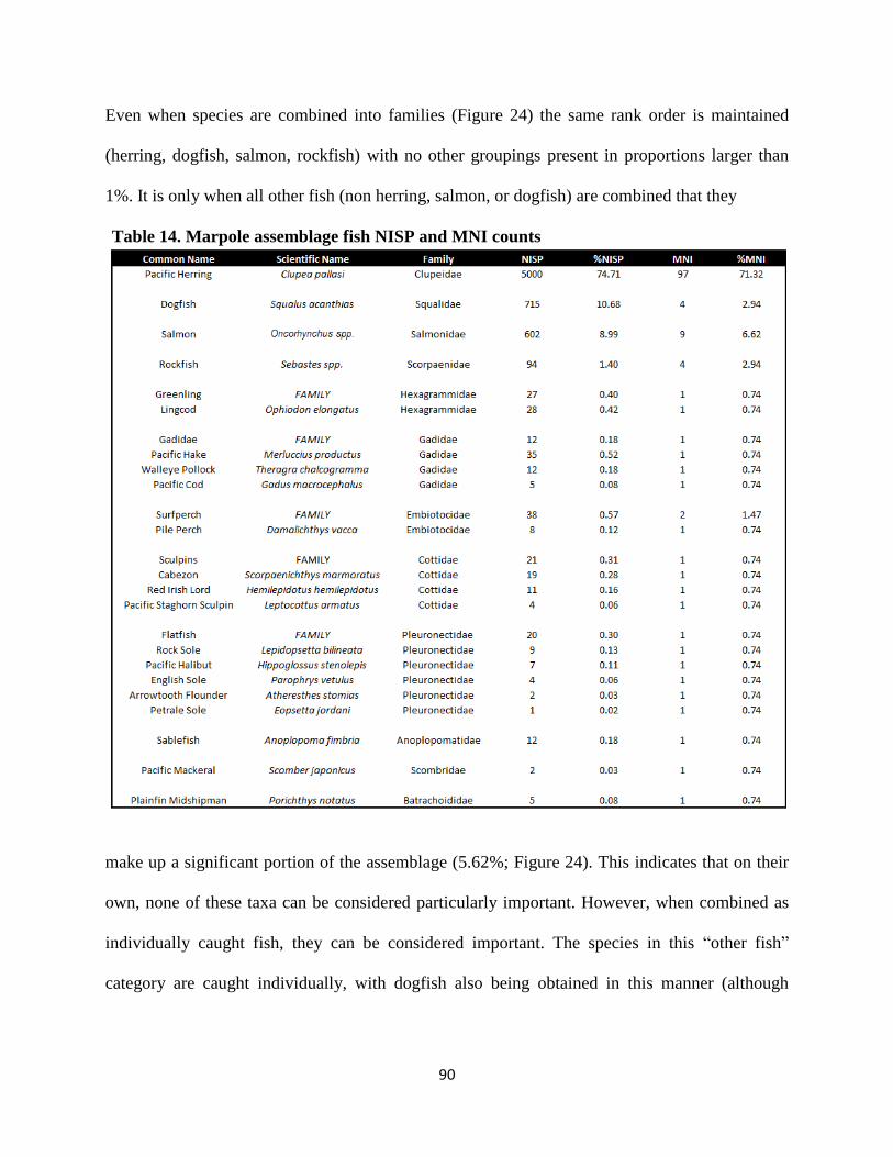
90
Even when species are combined into families (Figure 24) the same rank order is maintained
(herring, dogfish, salmon, rockfish) with no other groupings present in proportions larger than
1%. It is only when all other fish (non herring, salmon, or dogfish) are combined that they
Table 14. Marpole assemblage fish NISP and MNI counts
make up a significant portion of the assemblage (5.62%; Figure 24). This indicates that on their
own, none of these taxa can be considered particularly important. However, when combined as
individually caught fish, they can be considered important. The species in this “other fish”
category are caught individually, with dogfish also being obtained in this manner (although
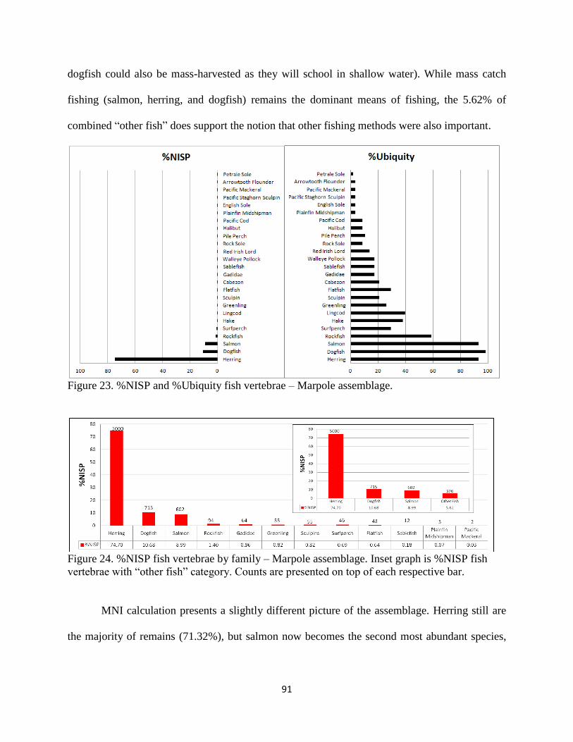
91
dogfish could also be mass-harvested as they will school in shallow water). While mass catch
fishing (salmon, herring, and dogfish) remains the dominant means of fishing, the 5.62% of
combined “other fish” does support the notion that other fishing methods were also important.
Figure 23. %NISP and %Ubiquity fish vertebrae – Marpole assemblage.
Figure 24. %NISP fish vertebrae by family – Marpole assemblage. Inset graph is %NISP fish
vertebrae with “other fish” category. Counts are presented on top of each respective bar.
MNI calculation presents a slightly different picture of the assemblage. Herring still are
the majority of remains (71.32%), but salmon now becomes the second most abundant species,
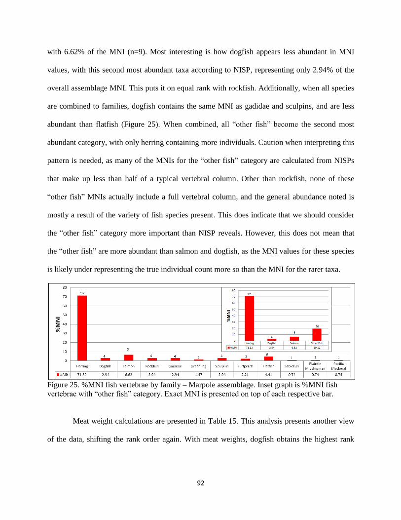
92
with 6.62% of the MNI (n=9). Most interesting is how dogfish appears less abundant in MNI
values, with this second most abundant taxa according to NISP, representing only 2.94% of the
overall assemblage MNI. This puts it on equal rank with rockfish. Additionally, when all species
are combined to families, dogfish contains the same MNI as gadidae and sculpins, and are less
abundant than flatfish (Figure 25). When combined, all “other fish” become the second most
abundant category, with only herring containing more individuals. Caution when interpreting this
pattern is needed, as many of the MNIs for the “other fish” category are calculated from NISPs
that make up less than half of a typical vertebral column. Other than rockfish, none of these
“other fish” MNIs actually include a full vertebral column, and the general abundance noted is
mostly a result of the variety of fish species present. This does indicate that we should consider
the “other fish” category more important than NISP reveals. However, this does not mean that
the “other fish” are more abundant than salmon and dogfish, as the MNI values for these species
is likely under representing the true individual count more so than the MNI for the rarer taxa.
Figure 25. %MNI fish vertebrae by family – Marpole assemblage. Inset graph is %MNI fish
vertebrae with “other fish” category. Exact MNI is presented on top of each respective bar.
Meat weight calculations are presented in Table 15. This analysis presents another view
of the data, shifting the rank order again. With meat weights, dogfish obtains the highest rank
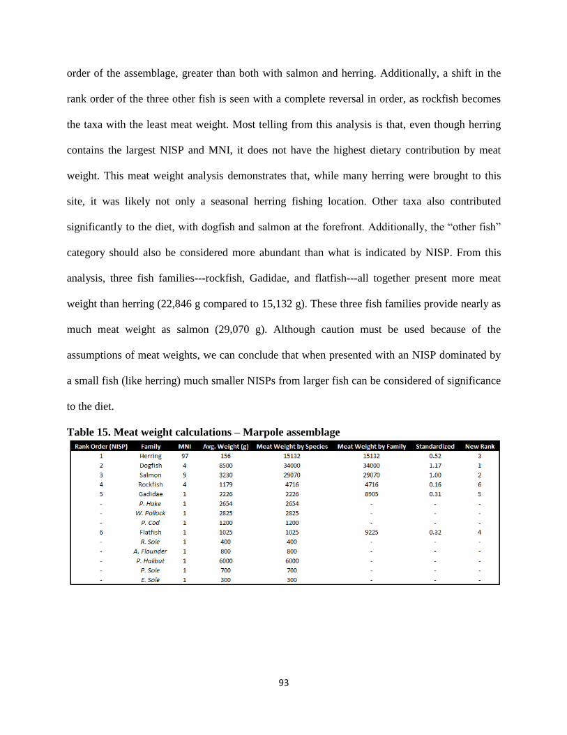
93
order of the assemblage, greater than both with salmon and herring. Additionally, a shift in the
rank order of the three other fish is seen with a complete reversal in order, as rockfish becomes
the taxa with the least meat weight. Most telling from this analysis is that, even though herring
contains the largest NISP and MNI, it does not have the highest dietary contribution by meat
weight. This meat weight analysis demonstrates that, while many herring were brought to this
site, it was likely not only a seasonal herring fishing location. Other taxa also contributed
significantly to the diet, with dogfish and salmon at the forefront. Additionally, the “other fish”
category should also be considered more abundant than what is indicated by NISP. From this
analysis, three fish families---rockfish, Gadidae, and flatfish---all together present more meat
weight than herring (22,846 g compared to 15,132 g). These three fish families provide nearly as
much meat weight as salmon (29,070 g). Although caution must be used because of the
assumptions of meat weights, we can conclude that when presented with an NISP dominated by
a small fish (like herring) much smaller NISPs from larger fish can be considered of significance
to the diet.
Table 15. Meat weight calculations – Marpole assemblage
94
Overall these analyses indicate a general diversity of many different fish taxa.
Proportions of individual taxa shift depending on the technique utilized to examine the data. For
NISP, we see a greater proportion of herring remains, with dogfish and salmon also obtaining
noticeable counts. All “other fish” taxa are minimally represented, only when combined do we
find larger proportions. Looking strictly at NISP, we would consider the site to be herring
dominated, with dogfish, salmon, and “other fish” being considered of secondary use. MNI
results present a different view of the data. Herring maintains the top of the rank order, but
salmon now becomes the second most abundant taxa, with dogfish dropping rank to be equal
with combined families of the seemingly less important “other fish.” Meat weights present us
with yet another view of the data, completely shifting the abundance ranking with herring
dropping significantly and salmon (rank order second), dogfish (rank order first), and even
combined categories of rockfish, cod, and flatfish overtaking herring. These meat weights
indicate that, even with smaller portions of NISP, taxa of the right size can be considered more
abundant than a greater NISP of a small taxon.
This general shifting of rank orders through each method suggests that no one taxon is
dominant in this assemblage. If a single taxon is dominating the assemblage it should maintain
that dominance across each of the methods and no such taxon does this. NISP counts should be
viewed as the fundamental quantification of the data, but we have to consider the patterns that
other analyses indicate as well. A general importance of herring, salmon, and dogfish is noted
overall. However, when combined, “other fish” also display a significant abundance in this
assemblage. Thus, I conclude that a diversity of fish species were important to this Marpole
assemblage, with no overall specialization on any taxa.
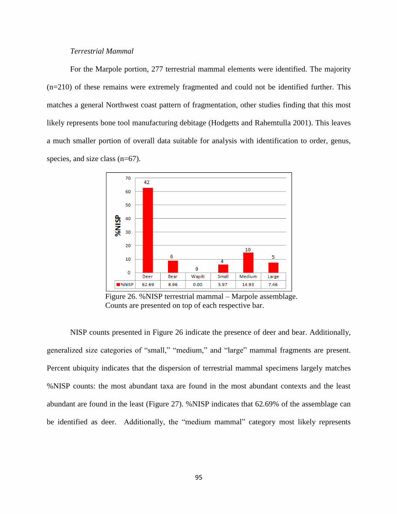
95
Terrestrial Mammal
For the Marpole portion, 277 terrestrial mammal elements were identified. The majority
(n=210) of these remains were extremely fragmented and could not be identified further. This
matches a general Northwest coast pattern of fragmentation, other studies finding that this most
likely represents bone tool manufacturing debitage (Hodgetts and Rahemtulla 2001). This leaves
a much smaller portion of overall data suitable for analysis with identification to order, genus,
species, and size class (n=67).
Figure 26. %NISP terrestrial mammal – Marpole assemblage.
Counts are presented on top of each respective bar.
NISP counts presented in Figure 26 indicate the presence of deer and bear. Additionally,
generalized size categories of “small,” “medium,” and “large” mammal fragments are present.
Percent ubiquity indicates that the dispersion of terrestrial mammal specimens largely matches
%NISP counts: the most abundant taxa are found in the most abundant contexts and the least
abundant are found in the least (Figure 27). %NISP indicates that 62.69% of the assemblage can
be identified as deer. Additionally, the “medium mammal” category most likely represents

96
fragmented deer remains. However, this cannot be independently verified, so caution is observed
with this notion.
Figure 27. %NISP and %Ubiquity terrestrial mammal - Marpole assemblage
MNI calculations present us with two deer and one bear. Bear remains consist of only one
distinctive element (a left humerus fragment). Deer remains consisted mostly of elements which
could not be sided due to fragmentation. However, several elements indicate at least one fully
grown individual, most interestingly by the presence of both left and right skull fragments
(frontals) with fractured antler bases. The other individual comes from an unfused femoral head,
indicative of a juvenile animal. Given the general fractured and degraded nature of the terrestrial
mammal remains these MNI counts are most likely under representing actual amounts of animals
(Marshall and Pigrim 1993).
Given the nature of the remains, very little can be gathered from the terrestrial mammals.
It does appear that deer was the most important taxon. Additionally, we can conclude that
terrestrial mammal elements were most likely being used as raw material for tool making due to
the highly fragmented nature of their remains at the site.

97
Sea Mammal
Making up just .03% of the assemblage, sea mammal remains are rare within the
assemblage. Overall three specimens have been identified as sea mammal (NSP). One specimen
could not be identified in more detail, while two specimens are identified, one as Harbor seal
(Phoca vitulina), and the other specimen in the size category of “large sea mammal.” All remains
were degraded and positive identifications on exact element could only be identified for the one
Harbor seal element (a distal rib fragment). Due to the rarity of these remains, it is concluded
that sea mammal was a very minor part of the diet.
Bird
The Marpole bird NSP is made up of 124 specimens. Fifty-two of these specimens could
not be identified, which leaves 72 specimens comprising the NISP. Varying levels of
identification were used for the bird remains with two orders, three families, one genus, and five
species making up the NISP counts.
Figure 28. %NISP bird – Marpole assemblage. Counts are presented on top of each bar.
Figure 28 presents NISP proportions and counts. This shows a fairly diverse assemblage
with Charadriiformes (water/sea birds) as the most abundant taxon. This makes sense, given the
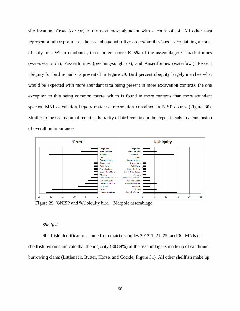
98
site location. Crow (corvus) is the next most abundant with a count of 14. All other taxa
represent a minor portion of the assemblage with five orders/families/species containing a count
of only one. When combined, three orders cover 62.5% of the assemblage: Charadriiformes
(water/sea birds), Passeriformes (perching/songbirds), and Anseriformes (waterfowl). Percent
ubiquity for bird remains is presented in Figure 29. Bird percent ubiquity largely matches what
would be expected with more abundant taxa being present in more excavation contexts, the one
exception to this being common murre, which is found in more contexts than more abundant
species. MNI calculation largely matches information contained in NISP counts (Figure 30).
Similar to the sea mammal remains the rarity of bird remains in the deposit leads to a conclusion
of overall unimportance.
Figure 29. %NISP and %Ubiquity bird – Marpole assemblage
Shellfish
Shellfish identifications come from matrix samples 2012-1, 21, 29, and 30. MNIs of
shellfish remains indicate that the majority (80.89%) of the assemblage is made up of sand/mud
burrowing clams (Littleneck, Butter, Horse, and Cockle; Figure 31). All other shellfish make up
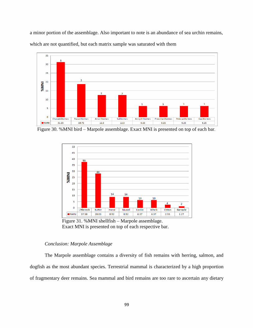
99
a minor portion of the assemblage. Also important to note is an abundance of sea urchin remains,
which are not quantified, but each matrix sample was saturated with them
Figure 30. %MNI bird – Marpole assemblage. Exact MNI is presented on top of each bar.
Figure 31. %MNI shellfish – Marpole assemblage.
Exact MNI is presented on top of each respective bar.
Conclusion: Marpole Assemblage
The Marpole assemblage contains a diversity of fish remains with herring, salmon, and
dogfish as the most abundant species. Terrestrial mammal is characterized by a high proportion
of fragmentary deer remains. Sea mammal and bird remains are too rare to ascertain any dietary
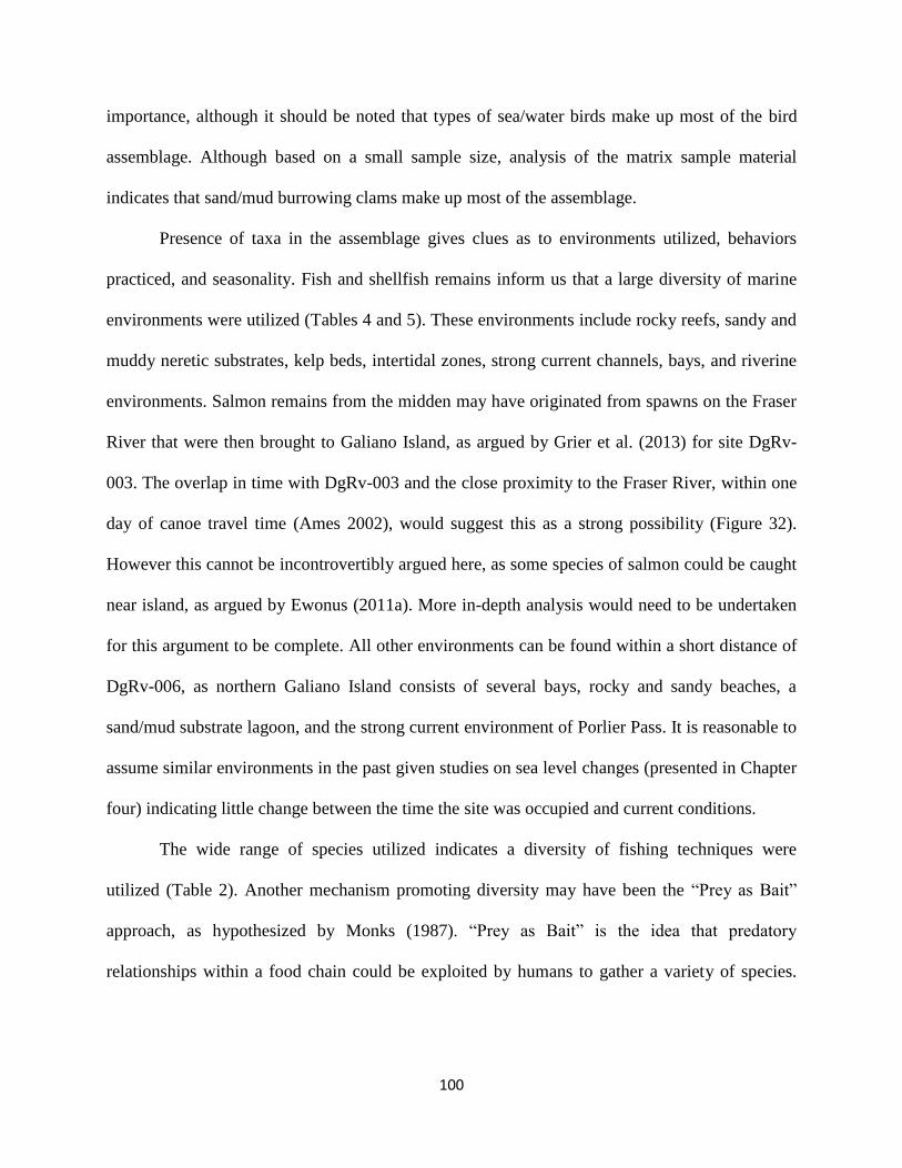
100
importance, although it should be noted that types of sea/water birds make up most of the bird
assemblage. Although based on a small sample size, analysis of the matrix sample material
indicates that sand/mud burrowing clams make up most of the assemblage.
Presence of taxa in the assemblage gives clues as to environments utilized, behaviors
practiced, and seasonality. Fish and shellfish remains inform us that a large diversity of marine
environments were utilized (Tables 4 and 5). These environments include rocky reefs, sandy and
muddy neretic substrates, kelp beds, intertidal zones, strong current channels, bays, and riverine
environments. Salmon remains from the midden may have originated from spawns on the Fraser
River that were then brought to Galiano Island, as argued by Grier et al. (2013) for site DgRv-
003. The overlap in time with DgRv-003 and the close proximity to the Fraser River, within one
day of canoe travel time (Ames 2002), would suggest this as a strong possibility (Figure 32).
However this cannot be incontrovertibly argued here, as some species of salmon could be caught
near island, as argued by Ewonus (2011a). More in-depth analysis would need to be undertaken
for this argument to be complete. All other environments can be found within a short distance of
DgRv-006, as northern Galiano Island consists of several bays, rocky and sandy beaches, a
sand/mud substrate lagoon, and the strong current environment of Porlier Pass. It is reasonable to
assume similar environments in the past given studies on sea level changes (presented in Chapter
four) indicating little change between the time the site was occupied and current conditions.
The wide range of species utilized indicates a diversity of fishing techniques were
utilized (Table 2). Another mechanism promoting diversity may have been the “Prey as Bait”
approach, as hypothesized by Monks (1987). “Prey as Bait” is the idea that predatory
relationships within a food chain could be exploited by humans to gather a variety of species.
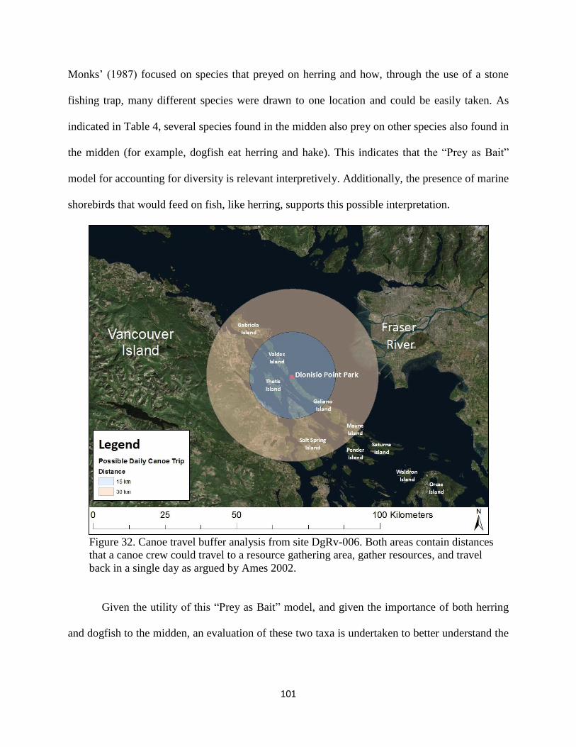
101
Monks’ (1987) focused on species that preyed on herring and how, through the use of a stone
fishing trap, many different species were drawn to one location and could be easily taken. As
indicated in Table 4, several species found in the midden also prey on other species also found in
the midden (for example, dogfish eat herring and hake). This indicates that the “Prey as Bait”
model for accounting for diversity is relevant interpretively. Additionally, the presence of marine
shorebirds that would feed on fish, like herring, supports this possible interpretation.
Figure 32. Canoe travel buffer analysis from site DgRv-006. Both areas contain distances
that a canoe crew could travel to a resource gathering area, gather resources, and travel
back in a single day as argued by Ames 2002.
Given the utility of this “Prey as Bait” model, and given the importance of both herring
and dogfish to the midden, an evaluation of these two taxa is undertaken to better understand the
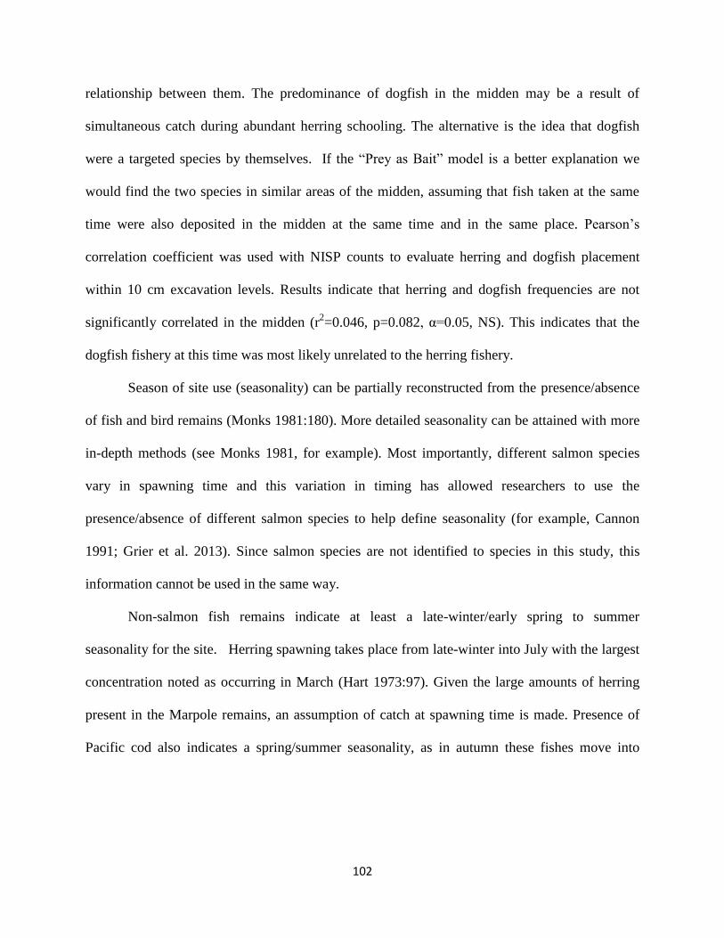
102
relationship between them. The predominance of dogfish in the midden may be a result of
simultaneous catch during abundant herring schooling. The alternative is the idea that dogfish
were a targeted species by themselves. If the “Prey as Bait” model is a better explanation we
would find the two species in similar areas of the midden, assuming that fish taken at the same
time were also deposited in the midden at the same time and in the same place. Pearson’s
correlation coefficient was used with NISP counts to evaluate herring and dogfish placement
within 10 cm excavation levels. Results indicate that herring and dogfish frequencies are not
significantly correlated in the midden (r2=0.046, p=0.082, α=0.05, NS). This indicates that the
dogfish fishery at this time was most likely unrelated to the herring fishery.
Season of site use (seasonality) can be partially reconstructed from the presence/absence
of fish and bird remains (Monks 1981:180). More detailed seasonality can be attained with more
in-depth methods (see Monks 1981, for example). Most importantly, different salmon species
vary in spawning time and this variation in timing has allowed researchers to use the
presence/absence of different salmon species to help define seasonality (for example, Cannon
1991; Grier et al. 2013). Since salmon species are not identified to species in this study, this
information cannot be used in the same way.
Non-salmon fish remains indicate at least a late-winter/early spring to summer
seasonality for the site. Herring spawning takes place from late-winter into July with the largest
concentration noted as occurring in March (Hart 1973:97). Given the large amounts of herring
present in the Marpole remains, an assumption of catch at spawning time is made. Presence of
Pacific cod also indicates a spring/summer seasonality, as in autumn these fishes move into

103
deeper water where spawning takes place, while in spring they occupy shallower, easier to catch
depths (Cannon 1991:58; Hart 1973:223).
Bird remains are largely unhelpful for the identification of seasonality, as the majority of
remains identified to species are available year round. The one exception to this is the presence
of Brandt’s Cormorant (n=2). This species of bird winters in British Columbia, following a
period of breeding around California (Baron and Acorn 1997:39). Given the low overall count of
Brant’s Cormorant we must be careful with drawing to much from this (Monks 1981:182-183),
but this presence lends support to the claim of at least a late-winter presence at the site.
Overall species presence/absence indicates a late-winter to early summer occupation for
site DgRv-006. However, this should not be interpreted as a lack of fall/winter presence. It is
only once we have gained species level identification of salmon that we can have a more
complete picture of seasonality. If salmon remains are similar to DgRv-003, we could conclude a
fall/winter presence with more confidence.
Late Period Assemblage
The Late Period assemblage is made up of 7,291 individual specimens with 462 (6.34%)
unidentifiable. The remaining 6,829 specimens have been identified to the broad NSP categories
(Figure 33). The majority of the NSP count consists of fish vertebral elements (67.43%;
n=4,605) and fish head/spines/fin/tail specimens (19.64%, n=1,341). Terrestrial mammal also
makes up a considerable portion of the NSP identified remains (10.41%; n=711). Sediment
excavated is notably smaller than the Marpole assemblage at 3,118.5 liters.

104
Of the NSP remains, 68.14% were identified to an order, family, genus, species, or size
class, and are considered the NISP remains (n=4,653). Of the remains not identified to NISP, fish
elements and fragmentary terrestrial mammal remains make up the majority of the unidentified
(n=1,341, 61.63% of the unidentified NSP; n=565, 26% of the unidentified). Similar to the
Marpole assemblage, the majority of the identified NISP consists of fish vertebral elements
(94.84% of the NISP, n=4413).
Figure 33. Pie chart of NSP remains – Late Period assemblage. Category,
Count, Proportion. NSP=6829.
Fish Vertebrae
Fifteen different species and two genera belonging to 12 families make up the Late
Period fish assemblage (Table 16). Matching the pattern noted above for both the overall midden
data, and the Marpole data, herring NISP counts are greater than all other taxa (71.20%), with
dogfish (15.57%) and salmon (7.07%) also occurring in significant proportions. All other taxa
individually make up very minor proportions of the NISP, with rockfish at 1.84% the most

105
abundant. Combined into their respective families, the same pattern of herring abundance, with
dogfish and salmon in the second and third rank order, remains (Figure 34). Similar to the
Marpole assemblage, it is only when all non-herring/salmon/dogfish are combined that they
make a sizable proportion of the assemblage. When combined, the “other fish” category is only
slightly less abundant than salmon, indicating a greater abundance for these taxa compared to
when these are listed individually.
Table 16. Late Period assemblage fish NISP and MNI count
Percent ubiquity indicates that the most abundant species are also found in the most
contexts with only minor shifts in rank order from the NISP counts (Figure 35). Similar to the
Marpole assemblage, this indicates widespread distribution of taxa across the midden rather than
specific clumping of same species in any one area. Dogfish, salmon, and rockfish percent
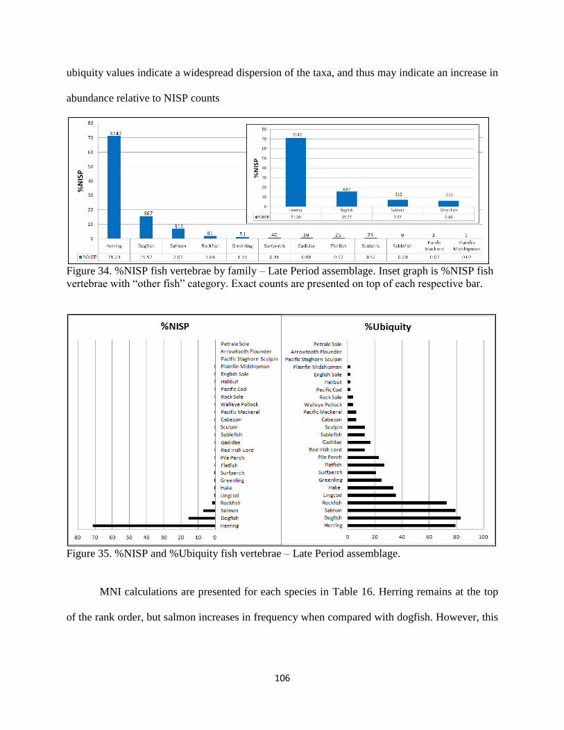
106
ubiquity values indicate a widespread dispersion of the taxa, and thus may indicate an increase in
abundance relative to NISP counts
Figure 34. %NISP fish vertebrae by family – Late Period assemblage. Inset graph is %NISP fish
vertebrae with “other fish” category. Exact counts are presented on top of each respective bar.
Figure 35. %NISP and %Ubiquity fish vertebrae – Late Period assemblage.
MNI calculations are presented for each species in Table 16. Herring remains at the top
of the rank order, but salmon increases in frequency when compared with dogfish. However, this

107
is only by one individual. All other patterns in the data are simply replicating the results seen in
the %NISP. When combined into the families we find several interesting changes from the NISP
(Figure 36). Dogfish rank order drops compared to the NISP results, as Gadidae and flatfish both
present the same MNI. This all indicates an increase in prevalence for the combined “other fish”.
Like with the Marpole assemblage, caution is needed as only one of the “other fish” has an NISP
value that makes up more than half of a single vertebral column.
Meat weights present another view of this data, and indicate that herring is not as
proportionally abundant in the Late Period deposits as NISP and MNI indicate (Table 17).
Herring, dogfish, and salmon maintain the top three ranks after meat weights are calculated,
Figure 36. %MNI fish vertebrae by family – Late Period assemblage. Inset graph is %MNI fish
vertebrae with “other fish” category. Exact MNI is presented on top of each respective bar.
but dogfish becomes the most abundant taxon. Additionally herring meat weight equals only
slightly more than half that of salmon. This indicates a large drop in prevalence for the herring
taxon overall. Another interesting trend seen in the meat weights is an increase in abundance of
the other fish families. Although rockfish drops in rank order to sixth, this is mainly due to large
increases seen in the Gadidae and flatfish families. Gadids in particular rise in abundance with a
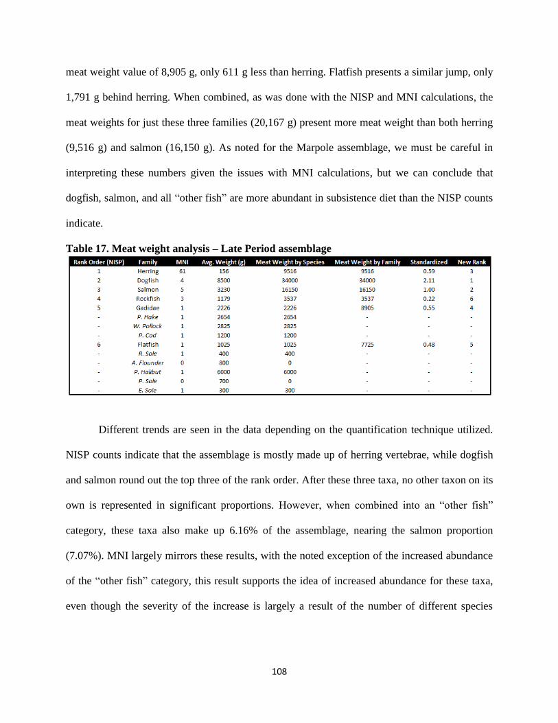
108
meat weight value of 8,905 g, only 611 g less than herring. Flatfish presents a similar jump, only
1,791 g behind herring. When combined, as was done with the NISP and MNI calculations, the
meat weights for just these three families (20,167 g) present more meat weight than both herring
(9,516 g) and salmon (16,150 g). As noted for the Marpole assemblage, we must be careful in
interpreting these numbers given the issues with MNI calculations, but we can conclude that
dogfish, salmon, and all “other fish” are more abundant in subsistence diet than the NISP counts
indicate.
Table 17. Meat weight analysis – Late Period assemblage
Different trends are seen in the data depending on the quantification technique utilized.
NISP counts indicate that the assemblage is mostly made up of herring vertebrae, while dogfish
and salmon round out the top three of the rank order. After these three taxa, no other taxon on its
own is represented in significant proportions. However, when combined into an “other fish”
category, these taxa also make up 6.16% of the assemblage, nearing the salmon proportion
(7.07%). MNI largely mirrors these results, with the noted exception of the increased abundance
of the “other fish” category, this result supports the idea of increased abundance for these taxa,
even though the severity of the increase is largely a result of the number of different species

109
present in the category. Results of meat weight analyses present a completely different view of
the data from what NISP and MNI show. Abundance of herring drops when considering meat
weight, with an increase in rank order for both dogfish (first) as well as the combined “other
fish” (second; with only three families considered).
Similar to the Marpole assemblage, the various rank orders across different methods of
quantification do not support the notion of specialization in any one fish. We can conclude that a
diverse array of taxa were important to the subsistence in this time period. Herring and dogfish
are the most abundant taxa, but salmon and the combined “other fish” are also significant.
Terrestrial Mammal
The terrestrial mammal component for this time period consists of 711 individual
specimens. The majority of these specimens, 565 (79.47%), are unidentifiable fragments. This
leaves 146 specimens for further evaluation.
Figure 37. %NISP terrestrial mammal – Late Period assemblage.
Counts are presented on top of each respective bar.
Figure 37 presents proportions of NISP with a species rank order of deer, wapiti, and
bear. Much of the assemblage is only identified as small, medium, or large mammal fragments.
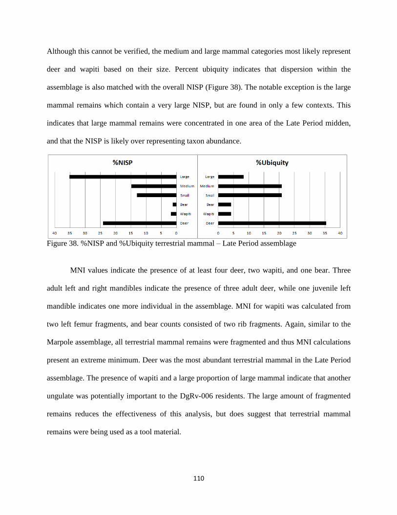
110
Although this cannot be verified, the medium and large mammal categories most likely represent
deer and wapiti based on their size. Percent ubiquity indicates that dispersion within the
assemblage is also matched with the overall NISP (Figure 38). The notable exception is the large
mammal remains which contain a very large NISP, but are found in only a few contexts. This
indicates that large mammal remains were concentrated in one area of the Late Period midden,
and that the NISP is likely over representing taxon abundance.
Figure 38. %NISP and %Ubiquity terrestrial mammal – Late Period assemblage
MNI values indicate the presence of at least four deer, two wapiti, and one bear. Three
adult left and right mandibles indicate the presence of three adult deer, while one juvenile left
mandible indicates one more individual in the assemblage. MNI for wapiti was calculated from
two left femur fragments, and bear counts consisted of two rib fragments. Again, similar to the
Marpole assemblage, all terrestrial mammal remains were fragmented and thus MNI calculations
present an extreme minimum. Deer was the most abundant terrestrial mammal in the Late Period
assemblage. The presence of wapiti and a large proportion of large mammal indicate that another
ungulate was potentially important to the DgRv-006 residents. The large amount of fragmented
remains reduces the effectiveness of this analysis, but does suggest that terrestrial mammal
remains were being used as a tool material.
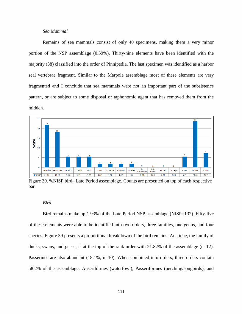
111
Sea Mammal
Remains of sea mammals consist of only 40 specimens, making them a very minor
portion of the NSP assemblage (0.59%). Thirty-nine elements have been identified with the
majority (38) classified into the order of Pinnipedia. The last specimen was identified as a harbor
seal vertebrae fragment. Similar to the Marpole assemblage most of these elements are very
fragmented and I conclude that sea mammals were not an important part of the subsistence
pattern, or are subject to some disposal or taphonomic agent that has removed them from the
midden.
Figure 39. %NISP bird– Late Period assemblage. Counts are presented on top of each respective
bar.
Bird
Bird remains make up 1.93% of the Late Period NSP assemblage (NISP=132). Fifty-five
of these elements were able to be identified into two orders, three families, one genus, and four
species. Figure 39 presents a proportional breakdown of the bird remains. Anatidae, the family of
ducks, swans, and geese, is at the top of the rank order with 21.82% of the assemblage (n=12).
Passerines are also abundant (18.1%, n=10). When combined into orders, three orders contain
58.2% of the assemblage: Anseriformes (waterfowl), Passeriformes (perching/songbirds), and
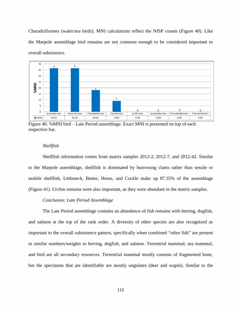
112
Charadriiformes (water/sea birds). MNI calculations reflect the NISP counts (Figure 40). Like
the Marpole assemblage bird remains are not common enough to be considered important to
overall subsistence.
Figure 40. %MNI bird – Late Period assemblage. Exact MNI is presented on top of each
respective bar.
Shellfish
Shellfish information comes from matrix samples 2012-2, 2012-7, and 2012-42. Similar
to the Marpole assemblage, shellfish is dominated by burrowing clams rather than sessile or
mobile shellfish, Littleneck, Butter, Horse, and Cockle make up 87.35% of the assemblage
(Figure 41). Urchin remains were also important, as they were abundant in the matrix samples.
Conclusion: Late Period Assemblage
The Late Period assemblage contains an abundance of fish remains with herring, dogfish,
and salmon at the top of the rank order. A diversity of other species are also recognized as
important to the overall subsistence pattern, specifically when combined “other fish” are present
in similar numbers/weights to herring, dogfish, and salmon. Terrestrial mammal, sea mammal,
and bird are all secondary resources. Terrestrial mammal mostly consists of fragmented bone,
but the specimens that are identifiable are mostly ungulates (deer and wapiti). Similar to the
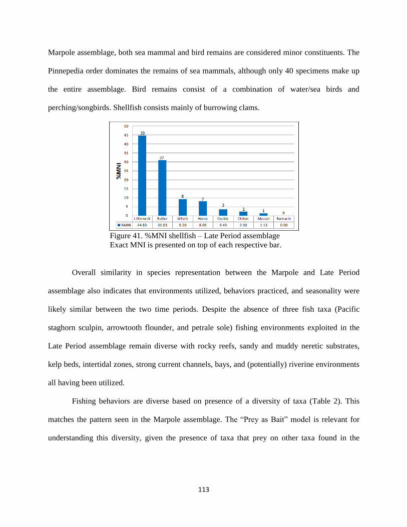
113
Marpole assemblage, both sea mammal and bird remains are considered minor constituents. The
Pinnepedia order dominates the remains of sea mammals, although only 40 specimens make up
the entire assemblage. Bird remains consist of a combination of water/sea birds and
perching/songbirds. Shellfish consists mainly of burrowing clams.
Figure 41. %MNI shellfish – Late Period assemblage
Exact MNI is presented on top of each respective bar.
Overall similarity in species representation between the Marpole and Late Period
assemblage also indicates that environments utilized, behaviors practiced, and seasonality were
likely similar between the two time periods. Despite the absence of three fish taxa (Pacific
staghorn sculpin, arrowtooth flounder, and petrale sole) fishing environments exploited in the
Late Period assemblage remain diverse with rocky reefs, sandy and muddy neretic substrates,
kelp beds, intertidal zones, strong current channels, bays, and (potentially) riverine environments
all having been utilized.
Fishing behaviors are diverse based on presence of a diversity of taxa (Table 2). This
matches the pattern seen in the Marpole assemblage. The “Prey as Bait” model is relevant for
understanding this diversity, given the presence of taxa that prey on other taxa found in the

114
midden. This relationship was again explored for the herring and dogfish taxa. Using Pearson’s
correlation coefficient, dogfish and herring are found to be significantly correlated spatially
(r2=0.26, p=0.0002, α= 0.05). This suggests that herring and dogfish could have been caught
together in a type of “Prey as Bait” subsistence strategy.
Seasonality results from the Marpole portion of the midden are also largely repeated. The
important fish taxa for assigning a late winter/early spring to early summer season of occupation
are all present in the Late assemblage, most importantly herring and Pacific cod. Bird remains
change from the Marpole period, as Brandt’s cormorant is absent in this assemblage. However,
the interpretation remains the same because of the presence of common loon. Common loons
spend summers at fresh-water lakes and winters in coastal environments, which support the
presence of people in winter/early spring at the site (Baron and Acorn 1997:39). This is an
incomplete seasonality estimate however; salmon may provide additional data when analyzed
further (Grier et al. 2013).
Temporal Comparison of Linear Complexity Models
The central question of this study can now be addressed: Do subsistence trends change at
DgRv-006 in relation to changing temporal and social landscapes? Do these changes match what
is expected given the expectations of the linear complexity models? Fish vertebrate remains will
be the only grouping discussed here. Fish remains are the most abundant in both Marpole and
Late Period assemblages and they should reflect what has been proposed as important regional
changes between the Marpole and Late period. According to the linear complexity models
described in earlier chapters, the Marpole component of this assemblage should be dominated by
115
salmon remains (more than half of the assemblage), indicating a specialization in that resource.
In comparison, the Late Period component should contain a more diverse (rich and even)
assemblage. A null hypothesis of no difference is established for the two time periods. If
accepted, we should reject linear complexity models and the interconnection of social and
subsistence change. If the null hypothesis is rejected, this could support the connection of social
and subsistence realms. The manner in which it is rejected determines if the exact regional linear
complexity models should be accepted. If diversity decreases between the two assemblages, than
we still reject the linear complexity model explanation. To evaluate these assemblages according
to the above hypothesis we must take an in-depth look at three lines of data: richness, evenness,
and the importance of salmon.
Richness
Before richness can be evaluated we must first ensure that sample size differences are not
driving taxonomic representation (NTAXA) in each assemblage. In order to evaluate this, a
cumulative frequency graph of NTAXA by fish NISP counts is presented in Figure 42. This is
referred to as the “sampling to redundancy” method (Lyman and Ames 2004; Lyman 2008:143-
144). A sampling to redundancy approach involves identifying when cumulative NTAXA
stabilizes (i.e., no or few new taxa are being added), at this point we can consider sample size
large enough to address richness. The analysis of additional samples or specimens will add little
to taxonomic richness and will simply be adding redundant information, since, a theoretical
maximum taxa richness has already been achieved (Lyman and Ames 2004).
A primary critique of this technique is that the order of accumulation of specimens can
affect where this stabilization occurs (Lepofsky and Lertzman 2005:179-181). This is mitigated

116
by adding contexts randomly, as I have done here. Figure 42a shows that the Marpole
assemblage attains redundancy after 5,260 specimens. In comparison the Late Period assemblage
(Figure 42b) appears to become redundant after 2,462 specimens. Both assemblages are sampled
to redundancy, and thus a comparison of their richness will not be affected substantially by
sample size.
Figure 42a. Sampling to redundancy for richness - Marpole assemblage. Samples (excavation
levels) were randomly added.
Figure 42b. Sampling to redundancy for richness - Late Period assemblage. Samples (excavation
levels) were randomly added.

117
According to the null hypothesis, richness values for both time periods should be similar.
Richness values are slightly different between the two assemblages. The Marpole assemblage
contains 25 different fish species/genus/families, while the Late Period assemblage contains 22
(Table 18). The Marpole assemblage is the richer assemblage, though only by three taxa. The
three taxa that are absent in the Late Period assemblage are rare and only amount to 0.11% of the
Marpole assemblage (n=7).
Table. 18. Comparison of species presence – Marpole and Late Period
Overall, a similar amount of richness is noted for both of the assemblages. This does not
match the linear complexity model expectation that the Late Period should be the richer
assemblage. The similar richness values between the assemblages are consistent with the null
hypothesis.
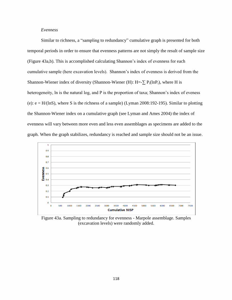
118
Evenness
Similar to richness, a “sampling to redundancy” cumulative graph is presented for both
temporal periods in order to ensure that evenness patterns are not simply the result of sample size
(Figure 43a,b). This is accomplished calculating Shannon’s index of evenness for each
cumulative sample (here excavation levels). Shannon’s index of evenness is derived from the
Shannon-Wiener index of diversity (Shannon-Wiener (H): H=-∑ Pi(lnPi), where H is
heterogeneity, ln is the natural log, and P is the proportion of taxa; Shannon’s index of eveness
(e): e = H/(lnS), where S is the richness of a sample) (Lyman 2008:192-195). Similar to plotting
the Shannon-Wiener index on a cumulative graph (see Lyman and Ames 2004) the index of
evenness will vary between more even and less even assemblages as specimens are added to the
graph. When the graph stabilizes, redundancy is reached and sample size should not be an issue.
Figure 43a. Sampling to redundancy for evenness - Marpole assemblage. Samples
(excavation levels) were randomly added.
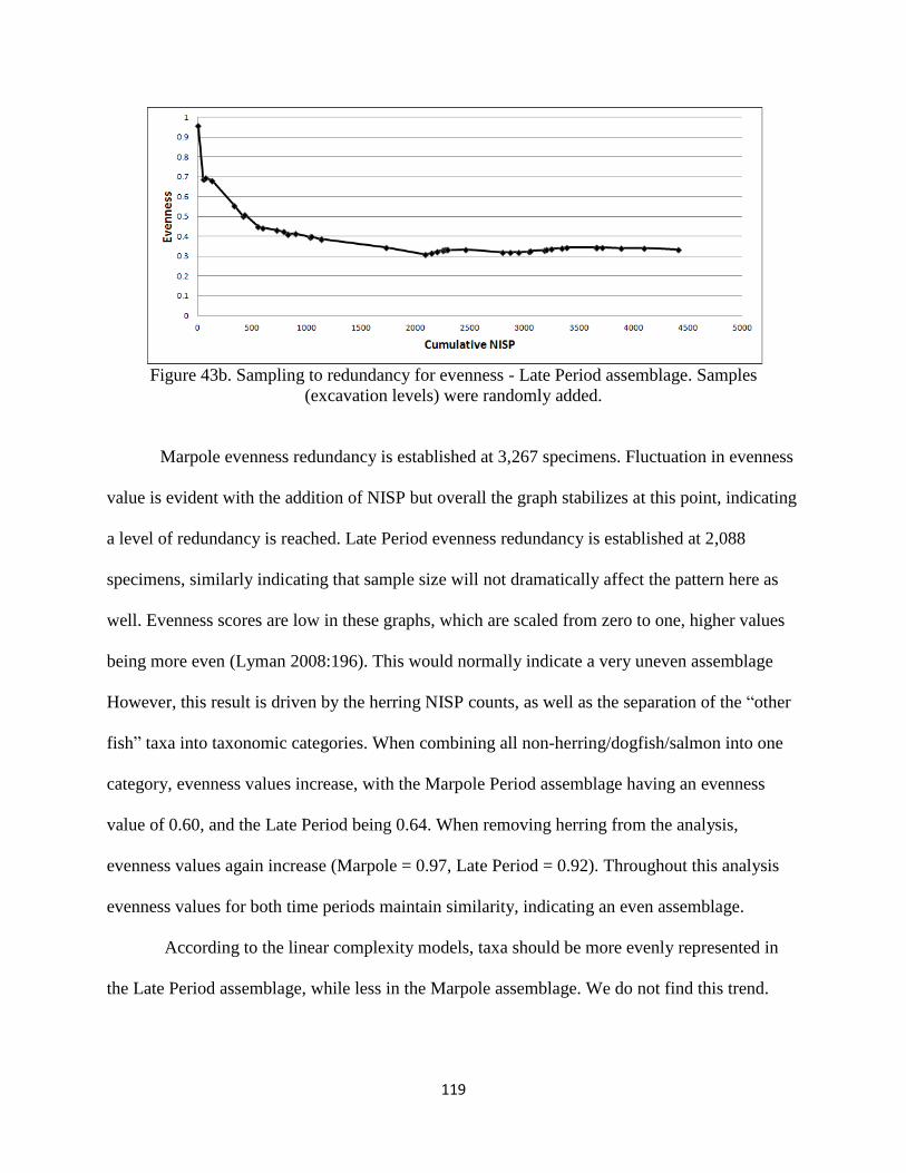
119
Figure 43b. Sampling to redundancy for evenness - Late Period assemblage. Samples
(excavation levels) were randomly added.
Marpole evenness redundancy is established at 3,267 specimens. Fluctuation in evenness
value is evident with the addition of NISP but overall the graph stabilizes at this point, indicating
a level of redundancy is reached. Late Period evenness redundancy is established at 2,088
specimens, similarly indicating that sample size will not dramatically affect the pattern here as
well. Evenness scores are low in these graphs, which are scaled from zero to one, higher values
being more even (Lyman 2008:196). This would normally indicate a very uneven assemblage
However, this result is driven by the herring NISP counts, as well as the separation of the “other
fish” taxa into taxonomic categories. When combining all non-herring/dogfish/salmon into one
category, evenness values increase, with the Marpole Period assemblage having an evenness
value of 0.60, and the Late Period being 0.64. When removing herring from the analysis,
evenness values again increase (Marpole = 0.97, Late Period = 0.92). Throughout this analysis
evenness values for both time periods maintain similarity, indicating an even assemblage.
According to the linear complexity models, taxa should be more evenly represented in
the Late Period assemblage, while less in the Marpole assemblage. We do not find this trend.
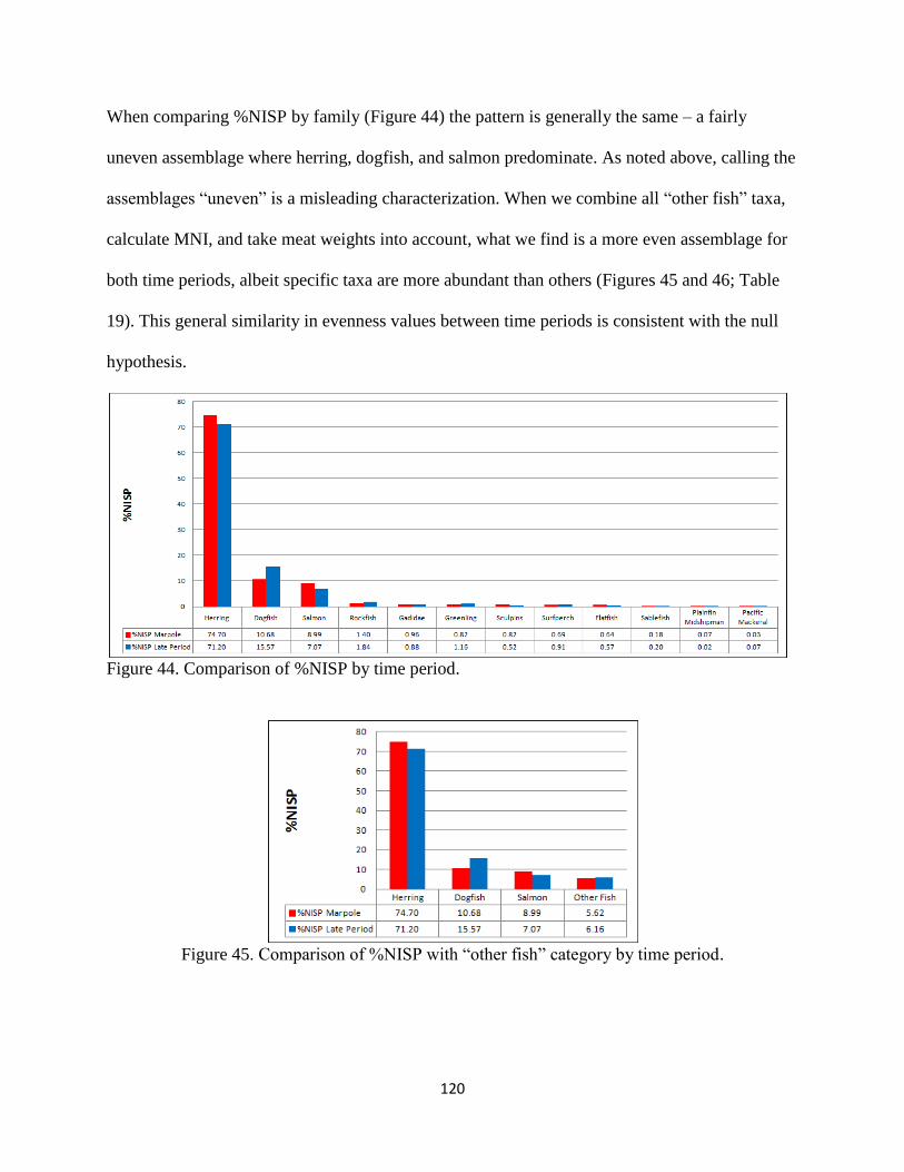
120
When comparing %NISP by family (Figure 44) the pattern is generally the same – a fairly
uneven assemblage where herring, dogfish, and salmon predominate. As noted above, calling the
assemblages “uneven” is a misleading characterization. When we combine all “other fish” taxa,
calculate MNI, and take meat weights into account, what we find is a more even assemblage for
both time periods, albeit specific taxa are more abundant than others (Figures 45 and 46; Table
19). This general similarity in evenness values between time periods is consistent with the null
hypothesis.
Figure 44. Comparison of %NISP by time period.
Figure 45. Comparison of %NISP with “other fish” category by time period.
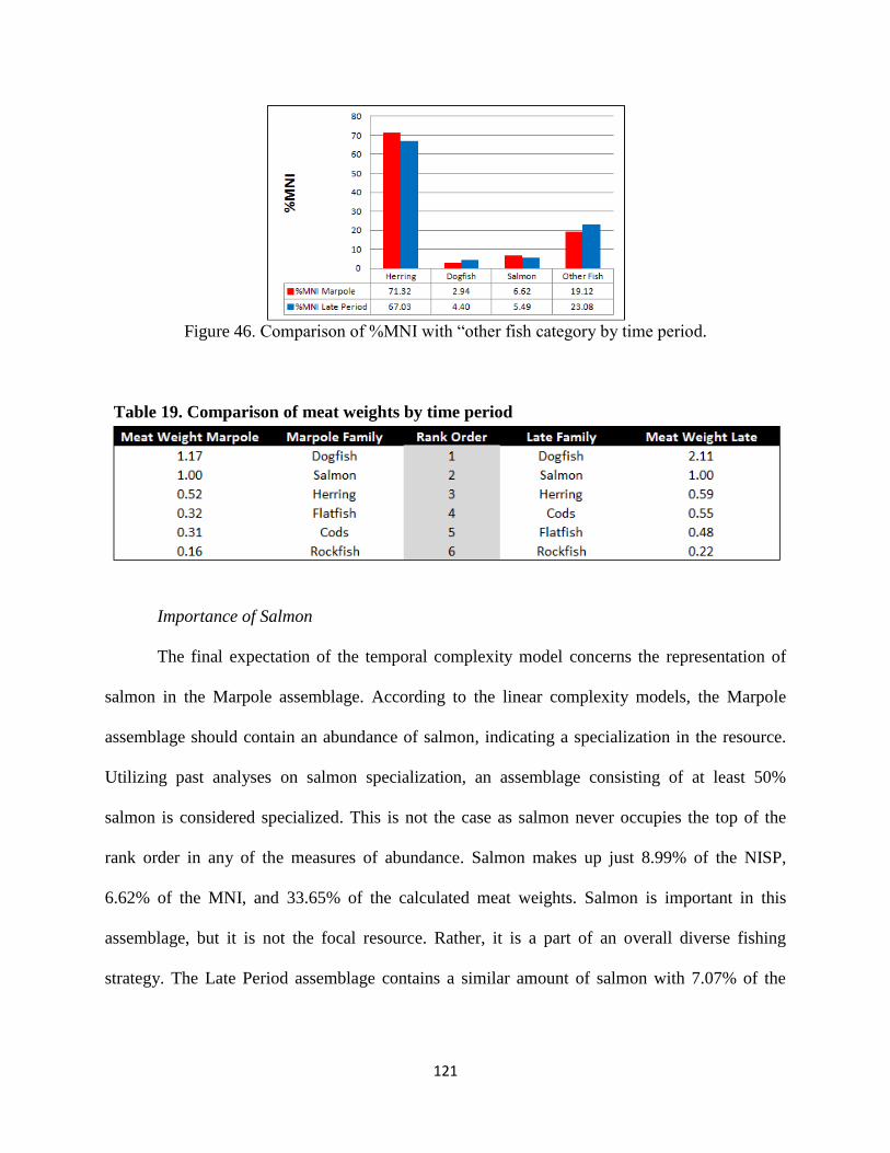
121
Figure 46. Comparison of %MNI with “other fish category by time period.
Table 19. Comparison of meat weights by time period
Importance of Salmon
The final expectation of the temporal complexity model concerns the representation of
salmon in the Marpole assemblage. According to the linear complexity models, the Marpole
assemblage should contain an abundance of salmon, indicating a specialization in the resource.
Utilizing past analyses on salmon specialization, an assemblage consisting of at least 50%
salmon is considered specialized. This is not the case as salmon never occupies the top of the
rank order in any of the measures of abundance. Salmon makes up just 8.99% of the NISP,
6.62% of the MNI, and 33.65% of the calculated meat weights. Salmon is important in this
assemblage, but it is not the focal resource. Rather, it is a part of an overall diverse fishing
strategy. The Late Period assemblage contains a similar amount of salmon with 7.07% of the

122
NISP, 5.49% of the MNI, and 20% of the calculated meat weights. Overall, this indicates a slight
decrease in salmon use overtime. This decrease is not large enough to support a difference
between time periods. This indicates that a shift from a specialized resource to a non-
specialization is not observed, thus, the null hypothesis of no difference is not rejected.
Conclusion
Temporal analysis of the PLM component of site DgRv-006 focused on an evaluation of
taxonomic difference in order to evaluate linear complexity model expectations that propose that
subsistence change is tied to social change (and vice-versa). The models predict a specialized
focus on salmon resources in the Marpole period, with a diversification of the fishing resource in
the Late Period. The analysis presented here found a similarity in richness and evenness values
for both assemblages, indicating continuity of a diverse fishing strategy. Additionally, no
evidence for a specialization in salmon was found in the Marpole period. This indicates that the
null hypothesis of no difference between temporal assemblages is not rejected. Thus, the regional
linear complexity models do not offer a sufficient explanation for faunal patterns at site DgRv-
006.
Overall both assemblages present a similar pattern despite quantification method. This
indicates a general continuity in fishing practices with herring, salmon, and dogfish the most
important individual species. Only minor shifts in the taxa are seen between the time periods,
with salmon use slightly decreasing in the later time period, while the use of dogfish increases.
In addition to continuity seen in the fish remains, all other taxa identified also indicate
general similarity in subsistence through time. Terrestrial mammal remains consist mainly of
deer, with the presence of wapiti in the Late Period the only major difference. Wapiti only
123
consists of three specimens, thus this does not indicate a major change in hunting practices.
Three orders of birds were abundant in both time periods with changes in the overall rank order
and a decrease of lesser orders as the only major temporal changes. For the Marpole period,
Charadriiformes are the most abundant followed by Passeriformes and Anseriformes. In
comparison, the Late Period rank order reverses this with Anseriformes at the top of the rank
order and Charadriiformes at the bottom. Shellfish in both time periods contain an abundance of
sand/mud burrowing species as well as sea urchin remains. A decrease in mussel usage overtime
is the only major temporal change. Lastly, sea mammal remains were extremely rare for both
assemblages. Taken together with the fish remains, these data show an overall pattern of
continuity between the Marpole and Late Period assemblages.

124
CHAPTER EIGHT
BULK SAMPLES AND BIAS TESTING
At this point in this study relative abundances, site seasonality, microenvironments, and an
evaluation of linear complexity model expectations, have been carried out. All conclusions were
based on material dry-screened and collected from 1/8” (3.2 mm) mesh. Several studies (Cannon
1999; Cannon 2000; Casteel 1972, 1976a,b; Grayson 1984:168-172; Hanson 1991, 1995;
McKechnie 2005, 2012; Shaffer 1992; Zohar and Belmaker 2005) have stressed the importance
of screen size bias on the archaeological record. Most important, these studies show that small
fishes (like herring) and smaller individuals of a taxon are often underrepresented in faunal
counts when large mesh sizes are used for recovery. Studies also stress how using column and
bulk samples can help identify this bias by providing finer-grained data.
In this chapter, I report on a screen size study undertaken using bulk matrix samples.
While this was done before analysis of the assemblage, I report on it here because it was
determined that major patterns were not affected by screen size. Seven two-liter samples were
analyzed. Four are located in the Marpole portion, and three from the Late Period. Each two liter
sample was dry sieved through a series of nested screens (1/4”, 1/8”, and 1/16”) in a controlled
laboratory environment. Identification of faunal material was accomplished through the same
methods described above. After identification of dry screened material was finished, the
sediment/shell mix was placed back on the nested screens and wet sieved until all sediment was
removed from each screen (1/4”, 1/8”, and 1/16”). Any faunal material was collected and
identified.
125
To evaluate how screen size bias may be directly affecting the larger excavation material
results, an additional analysis was run utilizing a correction factor developed from the bulk
matrix samples. The specific technique used was developed by Thomas (1969). This technique
involves taking the bulk sample NISP totals for the taxa of interest, then dividing by the bulk
sample total of the screen size of interest. In this study this is the 1/8” dry screen, which was
utilized for the in-field excavation material. This then gives a correction factor, which can be
multiplied with the larger excavation material to give corrected totals. To mitigate issues of
context comparability and sample size (see Cannon 1999), this will only be used to compare
corrected amounts with the original totals from specific excavation levels where bulk samples
were collected from.
Although it is important to note how certain excavation methods have influenced our
ability to recover material, the really important issue is how or if this affects our interpretations
of human behavior at site DgRv-006.
Screen Size Analysis
Results of both dry and wet screened matrix samples are presented in Tables 20, 21, and
22. Of the vertebrate remains, fish dominate, with herring the most abundant species. Also
numerically important is a count of 287 smelts (19.44% of the assemblage). Given the use of
1/8” dry screening in the larger excavation material, the presence of large amounts of taxa in
either 1/16” screens and in wet screens, would indicate the presence of some bias. Overall this
analysis shows that screen size bias does affect representation of several fish taxa. Of the
remains, 69.89% of the herring, 38.46% of dogfish, 52.17% of salmon, and 98.95% of the smelt

126
Tab
le 2
0. M
atr
ix s
am
ple
co
un
ts –
dry
scr
een
ed
*A
dd
itio
nal
ly,
two t
erre
stri
al m
amm
al f
ragm
ents
wer
e fo
und
in
th
e 1
/8”
scre
en,
and
tw
o f
rag
men
ts i
n t
he
1/1
6”
scre
en. O
ne
bir
d f
rag
men
t
was
fo
un
d i
n t
he
1/1
6”
scre
en
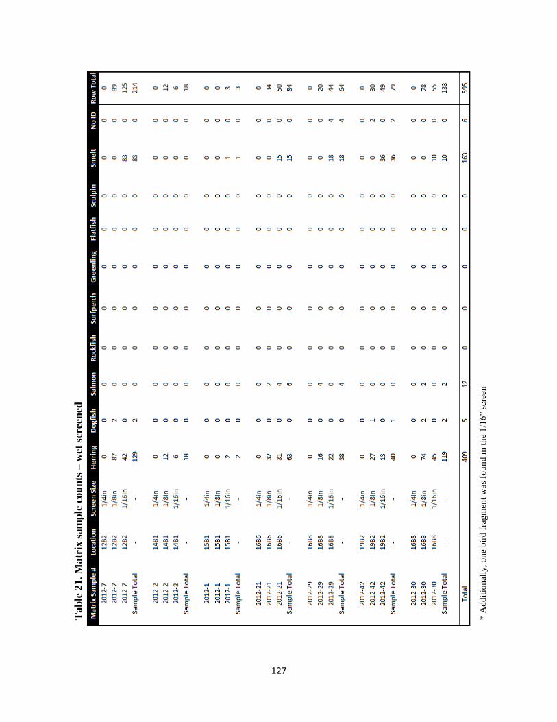
127
Tab
le 2
1. M
atr
ix s
am
ple
cou
nts
– w
et s
cre
ened
* A
dd
itio
nal
ly, o
ne
bir
d f
rag
men
t w
as f
ou
nd i
n t
he
1/1
6”
scre
en

128
were found in either the 1/16” dry screen or by wet screening, both methods that were not used
with the larger excavation material. All other fish in the matrix samples were found in either the
1/4” dry or the 1/8” dry. This supports the argument that smaller fish taxa (specifically herring
and smelts) are often lost in large proportions in excavations that utilize larger than 1/16”
screens. These differences are determined to be statistically significant using chi-squared tests.
Table 23 presents input data comparing small fish (herring and smelt) and larger fish (all other
fish) representation in different dry screen sizes. A null hypothesis of no relationship between
taxa representation and screen size is established. Results of the chi-squared analysis indicate a
rejection of this hypothesis (χ2=37.16, df=1, p<0.001, α=0.05), thus, dry screen size is
influencing the representation of the amount of fish remains. Table 24 presents input data for the
comparison of the 1/8” and 1/16” wet screens. The same null hypothesis is used in this analysis.
Again, this null hypothesis is rejected, indicating that taxa representation is affected by screen
size (χ2=41.43, df=1, p<0.001, α=0.05).
Taking a more in-depth look we can determine whether screen size or screening method
(wet vs. dry) helps in our collection of more material for each fish type. Figure 47 presents a
segmented bar graph for each fish type and screening method. For herring, a mixed picture
emerges, as both a smaller screen size, and wet screening increases the yield. This would indicate
that the use of both wet screening and the use of a smaller screen size would greatly aid in the
recovery of herring elements.
For dogfish and salmon a different pattern emerges, smaller screen size did not add much
to the overall assemblages (0% for dogfish, less than 20% for salmon and only in conjunction
with wet screening). The use of wet screening greatly increased the counts for both categories.

129
Table 22. NISP count totals for all matrix material
Table 23. Chi-Squared input values for dry screened bulk samples
*Small fish consist of both herring and smelts, large fish category consists of all other fish
Table 24. Chi-Squared input values for wet screened bulk samples
*Small fish consist of both herring and smelts, large fish category consists of all other fish.
Dry material was added with the assumption that they would have been collected, if they
were not already removed.
Figure 47. Segmented bar graph: matrix samples fish vertebrate remains.
Broken apart by different screening methods.
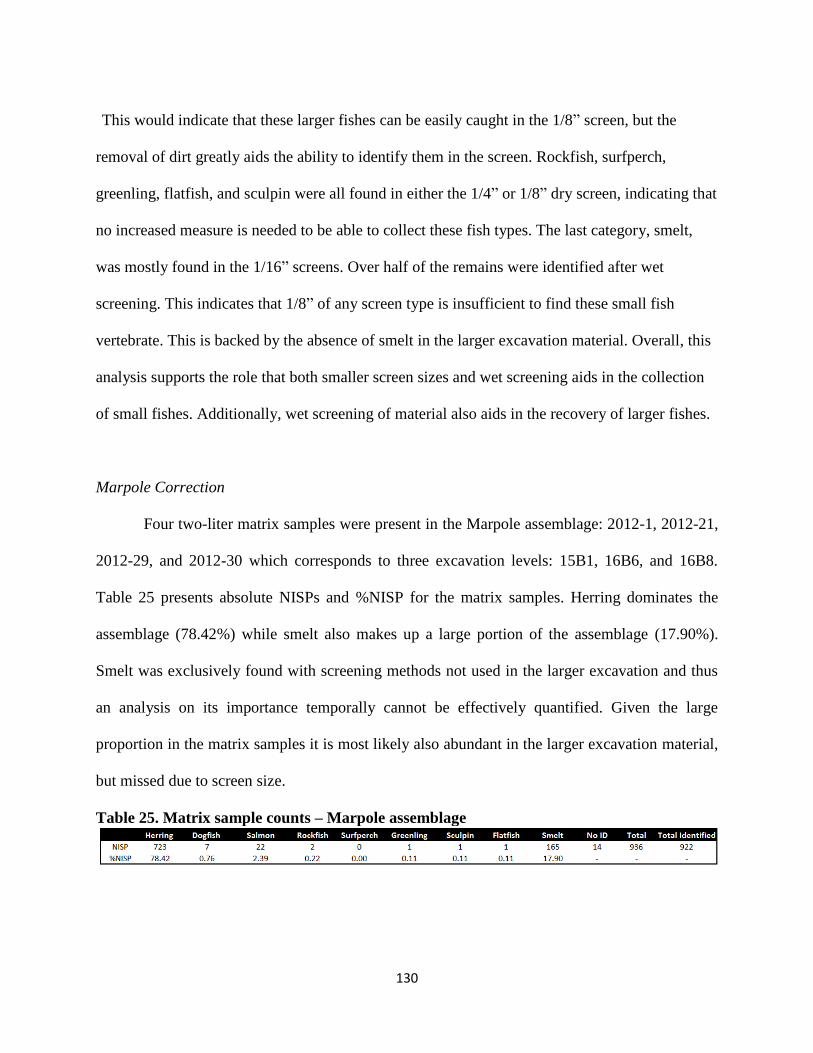
130
This would indicate that these larger fishes can be easily caught in the 1/8” screen, but the
removal of dirt greatly aids the ability to identify them in the screen. Rockfish, surfperch,
greenling, flatfish, and sculpin were all found in either the 1/4” or 1/8” dry screen, indicating that
no increased measure is needed to be able to collect these fish types. The last category, smelt,
was mostly found in the 1/16” screens. Over half of the remains were identified after wet
screening. This indicates that 1/8” of any screen type is insufficient to find these small fish
vertebrate. This is backed by the absence of smelt in the larger excavation material. Overall, this
analysis supports the role that both smaller screen sizes and wet screening aids in the collection
of small fishes. Additionally, wet screening of material also aids in the recovery of larger fishes.
Marpole Correction
Four two-liter matrix samples were present in the Marpole assemblage: 2012-1, 2012-21,
2012-29, and 2012-30 which corresponds to three excavation levels: 15B1, 16B6, and 16B8.
Table 25 presents absolute NISPs and %NISP for the matrix samples. Herring dominates the
assemblage (78.42%) while smelt also makes up a large portion of the assemblage (17.90%).
Smelt was exclusively found with screening methods not used in the larger excavation and thus
an analysis on its importance temporally cannot be effectively quantified. Given the large
proportion in the matrix samples it is most likely also abundant in the larger excavation material,
but missed due to screen size.
Table 25. Matrix sample counts – Marpole assemblage
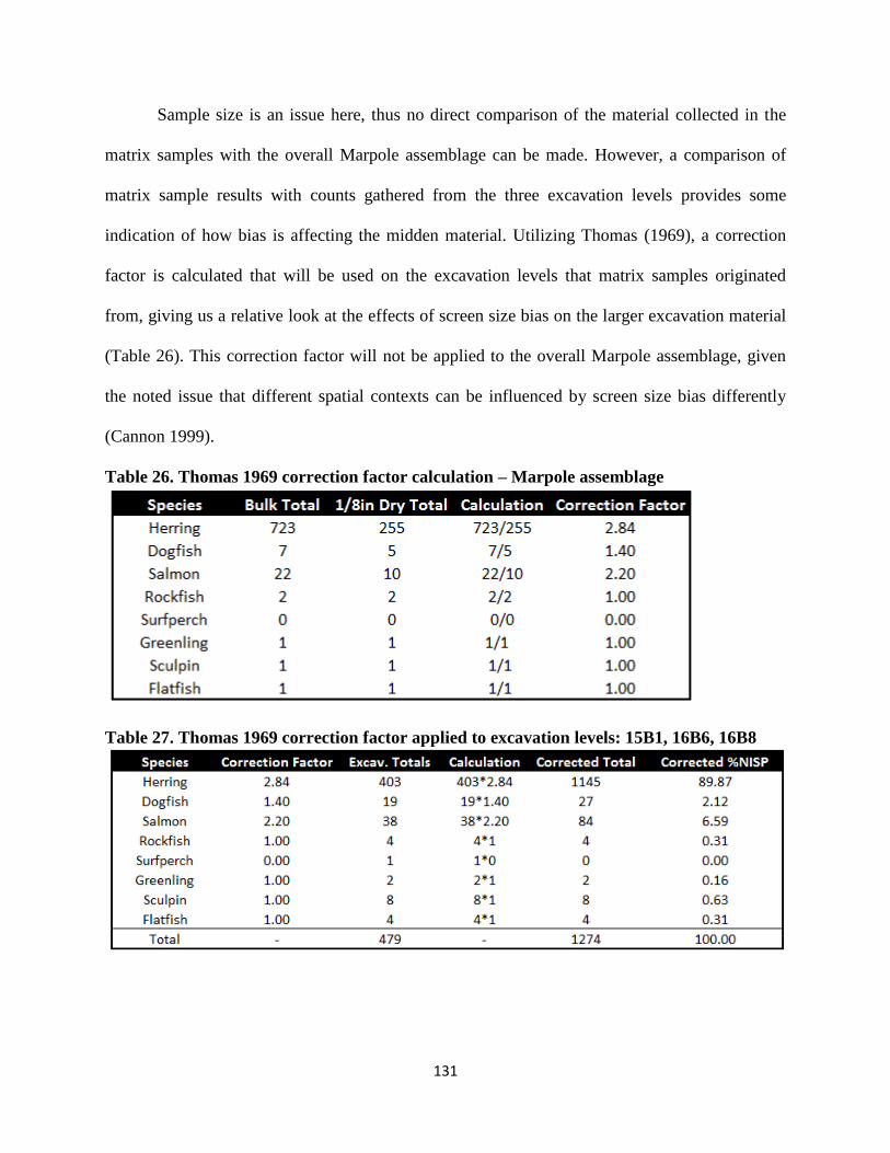
131
Sample size is an issue here, thus no direct comparison of the material collected in the
matrix samples with the overall Marpole assemblage can be made. However, a comparison of
matrix sample results with counts gathered from the three excavation levels provides some
indication of how bias is affecting the midden material. Utilizing Thomas (1969), a correction
factor is calculated that will be used on the excavation levels that matrix samples originated
from, giving us a relative look at the effects of screen size bias on the larger excavation material
(Table 26). This correction factor will not be applied to the overall Marpole assemblage, given
the noted issue that different spatial contexts can be influenced by screen size bias differently
(Cannon 1999).
Table 26. Thomas 1969 correction factor calculation – Marpole assemblage
Table 27. Thomas 1969 correction factor applied to excavation levels: 15B1, 16B6, 16B8
132
Results from this analysis indicate that three of the four major taxa are underrepresented
in the 1/8” screen. Applying the correction factor to the excavation levels of interest (Table 27)
we find an increased importance of herring, with a universal decrease in abundance of the other
taxa (Figure 48, note that given the technique corrected NISP counts for surfperch under-
represent that taxon, however, this does not change the overall results). Although this increase in
herring should be noted, it does not significantly change the results of the analysis. Even though
herring increases by five percentage points, there still are fairly large amounts of dogfish and
salmon. Meat weight analysis on these corrected values indicates that herring NISP abundance
does not equal a dietary dominance, even when screen size is accounted for (Table 28).
Smelt deserves a special consideration here. A large number of vertebrae (n=165) was
found in the Marpole assemblage. However, Thomas’ 1969 correction factor could not correct
the assemblage for smelt due to the absence of this taxa in the original excavation unit totals, as
well as the bulk sample 1/8” screen. Arbitrarily adding one smelt to both of these contexts allows
me to utilize Thomas’ 1969 correction factor. Doing this changes proportions of the corrected
taxa, with smelt now obtaining the second rank (Table 29). However, like herring, smelts are
small fish that do not contain a large amount of meat weight per animal. Thus, although possibly
numerically important to the Marpole Period assemblage, the inclusion of this additional taxa
does not largely change results noted above.
Late Period Correction
Three two-liter matrix samples were analyzed for the Late Period assemblage: 2012-2, 7,
and 42 (excavation levels 12B2, 14B1, 19B2). Herring dominates the samples with 77.3% of the

133
Figure 48. %NISP of excavation levels 15B1, 16B6, 16B8 compared with corrected values.
Table 28. Meat weight analysis on corrected values – Marpole assemblage
Table 29. %NISP of Marpole excavation levels, corrected, and smelt corrected assemblages

134
assemblage, while smelt makes up 21.14% (Table 30). Dogfish, salmon, and rockfish are only
marginally represented in these contexts, which may be attributed to the small sample size.
As noted for the Marpole assemblage, sample size is too small for direct comparisons
with the larger excavation material, thus no such analysis will be attempted here. Thomas’
(1969) correction factor (Table 31) is utilized for this assemblage as well. Here we find that
herring is particularly underrepresented in the excavation material, while all other fish analyzed
were collected by the 1/8 in screens. Tables 32 and 33 present the Thomas (1969) correction
factor on both NISP counts and meat weights for the three excavation levels covered.
Table 30. Matrix sample counts – Late Period
Table 31. Thomas 1969 correction factor calculation – Late Period assemblage
Herring maintains on top of the rank order in meat weights – the one measure in the
excavated assemblage, presented in chapter seven, that that it did not dominate. The fact that this
is a relative measure must be stressed here, as herring meat weights and counts are most likely
being overrepresented by the correction factor. Especially noteworthy is how no taxa, other than
herring and smelt, were found in the 1/16” wet screened material. In comparison, the Marpole

135
screen size analysis contained additional taxa in these smaller screens. The fact that no non-
herring remains were found within the more intensive screening methods is likely due to the
small sample size. Additionally, although at the top of the rank order, herring meat weight is not
as dominant as NISP counts indicate. It can be concluded that the original excavation material
may be under-representing herring NISP counts. However, the general rank order of herring,
dogfish, salmon, and “other fish” is still maintained, when comparing the corrected values with
the original (Figure 49). Thus, although some taxa loss occurred, the 1/8 in screen was still able
to capture the dominant pattern from the excavation levels considered.
Table 32. Thomas 1969 correction factor applied to excavation levels: 12B2, 14B1, 19B2
Table 33. Meat weight analysis on corrected values – Late Period assemblage

136
Figure 49. %NISP of excavation levels 12B2, 14B1, 19B2 compared with corrected values
Similar to the Marpole assemblage, smelt also deserves some consideration. Bulk
samples collected 122 smelt vertebrate, while original excavation levels do not contain any
smelt. Given this high number, I arbitrarily added “1” to the smelt excavation level so that a
correction factor coud be ran accounting for these smelt remains. Differing from the Marpole
assemblage, the Late Period bulk samples contained three smelt vertebrate in the 1/8 in dry
screen, which allows a correction factor to be made without arbitrarily adding smelt vertebrate to
this context. Results of this analysis is presented in Table 34. Similar to the Marpole assemblage,
the corrected smelt becomes second in the rank order, however, this with a very small proportion
of the assemblage. Apart from adding a new taxon, this analysis does not change the results
noted above, and the conclusion that the 1/8” dry screen established the overall pattern, remains.
Conclusion
Matrix sample counts include large amounts of two small fish types, herring and smelt,
with marginal amounts of all other fish types. Analysis of sample size utilizing these remains
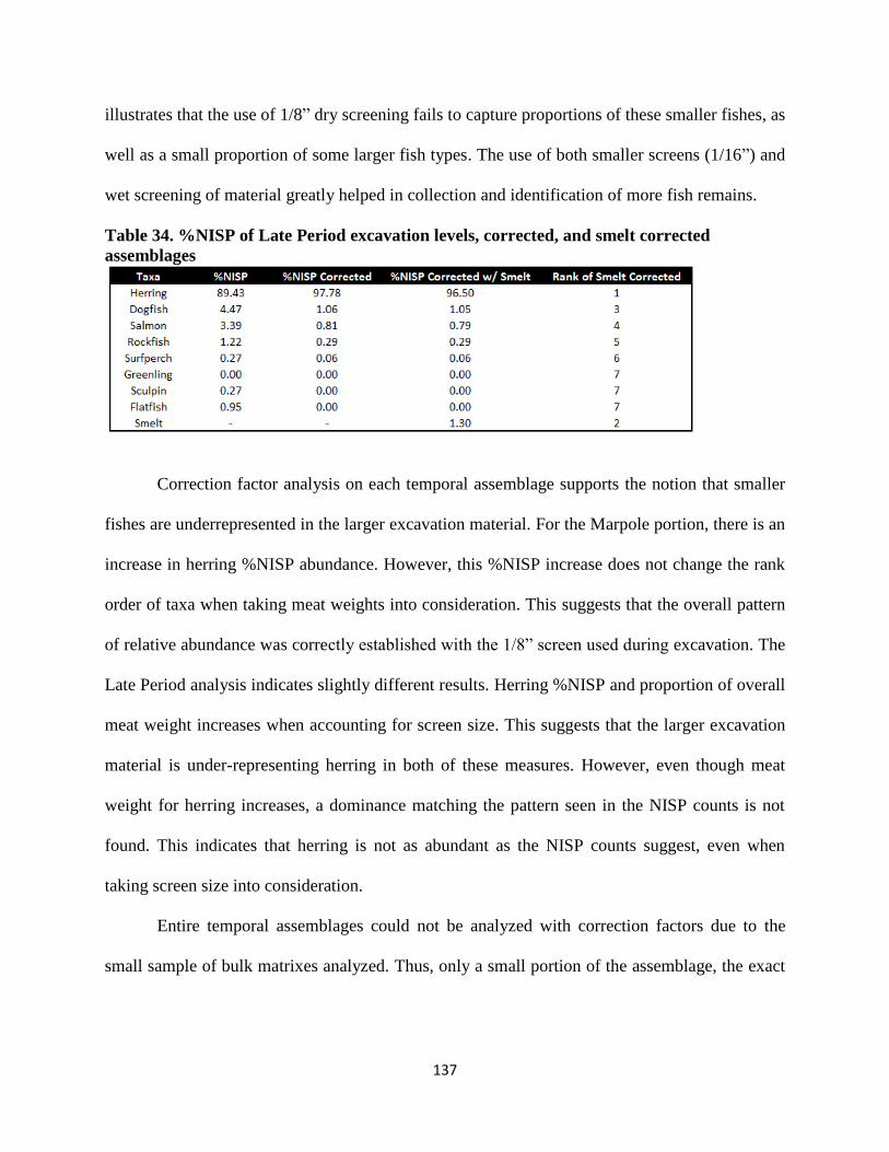
137
illustrates that the use of 1/8” dry screening fails to capture proportions of these smaller fishes, as
well as a small proportion of some larger fish types. The use of both smaller screens (1/16”) and
wet screening of material greatly helped in collection and identification of more fish remains.
Table 34. %NISP of Late Period excavation levels, corrected, and smelt corrected
assemblages
Correction factor analysis on each temporal assemblage supports the notion that smaller
fishes are underrepresented in the larger excavation material. For the Marpole portion, there is an
increase in herring %NISP abundance. However, this %NISP increase does not change the rank
order of taxa when taking meat weights into consideration. This suggests that the overall pattern
of relative abundance was correctly established with the 1/8” screen used during excavation. The
Late Period analysis indicates slightly different results. Herring %NISP and proportion of overall
meat weight increases when accounting for screen size. This suggests that the larger excavation
material is under-representing herring in both of these measures. However, even though meat
weight for herring increases, a dominance matching the pattern seen in the NISP counts is not
found. This indicates that herring is not as abundant as the NISP counts suggest, even when
taking screen size into consideration.
Entire temporal assemblages could not be analyzed with correction factors due to the
small sample of bulk matrixes analyzed. Thus, only a small portion of the assemblage, the exact
138
excavation levels where bulk samples were obtained, was analyzed. A more complete analysis of
screen size bias would involve the use of a larger collection of bulk matrix samples, to a level of
redundancy.

139
CHAPTER NINE
CONCLUSIONS
Several conclusions can be drawn from the results of this study. These are broken into three
categories: methodological, site specific, and linear complexity models. Additionally, future
research approaches are presented throughout this chapter.
Method-based Conclusions
Method-based conclusions can be drawn from matrix sample analyses, the application of
correspondence analysis, and the use of multiple quantification techniques to understand
assemblage structure. Matrix sample evaluation of screen size bias has shown that the use of 1/8”
dry screens does underestimate the amount of smaller fish taxa in recovered assemblages, as well
as identifiable fragments of some larger taxa. This indicates that the use of smaller screen sizes
(1/16”) and wet screening of material does help recover additional specimens. Especially
noteworthy is the collection of an entire taxon that was not found in the larger excavation
material (smelt). However, even with these biases, the general patterns observed in the
assemblages remain consistent. This shows that a smaller screen size is needed for thorough
recovery of small faunal material. However, it also indicates that 1/8” dry screening is sufficient
to collect enough material to establish consistent faunal representations. This supports the
conclusion that a switch to complete 1/16” wet screening of all excavated material is not
necessarily warranted, but that it is important to analyze matrix and/or column samples in future
studies to establish how bias affects each specific assemblage.
140
Additionally, as other studies have noted, the sifting of column and core samples through
fine mesh does compare favorably with what is obtained from the use of larger 1/8” screen
excavation (Casteel 1970; Cannon 2000). This indicates that small, intensively studied samples
of sediment may be more beneficial for establishing faunal patterns dominated by fish, given the
increased recovery of material.
This study also demonstrated the usefulness of Correspondence Analysis on faunal data
to evaluate stratigraphic interpretations. Other studies have demonstrated how CA (and CA-like
statistical approaches) can illuminate data patterns in regional settlement pattern studies (Betts
and Friesen 2004, Bilton 2013, Orchard and Clark 2005). This study finds similar utility in CA
as an exploratory approach for within-midden contexts. Preliminary distinctions of depositional
patterns were strengthened with the results of CA.
The last methodological conclusion that can be drawn from this study concerns the use of
NISP as a means of quantification. First, lumping fish taxa according to the mechanism of
procurement allowed for more robust interpretations of NISP values. Additionally, as noted
above, NISP remains a poor measure of diet (Lyman 2008:30) and the use of NISP counts alone
can produce erroneous interpretations of the importance of taxa that are mass-caught but also
anatomically small, here represented best by herring remains. Rather than simply using NISP
counts for analysis, more insight was found through the use of multiple measures consisting of
NISP, MNI, ubiquity, and meat weight analyses.
Each of these techniques on their own contains substantial issues in interpretation of
faunal patterns in archaeological contexts. However, the use of all four allowed for more
satisfying conclusions. The use of NISP along with some form of meat weight analysis seems

141
most useful for accurate interpretation of abundance in ichthyofaunal assemblages. Admittedly,
the meat weights employed here poorly address variance in fish weight, so future studies may
want to rely on regression formulae to obtain more precise meat weights.
Site-specific Conclusions
Both the Marpole and the Late Period components of the PLM contain similarly diverse
taxa compositions. Fish remains dominate both assemblages with herring, salmon, dogfish, and
“other fish” abundance indicating a diversified fishing pattern. This pattern of stability and
fishing diversity over time matches what has been observed in regionally-focused studies (Bilton
2013:298; Butler and Cambell 2004). The large NISP dominance of herring has also been
observed in southern Northwest Coast sites (MeKechnie et al. 2014). This analysis does support
a change in dogfish fishery practices between time periods, with dogfish specifically targeted in
the Marpole assemblage, while the Late Period fishery procurement was connected to the herring
harvest.
Overall taxa present in the midden indicate the use of myriad microenvironments for
subsistence production. All of the microenvironments are located adjacent to site DgRv-006
and/or easily reached by canoe, within a single travel day. This includes salmon, which may have
come from as far away as the Fraser River. Evidence for locally caught species of fish and
shellfish support the notion that the site was located in part to exploit a diverse array of marine
ecosystems (McLay 1999). However, this does not indicate a rejection of other reasons for site
location, the exploration of which is the subject of future research.
Species presence/absence indicators place both Marpole and Late Period portions of the
midden within the same late-winter/early spring to early summer seasonality. As noted above,

142
this is incomplete given the lack of species level designation for salmon. It is possible that
seasonality could be extended to include a winter residence, as argued by Grier (2001, 2006c) for
site DgRv-003.
Preliminary analysis of depositional aspects of the midden indicates the possible presence
of a prepared burial surface and mounding event at the beginning stage of midden formation
(Grier, personal communication). A shift to more typical midden deposition after this inital phase
of use is inferred from CA results. Given the presence of both dog and human burials in the
midden, as well as the very visible nature of the midden in an important travel corridor, I suggest
that this area was an important place associated closely with the social identity of the inhabitants
of sites DgRv-003 and DgRv-006 (Moss 2011:124).
Linear Complexity Models
Evaluation of linear complexity models indicates an overall disagreement between model
expectations and what is seen in the PLM faunal assemblage. Overall there is general continuity
of fishing practices over time, with small shifts in the relative abundance of herring, dogfish, and
salmon. Dogfish are more abundant in the Late Period, while salmon is slightly more abundant
in Marpole times. This contrasts directly with what was inferred to be happening to fish faunal
patterns in the linear models: salmon specialization should be present in the Marpole assemblage
with diversification of fish resources occurring in the Late Period. This provided for an
acceptance of the null hypothesis of no difference.
With the null hypothesis accepted at site DgRv-006, additional conclusions related to
social complexity and economy in Northwest Coast studies can be forwarded. First, this study
further solidifies the view that linear progressivism-based models need to be rejected in favor of

143
analysis at the local level to truly understand how social realities and subsistence/economic
realities are connected (Cannon and Moss 2011: 294; Moss 2011, 2012; Moss and Erlandson
1995).
More importantly, this study decouples social and subsistence changes. The linear models
assume that social changes would be driven and/or accompanied by shifts in subsistence and
economic patterns. At the PLM, however, we have evidence of a significant social shift
(abandonment of a village and settlement of a new plankhouse) that is not accompanied by
change in subsistence. Though social changes occurred at DgRv-006 with regards to how settled
village life was practiced, there was no corresponding shift in subsistence practices. This one site
does not necessarily indicate a regional pattern and future research should continue to test the
connection between social change and subsistence trend. However, other non-subsistence driven
hypotheses should also be evaluated in order to better understand how Northwest Coast societies
changed over time.

144
BIBLIOGRAPHY
Aikens, C. Melvin, Thomas J. Connely, and Dennis L. Jenkins
2011 Oregon Archaeology. Oregon State University Press, Corvallis, Oregon.
Ames, Ken
1981 The Evolution of Social Ranking on the Northwest Coast of North America. American
Antiquity 46(4):789-805.
1994 The Northwest Coast: Complex Hunter-Gatherers, Ecology, and Social Evolution.
Annual Review of Anthropology 23:209-229.
1995 Chiefly Power and Household Production on the Northwest Coast. In Foundations of
Social Inequality, edited by T. Douglas Price and Gary M. Feinman, pp. 155-187.
Plenum Press: New York, New York.
2002 Going by Boat: The Forager-Collector Continuum at Sea. In Beyond Foraging and
Collecting: Evolutionary Change in Hunter-Gatherer Settlement Systems, edited by
Ben Fitzhugh and J. Habu, pp. 17-50. Plenum Press, New York, New York.
Ames, Ken, and Herbert Maschner
1999 Peoples of the Northwest Coast: Their Archaeology and Prehistory. Thames and
Hudson: London.
Angelbeck, Bill, and Colin Grier
2012 Anarchism and the Archaeology of Anarchic Societies: Resistance to Centralization in
the Coast Salish Region of the Pacific Northwest Coast. Current Anthropology
53(4):1-41.
Angelbeck, Bill, and Eric McLay
2011 The Battle at Mapl Bay: The Dynamics of Coast Salish Political Organization through
Oral Histories. Ethnohistory 58(4):359-392.
Baron, Nancy, and John Acorn
1997 Birds of the Pacific Northwest Coast. Lone Pine Publishing, Edmonton, Alberta.
Barnett, Homer
1955 The Coast Salish of British Columbia. The University Press, Eugene, Oregon.
Baxter, M.J.
1994 Exploratory Multivariate Analysis in Archaeology. Edinburgh University Press,
Edinburgh, United Kingdom.
Betts, Matthew, and T. Max Friesen
2004 Quantifying hunter-gatherer intensification: a zooarchaeological case study from
145
Arctic Canada. Journal of Anthropological Archaeology 23:357-384.
Betts, Matthew, Hebert Maschner, Corey Schou, Robert Schlader, Jonathan Holmes, Nicholas
Clement, and Michael Smuin
2011 Virtual zooarchaeology: building a web-based reference collection of northern
Vertebrates for archaeofaunal research and education. Journal of Archaeological
Science 38:755-762.
Bilton, David
2013 Northern, Central, Diversified, Specialized: The Archaeology of Fishing Adaptations
in the Gulf of Georgia (Salish Sea), British Columbia. Unpublished dissertation,
Department of Anthropology, University of Toronto, Ontario.
Binford, Lewis
1978 Nunamiut Ethnoarchaeology. Academic Press: NewYork, New York.
1984 Faunal Remains from Klasies River Mouth. Academic Press: Orlando, Florida.
Boem, S. Gay
1973 Cultural and non-cultural variation in the artifact and faunal samples from the St.
Mungo Cannery Site, DgRr 2. Unpublished MA thesis, University of Victoria, British
Columbia.
Brown, Christopher, and Carl Gustafson
1990 A Key to Postcranial Skeletal Remains of Cattle/Bison, Elk, and Horse. Washington
State University Laboratory of Anthropology, Report of Investigations, No. 57:
Pullman, Washington.
Butler, Virginia, and James Chatters
1994 The Role of Bone Density in Structuring Prehistoric Salmon Bone Assemblages.
Journal of Archaeological Science 21:413-424.
Butler, Virginia, and Sarah Campbell
2004 Resource Intensification and Resource Depression in the Pacific Northwest of North
North America: A Zooarchaeological Review. Journal of World Prehistory 18(4):327-
405.
Burley, David
1989 Senewe’lets. Royal British Columbia Museum, Victoria, British Columbia.
Cannon, Aubrey
1991 The Economic Prehistory of Namu. Archaeology Press, Simon Fraser University,
Burnaby, British Columbia.

146
2000 Assessing Variability in Northwest Coast Salmon and Herring Fisheries: Bucket-
Auger Sampling of Shell Midden Sites on the Central Coast of British Columbia.
Journal of Archaeological Science 27:725-737.
Cannon, Debbi
1987 Marine Fish Osteology: A Manual for Archaeologists. Simon Fraser University,
Burnaby, British Columbia.
Cannon, Michael
1999 A Mathematical Model of the Effects of Screen Size on Zooarchaeological Relative
Abundance Measures. Journal of Archaeological Science 26:205-214.
Cannon, Aubrey, and Dongya Yang.
2006 Early Storage and Sedentism on the Pacific Northwest Coast: Ancient DNA Analysis
Of Salmon Remains from Namu, British Columbia. American Antiquity 71(1):123-
140.
2011 Pushing Limits and Finding Interpretive Balance: A Reply to Monks and Orchard.
American Antiquity 76(3):585-595.
Cannon, Aubrey, and Madonna Moss
2011 Conclusion: The Archaeology of North Pacific Fisheries. In The Archaeology of
North Pacific Fisheries, edited by Madonna Moss and Aubrey Cannon, pp. 293-300.
University of Alaska Press, Fairbanks, Alaska.
Carlson, Roy
1999 Sacred sites on the Northwest Coast of North America. In Bog Bodies, Sacred Sites
and Wetland Archaeology, edited by Bryony Coles, John Coles and Mogens Schou
Jørgenson, pp. 39-46. WARP (Wetland Archaeology Research Project), Occasional
Paper 12, Short Run Press, Exeter, United Kingdom.
Carlson, Roy, and Philip Hobler
1993 The Pender Canal Excavations and the Development of Coast Salish Culture. BC
Studies 99:25-52.
Casteel, Richard
1970 Core and Column Sampling. American Antiquity 35(4):465-467.
1972 Some biases in the recovery of archaeological faunal remains. Proceedings of the
Prehistoric Society (38):382-388.
1974 A Method for Estimation of Live Weight of Fish from the Size of Skeletal Elements.
American Antiquity 39(1):94-98.
1976a Fish Remains in Archaeology and Paleo-environmental Studies. Academic Press,
New York, New York.
1976b Comparison of Column and Whole Unit Samples for Recovering Fish Remains.
World Archaeology 8(2):192-196.
147
Claassen, Cheryl
2000 Quantifying Shell: Comments on Mason, Peterson, and Tiffany. American Antiquity
65(2):415-418.
Clark, Terence
2010 Rewriting Marpole: The Path to Cultural Complexity in the Gulf of Georgia. Doctoral
Dissertation. Department of Anthropology, University of Toronto, Ontario.
2013 Rewriting Marpole: The Path to Cultural Complexity in the Gulf of Georgia.
University of Ottawa Press, Ontario.
Clauge, John, John Harper, R.J. Hebda, and D.E. Howes
1982 Late Quaternary sea levels and crustal movements, coastal British Columbia.
Canadian Journal of Earth Science 19:597-618.
Codere, Helen
1950 Fighting with Property. J.J. Augustin, New York, New York.
Communications Directorate Fisheries and Oceans Canada
2002 Underwater world: Pacific Salmon. Electronic document,
http://www.dfo-mpo.gc.ca/Science/publications/uww-msm/articles/pacificsalmon-
saumonpacifique-eng.htm.
Coupland, Gary, Terence Clark, and Amanda Palmer
2009 Hierarchy, Communalism, and the Spatial Order of Northwest Coast Plank Houses:
A Comparative Study. American Antiquity 74(1):77-106.
Coupland, Gary, Kathlyn Stewart, and Katherine Patton
2010 Do you never get tired of salmon? Evidence for extreme salmon specialization at
Prince Rupert harbor, British Columbia. Journal of Anthropological Archaeology
29:189-207.
Croes, Dale, and Steven Hackenberger
1988 Hoko River Archaeological Complex: Modeling Prehistoric Northwest Coast
Economic Evolution. In Research in Economic Anthropology, Supplement 3. Pp. 19
85. JAI Press.
Crowell, Aron, and Wayne Howell
2013 Time, Oral Tradition, and Archaeology at Xakwnoowú, A Little Ice Age Fort in
Southeastern Alaska. American Antiquity 78(1):3-23.
Cybulski, Jerome
1992 A Greenville burial ground: human remains and mortuary elements in British
Columbia coast prehistory. Archaeological Survey of Canada Mercury Series
148
Paper No. 146. Canadian Museum of Civilization, Hull, Quebec.
Derr, Kelly, Doug Byers, and Colin Grier
2012 Of Sea Urchins and Sea Lions: Analysis of a Mass Consumption Feature in a Late
Period Northwest Coast Plankhouse. Poster presented at the Society for American
Archaeology 77th
Annual Meeting, Memphis.
Dolan, James Patrick
2009 Geoarchaeological Analysis of a Northwest Coast Plank House: Formation Processes
At The Dionisio Point Site. Unpublished MA Thesis. Washington State University,
Pullman, Washington.
Drucker, Philip, and Robert Heizer
1967 To Make My Name Good. University of California Press, Los Angeles, California.
Erlandson, Jon M., Michael H. Graham, Bruce J. Bourque, Debra Corbett, James A. Estes, and
Robert S. Steneck.
2007 The Kelp Highway Hypothesis: Marine Ecology, the Coastal Migration Theory, and
the Peopling of the Americas. Journal of Island and Coastal Archaeology 2:161-174.
Ewonus, Paul
2011a Social Zooarchaeology of a Northwest Coast House. Journal of Island and Coastal
Archaeology 6:72-97.
2011b Social Landscapes of the Southern Strait of Georgia, Pacific Northwest Coast.
Unpublished dissertation. University of Cambridge.
2012 Reflexive theory and practice in evaluating seasonal village settlement: a response to
Grier and Lukowski.” Journal of Island and Coastal Archaeology 7(3):437-445.
Ewonus, Paul, Aubrey Cannon, and Dongya Yang
2011 Addressing seasonal site use through ancient DNA species identification of Pacific
salmon at Dionisio Point, Galiano Island, British Columbia. Journal of
Archaeological Science 38:2536-2546.
Fedje, Daryl, and Tina Christensen
1999 Modeling Paleoshorelines and Locating Early Holocene Coastal Sites in Haida Gwaii.
American Antiquity 64(4):635-652.
Fedje, Daryl, Ian Sumpter, and John Southon
2009 Sea-levels and Archaeology in the Gulf Islands National Park Reserve. Canadian
Journal of Archaeology 33:234-253.
Fladmark, Knut
1975 A Paleoecological Model for Northwest Coast Prehistory. Archaeological Survey
of Canada Paper No. 43, Ottawa, Ontario.

149
Gilbert, B. Miles
1990 Mammalian Osteology. Missouri Archaeological Society, Columbia, Missouri.
Gilbert, B. Miles, Larry Martin, and Howard Savage
1996 Avian Osteology. Missouri Archaeological Society Inc, Columbia, Missouri.
Gosden, Chris
1999 Anthropology and Archaeology: A Changing Relationship. Routledge: London and
New York
Grayson, Donald
1984 Quantitative Zooarchaeology. Academic Press, Orlando, Florida.
Green, A.J., L.J.P van Vliet, and F.A. Kenney
1989 Soils of the Gulf Islands of British Columbia: Volume 3 Soils of Galiano, Valdes,
Thetis, Kuper, and lesser islands. British Columbia Soil Survey Report No. 43,
Vancouver, British Columbia.
Grier, Colin
2001 The Social Economy of a Prehistoric Northwest Coast Plankhouse. Unpublished
Ph.D dissertation, Arizona State University, Tempe.
2003 Dimensions of Regional Interaction in the Prehistoric Gulf of Georgia. In Emerging
From the Mist, edited by R.G. Matson, Gary Coupland, and Quentin Mackie, pp.
170-187. UBC Press, Vancouver, British Columbia.
2006a Affluence on the Prehistoric Northwest Coast of North America. In Beyond Affluent
Foragers: Rethinking Hunter-Gatherer Complexity, edited by C. Grier, J. Kim, and
J. Uchiyama, pp. 192-200. Oxbow Books, Oxford.
2006b The Political Context of Prehistoric Coast Salish Residences on the Northwest Coast.
In Palaces and Power in the Americas: From Peru to the Northwest Coast, edited by
J.J. Christie and P.J. Sarro, pp. 141-165. University of Texas Press, Austin, Texas.
2006c Temporality in Northwest Coast Households. In Household Archaeology on the
Northwest Coast, edited by E.A. Sovel, D.A. Trieu Gahr, and K.M. Ames, pp 97-
119. International Monographs in Prehistory, Ann Arbor, Michigan.
2007 Consuming the Recent for Constructing the Ancient: The Role of Ethnography in
Coast Salish Archaeological Interpretation. In Be of Good Mind: Essays on the
Coast Salish, edited by B.G. Miller, pp. 284-307. UBC Press, Vancouver, British
Columbia.
2014 Which Way Forward? Canadian Journal of Archaeology 38:135-139.
Grier, Colin, Kelli Flanigan, Misa Waters, Leah G. Jordan, Susan Lukowski and Brian Kemp
2013 Using Ancient DNA Identification and Osteometric Measures of Archaeological
Pacific Salmon Vertebrae for Reconstructing Salmon Fisheries and Site Seasonality
at Dionisio Point, British Columbia. Journal of Archaeological Science 40(1):544-
555.

150
Grier, Colin, Patrick Dolan, Kelly Derr, and Eric McLay
2009 Assessing Sea Level Changes in the Southern Gulf Island of British Columbia Using
Archaeological Data from Coastal Spit Locations. Canadian Journal of Archaeology
33:12-18.
Grier, Colin, and Susan Lukowski
2012 On Villages, Quantification, and Appropriate Context: A Comment on “Social
Zooarchaeology of a Northwest Coast House” by Paul A. Ewonus. Journal of Island
and Coastal Archaeology 7(3):430-436.
Grier, Colin, and Eric McLay
2007 Archaeological Inventory of DgRv-006, Dionisio Point Provincial Park, Galiano
Island, British Columbia. Unpublished permit report (2007-144) submitted to the
British Columbia Archaeology Branch, Victoria.
Grier, Colin, Eric McLay, and Michael Richards
2012 Stable Isotopes, Human Diet and Subsistence Practices at Two Precontact Villages at
Dionisio Point on the Southwestern British Columbia Coast. Poster presented at the
Society for American Archaeology 77th
Annual Meeting, Memphis
Guthrie, R.D.
1968 Paleoecology of the Large-Mammal Community in Interior Alaska during the Late
Pleistocene. American Midland Naturalist 79(2):346-363.
Haist, V., and M. Stocker
1985 Growth and Maturation of Pacific Herring (Clupea harengus pallasi) in the Strait of
Georgia. Canadian Journal of Fish and Aquatic Sciences 42(1):138-146.
Hanson, Diane
1991 Late Prehistoric Subsistence in the Strait of Georgia Region of the Northwest Coast.
Unpublished Ph.D dissertation, Department of Archaeology. Simon Fraser
University, Burnaby, British Columbia.
1995 Subsistence during the Late Prehistoric Occupation of Pender Canal, British
Columbia (DeRt-1). Canadian Journal of Archaeology 19:29-48.
2008 Salmon and Models of Social Complexity on the Northwest Coast. North Pacific
Prehistory 2:123-132.
Hart, J.L.
1973 Pacific Fishes of Canada. Fisheries Research Board of Canada, Ottawa, Ontario.
Hayden, Brian
1995 Pathways to Power: Principles for Creating Socioeconomic Inequalities. In
Foundations of Social Inequality, edited by T. Douglas Price and Gary M. Feinman,
151
pp. 15-86. Plenum Press: New York and London.
Hayden, Brian, and Aubrey Cannon
1983 Where the Garbage Goes: Refuse Disposal in the Maya Highlands. Journal of
Anthropological Archaeology 2:117-163.
Hodgetts, Lisa, and Farid Rahemtulla
2001 Land and Sea: use of terrestrial mammal bones in coastal hunter-gatherer
communities. Antiquity 75:56-62.
Hopt, Justin
2014 Fish and Complexity: Faunal Analysis at the Shell Midden Component of site
DgRv-006, Galiano Island, B.C. Paper presented at the 2014 Northwest
Anthropological Conference, Bellingham, Washington.
Hopt, Justin and Colin Grier
2013 Subsistence and Resource Use at a Late Period Plankhouse at the Dionisio Point
Locality (Site DgRv-006), Galiano Island, BC. Poster presented at the 78th
Annual
Meeting of the Society for American Archaeology, Honolulu, Hawaii.
Huber, Harriet, Jeffrey Jorgensen, Virginia Butler, Greg Baker, an Rebecca Stevens
2011 Can salmonids (Oncorhynchus spp.) be identified to species using vertebral
morphometrics? Journal of Archaeological Science 38:136-146.
Ingold, Tim
1993 The Temporality of the Landscape. World Archaeology 25(2):152-174.
Jenkins, Dennis L., Loren G. Davis, Thomas W. Stafford Jr., Paula F Campos, Bryan Hockett,
George T. Jones, Linda Scott Cummings, Chad Yost, Thomas J. Connolly, Robert M. Yohe
II, Summer C. Gibbons, Maanasa Raghaven, Morten Rasmussen, Johanna L.A. Paijmans,
Michael Hofreiter, Brian M. Kemp, Jodi Lynn Barta, Cara Monroe, M. Thomas P. Gilbert,
and Eske Willerslev
2012 Clovis Age Western Stemmed Projectile Points and Human Coprolites at the Paisley
Caves. Science 337:223-228.
Jensen, A.C.
1965 Life History of the Spiny Dogfish. Fishery Bulletin 65(3):527-554.
Johnstone, Patrick
2006 Geology of the Upper Cretaceous Nanaimo Group, Southernmost Gulf Islands and
adjacent Saanich Peninsula, Southwestern British Columbia. Unpublished MA
Thesis, Department of Earth Sciences, Simon Fraser University, Burnaby, British
Columbia.

152
Lamb, Andy, and Phil Edgell
1986 Coastal Fishes of the Pacific Northwest. Harbour Publishing, Madeira Park, British
Columbia.
2010 Coastal Fishes of the Pacific Northwest. Harbour Publishing, Madeira Park, British
Columbia.
Lepofsky, Dana, and Ken Lertzman
2005 More on Sampling for Richness and Diversity in Archaeobiological Assemblages.
Journal of Ethnobiology 25(2):175-188.
Losey, Robert
2010 Anamism as a Means of Exploring Archaeological Fishing Structures on Willapa
Bay,Washington, USA. Cambridge Archaeological Journal 20(1):17-32.
Lyman, R. Lee
2002 Taxonomic Identification of Zooarchaeological Remains. The Review of Archaeology
23(2):13-20.
2008 Quantitative Paleozoology. Cambridge University Press, Cambridge.
Lyman, R. Lee, and Ken Ames
2004 Sampling to Redundancy in Zooarchaeology: Lessons from the Portland Basin,
Northwestern Oregon and Southwestern Washington. Journal of Ethnobiology 24(2):
329-346.
Marino, Matthew, and Justin Hopt
2014 (Dis)continuity in a Northwest Coast Midden/Cemetary: Two Perspectives on Faunal
Remains from Galiano Island. Poster presented at the Society for American
Archaeology annual meeting, Austin, Texas.
Martindale, Andrew, and Susan Marsden
2003 Defining the Middle Period (3500 BP to 1500 BP) in Tsimshian History through a
Comparison of Archaeological and Oral Records. BC Studies 138:13-50.
Marshall, Fiona, and Tom Pilgram
1993 NISP vs. MNI in Quantification of Body-Part Representation. American Antiquity 58:
2:261-269.
Mason, R., M.L. Peterson, and J.A. Tiffany
1998 Weighing vs. Counting: Measurement Reliability and the California School of
Midden Analysis. American Antiquity 63:303-324.
Mathewes, Rolf, and John Clague
1994 Detection of Large Prehistoric Earthquakes in the Pacific Northwest by Microfossil
Analysis. Science 264(5159):688-691.

153
Matson, R.G.
1976 The Glenrose Cannery Site. National Museum of Man, Mercury Series,
Archaeological Survey of Canada, No. 52, Ottawa, Ontario.
1983 Intensification and the Development of Cultural Complexity: The Northwest versus
the Northeast Coast. In The Evolution of Maritime Cultures on the Northeast and the
Northwest Coastsof America, edited by Ronald J. Nash, pp. 125-148. Publication No.
11, Simon Fraer University, Burnaby, British Columbia.
1985 The Relationship between Sedentism and Status Inequalities among Hunters and
Gatherers. Status, Structure and Stratification: Current Archaeological
Reconstructions:245-252.
1992 The Evolution of Northwest Coast Subsistence. In Research in economic anthropology
Sup.6 long-term subsistence change in prehistoric North America, edited by D. Croes,
R. Hawkins, and B.L. Isaac, pp. 367-428. JAI Press, Greenwich, Connecticut.
Matson, R.G., and Gary Coupland
1995 The Prehistory of the Northwest Coast. Academic Press, San Diego, California.
Matson, R.G., Joanne Green, and Eric McLay
1999 Houses and Households in the Gulf of Georgia: Archaeological Investigations of
Shingle Point (DgRv 2), Valdes Island, British Columbia. Report to Archaeology
Branch, Victoria, British Columbia.
McFarlane, G.A, W. Shaw, and R.J. Beamish
1983 Observations on the Biology and Distribution of Pacific Hake, Walleye Pollock, and
Spiny Dogfish in the Strait of Georgia, February 20-May 2, and July 3, 1981.
Canadian Manuscript Report and Fisheries and Aquatic Sciences No. 1722
McKechnie, Iain
2005 Column Sampling and the Archaeology of Small fish at Ts’ishaa. In Ts’ishaa:
Archaeology and Ethnography of a Nuu-chah-nulth Origin Site in Barkley Sound,
By Alan D. McMillan and Denis St. Claire, pp. 206-223. Archaeology Press,
Simon Fraser University, Burnaby, British Columbia.
2012 Zooarchaeological Analysis of the Indigenous Fishery at the Huu7ii Big House and
Back Terrace, Huu-ay-aht Territory, Southwestern Vancouver Island. In Household
Archaeology at a Nuu-chah-nulth Village Site in Barkley Sound, edited by Alan
McMillan and Denis St. Claire, pp. 154-186. Archaeology Press, Simon Fraser
University, Burnaby, British Columbia.
McKechnie, Iain, Dana Lepofsky, Madonna Moss, Virginia Butler, Trevor Orchard, Gary
Coupland, Frederick Foster, Megan Caldwell, and Ken Lertzman.
2014 Archaeological data provide alternative hypotheses on Pacific herring (Clupea
pallasii) distribution, abundance, and variability. PNAS:1-10.

154
McLay, Eric
1999 The Diversity of Northwest Coast Shell Middens: Late Pre-Contact Settlement-
Subsistence Patterns on Valdes Island, British Columbia. Unpublished MA
Thesis, University of British Columbia, Vancouver, British Columbia.
Mecklenburg, Catherine, T. Anthony Mecklenburg, and Lyman Thorsteinson
2002 Fishes of Alaska. American Fisheries Society, Bethesda Maryland.
Meidinger, Del and Jom Pojar
1991 Ecosystems of British Columbia. Special Report Series 6, BC Ministry of Forests.
Mitchell, Donald
1971 Archaeology of the Gulf of Georgia area: a Natural region and its culture types.
British Columbia Provincial Museum.
Monks, Gregory
1981 Seasonality Studies. In Advances in Archaeological Method and Theory Vol. 4, edited
By Michael B. Schiffer, pp.177-240. Academic Press, New York, New York.
1987 Prey as Bait: the Deep Bay Example. Candian Journal of Archaeology 11:119-142.
Monks, Gregory, and Trevor Orchard
2011 Comment on Cannon and Yang: Early Storage and Sedentism on the Pacific
Northwest Coast. American Antiquity 76(3):573-584.
Moss, Madonna
2011 Northwest Coast: Archaeology as Deep History. SAA Press, Washington, D.C.
2012 Understanding Variability in Northwest Coast Faunal Assemblages: Beyond
Economic Intensification and Cultural Complexity. Journal of Island and Coastal
Archaeology 7:1-22.
Moss, Madonna, and Jon Erlandson
1995 Reflections on North American Pacific Coast Prehistory. Journal of World Prehistory
9(1):1-45.
Olsen, N., K.L. Rutherfod, R.D. Stanley, and M.R. Wyeth
2009 Hecate Strait Groundfish Bottom Trawl Survey, May 26th
to June 21st, 2009.
CanadianManuscript Report of Fisheries and Aquatic Sciences 2901. Fisheries and
Oceans, Canada
Olsen, Stanley
1964 Mammal remains from archaeological sites, Part I: Southeastern and Southwestern
United States. Papers of the Peabody Museum, Volume 56, Number 1, Cambridge,
Massachusetts.
155
Orchard, Trevor
2001 The Role of Selected Fish Species in Aleut Paleodiet. Unpublished MA thesis,
Department of Anthropology, University of Victoria, Victoria, British Columbia.
2005 The Use of Statistical Size Estimations in Minimum Number Calculations.
International Journal of Osteoarchaeology 15:351-359.
Orchard, Trevor, and Terence Clark
2005 Multidimensional Scaling of Northwest Coast Faunal Assemblages: A Case Study
from Southern Haida Gwaii, British Columbia. Candian Journal of Archaeoogy
29:88-112.
Orchard, Trevor, and Paul Szpak
2011 Identification of Salmon Species from Archaeological Remains on the Northwest
Coast. In The Archaeology of North Pacific Fisheries, edited by Madonna Moss and
Aubrey Cannon, pp. 17-29. University of Alaska Press, Fairbanks, Alaska.
Post, Lee
2004 The Moose Manual: How to Prepare and Articulate Large Hoofed Mammal Skeletons.
Self-published.
2013 Pinniped Projects: Articulating Seal and Sea Lion Skeletons. Self-published.
Punke, Michele, and Loren Davis
2006 Problems and Prospects in the Preservation of Late Pleistocene Cultural Sites in
Southern Oregon Coastal River Valleys: Implications for Evaluating Coatal Migration
Routes. Geoarchaeology: An International Journal 24(4):333-350.
Ricketts, Edward, Jack Calvin, and Joel Hedgpeth
1968 Between Pacific Tides. Stanford University Press, Stanford, California.
Ruzicka, Annette
2013 Indigenous Archaeology at Dionisio Point on Galiano Island, British Columbia,
Canada: Contemporary Impacts and Implications for Archaeological Research and
Practice. Unpublished MA thesis. Washington State University, Pullman, WA.
Schalk, Randall
1977 The Structure of an Anadromous Fish Resource. In For Theory Building in
Archaeology: Essays on Faunal Remains, Aquatic Resource, Spatial Analysis, and
Systemic Modeling, edited by Lewis Binford, pp. 207-249. Academic Press, New
York, New York,
1981 Land Use and Organizational Complexity among Foragers of Northwestern North
America. Senri Ethnological Studies 9:53-75.
Schmid, Elisabeth
1972 Atlas of Animal Bones: For Prehistorians, Archaeologists and Quaternary Geologists.
156
Elsevier Publishing Company, Amsterdam.
Shaffer, Brian
1992 Quarter-Inch Screening: Understanding Biases in Recovery of Vertebrate Faunal
Remains. American Antiquity 57(1):129-136.
Shennan, Stephan
1997 Quantifying Archaeology. University of Iowa Press, Iowa City, Iowa.
Smith, Ross
2008 Structural Bone Density of Pacific Cod (Gadus macrocephalus) and Halibut
(Hippoglossus stenolepis): Taphonomic and Archaeological Implications.
Unpublished MA thesis. Portland State University, Portland, Oregon.
Smith, Ross, Virginia Butler, Shelia Orwoll, and Catherine Wilson-Skogan
2011 Pacific Cod and Salmon Structured Bone Density: Implications for Interpreting
Butchering Patterns in North Pacific Archaeofaunas. In The Archaeology of North
Pacific Fisheries, edited by Madonna Moss and Aubrey Cannon, pp. 45-56.
University of Alaska Press, Fairbanks, Alaska.
Stein, Julie
1992 Interpreting Stratification of a Shell Midden. In Deciphering a Shell Midden, edited
by Julie Stein, pp. 71-93. Academic Press, San Diego, California.
Suttles, Wayne
1974 Economic Life of the Coast Salish of Haro and Rosario Straits. Garland Publishing,
New York and London.
1987a Affinal Ties, Subsistence, and Prestige among the Coast Salish. In Coast Salish
Essays, pp. 15-25. University of Washington Press, Seattle, Washington.
1987b Private Knowledge, Morality, and Social Classes among the Coast Salish. In Coast
Salish Essays, pp. 3-14. University of Washington Press, Seattle, Washington.
1987c Variation in Habitat and Culture on the Northwest Coast. In Coast Salish Essays, pp.
26-44. University of Washington Press, Seattle, Washington.
1987d Notes on Coast Salish Sea-Mammal Hunting. In Coast Salish Essays, pp. 233-247.
University of Washington Press, Seattle, Washington.
Thom, Brian
1995 The Dead and the Living: Burial Mounds and Cairns and the Development of Social
Classes in the Gulf of Georgia Region. Unpublished MA Thesis. University of British
Columbia. Vancouver, British Columbia.
Thomas, D.H.
1969 Great Basin Hunting Patterns: A Quantitative Method for Treating Faunal Remains.
American Antiquity 36:392-401.
157
VanPool, Christine and Elizabeth Newsome
2012 The Spirit in the Material: A Case Study of Animism in the American Southwest.
American Antiquity 77(2):243-262.
Wheeler, Alwyne, and Andrew K.G. Jones
1989 Fishes. Cambridge University Press, Cambridge.
White, Theodore
1953 A Method of Calculating the Dietary Percentage of Various Food Animals Utilized
by Aboriginal Peoples. American Antiquity 18(4):396-398
Wilby, G.V.
1937 Bulletin No. LIV: The Ling Cod, Ophiodon Elongatus Girard. The Biological Board
of Canada, Ottawa, Ontario.
Zohar, Irit and Miriam Belmaker
2005 Size does Matter: Methodological Comments on Sieve Size and Species Richness in
Fishbone Assemblage. Journal of Archaeological Science 32:635-641.
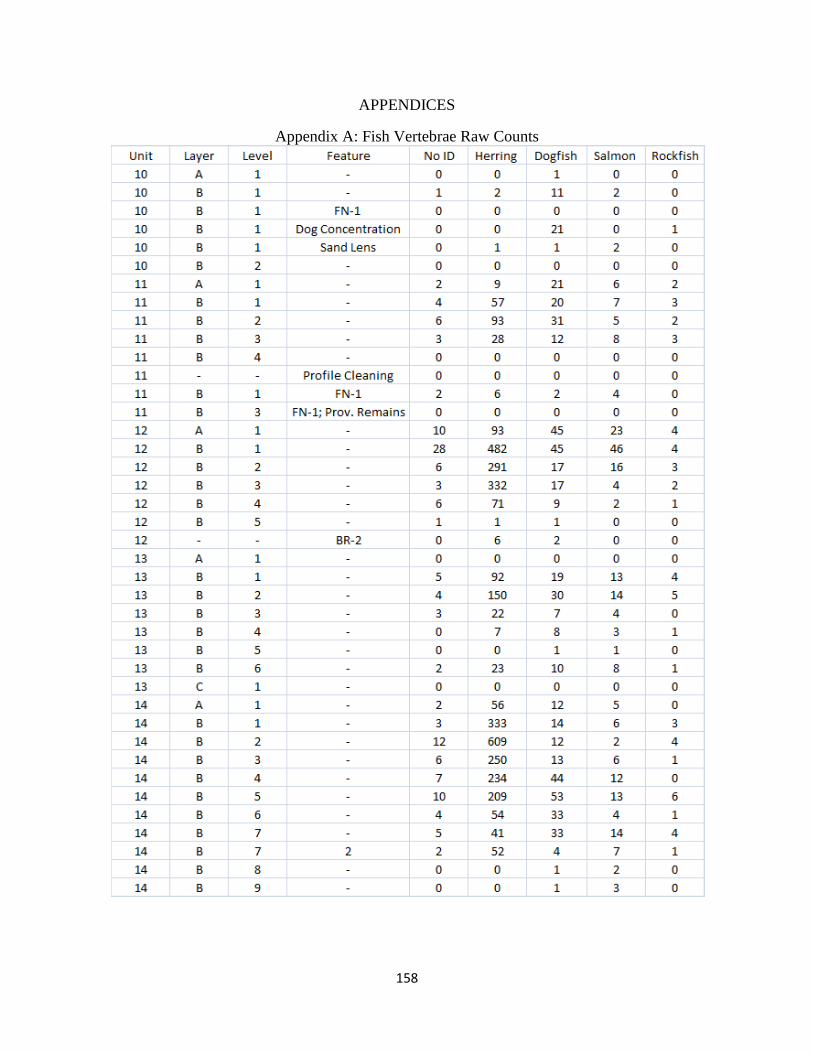
158
APPENDICES
Appendix A: Fish Vertebrae Raw Counts
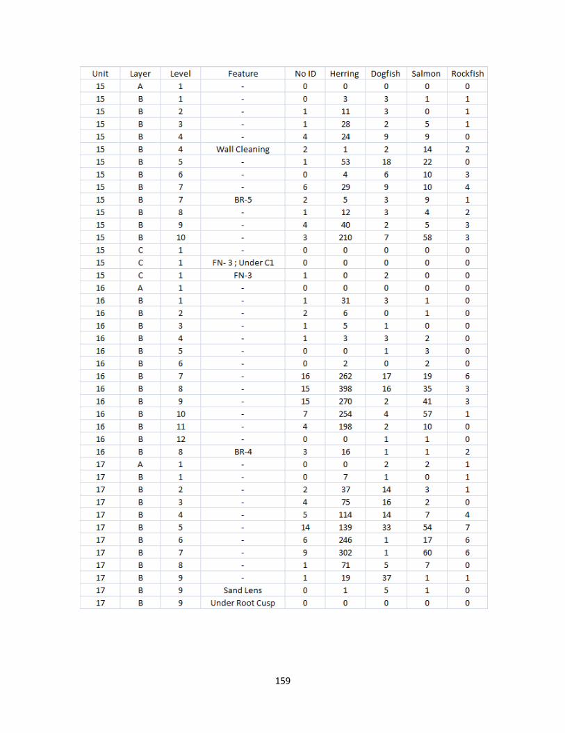
159

160
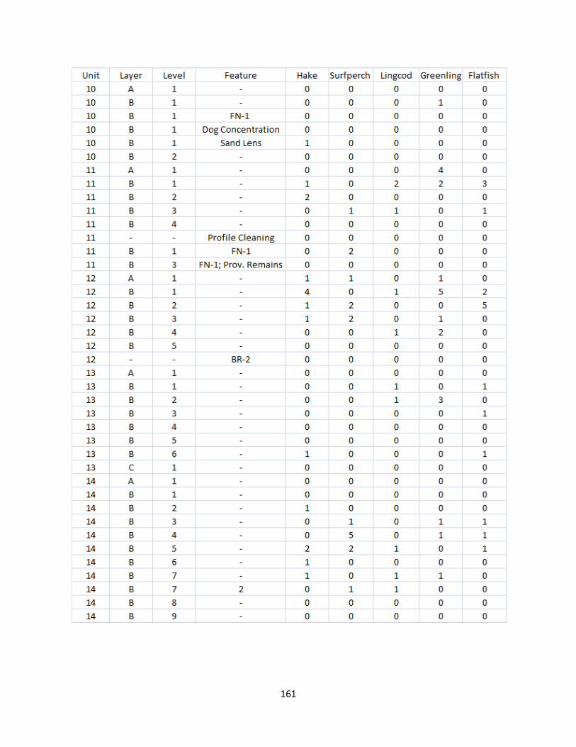
161
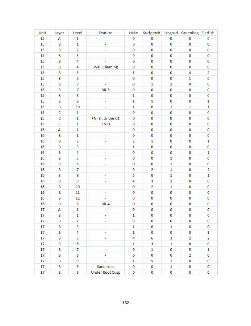
162
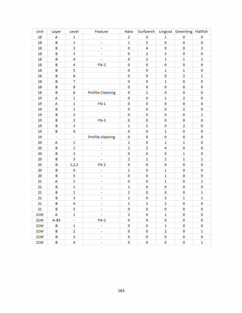
163

164
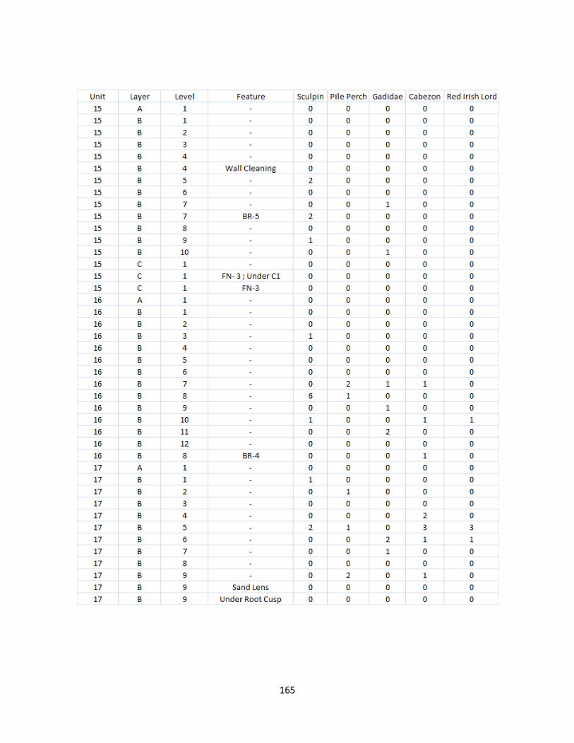
165
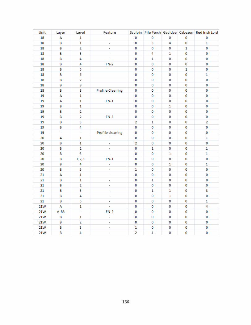
166

167

168

169
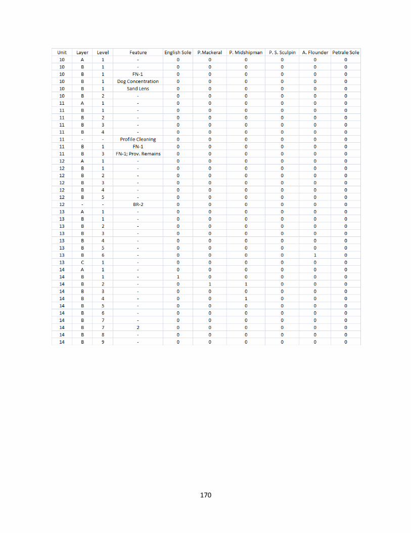
170
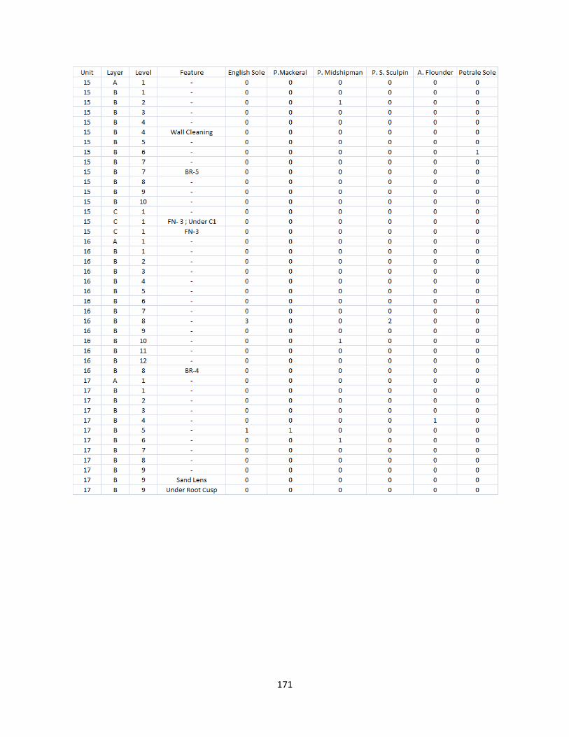
171
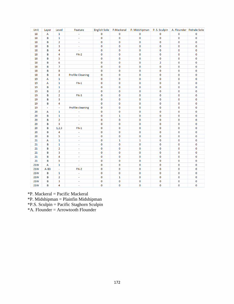
172
*P. Mackeral = Pacific Mackeral
*P. Midshipman = Plainfin Midshipman
*P.S. Sculpin = Pacific Staghorn Sculpin
*A. Flounder = Arrowtooth Flounder

173
Appendix B: Fish Vertebrae Raw Data
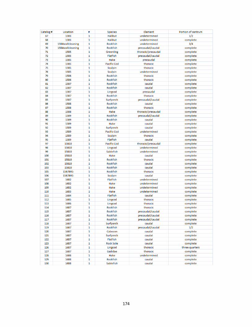
174

175
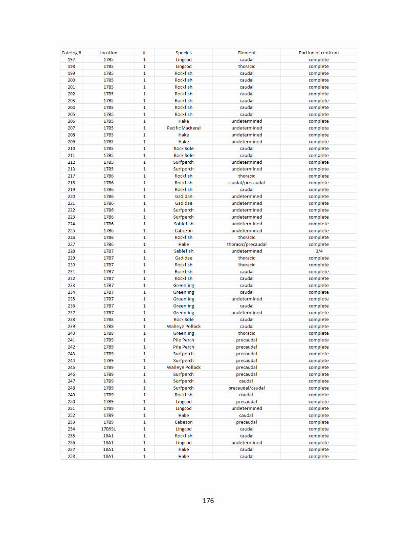
176
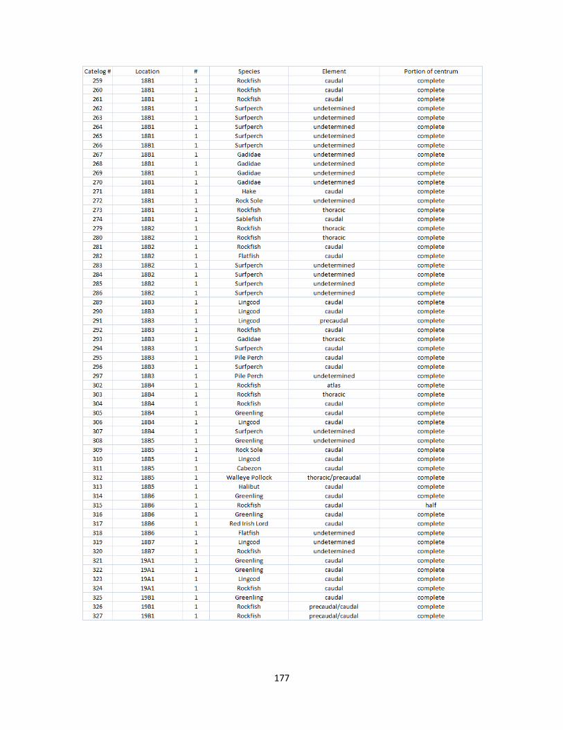
177
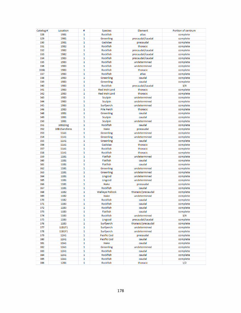
178
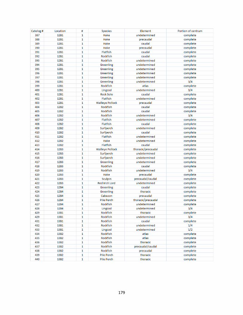
179

180
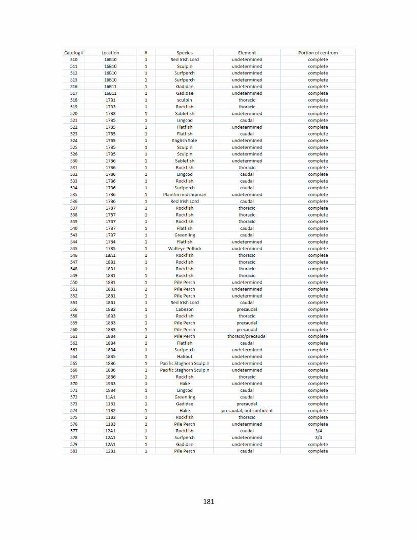
181
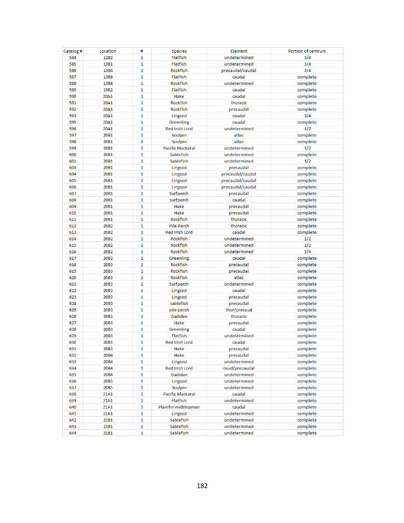
182
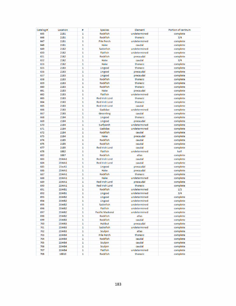
183
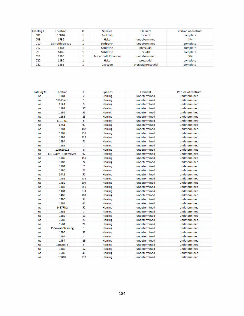
184

185
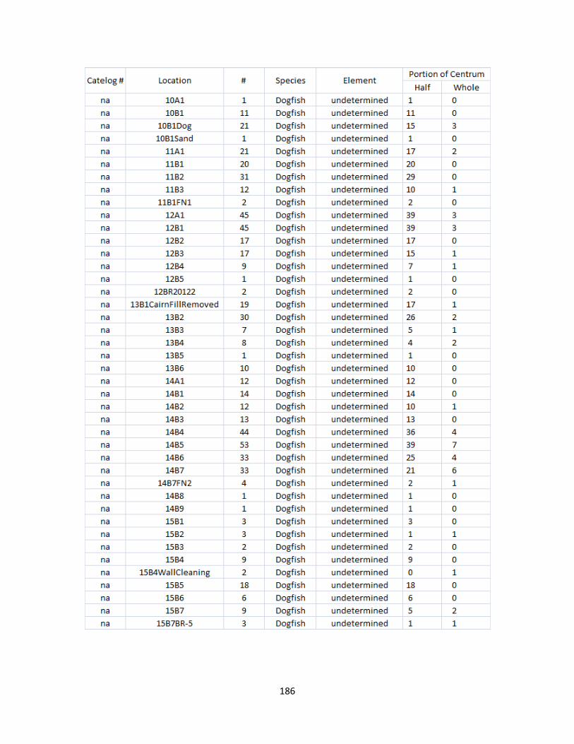
186

187
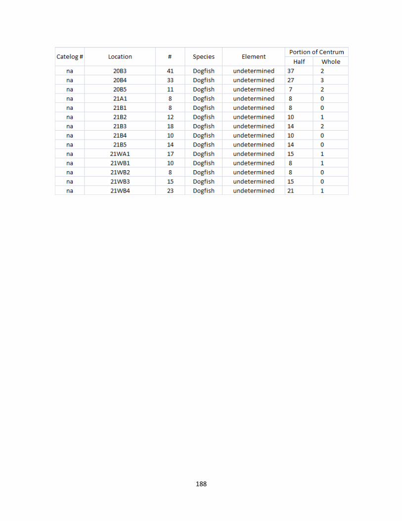
188

189
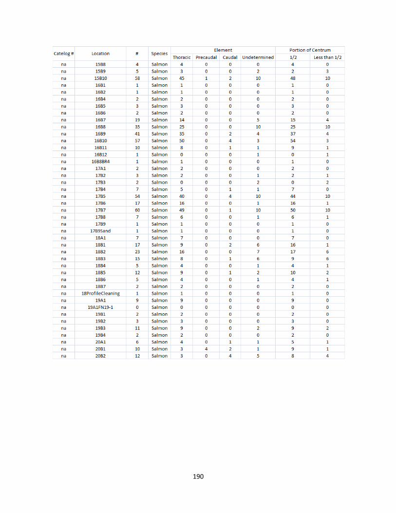
190
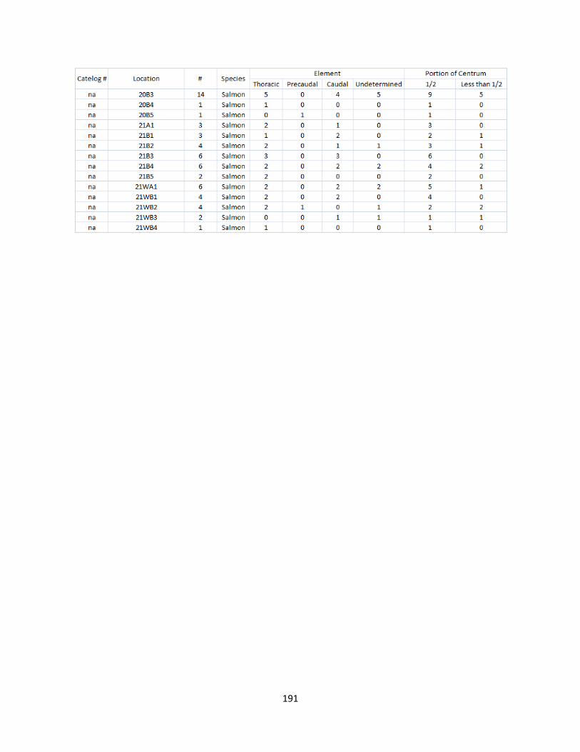
191

192
Appendix C: Terrestrial Mammal Raw Counts
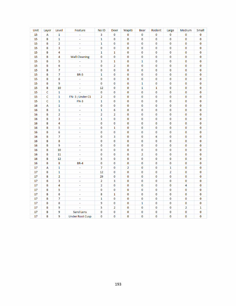
193

194

195
Appendix D: Terrestrial Mammal Raw Data
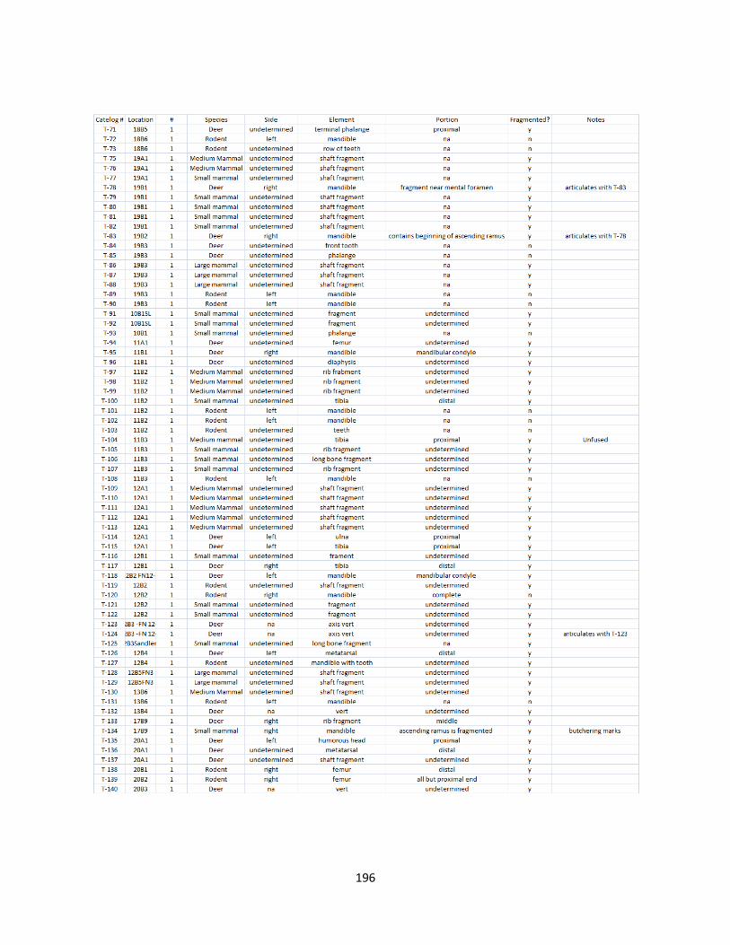
196

197

198
Appendix E: Sea Mammal Raw Counts
Appendix F: Sea Mammal Raw Data

199
Appendix G: Bird Raw Counts
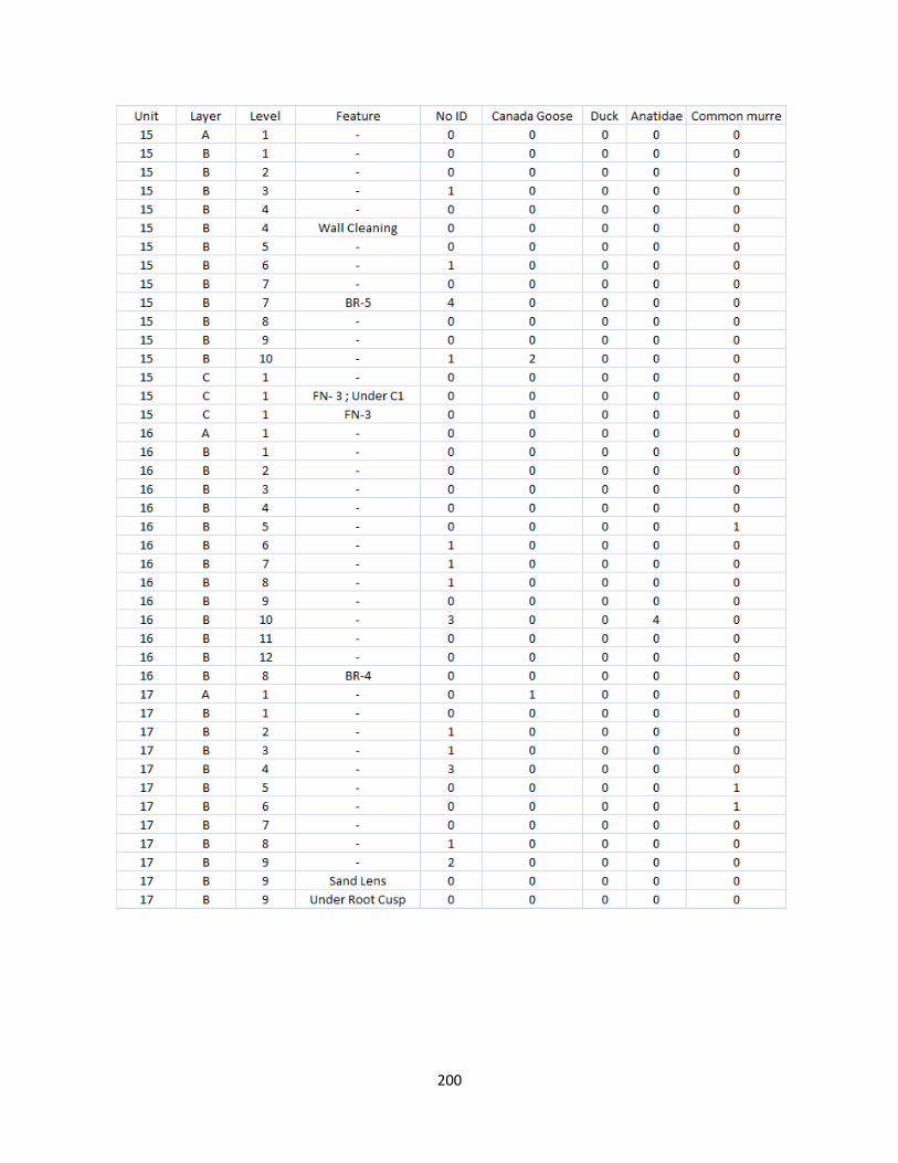
200
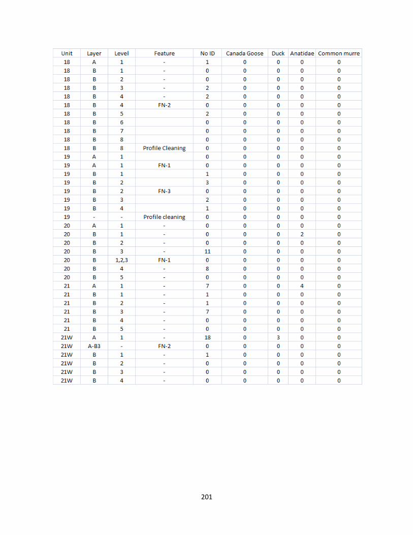
201
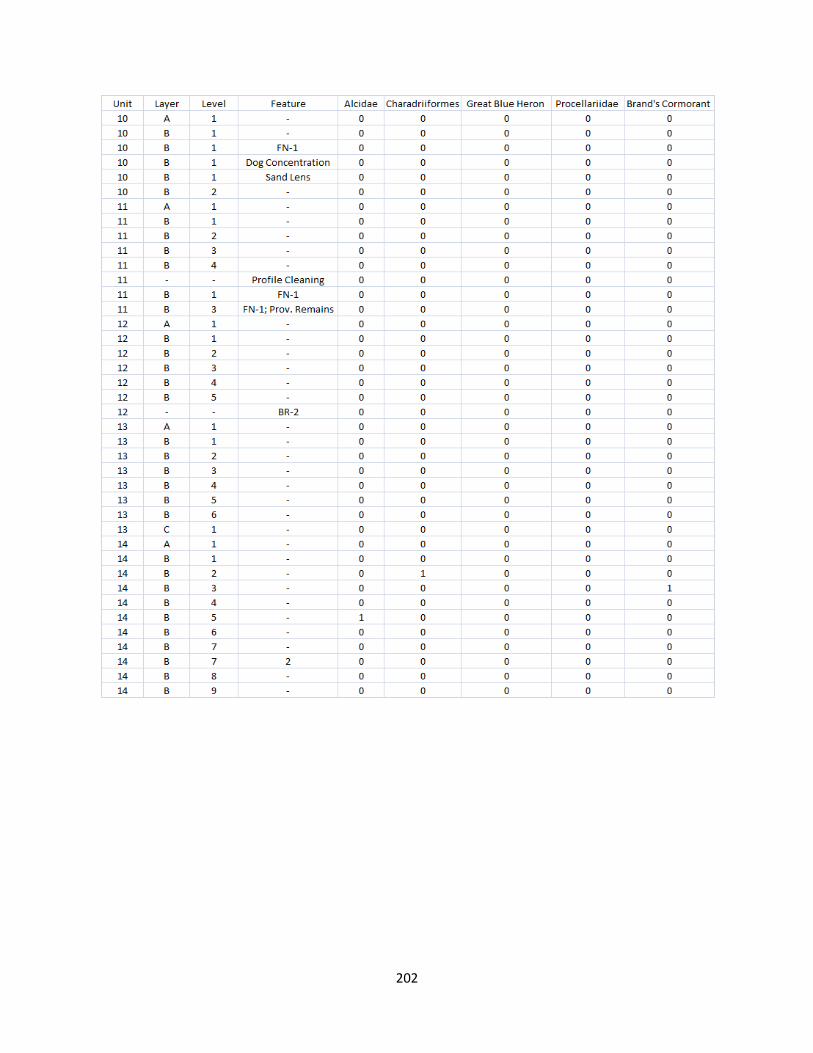
202

203
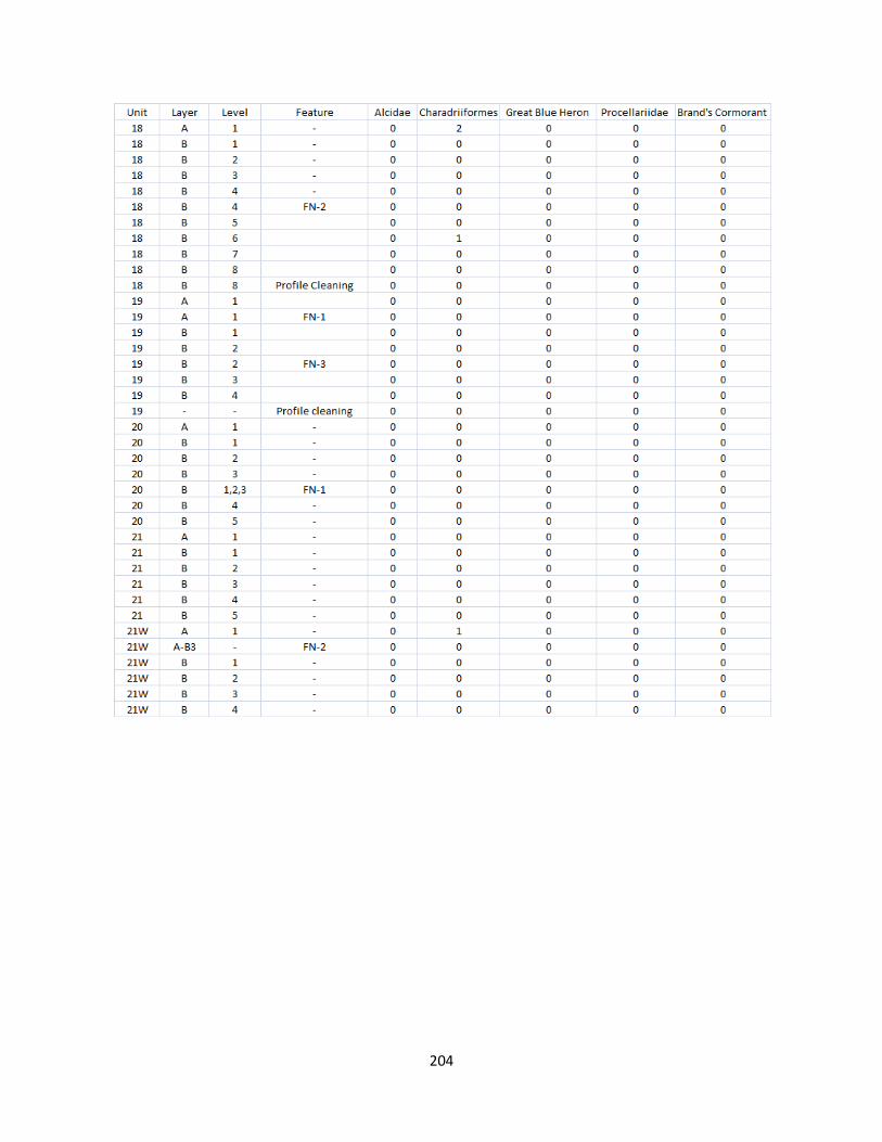
204
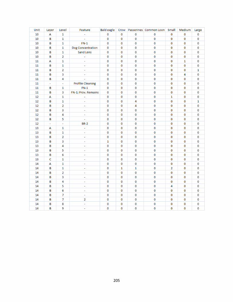
205

206
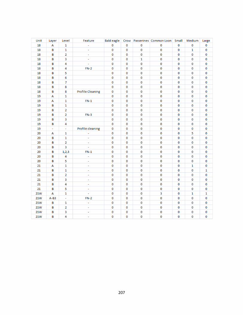
207
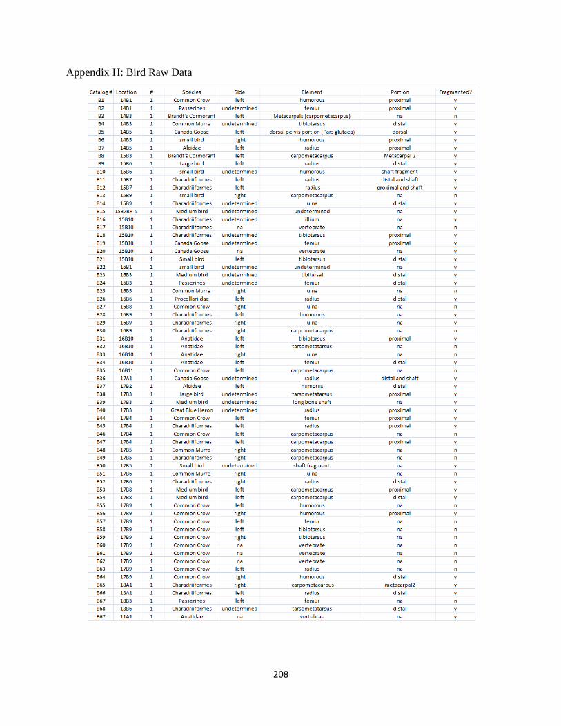
208
Appendix H: Bird Raw Data
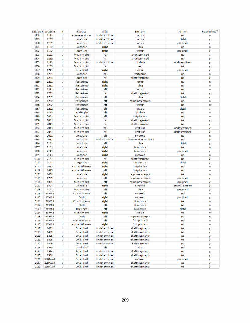
209
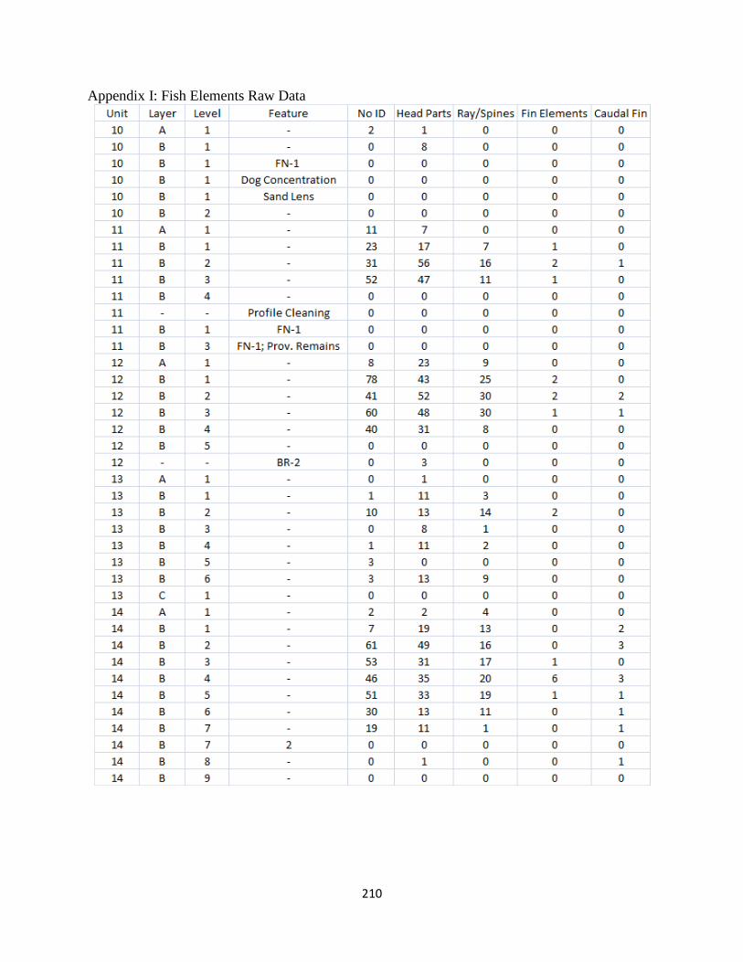
210
Appendix I: Fish Elements Raw Data
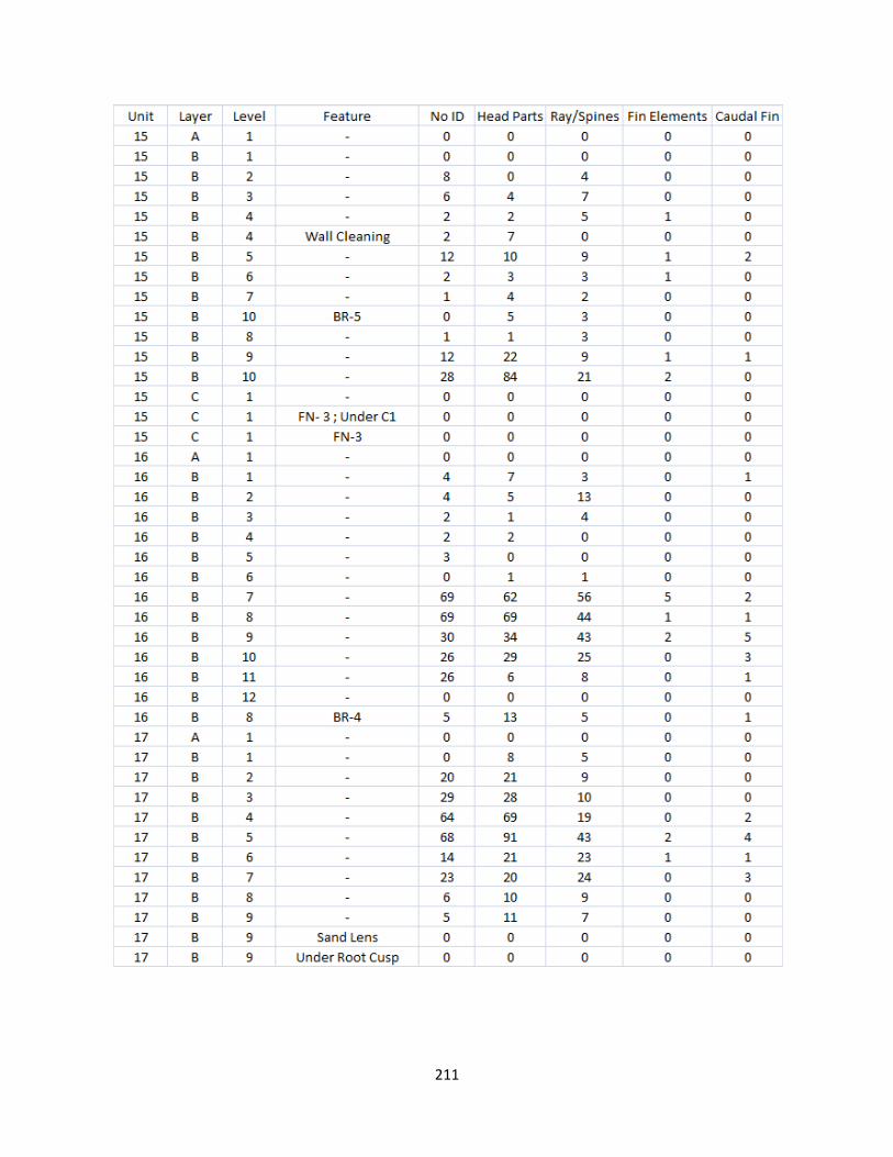
211

212

213
Appendix J: “No ID” Raw Data

214

215

216
Appendix K: Temporal and Depositional Unit Level Designation
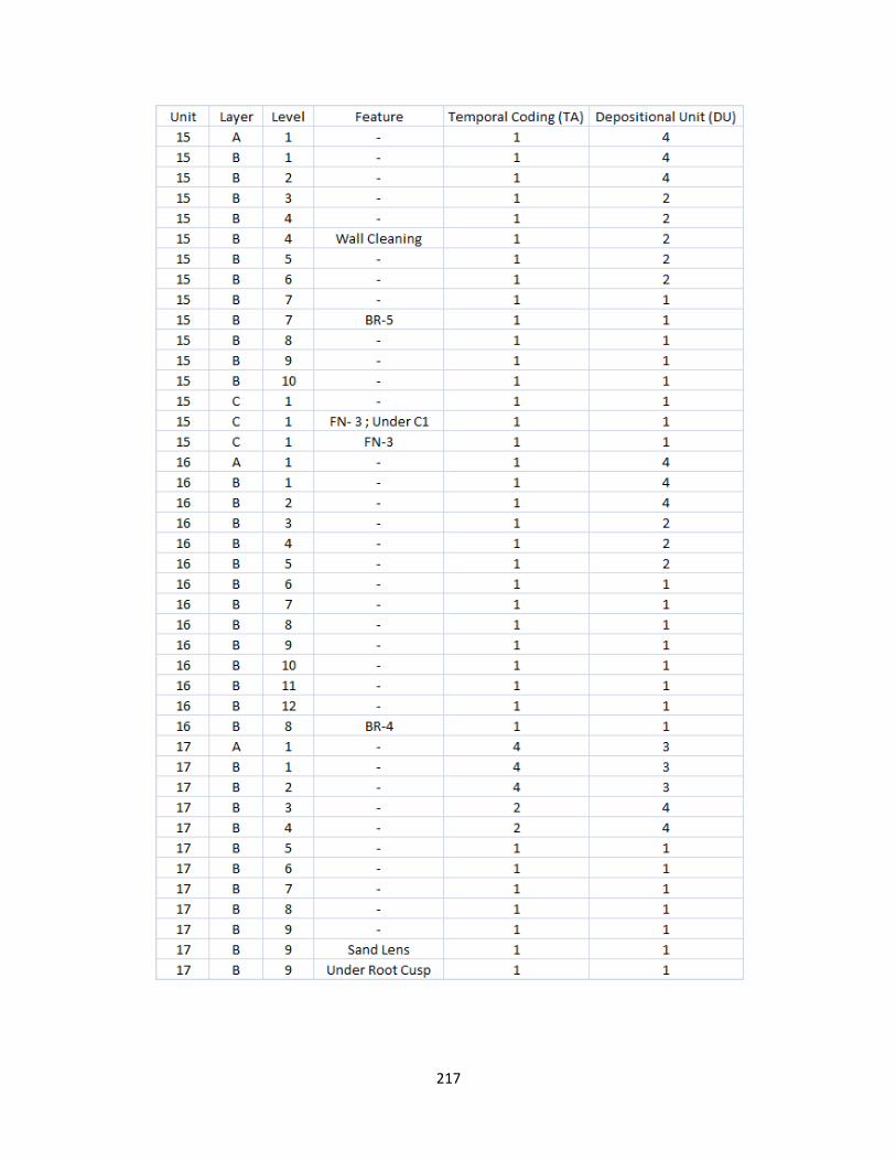
217
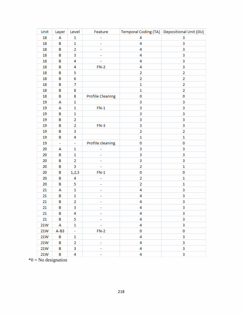
218
*0 = No designation
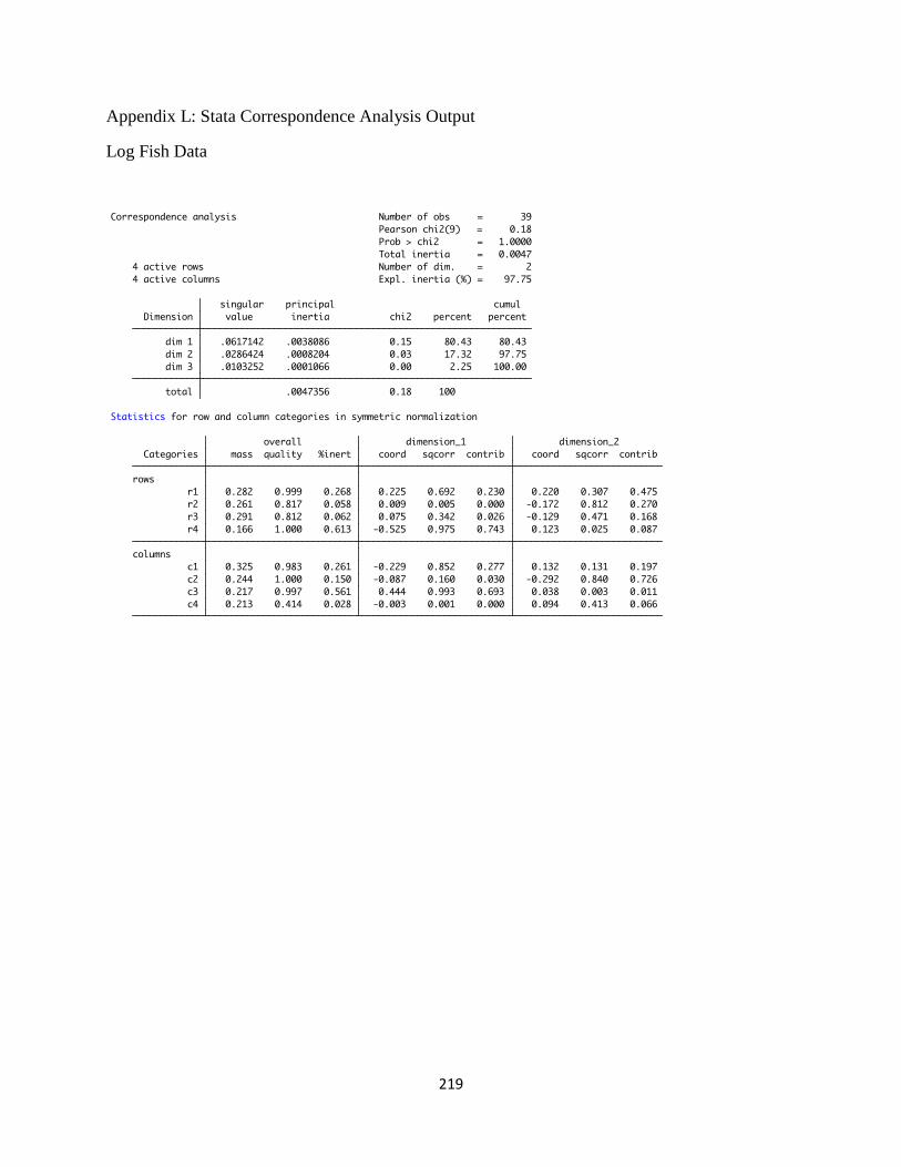
219
Appendix L: Stata Correspondence Analysis Output
Log Fish Data
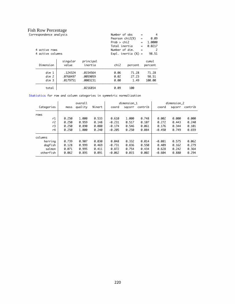
220
Fish Row Percentage
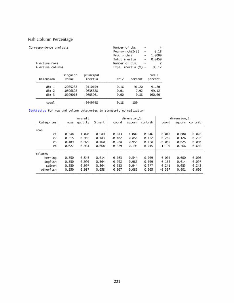
221
Fish Column Percentage
Top Related
Copyright © 2022 FDOKUMEN

