


Bahasa
Halaman
Hukum


Device-Tagged Feature-based Localization and Mapping
of Wide Areas with a PTZ Camera
Alberto Del Bimbo Giuseppe Lisanti Iacopo Masi Federico Pernici
{delbimbo, lisanti, masi, pernici}@dsi.unifi.it
Media Integration and Communication Center (MICC)
University of Florence, Viale Morgagni, 65 (FI) - Italy
Abstract
This paper proposes a new method for estimating and
maintaining over time the pose of a single Pan-Tilt-Zoom
camera (PTZ). This is achieved firstly by building offline a
keypoints database of the scene; then, in the online step, a
coarse localization is obtained from camera odometry and
finally refined by visual landmarks matching. A mainte-
nance step is also performed at runtime to keep updated
the geometry and appearance of the map.
At the present state-of-the-art, there are no methods ad-
dressing the problem of being operative for a long period of
time. Also, differently from our proposal these methods do
not take into account for variations in focal length.
Experimental evaluation shows that the proposed ap-
proach makes it possible to deliver stable camera pose
tracking over time with hundreds of thousand landmarks,
which can be kept updated at runtime.
1. Introduction
In recent years, pan-tilt-zoom cameras are becoming in-
creasingly common, especially for use as surveillance de-
vices in large areas. Despite its widespread usage, there
are still issues to be resolved regarding their effective ex-
ploitation for scene understanding at a distance. A typical
operating scenario is that of abnormal behavior detection
which requires both simultaneous target trajectories analy-
sis on the 3D ground plane and the indispensable image res-
olution to perform target biometric recognition. This can-
not generally be achieved with a single stationary camera
mainly because of the limited field of view and poor resolu-
tion with respect to scene depth. PTZ sensors indeed assure
a superior image quality (for example as zoom increases
towards distant objects in the scene) and this will be cru-
cial for the task of managing the sensor to detect and track
several moving targets at a distance. To this end we are in-
terested in the acquisition and maintenance of camera pose
estimation, relative to some geometric 3D representation of
its surroundings, as the sensor performs pan-tilt and zoom
operations. This allows continuous dynamic-calibration of
the sensor for a tracking system based on target scale infer-
ence and robust data-association [9].
1.1. Related Work
In its basic form this approach resembles the Simulta-
neous Localization And Mapping (SLAM) [10] made more
challenging by the requirement of detection and tracking
of moving objects. Nevertheless there are some important
differences between the standard Visual monocular SLAM
(monoSLAM) [8] and the PTZ-SLAM: monoSLAM as-
sumes a static environment and known internal camera pa-
rameters, considering a freely moving observer (6DOF). On
the contrary PTZ-SLAM must solve for 8DOF (three for the
pose and five for the intrinsic parameters) and deals with dy-
namic environments. Civera et al. [6] present a sequential
mosaicing algorithm for an internal calibrated rotating cam-
era using an Extended Kalman Filter SLAM approach. Au-
thors point out that their results are mainly occurred because
a rotating camera is a constrained and well-understood lin-
ear problem. Here, we argue that tracking a zooming cam-
era is much more difficult, because the structure of the prob-
lem is highly non-linear and near-ambiguities may arise
when the perspective effects are small, due to large focal
lengths [1]. Such difficulties make it unsuitable for most
real-world PTZ surveillance scenarios and motivate the de-
velopment of a system able to perform loop closure1 over
an extended area.
To avoid data association errors of EKF-SLAM based
methods, Klein and Murray propose the Parallel Tracking
and Mapping (PTAM) for small workspace [11] that em-
ploys standard Structure from Motion (SfM) bundle adjust-
1Loop closure refers to data association between two distinct parts of
the map even when tracking is proceeding smoothly.
1
Tag
Current Frame
Raw Device Tagged Localization
Keypoints Maintenance and Localization
Base-set
3D ground plane
PTZ camera
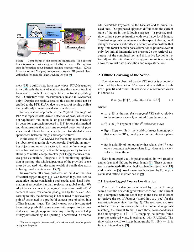
Figure 1. Components of the proposed framework. The current
frame is associated with a tag provided by the device. The tag con-
tains information about internal machine encoder values. (Top):
Localization and Mapping component. (Right): 3D ground plane
estimation for multiple target tracking system [9].
ment [13] to build a map from many views. PTAM separates
in two threads the task of maintaining the camera track at
frame-rate from the less stringent task of optimally updating
the 3D structure from measurements (made in keyframes
only). Despite the positive results, this system could not be
applied to the PTZ-SLAM due to the cost of solving online
the bundle adjustment considering a wide area.
An alternative approach to the “hybrid tracking” of
PTAM is repeated data-driven detection of pose, which does
not require any motion model on pose estimation. Tracking
by detection approach proposed in [14] follows this method
and demonstrates that real-time repeated detection of pose
via a forest of fast classifiers can be used to establish corre-
spondences between image and target features.
In the case of PTZ-SLAM the matching system should
be robust to changes in viewpoint/scale, blur/lighting, mov-
ing objects and other distractors; it must be fast enough to
run online without any drift in the map geometry to ensure
stability to multiple target tracker (MTT) [9] that uses cam-
era pose estimation. Imagine a 24/7 monitoring applica-
tion of parking: the whole appearance of the provided scene
must be updated with the same wealth of details that exists
in background maintenance [15, 2].
To overcome all above problems we build on the idea
of textual tagged images [7]. Geo-located tags, are used to
categorize images considering both spatial and visual infor-
mation at respectively urban, regional or global scale. We
adopt the same concept by tagging images taken with a PTZ
camera at some raw camera pose given by the device. Ac-
cording to this, the device tag is hence used to retrieve key-
points2 associated to a pre-build camera pose obtained in a
offline learning stage. The final camera pose is computed
by refining pre-build camera pose with respect to the cur-
rent view through keypoint matching. Finally a novel step
of keypoints tracking and updating is performed in order to
2The terms keypoint, feature and landmark are used interchangeably
throughout the paper.
add new/stable keypoints to the base-set and to prune un-
used ones. Our proposed approach differs from the current
state-of-the-art in the following aspects: 1) precise, real-
time camera pose estimation with very large focal length;
2) robust keypoints maintenance with respect to background
changes that occur naturally in a scene; we demonstrate that
long-time robust camera pose estimation is possible even if
only few initial landmarks are present; 3) the retrieval ac-
curacy (of the combined text and distinctive keypoints re-
trieval) and the total absence of any prior on motion models
allow for robust data association and map estimation.
2. Offline Learning of the Scene
The wide area observed by the PTZ sensor is accurately
described by a base set of M images taken at different val-
ues of pan, tilt and zoom. This base-set B of reference views
is defined as:
B = [yi, {fij}
nj=1, HW , Hih : i = 1..M ] (1)
where:
• yi ∈ R3 is the raw device-tagged PTZ value, relative
to the reference view Ii acquired from the sensor;
• f ij is the jth keypoint of the ith reference view;
• HW : Π3D 7→ Πh is the world-to-image homography
that maps the 3D ground plane on the reference plane
Πh.
• Hih is a family of homography that relates the ith view
onto a common reference plane Πh, where h is a view
selected from the set.
Each homography Hih is parameterized by two rotation
angles (pan and tilt) and by focal length [1]. These parame-
ters are estimated offline with global bundle adjustment [13]
as described in [5]. World-to-image homography HW is pre-
calculated offline as described in [9].
2.1. DeviceTagged Coarse Localization
Real time Localization is achieved by first performing
search over the device-tagged reference views. The current
tag is compared with the set of tags in the base-set in order
to retrieve the set of features (stored in a k-d tree) for the
nearest reference view (see Fig. 2). The recovered k-d tree
is further queried to retrieve the set of potential keypoints
matching the current frame. From these correspondences
the homography Ht : It 7→ Ii, mapping the current frame
onto the retrieved view, is estimated with RANSAC. The
time variant world-to-image homography Gt : Π3D 7→ It is
finally obtained as in [9]:

Gt = H−1t
︸ ︷︷ ︸
It←Ii
· H−1
ih︸ ︷︷ ︸
Ii←Πh
· HW︸ ︷︷ ︸
Πh←Π3D
(2)
Localization performs real-time due to the fact that: 1)
the keypoints detection and description is performed by ex-
ploiting Speed Up Robust Feature (SURF) [3]; 2) at each
time only a region of the field of regard3 is updated by re-
building the local k-d tree.
Figure 2. The structure used for real-time localization of the PTZ
sensor. Raw camera encoder values are used to index the k-d tree
of each reference view Ii.
3. Real-Time Lifelong Mapping
Features update and maintenance is formalized as fol-
lows: given the model set of keypoints Fm.= {fj}
nj=1 in
eq. (1) extracted from the scene at time t, choose online
which ones keep in the set, remove or update, taking as ob-
servation the set of points of the current scene at time t ≫ t,
defined as Fc.= {fk}
mk=1
. The aim is to maintain consis-
tency among the offline Fm features database with respect
to current keypoints Fc so as to preserve a database of up-
dated features that allows continuous dynamic-calibration.
To this aim the SURF keypoint fj is extended as follows
to create a time-invariant feature descriptor:
fj = {ID , Xt , T (τ, t) , d} (3)
where:
• ID is the identifier of a landmark.
• Xt ∼ N (µX ,ΣX) is a 2D Gaussian random variable
where µX represents the averaged keypoint location
and ΣX is the relative covariance matrix.
• T (τ, t) is a random variable that describes the lifetime
of each keypoint in the model.
• d ∈ R128 is the local descriptor updated over time.
Keypoints matching is performed in the local k-d tree
according to approximate nearest neighbor search, as in [4].
3The camera field of regard (FOR) is defined as the union of all field of
view over the entire range of pan and tilt rotation angles and zoom values.
3.1. Map Geometry Updating
To avoid drift errors and preserve the global optimization
made offline, the geometry of each keypoint is estimated
into the matched reference view Ii. Furthermore, the noise
introduced by the Fast-Hessian detector is limited by per-
forming recursive time average of the keypoint geometry
Xt , without any adaptation, as:
µXt=
t − 1
t· µXt−1
+1
t· Zt (4)
σXt
2 =t − 1
t· σ2
Xt−1+
1
t − 1· (µX − Zt)
2 (5)
where Zt ∈ R2 is current SURF keypoint detection back-
projected on the reference view Ii.
3.2. Map Landmark Updating
During tracking each keypoint undergoes some changes
in appearance due to structural variations provided ,for ex-
ample, by a car that enters or leaves the scene, or by gradual
changes according to sunlight.
3.2.1 Birth and Death Process of Visual Landmarks
Figure 3. The set of points in the model Fm is bi-partitioned be-
tween points to keep and remove. The current set of points Fc
instead is bi-partitioned between the matched points and those can-
didate to be inserted.
Insertion and deletion of landmarks are obtained by the
intersection of the current keypoints set Fc with respect to
the model-set Fm, as shown in Fig. 3. Keypoints are classi-
fied as follows :
• Fmatched.= {Fm}
⋂{Fc} represents keypoints which
remain in the model.
• Fremove.= {Fm} \ {Fmatched} represents the set of
keypoints candidate to be removed.
• Fto add.= {Fc} \ {Fmatched} represents the subset of
keypoints from which new features will be selected.
To speed up feature matching we perform a random sam-
pling step on Fc; this allows also for some feature random-
ization which effectively makes RANSAC less likely to fail

in subsequent frames. According to this, a landmark re-
moval probability is defined as follows: a keypoint that has
not been seen for a long time will gain a high probability to
exit out from the set. This is motivated by the fact that it
has been part of Fremove for many times. On the contrary
a keypoint that was just observed will extend its lifetime
since that it has been ranked in the Fmatched. In this way,
we achieve a dynamic keypoint modeling with an effective
birth and death process of landmarks.
The lifetime of each discriminative keypoint is modeled
as a negative exponential random variable T (τ, t) ∼ τe−τt
of eq. (3) that varies with time in order to simulate a mem-
ory decay process (i.e. the loss of memory over time). Un-
der such assumption at each instant the lifetime is given by
a p.d.f. parameterized by τ ≥ 0 where τ models the ten-
dency for the keypoint of being removed. Each time there
is no observation the parameter τ is incremented, otherwise
it is set to zero. The death probability of a keypoint at time
t is then given by:
pdeath(T < t|τ) =
∫ t
0
τ · e−τxdx = 1 − e−τ ·t (6)
On the contrary the birth process, tackling structural
changes, is based on the set given by the classification
refinement step, previously defined as Fto add
.
= {Fc} \
{Fmatched}, representing new landmarks in the scene. Since
this set at time t contains some temporary outliers of the
model (i.e. features that do not belong to the scene), we
track them for a limited period in order to select the key-
points that will be able to enter the model.
The basic idea is to compare two sets of candidates so as
to finally decide which points to include as background: 1)
at time t the set of keypoints candidate to enter the model
F tto add is taken into account; 2) after a temporal window
δt, at time t + δt a new candidate set F t+δtto add is obtained;
3) the keypoints correspondences between these two sets
make a new set F t+δtadd that will become part of the map.
Otherwise, items without correspondences will be labeled
as foreground F t+δtforeground and will be discarded.
The parameter δt is used to refine the keypoints selec-
tion step that will decide about which landmarks may be
included. Low values for δt may let in landmarks that are
not required (e.g. foreground points generated from shad-
ows), while high values may void the research between the
two sets. In order to maintain persistence in the scene ap-
pearance we choose δt = 20.
It is important to remark that not every keypoints will
be added to Fm with the same probability, since they are
mapped to the reference view Ii through Ht. Indeed to sta-
bilize the estimated camera pose we keep updated the map
by firstly adding points with less uncertainty. Only after
that, keypoints with a larger uncertainty are considered.
This “exploration vs exploitation” trade-off governs the
process of adding new keypoints, while exploiting less un-
certainty. We proceed similarly as in [12] following the
idea that adding points far from the Fmatched may pro-
vide worse performance. Therefore we define the proba-
bility of a point to enter the model as the ratio between the
minimum bounding box area that contains the convex hull
of the Fmatched, and the same bounding box temporarily
expanded with the new feature to add. This process alone
however is not enough to deal with gradual changes in land-
mark appearance. Therefore each landmark descriptor is
updated by running average (α = 0.25 is used):
dr = (1 − α) · dr + α · dr ∀r = 1..128 (7)
−20 0 20 40 60 80 100 120 140−0.8
−0.6
−0.4
−0.2
0
0.2
0.4
0.6
0.8
1
Figure 4. Representation of changes occurred in a keypoint de-
scriptor over time. Error bars (blue) show the standard deviation
across realizations (red). Descriptor components are plotted in as-
cending order.
4. Experimental Results
We use a real dataset taken from a wide parking area
with an off-the shelf SONY PTZ camera placed at about
seven meters in height. The scene is learned, as described
in Sec. 2, from about n = 300 reference views (acquired
at different levels of pan, tilt and zoom) which results in
about 150, 000 keypoints for the whole initial database. The
video stream and the reference views have a resolution of
320 × 240 pixels. Our system implementation runs in real-
time at 30 fps on a Intel Xeon Quad-Core at 2.93 GHz. We
performed qualitative and quantitative experiments show-
ing the effectiveness of the system to handle with structural
changes of the scene.
Regarding qualitative experiments, Fig. 5 shows a de-
tailed example of structural change caused by a car that
has left the scene. Fig. 5top-right shows the reference
view Ii chosen by the raw camera localization system.
Fig. 5bottom-right is the current frame It. The mainte-
nance process automatically increases the death probability
pdeath(fi) for each keypoint of the car (in yellow), as shown
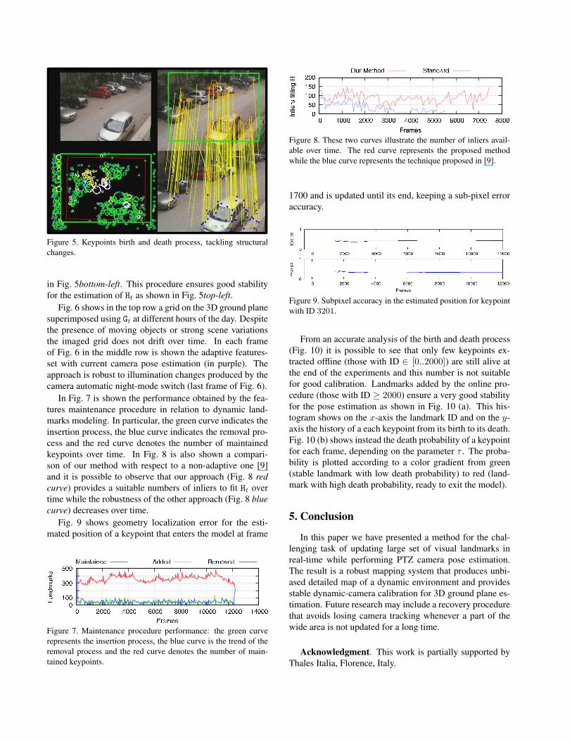
Figure 5. Keypoints birth and death process, tackling structural
changes.
in Fig. 5bottom-left. This procedure ensures good stability
for the estimation of Ht as shown in Fig. 5top-left.
Fig. 6 shows in the top row a grid on the 3D ground plane
superimposed using Gt at different hours of the day. Despite
the presence of moving objects or strong scene variations
the imaged grid does not drift over time. In each frame
of Fig. 6 in the middle row is shown the adaptive features-
set with current camera pose estimation (in purple). The
approach is robust to illumination changes produced by the
camera automatic night-mode switch (last frame of Fig. 6).
In Fig. 7 is shown the performance obtained by the fea-
tures maintenance procedure in relation to dynamic land-
marks modeling. In particular, the green curve indicates the
insertion process, the blue curve indicates the removal pro-
cess and the red curve denotes the number of maintained
keypoints over time. In Fig. 8 is also shown a compari-
son of our method with respect to a non-adaptive one [9]
and it is possible to observe that our approach (Fig. 8 red
curve) provides a suitable numbers of inliers to fit Ht over
time while the robustness of the other approach (Fig. 8 blue
curve) decreases over time.
Fig. 9 shows geometry localization error for the esti-
mated position of a keypoint that enters the model at frame
Figure 7. Maintenance procedure performance: the green curve
represents the insertion process, the blue curve is the trend of the
removal process and the red curve denotes the number of main-
tained keypoints.
Figure 8. These two curves illustrate the number of inliers avail-
able over time. The red curve represents the proposed method
while the blue curve represents the technique proposed in [9].
1700 and is updated until its end, keeping a sub-pixel error
accuracy.
Figure 9. Subpixel accuracy in the estimated position for keypoint
with ID 3201.
From an accurate analysis of the birth and death process
(Fig. 10) it is possible to see that only few keypoints ex-
tracted offline (those with ID ∈ [0..2000]) are still alive at
the end of the experiments and this number is not suitable
for good calibration. Landmarks added by the online pro-
cedure (those with ID ≥ 2000) ensure a very good stability
for the pose estimation as shown in Fig. 10 (a). This his-
togram shows on the x-axis the landmark ID and on the y-
axis the history of a each keypoint from its birth to its death.
Fig. 10 (b) shows instead the death probability of a keypoint
for each frame, depending on the parameter τ . The proba-
bility is plotted according to a color gradient from green
(stable landmark with low death probability) to red (land-
mark with high death probability, ready to exit the model).
5. Conclusion
In this paper we have presented a method for the chal-
lenging task of updating large set of visual landmarks in
real-time while performing PTZ camera pose estimation.
The result is a robust mapping system that produces unbi-
ased detailed map of a dynamic environment and provides
stable dynamic-camera calibration for 3D ground plane es-
timation. Future research may include a recovery procedure
that avoids losing camera tracking whenever a part of the
wide area is not updated for a long time.
Acknowledgment. This work is partially supported by
Thales Italia, Florence, Italy.

Figure 6. (Top row): Superimposed grid of the 3D ground plane. (Middle row): The adaptive feature-set over time. (Bottom row): The
reference view Ii selected by the localization system.
0
3000
6000
9000
12000
0 2000 4000 6000 8000 10000 12000 14000
Landm
ark
Lifetim
e
Landmark ID
(a) (b)
Figure 10. (a) The history of lifetime for each keypoint observed in a region of the FOR. (b) The histogram of death probability for each
visual landmark.
References
[1] L. D. Agapito, E.Hayman, and I.Reid. Self-calibration of rotating and
zooming cameras. International Journal of Computer Vision (IJCV),
45:2, 2001.
[2] G. Baugh and A. Kokaram. Feature-based object modelling for visual
surveillance. International Conference on Image Processing, 2008.
[3] H. Bay, T. Tuytelaars, V. Gool, and L. Surf: Speeded up robust
features. In Internation Conference on Computer Vision, 2006.
[4] J. Beis and D. Lowe. Indexing without invariants in 3d object recog-
nition. Pattern Analysis and Machine Intelligence, IEEE Transac-
tions on, 21(10):1000–1015, October 1999.
[5] M. Brown and D. Lowe. Recognising panoramas. In Proceedings of
the 9th International Conference on Computer Vision, 2003.
[6] J. Civera, A. J. Davison, J. A. Magallon, and J. M. Montiel. Drift-free
real-time sequential mosaicing. International Journal of Computer
Vision, 81(2):128–137, 2009.
[7] M. Cristani, A. Perina, U. Castellani, and V. Murino. Geo-located
image analysis using latent representations. In International Confer-
ence on Computer Vision and Pattern Recognition, 2008.
[8] A. J. Davison. Real-time simultaneous localisation and mapping with
a single camera. In International Conference on Computer Vision,
2003.
[9] A. Del Bimbo, G. Lisanti, and F. Pernici. Scale invariant 3d multi-
person tracking using a base set of bundle adjusted visual landmarks.
In Proc. of ICCV International Workshop on Visual Surveillance,
2009.
[10] H. Durrant-Whyte. Uncertain geometry in robotics. In Proceed-
ings of IEEE International Conference on Robotics and Automation.,
1987.
[11] G. Klein and D. Murray. Parallel tracking and mapping for small AR
workspaces. In International Symposium on Mixed and Augmented
Reality, 2007.
[12] S. Negahdaripour, R. Prados, and R. Garcia. Planar homography: ac-
curacy analysis and applications. International Conference on Image
Processing, 2005.
[13] B. Triggs, P. Mclauchlan, R. Hartley, and A. Fitzgibbon. Bundle
adjustment - a modern synthesis. Proceedings of the International
Workshop on Vision Algorithms, 2000.
[14] M. O. Vincent, V. Lepetit, F. Fleuret, and P. Fua. Feature harvest-
ing for tracking-by-detection. In European Conference on Computer
Vision, 2006.
[15] Q. Zhu, S. Avidan, and K.-T. Cheng. Learning a sparse, corner-based
representation for time-varying background modelling. International
Conference on Computer Vision, 2005.
Copyright © 2022 FDOKUMEN

