Denoising of continuous-wavetime-of-flight depth images usingconfidence measuresMario FrankDepartment of Computer Science, ETH Zurich

Haldeneggsteig 4, 8092 Zurich, Switzerland

Phone: +41 44 632 3179, Fax: +41 44 632 15 62, mario.frank[at]inf.ethz.ch

Matthias PlaueDepartment of Mathematics, Technische Universitat Berlin

Straße des 17. Juni 136, 10623 Berlin, Germany

Phone: +49 30 314 232 65, Fax: +49 30 314 792 82, plaue[at]math.tu-berlin.de

Fred A. Hamprecht†

Heidelberg Collaboratory for Image Processing, University of Heidelberg

Speyerer Straße 4, 69115 Heidelberg, Germany

Phone: +49 6221 54 88 75, Fax: +49 6221 54 52 76, fred.hamprecht[at]iwr.uni-heidelberg.de†corresponding

AbstractTime-of-flight range sensors with on-chip continuous-wavecorrelation ofradio frequency modulated signals are increasingly popular. They simul-taneously deliver depth maps and intensity images with noise and system-atic errors that are unique for this particular kind of data.Based on recenttheoretical findings on the dominating noise processes we propose specificvariants of normalized convolution and median filtering, both adaptive andnon-adaptive, to the denoising of the range images. We examine the pro-posed filters on real-world depth maps with varying reflectivity, structure,over-exposure, and illumination. The best results are obtained by adaptivefilters that locally adjust the level of smoothing using the estimated modula-tion amplitude as a measure of confidence.

Copyright 2008 Society of Photo-Optical Instrumentation Engineers. This paper was published inOptical Engineering

(OE), Vol. 48, No. 7,and is made available as an electronic reprint with permission of SPIE. One print or electronic copy

may be made for personal use only. Systematic or multiple reproduction, distribution to multiple locations via electronic or

other means, duplication of any material in this paper for a fee or for commercial purposes, or modification of the content

of the paper are prohibited.

1

1 Introduction

Time-of-flight (TOF) 3D cameras using radio frequency (RF) modulated lightsources an be applied to a whole array of problems, ranging from object track-ing [1, 2], object detection and recognition [3, 4], traffic [5, 6] to robotics andautomated production [7].

Since all available prototypes as well as future devices deliver range informa-tion that is subject to noise and systematic errors, for mostapplications, denois-ing/smoothing of the range images is necessary to produce reliable data for furtherprocessing. Systematic errors can be tackled by calibration [8, 9] or by avoidingthe responsible mechanisms, for example by suppressing backlight illumination[10]. In this article we investigate methods for the denoising of TOF depth mapswhich are specially tailored to this particular kind of data. All assessed methodsmake use of recent theoretical findings [11] for these sensors.

The range data of the investigated 3D cameras is acquired as follows. Infraredlight, modulated with radio frequency, is emitted by an LED array and reflected byobjects at distanced in the scene observed by the camera. After the time of flighttd = 2d

cthe reflected light is detected on the chip by a set ofn gates per pixel.

These gates correlate the signal shortly after charge generation with a referencesignal of the same frequency but phase-shifted withαn = 2πn

N, n = 0 . . . N − 1.

The results of these hardware based autocorrelation functions (ACF) give oneintensityIn for eachαn and for each pixel. From these intensities, the modulationamplitudeA of the optical signal and the phase delayφd corresponding totd iscomputed with

A =2

N

∣

∣

∣

∣

∣

N−1∑

n=0

Ine−2πi nN

∣

∣

∣

∣

∣

, φd = arg

(

N−1∑

n=0

Ine−2πi n

N

)

. (1)

Finally, the depthd is obtained from the phase delay byd = c4πf

φd. Technicaldetails of the 3D imaging system, the RF-modulated TOF method and the phase-shifting technique are discussed extensively in [12, 13]. The underlying phaseestimation problem is analyzed in [14, 15, 11] and the most important results aresummarized above without derivation. The resulting depth values are biased andcan be subject to strong noise due to various effects. One straightforward approachthat is frequently used in the context of TOF correlation detectors is to simply dis-card all depth measurements whose signal amplitude lies below a certain thresh-old. However, the information of these measurements is lostcompletely and theresulting depth image may contain holes that make further processing difficult.

2

Much previous work has focused on the denoising of 2D scalar images. An-isotropic diffusion [16, 17], wavelet denoising [18] (in particular wavelet shrink-age [19, 20]), non-local means [21, 22], total variation [23], Wiener filter [24, 25]or adaptive linear and non-linear filters [26] are well-established smoothing tech-niques, to only name the most prominent ones. There exist powerful (albeit com-putationally costly) smoothing procedures especially designed for surfaces or in-spired by surface theory that use various geometric flows like mean curvature flow[27, 28], Beltrami flow [29] or Willmore flow [30]. These measures optimize cer-tain functionals, and many other variational frameworks for surface smoothingand reconstruction have been proposed (cf. [31], also for other techniques). In[32], such a variational method is used to reconstruct noisyrange data by combi-nation with gray-level data – a problem very similar to the one described in thispaper. However, we cannot expect the proposed shape-from-shading algorithm tofunction with TOF images of real-world objects with varyingIR reflectivity.

As was noted in [33], the restoration error of various denoising methods canbe quite similar where other criteria such as aesthetics often play a fundamentalrole in real-world applications. Furthermore, in such applications non-parametricmethods are desired to minimize the need for user interaction, and limited com-putational resources must also be considered.

In this contribution, we focus on a limited class of low-complexity methodsthat allow one to explicitly take the uncertainty of the measurement in each in-dividual pixel into account. Any such adaptive image denoising algorithm hasto consider the respective noise model (see for example [34]). Fortunately, themeasurement errors and accuracy of TOF systems have been studied extensively[35, 36, 11], and as an important result, the standard deviation of the range datawas found to be reciprocal to the IR modulation signal amplitude [11]. Thus,an adaptive filter can be employed with the modulation amplitude as confidencevalue. In particular, we chose the normalized convolution as the basic technique,the optimality of which (in the mean-square sense) was proven in [37].

Our goal is to suggest and evaluate filtering methods that aretailored to thisparticular kind of data. To this end, we compare simple approaches that all havethe common aim to make depth images more reliable while preserving as muchdepth information as possible. The principal idea of our method is to smooth eachpixel to an extent that is determined by an estimation of its reliability. In thisway, the values of reliable pixels are preserved more faithfully while pixels witha suspected high variance are rigorously corrected.

Section 2 gives a short introduction to the estimation of thereliability of therange values and introduces our denoising methods and theirunderlying theory.

3

In section 3, their performance on various scenes is evaluated and extensivelydiscussed. Our experimental findings are summarized in section 4. Finally, weconclude in section 5.

2 Confidence Estimation and Denoising Strategies

In [11], we have shown that the probability distribution of the phase follows aspecial instance of the Offset Normal distribution

Gc (φd; A/σ)

=1

2πexp

[−A2

2σ2

][

1+

√

π

2

A

σcos (φd) exp

[

A2cos2(φd)

2σ2

](

1+erf

[

Acos(φd)√2σ

])]

(2)

with the same quantities as defined in section 1. Here,σ is the standard devia-tion of the raw intensitiesIn which are acquired directly on the chip. The spread ofthis particular instance of the Offset Normal distributionis σ

A. Hence, for a fixed

standard deviationσ of the sensitivity of the gates to a physical light signal, thistheoretical result establishes a relation between the varianceσ2

d of the estimatedrange and the physical amplitudeA of the modulation signal:σ2

d ∝ 1

A2 . There-fore, the amplitude is an optimal estimator for the reliability of a measurement.Moreover, since the modulation amplitude is calculated along with the distance atvery little extra effort this estimator also comes at low computational cost.

Based on this result we study a set of non-parametric smoothing techniquesthat use the modulation amplitude of the signal to determineto what extent eachimage region should be smoothed in order to obtain a particular confidence ofthe result. The selection is restricted to non-iterative, non-parametric approachesand can be divided into median-based filters and those using normalized convo-lution. In the following, all used filters are described. In section 3 we report theperformance of these methods measured by comparative assessment.

2.1 Normalized Convolution using Confidence Values

The simplest way to incorporate a measure of confidence to thesmoothing ofrange maps is to weight each pixel with its confidence estimate during the aver-aging process: depth values that are more reliable contribute more to the averagedepth while unreliable pixels have lower impact. Moreover,we want to take thespatial relationship of the pixels into account. Therefore, in addition to our con-fidence measure, we also use a Gaussian kernel as weighting factor. As reasoned

4

above, the variance of the depth information is proportional to the inverse squareof the amplitude. Thus, the amplitude is a well-suited measure of confidence. Inmany cases, other errors such as quantization noise and saturation effects due tooverexposure also reveal themselves by a vanishing modulation amplitude1 [11].

The pixel(i, j) of the smoothed depth imagedh;i,j is computed from the rawdepth mapd with

dh;i,j =

∑

n−1

2

ki=−n−1

2

∑

n−1

2

kj=−n−1

2

di+ki,j+kj· fh

ki,kj· A2

i+ki,j+kj

∑

n−1

2

ki=−n−1

2

∑

n−1

2

kj=−n−1

2

fhki,kj

· A2i+ki,j+kj

(3)

wherefhki,kj

are the coefficients of the smoothing mask with bandwidthh, andnis an odd mask size. In our experiments, a Gaussian kernel with fixed bandwidth(standard deviation) of one third of the mask sizen was used as filterfh

ki,kj. The

net effect of eq. 3 is to give more importance to those pixels for which a morereliable depth estimate is available. In all figures, this filter is abbreviated asWeighted Gaussian (WG).

2.2 Complex Normalized Convolution

The most natural way to represent the raw data acquired with the4-phase-shiftingtechnique is a vector-valued 2D image containing the measured intensity differ-ences(I0 − I2, I3 − I1). Regarded as a complex-valued image, the actual rangeimage is proportional to the argument, and the amplitudeA is the magnitude. Itis a reasonable approach to work on this original directional data rather than therange image computed from it:

φh;i,j = arg

n−1

2∑

ki=−n−1

2

n−1

2∑

kj=−n−1

2

exp(iφi+ki,j+kj) · fh

ki,kj· At

i+ki,j+kj

(4)

For t = 1, the above formula describes a Gaussian filter applied to each pairwisedifference of the raw intensities and subsequent computation of the phase/range.We have also computed this directional average fort = 2 in order to strongerpenalize those values with high variance. The latter methodshows similar resultscompared to the filter introduced in the previous subsectionif adjacent pixels donot differ more thanπ in phase. In all figures, this filter will be denoted dependingon the exponentt of the weighting factor either as “complex” or “A2-complex”.

1Unfortunately, the observed amplitude can still be high at the onset of overexposure.

5

2.3 Adaptive Normalized Convolution

The methods described so far can be extended to filters that locally adapt to thedata quality. A real scene typically consists of regions forwhich the depth canbe estimated with different reliabilities. An ideal filter should smooth each regiononly to the extent that is truly required by a specific region to obtain an estimatewith variance smaller than some user-selected threshold. To this end, each pixel isfirst weighted with its inverse variance (withA2), and the image is then convolvedwith several Gaussian kernels of different widthh as shown in eq. (3). Assumingspatially uncorrelated noise, the estimated variance of a smoothed pixel is now afunction of the bandwidth [38]:

σ2h;i,j =

∑

n−1

2

ki=−n−1

2

∑

n−1

2

kj=−n−1

2

(

fhki,kj

· Ai+ki,j+kj

)2

(

∑

n−1

2

ki=−n−1

2

∑

n−1

2

kj=−n−1

2

fhki,kj

· A2i+ki,j+kj

)2(5)

For each pixel, we choose the depth value computed from eq. (3) whose corre-sponding new variance – estimated with eq. (5) – is the highest variance below auser-defined thresholdσ2

thresh.This method causes every pixel to be averaged over only as many neighbors as

are strictly required to obtain sufficient “confidence”. If this criterion is reachedwith the smallest width for a particular pixel, it will not besmoothed at all, if thecriterion is not reached even with the largest mask, then theresult obtained withmaximal width is taken. A maximal width up to one third of the mask size isallowed in order to prevent discontinuity at the tails of theGaussian. The numberof convolutions with different Gaussiansfh determines how densely scale spaceis sampled. This is a crucial parameter regarding computational costs. Below werefer to this spatially adaptive filter as the “Adaptive Weighted Gaussian” (AWG)filter.

2.4 Median and Adaptive Median

In addition to the filters using variants of normalized convolution, the classicalmedian was used as well. In order to be able to locally adapt tothe image quality,we also implemented the Hampel Detector [39]. It is an adaptive non-linear filterthat, in analogy to the standard deviation, computes the spatial median absolutedeviation (MAD) from a median imagedmedn in ann × n neighborhood

MADn = medn|d − dmedn| (6)

6

Using this robust measure of the outlyingness for each pixel, the filter smoothswith a spatial median only those pixels with a MAD value lyingabove a user-defined threshold. This can be regarded as another way of allowing for a certainsurface roughness in the picture. However, this filter cannot distinguish a roughsurface from an even but noisy surface since it uses no measure of confidenceother than the depth data itself. In order to overcome this limitation, the Hampeldetector can be modified to better suit the features of the particular data type athand: instead of the MAD value, the modulation amplitudeA can be used as athreshold. In section 3 we report on the assessment of all three filters for severalthreshold parameters (A or MAD) and mask sizesn.

3 Data and Experiments

In this section, we assess the proposed methods on real-world data. In order toaccount for the influence of different conditions, all experiments were done on aset of complex indoor scenes. In addition to the quantitative analysis, the figuresshown in this section (Fig. 2 and Fig. 3) allow for qualitative judgment by visualinspection. As follows, we describe the experimental setting and the evaluationmethods. Then, we report on our results and discuss the observed effects in detail.

3.1 Real-World Data

We used various static scenes such that the quality of the results is expected todepend on the features of the image itself. All scenes were acquired with thePMD[vision] 19k camera from PMDtec in closed rooms, and mostof them underthe exclusion of daylight. One scene shows a flat surface without much structure(a locker) at close distance, another one is composed of a boxon a carpet of lowreflectivity with distant background. In order to observe the impact of the filterson a fine depth structure, an entangled hose was filmed as well (Fig. 1 right).Here the background is a mixture of distant objects and very close pillars. Thereis much fine structure in this depth map like cables and neighbored twists of thehose, and also sharp and deep edges. Other scenes were a boardwith numerousitems and finally a whole room (Fig. 1 left) with a selection ofbigger objectsplaced over the whole unambiguous range of 7.5m, such that illumination reachesfrom overexposure to insufficient illumination (both depending on the integrationtime). The latter scene also has a region where daylight is reflected on a surfaceclose to an open window. Various integration times were usedat every scene in

7

Figure 1: Pictures of two of the scenes used for filter assessment. Depth mapsand amplitude images together with filter results and additional information canbe seen in Fig. 2 and Fig. 3. The color pictures shown here may not exactly matchthe depth images.

order to study the filters impact on overexposed regions and suitable illuminatedareas as well as on low amplitude regions. The results shown in all figures referto the two scenes shown in Fig. 1.

3.2 Evaluation Methods

3.2.1 Reference Depth Map

We want to investigate the performance of a particular filteron an image withgiven features, ideally with respect to a ground truth. We have obtained this ref-erence depth map by taking the mean over a large number of frames from a staticscene. Initially, the median across frames was used becausethis method is ex-pected to be more robust. For reasons explained in section 4.4 this method turnedout to be inappropriate for this particular kind of data.

3.2.2 Extended Comparison

The comparison methods used here were introduced in [40]. A one-dimensionalmeasure of how well a filter performs is to take the mean absolute deviation fromthe reference depth map. For added insight, the performancecan be regarded as afunction of the uncertainty at a pixel, i.e. the difficulty inobtaining a good groundtruth estimate of that pixel. This uncertainty grows with the spread of all depth

8

values observed at a given pixel over various frames. In contrast to [40] wherethe MAD of the depth across frames was used as an uncertainty measure, we havedecided to use the inverse amplitude of the modulation signal since it is propor-tional to the standard deviation of the estimated distance and can be obtained as abyproduct from the camera for each pixel.

The distribution of the deviations of any image from the ground truth can nowbe summarized in a two-dimensional histogram (Fig. 6) mapping the inverse am-plitude (the “uncertainty”) in one direction and the absolute deviation from thereference depth map in the other direction. This allows to assess the “easy” and“difficult” regions performance separately, and provides information on how seri-ous the errors are in a particular type of region. Two filter results can be compareddirectly by subtracting their histograms from each other. Finally, accumulating allabsolute deviations at a given inverse amplitude allows us to compare more thantwo filters at once (see, for instance, Fig. 5).

9

Figure 2: Results for a static scene with regions of sufficient and insufficient il-lumination. On the top row the amplitude image and the unfiltered depth imageare shown. Then come the reference depth map and the filter results for a 7x7filter mask. In the bottom row the Gaussian width that was usedfor the Adap-tive Weighted Gaussian filter and the standard deviation over all frames is shown.Color scales of the depth images are in [m].

10

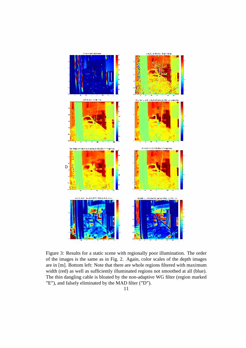
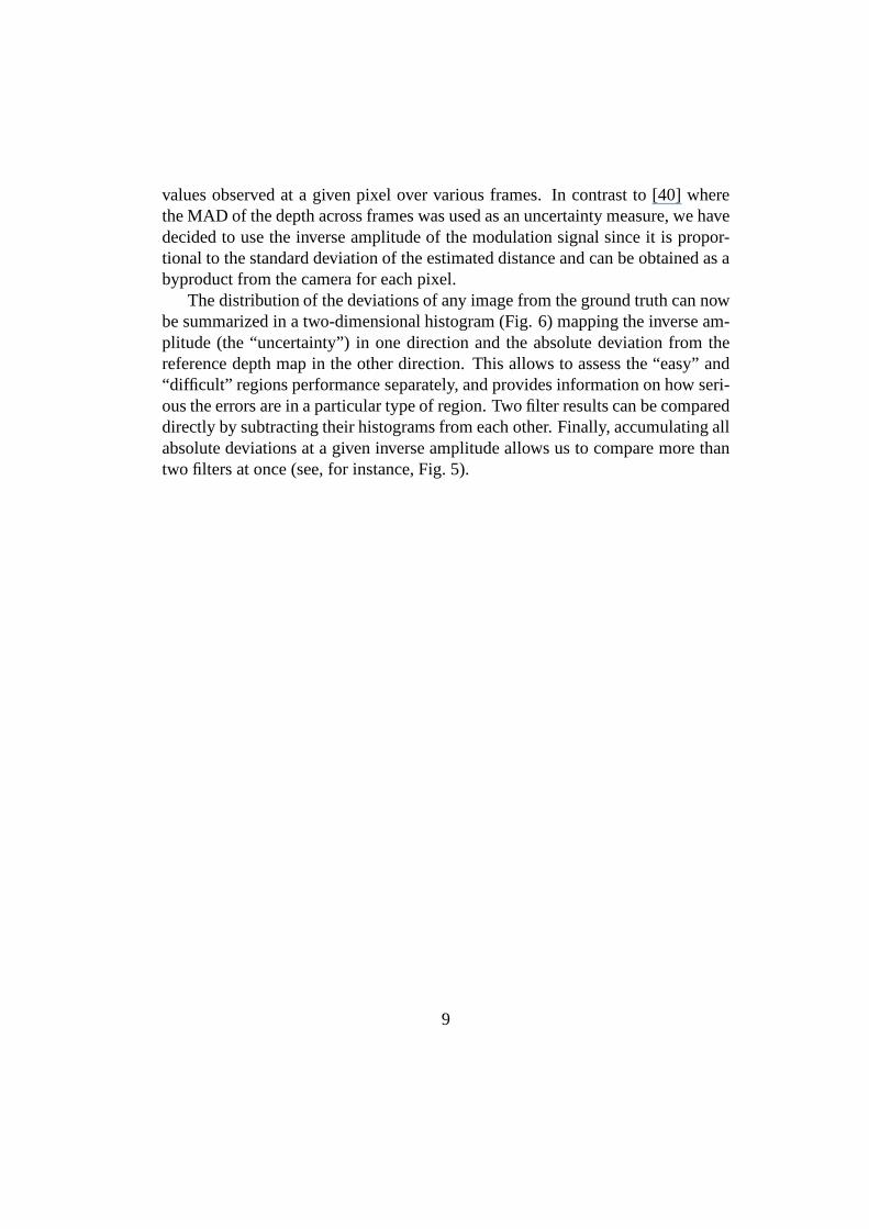
Figure 3: Results for a static scene with regionally poor illumination. The orderof the images is the same as in Fig. 2. Again, color scales of the depth imagesare in [m]. Bottom left: Note that there are whole regions filtered with maximumwidth (red) as well as sufficiently illuminated regions not smoothed at all (blue).The thin dangling cable is bloated by the non-adaptive WG filter (region marked”E”), and falsely eliminated by the MAD filter (”D”).

11

4 Results and Analysis

For the two scenes described above, the filter results are illustrated in Fig. 2 andFig. 3. Both results were obtained by running the filters witha parametrizationthat was optimal in terms of the average error per pixel (epp)for the particularscene. In both figures, the top left image shows the amplitudes of a single frame.Similar to a spotlight, the illumination fades radially from the center since thelight source can be approximated as a point (for larger distances). The objectshave highly varying reflectivities (note the chair cushion marked by “A”) whichmakes computing the correct depth very challenging. Comparing this with a singledepth frame of the original scene (top right), one can directly observe a relationbetween the amplitude and the confidence. In this context, also note the standarddeviation across repeated measurements of the scene (bottom right). The bottomleft picture shows the width of the Gaussian that was used with the AdaptiveWeighted Gaussian (AWG) filter. Note that there are whole regions filtered withthe maximum width of one third of the full mask size (red) as well as sufficientlyilluminated regions not smoothed at all (blue).

The reference depth map is shown on the left side of the secondrow. It wasconstructed by taking the mean over 300 repeated measurements of the staticscene. Adjacent to this are the results of three filters. The outcome of the AWGand the complex WG filter can be best compared by using the regions markedwith B and C together with the bottom left picture. AWG and WG give exactlythe same result for pixels smoothed with maximal width (red)and differ moreand more as the AWG filter uses smaller widths. The adaptive median filter usingMAD as the threshold performs well in preserving the edges but eliminates smallstructures (compare markers D and E in Fig. 3). Moreover, it leaves surprisinglynumerous outliers that intuitively should have been removed (see Fig. 3 D). Wewill refer to this effect later.

4.1 The Effect of Directed Blurring/Dilation

All filters using the amplitude as a measure of confidence haveto cope with ar-tifacts that appear as directed blurring at the edges. This problem is due to thefact that the amplitude is itself a function of distance: Objects further away have amuch lower amplitude than objects close to the camera. Spatially adjacent pixelsmay show objects of different distance, and as a result, of different amplitudes.When convolving withAt; t > 0 as a weighing factor, the pixels with smallerdepth value and larger amplitude will always have a much higher impact on the

12

result: closer objects grow at their edges and occlude the weakly illuminated ob-jects in the background. The impact of the effect grows witht and the mask size.This can be seen in Fig. 3 where the cable (marker E) and the pillow are muchbroader after filtering. Thus, in the context of the described effect, the selectionof t is a crucial choice. In assessing the complex filters introduced in section 2.2we observed that weighting withA2 performs better than usingA. This is due tothe fact that the former method penalizes values exactly according to the variance.However, with mask sizes of11 × 11 or higher (and therefore also with highermaximal Gaussian width, which is restricted to one third of the mask size) theboosted effect of “directed blurring” produces errors thatoutbalance the benefitof this penalization. This effect can dominate the mean absolute error per pixel(epp) obtained from comparing the resulting image with a reference depth map asdescribed in section 3.2.1.

The choice of the variance threshold for AWG and the maximal allowed Gaus-sian width have a large impact. One could argue that the AWG filter should allowfor a higher maximal width in order to decrease the often veryhigh fraction ofpixels convolved with that width. However, one has to consider that scenes withdeep depth edges would be strongly distorted, then. Since werestrict the maximalGaussian width to one third of the mask sizen we can observe this effect by com-paring filters with different mask sizes. Fig. 4 shows the average error per pixel(epp) against the AWG variance threshold for various mask sizes. With increasingvariance threshold, the fraction of pixels smoothed with maximal Gaussian widthdecreases to a small number of pixels having exactly zero amplitude. These pix-els are responsible for the constant differences at the right tails between curvesfor different mask sizen (top left in Fig. 4) because in this regime the AWG filteralways smooths with maximal allowed width, which increaseswith n. At verysmall variance threshold, almost every pixel is smoothed with maximal width andthus the error of larger masks rises very fast with vanishingthreshold.

4.2 Runtime

Depending on the application, the computation time may be a very important fac-tor for the choice of a particular filter. The fixed width filters are the fastest, withthe complex one being a bit slower due to the conversion from depth values tothe complex plane. Apart from the mask size, their runtime isindependent of anyparameters and of the image quality. The same holds for the median filter. TheAWG filter does not depend on the image quality either (if implemented noniter-atively) but depends strongly on the number of performed convolutions between

13

minimal and maximal Gaussian width in the scale selection process. There is atradeoff between speed and ensuring that every pixel is filtered with its appropri-ate Gaussian kernel. Experience shows that it suffices to sample the scale spaceat only a few Gaussian widths to achieve satisfactory results. The reason is thatthe amplitude varies a lot such that most pixels are either filtered with minimal ormaximal width and only a few need to be filtered with intermediate kernel sizes.

Figure 4: The mean absolute Error Per Pixel (epp) as a function of the thresholdfor the AWG and the Adaptive Median filter (weighted by amplitude A). Thegraphs within a row can be directly compared since they have the same scale forepp. The results of the first row were obtained by smoothing a room scene withmixed illumination and big objects (see Fig. 2). The second row shows the resultsfrom a highly structured scene (see Fig. 3). The steps in the right graphs resultfrom the fact that higher values of1

Acorrespond to small changes of the threshold

A. Since the amplitude in the images is quantized, a small change of the thresholdhas no impact on the filter behavior over somewhat large intervals of 1

A.

14

Figure 5: The absolute deviation from the reference depth map versus the expectedstandard deviation (1

A). Top row: results from the scene showing a room (Fig. 2).

Left: The adaptive filters lead to similar results. In the second row are results fromthe scene showing a hose (Fig. 3). Right: The WG graph and thecomplex2 graphare equal. For high amplitudes the filters with fixed width lead to errors higherthan the original image. The composition of the error can be analyzed in moredetail by employing Fig. 6.

Both the adaptive median filter using the spatial MAD value inorder to decideif to filter or not, and the one using the amplitude, depend on the image qualityitself (if implemented such that the unnecessary computations for “good” pixelsare avoided). “Difficult” images are filtered more intensively and therefore needmore time. The amplitude-controlled median is always faster since its variancemeasure is available for free in terms of computational costs. All computationswere performed with MATLAB on an Athlon 64 2.2 GHz processor with 2 GBmemory. The most illustrative results are summarized in Tab. 1 and Tab. 2.

15

Figure 6: Top left: error histogram of the original hose scene (Fig. 3) with log-arithmic frequencies (color scale). At very high amplitudes all errors are smallwhereas with decreasing amplitude the errors become very high. The other plotsshow subtracted pairwise filtering histograms. Note that the ranges of the differ-ence histograms are smaller. Counts outside the displayed axes are summarizedin the highest bins respectively. G: The adaptive median (weighted by amplitudeA) reduced the error of well illuminated pixels more than AWGbut was worse atvery bad pixels (H). Smoothing with maximal width improves the quality of flatsurfaces (I) but can lead to high errors at the edges due to directed blurring (J).

4.3 Comparison of the filters using Normalized Convolution

The filters with fixed width were the fastest and produced verysimilar results.All investigations have shown that the weighted Gaussian filter (WG) with fixedwidth leads to the same result as directional averaging in the complex plane withA2. Both filters use the same technique (normalized convolution) and the sameweighting factors. A difference only occurs if many adjacent pixels differ bymore thanπ in phase. In most cases, the complex filter usingA as a weightingfactor performed worse than the WG and the AWG filter. Only with mask sizes of11×11 or higher did the weaker penalization of a low amplitude pay off since theeffect of directed blurring was not that strong. This filter corresponds to weighting

16

Table 1: Computation time in [s] for an image with 160 by 120 pixels of mediumquality (the room scene) and a large number of convolutions (steps) for AWG inthe scale selection process. The time is averaged over 100 runs and the empiricalstandard deviation is given.

n AWGsteps AWG AdMed (MAD) AdMed (A) WG Complex-A2

3 45 1.27±0.03 2.60±0.04 0.98±0.02 0.0054±0.0001 0.023±0.0015 78 3.18±0.09 2.64±0.04 1.00±0.02 0.0066±0.0003 0.042±0.0017 112 6.0±0.5 2.70±0.07 1.02±0.02 0.0073±0.0006 0.072±0.007

Table 2: Computation time in [s] for an image with 160 by 120 pixels of poor qual-ity (the box, see Fig. 8) and a small number of convolutions (steps) for AWG inthe scale selection process. The time is averaged over 100 runs and the empiricalstandard deviation is given.

n AWGsteps AWG AdMed(MAD) AdMed(A) WG Complex-A2

3 9 0.16±0.01 2.61±0.03 0.99±0.01 0.005±0.001 0.024±0.0015 16 0.32±0.01 2.67±0.03 1.00±0.02 0.007±0.001 0.044±0.0017 22 0.53±0.01 2.70±0.04 1.03±0.02 0.007±0.001 0.071±0.001

directly on the raw data which implicitly makes use of the amplitudes and takesplace in the complex plane as well.

In slightly overexposed regions where the modulation amplitude is still high,all fixed width filters performed better than the AWG since thelatter does notsmooth at all at these amplitudes. Adjacent to slightly overexposed pixels, thereare either pixels without overexposure but sufficient illumination (and higher am-plitude) or others with even more saturation effects (and lower amplitude [11]).In these cases, non-adaptive amplitude-weighted filteringalways produces morereliable information (see Fig. 7, F). If the overexposed regions are too large, onlythe edges to non-saturated regions benefit from filtering.

Considering the effect of directed blurring, the adaptive approach is superior tothe non-adaptive. This is clearly illustrated at the dangling cable in Fig. 3 (markerE). Overall, adaptivity pays off in all observed scenes: theepp is always somewhat

17

lower as one can see in Fig. 4 left (WG corresponds to a variance threshold of 0)

Figure 7: Four depth images of the hose scene acquired with 20ms integrationtime. The region marked with F has a strong bias due to overexposure. Only theweighted Gaussian filters with fixed width were able to correct this bias.

4.4 Comparison of the Median Filters

In the first brief discussion of Fig. 3 we mentioned that the adaptive median usingMAD left a surprisingly large number of outliers in the image. This occurs inregions with high standard deviation and low amplitude. Thereason is that at van-ishing amplitude the depth values within the unambiguous range are only sparselypopulated due to strong quantization errors [11]. Taking the median of such a setof pixels always leads to the same value which in turn leads toa vanishing MADvalue (see Fig. 8). These pixels are not smoothed by the adaptive median exceptif the detector’s MAD threshold is set to zero (that is to say taking the median

18

nonadaptively). Therefore the simple median or the adaptive median usingA as athreshold performed better in the case of very low amplitudepixels.

All median filters completely removed fine structures in the depth images suchas the cable in Fig. 3 (marker E). In return, outliers are removed by the median andthe adaptive median using the amplitude, too. At acceptablyilluminated regionsor when adapting with respect to the amplitudeA, the results are comparable tothe AWG filter and better than that of the WG’s. In the case of very large masksizes, the median filters performed best since they cause no directed blurring.

Figure 8: Regions with low amplitude are subject to strong quantization effectssuch that only few different depth values are possible. Thisleads to frequentlyoccurring values and in consequence to a low MAD value even ifthe variance ishigh. The original scene shows an open box and background. Left: The spatialMAD value is zero for many pixels with low signal amplitude since the pixelspopulate only a few particular depth values there.

5 Conclusion and Outlook

We discussed various approaches to the denoising of depth maps obtained by TOF3D cameras. Two main concepts and their variations have beeninvestigated: nor-malized convolution with different weighting factors and median filtering, both inadaptive and in nonadaptive variants. An assessment has been performed usingqualitative and quantitative methods. It has turned out that the inverse squaredamplitude is indeed a reliable measure of confidence, as predicted by theory. TheWG filters with fixed width and weighting withA2 have performed well in allscenes if used up to a maximal mask size of7 × 7. For larger mask sizes, the

19

effect of directed blurring leads to large errors. They are the only ones to copewith small patches of overexposure and offer the fastest computation.

However, the fixed width filters unnecessarily blur the “good” pixels. There,the error can become larger than the error of the unfiltered image. The adaptiveweighted Gaussian filter (AWG) uses smaller Gaussian widthsat the edges thanthe WG filters and therefore has a reduced error at the edges. The adaptive medianusing MAD as a threshold has difficulty coping with the quantization effects ofthe data. However, if the modulation amplitude is used as thethreshold, results arecomparable to that of the AWG filter except for the drawback that small structuresare completely suppressed and the advantage of better edge preserving. Consider-ing the mean absolute error per pixel (epp) the AWG filter can reach better resultseven with suboptimal parametrization (see Fig. 4). Neglecting computation time,it is superior to all filters investigated.

All proposed filters can be implemented non-iteratively. Further effort couldbe directed towards iterative approaches or bilateral filters [42] to overcome thediscussed effect of directed blurring.

References

[1] A. Bevilacqua, L. D. Stefano, P. Azzari, “People Tracking Using a Time-of-Flight Depth Sensor”,AVSS ’06: Proc. of the IEEE Int. Conf. on Video andSignal Based Surveillance, p.98(2006)

[2] S. Knoop, S. Vacek, R. Dillmann, “Sensor Fusion for 3D Human BodyTracking with an Articulated 3D Body Model”,Proc. 2006 IEEE Int. Conf.on Robotics and Automation (ICRA 2006), pp. 1686-1691(2006)

[3] P. Breuer, C. Eckes, S. Muller, “Hand Gesture Recognition with a Novel IRTime-of-Flight Range Camera—A Pilot Study”,Computer Vision/ComputerGraphics Collaboration Techniques: Third Int. Conf. (MIRAGE 2007), vol.4418/2007, pp. 247-260(2007)

[4] M. Haker, M. Bohme, T. Martinetz, E. Barth, “Geometric Invariants for Fa-cial Feature Tracking with 3D TOF Cameras”,Proc. of the IEEE Int. Symp.on Signals, Circuits & Systems (ISSCS), vol. 1, pp. 109-112(2007)

[5] M. Juberts, A. Barbera, “Status Report on Next Generation LADAR forDriving Unmanned Ground Vehicles”,Tech. rep., National Inst. of Standardsand Technology (2004)

[6] J. Wikander, “Automated Vehicle Occupancy Technologies Study: SynthesisReport”,Tech. rep., Texas Transportation Inst. (2007)

[7] J. W. Weingarten, G. Gruener, R. Siegwart, “A State-of-the-Art 3D Sen-sor for Robot Navigation”,Proc. of the IEEE/RSJ Int. Conf. on IntelligentRobots and Systems (IROS), vol. 3, pp. 2155-216(2004)

[8] M. Lindner and A. Kolb: “Lateral and Depth Calibration ofPMD-DistanceSensors”,Advances in Visual Computing, Springer, 2, pages 524-533(2006)

[9] T. Kahlmann, F. Remondino, H. Ingensand, “Calibration for increased accu-racy of the range imaging camera Swissranger”ISPRS Commission V Sym-posium ’Image Engineering and Vision Metrology’ (IEVM)(2006)

[10] T. Moller, H. Kraft, J. Frey, “Robust 3D Measurement with PMD Sensors”,Proceedings of the 1st Range Imaging Research Day at ETH Zurich (2006)

[11] M. Frank, M. Plaue, H. Rapp, U. Kothe, B. Jahne, F. A. Hamprecht, “The-oretical and Experimental Error Analysis of Continuous-Wave Time-Of-Flight Range Cameras”Optical Engineering, vol. 48, No. 1, 013602(2009).

[12] T. Spirig, P. Seitz, O. Vietze, and F. Heitger, “The lock-in CCD - twodimen-sional synchronous detection of light”,IEEE Journal of Quantum Electron-ics, vol. 31, pp. 1705-1708, (1995)

[13] R. Schwarte, H. G. Heinol, Z. Xu, K. Hartmann, “A new active 3D-Visionsystem based on RF-modulation interferometry of incoherent light”, Pho-tonics East – Intelligent Systems and Advanced Manufacturing, Proceedingsof the SPIE, Vol. 2588, Philadelphia(1995)

[14] Z. Xu, “Investigation of 3D-Imaging Systems Based on Modulated Lightand Optical RF-Interferometry (ORFI)”,ZESS Forschungsberichte, vol. 14,pp. 214(1999)

[15] B. Schneider: “Der Photomischdetektor zur schnellen 3D-Vermessung furSicherheitssysteme und zur Informationsubertragung im Automobil”, Diss.,Department of Electrical Engineering and Computer Science, University ofSiegen(2003)

[16] G. Aubert, P. Kornprobst, “Mathematical Problems in Image Processing:Partial Differential Equations and the Calculus of Variations”, Springer(2006)

[17] J. Weickert, “Anisotropic Diffusion in Image Processing”, Diss., Univ. ofKaiserslautern

[18] R.-J. Recknagel, R. Kowarschik, G. Notni, “High-resolution Defect Detec-tion and Noise Reduction Using Wavelet Methods for Surface Measure-ment”,J. Opt. A: Pure Appl. Opt., vol. 2, pp.538-545(2000)

[19] R. Coifman, D. Donoho, “Translation Invariant De-noising”, Tech. rep.(1995)

[20] D. L. Donoho, I. M. Johnstone, G. Kerkyacharian, D. Picard, “WaveletShrinkage: Asymptopia?”,Tech. rep.(1994)

[21] A. Buades, B. Coll, J. M. Morel, “A Review of Image Denoising Algorithms,With a New One”,Multiscale Model. Simul., Vol. 4, No. 2, pp. 490-530(2005)

[22] A. Buades, B. Coll, J.-M. Morel, “A Non-local Algorithmfor Image De-noising”,IEEE Comp. Soc. Conf. on Comp. Vision and Pattern Recognition,CVPR, vol. 2, pp. 60-65(2005)

[23] L. I. Rudin, S. Osher, E. Fatemi, “Nonlinear Total Variation Based BoiseRemoval Algoritms”,Physica D 60, pp. 259-268(1992)

[24] J. Portilla, V. Strela, M. J. Wainwright, W. P. Simoncelli, “Adaptive WienerDenoising Using a Gaussian Scale Mixture Model in the Wavelet Domain”,Proc. of the 8th Int. Conf. on Image Processing, vol. 2, pp. 37-40 (2001)

[25] N. Wiener, “Extrapolation, Interpolation, and Smoothing of Stationary TimeSeries”, MIT Press (1964)

[26] T. Chen, K.-K. Ma, L.-H. Chen, “Tri-State Median Filterfor Image Denois-ing”, IEEE Trans. on Image Processing, vol. 8, No. 12(1999)

[27] K. Hildebrandt, K. Polthier, “Anisotropic Filtering of Non-Linear SurfaceFeatures”,Computer Graphics Forum, vol. 23 (3)(2004)

[28] C. Lange, K. Polthier, “Anisotropic Fairing of Point Sets”, Special Issue ofCAGD(2005)

[29] Ron Kimmel, Ravi Malladi, Nir A. Sochen, “Image Processing via the Bel-trami Operator”,Proc. of the Third Asian Conf. on Comp. Vision, vol. 1, pp.547-581(1998)

[30] A. I. Bobenko, P. Schroder, “Discrete Willmore Flow”,Eurographics Symp.on Geom. Processing, pp. 101-110, eds. M. Desbrun, H. Pottmann (2005)

[31] R. M. Bolle, B. C. Vermuri, “On Three-Dimensional Surface ReconstructionMethods”,IEEE Trans. on Pattern Analysis and Machine Intelligence, vol.13, No. 1(1991)

[32] J. Shah, H. H. Pien, J. M. Gauch, “Recovery of Surfaces with Discontinuitiesby Fusing Shading and Range Data Within a Variational Framework”, IEEETrans. on Image Processing, vol. 5, No. 8, pp. 1243-1251(1996)

[33] M. Bertero, P. Boccacci, “Introduction to Inverse Problems in Imaging”, Inst.of Phys. Publ. (1998)

[34] A. Foi, “Pointwise Shape-adaptive DCT Image Filteringand Signal-dependent Noise Estimation”,Tampere Univ. of Technology, Publication 710(2007)

[35] X. Luan, “Experimental Investigation of Photonic Mixer Device and Devel-opment of TOF 3D Ranging Systems Based on PMD Technology”,Diss.,Univ. Siegen (2001)

[36] H. Rapp, M. Frank, F. A. Hamprecht, B. Jahne, “A Theoretical and Exper-imental Investigation of the Systematic Errors and Statistical Uncertaintiesof Time-of-Flight Cameras”,Int. J. Intelligent Systems Technologies and Ap-plications, vol. 5, Nos. 3/4(2008)

[37] H. Knutsson, C.-F. Westin, “Normalized and Differential Convolution”,Proc. CVPR, pp. 515-523(1993)

[38] J. Restle, M. Hissmann, F. A. Hamprecht, “Nonparametric Smoothing of In-terferometric Height Maps Using Confidence Values”,Optical Engineering,Vol. 43 No. 4(2004)

[39] F. R. Hampel: “The Breakdown Points of the Mean Combinedwith SomeRejection Rules”Technometrics, Vol. 27, No. 2, pp. 95-107, (1985)

[40] M. Hissmann, F. A. Hamprecht: “Bayesian Surface Estimation for WhiteLight Interferometry”,Optical Engineering, Vol. 44 No. 1(2005)

[41] A. Kirsch, “An Introduction to the Mathematical Theoryof Inverse Prob-lems”, Springer (1996)

[42] C. Tomasi, R. Manduchi, “Bilateral Filtering for Gray and Color Images”Proceedings of the IEEE International Conference on Computer Vision,Bombay(1998)