


Bahasa
Halaman
Hukum


Data Mining & Warehousing
Chapter Two
Data warehousing and OLAP Technology
for Data Mining

DMW Lecture NoteKIoT
Data Warehousing and OLAP
What is a data warehouse?
A multi-dimensional data model
Data warehouse
architecture
Data warehouse implementation
From data warehousing
to data mining

DMW Lecture NoteKIoT
Data Warehouse
• Data warehousing provides architectures and tools
for business executives to systematically organize, underst
and, and use their data to make strategic decisions
• Data warehousing is the latest must have marketing weapon - away to retain customers by learning more about their needs.
• Data warehouse refers to a data repository that is
maintained separately from an organizational operational
databases.
• Data warehouse provides OLAP tools for the interactive
analysis of multidimensional data that helps to data
generalization and data mining.
3

DMW Lecture NoteKIoT
4
What is a Data Warehouse?
• Defined in many different ways, but not rigorously.
– A decision support database that is maintained separately from the
organization’s operational database
– Support information processing by providing a solid platform of
consolidated, historical data for analysis.
• A data warehouse is a subject-oriented, integrated, time-variant, and
nonvolatile collection of data in support of management’s decision-
making process
• Data warehousing:
– The process of constructing and using data warehouses

DMW Lecture NoteKIoT
5
Data Warehouse—Subject-Oriented
• Organized around major subjects, such as customer,
product, sales
• Focusing on the modeling and analysis of data for decision
makers, not on daily operations or transaction processing
• Provide a simple and concise view around particular subject
issues by excluding data that are not useful in the decision
support process

DMW Lecture NoteKIoT
6
Data Warehouse—Integrated
• Constructed by integrating multiple, heterogeneous data
sources
– relational databases, flat files, on-line
transaction records
• Data cleaning and data integration techniques are applied.
– Ensure consistency in naming conventions,
encoding structures, attribute measures, etc.
among different data sources
• E.g., Hotel price: currency, tax, breakfast covered, etc.
– When data is moved to the warehouse, it is
converted.
DMW Lecture NoteKIoT
7
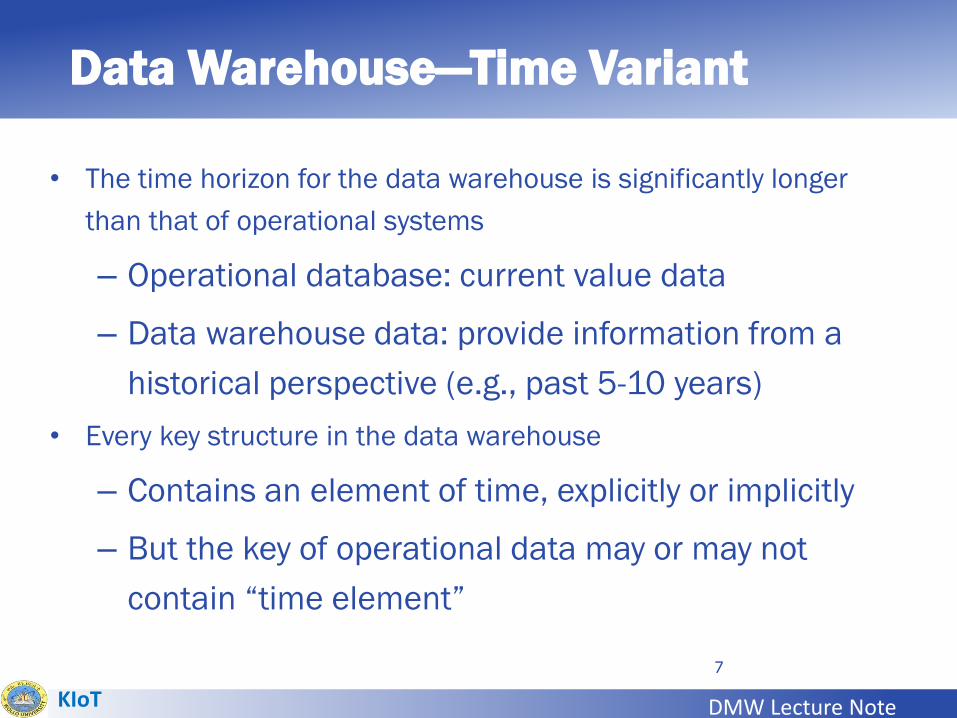
Data Warehouse—Time Variant
• The time horizon for the data warehouse is significantly longer
than that of operational systems
– Operational database: current value data
– Data warehouse data: provide information from a
historical perspective (e.g., past 5-10 years)
• Every key structure in the data warehouse
– Contains an element of time, explicitly or implicitly
– But the key of operational data may or may not
contain “time element”

DMW Lecture NoteKIoT
8
Data Warehouse—Nonvolatile
• A physically separate store of data transformed from the
operational environment
• Operational update of data does not occur in the data
warehouse environment
– Does not require transaction processing,
recovery, and concurrency control mechanisms
– Requires only two operations in data accessing:
• initial loading of data and access of data

DMW Lecture NoteKIoT
Data Warehouse
The DW persistently stores
Cleaned raw data
Derived (aggregated) data
Usual aggregates of the raw data e.g. quarter sales per regions
Performance reasons avoid computing (the
same) aggregates times and again at query time
Metadata
Describe the meaning, properties and origins of the data in
the data warehouse 9
DMW Lecture NoteKIoT
10
OLTP and OLAP
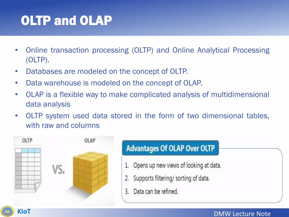
• Online transaction processing (OLTP) and Online Analytical Processing
(OLTP).
• Databases are modeled on the concept of OLTP.
• Data warehouse is modeled on the concept of OLAP.
• OLAP is a flexible way to make complicated analysis of multidimensional
data analysis
• OLTP system used data stored in the form of two dimensional tables,
with raw and columns

11
OLTP vs. OLAP
OLTP OLAP
users clerk, IT professional knowledge worker
function day to day operations decision support
DB design application-oriented subject-oriented
data current, up-to-date
detailed, flat relational
isolated
historical,
summarized, multidimensional
integrated, consolidated
usage repetitive ad-hoc
access read/write
index/hash on prim. key
lots of scans
unit of work short, simple transaction complex query
# records accessed tens millions
#users thousands hundreds
DB size 100MB-GB 100GB-TB
metric transaction throughput query throughput, response
DMW Lecture NoteKIoT
12
Why a Separate Data Warehouse?
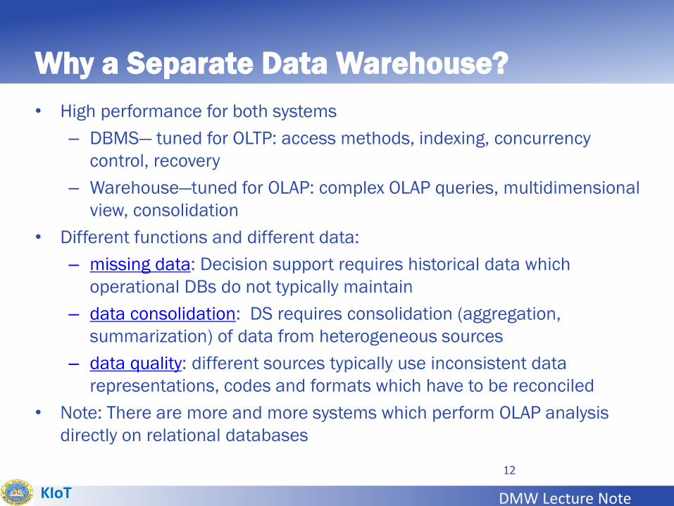
• High performance for both systems
– DBMS— tuned for OLTP: access methods, indexing, concurrency
control, recovery
– Warehouse—tuned for OLAP: complex OLAP queries, multidimensional
view, consolidation
• Different functions and different data:
– missing data: Decision support requires historical data which
operational DBs do not typically maintain
– data consolidation: DS requires consolidation (aggregation,
summarization) of data from heterogeneous sources
– data quality: different sources typically use inconsistent data
representations, codes and formats which have to be reconciled
• Note: There are more and more systems which perform OLAP analysis
directly on relational databases

DMW Lecture NoteKIoT
Data Warehouse Application
• A data warehouse helps business executives toorganize, analyze, and use their data for decisionmaking.
• A data warehouse serves as a sole part of a plan-execute-assess "closed-loop" feedback system for theenterprise management.
• Data warehouses are widely used in the followingfields:
– Financial services
– Banking services
– Consumer goods
– Retail sectors
– Controlled manufacturing 13

14
Data Warehouse: A Multi-Tiered Architecture
Data
Warehouse
Extract
Transform
Load
Refresh
OLAP Engine
Analysis
Query
Reports
Data mining
Monitor
&
Integrator
Metadata
Data Sources Front-End Tools
Serve
Data Marts
Operational
DBs
Other
sources
Data Storage
OLAP Server

DMW Lecture NoteKIoT
15
Three Data Warehouse Models
• Enterprise warehouse
– collects all of the information about subjects spanning the entire organization
• Data Mart
– a subset of corporate-wide data that is of value to a specific groups of users. Its scope is confined to specific, selected groups, such as marketing data mart• Independent vs. dependent (directly from warehouse) data
mart
• Virtual warehouse
– A set of views over operational databases
– Only some of the possible summary views may be materialized

DMW Lecture NoteKIoT
16
Extraction, Transformation, and Loading (ETL)
• Data extraction
– get data from multiple, heterogeneous, and external sources
• Data cleaning
– detect errors in the data and rectify them when possible
• Data transformation
– convert data from legacy or host format to warehouse format
• Load
– sort, summarize, consolidate, compute views, check integrity, and build indicies and partitions
• Refresh
– propagate the updates from the data sources to the warehouse

DMW Lecture NoteKIoT
17
Metadata Repository
• Meta data is the data defining warehouse objects. It stores:
• Description of the structure of the data warehouse
– schema, view, dimensions, hierarchies, derived data definition, data
mart locations and contents
• Operational meta-data
– data lineage (history of migrated data and transformation path),
currency of data (active, archived, or purged), monitoring information
(warehouse usage statistics, error reports, audit trails)
• The algorithms used for summarization
• The mapping from operational environment to the data warehouse
• Data related to system performance
– warehouse schema, view and derived data definitions
• Business data
– business terms and definitions, ownership of data, charging policies

DMW Lecture NoteKIoT
Chapter 2: Data Warehousing and OLAP
What is a data warehouse?
A multi-dimensional data model
Data warehouse
architecture
Data warehouse implementation
From data warehousing
to data mining
DMW Lecture NoteKIoT
Data Cube: A Multidimensional Data Model
Data Warehouse Modeling: Data Cube & OLAP
Data Cube: A Multidimensional Data Model
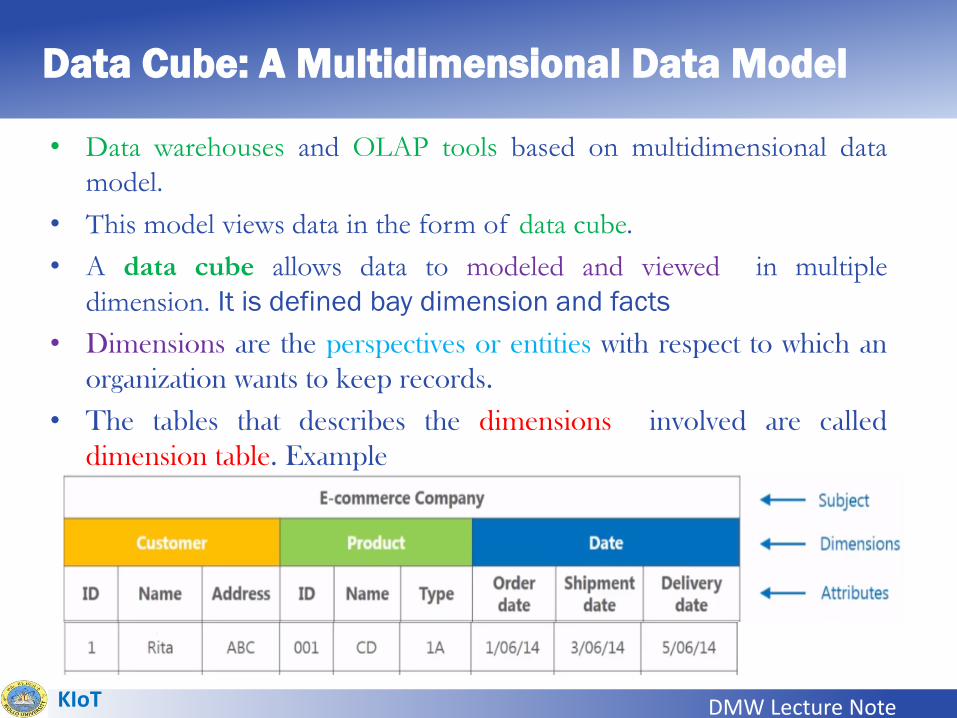
• Data warehouses and OLAP tools based on multidimensional data
model.
• This model views data in the form of data cube.
• A data cube allows data to modeled and viewed in multiple
dimension. It is defined bay dimension and facts
• Dimensions are the perspectives or entities with respect to which an
organization wants to keep records.
• The tables that describes the dimensions involved are called
dimension table. Example
19

DMW Lecture NoteKIoT
Data Cube: A Multidimensional Data Model
Data Cube: A Multidimensional Data Model• Each dimension may have a table associated with it, called a
dimension table, which further describes the dimension.
• For example, a dimension table for item may contain the
attributes item name, brand, and type.
• Dimension tables can be specified by users or experts, or
automatically generated and adjusted based on data distributions.
• A multidimensional data model is typically organized around a
central theme, such as sales.
• This theme is represented by a fact table. Facts are numeric
measures.
• Examples of facts for a sales data warehouse include dollars sold
(sales amount in dollars), units sold (number of units sold), and
amount budgeted.20

DMW Lecture NoteKIoT
Data Cube: A Multidimensional Data Model
• The fact table contains the names of the facts, or measures, as well as
keys to each of the related dimension tables.
• A 2-D view of sales data for AllElectronics according to thedimensions time and item, where the sales are from branches locatedin the city of Vancouver. The measure displayed is dollars sold (inthousands). Table 2.1
21

DMW Lecture NoteKIoT
Data Cube: A Multidimensional Data Model
• A 3-D view of sales data for AllElectronics, according to thedimensions time, item, and location. The measure displayedis dollars sold (in thousands). Table 2.2
22

DMW Lecture NoteKIoT
Data Cube: A Multidimensional Data Model
• We may display any n-dimensional data as a series of (n − 1)-
dimensional “cubes.” The data cube is a representation for
multidimensional data storage. A data cube like those shown in
above Figures is often referred to as a cuboid.
• Given a set of dimensions, we can generate a cuboid for each of
the possible subsets of the given dimensions.
• The result would form a lattice of cuboids, each showing the
data at a different level of summarization, or group-by.
• The lattice of cuboids is then referred to as a data cube.
• The following figure shows a lattice of cuboids forming a data
cube for the dimensions time, item, location.
• The cuboid that holds the lowest level of summarization is
called the base cuboid.23

DMW Lecture NoteKIoT
Data Cube: A Multidimensional Data Model
• 3-D data cube representation of the data in Table 2.2, according to
time, item, and location. The measure displayed is dollars sold (in
thousands).
24

DMW Lecture NoteKIoT
25
Data Cube: A Multidimensional Data Model
Cube: A Lattice of Cuboids
time,item
time,item,location
time, item, location, supplier
all
time item location supplier
time,location
time,supplier
item,location
item,supplier
location, supplier
time,item,supplier
time, location, supplier
item, location, supplier
0-D (apex) cuboid
1-D cuboids
2-D cuboids
3-D cuboids
4-D (base) cuboid

DMW Lecture NoteKIoT
26
Conceptual Modeling of Data Warehouses
• The entity-relationship data model is commonly used in the
design of relational databases, where a database schema
consists of a set of entities and the relationships between
them.
• Such a data model is appropriate for online transaction
processing.
• A data warehouse, however, requires a concise, subject-
oriented schema that facilitates online data analysis.
• The most popular data model for a data warehouse is a
multidimensional model, which can exist in the form of a star
schema, a snowflake schema, or a fact constellation
schema.
• Let’s look at each of these.

DMW Lecture NoteKIoT
27
Conceptual Modeling of Data Warehouses
• Modeling data warehouses: dimensions & measures
– Star schema: A fact table in the middle connected to a set
of dimension tables
– Snowflake schema: A refinement of star schema where
some dimensional hierarchy is normalized into a set of
smaller dimension tables, forming a shape similar to
snowflake
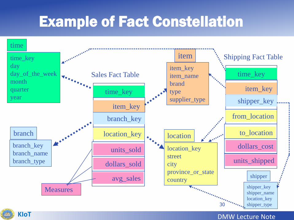
– Fact constellations: Multiple fact tables share dimension
tables, viewed as a collection of stars, therefore called
galaxy schema or fact constellation

DMW Lecture NoteKIoT
28
Example of Star Schema
time_key
day
day_of_the_week
month
quarter
year
time
location_key
street
city
state_or_province
country
location
Sales Fact Table
time_key
item_key
branch_key
location_key
units_sold
dollars_sold
avg_sales
Measures
item_key
item_name
brand
type
supplier_type
item
branch_key
branch_name
branch_type
branch

DMW Lecture NoteKIoT
29
Example of Snowflake Schema
time_key
day
day_of_the_week
month
quarter
year
time
location_key
street
city_key
location
Sales Fact Table
time_key
item_key
branch_key
location_key
units_sold
dollars_sold
avg_sales
Measures
item_key
item_name
brand
type
supplier_key
item
branch_key
branch_name
branch_type
branch
supplier_key
supplier_type
supplier
city_key
city
state_or_province
country
city
DMW Lecture NoteKIoT
30
Example of Fact Constellation
time_key
day
day_of_the_week
month
quarter
year
time
location_key
street
city
province_or_state
country
location
Sales Fact Table
time_key
item_key
branch_key
location_key
units_sold
dollars_sold
avg_sales
Measures
item_key
item_name
brand
type
supplier_type
item
branch_key
branch_name
branch_type
branch
Shipping Fact Table
time_key
item_key
shipper_key
from_location
to_location
dollars_cost
units_shipped
shipper_key
shipper_name
location_key
shipper_type
shipper

DMW Lecture NoteKIoT
Exercise
• Suppose that a data warehouse consists of the three dimensions
time, doctor, and patient, and the two measures count and
charge, where charge is the fee that a doctor charges a patient
for a visit.
Enumerate three classes of schemas that are popularly used for
modeling data warehouses.
Draw a schema diagram for the above data warehouse using star
schema
Answer
Three classes of schemas popularly used for modeling data
warehouses are the star schema, the snowflake schema, and the
fact constellations schema.
Answer for question b is on the next slide31

DMW Lecture NoteKIoT
32
Example of Star Schema
time_key day day_of_week month quarter year
time
Fact Table
time_key
dooctor_id
patient_id
Charge
dooctor_id dooctor_name
phone_# Address
Sex
Doctor
patient_id patient_name phone_# sex description address
Patient
count
Measures

DMW Lecture NoteKIoT
Data Warehouse Schema Definition
• Multidimensional schema is defined using Data Mining
Query Language (DMQL).
• The two primitives, cube definition and dimension
definition, can be used for defining the data warehouses
and data marts.
• Syntax for Cube Definitiondefine cube < cube_name > [ < dimension-list > }: < measure_list >
• Syntax for Dimension Definitiondefine dimension < dimension_name > as ( < attribute_or_dimension_list > )
33

DMW Lecture NoteKIoT
Data Warehouse Schema Definition
Star Schema Definition
• The star schema can be defined using Data Mining QueryLanguage (DMQL) as follows:
define cube sales star [time, item, branch, location]:
dollars sold = sum(sales in dollars), units sold = count(*)
define dimension time as (time key, day, day of week, month, quarter,
year)
define dimension item as (item key, item name, brand, type, supplier type)
define dimension branch as (branch key, branch name, branch type)
define dimension location as (location key, street, city, province or state,country)
34

DMW Lecture NoteKIoT
Data Warehouse Schema Definition
Snowflake Schema Definition
• Snowflake schema can be defined using DMQL as follows:
define cube sales snowflake [time, item, branch, location]:
dollars sold = sum(sales in dollars), units sold = count(*)
define dimension time as (time key, day, day of week, month, quarter, year)
define dimension item as (item key, item name, brand, type, supplier(supplier key, supplier type))
define dimension branch as (branch key, branch name, branch type)
define dimension location as (location key, street, city(city key, city, province or state, country))
35

DMW Lecture NoteKIoT
Data Warehouse Schema Definition
Fact Constellation Schema Definition
• Fact constellation schema can be defined using DMQL as follows:
define cube sales [time, item, branch, location]:
dollars sold = sum(sales in dollars), units sold = count(*)
define dimension time as (time key, day, day of week, month, quarter, year)
define dimension item as (item key, item name, brand, type, supplier type)
define dimension branch as (branch key, branch name, branch type)
define dimension location as (location key, street, city, province or state, country)
define cube shipping [time, item, shipper, from location, to location]:
dollars cost = sum(cost in dollars), units shipped = count(*)
define dimension time as time in cube sales
define dimension item as item in cube sales
define dimension shipper as (shipper key, shipper name, location as location in
cube sales, shipper type)
define dimension from location as location in cube sales
define dimension to location as location in cube sales 36

DMW Lecture NoteKIoT
A Concept Hierarchy: Dimension
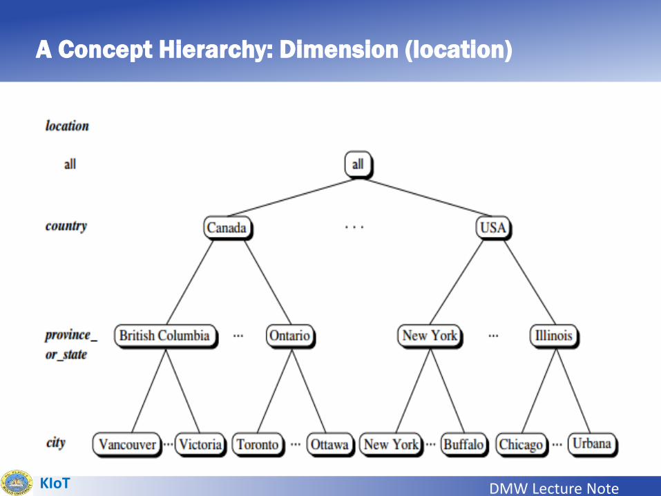
Dimensions: The Role of Concept Hierarchies• A concept hierarchy defines a sequence of mappings from a set of low-level
concepts to higher-level, more general concepts.
• Consider a concept hierarchy for the dimension location.
• City values for location include Vancouver, Toronto, New York,and Chicago.
• Each city, however, can be mapped to the province or state towhich it belongs.
• For example, Vancouver can be mapped to British Columbia,and Chicago to Illinois.
• The provinces and states can in turn be mapped to the country (e.g., Canadaor the United States) to which they belong.
• These mappings form a concept hierarchy for the dimension location,mapping a set of low-level concepts (i.e., cities) to higher-level, more generalconcepts (i.e., countries). This concept hierarchy is illustrated in followingfigure.
37
DMW Lecture NoteKIoT
A Concept Hierarchy: Dimension (location)
38

DMW Lecture NoteKIoT
Measures of Data Cube: Three Categories
Measures: Their Categorization and Computation
• How are measures computed?
• To answer this question, we first study how measures can becategorized. Note that a multidimensional point in the datacube space can be defined by a set of dimension–valuepairs; for example, time = “Q1”, location = “Vancouver”, item= “computer”.
• A data cube measure is a numeric function that can beevaluated at each point in the data cube space.
• A measure value is computed for a given point byaggregating the data corresponding to the respectivedimension–value pairs defining the given point.
• Measures can be organized into three categories—distributive, algebraic, and holistic—based on the kind ofaggregate functions used.
39

DMW Lecture NoteKIoT
40
Measures of Data Cube: Three Categories
• Distributive: if the result derived by applying the function to n
aggregate values is the same as that derived by applying the
function on all the data without partitioning
• E.g., count(), sum(), min(), max()
• Algebraic: if it can be computed by an algebraic function with
M arguments (where M is a bounded integer), each of which is
obtained by applying a distributive aggregate function
• E.g., avg(), min_N(), standard_deviation()
• Holistic: if there is no constant bound on the storage size
needed to describe a sub aggregate.
• E.g., median(), mode(), rank()

DMW Lecture NoteKIoT
Types of OLAP Operations
• How are concept hierarchies useful in OLAP?
• In the multidimensional model, data are organized into
multiple dimensions, and each dimension contains
multiple levels of abstraction defined by concept
hierarchies.
• This organization provides users with the flexibility to
view data from different perspectives.
• A number of OLAP data cube operations exist to
materialize these different views, allowing interactive
querying and analysis of the data at hand.
• Hence, OLAP provides a user-friendly environment for
interactive data analysis. 41

DMW Lecture NoteKIoT
OLAP Operations: Roll-up
• The Roll-up performs aggregation on a data cube in any of the
following ways:
By climbing up a concept hierarchy for a dimension
By dimension reduction
The following diagram illustrates how roll-up works.
• Roll-up is performed by climbing up a concept hierarchy for the
dimension location.
• Initially the concept hierarchy was "street<city<province< country".
• On rolling up, the data is aggregated by ascending the location
hierarchy from the level of city to the level of country.
• The data is grouped into cities rather than countries.
• When roll-up is performed, one or more dimensions from the data
cube are removed.42

DMW Lecture NoteKIoT
OLAP Operations: Roll-up
43
DMW Lecture NoteKIoT
OLAP Operations: Drill-down
• Drill-down is the reverse operation of roll-up. It is performed by
either of the following ways:
By stepping down a concept hierarchy for a dimension
By introducing a new dimension
• Drill-down is performed by stepping down a concept hierarchy
for the dimension time.
• Initially the concept hierarchy was "day < month < quarter < year.“
• On drilling down, the time dimension is descended from the
level of quarter to the level of month.
• When drill-down is performed, one or more dimensions from
the data cube are added.
• It navigates the data from less detailed data to highly detailed
data. 44

DMW Lecture NoteKIoT
OLAP Operations: Drill-down
45

OLAP Operations: Slice
• The slice operation selects one particular dimension from a given cube and provides a new sub-cube.
• Here Slice is performed for the dimension "time" using the criterion time = "Q1".
• It will form a new sub-cube by selecting one or more dimensions.
46

OLAP Operations: Dice
• Dice selects two or
more dimensions
from a given cube and
provides a new sub
cube.
• The dice operation on
the cube based on
the following selection
criteria involves three
dimensions.
(location="Toronto“ or
"Vancouver")
(time = "Q1" or "Q2")
(item="Mobile"or
"Modem"47

OLAP Operations: Pivot
• The pivot operation is
also known as rotation.
• It rotates the data axes
in view in order to
provide an alternative
presentation of data.
• Consider the following
diagram that shows the
pivot operation.
48
DMW Lecture NoteKIoT
Data Warehousing and OLAP
What is a data warehouse?
A multi-dimensional data model
Data warehouse
architecture
Data warehouse implementation
From data warehousing
to data mining
DMW Lecture NoteKIoT
A Business Analysis Framework for Data Warehouse Design
• Having a data warehouse offers the following advantages:
Provide a competitive advantage by presenting relevant
information from which to measure performance and make
critical adjustments to help win over competitors.
Enhance business productivity because it is able to quickly and
efficiently gather information that accurately describes the
organization.
Facilitates customer relationship management because it
provides a consistent view of customers and items across all
lines of business, all departments, and all markets.
A data warehouse also helps in cost reduction by tracking trends,
patterns, and exceptions over long periods in a consistent and
reliable manner.50

DMW Lecture NoteKIoT
A Business Analysis Framework for Data Warehouse Design
• To design an effective data warehouse we need to understandand analyze business needs and construct a business analysisframework.
• The construction of a large and complex information systemcan be viewed as the construction of a large and complexbuilding, for which the owner, architect, and builder havedifferent views.
• These views are combined to form a complex framework thatrepresents the top-down, business-driven, or owner’sperspective, as well as the bottom-up, builder-driven, orimplementer's view of the information system.
• Four different views regarding a data warehouse design must beconsidered: the top-down view, the data source view, the datawarehouse view, and the business query view.
51

DMW Lecture NoteKIoT
A Business Analysis Framework for Data Warehouse Design
• The top-down view allows the selection of the relevantinformation necessary for the data warehouse.
• The data source view exposes the information being captured,stored, and managed by operational systems.
This information may be documented at various levels of detailand accuracy, from individual data source tables to integrateddata source tables.
• The data warehouse view includes fact tables and dimensiontables. It represents the information that is stored inside the datawarehouse, including pre-calculated totals and counts, as well asinformation regarding the source, date, and time of origin,added to provide historical context.
• Finally, the business query view is the data perspective in thedata warehouse from the end-user’s viewpoint.
52

DMW Lecture NoteKIoT
A Business Analysis Framework for Data Warehouse Design
• Building and using a data warehouse is a complex task because it
requires business skills, technology skills, and program
management skills.
• Business skills, building a data warehouse involves understanding
how systems store and manage their data, how to build
extractors that transfer data from the operational system to the
data warehouse
• Technology skills, data analysts are required to understand how
to make assessments from quantitative information and derive
facts based on conclusions from historic information in the data
warehouse.
• Program management skills involve the need to interface with
many technologies, vendors, and end-users in order to deliver
results in a timely and cost effective manner. 53

DMW Lecture NoteKIoT
Data Warehouse Design Process• A data warehouse can be built using the following approach,
• The top-down approach starts with overall design and planning. It is
useful in cases where the technology is mature and well known, and
where the business problems that must be solved are clear and well
understood.
• The bottom-up approach starts with experiments and prototypes.
This is useful in the early stage of business modeling and
technology development. It allows an organization to move forward
at considerably less expense and to evaluate the technological
benefits before making significant commitments.
• The combined approach, an organization can exploit the planned
and strategic nature of the top-down approach while retaining the
rapid implementation and opportunistic application of the bottom-
up approach.54

DMW Lecture NoteKIoT
Data Warehouse Design Process
• From the software engineering point of view, the design and
construction of a data warehouse may consist of the following
steps: planning, requirements study, problem analysis, warehouse
design, data integration and testing, and finally deployment of the
data warehouse.
• Large software systems can be developed using one of two
methodologies: the waterfall method or the spiral method.
• The waterfall method performs a structured and systematic analysis
at each step before proceeding to the next, which is like a waterfall,
falling from one step to the next.
• The spiral method involves the rapid generation of increasingly
functional systems, with short intervals between successive releases.
55

DMW Lecture NoteKIoT
Data Warehouse Design Process
The warehouse design process consists of the following steps:
1. Choose a business process to model (e.g., orders, invoices,
inventory). Is the business process organizational or department ?
2. Choose the business process grain, which is the fundamental,
atomic level of data to be represented in the fact table for this
process (e.g., individual transactions, individual daily snapshots,
and so on).
3. Choose the dimensions that will apply to each fact table record.
Typical dimensions are time, item, customer, supplier,
warehouse, transaction type, and status.
4. Choose the measures that will populate each fact table record.
Typical measures are numeric additive quantities like dollars sold
and units sold.56

DMW Lecture NoteKIoT
Data Warehouse Design Process
• Because data warehouse construction is a difficult and long-term
task, its implementation scope should be clearly defined.
• It involves determining the time and budget allocations, the
subset of the organization that is to be modeled, the number of
data sources selected, and the number and types of departments
to be served.
• Once a data warehouse is designed and constructed, the initial
deployment of the warehouse includes initial installation, roll-out
planning, training, and orientation.
• Data warehouse administration includes data refreshment, data
source synchronization, planning for disaster recovery, managing
access control and security, managing data growth, managing
database performance, and data warehouse enhancement and
extension. 57

DMW Lecture NoteKIoT
Chapter 2: Data Warehousing and OLAP
What is a data
warehouse?
A multi-dimensional data model
Data warehouse
architecture
Data warehouse implementation
From data warehousing
to data mining

DMW Lecture NoteKIoT
59
Efficient Data Cube Computation
• The compute cube operator computes aggregates over
all subsets of the dimensions specified in the operation.
• This can require excessive storage space, especially for
large numbers of dimensions.
• Therefore it is crucial for data warehouse systems to
support highly efficient cube computation techniques,
access methods, and query processing techniques.
• Example: A data cube is a lattice of cuboids. Suppose
that you want to create a data cube for AllElectronics
sales that contains the following: city, item, year, and
sales in dollars.

DMW Lecture NoteKIoT
60
Efficient Data Cube Computation
• You want to be able to analyze the data, with queries such as the
following:
• Compute the sum of sales, grouping by city and item?
• Compute the sum of sales, grouping by city?
• Compute the sum of sales, grouping by item?
• What is the total number of cuboids, or group by’s, that can be
computed for this data cube?
• Taking the three attributes, city, item, and year, as the dimensions
for the data cube, and sales in dollars as the measure, the total
number of cuboids, or group by’s, that can be computed for this
data cube is 23 = 8.

Efficient Data Cube Computation
• The possible group by’s are the
following: {(city, item, year), (city,
item), (city, year), (item, year),
(city), (item), (year), ()}, where ()
means that the group-by is
empty (i.e., the dimensions are
not grouped).
• If we start at the apex cuboid
and explore downward in the
lattice, this is equivalent to
drilling down within the data
cube.
• If we start at the base cuboid
and explore upward, this is akin
to rolling up.
61

DMW Lecture NoteKIoT
62
Efficient Data Cube Computation
• The cube operator is the n-dimensional generalization of the group-by
operator.
• Similar to the SQL syntax, the data cube could be defined as
define cube sales cube [city, item, year]: sum(sales in dollars)
• Transform it into a SQL-like language (with a new operator cube by, introducedby Gray et al.)
SELECT item, city, year, SUM (amount)
FROM SALES
CUBE BY item, city, year
• For a cube with n dimensions, there are a total of 2n cuboids, including the
base cuboid.
• A statement such as compute cube sales-cube would explicitly instruct the
system to compute the sales aggregate cuboids for all eight subsets of the set
{city, item, year}, including the empty subset.

DMW Lecture NoteKIoT
Efficient Data Cube Computation
• There are three choices for data cube materialization given a base cuboid:
No materialization: Do not pre-compute any of the “nonbase”cuboids.
This leads to computing expensive multidimensional aggregates on-the-fly, which can be extremely slow.
Full materialization: Pre-compute all of the cuboids.
The resulting lattice of computed cuboids is referred to as the fullcube. This choice typically requires huge amounts of memory space inorder to store all of the pre-computed cuboids.
Partial materialization: Selectively compute a proper subset of thewhole set of possible cuboids.
Alternatively, we may compute a subset of the cube, which containsonly those cells that satisfy some user-specified criterion, such as wherethe tuple count of each cell is above some threshold.

DMW Lecture NoteKIoT
64
Indexing OLAP Data: Bitmap Index
• To facilitate efficient data accessing, most data warehouse systems support
index structures.
• How to index OLAP data by bitmap indexing and join indexing?
• The bitmap indexing method is popular in OLAP products because it allows
quick searching in data cubes.
• The bitmap index is an alternative representation of the record ID (RID) list.
• In the bitmap index for a given attribute, there is a distinct bit vector, Bv, for
each value v in the attribute’s domain.
• If a given attribute’s domain consists of n values, then n bits are needed for
each entry in the bitmap index (i.e., there are n bit vectors).
• If the attribute has the value v for a given row in the data table, then the
bit representing that value is set to 1 in the corresponding row of the
bitmap index.
• All other bits for that row are set to 0.
DMW Lecture NoteKIoT
65
Indexing OLAP Data: Bitmap Index
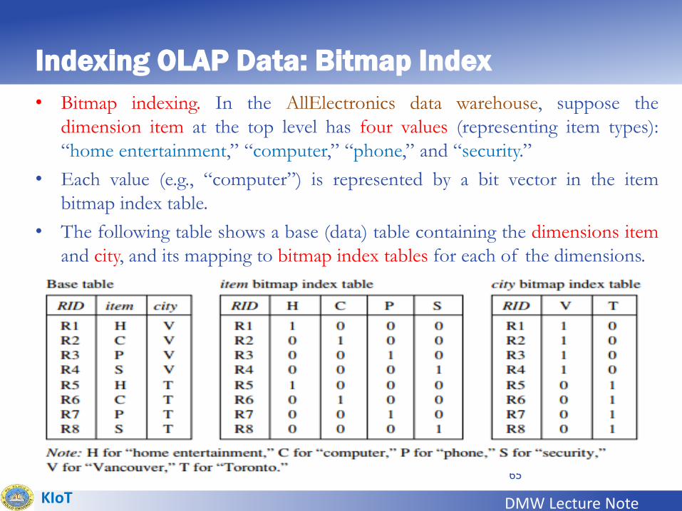
• Bitmap indexing. In the AllElectronics data warehouse, suppose the
dimension item at the top level has four values (representing item types):
“home entertainment,” “computer,” “phone,” and “security.”
• Each value (e.g., “computer”) is represented by a bit vector in the item
bitmap index table.
• The following table shows a base (data) table containing the dimensions item
and city, and its mapping to bitmap index tables for each of the dimensions.

DMW Lecture NoteKIoT
Indexing OLAP Data: Join Indices
• The join indexing method gained popularity from its use in
relational database query processing. Traditional indexing maps the
value in a given column to a list of rows having that value.
• In contrast, join indexing registers the joinable rows of two
relations from a relational database.
• For example, if two relations R(RID, A) and S(B, SID) join on the
attributes A and B, then the join index record contains the pair
(RID, SID), where RID and SID are record identifiers from the R
and S relations, respectively.
• Hence, the join index records can identify joinable tuples without
performing costly join operations.
• Join indexing is especially useful for maintaining the relationship
between a foreign key and its matching primary keys, from the
joinable relation. 66
DMW Lecture NoteKIoT
Indexing OLAP Data: Join Indices
• Join indexing maintains relationships between attribute valuesof a dimension and the corresponding rows in the fact table.
• Join indices may span multiple dimensions to form compositejoin indices.
• We can use join indices to identify sub cubes that are of interest.
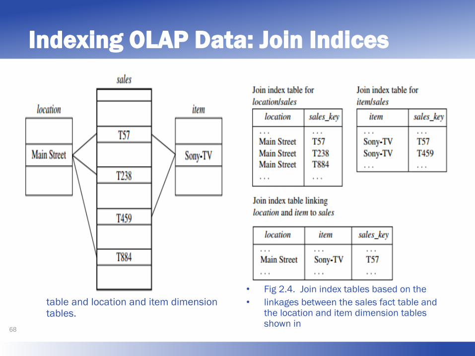
• Join indexing. An example of a join index relationship betweenthe sales fact table and the location and item dimension tablesshown in Figure 2.3.
• For example, the “Main Street” value in the location dimensiontable joins with tuples T57, T238, and T884 of the sales facttable.
• Similarly, the “Sony-TV” value in the item dimension table joinswith tuples T57 and T459 of the sales fact table.
• The corresponding join index tables are shown in Figure 2.4.67
Indexing OLAP Data: Join Indices
• Fig 2.3. Linkages between a sales fact table and location and item dimension tables.
• Fig 2.4. Join index tables based on the
• linkages between the sales fact table and the location and item dimension tables shown in
68

DMW Lecture NoteKIoT
69
Efficient Processing OLAP Queries• The purpose of materializing cuboids and constructing OLAP index structures is
to speed up query processing in data cubes.
• Given materialized views, query processing should proceed as follows:
Determine which operations should be performed on the available cuboids:
• This involves transforming any selection, projection, roll-up (group-by), and drill-
down operations specified in the query into corresponding SQL and/or OLAP
operations.
• For example, slicing and dicing a data cube may correspond to selection and/or
projection operations on a materialized cuboid.
Determine to which materialized cuboid(s) the relevant operations should
be applied:
• This involves identifying all of the materialized cuboids that may potentially be
used to answer the query, pruning the set using knowledge of “dominance”
relationships among the cuboids, estimating the costs of using the remaining
materialized cuboids, and selecting the cuboid with the least cost.

DMW Lecture NoteKIoT
OLAP Server Architectures
• Logically, OLAP servers present business users withmultidimensional data from data warehouses or datamarts, without concerns regarding how or where thedata are stored.
• However, the physical architecture and implementationof OLAP servers must consider data storage issues.
• Implementations of a warehouse server for OLAPprocessing include the following:
Relational OLAP (ROLAP)
Multidimensional OLAP (MOLAP)
Hybrid OLAP (HOLAP)
Specialized SQL Servers70

DMW Lecture NoteKIoT
OLAP Server Architectures
Relational OLAP
• ROLAP servers are placed between relational back-end server and client
front-end tools.
• To store and manage warehouse data, ROLAP uses relational or extended-
relational DBMS.
• ROLAP includes the following:
Implementation of aggregation navigation logic.
Optimization for each DBMS back-end.
Additional tools and services.
Multidimensional OLAP
• MOLAP uses array-based multidimensional storage engines for
multidimensional views of data. With multidimensional data stores, the
storage utilization may be low if the dataset is sparse.
• Therefore, many MOLAP servers use two levels of data storage
representation to handle dense and sparse datasets.71

DMW Lecture NoteKIoT
OLAP Server Architectures
Hybrid OLAP
• Hybrid OLAP is a combination of both ROLAP and MOLAP.
It offers higher scalability of ROLAP and faster computation of
MOLAP.
• HOLAP servers allow to store large data volumes of detailed
information.
• The aggregations are stored separately in MOLAP store.
Specialized SQL Servers
• Specialized SQL servers provide advanced query language and
query processing support for SQL queries over star and
snowflake schemas in a read-only environment.
72

DMW Lecture NoteKIoT
Chapter 2: Data Warehousing and OLAP
What is a data
warehouse?
A multi-dimensional data model
Data warehouse
architecture
Data warehouse implementation
From data warehousing
to data mining

DMW Lecture NoteKIoT
From OLAP to Multidimensional Data Mining
Multidimensional data mining (also known as online analytical mining, orOLAM) integrates OLAP with data mining to uncover knowledge inmultidimensional databases.
Why online analytical mining?
– High quality of data in data warehouses
• DW contains integrated, consistent, cleaned data
– Available information processing structure surrounding data warehouses• ODBC connection, Web accessing, service facilities, reporting & OLAP tools
– OLAP-based exploratory data analysis
• Mining with drilling, dicing, pivoting, etc.
– On-line selection of data mining functions
• Integration and swapping of multiple mining functions, algorithms, and tasks
74
Top Related
Copyright © 2022 FDOKUMEN

