Computational Techniques in Civil Engineering

Water Resources part: Tutorial solution Dr. K.N. Dulal

FDM

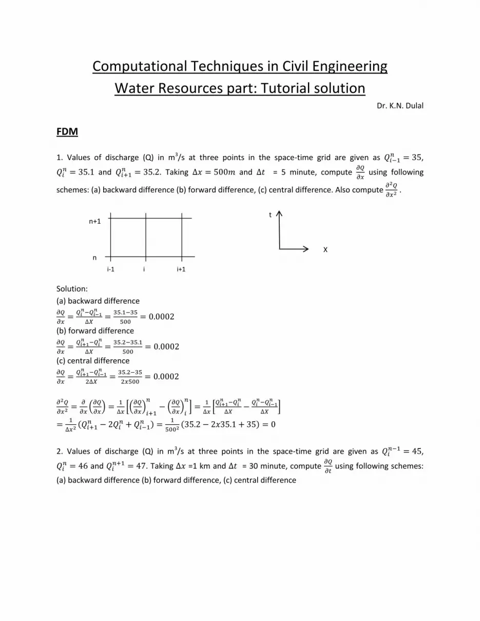
1. Values of discharge (Q) in m3/s at three points in the space-time grid are given as ,

and

. Taking and = 5 minute, compute

using following

schemes: (a) backward difference (b) forward difference, (c) central difference. Also compute

.

Solution:

(a) backward difference

(b) forward difference

(c) central difference

(

)

[(

)

(

)

]

[

]

(

)

( )

2. Values of discharge (Q) in m3/s at three points in the space-time grid are given as ,

and

. Taking =1 km and = 30 minute, compute

using following schemes:

(a) backward difference (b) forward difference, (c) central difference

t n+1

n

i-1 i i+1

X

Solution:

(a) backward difference

(b) forward difference

(c) central difference

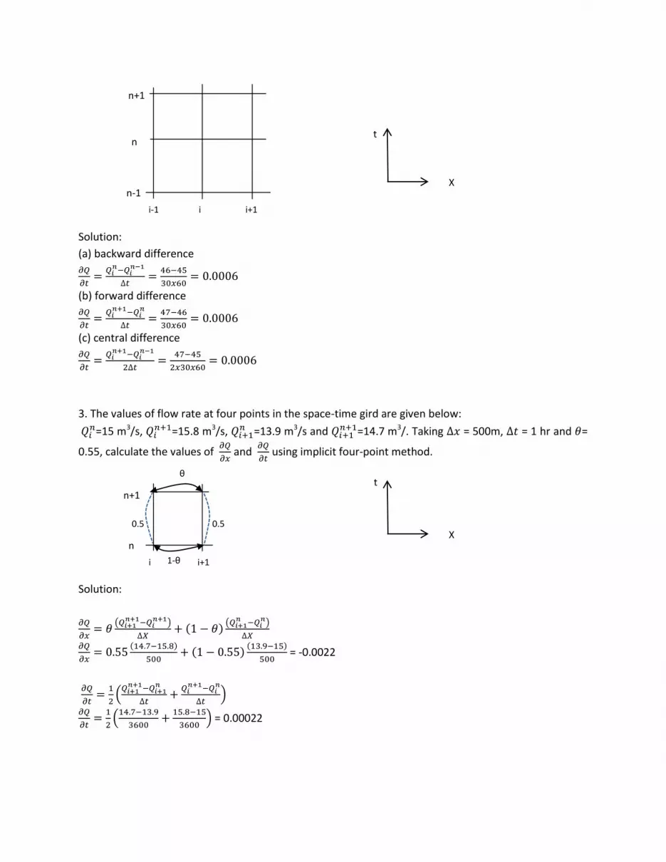
3. The values of flow rate at four points in the space-time gird are given below:

=15 m3/s,

=15.8 m3/s, =13.9 m3/s and

=14.7 m3/. Taking = 500m, = 1 hr and =

0.55, calculate the values of

and

using implicit four-point method.

Solution:

(

)

( )

(

)

( )

( )

( )

= -0.0022

(

)

(

) = 0.00022

0.5 0.5

θ t

n+1

t n

n-1

i-1 i i+1

X

n+1

n

i i+1

X

1-θ

4. Consider a rectangular channel, 30m wide, with bed slope of 0.015 and Manning’s n = 0.035. The

following flow rates are given: =30 m3/s,

=22 m3/s and =20 m3/s. Taking = 1500m and

= 10 min, determine using finite difference scheme for a linear kinematic wave model. Assume

lateral flow to be zero. The equation for linear kinematic wave model with no lateral flow is

(

)

(

(

)

)

. Take wetted perimeter is approximately equal to width of

channel.

Solution:

Width of channel (b) = 30m

Bed slope (S) = 0.015

Manning’s n = 0.035

from Manning’s equation

(

√ )

Comparing to

(

√ )

(

√ )

= 1.84

= 1500m and = 10 min = 600 s

(

)

(

(

)

)

(

)

(

(

)

) =25.67 m3/s

5. Solve exercise 4 by using non-linear kinematic wave model using the equation

( )

( )

Take value of computed in exercise 4 as initial value and solve by Newton-Raphson iteration.

Solution:

RHS=c =

( ) =

= 23.1

Residual error is ( )

( )

=

( )

( )=

( )

( ) (

)

Newton-Raphson formula

( )

(

)

(

)

( )

( )

= 25.67 m3/s (computed in 1)

Iteration 1

( )= ( ) = 0.0645

( ) ( ) =0.7

( )

= 25.577 m3/s

Iteration 2

( )= ( ) = -0.0007

( ) ( ) =0.7

( )

= 29.578 m3/s

As the difference in Q in iteration 1 and 2 is small, the iteration is stopped.

=25.578 m3/s

6. Consider a rectangular channel, 90m wide and 5km long with bed slope of 0.015 and Manning’s n =

0.02. The inflow hydrograph for the channel is given below:

Time (min) 0 5 10 15 20

Flow (m3/s) 14 19 28 32 40

The initial condition is a uniform flow of 14 m3/s and there is no lateral flow.

Use the linear kinematic wave model to route the inflow hydrograph through the channel taking =

1000m and = 5 min . The equation for routing is

(

)

(

(

)

)

. Take wetted perimeter is approximately equal to width of

channel.

Solution:

Width of channel (b) = 90m

Bed slope (S) = 0.015

Manning’s n = 0.02

from Manning’s equation

(

√ )

Comparing to

(

√ )

(

√ )

= 2

= 1000m and = 5 min = 300 s

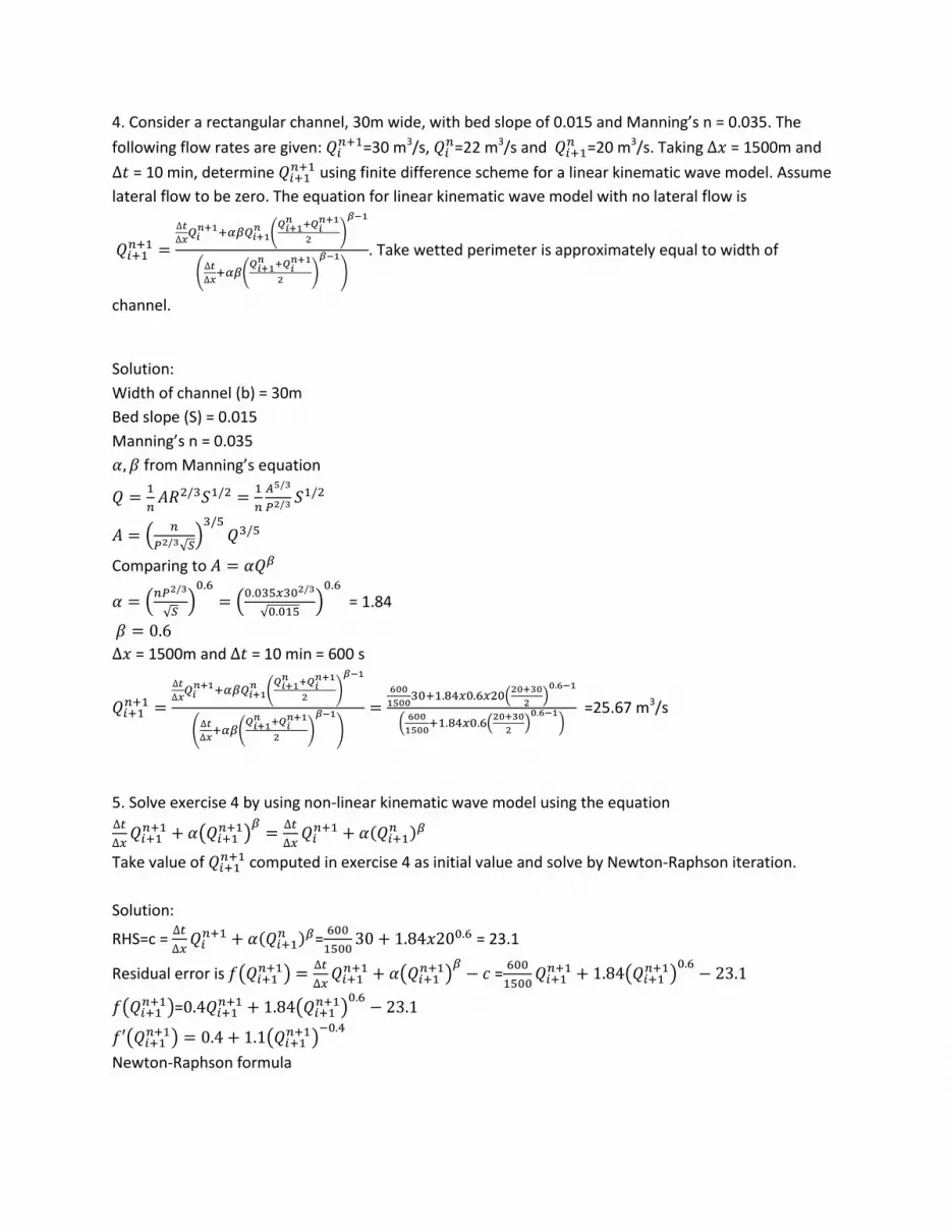
Routing

Distance (m)

Remarks Time (min)

Time index (n)

0 1000 2000 3000 4000 5000

i = 1 2 3 4 5 6

0 1 14 14 14 14 14 14 Given

5 2 19 16.17 14.92 14.39 14.16 14.07

10 3 28 21.65 17.91 15.91 14.91 14.42

15 4 32 26.64 21.96 18.62 16.52 15.32

20 5 40 33.37 27.50 22.77 19.34 17.09

Sample computation

For i = 1 all values are given for all t. For n = 1, all values are given for all i.

i = 1, n = 1:

=19 m3/s,

=14 m3/s and

=14 m3/s.

(

)

(

(

)

)

(

)

(

(

)

) =16.17 m3/s

Compute other values in a similar way.

7. A flood of 150 m3/s peak discharge passed a gauging station at 12:00 noon on a river. There is a

community adjacent to the river 7.2 km downstream. What will be the value of peak discharge at that

community at 12:00 noon if the velocity of flow is 1.2 m/s and peak discharge at that community at 9:00

A.M. is 100 m3/s. Assume width of river as inside and use first order accurate numerical scheme of

kinematic wave equation. Take = 7.2km and = 1 hr.

Solution: In kinematic wave equation,

, take q = 0. First finding the finite difference

equation

t

dx

n+1

dt

n

i i+1 x

Non-derivative terms

Substituting above values in

(

)

(

(

)

)

(

)

(

)

(

(

)

)

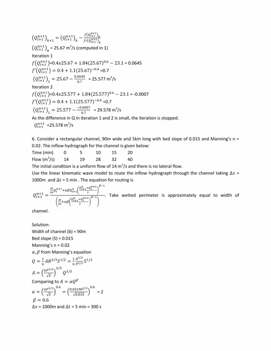
Routing

i =1 i=2

7200m

i=1: gauging station, i=2: community

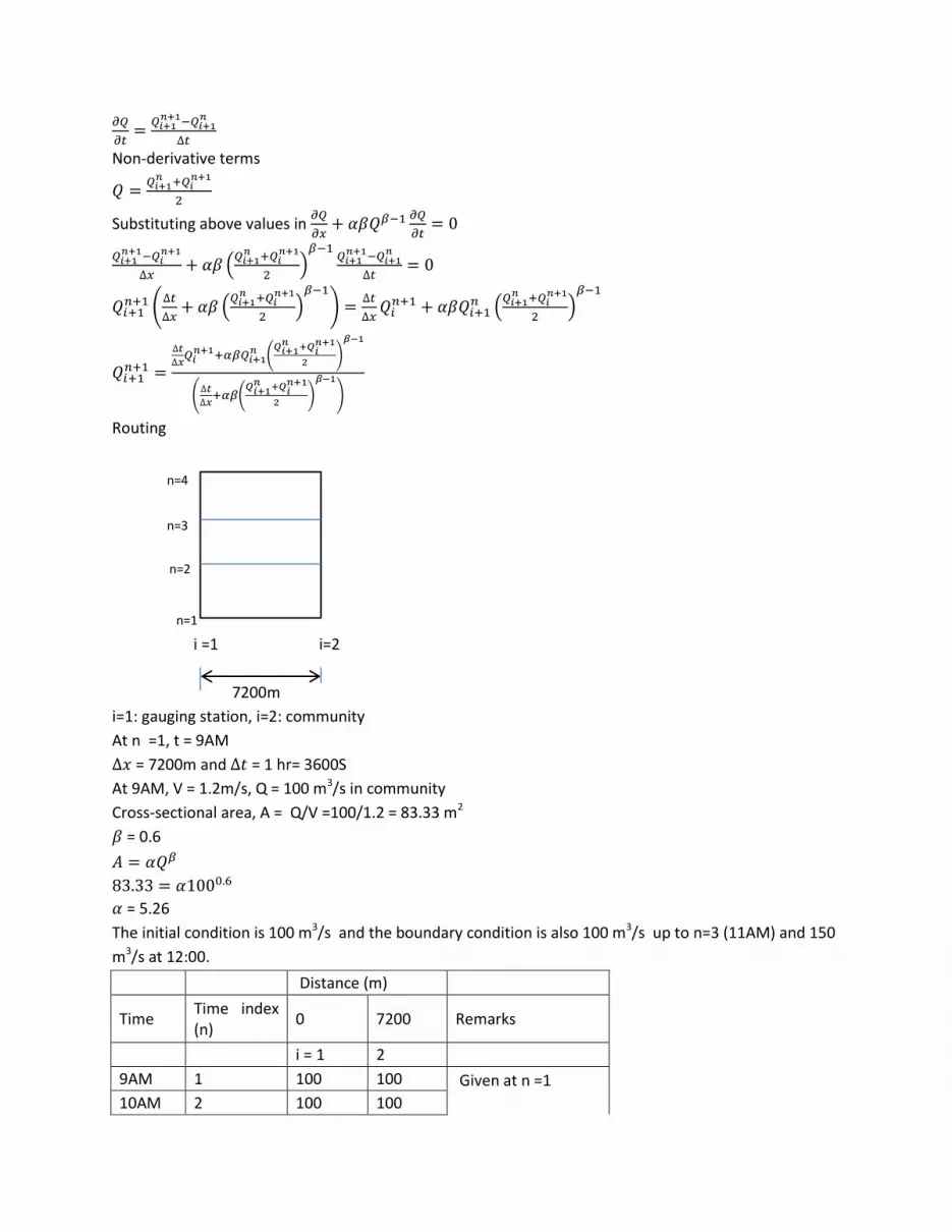
At n =1, t = 9AM

= 7200m and = 1 hr= 3600S

At 9AM, V = 1.2m/s, Q = 100 m3/s in community

Cross-sectional area, A = Q/V =100/1.2 = 83.33 m2

= 0.6

= 5.26

The initial condition is 100 m3/s and the boundary condition is also 100 m3/s up to n=3 (11AM) and 150

m3/s at 12:00.

Distance (m)

Time Time index (n)

0 7200 Remarks

i = 1 2

9AM 1 100 100 Given at n =1 10AM 2 100 100

n=1

n=2

n=3

n=4

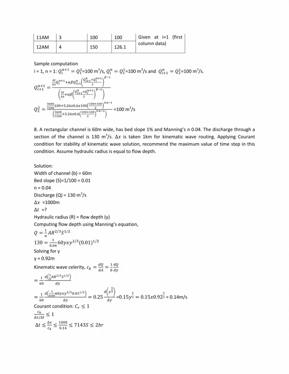
11AM 3 100 100 Given at i=1 (first column data)

12AM 4 150 126.1

Sample computation

i = 1, n = 1:

=100 m3/s,

=100 m3/s and

=100 m3/s.

(

)

(

(

)

)

(

)

(

(

)

) =100 m3/s

8. A rectangular channel is 60m wide, has bed slope 1% and Manning’s n 0.04. The discharge through a

section of the channel is 130 m3/s. is taken 1km for kinematic wave routing. Applying Courant

condition for stability of kinematic wave solution, recommend the maximum value of time step in this

condition. Assume hydraulic radius is equal to flow depth.

Solution:

Width of channel (b) = 60m

Bed slope (S)=1/100 = 0.01

n = 0.04

Discharge (Q) = 130 m3/s

=1000m

=?

Hydraulic radius (R) = flow depth (y)

Computing flow depth using Manning’s equation,

( )

Solving for y

y = 0.92m

Kinematic wave celerity,

(

)

(

)

( )

=

= 0.14m/s

Courant condition:

MOC

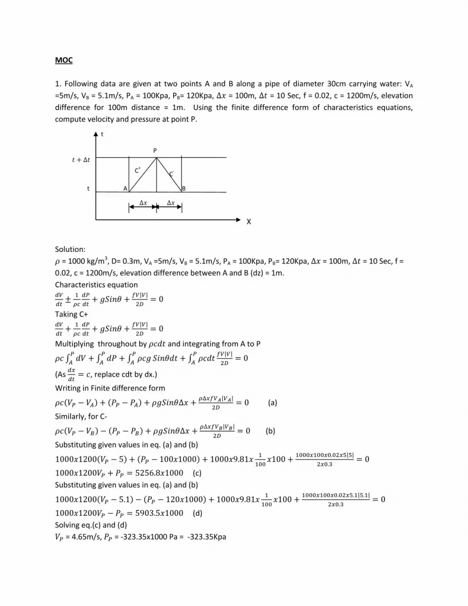
1. Following data are given at two points A and B along a pipe of diameter 30cm carrying water: VA

=5m/s, VB = 5.1m/s, PA = 100Kpa, PB= 120Kpa, = 100m, = 10 Sec, f = 0.02, c = 1200m/s, elevation

difference for 100m distance = 1m. Using the finite difference form of characteristics equations,

compute velocity and pressure at point P.

Solution:

= 1000 kg/m3, D= 0.3m, VA =5m/s, VB = 5.1m/s, PA = 100Kpa, PB= 120Kpa, = 100m, = 10 Sec, f =

0.02, c = 1200m/s, elevation difference between A and B (dz) = 1m.

Characteristics equation

| |

Taking C+

| |

Multiplying throughout by and integrating from A to P

∫ ∫ ∫

∫

| |

(As

, replace cdt by dx.)

Writing in Finite difference form

( ) ( ) | |

(a)

Similarly, for C-

( ) ( ) | |

(b)

Substituting given values in eq. (a) and (b)

( ) ( )

| |

(c)

Substituting given values in eq. (a) and (b)

( ) ( )

| |

(d)

Solving eq.(c) and (d)

= 4.65m/s, = -323.35x1000 Pa = -323.35Kpa

t

𝑡 𝑡

t

𝑥 𝑥

C-

B A

C+

P

X

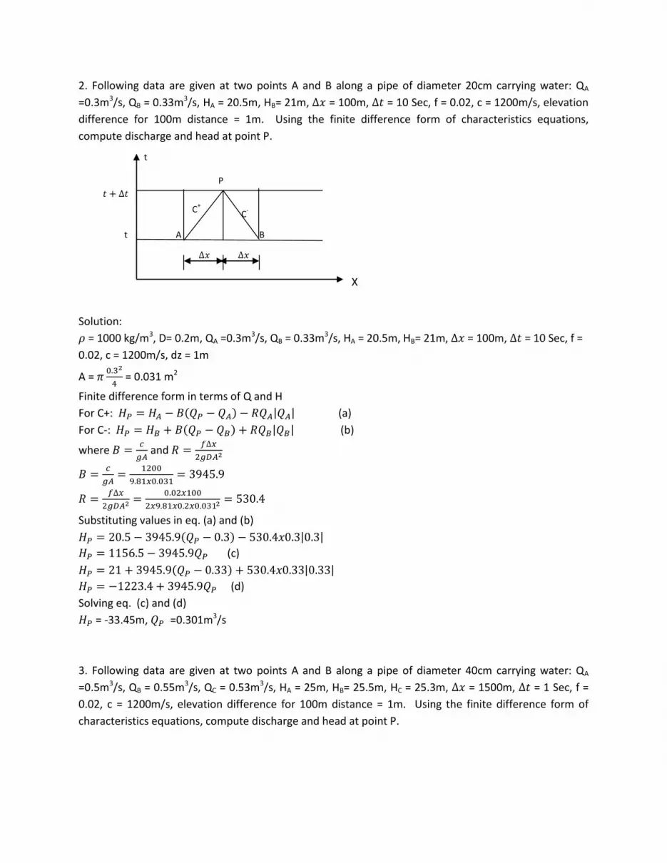
2. Following data are given at two points A and B along a pipe of diameter 20cm carrying water: QA

=0.3m3/s, QB = 0.33m3/s, HA = 20.5m, HB= 21m, = 100m, = 10 Sec, f = 0.02, c = 1200m/s, elevation

difference for 100m distance = 1m. Using the finite difference form of characteristics equations,

compute discharge and head at point P.

Solution:

= 1000 kg/m3, D= 0.2m, QA =0.3m3/s, QB = 0.33m3/s, HA = 20.5m, HB= 21m, = 100m, = 10 Sec, f =

0.02, c = 1200m/s, dz = 1m

A =

= 0.031 m2

Finite difference form in terms of Q and H

For C+: ( ) | | (a)

For C-: ( ) | | (b)

where

and

Substituting values in eq. (a) and (b)

( ) | |

(c)

( ) | |

(d)

Solving eq. (c) and (d)

= -33.45m, =0.301m3/s

3. Following data are given at two points A and B along a pipe of diameter 40cm carrying water: QA

=0.5m3/s, QB = 0.55m3/s, QC = 0.53m3/s, HA = 25m, HB= 25.5m, HC = 25.3m, = 1500m, = 1 Sec, f =

0.02, c = 1200m/s, elevation difference for 100m distance = 1m. Using the finite difference form of

characteristics equations, compute discharge and head at point P.

t

𝑡 𝑡

t

𝑥 𝑥

C-

B A

C+

P

X

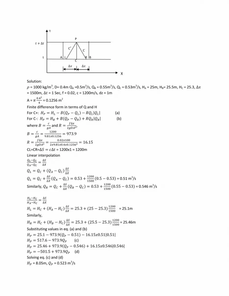
Solution:

= 1000 kg/m3, D= 0.4m QA =0.5m3/s, QB = 0.55m3/s, QC = 0.53m3/s, HA = 25m, HB= 25.5m, HC = 25.3,

= 1500m, = 1 Sec, f = 0.02, c = 1200m/s, dz = 1m

A =

= 0.1256 m2

Finite difference form in terms of Q and H

For C+: ( ) | | (a)

For C-: ( ) | | (b)

where

and

,

CL=CR= = 1200x1 = 1200m

Linear interpolation

( )

( )

( ) = 0.51 m3/s

Similarly,

( )

( ) = 0.546 m3/s

( )

( )

= 25.1m

Similarly,

( )

( )

= 25.46m

Substituting values in eq. (a) and (b)

( ) | |

(c)

( ) | |

(d)

Solving eq. (c) and (d)

= 8.05m, = 0.523 m3/s

C

t

𝑡 𝑡

t

𝑥 𝑥

C-

R B A L

C+

P

X

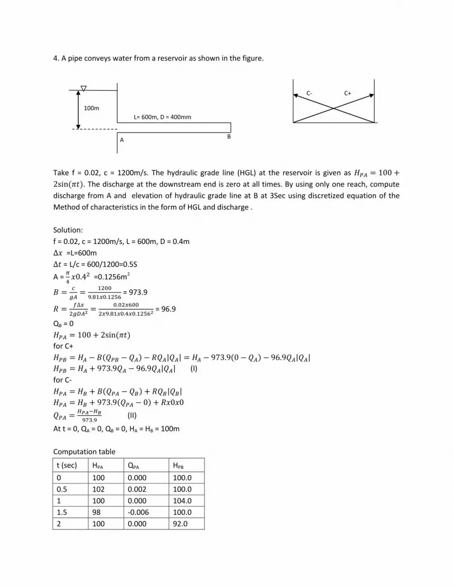
4. A pipe conveys water from a reservoir as shown in the figure.

Take f = 0.02, c = 1200m/s. The hydraulic grade line (HGL) at the reservoir is given as

( ). The discharge at the downstream end is zero at all times. By using only one reach, compute

discharge from A and elevation of hydraulic grade line at B at 3Sec using discretized equation of the

Method of characteristics in the form of HGL and discharge .

Solution:

f = 0.02, c = 1200m/s, L = 600m, D = 0.4m

=L=600m

= L/c = 600/1200=0.5S

A =

=0.1256m2

= 973.9

= 96.9

QB = 0

( )

for C+

( ) | | ( ) | |

| | (I)

for C-

( ) | |

( )

(II)

At t = 0, QA = 0, QB = 0, HA = HB = 100m

Computation table

t (sec) HPA QPA HPB

0 100 0.000 100.0

0.5 102 0.002 100.0

1 100 0.000 104.0

1.5 98 -0.006 100.0

2 100 0.000 92.0

C+ C-

B A

L= 600m, D = 400mm

100m

2.5 102 0.010 100.0

3 100 0.000 112.0

Computation sequence

( )

where HB = HPB of previous step

| | where HA = HPA of previous step and QA = QPA of previous step

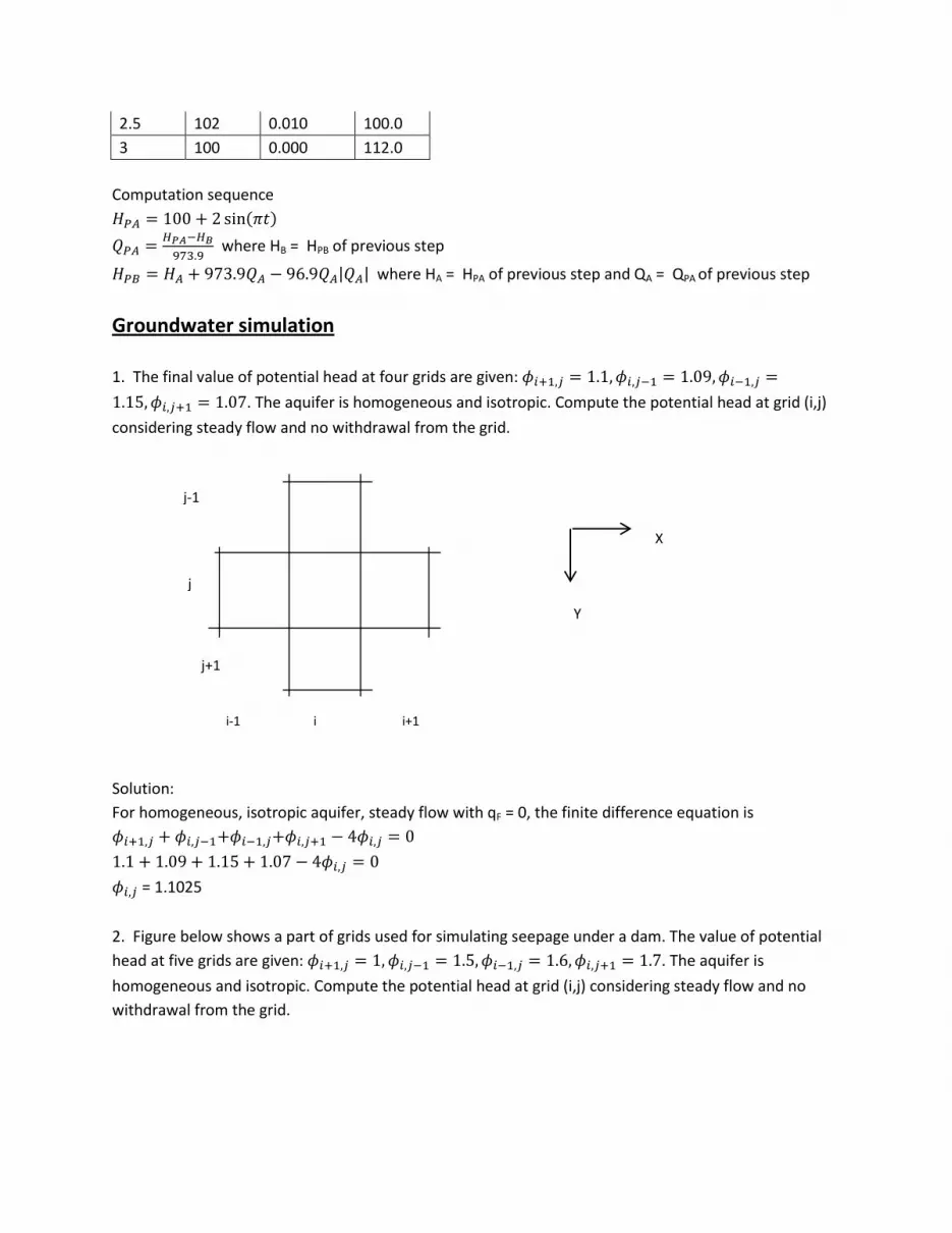
Groundwater simulation

1. The final value of potential head at four grids are given:

. The aquifer is homogeneous and isotropic. Compute the potential head at grid (i,j)

considering steady flow and no withdrawal from the grid.

Solution:

For homogeneous, isotropic aquifer, steady flow with qF = 0, the finite difference equation is

= 1.1025

2. Figure below shows a part of grids used for simulating seepage under a dam. The value of potential

head at five grids are given: . The aquifer is

homogeneous and isotropic. Compute the potential head at grid (i,j) considering steady flow and no

withdrawal from the grid.

j-1

Y

j

j+1

i-1 i i+1

X

Solution:

For homogeneous, isotropic aquifer, steady flow with qF = 0, the finite difference equation is

= 1.45

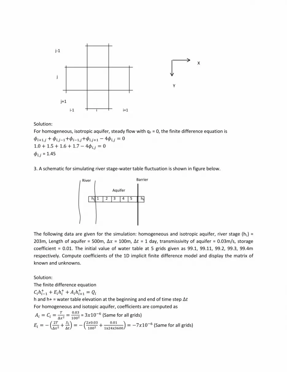
3. A schematic for simulating river stage-water table fluctuation is shown in figure below.

The following data are given for the simulation: homogeneous and isotropic aquifer, river stage (hL) =

203m, Length of aquifer = 500m, = 100m, = 1 day, transmissivity of aquifer = 0.03m/s, storage

coefficient = 0.01. The initial value of water table at 5 grids given as 99.1, 99.11, 99.2, 99.3, 99.4m

respectively. Compute coefficients of the 1D implicit finite difference model and display the matrix of

known and unknowns.

Solution:

The finite difference equation

h and h+ = water table elevation at the beginning and end of time step

For homogeneous and isotopic aquifer, coefficients are computed as

= (Same for all grids)

(

) (

) (Same for all grids)

River

hR

j-1

Y

j

j+1

i-1 i i+1

X

hL 1 2 3 4 5

Barrier

Aquifer

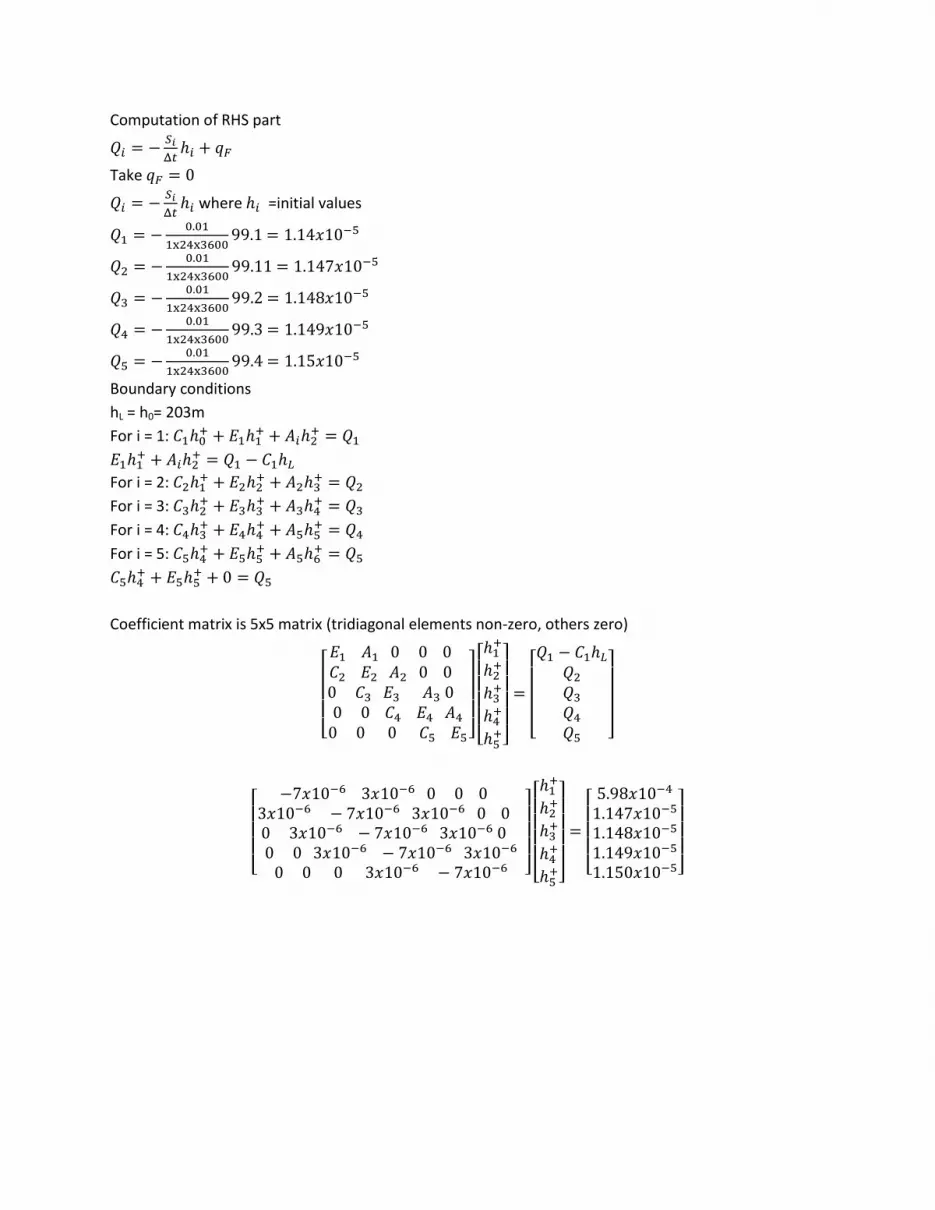
Computation of RHS part

Take

where =initial values

Boundary conditions

hL = h0= 203m

For i = 1:

For i = 2:

For i = 3:

For i = 4:

For i = 5:

Coefficient matrix is 5x5 matrix (tridiagonal elements non-zero, others zero)

[

]

[

]

[

]

[

]

[

]

[

]