


Bahasa
Halaman
Hukum


For Peer Review
Competition and efficiency in the Dutch life insurance industry
Journal: Applied Economics
Manuscript ID: APE-05-0726.R1
Journal Selection: Applied Economics
JEL Code:
D43 - Oligopoly and Other Forms of Market Imperfection < D4 - Market Structure and Pricing < D - Microeconomics, L11 - Production, Pricing, and Market Structure|Size Distribution of Firms < L1 - Market Structure, Firm Strategy, and Market Performance < L - Industrial Organization, G22 - Insurance|Insurance Companies < G2 - Financial Institutions and Services < G - Financial Economics, L13 - Oligopoly and Other Imperfect Markets < L1 - Market Structure, Firm Strategy, and Market Performance < L - Industrial Organization
Keywords:life insurance, market structure, concentration, competition, scale economies
Editorial Office, Dept of Economics, Warwick University, Coventry CV4 7AL, UK
Submitted Manuscriptpe
er-0
0582
036,
ver
sion
1 -
1 Ap
r 201
1Author manuscript, published in "Applied Economics 40, 16 (2008) 2063-2084"
DOI : 10.1080/00036840600949298

For Peer Review
Applied Economics
28-7-2006
Formatted: Font: 12 pt, Dutch(Netherlands)
1. Introduction
This article investigates efficiency and competitive behaviour on the Dutch life insurance
market. In the Netherlands, the life insurance sector is important with in 2003 a volume of
business in terms of annual premiums paid of € 24 billion, invested assets of € 238 billion
and insured capital of € 900 billion.1 This market provides important financial products, such
as endowment insurance, annuities, term insurance and burial funds, of often sizeable value
for consumers. Financial planning of many households depends on proper functioning of this
market. The complexity of the products and dependency on future investment returns make
many life insurance products rather opaque. Therefore, competition and efficiency in this
sector are important issues, both from the point of view of consumers as well as that of
supervisors whose duty it is to protect the interests of consumers.
Most life insurance policies have a long life span, which makes consumers sensitive
to the reliability of the respective firms. Life insurance firms need to remain in a financially
sound condition over decades in order to be able to pay out the promised benefits. The sector
has a safety net arrangement in the case a life insurer fails, but that does not cover all risks
and excludes policies of the largest ten firms. Without sufficient profitability it could be
questionable whether life insurers are able to face unfavourable developments such as a
long-lasting decline of long-term interest rates. Obviously, there may be a complex trade off
between increased competition with a short-run advantage for consumers of low premiums,
but possibly the drawback of higher long-run risk with respect to the insurance benefits. In
practice, the likelihood that an insurer in the Netherlands fails, appears to be rather limited
with only one bankruptcy in the last twenty years. Obviously, improvement of efficiency
would benefit all stakeholders, both in the short and the long run. Also the impact of
competition on this trade off between short and long term interests makes it worthwhile to
further investigate competition in this market.
1 In terms of premiums as a percentage of GDP, the Dutch market is around 40% above the European
weighted average.
Deleted: paper
Deleted: Complexity
Deleted: heavy
Deleted: the
Deleted: during
Deleted: From that perspective
Deleted: seems
Deleted: 28-7-2006
Deleted: 21-7-2006
Page 1 of 47
Editorial Office, Dept of Economics, Warwick University, Coventry CV4 7AL, UK
Submitted Manuscript
123456789101112131415161718192021222324252627282930313233343536373839404142434445464748495051525354555657585960
peer
-005
8203
6, v
ersi
on 1
- 1
Apr 2
011

For Peer Review
2
Life insurance firms sell different products using various distribution channels,
thereby creating several submarkets. The degree of competition may vary across these
submarkets. For instance, submarkets where parties bargain on collective contracts (mainly
pension schemes provided by the employer) and submarkets for direct writers are expected
to be more competitive than submarkets where insurance agents sell products to uninformed
but trusting customers. Lack of sufficient data on prices of life insurance products, market
shares of products and distribution channels, makes distinctions of competition on
submarkets impossible.
Lack of data also prohibits us to measure competition among life insurers directly
(for instance, by a price-cost margin), even for the total life insurance market. One
qualitative way to investigate this market is to work out what its structural features are,
particularly those related to its competitive nature. On the supply side, we find that market
power of insurance firms is limited due to their plurality and that ample entry possibilities
exist, all of which contributes to sound competitive conditions. But on the demand side, we
observe that consumer power is limited, particularly due to the opaque nature of many life
insurance products, and that there are few substitution possibilities for life insurance policies,
which could hamper increased competition. Combining these various insights, we have
reasons to analyse the competitive nature of this market further.
An often-used quantitative indirect measure of competition is efficiency. Increased
competition is assumed to force firms to operate more efficiently, so that high efficiency
might indicate the existence of competition and vice versa. We distinguish between various
types of efficiency, particularly scale efficiency and X-efficiency. Scale economies are
related to output volumes, whereas cost X-efficiency reflects managerial ability to drive
down production costs, controlled for output volumes and input price levels. There are
various methods to measure scale economies and X-efficiency.2 We use a translog cost
function to reveal the existence of scale economies, and a stochastic cost frontier model to
2 For an overview, see Bikker (2004) or Bikker and Bos (2005).
Deleted: uninformed
Deleted: Unavailable
Deleted: on
Deleted: more
Deleted: heavy
Deleted: Heavy
Page 2 of 47
Editorial Office, Dept of Economics, Warwick University, Coventry CV4 7AL, UK
Submitted Manuscript
123456789101112131415161718192021222324252627282930313233343536373839404142434445464748495051525354555657585960
peer
-005
8203
6, v
ersi
on 1
- 1
Apr 2
011

For Peer Review
3
measure X-efficiency. Further, large unemployed scale economies may raise questions about
the competitive pressure in the market. Note that the existence of scale efficiency is also
important for the potential entry of new firms, an important determinant of competition.
Strong scale effects would put new firms at a disadvantage.
A straightforward measure of competition is the profit margin. Supernormal profits
would indicate insufficient competition. We observe profits of Dutch life insurers over time
and compare them with profits of foreign peers.
Another indirect measure of competition is the so-called Boone indicator. This
approach is based on the notion that competition rewards efficiency and punishes
inefficiency. In competitive markets, efficient firms perform better – in terms of market
shares and hence profit – than inefficient firms. The Boone indicator measures the extent to
which efficiency differences between firms are translated into performance differences. The
more competitive the market is, the stronger is the relationship between efficiency
differences and performance differences. The Boone indicator is usually measured over time,
giving a picture of the development of competition. Further, the level of the Boone indicator
in life insurances can be compared with levels in other parts of the service sector, to assess
the relative competitiveness of the life insurance market.
Our article is part of a larger research project on competition in the life insurance
industry, see CPB. (2005). Other chapters of this report go into more detail with respect to
barriers of competition, product choice and the role of financial advice. This article aims at
measuring competitive behaviour and performance of the Dutch life insurance market as a
whole. The current article is complementary to the detailed studies in the following sense:
whatever goes on in the often discussed financial advice part of the business, the current
article verifies what can be said about competition on the market on an aggregate level. Any
problems (or lack of problems) should ultimately show up in aggregate indicators of
competition. Since we use four different empirical aggregate indicators (average profit
margins, scale economies, X-inefficiencies and the Boone indicator), we will get a
reasonable picture of competition in this market.
Deleted: into an unfavourable position
Deleted: which yields
Deleted: paper
Deleted: papers
Deleted: paper
Deleted: paper
Deleted: that
Deleted: paper
Deleted: are to
Page 3 of 47
Editorial Office, Dept of Economics, Warwick University, Coventry CV4 7AL, UK
Submitted Manuscript
123456789101112131415161718192021222324252627282930313233343536373839404142434445464748495051525354555657585960
peer
-005
8203
6, v
ersi
on 1
- 1
Apr 2
011

For Peer Review
4
The outline of the article is as follows. Section 2 provides a brief and general
explanation of the production of life insurance firms. Section 3 investigates the competitive
structure of demand and supply sides of the Dutch life insurance market. Section 4 measures
scale economies based on the so-called translog cost function, while the next section
introduces the measurement of X-efficiency. Section 6 discusses the Boone indicator.
Section 7 describes the data used and Section 8 presents the empirical results of the various
indirect measures of competition. The last section sums up and draws conclusions.
2. The production of life insurances
The core business of insurance firms is the sale of protection against risks.3 There are two
quite different types of insurance products: life insurance and non-life or property & casualty
(P&C) insurance.4 Life insurance covers deviations in the timing and size of predetermined
cash flows due to (non-)accidental death or disability. While some life insurance products
pay out only in the incident of death (term insurance and burial funds), others do so at the
end of a term or a number of terms (endowment insurance).5 A typical annuity policy pays
an annual amount starting on a given date (if a specific person is still alive) and continues
until that person passes away. The benefits of insurance can be guaranteed beforehand so
that the insurance firm bears the risk that invested premiums may not cover the promised
payments. Such guaranteed benefits may be accompanied by some kind of profit sharing,
e.g. depending on indices of bonds or shares. The benefits of insurance can also be linked to
capital market investments, e.g. a basket of shares, so that the insurance firm bears no
investment risk at all. Such policies are usually referred to as unit-linked funds. We also
observe mixed products, e.g. unit linked funds with guaranteed minimum investment returns.
3 For life insurances, a second motive is the accumulation of assets. Some countries see many buyers
of annuities eventually cashing out their contracts rather than annuitizing. 4 In the Netherlands, health insurance is part of non-life insurance, whereas in Anglo-Saxon countries,
health insurance is seen as part of life insurance.5 A typical endowment insurance policy pays a given amount at a given date if a given person is still
alive, or earlier when he or she passes away. Of course, there are many variants to these archetypes.
Deleted: paper
Deleted: four
Page 4 of 47
Editorial Office, Dept of Economics, Warwick University, Coventry CV4 7AL, UK
Submitted Manuscript
123456789101112131415161718192021222324252627282930313233343536373839404142434445464748495051525354555657585960
peer
-005
8203
6, v
ersi
on 1
- 1
Apr 2
011

For Peer Review
5
A major feature of life insurance is its long-term character, often continuing for
decades. Therefore, policyholders need to trust their life insurance company, making insurers
very sensitive to their reputation. Life insurers need large reserves to cover their calculated
insurance liabilities. These reserves are financed by – annual or single – insurance premiums
and invested mainly on the capital market. The major risk of life insurers concerns
mismatches between liabilities and assets. Idiosyncratic life risk is negligible as it can be
well diversified. Systematic life risk, however, such as increasing life expectancy, can also
pose a threat to life insurers. Yet their major risk will always be investment risk. The main
services which life insurance firms provide to their customers are life (and disability) risk
pooling and financial intermediation. Significant expenditures include sales expenses,
whether in the form of direct sales costs or of fees paid to insurance agencies, administrative
costs, investment management and product development.
In the Netherlands, the insurance product market is heavily influenced by fiscal
privileges. In the past, endowment-insurance allowances, including any related investment
income, used to be tax-exempt, up to certain limits, provided that certain none-too-restrictive
conditions were met. Annuity premiums were tax deductible, but annuity allowances were
taxed. Again this implies that investment income was enjoyed tax-free while consumers
could often also benefit from lower marginal tax rates after retirement. In 2001 a major tax
revision reduced the tax benefits for all new policies, while the rights of existing policies
were respected.6 The tax reduction was made public in earlier years, so that consumers could
bring forward their spending on annuities and insurers were eager to sell. Endowment
insurance policies became subject to wealth tax and income tax exemption limits were
reduced. At the same time, both the standard deduction for annuity premiums and the
permission for individuals to deduct annuity premiums to repair pension shortfalls were also
reduced. The reduced subsidy on annuities, in particular, has had a great impact on volumes.
6 The fiscal regime change might cause a structural break. However, re-estimation of our model for
two sub periods, before and after the change, did not give different results.
Deleted: adding value to the invested premiums
Deleted: advance
Deleted: sale
Page 5 of 47
Editorial Office, Dept of Economics, Warwick University, Coventry CV4 7AL, UK
Submitted Manuscript
123456789101112131415161718192021222324252627282930313233343536373839404142434445464748495051525354555657585960
peer
-005
8203
6, v
ersi
on 1
- 1
Apr 2
011

For Peer Review
6
Finally, in 2003, the standard deduction for annuity premiums was abolished entirely,
whereas the permission to do so on an individual basis was limited even further.
3. The competitive structure of the Dutch life insurance market
This section briefly discusses structural characteristics of the market for life insurance that
may affect competition.7 The diagnostic framework developed in CPB (2003) enables an
assessment whether a market structure constitutes a tight oligopoly. The latter is an oligopoly
which facilitates the realization of supernormal profits for a substantial period of time, where
‘facilitate’ reflects that the probability that supernormal profits are observed are higher than
in a more competitive market, ‘supernormal profits’ exceeds a market conform rate of risk-
adjusted return on capital, and ‘substantial period of time’ reflects that oligopolies will be
stable for a number of years.
3.1 Supply side factors
The diagnostic framework mentioned above contains a list of coordinated and unilateral
factors that increase the probability of a tight oligopoly, see Table 3.1. Coordinated factors
refer to explicit and tacit collusion, while unilateral factors denote actions undertaken by
individual firms without any form of coordination with other firms. Economic theory
indicates that a high concentration and high entry barriers are conducive to the realization of
supernormal profits. Frequent interaction, transparency and symmetry (in terms of equal cost
structures) are beneficial to a tight oligopoly since they make it easier for firms to coordinate
their actions and to detect and punish deviations from the (explicitly or tacitly) agreed upon
behaviour. Heterogeneous products make it easier for firms to raise prices independently of
competitors, as consumers are less likely to switch to another firm in response to price
differences. Structural links between firms such as cross-ownerships would give firms a
stake in each others’ performance, thus softening competition.8 Information about risks plays
7 For a fuller discussion we refer to CPB (2005). See also Kamerschen (2004).8 For a detailed analysis of the various effects we refer to CPB (2003).
Deleted: For a fuller discussion we refer to CPB (2005).
Deleted: A tight oligopoly
Deleted: .
Deleted: F
Deleted: . S
Deleted: . S
Deleted: presented in CPB (2003)
Deleted: refer to
Deleted: conducive
Page 6 of 47
Editorial Office, Dept of Economics, Warwick University, Coventry CV4 7AL, UK
Submitted Manuscript
123456789101112131415161718192021222324252627282930313233343536373839404142434445464748495051525354555657585960
peer
-005
8203
6, v
ersi
on 1
- 1
Apr 2
011

For Peer Review
7
a crucial role in markets for financial products. In the case of life insurance, adverse
selection may play a role when consumers have more information regarding their life
expectancy than insurance companies. Adverse selection may lead to higher price-costs
margins.
Table 3.1 Determinants of competition
Coordinated factors Unilateral factors
Supply side factors
Essential Few firms Few firms
High entry barriers High entry barriers
Frequent interaction Heterogeneous products
Important Transparency Structural links
Symmetry Adverse selection
Demand side factors
Low firm-level elasticity of demand
Stable demand Imperfection in financial advice
Source: CPB (2003), page 34 (except adverse selection).
An indicator of market concentration or the number of firms, the first determinant of
competition, is the Herfindahl-Hirschman Index (HHI).9 Over 1995–2003 we calculate an
average HHI index value of 780 for the Dutch life insurance industry, which is far below any
commonly accepted critical value. This low figure reflects also the large number of Dutch
life insurance firms, which, over the respective years, ranged from over one hundred to
above eighty. An alternative indicator is the so-called k-firm concentration ratio, which sums
the market shares of the k largest firms in the market. In 1999, the five largest firms together
controlled 66% of the market (see Table 3.2), where the largest firm had a market share of
26%. These figures are not unusual for large countries such as Australia, Canada and Japan,
although Germany, the UK and the US have considerably lower ratios. However, one should
keep in mind that, by definition, such ratios are substantially higher in smaller markets or
9 Concentration ratios are discussed in Bikker and Haaf (2002). ∑= =ni isHHI 12 where si represents the
market share of firm i.
Formatted Table
Deleted: adverse selection may play a role when consumers have more information regarding their life expectancy than insurance companies. Adverse selection may lead to higher price-costs margins.
Deleted: Deleted: 0.078
Deleted: see Table 3.2. T
Page 7 of 47
Editorial Office, Dept of Economics, Warwick University, Coventry CV4 7AL, UK
Submitted Manuscript
123456789101112131415161718192021222324252627282930313233343536373839404142434445464748495051525354555657585960
peer
-005
8203
6, v
ersi
on 1
- 1
Apr 2
011

For Peer Review
8
countries. We conclude that insurance market concentration in the Netherlands is moderate,
although in market segments, such as collective contracts, concentration may be substantial
(CPB, 2005).
The second determining factor of competition is the set of barriers to entry. Table 3.2
shows that the number of entrants as a percentage of the total sample of Dutch insurance
firms varied from 2% in 1991 to 8% in 1997. These numbers are relatively high compared to
countries such as Canada, Germany and the UK, where the degree of entry varied between
1% and 4%. This suggests that entry opportunities in the Dutch life insurance market seem to
be quite large compared to other countries.
Table 3.2 Concentration indices, numbers of firms and numbers of entrants as %
1990 1991 1992 1993 1994 1995 1996 1997 1998 1999
5-firm concentration ratio
France 48.2 48.9 51.3 49.2 48.5 49.6 53.9 53.2 58.4 56.0
Germany 29.9 29.1 29.4 29.6 29.5 29.5 29.1 28.9 29.9 29.4
Netherlands 65.7 63.3 63.6 63.3 63.1 61.4 60.5 59.0 57.7 65.7
UK 36.3 35.3 34.2 38.1 35.9 34.7 35.6 34.8 38.6
Australia 73.5 70.9 65.8 64.1 61.5 60.0 58.3 61.6 60.0
US 28.2 27.5 26 25.3 25.7 25.5 25.2
Canada 65.6 68.4 70.6 73.1 73.3
Japan 63.9 63.6 63.8 63.8 64.1 64.2 63.7 65.1 53.8
Nr. of firms and new entries
Germany, nr. of firms 338 342 326 327 319 323 320 319 318 314
Germany, entrants, (%) 0.9 0.9 2.2 1.6 1.3 1.3 1.6
Netherlands, nr. of firms 96 96 97 98 95 96 99 107 108 109
Netherlands, entrants (%) 0.0 4.2 2.1 5.1 5.3 3.1 6.1 8.4 2.8 3.7
UK, nr. of firms 205 202 196 194 191 174 177 177 176
UK, entrants (%) 4.4 2.0 1.5 2.1 1.0 3.4 1.1 1.1
Canada, nr. of firms 146 151 150 146
Canada, entrants (%) 2.1 3.3 0.7 0.7
Japan, nr. of firms 10 30 30 30 30 31 31 44 45 46 47
Japan, entrants (%) 0.0 0.0 0.0 0.0 3.2 0.0 29.5 2.2 2.2 4.3
Source: Group of Ten (2001).
10 In 1996 Japanese entrance increased sharply due to a structural change.
Formatted: RightFormatted: RightFormatted: RightFormatted: RightFormatted: RightFormatted: RightFormatted: Right
Formatted: Right
Formatted: RightFormatted: RightFormatted: RightFormatted: RightFormatted: LeftFormatted: LeftFormatted: Left
Deleted: For discussion on the other supply factors in Table 3.1 we refer to CPB (2005).
Page 8 of 47
Editorial Office, Dept of Economics, Warwick University, Coventry CV4 7AL, UK
Submitted Manuscript
123456789101112131415161718192021222324252627282930313233343536373839404142434445464748495051525354555657585960
peer
-005
8203
6, v
ersi
on 1
- 1
Apr 2
011

For Peer Review
9
3.2 Demand side factors
Coordinated and unilateral demand-side factors also affect the intensity of competition, see
Table 3.1. The elasticity of residual demand determines how attractive it is for a firm to
unilaterally change its prices. High search and switching costs contribute to low firm-level
demand elasticity. Stable, predictable demand makes it easier for firms to collude in order to
keep prices high, as in that case cheating by one or more firms will be easier to detect than
with fluctuating demand.
In practice, the elasticity of residual demand for life insurance policies is limited, due
to in the absence of perfect substitutes. Investment funds or bank savings could in principle
be an alternative for old-age savings (such as annuities), but lack the risk-pooling element,
which is essential for life insurance policies. Moreover, annuities generally enjoy a more
favourable fiscal status related to the tax deductibility of premiums (particularly in the
Netherlands, although less since 2001), which is another reason why alternatives are less
attractive. A large part of the endowment insurance policies is used in combination with
mortgage loans. Here, the importance of risk-pooling is less dominant and may diverge
across policyholders, but fiscal treatment with respect to income and wealth taxation is also
linked to the life-policy status.
High switching costs are typical for life insurance policies, since contracts are often
of a long-term nature and early termination of contracts is costly because it involves
disinvestments and a reimbursement of the client to the company of not yet paid acquisition
costs, which have a front loading nature.11
Search costs for life insurance products are high as these products are complicated
and the market is opaque. These costs could be alleviated if search could be entrusted to
insurance agents, which would help consumers to avoid errors in their product choice.
Moreover, it would make the market more competitive by raising the elasticity of demand.
However, the Dutch market for financial advice market may not function properly (CPB,
11 Acquisition costs are marketing costs and sales costs, which include commissions to insurance
agents.
Deleted: Also
Deleted: As above, we distinguish coordinated and unilateral factors.
Deleted: good
Deleted: hardly exist
Deleted: Search
Deleted: . This w
Deleted: choice of
Deleted: Thus, it is very desirable to have a well-functioning market for financial advice.
Page 9 of 47
Editorial Office, Dept of Economics, Warwick University, Coventry CV4 7AL, UK
Submitted Manuscript
123456789101112131415161718192021222324252627282930313233343536373839404142434445464748495051525354555657585960
peer
-005
8203
6, v
ersi
on 1
- 1
Apr 2
011

For Peer Review
10
2005).12 In particular, due to the incentive structure in this market (notably commissions)
coupled with inexperienced consumers, insurance agents may give advice that is not in the
best interest of consumers.
Consumer power is weaker as the market is less transparent. Strong brand names are
indicators of non-transparency, as confidence in a well-known brand may replace price
comparisons or personal judgment. Another indicator is the degree to which buyers organize
themselves, for instance, to be informed and to reduce the opaque nature of the market. The
major consumer organization in the Netherlands, many Internet sites13 and other sources
such as the magazine Money View, compare prices and inform consumers continuously on
life insurance policy conditions and prices in order to enable them to make comparisons and
well-founded choices. For a minority of the consumers this is sufficient to take out a life
insurance policy as direct writer or at bank or post offices. However, as products remain
complicated and come in a great variety of properties (type, age, and so on), the majority of
consumers are not able to take out policies themselves, or willing to take the effort, and call
upon services of insurance agents. A third indicator is the degree to which consumers can
take out life insurance policies collectively. Collective contracts are usually based on
thorough comparisons of conditions and prices by experts, are often negotiated via the
employer and contribute substantially to consumer power but, of course, many people are
unable to take advantage of this instrument to add to consumer power.
Finally, the number of suppliers, which is also an important factor, is sufficiently
large, as appears from Table 3.2. All in all, we conclude that buyer power is low as the life
12 Incidentally, a new Dutch Financial Services Act (Wet Financiële Dienstverlening) has came into
force at the begin of 2006, pressing for more transparency in this market, which may also work to
improve competition in this submarket.13 See Consumentenbond, 2004, Consumentengeldgids (Personal finance guide), September, 34–37.15 This interpretation would be different in a market with only few firms, so that further consolidation
would be impossible. Further, this interpretation would also change when new entrees incur
unfavourable scale effects during the initial phase of their growth path.
Deleted: many
Deleted: (Consumentenbond)
Deleted: As
Deleted: However, recent research reveals that the market of financial advice does not function properly (CPB, 2005).14
Deleted: . O
Deleted: . As we have seen above, this number
Page 10 of 47
Editorial Office, Dept of Economics, Warwick University, Coventry CV4 7AL, UK
Submitted Manuscript
123456789101112131415161718192021222324252627282930313233343536373839404142434445464748495051525354555657585960
peer
-005
8203
6, v
ersi
on 1
- 1
Apr 2
011

For Peer Review
11
insurance market is opaque, but that this problem has been reduced in part by various types
of cooperation in favour of consumers.
3.3 Conclusions
The supply side characteristics of the market for life insurance suggest limited supplier
power: the number of firms is quite large, the level of concentration is not particularly high
and entry opportunities are relatively large. However, at the demand side we find factors
high search costs and high switching costs, few substitution possibilities, limited consumer
power due to the opaque nature of life insurance products and substantial product
differentiation. The demand side conditions may impair the competitive nature of the life
insurance market and call for further analysis
4. Measuring scale economies
In the present market, we expect that scale economies would be reduced under increased
competition.15 The existence of non-exhausted scale economies is an indication that the
potential to reduce costs has not been employed fully and, therefore, can be seen as an
indirect indicator of (lack of) competition. This is the first reason why we investigate scale
economies in this article. A second reason is that we will correct for (potential) distortion by
possible scale economies in a subsequent analysis based on the Boone indicator. This
correction can be carried out using the estimation results of this section.
We measure scale economies using a translog cost function (TCF). The
measurement and analysis of differences in life insurance cost levels is based on the
assumption that the technology of an individual life insurer can be described by a production
function which links the various types of life insurer output to input factor prices, such as
wages (management), acquisition fees and so on. Under proper conditions, a dual cost
function can be derived, using output levels and factor prices as arguments. In line with most
of the literature, we use the translog function to describe costs. Christensen et al. (1973)
Deleted: . T
Deleted: heavy
Deleted: paper
Deleted: one
Page 11 of 47
Editorial Office, Dept of Economics, Warwick University, Coventry CV4 7AL, UK
Submitted Manuscript
123456789101112131415161718192021222324252627282930313233343536373839404142434445464748495051525354555657585960
peer
-005
8203
6, v
ersi
on 1
- 1
Apr 2
011

For Peer Review
12
proposed the TCF as a second-order Taylor expansion, usually around the mean, of a generic
function with all variables appearing as logarithms. This TCF is a flexible functional form
that has proven to be an effective tool for the empirical assessment of efficiency. For a
theoretical underpinning and an overview of applications in the literature, see Bikker et al.
(2006). The TCF reads as follows:
ln cit = α + ∑j βj ln xijt + ∑j ∑k γjk ln xijt ln xikt + vit (4.1)
where the dependent variable cit is the cost of production of the ith firm (i = 1, ..., N ) in year t
(t = 1, …, T ). The explanatory variables xijt represent output or output components ( j, k = 1,
..., m) and input prices ( j, k = m + 1, …, M ). The two sum terms constitute the multiproduct
TCF: the linear terms on the one hand and the squares and cross-terms on the other, each
accompanied by the unknown parameters βj and γjk, respectively. vit is the error term.
A number of additional calculations need to be executed to be able to understand the
coefficients of the TCF in Equation (4.1) and to draw conclusions from them. For these
calculations, the insurance firm-year observations are divided into a number of size classes,
based on the related value of premium income. The marginal costs of output category j (for j
= 1, ..., m) for size class q in units of the currency, mcj,q, is defined as:
mcj,q = ∂ c /∂ xj = (cq / xj,q) ∂ ln c / ∂ ln xj (4.2)
where Xj,q and cq are averages for size class q of the variables. It is important to check
whether marginal resource costs are positive at all average output levels in each size class.
Otherwise, from the point of view of economic theory, the estimates would not make sense.
Scale economies indicate the amount by which operating costs go up when all output
levels increase proportionately. We define scale economies as:16
16 Note that sometimes scale economies are defined by the reciprocal of Equation (4.3), see, for
instance, Baumol et al. (1982, page 21) and Resti (1997).
Deleted: 2005
Page 12 of 47
Editorial Office, Dept of Economics, Warwick University, Coventry CV4 7AL, UK
Submitted Manuscript
123456789101112131415161718192021222324252627282930313233343536373839404142434445464748495051525354555657585960
peer
-005
8203
6, v
ersi
on 1
- 1
Apr 2
011

For Peer Review
13
SE = Σj=1, ,m ∂ ln c /∂ ln xj (4.3)
where SE < 1 corresponds to economies of scale, that is, a less than proportionate increase in
cost when output levels are raised, whereas SE > 1 indicates diseconomies of scale.
The literature provides various examples of diseconomies-of-scale measurement.
Fecher et al. (1991) applied translog cost functions to estimate scale economies in the French
insurance industry. They find increasing returns to scale. However, it is unclear whether this
effect is significant. An increase of production by one per cent increases costs by only 0.85
per cent in France’s life insurance industry. Grace and Timme (1992) examine cost
economies in the US life insurance industry. They find strong and significant scale
economies for the US life insurance industry. Depending on the type of firm and the size of
the firm an increase of production by one per cent will increase costs by 0.73% to 0.96%.
This article applies two versions of the TCF. The first is used to estimate the scale
effects and marginal cost which will also be taken as input for the Boone-indicator model. In
this version, production is proxied by one variable, namely premium income. Particularly for
marginal costs, it is necessary to use a single measure of production, even if that would be
somewhat less accurate (see Section 8.1). The second is the stochastic cost approach model,
discussed in the next section, which is used to estimate X-inefficiencies. Here it is essential
that the multi-product character of life insurance is recognized, so that a set of five variables
has been used to approximate production (see Sections 5, 8.2 and 8.3).
5. Measuring X-inefficiency
It is expected that increased competition forces insurance firms to drive down their X-
inefficiency, Therefore, X-efficiency is often used as an indirect measure of competition. X-
efficiency reflects managerial ability to drive down production costs, controlled for output
volumes and input price levels. X-efficiency of firm i is defined as the difference in costs
between that firm and the best practice firms of similar size and input prices (Leibenstein,
Deleted: paper
Deleted: of
Deleted: heavy
Page 13 of 47
Editorial Office, Dept of Economics, Warwick University, Coventry CV4 7AL, UK
Submitted Manuscript
123456789101112131415161718192021222324252627282930313233343536373839404142434445464748495051525354555657585960
peer
-005
8203
6, v
ersi
on 1
- 1
Apr 2
011

For Peer Review
14
1966). Errors, lags between the adoption of the production plan and its implementation,
human inertia, distorted communications and uncertainty cause deviations between firms’
performance and the efficient frontier formed by the best-practice life insurers with the
lowest costs, controlled for output volumes and input price levels.
Various approaches are available to estimate X-inefficiency (see, for example,
Lozano-Vivas, 1998). All methods involve determining an efficient frontier on the basis of
observed (sets of) minimal values rather than presupposing certain technologically
determined minima. Each method, however, uses different assumptions and may result in
diverging estimates of inefficiency. In the case of banks, Berger and Humphrey (1997) report
a roughly equal split between studies applying non-parametric and parametric techniques.
The number of efficiency studies for life insurers is small compared to that for banks. For a
survey, see Cummins and Weiss (2000) and Bikker et al. (2006). Non-parametric
approaches, such as data envelopment analysis (DEA) and free disposable hull (FDH)
analysis, have the practical advantage that no functional form needs to be specified. At the
same time, however, they do not allow for random error terms, so that specification errors,
missing variable and so on, if they do exist may be wrongly measured as inefficiency, raising
the inefficiency estimate. The results of the DEA method are also sensitive to the number of
constraints specified. An even greater disadvantage of these techniques is that they generally
ignore prices and can, therefore, account only for technical, not for economic inefficiency.
One of the parametric methods is the stochastic frontier approach, which assumes that
the random error term is the sum of a random error term and an inefficiency term. These two
components can be distinguished by making one or more assumptions about the asymmetry
of the distribution of the inefficiency term. Although such assumptions are not very
restrictive, they are nevertheless criticized for being somewhat arbitrary. A flexible
alternative for panel data is the distribution-free approach, which avoids any assumption
Deleted: and
Deleted: similar extensive
Deleted: is not available for the former sector. 17
Deleted: so that such errors
Deleted: specification
Page 14 of 47
Editorial Office, Dept of Economics, Warwick University, Coventry CV4 7AL, UK
Submitted Manuscript
123456789101112131415161718192021222324252627282930313233343536373839404142434445464748495051525354555657585960
peer
-005
8203
6, v
ersi
on 1
- 1
Apr 2
011

For Peer Review
15
regarding the distribution of the inefficiency term, but supposes that the error term for each
life insurance company over time is zero. Hence, the average predicted error of a firm is its
estimated inefficiency. The assumption under this approach of – on average – zero random
error terms for each company is a very strong one, and, hence, a drawback. Moreover, shifts
in time remain unidentified. Finally, the thick frontier method does not compare single life
insurers with the best-practice life insurers on the frontier, but produces an inefficiency
measure for the whole sample. The 25th percentile of the life insurer cost distribution is
taken as the ‘thick’ frontier and the range between the 25th and 75th percentile as
inefficiency. This approach avoids the influence of outliers, but at the same time assumes
that all errors of the 25th percentile reflect only random error terms, not inefficiency.
All approaches have their pros and cons. All in all, the stochastic frontier approach,
which has been applied widely, is selected as being – in principle – the least biased. This
article will also use this approach. Berger and Mester (1997) have found that the efficiency
estimates are fairly robust to differences in methodology, which fortunately makes the choice
of efficiency measurement approach less critical.
The stochastic cost frontier (SCF) function18 elaborates on the TCF, splitting the error
term into two components, one to account for random effects due to the model specification
and another to account for cost X-inefficiencies:
ln cit = α + ∑j βj ln xijt + ∑j ∑k γjk ln xijt ln xikt + vit + uit (5.1)
The subindices refer to firms i and time t. The vit terms represent the random error terms of
the TCF, which are assumed to be identically and independently N(0,σv2 ) distributed and the
uit terms are non-negative random variables which describe cost inefficiency and are
assumed to be identically and independently half-normally (|N(0,σu2 )|) distributed and to be
18 The first stochastic frontier function for production was independently proposed by Aigner, Lovell
and Schmidt (1977) and Meeusen and Van den Broeck (1977). Schmidt and Lovell (1979) presented
its dual as a stochastic cost frontier function.
Deleted: specification errors
Deleted: specification errors
Deleted: paper
Deleted: first stochastic frontier function for production wasindependently proposed by Aigner, Lovell and Schmidt (1977) and Meeusen and Van den Broeck (1977). Schmidt and Lovell (1979) presented its dual as a
Deleted: .Deleted: This SCF model
Deleted: specification errors
Page 15 of 47
Editorial Office, Dept of Economics, Warwick University, Coventry CV4 7AL, UK
Submitted Manuscript
123456789101112131415161718192021222324252627282930313233343536373839404142434445464748495051525354555657585960
peer
-005
8203
6, v
ersi
on 1
- 1
Apr 2
011

For Peer Review
16
independent from the vits. In other words, the density function of the uits is (twice) the
positive half of the normal density function.
Cost efficiency of a life insurer relative to the cost frontier estimated by Equation
(5.1) is calculated as follows. X is the matrix containing the explanatory variables. Cost
efficiency is defined as:19
EFFit = E(cit | uit = 0, X ) / E(cit | uit, X ) = 1/ exp(uit) (5.2)
In other words, efficiency is the ratio of expected costs on the frontier (where production
would be completely efficient, or uit = 0) and expected costs, conditional upon the observed
degree of inefficiency.20 Numerator and denominator are both conditional upon X, the given
level of output components and input prices. Values of EFFit range from 0 to 1. We define
inefficiency as: INEFF = 1 –EFF.21
The SCF model encompasses the TCF in cases where the inefficiencies uit can be
ignored. A test on the restriction which reduces the former to the latter is available after
reparameterisation of the model of Equation (5.1) by replacing σv2 and σu
2 by, respectively,
σ2 = σv2 + σu
2 and λ = σu2/(σv
2 + σu2), see Battese and Corra (1977). The λ parameter can be
employed to test whether a SCF model is necessary at all. Acceptance of the null hypothesis
λ = 0 would imply that σu = 0 and hence that the term uit should be removed from the model,
so that Equation (5.1) narrows down to the TCF of Equation (4.1).
An extensive body of literature is devoted to the measurement of X-efficiency in the
life insurance markets, see Bikker et al. (2006) for an overview. Most studies estimate
efficiency on a single country base, using different methods to measure scale economies and
19 This expression relies upon the predicted value of the unobservable, uit, which can be calculated
from expectations of uit, conditional upon the observed values of vit and uit, (see Battese and Coelli
1992, 1993, 1995).20 Note that the E(cituit, X ) differs from actual costs, cit, due to vit.21 An alternative definition would be the inverse of EFFit, INEFFit = exp(uit), which is bounded
between 1 and ∞.
Deleted: essential
Deleted: .Deleted: 2005) provide a comprehensive
Page 16 of 47
Editorial Office, Dept of Economics, Warwick University, Coventry CV4 7AL, UK
Submitted Manuscript
123456789101112131415161718192021222324252627282930313233343536373839404142434445464748495051525354555657585960
peer
-005
8203
6, v
ersi
on 1
- 1
Apr 2
011

For Peer Review
17
X-efficiency of the life insurance industry. Furthermore, the studies employ diverging
definitions for output, input factors and input factor prices. Key results of the insurance
economies studies are that scale economies exist, that scope economies are small, rare or
even negative and that average X-inefficiencies vary from low levels around 10% to high
levels, even up to above 50%, generally with large dispersion of inefficiency for individual
forms. The studies present mixed results with respect to the relationship between size and
inefficiency. The stochastic cost frontier approach is generally seen as more reliable than the
non parametric methods, which appear to provide diverging levels and rankings of
inefficiencies.
6. The Boone indicator of competition
Recently Boone has presented a novel approach to measuring competition.22 His approach is
based on the idea that competition rewards efficiency. In general, an efficient firm will
realise higher market shares and hence higher profits than a less efficient one. Crucial for the
Boone indicator approach is that this effect will be stronger, the more competitive the market
is. This leads to the following empirical model:
πit / π jt = α + βt (mcit / mcjt) + γ τt + εit (6.1)
where α, βt and γ are parameters and πit denotes the profit of firm i in year t. Relative profits
πit / π jt are defined for any pair of firms and depend, among other things, on the relative
marginal costs of the respective firms, mcit / mcjt. The variable τt is a time trend and εit an
error term. The parameter of interest is βt. It is expected to have a negative sign, because
relatively efficient firms make higher profits. In what follows we will refer to βt as the
Boone-indicator. Boone shows that when profit differences are increasingly determined by
marginal cost differences, this indicates increased competition. The Boone indicator can be
used to answer two types of questions. The first type focuses the time dimension of βt ‘how
22 See Boone and Weigand in CPB (2000) and Boone (2001, 2004).
Deleted: contrary
Page 17 of 47
Editorial Office, Dept of Economics, Warwick University, Coventry CV4 7AL, UK
Submitted Manuscript
123456789101112131415161718192021222324252627282930313233343536373839404142434445464748495051525354555657585960
peer
-005
8203
6, v
ersi
on 1
- 1
Apr 2
011

For Peer Review
18
does competition evolve over time?’ and the second type looks at the potential cross-section
nature of Equation (6.1) ‘how does competition in the life insurance market compare to
competition in other service sectors?’ Since measurement errors are less likely to vary over
time than over industries the former interpretation is more robust than the latter one. For that
reason, Boone focuses on the change in βt,over time within a given sector. Comparisons of
βt, across sectors are possible, but unobserved sector specific factors may affect βt. An
advantage of the Boone indicator is that it is more directly linked to competition than
measures such as scale economies and X-inefficiency, or frequently used (both theoretically
and empirically) but often misleading measures as the concentration index.23 The Boone
indicator requires data of fairly homogeneous products. Although some heterogeneity in life
insurance products exists, its degree of homogeneity is high compared to similar studies
using the Boone-indicator (e.g. Creusen et al., 2005).
We are not aware of any empirical application of the Boone model to the life
insurance industry. Boone and Weigand in CPB (2000) and Boone (2004) have applied their
model on data from different manufacturing industries. Both papers approximate a firm’s
marginal costs by the ratio of variable costs and revenues, as marginal costs can not be
observed directly. CPB (2000) uses the relative values of profits and the ratio of variable
cost and revenues, whereas Boone et al. (2004) consider the absolute values. To obtain a
comparable scale for the dependent variable (relative profits) and the independent variable
(relative marginal costs) and to avoid that outliers have to much effect on the estimated
slope, these variables are both expressed in logarithms. Consequently, all observations of
companies with losses – instead of profits – have been deleted, introducing a bias in the
sample towards profitable firms. Boone realizes that this introduces a focus towards
23 More competition can force firms to consolidate (see our scale economies discussion). Claessens
and Laeven (2004) found in a world wide study on banking that concentration was positively instead
of negatively related to competition.
Deleted: s
Page 18 of 47
Editorial Office, Dept of Economics, Warwick University, Coventry CV4 7AL, UK
Submitted Manuscript
123456789101112131415161718192021222324252627282930313233343536373839404142434445464748495051525354555657585960
peer
-005
8203
6, v
ersi
on 1
- 1
Apr 2
011

For Peer Review
19
profitable firms, but states that the competitive effect of firms with losses is still present in
the behaviour and results of the other firms in the sample.24
Finally, we adjust the Boone model also by replacing often-used proxies for
marginal costs, such as average variable cost, by a model-based estimate of marginal cost
itself. We are able to do so using the translog cost function from Section 4. Moreover, this
enables us to correct the marginal cost for the effects of scale economies. The correction is
based on an auxiliary regression wherein marginal costs are explained by a quadratic
function of production. The residuals of this auxiliary regression are used as adjusted
marginal costs.
7. Description of the data
This article uses data of the former Pensions and Insurance Supervisory Authority of the
Netherlands, which recently merged with the Nederlandsche Bank. The data has been
reported by Dutch life insurance companies over 1995–2003 in the context of supervision
and consists of 867 firm-year observations. In our dataset, the number of active companies in
the Netherlands was 84 in 2003 and 105 in 1998. In 2003, 40 insurers were independent and
46 were owned by 16 different holding companies. Most of the latter 46 subsidiary
companies operated entirely or highly independently, hence, also competing with each other.
In a few cases, the subsidiary companies were more integrated, so less independent from
their holding companies. However, they focussed on different product types, used different
distribution channels or operated in different regions, so that the question whether they are
competing with one another is less relevant. We conclude that the aggregation of insurers to
the holding company level would be less appropriate.
24 Suppose that the negative profit firms are price fighters. In a well functioning market the price
fighters will influence profitability of the other firms. Formatted: Line spacing: Double
Deleted: paper
Deleted: A number of insurance firms are owned by a holding company
Deleted: and, hence, not fully independent
Deleted: .Deleted: The average size of a life insurance company in terms of total assets on its balance sheets is around € 2.5 billion. This firm has around half a million policies in its portfolio, insures a total endowment capital of 7 billion euro and current and future annual rents of almost 400 million euro. Profits are defined as technical results, so that profits arising from investments are included, and are taken before tax. Profits of an average firm amount to 5.5% of their premium income. An average firm uses five percent of its gross premiums for reinsurance. Roughly 63% of premiums are from individual contracts, the remainder is of a collective nature. More than half of the insurance firms have no collective contracts at all. Two-thirds of the contracts are based on periodic payments. Annual premiums reflect both old and new contracts. Because on average 48% of the premiums paid are of the lump sum type, whereas, on average, 15% of the periodic premiums refer also to new policies, the majority of the annual premiums stems from new business. Note that also cost and profit figures are based on a mixture of new and old business. Balance-sheet and profit and loss data for new policies only is not available. So called unit-linked fund policies, where policyholders bear the investment risk on their own deposits (that is, premiums minus costs), have become more popular: 44% of premiums are related to this kind of policies. Endowment insurance is the major product category, as 57% of all premiums are collected for this type of insurance. This type of insurance policy is often combined with a mortgage loan. The total costs are around 13% of the total premium income, half of which consists of acquisition (or sales) costs. The medians and the differences between weighted and unweighted averages reflect skewness in the (size) distributions. Larger firms tend to have higher profitmargins and relatively lower acquisition cost, lower management cost, less individual contracts, less periodic payments, more unit-linked funds policies and less endowment policies.
Page 19 of 47
Editorial Office, Dept of Economics, Warwick University, Coventry CV4 7AL, UK
Submitted Manuscript
123456789101112131415161718192021222324252627282930313233343536373839404142434445464748495051525354555657585960
peer
-005
8203
6, v
ersi
on 1
- 1
Apr 2
011
For Peer Review
20
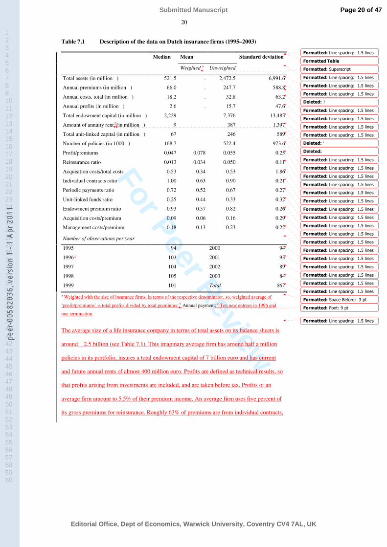
Table 7.1 Description of the data on Dutch insurance firms (1995–2003)
Median Mean Standard deviation
Weighted a Unweighted
Total assets (in million €) 521.5 . 2,472.5 6,991.6
Annual premiums (in million €) 66.0 . 247.7 588.8
Annual costs, total (in million €) 18.2 . 32.8 63.2
Annual profits (in million €) 2.6 . 15.7 47.6
Total endowment capital (in million €) 2,229 7,376 13,483
Amount of annuity rent b(in million €) 9 387 1,397
Total unit-linked capital (in million €) 67 246 589
Number of policies (in 1000 €) 168.7 522.4 973.6
Profit/premiums 0.047 0.078 0.055 0.25
Reinsurance ratio 0.013 0.034 0.050 0.11
Acquisition costs/total costs 0.53 0.34 0.53 1.86
Individual contracts ratio 1.00 0.63 0.90 0.21
Periodic payments ratio 0.72 0.52 0.67 0.27
Unit-linked funds ratio 0.25 0.44 0.33 0.32
Endowment premium ratio 0.93 0.57 0.82 0.26
Acquisition costs/premium 0.09 0.06 0.16 0.29
Management costs/premium 0.18 0.13 0.23 0.22
Number of observations per year
1995 94 2000 94
1996 c 103 2001 93
1997 104 2002 89
1998 105 2003 84
1999 101 Total 867
a Weighted with the size of insurance firms, in terms of the respective denominator, so, weighted average of
‘profit/premiums’ is total profits divided by total premiums; b Annual payment; c Ten new entrees in 1996 and
one termination.
The average size of a life insurance company in terms of total assets on its balance sheets is
around € 2.5 billion (see Table 7.1). This imaginary average firm has around half a million
policies in its portfolio, insures a total endowment capital of 7 billion euro and has current
and future annual rents of almost 400 million euro. Profits are defined as technical results, so
that profits arising from investments are included, and are taken before tax. Profits of an
average firm amount to 5.5% of their premium income. An average firm uses five percent of
its gross premiums for reinsurance. Roughly 63% of premiums are from individual contracts,
Formatted: Line spacing: 1.5 linesFormatted TableFormatted: SuperscriptFormatted: Line spacing: 1.5 linesFormatted: Line spacing: 1.5 linesFormatted: Line spacing: 1.5 lines
Formatted: Line spacing: 1.5 linesFormatted: Line spacing: 1.5 linesFormatted: Line spacing: 1.5 linesFormatted: Line spacing: 1.5 lines
Formatted: Line spacing: 1.5 linesFormatted: Line spacing: 1.5 linesFormatted: Line spacing: 1.5 linesFormatted: Line spacing: 1.5 linesFormatted: Line spacing: 1.5 linesFormatted: Line spacing: 1.5 linesFormatted: Line spacing: 1.5 linesFormatted: Line spacing: 1.5 linesFormatted: Line spacing: 1.5 linesFormatted: Line spacing: 1.5 linesFormatted: Line spacing: 1.5 linesFormatted: Line spacing: 1.5 linesFormatted: Line spacing: 1.5 linesFormatted: Line spacing: 1.5 linesFormatted: Line spacing: 1.5 linesFormatted: Line spacing: 1.5 linesFormatted: Line spacing: 1.5 linesFormatted: Space Before: 3 ptFormatted: Font: 9 pt
Formatted: Line spacing: 1.5 lines
Deleted: 7
Deleted: a
Deleted:
Page 20 of 47
Editorial Office, Dept of Economics, Warwick University, Coventry CV4 7AL, UK
Submitted Manuscript
123456789101112131415161718192021222324252627282930313233343536373839404142434445464748495051525354555657585960
peer
-005
8203
6, v
ersi
on 1
- 1
Apr 2
011
For Peer Review
21
the remainder is of a collective nature. More than half of the insurance firms have no
collective contracts at all. Two-thirds of the contracts are based on periodic payments.
Annual premiums reflect both old and new contracts. Because on average 48% of the
premiums paid are of the lump sum type, whereas, on average, 15% of the periodic
premiums refer also to new policies, the majority of the annual premiums stems from new
business. Note that cost and profit figures are also based on a mixture of new and old
business. Balance-sheet and profit and loss data for new policies only is not available. So
called unit-linked fund policies, where policyholders bear the investment risk on their own
deposits (that is, premiums minus costs), have become more popular: 44% of premiums are
related to this kind of policies. Endowment insurance is the major product category, as 57%
of all premiums are collected for this type of insurance. This type of insurance policy is often
combined with a mortgage loan. The total costs are around 13% of the total premium
income, half of which consists of acquisition (or sales) costs. The medians and the
differences between weighted and unweighted averages reflect skewness in the (size)
distributions. Larger firms tend to have higher profit margins and relatively lower acquisition
cost, lower management cost, fewer individual contracts, fewer periodic payments, more
unit-linked funds policies and fewer endowment policies.
8. Empirical results
8.1 Scale economies
This section estimates scale economies using the translog cost function (TCF). In a later
section of this article, the TCF is used also to calculate marginal costs (see Sections 4 and
8.4). For these two purposes, the TCF explains the insurance company’s cost by (only) one
measure of production, namely premiums. As both scale effects and marginal costs are
obtained from the first derivatives of the TCF to production, we will disregard other
production measures here. Generally, inclusion of more measures of components of
Deleted: paper
Page 21 of 47
Editorial Office, Dept of Economics, Warwick University, Coventry CV4 7AL, UK
Submitted Manuscript
123456789101112131415161718192021222324252627282930313233343536373839404142434445464748495051525354555657585960
peer
-005
8203
6, v
ersi
on 1
- 1
Apr 2
011

For Peer Review
22
production or proxies is common practice in the case of multi-product firms, and has indeed
been applied in the X-efficiency models in Sections 8.2 and 8.3.
In the literature, measuring output in the life insurance industry is much debated.
Where in many other industries, output is equal to the value added, we can not calculate this
figure for insurers, due to conceptual problems.25 Most studies on the life insurance industry
use premium income as output measure. Hirschhorn and Geehan (1977) view the
production of contracts as the main activity of a life insurance company. Premiums collected
directly concern the technical activity of an insurance company. The ability of an insurance
company to market products, to select clients and to accept risks are reflected by premiums.
However, premiums do not reflect financial activities properly, as e.g. asset management
represented by the returns on investment is ignored.26 Despite shortcomings, in this section
we also use premium income as the output measure.
As our model reads in logarithms, we can not use observations where one or more of
the variables have a zero or negative value. Insurance firms may employ various sales
channels: own sales organizations, tied and multiple insurance agencies, and other channels,
such as banks, post offices, etc. We have to drop observations of firms that do not use
insurance agencies and report zero acquisition costs. In this sense, we clearly are left with a
subsample of firms.
Table 8.1 presents the TCF estimates. We assume that costs are explained by
production (in terms of total premiums), reinsurance and acquisition (proxies of prices of
reinsurance and acquisition fees 27), so that these variables also emerge as squares and in
cross-terms. To test this basic model for robustness, we also add four control variables in an
extended version of the model. Periodic premium policies go with additional administration
25 Some insurance firms can approximate their value added by comparing their embedded value over
time. These data are not publicly available.26 The definition of production of life insurance firms is discussed further in Section 8.2.27 The price of management, or wages, has been excluded by applying the two standard properties of
cost functions, namely linear homogeneity in the input prices and cost-exhaustion (Jorgenson, 1986).
Deleted: ance
Deleted: use
Page 22 of 47
Editorial Office, Dept of Economics, Warwick University, Coventry CV4 7AL, UK
Submitted Manuscript
123456789101112131415161718192021222324252627282930313233343536373839404142434445464748495051525354555657585960
peer
-005
8203
6, v
ersi
on 1
- 1
Apr 2
011
For Peer Review
23
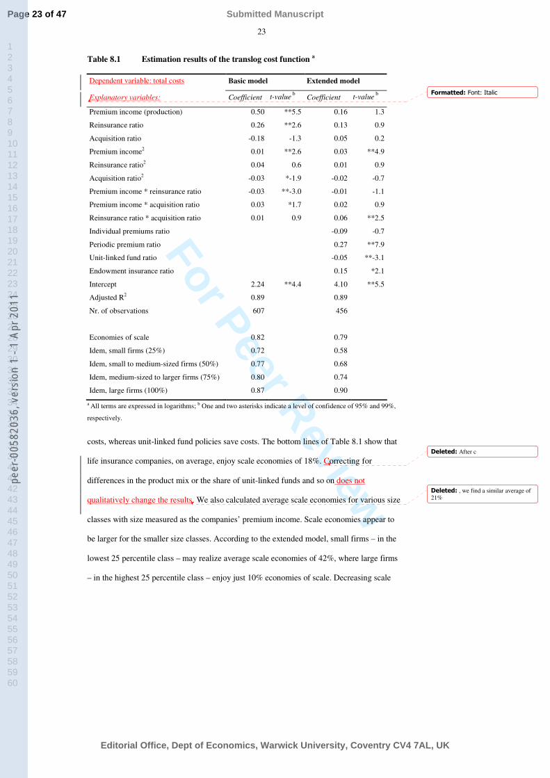
Table 8.1 Estimation results of the translog cost function a
Dependent variable: total costs Basic model Extended model
Explanatory variables: Coefficient t-value bCoefficient t-value b
Premium income (production) 0.50 **5.5 0.16 1.3
Reinsurance ratio 0.26 **2.6 0.13 0.9
Acquisition ratio -0.18 -1.3 0.05 0.2
Premium income2 0.01 **2.6 0.03 **4.9
Reinsurance ratio2 0.04 0.6 0.01 0.9
Acquisition ratio2 -0.03 *-1.9 -0.02 -0.7
Premium income * reinsurance ratio -0.03 **-3.0 -0.01 -1.1
Premium income * acquisition ratio 0.03 *1.7 0.02 0.9
Reinsurance ratio * acquisition ratio 0.01 0.9 0.06 **2.5
Individual premiums ratio -0.09 -0.7
Periodic premium ratio 0.27 **7.9
Unit-linked fund ratio -0.05 **-3.1
Endowment insurance ratio 0.15 *2.1
Intercept 2.24 **4.4 4.10 **5.5
Adjusted R2 0.89 0.89
Nr. of observations 607 456
Economies of scale 0.82 0.79
Idem, small firms (25%) 0.72 0.58
Idem, small to medium-sized firms (50%) 0.77 0.68
Idem, medium-sized to larger firms (75%) 0.80 0.74
Idem, large firms (100%) 0.87 0.90
a All terms are expressed in logarithms; b One and two asterisks indicate a level of confidence of 95% and 99%,
respectively.
costs, whereas unit-linked fund policies save costs. The bottom lines of Table 8.1 show that
life insurance companies, on average, enjoy scale economies of 18%. Correcting for
differences in the product mix or the share of unit-linked funds and so on does not
qualitatively change the results. We also calculated average scale economies for various size
classes with size measured as the companies’ premium income. Scale economies appear to
be larger for the smaller size classes. According to the extended model, small firms – in the
lowest 25 percentile class – may realize average scale economies of 42%, where large firms
– in the highest 25 percentile class – enjoy just 10% economies of scale. Decreasing scale
Formatted: Font: Italic
Deleted: After c
Deleted: , we find a similar average of 21%
Page 23 of 47
Editorial Office, Dept of Economics, Warwick University, Coventry CV4 7AL, UK
Submitted Manuscript
123456789101112131415161718192021222324252627282930313233343536373839404142434445464748495051525354555657585960
peer
-005
8203
6, v
ersi
on 1
- 1
Apr 2
011

For Peer Review
24
economies with firm size have also been found by Fecher et al. (1993) for the French life
insurance industry. The comparison between the basic model and the extended model makes
clear that the average scale economies per size class differ (only) slightly on the model
specification. Although the average economies of scale for both models are rather similar,
the dependency of the scale economies on size classes in the basic model is less than in the
extended model.
The optimal production volume in terms of gross premium is defined as the volume
where an additional increase would no longer diminish marginal costs, so that the derivative
of marginal costs is zero. According to the basic model, the optimal size can be calculated as
far above the size of all actual life insurance firms.28 This implies that (almost) all firms are
in the (upper) left-hand part of the well-known U-shaped average cost curve. The scale
economies suggest that consolidation in the Dutch insurance markets is still far from its
optimal level, but, of course, diseconomies of conglomeration and mistakes in post-merger
integration can outweigh scale economies.
The TCF estimates make clear that average scale economies of around 20% are an
important feature of the Dutch life insurance industry. These scale economies are generally
higher than those found for banks in the Netherlands (e.g. Bos and Kolari, 2005) and
elsewhere (e.g. Berger et al., 1993), but not uncommon in other sectors. Similar figures were
found in other countries. Fecher et al. (1991) find 15% for France and Grace and Timme
(1992) observe 4% to 27% for the US, depending on type and size of firm. The existence of
substantial scale economies might indicate a moderate degree of competition, as firms have
so far not been forced to employ all possible scale economies.
8.2 Cost X-inefficiency
In this section we apply the stochastic cost frontier model (5.1) to data of Dutch insurance
firms. Costs are defined as total operating expenses which consist of two components,
28 Of course, the accuracy of this optimal size is limited, as its calculated location lies far out of our
sample range.
Deleted: depend
Deleted: This suggests
Deleted: Dutch
Deleted: TDeleted: ies
Page 24 of 47
Editorial Office, Dept of Economics, Warwick University, Coventry CV4 7AL, UK
Submitted Manuscript
123456789101112131415161718192021222324252627282930313233343536373839404142434445464748495051525354555657585960
peer
-005
8203
6, v
ersi
on 1
- 1
Apr 2
011

For Peer Review
25
acquisition cost and other costs. The latter includes management costs, salaries, depreciation
on capital equipment, and so on. A further split of ‘other cost’ in its constituent components
would be highly welcome, but is regrettably unavailable. The price of the two input factors,
acquisition costs and other costs, has been estimated as the ratio of the respective costs and
the total assets. Such a proxy is fairly common in the efficiency model literature, in the
absence of a better alternative.
As said, the definition of production of life insurance firms is a complicated issue.
Insurance firms produce a bundle of services to their policy holders. Particularly for life
insurances, services may be provided over a long period. Given the available data, we have
selected the following five proxies of services to policyholders, together constituting the
multiple products of insurance firms: (1) annual premium income. This variable proxies the
production related to new and current policies. A drawback of this variable might be that
premiums are made up of the pure cost price plus a profit margin. But it is the only available
measure of new policies; (2) the total number of outstanding policies. This variable
approximates the services provided under all existing policies, hence the stock instead of the
flow. In particular, it reflects services supplied in respect of all policies, irrespective of their
size; (3) the sum total of insured capital; (4) the sum total of insured annuities. Endowment
insurances and annuity policies are different products. The two variables reflect the different
services which are provided to the respective groups of policy holders; and (5) unit-linked
funds policies. There are two types of policies regarding the risk on the investments
concerned. These risks may be born by the insurance firms or by the policy holders. The
latter type of policies are also known as ‘unit-linked’. As the insurance firm provides
different services in respect of these two types of policy, we include the variable ‘unit-linked
funds policies’. Note that these five production factors do not describe the production of
separate services, but aspects of the production. For example, a unit linked policy may be of
either of an endowment insurance type or an annuity type, so that two variables describe four
different types of services.
Page 25 of 47
Editorial Office, Dept of Economics, Warwick University, Coventry CV4 7AL, UK
Submitted Manuscript
123456789101112131415161718192021222324252627282930313233343536373839404142434445464748495051525354555657585960
peer
-005
8203
6, v
ersi
on 1
- 1
Apr 2
011

For Peer Review
26
The five production measures and the two input prices also appear as squares and
cross-terms in the translog cost function, making for a total of 35 explanatory variables. Such
models have proven to provide a close approximation to the complex multiproduct output of
financial institutions, resulting in an adequate explanation of cost, conditional on production
volume and input factor prices. In our sample, this model explains 94.0% of the variation in
the (logarithm of) cost.29
The set of suitable (non-zero) data consists of 105 licensed life insurance firms in the
Netherlands over the 1995–2003 period, providing a total of 689 firm-year observations.
This panel dataset includes new entries, taken-over firms and merged companies and, hence,
is unbalanced.
Table A.1 in Appendix I provides the full set of estimation results (see cost column).
Due to the non-linear nature of the TCF it is difficult to interpret the coefficients of the
individual explanatory variables. As indicated by γ, 91% of the variation in the stochastic
terms (σ2) of the cost model is attributed to the inefficiency term. A test on the hypothesis
that inefficiency can be ignored (γ= 0) is rejected strongly. The essential results are the cost
efficiency values calculated according to Equation (5.2). Table 8.2 provides average values
of cost X-efficiency per year and for the total sample (see cost column).
Table 8.2 Average cost X-efficiency in 1995-2003
Year Cost X-efficiency Year Cost X-efficiency
1995 0.716 2000 0.710
1996 0.727 2001 0.729
1997 0.741 2002 0.728
1998 0.724 2003 0.718
1999 0.725 Total 0.724
The average cost X-efficiency is 72%, so that the inefficiency is, on average, 28%. That
implies that costs are, on average, 28% higher than for the best practice firms, conditional on
29 This figure is based on the OLS estimates, which provides the starting values of the numerical
optimisation procedure. As OLS minimizes the errors terms and maximises the degree of fit, the latter
will be lower in the SCF model.
Formatted: Font: BoldFormatted Table
Formatted: Line spacing: 1.5 lines
Formatted: Line spacing: 1.5 linesFormatted: Line spacing: 1.5 linesFormatted: Line spacing: 1.5 linesFormatted: Line spacing: 1.5 linesFormatted: Line spacing: 1.5 linesFormatted: Line spacing: 1.5 linesFormatted: Line spacing: 1.5 lines
Formatted: Line spacing: 1.5 lines
Formatted: Line spacing: 1.5 linesFormatted: Line spacing: 1.5 lines
Deleted: . The dataset
Deleted: as 256 observations are missing or incomplete
Deleted: The average cost X-efficiency is 72%, so that the inefficiencyis, on average, 28%. That implies that costs are, on average, 28% higher than for the best practice firms, conditional on production composition, production scale and input prices. The average cost X-efficiencies fluctuate irregularly over time, so that apparently no clear time trends emerge. The inefficiencies are assumed to reflect managerial shortcomings in making optimal decisions in the composition of output and the use of input factors. A possible reduction of cost by at least one quarter does not seem plausible in a competitive market. However, it should be remembered that these inefficiency figures set an upper bound to the measured inefficiencies, because they may partly be the result of imperfect measurements of production and input factor prices. Particularly in the financial sector, production is difficult to measure, while our data set also suffers from none-too-exact information on input prices. Instead of drawing very strong conclusions regarding competition, it is better to compare 
Deleted: 2000 ... [1]
Page 26 of 47
Editorial Office, Dept of Economics, Warwick University, Coventry CV4 7AL, UK
Submitted Manuscript
123456789101112131415161718192021222324252627282930313233343536373839404142434445464748495051525354555657585960
peer
-005
8203
6, v
ersi
on 1
- 1
Apr 2
011
For Peer Review
27
production composition, production scale and input prices. The average cost X-efficiencies
fluctuate irregularly over time, so that apparently no clear time trends emerge. The
inefficiencies are assumed to reflect managerial shortcomings in making optimal decisions in
the composition of output factors and the use of input factors. A possible reduction of cost by
at least one quarter does not seem plausible in a competitive market. However, it should be
remembered that these inefficiency figures set an upper bound to the measured
inefficiencies, as they may partly be the result of imperfect measurements of production and
input factor prices. Particularly in services, such as in the financial sector, production is
difficult to measure, while our data set also suffers from none-too-exact information on input
prices. Instead of drawing very strong conclusions regarding competition, it is better to
compare these results with benchmarks. Any comparison should be handled with caution, as
estimation results are generally based on varying estimation techniques, different insurance
production models and diverging empirical specifications. In the literature, the insurance
inefficiency figures in other countries range from 10% to 65%. This implies that our
inefficiencies are quite common and even relatively low. They are similar to the
inefficiencies that have generally been found in the banking literature which spread – widely
– around 20% (Berger and Humphrey, 1997; Altunbas et al., 2000, Hauner, 2005, Kasman
and Yildirim, 2006). Bikker (2004, page 218) reports an average X-inefficiency for Dutch
banks in 1997 of 26%, remarkably similar to the figure for insurance firms.
Table 8.3 Average cost X-efficiency over size classes
Size class Cost Average size
(× € 1000)
Size class Cost Average size
(× € 1000)
1 0.747 13,261 6 0.701 2,107,749
2 0.763 94,904 7 0.742 14,479,608
3 0.731 277,937 Total average 0.724 2,447,891
4 0.693 548,474 Median 519,970
5 0.696 936,795
Formatted Table
Formatted: LeftFormatted: LeftFormatted: LeftFormatted: Left
Formatted Table
Deleted: lie earlier towards the
Deleted: er end
Deleted:
Deleted:
Deleted: 5
Deleted: Median
Deleted: 519,970
... [2]
Page 27 of 47
Editorial Office, Dept of Economics, Warwick University, Coventry CV4 7AL, UK
Submitted Manuscript
123456789101112131415161718192021222324252627282930313233343536373839404142434445464748495051525354555657585960
peer
-005
8203
6, v
ersi
on 1
- 1
Apr 2
011

For Peer Review
28
Table 8.3 shows average cost X-efficiency for seven size classes. Here we observe a clear U-
curve for cost efficiency: higher efficiency for small insurance firms, lower efficiency for
medium-sized companies and, again, increasing efficiency for larger firms. A possible
explanation could be that smaller firms generally profit from their orderly structure and
neatly arranged composition of products, so that differences in managerial inability across
smaller firms are limited (as has also been found for banks, see Bikker, 2004, page 209 ff. ).
The largest firms operate more on competitive submarkets such as pensions and on the more
competitive international markets, which have forced them to become more efficient.
8.4 Profitability
A straightforward measure of competition is the profit margin. Supernormal profits would
indicate insufficient competition. A traditional measure of profitability is the price-cost
margin.30 We cannot calculate the price-cost margin for life insurance companies, as we do
not know the output prices and market shares of all insurance products per firm. However,
we are able to calculate the average profit margin, defined as the ratio of profits before taxes
and gross premium written. Using figures on consolidated life insurance firms from the ISIS
dataset, we compare the Netherlands with some major European economies (see Table
8.4).31 We are aware that profits could be influenced by differences in accounting rules,
products, distribution channels, maturity or other characteristics of the markets.32 However,
we draw some conclusions from the remarkable profit margins in the Netherlands (around
9%) compared to those in other EU countries like France, Germany, Italy and the UK, with
respective profit margins of around 7%, 2%, 5% and 4%. The higher profits in the
30 This measure can be defined as ∑= =ni iiii )/pmc-(psPCM 1 where pi denotes the firm’s
equilibrium output price and mci its marginal cost.31 ISIS data concern both domestic and foreign activities. Pure domestic figures would be more
precise but are not available.32 For instance, firms in the Netherlands use more agents as selling channel than those in other
countries (CEDA, 2004, page 144).
Page 28 of 47
Editorial Office, Dept of Economics, Warwick University, Coventry CV4 7AL, UK
Submitted Manuscript
123456789101112131415161718192021222324252627282930313233343536373839404142434445464748495051525354555657585960
peer
-005
8203
6, v
ersi
on 1
- 1
Apr 2
011
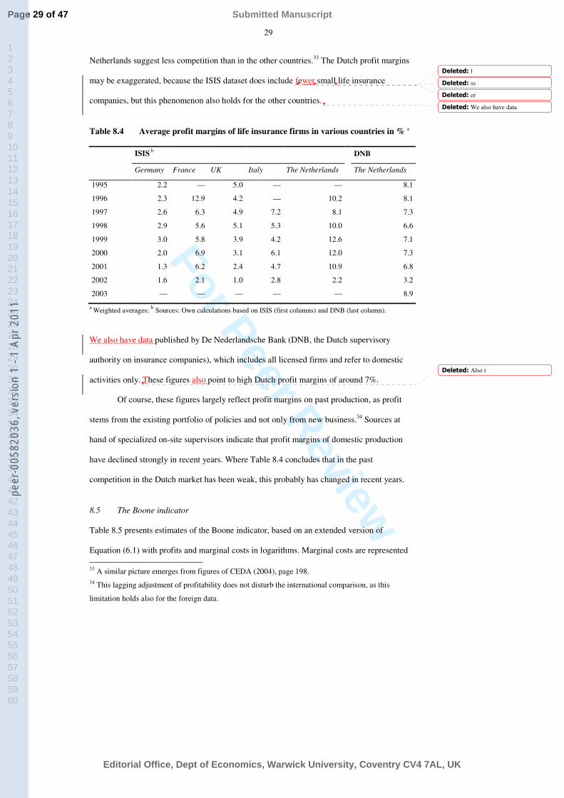
For Peer Review
29
Netherlands suggest less competition than in the other countries.33 The Dutch profit margins
may be exaggerated, because the ISIS dataset does include fewer small life insurance
companies, but this phenomenon also holds for the other countries.
Table 8.4 Average profit margins of life insurance firms in various countries in % a
ISIS b DNB
Germany France UK Italy The Netherlands The Netherlands
1995 2.2 — 5.0 — — 8.1
1996 2.3 12.9 4.2 — 10.2 8.1
1997 2.6 6.3 4.9 7.2 8.1 7.3
1998 2.9 5.6 5.1 5.3 10.0 6.6
1999 3.0 5.8 3.9 4.2 12.6 7.1
2000 2.0 6.9 3.1 6.1 12.0 7.3
2001 1.3 6.2 2.4 4.7 10.9 6.8
2002 1.6 2.1 1.0 2.8 2.2 3.2
2003 — — — — — 8.9
a Weighted averages; b Sources: Own calculations based on ISIS (first columns) and DNB (last column).
We also have data published by De Nederlandsche Bank (DNB, the Dutch supervisory
authority on insurance companies), which includes all licensed firms and refer to domestic
activities only. These figures also point to high Dutch profit margins of around 7%.
Of course, these figures largely reflect profit margins on past production, as profit
stems from the existing portfolio of policies and not only from new business.34 Sources at
hand of specialized on-site supervisors indicate that profit margins of domestic production
have declined strongly in recent years. Where Table 8.4 concludes that in the past
competition in the Dutch market has been weak, this probably has changed in recent years.
8.5 The Boone indicator
Table 8.5 presents estimates of the Boone indicator, based on an extended version of
Equation (6.1) with profits and marginal costs in logarithms. Marginal costs are represented
33 A similar picture emerges from figures of CEDA (2004), page 198.34 This lagging adjustment of profitability does not disturb the international comparison, as this
limitation holds also for the foreign data.
Deleted: lDeleted: ss
Deleted: er
Deleted: We also have data
Deleted: Also t
Page 29 of 47
Editorial Office, Dept of Economics, Warwick University, Coventry CV4 7AL, UK
Submitted Manuscript
123456789101112131415161718192021222324252627282930313233343536373839404142434445464748495051525354555657585960
peer
-005
8203
6, v
ersi
on 1
- 1
Apr 2
011

For Peer Review
30
in three ways: average variable cost, defined as management costs as share of the total
premium as in the traditional Boone model (see e.g. Boone, 2004; Creusen et.al., 2004),
marginal cost, derived from the translog cost function of Section 8.1, and adjusted marginal
costs, i.e. marginal costs adjusted for scale economies (see Appendix II).35 Average variable
costs have the advantage of being less complex, since they are not model based, but they are
less accurate because we can not distinguish between variable and fixed costs. In practice,
average variable costs are commonly proxied by average costs. We prefer the marginal cost
derived from a translog cost function, as this is the most accurate measure. Adjusted
marginal costs allow one to distinguish between the effects of two components of marginal
cost, namely scale economies and X-efficiency.
Table 8.5 Fixed effects estimates of the Boone model for profits a
Average variable cost Marginal cost
Adjusted marginal cost b
Coefficient t-value c Coefficient t-value c Coefficient t-value c
Resp. average variable and marginal cost, in 1995 (β) -0.52 **-2.7 -0.53 **-2.5 -0.32 -1.4Idem, 1996 -0.42 *-2.2 -0.38 *-1.8 -0.20 -0.9Idem, 1997 -0.43 *-2.0 -0.32 -1.3 -0.05 -0.2Idem, 1998 -0.69 **-3.2 -0.70 **-2.9 -0.23 -0.9Idem, 1999 -0.34 *-1.7 -0.35 -1.5 -0.08 -0.3Idem, 2000 -0.43 *-2.1 -0.38 -1.5 -0.10 -0.4Idem, 2001 -0.55 **-2.7 -0.42 *-1.7 -0.15 -0.6Idem, 2002 -0.17 -0.9 0.14 -0.5 0.39 1.3Idem, 2003 -0.37 *-1.7 -0.18 -0.7 0.35 1.2Individual premiums ratio 1.71 **3.0 1.46 **2.4 1.42 *2.3Periodic payments ratio 0.34 0.9 0.26 0.6 0.14 0.4Unit-linked funds ratio 0.22 0.6 0.34 0.8 0.34 0.8Endowment insurance ratio -0.27 -0.4 -0.25 -0.3 -0.52 -0.7Intercept 6.76 **8.1 7.48 **7.4 8.15 **11.5σu 2.01 1.97 0.25σe 0.66 0.67 0.11ρ 0.90 0.89 0.84Overall R2 0.01 0.01 0.00Within/between R2 0.26 0.04 0.28 0.04 0.26 0.08Nr. of observations (groups) 500 (89) 444 (85) 444 (85)
aProfits and marginal costs are in logarithms;
b Adjusted for scale economies;
c One and two asterisks indicate a
level of confidence of 95% and 99%, respectively.
35 Note that the variable cost may change over the size classes due to scale efficiency (just as the
marginal cost may do), so that the average variable cost may differ from the marginal cost. Apart
from this theoretical dissimilarity, these variables are also measured differently in practice.
Formatted: Space Before: 1 pt,After: 0 pt, Line spacing: At least12 ptFormatted: Line spacing: At least12 ptFormatted: Line spacing: At least12 ptFormatted: Line spacing: At least12 ptFormatted: Line spacing: At least12 ptFormatted: Line spacing: At least12 ptFormatted: Line spacing: At least12 ptFormatted: Line spacing: At least12 ptFormatted: Line spacing: At least12 ptFormatted: Line spacing: At least12 ptFormatted: Line spacing: At least12 ptFormatted: Line spacing: At least12 ptFormatted: Line spacing: At least12 ptFormatted: Line spacing: At least12 ptFormatted: Line spacing: At least12 ptFormatted: Line spacing: At least12 ptFormatted: Line spacing: At least12 ptFormatted: Line spacing: At least12 ptFormatted: Line spacing: At least12 ptFormatted: Line spacing: At least12 ptFormatted: Line spacing: At least12 ptFormatted: Line spacing: At least12 pt
Deleted: Following Boone (2004) and Creusen et al. (2004), we also introduce so-called fixed effects, that is, a dummy variable for each insurance firm (coefficients of these dummies are not reported here). The advantage is that these fixed effects pick up all company-specific characteristics, including scale, that are not captured by the other variables, so that part of the disturbances is eliminated. Around 10% of thevariance in the error term of the model 
Page 30 of 47
Editorial Office, Dept of Economics, Warwick University, Coventry CV4 7AL, UK
Submitted Manuscript
123456789101112131415161718192021222324252627282930313233343536373839404142434445464748495051525354555657585960
peer
-005
8203
6, v
ersi
on 1
- 1
Apr 2
011

For Peer Review
31
Following Boone (2004) and Creusen et al. (2004), we also introduce so-called fixed effects,
that is, a dummy variable for each insurance firm (coefficients of these dummies are not
reported here).36 The advantage is that these fixed effects pick up all company-specific
characteristics, including scale, that are not captured by the other variables, so that part of
the disturbances is eliminated. Around 10% of the variance in the error term of the model
without fixed effects (unexplained variance: σu2) can be explained by these fixed effects
(explained variance: σe2) when they are introduced, where ρ is equal to σu
2/(σu2
+ σe2). With
respect to the control variables, we find a systematic, significantly positive contribution of
individual policyholders to profits. The other control variables, policyholders with periodic
payments, unit-linked fund policies and endowment insurances, do not affect profits.
As indicators of competition, the annual estimates of beta are, of course, pivotal in
the analysis. The first two columns of Table 8.5 present estimates of beta based on average
variable costs, which range from -0.2 to -0.7 and are significant in all years but one. The
model-based marginal costs estimates are slightly higher and only significant in four out of
nine years. Although the level of the indicator is difficult to interpret, its low degree of
significance suggests moderate competition. When marginal costs are adjusted for scale
economies, none of the betas are significant. This indicates that scale economies are an
important component of the observed Boone indicator. Figure 8.1 shows that the coefficient
β fluctuates somewhat over time in all three model versions. We observe an upward trend,
indicating a (slight) decline in competition over the respective years. Average variable costs
and model-based marginal costs result into similar estimates. The third measure of marginal
cost renders a comparable pattern over time, but – due to the eliminated scale economies – at
a higher level.
36 We have also estimated random effect models for profits (Table 8.5) and markets shares (Table 8.6). Their coefficients were quite similar to those of the fixed effect models, with even slightly higher values and higher levels of significance. This suggests that the estimates presented in Tables 8.5 and 8.6 are quite robust. We tested for random effect using the Hausman test, but this test appeared to be undefined, suffering from the ‘small sample problem’. All models include year dummies, also not shown in the tables.
Page 31 of 47
Editorial Office, Dept of Economics, Warwick University, Coventry CV4 7AL, UK
Submitted Manuscript
123456789101112131415161718192021222324252627282930313233343536373839404142434445464748495051525354555657585960
peer
-005
8203
6, v
ersi
on 1
- 1
Apr 2
011

For Peer Review
32
In order to assess whether our estimates for the Boone indicator are high or low, we
compare them with estimates for other Dutch industries. Creusen et al. (2005) estimated the
traditional Boone model for the manufacturing and service industries and found elasticities
between average variable costs and profits of around, respectively, -5.7 and -2.5, for the
years 1993-2001. The Boone indicator of the life insurance industry is around -0.45. As
noted in section 6, comparisons of the Boone indicator across sectors are problematic due to
measurement error, for example due to differences in accounting practises of profits and
losses. However, the absolute value of the Boone indicator of insurances appears to be much
lower (closer to zero) than in other service industries. Moreover, estimations using exactly
the same definition for profit as in Creusen et al. (2005) render the same conclusion.37 All in
all, this implies that the life insurance industry is less competitive than the manufacturing
and service industries.
Figure 8.1 Effect on profits of average variable costs and (adjusted) marginal costs
-0.8
-0.6
-0.4
-0.2
0
0.2
0.4
0.6
1995 1996 1997 1998 1999 2000 2001 2002 2003
Ela
stic
ity
Average variable cost
Marginal cost
Adjusted marginal cost
Due to the logarithmic specification of the Boone model, all loss-making firms, including
new entrants, have been ignored. This creates a potential bias because 20% of our
37 The value of the Boone-indicator in these estimations is around -0.85. Results can be obtained from
the authors.
Deleted: becomes for
Deleted: of
Page 32 of 47
Editorial Office, Dept of Economics, Warwick University, Coventry CV4 7AL, UK
Submitted Manuscript
123456789101112131415161718192021222324252627282930313233343536373839404142434445464748495051525354555657585960
peer
-005
8203
6, v
ersi
on 1
- 1
Apr 2
011

For Peer Review
33
observations concerned loss-making companies. Estimations of the Boone indicator in a
model with ratios instead of logarithms using the full sample results in a significant more
negative relationship between efficiency and profits. Solving this bias would at most add -0.5
to the Boone indicator. The conclusion remains that the Boone-indicator is substantially
smaller in the life insurance industry than in other service industries. Furthermore, the Boone
indicator is subject to the same deficiencies as the profit margin in Section 8.4, as it is based
on profitability of past business instead of only new production. The next section solves
these issues by analysing another performance indicator: market shares. Note that similarly
to the description above for profits, market shares will react stronger on marginal costs, the
more competitive the market is. Market shares are based on annual premiums and a
significant part, 55% of these premiums, are due to new policies. Therefore, market shares
reflect largely the current business. Furthermore, using market shares, we can utilize
information of the full sample, loss-making firms included.
8.6 Sensitivity analysis: the Boone indicator based on markets shares
Although the indicator as originally formulated by Boone is based on relative profits, the
idea behind it – namely that competition rewards efficiency – implies that we could also use
the intermediate magnitude relative market shares as our outcome variable. Therefore, as a
check on the findings in the previous section, this section presents estimation results based
on markets shares. Results are shown in Table 8.6. We find that average variable costs
appear to have a significantly negative effect on market shares, see the first two columns. An
increase of this marginal cost measure by one percent results in a market share loss of around
0.45%. Note that this value is similar to the Boone indicator based on profits in Section 8.5.
If we consider changes in β1 over time, we observe larger negative values in the
years just before the major fiscal policy change-over of 2001 with respect to annuities, as
described in Section 2 (see also Figure 8.2). This indicates that competition has intensified
somewhat in these years, probably with respect to annuities, which is in line which the
Deleted: , as appears from estimations not presented here
Deleted: as
Deleted: bed
Deleted: with
Page 33 of 47
Editorial Office, Dept of Economics, Warwick University, Coventry CV4 7AL, UK
Submitted Manuscript
123456789101112131415161718192021222324252627282930313233343536373839404142434445464748495051525354555657585960
peer
-005
8203
6, v
ersi
on 1
- 1
Apr 2
011
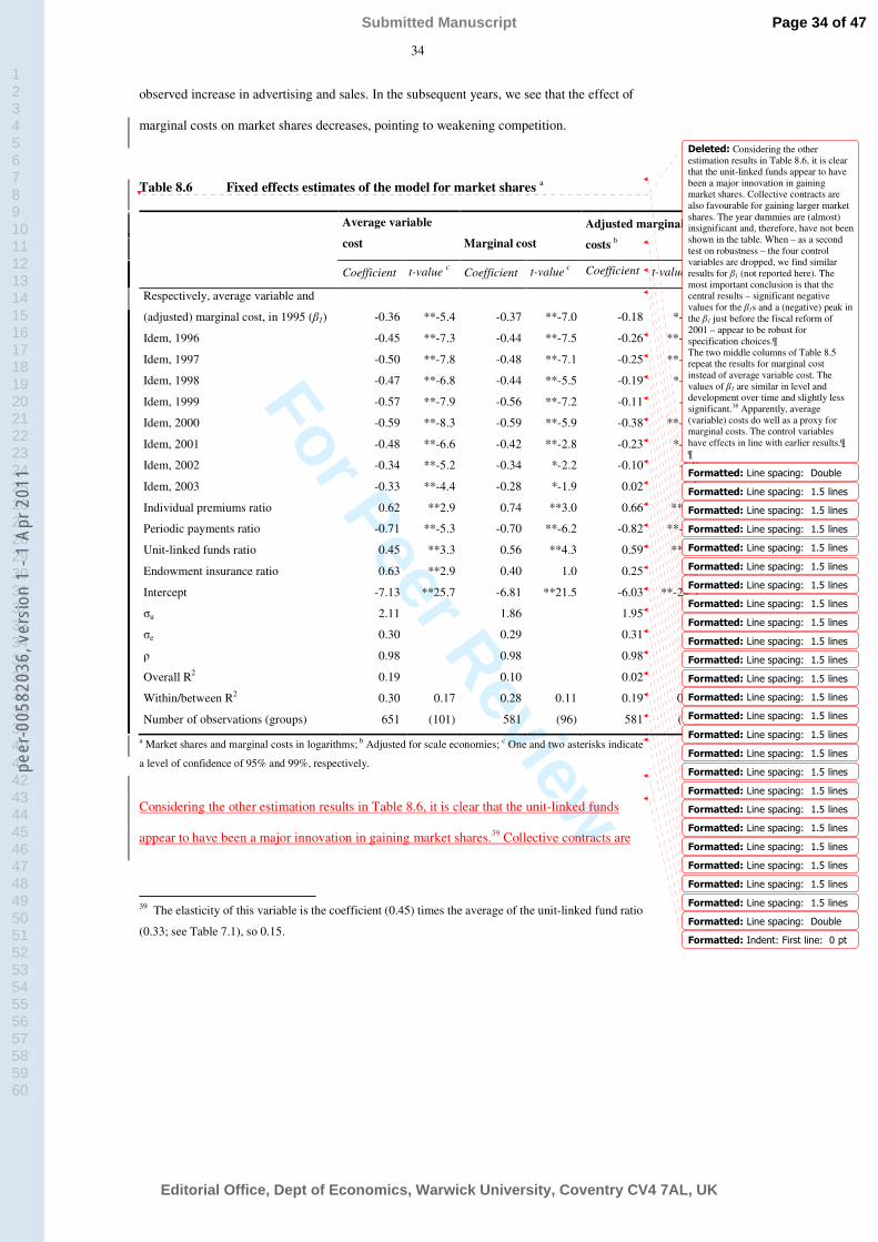
For Peer Review
34
observed increase in advertising and sales. In the subsequent years, we see that the effect of
marginal costs on market shares decreases, pointing to weakening competition.
Table 8.6 Fixed effects estimates of the model for market shares a
Average variable
cost Marginal cost
Adjusted marginal
costs b
Coefficient t-value cCoefficient t-value c Coefficient t-value c
Respectively, average variable and
(adjusted) marginal cost, in 1995 (β1) -0.36 **-5.4 -0.37 **-7.0 -0.18 *-2.2
Idem, 1996 -0.45 **-7.3 -0.44 **-7.5 -0.26 **-3.4
Idem, 1997 -0.50 **-7.8 -0.48 **-7.1 -0.25 **-3.1
Idem, 1998 -0.47 **-6.8 -0.44 **-5.5 -0.19 *-2.1
Idem, 1999 -0.57 **-7.9 -0.56 **-7.2 -0.11 -1.1
Idem, 2000 -0.59 **-8.3 -0.59 **-5.9 -0.38 **-4.1
Idem, 2001 -0.48 **-6.6 -0.42 **-2.8 -0.23 *-2.3
Idem, 2002 -0.34 **-5.2 -0.34 *-2.2 -0.10 -1.0
Idem, 2003 -0.33 **-4.4 -0.28 *-1.9 0.02 0.2
Individual premiums ratio 0.62 **2.9 0.74 **3.0 0.66 **2.8
Periodic payments ratio -0.71 **-5.3 -0.70 **-6.2 -0.82 **-5.7
Unit-linked funds ratio 0.45 **3.3 0.56 **4.3 0.59 **4.0
Endowment insurance ratio 0.63 **2.9 0.40 1.0 0.25 1.0
Intercept -7.13 **25.7 -6.81 **21.5 -6.03 **-24.5
σu 2.11 1.86 1.95
σe 0.30 0.29 0.31
ρ 0.98 0.98 0.98
Overall R2 0.19 0.10 0.02
Within/between R2 0.30 0.17 0.28 0.11 0.19 0.01
Number of observations (groups) 651 (101) 581 (96) 581 (96)
a Market shares and marginal costs in logarithms; b Adjusted for scale economies; c One and two asterisks indicate
a level of confidence of 95% and 99%, respectively.
Considering the other estimation results in Table 8.6, it is clear that the unit-linked funds
appear to have been a major innovation in gaining market shares.39 Collective contracts are
39 The elasticity of this variable is the coefficient (0.45) times the average of the unit-linked fund ratio
(0.33; see Table 7.1), so 0.15.
Formatted: Line spacing: DoubleFormatted: Line spacing: 1.5 linesFormatted: Line spacing: 1.5 linesFormatted: Line spacing: 1.5 linesFormatted: Line spacing: 1.5 linesFormatted: Line spacing: 1.5 linesFormatted: Line spacing: 1.5 linesFormatted: Line spacing: 1.5 linesFormatted: Line spacing: 1.5 linesFormatted: Line spacing: 1.5 linesFormatted: Line spacing: 1.5 linesFormatted: Line spacing: 1.5 linesFormatted: Line spacing: 1.5 linesFormatted: Line spacing: 1.5 linesFormatted: Line spacing: 1.5 linesFormatted: Line spacing: 1.5 linesFormatted: Line spacing: 1.5 linesFormatted: Line spacing: 1.5 linesFormatted: Line spacing: 1.5 linesFormatted: Line spacing: 1.5 linesFormatted: Line spacing: 1.5 linesFormatted: Line spacing: 1.5 linesFormatted: Line spacing: 1.5 linesFormatted: Line spacing: 1.5 linesFormatted: Line spacing: DoubleFormatted: Indent: First line: 0 pt
Deleted: Considering the other estimation results in Table 8.6, it is clear that the unit-linked funds appear to have been a major innovation in gaining market shares. Collective contracts are also favourable for gaining larger market shares. The year dummies are (almost) insignificant and, therefore, have not been shown in the table. When – as a second test on robustness – the four control variables are dropped, we find similar results for β1 (not reported here). The most important conclusion is that the central results – significant negative values for the β1s and a (negative) peak in the β1 just before the fiscal reform of 2001 – appear to be robust for specification choices.¶The two middle columns of Table 8.5 repeat the results for marginal cost instead of average variable cost. The values of β1 are similar in level and development over time and slightly less significant.38 Apparently, average (variable) costs do well as a proxy for marginal costs. The control variables have effects in line with earlier results.¶¶
Page 34 of 47
Editorial Office, Dept of Economics, Warwick University, Coventry CV4 7AL, UK
Submitted Manuscript
123456789101112131415161718192021222324252627282930313233343536373839404142434445464748495051525354555657585960
peer
-005
8203
6, v
ersi
on 1
- 1
Apr 2
011

For Peer Review
35
also favourable for gaining larger market shares. The year dummies are (almost)
insignificant and, therefore, have not been shown in the table. When – as a second test on
robustness – the four control variables are dropped, we find similar results for β1 (not
reported here). The most important conclusion is that the central results – significant
negative values for the β1s and a (negative) peak in the β1 just before the fiscal reform of
2001 – appear to be robust for specification choices.
The two middle columns of Table 8.5 repeat the results for marginal cost instead of
average variable cost. The values of β1 are similar in level and development over time and
slightly less significant.40 Apparently, average (variable) costs do well as a proxy for
marginal costs. The control variables have effects in line with earlier results.
Although the results presented above uniformly indicate that efficiency gains lead to
larger market shares, this could also fully or partly be due to scale economies, as observed in
Section 8.1. Large firms enjoy these scale economies which reduce marginal costs and work
to increase market shares. To avoid possible distortion due to this kind of endogeneity, we
correct the marginal costs (mc) for scale economies as set out in Appendix II. This correction
for scale economies yields the purest method of investigating the present relationship. The
right-hand side columns of Table 8.5 present the estimates for the market share model based
on marginal cost adjusted for scale economies. As in the earlier model versions, we find that
higher marginal cost tend to diminish a firm’s market share and vice versa. However, the
value of β1 and its level of significance are much lower now (namely around -0.2),
apparently due to the fact that the positive contribution of scale economies has been
eliminated (see also Figure 8.2). Note that this coefficient may also be affected by
measurement errors. Nevertheless, if we estimate one single β1 for the whole period, this
coefficient is significant (not reported). The control variable coefficients are similar to earlier
results. The conclusion is that even after correcting for scale economies, efficiency gains still
tend to increase market shares, although its contribution is smaller.
40 In the basic model, the β1 values for mc are lower than for average variable costs (namely around -1)
and for one year even not significant, see Table A.2 in the appendix.
Page 35 of 47
Editorial Office, Dept of Economics, Warwick University, Coventry CV4 7AL, UK
Submitted Manuscript
123456789101112131415161718192021222324252627282930313233343536373839404142434445464748495051525354555657585960
peer
-005
8203
6, v
ersi
on 1
- 1
Apr 2
011

For Peer Review
36
Figure 8.2 Effect on market shares of average variable costs and (adjusted)
marginal costs
-0.60
-0.40
-0.20
0.00
1995 1996 1997 1998 1999 2000 2001 2002 2003
Elasticity
Average variable cost
Marginal cost
Adjusted marginal cost
Figure 8.2 shows that the annual estimates of beta in each of the three model versions
indicate no upward or downward trend. Higher negative values of β are found in the years
just before the major fiscal policy change-over of 2001 with respect to annuities, as
described in Section 2. This indicates that competition has intensified somewhat in these
years with respect to annuities, which concern around 30% of the market. In the subsequent
years, we see that the effect of marginal costs on market shares decreases, pointing to weaker
competition. In these years, profit margins on annuities recovered (according to sector
experts). Apparently, the level of competition changed somewhat over time.
9. Conclusions
This article analyses competition and efficiency in the Dutch life insurance market. As
competition cannot be observed directly, we use five indicators to estimate competition in an
indirect manner.
The first indicator is of a qualitative nature. We investigate the structure of the
insurance market using the so-called tight oligopoly analysis, yielding diverging results. For
Deleted: paper
Page 36 of 47
Editorial Office, Dept of Economics, Warwick University, Coventry CV4 7AL, UK
Submitted Manuscript
123456789101112131415161718192021222324252627282930313233343536373839404142434445464748495051525354555657585960
peer
-005
8203
6, v
ersi
on 1
- 1
Apr 2
011

For Peer Review
37
the supply side factors we find that supplier power is limited, due to the large number of
insurance firms, and that ample entry possibilities exist, which in principle enable sound
competition. However, on the demand side we observe that consumer power is limited,
particularly due to the opaque nature of many life insurance products, and that few
substitution possibilities exist for life insurance policies, which may rein in competition. In
short, the resulting overall picture from these considerations is mixed.
The second indicator is the scale efficiency level. A translog cost function has been
applied to measure scale economies in the Dutch life insurance industry. Estimates indicate
that scale economies exist and amount to 20% on average, ranging from 10% for large firms
to 42% for small firms. Such scale economies are substantial compared to what has been
found in other countries and to what is usually found for other financial institutions such as
banks. All existing insurance companies are far below the estimated (theoretical) optimal
size, so that further consolidation in the Dutch life insurance market might be beneficial.
Apparently, competitive pressure in the insurance market has so far been insufficient to force
insurance firms to exploit these existing scale economies. Of course, consolidation could
interfere with entry of new competitors.
The third indicator is the X-efficiency level. We find cost X-inefficiency estimates
of around 25%, on average, a magnitude which would not be expected in a market with
increased competition. Incidentally, such inefficiencies are not uncommon for life insurance
in other countries or other financial institutions.
The fourth indicator is the profit margin. We observe that profit margins of the
Dutch life insurance firms have been high compared to those of their peers in other European
countries. This could indicate relatively less competitive pressure in the Netherlands.
However, this result mainly reflects the competitive situation in the past rather than in the
most recent years. Anecdotical evidence states that current profit margins in the domestic
market are small, whereas, given the current low interest rates, the outlook for the (near)
future is also not favourable.
Deleted: . This implies
Deleted: would
Deleted: heavy
Page 37 of 47
Editorial Office, Dept of Economics, Warwick University, Coventry CV4 7AL, UK
Submitted Manuscript
123456789101112131415161718192021222324252627282930313233343536373839404142434445464748495051525354555657585960
peer
-005
8203
6, v
ersi
on 1
- 1
Apr 2
011

For Peer Review
38
The fifth indicator is the Boone indicator. Estimates of this indicator point to weak
competition in the Dutch life insurance industry in comparison to indicator values in other
service industries. All our empirical analyses are based on balance sheet and profit and loss
data from both new and old business. Although the majority of annual premiums stems from
new policies, the portfolio of policies is built up over the years. Hence, eventual
improvement of competition shows up in these figures only with some delay, depending on
the approach. However, annual estimates of the Boone indicator for the most recent years
find a weakening rather than a strengthening of competition.
The evidence in this article does not allow us to draw strong conclusions on
competition in the insurance market. The reason is that our analysis is on an aggregate level
and disregards potentially relevant details with respect to e.g. product markets, distributional
channels and fiscal treatment, due to lack of data. Yet, all five indicators point to a lack of
competition.
Deliberations about possible policy measures to promote competition in the life
insurance market should take into account the trade-off that exists between heavier
competition, with the advantage of lower premiums and better services for consumers in the
short run, and its downside, the possibility of a long-term deterioration in insurers’ solvency,
leading to less assured future insurance benefits. Further, possible policy measures should be
aimed at the right submarkets or distribution channels. Due to data limitations, our analyses
could not distinguish between life insurers and independent insurance agents. Recent
research has revealed that the financial advice market does not function properly and may
hamper competition. This may be an important indication of where to start enforcing of
competition.
Beside, it seems obvious that reduction of both X-inefficiency and scale inefficiency
would be advantageous for all parties involved. Developments in information technology
make further improvements in efficiency possible. Our empirical research suggests that
consolidation might carry substantial cost savings. A comparison with other countries
Deleted: paper
Deleted: institutional
Deleted: are lacking
Deleted: would
Page 38 of 47
Editorial Office, Dept of Economics, Warwick University, Coventry CV4 7AL, UK
Submitted Manuscript
123456789101112131415161718192021222324252627282930313233343536373839404142434445464748495051525354555657585960
peer
-005
8203
6, v
ersi
on 1
- 1
Apr 2
011

For Peer Review
39
teaches that foreign markets are much more consolidated, so that scaling-up in the Dutch
market is apparently lagging. From that perspective and given the observed potential
savings, further consolidation would be sensible.
Acknowledgements
The authors are grateful to Jan Boone, Marcel Canoy, Wil Dullemond, Aerdt Houben, Marc Pomp and
participants of the CPB Conference on ‘Competition in markets for life insurance’ (the Hague, April
27, 2005), the DNB Research Seminar (Amsterdam, 2005), the ‘Dynamics of Insurance Markets:
Structure, Conduct, and Performance in the 21st Century,’ Conference of the Wharton School/Journal
of Banking and Finance (Philadelphia, USA, May 4-5, 2006) and Eurobanking 2006 (Dubrovnik,
Croatia, May 21-24, 2006) for useful comment, Miriam Holman-Rijken and Leo Kranenburg for
excellent research assistance and Marcel Eggenkamp and Usseb Karakhalil for providing the data.
Deleted: and the DNB Lunch Seminar
Page 39 of 47
Editorial Office, Dept of Economics, Warwick University, Coventry CV4 7AL, UK
Submitted Manuscript
123456789101112131415161718192021222324252627282930313233343536373839404142434445464748495051525354555657585960
peer
-005
8203
6, v
ersi
on 1
- 1
Apr 2
011

For Peer Review
40
References
Aigner, D.J., C.A.K. Lovell, P. Schmidt, 1979, Formulation and estimation of stochastic frontier
production function models, Journal of Econometrics 6, 21–37.
Altunbas, Y., E.P.M. Gardener, P. Molyneux, B. Moore, 2000, Efficiency in European banking,
European Economic Review 45, 1931-1955.
Battese, G.E., T.J. Coelli, 1992, Frontier production functions, technical efficiency and panel data:
with applications to paddy farmers in India, Journal of Productivity Analysis 3, 153–169.
Battese, G.E., T.J. Coelli, 1993, A stochastic frontier production function incorporating a model for
technical inefficiency effects, Working Papers in Econometrics and Applied Statistics nr. 69,
Department of Econometrics, University of New England, Armidale.
Battese, G.E., T.J. Coelli, 1995, A model for technical inefficiency effects in a stochastic frontier
production function for panel data, Empirical Economics 20, 325–332.
Battese, G.E., G.S. Corra, 1977, Estimation of a production frontier model: with application to the
pastoral zone of Eastern Australia, Australian Journal of Agricultural Economics 21, 169–179.
Baumol, W.J., J.C. Panzar, R.D. Willig, 1982, Contestable Markets and the Theory of Industry
Structure, Harcourt Brace Jovanovich, San Diego.
Berger, A.N., W.C. Hunter, S.G. Timme (1993), The efficiency of financial institutions: a review and
preview of researcj: past, present and future, Journal of Banking & Finance 17, 221-249.
Berger, A.N., D.B. Humphrey, 1997, Efficiency of financial institutions: international survey and
directions for future research, European Journal of Operational Research 98, 175–212.
Berger, A.N., L.J. Mester, 1997, Inside the black box: what explains differences in the efficiencies of
financial institutions, Journal of Banking & Finance 21, 895–947.
Bikker, J.A., K. Haaf, 2002, Measures of competition and concentration in the banking industry: a
review of the literature, Economic & Financial Modelling 9, 5–98.
Bikker, J.A., 2004, Competition and efficiency in a unified European banking market, Edward Elgar.
Bikker, J.A., J.W.B. Bos, 2005, Trends in competition and profitability in the banking industry: a
basic framework, Suerf Series 2005/2.
Deleted: , 326 pages
Page 40 of 47
Editorial Office, Dept of Economics, Warwick University, Coventry CV4 7AL, UK
Submitted Manuscript
123456789101112131415161718192021222324252627282930313233343536373839404142434445464748495051525354555657585960
peer
-005
8203
6, v
ersi
on 1
- 1
Apr 2
011

For Peer Review
41
Bikker J.A., J.W.B. Bos, L.G. Goldberg, 2006, The efficiency and productivity of European insurance
firms: what matters most for whom?, DNB Working Paper (forthcoming), De Nederlandsche
Bank.
Boone, J., 2001, Intensity of competition and the incentive to innovate, International Journal of
Industrial Organization 19, 705–726.
Boone, J., 2004, A New Way to Measure Competition, CEPR Discussion Papers: 4330.
Boone J., R. Griffith, R. Harrison, 2004, Measuring Competition, presented at the Encore Meeting
2004 ‘Measuring competition’.
Bos, J.W.B., J.W. Kolari, 2005, Large bank efficiency in Europe and the United States: are there
economic motivations for geographic expansion in financial services?, Journal of Business 78,
1-39.
CEDA, 2004, European Insurance in Figures, Comité Européen Des Assurances, June.
Claessens, S., L. Laeven, 2004, What drives banking competition? Some international evidence,
Journal of Money, Credit and Banking 36, 563-584.
CPB, 2000, Measuring competition: How are cost differentials mapped into profit differentials?
Working paper
CPB, 2003, Tight oligopolies, CPB Document 29, CPB Netherlands Bureau for Economic Policy
Analysis, The Hague.
CPB, 2005, Competition in markets for life insurance, CPB Document 1, CPB Netherlands Bureau for
Economic Policy Analysis, The Hague.
Creusen, H., B. Minne, H. van der Wiel, 2004, Competition in the Netherlands in the 1990s: what do
indicators tell?, presented at the Encore Meeting 2004 ‘Measuring competition’.
Creusen, H., B. Minne, H. van der Wiel, 2005, More competition in Dutch industries?, CPB
Document, CPB Netherlands Bureau for Economic Policy Analysis, The Hague, forthcoming.
Cummins, J.D., M.A. Weiss, 2000, Analyzing Firm Performance in the Insurance Industry Using
Frontier Efficiency and Productivity Methods, in G. Dionne, ed., Handbook of Insurance
(Boston: Kluwer Academic).
Fecher, F., S. Perelman, P. Pestieau, 1991, Scale economies and performance in the French insurance
industry, The Geneva Papers on Risk and Insurance 16, 315–326.
Deleted: 2005
Deleted: The economic relevance of efficiency and productivity: evidence from the European insurance industry
Deleted: , mimeo
Deleted: nr. 5
Page 41 of 47
Editorial Office, Dept of Economics, Warwick University, Coventry CV4 7AL, UK
Submitted Manuscript
123456789101112131415161718192021222324252627282930313233343536373839404142434445464748495051525354555657585960
peer
-005
8203
6, v
ersi
on 1
- 1
Apr 2
011

For Peer Review
42
Fecher, F., D. Kessler, S. Perelman, P. Pestieau, 1993, Productive performance of the French
insurance industry, Journal of Productivity Analysis 4, 73–93.
Grace, M.F., S.G Timme, 1992, An examination of cost economies in the US life insurance industry,
Journal of Risk and Insurance 59, 72–103.
Group of Ten, 2001, Report on Consolidation in the Financial Sector, Working Party on Financial
Sector Consolidation, BIS, IMF and OECD (www.bis.org, www.imf.org and www.oecd.org).
Hauner, D., 2005, Explaining efficiency differences among large German and Austrian banks, Applied
Economics 37, 969-980.
Hirschhorn, R., R. Geehan, 1977, Measuring the real output of the life insurance industry, Review of
Economics and statistics 59, 211 - 219.
Jorgenson, D.W., 1986, Econometric methods for modeling producer behaviour, in: Z. Griliches,
M.D. Intriligator (eds), Handbook of Econometrics, Volume III, Elsevier Science Publishers
BV, 1842–1905.
Kamerschen, D., 2004, A mnemonic for the major factors influencing the likelihood of collusion,
Applied Economics 36, 1021-1024.
Kasman, A., C. Yildirim, 2006, Cost and profit efficiencies in transition banking: the case of new EU
Members, Applied Economics 38, 1079-1090.
Leibenstein, H., 1966, Allocative efficiency versus X-efficiency, American Economic Review 56,
392–415.
Lozano-Vivas, A., 1998, Efficiency and technical changes for Spanish banks, Applied Financial
Economics 8, 289–300.
Meeusen, W., J. van den Broeck, 1977, Efficiency estimation from Cobb–Douglas production
functions with composed error, International Economic Review 18, 435–444.
OECD, 2002, Insurance Statistical Yearbook, 1993-2000, OECD, Paris.
Resti, A., 1997, Evaluating the cost-efficiency of the Italian banking system: what can be learnt from
the joint application of parametric and non-parametric techniques, Journal of Banking &
Finance 21, 221–250.
Schmidt, P., C.A.K. Lovell (1979), ‘Estimation technique and allocative inefficiency relative to
stochastic production and cost functions’, Journal of Econometrics 9, 343–366.
Page 42 of 47
Editorial Office, Dept of Economics, Warwick University, Coventry CV4 7AL, UK
Submitted Manuscript
123456789101112131415161718192021222324252627282930313233343536373839404142434445464748495051525354555657585960
peer
-005
8203
6, v
ersi
on 1
- 1
Apr 2
011

For Peer Review
43
APPENDIX I Estimation results
Table A.1 Estimation results of the cost and profit X-efficiency models for
insurance firms
Variables Coefficients t-values a
Intercept 4.020 **5.1
Premiums (1) 0.149 0.9
Unit-linked funds (2) 0.317 **4.5
Numbers of policies (3) -0.178 -1.3
Endowment insurance (4) 0.305 **3.4
Amount of annual annuities (5) 0.267 **4.0
Price of acquisition (6) 0.181 1.5
Price of other cost (7) 1.630 **8.0
Netput profit (8)
Squares (1) -0.054 **-2.6
Squares (2) 0.000 0.0
Squares (3) -0.005 -0.4
Squares (4) 0.013 **2.5
Squares (5) 0.004 1.5
Squares (6) 0.038 **5.3
Squares (7) -0.058 **-4.0
Squares (8)
Cross-terms (1, 2) 0.039 **4.4
Cross-terms (1, 3) 0.084 **3.4
Cross-terms (1, 4) -0.018 -1.3
Cross-terms (1, 5) 0.014 1.0
Cross-terms (1, 6) 0.025 1.2
Cross-terms (1, 7) -0.103 **-3.4
Cross-terms (1, 8) -0.028 **-3.9
Cross-terms (2, 3)
Cross-terms (2, 4) -0.006 *-2.3
Cross-terms (2, 5) -0.008 **-3.0
Cross-terms (2, 6) 0.020 **3.7
Cross-terms (2, 7) 0.032 **3.9
Cross-terms (2, 8)
Cross-terms (3, 4) -0.035 -1.6
Cross-terms (3, 5) -0.021 **-2.6
Cross-terms (3, 6) -0.019 -1.2
Formatted: Line spacing: 1.5 linesFormatted TableFormatted: Line spacing: 1.5 linesFormatted: Line spacing: 1.5 linesFormatted: Line spacing: 1.5 linesFormatted: Line spacing: 1.5 linesFormatted: Line spacing: 1.5 linesFormatted: Line spacing: 1.5 linesFormatted: Line spacing: 1.5 linesFormatted: Line spacing: 1.5 linesFormatted: Line spacing: 1.5 linesFormatted: Line spacing: 1.5 linesFormatted: Line spacing: 1.5 linesFormatted: Line spacing: 1.5 linesFormatted: Line spacing: 1.5 linesFormatted: Line spacing: 1.5 linesFormatted: Line spacing: 1.5 linesFormatted: Line spacing: 1.5 linesFormatted: Line spacing: 1.5 linesFormatted: Line spacing: 1.5 linesFormatted: Line spacing: 1.5 linesFormatted: Line spacing: 1.5 linesFormatted: Line spacing: 1.5 linesFormatted: Line spacing: 1.5 linesFormatted: Line spacing: 1.5 linesFormatted: Line spacing: 1.5 linesFormatted: Line spacing: 1.5 linesFormatted: Line spacing: 1.5 linesFormatted: Line spacing: 1.5 linesFormatted: Line spacing: 1.5 linesFormatted: Line spacing: 1.5 linesFormatted: Line spacing: 1.5 linesFormatted: Line spacing: 1.5 linesFormatted: Line spacing: 1.5 linesFormatted: Line spacing: 1.5 lines
Page 43 of 47
Editorial Office, Dept of Economics, Warwick University, Coventry CV4 7AL, UK
Submitted Manuscript
123456789101112131415161718192021222324252627282930313233343536373839404142434445464748495051525354555657585960
peer
-005
8203
6, v
ersi
on 1
- 1
Apr 2
011
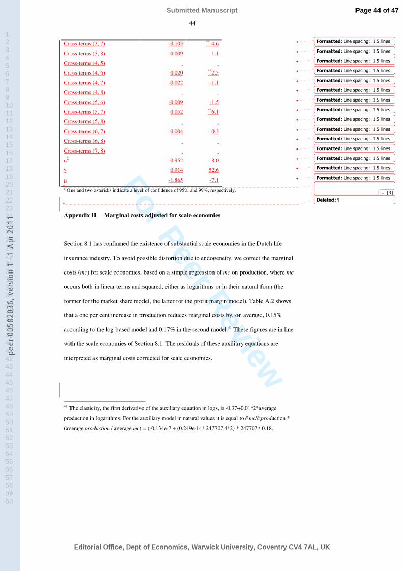
For Peer Review
44
Cross-terms (3, 7) -0.105 **-4.6
Cross-terms (3, 8) 0.009 1.1
Cross-terms (4, 5)
Cross-terms (4, 6) 0.020 **2.5
Cross-terms (4, 7) -0.022 -1.1
Cross-terms (4, 8)
Cross-terms (5, 6) -0.009 -1.5
Cross-terms (5, 7) 0.052 **6.1
Cross-terms (5, 8)
Cross-terms (6, 7) 0.004 0.3
Cross-terms (6, 8)
Cross-terms (7, 8)
σ2 0.952 8.0
γ 0.914 52.6
µ -1.865 -7.1
a One and two asterisks indicate a level of confidence of 95% and 99%, respectively.
Appendix II Marginal costs adjusted for scale economies
Section 8.1 has confirmed the existence of substantial scale economies in the Dutch life
insurance industry. To avoid possible distortion due to endogeneity, we correct the marginal
costs (mc) for scale economies, based on a simple regression of mc on production, where mc
occurs both in linear terms and squared, either as logarithms or in their natural form (the
former for the market share model, the latter for the profit margin model). Table A.2 shows
that a one per cent increase in production reduces marginal costs by, on average, 0.15%
according to the log-based model and 0.17% in the second model.41 These figures are in line
with the scale economies of Section 8.1. The residuals of these auxiliary equations are
interpreted as marginal costs corrected for scale economies.
41 The elasticity, the first derivative of the auxiliary equation in logs, is -0.37+0.01*2*average
production in logarithms. For the auxiliary model in natural values it is equal to ∂mc/∂production *
(average production / average mc) = (-0.134e-7 + (0.249e-14* 247707.4*2) * 247707 / 0.18.
Formatted: Line spacing: 1.5 linesFormatted: Line spacing: 1.5 linesFormatted: Line spacing: 1.5 linesFormatted: Line spacing: 1.5 linesFormatted: Line spacing: 1.5 linesFormatted: Line spacing: 1.5 linesFormatted: Line spacing: 1.5 linesFormatted: Line spacing: 1.5 linesFormatted: Line spacing: 1.5 linesFormatted: Line spacing: 1.5 linesFormatted: Line spacing: 1.5 linesFormatted: Line spacing: 1.5 linesFormatted: Line spacing: 1.5 linesFormatted: Line spacing: 1.5 linesFormatted: Line spacing: 1.5 lines
Deleted: ¶... [3]
Page 44 of 47
Editorial Office, Dept of Economics, Warwick University, Coventry CV4 7AL, UK
Submitted Manuscript
123456789101112131415161718192021222324252627282930313233343536373839404142434445464748495051525354555657585960
peer
-005
8203
6, v
ersi
on 1
- 1
Apr 2
011

For Peer Review
45
Table A.2 Auxiliary regressions for marginal cost and scale economies corrections
Model in logarithms Model in natural values
Coefficient t-value bCoefficient t-value b
Production -0.37 **-4.5 -1.34 a **-6.3
Production2 0.01 **2.7 2.49 a **4.6
Intercept 0.83 *1.9 0.20 **31.5
Adjusted R2 0.19 0.07
Number of observations 607 607
a In billions instead of in thousands of euros; b One and two asterisks indicate a level of confidence of 95% and
99%, respectively.
Page 45 of 47
Editorial Office, Dept of Economics, Warwick University, Coventry CV4 7AL, UK
Submitted Manuscript
123456789101112131415161718192021222324252627282930313233343536373839404142434445464748495051525354555657585960
peer
-005
8203
6, v
ersi
on 1
- 1
Apr 2
011
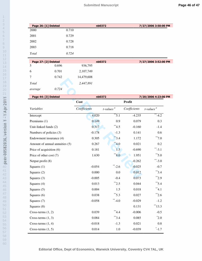
For Peer Review
Page 26: [1] Deleted nb0372 7/27/2006 3:50:00 PM 2000 0.710
2001 0.729
2002 0.728
2003 0.718
Total 0.724
Page 27: [2] Deleted nb0372 7/27/2006 3:52:00 PM 5 0.696 936,795
6 0.701 2,107,749
7 0.742 14,479,608
Total
average 0.724
2,447,891
Page 44: [3] Deleted nb0372 7/20/2006 4:23:00 PM Cost Profit
Variables Coefficients t-values a Coefficients t-values a
Intercept 4.020 **5.1 -4.235 **-4.2
Premiums (1) 0.149 0.9 0.079 0.3
Unit-linked funds (2) 0.317 **4.5 -0.160 -1.4
Numbers of policies (3) -0.178 -1.3 0.141 0.6
Endowment insurance (4) 0.305 **3.4 1.172 **7.0
Amount of annual annuities (5) 0.267 **4.0 0.021 0.2
Price of acquisition (6) 0.181 1.5 -0.690 **-3.1
Price of other cost (7) 1.630 **8.0 1.951 **5.0
Netput profit (8) -0.262 **-3.0
Squares (1) -0.054 **-2.6 -0.025 -0.7
Squares (2) 0.000 0.0 0.012 **3.4
Squares (3) -0.005 -0.4 0.073 **2.9
Squares (4) 0.013 **2.5 0.044 **5.4
Squares (5) 0.004 1.5 0.018 **4.1
Squares (6) 0.038 **5.3 0.027 **2.6
Squares (7) -0.058 **-4.0 -0.029 -1.2
Squares (8) 0.131 **13.3
Cross-terms (1, 2) 0.039 **4.4 -0.006 -0.5
Cross-terms (1, 3) 0.084 **3.4 0.085 *2.0
Cross-terms (1, 4) -0.018 -1.3 0.021 0.8
Cross-terms (1, 5) 0.014 1.0 -0.039 *-1.7
Page 46 of 47
Editorial Office, Dept of Economics, Warwick University, Coventry CV4 7AL, UK
Submitted Manuscript
123456789101112131415161718192021222324252627282930313233343536373839404142434445464748495051525354555657585960
peer
-005
8203
6, v
ersi
on 1
- 1
Apr 2
011
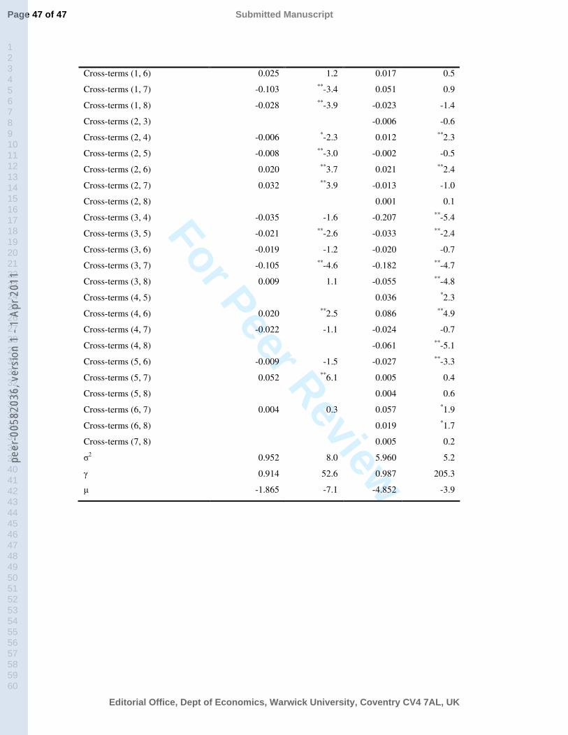
For Peer Review
Cross-terms (1, 6) 0.025 1.2 0.017 0.5
Cross-terms (1, 7) -0.103 **-3.4 0.051 0.9
Cross-terms (1, 8) -0.028 **-3.9 -0.023 -1.4
Cross-terms (2, 3) -0.006 -0.6
Cross-terms (2, 4) -0.006 *-2.3 0.012 **2.3
Cross-terms (2, 5) -0.008 **-3.0 -0.002 -0.5
Cross-terms (2, 6) 0.020 **3.7 0.021 **2.4
Cross-terms (2, 7) 0.032 **3.9 -0.013 -1.0
Cross-terms (2, 8) 0.001 0.1
Cross-terms (3, 4) -0.035 -1.6 -0.207 **-5.4
Cross-terms (3, 5) -0.021 **-2.6 -0.033 **-2.4
Cross-terms (3, 6) -0.019 -1.2 -0.020 -0.7
Cross-terms (3, 7) -0.105 **-4.6 -0.182 **-4.7
Cross-terms (3, 8) 0.009 1.1 -0.055 **-4.8
Cross-terms (4, 5) 0.036 *2.3
Cross-terms (4, 6) 0.020 **2.5 0.086 **4.9
Cross-terms (4, 7) -0.022 -1.1 -0.024 -0.7
Cross-terms (4, 8) -0.061 **-5.1
Cross-terms (5, 6) -0.009 -1.5 -0.027 **-3.3
Cross-terms (5, 7) 0.052 **6.1 0.005 0.4
Cross-terms (5, 8) 0.004 0.6
Cross-terms (6, 7) 0.004 0.3 0.057 *1.9
Cross-terms (6, 8) 0.019 *1.7
Cross-terms (7, 8) 0.005 0.2
σ2 0.952 8.0 5.960 5.2
γ 0.914 52.6 0.987 205.3
µ -1.865 -7.1 -4.852 -3.9
Page 47 of 47
Editorial Office, Dept of Economics, Warwick University, Coventry CV4 7AL, UK
Submitted Manuscript
123456789101112131415161718192021222324252627282930313233343536373839404142434445464748495051525354555657585960
peer
-005
8203
6, v
ersi
on 1
- 1
Apr 2
011
Copyright © 2022 FDOKUMEN

