


Bahasa
Halaman
Hukum

Architectural Principles for DatabaseSystems on Storage-Class Memory
Dissertation
zur Erlangung des akademischen GradesDoktoringenieur (Dr.-Ing.)
vorgelegt an derTechnischen Universität Dresden
Fakultät Informatik
eingereicht vonIsmail Oukid, M.Sc.
geboren am 19. Mai 1989 in Blida, Algerien
Gutachter: Prof. Dr.-Ing. Wolfgang LehnerTechnische Universität Dresden
Prof. Dr. Stefan ManegoldUniversiteit Leiden & Centrum voor Wiskunde en Informatica
Tag der Verteidigung: 5. Dezember 2017
Walldorf, den 15. Dezember 2017

Ismail Oukid: Architectural Principles for Database Systems on Storage-Class Memory ©December 15, 2017.
ii

To my parents.

iv
ABSTRACT
Database systems have long been optimized to hide the higher latency of storage media, yieldingcomplex persistence mechanisms. With the advent of large DRAM capacities, it became possible tokeep a full copy of the data in DRAM. Systems that leverage this possibility, such as main-memorydatabases, keep two copies of the data in two different formats: one in main memory and the otherone in storage. The two copies are kept synchronized using snapshotting and logging. This main-memory-centric architecture yields nearly two orders of magnitude faster analytical processing thantraditional, disk-centric ones. The rise of Big Data emphasized the importance of such systems withan ever-increasing need for more main memory. However, DRAM is hitting its scalability limits: It isintrinsically hard to further increase its density.
Storage-Class Memory (SCM) is a group of novel memory technologies that promise to alleviateDRAM’s scalability limits. They combine the non-volatility, density, and economic characteristicsof storage media with the byte-addressability and a latency close to that of DRAM. Therefore, SCMcan serve as persistent main memory, thereby bridging the gap between main memory and storage. Inthis dissertation, we explore the impact of SCM as persistent main memory on database systems. As-suming a hybrid SCM-DRAM hardware architecture, we propose a novel software architecture fordatabase systems that places primary data in SCM and directly operates on it, eliminating the needfor explicit I/O. This architecture yields many benefits: First, it obviates the need to reload data fromstorage to main memory during recovery, as data is discovered and accessed directly in SCM. Sec-ond, it allows replacing the traditional logging infrastructure by fine-grained, cheap micro-logging atdata-structure level. Third, secondary data can be stored in DRAM and reconstructed during recov-ery. Fourth, system runtime information can be stored in SCM to improve recovery time. Finally, thesystem may retain and continue in-flight transactions in case of system failures.
However, SCM is no panacea as it raises unprecedented programming challenges. Given its byte-addressability and low latency, processors can access, read, modify, and persist data in SCM usingload/store instructions at a CPU cache line granularity. The path from CPU registers to SCM is longand mostly volatile, including store buffers and CPU caches, leaving the programmer with little con-trol over when data is persisted. Therefore, there is a need to enforce the order and durability of SCMwrites using persistence primitives, such as cache line flushing instructions. This in turn creates newfailure scenarios, such as missing or misplaced persistence primitives.
We devise several building blocks to overcome these challenges. First, we identify the programmingchallenges of SCM and present a sound programming model that solves them. Then, we tackle me-mory management, as the first required building block to build a database system, by designing ahighly scalable SCM allocator, named PAllocator, that fulfills the versatile needs of database systems.Thereafter, we propose the FPTree, a highly scalable hybrid SCM-DRAM persistent B+-Tree thatbridges the gap between the performance of transient and persistent B+-Trees. Using these buildingblocks, we realize our envisioned database architecture in SOFORT, a hybrid SCM-DRAM columnartransactional engine. We propose an SCM-optimized MVCC scheme that eliminates write-ahead log-ging from the critical path of transactions. Since SCM-resident data is near-instantly available uponrecovery, the new recovery bottleneck is rebuilding DRAM-based data. To alleviate this bottleneck,we propose a novel recovery technique that achieves nearly instant responsiveness of the database byaccepting queries right after recovering SCM-based data, while rebuilding DRAM-based data in thebackground. Additionally, SCM brings new failure scenarios that existing testing tools cannot detect.Hence, we propose an online testing framework that is able to automatically simulate power failuresand detect missing or misplaced persistence primitives. Finally, our proposed building blocks canserve to build more complex systems, paving the way for future database systems on SCM.
v

vi
ACKNOWLEDGEMENTS
This thesis would not have been possible without the contributions, support, and companionship ofmany whom I would like to acknowledge.
First and foremost, I would like to express my deepest gratitude to my supervisor and mentor Prof.Wolfgang Lehner for his unconditional support throughout my thesis, both personally and profession-ally. Wolfgang has always been a positive presence. He had my back from day one until today andcontinuing, ensuring I was always in the best possible conditions to succeed, even beyond my thesis.By always offering constructive criticism and enthusiastically encouraging me to aim high, he gaveme confidence and guided me to strive for excellence.
Furthermore, I would like to thank Prof. Stefan Manegold for taking on the role of co-examiner of mythesis, for his invaluable feedback, and for his hospitality during my visit at CWI.
Moreover, I would like to express my gratitude to the SAP HANA Campus team, where I had theprivilege to conduct my thesis. I enjoyed my time as a PhD student in great part thanks to theircompanionship. First, there is Arne Schwarz, the heart and soul of the campus, who works hard sothat we only need to worry about our research. Then there is my fellow PhD students and friends:Ingo Müller, Michael Rudolf, Marcus Paradies, Iraklis Psaroudakis, David Kernert, Elena Vasilyeva,Hannes Rauhe, Robert Brunel, Thomas Bach, Florian Wolf, Matthias Hauck, Lucas Lersch, FrankTetzel, Robin Rehrmann, Stefan Noll, Georgios Psaropoulos, Jonathan Dees, Philipp Große, MartinKaufmann, and Francesc Trull. Ingo influenced me the most as a researcher and as a person. I lookedup to him as a mentor from day one; from him I learned scientific rigor, critical thinking, and thatquality needs time. I have been looking up to him as a big brother since and still strive to follow hisfootsteps. Michael’s willingness to help is unmatched; he came to the rescue countless times fortechnical and non-technical issues. My time in Germany surely would not have been as enjoyablewithout his help. I was lucky to travel with Marcus several times to conferences; he surely knows howto organize a trip – the Yosemite excursion is unforgettable. I had such an exciting time with Iraklis,Ingo, Frank, Matthias, and Thomas during the SIGMOD programming contests – I learned a lot fromeach one of them. Frank was the perfect night owl partner for the late evenings in the office, andGeorgios made my social life a thing again during the last year of my PhD. Additionally, I would liketo thank Robin, Frank, Lucas, Stefan, Michael, Marcus, Thomas, Matthias, and Ingo for reviewingparts of this dissertation. I am grateful to all of you guys!
Special thanks go to my SAP supervisors Daniel Booss, Anisoara Nica, and Peter Bumbulis, as wellas my Intel supervisor Thomas Willhalm for their help and guidance throughout my thesis. Daniel’stechnical expertise was key in jump starting the PAllocator. Peter was influential in laying out thevision for SOFORT during my visit to SAP Waterloo in April 2014. Ani supported me in several of mypapers and was instrumental in devising the adaptive recovery mechanism of SOFORT. Thomas wasalways prompt to give me feedback and get me access to the latest and fanciest Intel hardware. More-over, I would like to thank Norman May, Alexander Boehm, Roman Dementiev, Otto Bruggeman,and Abelkader Sellami for their support and insightful input. A special appreciation goes to OliverRebholz, my manager in my new role at SAP, for allowing me to finish my dissertation by easing myload in the first few months of my employment.
During my thesis, I was blessed with talented students that were of great help in building my prototypeSOFORT: Adrien Lespinasse worked on early versions of PAllocator and the testing framework, JohanLasperas worked on the FPTree, Daniel Bossle worked on SCM-optimized concurrency control, andGrégoire Gomes worked on the defragmentation scheme of PAllocator.
vii

I would also like to thank my colleagues at the TU Dresden Database Systems Group for their warmwelcome whenever I visited: Lars Dannecker, Ulrike Fischer, Katrin Braunschweig, Julian Eberius,Tim Kiefer, Robert Ulbricht, Ines Funke, Ulrike Schöbel, Dirk Habich, Maik Thiele, Martin Hahmann,Hannes Voigt, Thomas Kissinger, Tobias Jäkel, Tomas Karnagel, Till Kolditz, Claudio Hartmann, KaiHerrmann, Kasun Perera, Rihan Hai, Ahmad Ahmadov, Johannes Luong, Annett Ungethüm, PatrickDamme, Lars Kegel, Juliana Hildebrandt, Alexander Krause, Mikhail Zarubin, Elvis Koci, Nusrat LisaJahan, Muhammad Idris, and Rana Faisal Munir. A special appreciation goes to Hannes, Kai, Till, andMaik for their help regarding the PhD administrative procedure, and to Thomas for his contributionto the instant recovery paper.
I warmly thank my long-time friends Hamza Rihani and Amine Bentaiba who have always been therefor me and provided me with an outlet to escape my thesis whenever I needed to. Last but not least, Iwould like to thank my family, especially my parents, for believing in me more than anyone, for theirunconditional support, constant encouragement, and for indulging my character in stressful periods.
Ismail OukidDecember 15, 2017
viii
CONTENTS
ABSTRACT v
ACKNOWLEDGEMENTS vii
1 INTRODUCTION 5
2 LEVERAGING SCM IN DATABASE SYSTEMS 11
2.1 Storage-Class Memory . . . . . . . . . . . . . . . . . . . . . . . . . . . . . . 112.1.1 Architecting SCM . . . . . . . . . . . . . . . . . . . . . . . . . . . . . . . 12
2.1.2 SCM Performance Implications . . . . . . . . . . . . . . . . . . . . . . . . 14
2.2 SCM Emulation Techniques . . . . . . . . . . . . . . . . . . . . . . . . . . . 152.2.1 NUMA-Based SCM Emulation . . . . . . . . . . . . . . . . . . . . . . . . 16
2.2.2 Quartz . . . . . . . . . . . . . . . . . . . . . . . . . . . . . . . . . . . . 17
2.2.3 Intel SCM Emulation Platform . . . . . . . . . . . . . . . . . . . . . . . . 17
2.3 SCM and Databases: State-of-the-Art . . . . . . . . . . . . . . . . . . . . . 182.3.1 Storage and Recovery . . . . . . . . . . . . . . . . . . . . . . . . . . . . . 19
2.3.2 Query Optimization and Execution . . . . . . . . . . . . . . . . . . . . . . 24
2.4 Overview of SOFORT . . . . . . . . . . . . . . . . . . . . . . . . . . . . . . . 272.4.1 Design Principles . . . . . . . . . . . . . . . . . . . . . . . . . . . . . . . 27
2.4.2 Architecture Overview . . . . . . . . . . . . . . . . . . . . . . . . . . . . 27
2.4.3 Persistent Memory Management . . . . . . . . . . . . . . . . . . . . . . . 28
2.4.4 Data Layout . . . . . . . . . . . . . . . . . . . . . . . . . . . . . . . . . . 28
2.4.5 Concurrency Control . . . . . . . . . . . . . . . . . . . . . . . . . . . . . 29
2.4.6 Recovery Mechanisms . . . . . . . . . . . . . . . . . . . . . . . . . . . . 30
2.5 Conclusion . . . . . . . . . . . . . . . . . . . . . . . . . . . . . . . . . . . . . 31
3 PERSISTENT MEMORY MANAGEMENT 33
3.1 Persistent Memory Challenges . . . . . . . . . . . . . . . . . . . . . . . . . 343.1.1 Data consistency . . . . . . . . . . . . . . . . . . . . . . . . . . . . . . . 34
3.1.2 Data recovery . . . . . . . . . . . . . . . . . . . . . . . . . . . . . . . . . 35
3.1.3 Persistent memory leaks . . . . . . . . . . . . . . . . . . . . . . . . . . . 36
3.1.4 Partial writes . . . . . . . . . . . . . . . . . . . . . . . . . . . . . . . . . 36
3.1.5 Persistent memory fragmentation . . . . . . . . . . . . . . . . . . . . . . . 37
3.1.6 Address space fragmentation . . . . . . . . . . . . . . . . . . . . . . . . . 37
3.2 SCM Programming Models . . . . . . . . . . . . . . . . . . . . . . . . . . . 38
1
3.2.1 Recoverable Addressing Scheme . . . . . . . . . . . . . . . . . . . . . . . 38
3.2.2 Consistency Handling . . . . . . . . . . . . . . . . . . . . . . . . . . . . . 38
3.2.3 Persistent Memory Leak Prevention . . . . . . . . . . . . . . . . . . . . . 39
3.2.4 Related Work . . . . . . . . . . . . . . . . . . . . . . . . . . . . . . . . . 40
3.3 Persistent Memory Allocation . . . . . . . . . . . . . . . . . . . . . . . . . . 423.3.1 Pool Structure . . . . . . . . . . . . . . . . . . . . . . . . . . . . . . . . . 42
3.3.2 Allocation Strategies . . . . . . . . . . . . . . . . . . . . . . . . . . . . . 42
3.3.3 Concurrency Handling . . . . . . . . . . . . . . . . . . . . . . . . . . . . 43
3.3.4 Garbage Collection . . . . . . . . . . . . . . . . . . . . . . . . . . . . . . 44
3.3.5 Related Work . . . . . . . . . . . . . . . . . . . . . . . . . . . . . . . . . 45
3.4 PAllocator Design and Implementation . . . . . . . . . . . . . . . . . . . . 463.4.1 Design goals and decisions . . . . . . . . . . . . . . . . . . . . . . . . . . 46
3.4.2 Programming Model . . . . . . . . . . . . . . . . . . . . . . . . . . . . . 49
3.4.3 PAllocator Architecture . . . . . . . . . . . . . . . . . . . . . . . . . . . . 50
3.4.4 SmallPAllocator . . . . . . . . . . . . . . . . . . . . . . . . . . . . . . . . 51
3.4.5 BigPAllocator . . . . . . . . . . . . . . . . . . . . . . . . . . . . . . . . . 52
3.4.6 Defragmentation . . . . . . . . . . . . . . . . . . . . . . . . . . . . . . . 54
3.4.7 Recovery . . . . . . . . . . . . . . . . . . . . . . . . . . . . . . . . . . . 55
3.5 Evaluation . . . . . . . . . . . . . . . . . . . . . . . . . . . . . . . . . . . . . 563.5.1 Standalone allocation and deallocation . . . . . . . . . . . . . . . . . . . . 58
3.5.2 Random allocation and deallocation . . . . . . . . . . . . . . . . . . . . . 60
3.5.3 Larson benchmark . . . . . . . . . . . . . . . . . . . . . . . . . . . . . . 61
3.5.4 Recovery time . . . . . . . . . . . . . . . . . . . . . . . . . . . . . . . . . 63
3.5.5 Defragmentation . . . . . . . . . . . . . . . . . . . . . . . . . . . . . . . 64
3.5.6 Allocator impact on a persistent B-Tree performance . . . . . . . . . . . . . 64
3.6 Summary . . . . . . . . . . . . . . . . . . . . . . . . . . . . . . . . . . . . . . 65
4 PERSISTENT DATA STRUCTURES 67
4.1 Related Work . . . . . . . . . . . . . . . . . . . . . . . . . . . . . . . . . . . . 684.1.1 CDDS B-Tree . . . . . . . . . . . . . . . . . . . . . . . . . . . . . . . . . 69
4.1.2 wBTree . . . . . . . . . . . . . . . . . . . . . . . . . . . . . . . . . . . . 69
4.1.3 NV-Tree . . . . . . . . . . . . . . . . . . . . . . . . . . . . . . . . . . . . 70
4.1.4 Discussion . . . . . . . . . . . . . . . . . . . . . . . . . . . . . . . . . . 71
4.2 FPTree Design Principles . . . . . . . . . . . . . . . . . . . . . . . . . . . . . 734.2.1 Selective Persistence . . . . . . . . . . . . . . . . . . . . . . . . . . . . . 73
4.2.2 Fingerprints . . . . . . . . . . . . . . . . . . . . . . . . . . . . . . . . . . 74
4.2.3 Amortized Persistent Memory Allocations . . . . . . . . . . . . . . . . . . 76
4.2.4 Selective Concurrency . . . . . . . . . . . . . . . . . . . . . . . . . . . . 76
4.3 FPTree Base Operations . . . . . . . . . . . . . . . . . . . . . . . . . . . . . 784.3.1 Fixed-Size Key Operations . . . . . . . . . . . . . . . . . . . . . . . . . . 78
4.3.2 Variable-Size Key Operations . . . . . . . . . . . . . . . . . . . . . . . . . 84
4.3.3 Leaf group management . . . . . . . . . . . . . . . . . . . . . . . . . . . 87
2
4.4 Evaluation . . . . . . . . . . . . . . . . . . . . . . . . . . . . . . . . . . . . . 894.4.1 Experimental Setup . . . . . . . . . . . . . . . . . . . . . . . . . . . . . . 90
4.4.2 Single-Threaded Microbenchmarks . . . . . . . . . . . . . . . . . . . . . . 90
4.4.3 Concurrent Microbenchmarks . . . . . . . . . . . . . . . . . . . . . . . . 93
4.4.4 End-to-End Evaluation . . . . . . . . . . . . . . . . . . . . . . . . . . . . 97
4.5 Summary . . . . . . . . . . . . . . . . . . . . . . . . . . . . . . . . . . . . . . 100
5 SOFORT: A HYBRID SCM-DRAM TRANSACTIONAL STORAGE ENGINE 101
5.1 Design Space Exploration . . . . . . . . . . . . . . . . . . . . . . . . . . . . 1025.1.1 Concurrency Control . . . . . . . . . . . . . . . . . . . . . . . . . . . . . 102
5.1.2 Version Storage . . . . . . . . . . . . . . . . . . . . . . . . . . . . . . . . 105
5.1.3 Index Management . . . . . . . . . . . . . . . . . . . . . . . . . . . . . . 106
5.1.4 Garbage Collection . . . . . . . . . . . . . . . . . . . . . . . . . . . . . . 107
5.2 SOFORT Architecture . . . . . . . . . . . . . . . . . . . . . . . . . . . . . . . 1085.2.1 Concurrency Control . . . . . . . . . . . . . . . . . . . . . . . . . . . . . 109
5.2.2 Version Storage . . . . . . . . . . . . . . . . . . . . . . . . . . . . . . . . 109
5.2.3 Index Management . . . . . . . . . . . . . . . . . . . . . . . . . . . . . . 111
5.2.4 Garbage Collection . . . . . . . . . . . . . . . . . . . . . . . . . . . . . . 112
5.3 SOFORT Implementation . . . . . . . . . . . . . . . . . . . . . . . . . . . . 1135.3.1 MVCC Structures . . . . . . . . . . . . . . . . . . . . . . . . . . . . . . . 113
5.3.2 Start Transaction . . . . . . . . . . . . . . . . . . . . . . . . . . . . . . . 115
5.3.3 Select . . . . . . . . . . . . . . . . . . . . . . . . . . . . . . . . . . . . . 116
5.3.4 Insert . . . . . . . . . . . . . . . . . . . . . . . . . . . . . . . . . . . . . 117
5.3.5 Delete . . . . . . . . . . . . . . . . . . . . . . . . . . . . . . . . . . . . . 118
5.3.6 Update . . . . . . . . . . . . . . . . . . . . . . . . . . . . . . . . . . . . 118
5.3.7 Commit Transaction . . . . . . . . . . . . . . . . . . . . . . . . . . . . . 119
5.3.8 Abort Transaction . . . . . . . . . . . . . . . . . . . . . . . . . . . . . . . 120
5.3.9 Recovery . . . . . . . . . . . . . . . . . . . . . . . . . . . . . . . . . . . 122
5.3.10 Garbage Collection . . . . . . . . . . . . . . . . . . . . . . . . . . . . . . 124
5.4 Continuing Unfinished Transactions . . . . . . . . . . . . . . . . . . . . . . 125
5.5 Evaluation . . . . . . . . . . . . . . . . . . . . . . . . . . . . . . . . . . . . . 1265.5.1 Experimental Setup . . . . . . . . . . . . . . . . . . . . . . . . . . . . . . 127
5.5.2 OLTP Performance . . . . . . . . . . . . . . . . . . . . . . . . . . . . . . 127
5.5.3 Data Placement Impact on OLTP Performance . . . . . . . . . . . . . . . . 128
5.5.4 Durability Cost . . . . . . . . . . . . . . . . . . . . . . . . . . . . . . . . 130
5.5.5 Recovery Time . . . . . . . . . . . . . . . . . . . . . . . . . . . . . . . . 131
5.6 Summary . . . . . . . . . . . . . . . . . . . . . . . . . . . . . . . . . . . . . . 132
6 SOFORT RECOVERY TECHNIQUES 133
6.1 Recovery of Secondary Data Structures . . . . . . . . . . . . . . . . . . . . 1346.1.1 System Responsiveness . . . . . . . . . . . . . . . . . . . . . . . . . . . . 135
6.1.2 Balancing Query Performance with Recovery Performance . . . . . . . . . . 135
3
6.1.3 Discussion . . . . . . . . . . . . . . . . . . . . . . . . . . . . . . . . . . 136
6.2 Adaptive Recovery . . . . . . . . . . . . . . . . . . . . . . . . . . . . . . . . 1366.2.1 Characterization of Secondary Data Structures . . . . . . . . . . . . . . . . 136
6.2.2 Benefit Functions for Secondary Data . . . . . . . . . . . . . . . . . . . . . 137
6.2.3 Benefit Functions Benefitdep and Benefitindep . . . . . . . . . . . . . . . . . 139
6.2.4 Recovery Manager . . . . . . . . . . . . . . . . . . . . . . . . . . . . . . 141
6.3 Evaluation . . . . . . . . . . . . . . . . . . . . . . . . . . . . . . . . . . . . . 1426.3.1 Experimental Details . . . . . . . . . . . . . . . . . . . . . . . . . . . . . 142
6.3.2 Secondary Data Placement Impact on Recovery Performance . . . . . . . . . 143
6.3.3 Recovery Strategies . . . . . . . . . . . . . . . . . . . . . . . . . . . . . . 144
6.3.4 Adaptive Resource Allocation Algorithm . . . . . . . . . . . . . . . . . . . 146
6.3.5 Resilience to Workload Change . . . . . . . . . . . . . . . . . . . . . . . . 148
6.3.6 Impact of SCM Latency . . . . . . . . . . . . . . . . . . . . . . . . . . . . 148
6.3.7 Limits of Adaptive Recovery . . . . . . . . . . . . . . . . . . . . . . . . . 149
6.4 Related Work . . . . . . . . . . . . . . . . . . . . . . . . . . . . . . . . . . . . 150
6.5 Summary . . . . . . . . . . . . . . . . . . . . . . . . . . . . . . . . . . . . . . 151
7 TESTING OF SCM-BASED SOFTWARE 153
7.1 Background . . . . . . . . . . . . . . . . . . . . . . . . . . . . . . . . . . . . 1547.1.1 Related Work . . . . . . . . . . . . . . . . . . . . . . . . . . . . . . . . . 155
7.1.2 Memory Model . . . . . . . . . . . . . . . . . . . . . . . . . . . . . . . . 156
7.2 Testing of SCM-Based Software . . . . . . . . . . . . . . . . . . . . . . . . 1567.2.1 Crash Simulation . . . . . . . . . . . . . . . . . . . . . . . . . . . . . . . 156
7.2.2 Faster Testing with Copy-on-Write . . . . . . . . . . . . . . . . . . . . . . 159
7.2.3 Faster Code Coverage with Call Stack Tracing . . . . . . . . . . . . . . . . . 159
7.2.4 Memory Reordering . . . . . . . . . . . . . . . . . . . . . . . . . . . . . 160
7.2.5 Crash Simulation During Recovery . . . . . . . . . . . . . . . . . . . . . . 161
7.2.6 Crash Simulation in Multi-Threaded Programs . . . . . . . . . . . . . . . . 163
7.2.7 Limitations and Complementarity with Yat . . . . . . . . . . . . . . . . . . 163
7.3 Evaluation . . . . . . . . . . . . . . . . . . . . . . . . . . . . . . . . . . . . . 164
7.4 Summary and Future Work . . . . . . . . . . . . . . . . . . . . . . . . . . . 166
8 CONCLUSION 167
8.1 Summary of Contributions . . . . . . . . . . . . . . . . . . . . . . . . . . . . 167
8.2 Future Work . . . . . . . . . . . . . . . . . . . . . . . . . . . . . . . . . . . . 169
BIBLIOGRAPHY 173
LIST OF FIGURES 185
LIST OF TABLES 187
LIST OF ALGORITHMS 188
4
1INTRODUCTION
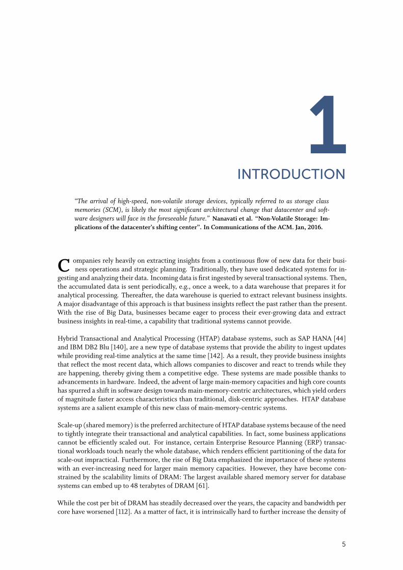
“The arrival of high-speed, non-volatile storage devices, typically referred to as storage classmemories (SCM), is likely the most significant architectural change that datacenter and soft-ware designers will face in the foreseeable future.” Nanavati et al. “Non-Volatile Storage: Im-plications of the datacenter’s shifting center”. In Communications of the ACM. Jan, 2016.
C ompanies rely heavily on extracting insights from a continuous flow of new data for their busi-ness operations and strategic planning. Traditionally, they have used dedicated systems for in-
gesting and analyzing their data. Incoming data is first ingested by several transactional systems. Then,the accumulated data is sent periodically, e.g., once a week, to a data warehouse that prepares it foranalytical processing. Thereafter, the data warehouse is queried to extract relevant business insights.A major disadvantage of this approach is that business insights reflect the past rather than the present.With the rise of Big Data, businesses became eager to process their ever-growing data and extractbusiness insights in real-time, a capability that traditional systems cannot provide.
Hybrid Transactional and Analytical Processing (HTAP) database systems, such as SAP HANA [44]and IBM DB2 Blu [140], are a new type of database systems that provide the ability to ingest updateswhile providing real-time analytics at the same time [142]. As a result, they provide business insightsthat reflect the most recent data, which allows companies to discover and react to trends while theyare happening, thereby giving them a competitive edge. These systems are made possible thanks toadvancements in hardware. Indeed, the advent of large main-memory capacities and high core countshas spurred a shift in software design towards main-memory-centric architectures, which yield ordersof magnitude faster access characteristics than traditional, disk-centric approaches. HTAP databasesystems are a salient example of this new class of main-memory-centric systems.
Scale-up (shared memory) is the preferred architecture of HTAP database systems because of the needto tightly integrate their transactional and analytical capabilities. In fact, some business applicationscannot be efficiently scaled out. For instance, certain Enterprise Resource Planning (ERP) transac-tional workloads touch nearly the whole database, which renders efficient partitioning of the data forscale-out impractical. Furthermore, the rise of Big Data emphasized the importance of these systemswith an ever-increasing need for larger main memory capacities. However, they have become con-strained by the scalability limits of DRAM: The largest available shared memory server for databasesystems can embed up to 48 terabytes of DRAM [61].
While the cost per bit of DRAM has steadily decreased over the years, the capacity and bandwidth percore have worsened [112]. As a matter of fact, it is intrinsically hard to further increase the density of
5
21 23 25 27 29 211 213 215 217 219 221 223
DRAM SCM Flash Hard DriveLL CacheEDRAM
L1 CacheSRAM
Main Memory High Performance Disk
Access Latency in Cycles for a 4 GHz Processor
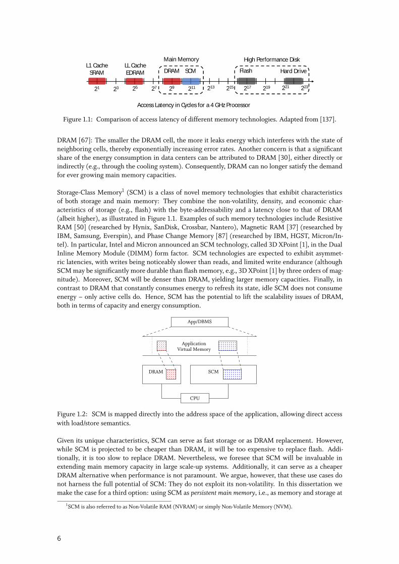
Figure 1.1: Comparison of access latency of different memory technologies. Adapted from [137].
DRAM [67]: The smaller the DRAM cell, the more it leaks energy which interferes with the state ofneighboring cells, thereby exponentially increasing error rates. Another concern is that a significantshare of the energy consumption in data centers can be attributed to DRAM [30], either directly orindirectly (e.g., through the cooling system). Consequently, DRAM can no longer satisfy the demandfor ever growing main memory capacities.
Storage-Class Memory1 (SCM) is a class of novel memory technologies that exhibit characteristicsof both storage and main memory: They combine the non-volatility, density, and economic char-acteristics of storage (e.g., flash) with the byte-addressability and a latency close to that of DRAM(albeit higher), as illustrated in Figure 1.1. Examples of such memory technologies include ResistiveRAM [50] (researched by Hynix, SanDisk, Crossbar, Nantero), Magnetic RAM [37] (researched byIBM, Samsung, Everspin), and Phase Change Memory [87] (researched by IBM, HGST, Micron/In-tel). In particular, Intel and Micron announced an SCM technology, called 3D XPoint [1], in the DualInline Memory Module (DIMM) form factor. SCM technologies are expected to exhibit asymmet-ric latencies, with writes being noticeably slower than reads, and limited write endurance (althoughSCM may be significantly more durable than flash memory, e.g., 3D XPoint [1] by three orders of mag-nitude). Moreover, SCM will be denser than DRAM, yielding larger memory capacities. Finally, incontrast to DRAM that constantly consumes energy to refresh its state, idle SCM does not consumeenergy – only active cells do. Hence, SCM has the potential to lift the scalability issues of DRAM,both in terms of capacity and energy consumption.
CPU
DRAM SCM
App/DBMS
ApplicationVirtual Memory
Figure 1.2: SCM is mapped directly into the address space of the application, allowing direct accesswith load/store semantics.
Given its unique characteristics, SCM can serve as fast storage or as DRAM replacement. However,while SCM is projected to be cheaper than DRAM, it will be too expensive to replace flash. Addi-tionally, it is too slow to replace DRAM. Nevertheless, we foresee that SCM will be invaluable inextending main memory capacity in large scale-up systems. Additionally, it can serve as a cheaperDRAM alternative when performance is not paramount. We argue, however, that these use cases donot harness the full potential of SCM: They do not exploit its non-volatility. In this dissertation wemake the case for a third option: using SCM as persistent main memory, i.e., as memory and storage at
1SCM is also referred to as Non-Volatile RAM (NVRAM) or simply Non-Volatile Memory (NVM).
6
| 3
>
Diese Zeile ersetzt man über: Einfügen > Kopf- und Fußzeile NICHT im Master
Tran
sient
Mai
nM
emor
yPe
rsist
ent
Stor
age
Log
logbuffer
buffer pool
… …
runtime data
a) Traditional Architecture b) Envisioned SCM-enabled Architecture
TransientMain Memory
Non-VolatileMain Memory
database
runtime data
Database moving the persistency bar
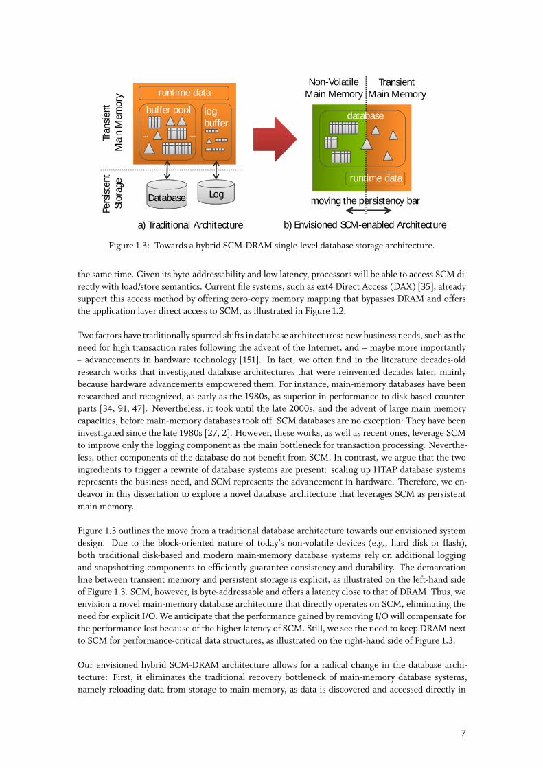
Figure 1.3: Towards a hybrid SCM-DRAM single-level database storage architecture.
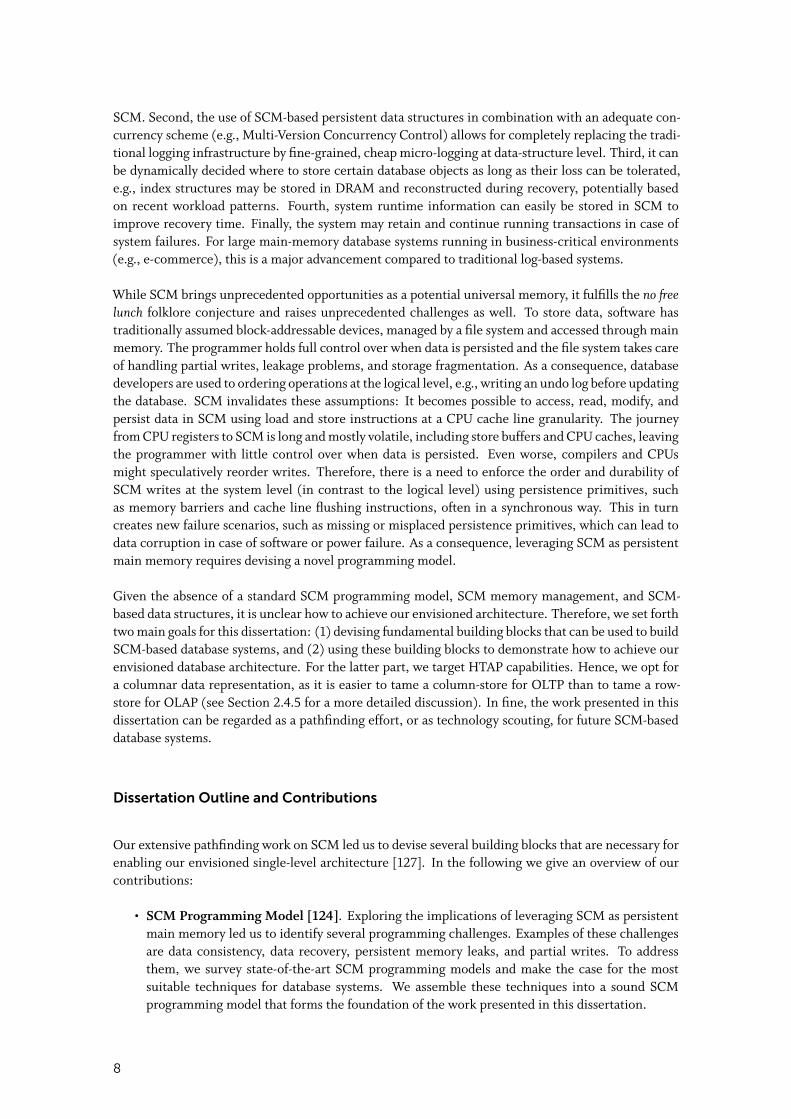
the same time. Given its byte-addressability and low latency, processors will be able to access SCM di-rectly with load/store semantics. Current file systems, such as ext4 Direct Access (DAX) [35], alreadysupport this access method by offering zero-copy memory mapping that bypasses DRAM and offersthe application layer direct access to SCM, as illustrated in Figure 1.2.
Two factors have traditionally spurred shifts in database architectures: new business needs, such as theneed for high transaction rates following the advent of the Internet, and – maybe more importantly– advancements in hardware technology [151]. In fact, we often find in the literature decades-oldresearch works that investigated database architectures that were reinvented decades later, mainlybecause hardware advancements empowered them. For instance, main-memory databases have beenresearched and recognized, as early as the 1980s, as superior in performance to disk-based counter-parts [34, 91, 47]. Nevertheless, it took until the late 2000s, and the advent of large main memorycapacities, before main-memory databases took off. SCM databases are no exception: They have beeninvestigated since the late 1980s [27, 2]. However, these works, as well as recent ones, leverage SCMto improve only the logging component as the main bottleneck for transaction processing. Neverthe-less, other components of the database do not benefit from SCM. In contrast, we argue that the twoingredients to trigger a rewrite of database systems are present: scaling up HTAP database systemsrepresents the business need, and SCM represents the advancement in hardware. Therefore, we en-deavor in this dissertation to explore a novel database architecture that leverages SCM as persistentmain memory.
Figure 1.3 outlines the move from a traditional database architecture towards our envisioned systemdesign. Due to the block-oriented nature of today’s non-volatile devices (e.g., hard disk or flash),both traditional disk-based and modern main-memory database systems rely on additional loggingand snapshotting components to efficiently guarantee consistency and durability. The demarcationline between transient memory and persistent storage is explicit, as illustrated on the left-hand sideof Figure 1.3. SCM, however, is byte-addressable and offers a latency close to that of DRAM. Thus, weenvision a novel main-memory database architecture that directly operates on SCM, eliminating theneed for explicit I/O. We anticipate that the performance gained by removing I/O will compensate forthe performance lost because of the higher latency of SCM. Still, we see the need to keep DRAM nextto SCM for performance-critical data structures, as illustrated on the right-hand side of Figure 1.3.
Our envisioned hybrid SCM-DRAM architecture allows for a radical change in the database archi-tecture: First, it eliminates the traditional recovery bottleneck of main-memory database systems,namely reloading data from storage to main memory, as data is discovered and accessed directly in
7
SCM. Second, the use of SCM-based persistent data structures in combination with an adequate con-currency scheme (e.g., Multi-Version Concurrency Control) allows for completely replacing the tradi-tional logging infrastructure by fine-grained, cheap micro-logging at data-structure level. Third, it canbe dynamically decided where to store certain database objects as long as their loss can be tolerated,e.g., index structures may be stored in DRAM and reconstructed during recovery, potentially basedon recent workload patterns. Fourth, system runtime information can easily be stored in SCM toimprove recovery time. Finally, the system may retain and continue running transactions in case ofsystem failures. For large main-memory database systems running in business-critical environments(e.g., e-commerce), this is a major advancement compared to traditional log-based systems.
While SCM brings unprecedented opportunities as a potential universal memory, it fulfills the no freelunch folklore conjecture and raises unprecedented challenges as well. To store data, software hastraditionally assumed block-addressable devices, managed by a file system and accessed through mainmemory. The programmer holds full control over when data is persisted and the file system takes careof handling partial writes, leakage problems, and storage fragmentation. As a consequence, databasedevelopers are used to ordering operations at the logical level, e.g., writing an undo log before updatingthe database. SCM invalidates these assumptions: It becomes possible to access, read, modify, andpersist data in SCM using load and store instructions at a CPU cache line granularity. The journeyfrom CPU registers to SCM is long and mostly volatile, including store buffers and CPU caches, leavingthe programmer with little control over when data is persisted. Even worse, compilers and CPUsmight speculatively reorder writes. Therefore, there is a need to enforce the order and durability ofSCM writes at the system level (in contrast to the logical level) using persistence primitives, suchas memory barriers and cache line flushing instructions, often in a synchronous way. This in turncreates new failure scenarios, such as missing or misplaced persistence primitives, which can lead todata corruption in case of software or power failure. As a consequence, leveraging SCM as persistentmain memory requires devising a novel programming model.
Given the absence of a standard SCM programming model, SCM memory management, and SCM-based data structures, it is unclear how to achieve our envisioned architecture. Therefore, we set forthtwo main goals for this dissertation: (1) devising fundamental building blocks that can be used to buildSCM-based database systems, and (2) using these building blocks to demonstrate how to achieve ourenvisioned database architecture. For the latter part, we target HTAP capabilities. Hence, we opt fora columnar data representation, as it is easier to tame a column-store for OLTP than to tame a row-store for OLAP (see Section 2.4.5 for a more detailed discussion). In fine, the work presented in thisdissertation can be regarded as a pathfinding effort, or as technology scouting, for future SCM-baseddatabase systems.
Dissertation Outline and Contributions
Our extensive pathfinding work on SCM led us to devise several building blocks that are necessary forenabling our envisioned single-level architecture [127]. In the following we give an overview of ourcontributions:
• SCM Programming Model [124]. Exploring the implications of leveraging SCM as persistentmain memory led us to identify several programming challenges. Examples of these challengesare data consistency, data recovery, persistent memory leaks, and partial writes. To addressthem, we survey state-of-the-art SCM programming models and make the case for the mostsuitable techniques for database systems. We assemble these techniques into a sound SCMprogramming model that forms the foundation of the work presented in this dissertation.
8
Chap
ter7
Test
ing
Fram
ewor
kfo
rSCM
-Ba
sed
Soft
war
e
Chap
ter3
SCM
Prog
ram
min
gM
odel
Chapter 3Persistent Memory Management
Chapter 4Persistent Data Structures
Chapter 5SCM-Optimized
Concurrency Control
Chapter 6Recovery Techniques
SOFORT
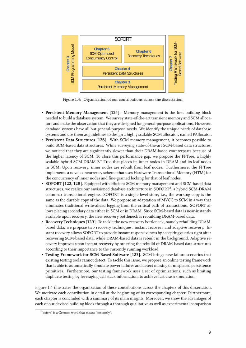
Figure 1.4: Organization of our contributions across the dissertation.
• Persistent Memory Management [124]. Memory management is the first building blockneeded to build a database system. We survey state-of-the-art transient memory and SCM alloca-tors and make the observation that they are designed for general-purpose applications. However,database systems have all but general-purpose needs. We identify the unique needs of databasesystems and use them as guidelines to design a highly scalable SCM allocator, named PAllocator.
• Persistent Data Structures [126]. With SCM memory management, it becomes possible tobuild SCM-based data structures. While surveying state-of-the-art SCM-based data structures,we noticed that they are significantly slower than their DRAM-based counterparts because ofthe higher latency of SCM. To close this performance gap, we propose the FPTree, a highlyscalable hybrid SCM-DRAM B+-Tree that places its inner nodes in DRAM and its leaf nodesin SCM. Upon recovery, inner nodes are rebuilt from leaf nodes. Furthermore, the FPTreeimplements a novel concurrency scheme that uses Hardware Transactional Memory (HTM) forthe concurrency of inner nodes and fine-grained locking for that of leaf nodes.
• SOFORT [122, 128]. Equipped with efficient SCM memory management and SCM-based datastructures, we realize our envisioned database architecture in SOFORT2, a hybrid SCM-DRAMcolumnar transactional engine. SOFORT is a single-level store, i.e., the working copy is thesame as the durable copy of the data. We propose an adaptation of MVCC to SCM in a way thateliminates traditional write-ahead logging from the critical path of transactions. SOFORT al-lows placing secondary data either in SCM or in DRAM. Since SCM-based data is near-instantlyavailable upon recovery, the new recovery bottleneck is rebuilding DRAM-based data.
• Recovery Techniques [129]. To tackle the new recovery bottleneck, namely rebuilding DRAM-based data, we propose two recovery techniques: instant recovery and adaptive recovery. In-stant recovery allows SOFORT to provide instant-responsiveness by accepting queries right afterrecovering SCM-based data, while DRAM-based data is rebuilt in the background. Adaptive re-covery improves upon instant recovery by ordering the rebuild of DRAM-based data structuresaccording to their importance to the currently running workload.
• Testing Framework for SCM-Based Software [123]. SCM brings new failure scenarios thatexisting testing tools cannot detect. To tackle this issue, we propose an online testing frameworkthat is able to automatically simulate power failures and detect missing or misplaced persistenceprimitives. Furthermore, our testing framework uses a set of optimizations, such as limitingduplicate testing by leveraging call stack information, to achieve fast crash simulation.
Figure 1.4 illustrates the organization of these contributions across the chapters of this dissertation.We motivate each contribution in detail at the beginning of its corresponding chapter. Furthermore,each chapter is concluded with a summary of its main insights. Moreover, we show the advantages ofeach of our devised building block through a thorough qualitative as well as experimental comparison
2“sofort” is a German word that means “instantly”.
9
with state-of-the-art competitors. In brief, our proposed building blocks can be used to build morecomplex systems, such as SOFORT, thereby paving the way for future database systems on SCM.
This dissertation is organized as follows: In Chapter 2 we elaborate on the characteristics of SCM, howto emulate it, and the performance implications of its higher latency. Then, we survey state-of-the-artdatabase research on SCM [125]. We conclude Chapter 2 by giving an overview of SOFORT and itsdifferent components, while contrasting its design decisions with those of state of the art. Thereafter,Chapter 3 details the programming challenges of SCM and explores how to solve them. Then, wedetail our SCM programming model and devise PAllocator, our highly scalable persistent memoryallocator. Next, in Chapter 4 we survey existing SCM-based data structures. Then, we present theFPTree, our hybrid SCM-DRAM B+-Tree. Afterwards, Chapter 5 demonstrates how we assemble ourdevised building blocks to build SOFORT. In particular, we elaborate on how we adapt MVCC to SCM.Furthermore, Chapter 6 presents SOFORT’s recovery techniques, namely instant recovery and adap-tive recovery. Later, we showcase in Chapter 7 our online testing framework for SCM-based software.Finally, Chapter 8 summarizes the contributions of this dissertation and presents an extended view onpromising future work directions. In particular, we present our vision on how to extend our work toaccount for hardware and media failures to achieve high availability by leveraging SCM and RemoteDirect Memory Access (RDMA).
10
2LEVERAGING SCM IN DATABASE SYSTEMS
S CM is emerging as a viable alternative to lift DRAM’s capacity limits. Since it exhibits charac-teristics of both storage and main memory, SCM can be architected in different ways: as main
memory extension, as disk-replacement, or as persistent main memory, i.e., as main memory andstorage at the same time. These unique properties enable several optimizations and architecturalenhancements for database systems. In this chapter we position our work with regards to state-of-the-art research on leveraging SCM in database systems. To do so, we first survey database optimizationopportunities enabled by SCM that were explored in the literature, starting from the most straightfor-ward ones to completely revising database architectures. Then, we highlight the gaps in state-of-the-art that our work ambitions to fill. We show that placing all data in SCM compromises performance,and argue instead for a hybrid SCM-DRAM architecture. While related works have mostly focused ontransactional row-store systems, we target hybrid analytical and transactional (HTAP) systems. In thiscontext, we propose SOFORT, a hybrid SCM-DRAM single-level columnar storage engine, designedfrom the ground up to explore the full potential of SCM.
This chapter is organized as follows: In Section 2.1 we present SCM, discussing how it can be inte-grated in the memory hierarchy, and exploring its performance implications with microbenchmarks.Since SCM is not available yet, we elaborate in Section 2.2 on practical ways to emulate its perfor-mance characteristics. Thereafter, Section 2.3 surveys state-of-the-art research on the use of SCM indatabase systems, with an emphasis on works that enhance database logging and storage architectures.Then, Section 2.4 positions our work with regards to related work and gives an overview of SOFORT.Finally, Section 2.5 summarizes this chapter.
2.1 STORAGE-CLASS MEMORY
Leon Chua predicted in the early 1970s the existence of the memristor [23], a fundamental circuitelement that is capable of storing and retaining a state variable. It the late 2000s, a team at HP Labsdiscovered the memristor in the form of Resistive RAM (RRAM) [50] [153]. It turned out that sev-eral works had already stumbled upon the memristor property, but they could not identify it as suchand deemed it an anomaly. Since then, several other memory technology candidates that exhibit thememristor property have been identified, e.g., Phase Change Memory (PCM) [87] and Spin Trans-fer Torque Magnetic RAM (STT-MRAM) [59]. In the industry, these novel memory technologies are
11
Parameter NAND DRAM PCM STT-RAM
Read Latency 25 µs 50 ns 50 ns 10 nsWrite Latency 500 µs 50 ns 500 ns 50 ns
Byte-addressable No Yes Yes YesEndurance 104–105 >1015 108–109 >1015
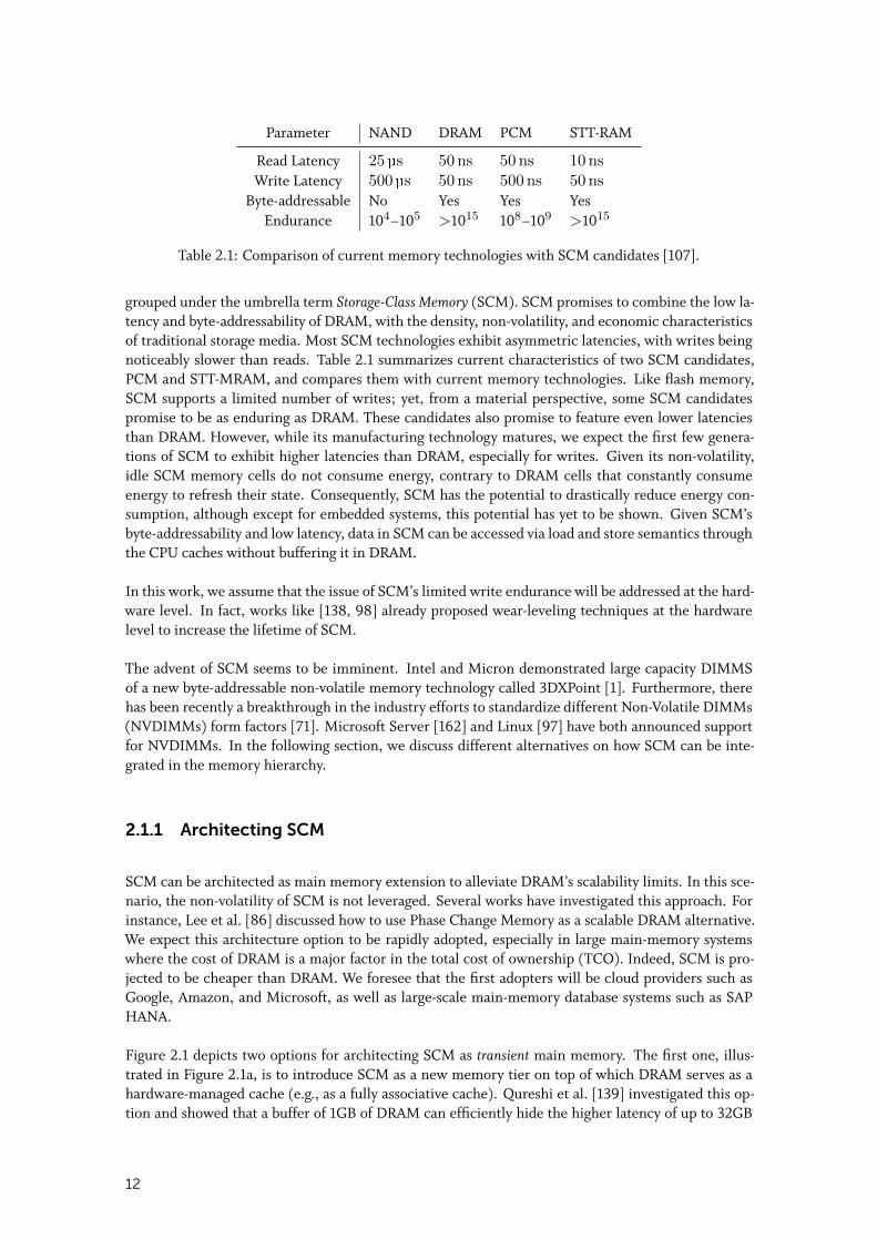
Table 2.1: Comparison of current memory technologies with SCM candidates [107].
grouped under the umbrella term Storage-Class Memory (SCM). SCM promises to combine the low la-tency and byte-addressability of DRAM, with the density, non-volatility, and economic characteristicsof traditional storage media. Most SCM technologies exhibit asymmetric latencies, with writes beingnoticeably slower than reads. Table 2.1 summarizes current characteristics of two SCM candidates,PCM and STT-MRAM, and compares them with current memory technologies. Like flash memory,SCM supports a limited number of writes; yet, from a material perspective, some SCM candidatespromise to be as enduring as DRAM. These candidates also promise to feature even lower latenciesthan DRAM. However, while its manufacturing technology matures, we expect the first few genera-tions of SCM to exhibit higher latencies than DRAM, especially for writes. Given its non-volatility,idle SCM memory cells do not consume energy, contrary to DRAM cells that constantly consumeenergy to refresh their state. Consequently, SCM has the potential to drastically reduce energy con-sumption, although except for embedded systems, this potential has yet to be shown. Given SCM’sbyte-addressability and low latency, data in SCM can be accessed via load and store semantics throughthe CPU caches without buffering it in DRAM.
In this work, we assume that the issue of SCM’s limited write endurance will be addressed at the hard-ware level. In fact, works like [138, 98] already proposed wear-leveling techniques at the hardwarelevel to increase the lifetime of SCM.
The advent of SCM seems to be imminent. Intel and Micron demonstrated large capacity DIMMSof a new byte-addressable non-volatile memory technology called 3DXPoint [1]. Furthermore, therehas been recently a breakthrough in the industry efforts to standardize different Non-Volatile DIMMs(NVDIMMs) form factors [71]. Microsoft Server [162] and Linux [97] have both announced supportfor NVDIMMs. In the following section, we discuss different alternatives on how SCM can be inte-grated in the memory hierarchy.
2.1.1 Architecting SCM
SCM can be architected as main memory extension to alleviate DRAM’s scalability limits. In this sce-nario, the non-volatility of SCM is not leveraged. Several works have investigated this approach. Forinstance, Lee et al. [86] discussed how to use Phase Change Memory as a scalable DRAM alternative.We expect this architecture option to be rapidly adopted, especially in large main-memory systemswhere the cost of DRAM is a major factor in the total cost of ownership (TCO). Indeed, SCM is pro-jected to be cheaper than DRAM. We foresee that the first adopters will be cloud providers such asGoogle, Amazon, and Microsoft, as well as large-scale main-memory database systems such as SAPHANA.
Figure 2.1 depicts two options for architecting SCM as transient main memory. The first one, illus-trated in Figure 2.1a, is to introduce SCM as a new memory tier on top of which DRAM serves as ahardware-managed cache (e.g., as a fully associative cache). Qureshi et al. [139] investigated this op-tion and showed that a buffer of 1GB of DRAM can efficiently hide the higher latency of up to 32GB
12
SCM
DRAM
Application
applicationaddress space
Virtual memory subsystem
(a) DRAM as hardware-managedcache for SCM
SCMDRAM
Application
applicationaddress space
Virtual memory subsystem
(b) SCM next to DRAM
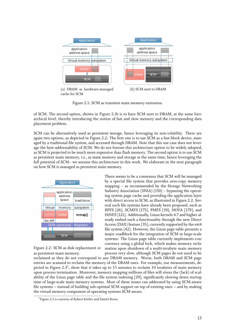
Figure 2.1: SCM as transient main memory extension.
of SCM. The second option, shown in Figure 2.1b is to have SCM next to DRAM, at the same hier-archical level, thereby introducing the notion of fast and slow memory and the corresponding dataplacement problem.
SCM can be alternatively used as persistent storage, hence leveraging its non-volatility. There areagain two options, as depicted in Figure 2.2: The first one is to use SCM as a fast block device, man-aged by a traditional file system, and accessed through DRAM. Note that this use case does not lever-age the byte-addressability of SCM. We do not foresee this architecture option to be widely adopted,as SCM is projected to be much more expensive than flash memory. The second option is to use SCMas persistent main memory, i.e., as main memory and storage at the same time, hence leveraging thefull potential of SCM– we assume this architecture in this work. We elaborate in the next paragraphon how SCM is managed as persistent main memory.
Application
SCM-optimized filesystem
applicationaddressspace
Virtual memory subsystem
mmap()
SCM
load/store
file API
DRAM
Figure 2.2: SCM as disk replacement oras persistent main memory.
There seems to be a consensus that SCM will be managedby a special file system that provides zero-copy memorymapping – as recommended by the Storage NetworkingIndustry Association (SNIA) [150] – bypassing the operat-ing system page cache and providing the application layerwith direct access to SCM, as illustrated in Figure 2.2. Sev-eral such file systems have already been proposed, such asBPFS [26], SCMFS [175], PMFS [39], NOVA [179], andHiNFS [121]. Additionally, Linux kernels 4.7 and higher al-ready embed such a functionality through the new DirectAccess (DAX) feature [35], currently supported by the ext4file system [42]. However, the Linux page table presents amajor roadblock for the integration of SCM in large-scalesystems: The Linux page table currently implements con-currency using a global lock, which makes memory recla-mation upon shutdown of a multi-terabyte main memoryprocess very slow, although SCM pages do not need to be
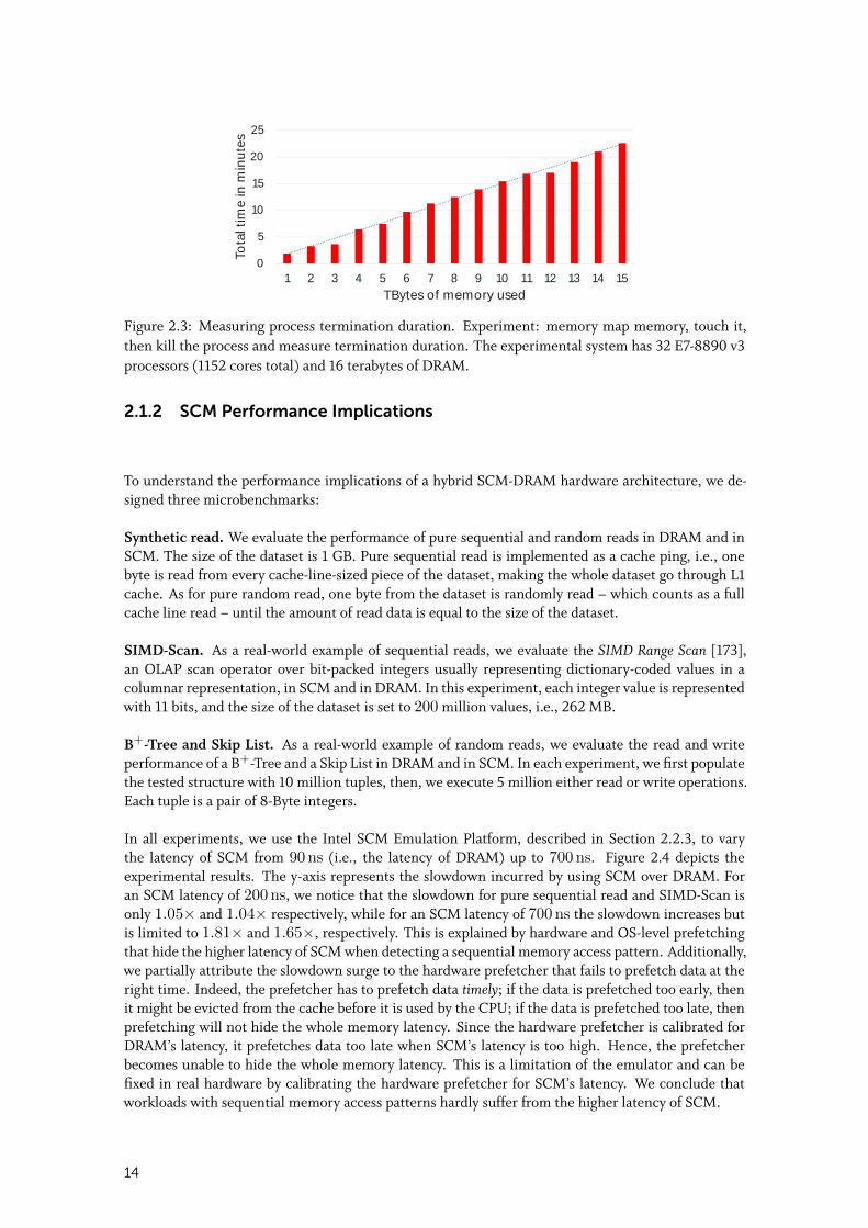
reclaimed as they do not correspond to any DRAM memory. Worse, both DRAM and SCM pageentries are scanned to reclaim the memory of the DRAM ones. For example, our measurements, de-picted in Figure 2.31, show that it takes up to 15 minutes to reclaim 10 terabytes of main memoryupon process termination. Moreover, memory mapping millions of files will stress the (lack) of scal-ability of the Linux page table and the file system indexing [29], significantly slowing down startuptime of large-scale main memory systems. Most of these issues can addressed by using SCM-awarefile systems – instead of building sub-optimal SCM support on top of existing ones – and by makingthe virtual memory component of operating systems SCM-aware.
1Figure 2.3 is courtesy of Robert Kettler and Daniel Booss.
13
0
5
10
15
20
25
1 2 3 4 5 6 7 8 9 10 11 12 13 14 15
Tota
ltim
ein
min
ute
s
TBytes of memory used
Figure 2.3: Measuring process termination duration. Experiment: memory map memory, touch it,then kill the process and measure termination duration. The experimental system has 32 E7-8890 v3processors (1152 cores total) and 16 terabytes of DRAM.
2.1.2 SCM Performance Implications
To understand the performance implications of a hybrid SCM-DRAM hardware architecture, we de-signed three microbenchmarks:
Synthetic read. We evaluate the performance of pure sequential and random reads in DRAM and inSCM. The size of the dataset is 1 GB. Pure sequential read is implemented as a cache ping, i.e., onebyte is read from every cache-line-sized piece of the dataset, making the whole dataset go through L1cache. As for pure random read, one byte from the dataset is randomly read – which counts as a fullcache line read – until the amount of read data is equal to the size of the dataset.
SIMD-Scan. As a real-world example of sequential reads, we evaluate the SIMD Range Scan [173],an OLAP scan operator over bit-packed integers usually representing dictionary-coded values in acolumnar representation, in SCM and in DRAM. In this experiment, each integer value is representedwith 11 bits, and the size of the dataset is set to 200 million values, i.e., 262 MB.
B+-Tree and Skip List. As a real-world example of random reads, we evaluate the read and writeperformance of a B+-Tree and a Skip List in DRAM and in SCM. In each experiment, we first populatethe tested structure with 10 million tuples, then, we execute 5 million either read or write operations.Each tuple is a pair of 8-Byte integers.
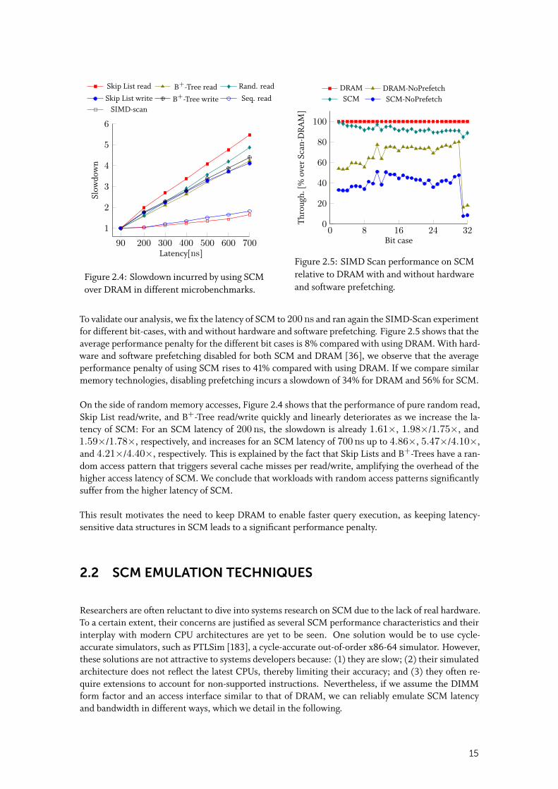
In all experiments, we use the Intel SCM Emulation Platform, described in Section 2.2.3, to varythe latency of SCM from 90 ns (i.e., the latency of DRAM) up to 700 ns. Figure 2.4 depicts theexperimental results. The y-axis represents the slowdown incurred by using SCM over DRAM. Foran SCM latency of 200 ns, we notice that the slowdown for pure sequential read and SIMD-Scan isonly 1.05× and 1.04× respectively, while for an SCM latency of 700 ns the slowdown increases butis limited to 1.81× and 1.65×, respectively. This is explained by hardware and OS-level prefetchingthat hide the higher latency of SCM when detecting a sequential memory access pattern. Additionally,we partially attribute the slowdown surge to the hardware prefetcher that fails to prefetch data at theright time. Indeed, the prefetcher has to prefetch data timely; if the data is prefetched too early, thenit might be evicted from the cache before it is used by the CPU; if the data is prefetched too late, thenprefetching will not hide the whole memory latency. Since the hardware prefetcher is calibrated forDRAM’s latency, it prefetches data too late when SCM’s latency is too high. Hence, the prefetcherbecomes unable to hide the whole memory latency. This is a limitation of the emulator and can befixed in real hardware by calibrating the hardware prefetcher for SCM’s latency. We conclude thatworkloads with sequential memory access patterns hardly suffer from the higher latency of SCM.
14
Skip List read B+-Tree read Rand. read
Skip List write B+-Tree write Seq. readSIMD-scan
90 200 300 400 500 600 700
1
2
3
4
5
6
Latency[ns]
Slow
dow
n
Figure 2.4: Slowdown incurred by using SCMover DRAM in different microbenchmarks.
DRAM DRAM-NoPrefetchSCM SCM-NoPrefetch
0 8 16 24 320
20
40
60
80
100
Bit case
Thro
ugh.
[%ov
erSc
an-D
RA
M]
Figure 2.5: SIMD Scan performance on SCMrelative to DRAM with and without hardwareand software prefetching.
To validate our analysis, we fix the latency of SCM to 200 ns and ran again the SIMD-Scan experimentfor different bit-cases, with and without hardware and software prefetching. Figure 2.5 shows that theaverage performance penalty for the different bit cases is 8% compared with using DRAM. With hard-ware and software prefetching disabled for both SCM and DRAM [36], we observe that the averageperformance penalty of using SCM rises to 41% compared with using DRAM. If we compare similarmemory technologies, disabling prefetching incurs a slowdown of 34% for DRAM and 56% for SCM.
On the side of random memory accesses, Figure 2.4 shows that the performance of pure random read,Skip List read/write, and B+-Tree read/write quickly and linearly deteriorates as we increase the la-tency of SCM: For an SCM latency of 200 ns, the slowdown is already 1.61×, 1.98×/1.75×, and1.59×/1.78×, respectively, and increases for an SCM latency of 700 ns up to 4.86×, 5.47×/4.10×,and 4.21×/4.40×, respectively. This is explained by the fact that Skip Lists and B+-Trees have a ran-dom access pattern that triggers several cache misses per read/write, amplifying the overhead of thehigher access latency of SCM. We conclude that workloads with random access patterns significantlysuffer from the higher latency of SCM.
This result motivates the need to keep DRAM to enable faster query execution, as keeping latency-sensitive data structures in SCM leads to a significant performance penalty.
2.2 SCM EMULATION TECHNIQUES
Researchers are often reluctant to dive into systems research on SCM due to the lack of real hardware.To a certain extent, their concerns are justified as several SCM performance characteristics and theirinterplay with modern CPU architectures are yet to be seen. One solution would be to use cycle-accurate simulators, such as PTLSim [183], a cycle-accurate out-of-order x86-64 simulator. However,these solutions are not attractive to systems developers because: (1) they are slow; (2) their simulatedarchitecture does not reflect the latest CPUs, thereby limiting their accuracy; and (3) they often re-quire extensions to account for non-supported instructions. Nevertheless, if we assume the DIMMform factor and an access interface similar to that of DRAM, we can reliably emulate SCM latencyand bandwidth in different ways, which we detail in the following.
15
Socket 1
C1 C2
C3 C4
Socket 2
C1 C2
C3 C4Interconnect
DRAM DRAM
Bind applicationto socket 1
Memory ofsocket 2 as
emulated SCMSCM
Higher latency, lower bandwidth
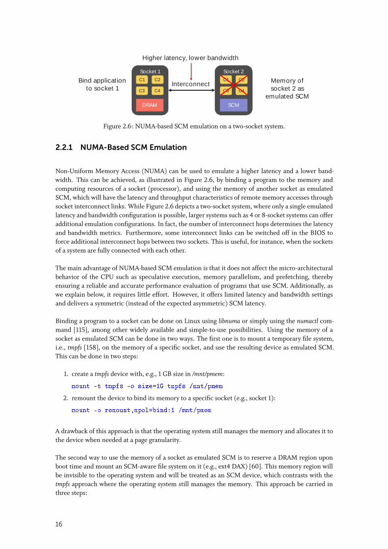
Figure 2.6: NUMA-based SCM emulation on a two-socket system.
2.2.1 NUMA-Based SCM Emulation
Non-Uniform Memory Access (NUMA) can be used to emulate a higher latency and a lower band-width. This can be achieved, as illustrated in Figure 2.6, by binding a program to the memory andcomputing resources of a socket (processor), and using the memory of another socket as emulatedSCM, which will have the latency and throughput characteristics of remote memory accesses throughsocket interconnect links. While Figure 2.6 depicts a two-socket system, where only a single emulatedlatency and bandwidth configuration is possible, larger systems such as 4 or 8-socket systems can offeradditional emulation configurations. In fact, the number of interconnect hops determines the latencyand bandwidth metrics. Furthermore, some interconnect links can be switched off in the BIOS toforce additional interconnect hops between two sockets. This is useful, for instance, when the socketsof a system are fully connected with each other.
The main advantage of NUMA-based SCM emulation is that it does not affect the micro-architecturalbehavior of the CPU such as speculative execution, memory parallelism, and prefetching, therebyensuring a reliable and accurate performance evaluation of programs that use SCM. Additionally, aswe explain below, it requires little effort. However, it offers limited latency and bandwidth settingsand delivers a symmetric (instead of the expected asymmetric) SCM latency.
Binding a program to a socket can be done on Linux using libnuma or simply using the numactl com-mand [115], among other widely available and simple-to-use possibilities. Using the memory of asocket as emulated SCM can be done in two ways. The first one is to mount a temporary file system,i.e., tmpfs [158], on the memory of a specific socket, and use the resulting device as emulated SCM.This can be done in two steps:
1. create a tmpfs device with, e.g., 1 GB size in /mnt/pmem:
mount �t tmpfs �o size=1G tmpfs /mnt/pmem
2. remount the device to bind its memory to a specific socket (e.g., socket 1):
mount -o remount,mpol=bind:1 /mnt/pmem
A drawback of this approach is that the operating system still manages the memory and allocates it tothe device when needed at a page granularity.
The second way to use the memory of a socket as emulated SCM is to reserve a DRAM region uponboot time and mount an SCM-aware file system on it (e.g., ext4 DAX) [60]. This memory region willbe invisible to the operating system and will be treated as an SCM device, which contrasts with thetmpfs approach where the operating system still manages the memory. This approach be carried inthree steps:
16
• reserve a DRAM region using the memmap kernel boot parameter. For example, to reserve32 GB starting from physical address 64 GB, the parameter is:
memmap=32G!64G
• format the resulting SCM device to a file system format that supports DAX, e.g., ext4:
mkfs.ext4 /dev/pmem0
• mount the device with the DAX option:
mount �o dax /dev/pmem0 /mnt/pmem
In summary, NUMA-based SCM emulation is easy to use and requires little effort.
2.2.2 Quartz
Quartz [167] is a DRAM-based, software-based SCM performance emulator that leverages existinghardware features to emulate different latency and bandwidth characteristics. Instead of injecting de-lays to every single SCM access, which the authors argue is infeasible in software without a significantoverhead, Quartz models the average application perceived latency by injecting delays at boundariesof epochs. An epoch has a fixed time duration upon which hardware performance counters are read.A delay is then introduced based on the number of stalled cycles induced by references to SCM. Thedelay is computed as follows:
Delay = (Stalled cycles / Average latency) X latency differential
Time
DelayEpoch duration
Hence, Quartz can vary the emulated latency of SCM by changing the latency differential betweenDRAM and SCM in the formula above. The authors evaluated the emulation accuracy of Quartz bycomparing it with NUMA-based emulation and reported an error rate no higher than 9%. Quartz canemulate either a system with only SCM, or a system with fast memory (DRAM) and slow memory(SCM). The latter is achieved by combining Quartz with NUMA-based emulation; Quartz would adddelays that correspond to only remote memory accesses, which can be quantified by means of hard-ware performance counters.
Quartz consists of two parts: a user-mode dynamic library that manages epochs, and a kernel modulethat manages performance counters. Using Quartz is as easy as pre-loading the user-mode, which willregister the threads of the program and manage delay injection. To sum up, Quartz has the advan-tage of relying counters available in commodity hardware and offering a wide range of latency andbandwidth setting. However, it might interfere with the micro-architectural behavior of the proces-sor, emulates a symmetric SCM latency, and is less accurate than NUMA-based emulation. HP hasrecently open-sourced Quartz [136], enabling its adoption by some works [90].
2.2.3 Intel SCM Emulation Platform
Intel has made available an SCM emulation platform [38] to several academic and industry partners,and many publications have already used it [39, 122, 6]. It is equipped with four Intel Xeon E5
17
Socket 0
DRAM DRAMSCM
CPU (8 cores) CPU (8 cores)
Socket 1QPI
Memory Channels
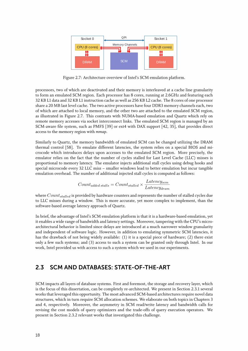
Figure 2.7: Architecture overview of Intel’s SCM emulation platform.
processors, two of which are deactivated and their memory is interleaved at a cache line granularityto form an emulated SCM region. Each processor has 8 cores, running at 2.6GHz and featuring each32 KB L1 data and 32 KB L1 instruction cache as well as 256 KB L2 cache. The 8 cores of one processorshare a 20 MB last level cache. The two active processors have four DDR3 memory channels each, twoof which are attached to local memory, and the other two are attached to the emulated SCM region,as illustrated in Figure 2.7. This contrasts with NUMA-based emulation and Quartz which rely onremote memory accesses via socket interconnect links. The emulated SCM region is managed by anSCM-aware file system, such as PMFS [39] or ext4 with DAX support [42, 35], that provides directaccess to the memory region with mmap.
Similarly to Quartz, the memory bandwidth of emulated SCM can be changed utilizing the DRAMthermal control [58]. To emulate different latencies, the system relies on a special BIOS and mi-crocode which introduces delays upon accesses to the emulated SCM region. More precisely, theemulator relies on the fact that the number of cycles stalled for Last Level Cache (LLC) misses isproportional to memory latency. The emulator injects additional stall cycles using debug hooks andspecial microcode every 32 LLC miss – smaller windows lead to better emulation but incur tangibleemulation overhead. The number of additional injected stall cycles is computed as follows:
Countadded stalls = Countstalled ×LatencyscmLatencydram
where Countstalled is provided by hardware counters and represents the number of stalled cycles dueto LLC misses during a window. This is more accurate, yet more complex to implement, than thesoftware-based average latency approach of Quartz.
In brief, the advantage of Intel’s SCM emulation platform is that it is a hardware-based emulation, yetit enables a wide range of bandwidth and latency settings. Moreover, tampering with the CPU’s micro-architectural behavior is limited since delays are introduced at a much narrower window granularityand independent of software logic. However, in addition to emulating symmetric SCM latencies, ithas the drawback of not being widely available: (1) it is a special piece of hardware; (2) there existonly a few such systems; and (3) access to such a system can be granted only through Intel. In ourwork, Intel provided us with access to such a system which we used in our experiments.
2.3 SCM AND DATABASES: STATE-OF-THE-ART
SCM impacts all layers of database systems. First and foremost, the storage and recovery layer, whichis the focus of this dissertation, can be completely re-architected. We present in Section 2.3.1 severalworks that leveraged this opportunity. The most advanced SCM-based architectures require novel datastructures, which in turn require SCM allocation schemes. We elaborate on both topics in Chapters 3and 4, respectively. Moreover, the asymmetry in SCM read/write latency and bandwidth calls forrevising the cost models of query optimizers and the trade-offs of query execution operators. Wepresent in Section 2.3.2 relevant works that investigated this challenge.
18
Transactions
DRAM
Data Cache Centra-lizedLog
Buffer
HDDs/SSDs
Data Files Log Files
Secondary Data
Primary Data
Data accessvia DRAM
Log written todisk via DRAM
Figure 2.8: Traditional database architecture.
2.3.1 Storage and Recovery
In this section we discuss optimization opportunities brought by SCM to database storage and recov-ery architecture. We classify related work into two categories: (1) works that focus solely on improv-ing the logging infrastructure using SCM; and (2) works that go further and propose to re-architectdatabase storage and logging using SCM.
Traditional database architecture
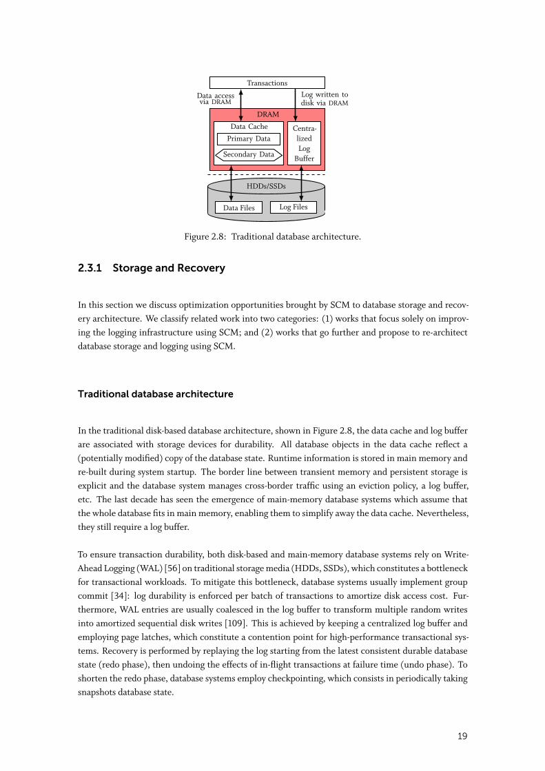
In the traditional disk-based database architecture, shown in Figure 2.8, the data cache and log bufferare associated with storage devices for durability. All database objects in the data cache reflect a(potentially modified) copy of the database state. Runtime information is stored in main memory andre-built during system startup. The border line between transient memory and persistent storage isexplicit and the database system manages cross-border traffic using an eviction policy, a log buffer,etc. The last decade has seen the emergence of main-memory database systems which assume thatthe whole database fits in main memory, enabling them to simplify away the data cache. Nevertheless,they still require a log buffer.
To ensure transaction durability, both disk-based and main-memory database systems rely on Write-Ahead Logging (WAL) [56] on traditional storage media (HDDs, SSDs), which constitutes a bottleneckfor transactional workloads. To mitigate this bottleneck, database systems usually implement groupcommit [34]: log durability is enforced per batch of transactions to amortize disk access cost. Fur-thermore, WAL entries are usually coalesced in the log buffer to transform multiple random writesinto amortized sequential disk writes [109]. This is achieved by keeping a centralized log buffer andemploying page latches, which constitute a contention point for high-performance transactional sys-tems. Recovery is performed by replaying the log starting from the latest consistent durable databasestate (redo phase), then undoing the effects of in-flight transactions at failure time (undo phase). Toshorten the redo phase, database systems employ checkpointing, which consists in periodically takingsnapshots database state.
19
Improving the logging infrastructure using SCM
SCM-based database systems have been investigated as early as in the 1980s. For instance, Copelandet al. [27] made the observation that a system with battery-backed DRAM – an economically viabletechnology at the time – would allow to remove disk I/O from the critical path of transactions, therebyalleviating the need for group commit [34] and reducing transaction latencies. Agrawal et al. [2] inves-tigated database recovery algorithms assuming a back-then hypothetical non-volatile main-memorysystem. While using two-phase locking for concurrency control, they devised optimized recoveryalgorithms for both page locking and record locking schemes. While these works only look at howto optimize existing logging and recovery algorithms in presence of non-volatile main memory in anon-disruptive way, Copeland et al. [27] recognize the possibility of devising novel counterparts.
The advent of SCM has spurred a renewed interest in non-volatile main memory database systems.Fang et al. [43] were the first to introduce SCM in the database architecture. They propose to placethe database log, access it, and update it directly in SCM, which simplifies the log architecture sincethe log buffer is not required anymore. The log can be asynchronously written to disk for archivalpurposes. This architecture has two advantages: (1) As Copeland et al. [27] previously observed,group commit is not needed anymore, because SCM is several orders of magnitude faster than disks;and (2) transaction logs are traditionally grouped in contiguous pages to amortize disk access, whichnecessitates the use of page latches; being a random-access, byte-addressable memory, SCM alleviatesthis constraint, making log page latches unnecessary. These two advantages result in lower transactionlatencies and higher transaction throughput.
Gao et al. [46] propose to use SCM as a new, persistent buffering layer between main memory anddisks. They introduce PCMLogging, a new logging scheme that integrates implicit logs into modifiedpages. PCMLogging flushes the modified pages of a transaction from main memory to SCM uponcommit, which ensures that the database state is always up-to-date. Therefore, checkpointing is notrequired anymore. However, undoing the effects of unfinished transactions during recovery is stillneeded. Indeed, a full main memory cache might need to flush modified pages to SCM. To handlethis case, PCMLogging keeps in SCM a list of all running transactions and their respective modifiedpages that were flushed to SCM. To provide undo capabilities, PCMLogging writes flushed pages out-of-place in SCM. Recovery is performed by scanning the pages in SCM, retrieving their transactionID, and rolling back the ones modified by in-flight transaction at failure time. We argue that, contraryto Fang et al. [43], PCMLogging introduces additional complexity in durability management and doesnot leverage the byte-addressability of SCM. Additionally, the authors compare PCMLogging only to atraditional database architecture with emulated PCM as main memory, which does not allow to drawcompelling conclusions.
Wang et al. [170] make the observation that while distributed logging has been historically a no-gofor single node systems because of I/O overheads, the characteristics of SCM make it relevant formulti-socket systems. Hence, they propose a distributed logging scheme that maintains one SCM logbuffer per socket, thereby relieving log contention. A log object is considered durable as soon as itis written to the SCM log buffer. When the latter becomes full, it is flushed to disk. The authorsinvestigate two flavors of distributed logging: page-level and transaction-level log space partitioning.In page-level log space partitioning, a transaction can write log records to any log partition, whichmight incur expensive remote memory accesses. Additionally, transactions lose access to the previousLog Sequence Number (LSN) of each log record, because LSNs are bound to a single log partition.This compromises the ability of a transaction to undo its changes when it aborts. To remedy thisproblem, the authors propose to keep a private DRAM undo buffer per transaction. In transaction-level log space partitioning, transactions write log records only to their local log partition. This posesan issue during recovery as the order of log records per page is lost, thereby compromising the redoand undo phases. To solve this issue, the authors propose to uniquely identify log records using global
20
sequence numbers (GSNs) based on a logical clock [82] for each page, transaction, and log record. Theorder of log records can therefore be established during the log analysis phase of recovery.
SCM log buffers are marked as write-combining, meaning that read and write operations to SCMbypass the CPU cache. Writes are lazily drained from the write-combining buffers to SCM. Therefore,it is necessary to employ memory fences which (among other things) drain the contents of the write-combining buffers. Nevertheless, a memory fence drains the buffers of only its local core, whichposes a challenge for transaction commit. Indeed, before committing, a transaction must ensure thepersistence of all its log records, in addition to all log records that logically precede them. To solvethis problem, the authors introduce passive group commit. The general idea is as follows: (1) everycommitting transaction issues a memory fence and updates a variable (dgsn) in its working thread toits GSN; (2) committing transactions are registered into a group commit queue; and (3) a daemonfetches the smallest dgsn across working threads (i.e., the upper bound GSN of persisted log records)and dequeues any transaction that has a GSN smaller than this minimum. Following an empiricalevaluation, the authors conclude that transaction-level log space partitioning is more promising thatthe page-level counterpart.
Huang et al. [62] focus on the most cost-effective use of SCM. Since SCM will be more expensivethan disks, they propose to restrict the use of SCM to the database log, which is the main bottleneckfor OLTP systems. Doing so shifts the logging bottleneck from I/O to software overheads, mainlyincurred by contention on the centralized log buffer. Therefore, the authors propose NV-logging, aper-transaction decentralized logging scheme. Basically, transactions keep private logs in the form ofa linked-list of transaction objects. Log objects are first constructed in DRAM, then flushed to a globalcircular log index, which is truncated upon checkpointing. A global counter is used to generate LSNs.The internal structure of log objects is similar to that of ARIES [109], except that NV-logging keepsa backward pointer instead of keeping the LSN of the previous log object. The recovery procedurefollows the ARIES protocol. While the authors claim that NV-logging is the most cost-effective use ofSCM in OLTP systems, it misses out on the opportunity of introducing SCM in the main-memorylayer, SCM being projected to be cheaper than DRAM.
Re-architecting database storage and logging using SCM
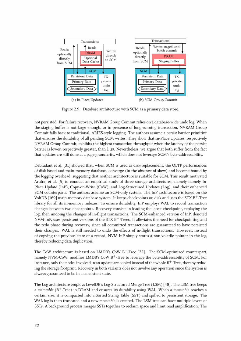
While the logging component might be a target of choice for SCM in the short term, SCM can spura more radical change in database architecture. For instance, Pelley et al. [133] investigated threearchitecture alternatives for SCM in database systems. The first one is to use SCM as a drop-in diskreplacement, which enables near-instantaneous recovery since dirty pages can be flushed at a highrate, significantly reducing the redo phase during recovery. However, this architecture retains all thesoftware complexity introduced to amortize costly disk I/O. The second architecture option, denotedIn-Place Updates and illustrated in Figure 2.9a, assumes that SCM reads are optionally performedthrough a software-managed DRAM cache, while writes are performed directly to SCM. The central-ized log that keeps a total order of updates is not needed anymore: Undo logs are distributed pertransaction (i.e., each transaction keeps a private log), which is possible since in-flight transactionsmodify mutually exclusive sets of pages. In-Place Updates completely removes redo logging and pageflushing, but it is highly sensitive to the latency of SCM writes.
To lift this shortcoming, the authors introduced a third architecture option, named NVRAM groupcommit. It executes transactions in batches, which are then either all committed or aborted. Thechanges of a transaction batch are buffered in a DRAM staging buffer and flushed to SCM upon com-mit, as depicted in Figure 2.9b. Aborting batches can undo their changes in the staging buffer byleveraging the transactions’ private undo logs. Note that, in contrast to in-place updates, these logs are
21
DRAM
Transactions
SCM
Persistent Data TX-privateundologSecondary Data
Primary Data
OptionalData Cache
Readsoptionally
directlyfrom SCM
ReadsWritesdirectlyto SCM
(a) In-Place Updates
DRAMStaging Buffer
Transactions
SCM
Persistent Data TX-privateundologSecondary Data
Primary Data
Readsoptionally
directlyfrom SCM
Writes staged untilbatch commit
(b) SCM-Group Commit
Figure 2.9: Database architecture with SCM as a primary data store.
not persisted. For failure recovery, NVRAM Group Commit relies on a database-wide undo log. Whenthe staging buffer is not large enough, or in presence of long-running transaction, NVRAM GroupCommit falls back to traditional, ARIES-style logging. The authors assume a persist barrier primitivethat ensures the durability of all pending SCM writes. They show that In-Place Updates, respectivelyNVRAM Group Commit, exhibits the highest transaction throughput when the latency of the persistbarrier is lower, respectively greater, than 1 µs. Nevertheless, we argue that both suffer from the factthat updates are still done at a page granularity, which does not leverage SCM’s byte-addressability.
Debradant et al. [31] showed that, when SCM is used as disk-replacement, the OLTP performancesof disk-based and main-memory databases converge (in the absence of skew) and become bound bythe logging overhead, suggesting that neither architecture is suitable for SCM. This result motivatedArulraj et al. [5] to conduct an empirical study of three storage architectures, namely namely In-Place Update (InP), Copy-on-Write (CoW), and Log-Structured Updates (Log), and their enhancedSCM counterparts. The authors assume an SCM-only system. The InP architecture is based on theVoltDB [169] main-memory database system. It keeps checkpoints on disk and uses the STX B+-Treelibrary for all its in-memory indexes. To ensure durability, InP employs WAL to record transactionchanges between two checkpoints. Recovery consists in loading the latest checkpoint, replaying thelog, then undoing the changes of in-flight transactions. The SCM-enhanced version of InP, denotedNVM-InP, uses persistent versions of the STX B+-Trees. It alleviates the need for checkpointing andthe redo phase during recovery, since all committed transactions are guaranteed to have persistedtheir changes. WAL is still needed to undo the effects of in-flight transactions. However, insteadof copying the previous state of a record, NVM-InP simply stores a non-volatile pointer in the log,thereby reducing data duplication.
The CoW architecture is based on LMDB’s CoW B+-Tree [22]. The SCM-optimized counterpart,namely NVM-CoW, modifies LMDB’s CoW B+-Tree to leverage the byte-addressability of SCM. Forinstance, only the nodes involved in an update are copied instead of the whole B+-Tree, thereby reduc-ing the storage footprint. Recovery in both variants does not involve any operation since the system isalways guaranteed to be in a consistent state.
The Log architecture employs LevelDB’s Log-Structured Merge Tree (LSM) [48]. The LSM tree keepsa memtable (B+-Tree) in DRAM and ensures its durability using WAL. When a memtable reaches acertain size, it is compacted into a Sorted String Table (SST) and spilled to persistent storage. TheWAL log is then truncated and a new memtable is created. The LSM tree can have multiple layers ofSSTs. A background process merges SSTs together to reclaim space and limit read amplification. The
22
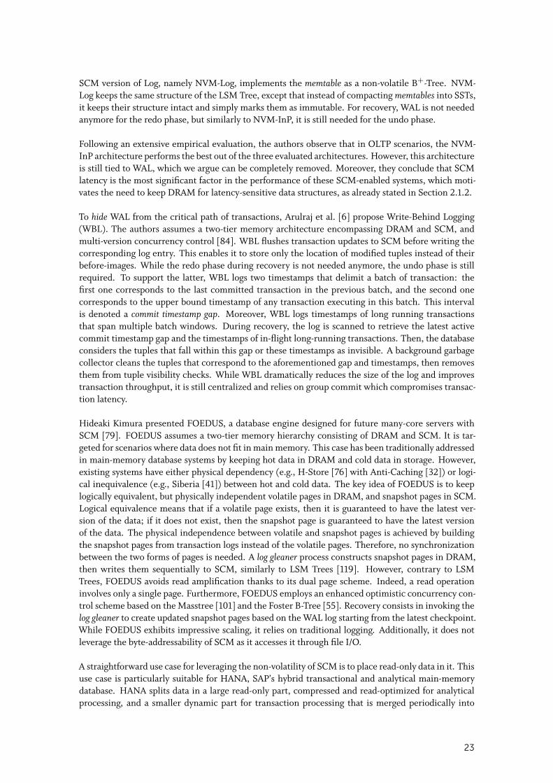
SCM version of Log, namely NVM-Log, implements the memtable as a non-volatile B+-Tree. NVM-Log keeps the same structure of the LSM Tree, except that instead of compacting memtables into SSTs,it keeps their structure intact and simply marks them as immutable. For recovery, WAL is not neededanymore for the redo phase, but similarly to NVM-InP, it is still needed for the undo phase.
Following an extensive empirical evaluation, the authors observe that in OLTP scenarios, the NVM-InP architecture performs the best out of the three evaluated architectures. However, this architectureis still tied to WAL, which we argue can be completely removed. Moreover, they conclude that SCMlatency is the most significant factor in the performance of these SCM-enabled systems, which moti-vates the need to keep DRAM for latency-sensitive data structures, as already stated in Section 2.1.2.
To hide WAL from the critical path of transactions, Arulraj et al. [6] propose Write-Behind Logging(WBL). The authors assumes a two-tier memory architecture encompassing DRAM and SCM, andmulti-version concurrency control [84]. WBL flushes transaction updates to SCM before writing thecorresponding log entry. This enables it to store only the location of modified tuples instead of theirbefore-images. While the redo phase during recovery is not needed anymore, the undo phase is stillrequired. To support the latter, WBL logs two timestamps that delimit a batch of transaction: thefirst one corresponds to the last committed transaction in the previous batch, and the second onecorresponds to the upper bound timestamp of any transaction executing in this batch. This intervalis denoted a commit timestamp gap. Moreover, WBL logs timestamps of long running transactionsthat span multiple batch windows. During recovery, the log is scanned to retrieve the latest activecommit timestamp gap and the timestamps of in-flight long-running transactions. Then, the databaseconsiders the tuples that fall within this gap or these timestamps as invisible. A background garbagecollector cleans the tuples that correspond to the aforementioned gap and timestamps, then removesthem from tuple visibility checks. While WBL dramatically reduces the size of the log and improvestransaction throughput, it is still centralized and relies on group commit which compromises transac-tion latency.
Hideaki Kimura presented FOEDUS, a database engine designed for future many-core servers withSCM [79]. FOEDUS assumes a two-tier memory hierarchy consisting of DRAM and SCM. It is tar-geted for scenarios where data does not fit in main memory. This case has been traditionally addressedin main-memory database systems by keeping hot data in DRAM and cold data in storage. However,existing systems have either physical dependency (e.g., H-Store [76] with Anti-Caching [32]) or logi-cal inequivalence (e.g., Siberia [41]) between hot and cold data. The key idea of FOEDUS is to keeplogically equivalent, but physically independent volatile pages in DRAM, and snapshot pages in SCM.Logical equivalence means that if a volatile page exists, then it is guaranteed to have the latest ver-sion of the data; if it does not exist, then the snapshot page is guaranteed to have the latest versionof the data. The physical independence between volatile and snapshot pages is achieved by buildingthe snapshot pages from transaction logs instead of the volatile pages. Therefore, no synchronizationbetween the two forms of pages is needed. A log gleaner process constructs snapshot pages in DRAM,then writes them sequentially to SCM, similarly to LSM Trees [119]. However, contrary to LSMTrees, FOEDUS avoids read amplification thanks to its dual page scheme. Indeed, a read operationinvolves only a single page. Furthermore, FOEDUS employs an enhanced optimistic concurrency con-trol scheme based on the Masstree [101] and the Foster B-Tree [55]. Recovery consists in invoking thelog gleaner to create updated snapshot pages based on the WAL log starting from the latest checkpoint.While FOEDUS exhibits impressive scaling, it relies on traditional logging. Additionally, it does notleverage the byte-addressability of SCM as it accesses it through file I/O.
A straightforward use case for leveraging the non-volatility of SCM is to place read-only data in it. Thisuse case is particularly suitable for HANA, SAP’s hybrid transactional and analytical main-memorydatabase. HANA splits data in a large read-only part, compressed and read-optimized for analyticalprocessing, and a smaller dynamic part for transaction processing that is merged periodically into
23
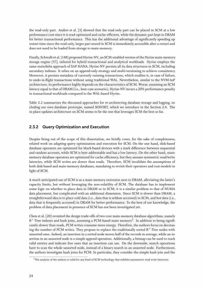
the read-only part. Andrei et al. [3] showed that the read-only part can be placed in SCM at a lowperformance cost since it is read-optimized and cache-efficient, while the dynamic part kept in DRAMfor better transactional performance. This has the additional advantage of significantly speeding uprestart time since the read-only, larger part stored in SCM is immediately accessible after a restart anddoes not need to be loaded from storage to main memory.
Finally, Schwalb et al. [148] proposed Hyrise-NV, an SCM-enabled version of the Hyrise main-memorystorage engine [57], tailored for hybrid transactional and analytical workloads. Hyrise employs thesame main/delta approach of SAP HANA. Hyrise-NV persists all its data structures in SCM, includingsecondary indexes. It relies on an append-only strategy and multi-versioning to achieve consistency.Moreover, it persists metadata of currently running transactions, which enables it, in case of failure,to undo in-flight transactions without using traditional WAL. Nevertheless, similar to the NVM-InParchitecture, its performance highly depends on the characteristics of SCM. Worse, assuming an SCMlatency equal to that of DRAM (i.e., best-case scenario), Hyrise-NV incurs a 20% performance penaltyin transactional workloads compared to the WAL-based Hyrise.
Table 2.2 summarizes the discussed approaches for re-architecting database storage and logging, in-cluding our own database prototype, named SOFORT, which we introduce in the Section 2.4. Thein-place updates architecture on SCM seems to be the one that leverages SCM the best so far.
2.3.2 Query Optimization and Execution
Despite being out of the scope of this dissertation, we briefly cover, for the sake of completeness,related work on adapting query optimization and execution for SCM. On the one hand, disk-baseddatabase operators are optimized for block-based devices with a stark difference between sequentialand random accesses, while SCM is byte-addressable and has a low latency. On the other hand, main-memory database operators are optimized for cache efficiency, but they assume symmetric read/writelatencies, while SCM writes are slower than reads. Therefore, SCM invalidate the assumptions ofboth disk-based and main-memory databases, mandating to revisit their operators and cost-models inlight of SCM.
A much anticipated use of SCM is as a main memory extension next to DRAM, alleviating the latter’scapacity limits, but without leveraging the non-volatility of SCM. The database has to implementsome logic on whether to place data in DRAM or in SCM; it is a similar problem to that of NUMAdata placement, but complicated with an additional dimension. Since SCM is slower than DRAM, astraightforward idea is to place cold data (i.e., data that is seldom accessed) in SCM, and hot data (i.e.,data that is frequently accessed) in DRAM for better performance. To the best of our knowledge, theproblem of data placement in presence of SCM has not been investigated yet.
Chen et al. [20] revisited the design trade-offs of two core main-memory database algorithms, namelyB+-Tree indexes and hash joins, assuming a PCM-based main memory2. In addition to being signifi-cantly slower than reads, PCM writes consume more energy. Therefore, the authors focus on decreas-ing the number of PCM writes. They propose to replace the traditionally sorted B+-Tree nodes withunsorted ones. Indeed, an insertion in a sorted node moves half of the records in average, while an in-sertion in an unsorted node is a simple append operation. Additionally, a bitmap can be used to trackvalid entries and indicate free ones that an insertion can use. On the downside, search operationshave to scan the whole unsorted node, instead of a binary search in an unsorted node. Furthermore,the authors investigate hash joins for PCM. In particular, they consider the simple hash join and the
2The analysis of the authors is valid for any kind of SCM technology that exhibits asymmetric read write latencies.
24
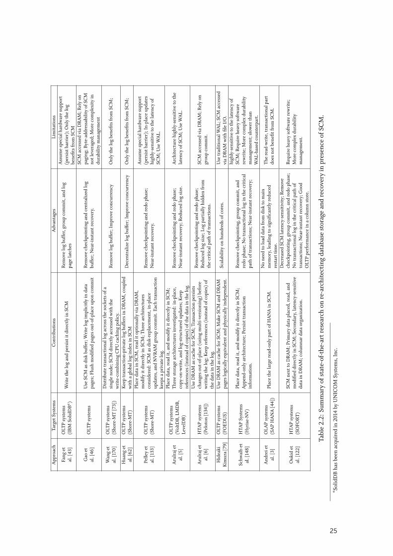
App
roac
hTa
rget
Syst
ems
Con
trib
utio
nsA
dvan
tage
sLi
mit
atio
ns
Fang
etal
.[43
]O
LTP
syst
ems
(IB
MSo
lidD
Ba )
Wri
teth
elo
gan
dpe
rsis
titd
irec
tlyin
SCM
Rem
ove
log
buff
er,g
roup
com
mit
,and
log
page
latc
hes
Ass
ume
spec
ialh
ardw
are
supp
ort
(per
sist
barr
ier)
;Onl
yth
elo
gbe
nefit
sfr
omSC
M
Gao
etal
.[46
]O
LTP
syst
ems
Use
SCM
asdi
skbu
ffer
;Wri
telo
gim
plic
itly
inda
tapa
ges;
Flus
hm
odifi
edpa
ges
out-
of-p
lace
upon
com
mit
Rem
ove
chec
kpoi
ntin
gan
dce
ntra
lized
log
buff
er;N
ear-
inst
antr
ecov
ery.
SCM
acce
ssed
via
DR
AM
;Rel
yon
pagi
ng;B
yte-
addr
essa
bilit
yof
SCM
notl
ever
aged
;Mor
eco
mpl
exity
indu
rabi
lity
man
agem
ent
Wan
get
al.[
170]
OLT
Psy
stem
s(S
hore
-MT
[73]
)
Dis
trib
ute
tran
sact
iona
llog
acro
ssth
eso
cket
sof
asi
ngle
node
;SC
Mdi
rect
lyac
cess
edw
ith
the
wri
te-c
ombi
ning
CPU
cach
ing
polic
y.R
emov
elo
gbu
ffer
;Im
prov
eco
ncur
renc
yO
nly
the
log
bene
fits
from
SCM
;
Hua
nget
al.[
62]
OLT
Psy
stem
s(S
hore
-MT)
Kee
ptr
ansa
ctio
n-pr
ivat
elo
gbu
ffer
sin
DR
AM
,cou
pled
wit
ha
glob
allo
gin
dex
inSC
MD
ecen
tral
ize
log
buff
er;I
mpr
ove
conc
urre
ncy
Onl
yth
elo
gbe
nefit
sfr
omSC
M;
Pelle
yet
al.[
133]
OLT
Psy
stem
s(S
hore
-MT)
Plac
eda
tain
SCM
,rea
dit
opti
onal
lyvi
aD
RA
M,
mod
ifyit
dire
ctly
inSC
M;T
hree
arch
itec
ture
sco
nsid
ered
:SC
Mas
disk
-rep
lace
men
t,in
-pla
ceup
date
s,an
dN
VR
AM
grou
pco
mm
it.Ea
chtr
ansa
ctio
nke
eps
apr
ivat
elo
g.
Rem
ove
chec
kpoi
ntin
gan
dre
doph
ase;
Nea
r-in
stan
trec
over
y.
Ass
ume
spec
ialh
ardw
are
supp
ort
(per
sist
barr
ier)
;In-
plac
eup
date
shi
ghly
-sen
siti
veto
the
late
ncy
ofSC
M;U
seW
AL.
Aru
lraj
etal
.[5]
OLT
Psy
stem
s(V
oltD
B,LM
DB,
Leve
lDB
)
Plac
eda
ta,r
ead
it,a
ndm
odify
itdi
rect
lyin
SCM
;Th
ree
stor
age
arch
itec
ture
sin
vest
igat
ed:i
n-pl
ace,
copy
-on-
wri
te,a
ndlo
g-st
ruct
ured
upda
tes;
Kee
pre
fere
nces
(ins
tead
ofco
pies
)of
the
data
inth
elo
g.
Rem
ove
chec
kpoi
ntin
gan
dre
doph
ase;
Nea
r-in
stan
trec
over
y;R
educ
edlo
gsi
ze.
Arc
hite
ctur
ehi
ghly
-sen
siti
veto
the
late
ncy
ofSC
M;U
seW
AL.
Aru
lraj
etal
.[6]
HTA
Psy
stem
s(P
elot
on[1
34])
Use
DR
AM
asca
che
for
SCM
;Tra
nsac
tion
pers
ists
chan
ges
out-
of-p
lace
(usi
ngm
ulti
-ver
sion
ing)
befo
rew
riti
ngth
elo
g;K
eep
refe
renc
es(i
nste
adof
copi
es)
ofth
eda
tain
the
log.
Rem
ove
chec
kpoi
ntin
gan
dre
doph
ase;
Red
uced
log
size
;Log
part
ially
hidd
enfr
omth
ecr
itic
alpa
thof
tran
sact
ions
.
SCM
acce
ssed
via
DR
AM
;Rel
yon
grou
pco
mm
it.
Hid
eaki
Kim
ura
[79]
OLT
Psy
stem
s(F
OED
US)
Use
DR
AM
asca
che
for
SCM
;Mak
eSC
Man
dD
RA
Mpa
ges
logi
cally
equi
vale
ntan
dph
ysic
ally
inde
pend
ent.
Scal
abili
tyon
hund
reds
ofco
res.
Use
trad
itio
nalW
AL;
SCM
acce
ssed
via
DR
AM
wit
hfil
eI/
O.
Schw
alb
etal
.[14
8]H
TAP
Syst
ems
(Hyr
ise-
NV
)
Plac
eda
ta,r
ead
it,a
ndm
odify
itdi
rect
lyin
SCM
;A
ppen
d-on
lyar
chit
ectu
re;P
ersi
sttr
ansa
ctio
nin
form
atio
n.
Rem
ove
chec
kpoi
ntin
g,gr
oup
com
mit
,and
redo
phas
e;N
otr
ansa
ctio
nall
ogin
the
crit
ical
path
oftr
ansa
ctio
ns;N
ear-
inst
antr
ecov
ery;
high
ly-s
ensi
tive
toth
ela
tenc
yof
SCM
;Req
uire
heav
yso
ftw
are
rew
rite
;Mor
eco
mpl
exdu
rabi
lity
man
agem
ent;
slow
erth
anW
AL-
base
dco
unte
rpar
t.
And
reie
tal
.[3]
OLA
Psy
stem
s(S
AP
HA
NA
[44]
)Pl
ace
the
larg
ere
ad-o
nly
part
ofH
AN
Ain
SCM
.N
one
edto
load
data
from
disk
tom
ain
mem
ory,
lead
ing
tosi
gnifi
cant
lyre
duce
dre
star
ttim
e.
The
read
-wri
te,t
rans
acti
onal
part
does
notb
enefi
tfro
mSC
M.
Ouk
idet
al.[
122]
HTA
Psy
stem
s(S
OFO
RT)
SCM
next
toD
RA
M;P
rim
ary
data
plac
ed,r
ead,
and
mod
ified
dire
ctly
inSC
M;S
econ
dary
,lat
ency
-sen
siti
veda
tain
DR
AM
;col
umna
rda
taor
gani
zati
on.
Dec
reas
edSC
Mla
tenc
y-se
nsit
ivity
;Rem
ove
chec
kpoi
ntin
g,gr
oup
com
mit
,and
redo
phas
e;N
otr
ansa
ctio
nall
ogin
the
crit
ical
path
oftr
ansa
ctio
ns;N
ear-
inst
antr
ecov
ery;
Goo
dO
LTP
perf
orm
ance
ina
colu
mn
stor
e.
Req
uire
heav
yso
ftw
are
rew
rite
;M
ore
com
plex
dura
bilit
ym
anag
emen
t.
Tabl
e2.
2:Su
mm
ary
ofst
ate-
of-t
he-a
rtre
sear
chon
re-a
rchi
tect
ing
data
base
stor
age
and
reco
very
inpr
esen
ceof
SCM
.
a Solid
DB
has
been
acqu
ired
in20
14by
UN
ICO
MSy
stem
s,In
c.
25
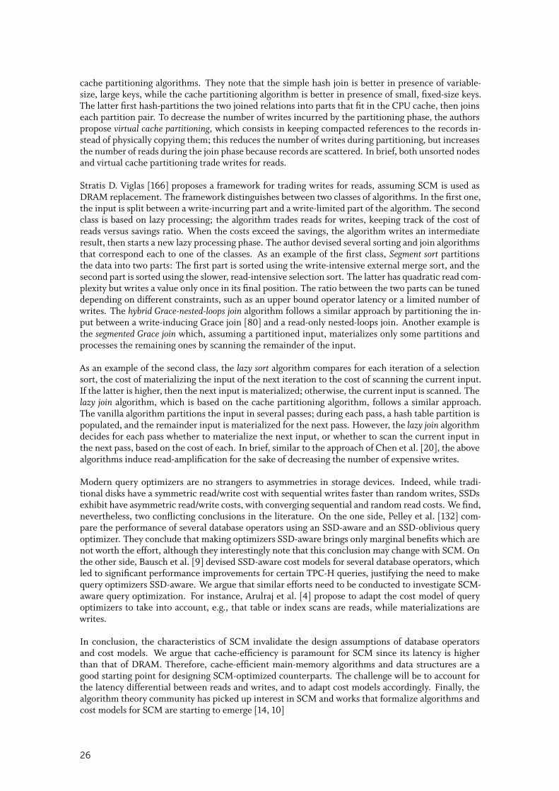
cache partitioning algorithms. They note that the simple hash join is better in presence of variable-size, large keys, while the cache partitioning algorithm is better in presence of small, fixed-size keys.The latter first hash-partitions the two joined relations into parts that fit in the CPU cache, then joinseach partition pair. To decrease the number of writes incurred by the partitioning phase, the authorspropose virtual cache partitioning, which consists in keeping compacted references to the records in-stead of physically copying them; this reduces the number of writes during partitioning, but increasesthe number of reads during the join phase because records are scattered. In brief, both unsorted nodesand virtual cache partitioning trade writes for reads.
Stratis D. Viglas [166] proposes a framework for trading writes for reads, assuming SCM is used asDRAM replacement. The framework distinguishes between two classes of algorithms. In the first one,the input is split between a write-incurring part and a write-limited part of the algorithm. The secondclass is based on lazy processing; the algorithm trades reads for writes, keeping track of the cost ofreads versus savings ratio. When the costs exceed the savings, the algorithm writes an intermediateresult, then starts a new lazy processing phase. The author devised several sorting and join algorithmsthat correspond each to one of the classes. As an example of the first class, Segment sort partitionsthe data into two parts: The first part is sorted using the write-intensive external merge sort, and thesecond part is sorted using the slower, read-intensive selection sort. The latter has quadratic read com-plexity but writes a value only once in its final position. The ratio between the two parts can be tuneddepending on different constraints, such as an upper bound operator latency or a limited number ofwrites. The hybrid Grace-nested-loops join algorithm follows a similar approach by partitioning the in-put between a write-inducing Grace join [80] and a read-only nested-loops join. Another example isthe segmented Grace join which, assuming a partitioned input, materializes only some partitions andprocesses the remaining ones by scanning the remainder of the input.
As an example of the second class, the lazy sort algorithm compares for each iteration of a selectionsort, the cost of materializing the input of the next iteration to the cost of scanning the current input.If the latter is higher, then the next input is materialized; otherwise, the current input is scanned. Thelazy join algorithm, which is based on the cache partitioning algorithm, follows a similar approach.The vanilla algorithm partitions the input in several passes; during each pass, a hash table partition ispopulated, and the remainder input is materialized for the next pass. However, the lazy join algorithmdecides for each pass whether to materialize the next input, or whether to scan the current input inthe next pass, based on the cost of each. In brief, similar to the approach of Chen et al. [20], the abovealgorithms induce read-amplification for the sake of decreasing the number of expensive writes.
Modern query optimizers are no strangers to asymmetries in storage devices. Indeed, while tradi-tional disks have a symmetric read/write cost with sequential writes faster than random writes, SSDsexhibit have asymmetric read/write costs, with converging sequential and random read costs. We find,nevertheless, two conflicting conclusions in the literature. On the one side, Pelley et al. [132] com-pare the performance of several database operators using an SSD-aware and an SSD-oblivious queryoptimizer. They conclude that making optimizers SSD-aware brings only marginal benefits which arenot worth the effort, although they interestingly note that this conclusion may change with SCM. Onthe other side, Bausch et al. [9] devised SSD-aware cost models for several database operators, whichled to significant performance improvements for certain TPC-H queries, justifying the need to makequery optimizers SSD-aware. We argue that similar efforts need to be conducted to investigate SCM-aware query optimization. For instance, Arulraj et al. [4] propose to adapt the cost model of queryoptimizers to take into account, e.g., that table or index scans are reads, while materializations arewrites.
In conclusion, the characteristics of SCM invalidate the design assumptions of database operatorsand cost models. We argue that cache-efficiency is paramount for SCM since its latency is higherthan that of DRAM. Therefore, cache-efficient main-memory algorithms and data structures are agood starting point for designing SCM-optimized counterparts. The challenge will be to account forthe latency differential between reads and writes, and to adapt cost models accordingly. Finally, thealgorithm theory community has picked up interest in SCM and works that formalize algorithms andcost models for SCM are starting to emerge [14, 10]
26
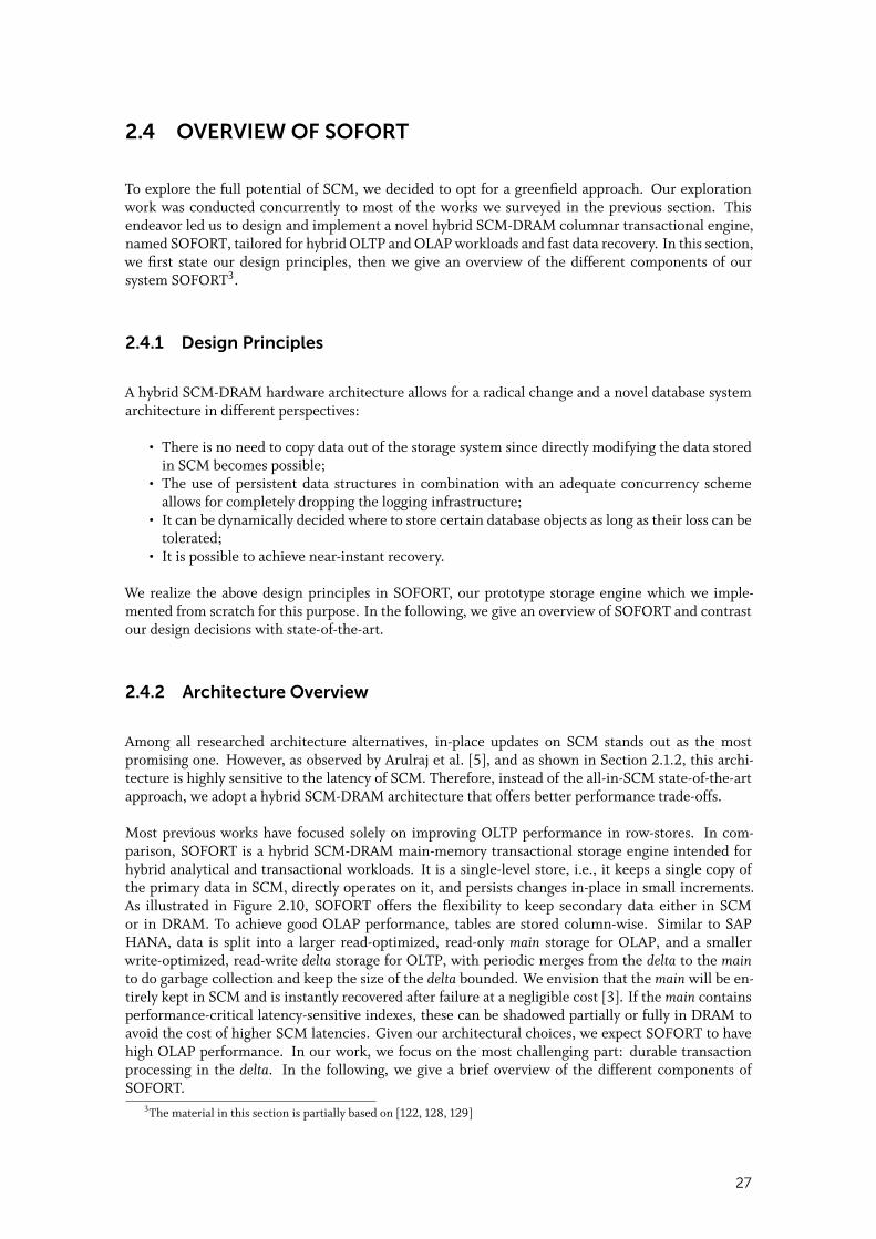
2.4 OVERVIEW OF SOFORT
To explore the full potential of SCM, we decided to opt for a greenfield approach. Our explorationwork was conducted concurrently to most of the works we surveyed in the previous section. Thisendeavor led us to design and implement a novel hybrid SCM-DRAM columnar transactional engine,named SOFORT, tailored for hybrid OLTP and OLAP workloads and fast data recovery. In this section,we first state our design principles, then we give an overview of the different components of oursystem SOFORT3.
2.4.1 Design Principles
A hybrid SCM-DRAM hardware architecture allows for a radical change and a novel database systemarchitecture in different perspectives:
• There is no need to copy data out of the storage system since directly modifying the data storedin SCM becomes possible;
• The use of persistent data structures in combination with an adequate concurrency schemeallows for completely dropping the logging infrastructure;
• It can be dynamically decided where to store certain database objects as long as their loss can betolerated;
• It is possible to achieve near-instant recovery.
We realize the above design principles in SOFORT, our prototype storage engine which we imple-mented from scratch for this purpose. In the following, we give an overview of SOFORT and contrastour design decisions with state-of-the-art.
2.4.2 Architecture Overview
Among all researched architecture alternatives, in-place updates on SCM stands out as the mostpromising one. However, as observed by Arulraj et al. [5], and as shown in Section 2.1.2, this archi-tecture is highly sensitive to the latency of SCM. Therefore, instead of the all-in-SCM state-of-the-artapproach, we adopt a hybrid SCM-DRAM architecture that offers better performance trade-offs.
Most previous works have focused solely on improving OLTP performance in row-stores. In com-parison, SOFORT is a hybrid SCM-DRAM main-memory transactional storage engine intended forhybrid analytical and transactional workloads. It is a single-level store, i.e., it keeps a single copy ofthe primary data in SCM, directly operates on it, and persists changes in-place in small increments.As illustrated in Figure 2.10, SOFORT offers the flexibility to keep secondary data either in SCMor in DRAM. To achieve good OLAP performance, tables are stored column-wise. Similar to SAPHANA, data is split into a larger read-optimized, read-only main storage for OLAP, and a smallerwrite-optimized, read-write delta storage for OLTP, with periodic merges from the delta to the mainto do garbage collection and keep the size of the delta bounded. We envision that the main will be en-tirely kept in SCM and is instantly recovered after failure at a negligible cost [3]. If the main containsperformance-critical latency-sensitive indexes, these can be shadowed partially or fully in DRAM toavoid the cost of higher SCM latencies. Given our architectural choices, we expect SOFORT to havehigh OLAP performance. In our work, we focus on the most challenging part: durable transactionprocessing in the delta. In the following, we give a brief overview of the different components ofSOFORT.
3The material in this section is partially based on [122, 128, 129]
27
Transactions
SCM DRAM
Primary Data Secondary Data
micro-logs micro-logs
Figure 2.10: Hybrid SCM-DRAM architecture of SOFORT.
2.4.3 Persistent Memory Management
While popular in the operating systems community, SCM memory management remains an almostunexplored topic in database systems. With few exceptions [5], works that leverage SCM as persistentmain memory do not elaborate on how they allocate memory, or on how they recover data. Thissection gives an overview on how we fill this gap.
SCM is managed using a file system. User space access to SCM is granted via memory mapping usingmmap. The mapping behaves like mmap for traditional files, except that the persistent data is directlymapped to the virtual address space, instead of to a DRAM-cached copy.
When a program crashes, its pointers become invalid since the program gets a new address spacewhen it restarts. This implies that these pointers cannot be used to recover persistent data structures.To solve this problem, we propose a new pointer type, denoted Persistent Pointer (PPtr), that remainsvalid across restarts. It consists of a base, which is a file ID, and an offset within that file that indicatesthe start of the block pointed to. To manage SCM, we propose a persistent memory allocator (PAllo-cator) that provides a mapping of SCM to virtual memory, enabling the conversion of PPtrs to regularpointers. We denote work pointers regular pointers that are conversions of PPtrs. This is a similarapproach to pointer swizzling [174], where disk pointers are converted to virtual memory pointers atpage fault time. While our pointer conversion principle is the same as in [174], we convert pointersonly at restart time and not for every page fault.
PAllocator uses big SCM files that are cut into smaller blocks for allocation. It maps these files tovirtual memory to enable the conversion of PPtrs to work pointers. At restart time, a new mapping tovirtual memory is created, allowing to re-convert PPtrs to new valid work pointers. PAllocator is alsopersistent. It maintains a persistent file counter to know how many files it has created. It also storesmeta-data for every allocated block.
To perform recovery, we need to keep track of an entry point. One entry point is sufficient for thewhole storage engine since every structure is encapsulated into a larger structure up to the full engine.An entry point can simply be two PPtrs: the first points to the root object of SOFORT and the secondto the root object of PAllocator. The entry point is kept in SCM in a special file at a known offset. Wegive a full description of SOFORT’s persistent memory management in Chapter 3.
2.4.4 Data Layout
The closest works to ours are the Peloton [6, 134] and Hyrise-NV [148] hybrid OLTP and OLAPdatabase systems. To achieve good OLTP and OLAP performance, Peloton organizes data in tiles [157].
28
SOFORT Table Column
ValIDArray
ColumnIndex(es) DictColumnsMVCC
Array
CTSMVCC Entry
DTS
TXArray Tables
DictIndex
Must be persistentTransient, persistent, or hybrid
Figure 2.11: Data layout overview in SOFORT.
A tile stores subsets of attributes of a table row-wise, resulting in a middle ground between the row-oriented and the column-oriented representations. In contrast, SOFORT is a column-oriented main-memory storage engine that uses dictionary compression. Hyrise-NV is similar to SOFORT in thatregard. The remainder of this section gives an overview of data organization in SOFORT.
Figure 2.11 gives an overview of data organization in SOFORT. Tables are stored as a collection ofappend-only columns. Each column consists of an unsorted dictionary stored as an array of the col-umn’s unique data values, and an array of value IDs, where a value ID is simply a dictionary index(position). These two arrays are sufficient to provide data durability and constitute the primary data.SOFORT stores primary data, accesses it, and updates it directly in SCM. Other data structures arerequired to achieve reasonable performance including, for each column, a dictionary index that mapsvalues to value IDs, and for each table, a set of multi-column inverted indexes that map sets of valueIDs to the set of corresponding row IDs. We refer to these structures as secondary data since theycan be reconstructed from the primary data. SOFORT can keep secondary data in DRAM or in SCM.Putting all indexes in DRAM gives the best performance but might stress DRAM resources, while plac-ing indexes in SCM exposes them to its higher latency which compromises performance. To solve thisissue, we devise novel hybrid SCM-DRAM data structures that exhibit nearly the same performanceas DRAM-based counterparts, while using only a small portion of DRAM. We elaborate on SOFORT’shybrid data structures in Chapter 4.
2.4.5 Concurrency Control
A columnar data layout preserves analytical performance, but poses great challenges for transactionalperformance. Indeed, materializing rows in a column-store necessitates several random memory ac-cesses, which exacerbates the cost of higher SCM latencies. Moreover, most previous works still relyon some sort of write-ahead logging. In this section, we highlight how SOFORT gets completely ridof traditional logging in the critical path of transactions and manages to achieve competitive OLTPperformance despite its columnar data layout.
Multi-Version Concurrency Control (MVCC) [84, 81] is a natural design decision for SOFORT, asversioning simplifies durability management with regards to partial writes. SOFORT adapts to SCMa similar MVCC scheme to that of the Hekaton main-memory database system [84]. As shown inFigure 2.11, SOFORT keeps a transaction object array that stores the metadata of currently runningtransactions. Contrary to Hyrise-NV which persists the whole transaction object, SOFORT splits itinto a transient and a persistent part. The transient part consists of a transaction ID, the start times-tamp of the transaction, a read set containing the row IDs of all visited rows, and a status variable.The persistent part encompasses the commit timestamp of the transaction, and a write set containingthe row IDs of all modified rows. To undo the effects of aborted transactions or in-flight transactions
29
during recovery, it is sufficient to update the MVCC timestamps of inserted or deleted rows, whichare tracked in the persistent write set of each transaction. Therefore, SOFORT does not require a tra-ditional transaction log to achieve durability, as changes are applied directly to the primary, persistentdata, and undo capability is provided by persisting the transactions’ write sets. Additionally, SOFORTimplement a background garbage collection mechanism that cleans indexes and enables the reuse ofdeleted rows. A detailed description of the concurrency control mechanism and garbage collection ofSOFORT is available in Chapter 5.
2.4.6 Recovery Mechanisms
Previous works either assume that secondary indexes are persistent, or they do not account for theirrebuild when measuring recovery time. Yet, rebuilding transient data will become the new bottleneckin database systems that access data directly in SCM. This section briefly elaborates on how we tacklethis issue in SOFORT.
SOFORT recovers by first recovering primary data that is persisted in SCM at a negligible cost, thenundoing the effects of unfinished transactions. The last phase of the recovery procedure, that is,rebuilding secondary data, can be handled in three different ways: in the first approach, denotedSynchronous Recovery, SOFORT does not accept requests until the end of the recovery process, i.e.,until all secondary data structures have been rebuilt. The main advantage of this approach is thatit rebuilds secondary data structures as fast as possible since all system resources are allocated torecovery. However, this approach suffers from the fact that the database is not responsive during thewhole recovery period, which might be long as its duration depends directly on the size of secondarydata structures to be rebuilt.
The second approach, named Instant Recovery, starts accepting requests right after recovering primarydata. Instant recovery follows a crawl before run approach: it uses primary data, which is recoveredat a negligible cost, to answer queries, while secondary data structures, whose purpose is to speed upquery processing, are rebuilt in the background. For example, lookups to a dictionary index and aninverted index are replaced by scans of the corresponding dictionary array and the value IDs arrays,respectively. Partially rebuilt DRAM-based indexes can be progressively leveraged as they are beingrebuilt. For instance, a regular dictionary index lookup is replaced by the following sequence: lookup the partially rebuilt dictionary index; if the value is not found, then scan only the portion of thedictionary array that has not been indexed yet. Hybrid SCM-DRAM indexes, however, need to befully recovered in order to be leveraged. The main advantage of this approach is that it enables instantrecovery, i.e., instant responsiveness of the database after failure. However, it takes the databaselonger than for synchronous recovery to approach peak performance observed before failure. Thisis because system resources are split between recovery and query processing, while in synchronousrecovery, all system resources are allocated to recovery.
To cure the shortcomings of both approaches, SOFORT has a third recovery technique, named Adap-tive Recovery. It dynamically ranks transient secondary data structures based on their importance tothe current workload. During recovery, it prioritizes the rebuild of the most highly ranked data struc-tures. Furthermore, adaptive recovery employs a dynamic resource allocation algorithm that releasesresources from the recovery process to query execution when it detects that system has approachedpeak performance. Therefore, adaptive recovery achieves instant responsiveness while reaching peakperformance quickly, well before the end of the recovery process. We present the details of SOFORT’srecovery techniques in Chapter 6.
30
2.5 CONCLUSION
SCM is driving a necessary rethink of database architectures. In this chapter we presented severalworks that propose to re-architect parts or all of the traditional database storage architecture. Contraryto the state-of-the-art that focuses mostly on OLTP row-store systems, we focus on HTAP systemswhich usually adopt a columnar data representation. We showed that a hybrid SCM-DRAM storagearchitecture enables better performance than an SCM-only one. Furthermore, we anticipate that it ispossible to completely remove traditional WAL from the critical path of transactions. We materializeour design principle in SOFORT, a hybrid single-level transactional storage engine that makes themost out of both DRAM and SCM. SOFORT persists its primary data directly in SCM at cache-linegranularity.
While a single-level architecture brings many benefits, such as instant recovery, it does not come as afree lunch: it requires heavy software rewrite and introduces unprecedented programming challenges,on which we elaborate in the next chapter.
31

32
3PERSISTENT MEMORY MANAGEMENT
M emory allocation has always been a topic in database systems. In the disk-based database sys-tems era, memory management was mostly synonymous of buffer pool management. For
instance, Traiger [160] investigated how to optimize the operating system virtual memory compo-nent such that it is efficiently used as replacement for the buffer pool. In the era of main-memorydatabase systems, we switched to using transient allocators, such as jemalloc [72], tcmalloc [49], andHoard [11]. However, these allocators are general-purpose and database systems have all but general-purpose needs. Hence, to no surprise, several database system vendors, such as SAP, IBM, and Oracleimplement their own memory management [145, 156, 120]. The rise of SCM might spur a majorchange in the architecture of database systems, and in this incoming era of SCM-based database sys-tems, everything is yet to be done, starting from persistent memory management as a fundamentalbuilding block. However, SCM as persistent main memory is still at its pathfinding stages. Therefore,we explore in the first part of this chapter the programming challenges of SCM, then survey state-of-the-art techniques on how to solve them. Thereafter, we devise a sound SCM programming modelthat takes into account database system requirements.
In the second part of this chapter, we present SOFORT’s memory management component, calledPAllocator, a highly scalable, fail-safe, and persistent allocator for SCM, specifically designed fordatabases that require very large main memory capacities1. PAllocator uses internally two differentallocators: SmallPAllocator, a small block persistent allocator that implements a segregated-fit strat-egy; and BigPAllocator, a big block persistent allocator that implements a best-fit strategy and useshybrid SCM-DRAM trees to persist and index its metadata. The use of hybrid trees enables PAllocatorto also offer a fast recovery mechanism. Moreover, PAllocator addresses fragmentation in persistentmemory, which we argue is an important challenge, and implements an efficient defragmentationalgorithm that is able to reclaim the memory of fragmented blocks by leveraging the hole punchingfeature of sparse files. To the best of our knowledge, PAllocator is the first SCM allocator that proposesa transparent defragmentation algorithm as a core component for SCM-based database systems. Ourevaluation shows that PAllocator improves on state-of-the-art persistent allocators by up to two ordersof magnitude in operation throughput, and by up to three orders of magnitude in recovery time. Fur-thermore, we integrate PAllocator and a state-of-the-art persistent allocator in a persistent B+-Tree,and show that PAllocator enables up to 2.39x better operation throughput than its counterpart.
This chapter is organized as follows: We contribute in Section 3.1 an analysis of the challenges posedby SCM that we drew from our experience in designing and implementing SOFORT. Then, Section 3.2
1Parts of the material in this chapter are based on [124].
33
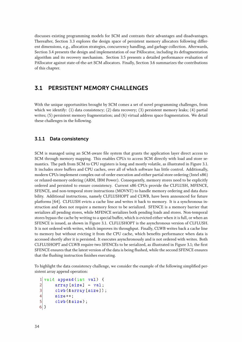
discusses existing programming models for SCM and contrasts their advantages and disadvantages.Thereafter, Section 3.3 explores the design space of persistent memory allocators following differ-ent dimensions, e.g., allocation strategies, concurrency handling, and garbage collection. Afterwards,Section 3.4 presents the design and implementation of our PAllocator, including its defragmentationalgorithm and its recovery mechanism. Section 3.5 presents a detailed performance evaluation ofPAllocator against state-of-the-art SCM allocators. Finally, Section 3.6 summarizes the contributionsof this chapter.
3.1 PERSISTENT MEMORY CHALLENGES
With the unique opportunities brought by SCM comes a set of novel programming challenges, fromwhich we identify: (1) data consistency; (2) data recovery; (3) persistent memory leaks; (4) partialwrites; (5) persistent memory fragmentation; and (6) virtual address space fragmentation. We detailthese challenges in the following.
3.1.1 Data consistency
SCM is managed using an SCM-aware file system that grants the application layer direct access toSCM through memory mapping. This enables CPUs to access SCM directly with load and store se-mantics. The path from SCM to CPU registers is long and mostly volatile, as illustrated in Figure 3.1.It includes store buffers and CPU caches, over all of which software has little control. Additionally,modern CPUs implement complex out-of-order execution and either partial store ordering (Intel x86)or relaxed-memory ordering (ARM, IBM Power). Consequently, memory stores need to be explicitlyordered and persisted to ensure consistency. Current x86 CPUs provide the CLFLUSH, MFENCE,SFENCE, and non-temporal store instructions (MOVNT) to handle memory ordering and data dura-bility. Additional instructions, namely CLFLUSHOPT and CLWB, have been announced for futureplatforms [64]. CLFLUSH evicts a cache line and writes it back to memory. It is a synchronous in-struction and does not require a memory fence to be serialized. SFENCE is a memory barrier thatserializes all pending stores, while MFENCE serializes both pending loads and stores. Non-temporalstores bypass the cache by writing to a special buffer, which is evicted either when it is full, or when anSFENCE is issued, as shown in Figure 3.1. CLFLUSHOPT is the asynchronous version of CLFLUSH.It is not ordered with writes, which improves its throughput. Finally, CLWB writes back a cache lineto memory but without evicting it from the CPU cache, which benefits performance when data isaccessed shortly after it is persisted. It executes asynchronously and is not ordered with writes. BothCLFLUSHOPT and CLWB require two SFENCEs to be serialized, as illustrated in Figure 3.1; the firstSFENCE ensures that the latest version of the data is being flushed, while the second SFENCE ensuresthat the flushing instruction finishes executing.
To highlight the data consistency challenge, we consider the example of the following simplified per-sistent array append operation:
1 void append(int val) {
2 array[size] = val;
3 clwb(&array[size]);
4 size ++;
5 clwb(&size);
6 }
34
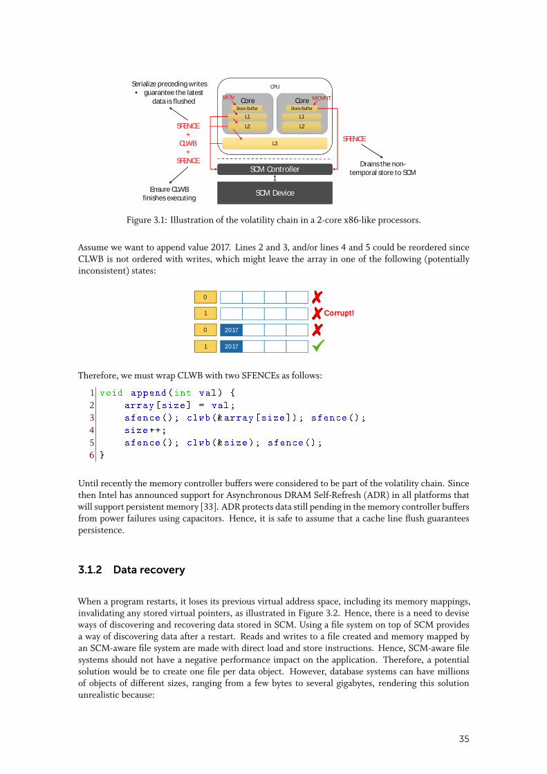
SCM Controller
SCM Device
CPU
Core Core
L3
L1
L2
L1
L2
Store Buffer Store Buffer
MOV MOVNT
SFENCE
SFENCE+
CLWB+
SFENCE Drains the non-temporal store to SCM
Serialize preceding writes• guarantee the latest
data is flushed
Ensure CLWBfinishes executing
Figure 3.1: Illustration of the volatility chain in a 2-core x86-like processors.
Assume we want to append value 2017. Lines 2 and 3, and/or lines 4 and 5 could be reordered sinceCLWB is not ordered with writes, which might leave the array in one of the following (potentiallyinconsistent) states:
0
1
0 2017
1 2017
Corrupt!
Therefore, we must wrap CLWB with two SFENCEs as follows:
1 void append(int val) {
2 array[size] = val;
3 sfence (); clwb(&array[size]); sfence ();
4 size ++;
5 sfence (); clwb(&size); sfence ();
6 }
Until recently the memory controller buffers were considered to be part of the volatility chain. Sincethen Intel has announced support for Asynchronous DRAM Self-Refresh (ADR) in all platforms thatwill support persistent memory [33]. ADR protects data still pending in the memory controller buffersfrom power failures using capacitors. Hence, it is safe to assume that a cache line flush guaranteespersistence.
3.1.2 Data recovery
When a program restarts, it loses its previous virtual address space, including its memory mappings,invalidating any stored virtual pointers, as illustrated in Figure 3.2. Hence, there is a need to deviseways of discovering and recovering data stored in SCM. Using a file system on top of SCM providesa way of discovering data after a restart. Reads and writes to a file created and memory mapped byan SCM-aware file system are made with direct load and store instructions. Hence, SCM-aware filesystems should not have a negative performance impact on the application. Therefore, a potentialsolution would be to create one file per data object. However, database systems can have millionsof objects of different sizes, ranging from a few bytes to several gigabytes, rendering this solutionunrealistic because:
35
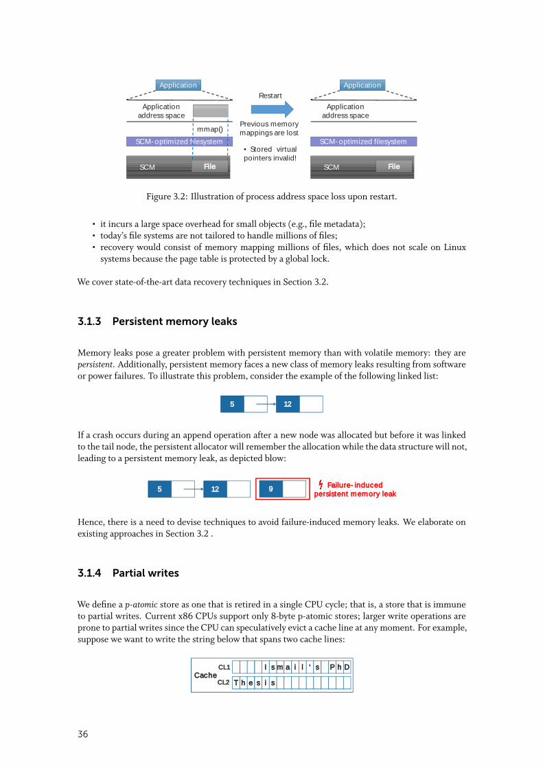
Application
SCM-optimized filesystem
SCM
Applicationaddress space
File
mmap()
Application
SCM-optimized filesystem
SCM
Applicationaddress space
File
Restart
Previous memorymappings are lost
• Stored virtualpointers invalid!
Figure 3.2: Illustration of process address space loss upon restart.
• it incurs a large space overhead for small objects (e.g., file metadata);• today’s file systems are not tailored to handle millions of files;• recovery would consist of memory mapping millions of files, which does not scale on Linux
systems because the page table is protected by a global lock.
We cover state-of-the-art data recovery techniques in Section 3.2.
3.1.3 Persistent memory leaks
Memory leaks pose a greater problem with persistent memory than with volatile memory: they arepersistent. Additionally, persistent memory faces a new class of memory leaks resulting from softwareor power failures. To illustrate this problem, consider the example of the following linked list:
5 12
If a crash occurs during an append operation after a new node was allocated but before it was linkedto the tail node, the persistent allocator will remember the allocation while the data structure will not,leading to a persistent memory leak, as depicted blow:
5 12 9 Failure-inducedpersistent memory leak
Hence, there is a need to devise techniques to avoid failure-induced memory leaks. We elaborate onexisting approaches in Section 3.2 .
3.1.4 Partial writes
We define a p-atomic store as one that is retired in a single CPU cycle; that is, a store that is immuneto partial writes. Current x86 CPUs support only 8-byte p-atomic stores; larger write operations areprone to partial writes since the CPU can speculatively evict a cache line at any moment. For example,suppose we want to write the string below that spans two cache lines:
I s m a i l ‘ s P h D
T h e s i s
CL1
CL2Cache
36
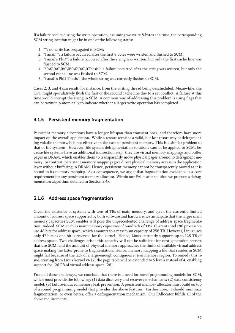
If a failure occurs during the write operation, assuming we write 8-bytes at a time, the correspondingSCM string location might be in one of the following states:
1. “”: no write has propagated to SCM;2. “Ismail’ ”: a failure occurred after the first 8 bytes were written and flushed to SCM;3. “Ismail’s PhD”: a failure occurred after the string was written, but only the first cache line was
flushed to SCM;4. “\0\0\0\0\0\0\0\0\0\0\0\0Thesis”: a failure occurred after the string was written, but only the
second cache line was flushed to SCM.5. “Ismail’s PhD Thesis”: the whole string was correctly flushes to SCM.
Cases 2, 3, and 4 can result, for instance, from the writing thread being descheduled. Meanwhile, theCPU might speculatively flush the first or the second cache line due to a set conflict. A failure at thistime would corrupt the string in SCM. A common way of addressing this problem is using flags thatcan be written p-atomically to indicate whether a larger write operation has completed.
3.1.5 Persistent memory fragmentation
Persistent memory allocations have a longer lifespan than transient ones, and therefore have moreimpact on the overall application. While a restart remains a valid, but last-resort way of defragment-ing volatile memory, it is not effective in the case of persistent memory. This is a similar problem tothat of file systems. However, file system defragmentation solutions cannot be applied to SCM, be-cause file systems have an additional indirection step: they use virtual memory mappings and bufferpages in DRAM, which enables them to transparently move physical pages around to defragment me-mory. In contrast, persistent memory mappings give direct physical memory access to the applicationlayer without buffering in DRAM. Hence, persistent memory cannot be transparently moved as it isbound to its memory mapping. As a consequence, we argue that fragmentation avoidance is a corerequirement for any persistent memory allocator. Within our PAllocator solution we propose a defrag-mentation algorithm, detailed in Section 3.4.6.
3.1.6 Address space fragmentation
Given the existence of systems with tens of TBs of main memory, and given the currently limitedamount of address space supported by both software and hardware, we anticipate that the larger mainmemory capacities SCM enables will pose the unprecedented challenge of address space fragmenta-tion. Indeed, SCM enables main memory capacities of hundreds of TBs. Current Intel x86 processorsuse 48 bits for address space, which amounts to a maximum capacity of 256 TB. However, Linux usesonly 47 bits as one bit is reserved for the kernel. Hence, Linux currently supports up to 128 TB ofaddress space. Two challenges arise: this capacity will not be sufficient for next-generation serversthat use SCM, and the amount of physical memory approaches the limits of available virtual addressspace making the latter prone to fragmentation. Hence, memory mapping a file that resides in SCMmight fail because of the lack of a large-enough contiguous virtual memory region. To remedy this is-sue, starting from Linux kernel v4.12, the page table will be extended to 5 levels instead of 4, enablingsupport for 128 PB of virtual address space [28].
From all these challenges, we conclude that there is a need for novel programming models for SCM,which must provide the following: (1) data discovery and recovery mechanisms; (2) data consistencymodel; (3) failure-induced memory leak prevention. A persistent memory allocator must build on topof a sound programming model that provides the above features. Furthermore, it should minimizefragmentation, or even better, offer a defragmentation mechanism. Our PAllocator fulfills all of theabove requirements.
37
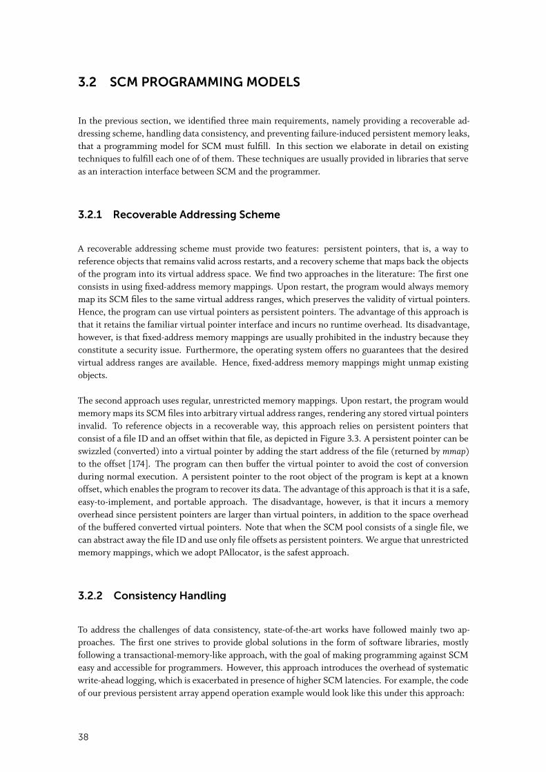
3.2 SCM PROGRAMMING MODELS
In the previous section, we identified three main requirements, namely providing a recoverable ad-dressing scheme, handling data consistency, and preventing failure-induced persistent memory leaks,that a programming model for SCM must fulfill. In this section we elaborate in detail on existingtechniques to fulfill each one of of them. These techniques are usually provided in libraries that serveas an interaction interface between SCM and the programmer.
3.2.1 Recoverable Addressing Scheme
A recoverable addressing scheme must provide two features: persistent pointers, that is, a way toreference objects that remains valid across restarts, and a recovery scheme that maps back the objectsof the program into its virtual address space. We find two approaches in the literature: The first oneconsists in using fixed-address memory mappings. Upon restart, the program would always memorymap its SCM files to the same virtual address ranges, which preserves the validity of virtual pointers.Hence, the program can use virtual pointers as persistent pointers. The advantage of this approach isthat it retains the familiar virtual pointer interface and incurs no runtime overhead. Its disadvantage,however, is that fixed-address memory mappings are usually prohibited in the industry because theyconstitute a security issue. Furthermore, the operating system offers no guarantees that the desiredvirtual address ranges are available. Hence, fixed-address memory mappings might unmap existingobjects.
The second approach uses regular, unrestricted memory mappings. Upon restart, the program wouldmemory maps its SCM files into arbitrary virtual address ranges, rendering any stored virtual pointersinvalid. To reference objects in a recoverable way, this approach relies on persistent pointers thatconsist of a file ID and an offset within that file, as depicted in Figure 3.3. A persistent pointer can beswizzled (converted) into a virtual pointer by adding the start address of the file (returned by mmap)to the offset [174]. The program can then buffer the virtual pointer to avoid the cost of conversionduring normal execution. A persistent pointer to the root object of the program is kept at a knownoffset, which enables the program to recover its data. The advantage of this approach is that it is a safe,easy-to-implement, and portable approach. The disadvantage, however, is that it incurs a memoryoverhead since persistent pointers are larger than virtual pointers, in addition to the space overheadof the buffered converted virtual pointers. Note that when the SCM pool consists of a single file, wecan abstract away the file ID and use only file offsets as persistent pointers. We argue that unrestrictedmemory mappings, which we adopt PAllocator, is the safest approach.
3.2.2 Consistency Handling
To address the challenges of data consistency, state-of-the-art works have followed mainly two ap-proaches. The first one strives to provide global solutions in the form of software libraries, mostlyfollowing a transactional-memory-like approach, with the goal of making programming against SCMeasy and accessible for programmers. However, this approach introduces the overhead of systematicwrite-ahead logging, which is exacerbated in presence of higher SCM latencies. For example, the codeof our previous persistent array append operation example would look like this under this approach:
38
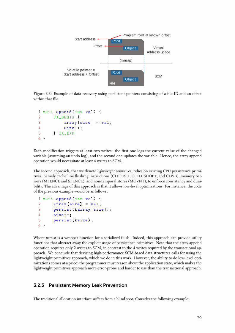
Program root at known offsetStart address
Object
FileObject
Root
Root
Offset
(mmap)
SCM
VirtualAddress Space
Volatile pointer =Start address + Offset
Figure 3.3: Example of data recovery using persistent pointers consisting of a file ID and an offsetwithin that file.
1 void append(int val) {
2 TX_BEGIN {
3 array[size] = val;
4 size ++;
5 } TX_END
6 }
Each modification triggers at least two writes: the first one logs the current value of the changedvariable (assuming an undo log), and the second one updates the variable. Hence, the array appendoperation would necessitate at least 4 writes to SCM.
The second approach, that we denote lightweight primitives, relies on existing CPU persistence primi-tives, namely cache line flushing instructions (CLFLUSH, CLFLUSHOPT, and CLWB), memory bar-riers (MFENCE and SFENCE), and non-temporal stores (MOVNT), to enforce consistency and dura-bility. The advantage of this approach is that it allows low-level optimizations. For instance, the codeof the previous example would be as follows:
1 void append(int val) {
2 array[size] = val;
3 persist (&array[size]);
4 size ++;
5 persist (&size);
6 }
Where persist is a wrapper function for a serialized flush. Indeed, this approach can provide utilityfunctions that abstract away the explicit usage of persistence primitives. Note that the array appendoperation requires only 2 writes to SCM, in contrast to the 4 writes required by the transactional ap-proach. We conclude that devising high-performance SCM-based data structures calls for using thelightweight primitives approach, which we do in this work. However, the ability to do low-level opti-mizations comes at a price: the programmer must reason about the application state, which makes thelightweight primitives approach more error-prone and harder to use than the transactional approach.
3.2.3 Persistent Memory Leak Prevention
The traditional allocation interface suffers from a blind spot. Consider the following example:
39

1 pptr = allocate(size);
2 persist (&pptr);
Where pptr is a persistent pointer belonging to the calling data structure. If a failure occurs betweenlines 1 and 2, the allocator will have completed the allocation request and will remember that itallocated this block, while the data structure might loose its reference to that block because it wasnot persistent before the failure occurred. We find three approaches that remedy this issue in theliterature. The first one uses reference passing; the allocator interface is modified to take a referenceto a persistent pointer that belongs to the calling data structure and that must reside in SCM:
1 allocate(PPtr& p, size_t size);
The allocator will set the persistent pointer to the address of the allocated memory and persist itbefore returning, hence removing the aforementioned blind spot. Note that reference passing, whichwe adopt in this work, is ideal for the lightweight primitives approach.
The second approach consists in to wrap code that is prone to persistent memory leaks inside a fail-atomic transaction, e.g., as follows:
1 TX_BEGIN {
2 pptr = allocate(size);
3 persist (&pptr);
4 } TX_END
Finally, the third approach consists in using offiline garbage collection [13]. It consists in scanning al-located blocks during recovery to detect persistent memory leaks. We elaborate on the latter approachin more details in Section 3.3.4.
3.2.4 Related Work
Table 3.1 summarizes existing libraries that aim to address the programming challenges of SCM.Among early works, Volos et al. [168] proposed Mnemosyne, a library collection to program SCMthat require kernel modifications and compiler support. Following a similar approach, Coburn etal. [24] proposed NV-Heap, a persistent heap that implements garbage collection through referencecounting. Later, Chakrabarti et al. [18] and Chatzistergiou et al. [19] proposed respectively Atlas andREWIND, two log-based user-mode libraries that manage persistent data structures in SCM in a re-coverable state using undo/redo logging. An original characteristic of Atlas is that it assumes that theconsistency-critical code sections are protected with locks. Atlas then transforms these locked scopesinto fail-atomic transactions at compile time. This means, however, that single-threaded programsneed to be modified by inserting locks where changes to SCM-based structures occur. Most recently,Avni et al. [8] proposed PHyTM, a persistent hybrid transactional memory system that leverages hard-ware transactional memory, while assuming hardware support for single-bit atomic commit to SCM.Intel’s NVML [117] offers an elaborate collection of libraries that spans both the raw and the transac-tional approaches. Additionally, it offers a middle-ground approach based on the raw one augmentedwith useful transaction support, such as atomic execution of object constructors upon persistent me-mory allocation, which greatly simplifies fail-safe atomicity management. In our work we follow thelightweight primitives approach.
40
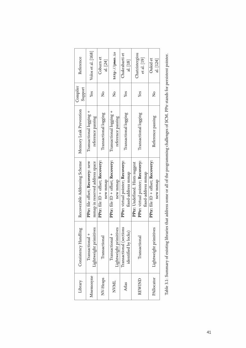
Libr
ary
Con
sist
ency
Han
dlin
gR
ecov
erab
leA
ddre
ssin
gSc
hem
eM
emor
yLe
akPr
even
tion
Com
pile
rSu
ppor
tR
efer
ence
Mne
mos
yne
Tran
sact
iona
l+Li
ghtw
eigh
tpri
mit
ives
PPtr:fi
leof
fset
;Recovery:
new
mm
apin
rese
rved
addr
ess
spac
eTr
ansa
ctio
nall
oggi
ng+
refe
renc
epa
ssin
gYe
sVo
los
etal
.[16
8]
NV-
Hea
psTr
ansa
ctio
nal
PPtr:fi
leID
+of
fset
;Recovery:
new
mm
apTr
ansa
ctio
nall
oggi
ngN
oC
obur
net
al.[
24]
NV
ML
Tran
sact
iona
l+Li
ghtw
eigh
tpri
mit
ives
PPtr:fi
leID
+of
fset
;Recovery:
new
mm
apTr
ansa
ctio
nall
oggi
ng+
refe
renc
epa
ssin
gN
ohttp://pmem.io
Atla
sTr
ansa
ctio
nal(
sect
ions
iden
tifie
dby
lock
s)PP
tr:v
irtu
alpo
inte
r;Recovery:
fixed
-add
ress
mm
apTr
ansa
ctio
nall
oggi
ngYe
sC
hakr
abar
tiet
al.[
18]
REW
IND
Tran
sact
iona
lPP
tr:U
ndefi
ned.
Hin
tssu
gges
tPP
tr:v
irtu
alpo
inte
r;Recovery:
fixed
-add
ress
mm
apTr
ansa
ctio
nall
oggi
ngYe
sC
hatz
iste
rgio
uet
al.[
19]
PAllo
cato
rLi
ghtw
eigh
tpri
mit
ives
PPtr:fi
leID
+of
fset
;Recovery:
new
mm
apR
efer
ence
pass
ing
No
Ouk
idet
al.[
124]
Tabl
e3.
1:Su
mm
ary
ofex
isti
nglib
rari
esth
atad
dres
sso
me
oral
loft
hepr
ogra
mm
ing
chal
leng
esof
SCM
.PPt
rst
ands
for
pers
iste
ntpo
inte
r.
41
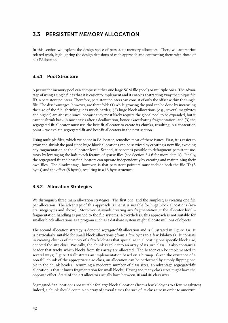
3.3 PERSISTENT MEMORY ALLOCATION
In this section we explore the design space of persistent memory allocators. Then, we summarizerelated work, highlighting the design decisions of each approach and contrasting them with those ofour PAllocator.
3.3.1 Pool Structure
A persistent memory pool can comprise either one large SCM file (pool) or multiple ones. The advan-tage of using a single file is that it is easier to implement and it enables abstracting away the unique fileID in persistent pointers. Therefore, persistent pointers can consist of only the offset within the singlefile. The disadvantages, however, are threefold: (1) while growing the pool can be done by increasingthe size of the file, shrinking it is much harder; (2) huge block allocations (e.g., several megabytesand higher) are an issue since, because they most likely require the global pool to be expanded, but itcannot shrink back in most cases after a deallocation, hence exacerbating fragmentation; and (3) thesegregated-fit allocator must use the best-fit allocator to create its chunks, resulting in a contentionpoint – we explain segregated-fit and best-fit allocators in the next section.
Using multiple files, which we adopt in PAllocator, remedies most of these issues. First, it is easier togrow and shrink the pool since huge block allocations can be serviced by creating a new file, avoidingany fragmentation at the allocator level. Second, it becomes possible to defragment persistent me-mory by leveraging the hole punch feature of sparse files (see Section 3.4.6 for more details). Finally,the segregated-fit and best-fit allocators can operate independently by creating and maintaining theirown files. The disadvantage, however, is that persistent pointers must include both the file ID (8bytes) and the offset (8 bytes), resulting in a 16-byte structure.
3.3.2 Allocation Strategies
We distinguish three main allocation strategies. The first one, and the simplest, is creating one fileper allocation. The advantage of this approach is that it is suitable for huge block allocations (sev-eral megabytes and above). Moreover, it avoids creating any fragmentation at the allocator level –fragmentation handling is pushed to the file systems. Nevertheless, this approach is not suitable forsmaller block allocations as a program such as a database system might allocate millions of objects.
The second allocation strategy is denoted segregated-fit allocation and is illustrated in Figure 3.4. Itis particularly suitable for small block allocations (from a few bytes to a few kilobytes). It consistsin creating chunks of memory of a few kilobytes that specialize in allocating one specific block size,denoted the size class. Basically, the chunk is split into an array of its size class. It also contains aheader that tracks which blocks from this array are allocated. The header can be implemented inseveral ways; Figure 3.4 illustrates an implementation based on a bitmap. Given the existence of anon-full chunk of the appropriate size class, an allocation can be performed by simply flipping onebit in the chunk header. Assuming a moderate number of class sizes, an advantage segregated-fitallocation is that it limits fragmentation for small blocks. Having too many class sizes might have theopposite effect. State-of-the-art allocators usually have between 30 and 40 class sizes.
Segregated-fit allocation is not suitable for large block allocation (from a few kilobytes to a few megabytes).Indeed, a chunk should contain an array of several times the size of its class size in order to amortize
42
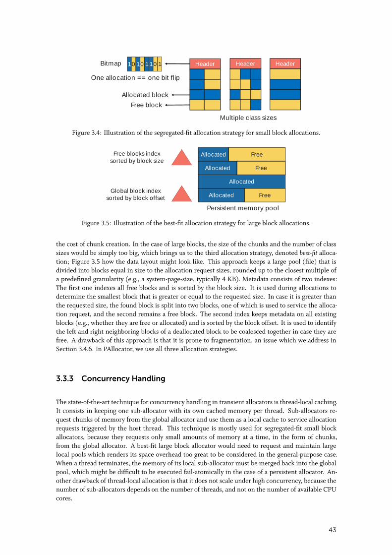
HeaderHeader Header
Multiple class sizes
One allocation == one bit flip
1 0 1 0 1 1 0 1Bitmap
Allocated block
Free block
Figure 3.4: Illustration of the segregated-fit allocation strategy for small block allocations.
Allocated Free
Allocated Allocated Free
Allocated
Allocated Free
Persistent memory pool
Free blocks indexsorted by block size
Global block indexsorted by block offset
FreeFree
Figure 3.5: Illustration of the best-fit allocation strategy for large block allocations.
the cost of chunk creation. In the case of large blocks, the size of the chunks and the number of classsizes would be simply too big, which brings us to the third allocation strategy, denoted best-fit alloca-tion; Figure 3.5 how the data layout might look like. This approach keeps a large pool (file) that isdivided into blocks equal in size to the allocation request sizes, rounded up to the closest multiple ofa predefined granularity (e.g., a system-page-size, typically 4 KB). Metadata consists of two indexes:The first one indexes all free blocks and is sorted by the block size. It is used during allocations todetermine the smallest block that is greater or equal to the requested size. In case it is greater thanthe requested size, the found block is split into two blocks, one of which is used to service the alloca-tion request, and the second remains a free block. The second index keeps metadata on all existingblocks (e.g., whether they are free or allocated) and is sorted by the block offset. It is used to identifythe left and right neighboring blocks of a deallocated block to be coalesced together in case they arefree. A drawback of this approach is that it is prone to fragmentation, an issue which we address inSection 3.4.6. In PAllocator, we use all three allocation strategies.
3.3.3 Concurrency Handling
The state-of-the-art technique for concurrency handling in transient allocators is thread-local caching.It consists in keeping one sub-allocator with its own cached memory per thread. Sub-allocators re-quest chunks of memory from the global allocator and use them as a local cache to service allocationrequests triggered by the host thread. This technique is mostly used for segregated-fit small blockallocators, because they requests only small amounts of memory at a time, in the form of chunks,from the global allocator. A best-fit large block allocator would need to request and maintain largelocal pools which renders its space overhead too great to be considered in the general-purpose case.When a thread terminates, the memory of its local sub-allocator must be merged back into the globalpool, which might be difficult to be executed fail-atomically in the case of a persistent allocator. An-other drawback of thread-local allocation is that it does not scale under high concurrency, because thenumber of sub-allocators depends on the number of threads, and not on the number of available CPUcores.
43
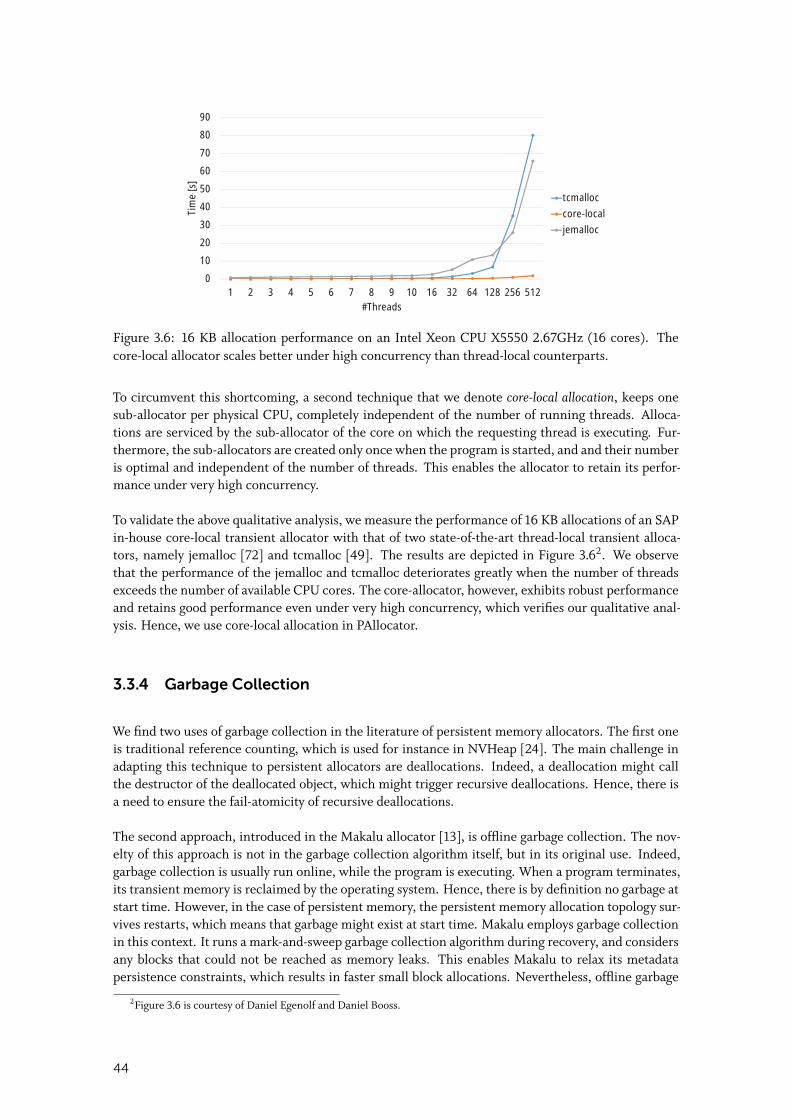
0
10
20
30
40
50
60
70
80
90
1 2 3 4 5 6 7 8 9 10 16 32 64 128 256 512
Tim
e[s
]
#Threads
tcmalloccore-localjemalloc
Figure 3.6: 16 KB allocation performance on an Intel Xeon CPU X5550 2.67GHz (16 cores). Thecore-local allocator scales better under high concurrency than thread-local counterparts.
To circumvent this shortcoming, a second technique that we denote core-local allocation, keeps onesub-allocator per physical CPU, completely independent of the number of running threads. Alloca-tions are serviced by the sub-allocator of the core on which the requesting thread is executing. Fur-thermore, the sub-allocators are created only once when the program is started, and and their numberis optimal and independent of the number of threads. This enables the allocator to retain its perfor-mance under very high concurrency.
To validate the above qualitative analysis, we measure the performance of 16 KB allocations of an SAPin-house core-local transient allocator with that of two state-of-the-art thread-local transient alloca-tors, namely jemalloc [72] and tcmalloc [49]. The results are depicted in Figure 3.62. We observethat the performance of the jemalloc and tcmalloc deteriorates greatly when the number of threadsexceeds the number of available CPU cores. The core-allocator, however, exhibits robust performanceand retains good performance even under very high concurrency, which verifies our qualitative anal-ysis. Hence, we use core-local allocation in PAllocator.
3.3.4 Garbage Collection
We find two uses of garbage collection in the literature of persistent memory allocators. The first oneis traditional reference counting, which is used for instance in NVHeap [24]. The main challenge inadapting this technique to persistent allocators are deallocations. Indeed, a deallocation might callthe destructor of the deallocated object, which might trigger recursive deallocations. Hence, there isa need to ensure the fail-atomicity of recursive deallocations.
The second approach, introduced in the Makalu allocator [13], is offline garbage collection. The nov-elty of this approach is not in the garbage collection algorithm itself, but in its original use. Indeed,garbage collection is usually run online, while the program is executing. When a program terminates,its transient memory is reclaimed by the operating system. Hence, there is by definition no garbage atstart time. However, in the case of persistent memory, the persistent memory allocation topology sur-vives restarts, which means that garbage might exist at start time. Makalu employs garbage collectionin this context. It runs a mark-and-sweep garbage collection algorithm during recovery, and considersany blocks that could not be reached as memory leaks. This enables Makalu to relax its metadatapersistence constraints, which results in faster small block allocations. Nevertheless, offline garbage
2Figure 3.6 is courtesy of Daniel Egenolf and Daniel Booss.
44
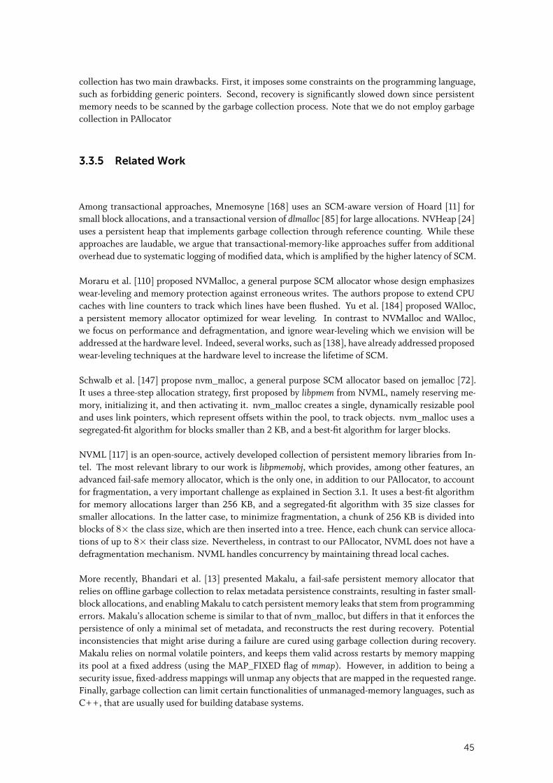
collection has two main drawbacks. First, it imposes some constraints on the programming language,such as forbidding generic pointers. Second, recovery is significantly slowed down since persistentmemory needs to be scanned by the garbage collection process. Note that we do not employ garbagecollection in PAllocator
3.3.5 Related Work
Among transactional approaches, Mnemosyne [168] uses an SCM-aware version of Hoard [11] forsmall block allocations, and a transactional version of dlmalloc [85] for large allocations. NVHeap [24]uses a persistent heap that implements garbage collection through reference counting. While theseapproaches are laudable, we argue that transactional-memory-like approaches suffer from additionaloverhead due to systematic logging of modified data, which is amplified by the higher latency of SCM.
Moraru et al. [110] proposed NVMalloc, a general purpose SCM allocator whose design emphasizeswear-leveling and memory protection against erroneous writes. The authors propose to extend CPUcaches with line counters to track which lines have been flushed. Yu et al. [184] proposed WAlloc,a persistent memory allocator optimized for wear leveling. In contrast to NVMalloc and WAlloc,we focus on performance and defragmentation, and ignore wear-leveling which we envision will beaddressed at the hardware level. Indeed, several works, such as [138], have already addressed proposedwear-leveling techniques at the hardware level to increase the lifetime of SCM.
Schwalb et al. [147] propose nvm_malloc, a general purpose SCM allocator based on jemalloc [72].It uses a three-step allocation strategy, first proposed by libpmem from NVML, namely reserving me-mory, initializing it, and then activating it. nvm_malloc creates a single, dynamically resizable pooland uses link pointers, which represent offsets within the pool, to track objects. nvm_malloc uses asegregated-fit algorithm for blocks smaller than 2 KB, and a best-fit algorithm for larger blocks.
NVML [117] is an open-source, actively developed collection of persistent memory libraries from In-tel. The most relevant library to our work is libpmemobj, which provides, among other features, anadvanced fail-safe memory allocator, which is the only one, in addition to our PAllocator, to accountfor fragmentation, a very important challenge as explained in Section 3.1. It uses a best-fit algorithmfor memory allocations larger than 256 KB, and a segregated-fit algorithm with 35 size classes forsmaller allocations. In the latter case, to minimize fragmentation, a chunk of 256 KB is divided intoblocks of 8× the class size, which are then inserted into a tree. Hence, each chunk can service alloca-tions of up to 8× their class size. Nevertheless, in contrast to our PAllocator, NVML does not have adefragmentation mechanism. NVML handles concurrency by maintaining thread local caches.
More recently, Bhandari et al. [13] presented Makalu, a fail-safe persistent memory allocator thatrelies on offline garbage collection to relax metadata persistence constraints, resulting in faster small-block allocations, and enabling Makalu to catch persistent memory leaks that stem from programmingerrors. Makalu’s allocation scheme is similar to that of nvm_malloc, but differs in that it enforces thepersistence of only a minimal set of metadata, and reconstructs the rest during recovery. Potentialinconsistencies that might arise during a failure are cured using garbage collection during recovery.Makalu relies on normal volatile pointers, and keeps them valid across restarts by memory mappingits pool at a fixed address (using the MAP_FIXED flag of mmap). However, in addition to being asecurity issue, fixed-address mappings will unmap any objects that are mapped in the requested range.Finally, garbage collection can limit certain functionalities of unmanaged-memory languages, such asC++, that are usually used for building database systems.
45
Anchor Segment
ASLnASL1 ...ActiveSegmentsLists
FSLnFSL1 ...FullSegmentsLists
SegCounter
Free Segments List
SegmentListManager
PLMnPLM1 ...PageListManagers
BBMnBBM1 ...BigBlockManagers
PAllocatorAnchor
BRcInBRcI1 ...BigBlockRcItems
SRcInSRcI1 ...SmallBlockRcItems
Huge Block RcItem
RecoveryItemManagerEntry Point Status Flag
DRAM
SCM
PAllocator
SegmentListManager
SBAnSBA1 ...SmallBlockAllocator
BBAnBBA1 ...BigBlockAllocator
Huge Block Allocator
SegID toAddress
Map
Address to(SegID,SegSize)
Map
SegID toAllocID
Map
Figure 3.7: Architecture overview of PAllocator.
To the best of our knowledge, Mnemosyne, NVML, nvm_malloc, Makalu, and NVMalloc are the onlypersistent allocators publicly available. We compare the performance of PAllocator against NVML,Makalu, and nvm_malloc; we exclude NVMalloc since it does not provide a recovery mechanism(see Section 3.5 for further details), and Mnemosyne since its default allocator is outperformed byMakalu [13].
Table 3.2 summarizes the design characteristics of existing persistent memory allocators. PAlloca-tor exhibits radically different design characteristics than state-of-the-art persistent allocators. Thisdifference stems from our design goals on which we elaborate in the next section.
3.4 PALLOCATOR DESIGN AND IMPLEMENTATION
In this section we present our proposed PAllocator and its different components.
3.4.1 Design goals and decisions
We identify the following design goals for persistent memory allocators tailored for large-scale SCM-based systems:
46

Allo
cato
rPu
rpos
ePo
olSt
ruct
ure
Allo
cati
onSt
rate
gies
Con
curr
ency
Han
dlin
gG
arba
geC
olle
ctio
nD
efra
gmen
-ta
tion
Ref
eren
ce
Mne
mos
yne
Gen
eral
Mul
tipl
efil
esSe
greg
ated
-fit
+be
st-fi
t
Thre
ad-lo
calf
orsm
all
bloc
ks;g
loba
lloc
kfo
rla
rge
bloc
ksYe
sN
oVo
los
etal
.[16
8]
NV-
Hea
psG
ener
alSi
ngle
file
Und
efine
dTh
read
-loca
lYe
sN
oC
obur
net
al.[
24]
nvm
_mal
loc
Gen
eral
Sing
lefil
eSe
greg
ated
-fit
+be
st-fi
t
Thre
ad-lo
calf
orsm
all
bloc
ks;g
loba
lloc
kfo
rla
rge
bloc
ksN
oN
oSc
hwal
bet
al.[
147]
NV
ML
Gen
eral
Sing
lefil
eSe
greg
ated
-fit
+be
st-fi
t
Thre
ad-lo
calf
orsm
all
bloc
ks;g
loba
lloc
kfo
rla
rge
bloc
ksN
oN
ohttp://pmem.io
Mak
alu
Gen
eral
Sing
lefil
eSe
greg
ated
-fit
+be
st-fi
t
Thre
ad-lo
calf
orsm
all
bloc
ks;g
loba
lloc
kfo
rla
rge
bloc
ks
Yes
(offl
ine)
No
Bha
ndar
iet
al.[
13]
PAllo
cato
rSp
ecia
l(l
arge
-sca
lesy
stem
s)M
ulti
ple
files
Segr
egat
ed-
fit+
best
-fit
+fil
e
Cor
e-lo
calf
orsm
alla
ndla
rge
bloc
ks;g
loba
lloc
kfo
rhu
gebl
ocks
No
Yes
Ouk
idet
al.[
124]
Tabl
e3.
2:Su
mm
ary
ofth
ede
sign
char
acte
rist
ics
ofex
isti
ngpe
rsis
tent
mem
ory
allo
cato
rs.T
here
are
salie
ntdi
ffer
ence
sin
the
desi
gnde
cisi
ons
ofPA
lloca
tor
and
stat
e-of
-the
-art
pers
iste
ntal
loca
tors
.
47
• The ability to adapt to changes in available memory resources. This is particularly important ina cloud environment.
• High concurrency scalability. Large main-memory systems run on multi-socket systems with upto 1000 cores. Thus, it is important for the persistent allocator to provide robust and scalableperformance.
• Provide robust performance for all sizes of allocations, as database-system allocation sizes covera wide range, from a few bytes to hundreds of gigabytes.
• Fast recovery. Currently there are instances of single-node main-memory database systems suchas SAP HANA [44] with up to 48 TB of main memory. With SCM this capacity will quicklyexceed 100 TB. Thus, the persistent allocator must exhibit fast recovery and should not rely onscanning memory to recover its metadata.
• Defragmentation ability; Database systems run for a very long time, much longer than general-purpose applications, making fragmentation much more likely to happen.
So far, state-of-the-art persistent allocators, such as NVML, nvm_malloc, and Makalu have been en-gineered as general-purpose allocators, taking inspiration from state-of-the-art general-purpose tran-sient allocators. We argue that they are unfit for large-scale SCM-based database systems because:
• They all use a single pool (file), which is difficult to both grow and shrink (to the best of ourknowledge, none of them can grow or shrink their pool beyond its initial size).
• They put an emphasis on the scalability of small-block allocations (from a few bytes up to a fewkilobytes), and neglect that of middle-sized and large-block allocations.
• They do not provide defragmentation capabilities.• They often rely on scanning memory to recover their metadata during recovery.
PAllocator is not a general-purpose allocator. It fulfills the above design goals following radicallydifferent design decisions than state-of-the-art persistent allocators:
• We use multiple files instead of a single pool, which allows us to easily grow and shrink our poolof persistent memory.
• We use large files to avoid having a large number of them which would hit the limitations ofcurrent file systems.
• We use three different allocation strategies for small, big, and huge allocation sizes, mostlyindependent from each other, to ensure robust performance for all allocation sizes.
• We aggressively cache free memory by not removing free files. Instead, we keep them to speedup future allocations. This is acceptable since main-memory database systems usually havededicated resources.
• Instead of thread-local pools, we use one allocator object per physical core. Database systemscan create and terminate threads at a high rate during query processing. Using thread-localpools in this case might hurt performance and complicates fail-safety management as the localpool has to be given back and integrated in the global pool upon thread termination. Using strip-ing per physical core combined with aggressive caching provides a stable, robust, and scalableallocation and deallocation performance.
• To defragment memory, we leverage the hole punching feature of sparse files. This is an addi-tional advantage of using multiple files.
• To provide fast recovery, we persist most of PAllocator’s metadata and rely on hybrid SCM-DRAM trees to trade off between performance and recovery time when necessary.
48
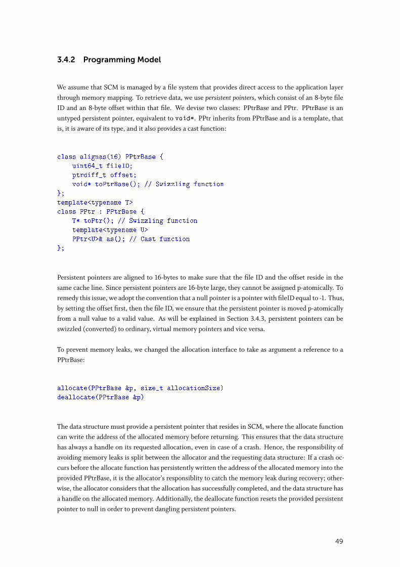
3.4.2 Programming Model
We assume that SCM is managed by a file system that provides direct access to the application layerthrough memory mapping. To retrieve data, we use persistent pointers, which consist of an 8-byte fileID and an 8-byte offset within that file. We devise two classes: PPtrBase and PPtr. PPtrBase is anuntyped persistent pointer, equivalent to void*. PPtr inherits from PPtrBase and is a template, thatis, it is aware of its type, and it also provides a cast function:
class alignas(16) PPtrBase {
uint64_t fileID;
ptrdiff_t offset;
void* toPtrBase(); // Swizzling function
};
template<typename T>
class PPtr : PPtrBase {
T* toPtr(); // Swizzling function
template<typename U>
PPtr<U>& as(); // Cast function
};
Persistent pointers are aligned to 16-bytes to make sure that the file ID and the offset reside in thesame cache line. Since persistent pointers are 16-byte large, they cannot be assigned p-atomically. Toremedy this issue, we adopt the convention that a null pointer is a pointer with fileID equal to -1. Thus,by setting the offset first, then the file ID, we ensure that the persistent pointer is moved p-atomicallyfrom a null value to a valid value. As will be explained in Section 3.4.3, persistent pointers can beswizzled (converted) to ordinary, virtual memory pointers and vice versa.
To prevent memory leaks, we changed the allocation interface to take as argument a reference to aPPtrBase:
allocate(PPtrBase &p, size_t allocationSize)
deallocate(PPtrBase &p)
The data structure must provide a persistent pointer that resides in SCM, where the allocate functioncan write the address of the allocated memory before returning. This ensures that the data structurehas always a handle on its requested allocation, even in case of a crash. Hence, the responsibility ofavoiding memory leaks is split between the allocator and the requesting data structure: If a crash oc-curs before the allocate function has persistently written the address of the allocated memory into theprovided PPtrBase, it is the allocator’s responsiblity to catch the memory leak during recovery; other-wise, the allocator considers that the allocation has successfully completed, and the data structure hasa handle on the allocated memory. Additionally, the deallocate function resets the provided persistentpointer to null in order to prevent dangling persistent pointers.
49
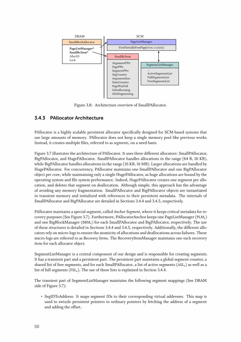
SmallBlockAllocator
PageListManager*SmallRcItem*AllocIDLock
PageListManager
FirstPartiallyFreePage[NUM_CLASSES]
SmallRcItem
ArgumentPPtrPagePPtrSegmentPPtrSegCounterArgumentSizeStateCounterPageWasFullIsDeallocatingIsDefragmenting
SegmentListManager
...ActiveSegmentsListFullSegmentsListFreeSegmentsList
SCMDRAM
Figure 3.8: Architecture overview of SmallPAllocator.
3.4.3 PAllocator Architecture
PAllocator is a highly scalable persistent allocator specifically designed for SCM-based systems thatuse large amounts of memory. PAllocator does not keep a single memory pool like previous works.Instead, it creates multiple files, referred to as segments, on a need basis.
Figure 3.7 illustrates the architecture of PAllocator. It uses three different allocators: SmallPAllocator,BigPAllocator, and HugePAllocator. SmallPAllocator handles allocations in the range [64 B, 16 KB),while BigPAllocator handles allocations in the range [16 KB, 16 MB). Larger allocations are handled byHugePAllocator. For concurrency, PAllocator maintains one SmallPAllocator and one BigPAllocatorobject per core, while maintaining only a single HugePAllocator, as huge allocations are bound by theoperating system and file system performance. Indeed, HugePAllocator creates one segment per allo-cation, and deletes that segment on deallocation. Although simple, this approach has the advantageof avoiding any memory fragmentation. SmallPAllocator and BigPAllocator objects are instantiatedin transient memory and initialized with references to their persistent metadata. The internals ofSmallPAllocator and BigPAllocator are detailed in Sections 3.4.4 and 3.4.5, respectively.
PAllocator maintains a special segment, called Anchor Segment, where it keeps critical metadata for re-covery purposes (See Figure 3.7). Furthermore, PAllocatorAnchor keeps one PageListManager (PLMi)and one BigBlockManager (BBMi) for each SmallPAllocator and BigPAllocator, respectively. The useof these structures is detailed in Sections 3.4.4 and 3.4.5, respectively. Additionally, the different allo-cators rely on micro-logs to ensure the atomicity of allocations and deallocations across failures. Thesemicro-logs are referred to as Recovery Items. The RecoveryItemManager maintains one such recoveryitem for each allocator object.
SegmentListManager is a central component of our design and is responsible for creating segments.It has a transient part and a persistent part. The persistent part maintains a global segment counter, ashared list of free segments, and for each SmallPAllocator, a list of active segments (ASLi) as well as alist of full segments (FSLi). The use of these lists is explained in Section 3.4.4.
The transient part of SegmentListManager maintains the following segment mappings (See DRAMside of Figure 3.7):
• SegIDToAddress: It maps segment IDs to their corresponding virtual addresses. This map isused to swizzle persistent pointers to ordinary pointers by fetching the address of a segmentand adding the offset.
50
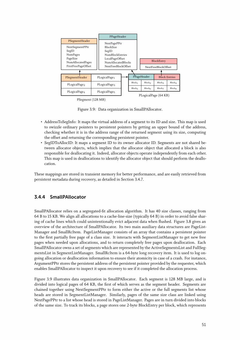
PSegmentHeader PLogicalPage1
PLogicalPage2 PLogicalPage3
PLogicalPage4 PLogicalPage5
PSegment (128 MB)PLogicalPage (64 KB)
NextSegmentPPtrSegIDNumPagesPageSizeNumAllocatedPagesFirstFreePageOffset
PSegmentHeader
PPageHeader
Block1 Block2
Block5 Block6 Block7 Block8
Block3 Block4
NextPagePPtrBlockSizeSegIDNumBlockEntriesLocalPageOffsetNumAllocatedBlocksNextFreeBlockOffset
PPageHeader
Block Entries
NextFreeBlockOffset
BlockEntry
Figure 3.9: Data organization in SmallPAllocator.
• AddressToSegInfo: It maps the virtual address of a segment to its ID and size. This map is usedto swizzle ordinary pointers to persistent pointers by getting an upper bound of the address,checking whether it is in the address range of the returned segment using its size, computingthe offset and returning the corresponding persistent pointer.
• SegIDToAllocID: It maps a segment ID to its owner allocator ID. Segments are not shared be-tween allocator objects, which implies that the allocator object that allocated a block is alsoresponsible for deallocating it. Indeed, allocator objects operate independently from each other.This map is used in deallocations to identify the allocator object that should perform the deallo-cation.
These mappings are stored in transient memory for better performance, and are easily retrieved frompersistent metadata during recovery, as detailed in Section 3.4.7.
3.4.4 SmallPAllocator
SmallPAllocator relies on a segregated-fit allocation algorithm. It has 40 size classes, ranging from64 B to 15 KB. We align all allocations to a cache-line-size (typically 64 B) in order to avoid false shar-ing of cache lines which could unintentionally evict adjacent data when flushed. Figure 3.8 gives anoverview of the architecture of SmallPAllocator. Its two main auxiliary data structures are PageList-Manager and SmallRcItem. PageListManager consists of an array that contains a persistent pointerto the first partially free page of a class size. It interacts with SegmentListManager to get new freepages when needed upon allocations, and to return completely free pages upon deallocation. EachSmallPAllocator owns a set of segments which are represented by the ActiveSegmentsList and FullSeg-mentsList in SegmentListManager. SmallRcItem is a 64-byte long recovery item. It is used to log on-going allocation or deallocation information to ensure their atomicity in case of a crash. For instance,ArgumentPPtr stores the persistent address of the persistent pointer provided by the requester, whichenables SmallPAllocator to inspect it upon recovery to see if it completed the allocation process.
Figure 3.9 illustrates data organization in SmallPAllocator. Each segment is 128 MB large, and isdivided into logical pages of 64 KB, the first of which serves as the segment header. Segments arechained together using NextSegmentPPtr to form either the active or the full segments list whoseheads are stored in SegmentListManager. Similarly, pages of the same size class are linked usingNextPagePPtr to a list whose head is stored in PageListManager. Pages are in turn divided into blocksof the same size. To track its blocks, a page stores one 2-byte BlockEntry per block, which represents
51
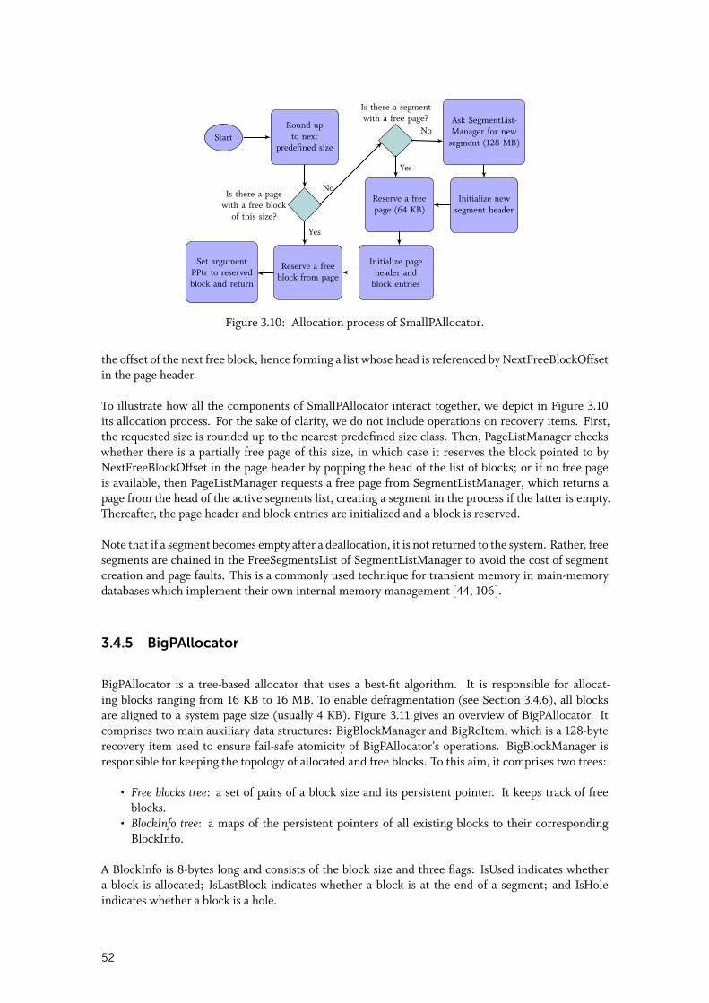
Reserve a freeblock from page
Initialize pageheader and
block entries
Initialize newsegment header
Ask SegmentList-Manager for new
segment (128 MB)
Reserve a freepage (64 KB)
Round upto next
predefined size
Set argumentPPtr to reservedblock and return
Start
Is there a pagewith a free block
of this size?
Is there a segmentwith a free page?
Yes
No
Yes
No
Figure 3.10: Allocation process of SmallPAllocator.
the offset of the next free block, hence forming a list whose head is referenced by NextFreeBlockOffsetin the page header.
To illustrate how all the components of SmallPAllocator interact together, we depict in Figure 3.10its allocation process. For the sake of clarity, we do not include operations on recovery items. First,the requested size is rounded up to the nearest predefined size class. Then, PageListManager checkswhether there is a partially free page of this size, in which case it reserves the block pointed to byNextFreeBlockOffset in the page header by popping the head of the list of blocks; or if no free pageis available, then PageListManager requests a free page from SegmentListManager, which returns apage from the head of the active segments list, creating a segment in the process if the latter is empty.Thereafter, the page header and block entries are initialized and a block is reserved.
Note that if a segment becomes empty after a deallocation, it is not returned to the system. Rather, freesegments are chained in the FreeSegmentsList of SegmentListManager to avoid the cost of segmentcreation and page faults. This is a commonly used technique for transient memory in main-memorydatabases which implement their own internal memory management [44, 106].
3.4.5 BigPAllocator
BigPAllocator is a tree-based allocator that uses a best-fit algorithm. It is responsible for allocat-ing blocks ranging from 16 KB to 16 MB. To enable defragmentation (see Section 3.4.6), all blocksare aligned to a system page size (usually 4 KB). Figure 3.11 gives an overview of BigPAllocator. Itcomprises two main auxiliary data structures: BigBlockManager and BigRcItem, which is a 128-byterecovery item used to ensure fail-safe atomicity of BigPAllocator’s operations. BigBlockManager isresponsible for keeping the topology of allocated and free blocks. To this aim, it comprises two trees:
• Free blocks tree: a set of pairs of a block size and its persistent pointer. It keeps track of freeblocks.
• BlockInfo tree: a maps of the persistent pointers of all existing blocks to their correspondingBlockInfo.
A BlockInfo is 8-bytes long and consists of the block size and three flags: IsUsed indicates whethera block is allocated; IsLastBlock indicates whether a block is at the end of a segment; and IsHoleindicates whether a block is a hole.
52
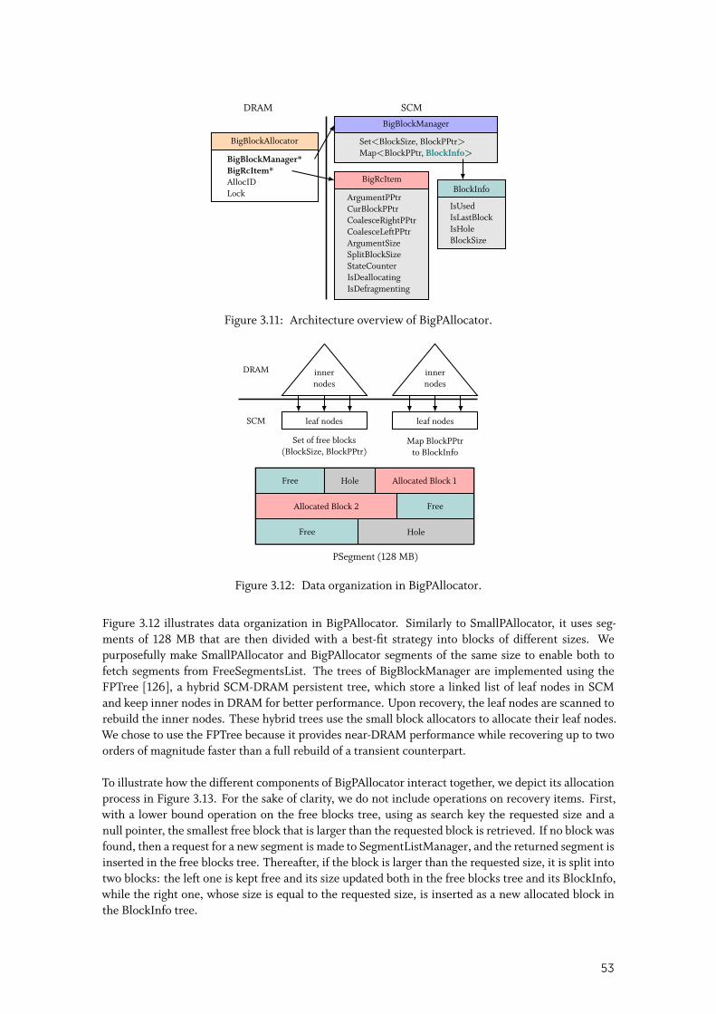
BigBlockAllocator
BigBlockManager*BigRcItem*AllocIDLock
BigBlockManager
Set<BlockSize, BlockPPtr>Map<BlockPPtr, BlockInfo>
BigRcItem
ArgumentPPtrCurBlockPPtrCoalesceRightPPtrCoalesceLeftPPtrArgumentSizeSplitBlockSizeStateCounterIsDeallocatingIsDefragmenting
BlockInfo
IsUsedIsLastBlockIsHoleBlockSize
SCMDRAM
Figure 3.11: Architecture overview of BigPAllocator.
Allocated Block 1Free
Allocated Block 2 Free
Hole
PSegment (128 MB)
DRAM
SCM leaf nodes leaf nodes
innernodes
innernodes
Set of free blocks(BlockSize, BlockPPtr)
Map BlockPPtrto BlockInfo
Hole
Free
Figure 3.12: Data organization in BigPAllocator.
Figure 3.12 illustrates data organization in BigPAllocator. Similarly to SmallPAllocator, it uses seg-ments of 128 MB that are then divided with a best-fit strategy into blocks of different sizes. Wepurposefully make SmallPAllocator and BigPAllocator segments of the same size to enable both tofetch segments from FreeSegmentsList. The trees of BigBlockManager are implemented using theFPTree [126], a hybrid SCM-DRAM persistent tree, which store a linked list of leaf nodes in SCMand keep inner nodes in DRAM for better performance. Upon recovery, the leaf nodes are scanned torebuild the inner nodes. These hybrid trees use the small block allocators to allocate their leaf nodes.We chose to use the FPTree because it provides near-DRAM performance while recovering up to twoorders of magnitude faster than a full rebuild of a transient counterpart.
To illustrate how the different components of BigPAllocator interact together, we depict its allocationprocess in Figure 3.13. For the sake of clarity, we do not include operations on recovery items. First,with a lower bound operation on the free blocks tree, using as search key the requested size and anull pointer, the smallest free block that is larger than the requested block is retrieved. If no block wasfound, then a request for a new segment is made to SegmentListManager, and the returned segment isinserted in the free blocks tree. Thereafter, if the block is larger than the requested size, it is split intotwo blocks: the left one is kept free and its size updated both in the free blocks tree and its BlockInfo,while the right one, whose size is equal to the requested size, is inserted as a new allocated block inthe BlockInfo tree.
53
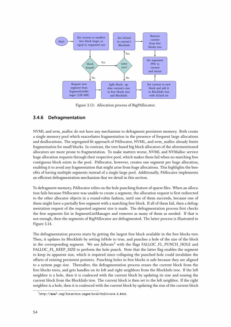
Set current to smallestfree block larger or
equal to requested size
Request newsegment from
SegmentListMa-nager (128 MB)
Set IsUsedin current’sBlockInfo
Split block: up-date current’s sizein free blocks tree
and BlockInfo
Removecurrent
from freeblocks tree
Set current to newblock and add itto BlockInfo treewith IsUsed set
Set argumentPPtr tocurrent
and return
Start
blockfound?
samesize?
Yes
Yes
No No
Figure 3.13: Allocation process of BigPAllocator.
3.4.6 Defragmentation
NVML and nvm_malloc do not have any mechanism to defragment persistent memory. Both createa single memory pool which exacerbates fragmentation in the presence of frequent large allocationsand deallocations. The segregated-fit approach of PAllocator, NVML, and nvm_malloc already limitsfragmentation for small blocks. In contrast, the tree-based big block allocators of the aforementionedallocators are more prone to fragmentation. To make matters worse, NVML and NVMalloc servicehuge allocation requests through their respective pool, which makes them fail when no matching freecontiguous block exists in the pool. PAllocator, however, creates one segment per huge allocation,enabling it to avoid any fragmentation that might arise from huge allocations. This highlights the ben-efits of having multiple segments instead of a single large pool. Additionally, PAllocator implementsan efficient defragmentation mechanism that we detail in this section.
To defragment memory, PAllocator relies on the hole punching feature of sparse files. When an alloca-tion fails because PAllocator was unable to create a segment, the allocation request is first redirectedto the other allocator objects in a round-robin fashion, until one of them succeeds, because one ofthem might have a partially free segment with a matching free block. If all of them fail, then a defrag-mentation request of the requested segment size is made. The defragmentation process first checksthe free segments list in SegmentListManager and removes as many of them as needed. If that isnot enough, then the segments of BigPAllocator are defragmented. The latter process is illustrated inFigure 3.14.
The defragmentation process starts by getting the largest free block available in the free blocks tree.Then, it updates its BlockInfo by setting IsHole to true, and punches a hole of the size of the blockin the corresponding segment. We use fallocate3 with the flags FALLOC_FL_PUNCH_HOLE andFALLOC_FL_KEEP_SIZE to perform the hole punch. Note that the latter flag enables the segmentto keep its apparent size, which is required since collapsing the punched hole could invalidate theoffsets of existing persistent pointers. Punching holes in free blocks is safe because they are alignedto a system page size. Thereafter, the defragmentation process erases the current block from thefree blocks trees, and gets handles on its left and right neighbors from the BlockInfo tree. If the leftneighbor is a hole, then it is coalesced with the current block by updating its size and erasing thecurrent block from the BlockInfo tree. The current block is then set to the left neighbor. If the rightneighbor is a hole, then it is coalesced with the current block by updating the size of the current block
3http://man7.org/linux/man-pages/man2/fallocate.2.html
54
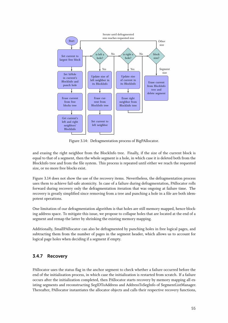
Set current tolargest free block
Set IsHolein current’s
BlockInfo andpunch hole
Erase currentfrom free
blocks tree
Get current’sleft and right
neighbors’BlockInfo
Update size ofleft neighbor in
its BlockInfo
Erase cur-rent from
BlockInfo tree
Set current toleft neighbor
Update sizeof current inits BlockInfo
Erase rightneighbor fromBlockInfo tree
Erase currentfrom BlockInfo
tree anddelete segment
Start
is left ahole?
is right ahole?
blocksize?
YesYes
NoNo
Segmentsize
Othersize
Iterate until defragmentedsize reaches requested size
Figure 3.14: Defragmentation process of BigPAllocator.
and erasing the right neighbor from the BlockInfo tree. Finally, if the size of the current block isequal to that of a segment, then the whole segment is a hole, in which case it is deleted both from theBlockInfo tree and from the file system. This process is repeated until either we reach the requestedsize, or no more free blocks exist.
Figure 3.14 does not show the use of the recovery items. Nevertheless, the defragmentation processuses them to achieve fail-safe atomicity. In case of a failure during defragmentation, PAllocator rollsforward during recovery only the defragmentation iteration that was ongoing at failure time. Therecovery is greatly simplified since removing from a tree and punching a hole in a file are both idem-potent operations.
One limitation of our defragmentation algorithm is that holes are still memory mapped, hence block-ing address space. To mitigate this issue, we propose to collapse holes that are located at the end of asegment and remap the latter by shrinking the existing memory mapping.
Additionally, SmallPAllocator can also be defragmented by punching holes in free logical pages, andsubtracting them from the number of pages in the segment header, which allows us to account forlogical page holes when deciding if a segment if empty.
3.4.7 Recovery
PAllocator uses the status flag in the anchor segment to check whether a failure occurred before theend of the initialization process, in which case the initialization is restarted from scratch. If a failureoccurs after the initialization completed, then PAllocator starts recovery by memory mapping all ex-isting segments and reconstructing SegIDToAddress and AddressToSegInfo of SegmentListManager.Thereafter, PAllocator instantiates the allocator objects and calls their respective recovery functions,
55
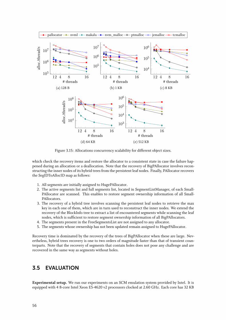
pallocator nvml makalu nvm_malloc ptmalloc jemalloc tcmalloc
12 4 8 16105
106
107
# threads
allo
c./t
hrea
d/s
(a) 128 B
12 4 8 16
105
106
107
# threads
(b) 1 KB
12 4 8 16
104
105
106
# threads
(c) 8 KB
12 4 8 16
104
105
106
# threads
allo
c./t
hrea
d/s
(d) 64 KB
12 4 8 16
103
104
105
106
# threads
(e) 512 KB
Figure 3.15: Allocations concurrency scalability for different object sizes.
which check the recovery items and restore the allocator to a consistent state in case the failure hap-pened during an allocation or a deallocation. Note that the recovery of BigPAllocator involves recon-structing the inner nodes of its hybrid trees from the persistent leaf nodes. Finally, PAllocator recoversthe SegIDToAllocID map as follows:
1. All segments are initially assigned to HugePAllocator.2. The active segments list and full segments list, located in SegmentListManager, of each Small-
PAllocator are scanned. This enables to restore segment ownership information of all Small-PAllocators.
3. The recovery of a hybrid tree involves scanning the persistent leaf nodes to retrieve the maxkey in each one of them, which are in turn used to reconstruct the inner nodes. We extend therecovery of the BlockInfo tree to extract a list of encountered segments while scanning the leafnodes, which is sufficient to restore segment ownership information of all BigPAllocators.
4. The segments present in the FreeSegmentsList are not assigned to any allocator.5. The segments whose ownership has not been updated remain assigned to HugePAllocator.
Recovery time is dominated by the recovery of the trees of BigPAllocator when these are large. Nev-ertheless, hybrid trees recovery is one to two orders of magnitude faster than that of transient coun-terparts. Note that the recovery of segments that contain holes does not pose any challenge and arerecovered in the same way as segments without holes.
3.5 EVALUATION
Experimental setup. We run our experiments on an SCM emulation system provided by Intel. It isequipped with 4 8-core Intel Xeon E5-4620 v2 processors clocked at 2.60 GHz. Each core has 32 KB
56
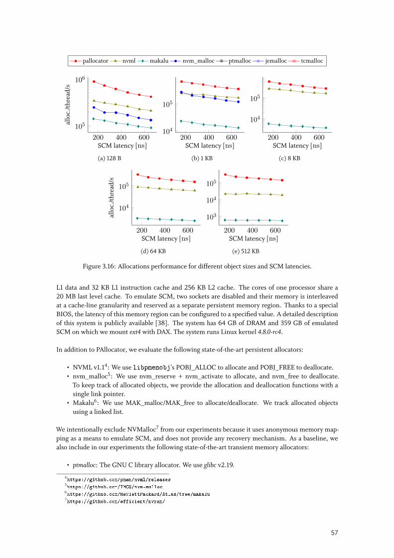
pallocator nvml makalu nvm_malloc ptmalloc jemalloc tcmalloc
200 400 600
105
106
SCM latency [ns]
allo
c./t
hrea
d/s
(a) 128 B
200 400 600104
105
SCM latency [ns]
(b) 1 KB
200 400 600
104
105
SCM latency [ns]
(c) 8 KB
200 400 600
104
105
SCM latency [ns]
allo
c./t
hrea
d/s
(d) 64 KB
200 400 600
103
104
105
SCM latency [ns]
(e) 512 KB
Figure 3.16: Allocations performance for different object sizes and SCM latencies.
L1 data and 32 KB L1 instruction cache and 256 KB L2 cache. The cores of one processor share a20 MB last level cache. To emulate SCM, two sockets are disabled and their memory is interleavedat a cache-line granularity and reserved as a separate persistent memory region. Thanks to a specialBIOS, the latency of this memory region can be configured to a specified value. A detailed descriptionof this system is publicly available [38]. The system has 64 GB of DRAM and 359 GB of emulatedSCM on which we mount ext4 with DAX. The system runs Linux kernel 4.8.0-rc4.
In addition to PAllocator, we evaluate the following state-of-the-art persistent allocators:
• NVML v1.14: We use libpmemobj’s POBJ_ALLOC to allocate and POBJ_FREE to deallocate.• nvm_malloc5: We use nvm_reserve + nvm_activate to allocate, and nvm_free to deallocate.
To keep track of allocated objects, we provide the allocation and deallocation functions with asingle link pointer.
• Makalu6: We use MAK_malloc/MAK_free to allocate/deallocate. We track allocated objectsusing a linked list.
We intentionally exclude NVMalloc7 from our experiments because it uses anonymous memory map-ping as a means to emulate SCM, and does not provide any recovery mechanism. As a baseline, wealso include in our experiments the following state-of-the-art transient memory allocators:
• ptmalloc: The GNU C library allocator. We use glibc v2.19.
4https://github.com/pmem/nvml/releases
5https://github.com/IMCG/nvm-malloc
6https://github.com/HewlettPackard/Atlas/tree/makalu
7https://github.com/efficient/nvram/
57
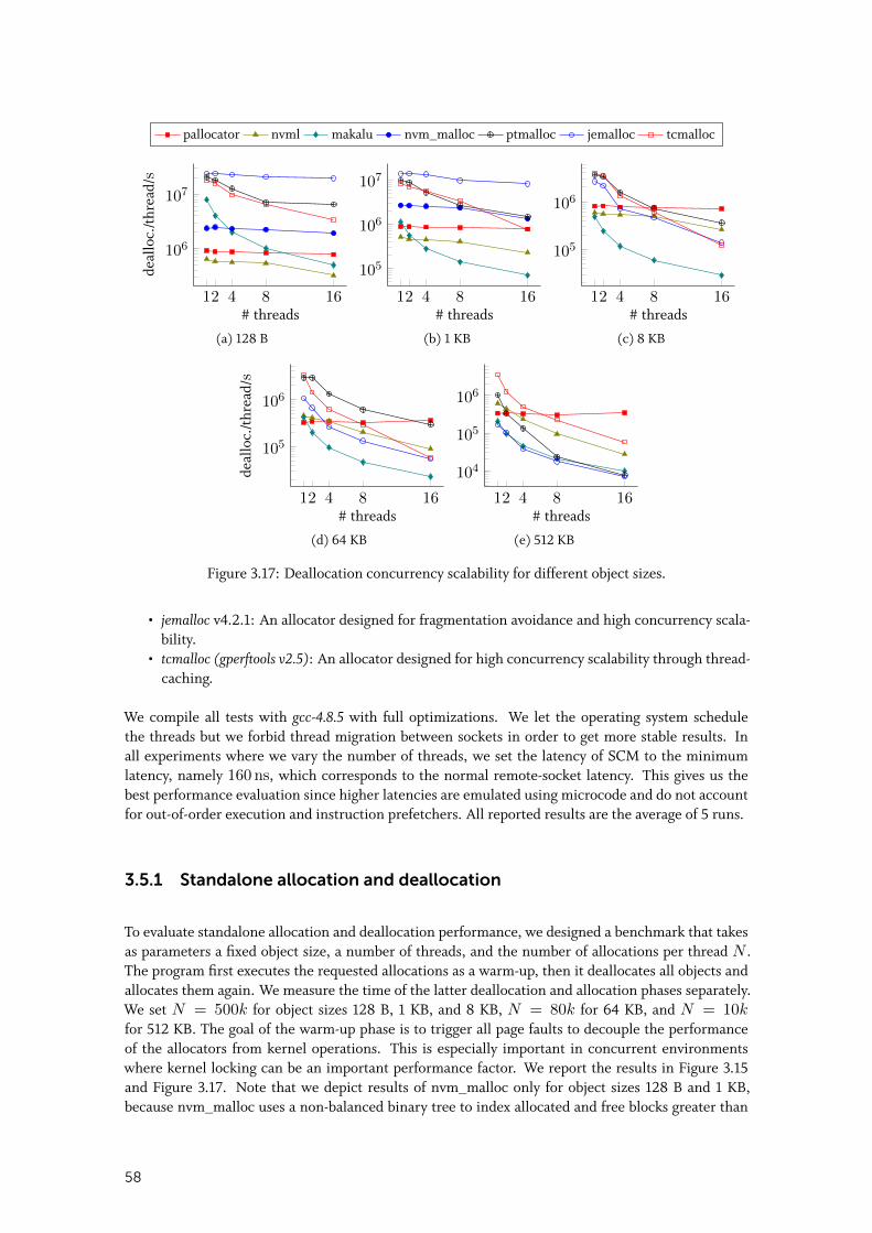
pallocator nvml makalu nvm_malloc ptmalloc jemalloc tcmalloc
12 4 8 16
106
107
# threads
deal
loc.
/thr
ead/s
(a) 128 B
12 4 8 16
105
106
107
# threads
(b) 1 KB
12 4 8 16
105
106
# threads
(c) 8 KB
12 4 8 16
105
106
# threads
deal
loc.
/thr
ead/s
(d) 64 KB
12 4 8 16
104
105
106
# threads
(e) 512 KB
Figure 3.17: Deallocation concurrency scalability for different object sizes.
• jemalloc v4.2.1: An allocator designed for fragmentation avoidance and high concurrency scala-bility.
• tcmalloc (gperftools v2.5): An allocator designed for high concurrency scalability through thread-caching.
We compile all tests with gcc-4.8.5 with full optimizations. We let the operating system schedulethe threads but we forbid thread migration between sockets in order to get more stable results. Inall experiments where we vary the number of threads, we set the latency of SCM to the minimumlatency, namely 160 ns, which corresponds to the normal remote-socket latency. This gives us thebest performance evaluation since higher latencies are emulated using microcode and do not accountfor out-of-order execution and instruction prefetchers. All reported results are the average of 5 runs.
3.5.1 Standalone allocation and deallocation
To evaluate standalone allocation and deallocation performance, we designed a benchmark that takesas parameters a fixed object size, a number of threads, and the number of allocations per thread N .The program first executes the requested allocations as a warm-up, then it deallocates all objects andallocates them again. We measure the time of the latter deallocation and allocation phases separately.We set N = 500k for object sizes 128 B, 1 KB, and 8 KB, N = 80k for 64 KB, and N = 10kfor 512 KB. The goal of the warm-up phase is to trigger all page faults to decouple the performanceof the allocators from kernel operations. This is especially important in concurrent environmentswhere kernel locking can be an important performance factor. We report the results in Figure 3.15and Figure 3.17. Note that we depict results of nvm_malloc only for object sizes 128 B and 1 KB,because nvm_malloc uses a non-balanced binary tree to index allocated and free blocks greater than
58
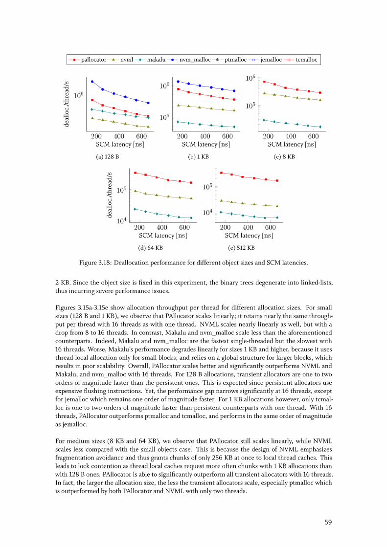
pallocator nvml makalu nvm_malloc ptmalloc jemalloc tcmalloc
200 400 600
106
SCM latency [ns]
deal
loc.
/thr
ead/s
(a) 128 B
200 400 600
105
106
SCM latency [ns]
(b) 1 KB
200 400 600
105
106
SCM latency [ns]
(c) 8 KB
200 400 600104
105
SCM latency [ns]
deal
loc.
/thr
ead/s
(d) 64 KB
200 400 600
104
105
SCM latency [ns]
(e) 512 KB
Figure 3.18: Deallocation performance for different object sizes and SCM latencies.
2 KB. Since the object size is fixed in this experiment, the binary trees degenerate into linked-lists,thus incurring severe performance issues.
Figures 3.15a-3.15e show allocation throughput per thread for different allocation sizes. For smallsizes (128 B and 1 KB), we observe that PAllocator scales linearly; it retains nearly the same through-put per thread with 16 threads as with one thread. NVML scales nearly linearly as well, but with adrop from 8 to 16 threads. In contrast, Makalu and nvm_malloc scale less than the aforementionedcounterparts. Indeed, Makalu and nvm_malloc are the fastest single-threaded but the slowest with16 threads. Worse, Makalu’s performance degrades linearly for sizes 1 KB and higher, because it usesthread-local allocation only for small blocks, and relies on a global structure for larger blocks, whichresults in poor scalability. Overall, PAllocator scales better and significantly outperforms NVML andMakalu, and nvm_malloc with 16 threads. For 128 B allocations, transient allocators are one to twoorders of magnitude faster than the persistent ones. This is expected since persistent allocators useexpensive flushing instructions. Yet, the performance gap narrows significantly at 16 threads, exceptfor jemalloc which remains one order of magnitude faster. For 1 KB allocations however, only tcmal-loc is one to two orders of magnitude faster than persistent counterparts with one thread. With 16threads, PAllocator outperforms ptmalloc and tcmalloc, and performs in the same order of magnitudeas jemalloc.
For medium sizes (8 KB and 64 KB), we observe that PAllocator still scales linearly, while NVMLscales less compared with the small objects case. This is because the design of NVML emphasizesfragmentation avoidance and thus grants chunks of only 256 KB at once to local thread caches. Thisleads to lock contention as thread local caches request more often chunks with 1 KB allocations thanwith 128 B ones. PAllocator is able to significantly outperform all transient allocators with 16 threads.In fact, the larger the allocation size, the less the transient allocators scale, especially ptmalloc whichis outperformed by both PAllocator and NVML with only two threads.
59
For large sizes (512 KB), we observe that PAllocator is the only allocator that scales linearly, and itoutperforms NVML and all transient allocators with only 2 threads. We note that NVML is fasterthan PAllocator with one thread: NVML uses transient trees to index its large blocks, while we usehybrid SCM-DRAM trees which incur a small additional overhead but enable much faster recovery(see recovery experiments below).
Figures 3.16a-3.16e show allocation throughput per thread for different allocation sizes, varying SCMlatencies, and 16 threads. We observe that performance degrades with higher latencies, but the over-head does not exceed 54%, 43%, 44%, and 57% for PAllocator, NVML, Makalu, and nvm_malloc,respectively, with an SCM latency of 650 ns compared with 160 ns. We also observe that for alloca-tion sizes 64 KB and 512 KB, PAllocator seems to suffer more from higher SCM latencies than NVML.This is explained by two factors: (1) the bottleneck for NVML with 16 threads is synchronizationrather than persistence; and (2) accessing the leaf nodes of PAllocator’s hybrid trees becomes moreexpensive with higher SCM latencies.
Figures 3.17a-3.17e show deallocation throughput per thread for different allocation sizes. Similarto allocations, PAllocator scales linearly for all allocation sizes. NVML exhibits similar behaviour toits allocations as well and has lower throughput than PAllocator except for sizes 64 KB and 512 KBwith up to 4 threads. This is again explained by the fact that PAllocator uses its big block allocatorfor these allocation sizes, which involves operations on its hybrid trees that incur an extra overheadcompared with NVML’s transient counterparts. We note that nvm_malloc has 2× higher throughputfor deallocations than for allocations for sizes 128 B and 1 KB, and outperforms PAllocator even with16 threads. Indeed, in contrast to its allocations, nvm_malloc deallocations scale linearly. As forMakalu, it is the fastest for 128 B, but its performance drops linearly in all cases. Interestingly, with16 threads and for 8 KB and larger, PAllocator outperforms again all allocators including transientones.
Figures 3.18a-3.18e show deallocation throughput per thread for different allocation sizes, varyingSCM latencies, and 16 threads. We observe the same patterns as with allocations. We note that theperformance of all persistent allocators degrades gradually with increasing SCM latencies up to 60%,46%, 48%, and 64% for PAllocator, NVML, Makalu, and nvm_malloc, respectively, with an SCMlatency of 650 ns compared with 160 ns. We argue that this drop is still acceptable given the 4×higher latency.
3.5.2 Random allocation and deallocation
In this experiment we evaluate the performance of mixed random allocations and deallocations. Theexperiment consists in executing 10 iterations ofN allocations followed byN deallocations of randomsize per thread. We fix the range of object sizes between 64 B and 128 KB, and we consider three differ-ent object size distributions: (1) Uniform distribution; (2) Binomial distribution with skew factor 0.01to emphasize smaller sizes; (3) Binomial distribution with skew factor 0.7 to emphasize larger sizes.We set N = 500k for Binomial small, and N = 50k for Uniform and Binomial large. Figure 3.19depicts the results.
Figures 3.19a-3.19c show operation throughput per thread. We observe that PAllocator scales linearlyfor all distributions. Additionally, it manages to outperform all transient allocators in the Uniform andBinomial large cases, while outperforming only ptmalloc in the Binomial small case. In the Uniformcase, PAllocator outperforms NVML, Makalu, and nvm_malloc by up to 7.5×, 49.7×, and 6.7×,respectively. nvm_malloc’s performance degrades significantly in the case of Binomial large because
60
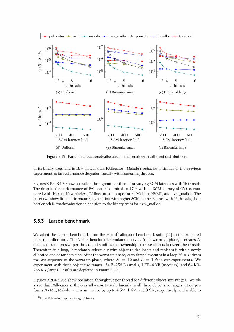
pallocator nvml makalu nvm_malloc ptmalloc jemalloc tcmalloc
12 4 8 16
104
105
106
# threads
op./t
hrea
d/s
(a) Uniform
12 4 8 16
105
106
107
# threads
(b) Binomial small
12 4 8 16
104
105
106
# threads
(c) Binomial large
200 400 600
104
105
SCM latency [ns]
op./t
hrea
d/s
(d) Uniform
200 400 600
105
SCM latency [ns]
(e) Binomial small
200 400 600
104
105
SCM latency [ns]
(f) Binomial large
Figure 3.19: Random allocation/deallocation benchmark with different distributions.
of its binary trees and is 19× slower than PAllocator. Makalu’s behavior is similar to the previousexperiment as its performance degrades linearly with increasing threads.
Figures 3.19d-3.19f show operation throughput per thread for varying SCM latencies with 16 threads.The drop in the performance of PAllocator is limited to 47% with an SCM latency of 650 ns com-pared with 160 ns. Nevertheless, PAllocator still outperforms Makalu, NVML, and nvm_malloc. Thelatter two show little performance degradation with higher SCM latencies since with 16 threads, theirbottleneck is synchronization in addition to the binary trees for nvm_malloc.
3.5.3 Larson benchmark
We adapt the Larson benchmark from the Hoard8 allocator benchmark suite [11] to the evaluatedpersistent allocators. The Larson benchmark simulates a server. In its warm-up phase, it creates Nobjects of random size per thread and shuffles the ownership of these objects between the threads.Thereafter, in a loop, it randomly selects a victim object to deallocate and replaces it with a newlyallocated one of random size. After the warm-up phase, each thread executes in a loop N × L timesthe last sequence of the warm-up phase, where N = 1k and L = 10k in our experiments. Weexperiment with three object size ranges: 64 B–256 B (small), 1 KB–4 KB (medium), and 64 KB–256 KB (large). Results are depicted in Figure 3.20.
Figures 3.20a-3.20c show operation throughput per thread for different object size ranges. We ob-serve that PAllocator is the only allocator to scale linearly in all three object size ranges. It outper-forms NVML, Makalu, and nvm_malloc by up to 4.5×, 1.6×, and 3.9×, respectively, and is able to
8https://github.com/emeryberger/Hoard/
61
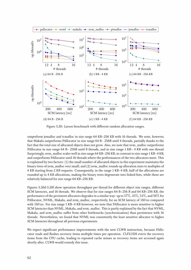
pallocator nvml makalu nvm_malloc ptmalloc jemalloc tcmalloc
12 4 8 16
106
107
# threads
op./t
hrea
d/s
(a) 64 B - 256 B
12 4 8 16
105
106
107
# threads
(b) 1 KB - 4 KB
12 4 8 16103
105
107
# threads
(c) 64 KB - 256 KB
200 400 600
105
SCM latency [ns]
op./t
hrea
d/s
(d) 64 B - 256 B
200 400 600104
105
SCM latency [ns]
(e) 1 KB - 4 KB
200 400 600103
104
105
SCM latency [ns]
(f) 64 KB - 256 KB
Figure 3.20: Larson benchmark with different random allocation ranges.
outperform jemalloc and tcmalloc in size range 64 KB–256 KB with 16 threads. We note, however,that Makalu outperforms PAllocator in size range 64 B– 256B until 4 threads, partially thanks to thefact that the total size of allocated objects does not grow. Also, we note that nvm_malloc outperformsPAllocator in size range 64 B– 256B until 8 threads, and in size range 1 KB– 4 KB with one thread.Surprisingly, nvm_malloc scales well in size range 64 KB–256 KB, in contrast to size range 1 KB–4 KB,and outperforms PAllocator until 16 threads where the performances of the two allocators meet. Thisis explained by two factors: (1) the small number of allocated objects in this experiment maintains thebinary trees of nvm_malloc very small; and (2) nvm_malloc rounds up allocation sizes to multiples of4 KB starting from 2 KB requests. Consequently, in the range 1 KB–4 KB, half of the allocations arerounded up to 4 KB allocations, making the binary trees degenerate into linked-lists, while these arerelatively balanced for size range 64 KB–256 KB.
Figures 3.20d-3.20f show operation throughput per thread for different object size ranges, differentSCM latencies, and 16 threads. We observe that for size ranges 64 B–256 B and 64 KB–256 KB, theperformance of the persistent allocators degrades in a similar way: up to 57%, 45%, 54%, and 56% forPAllocator, NVML, Makalu, and nvm_malloc, respectively, for an SCM latency of 160 ns comparedwith 160 ns. For size range 1 KB–4 KB however, we note that PAllocator is more sensitive to higherSCM latencies than NVML, Makalu, and nvm_malloc. This is partly explained by the fact that NVML,Makalu, and nvm_malloc suffer from other bottlenecks (synchronization) than persistence with 16threads. Nevertheless, we found that NVML was consistently the least sensitive allocator to higherSCM latencies throughout all previous experiments.
We expect significant performance improvements with the new CLWB instruction, because PAllo-cator reads and flushes recovery items multiple times per operation. CLFLUSH evicts the recoveryitems from the CPU cache, leading to repeated cache misses as recovery items are accessed againshortly after. CLWB would remedy this issue.
62
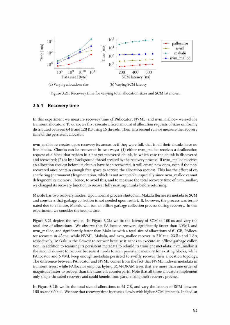
108 109 1010 1011
100
102
104
Data size [Byte]
Tim
e[m
s]
(a) Varying allocations size
200 400 600
102
103
104
105
SCM latency [ns]
Tim
e[m
s]
(b) Varying SCM latency
pallocatornvml
makalunvm_malloc
Figure 3.21: Recovery time for varying total allocation sizes and SCM latencies.
3.5.4 Recovery time
In this experiment we measure recovery time of PAllocator, NVML, and nvm_malloc– we excludetransient allocators. To do so, we first execute a fixed amount of allocation requests of sizes uniformlydistributed between 64 B and 128 KB using 16 threads. Then, in a second run we measure the recoverytime of the persistent allocator.
nvm_malloc re-creates upon recovery its arenas as if they were full, that is, all their chunks have nofree blocks. Chunks can be recovered in two ways: (1) either nvm_malloc receives a deallocationrequest of a block that resides in a not-yet-recovered chunk, in which case the chunk is discoveredand recovered; (2) or by a background thread created by the recovery process. If nvm_malloc receivesan allocation request before its chunks have been recovered, it will create new ones, even if the non-recovered ones contain enough free space to service the allocation request. This has the effect of ex-acerbating (permanent) fragmentation, which is not acceptable, especially since nvm_malloc cannotdefragment its memory. Hence, to avoid this, and to measure the total recovery time of nvm_malloc,we changed its recovery function to recover fully existing chunks before returning.
Makalu has two recovery modes: Upon normal process shutdown, Makalu flushes its metada to SCMand considers that garbage collection is not needed upon restart. If, however, the process was termi-nated due to a failure, Makalu will run an offline garbage collection process during recovery. In thisexperiment, we consider the second case.
Figure 3.21 depicts the results. In Figure 3.21a we fix the latency of SCM to 160 ns and vary thetotal size of allocations. We observe that PAllocator recovers significantly faster than NVML andnvm_malloc, and significantly faster than Makalu: with a total size of allocations of 61 GB, PAlloca-tor recovers in 45ms, while NVML, Makalu, and nvm_malloc recover in 210ms, 23.5 s and 1.3 s,respectively. Makalu is the slowest to recover because it needs to execute an offline garbage collec-tion, in addition to scanning its persistent metadata to rebuild its transient metadata. nvm_malloc isthe second slowest to recover because it needs to scan persistent memory for existing blocks, whilePAllocator and NVML keep enough metadata persisted to swiftly recover their allocation topology.The difference between PAllocator and NVML comes from the fact that NVML indexes metadata intransient trees, while PAllocator employs hybrid SCM-DRAM trees that are more than one order ofmagnitude faster to recover than the transient counterparts. Note that all three allocators implementonly single-threaded recovery and could benefit from parallelizing their recovery process.
In Figure 3.21b we fix the total size of allocations to 61 GB, and vary the latency of SCM between160 ns and 650 ns. We note that recovery time increases slowly with higher SCM latencies. Indeed, at
63
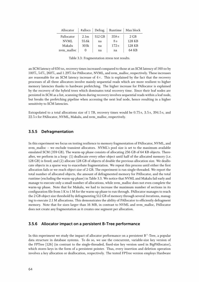
Allocator #allocs Defrag. Runtime Max block
Pallocator 2.1m 512 GB 358 s 2 GBNVML 55.6k na 8 s 128 KBMakalu 303k na 172 s 128 KB
nvm_malloc 0 na na 64 KB
Table 3.3: Fragmentation stress test results.
an SCM latency of 650 ns, recovery times increased compared to those at an SCM latency of 160 ns by100%, 54%, 260%, and 1.29% for PAllocator, NVML, and nvm_malloc, respectively. These increasesare reasonable for an SCM latency increase of 4×. This is explained by the fact that the recoveryprocesses of all three allocators involve mainly sequential reads which are more resilient to highermemory latencies thanks to hardware prefetching. The higher increase for PAllocator is explainedby the recovery of the hybrid trees which dominates total recovery time. Since their leaf nodes arepersisted in SCM as a list, scanning them during recovery involves sequential reads within a leaf node,but breaks the prefetching pipeline when accessing the next leaf node, hence resulting in a highersensitivity to SCM latencies.
Extrapolated to a total allocations size of 1 TB, recovery times would be 0.75 s, 3.5 s, 394.5 s, and22.5 s for PAllocator, NVML, Makalu, and nvm_malloc, respectively.
3.5.5 Defragmentation
In this experiment we focus on testing resilience to memory fragmentation of PAllocator, NVML, andnvm_malloc – we exclude transient allocators. NVML’s pool size is set to the maximum availableemulated SCM (359 GB). The warm-up phase consists of allocating 256 GB of 64 KB objects. There-after, we perform in a loop: (1) deallocate every other object until half of the allocated memory (i.e.128 GB) is freed; and (2) allocate 128 GB of objects of double the previous allocation size. We deallo-cate objects in a sparse way to exacerbate fragmentation. We repeat this process until either the firstallocation fails or we reach object size of 2 GB. The experiment is run single-threaded. We report thetotal number of allocated objects, the amount of defragmented memory for PAllocator, and the totalruntime (excluding the warm-up phase) in Table 3.3. We notice that NVML and Makalu fail early andmanage to execute only a small number of allocations, while nvm_malloc does not even complete thewarm-up phase. Note that for Makalu, we had to increase the maximum number of sections in itsconfiguration file from 1 K to 1 M for the warm-up phase to run through. PAllocator manages to reachthe 2 GB object size threshold by defragmenting 512 GB of memory through several iterations, manag-ing to execute 2.1 M allocations. This demonstrates the ability of PAllocator to efficiently defragmentmemory. Note that for sizes larger than 16 MB, in contrast to NVML and nvm_malloc, PAllocatordoes not create any fragmentation as it creates one segment per allocation.
3.5.6 Allocator impact on a persistent B-Tree performance
In this experiment we study the impact of allocator performance on a persistent B+-Tree, a populardata structure in database systems. To do so, we use the concurrent, variable-size key version ofthe FPTree [126] (in contrast to the single-threaded, fixed-size key version used in BigPAllocator),which stores keys in the form of a persistent pointer. Thus, every insertion and deletion operationinvolves a key allocation or deallocation, respectively. The tested FPTree version employs Hardware
64
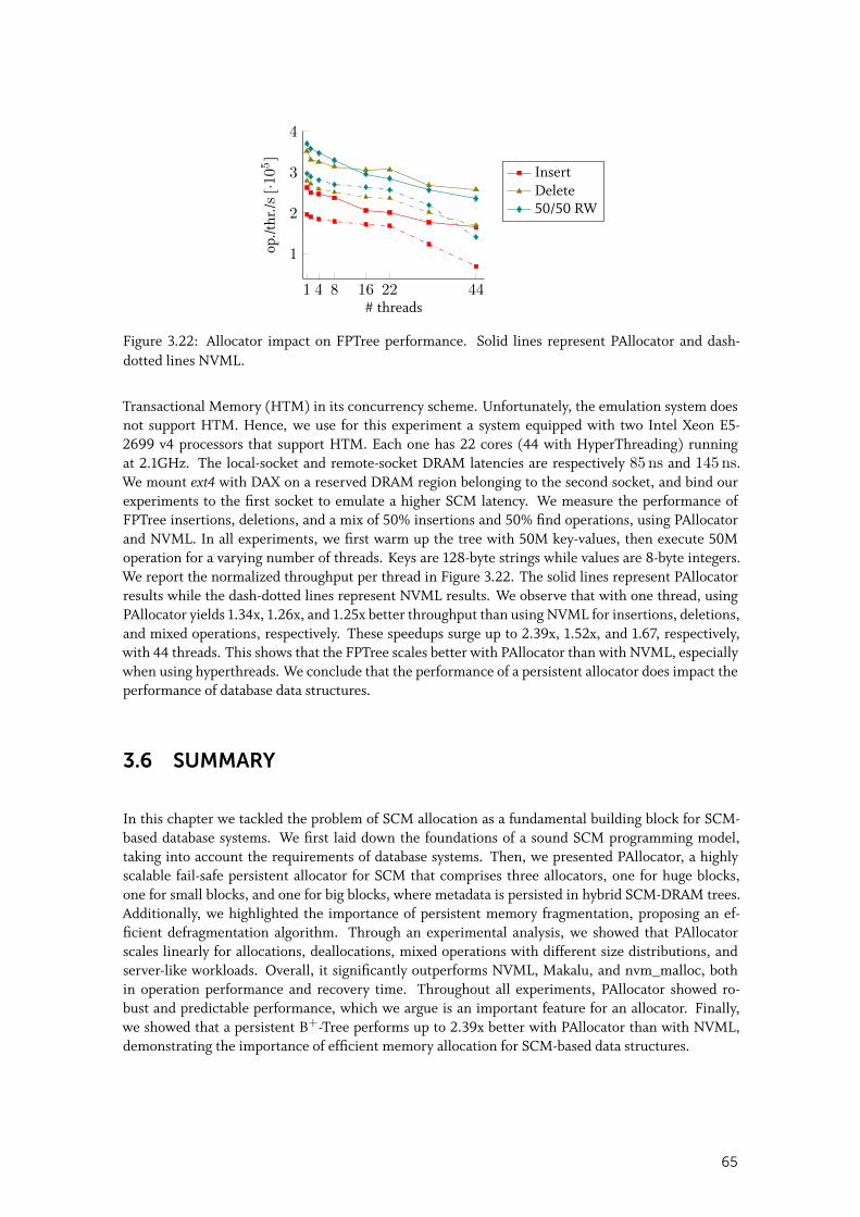
1 4 8 16 22 44
1
2
3
4
# threads
op./t
hr./s
[·105]
InsertDelete50/50 RW
Figure 3.22: Allocator impact on FPTree performance. Solid lines represent PAllocator and dash-dotted lines NVML.
Transactional Memory (HTM) in its concurrency scheme. Unfortunately, the emulation system doesnot support HTM. Hence, we use for this experiment a system equipped with two Intel Xeon E5-2699 v4 processors that support HTM. Each one has 22 cores (44 with HyperThreading) runningat 2.1GHz. The local-socket and remote-socket DRAM latencies are respectively 85 ns and 145 ns.We mount ext4 with DAX on a reserved DRAM region belonging to the second socket, and bind ourexperiments to the first socket to emulate a higher SCM latency. We measure the performance ofFPTree insertions, deletions, and a mix of 50% insertions and 50% find operations, using PAllocatorand NVML. In all experiments, we first warm up the tree with 50M key-values, then execute 50Moperation for a varying number of threads. Keys are 128-byte strings while values are 8-byte integers.We report the normalized throughput per thread in Figure 3.22. The solid lines represent PAllocatorresults while the dash-dotted lines represent NVML results. We observe that with one thread, usingPAllocator yields 1.34x, 1.26x, and 1.25x better throughput than using NVML for insertions, deletions,and mixed operations, respectively. These speedups surge up to 2.39x, 1.52x, and 1.67, respectively,with 44 threads. This shows that the FPTree scales better with PAllocator than with NVML, especiallywhen using hyperthreads. We conclude that the performance of a persistent allocator does impact theperformance of database data structures.
3.6 SUMMARY
In this chapter we tackled the problem of SCM allocation as a fundamental building block for SCM-based database systems. We first laid down the foundations of a sound SCM programming model,taking into account the requirements of database systems. Then, we presented PAllocator, a highlyscalable fail-safe persistent allocator for SCM that comprises three allocators, one for huge blocks,one for small blocks, and one for big blocks, where metadata is persisted in hybrid SCM-DRAM trees.Additionally, we highlighted the importance of persistent memory fragmentation, proposing an ef-ficient defragmentation algorithm. Through an experimental analysis, we showed that PAllocatorscales linearly for allocations, deallocations, mixed operations with different size distributions, andserver-like workloads. Overall, it significantly outperforms NVML, Makalu, and nvm_malloc, bothin operation performance and recovery time. Throughout all experiments, PAllocator showed ro-bust and predictable performance, which we argue is an important feature for an allocator. Finally,we showed that a persistent B+-Tree performs up to 2.39x better with PAllocator than with NVML,demonstrating the importance of efficient memory allocation for SCM-based data structures.
65

66
4PERSISTENT DATA STRUCTURES
G iven the characteristics of SCM, it is theoretically possible to persist data structures in SCMand at the same time obtain near-DRAM performance. This potential has been acknowledged
by recent works and new systems that adopt this novel paradigm are emerging [5, 128, 79]. Wedevised in the previous chapter the foundations for a sound programming model and efficient, fail-safepersistent memory allocation techniques, both of which are necessary building blocks for SCM-basedpersistent data structures. In this chapter we investigate the design of persistent index structuresas one of the core database structures, motivated by the observation that traditional main memoryB+-Tree implementations do not fulfill the consistency requirements needed for such a use case1.Furthermore, while expected in the range of DRAM, SCM latencies are higher and asymmetric withwrites noticeably slower than reads. We argue that these performance differences between SCM andDRAM imply that the design assumptions made for previous well-established main memory B+-Treeimplementations might not hold anymore. Therefore, we see the need to design a novel, persistent B+-Tree that leverages the capabilities of SCM while exhibiting performance similar to that of a traditionaltransient B+-Tree.
Designing persistent data structures comes with unprecedented challenges for data consistency sinceSCM is accessed via the volatile CPU cache over which software has only little control. Several worksproposed SCM-optimized B+-Trees such as the CDDS B+-Tree [164], the wBTree [20], and the NV-Tree [180], but they fail to match the speed of an optimized DRAM-based B+-Tree. Additionally,they do not address all SCM programming challenges we identify in Chapter 3, especially those ofpersistent memory leaks and data recovery.
To lift this shortcoming, we propose the Fingerprinting Persistent Tree (FPTree) that is based on fourdesign principles to achieve near-DRAM-based data structure performance:
1. Fingerprinting. Fingerprints are one-byte hashes of in-leaf keys, placed contiguously in thefirst cache-line-sized piece of the leaf. The FPTree uses unsorted leaves with in-leaf bitmaps –originally proposed in [20] – such that a search iterates linearly over all valid keys in a leaf. Byscanning the fingerprints first, we are able to limit the number of in-leaf probed keys to one inthe average case, which leads to a significant performance improvement.
2. Selective Persistence. The idea is based on the well-known distinction between primary data,whose loss infers an irreversible loss of information, and non-primary data that can be rebuiltfrom the former. Selective persistence consists in storing primary data in SCM and non-primarydata in DRAM. Applied to the FPTree, this corresponds to storing the leaf nodes in SCM andthe inner nodes in DRAM. Hence, only leaf accesses are more expensive during a tree traversalcompared to a fully transient counterpart.
1Parts of the material in this chapter are based on [126].
67
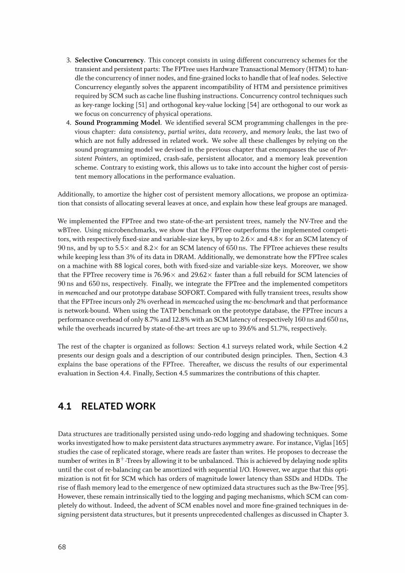
3. Selective Concurrency. This concept consists in using different concurrency schemes for thetransient and persistent parts: The FPTree uses Hardware Transactional Memory (HTM) to han-dle the concurrency of inner nodes, and fine-grained locks to handle that of leaf nodes. SelectiveConcurrency elegantly solves the apparent incompatibility of HTM and persistence primitivesrequired by SCM such as cache line flushing instructions. Concurrency control techniques suchas key-range locking [51] and orthogonal key-value locking [54] are orthogonal to our work aswe focus on concurrency of physical operations.
4. Sound Programming Model. We identified several SCM programming challenges in the pre-vious chapter: data consistency, partial writes, data recovery, and memory leaks, the last two ofwhich are not fully addressed in related work. We solve all these challenges by relying on thesound programming model we devised in the previous chapter that encompasses the use of Per-sistent Pointers, an optimized, crash-safe, persistent allocator, and a memory leak preventionscheme. Contrary to existing work, this allows us to take into account the higher cost of persis-tent memory allocations in the performance evaluation.
Additionally, to amortize the higher cost of persistent memory allocations, we propose an optimiza-tion that consists of allocating several leaves at once, and explain how these leaf groups are managed.
We implemented the FPTree and two state-of-the-art persistent trees, namely the NV-Tree and thewBTree. Using microbenchmarks, we show that the FPTree outperforms the implemented competi-tors, with respectively fixed-size and variable-size keys, by up to 2.6× and 4.8× for an SCM latency of90 ns, and by up to 5.5× and 8.2× for an SCM latency of 650 ns. The FPTree achieves these resultswhile keeping less than 3% of its data in DRAM. Additionally, we demonstrate how the FPTree scaleson a machine with 88 logical cores, both with fixed-size and variable-size keys. Moreover, we showthat the FPTree recovery time is 76.96× and 29.62× faster than a full rebuild for SCM latencies of90 ns and 650 ns, respectively. Finally, we integrate the FPTree and the implemented competitorsin memcached and our prototype database SOFORT. Compared with fully transient trees, results showthat the FPTree incurs only 2% overhead in memcached using the mc-benchmark and that performanceis network-bound. When using the TATP benchmark on the prototype database, the FPTree incurs aperformance overhead of only 8.7% and 12.8% with an SCM latency of respectively 160 ns and 650 ns,while the overheads incurred by state-of-the-art trees are up to 39.6% and 51.7%, respectively.
The rest of the chapter is organized as follows: Section 4.1 surveys related work, while Section 4.2presents our design goals and a description of our contributed design principles. Then, Section 4.3explains the base operations of the FPTree. Thereafter, we discuss the results of our experimentalevaluation in Section 4.4. Finally, Section 4.5 summarizes the contributions of this chapter.
4.1 RELATED WORK
Data structures are traditionally persisted using undo-redo logging and shadowing techniques. Someworks investigated how to make persistent data structures asymmetry aware. For instance, Viglas [165]studies the case of replicated storage, where reads are faster than writes. He proposes to decrease thenumber of writes in B+-Trees by allowing it to be unbalanced. This is achieved by delaying node splitsuntil the cost of re-balancing can be amortized with sequential I/O. However, we argue that this opti-mization is not fit for SCM which has orders of magnitude lower latency than SSDs and HDDs. Therise of flash memory lead to the emergence of new optimized data structures such as the Bw-Tree [95].However, these remain intrinsically tied to the logging and paging mechanisms, which SCM can com-pletely do without. Indeed, the advent of SCM enables novel and more fine-grained techniques in de-signing persistent data structures, but it presents unprecedented challenges as discussed in Chapter 3.
68
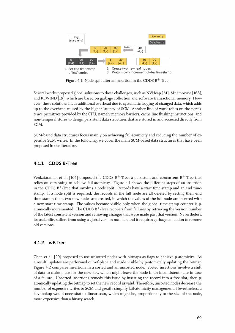
Key[start, end)
Dead entry
Live entry
5[2,-)
20[3,-)
40[4,-)
99[4,-)
5[4,-)
20[4,-)
99[1,-)
5[2,4)
20[3,4)
99[1,4)
40(4,-)
Insert
2. Create two new leaf nodes3. P-atomically increment global timestamp
1. Set end timestampof leaf entries
Figure 4.1: Node split after an insertion in the CDDS B+-Tree.
Several works proposed global solutions to these challenges, such as NVHeap [24], Mnemosyne [168],and REWIND [19], which are based on garbage collection and software transactional memory. How-ever, these solutions incur additional overhead due to systematic logging of changed data, which addsup to the overhead caused by the higher latency of SCM. Another line of work relies on the persis-tence primitives provided by the CPU, namely memory barriers, cache line flushing instructions, andnon-temporal stores to design persistent data structures that are stored in and accessed directly fromSCM.
SCM-based data structures focus mainly on achieving fail-atomicity and reducing the number of ex-pensive SCM writes. In the following, we cover the main SCM-based data structures that have beenproposed in the literature.
4.1.1 CDDS B-Tree
Venkataraman et al. [164] proposed the CDDS B+-Tree, a persistent and concurrent B+-Tree thatrelies on versioning to achieve fail-atomicity. Figure 4.1 shows the different steps of an insertionin the CDDS B+-Tree that involves a node split. Records have a start time-stamp and an end time-stamp. If a node split is required, the records in the full node are all deleted by setting their endtime-stamp; then, two new nodes are created, in which the values of the full node are inserted witha new start time-stamp. The values become visible only when the global time-stamp counter is p-atomically incremented. The CDDS B+-Tree recovers from failures by retrieving the version numberof the latest consistent version and removing changes that were made past that version. Nevertheless,its scalability suffers from using a global version number, and it requires garbage collection to removeold versions.
4.1.2 wBTree
Chen et al. [20] proposed to use unsorted nodes with bitmaps as flags to achieve p-atomicity. Asa result, updates are performed out-of-place and made visible by p-atomically updating the bitmap.Figure 4.2 compares insertions in a sorted and an unsorted node. Sorted insertions involve a shiftof data to make place for the new key, which might leave the node in an inconsistent state in caseof a failure. Unsorted insertions remedy this issue by inserting the record into a free slot, then p-atomically updating the bitmap to set the new record as valid. Therefore, unsorted nodes decrease thenumber of expensive writes to SCM and greatly simplify fail-atomicity management. Nevertheless, akey lookup would necessitate a linear scan, which might be, proportionally to the size of the node,more expensive than a binary search.
69
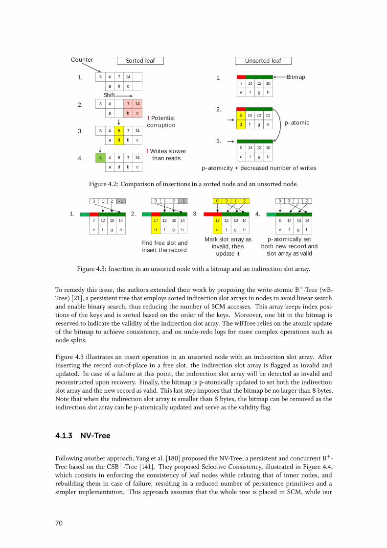
3 4 7 14
a b c7 14 12 10
e f g h
Bitmap
Sorted leaf Unsorted leaf
3 4 7 14
a b c5 14 12 10
d f g h
3 4 5 7 14
a d b c
5 14 12 10
d f g h4 4 5 7 14
a d b c
p-atomic! Potentialcorruption
! Writes slowerthan reads
Counter
2.
3.
4.
1. 1.
2.
3.
p-atomicity + decreased number of writes
Shift
Figure 4.2: Comparison of insertions in a sorted node and an unsorted node.
7 12 10 14
e f g h
3 1 2 -1
17 12 10 14
d f g h
5 12 10 14
d f g h
2. 4.1.
3 1 2 -1
17 12 10 14
d f g h
3.
0 3 1 2
Mark slot array asinvalid, then
update it
Find free slot andinsert the record
p-atomically setboth new record and
slot array as valid
0 3 1 2
Figure 4.3: Insertion in an unsorted node with a bitmap and an indirection slot array.
To remedy this issue, the authors extended their work by proposing the write-atomic B+-Tree (wB-Tree) [21], a persistent tree that employs sorted indirection slot arrays in nodes to avoid linear searchand enable binary search, thus reducing the number of SCM accesses. This array keeps index posi-tions of the keys and is sorted based on the order of the keys. Moreover, one bit in the bitmap isreserved to indicate the validity of the indirection slot array. The wBTree relies on the atomic updateof the bitmap to achieve consistency, and on undo-redo logs for more complex operations such asnode splits.
Figure 4.3 illustrates an insert operation in an unsorted node with an indirection slot array. Afterinserting the record out-of-place in a free slot, the indirection slot array is flagged as invalid andupdated. In case of a failure at this point, the indirection slot array will be detected as invalid andreconstructed upon recovery. Finally, the bitmap is p-atomically updated to set both the indirectionslot array and the new record as valid. This last step imposes that the bitmap be no larger than 8 bytes.Note that when the indirection slot array is smaller than 8 bytes, the bitmap can be removed as theindirection slot array can be p-atomically updated and serve as the validity flag.
4.1.3 NV-Tree
Following another approach, Yang et al. [180] proposed the NV-Tree, a persistent and concurrent B+-Tree based on the CSB+-Tree [141]. They proposed Selective Consistency, illustrated in Figure 4.4,which consists in enforcing the consistency of leaf nodes while relaxing that of inner nodes, andrebuilding them in case of failure, resulting in a reduced number of persistence primitives and asimpler implementation. This approach assumes that the whole tree is placed in SCM, while our
70
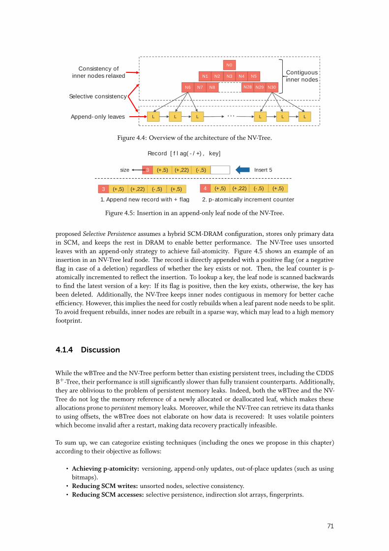
Consistency ofinner nodes relaxed
Selective consistency
Append-only leaves
N0
N3 N4N2 N5N1
N6 N7 N8
L L L L LL…
N28 N29 N30
Contiguousinner nodes
Figure 4.4: Overview of the architecture of the NV-Tree.
Record [flag(-/+), key]
2. p-atomically increment counter
3 (+,5) (+,22) (-,5)
3 (+,5) (+,22) (-,5) 4 (+,5) (+,22) (-,5)
size Insert 5
(+,5) (+,5)
1. Append new record with + flag
Figure 4.5: Insertion in an append-only leaf node of the NV-Tree.
proposed Selective Persistence assumes a hybrid SCM-DRAM configuration, stores only primary datain SCM, and keeps the rest in DRAM to enable better performance. The NV-Tree uses unsortedleaves with an append-only strategy to achieve fail-atomicity. Figure 4.5 shows an example of aninsertion in an NV-Tree leaf node. The record is directly appended with a positive flag (or a negativeflag in case of a deletion) regardless of whether the key exists or not. Then, the leaf counter is p-atomically incremented to reflect the insertion. To lookup a key, the leaf node is scanned backwardsto find the latest version of a key: If its flag is positive, then the key exists, otherwise, the key hasbeen deleted. Additionally, the NV-Tree keeps inner nodes contiguous in memory for better cacheefficiency. However, this implies the need for costly rebuilds when a leaf parent node needs to be split.To avoid frequent rebuilds, inner nodes are rebuilt in a sparse way, which may lead to a high memoryfootprint.
4.1.4 Discussion
While the wBTree and the NV-Tree perform better than existing persistent trees, including the CDDSB+-Tree, their performance is still significantly slower than fully transient counterparts. Additionally,they are oblivious to the problem of persistent memory leaks. Indeed, both the wBTree and the NV-Tree do not log the memory reference of a newly allocated or deallocated leaf, which makes theseallocations prone to persistent memory leaks. Moreover, while the NV-Tree can retrieve its data thanksto using offsets, the wBTree does not elaborate on how data is recovered: It uses volatile pointerswhich become invalid after a restart, making data recovery practically infeasible.
To sum up, we can categorize existing techniques (including the ones we propose in this chapter)according to their objective as follows:
• Achieving p-atomicity: versioning, append-only updates, out-of-place updates (such as usingbitmaps).
• Reducing SCM writes: unsorted nodes, selective consistency.• Reducing SCM accesses: selective persistence, indirection slot arrays, fingerprints.
71
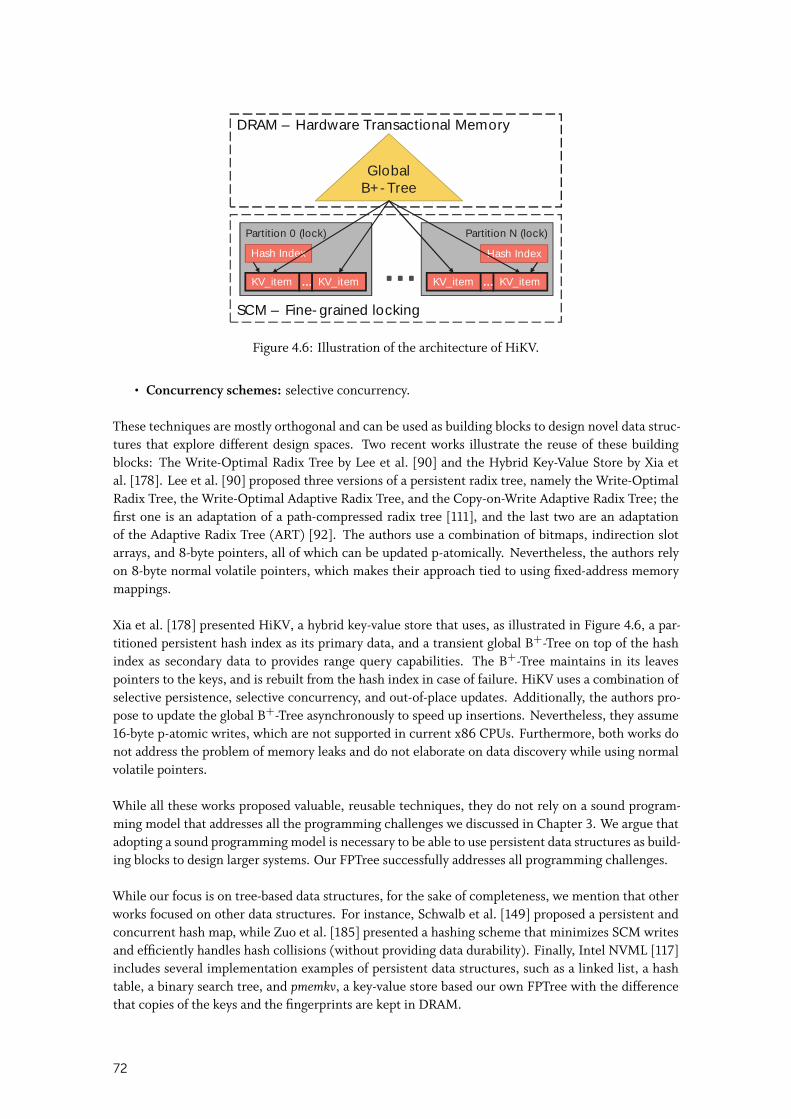
…SCM – Fine-grained locking
DRAM – Hardware Transactional Memory
GlobalB+-Tree
Partition 0 (lock)
Hash Index
KV_item KV_item…
Partition N (lock)
Hash Index
KV_item KV_item…
Figure 4.6: Illustration of the architecture of HiKV.
• Concurrency schemes: selective concurrency.
These techniques are mostly orthogonal and can be used as building blocks to design novel data struc-tures that explore different design spaces. Two recent works illustrate the reuse of these buildingblocks: The Write-Optimal Radix Tree by Lee et al. [90] and the Hybrid Key-Value Store by Xia etal. [178]. Lee et al. [90] proposed three versions of a persistent radix tree, namely the Write-OptimalRadix Tree, the Write-Optimal Adaptive Radix Tree, and the Copy-on-Write Adaptive Radix Tree; thefirst one is an adaptation of a path-compressed radix tree [111], and the last two are an adaptationof the Adaptive Radix Tree (ART) [92]. The authors use a combination of bitmaps, indirection slotarrays, and 8-byte pointers, all of which can be updated p-atomically. Nevertheless, the authors relyon 8-byte normal volatile pointers, which makes their approach tied to using fixed-address memorymappings.
Xia et al. [178] presented HiKV, a hybrid key-value store that uses, as illustrated in Figure 4.6, a par-titioned persistent hash index as its primary data, and a transient global B+-Tree on top of the hashindex as secondary data to provides range query capabilities. The B+-Tree maintains in its leavespointers to the keys, and is rebuilt from the hash index in case of failure. HiKV uses a combination ofselective persistence, selective concurrency, and out-of-place updates. Additionally, the authors pro-pose to update the global B+-Tree asynchronously to speed up insertions. Nevertheless, they assume16-byte p-atomic writes, which are not supported in current x86 CPUs. Furthermore, both works donot address the problem of memory leaks and do not elaborate on data discovery while using normalvolatile pointers.
While all these works proposed valuable, reusable techniques, they do not rely on a sound program-ming model that addresses all the programming challenges we discussed in Chapter 3. We argue thatadopting a sound programming model is necessary to be able to use persistent data structures as build-ing blocks to design larger systems. Our FPTree successfully addresses all programming challenges.
While our focus is on tree-based data structures, for the sake of completeness, we mention that otherworks focused on other data structures. For instance, Schwalb et al. [149] proposed a persistent andconcurrent hash map, while Zuo et al. [185] presented a hashing scheme that minimizes SCM writesand efficiently handles hash collisions (without providing data durability). Finally, Intel NVML [117]includes several implementation examples of persistent data structures, such as a linked list, a hashtable, a binary search tree, and pmemkv, a key-value store based our own FPTree with the differencethat copies of the keys and the fingerprints are kept in DRAM.
72
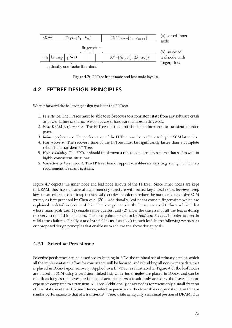
bitmap pNext KV={(k1,v1)...(kn,vn)}lock
fingerprints
optimally one-cache-line-sized
nKeys Keys={k1...km} Children={c1...cm+1} (a) sorted innernode
(b) unsortedleaf node withfingerprints
Figure 4.7: FPTree inner node and leaf node layouts.
4.2 FPTREE DESIGN PRINCIPLES
We put forward the following design goals for the FPTree:
1. Persistence. The FPTree must be able to self-recover to a consistent state from any software crashor power failure scenario. We do not cover hardware failures in this work.
2. Near-DRAM performance. The FPTree must exhibit similar performance to transient counter-parts.
3. Robust performance. The performance of the FPTree must be resilient to higher SCM latencies.4. Fast recovery. The recovery time of the FPTree must be significantly faster than a complete
rebuild of a transient B+-Tree.5. High scalability. The FPTree should implement a robust concurrency scheme that scales well in
highly concurrent situations.6. Variable-size keys support. The FPTree should support variable-size keys (e.g. strings) which is a
requirement for many systems.
Figure 4.7 depicts the inner node and leaf node layouts of the FPTree. Since inner nodes are keptin DRAM, they have a classical main memory structure with sorted keys. Leaf nodes however keepkeys unsorted and use a bitmap to track valid entries in order to reduce the number of expensive SCMwrites, as first proposed by Chen et al [20]. Additionally, leaf nodes contain fingerprints which areexplained in detail in Section 4.2.2. The next pointers in the leaves are used to form a linked listwhose main goals are: (1) enable range queries, and (2) allow the traversal of all the leaves duringrecovery to rebuild inner nodes. The next pointers need to be Persistent Pointers in order to remainvalid across failures. Finally, a one-byte field is used as a lock in each leaf. In the following we presentour proposed design principles that enable us to achieve the above design goals.
4.2.1 Selective Persistence
Selective persistence can be described as keeping in SCM the minimal set of primary data on whichall the implementation effort for consistency will be focused, and rebuilding all non-primary data thatis placed in DRAM upon recovery. Applied to a B+-Tree, as illustrated in Figure 4.8, the leaf nodesare placed in SCM using a persistent linked list, while inner nodes are placed in DRAM and can berebuilt as long as the leaves are in a consistent state. As a result, only accessing the leaves is moreexpensive compared to a transient B+-Tree. Additionally, inner nodes represent only a small fractionof the total size of the B+-Tree. Hence, selective persistence should enable our persistent tree to havesimilar performance to that of a transient B+-Tree, while using only a minimal portion of DRAM. Our
73
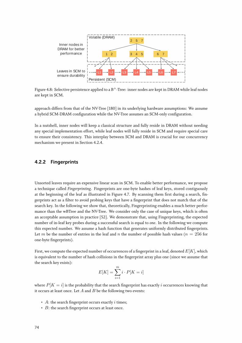
2 5 7
6 73 4 51 2
L5L4L3
Persistent (SCM)
L2L1 L7L6
Volatile (DRAM)
Inner nodes inDRAM for better
performance
Leaves in SCM toensure durability
… …
Figure 4.8: Selective persistence applied to a B+-Tree: inner nodes are kept in DRAM while leaf nodesare kept in SCM.
approach differs from that of the NV-Tree [180] in its underlying hardware assumptions: We assumea hybrid SCM-DRAM configuration while the NV-Tree assumes an SCM-only configuration.
In a nutshell, inner nodes will keep a classical structure and fully reside in DRAM without needingany special implementation effort, while leaf nodes will fully reside in SCM and require special careto ensure their consistency. This interplay between SCM and DRAM is crucial for our concurrencymechanism we present in Section 4.2.4.
4.2.2 Fingerprints
Unsorted leaves require an expensive linear scan in SCM. To enable better performance, we proposea technique called Fingerprinting. Fingerprints are one-byte hashes of leaf keys, stored contiguouslyat the beginning of the leaf as illustrated in Figure 4.7. By scanning them first during a search, fin-gerprints act as a filter to avoid probing keys that have a fingerprint that does not match that of thesearch key. In the following we show that, theoretically, Fingerprinting enables a much better perfor-mance than the wBTree and the NV-Tree. We consider only the case of unique keys, which is oftenan acceptable assumption in practice [52]. We demonstrate that, using Fingerprinting, the expectednumber of in-leaf key probes during a successful search is equal to one. In the following we computethis expected number. We assume a hash function that generates uniformly distributed fingerprints.Let m be the number of entries in the leaf and n the number of possible hash values (n = 256 forone-byte fingerprints).
First, we compute the expected number of occurrences of a fingerprint in a leaf, denoted E[K], whichis equivalent to the number of hash collisions in the fingerprint array plus one (since we assume thatthe search key exists):
E[K] =m∑i=1
i · P [K = i]
where P [K = i] is the probability that the search fingerprint has exactly i occurrences knowing thatit occurs at least once. Let A and B be the following two events:
• A: the search fingerprint occurs exactly i times;• B: the search fingerprint occurs at least once.
74
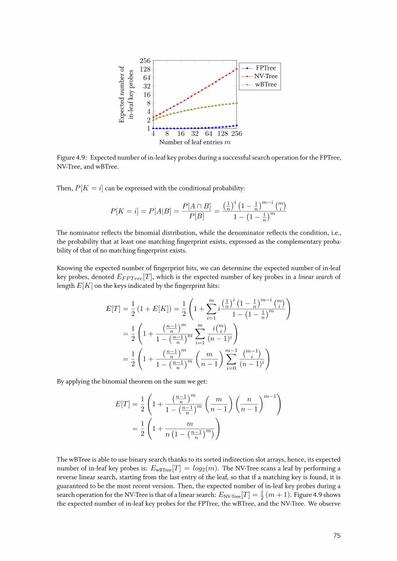
4 8 16 32 64 128 2561248
163264128256
Number of leaf entries m
Expe
cted
num
ber
ofin
-leaf
key
prob
es
FPTreeNV-TreewBTree
Figure 4.9: Expected number of in-leaf key probes during a successful search operation for the FPTree,NV-Tree, and wBTree.
Then, P [K = i] can be expressed with the conditional probability:
P [K = i] = P [A|B] =P [A ∩B]
P [B]=
(1n
)i (1− 1
n
)m−i (mi
)1−
(1− 1
n
)mThe nominator reflects the binomial distribution, while the denominator reflects the condition, i.e.,the probability that at least one matching fingerprint exists, expressed as the complementary proba-bility of that of no matching fingerprint exists.
Knowing the expected number of fingerprint hits, we can determine the expected number of in-leafkey probes, denoted EFPTree[T ], which is the expected number of key probes in a linear search oflength E[K] on the keys indicated by the fingerprint hits:
E[T ] =1
2(1 + E[K]) =
1
2
(1 +
m∑i=1
i
(1n
)i (1− 1
n
)m−i (mi
)1−
(1− 1
n
)m)
=1
2
(1 +
(n−1n
)m1−
(n−1n
)m m∑i=1
i(mi
)(n− 1)i
)
=1
2
(1 +
(n−1n
)m1−
(n−1n
)m ( m
n− 1
)m−1∑i=0
(m−1i
)(n− 1)i
)
By applying the binomial theorem on the sum we get:
E[T ] =1
2
(1 +
(n−1n
)m1−
(n−1n
)m ( m
n− 1
)(n
n− 1
)m−1)
=1
2
(1 +
m
n(1−
(n−1n
)m))
The wBTree is able to use binary search thanks to its sorted indirection slot arrays, hence, its expectednumber of in-leaf key probes is: EwBTree[T ] = log2(m). The NV-Tree scans a leaf by performing areverse linear search, starting from the last entry of the leaf, so that if a matching key is found, it isguaranteed to be the most recent version. Then, the expected number of in-leaf key probes during asearch operation for the NV-Tree is that of a linear search: ENV-Tree[T ] =
12 (m+ 1). Figure 4.9 shows
the expected number of in-leaf key probes for the FPTree, the wBTree, and the NV-Tree. We observe
75
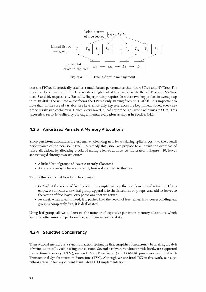
L1 L2 L3 L4 L5 L6 L7 L8Linked list of
leaf groups
L2 L4 L5 L7Volatile arrayof free leaves
L1 L3 L6 L8Linked list of
leaves in the tree
Figure 4.10: FPTree leaf group management.
that the FPTree theoretically enables a much better performance than the wBTree and NV-Tree. Forinstance, for m = 32, the FPTree needs a single in-leaf key probe, while the wBTree and NV-Treeneed 5 and 16, respectively. Basically, fingerprinting requires less than two key probes in average upto m ≈ 400. The wBTree outperforms the FPTree only starting from m ≈ 4096. It is important tonote that, in the case of variable-size keys, since only key references are kept in leaf nodes, every keyprobe results in a cache miss. Hence, every saved in-leaf key probe is a saved cache miss to SCM. Thistheoretical result is verified by our experimental evaluation as shown in Section 4.4.2.
4.2.3 Amortized Persistent Memory Allocations
Since persistent allocations are expensive, allocating new leaves during splits is costly to the overallperformance of the persistent tree. To remedy this issue, we propose to amortize the overhead ofthose allocations by allocating blocks of multiple leaves at once. As illustrated in Figure 4.10, leavesare managed through two structures:
• A linked list of groups of leaves currently allocated;• A transient array of leaves currently free and not used in the tree.
Two methods are used to get and free leaves:
• GetLeaf: if the vector of free leaves is not empty, we pop the last element and return it. If it isempty, we allocate a new leaf group, append it to the linked list of groups, and add its leaves tothe vector of free leaves, except the one that we return.
• FreeLeaf: when a leaf is freed, it is pushed into the vector of free leaves. If its corresponding leafgroup is completely free, it is deallocated.
Using leaf groups allows to decrease the number of expensive persistent memory allocations whichleads to better insertion performance, as shown in Section 4.4.2.
4.2.4 Selective Concurrency
Transactional memory is a synchronization technique that simplifies concurrency by making a batchof writes atomically visible using transactions. Several hardware vendors provide hardware-supportedtransactional memory (HTM), such as IBM on Blue Gene/Q and POWER8 processors, and Intel withTransactional Synchronization Extensions (TSX). Although we use Intel TSX in this work, our algo-rithms are valid for any currently available HTM implementation.
76
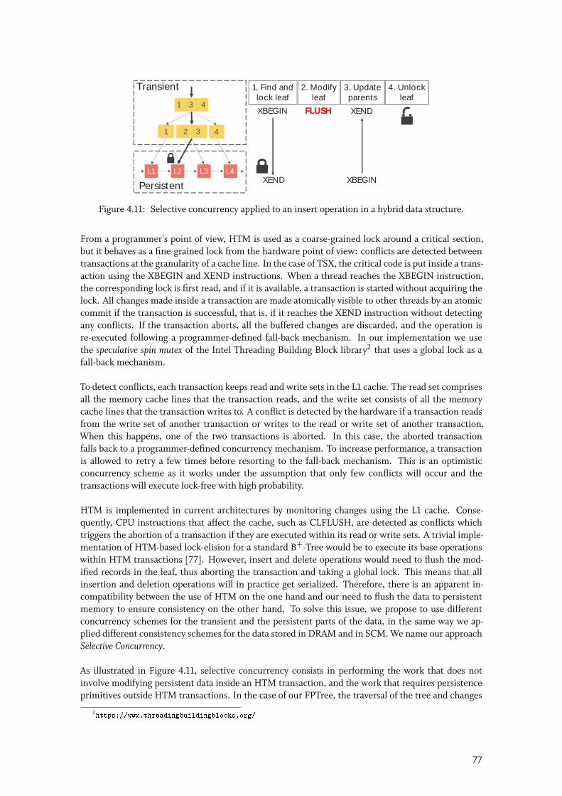
Persistent
Transient
1 3 4
42 31
L4L3L2L1
XBEGIN XEND
1. Find andlock leaf
2. Modifyleaf
3. Updateparents
XBEGINXEND
4. Unlockleaf
FLUSH
Figure 4.11: Selective concurrency applied to an insert operation in a hybrid data structure.
From a programmer’s point of view, HTM is used as a coarse-grained lock around a critical section,but it behaves as a fine-grained lock from the hardware point of view: conflicts are detected betweentransactions at the granularity of a cache line. In the case of TSX, the critical code is put inside a trans-action using the XBEGIN and XEND instructions. When a thread reaches the XBEGIN instruction,the corresponding lock is first read, and if it is available, a transaction is started without acquiring thelock. All changes made inside a transaction are made atomically visible to other threads by an atomiccommit if the transaction is successful, that is, if it reaches the XEND instruction without detectingany conflicts. If the transaction aborts, all the buffered changes are discarded, and the operation isre-executed following a programmer-defined fall-back mechanism. In our implementation we usethe speculative spin mutex of the Intel Threading Building Block library2 that uses a global lock as afall-back mechanism.
To detect conflicts, each transaction keeps read and write sets in the L1 cache. The read set comprisesall the memory cache lines that the transaction reads, and the write set consists of all the memorycache lines that the transaction writes to. A conflict is detected by the hardware if a transaction readsfrom the write set of another transaction or writes to the read or write set of another transaction.When this happens, one of the two transactions is aborted. In this case, the aborted transactionfalls back to a programmer-defined concurrency mechanism. To increase performance, a transactionis allowed to retry a few times before resorting to the fall-back mechanism. This is an optimisticconcurrency scheme as it works under the assumption that only few conflicts will occur and thetransactions will execute lock-free with high probability.
HTM is implemented in current architectures by monitoring changes using the L1 cache. Conse-quently, CPU instructions that affect the cache, such as CLFLUSH, are detected as conflicts whichtriggers the abortion of a transaction if they are executed within its read or write sets. A trivial imple-mentation of HTM-based lock-elision for a standard B+-Tree would be to execute its base operationswithin HTM transactions [77]. However, insert and delete operations would need to flush the mod-ified records in the leaf, thus aborting the transaction and taking a global lock. This means that allinsertion and deletion operations will in practice get serialized. Therefore, there is an apparent in-compatibility between the use of HTM on the one hand and our need to flush the data to persistentmemory to ensure consistency on the other hand. To solve this issue, we propose to use differentconcurrency schemes for the transient and the persistent parts of the data, in the same way we ap-plied different consistency schemes for the data stored in DRAM and in SCM. We name our approachSelective Concurrency.
As illustrated in Figure 4.11, selective concurrency consists in performing the work that does notinvolve modifying persistent data inside an HTM transaction, and the work that requires persistenceprimitives outside HTM transactions. In the case of our FPTree, the traversal of the tree and changes
2https://www.threadingbuildingblocks.org/
77
to inner nodes only involve transient data. Therefore, these operations are executed within an HTMtransaction and are thus protected against other operations done in concurrent HTM transactions. Forother operations that cannot be executed inside the transaction, fine-grained locks are used. Basically,the leaf nodes to be modified are locked during the traversal of the tree inside the HTM transaction.After all modifications on the transient part are done, the transaction is committed. The remainingmodifications on the persistent part are then processed outside of the transaction. Finally, the lockson the persistent part are released. The implementation of the base operations using TSX are detailedin Section 4.3.
4.3 FPTREE BASE OPERATIONS
We implement three different persistent trees:
1. FPTree. It is the single-threaded version that implements selective persistence, fingerprinting,amortized allocations, and unsorted leaves.
2. Concurrent FPTree. This version implements selective persistence, selective concurrency, fin-gerprinting, and unsorted leaves. As for amortized allocations, since they constitute a centralsynchronization point, we found that they hinder scalability. Hence, they are used only in thesingle-threaded version of the FPTree.
3. PTree. It reflects a light version of the FPTree that implements only selective persistence andunsorted leaves. Contrary to the FPTree and the wBTree, it keeps keys and values in separatearrays for better data locality when linearly scanning the keys.
In the following, Section 4.3.1 discusses the base operations of the FPTree with fixed-size keys. There-after, Section 4.3.2 presents a similar discussion for variable-size keys. Finally, Section 4.3.3 detailsthe algorithms for managing the leaf groups in the single-threaded version of the FPTree.
In the course of this section, speculative lock denotes a TSX-enabled lock such as the Intel TBB spec-ulative read write lock. Since leaf locks are only taken within TSX transactions, there is no need tomodify them using atomics. As a result, if many threads try to write the same lock – thus writing tothe same cache line – only one will succeed and the others will be aborted.
4.3.1 Fixed-Size Key Operations
This section discusses the find, range search, insert, delete, and update operations of the concurrentFPTree with fixed-size keys and explains how the FPTree can recover in a consistent state from anysoftware crash or power failure scenario.
Find
Since search operations do not modify persistent data, they can be fully wrapped in a TSX transactionthat protects them from conflicting with write operations of other threads. If another thread writes toa location read by the thread performing the lookup, the transaction will abort and retry, eventuallytaking a global lock if the retry threshold is exceeded. Search operations still need to check for any
78
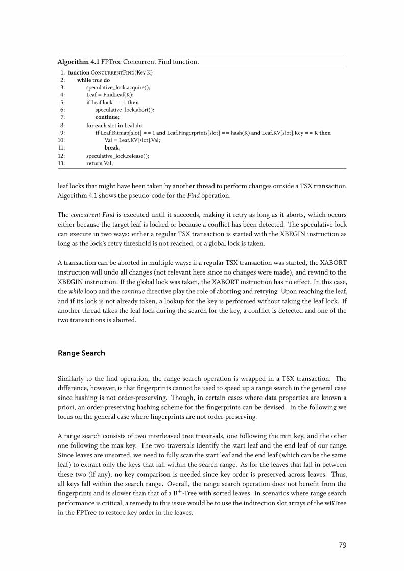
Algorithm 4.1 FPTree Concurrent Find function.1: function ConcurrentFind(Key K)2: while true do3: speculative_lock.acquire();4: Leaf = FindLeaf(K);5: if Leaf.lock == 1 then6: speculative_lock.abort();7: continue;8: for each slot in Leaf do9: if Leaf.Bitmap[slot] == 1 and Leaf.Fingerprints[slot] == hash(K) and Leaf.KV[slot].Key == K then
10: Val = Leaf.KV[slot].Val;11: break;12: speculative_lock.release();13: return Val;
leaf locks that might have been taken by another thread to perform changes outside a TSX transaction.Algorithm 4.1 shows the pseudo-code for the Find operation.
The concurrent Find is executed until it succeeds, making it retry as long as it aborts, which occurseither because the target leaf is locked or because a conflict has been detected. The speculative lockcan execute in two ways: either a regular TSX transaction is started with the XBEGIN instruction aslong as the lock’s retry threshold is not reached, or a global lock is taken.
A transaction can be aborted in multiple ways: if a regular TSX transaction was started, the XABORTinstruction will undo all changes (not relevant here since no changes were made), and rewind to theXBEGIN instruction. If the global lock was taken, the XABORT instruction has no effect. In this case,the while loop and the continue directive play the role of aborting and retrying. Upon reaching the leaf,and if its lock is not already taken, a lookup for the key is performed without taking the leaf lock. Ifanother thread takes the leaf lock during the search for the key, a conflict is detected and one of thetwo transactions is aborted.
Range Search
Similarly to the find operation, the range search operation is wrapped in a TSX transaction. Thedifference, however, is that fingerprints cannot be used to speed up a range search in the general casesince hashing is not order-preserving. Though, in certain cases where data properties are known apriori, an order-preserving hashing scheme for the fingerprints can be devised. In the following wefocus on the general case where fingerprints are not order-preserving.
A range search consists of two interleaved tree traversals, one following the min key, and the otherone following the max key. The two traversals identify the start leaf and the end leaf of our range.Since leaves are unsorted, we need to fully scan the start leaf and the end leaf (which can be the sameleaf) to extract only the keys that fall within the search range. As for the leaves that fall in betweenthese two (if any), no key comparison is needed since key order is preserved across leaves. Thus,all keys fall within the search range. Overall, the range search operation does not benefit from thefingerprints and is slower than that of a B+-Tree with sorted leaves. In scenarios where range searchperformance is critical, a remedy to this issue would be to use the indirection slot arrays of the wBTreein the FPTree to restore key order in the leaves.
79
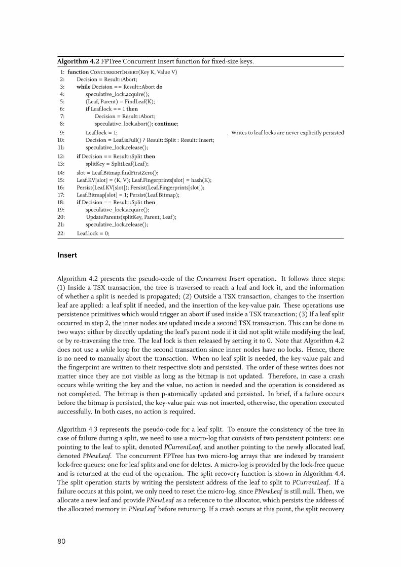
Algorithm 4.2 FPTree Concurrent Insert function for fixed-size keys.1: function ConcurrentInsert(Key K, Value V)2: Decision = Result::Abort;3: while Decision == Result::Abort do4: speculative_lock.acquire();5: (Leaf, Parent) = FindLeaf(K);6: if Leaf.lock == 1 then7: Decision = Result::Abort;8: speculative_lock.abort(); continue;
9: Leaf.lock = 1; ◃ Writes to leaf locks are never explicitly persisted10: Decision = Leaf.isFull() ? Result::Split : Result::Insert;11: speculative_lock.release();
12: if Decision == Result::Split then13: splitKey = SplitLeaf(Leaf);
14: slot = Leaf.Bitmap.findFirstZero();15: Leaf.KV[slot] = (K, V); Leaf.Fingerprints[slot] = hash(K);16: Persist(Leaf.KV[slot]); Persist(Leaf.Fingerprints[slot]);17: Leaf.Bitmap[slot] = 1; Persist(Leaf.Bitmap);18: if Decision == Result::Split then19: speculative_lock.acquire();20: UpdateParents(splitKey, Parent, Leaf);21: speculative_lock.release();
22: Leaf.lock = 0;
Insert
Algorithm 4.2 presents the pseudo-code of the Concurrent Insert operation. It follows three steps:(1) Inside a TSX transaction, the tree is traversed to reach a leaf and lock it, and the informationof whether a split is needed is propagated; (2) Outside a TSX transaction, changes to the insertionleaf are applied: a leaf split if needed, and the insertion of the key-value pair. These operations usepersistence primitives which would trigger an abort if used inside a TSX transaction; (3) If a leaf splitoccurred in step 2, the inner nodes are updated inside a second TSX transaction. This can be done intwo ways: either by directly updating the leaf’s parent node if it did not split while modifying the leaf,or by re-traversing the tree. The leaf lock is then released by setting it to 0. Note that Algorithm 4.2does not use a while loop for the second transaction since inner nodes have no locks. Hence, thereis no need to manually abort the transaction. When no leaf split is needed, the key-value pair andthe fingerprint are written to their respective slots and persisted. The order of these writes does notmatter since they are not visible as long as the bitmap is not updated. Therefore, in case a crashoccurs while writing the key and the value, no action is needed and the operation is considered asnot completed. The bitmap is then p-atomically updated and persisted. In brief, if a failure occursbefore the bitmap is persisted, the key-value pair was not inserted, otherwise, the operation executedsuccessfully. In both cases, no action is required.
Algorithm 4.3 represents the pseudo-code for a leaf split. To ensure the consistency of the tree incase of failure during a split, we need to use a micro-log that consists of two persistent pointers: onepointing to the leaf to split, denoted PCurrentLeaf, and another pointing to the newly allocated leaf,denoted PNewLeaf. The concurrent FPTree has two micro-log arrays that are indexed by transientlock-free queues: one for leaf splits and one for deletes. A micro-log is provided by the lock-free queueand is returned at the end of the operation. The split recovery function is shown in Algorithm 4.4.The split operation starts by writing the persistent address of the leaf to split to PCurrentLeaf. If afailure occurs at this point, we only need to reset the micro-log, since PNewLeaf is still null. Then, weallocate a new leaf and provide PNewLeaf as a reference to the allocator, which persists the address ofthe allocated memory in PNewLeaf before returning. If a crash occurs at this point, the split recovery
80
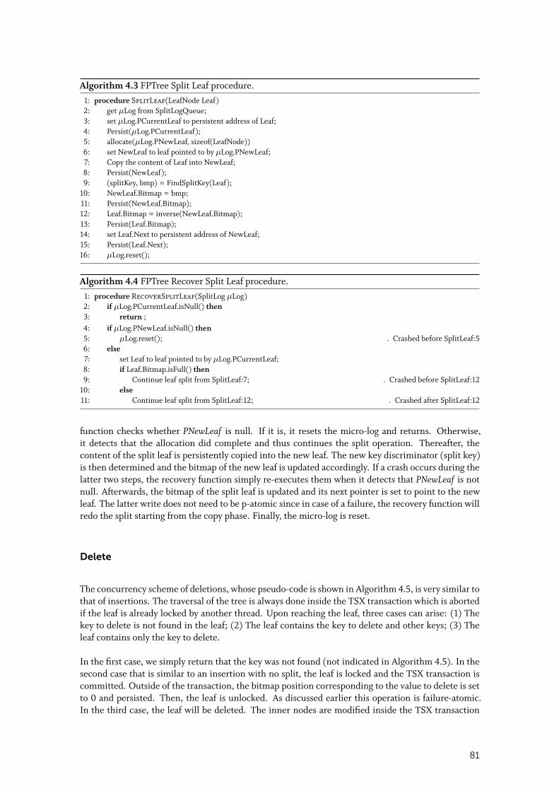
Algorithm 4.3 FPTree Split Leaf procedure.1: procedure SplitLeaf(LeafNode Leaf)2: get µLog from SplitLogQueue;3: set µLog.PCurrentLeaf to persistent address of Leaf;4: Persist(µLog.PCurrentLeaf);5: allocate(µLog.PNewLeaf, sizeof(LeafNode))6: set NewLeaf to leaf pointed to by µLog.PNewLeaf;7: Copy the content of Leaf into NewLeaf;8: Persist(NewLeaf);9: (splitKey, bmp) = FindSplitKey(Leaf);
10: NewLeaf.Bitmap = bmp;11: Persist(NewLeaf.Bitmap);12: Leaf.Bitmap = inverse(NewLeaf.Bitmap);13: Persist(Leaf.Bitmap);14: set Leaf.Next to persistent address of NewLeaf;15: Persist(Leaf.Next);16: µLog.reset();
Algorithm 4.4 FPTree Recover Split Leaf procedure.1: procedure RecoverSplitLeaf(SplitLog µLog)2: if µLog.PCurrentLeaf.isNull() then3: return ;4: if µLog.PNewLeaf.isNull() then5: µLog.reset(); ◃ Crashed before SplitLeaf:56: else7: set Leaf to leaf pointed to by µLog.PCurrentLeaf;8: if Leaf.Bitmap.isFull() then9: Continue leaf split from SplitLeaf:7; ◃ Crashed before SplitLeaf:12
10: else11: Continue leaf split from SplitLeaf:12; ◃ Crashed after SplitLeaf:12
function checks whether PNewLeaf is null. If it is, it resets the micro-log and returns. Otherwise,it detects that the allocation did complete and thus continues the split operation. Thereafter, thecontent of the split leaf is persistently copied into the new leaf. The new key discriminator (split key)is then determined and the bitmap of the new leaf is updated accordingly. If a crash occurs during thelatter two steps, the recovery function simply re-executes them when it detects that PNewLeaf is notnull. Afterwards, the bitmap of the split leaf is updated and its next pointer is set to point to the newleaf. The latter write does not need to be p-atomic since in case of a failure, the recovery function willredo the split starting from the copy phase. Finally, the micro-log is reset.
Delete
The concurrency scheme of deletions, whose pseudo-code is shown in Algorithm 4.5, is very similar tothat of insertions. The traversal of the tree is always done inside the TSX transaction which is abortedif the leaf is already locked by another thread. Upon reaching the leaf, three cases can arise: (1) Thekey to delete is not found in the leaf; (2) The leaf contains the key to delete and other keys; (3) Theleaf contains only the key to delete.
In the first case, we simply return that the key was not found (not indicated in Algorithm 4.5). In thesecond case that is similar to an insertion with no split, the leaf is locked and the TSX transaction iscommitted. Outside of the transaction, the bitmap position corresponding to the value to delete is setto 0 and persisted. Then, the leaf is unlocked. As discussed earlier this operation is failure-atomic.In the third case, the leaf will be deleted. The inner nodes are modified inside the TSX transaction
81
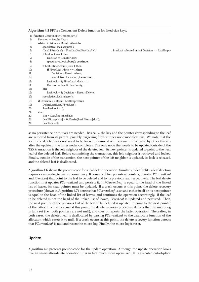
Algorithm 4.5 FPTree Concurrent Delete function for fixed-size keys.1: function ConcurrentDelete(Key K)2: Decision = Result::Abort;3: while Decision == Result::Abort do4: speculative_lock.acquire();5: (Leaf, PPrevLeaf) = FindLeafAndPrevLeaf(K); ◃ PrevLeaf is locked only if Decision == LeafEmpty6: if Leaf.lock == 1 then7: Decision = Result::Abort;8: speculative_lock.abort(); continue;
9: if Leaf.Bitmap.count() == 1 then10: if PPrevLeaf->lock == 1 then11: Decision = Result::Abort;12: speculative_lock.abort(); continue;
13: Leaf.lock = 1; PPrevLeaf->lock = 1;14: Decision = Result::LeafEmpty;15: else16: Leaf.lock = 1; Decision = Result::Delete;17: speculative_lock.release();
18: if Decision == Result::LeafEmpty then19: DeleteLeaf(Leaf, PPrevLeaf);20: PrevLeaf.lock = 0;21: else22: slot = Leaf.findInLeaf(K);23: Leaf.Bitmap[slot] = 0; Persist(Leaf.Bitmap[slot]);24: Leaf.lock = 0;
as no persistence primitives are needed. Basically, the key and the pointer corresponding to the leafare removed from its parent, possibly triggering further inner node modifications. We note that theleaf to be deleted does not need to be locked because it will become unreachable by other threadsafter the update of the inner nodes completes. The only node that needs to be updated outside of theTSX transaction is the left neighbor of the deleted leaf; its next pointer is updated to point to the nextleaf of the deleted leaf. Before committing the transaction, this left neighbor is retrieved and locked.Finally, outside of the transaction, the next pointer of the left neighbor is updated, its lock is released,and the deleted leaf is deallocated.
Algorithm 4.6 shows the pseudo-code for a leaf delete operation. Similarly to leaf splits, a leaf deletionrequires a micro-log to ensure consistency. It consists of two persistent pointers, denoted PCurrentLeafand PPrevLeaf that point to the leaf to be deleted and to its previous leaf, respectively. The leaf deletefunction first updates PCurrentLeaf and persists it. If PCurrentLeaf is equal to the head of the linkedlist of leaves, its head pointer must be updated. If a crash occurs at this point, the delete recoveryprocedure (shown in Algorithm 4.7) detects that PCurrentLeaf is set and either itself or its next pointeris equal to the head of the linked list of leaves, and continues the operation accordingly. If the leafto be deleted is not the head of the linked list of leaves, PPrevLeaf is updated and persisted. Then,the next pointer of the previous leaf of the leaf to be deleted is updated to point to the next pointerof the latter. If a crash occurs at this point, the delete recovery procedure detects that the micro-logis fully set (i.e., both pointers are not null), and thus, it repeats the latter operation. Thereafter, inboth cases, the deleted leaf is deallocated by passing PCurrentLeaf to the deallocate function of theallocator, which resets it to null. If a crash occurs at this point, the delete recovery function detectsthat PCurrentLeaf is null and resets the micro-log. Finally, the micro-log is reset.
Update
Algorithm 4.8 presents pseudo-code for the update operation. Although the update operation lookslike an insert-after-delete operation, it is in fact much more optimized: It is executed out-of-place.
82
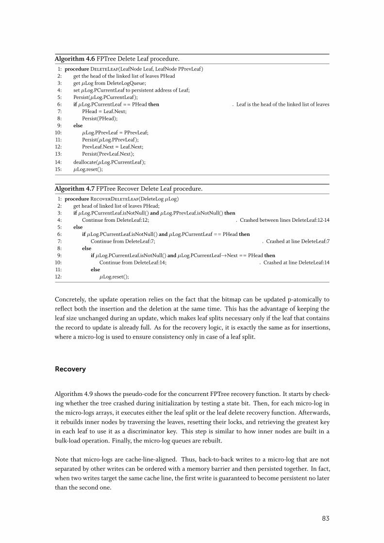
Algorithm 4.6 FPTree Delete Leaf procedure.1: procedure DeleteLeaf(LeafNode Leaf, LeafNode PPrevLeaf)2: get the head of the linked list of leaves PHead3: get µLog from DeleteLogQueue;4: set µLog.PCurrentLeaf to persistent address of Leaf;5: Persist(µLog.PCurrentLeaf);6: if µLog.PCurrentLeaf == PHead then ◃ Leaf is the head of the linked list of leaves7: PHead = Leaf.Next;8: Persist(PHead);9: else
10: µLog.PPrevLeaf = PPrevLeaf;11: Persist(µLog.PPrevLeaf);12: PrevLeaf.Next = Leaf.Next;13: Persist(PrevLeaf.Next);
14: deallocate(µLog.PCurrentLeaf);15: µLog.reset();
Algorithm 4.7 FPTree Recover Delete Leaf procedure.1: procedure RecoverDeleteLeaf(DeleteLog µLog)2: get head of linked list of leaves PHead;3: if µLog.PCurrentLeaf.isNotNull() and µLog.PPrevLeaf.isNotNull() then4: Continue from DeleteLeaf:12; ◃ Crashed between lines DeleteLeaf:12-145: else6: if µLog.PCurrentLeaf.isNotNull() and µLog.PCurrentLeaf == PHead then7: Continue from DeleteLeaf:7; ◃ Crashed at line DeleteLeaf:78: else9: if µLog.PCurrentLeaf.isNotNull() and µLog.PCurrentLeaf→Next == PHead then
10: Continue from DeleteLeaf:14; ◃ Crashed at line DeleteLeaf:1411: else12: µLog.reset();
Concretely, the update operation relies on the fact that the bitmap can be updated p-atomically toreflect both the insertion and the deletion at the same time. This has the advantage of keeping theleaf size unchanged during an update, which makes leaf splits necessary only if the leaf that containsthe record to update is already full. As for the recovery logic, it is exactly the same as for insertions,where a micro-log is used to ensure consistency only in case of a leaf split.
Recovery
Algorithm 4.9 shows the pseudo-code for the concurrent FPTree recovery function. It starts by check-ing whether the tree crashed during initialization by testing a state bit. Then, for each micro-log inthe micro-logs arrays, it executes either the leaf split or the leaf delete recovery function. Afterwards,it rebuilds inner nodes by traversing the leaves, resetting their locks, and retrieving the greatest keyin each leaf to use it as a discriminator key. This step is similar to how inner nodes are built in abulk-load operation. Finally, the micro-log queues are rebuilt.
Note that micro-logs are cache-line-aligned. Thus, back-to-back writes to a micro-log that are notseparated by other writes can be ordered with a memory barrier and then persisted together. In fact,when two writes target the same cache line, the first write is guaranteed to become persistent no laterthan the second one.
83
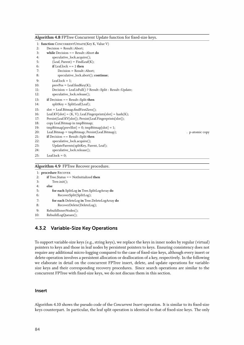
Algorithm 4.8 FPTree Concurrent Update function for fixed-size keys.1: function ConcurrentUpdate(Key K, Value V)2: Decision = Result::Abort;3: while Decision == Result::Abort do4: speculative_lock.acquire();5: (Leaf, Parent) = FindLeaf(K);6: if Leaf.lock == 1 then7: Decision = Result::Abort;8: speculative_lock.abort(); continue;
9: Leaf.lock = 1;10: prevPos = Leaf.findKey(K);11: Decision = Leaf.isFull() ? Result::Split : Result::Update;12: speculative_lock.release();
13: if Decision == Result::Split then14: splitKey = SplitLeaf(Leaf);
15: slot = Leaf.Bitmap.findFirstZero();16: Leaf.KV[slot] = (K, V); Leaf.Fingerprints[slot] = hash(K);17: Persist(Leaf.KV[slot]); Persist(Leaf.Fingerprints[slot]);18: copy Leaf.Bitmap in tmpBitmap;19: tmpBitmap[prevSlot] = 0; tmpBitmap[slot] = 1;20: Leaf.Bitmap = tmpBitmap; Persist(Leaf.Bitmap); ◃ p-atomic copy21: if Decision == Result::Split then22: speculative_lock.acquire();23: UpdateParents(splitKey, Parent, Leaf);24: speculative_lock.release();
25: Leaf.lock = 0;
Algorithm 4.9 FPTree Recover procedure.1: procedure Recover2: if Tree.Status == NotInitialized then3: Tree.init();4: else5: for each SplitLog in Tree.SplitLogArray do6: RecoverSplit(SplitLog);
7: for each DeleteLog in Tree.DeleteLogArray do8: RecoverDelete(DeleteLog);
9: RebuildInnerNodes();10: RebuildLogQueues();
4.3.2 Variable-Size Key Operations
To support variable-size keys (e.g., string keys), we replace the keys in inner nodes by regular (virtual)pointers to keys and those in leaf nodes by persistent pointers to keys. Ensuring consistency does notrequire any additional micro-logging compared to the case of fixed-size keys, although every insert ordelete operation involves a persistent allocation or deallocation of a key, respectively. In the followingwe elaborate in detail on the concurrent FPTree insert, delete, and update operations for variable-size keys and their corresponding recovery procedures. Since search operations are similar to theconcurrent FPTree with fixed-size keys, we do not discuss them in this section.
Insert
Algorithm 4.10 shows the pseudo code of the Concurrent Insert operation. It is similar to its fixed-sizekeys counterpart. In particular, the leaf split operation is identical to that of fixed-size keys. The only
84
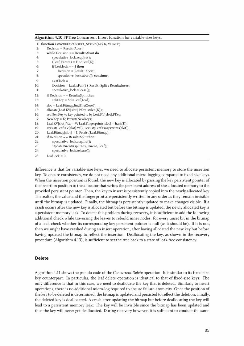
Algorithm 4.10 FPTree Concurrent Insert function for variable-size keys.1: function ConcurrentInsert_String(Key K, Value V)2: Decision = Result::Abort;3: while Decision == Result::Abort do4: speculative_lock.acquire();5: (Leaf, Parent) = FindLeaf(K);6: if Leaf.lock == 1 then7: Decision = Result::Abort;8: speculative_lock.abort(); continue;
9: Leaf.lock = 1;10: Decision = Leaf.isFull() ? Result::Split : Result::Insert;11: speculative_lock.release();
12: if Decision == Result::Split then13: splitKey = SplitLeaf(Leaf);
14: slot = Leaf.Bitmap.findFirstZero();15: allocate(Leaf.KV[slot].PKey, strlen(K));16: set NewKey to key pointed to by Leaf.KV[slot].PKey;17: NewKey = K; Persist(NewKey);18: Leaf.KV[slot].Val = V; Leaf.Fingerprints[slot] = hash(K);19: Persist(Leaf.KV[slot].Val); Persist(Leaf.Fingerprints[slot]);20: Leaf.Bitmap[slot] = 1; Persist(Leaf.Bitmap);21: if Decision == Result::Split then22: speculative_lock.acquire();23: UpdateParents(splitKey, Parent, Leaf);24: speculative_lock.release();
25: Leaf.lock = 0;
difference is that for variable-size keys, we need to allocate persistent memory to store the insertionkey. To ensure consistency, we do not need any additional micro-logging compared to fixed-size keys.When the insertion position is found, the new key is allocated by passing the key persistent pointer ofthe insertion position to the allocator that writes the persistent address of the allocated memory to theprovided persistent pointer. Then, the key to insert is persistently copied into the newly allocated key.Thereafter, the value and the fingerprint are persistently written in any order as they remain invisibleuntil the bitmap is updated. Finally, the bitmap is persistently updated to make changes visible. If acrash occurs after the new key is allocated but before the bitmap is updated, the newly allocated key isa persistent memory leak. To detect this problem during recovery, it is sufficient to add the followingadditional check while traversing the leaves to rebuild inner nodes: for every unset bit in the bitmapof a leaf, check whether its corresponding key persistent pointer is null (as it should be). If it is not,then we might have crashed during an insert operation, after having allocated the new key but beforehaving updated the bitmap to reflect the insertion. Deallocating the key, as shown in the recoveryprocedure (Algorithm 4.13), is sufficient to set the tree back to a state of leak-free consistency.
Delete
Algorithm 4.11 shows the pseudo code of the Concurrent Delete operation. It is similar to its fixed-sizekey counterpart. In particular, the leaf delete operation is identical to that of fixed-size keys. Theonly difference is that in this case, we need to deallocate the key that is deleted. Similarly to insertoperations, there is no additional micro-log required to ensure failure-atomicity. Once the position ofthe key to be deleted is determined, the bitmap is updated and persisted to reflect the deletion. Finally,the deleted key is deallocated. A crash after updating the bitmap but before deallocating the key willlead to a persistent memory leak: The key will be invisible since the bitmap has been updated andthus the key will never get deallocated. During recovery however, it is sufficient to conduct the same
85
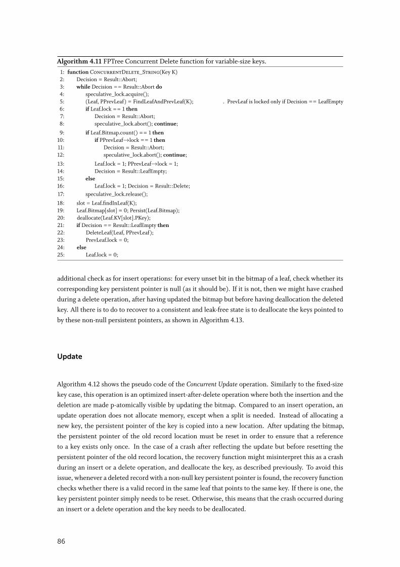
Algorithm 4.11 FPTree Concurrent Delete function for variable-size keys.1: function ConcurrentDelete_String(Key K)2: Decision = Result::Abort;3: while Decision == Result::Abort do4: speculative_lock.acquire();5: (Leaf, PPrevLeaf) = FindLeafAndPrevLeaf(K); ◃ PrevLeaf is locked only if Decision == LeafEmpty6: if Leaf.lock == 1 then7: Decision = Result::Abort;8: speculative_lock.abort(); continue;
9: if Leaf.Bitmap.count() == 1 then10: if PPrevLeaf→lock == 1 then11: Decision = Result::Abort;12: speculative_lock.abort(); continue;
13: Leaf.lock = 1; PPrevLeaf→lock = 1;14: Decision = Result::LeafEmpty;15: else16: Leaf.lock = 1; Decision = Result::Delete;17: speculative_lock.release();
18: slot = Leaf.findInLeaf(K);19: Leaf.Bitmap[slot] = 0; Persist(Leaf.Bitmap);20: deallocate(Leaf.KV[slot].PKey);21: if Decision == Result::LeafEmpty then22: DeleteLeaf(Leaf, PPrevLeaf);23: PrevLeaf.lock = 0;24: else25: Leaf.lock = 0;
additional check as for insert operations: for every unset bit in the bitmap of a leaf, check whether itscorresponding key persistent pointer is null (as it should be). If it is not, then we might have crashedduring a delete operation, after having updated the bitmap but before having deallocation the deletedkey. All there is to do to recover to a consistent and leak-free state is to deallocate the keys pointed toby these non-null persistent pointers, as shown in Algorithm 4.13.
Update
Algorithm 4.12 shows the pseudo code of the Concurrent Update operation. Similarly to the fixed-sizekey case, this operation is an optimized insert-after-delete operation where both the insertion and thedeletion are made p-atomically visible by updating the bitmap. Compared to an insert operation, anupdate operation does not allocate memory, except when a split is needed. Instead of allocating anew key, the persistent pointer of the key is copied into a new location. After updating the bitmap,the persistent pointer of the old record location must be reset in order to ensure that a referenceto a key exists only once. In the case of a crash after reflecting the update but before resetting thepersistent pointer of the old record location, the recovery function might misinterpret this as a crashduring an insert or a delete operation, and deallocate the key, as described previously. To avoid thisissue, whenever a deleted record with a non-null key persistent pointer is found, the recovery functionchecks whether there is a valid record in the same leaf that points to the same key. If there is one, thekey persistent pointer simply needs to be reset. Otherwise, this means that the crash occurred duringan insert or a delete operation and the key needs to be deallocated.
86
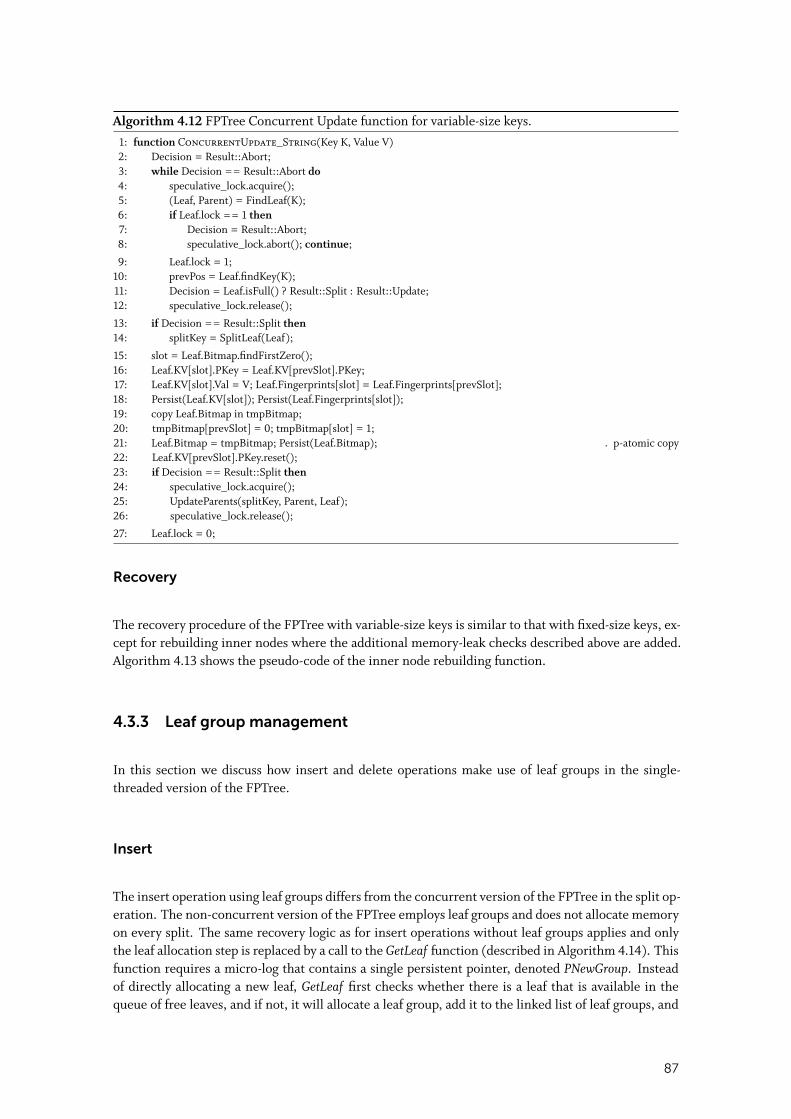
Algorithm 4.12 FPTree Concurrent Update function for variable-size keys.1: function ConcurrentUpdate_String(Key K, Value V)2: Decision = Result::Abort;3: while Decision == Result::Abort do4: speculative_lock.acquire();5: (Leaf, Parent) = FindLeaf(K);6: if Leaf.lock == 1 then7: Decision = Result::Abort;8: speculative_lock.abort(); continue;
9: Leaf.lock = 1;10: prevPos = Leaf.findKey(K);11: Decision = Leaf.isFull() ? Result::Split : Result::Update;12: speculative_lock.release();
13: if Decision == Result::Split then14: splitKey = SplitLeaf(Leaf);
15: slot = Leaf.Bitmap.findFirstZero();16: Leaf.KV[slot].PKey = Leaf.KV[prevSlot].PKey;17: Leaf.KV[slot].Val = V; Leaf.Fingerprints[slot] = Leaf.Fingerprints[prevSlot];18: Persist(Leaf.KV[slot]); Persist(Leaf.Fingerprints[slot]);19: copy Leaf.Bitmap in tmpBitmap;20: tmpBitmap[prevSlot] = 0; tmpBitmap[slot] = 1;21: Leaf.Bitmap = tmpBitmap; Persist(Leaf.Bitmap); ◃ p-atomic copy22: Leaf.KV[prevSlot].PKey.reset();23: if Decision == Result::Split then24: speculative_lock.acquire();25: UpdateParents(splitKey, Parent, Leaf);26: speculative_lock.release();
27: Leaf.lock = 0;
Recovery
The recovery procedure of the FPTree with variable-size keys is similar to that with fixed-size keys, ex-cept for rebuilding inner nodes where the additional memory-leak checks described above are added.Algorithm 4.13 shows the pseudo-code of the inner node rebuilding function.
4.3.3 Leaf group management
In this section we discuss how insert and delete operations make use of leaf groups in the single-threaded version of the FPTree.
Insert
The insert operation using leaf groups differs from the concurrent version of the FPTree in the split op-eration. The non-concurrent version of the FPTree employs leaf groups and does not allocate memoryon every split. The same recovery logic as for insert operations without leaf groups applies and onlythe leaf allocation step is replaced by a call to the GetLeaf function (described in Algorithm 4.14). Thisfunction requires a micro-log that contains a single persistent pointer, denoted PNewGroup. Insteadof directly allocating a new leaf, GetLeaf first checks whether there is a leaf that is available in thequeue of free leaves, and if not, it will allocate a leaf group, add it to the linked list of leaf groups, and
87
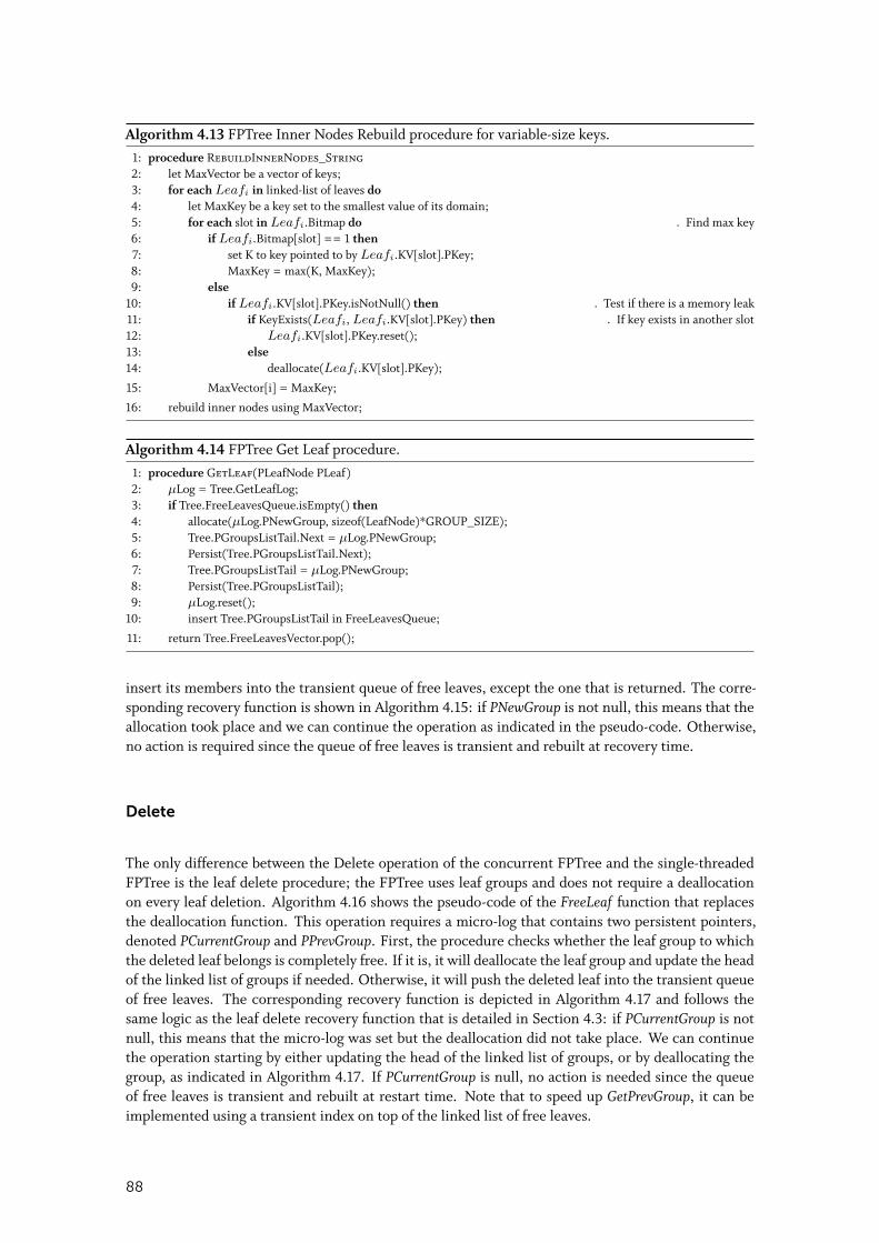
Algorithm 4.13 FPTree Inner Nodes Rebuild procedure for variable-size keys.1: procedure RebuildInnerNodes_String2: let MaxVector be a vector of keys;3: for each Leafi in linked-list of leaves do4: let MaxKey be a key set to the smallest value of its domain;5: for each slot in Leafi.Bitmap do ◃ Find max key6: if Leafi.Bitmap[slot] == 1 then7: set K to key pointed to by Leafi.KV[slot].PKey;8: MaxKey = max(K, MaxKey);9: else
10: if Leafi.KV[slot].PKey.isNotNull() then ◃ Test if there is a memory leak11: if KeyExists(Leafi, Leafi.KV[slot].PKey) then ◃ If key exists in another slot12: Leafi.KV[slot].PKey.reset();13: else14: deallocate(Leafi.KV[slot].PKey);
15: MaxVector[i] = MaxKey;
16: rebuild inner nodes using MaxVector;
Algorithm 4.14 FPTree Get Leaf procedure.1: procedure GetLeaf(PLeafNode PLeaf)2: µLog = Tree.GetLeafLog;3: if Tree.FreeLeavesQueue.isEmpty() then4: allocate(µLog.PNewGroup, sizeof(LeafNode)*GROUP_SIZE);5: Tree.PGroupsListTail.Next = µLog.PNewGroup;6: Persist(Tree.PGroupsListTail.Next);7: Tree.PGroupsListTail = µLog.PNewGroup;8: Persist(Tree.PGroupsListTail);9: µLog.reset();
10: insert Tree.PGroupsListTail in FreeLeavesQueue;
11: return Tree.FreeLeavesVector.pop();
insert its members into the transient queue of free leaves, except the one that is returned. The corre-sponding recovery function is shown in Algorithm 4.15: if PNewGroup is not null, this means that theallocation took place and we can continue the operation as indicated in the pseudo-code. Otherwise,no action is required since the queue of free leaves is transient and rebuilt at recovery time.
Delete
The only difference between the Delete operation of the concurrent FPTree and the single-threadedFPTree is the leaf delete procedure; the FPTree uses leaf groups and does not require a deallocationon every leaf deletion. Algorithm 4.16 shows the pseudo-code of the FreeLeaf function that replacesthe deallocation function. This operation requires a micro-log that contains two persistent pointers,denoted PCurrentGroup and PPrevGroup. First, the procedure checks whether the leaf group to whichthe deleted leaf belongs is completely free. If it is, it will deallocate the leaf group and update the headof the linked list of groups if needed. Otherwise, it will push the deleted leaf into the transient queueof free leaves. The corresponding recovery function is depicted in Algorithm 4.17 and follows thesame logic as the leaf delete recovery function that is detailed in Section 4.3: if PCurrentGroup is notnull, this means that the micro-log was set but the deallocation did not take place. We can continuethe operation starting by either updating the head of the linked list of groups, or by deallocating thegroup, as indicated in Algorithm 4.17. If PCurrentGroup is null, no action is needed since the queueof free leaves is transient and rebuilt at restart time. Note that to speed up GetPrevGroup, it can beimplemented using a transient index on top of the linked list of free leaves.
88
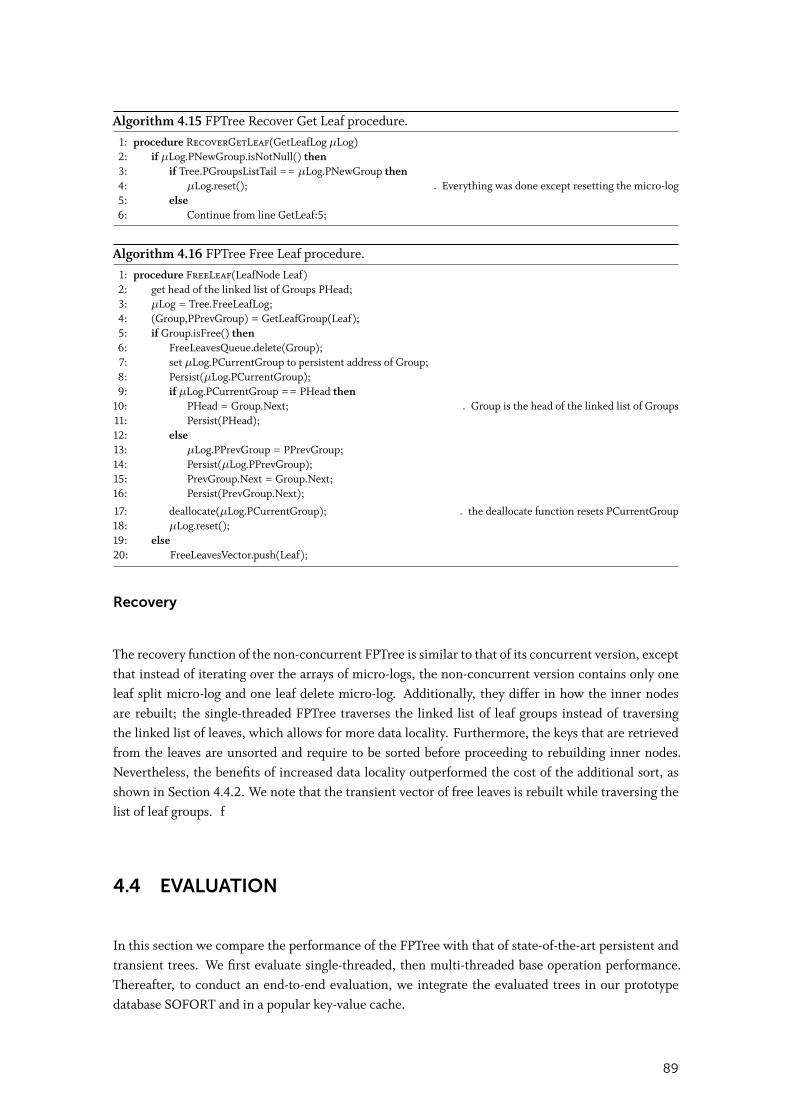
Algorithm 4.15 FPTree Recover Get Leaf procedure.1: procedure RecoverGetLeaf(GetLeafLog µLog)2: if µLog.PNewGroup.isNotNull() then3: if Tree.PGroupsListTail == µLog.PNewGroup then4: µLog.reset(); ◃ Everything was done except resetting the micro-log5: else6: Continue from line GetLeaf:5;
Algorithm 4.16 FPTree Free Leaf procedure.1: procedure FreeLeaf(LeafNode Leaf)2: get head of the linked list of Groups PHead;3: µLog = Tree.FreeLeafLog;4: (Group,PPrevGroup) = GetLeafGroup(Leaf);5: if Group.isFree() then6: FreeLeavesQueue.delete(Group);7: set µLog.PCurrentGroup to persistent address of Group;8: Persist(µLog.PCurrentGroup);9: if µLog.PCurrentGroup == PHead then
10: PHead = Group.Next; ◃ Group is the head of the linked list of Groups11: Persist(PHead);12: else13: µLog.PPrevGroup = PPrevGroup;14: Persist(µLog.PPrevGroup);15: PrevGroup.Next = Group.Next;16: Persist(PrevGroup.Next);
17: deallocate(µLog.PCurrentGroup); ◃ the deallocate function resets PCurrentGroup18: µLog.reset();19: else20: FreeLeavesVector.push(Leaf);
Recovery
The recovery function of the non-concurrent FPTree is similar to that of its concurrent version, exceptthat instead of iterating over the arrays of micro-logs, the non-concurrent version contains only oneleaf split micro-log and one leaf delete micro-log. Additionally, they differ in how the inner nodesare rebuilt; the single-threaded FPTree traverses the linked list of leaf groups instead of traversingthe linked list of leaves, which allows for more data locality. Furthermore, the keys that are retrievedfrom the leaves are unsorted and require to be sorted before proceeding to rebuilding inner nodes.Nevertheless, the benefits of increased data locality outperformed the cost of the additional sort, asshown in Section 4.4.2. We note that the transient vector of free leaves is rebuilt while traversing thelist of leaf groups. f
4.4 EVALUATION
In this section we compare the performance of the FPTree with that of state-of-the-art persistent andtransient trees. We first evaluate single-threaded, then multi-threaded base operation performance.Thereafter, to conduct an end-to-end evaluation, we integrate the evaluated trees in our prototypedatabase SOFORT and in a popular key-value cache.
89
Algorithm 4.17 FPTree Recover Free Leaf procedure.1: procedure RecoverFreeLeaf(FreeLeafLog µLog)2: get head of linked list of groups PHead;3: if µLog.PCurrentGroup.isNotNull() and µLog.PPrevGroup.isNotNull() then4: Continue from FreeLeaf:15; ◃ Crashed between lines FreeLeaf:15-175: else6: if µLog.PCurrentGroup.isNotNull() and µLog.PCurrentGroup == PHead then7: Continue from FreeLeaf:10; ◃ Crashed at line FreeLeaf:108: else9: if µLog.PCurrentGroup.isNotNull() and µLog.PCurrentGroup→Next == PHead then
10: Continue from FreeLeaf:17; ◃ Crashed at line FreeLeaf:1411: else12: µLog.reset();
4.4.1 Experimental Setup
In addition to the PTree and the FPTree, we re-implemented the wBTree with indirection slot arraysand the NV-Tree as faithfully as possible with regard to their description in their respective originalpaper. To ensure the NV-Tree has the same level of optimization as the FPTree, we placed its innernodes in DRAM. For the same purpose, we replaced the wBTree’s undo-redo logs with the morelightweight FPTree micro-logs. As a reference transient implementation, we use the STXTree, anopen-source optimized main memory B+-Tree [154]. The test programs were compiled using GCC-4.7.2. We used jemalloc-4.0 as DRAM allocator, and our own persistent allocator for SCM.
To emulate different SCM latencies, we use the Intel SCM Emulation Platform that we described inChapter 2. This SCM evaluation platform is equipped with two Intel Xeon E5 processors. Each onehas 8 cores, running at 2.6 GHz and featuring each 32 KB L1 data and 32 KB L1 instruction cache aswell as 256 KB L2 cache. The 8 cores of one processor share a 20 MB last level cache. The system has64 GB of DRAM and 192 GB of emulated SCM. The same type of emulation system was used in [5, 39,128]. In the experiments, we vary the latency of SCM between 160 ns (the lowest latency that can beemulated) and 650 ns. Additionally, we use ext4 with Direct Access [35] (DAX) support to emulate aDRAM-like latency of SCM (90 ns).
Unfortunately, the emulation system does not support TSX which prevents us from testing concur-rency on this system. Hence, we use for concurrency tests a system equipped with two Intel XeonE5-2699 v4 processors that support TSX. Each one has 22 cores (44 with HyperThreading) runningat 2.1 GHz. The system has 128 GB of DRAM. The local-socket and remote-socket DRAM latenciesare respectively 85 ns and 145 ns. We mount ext4 DAX on a reserved DRAM region to emulate SCM.
We conducted a preliminary experiment to determine the best node sizes for every tree consideredin the evaluation. Table 4.1 summarizes the results. We note that the best node sizes for the single-threaded and the concurrent versions of the FPTree differ. This is because larger inner nodes increasethe probability of conflicts inside TSX transactions.
4.4.2 Single-Threaded Microbenchmarks
In this sub-section, we focus on the single-threaded performance of the base operations of the trees.In all our microbenchmarks, we use uniformly distributed generated data. For fixed-size keys, keysand values are 8-byte integers, while for variable sized-keys, keys are 16-byte strings and values are8-byte integers.
90
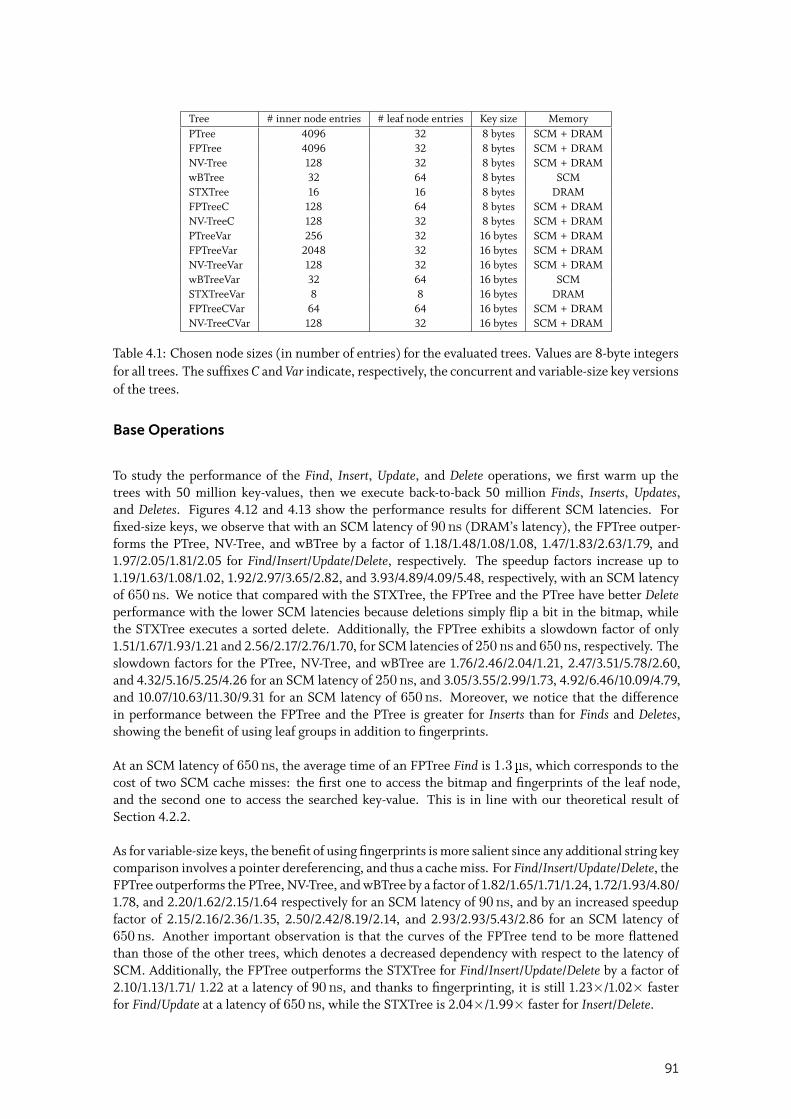
Tree # inner node entries # leaf node entries Key size MemoryPTree 4096 32 8 bytes SCM + DRAMFPTree 4096 32 8 bytes SCM + DRAMNV-Tree 128 32 8 bytes SCM + DRAMwBTree 32 64 8 bytes SCMSTXTree 16 16 8 bytes DRAMFPTreeC 128 64 8 bytes SCM + DRAMNV-TreeC 128 32 8 bytes SCM + DRAMPTreeVar 256 32 16 bytes SCM + DRAMFPTreeVar 2048 32 16 bytes SCM + DRAMNV-TreeVar 128 32 16 bytes SCM + DRAMwBTreeVar 32 64 16 bytes SCMSTXTreeVar 8 8 16 bytes DRAMFPTreeCVar 64 64 16 bytes SCM + DRAMNV-TreeCVar 128 32 16 bytes SCM + DRAM
Table 4.1: Chosen node sizes (in number of entries) for the evaluated trees. Values are 8-byte integersfor all trees. The suffixes C and Var indicate, respectively, the concurrent and variable-size key versionsof the trees.
Base Operations
To study the performance of the Find, Insert, Update, and Delete operations, we first warm up thetrees with 50 million key-values, then we execute back-to-back 50 million Finds, Inserts, Updates,and Deletes. Figures 4.12 and 4.13 show the performance results for different SCM latencies. Forfixed-size keys, we observe that with an SCM latency of 90 ns (DRAM’s latency), the FPTree outper-forms the PTree, NV-Tree, and wBTree by a factor of 1.18/1.48/1.08/1.08, 1.47/1.83/2.63/1.79, and1.97/2.05/1.81/2.05 for Find/Insert/Update/Delete, respectively. The speedup factors increase up to1.19/1.63/1.08/1.02, 1.92/2.97/3.65/2.82, and 3.93/4.89/4.09/5.48, respectively, with an SCM latencyof 650 ns. We notice that compared with the STXTree, the FPTree and the PTree have better Deleteperformance with the lower SCM latencies because deletions simply flip a bit in the bitmap, whilethe STXTree executes a sorted delete. Additionally, the FPTree exhibits a slowdown factor of only1.51/1.67/1.93/1.21 and 2.56/2.17/2.76/1.70, for SCM latencies of 250 ns and 650 ns, respectively. Theslowdown factors for the PTree, NV-Tree, and wBTree are 1.76/2.46/2.04/1.21, 2.47/3.51/5.78/2.60,and 4.32/5.16/5.25/4.26 for an SCM latency of 250 ns, and 3.05/3.55/2.99/1.73, 4.92/6.46/10.09/4.79,and 10.07/10.63/11.30/9.31 for an SCM latency of 650 ns. Moreover, we notice that the differencein performance between the FPTree and the PTree is greater for Inserts than for Finds and Deletes,showing the benefit of using leaf groups in addition to fingerprints.
At an SCM latency of 650 ns, the average time of an FPTree Find is 1.3 µs, which corresponds to thecost of two SCM cache misses: the first one to access the bitmap and fingerprints of the leaf node,and the second one to access the searched key-value. This is in line with our theoretical result ofSection 4.2.2.
As for variable-size keys, the benefit of using fingerprints is more salient since any additional string keycomparison involves a pointer dereferencing, and thus a cache miss. For Find/Insert/Update/Delete, theFPTree outperforms the PTree, NV-Tree, and wBTree by a factor of 1.82/1.65/1.71/1.24, 1.72/1.93/4.80/1.78, and 2.20/1.62/2.15/1.64 respectively for an SCM latency of 90 ns, and by an increased speedupfactor of 2.15/2.16/2.36/1.35, 2.50/2.42/8.19/2.14, and 2.93/2.93/5.43/2.86 for an SCM latency of650 ns. Another important observation is that the curves of the FPTree tend to be more flattenedthan those of the other trees, which denotes a decreased dependency with respect to the latency ofSCM. Additionally, the FPTree outperforms the STXTree for Find/Insert/Update/Delete by a factor of2.10/1.13/1.71/ 1.22 at a latency of 90 ns, and thanks to fingerprinting, it is still 1.23×/1.02× fasterfor Find/Update at a latency of 650 ns, while the STXTree is 2.04×/1.99× faster for Insert/Delete.
91
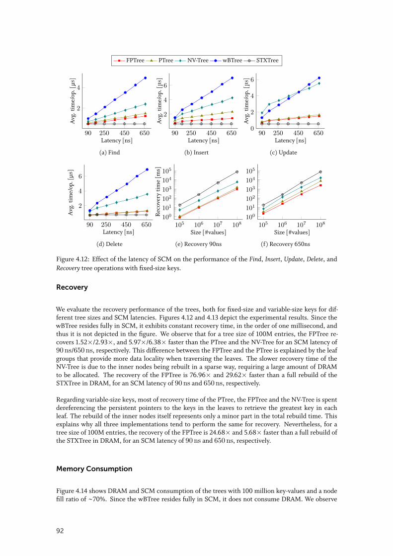
FPTree PTree NV-Tree wBTree STXTree
90 250 450 650
2
4
Latency [ns]
Avg
.tim
e/op
.[µs]
(a) Find
90 250 450 650
2
4
6
Latency [ns]
Avg
.tim
e/op
.[µs]
(b) Insert
90 250 450 6500
2
4
6
Latency [ns]
Avg
.tim
e/op
.[µs]
(c) Update
90 250 450 650
2
4
6
Latency [ns]
Avg
.tim
e/op
.[µs]
(d) Delete
105 106 107 108100101102103104105
Size [#values]
Rec
over
yti
me
[ms]
(e) Recovery 90ns
105 106 107 108100101102103104105
Size [#values]
(f) Recovery 650ns
Figure 4.12: Effect of the latency of SCM on the performance of the Find, Insert, Update, Delete, andRecovery tree operations with fixed-size keys.
Recovery
We evaluate the recovery performance of the trees, both for fixed-size and variable-size keys for dif-ferent tree sizes and SCM latencies. Figures 4.12 and 4.13 depict the experimental results. Since thewBTree resides fully in SCM, it exhibits constant recovery time, in the order of one millisecond, andthus it is not depicted in the figure. We observe that for a tree size of 100M entries, the FPTree re-covers 1.52×/2.93×, and 5.97×/6.38× faster than the PTree and the NV-Tree for an SCM latency of90 ns/650 ns, respectively. This difference between the FPTree and the PTree is explained by the leafgroups that provide more data locality when traversing the leaves. The slower recovery time of theNV-Tree is due to the inner nodes being rebuilt in a sparse way, requiring a large amount of DRAMto be allocated. The recovery of the FPTree is 76.96× and 29.62× faster than a full rebuild of theSTXTree in DRAM, for an SCM latency of 90 ns and 650 ns, respectively.
Regarding variable-size keys, most of recovery time of the PTree, the FPTree and the NV-Tree is spentdereferencing the persistent pointers to the keys in the leaves to retrieve the greatest key in eachleaf. The rebuild of the inner nodes itself represents only a minor part in the total rebuild time. Thisexplains why all three implementations tend to perform the same for recovery. Nevertheless, for atree size of 100M entries, the recovery of the FPTree is 24.68× and 5.68× faster than a full rebuild ofthe STXTree in DRAM, for an SCM latency of 90 ns and 650 ns, respectively.
Memory Consumption
Figure 4.14 shows DRAM and SCM consumption of the trees with 100 million key-values and a nodefill ratio of ~70%. Since the wBTree resides fully in SCM, it does not consume DRAM. We observe
92
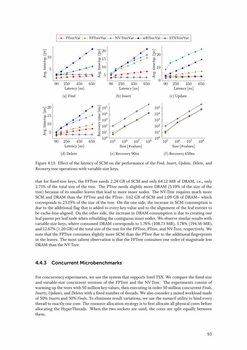
PTreeVar FPTreeVar NV-TreeVar wBTreeVar STXTreeVar
90 250 450 650
5
10
Latency [ns]
Avg
.tim
e/op
.[µs]
(a) Find
90 250 450 650
5
10
15
20
Latency [ns]
Avg
.tim
e/op
.[µs]
(b) Insert
90 250 450 6500
10
20
Latency [ns]
Avg
.tim
e/op
.[µs]
(c) Update
90 250 450 650
5
10
15
20
Latency [ns]
Avg
.tim
e/op
.[µs]
(d) Delete
105 106 107 108100101102103104105
Size [#values]
Rec
over
yti
me
[ms]
(e) Recovery 90ns
105 106 107 108100101102103104105
Size [#values]
(f) Recovery 650ns
Figure 4.13: Effect of the latency of SCM on the performance of the Find, Insert, Update, Delete, andRecovery tree operations with variable-size keys.
that for fixed-size keys, the FPTree needs 2.24 GB of SCM and only 64.12 MB of DRAM, i.e., only2.71% of the total size of the tree. The PTree needs slightly more DRAM (5.19% of the size of thetree) because of its smaller leaves that lead to more inner nodes. The NV-Tree requires much moreSCM and DRAM than the FPTree and the PTree: 3.62 GB of SCM and 1.09 GB of DRAM– whichcorresponds to 23.19% of the size of the tree. On the one side, the increase in SCM consumption isdue to the additional flag that is added to every key-value and to the alignment of the leaf entries tobe cache-line-aligned. On the other side, the increase in DRAM consumption is due to creating oneleaf parent per leaf node when rebuilding the contiguous inner nodes. We observe similar results withvariable-size keys, where consumed DRAM corresponds to 1.76% (108.73 MB), 3.78% (194.56 MB),and 12.67% (1.20 GB) of the total size of the tree for the FPTree, PTree, and NV-Tree, respectively. Wenote that the FPTree consumes slightly more SCM than the PTree due to the additional fingerprintsin the leaves. The most salient observation is that the FPTree consumes one order of magnitude lessDRAM than the NV-Tree.
4.4.3 Concurrent Microbenchmarks
For concurrency experiments, we use the system that supports Intel TSX. We compare the fixed-sizeand variable-size concurrent versions of the FPTree and the NV-Tree. The experiments consist ofwarming up the trees with 50 million key-values, then executing in order 50 million concurrent Finds,Inserts, Updates, and Deletes with a fixed number of threads. We also consider a mixed workload madeof 50% Inserts and 50% Finds. To eliminate result variations, we use the numactl utility to bind everythread to exactly one core. The resource allocation strategy is to first allocate all physical cores beforeallocating the HyperThreads. When the two sockets are used, the cores are split equally betweenthem.
93
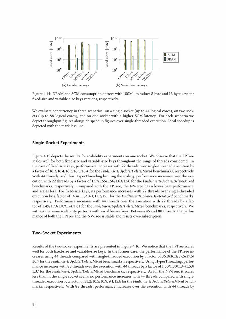
FPTreePTree
NV-Tree
wBTree
STXTree107
108
109
1010
Use
dm
em.[
Byt
e]
(a) Fixed-size keys
FPTreePTree
NV-Tree
wBTree
STXTree107
108
109
1010
Use
dm
em.[
Byt
e]
(b) Variable-size keys
SCMDRAM
Figure 4.14: DRAM and SCM consumption of trees with 100M key-value: 8-byte and 16-byte keys forfixed-size and variable-size keys versions, respectively.
We evaluate concurrency in three scenarios: on a single socket (up to 44 logical cores), on two sock-ets (up to 88 logical cores), and on one socket with a higher SCM latency. For each scenario wedepict throughput figures alongside speedup figures over single-threaded execution. Ideal speedup isdepicted with the mark-less line.
Single-Socket Experiments
Figure 4.15 depicts the results for scalability experiments on one socket. We observe that the FPTreescales well for both fixed-size and variable-size keys throughout the range of threads considered. Inthe case of fixed-size keys, performance increases with 22 threads over single-threaded execution bya factor of 18.3/18.4/18.3/18.5/18.4 for the Find/Insert/Update/Delete/Mixed benchmarks, respectively.With 44 threads, and thus HyperThreading limiting the scaling, performance increases over the exe-cution with 22 threads by a factor of 1.57/1.55/1.56/1.63/1.56 for the Find/Insert/Update/Delete/Mixedbenchmarks, respectively. Compared with the FPTree, the NV-Tree has a lower base performance,and scales less. For fixed-size keys, its performance increases with 22 threads over single-threadedexecution by a factor of 16.4/11.5/14.1/11.2/15.1 for the Find/Insert/Update/Delete/Mixed benchmarks,respectively. Performance increases with 44 threads over the execution with 22 threads by a fac-tor of 1.49/1.73/1.07/1.74/1.61 for the Find/Insert/Update/Delete/Mixed benchmarks, respectively. Wewitness the same scalability patterns with variable-size keys. Between 45 and 88 threads, the perfor-mance of both the FPTree and the NV-Tree is stable and resists over-subscription.
Two-Socket Experiments
Results of the two-socket experiments are presented in Figure 4.16. We notice that the FPTree scaleswell for both fixed-size and variable-size keys. In the former case, the performance of the FPTree in-creases using 44 threads compared with single-threaded execution by a factor of 36.8/36.3/37.5/37.6/36.7 for the Find/Insert/Update/Delete/Mixed benchmarks, respectively. Using HyperThreading, perfor-mance increases with 88 threads over the execution with 44 threads by a factor of 1.50/1.30/1.34/1.53/1.37 for the Find/Insert/Update/Delete/Mixed benchmarks, respectively. As for the NV-Tree, it scalesless than in the single socket scenario: performance increases with 44 threads compared with single-threaded execution by a factor of 31.2/10.5/10.9/9.1/15.6 for the Find/Insert/Update/Delete/Mixed bench-marks, respectively. With 88 threads, performance increases over the execution with 44 threads by
94
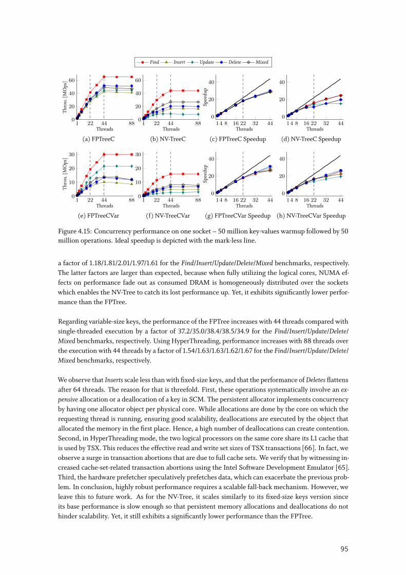
Find Insert Update Delete Mixed
1 22 44 880
20
40
60
HT OSThreads
Thro
u.[M
Ops
]
(a) FPTreeC
1 22 44 880
20
40
60
HT OSThreads
(b) NV-TreeC
14 8 16 22 32 440
20
40
HT
Threads
Spee
dup
(c) FPTreeC Speedup
14 8 16 22 32 440
20
40
HT
Threads
(d) NV-TreeC Speedup
1 22 44 880
10
20
30
HT OSThreads
Thro
u.[M
Ops
]
(e) FPTreeCVar
1 22 44 880
10
20
30
HT OSThreads
(f) NV-TreeCVar
14 8 16 22 32 440
20
40
HT
ThreadsSp
eedu
p
(g) FPTreeCVar Speedup
14 8 16 22 32 440
20
40
HT
Threads
(h) NV-TreeCVar Speedup
Figure 4.15: Concurrency performance on one socket – 50 million key-values warmup followed by 50million operations. Ideal speedup is depicted with the mark-less line.
a factor of 1.18/1.81/2.01/1.97/1.61 for the Find/Insert/Update/Delete/Mixed benchmarks, respectively.The latter factors are larger than expected, because when fully utilizing the logical cores, NUMA ef-fects on performance fade out as consumed DRAM is homogeneously distributed over the socketswhich enables the NV-Tree to catch its lost performance up. Yet, it exhibits significantly lower perfor-mance than the FPTree.
Regarding variable-size keys, the performance of the FPTree increases with 44 threads compared withsingle-threaded execution by a factor of 37.2/35.0/38.4/38.5/34.9 for the Find/Insert/Update/Delete/Mixed benchmarks, respectively. Using HyperThreading, performance increases with 88 threads overthe execution with 44 threads by a factor of 1.54/1.63/1.63/1.62/1.67 for the Find/Insert/Update/Delete/Mixed benchmarks, respectively.
We observe that Inserts scale less than with fixed-size keys, and that the performance of Deletes flattensafter 64 threads. The reason for that is threefold. First, these operations systematically involve an ex-pensive allocation or a deallocation of a key in SCM. The persistent allocator implements concurrencyby having one allocator object per physical core. While allocations are done by the core on which therequesting thread is running, ensuring good scalability, deallocations are executed by the object thatallocated the memory in the first place. Hence, a high number of deallocations can create contention.Second, in HyperThreading mode, the two logical processors on the same core share its L1 cache thatis used by TSX. This reduces the effective read and write set sizes of TSX transactions [66]. In fact, weobserve a surge in transaction abortions that are due to full cache sets. We verify that by witnessing in-creased cache-set-related transaction abortions using the Intel Software Development Emulator [65].Third, the hardware prefetcher speculatively prefetches data, which can exacerbate the previous prob-lem. In conclusion, highly robust performance requires a scalable fall-back mechanism. However, weleave this to future work. As for the NV-Tree, it scales similarly to its fixed-size keys version sinceits base performance is slow enough so that persistent memory allocations and deallocations do nothinder scalability. Yet, it still exhibits a significantly lower performance than the FPTree.
95
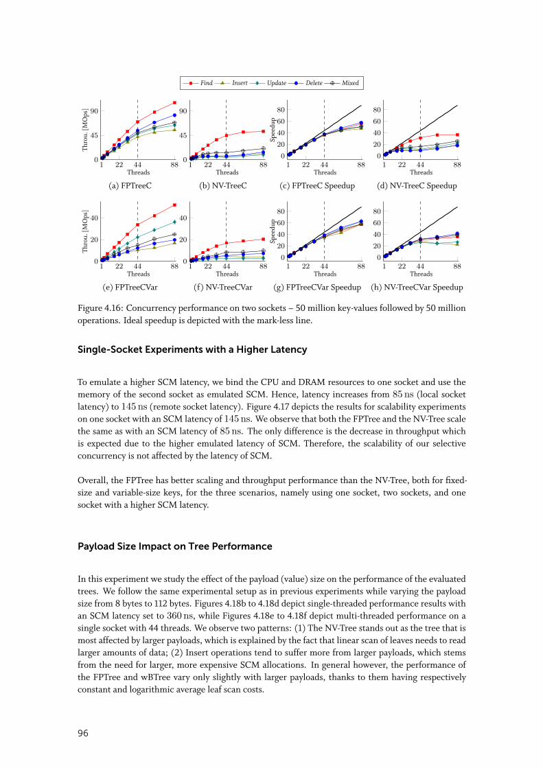
Find Insert Update Delete Mixed
1 22 44 880
45
90
HTThreads
Thro
u.[M
Ops
]
(a) FPTreeC
1 22 44 880
45
90
HTThreads
(b) NV-TreeC
1 22 44 880
20
40
60
80
HT
Threads
Spee
dup
(c) FPTreeC Speedup
1 22 44 880
20
40
60
80
HT
Threads
(d) NV-TreeC Speedup
1 22 44 880
20
40
HTThreads
Thro
u.[M
Ops
]
(e) FPTreeCVar
1 22 44 880
20
40
HTThreads
(f) NV-TreeCVar
1 22 44 880
20
40
60
80
HT
ThreadsSp
eedu
p
(g) FPTreeCVar Speedup
1 22 44 880
20
40
60
80
HT
Threads
(h) NV-TreeCVar Speedup
Figure 4.16: Concurrency performance on two sockets – 50 million key-values followed by 50 millionoperations. Ideal speedup is depicted with the mark-less line.
Single-Socket Experiments with a Higher Latency
To emulate a higher SCM latency, we bind the CPU and DRAM resources to one socket and use thememory of the second socket as emulated SCM. Hence, latency increases from 85 ns (local socketlatency) to 145 ns (remote socket latency). Figure 4.17 depicts the results for scalability experimentson one socket with an SCM latency of 145 ns. We observe that both the FPTree and the NV-Tree scalethe same as with an SCM latency of 85 ns. The only difference is the decrease in throughput whichis expected due to the higher emulated latency of SCM. Therefore, the scalability of our selectiveconcurrency is not affected by the latency of SCM.
Overall, the FPTree has better scaling and throughput performance than the NV-Tree, both for fixed-size and variable-size keys, for the three scenarios, namely using one socket, two sockets, and onesocket with a higher SCM latency.
Payload Size Impact on Tree Performance
In this experiment we study the effect of the payload (value) size on the performance of the evaluatedtrees. We follow the same experimental setup as in previous experiments while varying the payloadsize from 8 bytes to 112 bytes. Figures 4.18b to 4.18d depict single-threaded performance results withan SCM latency set to 360 ns, while Figures 4.18e to 4.18f depict multi-threaded performance on asingle socket with 44 threads. We observe two patterns: (1) The NV-Tree stands out as the tree that ismost affected by larger payloads, which is explained by the fact that linear scan of leaves needs to readlarger amounts of data; (2) Insert operations tend to suffer more from larger payloads, which stemsfrom the need for larger, more expensive SCM allocations. In general however, the performance ofthe FPTree and wBTree vary only slightly with larger payloads, thanks to them having respectivelyconstant and logarithmic average leaf scan costs.
96
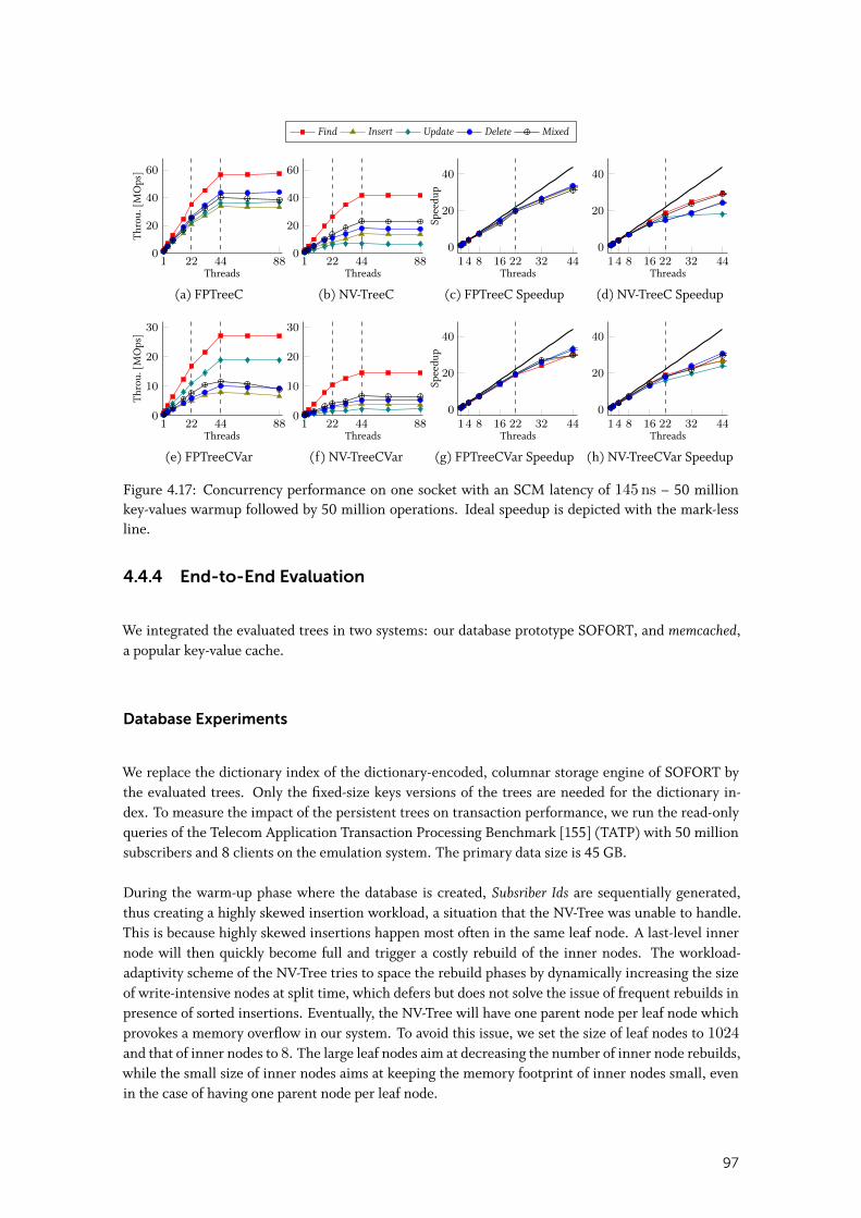
Find Insert Update Delete Mixed
1 22 44 880
20
40
60
HT OSThreads
Thro
u.[M
Ops
]
(a) FPTreeC
1 22 44 880
20
40
60
HT OSThreads
(b) NV-TreeC
14 8 16 22 32 440
20
40
HT
Threads
Spee
dup
(c) FPTreeC Speedup
14 8 16 22 32 440
20
40
HT
Threads
(d) NV-TreeC Speedup
1 22 44 880
10
20
30
HT OSThreads
Thro
u.[M
Ops
]
(e) FPTreeCVar
1 22 44 880
10
20
30
HT OSThreads
(f) NV-TreeCVar
14 8 16 22 32 440
20
40
HT
ThreadsSp
eedu
p
(g) FPTreeCVar Speedup
14 8 16 22 32 440
20
40
HT
Threads
(h) NV-TreeCVar Speedup
Figure 4.17: Concurrency performance on one socket with an SCM latency of 145 ns – 50 millionkey-values warmup followed by 50 million operations. Ideal speedup is depicted with the mark-lessline.
4.4.4 End-to-End Evaluation
We integrated the evaluated trees in two systems: our database prototype SOFORT, and memcached,a popular key-value cache.
Database Experiments
We replace the dictionary index of the dictionary-encoded, columnar storage engine of SOFORT bythe evaluated trees. Only the fixed-size keys versions of the trees are needed for the dictionary in-dex. To measure the impact of the persistent trees on transaction performance, we run the read-onlyqueries of the Telecom Application Transaction Processing Benchmark [155] (TATP) with 50 millionsubscribers and 8 clients on the emulation system. The primary data size is 45 GB.
During the warm-up phase where the database is created, Subsriber Ids are sequentially generated,thus creating a highly skewed insertion workload, a situation that the NV-Tree was unable to handle.This is because highly skewed insertions happen most often in the same leaf node. A last-level innernode will then quickly become full and trigger a costly rebuild of the inner nodes. The workload-adaptivity scheme of the NV-Tree tries to space the rebuild phases by dynamically increasing the sizeof write-intensive nodes at split time, which defers but does not solve the issue of frequent rebuilds inpresence of sorted insertions. Eventually, the NV-Tree will have one parent node per leaf node whichprovokes a memory overflow in our system. To avoid this issue, we set the size of leaf nodes to 1024
and that of inner nodes to 8. The large leaf nodes aim at decreasing the number of inner node rebuilds,while the small size of inner nodes aims at keeping the memory footprint of inner nodes small, evenin the case of having one parent node per leaf node.
97
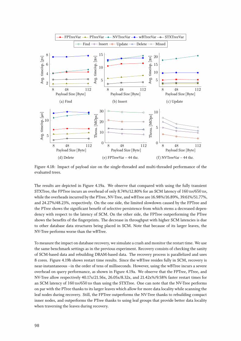
FPTreeVar PTreeVar NVTreeVar wBTreeVar STXTreeVar
Find Insert Update Delete Mixed
8 48 112
2
4
6
8
Payload Size [Byte]
Avg
.tim
e/op
.[µs]
(a) Find
8 48 112
5
10
15
Payload Size [Byte]A
vg.t
ime/
op.[µs]
(b) Insert
8 48 112
5
10
15
20
Payload Size [Byte]
Avg
.tim
e/op
.[µs]
(c) Update
8 48 112
5
10
Payload Size [Byte]
Avg
.tim
e/op
.[µs]
(d) Delete
8 48 1120
10
20
30
Payload Size [Byte]
Thro
u.[M
Ops
]
(e) FPTreeVar – 44 thr.
8 48 1120
5
10
Payload Size [Byte]Th
rou.
[MO
ps]
(f) NVTreeVar – 44 thr.
Figure 4.18: Impact of payload size on the single-threaded and multi-threaded performance of theevaluated trees.
The results are depicted in Figure 4.19a. We observe that compared with using the fully transientSTXTree, the FPTree incurs an overhead of only 8.74%/12.80% for an SCM latency of 160 ns/650 ns,while the overheads incurred by the PTree, NV-Tree, and wBTree are 16.98%/16.89%, 39.61%/51.77%,and 24.27%/48.23%, respectively. On the one side, the limited slowdown caused by the FPTree andthe PTree shows the significant benefit of selective persistence from which stems a decreased depen-dency with respect to the latency of SCM. On the other side, the FPTree outperforming the PTreeshows the benefits of the fingerprints. The decrease in throughput with higher SCM latencies is dueto other database data structures being placed in SCM. Note that because of its larger leaves, theNV-Tree performs worse than the wBTree.
To measure the impact on database recovery, we simulate a crash and monitor the restart time. We usethe same benchmark settings as in the previous experiment. Recovery consists of checking the sanityof SCM-based data and rebuilding DRAM-based data. The recovery process is parallelized and uses8 cores. Figure 4.19b shows restart time results. Since the wBTree resides fully in SCM, recovery isnear-instantaneous –in the order of tens of milliseconds. However, using the wBTree incurs a severeoverhead on query performance, as shown in Figure 4.19a. We observe that the FPTree, PTree, andNV-Tree allow respectively 40.17x/21.56x, 26.05x/8.32x, and 21.42x%/9.58% faster restart times foran SCM latency of 160 ns/650 ns than using the STXTree. One can note that the NV-Tree performson par with the PTree thanks to its larger leaves which allow for more data locality while scanning theleaf nodes during recovery. Still, the FPTree outperforms the NV-Tree thanks to rebuilding compactinner nodes, and outperforms the PTree thanks to using leaf groups that provide better data localitywhen traversing the leaves during recovery.
98
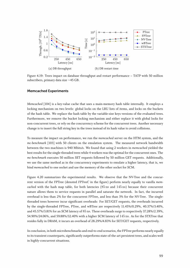
250 450 6500.2
0.6
1
1.4
1.8
Latency [ns]
Thro
ugh.
[106
TX/s
]
(a) DB throughput
250 450 65010−2
10−1
100
101
102
Latency [ns]
Tim
e[s
]
(b) DB restart time
PTreeFPTree
NV-TreewBTreeSTXTree
Figure 4.19: Trees impact on database throughput and restart performance – TATP with 50 millionsubscribers, primary data size ~45 GB.
Memcached Experiments
Memcached [104] is a key-value cache that uses a main-memory hash table internally. It employs alocking mechanism on two levels: global locks on the LRU lists of items, and locks on the bucketsof the hash table. We replace the hash table by the variable-size keys versions of the evaluated trees.Furthermore, we remove the bucket locking mechanism and either replace it with global locks fornon-concurrent trees, or rely on the concurrency scheme for the concurrent trees. Another necessarychange is to insert the full string key in the trees instead of its hash value to avoid collisions.
To measure the impact on performance, we run the memcached server on the HTM system, and themc-benchmark [103] with 50 clients on the emulation system. The measured network bandwidthbetween the two machines is 940 Mbits/s. We found that using 2 workers in memcached yielded thebest results for the single-threaded trees while 4 workers was the optimal for the concurrent ones. Themc-benchmark executes 50 million SET requests followed by 50 million GET requests. Additionally,we use the same method as in the concurrency experiments to emulate a higher latency, that is, webind memcached to one socket and use the memory of the other socket for SCM.
Figure 4.20 summarizes the experimental results. We observe that the NV-Tree and the concur-rent version of the FPTree (denoted FPTreeC in the figure) perform nearly equally to vanilla mem-cached with the hash map table, for both latencies (85 ns and 145 ns) because their concurrentnature allows them to service requests in parallel and saturate the network. In fact, the incurredoverhead is less than 2% for the concurrent FPTree, and less than 3% for the NV-Tree. The single-threaded trees however incur significant overheads: For SET/GET requests, the overheads incurredby the single-threaded FPTree, PTree, and wBTree are respectively 11.45%/0.29%, 40.37%/3.40%,and 45.57%/3.81% for an SCM latency of 85 ns. These overheads surge to respectively 37.28%/2.39%,54.90%/24.06%, and 59.88%/32.40% with a higher SCM latency of 145 ns. As for the STXTree thatresides fully in DRAM, it incurs an overhead of 28.29%/4.83% for SET/GET requests, respectively.
In conclusion, in both microbenchmarks and end-to-end scenarios, the FPTree performs nearly equallyto its transient counterparts, significantly outperforms state-of-the-art persistent trees, and scales wellin highly-concurrent situations.
99
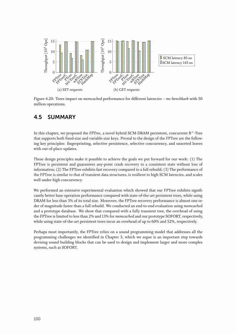
FPTree
FPTreeCPTree
NV-TreeC
wBTree
STXTree
HashM
ap0
5
10
15Th
roug
hput
[104
Ops
]
(a) SET requests
FPTree
FPTreeCPTree
NV-TreeC
wBTree
STXTree
HashM
ap0
5
10
15
Thro
ughp
ut[104
Ops
]
(b) GET requests
SCM latency 85 nsSCM latency 145 ns
Figure 4.20: Trees impact on memcached performance for different latencies – mc-benchkark with 50million operations.
4.5 SUMMARY
In this chapter, we proposed the FPTree, a novel hybrid SCM-DRAM persistent, concurrent B+-Treethat supports both fixed-size and variable-size keys. Pivotal to the design of the FPTree are the follow-ing key principles: fingerprinting, selective persistence, selective concurrency, and unsorted leaveswith out-of-place updates.
These design principles make it possible to achieve the goals we put forward for our work: (1) TheFPTree is persistent and guarantees any-point crash recovery to a consistent state without loss ofinformation; (2) The FPTree exhibits fast recovery compared to a full rebuild; (3) The performance ofthe FPTree is similar to that of transient data structures, is resilient to high SCM latencies, and scaleswell under high concurrency.
We performed an extensive experimental evaluation which showed that our FPTree exhibits signifi-cantly better base operation performance compared with state-of-the-art persistent trees, while usingDRAM for less than 3% of its total size. Moreover, the FPTree recovery performance is almost one or-der of magnitude faster than a full rebuild. We conducted an end-to-end evaluation using memcachedand a prototype database. We show that compared with a fully transient tree, the overhead of usingthe FPTree is limited to less than 2% and 13% for memcached and our prototype SOFORT, respectively,while using state-of-the-art persistent trees incur an overhead of up to 60% and 52%, respectively.
Perhaps most importantly, the FPTree relies on a sound programming model that addresses all theprogramming challenges we identified in Chapter 3, which we argue is an important step towardsdevising sound building blocks that can be used to design and implement larger and more complexsystems, such as SOFORT.
100
5SOFORT: A HYBRID SCM-DRAM
TRANSACTIONAL STORAGE ENGINE
I n the previous chapters, we devised necessary building blocks, namely memory management anddata structures for the design and implementation of SCM-based data-management systems. In
this chapter we demonstrate such a system and present SOFORT, a hybrid SCM-DRAM dictionary-encoded columnar transactional engine tailored for hybrid transactional and analytical workloads andfast data recovery1. SOFORT is a single-level store, i.e., the working copy of the data is the same asthe durable copy of the data. To achieve this, SOFORT leverages the byte-addressability of SCM topersist data in small increments at cache-line granularity. Since the database state is always up-to-date, SOFORT does not need a redo log. SOFORT implements serializable multi-version concurrencycontrol (MVCC) coupled with cooperative garbage collection.
SOFORT is architected as a twin-store columnar main-memory database, with a larger static im-mutable read-optimized store and a smaller dynamic read/write store. The dynamic store is peri-odically merged into the static store to do compaction. This keeps the size of the dynamic store small,and therefore results in an optimal performance for reads and writes. The results of the microbench-marks shown in Section 2.1.2 led us to envision that the static store can be entirely kept in SCM at anegligible cost for query execution, and instantly recovered after failure [3]. Therefore, we focus onlyon the dynamic part in this dissertation.
To track conflicts between transactions, MVCC keeps for every transaction, among other metadata,a write set that contains the row IDs of the tuples that the transaction inserted or deleted. This in-formation is enough to undo a transaction in case it is aborted. We make the observation that thesame information can be used to undo the effects of in-flight transactions during recovery. Therefore,to provide durability, SOFORT places the MVCC write set in SCM, which enables it to remove thetraditional write-ahead log from the critical path of transactions. SOFORT stores its columns contigu-ously in memory, which complicates memory reclamation of deleted tuples. Indeed, the latter wouldrequire a writer-blocking process which would replace the current columns with new, garbage-freeones. To remedy this issue, we propose to keep track of deleted rows and re-use them when insertingnew tuples whenever possible instead of appending them to the table.
Through an extensive experimental evaluation, we show that SOFORT exhibits competitive OLTP per-formance despite being a column-store. We also demonstrate the effectiveness and scalability of ourgarbage collection. We defer the performance evaluation of recovery to Chapter 6. The contributionsof this chapter are as follows:
1The material in this chapter is partially based on [122, 128]
101
• the design of SOFORT, an OLAP-friendly columnar storage engine that achieves competitiveOLTP performance;
• an adaptation of MVCC to SCM in a way that removes traditional write-ahead logging from thecritical path of transactions;
• an extension of our SCM-optimized MVCC that enables SOFORT to continue unfinished trans-actions after failure;
• an efficient garbage collection scheme for a column-store.
This chapter is organized as follows: Section 5.1 surveys state-of-the-art multi-versioned database sys-tems following four dimensions, namely concurrency control, version storage, indexing, and garbagecollection. Thereafter, following the same structure, Section 5.2 presents the architecture of SOFORT,contrasting our design decisions with those of the state of the art. Afterwards, Section 5.3 presents theimplementation details of SOFORT, with a focus on how it achieves failure atomicity. Moreover, Sec-tion 5.4 elaborates on how SOFORT can continue unfinished transactions after failure. We provide aperformance evaluation in Section 5.5. Finally, Section 5.6 summarizes this chapter.
5.1 DESIGN SPACE EXPLORATION
Multi-Version Concurrency Control (MVCC) was first proposed by Reed in 1978 [144]. Since then,MVCC has co-existed with single-version concurrency control. However, the advent of main-memorydatabase systems in the last decade made MVCC the de facto choice because it allows the database tobetter leverage the additional concurrency offered by hardware. Multi-versioning consists in keepingseveral versions of a single tuple, each of which representing the state of the tuple in mutually exclu-sive time intervals. Therefore, read queries can always read a consistent version of a tuple regardlessof whether this tuple is being updated. By loosening the coupling between reads and writes, MVCCallows for more concurrency. Moreover, if old tuple versions are never deleted, any past state of thedatabase can be queried. Wu et al. [176] presented an empirical survey of MVCC techniques. Theydistinguished four design dimentions: concurrency control, version storage, index management, andgarbage collection. Based on their analysis, we propose in the following a summary of the designspace of MVCC database systems.
5.1.1 Concurrency Control
MVCC usually keeps for each tuple the following metadata (all of which are initialized to zero):
• a creation timestamp (CTS) that indicates the time starting from which a tuple is visible;• a deletion timestamp (DTS) indicating the time up to a tuple is visible;• a transaction ID (TXID) that serves as a write lock for the tuple;• a pointer to either the previous or the next version of this tuple (see Section 5.1.2 for more
details).
MVCC has been extensively researched in the last decade. Since our goal is not to devise a newconcurrency control protocol, but rather to adapt one to SCM, we only sample related work. Wu etal. [176] identified four main families of concurrency control protocols for multi-versioned databasesystems, which we present in the following.
102
Timestamp Ordering (MVTO)
MVTO is Reed’s original proposed concurrency control protocol [144, 143]. The main idea behindMVTO is to use the start timestamp (STS) of transactions to determine their serial execution order.The STS serves as the TXID in this case. MVTO keeps additionally in the tuple’s metadata the STS ofthe last transaction that read a tuple. We denote this field as read timestamp (RTS).
A transaction T1 is allowed to read a tuple’s latest version if: (1) the tuple is not locked by anothertransaction (i.e., its TXID is equal to zero or to T1’s TXID); and (2) T1’s TXID falls in between thetuple’s CTS and DTS. If these conditions are satisfied, then T1 sets the RTS of the tuple to its TXIDif the existing RTS is lower than its TXID. If the conditions are not satisfied, then T1 reads an olderversion of the tuple and does not need to update the tuple’s RTS.
A transaction T1 is allowed to update a tuple an if: (1) an is not locked by any active transaction;and (2) T1’s TXID is greater than an’s RTS. The second condition ensures that the serial order oftransactions, decided by their TXID, is respected. If these conditions are not satisfied, then T1 isaborted. Otherwise, T1 locks an, then updates it by creating a new (locked) version an+1. When T1commits, it sets the DTS of an to its TXID and the CTS and DTS of an+1 to its TXID and infinity,respectively.
Finally, we discuss phantom prevention. Consider two transactions T1 and T2, where T1 logicallyprecedes T2 (i.e., the serial order is T1 then T2). Since T1 logically precedes T2, then T2 must be ableto see all tuples that T1 inserted. Assume that T2 reads a set of tuples that satisfy a specific predicate.Thereafter, T1 inserts a tuple that satisfies the aforementioned predicate. T2 is unable to see this tuplebecause it has already completed its read operation. Therefore, the newly inserted tuple is a phantom.MVTO as described above does not prevent such a scenario, therefore, it is not serializable. A way toremedy this issue is to use key range locks when reading [108, 54], which prevents other transactionsfrom inserting new tuples that fall within the locked range.
Optimistic Concurrency Control (MVOCC)
Optimistic Concurrency Control (OCC) was first proposed by Kung et al. [81], and was adapted tomulti-versioning by Larson et al. [84]. OCC relies on the assumption that conflicts between transac-tions are rare. Therefore, it allows transactions to read tuples without acquiring any locks. MVOCCsplits a transaction in three phases: First, the transaction issues its read and write requests in the readphase. During this phase, the transaction keeps a read set that consists of references to all its readtuples. If the transaction is ready to commit, then it enters the validation phase, where all the transac-tion’s read operations are redone, and the result intersected with the transaction’s read set. If no newtuples are observed, then the transaction is allowed to enter the write phase, which starts by acquiringa commit timestamp, then updating the metadata of modified tuples, i.e., setting the CTS of createdtuples and the DTS of deleted tuples to the commit timestamp. Otherwise, the transaction is aborted.Note that the checks of the valiadtion phase are able to detect phantoms.
When a transaction starts, it is assigned a unique TXID, and an STS equal to the current logical time.During the read phase, a transaction T1 is allowed to read a tuple if: (1) The tuple is not locked and T1’sSTS is in between the CTS and the DTS of the tuple; or (2) the tuple is locked for creation by anothertransaction that is in the validation phase; or (3) the tuple is locked for deletion by another transactionthat is in the read phase. Basically, if a conflict with another transaction T2 is detected, then MVOCCassumes that T2 will successfully commit before T1 if T2 is in the validation phase, thereby proceeding
103
optimistically. T1 registers a dependency to T2 and waits, during the validation phase, until T2 commits.If T2 aborts, then T1 must abort as well. Keeping transaction dependencies might lead to cascadedaborts. T1 is allowed to update a tuple if it is not locked. If T1 successfully locks a tuple, then itupdates it similarly to MVTO. Otherwise, T1 is aborted.
The main advantage of MVOCC is that read operations do not require any locking. However, thiscomes at the cost of potentially expensive checks during the validation phase. Moreover, a transactionfinds out that it must abort due to a conflict only in the validation phase.
There is a large body of work that focused on optimizing the implementation of MVOCC in the lastyears. For instance, Tu et al. [161] propose Silo, a main-memory storage engine that uses a decentral-ized, epoch-based design to achieve high scalability. Several systems, such as FOEDUS [172] and ER-MIA [78] improved on top of Silo’s ideas. Moreover, Neumann et al. [114] adapt precision locking [75]to MVOCC, which enables to significantly decrease the amount of metadata required for pre-commitvalidation. Finally, Wu et al. [177] propose to redo only conflicting reads or writes when retrying anaborted transaction, and reuse the results that did not conflict, thereby significantly decreasing thecost of retrying aborted transactions.
Two-Phase Locking (MV2PL)
Two-phase locking (2PL) [12] follows a pessimistic approach: a transaction must first acquire locks onboth tuples it reads and modifies. To adapt 2PL to multi-versioning, we need to extend the metadataof tuples to encompass a read lock in the form of a counter (i.e., shared lock) that we denote RCTR.The tuple’s TXID serves as an exclusive write lock. The RCTR of a tuple an is incremented whenevera transaction accesses an, and decremented whenever that transaction commits or aborts.
A transaction T1 is allowed to read a tuple if: (1) the tuple is not locked for write (i.e., its TXID is equalto zero); and (2) T1’s TXID is in between the tuple’s CTS and DTS. If these conditions are satisfied,then T1 locks the tuple for read by atomically incrementing its RCTR. T1 is allowed to modify a tuple ifit is not locked neither for read nor for write (i.e., both the tuple’s TXID and RCTR are equal to zero).If these conditions are satisfied, then T1 locks the tuple for write. If T1 fails to acquire either a read ora write lock, it can either wait until it acquires a lock, which might lead to deadlocks, or eagerly abort.
Similarly to MVTO, MV2PL as described above does not guarantee serializability because it does notprevent phantoms. To make MV2PL serializable, we need to employ key range locks.
Serialization Certifier
Another approach is to rely on a serialization certifier to arbitrate concurrent transactions. A certifieris usually employed on top of an existing, weaker isolation level to provide serializability. In essence,a certifier aims to offer the performance of the lower isolation level with the guarantees of serializ-ability. The first certifier proposals relied on constructing offline a serialization graph for detectingtransaction conflicts that would break serializability constraints [45]. Therefore, this approach doesnot support ad-hoc or data-dependant queries and requires a new analysis whenever the set of trans-action templates of an application is changed.
To remedy this shortcoming, Cahill et al. [16] proposed Serializable Snapshot Isolation (SSI), a certifier-based concurrency algorithms that builds on top of snapshot isolation to provide serializability. Under
104
snapshop isolation, when a transaction starts, it is assigned an STS, which will also serve as its com-mit timestamp. Instead of building an expensive serialization graph, SSI tracks only anti-dependenciesbetween transactions. SSI maintains two booleans per transaction: outConflict and inConflict. Ananti-dependency characterizes one of two scenarios: The first one is when a transaction T1 reads atuple that does not represent the latest version, because a transaction T2 (that must have started afterT1) updated it. When this scenario is encountered, there is an anti-dependency from T1 to T2, there-fore, SSI sets T1.outConflict and T2.inConflict to true. The second scenario is when a transaction T1reads the latest version of a tuple, then a subsequent transaction T2 updates this tuple. When thisscenario is encountered, there is an anti-dependency from T1 to T2, therefore, SSI sets T1.outConflictand T2.inConflict to true. Detecting this scenario is more challenging than the previous one. To detectit, Cahill et al. [16] propose to introduce a new shared lock, denoted SIREAD, which is set when atransaction reads a version of a tuple. Anti-dependencies are then identified whenever both SIREADand the write lock of a tuple are set. To set properly the transaction flags, the database must providewhich transactions hold a particular SIREAD. SSI aborts a transaction whenever both its outConflictand inConflict flags are true, which is proven to be sufficient in preventing the anomalies of snapshotisolation [45]. Nevertheless, this condition is only sufficient, which means that there might be falsepositives.
More recently, Wang et al. [171] proposed the Serial Safety Net (SSN). SSN is more accurate and morepowerful than SSI because it can serialize any isolation level that is at least as strict as read-committed,which is a weaker isolation level than snapshot isolation.
5.1.2 Version Storage
Multi-version storage engines usually chain together the versions of a tuple into a latch-free linked listusing the pointer field of MVCC metadata. We find multiple ways of doing so in the literature. In thefollowing we discuss the two major ones identified in the literature.
Append-Only Storage
An append-only MVCC storage scheme is characterized by the fact that any tuple update generates anew full tuple, even if only one attribute of the tuple is updated. In fact, a tuple update in an append-only table requires the following steps: (1) create and append a copy of the tuple (i.e., a new version)to the table; (2) update the attributes of the new version; and (3) link the new version to the previousversions of the tuple. Step (1) depends on how tuples are stored in a table. For instance, tuples can bestored contiguously in memory, or stored next to the keys of the primary index. Step (3) can be doneby making the new tuple either the head or the tail of the version chain. Therefore, version chainsare either ordered from oldest to newest (O2N), such as in the Hekaton [84] main-memory database,or from newest to oldest (N2O), such as in the MemSQL [105] main-memory database. O2N has theadvantage that an update does not require updating indexes over non-updated attributes. However,the disadvantage of O2N is that read queries have to traverse the whole version chain to access thelatest version of tuple, because the version chain is a simple linked-list. Therefore, the performanceof O2N highly depends on the ability of the system to swiftly reclaim garbage versions. N2O remediesthis issue by always indexing the latest version of a tuple. However, this comes at the cost of updatingall the indexes of the table, regardless of whether the attributes they index are updated or not, when atuple is updated.
105
A special case of append-only storage is time travel storage, in which an MVCC storage engine neverdeletes any versions to provide anytime snapshot isolation capability. In this scheme, each table en-compasses two parts: the master table, and the time travel table. An advantage of time travel storageis that indexes always refer to the tuple in the master table, which lifts the need to update indexesover non-updated attributes. The master table contains the newest versions of the tuples, while thetime travel table contains older versions (i.e., N2O version chain). A tuple update is performed bycreating a copy of the newest version in the time travel table, then updating the tuple stored in themaster table. Note that storing the oldest version in the main table and newer versions in the timetravel table (i.e., O2N version chain) is possible and is implemented in some database systems such asSAP HANA [88].
Delta Storage
Delta storage keeps a master table that contains the master tuples (oldest if O2N, newest if N2O),and for each tuple, a list of delta versions such that each version contains only the attributes that aredifferent from its preceding version. Delta versions are managed in a delta storage, called undo bufferin Hyper [114], which we use to illustrate how a tuple update in a delta storage scheme works. Hyperkeeps transaction-local undo buffers, that are used to store the older tuple versions until they can bereclaimed by the garbage collector. Basically, tuples are updated in-place at the attribute level and thepre-image of their modified attributes is copied to the undo buffer. This improves the performance ofconcurrency control by reducing the amount of data that needs to be copied, and avoiding to updateindexes that track non-updated attributes. It also speeds garbage collection because an undo buffercan be reclaimed entirely as a garbage unit.
By copying only modified attributes, delta storage significantly decreases the memory footprint of anMVCC system. However, to access a tuple version other than the master one, a transaction needs totraverse the version chain to reconstruct, potentially attribute by attribute, the desired tuple version.
5.1.3 Index Management
Indexing is an important and necessary part of any transactional system. MVCC introduces morecomplexity in index management since indexes have to account for different tuple versions. Tuplevisibility metadata is decoupled from the indexes. Therefore, an index can contain entries for invisibleversions. Primary and secondary indexes are managed differently in an MVCC system. An indexmaps a set of attributes, which constitutes the key, to a tuple reference, which constitutes the value.Depending on the version storage scheme, primary keys always reference either the newest or theoldest version of a tuple. In contrast, secondary indexes can reference any existing tuple version,because both their keys and values can change, while only the value can change in a primary index.Therefore, secondary indexes are more challenging to manage than primary indexes.
Transactions are allowed to update and insert in primary indexes, but only to insert in secondary in-dexes. Index delete operations are exclusively handled by the garbage collector to ensure snapshotvisibility. In Section 5.1.2 we discussed when index updates are required for each version storagescheme. In particular, while the N2O append-only version storage scheme requires to update pri-mary and secondary indexes when a tuple is updated, the O2N append-only and delta version storageschemes require only to update secondary indexes that index modified attributes. Moreover, in thecase of an O2N version storage scheme, the garbage collector has the additional responsibility of up-dating primary indexes when reclaiming the oldest version of a tuple.
106
We distinguish two ways of implementing indexes depending on the nature of tuple references theyemploy. The first way is to use physical pointers to refer to a tuple, which is always possible forprimary indexes since they reference the master tuple versions. However, secondary indexes can usephysical pointers only in append-only version storage schemes, because each version is stored with allof its attributes. In the delta version storage scheme, non-master versions are stored as a sequence ofmodified attributes, which means that they cannot be referenced with a physical pointer. Examplesof MVCC database systems that use physical pointers include Hekaton [84] and MemSQL [105].
The second way of implementing indexes is using logical pointers. In this approach, each tuple isassociated with a unique ID. The system provides additionally a map that translates tuple IDs to thephysical address of the master version of the corresponding tuple. This map needs to be updatedwhenever the master version of a tuple changes, e.g., when updating a tuple in an append-only versionstorage scheme. Delta version storage schemes adopt logical pointers by design. Nevertheless, logicalpointers can be used with any version storage scheme. A straightforward implementation, exemplifiedby NuoDB [116], is to use the primary key as the unique ID, and the primary index as the mappingfrom tuple ID to physical pointer. In this case, secondary indexes need to store the whole primary keyas its entry value. A lookup consists in retrieving the primary key, then probing the primary index toget the tuple physical pointer. This is not optimal, especially for large primary keys, because it incursa significant memory overhead and a systematic, additional primary index lookup. An alternative isto generate unique integer tuple IDs, and map them to their corresponding tuple physical pointers ina hash table. Hyper [114] is an example of this approach.
The main advantage of logical pointers is that they alleviate the need to update indexes whose indexedattributes were not modified, thereby improving the system’s update performance. However, thiscomes at the cost of read performance: Secondary index scans return tuple IDs, which then need tobe translated into physical pointers to master tuple versions. However, the master version might notrepresent the indexed version. Therefore, the version chain needs to be traversed in order to find theappropriate version. In contrast, secondary indexes that use physical pointers give direct access to theright version. In summary, physical pointers favor reads while logical pointers favor writes.
5.1.4 Garbage Collection
The main purpose of garbage collection is to reclaim the space of deleted versions to limit the me-mory footprint of the system and prevent the system from running out of storage. Additionally, moregarbage translates into longer version chains, which has a negative impact on performance. For in-stance, in an O2N scheme, a transaction needs to traverse the whole version chain to retrieve thelatest version of a tuple, which is proportionally expensive to the number of versions, therefore, tothe amount of garbage tuples. In an N2O scheme, indexes are updated for each tuple update, whichmeans that indexes contain more garbage entries than in the O2N scheme. The performance of theseindexes decreases proportionally to the number of garbage entries they contain. Hence, a second pur-pose of garbage collection is to delete garbage entries from indexes to maintain performance. In brief,garbage collection is essential for both limiting memory consumption and maintaining performance.
A tuple is considered as garbage if it was created by an aborted transaction, or if it was deleted andits DTS is lower or equal to the STS of the oldest active transaction. To reclaim a garbage tuple,the garbage collector removes it from its corresponding version chain, deletes its corresponding indexentries, and claims its storage space. There are two approaches to garbage collection depending on theconsidered garbage unit. A garbage unit is either a single tuple version, or the set of deleted (created)tuples by a committed (aborted) transaction; these two approaches are referred to as tuple-level andtransaction-level garbage collection, respectively.
107
Tuple-level garbage collection tests the visibility of each tuple to determine whether it can be re-claimed. It can be implemented in two ways. The first option, denoted background vacuuming andexemplified by Postgres [152], is to have background threads scan the database to identify garbagetuples. However, it does not scale to large database instances. There are several optimizations thatcan attenuate this, such as maintaining bitmaps or dirty blocks of tuples to avoid scanning blocks thatwere not modified since the last garbage collection pass. The second option, named cooperative clean-ing and exemplified by Hekaton [84], makes transactions reclaim garbage versions they encounterwhen issuing scan requests. While cooperative cleaning scales better than background vacuuming, itis limited to the O2N append-only version storage scheme. Moreover, cooperative cleaning requiresan additional periodic background garbage collector that reclaims old tuples that are never queried,hence, never detected by transactions.
Transaction-level garbage collection leverages the fact that garbage versions created by the same trans-action share the same visibility. In the case of a committed transaction, the DTS of all its deleted tu-ples is equal to its commit timestamp, therefore, all these tuples qualify for reclamation if the committimestamp is lower or equal to the smallest STS among active transactions. In the case of an abortedtransaction, all its created rows qualify immediately for reclamation since they were never visible.The reclamation can either be done by background threads, or by the worker threads between run-ning two transactions. Transaction-level garbage collection is simpler and more efficient than tuple-level garbage collection. However, it requires to keep a centralized data structure where transactionsregister their garbage, which might become a bottleneck if not implemented properly. Nevertheless,this can be mitigated by making transactions register their garbage in core-local structures [161]. Theworkers threads reclaim garbage only from their local garbage structure. Another optimization is touse read-copy-update-style epochs to reclaim garbage [161].
Garbage collection in hybrid OLTP and OLAP systems faces the challenge if long-running analyticaltransactions, which block the reclamation of old tuples. This leads to an accumulation of garbage,which both decreases performance and increases memory consumption. None of the solutions dis-cussed above can efficiently address this problem. Lee et al. [89] propose a solution that identifiesgarbage versions based on timestamp visibility intervals, instead of the minimum STS among activetransactions. The main idea is to block the reclamation of only the versions that should be visible tocurrently running transactions. Therefore, a long-running transaction can block the reclamation ofonly one version per tuple, instead of all versions in the minimum STS approach. The authors devisea hybrid solution, implemented in SAP HANA, that executes in three steps. The first one is to exe-cute transaction-level garbage collection as described above. The second step is to execute table-levelgarbage collection, which consists in reclaiming the garbage of the tables that are not accessed by long-running transactions – known in the case of pre-compiled stored procedures. The third and final stepis to execute tuple-level garbage collection based on timestamp visibility intervals.
5.2 SOFORT ARCHITECTURE
In this section we describe the architecture of SOFORT. We follow the same structure as the previoussection to enable the reader to contrast our design decisions with those of the state of the art.
108
5.2.1 Concurrency Control
We choose to implement MVOCC in SOFORT because it favors read queries, which are frequent inhybrid OLTP and OLAP workloads. Indeed, MVOCC does not require any locking while reading. Forsimplicity of design, and to avoid the problem of cascading aborts, we choose to abort transactionswhenever they encounter a locked tuple. This contrasts with the more optimistic approach of Larsonet al. [84] where registering transaction dependencies allows to consider tuples locked by other trans-actions currently in their validation phase. In this case, a transaction must wait at commit time untilall transactions it depends on are committed; if one of them aborts, then the transaction must alsoabort. This might lead to cascaded aborts.
An important design decision we made in our MVOCC is to have read-only transactions run at snap-shot isolation level. This decision was motivated by the fact that long-running read-only transactionscan suffer from starvation in MVOCC – a well-known limitation of OCC in general. Indeed, sincereads do not require any locking, a long-running read-only transaction is likely to discover duringpre-commit verification that it has to abort due to a conflict. We argue that running read-only transac-tions at snapshot isolation level does not break serializability: If we consider the start timestamp of theread-only transaction as its commit timestamp, then the read-only transaction satisfies serializabilityconstraints.
In MVOCC, a transaction object maintains a read set and a write set that contain references to theread and modified tuples, respectively. An optimization of our MVOCC is to have one reusable trans-action object per CPU core. We make the observation that a transaction object contains already allnecessary metadata for recovering in-flight transactions. Therefore, we decided to split transactionobjects into a transient part and a persistent part, such that the latter contains only necessary meta-data for recovery, namely the commit timestamp and the write set. This is in contrast to Hyrise-NVwhich persists the whole transaction object [148]. Therefore, SOFORT achieves transaction atomicityacross failures without relying on the traditional write-ahead log. Section 5.3 details our concurrencycontrol implementation.
Nevertheless, the log is not only used to ensure transaction atomicity across failures. It contains a com-plete redo-history of the database, which enables point-in-time recovery. Furthermore, replication forhigh availability most often requires shipping the log to remote systems. Therefore, it is unlikely thatany industrial system will do away with a traditional log. Nevertheless, SOFORT removes the log fromthe critical path of transactions; we envision that a traditional log could be shipped asynchronouslywhile the transactions execute.
5.2.2 Version Storage
We adopt an append-only columnar strategy for two reasons: (1) An append-only columnar strategyyields better analytical performance, because attributes are stored contiguously in memory, whichminimizes CPU cache misses; and (2) the design simplicity of an append-only strategy makes it idealfor SCM, because failure-atomicity is easy to reason about. Although we choose a columnar dataorganization to favor OLAP workloads, we show in Section 5.5 that we can achieve competitive OLTPperformance as well. The tuple MVCC metadata consists of only a CTS and a DTS; we do not employchain pointers. Instead, we rely on inverted indexes to track different versions of a tuple (more detailsin Section 5.2.3).
SOFORT is a dictionary-encoded column-store. Figure 5.1 gives an overview of data organizationin SOFORT. Tables are stored as a collection of append-only columns. Each column c consists of
109
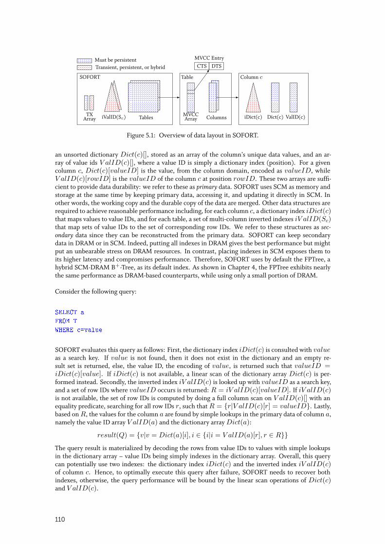
SOFORT Table Column c
ValID(c)iValID(Sc) Dict(c)ColumnsMVCCArray
CTSMVCC Entry
DTS
TXArray Tables iDict(c)
Must be persistentTransient, persistent, or hybrid
Figure 5.1: Overview of data layout in SOFORT.
an unsorted dictionary Dict(c)[], stored as an array of the column’s unique data values, and an ar-ray of value ids V alID(c)[], where a value ID is simply a dictionary index (position). For a givencolumn c, Dict(c)[valueID] is the value, from the column domain, encoded as valueID, whileV alID(c)[rowID] is the valueID of the column c at position rowID. These two arrays are suffi-cient to provide data durability: we refer to these as primary data. SOFORT uses SCM as memory andstorage at the same time by keeping primary data, accessing it, and updating it directly in SCM. Inother words, the working copy and the durable copy of the data are merged. Other data structures arerequired to achieve reasonable performance including, for each column c, a dictionary index iDict(c)that maps values to value IDs, and for each table, a set of multi-column inverted indexes iV alID(Sc)that map sets of value IDs to the set of corresponding row IDs. We refer to these structures as sec-ondary data since they can be reconstructed from the primary data. SOFORT can keep secondarydata in DRAM or in SCM. Indeed, putting all indexes in DRAM gives the best performance but mightput an unbearable stress on DRAM resources. In contrast, placing indexes in SCM exposes them toits higher latency and compromises performance. Therefore, SOFORT uses by default the FPTree, ahybrid SCM-DRAM B+-Tree, as its default index. As shown in Chapter 4, the FPTree exhibits nearlythe same performance as DRAM-based counterparts, while using only a small portion of DRAM.
Consider the following query:
SELECT a
FROM T
WHERE c=value
SOFORT evaluates this query as follows: First, the dictionary index iDict(c) is consulted with valueas a search key. If value is not found, then it does not exist in the dictionary and an empty re-sult set is returned, else, the value ID, the encoding of value, is returned such that valueID =iDict(c)[value]. If iDict(c) is not available, a linear scan of the dictionary array Dict(c) is per-formed instead. Secondly, the inverted index iV alID(c) is looked up with valueID as a search key,and a set of row IDs where valueID occurs is returned: R = iV alID(c)[valueID]. If iV alID(c)is not available, the set of row IDs is computed by doing a full column scan on V alID(c)[] with anequality predicate, searching for all row IDs r, such that R = {r|V alID(c)[r] = valueID}. Lastly,based on R, the values for the column a are found by simple lookups in the primary data of column a,namely the value ID array V alID(a) and the dictionary array Dict(a):
result(Q) = {v|v = Dict(a)[i], i ∈ {i|i = V alID(a)[r], r ∈ R}}
The query result is materialized by decoding the rows from value IDs to values with simple lookupsin the dictionary array – value IDs being simply indexes in the dictionary array. Overall, this querycan potentially use two indexes: the dictionary index iDict(c) and the inverted index iV alID(c)of column c. Hence, to optimally execute this query after failure, SOFORT needs to recover bothindexes, otherwise, the query performance will be bound by the linear scan operations of Dict(c)and V alID(c).
110
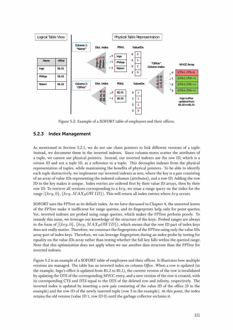
Name Office
Ingo B1.01
Philipp B1.02
Robert B1.02
Column 1:“Name”
Column 2:“Office”
Ingo
Philipp
Robert
0
1
2
0
1
2
0
PDict. ValueIDs
B1.01
B1.02
0
1
1
1
1
0
PDict. ValueIDs
MVCC Array
(CTS=1, DTS= 4)
(CTS=2, DTS= ∞)
(CTS=3, DTS= ∞)
(CTS=4, DTS= ∞)
0
1
2
3
0
1
2
3
0
1
2
3
Physical Table RepresentationLogical Table View
Dict. Index
Dict. Index
“Office”Column Index(In
go,0
),(P
hilip
p,1)
,(R
ober
t,2)
(B1.
01,0
),(B
1.02
,1)
{1,0
},{1
,1},
{1,2
},{0
,3}
Ingo‘s officeupdated fromB1.02 to B1.01
Figure 5.2: Example of a SOFORT table of employees and their offices.
5.2.3 Index Management
As mentioned in Section 5.2.1, we do not use chain pointers to link different versions of a tuple.Instead, we document them in the inverted indexes. Since column-stores scatter the attributes ofa tuple, we cannot use physical pointers. Instead, our inverted indexes use the row ID, which is aversion ID and not a tuple ID, as a reference to a tuple. This decouples indexes from the physicalrepresentation of tuples, while maintaining the benefits of physical pointers. To be able to identifyeach tuple distinctively, we implement our inverted indexes as sets, where the key is a pair consistingof an array of value IDs representing the indexed columns (attributes), and a row ID. Adding the rowID to the key makes it unique. Index entries are ordered first by their value ID arrays, then by theirrow ID. To retrieve all versions corresponding to a key, we issue a range query on the index for therange [{key, 0}, {key,MAXROWID}). This will return all index entries where key occurs.
SOFORT uses the FPTree as its default index. As we have discussed in Chapter 4, the unsorted leavesof the FPTree make it inefficient for range queries, and its fingerprints help only for point queries.Yet, inverted indexes are probed using range queries, which makes the FPTree perform poorly. Toremedy this issue, we leverage our knowledge of the structure of the keys: Probed ranges are alwaysin the form of [{key, 0}, {key,MAXROWID}), which means that the row ID part of index keysdoes not really matter. Therefore, we construct the fingerprints of the FPTree using only the value IDsarray part of index keys. Therefore, we can leverage fingerprints during an index probe by testing forequality on the value IDs array rather than testing whether the full key falls within the queried range.Note that this optimization does not apply when we use another data structure than the FPTree forinverted indexes.
Figure 5.2 is an example of a SOFORT table of employees and their offices. It illustrates how multipleversions are managed. The table has an inverted index on column Office. When a row is updated (inthe example, Ingo’s office is updated from B1.2 to B1.1), the current version of the row is invalidatedby updating the DTS of the corresponding MVCC entry, and a new version of the row is created, withits corresponding CTS and DTS equal to the DTS of the deleted row and infinity, respectively. Theinverted index is updated by inserting a new pair consisting of the value ID of the office (0 in theexample) and the row ID of the newly inserted tuple (row 3 in the example). At this point, the indexretains the old version (value ID 1, row ID 0) until the garbage collector reclaims it.
111
An index lookup returns the row IDs of all rows where the key occurs, which might include garbagerows. In contrast, an MVCC system that indexes only the newest version of a tuple does need tocheck the visibility of older versions. In fact, the more garbage row IDs are returned by our index, themore visibility checks a transaction has to perform, hence, the lower the performance. Therefore, ourindexing scheme makes SOFORT’s transactional performance highly dependent on the ability of thegarbage collection scheme to maintain a low rate of garbage. This motivated us to adopt an aggressivegarbage collection scheme which we describe in the next section.
5.2.4 Garbage Collection
While row-stores and column-stores share the same garbage collection design patters, they differ inhow the memory of deleted tuples are reclaimed. Row-stores usually allocate one block of memoryper tuple, which makes memory reclamation during garbage collection as easy as freeing the memorydedicated to a deleted tuple. In column-stores, however, the attributes of a tuple are scattered acrossmemory, which makes reclaiming the memory of deleted tuple versions less trivial. Indeed, thiswould require a writer-blocking process which would replace the current columns with new, garbage-free ones. To remedy this issue, we propose to keep track of deleted rows and re-use them wheninserting new tuples whenever possible instead of appending them to the table. To do so, we maintaina transient queue of reusable row IDs per table.
SOFORT implements a form of transaction-level, cooperative garbage collection. When a transactionfinishes, it registers the garbage it created (deleted rows for committing transactions, and createdrows for aborting transactions) in the garbage list of its transaction object with an associated times-tamp (the commit timestamp for committing transactions, and the minimum timestamp for abortingtransactions). Transaction objects are core-local and get reused by subsequent transactions. Startingtransactions check the garbage list of its transaction object, and collect any garbage that qualifies forreclamation. A garbage entry is reclaimable if its associated timestamp is lower or equal to the starttimestamp of the oldest running transaction. This condition ensures that any running transaction isable to see versions that were visible when it started. Reclaiming a garbage entry consists in cleaningthe inverted indexes and registering the reclaimed rows as reusable in their respective tables.
Our garbage collection scheme ensures that the system never lets garbage accumulate more thannecessary. This is important for maintaining performance, since the performance of OLTP queriesdeteriorates with the accumulation of garbage. We verified this by evaluating a tuple-level vacuuminggarbage collection scheme that relies on a single background thread that scans garbage. This schemesuccessfully maintained a very low garbage ratio with up to 10 worker threads. However, when thenumber of worker threads exceeds 10, the garbage collector thread is overwhelmed as the systemproduces garbage at a higher rate than what the garbage collector can handle. As a result, the systemwas slowed down until a balance was found between the rate of garbage production (i.e., transactionthroughput) and garbage collection. Using more background threads solves the issue but wastes moreCPU resources. Our transaction-level cooperative garbage collection prevents this scenario by makingall transactions proactively collect garbage when they start. Finally, to address the problem of long-running transactions, we could use the timestamp visibility interval approach [89]. However, we leavethis for future work since we focus on transactional behavior in this work.
112
5.3 SOFORT IMPLEMENTATION
In this section, we detail the core operations of SOFORT to demonstrate how serializable ACID trans-actions are performed. We also elaborate on how these operations achieve failure-atomicity: regard-less of software crash conditions, we can recover the database to a consistent state, without relying ona traditional transactional log.
In this section, we use the following persistence functions: Flush calls the most advanced flushinginstruction available, which might be asynchronous (e.g., CLFLUSHOPT and CLWB), while Persist isa Flush surrounded by two memory fences such as SFENCE (MemBarrier).
5.3.1 MVCC Structures
SOFORT implements a fixed-size array of transaction objects, whose size corresponds to the maxi-mum number of allowed concurrent transactions (MaxParallelTX), e.g., the number of logical coreson a system. Each worker thread is assigned a transaction object and a unique ID corresponding tothe position of its transaction object in the transaction object array. A worker thread reuses the sametransaction object during its lifetime. A transaction object holds all necessary information to achieveserializability in our concurrency control protocol. As discussed in Section 5.2.1, we split this informa-tion in a transient part and a persistent part. The persistent part contains only necessary informationfor recovery (See Section 5.3.9 for recovery details), namely:
• a flag IsCommitted that indicates whether the transaction committed.• the transaction commit timestamp;• a create set that references all rows created by the transaction;• a delete set that references all rows deleted by the transaction.
As for the transient part, it contains the following:
• a status variable that indicates whether a transaction is Invalid, Active, Committed, or Aborted;• the transaction ID (TXID);• the transaction start timestamp (STS);• the transaction commit timestamp;• a scan set containing all scan predicates issued by the transaction during its lifetime. The scan
set is needed for the commit protocol (See Section 5.3.7 for full details);• a read set that references all visible rows read by the transaction during its lifetime, excluding
the rows referenced in the create and delete sets;• a list of garbage entries registered by previous transactions that used the same transaction object;• a flag willAbort that warns the transaction when it has to abort, e.g., when a conflict with another
transaction is detected.
We keep the commit timestamp in both the persistent and the transient part of the transaction object.
MVCC entries are treated as a column of the table; there is one MVCC entry per row of a table. AnMVCC entry consists of a commit timestamp (CTS) and a deletion timestamp (DTS) which are bothinitially equal to zero. Timestamps are 8-byte unsigned integers generated by a global timestampcounter (CurrentTime) which is atomically incremented for every commit. Additionally, SOFORTkeeps another global timestamp used in garbage collection, denoted CurMinSTS, which keeps trackof the lowest STS among active transactions. A transaction locks a row by setting the CTS (in case of
113
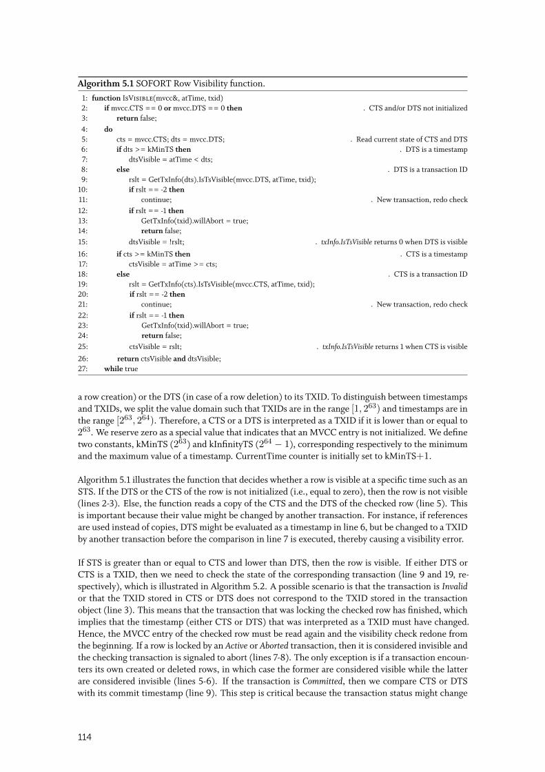
Algorithm 5.1 SOFORT Row Visibility function.1: function IsVisible(mvcc&, atTime, txid)2: if mvcc.CTS == 0 or mvcc.DTS == 0 then ◃ CTS and/or DTS not initialized3: return false;4: do5: cts = mvcc.CTS; dts = mvcc.DTS; ◃ Read current state of CTS and DTS6: if dts >= kMinTS then ◃ DTS is a timestamp7: dtsVisible = atTime < dts;8: else ◃ DTS is a transaction ID9: rslt = GetTxInfo(dts).IsTsVisible(mvcc.DTS, atTime, txid);
10: if rslt == -2 then11: continue; ◃ New transaction, redo check12: if rslt == -1 then13: GetTxInfo(txid).willAbort = true;14: return false;15: dtsVisible = !rslt; ◃ txInfo.IsTsVisible returns 0 when DTS is visible
16: if cts >= kMinTS then ◃ CTS is a timestamp17: ctsVisible = atTime >= cts;18: else ◃ CTS is a transaction ID19: rslt = GetTxInfo(cts).IsTsVisible(mvcc.CTS, atTime, txid);20: if rslt == -2 then21: continue; ◃ New transaction, redo check22: if rslt == -1 then23: GetTxInfo(txid).willAbort = true;24: return false;25: ctsVisible = rslt; ◃ txInfo.IsTsVisible returns 1 when CTS is visible
26: return ctsVisible and dtsVisible;27: while true
a row creation) or the DTS (in case of a row deletion) to its TXID. To distinguish between timestampsand TXIDs, we split the value domain such that TXIDs are in the range [1, 263) and timestamps are inthe range [263, 264). Therefore, a CTS or a DTS is interpreted as a TXID if it is lower than or equal to263. We reserve zero as a special value that indicates that an MVCC entry is not initialized. We definetwo constants, kMinTS (263) and kInfinityTS (264 − 1), corresponding respectively to the minimumand the maximum value of a timestamp. CurrentTime counter is initially set to kMinTS+1.
Algorithm 5.1 illustrates the function that decides whether a row is visible at a specific time such as anSTS. If the DTS or the CTS of the row is not initialized (i.e., equal to zero), then the row is not visible(lines 2-3). Else, the function reads a copy of the CTS and the DTS of the checked row (line 5). Thisis important because their value might be changed by another transaction. For instance, if referencesare used instead of copies, DTS might be evaluated as a timestamp in line 6, but be changed to a TXIDby another transaction before the comparison in line 7 is executed, thereby causing a visibility error.
If STS is greater than or equal to CTS and lower than DTS, then the row is visible. If either DTS orCTS is a TXID, then we need to check the state of the corresponding transaction (line 9 and 19, re-spectively), which is illustrated in Algorithm 5.2. A possible scenario is that the transaction is Invalidor that the TXID stored in CTS or DTS does not correspond to the TXID stored in the transactionobject (line 3). This means that the transaction that was locking the checked row has finished, whichimplies that the timestamp (either CTS or DTS) that was interpreted as a TXID must have changed.Hence, the MVCC entry of the checked row must be read again and the visibility check redone fromthe beginning. If a row is locked by an Active or Aborted transaction, then it is considered invisible andthe checking transaction is signaled to abort (lines 7-8). The only exception is if a transaction encoun-ters its own created or deleted rows, in which case the former are considered visible while the latterare considered invisible (lines 5-6). If the transaction is Committed, then we compare CTS or DTSwith its commit timestamp (line 9). This step is critical because the transaction status might change
114
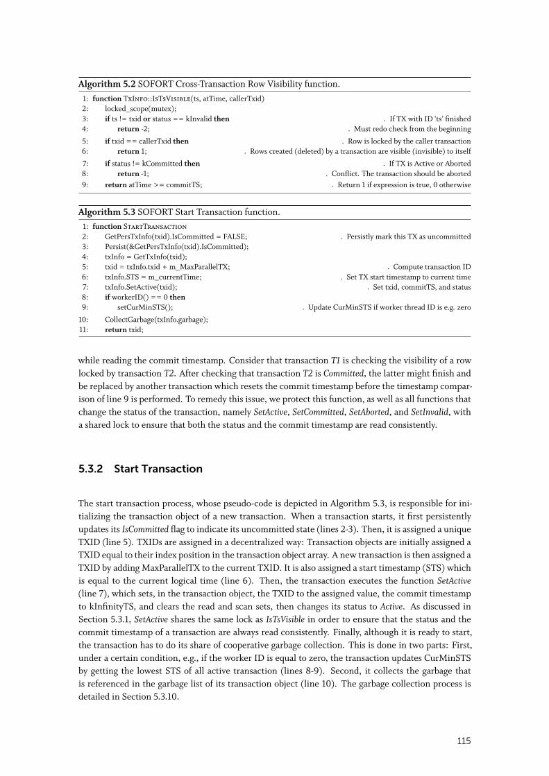
Algorithm 5.2 SOFORT Cross-Transaction Row Visibility function.1: function TxInfo::IsTsVisible(ts, atTime, callerTxid)2: locked_scope(mutex);3: if ts != txid or status == kInvalid then ◃ If TX with ID ‘ts’ finished4: return -2; ◃ Must redo check from the beginning
5: if txid == callerTxid then ◃ Row is locked by the caller transaction6: return 1; ◃ Rows created (deleted) by a transaction are visible (invisible) to itself
7: if status != kCommitted then ◃ If TX is Active or Aborted8: return -1; ◃ Conflict. The transaction should be aborted9: return atTime >= commitTS; ◃ Return 1 if expression is true, 0 otherwise
Algorithm 5.3 SOFORT Start Transaction function.1: function StartTransaction2: GetPersTxInfo(txid).IsCommitted = FALSE; ◃ Persistly mark this TX as uncommitted3: Persist(&GetPersTxInfo(txid).IsCommitted);4: txInfo = GetTxInfo(txid);5: txid = txInfo.txid + m_MaxParallelTX; ◃ Compute transaction ID6: txInfo.STS = m_currentTime; ◃ Set TX start timestamp to current time7: txInfo.SetActive(txid); ◃ Set txid, commitTS, and status8: if workerID() == 0 then9: setCurMinSTS(); ◃ Update CurMinSTS if worker thread ID is e.g. zero
10: CollectGarbage(txInfo.garbage);11: return txid;
while reading the commit timestamp. Consider that transaction T1 is checking the visibility of a rowlocked by transaction T2. After checking that transaction T2 is Committed, the latter might finish andbe replaced by another transaction which resets the commit timestamp before the timestamp compar-ison of line 9 is performed. To remedy this issue, we protect this function, as well as all functions thatchange the status of the transaction, namely SetActive, SetCommitted, SetAborted, and SetInvalid, witha shared lock to ensure that both the status and the commit timestamp are read consistently.
5.3.2 Start Transaction
The start transaction process, whose pseudo-code is depicted in Algorithm 5.3, is responsible for ini-tializing the transaction object of a new transaction. When a transaction starts, it first persistentlyupdates its IsCommitted flag to indicate its uncommitted state (lines 2-3). Then, it is assigned a uniqueTXID (line 5). TXIDs are assigned in a decentralized way: Transaction objects are initially assigned aTXID equal to their index position in the transaction object array. A new transaction is then assigned aTXID by adding MaxParallelTX to the current TXID. It is also assigned a start timestamp (STS) whichis equal to the current logical time (line 6). Then, the transaction executes the function SetActive(line 7), which sets, in the transaction object, the TXID to the assigned value, the commit timestampto kInfinityTS, and clears the read and scan sets, then changes its status to Active. As discussed inSection 5.3.1, SetActive shares the same lock as IsTsVisible in order to ensure that the status and thecommit timestamp of a transaction are always read consistently. Finally, although it is ready to start,the transaction has to do its share of cooperative garbage collection. This is done in two parts: First,under a certain condition, e.g., if the worker ID is equal to zero, the transaction updates CurMinSTSby getting the lowest STS of all active transaction (lines 8-9). Second, it collects the garbage thatis referenced in the garbage list of its transaction object (line 10). The garbage collection process isdetailed in Section 5.3.10.
115
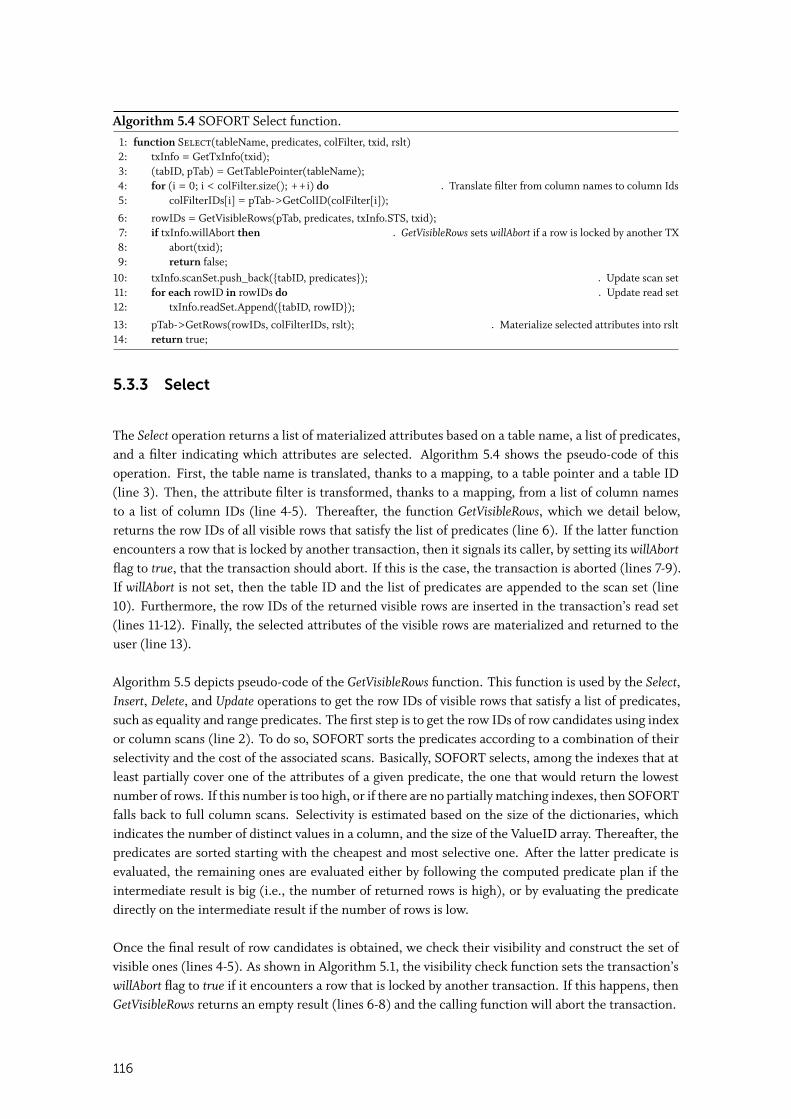
Algorithm 5.4 SOFORT Select function.1: function Select(tableName, predicates, colFilter, txid, rslt)2: txInfo = GetTxInfo(txid);3: (tabID, pTab) = GetTablePointer(tableName);4: for (i = 0; i < colFilter.size(); ++i) do ◃ Translate filter from column names to column Ids5: colFilterIDs[i] = pTab->GetColID(colFilter[i]);
6: rowIDs = GetVisibleRows(pTab, predicates, txInfo.STS, txid);7: if txInfo.willAbort then ◃ GetVisibleRows sets willAbort if a row is locked by another TX8: abort(txid);9: return false;
10: txInfo.scanSet.push_back({tabID, predicates}); ◃ Update scan set11: for each rowID in rowIDs do ◃ Update read set12: txInfo.readSet.Append({tabID, rowID});
13: pTab->GetRows(rowIDs, colFilterIDs, rslt); ◃ Materialize selected attributes into rslt14: return true;
5.3.3 Select
The Select operation returns a list of materialized attributes based on a table name, a list of predicates,and a filter indicating which attributes are selected. Algorithm 5.4 shows the pseudo-code of thisoperation. First, the table name is translated, thanks to a mapping, to a table pointer and a table ID(line 3). Then, the attribute filter is transformed, thanks to a mapping, from a list of column namesto a list of column IDs (line 4-5). Thereafter, the function GetVisibleRows, which we detail below,returns the row IDs of all visible rows that satisfy the list of predicates (line 6). If the latter functionencounters a row that is locked by another transaction, then it signals its caller, by setting its willAbortflag to true, that the transaction should abort. If this is the case, the transaction is aborted (lines 7-9).If willAbort is not set, then the table ID and the list of predicates are appended to the scan set (line10). Furthermore, the row IDs of the returned visible rows are inserted in the transaction’s read set(lines 11-12). Finally, the selected attributes of the visible rows are materialized and returned to theuser (line 13).
Algorithm 5.5 depicts pseudo-code of the GetVisibleRows function. This function is used by the Select,Insert, Delete, and Update operations to get the row IDs of visible rows that satisfy a list of predicates,such as equality and range predicates. The first step is to get the row IDs of row candidates using indexor column scans (line 2). To do so, SOFORT sorts the predicates according to a combination of theirselectivity and the cost of the associated scans. Basically, SOFORT selects, among the indexes that atleast partially cover one of the attributes of a given predicate, the one that would return the lowestnumber of rows. If this number is too high, or if there are no partially matching indexes, then SOFORTfalls back to full column scans. Selectivity is estimated based on the size of the dictionaries, whichindicates the number of distinct values in a column, and the size of the ValueID array. Thereafter, thepredicates are sorted starting with the cheapest and most selective one. After the latter predicate isevaluated, the remaining ones are evaluated either by following the computed predicate plan if theintermediate result is big (i.e., the number of returned rows is high), or by evaluating the predicatedirectly on the intermediate result if the number of rows is low.
Once the final result of row candidates is obtained, we check their visibility and construct the set ofvisible ones (lines 4-5). As shown in Algorithm 5.1, the visibility check function sets the transaction’swillAbort flag to true if it encounters a row that is locked by another transaction. If this happens, thenGetVisibleRows returns an empty result (lines 6-8) and the calling function will abort the transaction.
116
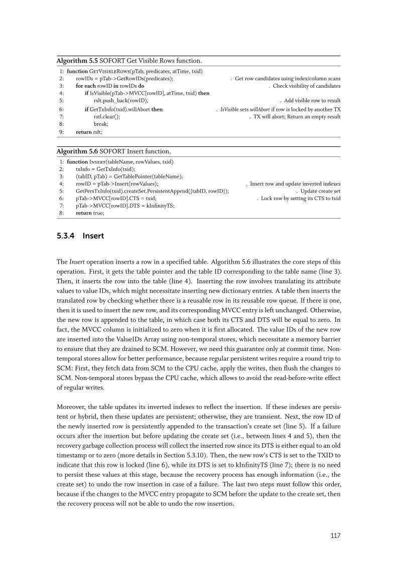
Algorithm 5.5 SOFORT Get Visible Rows function.1: function GetVisibleRows(pTab, predicates, atTime, txid)2: rowIDs = pTab->GetRowIDs(predicates); ◃ Get row candidates using index/column scans3: for each rowID in rowIDs do ◃ Check visibility of candidates4: if IsVisible(pTab->MVCC[rowID], atTime, txid) then5: rslt.push_back(rowID); ◃ Add visible row to result
6: if GetTxInfo(txid).willAbort then ◃ IsVisible sets willAbort if row is locked by another TX7: rstl.clear(); ◃ TX will abort; Return an empty result8: break;9: return rslt;
Algorithm 5.6 SOFORT Insert function.1: function Insert(tableName, rowValues, txid)2: txInfo = GetTxInfo(txid);3: (tabID, pTab) = GetTablePointer(tableName);4: rowID = pTab->Insert(rowValues); ◃ Insert row and update inverted indexes5: GetPersTxInfo(txid).createSet.PersistentAppend({tabID, rowID}); ◃ Update create set6: pTab->MVCC[rowID].CTS = txid; ◃ Lock row by setting its CTS to txid7: pTab->MVCC[rowID].DTS = kInfinityTS;8: return true;
5.3.4 Insert
The Insert operation inserts a row in a specified table. Algorithm 5.6 illustrates the core steps of thisoperation. First, it gets the table pointer and the table ID corresponding to the table name (line 3).Then, it inserts the row into the table (line 4). Inserting the row involves translating its attributevalues to value IDs, which might necessitate inserting new dictionary entries. A table then inserts thetranslated row by checking whether there is a reusable row in its reusable row queue. If there is one,then it is used to insert the new row, and its corresponding MVCC entry is left unchanged. Otherwise,the new row is appended to the table, in which case both its CTS and DTS will be equal to zero. Infact, the MVCC column is initialized to zero when it is first allocated. The value IDs of the new roware inserted into the ValueIDs Array using non-temporal stores, which necessitate a memory barrierto ensure that they are drained to SCM. However, we need this guarantee only at commit time. Non-temporal stores allow for better performance, because regular persistent writes require a round trip toSCM: First, they fetch data from SCM to the CPU cache, apply the writes, then flush the changes toSCM. Non-temporal stores bypass the CPU cache, which allows to avoid the read-before-write effectof regular writes.
Moreover, the table updates its inverted indexes to reflect the insertion. If these indexes are persis-tent or hybrid, then these updates are persistent; otherwise, they are transient. Next, the row ID ofthe newly inserted row is persistently appended to the transaction’s create set (line 5). If a failureoccurs after the insertion but before updating the create set (i.e., between lines 4 and 5), then therecovery garbage collection process will collect the inserted row since its DTS is either equal to an oldtimestamp or to zero (more details in Section 5.3.10). Then, the new row’s CTS is set to the TXID toindicate that this row is locked (line 6), while its DTS is set to kInfinityTS (line 7); there is no needto persist these values at this stage, because the recovery process has enough information (i.e., thecreate set) to undo the row insertion in case of a failure. The last two steps must follow this order,because if the changes to the MVCC entry propagate to SCM before the update to the create set, thenthe recovery process will not be able to undo the row insertion.
117
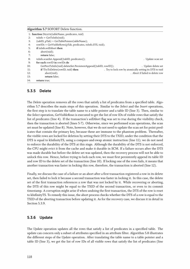
Algorithm 5.7 SOFORT Delete function.1: function Delete(tableName, predicates, txid)2: txInfo = GetTxInfo(txid);3: (tabID, pTab) = GetTablePointer(tableName);4: rowIDs = GetVisibleRows(pTab, predicates, txInfo.STS, txid);5: if txInfo.willAbort then6: abort(txid);7: return false;8: txInfo.scanSet.Append({tabID, predicates}); ◃ Update scan set9: for each rowID in rowIDs do
10: GetPersTxInfo(txid).deleteSet.PersistentAppend({tabID, rowID}); ◃ Update delete set11: if !TryToDelete(rowID, txid) then ◃ Try to lock row by atomically setting its DTS to txid12: abort(txid); ◃ Abort if failed to delete row13: return false;14: return true;
5.3.5 Delete
The Delete operation removes all the rows that satisfy a list of predicates from a specified table. Algo-rithm 5.7 describes the main steps of this operation. Similar to the Select and the Insert operations,the first step is to translate the table name to a table pointer and a table ID (line 3). Then, similar tothe Select operation, GetVisibleRows is executed to get the list of row IDs of visible rows that satisfy thelist of predicates (line 4). If the transaction’s willAbort flag was set to true during the visibility check,then the transaction is aborted (lines 5-7). Otherwise, since we performed scan operations, the scanset must be updated (line 8). Note, however, that we do not need to update the scan set for point pred-icates that contain the primary key, because these are immune to the phantom problem. Thereafter,the visible rows are locked for deletion by setting their DTS to the TXID, under the condition that theDTS is equal to kInfinityTS, using a compare-and-swap atomic instruction (line 11); we do not needto enforce the durability of the DTS at this stage. Although the durability of the DTS is not enforced,the CPU might evict it from the cache and make it durable in SCM. If a failure occurs after the DTSwas made durable but before the delete set was updated, then the recovery process will not be able tounlock this row. Hence, before trying to lock each row, we must first persistently append its table IDand row ID to the delete set of the transaction (line 10). If locking one of the rows fails, it means thatanother transaction was faster in locking this row, therefore, the transaction is aborted (line 12).
Finally, we discuss the case of a failure or an abort after a first transaction registered a row in its deleteset, then failed to lock it because a second transaction was faster in locking it. In this case, the deleteset of the first transaction references a row that was not locked by it. While recovering or aborting,the DTS of this row might be equal to the TXID of the second transaction, or even to its committimestamp. A corruption might arise if when undoing the first transaction, the DTS of the row is resetto kInfinityTS. To remedy this issue, the abort process checks whether the DTS of a row is equal to theTXID of the aborting transaction before updating it. As for the recovery case, we discuss it in detail inSection 5.3.9.
5.3.6 Update
The Update operation updates all the rows that satisfy a list of predicates in a specified table. Theupdate can concern only a subset of attributes specified in an attribute filter. Algorithm 5.8 illustratesthe different steps of the Update operation. After translating the table name to a table pointer and atable ID (line 3), we get the list of row IDs of all visible rows that satisfy the list of predicates (line
118
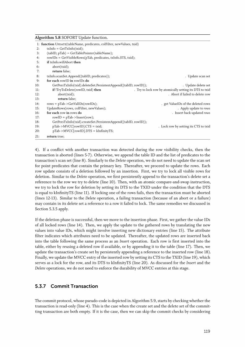
Algorithm 5.8 SOFORT Update function.1: function Update(tableName, predicates, colFilter, newValues, txid)2: txInfo = GetTxInfo(txid);3: (tabID, pTab) = GetTablePointer(tableName);4: rowIDs = GetVisibleRows(pTab, predicates, txInfo.STS, txid);5: if txInfo.willAbort then6: abort(txid);7: return false;8: txInfo.scanSet.Append({tabID, predicates}); ◃ Update scan set9: for each rowID in rowIDs do
10: GetPersTxInfo(txid).deleteSet.PersistentAppend({tabID, rowID}); ◃ Update delete set11: if !TryToDelete(rowID, txid) then ◃ Try to lock row by atomically setting its DTS to txid12: abort(txid); ◃ Abort if failed to delete row13: return false;14: rows = pTab->GetValIDs(rowIDs); ◃ get ValueIDs of the deleted rows15: UpdateRows(rows, colFilter, newValues); ◃ Apply update to rows16: for each row in rows do ◃ Insert back updated rows17: rowID = pTab->Insert(row);18: GetPersTxInfo(txid).createSet.PersistentAppend({tabID, rowID});19: pTab->MVCC[rowID].CTS = txid; ◃ Lock row by setting its CTS to txid20: pTab->MVCC[rowID].DTS = kInfinityTS;
21: return true;
4). If a conflict with another transaction was detected during the row visibility checks, then thetransaction is aborted (lines 5-7). Otherwise, we append the table ID and the list of predicates to thetransaction’s scan set (line 8). Similarly to the Delete operation, we do not need to update the scan setfor point predicates that contain the primary key. Thereafter, we proceed to update the rows. Eachrow update consists of a deletion followed by an insertion. First, we try to lock all visible rows fordeletion. Similar to the Delete operation, we first persistently append to the transaction’s delete set areference to the row we try to delete (line 10). Then, with an atomic compare-and-swap instruction,we try to lock the row for deletion by setting its DTS to the TXID under the condition that the DTSis equal to kInfinityTS (line 11). If locking one of the rows fails, then the transaction must be aborted(lines 12-13). Similar to the Delete operation, a failing transaction (because of an abort or a failure)may contain in its delete set a reference to a row it failed to lock. The same remedies we discussed inSection 5.3.5 apply.
If the deletion phase is successful, then we move to the insertion phase. First, we gather the value IDsof all locked rows (line 14). Then, we apply the update to the gathered rows by translating the newvalues into value IDs, which might involve inserting new dictionary entries (line 15). The attributefilter indicates which attributes need to be updated. Thereafter, the updated rows are inserted backinto the table following the same process as an Insert operation. Each row is first inserted into thetable, either by reusing a deleted row if available, or by appending it to the table (line 17). Then, weupdate the transaction’s create set by persistently appending a reference to the inserted row (line 18).Finally, we update the MVCC entry of the inserted row by setting its CTS to the TXID (line 19), whichserves as a lock for the row, and its DTS to kInfinityTS (line 20). As discussed for the Insert and theDelete operations, we do not need to enforce the durability of MVCC entries at this stage.
5.3.7 Commit Transaction
The commit protocol, whose pseudo-code is depicted in Algorithm 5.9, starts by checking whether thetransaction is read-only (line 4). This is the case when the create set and the delete set of the commit-ting transaction are both empty. If it is the case, then we can skip the commit checks by considering
119
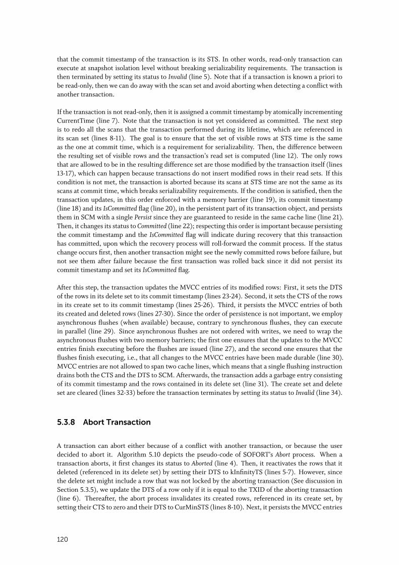
that the commit timestamp of the transaction is its STS. In other words, read-only transaction canexecute at snapshot isolation level without breaking serializability requirements. The transaction isthen terminated by setting its status to Invalid (line 5). Note that if a transaction is known a priori tobe read-only, then we can do away with the scan set and avoid aborting when detecting a conflict withanother transaction.
If the transaction is not read-only, then it is assigned a commit timestamp by atomically incrementingCurrentTime (line 7). Note that the transaction is not yet considered as committed. The next stepis to redo all the scans that the transaction performed during its lifetime, which are referenced inits scan set (lines 8-11). The goal is to ensure that the set of visible rows at STS time is the sameas the one at commit time, which is a requirement for serializability. Then, the difference betweenthe resulting set of visible rows and the transaction’s read set is computed (line 12). The only rowsthat are allowed to be in the resulting difference set are those modified by the transaction itself (lines13-17), which can happen because transactions do not insert modified rows in their read sets. If thiscondition is not met, the transaction is aborted because its scans at STS time are not the same as itsscans at commit time, which breaks serializability requirements. If the condition is satisfied, then thetransaction updates, in this order enforced with a memory barrier (line 19), its commit timestamp(line 18) and its IsCommitted flag (line 20), in the persistent part of its transaction object, and persiststhem in SCM with a single Persist since they are guaranteed to reside in the same cache line (line 21).Then, it changes its status to Committed (line 22); respecting this order is important because persistingthe commit timestamp and the IsCommitted flag will indicate during recovery that this transactionhas committed, upon which the recovery process will roll-forward the commit process. If the statuschange occurs first, then another transaction might see the newly committed rows before failure, butnot see them after failure because the first transaction was rolled back since it did not persist itscommit timestamp and set its IsCommitted flag.
After this step, the transaction updates the MVCC entries of its modified rows: First, it sets the DTSof the rows in its delete set to its commit timestamp (lines 23-24). Second, it sets the CTS of the rowsin its create set to its commit timestamp (lines 25-26). Third, it persists the MVCC entries of bothits created and deleted rows (lines 27-30). Since the order of persistence is not important, we employasynchronous flushes (when available) because, contrary to synchronous flushes, they can executein parallel (line 29). Since asynchronous flushes are not ordered with writes, we need to wrap theasynchronous flushes with two memory barriers; the first one ensures that the updates to the MVCCentries finish executing before the flushes are issued (line 27), and the second one ensures that theflushes finish executing, i.e., that all changes to the MVCC entries have been made durable (line 30).MVCC entries are not allowed to span two cache lines, which means that a single flushing instructiondrains both the CTS and the DTS to SCM. Afterwards, the transaction adds a garbage entry consistingof its commit timestamp and the rows contained in its delete set (line 31). The create set and deleteset are cleared (lines 32-33) before the transaction terminates by setting its status to Invalid (line 34).
5.3.8 Abort Transaction
A transaction can abort either because of a conflict with another transaction, or because the userdecided to abort it. Algorithm 5.10 depicts the pseudo-code of SOFORT’s Abort process. When atransaction aborts, it first changes its status to Aborted (line 4). Then, it reactivates the rows that itdeleted (referenced in its delete set) by setting their DTS to kInfinityTS (lines 5-7). However, sincethe delete set might include a row that was not locked by the aborting transaction (See discussion inSection 5.3.5), we update the DTS of a row only if it is equal to the TXID of the aborting transaction(line 6). Thereafter, the abort process invalidates its created rows, referenced in its create set, bysetting their CTS to zero and their DTS to CurMinSTS (lines 8-10). Next, it persists the MVCC entries
120
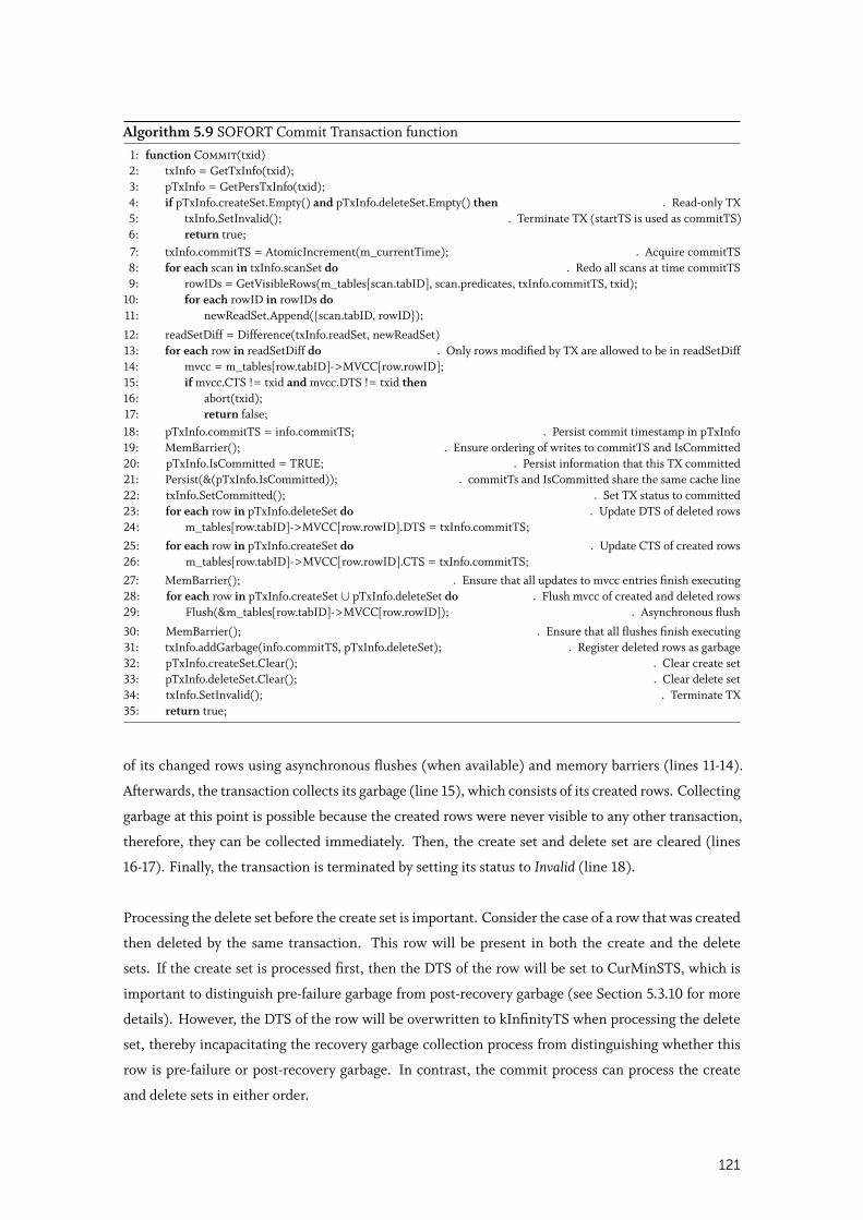
Algorithm 5.9 SOFORT Commit Transaction function1: function Commit(txid)2: txInfo = GetTxInfo(txid);3: pTxInfo = GetPersTxInfo(txid);4: if pTxInfo.createSet.Empty() and pTxInfo.deleteSet.Empty() then ◃ Read-only TX5: txInfo.SetInvalid(); ◃ Terminate TX (startTS is used as commitTS)6: return true;7: txInfo.commitTS = AtomicIncrement(m_currentTime); ◃ Acquire commitTS8: for each scan in txInfo.scanSet do ◃ Redo all scans at time commitTS9: rowIDs = GetVisibleRows(m_tables[scan.tabID], scan.predicates, txInfo.commitTS, txid);
10: for each rowID in rowIDs do11: newReadSet.Append({scan.tabID, rowID});
12: readSetDiff = Difference(txInfo.readSet, newReadSet)13: for each row in readSetDiff do ◃ Only rows modified by TX are allowed to be in readSetDiff14: mvcc = m_tables[row.tabID]->MVCC[row.rowID];15: if mvcc.CTS != txid and mvcc.DTS != txid then16: abort(txid);17: return false;18: pTxInfo.commitTS = info.commitTS; ◃ Persist commit timestamp in pTxInfo19: MemBarrier(); ◃ Ensure ordering of writes to commitTS and IsCommitted20: pTxInfo.IsCommitted = TRUE; ◃ Persist information that this TX committed21: Persist(&(pTxInfo.IsCommitted)); ◃ commitTs and IsCommitted share the same cache line22: txInfo.SetCommitted(); ◃ Set TX status to committed23: for each row in pTxInfo.deleteSet do ◃ Update DTS of deleted rows24: m_tables[row.tabID]->MVCC[row.rowID].DTS = txInfo.commitTS;
25: for each row in pTxInfo.createSet do ◃ Update CTS of created rows26: m_tables[row.tabID]->MVCC[row.rowID].CTS = txInfo.commitTS;
27: MemBarrier(); ◃ Ensure that all updates to mvcc entries finish executing28: for each row in pTxInfo.createSet ∪ pTxInfo.deleteSet do ◃ Flush mvcc of created and deleted rows29: Flush(&m_tables[row.tabID]->MVCC[row.rowID]); ◃ Asynchronous flush
30: MemBarrier(); ◃ Ensure that all flushes finish executing31: txInfo.addGarbage(info.commitTS, pTxInfo.deleteSet); ◃ Register deleted rows as garbage32: pTxInfo.createSet.Clear(); ◃ Clear create set33: pTxInfo.deleteSet.Clear(); ◃ Clear delete set34: txInfo.SetInvalid(); ◃ Terminate TX35: return true;
of its changed rows using asynchronous flushes (when available) and memory barriers (lines 11-14).
Afterwards, the transaction collects its garbage (line 15), which consists of its created rows. Collecting
garbage at this point is possible because the created rows were never visible to any other transaction,
therefore, they can be collected immediately. Then, the create set and delete set are cleared (lines
16-17). Finally, the transaction is terminated by setting its status to Invalid (line 18).
Processing the delete set before the create set is important. Consider the case of a row that was created
then deleted by the same transaction. This row will be present in both the create and the delete
sets. If the create set is processed first, then the DTS of the row will be set to CurMinSTS, which is
important to distinguish pre-failure garbage from post-recovery garbage (see Section 5.3.10 for more
details). However, the DTS of the row will be overwritten to kInfinityTS when processing the delete
set, thereby incapacitating the recovery garbage collection process from distinguishing whether this
row is pre-failure or post-recovery garbage. In contrast, the commit process can process the create
and delete sets in either order.
121
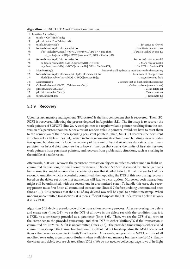
Algorithm 5.10 SOFORT Abort Transaction function.1: function Abort(txid)2: txInfo = GetTxInfo(txid);3: pTxInfo = GetPersTxInfo(txid);4: txInfo.SetAborted(); ◃ Set status to Aborted5: for each row in pTxInfo.deleteSet do ◃ Reactivate deleted rows6: if m_tables[row.tabID]->MVCC[row.rowID].DTS == txid then ◃ If DTS is locked by this TX7: m_tables[row.tabID]->MVCC[row.rowID].DTS = kInfinityTS;
8: for each row in pTxInfo.createSet do ◃ Set created rows as invalid9: m_tables[row.tabID]->MVCC[row.rowID].CTS = 0; ◃ Mark row as invalid
10: m_tables[row.tabID]->MVCC[row.rowID].DTS = CurMinSTS; ◃ Set DTS to CurMinSTS
11: MemBarrier(); ◃ Ensure that all updates to mvcc entries finish executing12: for each row in pTxInfo.createSet ∪ pTxInfo.deleteSet do ◃ Flush mvcc of changed rows13: Flush(&m_tables[row.tabID]->MVCC[row.rowID]); ◃ Asynchronous flush
14: MemBarrier(); ◃ Ensure that all flushes finish executing15: CollectGarbage({kMinTS, pTxInfo.createSet}); ◃ Collect garbage (created rows)16: pTxInfo.deleteSet.Clear(); ◃ Clear delete set17: pTxInfo.createSet.Clear(); ◃ Clear create set18: txInfo.SetInvalid(); ◃ Terminate TX
5.3.9 Recovery
Upon restart, memory management (PAllocator) is the first component that is recovered. Then, SO-FORT is recovered following the process depicted in Algorithm 5.11. The first step is to recover thework pointers of SOFORT (line 2). A work pointer is a regular volatile pointer resulting from the con-version of a persistent pointer. Since a restart renders volatile pointers invalid, we have to reset themto the conversion of their corresponding persistent pointers. Then, SOFORT recovers the persistentstructures of its tables (lines 3-4), which includes recovering its columns and building a new reusablerow queue, but does not include the recovery of transient or hybrid secondary data structures. Everypersistent or hybrid data structure has a Recover function that checks the sanity of its state, restoreswork pointers from persistent pointers, and recovers from problematic situations, such as crashing inthe middle of a table resize.
Afterwards, SOFORT recovers the persistent transaction objects in order to either undo in-flight un-committed transactions, or finish committed ones. In Section 5.3.5 we discussed the challenge that afirst transaction might reference in its delete set a row that it failed to lock. If that row was locked by asecond transaction which successfully committed, then updating the DTS of this row during recoverybased on the delete set of the first transaction will lead to a corruption. Moreover, both transactionsmight still be unfinished, with the second one in a committed state. To handle this case, the recov-ery process must first finish all committed transactions (lines 5-7) before undoing uncommitted ones(lines 8-10). This ensures that the DTS of any deleted row will be equal to a valid timestamp. Whenundoing uncommitted transactions, it is then sufficient to update the DTS of a row in a delete set onlyif it is a TXID.
Algorithm 5.12 depicts pseudo-code of the transaction recovery process. After recovering the deleteand create sets (lines 2-3), we set the DTS of all rows in the delete set with the condition that it isa TXID, to a timestamp provided as a parameter (lines 4-6). Then, we set the CTS of all rows inthe create set to the provided timestamp, and their DTS to either kInfinityTS if the transaction iscommitted or CurMinSTS if it is uncommitted (lines 7-12). The provided timestamp is either a validcommit timestamp if the transaction had committed but did not finish updating the MVCC entries ofits modified rows, or equal to kInfinityTS otherwise. Afterwards, we persist the MVCC entries of allmodified rows using asynchronous flushes (when available) and memory barriers (line 13-16). Finally,the create and delete sets are cleared (lines 17-18). We do not need to collect garbage rows of in-flight
122
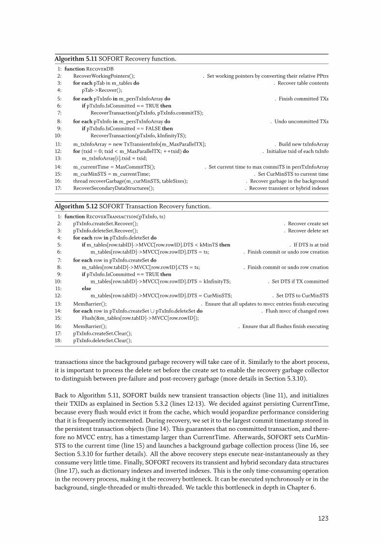
Algorithm 5.11 SOFORT Recovery function.1: function RecoverDB2: RecoverWorkingPointers(); ◃ Set working pointers by converting their relative PPtrs3: for each pTab in m_tables do ◃ Recover table contents4: pTab->Recover();
5: for each pTxInfo in m_persTxInfoArray do ◃ Finish committed TXs6: if pTxInfo.IsCommitted == TRUE then7: RecoverTransaction(pTxInfo, pTxInfo.commitTS);
8: for each pTxInfo in m_persTxInfoArray do ◃ Undo uncommitted TXs9: if pTxInfo.IsCommitted == FALSE then
10: RecoverTransaction(pTxInfo, kInfinityTS);
11: m_txInfoArray = new TxTransientInfo[m_MaxParallelTX]; ◃ Build new txInfoArray12: for (txid = 0; txid < m_MaxParallelTX; ++txid) do ◃ Initialize txid of each txInfo13: m_txInfoArray[i].txid = txid;
14: m_currentTime = MaxCommitTS(); ◃ Set current time to max commiTS in persTxInfoArray15: m_curMinSTS = m_currentTime; ◃ Set CurMinSTS to current time16: thread recoverGarbage(m_curMinSTS, tableSizes); ◃ Recover garbage in the background17: RecoverSecondaryDataStructures(); ◃ Recover transient or hybrid indexes
Algorithm 5.12 SOFORT Transaction Recovery function.1: function RecoverTransaction(pTxInfo, ts)2: pTxInfo.createSet.Recover(); ◃ Recover create set3: pTxInfo.deleteSet.Recover(); ◃ Recover delete set4: for each row in pTxInfo.deleteSet do5: if m_tables[row.tabID]->MVCC[row.rowID].DTS < kMinTS then ◃ If DTS is at txid6: m_tables[row.tabID]->MVCC[row.rowID].DTS = ts; ◃ Finish commit or undo row creation
7: for each row in pTxInfo.createSet do8: m_tables[row.tabID]->MVCC[row.rowID].CTS = ts; ◃ Finish commit or undo row creation9: if pTxInfo.IsCommitted == TRUE then
10: m_tables[row.tabID]->MVCC[row.rowID].DTS = kInfinityTS; ◃ Set DTS if TX committed11: else12: m_tables[row.tabID]->MVCC[row.rowID].DTS = CurMinSTS; ◃ Set DTS to CurMinSTS
13: MemBarrier(); ◃ Ensure that all updates to mvcc entries finish executing14: for each row in pTxInfo.createSet ∪ pTxInfo.deleteSet do ◃ Flush mvcc of changed rows15: Flush(&m_tables[row.tabID]->MVCC[row.rowID]);
16: MemBarrier(); ◃ Ensure that all flushes finish executing17: pTxInfo.createSet.Clear();18: pTxInfo.deleteSet.Clear();
transactions since the background garbage recovery will take care of it. Similarly to the abort process,it is important to process the delete set before the create set to enable the recovery garbage collectorto distinguish between pre-failure and post-recovery garbage (more details in Section 5.3.10).
Back to Algorithm 5.11, SOFORT builds new transient transaction objects (line 11), and initializestheir TXIDs as explained in Section 5.3.2 (lines 12-13). We decided against persisting CurrentTime,because every flush would evict it from the cache, which would jeopardize performance consideringthat it is frequently incremented. During recovery, we set it to the largest commit timestamp stored inthe persistent transaction objects (line 14). This guarantees that no committed transaction, and there-fore no MVCC entry, has a timestamp larger than CurrentTime. Afterwards, SOFORT sets CurMin-STS to the current time (line 15) and launches a background garbage collection process (line 16, seeSection 5.3.10 for further details). All the above recovery steps execute near-instantaneously as theyconsume very little time. Finally, SOFORT recovers its transient and hybrid secondary data structures(line 17), such as dictionary indexes and inverted indexes. This is the only time-consuming operationin the recovery process, making it the recovery bottleneck. It can be executed synchronously or in thebackground, single-threaded or multi-threaded. We tackle this bottleneck in depth in Chapter 6.
123
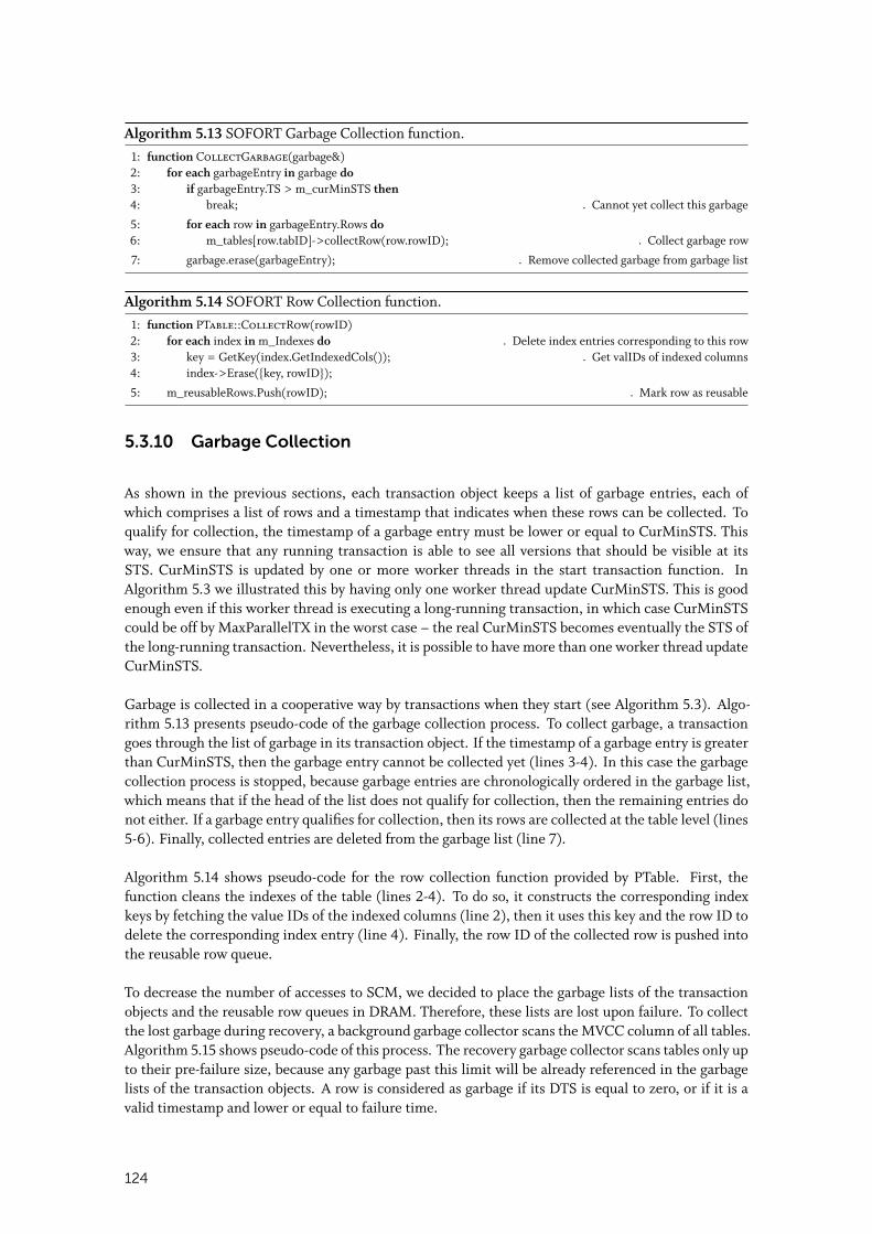
Algorithm 5.13 SOFORT Garbage Collection function.1: function CollectGarbage(garbage&)2: for each garbageEntry in garbage do3: if garbageEntry.TS > m_curMinSTS then4: break; ◃ Cannot yet collect this garbage
5: for each row in garbageEntry.Rows do6: m_tables[row.tabID]->collectRow(row.rowID); ◃ Collect garbage row
7: garbage.erase(garbageEntry); ◃ Remove collected garbage from garbage list
Algorithm 5.14 SOFORT Row Collection function.1: function PTable::CollectRow(rowID)2: for each index in m_Indexes do ◃ Delete index entries corresponding to this row3: key = GetKey(index.GetIndexedCols()); ◃ Get valIDs of indexed columns4: index->Erase({key, rowID});
5: m_reusableRows.Push(rowID); ◃ Mark row as reusable
5.3.10 Garbage Collection
As shown in the previous sections, each transaction object keeps a list of garbage entries, each ofwhich comprises a list of rows and a timestamp that indicates when these rows can be collected. Toqualify for collection, the timestamp of a garbage entry must be lower or equal to CurMinSTS. Thisway, we ensure that any running transaction is able to see all versions that should be visible at itsSTS. CurMinSTS is updated by one or more worker threads in the start transaction function. InAlgorithm 5.3 we illustrated this by having only one worker thread update CurMinSTS. This is goodenough even if this worker thread is executing a long-running transaction, in which case CurMinSTScould be off by MaxParallelTX in the worst case – the real CurMinSTS becomes eventually the STS ofthe long-running transaction. Nevertheless, it is possible to have more than one worker thread updateCurMinSTS.
Garbage is collected in a cooperative way by transactions when they start (see Algorithm 5.3). Algo-rithm 5.13 presents pseudo-code of the garbage collection process. To collect garbage, a transactiongoes through the list of garbage in its transaction object. If the timestamp of a garbage entry is greaterthan CurMinSTS, then the garbage entry cannot be collected yet (lines 3-4). In this case the garbagecollection process is stopped, because garbage entries are chronologically ordered in the garbage list,which means that if the head of the list does not qualify for collection, then the remaining entries donot either. If a garbage entry qualifies for collection, then its rows are collected at the table level (lines5-6). Finally, collected entries are deleted from the garbage list (line 7).
Algorithm 5.14 shows pseudo-code for the row collection function provided by PTable. First, thefunction cleans the indexes of the table (lines 2-4). To do so, it constructs the corresponding indexkeys by fetching the value IDs of the indexed columns (line 2), then it uses this key and the row ID todelete the corresponding index entry (line 4). Finally, the row ID of the collected row is pushed intothe reusable row queue.
To decrease the number of accesses to SCM, we decided to place the garbage lists of the transactionobjects and the reusable row queues in DRAM. Therefore, these lists are lost upon failure. To collectthe lost garbage during recovery, a background garbage collector scans the MVCC column of all tables.Algorithm 5.15 shows pseudo-code of this process. The recovery garbage collector scans tables only upto their pre-failure size, because any garbage past this limit will be already referenced in the garbagelists of the transaction objects. A row is considered as garbage if its DTS is equal to zero, or if it is avalid timestamp and lower or equal to failure time.
124
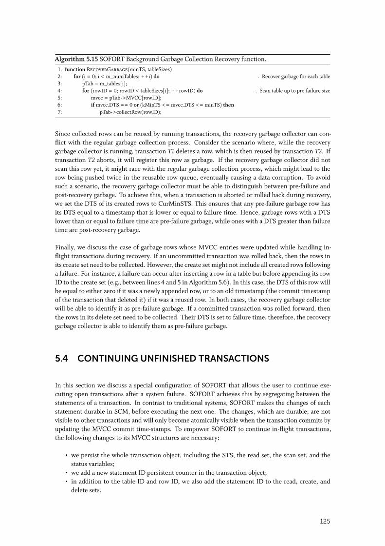
Algorithm 5.15 SOFORT Background Garbage Collection Recovery function.1: function RecoverGarbage(minTS, tableSizes)2: for (i = 0; i < m_numTables; ++i) do ◃ Recover garbage for each table3: pTab = m_tables[i];4: for (rowID = 0; rowID < tableSizes[i]; ++rowID) do ◃ Scan table up to pre-failure size5: mvcc = pTab->MVCC[rowID];6: if mvcc.DTS == 0 or (kMinTS <= mvcc.DTS <= minTS) then7: pTab->collectRow(rowID);
Since collected rows can be reused by running transactions, the recovery garbage collector can con-flict with the regular garbage collection process. Consider the scenario where, while the recoverygarbage collector is running, transaction T1 deletes a row, which is then reused by transaction T2. Iftransaction T2 aborts, it will register this row as garbage. If the recovery garbage collector did notscan this row yet, it might race with the regular garbage collection process, which might lead to therow being pushed twice in the reusable row queue, eventually causing a data corruption. To avoidsuch a scenario, the recovery garbage collector must be able to distinguish between pre-failure andpost-recovery garbage. To achieve this, when a transaction is aborted or rolled back during recovery,we set the DTS of its created rows to CurMinSTS. This ensures that any pre-failure garbage row hasits DTS equal to a timestamp that is lower or equal to failure time. Hence, garbage rows with a DTSlower than or equal to failure time are pre-failure garbage, while ones with a DTS greater than failuretime are post-recovery garbage.
Finally, we discuss the case of garbage rows whose MVCC entries were updated while handling in-flight transactions during recovery. If an uncommitted transaction was rolled back, then the rows inits create set need to be collected. However, the create set might not include all created rows followinga failure. For instance, a failure can occur after inserting a row in a table but before appending its rowID to the create set (e.g., between lines 4 and 5 in Algorithm 5.6). In this case, the DTS of this row willbe equal to either zero if it was a newly appended row, or to an old timestamp (the commit timestampof the transaction that deleted it) if it was a reused row. In both cases, the recovery garbage collectorwill be able to identify it as pre-failure garbage. If a committed transaction was rolled forward, thenthe rows in its delete set need to be collected. Their DTS is set to failure time, therefore, the recoverygarbage collector is able to identify them as pre-failure garbage.
5.4 CONTINUING UNFINISHED TRANSACTIONS
In this section we discuss a special configuration of SOFORT that allows the user to continue exe-cuting open transactions after a system failure. SOFORT achieves this by segregating between thestatements of a transaction. In contrast to traditional systems, SOFORT makes the changes of eachstatement durable in SCM, before executing the next one. The changes, which are durable, are notvisible to other transactions and will only become atomically visible when the transaction commits byupdating the MVCC commit time-stamps. To empower SOFORT to continue in-flight transactions,the following changes to its MVCC structures are necessary:
• we persist the whole transaction object, including the STS, the read set, the scan set, and thestatus variables;
• we add a new statement ID persistent counter in the transaction object;• in addition to the table ID and row ID, we also add the statement ID to the read, create, and
delete sets.
125
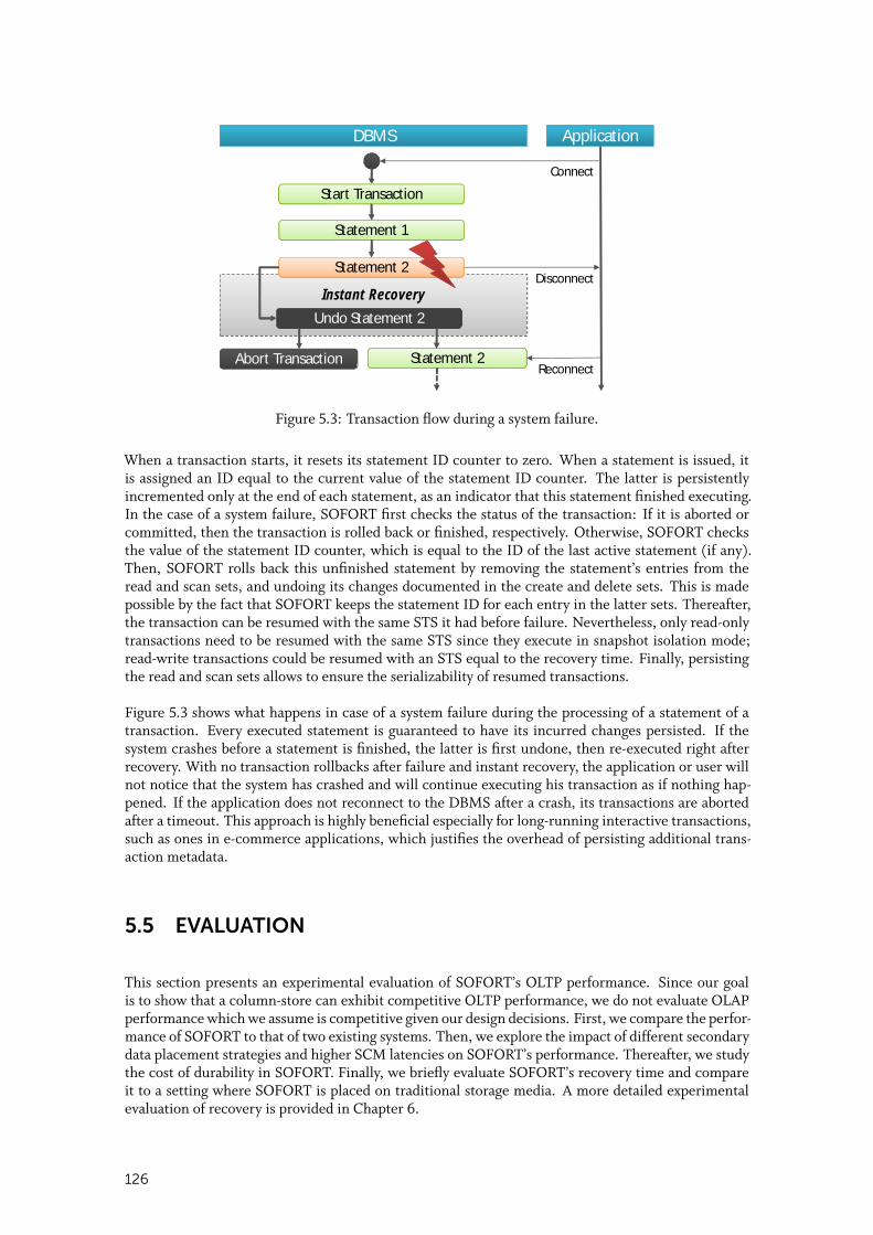
| 2
Transaction Continuation
Diese Zeile ersetzt man über: Einfügen > Kopf- und Fußzeile NICHT im Master
DBMS Application
Statement 1
Statement 2
Undo Statement 2
Abort Transaction Statement 2
Instant Recovery
Connect
Disconnect
Reconnect
Start Transaction
Figure 5.3: Transaction flow during a system failure.
When a transaction starts, it resets its statement ID counter to zero. When a statement is issued, itis assigned an ID equal to the current value of the statement ID counter. The latter is persistentlyincremented only at the end of each statement, as an indicator that this statement finished executing.In the case of a system failure, SOFORT first checks the status of the transaction: If it is aborted orcommitted, then the transaction is rolled back or finished, respectively. Otherwise, SOFORT checksthe value of the statement ID counter, which is equal to the ID of the last active statement (if any).Then, SOFORT rolls back this unfinished statement by removing the statement’s entries from theread and scan sets, and undoing its changes documented in the create and delete sets. This is madepossible by the fact that SOFORT keeps the statement ID for each entry in the latter sets. Thereafter,the transaction can be resumed with the same STS it had before failure. Nevertheless, only read-onlytransactions need to be resumed with the same STS since they execute in snapshot isolation mode;read-write transactions could be resumed with an STS equal to the recovery time. Finally, persistingthe read and scan sets allows to ensure the serializability of resumed transactions.
Figure 5.3 shows what happens in case of a system failure during the processing of a statement of atransaction. Every executed statement is guaranteed to have its incurred changes persisted. If thesystem crashes before a statement is finished, the latter is first undone, then re-executed right afterrecovery. With no transaction rollbacks after failure and instant recovery, the application or user willnot notice that the system has crashed and will continue executing his transaction as if nothing hap-pened. If the application does not reconnect to the DBMS after a crash, its transactions are abortedafter a timeout. This approach is highly beneficial especially for long-running interactive transactions,such as ones in e-commerce applications, which justifies the overhead of persisting additional trans-action metadata.
5.5 EVALUATION
This section presents an experimental evaluation of SOFORT’s OLTP performance. Since our goalis to show that a column-store can exhibit competitive OLTP performance, we do not evaluate OLAPperformance which we assume is competitive given our design decisions. First, we compare the perfor-mance of SOFORT to that of two existing systems. Then, we explore the impact of different secondarydata placement strategies and higher SCM latencies on SOFORT’s performance. Thereafter, we studythe cost of durability in SOFORT. Finally, we briefly evaluate SOFORT’s recovery time and compareit to a setting where SOFORT is placed on traditional storage media. A more detailed experimentalevaluation of recovery is provided in Chapter 6.
126
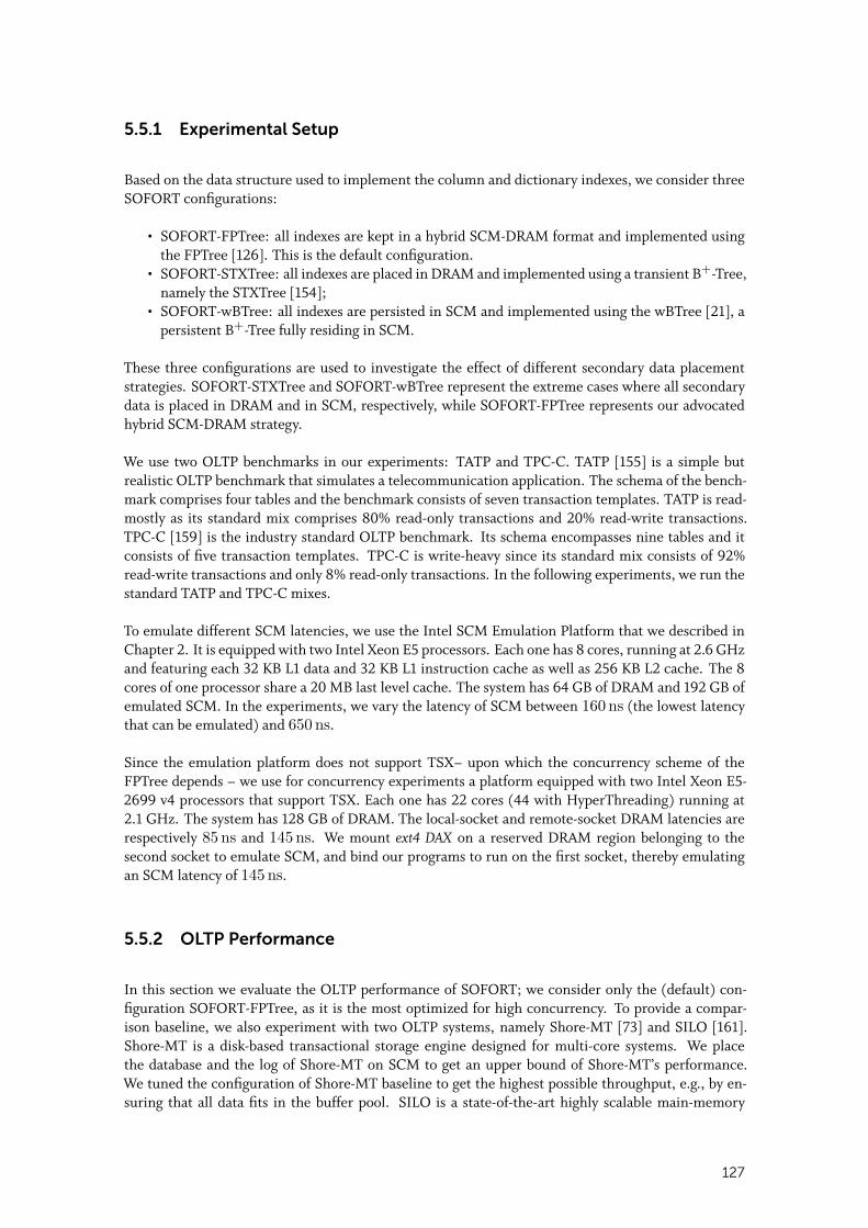
5.5.1 Experimental Setup
Based on the data structure used to implement the column and dictionary indexes, we consider threeSOFORT configurations:
• SOFORT-FPTree: all indexes are kept in a hybrid SCM-DRAM format and implemented usingthe FPTree [126]. This is the default configuration.
• SOFORT-STXTree: all indexes are placed in DRAM and implemented using a transient B+-Tree,namely the STXTree [154];
• SOFORT-wBTree: all indexes are persisted in SCM and implemented using the wBTree [21], apersistent B+-Tree fully residing in SCM.
These three configurations are used to investigate the effect of different secondary data placementstrategies. SOFORT-STXTree and SOFORT-wBTree represent the extreme cases where all secondarydata is placed in DRAM and in SCM, respectively, while SOFORT-FPTree represents our advocatedhybrid SCM-DRAM strategy.
We use two OLTP benchmarks in our experiments: TATP and TPC-C. TATP [155] is a simple butrealistic OLTP benchmark that simulates a telecommunication application. The schema of the bench-mark comprises four tables and the benchmark consists of seven transaction templates. TATP is read-mostly as its standard mix comprises 80% read-only transactions and 20% read-write transactions.TPC-C [159] is the industry standard OLTP benchmark. Its schema encompasses nine tables and itconsists of five transaction templates. TPC-C is write-heavy since its standard mix consists of 92%read-write transactions and only 8% read-only transactions. In the following experiments, we run thestandard TATP and TPC-C mixes.
To emulate different SCM latencies, we use the Intel SCM Emulation Platform that we described inChapter 2. It is equipped with two Intel Xeon E5 processors. Each one has 8 cores, running at 2.6 GHzand featuring each 32 KB L1 data and 32 KB L1 instruction cache as well as 256 KB L2 cache. The 8cores of one processor share a 20 MB last level cache. The system has 64 GB of DRAM and 192 GB ofemulated SCM. In the experiments, we vary the latency of SCM between 160 ns (the lowest latencythat can be emulated) and 650 ns.
Since the emulation platform does not support TSX– upon which the concurrency scheme of theFPTree depends – we use for concurrency experiments a platform equipped with two Intel Xeon E5-2699 v4 processors that support TSX. Each one has 22 cores (44 with HyperThreading) running at2.1 GHz. The system has 128 GB of DRAM. The local-socket and remote-socket DRAM latencies arerespectively 85 ns and 145 ns. We mount ext4 DAX on a reserved DRAM region belonging to thesecond socket to emulate SCM, and bind our programs to run on the first socket, thereby emulatingan SCM latency of 145 ns.
5.5.2 OLTP Performance
In this section we evaluate the OLTP performance of SOFORT; we consider only the (default) con-figuration SOFORT-FPTree, as it is the most optimized for high concurrency. To provide a compar-ison baseline, we also experiment with two OLTP systems, namely Shore-MT [73] and SILO [161].Shore-MT is a disk-based transactional storage engine designed for multi-core systems. We placethe database and the log of Shore-MT on SCM to get an upper bound of Shore-MT’s performance.We tuned the configuration of Shore-MT baseline to get the highest possible throughput, e.g., by en-suring that all data fits in the buffer pool. SILO is a state-of-the-art highly scalable main-memory
127
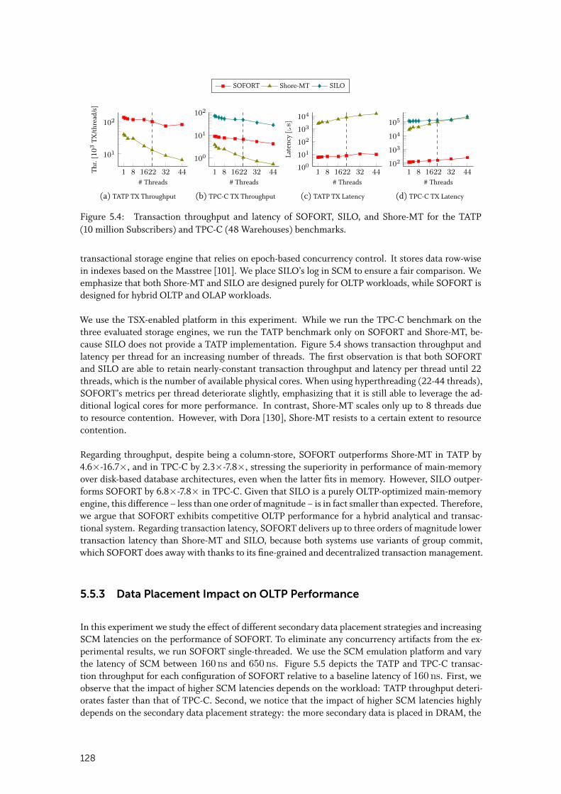
SOFORT Shore-MT SILO
1 8 1622 32 44
101
102
HT# Threads
Thr.
[103
TX/t
hrea
d/s]
(a) TATP TX Throughput
1 8 1622 32 44
100
101
102
HT# Threads
(b) TPC-C TX Throughput
1 8 1622 32 44100
101
102
103
104
HT# Threads
Late
ncy
[µs]
(c) TATP TX Latency
1 8 1622 32 44102
103
104
105
HT# Threads
(d) TPC-C TX Latency
Figure 5.4: Transaction throughput and latency of SOFORT, SILO, and Shore-MT for the TATP(10 million Subscribers) and TPC-C (48 Warehouses) benchmarks.
transactional storage engine that relies on epoch-based concurrency control. It stores data row-wisein indexes based on the Masstree [101]. We place SILO’s log in SCM to ensure a fair comparison. Weemphasize that both Shore-MT and SILO are designed purely for OLTP workloads, while SOFORT isdesigned for hybrid OLTP and OLAP workloads.
We use the TSX-enabled platform in this experiment. While we run the TPC-C benchmark on thethree evaluated storage engines, we run the TATP benchmark only on SOFORT and Shore-MT, be-cause SILO does not provide a TATP implementation. Figure 5.4 shows transaction throughput andlatency per thread for an increasing number of threads. The first observation is that both SOFORTand SILO are able to retain nearly-constant transaction throughput and latency per thread until 22threads, which is the number of available physical cores. When using hyperthreading (22-44 threads),SOFORT’s metrics per thread deteriorate slightly, emphasizing that it is still able to leverage the ad-ditional logical cores for more performance. In contrast, Shore-MT scales only up to 8 threads dueto resource contention. However, with Dora [130], Shore-MT resists to a certain extent to resourcecontention.
Regarding throughput, despite being a column-store, SOFORT outperforms Shore-MT in TATP by4.6×-16.7×, and in TPC-C by 2.3×-7.8×, stressing the superiority in performance of main-memoryover disk-based database architectures, even when the latter fits in memory. However, SILO outper-forms SOFORT by 6.8×-7.8× in TPC-C. Given that SILO is a purely OLTP-optimized main-memoryengine, this difference – less than one order of magnitude – is in fact smaller than expected. Therefore,we argue that SOFORT exhibits competitive OLTP performance for a hybrid analytical and transac-tional system. Regarding transaction latency, SOFORT delivers up to three orders of magnitude lowertransaction latency than Shore-MT and SILO, because both systems use variants of group commit,which SOFORT does away with thanks to its fine-grained and decentralized transaction management.
5.5.3 Data Placement Impact on OLTP Performance
In this experiment we study the effect of different secondary data placement strategies and increasingSCM latencies on the performance of SOFORT. To eliminate any concurrency artifacts from the ex-perimental results, we run SOFORT single-threaded. We use the SCM emulation platform and varythe latency of SCM between 160 ns and 650 ns. Figure 5.5 depicts the TATP and TPC-C transac-tion throughput for each configuration of SOFORT relative to a baseline latency of 160 ns. First, weobserve that the impact of higher SCM latencies depends on the workload: TATP throughput deteri-orates faster than that of TPC-C. Second, we notice that the impact of higher SCM latencies highlydepends on the secondary data placement strategy: the more secondary data is placed in DRAM, the
128
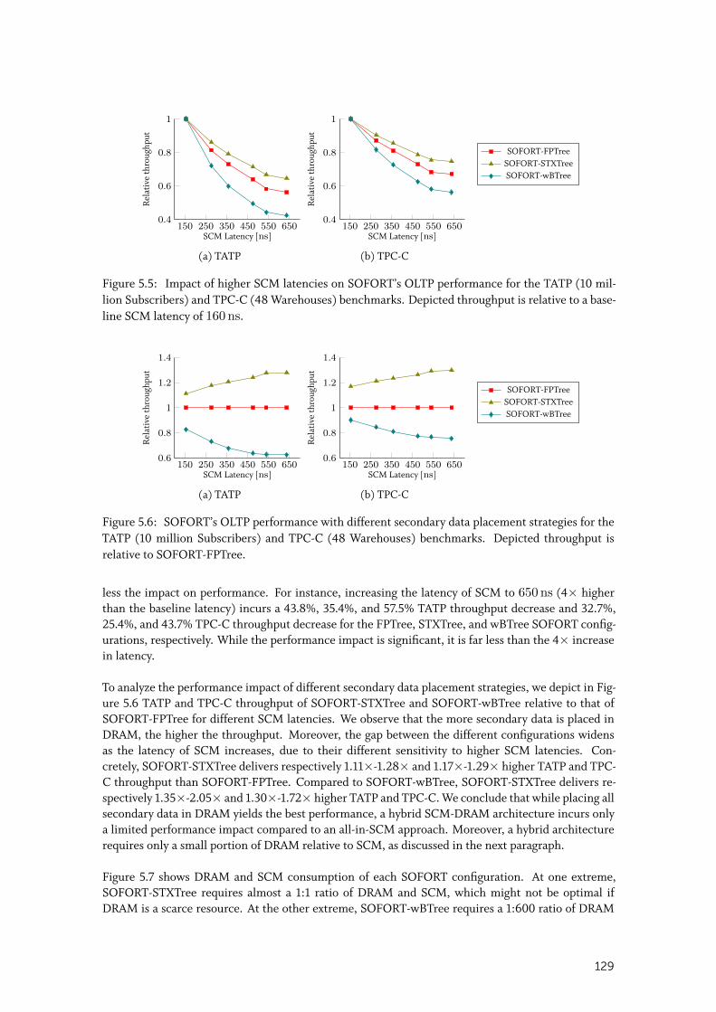
150 250 350 450 550 6500.4
0.6
0.8
1
SCM Latency [ns]
Rel
ativ
eth
roug
hput
(a) TATP
150 250 350 450 550 6500.4
0.6
0.8
1
SCM Latency [ns]
Rel
ativ
eth
roug
hput
(b) TPC-C
SOFORT-FPTreeSOFORT-STXTreeSOFORT-wBTree
Figure 5.5: Impact of higher SCM latencies on SOFORT’s OLTP performance for the TATP (10 mil-lion Subscribers) and TPC-C (48 Warehouses) benchmarks. Depicted throughput is relative to a base-line SCM latency of 160 ns.
150 250 350 450 550 6500.6
0.8
1
1.2
1.4
SCM Latency [ns]
Rel
ativ
eth
roug
hput
(a) TATP
150 250 350 450 550 6500.6
0.8
1
1.2
1.4
SCM Latency [ns]
Rel
ativ
eth
roug
hput
(b) TPC-C
SOFORT-FPTreeSOFORT-STXTreeSOFORT-wBTree
Figure 5.6: SOFORT’s OLTP performance with different secondary data placement strategies for theTATP (10 million Subscribers) and TPC-C (48 Warehouses) benchmarks. Depicted throughput isrelative to SOFORT-FPTree.
less the impact on performance. For instance, increasing the latency of SCM to 650 ns (4× higherthan the baseline latency) incurs a 43.8%, 35.4%, and 57.5% TATP throughput decrease and 32.7%,25.4%, and 43.7% TPC-C throughput decrease for the FPTree, STXTree, and wBTree SOFORT config-urations, respectively. While the performance impact is significant, it is far less than the 4× increasein latency.
To analyze the performance impact of different secondary data placement strategies, we depict in Fig-ure 5.6 TATP and TPC-C throughput of SOFORT-STXTree and SOFORT-wBTree relative to that ofSOFORT-FPTree for different SCM latencies. We observe that the more secondary data is placed inDRAM, the higher the throughput. Moreover, the gap between the different configurations widensas the latency of SCM increases, due to their different sensitivity to higher SCM latencies. Con-cretely, SOFORT-STXTree delivers respectively 1.11×-1.28× and 1.17×-1.29× higher TATP and TPC-C throughput than SOFORT-FPTree. Compared to SOFORT-wBTree, SOFORT-STXTree delivers re-spectively 1.35×-2.05× and 1.30×-1.72× higher TATP and TPC-C. We conclude that while placing allsecondary data in DRAM yields the best performance, a hybrid SCM-DRAM architecture incurs onlya limited performance impact compared to an all-in-SCM approach. Moreover, a hybrid architecturerequires only a small portion of DRAM relative to SCM, as discussed in the next paragraph.
Figure 5.7 shows DRAM and SCM consumption of each SOFORT configuration. At one extreme,SOFORT-STXTree requires almost a 1:1 ratio of DRAM and SCM, which might not be optimal ifDRAM is a scarce resource. At the other extreme, SOFORT-wBTree requires a 1:600 ratio of DRAM
129
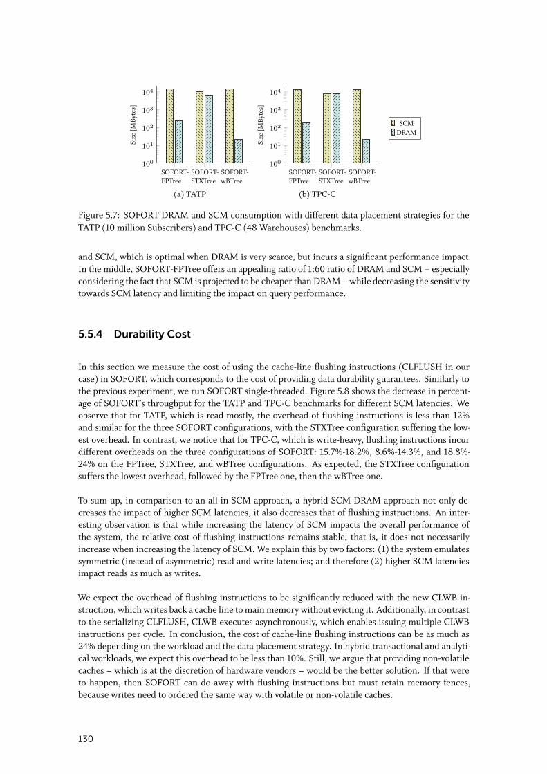
SOFORT-FPTree
SOFORT-STXTree
SOFORT-wBTree
100
101
102
103
104
Size
[MB
ytes
]
(a) TATP
SOFORT-FPTree
SOFORT-STXTree
SOFORT-wBTree
100
101
102
103
104
Size
[MB
ytes
]
(b) TPC-C
SCMDRAM
Figure 5.7: SOFORT DRAM and SCM consumption with different data placement strategies for theTATP (10 million Subscribers) and TPC-C (48 Warehouses) benchmarks.
and SCM, which is optimal when DRAM is very scarce, but incurs a significant performance impact.In the middle, SOFORT-FPTree offers an appealing ratio of 1:60 ratio of DRAM and SCM – especiallyconsidering the fact that SCM is projected to be cheaper than DRAM – while decreasing the sensitivitytowards SCM latency and limiting the impact on query performance.
5.5.4 Durability Cost
In this section we measure the cost of using the cache-line flushing instructions (CLFLUSH in ourcase) in SOFORT, which corresponds to the cost of providing data durability guarantees. Similarly tothe previous experiment, we run SOFORT single-threaded. Figure 5.8 shows the decrease in percent-age of SOFORT’s throughput for the TATP and TPC-C benchmarks for different SCM latencies. Weobserve that for TATP, which is read-mostly, the overhead of flushing instructions is less than 12%and similar for the three SOFORT configurations, with the STXTree configuration suffering the low-est overhead. In contrast, we notice that for TPC-C, which is write-heavy, flushing instructions incurdifferent overheads on the three configurations of SOFORT: 15.7%-18.2%, 8.6%-14.3%, and 18.8%-24% on the FPTree, STXTree, and wBTree configurations. As expected, the STXTree configurationsuffers the lowest overhead, followed by the FPTree one, then the wBTree one.
To sum up, in comparison to an all-in-SCM approach, a hybrid SCM-DRAM approach not only de-creases the impact of higher SCM latencies, it also decreases that of flushing instructions. An inter-esting observation is that while increasing the latency of SCM impacts the overall performance ofthe system, the relative cost of flushing instructions remains stable, that is, it does not necessarilyincrease when increasing the latency of SCM. We explain this by two factors: (1) the system emulatessymmetric (instead of asymmetric) read and write latencies; and therefore (2) higher SCM latenciesimpact reads as much as writes.
We expect the overhead of flushing instructions to be significantly reduced with the new CLWB in-struction, which writes back a cache line to main memory without evicting it. Additionally, in contrastto the serializing CLFLUSH, CLWB executes asynchronously, which enables issuing multiple CLWBinstructions per cycle. In conclusion, the cost of cache-line flushing instructions can be as much as24% depending on the workload and the data placement strategy. In hybrid transactional and analyti-cal workloads, we expect this overhead to be less than 10%. Still, we argue that providing non-volatilecaches – which is at the discretion of hardware vendors – would be the better solution. If that wereto happen, then SOFORT can do away with flushing instructions but must retain memory fences,because writes need to ordered the same way with volatile or non-volatile caches.
130
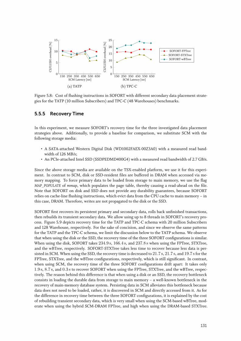
150 250 350 450 550 6500
5
10
15
SCM Latency [ns]
CLF
LUSH
over
head
[%]
(a) TATP
150 250 350 450 550 6500
5
10
15
20
25
SCM Latency [ns]
CLF
LUSH
over
head
[%]
(b) TPC-C
SOFORT-FPTreeSOFORT-STXTreeSOFORT-wBTree
Figure 5.8: Cost of flushing instructions in SOFORT with different secondary data placement strate-gies for the TATP (10 million Subscribers) and TPC-C (48 Warehouses) benchmarks.
5.5.5 Recovery Time
In this experiment, we measure SOFORT’s recovery time for the three investigated data placementstrategies above. Additionally, to provide a baseline for comparison, we substitute SCM with thefollowing storage media:
• A SATA-attached Western Digital Disk (WD1002FAEX-00Z3A0) with a measured read band-width of 126 MB/s;
• An PCIe-attached Intel SSD (SSDPEDMD400G4) with a measured read bandwidth of 2.7 GB/s.
Since the above storage media are available on the TSX-enabled platform, we use it for this experi-ment. In contrast to SCM, disk or SSD-resident files are buffered in DRAM when accessed via me-mory mapping. To force primary data to be loaded from storage to main memory, we use the flagMAP_POPULATE of mmap, which populates the page table, thereby causing a read-ahead on the file.Note that SOFORT on disk and SSD does not provide any durability guarantees, because SOFORTrelies on cache-line flushing instructions, which evict data from the CPU cache to main memory – inthis case, DRAM. Therefore, writes are not propagated to the disk or the SSD.
SOFORT first recovers its persistent primary and secondary data, rolls back unfinished transactions,then rebuilds its transient secondary data. We allow using up to 8 threads in SOFORT’s recovery pro-cess. Figure 5.9 depicts recovery time for the TATP and TPC-C schema with 20 million Subscribersand 128 Warehouse, respectively. For the sake of concision, and since we observe the same patternsfor the TATP and the TPC-C schema, we limit the discussion below to the TATP schema. We observethat when using the disk or the SSD, the recovery time of the three SOFORT configurations is similar.When using the disk, SOFORT takes 234.9 s, 166.4 s, and 237.8 s when using the FPTree, STXTree,and the wBTree, respectively. SOFORT-STXTree takes less time to recover because less data is per-sisted in SCM. When using the SSD, the recovery time is decreased to 21.7 s, 21.7 s, and 19.7 s for theFPTree, STXTree, and the wBTree configurations, respectively, which is still significant. In contrast,when using SCM, the recovery time of the three SOFORT configurations drift apart: It takes only1.9 s, 8.7 s, and 0.3 s to recover SOFORT when using the FPTree, STXTree, and the wBTree, respec-tively. The reason behind this difference is that when using a disk or an SSD, the recovery bottleneckconsists in loading the durable data from storage to main memory – a well-known bottleneck in therecovery of main-memory database system. Persisting data in SCM alleviates this bottleneck becausedata does not need to be loaded, rather, it is discovered in SCM and directly accessed from it. As forthe difference in recovery time between the three SOFORT configurations, it is explained by the costof rebuilding transient secondary data, which is very small when using the SCM-based wBTree, mod-erate when using the hybrid SCM-DRAM FPTree, and high when using the DRAM-based STXTree.
131
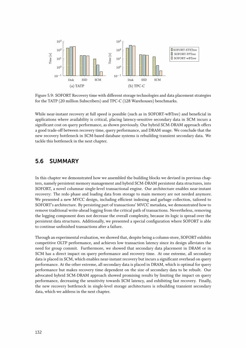
Disk SSD SCM10−1
100
101
102
103
Tim
e[s
]
(a) TATP
Disk SSD SCM10−1
100
101
102
103
Tim
e[s
]
(b) TPC-C
SOFORT-STXTreeSOFORT-FPTreeSOFORT-wBTree
Figure 5.9: SOFORT Recovery time with different storage technologies and data placement strategiesfor the TATP (20 million Subscribers) and TPC-C (128 Warehouses) benchmarks.
While near-instant recovery at full speed is possible (such as in SOFORT-wBTree) and beneficial inapplications where availability is critical, placing latency-sensitive secondary data in SCM incurs asignificant cost on query performance, as shown previously. Our hybrid SCM-DRAM approach offersa good trade-off between recovery time, query performance, and DRAM usage. We conclude that thenew recovery bottleneck in SCM-based database systems is rebuilding transient secondary data. Wetackle this bottleneck in the next chapter.
5.6 SUMMARY
In this chapter we demonstrated how we assembled the building blocks we devised in previous chap-ters, namely persistent memory management and hybrid SCM-DRAM persistent data structures, intoSOFORT, a novel columnar single-level transactional engine. Our architecture enables near-instantrecovery: The redo phase and loading data from storage to main memory are not needed anymore.We presented a new MVCC design, including efficient indexing and garbage collection, tailored toSOFORT’s architecture. By persisting part of transactions’ MVCC metadata, we demonstrated how toremove traditional write-ahead logging from the critical path of transactions. Nevertheless, removingthe logging component does not decrease the overall complexity, because its logic is spread over thepersistent data structures. Additionally, we presented a special configuration where SOFORT is ableto continue unfinished transactions after a failure.
Through an experimental evaluation, we showed that, despite being a column-store, SOFORT exhibitscompetitive OLTP performance, and achieves low transaction latency since its design alleviates theneed for group commit. Furthermore, we showed that secondary data placement in DRAM or inSCM has a direct impact on query performance and recovery time. At one extreme, all secondarydata is placed in SCM, which enables near-instant recovery but incurs a significant overhead on queryperformance. At the other extreme, all secondary data is placed in DRAM, which is optimal for queryperformance but makes recovery time dependent on the size of secondary data to be rebuilt. Ouradvocated hybrid SCM-DRAM approach showed promising results by limiting the impact on queryperformance, decreasing the sensitivity towards SCM latency, and exhibiting fast recovery. Finally,the new recovery bottleneck in single-level storage architectures is rebuilding transient secondarydata, which we address in the next chapter.
132
6SOFORT RECOVERY TECHNIQUES
A vailability guarantees form an important part of many service level agreements (SLAs) for pro-duction database systems [25]. Database recovery time has a significant and direct impact
on database availability as many database crash conditions are transient (e.g., software bugs, hard-ware faults, and user errors) and for these, restarting is a reasonable approach to recovery. To en-sure transaction durability, traditional in-memory DBMSs periodically persist a copy (checkpoint) ofthe database state and log subsequent updates. Recovery consists of reloading the most recent per-sisted state, applying subsequent updates, and undoing the effects of unfinished transactions. Forin-memory DBMSs reloading the persisted state is typically the bottleneck in this process.
SCM has empowered a new class of database architectures where memory and storage are merged [5,122, 79, 148]. SCM-enabled database systems such as SOFORT keep a single copy of the data that isstored, accessed, and modified directly in SCM. This eliminates the need to reload a consistent statefrom durable media to memory upon recovery, as primary data is accessed directly in SCM. Hence,the new recovery bottleneck is rebuilding DRAM-based data structures. SOFORT allows trading offquery performance for recovery performance by judiciously placing certain secondary data structuresin SCM. However, while this is beneficial for systems with critical availability needs, database systemsare generally optimized for query performance. In this chapter we aim to improve recovery perfor-mance without compromising query performance. Therefore, we assume that all latency-sensitivesecondary data structures are kept in DRAM.
After recovering its SCM-based data structures, SOFORT rebuilds DRAM-based secondary data struc-tures, then starts accepting requests. If DRAM-based secondary data structures are large, restart timescan still be unacceptably long. To address this, we propose an Instant Recovery strategy. It allowsqueries to be processed concurrently with the rebuilding of DRAM-based data structures. However,while the secondary data structures are being rebuilt, request throughput is reduced. Part of the per-formance drop is due to the overhead of rebuilding but a more significant factor is the unavailabilityof the DRAM-based secondary data structures, resulting in sub-optimal access plans.
In this chapter1, we propose a novel recovery strategy, Adaptive Recovery. It is inspired by the observa-tion that not all secondary data structures are equally important to a given workload. It improves oninstant recovery in two ways. First, it prioritizes the rebuilding of DRAM-based secondary data struc-tures based on their benefit to a workload (instant recovery simply uses an arbitrary order). Second,it releases most of the CPU resources dedicated to recovery once all of the important secondary data
1This chapter is partially based on the material in [128, 129].
133
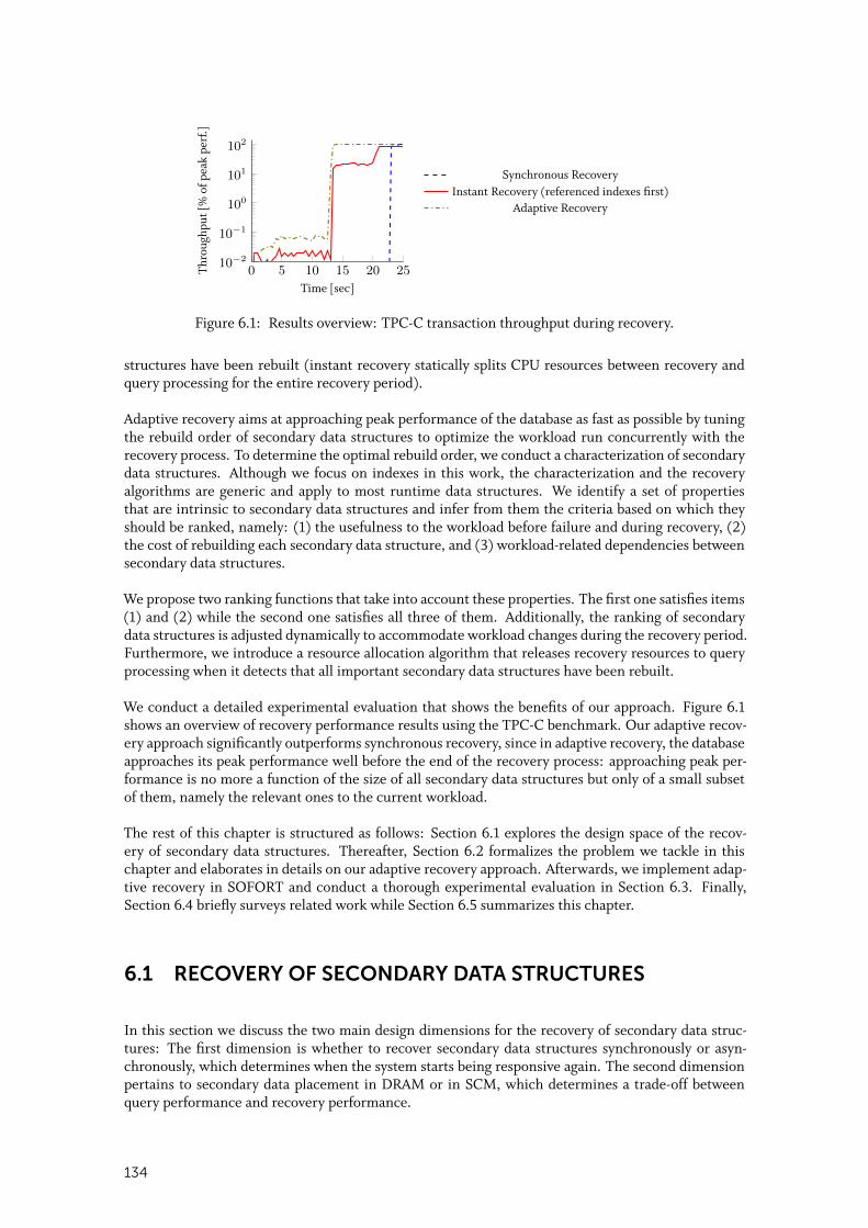
0 5 10 15 20 2510−2
10−1
100
101
102
Time [sec]
Thro
ughp
ut[%
ofpe
akpe
rf.]
Synchronous RecoveryInstant Recovery (referenced indexes first)
Adaptive Recovery
Figure 6.1: Results overview: TPC-C transaction throughput during recovery.
structures have been rebuilt (instant recovery statically splits CPU resources between recovery andquery processing for the entire recovery period).
Adaptive recovery aims at approaching peak performance of the database as fast as possible by tuningthe rebuild order of secondary data structures to optimize the workload run concurrently with therecovery process. To determine the optimal rebuild order, we conduct a characterization of secondarydata structures. Although we focus on indexes in this work, the characterization and the recoveryalgorithms are generic and apply to most runtime data structures. We identify a set of propertiesthat are intrinsic to secondary data structures and infer from them the criteria based on which theyshould be ranked, namely: (1) the usefulness to the workload before failure and during recovery, (2)the cost of rebuilding each secondary data structure, and (3) workload-related dependencies betweensecondary data structures.
We propose two ranking functions that take into account these properties. The first one satisfies items(1) and (2) while the second one satisfies all three of them. Additionally, the ranking of secondarydata structures is adjusted dynamically to accommodate workload changes during the recovery period.Furthermore, we introduce a resource allocation algorithm that releases recovery resources to queryprocessing when it detects that all important secondary data structures have been rebuilt.
We conduct a detailed experimental evaluation that shows the benefits of our approach. Figure 6.1shows an overview of recovery performance results using the TPC-C benchmark. Our adaptive recov-ery approach significantly outperforms synchronous recovery, since in adaptive recovery, the databaseapproaches its peak performance well before the end of the recovery process: approaching peak per-formance is no more a function of the size of all secondary data structures but only of a small subsetof them, namely the relevant ones to the current workload.
The rest of this chapter is structured as follows: Section 6.1 explores the design space of the recov-ery of secondary data structures. Thereafter, Section 6.2 formalizes the problem we tackle in thischapter and elaborates in details on our adaptive recovery approach. Afterwards, we implement adap-tive recovery in SOFORT and conduct a thorough experimental evaluation in Section 6.3. Finally,Section 6.4 briefly surveys related work while Section 6.5 summarizes this chapter.
6.1 RECOVERY OF SECONDARY DATA STRUCTURES
In this section we discuss the two main design dimensions for the recovery of secondary data struc-tures: The first dimension is whether to recover secondary data structures synchronously or asyn-chronously, which determines when the system starts being responsive again. The second dimensionpertains to secondary data placement in DRAM or in SCM, which determines a trade-off betweenquery performance and recovery performance.
134
6.1.1 System Responsiveness
SOFORT recovers by first recovering primary data that is persisted in SCM at a negligible cost, thenundoing the effects of unfinished transactions [122]. The last phase of the recovery procedure, thatis, rebuilding secondary data, can be handled in two different ways: In the first approach, denotedSynchronous Recovery, SOFORT does not accept requests until the end of the recovery process, i.e.,until all secondary data structures have been rebuilt. The main advantage of this approach is thatit rebuilds secondary data structures as fast as possible since all system resources are allocated torecovery. However, this approach suffers from the fact that the database is not responsive during thewhole recovery period, which might be long as its duration depends directly on the size of secondarydata structures to be rebuilt.
In the second approach, denoted Instant Recovery, SOFORT starts accepting new transactions rightafter recovering the persistent data structures. This is possible because all of the primary data arepersistent in SCM, allowing us to process transactions without the vanished transient data structures.However, since the latter are responsible for speeding up query processing, the transaction throughputcould be low at this point in time. Moreover, the rebuilding of the transient data structures can bedone in a specific order, e.g., based on the transactions which need to be continued during recovery.To achieve instant recovery, SOFORT adopts a crawl before run approach: it uses primary data, whichis recovered at a negligible cost, to answer queries, while secondary data structures are rebuilt inthe background. For example, lookups to a dictionary index and an inverted index are replaced byscans of the corresponding dictionary array and the value ID arrays, respectively. Partially rebuiltDRAM-based indexes can be progressively leveraged as they are being rebuilt. For instance, a regulardictionary index lookup is replaced by the following sequence: look up the partially rebuilt dictionaryindex; if the value is not found, then scan only the portion of the dictionary array that has not beenindexed yet. As for hybrid SCM-DRAM indexes, we can only scan their persistent part before theyare fully recovered. Hence, transaction throughput during recovery continuously increases until itreaches, once all data structures have been completely rebuilt, its value observed before failure. Themain advantage of this approach is that it enables instant recovery, i.e., instant responsiveness of thedatabase after failure. However, it takes the database a considerable amount of time, potentially longerthan for synchronous recovery, to approach peak performance observed before failure. This is becausesystem resources are split between recovery and query processing, while in synchronous recovery, allsystem resources are allocated to recovery.
6.1.2 Balancing Query Performance with Recovery Performance
As we have shown in Section 2.1.2, latency-sensitive data structures, such as indexes, perform up toseveral times better when they are located in DRAM, because of its low latency. However, storingsecondary index structures in DRAM causes a significant drop in transaction throughput immediatelyafter recovery, since they have to be rebuilt before the database system can leverage such indexes foroptimized query processing. Operational database systems often require certain guarantees in termsof minimum transaction throughput per second. To enable SOFORT to meet such constraints, weallow placing a certain amount of transient data structures (or all in the extreme scenario) in SCMto store them in a persistent way. By varying the amount of transient and persistent data structures,we are able to balance between a high transaction throughput during usual query processing and aguaranteed minimum throughput during recovery. While SOFORT can achieve near instant recoveryif most secondary data structures are stored in SCM, there is a query performance cost, as many ofthese data structures are latency-sensitive and SCM is expected to have higher latencies than DRAM(cf. Section 5.5).
135
6.1.3 Discussion
From the above description of different recovery trade-offs, we observe that the bottleneck of recov-ery is shifted in SCM-enabled databases from reloading primary data from durable media to mainmemory, to rebuilding secondary data structures. Optimizing the latter did not get much attention inthe past because it was shadowed by the former, more prominent bottleneck. In this chapter we pro-pose a solution to overcome this new bottleneck. For operational databases with critical availabilityrequirements, placing all secondary data in SCM provides near-instant recovery. However, opera-tional databases most often optimize for query performance; we focus on the latter scenario in thischapter. Therefore, we assume in the remainder of this chapter that all latency-sensitive secondarydata structures are kept in DRAM as our goal is to improve recovery performance without compro-mising query performance. Although synchronous recovery and instant recovery exhibit interestingadvantages, they both suffer from (different) noticeable shortcomings. We try to cure the shortcom-ings of both approaches by achieving instant responsiveness and reaching peak performance quickly,well before the end of the recovery process. The following section formalizes the problem and explainsin details how we achieve this.
6.2 ADAPTIVE RECOVERY
Adaptive recovery is based on the observation that not all secondary data structures are equally im-portant to a specific workload. Therefore, rebuilding the most relevant ones first should significantlyimprove the performance of the workload run concurrently with the recovery process, eventually im-proving the overall recovery performance. The following questions arise: What are the characteristicsof secondary data structures? How are secondary data structures rebuilt? How can the benefit of asecondary data structure be measured and estimated for a specific workload?
In this section, we answer these questions in order. We discuss the recovery procedure of secondarydata structures based on a characterization of their recovery properties. Then, we introduce benefitfunctions centered on the usefulness and rebuild cost of these structures given a recovery workload.As the recovery process is usually a very short period of time compared with the time the system isin normal operation, the benefit functions must quickly adapt to the current workload to maximizeperformance of the system during recovery. A recovery manager will take into account the workloadright before the crash and the workload during recovery to decide the recovery procedure of the sec-ondary data structures by answering these questions: What resources are allocated to the recoveryprocess? Does the recovery happen in a background process or synchronously with the statementsneeding them? And what is the recovery order?
6.2.1 Characterization of Secondary Data Structures
Secondary data structures can reside in SCM or in DRAM. The decision for this characteristic can bedecided as part of the database physical design process, based on cost estimated that takes into accountthe schema, the base data properties, the workload, and how fast the recovery process must be. Ina robust system, when recovery must be guaranteed to be almost instantaneous, it may be desired tohave all primary data and secondary data structures in SCM for fast recovery. However, this approachwill significantly impact query performance as discussed in Section 2.1.2.
Secondary data structures, such as indexes, materialized views, intermediate cached results are struc-tures that can be completely rebuilt from primary data. In this work, we identify and assume thefollowing general properties of using and maintaining secondary data structures:
136
1. query processing can be correctly done (i.e. correct result sets) without using any secondarydata structures;
2. secondary data structures are used for improving global performance;3. the decisions to build and use them is cost-based taking into account the cost of maintaining
them, and the performance benefit their usage will bring;4. for a particular statement, the decision to use an available secondary data structure is cost-based;5. secondary data structures may be useful when they are only partially built, and the query opti-
mizer will build correct plans capable of compensating for missing data. For example, this canbe implemented using partially materialized views or cracked indexes.
In an SCM-DRAM hybrid system such as SOFORT, secondary data structures can be built and storedas follows:
• Transient data structures fully residing in DRAM. These structures must be fully rebuilt fromprimary data at restart to reach a consistent state similar to the state before the crash.
• Persistent data structures fully residing in SCM and persisted in real-time. These structures areavailable to be used by query processing, almost instantaneously, after a recover process whichincludes sanity checks and repairs if needed.
• Hybrid transient-persistent data structures partially residing in DRAM, and partially in SCM (e.g.,the FPTree [126]). The persistent part must go through a recovery process which includes sanitychecks and repairs if needed. The transient part is rebuilt based on one or both of the persistentpart and the primary data.
Regardless of the type of a secondary data structure, the rebuild or reload can be executed to comple-tion for the whole structure, or it can be partially done on a need-to-do basis based on the workload,e.g., data cracking techniques [63]. Each secondary data structure can be rebuilt right after restartor on demand, e.g., when this structure is first needed by a transaction (for writes or reads). Thesedecisions should be cost-based, balancing the performance benefit for the workload during recoverywith the overhead of recovery, i.e., reloading and rebuilding.
6.2.2 Benefit Functions for Secondary Data
Regardless of where a secondary data structure resides or what the recovery process for a specificsecondary data structure is, we can compare and rank them based on the usefulness to past and cur-rent workloads, and how expensive it is to rebuild them at recovery time. Our goal is to maximizeperformance of the workload run in parallel with the recovery process. In real database systems, theworkload right after restart can be similar to the workload at crash time (e.g., unfinished transactionsare resubmitted after restart), it can be very different (e.g., the system must execute a specific restartworkload), or a mixed workload including both special restart transactions and resubmitted transac-tions. As the recovery time can be very short, the benefit functions for secondary data structures mustquickly adapt to the current workload and available resources for recovery process.
At first glance, using benefit functions to rank the usefulness of secondary data structures is similar totechniques used for indexes and materialized views selection. Index selection has been studied in theresearch literature, and most commercial database systems have a physical design adviser tool (see,for example, [146] for a survey). The main characteristics of index selection are:
1. Index selection works with a large, known workload that is representative of normal usage ofthe database system;
2. Algorithms for index selection are run off-line, and can take hours;
137
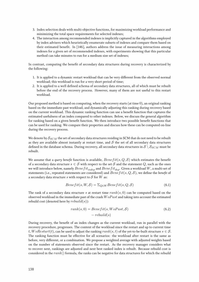
3. Index selection deals with multi-objective functions, for maximizing workload performance andminimizing the total space requirements for selected indexes;
4. The interaction among recommended indexes is implicitly captured in the algorithms employedby index advisers which heuristically enumerate subsets of indexes and compare them based ontheir estimated benefit. In [146], authors address the issue of measuring interactions amongindexes for a given set of recommended indexes, with experiments showing that this particularmethod can take minutes to run for a medium size set of indexes;
In contrast, computing the benefit of secondary data structures during recovery is characterized bythe following:
1. It is applied to a dynamic restart workload that can be very different from the observed normalworkload; this workload is run for a very short period of time;
2. It is applied to a well defined schema of secondary data structures, all of which must be rebuiltbefore the end of the recovery process. However, many of them are not useful to this restartworkload.
Our proposed method is based on computing, when the recovery starts (at time 0), an original rankingbased on the immediate past workload, and dynamically adjusting this ranking during recovery basedon the current workload. This dynamic ranking function can use a benefit function that captures theestimated usefulness of an index compared to other indexes. Below, we discuss the general algorithmfor ranking based on a given benefit function. We then introduce two possible benefit functions thatcan be used for ranking. We compare their properties and discuss how these can be computed on-lineduring the recovery process.
We denote bySSCM the set of secondary data structures residing in SCM that do not need to be rebuiltas they are available almost instantly at restart time, and S the set of all secondary data structuresdefined in the database schema. During recovery, all secondary data structures in S \ SSCM must berebuilt.
We assume that a query benefit function is available, Benefit(s,Q,S) which estimates the benefitof a secondary data structure s ∈ S with respect to the set S and the statement Q, such as the oneswe will introduce below, namely Benefitindep and Benefitdep. Given a workload W , a multi-set ofstatements (i.e., repeated statements are considered) and Benefit(s,Q,S), we define the benefit ofa secondary data structure s with respect to S for W as:
Benefit(s,W,S) = ΣQ∈WBenefit(s,Q,S) (6.1)
The rank of a secondary data structure s at restart time rank(s, 0) can be computed based on theobserved workload in the immediate past of the crash WoPast and taking into account the estimatedrebuild cost (denoted here by rebuild(s)):
rank(s, 0) =Benefit(s,WoPast,S) (6.2)
− rebuild(s)
During recovery, the benefit of an index changes as the current workload, run in parallel with therecovery procedure, progresses. The content of the workload since the restart and up to current timet, WoRestart(t), can be used to adjust the ranking rank(s, t) of the yet-to-be-built structure s ∈ S.The ranking function must be effective for all scenarios: the workload after restart is the same asbefore, very different, or a combination. We propose a weighted average with adjusted weights basedon the number of statements observed since the restart. As the recovery manager considers whatto recover next, rankings are adjusted and next best ranked index is rebuilt. Because rebuild cost isconsidered in the rank() formula, the ranks can be negative for data structures for which the rebuild
138
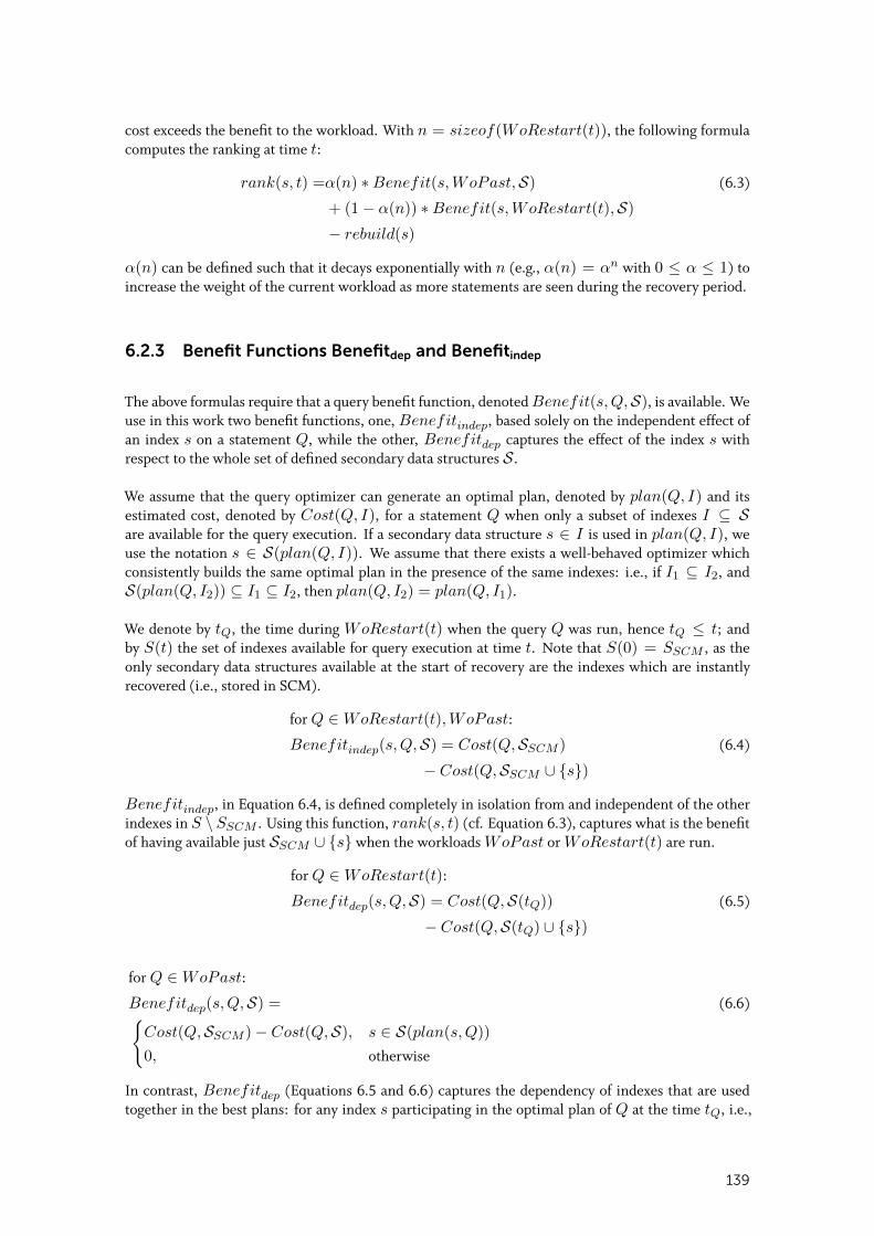
cost exceeds the benefit to the workload. With n = sizeof(WoRestart(t)), the following formulacomputes the ranking at time t:
rank(s, t) =α(n) ∗Benefit(s,WoPast,S) (6.3)
+ (1− α(n)) ∗Benefit(s,WoRestart(t),S)− rebuild(s)
α(n) can be defined such that it decays exponentially with n (e.g., α(n) = αn with 0 ≤ α ≤ 1) toincrease the weight of the current workload as more statements are seen during the recovery period.
6.2.3 Benefit Functions Benefitdep and Benefitindep
The above formulas require that a query benefit function, denoted Benefit(s,Q,S), is available. Weuse in this work two benefit functions, one, Benefitindep, based solely on the independent effect ofan index s on a statement Q, while the other, Benefitdep captures the effect of the index s withrespect to the whole set of defined secondary data structures S.
We assume that the query optimizer can generate an optimal plan, denoted by plan(Q, I) and itsestimated cost, denoted by Cost(Q, I), for a statement Q when only a subset of indexes I ⊆ Sare available for the query execution. If a secondary data structure s ∈ I is used in plan(Q, I), weuse the notation s ∈ S(plan(Q, I)). We assume that there exists a well-behaved optimizer whichconsistently builds the same optimal plan in the presence of the same indexes: i.e., if I1 ⊆ I2, andS(plan(Q, I2)) ⊆ I1 ⊆ I2, then plan(Q, I2) = plan(Q, I1).
We denote by tQ, the time during WoRestart(t) when the query Q was run, hence tQ ≤ t; andby S(t) the set of indexes available for query execution at time t. Note that S(0) = SSCM , as theonly secondary data structures available at the start of recovery are the indexes which are instantlyrecovered (i.e., stored in SCM).
for Q ∈ WoRestart(t),WoPast:
Benefitindep(s,Q,S) = Cost(Q,SSCM ) (6.4)
− Cost(Q,SSCM ∪ {s})
Benefitindep, in Equation 6.4, is defined completely in isolation from and independent of the otherindexes in S \ SSCM . Using this function, rank(s, t) (cf. Equation 6.3), captures what is the benefitof having available just SSCM ∪ {s} when the workloads WoPast or WoRestart(t) are run.
for Q ∈ WoRestart(t):
Benefitdep(s,Q,S) = Cost(Q,S(tQ)) (6.5)
− Cost(Q,S(tQ) ∪ {s})
for Q ∈ WoPast:
Benefitdep(s,Q,S) = (6.6){Cost(Q,SSCM )− Cost(Q,S), s ∈ S(plan(s,Q))
0, otherwise
In contrast, Benefitdep (Equations 6.5 and 6.6) captures the dependency of indexes that are usedtogether in the best plans: for any index s participating in the optimal plan of Q at the time tQ, i.e.,
139
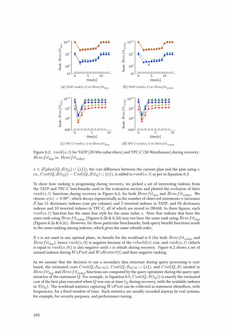
0 5 10
100
107
1014
time[s]
Ran
k:Ben
efit
dep
-15
(a) TATP rank(s, t) w/ Benefitdep
0 5 10
100
107
1014
time[s]
Ran
k:Ben
efit
indep
-15
(b) TATP rank(s, t) w/ Benefitindep
0 5 10
106
109
1012
time[s]
Ran
k:Ben
efit
dep
-650
(c) TPC-C rank(s, t) w/ Benefitdep
0 5 10
106
109
1012
time[s]
Ran
k:Ben
efit
indep
-650
(d) TPC-C rank(s, t) w/ Benefitindep
Figure 6.2: rank(s, t) for TATP (20 Mio subscribers) and TPC-C (50 Warehouses) during recovery :Benefitdep vs. Benefitindep.
s ∈ S(plan(Q,S(tQ) ∪ {s})), the cost difference between the current plan and the plan using s,i.e., Cost(Q,S(tQ))− Cost(Q,S(tQ) ∪ {s}), is added to rank(s, t) as per in Equation 6.3.
To show how ranking is progressing during recovery, we picked a set of interesting indexes fromthe TATP and TPC-C benchmarks used in the evaluation section and plotted the evolution of theirrank(s, t) functions during recovery in Figure 6.2, for both Benefitdep and Benefitindep. Wechoose α(n) = 0.99n, which decays exponentially as the number of observed statements n increases.S has 51 dictionary indexes (one per column) and 5 inverted indexes in TATP, and 94 dictionaryindexes and 10 inverted indexes in TPC-C, all of which are stored in DRAM. In these figures, eachrank(s, t) function has the same line style for the same index s. Note that indexes that have thesame rank using Benefitindep (Figures 6.2b & 6.2d) may not have the same rank using Benefitdep(Figures 6.2a & 6.2c). However, for these particular benchmarks, both query benefit functions resultin the same ranking among indexes, which gives the same rebuild order.
If s is not used in any optimal plans, its benefit for the workload is 0 (for both Benefitindep andBenefitdep), hence rank(s, 0) is negative because of the rebuild(s) cost, and rank(s, t) (whichis equal to rank(s, 0)) is also negative until s is rebuilt during recovery. Figure 6.2 shows a set ofunused indexes during WoPast and WoRestart(t) and their negative ranking.
As we assume that the decision to use a secondary data structure during query processing is cost-based, the estimated costs Cost(Q,SSCM ), Cost(Q,SSCM ∪ {s}), and Cost(Q,S) needed inBenefitdep and Benefitindep functions are computed by the query optimizer during the query opti-mization of the statement Q. For example, in Equation 6.5, Cost(Q,S(tQ)) is exactly the estimatedcost of the best plan executed when Q was run at time tQ during recovery, with the available indexesin S(tQ). The workload statistics capturing WoPast can be collected as statement identifiers, withfrequencies, for a fixed window of time. Such statistics are usually recorded anyway by real systems,for example, for security purposes, and performance tuning.
140
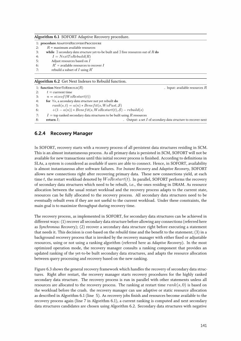
Algorithm 6.1 SOFORT Adaptive Recovery procedure.1: procedure AdaptiveRecoveryProcedure2: R = maximum available resources3: while ∃ secondary data structure yet-to-be built and ∃ free resources out of R do4: I = NextToRebuild(R)5: Adjust resources based on I6: R′ = available resources to recover I7: rebuild a subset of I using R′
Algorithm 6.2 Get Next Indexes to Rebuild function.1: function NextToRebuild(R) ◃ Input: available resources R2: t = currrent time3: n = sizeof(WoRestart(t))4: for ∀s, a secondary data structure not yet rebuilt do5: rank(s, t) = α(n) ∗Benefit(s,WoPast,S)6: +(1− α(n)) ∗Benefit(s,WoRestart(t),S)− rebuild(s)
7: I = top ranked secondary data structures to be built using R resources8: return I; ◃ Output: a set I of secondary data structure to recover next
6.2.4 Recovery Manager
In SOFORT, recovery starts with a recovery process of all persistent data structures residing in SCM.This is an almost instantaneous process. As all primary data is persisted in SCM, SOFORT will not beavailable for new transactions until this initial recover process is finished. According to definitions inSLAs, a system is considered as available if users are able to connect. Hence, in SOFORT, availabilityis almost instantaneous after software failures. For Instant Recovery and Adaptive Recovery, SOFORTallows new connections right after recovering primary data. These new connections yield, at eachtime t, the restart workload denoted by WoRestart(t). In parallel, SOFORT performs the recoveryof secondary data structures which need to be rebuilt, i.e., the ones residing in DRAM. As resourceallocation between the usual restart workload and the recovery process adapts to the current state,resources can be fully allocated to the recovery process. All secondary data structures need to beeventually rebuilt even if they are not useful to the current workload. Under these constraints, themain goal is to maximize throughput during recovery time.
The recovery process, as implemented in SOFORT, for secondary data structures can be achieved indifferent ways: (1) recover all secondary data structure before allowing any connections (referred hereas Synchronous Recovery); (2) recover a secondary data structure right before executing a statementthat needs it. This decision is cost-based on the rebuild time and the benefit to the statement; (3) in abackground recovery process that is invoked by the recovery manager with either fixed or adjustableresources, using or not using a ranking algorithm (referred here as Adaptive Recovery). In the mostoptimized operation mode, the recovery manager consults a ranking component that provides anupdated ranking of the yet-to-be built secondary data structures, and adapts the resource allocationbetween query processing and recovery based on the new ranking.
Figure 6.3 shows the general recovery framework which handles the recovery of secondary data struc-tures. Right after restart, the recovery manager starts recovery procedures for the highly rankedsecondary data structure. The recovery process is run in parallel with other statements unless allresources are allocated to the recovery process. The ranking at restart time rank(s, 0) is based onthe workload before the crash. the recovery manager can use adaptive or static resource allocationas described in Algorithm 6.1 (line 5). As recovery jobs finish and resources become available to therecovery process again (line 7 in Algorithm 6.1), a current ranking is computed and next secondarydata structures candidates are chosen using Algorithm 6.2. Secondary data structures with negative
141
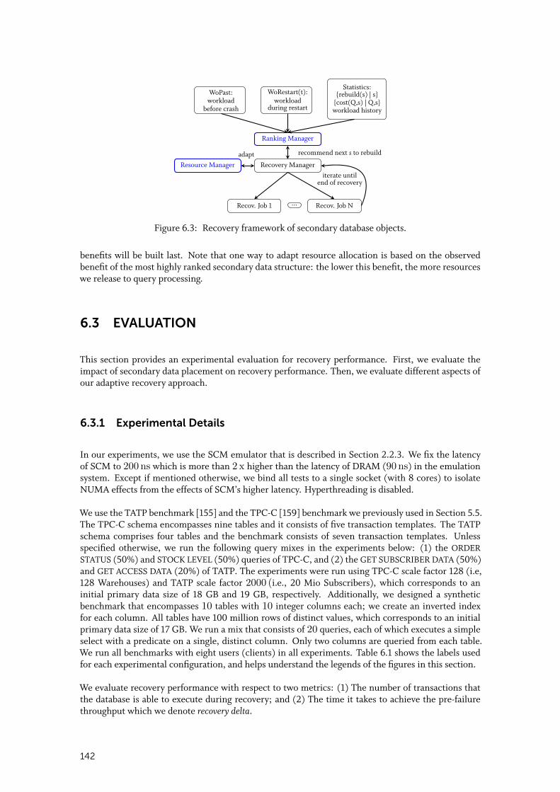
WoPast:workload
before crash
WoRestart(t):workload
during restart
Statistics:{rebuild(s) | s}
{cost(Q,s) | Q,s}workload history
Ranking Manager
Recovery ManagerResource Manager
Recov. Job 1 Recov. Job N
recommend next s to rebuildadapt
iterate untilend of recovery
...
Figure 6.3: Recovery framework of secondary database objects.
benefits will be built last. Note that one way to adapt resource allocation is based on the observedbenefit of the most highly ranked secondary data structure: the lower this benefit, the more resourceswe release to query processing.
6.3 EVALUATION
This section provides an experimental evaluation for recovery performance. First, we evaluate theimpact of secondary data placement on recovery performance. Then, we evaluate different aspects ofour adaptive recovery approach.
6.3.1 Experimental Details
In our experiments, we use the SCM emulator that is described in Section 2.2.3. We fix the latencyof SCM to 200 ns which is more than 2 x higher than the latency of DRAM (90 ns) in the emulationsystem. Except if mentioned otherwise, we bind all tests to a single socket (with 8 cores) to isolateNUMA effects from the effects of SCM’s higher latency. Hyperthreading is disabled.
We use the TATP benchmark [155] and the TPC-C [159] benchmark we previously used in Section 5.5.The TPC-C schema encompasses nine tables and it consists of five transaction templates. The TATPschema comprises four tables and the benchmark consists of seven transaction templates. Unlessspecified otherwise, we run the following query mixes in the experiments below: (1) the ORDERSTATUS (50%) and STOCK LEVEL (50%) queries of TPC-C, and (2) the GET SUBSCRIBER DATA (50%)and GET ACCESS DATA (20%) of TATP. The experiments were run using TPC-C scale factor 128 (i.e,128 Warehouses) and TATP scale factor 2000 (i.e., 20 Mio Subscribers), which corresponds to aninitial primary data size of 18 GB and 19 GB, respectively. Additionally, we designed a syntheticbenchmark that encompasses 10 tables with 10 integer columns each; we create an inverted indexfor each column. All tables have 100 million rows of distinct values, which corresponds to an initialprimary data size of 17 GB. We run a mix that consists of 20 queries, each of which executes a simpleselect with a predicate on a single, distinct column. Only two columns are queried from each table.We run all benchmarks with eight users (clients) in all experiments. Table 6.1 shows the labels usedfor each experimental configuration, and helps understand the legends of the figures in this section.
We evaluate recovery performance with respect to two metrics: (1) The number of transactions thatthe database is able to execute during recovery; and (2) The time it takes to achieve the pre-failurethroughput which we denote recovery delta.
142
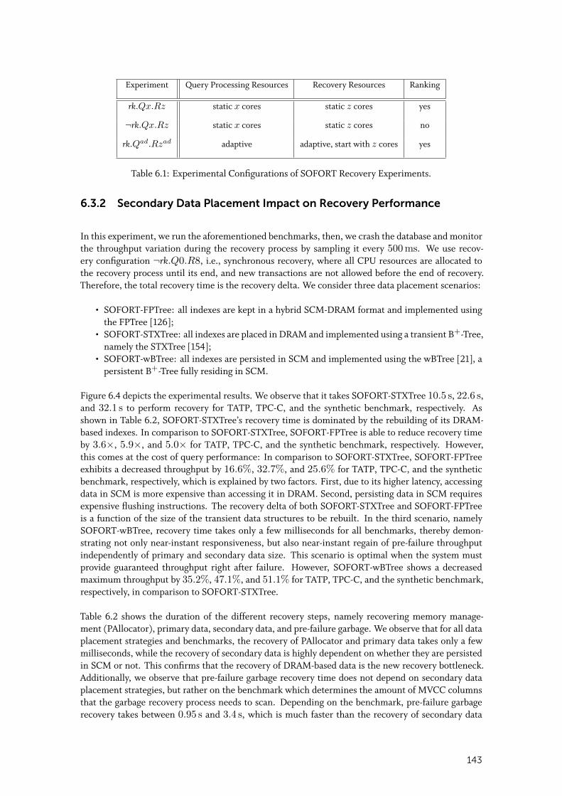
Experiment Query Processing Resources Recovery Resources Ranking
rk.Qx.Rz static x cores static z cores yes
¬rk.Qx.Rz static x cores static z cores no
rk.Qad.Rzad adaptive adaptive, start with z cores yes
Table 6.1: Experimental Configurations of SOFORT Recovery Experiments.
6.3.2 Secondary Data Placement Impact on Recovery Performance
In this experiment, we run the aforementioned benchmarks, then, we crash the database and monitorthe throughput variation during the recovery process by sampling it every 500ms. We use recov-ery configuration ¬rk.Q0.R8, i.e., synchronous recovery, where all CPU resources are allocated tothe recovery process until its end, and new transactions are not allowed before the end of recovery.Therefore, the total recovery time is the recovery delta. We consider three data placement scenarios:
• SOFORT-FPTree: all indexes are kept in a hybrid SCM-DRAM format and implemented usingthe FPTree [126];
• SOFORT-STXTree: all indexes are placed in DRAM and implemented using a transient B+-Tree,namely the STXTree [154];
• SOFORT-wBTree: all indexes are persisted in SCM and implemented using the wBTree [21], apersistent B+-Tree fully residing in SCM.
Figure 6.4 depicts the experimental results. We observe that it takes SOFORT-STXTree 10.5 s, 22.6 s,and 32.1 s to perform recovery for TATP, TPC-C, and the synthetic benchmark, respectively. Asshown in Table 6.2, SOFORT-STXTree’s recovery time is dominated by the rebuilding of its DRAM-based indexes. In comparison to SOFORT-STXTree, SOFORT-FPTree is able to reduce recovery timeby 3.6×, 5.9×, and 5.0× for TATP, TPC-C, and the synthetic benchmark, respectively. However,this comes at the cost of query performance: In comparison to SOFORT-STXTree, SOFORT-FPTreeexhibits a decreased throughput by 16.6%, 32.7%, and 25.6% for TATP, TPC-C, and the syntheticbenchmark, respectively, which is explained by two factors. First, due to its higher latency, accessingdata in SCM is more expensive than accessing it in DRAM. Second, persisting data in SCM requiresexpensive flushing instructions. The recovery delta of both SOFORT-STXTree and SOFORT-FPTreeis a function of the size of the transient data structures to be rebuilt. In the third scenario, namelySOFORT-wBTree, recovery time takes only a few milliseconds for all benchmarks, thereby demon-strating not only near-instant responsiveness, but also near-instant regain of pre-failure throughputindependently of primary and secondary data size. This scenario is optimal when the system mustprovide guaranteed throughput right after failure. However, SOFORT-wBTree shows a decreasedmaximum throughput by 35.2%, 47.1%, and 51.1% for TATP, TPC-C, and the synthetic benchmark,respectively, in comparison to SOFORT-STXTree.
Table 6.2 shows the duration of the different recovery steps, namely recovering memory manage-ment (PAllocator), primary data, secondary data, and pre-failure garbage. We observe that for all dataplacement strategies and benchmarks, the recovery of PAllocator and primary data takes only a fewmilliseconds, while the recovery of secondary data is highly dependent on whether they are persistedin SCM or not. This confirms that the recovery of DRAM-based data is the new recovery bottleneck.Additionally, we observe that pre-failure garbage recovery time does not depend on secondary dataplacement strategies, but rather on the benchmark which determines the amount of MVCC columnsthat the garbage recovery process needs to scan. Depending on the benchmark, pre-failure garbagerecovery takes between 0.95 s and 3.4 s, which is much faster than the recovery of secondary data
143
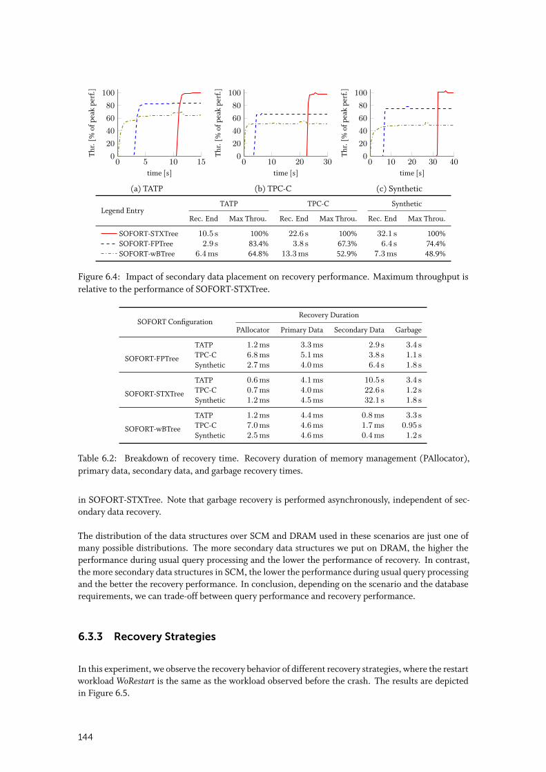
0 5 10 150
20
40
60
80
100
time [s]
Thr.
[%of
peak
perf
.]
(a) TATP
0 10 20 300
20
40
60
80
100
time [s]
Thr.
[%of
peak
perf
.]
(b) TPC-C
0 10 20 30 400
20
40
60
80
100
time [s]
Thr.
[%of
peak
perf
.]
(c) Synthetic
Legend EntryTATP TPC-C Synthetic
Rec. End Max Throu. Rec. End Max Throu. Rec. End Max Throu.
SOFORT-STXTree 10.5 s 100% 22.6 s 100% 32.1 s 100%SOFORT-FPTree 2.9 s 83.4% 3.8 s 67.3% 6.4 s 74.4%SOFORT-wBTree 6.4ms 64.8% 13.3ms 52.9% 7.3ms 48.9%
Figure 6.4: Impact of secondary data placement on recovery performance. Maximum throughput isrelative to the performance of SOFORT-STXTree.
SOFORT ConfigurationRecovery Duration
PAllocator Primary Data Secondary Data Garbage
SOFORT-FPTree
TATP 1.2ms 3.3ms 2.9 s 3.4 sTPC-C 6.8ms 5.1ms 3.8 s 1.1 sSynthetic 2.7ms 4.0ms 6.4 s 1.8 s
SOFORT-STXTree
TATP 0.6ms 4.1ms 10.5 s 3.4 sTPC-C 0.7ms 4.0ms 22.6 s 1.2 sSynthetic 1.2ms 4.5ms 32.1 s 1.8 s
SOFORT-wBTree
TATP 1.2ms 4.4ms 0.8ms 3.3 sTPC-C 7.0ms 4.6ms 1.7ms 0.95 sSynthetic 2.5ms 4.6ms 0.4ms 1.2 s
Table 6.2: Breakdown of recovery time. Recovery duration of memory management (PAllocator),primary data, secondary data, and garbage recovery times.
in SOFORT-STXTree. Note that garbage recovery is performed asynchronously, independent of sec-ondary data recovery.
The distribution of the data structures over SCM and DRAM used in these scenarios are just one ofmany possible distributions. The more secondary data structures we put on DRAM, the higher theperformance during usual query processing and the lower the performance of recovery. In contrast,the more secondary data structures in SCM, the lower the performance during usual query processingand the better the recovery performance. In conclusion, depending on the scenario and the databaserequirements, we can trade-off between query performance and recovery performance.
6.3.3 Recovery Strategies
In this experiment, we observe the recovery behavior of different recovery strategies, where the restartworkload WoRestart is the same as the workload observed before the crash. The results are depictedin Figure 6.5.
144
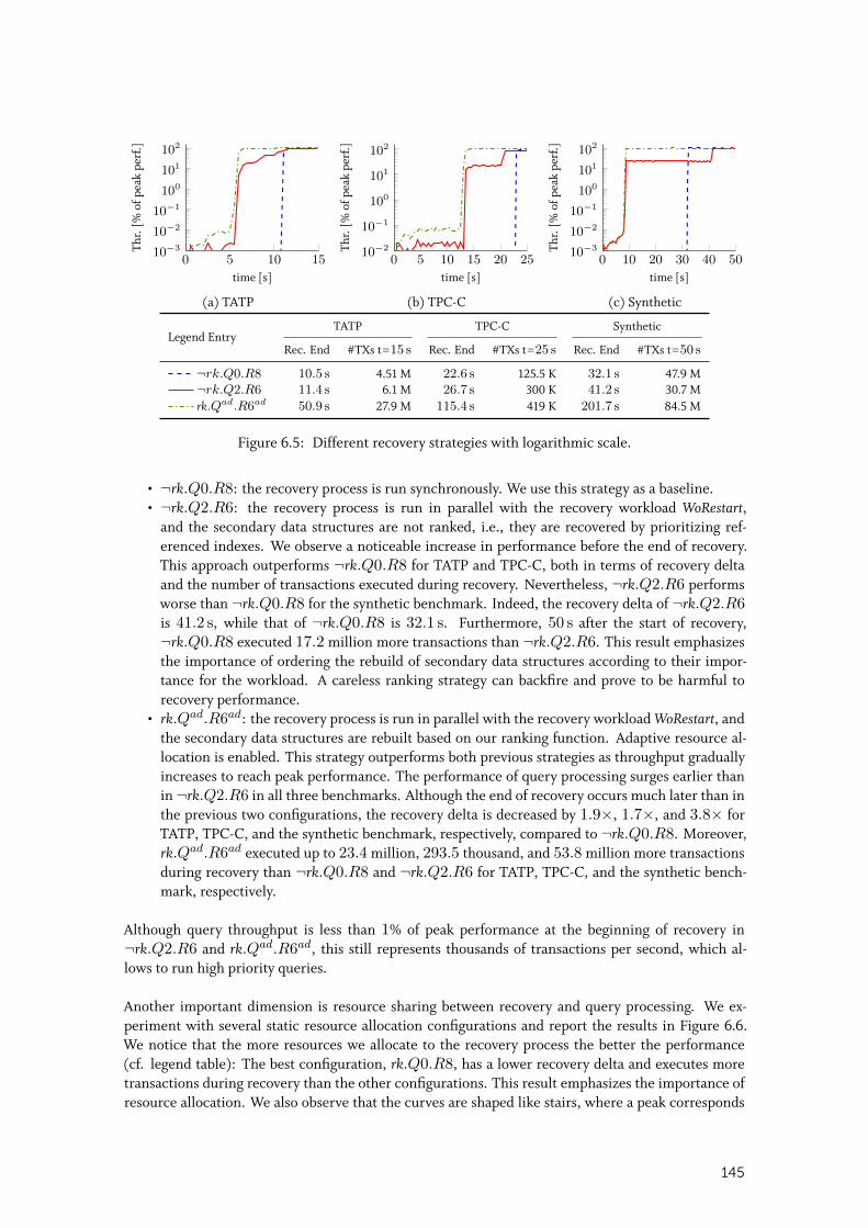
0 5 10 1510−3
10−2
10−1
100101102
time [s]
Thr.
[%of
peak
perf
.]
(a) TATP
0 5 10 15 20 2510−2
10−1
100
101
102
time [s]
Thr.
[%of
peak
perf
.]
(b) TPC-C
0 10 20 30 40 5010−3
10−2
10−1
100101102
time [s]
Thr.
[%of
peak
perf
.]
(c) Synthetic
Legend EntryTATP TPC-C Synthetic
Rec. End #TXs t=15 s Rec. End #TXs t=25 s Rec. End #TXs t=50 s
¬rk.Q0.R8 10.5 s 4.51 M 22.6 s 125.5 K 32.1 s 47.9 M¬rk.Q2.R6 11.4 s 6.1 M 26.7 s 300 K 41.2 s 30.7 Mrk.Qad.R6ad 50.9 s 27.9 M 115.4 s 419 K 201.7 s 84.5 M
Figure 6.5: Different recovery strategies with logarithmic scale.
• ¬rk.Q0.R8: the recovery process is run synchronously. We use this strategy as a baseline.• ¬rk.Q2.R6: the recovery process is run in parallel with the recovery workload WoRestart,
and the secondary data structures are not ranked, i.e., they are recovered by prioritizing ref-erenced indexes. We observe a noticeable increase in performance before the end of recovery.This approach outperforms ¬rk.Q0.R8 for TATP and TPC-C, both in terms of recovery deltaand the number of transactions executed during recovery. Nevertheless, ¬rk.Q2.R6 performsworse than ¬rk.Q0.R8 for the synthetic benchmark. Indeed, the recovery delta of ¬rk.Q2.R6is 41.2 s, while that of ¬rk.Q0.R8 is 32.1 s. Furthermore, 50 s after the start of recovery,¬rk.Q0.R8 executed 17.2 million more transactions than ¬rk.Q2.R6. This result emphasizesthe importance of ordering the rebuild of secondary data structures according to their impor-tance for the workload. A careless ranking strategy can backfire and prove to be harmful torecovery performance.
• rk.Qad.R6ad: the recovery process is run in parallel with the recovery workload WoRestart, andthe secondary data structures are rebuilt based on our ranking function. Adaptive resource al-location is enabled. This strategy outperforms both previous strategies as throughput graduallyincreases to reach peak performance. The performance of query processing surges earlier thanin ¬rk.Q2.R6 in all three benchmarks. Although the end of recovery occurs much later than inthe previous two configurations, the recovery delta is decreased by 1.9×, 1.7×, and 3.8× forTATP, TPC-C, and the synthetic benchmark, respectively, compared to ¬rk.Q0.R8. Moreover,rk.Qad.R6ad executed up to 23.4 million, 293.5 thousand, and 53.8 million more transactionsduring recovery than ¬rk.Q0.R8 and ¬rk.Q2.R6 for TATP, TPC-C, and the synthetic bench-mark, respectively.
Although query throughput is less than 1% of peak performance at the beginning of recovery in¬rk.Q2.R6 and rk.Qad.R6ad, this still represents thousands of transactions per second, which al-lows to run high priority queries.
Another important dimension is resource sharing between recovery and query processing. We ex-periment with several static resource allocation configurations and report the results in Figure 6.6.We notice that the more resources we allocate to the recovery process the better the performance(cf. legend table): The best configuration, rk.Q0.R8, has a lower recovery delta and executes moretransactions during recovery than the other configurations. This result emphasizes the importance ofresource allocation. We also observe that the curves are shaped like stairs, where a peak corresponds
145

0 5 15 25 350
20
40
60
80
100
time [s]
Thr.
[%of
peak
perf
.]
(a) TATP
0 10 20 30 40 50 60 700
20
40
60
80
100
time [s]
Thr.
[%of
peak
perf
.]
(b) TPC-C
0 10 20 30 40 50 60 700
20
40
60
80
100
time [s]
Thr.
[%of
peak
perf
.]
(c) Synthetic
Legend EntryTATP TPC-C Synthetic
Rec. End #TXs t=35 s Rec. End #TXs t=70 s Rec. End #TXs t=70 s
rk.Q6.R2 29.3 s 24.2 M 62.2 s 2.4 M 121.1 s 89.9 Mrk.Q4.R4 15.9 s 25.4 M 36.6 s 2.5 M 61.3 s 86.5 Mrk.Q2.R6 11.4 s 27.4 M 27.1 s 2.6 M 41.0 s 96.7 Mrk.Q0.R8 10.6 s 28.3 M 25.0 s 2.8 M 31.2 s 102.2 M
Figure 6.6: Static resource allocation impact on recovery.
to the end of the recovery of an important secondary data structures group. The reason why the in-crease in throughput is in stair-steps and not linear is the design of the benchmark: all users run thesame mix of queries, which means that even if only one single query did not regain its optimal perfor-mance, it will drain the query throughput down across all users. Hence, substantial improvements inthroughput occur only once the performance of all queries improves. This setup is not in favor of ourapproach, as earlier benefits of our approach could be observed in a different setup where users rundifferent queries from each other, or run the same queries on different copies of the data.
We also notice that the more resources allocated to recovery, the sooner the first stair-step appearsand the lower it is. This is due to the fact that more resources for recovery means faster rebuild ofsecondary data structures (hence faster appearance of stair-steps) and slower query processing due tothe lack of resources (hence, the lower the stair-steps). The last peak that brings each configurationback to peak performance takes place at the end of the recovery process, which again happens soonerwith more recovery resources, but configurations with less recovery resources compensate with higherstair-steps. An intuition that stems from this result is that a combination of all configurations, suchthat recovery starts with more resources and releases them gradually whenever query performancesurges might lead to a better recovery performance.
6.3.4 Adaptive Resource Allocation Algorithm
In this experiment, we investigate the efficiency of our adaptive resource allocation algorithm. Therecovery manager is given specific resources and is free to use them fully and/or return them partial-ly/fully to query processing. Basically, the recovery manager decides to give back recovery resourcesto query processing once it detects, based on the benefit value of the most highly ranked index, thatenough secondary data structures have been rebuilt to allow the system to run at nearly full speed.The remaining secondary data structures are recovered in the background whenever the CPU idles.
Figure 6.7 summarizes the results of this experiment. Theoretically, allocating more resources torecovery should enable the database to reach peak performance sooner. Notably, we observe that forTATP and TPC-C, all investigated recovery configurations perform nearly equally. This is explained
146
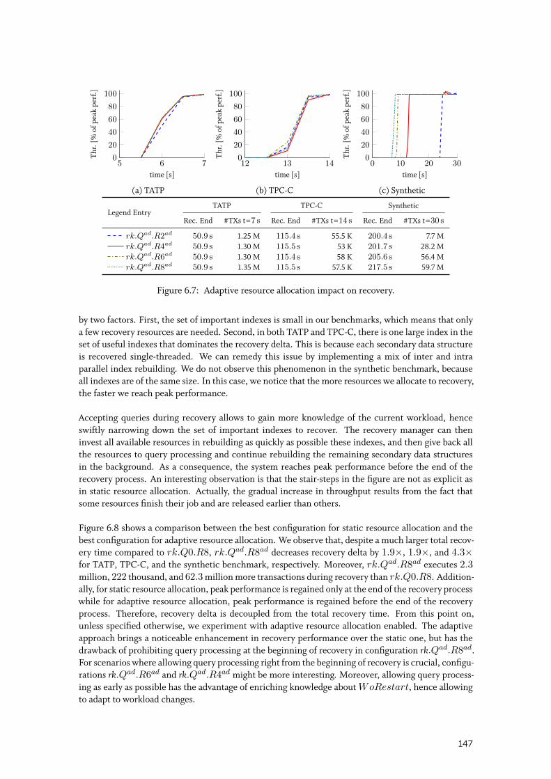
5 6 70
20
40
60
80
100
time [s]
Thr.
[%of
peak
perf
.]
(a) TATP
12 13 140
20
40
60
80
100
time [s]
Thr.
[%of
peak
perf
.]
(b) TPC-C
0 10 20 300
20
40
60
80
100
time [s]
Thr.
[%of
peak
perf
.]
(c) Synthetic
Legend EntryTATP TPC-C Synthetic
Rec. End #TXs t=7 s Rec. End #TXs t=14 s Rec. End #TXs t=30 s
rk.Qad.R2ad 50.9 s 1.25 M 115.4 s 55.5 K 200.4 s 7.7 Mrk.Qad.R4ad 50.9 s 1.30 M 115.5 s 53 K 201.7 s 28.2 Mrk.Qad.R6ad 50.9 s 1.30 M 115.4 s 58 K 205.6 s 56.4 Mrk.Qad.R8ad 50.9 s 1.35 M 115.5 s 57.5 K 217.5 s 59.7 M
Figure 6.7: Adaptive resource allocation impact on recovery.
by two factors. First, the set of important indexes is small in our benchmarks, which means that onlya few recovery resources are needed. Second, in both TATP and TPC-C, there is one large index in theset of useful indexes that dominates the recovery delta. This is because each secondary data structureis recovered single-threaded. We can remedy this issue by implementing a mix of inter and intraparallel index rebuilding. We do not observe this phenomenon in the synthetic benchmark, becauseall indexes are of the same size. In this case, we notice that the more resources we allocate to recovery,the faster we reach peak performance.
Accepting queries during recovery allows to gain more knowledge of the current workload, henceswiftly narrowing down the set of important indexes to recover. The recovery manager can theninvest all available resources in rebuilding as quickly as possible these indexes, and then give back allthe resources to query processing and continue rebuilding the remaining secondary data structuresin the background. As a consequence, the system reaches peak performance before the end of therecovery process. An interesting observation is that the stair-steps in the figure are not as explicit asin static resource allocation. Actually, the gradual increase in throughput results from the fact thatsome resources finish their job and are released earlier than others.
Figure 6.8 shows a comparison between the best configuration for static resource allocation and thebest configuration for adaptive resource allocation. We observe that, despite a much larger total recov-ery time compared to rk.Q0.R8, rk.Qad.R8ad decreases recovery delta by 1.9×, 1.9×, and 4.3×for TATP, TPC-C, and the synthetic benchmark, respectively. Moreover, rk.Qad.R8ad executes 2.3million, 222 thousand, and 62.3 million more transactions during recovery than rk.Q0.R8. Addition-ally, for static resource allocation, peak performance is regained only at the end of the recovery processwhile for adaptive resource allocation, peak performance is regained before the end of the recoveryprocess. Therefore, recovery delta is decoupled from the total recovery time. From this point on,unless specified otherwise, we experiment with adaptive resource allocation enabled. The adaptiveapproach brings a noticeable enhancement in recovery performance over the static one, but has thedrawback of prohibiting query processing at the beginning of recovery in configuration rk.Qad.R8ad.For scenarios where allowing query processing right from the beginning of recovery is crucial, configu-rations rk.Qad.R6ad and rk.Qad.R4ad might be more interesting. Moreover, allowing query process-ing as early as possible has the advantage of enriching knowledge about WoRestart, hence allowingto adapt to workload changes.
147
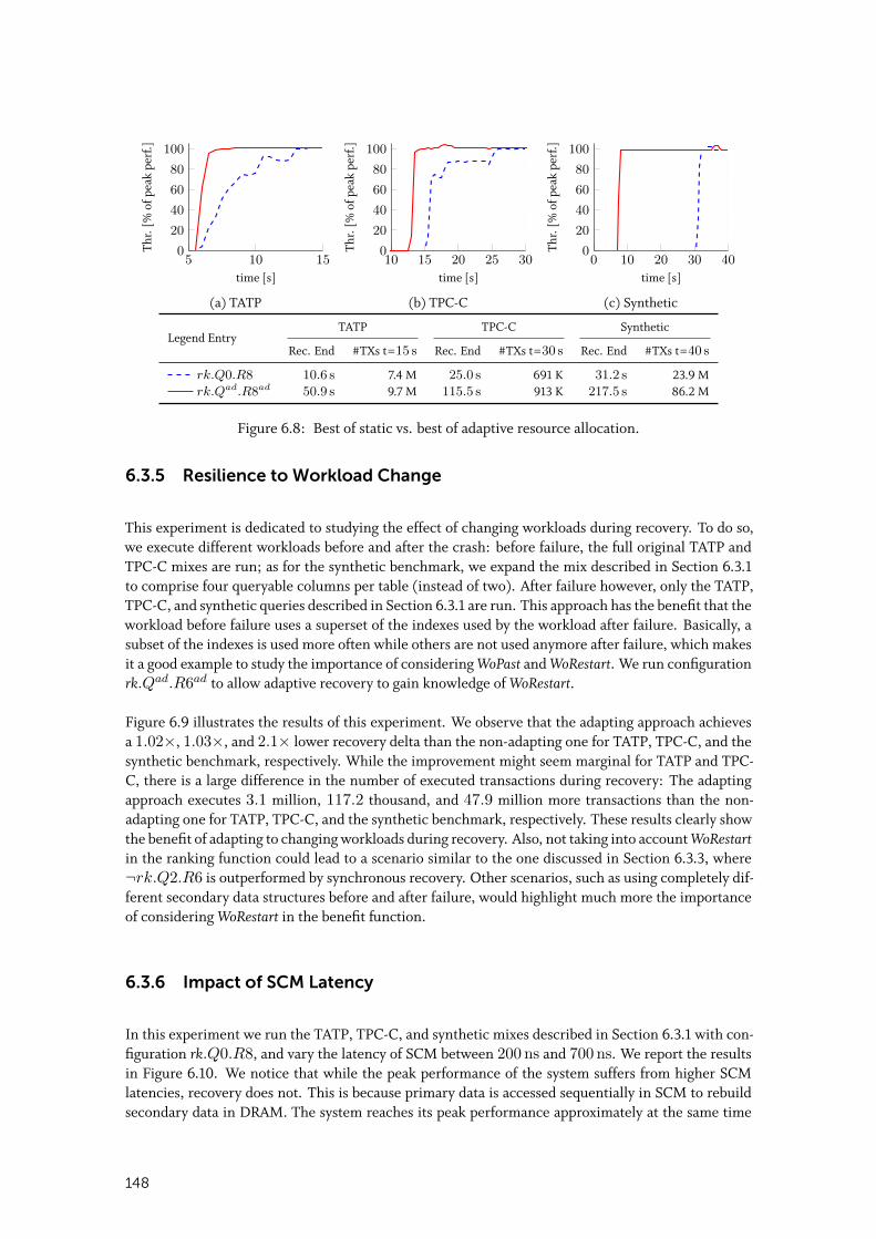
5 10 150
20
40
60
80
100
time [s]
Thr.
[%of
peak
perf
.]
(a) TATP
10 15 20 25 300
20
40
60
80
100
time [s]
Thr.
[%of
peak
perf
.]
(b) TPC-C
0 10 20 30 400
20
40
60
80
100
time [s]
Thr.
[%of
peak
perf
.]
(c) Synthetic
Legend EntryTATP TPC-C Synthetic
Rec. End #TXs t=15 s Rec. End #TXs t=30 s Rec. End #TXs t=40 s
rk.Q0.R8 10.6 s 7.4 M 25.0 s 691 K 31.2 s 23.9 Mrk.Qad.R8ad 50.9 s 9.7 M 115.5 s 913 K 217.5 s 86.2 M
Figure 6.8: Best of static vs. best of adaptive resource allocation.
6.3.5 Resilience to Workload Change
This experiment is dedicated to studying the effect of changing workloads during recovery. To do so,we execute different workloads before and after the crash: before failure, the full original TATP andTPC-C mixes are run; as for the synthetic benchmark, we expand the mix described in Section 6.3.1to comprise four queryable columns per table (instead of two). After failure however, only the TATP,TPC-C, and synthetic queries described in Section 6.3.1 are run. This approach has the benefit that theworkload before failure uses a superset of the indexes used by the workload after failure. Basically, asubset of the indexes is used more often while others are not used anymore after failure, which makesit a good example to study the importance of considering WoPast and WoRestart. We run configurationrk.Qad.R6ad to allow adaptive recovery to gain knowledge of WoRestart.
Figure 6.9 illustrates the results of this experiment. We observe that the adapting approach achievesa 1.02×, 1.03×, and 2.1× lower recovery delta than the non-adapting one for TATP, TPC-C, and thesynthetic benchmark, respectively. While the improvement might seem marginal for TATP and TPC-C, there is a large difference in the number of executed transactions during recovery: The adaptingapproach executes 3.1 million, 117.2 thousand, and 47.9 million more transactions than the non-adapting one for TATP, TPC-C, and the synthetic benchmark, respectively. These results clearly showthe benefit of adapting to changing workloads during recovery. Also, not taking into account WoRestartin the ranking function could lead to a scenario similar to the one discussed in Section 6.3.3, where¬rk.Q2.R6 is outperformed by synchronous recovery. Other scenarios, such as using completely dif-ferent secondary data structures before and after failure, would highlight much more the importanceof considering WoRestart in the benefit function.
6.3.6 Impact of SCM Latency
In this experiment we run the TATP, TPC-C, and synthetic mixes described in Section 6.3.1 with con-figuration rk.Q0.R8, and vary the latency of SCM between 200 ns and 700 ns. We report the resultsin Figure 6.10. We notice that while the peak performance of the system suffers from higher SCMlatencies, recovery does not. This is because primary data is accessed sequentially in SCM to rebuildsecondary data in DRAM. The system reaches its peak performance approximately at the same time
148
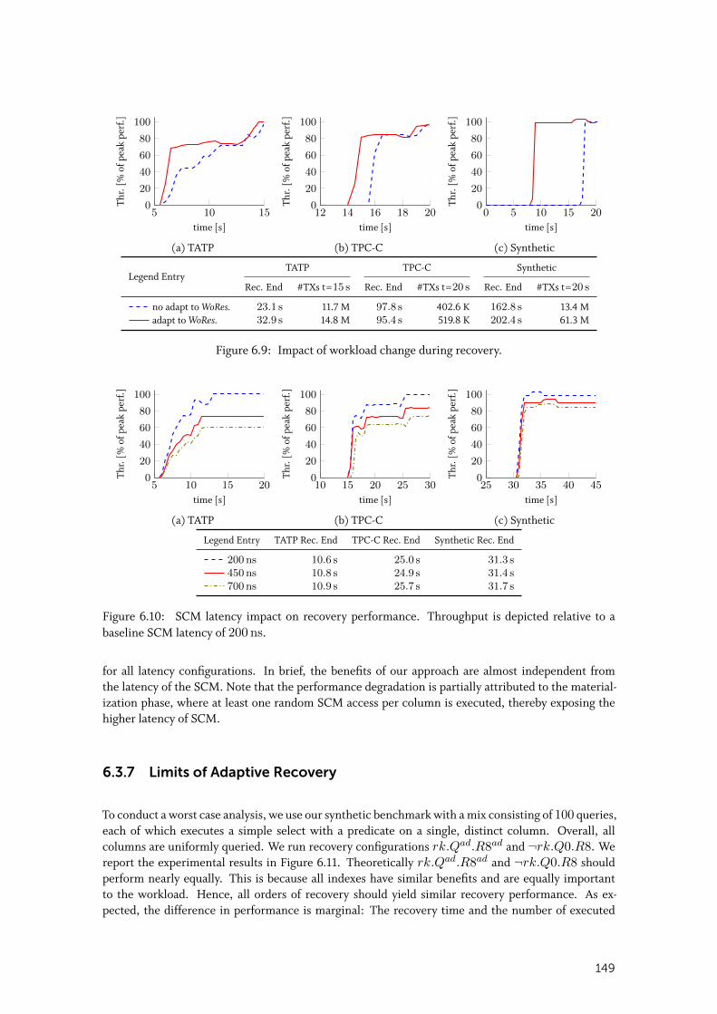
5 10 150
20
40
60
80
100
time [s]
Thr.
[%of
peak
perf
.]
(a) TATP
12 14 16 18 200
20
40
60
80
100
time [s]
Thr.
[%of
peak
perf
.]
(b) TPC-C
0 5 10 15 200
20
40
60
80
100
time [s]
Thr.
[%of
peak
perf
.]
(c) Synthetic
Legend EntryTATP TPC-C Synthetic
Rec. End #TXs t=15 s Rec. End #TXs t=20 s Rec. End #TXs t=20 s
no adapt to WoRes. 23.1 s 11.7 M 97.8 s 402.6 K 162.8 s 13.4 Madapt to WoRes. 32.9 s 14.8 M 95.4 s 519.8 K 202.4 s 61.3 M
Figure 6.9: Impact of workload change during recovery.
5 10 15 200
20
40
60
80
100
time [s]
Thr.
[%of
peak
perf
.]
(a) TATP
10 15 20 25 300
20
40
60
80
100
time [s]
Thr.
[%of
peak
perf
.]
(b) TPC-C
25 30 35 40 450
20
40
60
80
100
time [s]
Thr.
[%of
peak
perf
.]
(c) Synthetic
Legend Entry TATP Rec. End TPC-C Rec. End Synthetic Rec. End
200 ns 10.6 s 25.0 s 31.3 s450 ns 10.8 s 24.9 s 31.4 s700 ns 10.9 s 25.7 s 31.7 s
Figure 6.10: SCM latency impact on recovery performance. Throughput is depicted relative to abaseline SCM latency of 200 ns.
for all latency configurations. In brief, the benefits of our approach are almost independent fromthe latency of the SCM. Note that the performance degradation is partially attributed to the material-ization phase, where at least one random SCM access per column is executed, thereby exposing thehigher latency of SCM.
6.3.7 Limits of Adaptive Recovery
To conduct a worst case analysis, we use our synthetic benchmark with a mix consisting of 100 queries,each of which executes a simple select with a predicate on a single, distinct column. Overall, allcolumns are uniformly queried. We run recovery configurations rk.Qad.R8ad and ¬rk.Q0.R8. Wereport the experimental results in Figure 6.11. Theoretically rk.Qad.R8ad and ¬rk.Q0.R8 shouldperform nearly equally. This is because all indexes have similar benefits and are equally importantto the workload. Hence, all orders of recovery should yield similar recovery performance. As ex-pected, the difference in performance is marginal: The recovery time and the number of executed
149
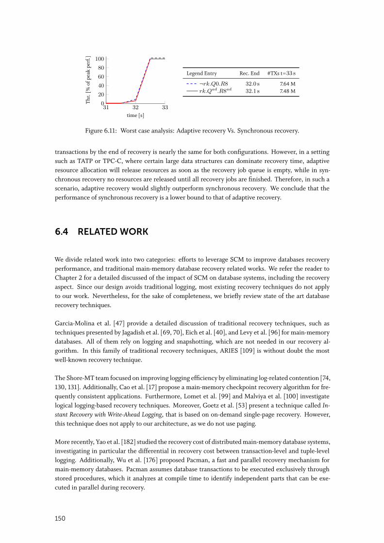
31 32 330
20
40
60
80
100
time [s]
Thr.
[%of
peak
perf
.]
Legend Entry Rec. End #TXs t=33 s
¬rk.Q0.R8 32.0 s 7.64 Mrk.Qad.R8ad 32.1 s 7.48 M
Figure 6.11: Worst case analysis: Adaptive recovery Vs. Synchronous recovery.
transactions by the end of recovery is nearly the same for both configurations. However, in a settingsuch as TATP or TPC-C, where certain large data structures can dominate recovery time, adaptiveresource allocation will release resources as soon as the recovery job queue is empty, while in syn-chronous recovery no resources are released until all recovery jobs are finished. Therefore, in such ascenario, adaptive recovery would slightly outperform synchronous recovery. We conclude that theperformance of synchronous recovery is a lower bound to that of adaptive recovery.
6.4 RELATED WORK
We divide related work into two categories: efforts to leverage SCM to improve databases recoveryperformance, and traditional main-memory database recovery related works. We refer the reader toChapter 2 for a detailed discussed of the impact of SCM on database systems, including the recoveryaspect. Since our design avoids traditional logging, most existing recovery techniques do not applyto our work. Nevertheless, for the sake of completeness, we briefly review state of the art databaserecovery techniques.
Garcia-Molina et al. [47] provide a detailed discussion of traditional recovery techniques, such astechniques presented by Jagadish et al. [69, 70], Eich et al. [40], and Levy et al. [96] for main-memorydatabases. All of them rely on logging and snapshotting, which are not needed in our recovery al-gorithm. In this family of traditional recovery techniques, ARIES [109] is without doubt the mostwell-known recovery technique.
The Shore-MT team focused on improving logging efficiency by eliminating log-related contention [74,130, 131]. Additionally, Cao et al. [17] propose a main-memory checkpoint recovery algorithm for fre-quently consistent applications. Furthermore, Lomet et al. [99] and Malviya et al. [100] investigatelogical logging-based recovery techniques. Moreover, Goetz et al. [53] present a technique called In-stant Recovery with Write-Ahead Logging, that is based on on-demand single-page recovery. However,this technique does not apply to our architecture, as we do not use paging.
More recently, Yao et al. [182] studied the recovery cost of distributed main-memory database systems,investigating in particular the differential in recovery cost between transaction-level and tuple-levellogging. Additionally, Wu et al. [176] proposed Pacman, a fast and parallel recovery mechanism formain-memory databases. Pacman assumes database transactions to be executed exclusively throughstored procedures, which it analyzes at compile time to identify independent parts that can be exe-cuted in parallel during recovery.
150
6.5 SUMMARY
The advent of SCM has enabled single-level database architectures to emerge. These store, access,and modify data directly in SCM, alleviating the traditional recovery bottleneck of main-memorydatabases, i.e., reloading data from storage to memory. Thus, the new recovery bottleneck for suchsystems is rebuilding DRAM-based data. In this chapter we addressed this bottleneck following twoorthogonal dimensions: The first one pertains to secondary data placement in SCM, in DRAM, orin a hybrid SCM-DRAM format. We showed that near-instant recovery is achievable if all secondarydata is persisted in SCM. However, this comes at the cost of a decreased query performance by upto 51.1%. Nevertheless, near-instant recovery offers guarantees that are appealing to business appli-cations where availability is critical. Hybrid SCM-DRAM data structures offer a good compromiseby reducing recovery time by up to 5.9× while limiting the impact on query performance between16.6% and 32.7%. The second dimension is optimizing the recovery of DRAM-based data indepen-dent of data placement. To address this problem, we presented a novel recovery technique, namedadaptive recovery, that relies on: (1) a characterization of secondary data structures, (2) a rankingfunction for secondary data structures that takes into account the workload before and after crash,and (3) an adaptive resource allocation algorithm. We presented two benefit functions for secondarydata structures: the first one considers indexes independently while the second one takes into accountindexes interdependence. Our recovery algorithm aims at maximizing performance of the workloadrun in parallel with recovery. We have implemented adaptive recovery in SOFORT, our SCM-enableddatabase prototype. Through our experimental evaluation, we showed that SOFORT regains its max-imum performance up to 4.3× faster with adaptive recovery than with synchronous recovery, whileallowing the system to be responsive near-instantly. Additionally, the adaptive resource allocationalgorithm brings a significant performance improvement over static resource allocation. We havedemonstrated that our ranking functions adapt well to workload changes during recovery and regainspre-failure throughput up to 2.1× faster than rankings that do not take into consideration the recoveryworkload.
151

152
7TESTING OF SCM-BASED SOFTWARE
T he advent of SCM is disrupting the database landscape and driving novel database architecturesthat store data, access it, and modify it directly from SCM at a cache-line granularity. However,
the no free lunch folklore conjecture holds more than ever as SCM brings unprecedented challengesthat we detailed in Chapter 3. Consistency failure scenarios and recovery strategies of software thatpersists data depend on the underlying storage technology. In the traditional case of block-baseddevices, illustrated in the left side of Figure 7.1, software has full control over when data is madepersistent. Basically, software schedules I/O to persist modified data at a page granularity. The appli-cation has no direct access to the primary copy of the data and can only access copies of the data thatare buffered in main memory. Hence, software errors can corrupt data only in main memory whichcan be reverted as long as the corruption was not explicitly propagated to storage. In fact, crash-safetyfor block-based software highly depends on the correctness of the underlying file system. In contrast,SCM is byte-addressable and is accessed via a long volatility chain that includes store buffers and CPUcaches, over all of which software has little control. As a side effect, changes can be speculatively prop-agated from the CPU cache to SCM at any time, and compilers and out-of-order CPU execution canjeopardize consistency by reordering memory operations. Moreover, changes are made persistent ata cache line granularity which necessitates the use of CPU persistence primitives. This adds anotherlevel of complexity as enforcing the order in which changes are made persistent cannot be delayed likewith block-based devices, and must be synchronous. Hence, storing the primary copy of the data inSCM and directly updating it in-place significantly aggravates the risk of data corruption. In additionto data consistency, memory leaks in SCM have a deeper impact than in DRAM. This is because SCMallocations are persistent, hence, a memory leak would also be persistent.
Several proposals tackled these challenges following two main approaches. The first one focuses onproviding global software-based solutions, mainly transactional-memory-like libraries, to make it eas-ier for developers to write SCM-based software. The second and more mainstream approach is to relysolely on existing hardware persistence primitives, such as cache line flushing instructions and me-mory barriers to achieve consistency. Nevertheless, all approaches have in common that SCM-relatederrors may result in data corruption. In contrast to volatile RAM where data corruption can be curedwith a restart of the program, data corruption in SCM might be irreversible as it is persistent. There-fore, we argue for the need of testing the correctness of SCM-based software against software crashesand power failures–which result in the loss of the content of the CPU cache. We remark that testingis orthogonal to devising recovery strategies that solve the challenges introduced by SCM.
153
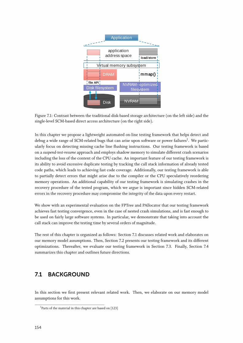
Application
NVRAM-optimizedfilesystem
applicationaddress space
Virtual memory subsystem
Disk
mmap()
NVRAM
load/store
Disk filesystemfile API
DRAM
Figure 7.1: Contrast between the traditional disk-based storage architecture (on the left side) and thesingle-level SCM-based direct access architecture (on the right side).
In this chapter we propose a lightweight automated on-line testing framework that helps detect anddebug a wide range of SCM-related bugs that can arise upon software or power failures1. We partic-ularly focus on detecting missing cache line flushing instructions. Our testing framework is basedon a suspend-test-resume approach and employs shadow memory to simulate different crash scenariosincluding the loss of the content of the CPU cache. An important feature of our testing framework isits ability to avoid excessive duplicate testing by tracking the call stack information of already testedcode paths, which leads to achieving fast code coverage. Additionally, our testing framework is ableto partially detect errors that might arise due to the compiler or the CPU speculatively reorderingmemory operations. An additional capability of our testing framework is simulating crashes in therecovery procedure of the tested program, which we argue is important since hidden SCM-relatederrors in the recovery procedure may compromise the integrity of the data upon every restart.
We show with an experimental evaluation on the FPTree and PAllocator that our testing frameworkachieves fast testing convergence, even in the case of nested crash simulations, and is fast enough tobe used on fairly large software systems. In particular, we demonstrate that taking into account thecall stack can improve the testing time by several orders of magnitude.
The rest of this chapter is organized as follows: Section 7.1 discusses related work and elaborates onour memory model assumptions. Then, Section 7.2 presents our testing framework and its differentoptimizations. Thereafter, we evaluate our testing framework in Section 7.3. Finally, Section 7.4summarizes this chapter and outlines future directions.
7.1 BACKGROUND
In this section we first present relevant related work. Then, we elaborate on our memory modelassumptions for this work.
1Parts of the material in this chapter are based on [123]
154

7.1.1 Related Work
Crash-safety for disk-based software has been extensively researched and several tools that combineexperimental testing and model checking have been proposed [135, 181]. Although they share thesame goals, crash-safety testing for disk-based and SCM-based software are different in that they haveto address radically different failure modes.
Consistency and recovery testing of SCM-based software did not get much attention so far. Lantz et al.proposed Yat [83], a hypervisor-based off-line testing framework for SCM-based software. Yat is basedon a record-and-replay approach. First, it records all SCM write operations by logging hypervisor exitsthat are caused by writes to SCM. Persistence primitive instructions need to be replaced in testedsoftware by illegal instructions to make them traceable by causing a VMM exit. Yat then divides thememory trace into segments, each of which is delimited by two persistence barriers. It considers thatSCM write operations can be arbitrarily reordered within a segment, with the exception of writesto the same cache line which are considered to be of fixed order. Yat replays the trace until a non-tested segment and runs the recovery procedure of the tested software for every possible reorderingcombination inside that segment. Since the number of combinations can grow exponentially, theauthors propose to limit the number of combinations per segment to a certain threshold.
Given a program that covers the whole code base of the tested software, and given a sanity checkprogram that detects any present data corruption – both of which are challenging to produce – Yatcan achieve comprehensive testing for single-threaded SCM-based software. In practice however,that may still require prohibitive testing time. In the case of a multi-threaded program, Yat recordsthe sequence of operations executed by the various threads, which can differ between two runs due tothe non-determinism of multi-threading. Hence, comprehensive testing of a recorded sequence doesnot imply comprehensive testing of the software.
In contrast to Yat, our testing framework performs on-line testing and is non-invasive as it does notrequire software changes in most cases. While it covers only partially memory-reordering-relatederrors, our testing framework achieves fast code coverage by limiting duplicate testing, and is able toautomate crash testing inside the recovery procedure of a program, both of which Yat does not provide.We explain in Section 7.2.7 how our testing framework can be combined with Yat to make up for thelimitations of both tools.
Moreover, we mention an experimental persistent memory extension to Valgrind [163]. It providesseveral functionalities, such as indicating when:
• Writes are not guaranteed to be durable (e.g., missing flushing instruction);• Multiple writes are made to the same location without flushing the first one, which hints to
possible consistency issues;• Flushes made to non-dirty cache lines, which hints to possible optimizations.
However, the program must be modified to notify Valgrind about persistent memory operations suchas flushing instructions, memory fences, and persistent memory mappings, so that Valgrind can trackand shadow persistent memory.
We conjecture that providing comprehensive consistency and recovery testing for large SCM-basedsoftware is – as of now – impractical. Instead, our focus is on improving the quality of such software bycovering a wide range of SCM-related errors in a reasonable amount of time. We argue that similarlyto concurrent software, providing theoretical correctness guarantees should be a prerequisite for anySCM-based software, and that experimental testing should not (and cannot) make up for the lack ofsuch theoretical guarantees.
155
It is also woth mentioning that techniques to prevent data corruption in SCM-based software startto emerge, such as the work of Moraru et al. [110] who proposed to use virtual memory protectionkeys to prevent dangling pointers from corrupting data in SCM. This is, however, orthogonal to thechallenges we tackle in this chapter.
7.1.2 Memory Model
In this work we assume, without loss of generality, an Intel x86 architecture that provides the follow-ing persistence primitives [64]:
• CLFLUSH evicts a cache line from the CPU cache and writes it back to memory. CLFLUSHexecutes synchronously.
• SFENCE guarantees that all preceding stores have been executed.• CLFLUSHOPT evicts a cache line and writes asynchronously its content to memory. It is or-
dered with SFENCE but not with writes.• CLWB asynchronously writes back a cache line without invalidating it. It is ordered with
SFENCE but not with writes.
CLFLUSHOPT and CLWB need to be wrapped by two SFENCE to be fully ordered and serialized; thefirst SFENCE ensures that the latest version of the data is flushed, while the second one ensures thatthe flushing instruction finishes executing. In the following we refer to a serialized flushing operationby the persist function.
The Intel x86 architecture implements a total store order, with two exceptions: 1) non-temporalstores are not ordered between themselves or with other writes [66]. Hence, they can be arbitrar-ily reordered; and 2) the read-before-right effect. Consequently, normal store instructions cannot bereordered and reach the store buffer of the CPU in the same order in which they were executed. Aswe will show, the flexibility of our testing framework makes it easy to take into account other, morerelaxed memory ordering models, such as the ones implemented by ARM and IBM POWER [102].
7.2 TESTING OF SCM-BASED SOFTWARE
We propose a lightweight on-line testing framework that is able to simulate software crashes andpower failures that cover a wide range of consistency and recovery bugs. As an implementation exam-ple, we integrate the framework with PAllocator, our own persistent SCM allocator. The persistentallocator creates large files, referred to as segments, and then logically divides them into smaller blocksfor allocation.
7.2.1 Crash Simulation
In this section we explain how our testing framework is able to simulate software and power fail-ures. The main challenge in simulating a power failure is to simulate the loss of the content of theCPU caches. To achieve this, we devise the following strategy that is based on a suspend-test-resumeapproach:
156
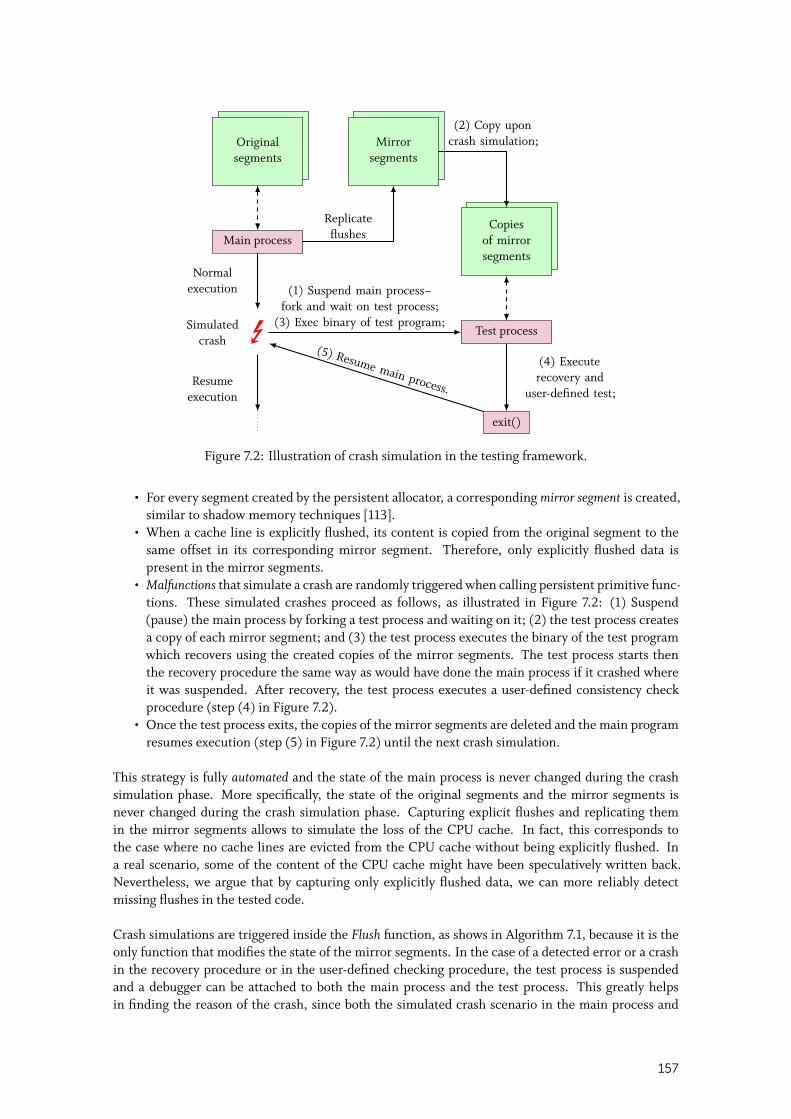
Main process
Originalsegments
Mirrorsegments
Replicateflushes
Test processESimulatedcrash
Normalexecution
Resumeexecution
(1) Suspend main process–fork and wait on test process;
(3) Exec binary of test program;
exit()
(5) Resume main process.
(4) Executerecovery and
user-defined test;
Copiesof mirrorsegments
(2) Copy uponcrash simulation;
Figure 7.2: Illustration of crash simulation in the testing framework.
• For every segment created by the persistent allocator, a corresponding mirror segment is created,similar to shadow memory techniques [113].
• When a cache line is explicitly flushed, its content is copied from the original segment to thesame offset in its corresponding mirror segment. Therefore, only explicitly flushed data ispresent in the mirror segments.
• Malfunctions that simulate a crash are randomly triggered when calling persistent primitive func-tions. These simulated crashes proceed as follows, as illustrated in Figure 7.2: (1) Suspend(pause) the main process by forking a test process and waiting on it; (2) the test process createsa copy of each mirror segment; and (3) the test process executes the binary of the test programwhich recovers using the created copies of the mirror segments. The test process starts thenthe recovery procedure the same way as would have done the main process if it crashed whereit was suspended. After recovery, the test process executes a user-defined consistency checkprocedure (step (4) in Figure 7.2).
• Once the test process exits, the copies of the mirror segments are deleted and the main programresumes execution (step (5) in Figure 7.2) until the next crash simulation.
This strategy is fully automated and the state of the main process is never changed during the crashsimulation phase. More specifically, the state of the original segments and the mirror segments isnever changed during the crash simulation phase. Capturing explicit flushes and replicating themin the mirror segments allows to simulate the loss of the CPU cache. In fact, this corresponds tothe case where no cache lines are evicted from the CPU cache without being explicitly flushed. Ina real scenario, some of the content of the CPU cache might have been speculatively written back.Nevertheless, we argue that by capturing only explicitly flushed data, we can more reliably detectmissing flushes in the tested code.
Crash simulations are triggered inside the Flush function, as shows in Algorithm 7.1, because it is theonly function that modifies the state of the mirror segments. In the case of a detected error or a crashin the recovery procedure or in the user-defined checking procedure, the test process is suspendedand a debugger can be attached to both the main process and the test process. This greatly helpsin finding the reason of the crash, since both the simulated crash scenario in the main process and
157
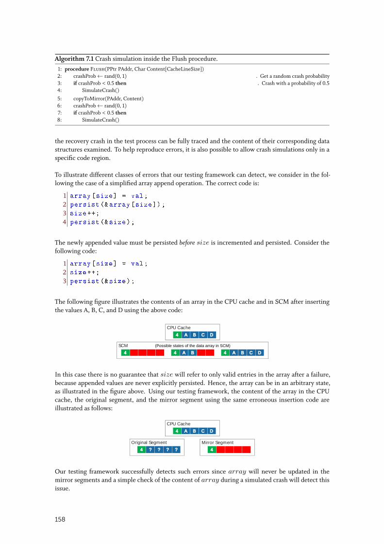
Algorithm 7.1 Crash simulation inside the Flush procedure.1: procedure Flush(PPtr PAddr, Char Content[CacheLineSize])2: crashProb← rand(0, 1) ◃ Get a random crash probability3: if crashProb < 0.5 then ◃ Crash with a probability of 0.54: SimulateCrash()
5: copyToMirror(PAddr, Content)6: crashProb← rand(0, 1)7: if crashProb < 0.5 then8: SimulateCrash()
the recovery crash in the test process can be fully traced and the content of their corresponding datastructures examined. To help reproduce errors, it is also possible to allow crash simulations only in aspecific code region.
To illustrate different classes of errors that our testing framework can detect, we consider in the fol-lowing the case of a simplified array append operation. The correct code is:
1 array[size] = val;
2 persist (&array[size]);
3 size ++;
4 persist (&size);
The newly appended value must be persisted before size is incremented and persisted. Consider thefollowing code:
1 array[size] = val;
2 size ++;
3 persist (&size);
The following figure illustrates the contents of an array in the CPU cache and in SCM after insertingthe values A, B, C, and D using the above code:
CPU Cache
SCM
4 A B C D
4 A B4 4 A B C D
(Possible states of the data array in SCM)
In this case there is no guarantee that size will refer to only valid entries in the array after a failure,because appended values are never explicitly persisted. Hence, the array can be in an arbitrary state,as illustrated in the figure above. Using our testing framework, the content of the array in the CPUcache, the original segment, and the mirror segment using the same erroneous insertion code areillustrated as follows:
CPU Cache
Original Segment
4 A B C D
4 A B
Mirror Segment
44 ? ? ? ?
Our testing framework successfully detects such errors since array will never be updated in themirror segments and a simple check of the content of array during a simulated crash will detect thisissue.
158
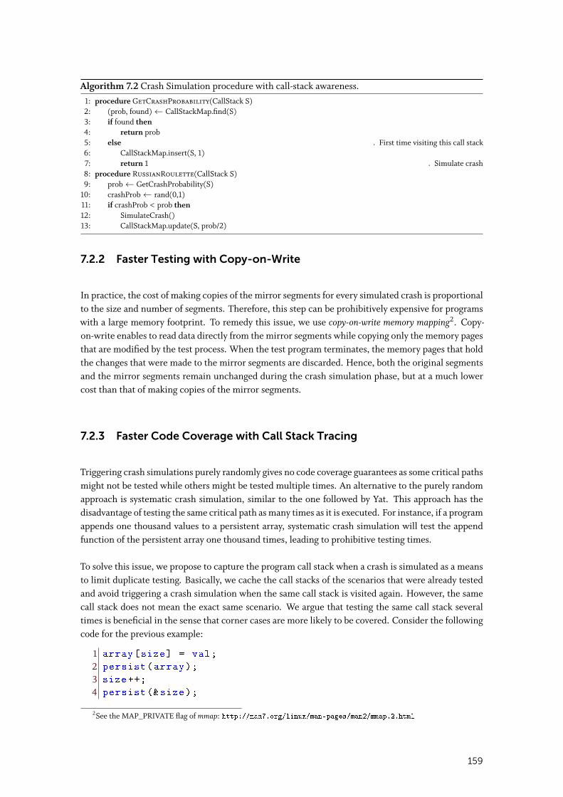
Algorithm 7.2 Crash Simulation procedure with call-stack awareness.1: procedure GetCrashProbability(CallStack S)2: (prob, found)← CallStackMap.find(S)3: if found then4: return prob5: else ◃ First time visiting this call stack6: CallStackMap.insert(S, 1)7: return 1 ◃ Simulate crash8: procedure RussianRoulette(CallStack S)9: prob← GetCrashProbability(S)
10: crashProb← rand(0,1)11: if crashProb < prob then12: SimulateCrash()13: CallStackMap.update(S, prob/2)
7.2.2 Faster Testing with Copy-on-Write
In practice, the cost of making copies of the mirror segments for every simulated crash is proportionalto the size and number of segments. Therefore, this step can be prohibitively expensive for programswith a large memory footprint. To remedy this issue, we use copy-on-write memory mapping2. Copy-on-write enables to read data directly from the mirror segments while copying only the memory pagesthat are modified by the test process. When the test program terminates, the memory pages that holdthe changes that were made to the mirror segments are discarded. Hence, both the original segmentsand the mirror segments remain unchanged during the crash simulation phase, but at a much lowercost than that of making copies of the mirror segments.
7.2.3 Faster Code Coverage with Call Stack Tracing
Triggering crash simulations purely randomly gives no code coverage guarantees as some critical pathsmight not be tested while others might be tested multiple times. An alternative to the purely randomapproach is systematic crash simulation, similar to the one followed by Yat. This approach has thedisadvantage of testing the same critical path as many times as it is executed. For instance, if a programappends one thousand values to a persistent array, systematic crash simulation will test the appendfunction of the persistent array one thousand times, leading to prohibitive testing times.
To solve this issue, we propose to capture the program call stack when a crash is simulated as a meansto limit duplicate testing. Basically, we cache the call stacks of the scenarios that were already testedand avoid triggering a crash simulation when the same call stack is visited again. However, the samecall stack does not mean the exact same scenario. We argue that testing the same call stack severaltimes is beneficial in the sense that corner cases are more likely to be covered. Consider the followingcode for the previous example:
1 array[size] = val;
2 persist(array);
3 size ++;
4 persist (&size);
2See the MAP_PRIVATE flag of mmap: http://man7.org/linux/man-pages/man2/mmap.2.html
159
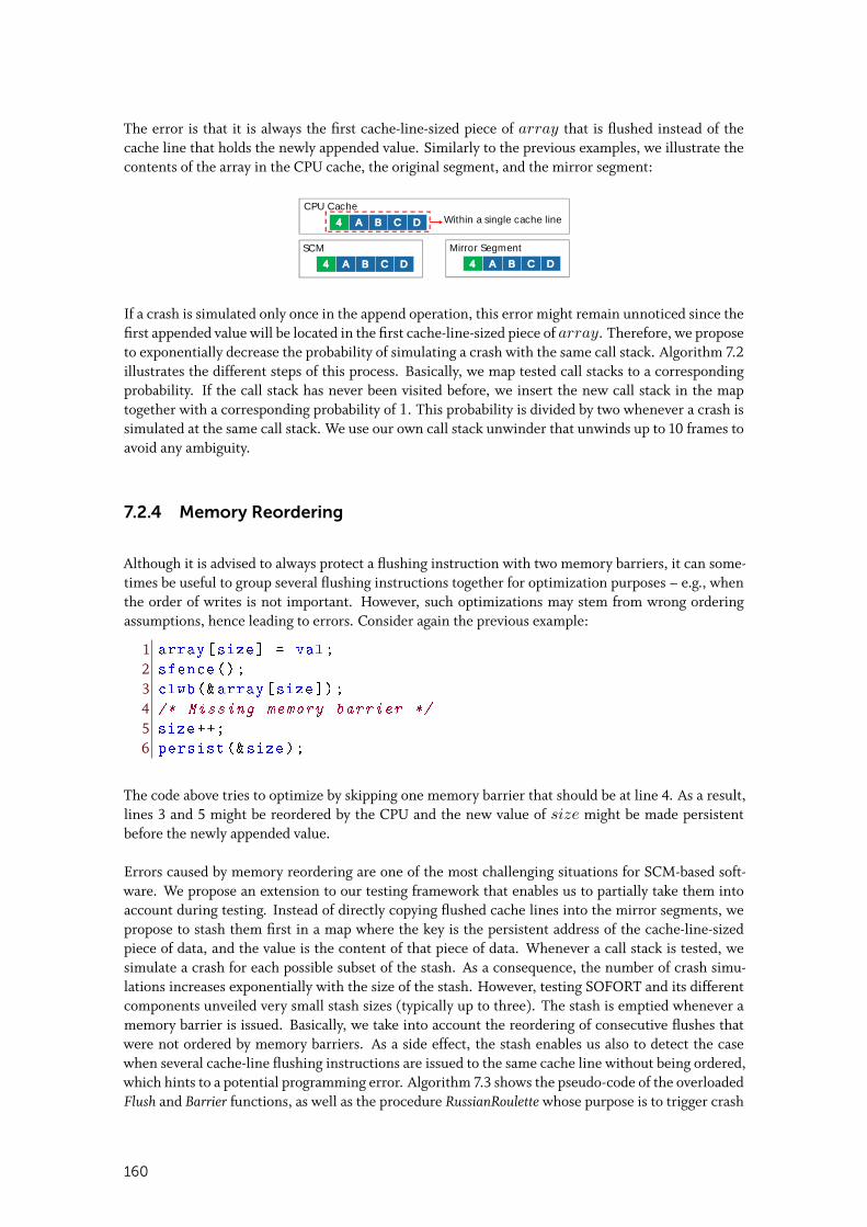
The error is that it is always the first cache-line-sized piece of array that is flushed instead of thecache line that holds the newly appended value. Similarly to the previous examples, we illustrate thecontents of the array in the CPU cache, the original segment, and the mirror segment:
CPU Cache
SCM
4 A B C D
4 A B C D
Mirror Segment
4 A B C D
Within a single cache line
If a crash is simulated only once in the append operation, this error might remain unnoticed since thefirst appended value will be located in the first cache-line-sized piece of array. Therefore, we proposeto exponentially decrease the probability of simulating a crash with the same call stack. Algorithm 7.2illustrates the different steps of this process. Basically, we map tested call stacks to a correspondingprobability. If the call stack has never been visited before, we insert the new call stack in the maptogether with a corresponding probability of 1. This probability is divided by two whenever a crash issimulated at the same call stack. We use our own call stack unwinder that unwinds up to 10 frames toavoid any ambiguity.
7.2.4 Memory Reordering
Although it is advised to always protect a flushing instruction with two memory barriers, it can some-times be useful to group several flushing instructions together for optimization purposes – e.g., whenthe order of writes is not important. However, such optimizations may stem from wrong orderingassumptions, hence leading to errors. Consider again the previous example:
1 array[size] = val;
2 sfence ();
3 clwb(&array[size]);
4 /* Missing memory barrier */
5 size ++;
6 persist (&size);
The code above tries to optimize by skipping one memory barrier that should be at line 4. As a result,lines 3 and 5 might be reordered by the CPU and the new value of size might be made persistentbefore the newly appended value.
Errors caused by memory reordering are one of the most challenging situations for SCM-based soft-ware. We propose an extension to our testing framework that enables us to partially take them intoaccount during testing. Instead of directly copying flushed cache lines into the mirror segments, wepropose to stash them first in a map where the key is the persistent address of the cache-line-sizedpiece of data, and the value is the content of that piece of data. Whenever a call stack is tested, wesimulate a crash for each possible subset of the stash. As a consequence, the number of crash simu-lations increases exponentially with the size of the stash. However, testing SOFORT and its differentcomponents unveiled very small stash sizes (typically up to three). The stash is emptied whenever amemory barrier is issued. Basically, we take into account the reordering of consecutive flushes thatwere not ordered by memory barriers. As a side effect, the stash enables us also to detect the casewhen several cache-line flushing instructions are issued to the same cache line without being ordered,which hints to a potential programming error. Algorithm 7.3 shows the pseudo-code of the overloadedFlush and Barrier functions, as well as the procedure RussianRoulette whose purpose is to trigger crash
160
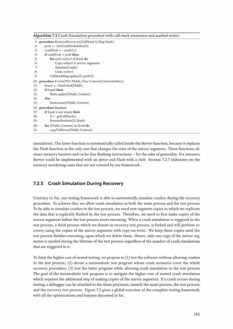
Algorithm 7.3 Crash Simulation procedure with call-stack awareness and stashed writes.1: procedure RussianRoulette(CallStack S, Map Stash)2: prob← GetCrashProbability(S)3: crashProb← rand(0,1)4: if crashProb < prob then5: for each subset of Stash do6: Copy subset to mirror segments7: SimulateCrash()8: Undo subset9: CallStackMap.update(S, prob/2)
10: procedure Flush(PPtr PAddr, Char Content[CacheLineSize])11: found← Stash.find(PAddr)12: if found then13: Stash.update(PAddr, Content)14: else15: Stash.insert(PAddr, Content)
16: procedure Barrier17: if Stash is not empty then18: S← getCallStack()19: RussianRoulette(S, Stash)
20: for (PAddr, Content) in Stash do21: copyToMirror(PAddr, Content)
simulations. The latter function is systematically called inside the Barrier function, because it replacesthe Flush function as the only one that changes the state of the mirror segments. These functions ab-stract memory barriers and cache-line flushing instructions – for the sake of generality. For instance,Barrier could be implemented with an sfence and Flush with a clwb. Section 7.2.7 elaborates on thememory reordering cases that are not covered by our framework.
7.2.5 Crash Simulation During Recovery
Contrary to Yat, our testing framework is able to automatically simulate crashes during the recoveryprocedure. To achieve this, we allow crash simulation in both the main process and the test process.To be able to simulate crashes in the test process, we need new segment copies in which we replicatethe data that is explicitly flushed by the test process. Therefore, we need to first make copies of themirror segments before the test process starts executing. When a crash simulation is triggered in thetest process, a third process which we denote as recovery test process, is forked and will perform re-covery using the copies of the mirror segments with copy-on-write. We keep these copies until thetest process finishes executing, upon which we delete them. Hence, only one copy of the mirror seg-ments is needed during the lifetime of the test process regardless of the number of crash simulationsthat are triggered in it.
To limit the higher cost of nested testing, we propose to (1) test the software without allowing crashesin the test process; (2) devise a minimalistic test program whose crash scenarios cover the wholerecovery procedure; (3) test the latter program while allowing crash simulation in the test process.The goal of the minimalistic test program is to mitigate the higher cost of nested crash simulationwhich requires the additional step of making copies of the mirror segments. If a crash occurs duringtesting, a debugger can be attached to the three processes, namely the main process, the test process,and the recovery test process. Figure 7.3 gives a global overview of the complete testing framework,with all the optimizations and features discussed so far.
161
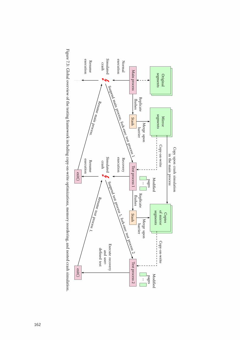
Main
process
Original
segments
Mirror
segments
Replicateflushes
Testprocess1
ESim
ulatedcrash
Norm
alexecution
Resum
eexecution
Suspendm
ainprocess, fork-exec
testprocess
1
exit()
Resum
em
ainprocess.
Copy-on-w
rite
...
Modified
pages
Testprocess2
E
Recovery
execution
Simulated
crash
Resum
eexecution
Stash Merge
uponbarrier
Copies
ofm
irrorsegm
entsC
opy-on-write
...
Modified
pages
Replicateflushes
Stash Merge
uponbarrier
Suspendtest
process1, fork-exec
testprocess
2
exit()
Resum
etest
process1.
Copy
uponcrash
simulation
inthe
main
process
Executerecovery
anduser-
definedtest
Figure7.3:G
lobaloverviewofthe
testingfram
ework
includingcopy-on-w
riteoptim
izations,mem
oryreordering,and
nestedcrash
simulation.
162
7.2.6 Crash Simulation in Multi-Threaded Programs
Single-threaded consistency and recovery correctness in addition to concurrency correctness (e.g., norace conditions) is a good indicator of multi-threaded consistency and recovery correctness. However,there are programming errors that cannot be detected in single-threaded execution. These errors typ-ically concern code paths that execute only in multi-threaded mode. Consider the following examplewhere two threads try to increment one of two persistent counters, ctr1 and ctr2:
1 mutex m1, m2;
2 if(m1.try_lock ()){
3 ctr1 ++;
4 persist (&ctr1);
5 m1.unlock ();
6 }else if(m2.try_lock ()){
7 ctr2 ++;
8 persist (&ctr1) /* Should be ctr2 */
9 m2.unlock ();
10 }
The error in the code above is at line 8 where ctr1 is persisted instead of ctr2. In the case of single-threaded execution, lock m1 will always be successfully acquired, hence, lines 7 to 9 will never beexecuted and the error will not be detected.
Our testing framework is capable of testing multi-threaded programs. Indeed, it is possible to suspendall the threads of a process as long as the process keeps references to all its threads. Only when thisis not the case (e.g. if some threads are detached) the program needs to be changed to provide aprocedure that halts all its threads. Additionally, the call stack map and the stash of pending writesneed to be made thread-safe using global locks so that only one thread is allowed to try and triggera crash simulation at a time. Avoiding duplicate testing by caching the call stack of the thread thattriggered the crash simulation becomes less effective in a multi-threaded environment. This is becausethe crash scenario depends on the state of all threads and not only the thread that triggered the crashsimulation. Nevertheless, exhaustive testing for multi-threaded programs is infeasible because threadscheduling is non-deterministic, hence, two runs of the same multi-threaded program may producedifferent scenarios.
7.2.7 Limitations and Complementarity with Yat
While our testing framework is able to detect a wide range of consistency-related errors, it is unable tofind errors that stem from the reordering of consecutive SCM writes whose persistence is delayed butstill enforced in the right order. Consider the following code snippet of an array append operation:
1 array[size] = val;
2 size ++;
3 persist (&array[size]);
4 persist (&size);
The issue in the code above is that the new value of size can be speculatively evicted from the CPUcache and become persistent before the newly appended value. A power failure at this same instant
163
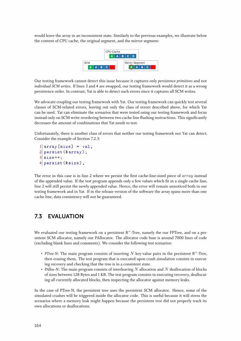
would leave the array in an inconsistent state. Similarly to the previous examples, we illustrate belowthe content of CPU cache, the original segment, and the mirror segment:
CPU Cache
SCM
4 A B C D
4 A B C
Mirror Segment
3 A B C
Our testing framework cannot detect this issue because it captures only persistence primitives and notindividual SCM writes. If lines 3 and 4 are swapped, our testing framework would detect it as a wrongpersistence order. In contrast, Yat is able to detect such errors since it captures all SCM writes.
We advocate coupling our testing framework with Yat. Our testing framework can quickly test severalclasses of SCM-related errors, leaving out only the class of errors described above, for which Yatcan be used. Yat can eliminate the scenarios that were tested using our testing framework and focusinstead only on SCM write reordering between two cache line flushing instructions. This significantlydecreases the amount of combinations that Yat needs to test.
Unfortunately, there is another class of errors that neither our testing framework nor Yat can detect.Consider the example of Section 7.2.3:
1 array[size] = val;
2 persist (&array);
3 size ++;
4 persist (&size);
The error in this case is in line 2 where we persist the first cache-line-sized piece of array insteadof the appended value. If the test program appends only a few values which fit in a single cache line,line 2 will still persist the newly appended value. Hence, the error will remain unnoticed both in ourtesting framework and in Yat. If in the release version of the software the array spans more than onecache line, data consistency will not be guaranteed.
7.3 EVALUATION
We evaluated our testing framework on a persistent B+-Tree, namely the our FPTree, and on a per-sistent SCM allocator, namely our PAllocator. The allocator code base is around 7000 lines of code(excluding blank lines and comments). We consider the following test scenarios:
• PTree-N: The main program consists of inserting N key-value pairs in the persistent B+-Tree,then erasing them. The test program that is executed upon crash simulation consists in execut-ing recovery and checking that the tree is in a consistent state.
• PAlloc-N: The main program consists of interleaving N allocation and N deallocation of blocksof sizes between 128 Bytes and 1 KB. The test program consists in executing recovery, deallocat-ing all currently allocated blocks, then inspecting the allocator against memory leaks.
In the case of PTree-N, the persistent tree uses the persistent SCM allocator. Hence, some of thesimulated crashes will be triggered inside the allocator code. This is useful because it will stress thescenarios where a memory leak might happen because the persistent tree did not properly track itsown allocations or deallocations.
164
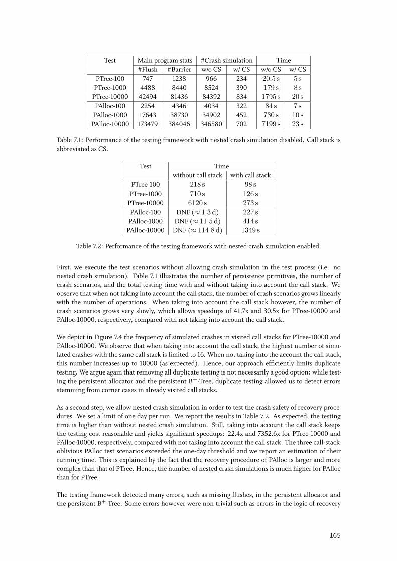
Test Main program stats #Crash simulation Time#Flush #Barrier w/o CS w/ CS w/o CS w/ CS
PTree-100 747 1238 966 234 20.5 s 5 sPTree-1000 4488 8440 8524 390 179 s 8 s
PTree-10000 42494 81436 84392 834 1795 s 20 s
PAlloc-100 2254 4346 4034 322 84 s 7 sPAlloc-1000 17643 38730 34902 452 730 s 10 s
PAlloc-10000 173479 384046 346580 702 7199 s 23 s
Table 7.1: Performance of the testing framework with nested crash simulation disabled. Call stack isabbreviated as CS.
Test Timewithout call stack with call stack
PTree-100 218 s 98 sPTree-1000 710 s 126 s
PTree-10000 6120 s 273 s
PAlloc-100 DNF (≈ 1.3 d) 227 sPAlloc-1000 DNF (≈ 11.5 d) 414 s
PAlloc-10000 DNF (≈ 114.8 d) 1349 s
Table 7.2: Performance of the testing framework with nested crash simulation enabled.
First, we execute the test scenarios without allowing crash simulation in the test process (i.e. nonested crash simulation). Table 7.1 illustrates the number of persistence primitives, the number ofcrash scenarios, and the total testing time with and without taking into account the call stack. Weobserve that when not taking into account the call stack, the number of crash scenarios grows linearlywith the number of operations. When taking into account the call stack however, the number ofcrash scenarios grows very slowly, which allows speedups of 41.7x and 30.5x for PTree-10000 andPAlloc-10000, respectively, compared with not taking into account the call stack.
We depict in Figure 7.4 the frequency of simulated crashes in visited call stacks for PTree-10000 andPAlloc-10000. We observe that when taking into account the call stack, the highest number of simu-lated crashes with the same call stack is limited to 16. When not taking into the account the call stack,this number increases up to 10000 (as expected). Hence, our approach efficiently limits duplicatetesting. We argue again that removing all duplicate testing is not necessarily a good option: while test-ing the persistent allocator and the persistent B+-Tree, duplicate testing allowed us to detect errorsstemming from corner cases in already visited call stacks.
As a second step, we allow nested crash simulation in order to test the crash-safety of recovery proce-dures. We set a limit of one day per run. We report the results in Table 7.2. As expected, the testingtime is higher than without nested crash simulation. Still, taking into account the call stack keepsthe testing cost reasonable and yields significant speedups: 22.4x and 7352.6x for PTree-10000 andPAlloc-10000, respectively, compared with not taking into account the call stack. The three call-stack-oblivious PAlloc test scenarios exceeded the one-day threshold and we report an estimation of theirrunning time. This is explained by the fact that the recovery procedure of PAlloc is larger and morecomplex than that of PTree. Hence, the number of nested crash simulations is much higher for PAllocthan for PTree.
The testing framework detected many errors, such as missing flushes, in the persistent allocator andthe persistent B+-Tree. Some errors however were non-trivial such as errors in the logic of recovery
165
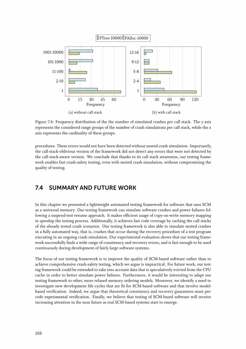
PTree-10000 PAlloc-10000
0 15 30 45 60
1
2-10
11-100
101-1000
1001-10000
Frequency
(a) without call stack
0 30 60 90 120
1
2-4
5-8
9-12
12-16
Frequency
(b) with call stack
Figure 7.4: Frequency distribution of the the number of simulated crashes per call stack. The y axisrepresents the considered range groups of the number of crash simulations per call stack, while the xaxis represents the cardinality of these groups.
procedures. These errors would not have been detected without nested crash simulation. Importantly,the call-stack-oblivious version of the framework did not detect any errors that were not detected bythe call-stack-aware version. We conclude that thanks to its call stack awareness, our testing frame-work enables fast crash-safety testing, even with nested crash simulation, without compromising thequality of testing.
7.4 SUMMARY AND FUTURE WORK
In this chapter we presented a lightweight automated testing framework for software that uses SCMas a universal memory. Our testing framework can simulate software crashes and power failures fol-lowing a suspend-test-resume approach. It makes efficient usage of copy-on-write memory mappingto speedup the testing process. Additionally, it achieves fast code coverage by caching the call stacksof the already tested crash scenarios. Our testing framework is also able to simulate nested crashesin a fully automated way, that is, crashes that occur during the recovery procedure of a test programexecuting in an ongoing crash simulation. Our experimental evaluation shows that our testing frame-work successfully finds a wide range of consistency and recovery errors, and is fast enough to be usedcontinuously during development of fairly large software systems.
The focus of our testing framework is to improve the quality of SCM-based software rather than toachieve comprehensive crash-safety testing, which we argue is impractical. For future work, our test-ing framework could be extended to take into account data that is speculatively evicted from the CPUcache in order to better simulate power failures. Furthermore, it would be interesting to adapt ourtesting framework to other, more relaxed memory ordering models. Moreover, we identify a need toinvestigate new development life cycles that are fit for SCM-based software and that involve model-based verification. Indeed, we argue that theoretical consistency and recovery guarantees must pre-cede experimental verification. Finally, we believe that testing of SCM-based software will receiveincreasing attention in the near future as real SCM-based systems start to emerge.
166
8CONCLUSION
S CM is emerging as a disruptive memory technology that might have the same level of impactas high core counts and large main-memory capacities, requiring us to rethink current database
system architectures. In this dissertation, we endeavored to explore this potential by building a hybridtransactional and analytical database system from the ground up that leverages SCM as persistentmain memory. This led us to devise several database building blocks. This chapter concludes thisdissertation by first summarizing our contributions, then sketching promising directions for futurework.
8.1 SUMMARY OF CONTRIBUTIONS
SCM Programming Model. We identified several SCM programming challenges, namely data con-sistency, data recovery, persistent memory leaks, and partial writes. To address these challenges, wedevised a sound programming model that relies on lightweight persistence primitives to achieve dataconsistency. To provide data recovery, we propose to use persistent pointers in the form of a file IDand an offset within that file. Persistent pointers remain valid across restarts, thereby enabling datarecovery. Additionally, we provide a swizzling mechanism from persistent pointers to volatile point-ers and vice versa. To avoid persistent memory leaks, we employ reference passing, which consistsin extending the allocation interface to take a reference to a persistent pointer belonging to the callerdata structure. Furthermore, to avoid partial writes, we use p-atomic flags to indicate when a largewrite operation is completed. We argue that our sound programming model is the guarantee of thetechnical feasibility and correctness of the work presented in this dissertation.
PersistentMemoryManagement. The ability to allocate and deallocate SCM is a fundamental build-ing block for building SCM-based data structures. Therefore, we propose PAllocator, a persistent andhighly scalable SCM allocator. In contrast to transient memory allocators, our persistent allocator re-tains the topology of its allocated blocks across restarts. PAllocator’s design is tailored to the versatileneeds of large-scale hybrid transactional and analytical SCM-based database system. As a result, PAllo-cator adopts radically different design decisions compared to state-of-the-art transient and persistentallocators. PAllocator implements its memory pool using multiple files, which allows to easily growand shrink the memory pool, in contrast to state-of-the-art persistent allocators that use a single-filepool. For concurrency, PAllocator creates core-local memory pools, which, in contrast to thread-localmemory pools, has the advantage of decoupling local pool management from thread management.
167
To provide robust performance for a wide range of allocation sizes and to minimize fragmentation,PAllocator relies on three allocation strategies: a segregated-fit strategy for small blocks, a best-fitstrategy for large blocks, and creating one file per allocation for huge blocks. Furthermore, PAllocatoraddresses the important issue of persistent memory fragmentation by providing a defragmentation al-gorithm that relies on the hole punching feature of sparse files. Our experiments show that PAllocatoroutperforms both transient and persistent state-of-the-art allocators under high contention.
Hybrid SCM-DRAM Persistent Data Structures. Motivated by the observation that placing tree-based data structures in SCM significantly slows them down, we propose the FPTree, a novel hybridSCM-DRAM B+-Tree. The FPTree builds on a number of design principles, namely selective persis-tence, unsorted leaves, fingerprinting, and selective concurrency. Selective persistence consists inplacing primary data in SCM and secondary data, which can be rebuilt from primary data, in DRAM.Applied to the FPTree, this corresponds to placing inner nodes in DRAM and leaf nodes in SCM.Hence, when traversing the FPTree, only accessing the leaf nodes is more expensive compared to atransient B+-Tree. Moreover, to decrease the number of writes and simplify failure atomicity of up-dates, we keep the FPTree’s leaf nodes unsorted and track valid entries using a bitmap. Nevertheless,looking up unsorted leaves requires a linear scan, which is more expensive (in case of large leaf nodes)than the traditional binary search. To remedy this issue, we introduce fingerprinting, which consistsof keeping in leaf nodes one-byte hashes of the keys used as filters. Through an asymptotic analysis aswell as an experimental evaluation, we show that fingerprints limit the number of key probes in leafnodes to exactly one. Furthermore, we devise selective concurrency, a highly scalable hybrid concur-rency scheme that uses HTM for the concurrency of inner nodes and fine-grained locks for that of leafnodes, thereby solving the apparent incompatibility of HTM and SCM.
SOFORT. We use the above building blocks to build SOFORT, a novel single-level hybrid SCM-DRAMcolumnar transactional engine. SOFORT places its primary data in SCM and its secondary data eitherin DRAM, in SCM, or in a hybrid SCM-DRAM format. We propose an adaptation of MVCC to SCMthat removes traditional write-ahead logging from the critical path of transactions. We achieve thisby persisting part of MVCC transaction metadata, namely the write set and the commit timestamp,in SCM. Furthermore, we show that by persisting additional MVCC transaction metadata, SOFORTavoids aborting in-flight transaction during recovery; instead, SOFORT rolls back only the last unfin-ished statement, and offers the user the ability to continue in-flight transactions. Additionally, we pro-pose an efficient recoverable garbage collection scheme in conjunction with our MVCC scheme. Thedecentralized design of SOFORT removes the need for group commit, which translates into low trans-action latencies. Upon recovery, SOFORT simply discovers primary data in SCM, which removes thetraditional bottleneck of main-memory database recovery, namely loading data from storage to mainmemory. Since committed transactions are guaranteed to have persisted their changes, SOFORT doesnot require a redo phase. Thereafter, SOFORT rebuilds its transient secondary data from its primarydata. By investigating several secondary data placement strategies, we show that on one extreme, per-sisting all secondary data in SCM enables near-instant recovery at full speed, but at a significant queryperformance cost due to the higher latency of SCM. On the other extreme, placing all secondary datain DRAM yields the best query performance, but incurs slow restart times due to the large amountof secondary data that needs to be rebuilt. Using our hybrid FPTree proved to be a promising com-promise as it limits the impact on query performance while speeding up recovery by more than oneorder of magnitude compared to using DRAM-based secondary data, all of which while requiring onlya 1:60 DRAM to SCM ratio.
Recovery Techniques. The new recovery bottleneck in SCM-based database systems is rebuildingtransient secondary data structures. To address this bottleneck, we propose two recovery techniques:instant recovery and adaptive recovery. Motivated by the observation that primary data is sufficient toanswer queries, instant recovery allows accepting queries right after recovering primary data, therebyenabling near-instant responsiveness of the database. This is achieved by statically splitting CPU
168
resources between query processing and the recovery of secondary data structures. However, ourexperimental evaluation showed that it takes SOFORT a significant amount of time to regain its pre-failure throughput due to the slow recovery of secondary data. To remedy this issue, we proposedadaptive recovery, a new secondary data recovery technique that builds on the observation that notall secondary data are equally important. Adaptive recovery uses a ranking function that takes intoaccount the pre-failure workload as well as the recovery workload to prioritize the rebuild of the mostimportant secondary data structures. Moreover, adaptive recovery gradually releases its resources toquery processing as it finishes rebuilding the most important secondary data structures, and continuesrebuilding the remaining ones in the background. As a result, adaptive recovery enables SOFORT toregain its pre-failure throughput well before the end of the recovery process while still providing near-instant responsiveness.
Testing Framework for SCM-Based Software. Programming SCM as persistent main memory in-troduces new failure scenarios, such as missing persistence primitives, wrong writes ordering, andfailure-induced persistent memory leaks. To tackle this issue, we propose an online testing frame-work that relies on a suspend-test-resume strategy. Our testing framework creates for each SCM filea mirror file that contains only explicitly flushed data. Our testing framework automatically triggerscrash simulations at the boundaries of persistence primitives by halting the main process, then fork-ing a test process that executes recovery on the mirror files using copy-on-write semantics. Sincethey contain only explicitly flushed data, the mirror files simulate the loss of the CPU caches, whichallows catching missing or misplaced flushing instructions. By using copy-on-write semantics, anychanges to the mirror files are discarded when the test process exits, enabling the main process toresume execution and reuse the mirror files for future crash simulations. To limit duplicate testing,we proposed to associate the call-stack of each crash scenario with a crash probability that is expo-nentially decreased each time a crash is simulated for that scenario. This significantly reduces testingtime, thereby making it feasible to test fairly large SCM-based software systems. Moreover, our testingframework supports nested crash simulation, i.e., simulating crashes in the test process; this enablesto thoroughly test recovery procedures, which are otherwise not tested in the main process.
To summarize, our pathfinding work led us to identify the challenges and opportunities brought bySCM for database systems. As a result, we devised a set of building blocks, including a programmingmodel, an SCM allocator, a hybrid SCM-DRAM data structure, an adaptation of MVCC for SCM, newdatabase recovery techniques, and a testing tool for SCM-based software. These building blocks canbe used to build more complex systems, thereby paving the way for future database systems on SCM.
8.2 FUTURE WORK
Research on SCM-based databases is still in its early stages. Some database research areas, such asquery optimization and query processing, need to be extended, but not rewritten, to account for SCMand its asymmetric read write latency and bandwidth. In contrast, other areas, such as storage andreplication, need to be revisited from the ground up, while new areas, such as testing of SCM-baseddata structures, require fundamental groundwork. In this context, we present promising researchdirections for SCM in the following. Our focus is twofold: (1) hardware, software, and theoreticalgroundwork advancements that can catalyze the adoption of SCM; and (2) ideas that can build on topof the contributions of this dissertation.
169
Persistent Memory Management
Similar to programming multi-threaded software, programming SCM as a persistent main memorywill require a set of mature tools and programming models to be adopted by a larger audience. Whileseveral programming models have been proposed, none can claim to have reached standard status.One major concern hindering the widespread adoption of SCM programming is the need to explicitlyorder and persist writes at a cache line granularity. Libraries providing an interface like transactionalmemory can hide this complexity, but at the cost of doubling the number of writes (and flushes) toSCM due to systematic undo or redo logging. We envision that new hardware features could dramati-cally decrease this overhead, thereby making these libraries competitive with hand-tuned code. Suchhardware features could include:
• Hardware-Managed Undo-Redo Logs. SCM transactional libraries usually rely on either redo orundo logging to ensure failure atomicity. We conceive that hardware-driven undo-redo loggingwould decrease the overhead of these libraries. For instance, Ogleari et al. [118] propose ahardware-based undo-redo logging scheme that uses a combination of cache-resident and SCM-resident buffers. Writes are kept in cache-resident buffers and flushed to SCM only if theirdependent writes are evicted from the cache. This has the advantage of decreasing the cost offlushing instructions and relaxing write ordering constraints.
• SCM Support in HTM. As explained in Chapter 4, HTM transactions must buffer changes inthe L1 CPU cache to ensure their atomic visibility at the end of the transaction. Therefore,flushing instructions will automatically abort HTM transactions. Extending HTM to supportSCM would further ease the adoption of SCM and provide a baseline for concurrency supportin SCM transactional libraries. Research works on the subject started to emerge, exemplifiedby PhyTM [8], which requires only the ability to commit one bit atomically to SCM to supportSCM transactions.
• Providing Non-Volatile Caches. This would remove the need for flushing instructions, whichwould significantly reduce the overhead of SCM transactional libraries. Moreover, this wouldfacilitate SCM support in HTM because data changes can be buffered in the L1 CPU cache with-out jeopardizing data durability.
In 1983, Atkinson et al. [7] formulated the concept of decoupling the data representation from datamanipulation. In other words, each data object can be persistent or transient, independent of its in-ternal representation. It would be interesting to revisit this concept in light of SCM, especially sincetransient (DRAM-based) and persistent (SCM-based) data structures share most of their layout opti-mization techniques. Additionally, this concept could be implemented in SCM transactional libraries.
Furthermore, fragmentation will be a major issue in SCM memory management. We addressed thisissue in this dissertation for the versatile needs of hybrid analytical and transactional systems. How-ever, other systems with more predictable memory management needs, such as FOEDUS [79] – apurely transactional system – can opt to go back to the fundamentals of buffer pool management, thatis, dividing memory into fixed-size chunks, thereby avoiding any fragmentation. We expect differentsystems with different needs to devise tailor-made SCM management techniques. These techniqueswill exploit knowledge of the memory allocation patterns of the underlying system to minimize frag-mentation or avoid it completely when possible.
Finally, it is worth considering rewriting part or all of the operating system such that it intrinsicallysupports SCM. One can argue that the support for SCM that is currently being built in Linux andWindows treats SCM as a second-class citizen. For instance, the Direct Access (DAX) filesystemfeature [35] builds on top of block-based filesystem architectures. Several SCM-optimized filesystemproposals, such as NOVA [179], have showcased the benefits of rearchitecting file management forSCM. Following a more radical approach, Bryson et al. [15] are working on Twizzler, a novel operatingsystem designed from scratch around SCM. We believe that such endeavors are essential to unveil thefull potential of SCM.
170
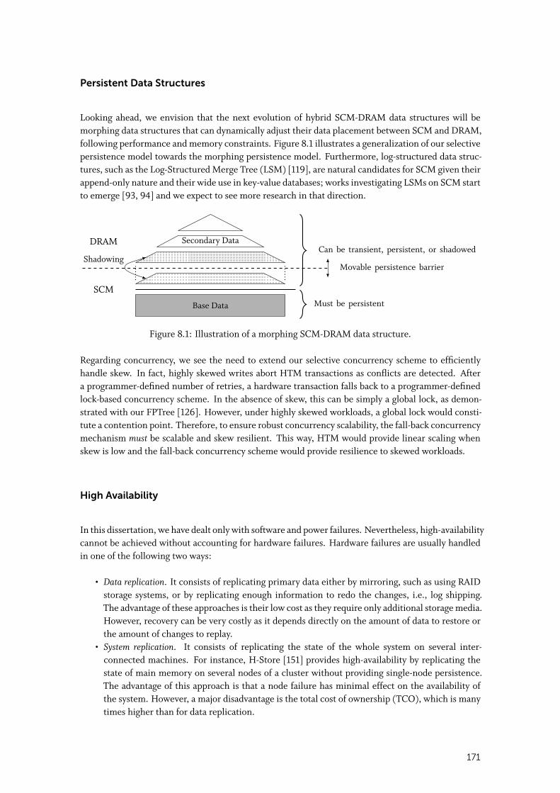
Persistent Data Structures
Looking ahead, we envision that the next evolution of hybrid SCM-DRAM data structures will bemorphing data structures that can dynamically adjust their data placement between SCM and DRAM,following performance and memory constraints. Figure 8.1 illustrates a generalization of our selectivepersistence model towards the morphing persistence model. Furthermore, log-structured data struc-tures, such as the Log-Structured Merge Tree (LSM) [119], are natural candidates for SCM given theirappend-only nature and their wide use in key-value databases; works investigating LSMs on SCM startto emerge [93, 94] and we expect to see more research in that direction.
Base Data
Secondary Data
Shadowing
DRAM
SCMMust be persistent
Can be transient, persistent, or shadowed
Movable persistence barrier
Figure 8.1: Illustration of a morphing SCM-DRAM data structure.
Regarding concurrency, we see the need to extend our selective concurrency scheme to efficientlyhandle skew. In fact, highly skewed writes abort HTM transactions as conflicts are detected. Aftera programmer-defined number of retries, a hardware transaction falls back to a programmer-definedlock-based concurrency scheme. In the absence of skew, this can be simply a global lock, as demon-strated with our FPTree [126]. However, under highly skewed workloads, a global lock would consti-tute a contention point. Therefore, to ensure robust concurrency scalability, the fall-back concurrencymechanism must be scalable and skew resilient. This way, HTM would provide linear scaling whenskew is low and the fall-back concurrency scheme would provide resilience to skewed workloads.
High Availability
In this dissertation, we have dealt only with software and power failures. Nevertheless, high-availabilitycannot be achieved without accounting for hardware failures. Hardware failures are usually handledin one of the following two ways:
• Data replication. It consists of replicating primary data either by mirroring, such as using RAIDstorage systems, or by replicating enough information to redo the changes, i.e., log shipping.The advantage of these approaches is their low cost as they require only additional storage media.However, recovery can be very costly as it depends directly on the amount of data to restore orthe amount of changes to replay.
• System replication. It consists of replicating the state of the whole system on several inter-connected machines. For instance, H-Store [151] provides high-availability by replicating thestate of main memory on several nodes of a cluster without providing single-node persistence.The advantage of this approach is that a node failure has minimal effect on the availability ofthe system. However, a major disadvantage is the total cost of ownership (TCO), which is manytimes higher than for data replication.
171
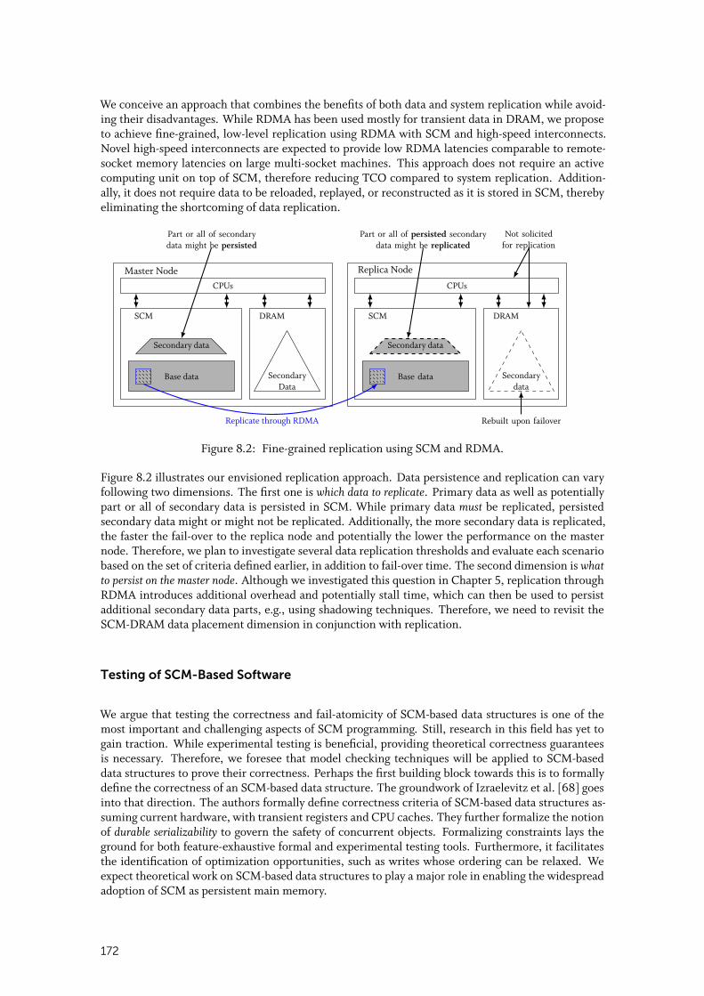
We conceive an approach that combines the benefits of both data and system replication while avoid-ing their disadvantages. While RDMA has been used mostly for transient data in DRAM, we proposeto achieve fine-grained, low-level replication using RDMA with SCM and high-speed interconnects.Novel high-speed interconnects are expected to provide low RDMA latencies comparable to remote-socket memory latencies on large multi-socket machines. This approach does not require an activecomputing unit on top of SCM, therefore reducing TCO compared to system replication. Addition-ally, it does not require data to be reloaded, replayed, or reconstructed as it is stored in SCM, therebyeliminating the shortcoming of data replication.
Master Node Replica Node
SCM DRAM SCM DRAM
CPUs CPUs
Base data Base data
Secondary data Secondary data
Replicate through RDMA
SecondaryData
Secondarydata
Rebuilt upon failover
Part or all of secondarydata might be persisted
Part or all of persisted secondarydata might be replicated
Not solicitedfor replication
Figure 8.2: Fine-grained replication using SCM and RDMA.
Figure 8.2 illustrates our envisioned replication approach. Data persistence and replication can varyfollowing two dimensions. The first one is which data to replicate. Primary data as well as potentiallypart or all of secondary data is persisted in SCM. While primary data must be replicated, persistedsecondary data might or might not be replicated. Additionally, the more secondary data is replicated,the faster the fail-over to the replica node and potentially the lower the performance on the masternode. Therefore, we plan to investigate several data replication thresholds and evaluate each scenariobased on the set of criteria defined earlier, in addition to fail-over time. The second dimension is whatto persist on the master node. Although we investigated this question in Chapter 5, replication throughRDMA introduces additional overhead and potentially stall time, which can then be used to persistadditional secondary data parts, e.g., using shadowing techniques. Therefore, we need to revisit theSCM-DRAM data placement dimension in conjunction with replication.
Testing of SCM-Based Software
We argue that testing the correctness and fail-atomicity of SCM-based data structures is one of themost important and challenging aspects of SCM programming. Still, research in this field has yet togain traction. While experimental testing is beneficial, providing theoretical correctness guaranteesis necessary. Therefore, we foresee that model checking techniques will be applied to SCM-baseddata structures to prove their correctness. Perhaps the first building block towards this is to formallydefine the correctness of an SCM-based data structure. The groundwork of Izraelevitz et al. [68] goesinto that direction. The authors formally define correctness criteria of SCM-based data structures as-suming current hardware, with transient registers and CPU caches. They further formalize the notionof durable serializability to govern the safety of concurrent objects. Formalizing constraints lays theground for both feature-exhaustive formal and experimental testing tools. Furthermore, it facilitatesthe identification of optimization opportunities, such as writes whose ordering can be relaxed. Weexpect theoretical work on SCM-based data structures to play a major role in enabling the widespreadadoption of SCM as persistent main memory.
172
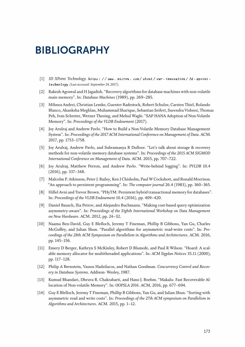
BIBLIOGRAPHY
[1] 3D XPoint Technology. https : / / www . micron . com / about / our - innovation / 3d - xpoint -
technology (Last accessed: September 24, 2017).
[2] Rakesh Agrawal and H Jagadish. “Recovery algorithms for database machines with non-volatilemain memory”. In: Database Machines (1989), pp. 269–285.
[3] Mihnea Andrei, Christian Lemke, Guenter Radestock, Robert Schulze, Carsten Thiel, RolandoBlanco, Akanksha Meghlan, Muhammad Sharique, Sebastian Seifert, Surendra Vishnoi, ThomasPeh, Ivan Schreter, Werner Thesing, and Mehul Wagle. “SAP HANA Adoption of Non-VolatileMemory”. In: Proceedings of the VLDB Endowment (2017).
[4] Joy Arulraj and Andrew Pavlo. “How to Build a Non-Volatile Memory Database ManagementSystem”. In: Proceedings of the 2017 ACM International Conference on Management of Data. ACM.2017, pp. 1753–1758.
[5] Joy Arulraj, Andrew Pavlo, and Subramanya R Dulloor. “Let’s talk about storage & recoverymethods for non-volatile memory database systems”. In: Proceedings of the 2015 ACM SIGMODInternational Conference on Management of Data. ACM. 2015, pp. 707–722.
[6] Joy Arulraj, Matthew Perron, and Andrew Pavlo. “Write-behind logging”. In: PVLDB 10.4(2016), pp. 337–348.
[7] Malcolm P. Atkinson, Peter J. Bailey, Ken J Chisholm, Paul W Cockshott, and Ronald Morrison.“An approach to persistent programming”. In: The computer journal 26.4 (1983), pp. 360–365.
[8] Hillel Avni and Trevor Brown. “PHyTM: Persistent hybrid transactional memory for databases”.In: Proceedings of the VLDB Endowment 10.4 (2016), pp. 409–420.
[9] Daniel Bausch, Ilia Petrov, and Alejandro Buchmann. “Making cost-based query optimizationasymmetry-aware”. In: Proceedings of the Eighth International Workshop on Data Managementon New Hardware. ACM. 2012, pp. 24–32.
[10] Naama Ben-David, Guy E Blelloch, Jeremy T Fineman, Phillip B Gibbons, Yan Gu, CharlesMcGuffey, and Julian Shun. “Parallel algorithms for asymmetric read-write costs”. In: Pro-ceedings of the 28th ACM Symposium on Parallelism in Algorithms and Architectures. ACM. 2016,pp. 145–156.
[11] Emery D Berger, Kathryn S McKinley, Robert D Blumofe, and Paul R Wilson. “Hoard: A scal-able memory allocator for multithreaded applications”. In: ACM Sigplan Notices 35.11 (2000),pp. 117–128.
[12] Philip A Bernstein, Vassos Hadzilacos, and Nathan Goodman. Concurrency Control and Recov-ery in Database Systems. Addison- Wesley, 1987.
[13] Kumud Bhandari, Dhruva R. Chakrabarti, and Hans-J. Boehm. “Makalu: Fast Recoverable Al-location of Non-volatile Memory”. In: OOPSLA 2016. ACM, 2016, pp. 677–694.
[14] Guy E Blelloch, Jeremy T Fineman, Phillip B Gibbons, Yan Gu, and Julian Shun. “Sorting withasymmetric read and write costs”. In: Proceedings of the 27th ACM symposium on Parallelism inAlgorithms and Architectures. ACM. 2015, pp. 1–12.
173
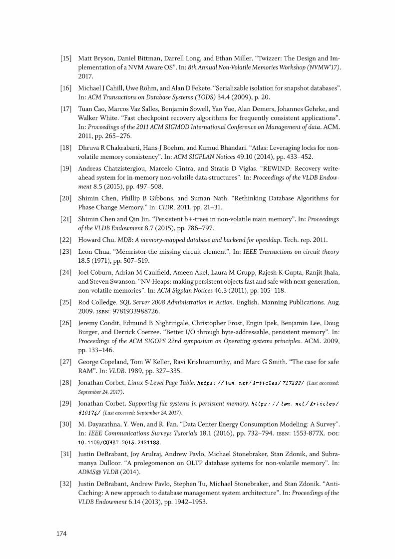
[15] Matt Bryson, Daniel Bittman, Darrell Long, and Ethan Miller. “Twizzer: The Design and Im-plementation of a NVM Aware OS”. In: 8th Annual Non-Volatile Memories Workshop (NVMW’17).2017.
[16] Michael J Cahill, Uwe Röhm, and Alan D Fekete. “Serializable isolation for snapshot databases”.In: ACM Transactions on Database Systems (TODS) 34.4 (2009), p. 20.
[17] Tuan Cao, Marcos Vaz Salles, Benjamin Sowell, Yao Yue, Alan Demers, Johannes Gehrke, andWalker White. “Fast checkpoint recovery algorithms for frequently consistent applications”.In: Proceedings of the 2011 ACM SIGMOD International Conference on Management of data. ACM.2011, pp. 265–276.
[18] Dhruva R Chakrabarti, Hans-J Boehm, and Kumud Bhandari. “Atlas: Leveraging locks for non-volatile memory consistency”. In: ACM SIGPLAN Notices 49.10 (2014), pp. 433–452.
[19] Andreas Chatzistergiou, Marcelo Cintra, and Stratis D Viglas. “REWIND: Recovery write-ahead system for in-memory non-volatile data-structures”. In: Proceedings of the VLDB Endow-ment 8.5 (2015), pp. 497–508.
[20] Shimin Chen, Phillip B Gibbons, and Suman Nath. “Rethinking Database Algorithms forPhase Change Memory.” In: CIDR. 2011, pp. 21–31.
[21] Shimin Chen and Qin Jin. “Persistent b+-trees in non-volatile main memory”. In: Proceedingsof the VLDB Endowment 8.7 (2015), pp. 786–797.
[22] Howard Chu. MDB: A memory-mapped database and backend for openldap. Tech. rep. 2011.
[23] Leon Chua. “Memristor-the missing circuit element”. In: IEEE Transactions on circuit theory18.5 (1971), pp. 507–519.
[24] Joel Coburn, Adrian M Caulfield, Ameen Akel, Laura M Grupp, Rajesh K Gupta, Ranjit Jhala,and Steven Swanson. “NV-Heaps: making persistent objects fast and safe with next-generation,non-volatile memories”. In: ACM Sigplan Notices 46.3 (2011), pp. 105–118.
[25] Rod Colledge. SQL Server 2008 Administration in Action. English. Manning Publications, Aug.2009. isbn: 9781933988726.
[26] Jeremy Condit, Edmund B Nightingale, Christopher Frost, Engin Ipek, Benjamin Lee, DougBurger, and Derrick Coetzee. “Better I/O through byte-addressable, persistent memory”. In:Proceedings of the ACM SIGOPS 22nd symposium on Operating systems principles. ACM. 2009,pp. 133–146.
[27] George Copeland, Tom W Keller, Ravi Krishnamurthy, and Marc G Smith. “The case for safeRAM”. In: VLDB. 1989, pp. 327–335.
[28] Jonathan Corbet. Linux 5-Level Page Table. https: // lwn. net/ Articles/ 717293/ (Last accessed:
September 24, 2017).
[29] Jonathan Corbet. Supporting file systems in persistent memory. https: // lwn. net/ Articles/
610174/ (Last accessed: September 24, 2017).
[30] M. Dayarathna, Y. Wen, and R. Fan. “Data Center Energy Consumption Modeling: A Survey”.In: IEEE Communications Surveys Tutorials 18.1 (2016), pp. 732–794. issn: 1553-877X. doi:10.1109/COMST.2015.2481183.
[31] Justin DeBrabant, Joy Arulraj, Andrew Pavlo, Michael Stonebraker, Stan Zdonik, and Subra-manya Dulloor. “A prolegomenon on OLTP database systems for non-volatile memory”. In:ADMS@ VLDB (2014).
[32] Justin DeBrabant, Andrew Pavlo, Stephen Tu, Michael Stonebraker, and Stan Zdonik. “Anti-Caching: A new approach to database management system architecture”. In: Proceedings of theVLDB Endowment 6.14 (2013), pp. 1942–1953.
174
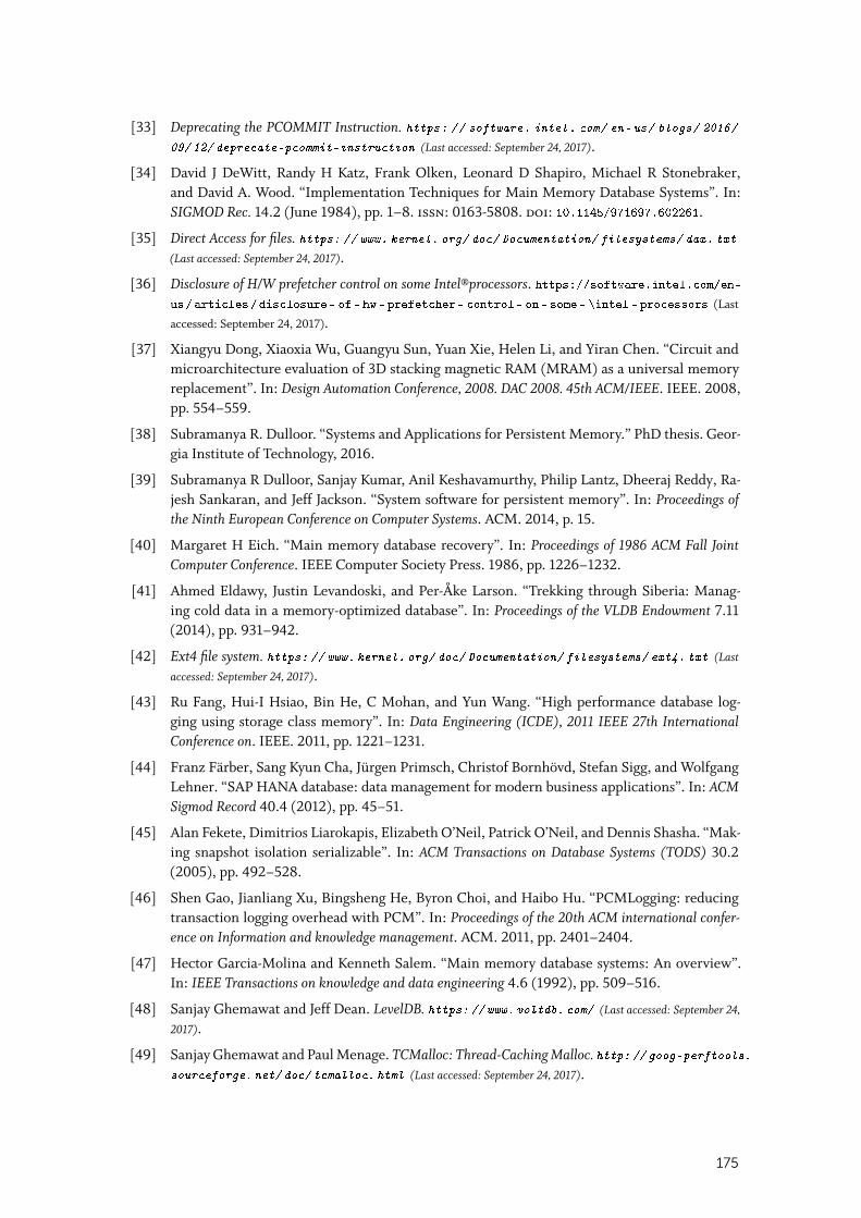
[33] Deprecating the PCOMMIT Instruction. https: // software. intel. com/ en-us/ blogs/ 2016/09/ 12/ deprecate-pcommit-instruction (Last accessed: September 24, 2017).
[34] David J DeWitt, Randy H Katz, Frank Olken, Leonard D Shapiro, Michael R Stonebraker,and David A. Wood. “Implementation Techniques for Main Memory Database Systems”. In:SIGMOD Rec. 14.2 (June 1984), pp. 1–8. issn: 0163-5808. doi: 10.1145/971697.602261.
[35] Direct Access for files. https: // www. kernel. org/ doc/ Documentation/ filesystems/ dax. txt(Last accessed: September 24, 2017).
[36] Disclosure of H/W prefetcher control on some Intel®processors. https://software.intel.com/en-us/articles/disclosure- of- hw- prefetcher- control- on- some- \intel- processors (Last
accessed: September 24, 2017).
[37] Xiangyu Dong, Xiaoxia Wu, Guangyu Sun, Yuan Xie, Helen Li, and Yiran Chen. “Circuit andmicroarchitecture evaluation of 3D stacking magnetic RAM (MRAM) as a universal memoryreplacement”. In: Design Automation Conference, 2008. DAC 2008. 45th ACM/IEEE. IEEE. 2008,pp. 554–559.
[38] Subramanya R. Dulloor. “Systems and Applications for Persistent Memory.” PhD thesis. Geor-gia Institute of Technology, 2016.
[39] Subramanya R Dulloor, Sanjay Kumar, Anil Keshavamurthy, Philip Lantz, Dheeraj Reddy, Ra-jesh Sankaran, and Jeff Jackson. “System software for persistent memory”. In: Proceedings ofthe Ninth European Conference on Computer Systems. ACM. 2014, p. 15.
[40] Margaret H Eich. “Main memory database recovery”. In: Proceedings of 1986 ACM Fall JointComputer Conference. IEEE Computer Society Press. 1986, pp. 1226–1232.
[41] Ahmed Eldawy, Justin Levandoski, and Per-Åke Larson. “Trekking through Siberia: Manag-ing cold data in a memory-optimized database”. In: Proceedings of the VLDB Endowment 7.11(2014), pp. 931–942.
[42] Ext4 file system. https: // www. kernel. org/ doc/ Documentation/ filesystems/ ext4. txt (Last
accessed: September 24, 2017).
[43] Ru Fang, Hui-I Hsiao, Bin He, C Mohan, and Yun Wang. “High performance database log-ging using storage class memory”. In: Data Engineering (ICDE), 2011 IEEE 27th InternationalConference on. IEEE. 2011, pp. 1221–1231.
[44] Franz Färber, Sang Kyun Cha, Jürgen Primsch, Christof Bornhövd, Stefan Sigg, and WolfgangLehner. “SAP HANA database: data management for modern business applications”. In: ACMSigmod Record 40.4 (2012), pp. 45–51.
[45] Alan Fekete, Dimitrios Liarokapis, Elizabeth O’Neil, Patrick O’Neil, and Dennis Shasha. “Mak-ing snapshot isolation serializable”. In: ACM Transactions on Database Systems (TODS) 30.2(2005), pp. 492–528.
[46] Shen Gao, Jianliang Xu, Bingsheng He, Byron Choi, and Haibo Hu. “PCMLogging: reducingtransaction logging overhead with PCM”. In: Proceedings of the 20th ACM international confer-ence on Information and knowledge management. ACM. 2011, pp. 2401–2404.
[47] Hector Garcia-Molina and Kenneth Salem. “Main memory database systems: An overview”.In: IEEE Transactions on knowledge and data engineering 4.6 (1992), pp. 509–516.
[48] Sanjay Ghemawat and Jeff Dean. LevelDB. https: // www. voltdb. com/ (Last accessed: September 24,
2017).
[49] Sanjay Ghemawat and Paul Menage. TCMalloc: Thread-Caching Malloc. http: // goog-perftools.sourceforge. net/ doc/ tcmalloc. html (Last accessed: September 24, 2017).
175
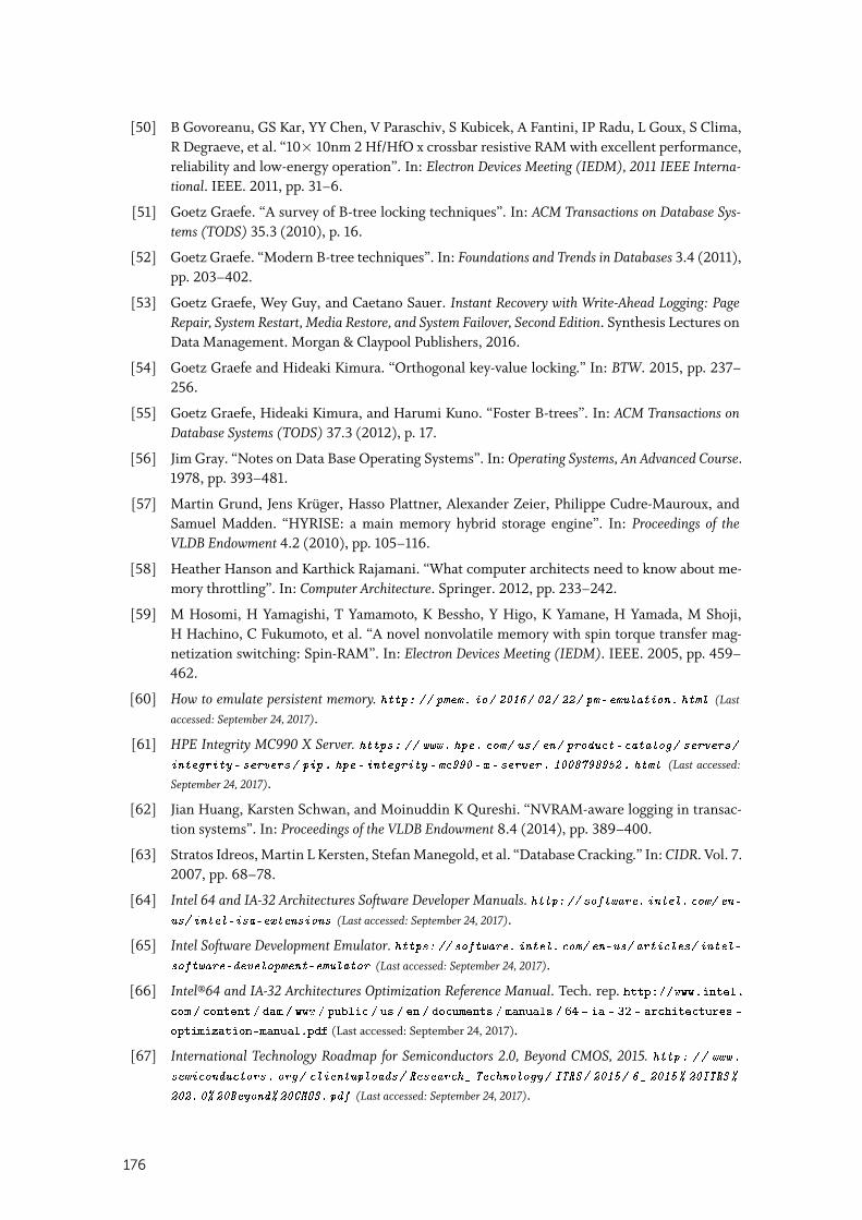
[50] B Govoreanu, GS Kar, YY Chen, V Paraschiv, S Kubicek, A Fantini, IP Radu, L Goux, S Clima,R Degraeve, et al. “10× 10nm 2 Hf/HfO x crossbar resistive RAM with excellent performance,reliability and low-energy operation”. In: Electron Devices Meeting (IEDM), 2011 IEEE Interna-tional. IEEE. 2011, pp. 31–6.
[51] Goetz Graefe. “A survey of B-tree locking techniques”. In: ACM Transactions on Database Sys-tems (TODS) 35.3 (2010), p. 16.
[52] Goetz Graefe. “Modern B-tree techniques”. In: Foundations and Trends in Databases 3.4 (2011),pp. 203–402.
[53] Goetz Graefe, Wey Guy, and Caetano Sauer. Instant Recovery with Write-Ahead Logging: PageRepair, System Restart, Media Restore, and System Failover, Second Edition. Synthesis Lectures onData Management. Morgan & Claypool Publishers, 2016.
[54] Goetz Graefe and Hideaki Kimura. “Orthogonal key-value locking.” In: BTW. 2015, pp. 237–256.
[55] Goetz Graefe, Hideaki Kimura, and Harumi Kuno. “Foster B-trees”. In: ACM Transactions onDatabase Systems (TODS) 37.3 (2012), p. 17.
[56] Jim Gray. “Notes on Data Base Operating Systems”. In: Operating Systems, An Advanced Course.1978, pp. 393–481.
[57] Martin Grund, Jens Krüger, Hasso Plattner, Alexander Zeier, Philippe Cudre-Mauroux, andSamuel Madden. “HYRISE: a main memory hybrid storage engine”. In: Proceedings of theVLDB Endowment 4.2 (2010), pp. 105–116.
[58] Heather Hanson and Karthick Rajamani. “What computer architects need to know about me-mory throttling”. In: Computer Architecture. Springer. 2012, pp. 233–242.
[59] M Hosomi, H Yamagishi, T Yamamoto, K Bessho, Y Higo, K Yamane, H Yamada, M Shoji,H Hachino, C Fukumoto, et al. “A novel nonvolatile memory with spin torque transfer mag-netization switching: Spin-RAM”. In: Electron Devices Meeting (IEDM). IEEE. 2005, pp. 459–462.
[60] How to emulate persistent memory. http: // pmem. io/ 2016/ 02/ 22/ pm-emulation. html (Last
accessed: September 24, 2017).
[61] HPE Integrity MC990 X Server. https: // www. hpe. com/ us/ en/ product-catalog/ servers/integrity- servers/ pip. hpe- integrity- mc990- x- server. 1008798952. html (Last accessed:
September 24, 2017).
[62] Jian Huang, Karsten Schwan, and Moinuddin K Qureshi. “NVRAM-aware logging in transac-tion systems”. In: Proceedings of the VLDB Endowment 8.4 (2014), pp. 389–400.
[63] Stratos Idreos, Martin L Kersten, Stefan Manegold, et al. “Database Cracking.” In: CIDR. Vol. 7.2007, pp. 68–78.
[64] Intel 64 and IA-32 Architectures Software Developer Manuals. http: // software. intel. com/ en-us/ intel-isa-extensions (Last accessed: September 24, 2017).
[65] Intel Software Development Emulator. https: // software. intel. com/ en-us/ articles/ intel-software-development-emulator (Last accessed: September 24, 2017).
[66] Intel®64 and IA-32 Architectures Optimization Reference Manual. Tech. rep. http://www.intel.com / content / dam / www / public / us / en / documents / manuals / 64 - ia - 32 - architectures -
optimization-manual.pdf (Last accessed: September 24, 2017).
[67] International Technology Roadmap for Semiconductors 2.0, Beyond CMOS, 2015. http: // www.
semiconductors. org/ clientuploads/ Research_ Technology/ ITRS/ 2015/ 6_ 2015% 20ITRS%
202. 0% 20Beyond% 20CMOS. pdf (Last accessed: September 24, 2017).
176
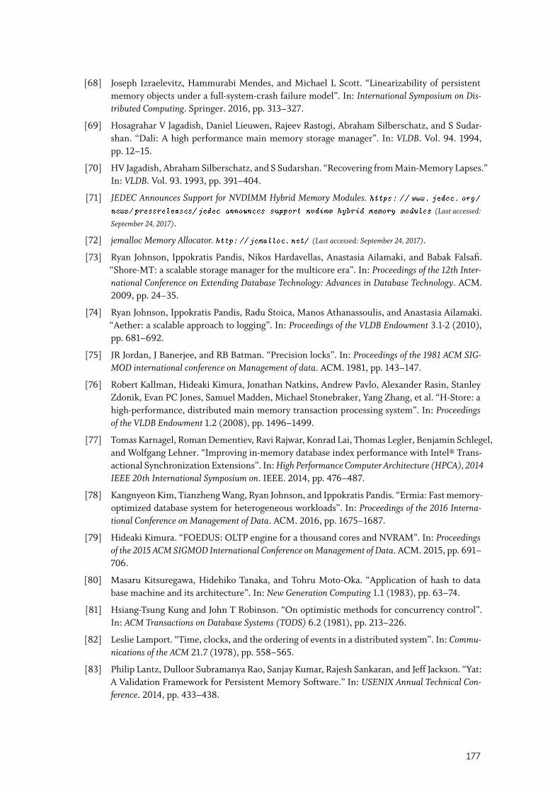
[68] Joseph Izraelevitz, Hammurabi Mendes, and Michael L Scott. “Linearizability of persistentmemory objects under a full-system-crash failure model”. In: International Symposium on Dis-tributed Computing. Springer. 2016, pp. 313–327.
[69] Hosagrahar V Jagadish, Daniel Lieuwen, Rajeev Rastogi, Abraham Silberschatz, and S Sudar-shan. “Dali: A high performance main memory storage manager”. In: VLDB. Vol. 94. 1994,pp. 12–15.
[70] HV Jagadish, Abraham Silberschatz, and S Sudarshan. “Recovering from Main-Memory Lapses.”In: VLDB. Vol. 93. 1993, pp. 391–404.
[71] JEDEC Announces Support for NVDIMM Hybrid Memory Modules. https: // www. jedec. org/
news/ pressreleases/ jedec-announces-support-nvdimm-hybrid-memory-modules (Last accessed:
September 24, 2017).
[72] jemalloc Memory Allocator. http: // jemalloc. net/ (Last accessed: September 24, 2017).
[73] Ryan Johnson, Ippokratis Pandis, Nikos Hardavellas, Anastasia Ailamaki, and Babak Falsafi.“Shore-MT: a scalable storage manager for the multicore era”. In: Proceedings of the 12th Inter-national Conference on Extending Database Technology: Advances in Database Technology. ACM.2009, pp. 24–35.
[74] Ryan Johnson, Ippokratis Pandis, Radu Stoica, Manos Athanassoulis, and Anastasia Ailamaki.“Aether: a scalable approach to logging”. In: Proceedings of the VLDB Endowment 3.1-2 (2010),pp. 681–692.
[75] JR Jordan, J Banerjee, and RB Batman. “Precision locks”. In: Proceedings of the 1981 ACM SIG-MOD international conference on Management of data. ACM. 1981, pp. 143–147.
[76] Robert Kallman, Hideaki Kimura, Jonathan Natkins, Andrew Pavlo, Alexander Rasin, StanleyZdonik, Evan PC Jones, Samuel Madden, Michael Stonebraker, Yang Zhang, et al. “H-Store: ahigh-performance, distributed main memory transaction processing system”. In: Proceedingsof the VLDB Endowment 1.2 (2008), pp. 1496–1499.
[77] Tomas Karnagel, Roman Dementiev, Ravi Rajwar, Konrad Lai, Thomas Legler, Benjamin Schlegel,and Wolfgang Lehner. “Improving in-memory database index performance with Intel® Trans-actional Synchronization Extensions”. In: High Performance Computer Architecture (HPCA), 2014IEEE 20th International Symposium on. IEEE. 2014, pp. 476–487.
[78] Kangnyeon Kim, Tianzheng Wang, Ryan Johnson, and Ippokratis Pandis. “Ermia: Fast memory-optimized database system for heterogeneous workloads”. In: Proceedings of the 2016 Interna-tional Conference on Management of Data. ACM. 2016, pp. 1675–1687.
[79] Hideaki Kimura. “FOEDUS: OLTP engine for a thousand cores and NVRAM”. In: Proceedingsof the 2015 ACM SIGMOD International Conference on Management of Data. ACM. 2015, pp. 691–706.
[80] Masaru Kitsuregawa, Hidehiko Tanaka, and Tohru Moto-Oka. “Application of hash to database machine and its architecture”. In: New Generation Computing 1.1 (1983), pp. 63–74.
[81] Hsiang-Tsung Kung and John T Robinson. “On optimistic methods for concurrency control”.In: ACM Transactions on Database Systems (TODS) 6.2 (1981), pp. 213–226.
[82] Leslie Lamport. “Time, clocks, and the ordering of events in a distributed system”. In: Commu-nications of the ACM 21.7 (1978), pp. 558–565.
[83] Philip Lantz, Dulloor Subramanya Rao, Sanjay Kumar, Rajesh Sankaran, and Jeff Jackson. “Yat:A Validation Framework for Persistent Memory Software.” In: USENIX Annual Technical Con-ference. 2014, pp. 433–438.
177
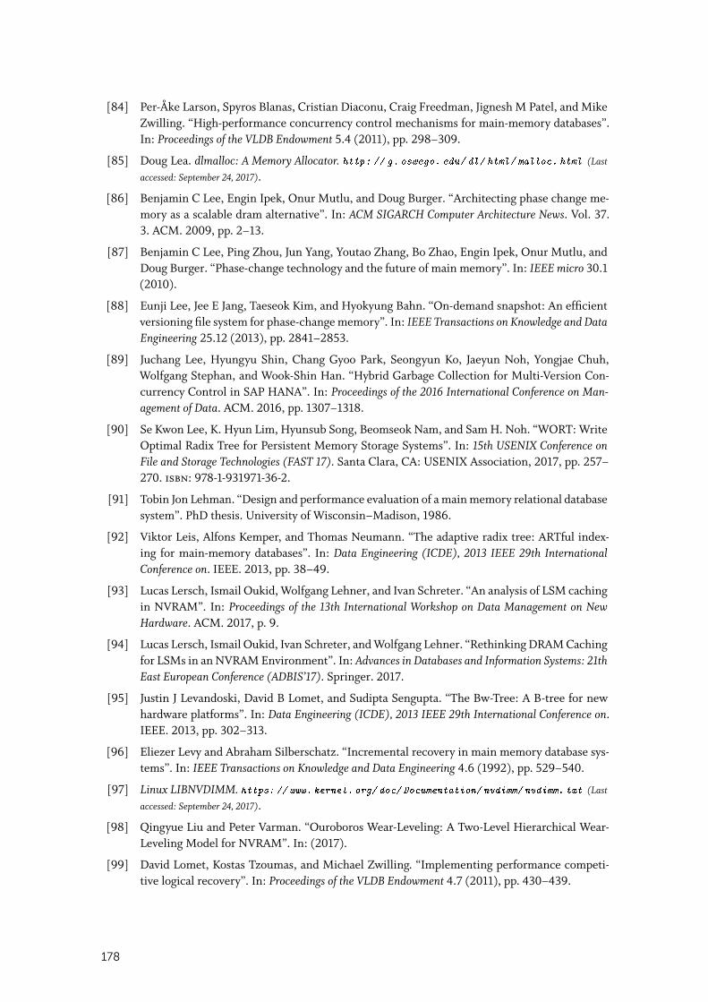
[84] Per-Åke Larson, Spyros Blanas, Cristian Diaconu, Craig Freedman, Jignesh M Patel, and MikeZwilling. “High-performance concurrency control mechanisms for main-memory databases”.In: Proceedings of the VLDB Endowment 5.4 (2011), pp. 298–309.
[85] Doug Lea. dlmalloc: A Memory Allocator. http: // g. oswego. edu/ dl/ html/ malloc. html (Last
accessed: September 24, 2017).
[86] Benjamin C Lee, Engin Ipek, Onur Mutlu, and Doug Burger. “Architecting phase change me-mory as a scalable dram alternative”. In: ACM SIGARCH Computer Architecture News. Vol. 37.3. ACM. 2009, pp. 2–13.
[87] Benjamin C Lee, Ping Zhou, Jun Yang, Youtao Zhang, Bo Zhao, Engin Ipek, Onur Mutlu, andDoug Burger. “Phase-change technology and the future of main memory”. In: IEEE micro 30.1(2010).
[88] Eunji Lee, Jee E Jang, Taeseok Kim, and Hyokyung Bahn. “On-demand snapshot: An efficientversioning file system for phase-change memory”. In: IEEE Transactions on Knowledge and DataEngineering 25.12 (2013), pp. 2841–2853.
[89] Juchang Lee, Hyungyu Shin, Chang Gyoo Park, Seongyun Ko, Jaeyun Noh, Yongjae Chuh,Wolfgang Stephan, and Wook-Shin Han. “Hybrid Garbage Collection for Multi-Version Con-currency Control in SAP HANA”. In: Proceedings of the 2016 International Conference on Man-agement of Data. ACM. 2016, pp. 1307–1318.
[90] Se Kwon Lee, K. Hyun Lim, Hyunsub Song, Beomseok Nam, and Sam H. Noh. “WORT: WriteOptimal Radix Tree for Persistent Memory Storage Systems”. In: 15th USENIX Conference onFile and Storage Technologies (FAST 17). Santa Clara, CA: USENIX Association, 2017, pp. 257–270. isbn: 978-1-931971-36-2.
[91] Tobin Jon Lehman. “Design and performance evaluation of a main memory relational databasesystem”. PhD thesis. University of Wisconsin–Madison, 1986.
[92] Viktor Leis, Alfons Kemper, and Thomas Neumann. “The adaptive radix tree: ARTful index-ing for main-memory databases”. In: Data Engineering (ICDE), 2013 IEEE 29th InternationalConference on. IEEE. 2013, pp. 38–49.
[93] Lucas Lersch, Ismail Oukid, Wolfgang Lehner, and Ivan Schreter. “An analysis of LSM cachingin NVRAM”. In: Proceedings of the 13th International Workshop on Data Management on NewHardware. ACM. 2017, p. 9.
[94] Lucas Lersch, Ismail Oukid, Ivan Schreter, and Wolfgang Lehner. “Rethinking DRAM Cachingfor LSMs in an NVRAM Environment”. In: Advances in Databases and Information Systems: 21thEast European Conference (ADBIS’17). Springer. 2017.
[95] Justin J Levandoski, David B Lomet, and Sudipta Sengupta. “The Bw-Tree: A B-tree for newhardware platforms”. In: Data Engineering (ICDE), 2013 IEEE 29th International Conference on.IEEE. 2013, pp. 302–313.
[96] Eliezer Levy and Abraham Silberschatz. “Incremental recovery in main memory database sys-tems”. In: IEEE Transactions on Knowledge and Data Engineering 4.6 (1992), pp. 529–540.
[97] Linux LIBNVDIMM. https: // www. kernel. org/ doc/ Documentation/ nvdimm/ nvdimm. txt (Last
accessed: September 24, 2017).
[98] Qingyue Liu and Peter Varman. “Ouroboros Wear-Leveling: A Two-Level Hierarchical Wear-Leveling Model for NVRAM”. In: (2017).
[99] David Lomet, Kostas Tzoumas, and Michael Zwilling. “Implementing performance competi-tive logical recovery”. In: Proceedings of the VLDB Endowment 4.7 (2011), pp. 430–439.
178
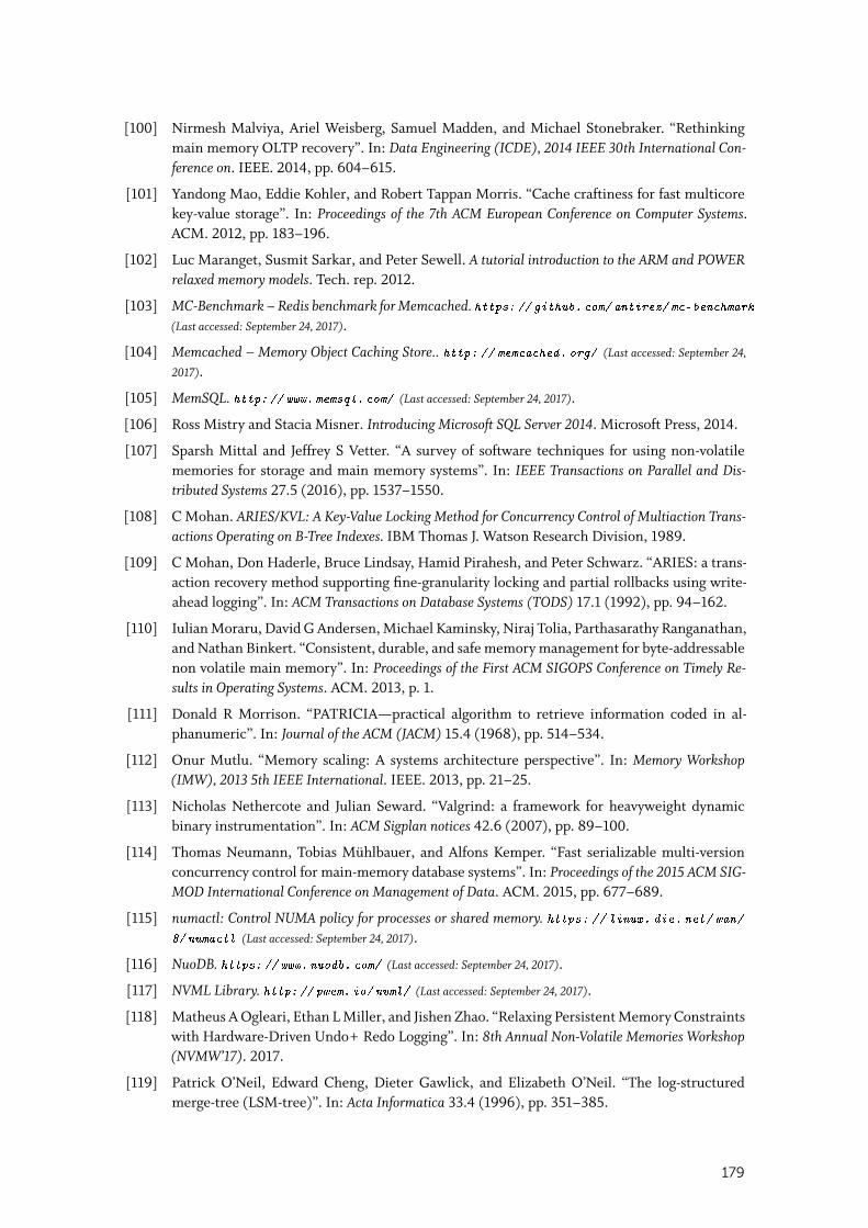
[100] Nirmesh Malviya, Ariel Weisberg, Samuel Madden, and Michael Stonebraker. “Rethinkingmain memory OLTP recovery”. In: Data Engineering (ICDE), 2014 IEEE 30th International Con-ference on. IEEE. 2014, pp. 604–615.
[101] Yandong Mao, Eddie Kohler, and Robert Tappan Morris. “Cache craftiness for fast multicorekey-value storage”. In: Proceedings of the 7th ACM European Conference on Computer Systems.ACM. 2012, pp. 183–196.
[102] Luc Maranget, Susmit Sarkar, and Peter Sewell. A tutorial introduction to the ARM and POWERrelaxed memory models. Tech. rep. 2012.
[103] MC-Benchmark – Redis benchmark for Memcached. https: // github. com/ antirez/ mc-benchmark(Last accessed: September 24, 2017).
[104] Memcached – Memory Object Caching Store.. http: // memcached. org/ (Last accessed: September 24,
2017).
[105] MemSQL. http: // www. memsql. com/ (Last accessed: September 24, 2017).
[106] Ross Mistry and Stacia Misner. Introducing Microsoft SQL Server 2014. Microsoft Press, 2014.
[107] Sparsh Mittal and Jeffrey S Vetter. “A survey of software techniques for using non-volatilememories for storage and main memory systems”. In: IEEE Transactions on Parallel and Dis-tributed Systems 27.5 (2016), pp. 1537–1550.
[108] C Mohan. ARIES/KVL: A Key-Value Locking Method for Concurrency Control of Multiaction Trans-actions Operating on B-Tree Indexes. IBM Thomas J. Watson Research Division, 1989.
[109] C Mohan, Don Haderle, Bruce Lindsay, Hamid Pirahesh, and Peter Schwarz. “ARIES: a trans-action recovery method supporting fine-granularity locking and partial rollbacks using write-ahead logging”. In: ACM Transactions on Database Systems (TODS) 17.1 (1992), pp. 94–162.
[110] Iulian Moraru, David G Andersen, Michael Kaminsky, Niraj Tolia, Parthasarathy Ranganathan,and Nathan Binkert. “Consistent, durable, and safe memory management for byte-addressablenon volatile main memory”. In: Proceedings of the First ACM SIGOPS Conference on Timely Re-sults in Operating Systems. ACM. 2013, p. 1.
[111] Donald R Morrison. “PATRICIA—practical algorithm to retrieve information coded in al-phanumeric”. In: Journal of the ACM (JACM) 15.4 (1968), pp. 514–534.
[112] Onur Mutlu. “Memory scaling: A systems architecture perspective”. In: Memory Workshop(IMW), 2013 5th IEEE International. IEEE. 2013, pp. 21–25.
[113] Nicholas Nethercote and Julian Seward. “Valgrind: a framework for heavyweight dynamicbinary instrumentation”. In: ACM Sigplan notices 42.6 (2007), pp. 89–100.
[114] Thomas Neumann, Tobias Mühlbauer, and Alfons Kemper. “Fast serializable multi-versionconcurrency control for main-memory database systems”. In: Proceedings of the 2015 ACM SIG-MOD International Conference on Management of Data. ACM. 2015, pp. 677–689.
[115] numactl: Control NUMA policy for processes or shared memory. https: // linux. die. net/ man/8/ numactl (Last accessed: September 24, 2017).
[116] NuoDB. https: // www. nuodb. com/ (Last accessed: September 24, 2017).
[117] NVML Library. http: // pmem. io/ nvml/ (Last accessed: September 24, 2017).
[118] Matheus A Ogleari, Ethan L Miller, and Jishen Zhao. “Relaxing Persistent Memory Constraintswith Hardware-Driven Undo+ Redo Logging”. In: 8th Annual Non-Volatile Memories Workshop(NVMW’17). 2017.
[119] Patrick O’Neil, Edward Cheng, Dieter Gawlick, and Elizabeth O’Neil. “The log-structuredmerge-tree (LSM-tree)”. In: Acta Informatica 33.4 (1996), pp. 351–385.
179
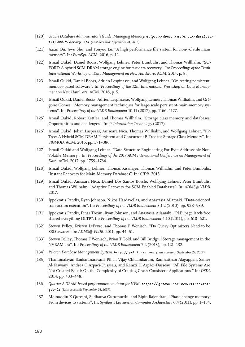
[120] Oracle Database Administrator’s Guide: Managing Memory. https: // docs. oracle. com/ database/121/ ADMIN/ memory. htm (Last accessed: September 24, 2017).
[121] Jiaxin Ou, Jiwu Shu, and Youyou Lu. “A high performance file system for non-volatile mainmemory”. In: EuroSys. ACM. 2016, p. 12.
[122] Ismail Oukid, Daniel Booss, Wolfgang Lehner, Peter Bumbulis, and Thomas Willhalm. “SO-FORT: A hybrid SCM-DRAM storage engine for fast data recovery”. In: Proceedings of the TenthInternational Workshop on Data Management on New Hardware. ACM. 2014, p. 8.
[123] Ismail Oukid, Daniel Booss, Adrien Lespinasse, and Wolfgang Lehner. “On testing persistent-memory-based software”. In: Proceedings of the 12th International Workshop on Data Manage-ment on New Hardware. ACM. 2016, p. 5.
[124] Ismail Oukid, Daniel Booss, Adrien Lespinasse, Wolfgang Lehner, Thomas Willhalm, and Gré-goire Gomes. “Memory management techniques for large-scale persistent-main-memory sys-tems”. In: Proceedings of the VLDB Endowment 10.11 (2017), pp. 1166–1177.
[125] Ismail Oukid, Robert Kettler, and Thomas Willhalm. “Storage class memory and databases:Opportunities and challenges”. In: it-Information Technology (2017).
[126] Ismail Oukid, Johan Lasperas, Anisoara Nica, Thomas Willhalm, and Wolfgang Lehner. “FP-Tree: A Hybrid SCM-DRAM Persistent and Concurrent B-Tree for Storage Class Memory”. In:SIGMOD. ACM. 2016, pp. 371–386.
[127] Ismail Oukid and Wolfgang Lehner. “Data Structure Engineering For Byte-Addressable Non-Volatile Memory”. In: Proceedings of the 2017 ACM International Conference on Management ofData. ACM. 2017, pp. 1759–1764.
[128] Ismail Oukid, Wolfgang Lehner, Thomas Kissinger, Thomas Willhalm, and Peter Bumbulis.“Instant Recovery for Main-Memory Databases”. In: CIDR. 2015.
[129] Ismail Oukid, Anisoara Nica, Daniel Dos Santos Bossle, Wolfgang Lehner, Peter Bumbulis,and Thomas Willhalm. “Adaptive Recovery for SCM-Enabled Databases”. In: ADMS@ VLDB.2017.
[130] Ippokratis Pandis, Ryan Johnson, Nikos Hardavellas, and Anastasia Ailamaki. “Data-orientedtransaction execution”. In: Proceedings of the VLDB Endowment 3.1-2 (2010), pp. 928–939.
[131] Ippokratis Pandis, Pinar Tözün, Ryan Johnson, and Anastasia Ailamaki. “PLP: page latch-freeshared-everything OLTP”. In: Proceedings of the VLDB Endowment 4.10 (2011), pp. 610–621.
[132] Steven Pelley, Kristen LeFevre, and Thomas F Wenisch. “Do Query Optimizers Need to beSSD-aware?” In: ADMS@ VLDB. 2011, pp. 44–51.
[133] Steven Pelley, Thomas F Wenisch, Brian T Gold, and Bill Bridge. “Storage management in theNVRAM era”. In: Proceedings of the VLDB Endowment 7.2 (2013), pp. 121–132.
[134] Peloton Database Management System. http: // pelotondb. org (Last accessed: September 24, 2017).
[135] Thanumalayan Sankaranarayana Pillai, Vijay Chidambaram, Ramnatthan Alagappan, SamerAl-Kiswany, Andrea C Arpaci-Dusseau, and Remzi H Arpaci-Dusseau. “All File Systems AreNot Created Equal: On the Complexity of Crafting Crash-Consistent Applications.” In: OSDI.2014, pp. 433–448.
[136] Quartz: A DRAM-based performance emulator for NVM. https: // github. com/ HewlettPackard/quartz (Last accessed: September 24, 2017).
[137] Moinuddin K Qureshi, Sudhanva Gurumurthi, and Bipin Rajendran. “Phase change memory:From devices to systems”. In: Synthesis Lectures on Computer Architecture 6.4 (2011), pp. 1–134.
180
[138] Moinuddin K Qureshi, John Karidis, Michele Franceschini, Vijayalakshmi Srinivasan, LuisLastras, and Bulent Abali. “Enhancing lifetime and security of PCM-based main memory withstart-gap wear leveling”. In: Proceedings of the 42nd Annual IEEE/ACM International Symposiumon Microarchitecture. ACM. 2009, pp. 14–23.
[139] Moinuddin K Qureshi, Vijayalakshmi Srinivasan, and Jude A Rivers. “Scalable high perfor-mance main memory system using phase-change memory technology”. In: ACM SIGARCHComputer Architecture News 37.3 (2009), pp. 24–33.
[140] Vijayshankar Raman, Gopi Attaluri, Ronald Barber, Naresh Chainani, David Kalmuk, VincentKulandaiSamy, Jens Leenstra, Sam Lightstone, Shaorong Liu, Guy M Lohman, et al. “DB2with BLU acceleration: So much more than just a column store”. In: Proceedings of the VLDBEndowment 6.11 (2013), pp. 1080–1091.
[141] Jun Rao and Kenneth A Ross. “Making B+-trees cache conscious in main memory”. In: ACMSIGMOD Record. Vol. 29. 2. ACM. 2000, pp. 475–486.
[142] Real-Time Decision Making Using Hybrid Streaming, In-Memory Computing Analytics and Transac-tion Processing. Gartner, 2017. https: // www. gartner. com/ imagesrv/ media-products/ pdf/Kx/ KX-1-3CZ44RH. pdf (Last accessed: September 24, 2017).
[143] David P Reed. “Implementing atomic actions on decentralized data”. In: ACM Transactions onComputer Systems (TOCS) 1.1 (1983), pp. 3–23.
[144] David Patrick Reed. “Naming and synchronization in a decentralized computer system”. PhDthesis. Massachusetts Institute of Technology, 1978.
[145] SAP HANA Memory Usage Explained. https: // www. sap. com/ documents/ 2016/ 08/ 205c8299-867c-0010-82c7-eda71af511fa. html (Last accessed: September 24, 2017).
[146] Karl Schnaitter, Neoklis Polyzotis, and Lise Getoor. “Index interactions in physical design tun-ing: modeling, analysis, and applications”. In: Proceedings of the VLDB Endowment 2.1 (2009),pp. 1234–1245.
[147] David Schwalb, Tim Berning, Martin Faust, Markus Dreseler, and Hasso Plattner. “nvm mal-loc: Memory Allocation for NVRAM.” In: ADMS@ VLDB. 2015, pp. 61–72.
[148] David Schwalb, Girish Kumar BK, Markus Dreseler, S Anusha, Martin Faust, Adolf Hohl, TimBerning, Gaurav Makkar, Hasso Plattner, and Parag Deshmukh. “Hyrise-NV: Instant Recov-ery for In-Memory Databases Using Non-Volatile Memory”. In: International Conference onDatabase Systems for Advanced Applications. Springer. 2016, pp. 267–282.
[149] David Schwalb, Markus Dreseler, Matthias Uflacker, and Hasso Plattner. “NVC-hashmap: Apersistent and concurrent hashmap for non-volatile memories”. In: Proceedings of the 3rd VLDBWorkshop on In-Memory Data Mangement and Analytics. ACM. 2015, p. 4.
[150] SNIA NVM Programming Model V1.1. Tech. rep. http://www.snia.org/sites/default/files/NVMProgrammingModel_v1.1.pdf (Last accessed: September 24, 2017).
[151] Michael Stonebraker, Samuel Madden, Daniel J Abadi, Stavros Harizopoulos, Nabil Hachem,and Pat Helland. “The end of an architectural era: (it’s time for a complete rewrite)”. In: Pro-ceedings of the 33rd international conference on Very large data bases. VLDB Endowment. 2007,pp. 1150–1160.
[152] Michael Stonebraker and Lawrence A. Rowe. “The Design of POSTGRES”. In: Proceedings ofthe 1986 ACM SIGMOD International Conference on Management of Data. SIGMOD ’86. Wash-ington, D.C., USA: ACM, 1986, pp. 340–355.
[153] Dmitri B Strukov, Gregory S Snider, Duncan R Stewart, and R Stanley Williams. “The missingmemristor found”. In: nature 453.7191 (2008), pp. 80–83.
181
[154] STX B+-Tree C++ Template Classes. https: // panthema. net/ 2007/ stx-btree/ (Last accessed:
September 24, 2017).
[155] Telecom Application Transaction Processing Benchmark. http: // tatpbenchmark. sourceforge.net/ (Last accessed: September 24, 2017).
[156] The DB2 UDB memory model. https : / / www . ibm . com / developerworks / data / library /
techarticle/ dm-0406qi/ (Last accessed: September 24, 2017).
[157] Tile Based Architecture in Peloton. https: // github. com/ cmu-db/ peloton/ wiki/ Tile-Based-Architecture (Last accessed: September 24, 2017).
[158] Tmpfs file system.https: // www. kernel. org/ doc/ Documentation/ filesystems/ tmpfs. txt (Last accessed: Septem-
ber 24, 2017).
[159] TPC-C Benchmark. http: // www. tpc. org/ tpcc/ (Last accessed: September 24, 2017).
[160] Irving L Traiger. “Virtual memory management for database systems”. In: ACM SIGOPS Oper-ating Systems Review 16.4 (1982), pp. 26–48.
[161] Stephen Tu, Wenting Zheng, Eddie Kohler, Barbara Liskov, and Samuel Madden. “Speedytransactions in multicore in-memory databases”. In: Proceedings of the Twenty-Fourth ACM Sym-posium on Operating Systems Principles. ACM. 2013, pp. 18–32.
[162] Using Non-volatile Memory (NVDIMM-N) as Byte-Addressable Storage in Windows Server 2016.https: // channel9. msdn. com/ events/ build/ 2016/ p470 (Last accessed: September 24, 2017).
[163] Valgrind extension for persistent memory. https: // github. com/ pmem/ valgrind (Last accessed:
September 24, 2017).
[164] Shivaram Venkataraman, Niraj Tolia, Parthasarathy Ranganathan, Roy H Campbell, et al. “Con-sistent and Durable Data Structures for Non-Volatile Byte-Addressable Memory.” In: 9th USENIXConference on File and Storage Technologies (FAST 11). Vol. 11. USENIX Association, 2011, pp. 61–75.
[165] Stratis D Viglas. “Adapting the B+-tree for asymmetric I/O”. In: East European Conference onAdvances in Databases and Information Systems. Springer. 2012, pp. 399–412.
[166] Stratis D Viglas. “Write-limited sorts and joins for persistent memory”. In: Proceedings of theVLDB Endowment 7.5 (2014), pp. 413–424.
[167] Haris Volos, Guilherme Magalhaes, Ludmila Cherkasova, and Jun Li. “Quartz: A LightweightPerformance Emulator for Persistent Memory Software”. In: Proceedings of the 16th AnnualMiddleware Conference. ACM. 2015, pp. 37–49.
[168] Haris Volos, Andres Jaan Tack, and Michael M Swift. “Mnemosyne: Lightweight persistentmemory”. In: ACM SIGARCH Computer Architecture News 39.1 (2011), pp. 91–104.
[169] VoltDB. https: // www. voltdb. com/ (Last accessed: September 24, 2017).
[170] Tianzheng Wang and Ryan Johnson. “Scalable logging through emerging non-volatile me-mory”. In: Proceedings of the VLDB Endowment 7.10 (2014), pp. 865–876.
[171] Tianzheng Wang, Ryan Johnson, Alan Fekete, and Ippokratis Pandis. “Efficiently making (al-most) any concurrency control mechanism serializable”. In: The VLDB Journal 26.4 (2017),pp. 537–562.
[172] Tianzheng Wang and Hideaki Kimura. “Mostly-optimistic concurrency control for highly con-tended dynamic workloads on a thousand cores”. In: Proceedings of the VLDB Endowment 10.2(2016), pp. 49–60.
182
[173] Thomas Willhalm, Nicolae Popovici, Yazan Boshmaf, Hasso Plattner, Alexander Zeier, andJan Schaffner. “SIMD-scan: ultra fast in-memory table scan using on-chip vector processingunits”. In: Proceedings of the VLDB Endowment 2.1 (2009), pp. 385–394.
[174] Paul R. Wilson. “Pointer Swizzling at Page Fault Time: Efficiently Supporting Huge AddressSpaces on Standard Hardware”. In: SIGARCH Comput. Archit. News 19.4 (July 1991), pp. 6–13.issn: 0163-5964. doi: 10.1145/122576.122577.
[175] Xiaojian Wu and AL Reddy. “SCMFS: a file system for storage class memory”. In: Proceedings of2011 International Conference for High Performance Computing, Networking, Storage and Analysis.ACM. 2011, p. 39.
[176] Yingjun Wu, Joy Arulraj, Jiexi Lin, Ran Xian, and Andrew Pavlo. “An empirical evaluation ofin-memory multi-version concurrency control”. In: Proceedings of the VLDB Endowment 10.7(2017), pp. 781–792.
[177] Yingjun Wu, Chee-Yong Chan, and Kian-Lee Tan. “Transaction healing: Scaling optimisticconcurrency control on multicores”. In: Proceedings of the 2016 International Conference onManagement of Data. ACM. 2016, pp. 1689–1704.
[178] Fei Xia, Dejun Jiang, Jin Xiong, and Ninghui Sun. “HiKV: A Hybrid Index Key-Value Store forDRAM-NVM Memory Systems”. In: 2017 USENIX Annual Technical Conference (USENIX ATC17). Santa Clara, CA: USENIX Association, 2017.
[179] Jian Xu and Steven Swanson. “NOVA: a log-structured file system for hybrid volatile/non-volatile main memories”. In: 14th USENIX Conference on File and Storage Technologies (FAST16). USENIX Association, 2016, pp. 323–338.
[180] J. Yang, Q. Wei, C. Wang, C. Chen, K. Yong, and B. He. “NV-Tree: A Consistent and Workload-adaptive Tree Structure for Non-volatile Memory”. In: IEEE Transactions on Computers PP.99(2015). issn: 0018-9340. doi: 10.1109/TC.2015.2479621.
[181] Junfeng Yang, Can Sar, and Dawson Engler. “Explode: a lightweight, general system for findingserious storage system errors”. In: Proceedings of the 7th symposium on Operating systems designand implementation. USENIX Association. 2006, pp. 131–146.
[182] Chang Yao, Divyakant Agrawal, Gang Chen, Beng Chin Ooi, and Sai Wu. “Adaptive logging:Optimizing logging and recovery costs in distributed in-memory databases”. In: Proceedings ofthe 2016 International Conference on Management of Data. ACM. 2016, pp. 1119–1134.
[183] Matt T Yourst. “PTLsim: A cycle accurate full system x86-64 microarchitectural simulator”. In:Performance Analysis of Systems & Software, 2007. ISPASS 2007. IEEE International Symposium on.IEEE. 2007, pp. 23–34.
[184] Songping Yu, Nong Xiao, Mingzhu Deng, Yuxuan Xing, Fang Liu, Zhiping Cai, and Wei Chen.“WAlloc: An efficient wear-aware allocator for non-volatile main memory”. In: IPCCC. IEEE.2015, pp. 1–8.
[185] Pengfei Zuo and Yu Hua. “A Write-friendly Hashing Scheme for Non-Volatile Memory Sys-tems”. In: (2017).
183

184
LIST OF FIGURES
1.1 Comparison of access latency of different memory technologies. Adapted from [137]. 61.2 SCM is mapped directly into the address space of the application, allowing direct ac-
cess with load/store semantics. . . . . . . . . . . . . . . . . . . . . . . . . . . . . 61.3 Towards a hybrid SCM-DRAM single-level database storage architecture. . . . . . . 71.4 Organization of our contributions across the dissertation. . . . . . . . . . . . . . . 9
2.1 SCM as transient main memory extension. . . . . . . . . . . . . . . . . . . . . . . 132.2 SCM as disk replacement or as persistent main memory. . . . . . . . . . . . . . . . 132.3 Measuring process termination duration. Experiment: memory map memory, touch
it, then kill the process and measure termination duration. The experimental systemhas 32 E7-8890 v3 processors (1152 cores total) and 16 terabytes of DRAM. . . . . . 14
2.4 Slowdown incurred by using SCM over DRAM in different microbenchmarks. . . . . 152.5 SIMD Scan performance on SCM relative to DRAM with and without hardware and
software prefetching. . . . . . . . . . . . . . . . . . . . . . . . . . . . . . . . . . 152.6 NUMA-based SCM emulation on a two-socket system. . . . . . . . . . . . . . . . . 162.7 Architecture overview of Intel’s SCM emulation platform. . . . . . . . . . . . . . . 182.8 Traditional database architecture. . . . . . . . . . . . . . . . . . . . . . . . . . . . 192.9 Database architecture with SCM as a primary data store. . . . . . . . . . . . . . . . 222.10 Hybrid SCM-DRAM architecture of SOFORT. . . . . . . . . . . . . . . . . . . . . 282.11 Data layout overview in SOFORT. . . . . . . . . . . . . . . . . . . . . . . . . . . 29
3.1 Illustration of the volatility chain in a 2-core x86-like processors. . . . . . . . . . . . 353.2 Illustration of process address space loss upon restart. . . . . . . . . . . . . . . . . 363.3 Example of data recovery using persistent pointers consisting of a file ID and an offset
within that file. . . . . . . . . . . . . . . . . . . . . . . . . . . . . . . . . . . . . 393.4 Illustration of the segregated-fit allocation strategy for small block allocations. . . . . 433.5 Illustration of the best-fit allocation strategy for large block allocations. . . . . . . . 433.6 16 KB allocation performance on an Intel Xeon CPU X5550 2.67GHz (16 cores). The
core-local allocator scales better under high concurrency than thread-local counterparts. 443.7 Architecture overview of PAllocator. . . . . . . . . . . . . . . . . . . . . . . . . . 463.8 Architecture overview of SmallPAllocator. . . . . . . . . . . . . . . . . . . . . . . 503.9 Data organization in SmallPAllocator. . . . . . . . . . . . . . . . . . . . . . . . . 513.10 Allocation process of SmallPAllocator. . . . . . . . . . . . . . . . . . . . . . . . . 523.11 Architecture overview of BigPAllocator. . . . . . . . . . . . . . . . . . . . . . . . 533.12 Data organization in BigPAllocator. . . . . . . . . . . . . . . . . . . . . . . . . . . 533.13 Allocation process of BigPAllocator. . . . . . . . . . . . . . . . . . . . . . . . . . 543.14 Defragmentation process of BigPAllocator. . . . . . . . . . . . . . . . . . . . . . . 553.15 Allocations concurrency scalability for different object sizes. . . . . . . . . . . . . . 563.16 Allocations performance for different object sizes and SCM latencies. . . . . . . . . 573.17 Deallocation concurrency scalability for different object sizes. . . . . . . . . . . . . 583.18 Deallocation performance for different object sizes and SCM latencies. . . . . . . . 593.19 Random allocation/deallocation benchmark with different distributions. . . . . . . 613.20 Larson benchmark with different random allocation ranges. . . . . . . . . . . . . . 623.21 Recovery time for varying total allocation sizes and SCM latencies. . . . . . . . . . . 63
185
3.22 Allocator impact on FPTree performance. Solid lines represent PAllocator and dash-dotted lines NVML. . . . . . . . . . . . . . . . . . . . . . . . . . . . . . . . . . . 65
4.1 Node split after an insertion in the CDDS B+-Tree. . . . . . . . . . . . . . . . . . . 694.2 Comparison of insertions in a sorted node and an unsorted node. . . . . . . . . . . 704.3 Insertion in an unsorted node with a bitmap and an indirection slot array. . . . . . . 704.4 Overview of the architecture of the NV-Tree. . . . . . . . . . . . . . . . . . . . . . 714.5 Insertion in an append-only leaf node of the NV-Tree. . . . . . . . . . . . . . . . . 714.6 Illustration of the architecture of HiKV. . . . . . . . . . . . . . . . . . . . . . . . 724.7 FPTree inner node and leaf node layouts. . . . . . . . . . . . . . . . . . . . . . . . 734.8 Selective persistence applied to a B+-Tree: inner nodes are kept in DRAM while leaf
nodes are kept in SCM. . . . . . . . . . . . . . . . . . . . . . . . . . . . . . . . . 744.9 Expected number of in-leaf key probes during a successful search operation for the
FPTree, NV-Tree, and wBTree. . . . . . . . . . . . . . . . . . . . . . . . . . . . . 754.10 FPTree leaf group management. . . . . . . . . . . . . . . . . . . . . . . . . . . . 764.11 Selective concurrency applied to an insert operation in a hybrid data structure. . . . 774.12 Effect of the latency of SCM on the performance of the Find, Insert, Update, Delete,
and Recovery tree operations with fixed-size keys. . . . . . . . . . . . . . . . . . . . 924.13 Effect of the latency of SCM on the performance of the Find, Insert, Update, Delete,
and Recovery tree operations with variable-size keys. . . . . . . . . . . . . . . . . . 934.14 DRAM and SCM consumption of trees with 100M key-value: 8-byte and 16-byte keys
for fixed-size and variable-size keys versions, respectively. . . . . . . . . . . . . . . 944.15 Concurrency performance on one socket – 50 million key-values warmup followed by
50 million operations. Ideal speedup is depicted with the mark-less line. . . . . . . 954.16 Concurrency performance on two sockets – 50 million key-values followed by 50 mil-
lion operations. Ideal speedup is depicted with the mark-less line. . . . . . . . . . . 964.17 Concurrency performance on one socket with an SCM latency of 145 ns – 50 million
key-values warmup followed by 50 million operations. Ideal speedup is depicted withthe mark-less line. . . . . . . . . . . . . . . . . . . . . . . . . . . . . . . . . . . 97
4.18 Impact of payload size on the single-threaded and multi-threaded performance of theevaluated trees. . . . . . . . . . . . . . . . . . . . . . . . . . . . . . . . . . . . . 98
4.19 Trees impact on database throughput and restart performance – TATP with 50 millionsubscribers, primary data size ~45 GB. . . . . . . . . . . . . . . . . . . . . . . . . 99
4.20 Trees impact on memcached performance for different latencies – mc-benchkark with50 million operations. . . . . . . . . . . . . . . . . . . . . . . . . . . . . . . . . 100
5.1 Overview of data layout in SOFORT. . . . . . . . . . . . . . . . . . . . . . . . . . 1105.2 Example of a SOFORT table of employees and their offices. . . . . . . . . . . . . . 1115.3 Transaction flow during a system failure. . . . . . . . . . . . . . . . . . . . . . . . 1265.4 Transaction throughput and latency of SOFORT, SILO, and Shore-MT for the TATP
(10 million Subscribers) and TPC-C (48 Warehouses) benchmarks. . . . . . . . . . 1285.5 Impact of higher SCM latencies on SOFORT’s OLTP performance for the TATP (10 mil-
lion Subscribers) and TPC-C (48 Warehouses) benchmarks. Depicted throughput isrelative to a baseline SCM latency of 160 ns. . . . . . . . . . . . . . . . . . . . . . 129
5.6 SOFORT’s OLTP performance with different secondary data placement strategies forthe TATP (10 million Subscribers) and TPC-C (48 Warehouses) benchmarks. De-picted throughput is relative to SOFORT-FPTree. . . . . . . . . . . . . . . . . . . . 129
5.7 SOFORT DRAM and SCM consumption with different data placement strategies forthe TATP (10 million Subscribers) and TPC-C (48 Warehouses) benchmarks. . . . . 130
5.8 Cost of flushing instructions in SOFORT with different secondary data placementstrategies for the TATP (10 million Subscribers) and TPC-C (48 Warehouses) bench-marks. . . . . . . . . . . . . . . . . . . . . . . . . . . . . . . . . . . . . . . . . 131
186
5.9 SOFORT Recovery time with different storage technologies and data placement strate-gies for the TATP (20 million Subscribers) and TPC-C (128 Warehouses) benchmarks. 132
6.1 Results overview: TPC-C transaction throughput during recovery. . . . . . . . . . . 1346.2 rank(s, t) for TATP (20 Mio subscribers) and TPC-C (50 Warehouses) during recov-
ery : Benefitdep vs. Benefitindep. . . . . . . . . . . . . . . . . . . . . . . . . . 1406.3 Recovery framework of secondary database objects. . . . . . . . . . . . . . . . . . 1426.4 Impact of secondary data placement on recovery performance. Maximum throughput
is relative to the performance of SOFORT-STXTree. . . . . . . . . . . . . . . . . . 1446.5 Different recovery strategies with logarithmic scale. . . . . . . . . . . . . . . . . . 1456.6 Static resource allocation impact on recovery. . . . . . . . . . . . . . . . . . . . . 1466.7 Adaptive resource allocation impact on recovery. . . . . . . . . . . . . . . . . . . 1476.8 Best of static vs. best of adaptive resource allocation. . . . . . . . . . . . . . . . . 1486.9 Impact of workload change during recovery. . . . . . . . . . . . . . . . . . . . . . 1496.10 SCM latency impact on recovery performance. Throughput is depicted relative to a
baseline SCM latency of 200 ns. . . . . . . . . . . . . . . . . . . . . . . . . . . . 1496.11 Worst case analysis: Adaptive recovery Vs. Synchronous recovery. . . . . . . . . . . 150
7.1 Contrast between the traditional disk-based storage architecture (on the left side) andthe single-level SCM-based direct access architecture (on the right side). . . . . . . 154
7.2 Illustration of crash simulation in the testing framework. . . . . . . . . . . . . . . . 1577.3 Global overview of the testing framework including copy-on-write optimizations, me-
mory reordering, and nested crash simulation. . . . . . . . . . . . . . . . . . . . . 1627.4 Frequency distribution of the the number of simulated crashes per call stack. The y
axis represents the considered range groups of the number of crash simulations percall stack, while the x axis represents the cardinality of these groups. . . . . . . . . . 166
8.1 Illustration of a morphing SCM-DRAM data structure. . . . . . . . . . . . . . . . . 1718.2 Fine-grained replication using SCM and RDMA. . . . . . . . . . . . . . . . . . . . 172
LIST OF TABLES
2.1 Comparison of current memory technologies with SCM candidates [107]. . . . . . . 122.2 Summary of state-of-the-art research on re-architecting database storage and recovery
in presence of SCM. . . . . . . . . . . . . . . . . . . . . . . . . . . . . . . . . . 25
3.1 Summary of existing libraries that address some or all of the programming challengesof SCM. PPtr stands for persistent pointer. . . . . . . . . . . . . . . . . . . . . . . 41
3.2 Summary of the design characteristics of existing persistent memory allocators. Thereare salient differences in the design decisions of PAllocator and state-of-the-art persis-tent allocators. . . . . . . . . . . . . . . . . . . . . . . . . . . . . . . . . . . . . 47
3.3 Fragmentation stress test results. . . . . . . . . . . . . . . . . . . . . . . . . . . . 64
4.1 Chosen node sizes (in number of entries) for the evaluated trees. Values are 8-byteintegers for all trees. The suffixes C and Var indicate, respectively, the concurrent andvariable-size key versions of the trees. . . . . . . . . . . . . . . . . . . . . . . . . . 91
6.1 Experimental Configurations of SOFORT Recovery Experiments. . . . . . . . . . . 143
187
6.2 Breakdown of recovery time. Recovery duration of memory management (PAllocator),primary data, secondary data, and garbage recovery times. . . . . . . . . . . . . . . 144
7.1 Performance of the testing framework with nested crash simulation disabled. Callstack is abbreviated as CS. . . . . . . . . . . . . . . . . . . . . . . . . . . . . . . 165
7.2 Performance of the testing framework with nested crash simulation enabled. . . . . 165
LIST OF ALGORITHMS
4.1 FPTree Concurrent Find function. . . . . . . . . . . . . . . . . . . . . . . . . . . 794.2 FPTree Concurrent Insert function for fixed-size keys. . . . . . . . . . . . . . . . . 804.3 FPTree Split Leaf procedure. . . . . . . . . . . . . . . . . . . . . . . . . . . . . . 814.4 FPTree Recover Split Leaf procedure. . . . . . . . . . . . . . . . . . . . . . . . . . 814.5 FPTree Concurrent Delete function for fixed-size keys. . . . . . . . . . . . . . . . . 824.6 FPTree Delete Leaf procedure. . . . . . . . . . . . . . . . . . . . . . . . . . . . . 834.7 FPTree Recover Delete Leaf procedure. . . . . . . . . . . . . . . . . . . . . . . . . 834.8 FPTree Concurrent Update function for fixed-size keys. . . . . . . . . . . . . . . . 844.9 FPTree Recover procedure. . . . . . . . . . . . . . . . . . . . . . . . . . . . . . . 844.10 FPTree Concurrent Insert function for variable-size keys. . . . . . . . . . . . . . . . 854.11 FPTree Concurrent Delete function for variable-size keys. . . . . . . . . . . . . . . 864.12 FPTree Concurrent Update function for variable-size keys. . . . . . . . . . . . . . . 874.13 FPTree Inner Nodes Rebuild procedure for variable-size keys. . . . . . . . . . . . . 884.14 FPTree Get Leaf procedure. . . . . . . . . . . . . . . . . . . . . . . . . . . . . . . 884.15 FPTree Recover Get Leaf procedure. . . . . . . . . . . . . . . . . . . . . . . . . . 894.16 FPTree Free Leaf procedure. . . . . . . . . . . . . . . . . . . . . . . . . . . . . . 894.17 FPTree Recover Free Leaf procedure. . . . . . . . . . . . . . . . . . . . . . . . . . 90
5.1 SOFORT Row Visibility function. . . . . . . . . . . . . . . . . . . . . . . . . . . . 1145.2 SOFORT Cross-Transaction Row Visibility function. . . . . . . . . . . . . . . . . . 1155.3 SOFORT Start Transaction function. . . . . . . . . . . . . . . . . . . . . . . . . . 1155.4 SOFORT Select function. . . . . . . . . . . . . . . . . . . . . . . . . . . . . . . . 1165.5 SOFORT Get Visible Rows function. . . . . . . . . . . . . . . . . . . . . . . . . . 1175.6 SOFORT Insert function. . . . . . . . . . . . . . . . . . . . . . . . . . . . . . . . 1175.7 SOFORT Delete function. . . . . . . . . . . . . . . . . . . . . . . . . . . . . . . 1185.8 SOFORT Update function. . . . . . . . . . . . . . . . . . . . . . . . . . . . . . . 1195.9 SOFORT Commit Transaction function . . . . . . . . . . . . . . . . . . . . . . . . 1215.10 SOFORT Abort Transaction function. . . . . . . . . . . . . . . . . . . . . . . . . . 1225.11 SOFORT Recovery function. . . . . . . . . . . . . . . . . . . . . . . . . . . . . . 1235.12 SOFORT Transaction Recovery function. . . . . . . . . . . . . . . . . . . . . . . . 1235.13 SOFORT Garbage Collection function. . . . . . . . . . . . . . . . . . . . . . . . . 1245.14 SOFORT Row Collection function. . . . . . . . . . . . . . . . . . . . . . . . . . . 1245.15 SOFORT Background Garbage Collection Recovery function. . . . . . . . . . . . . 1256.1 SOFORT Adaptive Recovery procedure. . . . . . . . . . . . . . . . . . . . . . . . 1416.2 Get Next Indexes to Rebuild function. . . . . . . . . . . . . . . . . . . . . . . . . 141
7.1 Crash simulation inside the Flush procedure. . . . . . . . . . . . . . . . . . . . . . 1587.2 Crash Simulation procedure with call-stack awareness. . . . . . . . . . . . . . . . . 1597.3 Crash Simulation procedure with call-stack awareness and stashed writes. . . . . . . 161
188

CONFIRMATION
I confirm that I independently prepared the dissertation and that I used only the references and auxil-iary means indicated in the dissertation.
Walldorf, December 15, 2017
189

190

191
Top Related
Copyright © 2022 FDOKUMEN

