


Bahasa
Halaman
Hukum


UNIVERSITY OF BELGRADE
FACULTY OF CIVIL ENGINEERING
Milos S. Marjanovic
Analysis of Interaction Inside the PileGroup Subjected to Arbitrary Horizontal
Loading
Doctoral Dissertation
Belgrade, 2020.

UNIVERZITET U BEOGRADU
GRA–DEVINSKI FAKULTET
Milos S. Marjanovic
Analiza interakcije sipova u grupiopterecenoj horizontalnim opterecenjem
proizvoljnog pravca
Doktorska disertacija
Beograd, 2020.
Milos S. Marjanovic
Analysis of Interaction Inside the Pile Group Subjected to ArbitraryHorizontal Loading
Advisors:
Prof. Dr. Mirjana VukicevicUniversity of Belgrade, Faculty of Civil Engineering
Dr.-Ing. Diethard Konig (AkadOR)Ruhr Universitat Bochum, Chair of Soil Mechanics, Foundation Engineeringand Environmental Geotechnics
Committee:
Prof. Dr. Mirjana VukicevicUniversity of Belgrade, Faculty of Civil Engineering
Dr.-Ing. Diethard KonigRuhr Universitat Bochum, Chair of Soil Mechanics, Foundation Engineeringand Environmental Geotechnics
Assist. Prof. Dr. Sanja JockovicUniversity of Belgrade, Faculty of Civil Engineering
Assist. Prof. Dr. Selimir LelovicUniversity of Belgrade, Faculty of Civil Engineering
Assoc. Prof. Dr. Petar SantracUniversity of Novi Sad, Faculty of Civil Engineering Subotica
Belgrade, . . 2020.

Acknowledgments
This thesis is the result of the research carried mainly at the Chair of Geotech-nical Engineering of University of Belgrade and partially at the Chair of SoilMechanics, Foundation Engineering and Environmental Geotechnics of RuhrUniversity Bochum (RUB) during 2015-2020.
First and foremost, I would like to thank to my thesis advisor, Prof. Dr. Mir-jana Vukicevic from University of Belgrade, for giving me the opportunity tostart the research career in the field of Geotechnical Engineering, for her con-tinuous support during the development of the thesis, valuable discussions andthe scientific freedom that allowed me to grow as a researcher.
I express my sincerest gratitude to thesis coadvisor, Dr. Diethard Konig fromRUB for introducing me into the field of horizontally loaded pile groups, forconstant enthusiasm, motivation and important comments during my research.Beside his academic support, Dr. Konig helped me with his warm welcomesduring my research stays in Bochum, provided and arranged all necessary re-sources during my work, removed every obstacle that he could, and made methink only about the research. He really made my dream come true.
My forever gratitude goes to Prof. Dr. Tom Schanz, late Head of the Chairof Soil Mechanics, Foundation Engineering and Environmental Geotechnics atRUB, who suddenly passed away in October 2017. His scientific achievements,dedication, outstanding personality and leadership were true inspiration for ev-eryone of us who had the privilege to be the part of his research group. Hismemory will always be with me as an example of what does it really mean tobe a modern scientist.
Initial discussions with Prof. Dr. Rene Schafer from Hochschule Ruhr West areacknowledged. I also thank to all Committee members for review of the thesisand the valuable comments.
My special thanks go to Prof. Dr. Mira Petronijevic from the University ofBelgrade, for her dedication to young researchers, involvement and coordinationof the SEEFORM scholarship project, that made my visits to the RUB possible.

I am grateful to all of my colleagues at the Chair of Geotechnical Engineeringfor valuable discussions and continuous support during my research: Prof. Dr.Slobodan Coric, Dr. Selimir Lelovic, Uros Djuric, Dr. Zoran Radic, Dr. DejanDivac and Slobodan D. Radovanovic. Special thanks go to my office 160-162 col-leagues, for making the everyday work great: Dr. Sanja Jockovic, Dr. SnezanaMaras-Dragojevic, Veljko Pujevic, Nikola Obradovic and Dobrivoje Simic.
I am also very grateful to many colleagues from RUB, who welcomed me friendlyand made my research stays in Bochum unforgettable and exciting experienceinside and outside the office: Dr. Jelena Ninic, Dr. David Oswald, Dr. TimoKasper, Christoph Schmudderich, Thomas Barciaga, Dr. Nina Muthing, Achimvon Blumenthal, Wolfgang Lieske, Florian Christ, Max Schoen, Dr. LinzhiLang, Dr. Elham Mahmoudi, Raoul Holter, Dr. Kavan Khaledi, Dr. AbhishekRawat, Debdeep Sarkar, Peyman Mianji, Alireza Jafari Jebeli, Lingyun Li, Dr.Gaziz Seidalinov, Dr. Usama Al-Anbaki, Manh Cuong Le, Dr. Wiebke Baille,Dr. Negar Rahemi, Dr. Anina Glumac, Prof. Dr. Tamara Nestorovic, VladislavGudzulic, Ana Cvetkovic, Mirjana Ratkovac, Sahir Butt, Armel Meda, Rein-hard Mosinski and Doris Traas. Special thanks go to my office colleagues: Dr.Arash Lavasan, Dr. Chenyang Zhao, Dr. Meisam Goudarzy and Qian Gu.
My thanks are also addressed to colleagues from the SEEFORM scholarship pro-gram, for the great moments during our meetings, seminars and research staysas well: Dr. Marko Radisic, Milos Jockovic, Dragan Kovacevic, Dr. MarkoMarinkovic and Nemanja Markovic.
The writing of this thesis took a lot of time that could have been spent with myfamily. I am very grateful to my wife Andrea for her love, endless patience andincredible support during my PhD studies and long absences from our home.I would never complete my work without her understanding, positive thinkingand encouragement in many hard moments, when things looked impossible.Thank you for always being my better half.
I am also very grateful to my brother, Dr. Miroslav Marjanovic, who walkedthe same path before me, helped me with his useful comments and did the finalproof read of this thesis. He was the ”in− situ” and best possible example ofwhat one PhD student should look like. The support and true love from himand his wife Dragana were of the great importance in this endeavour. Specialthanks go to Strahinja, our star, for the laugh, fun, happiness and true purposethat he brought in our lives.

Last but not least, I am grateful to my beloved parents Slobodan and Svetlana,for showing me the true values of life, and their endless love.
Belgrade, July 2020.
Milos Marjanovic
”...When something is worth doing, it’s worth overdoing...” (Dr. Brian May)

Financial Support
The work on this thesis was supported by the Government of the Republic ofSerbia - Ministry of Education, Science and Technological Development, underthe Project TR-36046 (project leader Prof. Dr. Mira Petronijevic).
The financial support has been also provided through the SEEFORM (SouthEastern European Graduate School for Master and Ph.D. Formation in En-gineering) project financed by German Academic Exchange Service - DAAD(project leader Prof. Dr. Rudiger Hoffer).
The significant financial support for research stays in 2018-2019 was providedboth by the Chair of Soil Mechanics, Foundation Engineering and Environmen-tal Geotechnics of Ruhr University in Bochum (RUB) and through the Collabo-rative Research Center SFB 837 ”Interactions Modelling in MechanizedTunneling” (project leader Prof. Dr. Gunther Meschke).
The network licence of the PLAXIS 3Dr software was provided by the Chairof Soil Mechanics, Foundation Engineering and Environmental Geotechnics ofRuhr University Bochum and the PLAXIS BV Delft company.

To the Memory ofProfessor Tom Schanz

Analysis of Interaction Inside the Pile Group Subjected to Arbitrary
Horizontal Loading
Abstract
The analysis of pile groups subjected to horizontal loading in one of two orthogonal directions is
a common problem in geotechnical engineering. However, the above analysis should sometimes
be extended with the additional cases of horizontal loading, in arbitrary direction. Although the
full scale experiments can provide the best insight into the above problem, they are expensive
and therefore not feasible solution. Instead, numerical (i.e. finite element) analysis usually
remains the ultimate tool for large scope studies.
The main objective of this research is the improvement of the analysis methodology of pile
group for the case of arbitrary static horizontal loading. Its influence is investigated numerically
to check for the existence of the ”critical” pile group configurations and soil conditions, that
may lead to the failure of the foundation structure and superstructure itself.
To reach the above objective, apriori sensitivity analysis of the considered problem and
identification of the main problem parameters are conducted in the first phase. After that, series
of complex 3D numerical models for laterally loaded pile group analysis have been generated
using PLAXIS 3D. Model validation is done by the back-calculation of available experimental
results. Parametric study of pile groups with various configurations under arbitrary horizontal
loading is performed, with an emphasis on pile force distribution, bending response and pile
group efficiency.
Modelling and simulation processes and the optimization of the calculation time were im-
proved using the originally developed codes in Python. The use of multiple computers was
allowed by using the author’s scripts developed within the thesis. The above research resulted
in thousands of numerical simulations, whose findings provided the improved design method-
ology of pile groups under arbitrary static horizontal loading.
Keywords: pile group, horizontal static loading, PLAXIS 3D, Hardening Soil model, Python
Scientific Field: Civil Engineering
Scientifis Subfield: Geotechnical Engineering
UDC: 624.13(043.3)
Analiza interakcije sipova u grupi opterecenoj horizontalnim opterecenjem
proizvoljnog pravca
Rezime
Analiza sipova u grupi izlozenoj horizontalnom opterecenju u nekom od dva ortogonalna pravca
je uobicajen problem u geotehnici. Medjutim, navedena analiza ponekad se mora prosiriti do-
datnim slucajevima horizontalnog opterecenja, u proizvoljnom pravcu. Iako eksperimenti na
realnim konstrukcijama mogu pruziti najbolji uvid u navedeni problem, oni predstavljaju skupo
(i samim tim neizvodljivo) resenje. Umesto toga, numericka analiza (npr. primenom metoda
konacnih elemenata) obicno postaje primarni alat za studije velikog obima.
Glavni cilj ovog istrazivanja je poboljsanje metodologije za analizu grupe sipova za slucaj
proizvoljnog statickog horizontalnog opterecenja. Njegov uticaj je razmatran numericki kako
bi se utvrdilo postojanje ”kriticne” konfiguracije sipova u grupi i uslova tla, koja moze dovesti
do loma temeljne konstrukcije i samog objekta.
Radi ostvarenja gore navedenog cilja, u prvoj fazi sprovedena je uvodna analiza osetljivosti
razmatranog problema i identifikacija glavnih parametara problema. Nakon toga, generisane
su serije slozenih 3D numerickih modela za analizu bocno opterecenih grupa sipova u PLAXIS
3D. Validacija modela izvrsena je povratnim proracunom na osnovu dostupnih eksperimental-
nih rezultata. Sprovedena je parametarska studija bocno opterecenih grupa sipova razlicitih
konfiguracija, sa akcentom na raspodelu sila u sipu, odgovor sipa pri savijanju i efikasnost grupe
sipova.
Postupci modeliranja i simulacije, kao i optimizacija vremena proracuna, poboljsani su pri-
menom originalnih programa u Python-u. Upotreba vise racunara za proracun omogucena je
primenom autorovih programa razvijenih u okviru ove teze. Navedeno istrazivanje rezulto-
valo je u hiljadama numerickih simulacija, ciji su rezultati doveli do poboljsanja metodologije
proracuna sipova u grupi usled proizvoljnog statickog horizontalnog opterecenja.
Kljucne reci: grupa sipova, horizontalno staticko opterecenje, PLAXIS 3D, Hardening Soil
model, Python
Naucna oblast: Gradjevinarstvo
Uza naucna oblast: Gradjevinska geotehnika
UDK: 624.13(043.3)

Contents
1 Introduction 1
1.1 Motivation . . . . . . . . . . . . . . . . . . . . . . . . . . . . . . 1
1.2 Arbitrary lateral loading direction . . . . . . . . . . . . . . . . . 4
1.3 Research objectives and assumptions . . . . . . . . . . . . . . . 6
1.4 Research methodology . . . . . . . . . . . . . . . . . . . . . . . 8
1.5 Organization of the Dissertation . . . . . . . . . . . . . . . . . . 10
2 State of the art 11
2.1 Differential equation of a laterally loaded pile . . . . . . . . . . 11
2.2 Pile group interaction effects . . . . . . . . . . . . . . . . . . . . 13
2.3 Numerical methods . . . . . . . . . . . . . . . . . . . . . . . . . 16
2.4 Notable numerical studies on laterally pile group interaction effects 22
2.5 Experimental studies on laterally loaded pile group interactioneffects . . . . . . . . . . . . . . . . . . . . . . . . . . . . . . . . 26
2.6 Problem sensitivity analysis . . . . . . . . . . . . . . . . . . . . 28
2.7 Concluding remarks . . . . . . . . . . . . . . . . . . . . . . . . . 33
3 Numerical model generation 35
3.1 PLAXIS 3D overview . . . . . . . . . . . . . . . . . . . . . . . . 35
3.2 Constitutive models . . . . . . . . . . . . . . . . . . . . . . . . . 35
3.3 FEM model of the pile group under lateral loading . . . . . . . 39
3.4 Calculation stages . . . . . . . . . . . . . . . . . . . . . . . . . . 43
3.5 Proposed model parameters . . . . . . . . . . . . . . . . . . . . 43
3.6 Model geometry . . . . . . . . . . . . . . . . . . . . . . . . . . . 44
3.7 Automatization of calculation procedures . . . . . . . . . . . . . 51
3.8 Concluding remarks . . . . . . . . . . . . . . . . . . . . . . . . . 57
4 Numerical Model Validation 59
4.1 Model validation - Kotthaus 1992. . . . . . . . . . . . . . . . . . 59
4.2 Concluding remarks . . . . . . . . . . . . . . . . . . . . . . . . . 63
5 Parametric Study and Results Interpretation 65
i

6 Discussion 87
7 Conclusions 89
8 Future Work 91
Bibliography 103
Biography 105
Appendix - Computer Programs 107
ii

List of Figures
1.1 Examples of laterally loaded pile foundations (sources: CNBM,China, Encyclopedia Britannica and ESCO Consultant and En-gineers Co., Ltd., South Korea) . . . . . . . . . . . . . . . . . 2
1.2 Front and trailing rows in laterally loaded pile group. HG -horizontal force, sx and sy - center-to-center spacings betweenthe piles in X and Y directions, respectively . . . . . . . . . . 3
1.3 Influence of the ”shadowing” on the force distribution insidethe pile group (Hi denotes the horizontal force on pile i) . . . . 3
1.4 Pile group under arbitrary horizontal loading (shaded areasshow the overlapping of the shear zones) . . . . . . . . . . . . 6
1.5 Long and short pile (after Broms 1964. [23, 24]) and theirfailure mechanisms . . . . . . . . . . . . . . . . . . . . . . . . 8
1.6 Flowchart of the study and the description of WPs . . . . . . 9
2.1 Distribution of modulus of subgrade reaction ks for differentsoil types (Ki is the stiffness of the elastic spring at point i,calculated as Ki = ks · dz ·D (F/L)) . . . . . . . . . . . . . . 12
2.2 Interaction factors based on the pile position (after Kotthaus1992. [21]). sL and sQ are pile center-to-center spacings in thedirection of the loading HG, and perpendicular to direction ofthe loading, respectively. . . . . . . . . . . . . . . . . . . . . . 14
2.3 Partial interaction factor values based on the pile spacing inloading direction (sL) and perpendicular to loading direction(sQ), after Kotthaus 1992. [21]. Note that at the pile spacingsαL ≥ 6D and αQ ≥ 3D, no interaction occurs. . . . . . . . . . 15
2.4 Strain wedge model parameters (after Norris 1986. [33]) . . . . 18
2.5 Definition of p-multipliers Pm (SP - single pile) . . . . . . . . 19
2.6 Example of p-multipliers for the pile group. The p-y curve forthe pile inside the pile group is scaled for the entire displace-ments range. . . . . . . . . . . . . . . . . . . . . . . . . . . . . 20
2.7 Initial elastic interaction factors αρF for 2 inclined piles (afterstudies of Poulos 1971. [57] and Randolph 1981. [13]) . . . . . 23
2.8 Pile types based on the location inside the pile group and theloading direction (after Papadopoulou and Comodromos, 2014[68]) . . . . . . . . . . . . . . . . . . . . . . . . . . . . . . . . 26
iii
2.9 P-multipliers for different pile spacings from different sources(after Ashour and Ardalan, 2011 [84]) . . . . . . . . . . . . . . 28
2.10 Influencing factors for the laterally loaded pile group . . . . . 30
3.1 HS model stiffness parameters (after Schanz and Vermeer 1999.[115]) . . . . . . . . . . . . . . . . . . . . . . . . . . . . . . . . 37
3.2 EB model in PLAXIS 3D (after Brinkgreve, 2015 [25]). Kn,Kt, Ks and Kfoot denote the interface spring stiffness at pileshaft (in 3 directions) and pile tip (in vertical direction). . . . 40
3.3 Sketch of the model with parametrized geometry, assigned bound-ary conditions and corresponding model parameters . . . . . . 46
3.4 Model parameters in the mesh refinement zone . . . . . . . . . 47
3.5 Directions of the maximum displacements ymax, shear forcesHmax and bending moments Mmax. Loading direction is gov-erned by the loading direction angle β. X, Y , Q12, Q13, M2and M3 denotes the directions of displacements, shear forcesand bending moments in Euclidean XY space in PLAXIS 3D,respectively. . . . . . . . . . . . . . . . . . . . . . . . . . . . . 47
3.6 Shape of the characteristic diagrams for a free head pile . . . . 50
3.7 Verification of shear forces fitting for a single pile (screenshotfrom author’s computer program). Spline fitting of bendingmoments and displacements provides more logical results, es-pecially at the end of the pile, where polynomial fitting showsunrealistically high shear forces. The shear forces calculatedby the spline fitting and differentiation of bending moments(marked with green triangles) is the most realistic, so this fit-ting technique was adopted. . . . . . . . . . . . . . . . . . . . 50
3.8 Verification of bending moments fitting for a single pile (screen-shot from author’s computer program). Spline fitting of bend-ing moments and displacements provides more logical results,especially at the end of the pile, where polynomial fitting showsunrealistically high bending moments. . . . . . . . . . . . . . . 51
3.9 Scheme of the computer network for distributed computingsolution. Main program is installed on the server computerand controlled by user, while the network computers containPLAXIS 3D and they are only accessed remotely, using Pythonscripts . . . . . . . . . . . . . . . . . . . . . . . . . . . . . . . 53
3.10 Modules of computer programs used for the automatization ofnumerical simulations (developed by author) . . . . . . . . . . 54
3.11 Screenshot of Module 2 before distributed computing is started 55
3.12 Screenshot of Module 2 during simulations . . . . . . . . . . . 55
iv

4.1 Measured (triangles) vs. computed (red line) load-displacementresponse - single pile . . . . . . . . . . . . . . . . . . . . . . . 61
4.2 Measured (triangles) vs. computed (red line) load-displacementresponse - piles in a row - front pile . . . . . . . . . . . . . . . 63
4.3 Measured (triangles) vs. computed (red line) load-displacementresponse - piles in a row - front pile . . . . . . . . . . . . . . . 63
4.4 Measured (triangles) vs. computed (red line) load-displacementresponse - piles in a row - front pile . . . . . . . . . . . . . . . 64
5.1 Input parameters for parametric study . . . . . . . . . . . . . 66
5.2 Pile numbering . . . . . . . . . . . . . . . . . . . . . . . . . . 68
5.3 Pile Interaction Factors for 2x2 pile group (sx=2D, sy=2D),considering different normalized displacements y/D and differ-ent horizontal loading directions. Full lines - loose sand; dashedlines - dense sand. . . . . . . . . . . . . . . . . . . . . . . . . . 70
5.4 Pile Interaction Factors for 2x2 pile group (sx=2D, sy=3D),considering different normalized displacements y/D and differ-ent horizontal loading directions. Full lines - loose sand; dashedlines - dense sand. . . . . . . . . . . . . . . . . . . . . . . . . . 70
5.5 Pile Interaction Factors for 2x2 pile group (sx=2D, sy=4D),considering different normalized displacements y/D and differ-ent horizontal loading directions. Full lines - loose sand; dashedlines - dense sand. . . . . . . . . . . . . . . . . . . . . . . . . . 70
5.6 Pile Interaction Factors for 2x2 pile group (sx=2D, sy=5D),considering different normalized displacements y/D and differ-ent horizontal loading directions. Full lines - loose sand; dashedlines - dense sand. . . . . . . . . . . . . . . . . . . . . . . . . . 71
5.7 Pile Interaction Factors for 2x2 pile group (sx=3D, sy=4D),considering different normalized displacements y/D and differ-ent horizontal loading directions. Full lines - loose sand; dashedlines - dense sand. . . . . . . . . . . . . . . . . . . . . . . . . . 71
5.8 Pile Interaction Factors for 2x2 pile group (sx=3D, sy=5D),considering different normalized displacements y/D and differ-ent horizontal loading directions. Full lines - loose sand; dashedlines - dense sand. . . . . . . . . . . . . . . . . . . . . . . . . . 71
5.9 Pile Interaction Factors for 2x2 pile group (sx=4D, sy=5D),considering different normalized displacements y/D and differ-ent horizontal loading directions. Full lines - loose sand; dashedlines - dense sand. . . . . . . . . . . . . . . . . . . . . . . . . . 72
v

5.10 Pile Interaction Factors for 3x3 pile group (sx=3D, sy=3D),considering different normalized displacements y/D and differ-ent horizontal loading directions. Full lines - loose sand; dashedlines - dense sand. . . . . . . . . . . . . . . . . . . . . . . . . . 72
5.11 Pile Interaction Factors for 3x3 pile group (sx=2D, sy=3D),considering different normalized displacements y/D and differ-ent horizontal loading directions. Full lines - loose sand; dashedlines - dense sand. . . . . . . . . . . . . . . . . . . . . . . . . . 72
5.12 Pile Interaction Factors for 3x3 pile group (sx=2D, sy=4D),considering different normalized displacements y/D and differ-ent horizontal loading directions. Full lines - loose sand; dashedlines - dense sand. . . . . . . . . . . . . . . . . . . . . . . . . . 73
5.13 Pile Interaction Factors for 3x3 pile group (sx=2D, sy=5D),considering different normalized displacements y/D and differ-ent horizontal loading directions. Full lines - loose sand; dashedlines - dense sand. . . . . . . . . . . . . . . . . . . . . . . . . . 73
5.14 Pile Interaction Factors for 3x3 pile group (sx=3D, sy=4D),considering different normalized displacements y/D and differ-ent horizontal loading directions. Full lines - loose sand; dashedlines - dense sand. . . . . . . . . . . . . . . . . . . . . . . . . . 73
5.15 Pile Interaction Factors for 3x3 pile group (sx=3D, sy=5D),considering different normalized displacements y/D and differ-ent horizontal loading directions. Full lines - loose sand; dashedlines - dense sand. . . . . . . . . . . . . . . . . . . . . . . . . . 74
5.16 Pile Interaction Factors for 3x3 pile group (sx=4D, sy=5D),considering different normalized displacements y/D and differ-ent horizontal loading directions. Full lines - loose sand; dashedlines - dense sand. . . . . . . . . . . . . . . . . . . . . . . . . . 74
5.17 Pile Interaction Factors for 2x3 pile group (sx=2D, sy=2D),considering different normalized displacements y/D and differ-ent horizontal loading directions. Full lines - loose sand; dashedlines - dense sand. . . . . . . . . . . . . . . . . . . . . . . . . . 74
5.18 Pile Interaction Factors for 2x3 pile group (sx=2D, sy=3D),considering different normalized displacements y/D and differ-ent horizontal loading directions. Full lines - loose sand; dashedlines - dense sand. . . . . . . . . . . . . . . . . . . . . . . . . . 75
5.19 Pile Interaction Factors for 2x3 pile group (sx=2D, sy=4D),considering different normalized displacements y/D and differ-ent horizontal loading directions. Full lines - loose sand; dashedlines - dense sand. . . . . . . . . . . . . . . . . . . . . . . . . . 75
vi

5.20 Pile Interaction Factors for 2x3 pile group (sx=3D, sy=2D),considering different normalized displacements y/D and differ-ent horizontal loading directions. Full lines - loose sand; dashedlines - dense sand. . . . . . . . . . . . . . . . . . . . . . . . . . 75
5.21 Pile Interaction Factors for 2x3 pile group (sx=3D, sy=3D),considering different normalized displacements y/D and differ-ent horizontal loading directions. Full lines - loose sand; dashedlines - dense sand. . . . . . . . . . . . . . . . . . . . . . . . . . 76
5.22 Pile Interaction Factors for 2x3 pile group (sx=3D, sy=4D),considering different normalized displacements y/D and differ-ent horizontal loading directions. Full lines - loose sand; dashedlines - dense sand. . . . . . . . . . . . . . . . . . . . . . . . . . 76
5.23 Pile Interaction Factors for 2x3 pile group (sx=3D, sy=5D),considering different normalized displacements y/D and differ-ent horizontal loading directions. Full lines - loose sand; dashedlines - dense sand. . . . . . . . . . . . . . . . . . . . . . . . . . 76
5.24 Pile Interaction Factors for 2x3 pile group (sx=4D, sy=2D),considering different normalized displacements y/D and differ-ent horizontal loading directions. Full lines - loose sand; dashedlines - dense sand. . . . . . . . . . . . . . . . . . . . . . . . . . 77
5.25 Pile Interaction Factors for 2x3 pile group (sx=4D, sy=3D),considering different normalized displacements y/D and differ-ent horizontal loading directions. Full lines - loose sand; dashedlines - dense sand. . . . . . . . . . . . . . . . . . . . . . . . . . 77
5.26 Pile Interaction Factors for 2x3 pile group (sx=4D, sy=4D),considering different normalized displacements y/D and differ-ent horizontal loading directions. Full lines - loose sand; dashedlines - dense sand. . . . . . . . . . . . . . . . . . . . . . . . . . 77
5.27 Pile Interaction Factors for 2x3 pile group (sx=4D, sy=5D),considering different normalized displacements y/D and differ-ent horizontal loading directions. Full lines - loose sand; dashedlines - dense sand. . . . . . . . . . . . . . . . . . . . . . . . . . 78
5.28 Pile Interaction Factors for 2x3 pile group (sx=5D, sy=3D),considering different normalized displacements y/D and differ-ent horizontal loading directions. Full lines - loose sand; dashedlines - dense sand. . . . . . . . . . . . . . . . . . . . . . . . . . 78
5.29 Pile Interaction Factors for 2x3 pile group (sx=5D, sy=4D),considering different normalized displacements y/D and differ-ent horizontal loading directions. Full lines - loose sand; dashedlines - dense sand. . . . . . . . . . . . . . . . . . . . . . . . . . 78
vii
5.30 Pile Interaction Factors for 2x3 pile group (sx=5D, sy=5D),considering different normalized displacements y/D and differ-ent horizontal loading directions. Full lines - loose sand; dashedlines - dense sand. . . . . . . . . . . . . . . . . . . . . . . . . . 79
5.31 Maximum Bending Moments for 2x2 pile group (sx=2D, sy=2D),considering different normalized displacements y/D and differ-ent horizontal loading directions. Full lines - loose sand; dashedlines - dense sand. . . . . . . . . . . . . . . . . . . . . . . . . . 79
5.32 Maximum Bending Moments for 2x2 pile group (sx=2D, sy=3D),considering different normalized displacements y/D and differ-ent horizontal loading directions. Full lines - loose sand; dashedlines - dense sand. . . . . . . . . . . . . . . . . . . . . . . . . . 79
5.33 Maximum Bending Moments for 2x2 pile group (sx=2D, sy=4D),considering different normalized displacements y/D and differ-ent horizontal loading directions. Full lines - loose sand; dashedlines - dense sand. . . . . . . . . . . . . . . . . . . . . . . . . . 80
5.34 Maximum Bending Moments for 2x2 pile group (sx=2D, sy=5D),considering different normalized displacements y/D and differ-ent horizontal loading directions. Full lines - loose sand; dashedlines - dense sand. . . . . . . . . . . . . . . . . . . . . . . . . . 80
5.35 Maximum Bending Moments for 2x2 pile group (sx=3D, sy=4D),considering different normalized displacements y/D and differ-ent horizontal loading directions. Full lines - loose sand; dashedlines - dense sand. . . . . . . . . . . . . . . . . . . . . . . . . . 80
5.36 Maximum Bending Moments for 2x2 pile group (sx=3D, sy=5D),considering different normalized displacements y/D and differ-ent horizontal loading directions. Full lines - loose sand; dashedlines - dense sand. . . . . . . . . . . . . . . . . . . . . . . . . . 81
5.37 Maximum Bending Moments for 2x2 pile group (sx=4D, sy=5D),considering different normalized displacements y/D and differ-ent horizontal loading directions. Full lines - loose sand; dashedlines - dense sand. . . . . . . . . . . . . . . . . . . . . . . . . . 81
5.38 Maximum Bending Moments for 2x3 pile group (sx=2D, sy=2D),considering different normalized displacements y/D and differ-ent horizontal loading directions. Full lines - loose sand; dashedlines - dense sand. . . . . . . . . . . . . . . . . . . . . . . . . . 81
5.39 Maximum Bending Moments for 2x3 pile group (sx=2D, sy=3D),considering different normalized displacements y/D and differ-ent horizontal loading directions. Full lines - loose sand; dashedlines - dense sand. . . . . . . . . . . . . . . . . . . . . . . . . . 82
viii

5.40 Maximum Bending Moments for 2x3 pile group (sx=2D, sy=4D),considering different normalized displacements y/D and differ-ent horizontal loading directions. Full lines - loose sand; dashedlines - dense sand. . . . . . . . . . . . . . . . . . . . . . . . . . 82
5.41 Maximum Bending Moments for 2x3 pile group (sx=3D, sy=2D),considering different normalized displacements y/D and differ-ent horizontal loading directions. Full lines - loose sand; dashedlines - dense sand. . . . . . . . . . . . . . . . . . . . . . . . . . 82
5.42 Maximum Bending Moments for 2x3 pile group (sx=3D, sy=3D),considering different normalized displacements y/D and differ-ent horizontal loading directions. Full lines - loose sand; dashedlines - dense sand. . . . . . . . . . . . . . . . . . . . . . . . . . 83
5.43 Maximum Bending Moments for 2x3 pile group (sx=3D, sy=4D),considering different normalized displacements y/D and differ-ent horizontal loading directions. Full lines - loose sand; dashedlines - dense sand. . . . . . . . . . . . . . . . . . . . . . . . . . 83
5.44 Maximum Bending Moments for 2x3 pile group (sx=3D, sy=5D),considering different normalized displacements y/D and differ-ent horizontal loading directions. Full lines - loose sand; dashedlines - dense sand. . . . . . . . . . . . . . . . . . . . . . . . . . 83
5.45 Maximum Bending Moments for 2x3 pile group (sx=4D, sy=2D),considering different normalized displacements y/D and differ-ent horizontal loading directions. Full lines - loose sand; dashedlines - dense sand. . . . . . . . . . . . . . . . . . . . . . . . . . 84
5.46 Maximum Bending Moments for 2x3 pile group (sx=4D, sy=3D),considering different normalized displacements y/D and differ-ent horizontal loading directions. Full lines - loose sand; dashedlines - dense sand. . . . . . . . . . . . . . . . . . . . . . . . . . 84
5.47 Maximum Bending Moments for 2x3 pile group (sx=4D, sy=4D),considering different normalized displacements y/D and differ-ent horizontal loading directions. Full lines - loose sand; dashedlines - dense sand. . . . . . . . . . . . . . . . . . . . . . . . . . 84
5.48 Maximum Bending Moments for 2x3 pile group (sx=4D, sy=5D),considering different normalized displacements y/D and differ-ent horizontal loading directions. Full lines - loose sand; dashedlines - dense sand. . . . . . . . . . . . . . . . . . . . . . . . . . 85
5.49 Maximum Bending Moments for 2x3 pile group (sx=5D, sy=3D),considering different normalized displacements y/D and differ-ent horizontal loading directions. Full lines - loose sand; dashedlines - dense sand. . . . . . . . . . . . . . . . . . . . . . . . . . 85
ix

5.50 Maximum Bending Moments for 2x3 pile group (sx=5D, sy=4D),considering different normalized displacements y/D and differ-ent horizontal loading directions. Full lines - loose sand; dashedlines - dense sand. . . . . . . . . . . . . . . . . . . . . . . . . . 85
5.51 Maximum Bending Moments for 2x3 pile group (sx=5D, sy=5D),considering different normalized displacements y/D and differ-ent horizontal loading directions. Full lines - loose sand; dashedlines - dense sand. . . . . . . . . . . . . . . . . . . . . . . . . . 86
x
List of Tables
2.1 Summary of experimental studies on laterally loaded pile groups 27
3.1 Proposed parameters of the FEM model of laterally loaded pilegroup. Integer and float are common numerical data types usedin many programming languages. . . . . . . . . . . . . . . . . 44
4.1 Centrifuge model dimensions [21]. Prototype model correspondsto real concrete pile (between C20/25 and C25/30 concreteclasses) . . . . . . . . . . . . . . . . . . . . . . . . . . . . . . . 60
4.2 Final model parameters after back-calculation of experimentalresults. Model parameters are explained in the previous Chapter. 62
5.1 Adopted numerical model parameters (based on the parametersof the validated numerical model) . . . . . . . . . . . . . . . . 66
5.2 Hardening Soil model parameters for the validated numericalmodel, compared with the synthetic soil parameters . . . . . . 67
5.3 Parametric study scenarios . . . . . . . . . . . . . . . . . . . . 69
xi

xii

1 Introduction
1.1 Motivation
Increasing world population has led to the construction of the large number ofhigh buildings in the last decades [1]. For the purpose of economic foundationof structures, the application of shallow foundations is usually the first option,with the use of minimum required foundation depth. However, in situationswhere the surface soil layers have low bearing capacity, the use of shallow foun-dations is not possible. Instead, the deep foundation systems are used, wherethe load is transmitted to the deeper soil layers with higher bearing capacityusing special structural elements, mostly piles. Single piles are used in a veryfew cases. Instead, piled foundations are usually designed as closely spacedpile groups. Joint work of the piles is enabled by constructing the rigid pilecap that connects the pile tops and provides the load transfer from the struc-ture. Pile cap is usually in the contact with the ground, or above the groundlevel (in offshore structures). The pile group configuration is mostly squared orrectangular.
Pile group under horizontal loading
Beside the primary function to transfer vertical loads to a deeper soil layers, pilefoundations can be significantly loaded with horizontal loads. The examples ofhorizontally loaded structures are high rise ones (industrial chimneys, build-ings, wind turbines), harbour structures, bridges, retaining structures, offshoreplatforms, among others. Horizontal loads on these structures mostly originatefrom:
• Wind pressure,
• Earthquake,
• Wave, current and ice action,
• Impact of ships and other vessels,
• Traffic acceleration, braking and turning forces,
• Earth pressures,
1

1. Introduction
• Soil displacements due to landslides or liquefaction,
• Differences in excavation levels around the foundation structures, etc.
(a) Wind turbine foundations (b) Harbour structure foundations
(c) Bridge foundations
Figure 1.1: Examples of laterally loaded pile foundations (sources: CNBM, China, Encyclo-
pedia Britannica and ESCO Consultant and Engineers Co., Ltd., South Korea)
The magnitude of lateral load is usually 10-15% of vertical load, and about30% in offshore structures [2]. When the horizontal load on the pile head iscaused by the superstructure, such piles are generally referred as ”active piles”.On the contrary, when the piles are loaded due to the horizontal soil movements(for example, in the case of pile stabilized landslides), these piles are referredas ”passive piles”.
The problems that can arise due to the inappropriate assessment of horizon-tal loadings in piles can be very large. Failure in these cases can lead to a severedamage or even collapse of the entire structure.
”Shadowing” effect
The problem of interaction between the piles inside the laterally loaded pilegroup has been recognized by scientific community. It is, in general, consideredas more complex than the problem of axially loaded piles. When the pile
2

1. Introduction
group is laterally loaded, the stress-strain fields of neighbouring piles overlap.The soil in front of the piles becomes stiffer, while the soil behind the piles isconsequently softened. Also, a separation (”gapping”) between the piles andsoil at the back of the pile occurs. This influence of the leading pile rows to thelateral response of trailing pile rows is called ”shadowing”, because the trailingrows are in the shadow of the front pile row (as shown in Fig. 1.2).
Figure 1.2: Front and trailing rows in laterally loaded pile group. HG - horizontal force,
sx and sy - center-to-center spacings between the piles in X and Y directions,
respectively
Ideally, the piles in the group should be spaced so that the load-bearingcapacity of the group is no less than the sum of the bearing capacity of theindividual piles. However, due to the soil-structure interaction effects, the load-displacement behaviour of a pile inside the group is different than of the equiv-alent single pile. Therefore, unequal load distribution occurs inside the pilegroup (see Figure 1.3).
Figure 1.3: Influence of the ”shadowing” on the force distribution inside the pile group (Hi
denotes the horizontal force on pile i)
The maximum bending moment in a group will also be larger than that
3

1. Introduction
for an equivalent single pile, because the soil behaves as it has less resistance,allowing the group to deflect more for the same load per pile. When the pilespacing is increased, the effects of overlapping between the resisting zones areless significant.
Design requirements
Every foundation structure must provide the stability of the structure underall patterns and combinations of loads (ultimate limit state, ULS ). Also, totaland differential settlements, lateral displacements and rotations must remainwithin acceptable limits (serviceability limit state, SLS ). While ULS analysiseliminates the threat to structures and human life, SLS analysis ensures long-term usability.
Traditional approach in the design of pile foundations, followed by the cur-rent design codes, is based on the capacity-based design, while the estimationof the deformations is treated as the secondary issue. However, although thecapacity-based design is still widely used in engineering practice, many authorspointed out that the opposite, displacement-based design approach, is moreappropriate in a variety of practical applications [1, 3–9].
There are two important factors for the design of laterally loaded pile foun-dations:
• maximum lateral displacement at the pile top,
• maximum bending moment in the pile.
In the cases of bridges or other structures founded on pile foundations, only afew centimeters of lateral displacements can cause significant stress developmentin these (statically indeterminant) structures [10]. According to Eurocode 7[11], pile horizontal displacement is usually limited to 3% of a pile diameter, ormax 2 cm.
1.2 Arbitrary lateral loading direction
Despite many experimental and numerical research done in the field of laterallyloaded pile groups in last decades (presented in Chapter 2), some importantquestions are still unresolved.
The most of the (so-far conducted) laterally loaded pile group studies haveconsidered rectangular pile groups, assuming that horizontal loading acts alongthe one of the two orthogonal directions, parallel to the edges of the group.However, the horizontal loading on the pile group may have arbitrary direction,
4

1. Introduction
mainly because of the stochastic nature of its source (such as wind, earthquake,wave loading, ship impact etc.). When the direction of the loading is unknown,the worst case scenario is the loading direction that results in minimum foun-dation capacity.
The number of the research papers dealing with the pile groups under ar-bitrary lateral loading is very limited. Ochoa and O’Neill [12] developed theinteraction factors based on the experimental results of the free and pinned-head piles in the submerged sand. These interaction factors are dependent onthe angle between the load vector and the line that connects the pile heads.Randolph [13] defined the influence of the loading direction for two laterallyloaded piles. Fan and Long [14] analyzed the interaction between the piles un-der various loading directions, and derived the modulus reduction factors toaccount for the pile group interaction effects at the ultimate limit state. In thisstudy, a procedure for determination of the individual pile response inside thepile group with arbitrary geometric layout was proposed. Su and Yan [15] for-mulated a multidirectional p-y model for sands that was incorporated into FEMand validated through the simulations of piles under unidirectional and multi-directional lateral loading. Mayoral et al. [16] formulated the p-y curves forpiles under multidirectional loading in soft clays, emphasizing the complexity ofthe soil-pile interaction under multidirectional loading. The simple applicationof the common p-y curves in two orthogonal direction was found to be impos-sible. Some more complex cases of the pile-soil-pile interactions, such as thebehaviour of the pile group under either eccentric lateral [17] or torsional load-ing [18], have also been reported. The influence of the arbitrary lateral loadingon the ultimate resistance of the pile group with 2 rigid piles was analyzed byGeorgiadis et al. [19], through finite element method (FEM) analysis.
Comments on the study of Su and Zhou 2015.
In their recent paper, Su and Zhou [20] presented the experimental study oflaterally loaded pile groups under different horizontal loading directions. Thisstudy included square and rectangular 2x2 pile groups in sand. Individual(equivalent) single piles were also tested in order to evaluate the pile interactioneffects (i.e. pile group efficiency and pile interaction factors). Model pile groupswith different pile spacings were subjected to the static lateral loading. Theload was applied by hanging the weights connected to the loading point withthe steel rope. Only the values at the ultimate displacement level of 0.2D werepresented, despite the fact that the pile group interaction is strongly influencedby the displacement level [21].
The results have shown that the loading direction has great influence on theredistribution of loads between the piles inside the group, as well as on the
5

1. Introduction
total lateral bearing capacity of the pile group. The pile group at medium pilespacing is more sensitive to the changes in loading direction. This is probablydue to the fact that the variation of the overlapping zone is higher at mediumspacings.
For some pile groups, the increase of the total load proportion for some pileswas observed for the loading direction that was different than the usual 0/90◦
case, which leads to the assumption that additional critical loading cases exist,associated with new critical loading direction. The total load proportion insome individual piles may be underestimated, which can lead to the design onthe unsafe side. For the 2x2 pile group, the increase was found to be from 25%to 35%, which is the relative increase of the pile force of about 40%. At thesmall deflection level, load proportions are almost equal for all piles.
The conclusions from this research, as well as the fact that, up to the author’sknowledge, there are almost no research papers considering such loading case,have mainly motivated the further research presented within this Dissertation.
Figure 1.4: Pile group under arbitrary horizontal loading (shaded areas show the overlapping
of the shear zones)
1.3 Research objectives and assumptions
Objectives
The main objective of this research is the improvement of the analysis of pilegroups for the case of arbitrary static horizontal loading. The main questionsthat will be addressed within this Dissertation are:
• Are there the ”critical” pile group configurations and soil conditions, thatcan lead to the failure, if the influence of arbitrary loading direction is notconsidered in the design phase?
6

1. Introduction
• What is the influence of loading direction on the horizontal force distribu-tion, bending response and pile group efficiency?
• Shall the common concept of analysis of pile groups subjected to horizontalloading in two orthogonal directions be extended with additional cases ofloading in arbitrary direction, as shown in Figure 1.4?
Assumptions
This research is based on the following assumptions:
1. Piles are bored and have circular cross section.
2. Piles are long and flexible.
3. Load acting on the pile group is static, monotonic load in a horizontalplane at the pile top (”active piles”).
4. Soil conditions are drained, homogeneous and isotropic.
These assumptions are based on the facts summarized in the following para-graphs.
Bored piles
Bored piles are more expected for the urban environment, and also they sustainlarger vertical loading, so the horizontal component from such large structuresis expected to be relatively high. According to [22], ”bored and CFA pilesaccount for 50% of the world pile market, while the remaining is mainly coveredby driven (42%) and screw (6%) piles. Summing up, the market is equallysubdivided between displacement and non-displacement piles”. As given in [1],bored piles are the most common form of piling in ”contemporary high riseconstruction”.
Long flexible piles
The influence of the pile length on the pile lateral response is widely known(see Figure 1.5). Usually considered pile failure modes are:
• Failure of the soil supporting the pile (”short pile failure”),
• Structural failure of the pile (”long pile failure”).
Long piles are considered in this study, as more common case in the currentengineering practice [13]. Most piles supporting buildings and bridges fall inthis category.
7

1. Introduction
Figure 1.5: Long and short pile (after Broms 1964. [23, 24]) and their failure mechanisms
Static monotonic horizontal loading / Drained conditions
Many design codes use a pseudo-static approach to assess the action of dynamichorizontal forces on the foundation structure. In these approaches, equivalentstatic monotonic horizontal loading is applied to a structure [1].
Due to the fact that the static horizontal loading is considered, soil conditionsare assumed as drained.
1.4 Research methodology
Full scale experiments can provide the best guidance in the behaviour of pilegroups, but they are expensive and therefore not feasible solution for pile groupanalysis. Instead, numerical analysis usually remains the ultimate tool for largescope studies. Compared to the real experiments, numerical simulations allowfor the large number of analyses to be executed faster and cheaper. The method-ology used in this study follows the concept of ”numerical experiment”, wherea numerical simulation is used to mimic the real experiment.
In order to achieve the defined research objectives, based on the presentedassumptions, following working packages (WPs) have been established withinthis study:
• (WP 1) Problem introduction and definition of research objectives andmethodology.
8
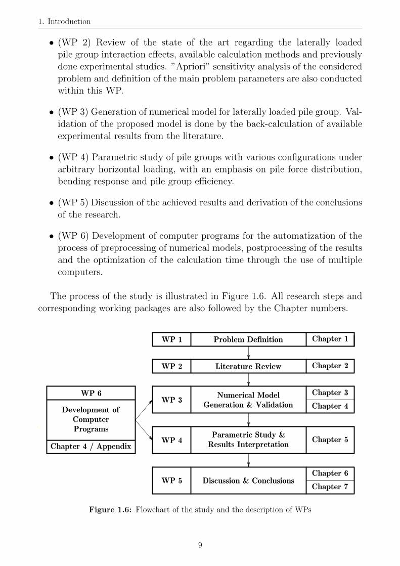
1. Introduction
• (WP 2) Review of the state of the art regarding the laterally loadedpile group interaction effects, available calculation methods and previouslydone experimental studies. ”Apriori” sensitivity analysis of the consideredproblem and definition of the main problem parameters are also conductedwithin this WP.
• (WP 3) Generation of numerical model for laterally loaded pile group. Val-idation of the proposed model is done by the back-calculation of availableexperimental results from the literature.
• (WP 4) Parametric study of pile groups with various configurations underarbitrary horizontal loading, with an emphasis on pile force distribution,bending response and pile group efficiency.
• (WP 5) Discussion of the achieved results and derivation of the conclusionsof the research.
• (WP 6) Development of computer programs for the automatization of theprocess of preprocessing of numerical models, postprocessing of the resultsand the optimization of the calculation time through the use of multiplecomputers.
The process of the study is illustrated in Figure 1.6. All research steps andcorresponding working packages are also followed by the Chapter numbers.
Figure 1.6: Flowchart of the study and the description of WPs
9

1. Introduction
1.5 Organization of the Dissertation
This Dissertation comprises of eight Chapters and one Appendix. The wholeDissertation is organized in a progressive manner, so the final remarks in eachChapter serve as the basis for the next Chapter.
In Chapter 2, the review of different methods for analysis of the pile groupsunder lateral loading is presented. Important advantages and limitations of thecurrent methods are explained. The most important problem parameters andobservation points are identified and they serve as the basis for the generationof the numerical model. Also, current available experimental results have beensummarized in order to support the scope of the research done within thisDissertation.
In Chapter 3, the 3D FEM modelling approach used as the basis forthis study has been explained. Commercially available FEM software pack-age PLAXIS 3D [25] has been briefly described. A detailed explanation of allnumerical model components is presented, including the constitutive laws usedfor the representation of the soil, pile and the pile-soil interface. The limi-tations of the alternative available modelling techniques have been presentedto scientifically support the chosen modelling approach. Developed computerprograms and procedures for the support of the calculation process have beensummarized.
In Chapter 4, calibration and validation of the proposed numerical modelhas been presented, based on the available results from the literature.
In Chapter 5, the scope and the results of the performed parametric studyhave been presented. The selection of the scope of the study has been explainedand all calculation scenarios have been summarized.
In Chapters 6 and 7, obtained results were discussed and the main con-clusions have been delivered. The magnitude (impact) of the pile group effectsunder arbitrary loading has been elaborated, in comparison with the behaviourof equivalent single pile. Additional recommendations for pile group designhave been given.
In Chapter 8, the recommendations for the future research in in the fieldof laterally loaded pile groups have been given.
In Appendix, the developed computer programs used in this study havebeen elaborated to serve as a basis for further research.
10

2 State of the art
The pile group response under lateral loading has been investigated intensivelyin the past decades. Many interesting conclusions from both full scale and smallscale experiments and various numerical studies have been drawn.
2.1 Differential equation of a laterally loaded pile
The most basic representation of a laterally loaded pile is the model of elasticvertical beam, laterally loaded and supported by uncoupled springs along thepile length. Winkler (1867) [26] introduced the modelling of pile behaviourusing the springs to represent soil reactions against pile movement, with thehypothesis which states: ”the soil resistance at any point is a function of thedisplacements in that point”. The stiffness of the uncoupled springs is usuallyreferred as the modulus of subgrade reaction ks. In its basic form, ks is assumedas constant, which leads to linear elastic approach. This method of analysis isusually reffered to as the linear subgrade reaction method or beam on Winklerfoundation (BWF).
The differential equation of laterally loaded elastic beam is given as [27]:
EId4y
dz4+ Pz
d2y
dz2+ p(z) = 0 (2.1)
• y - pile deflection (L),
• z - length along the pile (L),
• EI - flexural stiffness of the pile (FL2),
• Pz - axial load of the pile (F ),
• p(z) - soil pressure at the depth z (F/L2),
• ks - modulus of subgrade reaction (F/L3).
F and L denote the force and length units, respectively.
If we consider the pure lateral loading case (Pz=0) and introduce the afore-mentioned modulus of subgrade reaction ks as proportional to soil pressure(ks = p(z)/y), previous differential equation can be simplified to:
11

2. State of the art
EId4y
dz4+ ksy = 0 (2.2)
Terzaghi [28] pointed out the importance of different ks distributions fordifferent soil types, governed by exponent a. The value of the modulus ofsubgrade reaction for each spring is usually defined as the function of the depthz and pile diameter D. In general, it can be defined as:
ks = nh(z
D)a (2.3)
where:
• nh - coefficient of the modulus of subgrade reaction (F/L3),
• a - distibution exponent (-).
The following recommendations for the distribution of ks are commonly used,as shown in Figure 2.1:
• For OC clay: ks = nh (a = 0),
• For sand and NC clay: ks = nhzD (a = 1).
Figure 2.1: Distribution of modulus of subgrade reaction ks for different soil types (Ki is the
stiffness of the elastic spring at point i, calculated as Ki = ks · dz ·D (F/L))
The following expressions for the shear forces Q and bending moments Mfor the elastic beam are well-known from the linear theory of elasticity:
M(z) = EId2y
dz2(2.4)
Q(z) =dM(z)
dz= EI
d3y
dz3(2.5)
12

2. State of the art
Critical pile length
As mentioned in the research assumptions, usually considered pile failure modesare [23, 24]:
• Failure of the soil supporting the pile (”short pile failure”),
• Structural failure of the pile (”long pile failure”).
For every pile, critical pile length Lc can be defined, beyond which anyadditional length doesn’t affect the lateral pile response [27].
Long, flexible pile can then be defined using the following criterion:
Lc > 4T (2.6)
where:
• T - relative stiffness factor, sometimes referred to as the elastic length ofthe pile (L).
Relative stiffness factor T is calculated according to the following expressionsfor sand/NC clay and OC clay, respectively:
T = (EI
nh)0.2 (2.7)
T = (EI
nh)0.25 (2.8)
It has to be pointed out that these critical length values will vary in real soilconditions, because of different distributions of the ks over soil depth.
2.2 Pile group interaction effects
Interaction factors
The magnitude of the pile group interaction can be described by comparing theimportant parameters (horizontal displacements and bending moments) of apile inside the group, against the parameters of equivalent single pile under thesame mean loading. This concept is still used today in Germany, in everydayengineering practice, through the recommendations of DIN/EN codes [29, 30]and the recommendations of the Working group ”Piles” (EAP) [31].
The pile interaction factor αi for pile i inside the pile group is defined usingthe following expression:
13

2. State of the art
αi =Hi
HSP(2.9)
Based on the studies by Kluber and Kotthaus [21, 32], pile interaction factorsare dependent on: pile spacing in two orthogonal directions, and pile positioninside the pile group. Four types of the piles are distinguished.
Total interaction factor αi is calculated using the non-dimensional partialinteraction factors αL, αQA and αQA, according to the Equations 2.10 and 2.11:
αi = αL · αQA (2.10)
αi = αL · αQZ (2.11)
where:
• αL - partial interaction factor in the loading direction (-),
• αQA - partial interaction factor perpendicular to the loading direction (-)- outer piles,
• αQZ - partial interaction factor perpendicular to the loading direction (-)- inner piles.
The calculation of the interaction factor αi is illustrated in the Figure 2.2:
Figure 2.2: Interaction factors based on the pile position (after Kotthaus 1992. [21]). sL
and sQ are pile center-to-center spacings in the direction of the loading HG, and
perpendicular to direction of the loading, respectively.
The proposed values of partial interaction factors αL, αQA and αQA are givenin Figure 2.3.
Based on the recommendations of EAP [31], the values of interaction factorscan be used to calculate the modulus of subgrade reaction ks,i and pile bendingmoments Mi for the pile i inside the pile group. For the linear distribution of
14
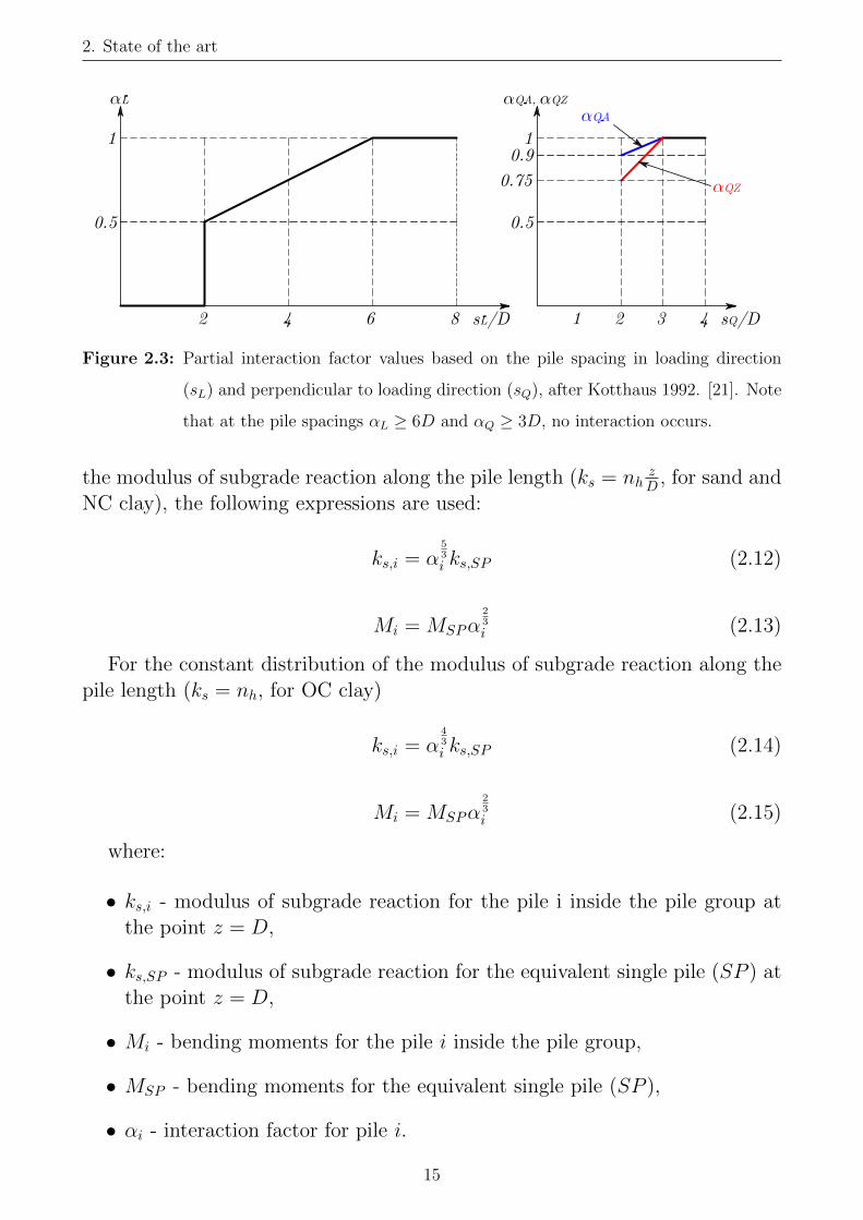
2. State of the art
Figure 2.3: Partial interaction factor values based on the pile spacing in loading direction
(sL) and perpendicular to loading direction (sQ), after Kotthaus 1992. [21]. Note
that at the pile spacings αL ≥ 6D and αQ ≥ 3D, no interaction occurs.
the modulus of subgrade reaction along the pile length (ks = nhzD , for sand and
NC clay), the following expressions are used:
ks,i = α53
i ks,SP (2.12)
Mi = MSPα23
i (2.13)
For the constant distribution of the modulus of subgrade reaction along thepile length (ks = nh, for OC clay)
ks,i = α43
i ks,SP (2.14)
Mi = MSPα23
i (2.15)
where:
• ks,i - modulus of subgrade reaction for the pile i inside the pile group atthe point z = D,
• ks,SP - modulus of subgrade reaction for the equivalent single pile (SP ) atthe point z = D,
• Mi - bending moments for the pile i inside the pile group,
• MSP - bending moments for the equivalent single pile (SP ),
• αi - interaction factor for pile i.
15

2. State of the art
Pile group efficiency and load proportions
The pile group efficiency under lateral loading (non-dimensional, usually de-noted as GW or η) can be described using the following equation:
η = GW =HG
nHSP=
n∑i=1
Hi
nHSP(2.16)
where:
• Hi - lateral force acting on the pile i (F),
• HG - total lateral force acting on the pile group (F),
• HSP - lateral force acting on the equivalent single pile (F),
• n - total number of piles (-).
It can be shown that the pile group efficiency is equal to the mean value ofall pile interaction factors αi:
η = GW =
n∑i=1
Hi
nHSP=
1
n
n∑i=1
Hi
HSP=
1
n
n∑i=1
αi = αi,mean (2.17)
Load proportion for the pile i is defined as:
LPi =Hi
HG(2.18)
It can be easily shown that the sum of all load proportions LPi (for all pilesinside the group) is always equal to 1.
2.3 Numerical methods
As the alternative to the expensive experimental studies, different numericalmethods for the response prediction of pile groups under lateral loading havebeen developed. From a theoretical point of view, these methods can be dividedinto several categories:
• Closed form and empirical solutions,
• Limit equilibrium method,
• Strain Wedge (SW) method,
16
2. State of the art
• Discrete load transfer methods,
• Continuum based methods.
As in the case of analysis of other geotechnical problems, the development inthis field had similar progress, which is reflected in the gradual increase of thecomplexity of the calculation model, in order to take into account more aspectsof real soil behaviour, as well as the soil-structure interaction effects.
Closed form and empirical solutions
Closed-form solutions for the problem of laterally loaded pile group are verylimited. The most of these solutions assumes the soil as an elastic and isotropichalf-space. Notable are the works of Winkler (1867) [26], Hetenyi (1946) [27]and Terzaghi (1955) [28].
Limit equilibrium method
Limit equilibrium method is represented by the work of Broms [23, 24]. Thistype of analysis is related to the ultimate (failure) conditions, where reasonableengineering assumptions regarding the soil pressure distribution can be made.These methods are nowadays mostly overcame by the load transfer and contin-uum based methods, especially because of the fact that the serviceability limitstates under working load conditions (far from ultimate loading conditions) be-came the governing factor in the pile foundations design. Nevertheless, the limitequilibrium methods have founded the basis for the distinction between rigidand flexible pile response.
Strain Wedge Method
The Strain Wedge (SW) method for the analysis of laterally loaded piles and pilegroups is based on the concept of mobilized passive soil wedge that resists thepile. Originally developed by Norris [33] for laterally loaded flexible free headpile in sand, it has been further improved for clay soils, pile groups, layered soils,boundary conditions and nonlinear behavior of pile material [34–37]. The mainassumptions are that the deflection pattern of the pile is linear over the depth,which leads to the uniform horizontal and vertical strains. The horizontal strainε in the soil in the passive wedge is the predominant parameter in the StrainWedge model.
Geometry of the assumed 3D passive wedge (Figure 2.4) is defined by:
• Spreading angle (equal to the mobilized effective friction angle φ′m),
17

2. State of the art
• Height h (mobilized depth of a passive wedge),
• Mobilized base angle βm = 90− θm.
Figure 2.4: Strain wedge model parameters (after Norris 1986. [33])
The assumed resistance mechanism consists of the horizontal stress ∆σh(assumed equal to deviatoric triaxial stress) along the width of the wedge, andmobilized shear friction τ along the pile side. Every wedge is assumed to beformed of sublayers that represent the different stress states along the depth.3D wedges are used to establish the equivalent nonlinear elastic springs for eachsublayer. A power function for the stress-strain relationship is used to representthe constitutive behaviour for sand and clay, and every sublayer is consideredas an uniform soil.
By introducing the equivalent springs for each sublayer, SW model connectsthe discrete load-transfer approach and limit equilibrium approach. The stiff-ness of each spring represents the secant value ks = p(z)/y(z), appropriate tothe current deflection of the pile-soil system.
Discrete load transfer methods
Beside the previously mentioned elastic load transfer method (beam on Win-kler foundation - BWF), further improvements of the subgrade reaction theoryled to the nonlinear load-transfer approach, that included soil representationwith nonlinear springs at discrete points along the pile length. This analysis isnowadays well recognized as p-y curve method. It was first introduced by
18
2. State of the art
McCelland and Focht in 1958 [38]. It can also be denoted as beam on nonlinearWinkler foundation (BNWF).
Nonlinear behavior of the soil is defined by p-y curves associated to eachspring, where p is lateral soil resistance per unit length of the pile and y islateral deflection of the pile. Problem solution requires the nonlinear iterativeanalysis, in order to match the p-y nonlinear curve with the response of the onedimensional beam.
p-y curves are usually expressed using hyperbolic or power functions. Theyare mainly derived by back-calculation of the experimental results, which pro-vide the confidence among the designers. In routine practice, p-y curves from1970’s [39, 40] are used as ”the industry standard” [41], and these curves areimplemented into the software solutions such as LPILE [42] and GROUP [43],as ”standard” sand and clay curves. Additional enhancements of these curveshave been attempted through the use of cone penetration (CPT), flat dilatome-ter [44] and pressuremeter tests [45], as well as the FEM [46, 47] for p-y curvederivation.
p-multipliers (Pm)
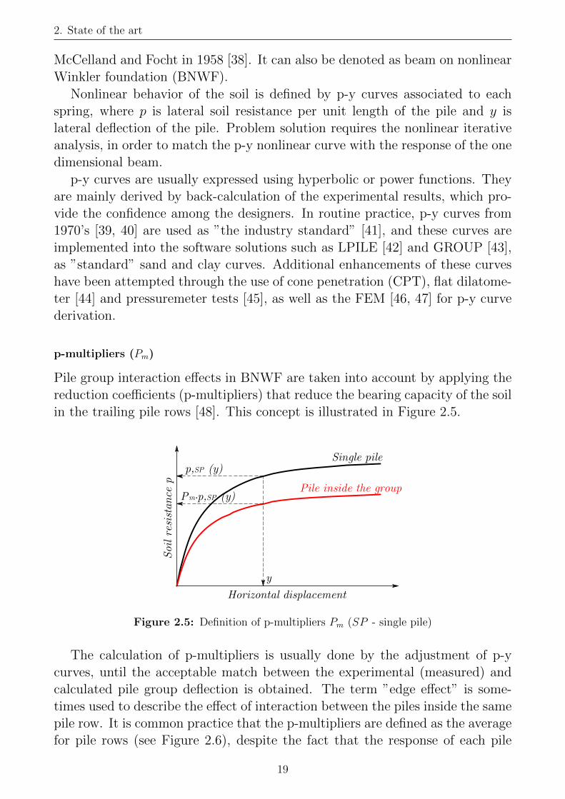
Pile group interaction effects in BNWF are taken into account by applying thereduction coefficients (p-multipliers) that reduce the bearing capacity of the soilin the trailing pile rows [48]. This concept is illustrated in Figure 2.5.
Figure 2.5: Definition of p-multipliers Pm (SP - single pile)
The calculation of p-multipliers is usually done by the adjustment of p-ycurves, until the acceptable match between the experimental (measured) andcalculated pile group deflection is obtained. The term ”edge effect” is some-times used to describe the effect of interaction between the piles inside the samepile row. It is common practice that the p-multipliers are defined as the averagefor pile rows (see Figure 2.6), despite the fact that the response of each pile
19

2. State of the art
inside the row is different. As an alternative, the average p-multiplier for theentire group can be used, which is called group interaction factor [49, 50]. Cur-rently, there are many recommendations regarding the values of p-multipliersfor different pile group configurations.
Figure 2.6: Example of p-multipliers for the pile group. The p-y curve for the pile inside the
pile group is scaled for the entire displacements range.
Limitations
Linear discrete load transfer method have certain limitations, that are widelyrecognized in the engineering community:
• Soil resistance is modeled using discrete (discontinuous) springs, despitethe fact that the soil is continuum (3D continuum interaction effects areneglected).
• Pile geometry is simplified to 1D beam element.
• The modulus of subgrade reaction ks is not the physical soil parameter.Instead, it is the measure of the total soil-pile interaction at the specificdepth, and hence it depends not only on the soil properties, but also the pileproperties and loading conditions [51]. In other words, it is a convenientmathematical parameter that relates soil reaction and pile deflection [38].
• Soil resistance is linearly proportional to the pile displacements, despitewidely known soil nonlinear behaviour.
Nonlinear (p-y) method has the additional limitation: it is very hard todecide which p-y curve to select. The p-y curves are mostly determined based onthe experimental results and therefore are somehow bound to a certain soil type- the extrapolation to the different soil conditions and pile group configurationsis questionable.
20

2. State of the art
Despite the aforementioned limitations, linear and nonlinear subgrade re-action methods are widely used in the everyday engineering practice, due totheir simplicity and the ability to model and predict the real pile behaviouraccurately.
Continuum based methods
The limitations of the discrete load transfer methods, presented in the previoussection, can be overcome using the continuum based methods. The developmentof computers has led to the rapid development of these methods, which allowfor the full discretization of both the soil and the structure, combined with theapplication of advanced constitutive soil models. Applied to laterally loadedpiles, representation of the soil and piles through the continuum provides amore fundamental and realistic approach to the analysis of pile-soil interaction.Also, material properties used within these methods now have clear physicalmeaning, and can be measured directly, using conventional geomechanical tests.
On the other hand, continuum based analysis requires more effort for the datapreparation and higher computational demands. The fact that the most of thecurrent structural design codes require the use of multiple load combinationsmakes the use of continuum based methods still impractical for the routineengineering design.
Continuum based solutions are mainly based on the following numerical anal-ysis methods:
• Finite Element Method (FEM),
• Finite Difference Method (FDM),
• Boundary Element Method (BEM).
Each of these methods can be used with the different level of complexity.Usually, distinction between linear and nonlinear analysis is made.
FEM
The finite element method (FEM) is today considered as the most reliable andmost widely used numerical method for engineering analysis of complex founda-tion systems [1, 52]. It is capable of performing 2D or 3D analysis. Regardingthe laterally loaded pile, FEM allows for detail modelling of all model compo-nents: pile geometry, soil continuity and nonlinear behaviour, and especiallythe pile-soil interface through slippage and gapping. According to [41], ”model-ing lateral behavior in any way other than with three-dimensional models usingnonlinear soil models and interface elements must constitute a compromise”.
21

2. State of the art
Many software packages such as PLAXIS 3D [25], ABAQUS [53], ETABS[54], ANSYS [55], SOFiSTiK [56] are commercially available. Regarding thepile foundations analysis, the alternative program FLAC 3D, based on the finitedifference method (FDM) is also very common solution.
2.4 Notable numerical studies on laterally pile group
interaction effects
Initial linear solutions
Poulos (1971)
Poulos proposed BEM model to predict the response of a laterally loaded freeand fixed-head single piles [57] and pile groups [58] in 3D elastic, homogeneousand isotropic, semi-infinite continuum. Pile-soil separation was not taken intoaccount. Pile displacements were computed using bending moment equations.Soil displacements were calculated using Mindlin’s method, that accounts foradditional displacements and rotations. The pile was assumed as the thin rect-angular strip with the width equal to the pile diameter D, and the length Land bending stiffness EI.
Pile-to-pile interaction factors were introduced to account for the additionallateral displacements/rotations for the piles inside the pile group. The im-portance of pile orientation with respect to loading direction was emphasized,pointing out that the interaction between piles is the highest when two pilesare aligned with the line parallel to loading direction.
Based on this solution, a series of design curves were developed [6] to presentthe lateral interaction factors as the function of spacing, orientation and relativepile flexibility. This solution was later improved by Banerjee and Driscoll [59],considering the simultaneous pile-to-pile interaction.
Randolph (1981)
Randolph [13] proposed interaction factors in the form of a convenient algebraicexpression for flexible piles subjected to lateral loads and moments at the pilehead. The FEM study, both for elastic homogeneous and Gibson (with linearlyincreasing stiffness with depth) soil was done. Proposed expression defines theinteraction factor for two piles under inclination angle ψ.
Interaction factor αρF for a free head flexible pile in homogeneous soil isexpressed as:
22

2. State of the art
αρF = 0.5(Ep
Gc)1/7
D
s(1 + cos2ψ) (2.19)
where:
• αρF - Poulos [58] interaction factor giving the increase in deflection of freehead pile under lateral loading,
• s - pile center-to-center spacing,
• Ep – pile Young’s modulus,
• Gc – average value of G∗ over active length of pile, where G∗ = G(1+3ν/4),
• ν - Poisson’s ratio,
• ψ – angle between the line connecting the pile centers and the loadingdirection.
The solutions of Poulos [58] and Randolph [13] for 2 inclined piles are illus-trated in Figure 2.7.
Figure 2.7: Initial elastic interaction factors αρF for 2 inclined piles (after studies of Poulos
1971. [57] and Randolph 1981. [13])
23

2. State of the art
Limitations of elastic solutions
Conventional structural design is still mostly based on the assumption of linearelasticity, which allows for the use of principle of superposition and thereforethe ease of analysis and lower computation costs. However, in the case ofvery important structures, such as high rise buildings, power plants etc., theeffects of nonlinear soil behavior and soil-structure interaction must be takeninto account. As observed by Kotthaus [21], the interaction effects are not thesame for different loading levels. Therefore, it is necessary to use the nonlinearanalysis to assess the interaction effects at higher loading levels.
Elastic solutions are appropriate for the analysis of laterally loaded pilesat very low loading levels. Pecker and Pender [60] noted that for 3x3 pilegroups under static lateral loading and deflections up to 0.03D, load distributionbetween the piles can be predicted using the elastic interaction factors.
Nonlinear numerical studies
Brown and Shie (1990-1991)
Brown and Shie [61, 62] conducted the numerical experiments using 3D FEMsimulations to investigate the free head pile group effects, with group spacing of3D and 5D. Numerical model featured plastic yield, slippage and gapping at thepile-soil interface. Two soil types (clay and sand) were considered, using bothVon Mises [63] and extended Drucker-Prager [64] models. Pile group effectswere presented by p-multipliers, which are obtained through the polynomialfitting and differentiation of bending moment curves along the piles. This workmotivated the further use of three dimensional FEM for the analysis of the pilegroup response. Linear elastic model was used for the representation of the pile.
Wakai et al. (1999)
Wakai et al. [65] performed the 3D elastoplastic FEM simulation of a full scale3x3 pile group test. Soil was modeled using Mohr-Coulomb failure criterion anda non-associated flow rule. Interface slippage was modeled by means of thinelastoplastic elements in the pile-soil zone. However, the discrepancy betweencalculated and measured pile group response was observed at the higher loadinglevels (above 0.1D). The load distribution ratio was found to be independenton the pile head fixity.
24
2. State of the art
Yang and Jeremic (2003)
Yang and Jeremic [66] have analyzed the pile group interaction effects underlateral loading using 3D FEM model with separation and slippage capabilities.Layered sand soil cases were considered. Special attention was given to thebending moments in the plane perpendicular to the loading plane, and the p-ybehaviour of individual piles in a group. It was shown that the pile row loadsare different, as well as that the pile loads inside the same row is different. Thebending moment inside the individual piles within the same row was different,as well. The level of pile group interaction was found to be dependent on thedisplacement level.
Comodromos et al. (2005-2013)
Comodromos and Pitilakis [10] analyzed the response of the laterally loadedfixed-head pile groups using 3D finite difference nonlinear analysis. Differentpile group configurations were evaluated, and the influence of different parame-ters, such as number of piles, pile spacing and the deflection level was discussed.The pile installation effects were neglected. Papadopoulou and Comodromosfurther investigated the response of horizontally loaded fixed-head pile groups insands [7] and clay soils [67]. The relationship between the load-deflection curveof the single pile and individual piles inside the pile group was derived by intro-ducing the amplification factor Ra, defined as the ratio of group displacementvs. individual pile displacement for the same mean load.
Further research in this field led to the extension of the p-y method for sand[68] and clay soil [69], to account for the unequal load distribution inside thepile row. Location weighting factor lwj was introduced to adjust the previouslyintroduced amplification factor Ra using the effect of pile location. The valuesof the lwj are slightly lower than those for the external piles, and slightly abovethose for the internal piles. The use of location weighting factors providesthe calculation of forces and bending moments for each pile inside the pilegroup. This pile location weight factor lwj can be directly associated with thepreviously defined interaction factors αi and pile group efficiency GW, usingsimple algebraic transformations.
According to the above research, piles inside the pile group are divided intofront corner (FC), front (FR), internal (IN) and perimetric (PE) piles, respec-tively (see Figure 2.8).
25
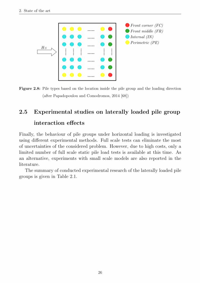
2. State of the art
Figure 2.8: Pile types based on the location inside the pile group and the loading direction
(after Papadopoulou and Comodromos, 2014 [68])
2.5 Experimental studies on laterally loaded pile group
interaction effects
Finally, the behaviour of pile groups under horizontal loading is investigatedusing different experimental methods. Full scale tests can eliminate the mostof uncertainties of the considered problem. However, due to high costs, only alimited number of full scale static pile load tests is available at this time. Asan alternative, experiments with small scale models are also reported in theliterature.
The summary of conducted experimental research of the laterally loaded pilegroups is given in Table 2.1.
26

2.State
ofth
eart
Table 2.1: Summary of experimental studies on laterally loaded pile groups
Reference
Soil Test Pile Pile size Installation Pile head Pile group
s/D
Pile row P-multipliers
type type type (cm) method BC N x M 1 2 3 4 5
Brown et al. (1987) [70] Stiff clay Full scale Steel pipe 27.3 Driven Free 3x3 3 0.70 0.60 0.50
Brown et al. (1988) [48] Dense sand Full scale Steel pipe 27.3 Bored Free 3x3 3 0.80 0.40 0.30
Brown et al. (2001) [49] Silty sand Full scaleReinforced concrete 150.0 Bored Fixed 2x3 3 0.50 0.40 0.30
Precast reinforced concrete 80.0 Driven Free 3x4 3 0.90 0.70 0.50 0.40
Christensen (2006) [71] Sand Full scale Steel pipe 32.4 Driven Free 3x3 5.65 1.00 0.70 0.65
Huang et al. (2001) [72] Silty sand Full scale
Reinforced concrete 150 Bored Fixed 3x3 3 0.93 0.70 0.74
Precast reinforced concrete 80 Driven Fixed 4x4 3 0.89 0.61 0.61 0.66
Ilyas et al. (2004) [73] Clay (kaolin) Centrifuge Aluminum pipe (squared) 84.0 Jacked Free
3x3 3 0.65 0.50 0.48
4x4 3 0.65 0.49 0.42 0.46
2x2 3 0.96 0.78
1x2 3 0.80 0.63
Kotthaus et al. (1994) [74] Dense sand Centrifuge Aluminum pipe
150
Sand rainfall
Free 1x3 3 0.75 0.45 0.45
150 Free 1x3 4 0.95 0.65 0.65
McVay et al. (1995) [75] Sand Centrifuge Aluminum pipe 43.0 Sand rainfall Free
3x3 5 1.00 0.85 0.70
3x3 5 1.00 0.85 0.70
3x3 3 0.65 0.45 0.35
3x3 3 0.80 0.40 0.30
Morrison and Reese (1986) [76] Medium dense sand Full scale Steel pipe 27.3 Driven Free 3x3 3 0.80 0.40 0.30
Rollins et al. (1998) [77] Clay Full scale Steel pipe 30.5 Driven Free 3x3 3 0.60 0.38 0.43
Rollins and Sparks (2002) [78] Silts and clays Full scale Steel pipe 32.4 Driven Fixed 3x3 3 0.60 0.38 0.43
Rollins et al. (2005) [79] Sand Full scale Steel pipe 32.4 Driven Free 3x3 3.30 0.80 0.40 0.40
Rollins et al. (2006) [80] Stiff clay Full scale Steel pipe
61.0
Driven Free
5x3 3 0.82 0.61 0.45
32.4 3x3 5.65 0.95 0.88 0.77
32.4 3x4 4.40 0.90 0.80 0.69 0.73
32.4 3x5 3.30 0.82 0.61 0.45 0.45 0.51
Ruesta and Townsend (1997) [81] Loose sand Full scale Prestressed concrete (squared) 76.0 Driven Free 4x4 3 0.80 0.70 0.30 0.30
Snyder (2004) [82] Soft clay Full scale Steel pipe 32.4 Driven Free 3x5 3.92 1.00 0.81 0.59 0.71 0.59
Walsh (2005) [83] Sand Full scale Steel pipe 32.4 Driven Free 3x5 3.92 1.00 0.50 0.35 0.30 0.40
27

2. State of the art
Beside the fact that full scale pile group tests are the most realistic approach,summarized experimental results show the lack of the studies for the arbitraryloading case, as well as some inconsistency (see Figure 2.9). The limitations inthe available experimental database support the use of numerical methods tostudy the pile group interaction effects.
the degradation of Pm values (Ilyas et al. 2004). Once pile interac-tion and stress overlapping with front and side piles occurs, Pm de-velops and varies rapidly, especially in close-spaced pile groups.However, the pile interaction could develop with the back rows ear-lier and faster than the front row, which is realistic and agrees withthe test results presented by Rollins et al. (2005).
Because the actual depth of the zone of interaction among thepiles in a group (i.e., soil stress overlap) is unknown and increases
with the progress of lateral loads, current practice applies Pm as asingle value along the whole length of the pile (Fig. 1). Conse-quently, the value of the Pm suggested for the same pile group basedon pile spacings may change in response to the change of thepile length to obtain a good agreement with the measured data(Rao et al. 1998).
Currently, Pm is utilized as a function of pile-row spacing inthe loading direction, SL [AASHTO 2007; U.S. Army Corps ofEngineers (USACE) 1993]. An interpolation between suggestedPm values should be conducted to determine Pm for other pile spac-ings, as is the case in AASHTO (2007), which provides Pm for only3D and 5D pile-row spacings. Such suggestion may not apply toone-row pile-group analysis loaded in the longitudinal direction(side by side) where no pile-row spacings exist. Moreover, thePm value recommended for the side-by-side pile group must be ad-justed when the one-row pile group is loaded in-line (Fig. 4). Asobserved in experimental results, Gandhi and Selvam (1997) ad-dressed the difference in pile-group lateral response that resultedfrom changing the direction of lateral loads on the pile group fromlongitudinal to transverse, which requires different values of Pm.
Rollins et al. (2003, 2005) presented two sets of Pm based onfull-scale load tests in clay and sand soils, respectively. The datashown in Fig. 2 reflect the effect of the soil type (in the dominantnear-surface soil layers) on the Pm values utilized with the same pilegroup and the need to perform full-scale load tests at the site inquestion to assess the appropriate Pm values for that particular site.The topic of this study coincides with the Brown et al. (1988) em-phasis on the need to establish a methodology for predicting thevariation of Pm with soil properties, pile stiffness and spacing,and depth. This indicates the need for more full- and model-scaleload test data to consider these factors in the suggested values ofPm. The full- and model-scale load tests conducted by Rollins,
Fig. 1. Current practice of P-multiplier (Pm) in pile-group analysis:(a) concept of the P-multiplier applied to a pile in a group, as suggestedby Brown et al. (1988); (b) piles in a group subjected to the P-multiplier
2 3 4 5 6 7 8Pile Spacing / Pile Diameter (SL/D)
0
0.2
0.4
0.6
0.8
1
1.2P
-mul
tiplie
r
AASHTO (2007)AASHTO (2000)US Army (1993)WSDOT (2000)
Reese et al. (1996)
Rollins et al. (2003), ClayRollins et al. (2005), Sand
Loading Direction
Leading Row
Trailing Row
Trailing RowST ST
SL
SL
Fig. 2. P-multiplier versus pile spacing for a front row of pile groupfrom different sources
Stress Zone @ 10D Below G.L.
@ G.L.
3D
3D2D
2D
2DS10D
D
7D
Stress Zone @ G.L.
Stress Zone @ 10D Below G.L.
4D
4D
S
3D
3D
2D8D
6D 1.5D
D
Stress Zone @ G.L.Stress Zone @ 10D Below G.L.
@ G.L.
3D
3D2D
2D
2DS10D
D
7D
Stress Zone @ G.L.
Stress Zone @ 10D Below G.L.
4D
4D
S
3D
3D
2D8D
6D 1.5D
D
Stress Zone @ G.L.
Fig. 3. Stress zones in soil at different depths around rigid piles in-lineand side-by-side in pile groups (Rao et al. 1998, ASCE)
JOURNAL OF BRIDGE ENGINEERING © ASCE / SEPTEMBER/OCTOBER 2011 / 613
J. Bridge Eng., 2011, 16(5): 612-623
Dow
nloa
ded
from
asc
elib
rary
.org
by
ET
H Z
ueri
ch -
ET
H-B
iblio
thek
on
11/1
2/15
. Cop
yrig
ht A
SCE
. For
per
sona
l use
onl
y; a
ll ri
ghts
res
erve
d.
Figure 2.9: P-multipliers for different pile spacings from different sources (after Ashour and
Ardalan, 2011 [84])
Deformation patterns
Recent experimental studies in the field of laterally loaded pile groups haveanalysed and visualized the soil deformation patterns around the piles. Theimprovement of the CT (computer tomography) and PIV (particle image ve-locimetry) technologies allowed to precisely define the shape of the deformedsoil zone during lateral loading. Works by Otani et al. [85], Hajialilue-Bonab etal. [86, 87], Iai et al. [88], Morita et al. [89], are notable. The findings of theseworks clearly indicate the three-dimensional nature of the problem of laterallyloaded pile group and indicate the almost conical shape of the soil deformationpattern. The soil failure was found to be progressive, and the failure zone isenlarged when the lateral load is increased.
2.6 Problem sensitivity analysis
As shown in previous sections, various factors can influence the interactionsinside the laterally loaded pile group. Significant number of research papers
28

2. State of the art
[48, 49, 72, 75, 77, 90–93] indicate and rank the most important factors thatinfluence this problem. The most recognized parameters are:
• pile spacing in the loading direction,
• pile arrangement, position and total number of piles,
• pile stiffness, length and diameter,
• pile installation method,
• soil type and density,
• load/displacement level,
• pile head conditions,
• pile soil slippage and separation,
• presence of axial loading.
As stated by Mokwa and Duncan [94], in the adoption od p-multipliers,effects of pile-head fixity, soil type and density, as well as the displacement level,can be considered as the secondary issue that do not need to be considered forthe most of the engineering purposes. According to Kluber [32], pile groupefficiency is not the function of pile bending stiffness, relative density and pilehead conditions.
The overview of the problem influencing factors is shown in Figure 2.10. Thelisted parameters are elaborated in more detail in the following paragraphs.
Pile spacing and configuration
It has been shown both theoretically and experimentally that the previouslydescribed shadowing effect becomes smaller when the pile spacing increases[10, 51]. There is general agreement in the literature that group effects aresmall when center-to-center pile spacing exceeds 6D in a direction parallel tothe load, and 3D measured in a direction perpendicular to the load.
From the practical standpoint, if the pile spacing is higher than 5D, thecosts of the pile cap will increase to a very high level. According to McVayet al. (1995) [75], ”pile spacing higher than 5D is considered as an extreme.”Pile spacing of 2D is also not recommended due to the problems regarding theinstallation of closely spaced piles.
Based on the results of Comodromos and Pitilakis [10], both the number ofpile rows and total number of piles play an important, but less affecting rolein the pile group interaction effects. Same authors introduced the pile location
29
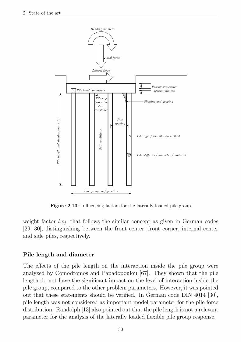
2. State of the art
Figure 2.10: Influencing factors for the laterally loaded pile group
weight factor lwj, that follows the similar concept as given in German codes[29, 30], distinguishing between the front center, front corner, internal centerand side piles, respectively.
Pile length and diameter
The effects of the pile length on the interaction inside the pile group wereanalyzed by Comodromos and Papadopoulou [67]. They shown that the pilelength do not have the significant impact on the level of interaction inside thepile group, compared to the other problem parameters. However, it was pointedout that these statements should be verified. In German code DIN 4014 [30],pile length was not considered as important model parameter for the pile forcedistribution. Randolph [13] also pointed out that the pile length is not a relevantparameter for the analysis of the laterally loaded flexible pile group response.
30
2. State of the art
According to Comodromos and Papadopoulou [67], it was shown that the pilediameter do not have the significant influence on the interaction level inside thepile group, compared to other parameters. However, some experimental studies[95, 96] have indicated the stiffer pile response with increasing pile diameter. Inthe work of Terzaghi [28], the subgrade modulus was considered independentof the pile diameter.
Pile stiffness and concrete cracking
Bowles [97] pointed out the possibility of concrete cracking as the problem inrealistic modelling of the laterally loaded pile. Due to decrease in pile stiff-ness, nonlinear foundation response can be affected. Comodromos and Pa-padopoulou [98] analysed the influence of concrete cracking on the responseof laterally loaded piles. As expected, this problem is more important in thecase of free head pile response, because the cracks develop earlier due to thehigher bending curvature. Free head piles are also affected to a higher depth,compared to a fixed head pile. However, for the working load level, which ismostly expected to occur for the laterally loaded piles, fully elastic assumptionof the pile behaviour will not lead to the significant change in the interactioneffects and stress redistribution. As the conclusion, pile cracking should be con-sidered when extremely high accuracy is required and when the loading level issignificant.
Displacement level
Many researches [10, 21, 80, 99] have shown that the pile group efficiency underlateral loading is decreased with the increase of the total pile group displace-ment level. Based on the studies of Comodromos and Papadopoulou [7, 67], adisplacement of about 10% for sandy and about 15% for clay soil was sufficientto reach the constant level of interaction. Same authors also note that the inter-action is significantly changed inside the displacement range of 1-5%. The levelof displacement of 0.10D is, in general, higher than the level of displacementsthat is allowed in most practical cases. The serviceability limit state usuallycorresponds to a deflection level of 0.05D [69].
Pile head boundary conditions
In classical geotechnical engineering, two limiting pile head boundary conditionsare usually considered within the analysis of laterally loaded pile groups:
• Free head pile, when pile head rotation is not constrained,
31

2. State of the art
• Fixed head pile, when pile head rotation is constrained by the pile cap.
According to Mokwa and Duncan [99], boundary conditions at the pile headare somewhere in between the fixed and free head pile. Same authors pointedout that the pure fixed-head conditions are hard to achieve in reality, even whenthe pile cap is very stiff. In piled raft foundations, according to Katzenbach[100], ”the connection between the piles and the raft is seen as flexible joint”.
It is generally accepted that, due to different boundary conditions, the re-sponse of the free and fixed head pile groups subjected to lateral loading issignificantly different [98]. Namely the deflection of the free head pile is higherthan the fixed head pile for the same mean load.
Despite the different deflection response, pile load redistribution inside thepile group can be considered independent on the pile head conditions. Variousresearches, such as Matlock (1970) [39], Reese and Van Impe (2001) [101], orComodromos and Papadopoulou (2012) [67], confirm this statement, especiallywithin the practical ranges of the pile group displacements (working load con-ditions). The most of the recommended p-y curves in the current engineeringpractice are independent on the pile head conditions.
It should be noted here that the pile cap is usually in the contact with thesoil, and therefore will contribute to the lateral bearing capacity of the pilegroup. However, this effect is usually neglected, because the cap-soil contactmay be lost due to soil erosion or excavation [102].
Pile-soil slippage and separation
In reality, the contact between the piles and the surrounding soil is not fullyrigid, but weaker, so there are small relative displacements along the pile-soilinterface. Many authors [10, 41, 61, 103–105] pointed out the importance ofsimulating the slippage and separation between the soil and the pile on the moreaccurate model response. According to Comodromos [106], pile-soil separationis considered as the main reason for non-linear interaction inside the pile group.Regarding the affected zone, pile group response is mainly governed by theproperties of the top soil layer (near-surface soil conditions) [1, 10].
Presence of axial loading
Pile foundations are always subjected to simultaneous vertical and lateral load-ing. Due to pile-soil interaction, there is an interaction between the axial andlateral response of the piles. However, in current design practice these in-teraction effects are usually neglected, and pile group interaction is analysedindependently for vertical and lateral loading cases. Several studies have shown
32
2. State of the art
the interest in the analysis of combined axial and lateral loadings, both forclay and sand soils [107–113]. The general conclusions are that in the case ofclays, the presence of vertical loading reduces the lateral capacity of piles, whilethe lateral capacity in sands is increased. These effects are observed at higherloading levels, while for working loading levels these combined effects can beneglected.
2.7 Concluding remarks
Based on the presented literature review and problem sensitivity analysis, thefollowing conclusions for the next research phase were derived:
• The problem of laterally loaded pile group is, in general, a 3D engineeringproblem, so the 3D model will be used for the numerical study. Eurocode 7[11] strongly suggests the use of soil-structure interaction in the numericalanalysis, especially in the case of complex foundations such as piled raftfoundations, laterally loaded pile foundations and flexible retaining struc-tures. The use of advanced constitutive models is also suggested. Thepresented overview of previously conducted numerical studies has shownthat a 3D continuum approach can provide a greater degree of realism.This is even more emphasized considering the arbitrary loading direction,because the symmetry modelling simplifications cannot be made.
• Only free head model will be validated and used in the parametric study.Despite the fact that the displacement level is influenced by the pile topboundary conditions, the presented literature review suggests that pile loadredistribution is independent on the pile head fixity.
• For the considered working loading conditions within this study, fully elas-tic assumption of the pile behaviour will not lead to the significant changein interaction effects. Pile section properties will be modelled as constantalong the pile length.
• Pile-soil slippage and separation effects must be considered in order toproperly assess the pile group response.
• Soil profile will be considered as homogeneous, because only the top soillayer properties significantly influence the lateral pile group response. Thisis even more pronounced in the considered case of long piles.
• Pile length and diameter can be considered as the secondary problem pa-rameters and they will be kept constant throughout the parametric study.Sand soil profile with two different densities will be analyzed.
33

2. State of the art
• Maximum displacement level in the numerical model will be kept at about0.10D, which slightly exceeds the working load limits, but doesn’t reachthe ultimate limit state. For the problem under consideration, the workingloads are more interesting. Also, by reducing the maximum displacements,the speed of numerical simulations is optimized.
• Influence of the axial load can be neglected in the numerical model. Forconsidered working load conditions, the axial load will not significantlyinfluence the lateral response of the pile group, or, in the case of the sandsoil, neglecting of the axial load will be on the safe side.
34
3 Numerical model generation
3.1 PLAXIS 3D overview
Within this thesis, the response of the pile groups under arbitrary horizontalloading was computed using FEM code PLAXIS 3D [25], in a series of extensivenumerical computations. It is a world-wide famous code for the stress-strain,stability and groundwater flow analysis in geotechnical engineering. Its develop-ment began in 1987 at Delft University of Technology, and in subsequent yearsit was extended to cover many areas of geotechnical engineering. 3D analysissupport was introduced in 2001.
PLAXIS 3D features fully 3D graphical pre- and post-processor, that allowsfor an easy graphical input of the models with complex geometry, as well asthe illustrative presentation of the results. FE mesh is mainly generated auto-matically, with the state-of-the-art algorithms for check of mesh regularity. Arange of other structural members, such as beams, anchors, plates and geogridscan be modelled, as well. Staged (phase) analysis is also supported, so realis-tic simulation of excavation and construction process, starting from the initialstress states, can be modelled.
Special feature is the simulation of the conventional soil tests. This feature,denoted as SoilTest, allows for the calibration of the constitutive model param-eters using the results of the standard soil laboratory tests. It is based on thesingle point algorithm, and it works for all soil models in PLAXIS 3D. Theparameter optimization and local sensitivity analysis can be done in order tobest fit the experimental results with the constitutive model.
3.2 Constitutive models
PLAXIS 3D features the constitutive models with different level of complexity.Also, user defined models can be implemented. Constitutive models used inthis study are presented in the following sections. It must be noted here thatthe stress path around the laterally loaded pile does not match the conventionalgeomechanical laboratory tests [106].
35

3. Numerical model generation
Linear elastic (LE) model
The linear elastic model in PLAXIS 3D is based on the generalized Hooke’s lawof isotropic elasticity. It includes 2 basic elastic parameters – Young’s modulusE and Poisson’s ratio ν. Stress states in linear elastic model in PLAXIS 3D arenot limited, which means that the simulated material can have infinite strength.
However, in order to simulate the piles using the linear elastic model, the oneshould ensure that the pile material (e.g. concrete) strength is not exceeded inthe considered problem. This assumption is usually satisfactory in the case ofthe working load conditions, where concrete cracking can be neglected.
The parameters of the LE model used in this study are given in Table 3.1,and denoted as E CONCRETE, NU CONCRETE and W CONCRETE.
Mohr-Coulomb (MC) model
The linear elastic-perfectly plastic Mohr-Coulomb (MC) model is based on thewell-known Mohr-Coulomb failure criterion. This model usually represent thefirst order of the approximation of the soil and rock behaviour [25], and canbe relevant for simple stress paths. This model involves five input parameters:Young’s modulus E and Poisson’s ratio ν for soil elasticity, and cohesion c′,angle of internal friction φ′ and dilation angle ψ for soil plasticity.
The stiffness in Mohr-Coulomb model is constant stiffness, independent ofstress and strain levels (only controlled by Young’s modulus E and Poisson’sratio ν). The volume changes and the rate of plastic strain variation are con-trolled by a non-associated flow rule, where the potential surface is defined bydilation angle ψ.
MC model is commonly used in practice due to the straightforward param-eter determination using conventional laboratory tests. However, this modelcannot account for the stress dependant stiffness, the stress-path dependantstiffness, as well as for the soil anisotropy. This means that the results will bequestionable in the case of complex stress paths and large domains with widestress variation.
In general, this model is considered adequate for stability analysis (thatinclude shear strength of frictional soil), but inadequate for the problems thatinclude deformation analysis or cyclic loading [114].
In this study, the constitutive behaviour of pile-soil interface is defined bythe elastic-perfectly plastic Mohr-Coulomb model, in conjunction with a non-associated flow rule and zero tension cut-off criterion (when tension develops,a gap between the pile and the surrounding soil is created).
The parameters of the MC model used in this study are given in Table 3.1(denoted as COHESION , PHI, NU and RINTER).
36

3. Numerical model generation
Hardening Soil (HS) model
The Hardening Soil (HS) constitutive model [115] is an advanced model. Asin the case of the MC model, the limit stress states are defined through theparameters of MC failure criterion (c′, φ′, ψ). However, the soil stiffness in theHS model is described more accurately, through the three advanced stiffnessparameters: the triaxial loading stiffness E50, the triaxial unloading stiffnessEur and the oedometer loading stiffness Eoed. These three values are not mutu-ally independent: usually the Eoed is assumed equal to E50, and Eur is assumedequal to 3E50. These default relations are implemented into PLAXIS 3D code,but very soft and very stiff soils tend to give other relations. All three inputstiffnesses are related to the reference stress pref = 100 kPa.
HS model is isotropic hardening model, that cannot account for and simulatecyclic behaviour. It also does not account for different stiffness at different strainlevels – the user should input the stiffness according to the expected strain level.From the calculation point of view, this model also needs more calculation time.The HS model stiffness parameters are more precisely explained in Figure 3.1.
Figure 3.1: HS model stiffness parameters (after Schanz and Vermeer 1999. [115])
In contrast to MC model, the yield surface of the HS model is not fixedin the principal stress space, but it can expand due to plastic straining. Twotypes of hardening are contained in the model: shear hardening (due to primarydeviatoric loading) and compression hardening (due to oedometer and isotropicloading). As soon as ultimate deviatoric stress qf is reached, the MC failurecriterion is satisfied and perfectly plastic yielding occurs. When subjected toprimary deviatoric loading, soil shows a decreasing stiffness and simultaneously
37

3. Numerical model generation
irreversible plastic strains develop.
The main property of Hardening Soil model is the hyperbolic relationshipbetween deviatoric stress q and the axial strain ε1 in primary triaxial loading.This type of soil behavior is observed in the drained triaxial test.
Likewise MC model, the HS model parameters can be extracted from con-ventional laboratory tests (i.e. triaxial and oedometer tests for non-monotonicloading).
Stress dependent stiffnesses (E50, Eoed, Eur) in the HS model are defined viathe following equations:
Eoed = Erefoed (
σ1 + cctgϕ
pref + cctgϕ)m (3.1)
E50 = Eref50 (
σ3 + cctgϕ
pref + cctgϕ)m (3.2)
Eur = Erefur (
σ3 + cctgϕ
pref + cctgϕ)m (3.3)
where:
• Erefoed - reference tangent oedometric stiffness modulus, corresponding to
the reference confining pressure pref (F/L2),
• Eref50 - reference secant stiffness modulus corresponding to the reference
confining pressure pref (F/L2),
• Erefur - reference Young’s modulus for unloading/reloading, corresponding
to the reference confining pressure pref (F/L2),
• σ1 - first principal stress (F/L2),
• σ3 - third principal stress (F/L2),
• c - cohesion (F/L2),
• ϕ - angle of internal friction (degrees),
• pref - reference confining pressure (F/L2),
• m - power for stress level dependency of stiffness (F/L2).
The parameters of the HS model used in this study are given in Table3.1 (denoted as COHESION , PHI, NU , SOIL WEIGHT , E50 EOED,EUR MULTIPLIER and POWERM).
38

3. Numerical model generation
3.3 FEM model of the pile group under lateral loading
Numerical prediction of the laterally loaded pile group is a challenging task,because it requires realistic modelling of the deformation behaviour of the soil,pile and the interface between the soil and the pile. Two pile modelling tech-niques are mainly used in PLAXIS 3D: full 3D (solid) pile model and recentlyimplemented embedded beam (EB) model.
Full 3D (solid) pile model
In full 3D analysis, piles are discretized using 3D (solid) finite elements. Theadvantage in this type of modelling is the fact that the pile shaft geometry andsoil-structure interaction along it are modelled accurately. However, this oftenleads to very large models (by means of computational complexity), which canbe time consuming in everyday engineering practice.
The soil volumes in PLAXIS 3D are modelled using 10-node tetrahedral ele-ments. These elements have three translational degrees of freedom (ux, uy, uz)per node. Nodes are located in the corners and the middles of the tetrahedron,as shown in Figure 3.2 (left). This type of element provides a second-order(quadratic) interpolation of nodal displacements.
Embedded beam model (EB)
The embedded beam model was introduced by Sadek and Shahrour (2004)[116]. In this concept, pile volume isn’t discretized using 3D elements, butreplaced with advanced formulation. EB is a beam element that can be inserted(embedded) at arbitrary direction into the existing FE mesh of solid elements.After insertion, additional ”virtual” nodes are generated at penetration points,inside the existing FE mesh of soil elements (Figure 3.2). Therefore, theydon’t affect the discretization of soil continuum. As an improvement of initialformulation [116], an elastic zone is assumed around the EB element [117],where plasticity in soil elements cannot occur. This elastic zone bounds thespace occupied by a real pile, and its size is governed by the pile diameter D.
Pile-soil interaction at both the pile shaft and the pile tip is modelled usingspecial interface 3-node spring elements in axial and lateral directions. Theseelements ”connect” the EB nodes with the virtual soil nodes.
The main advantage of EB is increased calculation speed and easy determi-nation of section forces along the pile. However, because no real discretizationof pile volume is made, EB doesn’t take into account the sliding between thepile and the surrounding soil. The soil-structure interaction is modeled along
39
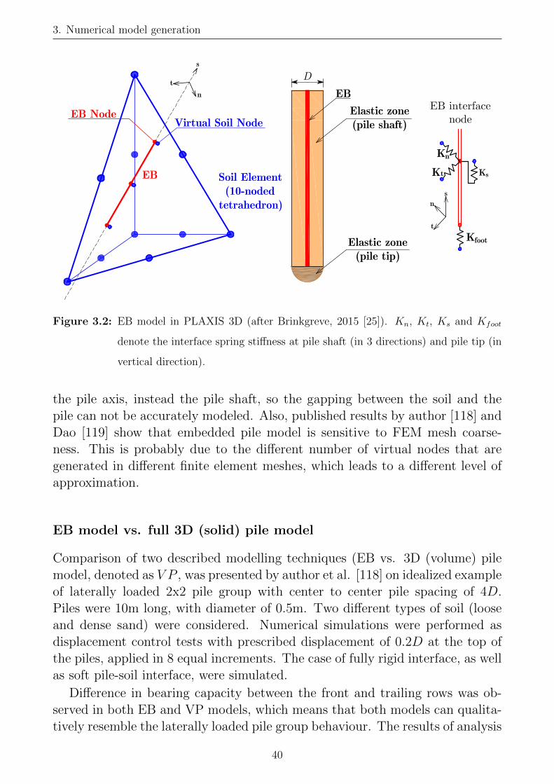
3. Numerical model generation
Figure 3.2: EB model in PLAXIS 3D (after Brinkgreve, 2015 [25]). Kn, Kt, Ks and Kfoot
denote the interface spring stiffness at pile shaft (in 3 directions) and pile tip (in
vertical direction).
the pile axis, instead the pile shaft, so the gapping between the soil and thepile can not be accurately modeled. Also, published results by author [118] andDao [119] show that embedded pile model is sensitive to FEM mesh coarse-ness. This is probably due to the different number of virtual nodes that aregenerated in different finite element meshes, which leads to a different level ofapproximation.
EB model vs. full 3D (solid) pile model
Comparison of two described modelling techniques (EB vs. 3D (volume) pilemodel, denoted as V P , was presented by author et al. [118] on idealized exampleof laterally loaded 2x2 pile group with center to center pile spacing of 4D.Piles were 10m long, with diameter of 0.5m. Two different types of soil (looseand dense sand) were considered. Numerical simulations were performed asdisplacement control tests with prescribed displacement of 0.2D at the top ofthe piles, applied in 8 equal increments. The case of fully rigid interface, as wellas soft pile-soil interface, were simulated.
Difference in bearing capacity between the front and trailing rows was ob-served in both EB and VP models, which means that both models can qualita-tively resemble the laterally loaded pile group behaviour. The results of analysis
40
3. Numerical model generation
have shown also that interface properties don’t influence the lateral behaviourof EB models, while the VP models are influenced, as expected. This is associ-ated with the formulation of EB interface, where only the shear stresses in axialdirection are governed by interface input parameters. It was presented that EBsingle pile model agrees well with the volume pile model with rigid interface,while the weaker pile-soil contact cannot be resembled with EB interface pa-rameters.
The obtained results concludes that the interface properties in the EB modelformulation in PLAXIS 3D do not influence the lateral response of the pilegroup. However, when shear pile forces become large, plasticity will occur inthe surrounding soil elements, outside the elastic zone. In other words, pile-soilinteraction in lateral directions can only be controlled by the adjustments ofsurrounding soil stiffness parameters.
Concluding remarks
Recent researches by several authors in the direction of improvement of initialEB model to account for the lateral interface interaction have been done andthe results are very promising [120–122]. However, due to the current thelimitations of the PLAXIS 3D EB model for lateral loading and lack of softwarepackages with implemented improved EB formulations, full 3D pile analysis hasbeen done within this Dissertation.
Pile-soil interface
The modelling of pile-soil interface (contact) is another important factor inrealistic pile group simulation. In general, the pile-soil interface strength de-pends on the type of pile material (wood, steel or concrete) and pile installationmethod (driven or bored). Due to the fact that this study only considered thebored piles, installation effects and loading history were not taken into account.In the case of driven piles, installation effects are found to be important [72,81].
Because the soil has limited or no capacity in sustaining tension, slippageand separation (gapping) between the pile and the soil will occur. In orderto simulate these effects, thin 2D interface elements are inserted between thesoil and pile elements. These elements are different from the regular finiteelements: they have pairs of nodes instead of single nodes (the distance betweenthe two nodes of a node pair is zero), and each node has three translationaldegrees of freedom (ux, uy, uz). As a result, these elements allow for differentialdisplacements between the node pairs to simulate both slipping and gapping onthe pile-soil contact [25].
41

3. Numerical model generation
The shear strength parameters of the pile-soil interface in PLAXIS 3D arerelated to the strength reduction factor Rinter, that reduces the parameters ofMC model (soil cohesion c′ and angle of internal friction ϕ′), according to thefollowing expressions:
cint = Rinterc′ (3.4)
tanϕint = Rintertanϕ′ (3.5)
where:
• cint - cohesion of the pile-soil interface,
• ϕint - angle of internal friction of the pile-soil interface.
In general, there is the lack of the experimental data for real pile-soil interfaceparameters. Suitable values of Rinter are recommended in the literature [25] fordifferent soil types, and usual value is around Rinter = 0.5 (that yields thewell-known relationship ϕint = 2/3ϕ′).
”Dummy” beams
The extraction of the pile group results from the 3D FEM simulation is nota simple task. This is mainly related to determination of pile section forces.That is theoretically done by integration of component stresses over the pilecross section. Despite the fact that the calculation of the section forces fromvolumes is implemented in PLAXIS 3D, this step cannot be done automatically,but requires that the user perform the whole procedure manually for each pilevolume.
In order to simplify the extraction of pile section forces and displacementsand to automatize the post-processing as well, the concept of ”dummy” beamsis used. This modelling concept is common when the laterally loaded piles aremodelled using 3D elements [123, 124]. The elastic beam elements with verysmall bending stiffness (106 times smaller than the pile bending stiffness) areinserted along the pile axis. Because the beam stiffness is very small, systemstiffness matrix remains almost unchanged. On the other hand, ”dummy” beamis enforced to deform together with the pile axis. Because the pile displacementsand forces are directly coupled through the basic equations of elastic beam, realvalues of pile section forces are now easily obtained by multiplication of sectionforces in ”dummy” beams with 106 (the bending stiffness ratio between realpile and ”dummy” beam).
42
3. Numerical model generation
3.4 Calculation stages
Numerical simulations within the thesis were done as the staged (phase) analysisand consisted of the following stages:
1. Initial (K0) phase - initial stress field in the soil, due to the soil selfweight, was established. Horizontal stress state is calculated based on thewell-known Jaky’s formula [125]: K0 = 1− sinϕ′.
2. Construction stage - after initial stress state has been established, soilvolume is replaced with 3D pile finite elements (wished-in-place concept).Thin 2D pile-soil interface elements are also activated in this phase.
3. Prescribed displacements (Displacement control test) - 4 succes-sive phases - the incremental prescribed displacements up to 10% of thepile diameter were applied at the pile top. The direction of loading wasgoverned by the loading direction angle β (denoted as parameter ANGLEin Table 3.1).
Optimization of the PLAXIS 3D calculation algorithm
Computation time and size of the saved raw simulation on computer drivein PLAXIS 3D is directly proportional to the number of calculation stages.Because of this, the optimization has been done, in order to reduce the storageneeds of calculation computers, as well as the calculation speed. The trial-and-error sensitivity analysis was executed to find the optimal solution. Thetrials with equally and non-equally spaced prescribed displacements were done.It was found that the model with 4 prescribed displacements and 20 savedsteps provide the same quality of results (load-displacement curves and bendingmoments) as the 10 stages model, but with significantly less storage space andcalculation time. Finally, the following non-equally prescribed displacementswere adopted as the optimum solution: 0.015D, 0.03D, 0.06D and 0.10D.
The calculation speed can also be adjusted by setting the tolerated error ofthe numerical algorithm in PLAXIS 3D. The default value is 1%, but it can bechanged by the user. This parameter is also included in the numerical modelof the pile group (denoted as parameter TOLERANCE in Table 3.1).
3.5 Proposed model parameters
Proposed FEM model of the pile group contains 28 different parameters thatfully describe pile group configuration, geometry, material properties, loading
43

3. Numerical model generation
conditions, numerical algorithm, model domain, boundary conditions and finiteelement mesh. The model parameters are presented in Table 3.1.
The most of the model geometry parameters have been designed as themultiplicators of pile diameter D, so the whole model geometry is parametrizedas the function of the pile diameter D.
Table 3.1: Proposed parameters of the FEM model of laterally loaded pile group. Integer and
float are common numerical data types used in many programming languages.
Parameter group Parameter Unit Description Data type
Pile dimensions
D
L
Pile diameter Float
L1 Pile length below ground surface Float
L2 Pile length above ground surface Float
N - Pile rows (X direction) Integer
Pile group M - Pile columns (Y direction) Integer
configuration SXDiameters
Normalized c-c pile spacing in X direction Float
SY Normalized c-c pile spacing in Y direction Float
BXFRONT
Diameters
Distance from pile group edge to the model sides Float
BZDOWN Distance from pile bottom to the model bottom Float
Model domain REF ZONE XFRONT Size of mesh refinement zone, measured from pile group edge Float
and discretization REF ZONE BOTTOM Distance between the bottom of refinement zone and the model bottom Float
SMALL FE SIZE FE size in refinement zone Float
BIG FE SIZE Global FE size Float
CMODEL - Constitutive model index (1-MC model, 2-HS model) Integer
SOIL WEIGHT F/L3 Unsaturated soil volumetric weight Float
COHESION F/L2 Cohesion Float
Soil and interface PHI degrees Angle of internal friction Float
parameters E50 EOED F/L2 E50=Eoed (Hardening Soil Model) Float
EUR MULTIPLIER - Eur/E50 (Hardening Soil Model) Float
NU - Poisson’s ratio Float
POWERM - m (Hardening Soil Model) Float
RINTER - Interface strength reduction factor Float
LE model parameters
E CONCRETE F/L2 Young’s modulus (Concrete) Float
NU CONCRETE - Poisson’s ratio (Concrete) Float
W CONCRETE F/L3 Volumetric weight (Concrete) Float
Calculation TOLERANCE % Tolerated error for PLAXIS 3D calculation algorithm Float
Loading
MAX D - Max displacement (0.XX of pile Diameters) Float
ANGLE degrees Loading direction angle β Float
3.6 Model geometry
Domain and boundary conditions
Model boundaries should be far enough from the center of the pile group, so thestress change at the boundary does not affect the model response. Sensitivityanalyses were carried out to determine the optimum size of the model. Theresults are presented in Chapter 4.
Because the model geometry will change for different pile group configura-tions, it was adopted that the distances to the model boundaries remain the
44

3. Numerical model generation
same (governed by independent input parameter BFRONT (see Table 3.1),and scaled by pile diameter D). This can be justified with the fact that in thedisplacement control test, the same level of deformation is ”introduced” to themodel.
The displacements on the model boundaries were fully fixed in all directionsat the bottom of the model, while the displacements on the side planes werelimited to vertical direction. According to Fayyazi et al. [50], the pile modelcan be truncated at the pile bottom. The reason is due to the fact that thelateral pile group response is mostly governed by the top soil layer, in the caseof flexible piles. According to [98], pile-soil separation will occur near the topand behind the pile, no deeper than 20% of the pile length (depending on thepile and soil stiffness), but not less than 8D [126].
Discretization
FE mesh in PLAXIS 3D is mainly automatically generated, and it is governedby a single parameter coarseness ratio, that relates the model domain size andthe size of finite elements. Alternatively, average FE size can be used as meshingparameter. PLAXIS 3D does not allow for very precise control of the modeldiscretization. However, it allows the user to define ”refinement zones” insidethe model volume, where the mesh discretization can be finer. Every refinementzone is controlled using individual coefficient of the refinement. This coefficientrelates the size of the FE inside the refined zone with the global FE size. Aroundthe structural model components, such as beams, anchors and interfaces, FEmesh is (automatically) refined by the PLAXIS 3D.
The FE mesh size can be optimized for both accuracy and computationalcost based on the analyses of several meshes with different numbers of elementsand mesh sizes. In order to optimize the mesh discretization without influenc-ing the model precision, trial analyses were executed on models with differentdiscretization setups. Generally, the optimal grid size is taken to be the largestone that will resolve all the important features of the problem, giving the mosteconomical solution that is still accurate.
Very important fact regarding the size and the quality of the FE mesh isthat the finite elements have regular shapes and approximately equal dimen-sions. Around the pile group, rectangular prismatic mesh refinement zone isadopted (governed by parameter REF ZONE XFRONT ). The model do-main extension around the pile group towards the boundaries was chosen toconsist of finite number of pile diameters (scalable with D).
The sketch of the model boundaries, with the position of the refinement zoneand governing model parameters is displayed in Figures 3.3 and 3.4.
45
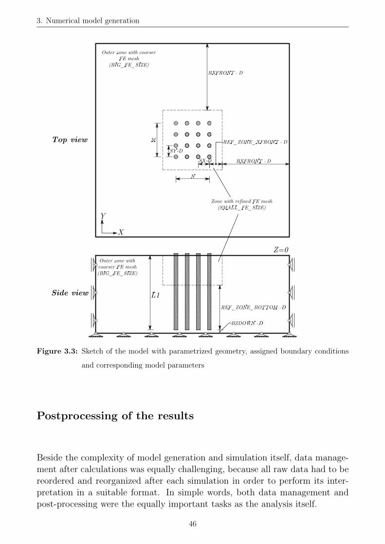
3. Numerical model generation
Figure 3.3: Sketch of the model with parametrized geometry, assigned boundary conditions
and corresponding model parameters
Postprocessing of the results
Beside the complexity of model generation and simulation itself, data manage-ment after calculations was equally challenging, because all raw data had to bereordered and reorganized after each simulation in order to perform its inter-pretation in a suitable format. In simple words, both data management andpost-processing were the equally important tasks as the analysis itself.
46

3. Numerical model generation
Figure 3.4: Model parameters in the mesh refinement zone
Maximum displacements, shear forces and bending moments
PLAXIS 3D post-processor allows the extraction of all results in Euclidean XYspace. The most important results, such as displacements and bending momentsare extracted separately in X and Y direction. However, for the arbitraryloading case, the resultant maximum displacements and bending moments mustbe calculated separately (Figure 3.5).
Figure 3.5: Directions of the maximum displacements ymax, shear forces Hmax and bending
moments Mmax. Loading direction is governed by the loading direction angle
β. X, Y , Q12, Q13, M2 and M3 denotes the directions of displacements, shear
forces and bending moments in Euclidean XY space in PLAXIS 3D, respectively.
Based on simple vector algebra, displacements and section forces extracteddirectly from ”dummy” beams in PLAXIS 3D Euclidean XY space (displace-ments Ux and Uy, shear forces Q12 and Q13 and bending moments M2 and
47

3. Numerical model generation
M3), are transformed towards the loading direction. The corresponding axesare given in Figure 3.5. Transformations are done using the following equations:
ymax = Uxcosβ + Uysinβ (3.6)
Hmax = Q12cosβ +Q13sinβ (3.7)
Mmax = M3cosβ–M2sinβ (3.8)
Displacements, shear forces and bending moments in loading direction (Equa-tions 3.6, 3.7 and 3.8) are assumed as maximum values and are used as mainobservation points for the interpretation of the pile group interaction analysis.However, comparison was made on a trial model with the ”absolute” maximum
values (e.g. yabs,max =√Ux
2 + Uy2), and the observed differences were about
2%. However, above expressions were adopted as the more straightforward.
Derivation of section forces
The most important step in the post-processing of the results is the evaluationof shear forces in the pile. These forces must be precisely calculated, in orderto obtain the load-displacement curves and further evaluate the pile group in-teraction effects. However, the shear forces extracted from ”dummy” beamsin PLAXIS 3D are slightly unrealistic (”zig-zag”). This issue was analyzed byTedesco (2013) [123], who concluded that such behaviour could be associatedwith the PLAXIS 3D beam elements, that compute the shear forces using thebending moment derivative along the pile length.
In order to evaluate the shear forces properly, the pile displacements andbending moments are approximated (fitted) using the polynomial or spline ap-proximations. After fitting, shear forces can be evaluated by differentiation ofthe bending moments or displacements. Python [127] scripts written by theauthor are used for this step.
Data fitting and integrity check
In experimental testing of the laterally loaded piled foundations, the bendingmoments are commonly measured at a finite number of discrete strain gaugesalong the pile. In order to obtain the continuous bending moment line, itis common practice to fit the measured data using a smooth fitting curve.Continuity is obtained using different fitting techniques, such as splines andpolynomials. Hussien et al. [128] analyzed the optimal positioning of the strain
48
3. Numerical model generation
gauges and the different curve fitting techniques (i.e. cubic splines, B-splines,polynomials) for the analysis of laterally loaded piles and the derivation of thep-y curves. Cubic and cubic B-splines were found to be the most appropriatefitting methods for the considered problem. In this study, the same conceptwas used for the derivation of shear forces from ”dummy” beams.
Polynomial fitting uses the least square method to approximate the measure-ment points, using 3rd to 10th order polynomials. The quality of the fittingis described by R2 (coefficient of determination). On the other hand, splinefitting is the approximation method that interpolates the polynomial insidesubintervals between 2 or 3 points. The most common way of interpolationis cubic spline, where the cubic polynomial is interpolated. B-splines createthe continuity between the adjacent spline fittings. One also important pa-rameter in the spline fitting is the number of interior knots that are used forbetter interpolation. Interior knots are equally spaced inside the single interval.For approximation of displacements, minimum 6th order of the polynomial isrecommended, so the 4th derivative is a smooth function.
Trial and error estimations have been done in order to select optimum fittingmethod for this study. Simple visual inspection proved to be enough for thedata integrity check. Even all of these checks can be considered as routineones, they enforced some important decisions in the whole analysis process.The checks of the pile bending moments, shear forces and displacements weremajor inspections. The fitting methods that gave the unexpected results havebeen excluded. The analysis was done on both free head single pile and 2x2pile group models. It is important to point out that the observation point forload-displacement behaviour is the ground point. After inspection checks, itwas found that the spline fitting is the best option for the fitting of the bendingmoments curves. The polynomial fitting was also tried, but discrepancies thatoccurred were higher than in the case of spline fitting. It was also concluded thatall important parameters should be calculated by differentiating the bendingmoments, instead of differentiating the displacements.
Following fitting parameters have been selected: B-splines fitting, with 10interior knots and 5th order spline interpolation (as recommended by Haideraliand Madabhushi 2016 [129]) was adopted.
In order to do that, additional computer scripts were written in order toquickly present the results in a suitable format.
The pile displacements and section forces for free head pile should follow thewell-known behaviour pattern, as shown in Figure 3.6:
Verification example for the single pile is presented in Figures 3.7 and 3.8.
In order to calculate the interaction factor for any desired load level, load-displacement curves for each pile were approximated by 10th order polynomials.
49

3. Numerical model generation
Figure 3.6: Shape of the characteristic diagrams for a free head pile
Figure 3.7: Verification of shear forces fitting for a single pile (screenshot from author’s com-
puter program). Spline fitting of bending moments and displacements provides
more logical results, especially at the end of the pile, where polynomial fitting
shows unrealistically high shear forces. The shear forces calculated by the spline
fitting and differentiation of bending moments (marked with green triangles) is
the most realistic, so this fitting technique was adopted.
The quality of the fitting have been found to be correct, so the fitting error canbe neglected.
50
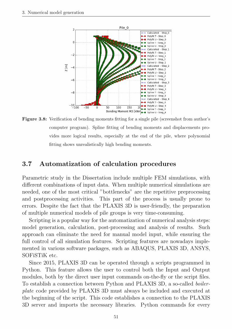
3. Numerical model generation
Figure 3.8: Verification of bending moments fitting for a single pile (screenshot from author’s
computer program). Spline fitting of bending moments and displacements pro-
vides more logical results, especially at the end of the pile, where polynomial
fitting shows unrealistically high bending moments.
3.7 Automatization of calculation procedures
Parametric study in the Dissertation include multiple FEM simulations, withdifferent combinations of input data. When multiple numerical simulations areneeded, one of the most critical ”bottlenecks” are the repetitive preprocessingand postprocessing activities. This part of the process is usually prone toerrors. Despite the fact that the PLAXIS 3D is user-friendly, the preparationof multiple numerical models of pile groups is very time-consuming.
Scripting is a popular way for the automatization of numerical analysis steps:model generation, calculation, post-processing and analysis of results. Suchapproach can eliminate the need for manual model input, while ensuring thefull control of all simulation features. Scripting features are nowadays imple-mented in various software packages, such as ABAQUS, PLAXIS 3D, ANSYS,SOFiSTiK etc.
Since 2015, PLAXIS 3D can be operated through a scripts programmed inPython. This feature allows the user to control both the Input and Outputmodules, both by the direct user input commands on-the-fly or the script files.To establish a connection between Python and PLAXIS 3D, a so-called boiler-plate code provided by PLAXIS 3D must always be included and executed atthe beginning of the script. This code establishes a connection to the PLAXIS3D server and imports the necessary libraries. Python commands for every
51
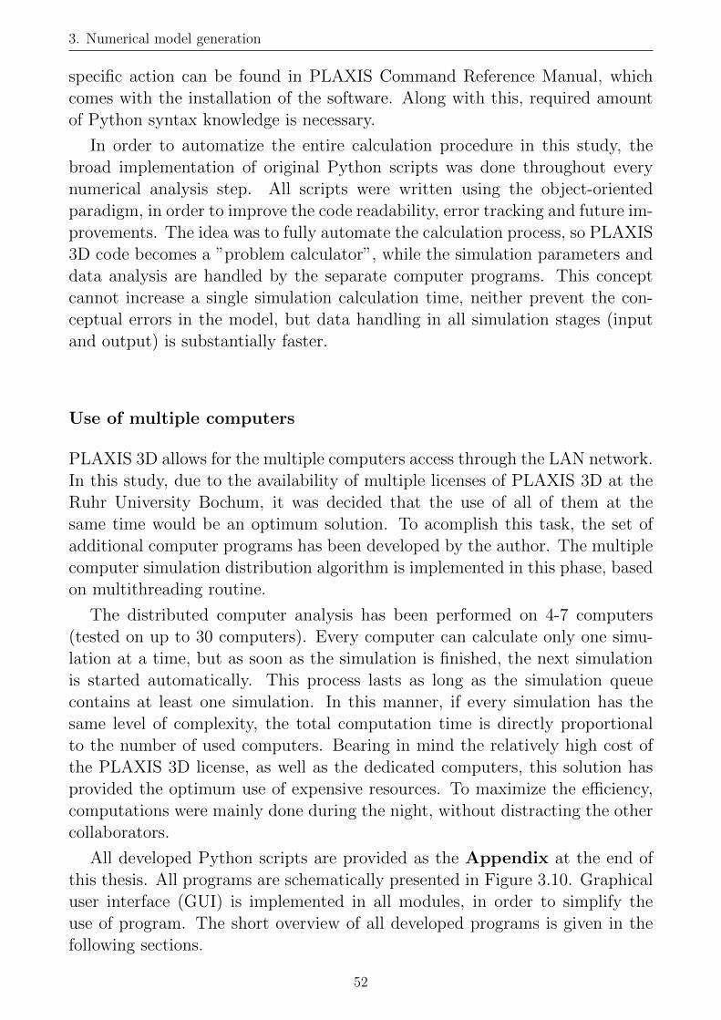
3. Numerical model generation
specific action can be found in PLAXIS Command Reference Manual, whichcomes with the installation of the software. Along with this, required amountof Python syntax knowledge is necessary.
In order to automatize the entire calculation procedure in this study, thebroad implementation of original Python scripts was done throughout everynumerical analysis step. All scripts were written using the object-orientedparadigm, in order to improve the code readability, error tracking and future im-provements. The idea was to fully automate the calculation process, so PLAXIS3D code becomes a ”problem calculator”, while the simulation parameters anddata analysis are handled by the separate computer programs. This conceptcannot increase a single simulation calculation time, neither prevent the con-ceptual errors in the model, but data handling in all simulation stages (inputand output) is substantially faster.
Use of multiple computers
PLAXIS 3D allows for the multiple computers access through the LAN network.In this study, due to the availability of multiple licenses of PLAXIS 3D at theRuhr University Bochum, it was decided that the use of all of them at thesame time would be an optimum solution. To acomplish this task, the set ofadditional computer programs has been developed by the author. The multiplecomputer simulation distribution algorithm is implemented in this phase, basedon multithreading routine.
The distributed computer analysis has been performed on 4-7 computers(tested on up to 30 computers). Every computer can calculate only one simu-lation at a time, but as soon as the simulation is finished, the next simulationis started automatically. This process lasts as long as the simulation queuecontains at least one simulation. In this manner, if every simulation has thesame level of complexity, the total computation time is directly proportionalto the number of used computers. Bearing in mind the relatively high cost ofthe PLAXIS 3D license, as well as the dedicated computers, this solution hasprovided the optimum use of expensive resources. To maximize the efficiency,computations were mainly done during the night, without distracting the othercollaborators.
All developed Python scripts are provided as the Appendix at the end ofthis thesis. All programs are schematically presented in Figure 3.10. Graphicaluser interface (GUI) is implemented in all modules, in order to simplify theuse of program. The short overview of all developed programs is given in thefollowing sections.
52
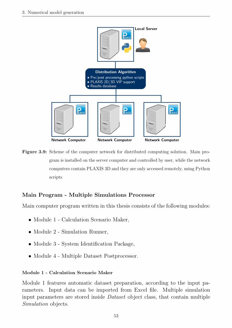
3. Numerical model generation
Low stiffness beams
Pile-soil interface
Pile 3D elements
Prescribed displacements (max 0.1D)
Soil 3D elements
Main elements of 3D numerical model
• Pre/post processing python scripts• PLAXIS 2D/3D VIP support• Results database
Distribution Algorithm
Network Computer Network Computer Network Computer
Local Server
Multiple simulations solution using PLAXIS remote scriptingFigure 3.9: Scheme of the computer network for distributed computing solution. Main pro-
gram is installed on the server computer and controlled by user, while the network
computers contain PLAXIS 3D and they are only accessed remotely, using Python
scripts
Main Program - Multiple Simulations Processor
Main computer program written in this thesis consists of the following modules:
• Module 1 - Calculation Scenario Maker,
• Module 2 - Simulation Runner,
• Module 3 - System Identification Package,
• Module 4 - Multiple Dataset Postprocessor.
Module 1 - Calculation Scenario Maker
Module 1 features automatic dataset preparation, according to the input pa-rameters. Input data can be imported from Excel file. Multiple simulationinput parameters are stored inside Dataset object class, that contain multipleSimulation objects.
53

3. Numerical model generation
Figure 3.10: Modules of computer programs used for the automatization of numerical simu-
lations (developed by author)
Module 2 - Simulation Runner
Module 2 provides scripts for model preprocessing, running the simulation onmultiple computers and the postprocessing of raw simulations. The whole cal-culation process can be paused and later continued, swapped to a different PCconfiguration and fully downloaded for archiving. Additional configuration files(such as IP addresses of remote computers, remote folder paths for data stor-age and PLAXIS 3D connection port names) is obtained through the separateconfiguration files.
Finally, all completed simulations are saved into the separate directory. Allsimulations can also be stored on joint network storage device, under uniquefilename, so the overwriting is avoided. The simulation scenario, as well asthe extracted data results, are stored inside the single dataset file. After thenumerical simulations are done and the ”raw” results are extracted into theresults database, further postprocessing of the results is done in the separateprogram for pile group analysis.
Screenshots of the Module 2 before and during simulation running are shownin Figures 3.11 and 3.12, respectively.
54

3. Numerical model generation
Figure 3.11: Screenshot of Module 2 before distributed computing is started
Figure 3.12: Screenshot of Module 2 during simulations
Model ”template” concept
Module 2 allow for the use of so-called ”template” modelling concept. Thisconcept is used mostly in order to speed up the multiple simulation analysis.In this concept, initial numerical model is formed, and the most important,
55
3. Numerical model generation
the finite element meshing (very slow step), is done. Then the model is savedand used as the basis (start point) for the generation of other models. Thisis possible when the difference between the model is in the order of materialparameters or calculation phases. The pre-processing Python script in thiscase is written to open the template model, perform adjustments of the initialtemplate model, and then to calculate and save a new model under anotherfilename.
Because the remote computer cannot be fully accessed through the LANconnection, before calculating the model template case, the existence of theTEMPLATE.p3d files inside the local/remote folders on each PC must be en-sured.
Module 3 - System Identification Package
The another part of developed program includes routines for global model sen-sitivity analysis (Variance-Based [130]) and parameter back calculation. Math-ematical algorithms such as Proper Orthogonal Decomposition using ExtendedRadial Basis functions (POD-ERBF and ERBF [131]) are included for replac-ing of the FEM model with computationally less expensive metamodel, usinglimited number of performed FEM simulations. For solving the optimizationproblem and parameter back calculation, population-based Particle Swarm Op-timization algorithm [132] is implemented within the program.
Pile Group Analysis Program
The main part of computer program, written by the author within this thesis,is the pile group postprocessing script, that consists of several phases:
• Loading of the raw pile group simulation,
• Extraction of results and their splitting to each pile (pile separation algo-rithm),
• Approximation of all pile results using B-splines,
• Calculation of ymax, Qmax and Mmax
• Creation of load-displacement curves for each pile and their approximationusing the polynomials for further easier determination of interaction factorsfor any displacement level.
All results are extracted for each loading step. The multidimensional dataarrays were used to store and manipulate the large amount of data. The data
56

3. Numerical model generation
export into Excel tables is provided as well, in order to simplify the data man-agement. After postprocessing is done and results are inspected, there is noneed for raw simulation data anymore.
Equivalent single pile
The calculation of the most important pile group results is based on the com-bination of the results for the pile group and the equivalent single pile. Pileis equivalent to a pile group if pile diameter, length, stiffness, head fixity andsurrounding soil are the same. Equivalent single pile calculations are done inseparate dataset, and then the results are linked to the appropriate simulation.
3.8 Concluding remarks
Based on the presented literature review and critical approach to presentedmethodologies of FEM modelling, numerical model is defined to simulate thepile group behaviour under lateral loading. Total of 28 model parameters wereintroduced to account for all aspects of considered engineering problem. Com-puter programs for automatization of the entire process of numerical analysis,including the use of multiple computers, were developed by the author. Addi-tional computer programs were developed and verified for the fast postprocess-ing of the simulation results.
Based on the available results in the literature, the proposed numerical modelis validated in the next Chapter 4.
57

3. Numerical model generation
58

4 Numerical Model Validation
In order to assess the capabilities of the proposed FEM numerical model toaccurately predict the pile group response in PLAXIS 3D, model calibrationand validation were done. Validation was based on the back-calculation of thesmall-scale centrifuge pile group test.
The model validation procedure consisted of the following phases:
• Constitutive model calibration using the results of laboratory tests.
• Domain and FE mesh size selection. In this phase, model domain and thesize of the finite elements were chosen through the simplified sensitivityand convergence analyses, in order to optimize precision of the results andspeed of numerical simulation.
• Validation of numerical model by comparing with the available experimen-tal results. Trial and error analysis was used to match the experimentalresults with the model response.
4.1 Model validation - Kotthaus 1992.
Quasi-static load test in the geotechnical centrifuge at 50g, done by Kotthaus(1992) [21], was used for model validation. Results for a single pile and thepile row at 3D spacing were available. Load-displacement curves at the groundlevel were used as the main observation parameter for comparison with theexperimental results.
Centrifuge modelling may be considered to be the best alternative to the fullscale tests, because the stress and strain conditions at similar locations in thecentrifuge model and the prototype are the same. For parametric studies, cen-trifuge modelling can provide data for understanding the behaviour of the pilegroups at low costs. In the case of centrifuge experiment, the most importantgoal is to preserve the representative stress states on the small scale model, dueto the fact that the soil stiffness and strength is, in general, stress dependent.
The Kotthaus experimental setup was prepared by sand rainfall method, toachieve the desired relative sand density [21]. Experimental aluminium pileswere fabricated as hollow tubes. Strain gauges along the pile axis were usedfor the determination of bending moments. Load cell at the pile top allowedfor the calculation of pile group displacement. Free head pile top conditions
59

4. Numerical Model Validation
were enforced using the screws that allowed for the rotation of pile head, butenforced the same pile top displacements. Therefore, the whole experimentalsetup followed the displacement control setup. In order to increase the pile-soil friction inside the dense sand, soil particles were glued onto the pile shaft.Because of the experimental setup, the point of loading application was abovethe ground level.
The section properties and the experimental setup model geometry are givenin Table 4.1. The outside pile diameter was 30 mm, and the pipe wall thicknesswas 2 mm. Equivalent centrifuge model parameters are calculated using thescaling laws [133].
Table 4.1: Centrifuge model dimensions [21]. Prototype model corresponds to real concrete
pile (between C20/25 and C25/30 concrete classes)
Centrifuge model Prototype scale Real structure
D (m) 0.030 1.50 1.50
L1 (m) 0.600 30.00 30.00
L2 (m) 0.085 4.25 4.25
t (m) 0.002 0.10
d (m) 0.026 1.30
E (MPa) 70000 70000 30508
I (m4) 1.73E-08 1.08E-01 0.2485
EI (kNm2) 1.2130 7581448 7581448
FEM model geometry was adopted to mimic the centrifuge model. Free headpile with prototype size of 4.25+30m and the diameter of 1.5m was modelled.
Constitutive model calibration
For the accurate numerical simulation of geotechnical problem, first step isselection and proper calibration of the selected soil constitutive model. Theavailable experimental soil triaxial testing results for the dense sand, denotedas Normensand 942e (CU = 2.08, D10 = 0.12mm, D50 = 0.23mm, emax = 0.914and emin = 0.583), that was used in centrifuge study by Kotthaus (1992), wereused for Hardening Soil model calibration.
The effective friction angle of the dense sand used in experimental study wasinitially assumed to be 41 degrees. Oedometer modulus was initially adoptedas equal to 28 MPa, based on the study of the same sand by Kayalar 2012 [134].
60

4. Numerical Model Validation
However, the trial and error adjustments of the laboratory determined valueshad to be done in order to better match the measured pile group response. Thisalteration can be justified by the fact that the stress states around the laterallyloaded piles are not fully matched by conventional triaxial tests.
Finally adopted constitutive model parameters are given in Table 4.2.
FE mesh
After trial and error analysis, the global size of finite elements (outside therefinements zone) was adopted as 3D. Smaller sizes of 1D and 2D were alsoinvestigated, but model precision was not justified with increased computationtime. The size of the finite elements inside the refinement zone has shown tobe more important for the model response. Final size of the elements inside therefinement zone was adopted as 1D.
Due to the fact that global finite element size was 3D, the domain size wasadopted to be scalable by 3, in order to preserve the equality of the finite elementdimensions inside the mesh. Adopted model geometry and mesh parametersare given in Table 4.2.
Results of model validation
After a series of trial and error simulations, satisfactory agreement betweencomputed and measured response was obtained both for the single pile (Fig-ure 4.1) and pile row models (Figures 4.2 - 4.4). The final calibrated modelparameters are displayed in Table 4.2.
0
500
1000
1500
2000
2500
3000
0 0.02 0.04 0.06 0.08 0.1 0.12 0.14
Lateral load
[kN
]
Horizontal displacement [m]
Figure 4.1: Measured (triangles) vs. computed (red line) load-displacement response - single
pile
61

4. Numerical Model Validation
Table 4.2: Final model parameters after back-calculation of experimental results. Model pa-
rameters are explained in the previous Chapter.
Parameter Value
BXFRONT 21.5D
BZDOWN 1D
REF ZONE XFRONT 3.5D
REF ZONE BOTTOM 12D
SMALL FE SIZE 1D
BIG FE SIZE 3D
SOIL WEIGHT 16.6 kN/m3
COHESION 0
PHI 35
E50 EOED 28800 kN/m2
EUR MULTIPLIER 4
NU 0.25
POWERM 0.47
RINTER 0.654
E CONCRETE 30508 kN/m2
NU CONCRETE 0.2
W CONCRETE 25 kN/m3
TOLERANCE 1.5%
62

4. Numerical Model Validation
0
500
1000
1500
2000
2500
3000
0.00 0.02 0.04 0.06 0.08 0.10 0.12 0.14
Lateral load
[kN
]
Horizontal displacement [m]
Figure 4.2: Measured (triangles) vs. computed (red line) load-displacement response - piles
in a row - front pile
0
500
1000
1500
2000
0.00 0.02 0.04 0.06 0.08 0.10 0.12 0.14
Lateral load
[kN
]
Horizontal displacement [m]
Figure 4.3: Measured (triangles) vs. computed (red line) load-displacement response - piles
in a row - front pile
4.2 Concluding remarks
Presented results of the single pile and pile row validation show satisfactorymatch with the experimental results in the domain of interest. The overallperformance of the proposed numerical model is therefore considered to beacceptably accurate for the parametric study of the problem, despite the slightdiscrepancies.
63
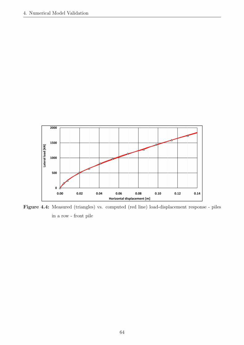
4. Numerical Model Validation
0
500
1000
1500
2000
0.00 0.02 0.04 0.06 0.08 0.10 0.12 0.14
Lateral load
[kN
]
Horizontal displacement [m]
Figure 4.4: Measured (triangles) vs. computed (red line) load-displacement response - piles
in a row - front pile
64

5 Parametric Study and Results
Interpretation
The extensive parametric study using the synthetic soils was carried out toassess the influence of the arbitrary horizontal loading direction on the lateralresponse of different pile groups.
Adopted numerical model parameters
In all simulations, a pile elastic modulus of 30.5 GPa was adopted to simulatethe most common concrete class used in the routine engineering practice. Re-garding the pile length, Duncan [126] showed that for the common pile–soil stiff-ness ratios, piles are considered long when their lengths exceed 6–14D. In thisstudy, pile diameter D=1m was adopted. The length of L1=20m (L/D=20) wasadopted to provide the flexible pile behaviour. Finally, L2=0.25m was taken assmall as possible above the ground level to avoid numerical instabilities causedby the high concentrated forces at the place of monitoring the horizontal dis-placements. The adopted numerical model parameters are elaborated in Table5.1.
Problem parameters
The following major problem parameters, according to presented apriori sen-sitivity analysis, were selected for this study: loading direction, soil type, pilegroup configuration and spacing. All these parameters are further explainedand their range is discussed, as follows. They are illustrated in Figure 5.1.
Loading direction
Loading direction was simulated by varying the inclination angle of the loadingat the pile tops in horizontal plane.
Soil type
The focus on the sand soil types was made to reflect the usual scope of thesand types from the literature. Great distinction between loose and dense sandwas adopted in order to compare the soil stiffening effects to the pile group
65
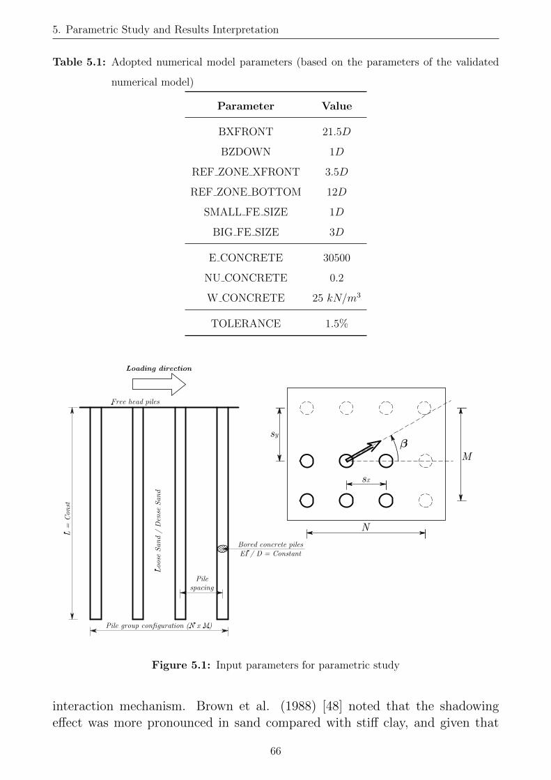
5. Parametric Study and Results Interpretation
Table 5.1: Adopted numerical model parameters (based on the parameters of the validated
numerical model)
Parameter Value
BXFRONT 21.5D
BZDOWN 1D
REF ZONE XFRONT 3.5D
REF ZONE BOTTOM 12D
SMALL FE SIZE 1D
BIG FE SIZE 3D
E CONCRETE 30500
NU CONCRETE 0.2
W CONCRETE 25 kN/m3
TOLERANCE 1.5%
Figure 5.1: Input parameters for parametric study
interaction mechanism. Brown et al. (1988) [48] noted that the shadowingeffect was more pronounced in sand compared with stiff clay, and given that
66
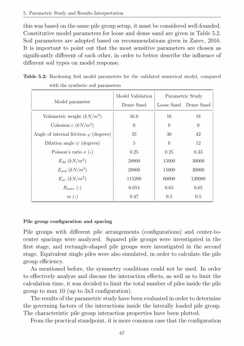
5. Parametric Study and Results Interpretation
this was based on the same pile group setup, it must be considered well-founded.Constitutive model parameters for loose and dense sand are given in Table 5.2.Soil parameters are adopted based on recommendations given in Zarev, 2016.It is important to point out that the most sensitive parameters are chosen assignificantly different of each other, in order to better describe the influence ofdifferent soil types on model response.
Table 5.2: Hardening Soil model parameters for the validated numerical model, compared
with the synthetic soil parameters
Model parameterModel Validation Parametric Study
Dense Sand Loose Sand Dense Sand
Volumetric weight (kN/m3) 16.6 16 18
Cohesion c (kN/m2) 0 0 0
Angle of internal friction ϕ (degrees) 35 30 42
Dilation angle ψ (degrees) 5 0 12
Poisson’s ratio ν (-) 0.25 0.25 0.33
E50 (kN/m2) 28800 15000 30000
Eoed (kN/m2) 28800 15000 30000
Eur (kN/m2) 115200 60000 120000
Rinter (-) 0.654 0.65 0.65
m (-) 0.47 0.5 0.5
Pile group configuration and spacing
Pile groups with different pile arrangements (configurations) and center-to-center spacings were analyzed. Squared pile groups were investigated in thefirst stage, and rectangle-shaped pile groups were investigated in the secondstage. Equivalent single piles were also simulated, in order to calculate the pilegroup efficiency.
As mentioned before, the symmetry conditions could not be used. In orderto effectively analyze and discuss the interaction effects, as well as to limit thecalculation time, it was decided to limit the total number of piles inside the pilegroup to max 10 (up to 3x3 configuration).
The results of the parametric study have been evaluated in order to determinethe governing factors of the interactions inside the laterally loaded pile group.The characteristic pile group interaction properties have been plotted.
From the practical standpoint, it is more common case that the configuration
67

5. Parametric Study and Results Interpretation
of the group (N, M) can be different (square, rectangular, circular etc.), whilethe spacing between the piles is kept on the lowest possible level.
As given in [75], pile group spacing smaller than 3D is not recommendedby the USA authorities (FHWA [135] and AASHTO [136]), due to difficult pileinstallation. According to Das [102], the minimum pile center-to-center spacingin practice is 2.5D, and in ordinary situations, it is about 3-3.5D. Even startingfrom 3D spacing, the costs of the pile cap become very large, while 5D spacingis considered as an extreme case [75].
Calculation Scenarios
Previously described and validated FEM model was used for the parametricstudy. The model input parameters inside the parametric study slightly differfrom the validated model, as shown in Table 5.2. Mainly, all validated modelparameters are the same as in the parametric study, except for the soil.
Several scenarios of the different pile group configurations were investigated.In the process of selection of pile group configurations to be investigated, totalpile cap size was limited, and large cap area cases were eliminated as unrealistic.The summary of study scenarios with all varied model parameters are given inTable 5.1.
Results Catalogue
The results of conducted parametric study are summarized in the followingResults Catalogue, in the form of pile interaction factors for each pile andmaximum bending moments for each pile inside the pile group, with respect toloading direction. Full lines denote the results for loose sand, and dashed linesdenote results for dense sand, respectively.
Pile positions on diagrams are numbered according to the Figure 5.2
Figure 5.2: Pile numbering
68

5. Parametric Study and Results Interpretation
Table 5.3: Parametric study scenarios
PG AnalysisN x M
Sx Sy Loading Direction
Shape Scenario (D) (D) (degrees)
Square 12 x 2 2 2
0 / 15 / 30 / 453 x 3 3 3
Rectangle
2 2 x 2
2 3
0 / 15 / 30 / 45 / 60 / 75 / 90
2 4
2 5
3 4
3 5
4 5
3 2 x 3
2 2
2 3
2 4
3 2
3 3
3 4
3 5
4 2
4 3
4 4
4 5
5 3
5 4
5 5
4 3 x 3
2 3
2 4
2 5
3 4
3 5
4 5
69

5. Parametric Study and Results Interpretation
y/d=0.03 0 15 30 45
pile 11 0.612377 0.589796 0.570481 0.561688
pile 12 0.612518 0.654787 0.695971 0.735514
pile 21 0.775873 0.778772 0.764293 0.735328
pile 22 0.773369 0.771345 0.76118 0.757896
pile 11 0.58874 0.557407 0.534363 0.523372
pile 12 0.589348 0.642293 0.702294 0.755914
pile 21 0.828034 0.818045 0.794913 0.755772
pile 22 0.824758 0.826577 0.826098 0.825558
y/d=0.10 0 15 30 45
pile 11 0.588769 0.537099 0.51151 0.508751
pile 12 0.587496 0.648036 0.71576 0.78075
pile 21 0.848239 0.831174 0.815615 0.781435
pile 22 0.843559 0.850361 0.856358 0.861538
pile 11 0.533243 0.477814 0.445699 0.434631
pile 12 0.533173 0.59908 0.673488 0.738838
pile 21 0.824495 0.806776 0.780876 0.737443
pile 22 0.819745 0.830891 0.835377 0.837081
beta
Loo
se s
and
De
nse
san
dLo
ose
san
dD
en
se s
and
beta
0.00
0.20
0.40
0.60
0.80
1.00
0 15 30 45
Pile
In
tera
ctio
n F
acto
r
Horizontal Loading Direction [deg]
y/D = 0.03
0.00
0.20
0.40
0.60
0.80
1.00
0 15 30 45
Pile
In
tera
ctio
n F
acto
r
Horizontal Loading Direction [deg]
y/D = 0.10 pile 11
pile 12
pile 21
pile 22
pile 11
pile 12
pile 21
pile 22
Figure 5.3: Pile Interaction Factors for 2x2 pile group (sx=2D, sy=2D), considering different
normalized displacements y/D and different horizontal loading directions. Full
lines - loose sand; dashed lines - dense sand.
y/d=0.03 0 15 30 45 60 75 90
pile 11 0.649451 0.630638 0.622502 0.621974 0.637046 0.653167 0.671383
pile 12 0.649274 0.685413 0.728413 0.761002 0.785152 0.798861 0.801063
pile 21 0.825575 0.822886 0.808391 0.775036 0.735265 0.699048 0.671467
pile 22 0.826979 0.820999 0.80941 0.797683 0.795502 0.798094 0.800857
pile 11 0.629682 0.603813 0.590381 0.595004 0.612289 0.63612 0.656705
pile 12 0.627926 0.675561 0.728665 0.775892 0.812941 0.83604 0.847441
pile 21 0.881532 0.866346 0.841963 0.800698 0.746957 0.695404 0.656432
pile 22 0.883827 0.87756 0.870002 0.861882 0.855619 0.85016 0.846811
y/d=0.10 0 15 30 45 60 75 90
pile 11 0.607828 0.563112 0.540858 0.568689 0.587469 0.613453 0.643023
pile 12 0.607145 0.668476 0.720725 0.79614 0.832303 0.855532 0.870685
pile 21 0.888759 0.875425 0.837775 0.816281 0.748623 0.685294 0.641068
pile 22 0.889949 0.898844 0.885133 0.908079 0.900141 0.887876 0.869833
pile 11 0.570234 0.514185 0.485078 0.486906 0.511926 0.551032 0.5882
pile 12 0.569642 0.636684 0.702715 0.758955 0.799991 0.826852 0.846602
pile 21 0.886954 0.866896 0.836664 0.784817 0.712657 0.634859 0.586982
pile 22 0.887417 0.896052 0.895685 0.889774 0.878115 0.861766 0.846687
beta
Loo
se s
and
De
nse
san
d
beta
Loo
se s
and
De
nse
san
d
0.00
0.20
0.40
0.60
0.80
1.00
0 15 30 45 60 75 90
Pile
In
tera
ctio
n F
acto
r
Horizontal Loading Direction [deg]
y/D = 0.03
0.00
0.20
0.40
0.60
0.80
1.00
0 15 30 45 60 75 90
Pile
In
tera
ctio
n F
acto
r
Horizontal Loading Direction [deg]
y/D = 0.10 pile 11
pile 12
pile 21
pile 22
pile 11
pile 12
pile 21
pile 22
Figure 5.4: Pile Interaction Factors for 2x2 pile group (sx=2D, sy=3D), considering different
normalized displacements y/D and different horizontal loading directions. Full
lines - loose sand; dashed lines - dense sand.
y/d=0.03 0 15 30 45 60 75 90
pile 11 0.665073 0.654389 0.655245 0.670128 0.688657 0.710582 0.715203
pile 12 0.665798 0.69704 0.734119 0.7725 0.79971 0.824213 0.819457
pile 21 0.847031 0.8439 0.821358 0.794718 0.761146 0.742572 0.714451
pile 22 0.849041 0.847191 0.833595 0.827097 0.823432 0.831431 0.820446
pile 11 0.650915 0.63695 0.643797 0.661143 0.686664 0.704322 0.718447
pile 12 0.651626 0.692377 0.743266 0.786899 0.829876 0.858324 0.872926
pile 21 0.909326 0.899707 0.869702 0.821894 0.777728 0.740008 0.717593
pile 22 0.908942 0.913951 0.904911 0.891835 0.889155 0.883168 0.874847
y/d=0.10 0 15 30 45 60 75 90
pile 11 0.631731 0.585417 0.58864 0.62461 0.655099 0.649324 0.690033
pile 12 0.629911 0.666798 0.725066 0.795766 0.838183 0.835378 0.885745
pile 21 0.925706 0.889502 0.858776 0.826075 0.763993 0.687318 0.687913
pile 22 0.929579 0.91778 0.91929 0.933108 0.923857 0.876552 0.886364
pile 11 0.588083 0.547822 0.54001 0.557375 0.594551 0.629851 0.650058
pile 12 0.58641 0.646015 0.707229 0.76125 0.807693 0.840927 0.86536
pile 21 0.919439 0.896616 0.858062 0.800597 0.730063 0.67375 0.648597
pile 22 0.922395 0.930179 0.928231 0.919019 0.904674 0.885371 0.866942
beta
Loo
se s
and
De
nse
san
d
beta
Loo
se s
and
De
nse
san
d
0.00
0.20
0.40
0.60
0.80
1.00
0 15 30 45 60 75 90
Pile
In
tera
ctio
n F
acto
r
Horizontal Loading Direction [deg]
y/D = 0.03
0.00
0.20
0.40
0.60
0.80
1.00
0 15 30 45 60 75 90
Pile
In
tera
ctio
n F
acto
r
Horizontal Loading Direction [deg]
y/D = 0.10 pile 11
pile 12
pile 21
pile 22
pile 11
pile 12
pile 21
pile 22
Figure 5.5: Pile Interaction Factors for 2x2 pile group (sx=2D, sy=4D), considering different
normalized displacements y/D and different horizontal loading directions. Full
lines - loose sand; dashed lines - dense sand.
70

5. Parametric Study and Results Interpretation
y/d=0.03 0 15 30 45 60 75 90
pile 11 0.677848 0.676196 0.683603 0.705344 0.727999 0.737028 0.759199
pile 12 0.678652 0.708962 0.743395 0.780831 0.812432 0.824609 0.844598
pile 21 0.860293 0.856373 0.833947 0.812671 0.790097 0.763448 0.758187
pile 22 0.859802 0.861423 0.849877 0.845236 0.845269 0.836371 0.84254
pile 11 0.661119 0.652005 0.674789 0.70373 0.731747 0.751459 0.765113
pile 12 0.662583 0.697266 0.74515 0.79388 0.836707 0.869185 0.889845
pile 21 0.922039 0.907125 0.87631 0.841144 0.806786 0.78082 0.763701
pile 22 0.9213 0.924235 0.914885 0.909687 0.904887 0.898882 0.887886
y/d=0.10 0 15 30 45 60 75 90
pile 11 0.628847 0.616628 0.622893 0.647692 0.692367 0.70496 0.744943
pile 12 0.630691 0.681636 0.725102 0.773011 0.831761 0.857324 0.909723
pile 21 0.923559 0.911447 0.871464 0.821386 0.781863 0.737955 0.742839
pile 22 0.923446 0.939334 0.930939 0.924853 0.930334 0.901067 0.904495
pile 11 0.598898 0.577379 0.583952 0.612505 0.655659 0.68627 0.702706
pile 12 0.601808 0.650056 0.704702 0.761092 0.811055 0.850075 0.88068
pile 21 0.937189 0.90798 0.867099 0.815406 0.756584 0.717433 0.700398
pile 22 0.93604 0.943369 0.940164 0.933185 0.920892 0.902265 0.878627
beta
Loo
se s
and
De
nse
san
d
beta
Loo
se s
and
De
nse
san
d
0.00
0.20
0.40
0.60
0.80
1.00
0 15 30 45 60 75 90
Pile
In
tera
ctio
n F
acto
r
Horizontal Loading Direction [deg]
y/D = 0.03
0.00
0.20
0.40
0.60
0.80
1.00
0 15 30 45 60 75 90
Pile
In
tera
ctio
n F
acto
r
Horizontal Loading Direction [deg]
y/D = 0.10 pile 11
pile 12
pile 21
pile 22
pile 11
pile 12
pile 21
pile 22
Figure 5.6: Pile Interaction Factors for 2x2 pile group (sx=2D, sy=5D), considering different
normalized displacements y/D and different horizontal loading directions. Full
lines - loose sand; dashed lines - dense sand.y/d=0.03 0 15 30 45 60 75 90
pile 11 0.744905 0.735395 0.714461 0.724591 0.733642 0.74616 0.765759
pile 12 0.74336 0.780254 0.797839 0.833403 0.853586 0.860174 0.860106
pile 21 0.873314 0.880652 0.854001 0.842348 0.817472 0.790788 0.763923
pile 22 0.87341 0.880532 0.859005 0.863287 0.862471 0.861221 0.858865
pile 11 0.74717 0.717244 0.701713 0.703133 0.718303 0.742464 0.77383
pile 12 0.744803 0.783337 0.824234 0.860976 0.889348 0.905702 0.915699
pile 21 0.925177 0.918113 0.9028 0.876718 0.843512 0.809473 0.772256
pile 22 0.926749 0.928934 0.926828 0.92483 0.92347 0.920703 0.914594
y/d=0.10 0 15 30 45 60 75 90
pile 11 0.70777 0.677253 0.642844 0.65801 0.677545 0.71271 0.751751
pile 12 0.70671 0.767124 0.794513 0.847929 0.884974 0.919121 0.940404
pile 21 0.93998 0.935784 0.890789 0.866257 0.82359 0.786965 0.746884
pile 22 0.941605 0.961538 0.941216 0.954354 0.952331 0.951762 0.938744
pile 11 0.678897 0.620362 0.583358 0.580153 0.610728 0.65562 0.703557
pile 12 0.676741 0.730554 0.784729 0.830638 0.871651 0.900526 0.922905
pile 21 0.946681 0.926607 0.897934 0.8585 0.807413 0.751945 0.701215
pile 22 0.949584 0.958353 0.961913 0.959472 0.952419 0.939731 0.921742
beta
Loo
se s
and
De
nse
san
d
beta
Loo
se s
and
De
nse
san
d
0.00
0.20
0.40
0.60
0.80
1.00
0 15 30 45 60 75 90
Pile
In
tera
ctio
n F
acto
r
Horizontal Loading Direction [deg]
y/D = 0.03
0.00
0.20
0.40
0.60
0.80
1.00
0 15 30 45 60 75 90
Pile
In
tera
ctio
n F
acto
r
Horizontal Loading Direction [deg]
y/D = 0.10 pile 11
pile 12
pile 21
pile 22
pile 11
pile 12
pile 21
pile 22
Figure 5.7: Pile Interaction Factors for 2x2 pile group (sx=3D, sy=4D), considering different
normalized displacements y/D and different horizontal loading directions. Full
lines - loose sand; dashed lines - dense sand.
y/d=0.03 0 15 30 45 60 75 90
pile 11 0.75467 0.741601 0.741158 0.75645 0.764472 0.784997 0.791682
pile 12 0.756065 0.779303 0.808695 0.842932 0.858823 0.876614 0.870266
pile 21 0.886782 0.882615 0.869847 0.860611 0.835439 0.821891 0.790248
pile 22 0.887865 0.884934 0.880818 0.885318 0.87792 0.882955 0.868276
pile 11 0.759718 0.736454 0.7385 0.747966 0.769572 0.790878 0.817313
pile 12 0.762368 0.790852 0.829719 0.862071 0.896095 0.91907 0.936124
pile 21 0.945651 0.937121 0.918088 0.890264 0.867833 0.84297 0.81639
pile 22 0.945971 0.949764 0.945258 0.940446 0.944067 0.940758 0.933544
y/d=0.10 0 15 30 45 60 75 90
pile 11 0.723827 0.692372 0.681287 0.682479 0.734339 0.744547 0.779108
pile 12 0.723631 0.762618 0.800234 0.830366 0.902495 0.918195 0.945444
pile 21 0.966729 0.945091 0.912372 0.860849 0.853283 0.804541 0.774626
pile 22 0.966867 0.968615 0.963535 0.947702 0.975885 0.949894 0.937397
pile 11 0.692575 0.651865 0.631589 0.642268 0.675155 0.712437 0.750299
pile 12 0.695138 0.739172 0.785894 0.832156 0.876998 0.910898 0.938266
pile 21 0.96717 0.947227 0.914157 0.875904 0.831067 0.788349 0.748566
pile 22 0.967943 0.975604 0.977523 0.974605 0.966216 0.953714 0.931925
beta
Loo
se s
and
De
nse
san
d
beta
Loo
se s
and
De
nse
san
d
0.00
0.20
0.40
0.60
0.80
1.00
0 15 30 45 60 75 90
Pile
In
tera
ctio
n F
acto
r
Horizontal Loading Direction [deg]
y/D = 0.03
0.00
0.20
0.40
0.60
0.80
1.00
0 15 30 45 60 75 90
Pile
In
tera
ctio
n F
acto
r
Horizontal Loading Direction [deg]
y/D = 0.10 pile 11
pile 12
pile 21
pile 22
pile 11
pile 12
pile 21
pile 22
Figure 5.8: Pile Interaction Factors for 2x2 pile group (sx=3D, sy=5D), considering different
normalized displacements y/D and different horizontal loading directions. Full
lines - loose sand; dashed lines - dense sand.
71

5. Parametric Study and Results Interpretation
y/d=0.03 0 15 30 45 60 75 90
pile 11 0.808646 0.787614 0.783875 0.788115 0.794713 0.809409 0.825263
pile 12 0.808756 0.823967 0.848028 0.869973 0.885857 0.896949 0.898466
pile 21 0.905894 0.896491 0.89064 0.88055 0.864321 0.848113 0.826702
pile 22 0.906038 0.899453 0.901485 0.904143 0.905362 0.90771 0.903235
pile 11 0.826681 0.800818 0.787723 0.786792 0.799171 0.82018 0.848992
pile 12 0.826559 0.855116 0.884997 0.911387 0.933739 0.948886 0.958307
pile 21 0.962287 0.954378 0.941932 0.925215 0.904987 0.879045 0.849996
pile 22 0.96271 0.965501 0.966857 0.969356 0.970862 0.969435 0.962739
y/d=0.10 0 15 30 45 60 75 90
pile 11 0.791224 0.763064 0.739958 0.753857 0.768429 0.788253 0.802078
pile 12 0.790424 0.832107 0.860543 0.907909 0.937996 0.9541 0.950912
pile 21 0.977988 0.969782 0.940253 0.925788 0.897894 0.85882 0.804764
pile 22 0.979847 0.991725 0.988313 1.001844 1.001546 0.990318 0.957824
pile 11 0.765285 0.718955 0.683025 0.672742 0.699715 0.740722 0.788367
pile 12 0.767806 0.813274 0.856233 0.893083 0.923745 0.946693 0.966954
pile 21 0.982871 0.965646 0.941668 0.913824 0.880113 0.840961 0.792548
pile 22 0.981514 0.990325 0.99673 1.00077 0.997354 0.988122 0.97326
beta
Loo
se s
and
De
nse
san
d
beta
Loo
se s
and
De
nse
san
d
0.00
0.20
0.40
0.60
0.80
1.00
0 15 30 45 60 75 90
Pile
In
tera
ctio
n F
acto
r
Horizontal Loading Direction [deg]
y/D = 0.03
0.00
0.20
0.40
0.60
0.80
1.00
0 15 30 45 60 75 90
Pile
In
tera
ctio
n F
acto
r
Horizontal Loading Direction [deg]
y/D = 0.10 pile 11
pile 12
pile 21
pile 22
pile 11
pile 12
pile 21
pile 22
Figure 5.9: Pile Interaction Factors for 2x2 pile group (sx=4D, sy=5D), considering different
normalized displacements y/D and different horizontal loading directions. Full
lines - loose sand; dashed lines - dense sand.
y/d=0.03 0 15 30 45
pile 11 0.64979 0.622094 0.600006 0.588652
pile 12 0.581636 0.580897 0.581255 0.585523
pile 13 0.651244 0.684933 0.724473 0.761268
pile 21 0.620127 0.601315 0.593102 0.585708
pile 22 0.553595 0.555848 0.561215 0.563476
pile 23 0.621575 0.648364 0.677351 0.704039
pile 31 0.791379 0.795751 0.789169 0.765109
pile 32 0.744934 0.739152 0.724543 0.701033
pile 33 0.789493 0.777564 0.76659 0.760851
pile 11 0.634104 0.595044 0.566455 0.555883
pile 12 0.563048 0.56435 0.563264 0.572501
pile 13 0.63368 0.685073 0.738922 0.78626
pile 21 0.637158 0.606068 0.584152 0.572652
pile 22 0.580624 0.584652 0.589965 0.592015
pile 23 0.638336 0.680015 0.722947 0.763466
pile 31 0.837225 0.834886 0.820661 0.789953
pile 32 0.823678 0.816929 0.794856 0.760467
pile 33 0.836294 0.836146 0.832489 0.831427
y/d=0.10 0 15 30 45
pile 11 0.611379 0.567336 0.544202 0.534852
pile 12 0.559495 0.561239 0.566265 0.571203
pile 13 0.610952 0.672155 0.742358 0.805364
pile 21 0.644934 0.597491 0.578604 0.572092
pile 22 0.612009 0.618269 0.624779 0.626137
pile 23 0.646719 0.701685 0.752877 0.798378
pile 31 0.866086 0.860886 0.847514 0.810445
pile 32 0.857138 0.851267 0.830437 0.793898
pile 33 0.86409 0.867404 0.864983 0.863457
pile 11 0.541911 0.480761 0.440287 0.426529
pile 12 0.478267 0.481525 0.487436 0.491512
pile 13 0.542027 0.613378 0.69455 0.76041
pile 21 0.603323 0.545041 0.504315 0.492344
pile 22 0.557802 0.564858 0.573022 0.574148
pile 23 0.603089 0.661785 0.720015 0.772299
pile 31 0.843174 0.828635 0.803075 0.764122
pile 32 0.837633 0.833408 0.809555 0.76766
pile 33 0.841959 0.848546 0.849232 0.849139
beta
Loo
se s
and
De
nse
san
d
beta
Loo
se s
and
De
nse
san
d
0.00
0.20
0.40
0.60
0.80
1.00
0 15 30 45
Pile
In
tera
ctio
n F
acto
r
Horizontal Loading Direction [deg]
y/D = 0.03
0.00
0.20
0.40
0.60
0.80
1.00
0 15 30 45
Pile
In
tera
ctio
n F
acto
r
Horizontal Loading Direction [deg]
y/D = 0.10 pile 11pile 12pile 13pile 21pile 22pile 23pile 31pile 32pile 33pile 11pile 12pile 13pile 21pile 22pile 23pile 31pile 32
Figure 5.10: Pile Interaction Factors for 3x3 pile group (sx=3D, sy=3D), considering different
normalized displacements y/D and different horizontal loading directions. Full
lines - loose sand; dashed lines - dense sand.
y/d=0.03 0 15 30 45 60 75 90
pile 11 0.572171 0.547685 0.531733 0.530237 0.546755 0.567231 0.593367
pile 12 0.513785 0.516216 0.521838 0.529252 0.536379 0.544481 0.560013
pile 13 0.572662 0.611906 0.660238 0.702608 0.730706 0.741418 0.736794
pile 21 0.542798 0.527139 0.518943 0.513088 0.506662 0.503786 0.505648
pile 22 0.499008 0.50123 0.500865 0.492052 0.475954 0.46222 0.457964
pile 23 0.543421 0.571893 0.606783 0.635785 0.655276 0.665364 0.669675
pile 31 0.755632 0.759455 0.751404 0.723528 0.677411 0.628183 0.594204
pile 32 0.719988 0.711488 0.688905 0.656018 0.618208 0.58367 0.560304
pile 33 0.756587 0.741512 0.723542 0.712438 0.711564 0.72155 0.737068
pile 11 0.548939 0.510946 0.493945 0.495629 0.513373 0.535211 0.564697
pile 12 0.490105 0.491334 0.497881 0.506962 0.519398 0.537746 0.562928
pile 13 0.547127 0.596683 0.659239 0.712347 0.751979 0.774717 0.780137
pile 21 0.546328 0.522907 0.513365 0.503394 0.492994 0.484641 0.483349
pile 22 0.512547 0.515848 0.519366 0.512119 0.497662 0.484947 0.480715
pile 23 0.545785 0.584444 0.635052 0.679698 0.714671 0.736158 0.74373
pile 31 0.806846 0.799445 0.779973 0.740309 0.68237 0.616064 0.565975
pile 32 0.800084 0.787088 0.756223 0.708806 0.654221 0.601785 0.561947
pile 33 0.808696 0.799659 0.788714 0.779383 0.775338 0.777658 0.780746
y/d=0.10 0 15 30 45 60 75 90
pile 11 0.532233 0.490975 0.478713 0.481748 0.498052 0.515449 0.546869
pile 12 0.497455 0.501476 0.509132 0.516055 0.521174 0.532509 0.56553
pile 13 0.529164 0.600061 0.67481 0.738128 0.779346 0.797496 0.797523
pile 21 0.566831 0.525287 0.509396 0.502313 0.49665 0.487604 0.484042
pile 22 0.558814 0.563065 0.560604 0.545336 0.524509 0.507235 0.501189
pile 23 0.566316 0.624753 0.679 0.723659 0.754951 0.765506 0.764732
pile 31 0.831707 0.829292 0.814495 0.770306 0.695039 0.610755 0.548114
pile 32 0.837397 0.828402 0.797946 0.746554 0.682739 0.617914 0.56447
pile 33 0.833808 0.83313 0.823376 0.81184 0.802775 0.798685 0.798378
pile 11 0.462623 0.409632 0.384025 0.386669 0.406935 0.437268 0.483334
pile 12 0.41887 0.420418 0.425714 0.429552 0.439501 0.472783 0.521664
pile 13 0.462195 0.537721 0.617892 0.684423 0.730858 0.755724 0.770013
pile 21 0.532156 0.479854 0.453148 0.443444 0.433512 0.421944 0.418864
pile 22 0.512586 0.512526 0.508198 0.495165 0.474246 0.45326 0.448091
pile 23 0.529776 0.587725 0.643541 0.691014 0.723957 0.737458 0.740918
pile 31 0.809676 0.793068 0.768525 0.720892 0.646031 0.555452 0.483468
pile 32 0.810721 0.803871 0.773046 0.718642 0.652555 0.58288 0.520739
pile 33 0.811067 0.811836 0.803505 0.791937 0.781949 0.77693 0.770466
beta
Loo
se s
and
De
nse
san
d
beta
Loo
se s
and
De
nse
san
d
0.00
0.20
0.40
0.60
0.80
1.00
0 15 30 45 60 75 90
Pile
In
tera
ctio
n F
acto
r
Horizontal Loading Direction [deg]
y/D = 0.03
0.00
0.20
0.40
0.60
0.80
1.00
0 15 30 45 60 75 90
Pile
In
tera
ctio
n F
acto
r
Horizontal Loading Direction [deg]
y/D = 0.10 pile 11pile 12pile 13pile 21pile 22pile 23pile 31pile 32pile 33pile 11pile 12pile 13pile 21pile 22pile 23pile 31pile 32
Figure 5.11: Pile Interaction Factors for 3x3 pile group (sx=2D, sy=3D), considering different
normalized displacements y/D and different horizontal loading directions. Full
lines - loose sand; dashed lines - dense sand.
72

5. Parametric Study and Results Interpretation
y/d=0.03 0 15 30 45 60 75 90
pile 11 0.597309 0.581455 0.576992 0.586381 0.606961 0.624006 0.644059
pile 12 0.553048 0.55907 0.571118 0.585078 0.595135 0.599562 0.607157
pile 13 0.595107 0.632322 0.678505 0.719705 0.750097 0.76545 0.767579
pile 21 0.569433 0.5589 0.555 0.555614 0.558993 0.564013 0.568087
pile 22 0.541475 0.543737 0.542884 0.535804 0.522793 0.513417 0.512001
pile 23 0.569557 0.595738 0.630226 0.661601 0.685087 0.696229 0.699518
pile 31 0.795446 0.795857 0.781927 0.753937 0.712742 0.671901 0.645008
pile 32 0.772182 0.762996 0.73608 0.697675 0.656785 0.623495 0.606766
pile 33 0.792235 0.781657 0.764988 0.753832 0.750291 0.755783 0.766747
pile 11 0.572588 0.547323 0.550529 0.566309 0.588179 0.60399 0.621687
pile 12 0.533591 0.538617 0.558617 0.575597 0.589009 0.598619 0.610551
pile 13 0.571149 0.616202 0.675803 0.726174 0.767662 0.796783 0.807823
pile 21 0.573244 0.56251 0.555813 0.554513 0.555076 0.562271 0.567127
pile 22 0.558575 0.559115 0.564255 0.558734 0.550304 0.550469 0.552857
pile 23 0.572781 0.603568 0.65423 0.700746 0.740669 0.766231 0.774395
pile 31 0.849084 0.839639 0.815405 0.7711 0.715835 0.66049 0.622842
pile 32 0.855454 0.842481 0.8058 0.750158 0.690699 0.641217 0.610006
pile 33 0.84727 0.841817 0.830081 0.818154 0.810476 0.809771 0.807707
y/d=0.10 0 15 30 45 60 75 90
pile 11 0.552517 0.524878 0.530976 0.551116 0.574904 0.588523 0.606085
pile 12 0.536155 0.545005 0.566634 0.584487 0.592093 0.596249 0.609973
pile 13 0.549641 0.615086 0.686604 0.746032 0.791245 0.818804 0.828565
pile 21 0.591728 0.554383 0.543684 0.542492 0.544844 0.548234 0.553131
pile 22 0.592706 0.594244 0.589833 0.574821 0.555896 0.549111 0.550337
pile 23 0.589939 0.640956 0.69283 0.740515 0.77908 0.794759 0.795083
pile 31 0.881265 0.874976 0.851829 0.803307 0.726425 0.650893 0.606382
pile 32 0.899485 0.886414 0.845232 0.784232 0.71246 0.647421 0.609466
pile 33 0.878171 0.879164 0.870055 0.857922 0.844458 0.834166 0.826906
pile 11 0.488755 0.449064 0.443495 0.465034 0.492562 0.515023 0.544503
pile 12 0.463324 0.469529 0.487831 0.50179 0.516105 0.536939 0.569943
pile 13 0.487434 0.554822 0.628873 0.691497 0.741491 0.775637 0.796983
pile 21 0.566357 0.52192 0.496193 0.491417 0.489549 0.489164 0.490686
pile 22 0.567605 0.563064 0.551584 0.534118 0.51257 0.507212 0.506302
pile 23 0.565709 0.61277 0.661274 0.708497 0.744891 0.762416 0.767927
pile 31 0.860095 0.840319 0.811684 0.758292 0.680809 0.598156 0.544897
pile 32 0.875976 0.864707 0.825325 0.761231 0.688101 0.618008 0.569313
pile 33 0.856801 0.858575 0.850024 0.836274 0.820806 0.80853 0.796487
beta
Loo
se s
and
De
nse
san
d
beta
Loo
se s
and
De
nse
san
d
0.00
0.20
0.40
0.60
0.80
1.00
0 15 30 45 60 75 90
Pile
In
tera
ctio
n F
acto
r
Horizontal Loading Direction [deg]
y/D = 0.03
0.00
0.20
0.40
0.60
0.80
1.00
0 15 30 45 60 75 90
Pile
In
tera
ctio
n F
acto
r
Horizontal Loading Direction [deg]
y/D = 0.10 pile 11pile 12pile 13pile 21pile 22pile 23pile 31pile 32pile 33pile 11pile 12pile 13pile 21pile 22pile 23pile 31pile 32
Figure 5.12: Pile Interaction Factors for 3x3 pile group (sx=2D, sy=4D), considering different
normalized displacements y/D and different horizontal loading directions. Full
lines - loose sand; dashed lines - dense sand.
y/d=0.03 0 15 30 45 60 75 90
pile 11 0.616073 0.605033 0.610762 0.627292 0.651549 0.668884 0.686303
pile 12 0.584864 0.590619 0.607212 0.624618 0.638172 0.643001 0.649788
pile 13 0.616838 0.648913 0.692717 0.733026 0.765479 0.783708 0.789634
pile 21 0.590421 0.581451 0.583797 0.592055 0.606245 0.61864 0.624591
pile 22 0.572502 0.572226 0.573261 0.573182 0.57102 0.569164 0.569936
pile 23 0.587861 0.610284 0.644755 0.679019 0.708211 0.722102 0.726693
pile 31 0.818209 0.814372 0.798703 0.772728 0.740995 0.709383 0.687989
pile 32 0.805806 0.795702 0.768078 0.730715 0.694855 0.66596 0.652484
pile 33 0.818717 0.809316 0.794761 0.785091 0.78231 0.784888 0.789903
pile 11 0.588748 0.577957 0.592377 0.61936 0.64599 0.661017 0.675855
pile 12 0.561448 0.572562 0.598686 0.62359 0.641171 0.648084 0.658018
pile 13 0.590193 0.631234 0.687524 0.738615 0.787039 0.813647 0.830976
pile 21 0.593587 0.585351 0.588213 0.598504 0.617216 0.632529 0.640186
pile 22 0.587592 0.590703 0.595271 0.598313 0.60446 0.613713 0.618975
pile 23 0.590058 0.62127 0.667499 0.716816 0.764591 0.789498 0.800029
pile 31 0.871269 0.860624 0.834263 0.793437 0.752635 0.702877 0.676466
pile 32 0.88651 0.875567 0.837711 0.784302 0.732125 0.685068 0.661208
pile 33 0.872666 0.870721 0.859408 0.849825 0.847861 0.837118 0.831202
y/d=0.10 0 15 30 45 60 75 90
pile 11 0.565181 0.548982 0.568514 0.599597 0.629039 0.644693 0.657254
pile 12 0.555454 0.567424 0.59986 0.628004 0.642355 0.64535 0.651829
pile 13 0.565332 0.622186 0.689576 0.75052 0.801274 0.835648 0.853456
pile 21 0.604455 0.573246 0.572565 0.584827 0.598489 0.613892 0.621932
pile 22 0.612043 0.610688 0.611069 0.604866 0.599002 0.603061 0.605918
pile 23 0.602629 0.647559 0.699914 0.753402 0.796393 0.818368 0.823695
pile 31 0.902771 0.89419 0.868205 0.819063 0.751681 0.691741 0.658726
pile 32 0.925328 0.912394 0.871307 0.810276 0.740677 0.681703 0.652685
pile 33 0.900754 0.903851 0.899786 0.890814 0.877789 0.864779 0.853473
pile 11 0.505208 0.484093 0.497907 0.529214 0.561177 0.581031 0.599149
pile 12 0.489722 0.504112 0.536204 0.561035 0.578512 0.592521 0.612546
pile 13 0.507191 0.566205 0.633743 0.699151 0.754482 0.792166 0.818074
pile 21 0.585688 0.548096 0.529039 0.536068 0.548016 0.555704 0.558229
pile 22 0.598626 0.591692 0.577733 0.565268 0.558863 0.565796 0.566525
pile 23 0.583741 0.624233 0.668899 0.718374 0.759205 0.784276 0.792589
pile 31 0.886107 0.866304 0.831902 0.776571 0.703818 0.636376 0.601041
pile 32 0.915551 0.903295 0.858891 0.792101 0.717035 0.652224 0.613384
pile 33 0.887825 0.889825 0.88269 0.869909 0.854987 0.837277 0.818976
beta
Loo
se s
and
De
nse
san
d
beta
Loo
se s
and
De
nse
san
d
0.00
0.20
0.40
0.60
0.80
1.00
0 15 30 45 60 75 90
Pile
In
tera
ctio
n F
acto
r
Horizontal Loading Direction [deg]
y/D = 0.03
0.00
0.20
0.40
0.60
0.80
1.00
0 15 30 45 60 75 90
Pile
In
tera
ctio
n F
acto
r
Horizontal Loading Direction [deg]
y/D = 0.10 pile 11pile 12pile 13pile 21pile 22pile 23pile 31pile 32pile 33pile 11pile 12pile 13pile 21pile 22pile 23pile 31pile 32
Figure 5.13: Pile Interaction Factors for 3x3 pile group (sx=2D, sy=5D), considering different
normalized displacements y/D and different horizontal loading directions. Full
lines - loose sand; dashed lines - dense sand.
y/d=0.03 0 15 30 45 60 75 90
pile 11 0.681775 0.658629 0.643511 0.641235 0.655352 0.6765 0.703671
pile 12 0.629221 0.630547 0.63557 0.643238 0.651806 0.660665 0.67537
pile 13 0.679733 0.711701 0.749292 0.783499 0.809004 0.819197 0.818176
pile 21 0.653407 0.637716 0.631924 0.628927 0.629097 0.633241 0.6361
pile 22 0.609433 0.61059 0.613812 0.611495 0.605511 0.598689 0.596679
pile 23 0.65162 0.677054 0.70802 0.736127 0.75691 0.768641 0.772009
pile 31 0.827055 0.828918 0.821328 0.800506 0.771162 0.738321 0.707087
pile 32 0.793409 0.788052 0.773083 0.747924 0.722135 0.697445 0.676227
pile 33 0.824086 0.814629 0.805749 0.799841 0.801455 0.808765 0.817473
pile 11 0.677151 0.641668 0.618935 0.620246 0.635112 0.659727 0.697293
pile 12 0.623714 0.623699 0.627225 0.638227 0.65045 0.6698 0.699312
pile 13 0.674246 0.718751 0.765244 0.807277 0.839244 0.856153 0.865594
pile 21 0.672233 0.647569 0.631839 0.629337 0.626678 0.63064 0.632942
pile 22 0.640732 0.644838 0.647019 0.647953 0.642933 0.637714 0.638038
pile 23 0.67166 0.707595 0.749966 0.792138 0.825434 0.845594 0.855394
pile 31 0.877168 0.872251 0.857683 0.827867 0.788578 0.742564 0.700212
pile 32 0.87652 0.867046 0.846285 0.809711 0.770607 0.733831 0.701509
pile 33 0.875496 0.872843 0.870435 0.866942 0.866079 0.86445 0.864979
y/d=0.10 0 15 30 45 60 75 90
pile 11 0.653613 0.612765 0.598512 0.598762 0.613054 0.632918 0.668581
pile 12 0.623801 0.626816 0.63415 0.642357 0.650106 0.665394 0.698721
pile 13 0.651086 0.709774 0.772577 0.823562 0.859955 0.878461 0.887545
pile 21 0.682398 0.640607 0.620463 0.613341 0.61085 0.613489 0.614543
pile 22 0.672785 0.677107 0.677214 0.670245 0.663772 0.658164 0.657538
pile 23 0.679077 0.732669 0.782202 0.824078 0.857038 0.874337 0.878837
pile 31 0.914154 0.904698 0.887122 0.849877 0.793057 0.730028 0.675641
pile 32 0.917429 0.909088 0.883253 0.84133 0.795415 0.747408 0.701304
pile 33 0.910102 0.911578 0.907949 0.903048 0.898378 0.89432 0.887462
pile 11 0.587208 0.528141 0.4945 0.492479 0.514477 0.552125 0.605173
pile 12 0.538802 0.541222 0.548312 0.554171 0.572654 0.611597 0.65765
pile 13 0.585598 0.65235 0.722498 0.778345 0.81805 0.845998 0.866125
pile 21 0.653823 0.599661 0.562534 0.553869 0.549357 0.544865 0.545424
pile 22 0.638096 0.638393 0.634733 0.629128 0.622353 0.613461 0.611307
pile 23 0.651135 0.704193 0.753764 0.79912 0.835242 0.854911 0.861042
pile 31 0.892306 0.876728 0.850662 0.81171 0.751758 0.67592 0.60943
pile 32 0.900252 0.893526 0.867237 0.822561 0.769013 0.713703 0.659914
pile 33 0.889269 0.894519 0.893442 0.888804 0.882469 0.875837 0.864904
beta
Loo
se s
and
De
nse
san
d
beta
Loo
se s
and
De
nse
san
d
0.00
0.20
0.40
0.60
0.80
1.00
0 15 30 45 60 75 90
Pile
In
tera
ctio
n F
acto
r
Horizontal Loading Direction [deg]
y/D = 0.03
0.00
0.20
0.40
0.60
0.80
1.00
0 15 30 45 60 75 90
Pile
In
tera
ctio
n F
acto
r
Horizontal Loading Direction [deg]
y/D = 0.10 pile 11pile 12pile 13pile 21pile 22pile 23pile 31pile 32pile 33pile 11pile 12pile 13pile 21pile 22pile 23pile 31pile 32
Figure 5.14: Pile Interaction Factors for 3x3 pile group (sx=3D, sy=4D), considering different
normalized displacements y/D and different horizontal loading directions. Full
lines - loose sand; dashed lines - dense sand.
73

5. Parametric Study and Results Interpretation
y/d=0.03 0 15 30 45 60 75 90
pile 11 0.701708 0.681754 0.680768 0.683342 0.698825 0.720206 0.744921
pile 12 0.661028 0.662002 0.675481 0.684562 0.694556 0.704916 0.717045
pile 13 0.701707 0.728626 0.767461 0.799108 0.825322 0.839278 0.84091
pile 21 0.675093 0.66234 0.664999 0.664215 0.670507 0.679163 0.683036
pile 22 0.64639 0.646627 0.652939 0.650365 0.646707 0.642422 0.641785
pile 23 0.674875 0.695 0.727733 0.755984 0.780098 0.794603 0.799669
pile 31 0.85319 0.850707 0.845194 0.824582 0.800832 0.775536 0.747874
pile 32 0.832228 0.82401 0.810341 0.781909 0.756197 0.734468 0.718079
pile 33 0.852046 0.843056 0.838708 0.831168 0.831987 0.836412 0.840209
pile 11 0.698569 0.673554 0.665349 0.674755 0.691571 0.715008 0.746094
pile 12 0.65814 0.66253 0.675245 0.68972 0.703259 0.71998 0.741399
pile 13 0.697446 0.737107 0.782481 0.824436 0.857654 0.87896 0.888422
pile 21 0.693863 0.677199 0.670355 0.674258 0.683051 0.696507 0.700135
pile 22 0.67706 0.680386 0.684932 0.688998 0.690813 0.693972 0.696802
pile 23 0.692061 0.72294 0.763371 0.809044 0.847843 0.872616 0.881735
pile 31 0.90346 0.899626 0.883246 0.855565 0.821421 0.784743 0.748491
pile 32 0.913024 0.906641 0.882101 0.845784 0.806297 0.771984 0.742616
pile 33 0.903166 0.90478 0.901316 0.898407 0.896623 0.894454 0.887004
y/d=0.10 0 15 30 45 60 75 90
pile 11 0.671541 0.634866 0.630145 0.639912 0.665756 0.686552 0.719293
pile 12 0.65188 0.652984 0.66676 0.681644 0.700186 0.713587 0.736356
pile 13 0.671428 0.717353 0.771789 0.822523 0.871607 0.896795 0.909716
pile 21 0.699264 0.658084 0.639811 0.63879 0.652671 0.666318 0.672896
pile 22 0.69873 0.695866 0.692711 0.68901 0.693735 0.696984 0.701092
pile 23 0.699368 0.739708 0.782447 0.827782 0.874447 0.898818 0.906974
pile 31 0.941846 0.926281 0.897226 0.859727 0.819587 0.768646 0.725105
pile 32 0.955242 0.939896 0.905838 0.861004 0.820004 0.774214 0.737549
pile 33 0.940169 0.937244 0.929635 0.926436 0.928917 0.920062 0.909143
pile 11 0.614223 0.569228 0.551366 0.558797 0.583036 0.616971 0.660322
pile 12 0.582317 0.588436 0.602685 0.614469 0.634906 0.663608 0.699628
pile 13 0.614921 0.673146 0.734791 0.788709 0.831914 0.862671 0.883804
pile 21 0.680314 0.634506 0.602574 0.599611 0.601803 0.608303 0.612609
pile 22 0.680258 0.677767 0.669 0.664228 0.658467 0.661483 0.663617
pile 23 0.678933 0.721693 0.765903 0.812464 0.851724 0.874719 0.881525
pile 31 0.921845 0.90837 0.879864 0.839709 0.782714 0.718279 0.663338
pile 32 0.944044 0.935208 0.904475 0.855783 0.801396 0.747792 0.699115
pile 33 0.921562 0.928226 0.926042 0.919721 0.912074 0.902075 0.885034
beta
Loo
se s
and
De
nse
san
d
beta
Loo
se s
and
De
nse
san
d
0.00
0.20
0.40
0.60
0.80
1.00
0 15 30 45 60 75 90
Pile
In
tera
ctio
n F
acto
r
Horizontal Loading Direction [deg]
y/D = 0.03
0.00
0.20
0.40
0.60
0.80
1.00
0 15 30 45 60 75 90
Pile
In
tera
ctio
n F
acto
r
Horizontal Loading Direction [deg]
y/D = 0.10 pile 11pile 12pile 13pile 21pile 22pile 23pile 31pile 32pile 33pile 11pile 12pile 13pile 21pile 22pile 23pile 31pile 32
Figure 5.15: Pile Interaction Factors for 3x3 pile group (sx=3D, sy=5D), considering different
normalized displacements y/D and different horizontal loading directions. Full
lines - loose sand; dashed lines - dense sand.
y/d=0.03 0 15 30 45 60 75 90
pile 11 0.763715 0.742383 0.731339 0.728924 0.737889 0.757105 0.784721
pile 12 0.721077 0.720101 0.72447 0.729356 0.735123 0.746026 0.762911
pile 13 0.764146 0.787636 0.815532 0.840219 0.858569 0.87004 0.876085
pile 21 0.744009 0.729274 0.724373 0.724051 0.724745 0.729865 0.736226
pile 22 0.706465 0.706063 0.707856 0.707981 0.706003 0.70448 0.706732
pile 23 0.742769 0.759706 0.783928 0.806696 0.826673 0.8412 0.849381
pile 31 0.877105 0.875737 0.869206 0.853735 0.833088 0.810924 0.789567
pile 32 0.855937 0.850297 0.83871 0.819157 0.796433 0.778293 0.76346
pile 33 0.876688 0.87142 0.868293 0.865744 0.867185 0.871329 0.877572
pile 11 0.771705 0.742559 0.723354 0.720616 0.732877 0.755908 0.790587
pile 12 0.727093 0.727757 0.730452 0.736679 0.747767 0.766934 0.792645
pile 13 0.771589 0.807783 0.84269 0.873229 0.897159 0.912826 0.921528
pile 21 0.77104 0.748181 0.736166 0.734286 0.737154 0.742016 0.74638
pile 22 0.745184 0.746474 0.750072 0.752927 0.753811 0.752573 0.751568
pile 23 0.769563 0.798222 0.832533 0.868798 0.900796 0.921587 0.929542
pile 31 0.926237 0.921952 0.910324 0.888936 0.863531 0.831469 0.795794
pile 32 0.936772 0.932199 0.911934 0.884481 0.852933 0.821904 0.793441
pile 33 0.92606 0.928411 0.928353 0.928278 0.929535 0.927563 0.923524
y/d=0.10 0 15 30 45 60 75 90
pile 11 0.75001 0.712718 0.696178 0.698253 0.71174 0.729351 0.749979
pile 12 0.72219 0.718634 0.724847 0.735649 0.748235 0.763293 0.78073
pile 13 0.750553 0.788441 0.834288 0.879904 0.912475 0.927202 0.926483
pile 21 0.777141 0.73573 0.714041 0.713957 0.720044 0.722918 0.716755
pile 22 0.766652 0.765055 0.76518 0.769139 0.773126 0.769599 0.759992
pile 23 0.775142 0.811507 0.850398 0.890388 0.925476 0.94479 0.940635
pile 31 0.955881 0.940322 0.920639 0.897776 0.863758 0.814241 0.756681
pile 32 0.969588 0.955767 0.932118 0.904085 0.869868 0.828899 0.782268
pile 33 0.953446 0.953467 0.955253 0.961398 0.961186 0.951015 0.927534
pile 11 0.692384 0.643923 0.608466 0.599625 0.620533 0.657464 0.708076
pile 12 0.649402 0.65339 0.659914 0.662121 0.684344 0.721458 0.764563
pile 13 0.694159 0.75185 0.808315 0.851935 0.881685 0.903817 0.92515
pile 21 0.758629 0.709838 0.671299 0.659549 0.661224 0.661367 0.66145
pile 22 0.750262 0.748002 0.746917 0.745783 0.744451 0.742979 0.7425
pile 23 0.755332 0.798048 0.839861 0.880233 0.913808 0.934394 0.941637
pile 31 0.938818 0.925037 0.902869 0.872672 0.8289 0.774255 0.712893
pile 32 0.964949 0.957037 0.932592 0.897383 0.854573 0.80901 0.765887
pile 33 0.938401 0.945263 0.949051 0.951469 0.948755 0.941977 0.925836
beta
Loo
se s
and
De
nse
san
d
beta
Loo
se s
and
De
nse
san
d
0.00
0.20
0.40
0.60
0.80
1.00
0 15 30 45 60 75 90
Pile
In
tera
ctio
n F
acto
r
Horizontal Loading Direction [deg]
y/D = 0.03
0.00
0.20
0.40
0.60
0.80
1.00
0 15 30 45 60 75 90
Pile
In
tera
ctio
n F
acto
r
Horizontal Loading Direction [deg]
y/D = 0.10 pile 11pile 12pile 13pile 21pile 22pile 23pile 31pile 32pile 33pile 11pile 12pile 13pile 21pile 22pile 23pile 31pile 32
Figure 5.16: Pile Interaction Factors for 3x3 pile group (sx=4D, sy=5D), considering different
normalized displacements y/D and different horizontal loading directions. Full
lines - loose sand; dashed lines - dense sand.
y/d=0.03 0 15 30 45 60 75 90
pile 11 0.587126 0.553942 0.529776 0.514666 0.517631 0.528751 0.547261
pile 12 0.51963 0.519148 0.518003 0.510282 0.503535 0.501458 0.51554
pile 21 0.588222 0.6288 0.675551 0.710017 0.733203 0.740002 0.734962
pile 22 0.742705 0.743549 0.732787 0.694112 0.641173 0.585019 0.546853
pile 31 0.686605 0.678882 0.660485 0.626849 0.587223 0.546447 0.514565
pile 32 0.740706 0.732109 0.724485 0.714751 0.71454 0.724017 0.733798
pile 11 0.563171 0.523302 0.490731 0.471723 0.474194 0.486803 0.512949
pile 12 0.498944 0.499875 0.497653 0.490187 0.487809 0.49426 0.51749
pile 21 0.564098 0.618423 0.677552 0.727909 0.765449 0.785013 0.790244
pile 22 0.789387 0.778462 0.751686 0.704389 0.640921 0.56843 0.512111
pile 31 0.753292 0.74309 0.713802 0.671612 0.618832 0.562453 0.517224
pile 32 0.78704 0.786946 0.783118 0.781508 0.783374 0.787132 0.789259
y/d=0.10 0 15 30 45 60 75 90
pile 11 0.570854 0.514304 0.470117 0.463655 0.46398 0.469086 0.496958
pile 12 0.537744 0.537162 0.521594 0.514921 0.500936 0.498884 0.53143
pile 21 0.568637 0.637641 0.695508 0.762789 0.795708 0.800558 0.795623
pile 22 0.809317 0.801056 0.770514 0.732614 0.651345 0.564423 0.496055
pile 31 0.796411 0.789471 0.754176 0.717042 0.656815 0.592263 0.529211
pile 32 0.810603 0.817661 0.803127 0.812196 0.808491 0.802982 0.795257
pile 11 0.51014 0.446796 0.401329 0.382669 0.379294 0.393708 0.435769
pile 12 0.466911 0.467273 0.46151 0.44773 0.434591 0.446975 0.490895
pile 21 0.508561 0.578517 0.653217 0.715262 0.753172 0.766648 0.775769
pile 22 0.781544 0.761689 0.73283 0.680899 0.599647 0.508082 0.43479
pile 31 0.754004 0.75047 0.727181 0.68211 0.622305 0.553797 0.489632
pile 32 0.781837 0.789606 0.788121 0.787566 0.78658 0.783115 0.774331
beta
Loo
se s
and
De
nse
san
d
beta
Loo
se s
and
De
nse
san
d
0.00
0.20
0.40
0.60
0.80
1.00
0 15 30 45 60 75 90
Pile
In
tera
ctio
n F
acto
r
Horizontal Loading Direction [deg]
y/D = 0.03
0.00
0.20
0.40
0.60
0.80
1.00
0 15 30 45 60 75 90
Pile
In
tera
ctio
n F
acto
r
Horizontal Loading Direction [deg]
y/D = 0.10 pile 11
pile 12
pile 21
pile 22
pile 31
pile 32
pile 11
pile 12
pile 21
pile 22
pile 31
pile 32
Figure 5.17: Pile Interaction Factors for 2x3 pile group (sx=2D, sy=2D), considering different
normalized displacements y/D and different horizontal loading directions. Full
lines - loose sand; dashed lines - dense sand.
74

5. Parametric Study and Results Interpretation
y/d=0.03 0 15 30 45 60 75 90
pile 11 0.634295 0.60623 0.59439 0.587976 0.598779 0.611792 0.62566
pile 12 0.591319 0.588913 0.592341 0.587676 0.584159 0.579122 0.583149
pile 21 0.634668 0.668233 0.71319 0.743423 0.765699 0.775166 0.773895
pile 22 0.804484 0.796462 0.782808 0.743158 0.694547 0.650674 0.625922
pile 31 0.778016 0.764879 0.738103 0.691514 0.642925 0.603317 0.583965
pile 32 0.804313 0.793429 0.784374 0.770488 0.765607 0.767022 0.772972
pile 11 0.612402 0.581512 0.56415 0.563731 0.575937 0.586314 0.600515
pile 12 0.575643 0.577872 0.579144 0.579504 0.578311 0.581713 0.593427
pile 21 0.611807 0.661733 0.714743 0.760661 0.795362 0.816333 0.825429
pile 22 0.850598 0.839422 0.808954 0.762131 0.699065 0.636968 0.600573
pile 31 0.850489 0.838663 0.800105 0.74341 0.678629 0.622897 0.593789
pile 32 0.851787 0.851833 0.843909 0.836612 0.829692 0.82568 0.824353
y/d=0.10 0 15 30 45 60 75 90
pile 11 0.603508 0.552098 0.532242 0.543051 0.553438 0.561198 0.57589
pile 12 0.593311 0.588705 0.586444 0.589858 0.580857 0.576884 0.590322
pile 21 0.60126 0.663373 0.725503 0.786669 0.817022 0.831985 0.836869
pile 22 0.871844 0.853757 0.822441 0.780343 0.6995 0.619972 0.574573
pile 31 0.88936 0.87353 0.831512 0.777025 0.700753 0.631047 0.59023
pile 32 0.872628 0.876424 0.871984 0.877221 0.865547 0.850715 0.836443
pile 11 0.556783 0.498898 0.464227 0.459963 0.471838 0.492004 0.516804
pile 12 0.535731 0.532205 0.524998 0.514342 0.50845 0.524113 0.553466
pile 21 0.55632 0.623697 0.687872 0.740989 0.778779 0.799574 0.81342
pile 22 0.858167 0.836463 0.798959 0.737492 0.65266 0.564958 0.516164
pile 31 0.865218 0.856186 0.817286 0.75347 0.675235 0.599788 0.553677
pile 32 0.858265 0.868015 0.864234 0.856571 0.842809 0.825834 0.813001
beta
Loo
se s
and
De
nse
san
d
beta
Loo
se s
and
De
nse
san
d
0.00
0.20
0.40
0.60
0.80
1.00
0 15 30 45 60 75 90
Pile
In
tera
ctio
n F
acto
r
Horizontal Loading Direction [deg]
y/D = 0.03
0.00
0.20
0.40
0.60
0.80
1.00
0 15 30 45 60 75 90
Pile
In
tera
ctio
n F
acto
r
Horizontal Loading Direction [deg]
y/D = 0.10 pile 11
pile 12
pile 21
pile 22
pile 31
pile 32
pile 11
pile 12
pile 21
pile 22
pile 31
pile 32
Figure 5.18: Pile Interaction Factors for 2x3 pile group (sx=2D, sy=3D), considering different
normalized displacements y/D and different horizontal loading directions. Full
lines - loose sand; dashed lines - dense sand.
y/d=0.03 0 15 30 45 60 75 90
pile 11 0.659417 0.639176 0.634594 0.647437 0.664645 0.674524 0.684373
pile 12 0.629382 0.629234 0.635181 0.645866 0.648225 0.643235 0.642958
pile 21 0.660622 0.687664 0.72461 0.761671 0.787435 0.800101 0.80312
pile 22 0.839536 0.827536 0.803357 0.774029 0.736324 0.703763 0.684861
pile 31 0.825108 0.809526 0.775458 0.734044 0.690364 0.656266 0.643322
pile 32 0.837648 0.828238 0.81572 0.81095 0.806607 0.803845 0.804454
pile 11 0.635519 0.616505 0.618259 0.636184 0.657217 0.667984 0.676556
pile 12 0.613062 0.619836 0.633454 0.644317 0.654524 0.657924 0.660687
pile 21 0.634982 0.676609 0.72602 0.769747 0.811652 0.8377 0.852541
pile 22 0.888214 0.873311 0.839262 0.789441 0.739881 0.696712 0.676933
pile 31 0.901203 0.886885 0.841632 0.779789 0.721069 0.678382 0.661391
pile 32 0.886478 0.887003 0.877795 0.869083 0.866297 0.859192 0.853376
y/d=0.10 0 15 30 45 60 75 90
pile 11 0.613891 0.592005 0.587253 0.59929 0.607137 0.639111 0.638297
pile 12 0.611697 0.627558 0.638967 0.645182 0.631464 0.649485 0.644127
pile 21 0.61094 0.679666 0.736747 0.783202 0.803336 0.84947 0.860526
pile 22 0.898378 0.897333 0.859658 0.796788 0.707242 0.670617 0.640093
pile 31 0.922839 0.922001 0.871746 0.79945 0.708436 0.67165 0.644805
pile 32 0.894135 0.921773 0.919278 0.908673 0.879324 0.888069 0.862414
pile 11 0.579963 0.538176 0.525198 0.535929 0.563886 0.582682 0.594193
pile 12 0.570777 0.574607 0.582696 0.585139 0.593611 0.609307 0.620061
pile 21 0.579984 0.637888 0.693812 0.745861 0.789389 0.820061 0.841815
pile 22 0.903045 0.87744 0.831674 0.768548 0.68692 0.620273 0.595244
pile 31 0.92642 0.91122 0.859276 0.786963 0.706387 0.647459 0.621189
pile 32 0.901919 0.910511 0.904391 0.897139 0.881023 0.860541 0.842309
beta
Loo
se s
and
De
nse
san
d
beta
Loo
se s
and
De
nse
san
d
0.00
0.20
0.40
0.60
0.80
1.00
0 15 30 45 60 75 90
Pile
In
tera
ctio
n F
acto
r
Horizontal Loading Direction [deg]
y/D = 0.03
0.00
0.20
0.40
0.60
0.80
1.00
0 15 30 45 60 75 90
Pile
In
tera
ctio
n F
acto
r
Horizontal Loading Direction [deg]
y/D = 0.10 pile 11
pile 12
pile 21
pile 22
pile 31
pile 32
pile 11
pile 12
pile 21
pile 22
pile 31
pile 32
Figure 5.19: Pile Interaction Factors for 2x3 pile group (sx=2D, sy=4D), considering different
normalized displacements y/D and different horizontal loading directions. Full
lines - loose sand; dashed lines - dense sand.
y/d=0.03 0 15 30 45 60 75 90
pile 11 0.645571 0.614073 0.590974 0.56802 0.565668 0.568594 0.585798
pile 12 0.563345 0.559531 0.556424 0.550862 0.551049 0.546113 0.55798
pile 21 0.644852 0.678947 0.719623 0.753008 0.779514 0.781323 0.778611
pile 22 0.767717 0.765538 0.752376 0.71789 0.676696 0.62239 0.58443
pile 31 0.705675 0.698922 0.685173 0.65821 0.627494 0.585747 0.556562
pile 32 0.766852 0.757606 0.75263 0.748817 0.758544 0.766651 0.777369
pile 11 0.628251 0.592327 0.557216 0.532355 0.517458 0.533047 0.559205
pile 12 0.554427 0.554179 0.551928 0.548398 0.542543 0.549342 0.565118
pile 21 0.628137 0.676351 0.7309 0.779675 0.817549 0.833537 0.838119
pile 22 0.810266 0.799484 0.773408 0.729357 0.674435 0.611802 0.557622
pile 31 0.774949 0.766647 0.742936 0.70154 0.652931 0.602765 0.562671
pile 32 0.808763 0.812486 0.81667 0.817439 0.827595 0.834108 0.837011
y/d=0.10 0 15 30 45 60 75 90
pile 11 0.626399 0.577376 0.534077 0.516811 0.493176 0.504955 0.536597
pile 12 0.576326 0.5719 0.555901 0.552849 0.535691 0.549552 0.581488
pile 21 0.626194 0.68527 0.741435 0.808677 0.830846 0.855981 0.858337
pile 22 0.834442 0.822382 0.78692 0.75026 0.668636 0.602367 0.534165
pile 31 0.812441 0.808274 0.780258 0.747616 0.683583 0.636655 0.57632
pile 32 0.834612 0.845233 0.839701 0.853723 0.843525 0.860746 0.85488
pile 11 0.561348 0.505767 0.453345 0.420607 0.408597 0.422431 0.472144
pile 12 0.502781 0.501654 0.50062 0.494849 0.4879 0.505851 0.549545
pile 21 0.561488 0.627039 0.70282 0.766762 0.807214 0.823863 0.835523
pile 22 0.805006 0.785829 0.750563 0.699613 0.630015 0.544805 0.47094
pile 31 0.777481 0.773599 0.754312 0.71389 0.663224 0.605031 0.546235
pile 32 0.804449 0.816945 0.824658 0.832995 0.841046 0.842148 0.833566
beta
Loo
se s
and
De
nse
san
d
beta
Loo
se s
and
De
nse
san
d
0.00
0.20
0.40
0.60
0.80
1.00
0 15 30 45 60 75 90
Pile
In
tera
ctio
n F
acto
r
Horizontal Loading Direction [deg]
y/D = 0.03
0.00
0.20
0.40
0.60
0.80
1.00
0 15 30 45 60 75 90
Pile
In
tera
ctio
n F
acto
r
Horizontal Loading Direction [deg]
y/D = 0.10 pile 11
pile 12
pile 21
pile 22
pile 31
pile 32
pile 11
pile 12
pile 21
pile 22
pile 31
pile 32
Figure 5.20: Pile Interaction Factors for 2x3 pile group (sx=3D, sy=2D), considering different
normalized displacements y/D and different horizontal loading directions. Full
lines - loose sand; dashed lines - dense sand.
75

5. Parametric Study and Results Interpretation
y/d=0.03 0 15 30 45 60 75 90
pile 11 0.704024 0.673659 0.64935 0.642781 0.641831 0.651079 0.671897
pile 12 0.648153 0.645766 0.640965 0.640908 0.631617 0.626575 0.638747
pile 21 0.705067 0.738637 0.770066 0.803173 0.81502 0.815077 0.814163
pile 22 0.824501 0.823695 0.807997 0.785358 0.740266 0.699327 0.670304
pile 31 0.792251 0.786319 0.765168 0.738909 0.699706 0.663967 0.638692
pile 32 0.824487 0.820469 0.810977 0.810463 0.804435 0.805243 0.814481
pile 11 0.69941 0.655819 0.620717 0.603676 0.605854 0.625626 0.656173
pile 12 0.647192 0.643426 0.63552 0.627835 0.62271 0.632144 0.655514
pile 21 0.699188 0.745488 0.78877 0.825408 0.849776 0.862703 0.865776
pile 22 0.869227 0.858963 0.837711 0.801963 0.750988 0.700169 0.654328
pile 31 0.864501 0.855056 0.828502 0.788551 0.741513 0.695431 0.655671
pile 32 0.869451 0.871035 0.86882 0.867766 0.866636 0.86809 0.866698
y/d=0.10 0 15 30 45 60 75 90
pile 11 0.686514 0.622064 0.588165 0.556237 0.568636 0.58571 0.614039
pile 12 0.658635 0.645183 0.636366 0.605683 0.608962 0.620186 0.649461
pile 21 0.68747 0.736924 0.793121 0.813639 0.858194 0.876948 0.87576
pile 22 0.903497 0.875596 0.850524 0.78383 0.731815 0.669294 0.611277
pile 31 0.913579 0.895975 0.866345 0.798468 0.754172 0.705003 0.648185
pile 32 0.903935 0.902398 0.902614 0.878325 0.886974 0.889681 0.875213
pile 11 0.627238 0.559649 0.50471 0.481296 0.484257 0.511494 0.560537
pile 12 0.587201 0.58195 0.572704 0.557742 0.552288 0.57596 0.620677
pile 21 0.629387 0.694541 0.757116 0.807763 0.839996 0.856576 0.867572
pile 22 0.881274 0.859153 0.824152 0.775238 0.704364 0.623368 0.557774
pile 31 0.884609 0.877925 0.848729 0.800675 0.742191 0.677249 0.620696
pile 32 0.881493 0.893156 0.895148 0.894045 0.888499 0.879933 0.868255
beta
Loo
se s
and
De
nse
san
d
beta
Loo
se s
and
De
nse
san
d
0.00
0.20
0.40
0.60
0.80
1.00
0 15 30 45 60 75 90
Pile
In
tera
ctio
n F
acto
r
Horizontal Loading Direction [deg]
y/D = 0.03
0.00
0.20
0.40
0.60
0.80
1.00
0 15 30 45 60 75 90
Pile
In
tera
ctio
n F
acto
r
Horizontal Loading Direction [deg]
y/D = 0.10 pile 11
pile 12
pile 21
pile 22
pile 31
pile 32
pile 11
pile 12
pile 21
pile 22
pile 31
pile 32
Figure 5.21: Pile Interaction Factors for 2x3 pile group (sx=3D, sy=3D), considering different
normalized displacements y/D and different horizontal loading directions. Full
lines - loose sand; dashed lines - dense sand.
y/d=0.03 0 15 30 45 60 75 90
pile 11 0.728767 0.701452 0.683524 0.689421 0.697577 0.709317 0.733812
pile 12 0.687817 0.684623 0.682973 0.692176 0.689981 0.686224 0.699664
pile 21 0.726518 0.751937 0.777584 0.81316 0.832803 0.840293 0.848782
pile 22 0.859068 0.850464 0.827899 0.811179 0.780876 0.750864 0.731745
pile 31 0.837719 0.82634 0.799067 0.774088 0.741175 0.712499 0.700138
pile 32 0.858742 0.849958 0.836445 0.839129 0.837355 0.837946 0.846528
pile 11 0.730151 0.6952 0.669872 0.674477 0.684151 0.699217 0.724675
pile 12 0.693574 0.693746 0.692072 0.696414 0.696382 0.70294 0.720167
pile 21 0.728378 0.766474 0.80452 0.842916 0.871436 0.888792 0.899016 0.687817 0.684623 0.682973 0.692176 0.689981 0.686224 0.699664
pile 22 0.906565 0.895093 0.875981 0.840623 0.799321 0.759789 0.722568 0.726518 0.751937 0.777584 0.81316 0.832803 0.840293 0.848782
pile 31 0.913436 0.902582 0.87911 0.834822 0.789271 0.751627 0.721309
pile 32 0.906324 0.906604 0.909223 0.903015 0.90128 0.898832 0.897008
y/d=0.10 0 15 30 45 60 75 90
pile 11 0.7106 0.667807 0.644644 0.625705 0.631422 0.657677 0.694209
pile 12 0.696842 0.700719 0.699686 0.681267 0.671078 0.68953 0.719784
pile 21 0.706713 0.763295 0.811401 0.830134 0.854581 0.889893 0.914786
pile 22 0.941952 0.927191 0.893188 0.822507 0.758222 0.720591 0.689768
pile 31 0.958615 0.949483 0.912186 0.838995 0.776499 0.742324 0.719866
pile 32 0.943171 0.952266 0.94887 0.921472 0.908233 0.914231 0.911588
pile 11 0.663862 0.605653 0.565476 0.558343 0.571499 0.599212 0.636712
pile 12 0.640384 0.638436 0.632738 0.625177 0.631703 0.65531 0.683291
pile 21 0.66497 0.721064 0.773957 0.818332 0.852222 0.875517 0.89555
pile 22 0.928843 0.906363 0.868189 0.818978 0.751798 0.684076 0.634636
pile 31 0.946436 0.934396 0.89867 0.845614 0.783162 0.7264 0.684961
pile 32 0.928054 0.935865 0.935458 0.93235 0.922736 0.908128 0.892128
beta
Loo
se s
and
De
nse
san
d
beta
Loo
se s
and
De
nse
san
d
0.00
0.20
0.40
0.60
0.80
1.00
0 15 30 45 60 75 90
Pile
In
tera
ctio
n F
acto
r
Horizontal Loading Direction [deg]
y/D = 0.03
0.00
0.20
0.40
0.60
0.80
1.00
0 15 30 45 60 75 90
Pile
In
tera
ctio
n F
acto
r
Horizontal Loading Direction [deg]
y/D = 0.10 pile 11
pile 12
pile 21
pile 22
pile 31
pile 32
pile 11
pile 12
pile 21
pile 22
pile 31
pile 32
Figure 5.22: Pile Interaction Factors for 2x3 pile group (sx=3D, sy=4D), considering different
normalized displacements y/D and different horizontal loading directions. Full
lines - loose sand; dashed lines - dense sand.
y/d=0.03 0 15 30 45 60 75 90
pile 11 0.747148 0.730068 0.726066 0.730311 0.746777 0.7528 0.770489
pile 12 0.71865 0.720133 0.726322 0.731498 0.739608 0.733152 0.739289
pile 21 0.74635 0.772234 0.801577 0.827003 0.853626 0.856287 0.861426
pile 22 0.881481 0.876801 0.860637 0.836416 0.8191 0.789313 0.770125
pile 31 0.866736 0.860366 0.84002 0.807537 0.783921 0.753166 0.73879
pile 32 0.88124 0.879136 0.873535 0.867189 0.872263 0.863183 0.861687
pile 11 0.750971 0.72712 0.72063 0.729095 0.745487 0.763203 0.78571
pile 12 0.726716 0.728636 0.736966 0.745761 0.753984 0.76343 0.776934
pile 21 0.749794 0.783153 0.821018 0.855779 0.886036 0.906875 0.920993
pile 22 0.933378 0.922924 0.901941 0.868426 0.838091 0.81133 0.785872
pile 31 0.944023 0.93539 0.908829 0.86851 0.827708 0.797577 0.776756
pile 32 0.933095 0.935044 0.933179 0.932207 0.932239 0.930223 0.921895
y/d=0.10 0 15 30 45 60 75 90
pile 11 0.730726 0.687425 0.672488 0.693747 0.66734 0.709581 0.748158
pile 12 0.720566 0.716229 0.719713 0.741929 0.707412 0.737311 0.76495
pile 21 0.724575 0.761375 0.800298 0.85612 0.849217 0.902246 0.935509
pile 22 0.968788 0.941812 0.902978 0.870897 0.77604 0.764177 0.747376
pile 31 0.985404 0.964556 0.922526 0.882914 0.786712 0.775279 0.765213
pile 32 0.966258 0.963461 0.956804 0.967085 0.915535 0.936011 0.934074
pile 11 0.689826 0.645847 0.621248 0.625221 0.644495 0.67083 0.701367
pile 12 0.676288 0.676565 0.679783 0.683629 0.697994 0.714908 0.737823
pile 21 0.68744 0.733671 0.779635 0.824666 0.864016 0.890893 0.91506
pile 22 0.958089 0.936628 0.897977 0.848085 0.789159 0.736857 0.699915
pile 31 0.983007 0.968625 0.930028 0.875576 0.814488 0.769297 0.738893
pile 32 0.957003 0.963861 0.963321 0.959159 0.949474 0.935108 0.914499
beta
Loo
se s
and
De
nse
san
d
beta
Loo
se s
and
De
nse
san
d
0.00
0.20
0.40
0.60
0.80
1.00
0 15 30 45 60 75 90
Pile
In
tera
ctio
n F
acto
r
Horizontal Loading Direction [deg]
y/D = 0.03
0.00
0.20
0.40
0.60
0.80
1.00
0 15 30 45 60 75 90
Pile
In
tera
ctio
n F
acto
r
Horizontal Loading Direction [deg]
y/D = 0.10 pile 11
pile 12
pile 21
pile 22
pile 31
pile 32
pile 11
pile 12
pile 21
pile 22
pile 31
pile 32
Figure 5.23: Pile Interaction Factors for 2x3 pile group (sx=3D, sy=5D), considering different
normalized displacements y/D and different horizontal loading directions. Full
lines - loose sand; dashed lines - dense sand.
76
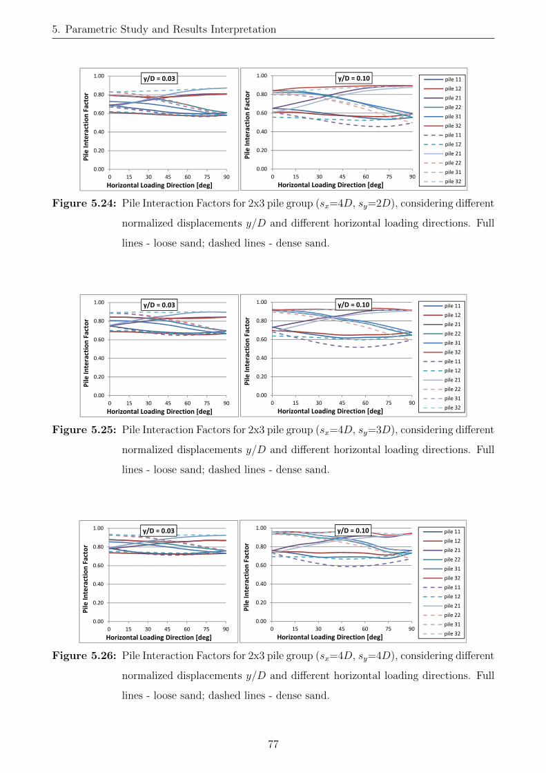
5. Parametric Study and Results Interpretation
y/d=0.03 0 15 30 45 60 75 90
pile 11 0.687661 0.660683 0.638131 0.612681 0.598152 0.594033 0.606231
pile 12 0.611446 0.603407 0.591822 0.582477 0.575461 0.571895 0.579821
pile 21 0.687568 0.709934 0.741582 0.772681 0.797966 0.80841 0.808307
pile 22 0.793113 0.784839 0.76616 0.733333 0.69119 0.641266 0.60636
pile 31 0.727743 0.718129 0.702569 0.674836 0.641551 0.605551 0.580877
pile 32 0.79225 0.782122 0.77688 0.77673 0.785791 0.798444 0.808346
pile 11 0.670064 0.646323 0.622284 0.593771 0.572369 0.566058 0.582655
pile 12 0.617828 0.610947 0.596759 0.588639 0.581816 0.57796 0.585303
pile 21 0.669879 0.705369 0.753289 0.801872 0.838677 0.861624 0.871513
pile 22 0.829105 0.814396 0.785562 0.742874 0.690203 0.629098 0.581835
pile 31 0.795884 0.785834 0.758796 0.716605 0.668254 0.621903 0.589842
pile 32 0.828332 0.835035 0.83955 0.846566 0.855798 0.8654 0.87182
y/d=0.10 0 15 30 45 60 75 90
pile 11 0.651468 0.634369 0.605046 0.575531 0.548928 0.533204 0.553763
pile 12 0.610583 0.608829 0.586787 0.57294 0.565004 0.5639 0.592161
pile 21 0.650971 0.706293 0.76308 0.824681 0.867467 0.887116 0.891965
pile 22 0.839794 0.837284 0.804383 0.757763 0.69218 0.617954 0.555164
pile 31 0.81791 0.821953 0.797107 0.751967 0.699507 0.645509 0.595982
pile 32 0.840188 0.868011 0.877388 0.884803 0.892168 0.896538 0.892725
pile 11 0.609326 0.568138 0.527208 0.485695 0.460004 0.457987 0.493889
pile 12 0.556005 0.54953 0.53689 0.528833 0.522241 0.537277 0.577249
pile 21 0.609005 0.658348 0.72699 0.793021 0.838396 0.861466 0.876542
pile 22 0.822818 0.799118 0.760197 0.707694 0.641763 0.564054 0.496017
pile 31 0.797324 0.788908 0.764335 0.722652 0.67298 0.624577 0.57785
pile 32 0.82413 0.839328 0.852906 0.867881 0.878792 0.881407 0.875512
beta
Loo
se s
and
De
nse
san
d
beta
Loo
se s
and
De
nse
san
d
0.00
0.20
0.40
0.60
0.80
1.00
0 15 30 45 60 75 90
Pile
In
tera
ctio
n F
acto
r
Horizontal Loading Direction [deg]
y/D = 0.03
0.00
0.20
0.40
0.60
0.80
1.00
0 15 30 45 60 75 90
Pile
In
tera
ctio
n F
acto
r
Horizontal Loading Direction [deg]
y/D = 0.10 pile 11
pile 12
pile 21
pile 22
pile 31
pile 32
pile 11
pile 12
pile 21
pile 22
pile 31
pile 32
Figure 5.24: Pile Interaction Factors for 2x3 pile group (sx=4D, sy=2D), considering different
normalized displacements y/D and different horizontal loading directions. Full
lines - loose sand; dashed lines - dense sand.
y/d=0.03 0 15 30 45 60 75 90
pile 11 0.747428 0.719289 0.694245 0.679997 0.672032 0.676627 0.69576
pile 12 0.68829 0.684697 0.675253 0.668295 0.658361 0.655204 0.666844
pile 21 0.748126 0.778602 0.803888 0.827881 0.836886 0.841635 0.842604
pile 22 0.842681 0.840635 0.825716 0.801288 0.760634 0.723881 0.697438
pile 31 0.806625 0.801614 0.783685 0.758904 0.72212 0.689616 0.667561
pile 32 0.84397 0.840329 0.833216 0.83161 0.82822 0.833124 0.842552
pile 11 0.753239 0.711643 0.677426 0.652359 0.649245 0.661901 0.687659
pile 12 0.699249 0.694402 0.683249 0.671204 0.665979 0.669673 0.686624
pile 21 0.754515 0.796255 0.833764 0.859625 0.886683 0.897981 0.896543
pile 22 0.891846 0.879555 0.857885 0.82169 0.782992 0.735112 0.689923
pile 31 0.885237 0.875866 0.851965 0.80962 0.767588 0.723274 0.686593
pile 32 0.891482 0.895568 0.896374 0.891877 0.898597 0.90059 0.895309
y/d=0.10 0 15 30 45 60 75 90
pile 11 0.732721 0.6812 0.645143 0.617219 0.622117 0.627722 0.648582
pile 12 0.696169 0.684509 0.666868 0.647019 0.650798 0.654657 0.676372
pile 21 0.731202 0.779386 0.825597 0.859158 0.903696 0.916549 0.91233
pile 22 0.913307 0.888393 0.858858 0.812378 0.772742 0.708697 0.648368
pile 31 0.921612 0.90674 0.876702 0.826969 0.791713 0.738223 0.677748
pile 32 0.914879 0.922272 0.924639 0.919034 0.934013 0.931313 0.911953
pile 11 0.681923 0.621161 0.563939 0.525172 0.518109 0.544591 0.594826
pile 12 0.637089 0.631621 0.620756 0.604932 0.596768 0.621063 0.665402
pile 21 0.682197 0.742367 0.801049 0.847318 0.879036 0.896344 0.907385
pile 22 0.895203 0.86973 0.833357 0.791163 0.733853 0.660621 0.594827
pile 31 0.898093 0.889889 0.863067 0.820095 0.770891 0.717981 0.66673
pile 32 0.897393 0.911712 0.917657 0.923065 0.924248 0.918318 0.906721
beta
Loo
se s
and
De
nse
san
d
beta
Loo
se s
and
De
nse
san
d
0.00
0.20
0.40
0.60
0.80
1.00
0 15 30 45 60 75 90
Pile
In
tera
ctio
n F
acto
r
Horizontal Loading Direction [deg]
y/D = 0.03
0.00
0.20
0.40
0.60
0.80
1.00
0 15 30 45 60 75 90
Pile
In
tera
ctio
n F
acto
r
Horizontal Loading Direction [deg]
y/D = 0.10 pile 11
pile 12
pile 21
pile 22
pile 31
pile 32
pile 11
pile 12
pile 21
pile 22
pile 31
pile 32
Figure 5.25: Pile Interaction Factors for 2x3 pile group (sx=4D, sy=3D), considering different
normalized displacements y/D and different horizontal loading directions. Full
lines - loose sand; dashed lines - dense sand.
y/d=0.03 0 15 30 45 60 75 90
pile 11 0.785666 0.754413 0.733327 0.726105 0.727029 0.741864 0.757455
pile 12 0.738514 0.732395 0.727462 0.724875 0.720642 0.724602 0.731399
pile 21 0.781481 0.802069 0.823646 0.845584 0.857832 0.871072 0.869141
pile 22 0.87845 0.869162 0.852732 0.833641 0.805775 0.784094 0.758558
pile 31 0.856288 0.845113 0.825653 0.801818 0.773421 0.752624 0.731476
pile 32 0.87884 0.870085 0.862274 0.860092 0.860036 0.869841 0.869238
pile 11 0.795707 0.75524 0.72628 0.712909 0.716072 0.732184 0.761888
pile 12 0.751301 0.747343 0.7428 0.736477 0.734606 0.741845 0.761666
pile 21 0.791316 0.826794 0.861969 0.888214 0.908245 0.919468 0.924892
pile 22 0.926446 0.914495 0.897503 0.870321 0.838258 0.799356 0.763521
pile 31 0.934196 0.924333 0.903451 0.869288 0.830916 0.79347 0.761994
pile 32 0.927185 0.928271 0.928128 0.927121 0.928465 0.9279 0.925434
y/d=0.10 0 15 30 45 60 75 90
pile 11 0.762617 0.727129 0.689137 0.690316 0.690137 0.675812 0.732116
pile 12 0.739439 0.745918 0.733131 0.738083 0.731406 0.711783 0.761139
pile 21 0.75736 0.81555 0.848823 0.895683 0.919423 0.903432 0.943505
pile 22 0.938325 0.931624 0.897631 0.875878 0.824103 0.744494 0.73235
pile 31 0.960404 0.958944 0.922682 0.894947 0.847671 0.776207 0.760094
pile 32 0.938283 0.956621 0.950333 0.963931 0.958179 0.924005 0.942708
pile 11 0.732017 0.669886 0.61983 0.588385 0.593646 0.623974 0.671963
pile 12 0.693342 0.691995 0.684586 0.668886 0.673402 0.699856 0.737454
pile 21 0.728807 0.784358 0.833133 0.870415 0.896639 0.915322 0.931424
pile 22 0.940494 0.916723 0.886875 0.847901 0.795171 0.731219 0.673737
pile 31 0.962441 0.950734 0.923294 0.882444 0.833414 0.782924 0.738159
pile 32 0.940731 0.950426 0.955582 0.956751 0.950949 0.941396 0.92855
beta
Loo
se s
and
De
nse
san
d
beta
Loo
se s
and
De
nse
san
d
0.00
0.20
0.40
0.60
0.80
1.00
0 15 30 45 60 75 90
Pile
In
tera
ctio
n F
acto
r
Horizontal Loading Direction [deg]
y/D = 0.03
0.00
0.20
0.40
0.60
0.80
1.00
0 15 30 45 60 75 90
Pile
In
tera
ctio
n F
acto
r
Horizontal Loading Direction [deg]
y/D = 0.10 pile 11
pile 12
pile 21
pile 22
pile 31
pile 32
pile 11
pile 12
pile 21
pile 22
pile 31
pile 32
Figure 5.26: Pile Interaction Factors for 2x3 pile group (sx=4D, sy=4D), considering different
normalized displacements y/D and different horizontal loading directions. Full
lines - loose sand; dashed lines - dense sand.
77

5. Parametric Study and Results Interpretation
y/d=0.03 0 15 30 45 60 75 90
pile 11 0.800512 0.779809 0.768272 0.768602 0.775673 0.781139 0.799413
pile 12 0.768498 0.765992 0.766734 0.769262 0.769895 0.765649 0.77598
pile 21 0.799838 0.820513 0.841815 0.864066 0.879337 0.880515 0.886745
pile 22 0.896446 0.888135 0.875673 0.861553 0.842965 0.816288 0.799195
pile 31 0.882827 0.875523 0.859019 0.839338 0.817735 0.791864 0.778579
pile 32 0.895389 0.890723 0.88646 0.886559 0.888298 0.882711 0.886223
pile 11 0.813997 0.783583 0.764934 0.76403 0.772992 0.789485 0.815975
pile 12 0.78392 0.781224 0.780769 0.782928 0.784324 0.793778 0.814094
pile 21 0.81301 0.842406 0.871416 0.900207 0.920439 0.93411 0.944537
pile 22 0.942068 0.929611 0.913812 0.894984 0.87099 0.843197 0.815893
pile 31 0.955754 0.9469 0.927269 0.901337 0.869994 0.841174 0.815457
pile 32 0.94255 0.942829 0.942971 0.946982 0.947872 0.946453 0.944052
y/d=0.10 0 15 30 45 60 75 90
pile 11 0.797793 0.758618 0.737288 0.73308 0.729435 0.748363 0.78249
pile 12 0.786483 0.783559 0.782798 0.78235 0.774178 0.78514 0.80954
pile 21 0.795445 0.833556 0.869714 0.900367 0.915813 0.937996 0.958729
pile 22 0.977312 0.955804 0.929072 0.894986 0.844277 0.808986 0.781277
pile 31 0.998021 0.984445 0.957442 0.917692 0.866807 0.833979 0.809004
pile 32 0.974669 0.977373 0.978736 0.976694 0.960688 0.959137 0.956152
pile 11 0.760791 0.711442 0.67134 0.655023 0.667593 0.694012 0.733905
pile 12 0.739632 0.738846 0.733331 0.726279 0.735866 0.756818 0.788956
pile 21 0.759134 0.805809 0.847616 0.883431 0.909801 0.927452 0.945859
pile 22 0.966609 0.944778 0.914131 0.878243 0.833931 0.781625 0.733819
pile 31 0.995104 0.98289 0.954616 0.917347 0.870847 0.82618 0.787462
pile 32 0.966013 0.97221 0.974474 0.975859 0.969551 0.957812 0.945373
beta
Loo
se s
and
De
nse
san
d
beta
Loo
se s
and
De
nse
san
d
0.00
0.20
0.40
0.60
0.80
1.00
0 15 30 45 60 75 90
Pile
In
tera
ctio
n F
acto
r
Horizontal Loading Direction [deg]
y/D = 0.03
0.00
0.20
0.40
0.60
0.80
1.00
0 15 30 45 60 75 90
Pile
In
tera
ctio
n F
acto
r
Horizontal Loading Direction [deg]
y/D = 0.10 pile 11
pile 12
pile 21
pile 22
pile 31
pile 32
pile 11
pile 12
pile 21
pile 22
pile 31
pile 32
Figure 5.27: Pile Interaction Factors for 2x3 pile group (sx=4D, sy=5D), considering different
normalized displacements y/D and different horizontal loading directions. Full
lines - loose sand; dashed lines - dense sand.
y/d=0.03 0 15 30 45 60 75 90
pile 11 0.779579 0.754907 0.73047 0.714535 0.69769 0.693137 0.707731
pile 12 0.721699 0.718064 0.705968 0.69571 0.680369 0.673551 0.682762
pile 21 0.778641 0.805427 0.826775 0.847812 0.854236 0.856002 0.858257
pile 22 0.858247 0.854698 0.838498 0.814042 0.772219 0.733635 0.70868
pile 31 0.820516 0.815679 0.798163 0.774049 0.735403 0.701482 0.68273
pile 32 0.857447 0.85758 0.853372 0.853509 0.847969 0.848953 0.856551
pile 11 0.78939 0.755252 0.7237 0.698892 0.68588 0.687892 0.708154
pile 12 0.746703 0.740201 0.722152 0.704791 0.693857 0.69411 0.707257
pile 21 0.787657 0.821983 0.852834 0.879843 0.901709 0.91445 0.918419
pile 22 0.903333 0.889892 0.866304 0.833562 0.791469 0.746122 0.708649
pile 31 0.899344 0.88986 0.861789 0.820165 0.77535 0.737385 0.708943
pile 32 0.902472 0.911748 0.913102 0.912628 0.914731 0.917115 0.916053
y/d=0.10 0 15 30 45 60 75 90
pile 11 0.77534 0.724384 0.678009 0.652325 0.646942 0.648492 0.670484
pile 12 0.740407 0.71778 0.679945 0.657952 0.659228 0.672336 0.699251
pile 21 0.772874 0.803921 0.828882 0.86348 0.908986 0.934313 0.941174
pile 22 0.933687 0.899918 0.852 0.808162 0.770425 0.720321 0.672298
pile 31 0.936407 0.914016 0.866887 0.819391 0.782411 0.741725 0.69802
pile 32 0.931623 0.934364 0.926207 0.925708 0.939974 0.947516 0.940255
pile 11 0.72313 0.673087 0.625595 0.583608 0.567591 0.579757 0.619762
pile 12 0.685184 0.676716 0.657369 0.637162 0.627596 0.65138 0.689842
pile 21 0.72072 0.772371 0.826546 0.870725 0.90183 0.920267 0.933492
pile 22 0.907879 0.87996 0.842358 0.797063 0.741757 0.678045 0.622323
pile 31 0.909568 0.898085 0.867027 0.822873 0.775803 0.730428 0.689079
pile 32 0.907217 0.924289 0.933365 0.940357 0.943498 0.940588 0.93089
beta
Loo
se s
and
De
nse
san
d
beta
Loo
se s
and
De
nse
san
d
0.00
0.20
0.40
0.60
0.80
1.00
0 15 30 45 60 75 90
Pile
In
tera
ctio
n F
acto
r
Horizontal Loading Direction [deg]
y/D = 0.03
0.00
0.20
0.40
0.60
0.80
1.00
0 15 30 45 60 75 90
Pile
In
tera
ctio
n F
acto
r
Horizontal Loading Direction [deg]
y/D = 0.10 pile 11
pile 12
pile 21
pile 22
pile 31
pile 32
pile 11
pile 12
pile 21
pile 22
pile 31
pile 32
Figure 5.28: Pile Interaction Factors for 2x3 pile group (sx=5D, sy=3D), considering different
normalized displacements y/D and different horizontal loading directions. Full
lines - loose sand; dashed lines - dense sand.
y/d=0.03 0 15 30 45 60 75 90
pile 11 0.813424 0.785894 0.769803 0.763545 0.756306 0.75643 0.769858
pile 12 0.769307 0.762491 0.759126 0.757718 0.747498 0.742273 0.748908
pile 21 0.810958 0.829488 0.852558 0.875042 0.882015 0.880971 0.880673
pile 22 0.889973 0.880349 0.871367 0.858173 0.828336 0.796985 0.77287
pile 31 0.862727 0.852093 0.839998 0.824998 0.797186 0.769869 0.751529
pile 32 0.887126 0.8816 0.881212 0.886147 0.88292 0.879102 0.881011
pile 11 0.833201 0.794996 0.766044 0.748936 0.747568 0.758513 0.783092
pile 12 0.79025 0.784996 0.776221 0.765958 0.761402 0.765497 0.781645
pile 21 0.829592 0.861139 0.890346 0.910352 0.926402 0.934961 0.939612
pile 22 0.938523 0.925273 0.908527 0.882383 0.852095 0.816723 0.785121
pile 31 0.943401 0.931747 0.911603 0.879015 0.843198 0.810204 0.784052
pile 32 0.937141 0.939093 0.941838 0.942788 0.943297 0.942633 0.940445
y/d=0.10 0 15 30 45 60 75 90
pile 11 0.809667 0.777288 0.737681 0.70543 0.699484 0.722238 0.755527
pile 12 0.786115 0.786449 0.766168 0.736803 0.729577 0.753246 0.783127
pile 21 0.807201 0.857093 0.884972 0.894566 0.915077 0.94912 0.967625
pile 22 0.959308 0.948793 0.91255 0.860869 0.81913 0.792714 0.760324
pile 31 0.972015 0.966967 0.933148 0.879314 0.838799 0.817207 0.786109
pile 32 0.954292 0.97162 0.967806 0.950141 0.948895 0.966339 0.966843
pile 11 0.776111 0.71982 0.668304 0.631076 0.629736 0.65622 0.699592
pile 12 0.738014 0.734208 0.722932 0.704426 0.70466 0.730744 0.76537
pile 21 0.772884 0.826701 0.87013 0.903022 0.922665 0.938314 0.952004
pile 22 0.9528 0.927327 0.895723 0.860571 0.814033 0.760107 0.701099
pile 31 0.966607 0.954943 0.930559 0.894745 0.851387 0.809091 0.76947
pile 32 0.949632 0.959845 0.964508 0.969867 0.967165 0.960088 0.949864
beta
Loo
se s
and
De
nse
san
d
beta
Loo
se s
and
De
nse
san
d
0.00
0.20
0.40
0.60
0.80
1.00
0 15 30 45 60 75 90
Pile
In
tera
ctio
n F
acto
r
Horizontal Loading Direction [deg]
y/D = 0.03
0.00
0.20
0.40
0.60
0.80
1.00
0 15 30 45 60 75 90
Pile
In
tera
ctio
n F
acto
r
Horizontal Loading Direction [deg]
y/D = 0.10 pile 11
pile 12
pile 21
pile 22
pile 31
pile 32
pile 11
pile 12
pile 21
pile 22
pile 31
pile 32
Figure 5.29: Pile Interaction Factors for 2x3 pile group (sx=5D, sy=4D), considering different
normalized displacements y/D and different horizontal loading directions. Full
lines - loose sand; dashed lines - dense sand.
78

5. Parametric Study and Results Interpretation
y/d=0.03 0 15 30 45 60 75 90
pile 11 0.836257 0.811908 0.796906 0.793128 0.803574 0.804346 0.816244
pile 12 0.804419 0.797588 0.792149 0.790942 0.796535 0.790895 0.796585
pile 21 0.838602 0.853554 0.86923 0.885863 0.906713 0.902963 0.901367
pile 22 0.910864 0.900144 0.887204 0.874195 0.865638 0.837741 0.815924
pile 31 0.894917 0.885 0.870142 0.853803 0.84133 0.815386 0.798989
pile 32 0.908118 0.903034 0.899903 0.902171 0.913473 0.906118 0.902668
pile 11 0.856652 0.826376 0.80437 0.793679 0.796704 0.812066 0.834763
pile 12 0.825062 0.822424 0.816394 0.810762 0.809872 0.818219 0.834086
pile 21 0.85852 0.887868 0.912409 0.930276 0.944359 0.956167 0.958642
pile 22 0.959 0.94858 0.934128 0.913628 0.890474 0.864245 0.834378
pile 31 0.969243 0.962095 0.944838 0.917891 0.88988 0.860918 0.835597
pile 32 0.957437 0.960518 0.962353 0.962306 0.965443 0.968352 0.961791
y/d=0.10 0 15 30 45 60 75 90
pile 11 0.837395 0.803671 0.778411 0.764864 0.735987 0.769661 0.808999
pile 12 0.826576 0.824097 0.814493 0.8042 0.77186 0.80085 0.8336
pile 21 0.83993 0.877714 0.905719 0.925683 0.909834 0.948512 0.974734
pile 22 0.981672 0.965872 0.94015 0.905825 0.840045 0.827894 0.809399
pile 31 0.999418 0.991362 0.966851 0.930715 0.863253 0.850318 0.835247
pile 32 0.977367 0.987193 0.988048 0.984902 0.948004 0.967319 0.97542
pile 11 0.804135 0.756553 0.711822 0.684024 0.690763 0.718261 0.758816
pile 12 0.781027 0.780265 0.77107 0.755309 0.761229 0.786221 0.817854
pile 21 0.807237 0.856919 0.896681 0.920689 0.937222 0.949752 0.961275
pile 22 0.975829 0.9543 0.928027 0.898612 0.859527 0.811044 0.759548
pile 31 1.00357 0.992067 0.970019 0.938689 0.897184 0.854674 0.818526
pile 32 0.97369 0.980824 0.98425 0.987913 0.984655 0.977181 0.965194
beta
Loo
se s
and
De
nse
san
d
beta
Loo
se s
and
De
nse
san
d
0.00
0.20
0.40
0.60
0.80
1.00
0 15 30 45 60 75 90
Pile
In
tera
ctio
n F
acto
r
Horizontal Loading Direction [deg]
y/D = 0.03
0.00
0.20
0.40
0.60
0.80
1.00
0 15 30 45 60 75 90
Pile
In
tera
ctio
n F
acto
r
Horizontal Loading Direction [deg]
y/D = 0.10 pile 11
pile 12
pile 21
pile 22
pile 31
pile 32
pile 11
pile 12
pile 21
pile 22
pile 31
pile 32
Figure 5.30: Pile Interaction Factors for 2x3 pile group (sx=5D, sy=5D), considering different
normalized displacements y/D and different horizontal loading directions. Full
lines - loose sand; dashed lines - dense sand.
y/d=0.03 0 15 30 45
pile 11 1066.134 1050.449 1037.18 1030.552
pile 12 1068.577 1096.467 1112.336 1115.816
pile 21 1091.197 1109.932 1117.632 1114.141
pile 22 1091.9 1083.042 1070.541 1059.976
pile 11 1354.062 1338.246 1317.88 1308.461
pile 12 1358.309 1401.31 1423.194 1436.575
pile 21 1406.657 1428.172 1433.399 1427.786
pile 22 1406.723 1407.823 1400.484 1399.336
y/d=0.10 0 15 30 45
pile 11 3557.264 3505.619 3461.946 3440.087
pile 12 3565.565 3657.656 3709.487 3719.904
pile 21 3633.84 3697.443 3724.419 3714.163
pile 22 3636.86 3606.756 3564.741 3529.437
pile 11 4515.934 4463.794 4396.288 4365.041
pile 12 4530.172 4672.902 4745.119 4788.917
pile 21 4686.477 4758.993 4777.321 4759.561
pile 22 4687.016 4690.268 4665.562 4661.676
beta
beta
Loo
se s
and
De
nse
san
dLo
ose
san
dD
en
se s
and
0
200
400
600
800
1,000
1,200
1,400
1,600
0 15 30 45
Mm
ax [
kNm
]
Horizontal Loading Direction [deg]
y/D = 0.03
0
1,000
2,000
3,000
4,000
5,000
6,000
0 15 30 45
Mm
ax [
kNm
]
Horizontal Loading Direction [deg]
y/D = 0.10 pile 11
pile 12
pile 21
pile 22
pile 11
pile 12
pile 21
pile 22
Figure 5.31: Maximum Bending Moments for 2x2 pile group (sx=2D, sy=2D), considering
different normalized displacements y/D and different horizontal loading direc-
tions. Full lines - loose sand; dashed lines - dense sand.y/d=0.03 0 15 30 45 60 75 90
pile 11 1121.719 1105.675 1085.048 1084.496 1089.185 1088.358 1104.333
pile 12 1122.149 1136.634 1140.506 1154.537 1154.982 1131.475 1118.064
pile 21 1137.467 1150.503 1148.222 1155.084 1148.319 1120.236 1102.691
pile 22 1138.922 1124.541 1104.565 1105.672 1108.585 1103.164 1117.434
pile 11 1412.924 1389.927 1371.088 1363.229 1369.383 1386.983 1407.468
pile 12 1413.484 1432.49 1449.536 1461.293 1466.541 1462.701 1455.621
pile 21 1454.69 1461.142 1460.967 1454.967 1443.684 1426.854 1405.359
pile 22 1456.135 1448.521 1441.631 1438.724 1440.281 1445.056 1455.67
y/d=0.10 0 15 30 45 60 75 90
pile 11 3742.182 3689.647 3621.56 3620.068 3635.696 3632.593 3685.176
pile 12 3743.505 3790.93 3802.83 3848.514 3848.909 3769.532 3723.95
pile 21 3788.449 3833.066 3826.758 3850.973 3829.718 3737.262 3679.724
pile 22 3793.374 3744.774 3677.774 3681.333 3691.2 3673.566 3721.816
pile 11 4711.852 4635.841 4573.506 4547.553 4568.073 4626.509 4694.343
pile 12 4713.697 4776.391 4832.453 4870.852 4887.503 4873.925 4849.666
pile 21 4846.728 4869.078 4869.437 4850.405 4813.651 4758.334 4687.325
pile 22 4851.552 4825.632 4802.315 4792.485 4797.758 4813.975 4849.85De
nse
san
d
beta
Loo
se s
and
De
nse
san
d
beta
Loo
se s
and
0
200
400
600
800
1,000
1,200
1,400
1,600
0 15 30 45 60 75 90
Mm
ax [
kNm
]
Horizontal Loading Direction [deg]
y/D = 0.03
0
1,000
2,000
3,000
4,000
5,000
6,000
0 15 30 45 60 75 90
Mm
ax [
kNm
]
Horizontal Loading Direction [deg]
y/D = 0.10 pile 11
pile 12
pile 21
pile 22
pile 11
pile 12
pile 21
pile 22
Figure 5.32: Maximum Bending Moments for 2x2 pile group (sx=2D, sy=3D), considering
different normalized displacements y/D and different horizontal loading direc-
tions. Full lines - loose sand; dashed lines - dense sand.
79
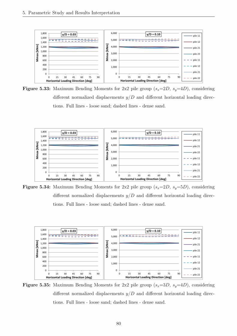
5. Parametric Study and Results Interpretation
y/d=0.03 0 15 30 45 60 75 90
pile 11 1189.1 1161.723 1147.531 1137.926 1135.366 1144.215 1154.634
pile 12 1191.083 1191.994 1201.967 1206.49 1204.819 1201.688 1185.963
pile 21 1210.809 1204.415 1206.594 1200.727 1188.223 1173.022 1152.621
pile 22 1210.927 1184.249 1173.013 1166.526 1167.506 1179.962 1185.407
pile 11 1489.018 1469.343 1452.463 1443.928 1446.395 1457.772 1473.295
pile 12 1491.767 1509.108 1524.04 1535.067 1541.66 1542.8 1539.658
pile 21 1536.857 1538.418 1533.551 1521.5 1505.835 1488.729 1471.529
pile 22 1538.483 1532.775 1528.553 1527.888 1530.251 1534.398 1539.659
y/d=0.10 0 15 30 45 60 75 90
pile 11 3966.627 3876.267 3829.732 3798.176 3789.754 3819.179 3853.297
pile 12 3973.192 3975.175 4007.419 4021.342 4014.637 4003.167 3949.882
pile 21 4033.022 4012.985 4021.639 4003.499 3963.162 3913.669 3846.598
pile 22 4033.522 3943.808 3905.819 3883.95 3887.273 3929.15 3947.935
pile 11 4965.489 4900.658 4844.955 4816.832 4825.128 4862.865 4914.175
pile 12 4974.671 5031.729 5080.665 5116.544 5137.67 5140.701 5129.59
pile 21 5120.749 5126.853 5111.61 5072.441 5021.17 4964.975 4908.298
pile 22 5126.184 5106.552 5092.057 5089.632 5097.525 5111.592 5129.581De
nse
san
d
beta
Loo
se s
and
De
nse
san
d
beta
Loo
se s
and
0
200
400
600
800
1,000
1,200
1,400
1,600
1,800
0 15 30 45 60 75 90
Mm
ax [
kNm
]
Horizontal Loading Direction [deg]
y/D = 0.03
0
1,000
2,000
3,000
4,000
5,000
6,000
0 15 30 45 60 75 90
Mm
ax [
kNm
]
Horizontal Loading Direction [deg]
y/D = 0.10 pile 11
pile 12
pile 21
pile 22
pile 11
pile 12
pile 21
pile 22
Figure 5.33: Maximum Bending Moments for 2x2 pile group (sx=2D, sy=4D), considering
different normalized displacements y/D and different horizontal loading direc-
tions. Full lines - loose sand; dashed lines - dense sand.y/d=0.03 0 15 30 45 60 75 90
pile 11 1195.673 1182.645 1170.95 1163.161 1161.698 1168.094 1180.769
pile 12 1197.087 1210.635 1221.262 1227.497 1229.233 1226.394 1220.254
pile 21 1218.544 1224.734 1225.97 1220.763 1210.581 1196.927 1182.239
pile 22 1220.653 1213.376 1206.073 1202.524 1204.813 1211.983 1220.904
pile 11 1501.136 1487.181 1475.583 1471.283 1474.116 1486.012 1500.244
pile 12 1505.713 1519.005 1531.36 1543.125 1551.974 1558.131 1559.98
pile 21 1546.141 1547.074 1544.093 1536.169 1524.346 1512.921 1501.389
pile 22 1552.758 1550.497 1549.629 1551.698 1554.674 1557.885 1561.198
y/d=0.10 0 15 30 45 60 75 90
pile 11 3988.233 3945.744 3907.778 3882.351 3877.661 3898.801 3940.521
pile 12 3993.132 4037.226 4071.459 4091.015 4095.619 4085.095 4063.765
pile 21 4059.022 4080.954 4086.475 4070.526 4037.904 3993.529 3945.448
pile 22 4066.429 4041.303 4016.317 4004.109 4011.655 4035.77 4066.007
pile 11 5005.754 4960.015 4921.947 4907.98 4917.538 4957.044 5004.087
pile 12 5021.059 5064.55 5104.841 5143.141 5171.763 5191.513 5197.055
pile 21 5151.798 5155.825 5146.881 5121.464 5082.991 5045.717 5007.907
pile 22 5174.125 5165.994 5162.663 5169.312 5179.19 5190.057 5201.463De
nse
san
d
beta
Loo
se s
and
De
nse
san
d
beta
Loo
se s
and
0
200
400
600
800
1,000
1,200
1,400
1,600
1,800
0 15 30 45 60 75 90
Mm
ax [
kNm
]
Horizontal Loading Direction [deg]
y/D = 0.03
0
1,000
2,000
3,000
4,000
5,000
6,000
0 15 30 45 60 75 90
Mm
ax [
kNm
]
Horizontal Loading Direction [deg]
y/D = 0.10 pile 11
pile 12
pile 21
pile 22
pile 11
pile 12
pile 21
pile 22
Figure 5.34: Maximum Bending Moments for 2x2 pile group (sx=2D, sy=5D), considering
different normalized displacements y/D and different horizontal loading direc-
tions. Full lines - loose sand; dashed lines - dense sand.y/d=0.03 0 15 30 45 60 75 90
pile 11 1205.287 1191.631 1179.792 1173.833 1176.405 1187.452 1200.749
pile 12 1202.545 1217.52 1229.63 1236.948 1237.331 1230.925 1218.425
pile 21 1220.053 1231.06 1236.802 1236.615 1229.6 1218.05 1203.469
pile 22 1217.572 1207.244 1199.276 1196.574 1199.869 1208.971 1219.193
pile 11 1535.651 1517.649 1501.104 1493.5 1498.516 1514.263 1533.504
pile 12 1533.331 1553.075 1568.696 1579.473 1584.313 1583.628 1578.345
pile 21 1576.856 1581.381 1581.591 1577.414 1568.772 1554.774 1536.856
pile 22 1573.411 1570.547 1569.041 1570.262 1572.296 1575.59 1579.23
y/d=0.10 0 15 30 45 60 75 90
pile 11 4020.951 3976.401 3937.612 3918.085 3926.632 3963.069 4006.672
pile 12 4012.084 4060.929 4100.067 4123.082 4122.986 4100.36 4057.604
pile 21 4063.412 4101.358 4121.901 4122.732 4100.76 4063.425 4015.816
pile 22 4055.15 4019.939 3992.882 3983.698 3994.837 4025.656 4060.497
pile 11 5121.406 5062.122 5007.47 4982.364 4999.05 5051.233 5114.814
pile 12 5113.901 5178.963 5230.14 5265.093 5280.241 5277.031 5258.609
pile 21 5253.629 5269.603 5271.308 5258.437 5230.653 5184.922 5125.963
pile 22 5242.109 5231.951 5226.534 5230.455 5237.343 5248.676 5261.39De
nse
san
d
beta
Loo
se s
and
De
nse
san
d
beta
Loo
se s
and
0
200
400
600
800
1,000
1,200
1,400
1,600
1,800
0 15 30 45 60 75 90
Mm
ax [
kNm
]
Horizontal Loading Direction [deg]
y/D = 0.03
0
1,000
2,000
3,000
4,000
5,000
6,000
0 15 30 45 60 75 90
Mm
ax [
kNm
]
Horizontal Loading Direction [deg]
y/D = 0.10 pile 11
pile 12
pile 21
pile 22
pile 11
pile 12
pile 21
pile 22
Figure 5.35: Maximum Bending Moments for 2x2 pile group (sx=3D, sy=4D), considering
different normalized displacements y/D and different horizontal loading direc-
tions. Full lines - loose sand; dashed lines - dense sand.
80

5. Parametric Study and Results Interpretation
y/d=0.03 0 15 30 45 60 75 90
pile 11 1236.432 1225.536 1213.667 1205.48 1206.247 1215.296 1230.569
pile 12 1238.998 1255.844 1268.336 1273.578 1276.654 1274.359 1268.603
pile 21 1253.937 1266.975 1270.287 1267.138 1258.273 1244.793 1231.188
pile 22 1255.281 1252.035 1245.657 1242.782 1247.299 1256.979 1268.524
pile 11 1590.366 1559.443 1545.373 1544.075 1552.482 1555.679 1570.498
pile 12 1597.276 1595.726 1609.924 1628.064 1645.84 1636.759 1637.914
pile 21 1631.725 1618.259 1614.967 1614.147 1609.019 1585.556 1571.894
pile 22 1633.392 1620.298 1622.835 1634.116 1642.839 1637.136 1639.899
y/d=0.10 0 15 30 45 60 75 90
pile 11 4124.703 4089.47 4050.7 4023.849 4026.466 4056.305 4106.529
pile 12 4133.2 4188.296 4228.732 4244.935 4253.944 4245.152 4225.011
pile 21 4176.622 4221.408 4233.899 4224.88 4196.734 4153.037 4108.665
pile 22 4181.081 4169.415 4147.587 4137.745 4152.877 4185.544 4224.728
pile 11 5303.633 5201.327 5154.981 5150.952 5178.997 5189.401 5238.284
pile 12 5326.67 5320.709 5367.129 5426.642 5484.956 5453.829 5456.959
pile 21 5436.714 5392.763 5382.826 5381.154 5365.077 5287.767 5242.953
pile 22 5442.243 5397.966 5406.003 5443.419 5472.557 5453.852 5463.588De
nse
san
d
beta
Loo
se s
and
De
nse
san
d
beta
Loo
se s
and
0
200
400
600
800
1,000
1,200
1,400
1,600
1,800
0 15 30 45 60 75 90
Mm
ax [
kNm
]
Horizontal Loading Direction [deg]
y/D = 0.03
0
1,000
2,000
3,000
4,000
5,000
6,000
0 15 30 45 60 75 90
Mm
ax [
kNm
]
Horizontal Loading Direction [deg]
y/D = 0.10 pile 11
pile 12
pile 21
pile 22
pile 11
pile 12
pile 21
pile 22
Figure 5.36: Maximum Bending Moments for 2x2 pile group (sx=3D, sy=5D), considering
different normalized displacements y/D and different horizontal loading direc-
tions. Full lines - loose sand; dashed lines - dense sand.
y/d=0.03 0 15 30 45 60 75 90
pile 11 1269.992 1252.858 1240.846 1238.849 1245.23 1257.824 1274.035
pile 12 1273.11 1285.68 1298.541 1312.006 1319.483 1319.138 1313.74
pile 21 1308.747 1311.848 1312.902 1312.901 1306.291 1293.046 1278.344
pile 22 1306.875 1295.367 1287.219 1287.703 1294.386 1304.938 1315.959
pile 11 1610.241 1593.064 1578.79 1573.792 1581.086 1597.5 1616.411
pile 12 1618.146 1632.757 1645.995 1658.115 1669.327 1678.167 1683.635
pile 21 1678.931 1676.058 1670.57 1662.078 1651.033 1638.057 1623.529
pile 22 1681.225 1682.27 1684.62 1688.218 1691.078 1693.137 1693.877
y/d=0.10 0 15 30 45 60 75 90
pile 11 4237.983 4182.004 4142.703 4136.337 4157.433 4198.782 4251.78
pile 12 4248.378 4289.082 4330.518 4373.829 4397.145 4394.466 4375.125
pile 21 4358.196 4370.036 4375.245 4377.008 4356.697 4314.107 4266.388
pile 22 4351.857 4312.517 4284.746 4286.152 4308.646 4344.442 4382.167
pile 11 5371.439 5315.029 5267.969 5251.465 5275.558 5329.694 5391.834
pile 12 5397.862 5445.575 5488.504 5527.58 5563.593 5591.756 5608.824
pile 21 5593.127 5584.76 5567.819 5540.913 5505.452 5463.421 5415.995
pile 22 5600.742 5603.437 5610.764 5622.566 5632.237 5639.56 5642.773De
nse
san
d
beta
Loo
se s
and
De
nse
san
d
beta
Loo
se s
and
0
200
400
600
800
1,000
1,200
1,400
1,600
1,800
0 15 30 45 60 75 90
Mm
ax [
kNm
]
Horizontal Loading Direction [deg]
y/D = 0.03
0
1,000
2,000
3,000
4,000
5,000
6,000
0 15 30 45 60 75 90
Mm
ax [
kNm
]
Horizontal Loading Direction [deg]
y/D = 0.10 pile 11
pile 12
pile 21
pile 22
pile 11
pile 12
pile 21
pile 22
Figure 5.37: Maximum Bending Moments for 2x2 pile group (sx=4D, sy=5D), considering
different normalized displacements y/D and different horizontal loading direc-
tions. Full lines - loose sand; dashed lines - dense sand.
y/d=0.03 0 15 30 45 60 75 90
pile 11 1022.968 982.2023 957.8367 945.5058 944.9383 958.8831 982.5255
pile 12 890.5171 880.9263 876.0532 877.8017 875.3218 877.1694 883.8674
pile 21 1026.557 1038.053 1056.434 1064.451 1059.843 1046.297 1033.603
pile 22 1052.121 1058.592 1062.762 1052.802 1033.582 1008.352 980.0407
pile 31 925.8485 914.677 909.2782 901.4495 894.379 886.7863 883.8673
pile 32 1053.142 1021.736 1003.152 989.6708 994.5557 1008.665 1031.247
pile 11 1305.333 1257.676 1213.729 1194.131 1195.48 1214.952 1240.352
pile 12 1131.707 1123.119 1113.195 1111.894 1111.972 1114.999 1118.373
pile 21 1305.829 1326.459 1341.158 1353.282 1351.713 1341.046 1327.156
pile 22 1350.315 1356.002 1342.416 1331.334 1308.291 1277.538 1236.899
pile 31 1208.313 1200.057 1179.41 1164.166 1147.033 1131.681 1119.271
pile 32 1352.603 1333.829 1311.548 1306.314 1307.206 1314.337 1324.629
y/d=0.10 0 15 30 45 60 75 90
pile 11 3414.089 3279.814 3199.502 3159.064 3157.385 3203.906 3281.859
pile 12 2973.145 2941.172 2924.601 2929.8 2920.646 2925.719 2946.779
pile 21 3425.975 3462.675 3522.153 3547.039 3529.917 3483.201 3439.626
pile 22 3502.89 3526.405 3542.399 3511.307 3449.213 3366.814 3273.762
pile 31 3081.656 3044.812 3027.491 3002.304 2979.817 2955.688 2947.156
pile 32 3506.626 3400.539 3337.552 3292.001 3308.143 3355.51 3431.578
pile 11 4354.007 4196.246 4050.577 3985.748 3990.377 4055.047 4139.122
pile 12 3775.511 3746.861 3713.544 3708.77 3708.429 3717.789 3728.23
pile 21 4355.532 4423.291 4470.98 4510.053 4503.546 4466.858 4419.652
pile 22 4498.128 4518.453 4474.644 4439.184 4363.642 4262.264 4127.673
pile 31 4024.893 3997.621 3929.22 3878.977 3822.543 3772.191 3731.504
pile 32 4505.822 4442.263 4367.272 4349.414 4352.318 4376.36 4411.261
De
nse
san
d
beta
Loo
se s
and
De
nse
san
d
beta
Loo
se s
and
0
200
400
600
800
1,000
1,200
1,400
1,600
0 15 30 45 60 75 90
Mm
ax [
kNm
]
Horizontal Loading Direction [deg]
y/D = 0.03
0
500
1,000
1,500
2,000
2,500
3,000
3,500
4,000
4,500
5,000
0 15 30 45 60 75 90
Mm
ax [
kNm
]
Horizontal Loading Direction [deg]
y/D = 0.10 pile 11
pile 12
pile 21
pile 22
pile 31
pile 32
pile 11
pile 12
pile 21
pile 22
pile 31
pile 32
Figure 5.38: Maximum Bending Moments for 2x3 pile group (sx=2D, sy=2D), considering
different normalized displacements y/D and different horizontal loading direc-
tions. Full lines - loose sand; dashed lines - dense sand.
81

5. Parametric Study and Results Interpretation
y/d=0.03 0 15 30 45 60 75 90
pile 11 1086.193 1066.255 1043.926 1029.219 1026.029 1027.321 1049.065
pile 12 971.2811 984.0967 975.5491 964.2014 953.3202 934.5373 935.9887
pile 21 1083.241 1124.917 1136.797 1138.392 1129.21 1098.816 1084.49
pile 22 1106.582 1129.977 1128.948 1116.519 1096.303 1064.354 1050.545
pile 31 998.0371 1010.058 998.1455 982.6274 966.4102 939.88 936.8904
pile 32 1103.57 1107.999 1087.551 1073.462 1071.593 1066.358 1084.445
pile 11 1381.32 1353.116 1322.626 1304.442 1295.639 1310.032 1338.827
pile 12 1245.202 1252.906 1244.791 1233.948 1214.46 1213.132 1218.909
pile 21 1379.576 1425.002 1444.614 1454.496 1435.524 1427.494 1419.728
pile 22 1423.111 1438.617 1430.321 1416.323 1383.11 1359.105 1341.828
pile 31 1302.789 1313.514 1300.031 1280.506 1242.221 1225.2 1219.526
pile 32 1420.668 1434.722 1424.857 1421.742 1403.31 1407.451 1419.041
y/d=0.10 0 15 30 45 60 75 90
pile 11 3624.08 3559.347 3486.292 3438.198 3427.985 3432.171 3504.006
pile 12 3242.153 3284.898 3256.121 3217.718 3180.616 3116.952 3120.71
pile 21 3614.195 3751.475 3789.314 3792.819 3760.496 3657.707 3608.822
pile 22 3685.103 3764.941 3763.653 3724.333 3658.771 3553.829 3508.95
pile 31 3322.202 3362.607 3323.524 3272.67 3219.672 3132.414 3123.703
pile 32 3675.172 3688.302 3619.035 3571.381 3564.929 3547.735 3608.744
pile 11 4606.864 4514.256 4413.631 4353.692 4324.35 4372.521 4468.011
pile 12 4153.63 4179.305 4152.052 4115.513 4050.003 4044.901 4063.405
pile 21 4601.186 4751.33 4815.337 4846.914 4782.407 4754.554 4727.838
pile 22 4741.066 4794.198 4768.073 4722.919 4613.588 4534.734 4478.005
pile 31 4339.434 4375.398 4330.871 4266.379 4139.488 4083.595 4065.47
pile 32 4732.947 4778.698 4744.974 4734.061 4672.438 4686.414 4725.567
De
nse
san
d
beta
Loo
se s
and
De
nse
san
d
beta
Loo
se s
and
0
200
400
600
800
1,000
1,200
1,400
1,600
0 15 30 45 60 75 90
Mm
ax [
kNm
]
Horizontal Loading Direction [deg]
y/D = 0.03
0
1,000
2,000
3,000
4,000
5,000
6,000
0 15 30 45 60 75 90
Mm
ax [
kNm
]
Horizontal Loading Direction [deg]
y/D = 0.10 pile 11
pile 12
pile 21
pile 22
pile 31
pile 32
pile 11
pile 12
pile 21
pile 22
pile 31
pile 32
Figure 5.39: Maximum Bending Moments for 2x3 pile group (sx=2D, sy=3D), considering
different normalized displacements y/D and different horizontal loading direc-
tions. Full lines - loose sand; dashed lines - dense sand.
y/d=0.03 0 15 30 45 60 75 90
pile 11 1147.305 1122.031 1101.979 1086.705 1086.156 1082.794 1095.323
pile 12 1059.062 1048.117 1037.51 1022.484 1015.213 994.6184 994.5396
pile 21 1150.526 1160.121 1169.094 1168.642 1170.686 1143.806 1131.768
pile 22 1165.561 1165.574 1162.89 1150.196 1140.423 1112.081 1095.602
pile 31 1078.1 1067.219 1054.839 1036.826 1026.849 1000.443 995.1013
pile 32 1167.608 1147.134 1133.205 1122.231 1126.925 1118.855 1131.615
pile 11 1441.603 1421.932 1399.871 1385.74 1379.064 1390.282 1405.141
pile 12 1339.246 1337.312 1329.929 1321.491 1307.113 1304.133 1307.614
pile 21 1450.734 1471.71 1488.71 1497.833 1490.661 1485.778 1481.19
pile 22 1481.178 1483.952 1477.249 1463.238 1440.439 1423.355 1405.493
pile 31 1388.724 1386.191 1374.17 1356.489 1330.047 1314.503 1308.177
pile 32 1488.012 1483.509 1479.386 1476.698 1470.555 1472.772 1480.513
y/d=0.10 0 15 30 45 60 75 90
pile 11 3827.486 3745.031 3679.649 3629.758 3628.443 3617.214 3658.416
pile 12 3534.194 3497.723 3462.11 3411.511 3386.542 3316.99 3315.715
pile 21 3838.349 3868.55 3896.577 3893.179 3898.231 3807.143 3765.906
pile 22 3881.977 3884.093 3877.298 3837.068 3806.364 3713.264 3659.379
pile 31 3589.349 3553.562 3512.831 3453.549 3421.227 3334.251 3317.525
pile 32 3888.495 3818.611 3770.894 3733.47 3748.766 3722.039 3765.257
pile 11 4807.75 4743.524 4671.072 4624.725 4602.848 4640.213 4689.304
pile 12 4467.1 4460.659 4435.859 4407.35 4358.881 4348.277 4359.132
pile 21 4838.227 4906.849 4962.139 4991.188 4966.028 4948.694 4932.608
pile 22 4934.843 4945.595 4924.816 4879.637 4805.012 4749.198 4690.471
pile 31 4626.073 4617.834 4578.163 4519.787 4432.332 4381.285 4360.989
pile 32 4957.295 4941.104 4926.451 4916.907 4896.218 4903.78 4930.126
De
nse
san
d
beta
Loo
se s
and
De
nse
san
d
beta
Loo
se s
and
0
200
400
600
800
1,000
1,200
1,400
1,600
0 15 30 45 60 75 90
Mm
ax [
kNm
]
Horizontal Loading Direction [deg]
y/D = 0.03
0
1,000
2,000
3,000
4,000
5,000
6,000
0 15 30 45 60 75 90
Mm
ax [
kNm
]
Horizontal Loading Direction [deg]
y/D = 0.10 pile 11
pile 12
pile 21
pile 22
pile 31
pile 32
pile 11
pile 12
pile 21
pile 22
pile 31
pile 32
Figure 5.40: Maximum Bending Moments for 2x3 pile group (sx=2D, sy=4D), considering
different normalized displacements y/D and different horizontal loading direc-
tions. Full lines - loose sand; dashed lines - dense sand.
y/d=0.03 0 15 30 45 60 75 90
pile 11 1048.231 1026.006 1003.575 993.9256 992.4051 1007.816 1027.954
pile 12 915.5439 922.1706 925.3188 931.8766 933.0698 938.7697 934.7166
pile 21 1050.99 1087.743 1109.402 1118.374 1118.93 1106.501 1071.396
pile 22 1076.565 1106.545 1110.384 1104.36 1080.162 1054.262 1025.56
pile 31 949.65 959.9602 956.1185 952.5278 946.3642 942.9715 933.0012
pile 32 1077.384 1071.134 1049.853 1036.645 1042.758 1058.794 1069.536
pile 11 1334.902 1298.726 1265.522 1240.313 1244.631 1266.849 1305.376
pile 12 1168.649 1166.604 1167.413 1162.881 1170.716 1180.396 1190.852
pile 21 1339.101 1378.991 1403.035 1401.013 1405.124 1400.078 1383.089
pile 22 1391.291 1409.364 1405.698 1381.254 1360.871 1331.345 1301.131
pile 31 1252.368 1261.082 1250.704 1226.811 1213.543 1200.508 1188.732
pile 32 1391.835 1392.42 1383.48 1368.616 1371.346 1377.229 1382.861
y/d=0.10 0 15 30 45 60 75 90
pile 11 3498.917 3426.362 3352.688 3321.115 3316.089 3366.953 3433.054
pile 12 3056.815 3078.832 3088.917 3110.06 3113.062 3130.893 3116.101
pile 21 3508.267 3629.101 3699.419 3727.245 3727.062 3683.78 3565.224
pile 22 3583.779 3685.456 3700.424 3682.571 3604.048 3519.422 3425.212
pile 31 3160.33 3195.024 3182.876 3171.849 3152.468 3142.575 3110.626
pile 32 3586.607 3564.217 3492.379 3447.935 3468.411 3522.47 3559.349
pile 11 4453.133 4333.657 4223.773 4139.858 4154.285 4228.307 4355.725
pile 12 3899.02 3892.163 3894.582 3878.981 3904.416 3935.866 3969.818
pile 21 4467.349 4599.142 4677.944 4669.782 4682.08 4663.969 4606.251
pile 22 4634.19 4695.783 4685.054 4605.108 4538.634 4441.517 4341.596
pile 31 4170.827 4200.095 4165.959 4087.113 4043.67 4001.108 3962.778
pile 32 4635.991 4636.973 4606.505 4556.639 4565.788 4585.812 4605.339
De
nse
san
d
beta
Loo
se s
and
De
nse
san
d
beta
Loo
se s
and
0
200
400
600
800
1,000
1,200
1,400
1,600
0 15 30 45 60 75 90
Mm
ax [
kNm
]
Horizontal Loading Direction [deg]
y/D = 0.03
0
500
1,000
1,500
2,000
2,500
3,000
3,500
4,000
4,500
5,000
0 15 30 45 60 75 90
Mm
ax [
kNm
]
Horizontal Loading Direction [deg]
y/D = 0.10 pile 11
pile 12
pile 21
pile 22
pile 31
pile 32
pile 11
pile 12
pile 21
pile 22
pile 31
pile 32
Figure 5.41: Maximum Bending Moments for 2x3 pile group (sx=3D, sy=2D), considering
different normalized displacements y/D and different horizontal loading direc-
tions. Full lines - loose sand; dashed lines - dense sand.
82
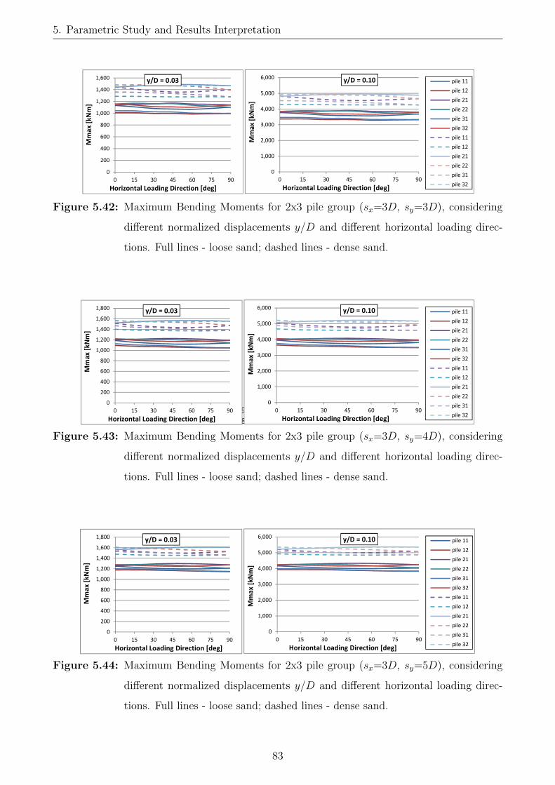
5. Parametric Study and Results Interpretation
y/d=0.03 0 15 30 45 60 75 90
pile 11 1132.63 1109.062 1080.593 1071.975 1067.493 1081.752 1103.717
pile 12 1009.272 1009.486 997.1348 998.459 986.5498 992.1018 997.7525
pile 21 1131.344 1151.555 1158.735 1172.757 1156.844 1151.288 1140.107
pile 22 1155.661 1170.298 1163.081 1162.361 1135.998 1119.591 1101.475
pile 31 1042.107 1040.429 1024.525 1021.609 1002.107 1000.001 996.544
pile 32 1156.279 1138.742 1112.613 1107.756 1102.384 1119.436 1140.571
pile 11 1444.248 1410.648 1379.793 1361.29 1362.815 1380.289 1397.847
pile 12 1287.724 1286.722 1281.624 1278.635 1277.68 1280.654 1278.48
pile 21 1441.643 1459.983 1478.734 1488.259 1486.622 1478.23 1465.858
pile 22 1478.901 1481.504 1479.507 1471.903 1455.401 1431.635 1395.085
pile 31 1360.938 1356.319 1346.518 1334.236 1317.946 1301.926 1277.341
pile 32 1480.965 1474.861 1468.551 1465.12 1463.991 1466.439 1466.522
y/d=0.10 0 15 30 45 60 75 90
pile 11 3779.643 3702.796 3609.206 3581.298 3566.624 3613.856 3686.228
pile 12 3369.38 3370.093 3328.573 3332.311 3291.657 3308.991 3326.52
pile 21 3775.242 3841.034 3863.024 3907.783 3852.854 3832.671 3794.076
pile 22 3847.766 3898.591 3876.733 3876.545 3790.742 3737.654 3678.604
pile 31 3468.289 3463.045 3410.929 3402.167 3338.333 3332.625 3322.465
pile 32 3849.904 3789.974 3701.803 3685.009 3667.012 3724.278 3795.642
pile 11 4817.34 4706.597 4604.702 4543.613 4548.875 4606.883 4664.768
pile 12 4296.086 4292.717 4275.447 4264.976 4261.093 4270.158 4261.973
pile 21 4808.621 4868.448 4929.516 4959.806 4952.963 4923.767 4881.555
pile 22 4926.462 4936.605 4931.535 4907.786 4854.278 4776.356 4655.53
pile 31 4532.757 4517.585 4485.373 4445.099 4391.627 4339.155 4258.176
pile 32 4933.365 4911.932 4890.102 4878.216 4874.38 4882.848 4883.789
De
nse
san
d
beta
Loo
se s
and
De
nse
san
d
beta
Loo
se s
and
0
200
400
600
800
1,000
1,200
1,400
1,600
0 15 30 45 60 75 90
Mm
ax [
kNm
]
Horizontal Loading Direction [deg]
y/D = 0.03
0
1,000
2,000
3,000
4,000
5,000
6,000
0 15 30 45 60 75 90
Mm
ax [
kNm
]
Horizontal Loading Direction [deg]
y/D = 0.10 pile 11
pile 12
pile 21
pile 22
pile 31
pile 32
pile 11
pile 12
pile 21
pile 22
pile 31
pile 32
Figure 5.42: Maximum Bending Moments for 2x3 pile group (sx=3D, sy=3D), considering
different normalized displacements y/D and different horizontal loading direc-
tions. Full lines - loose sand; dashed lines - dense sand.
y/d=0.03 0 15 30 45 60 75 90
pile 11 1185.968 1153.479 1132.678 1119.221 1116.864 1125.25 1140.267
pile 12 1092.583 1076.868 1070.204 1060.85 1051.905 1047.205 1046.897
pile 21 1192.151 1207.157 1220.177 1223.938 1218.274 1205.946 1187.111
pile 22 1214.869 1211.312 1211.664 1202.08 1185.332 1166.014 1142.95
pile 31 1125.653 1103.08 1094.193 1081.275 1066.363 1052.514 1047.055
pile 32 1219.399 1191.696 1177.083 1168.007 1168.672 1176.992 1187.458
pile 11 1511.375 1475.023 1450.366 1435.19 1434.782 1447.172 1470.569
pile 12 1400.622 1384.344 1378.442 1372.426 1369.588 1370.362 1376.502
pile 21 1521.716 1540.247 1556.728 1565.494 1567.041 1563.419 1552.475 0.687817 0.684623 0.682973 0.692176 0.689981 0.686224 0.699664
pile 22 1560.849 1549.947 1544.797 1534.797 1520.932 1502.969 1475.509 0.726518 0.751937 0.777584 0.81316 0.832803 0.840293 0.848782
pile 31 1467.054 1440.007 1432.031 1417.716 1399.756 1381.982 1376.98
pile 32 1568.417 1547.87 1545.356 1545.55 1546.927 1549.766 1551.164
y/d=0.10 0 15 30 45 60 75 90
pile 11 3957.121 3850.653 3782.752 3738.846 3731.385 3759.156 3808.463
pile 12 3647.168 3594.579 3571.973 3540.087 3509.297 3492.453 3490.116
pile 21 3978.184 4026.26 4067.555 4077.964 4057.084 4014.248 3950.106
pile 22 4045.669 4035.9 4039.288 4009.524 3955.708 3893.009 3817.394
pile 31 3747.185 3672.226 3643.208 3601.033 3552.431 3507.515 3490.628
pile 32 4060.307 3966.389 3916.509 3885.571 3887.63 3915.751 3951.536
pile 11 5040.875 4921.04 4839.899 4789.994 4788.906 4830.05 4907.465
pile 12 4672.519 4618.271 4598.345 4577.802 4567.645 4569.366 4588.872
pile 21 5075.848 5136.205 5189.589 5217.221 5220.868 5207.459 5169.91
pile 22 5199.828 5165.017 5149.475 5117.757 5073.038 5014.433 4923.864
pile 31 4886.483 4796.544 4770.414 4723.354 4664.312 4605.99 4590.286
pile 32 5224.685 5155.087 5145.903 5146.104 5150.638 5160.44 5165.812
De
nse
san
d
beta
Loo
se s
and
De
nse
san
d
beta
Loo
se s
and
0
200
400
600
800
1,000
1,200
1,400
1,600
1,800
0 15 30 45 60 75 90
Mm
ax [
kNm
]
Horizontal Loading Direction [deg]
y/D = 0.03
0
1,000
2,000
3,000
4,000
5,000
6,000
0 15 30 45 60 75 90
Mm
ax [
kNm
]
Horizontal Loading Direction [deg]
y/D = 0.10 pile 11
pile 12
pile 21
pile 22
pile 31
pile 32
pile 11
pile 12
pile 21
pile 22
pile 31
pile 32
Figure 5.43: Maximum Bending Moments for 2x3 pile group (sx=3D, sy=4D), considering
different normalized displacements y/D and different horizontal loading direc-
tions. Full lines - loose sand; dashed lines - dense sand.
y/d=0.03 0 15 30 45 60 75 90
pile 11 1248.923 1228.017 1210.544 1199.144 1195.676 1201.632 1214.33
pile 12 1178.254 1178.288 1174.363 1166.773 1157.8 1151.137 1149.034
pile 21 1252.951 1274.224 1290.688 1298.66 1296.855 1287.414 1273.325
pile 22 1273.789 1280.585 1279.596 1269.607 1251.784 1229.952 1208.569
pile 31 1197.852 1194.852 1186.148 1174.162 1162.459 1152.594 1145.826
pile 32 1275.714 1265.17 1254.45 1248.312 1250.503 1260.6 1273.789
pile 11 1563.41 1531.604 1511.055 1499.855 1501.2 1512.202 1526.857
pile 12 1477.314 1464.651 1459.431 1455.116 1454.414 1456.785 1462.266
pile 21 1566.507 1576.568 1592.544 1603.638 1610.053 1611.387 1609.044
pile 22 1606.68 1590.86 1582.327 1569.324 1554.916 1539.981 1524.763
pile 31 1528.238 1514.128 1507.1 1496.799 1484.126 1470.634 1459.686
pile 32 1607.224 1595.85 1597.578 1600.668 1603.789 1606.103 1607.906
y/d=0.10 0 15 30 45 60 75 90
pile 11 4166.788 4099.079 4042.423 4005.517 3994.48 4014.247 4055.891
pile 12 3932.174 3932.252 3918.819 3892.875 3862.074 3838.787 3830.587
pile 21 4180.174 4249.129 4301.939 4326.464 4318.565 4285.502 4237.347
pile 22 4242.297 4267.168 4266.19 4235.15 4177.784 4106.702 4036.651
pile 31 3988.089 3978.381 3949.968 3910.874 3872.929 3841.243 3819.929
pile 32 4248.768 4211.911 4174.83 4153.475 4160.402 4194.224 4238.881
pile 11 5214.2 5109.591 5042.211 5005.633 5010.45 5047.021 5095.337
pile 12 4927.742 4885.493 4867.828 4852.971 4849.983 4857.106 4874.515
pile 21 5224.508 5256.581 5308.28 5343.717 5363.675 5366.914 5358.195
pile 22 5352.78 5301.646 5274.886 5233.191 5186.671 5138.149 5088.349
pile 31 5090.728 5043.886 5020.866 4987.128 4945.636 4901.51 4865.906
pile 32 5354.612 5315.43 5320.197 5329.852 5339.995 5347.858 5354.413
De
nse
san
d
beta
Loo
se s
and
De
nse
san
d
beta
Loo
se s
and
0
200
400
600
800
1,000
1,200
1,400
1,600
1,800
0 15 30 45 60 75 90
Mm
ax [
kNm
]
Horizontal Loading Direction [deg]
y/D = 0.03
0
1,000
2,000
3,000
4,000
5,000
6,000
0 15 30 45 60 75 90
Mm
ax [
kNm
]
Horizontal Loading Direction [deg]
y/D = 0.10 pile 11
pile 12
pile 21
pile 22
pile 31
pile 32
pile 11
pile 12
pile 21
pile 22
pile 31
pile 32
Figure 5.44: Maximum Bending Moments for 2x3 pile group (sx=3D, sy=5D), considering
different normalized displacements y/D and different horizontal loading direc-
tions. Full lines - loose sand; dashed lines - dense sand.
83

5. Parametric Study and Results Interpretation
y/d=0.03 0 15 30 45 60 75 90
pile 11 1100.85 1074.051 1055.146 1038.015 1042.19 1056.645 1078.235
pile 12 971.8668 972.8324 978.6876 972.99 978.3094 983.0788 986.9247
pile 21 1101.936 1128.042 1150.17 1149.952 1149.069 1137.19 1118.237
pile 22 1141.68 1156.113 1163.13 1145.192 1127.345 1102.436 1076.185
pile 31 1009.145 1008.248 1008.006 997.3581 994.2555 991.1142 987.0924
pile 32 1139.01 1117.798 1098.816 1080.924 1084.571 1099.23 1118.857
pile 11 1372.938 1343.217 1311.24 1298.045 1302.418 1321.881 1348.784
pile 12 1209.474 1209.804 1206.042 1211.871 1220.082 1229.081 1237.877
pile 21 1373.512 1401.225 1415.557 1428.673 1433.31 1430.594 1423.964
pile 22 1444.709 1446.875 1434.635 1421.721 1401.794 1376.407 1348.158
pile 31 1314.75 1311.007 1291.956 1276.537 1262.193 1249.416 1238.488
pile 32 1440.403 1434.019 1420.583 1417.306 1415.636 1418.06 1423.836
y/d=0.10 0 15 30 45 60 75 90
pile 11 3675.36 3587.503 3525.193 3468.481 3482.214 3529.651 3600.363
pile 12 3245.056 3248.222 3267.316 3247.559 3264.234 3278.858 3290.272
pile 21 3678.488 3763.929 3835.852 3833.154 3828.24 3786.81 3722.061
pile 22 3799.725 3849.748 3875.326 3817.837 3760.617 3679.667 3593.669
pile 31 3358.778 3355.936 3355.616 3320.906 3311.595 3302.332 3290.227
pile 32 3791.447 3719.363 3655.165 3595.117 3607.407 3656.935 3723.514
pile 11 4580.802 4482.776 4376.86 4333.141 4347.548 4411.838 4500.547
pile 12 4035.641 4036.639 4023.729 4042.543 4069.093 4098.126 4126.397
pile 21 4582.279 4673.437 4719.813 4762.044 4776.026 4765.614 4742.358
pile 22 4811.524 4820.139 4780.924 4739.542 4674.754 4591.62 4498.702
pile 31 4378.661 4366.306 4303.173 4252.495 4205.406 4163.672 4128.173
pile 32 4797.582 4775.251 4729.74 4718.47 4712.957 4721.488 4741.561
De
nse
san
d
beta
Loo
se s
and
De
nse
san
d
beta
Loo
se s
and
0
200
400
600
800
1,000
1,200
1,400
1,600
0 15 30 45 60 75 90
Mm
ax [
kNm
]
Horizontal Loading Direction [deg]
y/D = 0.03
0
1,000
2,000
3,000
4,000
5,000
6,000
0 15 30 45 60 75 90
Mm
ax [
kNm
]
Horizontal Loading Direction [deg]
y/D = 0.10 pile 11
pile 12
pile 21
pile 22
pile 31
pile 32
pile 11
pile 12
pile 21
pile 22
pile 31
pile 32
Figure 5.45: Maximum Bending Moments for 2x3 pile group (sx=4D, sy=2D), considering
different normalized displacements y/D and different horizontal loading direc-
tions. Full lines - loose sand; dashed lines - dense sand.
y/d=0.03 0 15 30 45 60 75 90
pile 11 1174.493 1145.608 1122.438 1109.126 1108.149 1119.21 1139.424
pile 12 1048.185 1047.062 1046.612 1046.579 1046.997 1047.982 1050.747
pile 21 1175.51 1201.412 1220.223 1227.427 1222.867 1208.992 1189.946
pile 22 1212.89 1225.574 1227.426 1216.639 1194.9 1168.238 1142.562
pile 31 1096.438 1092.924 1085.882 1077.53 1067.691 1059.447 1054.261
pile 32 1214.546 1192.416 1171.538 1158.767 1159.626 1172.296 1191.027
pile 11 1474.505 1443.325 1414.967 1399.265 1402.52 1420.936 1447.534
pile 12 1320.208 1319.277 1318.382 1320.827 1328.128 1337.406 1349.211
pile 21 1472.121 1500.02 1520.944 1533.416 1539.015 1536.839 1532.255
pile 22 1540.925 1540.001 1531.796 1516.907 1498.246 1474.272 1448.015
pile 31 1429.601 1425.603 1415.197 1401.113 1385.585 1369.084 1355.493
pile 32 1544.606 1540.515 1535.082 1530.804 1529.783 1530.532 1534.289
y/d=0.10 0 15 30 45 60 75 90
pile 11 3919.963 3825.374 3749.385 3705.713 3702.569 3738.956 3805.293
pile 12 3499.233 3495.454 3493.558 3492.727 3493.114 3495.18 3503.047
pile 21 3923.359 4007.923 4068.629 4090.561 4073.341 4025.265 3960.278
pile 22 4037.779 4082.064 4090.457 4056.784 3986.514 3899.597 3815.593
pile 31 3649.158 3637.72 3614.889 3588.014 3556.438 3530.35 3514.553
pile 32 4043.458 3968.243 3897.641 3854.572 3857.484 3900.302 3963.829
pile 11 4918.511 4815.781 4722.138 4670.301 4681.24 4742.294 4830.224
pile 12 4404.57 4401.415 4398.12 4405.72 4429.305 4459.326 4497.684
pile 21 4910.58 5002.265 5070.549 5110.607 5127.812 5119.251 5102.904
pile 22 5132.641 5131.052 5105.347 5057.404 4996.817 4918.34 4831.972
pile 31 4761.36 4748.233 4714.002 4667.738 4616.839 4562.816 4518.552
pile 32 5145.106 5130.398 5111.535 5096.889 5093.497 5096.394 5109.688
De
nse
san
d
beta
Loo
se s
and
De
nse
san
d
beta
Loo
se s
and
0
200
400
600
800
1,000
1,200
1,400
1,600
1,800
0 15 30 45 60 75 90
Mm
ax [
kNm
]
Horizontal Loading Direction [deg]
y/D = 0.03
0
1,000
2,000
3,000
4,000
5,000
6,000
0 15 30 45 60 75 90
Mm
ax [
kNm
]
Horizontal Loading Direction [deg]
y/D = 0.10 pile 11
pile 12
pile 21
pile 22
pile 31
pile 32
pile 11
pile 12
pile 21
pile 22
pile 31
pile 32
Figure 5.46: Maximum Bending Moments for 2x3 pile group (sx=4D, sy=3D), considering
different normalized displacements y/D and different horizontal loading direc-
tions. Full lines - loose sand; dashed lines - dense sand.
y/d=0.03 0 15 30 45 60 75 90
pile 11 1224.286 1197.043 1173.894 1158.945 1148.469 1156.134 1182.459
pile 12 1123.973 1122.309 1117.788 1111.777 1102.084 1101.461 1108.973
pile 21 1225.495 1250.644 1268.272 1274.813 1268.264 1257.397 1242.213
pile 22 1259.144 1268.954 1267.542 1254.996 1227.71 1200.367 1185.384
pile 31 1164.468 1161.089 1151.714 1139.829 1126.279 1114.435 1110.003
pile 32 1258.812 1242.735 1225.282 1214.407 1216.459 1227.299 1241.839
pile 11 1549.075 1517.801 1489.806 1475.385 1476.163 1493.91 1509.237
pile 12 1432.705 1428.519 1423.268 1422.095 1425.23 1441.747 1438.588
pile 21 1555.137 1578.865 1595.713 1603.954 1608.404 1618.534 1606.878
pile 22 1614.449 1606.21 1593.968 1578.476 1563.429 1548.588 1513.873
pile 31 1515.663 1509.786 1500.157 1481.353 1463.836 1454.186 1438.155
pile 32 1609.429 1605.528 1603.26 1595.897 1595.333 1603.758 1605.217
y/d=0.10 0 15 30 45 60 75 90
pile 11 4085.669 3996.74 3921.006 3872.063 3837.42 3862.619 3949.419
pile 12 3752.717 3747.104 3731.555 3710.659 3677.166 3673.663 3697.134
pile 21 4090.183 4171.981 4228.495 4247.992 4223.945 4185.755 4133.55
pile 22 4192.379 4227.288 4224.968 4185.541 4096.833 4007.629 3959.19
pile 31 3876.173 3865.228 3834.645 3795.993 3752.028 3713.899 3700.54
pile 32 4191.284 4135.884 4076.344 4039.271 4045.886 4082.404 4131.843
pile 11 5167.058 5064.18 4971.903 4924.472 4927.26 4986.155 5036.541
pile 12 4780.077 4766.127 4748.325 4743.84 4753.475 4807.532 4795.885
pile 21 5187.836 5265.439 5319.937 5345.684 5358.848 5391.116 5351.038
pile 22 5377.715 5352.008 5312.996 5263.168 5214.713 5166.723 5052.162
pile 31 5048.359 5029.039 4997.46 4935.508 4878.003 4846.818 4794.398
pile 32 5361.108 5346.864 5338.397 5313.345 5311.383 5339.821 5345.451
De
nse
san
d
beta
Loo
se s
and
De
nse
san
d
beta
Loo
se s
and
0
200
400
600
800
1,000
1,200
1,400
1,600
1,800
0 15 30 45 60 75 90
Mm
ax [
kNm
]
Horizontal Loading Direction [deg]
y/D = 0.03
0
1,000
2,000
3,000
4,000
5,000
6,000
0 15 30 45 60 75 90
Mm
ax [
kNm
]
Horizontal Loading Direction [deg]
y/D = 0.10 pile 11
pile 12
pile 21
pile 22
pile 31
pile 32
pile 11
pile 12
pile 21
pile 22
pile 31
pile 32
Figure 5.47: Maximum Bending Moments for 2x3 pile group (sx=4D, sy=4D), considering
different normalized displacements y/D and different horizontal loading direc-
tions. Full lines - loose sand; dashed lines - dense sand.
84
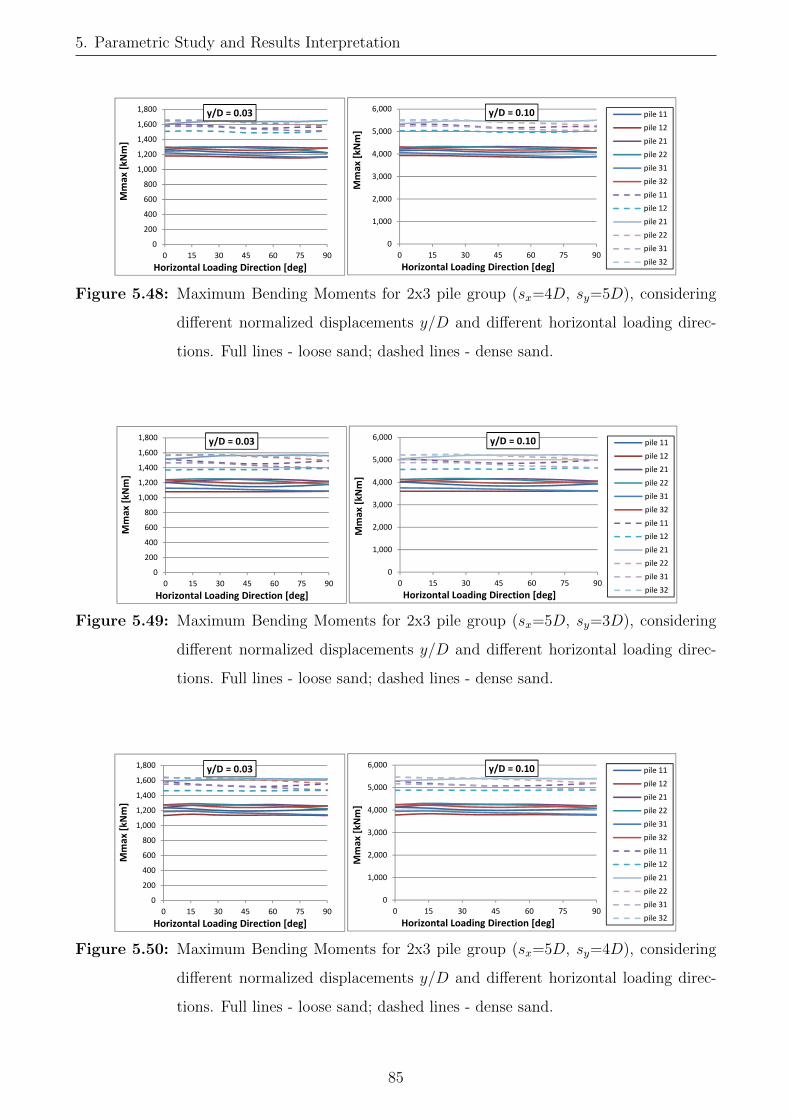
5. Parametric Study and Results Interpretation
y/d=0.03 0 15 30 45 60 75 90
pile 11 1243.813 1249.507 1232.029 1221.951 1221.932 1229.99 1220.925
pile 12 1179.696 1178.029 1170.888 1162.521 1155.839 1153.183 1165.299
pile 21 1266.012 1283.322 1294.955 1299.547 1296.966 1288.858 1284
pile 22 1290.024 1300.059 1298.283 1289.694 1275.631 1259.313 1224.408
pile 31 1220.233 1209.25 1200.215 1188.588 1176.155 1164.775 1167.034
pile 32 1298.225 1274.608 1262.525 1255.533 1257.03 1265.044 1285.362
pile 11 1591.993 1595.144 1575.073 1548.901 1550.891 1562.82 1564.024
pile 12 1507.768 1513.103 1506.973 1489.97 1489.03 1492.422 1514.925
pile 21 1601.963 1629.513 1643.715 1636.684 1639.646 1639.532 1651.737
pile 22 1656.246 1656.227 1650.501 1624.005 1611.506 1596.465 1579.069
pile 31 1574.035 1573.966 1566.111 1542.384 1529.433 1516.049 1515.352
pile 32 1644.032 1644.885 1643.734 1632.384 1633.391 1634.659 1653.157
y/d=0.10 0 15 30 45 60 75 90
pile 11 4151.461 4172.474 4115.737 4083.059 4083.233 4109.641 4078.314
pile 12 3938.597 3932.897 3908.532 3879.702 3856.173 3845.834 3884.602
pile 21 4224.564 4280.179 4316.703 4329.746 4319.019 4290.158 4272.537
pile 22 4295.188 4331.114 4327.832 4301.83 4257.384 4205.06 4090.281
pile 31 4061.443 4024.992 3995.432 3957.595 3917.364 3880.86 3889.937
pile 32 4323.095 4242.488 4200.752 4176.507 4181.143 4208.118 4276.695
pile 11 5311.166 5323.187 5257.387 5170.769 5177.49 5216.809 5219.872
pile 12 5030.958 5048.552 5027.599 4970.102 4965.908 4975.987 5049.683
pile 21 5343.504 5433.691 5479.252 5454.024 5462.214 5460.37 5499.915
pile 22 5517.05 5518.897 5501.852 5415.557 5375.769 5327.23 5270.454
pile 31 5242.343 5242.197 5216.398 5137.962 5095.673 5052.104 5050.924
pile 32 5476.763 5478.08 5473.051 5434.438 5437.484 5441.882 5504.195
De
nse
san
d
beta
Loo
se s
and
De
nse
san
d
beta
Loo
se s
and
0
200
400
600
800
1,000
1,200
1,400
1,600
1,800
0 15 30 45 60 75 90
Mm
ax [
kNm
]
Horizontal Loading Direction [deg]
y/D = 0.03
0
1,000
2,000
3,000
4,000
5,000
6,000
0 15 30 45 60 75 90
Mm
ax [
kNm
]
Horizontal Loading Direction [deg]
y/D = 0.10 pile 11
pile 12
pile 21
pile 22
pile 31
pile 32
pile 11
pile 12
pile 21
pile 22
pile 31
pile 32
Figure 5.48: Maximum Bending Moments for 2x3 pile group (sx=4D, sy=5D), considering
different normalized displacements y/D and different horizontal loading direc-
tions. Full lines - loose sand; dashed lines - dense sand.
y/d=0.03 0 15 30 45 60 75 90
pile 11 1205.243 1180.444 1159.967 1148.814 1148.498 1159 1177.654
pile 12 1079.299 1078.72 1079.249 1079.831 1080.353 1082.252 1085.699
pile 21 1203.88 1225.728 1241.461 1247.854 1244.655 1233.465 1217.86
pile 22 1239.829 1249.892 1251.074 1241.389 1222.907 1200.373 1177.919
pile 31 1127.421 1124.629 1118.351 1109.362 1099.351 1091.479 1086.359
pile 32 1239.721 1222.247 1203.578 1191.452 1191.316 1201.764 1217.618
pile 11 1514.86 1491.066 1468.84 1453.468 1455.558 1472.524 1494.819
pile 12 1370.184 1374.958 1377.558 1374.483 1377.396 1388.291 1390.575
pile 21 1514.028 1538.096 1559.302 1563.442 1565.001 1569.959 1561.654
pile 22 1567.648 1572.151 1572.737 1554.64 1537.927 1520.644 1495.133
pile 31 1464.482 1464.732 1460.22 1436.638 1417.836 1408.656 1392.911
pile 32 1563.823 1569.133 1572.484 1561.857 1557.073 1562.351 1557.212
y/d=0.10 0 15 30 45 60 75 90
pile 11 4022.826 3941.787 3874.682 3838.1 3837.05 3871.462 3932.499
pile 12 3603.271 3601.311 3602.664 3603.84 3604.443 3609.528 3619.638
pile 21 4018.247 4089.36 4139.844 4159.081 4146.378 4107.203 4053.609
pile 22 4127.242 4162.706 4168.814 4138.795 4079.397 4006.282 3933.092
pile 31 3752.334 3743.276 3722.975 3693.966 3661.816 3636.982 3621.386
pile 32 4126.983 4067.337 4004.175 3963.349 3963.049 3998.573 4052.613
pile 11 5053.344 4975.207 4901.956 4851.152 4858.13 4914.269 4987.769
pile 12 4571.365 4587.214 4595.544 4584.702 4593.613 4628.973 4635.54
pile 21 5050.536 5129.453 5198.659 5210.913 5214.599 5229.759 5200.94
pile 22 5221.651 5238.059 5241.578 5182.881 5128.745 5072.552 4988.675
pile 31 4877.361 4878.414 4863.872 4785.999 4724.252 4694.706 4643.332
pile 32 5208.854 5225.554 5236.06 5200.351 5184.515 5202.609 5186.34
De
nse
san
d
beta
Loo
se s
and
De
nse
san
d
beta
Loo
se s
and
0
200
400
600
800
1,000
1,200
1,400
1,600
1,800
0 15 30 45 60 75 90
Mm
ax [
kNm
]
Horizontal Loading Direction [deg]
y/D = 0.03
0
1,000
2,000
3,000
4,000
5,000
6,000
0 15 30 45 60 75 90
Mm
ax [
kNm
]
Horizontal Loading Direction [deg]
y/D = 0.10 pile 11
pile 12
pile 21
pile 22
pile 31
pile 32
pile 11
pile 12
pile 21
pile 22
pile 31
pile 32
Figure 5.49: Maximum Bending Moments for 2x3 pile group (sx=5D, sy=3D), considering
different normalized displacements y/D and different horizontal loading direc-
tions. Full lines - loose sand; dashed lines - dense sand.
y/d=0.03 0 15 30 45 60 75 90
pile 11 1235.83 1222.995 1200.844 1191.925 1196.497 1205.598 1218.443
pile 12 1132.391 1149.66 1139.327 1135.606 1138.723 1137.524 1133.402
pile 21 1237.24 1268.242 1272.591 1275.608 1278.529 1268.341 1257.576
pile 22 1274.718 1290.66 1282.321 1273.01 1263.398 1244.195 1222.266
pile 31 1184.536 1189.489 1175.463 1164.637 1159.158 1148.949 1141.976
pile 32 1274.141 1268.185 1247.679 1238.919 1243.27 1250.113 1262.623
pile 11 1585.39 1553.544 1531.841 1519.384 1522.047 1535.704 1555.705
pile 12 1462.152 1464.931 1462.42 1460.636 1462.247 1467.033 1466.091
pile 21 1588.787 1602.595 1615.69 1621.349 1622.028 1618.729 1619.302
pile 22 1640.185 1631.584 1624.906 1613.452 1598.76 1579.891 1556.332
pile 31 1552.144 1542.921 1533.471 1519.189 1503.013 1487.357 1473.212
pile 32 1639.051 1630.864 1629.085 1626.112 1623.373 1621.264 1622.142
y/d=0.10 0 15 30 45 60 75 90
pile 11 4125.142 4084.223 4011.735 3982.747 3998.071 4027.823 4069.435
pile 12 3780.877 3838.397 3803.483 3790.222 3799.422 3793.985 3778.651
pile 21 4129.659 4231.041 4243.34 4251.102 4258.61 4222.635 4185.09
pile 22 4243.391 4298.745 4273.395 4244.874 4215.248 4153.384 4082.019
pile 31 3942.529 3959.322 3913.234 3878.155 3861.166 3828.597 3806.896
pile 32 4241.938 4220.475 4150.971 4121.165 4135.647 4159.019 4201.828
pile 11 5288.889 5184.069 5112.681 5071.668 5080.57 5125.64 5191.403
pile 12 4878.455 4887.669 4878.94 4872.345 4876.826 4891.709 4887.388
pile 21 5300.363 5344.947 5386.953 5404.085 5404.643 5392.083 5392.683
pile 22 5463.244 5436.212 5415.753 5379.415 5332.201 5270.859 5193.57
pile 31 5169.413 5138.87 5107.858 5060.992 5008.013 4956.907 4910.904
pile 32 5459.844 5431.355 5424.559 5414.171 5404.989 5398.331 5402.03
De
nse
san
d
beta
Loo
se s
and
De
nse
san
d
beta
Loo
se s
and
0
200
400
600
800
1,000
1,200
1,400
1,600
1,800
0 15 30 45 60 75 90
Mm
ax [
kNm
]
Horizontal Loading Direction [deg]
y/D = 0.03
0
1,000
2,000
3,000
4,000
5,000
6,000
0 15 30 45 60 75 90
Mm
ax [
kNm
]
Horizontal Loading Direction [deg]
y/D = 0.10 pile 11
pile 12
pile 21
pile 22
pile 31
pile 32
pile 11
pile 12
pile 21
pile 22
pile 31
pile 32
Figure 5.50: Maximum Bending Moments for 2x3 pile group (sx=5D, sy=4D), considering
different normalized displacements y/D and different horizontal loading direc-
tions. Full lines - loose sand; dashed lines - dense sand.
85
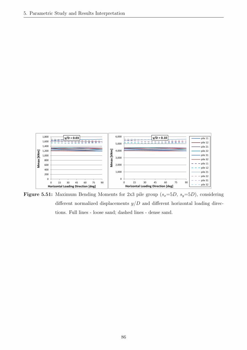
5. Parametric Study and Results Interpretation
y/d=0.03 0 15 30 45 60 75 90
pile 11 1297.488 1275.872 1256.958 1244.981 1243.36 1250.206 1260.922
pile 12 1207.199 1204.786 1199.538 1193.563 1192.968 1194.246 1197.231
pile 21 1294.206 1313.782 1328.061 1335.306 1337.538 1330.963 1317.848
pile 22 1328.712 1334.746 1332.597 1321.606 1305.524 1284.264 1260.286
pile 31 1248.67 1245.872 1238.079 1227.731 1218.024 1207.401 1196.62
pile 32 1321.919 1310.73 1298.329 1291.148 1294.452 1303.315 1312.784
pile 11 1647.096 1624.048 1591.869 1579.157 1580.005 1591.851 1608.944
pile 12 1542.132 1540.036 1527.571 1526.536 1530.694 1537.48 1553.338
pile 21 1644.81 1664.284 1664.959 1674.283 1681.963 1686.299 1696.652
pile 22 1695.46 1689.615 1668.496 1656.841 1643.297 1626.735 1609.584
pile 31 1620.676 1617.735 1599.896 1587.992 1574.397 1559.203 1552.098
pile 32 1688.325 1689.955 1681.604 1682.358 1683.579 1683.156 1690.809
y/d=0.10 0 15 30 45 60 75 90
pile 11 4329.721 4259.586 4198.003 4158.986 4153.876 4176.35 4211.113
pile 12 4029.52 4021.412 4003.478 3982.782 3979.729 3982.704 3991.24
pile 21 4318.833 4382.077 4427.472 4449.382 4454.694 4430.904 4385.7
pile 22 4424.134 4446.459 4441.691 4407.47 4356.135 4287.239 4208.854
pile 31 4156.323 4147.262 4121.93 4088.425 4057.33 4023.367 3988.968
pile 32 4401.526 4362.48 4319.845 4295.149 4305.996 4335.974 4368.547
pile 11 5493.829 5418.343 5312.089 5270.327 5273.322 5312.526 5368.788
pile 12 5144.465 5137.405 5095.508 5091.468 5104.535 5126.205 5178.032
pile 21 5486.165 5549.598 5550.228 5579.668 5603.713 5616.802 5650.235
pile 22 5647.954 5630.026 5561.324 5524.19 5480.667 5426.876 5370.824
pile 31 5397.878 5388.299 5329.342 5290.419 5246.053 5196.491 5173.951
pile 32 5624.094 5628.347 5599.661 5601.712 5605.741 5604.71 5630.995
De
nse
san
d
beta
Loo
se s
and
De
nse
san
d
beta
Loo
se s
and
0
200
400
600
800
1,000
1,200
1,400
1,600
1,800
0 15 30 45 60 75 90
Mm
ax [
kNm
]
Horizontal Loading Direction [deg]
y/D = 0.03
0
1,000
2,000
3,000
4,000
5,000
6,000
0 15 30 45 60 75 90
Mm
ax [
kNm
]
Horizontal Loading Direction [deg]
y/D = 0.10 pile 11
pile 12
pile 21
pile 22
pile 31
pile 32
pile 11
pile 12
pile 21
pile 22
pile 31
pile 32
Figure 5.51: Maximum Bending Moments for 2x3 pile group (sx=5D, sy=5D), considering
different normalized displacements y/D and different horizontal loading direc-
tions. Full lines - loose sand; dashed lines - dense sand.
86

6 Discussion
The conducted parametric study served as a basis for improvement of the designmethodology of laterally loaded pile groups. This statement is supported by thefact that there exist considerable discrepancies between interaction factors andbending moments inside the pile group, which confirms the different behaviourof piles inside the group.
The level of interaction between the piles inside the group is higher at higherload levels, as expected. It was shown that interaction factor levels highlydepend on the soil type - they are slightly lower for dense, in comparison withloose sands. These differences are smaller at lower load levels, where less plasticdeformation occurs.
By means of quantification, interaction factors are between 0.6-0.8 for work-ing load levels, and 0.4-0.8 for high load levels. Finally, the interaction factorsincrease with increasing pile spacings, as expected.
The differences in bending moments were observed for different piles insidethe group. However, the influence of loading direction on the bending momentwas relatively small.
The force in some individual piles changes significantly with the loadingdirection, characterized by skewed lines in the interaction factor plots. Thesepiles are therefore more sensitive to the change (or unpredictable) horizontalloading direction. It was observed that the pile location within the group playsthe more significant role than the considered load direction. This aspect ofthe pile behaviour should be analyzed in more detail, in order to identify the”critical” pile positions inside the pile group. The fact that some piles are moresensitive to the change of loading direction can be the governing design factor.
87

6. Discussion
88
7 Conclusions
This dissertation deal with the extensive numerical study on the influence of thearbitrary lateral load direction on the response of piles inside the pile groups.Apriori sensitivity analysis of the considered problem has been done in the firstphase of this research. The main problem parameters have been identified andserved as a basis for numerical model generation and selection of parametricstudy parameters.
Within the thesis, two cutting-edge pile modelling techniques were compared.The full 3D pile model was adopted as a more reliable solution in comparisonwith the embedded beam (EB) model. The obtained results showed that theinterface properties in the EB model formulation in PLAXIS 3D do not influencethe lateral response of the pile group severely. However, when shear forces in thepile become large, plasticity will occur in the surrounding soil elements, outsidethe elastic zone. In other words, pile-soil interaction in lateral directions canonly be controlled by the adjustments of surrounding soil stiffness parameters.
Numerical model of the laterally loaded pile group was proposed and vali-dated against the measured results of laterally loaded single pile and pile row.Fitting techniques for the approximation of shear forces in the pile have beenevaluated.
The capabilities of PLAXIS 3D software to perform multiple numerical sim-ulations have been tested in an automated scripting environment, through thedevelopment of own computer programs. The performances of such a concepthave shown to be acceptable and, in the case of this thesis, completely necessaryfor the solution.
The common approach to the analysis of horizontal loaded pile groups isexpanded with the influence of arbitrary direction of horizontal loading, whichwill gain a better insight into the real behaviour of a pile groups. The presentedresults are improvement of methodology for analysis of pile groups under arbi-trary horizontal loading. The results of this study provide clearer insight intothe pile group mechanisms under lateral loading.
All presented results are to be used with caution when the significant dif-ference from the research assumptions is present. This is especially importantbearing in mind the different pile cap boundary conditions in the real pilegroups. Finally, developed computer programs and scripts presented in thisthesis will serve as a strong starting point for both academia and engineers forfurther studies of geotechnical problems.
89

7. Conclusions
90

8 Future Work
Beside the fact that this research provided significant insight into the pile groupinteractions under arbitrary loading, still many research topics remain open.Based upon the assumptions and restrictions which served as a basis for thepresented study, as well as based on the main conclusions of this work, recom-mendations for further research topics are specified below:
• Analysis of the laterally loaded pile group under arbitrary loading, usingthe Strain Wedge model with arbitrary wedge orientation
• Experimental study of the pile group deformation patterns using moderntechnologies such as PIV and CT
• Study of the influence of concrete nonlinearity and cracking on the lateralresponse of pile group under working loading conditions
• Formulation and verification of the embedded beam model with advancedinterface formulation, that can account for the lateral loading
• Analysis of the interaction effects under arbitrary lateral loading for the pilegroups with irregular pile positions and lengths (e.g. piled raft foundations)
• Analysis of interaction inside the laterally loaded pile group of jacked-inpiles
• Analysis of the influence of soil heterogeneity, especially the influence ofsoft top layer with variable thickness, on the lateral response of pile groups
91

92

Bibliography
[1] Poulos HG. Tall building foundation design. CRC Press, 2017.
[2] Rao SN, Ramakrishna V, Rao MB. “Influence of rigidity on laterally loaded pile groups
in marine clay”. In: Journal of Geotechnical and Geoenvironmental Engineering 124.6
(1998), pp. 542–549.
[3] Randolph M. “Design methods for pile group and piled rafts”. In: Proc. 13th Int. Conf.
on SMFE. Vol. 5. 1994, pp. 61–82.
[4] Burland J, Broms B, De Mello V. “B (1977). Behaviour of foundations and structures”.
In: Proc. 9th Int. Conf. Soil Mech. Found. Engng, Tokyo. Vol. 2, pp. 495–546.
[5] Mandolini A, Viggiani C. “Settlement of piled foundations”. In: Geotechnique 47.4
(1997), pp. 791–816.
[6] Poulos HG, Davis EH. Pile foundation analysis and design. Monograph. 1980.
[7] Papadopoulou MC, Comodromos EM. “On the response prediction of horizontally loaded
fixed-head pile groups in sands”. In: Computers and Geotechnics 37.7-8 (2010), pp. 930–
941.
[8] Lesny K. “Design of Laterally Loaded Piles-Limits of Limit State Design?” In: Geo-Risk
2017: Reliability-Based Design and Code Developments (GSP 283) (2017), pp. 267–276.
[9] Rudolph C, Bienen B, Grabe J. “Effect of variation of the loading direction on the
displacement accumulation of large-diameter piles under cyclic lateral loading in sand”.
In: Canadian geotechnical journal 51.10 (2014), pp. 1196–1206.
[10] Comodromos EM, Pitilakis KD. “Response evaluation for horizontally loaded fixed-head
pile groups using 3-D non-linear analysis”. In: International Journal for Numerical and
Analytical Methods in Geomechanics 29.6 (2005), pp. 597–625.
[11] Eurocode 7: Geotechnical design - Part 1: General rules. 2004.
[12] Ochoa M, W. O’Neill M. “Lateral pile interaction factors in submerged sand”. In: Journal
of Geotechnical Engineering 115.3 (1989), pp. 359–378.
[13] Randolph MF. “The response of flexible piles to lateral loading”. In: Geotechnique 31.2
(1981), pp. 247–259.
93

[14] Fan CC, H. Long J. “A modulus-multiplier approach for non-linear analysis of laterally
loaded pile groups”. In: International journal for numerical and analytical methods in
geomechanics 31.9 (2007), pp. 1117–1145.
[15] Su D, Yan W. “A multidirectional p–y model for lateral sand–pile interactions”. In: Soils
and foundations 53.2 (2013), pp. 199–214.
[16] Mayoral JM, Pestana JM, Seed RB. “Multi-directional cyclic p–y curves for soft clays”.
In: Ocean Engineering 115 (2016), pp. 1–18.
[17] Gu M et al. “Response of 1 x 2 pile group under eccentric lateral loading”. In: Computers
and Geotechnics 57 (2014), pp. 114–121.
[18] Chen S, Kong L, Zhang LM. “Analysis of pile groups subjected to torsional loading”.
In: Computers and Geotechnics 71 (2016), pp. 115–123.
[19] Georgiadis K, Sloan S, Lyamin A. “Ultimate lateral pressure of two side-by-side piles in
clay”. In: Geotechnique 63.9 (2013), pp. 733–745. doi: 10.1680/geot.12.P.030.
[20] Su D, Zhou YG. “Effect of Loading Direction on the Response of Laterally Loaded Pile
Groups in Sand”. In: International Journal of Geomechanics (2015). doi: 10.1061/
(ASCE)GM.1943-5622.0000544.
[21] Kotthaus M. “Zum Tragverhalten von horizontal belasteten Pfahlreihen aus langen
Pfahlen in Sand”. PhD thesis. Lehrstuhl fur Grundbau und Bodenmechanik, Ruhr-
Universitat Bochum, 1992.
[22] VAN IMPE W. “Foreword: Belgian geotechnics’ experts research on screw piles”. In:
BELGIAN SCREW PILE TECHNOLOGY DESIGN AND RECENT DEVELOPMENTS
(2003).
[23] Broms BB. “Lateral resistance of piles in cohesive soils”. In: Journal of the Soil Mechan-
ics and Foundations Division 90.2 (1964), pp. 27–64.
[24] Broms BB. “Lateral resistance of piles in cohesionless soils”. In: Journal of the Soil
Mechanics and Foundations Division 90.3 (1964), pp. 123–158.
[25] Brinkgreve R et al. “PLAXIS 3D AE”. In: User manual, Plaxis bv (2015).
[26] Winkler E. Die Lehre von der Elasticitaet und Festigkeit mit besonderer Rucksicht auf
ihre Anwendung in der Technik. 1867.
[27] Hetenyi M. “Beams on Elastic Foundation, University of Michigan”. In: Ann Arbor
(1946).
94

[28] Terzaghi K. “Evalution of conefficients of subgrade reaction”. In: Geotechnique 5.4
(1955), pp. 297–326.
[29] Subsoil - Verification of the safety of earthworks and foundations - Supplementary rules
to DIN EN 1997-1. DIN, 2010.
[30] Bored cast-in-place piles: Formation, design and bearing capacity. DIN, 1990.
[31] Geotechnik APDG fur. EA-Pfahle: Empfehlungen des Arbeitskreises” Pfahle”. Ernst,
2012.
[32] Tragverhalten von Pfahlgruppen unter Horizontal Belastung, author=Kluber, E, year=1988,
publisher=Institut fur Grundbau, Boden- und Felsmechanik, TH Darmstadt.
[33] Norris G. “Theoretically based BEF laterally loaded pile analysis”. In: Proceedings of the
3rd International Conference on Numerical Methods in Offshore Piling. Navtes. 1986,
pp. 361–386.
[34] Ashour M, Pilling P, Norris G. “Documentation of the strain wedge model program for
analyzing laterally loaded piles and pile groups”. In: Proc., 32nd Engineering Geology
and Geotechnical Engineering Symposium. 1997, pp. 26–28.
[35] Ashour M, Norris G, Pilling P. “Lateral loading of a pile in layered soil using the
strain wedge model”. In: Journal of geotechnical and geoenvironmental engineering 124.4
(1998), pp. 303–315.
[36] Ashour M, Pilling P, Norris G. “Assessment of pile group response under lateral load”.
In: (2001).
[37] Ashour M, Pilling P, Norris G. “Lateral behavior of pile groups in layered soils”. In:
Journal of Geotechnical and Geoenvironmental Engineering 130.6 (2004), pp. 580–592.
[38] McClelland B, Focht J. “Soil modulus for laterally loaded piles. J Soil Mech Found Div”.
In: Proceedings of the American society of civil engineers. Vol. 1. 1958, p. 22.
[39] Matlock H. “Correlations for design of laterally loaded piles in soft clay”. In: Offshore
technology in civil engineering’s hall of fame papers from the early years (1970), pp. 77–
94.
[40] Reese LC, Cox WR, Koop FD. “Analysis of laterally loaded piles in sand”. In: Off-
shore Technology in Civil Engineering Hall of Fame Papers from the Early Years (1974),
pp. 95–105.
95
[41] Dodds AM, Martin GR. Modeling Pile Behavior in Large Pile Groups under Lateral
Loading (Technical Report MCEER-07-0004). Tech. rep. University of Southern Califor-
nia, 2007.
[42] Reese L et al. “LPILE Plus Version 4.0—A Program for the Analysis of Piles and Drilled
Shafts under Lateral Loads; Ensoft”. In: Inc. Austin, Texas (2000).
[43] Reese L et al. “Computer program GROUP version 8.0 technical manual, Ensoft”. In:
Inc., Austin, Texas (2010).
[44] Robertson PK, Davies MP, Campanella RG. “Design of laterally loaded driven piles
using the flat dilatometer”. In: Geotechnical Testing Journal 12.1 (1989), pp. 30–38.
[45] Briaud JL, Smith T, Meyer B. “Laterally loaded piles and the pressuremeter: comparison
of existing methods”. In: Laterally loaded deep foundations: Analysis and performance.
ASTM International, 1984.
[46] Brown DA, Shie CF. “Three dimensional finite element model of laterally loaded piles”.
In: Computers and Geotechnics 10.1 (1990), pp. 59–79.
[47] Brown DA, Shie CF. “Some numerical experiments with a three dimensional finite el-
ement model of a laterally loaded pile”. In: Computers and Geotechnics 12.2 (1991),
pp. 149–162.
[48] Brown DA, Morrison C, Reese LC. “Lateral load behavior of pile group in sand”. In:
Journal of Geotechnical Engineering 114.11 (1988), pp. 1261–1276.
[49] Brown DA et al. Static and dynamic lateral loading of pile groups. TRB Washington,
DC, USA, 2001.
[50] Fayyazi MS, Taiebat M, Finn WL. “Group reduction factors for analysis of laterally
loaded pile groups”. In: Canadian geotechnical journal 51.7 (2014), pp. 758–769.
[51] Basile F. “Analysis and design of pile groups”. In: Numerical analysis and modelling in
geomechanics (2003), pp. 278–315.
[52] Briaud JL. Geotechnical Engineering: unsaturated and saturated soils. John Wiley &
Sons, 2013.
[53] Smith M. ABAQUS/Standard User’s Manual, Version 6.9. English. United States: Das-
sault Systemes Simulia Corp, 2009.
[54] CSI. ETABS. Version 18.
[55] Ansys. Ansys.
96
[56] SOFiSTiK. SOFiSTiK. Version 2020.
[57] Poulos HG. “Behavior of laterally loaded piles I. single piles”. In: Journal of Soil Me-
chanics & Foundations Div (1971).
[58] Poulos HG. “Behavior of laterally loaded piles II. Pile groups”. In: Journal of Soil
Mechanics & Foundations Div (1971).
[59] Banerjee PK, Driscoll RM. “Three-dimensional analysis of vertical pile groups”. In: ha
Proceedings, Second International Conference on Numerical Methods in Geomechanics,
held at Virginia Polytechnic, Blacksburg, Virginia in June. 1976, pp. 438–450.
[60] Pecker A, Pender M, et al. “Earthquake resistant design of foundations: new construc-
tion”. In: ISRM International Symposium. International Society for Rock Mechanics and
Rock Engineering. 2000.
[61] Brown DA, Shie CF. “Three dimensional finite element model of laterally loaded piles”.
In: Computers and Geotechnics 10.1 (1990), pp. 59–79.
[62] Brown DA, Shie CF. “Numerical experiments into group effects on the response of piles
to lateral loading”. In: Computers and Geotechnics 10.3 (1990), pp. 211–230.
[63] Mises Rv. “Mechanik der festen Korper im plastisch-deformablen Zustand”. In: Nachrichten
von der Gesellschaft der Wissenschaften zu Gottingen, Mathematisch-Physikalische Klasse
1913 (1913), pp. 582–592.
[64] Drucker DC, Prager W. “Soil mechanics and plastic analysis or limit design”. In: Quar-
terly of Applied Mathematics 10.2 (1952), pp. 157–165.
[65] Wakai A, Gose S, Ugai K. “3-D elasto-plastic finite element analyses of pile foundations
subjected to lateral loading”. In: Soils and Foundations 39.1 (1999), pp. 97–111.
[66] Yang Z, Jeremic B. “Numerical study of group effects for pile groups in sands”. In:
International Journal for Numerical and Analytical Methods in Geomechanics 27.15
(2003), pp. 1255–1276.
[67] Comodromos E, Papadopoulou M. “Response evaluation of horizontally loaded pile
groups in clayey soils”. In: Geotechnique 62.4 (2012), p. 329.
[68] Papadopoulou MC, Comodromos EM. “Explicit extension of the p–y method to pile
groups in sandy soils”. In: Acta Geotechnica 9.3 (2014), pp. 485–497.
[69] Comodromos EM, Papadopoulou MC. “Explicit extension of the p–y method to pile
groups in cohesive soils”. In: Computers and Geotechnics 47 (2013), pp. 28–41.
97

[70] Brown DA, Reese LC, O’Neill MW. “Cyclic lateral loading of a large-scale pile group”.
In: Journal of Geotechnical Engineering 113.11 (1987), pp. 1326–1343.
[71] Christensen DS. “Full Scale Static Lateral Load Test of a 9 Pile Group in Sand”. In:
(2006).
[72] Huang AB et al. “Effects of construction on laterally loaded pile groups”. In: Journal of
geotechnical and geoenvironmental engineering 127.5 (2001), pp. 385–397.
[73] Ilyas T et al. “Centrifuge Model Study of Laterally Loaded Pile Groups in Clay”. In:
Journal of Geotechnical and Geoenvironmental Engineering 130.3 (2004), pp. 274–283.
doi: 10.1061/(ASCE)1090-0241(2004)130:3(274).
[74] Kotthaus M, Grundhoff T, Jessberger HL. “Single piles and pile rows subjected to static
and dynamic lateral load”. In: International Conference Centrifuge 94. 1994, pp. 497–
502.
[75] McVay M, Casper R, Shang TI. “Lateral response of three-row groups in loose to dense
sands at 3D and 5D pile spacing”. In: Journal of Geotechnical Engineering 121.5 (1995),
pp. 436–441.
[76] Morrison CS, Reese LC, et al. “A lateral-load test of a full-scale pile group in sand”. In:
(1988).
[77] Rollins KM, Peterson KT, Weaver TJ. “Lateral load behavior of full-scale pile group
in clay”. In: Journal of geotechnical and geoenvironmental engineering 124.6 (1998),
pp. 468–478.
[78] Rollins KM, Sparks A. “Lateral resistance of full-scale pile cap with gravel backfill”. In:
Journal of Geotechnical and Geoenvironmental Engineering 128.9 (2002), pp. 711–723.
[79] Rollins KM, Lane JD, Gerber TM. “Measured and computed lateral response of a pile
group in sand”. In: Journal of Geotechnical and Geoenvironmental Engineering 131.1
(2005), pp. 103–114.
[80] Rollins KM et al. “Pile spacing effects on lateral pile group behavior: load tests”. In:
Journal of geotechnical and geoenvironmental engineering 132.10 (2006), pp. 1262–1271.
[81] Ruesta PF, Townsend FC. “Evaluation of laterally loaded pile group at Roosevelt
Bridge”. In: Journal of Geotechnical and Geoenvironmental Engineering 123.12 (1997),
pp. 1153–1161.
98
[82] Snyder JL. “Full-Scale Lateral-Load Tests of a 3x5 Pile Group in Soft Clays and Silts”.
In: (2004).
[83] Walsh JM. “Full-scale lateral load test of a 3x5 pile group in sand”. In: (2005).
[84] Ashour M, Ardalan H. “Employment of the p-multiplier in pile-group analysis”. In:
Journal of Bridge Engineering 16.5 (2011), pp. 612–623.
[85] Otani J, Pham KD, Sano J. “Investigation of failure patterns in sand due to laterally
loaded pile using X-ray CT”. In: Soils and Foundations 46.4 (2006), pp. 529–535.
[86] Hajialilue-Bonab M, Azarnya-Shahgoli H, Sojoudi Y. “Soil deformation pattern around
laterally loaded piles”. In: International Journal of Physical Modelling in Geotechnics
11.3 (2011), pp. 116–125.
[87] Hajialilue-Bonab M, Sojoudi Y, Puppala AJ. “Study of strain wedge parameters for
laterally loaded piles”. In: International Journal of Geomechanics 13.2 (2013), pp. 143–
152.
[88] Iai S et al. “Soil-pile interaction under lateral load”. In: Soil-Foundation-Structure In-
teraction. CRC Press, 2010, pp. 117–124.
[89] Morita K et al. “Evaluation of vertical and lateral bearing capacity mechanisms of pile
foundations using X-ray CT”. In: Proceedings of international workshop on recent ad-
vances of deep foundations (IWDPF07), Yokosuka, Japan (eds Y. Kikuchi, M. Kimura,
J. Otani and Y. Morikawa). 2007, pp. 217–223.
[90] Cox WR, Dixon DA, Murphy BS. “Lateral-load tests on 25.4-mm (1-in.) diameter piles
in very soft clay in side-by-side and in-line groups”. In: Laterally loaded deep foundations:
Analysis and performance. ASTM International, 1984.
[91] Reese LC, Van Impe WF. Single piles and pile groups under lateral loading. CRC press,
2010.
[92] Chandrasekaran S, Boominathan A, Dodagoudar G. “Group interaction effects on later-
ally loaded piles in clay”. In: Journal of geotechnical and geoenvironmental engineering
136.4 (2010), pp. 573–582.
[93] McVay M et al. “Centrifuge testing of large laterally loaded pile groups in sands”. In:
Journal of Geotechnical and Geoenvironmental Engineering 124.10 (1998), pp. 1016–
1026.
99
[94] Mokwa RL, Duncan JM. “Laterally loaded pile group effects and py multipliers”. In:
Foundations and ground improvement. ASCE. 2001, pp. 728–742.
[95] Pender M. “Aseismic pile foundation design analysis”. In: Bulletin of the New Zealand
Society for Earthquake Engineering 26.1 (1993), pp. 49–160.
[96] Curras CJ et al. “Lateral loading & seismic response of CIDH pile supported bridge
structures”. In: Foundations and Ground Improvement. ASCE. 2001, pp. 260–275.
[97] Bowles J. Foundation Analysis and Design. McGraw-hill, 1996.
[98] Comodromos EM, Papadopoulou MC, Rentzeperis IK. “Effect of cracking on the re-
sponse of pile test under horizontal loading”. In: Journal of geotechnical and geoenvi-
ronmental engineering 135.9 (2009), pp. 1275–1284.
[99] Mokwa RL, Duncan JM. “Rotational Restraint of Pile Caps during Lateral Loading”.
In: Journal of Geotechnical and Geoenvironmental Engineering 129.9 (2003), pp. 829–
837. doi: 10.1061/(ASCE)1090-0241(2003)129:9(829).
[100] Katzenbach R, Leppla S, Choudhury D. Foundation systems for high-rise structures.
CRC press, 2016.
[101] Reese LC, Van Impe W. F.(2001) Single Piles and Pile Groups Under Lateral Loading.
[102] Das BM. Principles of foundation engineering. Cengage learning, 2015.
[103] Dunnavant TW, O’Neill MW. “Experimental p-y model for submerged, stiff clay”. In:
Journal of Geotechnical Engineering 115.1 (1989), pp. 95–114.
[104] Brown DA, SHIE CF, KUMAR M. “Py curves for laterally loaded piles derived from
three-dimensional finite element model”. In: International symposium on numerical mod-
els in geomechanics. 3 (NUMOG III). 1989, pp. 683–690.
[105] Potts DM et al. Finite element analysis in geotechnical engineering: application. Vol. 2.
Thomas Telford London, 2001.
[106] Comodromos EM. “The contribution of numerical analysis to the response prediction of
pile foundations”. In: Linear and Non-linear Numerical Analysis of Foundations. CRC
Press, 2014, pp. 49–96.
[107] Sastry V, Meyerhof G. “Behaviour of flexible piles under inclined loads”. In: Canadian
Geotechnical Journal 27.1 (1990), pp. 19–28.
[108] Anagnostopoulos C, Georgiadis M. “Interaction of axial and lateral pile responses”. In:
Journal of Geotechnical Engineering 119.4 (1993), pp. 793–798.
100

[109] Karthigeyan S, Ramakrishna V, Rajagopal K. “Numerical investigation of the effect of
vertical load on the lateral response of piles”. In: Journal of Geotechnical and Geoenvi-
ronmental Engineering 133.5 (2007), pp. 512–521.
[110] Hussien MN et al. “Vertical loads effect on the lateral pile group resistance in sand”. In:
Geomechanics and Geoengineering 7.4 (2012), pp. 263–282.
[111] Hussien MN et al. “On the influence of vertical loads on the lateral response of pile
foundation”. In: Computers and Geotechnics 55 (2014), pp. 392–403.
[112] Comodromos EM, Papadopoulou MC, Laloui L. “Contribution to the design method-
ologies of piled raft foundations under combined loadings”. In: Canadian Geotechnical
Journal 53.4 (2015), pp. 559–577.
[113] Hazzar L, Hussien MN, Karray M. “Vertical load effects on the lateral response of piles
in layered media”. In: International Journal of Geomechanics 17.9 (2017), p. 04017078.
[114] Zhao C. “A Contribution to Modelling of Mechanized Tunnel Excavation”. PhD. Thesis.
Ruhr University Bochum, 2018.
[115] Schanz T, Vermeer PA. “Formulation and verification of the Hardening Soil Model”. In:
Beyond 2000 in Computation Geotechnics - 10 Years of PLAXIS. Rotterdam: Balkema,
1999, pp. 1–16.
[116] Sadek M, Shahrour I. “A three dimensional embedded beam element for reinforced
geomaterials”. In: International Journal for Numerical and Analytical Methods in Ge-
omechanics 28.9 (2004), pp. 931–946.
[117] Engin H, Septanika E, Brinkgreve R. “Improved embedded beam elements for the mod-
elling of piles”. In: (2007).
[118] Marjanovic M et al. “Modeling of laterally loaded piles using embedded beam elements”.
English. In: Proceedings of the International Conference ”Contemporary achievements
in Civil Engineering 2016”. Ed. by M Besevic et al. Subotica, Serbia: University of
Novi Sad - Faculty of Civi Enginering Subotica, 2016, pp. 349–358. doi: 10.14415/
konferencijaGFS2016.035.
[119] Dao T. “Validation of PLAXIS Embedded Piles For Lateral Loading Validation of
PLAXIS Embedded Piles For Lateral Loading”. MSc. Thesis. TU Delft, 2011.
101
[120] Turello DF, Pinto F, Sanchez PJ. “Three dimensional elasto-plastic interface for embed-
ded beam elements with interaction surface for the analysis of lateral loading of piles”.
In: International Journal for Numerical and Analytical Methods in Geomechanics 41.6
(2017), pp. 859–879.
[121] Turello DF, Pinto F, Sanchez PJ. “Embedded beam element with interaction surface for
lateral loading of piles”. In: International Journal for Numerical and Analytical Methods
in Geomechanics 40.March 2007 (2016), pp. 568–582. doi: 10.1002/nag. arXiv: nag.
2347 [10.1002].
[122] Ninic J, Ninic J. “Computational strategies for predictions of the soil-structure interac-
tion during mechanized tunneling”. In: June (2015).
[123] Tedesco G. “Offshore tower or platform foundations : numerical analysis of a laterally
loaded single pile or pile group in soft clay and analysis of actions on a jacket structure”.
MSc. Thesis. University of Bologna, 2013.
[124] Zhang Y, Andersen KH, Tedesco G. “Ultimate bearing capacity of laterally loaded piles
in clay – Some practical considerations”. In: Marine Structures 50 (2016), pp. 260–275.
doi: 10.1016/j.marstruc.2016.09.002.
[125] Jaky J. “The coefficient of earth pressure at rest”. In: Journal of the Society of Hungarian
Architects and Engineers (1944), pp. 355–358.
[126] Duncan JM, Evans Jr LT, Ooi PS. “Lateral load analysis of single piles and drilled
shafts”. In: Journal of geotechnical engineering 120.6 (1994), pp. 1018–1033.
[127] Van Rossum G, Drake Jr FL. Python Reference Manual. Centrum voor Wiskunde en
Informatica Amsterdam, 1995.
[128] Hussien MN et al. “Soil–pile separation effect on the performance of a pile group un-
der static and dynamic lateral loads”. In: Canadian Geotechnical Journal 47.11 (2010),
pp. 1234–1246.
[129] Haiderali AE, Madabhushi G. “Evaluation of Curve Fitting Techniques in Deriving p–y
Curves for Laterally Loaded Piles”. In: Geotechnical and Geological Engineering 34.5
(2016). doi: 10.1007/s10706-016-0054-2.
[130] Saltelli A et al. Global sensitivity analysis: the primer. John Wiley & Sons, 2008.
[131] Khaledi K et al. “Robust and reliable metamodels for mechanized tunnel simulations”.
In: Computers and Geotechnics 61 (2014), pp. 1–12. doi: 10.1016/j.compgeo.2014.
04.005.
102

[132] Kennedy J, Eberhart R. “Particle swarm optimization”. In: Neural Networks, 1995.
Proceedings., IEEE International Conference on 4 (1995), 1942–1948 vol.4. doi: 10.
1109/ICNN.1995.488968.
[133] Garnier J et al. “Catalogue of scaling laws and similitude questions in geotechnical
centrifuge modelling”. In: International Journal of Physical Modelling in Geotechnics
7.3 (2007), pp. 01–23.
[134] Kayalar A. “Bettung von horizontal belasteten Pfahlreihen und Bohrpfahlwanden”. In:
(2012).
[135] Hannigan P et al. Design and Construction of Driven Pile Foundations, Federal Highway
Administration, FHWA, Reference Manual-Volume I and II, National Highway Institute.
Tech. rep. NHI-05-042, Courses, 2006.
[136] State Highway AA of, Officials T. AASHTO LRFD Bridge Design Specifications, Cus-
tomary US Units: 2006 Interim Revisions. American Association of State Highway and
Transportation Officials, 2006.
103

104

Biography
Milos Marjanovic was born on January 8th 1986 in Uzice, Re-
public of Serbia, where he finished elementary school and Gym-
nasium. He received the ”Vuk Karadzic” Award during the
elementary school, and the Gymnasium Award for the best
graduation thesis. He completed both BSc. (2005-2009) and
MSc. studies (2009-2010) at the Faculty of Civil Engineering
in Belgrade, Module Structural Engineering. Milos Marjanovic
won the Prize of the Faculty of Civil Engineering in Belgrade
(Academician Prof. Djordje Lazarevic Fund) for the best MSc.
thesis in the field of concrete structures. He won the Prize of
the Regional Chamber of Commerce Uzice for the best students in 2009. He received several
scholarships for achieved success during regular studies.
Milos Marjanovic enrolled the PhD studies at the Faculty of Civil Engineering in Belgrade in
2010. Since December 2010 he has been working at the Faculty of Civil Engineering as a Teach-
ing Assistant in scientific fields: Soil Mechanics and Geotechnics in Transportation Engineering.
Since 2015, Milos Marjanovic participates as the Scholarship Holder in the international PhD
program SEEFORM, in which he stayed for 13 months at Ruhr University Bochum, Chair of
Foundation Engineering, Soil and Rock Mechanics. He also participated in several seminars for
PhD students in Serbia and abroad. He is also engaged as a researcher on the Project of the
Ministry of Education, Science and Technological Development of Serbia N0 TR-36046.
Close field of his scientific research is related to the static and dynamic analysis of soil-
structure interaction using Finite Element Method. He authored and co-authored 4 papers in
peer-reviewed journals and 24 papers in national and international conference proceedings.
He is a member of the Serbian Society for Soil Mechanics and Geotechnical Engineering
and the International Society for Soil Mechanics and Geotechnical Engineering (ISSMGE). He
speaks and writes English and German, and uses Russian with basic knowledge. He is a long-
term member of the Artistic Association of University of Belgrade ”Branko Krsmanovic”. He
is married and lives in Belgrade.
105

106

Appendix - Computer Programs
Main Program - Multiple Simulations Processor
Configuration Constants Main ConfigConstants.py
import os
SimExtension = ’.p3d’
RecordExtension = ’.sav’
DefaultSimDir = os.getcwd() + ’\\Simulations’
DSExtension = ’.dat’
DefaultBlueprint = ’BLUEPRINT’+SimExtension
IconTrue = os.getcwd() + ’\\Config\\Icon_True.png’
IconFalse = os.getcwd() + ’\\Config\\Icon_False.png’
Basic Functions Main Functions.py
import numpy as np
import pickle
import openpyxl as xl
from openpyxl.chart import Series, Reference, ScatterChart
import os
from PyQt5.QtWidgets import QFileDialog, QMessageBox, QDialog, QGridLayout
# FILE/OBJECT OPERATORS ############################################################
def folder_size(path):
total_size = 0
for dirpath, dirnames, filenames in os.walk(path):
for f in filenames:
fp = os.path.join(dirpath, f)
total_size += os.path.getsize(fp)
return total_size
def save_object(obj, path):
107

obj_file = open(path, ’wb’)
pickle.dump(obj, obj_file)
obj_file.close()
def load_object(path):
obj_file = open(path, ’rb’)
obj = pickle.load(obj_file)
obj_file.close()
return obj
# ND ARRAY ##########################################################################
def unique_ndarray(numpy_ndarray):
row_num, col_num = np.shape(numpy_ndarray)
unique_rows = []
duplicate_rows = []
for r_1 in range(0, row_num):
# Search for duplicated rows (all values in both rows are the same!)
if (r_1 in duplicate_rows) is False:
unique_rows.append(r_1)
for r_2 in range(r_1 + 1, row_num):
if list(numpy_ndarray[r_1, :]) == list(numpy_ndarray[r_2, :]):
duplicate_rows.append(r_2)
# If duplicated rows found, reshape ndarray by inserting unique rows from original
table
if len(duplicate_rows) > 0: # Some duplicates are found
new_table = np.ndarray(shape=(len(unique_rows), col_num))
for j, old_row in enumerate(unique_rows):
new_table[j, :] = numpy_ndarray[old_row, :]
else:
new_table = numpy_ndarray
return new_table, len(duplicate_rows)
# Return unique ndarray and number of deleted rows
def link_np_tables(table1, table2):
# Connects two tables, one below the other
len1 = len(table1)
len3 = len1 + len(table2)
108

new_table = np.ndarray(shape=(len3, len(table1[0])))
for r in range(0, len1):
new_table[r, :] = table1[r, :]
for r in range(len1, len3):
new_table[r, :] = table2[r - len1, :]
return new_table # Return linked table
def np_slicer(r_c, filter_list, input_table):
""" This function extracts desired rows or columns from initial numpy array (2D)
and creates new (sliced) array """
rows0, columns0 = np.shape(input_table)
if r_c == ’C’:
new_table = np.zeros((rows0, len(filter_list)))
for c1, c0 in enumerate(filter_list):
new_table[:, c1] = input_table[:, c0]
else:
new_table = np.zeros((len(filter_list), columns0))
for r1, r0 in enumerate(filter_list):
new_table[r1, :] = input_table[r0, :]
return new_table
def vector_nd(x):
new_vector = np.zeros((len(x), 1))
for j, x1 in enumerate(x):
new_vector[j, 0] = x1
return new_vector
# OPENPYXL #########################################################################
def parse_xl_ws_nd(ws, rows, cols):
data_table = np.ndarray(shape=(rows, cols))
for r in range(1, rows + 1):
for c in range(1, cols + 1):
cell_value = ws.cell(row=r, column=c).value
if type(cell_value) == int or type(cell_value) == float:
109
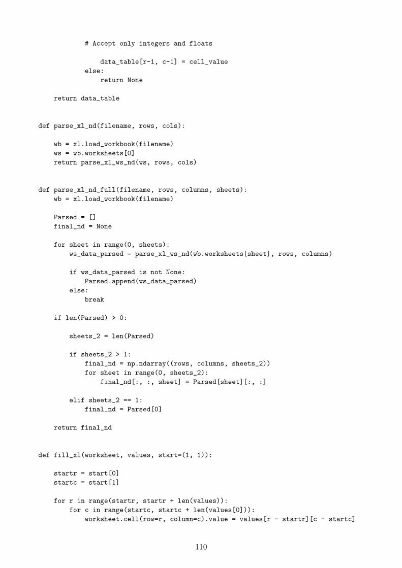
# Accept only integers and floats
data_table[r-1, c-1] = cell_value
else:
return None
return data_table
def parse_xl_nd(filename, rows, cols):
wb = xl.load_workbook(filename)
ws = wb.worksheets[0]
return parse_xl_ws_nd(ws, rows, cols)
def parse_xl_nd_full(filename, rows, columns, sheets):
wb = xl.load_workbook(filename)
Parsed = []
final_nd = None
for sheet in range(0, sheets):
ws_data_parsed = parse_xl_ws_nd(wb.worksheets[sheet], rows, columns)
if ws_data_parsed is not None:
Parsed.append(ws_data_parsed)
else:
break
if len(Parsed) > 0:
sheets_2 = len(Parsed)
if sheets_2 > 1:
final_nd = np.ndarray((rows, columns, sheets_2))
for sheet in range(0, sheets_2):
final_nd[:, :, sheet] = Parsed[sheet][:, :]
elif sheets_2 == 1:
final_nd = Parsed[0]
return final_nd
def fill_xl(worksheet, values, start=(1, 1)):
startr = start[0]
startc = start[1]
for r in range(startr, startr + len(values)):
for c in range(startc, startc + len(values[0])):
worksheet.cell(row=r, column=c).value = values[r - startr][c - startc]
110

def fill_xl_row_col(worksheet, rowcol, vector, start=(1, 1)):
if rowcol == ’R’:
startc = start[1]
for c in range(startc, startc + len(vector)):
worksheet.cell(row=start[0], column=c).value = vector[c - startc]
elif rowcol == ’C’:
startr = start[0]
for r in range(startr, startr + len(vector)):
worksheet.cell(row=r, column=start[1]).value = vector[r - startr]
def fill_xl_with_headers(ws, captions, data, start=(1, 1)):
fill_xl_row_col(ws, ’R’, captions, start) # Fill Header Row
fill_xl(ws, data, (start[0] + 1, start[1])) # Fill the Rest Data
def xl_headers(worksheet, row_title, column_title):
col_he, row_he = (False, False)
if row_title is not None:
row_he = True
if column_title is not None:
col_he = True
if col_he is True and row_he is True:
fill_xl_row_col(worksheet, ’R’, column_title, (1, 2))
fill_xl_row_col(worksheet, ’C’, row_title, (2, 1))
elif col_he is True:
fill_xl_row_col(worksheet, ’R’, column_title, (1, 1))
elif row_he is True:
fill_xl_row_col(worksheet, ’C’, row_title, (1, 1))
def xl_dimensions(shape_tuple):
shape_list = list(shape_tuple)
rows, columns, tabs = (shape_list[0], 1, 1)
if len(shape_list) == 3:
columns = shape_list[1]
tabs = shape_list[2]
elif len(shape_list) == 2:
columns = shape_list[1]
return rows, columns, tabs
111

def measure_xl_3D(fn):
# Calculate Number of Rows, Columns and Sheets based on First Row and Column size
on first sheet
wb = xl.load_workbook(fn)
ws = wb.worksheets[0]
total_sheets = len(wb.worksheets)
r, c = (1, 1)
# Measure Row
search = True
while search is True:
read = ws.cell(row=r, column=1).value
if read is not None:
r += 1
else:
search = False
# Measure Column
search = True
while search is True:
read = ws.cell(row=1, column=c).value
if read is not None:
c += 1
else:
search = False
return r - 1, c - 1, total_sheets
def get_xl_row(ws, start, length):
r_i = start[0]
c_i = start[1]
get_tuple = (ws.cell(row=r_i, column=c_i).value,)
if length > 1:
for c in range(c_i+1, c_i+length):
get_tuple += (ws.cell(row=r_i, column=c).value,)
return get_tuple
def export_nd_xl(row_titles, column_titles, tab_titles, nd_input, row_start=1,
column_start=1):
if column_titles is not None:
row_start = 2
if row_titles is not None:
112
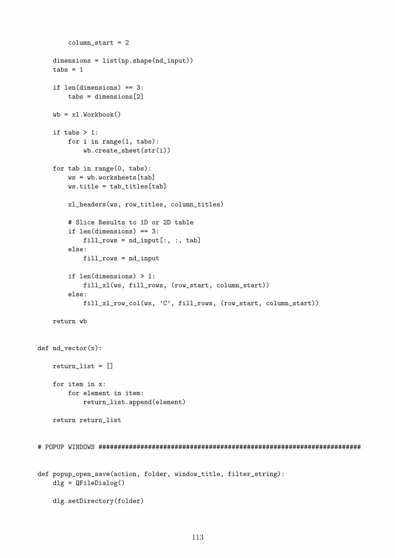
column_start = 2
dimensions = list(np.shape(nd_input))
tabs = 1
if len(dimensions) == 3:
tabs = dimensions[2]
wb = xl.Workbook()
if tabs > 1:
for i in range(1, tabs):
wb.create_sheet(str(i))
for tab in range(0, tabs):
ws = wb.worksheets[tab]
ws.title = tab_titles[tab]
xl_headers(ws, row_titles, column_titles)
# Slice Results to 1D or 2D table
if len(dimensions) == 3:
fill_rows = nd_input[:, :, tab]
else:
fill_rows = nd_input
if len(dimensions) > 1:
fill_xl(ws, fill_rows, (row_start, column_start))
else:
fill_xl_row_col(ws, ’C’, fill_rows, (row_start, column_start))
return wb
def nd_vector(x):
return_list = []
for item in x:
for element in item:
return_list.append(element)
return return_list
# POPUP WINDOWS #####################################################################
def popup_open_save(action, folder, window_title, filter_string):
dlg = QFileDialog()
dlg.setDirectory(folder)
113

if action == ’Save’:
dlg.setFileMode(QFileDialog.AnyFile)
return dlg.getSaveFileName(dlg, window_title, folder, filter_string)[0]
elif action == ’Open’:
dlg.setFileMode(QFileDialog.ExistingFile)
return dlg.getOpenFileName(dlg, window_title, folder, filter_string)[0]
# Selected filename
def popup_open_multiple(folder, window_title, filter_string):
dlg = QFileDialog()
dlg.setDirectory(folder)
dlg.setFileMode(QFileDialog.ExistingFiles)
return dlg.getOpenFileNames(dlg, window_title, folder, filter_string)[0]
def popup_message(message_text, icon, title, buttons):
msg = QMessageBox()
msg.setStandardButtons(buttons)
msg.setIcon(icon)
msg.setText(message_text)
msg.setWindowTitle(title)
return msg.exec_()
def popup_simple_dialog(window_title, widgets_table):
dlg = QDialog()
dlg.setWindowTitle(window_title)
layout = QGridLayout()
dlg.setLayout(layout)
for r in range(0, len(widgets_table)):
for c in range(0, len(widgets_table[0])):
layout.addWidget(widgets_table[r][c], r, c)
dlg.exec_()
def popup_yes_no_dialog(message_text, icon, window_title):
dlg = QMessageBox()
dlg.setIcon(icon)
dlg.setText(message_text)
dlg.setWindowTitle(window_title)
dlg.setStandardButtons(QMessageBox.Ok | QMessageBox.Cancel)
return dlg.exec_()
114

def popup_select_folder(folder):
dlg = QFileDialog()
return dlg.getExistingDirectory(dlg, ’Select Folder’, folder,
QFileDialog.ShowDirsOnly)
# SPECIAL FUNCTIONS (MODULES 2, 3) ##################################################
def all_processed(result_tables):
for table in result_tables:
if table is None:
return False
return True
def set_shapes(np_tables_list):
return_list = []
for res_table in np_tables_list:
if res_table is not None:
return_list.append(np.shape(res_table))
else:
return_list.append(None)
return return_list
def global_shape(shapes_list):
return_value = None
real_shapes = [shape for shape in shapes_list if shape is not None]
# Get shape tuples if they exist
if len(real_shapes) > 0: # There are some real shapes. Check if all are the same
unique_shapes = list(set(real_shapes))
# Remove duplicated shapes. Only one should stay if Consistent
if len(unique_shapes) == 1:
return_value = unique_shapes[0]
return return_value
# MATH/LIST OPERATIONS #############################################################
def norm_extrap_2D(input_matrix, x_range, n_e, limits=(0.1, 0.9)):
115

""" Normalizes or extrapolates 2D numpy array within desired limits and using real
data ranges. Default interpolation range is 0.1-0.9, because we don’t want
normalized values to be close to 0 and 1. Input matrix must be 2D numpy
array """
m, n = np.shape(input_matrix)
x_out = np.zeros((m, n))
for i in range(0, m):
xmin_r = x_range[i, 0]
xmax_r = x_range[i, 1]
delta_x = xmax_r - xmin_r
delta_y = limits[1] - limits[0]
for j in range(0, n):
if n_e == ’N’:
x_out[i, j] = limits[0] + delta_y / delta_x * (input_matrix[i, j]
- xmin_r) # Normalization
else:
x_out[i, j] = xmin_r + delta_x / delta_y * (input_matrix[i, j]
- limits[0]) # Extrapolation
return x_out
def is_number(x):
try:
float(x)
return True
except ValueError:
return False
def remove_duplicates(test_list):
unique_list = []
search_list = test_list
while len(search_list) > 0:
unique_list.append(search_list[0])
new_search_list = []
for j in range(1, len(search_list)):
if search_list[0] != search_list[j]:
new_search_list.append(search_list[j])
search_list = new_search_list[:]
116

return unique_list
def show_notice(label_object, notice_text):
label_object.setText(notice_text)
label_object.repaint()
def xy_series_xl(ws, row_start, col_start, length, series_title, mark_sym,
title_from_data=False):
# Creates excel series from {length x 2} excel block of XY data
x_values = Reference(ws, min_col=col_start, min_row=row_start, max_row=row_start
+ length)
y_values = Reference(ws, min_col=col_start+1, min_row=row_start, max_row=row_start
+ length)
new_series = Series(y_values, x_values, title=series_title,
title_from_data=title_from_data)
new_series.marker.symbol = mark_sym
new_series.graphicalProperties.line.noFill = True
return new_series
def xl_scatter_chart(title, style, x_title, y_title):
chart = ScatterChart()
chart.title = title
chart.style = style
chart.x_axis.title = x_title
chart.y_axis.title = y_title
return chart
Main Classes MyClasses1.py
from pyDOE import lhs
import time
import numpy as np
import os
import openpyxl as xl
from Main_Functions import unique_ndarray, save_object, link_np_tables, folder_size,
load_object, fill_xl_row_col
from Main_Functions import fill_xl_with_headers, norm_extrap_2D
117
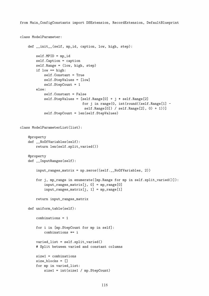
from Main_ConfigConstants import DSExtension, RecordExtension, DefaultBlueprint
class ModelParameter:
def __init__(self, mp_id, caption, low, high, step):
self.MPID = mp_id
self.Caption = caption
self.Range = (low, high, step)
if low == high:
self.Constant = True
self.StepValues = [low]
self.StepCount = 1
else:
self.Constant = False
self.StepValues = [self.Range[0] + j * self.Range[2]
for j in range(0, int(round((self.Range[1] -
self.Range[0]) / self.Range[2], 0) + 1))]
self.StepCount = len(self.StepValues)
class ModelParameterList(list):
@property
def __NoOfVariables(self):
return len(self.split_varied())
@property
def __InputRanges(self):
input_ranges_matrix = np.zeros((self.__NoOfVariables, 2))
for j, mp_range in enumerate([mp.Range for mp in self.split_varied()]):
input_ranges_matrix[j, 0] = mp_range[0]
input_ranges_matrix[j, 1] = mp_range[1]
return input_ranges_matrix
def uniform_table(self):
combinations = 1
for i in [mp.StepCount for mp in self]:
combinations *= i
varied_list = self.split_varied()
# Split between varied and constant columns
size1 = combinations
size_blocks = []
for mp in varied_list:
size1 = int(size1 / mp.StepCount)
118

size_blocks.append(size1)
variations = []
for c, mp in enumerate(varied_list):
block2 = []
for j in range(0, mp.StepCount):
for item in [mp.StepValues[j]] * size_blocks[c]:
block2.append(item)
column = []
for j in range(0, int(combinations / len(block2))):
for item in block2:
column.append(item)
variations.append(column)
full_table = np.zeros(shape=(combinations, len(self)))
for c, mp in enumerate(varied_list):
full_table[:, mp.MPID] = variations[c]
for c, mp in enumerate([mp for mp in self if mp.Constant]):
for row1 in range(0, combinations):
full_table[:, mp.MPID] = mp.StepValues
return full_table
def split_varied(self):
return [mp for mp in self if not mp.Constant]
def lhs_table(self, number_of_points, integers_list):
# Create latin hypercube set using existing data - values are between 0-1
lhs_01 = lhs(number_of_points, samples=self.__NoOfVariables)
# {Variables x number_of_points}
# Extrapolate input parameter matrix within defined input ranges
data_table_1 = norm_extrap_2D(lhs_01, self.__InputRanges, ’E’, limits=(0, 1))
# Initialize final results table
result_table = np.zeros(shape=[len(self), number_of_points])
# Check if parameter datatype is integer -- round data in the table to zero
decimals (it is still float64!)
for j, mp_index in enumerate(self.get_var_id()):
if mp_index in integers_list:
data_table_1[j, :] = np.round(data_table_1[j, :])
# Expand data_table_1 to full size using constant values of other parameters.
constant_mp_list = [mp for mp in self if mp.Constant]
for id_value in zip([mp.MPID for mp in constant_mp_list], [mp.StepValues for
mp in constant_mp_list]):
119
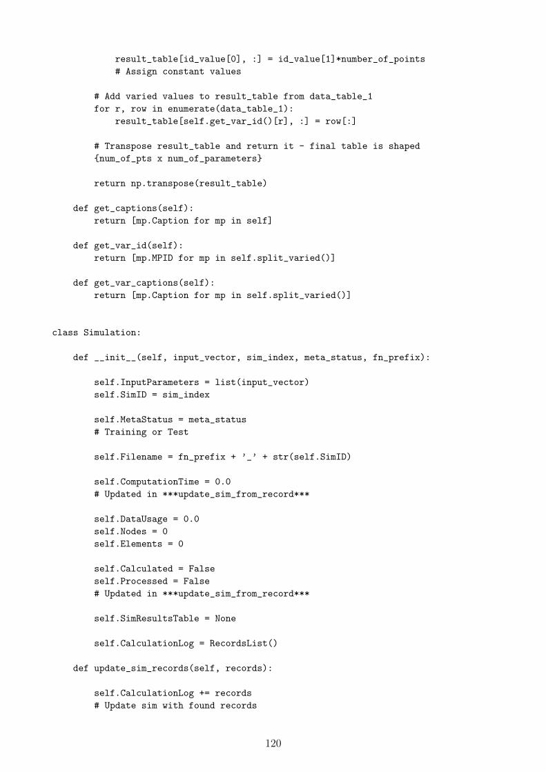
result_table[id_value[0], :] = id_value[1]*number_of_points
# Assign constant values
# Add varied values to result_table from data_table_1
for r, row in enumerate(data_table_1):
result_table[self.get_var_id()[r], :] = row[:]
# Transpose result_table and return it - final table is shaped
{num_of_pts x num_of_parameters}
return np.transpose(result_table)
def get_captions(self):
return [mp.Caption for mp in self]
def get_var_id(self):
return [mp.MPID for mp in self.split_varied()]
def get_var_captions(self):
return [mp.Caption for mp in self.split_varied()]
class Simulation:
def __init__(self, input_vector, sim_index, meta_status, fn_prefix):
self.InputParameters = list(input_vector)
self.SimID = sim_index
self.MetaStatus = meta_status
# Training or Test
self.Filename = fn_prefix + ’_’ + str(self.SimID)
self.ComputationTime = 0.0
# Updated in ***update_sim_from_record***
self.DataUsage = 0.0
self.Nodes = 0
self.Elements = 0
self.Calculated = False
self.Processed = False
# Updated in ***update_sim_from_record***
self.SimResultsTable = None
self.CalculationLog = RecordsList()
def update_sim_records(self, records):
self.CalculationLog += records
# Update sim with found records
120

last_results = self.CalculationLog.last_calc_data()[2]
last_proc_results = self.CalculationLog.last_proc_res()
if last_results is not None:
self.Calculated, self.Nodes, self.Elements, self.ComputationTime,
self.DataUsage = last_results
if last_proc_results is not None:
self.Processed, self.SimResultsTable = last_proc_results
def datatable_2(self):
last_calculation_data = self.CalculationLog.last_calc_data()
return [self.Filename, self.Calculated, self.Processed,
last_calculation_data[0], last_calculation_data[1]]
class Dataset:
def __init__(self, mp_list, scenario_type, description, blueprint):
# Upon initialization, only model parameter list is provided. Other properties
are set to initial zero values
self.__Parameters = mp_list
self.__ScenarioType = scenario_type
self.__Description = description
self.__ModellingSequence = blueprint
self.__DataTable = None
self.__MyName = ’’
self.__Simulations = []
self.CurrentPath = ’’
# This is temporary attribute, which changes each time when DS is loaded
self.SnapMatrices = []
@property
def __Captions(self):
return self.__Parameters.get_captions()
@property
def __NotCalculatedSims(self):
return [sim for sim in self.__Simulations if not sim.Calculated]
@property
def __CalculatedSims(self):
return [sim for sim in self.__Simulations if sim.Calculated]
121

@property
def __ProcessedSims(self):
return [sim for sim in self.__Simulations if sim.Processed]
@property
def __NotProcessedSims(self):
return [sim for sim in self.__CalculatedSims if not sim.Processed]
@property
def __LocalSubfolder(self):
return self.CurrentPath[0:(len(self.CurrentPath)-len(DSExtension))]
@property
def SummaryTable(self):
# Calculate number of simulations for display (for example: 12+5 in MM case)
if self.__ScenarioType == ’Metamodel’:
train = len([sim for sim in self.__Simulations if sim.MetaStatus ==
’Training’])
test = len([sim for sim in self.__Simulations if sim.MetaStatus ==
’Test’])
sims_no = str(train) + ’+’ + str(test)
else:
sims_no = str(len(self.__Simulations))
block1 = [self.__ScenarioType,
self.__Description,
self.__ModellingSequence,
sims_no]
table2 = [self.__Captions,
self.__DataTable]
SimTableHeaders = [’Simulation’, ’Calculated’, ’Processed’, ’Computation Time
[min]’, ’Size on Disk [MB]’, ’Metamodel Status’, ’Mesh nodes’, ’Mesh
elements’]
sim_data = [[sim.Filename,
sim.Calculated,
sim.Processed,
sim.ComputationTime,
sim.DataUsage,
sim.MetaStatus,
sim.Nodes,
sim.Elements] for sim in self.__Simulations]
table1 = [SimTableHeaders, sim_data]
122

return [block1, table1, table2]
@property
def SummaryTable_2(self):
block1 = [self.__ScenarioType,
self.__Description,
self.__ModellingSequence]
table1 = [[’Simulation’, ’Calculated’, ’Processed’, ’Last Calculation PC’,
’Last Calculation Path’], [sim.datatable_2() for sim in self.__Simulations]]
return [block1, table1]
def SummaryTable_2_1(self, list_indices):
captions = [’Simulation’, ’Action’, ’Computer’, ’Path’]
data = []
for sim in self.__get_sims_by_id(list_indices):
sim_block = [sim.Filename, ’Awaiting start...’, ’None’, ’None’]
data.append(sim_block)
return [data, captions]
@property
def SummaryTable_2_2(self):
# Calculate number of simulations for display (for example: 12+5 in MM case)
SimTableHeaders = [’Simulation’, ’Computation Time [min]’, ’Size on Disk
[MB]’, ’Mesh nodes’, ’Mesh elements’, ’Processed’]
sim_data = [[sim.Filename,
sim.ComputationTime,
sim.DataUsage,
sim.Nodes,
sim.Elements,
sim.Processed] for sim in self.__Simulations]
sim_results = [sim.SimResultsTable for sim in self.__Simulations]
return SimTableHeaders, sim_data, sim_results
@property
def SummaryTable_3(self):
block1 = [self.__ScenarioType, self.__Description,
str(len(self.__Simulations))]
return block1, [[sim.SimResultsTable, sim.MetaStatus] for sim in
self.__Simulations], self.__varied_table()
@property
def SummaryTable_4(self):
123

return [[sim.InputParameters, sim.SimResultsTable] for sim in
self.__Simulations]
def __varied_table(self):
varied_indices = self.__Parameters.get_var_id()
varied_captions = self.__Parameters.get_var_captions()
if len(varied_indices) == 0:
return None
else:
rows = len(varied_indices)
columns = len(self.__Simulations)
table = np.zeros((rows, columns))
for r in range(0, rows):
table[r, :] = self.__DataTable[:, varied_indices[r]]
return table, varied_captions
def __save(self):
save_object(self, self.CurrentPath) # Save into File
def __save_task_record(self, record_and_sim):
rec_list = [file for file in os.listdir(self.__LocalSubfolder)
if file.endswith(RecordExtension)]
start = 0
if len(rec_list) > 0:
# Search for first available index if there are other records
indices = [int(fname[0:(len(fname) - len(RecordExtension))].split(’_’)[1])
for fname in rec_list]
indices.sort()
found = False
while not found:
if start not in indices:
# Find first free index, start from 0, and assign it to the record
file name
found = True
else:
start += 1
# Record index determined. Save record to dataset subfolder
save_object(record_and_sim, self.__LocalSubfolder + ’\\’ + ’Record_’ +
str(start) + RecordExtension)
124

def __get_sims_by_id(self, id_list):
return [sim for sim in self.__Simulations if sim.SimID in id_list]
def get_sim_by_index(self, i):
return self.__Simulations[i]
def __remote_path(self, remote_folder_path):
return remote_folder_path + ’\\’ + self.__MyName + ’----’
def save_first(self, full_path):
just_name_ext = os.path.basename(full_path)
self.__MyName = just_name_ext[0:(len(just_name_ext) - len(DSExtension))]
self.CurrentPath = full_path
self.__save()
def assign_datatable(self, arguments, sim_fn_prefix):
training_table = None
test_table = None
meta_status = None
if self.__ScenarioType == ’Simple’:
self.__DataTable = self.__Parameters.uniform_table()
meta_status = [None] * len(self.__DataTable)
elif self.__ScenarioType == ’Custom’:
self.__DataTable = arguments
meta_status = [None] * len(self.__DataTable)
elif self.__ScenarioType == ’Metamodel’:
if len(self.__Parameters.split_varied()) > 0:
# Check number of variable parameters
training_pts, test_pts, training_alg, test_alg = arguments[0]
integers_list = arguments[1]
if training_alg == ’Latin Hypercube Sampling’:
training_table = self.__Parameters.lhs_table(training_pts,
integers_list) # Calculate LHS Sample
training_unique = unique_ndarray(training_table)[0]
# Get unique values
if test_pts > 0:
if test_alg == ’Latin Hypercube Sampling’:
test_table = self.__Parameters.lhs_table(test_pts,
integers_list) # Calculate LHS Sample
test_unique = unique_ndarray(test_table)[0]
125

final_table = link_np_tables(training_unique, test_unique)
# Link two tables into single dataset
meta_status = [’Training’]*len(training_unique) +
[’Test’]*len(test_unique)
else:
final_table = training_unique
meta_status = [’Training’] * len(training_unique)
self.__DataTable = final_table
else:
return False
# All parameters are constants - dataset cannot be created.
Exit function
self.__Simulations = [Simulation(vector, sim_id, meta_status[sim_id],
sim_fn_prefix)
for sim_id, vector in enumerate(self.__DataTable)]
return True
def export_SummaryTable_1(self, export_filename):
wb = xl.Workbook()
wb.create_sheet(’Basics’)
fill_xl_row_col(wb.worksheets[1], ’R’, [’Dataset Type’, ’Dataset Description’,
’Modelling Sequence’, ’Total Number
of Simulations’])
fill_xl_row_col(wb.worksheets[1], ’R’, self.SummaryTable[0], start=(2, 1))
wb.create_sheet(’Simulations Info’)
fill_xl_with_headers(wb.worksheets[2], self.SummaryTable[1][0],
self.SummaryTable[1][1])
wb.create_sheet(’Input Values’)
fill_xl_with_headers(wb.worksheets[3], self.SummaryTable[2][0],
self.SummaryTable[2][1], start=(1, 2))
fill_xl_row_col(wb.worksheets[3], ’C’,
[’Simulation/Parameter’] + [item[0]
for item in self.SummaryTable[1][1]])
wb.remove_sheet(wb.worksheets[0])
wb.save(export_filename)
def filter(self, selected_indexes, io):
if io == ’Input’:
126

sims_to_run = [sim.SimID for sim in self.__NotCalculatedSims
if sim.SimID in selected_indexes]
sims_to_exclude = [sim.SimID for sim in self.__CalculatedSims
if sim.SimID in selected_indexes]
else:
sims_to_run = [sim.SimID for sim in self.__NotProcessedSims
if sim.SimID in selected_indexes]
sims_to_exclude = [sim.SimID for sim in self.__ProcessedSims
if sim.SimID in selected_indexes]
return sims_to_run, sims_to_exclude
def start_local(self, sim_index, pc_id, sim_file_path, job_type):
sim = self.__Simulations[sim_index]
blueprint_path = self.__LocalSubfolder + ’\\’ + DefaultBlueprint
if job_type == ’Calculation’:
# Define path to save calculation file
sim_file_path = self.__LocalSubfolder + ’\\’ + sim.Filename
# Initialize timer and data space
sim.ComputationTime = float(time.time())
sim.DataUsage = float(folder_size(self.__LocalSubfolder))
self.__save_task_record((sim_index, Record(pc_id, sim_file_path, None,
job_type, ’Begin’, ’Local’)))
return sim.InputParameters, sim_file_path, blueprint_path
def end_local(self, sim_index, pc_id, results, sim_file_path, job_type):
sim = self.__Simulations[sim_index]
if job_type == ’Calculation’:
# Define path to save calculation file
sim_file_path = self.__LocalSubfolder + ’\\’ + sim.Filename
# Calculate data usage and computation time
comp_time = (time.time() - sim.ComputationTime)/60
data_usage = (folder_size(self.__LocalSubfolder) - sim.DataUsage)/1048576
results = (results[0], results[1], results[2], comp_time, data_usage)
self.__save_task_record((sim_index, Record(pc_id, sim_file_path, results,
job_type, ’End’, ’Local’)))
127

def start_remote(self, sim_index, pc_id, job_type, remote_folder_path):
sim = self.__Simulations[sim_index]
blueprint_path = self.__remote_path(remote_folder_path) + DefaultBlueprint
sim_file_path = self.__remote_path(remote_folder_path) + sim.Filename
if job_type == ’Calculation’:
sim.ComputationTime = float(time.time())
sim.DataUsage = 0.0
self.__save_task_record((sim_index, Record(pc_id, sim_file_path, None,
job_type, ’Begin’, ’Remote’)))
return sim.InputParameters, sim_file_path, blueprint_path
def end_remote(self, sim_index, pc_id, results, remote_folder_path, job_type):
sim = self.__Simulations[sim_index]
sim_file_path = self.__remote_path(remote_folder_path) + sim.Filename
if job_type == ’Calculation’:
results = (results[0], results[1], results[2], (time.time() -
sim.ComputationTime)/60, 0.0)
self.__save_task_record((sim_index, Record(pc_id, sim_file_path, results,
job_type, ’End’, ’Remote’)))
def update_records(self):
# Get list of files containing previous records. Continue if found
saved_records_list = [file for file in os.listdir(self.__LocalSubfolder)
if file.endswith(RecordExtension)]
if len(saved_records_list) > 0:
# Load simulation instances from records
records_sims = [load_object(self.__LocalSubfolder + ’\\’ + record_fn)
for record_fn in saved_records_list]
for sim in self.__Simulations:
sim.update_sim_records([rec_set[1] for rec_set in records_sims
if sim.SimID == rec_set[0]])
# Erase record files, because we don’t need them anymore
for file in [(self.__LocalSubfolder + ’\\’ + record_fn)
for record_fn in saved_records_list]:
os.remove(file)
self.__save() # Save dataset after changes
128

def change_results(self, changed_set):
self.__Simulations[changed_set[0]].Processed = True
self.__Simulations[changed_set[0]].SimResultsTable = changed_set[1]
self.__save()
def add_snapshot_matrices(self, added_matrices):
for matrix in added_matrices:
self.SnapMatrices.append(matrix)
self.__save()
def update_from_child(self, child_ds, update_list):
for sim_id in update_list:
child_sim = child_ds.get_sim_by_index(sim_id)
self.__Simulations[sim_id] = child_sim
self.__save()
def get_name(self):
return self.__MyName
class Record:
def __init__(self, pc_id, sim_path, results_tuple, analysis_type, start_stop,
session):
self.ComputerID = pc_id
self.SimPath = sim_path
self.Results = results_tuple
self.AnalysisType = analysis_type
self.StartStop = start_stop
self.__Session = session
self.__Time = time.time()
class RecordsList(list):
def __last_ended(self, calc_proc):
records = [rec for rec in self if rec.AnalysisType == calc_proc and
rec.StartStop == ’End’]
if len(records) > 0:
# Return last record (if there are any records)
return records[-1]
else:
return Record(None, None, None, None, None, None)
129

def last_calc_data(self):
last_rec = self.__last_ended(’Calculation’)
return last_rec.ComputerID, last_rec.SimPath, last_rec.Results
def last_proc_res(self):
return self.__last_ended(’Processing’).Results
class SnapshotMatrix:
def __init__(self, data_table, captions):
self.Data = data_table
self.Captions = captions
User Interface Classes Main WidgetClasses.py
import os
from Main_ConfigConstants import DefaultSimDir, SimExtension, DefaultServerName
from PyQt5.QtCore import Qt
from PyQt5.QtGui import QIcon
from PyQt5.QtWidgets import QTableWidgetItem, QTableWidget, QAbstractScrollArea,
QPushButton, QLineEdit, QMessageBox
from PyQt5.QtWidgets import QLabel, QGridLayout, QDialog, QWidget
from Main_ConfigConstants import IconTrue, IconFalse
from Main_Functions import popup_message, load_object, popup_open_save
def cell_label_button(value_cell, button_widget, color=None):
cell_widget = QWidget()
cell_layout = QGridLayout()
cell_widget.setLayout(cell_layout)
label = QLabel(str(value_cell))
if color is not None:
label.setStyleSheet(’color: ’ + color)
cell_layout.addWidget(label, 0, 0)
cell_layout.addWidget(button_widget, 0, 1)
cell_layout.setAlignment(Qt.AlignCenter)
cell_layout.setContentsMargins(0, 0, 0, 0)
return cell_widget
130
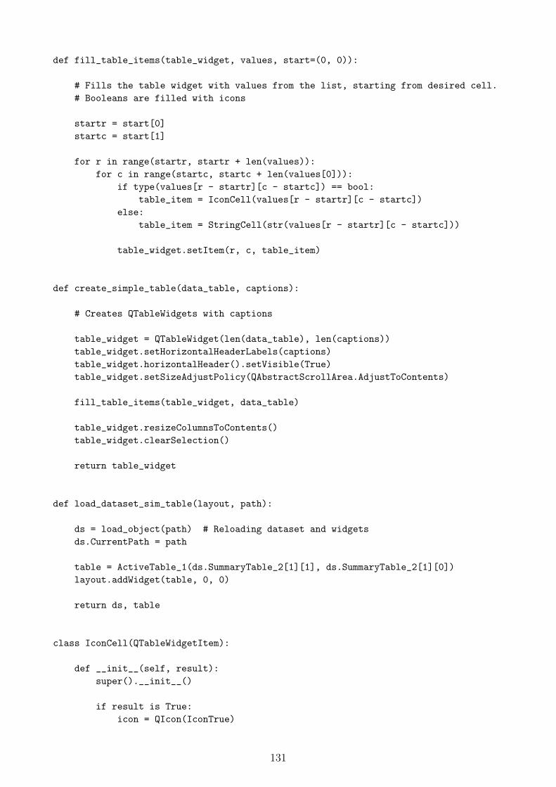
def fill_table_items(table_widget, values, start=(0, 0)):
# Fills the table widget with values from the list, starting from desired cell.
# Booleans are filled with icons
startr = start[0]
startc = start[1]
for r in range(startr, startr + len(values)):
for c in range(startc, startc + len(values[0])):
if type(values[r - startr][c - startc]) == bool:
table_item = IconCell(values[r - startr][c - startc])
else:
table_item = StringCell(str(values[r - startr][c - startc]))
table_widget.setItem(r, c, table_item)
def create_simple_table(data_table, captions):
# Creates QTableWidgets with captions
table_widget = QTableWidget(len(data_table), len(captions))
table_widget.setHorizontalHeaderLabels(captions)
table_widget.horizontalHeader().setVisible(True)
table_widget.setSizeAdjustPolicy(QAbstractScrollArea.AdjustToContents)
fill_table_items(table_widget, data_table)
table_widget.resizeColumnsToContents()
table_widget.clearSelection()
return table_widget
def load_dataset_sim_table(layout, path):
ds = load_object(path) # Reloading dataset and widgets
ds.CurrentPath = path
table = ActiveTable_1(ds.SummaryTable_2[1][1], ds.SummaryTable_2[1][0])
layout.addWidget(table, 0, 0)
return ds, table
class IconCell(QTableWidgetItem):
def __init__(self, result):
super().__init__()
if result is True:
icon = QIcon(IconTrue)
131

else:
icon = QIcon(IconFalse)
self.setIcon(icon)
self.setTextAlignment(Qt.AlignCenter)
self.setFlags(Qt.ItemIsEnabled | Qt.ItemIsSelectable)
class StringCell(QTableWidgetItem):
def __init__(self, string):
super().__init__(string)
self.setTextAlignment(Qt.AlignCenter)
self.setFlags(Qt.ItemIsEnabled | Qt.ItemIsSelectable)
class Input_ExcelCaptions(QDialog):
def __init__(self, parameters_number, title, caption1):
super(Input_ExcelCaptions, self).__init__()
self.setWindowTitle(title)
layout = QGridLayout()
self.setLayout(layout)
cmdOK = QPushButton(’OK’)
cmdOK.clicked.connect(self.cmdOK_clicked)
layout.addWidget(QLabel(caption1), 0, 0)
layout.addWidget(QLabel(’Unit’), 0, 1)
layout.addWidget(cmdOK, parameters_number+2, 1)
self.TextFields = []
for r in range(0, parameters_number):
p_i = QLineEdit(caption1 + ’_’ + str(r+1))
u_i = QLineEdit(’Unit_’ + str(r+1))
layout.addWidget(p_i, r+1, 0)
layout.addWidget(u_i, r+1, 1)
self.TextFields.append((p_i, u_i))
self.ReturnValues = None
self.exec_()
def cmdOK_clicked(self):
data_empty = False
132

for param_set in self.TextFields: # Check if some fields are empty
for input_widget in param_set:
if input_widget.text() == ’’:
data_empty = True
popup_message(’Please fill all fields!’, QMessageBox.Critical,
’Input Error’, QMessageBox.Ok)
break
if not data_empty:
self.ReturnValues = [(p[0].text(), p[1].text()) for p in self.TextFields]
self.close()
class ActiveTable_1(QTableWidget):
def __init__(self, table_data, table_captions):
super().__init__(len(table_data), len(table_captions))
# Observer Variables that monitor the content of table columns
self.LinkedPaths = [item[4] for item in table_data]
self.LinkedComputers = [item[3] for item in table_data]
self.ChangedPaths = []
self.LinkButtons = []
self.CalculatedList = [item[1] for item in table_data]
self.ProcessedList = [item[2] for item in table_data]
self.setHorizontalHeaderLabels(table_captions)
self.horizontalHeader().setVisible(True)
self.setSizeAdjustPolicy(QAbstractScrollArea.AdjustToContents)
fill_table_items(self, table_data)
# Check if all local paths exist on local pc. For remote computer this is not
possible at this moment.
self.InvalidLocalPaths = []
for j, calc_path in enumerate(self.LinkedPaths):
if calc_path is not None:
if not os.path.isfile(calc_path + SimExtension) and
self.LinkedComputers[j] == DefaultServerName:
self.InvalidLocalPaths.append(j)
# Create link buttons
for r in range(0, len(self.LinkedPaths)):
button = QPushButton(’Link calculated’)
button.clicked.connect(self.link_button_clicked)
self.LinkButtons.append(button)
self.setItem(r, 4, StringCell(’’))
# Erase previous cell content and add new widget
133

if r in self.InvalidLocalPaths:
color = ’red’
else:
color = None
self.setCellWidget(r, 4, cell_label_button(self.LinkedPaths[r], button,
color))
self.clearSelection()
self.resizeColumnsToContents()
def link_button_clicked(self):
# Find which button was clicked
i = 0
for i, button in enumerate(self.LinkButtons):
if self.sender() == button:
break # Button found
link_fn = popup_open_save(’Open’, DefaultSimDir, ’Select Simulation’,
’Simulations (*’ + SimExtension + ’)’)
if link_fn != ’’:
self.__add_linked(i, link_fn)
def link_multiple(self, files_list):
for i, file in zip(self.SelectedRows, files_list):
self.__add_linked(i, file)
def __add_linked(self, i, link_filename):
# Update Table Cell
self.setItem(i, 3, StringCell(DefaultServerName))
# Set computer cell to local Computer
self.setItem(i, 4, StringCell(’’))
# Erase previous cell content and add new widget
self.setCellWidget(i, 4, cell_label_button(link_filename, self.LinkButtons[i],
’blue’))
self.resizeColumnsToContents()
# Update observer variables
self.LinkedPaths[i] = link_filename
self.LinkedComputers[i] = DefaultServerName
self.ChangedPaths.append(i)
self.CalculatedList[i] = True
if i in self.InvalidLocalPaths:
self.InvalidLocalPaths.remove(i)
134

@property
def SelectedRows(self):
return sorted(set(i.row() for i in self.selectedIndexes()))
@property
def SelectedLinked(self):
return [i for i in list(set(self.ChangedPaths)) if i in self.SelectedRows]
@property
def NeededComputers(self):
return list(set([self.LinkedComputers[j] for j in self.SelectedRows]))
@property
def SelectedInvalidPaths(self):
return [j for j in self.SelectedRows if j in self.InvalidLocalPaths]
@property
def ProcessingQueue(self):
# Here we sort simulations according to linked computer. Each computer gets
its own processing sim Queue
# We need to exclude NOT CALCULATED SIMS (except if they are linked outside)
return [(computer, [j for j in self.SelectedRows if self.LinkedComputers[j]
== computer])
for computer in self.NeededComputers]
def get_paths(self, sim_indices):
return [self.LinkedPaths[j] for j in sim_indices]
def selected_calculated(self):
ok = True
for j in self.SelectedRows:
if self.CalculatedList[j] is False:
ok = False
break
return ok
User Interface Classes - 2 Main WidgetClasses small.py
from PyQt5.QtCore import Qt
from PyQt5.QtGui import QIcon
from PyQt5.QtWidgets import QTableWidgetItem, QTableWidget, QAbstractScrollArea,
QPushButton, QMdiSubWindow, QWidget
from PyQt5.QtWidgets import QLabel, QGridLayout, QDialog, QLineEdit, QMessageBox
from Main_ConfigConstants import IconTrue, IconFalse
from Main_Functions import popup_message
def fill_table_items(table_widget, values, start=(0, 0)):
135

# Fills the QTableWidget with values from the list, starting from desired cell.
# Booleans are filled with icons
startr = start[0]
startc = start[1]
for r in range(startr, startr + len(values)):
for c in range(startc, startc + len(values[0])):
if type(values[r - startr][c - startc]) == bool:
table_item = IconCell(values[r - startr][c - startc])
else:
table_item = StringCell(str(values[r - startr][c - startc]))
table_widget.setItem(r, c, table_item)
def create_simple_table(data_table, captions):
# Creates QTableWidgets with captions
table_widget = QTableWidget(len(data_table), len(captions))
table_widget.setHorizontalHeaderLabels(captions)
table_widget.horizontalHeader().setVisible(True)
table_widget.setSizeAdjustPolicy(QAbstractScrollArea.AdjustToContents)
fill_table_items(table_widget, data_table)
table_widget.resizeColumnsToContents()
table_widget.clearSelection()
return table_widget
def new_subwindow(title, dimensions):
new_window = QMdiSubWindow()
top_widget = QWidget()
new_layout = QGridLayout(top_widget)
top_widget.setLayout(new_layout)
new_window.setWindowTitle(title)
new_window.setFixedSize(dimensions[0], dimensions[1])
new_window.setWindowFlags(Qt.CustomizeWindowHint)
new_window.setWidget(top_widget)
return new_window, new_layout
class IconCell(QTableWidgetItem):
def __init__(self, result):
super().__init__()
if result is True:
icon = QIcon(IconTrue)
136

else:
icon = QIcon(IconFalse)
self.setIcon(icon)
self.setTextAlignment(Qt.AlignCenter)
self.setFlags(Qt.ItemIsEnabled | Qt.ItemIsSelectable)
class StringCell(QTableWidgetItem):
def __init__(self, string):
super().__init__(string)
self.setTextAlignment(Qt.AlignCenter)
self.setFlags(Qt.ItemIsEnabled | Qt.ItemIsSelectable)
class Input_ExcelCaptions(QDialog):
def __init__(self, parameters_number, title, caption1):
super(Input_ExcelCaptions, self).__init__()
self.setWindowTitle(title)
layout = QGridLayout()
self.setLayout(layout)
cmdOK = QPushButton(’OK’)
cmdOK.clicked.connect(self.cmdOK_clicked)
layout.addWidget(QLabel(caption1), 0, 0)
layout.addWidget(QLabel(’Unit’), 0, 1)
layout.addWidget(cmdOK, parameters_number+2, 1)
self.TextFields = []
for r in range(0, parameters_number):
p_i = QLineEdit(caption1 + ’_’ + str(r+1))
u_i = QLineEdit(’Unit_’ + str(r+1))
layout.addWidget(p_i, r+1, 0)
layout.addWidget(u_i, r+1, 1)
self.TextFields.append((p_i, u_i))
self.ReturnValues = None
self.exec_()
def cmdOK_clicked(self):
data_empty = False
137
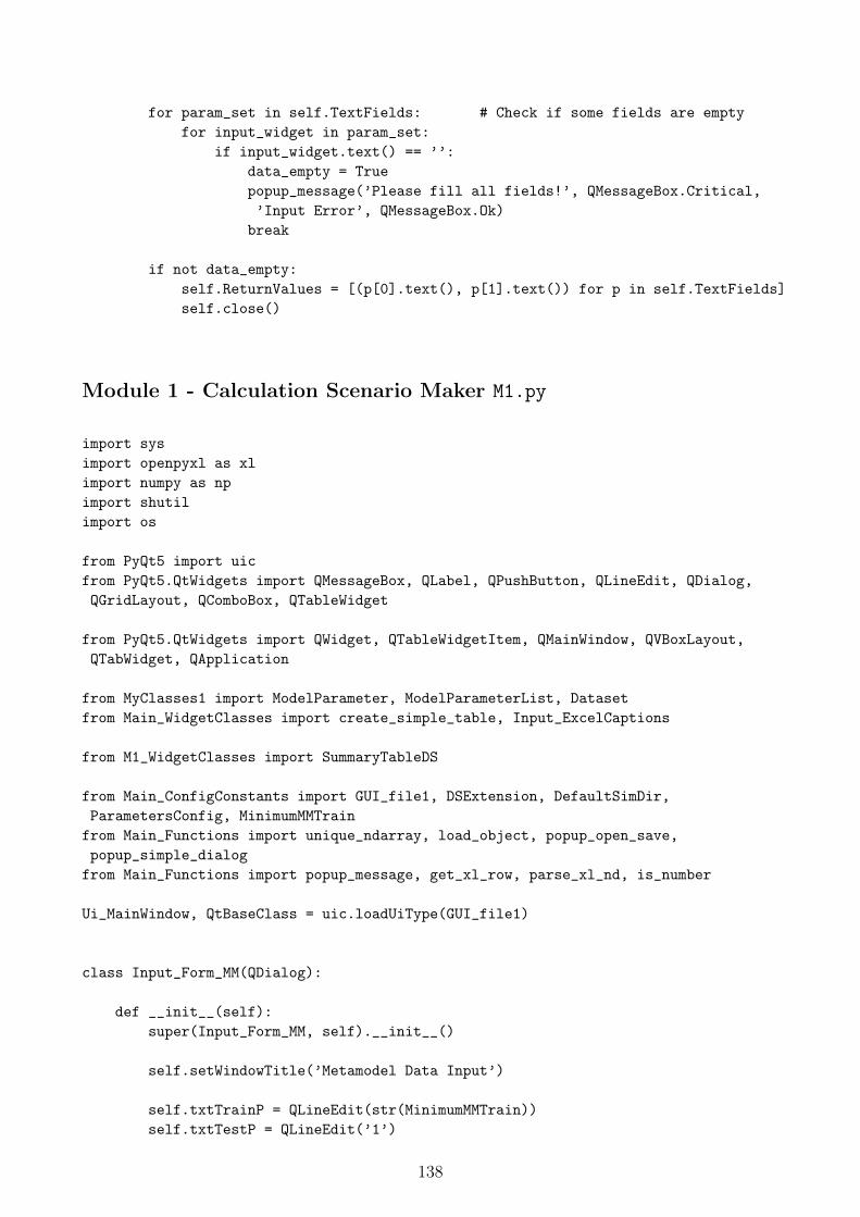
for param_set in self.TextFields: # Check if some fields are empty
for input_widget in param_set:
if input_widget.text() == ’’:
data_empty = True
popup_message(’Please fill all fields!’, QMessageBox.Critical,
’Input Error’, QMessageBox.Ok)
break
if not data_empty:
self.ReturnValues = [(p[0].text(), p[1].text()) for p in self.TextFields]
self.close()
Module 1 - Calculation Scenario Maker M1.py
import sys
import openpyxl as xl
import numpy as np
import shutil
import os
from PyQt5 import uic
from PyQt5.QtWidgets import QMessageBox, QLabel, QPushButton, QLineEdit, QDialog,
QGridLayout, QComboBox, QTableWidget
from PyQt5.QtWidgets import QWidget, QTableWidgetItem, QMainWindow, QVBoxLayout,
QTabWidget, QApplication
from MyClasses1 import ModelParameter, ModelParameterList, Dataset
from Main_WidgetClasses import create_simple_table, Input_ExcelCaptions
from M1_WidgetClasses import SummaryTableDS
from Main_ConfigConstants import GUI_file1, DSExtension, DefaultSimDir,
ParametersConfig, MinimumMMTrain
from Main_Functions import unique_ndarray, load_object, popup_open_save,
popup_simple_dialog
from Main_Functions import popup_message, get_xl_row, parse_xl_nd, is_number
Ui_MainWindow, QtBaseClass = uic.loadUiType(GUI_file1)
class Input_Form_MM(QDialog):
def __init__(self):
super(Input_Form_MM, self).__init__()
self.setWindowTitle(’Metamodel Data Input’)
self.txtTrainP = QLineEdit(str(MinimumMMTrain))
self.txtTestP = QLineEdit(’1’)
138

self.cmbTrainP = QComboBox()
self.cmbTestP = QComboBox()
self.cmbTrainP.addItems([’Latin Hypercube Sampling’])
self.cmbTestP.addItems([’Latin Hypercube Sampling’])
cmdOK = QPushButton(’OK’)
cmdOK.clicked.connect(self.cmdOK_clicked)
layout = QGridLayout()
layout.addWidget(QLabel(’Sampling Algorithm’), 0, 2)
layout.addWidget(QLabel(’Number of Training Points: ’), 1, 0)
layout.addWidget(self.txtTrainP, 1, 1)
layout.addWidget(self.cmbTrainP, 1, 2)
layout.addWidget(QLabel(’Number of Test Points: ’), 2, 0)
layout.addWidget(self.txtTestP, 2, 1)
layout.addWidget(self.cmbTestP, 2, 2)
layout.addWidget(cmdOK, 3, 2)
self.setLayout(layout)
self.ReturnValues = None # Return values container variable
self.exec_()
def cmdOK_clicked(self):
training_pts = int(self.txtTrainP.text())
# Obtain data from input fields
test_pts = int(self.txtTestP.text())
# Check number of Training and Test Points.
#If TestPoints is 0, notify and use training points as test points
if training_pts < MinimumMMTrain:
popup_message(’Invalid number of Training points. Minimum is ’ +
str(MinimumMMTrain) + ’!’,
QMessageBox.Critical, ’Input Error’, QMessageBox.Ok)
else:
if test_pts == 0:
popup_message(’Test points not selected! Training points will be
used for Metamodel test!’,
QMessageBox.Information, ’Information’,
QMessageBox.Ok)
self.ReturnValues = (training_pts, test_pts,
str(self.cmbTrainP.currentText()),
str(self.cmbTestP.currentText()))
# Return Values
self.close()
class Input_Form_CustomDS(QDialog):
def __init__(self):
super(Input_Form_CustomDS, self).__init__()
self.setWindowTitle(’Custom Dataset Input’)
139

layout = QGridLayout()
self.txtRows = QLineEdit(’2’)
self.txtColumns = QLineEdit(’2’)
cmdBrowseTable = QPushButton(’Select Excel File’)
self.cmdOK = QPushButton(’OK’)
self.cmdOK.setEnabled(False)
self.lblFilename = QLabel(’*** Data Table not loaded ***’)
self.lblFilename.setEnabled(False)
layout.addWidget(QLabel(’Number of Rows (Simulations): ’), 0, 0)
layout.addWidget(self.txtRows, 0, 1)
layout.addWidget(QLabel(’Number of Columns
(Input Parameter Values): ’),1, 0)
layout.addWidget(self.txtColumns, 1, 1)
layout.addWidget(self.lblFilename, 2, 0)
layout.addWidget(cmdBrowseTable, 2, 1)
layout.addWidget(self.cmdOK, 3, 1)
self.cmdOK.clicked.connect(self.cmdOK_clicked)
cmdBrowseTable.clicked.connect(self.cmdBrowseTable_clicked)
self.setLayout(layout)
self.ReturnValues = None
self.FileName = ’’
self.exec_()
def cmdOK_clicked(self):
def __message_duplicated_row(num_r):
sentence1 = ’Data Table succesfully loaded. ’
string2 = ’’
if num_r == 1:
string2 = ’One duplicated row was removed.’
elif num_r > 1:
string2 = str(num_r) + ’ duplicated rows were removed.’
return sentence1 + string2
no_errors = True # Error catcher
try:
rows = int(self.txtRows.text())
cols = int(self.txtColumns.text())
# No ValueError found.
if rows <= 0 or cols <= 0: # Rows or columns equal to 0
popup_message(’Invalid number of rows or columns’,
QMessageBox.Critical, ’Input Error’, QMessageBox.Ok)
no_errors = False
if no_errors:
# Rows and Columns ok. Open the excel file.
140

parsed_xl = parse_xl_nd(self.FileName, rows, cols)
# FileName exists, because button is Enabled
if parsed_xl is not None:
unique_data_table, erased = unique_ndarray(parsed_xl)
# Erase duplicated rows and notify user.
popup_message(__message_duplicated_row(erased),
QMessageBox.Information,
’Information’, QMessageBox.Ok)
captions_dialog = Input_ExcelCaptions(cols,
’Input Parameter Descriptions’,
’Parameter’).ReturnValues
if captions_dialog is not None:
self.ReturnValues = unique_data_table, captions_dialog
self.close()
else:
popup_message(’Error in the Excel file. Please check the
data!’,
QMessageBox.Critical, ’Excel Table Error’, QMessageBox.Ok)
except ValueError:
# No integers entered. Error catched during text to int conversion
popup_message(’Invalid number of rows or columns!’,
QMessageBox.Critical, ’Input Error’, QMessageBox.Ok)
def cmdBrowseTable_clicked(self):
filename = popup_open_save(’Open’, DefaultSimDir, ’Open Excel Table’,
’Excel files (*.xls *.xlsx)’)
if filename != ’’:
self.lblFilename.setText(filename)
self.lblFilename.repaint()
self.lblFilename.setEnabled(True)
self.FileName = filename
self.cmdOK.setEnabled(True)
class Input_Form_DatasetBasic(QDialog):
def __init__(self):
super(Input_Form_DatasetBasic, self).__init__()
self.setWindowTitle(’Dataset Description’)
layout = QGridLayout()
self.cmbDSType = QComboBox()
self.cmbDSType.addItems([’Simple’, ’Metamodel’, ’Custom’])
self.txtFilename = QLineEdit(’SIMULATION’)
self.cmbBlueprint = QComboBox()
self.cmbBlueprint.addItems([’Full Model Generation’,
141

’Use Model Blueprint’])
self.txtDescription = QLineEdit(’Dataset Description...’)
cmdOK = QPushButton(’OK’)
layout.addWidget(QLabel(’Dataset Type’), 0, 0)
layout.addWidget(QLabel(’Modelling Sequence’), 1, 0)
layout.addWidget(QLabel(’Simulation File Prefix’), 2, 0)
layout.addWidget(QLabel(’Dataset Description’), 3, 0)
layout.addWidget(self.cmbDSType, 0, 1)
layout.addWidget(self.cmbBlueprint, 1, 1)
layout.addWidget(self.txtFilename, 2, 1)
layout.addWidget(self.txtDescription, 3, 1)
layout.addWidget(cmdOK, 4, 1)
cmdOK.clicked.connect(self.cmdOK_clicked)
self.setLayout(layout)
self.ReturnValues = None
self.exec_()
def cmdOK_clicked(self):
filename_string = self.txtFilename.text()
if len(filename_string.split()) != 1:
# Check number of words for simulation prefix
popup_message(’Use single word as filename prefix!’,
QMessageBox.Critical, ’Input Error’, QMessageBox.Ok)
else:
self.ReturnValues = (self.cmbDSType.currentText(),
self.cmbBlueprint.currentText(), filename_string,
self.txtDescription.text())
self.close()
class Summary_Form_Dataset(QDialog):
def __init__(self, all_data, state):
super(Summary_Form_Dataset, self).__init__()
buttonok = ’Accept and Save’
buttonno = ’Decline’
self.TableData = (all_data[1], all_data[2])
# Data Tables
self.PopupArgs = [’Save’, DefaultSimDir, ’Save Dataset As’,
’Dataset files (*.dat)’]
self.setWindowTitle(’Dataset Summary - NOT SAVED!’)
layout = QGridLayout()
if state[0] == ’Loaded’:
142

buttonok = ’Export to Excel’
buttonno = ’Unload’
self.setWindowTitle(’LOADED DATASET - ’ + state[1])
self.PopupArgs = [’Save’, DefaultSimDir, ’Save Excel Table As’,
’Excel files (*.xlsx)’]
self.cmdDataTable = QPushButton(’Input Values Table’)
self.cmdSimsTable = QPushButton(’Simulations Data Table’)
layout.addWidget(QLabel(’Dataset Type’), 0, 0)
layout.addWidget(QLabel(’Dataset Description’), 1, 0)
layout.addWidget(QLabel(’Modelling Sequence’), 2, 0)
layout.addWidget(QLabel(’Total Number of Simulations’), 3, 0)
for j in range(0, 4):
# Fill label values
layout.addWidget(QLabel(all_data[0][j]), j, 1)
self.cmdOK = QPushButton(buttonok)
self.cmdCancel = QPushButton(buttonno)
layout.addWidget(self.cmdSimsTable, 4, 0)
layout.addWidget(self.cmdDataTable, 4, 1)
layout.addWidget(self.cmdOK, 5, 0)
layout.addWidget(self.cmdCancel, 5, 1)
self.cmdOK.clicked.connect(self.cmdOK_clicked)
self.cmdCancel.clicked.connect(self.cmdCancel_clicked)
self.cmdDataTable.clicked.connect(self.cmdDataTable_clicked)
self.cmdSimsTable.clicked.connect(self.cmdSimsTable_clicked)
self.setLayout(layout)
self.ReturnValues = None
# Return values container variable
self.exec_()
def cmdOK_clicked(self):
self.ReturnValues = popup_open_save(self.PopupArgs[0], self.PopupArgs[1],
self.PopupArgs[2], self.PopupArgs[3])
self.close()
def cmdCancel_clicked(self):
self.ReturnValues = None
self.close()
def cmdDataTable_clicked(self):
popup_simple_dialog(’Data Table’, [[SummaryTableDS(self.TableData[1][1],
self.TableData[1][0],
[item[0] for item in
self.TableData[0[1]])]])
def cmdSimsTable_clicked(self):
popup_simple_dialog(’Simulations Table’,
143
[[create_simple_table(self.TableData[0][1], self.TableData[0][0])]])
class MyApp(QMainWindow, Ui_MainWindow):
def __init__(self):
def __load_parameters():
wb = xl.load_workbook(ParametersConfig)
ws = wb[’Parameters’]
data_types = []
tab_titles = []
r = 2
row_index = ws.cell(row=2, column=2).value
while row_index is not None:
data_type = ws.cell(row=r, column=9).value
# Check data type
if data_type is not None and data_type == ’Integer’:
data_types.append(row_index)
tab_title = ws.cell(row=r, column=1).value
# Check tab limits
if tab_title is not None:
# Found tab title
tab_titles.append((tab_title, row_index))
r += 1
row_index = ws.cell(row=r, column=2).value
tab_titles.append((None, r-2))
tab_lengths = [(tab_titles[i+1][1]-tab_titles[i][1])
for i in range(0, len(tab_titles)-1)]
tabs_all = []
for i in range(0, len(tab_titles)-1):
tab_title = tab_titles[i][0]
tab_start = tab_titles[i][1]
tab_length = tab_lengths[i]
tab_set = []
for j in range(0, tab_length):
tab_set.append(get_xl_row(ws, (j+tab_start+2, 2), 7))
tabs_all.append((tab_title, tab_set))
Tables_Widgets = [] # Generate GUI widgets
tab_widget = QTabWidget()
start_row_label = 0
for tab in tabs_all:
rows = len(tab[1])
columns = len(tab[1][0])-1
144

table = QTableWidget(rows, columns)
table.setHorizontalHeaderLabels((’Parameter’, ’Unit’, ’Min’,
’Max’, ’Step’, ’Description’))
table.setVerticalHeaderLabels((str(index) for index in
range(start_row_label, start_row_label+rows)))
table.horizontalHeader().setStretchLastSection(True)
for r in range(0, rows):
for c in range(0, columns):
table.setItem(r, c, QTableWidgetItem(str(tab[1][r][c+1])))
tab_page = QWidget()
tab_widget.addTab(tab_page, tab[0])
tab_page_layout = QVBoxLayout()
tab_page_layout.addWidget(table)
tab_page.setLayout(tab_page_layout)
Tables_Widgets.append((table, start_row_label,
start_row_label+rows))
start_row_label += rows
return data_types, Tables_Widgets, tab_widget
QMainWindow.__init__(self)
Ui_MainWindow.__init__(self)
self.setupUi(self)
integersList, par_t, Tab_widget = __load_parameters()
# Initialize MP from config file
self.DataIntegers = integersList
# List model parameters with integer data type
self.ParameterTableWidgets = par_t
self.ParametersLayout.addWidget(Tab_widget)
self.cmdGenerateData.clicked.connect(self.cmdGenerateData_clicked)
self.cmdLoadDataset.clicked.connect(self.cmdLoadDataset_clicked)
def cmdGenerateData_clicked(self):
def __get_input_table_data():
data_input_error_list = []
mp_list = []
for table_set in self.ParameterTableWidgets:
tbl_widget = table_set[0]
start = table_set[1]
for j in range(start, table_set[2]):
# Read Table Data as text. All cells are editable
cell_name = tbl_widget.item(j - start, 0).text()
cell_min = tbl_widget.item(j - start, 2).text()
cell_max = tbl_widget.item(j - start, 3).text()
145
cell_step = tbl_widget.item(j - start, 4).text()
# Check if input is correct
founderrors = (cell_name == ’’)
# User must enter something as parameter name
if not (is_number(cell_min) and is_number(cell_max)
and is_number(cell_step)): # Must be numbers
founderrors = True
else:
# Check for errors Min>Max or Step > Interval
mp_min = float(cell_min) # Min
mp_max = float(cell_max) # Max
mp_step = float(cell_step) # Step
if (mp_min > mp_max) or (mp_min < mp_max
and mp_max - mp_min < mp_step):
founderrors = True
# Error check finished. Create Model_Parameter
if no errors have been found.
if not founderrors:
mp_list.append(ModelParameter(j,
cell_name + ’ [’ +
tbl_widget.item(j - start,
1).text() + ’]’,
float(cell_min),
float(cell_max),
float(cell_step)))
else:
data_input_error_list.append(j)
# Inform user on errors
if len(data_input_error_list) == 0:
return mp_list
else:
popup_message(’Please fix errors in rows: ’ +
str(data_input_error_list)[1:-1] + ’ and repeat!’,
QMessageBox.Critical, ’Data Table Error’,
QMessageBox.Ok)
def __parse_to_mpl(data_table, captions):
mp_list = []
for mp_col in range(0, len(data_table[0])):
p_min = np.min(data_table[:, mp_col])
p_max = np.max(data_table[:, mp_col])
caption = captions[mp_col][0] + ’ [’ + captions[mp_col][1] + ’]’
mp_list.append(ModelParameter(mp_col, caption,
p_min, p_max, p_max - p_min))
return mp_list
146

def __prepare_dataset_subfolder(fn, extension):
proceed = True
subfolder_path = fn[0:len(fn) - len(extension)]
if not os.path.exists(subfolder_path):
# Subfolder does not exist. Create without notification!
os.makedirs(subfolder_path)
elif len(os.listdir(subfolder_path)) > 0:
# Subfolder exists with data. Prompt for data erase.
confirm_erase = popup_message(’Dataset Subdirectory contains
files and folders! ’
’Do you want to erase ALL DATA data
in Subdirectory?’,
QMessageBox.Warning, ’Confirm
Delete’,
QMessageBox.Ok | QMessageBox.Cancel)
if confirm_erase == QMessageBox.Ok:
# Erase allowed by user
shutil.rmtree(subfolder_path, ignore_errors=True)
os.makedirs(subfolder_path)
else:
proceed = False
# User chooses to keep subfolder. Do not proceed
return proceed
basic_dialog = Input_Form_DatasetBasic().ReturnValues
# Get basic dataset input from Dialog Window
if basic_dialog is not None:
ds_type, blueprint, sim_fn_prefix, ds_desc = basic_dialog
# Basic dataset data
no_input_errors = True
# Error catcher
ds_creator = None
if ds_type != ’Custom’:
mpr_list = __get_input_table_data()
# Get input from table widget, Handle errors
if mpr_list is not None:
# No input errors found in datatable
ds_creator = Dataset(ModelParameterList(mpr_list), ds_type,
ds_desc, blueprint)
if ds_type == ’Simple’:
ds_creator.assign_datatable(None, sim_fn_prefix)
# No additional input needed. assign table
elif ds_type == ’Metamodel’:
147
# Additional input needed. prompt for input
mm_dialog = Input_Form_MM().ReturnValues
if mm_dialog is not None:
# Input values ok. assign table.
if not ds_creator.assign_datatable((mm_dialog,
self.DataIntegers), sim_fn_prefix):
no_input_errors = False
popup_message(’At least one input parameter
should have range!’, QMessageBox.Critical,
’Input Error’, QMessageBox.Ok)
else:
no_input_errors = False
else:
no_input_errors = False
else:
custom_dialog = Input_Form_CustomDS().ReturnValues
if custom_dialog is not None:
table, titles = custom_dialog
ds_creator = Dataset(ModelParameterList(__parse_to_mpl(table,
titles)), ds_type, ds_desc, blueprint)
ds_creator.assign_datatable(table, sim_fn_prefix)
else:
no_input_errors = False
# Input canceled. Program stops
# dataset with simulations is prepared at this point. Display summary.
Prompt user for final confirmation.
if no_input_errors:
choice1 = Summary_Form_Dataset(ds_creator.SummaryTable,
(’Summary’, None)).ReturnValues
if choice1 is not None and choice1 != ’’ and
__prepare_dataset_subfolder(choice1, DSExtension):
ds_creator.save_first(choice1)
# Save dataset for the first time
popup_message(’Dataset saved’, QMessageBox.Information,
’Information’, QMessageBox.Ok)
@staticmethod
def cmdLoadDataset_clicked():
ds_filename = popup_open_save(’Open’, DefaultSimDir, ’Open Dataset’,
’Dataset files (*.dat)’)
if ds_filename != ’’:
try:
ds_loaded = load_object(ds_filename)
148

choice2 = Summary_Form_Dataset(ds_loaded.SummaryTable,
(’Loaded’, ds_filename)).ReturnValues
if choice2 is not None and choice2 != ’’:
ds_loaded.export_SummaryTable_1(choice2)
popup_message(’Excel file successfuly created.’,
QMessageBox.Information, ’File Export’,
QMessageBox.Ok)
except ImportError:
popup_message(’Invalid File’, QMessageBox.Critical, ’File Error’,
QMessageBox.Ok)
except PermissionError:
popup_message(’Permission Error. File already opened.
Close it and repeat.’,
QMessageBox.Critical, ’File Error’, QMessageBox.Ok)
if __name__ == "__main__":
app = QApplication(sys.argv)
window = MyApp()
window.show()
sys.exit(app.exec_())
Module 2 - Simulation Runner M2.py
import sys
import zipfile
import math
import multiprocessing
from multiprocessing import Process
import time
import datetime
import openpyxl as xl
from PyQt5.QtCore import Qt, pyqtSlot, QRunnable, QThreadPool, pyqtSignal, QObject
from PyQt5.QtWidgets import QMainWindow, QApplication, QMdiArea, QMdiSubWindow,
QMessageBox, QLabel, QGridLayout
from PyQt5.QtWidgets import QWidget, QPushButton, QLineEdit, QProgressBar,
QDialog, QComboBox
from Main_Functions import popup_open_save, popup_message, get_xl_row,
popup_yes_no_dialog, popup_open_multiple
from Main_ConfigConstants import DefaultSimDir, Machines_List, DefaultServerName,
PreProcessing, PostProcessing
from Main_ConfigConstants import SimExtension, MaxComputers
149
from M2_Classes import PLAXIS_Machine
from M2_WidgetClasses import DataTable, Console, ActiveTable_2
from Main_WidgetClasses import load_dataset_sim_table
from Main_WidgetClasses import create_simple_table, StringCell
import M2_Solvers
class DialerSignals(QObject):
answer = pyqtSignal(str, str, str)
class SimRunnerSignals(QObject):
started = pyqtSignal(int, object)
# Returns simulation ID, machine ID
ended = pyqtSignal(int, object, bool, str)
# Returns simulation ID, machine ID and result (T/F)
class Dialer(QRunnable):
def __init__(self, machine, io, timeout):
super(Dialer, self).__init__()
self.__Machine = machine
self.__IO = io
self.__Timeout = timeout
self.DSignals = DialerSignals()
@pyqtSlot()
def run(self):
# Run connection check on local/remote machine
if self.__IO == ’Input’:
function_run = self.__Machine.check_input_connection
else:
function_run = self.__Machine.check_output_connection
# Try to join Pool after timeout period. If False, return timeout event.
Return if ok. Return on error.
try:
p = multiprocessing.Process(target=function_run)
p.start()
p.join(self.__Timeout)
150
if p.is_alive():
p.terminate()
p.join()
self.DSignals.answer.emit(self.__Machine.MachineID,
self.__IO, ’Timeout’) # connection timeout
else:
self.DSignals.answer.emit(self.__Machine.MachineID,
self.__IO, ’Connected’) # connected
except:
self.DSignals.answer.emit(self.__Machine.MachineID, self.__IO,
’Failed’) # connection failed
class SimRunner(QRunnable):
def __init__(self, simulation_id, machine, dataset, analysis_type,
sim_path, script_to_run):
super(SimRunner, self).__init__()
self.__SimID = simulation_id
self.__PC = machine
self.__DS = dataset
self.__Job = analysis_type
self.__SimPath = sim_path
self.__Script = script_to_run
self.RSignals = SimRunnerSignals()
@pyqtSlot()
def run(self):
self.RSignals.started.emit(self.__SimID, self.__PC)
# Emit START signal to main program
# Initialize simulation start and write record
if self.__PC.NetworkPosition == ’Local’:
i1, i2, i3 = self.__DS.start_local(self.__SimID,
self.__PC.MachineID, self.__SimPath, self.__Job)
else:
i1, i2, i3 = self.__DS.start_remote(self.__SimID, self.__PC.MachineID,
self.__Job, self.__PC.SimsPath)
# Run simulation Pre/Post processing Script
if self.__Job == ’Calculation’:
results = self.__Script(i1, i2, i3, self.__PC.HostName,
self.__PC.PortInput)
# Run Calc Script
else:
results = self.__Script(self.__SimPath, self.__PC.HostName,
self.__PC.PortOutput)
151
# Run PostScript
# End simulation and write record
if self.__PC.NetworkPosition == ’Local’:
self.__DS.end_local(self.__SimID, self.__PC.MachineID, results,
self.__SimPath,
self.__Job)
else:
self.__DS.end_remote(self.__SimID, self.__PC.MachineID, results,
self.__PC.SimsPath, self.__Job)
# Emit appropriate ENDED signal to main program
if self.__Job == ’Calculation’:
self.RSignals.ended.emit(self.__SimID, self.__PC, results[0], i2)
else:
self.RSignals.ended.emit(self.__SimID, self.__PC, results[0],
self.__SimPath)
class Data_Explorer(QDialog):
def __init__(self, table_data):
super(Data_Explorer, self).__init__()
captions, data_table, result_tables = table_data
# Unpack input tuple
self.setFixedSize(1000, 500)
self.setWindowFlags(Qt.CustomizeWindowHint)
self.setWindowTitle(’Data Explorer’)
layout = QGridLayout()
self.setLayout(layout)
self.cmdExport = QPushButton(’Export All Results’)
self.cmdClose = QPushButton(’Close’)
self.tblDataTable = DataTable(data_table, captions, result_tables)
self.cmdExport.clicked.connect(self.cmdExport_clicked)
self.cmdClose.clicked.connect(self.cmdClose_clicked)
self.tblDataTable.table_added.connect(self.Data_Added)
layout.addWidget(self.tblDataTable, 0, 0)
layout.addWidget(self.cmdExport, 1, 0)
layout.addWidget(self.cmdClose, 2, 0)
self.Changes = []
self.exec_()
def cmdExport_clicked(self):
152

if self.tblDataTable.can_export():
# We have some results and we export them to excel or numpy
if self.tblDataTable.GlobalShape is not None:
# All data tables have the same shape
if len(self.tblDataTable.GlobalShape) > 3:
# Export 4D+ tables to numpy
self.tblDataTable.export_numpy_tables()
else:
# Export 1D/2D/3D tables to Excel
self.tblDataTable.export_excel_consistent()
else:
self.tblDataTable.export_all()
@pyqtSlot(int, object)
def Data_Added(self, sim_index, res_table):
self.Changes.append((sim_index, res_table))
def cmdClose_clicked(self):
self.close()
class Calculation_Window(QDialog):
def __init__(self, computers, loaded_ds, sims_list, calc_or_proc,
pc_controller, calc_paths, script):
super(Calculation_Window, self).__init__()
self.OnlineComputers = computers
self.Dataset = loaded_ds
self.Job = calc_or_proc
self.MachinesController = pc_controller
self.CalculatedPaths = calc_paths
self.RunnerScript = script
self.SimulationIDList = sims_list
self.Sims_Pool = sims_list[:]
self.Calculated = 0
self.Remaining = len(sims_list)
self.TotalSims = len(sims_list)
self.Timers = []
self.ReturnValue = None
self.RunThreads = QThreadPool()
self.RunThreads.setMaxThreadCount(MaxComputers)
# Setting up GUI ########################################################
layout = QGridLayout()
self.setLayout(layout)
self.setFixedSize(1000, 500)
153

self.setWindowFlags(Qt.CustomizeWindowHint)
self.setWindowTitle(’Job Runner’)
data_table = self.Dataset.SummaryTable_2_1(sims_list)[0]
captions = self.Dataset.SummaryTable_2_1(sims_list)[1]
self.tblTable = create_simple_table(data_table, captions)
self.cnConsole1 = Console(app)
self.pbProgress1 = QProgressBar()
self.pbProgress1.setValue(0)
self.lblTimer = QLabel(’Remaining Time: ***’)
self.lblRemainingSims = QLabel(’Remaining Simulations: ’ +
str(len(sims_list)) + ’/’ + str(len(sims_list)))
self.cmdStart = QPushButton(’START JOB’)
self.cmdClose = QPushButton(’CLOSE WINDOW’)
self.cmdStart.clicked.connect(self.cmdStart_clicked)
self.cmdClose.clicked.connect(self.cmdClose_clicked)
# Add widgets to layout
layout.addWidget(self.tblTable, 0, 0)
layout.addWidget(self.cnConsole1, 1, 0)
layout.addWidget(self.pbProgress1, 2, 0)
layout.addWidget(self.lblRemainingSims, 3, 0)
layout.addWidget(self.lblTimer, 4, 0)
layout.addWidget(self.cmdStart, 5, 0)
layout.addWidget(self.cmdClose, 6, 0)
self.__widgets_init()
self.exec_()
def __start_worker(self, sim, machine, path):
self.Sims_Pool.remove(sim)
# Simulation is Started. Remove it from the list
worker = SimRunner(sim, machine, self.Dataset, self.Job, path,
self.RunnerScript)
worker.RSignals.started.connect(self.Sim_Started)
worker.RSignals.ended.connect(self.Sim_Ended)
self.RunThreads.start(worker)
def cmdStart_clicked(self):
if popup_yes_no_dialog(’Job Cannot be stopped! Proceed?’,
QMessageBox.Question, ’Confirm Start’) == QMessageBox.Ok:
154
self.Timers.append(time.time())
self.__widgets_job_start()
# Initialize Observer GUI Widgets
# Start first job. Then wait for simulation to finish and assign new
simulation to freed computer
first_job_count = min(len(self.Sims_Pool), len(self.OnlineComputers))
# Min of Sims/Machines num
first_machines = [self.OnlineComputers[i] for i in range(0,
first_job_count)]
if self.Job == ’Processing’:
first_sims = [self.MachinesController[i][1][0] for i in range(0,
len(first_machines))]
first_paths = [self.CalculatedPaths[self.__sim_row(sim_index)]
for sim_index in first_sims]
else:
first_sims = [self.Sims_Pool[i] for i in range(0,
first_job_count)]
first_paths = [None]*first_job_count
for i, machine in enumerate(first_machines):
# Assign simulation to each machine - Initial Job
self.__start_worker(first_sims[i], machine, first_paths[i])
def cmdClose_clicked(self):
if self.Calculated == 0:
self.ReturnValue = ’Nothing Happened’
else:
self.ReturnValue = ’Closed’
self.close()
@pyqtSlot(int, str)
def Sim_Started(self, sim_id, machine):
self.__widgets_sim_started(sim_id, machine.MachineID)
@pyqtSlot(int, str, bool, str)
def Sim_Ended(self, sim_id, machine, success, path):
self.Remaining -= 1
self.Calculated += 1
self.Timers.append(time.time())
155
self.__widgets_sim_ended(sim_id, machine, success, path)
# Update widgets after simulation is Ended
# Create new job if there are simulations in the queue
if len(self.Sims_Pool) > 0:
# There are non-calculated sims. Find next sim to run on freed machine
sim_to_run = self.Sims_Pool[0]
run_next, next_path = (True, None)
# Set for Calculation Case.
if self.Job == ’Processing’:
# Determine next simulation for postprocessing using Controller,
which determines next sim on freed PC!
next_sim = None
for machine_set in self.MachinesController:
if machine.MachineID == machine_set[0]:
# Found set of simulations on freed PC
# Search for next simulation among freed PC’s simulations
sims_on_pc = machine_set[1]
for j, sim in enumerate(sims_on_pc):
# Search for next simulation
if sim_id == sim and j + 1 < len(sims_on_pc):
# Simulation Found. Check if next exists
next_sim = sims_on_pc[j + 1]
if next_sim is not None:
sim_to_run = next_sim
next_path = self.CalculatedPaths[self.__sim_row(sim_to_run)]
else:
run_next = False
if run_next:
self.__start_worker(sim_to_run, machine, next_path)
# Start new sim in queue
else:
# At this point, there are no NEW sims to be started. However,
we must check if ALL simulations
# are finished, and then call <<__widgets_job_ended>> method
if self.Remaining == 0:
# It will be ZERO when the LAST simulation is ENDED
156

self.__widgets_job_ended() # Reset Widgets on job End
# WIDGET UPDATE METHODS #####################################################
def __sim_row(self, sim_id):
return self.SimulationIDList.index(sim_id)
def __t_rem(self):
t_average_per_sim = (self.Timers[-1] - self.Timers[0]) / self.Calculated
return int(t_average_per_sim * self.Remaining)
def __table_row_fill(self, row, data, cstart):
for c in range(cstart, cstart+len(data)):
self.tblTable.setItem(row, c, StringCell(data[c-cstart]))
self.tblTable.resizeColumnsToContents()
def __table_sim_ended(self, row, success, pc_id, path):
if success:
action_table = ’Successfully Finished’
else:
action_table = ’Not Successfully Finished’
self.__table_row_fill(row, [action_table, pc_id, path], 1)
def __widgets_sim_started(self, sim_id, pc_id):
self.__table_row_fill(self.__sim_row(sim_id),
[’In Progress...’, pc_id], 1) # Update simulation table
self.cnConsole1.twrite(’*** Simulation ’ + str(sim_id) + ’ started on
Computer ’ + str(pc_id) + ’ ***’)
def __widgets_init(self):
self.cnConsole1.twrite(’*** Job Initialized ***’)
self.cnConsole1.write(’’)
self.cnConsole1.write(’Number of Online Computers: ’ +
str(len(self.OnlineComputers)))
self.cnConsole1.write(’Number of Simulations: ’ + str(self.TotalSims))
self.cnConsole1.write(’’)
def __widgets_job_start(self):
self.cnConsole1.twrite(’*** Job Started ***’)
# Reset progress Widgets Data
self.cnConsole1.write(’’)
self.cmdStart.setEnabled(False)
157
self.cmdClose.setEnabled(False)
def __widgets_job_ended(self):
self.lblTimer.setText(’Remaining Time: ***’)
self.cnConsole1.write(’’)
self.cnConsole1.twrite(’*** Job Ended ***’)
self.cmdClose.setEnabled(True)
def __widgets_sim_ended(self, sim_id, machine, success, path):
self.__table_sim_ended(self.__sim_row(sim_id), success, machine.MachineID,
path)
self.lblRemainingSims.setText(’Remaining Simulations: ’ +
str(self.Remaining) + ’/’ + str(self.TotalSims))
self.lblTimer.setText(’Remaining Time: ’ +
str(datetime.timedelta(seconds=self.__t_rem())))
progress = math.ceil((self.Calculated / self.TotalSims) * 100)
if progress > 100:
progress = 100
self.pbProgress1.setValue(progress)
self.cnConsole1.twrite(’*** Simulation ’ + str(sim_id) + ’ ended on
Computer ’ + str(machine.MachineID) + ’ ***’)
class MainWindow(QMainWindow):
def __init__(self, parent=None):
super(MainWindow, self).__init__(parent)
self.LOADED_DATASET = None
self.SimsTable = None
self.DialerPool = QThreadPool()
self.Worker_1 = None
self.Worker_2 = None
self.setWindowTitle(’SIMULATION RUNNER’)
self.mdi = QMdiArea()
self.setCentralWidget(self.mdi) # Sub Windowed GUI
# Commands Window
top_widget_1 = QWidget()
layout1 = QGridLayout(top_widget_1)
top_widget_1.setLayout(layout1)
158

self.commands_window = QMdiSubWindow()
self.mdi.addSubWindow(self.commands_window)
self.commands_window.setWindowTitle(’Dataset Not Loaded’)
self.commands_window.setFixedSize(400, 300)
self.commands_window.setWindowFlags(Qt.CustomizeWindowHint)
self.commands_window.setWidget(top_widget_1)
cmdOpenDataset = QPushButton(’LOAD DATASET’)
self.cmdInspectResults = QPushButton(’VIEW RESULTS’)
self.cmdRunAll = QPushButton(’RUN CALCULATIONS’)
self.cmdOutput = QPushButton(’RUN POST PROCESSING’)
self.cmdRunAll.setEnabled(False)
self.cmdOutput.setEnabled(False)
self.cmdInspectResults.setEnabled(False)
cmdOpenDataset.clicked.connect(self.cmdOpenDataset_clicked)
self.cmdRunAll.clicked.connect(self.cmdRunAll_clicked)
self.cmdOutput.clicked.connect(self.cmdOutput_clicked)
self.cmdInspectResults.clicked.connect(self.cmdInspectResults_clicked)
# Create List of Pre/Post processing functions
self.cmbPreProcess = QComboBox()
self.cmbPreProcess.addItems([item[1] for item in PreProcessing])
self.cmbPreProcess.setCurrentIndex(0)
self.cmbPostProcess = QComboBox()
self.cmbPostProcess.addItems([item[1] for item in PostProcessing])
self.cmbPostProcess.setCurrentIndex(0)
layout1.addWidget(QLabel(’Dataset Type’), 0, 0)
layout1.addWidget(QLabel(’Dataset Description’), 1, 0)
layout1.addWidget(QLabel(’Modelling Sequence’), 2, 0)
layout1.addWidget(cmdOpenDataset, 3, 0)
layout1.addWidget(self.cmdInspectResults, 3, 1)
layout1.addWidget(self.cmdRunAll, 4, 0)
layout1.addWidget(self.cmdOutput, 4, 1)
layout1.addWidget(QLabel(’PreProcessing Script: ’), 5, 0)
layout1.addWidget(self.cmbPreProcess, 5, 1)
layout1.addWidget(QLabel(’PostProcessing Script: ’), 6, 0)
layout1.addWidget(self.cmbPostProcess, 6, 1)
self.Labels = []
for j in range(0, 3):
# Fill label values
label = QLabel(’***DATASET NOT LOADED***’)
self.Labels.append(label)
layout1.addWidget(label, j, 1)
# Simulations Table Window
159
top_widget_2 = QWidget()
self.Layout2 = QGridLayout(top_widget_2)
top_widget_2.setLayout(self.Layout2)
sim_window = QMdiSubWindow()
self.mdi.addSubWindow(sim_window)
sim_window.setWindowTitle(’Simulations’)
sim_window.setFixedSize(1000, 600)
sim_window.setWindowFlags(Qt.CustomizeWindowHint)
sim_window.setWidget(top_widget_2)
# Machines List Window
self.LOADED_MACHINES = []
top_widget_3 = QWidget()
self.Layout3 = QGridLayout(top_widget_3)
top_widget_3.setLayout(self.Layout3)
machines_window = QMdiSubWindow()
self.mdi.addSubWindow(machines_window)
machines_window.setWindowTitle(’Computers’)
machines_window.setFixedSize(600, 600)
machines_window.setWindowFlags(Qt.CustomizeWindowHint)
machines_window.setWidget(top_widget_3)
self.cnConsole = Console(app)
# Initialize custom Console (inherits QTextEdit)
self.cnConsole.write(’*** Computers Loaded ***’)
self.txtConnectionTimeout = QLineEdit(’3’)
self.pbConnect = QProgressBar()
self.__initialize_machines()
# Show sub windows
self.commands_window.show()
sim_window.show()
machines_window.show()
def __return_online(self, io):
# This is block code function that checks if there are ANY machine
and simulation selected in the list.
# Then it checks if selected computers are online for the
desired purpose (calculation or postprocessing).
# Returns state and online computers - True + ComputersList / False
+ empty list
computers_online = []
proceed = False
160

not_executed = None
executed = None
if len(self.MachinesTable.SelectedRows) == 0 or
len(self.SimsTable.SelectedRows)
== 0:
popup_message(’Select at least one Computer and Simulation to
proceed!’,
QMessageBox.Critical, ’Error’, QMessageBox.Ok)
else:
computers_online = [self.LOADED_MACHINES[i]
for i in self.MachinesTable.SelectedRows if
self.LOADED_MACHINES[i].online(io)]
if len(computers_online) == 0:
popup_message(’All Selected Computers are Offline!’,
QMessageBox.Critical, ’Error’, QMessageBox.Ok)
else:
not_executed, executed =
self.LOADED_DATASET.filter(self.SimsTable.SelectedRows, io)
proceed = True
return computers_online, not_executed, executed, proceed
def __link_all(self):
self.cmdLinkAll = QPushButton(’Link Multiple Calculated Simulations’)
self.cmdLinkAll.clicked.connect(self.cmdLinkAll_clicked)
self.Layout2.addWidget(self.cmdLinkAll, 1, 0)
def __reload_dataset(self):
reload_path = self.LOADED_DATASET.CurrentPath
del self.LOADED_DATASET # DS Unloaded
self.LOADED_DATASET, self.SimsTable = load_dataset_sim_table(self.Layout2,
reload_path)
self.__link_all()
def cmdLinkAll_clicked(self):
to_link = len(self.SimsTable.SelectedRows)
if to_link > 0: # At least one simulation is selected for linking
link_filenames = popup_open_multiple(DefaultSimDir,
’Select Simulations’, ’Simulations (*’ + SimExtension + ’)’)
selected = len(link_filenames)
if selected > 0:
161
if to_link != selected:
popup_message(’Number of selected simulations and number of
files must match!’, QMessageBox.Warning, ’Error’,
QMessageBox.Ok)
else:
self.SimsTable.link_multiple(link_filenames)
else:
popup_message(’Select at least one simulation and repeat.’,
QMessageBox.Warning, ’Error’, QMessageBox.Ok)
def __initialize_machines(self):
def __load_plaxis_machines_xl():
Parsed_Data = []
try:
wb = xl.load_workbook(Machines_List)
ws = wb[’MACHINES’]
r1 = 2
check = ws.cell(row=r1, column=1).value
while check is not None:
Parsed_Data.append(get_xl_row(ws, (r1, 1), 7))
r1 += 1
check = ws.cell(row=r1, column=2).value
except FileNotFoundError:
popup_message(’Computers File Not Found’, QMessageBox.Critical,
’File Error’, QMessageBox.Ok)
except zipfile.BadZipFile:
popup_message(’Invalid File’, QMessageBox.Critical, ’File Error’,
QMessageBox.Ok)
return Parsed_Data
def __create_machine_instances():
loaded_machines = []
for machine_data_xl in __load_plaxis_machines_xl():
machine_name = machine_data_xl[6]
sim_path = machine_data_xl[5]
ip = machine_data_xl[0]
position = ’Remote’
if machine_name == DefaultServerName:
# Override excel data if computer is SERVER by default name
162

ip = ’localhost’
sim_path = DefaultSimDir
position = ’Local’
loaded_machines.append(PLAXIS_Machine(ip, machine_name, position,
sim_path,
machine_data_xl[3],
machine_data_xl[4],
machine_data_xl[1],
machine_data_xl[2]))
return loaded_machines
self.LOADED_MACHINES = __create_machine_instances()
if len(self.LOADED_MACHINES) == 0:
popup_message(’No Computers!’, QMessageBox.Information, ’Information’,
QMessageBox.Ok)
else:
self.MachinesTable = ActiveTable_2([item.SummaryData for item in
self.LOADED_MACHINES],
[’Computer Name’, ’IP’,
’PreProcessor Online’,
’PostProcessor Online’],
2, [’Check Connection’, ’Check
Connection’], 2)
self.cmdCheckAll = QPushButton(’CHECK ALL CONNECTIONS’)
self.MachinesTable.cell_button_clicked.connect
(self.check_single_connect)
self.cmdCheckAll.clicked.connect(self.cmdCheckAllConnections_clicked)
self.Layout3.addWidget(self.MachinesTable, 0, 0)
self.Layout3.addWidget(self.cnConsole, 1, 0)
self.Layout3.addWidget(QLabel(’Connection Timeout [s]: ’), 2, 0)
self.Layout3.addWidget(self.txtConnectionTimeout, 3, 0)
self.Layout3.addWidget(self.cmdCheckAll, 4, 0)
self.Layout3.addWidget(self.pbConnect, 5, 0)
def __prepare_final_queue(self, final_queue, comp_online):
sim_indices = []
for item in final_queue:
for index in item[1]:
sim_indices.append(index)
sim_indices.sort()
job_machines = []
for item in final_queue:
163

for m in comp_online:
if m.MachineID == item[0]:
job_machines.append(m)
return job_machines, sim_indices, self.SimsTable.get_paths(sim_indices)
@pyqtSlot(int, int)
def check_single_connect(self, i, j):
if j == 2:
i_o = ’Input’
pc_str = ’PreProcessor’
else:
i_o = ’Output’
pc_str = ’PostProcessor’
M = self.LOADED_MACHINES[i]
self.cnConsole.write(’*** Connecting with ’ + pc_str + ’ Computer ’ +
M.MachineID + ’ ...’)
worker = Dialer(M, i_o, float(self.txtConnectionTimeout.text()))
worker.DSignals.answer.connect(self.connection_answer)
self.DialerPool.start(worker)
@pyqtSlot(str, str, str)
def connection_answer(self, machine_id, i_o, answer):
# Search for machine using ***UNIQUE*** machineID
row = 0
M = self.LOADED_MACHINES[0]
for row, M in enumerate(self.LOADED_MACHINES):
if M.MachineID == machine_id:
break # Machine found
if i_o == ’Input’:
pc_string = ’PreProcessor’
column = 2
else:
pc_string = ’PostProcessor’
column = 3
if answer == ’Connected’:
update_status = True
say = ’*** ’ + pc_string + ’ Computer ’ + M.MachineID + ’ Connected!’
elif answer == ’Timeout’:
update_status = False
say = ’*** Connection Timeout on Computer ’ + M.MachineID + ’ ***’
else:
update_status = False
say = ’*** Connection with ’ + pc_string + ’ Computer ’ +
164
M.MachineID + ’ Failed!’
M.ConnectionStatus[column-2] = update_status
self.cnConsole.write(say)
self.MachinesTable.reset_cell(update_status, row, column)
def update_progress_bar(self):
new_value = self.pbConnect.value() + math.ceil(50
/len(self.LOADED_MACHINES))
if new_value > 100:
new_value = 100
self.pbConnect.setValue(new_value)
def cmdRunAll_clicked(self):
script = getattr(M2_Solvers,
PreProcessing[self.cmbPreProcess.currentIndex()][0])
pc_online, not_calculated, calculated, proceed =
self.__return_online(’Input’)
if proceed:
# Check if calculated (including linked) simulations are selected for
re-calculation
# This is additional conditional question, it doesn’t happen in all
cases. Ask user to repeat
proceed1 = True
if len(calculated) + len(self.SimsTable.SelectedLinked) > 0:
if popup_yes_no_dialog(’Some selected Simulations already have
results. ’Previous results might be overwritten! Calculate
Again?’,
QMessageBox.Information, ’Confirm
Continue’) ==
QMessageBox.Cancel:
proceed1 = False
# User chooses not to proceed with repeated execution
if proceed1:
# Start Calculation Window. If properly closed, update dataset
sim_list = list(set(not_calculated + calculated))
sim_list.sort()
if Calculation_Window(pc_online, self.LOADED_DATASET, sim_list,
165

’Calculation’, None, None,
script).ReturnValue == ’Closed’:
self.LOADED_DATASET.update_records()
# Dataset is saved again after this line. Reload.
self.__reload_dataset()
def cmdOutput_clicked(self):
Computers_Online, not_processed, processed,
proceed = self.__return_online(’Output’)
script = getattr(M2_Solvers,
PostProcessing[self.cmbPostProcess.currentIndex()][0])
if proceed:
# We have computers online. Check further.
# Check if some results already exists and Ask user to repeat
processing.
proceed1 = True
if len(processed) > 0:
if popup_yes_no_dialog(’Some selected Simulations are already
processed.
Process Again?’,
QMessageBox.Information, ’Confirm
Continue’) == QMessageBox.Cancel:
proceed1 = False
if proceed1:
# Here we must check if some simulations selected for processing
are not calculated. From that list we exclude the simulations
that are linked externally
if self.SimsTable.selected_calculated() is False:
popup_message(’Some selected simulations are not calculated
or externally linked!’, QMessageBox.Critical, ’Error’,
QMessageBox.Ok)
else:
# Check if needed computers are available. Notify if so.
Recreate Queue for next step
queue = []
online_computers = [m.MachineID for m in Computers_Online]
# Just names of Online Computers
proceed2 = True
notice2 = False
for j1, needed_computer in
166
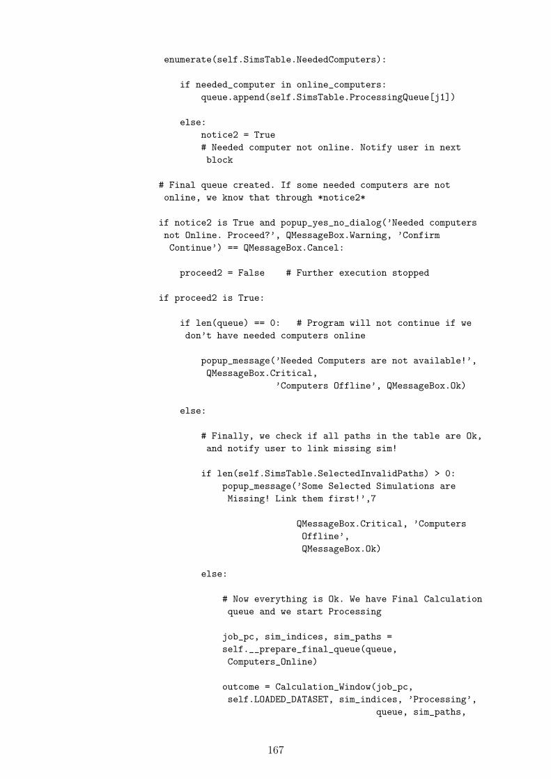
enumerate(self.SimsTable.NeededComputers):
if needed_computer in online_computers:
queue.append(self.SimsTable.ProcessingQueue[j1])
else:
notice2 = True
# Needed computer not online. Notify user in next
block
# Final queue created. If some needed computers are not
online, we know that through *notice2*
if notice2 is True and popup_yes_no_dialog(’Needed computers
not Online. Proceed?’, QMessageBox.Warning, ’Confirm
Continue’) == QMessageBox.Cancel:
proceed2 = False # Further execution stopped
if proceed2 is True:
if len(queue) == 0: # Program will not continue if we
don’t have needed computers online
popup_message(’Needed Computers are not available!’,
QMessageBox.Critical,
’Computers Offline’, QMessageBox.Ok)
else:
# Finally, we check if all paths in the table are Ok,
and notify user to link missing sim!
if len(self.SimsTable.SelectedInvalidPaths) > 0:
popup_message(’Some Selected Simulations are
Missing! Link them first!’,7
QMessageBox.Critical, ’Computers
Offline’,
QMessageBox.Ok)
else:
# Now everything is Ok. We have Final Calculation
queue and we start Processing
job_pc, sim_indices, sim_paths =
self.__prepare_final_queue(queue,
Computers_Online)
outcome = Calculation_Window(job_pc,
self.LOADED_DATASET, sim_indices, ’Processing’,
queue, sim_paths,
167

script)
if outcome.ReturnValue == ’Closed’:
self.LOADED_DATASET.update_records()
# DS is saved again after this line. Reload.
self.__reload_dataset()
def cmdOpenDataset_clicked(self):
ds_filename = popup_open_save(’Open’, DefaultSimDir, ’Open Dataset’,
’Dataset files (*.dat)’)
if ds_filename != ’’:
try:
self.commands_window.setWindowTitle(ds_filename)
self.LOADED_DATASET, self.SimsTable =
load_dataset_sim_table(self.Layout2, ds_filename)
self.LOADED_DATASET.update_records()
self.__link_all()
self.cmdInspectResults.setEnabled(True)
if len(self.LOADED_MACHINES) > 0:
self.cmdRunAll.setEnabled(True)
self.cmdOutput.setEnabled(True)
# Fill data in Window 1
for lbl, value in zip(self.Labels,
self.LOADED_DATASET.SummaryTable_2[0]):
lbl.setText(value)
except ImportError:
popup_message(’Invalid File’, QMessageBox.Critical, ’File Error’,
QMessageBox.Ok)
except PermissionError:
popup_message(’Permission Error. File already opened. Close it
and repeat.’,
QMessageBox.Critical, ’File Error’, QMessageBox.Ok)
except AttributeError:
popup_message(’Invalid File’, QMessageBox.Critical, ’File Error’,
QMessageBox.Ok)
def cmdCheckAllConnections_clicked(self):
if self.DialerPool.activeThreadCount() == 0:
168

# If searching is not in progress, check all connections
# Update Widgets
self.cnConsole.write(’’)
self.cnConsole.write(’*** Checking all Connections ***’)
self.MachinesTable.disable_buttons()
self.pbConnect.setValue(0)
to = float(self.txtConnectionTimeout.text())
for M in self.LOADED_MACHINES:
for i_o in [’Input’, ’Output’]:
worker = Dialer(M, i_o, to)
# Create workers for all machines/cases
worker.DSignals.answer.connect(self.connection_answer)
# Two functions added to the same event
worker.DSignals.answer.connect(self.update_progress_bar)
# Update progress bar
self.DialerPool.start(worker)
def cmdInspectResults_clicked(self):
changes = Data_Explorer(self.LOADED_DATASET.SummaryTable_2_2).Changes
if len(changes) > 0:
if popup_yes_no_dialog(’Save changes to Dataset?’,
QMessageBox.Question,
’Confirm changes’) == QMessageBox.Ok:
# Discard changes and close
for changed_set in changes:
self.LOADED_DATASET.change_results(changed_set)
self.__reload_dataset()
if __name__ == "__main__":
app = QApplication(sys.argv)
window = MainWindow()
window.show()
sys.exit(app.exec_())
Main Classes M2 Classes.py
import imp
import subprocess
169

from Main_ConfigConstants import PLAXIS_Path_MAIN_SERVER_PC
# PLAXIS Boilerplate Code #
found_module = imp.find_module(’plxscripting’, [PLAXIS_Path_MAIN_SERVER_PC])
plxscripting = imp.load_module(’plxscripting’, *found_module)
from plxscripting.easy import *
class Machine:
def __init__(self, ip, name, position, sims_path, i_path, o_path):
self.MachineID = name
# Initialize Basic Computer+Software machine Data
self.HostName = ip
self.NetworkPosition = position
self.SimsPath = sims_path
self.I_Path = i_path
self.O_Path = o_path
def __eq__(self, other):
return self.MachineID == other.MachineID
class PLAXIS_Machine(Machine):
def __init__(self, ip, name, position, sims_path, i_path, o_path, i_port, o_port):
super().__init__(ip, name, position, sims_path, i_path, o_path)
self.PortInput = i_port
# Input/Output ports for Plaxis Remote scripting
self.PortOutput = o_port
self.ConnectionStatus = [False, False]
# Preprocessor/Postprocessor are Offline
@property
def SummaryData(self):
return [self.MachineID, self.HostName, self.ConnectionStatus[0],
self.ConnectionStatus[1]]
def check_input_connection(self):
# If computer is remote, then we cannot run subprocess commands at it.
Instead, user should manually start batch
# file on the remote PC upon turning on. Checking of input and output
connection at remote pc is done just using
# the simple new_server(host, port) commands
170

if self.NetworkPosition == ’Local’:
# Open PLAXIS using Batch commands. Only possible for Local PC
subprocess.Popen(self.I_Path + ’ --AppServerPort=’ + str(self.PortInput))
S, G = new_server(self.HostName, self.PortInput)
def check_output_connection(self):
if self.NetworkPosition == ’Local’:
# Open PLAXIS using Batch commands. Only possible for Local PC
subprocess.Popen(self.O_Path + ’ --AppServerPort=’ + str(self.PortOutput))
S, G = new_server(self.HostName, self.PortOutput)
def online(self, io):
if io == ’Input’:
return self.ConnectionStatus[0]
elif io == ’Output’:
return self.ConnectionStatus[1]
PLAXIS Pre-/Postprocessing Scripts M2 Solvers.py
import imp
import time
import random
import numpy as np
from Main_ConfigConstants import PLAXIS_Path_MAIN_SERVER_PC
from M2_Solvers_PLAXIS_Functions import *
found_module = imp.find_module(’plxscripting’, [PLAXIS_Path_MAIN_SERVER_PC])
plxscripting = imp.load_module(’plxscripting’, *found_module)
from plxscripting.easy import *
# Pre/Postprocessing Scripts ########################################################
class Point:
def __init__(self, x, y, z):
self.X = x
self.Y = y
self.Z = z
def move(self, direction_vector):
self.X += direction_vector[0]
self.Y += direction_vector[1]
self.Z += direction_vector[2]
171

def distance(self, pt2):
dx = self.X - pt2.X
dy = self.Y - pt2.Y
dz = self.Z - pt2.Z
return (dx ** 2 + dy ** 2 + dz ** 2) ** 0.5
@property
def Coordinates(self):
return self.X, self.Y, self.Z
def rect_around_group(n, m, sx, sy, d, width, z):
# z in [m], other dimensions in diameters
x1 = -width*d
y1 = -width*d
x2 = ((n-1)*sx + width)*d
y2 = ((m-1)*sy + width)*d
return (x1, y1, z), (x2, y1, z), (x2, y2, z), (x1, y2, z)
def pile_group_preprocess(input_vector, save_filename, bp_path, host, port):
"""
Custom pile group 3D FEM model (PLAXIS 3D) v0.2
Model description:
3D pile is generated by replacing soil material in pile zone with pile material
(Concrete) - Wished-in-place pile
Pile installation effects are neglected
Soil-pile interface is simulated using 2D thin line elements and MC law.
Rint is the governing interface property
Structural forces in the pile are obtained using ’dummy’ beam through the pile
center. This beam has low stiffness and zero weight, in order to minimize its
impact on the global stiffness matrix. This also means that the pile behaviour
is assumed to be like Bernoulli-Euler beam (no deformation in the pile cross
section plane)
Pile material is LINEAR ELASTIC
Hardening Soil and Mohr-Coulomb constitutive models are supported through <<soil
model>> parameter.
Analysis is DRAINED
172
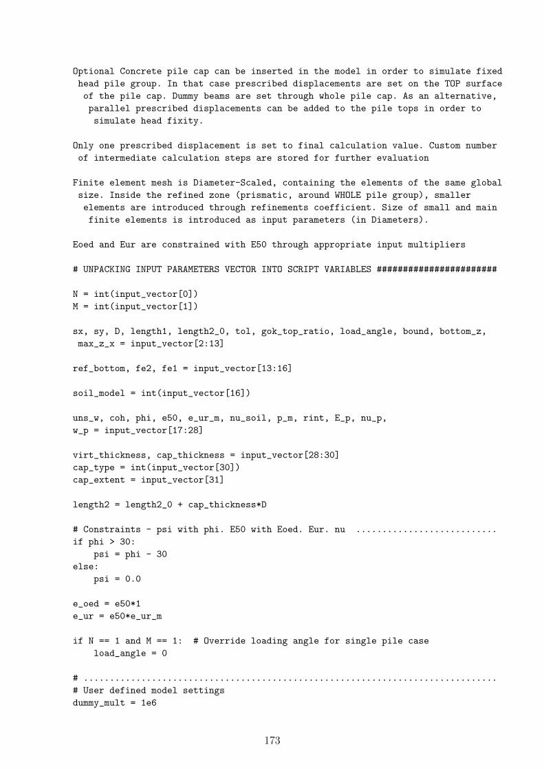
Optional Concrete pile cap can be inserted in the model in order to simulate fixed
head pile group. In that case prescribed displacements are set on the TOP surface
of the pile cap. Dummy beams are set through whole pile cap. As an alternative,
parallel prescribed displacements can be added to the pile tops in order to
simulate head fixity.
Only one prescribed displacement is set to final calculation value. Custom number
of intermediate calculation steps are stored for further evaluation
Finite element mesh is Diameter-Scaled, containing the elements of the same global
size. Inside the refined zone (prismatic, around WHOLE pile group), smaller
elements are introduced through refinements coefficient. Size of small and main
finite elements is introduced as input parameters (in Diameters).
Eoed and Eur are constrained with E50 through appropriate input multipliers
# UNPACKING INPUT PARAMETERS VECTOR INTO SCRIPT VARIABLES #######################
N = int(input_vector[0])
M = int(input_vector[1])
sx, sy, D, length1, length2_0, tol, gok_top_ratio, load_angle, bound, bottom_z,
max_z_x = input_vector[2:13]
ref_bottom, fe2, fe1 = input_vector[13:16]
soil_model = int(input_vector[16])
uns_w, coh, phi, e50, e_ur_m, nu_soil, p_m, rint, E_p, nu_p,
w_p = input_vector[17:28]
virt_thickness, cap_thickness = input_vector[28:30]
cap_type = int(input_vector[30])
cap_extent = input_vector[31]
length2 = length2_0 + cap_thickness*D
# Constraints - psi with phi. E50 with Eoed. Eur. nu ...........................
if phi > 30:
psi = phi - 30
else:
psi = 0.0
e_oed = e50*1
e_ur = e50*e_ur_m
if N == 1 and M == 1: # Override loading angle for single pile case
load_angle = 0
# ...............................................................................
# User defined model settings
dummy_mult = 1e6
173

split_vector = [0.015, 0.03, 0.06, 0.1] # Vector 1
steps = 20
# START ##########################################################################
s_i, g_i = new_server(host, port)
s_i.new()
g_i.save(save_filename)
# Save at the beginning. If something is wrong, we know which simulation was
running
# MATERIAL SETS #################################################################
Soil_M = None
if soil_model == 1:
Soil_M = MC_soil_drained(g_i, ’MC-Soil’, (uns_w, uns_w, e50, nu_soil, coh,
phi, psi, rint))
if soil_model == 2:
Soil_M = HS_soil_drained(g_i, ’HS-Soil’, (uns_w, uns_w, e50, e_oed, e_ur, p_m,
nu_soil, coh, phi, psi, rint))
Pile_Material = LE_soil(g_i, ’Concrete-Soil’, (w_p, E_p, nu_p))
Dummy_Material = LE_Beam(g_i, ’Dummy-Beam’, (0, E_p/dummy_mult, nu_p, A_Circle(D),
I_Circle(D), I_Circle(D), 0))
# BOREHOLES AND DOMAIN ##########################################################
# Setup model boundaries and mesh coefficients using scaled model parameters
min_Z_bound = length1 + bottom_z*D
# Calculate model domain size
X1 = ((N-1)*sx + 2*bound)*D
Y1 = ((M-1)*sy + 2*bound)*D
Z1 = length2 + min_Z_bound
zone_refinements = fe2/fe1
global_mesh = (fe1*D) / ((X1 ** 2 + Y1 ** 2 + Z1 ** 2) ** 0.5)
# BOREHOLES AND DOMAIN
g_i.SoilContour.initializerectangular(-bound*D,
-bound*D,
((N-1)*sx + bound)*D,
((M-1)*sy + bound)*D)
borehole = g_i.borehole(0, 0)
# Create Borehole and ground water level
borehole.Head = -min_Z_bound
soil_layer = g_i.soillayer(min_Z_bound)
# Create Soil Layer and assign material
174

soil_layer.Soil.Material = Soil_M
# STRUCTURES #####################################################################
g_i.gotostructures()
BottomPileVolumes = []
Surfaces_to_Create = []
for row in range(0, N):
for col in range(0, M):
Xp = row*sx*D
Yp = col*sy*D
# Setup points - coordinates
TopPoint = Point(Xp, Yp, length2)
BottomPoint = Point(Xp, Yp, -length1)
GroundPoint = Point(Xp, Yp, 0)
CapPoint = Point(Xp, Yp, length2-virt_thickness*D)
# Create 3D volume pile
ground_surf = surf_1(g_i, circle_polyline(g_i, D/2, GroundPoint), True)
bottom_volume, bottom_soil = g_i.extrude(ground_surf, (0, 0, -length1))
bottom_soil.Material = Soil_M
BottomPileVolumes.append(bottom_volume)
upper_volume, upper_soil = g_i.extrude(ground_surf, (0, 0, length2))
upper_soil.Material = Pile_Material
g_i.delete(ground_surf)
# Create Dummy Beam
Dummy_Beam = g_i.beam(TopPoint.Coordinates, BottomPoint.Coordinates)[3]
Dummy_Beam.Material = Dummy_Material
# Create Interface
surf1, surf2, surf3, group_1 = g_i.decomposesrf(bottom_volume)
g_i.delete(surf1, surf3)
# Remove not needed surface
g_i.posinterface(surf2)
# Pile shaft
# Create Pile Cap. Choose between real 3D (CASE 1) or parallel prescribed
displacements (CASE 0)
if cap_type == 0:
Surfaces_to_Create.append(surf_1(g_i, circle_polyline(g_i, D/2,
TopPoint), True)) # Top circle
if cap_type == 1:
175

Surfaces_to_Create.append(surf_1(g_i, circle_polyline(g_i, D/2,
TopPoint), True)) # Top circle
Surfaces_to_Create.append(surf_1(g_i, circle_polyline(g_i, D/2,
CapPoint), True)) # Bottom circle
if cap_type == 2:
pts_rect_cap_1 = rect_around_group(N, M, sx, sy, D, cap_extent, length2)
pts_rect_cap_2 = rect_around_group(N, M, sx, sy, D, cap_extent,
length2-virt_thickness*D)
Surfaces_to_Create.append(g_i.surface(pts_rect_cap_1[0], pts_rect_cap_1[1],
pts_rect_cap_1[2], pts_rect_cap_1[3]))
# Top rect
Surfaces_to_Create.append(g_i.surface(pts_rect_cap_2[0], pts_rect_cap_2[1],
pts_rect_cap_2[2], pts_rect_cap_2[3]))
cap_vol, cap_soil = g_i.extrude(Surfaces_to_Create[0],
(0, 0, -cap_thickness*D))
cap_soil.Material = Pile_Material
for surface in Surfaces_to_Create:
surf_displacement(g_i, surface, ’Prescribed’, ’Prescribed’, ’Free’)
# Create refinements zone around whole pile group
pts_rect_top = rect_around_group(N, M, sx, sy, D, max_z_x, -fe2*D)
rectangle_top = g_i.surface(pts_rect_top[0], pts_rect_top[1], pts_rect_top[2],
pts_rect_top[3])
extruded_vol, extruded_soil = g_i.extrude(rectangle_top,
(0, 0, -(min_Z_bound-(ref_bottom+fe2)*D)))
extruded_soil.Material = Soil_M
g_i.delete(rectangle_top)
# MESH ##########################################################################
g_i.gotomesh()
# Setup mesh refinements
for item in (g_i.Points[:] + g_i.Lines[:] + g_i.Surfaces[:]):
# Reset all coarseness to 1
item.CoarsenessFactor = 1
for volume in g_i.Volumes[:]:
# Setup all created volumes to refinement factor
volume.CoarsenessFactor = zone_refinements
# Scaled model geometry parametrization
176

echo = g_i.mesh(global_mesh)
elements = int(echo.split()[1])
nodes = int(echo.split()[3])
# PHASES #######################################################################
g_i.gotostages()
# [InitialPhase] - already created (default)
# [Construction] - Change Pile material to Concrete, activate Upper pile Volume,
DummyBeams and Interfaces
phase_2 = create_phase(g_i, ’Construction’, None)
for vol in BottomPileVolumes:
g_i.setmaterial(vol, phase_2, Pile_Material)
for item in g_i.Beams[:] + g_i.Soils[:] + g_i.SurfaceDisplacements[:] +
g_i.Interfaces[:]:
item.Active[phase_2] = True
# [Prescribed Displacements] .....................................................
fx_list = [round(item*D*Cosinus(load_angle)/gok_top_ratio, 4)
for item in split_vector]
fy_list = [round(item*D*Sinus(load_angle)/gok_top_ratio, 4)
for item in split_vector]
for fx, fy in zip(fx_list, fy_list):
load_phase = create_phase(g_i,
’Ux=’ + str(fx) + ’ m ’ + ’Uy=’ + str(fy) + ’ m’, (tol, steps))
for s_d in g_i.SurfaceDisplacements[:]:
s_d.ux[load_phase] = fx
s_d.uy[load_phase] = fy
# CALCULATION ##################################################################
g_i.calculate()
calc_success = not any(phase.CalculationResult != 1 for phase in g_i.Phases)
g_i.save(save_filename)
s_i.close()
return calc_success, nodes, elements
def pile_group_check_mat(input_vector, save_filename, bp_path, host, port):
177

# This short PLAXIS script creates the material set with given input parameters.
If error inside the PLAXIS occurs, this script returns FALSE, and continues to
check the next simulation. Results are written into the dataset, and displayed
on Console. After datasets are checked, we can run real simulations
with new script.
soil_model = int(input_vector[16])
uns_w, coh, phi, e50, e_ur_m, nu_soil, p_m, rint = input_vector[17:25]
# Constraints - psi with phi. E50 with Eoed. Eur. nu
if phi > 30:
psi = phi - 30
else:
psi = 0.0
e_oed = e50*1
e_ur = e50*e_ur_m
s_i, g_i = new_server(host, port)
s_i.new()
try: # Error can occur in this block of code.
if soil_model == 1:
MC_soil_drained(g_i, ’MC-Soil’, (uns_w, uns_w, e50, nu_soil, coh, phi,
psi, rint))
if soil_model == 2:
HS_soil_drained(g_i, ’HS-Soil’, (uns_w, uns_w, e50, e_oed, e_ur, p_m,
nu_soil, coh, phi, psi, rint))
except:
s_i.close()
print(False, save_filename)
return False, 0, 0
s_i.close()
print(True, save_filename)
return True, 0, 0
def pile_group_postprocess(filename, host, port):
"""
Custom pile group 3D FEM model (PLAXIS 3D) v0.1 - POSTPROCESSING
Model description:
At this stage, only results from Dummy Beams are extracted for postprocessing.
Soil and interface results remain in the raw simulation results.
Loading is applied in following phases:
1. K0 - InitialPhase
178

2. Construction (Horizontal Displacements are set to zero, small vertical
displacements occur due to gravity load)
3+ Horizontal displacement increments
Results are extracted phase by phase, starting from <<Construction>> phase where
Horizontal Displacements are 0
Results are extracted from MESH NODES and using results SMOOTHING in PLAXIS
Result Types: Displacements (x, y, z, total), Structural Forces (N, Q12, Q13, M2,
M3), Node Coordinates (x, y, z)
In postprocessing, raw data is splitted pile by pile using pile coordinates filter
"""
dummy_mult = 1e6
# START
try:
s_o, g_o = new_server(host, port)
s_o.open(filename)
ResultTypes_Beam = [’X’, ’Y’, ’Z’, ’Ux’, ’Uy’, ’Uz’, ’Utot’,
’LinearStructureN’, ’LinearStructureQ12’, ’LinearStructureQ13’,
’LinearStructureM2’, ’LinearStructureM3’]
# Determine number of PLAXIS Results Table rows
rows = len(g_o.getresults(g_o.Phases[1], g_o.ResultTypes.Beam.X,
’node’, True)[:])
# Determine number of stored loading steps. K0 calculation is ignored
saved_steps = [step for step in g_o.Steps[1:] if hasattr(step.Info,
’GlobalError’)]
layers = len(saved_steps)
# Extract results for Beams, step by step
results = np.zeros((rows, len(ResultTypes_Beam), layers))
for i, step in enumerate(saved_steps):
for j, res_type in enumerate(ResultTypes_Beam):
results[:, j, i] = g_o.getresults(step, getattr(g_o.ResultTypes.Beam,
res_type), ’node’, True)[:]
# Multiply Q12, Q13, M2, M3 with dummy multiplier to get real results for
Dummy Beam structural forces
for r in range(0, rows):
for p in range(0, layers):
for c in range(8, 12):
results[r, c, p] *= dummy_mult
179
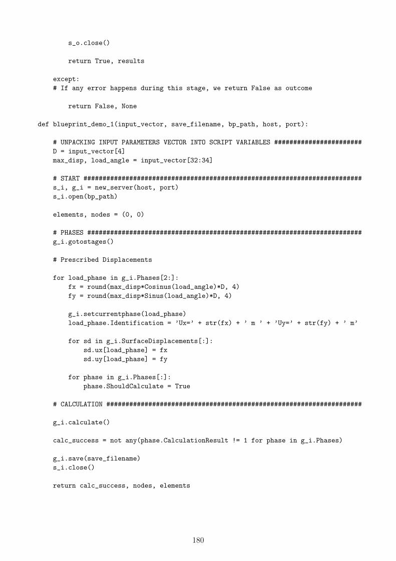
s_o.close()
return True, results
except:
# If any error happens during this stage, we return False as outcome
return False, None
def blueprint_demo_1(input_vector, save_filename, bp_path, host, port):
# UNPACKING INPUT PARAMETERS VECTOR INTO SCRIPT VARIABLES #######################
D = input_vector[4]
max_disp, load_angle = input_vector[32:34]
# START #########################################################################
s_i, g_i = new_server(host, port)
s_i.open(bp_path)
elements, nodes = (0, 0)
# PHASES ########################################################################
g_i.gotostages()
# Prescribed Displacements
for load_phase in g_i.Phases[2:]:
fx = round(max_disp*Cosinus(load_angle)*D, 4)
fy = round(max_disp*Sinus(load_angle)*D, 4)
g_i.setcurrentphase(load_phase)
load_phase.Identification = ’Ux=’ + str(fx) + ’ m ’ + ’Uy=’ + str(fy) + ’ m’
for sd in g_i.SurfaceDisplacements[:]:
sd.ux[load_phase] = fx
sd.uy[load_phase] = fy
for phase in g_i.Phases[:]:
phase.ShouldCalculate = True
# CALCULATION ###################################################################
g_i.calculate()
calc_success = not any(phase.CalculationResult != 1 for phase in g_i.Phases)
g_i.save(save_filename)
s_i.close()
return calc_success, nodes, elements
180
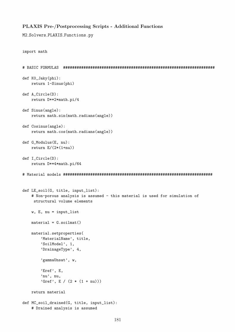
PLAXIS Pre-/Postprocessing Scripts - Additional Functions
M2 Solvers PLAXIS Functions.py
import math
# BASIC FORMULAS ###################################################################
def K0_Jaky(phi):
return 1-Sinus(phi)
def A_Circle(D):
return D**2*math.pi/4
def Sinus(angle):
return math.sin(math.radians(angle))
def Cosinus(angle):
return math.cos(math.radians(angle))
def G_Modulus(E, nu):
return E/(2*(1+nu))
def I_Circle(D):
return D**4*math.pi/64
# Material models ##################################################################
def LE_soil(G, title, input_list):
# Non-porous analysis is assumed - this material is used for simulation of
structural volume elements
w, E, nu = input_list
material = G.soilmat()
material.setproperties(
’MaterialName’, title,
’SoilModel’, 1,
’DrainageType’, 4,
’gammaUnsat’, w,
’Eref’, E,
’nu’, nu,
’Gref’, E / (2 * (1 + nu)))
return material
def MC_soil_drained(G, title, input_list):
# Drained analysis is assumed
181
unsat_w, sat_w, E, nu, c, phi, psi, rint = input_list
material = G.soilmat()
material.setproperties(
’MaterialName’, title,
’SoilModel’, 2,
’DrainageType’, 0,
’gammaUnsat’, unsat_w,
’gammaSat’, sat_w,
’Gref’, G_Modulus(E, nu),
’nu’, nu,
’cref’, c,
’phi’, phi,
’psi’, psi,
’K0Primary’, K0_Jaky(phi),
’K0Secondary’, K0_Jaky(phi),
’DefaultValuesAdvanced’, True,
’Rinter’, rint)
return material
def HS_soil_drained(G, title, input_list):
# p=100 kPa is assumed. It is also a default value (default)
# Rf = 0.9 is assumed (default value)
# Drained Analysis is assumed
unsat_w, sat_w, e50, e_oed, e_ur, power_m, nu, c, phi, psi, rint = input_list
material = G.soilmat()
material.setproperties(
’MaterialName’, title,
’SoilModel’, 3,
’DrainageType’, 0,
’gammaUnsat’, unsat_w,
’gammaSat’, sat_w,
’E50ref’, e50,
’EoedRef’, e_oed,
’Gref’, G_Modulus(e_ur, nu),
’nu’, nu,
’powerm’, power_m,
182

’cref’, c,
’phi’, phi,
’psi’, psi,
’K0nc’, K0_Jaky(phi),
’K0Primary’, K0_Jaky(phi),
’K0Secondary’, K0_Jaky(phi),
’DefaultValuesAdvanced’, True,
’Rinter’, rint)
return material
def LE_Beam(G, title, input_list):
w, E, nu, area, I2, I3, I23 = input_list
material = G.beammat()
material.setproperties(
’MaterialName’, title,
’IsLinear’, True,
’w’, w,
’E’, E,
’nu’, nu,
’A’, area,
’Iyy’, I3,
’Izz’, I2,
’Iyz’, I23)
return material
# Geometry ..........................................................................
def circle_polyline(G, radius, center):
# Create horizontal circle line in PLAXIS
xs, ys, zs = center.Coordinates
line_1, point_1 = G.polycurve((xs, ys - radius, zs), (1, 0, 0), (0, 1, 0), ’Arc’,
(0, 360, radius))
return line_1
def surf_1(G, line, delete_line=True):
surf = G.surface(line)
if delete_line:
G.delete(line)
183

return surf
def surf_displacement(G, surface, x, y, z):
surf_disp = G.surfdispl(surface)
surf_disp.Displacement_x = x
surf_disp.Displacement_y = y
surf_disp.Displacement_z = z
return surf_disp
# Phases ............................................................................
def create_phase(G, title, tol_steps):
new_phase = G.phase(G.Phases[-1])
G.setcurrentphase(new_phase)
new_phase.Identification = title
if tol_steps is not None:
new_phase.Deform.UseDefaultIterationParams = False
new_phase.Deform.ToleratedError = tol_steps[0]/100
new_phase.MaxStepsStored = tol_steps[1]
return new_phase
User Interface Classes M2 WidgetClasses.py
import numpy as np
import time
from PyQt5.QtCore import pyqtSignal, Qt
from PyQt5.QtWidgets import QMessageBox, QAbstractScrollArea, QPushButton,
QTableWidget, QDialog, QLineEdit, QLabel
from PyQt5.QtWidgets import QComboBox, QCheckBox, QGridLayout, QTextEdit, QTabWidget,
QWidget
from Main_Functions import popup_open_save, popup_message, popup_yes_no_dialog,
popup_select_folder, export_nd_xl
from Main_Functions import set_shapes, all_processed, global_shape, parse_xl_nd_full,
measure_xl_3D, xl_dimensions
from Main_ConfigConstants import DefaultSimDir, Max_Widgets
from Main_WidgetClasses import IconCell, fill_table_items, StringCell,
cell_label_button
184

class DataTable(QTableWidget):
table_added = pyqtSignal(int, object)
def __init__(self, table_data, table_headers, result_tables_list):
super().__init__(len(table_data), len(table_headers))
self.__ResultTables = result_tables_list
self.__Data_Buttons = []
self.__SimNames = [item[0] for item in table_data]
self.__Shapes = set_shapes(self.__ResultTables)
# Read numpy table shapes
self.setHorizontalHeaderLabels(table_headers)
# Fill Table items
self.horizontalHeader().setVisible(True)
self.setSizeAdjustPolicy(QAbstractScrollArea.AdjustToContents)
fill_table_items(self, table_data)
for r, shape in enumerate(self.__Shapes):
# Create buttons
button = DataTable.__table_button(shape)
button.clicked.connect(self.__emit_button_clicked)
self.setCellWidget(r, 5, cell_label_button(’’, button))
self.__Data_Buttons.append(button)
self.clearSelection()
self.resizeColumnsToContents()
@property
def GlobalShape(self):
return global_shape(self.__Shapes)
@staticmethod
def __table_button(shape):
enabled = True
if shape is not None:
if len(shape) <= 3:
caption = ’Show Data Table ’ + str(shape)
else:
caption = ’4D+ Table’
enabled = False
else:
caption = ’Add Data Table’
new_button = QPushButton(caption)
185

new_button.setEnabled(enabled)
return new_button
def __emit_button_clicked(self):
r = 0
# Determine which button was clicked, r is a button index
for r in range(0, len(self.__Data_Buttons)):
if self.sender() == self.__Data_Buttons[r]:
break
button_caption = self.__Data_Buttons[r].text()
# Button Found. Define what to do depending on button caption
if button_caption != ’Add Data Table’: # Showing Data
Numpy_Table(self.__ResultTables[r])
elif button_caption == ’Add Data Table’: # Adding Data Table
filename = popup_open_save(’Open’, DefaultSimDir, ’Import Data’,
’Data files (*.xls *.xlsx *.npy)’)
if filename != ’’: # Something Chosen
try:
# file load errors catcher
data_to_add = None
if filename.endswith(’.npy’):
# Determine file type
data_to_add = np.load(filename)
# Numpy array
else:
# Parse Excel File
rows, columns, sheets = measure_xl_3D(filename)
if rows > 0 and columns > 0:
data_to_add = parse_xl_nd_full(filename, rows, columns
, sheets)
if data_to_add is None:
popup_message(’Error in the Excel file. Nothing to Load!
Please check the data!’, QMessageBox.Critical,
’Excel Table Error’, QMessageBox.Ok)
else:
self.__add_Data_Table(data_to_add, r)
except:
186

# Catched: [InvalidFileException], [BadZipFile], [OSError]
popup_message(’Data Import Error! ’, QMessageBox.Critical,
’Import Error’, QMessageBox.Ok)
def __add_Data_Table(self, data_to_add, r):
if popup_yes_no_dialog(’Add Data Table with shape ’ +
str(np.shape(data_to_add)) + ’ to Dataset?’, QMessageBox.Information,
’Confirm Continue’) == QMessageBox.Ok:
self.__ResultTables[r] = data_to_add
self.__Shapes[r] = np.shape(data_to_add)
new_button = DataTable.__table_button(np.shape(data_to_add))
new_button.clicked.connect(self.__emit_button_clicked)
self.__Data_Buttons[r] = new_button
self.setItem(r, 5, IconCell(True))
self.setCellWidget(r, 5, cell_label_button(’’, new_button))
self.table_added.emit(r, data_to_add)
def __all_processed(self):
return all_processed(self.__ResultTables)
def __nothing_processed(self):
for table in self.__ResultTables:
if table is not None:
return False
return True
def __default_captions(self):
if self.GlobalShape is not None and len(self.GlobalShape) <= 3:
# Consistent/max 3D tables are results
rows, columns, tabs = xl_dimensions(self.GlobalShape)
row_captions = [’Row_’ + str(r) for r in range(1, rows + 1)]
columns_captions = [’Column_’ + str(c) for c in range(1, columns + 1)]
tab_captions = [’Tab_’ + str(t) for t in range(1, tabs + 1)]
return row_captions, columns_captions, tab_captions
else:
return None
def can_export(self):
# Check if there are any results for export. Also, if some results are
missing, ask user for continue
# Return True if there is something for export. False - program will not
continue
187
proceed = True
if self.__nothing_processed() is True:
popup_message(’Nothing for Export!’, QMessageBox.Warning, ’No Results’,
QMessageBox.Ok)
proceed = False
else:
if not self.__all_processed():
if popup_yes_no_dialog(’Some results are missing. Proceed?’,
QMessageBox.Information,
’Confirm Continue’) == QMessageBox.Cancel:
proceed = False
return proceed
def export_numpy_tables(self):
saved = False
folder_to_save = popup_select_folder(DefaultSimDir)
if folder_to_save != ’’:
for j, table in enumerate(self.__ResultTables):
if table is not None:
np.save(folder_to_save + ’\\’ + self.__SimNames[j], table)
popup_message(’Results Succesfully Exported as Numpy Tables.’,
QMessageBox.Information, ’Export Succesfull’, QMessageBox.Ok)
saved = True
return saved
def __export_joined(self, r_c, c_c):
tab_names = []
data_tables = []
rows, columns, tabs = xl_dimensions(self.GlobalShape)
for j, table in enumerate(self.__ResultTables):
if table is not None:
tab_names.append(self.__SimNames[j])
data_tables.append(table)
data_table_2 = np.ndarray((rows, columns, len(data_tables)))
for j in range(0, len(data_tables)):
if len(self.GlobalShape) == 2:
data_table_2[:, :, j] = data_tables[j]
188

elif len(self.GlobalShape) == 1:
data_table_2[:, 0, j] = data_tables[j]
exported = False
wb = export_nd_xl(r_c, c_c, tab_names, data_table_2)
filename = popup_open_save(’Save’, DefaultSimDir, ’Save As’, ’Excel files
(*.xlsx)’)
if filename != ’’:
try:
wb.save(filename)
exported = True
except PermissionError:
popup_message(’Permission Error. File already opened. Close it and
repeat.’, QMessageBox.Critical, ’File Error’, QMessageBox.Ok)
return exported
def __export_sim_sim_excel(self, r_c, c_c, t_c):
folder_to_save = popup_select_folder(DefaultSimDir)
successfull = False
if folder_to_save != ’’:
for j, table in enumerate(self.__ResultTables):
if table is not None:
wb = export_nd_xl(r_c, c_c, t_c, table)
try:
wb.save(folder_to_save + ’\\’ + self.__SimNames[j] + ’.xlsx’)
successfull = True
except PermissionError:
popup_message(’Permission Error. File already opened.
Close it and repeat.’, QMessageBox.Critical, ’File Error’,
QMessageBox.Ok)
return successfull
def export_excel_consistent(self):
input_data = Input_Form_Excel_Captions(self.__default_captions(),
self.GlobalShape).ReturnValues
if input_data is not None:
(joined, sim_by_sim), (r_c, c_c, t_c) = input_data
successfull = False
if joined:
189
successfull = self.__export_joined(r_c, c_c)
if sim_by_sim:
successfull = self.__export_sim_sim_excel(r_c, c_c, t_c)
if successfull:
popup_message(’Results Succesfully Exported to Excel format.’,
QMessageBox.Information, ’Export Succesfull’, QMessageBox.Ok)
def export_all(self):
folder_to_save = popup_select_folder(DefaultSimDir)
if folder_to_save != ’’:
successfull = True
for j, shape in enumerate(self.__Shapes):
if shape is not None:
if len(shape) > 3:
np.save(folder_to_save + ’\\’ + self.__SimNames[j],
self.__ResultTables[j])
else:
r, c, t = xl_dimensions(shape)
wb = export_nd_xl(None, None,
[’Tab_’+str(i) for i in range(0, t)], self.__ResultTables[j])
try:
wb.save(folder_to_save + ’\\’ + self.__SimNames[j] +
’.xlsx’)
except PermissionError:
popup_message(’Permission Error. File already opened.
Close it and repeat.’, QMessageBox.Critical, ’File
Error’, QMessageBox.Ok)
successfull = False
if successfull:
popup_message(’Results Succesfully Exported!’,
QMessageBox.Information, ’Export Succesfull’, QMessageBox.Ok)
class ActiveTable_2(QTableWidget):
cell_button_clicked = pyqtSignal(int, int)
def __init__(self, table_data, table_captions, columns, button_captions, start_c):
super().__init__(len(table_data), len(table_captions))
# Create simple table widget
self.setHorizontalHeaderLabels(table_captions)
190

self.horizontalHeader().setVisible(True)
self.setSizeAdjustPolicy(QAbstractScrollArea.AdjustToContents)
fill_table_items(self, table_data)
# Create Custom Widgets inside Cells (2 columns). Custom widgets consist of
Button and Label.
self.Buttons = []
self.StartingColumn = start_c
for c in range(self.StartingColumn, self.StartingColumn+columns):
button_col = []
for r in range(0, len(table_data)):
button = QPushButton(button_captions[c-self.StartingColumn])
button.clicked.connect(self.emit_clicked)
self.setCellWidget(r, c, cell_label_button(’’, button))
button_col.append(button)
self.Buttons.append(button_col)
self.clearSelection()
self.resizeColumnsToContents()
@property
def SelectedRows(self):
return sorted(set(i.row() for i in self.selectedIndexes()))
def emit_clicked(self):
for c in range(0, len(self.Buttons)):
for r in range(0, len(self.Buttons[0])):
if self.sender() == self.Buttons[c][r]:
self.Buttons[c][r].setEnabled(False)
# Disable button on click
self.cell_button_clicked.emit(r, c+self.StartingColumn)
break
def reset_cell(self, value, row, col):
button = self.Buttons[col-self.StartingColumn][row]
button.setEnabled(True)
self.setItem(row, col, IconCell(value))
self.setCellWidget(row, col, cell_label_button(’’, button))
self.resizeColumnsToContents()
self.clearSelection()
def disable_buttons(self):
for column_buttons in self.Buttons:
for button in column_buttons:
191

button.setEnabled(False)
class Console(QTextEdit):
def __init__(self, app):
super().__init__()
self.TopApp = app
def write(self, text_string):
self.append(text_string)
self.verticalScrollBar().setValue(self.verticalScrollBar().maximum())
self.TopApp.processEvents()
def twrite(self, text_string):
self.write(time.strftime("%b %d %Y %H:%M:%S") + ’ ’ + text_string)
class Numpy_Table(QDialog):
def __init__(self, results_table):
super().__init__()
tab_widget = QTabWidget()
top_layout = QGridLayout()
self.setLayout(top_layout)
top_layout.addWidget(tab_widget)
dimensions = list(np.shape(results_table))
# Set rows, columns, tabs
tabs = 1
columns = 1
if len(dimensions) == 3:
rows, columns, tabs = (dimensions[0], dimensions[1], dimensions[2])
elif len(dimensions) == 2:
rows, columns = (dimensions[0], dimensions[1])
elif len(dimensions) == 1:
rows = dimensions[0]
for tab in range(0, tabs):
# Create Tab widget page
tab_page = QWidget()
tab_page_layout = QGridLayout()
tab_page.setLayout(tab_page_layout)
tab_widget.addTab(tab_page, str(tab+1))
tab_table = QTableWidget(rows, columns)
tab_page_layout.addWidget(tab_table)
# Slice Results to 1D or 2D table - create fill_table
if len(dimensions) == 3:
192

fill_table = results_table[:, :, tab]
fill_rows = fill_table[:]
else:
fill_rows = results_table[:]
if len(dimensions) > 1:
for r in range(0, rows): # Fill Table
for c in range(0, columns):
tab_table.setItem(r, c, StringCell(str(fill_rows[r][c])))
else:
for r in range(0, rows):
tab_table.setItem(r, 0, StringCell(str(fill_rows[r])))
self.exec_()
class Input_Form_Excel_Captions(QDialog):
def __init__(self, captions_tuple, glob_shape):
super(Input_Form_Excel_Captions, self).__init__()
self.setWindowTitle(’Setup Export Table’)
self.setWindowFlags(Qt.CustomizeWindowHint)
self.layout = QGridLayout()
self.setLayout(self.layout)
cmdOK = QPushButton(’Accept’)
cmdOK.clicked.connect(self.cmdOK_clicked)
self.cbNoCaptions = QCheckBox(’No Captions’)
self.cbNoCaptions.setChecked(False)
self.cbNoCaptions.stateChanged.connect(self.cbNoCaptions_set)
row_labels = captions_tuple[0]
col_labels = captions_tuple[1]
tab_labels = captions_tuple[2]
rows = len(row_labels)
cols = len(col_labels)
tabs = len(tab_labels)
last_text_field_row = max(rows, cols, tabs)+1
self.RowFields = [QLineEdit(row_labels[r]) for r in range(0, rows)]
self.ColFields = [QLineEdit(col_labels[c]) for c in range(0, cols)]
self.TabFields = [QLineEdit(tab_labels[t]) for t in range(0, tabs)]
self.layout.addWidget(QLabel(’Rows’), 0, 0)
self.layout.addWidget(QLabel(’Columns’), 0, 1)
self.layout.addWidget(QLabel(’Sheets’), 0, 2)
if rows > Max_Widgets or cols > Max_Widgets or tabs > Max_Widgets:
193

last_text_field_row = Max_Widgets + 1
popup_message(’Maximum number of fields reached!’,
QMessageBox.Information, ’Input Fields’, QMessageBox.Ok)
self.__add_widgets(rows, self.RowFields, 0)
self.__add_widgets(cols, self.ColFields, 1)
self.__add_widgets(tabs, self.TabFields, 2)
self.cmbJoinSplit = QComboBox()
if len(glob_shape) <= 2:
self.cmbJoinSplit.addItems([’Export to Single File’,
’Export to Separate Files’])
for widget in self.TabFields:
# Disable Tab Captions if we export to single file
widget.setEnabled(False)
else:
self.cmbJoinSplit.addItems([’Export to Separate Files’])
self.cmbJoinSplit.currentIndexChanged.connect(self.cmbJoinSplit_changed)
self.layout.addWidget(self.cmbJoinSplit, last_text_field_row+2, 0)
self.layout.addWidget(self.cbNoCaptions, last_text_field_row+2, 1)
self.layout.addWidget(cmdOK, last_text_field_row+2, 2)
self.ReturnValues = None
self.exec_()
def __add_widgets(self, size, widgets_list, col_index):
if size <= Max_Widgets:
# Add all widgets from the list
for j, widget in enumerate(widgets_list):
self.layout.addWidget(widget, j+1, col_index)
else:
# Add first <<Max_Widgets>> from the list
for i in range(0, Max_Widgets):
self.layout.addWidget(widgets_list[i], i+1, col_index)
def cbNoCaptions_set(self):
for widget in (self.RowFields + self.ColFields):
widget.setEnabled(not self.cbNoCaptions.isChecked())
def cmdOK_clicked(self):
data_empty = False
for text_field in (self.RowFields + self.ColFields + self.TabFields):
if text_field.text() == ’’:
data_empty = True
194

popup_message(’Please fill all fields!’, QMessageBox.Warning,
’Input Error’, QMessageBox.Ok)
break
if not data_empty:
new_rows = [r_f.text() for r_f in self.RowFields]
new_cols = [c_f.text() for c_f in self.ColFields]
new_tabs = [t_f.text() for t_f in self.TabFields]
if self.cmbJoinSplit.currentText() == ’Export to Single File’:
joined, sim_by_sim = (True, False)
else:
joined, sim_by_sim = (False, True)
if self.cbNoCaptions.isChecked():
titles = (None, None, new_tabs)
else:
titles = (new_rows, new_cols, new_tabs)
self.ReturnValues = ((joined, sim_by_sim), titles)
self.close()
def cmbJoinSplit_changed(self):
if self.cmbJoinSplit.currentText() == ’Export to Separate Files’:
enabled = True
else:
enabled = False
for widget in self.TabFields:
widget.setEnabled(enabled)
Module 3 - System Identification Package M3.py
import sys
import numpy as np
from PyQt5.QtCore import Qt, QObject, QRunnable, pyqtSignal, pyqtSlot, QThreadPool
from PyQt5.QtGui import QColor
from PyQt5.QtWidgets import QComboBox, QMessageBox, QGridLayout, QDialog, QPushButton,
QLineEdit, QLabel, QMdiArea
from PyQt5.QtWidgets import QMainWindow, QApplication, QMdiSubWindow, QWidget
from Main_Functions import load_object, parse_xl_nd, popup_message,
popup_yes_no_dialog, popup_open_save
from Main_Functions import export_nd_xl, vector_nd, nd_vector, set_shapes,
195

all_processed, global_shape
from Main_ConfigConstants import DefaultSimDir, MinimumMMTrain
from Main_WidgetClasses import Input_ExcelCaptions
from MyClasses1 import SnapshotMatrix
from M3_Metamodels import MM_LIST, MM_CALLER_2
from M3_GSA import GSA_LIST, GSA_CALLER
from M3_BackAnalysis import BA_CALLER, BA_LIST
from M3_Observers import MM_BA_Observer, BA_GSA_Worker
from M3_WidgetClasses import Snapshot_Table, BA_Parameters, MMParameterTable, PB,
Simple_Table
from M3_Classes import Metamodel
from M3_Plotting import XY_Plot, Plotter_2D
def on_off_widgets(on_off, w_list):
for widget in w_list:
widget.setEnabled(on_off)
class TrainerSignals(QObject):
finished = pyqtSignal(object, tuple)
started = pyqtSignal()
class Trainer(QRunnable):
def __init__(self, input_data, test_data):
super(Trainer, self).__init__()
self.TSignals = TrainerSignals()
self.__InputData = input_data
self.__TestData = test_data
@pyqtSlot()
def run(self):
self.TSignals.started.emit()
input1, input2, input3 = self.__InputData
new_metamodel = Metamodel(input1, input2, input3)
# Test new Metamodel
input_test_m = self.__TestData[0]
output_test_m = self.__TestData[1]
196
nrmse_1 = new_metamodel.Training_NRMSE
if input_test_m is not None:
nrmse_2 = new_metamodel.test(input_test_m, output_test_m)
else:
nrmse_2 = None
self.TSignals.finished.emit(new_metamodel, (nrmse_1, nrmse_2))
class BA_Window(QDialog):
def __init__(self, metamodel):
super(BA_Window, self).__init__()
self.Metamodel = metamodel[0]
self.InputCaptions = metamodel[1][3]
self.SnapCaptions = metamodel[2][3]
self.BAPool = QThreadPool()
self.setFixedSize(700, 1000)
self.setWindowFlags(Qt.CustomizeWindowHint)
self.setWindowTitle(’Back Analysis’)
layout = QGridLayout()
self.setLayout(layout)
self.tblInput = BA_Parameters(self.InputCaptions, metamodel[1][2], ’Input’)
self.tblSnapshots = BA_Parameters(self.SnapCaptions, metamodel[2][2],
’Snapshots’)
self.pbBAProgress = PB()
self.cmbBA = QComboBox()
self.cmbBA.addItems(BA_LIST)
self.cmdStart = QPushButton(’Start Back Analysis’)
self.cmdClose = QPushButton(’Close’)
self.cmdExport = QPushButton(’Export Results to Excel’)
self.cmdPlotResults = QPushButton(’Plot Results’)
self.cmdStart.clicked.connect(self.cmdStart_clicked)
self.cmdClose.clicked.connect(self.cmdClose_clicked)
self.cmdExport.clicked.connect(self.cmdExport_clicked)
self.cmdPlotResults.clicked.connect(self.cmdPlotResults_clicked)
layout.addWidget(QLabel(’Select Back Analysis Algorithm’), 0, 0)
layout.addWidget(self.cmbBA, 1, 0)
layout.addWidget(QLabel(’Input Parameters’), 2, 0)
layout.addWidget(self.tblInput, 3, 0)
layout.addWidget(QLabel(’Snapshots’), 4, 0)
layout.addWidget(self.tblSnapshots, 5, 0)
197

layout.addWidget(self.cmdStart, 6, 0)
layout.addWidget(self.cmdPlotResults, 7, 0)
layout.addWidget(self.cmdExport, 8, 0)
layout.addWidget(self.cmdClose, 9, 0)
layout.addWidget(self.pbBAProgress, 10, 0)
self.Identified = None
self.Search = None
self.BA_Object = None
self.WList1 = [self.cmdStart, self.cmdClose]
self.WList2 = [self.cmdExport, self.cmdPlotResults]
on_off_widgets(False, self.WList2)
self.exec_()
def cmdStart_clicked(self):
if popup_yes_no_dialog(’Process Cannot be stopped! Proceed?’,
QMessageBox.Question, ’Confirm Start’) == QMessageBox.Ok:
ba_input = self.tblInput.analysis_data()
# Obtain BA search parameters
ba_output = self.tblSnapshots.analysis_data()
self.Search = ba_output[1]
if ba_input is not None and ba_output is not None:
ba_algorithm_class, input_p_list = BA_CALLER[self.cmbBA.currentText()]
# Obtain BA from BA database
ba_alg_input = InputParameters(input_p_list, ’Input
Parameters’).ReturnValues
if ba_alg_input is not None:
# Initialize Back analysis algorithm object instance and attach
observers for GUI
self.BA_Object = ba_algorithm_class(self.Metamodel, ba_alg_input,
ba_input, ba_output, self.InputCaptions, self.SnapCaptions)
self.BA_Object.attach_observer(MM_BA_Observer
(self.pbBAProgress.update))
self.pbBAProgress.initialize(self.BA_Object.MaxIterations)
on_off_widgets(False, self.WList1 + self.WList2)
worker = BA_GSA_Worker(self.BA_Object)
worker.Signals.finished.connect(self.BA_ended)
self.BAPool.start(worker)
198

else:
popup_message(’Check Search Parameters and Repeat!’,
QMessageBox.Warning, ’Input Error’, QMessageBox.Ok)
def cmdClose_clicked(self):
self.close()
def cmdExport_clicked(self):
self.BA_Object.export_results()
def cmdPlotResults_clicked(self):
self.BA_Object.plot_results()
@pyqtSlot(tuple)
def BA_ended(self, result_tuple):
self.Identified, of_value_final = result_tuple
ident_vector = nd_vector(self.Metamodel.calculate(vector_nd(self.Identified)))
self.__update_GUI_end(self.Identified, ident_vector)
def __update_GUI_end(self, found_vector, identified_vector):
on_off_widgets(True, self.WList1 + self.WList2)
self.pbBAProgress.end()
Dividend, Divisor = (0, 0)
# Calculate NRMSE using identified parameters
for i in range(0, len(identified_vector)):
Dividend += (self.Search[i] - identified_vector[i]) ** 2
Divisor += self.Search[i] ** 2
nrmse_perc = np.sqrt(Dividend / Divisor)*100
# Update I/O tables
self.tblInput.update_column(5, found_vector)
self.tblSnapshots.update_column(5, identified_vector)
popup_message(’Back Analysis Completed! NRMSE = ’ + str(round(nrmse_perc, 2))
+ ’%’, QMessageBox.Information, ’Back Analysis Completed’, QMessageBox.Ok)
class GSA_Window(QDialog):
def __init__(self, metamodel):
super(GSA_Window, self).__init__()
self.Metamodel = metamodel[0]
self.GSAPool = QThreadPool()
self.InputCaptions = metamodel[1][3]
self.OutputCaptions = metamodel[2][3]
199

self.setFixedSize(300, 300)
self.setWindowFlags(Qt.CustomizeWindowHint)
self.setWindowTitle(’Global Sensitivity Analysis’)
layout = QGridLayout()
self.setLayout(layout)
self.pbGSAProgress = PB()
self.cmbGSA = QComboBox()
self.cmbGSA.addItems(GSA_LIST)
self.cmdStart = QPushButton(’Start GSA’)
self.cmdClose = QPushButton(’Close’)
self.cmdShow = QPushButton(’Show Results’)
self.cmdExport = QPushButton(’Export Results to Excel’)
self.cmdPlotResults = QPushButton(’Plot Results’)
self.cmdStart.clicked.connect(self.cmdStart_clicked)
self.cmdClose.clicked.connect(self.cmdClose_clicked)
self.cmdShow.clicked.connect(self.cmdShow_clicked)
self.cmdExport.clicked.connect(self.cmdExport_clicked)
self.cmdPlotResults.clicked.connect(self.cmdPlotResults_clicked)
self.WList_1 = [self.cmdStart, self.cmdClose]
self.WList_2 = [self.cmdExport, self.cmdShow, self.cmdPlotResults]
layout.addWidget(QLabel(’Select GSA Algorithm’), 0, 0)
layout.addWidget(self.cmbGSA, 1, 0)
layout.addWidget(self.cmdStart, 2, 0)
layout.addWidget(self.pbGSAProgress, 3, 0)
layout.addWidget(self.cmdShow, 4, 0)
layout.addWidget(self.cmdExport, 5, 0)
layout.addWidget(self.cmdPlotResults, 6, 0)
layout.addWidget(self.cmdClose, 7, 0)
on_off_widgets(False, self.WList_2)
self.GSA_Object = None
self.exec_()
def cmdShow_clicked(self):
self.GSA_Object.show_results()
def cmdExport_clicked(self):
self.GSA_Object.export_results()
def cmdPlotResults_clicked(self):
self.GSA_Object.plot_results()
def cmdClose_clicked(self):
self.close()
200

def cmdStart_clicked(self):
if popup_yes_no_dialog(’Process Cannot be stopped! Proceed?’,
QMessageBox.Question, ’Confirm Start’) == QMessageBox.Ok:
self.GSA_Object = None
gsa_class, input_p_list = GSA_CALLER[self.cmbGSA.currentText()]
gsa_input = InputParameters(input_p_list, ’Input Parameters’).ReturnValues
if gsa_input is not None: # Data entered. Proceed to GSA
self.GSA_Object = gsa_class((gsa_input, self.InputCaptions,
self.OutputCaptions), self.Metamodel)
self.GSA_Object.attach_observer(MM_BA_Observer
(self.pbGSAProgress.update))
on_off_widgets(False, self.WList_1 + self.WList_2)
self.pbGSAProgress.initialize(self.GSA_Object.TotalIterations)
worker = BA_GSA_Worker(self.GSA_Object)
worker.Signals.finished.connect(self.GSA_ended)
self.GSAPool.start(worker)
@pyqtSlot(tuple)
def GSA_ended(self):
popup_message(’Global sensitivity analysis Completed!’,
QMessageBox.Information, ’GSA Completed’, QMessageBox.Ok)
on_off_widgets(True, self.WList_1 + self.WList_2)
self.pbGSAProgress.end()
class Metamodel_Training_Window(QDialog):
def __init__(self, i_set, o_set):
super(Metamodel_Training_Window, self).__init__()
# Unpack input data sets
self.InputTrainingMatrix, self.InputTestMatrix, self.InputRanges,
self.InputCaptions = i_set
self.SnapshotTrainingMatrix, self.SnapshotTestMatrix, self.SnapshotRanges,
self.SnapshotCaptions = o_set
self.Metamodel = None
self.TrainerPool = QThreadPool()
self.setFixedSize(400, 200)
self.setWindowFlags(Qt.CustomizeWindowHint)
self.setWindowTitle(’Metamodel Training’)
201

layout = QGridLayout()
self.setLayout(layout)
# Write Captions with basic input data .....................................
if self.InputTestMatrix is not None:
test_pts = str(len(self.InputTestMatrix[0]))
else:
test_pts = ’None’
layout.addWidget(QLabel(’Number of Input Parameters: ’), 0, 0)
layout.addWidget(QLabel(str(len(self.InputTrainingMatrix))), 0, 1)
layout.addWidget(QLabel(’Number of Snapshots: ’), 1, 0)
layout.addWidget(QLabel(str(len(self.SnapshotTrainingMatrix))), 1, 1)
layout.addWidget(QLabel(’Number of Training Points: ’), 2, 0)
layout.addWidget(QLabel(str(len(self.InputTrainingMatrix[0]))), 2, 1)
layout.addWidget(QLabel(’Number of Test Points: ’), 3, 0)
layout.addWidget(QLabel(test_pts), 3, 1)
self.lblNotice1 = QLabel(’Current Status: ’)
self.lblNotice2 = QLabel(’*** Metamodel Not Trained ***’)
self.lblNotice2.setEnabled(False)
self.lblNotice1.setEnabled(False)
# ..........................................................................
self.pbPlot = PB()
self.cmbMM = QComboBox()
self.cmbMM.addItems(MM_LIST)
self.cmdTrain = QPushButton(’Train Metamodel’)
self.cmdPlot = QPushButton(’Plot Training Results’)
self.cmdClose = QPushButton(’Close’)
self.cmdTrain.setEnabled(True)
self.cmdPlot.setEnabled(False)
self.cmdClose.setEnabled(True)
self.cmdTrain.clicked.connect(self.cmdTrain_clicked)
self.cmdPlot.clicked.connect(self.cmdPlot_clicked)
self.cmdClose.clicked.connect(self.cmdClose_clicked)
layout.addWidget(QLabel(’Select Metamodel Algorithm’), 4, 0)
layout.addWidget(self.cmbMM, 4, 1)
layout.addWidget(self.lblNotice1, 5, 0)
layout.addWidget(self.lblNotice2, 5, 1)
layout.addWidget(self.cmdTrain, 6, 0)
layout.addWidget(self.cmdPlot, 6, 1)
layout.addWidget(self.cmdClose, 7, 0)
layout.addWidget(self.pbPlot, 7, 1)
202

self.WList_1 = [self.lblNotice1, self.lblNotice2, self.cmdPlot,
self.cmdTrain, self.cmdClose]
self.exec_()
def __MM_train_start(self):
on_off_widgets(False, self.WList_1)
self.lblNotice2.setText(’*** Metamodel Training In Progress. ***’)
@staticmethod
def __nrmse_popup(nrmse_tuple):
nrmse_1 = nrmse_tuple[0]
nrmse_2 = nrmse_tuple[1]
if nrmse_2 is not None:
nrmse_2_m = str(round(100 * nrmse_2, 2))
else:
nrmse_2_m = ’None’
message = ’Metamodel Ready! NRMSE (Training) = ’ + str(
round(100 * nrmse_1, 2)) + ’%, NRMSE (Test) = ’ + nrmse_2_m + ’%.’
popup_message(message, QMessageBox.Information, ’Metamodel Ready’,
QMessageBox.Ok)
@pyqtSlot(object, tuple)
def __MM_prepared(self, new_mm, nrmse):
self.Metamodel = new_mm
Metamodel_Training_Window.__nrmse_popup(nrmse) # Setup GUI Response
on_off_widgets(True, self.WList_1)
self.lblNotice2.setText(’Metamodel Ready!’)
def __initialize_gui(self):
if self.SnapshotTestMatrix is not None:
plots_2 = len(self.SnapshotTestMatrix) * len(self.InputTestMatrix)
else:
plots_2 = 0
total_plots = len(self.InputTrainingMatrix) * len(self.SnapshotTrainingMatrix)
+ plots_2
self.pbPlot.initialize(total_plots)
on_off_widgets(False, self.WList_1)
def __plot_nrmse(self, input_m, snap_m, colors, tt):
appr_matrix = self.Metamodel.calculate(input_m)
for i in range(0, len(input_m)):
203

x_limits = (self.InputRanges[i, 0], self.InputRanges[i, 1])
x_label = self.InputCaptions[i]
for j in range(0, len(snap_m)):
y_label = self.SnapshotCaptions[j]
plot1 = XY_Plot(input_m[i, :], snap_m[j, :], colors[0], ’+’, ’-’, 1,
’Forward Solver’, None)
plot2 = XY_Plot(input_m[i, :], appr_matrix[j, :], colors[1], ’x’, ’-’,
1, ’Metamodel’, None)
plotter = Plotter_2D(’Metamodel Evaluation - ’ + tt + ’ Data’,
x_label, y_label, x_limit=x_limits)
plotter.plot_multiple([plot1, plot2], ’SCATTER’, True, False)
self.pbPlot.update()
on_off_widgets(True, self.WList_1)
def cmdPlot_clicked(self):
self.__initialize_gui()
self.__plot_nrmse(self.InputTrainingMatrix, self.SnapshotTrainingMatrix,
[’c’, ’g’], ’Training’)
if self.SnapshotTestMatrix is not None:
self.__plot_nrmse(self.InputTestMatrix, self.SnapshotTestMatrix, [’b’,
’r’], ’Test’)
self.pbPlot.end()
def cmdTrain_clicked(self):
# Input metamodel specific parameters for training algorithm. Obtain data
from MM database using MM_CALLER_2
model_input_parameters =
InputParameters(MM_CALLER_2[self.cmbMM.currentText()], ’Input Metamodel
Parameters’).ReturnValues
if model_input_parameters is not None: # Data entered. Proceed to MM training
worker = Trainer((model_input_parameters,
(self.InputTrainingMatrix, self.SnapshotTrainingMatrix,
self.InputRanges, self.SnapshotRanges),
self.cmbMM.currentText()),
(self.InputTestMatrix, self.SnapshotTestMatrix))
worker.TSignals.started.connect(self.__MM_train_start)
# Use Threaded worker for slow part of the code
204

worker.TSignals.finished.connect(self.__MM_prepared)
self.TrainerPool.start(worker)
def cmdClose_clicked(self):
self.close()
class InputParameters(QDialog):
def __init__(self, input_list, title):
super(InputParameters, self).__init__()
self.ReturnValues = None
self.setFixedSize(300, 300)
self.setWindowTitle(title)
layout = QGridLayout()
self.setLayout(layout)
self.cmdAccept = QPushButton(’OK’)
self.cmdAccept.clicked.connect(self.cmdAccept_clicked)
self.InputBoxes = []
for j, item in enumerate(input_list):
text_box = QLineEdit(str(item[1]))
layout.addWidget(QLabel(item[0]), j, 0)
layout.addWidget(text_box, j, 1)
self.InputBoxes.append(text_box)
layout.addWidget(self.cmdAccept, len(self.InputBoxes), 0)
self.exec_()
def cmdAccept_clicked(self):
try:
values = []
for text_box in self.InputBoxes:
text1 = text_box.text()
if text1 == ’’:
raise ValueError
# Error #1 - Nothing Entered
else:
values.append(float(text1))
# Possible Error #2 - string to float conversion
205

if len(values) == len(self.InputBoxes): # All data is OK
self.ReturnValues = values
self.close()
except ValueError:
# Catch input error during conversion from string to float + empty fields
popup_message(’Invalid Data! Please check and fill all Fields!’,
QMessageBox.Warning, ’Input Error’, QMessageBox.Ok)
class Input_Form_MM_1(QDialog):
def __init__(self, total_simulations):
super(Input_Form_MM_1, self).__init__()
self.ReturnValues = None
# Return values container variable
self.__TotalSims = total_simulations
self.setWindowTitle(’Set number of training and test points’)
layout = QGridLayout()
self.setLayout(layout)
self.txtTrainP = QLineEdit(str(MinimumMMTrain))
self.txtTestP = QLineEdit(’1’)
cmdOK = QPushButton(’OK’)
cmdOK.clicked.connect(self.cmdOK_clicked)
layout.addWidget(QLabel(’Number of Training Points: ’), 0, 0)
layout.addWidget(QLabel(’Number of Test Points: ’), 1, 0)
layout.addWidget(self.txtTrainP, 0, 1)
layout.addWidget(self.txtTestP, 1, 1)
layout.addWidget(cmdOK, 2, 1)
self.exec_()
def cmdOK_clicked(self):
try:
training_pts = int(self.txtTrainP.text())
# Obtain data from input fields
test_pts = int(self.txtTestP.text())
if training_pts < MinimumMMTrain:
popup_message(’Invalid number of Training points. Minimum is ’ +
str(MinimumMMTrain) + ’!’, QMessageBox.Critical, ’Input Error’,
QMessageBox.Ok)
206

else:
if training_pts + test_pts != self.__TotalSims:
popup_message(’Sum of Training and Test points must match total
number of simulations’, QMessageBox.Warning, ’Input Error’,
QMessageBox.Ok)
else:
if test_pts == 0:
popup_message(’Test points not selected! Training points will
be used for Metamodel test!’, QMessageBox.Information,
’Information’, QMessageBox.Ok)
self.ReturnValues = (training_pts, test_pts)
self.close()
except ValueError: # Cannot convert to integer
popup_message(’Invalid number of rows or columns!’, QMessageBox.Critical,
’Input Error’, QMessageBox.Ok)
class Input_Form_SHNum(QDialog):
def __init__(self):
super(Input_Form_SHNum, self).__init__()
self.setFixedSize(300, 200)
self.setWindowFlags(Qt.CustomizeWindowHint)
self.setWindowTitle(’Select number of Snapshots’)
layout = QGridLayout()
self.setLayout(layout)
self.cmdOK = QPushButton(’OK’)
self.cmdOK.clicked.connect(self.cmdOK_clicked)
self.txtRows = QLineEdit(’1’)
layout.addWidget(QLabel(’Number of Snapshots (Rows)?’), 0, 0)
layout.addWidget(self.txtRows, 1, 0)
layout.addWidget(self.cmdOK, 2, 0)
self.Answer = None
self.exec_()
def cmdOK_clicked(self):
try:
rows = int(self.txtRows.text())
if rows <= 0:
popup_message(’Invalid number of rows’, QMessageBox.Critical, ’Input
Error’, QMessageBox.Ok)
207
else:
self.Answer = rows
self.close()
except ValueError:
popup_message(’Invalid number of rows’, QMessageBox.Critical, ’Input
Error’, QMessageBox.Ok)
class DisplayMatrix(QDialog):
def __init__(self, snapshot_matrix, export, message):
super(DisplayMatrix, self).__init__()
self.setFixedSize(300, 200)
self.setWindowFlags(Qt.CustomizeWindowHint)
self.setWindowTitle(’Display Snapshot Matrix’)
layout = QGridLayout()
self.setLayout(layout)
self.cmdShow = QPushButton(’Show Matrix’)
self.cmdExport = QPushButton(’Export to Excel’)
self.cmdAdd = QPushButton(’Add to Dataset’)
self.cmdClose = QPushButton(’Close’)
self.cmdShow.clicked.connect(self.cmdShow_clicked)
self.cmdExport.clicked.connect(self.cmdExport_clicked)
self.cmdAdd.clicked.connect(self.cmdAdd_clicked)
self.cmdClose.clicked.connect(self.cmdClose_clicked)
layout.addWidget(QLabel(message), 0, 0)
layout.addWidget(self.cmdShow, 1, 0)
if export:
layout.addWidget(self.cmdExport, 2, 0)
layout.addWidget(self.cmdAdd, 3, 0)
layout.addWidget(self.cmdClose, 4, 0)
self.Answer = None
self.__Matrix = snapshot_matrix
self.exec_()
def cmdClose_clicked(self):
self.close()
def cmdShow_clicked(self):
Simple_Table(self.__Matrix)
208

def cmdAdd_clicked(self):
if popup_yes_no_dialog(’Add to Dataset?’, QMessageBox.Question, ’Confirm
Change’) == QMessageBox.Ok:
self.Answer = ’Add To Dataset’
def cmdExport_clicked(self):
filename = popup_open_save(’Save’, DefaultSimDir, ’Save As’, ’Excel files
(*.xlsx)’)
if filename != ’’:
wb = export_nd_xl(self.__Matrix.Captions, None, [’Snapshot Matrix’],
self.__Matrix.Data)
try:
wb.save(filename)
popup_message(’Matrix Successfully Exported!’,
QMessageBox.Information, ’File Error’, QMessageBox.Ok)
except PermissionError:
popup_message(’Permission Error. File already opened. Close it and
repeat.’, QMessageBox.Critical, ’File Error’, QMessageBox.Ok)
class ChooseSnapshot(QDialog):
def __init__(self, matrices):
super(ChooseSnapshot, self).__init__()
self.setFixedSize(300, 200)
self.setWindowFlags(Qt.CustomizeWindowHint)
self.setWindowTitle(’Select Snapshot Matrix’)
layout = QGridLayout()
self.setLayout(layout)
self.cmdShow = QPushButton(’Show Matrix’)
self.cmdSelect = QPushButton(’Select’)
self.cmbSHM = QComboBox()
self.cmbSHM.addItems([’Snapshot_’ + str(j) for j in range(0, len(matrices))])
self.cmdShow.clicked.connect(self.cmdShow_clicked)
self.cmdSelect.clicked.connect(self.cmdSelect_clicked)
layout.addWidget(QLabel(’Select Snapshot Matrix’), 0, 0)
layout.addWidget(self.cmbSHM, 1, 0)
layout.addWidget(self.cmdShow, 2, 0)
layout.addWidget(self.cmdSelect, 3, 0)
self.Answer = None
self.__Matrices = matrices
209

self.exec_()
def cmdSelect_clicked(self):
self.Answer = self.cmbSHM.currentIndex()
self.close()
def cmdShow_clicked(self):
Simple_Table(self.__Matrices[self.cmbSHM.currentIndex()])
class Create_Snapshot_Window(QDialog):
def __init__(self, result_tables, global_shape_tuple):
super(Create_Snapshot_Window, self).__init__()
self.setFixedSize(500, 500)
self.setWindowFlags(Qt.CustomizeWindowHint)
self.setWindowTitle(’Create Snapshot Matrix’)
layout = QGridLayout()
self.setLayout(layout)
self.cmdClose = QPushButton(’Close’)
self.cmdAddSnapshot = QPushButton(’Add Snapshot’)
self.cmdCreateMatrix = QPushButton(’Create Matrix’)
self.tblSnapshots = Snapshot_Table(result_tables, list(global_shape_tuple))
self.cmdClose.clicked.connect(self.cmdClose_clicked)
self.cmdAddSnapshot.clicked.connect(self.cmdAddSnapshot_clicked)
self.cmdCreateMatrix.clicked.connect(self.cmdCreateMatrix_clicked)
layout.addWidget(self.tblSnapshots, 0, 0)
layout.addWidget(self.cmdAddSnapshot, 1, 0)
layout.addWidget(self.cmdCreateMatrix, 2, 0)
layout.addWidget(self.cmdClose, 3, 0)
self.AddedMatrices = []
self.exec_()
def cmdAddSnapshot_clicked(self):
self.tblSnapshots.add_snapshot()
def cmdClose_clicked(self):
self.close()
def cmdCreateMatrix_clicked(self):
matrix = self.tblSnapshots.create_matrix()
if matrix is not None and DisplayMatrix(matrix, True, ’Snapshot Matrix Created
210

Successfully!’).Answer == ’Add To Dataset’:
self.AddedMatrices.append(matrix)
class MainWindow(QMainWindow):
def __init__(self, parent=None):
super(MainWindow, self).__init__(parent)
self.LOADED_DATASET = None
self.Training_Test = (None, None)
self.Labels = []
self.ACTIVE_METAMODEL = None
# ............................................................................
self.setWindowTitle(’METAMODEL CREATOR’)
self.mdi = QMdiArea()
self.setCentralWidget(self.mdi)
# ............................................................................
self.commands_window = QMdiSubWindow()
self.mdi.addSubWindow(self.commands_window)
top_widget_1 = QWidget()
self.commands_window.setWindowTitle(’Dataset Not Loaded’)
self.commands_window.setFixedSize(500, 300)
self.commands_window.setWindowFlags(Qt.CustomizeWindowHint)
self.commands_window.setWidget(top_widget_1)
layout1 = QGridLayout(top_widget_1)
top_widget_1.setLayout(layout1)
# ............................................................................
self.parameters_window = QMdiSubWindow()
self.mdi.addSubWindow(self.parameters_window)
top_widget_2 = QWidget()
self.parameters_window.setWindowTitle(’Input Parameters - Snapshots’)
self.parameters_window.setFixedSize(500, 1000)
self.parameters_window.setWindowFlags(Qt.CustomizeWindowHint)
self.parameters_window.setWidget(top_widget_2)
self.Layout2 = QGridLayout(top_widget_2)
top_widget_2.setLayout(self.Layout2)
# ............................................................................
cmdOpenDataset = QPushButton(’LOAD DATASET’)
self.cmdSnapshotMatrix = QPushButton(’CREATE SNAPSHOT MATRIX FROM RESULTS’)
self.cmdImportSnapshotMatrix = QPushButton(’IMPORT SNAPSHOT MATRIX FROM FILE’)
self.cmdLoadSnapshotMatrix = QPushButton(’SELECT EXISTING SNAPSHOT MATRIX’)
cmdOpenDataset.clicked.connect(self.cmdOpenDataset_clicked)
self.cmdSnapshotMatrix.clicked.connect(self.cmdSnapshotMatrix_clicked)
self.cmdImportSnapshotMatrix.clicked.connect
(self.cmdImportSnapshotMatrix_clicked)
211

self.cmdLoadSnapshotMatrix.clicked.connect(self.cmdLoadSnapshotMatrix_clicked)
self.cmdSnapshotMatrix.setEnabled(False)
self.cmdImportSnapshotMatrix.setEnabled(False)
self.cmdLoadSnapshotMatrix.setEnabled(False)
# ............................................................................
self.cmdTrainMM = QPushButton(’Create Metamodel’)
self.cmdPlotSimple = QPushButton(’Plot Selected Parameter Dependencies’)
self.cmdGSA = QPushButton(’Global Sensitivity Analysis’)
self.cmdBA = QPushButton(’Back Analysis’)
self.cmdTrainMM.clicked.connect(self.cmdTrainMM_clicked)
self.cmdPlotSimple.clicked.connect(self.cmdPlotSimple_clicked)
self.cmdGSA.clicked.connect(self.cmdGSA_clicked)
self.cmdBA.clicked.connect(self.cmdBA_clicked)
# ################################# ADD LAYOUTS ############################
layout1.addWidget(QLabel(’Dataset Type’), 0, 0)
layout1.addWidget(QLabel(’Dataset Description’), 1, 0)
layout1.addWidget(QLabel(’Total Number of Simulations’), 2, 0)
layout1.addWidget(cmdOpenDataset, 3, 0)
layout1.addWidget(self.cmdSnapshotMatrix, 4, 0)
layout1.addWidget(self.cmdImportSnapshotMatrix, 5, 0)
layout1.addWidget(self.cmdLoadSnapshotMatrix, 3, 1)
for j in range(0, 3):
label = QLabel(’***DATASET NOT LOADED***’)
self.Labels.append(label)
layout1.addWidget(label, j, 1)
# ...........................................................................
self.L2_Widgets = [QLabel(’Input Parameters:’), None, QLabel(’Snapshots:’),
None, self.cmdPlotSimple, self.cmdTrainMM, self.cmdGSA, self.cmdBA]
MainWindow.reset_layout(self.Layout2, self.L2_Widgets)
self.__disable_layout2_buttons()
@staticmethod
def reset_layout(layout, widgets_list):
for i in reversed(range(layout.count())):
# Remove (detach) all widgets
layout.itemAt(i).widget().setParent(None)
for j, widget in enumerate(widgets_list):
# Add (attach) new widgets
if widget is not None:
layout.addWidget(widget, j, 0)
def __disable_layout2_buttons(self):
self.cmdTrainMM.setEnabled(False)
212

self.cmdPlotSimple.setEnabled(False)
self.cmdGSA.setEnabled(False)
self.cmdBA.setEnabled(False)
def cmdSnapshotMatrix_clicked(self):
result_tables = [item[0] for item in self.LOADED_DATASET.SummaryTable_3[1]]
glob_shape = global_shape(set_shapes(result_tables))
if all_processed(result_tables) and glob_shape is not None:
added = Create_Snapshot_Window(result_tables, glob_shape).AddedMatrices
if len(added) > 0 and popup_yes_no_dialog(’Save changes to Dataset?’,
QMessageBox.Question, ’Confirm changes’) == QMessageBox.Ok:
self.LOADED_DATASET.add_snapshot_matrices(added)
else:
popup_message(’Simulations are not processed or Results are not Consistent
(different Shapes)! ’, ’Check Result Tables and Repeat!’,
QMessageBox.Critical, ’Results Error’, QMessageBox.Ok)
def cmdImportSnapshotMatrix_clicked(self):
rows = Input_Form_SHNum().Answer
if rows is not None:
cols = len(self.LOADED_DATASET.SummaryTable_3[1])
filename = popup_open_save(’Open’, DefaultSimDir, ’Open Excel Table’,
’Excel files (*.xls *.xlsx)’)
if filename != ’’:
parsed_xl = parse_xl_nd(filename, rows, cols)
if parsed_xl is not None:
captions_dialog = Input_ExcelCaptions(rows, ’Input Snapshot
Titles’, ’Title’).ReturnValues
if captions_dialog is not None:
sh_captions = [caption_set[0] + ’ [’ + caption_set[1] + ’]’
for caption_set in captions_dialog]
new_matrix = SnapshotMatrix(parsed_xl, sh_captions)
dlg1 = DisplayMatrix(new_matrix, False, ’Snapshot Matrix
Imported Successfully!’).Answer
if dlg1 == ’Add To Dataset’ and popup_yes_no_dialog(’Save
changes to Dataset?’, QMessageBox.Question,
’Confirm changes’) == QMessageBox.Ok:
213

self.LOADED_DATASET.add_snapshot_matrices([new_matrix])
else:
popup_message(’Error in the Excel file. Please check the data!’,
QMessageBox.Critical, ’Data Error’, QMessageBox.Ok)
def cmdOpenDataset_clicked(self):
def __train_test(ds_type1, mm_status1):
if len(mm_status) < MinimumMMTrain:
# Invalid dataset for metamodel purposes
popup_message(’Total number of simulations is smaller than minimum
number of metamodel training points’,
QMessageBox.Critical, ’Invalid Dataset’, QMessageBox.Ok)
return None
elif ds_type1 == ’Metamodel’:
return mm_status.count(’Training’), mm_status.count(’Test’)
else:
return Input_Form_MM_1(len(mm_status1)).ReturnValues
ds_filename = popup_open_save(’Open’, DefaultSimDir, ’Open Dataset’,
’Dataset files (*.dat)’)
if ds_filename != ’’:
try:
self.commands_window.setWindowTitle(ds_filename)
self.LOADED_DATASET = load_object(ds_filename)
self.LOADED_DATASET.CurrentPath = ds_filename
self.LOADED_DATASET.update_records()
self.cmdSnapshotMatrix.setEnabled(True)
self.cmdImportSnapshotMatrix.setEnabled(True)
self.cmdLoadSnapshotMatrix.setEnabled(True)
self.ACTIVE_METAMODEL = None
# Reset Metamodel upon dataset loading
for lbl, value in zip(self.Labels,
self.LOADED_DATASET.SummaryTable_3[0]):
lbl.setText(value)
# -------------------------------------------------------------------
if self.LOADED_DATASET.SummaryTable_3[2] is None:
popup_message(’All Model Parameters are Constant!’,
QMessageBox.Warning, ’Input Parameters’, QMessageBox.Ok)
self.L2_Widgets[1] = None # Reset I/O tables
214

self.L2_Widgets[3] = None
MainWindow.reset_layout(self.Layout2, self.L2_Widgets)
self.__disable_layout2_buttons()
else:
mm_status = [item[1] for item in
self.LOADED_DATASET.SummaryTable_3[1]]
ds_type = self.LOADED_DATASET.SummaryTable_3[0][0]
TrainingTest = __train_test(ds_type, mm_status)
# Set training and test points
if TrainingTest is not None:
self.Training_Test = TrainingTest
self.L2_Widgets[1] = MMParameterTable
(self.LOADED_DATASET.SummaryTable_3[2][0],
self.LOADED_DATASET.SummaryTable_3[2][1],
’Input Parameters’, self.Training_Test)
self.L2_Widgets[3] = None
MainWindow.reset_layout(self.Layout2, self.L2_Widgets)
self.__disable_layout2_buttons()
except ImportError:
popup_message(’Invalid File’, QMessageBox.Critical, ’File Error’,
QMessageBox.Ok)
except PermissionError:
popup_message(’Permission Error. File already opened. Close it and
repeat.’, QMessageBox.Critical, ’File Error’, QMessageBox.Ok)
except AttributeError:
popup_message(’Invalid File’, QMessageBox.Critical, ’File Error’,
QMessageBox.Ok)
def cmdLoadSnapshotMatrix_clicked(self):
if len(self.LOADED_DATASET.SnapMatrices) == 0:
popup_message(’No Snapshot Matrices in Dataset!’, QMessageBox.Critical,
’File Error’, QMessageBox.Ok)
else:
j = ChooseSnapshot(self.LOADED_DATASET.SnapMatrices).Answer
if j is not None:
matrix = self.LOADED_DATASET.SnapMatrices[j]
self.L2_Widgets[3] = MMParameterTable(matrix.Data, matrix.Captions,
’Snapshots’, self.Training_Test)
215

MainWindow.reset_layout(self.Layout2, self.L2_Widgets)
self.cmdTrainMM.setEnabled(True)
self.cmdPlotSimple.setEnabled(True)
def cmdPlotSimple_clicked(self):
x_set = self.L2_Widgets[1].PlotData
y_set = self.L2_Widgets[3].PlotData
if x_set is not None and y_set is not None:
x_data, x_captions = x_set
y_data, y_captions = y_set
for x_values, x_caption in zip(x_data, x_captions):
for y_values, y_caption in zip(y_data, y_captions):
plot1 = XY_Plot(x_values, y_values, ’b’, ’o’, ’-’, 1, None, None)
new_plotter = Plotter_2D(’Input Parameter vs Snapshot Plot’,
x_caption, y_caption)
new_plotter.plot_multiple([plot1], ’SCATTER’, True, False)
else:
popup_message(’Nothing Selected for Plotting!’, QMessageBox.Warning,
’Nothing Selected’, QMessageBox.Ok)
def cmdTrainMM_clicked(self):
train = False
# Check if metamodel already exists and ask for new training confirmation
if self.ACTIVE_METAMODEL is not None:
if popup_yes_no_dialog(’Metamodel Already Active! Change?’,
QMessageBox.Question, ’Change Metamodel’) == QMessageBox.Ok:
train = True
else: # MM inactive
train = True
if train:
input_set = self.L2_Widgets[1].final_set()
output_set = self.L2_Widgets[3].final_set()
if input_set is None:
popup_message(’Check Input Parameters Table Ranges! Select at least
one Row!’, QMessageBox.Warning, ’Input Table Error’, QMessageBox.Ok)
elif output_set is None:
popup_message(’Check Snapshots Table Ranges! Select at least one
Row!’, QMessageBox.Warning, ’Snapshots Table Error’, QMessageBox.Ok)
else:
216

created_mm = Metamodel_Training_Window(input_set,
output_set).Metamodel
if created_mm is not None:
popup_message(’Metamodel Active!’, QMessageBox.Information,
’Metamodel Active’, QMessageBox.Ok)
self.ACTIVE_METAMODEL = (created_mm, input_set, output_set)
self.L2_Widgets[1].color_sel_rows(QColor(153, 204, 255))
self.L2_Widgets[3].color_sel_rows(QColor(255, 178, 102))
self.cmdGSA.setEnabled(True)
self.cmdBA.setEnabled(True)
def cmdGSA_clicked(self):
if self.ACTIVE_METAMODEL is not None:
GSA_Window(self.ACTIVE_METAMODEL)
else:
popup_message(’Metamodel not Active! Train Metamodel and repeat!’,
QMessageBox.Warning, ’Metamodel not Active’, QMessageBox.Ok)
def cmdBA_clicked(self):
if self.ACTIVE_METAMODEL is not None:
return_vector = BA_Window(self.ACTIVE_METAMODEL).Identified
if return_vector is not None:
print(return_vector)
else:
popup_message(’Metamodel not Active! Train Metamodel and repeat!’,
QMessageBox.Warning, ’Metamodel not Active’, QMessageBox.Ok)
if __name__ == "__main__":
app = QApplication(sys.argv)
window = MainWindow()
window.show()
sys.exit(app.exec_())
Main Classes M3 Classes.py
import numpy as np
from Main_Functions import norm_extrap_2D
from M3_Metamodels import MM_CALLER
217

class Metamodel:
# Class instance can be observed to get response of the calculation progress.
# Signal is emmited to observer each time when single calculation is made inside
<< calculation >>
def __init__(self, m_par, data, name):
self.Name = name
self.Trainer = MM_CALLER[name][0]
self.Evaluator = MM_CALLER[name][1]
self.ModelParameters = m_par
self.TrainingInput, self.TrainingSnapshots, self.InputRange,
self.SnapshotRange = data
self.TRAINING_SET = None
self.Observers = []
self.train() # Start Metamodel Training
@property
def Training_NRMSE(self):
return self.test(self.TrainingInput, self.TrainingSnapshots)
@staticmethod
def __nrmse(RealValues, ApproxValues):
m, n = np.shape(RealValues) # Calculate NRMSE (Normalized Root Mean Square
Error)
Dividend, Divisor = (0, 0)
for i in range(0, n):
for j in range(0, m):
Dividend += (RealValues[j, i] - ApproxValues[j, i]) ** 2
Divisor += RealValues[j, i] ** 2
return np.sqrt(Dividend / Divisor)
def train(self):
U = norm_extrap_2D(self.TrainingSnapshots, self.SnapshotRange, ’N’)
P = norm_extrap_2D(self.TrainingInput, self.InputRange, ’N’)
self.TRAINING_SET = self.Trainer(U, P, self.ModelParameters)
def calculate(self, input_matrix):
if self.TRAINING_SET is not None: # Already trained
218
n = len(input_matrix[0])
P_n = norm_extrap_2D(input_matrix, self.InputRange, ’N’)
U_n = np.zeros((len(self.SnapshotRange), n))
for c in range(0, n):
U_n[:, c] = self.Evaluator(P_n[:, c], self.TRAINING_SET)
self.__update_observers()
return norm_extrap_2D(U_n, self.SnapshotRange, ’E’)
else:
return None
def test(self, input_matrix, real_output):
return Metamodel.__nrmse(real_output, self.calculate(input_matrix))
def attach_observer(self, observer):
self.Observers.append(observer)
def __update_observers(self):
for observer in self.Observers:
observer()
def vb_gsa_data(self):
# Returns s, m and input ranges for VB GSA
return len(self.TrainingInput), len(self.TrainingSnapshots), self.InputRange
Metamodel Algorithms M3.py
from numpy import linalg as la
import numpy as np
def __fL_fR_fB(x, g, n):
if x <= -g:
fL, fR = (-n * g**(n-1) * x + (1-n) * g**n, 0)
elif x <= 0:
fL, fR = (x**n, 0)
elif x <= g:
fL, fR = (0, x**n)
else:
fL, fR = (0, n * g**(n-1) * x + (1-n) * g**n)
return fL, fR, x
# POD-ERBF METAMODEL ALGORITHM
#
219

# POD-ERBF Metamodel algorithm according to paper
"Robust and reliable metamodels for mechanized tunnel simulations" by K. Khaledi et
al., published in Computers & Geotechnics 61 (2014)
def training_1(U, P, mm_parameters):
m, n = np.shape(U)
s, n = np.shape(P)
tolerance = mm_parameters[0] # Unpack model specific parameters
c1 = mm_parameters[1]
gamma = mm_parameters[2]
n1 = mm_parameters[3]
# -------------------------------------------------------------------------------
U_T = np.transpose(U)
D = np.dot(U_T, U) # D = UT x U
L, V = la.eig(D)
# Eigen Values and Eigen Vectors of matrix U. Consider only real parts of eigen
values
L = L.real
UV = np.dot(U, V)
# Proper Orthogonal Decomposition -----------------------------------------------
indices_eig_v = L.argsort()
# Indices of sorted eigenvalues in ascending order
k = 0
for i in range(0, n):
if L[i] > 0 and L[i] >= tolerance*max(L):
# Choose POSITIVE eigen values between max and cut off min value
k += 1
# Count positive eigen values higher than cut off eigen value
PHI_ = np.zeros((m, k))
# Truncate BASIS POD Matrix - PHI1 [m x k]
for i in range(0, k):
j = indices_eig_v[n-1-i]
# Pickup max eigen value index (backwards)
# Put the highest eigen value vector to first column (and descend)
uv = UV[:, j]
eigen_root = float(L[j]**(-0.5))
220
PHI_[:, i] = (np.multiply(uv, eigen_root)).real
PHI__T = np.transpose(PHI_)
A_ = np.dot(PHI__T, U) # Equation 9, A_[k x n]
# Radial Basis Functions -------------------------------------------------------
G = np.zeros((n, n))
for r in range(0, n):
for c in range(0, n):
x = P[:, r]
xi = P[:, c]
G[r, c] = ((la.norm(x-xi))**2 + c1**2)**(-0.5)
# H matrix and submatrices HL, HR, HB
H = np.zeros((3*s*n, n))
HL = np.zeros((s*n, n))
HR = np.zeros((s*n, n))
HB = np.zeros((s*n, n))
for i in range(0, n):
for j in range(0, n):
for k1 in range(0, s):
r = j*s+k1
ksi = P[k1, i] - P[k1, j] # Aprrox. vector
# Fill submatrices
HL[r, i], HR[r, i], HB[r, i] = __fL_fR_fB(ksi, gamma, n1)
# ------------------------------------------------------------------------------
# Fill matrix H using submatrices
for i in range(0, s*n): # Matrix HL
H[i, :] = HL[i, :]
for i in range(s*n, 2*s*n): # Matrix HR
H[i, :] = HR[i-s*n, :]
for i in range(2*s*n, 3*s*n): # Matrix HR
H[i, :] = HB[i-2*s*n, :]
# ------------------------------------------------------------------------------
# Solve undetermined system of linear equations BG+CH = PHI_*U
R = np.zeros((n*(3*s+1), n))
# Fill matrix R using submatrices G and H
for i in range(0, n):
R[i, :] = G[i, :]
for i in range(n, n*(3*s + 1)):
R[i, :] = H[i-n, :]
221

# Calculate vector of unknown coefficients using pseudo-inverse matrix R+
B = np.zeros((k, n))
C = np.zeros((k, 3*s*n))
# Alpha Vector (Eq. 27)
A1 = np.dot(A_, la.pinv(R))
# multiply A with Moore-Penrose Pseudo Inverse Matrix R+
# Separate vector of coefficients A1 into subvectors B and C
for i in range(0, n):
B[:, i] = A1[:, i]
for i in range(n, (3*s+1)*n):
C[:, i-n] = A1[:, i]
return P, B, C, PHI_, c1, gamma, n1, tolerance
def evaluation_1(x_input, training_set):
# Unpack metamodel input and training parameters -------------------------------
P, B, C, PHI_, c1, gamma, n1, tolerance = training_set
s, n = np.shape(P)
# ------------------------------------------------------------------------------
# Calculate approximation vectors g and h
g = np.zeros((n, 1))
h = np.zeros((3*n*s, 1))
hL = np.zeros((n*s, 1))
hR = np.zeros((n*s, 1))
hB = np.zeros((n*s, 1))
for r in range(0, n):
xi = P[:, r]
g[r] = ((la.norm(x_input-xi))**2 + c1**2)**(-0.5)
# g vector calculated
# Calculate subvectors hL, hR, hB
for i in range(0, s):
hL[r*s + i], hR[r*s + i], hB[r*s + i] = __fL_fR_fB(x_input[i] -
P[i, r], gamma, n1)
# Create full vector h
for i in range(0, s*n):
h[i] = hL[i]
for i in range(s*n, 2*s*n):
h[i] = hR[i - s*n]
for i in range(2*s*n, 3*s*n):
h[i] = hB[i - 2*s*n]
222

return list(np.dot(PHI_, np.dot(B, g) + np.dot(C, h)))
# Calculate response vector
INPUT_1 = [(’Eigen Value Tolerance’, 1e-9), (’c’, 1), (’Gamma’, 3), (’n’, 2)]
# ERBF METAMODEL ALGORITHM
def training_2(U, P, mm_parameters):
m, n = np.shape(U)
s, n = np.shape(P)
c1 = mm_parameters[0] # Unpack model specific parameters
gamma = mm_parameters[1]
n1 = mm_parameters[2]
# Radial Basis Functions --------------------------------------------------------
G = np.zeros((n, n))
for r in range(0, n):
for c in range(0, n):
x = P[:, r]
xi = P[:, c]
G[r, c] = ((la.norm(x-xi))**2 + c1**2)**(-0.5)
H = np.zeros((3*s*n, n)) # H matrix and submatrices HL, HR, HB
HL = np.zeros((s*n, n))
HR = np.zeros((s*n, n))
HB = np.zeros((s*n, n))
for i in range(0, n):
for j in range(0, n):
for k in range(0, s):
r = j*s+k
xi1 = P[k, i] - P[k, j] # Aprrox. vector
# Fill submatrices
HL[r, i], HR[r, i], HB[r, i] = __fL_fR_fB(xi1, gamma, n1)
# Fill matrix H using submatrices
for i in range(0, s*n): # Matrix HL
H[i, :] = HL[i, :]
for i in range(s*n, 2*s*n): # Matrix HR
H[i, :] = HR[i-s*n, :]
for i in range(2*s*n, 3*s*n): # Matrix HR
H[i, :] = HB[i-2*s*n, :]
# ------------------------------------------------------------------------------
223

# Solve undetermined system of linear equations BG+CH = U
R = np.zeros((n*(3*s+1), n))
# Fill matrix R using submatrices G and H
for i in range(0, n):
R[i, :] = G[i, :]
for i in range(n, n*(3*s + 1)):
R[i, :] = H[i-n, :]
# Calculate vector of unknown coefficients using pseudo-inverse matrix R+
A1 = np.dot(U, la.pinv(R))
# Separate vector of coefficients A1 into subvectors B and C
B = np.zeros((m, n))
C = np.zeros((m, 3*s*n))
for i in range(0, n):
B[:, i] = A1[:, i]
for i in range(n, (3*s+1)*n):
C[:, i-n] = A1[:, i]
return P, B, C, c1, gamma, n1
def evaluation_2(x_input, training_set):
# Unpack metamodel input and training parameters --------------------------------
P, B, C, c1, gamma, n1 = training_set
s, n = np.shape(P)
# -------------------------------------------------------------------------------
# Calculate approximation vectors g and h
g = np.zeros((n, 1))
h = np.zeros((3 * n * s, 1))
hL = np.zeros((n * s, 1))
hR = np.zeros((n * s, 1))
hB = np.zeros((n * s, 1))
for r in range(0, n):
xi = P[:, r]
g[r] = ((la.norm(x_input - xi)) ** 2 + c1 ** 2) ** (-0.5)
# g vector calculated
# Calculate subvectors hL, hR, hB
for i in range(0, s):
hL[r * s + i], hR[r * s + i], hB[r * s + i] = __fL_fR_fB(x_input[i]
- P[i, r], gamma, n1)
# Create full vector h
224

for i in range(0, s * n):
h[i] = hL[i]
for i in range(s * n, 2 * s * n):
h[i] = hR[i - s * n]
for i in range(2 * s * n, 3 * s * n):
h[i] = hB[i - 2 * s * n]
return list(np.dot(B, g) + np.dot(C, h)) # Calculate response vector
INPUT_2 = [(’c’, 1), (’Gamma’, 3), (’n’, 2)]
# ###################################################################################
MM_CALLER = {’POD-ERBF’: (training_1, evaluation_1), ’ERBF’: (training_2, evaluation_2)}
MM_CALLER_2 = {’POD-ERBF’: INPUT_1, ’ERBF’: INPUT_2}
MM_LIST = [’POD-ERBF’, ’ERBF’]
Back Analysis Algorithms M3 BackAnalysis.py
from pyswarm import pso
import numpy as np
from PyQt5.QtWidgets import QMessageBox
from Main_Functions import vector_nd
from Main_ConfigConstants import DefaultSimDir
from Main_Functions import export_nd_xl, popup_open_save, popup_message
from M3_Plotting import XY_Plot, Plotter_2D
class PSO:
def __init__(self, metamodel, input_parameters, search_i, search_o,
input_captions, snap_captions):
s = len(search_i[0])
swarm, omega, c1, c2, iterlimit, minf, minstep = input_parameters
self.Observers = []
self.Metamodel = metamodel
self.Metamodel.Observers = []
self.InputData = input_parameters
self.SearchDataInput = search_i
self.SearchDataOutput = search_o
225
self.InputCaptions = input_captions
self.SnapCaptions = snap_captions
self.Swarm = int(swarm)
self.MaxIterations = int((iterlimit+1))
self.SwarmCount = int(swarm)
self.Step = 0
self.ResultsTable = np.zeros((s+1, self.Swarm*self.MaxIterations))
self.ResultsTable2 = None
self.ResultsTable3 = None
def calculate(self):
# Decompose input data
swarm, omega, c1, c2, iterlimit, minf, minstep = self.InputData
Weights, U_measured = self.SearchDataOutput
lower_bounds, upper_bounds = self.SearchDataInput
objf_arguments = (U_measured, Weights) # Input for objective function
xopt, fopt = pso(self.objf, lower_bounds, upper_bounds, args=objf_arguments,
swarmsize=int(swarm), omega=omega, phip=c1, phig=c2, maxiter=int(iterlimit),
minfunc=minf, minstep=minstep)
self.__process_results()
# Process raw results table after calculation
return xopt, fopt
def objf(self, x, *args):
u_measured, weights = args
u_calculated = self.Metamodel.calculate(vector_nd(x))
# Calculate using metamodel
ofv = 0
# Calculate objective function
for j in range(0, len(u_calculated)):
ofv += weights[j] * (1 - u_calculated[j] / u_measured[j]) ** 2
self.update_results_and_observers(x, ofv)
return ofv
def update_results_and_observers(self, x, ofv):
s = len(x)
226

self.ResultsTable[0:s, self.Step] = list(x)
self.ResultsTable[s, self.Step] = ofv
self.Step += 1
# Update Swarm counter and observers
self.SwarmCount -= 1
if self.SwarmCount == 0:
# Swarm empty - Iteration Ended. Restart counter and update observers
self.SwarmCount = int(self.Swarm)
self.update_observers()
def attach_observer(self, observer):
self.Observers.append(observer)
def update_observers(self):
for observer in self.Observers:
observer()
def plot_results(self):
self.__plot_results_1()
self.__plot_results_2()
def export_results(self):
data_to_export = self.ResultsTable[:, 0:self.Step].transpose()
filename = popup_open_save(’Save’, DefaultSimDir, ’Save As’,
’Excel files (*.xlsx)’)
if filename != ’’:
wb = export_nd_xl([’Particle_’ + str(i) for i in range(0, self.Step)],
self.InputCaptions+[’Objective Function Value’],
[’PSO Results’], data_to_export)
try:
wb.save(filename)
popup_message(’Results Exported Successfully!’,
QMessageBox.Information, ’File Error’, QMessageBox.Ok)
except PermissionError:
popup_message(’Permission Error. File already opened. Close it and
repeat.’, QMessageBox.Critical, ’File Error’, QMessageBox.Ok)
def __process_results(self):
rows, max_particles = np.shape(self.ResultsTable)
s = rows - 1
full_iterations = self.Step // self.Swarm
if max_particles - full_iterations * self.Swarm > 0:
full_iterations += 1
self.ResultsTable2 = np.zeros((s + 1, self.Swarm, full_iterations))
self.ResultsTable3 = np.zeros((s + 1, 2, full_iterations))
227

for k in range(0, full_iterations):
self.ResultsTable2[:, :, k] = self.ResultsTable[:, k * self.Swarm:(k + 1)
* self.Swarm]
for k in range(0, full_iterations):
of_vector = self.ResultsTable2[s, :, k]
self.ResultsTable3[:, 0, k] = self.ResultsTable2[:, np.argmin(of_vector),
k]
self.ResultsTable3[:, 1, k] = self.ResultsTable2[:, np.argmax(of_vector),
k]
def __plot_results_1(self):
rows, columns, done_iterations = np.shape(self.ResultsTable3)
X = np.arange(1, done_iterations+1)
Y1 = self.ResultsTable3[rows - 1, 1, :] # Global Max of OF
Y2 = self.ResultsTable3[rows - 1, 0, :] # Global Min of OF
minY = np.min(Y2)
maxY = np.max(Y1)
plotter_1 = Plotter_2D(’OBJECTIVE FUNCTION GLOBAL MIN/MAX’, ’Iteration’,
’Objective function values’, x_limit=(1, done_iterations), y_limit=(minY,
maxY))
plotter_1.plot_start(scale_log=[’y’])
plotter_1.add_plot(XY_Plot(X, Y1, ’b’, ’.’, ’--’, 1, ’Maximum’, None), True,
False)
plotter_1.add_plot(XY_Plot(X, Y2, ’r’, ’.’, ’--’, 1, ’Minimum’, None), True,
False)
plotter_1.finalize()
def __plot_results_2(self):
rows, swarm, done_iterations = np.shape(self.ResultsTable2)
X1 = np.arange(1, done_iterations + 1)
for par in range(0, rows - 1):
label = self.InputCaptions[par]
# Calculate Ymin,max
Ymin = np.zeros(done_iterations)
Ymax = np.zeros(done_iterations)
for i in range(0, done_iterations):
Ymin[i] = np.min(self.ResultsTable2[par, :, i])
Ymax[i] = np.max(self.ResultsTable2[par, :, i])
plot1 = XY_Plot(X1, Ymin, ’b’, ’.’, ’--’, 1, ’Minimum’, None)
plot2 = XY_Plot(X1, Ymax, ’r’, ’.’, ’--’, 1, ’Maximum’, None)
228

plotter_2 = Plotter_2D(’SEARCH FOR PARAMETER: ’ + label, ’Iteration’,
label, x_limit=(1, done_iterations))
plotter_2.plot_multiple([plot1, plot2], ’PLOT’, True, False)
INPUT_1 = [(’Swarm Size’, 20),
(’Inertia Weight’, 0.8),
(’Cognitive parameter (c1)’, 0.5),
(’Social parameter (c2)’, 1.25),
(’Max Iterations’, 100),
(’Min Objective Function Value’, 1e-30),
(’Min Objective Function Change’, 1e-27)]
BA_LIST = [’Particle Swarm Optimization’]
BA_CALLER = {’Particle Swarm Optimization’: (PSO, INPUT_1)}
Global Sensitivity Analysis Algorithms M3 GSA.py
from pyDOE import lhs
import numpy as np
from PyQt5.QtGui import QColor
from PyQt5.QtWidgets import QTableWidget, QAbstractScrollArea, QDialog, QGridLayout,
QMessageBox
from Main_WidgetClasses import StringCell
from Main_Functions import norm_extrap_2D, export_nd_xl, popup_open_save,
popup_message
from Main_ConfigConstants import DefaultSimDir
from M3_Observers import MM_BA_Observer
# ----------------------------------------------------------------------------------
# VARIANCE BASED GLOBAL SENSITIVITY ANALYSIS ALGORITHM
# This algorithm is designed to be used with previously created metamodel, since it
uses a lot of forward calculations
# Some of input data are unpacked from metamodel
class VB_GSA:
def __init__(self, input_parameters, metamodel):
# Prepare metamodel. Attach observer to monitor calculation progress
self.Metamodel = metamodel
self.Metamodel.Observers = []
229
self.Metamodel.attach_observer(MM_BA_Observer(self.update_observers))
s, m, input_ranges = self.Metamodel.vb_gsa_data()
n = int(input_parameters[0][0])
# Ensure that n is integer
self.InputCaptions = input_parameters[1]
self.SnapCaptions = input_parameters[2]
self.TotalIterations = n * (s + 2)
self.InputData = s, m, n, input_ranges
self.Results = None
self.Observers = []
def calculate(self):
# INPUT DATA - unpack
s, m, n, input_ranges = self.InputData
metamodel = self.Metamodel
# VARIANCE BASED SENSITIVITY ANALYSIS ALGORITHM #############################
# Generate random samples using Latin Hypercube Sampling - creates input
samples [0, 1] - {s x n}
A_01_T = lhs(n, samples=s)
B_01_T = lhs(n, samples=s)
# Extrapolate input matrices using input ranges
A_T = norm_extrap_2D(A_01_T, input_ranges, ’E’, limits=(0, 1))
B_T = norm_extrap_2D(B_01_T, input_ranges, ’E’, limits=(0, 1))
A = np.transpose(A_T)
B = np.transpose(B_T) # Sample matrices A, B {n x s} created
C = np.zeros((n, s, s))
for j in range(0, s): # Fill matrix C
for i in range(0, s):
if i == j:
C[:, i, j] = A[:, i]
else:
C[:, i, j] = B[:, i]
# Calculate responses for input matrices A, B, C using attached metamodel.
# Metamodel calculates matrices shaped as {s x n}, so we provide transposed
matrices A and B for calculation
YA_T = metamodel.calculate(A_T)
# Metamodel returns matrices shaped as {m x n}
230

YB_T = metamodel.calculate(B_T)
# Transpose output matrices to shape {n x m}
YA = np.transpose(YA_T)
YB = np.transpose(YB_T)
YC = np.zeros((n, m, s))
for ci in range(0, s):
input_matrix = C[:, :, ci] # Input matrix {n x s}
# Provide matrix shaped as {s x n} to metamodel for calculation
mm_output = metamodel.calculate(np.transpose(input_matrix))
# Metamodel returns table shaped as {m x n}
YC[:, :, ci] = np.transpose(mm_output)
# Add metamodel output shaped as {n x m} to YC ndarray
# Evaluate Sobol Indices ....................................................
Si = np.zeros((s, m))
STi = np.zeros((s, m))
Sum_Si = []
Sum_STi = []
for k in range(0, m):
yA = YA[:, k]
yB = YB[:, k]
yA_T = np.transpose(yA)
yB_T = np.transpose(yB)
yA_m = np.mean(yA)
yB_m = np.mean(yB)
divider_Si = (np.dot(yA_T, yA) - n * yA_m ** 2)
# Divisors for Sobol sensitivity indices
divider_STi = 2 * (np.dot(yB_T, yB) - n * yB_m ** 2)
for i in range(0, s):
yCi = YC[:, k, i]
Si[i, k] = (np.dot(yA_T, yCi) - n * yA_m ** 2) / divider_Si
STi[i, k] = (np.dot(np.transpose(yB - yCi), yB - yCi)) / divider_STi
Sum_Si.append(np.sum(Si[:, k]))
Sum_STi.append(np.sum(STi[:, k]))
# ############################################################################
231

self.Results = Si, STi, Sum_Si, Sum_STi
return Si, STi, Sum_Si, Sum_STi
def attach_observer(self, observer):
self.Observers.append(observer)
def update_observers(self):
for observer in self.Observers:
observer()
def show_results(self):
result_table = VB_Results_Table(self.Results)
GSA_Results(result_table)
def plot_results(self):
this_plot.plot_bar(self.Results[0], ’Snapshots’, ’Si [-]’, self.InputCaptions,
self.SnapCaptions, ’First Order Sensitivity Indices’)
this_plot.plot_bar(self.Results[1], ’Snapshots’, ’STi [-]’,
self.InputCaptions, self.SnapCaptions, ’Total Effect Indices’)
this_plot.finalize()
def export_results(self):
# Prepare Data for export
s, m = np.shape(self.Results[0])
data_1 = np.zeros((s, m, 2))
data_1[:, :, 0] = self.Results[0]
data_1[:, :, 1] = self.Results[1]
filename = popup_open_save(’Save’, DefaultSimDir, ’Save As’,
’Excel files (*.xlsx)’)
if filename != ’’:
wb = export_nd_xl(self.InputCaptions, self.SnapCaptions, [’Si’, ’STi’],
data_1)
try:
wb.save(filename)
popup_message(’Results Exported Successfully!’,
QMessageBox.Information, ’File Error’, QMessageBox.Ok)
except PermissionError:
popup_message(’Permission Error. File already opened. Close it and
repeat.’, QMessageBox.Critical, ’File Error’, QMessageBox.Ok)
class VB_Results_Table(QTableWidget):
def __init__(self, results):
232

super().__init__()
Si, STi, Sum_Si, Sum_STi = results
s, m = np.shape(Si)
rows = 2 * s + 5
columns = m
self.setRowCount(rows)
self.setColumnCount(columns)
vertical_headers = [’S’ + str(i) for i in range(0, s)] + \
[’’, ’Sum Si’, ’’] + \
[’ST’ + str(i) for i in range(0, s)] + [’’, ’Sum STi’]
horizontal_headers = [’Snapshot_’ + str(i) for i in range(0, m)]
self.setHorizontalHeaderLabels(horizontal_headers)
self.setVerticalHeaderLabels(vertical_headers)
self.horizontalHeader().setVisible(True)
self.verticalHeader().setVisible(True)
self.setSizeAdjustPolicy(QAbstractScrollArea.AdjustToContents)
# Clear Contents
for r in range(0, rows):
for c in range(0, columns):
self.setItem(r, c, StringCell(’’))
# Fill Data
for c in range(0, m):
for r in range(0, s):
self.setItem(r, c, StringCell(str(round(Si[r, c], 4))))
for r in range(s + 3, 2 * s + 3):
self.setItem(r, c, StringCell(str(round(STi[r - 3 - s, c], 4))))
self.setItem(s + 1, c, StringCell(str(round(Sum_Si[c], 4))))
self.setItem(2 * s + 4, c, StringCell(str(round(Sum_STi[c], 4))))
self.color_wrong_values(self.check_VB_GSA(results), s, m)
self.clearSelection()
self.resizeColumnsToContents()
@staticmethod
def check_VB_GSA(results1):
Si, STi, Sum_Si, Sum_STi = results1
s, m = np.shape(Si)
Sum_Si_Wrong = [i for i, item in enumerate(Sum_Si) if item > 1]
# Case 1: Sum Si <= 1
233

Sum_STi_Wrong = [i for i, item in enumerate(Sum_STi) if item < 1]
# Case 2: Sum STi >= 1
STi_Wrong = []
Si_Wrong = []
for r in range(0, s):
for c in range(0, m):
if Si[r, c] < 0 or Si[r, c] > 1:
# Case 3: 0 =< Si =< 1
Si_Wrong.append((r, c))
for r in range(0, s):
for c in range(0, m):
if Si[r, c] > STi[r, c]:
# Case 4: STi > Si
STi_Wrong.append((r, c))
Si_Wrong.append((r, c))
return Si_Wrong, STi_Wrong, Sum_Si_Wrong, Sum_STi_Wrong
def paint(self, row, col):
self.item(row, col).setForeground(QColor(255, 0, 0))
def color_wrong_values(self, wrong_value_list, s, m):
rows = 2 * s + 5
columns = m
Si_Wrong, STi_Wrong, Sum_Si_Wrong, Sum_STi_Wrong = wrong_value_list
for r in range(0, rows):
for c in range(0, columns):
self.item(r, c).setForeground(QColor(0, 0, 0))
for c in range(0, m):
for r in range(0, s):
if (r, c) in Si_Wrong:
self.paint(r, c)
for r in range(s + 3, 2 * s + 3):
if (r-3-s, c) in STi_Wrong:
self.paint(r, c)
if c in Sum_Si_Wrong:
self.paint(s+1, c)
if c in Sum_STi_Wrong:
self.paint(2*s+4, c)
class GSA_Results(QDialog):
234
def __init__(self, widget):
super().__init__()
self.setWindowTitle(’GSA Results’)
self.setFixedSize(500, 500)
top_layout = QGridLayout()
self.setLayout(top_layout)
top_layout.addWidget(widget)
self.exec_()
INPUT_1 = [(’Number of Sample Points’, 100)]
# ###################################################################################
GSA_CALLER = {’Variance Based’: (VB_GSA, INPUT_1)}
GSA_LIST = [’Variance Based’]
Visualization Procedures M3 Plotting.py
import matplotlib.pyplot as plt
import numpy as np
from Main_ConfigConstants import Colors, grid_yn, LegendFont, LegendPos
def color_picker(x):
# Cycle colors by index
total_colors = len(Colors)
if x <= total_colors-1:
return Colors[x]
else:
return Colors[x-(x // total_colors)*total_colors]
class XY_Plot:
def __init__(self, x_data, y_data, color, marker, line_type, line_width,
legend_label, normalizer):
self.X = x_data
self.Y = y_data
self.LineColor = color
self.LineMarker = marker
235

self.LineType = line_type
self.LineLabel = legend_label
self.LineWidth = line_width
self.Normalizer = normalizer
class Plotter_2D:
Property_List = [’XLabel’, ’YLabel’, ’Title’, ’XLimit’, ’YLimit’]
Callers = [’xlabel’, ’ylabel’, ’title’, ’xlim’, ’ylim’]
def __init__(self, title, x_label, y_label, x_limit=None, y_limit=None):
self.Title = title
self.XLabel = x_label
self.YLabel = y_label
self.XLimit = x_limit
self.YLimit = y_limit
self.Plots = []
def plot_start(self, scale_log=None):
plt.figure()
for attribute_name, caller_name in zip(Plotter_2D.Property_List,
Plotter_2D.Callers):
plt_attibute = getattr(plt, caller_name)
attribute_value = getattr(self, attribute_name)
if attribute_value is not None:
plt_attibute(getattr(self, attribute_name))
if grid_yn is not None:
plt.grid(grid_yn)
if scale_log is not None:
for axis in scale_log:
caller = getattr(plt, axis+’scale’)
caller(’log’)
def plot_xy(self, plot_type, show_l=True, normalize=False, index=None):
if index is None:
plot_now = self.Plots[-1] # Plot last added plot
else:
plot_now = self.Plots[index] # Plot required plot
236

x_data = plot_now.X
if normalize:
x_data = [x/plot_now.Normalizer for x in x_data]
if plot_type == ’PLOT’:
plt.plot(x_data, plot_now.Y,
label=plot_now.LineLabel,
linestyle=plot_now.LineType,
linewidth=plot_now.LineWidth,
color=plot_now.LineColor,
marker=plot_now.LineMarker, )
elif plot_type == ’SCATTER’:
plt.scatter(x_data, plot_now.Y,
label=plot_now.LineLabel,
color=plot_now.LineColor,
marker=plot_now.LineMarker)
if show_l:
plt.legend(loc=LegendPos, fontsize=LegendFont)
def add_plot(self, plot, show_legend, normalize, plot_type=’PLOT’):
self.Plots.append(plot)
self.plot_xy(plot_type, show_l=show_legend, normalize=normalize)
@staticmethod
def finalize():
plt.show()
def plot_multiple(self, plot_list, plot_type, show_legend, normalize):
self.plot_start()
for plot in plot_list:
self.add_plot(plot, show_legend, normalize, plot_type=plot_type)
plt.show()
@staticmethod
def plot_bar(data_table, bar_labels, group_labels, show_l=True):
s, m = np.shape(data_table)
index = np.arange(m)
width = 1 / (s + 1)
fig, ax = plt.subplots()
for j in range(0, s):
ax.bar(index + j * width, data_table[j, :], width, label=bar_labels[j],
color=color_picker(j))
237

plt.xticks(index + (width + 1) / 2, group_labels)
plt.tight_layout()
if show_l:
plt.legend(loc=LegendPos, fontsize=LegendFont)
Observer Classes M3 Observers.py
from PyQt5.QtCore import QObject, QRunnable, pyqtSignal, pyqtSlot
class MM_BA_Observer:
def __init__(self, receiver):
self.Receiver = receiver
# Function that will receive signal from observer and react (GUI function)
def __call__(self):
self.Receiver()
class BA_GSA_Worker_Signals(QObject):
finished = pyqtSignal(tuple)
class BA_GSA_Worker(QRunnable):
def __init__(self, input_object):
super(BA_GSA_Worker, self).__init__()
self.Signals = BA_GSA_Worker_Signals()
self.Object = input_object
@pyqtSlot()
def run(self):
results = self.Object.calculate()
if results is not None:
self.Signals.finished.emit(results)
User interface Classes M3 WidgetClasses.py
import numpy as np
import math
from PyQt5.QtGui import QColor
from PyQt5.QtWidgets import QComboBox, QMessageBox, QLineEdit, QTableWidget,
QAbstractScrollArea, QTableWidgetItem
238
from PyQt5.QtWidgets import QCheckBox, QProgressBar, QDialog, QGridLayout
from Main_Functions import popup_message, np_slicer, remove_duplicates
from Main_WidgetClasses import StringCell, fill_table_items
from MyClasses1 import SnapshotMatrix
class Snapshot_Table(QTableWidget):
def __init__(self, result_tables, global_shape1):
super().__init__(1, len(global_shape1)+3)
self.__ResultTables = result_tables
self.__Snapshots = []
self.GlobalShape = list(global_shape1)
table_captions = [’Snapshot’, ’Unit’] + [’Pos_’ + str(i)
for i in range(0,
len(global_shape1))] +
[’Include in Matrix’]
self.setHorizontalHeaderLabels(table_captions)
self.horizontalHeader().setVisible(True)
self.setSizeAdjustPolicy(QAbstractScrollArea.AdjustToContents)
self.add_widgets_to_row(0)
# Create first, initial snapshot row
self.clearSelection()
self.resizeColumnsToContents()
@property
def Selected_Snapshots(self):
indices = [j for j, snapshot_set in enumerate(self.__Snapshots)
if snapshot_set[-1].isChecked()]
return [self.__Snapshots[j] for j in indices]
def add_snapshot(self):
self.insertRow(self.rowCount())
self.add_widgets_to_row(self.rowCount()-1)
def __has_duplicates(self):
getter_vectors = [[int(combo.currentText())
for combo in widgets[2:2+len(self.GlobalShape)]]
for widgets in self.Selected_Snapshots]
return len(getter_vectors) > len(remove_duplicates(getter_vectors))
def __titles_filled(self):
239

for widgets in self.Selected_Snapshots:
if widgets[0].text() == ’’ or widgets[1].text() == ’’:
return False
return True
def add_widgets_to_row(self, row_index):
Snapshot_Widgets = [QLineEdit(’Title’), QLineEdit(’Unit’)]
for c in range(0, len(self.GlobalShape)): # Create Combo Boxes
widget = QComboBox()
widget.addItems([str(j) for j in range(0, self.GlobalShape[c])])
Snapshot_Widgets.append(widget)
Snapshot_Widgets.append(QCheckBox())
# Snapshot widgets list created
self.__Snapshots.append(Snapshot_Widgets)
for j, widget in enumerate(Snapshot_Widgets):
# Add widgets to table row
self.setCellWidget(row_index, j, widget)
def create_matrix(self):
snapshot_matrix = None
snapshot_captions = None
if len(self.Selected_Snapshots) == 0:
popup_message(’Nothing selected! Select at least one snapshot!’,
QMessageBox.Warning, ’Error’, QMessageBox.Ok)
else:
if self.__has_duplicates():
popup_message(’Duplicated Snapshots found! Remove duplicates from
Combo Boxes!’, QMessageBox.Warning, ’Error’, QMessageBox.Ok)
else:
if not self.__titles_filled():
popup_message(’Please fill Name and Unit for each used Snapshot’,
QMessageBox.Warning, ’Error’, QMessageBox.Ok)
else:
# All checkpoints passed. Now create snapshot matrix and titles
snapshot_matrix = np.zeros((len(self.Selected_Snapshots),
len(self.__ResultTables)))
snapshot_captions = []
for k, widgets_set in enumerate(self.Selected_Snapshots):
snapshot_captions.append(widgets_set[0].text()
+ ’ [’ + widgets_set[1].text() + ’]’)
240

get_vector = [int(combo.currentText())
for combo in widgets_set[2:2+len(self.GlobalShape)]]
snapshot_matrix[k, :] = [table.item(tuple(get_vector))
for table in self.__ResultTables]
if snapshot_matrix is not None:
return SnapshotMatrix(snapshot_matrix, snapshot_captions)
else:
return None
class BA_Parameters(QTableWidget):
def __init__(self, parameter_names, ranges, i_o):
super().__init__(len(parameter_names), 6)
self.Rows = len(parameter_names)
self.Ranges = ranges
if i_o == ’Input’:
headers = [’Input Parameter’, ’Min’, ’Max’, ’Search Min’, ’Search Max’,
’Found Value’]
col_3 = self.Ranges[:, 0]
col_4 = self.Ranges[:, 1]
col_5 = np.zeros(self.Rows)
else:
headers = [’Snapshot’, ’Min’, ’Max’, ’Weight’, ’Search for’,
’Identified using Metamodel’]
col_3, col_4, col_5 = ([], [], [])
for i in range(0, self.Rows):
col_3.append(1)
col_4.append(self.Ranges[i, 0])
col_5.append(’’)
self.setHorizontalHeaderLabels(headers)
self.horizontalHeader().setVisible(True)
self.setSizeAdjustPolicy(QAbstractScrollArea.AdjustToContents)
for r in range(0, self.Rows):
self.setItem(r, 0, StringCell(parameter_names[r]))
self.setItem(r, 1, StringCell(str(round(self.Ranges[r, 0], 4))))
self.setItem(r, 2, StringCell(str(round(self.Ranges[r, 1], 4))))
self.setItem(r, 3, QTableWidgetItem(str(round(col_3[r], 4))))
241

# Editable cell #
self.setItem(r, 4, QTableWidgetItem(str(round(col_4[r], 4))))
# Editable cell #
self.setItem(r, 5, StringCell(str(col_5[r])))
self.clearSelection()
self.resizeColumnsToContents()
def analysis_data(self):
try:
vector_1 = [float(self.item(i, 3).text()) for i in range(0, self.Rows)]
vector_2 = [float(self.item(i, 4).text()) for i in range(0, self.Rows)]
return vector_1, vector_2
except ValueError:
# Catch input error during conversion from string to float
return None
def update_column(self, col_num, vector):
for r in range(0, self.Rows):
self.setItem(r, col_num, StringCell(str(round(vector[r], 4))))
class MMParameterTable(QTableWidget):
def __init__(self, table_data, parameter_names, title, tt):
super().__init__(len(parameter_names), 5)
training_pts = tt[0]
test_pts = tt[1]
self.Captions = parameter_names
self.FullTable = table_data
self.Minimums = [np.min(data_row) for data_row in self.FullTable]
# Calculate global maximums and minimums
self.Maximums = [np.max(data_row) for data_row in self.FullTable]
# Setup Training and Test Matrix. If no test points, Test Matrix is None
self.TrainingMatrix = np_slicer(’C’, list(range(0, training_pts)),
self.FullTable)
if test_pts > 0:
self.TestMatrix = np_slicer(’C’, list(range(training_pts,
training_pts+test_pts)), self.FullTable)
242
else:
self.TestMatrix = None
self.setHorizontalHeaderLabels([title, ’Min’, ’Max’, ’Custom Min’,
’Custom Max’])
self.horizontalHeader().setVisible(True)
self.setSizeAdjustPolicy(QAbstractScrollArea.AdjustToContents)
# Fill the data
for r in range(0, len(self.FullTable)):
self.setItem(r, 0, StringCell(parameter_names[r]))
self.setItem(r, 1, StringCell(str(round(self.Minimums[r], 4))))
self.setItem(r, 2, StringCell(str(round(self.Maximums[r], 4))))
self.setItem(r, 3, QTableWidgetItem(str(round(self.Minimums[r], 4))))
# Editable cell #
self.setItem(r, 4, QTableWidgetItem(str(round(self.Maximums[r], 4))))
# Editable cell #
self.clearSelection()
self.resizeColumnsToContents()
@property
def __SelectedRows(self):
return sorted(set(i.row() for i in self.selectedIndexes()))
def setup_ranges(self):
ranges_matrix = np.zeros((len(self.__SelectedRows), 2))
# Initialize Ranges Matrix
for j, r in enumerate(self.__SelectedRows):
try:
ranges_matrix[j, 0] = min(self.Minimums[r],
float(self.item(r, 3).text()))
# Smaller minimum adopted
ranges_matrix[j, 1] = max(self.Maximums[r],
float(self.item(r, 4).text()))
# Higher maximum adopted
except ValueError:
# Catch input error during conversion from string to float
return None
return ranges_matrix
def final_set(self):
"""
243
Creates universal metamodel input set - Training/Test matrix and
Parameter Ranges + Titles
If not a single row is selected, function returns None
Full Training and Test matrices are sliced using .__SelectedRows list
Return set: Training Matrix, Test Matrix, Ranges, Captions
"""
if len(self.__SelectedRows) > 0:
ranges_matrix = self.setup_ranges()
if ranges_matrix is not None:
training_matrix = np_slicer(’R’, self.__SelectedRows,
self.TrainingMatrix)
# Filter Training matrix
test_matrix = None
if self.TestMatrix is not None:
test_matrix = np_slicer(’R’, self.__SelectedRows,
self.TestMatrix)
# Filter Test matrix
return training_matrix, test_matrix, ranges_matrix,
[self.Captions[i] for i in self.__SelectedRows]
else:
return None
else:
return None
@property
def PlotData(self):
if len(self.__SelectedRows) > 0:
return np_slicer(’R’, self.__SelectedRows, self.FullTable),
[self.Captions[i] for i in self.__SelectedRows]
else:
return None
def color_sel_rows(self, color):
for r in range(0, len(self.Minimums)):
if r in self.__SelectedRows:
c1 = color # Shade color
else:
c1 = QColor(255, 255, 255) # White
for c in range(0, 5):
self.item(r, c).setBackground(c1)
244

class PB(QProgressBar):
def __init__(self):
super().__init__()
self.Total = None
self.Remaining = None
def initialize(self, total):
self.Total = int(total)
self.Remaining = int(total)
self.setValue(0)
def update(self):
self.Remaining -= 1
remain_perc = float(self.Remaining/self.Total)
new_value = math.floor((1-remain_perc)*100)
self.setValue(new_value)
def end(self):
self.setValue(100)
class Simple_Table(QDialog):
def __init__(self, matrix):
super().__init__()
self.setWindowTitle(’Snapshot Matrix’)
self.setFixedSize(500, 500)
top_layout = QGridLayout()
self.setLayout(top_layout)
table_widget = QTableWidget(len(matrix.Data), len(matrix.Data[0]))
table_widget.setVerticalHeaderLabels(matrix.Captions)
table_widget.verticalHeader().setVisible(True)
table_widget.setSizeAdjustPolicy(QAbstractScrollArea.AdjustToContents)
fill_table_items(table_widget, matrix.Data)
table_widget.resizeColumnsToContents()
table_widget.clearSelection()
top_layout.addWidget(table_widget)
self.exec_()
245

Module 4 - Multiple Dataset Postprocessor M4.py
import sys
from PyQt5.QtCore import Qt
from PyQt5.QtWidgets import QMainWindow, QApplication, QMdiArea, QMdiSubWindow,
QMessageBox, QLabel, QGridLayout
from PyQt5.QtWidgets import QWidget, QPushButton
from Main_Functions import popup_open_save, popup_message
from Main_ConfigConstants import DefaultSimDir
from Main_WidgetClasses import load_dataset_sim_table
class MainWindow(QMainWindow):
def __init__(self, parent=None):
super(MainWindow, self).__init__(parent)
self.LOADED_DATASET = None
self.LOADED_DATASET2 = None
self.SimsTable = None
self.SimsTable2 = None
# WINDOWS ###################################################################
self.setWindowTitle(’MERGE DATASETS’)
self.mdi = QMdiArea()
self.setCentralWidget(self.mdi) # Sub Windowed GUI
top_widget_1 = QWidget()
top_widget_2 = QWidget()
top_widget_3 = QWidget()
layout1 = QGridLayout(top_widget_1)
self.Layout2 = QGridLayout(top_widget_2)
self.Layout3 = QGridLayout(top_widget_3)
top_widget_1.setLayout(layout1)
top_widget_2.setLayout(self.Layout2)
top_widget_3.setLayout(self.Layout3)
self.commands_window = QMdiSubWindow()
sim_window = QMdiSubWindow()
sim_window2 = QMdiSubWindow()
self.mdi.addSubWindow(self.commands_window)
self.mdi.addSubWindow(sim_window)
self.mdi.addSubWindow(sim_window2)
self.commands_window.setWindowTitle(’Dataset Not Loaded’)
246
sim_window.setWindowTitle(’Parent Dataset Simulations’)
sim_window2.setWindowTitle(’Child Dataset Simulations’)
self.commands_window.setFixedSize(400, 200)
sim_window.setFixedSize(1000, 500)
sim_window2.setFixedSize(1000, 500)
self.commands_window.setWindowFlags(Qt.CustomizeWindowHint)
sim_window.setWindowFlags(Qt.CustomizeWindowHint)
sim_window2.setWindowFlags(Qt.CustomizeWindowHint)
self.commands_window.setWidget(top_widget_1)
sim_window.setWidget(top_widget_2)
sim_window2.setWidget(top_widget_3)
# WIDGETS ###################################################################
cmdOpenDataset = QPushButton(’LOAD PARENT DATASET’)
cmdOpenDataset2 = QPushButton(’LOAD CHILD DATASET’)
self.cmdUpdateDS = QPushButton(’UPDATE PARENT DATASET’)
self.cmdUpdateDS.setEnabled(False)
cmdOpenDataset.clicked.connect(self.cmdOpenDataset_clicked)
cmdOpenDataset2.clicked.connect(self.cmdOpenDataset2_clicked)
self.cmdUpdateDS.clicked.connect(self.cmdUpdate_clicked)
layout1.addWidget(QLabel(’Dataset Type’), 0, 0)
layout1.addWidget(QLabel(’Dataset Description’), 1, 0)
layout1.addWidget(QLabel(’Modelling Sequence’), 2, 0)
layout1.addWidget(cmdOpenDataset, 3, 0)
layout1.addWidget(cmdOpenDataset2, 3, 1)
layout1.addWidget(self.cmdUpdateDS, 4, 0)
self.Labels = []
for j in range(0, 3): # Fill label values
label = QLabel(’***DATASET NOT LOADED***’)
self.Labels.append(label)
layout1.addWidget(label, j, 1)
# Show sub windows ---------------------------------------------------------
self.commands_window.show()
sim_window.show()
sim_window2.show()
def cmdOpenDataset_clicked(self):
ds_filename = popup_open_save(’Open’, DefaultSimDir, ’Open Dataset’,
’Dataset files (*.dat)’)
if ds_filename != ’’:
try:
self.LOADED_DATASET, self.SimsTable =
247

load_dataset_sim_table(self.Layout2, ds_filename)
if self.LOADED_DATASET2 is not None:
self.cmdUpdateDS.setEnabled(True)
self.commands_window.setWindowTitle(ds_filename)
for lbl, value in zip(self.Labels,
self.LOADED_DATASET.SummaryTable_2[0]):
lbl.setText(value)
except ImportError:
popup_message(’Invalid File’, QMessageBox.Critical, ’File Error’,
QMessageBox.Ok)
except PermissionError:
popup_message(’Permission Error. File already opened. Close it and
repeat.’, QMessageBox.Critical, ’File Error’, QMessageBox.Ok)
except AttributeError:
popup_message(’Invalid File’, QMessageBox.Critical, ’File Error’,
QMessageBox.Ok)
def cmdOpenDataset2_clicked(self):
ds_filename = popup_open_save(’Open’, DefaultSimDir, ’Open Dataset’,
’Dataset files (*.dat)’)
if ds_filename != ’’:
try:
self.LOADED_DATASET2, self.SimsTable2 =
load_dataset_sim_table(self.Layout3, ds_filename)
if self.LOADED_DATASET is not None:
self.cmdUpdateDS.setEnabled(True)
except ImportError:
popup_message(’Invalid File’, QMessageBox.Critical, ’File Error’,
QMessageBox.Ok)
except PermissionError:
popup_message(’Permission Error. File already opened. Close it and
repeat.’, QMessageBox.Critical, ’File Error’, QMessageBox.Ok)
except AttributeError:
popup_message(’Invalid File’, QMessageBox.Critical, ’File Error’,
QMessageBox.Ok)
def cmdUpdate_clicked(self):
child_selected = self.SimsTable2.SelectedRows
248

if len(child_selected) > 0:
# Something is Selected
if max(child_selected) > self.SimsTable.rowCount()-1:
# Last child simulation can’t be added to parent
popup_message(’Child dataset size does not match the parent dataset!’,
QMessageBox.Critical, ’Error’, QMessageBox.Ok)
else:
# Size match. Proceed with an update
self.LOADED_DATASET.update_from_child(self.LOADED_DATASET2,
child_selected)
popup_message(’Dataset Successfully Updated’, QMessageBox.Information,
’Update Dataset’, QMessageBox.Ok)
# Reload parent DS
reload_path = self.LOADED_DATASET.CurrentPath
del self.LOADED_DATASET # DS Unloaded
self.LOADED_DATASET, self.SimsTable =
load_dataset_sim_table(self.Layout2, reload_path)
else:
popup_message(’Nothing selected!’, QMessageBox.Warning, ’Error’,
QMessageBox.Ok)
if __name__ == "__main__":
app = QApplication(sys.argv)
window = MainWindow()
window.show()
sys.exit(app.exec_())
Pile Group Analysis Program
Configuration Constants PG Main.py
import os
ldc_measure_Z = 0
PLOTS_1 = os.getcwd() + ’\\PLOT_SETS.xlsx’
SINGLE_PILES_FN = os.getcwd() + ’\\SINGLE_PILES.sps’
py_z_increments = 11
poly_order = 10
poly_order_ldc = 6
249

spline_order = 5
spline_knots_perc = 0.1
z_toler = 0.01
ldc_nodes_added = 50
Z_Fixed_Getters = [0,
-0.05, -0.10,
-0.15, -0.20,
-0.25, -0.30,
-0.35, -0.40,
-0.45, -0.50,
-0.55, -0.60,
-0.65, -0.70,
-0.75, -0.80,
-0.85, -0.90, -0.95]
Disp_Fixed_Getters = [0.005, 0.010,
0.015, 0.020,
0.025, 0.030,
0.035, 0.040,
0.045, 0.050,
0.055, 0.060,
0.065, 0.070,
0.075, 0.080,
0.085, 0.090,
0.095, 0.100] # Normalized by pile diameter (y/D [-])
# -----------------------------------------------------------------------------------
PS_PlotSet = {’P’: (’v’, ’:’, ’Polyfit - ’, ’g’),
’S’: (’s’, ’--’, ’Spline - ’, ’r’),
’C’: (’o’, ’-’, ’Calculated - ’, ’b’)}
Colors_2 = [’b’, ’r’, ’g’, ’m’, ’y’, ’c’, ’k’]
Z_Title = {True: ’Normalized Pile Length z/L [-]’,
False: ’Pile Length Z [m]’}
# ------------------------------------------------------------------------------------
Pile_Functions = {’LP’: (’lp_pile_curve’, ’lp_row_curve’, None, ’Load Proportions ’,
’Load Proportion [-]’),
’IF’: (’if_pile_curve’, ’if_row_curve’, None,
’Interaction Factors ’, ’Interaction Factor [-]’),
’LDC’: (’q_y_pile_curve’, ’q_y_row_curve’, ’q_y_group_curve’,
’Load-Displacement Curves ’, ’Horizontal Force [kN]’),
’GW’: (None, None, ’gw_curve’, ’Group efficiency ’, ’GW [-]’),
250
’PY’: (None, None, None, ’PY Curves ’,
’Soil resistance per unit length [kN/m]’)}
Markers = [’o’, ’s’, ’^’, ’D’, ’x’, ’8’]
Norm_Disp_Title = {True: ’Normalized Horizontal Displacements y/D [-]’,
False: ’Horizontal Displacements [m]’}
Title_Add = {’Pile’: ’- Piles’, ’Row’: ’- Pile Rows’, ’Group’: ’- Pile Group’}
Basic Classes PG Classes.py
import matplotlib.pyplot as plt
import openpyxl as xl
from Main_Functions import fill_xl_row_col, xy_series_xl
class XY_Series:
def __init__(self, x_data, y_data, color, marker, line_type, legend_label,
norm_x, norm_y):
# Store XY Data. Normalize XY Data.
self.X = x_data
self.Y = y_data
self.XN = [x / norm_x for x in x_data]
self.YN = [y / norm_y for y in y_data]
self.LineColor = color
self.LineMarker = marker
self.LineType = line_type
self.LineLabel = legend_label
def get_xy(self, normalized):
if normalized:
return self.XN, self.YN
else:
return self.X, self.Y
class XY_Diagram:
def __init__(self, title, x_label, y_label, xy_series):
self.Title = title
self.XLabel = x_label
251

self.YLabel = y_label
self.Plots = xy_series
def __matplot_figure(self, show_legend, normalized):
plt.figure()
plt.grid(True)
plt.title(self.Title)
plt.xlabel(self.XLabel)
plt.ylabel(self.YLabel)
for plot in self.Plots:
X, Y = plot.get_xy(normalized)
plt.plot(X, Y, label=plot.LineLabel,
linestyle=plot.LineType, color=plot.LineColor, marker=plot.LineMarker)
if show_legend:
plt.legend(loc=’best’, fontsize=10)
plt.show()
def fill_xl_ws(self, normalized, sim_name, ws, start_r, start_c, jumper):
for plot in self.Plots:
X, Y = plot.get_xy(normalized)
# Fill Headers
fill_xl_row_col(ws, ’R’, [sim_name, ’’], start=(start_r, start_c))
fill_xl_row_col(ws, ’R’, [plot.LineLabel, ’’], start=(start_r + 1,
start_c))
fill_xl_row_col(ws, ’R’, [self.XLabel, self.YLabel], start=(start_r + 2,
start_c))
fill_xl_row_col(ws, ’R’, [’X’, ’Y’], start=(start_r + 3, start_c))
# Fill XY Data.
fill_xl_row_col(ws, ’C’, X, start=(start_r+4, start_c))
fill_xl_row_col(ws, ’C’, Y, start=(start_r+4, start_c+1))
start_c += jumper # Jump to next column block
def create_xl_series(self, ws, start_r, start_c, jumper, sim_index):
all_series = []
for j, plot in enumerate(self.Plots):
252
all_series.append(xy_series_xl(ws, start_r, start_c, len(plot.X),
str(sim_index)+’_’ + str(j), ’triangle’))
start_c += jumper
return all_series
def execute(self, plot_export, show_legend, normalized, export_fn, sim_name):
if plot_export == ’Plot’:
self.__matplot_figure(show_legend, normalized)
else:
wb = xl.Workbook()
ws = wb.worksheets[0]
self.fill_xl_ws(normalized, sim_name, ws, 1, 1, 2)
wb.save(export_fn)
print(’Data Table ’ + export_fn + ’ succesfully exported!’)
Pile and Pile Group Models Classes PG ModelClasses.py
import numpy as np
from scipy.interpolate import make_lsq_spline
from M2_Solvers_PLAXIS_Functions import I_Circle, Sinus, Cosinus
from PG_Config import *
from PG_Classes import XY_Series, XY_Diagram
def color_picker(x):
total = len(Colors_2)
if x <= total-1:
return Colors_2[x]
return Colors_2[x-(x // total)*total]
def bspline(x1, y1, k=spline_order):
delta = max(x1)-min(x1)
knots = int(spline_knots_perc*len(x1))
knots_uniform = np.r_[(x1[-1],)*k, [min(x1) + i*delta/knots for i in range(0,
knots+1)], (x1[0],)*k]
253
return make_lsq_spline(x1[::-1], y1[::-1], knots_uniform, k)
def create_diagram(t1, title, x_label, y_label, plot_sets, plot_export, leg, norm,
export_filename, unique_fn):
diagram = XY_Diagram(title, x_label, y_label, plot_sets)
if t1 == 0:
# Trigger 0 >>> Create and plot/xl process single diagram with given plot sets
diagram.execute(plot_export, leg, norm, export_filename, unique_fn)
return diagram
# Trigger 1 >>> Return diagram without plotting/exporting, for further processing
def unpack_input(input_vector, single_group):
n, m, sx, sy, d, l1, l2_0 = input_vector[0:7]
angle = input_vector[9]
E = input_vector[25]
cap_thick, cap_type = input_vector[29:31]
if single_group == ’SINGLE’:
return d, l1, l2_0 + cap_thick*d, E, int(cap_type), cap_thick
else:
return n, m, sx, sy, d, l1, l2_0 + cap_thick*d, E, angle, int(cap_type),
cap_thick
def interpolate(xl, yl, xr, yr, x):
return yl + (x-xl)*(yr-yl)/(xr-xl)
def extrapolate_right(xl, yl, xr, yr, x):
return yr + (x-xr)*(yr-yl)/(xr-xl)
def extrapolate_left(xl, yl, xr, yr, x):
return yl + (x-xl)*(yr-yl)/(xr-xl)
def find_bounds(input_list, x):
# input_list must contain at least 2 elements. works better with sorted list
# Returns search status and boundary indices
min_x = min(input_list)
max_x = max(input_list)
254

size_list = len(input_list)
if min_x <= x <= max_x: # Search value is inside list boundaries
for i, x_list in enumerate(input_list[:-1]):
# Search all but last element of the list, starting from 0.
if x >= x_list:
return ’Interpolate’, i, i+1
elif x < min_x:
return ’ExtrapolateLeft’, 0, 1
else:
return ’ExtrapolateRight’, size_list-2, size_list-1
Interpolator = {’Interpolate’: interpolate,
’ExtrapolateRight’: extrapolate_right,
’ExtrapolateLeft’: extrapolate_left}
class Pile:
def __init__(self, diameter, length_below, length_above, E_pile, cap_type,
cap_thickness):
self.Diameter = diameter
self.LengthTotal = length_above + length_below
self.ZBottom = -length_below # Z=0 at the ground level
self.ZTop = length_above
if cap_type == 0:
self.HeadConditions = ’Free’
self.CapThickness = 0
else:
self.HeadConditions = ’Fixed’
self.CapThickness = cap_thickness*self.Diameter
# Measured from pile top to down
self.E = E_pile
self.I = I_Circle(diameter)
# Initialize class attributes for later use ##################################
# Group attributes ..........................................................
self.IndexPG = None
self.X = None
self.Y = None
self.LoadAngle = None
255
# Result Slots ...............................................................
self.ZRaw = None
self.Results = None
self.Steps = None
self.QForcesRaw = None
self.Ux_Fitting = None
self.Uy_Fitting = None
self.d2Mn_Fitting = None
self.Fitted = None
self.LDC_Fitted_P = None
self.LDC_Fitted_S = None
self.LDC_U_C = None
self.LDC_Q_P = None
self.LDC_Q_S = None
self.PY = None
self.PY_Z = None
@property
def Z(self):
return self.Results[:, 2, 0]
# Class methods. By order of appearance in the instance life ####################
# Pile initialization and results processing functions ..........................
def add_to_group_rectangular(self, i, x, y, beta):
self.IndexPG = i
self.X = x
self.Y = y
self.LoadAngle = beta
def set_alone(self):
self.IndexPG = 0
self.X = 0.0
self.Y = 0.0
self.LoadAngle = 0.0
def __match_my_axis(self, node_coordinates):
x, y, z = node_coordinates
check_x = abs(self.X-x) <= z_toler
check_y = abs(self.Y-y) <= z_toler
check_z = self.ZBottom-z_toler <= z <= self.ZTop+z_toler
return check_x and check_y and check_z
256

@staticmethod
def __sort_by_Z(unsorted):
sorted_results = np.zeros(np.shape(unsorted))
# Initialize results
for step in range(0, len(unsorted[0, 0, :])):
# Cycle each step
step_data = unsorted[:, :, step]
# Pick step data 2D table
z_sorted_indices = step_data[:, 2].argsort()
# Sort according to Z column (with index 2)
# Sort per Z (opposite direction)
for r1, r in enumerate(z_sorted_indices[::-1]):
# Cycle sorted indices backwards
sorted_results[r1, :, step] = step_data[r, :]
return sorted_results
def process_raw_results(self, results_raw):
rows, result_types, steps = np.shape(results_raw)
results_pile = np.zeros((rows, result_types, steps))
# Initialize empty table with same dim. as raw results
self.Steps = steps
# Filtering the raw results to the pile axis ................................
added_rows = 0
for r in range(0, rows):
if self.__match_my_axis(results_raw[r, 0:3, 0]):
results_pile[added_rows, :, :] = results_raw[r, :, :]
# Add filtered results to new table
added_rows += 1
pile_results_unsorted = np.resize(results_pile,
(added_rows, result_types, steps))
results_sorted = self.__sort_by_Z(pile_results_unsorted)
# Keep raw Q and Z results for further use. These vectors contain ALL
EXTRACTED, but SOME DUPLICATED results
self.QForcesRaw = results_sorted[:, 8:10, :]
self.ZRaw = results_sorted[:, 2, :]
257

# Remove duplicated values from results .....................................
results_unique = np.zeros(np.shape(results_sorted))
foundrows, r = (0, 0)
# Remove duplicated rows. Array is already sorted by Z
while r < added_rows:
results_unique[foundrows, :, :] = results_sorted[r, :, :]
duplicated_rows = []
for r1 in range(r+1, added_rows):
# Check next rows
if results_sorted[r1, 2, 0] == results_sorted[r, 2, 0]:
# Check Z coordiate equality
duplicated_rows.append(r1)
else:
break
r += 1+len(duplicated_rows)
# Skip Duplicated Rows
foundrows += 1
# Increase unique row counter by 1
# Save unique results table to a Pile object instance
self.Results = np.resize(results_unique, (foundrows, result_types, steps))
self.__fit_beam_curves()
def __count_cap_nodes(self):
if self.HeadConditions == ’Free’:
return 0, 0
else:
cap_bottom_Z = self.ZTop - (self.CapThickness + z_toler)
cap_points_M = len([z for z in self.Z if z >= cap_bottom_Z])
cap_points_Q = len([z for z in self.ZRaw[:, 0] if z >= cap_bottom_Z])
return cap_points_M, cap_points_Q
# M-unique, Q-raw nodes
def __fit_beam_curves(self):
FITTED_RESULTS = np.zeros((len(self.Results), 24, self.Steps))
# Initialize fitted results data table
# Fitting pile results using splines and polynoms.
258

# Unique Data OUTSIDE cap zone is used.
# Store fitting parameters for further use.
# Use Moments !!BELOW PILE CAP!! for approximation of results.
cap_points_M, cap_points_Q = self.__count_cap_nodes()
self.Ux_Fitting = []
self.Uy_Fitting = []
for step in range(0, self.Steps):
# Get initial CALCULATED data ...........................................
Ux = self.Results[:, 3, step]
Uy = self.Results[:, 4, step]
M2 = self.Results[:, 10, step]
M3 = self.Results[:, 11, step]
M2_cap = M2[cap_points_M:] # Bending moments below pile cap
M3_cap = M3[cap_points_M:]
Z_M = self.Z[cap_points_M:] # Z nodes below pile cap
# Calculate approximation polynoms and B-splines ........................
M2_fitp = np.polyfit(Z_M, M2_cap, poly_order)
M3_fitp = np.polyfit(Z_M, M3_cap, poly_order)
M2_spline = bspline(Z_M, M2_cap)
M3_spline = bspline(Z_M, M3_cap)
Ux_fitp = np.polyfit(self.Z, Ux, poly_order)
Uy_fitp = np.polyfit(self.Z, Uy, poly_order)
Ux_spline = bspline(self.Z, Ux)
Uy_spline = bspline(self.Z, Uy)
self.Ux_Fitting.append((Ux_fitp, Ux_spline))
self.Uy_Fitting.append((Uy_fitp, Uy_spline))
# Calculate approximation derivatives ...................................
d1M2_fitp = np.polyder(M2_fitp)
d2M2_fitp = np.polyder(M2_fitp, 2)
d1M3_fitp = np.polyder(M3_fitp)
d2M3_fitp = np.polyder(M3_fitp, 2)
d1M2_spline = M2_spline.derivative()
d2M2_spline = M2_spline.derivative(2)
d1M3_spline = M3_spline.derivative()
d2M3_spline = M3_spline.derivative(2)
# Calculate. All fittings are of the length of Z (unique Z nodes)
FITTED_RESULTS[:, 0, step] = Ux
# Ux calculated
259

FITTED_RESULTS[:, 1, step] = Uy
# Uy calculated
FITTED_RESULTS[:, 2, step] = M2
# M2 calculated
FITTED_RESULTS[:, 3, step] = M3
# M3 calculated
FITTED_RESULTS[:, 4, step] = [np.polyval(M2_fitp, z) for z in self.Z]
# M2 polyfit
FITTED_RESULTS[:, 5, step] = M2_spline(self.Z)
# M2 spline fit
FITTED_RESULTS[:, 6, step] = [np.polyval(M3_fitp, z) for z in self.Z]
# M3 polyfit
FITTED_RESULTS[:, 7, step] = M3_spline(self.Z)
# M3 spline fit
FITTED_RESULTS[:, 8, step] = [-np.polyval(d1M3_fitp, z) for z in self.Z]
# Q2=dM3/dz polyfit
FITTED_RESULTS[:, 9, step] = -d1M3_spline(self.Z)
# Q2=dM3/dz spline fit
FITTED_RESULTS[:, 10, step] = [np.polyval(d1M2_fitp, z) for z in self.Z]
# Q3=dM2/dz polyfit
FITTED_RESULTS[:, 11, step] = d1M2_spline(self.Z)
# Q3=dM2/dz spline fit
# P=d2M/dz2=dQ/dz - Soil reaction per unit length [kN/m]
# p=P/D - Soil pressure [kN/m2]
FITTED_RESULTS[:, 12, step] =
[-1 / self.Diameter * np.polyval(d2M3_fitp, z) for z in self.Z]
# p2 polyfit
FITTED_RESULTS[:, 13, step] =
-1 / self.Diameter * d2M3_spline(self.Z)
# p2 spline
FITTED_RESULTS[:, 14, step] =
[1 / self.Diameter * np.polyval(d2M2_fitp, z) for z in self.Z]
# p3 polyfit
FITTED_RESULTS[:, 15, step]
= 1 / self.Diameter * d2M2_spline(self.Z)
# p3 spline
260

# ############################################################################
# Calculate displacement and moments projections using loading angle
SinB, CosB = (Sinus(self.LoadAngle), Cosinus(self.LoadAngle))
for step in range(0, self.Steps):
for node in range(0, len(self.Results)):
Ux = self.Results[node, 3, step]
Uy = self.Results[node, 4, step]
Us = Ux * CosB + Uy * SinB
M2 = self.Results[node, 10, step]
M3 = self.Results[node, 11, step]
Mn = -M2 * SinB + M3 * CosB
FITTED_RESULTS[node, 16, step] = Us
# Displacements along loading direction - Us calculated
FITTED_RESULTS[node, 17, step] = Mn
# Moments in the loading dir. plane
# Approximate Max Moments using polynoms and splines.
# Recalculate Q12, Q13 from moment derivatives
self.d2Mn_Fitting = []
for step in range(0, self.Steps):
Mn = FITTED_RESULTS[:, 17, step]
Mn_cap = Mn[cap_points_M:]
# Remove pile cap nodes from bending moments
Z_M = self.Z[cap_points_M:]
# Calculate polyfit/spline of Mn. Calculate moment derivatives
Mn_fitp = np.polyfit(Z_M, Mn_cap, poly_order)
Mn_spline = bspline(Z_M, Mn_cap)
d1Mn_fitp = np.polyder(Mn_fitp)
d2Mn_fitp = np.polyder(Mn_fitp, 2)
d1Mn_spline = Mn_spline.derivative()
d2Mn_spline = Mn_spline.derivative(2)
# Calculate MAX bending moments, Q-forces and pressures
FITTED_RESULTS[:, 18, step] = [np.polyval(Mn_fitp, z) for z in self.Z]
# Mn polyfit (MAX M)
FITTED_RESULTS[:, 19, step] = Mn_spline(self.Z)
261

# Mn spline fit
FITTED_RESULTS[:, 20, step] = [-np.polyval(d1Mn_fitp, z) for z in self.Z]
# Qs polyfit (Max Q)
FITTED_RESULTS[:, 21, step] = -d1Mn_spline(self.Z)
# Qs spline fit
FITTED_RESULTS[:, 22, step] =
[-1 / self.Diameter * np.polyval(d2Mn_fitp, z) for z in self.Z]
# ps polyfit
FITTED_RESULTS[:, 23, step] =
-1 / self.Diameter * d2Mn_spline(self.Z)
# ps spline
self.d2Mn_Fitting.append((d2Mn_fitp, d2Mn_spline))
# Save moment derivative fitting for further use
self.Fitted = FITTED_RESULTS
self.__create_LDC()
self.__create_PY_nodes()
def __find_Z_node(self, z_to_find):
# Return index of the results node (from unique results table) closest
to the provided Z coordinate
for j, z in enumerate(self.Z):
lower = z_to_find - z_toler
upper = z_to_find + z_toler
if lower <= z <= upper:
return j
def __create_LDC(self):
results_table = np.zeros((3, self.Steps))
# Initialize empty table {3 x Steps}: [Us/Q_poly/Q_spline]
observation_Z = self.__find_Z_node(ldc_measure_Z)
# Point where displacements are measured (GOK by default)
for step in range(1, self.Steps):
# Starts from 1 because start point is already (0,0) - ZEROS
results_table[0, step] = self.Fitted[observation_Z, 16, step]
# Us calculated
results_table[1, step] = self.Fitted[observation_Z, 20, step]
# Qs polyfit
262
results_table[2, step] = self.Fitted[observation_Z, 21, step]
# Qs spline
# Results table created. Split it into pile attributes for further use.
# Polyfit/Spline Q results and calculated Us are stored
self.LDC_U_C = results_table[0, :]
self.LDC_Q_P = results_table[1, :]
self.LDC_Q_S = results_table[2, :]
# Fit Load-Displacement Curves using polynoms (order of poly_order_ldc),
USING POLY/SPLINE DATA.
self.LDC_Fitted_P = np.polyfit(self.LDC_U_C, self.LDC_Q_P, poly_order_ldc)
self.LDC_Fitted_S = np.polyfit(self.LDC_U_C, self.LDC_Q_S, poly_order_ldc)
def __create_PY_nodes(self):
# Creates PY curves for all depths below GOK (Z < 0)
self.PY_Z = [z for z in self.Z if z < 0] # Get Z values below GOK
PY = np.zeros((3, self.Steps, len(self.PY_Z))) # 3D Array to store PY Curves
first_z_below = self.__find_Z_node(0) + 1
for j, z in enumerate(self.PY_Z):
for step in range(1, self.Steps):
PY[0, step, j] = abs(self.Fitted[first_z_below + j, 16, step])
# Us - Calculated
PY[1, step, j] = abs(self.Fitted[first_z_below + j, 22,
step])*self.Diameter
# Ps - polyfit
PY[2, step, j] = abs(self.Fitted[first_z_below + j, 23,
step])*self.Diameter
# Ps - spline fit
self.PY = PY
# At this point, all pile results are processed and stored inside
Pile object instance
# Additional simple results DISPLAY functions
def __raw_results(self, results_index, step):
if results_index >= 100:
return self.QForcesRaw[:, results_index-100, step], self.ZRaw[:, step]
# Raw Q forces - Index 100+
else:
return self.Fitted[:, results_index, step], self.Z
# Other results - Index 0+
263

def __RAW_XY(self, results_index, step, p_s_c):
X, Y = self.__raw_results(results_index, step)
# Get XY results from stored result tables, by index
marker, linetype, label, color = PS_PlotSet[p_s_c]
return XY_Series(X, Y, color, marker, linetype, label + ’Step-’ + str(step),
1, -self.ZBottom)
def RAW_PLOT(self, x_label, i, steps, p_s_c, leg, p_exp, norm, unique_fn, t1):
export_filename = unique_fn + ’_’ + x_label + ’_’ + p_s_c + ’.xlsx’
return create_diagram(t1, ’Pile-’ + str(self.IndexPG), x_label, Z_Title[norm],
[self.__RAW_XY(i, s, p_s_c) for s in steps], p_exp, leg,
norm, export_filename, unique_fn)
def get_steps(self, which_steps):
if which_steps == ’LAST’:
# Return last step index (as the list)
return [self.Steps-1]
else:
return [x for x in range(0, self.Steps)]
# Return all steps indices list
# Pile LDC Processing functions
def q_y(self, y, p_s):
# Interpolate load for any given displacement value (recalculate from stored
pile LDC POLYNOMIAL TRENDLINE)
# NO LINEAR INTERPOLATION IS DONE!!!!!!
if p_s == ’P’:
return np.polyval(self.LDC_Fitted_P, y)
else:
return np.polyval(self.LDC_Fitted_S, y)
def qy_curve(self, U, p_s):
# Calculate loads for given vector of displacements U. Set first value to 0
(starting point)
curve = [self.q_y(u, p_s) for u in U]
curve[0] = 0
return curve
def __LDC_XY(self, p_s, fitted_calculated):
marker, linetype, label, color = PS_PlotSet[p_s]
264

X = self.LDC_U_C
# Saved vector of calculated Us displacements
if p_s == ’P’:
Y = self.LDC_Q_P
# Saved vector of Q-forces by polynomial interpolation of bending moments
else:
Y = self.LDC_Q_S
# Saved vector of Q-forces by spline interpolation of bending moments
return XY_Series(X, Y, color, marker, linetype, label, self.Diameter, 1)
def LDC_PY_PLOT(self, ldc_py, p_s, curve_parameter, leg, p_exp, norm,
unique_fn, t1):
# curve_parameter = FITTED/CALCULATED...NODES/Z
if ldc_py == ’LDC’:
plot_series = [self.__LDC_XY(p_s, curve_parameter)]
else:
plot_series = self.__PY_XY_SERIES(curve_parameter, p_s)
return create_diagram(t1,
’Pile-’ + str(self.IndexPG),
Norm_Disp_Title[norm],
Pile_Functions[ldc_py][4],
plot_series,
p_exp,
leg,
norm,
unique_fn + ’_’ + ldc_py + ’_’ + str(curve_parameter)
+ ’_’ + p_s + ’.xlsx’,
unique_fn)
# PY Curve funcions - Check later if needed
def __PY_z(self, z, p_s):
# Create py curve at desired z. First point is set to (0, 0)
SinB, CosB = Sinus(self.LoadAngle), Cosinus(self.LoadAngle)
PY = np.zeros((4, self.Steps))
for step in range(1, self.Steps):
Ux_fitp, Ux_spline = self.Ux_Fitting[step]
Uy_fitp, Uy_spline = self.Uy_Fitting[step]
d2Mn_fitp, d2Mn_spline = self.d2Mn_Fitting[step]
# Use previously created fitting polynoms and splines
265

Ux1 = np.polyval(Ux_fitp, z)
Uy1 = np.polyval(Uy_fitp, z)
Ux2 = Ux_spline(z)
Uy2 = Uy_spline(z)
PY[0, step] = abs(Ux1 * CosB + Uy1 * SinB) # Displacements - Polyfit
PY[1, step] = abs(np.polyval(d2Mn_fitp, z))
# Soil resistances - Polyfit
PY[2, step] = abs(Ux2 * CosB + Uy2 * SinB) # Displacements - Splines
PY[3, step] = abs(d2Mn_spline(z))
# Soil resistances - Spline
if p_s == ’P’:
return PY[0:2, :]
return PY[2:, :]
def __PY_node(self, z_node, p_s):
X = self.PY[0, :, z_node]
if p_s == ’P’:
Y = self.PY[1, :, z_node]
else:
Y = self.PY[2, :, z_node]
return X, Y
def __PY_Z_XY(self, p_s, z, j):
marker, linetype, label, color = PS_PlotSet[p_s]
py_curve = self.__PY_z(z, p_s)
X = py_curve[0, :]
Y = py_curve[1, :]
return XY_Series(X, Y, color_picker(j), marker, linetype,
label+’Z=’+str(round(z, 2)), self.Diameter, 1)
def __PY_NODE_XY(self, p_s, z, j):
marker, linetype, label, color = PS_PlotSet[p_s]
X = self.PY[0, :, j]
if p_s == ’P’:
Y = self.PY[1, :, j]
else:
Y = self.PY[2, :, j]
266

return XY_Series(X, Y, color_picker(j), marker, linetype, label+’Z=’
+ str(round(z, 2)), self.Diameter, 1)
def __PY_XY_SERIES(self, nodes_or_z, p_s):
if nodes_or_z == ’Z’:
z_list = [-i * self.Diameter for i in range(1, py_z_increments)]
py_curve_f = self.__PY_Z_XY
else:
z_list = self.PY_Z
py_curve_f = self.__PY_NODE_XY
return [py_curve_f(p_s, z, j) for j, z in enumerate(z_list)]
def interpolate_step_results(self, x, results_index):
x_list = self.LDC_U_C[:]
action, i0, i1 = find_bounds(x_list, x)
xl, xr = x_list[i0], x_list[i1]
list_y0, list_y1 = self.Fitted[:, results_index, i0],
self.Fitted[:, results_index, i1]
return [Interpolator[action](xl, yl, xr, yr, x)
for yl, yr in zip(list_y0, list_y1)]
def get_single_step_result(self, y_disp, z, results_index):
y_list = self.interpolate_step_results(y_disp, results_index)
action, i0, i1 = find_bounds(self.Z, z)
return Interpolator[action](self.Z[i0], y_list[i0], self.Z[i1], y_list[i1], z)
def get_maxM(self, y, p_s):
if p_s == ’P’:
return max(self.interpolate_step_results(y, 18))
else:
return max(self.interpolate_step_results(y, 19))
class PGModel_PLAXIS:
def __init__(self, input_vector, raw_results, eq_sp, soil):
n, m, sx, sy, d, l1, l2, E_pile, angle, cap_type, cap_thick =
267

unpack_input(input_vector, ’GROUP’)
self.N = int(n)
self.M = int(m)
self.Sx = sx
self.Sy = sy
if self.N == 1 and self.M == 1: # Single Pile
beta = 0
else: # Pile Group
beta = angle
self.Piles = []
# Create pile instances and add it to group
for r in range(0, self.N):
for c in range(0, self.M):
pile = Pile(d, l1, l2, E_pile, cap_type, cap_thick)
pile.add_to_group_rectangular(r*self.M + c, r*sx*d, c*sy*d, beta)
pile.process_raw_results(raw_results)
self.Piles.append(pile)
# Pile is added after results processing. Equivalent single pile is
empty!
self.EqSP = eq_sp
self.Soil = soil
self.DBResults_1 = None
self.DBResults_2 = None
self.DBResults_3 = []
@property
def __Displacements(self):
# Create equidistant displacement points 0-Max U
all_piles = self.Piles[:]
if self.EqSP is not None:
all_piles.append(self.EqSP)
max_pile_U = [np.max(pile.LDC_U_C) for pile in all_piles]
MAX_disp = max(max_pile_U)
return [j*MAX_disp/(ldc_nodes_added-1) for j in range(0, ldc_nodes_added)]
def __get_pile_by_id(self, index):
for pile in self.Piles:
if pile.IndexPG == index:
return pile
268

return None
# LOAD-DISPLACEMENT CURVES ......................................................
def q_y_pile_curve(self, p_i, p_s):
pile = self.__get_pile_by_id(p_i)
return pile.qy_curve(self.__Displacements, p_s)
def __q_y_row(self, y, r, t_a, p_s):
row_values = []
for c in range(0, self.M):
pile = self.__get_pile_by_id(r*self.M + c)
row_values.append(pile.q_y(y, p_s))
if t_a == ’Average’:
return sum(row_values)/len(row_values)
return sum(row_values)
def __q_y_group(self, y, t_a, p_s):
group_Q = sum([pile.q_y(y, p_s) for pile in self.Piles])
if t_a == ’Average’:
return group_Q/len(self.Piles)
return group_Q
def q_y_row_curve(self, r, p_s, t_a=’Total’):
curve = [self.__q_y_row(y, r, t_a, p_s) for y in self.__Displacements]
curve[0] = 0
return curve
def q_y_group_curve(self, p_s, t_a=’Total’):
curve = [self.__q_y_group(y, t_a, p_s) for y in self.__Displacements]
curve[0] = 0
return curve
# LOAD PROPORTIONS
def __lp_y_pile(self, y, p_i, p_s):
pile = self.__get_pile_by_id(p_i)
return pile.q_y(y, p_s)/self.__q_y_group(y, ’Total’, p_s)
269

def __lp_y_row(self, y, r, p_s):
return sum([self.__lp_y_pile(y, r*self.M + c, p_s)
for c in range(0, self.M)])
def lp_pile_curve(self, p_i, p_s):
curve = [self.__lp_y_pile(y, p_i, p_s) for y in self.__Displacements]
curve[0] = 1/len(self.Piles)
return curve
def lp_row_curve(self, r, p_s, t_a=’Total’):
curve = [self.__lp_y_row(y, r, p_s) for y in self.__Displacements]
curve[0] = 1/self.N
return curve
# INTERACTION FACTORS
def __if_y_pile(self, y, p_i, p_s):
pile = self.__get_pile_by_id(p_i)
return pile.q_y(y, p_s) / self.EqSP.q_y(y, p_s)
def __if_y_row(self, y, r, p_s):
return self.__q_y_row(y, r, ’Total’, p_s) / self.EqSP.q_y(y, p_s)
def if_pile_curve(self, p_i, p_s):
curve = [self.__if_y_pile(y, p_i, p_s) for y in self.__Displacements]
curve[0] = 1
return curve
def if_row_curve(self, r, p_s, t_a=’Total’):
curve = [self.__if_y_row(y, r, p_s) for y in self.__Displacements]
curve[0] = 1
return curve
# GROUP EFFICIENCY
def __gw_y(self, y, p_s):
Qg_total = self.__q_y_group(y, ’Total’, p_s)
Qsp = self.EqSP.q_y(y, p_s)
return Qg_total / (Qsp*len(self.Piles))
def gw_curve(self, p_s, t_a):
270

curve = [self.__gw_y(y, p_s) for y in self.__Displacements]
curve[0] = 1
return curve
# FINAL PLOT GENERATOR FUNCTIONS - PILES/ROWS/GROUP
def __PILE_XY(self, r, c, lp_if_ldc_gw, p_s):
marker, linetype, label, color = PS_PlotSet[p_s]
label += ’Pile-’ + str(r) + str(c)
pile_curve_f = getattr(self, Pile_Functions[lp_if_ldc_gw][0])
return XY_Series(self.__Displacements, pile_curve_f(r*self.M + c, p_s),
Colors_2[r], Markers[c], linetype, label,
self.Piles[0].Diameter, 1)
def __ROW_XY(self, r, lp_if_ldc_gw, p_s, t_a):
marker, linetype, label, color = PS_PlotSet[p_s]
label += ’Row-’ + str(r)
row_curve_f = getattr(self, Pile_Functions[lp_if_ldc_gw][1])
Y = row_curve_f(r, p_s)
if t_a is not None:
label += ’-’ + t_a
Y = row_curve_f(r, p_s, t_a)
return XY_Series(self.__Displacements, Y, Colors_2[r], marker, linetype,
label, self.Piles[0].Diameter, 1)
def __GROUP_XY(self, lp_if_ldc_gw, p_s, t_a):
marker, linetype, label, color = PS_PlotSet[p_s]
group_curve_f = getattr(self, Pile_Functions[lp_if_ldc_gw][2])
Y = group_curve_f(p_s, t_a)
if t_a is not None:
Y = group_curve_f(p_s, t_a)
label += ’-’ + t_a
return XY_Series(self.__Displacements, Y, color, marker, linetype, label,
self.Piles[0].Diameter, 1)
def __PICK_XY(self, r, c, lp_if_ldc_gw, p_s, prg, t_a):
271

if prg == ’Pile’:
return self.__PILE_XY(r, c, lp_if_ldc_gw, p_s)
elif prg == ’Row’:
return self.__ROW_XY(r, lp_if_ldc_gw, p_s, t_a)
else:
return self.__GROUP_XY(lp_if_ldc_gw, p_s, t_a)
def __XY_GROUP(self, lp_if_ldc_gw, p_s, prg, t_a):
rows, columns = (self.N, self.M)
if prg == ’Row’:
rows, columns = (self.N, 1)
elif prg == ’Group’:
rows, columns = (1, 1)
PlotSeries = []
for r in range(0, rows):
for c in range(0, columns):
PlotSeries.append(self.__PICK_XY(r, c, lp_if_ldc_gw, p_s, prg, t_a))
return PlotSeries
def PG_PLOT(self, prg, t_a, lp_if_ldc_gw, p_s, leg, p_exp, norm, unique_fn, t1):
exp_fn = unique_fn + ’_’ + lp_if_ldc_gw + ’_’ + prg + ’_’ + t_a
+ ’_’ + p_s + ’.xlsx’
return create_diagram(t1, Pile_Functions[lp_if_ldc_gw][3]
+ Title_Add[prg], Norm_Disp_Title[norm],
Pile_Functions[lp_if_ldc_gw][4],
self.__XY_GROUP(lp_if_ldc_gw, p_s, prg, t_a),
p_exp, leg, norm, exp_fn, unique_fn)
# Create Fixed Displacement Results based on configuration input list
Displacement_Fixed_Getters
def get_basics(self):
return self.Soil, self.Piles[0].HeadConditions, self.Piles[0].LoadAngle,
self.Sx, self.N, self.Sy, self.M
def set_fixed_results(self, p_s):
z_snaps = len(Z_Fixed_Getters)
new_table_1 = np.zeros((len(self.Piles), 3 + 2*z_snaps,
len(Disp_Fixed_Getters)))
272
new_table_2 = np.zeros((len(Disp_Fixed_Getters), 4))
for k, y_norm in enumerate(Disp_Fixed_Getters):
y = y_norm * self.Piles[0].Diameter
# Get results for each pile - DBResults_1 ................................
for p_i, pile in enumerate(self.Piles):
# These results are independent of Z - calculated for predefined Z
level (GROUND LEVEL)
new_table_1[p_i, 0, k] = pile.q_y(y, p_s)
new_table_1[p_i, 1, k] = self.__lp_y_pile(y, p_i, p_s)
new_table_1[p_i, 2, k] = self.__if_y_pile(y, p_i, p_s)
# Get results for each pile, along z axis, on predefined Z getters
for z_i, z_norm in enumerate(Z_Fixed_Getters):
new_table_1[p_i, 3+z_i, k] = pile.get_single_step_result
(y, -z_norm*pile.ZBottom, 16)
new_table_1[p_i, 3+z_i + z_snaps, k] =
pile.get_single_step_result(y, -z_norm*pile.ZBottom, 19)
# Get results for whole group - DBResults_2 .............................
new_table_2[k, :] = [self.__gw_y(y, p_s),
self.__q_y_group(y, ’Total’, p_s),
self.__q_y_group(y, ’Average’, p_s),
self.EqSP.q_y(y, p_s)]
# Store results in the database. These results are independent of the pile
shape
self.DBResults_1 = new_table_1
self.DBResults_2 = new_table_2
# Get interpolated curves for each pile, including single pile ##############
all_piles = self.Piles[:]
all_piles.append(self.EqSP)
for pile in all_piles:
pile_table = np.zeros((len(pile.Z), 2, len(Disp_Fixed_Getters)))
for k, y_norm in enumerate(Disp_Fixed_Getters):
y = y_norm * self.Piles[0].Diameter
pile_table[:, 0, k] = pile.interpolate_step_results(y, 16)
pile_table[:, 1, k] = pile.interpolate_step_results(y, 19)
self.DBResults_3.append(pile_table)
273
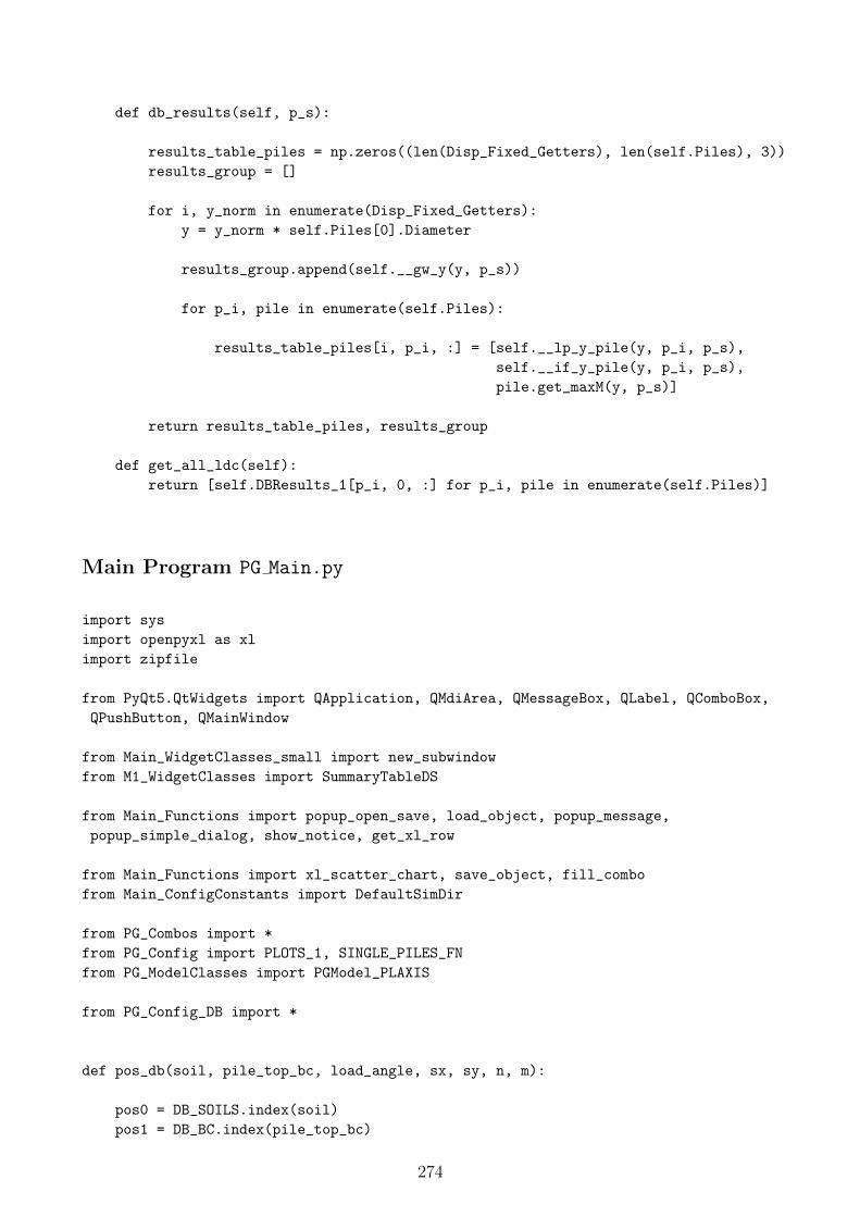
def db_results(self, p_s):
results_table_piles = np.zeros((len(Disp_Fixed_Getters), len(self.Piles), 3))
results_group = []
for i, y_norm in enumerate(Disp_Fixed_Getters):
y = y_norm * self.Piles[0].Diameter
results_group.append(self.__gw_y(y, p_s))
for p_i, pile in enumerate(self.Piles):
results_table_piles[i, p_i, :] = [self.__lp_y_pile(y, p_i, p_s),
self.__if_y_pile(y, p_i, p_s),
pile.get_maxM(y, p_s)]
return results_table_piles, results_group
def get_all_ldc(self):
return [self.DBResults_1[p_i, 0, :] for p_i, pile in enumerate(self.Piles)]
Main Program PG Main.py
import sys
import openpyxl as xl
import zipfile
from PyQt5.QtWidgets import QApplication, QMdiArea, QMessageBox, QLabel, QComboBox,
QPushButton, QMainWindow
from Main_WidgetClasses_small import new_subwindow
from M1_WidgetClasses import SummaryTableDS
from Main_Functions import popup_open_save, load_object, popup_message,
popup_simple_dialog, show_notice, get_xl_row
from Main_Functions import xl_scatter_chart, save_object, fill_combo
from Main_ConfigConstants import DefaultSimDir
from PG_Combos import *
from PG_Config import PLOTS_1, SINGLE_PILES_FN
from PG_ModelClasses import PGModel_PLAXIS
from PG_Config_DB import *
def pos_db(soil, pile_top_bc, load_angle, sx, sy, n, m):
pos0 = DB_SOILS.index(soil)
pos1 = DB_BC.index(pile_top_bc)
274
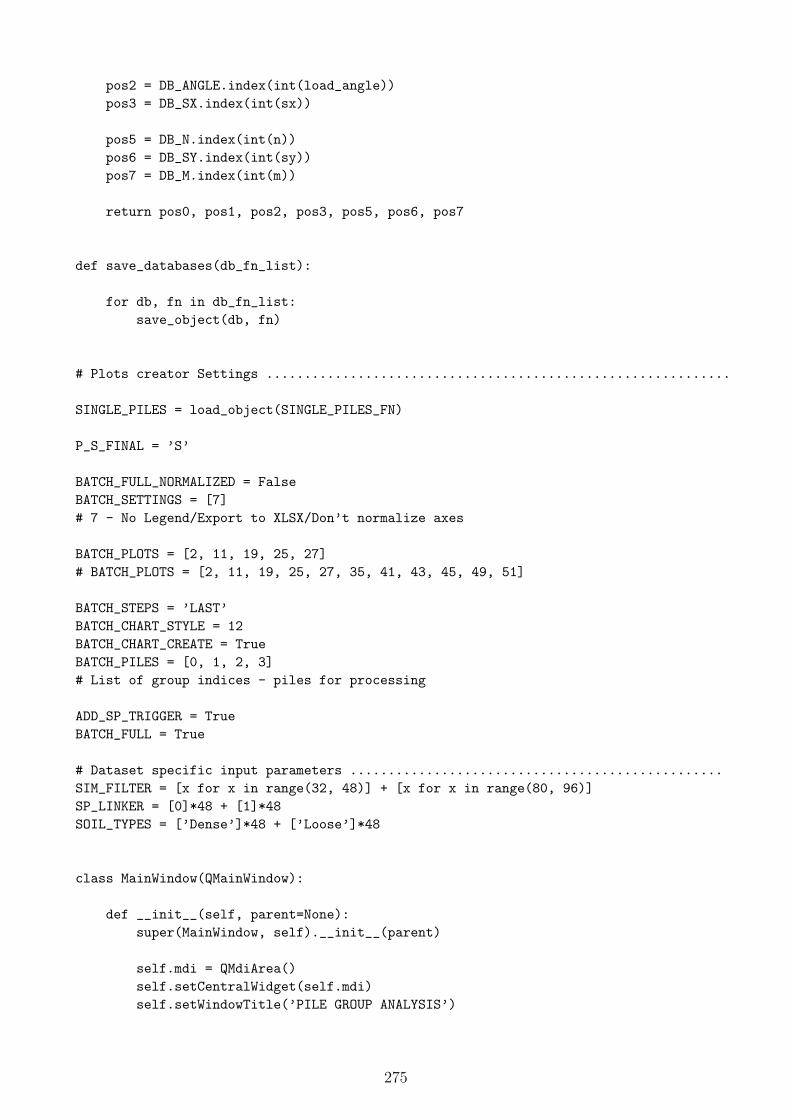
pos2 = DB_ANGLE.index(int(load_angle))
pos3 = DB_SX.index(int(sx))
pos5 = DB_N.index(int(n))
pos6 = DB_SY.index(int(sy))
pos7 = DB_M.index(int(m))
return pos0, pos1, pos2, pos3, pos5, pos6, pos7
def save_databases(db_fn_list):
for db, fn in db_fn_list:
save_object(db, fn)
# Plots creator Settings .............................................................
SINGLE_PILES = load_object(SINGLE_PILES_FN)
P_S_FINAL = ’S’
BATCH_FULL_NORMALIZED = False
BATCH_SETTINGS = [7]
# 7 - No Legend/Export to XLSX/Don’t normalize axes
BATCH_PLOTS = [2, 11, 19, 25, 27]
# BATCH_PLOTS = [2, 11, 19, 25, 27, 35, 41, 43, 45, 49, 51]
BATCH_STEPS = ’LAST’
BATCH_CHART_STYLE = 12
BATCH_CHART_CREATE = True
BATCH_PILES = [0, 1, 2, 3]
# List of group indices - piles for processing
ADD_SP_TRIGGER = True
BATCH_FULL = True
# Dataset specific input parameters .................................................
SIM_FILTER = [x for x in range(32, 48)] + [x for x in range(80, 96)]
SP_LINKER = [0]*48 + [1]*48
SOIL_TYPES = [’Dense’]*48 + [’Loose’]*48
class MainWindow(QMainWindow):
def __init__(self, parent=None):
super(MainWindow, self).__init__(parent)
self.mdi = QMdiArea()
self.setCentralWidget(self.mdi)
self.setWindowTitle(’PILE GROUP ANALYSIS’)
275

self.commands_window, self.Layout1 = new_subwindow(’Dataset Not Loaded’,
(400, 400))
self.mdi.addSubWindow(self.commands_window)
self.commands_window.show()
piles_window, self.Layout2 = new_subwindow(’Piles’, (500, 500))
self.mdi.addSubWindow(piles_window)
piles_window.show()
self.plot_choose_window, self.Layout3 = new_subwindow(’Plotting’, (500, 200))
self.mdi.addSubWindow(self.plot_choose_window)
self.plot_choose_window.show()
# SETTING WINDOWS WIDGETS ###################################################
# Window 1 ..................................................................
cmdOpenDataset = QPushButton(’LOAD DATASET’)
self.cmdDataTable = QPushButton(’SHOW INPUT PARAMETERS’)
self.cmdShowPG = QPushButton(’SHOW PILE GROUP’)
self.cmdDataTable.clicked.connect(self.cmdDataTable_clicked)
self.cmdShowPG.clicked.connect(self.cmdShowPG_clicked)
cmdOpenDataset.clicked.connect(self.cmdOpenDataset_clicked)
self.label_1 = QLabel(’***DATASET NOT LOADED***’)
self.label_2 = QLabel(’***DATASET NOT LOADED***’)
self.cmbSims = QComboBox()
self.Layout1.addWidget(QLabel(’Dataset Description’), 0, 0)
self.Layout1.addWidget(self.label_1, 0, 1)
self.Layout1.addWidget(QLabel(’Total Number of Simulations’), 1, 0)
self.Layout1.addWidget(self.label_2, 1, 1)
self.Layout1.addWidget(cmdOpenDataset, 2, 0)
self.Layout1.addWidget(self.cmdDataTable, 2, 1)
self.Layout1.addWidget(QLabel(’Select Simulation’), 3, 0)
self.Layout1.addWidget(self.cmbSims, 3, 1)
self.Layout1.addWidget(self.cmdShowPG, 4, 0)
self.__on_off_widgets(False)
# Window 2 ..................................................................
self.cmdPGResults = QPushButton(’Plot Group Results’)
self.cmdPGResults.clicked.connect(self.plot_pg_results)
self.cmdPGResults.setEnabled(False)
self.cmdPGResults_All = QPushButton(’Plot All Results’)
self.cmdPGResults_All.clicked.connect(self.pile_pg_results_batch)
self.cmdPGResults_All.setEnabled(False)
276

self.Layout2.addWidget(QLabel(’Select Pile Diagram to Plot’), 0, 2)
self.Layout2.addWidget(self.cmdPGResults, 3, 2)
self.Layout2.addWidget(self.cmdPGResults_All, 4, 2)
# Window 3 ..................................................................
self.lblSettings3 = QLabel(’Normalize Z axis’)
self.Combo0 = QComboBox()
self.Combo1 = QComboBox()
self.Combo2 = QComboBox()
self.Combo3 = QComboBox()
self.Combo00 = QComboBox()
self.Combo01 = QComboBox()
self.Combo02 = QComboBox()
self.Combo03 = QComboBox()
self.Combo00.addItems([’Plot’, ’Export’])
self.Combo01.addItems([’True’, ’False’])
self.Combo02.addItems([’True’, ’False’])
self.Combo0.currentIndexChanged.connect(self.Combo0_currentIndexChanged)
self.Combo1.currentIndexChanged.connect(self.Combo1_currentIndexChanged)
self.Combo2.currentIndexChanged.connect(self.Combo2_currentIndexChanged)
# ----------------------------------------------------------------------------
self.Layout3.addWidget(QLabel(’Plot Group’), 0, 0)
self.Layout3.addWidget(QLabel(’Plot Type’), 0, 1)
self.Layout3.addWidget(QLabel(’Settings 1’), 0, 2)
self.Layout3.addWidget(QLabel(’Settings 2’), 0, 3)
self.Layout3.addWidget(QLabel(’Plot/Export’), 2, 0)
self.Layout3.addWidget(QLabel(’Show Legend’), 2, 1)
self.Layout3.addWidget(self.lblSettings3, 2, 2)
self.Layout3.addWidget(QLabel(’Fitting’), 2, 3)
self.Layout3.addWidget(self.Combo0, 1, 0)
self.Layout3.addWidget(self.Combo1, 1, 1)
self.Layout3.addWidget(self.Combo2, 1, 2)
self.Layout3.addWidget(self.Combo3, 1, 3)
self.Layout3.addWidget(self.Combo00, 4, 0)
self.Layout3.addWidget(self.Combo01, 4, 1)
self.Layout3.addWidget(self.Combo02, 4, 2)
self.Layout3.addWidget(self.Combo03, 4, 3)
fill_combo(self.Combo0, COMBO_0)
# ---------------------------------------------------------------------------
self.LOADED_DATASET = None
self.ActivePG = None
self.PileButtons = None
277
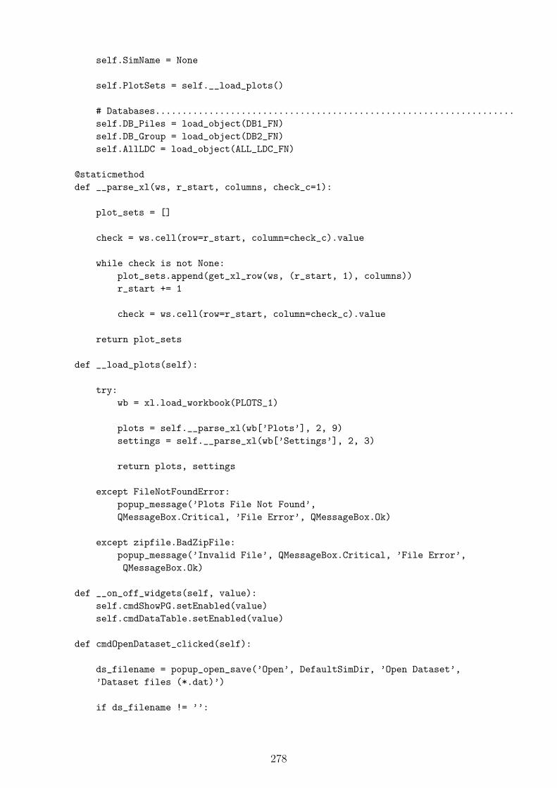
self.SimName = None
self.PlotSets = self.__load_plots()
# Databases...................................................................
self.DB_Piles = load_object(DB1_FN)
self.DB_Group = load_object(DB2_FN)
self.AllLDC = load_object(ALL_LDC_FN)
@staticmethod
def __parse_xl(ws, r_start, columns, check_c=1):
plot_sets = []
check = ws.cell(row=r_start, column=check_c).value
while check is not None:
plot_sets.append(get_xl_row(ws, (r_start, 1), columns))
r_start += 1
check = ws.cell(row=r_start, column=check_c).value
return plot_sets
def __load_plots(self):
try:
wb = xl.load_workbook(PLOTS_1)
plots = self.__parse_xl(wb[’Plots’], 2, 9)
settings = self.__parse_xl(wb[’Settings’], 2, 3)
return plots, settings
except FileNotFoundError:
popup_message(’Plots File Not Found’,
QMessageBox.Critical, ’File Error’, QMessageBox.Ok)
except zipfile.BadZipFile:
popup_message(’Invalid File’, QMessageBox.Critical, ’File Error’,
QMessageBox.Ok)
def __on_off_widgets(self, value):
self.cmdShowPG.setEnabled(value)
self.cmdDataTable.setEnabled(value)
def cmdOpenDataset_clicked(self):
ds_filename = popup_open_save(’Open’, DefaultSimDir, ’Open Dataset’,
’Dataset files (*.dat)’)
if ds_filename != ’’:
278

try:
self.commands_window.setWindowTitle(ds_filename)
self.LOADED_DATASET = load_object(ds_filename)
self.LOADED_DATASET.CurrentPath = ds_filename
self.label_1.setText(self.LOADED_DATASET.SummaryTable[0][1])
self.label_2.setText(self.LOADED_DATASET.SummaryTable[0][3])
# Fill Simulations Combo Box
fill_combo(self.cmbSims, [item[0]
for item in self.LOADED_DATASET.SummaryTable[1][1]])
self.__on_off_widgets(True) # Activate needed buttons
if BATCH_FULL:
self.full_batch(BATCH_FULL_NORMALIZED)
except ImportError:
popup_message(’Invalid File’, QMessageBox.Critical, ’File Error’,
QMessageBox.Ok)
except PermissionError:
popup_message(’Permission Error. File already opened. Close it and
repeat.’, QMessageBox.Critical, ’File Error’, QMessageBox.Ok)
except AttributeError:
popup_message(’Invalid File’, QMessageBox.Critical, ’File Error’,
QMessageBox.Ok)
def cmdDataTable_clicked(self):
data = (self.LOADED_DATASET.SummaryTable[1],
self.LOADED_DATASET.SummaryTable[2])
popup_simple_dialog(’Data Table’, [[SummaryTableDS(data[1][1], data[1][0],
[item[0] for item in data[0][1]])]])
def cmdShowPG_clicked(self):
s_i = self.cmbSims.currentIndex()
raw_results = self.LOADED_DATASET.SummaryTable_4[s_i][1]
if raw_results is not None:
self.__create_pg(s_i, raw_results, SOIL_TYPES[s_i])
self.PileButtons = []
for r in range(0, self.ActivePG.N):
for c in range(0, self.ActivePG.M):
new_button = QPushButton(’Pile-’ + str(r*self.ActivePG.M+c))
new_button.clicked.connect(self.pile_clicked)
self.PileButtons.append(new_button)
279

self.Layout2.addWidget(new_button, self.ActivePG.M-1-c, r)
self.cmdPGResults.setEnabled(True)
self.cmdPGResults_All.setEnabled(True)
self.SimName = self.cmbSims.currentText()
else:
popup_message(’No Results Found’, QMessageBox.Warning, ’No Results’,
QMessageBox.Ok)
def Combo0_currentIndexChanged(self):
i0 = self.Combo0.currentIndex()
fill_combo(self.Combo1, COMBO_1[i0])
# Adjust Settings Combos
if i0 == 0:
show_notice(self.lblSettings3, ’Normalize Z axis’)
self.Combo03.clear()
else:
show_notice(self.lblSettings3, ’Normalize Displacements’)
fill_combo(self.Combo03, [’Polyfit’, ’Spline’])
def Combo1_currentIndexChanged(self):
i0 = self.Combo0.currentIndex()
i1 = self.Combo1.currentIndex()
fill_combo(self.Combo2, COMBO_2[i0][i1])
def Combo2_currentIndexChanged(self):
i0 = self.Combo0.currentIndex()
i1 = self.Combo1.currentIndex()
i2 = self.Combo2.currentIndex()
combo_3_list = []
if i0 == 2:
combo_3_list = COMBO_3_2[i1][i2]
fill_combo(self.Combo3, combo_3_list)
def __combo_settings(self):
plot_export = self.Combo00.currentText()
show_legend = Combo_Translate[self.Combo01.currentText()]
normalized = Combo_Translate[self.Combo02.currentText()]
plot_type = self.Combo0.currentIndex()
if plot_type == 1:
p1 = Combo_Translate[self.Combo03.currentText()]
p2 = Combo_Translate[self.Combo1.currentText()]
p3 = Combo_Translate[self.Combo2.currentText()]
280

p4 = None
elif plot_type == 0:
p1 = self.Combo1.currentText()
p2 = Combo_Translate[self.Combo2.currentText()]
p3 = INDICES[self.Combo1.currentIndex()][self.Combo2.currentIndex()]
p4 = None
else:
p1 = Combo_Translate[self.Combo1.currentText()]
p2 = self.Combo2.currentText()
p3 = self.Combo3.currentText()
p4 = Combo_Translate[self.Combo03.currentText()]
return plot_type, p1, p2, p3, p4, plot_export, show_legend, normalized
def pile_clicked(self):
pile_index = 0
for pile_index, button in enumerate(self.PileButtons):
if self.sender() == button:
break
# Pile index found
plot_type, p1, p2, p3, p4, p_exp, show_legend, normalized =
self.__combo_settings()
if plot_type < 2:
self.__plot_caller(plot_type, pile_index, p1, p2, p3, p4, p_exp,
show_legend, normalized, 0, self.SimName)
def plot_pg_results(self):
plot_type, p1, p2, p3, p4, plot_export, show_legend, normalized =
self.__combo_settings()
if plot_type == 2:
self.__plot_caller(plot_type, 0, p1, p2, p3, p4, plot_export, show_legend,
normalized, 0, self.SimName)
def __plot_caller(self, plot_type, pile_id, p1, p2, p3, p4, plot_export, leg,
normalized, t1, sim_name):
pile = self.ActivePG.Piles[pile_id]
if plot_type == 0:
return pile.RAW_PLOT(p1, p3, pile.get_steps(BATCH_STEPS), p2, leg,
plot_export, normalized, sim_name, t1)
elif plot_type == 1:
return pile.LDC_PY_PLOT(p2, p1, p3, leg, plot_export, normalized,
sim_name, t1)
281

else:
return self.ActivePG.PG_PLOT(p2, p3, p1, p4, leg, plot_export, normalized,
sim_name, t1)
@staticmethod
def __translate_plot_set(plot_set):
plot_id, plot_type, caption, i1, lp_if_ldc_gw, curve_parameter, prg, t_a,
p_s_c = plot_set
if plot_type == 0:
return caption, p_s_c, i1, None, plot_type
elif plot_type == 1:
return p_s_c, lp_if_ldc_gw, curve_parameter, None, plot_type
else:
return lp_if_ldc_gw, prg, t_a, p_s_c, plot_type
# BATCH PROCESSING FUNCTIONS ####################################################
def pile_pg_results_batch(self):
all_plots, all_settings = self.PlotSets
settings_list = [all_settings[j] for j in BATCH_SETTINGS]
plot_list = [all_plots[j] for j in BATCH_PLOTS]
for pile_id in BATCH_PILES:
for settings in settings_list:
for plot_set in plot_list:
p1, p2, p3, p4, plot_type = self.__translate_plot_set(plot_set)
leg, p_exp, norm = settings
self.__plot_caller(plot_type, pile_id, p1, p2, p3, p4, p_exp, leg,
norm, 0, self.SimName)
def __create_pg(self, sim_index, results, soil):
if ADD_SP_TRIGGER:
pile_index = SP_LINKER[sim_index]
single_pile = SINGLE_PILES[pile_index]
print(’Equivalent single pile ’, pile_index, ’ added to PG simulation ’,
sim_index)
else:
single_pile = None
self.ActivePG = PGModel_PLAXIS(self.LOADED_DATASET.SummaryTable_4[sim_index
][0], results, single_pile, soil)
self.ActivePG.set_fixed_results(P_S_FINAL)
282
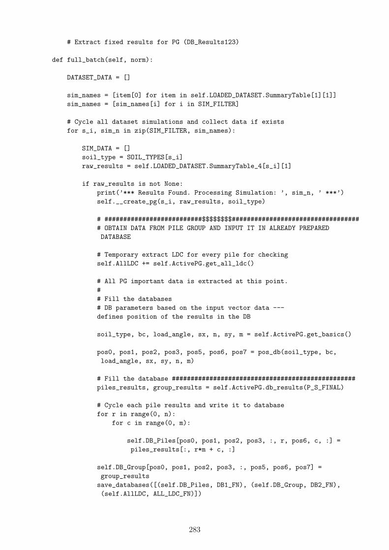
# Extract fixed results for PG (DB_Results123)
def full_batch(self, norm):
DATASET_DATA = []
sim_names = [item[0] for item in self.LOADED_DATASET.SummaryTable[1][1]]
sim_names = [sim_names[i] for i in SIM_FILTER]
# Cycle all dataset simulations and collect data if exists
for s_i, sim_n in zip(SIM_FILTER, sim_names):
SIM_DATA = []
soil_type = SOIL_TYPES[s_i]
raw_results = self.LOADED_DATASET.SummaryTable_4[s_i][1]
if raw_results is not None:
print(’*** Results Found. Processing Simulation: ’, sim_n, ’ ***’)
self.__create_pg(s_i, raw_results, soil_type)
# ##########################$$$$$$$$##################################
# OBTAIN DATA FROM PILE GROUP AND INPUT IT IN ALREADY PREPARED
DATABASE
# Temporary extract LDC for every pile for checking
self.AllLDC += self.ActivePG.get_all_ldc()
# All PG important data is extracted at this point.
#
# Fill the databases
# DB parameters based on the input vector data ---
defines position of the results in the DB
soil_type, bc, load_angle, sx, n, sy, m = self.ActivePG.get_basics()
pos0, pos1, pos2, pos3, pos5, pos6, pos7 = pos_db(soil_type, bc,
load_angle, sx, sy, n, m)
# Fill the database #################################################
piles_results, group_results = self.ActivePG.db_results(P_S_FINAL)
# Cycle each pile results and write it to database
for r in range(0, n):
for c in range(0, m):
self.DB_Piles[pos0, pos1, pos2, pos3, :, r, pos6, c, :] =
piles_results[:, r*m + c, :]
self.DB_Group[pos0, pos1, pos2, pos3, :, pos5, pos6, pos7] =
group_results
save_databases([(self.DB_Piles, DB1_FN), (self.DB_Group, DB2_FN),
(self.AllLDC, ALL_LDC_FN)])
283

# ####################################################################
for pile_i in BATCH_PILES:
PILE_DATA = []
for j in BATCH_PLOTS:
p1, p2, p3, p4, plot_type =
self.__translate_plot_set(self.PlotSets[0][j])
data = self.__plot_caller(plot_type, pile_i, p1, p2, p3, p4,
’Export’, False, norm, 1, sim_n)
PILE_DATA.append((pile_i, j, data))
SIM_DATA.append(PILE_DATA)
else:
print(’*** No Results ***’)
DATASET_DATA.append(SIM_DATA)
# ############################################################################
# Reorganize dataset before excel export ------------------------------------
DATASET_DATA_1 = []
for j, plot_id in enumerate(BATCH_PLOTS):
PLOT_DATA = []
for s_i, sim_data_set in enumerate(DATASET_DATA):
PILE_DATA = []
if not sim_data_set == []: # Results exists
for pile_data_set in sim_data_set:
PILE_DATA.append(pile_data_set[j])
PLOT_DATA.append(PILE_DATA)
DATASET_DATA_1.append((plot_id, PLOT_DATA))
# Create xl wb FOR EACH PROCESSED PILE (Case 0, 1).
Case 2 can use single pile index, and data goes together
print(’*********************************************************************’)
print(’Creating excel file...’)
print(’’)
for j1, p_i in enumerate(BATCH_PILES):
self.batch_pile_wb(sim_names, j1, p_i, DATASET_DATA_1, norm)
print(’Workbook successfully created!’)
print(’*********************************************************************’)
print(’’)
def batch_pile_wb(self, sim_names, j1, p_i, ds_data_1, norm):
284

# Create xlsx for each pile. Create tab for each plot type.
# Add data from all simulations in dataset.
wb = xl.Workbook()
wb_name = self.LOADED_DATASET.get_name() + ’_Pile_’ + str(p_i) + ’.xlsx’
for j2, pt_i in enumerate(BATCH_PLOTS):
# Cycle plot types. Add data to appropriate TABSHEET
sheet_title = ’Plot_’ + str(pt_i)
wb.create_sheet(sheet_title)
ws = wb.worksheets[j2 + 1]
if BATCH_CHART_CREATE:
new_chart = xl_scatter_chart(sheet_title, BATCH_CHART_STYLE, ’X’, ’Y’)
start_c = 1
for j3, simulation_data in enumerate(ds_data_1[j2][1]):
# Cycle data sim by sim and add it to ws
if not simulation_data == []:
xy_diagram = simulation_data[j1][2]
xy_diagram.fill_xl_ws(norm, sim_names[j3], ws, 1, start_c, 2)
added_columns = len(xy_diagram.Plots) * 2
if BATCH_CHART_CREATE:
for series in xy_diagram.create_xl_series(ws, 5, start_c, 2,
j3):
new_chart.series.append(series)
start_c += added_columns + 1
# Split simulations by empty column
ws.add_chart(new_chart, ’A1’)
wb.remove_sheet(wb.worksheets[0])
wb.save(wb_name)
if __name__ == "__main__":
app = QApplication(sys.argv)
window = MainWindow()
window.show()
sys.exit(app.exec_())
285
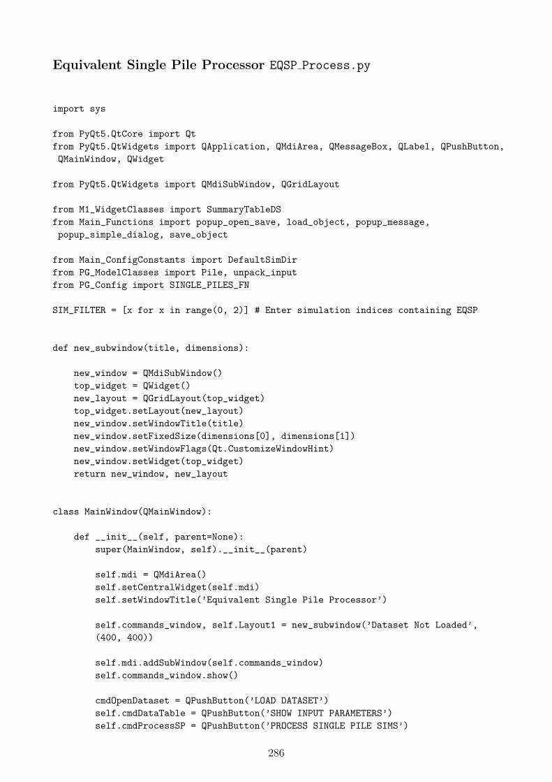
Equivalent Single Pile Processor EQSP Process.py
import sys
from PyQt5.QtCore import Qt
from PyQt5.QtWidgets import QApplication, QMdiArea, QMessageBox, QLabel, QPushButton,
QMainWindow, QWidget
from PyQt5.QtWidgets import QMdiSubWindow, QGridLayout
from M1_WidgetClasses import SummaryTableDS
from Main_Functions import popup_open_save, load_object, popup_message,
popup_simple_dialog, save_object
from Main_ConfigConstants import DefaultSimDir
from PG_ModelClasses import Pile, unpack_input
from PG_Config import SINGLE_PILES_FN
SIM_FILTER = [x for x in range(0, 2)] # Enter simulation indices containing EQSP
def new_subwindow(title, dimensions):
new_window = QMdiSubWindow()
top_widget = QWidget()
new_layout = QGridLayout(top_widget)
top_widget.setLayout(new_layout)
new_window.setWindowTitle(title)
new_window.setFixedSize(dimensions[0], dimensions[1])
new_window.setWindowFlags(Qt.CustomizeWindowHint)
new_window.setWidget(top_widget)
return new_window, new_layout
class MainWindow(QMainWindow):
def __init__(self, parent=None):
super(MainWindow, self).__init__(parent)
self.mdi = QMdiArea()
self.setCentralWidget(self.mdi)
self.setWindowTitle(’Equivalent Single Pile Processor’)
self.commands_window, self.Layout1 = new_subwindow(’Dataset Not Loaded’,
(400, 400))
self.mdi.addSubWindow(self.commands_window)
self.commands_window.show()
cmdOpenDataset = QPushButton(’LOAD DATASET’)
self.cmdDataTable = QPushButton(’SHOW INPUT PARAMETERS’)
self.cmdProcessSP = QPushButton(’PROCESS SINGLE PILE SIMS’)
286

self.label_1 = QLabel(’***DATASET NOT LOADED***’)
self.label_2 = QLabel(’***DATASET NOT LOADED***’)
cmdOpenDataset.clicked.connect(self.cmdOpenDataset_clicked)
self.cmdDataTable.clicked.connect(self.cmdDataTable_clicked)
self.cmdProcessSP.clicked.connect(self.cmdProcessSP_clicked)
self.Layout1.addWidget(QLabel(’Dataset Description’), 0, 0)
self.Layout1.addWidget(self.label_1, 0, 1)
self.Layout1.addWidget(QLabel(’Total Number of Simulations’), 1, 0)
self.Layout1.addWidget(self.label_2, 1, 1)
self.Layout1.addWidget(cmdOpenDataset, 2, 0)
self.Layout1.addWidget(self.cmdDataTable, 2, 1)
self.Layout1.addWidget(self.cmdProcessSP, 3, 0)
self.cmdProcessSP.setEnabled(False)
self.cmdDataTable.setEnabled(False)
self.LOADED_DATASET = None
def cmdOpenDataset_clicked(self):
ds_filename = popup_open_save(’Open’, DefaultSimDir, ’Open Dataset’,
’Dataset files (*.dat)’)
if ds_filename != ’’:
try:
self.commands_window.setWindowTitle(ds_filename)
self.LOADED_DATASET = load_object(ds_filename)
self.LOADED_DATASET.CurrentPath = ds_filename
self.label_1.setText(self.LOADED_DATASET.SummaryTable[0][1])
self.label_2.setText(self.LOADED_DATASET.SummaryTable[0][3])
self.cmdProcessSP.setEnabled(True)
self.cmdDataTable.setEnabled(True)
except ImportError:
popup_message(’Invalid File’, QMessageBox.Critical, ’File Error’,
QMessageBox.Ok)
except PermissionError:
popup_message(’Permission Error. File already opened. Close it and
repeat.’, QMessageBox.Critical, ’File Error’, QMessageBox.Ok)
except AttributeError:
popup_message(’Invalid File’, QMessageBox.Critical, ’File Error’,
QMessageBox.Ok)
def cmdDataTable_clicked(self):
287

data = (self.LOADED_DATASET.SummaryTable[1],
self.LOADED_DATASET.SummaryTable[2])
popup_simple_dialog(’Data Table’, [[SummaryTableDS(data[1][1], data[1][0],
[item[0] for item in data[0][1]])]])
def cmdProcessSP_clicked(self):
Processed_Piles = []
for sim_index in SIM_FILTER:
input_vector, results_table =
self.LOADED_DATASET.SummaryTable_4[sim_index]
if results_table is not None:
d, l1, l2, E_pile, cap_type, cap_thick =
unpack_input(input_vector, ’SINGLE’)
pile = Pile(d, l1, l2, E_pile, cap_type, cap_thick)
pile.set_alone()
pile.process_raw_results(results_table)
Processed_Piles.append(pile)
else:
Processed_Piles.append(None)
print(’Processed Single Pile Simulation: ’, sim_index)
# All piles are processed. Save list of processed piles
save_object(Processed_Piles, SINGLE_PILES_FN)
print(’’)
print(’---------------------------------------------------’)
print(’Single Pile object instances sucessfully saved’)
if __name__ == "__main__":
app = QApplication(sys.argv)
window = MainWindow()
window.show()
sys.exit(app.exec_())
Results Database Maker PG DB.py
import openpyxl as xl
from Main_Functions import load_object, xl_scatter_chart, fill_xl_row_col,
xy_series_xl
288
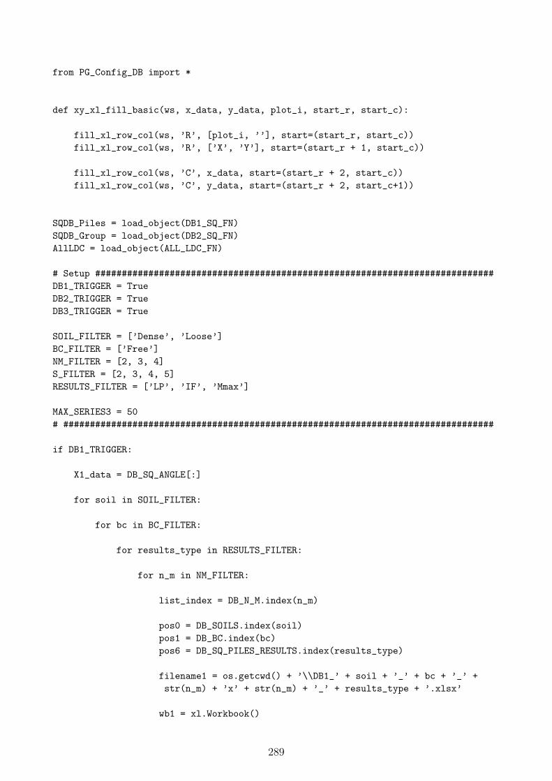
from PG_Config_DB import *
def xy_xl_fill_basic(ws, x_data, y_data, plot_i, start_r, start_c):
fill_xl_row_col(ws, ’R’, [plot_i, ’’], start=(start_r, start_c))
fill_xl_row_col(ws, ’R’, [’X’, ’Y’], start=(start_r + 1, start_c))
fill_xl_row_col(ws, ’C’, x_data, start=(start_r + 2, start_c))
fill_xl_row_col(ws, ’C’, y_data, start=(start_r + 2, start_c+1))
SQDB_Piles = load_object(DB1_SQ_FN)
SQDB_Group = load_object(DB2_SQ_FN)
AllLDC = load_object(ALL_LDC_FN)
# Setup ###########################################################################
DB1_TRIGGER = True
DB2_TRIGGER = True
DB3_TRIGGER = True
SOIL_FILTER = [’Dense’, ’Loose’]
BC_FILTER = [’Free’]
NM_FILTER = [2, 3, 4]
S_FILTER = [2, 3, 4, 5]
RESULTS_FILTER = [’LP’, ’IF’, ’Mmax’]
MAX_SERIES3 = 50
# #################################################################################
if DB1_TRIGGER:
X1_data = DB_SQ_ANGLE[:]
for soil in SOIL_FILTER:
for bc in BC_FILTER:
for results_type in RESULTS_FILTER:
for n_m in NM_FILTER:
list_index = DB_N_M.index(n_m)
pos0 = DB_SOILS.index(soil)
pos1 = DB_BC.index(bc)
pos6 = DB_SQ_PILES_RESULTS.index(results_type)
filename1 = os.getcwd() + ’\\DB1_’ + soil + ’_’ + bc + ’_’ +
str(n_m) + ’x’ + str(n_m) + ’_’ + results_type + ’.xlsx’
wb1 = xl.Workbook()
289

# Create workbook and add all empty worksheets for different y/D
for disp_level_norm in Disp_Fixed_Getters:
wb1.create_sheet(’yD = ’ + str(disp_level_norm))
wb1.remove_sheet(wb1.worksheets[0])
for pos4, disp_level_norm in enumerate(Disp_Fixed_Getters):
ws1 = wb1.worksheets[pos4]
start_col = 1
for s in S_FILTER:
pos3 = DB_SQ_S.index(s)
new_chart = xl_scatter_chart(’s/D = ’ + str(s), 20,
’Loading Angle [degrees]’, results_type)
for pos5 in range(0, n_m**2):
Y1_data = SQDB_Piles[list_index][pos0, pos1, :, pos3,
pos4, pos5, pos6]
xy_xl_fill_basic(ws1, X1_data, Y1_data, ’Pile_’ +
str(pos5), 1, start_col)
new_chart.series.append(xy_series_xl(ws1, 3,
start_col, len(X1_data), ’Pile_’ + str(pos5),
’triangle’))
start_col += 2
ws1.add_chart(new_chart)
wb1.save(filename1)
print(’Workbook ’ + filename1 + ’ saved.’)
print(’------------------------------------------------------------------------’)
print(’Database 1 processed’)
if DB2_TRIGGER:
X2_data = DB_SQ_ANGLE[:]
for soil in SOIL_FILTER:
for bc in BC_FILTER:
for n_m in NM_FILTER:
pos0 = DB_SOILS.index(soil)
290

pos1 = DB_BC.index(bc)
pos5 = DB_N_M.index(n_m)
filename2 = os.getcwd() + ’\\DB2_’ + soil + ’_’ + bc + ’_’ + str(n_m)
+ ’x’ + str(n_m) + ’.xlsx’
wb2 = xl.Workbook()
ws2 = wb2.worksheets[0]
start_col = 1
for pos4, disp_level_norm in enumerate(Disp_Fixed_Getters):
# Create chart for each displacement level
new_chart = xl_scatter_chart(’y/D = ’ + str(disp_level_norm),
12, ’Loading Angle [degrees]’,
’GW [-]’)
for s in S_FILTER:
pos3 = DB_SQ_S.index(s)
series_title = ’s/D = ’ + str(s)
Y2_data = SQDB_Group[pos0, pos1, :, pos3, pos4, pos5]
# Filter database and create plot xlsx
xy_xl_fill_basic(ws2, X2_data, Y2_data, series_title, 1,
start_col)
new_chart.series.append(xy_series_xl(ws2, 3, start_col,
len(X2_data), series_title, ’triangle’))
start_col += 2
ws2.add_chart(new_chart)
wb2.save(filename2)
print(’Workbook ’ + filename2 + ’ saved.’)
print(’------------------------------------------------------------------------’)
print(’Database 2 processed’)
if DB3_TRIGGER:
print(’Processing Database 3’)
X3_data = Disp_Fixed_Getters[:]
wb3 = xl.Workbook()
ws3 = wb3.worksheets[0]
full_plots, last_plot = divmod(len(AllLDC), MAX_SERIES3)
splitters = [MAX_SERIES3]*full_plots + [last_plot]
start_curve, start_col = 0, 1
291
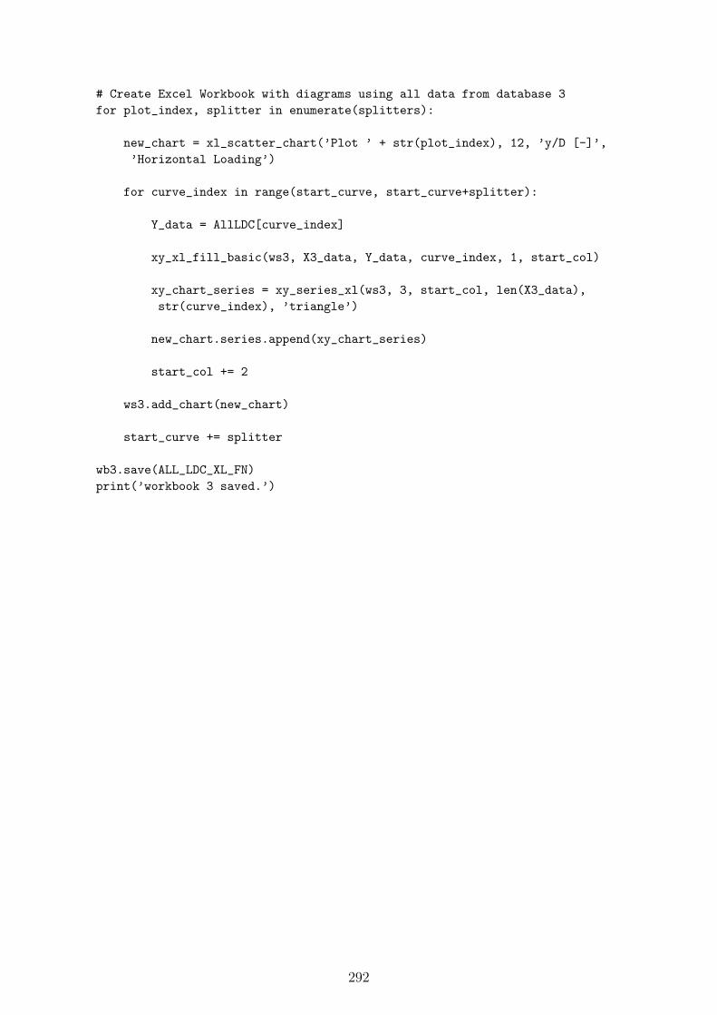
# Create Excel Workbook with diagrams using all data from database 3
for plot_index, splitter in enumerate(splitters):
new_chart = xl_scatter_chart(’Plot ’ + str(plot_index), 12, ’y/D [-]’,
’Horizontal Loading’)
for curve_index in range(start_curve, start_curve+splitter):
Y_data = AllLDC[curve_index]
xy_xl_fill_basic(ws3, X3_data, Y_data, curve_index, 1, start_col)
xy_chart_series = xy_series_xl(ws3, 3, start_col, len(X3_data),
str(curve_index), ’triangle’)
new_chart.series.append(xy_chart_series)
start_col += 2
ws3.add_chart(new_chart)
start_curve += splitter
wb3.save(ALL_LDC_XL_FN)
print(’workbook 3 saved.’)
292


Copyright © 2022 FDOKUMEN

