


Bahasa
Halaman
Hukum

AN EMPIRICAL APPROACH TO THE EVALUATION OF FACTORS IN LOCAL AUTHORITY HOUSING MAINTENANCE REQUIREMENTS IN THE
CITY OF MANCHESTER
OLUFEMI FESTUS OLUBODUN B. Sc. (lions), M. Sc., ARICS, MCIOB
T. I. M. E. RESEARCH INSTITUTE DEPARTMENT OF SURVEYING
UNIVERSITY OF SALFORD
SUBMITTED IN PARTIAL FULFILMENT FOR THE DEGREE OF DOCTOR OF PHILOSOPHY
DECEMBER 1996
TABLE OF CONTENT
CHAPTER ONE INTRODUCTION
1.1 Introduction to the subject matter 1
1.2 Economic importance and growth of maintenance 3
1.3 Statement of the problem 9
1.4 The choice of Manchester for the study 12
1.5 Aims of the Research 13
1.6 Research Hypothesis 13
1.7 Benefits of the Research 14
1.8 Organisation of the chapters 14
CHAPTER TWO METHODOLOGY
2.1 Introduction 16
2.2 The Research Approach 17
2.3 Research Tools 17
2.4 Research Framework 18
2.5 The working hypothesis 21
2.6 Data Collection Strategy 21
2.6.1 Measurement and Statistics 21
2.6.2 Nature of the Data 22
2.6.3 Scales of Measurement 22
2.7 A framework for the measurement of maintenance need 23
2.7.1 Approach to preliminary investigations 23
2.7.2 Measurement of maintenance need 24
2.7.3 Maintenance cost records 24
2.7.4 Problems with cost records as a basis for the measurement of
maintenance need 26
2.7.5 Preliminary questionnaire design and surveys 28
2.7.5.1 The preliminary survey - Data collection and subjects 28
2.7.5.2 Procedure for the preliminary survey 29
2.7.5.3 Results of preliminary survey 30
2.8 Final Questionnaire Design and Administration 32
i
2.8.1 The sampled Population for the final surveys 32
2.8.2 Information Sourcing 32
2.8.3 Building surveyor's questionnaire 33
2.8.3.1 Sampling for the surveyors' questionnaire survey 33
2.8.3.2 The Field Survey 34
2.8.3.3 Design and content of the Questionnaire 34
2.8.3.4 Piloting questionnaires for surveyors 36
2.8.4 Tenant's Questionnaire 37
2.8.4.1 Sampling for the tenants' questionnaire survey 37
2.8.4.2 The Field Survey, and design of the questionnaire 37
2.9 Exclusion of housing management team from the final surveys 40
2.10 Summary 40
CHAPTER THREE HISTORICAL CONTEXT OF HOUSING IN
MANCHESTER
3.1 Introduction 41
3.2 Manchester's stock 42
3.3 Local authority and the implementation of housing policy 43
3.4 The Inter-war Period 44
3.5 Importance of Housing legislation 47
3.6 The effect of the second World War 48
3.7 The Right-to-Buy Act of 1980 49
3.8 The theory of housing zoning 49
3.9 Tenure 52
3.10 Summary 54
11
CHAPTER FOUR DEFINITION PROBLEMS IN BUILDING
MAINTENANCE
4.1 Introduction 56
4.2 Review of general definition 57
4.3 The usage of terminologies 59
4.4 A cursory look at semantics 61
4.5 Summary of definitions 63
4.6 Maintenance Characteristics 64
4.7 Types of Maintenance 65
4.8 Maintenance expenditure 67
4.9 Expenditure forecasting approach 69
4.9.1 The Government Employee Housing Authority (GEHA) - Australian experience 70
4.10 The theory of Satisfaction among tenants 72
4.10.1 Satisfaction among tenants 74
4.11 Property Condition 76
4.12 Summary 76
CHAPTER FIVE FACTORS IN MAINTENANCE REQUIREMENT
PROFILE -A REVIEW OF LITERATURE
5.1 Introduction 78
5.2 Existing approaches to factorial studies in maintenance 78
5.3 Introduction to the factors 82
5.4 Vandalism 83
5.4.1 Development of the Vandalism Status Index 85
5.5 Age 86
5.6 Design 88
5.7 Maintenance Standard 89
5.8 Construction 91
5.9 Tenant issues 93
5.9.1 The Tenants' Charter 93
5.9.2 Tenants' consultation policy 94
5.9.3 Reporting of Defects 95
lÜ
5.10 Stock condition survey 96
5.10.1 Day-to-day survey 96
5.10.2 The surveyor's bias 97
5.11 The English House Condition Survey (EHCS) 97
5.12 Organisation of Housing Management 98
5.12.1 Stockholder's responsibility - Housing Management 98
5.12.2 Procedures for repair action 100
5.10.2.1 Defects reporting by tenants 100
5.10.2.2 Housing officer's inspection 100
5.12.3 Local budgetary control 101
5.13 Summary 101
CHAPTER SIX ANALYSIS OF SURVEYOR'S QUESTIONNAIRE
6.1 Introduction 103
6.2 Objective 103
6.3 The Thesis - Hypotheses 104
6.4 The survey 105
6.5 Reasons for non-response 106
6.6 Data collection, manipulation, analysis and presentation 106
6.6.1 The data 106
6.6.2 Missing values 107
6.6.3 Data Analysis 107
6.6.3.1 Test for homogeneity across groupings 108
6.6.3.2 Methods 111
6.6.3.2.1 The Kendall coefficient of concordance, W 111
6.6.3.2.2 Chi-square test for independence 113
6.6.3.2.3 Mean Rank 113
6.6.3.2.4 Multiple linear regression 114
6.6.3.2.5 Multiple Regression Statistics 115
6.6.3.2.6 Mechanics of the scorings by respondents 117
6.7 Data Manipulation 118
6.8 Analysis of results on Building characteristics 119
6.8.1 Questionnaire responses by job title 119
iv
6.8.2 Questionnaire responses by job experience 122
6.9 Discussion of Results on Building characteristics survey - Section One 122
6.9.1 Criterion Impact on Building Component Defects 130
6.9.1.1 Design Factors 130
6.9.1.2 Age Factors 131
6.9.1.3 Construction Factors 132
6.9.1.4 Vandalism Factors 133
6.9.1.5 Changing standard Factors 134
6.9.2 Interpretation of Results 134
6.10 Relationships Between the Five Defect Criteria 136
6.10.1 Generating the data 136
6.10.2 Weakness of the technique 138
6.10.3 The Dependent and Independent Variables. 138
6.10.4 Discussion of the individual regressor and its significance 138
6.10.5 Residuals Plotting 143
6.10.6 Normal Probability 143
6.10.7 Results and Analysis of the combined regression equation 145
6.11 Conclusion 148
CHAPTER SEVEN COMPONENT DEFECTS ANALYSIS
7.1 Objective 151
7.2 Statement of Hypothesis to be tested 151
7.3 Final Analysis of Building Surveyors Survey Data 152
7.4 Defect Criterion data analysis 155
7.5 Characteristics of the sample data and factor extraction 156
7.6 Component Analysis of the Extracted Factors 161
7.7 Identification of the Significant Component Defects on the Factors 161
7.8 Interpretation of the Factors 164
7.9 Discussion of the maintenance requirement factors based on factor analysis
technique 167
7.10 Conclusions 172
V
CHAPTER EIGHT MAINTENANCE - TENANT MODEL
8.1 Introduction 174
8.2 Research Approach and Limitation 175
8.3 The survey 175
8.4 Data characteristics for the dependent variables 175
8.4.1 Maintenance requirements Indices 175
8.4.2 Derivation and Characteristics of Satisfaction Index Distribution 176
8.4.3 Maintenance Costs - (MAINTCST) 180
8.4.4 Measurement, Assessment and Characteristics of Existing Property
Condition - (PROPCOND) 184
8.4.5 Data characteristics for independent variable - Vandalism Index
(VANDAL) 191
8.5 Variables selection 193
8.5.1 The independent variables 193
8.5.1.1 Tenant Attributes 194
8.5.1.2 Property Attributes 195
8.5.1.3 Environmental Attributes 195
8.5.1.4 Property Management Attribute 196
8.5.2 Characteristics of the Non-Interval variables 196
8.5.3 Interval scale 202
8.5.3.1 Interpretation of interval data 203
8.5.4 Summary of Variables 203
8.6 Relationships between the three indices and selected variables 203
8.7 Predicting maintenance need 206
8.7.1 Repair cost record model 206
8.7.1.1 Inference from the Maintenance Cost Models 210
8.7.1.2 Excluded variables from Maintenance Expenditure Models 213
8.7.2 Property condition model 214
8.7.2.1 Correcting for Endogenous Interference in the Property
Condition Model 218
8.7.2.2 Inference from the Property Condition Model 220
8.7.3 Satisfaction model 224
8.8 Conclusion 226
vi
CHAPTER NINE SUMMARY AND CONCLUSIONS
9.1 Summary 228
9.2 Final Conclusion 240
9.3 Scope and limitations 242
9.4 Recommendation for further study 242
REFERENCES 243
APPENDICES
APPENDIX 1AA: PRELIMINARY QUESTIONNAIRE ON FACTORS - HOUSING MANAGEMENT 255
APPENDIX IAB: PRELIMINARY QUESTIONNAIRE ON FACTORS - BUILDING SURVEYOR 256
APPENDIX 113: BUILDING SURVEYOR'S FINAL QUESTIONNAIRE 257
APPENDIX IC: TENANT'S FINAL QUESTIONNAIRE 260
APPENDIX 2A: INDIVIDUAL REGRESSION MODELS ON DESIGN AGE, STANDARD, CONSTRUCTION AND VANDALISM 265
APPENDIX 3.1: CORRELATIONS BETWEEN EACH OF THE SIX CRITERIA ON VANDALISM INDEX 269
APPENDIX 3.2: CONSISTENCY OF VANDALISM INDEX ALONG LOCATION 284
APPENDIX3.3: RELIABILITY ANALYSIS - SCALE (ALPHA) 290
APPENDIX 3.4: T-TESTS OF THE VANDALISM INDEX CRITERIA 291
APPENDIX 3.5: CHI-SQUARE STATISTICS ON DWELLING TYPES FOR SELECTED VARIABLES 294
APPENDIX 3.6: CROSSTABULATION OF PROPERTY TYPES BETWEEN NORTH AND SOUTH AREAS 307
APPENDIX 3.7: EXPLORATORY DATA DISPLAYS OF STEM-AND-LEAF AND BOXPLOTS FOR SELECTED VARIABLES 308
vii
LIST OF TABLES
Table 1.1 Expenditure on new work and repair and maintenance 4
Table 2.1 Frequency distribution of the two dwelling types 24
Table 2.2 Analysis of Variance of repair costs 24
Table 2.3 The Close-Ended questionnaire Likert scale format 38
Table 3.1 Dwelling distribution by type and year built 43
Table 3.2 New houses achieved by the 1923 Act 46
Table 6.1 Analysis of Variance results for selected variables on job title 109
Table 6.2a Surveyor's questionnaire by job title 120
Table 6.2b Surveyor's questionnaire by job title (collapsed) 120
Table 6.3a Surveyor's questionnaire by length of service (L. A. ) 120
Table 6.3b Surveyor's questionnaire by length of service (L. A. )
(collapsed) 120
Table 6.4a Surveyor's questionnaire by length of service (Dept. ) 120
Table 6.4b Surveyor's questionnaire by length of service (Dept. )
(collapsed) 120
Table 6.5 Strength of Design Factors on Building Component Defects 124
Table 6.5b Kendall Coefficient of Concordance test (listwise deletion of missing
values 124
Table 6.6 Strength of Age Factors on Building Component Defects 125
Table 6.6b Kendall Coefficient of Concordance test (listwise deletion of missing
values) 125
Table 6.7 Strength of Construction Factors on Building Component Defects 126
Table 6.7b Kendall Coefficient of Concordance test (listwise deletion of miss ing
values) 126
Table 6.8 Strength of Vandalism Factors on Building Component Defects 127
Table 6.8b Kendall Coefficient of Concordance test (listwise deletion of missing
values) 127
Table 6.9 Strength of (Changing Standard) Factors on Building Component
Defects 128
viii
Table 6.9b Kendall Coefficient of Concordance test (listwise deletion of missing
values) 128
Table 6.10 Combined ranking of Building Components 129
Table 6.10b Kendall coefficient of concordance test (listwise deletion of missing
values) 129
Table 6.11 Level of criterion significance 139
Table 6.12 Combined model equation 144
Table 6.13: Absolute coefficient contribution of variables (in per cent) to
variability in maintenance requirement equation. 146
Table 6.14 Component Defect indicators for the five Defect Criteria 149
Table 7.1 Data Characteristics for the Analysis 158
Table 7.2 Building Component Defects - Principal Component Analysis
(Unrotated Matrix) 160
Table 7.3 Statistics of the Extracted Factors 162
Table 7.4 Building Component Defects - Principal Component Analysis
(Rotated Matrix) 163
Table 7.5 Significant Component Defects on the Factors 165,
Table 7.6 Groupings of the Factors and the Components 166
Table 8.1 Correlation coefficient of satisfaction with home expressed by
tenants (HOMESAT) with satisfaction expressed by tenants
on actual work carried out (SATISFYI) 178
Table 8.2: Expenditure on repairs (MAINCST) in the last five years (before
removal of outliers 182
Table 8.3: Expenditure on repairs (MAINCST) in the last five years (after
removal of outliers 183 Table 8.4 Prior to Painting (PTP) scoring 185
Table 8.5 Physical condition scoring 186
Table 8.6 Output Listing for crosstabulation of property type
(CLASS 1) v. PHYCOND 186
Table 8.7 T-tests for independent samples of DISABLE 188
Table 8.8 Correlation between REPLIKE3 and tenant's age (TENAGE) 188
ix
Table 8.9 Relationship between three indices of existing condition
(PROCOND) 190
Table 8.10 Frequency tables for the dependent variables 198
Table 8.11 Summary of variables statistics 202
Table 8.12 Relationship between location, house type, social rating of
neighbourhood (vandal) and maintenance need indicators 204
Table 8.13 Initial regression equation on maintenance cost 207
Table 8.14 Final regression equation on maintenance cost 209
Table 8.15 Initial regression equation on property condition 215
Table 8.16 Intermediate regression equation on property condition 217
Table 8.17 Final regression equations on property condition 221
Table 8.18 Initial regression equation on tenant's satisfaction 223
Table 8.19 Final regression equation on tenant's satisfaction, 225
Table 9.1 Indicative component defects on defect-cause criteria 233
Table 9.2 Contributions of internal attribute criteria to overall maintenance Requirements 235
Table 9.3 Variables with substantial non-chance impact on the three indices 238
Table 9.4 Factorial listing confirming the research hypothesis 241
X
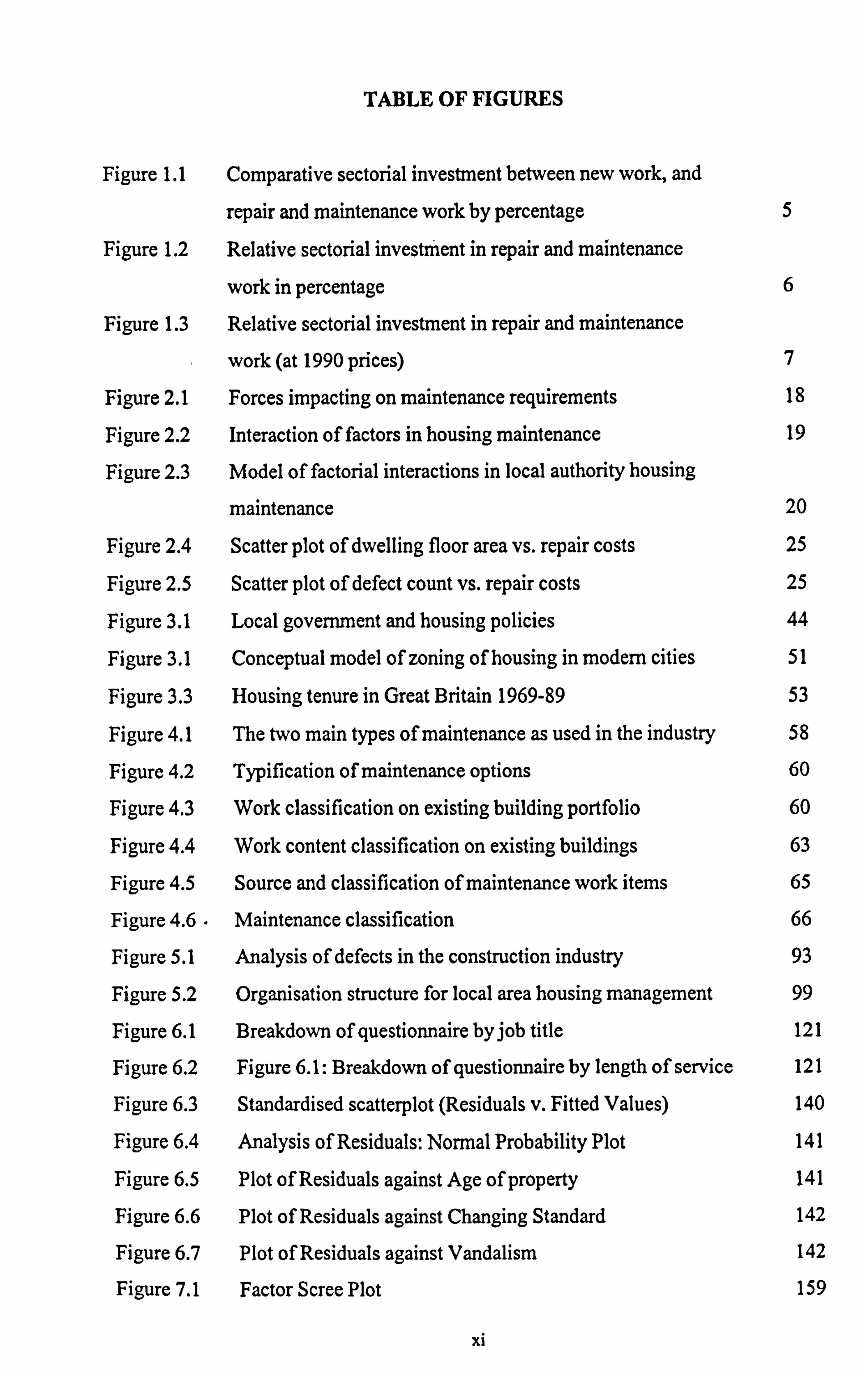
TABLE OF FIGURES
Figure 1.1 Comparative sectorial investment between new work, and
repair and maintenance work by percentage 5
Figure 1.2 Relative sectorial investment in repair and maintenance
work in percentage 6
Figure 1.3 Relative sectorial investment in repair and maintenance
work (at 1990 prices) 7
Figure 2.1 Forces impacting on maintenance requirements 18
Figure 2.2 Interaction of factors in housing maintenance 19
Figure 2.3 Model of factorial interactions in local authority housing
maintenance 20
Figure 2.4 Scatter plot of dwelling floor area vs. repair costs 25
Figure 2.5 Scatter plot of defect count vs. repair costs 25
Figure 3.1 Local government and housing policies 44
Figure 3.1 Conceptual model of zoning of housing in modern cities 51
Figure 3.3 Housing tenure in Great Britain 1969-89 53
Figure 4.1 The two main types of maintenance as used in the industry 58
Figure 4.2 Typification of maintenance options 60
Figure 4.3 Work classification on existing building portfolio 60
Figure 4.4 Work content classification on existing buildings 63
Figure 4.5 Source and classification of maintenance work items 65
Figure 4.6 " Maintenance classification 66
Figure 5.1 Analysis of defects in the construction industry 93
Figure 5.2 Organisation structure for local area housing management 99
Figure 6.1 Breakdown of questionnaire by job title 121
Figure 6.2 Figure 6.1: Breakdown of questionnaire by length of service 121
Figure 6.3 Standardised scatterplot (Residuals v. Fitted Values) 140
Figure 6.4 Analysis of Residuals: Normal Probability Plot 141
Figure 6.5 Plot of Residuals against Age of property 141
Figure 6.6 Plot of Residuals against Changing Standard 142
Figure 6.7 Plot of Residuals against Vandalism 142
Figure 7.1 Factor Scree Plot 159
X1
Figure 8.1 Histogram of Satisfaction
Figure 8.2 Boxplot and stem-and-leaf for satisfaction index
Figure 8.3 Boxplot of uncorrelated maintenance cost Figure 8.4 Histogram of neighbourhood social rating (VANDAL)
Figure 9.1 Work classification on existing building portfolio ,
177
179
181,
191
231
X11
ACKNOWLEDGEMENT
For a study over a long period as this, to prepare a shortlist of those to whom gratitude
should be extended is almost as difficult as the study itself. For such a task as this,
oversight and limitation find meaning and expression. However, life itself is about
recognising one's limitation and being prepared to own up to it when occasions demand. I therefore appreciate that I may not be able to acknowledge all worthies in
this page, but rest in the confidence that such worthies would understand and bear with
my limitation in this regard.
My thanks go to my supervisor, Trevor Mole without whose support and patience my
ambition of completing this study would have remained a perpetual mirage. Of him, I
could say, ̀ seest thou a man diligent in his ways, he shall stand before kings and not before mere men'. I shall not fail to acknowledge the man who held me by the hand
when as yet my sight in this field was dim and fuzzy, Vernon Marston. I owe so much to his fervour, support and concern during the early stages of this study.
My thanks go to Manchester City Council Housing Department for funding the
questionnaire survey. Most especially, I am grateful to Dean Williams (Principal
Research Officer) and Julie Jerram (Housing Team Leader) for their assistance and
advice at every stage of the work.
I am grateful to Dr. Akin Akintoye, Glasgow Caledonian University. He painstakingly
read through the draft thesis with very useful comments.
Without the encouragement of my wife, I long would have abandoned the study. It has
been a very hard journey but she kept my spirit buoyed up during the most difficult
days. I am also grateful for my two daughters who are so understanding and of the
kindest disposition. They bore with me through the days when I denied them of those
precious minutes I could have spent with them.
Through it all, I owe my life and my all to God who has never withheld from me those
things and gifts that I needed most at every stage in life's journey.
Xlii

DEDICATION
This thesis is dedicated to:
My wife, Olukemi;
My daughters, MoyinOluwa and FiyinfOluwa;
My father and mother, Folayan and Olawamide;
My uncle, Olayinka Olubodun; and'
My mother-in-law, Abike Fadeyi.
xiv
ABSTRACT
The thesis is concerned with the evaluation of factors in Local Authority housing
maintenance requirements in the City of Manchester.
Since 1982, expenditure in housing maintenance and repair works has consistently
accounted for more than 50% of total expenditure on maintenance and repair work. In
turn, maintenance and repair work accounts for almost 50% of total construction
output in the UK. Given this level of sectorial contribution, it is apt to understand the
factors which affect defects in dwelling buildings and hence maintenance
requirements. This thesis reviews the catalogue of building defect causative factors
leading to the conclusion that social and tenants' characteristics are equally important.
The study is based, chiefly, on a postal questionnaire survey of building surveyors
involved in day-to-day identification of defects as well as tenants of the sampled
dwellings; and computer cost records of maintenance on dwellings within the sample.
A total of 45 completed questionnaires from building surveyors, and 252 Council
tenants with corresponding computer cost records formed the data base for the
analyses conducted.
The building surveyors' questionnaire assisted in the identification of defect-cause
criteria which relate to the internal attribute of the dwelling building. The consistency
of the resulting data was confirmed by the use of Kendall Coefficient of Concordance.
An analysis is described of the manipulated data set using regression analysis. The
analysis found that Changing standard contributes (38%) of (building structure related factors') impact on maintenance requirement variance, construction factors (23%),
design factors (22%), vandalism (12%) and age factors (6%). The intercorrelations
among these five defect-cause criteria within the building object necessitated further
analysis using the principal component analysis. This resulted in the extraction of
nine significant factors showing how the initial five factors combine to exert their
influence on the building. In all, this family of building structure related factors
contribute 32% of the variation in maintenance requirements.
xv
Combining the data from the tenants' questionnaire, computer cost information and dwelling survey, regression model testing was employed to identify the significant factors. This was facilitated with the use of three indices of housing maintenance
requirements as the dependent variables, namely; reactive maintenance cost, property
condition and satisfaction among tenants. Nine factors (six of which relate to tenant's
characteristics) pertaining to tenant, environmental and housing management were
significantly influential.
xvi
i
CHAPTER ONE
INTRODUCTION
1.1 Introduction to the subject matter
The research was begun partly in response to earlier research efforts which generally
dealt with an examination of maintenance factors in isolation, most of which often
formulated maintenance action and priority out of context with factors bearing upon
those needs, and chiefly from the author's work experience as a principal surveyor
responsible for both programmed and day-to-day maintenance works on council
housing stock - consisting of about 9,000 mixed dwelling types.
Whilst earlier research efforts have formulated techniques for prioritising works, these
techniques can be described as generally prognostic, with a penchant to confirming the
stockholder's original ideas on how maintenance action should be pursued. In practice,
this approach may be justified in the light of funding restrictions and political
consideration. The position at the moment between the client and the building surveyor
is almost akin to patient-GP relationship, where the patient tells the GP his ailment, and
also informs him of his efforts at self-medications in the hope that the GP will find an
optimum prescription for his ailment around his self-medication. In contrast to this
analogy, the study strives to find a solution with or without existing self-medication
indulgences of the patient. To this end, the study can be described as being truly
diagnostic in relation to what components should take priority.
The depleting earth resources resulting from gross exploitation and growing global
population make a clarion call for the need to evolve a means of effectively conserving
these resources. This view was echoed when Jonge (1990) argued that past decades
have witnessed strong emphasis on the design and construction of new building and
called for a shift in emphasis as available physical and financial resources are almost
being over-stretched. This observation was a reverberation of Bromilow and Pawsey's
(1987) that property owners were more interested with the provision of new buildings
than they were with the costs of maintaining and operating their buildings.
2
A radical shift in emphasis of this nature requires the development of methods and instruments to manage existing portfolios of building assets. This need is all the more
urgent in the face of developing trends in nations' strict economic measures to conserve
scarce fund (Dixon, 1990), thereby making less and less fund available for new
developments.
It would appear that the way out is to seek to conserve available assets by prolonging
their lives, consistent with economy, in order to meet the ever growing human need for
controlled environment and space. In appreciation of this dire need, more thorough
attention to and examination of existing buildings has been gaining a high momentum
(Kondo et al, 1990). In their view, this is not purely because of increased safety
consciousness, but in order to gain a comprehensive understanding of building
deterioration and to develop effective methods of building maintenance and efficient
repair in suitable time.
An analogy between the human physiology and a building can be aptly drawn. Like the
human body, a building is a complex integration of different components, with each
meeting a definite function, and all working together in such a manner as to forestall
any likely impairment to the primary need of the specific building all through its life
time. This is the very essence of any maintenance action - its efficiency is in being able
to sustain the building in this condition at all times for the benefit of the user. In order
to achieve this objective, it is important to be able to relate each component of the
building to one another from the perspective of durability and life expectancy, and the
larger environment.
The paradox of the building structure is that those features of the building which appear
cosmetic in nature, are at_ the centre of its performance, the failure of which will cause
the building to significantly under perform. In fact, the most frequent maintenance items in housing are not necessarily the anatomical frame of the building.
The earlier the construction industry began to realise and to actualise that property investment is developing and maintaining assets, and not just constructing and
designing, the more the existing scarce funds will be conserved (Pollock, 1990), as the
3
construction of a building is merely the less significant beginning, in cost terms, of an
expensive life time (Bird 1987).
In a study of cost effectiveness of design decisions, White (1969) reported that running
costs of an office block will exceed capital costs in less than nine years of occupation.
Notwithstanding this stark finding, Harrison (1990) has noted the dismal backward
attitudes to maintenance in all sectors of the construction industry. This according to
him is evidenced in the attitudes of architects and quantity surveyors who always
presume that the cost-in-use of the building is necessarily inversely related to the initial
building cost. I
1.2 Economic importance and growth of maintenance
UK's expenditure on maintenance, repair and refurbishment now accounts for almost
half the turnover of the construction industry at current prices. In 1995 alone, work on
existing construction as repair maintenance accounted for £25.9 billion (as shown in
Table 1.1).
The quinquennial English House Condition Surveys reveal that spending on private
housing is often difficult to monitor to say the least. However, it is generally believed
that this may not be a serious shortcoming because this is an area which is relatively
insensitive to improvement by research and development. This view stands to reason
because of extensive individual variability involved and there is a difficulty in
persuading individuals to accept research findings unless such findings are adopted by
the government as policies.
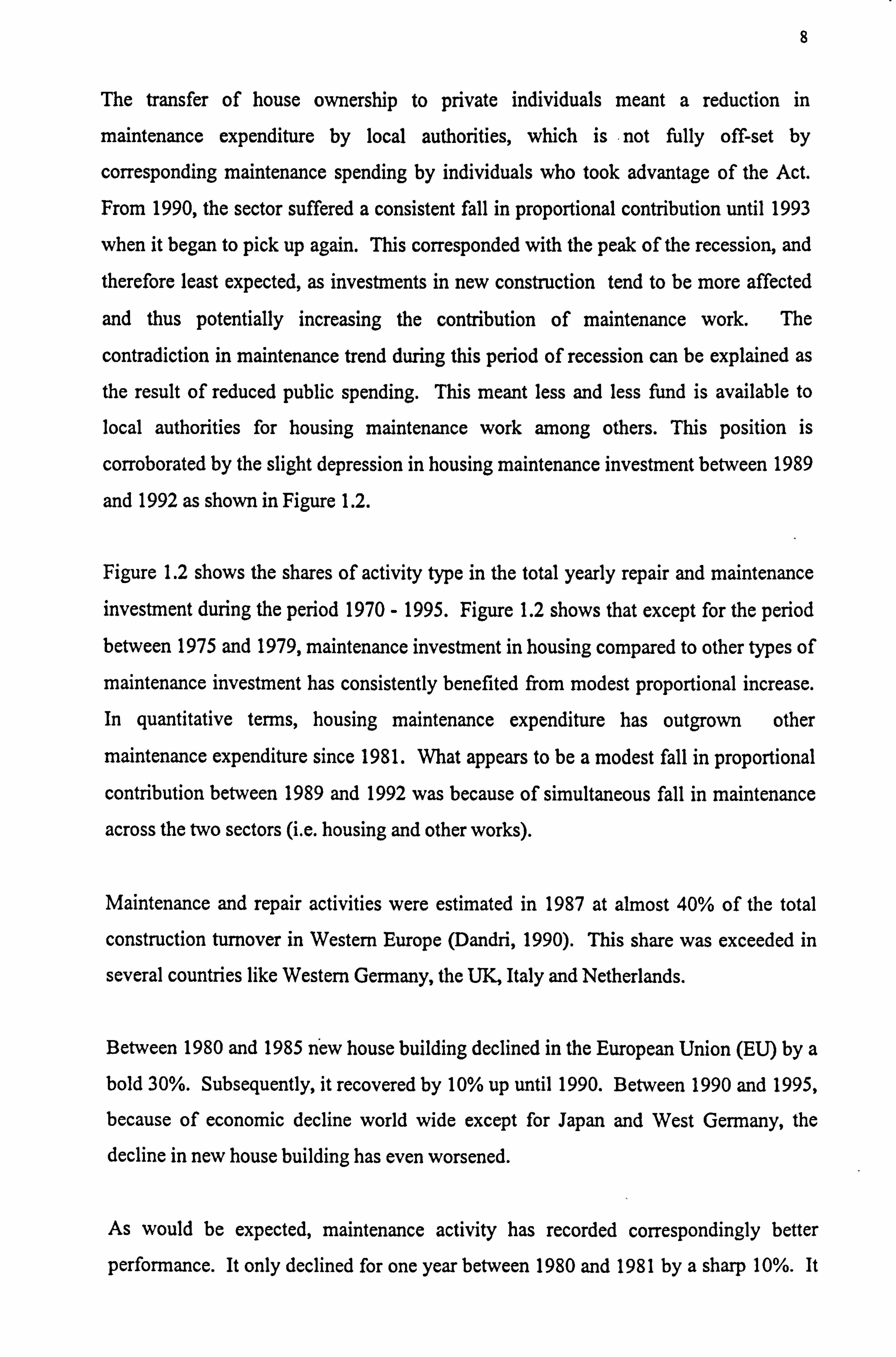
Figure 1.1 shows a comparative sectorial investment between new work, and repair and
maintenance work at 1990 prices during the period 1970-1995. The share of repair and
maintenance work increased steadily from 28% in 1970 to 45% in 1980. Between 1980
and 1990, there has been a general leverage in maintenance sector investment, with
slight depressions in 1982 and 1987. This period coincided with the periods when the
effects of the Right-To-Buy Act of 1980 began to be felt in public housing.
4
Table 1.1: Expenditure on new work and repair and maintenance (all construction excluding infrastructure)
Year New work Repair and Maintenance Total 1970 30,999 12,450 43,449 1971 31,643 12,546 44,190 1972 31,398 13,758 45,155 1973 31,259 14,409 45,667 1974 26,550 14,037 40,587 1975 25,338 12,816 38,155 1976 25,626 12,068 37,694 1977 24,928 12,482 37,409 1978 25,861 14,415 40,276 1979 24,106 16,559 40,665 1980 21,172 17,378 38,550 1981 18,994 15,826 34,820 1982 20,069 15,990 36,060 1983' 13,634 11,877 25,511 1984' 14,538 13,328 27,776 1985' 15,305 14,358 29,663 1986' 16,683 15,366 32,049 1987' 19,903 17,625 37,528 1988' 24,763 20,090 44,853 1989' 29,320 22,830 52,150 1990, 30,762 24,544 55,307 1991, 27,726 23,389 51,115 1992' 24,814 22,658 47,472 1993' 23,556 22,767 46,323 1994' 25,086 24,353 49,439 1995' 26,627 25,900 52,527
Year': 1983 to 1995 figures are at current prices, while 1970 to 1982 figures are at 1990 prices.
N C. ) C N
N
3ä a) aý
V66 I.
Z66 I.
0661.
8861.
9861.
1861
Z961
0861.
8L61.
9L6 1.
iL6 I.
ZL61.
OL6 OO
00 COO LOt) M
04
uoilnq! J; uo3 aäe; ueoJed
a) bi) cd
N
O
U U
N it
E
it bý'+
CCS
O
, G+ U
N
CÜ
OU
y .O UÜ
cC G"+ Ü
O U`.
aý
w
tn
a
cm c "cn
N O 2 C)
0
I 1
1I
1 11 11 11
11 1
I1 II 1I I1 1I
1 I
t 1
11 11 1I I1 1 11 11 1 I1 1
1I
1I
I
I1
I
1I
II
I
11
1
1
I
I
I
I
1
I
I
II
I
I
I(
I
1
I
1
I
II 1 I I
1
I
II
1I
1
1
1 1 1 1
I
1
I1 1
I 1
I1
1
II
1
1
1
1
I
1 1
1
1
I
I
1I I1
1 Ii
tI
II
I1
i
1
I1
1
i
II
II
1
1 1
I
i
-
1 1
V66 I.
Z66L
066L
886L
9861
V96 1
d Z86L >-
0866
8L6L
9L61.
t'L6 I.
ZL6L
AI vw r 000000
CO I) C') N
uolingiJ; uo3 ehe; uao. ied
C) bn cý .r aý 2 U C.
O
4)
b q
i O
y
O
cd
ýU U
U
ý, end
Fsr
N
y
ý bOA
w
%0
Co
- Fa Fý
Cr "N 6.
s
I 1
11 1I /
1 1
1 1 II 1 1
11 1I I1
1
1 t 1 1
1
1 1
1
I 11 1
t I I
II I f
I I
1 11 1
I 1
1 1
1 1 1
1
1 1 I
I
I
1 i
1I 11
I 1
1 1 1
1
1 1
1 I
I 4 1
I
1
1
1
1 I I 1
11 1 1
I
1
I 1
1 1
1
11 I 11 1
1
1 I 1 II
1 1
I
1
I 1
1 1
1
1
I
I 1
I1 1
0 0 0 0 0 c CD CD CD CD C) CD c CD C) CD 0 CO d' N
Ö 0 0 (0 d
r ý r r
suolII! W (seolad 0661. W)
V66 I
Z66I
0666
886
986v
186I. I-
Z961 }
0861.
8L61.
9L6 I.
VL6 I.
ZL61.
AIR, OO
vwr
O O N
enjen
U) 01-1 U
O O\ O\
cd
O
C
Fr
C_.
cd
ti
C4 U
ri
bA w
N
8
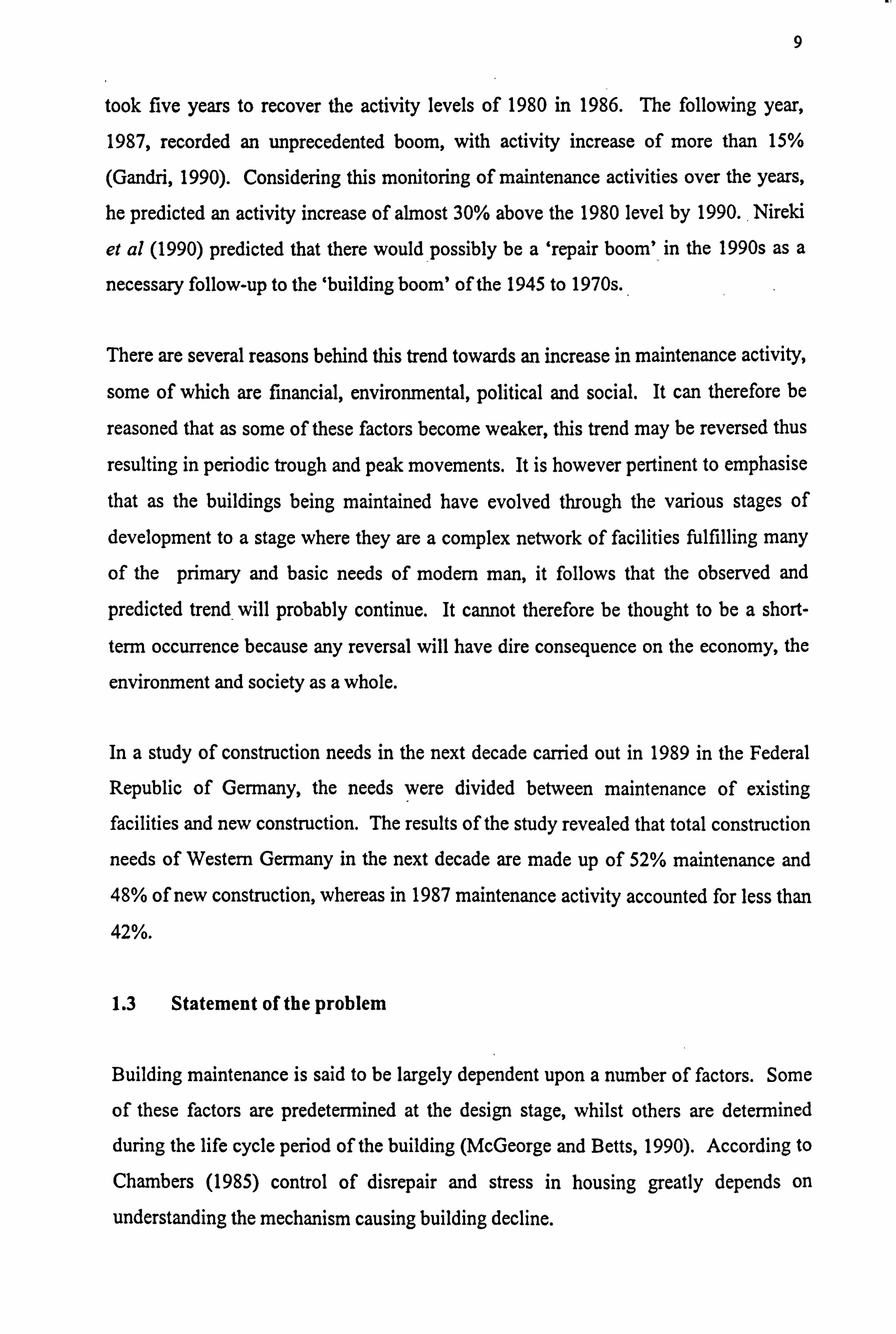
The transfer of house ownership to private individuals meant a reduction in
maintenance expenditure by local authorities, which is not fully off-set by
corresponding maintenance spending by individuals who took advantage of the Act.
From 1990, the sector suffered a consistent fall in proportional contribution until 1993
when it began to pick up again. This corresponded with the peak of the recession, and
therefore least expected, as investments in new construction tend to be more affected
and thus potentially increasing the contribution of maintenance work. The
contradiction in maintenance trend during this period of recession can be explained as
the result of reduced public spending. This meant less and less fund is available to
local authorities for housing maintenance work among others. This position is
corroborated by the slight depression in housing maintenance investment between 1989
and 1992 as shown in Figure 1.2.
Figure 1.2 shows the shares of activity type in the total yearly repair and maintenance investment during the period 1970 - 1995. Figure 1.2 shows that except for the period between 1975 and 1979, maintenance investment in housing compared to other types of
maintenance investment has consistently benefited from modest proportional increase.
In quantitative terms, housing maintenance expenditure has outgrown other
maintenance expenditure since 1981. What appears to be a modest fall in proportional
contribution between 1989 and 1992 was because of simultaneous fall in maintenance
across the two sectors (i. e. housing and other works).
Maintenance and repair activities were estimated in 1987 at almost 40% of the total
construction turnover in Western Europe (Dandri, 1990). This share was exceeded in
several countries like Western Germany, the UK, Italy and Netherlands.
Between 1980 and 1985 new house building declined in the European Union (EU) by a
bold 30%. Subsequently, it recovered by 10% up until 1990. Between 1990 and 1995,
because of economic decline world wide except for Japan and West Germany, the
decline in new house building has even worsened.
As would be expected, maintenance activity has recorded correspondingly better
performance. It only declined for one year between 1980 and 1981 by a sharp 10%. It
9
took five years to recover the activity levels of 1980 in 1986. The following year,
1987, recorded an unprecedented boom, with activity increase of more than 15%
(Gandri, 1990). Considering this monitoring of maintenance activities over the years,
he predicted an activity increase of almost 30% above the 1980 level by 1990., Nireki
et al (1990) predicted that there would possibly be a `repair boom' in the 1990s as a
necessary follow-up to the `building boom' of the 1945 to 1970s.
There are several reasons behind this trend towards an increase in maintenance activity,
some of which are financial, environmental, political and social. It can therefore be
reasoned that as some of these factors become weaker, this trend may be reversed thus
resulting in periodic trough and peak movements. It is however pertinent to emphasise
that as the buildings being maintained have evolved through the various stages of
development to a stage where they are a complex network of facilities fulfilling many
of the primary and basic needs of modern man, it follows that the observed and
predicted trend will probably continue. It cannot therefore be thought to be a short-
term occurrence because any reversal will have dire consequence on the economy, the
environment and society as a whole.
In a study of construction needs in the next decade carried out in 1989 in the Federal
Republic of Germany, the needs were divided between maintenance of existing facilities and new construction. The results of the study revealed that total construction
needs of Western Germany in the next decade are made up of 52% maintenance and 48% of new construction, whereas in 1987 maintenance activity accounted for less than
42%.
1.3 Statement of the problem
Building maintenance is said to be largely dependent upon a number of factors. Some
of these factors are predetermined at the design stage, whilst others are determined
during the life cycle period of the building (McGeorge and Betts, 1990). According to
Chambers (1985) control of disrepair and stress in housing greatly depends on
understanding the mechanism causing building decline.
10
A feasibility study sponsored by the R. I. C. S. in 1969, whose principal objective was the
development of a reciprocal service for the collection and exchange of maintenance,
cost data (Pullen, 1987), led to the establishment of the Building Maintenance, Cost
Information Service. The terms of reference of the study was the formation of a data
bank to furnish information which could help in the deployment of resources in
maintenance, and the problem of defining the scope of building maintenance costs.
This was a significant milestone in the evolution of an organised maintenance data
base. Prior to this time, there had been several studies on various aspects of building
maintenance (BRE, 1972; BRS, 1968; and BRS, 1963). Surprisingly, they all focused
on the pattern of raw data collected from surveys rather than the factors governing the
behaviour of the reported pattern. In drawing upon these studies, the BRE (1972)
attempted to bring meaning into the data collected to assist comparison and went a step
further to establish a trend between maintenance cost and the age of dwellings. The
`age' factor has since then been a common theme that runs through most, if not all of
subsequent studies in the field. Among the most important findings by the BRE were
existence of wide variations in maintenance expenditures resulting from the interplay of
factors other than physical characteristics of the buildings studied. No more was
however done by way of deciphering what these factors are or even could be.
Wyatt (1980) provided some insight into the complex phenomenon of maintenance
costs when he posited that it is not sufficient to set maintenance standard requirements
as a function of age of a dwelling. He contended that there are several other influencing
factors which are essentially social, environmental, usage, economic, physical
characteristics and even design.
In her study of public sector housing stock, Diacon (1991) identified the major cause of
concern in British housing as the poor quality and continuing deterioration of the
physical structure of residential dwellings. In reviewing her book, Malpass (1991)
underscored the fact that the real cause for concern is the set of underlying factors
which are responsible for disrepair and deterioration in the stock.
Holmes (1985) sought to consolidate upon these findings when in his work he analysed
maintenance expenditure components. He evolved deductive explanations in order to
11
identify various factors in maintenance. His data appeared as cost per dwelling without
any standard reference point to dwelling size or any other design parameters. His study
of the influence of the social environment of housing estates was not substantiated by
any form of estate stratification approach. These limitations undermine the authenticity
of his findings.
Certain inadequacies persist which bear upon the usefulness and reliability of the
findings in all of these studies for practical purposes:
9 The studies were conducted with a pre-conceived notion of which factor(s) should
be investigated. In order to gain an accurate perspective of maintenance
expenditure behaviour, exploratory synthesis and analysis need to be conducted to
determine which factors are actually significant.
" Data collected were based on price charged for the work, which is a biased measure
of maintenance need as it is usually made up of both the repair item and other items
of costs which may be unrelated to the original repair item. Hence, it is not
infrequent to have a gamut of redundant cost data in most of these studies.
" Existing studies dealt with the examination of independent and uncorrelated
singular factors. It is not conceivable to think of individual factors as being free
from interference within the larger system.
Despite the increase in awareness of the importance of maintenance to the construction
industry, current analytical academic efforts have incorporated these inadequacies as a
matter of norm. Furthermore, the mass of academic effort has concentrated on the
mathematical along side statistical modelling of narrow problems or the minutiae of
decision theory and forecasting. Among what is lacking and is the objective of this
research, is the development of a framework of factors which govern maintenance need
in housing stock.
The problem as it stands has been succinctly articulated by McGeorge and Betts (1990)
as follows:
"Building maintenance is dependent upon a number of factors ... Most of these factors are in some form of dynamic relationship with one another. The
12
problem is in identifying these key factors given the uncertainty of... the life cycle of a building".
With this typical problem is the added problem of the qualified nature of maintenance
expenditure. This has a far reaching effect upon the usability of historic maintenance
cost data for research purposes. One must therefore look elsewhere by way of
methodology to complement existing historic cost data.
1.4 The choice of Manchester for the study
The decision to use Manchester is more logical than sentimental. It is believed at the
on-set of the research that the information required for the study was not going to be
limited to qualitative primary data which are usually obtainable with minimum
confidentiality restrictions from respondents. In addition, substantial quantitative data
of some confidential sort will also be required.
In most, if not all housing organisations, records of maintenance expenditures are stored
in computer software which can only be accessed with the use of `password' only
available to a few individuals within the organisation. It was anticipated therefore that
such information will not be obtainable from any organisation which is not acquainted
with the person requiring the data. Whilst the study could attain some width, its depth
could be seriously hampered without a complete information set of both quantitative
and qualitative data.
The use of one single organisation is beneficial as it enhances the use of homogeneous
data set which allows for the specific variables of interest to be examined without
undue interference from organisational variability. Furthermore, Manchester housing
situation has been described by Short (1982) as broadly representative of housing
condition in the UK.
13
1.5 Aims of the Research
The overall aim of the research is to develop a framework of factors influencing
maintenance requirements in public sector housing.
To achieve this overall aim, the preliminary research (described in chapter 2) identified
that the following areas needed to be investigated:
1. Nature and characteristics of maintenance cost records - development of a
methodical approach to assessing overall maintenance requirements of housing
stock.
2. The characteristics of local authority tenants
3. Housing stock condition assessment as perceived by responsible building
surveyors
1.6 Research Hypothesis
To ensure the research aim was achieved, the following hypothesis was addressed throughout the research: - Maintenance requirements are influenced by:
(i) a number of precise building object attributes; (ii) the surrounding environment in which dwellings are located;
(iii) the characteristics of the tenants; and (iv) housing management responsiveness.
The formulation of this hypothesis is discussed in chapter 2

14
1.7 Benefits of the Research
The study will be of benefit to individual building surveyors, housing managers, those
involved in housing construction and design, and clients of the construction industry as follows: -
" Awareness and knowledge of issues bearing upon maintenance requirements should be of value to the individual housing managers at both estate and policy formulation
levels.
" Housing organisations could become more knowledgeable about optimum
maintenance strategies, and may become more attuned to users' needs.
9 For the construction industry as a whole, a conglomeration of factors having
significant influence on maintenance requirements will enhance judicious allocation
of limited funds to maximum effect.
The isolation of groups of components that are meaningfully related should benefit
architects and surveyors who are involved in various forms of design. It should assist
them in evaluating groups of components prone to common or identifiable defect
causing influence.
1.8 Organisation of the chapters
Chapter Two discusses the research methodology, the scope and methods of data
collection. The strategy for the procurement of the research and working hypotheses
are presented.
Chapter Three discusses the history of housing in the UK through the instruments of
Housing Acts.
Chapter Four reviews various definitions of maintenance advanced by exponents and discuses terminologies for describing various grades of work to existing buildings.
15
Literature review of maintenance requirements indices used in the research is made.
Chapter Five is the review of related literature on maintenance factors.
Chapters Six, Seven and Eight present the data obtained and the outcome of hypotheses
testing, and resulting factorial models. The study is concluded in Chapter Nine.
16
CHAPTER 2
METHODOLOGY
2.1 Introduction
This chapter sets out the research methodology adopted for the study. Part of the
problem lies in the nature of the subject matter; building condition and usage, involving
a myriad of variables, cannot be examined separately from its social and economics
context. Consequently, it is an exceedingly complex problem. Equally troublesome is
the existing level of measurement. The inherent limitation of historical data has been
aptly noted by Christer (1982), Bishop (1984) and Bird (1987). They all maintained
that historical cost alone is not reliable for predicting future maintenance costs.
Tucker (1990) was of the opinion that maintenance records lack adequate description of
details and hence, associated costs of such omitted details. He therefore advised that
everyone seeking to make judgements based upon such data must exercise serious
caution as historical data tend to be an underestimate. The observation about
inaccuracy and unreliability of historical maintenance information has become too
overwhelming to ignore. If they are typical of available records, unless rigorous
manipulative measures are taken, there will be little value in seeking any more
historical case studies. The need for theoretical modelling techniques is therefore even
more pressing if the costs of maintenance are to be properly planned in future. This
same problem was recognised by Wyatt (1980) when he argued that the interpretations
of maintenännce cost information are complicated by the extent that improvement and
repair obscure the actual maintenance cost.
In the face of this deficiency in quantitative records, rigorous inferential classification
techniques are called upon in order to evolve a set of reliable explanatory variables involved in maintenance requirements.
17
2.2 The Research Approach
The first stage of the research consisted of planning a research approach in order to
develop a framework of factors. This involved a literature review, brainstorming
sessions and contacts with individuals with experience in housing. As a result of this
stage the research areas, hypothesis and tools were determined.
2.3 Research Tools
To choose a strategy for empirical data collection, in addition to the literature, it is
important to define clearly the nature and applicability of historic maintenance cost
information available for the study.
The preliminary research identified three principal areas requiring investigation. These
are then decomposed into smaller identifiable elements.
To address the research areas, use is made of a mix of quantitative and qualitative
assessment of the condition of the housing stock. Each dwelling within the sample is
considered on its own merit and then the overall maintenance cost profile over a period
of five years is analysed. This analysis is complemented by a survey of the tenants of
the stock to be examined. In addition, a generalist survey of housing stock within the
council of interest is conducted through a sample of building surveyors working for the
housing department.
A cross-sectional study of housing authorities across the UK was not considered
necessary given the reasonably large size of dwelling population in Manchester
Council, and the time and cost limitations placed upon the research. It is more useful
and relevant however, to fine-tune the study to a level of detail as to afford discovery of
systematic exhibited characteristics, if any, within the housing stock without undue
inter-stock variations to the study. Hence, the choice of a case study for this research.
18
2.4 Research Framework
It is has been suggested that once a building is erected, the level of maintenance
required to keep it physically and functionally satisfactory is principally influenced by a
system of usage and environmental conditions rather than by the building dynamics.
The system of usage and. environmental conditions are regarded as those forces
`outside' of the building object which cause a series of stress action on it (Grassi et al, 1990). The building dynamics pertain to those building characteristics inherent in the
building fabric, which are traditionally believed to predicate its physical and functional
behaviour (Coskunoglu and Moore, 1990).
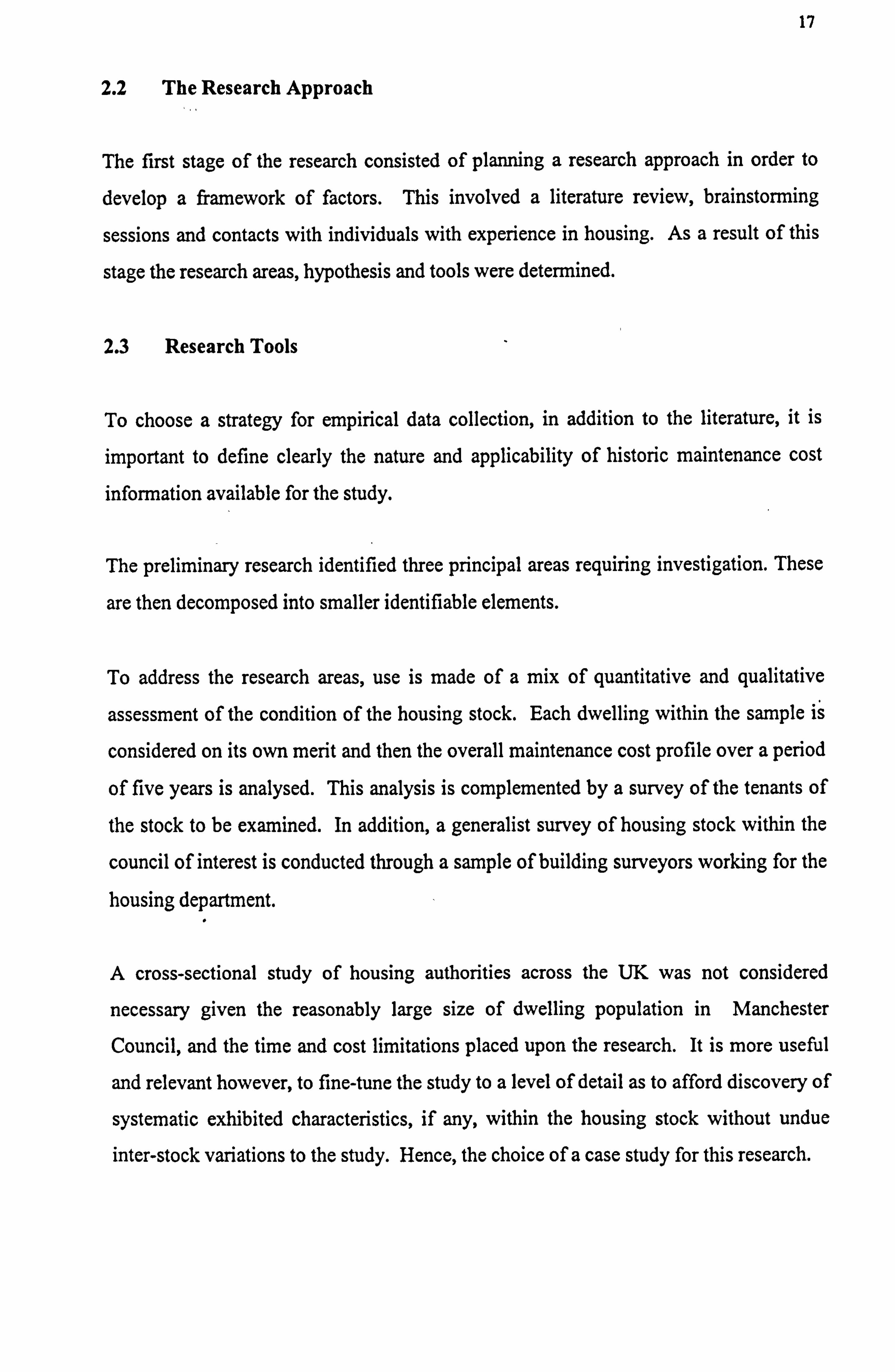
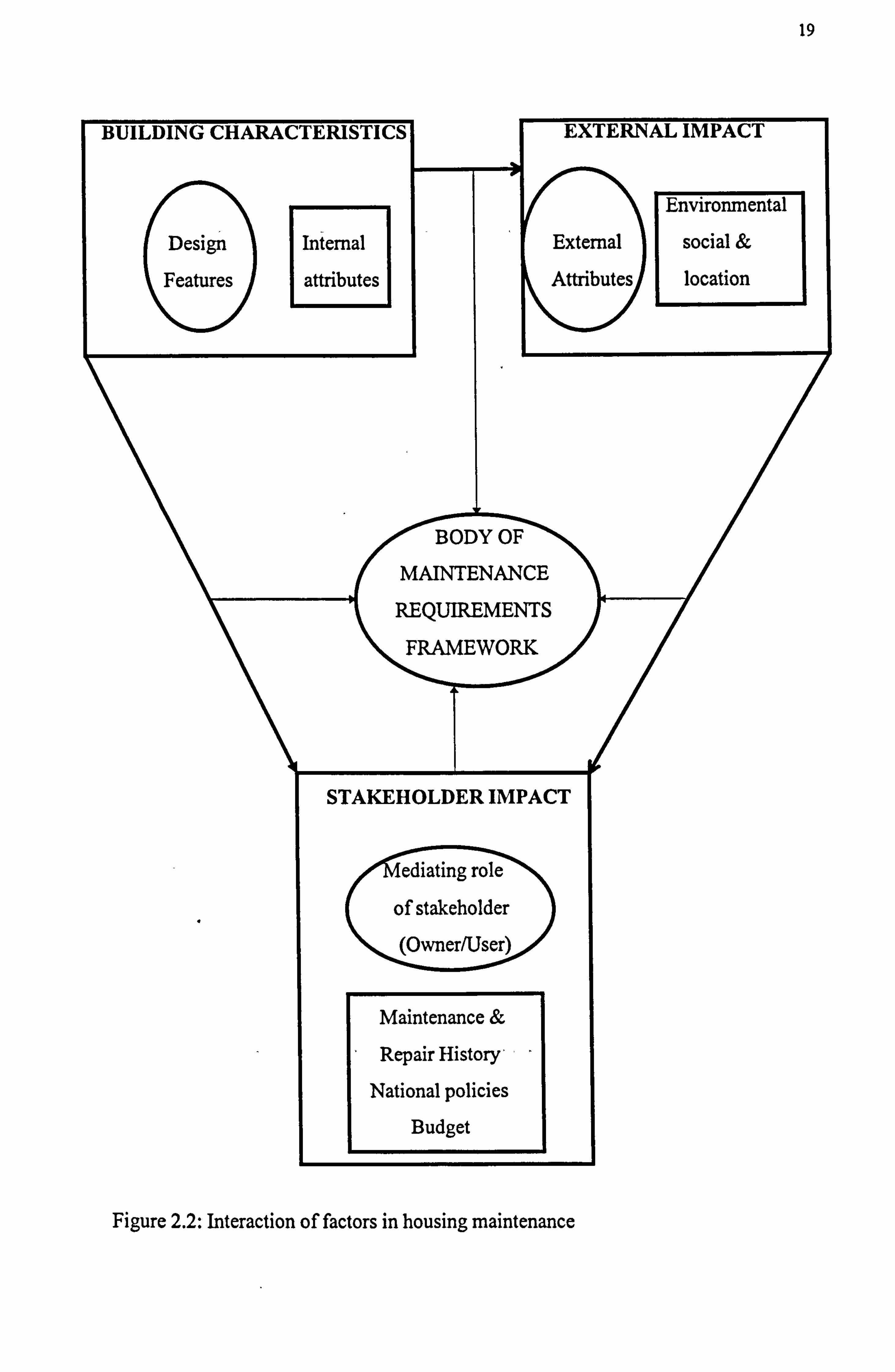
The development of thoughts on the relationships and hence the working hypothesis are illustrated in Figures 2.1,2.2 and 2.3.
Maintenance Requirements
Usage and Environment
Owner Characteristics
Figure 2.1: Forces impacting on maintenance requirements
Building Characteristics
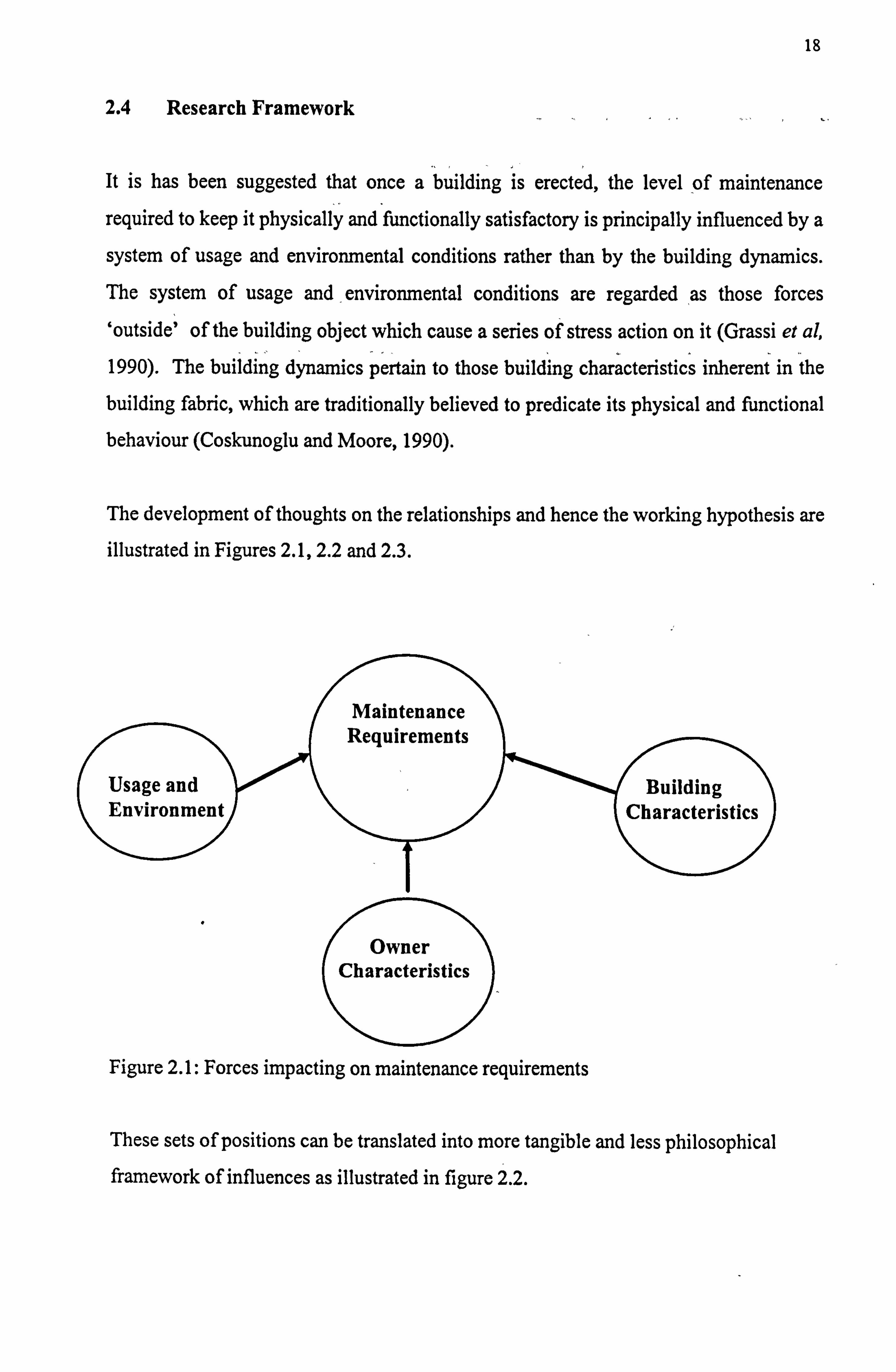
These sets of positions can be translated into more tangible and less philosophical framework of influences as illustrated in figure 2.2.
19
CS
Design
Features
Internal
attributes
BODY OF
MAINTENANCE
AL IMP
Environmental
External social &
Attributes location
REQUIREMENTS
FRAMEWORK
STAKEHOLDER IMPACT
C ediating role
of stakeholder (Owner/User)
Maintenance &
Repair History,
National policies Budget
Figure 2.2: Interaction of factors in housing maintenance
on
E
ev b 9
d k. Z v
Ici ä b 9 an on
U
Vii .
.:., aý ý" "N
CC S ý
0
w
.: r
-
ýN
1I FBI ý
4)
C6O
ö ý 'w o on
ay '
aw ' o " "
4 A ,.
c3
cä w O
I
I
0 u c
E
La'
0
0 .y
0
u
el:
0
w
0
0
N
i, WD
w
0 N
21
2.5 The working hypothesis
In the light of these interactions which come to light after an extensive review of
literature in the subject area, (Figures 3.1,3.2 and 3.3) the working hypotheses are
stated as follows:
1. The internal attributes of a dwelling (building fabric) as defined influence its
maintenance requirements.
2. The way the building is used and the environmental stress to which the building is
conditioned influence its maintenance requirements.
3. The response attitude of the stockholder influences the stock's maintenance
requirement profile.
Explanation for maintenance requirements characteristics to be meaningful should
focus upon the primary generators of maintenance at individual stock level as a basis
for any generalisation. The research scope has been selected with this in mind. Hence,
the research has been broadly divided into three possible areas for the purpose of this
investigation as shown in figure 2.2. That is, internally generated attributes in housing
stock, externally generated attributes and the mediating / response attribute of the
stockholder. All these possible areas are meant to complement one another towards the
development of a framework for the set of parameters in maintenance need, if in fact
they do exist.
2.6 Data Collection Strategy
2.6.1 Measurement and Statistics
Any kind of physical measurement made on living things will show variability across
subjects. People differ in abilities, interests, attitudes, temperament, etc. Some of these
individual differences can be measured more precisely than others depending on the
type of scale on which they are measured. An initial step in the research method is
therefore the measurement of the variables. Leedy (1989) describes measurement as
the quantifying of a phenomenon which results in a mathematical value.
22
2.6.2 Nature of the Data
In the absence of absolutely reliable quantitative measures of the important concepts,
recourse was made to classification techniques and pseudo quantitative measures. Random sampling technique is employed to ensure that the observations are truly
independent.
Prodigious use is made of categorical variables in the study as they best measure truly
discrete phenomena such as household size and attitude. In many instances, the
research has had to compress variables into a small, manageable number of categories.
This is a way to achieve mutual exclusiveness within the categories. According to
Reynolds (1977) this is a fundamental requirement of most of the statistical techniques
used in the analysis of data. An obvious problem with this need is that some
continuous variables have to be compressed which may lead to erroneous conclusion.
2.6.3 Scales of Measurement
The measurement of physical and psychological variables can be characterised by the
degree of refinement or precision in terms of four measurement scales (Aiken, 1991):
1. Nominal level of measurement divides the data into discrete categories. Any data
that can be differentiated merely by assigning a name to it falls in this level of
measurement. 2. Ordinal scale quantifies data or entity in terms of being of a higher or lower or
greater or lesser order than a comparative entity but without specifying the size of
the intervals.
The above two categories together comprise the non-interval level of measurement.
3. Interval level of measurement is characterised by two features; equal units of
measurements and an arbitrarily established zero point.
23
4. Ratio level of measurement which can express values in terms of multiples and
fractional parts. It has an absolute or true zero point which is the total absence of
the quantity being measured.
The interval and ratio levels together comprise the interval level of measurement.
The questionnaire survey instrument employs combined usage of the ordinal, nominal
and interval scales. This is so as most of the attributes being measured are either
attitudinal or opinion based which more readily lend themselves to the less precise
ordinal and nominal scales.
Where appropriate, some of the non-interval measures have been converted to interval
scale by some appropriate transformation techniques (after Kearns et al, 1991). This is
a common practice in social and medical sciences. Many researchers believe that this
practice does not lead to erroneous conclusions. According to Reynolds (1977),
statistics such as tests of significance or measures of association apply to numbers as
numbers and do not depend for their validity on the measurement model. According to
him empirical evidence abounds that violations in measurement assumptions do not
cause many mistakes in significance tests or parameter estimation. He alluded to
Labovitz's (1970) assertion that correlation coefficients are more or less unaffected by
applying them to ranked instead of numerical data, thus leading to the conclusion that
parametric statistics can be given their interval interpretation with only negligible errors
when used on ordinal data.
2.7 A framework for the measurement of maintenance need
2.7.1 Approach to preliminary investigations
The objectives of the preliminary investigations are twofold.
1. To identify the suitability or otherwise, of historic cost records for use as the
dependent variable for the study.
2. To devise a valid list of independent variables. To achieve this, the survey will seek
consensus agreements on a commonality of approach in housing property defect
identification among building surveyors and housing managers.
24
2.7.2 Measurement of maintenance need
A major concern among researchers is that the tests be useful and that they measure
what the authors claim (Aiken, 1991). Finding a reliable and consistent index or indices for measuring actual maintenance requirements of a housing unit is pivotal to
any useful elicitation of the general behaviour pattern of the phenomenon.
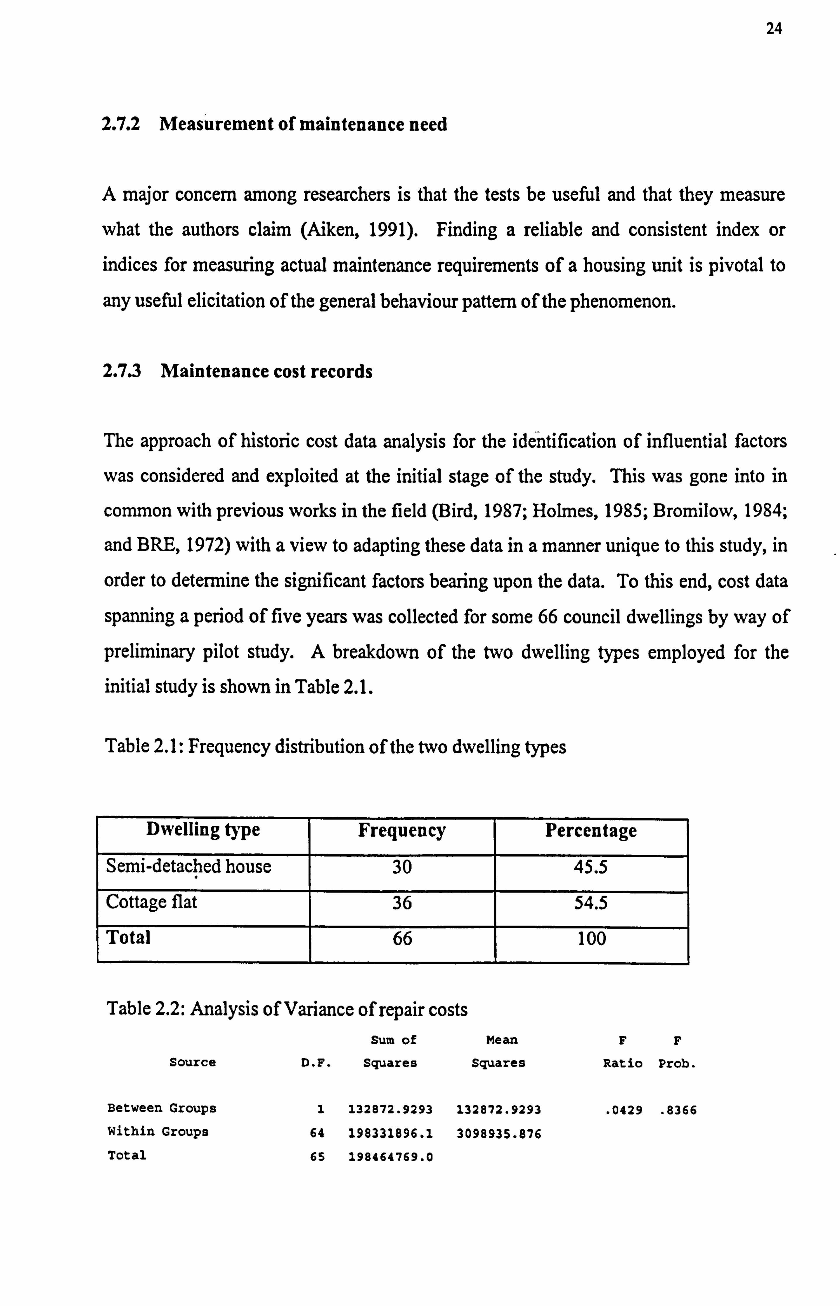
2.7.3 Maintenance cost records
The approach of historic cost data analysis for the identification of influential factors
was considered and exploited at the initial stage of the study. This was gone into in
common with previous works in the field (Bird, 1987; Holmes, 1985; Bromilow, 1984;
and BRE, 1972) with a view to adapting these data in a manner unique to this study, in
order to determine the significant factors bearing upon the data. To this end, cost data
spanning a period of five years was collected for some 66 council dwellings by way of
preliminary pilot study. A breakdown of the two dwelling types employed for the
initial study is shown in Table 2.1.
Table 2.1: Frequency distribution of the two dwelling types
Dwelling type Frequency Percentage
Semi-detached house 30 45.5
Cottage flat 36 54.5
Total 66 100
Table 2.2: Analysis of Variance of repair costs Sum of Mean FF
Source D. F. Squares Squares Ratio Prob.
Between Groups 1 132872.9293 132872.9293 . 0429 . 8366
Within Groups 64 198331896.1 3098935.876
Total 65 198464769.0
25
1ý cý aý A
vn
cý A
cý Q
O
O U
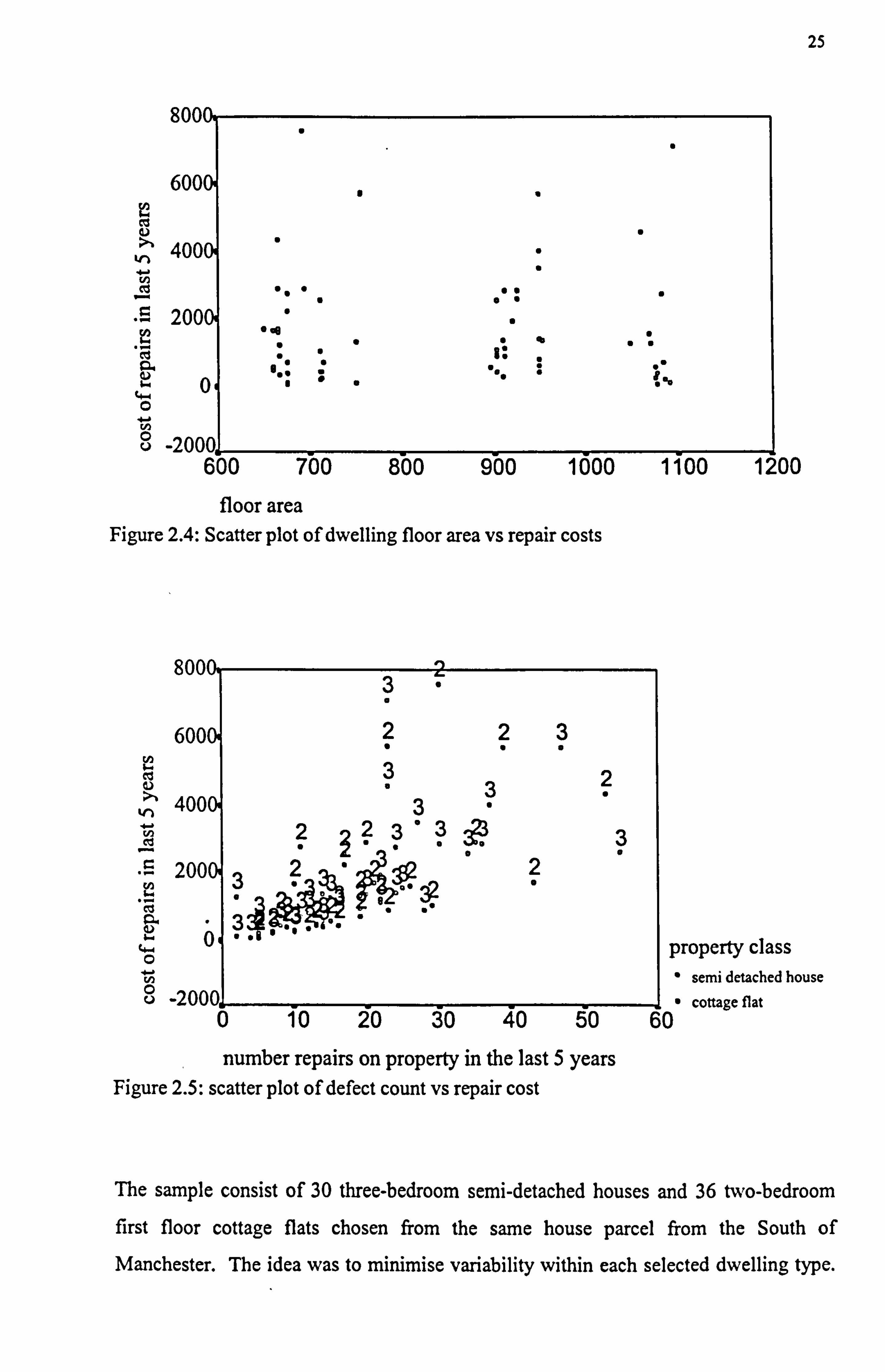
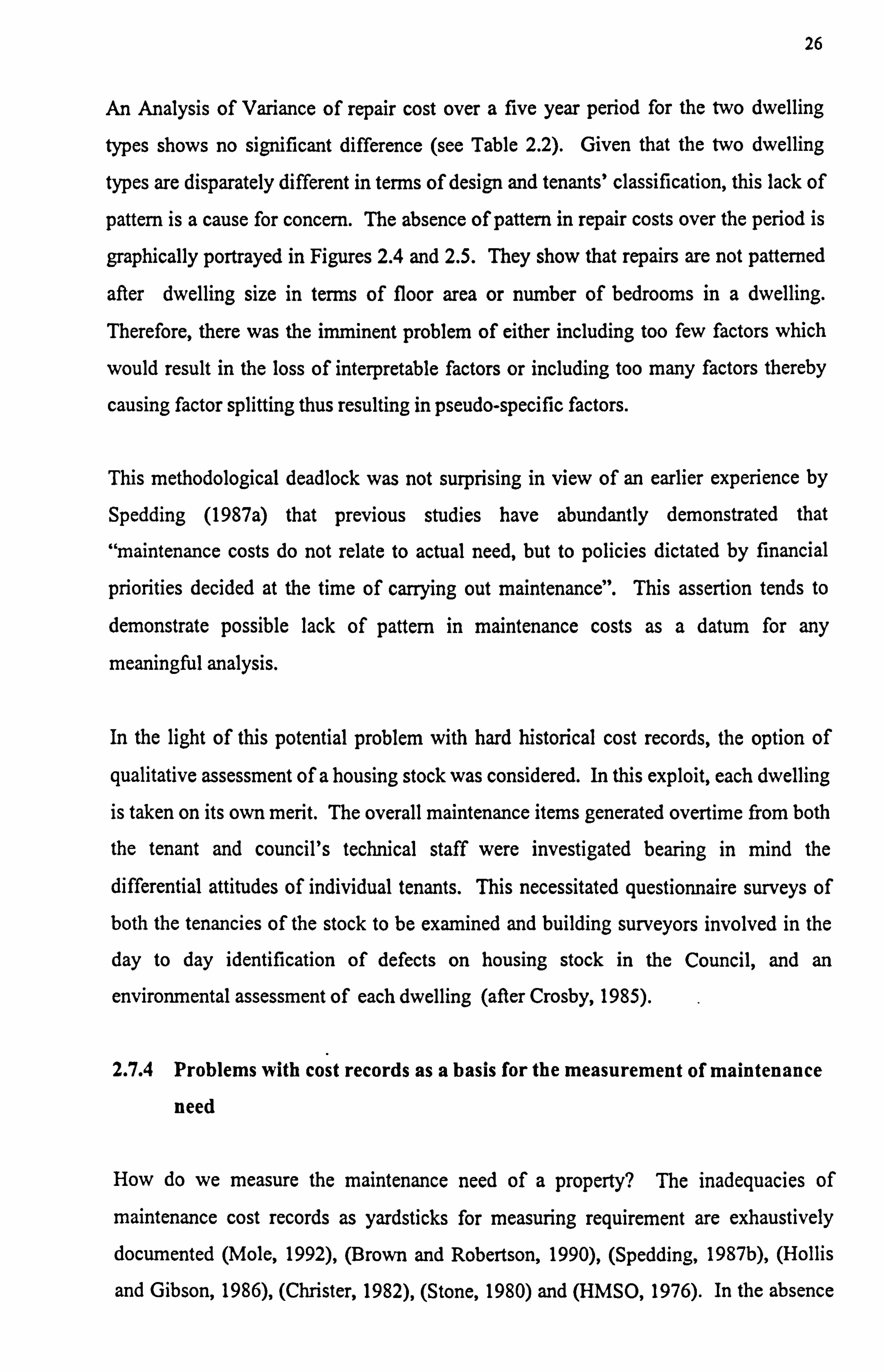
floor area Figure 2.4: Scatter plot of dwelling floor area vs repair costs
800 3"
223 6000 U) 3
400 33 3 2Z3
"ý 200 322
31 01
0
-2000 0 10 20 30 40
2
3
property class " semi detached house
" cottage flat 60
number repairs on property in the last 5 years Figure 2.5: scatter plot of defect count vs repair cost
The sample consist of 30 three-bedroom semi-detached houses and 36 two-bedroom
first floor cottage flats chosen from the same house parcel from the South of Manchester. The idea was to minimise variability within each selected dwelling type.
26
An Analysis of Variance of repair cost over a five year period for the two dwelling
types shows no significant difference (see Table 2.2). Given that the two dwelling
types are disparately different in terms of design and tenants' classification, this lack of
pattern is a cause for concern. The absence of pattern in repair costs over the period is
graphically portrayed in Figures 2.4 and 2.5. They show that repairs are not patterned
after dwelling size in terms of floor area or number of bedrooms in a dwelling.
Therefore, there was the imminent problem of either including too few factors which
would result in the loss of interpretable factors or including too many factors thereby
causing factor splitting thus resulting in pseudo-specific factors.
This methodological deadlock was not surprising in view of an earlier experience by
Spedding (1987a) that previous studies have abundantly demonstrated that
"maintenance costs do not relate to actual need, but to policies dictated by financial
priorities decided at the time of carrying out maintenance". This assertion tends to
demonstrate possible lack of pattern in maintenance costs as a datum for any
meaningful analysis.
In the light of this potential problem with hard historical cost records, the option of
qualitative assessment of a housing stock was considered. In this exploit, each dwelling
is taken on its own merit. The overall maintenance items generated overtime from both
the tenant and council's technical staff were investigated bearing in mind the
differential attitudes of individual tenants. This necessitated questionnaire surveys of
both the tenancies of the stock to be examined and building surveyors involved in the
day to day identification of defects on housing stock in the Council, and an
environmental assessment of each dwelling (after Crosby, 1985).
2.7.4 Problems with cost records as a basis for the measurement of maintenance
need
How do we measure the maintenance need of a property? The inadequacies of
maintenance cost records as yardsticks for measuring requirement are exhaustively documented (Mole, 1992), (Brown and Robertson, 1990), (Spedding, 1987b), (Hollis
and Gibson, 1986), (Christer, 1982), (Stone, 1980) and (HMSO, 1976). In the absence
27
of maintenance cost as an effective measure one is led to consider the total number of defects generated by the property through time as a ready-made objective indicator.
For this to be an efficient and valid measure, it must be established that every defect
reported by whatsoever means is equally important. To do this, the pattern and distribution of the mean cost of defects in each dwelling included in the final survey
were studied. The closer to zero the standard deviation of the mean is, the more
accurate it will be to assume that any two defects identified are equally important, at
least in terms of cost. For example, given the following statistics (Mean=1413.12 and
S. D =1517.75), the deviation is considered too high to allow for any assumption of
proximity within defects. Hence, it was decided that simply using the number of
defects as a measure of maintenance generated by a property cannot be a valid or
efficient index.
Further to preliminary interview with housing management team, the mechanism for
the identification of defect introduces a new dimension to the problem of using either
maintenance cost or number of defects for this purpose. It is useful to know that the
problem which impacts upon the criterion of interest has nothing to do with the pricing
mechanisms as identified by (Stone, 1980). Any problem connected with this
phenomenon is believed to have been taken care of by the homogeneity created by the
use of a case study (this makes pricing error a common denominator to the data). The
real problem lies in the way and manner defects are identified and the criteria for
actioning defects schedules prepared by surveyors:
1. The more aware tenants are of their rights, the higher the cost records associated
with his/her dwelling. This disposition among tenants will, more than anything
else, be dictated by whether or not the tenant is entitled to legal support. 2. The degree to which pressure is generated by the tenant on local housing
management depending upon user satisfaction and tolerance levels.
Whilst the total number of defects over time is less useful because of lack of validity
and efficiency, it would be tantamount to throwing the baby out with the bath water to
discard existing cost records on the ground of being totally useless. Given some vital
adjustments which can correct for existing anomalies in cost records, its validity and
28
efficiency can be substantially improved as to render it a more useful index. To achieve
this objective, it was decided to corroborate existing cost data with a further survey of
each dwelling in the sample (see chapter Eight).
2.7.5 Preliminary questionnaire design and surveys
The rest of this chapter describes both the introductory questionnaire survey (the
preliminary survey), and the final questionnaire survey (the final survey) for this study.
The objective of this section of the report is to ascertain the relevance or otherwise of
the factors included in the study as independent variables.
The preliminary survey was conducted during the early stage of the study following an
extensive literature search on the subject. The final surveys were conducted to establish
the observations and to justify or refute the hypothesis developed from the theoretical
background work and preliminary questionnaire.
2.7.5.1 The preliminary survey - Data collection and subjects
In appraising any set of attributes, the attributes should be discussed almost ad nauseam
(Fortune and Skitmore, 1994) with the individuals who practise (in this case, the
building surveyors), as well as those for whom they are responsible (in this case,
housing management team).
In view of this, it was considered appropriate to gather views from both building
surveyors and housing management officers in the first instance, and subsequently from
housing tenants in order to gain a rounded understanding of the subject of maintenance
need.
Research data was collected from the first two groups of subjects namely; building
surveyors and housing management team. The rationale for this was that of the three
groups identified, building surveyors and housing management team have a deep
dimension of impersonal interest in the stock by virtue of their professional training and
background. Whilst tenants have a highly variable but personal interest in their
29
respective properties. Since what is desired at this stage is an unbiased view of the
issues involved, it was not considered appropriate to involve tenants at this stage of the
study.
An important characteristic of the subjects in the preliminary survey is that the
researcher has worked with both the building surveying and housing management
teams at one time or the other in the last five years in his role as a 'principal surveyor
with the Council. The team have, therefore, been selected for this crucial part of the
study based upon their perceived individual competence and experience with the
council housing stock.
The building surveying group comprised 15 building surveyors. The housing
management team comprised 17 housing officers. All the subjects were visited on
appointment between February and June of 1993. A very brief interview and rank order
schedule (after Kerlinger, 1973) were used to collect the data from the two subject
groups for this part of the preliminary study.
2.7.5.2 Procedure for the preliminary survey
The introductory survey was conducted with building surveyors and housing
management officers, all of whom are primarily employed to look after the council
housing stock. The survey instrument was designed in the form of a questionnaire but
the implementation took the form of a structured interview, which meant the author,
read the questions and ticked the answers for the respondents.
Questionnaires as in Appendices 1AA and lAB were used to obtain data from each of
the two groups of subjects. Basically, identical procedures were used in the collection
of data from the different groups, consisting of the following.
1. A general introductory informal discussion with the subjects concerning the nature and
purpose of the study and the concept of defect. For the building surveying segment of
the sample, briefing session was somewhat superfluous as they are well informed and
trained in the technicalities of defects and maintenance. Nevertheless, the briefing
30
exercise was a means of creating a uniform basis for response and mitigating the
problem of subjectivity among surveyors (after Damen, 1990). For the local housing
management team, the exercise was as vital as it was educative.
2. Subjects were then asked to rate the factors on their level of importance in contributing
to maintenance generated on a dwelling. A number of factors were purposely repeated in such a way that it would not likely be detected by the subjects as control factors to
measure the consistency in the response of each subject (after Latham and Saari, 1984).
3. Each subject was given the opportunity to comment or add to the list of factors that
they were presented with, and then rate such factors on the same basis.
The total time taken for each of the interviews ranged between 20 and 30 minutes and it
was generally found that this was an appropriate period for maintaining interest and
motivation during the exercise. Each subject was asked to rate on a scale between 1
(very important) and 3 (not important) the importance of each of the listed factors. No
information was given to the subjects on the results of the interview and no
communication between subjects took place in the process of the data gathering.
2.7.5.3 Results of preliminary survey
In Question No. 1 participants were asked about the nature of their work. On analysis,
the sample consisted of 15 building surveyors and 17 housing management officers.
Question No. 2 related to the length of time the participant had worked with the local
authority in the role identified in Quesiton No. 1. The breakdown of response is given.
The mean period of service among building surveyors is 9.5 years with minimum 5
years, and maximum 15 years; whilst those of housing management officers are 7.9
years, 5 years and 12 years respectively. In general, it would appear that participants
are well experienced in their respective jobs, and hence can be depended upon to
provide seasoned and accurate considered opinions on questions.
Between the 15 building surveyors who participated in the preliminary survey, a total
of 7,800 properties which represent some nine per cent of the total housing stock owned
by the council have been surveyed in the last five years. It is possible that some of the
31
properties have had repeat surveys carried out on them, but should not be detrimental
on these results.
Between the 17 housing management officers, 4,500 dwellings (5 per cent of total
stock) are managed all across the city.
Question No. 4 was intended to highlight the existence of bogus reporting of defects
which may be on the one hand by informed tenants about improved chances of getting
work done during particular periods of the year, and on the other hand, by housing
management team where moratoria have been set and there is constraint either not to
exceed (in which case requests for defects are not responded to) or a need to achieve
spend (in which case works requiring expenditure are premeditatedly searched out).
The building surveying analogue of this question is to serve as a control question to
establish the validity or otherwise of the housing management participants' response.
Question No. 5 provided a comprehensive list of factors largely based upon the research framework. The response to this catalogue of factors was considered to be a sound
basis for discriminating between which factors should be included in the final set of
questionnaires on one hand, and the choice between whether or not a detailed
questionnaire survey of council housing tenants was justifiable.
The current position is that there is no clear indication about which building and social
related factors significantly affect maintenance requirements. In all, there is a gamut of
possible factors which have been advanced, albeit in exclusive isolation of one another.
Sanders and Thomas (1992) suggested that a compromise must be established between
analysing all possible factors and not considering any. This requires that the significant
factors be identified. No previous procedures have been developed to both "identify
and quantify" the effects of any of the factors other than age (Alners and Fellows,
1990).
The two-pronged approach to factorial discrimination (whereby data are gathered from
two different groups of professionals for the same set of factors) is unique to this study
32
and is believed to be beneficial in evolving an order out of what would have been a
chaotic array of factors - most of which do not lend themselves to any systematic
quantification.
2.8 Final Questionnaire Design and Administration
2.8.1 The sampled Population for the final surveys
The methodological problems of surveys fall into three broad groups namely; from
whom to collect information, what methods to use for collecting it and how to process,
analyse and interpret it.
The final survey was divided into two segments. The first sought to elicit information
on `the building object' defect and maintenance within a chosen local authority setting
herein referred to as `surveyor questionnaire'. The second elicited information from
council tenants across the city, and it is herein referred to as ̀ tenant questionnaire'.
2.8.2 Information Sourcing
This section identifies the sample population and sample frame for the study. In studies
of this nature, Egbu (1994) suggested that the population sample needs to be
homogeneous, comprehensive and must be truly representative of the entire population.
The process of sampling, or the selection of part of the population from which the
characteristics of the larger population are inferred, has long been accepted as a
legitimate and expeditious method of research (Egbu, 1994), (Schuessler, 1971),
(Lawson et al, 1975) and (Walker, 1985).
Sampling theory distinguishes between `probability' and `non-probability' sampling
(Kidder and Judd, 1986; Cochran, 1976). In the former, every subject in the population
has a known, non-zero probability of being included in the sample. In the latter, the
probability of inclusion of each subject is not known and many of the elements may
have zero probability (Kidder and Judd, 1986). In considering the sampling of a
population, due regards are paid to the purpose of the survey. This study involves
seeking the opinions of building surveyors engaged in the diagnosis of defects in
33
Manchester City Council's housing stock. Hence, the sampled population in this case
was restricted to building surveyors employed by the Manchester City Council, thus
implying that the adopted sampling technique belongs to the non-probability methods
of sampling.
Non-probability sampling works in a number of ways (Cochran, 1976). Of these, the
followings are the most relevant to this study:
a) It confines the sample to an easily accessible part of the population.
b) It seeks volunteers in cases where the investigation could be burdensome to the
people approached.
2.8.3 Building surveyor's questionnaire
2.8.3.1 Sampling for the surveyor's questionnaire survey
The sampling carried out in this study was deliberately limited to building surveyors in
Manchester City Council (who have responsibility for identifying and diagnosing
defects on housing stock, among other properties) large enough to be effectively
independent, and therefore capable of being seen as system in its own right. The
sampling also relied on volunteers for response, given the technical complexity of the
questionnaire. By this conscious and deliberate choice, compatibility with Cochran's
(1976) features of non-probability methods of sampling was achieved.
One hundred questionnaires were sent to building surveyors across the city. It should
be noted that these represent a wide spectrum of experience. The questionnaires were
mailed by the City Council's internal mailing system. The names of these surveyors
were obtained from the staff list of the Direct Works, City Architect and Housing
Department.
34
2.8.3.2 The Field Survey
A field survey was conducted among buildings surveyors as in section 2.8.3.1. This
could be done by collecting data through personal interview, telephone interview or by
written questionnaire. Each method has its advantages and disadvantages which the
researcher must evaluate for their suitability to the research question and to the
population concerned (Bouchard, 1976), as well as for their relative cost and time.
Personal interviews are the most costly both in terms of cost and time. Barring the
prohibitiveness for cost reasons, this method is highly plausible for the study, especially
as the participants are all located within a defined and narrow geographical bound.
Telephone interviews would not possibly have been less costly, and therefore also
prohibitive. Furthermore, since a complex and detailed questionnaire was to be put to
the surveyors, this method was clearly precluded for impracticality.
From the foregoing, the decision was to use a hybrid of mail questionnaire. Mail
surveys have been criticised because response rates are often low, with the attendant
problems of response bias, wording of questions, as well as the inability of the
investigator to verify the information provided (Walker et al 1987; Kanuk and
Berenson 1975; Kerlinger 1973; Adams 1956). The continued use of the technique
suggests, however, that the advantages such as being able to cover a wide spread of
sample of participants, administer the work simply, complete it in leisure time, and
maintain personal confidentiality, outweigh its limitations. In using this technique, the
main objective is to obtain quantitative data, which are otherwise unobtainable, thus,
facilitating statistical testing of the research hypotheses.
2.8.3.3 Design and content of the Questionnaire
The choice of the 28 building components was made by an examination of repair headings in the Direct Labour Organisation computer cost records. These components
35
are considered to be sufficiently frequent in the stock for every surveyor to understand
what each of them refers to. They are also considered to be highly representative of
defects in the council stock. From the initial examination conducted (section 2.7.3)
over 80 per cent of repair headings are classified under the selected 28 component items.
There is a plethora of literature on guidelines for the design of an effective
questionnaire. Kidder and Judd (1981) and Dillman (1978) provide comprehensive
suggestions on the process of questionnaire design, structure and administration.
A questionnaire is an effective instrument for observing data beyond the physical reach
of the observer. It also serves to sample the opinion of individuals in spatially diverse
locations. It can be economical and expeditious if designed along certain guidelines.
These include using unmistakably clear and courteous language, designing the
questionnaire to fulfil a specific research objective, simple expressions, brevity, checks
for consistency and an offer of the results of the study to the respondent.
The twenty-eight building components on which respondents are to express their
opinions on defects occurrence and causes on five-criterion model, are considered too
numerous to allow objective measurement for them to be practically used. Moser and
Kalton (1971) and Kidder and Judd (1981) have shown that the measurement of
relatively subjective phenomena may require as many as 15 or more questions for a
single variable alone in order to elicit the full intensity of attitude or opinion. Thus, on
the same scale, the questionnaire for this study would have required an unmanageably
huge number of (28 x 15) questions for each of the five criteria.
It was decided to devise an inventory of building components on which defects are
manifested, instead of asking component defect or maintenance need questions on each
component for each of the five-criterion levels. To achieve this, it is important to have
a layout which is suitable for respondents to rate themselves with speedy completion
(Gael, 1983) rather than a question and answer approach. Listing components against
defect causing criterion as opposed to asking component defects and maintenance need
questions, has the advantage of allowing respondents to concentrate and focus on the
36
object of the survey. Furthermore, as respondents could identify with the object of the
survey, for reason of robustness in its layout, this approach could have contributed to
increasing the number of responses. It is however worthy of note that a possible disadvantage of this approach to questionnaire layout and structure is the fact that the
researcher runs the risk of conditioning a respondent's responses. This potential draw-
back was not however observable from the pilot study conducted.
2.8.3.4 Piloting questionnaires for surveyors
Prior to sending out the final draft of the questionnaire to respondents, the questionnaire
was pre-tested to ensure that the instrument met the essential guidelines discussed in the
preceding section. For instance, a pre-test helps to verify whether the questionnaire
expresses clearly what the researcher expects from the 'respondents. The approach
adopted followed that suggested by Dillman (1978), who recommended that piloting
should include different groups, such as colleagues, and potential users of the data.
The initial draft of the questionnaire was presented to colleagues, who on this occasion
were the potential users, i. e. building surveyors with the city council.
Questionnaires were sent out to six surveyors - representing three to each of North and
South area offices of the city. After one week, four completed questionnaires were
received. One of the respondents pointed out that a score of `5' for `Not sure' can be
misleading and therefore suggested that `0' in place of `5' should be more desirable.
One of the two respondents who did not return his questionnaire after one week decided
to bring his partially completed questionnaire in person along with guidelines for
developing a more effective questionnaire survey instrument. He suggested that the
preamble to Q4 be re-written and that the words for occasional, often, frequent and
constant were confusing. Instead, he suggested that they were changed as follows;
Hardly ever -0 Very occasional -1 Occasional -2
Frequent -3 Very frequent - 4.
37
Apart from these comments and suggestions, the respondents were of the opinion that
the questionnaire was well structured and should be understandable to the target
population.
2.8.4 Tenant's Questionnaire
2.8.4.1 Sampling for the tenants' questionnaire survey
The sampling carried out in this segment of the study was limited to tenants with
Manchester City Housing Department. The house building stock from which the
sample is selected is large enough to be effectively independent, and therefore capable
of being seen as system in its own right. The sampling also relied on unsolicited
voluntary response from tenants, given the vastness and varieties in the population of
interest. By this conscious and deliberate choice, compatibility with Cochran's (1976)
features of non-probability methods of sampling was achieved.
Six hundred questionnaires were sent to tenants across the city. The selection of the
sample was based upon the method of stratification (after Walker, 1985) on the basis of house type so as to ensure a fair representation of every house type within the dwelling
population. Following from the stratification, the probability sampling technique (after
Kidder and Judd, 1986 and Cochran, 1976) was adopted. The questionnaires were
mailed by the City Council with their letter heading. This, doubtless, facilitated and
enhanced high response rate.
2.8.4.2 The Field Survey, and design of the questionnaire
A field survey was conducted among a large number of tenants with the council. In the
light of section 2.8.4.1 above, the decision was to use mail questionnaire.
38
The variables of interest in the study are by their nature too technical for the average
respondent in this segment of the study, and hence the need to express most variables in
such a manner understandable to the respondents. This need necessitated that the
questionnaire was designed to be in a close-ended format where practicable to do so;
that is, it prescribed for each question a specific choice of responses. This is usually a
very satisfactory way of obtaining data. Among its main advantages are that close-
ended questions are easily coded to produce meaningful results for analysis; and
response categories are provided, which may help to clarify the point of the question for
the respondents, or assist their memory (after Bufaied, 1987). This is a desirable
attribute for the type of subjects being dealt with in this instance.
The questionnaire was intended not simply to obtain an opinion but to discover how
strongly it was held. Therefore, where appropriate, answers were requested to be given in accordance with the Likert point-scale indicating the strength of the view held. One
of such point-scales is shown in Table 2.3.
Table 2.3: The Close-Ended questionnaire Likert scale format
Strength of opinion Scale
Very likely 4
Likely 3
Unlikely 2
Very unlikely 1
Don't know 9
Bufaied (1987) concluded, based upon some previous researchers' arguments, that
people are capable of making distinctions on a scale as wide as 7 points. Moser and Kalton (1971) have reported reliable results with a scale of 5. Youngman (1978) also
affirmed that it is not always easy to rank more than 4 or 5 items. Taking account of
the nature of the subjects, length of the questionnaire, and the need to improve the

39
chances of response from tenants, it is believed that a five-point scale or even lower is a
suitable choice. Moreover, advancements in computation and statistics make it feasible
to derive valuable results from such a scale.
Questions were carefully framed to convey to the respondents what information is
desired in order to ensure reliable responses. The questions were developed along the
following guidelines (after Latham and Saari, 1984):
" They should be as short as possible, in language simple enough for the unread, and likely to be interesting to them.
" They should not be vague or irrelevant.
" They should be as indirect as possible without leading the respondent towards the
answer.
" As people are always inclined, in answering questionnaire, to agree with what is
thought to be the point of view of the inquirer, it should include some negative
statements as a check for consistency. A contradiction in response to two differently framed questions would invalidate the point of view expressed in the
questionnaire.
In the questionnaire which was devised, Question No. 3 was included as a check on Question No. 7. Discordance between the response to the former and the summary
response to the latter, was sufficient ground for the rejection of a subject on account of
carelessness in the filling of the questionnaire.
An initial draft of the questionnaire was sent to a selected number of tenants to
safeguard the reliability of the instrument. Their comments and suggestions allowed a
number of useful amendments to be made, thus improving the quality of the final
instrument. These amendments consisted chiefly of avoiding technical questions which
may not be familiar to the least informed of the tenants. The final instrument was then
tested for clarity on a sample of 10 tenants and found to be workable. The
questionnaire in its final form is shown in Appendix 1C
40
2.9 Exclusion of housing management team from the final surveys
This cohort of professionals possesses vital knowledge and experience of generalist
nature on housing issues. However, they are not considered to possess technical
knowledge to sufficient depth for the desired knowledge elicitation required in the final
survey. In recognition of the width of their knowledge acquired chiefly by experience
rather than by training, they have been involved in the preliminary factor elicitation as
discussed earlier.
2.10 Summary
This chapter has described in detail the methodological approach adopted for the study.
It also attempted to develop a framework for the research by identifying the prime areas
requiring investigations. An extensive examination of the nature of housing
maintenance data was carried out in order to determine suitable data classification,
measurement and analysis methods for the study.
The methodology adopted chiefly comprised of data collection on repair costs and
postal questionnaires which yielded a higher than average response rate for studies of
this nature. This was preceded by pilot studies for the two sets of questionnaires. The
problems encountered and the strategies employed to mitigate them have been
discussed.
Overall, the methodology proved successful. The research method adopted has
provided the kinds of information needed for the study. These information sets relate to
local authority maintenance requirements in Manchester City and factors which influence them.
41
CHAPTER 3
HISTORICAL CONTEXT OF HOUSING IN MANCHESTER
3.1 Introduction
In criticism of this section, it may be said that undue emphasis has been laid on the
historic context of housing, but M. C. C. (1947) expressed that `right application of
future principles can only be made in the light of successes and failure' of the past.
Historical perspectives of any city will always date back to the existence of man in the
community. It is however not of particular import to this study to go as far back in time
as medieval or even Victorian times in an effort to bring retrospection to the problem of
interest in this study, as the germ of the housing maintenance problem is not found in
too distant a past.
Up until the closing years of the 19th century, new house building was not considered
by the state as a civic responsibility. This period was one of constant controversy over
how far the state and the municipality should be responsible for the proper housing of
the poorer classes.
The municipality's reluctance at taking on further responsibilities for housing according
to Dale (1980), was demonstrated by Manchester's opposition to the. passage of the
Artisan and Labourers' Act of 1875. This was a permissive Act which went some steps
further from the earlier Acts by contemplating clearance of slum areas and also gave the
local government power to supervise and initiate local action. However, Manchester
Council, in common with many other councils, showed strong objection on the ground
of expense.
State and municipality involvement in housing first started by way of concerted
elimination of some of the most pressing sanitary problems. The effort saw the
formation of the Health Committee in 1868.
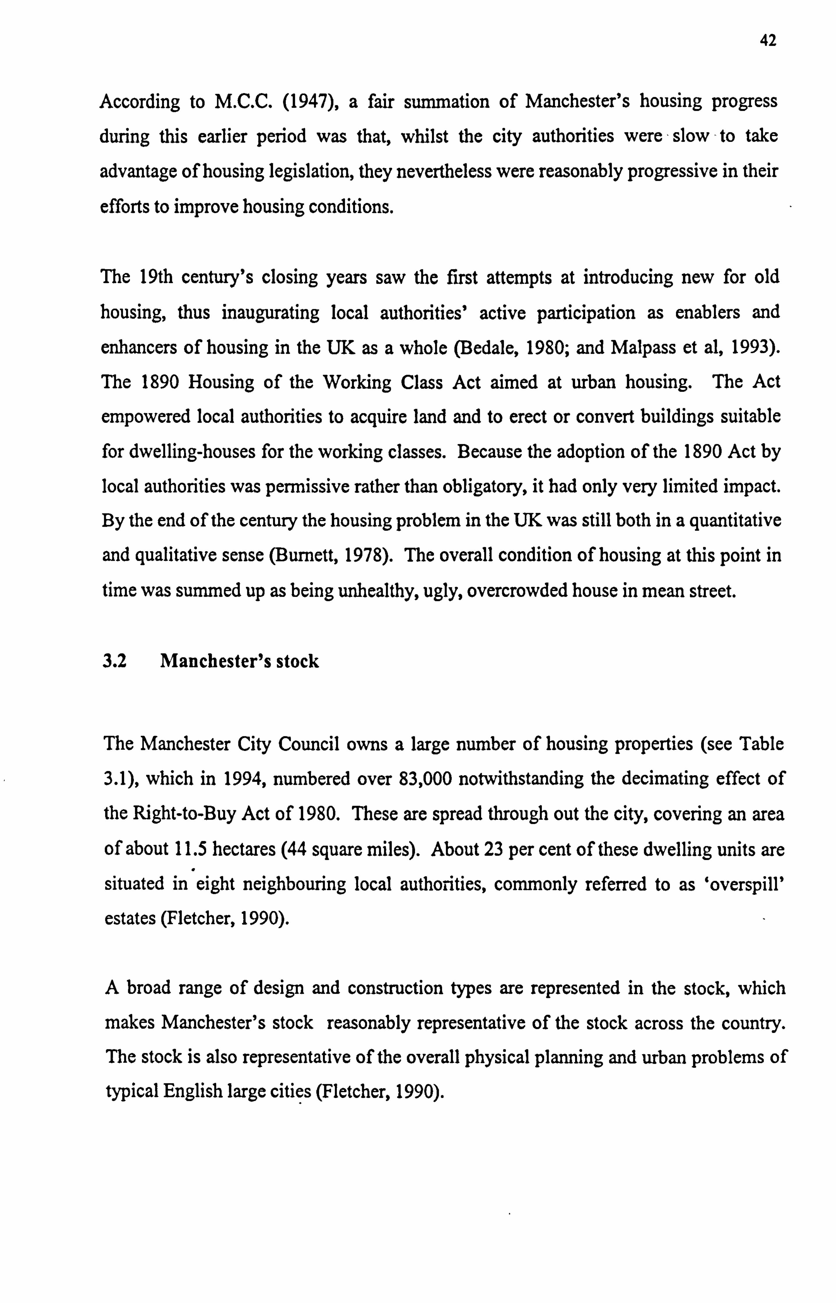
42
According to M. C. C. (1947), a fair summation of Manchester's housing progress
during this earlier period was that, whilst the city authorities were slow to take
advantage of housing legislation, they nevertheless were reasonably progressive in their
efforts to improve housing conditions.
The 19th century's closing years saw the first attempts at introducing new for old
housing, thus inaugurating local authorities' active participation as enablers and
enhancers of housing in the UK as a whole (Bedale, 1980; and Malpass et al, 1993).
The 1890 Housing of the Working Class Act aimed at urban housing. The Act
empowered local authorities to acquire land and to erect or convert buildings suitable
for dwelling-houses for the working classes. Because the adoption of the 1890 Act by
local authorities was permissive rather than obligatory, it had only very limited impact.
By the end of the century the housing problem in the UK was still both in a quantitative
and qualitative sense (Burnett, 1978). The overall condition of housing at this point in
time was summed up as being unhealthy, ugly, overcrowded house in mean street.
3.2 Manchester's stock
The Manchester City Council owns a large number of housing properties (see Table
3.1), which in 1994, numbered over 83,000 notwithstanding the decimating effect of
the Right-to-Buy Act of 1980. These are spread through out the city, covering an area
of about 11.5 hectares (44 square miles). About 23 per cent of these dwelling units are
situated in eight neighbouring local authorities, commonly referred to as `overspill'
estates (Fletcher, 1990).
A broad range of design and construction types are represented in the stock, which
makes Manchester's stock reasonably representative of the stock across the country.
The stock is also representative of the overall physical planning and urban problems of
typical English large cities (Fletcher, 1990).
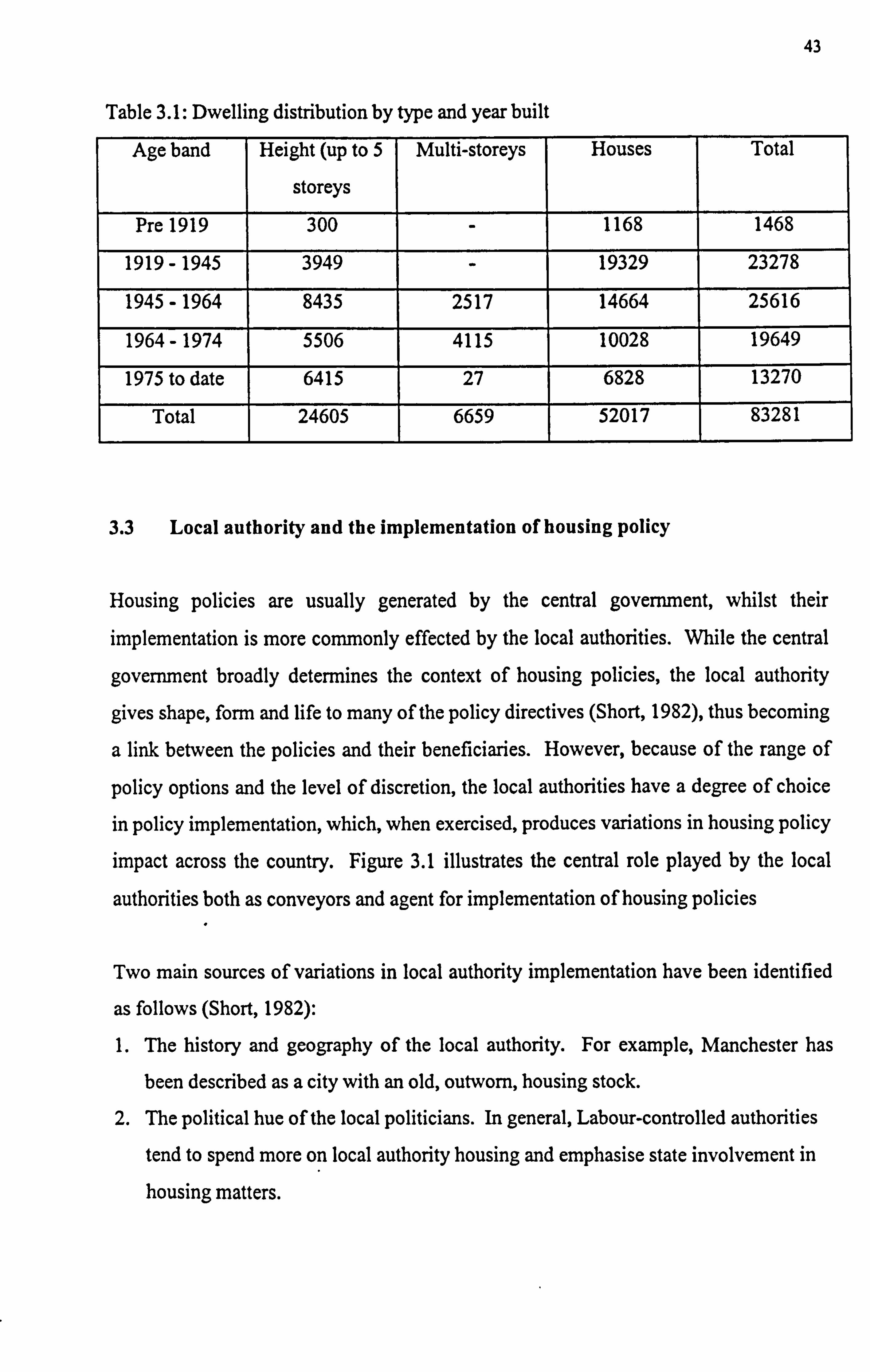
43
Table 3.1: Dwelling distribution by type and year built
Age band Height (up to 5
storeys
Multi-storeys Houses Total
Pre 1919 300 - 1168 1468
1919-1945 3949 - 19329 23278
1945-1964 8435 2517 14664 25616
1964-1974 5506 4115 10028 19649
1975 to date 6415 27 6828 13270
Total 24605 6659 52017 83281
3.3 Local authority and the implementation of housing policy
Housing policies are usually generated by the central government, whilst their
implementation is more commonly effected by the local authorities. While the central
government broadly determines the context of housing policies, the local authority
gives shape, form and life to many of the policy directives (Short, 1982), thus becoming
a link between the policies and their beneficiaries. However, because of the range of
policy options and the level of discretion, the local authorities have a degree of choice in policy implementation, which, when exercised, produces variations in housing policy
impact across the country. Figure 3.1 illustrates the central role played by the local
authorities both as conveyors and agent for implementation of housing policies
Two main sources of variations in local authority implementation have been identified
as follows (Short, 1982):
1. The history and geography of the local authority. For example, Manchester has
been described as a city with an old, outworn, housing stock. 2. The political hue of the local politicians. In general, Labour-controlled authorities
tend to spend more on local authority housing and emphasise state involvement in
housing matters.
44
Central Government
Subsides and is to Local Authority (LA)
Clearance New Construction
LA System Housing mgn't Private Sector Municipalistation Private Sector
Housing Sale of Council Houses Housing
LA Mortgages
Figure 3.1: Local government and housing policies Source: Short (1982)
3.4 The Inter-war Period
The extent to which the first war precipitated changes in society and in social policy
was far reaching. Headey (1978) has described World War I as a watershed in British
housing history. It was argued that the intense and great sacrifices from the whole
population as a result of the war demanded reciprocal commitment on the Part of
government to major social reforms which became an unwritten social contract
(Titmuss, 1958). The emotive electoral propaganda towards the end of the war in 1918
in relation to housing provision was the need to provide `houses fit for heroes'.
Following from the social reform policy which resulted from this noble and ambitious
phrase, the idea that central government finance should be used to subsidise local
authority building became acceptable for the reconstruction process.
It was reported by M. C. C. (1947) that prior to the first world war, the Manchester
municipality had never really embarked upon a large scale programme of new building*
45
Through the agency of the Health Committee, municipalities mainly strove to improve
appalling sanitary condition of existing houses.
The extreme shortage of houses for the first World War heroes led to the formation in
1920 of a Housing Special Committee for the implementation of the Housing Act of
1919, in order to bring the Act to full effect. The Act, commonly referred to as the
`Addision' Act set out to introduce the necessary drive to overcome housing shortage
by means of a generous subsidy from the central government. The implementation of
the objectives of the Act exerted strenuous demands upon available limited resources.
Most prominent was the shortage of bricklayers which called for special measures
which had significant impact upon construction methods for the period. The shortage
demanded that an alternative to brick had to be found to supplement brick as wall
materials for house building (M. C. C, 1986).
This problem posed a dominant handicap to the successful implementation of the house
building programme set by the Committee. This resulted in unimaginable delay and
frustration that even at the end of the second year of the four year plan, there were only
546 completed houses out of the original plan of 20,017 houses. Whilst progress
during the first two years was appalling and discouraging, the Committee justifiably felt
that much valuable ground work had been performed. Effective steps had been put in
place which led to the formation of an independent department which was to take
responsibility for the control and supervision of every phase of house building. At the
end of the plan period, only 3900 houses were completed.
The apparent failure of the 1919 Act was attributed to the attempt by the central
government to exercise too close a control over the local authorities, which led to the
passing of the 1923 Housing Act. Whilst the 1923 Act permitted local authorities to
continue to build upon the opportunities offered by the preceding Act, it primarily
sought to offer opportunity for private builders to build houses for owner occupation.
The emerging social classification problem of the time festered upon this Act, in that it
catered for the middle class family at the expense of the needs of the equally deserving
cases of those unable to provide necessary capital to make up the difference between
available mortgage and purchase price for houses. The early recognition of this
46
problem led to a passing of the 1924 Housing Act. In all, the 1923 Act produced 1,352
houses for letting as shown in Table 3.2, through the Manchester Corporation and gave
capital subsidies to enable 5,037 owner occupied houses to be built.
Table 3.2: New houses achieved by the 1923 Act
Estate No. of Houses A2 A3 B3
Burnage 620 36 382 202
Newton Heath 134 - 116 18
Wilbraham Road 598 76 422 100
1352 112 920 320
Source: M. C. C. (1947)
In the same manner as its predecessor, the Housing Act of 1924 was intended to secure
an entirely different set of conditions from its predecessor. Its main objective being to
secure houses to be let to the working classes at affordable rents. In this Act, the
central government was seen to play both roles of enabler and enhancer of house
building. This it achieved through the introduction of a scheme of skilled manpower
development in the building industry to sustain the continuous implementation of the
provisions of the Act over 15 year period, and an incentive plan entrenched in the Act
in order to increase the speed of house production for local authorities to give
consideration to alternative methods of construction to include a fair wage clause for
building trades apprentices.
The overall object of this Act was most ambitious and much more farsighted in
comparison with all its predecessors. A magnificent total of 16,277 out of a total of 27,447 houses was achieved under the 1924 Act. It was during the tenure of this Act
that Manchester housing conquest grew in leaps and bounds as articulated by the
(M. C. C. 1947).
`Prior to this Act, wistful eyes have been cast at the constituted authorities of Manchester's neighbouring districts, but it was during the tenure of this Act that the municipality began to actively overspill to neighbouring districts. The most prominent being the Wythenshawe estate, with 4,797 houses built under the Act' .

47
By 1930, it was estimated that Manchester still had 70,000 unfit dwellings out of its
total housing stock of 180,000 (private and council). The Housing Act of 1930 was the
first comprehensive attempt to deal with the problem of slum. Under the Act, measures
were taken to abolish slum area, to recondition unfit houses which were in no short
supply in the inner areas of Manchester. Under the Act, only a modest 15,000 houses
were earmarked for clearance by the city council in a five year programme (Burnett,
1986). The tardiness was most probably due to huge capital costs involved in the
provision of new dwellings at such a pace in keeping with the amount of demolition
over a relatively short period of time.
The 1930 Act made a number of provisions:
(a) in the declaration of clearance areas
(b) the setting up of improvement areas and,
(c) in dealing with individual unfit houses.
The Act thus heralded, in the most effective and legitimate manner, the process of
demolishing the old and erecting the new to the joy of many public health reformers.
3.5 Importance of Housing legislation
The review of the various Acts are helpful in fixing the history of housing endeavours
over time. The Acts constitute the charter under which local authorities could legitimately pursue their housing work.
Through out this period, Manchester was described (Dale, 1980) as an authority with
severe housing problems of an old industrial city with added complexities of residential
succession which are typical of metropolitan cities. The result was that the restriction
of government policy was always more problematic than authorities whose problems
were more straightforwardly those of physical obsolescence.
48
3.6 The effect of the second World War
At the out break of the war in 1939, it was generally believed that housing demand and
supply were in some state of equilibrium (Headey, 1978). By 1945, at the end of the
war, some 3.5 million dwellings were estimated to have been damaged to some degree,
whilst at the same time six years of stagnation on the construction front had been
suffered.
In Manchester alone, over a thousand dwellings had been destroyed or so badly
damaged that they were beyond repair (M. C. C., 1986) without accounting for
thousands more dwellings which had suffered less serious damage but nevertheless
requiring repair works to be carried out.
The Labour government elected in 1945 recognised the severity of the resulting housing
shortages and took some bold steps at combating the problem in a spirit reminiscent of
1919. Whilst the first few years after the war were concentrated on repairing bomb-
damaged housing, the government rigorously pursued the policy of construction rather
than one of improvement.
One of the pragmatic steps taken by the government was the tackling of the problem of
land shortage. During the inter-war period, land purchases had relied on philanthropic
large landowners, this trend was totally reversed by the impact of town planning
legislation from 1947. Compulsory purchase made the acquisition of building land
much easier for local authorities (Fletcher, 1990). The result was that by 1957 a total of
2.5 million new houses and flats had been built, 75 per cent of which was by local
authorities. The government, between 1965-69 inclusive produced approximately 1.8
million houses with a peak in 1968, almost equally divided between the public and
private sectors. Given this level of success in government housing pursuit and the
immediate post-war housing shortage had been met, an increasing important place was
given to slum clearance and the improvement of unfit dwellings (Burnett, 1978).
49
3.7 The Right-to-Buy Act of 1980
The most radical measure to denigrate local authority housing was the Housing Act of 1980 which provided the right for secure local authority tenants to buy their home at
substantial discounts from the market price, with automatic right to a local authority
mortgage if required. In order to gain a full appreciation of the impact of this policy
upon overall local authority housing, it is useful to examine the sales figures along side housing construction for 1979 to 1989. Table 3.1 shows that sales exceeded new building by local authorities from 1980 onwards reaching the lowest levels since the
introduction of subsidies in 1919.
Table 3.1: L. A. dwellings completed and sold in the UK 1979-1989
Year Dwellings completed Sales of local authorities dwellings
1979 75,573 42,285
1980 76,997 85,840
1981 54,889 112,061
1982 33,205 215,797
1983 32,805 157,382
1984 31,593 118,454
1985 26,125 106,268
1986 21,277 101,068
1987 18,671 122,319
1988 18,828 176,518
1989 15,107
3.8 Theory of housing zoning
The pattern of urban land uses in industrialised countries is often explained by the
concept of concentric zone model (Garner, 1970). This is especially relevant to the
problem of housing maintenance in any city as the pattern of evolution of housing bears
50
heavily upon the spread of deterioration in residential properties. Whilst the research
does not seek to test the hypothesis of the relationships between social class and
maintenance requirements, a conceptual understanding of how housing evolution is
informed by social classification would constitute a firm bedrock for a better
appreciation of the problems which are being studied.
Based upon Burgess's (1925) studies of Chicago, Baldwin (1979) developed a
conceptual zoning of housing in modem cities (see Figure 3.2).
At the epicentre of the concentric boundaries is the inner zone which is principally the
central business district (CBD) forming the nucleus of the city's commercial, cultural
and social life as well as being the focus of urban transport. Immediately surrounding
this is the urban zone being the main area of dilapidated housing, which also includes
light manufacturing, wholesaling and other businesses. This area has been described by
Balchin (1979) as the `twilight area' because of its blightful conditions of much of this
zone.
Surrounding the urban zone is the low class residential zone which according to
Balchin's (1979) interpretation of Burgess's observation, is "inhabited by the workers
of industries who have escaped from the area of deterioration but who desire to live
within easy access of their work". The low class zone is in turn surrounded by what is
described as middle and high income housing zone. Surrounding this is an outer zone beyond city boundaries, ̀a commuter belt of suburban and satellite settlements'.
Whilst the evolution of every city tends to follow this pattern, in actuality, departure
from such regimented concentric zones is inevitable in practice, and hence, the
acknowledgement that no urban area is a true fit of the ideal scheme.
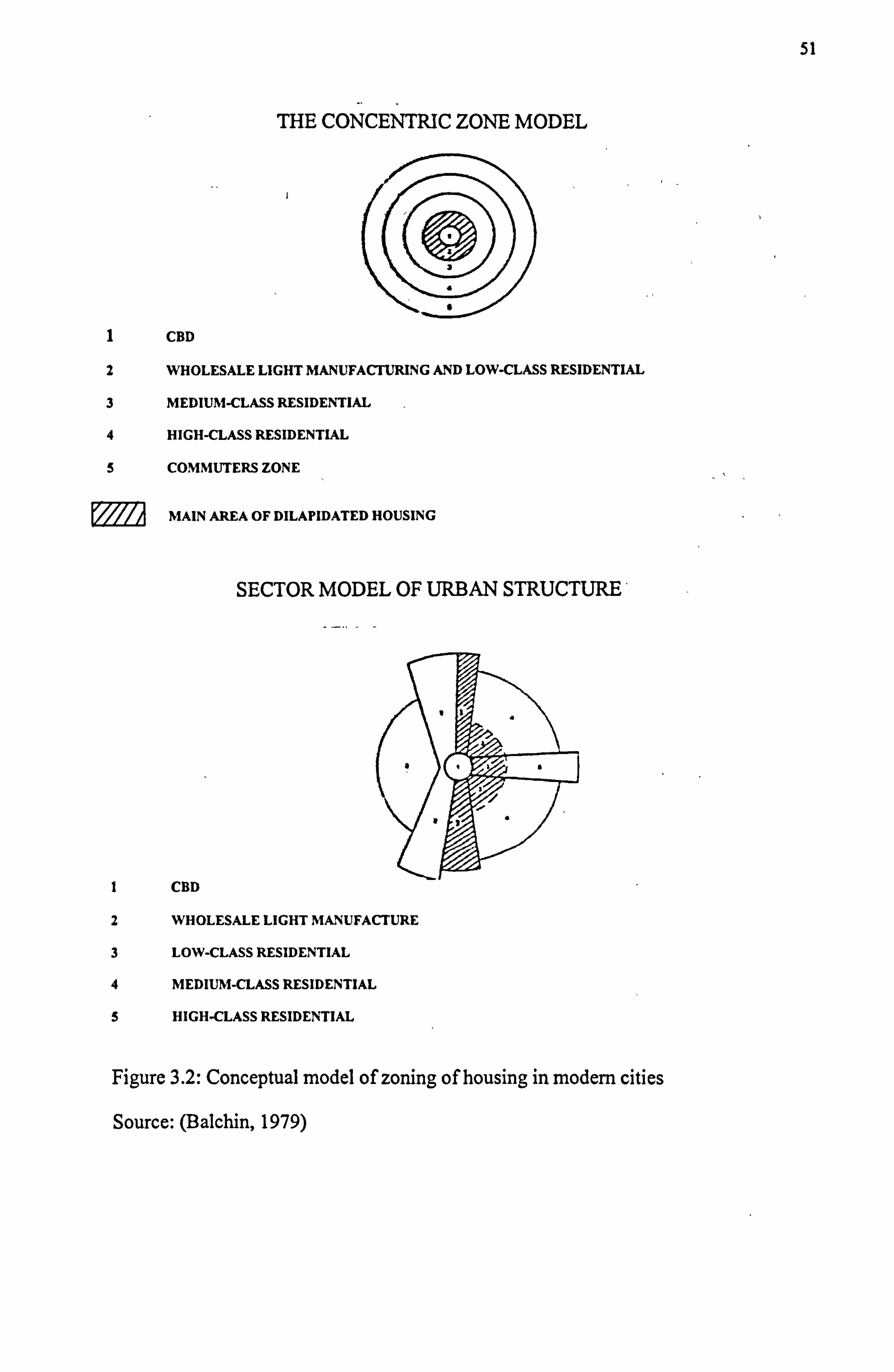
51
THE CONCENTRIC ZONE MODEL
ýÜý 1 CBD
2 WHOLESALE LIGHT MANUFACTURING AND LOW-CLASS RESIDENTIAL
3 MEDIUM-CLASS RESIDENTIAL
4 HIGH-CLASS RESIDENTIAL
5 COMMUTERS ZONE
® MAIN AREA OF DILAPIDATED HOUSING
SECTOR MODEL OF URBAN STRUCTURE'
1 CBD
2 WHOLESALE LIGHT MANUFACTURE
3 LOW-CLASS RESIDENTIAL
4 MEDIUM-CLASS RESIDENTIAL
5 HIGH-CLASS RESIDENTIAL
Figure 3.2: Conceptual model of zoning of housing in modem cities
Source: (Balchin, 1979)
52
In a real world, urban growth is influenced by three forces of nature namely; centripetal
forces of attraction, centrifugal forces of dispersion, and the forces of spatial
differentiation (Balchin, 1979) rather than by one homogeneous force which enable
urbanity to be fitted into a spatial mould as in the idealised `concentric model'. The
consequence of this multiple combinations of physical forces is a radial routeway
patterning of urban land uses. The result is that the pattern of urban settlements may
sometime be highly fuzzy around the urban zone, low class residential zone and the
middle and high income housing zone. Whilst the suburban and satellite zone tend to
retain its purity much more than the rest of the zones.
It is intriguing that neither of the two operational areas (North and South) of
Manchester from which the sample population was obtained falls into either the
epicentre or the satellite zone of Balchin's (1979) models. In other words, the
population sample dwellings are of moderate urbanity spread without the feature of
extreme zone characteristics.
3.9 Tenure
The tenure by which a household occupies its accommodation is an important
characteristic of that household. It has been described by Ball (1986) as the way
households pay for housing, and their relationship to its ownership. Farthing (1974)
emphasised the importance of the tenure of a household on legal and financial
responsibilities and rights of the tenants.
In reality, the basis on which individuals occupy their dwelling includes a large number
of individual circumstances. In the UK, tenures are believed to be associated with
different social images (Forest and Murie, 1988). The dominant image of owner-
occupation often reflects and reinforces social differentiation along tenure lines. Whilst
tenure categorisation can be listless and inexhaustive, it is common to condense these
categories into four main tenure categories in the UK (Farthing, 1974). These are,
owner-occupation, local authority renting, private renting, and housing association
renting. Figure 3.1 shows the housing tenure in GB between 1969 - 1989
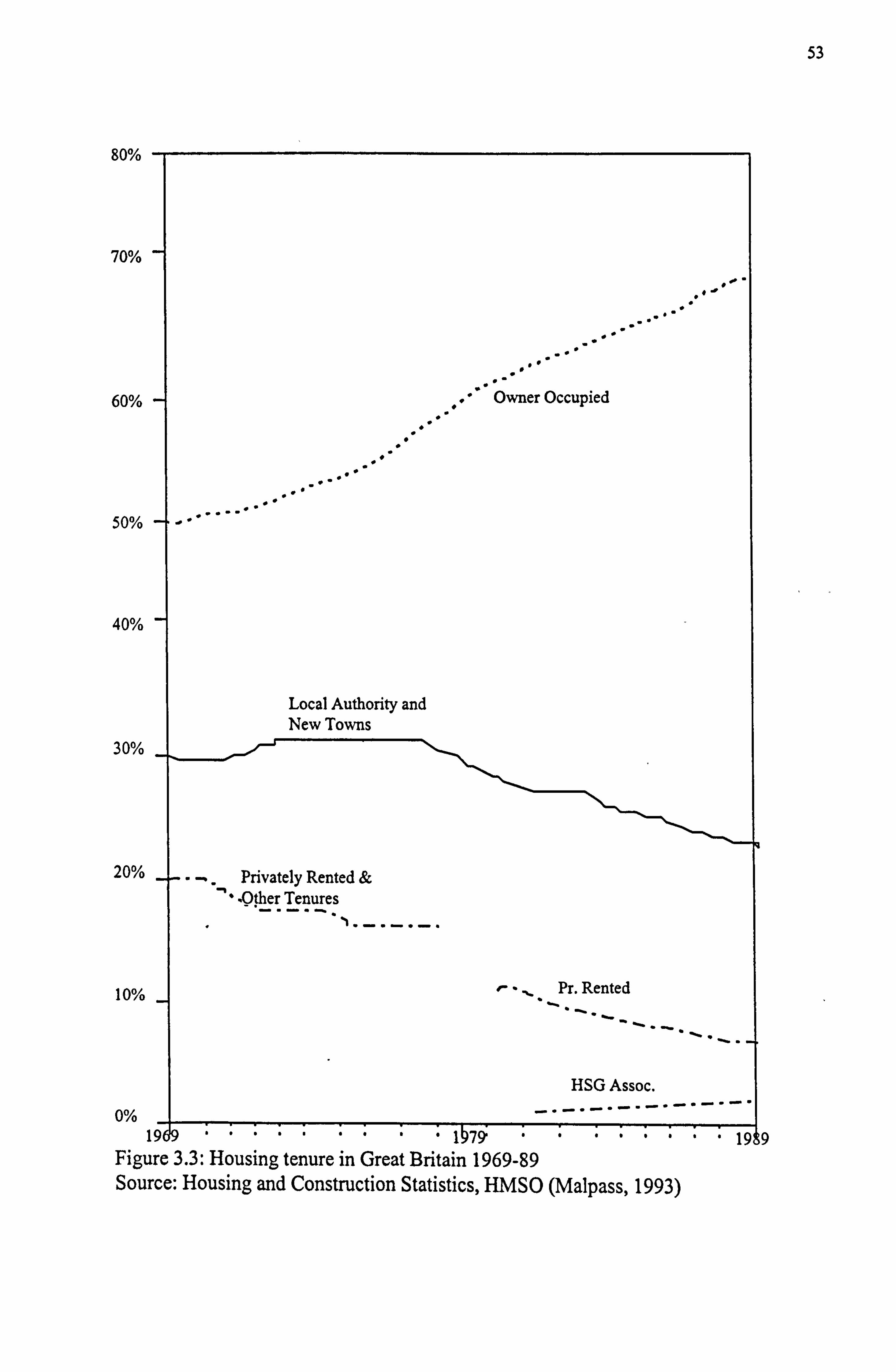
53
80%
70%
60%
50%
40%
30%
20%
10%
0%
Figure 3.3: Housing tenure in Great Britain 1969-89 Source: Housing and Construction Statistics, HMSO (Malpass, 1993)
54
According to Malpass (1993), before the First World War, about 90% of housing was
privately rented, with 10% being owner-occupied. Local authority provision at this
time was negligible. Since then, there has been a steady decline in private renting,
accompanied by a corresponding steady increase in owner occupation, and until 1979,
in local authority renting. Judging from Table 3.2 and Figure 3.3, the sale of public
sector dwellings from local authorities, government departments and housing
associations was the major source of growth in the owner-occupied sector in the post 1979 era. By 1979, local authority housing reached its peak in its proportion of
national housing provision at about 32% of total national stock. Since then local
authority housing provision has suffered a steady fall as shown in Figure 3.3.
One important feature of housing tenure is increasing social polarisation. Because
owner-occupation has been embraced by a large segment of society, it has become
increasingly socially diverse, whilst local authority housing has experienced a growing
concentration of the least well-off. Reporting on the Family Expenditure Survey data
of 1953-4 (Gray, 1979) claimed that only 16% of families in the bottom quarter of the
income distribution were local authority tenants, but has grown to 43% in 1976.
According to Malpass (1993) more recent data confirms this trend. In 1988, two-thirds
of council tenants had weekly incomes of less than £150, compared with 18% of
owners.
3.10 Summary
This chapter has reviewed the history of public housing, and discussed the significant
part played by the various Housing Acts mostly of the 20th century as precipitator for
the present public housing condition. The effect of the Housing Act of 1980 as the
most radical measure by the government to denigrate local authority housing is notable,
with sales attaining an all-time high of 215,797 in 1982 in contrast to just 33,205 being
completed.
The theory of housing tenure and land uses was set in perspective as a means to
understanding the evolution of cities and pattern of tenure, of which the city of our interest is no exception. The relationship of the theoretical residential location zoning
55
to the survey population from the two operational areas (North and South of
Manchester City Council) was defined as of moderate urbanity spread. Essentially, any
differences in maintenance characteristics between dwellings from any part of the city
could not be explained as resulting from housing tenure and zoning differential. The
link between tenure and social differentiation in the UK was discussed. Exponents are
generally agreed on the fact that council housing tenants fall into the lowest income
brackets of the population.
56
CHAPTER 4
DEFINITION PROBLEMS IN BUILDING MAINTENANCE
4.1 Introduction
The study has as its main objective, the identification of major factors which determine or
strongly influence maintenance need and then establishing the interaction, if any between
these factors. It is therefore pertinent to the study to clearly establish the bounds of
maintenance in order to be able to achieve the research objective.
The existing problem of lack of distinctions in maintenance activities is a major constraint to
the proposed study, which if not solved will distort any eventual findings.
In order to avoid this it has been found crucial to adopt a contextual definition of
maintenance and its scope. It is believed that this initial critique will ameliorate several of
the problems which could arise later on in the study.
There are few housing strategies which have been more widely and consistently advocated
than the maintenance of existing properties. This trend is being fostered by the developing
trends in nations' strict economic measures to conserve scarce funds and depleting resources. The trend tends to support making less funds available for new development or even
substantial reconstruction activities on existing properties.
Despite this, perhaps because of its commonplace day to day application, housing
maintenance has only very recently become the subject of much systematic, nation-wide
research. While there are a considerable number of studies (Drinkwater, 1967; Stoaling,
1985; Allen, 1986; Kelly, 1988 and Griffin, 1990), many are confined to industrial
boundaries (Drinkwater, 1967 and Kelly, 1988), whilst those intended to address
construction and property are ad hoc and sometimes too highly specialised (Stoaling, 1985;
Allen, 1986; and Griffin, 1990).
There is little consensus concerning maintenance definition and even more confusion concerning its different levels and interpretation. 'Repairs' versus 'servicing' versus
57
'replacement' versus 'improvement' versus 'rehabilitation' etc. These definitional ambiguities
reflect the character of building maintenance in that it can be many things and can assume a
wide range of guises. Amidst the present confusion, there may eventually be a black-out of historical sense of maintenance, except the current trend is reversed. It would appear that
this gloomy prospect and the overwhelming confusion surrounding terminologies in the field
of maintenance prompted Mole (1992) to suggest that building maintenance will do well to
be re-named.
To improve this situation, this chapter seeks to present a collection of meanings and definitions in order to achieve a justifiable industry wide definition for the term.
4.2 Review of general definition
The Oxford dictionary defines maintenance as "being maintained, keeping in repair........ to
maintain is to cause to continue........ to preserve in good order". Many definitions have been
proffered including those by Tucker & Rahilly (1990) and Pitt (1987). These definitions are
only tangential to the above definition.
The definition identifies the range of characteristics to be imparted to a property by any one
action of maintenance. Thus, the main aim of maintenance can be succinctly put as
providing serviceability to the building, hence, the need to highlight those attributes of
maintenance which contribute to building service.
The BS3811 (1984) definition of maintenance has become paradigmatic. It defines
maintenance as a "combination of any actions carried out to retain an item in, or restore it to
an acceptable condition". It should be kept in perspective that this definition does not have
any particular product or industry in focus, but is of general application.
Two processes are envisaged in the definition; namely preventive and corrective
maintenance. As illustrated in Figure 4.1, maintenance action is determined by a set
acceptable level of deterioration. This action comes either as preventive as in servicing of
components or as corrective in the form of repairs, partial improvement or replacement.
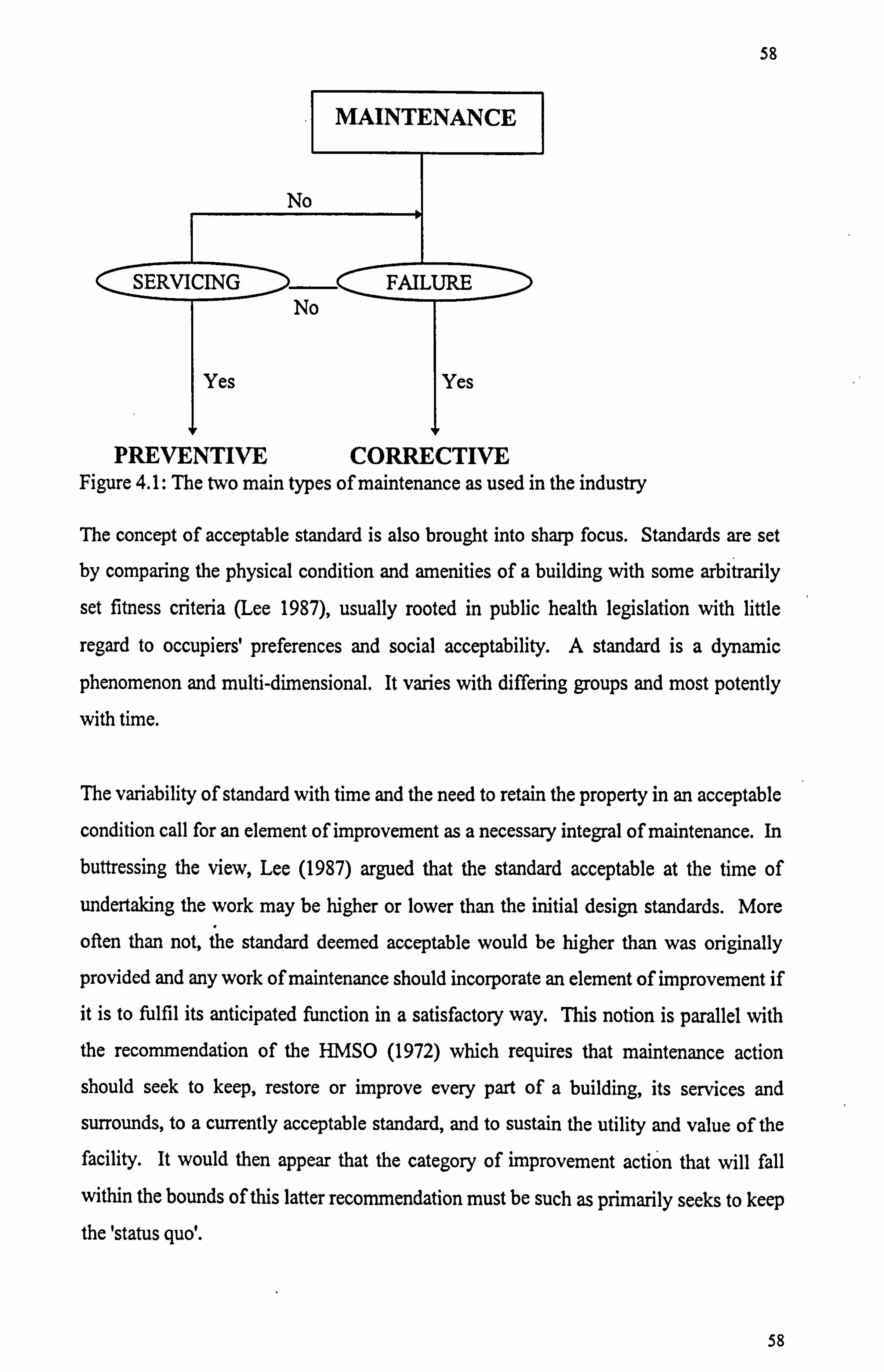
58
MAINTENANCE
No
SERVICING D -C FAILURE No
Yes I Yes
PREVENTIVE CORRECTIVE Figure 4.1: The two main types of maintenance as used in the industry
The concept of acceptable standard is also brought into sharp focus. Standards are set
by comparing the physical condition and amenities of a building with some arbitrarily
set fitness criteria (Lee 1987), usually rooted in public health legislation with little
regard to occupiers' preferences and social acceptability. A standard is a dynamic
phenomenon and multi-dimensional. It varies with differing groups and most potently
with time.
The variability of standard with time and the need to retain the property in an acceptable
condition call for an element of improvement as a necessary integral of maintenance. In
buttressing the view, Lee (1987) argued that the standard acceptable at the time of
undertaking the work may be higher or lower than the initial design standards. More
often than not, the standard deemed acceptable would be higher than was originally
provided and any work of maintenance should incorporate an element of improvement if
it is to fulfil its anticipated function in a satisfactory way. This notion is parallel with
the recommendation of the HMSO (1972) which requires that maintenance action
should seek to keep, restore or improve every part of a building, its services and
surrounds, to a currently acceptable standard, and to sustain the utility and value of the
facility. It would then appear that the category of improvement action that will fall
within the bounds of this latter recommendation must be such as primarily seeks to keep
the 'status quo'.
58
59
That is to say, any improvement action that is superfluous in the light of current standards
and the initial status of the building cannot be considered as falling within the bounds of the
BS3811 definition. This stance corroborates Whites et al's (1969) opinion that
maintenance is synonymous with controlling the condition of a building so that its pattern lies within "specified regions".
Figures 4.2 and 4.3 illustrate the interactions between the various possible estate activities.
There often do occur some overlapping between the different actions. The identification of
such common boundaries may prove problematic. The problem may only be overcome by
knowledgeable compromise in definition.
The term, 'specified regions' connotes that the status in which the building should be retained
or brought to, rather than being a determinate condition, is a continuum. This region then
becomes a reference condition upon which an improvement action will be judged to be
appropriately a maintenance action.
A note of caution is vital at this juncture. For an improvement action to be considered within
the ramification of maintenance, such an action should not, of necessity, be on a building
whose standard and attributes have so lagged behind currently acceptable standards as to
qualify it for a rehabilitation or modernisation exercise.
4.3 The usage of terminologies
The terms maintenance and repair are almost always used as twin words (Taylor, 1987;
Seeley 1987; and Lee 1987). The joint usage of both terms has evidently grown out of
simple idiosyncrasy among authors. In actual sense, repair is nothing but a component or
subset of maintenance action. The current academic idiosyncrasy can however be
misleading, and it does in fact show the extent and seriousness of conflicts yet to be resolved
in the field of maintenance. An action carried out on a building may not of necessity be a
repair action and it is however not understandable why most authors are inclined to using
both terms in conjunction, when in actual sense, the one is but a component of the other.
This general inclination may have arisen out of a general misconstruction of general repairs
being all that maintenance is.
60
MAINTENANCE
0
SERVICING 1 FAILURE No
Yes I Yes
PREVENTIVE
HIGHER STANDARD REQUIRED
No
CORRECTIVE IMPROVEMENT
Figure 4.2: Typification of maintenance options
Figure 4.3: Work classification on existing building portfolio
61
It is possible to infer that the joint usage of the terms means that the two processes act in
unison to fulfil one and the same purpose. In other words, each is a process which
constitutes an end in itself. Neither of the two suppositions is tenable in the light of earlier
contention that maintenance is a combination of several processes. Melville and Gordon
(1981) commented that the neglect of maintenance is what gives rise to many of the repairs
which do arise in buildings. The usage of maintenance in this context has been limited to
mean nothing more than non-technical house keeping, and does imply that repair is a
separate function from maintenance. In other words, the joint usage of the terminologies is
in respect of distinct processes which relate on a'cause and effect' basis, and having the same
end result of'keeping the building in good condition at all times'. The fallacy of this opinion
is obvious, and may have been precipitated by the wrong usage of terms in the sector.
With virtually no exceptions, authors use the two terms either interchangeably or jointly
without any rule of thumb guiding the usage.
For the purpose of this study, the existing position is considered misleading. It is contended
that whilst repair work is a maintenance action in its own right, maintenance is far more than
repairing. In fact, maintenance is an umbrella term encompassing repair.
4.4 A cursory look at semantics
In technical texts and journals treating the subject of maintenance and related construction
works upon existing building portfolios, the following terminologies are to be encountered,
namely: modernisation, rehabilitation, renewal, refurbishment, alteration, extension, improvement, repair and replacement. A lot of confusion exists in the usage of these
terminologies.
A distinction can be developed between rehabilitation and maintenance. Whereas
maintenance is most effective when a balance is struck between the two extremes of
portfolio management spectrum; abysmally low along the spectrum is a condition ranging
from total or near total neglect to under-maintenance. Highest up on the spectrum is the
range of over-maintenance. Neither of these two extremes is cost efficient. In fact, the two
62
conditions are two evils, the one of which is both uncertain and calamitous, whilst the other
is expensive but the asset's life and utility is at least guaranteed. The unknown evil is to be
held in greater derision and mostly to be avoided. If not avoided, but allowed to persist for
any length of time, it results in abject state of disrepair. In this condition, no ordinary act of
maintenance will serve to bring the building back to a satisfactory functional state. It is at
this stage that maintenance overhauling is required which is adequately termed rehabilitation.
Rehabilitation displays the general characteristics of maintenance operation, but much wider
in scope and spanning the entire building fabric, whereas normal maintenance action may
involve only a few building elements at any one time.
Refurbishment is often associated with the upgrading of the general features of a facility in
the form of re-decoration in order to make it more attractive in the property market. Whereas
rehabilitation makes a salvage of a defect-ridden facility, refurbishment redeems it from
imminent incursion of defects.
Dixon (1990) described modernisation as being concerned with alteration and enhancement
to buildings on both a small or large scale. This stance is rather pedantic, thus portraying
modernisation as the umbrella which houses other major estate actions. In its pure sense
modernisation is nothing more than an adaptation of a facility to meet present day needs and
demands in the services provided by a building without having to redevelop. It explores the
relevance of a functionally obsolete property in meeting new demands often occasioned by
technological development. It would seem that improvement is a minutiae of modernisation
in the sense that the former is usually widely spread throughout the building. In other words,
modernisation is an amplified improvement work on a building.
Figure 4.4 defines the work content classification for the various estate activities identified so far.
63
PROPERTY STRATEGY
SERVICING MAINTENANCE IREHABILITATION REFURBISHMENTI
RENEW MODERNISATION REPLACEMENT
Figure 4.4: Work content classification on existing buildings
Renewal has been described as an estate activity which often encompasses all the others but with significant actions in the form of new work to the property. It does however
fall short of redevelopment in that it retains the general features of the original building
whilst making substantial additions and/or alterations to it in order to enhance its
functionality.
4.5 Summary of definitions
Arguably, construction suffers from the effect of uncertainty more than most other human undertakings. This problem is most acute in the specialised field of construction
maintenance where reliable cost prediction is made difficult or impossible by poor
quality historical data or even an entire absence of it. This has led to the conclusion (Holmes, 1987) that in many cases the available data is of very little value in the
assessment of maintenance. The problem throughout the maintenance field is the lack
of suitable data to sensibly discuss performance and cost over time. In the light of this
problem, it is crucial to develop a model of cost prediction which places little reliance
upon existing poor historical records. In seeking to achieve this the following constraint has been established.
64
Maintenance is a generally semantically confused area of construction, with it assuming
various meanings with individuals with differing backgrounds and idiosyncrasies. The
foregoing section has addressed this constraint and raises such issues as are relevant to the
development of a clarity of thought on the subject. The conceptual definition of maintenance
adopted in this research is figuratively demonstrated in Figure 4.3.
4.6 Maintenance Characteristics
Apart from work due to `change of tenancy' and ̀ Prior to Painting' repairs all other repair
work is based on demand (Holmes, 1985). This observation is a valid one but it does not
support any generalisation as he did, that maintenance need or requirements are tenants' own
origination by way of reporting. This will only be the case if maintenance is purely
construed to mean day to day items of work to the exclusion of programmed repairs. To
posit a limiting definition of this sort will not be doing justice to a global understanding of
the general phenomenon, although by so positing, an otherwise intractable variable can
become more manageable.
Another distorting parameter in maintenance is the fact that maintenance is often dictated by
budget. Budget is controlled by certain policy decision as the financial year progresses and
so costs can be arbitrarily controlled to match budget. In essence, the time of the year is
related to the actual maintenance done. From this observation, it can be arguably inferred
that actual maintenance done is not a true index of actual maintenance need. This inference
has been implied by Spedding (1987a) when he asserted that maintenance is budget led. To
assess actual maintenance need, we must put ourselves in a position where we may correctly
determine demand for maintenance from all sources; be it from tenants or form the housing
organisation. This position is succinctly articulated in Figure 4.5.

65
PREDOMINANTLY Maintenance HOUSING ORGANISATION
TENANT REPORTED SURVEY DISCOVERY
Day-to-day II Programme work
Structural/Damp II Ad-hoc I Relet
(Tenancy Change)
Figure 4.5: Source and classification of maintenance work items
4.7 Types of Maintenance
Prior to Paint Repairs
Maintenance work has been broadly classified into two (Clifton, 1974; BS 3811,1984)
namely; planned and unplanned maintenance as shown in Figure 4.6. These two categories
or any further division of them are not completely separable and distinct (Spedding, 1987a).
The conventional thinking is that the higher the proportion of planned maintenance is to
unplanned maintenance the higher the level of control within the maintenance organisation.
The fallacy of this reasoning very easily comes to light when it is understood that these two
categories of work fall into two distinctive budget heads and that the administration of work
related to the former comes as a bona fide contract. Hence there exists no objective basis for
comparison of price or cost.
Spedding (1987a) concludes in his work that preventive maintenance does not relate to
actual failure but to assessments of tolerable risk. The significance of this conclusion is that
preventive maintenance is not an indication of sole maintenance need, but of an admixture
of actual and probabilistic maintenance need dictated by financial priority of the time.
Quah (1991) has underscored the general nonchalance of building owners which is evident by the limiting of upkeep to the very short term on one hand, and on the other hand to a
66
discrimination of cyclical work to such works as re-painting, re-roofing and routine
servicing of equipment. Maintenance of the remaining elements is most commonly -left to
reactive measures on receipt of complaint. It is almost not practicable to include more items
of cyclical work, as historical records of programmed work are seldom available and where it
is available, hardly ever accurate and complete (Holmes, 1985; Bromilow, 1987; Bird,
1987). In this light, if it was possible for one to decipher items of reactive maintenance from
the body of maintenance work carried out by an organisation and given the actual set of
requests from which the reaction was subjectively or otherwise extracted, one would be close
to a safe approximation of the body of maintenance requirement (for further discussion see
chapters two and eight on methodology and measurement of maintenance requirement
indices respectively). Figure 4.6 illustrates this point.
Maintenance
planned
maintenance
preventive
maintenance
unplanned
maintenance
(including emergency
maintenance)
maintenance II maintenance (including emergency
maintenance)
Figure 4.6: Maintenance classification
67
4.8 Maintenance expenditure
Property owners all too frequently endeavour to keep expenditure to a minimum, without
due considerations being given to the long term consequences of such an action or policy
(Hollis and Gibson, 1991). Whilst to an investor, the main criteria for further investment by
way of expenditure on the building is the net income plus the net capital appreciation that
can be expected in anyone period, this is not strictly the case with housing and particularly
with local authority housing as it runs its stock more or less as a social service. The main
objective for investment is to enhance the life span of the stock and to fulfil its legal
obligation to the tenants.
Wide variations exist in expenditures on housing stock owned by different landlords, be it
private or public. This results from varied attitudes to maintenance; whereas some prefer to
barely maintain the building, others choose to maintain at optimum level. This allows cost
differentials to exist (Brown and Robertson, 1990).
There are three phases of cost in anyone occurrence of maintenance item. This compounds
the problem of comprehensive understanding of the behaviour of expenditure patterns.
These stages as identified by Stone (1980) and Pitt (1987) are:
1. The direct cost incurred by the maintenance organisation in the form of labour, materials
with or without percentage overheads depending on which of the two options of
contracting and direct labour method of work execution is employed.
2. The actual price paid for work by the owner of the building; which is (1) above plus the
mark-up element of the contractor.
3. The direct loss suffered by the occupier of the building resulting from loss of output or
additional expenses to ensure the same level of output resulting from the disturbance.
Another major factor which distorts maintenance cost information is the frequent occurrence
of emergency repairs which divert funds away from routine maintenance programmes and
are so very often priced disproportionately to the actual cost incurred.
68
As at 1976 the percentage spent on maintenance in terms of capital value of the Local
Authority stock was 0.96 per cent and in the private sector was 0.91 per cent (National
Income Statistics, 1976). Between the ten year period from 1976 to 1986, Robertson (1988)
reported that increase in maintenance spending in the private sector has been more
significant than in the public sector.
The general view is still that in relation to the capital value of stock maintenance costs are
globally low. It has been argued that the extent of maintenance work done is a compromise between need and the ability or willingness to pay for it (Baker, 1976). The HMSO (1976)
referring to the whole area of maintenance costs commented as follows:
"very little is known about future maintenance requirement and .... past expenditure levels
are an inadequate guide to future requirement. "
This admission has serious implications for the housing stock management system and
leaves little or no room for manoeuvre in the management of housing maintenance
expenditure as it lacks any reliable history to live upon. There has been a long standing history of high variability in maintenance expenditure and standard in both the public and
private sectors. This, according to Wyatt (1980) is largely controlled by:
1. owner occupier's decision on whether to invest in his dwelling and maintain a high
standard of facilities or to do the minimum or nothing for reasons ranging from
ignorance to lack of fund;
2. affordability of landlords taking into account any legal requirement controlling standards
and financial returns; and 3. availability of financial resources represented by the level of income from the Housing
Revenue Account in L. A. housing authorities.
This renders cross-sectional maintenance expenditure data unamenable to analysis in order to
identify major parameters in maintenance need and performance. A way forward in order to
overcome this obstacle may be to focus upon the actual stock rather than a pre-emptive
phenomenon of the stock as its expenditure pattern. Most of the maintenance items are not defects in the sense that we have now come to associate their with premature failures.
69
A useful rhetoric that needs to be addressed in respect of efficient management of building
stock is "what will 1 need to spend on this building, year by year, during its foreseeable
life...... " (Bromilow, 1987). He went on to identify the issues to be addressed in relation to
maintenance expenditure as;
1) the most appropriate timing for maintenance operations to be done; and
2) the amount to be spent if buildings are to be kept at a given standard of performance
without significant backlogs being generated.
To fulfil these needs, there must needs be sufficient knowledge regarding the determinants
and mechanics of deterioration.
4.9 Expenditure forecasting approach
Three approaches for maintenance expenditure forecasting have been documented
(Bromilow, 1987). The first approach is to review the nature and incidence of maintenance
and other operations from past records of work done to each building as a basis for inference
for future needs. This is basically the approach employed by Holmes (1985) and Fletcher
(1989) in their studies on maintenance cost characteristics. The limitation of this approach is that cost histories are poorly documented, not only in terms of actual figures but also in
terms of work content and therefore unreliable.
The second approach generates future maintenance expenditure from a percentage figure of
the real capital value of building stock. The actual percentage adopted is based upon such
information as is available. The National Association of College and University Business
Officers (NACUBO) in the U. S. A. was quoted by Bromilow (1987) to have recommended 1.33 per cent of building cost annually. Sherman and Dergis (1980) on the other hand
proposed an age dependent formula that increases annually at the rate of 0.052 per cent,
which is in line with the Department of Environment's proposition of 1972. This approach
works upon the premise that the more expensive the market value of the stock, the more
costly it is to maintain. It takes no stretch of imagination to appreciate the fallacy behind this
thinking as several factors influence property market value which are not in any way related
70
to its maintenance. It is evident that this approach is rather too naive. The BMI (1988) has
criticised the use of percentage figure for future maintenance expenditure as a misleading
Rule of Thumb as more often than not these figures are estimates of national or local
expenditure and are inappropriate for assessing maintenance budget needs of specific
properties. It underpins the problem by stressing the need to prepare budget in the light of
factors affecting the building to be maintained, required standard and usage.
The third approach uses a simulated life pattern of a building using a mathematical model of
the activities that should take place in order to keep the building at a pre-determined level of
serviceability (Pitts, 1987; Phillips, 1986; and Bromilow, 1984). This, to every intent and
purpose is a very reliable technique for projecting likely future maintenance. It, however,
does not address the practical problems surrounding "the how and why" of the incidence of
maintenance items, and therefore doubtful if the simulated life pattern is reliable.
An evaluation of the (GEHA) forecasting technique would bring the common shortcomings
of maintenance expenditure prediction models to the fore.
4.9.1 The Government Employee Housing Authority (GEHA) - Australian
experience
In the bid to improve the efficiency and effectiveness of housing stock through better
management of capital and recurrent expenditure, an integrated maintenance forecasting
model was- developed in Australia in 1986. The model employs a combination of the first
and second approaches documented by Bromilow (1987).
The objectives of the model were; 1. to provide a basis for forward planning and budget forecasts
2. to contribute to the evaluation of options of maintenance, rehabilitation, demolition/rebuild or sale of stock (Tucker, 1990).
In this model, the house as a building is divided into 19 individual components. The
supposition being that each component gives rise to recognisable maintenance activities. The principal assumptions upon which the model is based are:
71
1. that the cost and timing of maintenance for each element can be pre-determined; 2. that costs are always dependent upon dwelling size (number of bedrooms); and
3. the application of stochastic distribution of the ̀ next due' dates for component failure
The problem with the approach of the model lies not only in the validity of the
assumptions but also in the fact that the model does not concern itself with exogenous
variables that impact upon decay and maintenance requirements. Furthermore, the
assumptions are founded upon very tenuous theoretical premise.
The estimation of the ̀ next due' dates is dependent on the assessor's judgements. Whilst
it may be possible to reduce judge's bias by some rationalisation and training, Walker's
(1989) experience shows that it nevertheless remains an unproved statistical method.
Because the model appropriately recognises that it is the exception rather than the rule for
maintenance to be done on schedule, Tucker employed a stochastic simulation construct to
perfect the model. The construct simulates a group of houses, and that maintenance falls
far short of the correct level. It presupposes that (a) only 20 per cent of items are done
between 90 per cent and 100' per cent of the scheduled time, and (b) the remainder are
completed by 190 per cent of the scheduled replacement time following a beta distribution
rather than a normal distribution.
So vital as the simulation construct is to the final model, there is no firm basis for its usage
in this instance. It is at best based upon hunch rather than scientific appropriateness.
Serious as this set-back may be, it would nevertheless not warrant that the model is
completely useless, were it possible to develop a fit for the model. In the absence of a fit,
given this serious aspersion, the reliability of any model should be called to serious
question.
72
4.10 The theory of Satisfaction among tenants
Satisfaction has been described as a user-response attitude to the comfort, convenience and fulfilment offered by the built form (Birks and Southan, 1992).
A large number of variables are believed to influence the level of satisfaction expressed by
residents of the built form (Bulbridge and Smith, 1973). Most importantly, this depends to
some extent on two points (Crosby, 1985). One is the density of housing scheme in
relation to the dwelling that is, whether high, medium or low rise and the other is the
housing management approach and responsiveness in relation to the various dwelling
forms and densities. Important as these influences may be, it is an over-simplification of
the nuances of satisfaction, which in itself is as complicated a subject as understanding human behaviour. Satisfaction is an individual attitude which is influenced by both
intrinsic as well as extrinsic parameters. Essentially, the design of built forms is an
expression of anticipated interaction between the consumer of the built form and the wider
environment. Newman (1972) argued that built forms have traditionally held the role of
social control of socially undesirable behaviours. In a symbiotic environment as this, we
may safely suppose that to the extent that housing design plays a role in the control of
deviant behaviours among residents, to the same extent would deviant anti-social behaviour result from an inefficient design.
A more pragmatic view of built environment was posited by Perin (1970) when he
suggested That a useful way of looking at built form is in terms of the changes (or neglect)
people wish to make to it to suit their behaviour, rather than how the built form determines
behaviour. These changes may be both positive (expressed by careful attention to the
fitness and up-keep of the dwelling) and negative (expressed in neglect and even avoidable
or wilful damage by residents).
He opined that "social relationships are always a concomitant of spatial arrangements and
physical elements is hardly a fact to be received with surprise. The quality of social
relationship however, is so much more a function of non-spatial and non-physical
variables that research in environmental design to predict quality is misguided". In
confirmation of this view, Crosby (1985) argued that environmental effects on individuals
73
and social structures depends on previously formed personality trait. He concluded that it
is erroneous to apply territoriality concepts in the hope that they will easily mould
individual or group behaviour.
This theory assumes a reasonable degree of residential mobility, which in itself is
frequently used as stress and tenants' satisfaction indicators for urban and sub urban areas
with social and physical problems. Valid as Crosby's (1985) theory may appear tobe, his
argument is based upon the premise that residents are necessarily `imported' to the
environment. The scenario will not be the same where individuals are bred from within
the context of the built environment. Hence, the character formed in offspring who may
never have to move away from that environment will, of necessity, be a product of the
design.
In a study of medium and high rise dwellings (Stevenson et al, 1967) found that high density
gives rise to social problems in housing estates as a result of children coming together into
groups, and invariably impacts upon the general satisfaction of tenants in such estates. Its
real problem in such instances is not so much with the children groupings as with the
vulnerability of the estate as a result of such groupings to infiltration from outsiders. Social
science research into the relationship between behaviour and physical environment has
tended to diversify, with a penchant for unification around the assumption that the quality of
human relationships cannot be directly related to territorial considerations. In a study of a
private housing scheme in London, as reported by Crosby (1985) it was found that in
higher density schemes, children's play was a major source of conflict and difficulty
(Shankland, Cox & Associates, 1971). Whilst some people see the open space as a place
for children to play on, others as something to gratify the sight.
Wherever conflicts such as this is inherent in the built form, satisfaction is dampened. The
effect of which may, by and large, be reflected on the immediate dwellings occupied by
individual residents. The loss in the level of satisfaction is often accompanied by the
desire to move and possible neglect by the resident.
74
Studies into tenants' satisfaction are commonly agreed in their findings that dwellings with
the least satisfied tenants tend to be in poorer state of repairs than those with more satisfied tenants (Burbridge and Smith, 1973; Shankland, 1971; and Stevenson et al, 1967).
4.10.1 Satisfaction among tenants
Tenants' satisfaction with the condition of a building is believed to depend on three points:
The density of dwellings in the neighbourhood (that is to say, whether high, medium or low rise),
" The allocation policies followed by the local authority in relation to the various built
forms and densities (Burbridge and Smith, 1973) and,
" The responsiveness of the landlord to repair problems (MCC, undated)
Satisfaction for housing tenants can mean any one or a combination of the following
(Birks and Southan, 1992);
1. increased loyalty to the housing department and organisation
2. encouragment to prospective tenants to patronise the same organisation
3. many complaints over trivial matters 4. failure to look after the dwelling or surrounding
5. rent avoidance.
From the above list of satisfaction indicators, it is clear that an assessment of the
satisfaction expressed by a tenant is a useful pointer to the level of care the tenant gives to
the physical dwelling which he/she inhabits. The age old proverb `action speaks louder
than voice' finds expression loud and clear. This position is at variance with the theory
that satisfaction is inexpressible as suggested by Birks and Southan (1992).
Birks and Southan (1992) have suggested that three factors should be considered in
measuring satisfaction among housing tenants. These are;
1. Validity: This has been described by Rowntree (1987) as the extent to which the test
measures what it is intended to measure, and is supposed to measure.
75
2. Reliability: This is described by Reece and Walker (1994) as the extent to which it
consistently measures what it is supposed to measure. It is believed that a perfectly
reliable test will give identical results in all conditions.
3. Actionability of the results: This is an assessment of the efficiency with which the test
can be administered.
The robustness of any measurement test is often threatened by the approach adopted for
the development of the survey instrument.
According to Birks and Southan (1992) one of the simplest and most consistent means of
measurement of satisfaction in terms of its administration is the bipolar scale. Simple and
consistent as this may be, the problem lies in the objectivity of the measure and what
satisfaction means to the individual.
In this study, we have tried to measure the level of satisfaction expressed by the tenant in
relation to the quality of repairs carried out by the local authority as perceived by the
tenant, albeit, from a layman's point of view across the entire building fabric. This
approach corrects for the relatively simpler approach adopted by the Department of
Environment in the Housing Appraisal kit, which according to Furbey and Goodchild
(1986) lacks the required ingredient for validity and reliability although, apparently
efficient.
If the DoE approach was adopted in this study, a less rigorous and obviously more
respondent friendly question as `How satisfied do you feel about repairs carried out by the
council? ' would have been used to develop a satisfaction index. As in Question No. 3 of
Appendix 1C, this type of question was actually asked in a validatory capacity rather than
as the chief instrument for the construct.
Overall, the satisfaction construct in the study measures two of the identified criteria by
Birks and Southan, namely; complaints over trivial matters and how well the dwelling and its surrounding environment is looked after.
76
Three key features of emerging paradigms of satisfaction have been identified by Birks and Southan (1992):
_ satisfaction is dynamic;
_ satisfaction occurs in a social context; and
_ satisfaction can be both conceivable and expressed.
4.11 Property Condition
The need to determine the weight of this maintenance criterion is underpinned by the fact
that no two dwellings are necessarily precisely at the same level and standard of
maintenance.
As would be expected, the traditional approach to determining the condition of the
property is to conduct a condition survey. The problems with condition survey is well
documented in the next chapter. Apart from the intractable problem of subjectivity among
surveyors, the employment of this method was made impracticable because of the
limitation of fund and time for the research, and the inauspiciousness of a second round of
visit to the subjects within the sample survey.
Confronted with these problems, it was decided to determine certain external components
in a property that most strongly indicate the general condition of the property in terms of
maintenance. The reason for this is to facilitate the conduct of condition survey on the
sample dwellings by merely conducting an external view without having to knock on
doors, thus avoiding the likely event of not being granted entrance or of not meeting the
tenant at home and the suspicion of incessant calls.
4.12 Summary
Chapter Four sets out, in part, to elucidate upon what constitutes maintenance having
firstly identified the confusion among authors on the various grades of work to existing
buildings. One of the major requirements in dealing with maintenance is to specify what
the terms mean. A conceptual meaning of maintenance that formed the basis for the study
is figuratively illustrated in the Figure 4.3. It illustrates that what is considered to be
maintenance action could be a moderate combination of the different grades of work
77
namely; rehabilitation, improvement and modernisation with what is customarily referred
to as repair action.
The chapter proceeded to review the theory of tenant's satisfaction in order to justify this
element as an important aspect of maintenance need. This was based upon the studies of
Burbridge and Smith (1973), Shankland (1971), and Stevenson et al (1967) which
commonly found that dwellings with the least satisfied tenants tend to be in poorer state of
repairs than those with more satisfied tenants. In this chapter a strategy for the
measurement of satisfaction expressed by tenant in relation to quality of repairs is devised.
78
CHAPTER 5
FACTORS IN MAINTENANCE REQUIREMENT PROFILE -A REVIEW OF
LITERATURE
5.1 Introduction
Maintenance expenditure by local authorities on housing properties is constantly being
squeezed up by central government as less and less funding is allocated to local
governments year in year out. The situation is further compounded by the government
privatisation programme which is being extended to social housing management sector.
This places every housing manager under serious pressure to cut costs without cutting
service, in order to survive imminent competitions.
The panacea for survival and improved competitiveness (effectiveness, economy and
efficiency) according to Mole and Olubodun (1995b) lies, in part, on the reduction of
maintenance expenditure. In order to achieve the desired cost reduction, there is a dire
need to possess a comprehensive understanding of how those costs are generated in terms
of factors which influence defect generation. Doing so will enable a pro-active strategy
whereby these causes are redressed at every stage in the life of the built-form.
5.2 Existing approaches to factorial studies in maintenance
In seeking to improve effectiveness, maintenance managers typically place their greatest
emphasis on the management of fmancial resources to control the standard of the physical
asset (Hodgkinson, 1990). Underlying this, is the implicit assumption that the greatest
opportunities for increasing effectiveness lie in this direction. Most maintenance
considerations, (Spedding, 1990; Ngo, 1990; Flanagan et al, 1987) have placed much
emphasis on budget - maintenance interaction rather than the actual mechanics for two
major reasons;
1. To execute financial control in line with maintenance expenditure budget-
2. To satisfy the needs for accountability.
79
An earlier study by Holmes and Droop (1982) stated that " maintenance is budget
oriented rather than needs oriented". This led Ashworth and Au-Yeung (1987) to deduce
that maintenance events will be carried out when and where the needs for maintenance
and the adequacy in the provision of maintenance funds co-exist. Although this state of
the art is yet to be empirically verified, there has not been reason to believe the contrary.
There has therefore been more emphasis on the magnitude of maintenance cost figures
than the causes which give rise to maintenance needs to the detriment of the development
of a systematic maintenance framework. It has been said that "the practical implication of
built asset management must be judged on its ability to secure adequate funding " (Then,
1990).
It has become an incontrovertible general notion therefore, that budget is a major
maintenance function parameter, but caution may have to be exercised to avoid the wrong
impression that the relationship between the two variables excludes the interplay of other
strongly influential factors. The issue is that some considerations give rise to budget, and
budget leads to the accomplishment of desired objectives. A synchronisation of these
tripod issues of consideration, budget, and objectives in the context of maintenance is
desirable. A balance in the assessment of the " cause and effect " phenomenon of all the
parameters involved is the most reliable safeguard to prudent maintenance management.
Some of these parameters have been identified by Ashworth and Au-Yeung (1987)
namely: physical characteristics, performance characteristics, environmental
characteristics, human characteristics, time characteristics and user characteristics.
The existing imbalance in these factors is the major cause of distortion to historic
maintenance cost data and planning. Thus merely representing at its best, affordable fund
by client organisation without any semblance of actual maintenance requirements.
Whereas, Ashworth and Au-Yeung (1987) identified these maintenance cost
characteristics, and schematically demonstrated the inter-relationship between them, it
goes without saying that relationships are not simply established by shear "links and
lines" without necessary substantiation with analytical information on how each
characteristic affects overall maintenance cost performance and how they all interact.
Their work seems therefore to be based upon the assumption of expected relationships.
80
Barlow and Proschan (1965) demonstrated in a mathematical manner how the time
characteristics influence maintenance cost forecast and sought to determine the optimum
replacement time which minimises the expected cost under specified conditions. Two
major flaws are evident in their work. The proposition treats the time aspect of
maintenance function in isolation, thereby making it as suspect as the existing paradigm
which isolates the budget factor in maintenance, and over emphasises it. Besides, it
would appear that the model has no place for any other maintenance option otherwise
than replacement whether or not such options offer more optimum choices. In the face of
this, an optimum forecast solution cannot be attained.
Nakagawa and Osaki (1982) have attempted to overcome the latter situation by
introducing some flexibility into their models which proposes a repair limit replacement
policy. This stipulates that a failed component be repaired if the repair time is short and
replaced if the repair time is long. This is expected to be achieved by stopping a repair if
it is not completed within specified time and the item is then replaced. The fact that this
model is based on trial and error calls for caution in any application of it. Since the first
may end up being abortive does make the approach less than optimal. A more efficient
approach must seek to pre-determine the time required for the repair to assess whether or
not it is short enough. On the other hand, Drinkwater and Hastings (1967) considered a
similar replacement problem for army vehicles, and then proposed that a component
requiring repair is first inspected and repair cost estimated. If the estimated cost exceeds a
certain amount then the unit is not repaired but is replaced. This certain amount remains
to be determined.
In another unrelated work, Ngo et al (1990) found physical and environmental (location)
characteristics to be significant factors in maintenance forecast, and went further to claim
the existence of correlation between the two factors. Whatever that correlation is, they are
silent about it. Though, it will appear from the work presented that the observation is
assumed rather than arrived at. It is nonetheless useful as it transcends the myopic
approach of isolating a factor without any consideration of the existence of dynamic
relationships with other factors.
81
Based upon data drawn from confidential BRE maintenance cost returns, Whyatt (1980)
alluded to the fact that some dwelling construction forms cost more to maintain than
others. This point corroborates HMSO (1976) view that non-traditional blocks of flats
built in the immediate post war period are known to cost more in annual maintenance than
traditional types of dwellings built at the same time. He further opined that maintenance
requirements are influenced by the actions and expectations of tenants in the public
sector. He claimed this to be particularly true on unpopular estates where vandalism is
rampant and where occupancy turnover is high and councils are required to redecorate.
So much as this observation appears valid, he limits the dwellers' influence only to the
impact of what they are and not to who they are. He also, as would be expected,
subscribed to the age-long notion that "the older the dwelling becomes the more the
financial resource need requirements".
The influence of age of building on maintenance has been well researched and almost
over-flogged (Amer pand Fellow, 1990; Holmes, 1985) to mention only a few.
In his work Holmes (1985) suggested that there are variable relationships between
maintenance expenditure and age and therefore forewarned of the risk of lack of
reliability in its use as an index for forward planning in maintenance. Amer pand Fellow
(1990) also generalised a relationship between the age of school buildings and cost of
maintaining them, and found this relationship to vary with construction method.
The factorial consideration of age in maintenance requirement is a necessity imposed by
the simple fact that some phenomena (both positive and negative) generate or degenerate
deterioration. As in the physical sciences, time is but a fundamental concept out of
which theory and observation is built (Hage and Foley, 1988). One of the basic laws of
physics, the second law of Thermodynamics says that physical systems tend to greater
disorder over time and that a physical system cannot remain in the same state it was in
previously without expenditure of additional energy. In the same vein, the maintenance
requirement of a building is bound to increase with time if left unattended, but in that
case, it is not time that causes disorder, rather , the forces which cause the disorder are
exercebated by time. To therefore focus primarily upon time (age) as a causative factor in
82
maintenance is an awkward way to understanding the actual characteristics of
maintenance and its interacting influences.
5.3 Introduction to the factors
There are many factors which determine the condition of housing stock. One of the two
most comprehensive list of factors so far provided was by Honstede (1990), though his
list was anything but specific. The factors which he identified were;
" the quality of the constructional components of the housing at the time it is
completed;
" technical aspects of the ageing process;
" the effect of maintenance and home improvement on the quality of the housing; and
" the manner in which occupants make their housing.
Whereas Honstede's (1990) factors emanated from a purely sociological appreciation of
the problem of housing quality, Gambardella and Moroni's (1990) study demonstrates a
more technical appreciation of the same problem. In their study of building pathology
Gambardella and Moroni (1990) identified three sets of factors which they believe
influence maintenance condition and its subsequent cost as follows:
1. A set of `internal parameters' that is to say, parameters that pertain to the building
object and determine its capability to provide individual performances. Within this
set, design, construction and interdependencies of the elements were identified.
Thus suggesting that maintenance should be related to design and construction not just on life cycle costing basis, but upon the basis of technology and practicality.
2. A system of usage and environmental conditions which cause a series of stress
actions on the building. The sub-system of tenants' characteristics and
environmental stress actions are associated with this system.
3. A set of previous maintenance actions.
In their work, Spedding et al (1995) considered four groups of factors in the development of the W. P. E. System Ltd priority category matrix method namely;
" physical condition
" property status
" user effect; and
83
9 fabric effect.
Their multi-attribute approach for prioritising maintenance was apparently based upon
nearly holistic but non-specific factorial considerations.
In the main, the works by Honstede's (1990) and Gambardella and Moroni (1990)
appear to identify virtually the same set of factors at play in building maintenance need
profile whereas that of Spedding et al (1995) built on the former by making practical
application of the factors identified.
5.4 Vandalism
Vandalism has been described as wilful damage to property or to public amenities, and
always with a motivation by an intention to do damage (Burbridge, 1973). Klama
(1988) defined vandalism as individual behaviour directed towards causing damage to
properties. As with the two exponents, there is a general consensus among exponents
as to what constitutes vandalism.
Contrary to common belief, vandalism is not made up of senseless and random acts, but
often calculated intention as a form of expression of dissatisfaction to the authority or
society at large. Vandalism is meaningful in the sense that it gives status to the vandal.
It is rooted in an attitude of lack of belonging whether or not the vandal possesses the
benefit of usage. Trying to understand its psychology, Schieffelin (1973) reports as
follows:
`A man whose expectation have been frustrated or who has suffered a wrong or injury at the hands of others does not usually surpress his annoyance. Rather, he is likely to orchestrate his anger into a splendid frightening rage projecting himself with threats and recriminations against his opponent'.
Building Research Station Digest (1971) pointed out that some of the factors which
promote this feeling of frustration that vents itself in vandalistic acts are boredom and lack of discipline among young people, and unsettled conditions of occupancy, which
they, by instinct, believe is the making of the society at large.
84
Following from these views, a feature of vandalism is that it is functional. To establish
whether behaviour is directed towards causing damage to properties, or not, we must
understand the root of that behaviour. Behaviour whose function is to cause damage to
properties, but which fails to achieve this aim, is nonetheless vandalistic; whereas behaviour whose function is not to cause damage but which happens to do so by
accident, is anything but vandalistic. Whilst all exponents agree that vandalism is
expressive, it is hardly ever recognised that it could also be passive as observed in
wilful neglect of affordable responsibility on a property.
Burbridge (1973) observed that certain aspects of vandalism relates to location as they
are rarely randomly distributed. They tend to be concentrated in particular places or on
particular types of properties and invariably influence the social rating of pockets of
areas where they are concentrated . In the Netherlands several studies have been
dedicated to the making of an inventory of bad functioning housing projects and estates
(Kempen and Musterd, 1991). It has been pointed out that the importance of the local
situation and history in understanding neighbourhood change should not be overlooked.
It is posited that whether the area is in a growing or declining part of the city is
essential to what happens to a neighbourhood. In his study, Burbridge (1973) opined
that certain aspects of design can facilitate or discourage the activities of the vandal,
although, as expressed by Kempen and Musterd (1991) associations between design
and vandalism should only be cautiously inferred. Burbridge (1973) went on to suggest
that an atmosphere of dereliction and neglect evokes misuse if not wilful destruction by
some users, while good maintenance are respected and cherished. Evidence from
DoE's surveys shows some increase in complaints about vandalism on high density
design, higher rise and larger housing schemes (Burbridge and Smith, 1973). Smith
(1990) claimed that the design of homes and the immediate environment can have a big
effect on people's behaviour, and Coleman (1985) drew attention to the significance of
design on the problems affecting housing estates.
The foregoing leaves us with an enlightened conjecture that vandalism is a surrogate to design factor and other social phenomenon.
85
Vacancy and turnover rates are frequently used criteria in determining potential
problem housing estates. According to Kempen and Musterd (1991) the use of these
indicators has the advantage of objectivity and standardisation. Having said that, the
claim can not be taken too far as incidences abound where a high turnover is associated
with young and transient population rather than dissatisfaction with the neighbourhood.
In regard to local authority housing, The Building Research Digest Station (1971)
found that vandalism is more rampant on flatted estates than in cottage estates and in
larger rather than smaller estates.
Inasmuch as vandalism is not entirely non-random, it is not altogether true to suggest
that it is restricted to certain locations or district. Indeed, one is inclined to suggest that
every neighbourhood or estate has its own share of vandalism to a greater or lesser
extent. It would appear that this led Crosby (1985) to suggest the use of an
Environmental Assessment Index in evaluating the quality of an estate or
neighbourhood. An adaptation of this index was the basis of the vandalism construct
used in chapter eight which is derived from Question No. 2 of the questionnaire
instrument (see appendix IC).
5.4.1 Development of the Vandalism Status Index
The Vandalism Assessment Index has been used in this thesis as an instrument to
provide an indication of the extent of environmental adversity to which each property
rather thari neighbourhood or operational area is subjected to. It has the potential to
isolate dwellings located within the same area and neighbourhood on the ground that
the combined exposure of every dwelling to social and environmental hazard is always
unique. Where features of the neighbourhood are common and similar, it is often the
case that individual tenant's reaction will differ.
The Vandalism Assessment Index is unusual and differs markedly from most
assessment scales which tend to have been developed in the realms of educational and
psychological instrumentation. It seeks to assess a social concept, namely the
vandalism assessment of housing units by applying an instrument which gathers
86
observable information, mainly of a physical nature. The following were therefore
selected for a Vandalism Status Index:
1. Individual subjective assessment of the problem or lack of problem posed by
unwelcome noise in the neighbourhood.
2. Individual awareness of the level of car theft and breakage in the immediate
neighbourhood. It could be disparagingly argued of this tool that since a high
proportion of the respondents are pensioners and therefore less likely to own or plan
to own a car, the awareness of this cohort of the sample may be limited. However,
it is also common knowledge that pensioners are usually more aware of their
neighbourhood than working members of the community who are seldom present in
the area during the period of activity in the day.
3. Individual assessment of environmental stress in the immediate vicinity of
dwellings by way of litters.
4. Individual assessment of environmental stress in the area by way of graffiti.
S. Individual assessment of the problem posed by the existence of empty properties, as in boarded-up houses.
6. Observable level of outright vandalism in the neighbourhood.
Based upon the response of each respondent to these six instruments, an index is
developed (see chapter Eight) for each housing unit for the perceived level of exposure
to vandalism. Whilst none of these six instruments is personal to the respondent,
however, the perception of a respondent with regards to these extrinsic attributes
largely influences his care or neglect of the dwelling.
5.5 Age
There is an overwhelming consensus among researchers that the age factor in
maintenance is very strongly influential. As early as 1955 Reiners (1955) found that
maintenance expenditures tend to increase with age for all age bands of dwellings
studied to a greater or lesser extent. In the inference drawn from his study Holmes
(1985) came up with a similar opinion. He concluded that age affects maintenance cost
of dwellings but subject to policy rather than to incidence of repair or design type. This
is considered to be more of a sweeping inference rather than methodically drawn. It is
87
however most intriguing to observe that Alner and Fellows (1990), upon a more sound
methodological technique came up with a similar inference as Reiners and Holmes,
although in their case, they considered educational buildings as against housing. Whilst
they did not detect any significant relationship between age and overall building decay
process, they nevertheless found a positive relationship between age and maintenance
cost.
The rationale behind the apparent similarity in the findings of these authors among
others is not far fetched. It is founded upon the commonality of the flaws which
characterise the data upon which such findings were based in the first place. To all of
these authors, maintenance is construed in its wildest, and obviously convenient sense.
And because maintenance data, as it exists in its raw form often exceeds the domain of
works as a result of incidence of repair, such data are more of derivatives of policy than
of incidence of failure and breakdown. Despite this academic latitude in maintenance
data application Kirby (1972) made a unique, though conflicting, observation which
substantially differs from the others. He found that future maintenance costs do not
depend on age but on the nature of maintenance operation previously performed. By
this he was establishing a link between estate work carried out on property and future
maintenance requirements. The confusion in Kirby's assertion with the issue of age
and maintenance cost was however reverberated when he appeared to have annulled his
earlier observation by concluding that historic maintenance costs tend to increase with
age.
In his analysis of the data resulting from the 1991 English House Condition Survey,
O'Dell (1995) found that the condition of the fabric of a dwelling deteriorates with age.
He argued further that at first, the rate of deterioration is rapid, and then slows down.
In coming to this conclusion, it would appear that he came short of discounting for such
variables as tenure, construction and design types. Without establishing a uniform basis in a comparative work of this sort, reliability and validity become very tenuous.
These literature go to prove that the conclusion can only be as good as the data upon
which basis it was drawn. Kempen and Musterd (1991) based on Bulos and Walker's
(1987) work emphasised the importance of sound methodological foundation for valid
88
inference, when they pleaded for more scientific data gathering for housing related
studies.
5.6 Design
It is incontrovertible that many, but not every aspect of design affect the level of
maintenance requirements and costs. According to Wyatt (1980), long before a
building begins to manifest significant decay, the characteristics for the decay process
would have been inherently sewn by the designer in his selection of the design; its
material specification and their quality and appropriateness to the site's exposure
category and local environment, and even the choice of construction form.
Design as it relates to maintenance is a nebulous factor, as design variables open to
researchers for consideration are gamut. It ranges from those variables which constitute
the actual building morphology such as size (floor area and number of bedrooms),
storey height, low or high rise, flatted or cottage houses, interior space organisation and
shape to variables relating to the intrinsic worth or quality 'of the building fabric such as
specifications for materials, complexity of detailings, cost yardsticks applied for design,
and housing standards of the time.
An analysis of building faults by BRE (undated) as shown in Figure 5.1 indicated that
over 50% of the faults were attributable to design. Whilst the methodological basis for
the analysis appears spurious, it would appear that the finding is further confirmed by
Seeley (1987) who, in a study on low-rise traditional housing estate found that 50% of
faults were attributed to design. He went a step further by classifying design faults into
41% to site and 8% to materials.
Harrison (1982) in his study limited the causative influence on defects to design or
construction when he contended that distinction must be made between fault in design
or construction when ever defects arise in buildings. It appears no view of defects
causation could be more short-sighted.
89
It is worth mentioning that most comments about relationships between design and
maintenance are merely conjectural. This position is supported by Holmes (1985)
when he argued that problem estates cost more to maintain, and that it is yet to be
established to what extent such variations are attributable to design. In reviewing an
earlier work, Attenburrow et al (1978) claimed that it is probable that problems on
some council estates are partially attributed to their design and layout. Whereas,
Baldwin (1974) was unequivocal in his assertion that physical features is relatively
unimportant in influencing social behaviour. The problem with conflicting views or
equivocation on the influence of design on maintenance requirements as with cost begs
the nebulous nature of design, with the result that researchers often view the `different
sides of the coin' in arriving at their inference.
(Coleman, 1985) argues that the influence of design on maintenance requirements
possesses a second order derivative interaction. Design first influences dwellers'
behaviour for good or ill and the resultant behaviour then impacts upon maintenance.
Again, this is a case of a researcher focusing too strongly on an aspect of design to the
exclusion of others. The `derivative interaction' argument fails woefully where poor details for example causes maintenance problems.
5.7 Maintenance Standard
Standards relating to residential premises are laid down in various Housing Acts and
relate to : 1. The condition of the fabric: repair, stability, dampness, natural lighting and natural
ventilation. 2. The equipment and services: sanitary fittings, hot and cold water supply, drainage,
cooking facilities, artificial lighting, heating installations.
3. The internal layout: space for activities and circulation, privacy in houses in
multiple occupation. 4. The quality of the surrounding environment: air pollution, noise level, open space,
traffic condition.
90
The Housing Act, 1957 section 4 re-enacted in Housing Act 1985 section 604 laid
down criteria for determining whether or not a house is unfit for human habitation (Lee,
1981). According to him, a house may be adjudged unfit as a result of the severity of
one, or the combined effect of two or more, of the following:
Repair: The state of repair should not be a threat to the health of, or seriously inconvenience the occupiers without any account for the internal decorative condition.
Lee argued that it is difficult to show direct causal relationship between disrepair and ill
health thereby making judgement about compliance or non-compliance with this
requirement one of subjectivity and social acceptability. Stability: There should be no indication of further movement which may constitute a
threat to the occupants. Freedom from damp: Lee (1981) has arguably opined that dampness is always a
consequence of lack of repair. This position is as false as it is laughable. Any attempt
at explaining dampness must of necessity identify the various types of it before its
cause(s) can be identified. Even when explaining for the causes of condensation, it is
too sweeping to arrogate every cause of condensation to careless neglect of repair or
simple housekeeping. As is not uncommon, condensation could be inherent in the
design of the dwelling without being the fault of the tenant in failing to exercise care, or
of the landlord in failing to repair as and when due.
Whatever the cause however, Lee's affirmation that dampness should not be extensive
as to be a threat to health remains inviolate. Again, true as this position may be, what is
tolerable for one may not be tolerable for the other. And it therefore very much remains
a matter for individual subjective judgement on the extent of dampness that can be
tolerated (Lee, 1981).
Ultimately, maintenance standards for housing can be considered: 1. a matter of individual judgement which in turn will influence the rate of defects
development; and
2. in the light of what stock owners or government is prepared to afford for
maintenance (Traynor, 1978).
91
It is apt, at this stage, to comment that maintenance standard requirements should not be confused with what Weicher (1989) describes as inadequate housing. The adequacy
or otherwise of a housing unit is a measure of physical features of the housing unit in its
unfailed condition, evaluated against the background of the standard of the day as
enunciated by Wyatt (1980). Adequacy primarily relates to what a housing unit has or does not have, without placing focus on the condition of those features. It is the
condition of the composite or individual features of the building that determines
maintenance and hence its requirements.
5.8 Construction
There is an underlying association between age factor and construction factor in
maintenance. The pre-World War 1 buildings, whilst substantially built of durable
materials are of traditional construction. Similarly inter war buildings are also
essentially of traditional construction.
The post war stock (1945 -1985) is believed to be basically traditional but with some
innovations characteristic of the period. Bargh (1987) argued that the shortage of
labour and materials after the war led to a lower standard of buildings and of course
increased defects. He observed that since 1965 two kinds of buildings have emerged.
The system lightweight structures and a recent turn to traditional building.
From the foregoing, it is highly probable that construction type employed in building
exerts a surrogate influence as necessary follow-up to age and design factors. Age, not in this case a measure of time since the building has been erected, but in the sense of
the custom at the time of interest. This position is only at best tentative, and therefore
we can not substitute the latter two factors for the former; not at least at this stage. In
fact, authors are commonly agreed on the dominant influence which construction has
on maintenance requirement profile (Bargh, 1987; Holmes, 1987; MCC, 1986b;
ANON, 1977).
Wyatt (1980) referring to a confidential BRE maintenance cost statistics reported the
result of a detailed study of some 20000 dwellings, where it was discovered that some
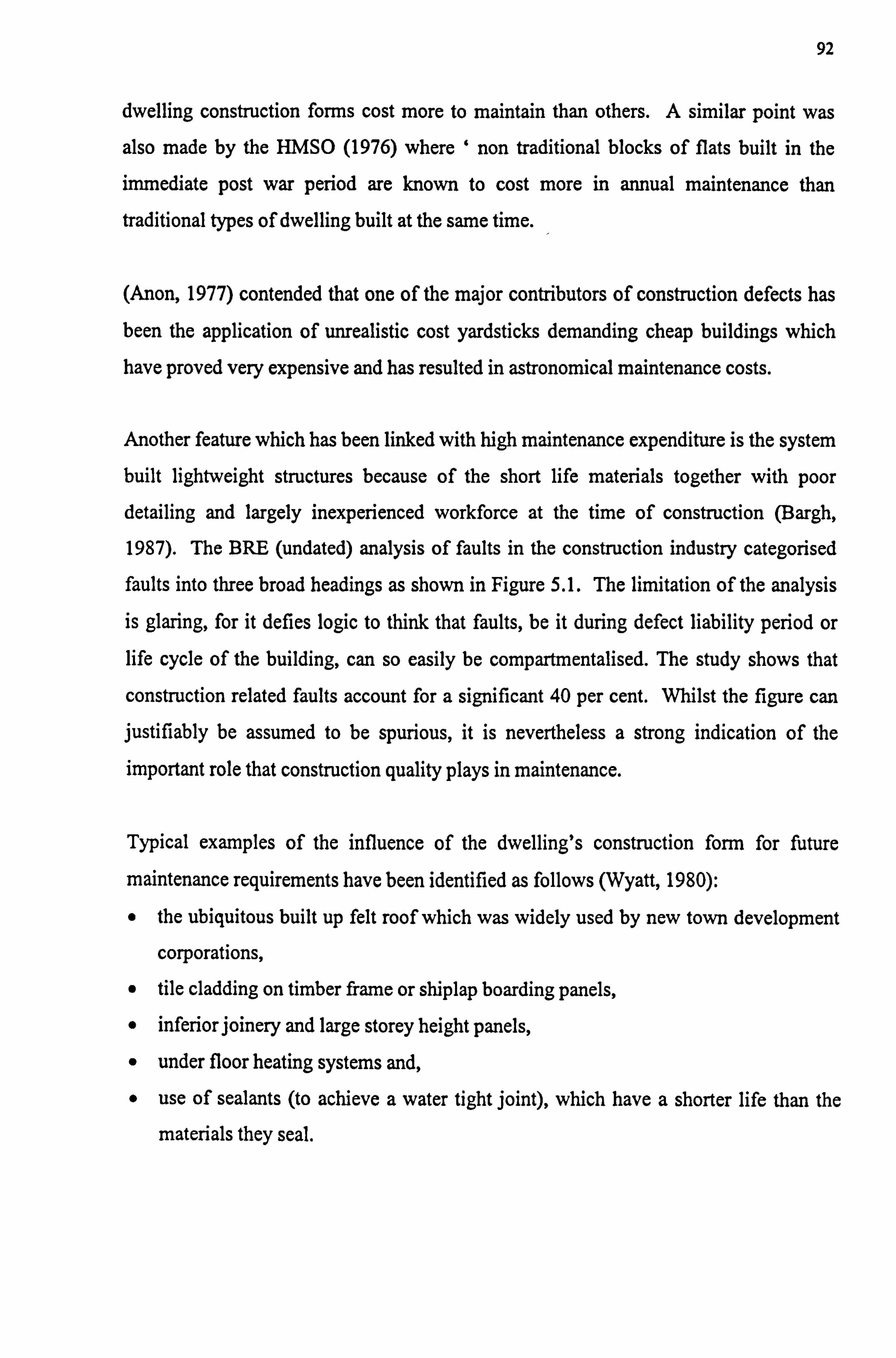
92
dwelling construction forms cost more to maintain than others. A similar point was
also made by the HMSO (1976) where ' non traditional blocks of flats built in the
immediate post war period are known to cost more in annual maintenance than
traditional types of dwelling built at the same time.
(Anon, 1977) contended that one of the major contributors of construction defects has
been the application of unrealistic cost yardsticks demanding cheap buildings which have proved very expensive and has resulted in astronomical maintenance costs.
Another feature which has been linked with high maintenance expenditure is the system
built lightweight structures because of the short life materials together with poor
detailing and largely inexperienced workforce at the time of construction (Bargh,
1987). The BRE (undated) analysis of faults in the construction industry categorised
faults into three broad headings as shown in Figure 5.1. The limitation of the analysis
is glaring, for it defies logic to think that faults, be it during defect liability period or
life cycle of the building, can so easily be compartmentalised. The study shows that
construction related faults account for a significant 40 per cent. Whilst the figure can
justifiably be assumed to be spurious, it is nevertheless a strong indication of the
important role that construction quality plays in maintenance.
Typical examples of the influence of the dwelling's construction form for future
maintenance requirements have been identified as follows (Wyatt, 1980):
" the ubiquitous built up felt roof which was widely used by new town development
corporations,
" tile cladding on timber frame or shiplap boarding panels,
" inferior joinery and large storey height panels,
" under floor heating systems and,
" use of sealants (to achieve a water tight joint), which have a shorter life than the
materials they seal.
93
Analysis of Faults in the construction industry
Construction Faults 40%
Design Faults 50%
Figure 5.1: Analysis of defects in the construction industry Source: BRE (undated)
5.9 Tenant issues
5.9.1 The Tenants' Charter
The Government's objective for the Tenants' Charter states as follows:
"those who prefer to remain as tenants, or who cannot afford ownership should be
respected as the valued customers of local authorities. They have to sustain its costs. They have the right to be consulted, to expect high standards and to prompt action when performance is poor"
The Government's Citizen Charter includes proposals relevant to council tenants.
Three of these refer to repairs and refurbishment (AMA, 1991):
1. Improving the rights of council tenants to the repair of their home.
2. Ensuring all tenants receive information about the standard and performance of
their local authority including repair times.
Product Faults
10%
94
3. Encouraging local authorities' to introduce refurbishment contracts, where
contractors and direct labour organisations who exceed the agreed completion date
would face financial penalties under the contract.
Whilst the government's intention in formulating the charter is noble, it is also true that
it has not backed up its good intentions with required resourcing, for without additional
resources and increased certainty about their future availability, local authorities will
struggle to deliver consistently the quality of service which tenants are entitled to
expect.
5.9.2 Tenants' consultation policy
The Tenants' Charter gives tenants the right to be kept informed and to be consulted
about matters that affect them, and should be involved, through their Tenants'
Associations, in the process of deciding Council policy. There are wide ranging
methods of consultation to suit different situations, from sending personal letters to
tenants, to sitting on area committee meetings, speaking and voting alongside
Councillors on issues that affect them.
The following methods of consultation are in use in the council on which the study is
based:
Consultation with individuals
Consultatiön with groups Consultation with Tenants' Associations
Consultation through project groups
Consultation through Area Housing Committees
Consultation through the Housing Advisory Committee
Consultation through a City-wide forum of all Tenants' Associations
The best way for tenants to have their say is to be in active Tenants' Association. Most,
if not all housing estates already have one Tenants' Association.
95
Tenants' Associations are a key element to the consultation process. They are involved
through Area Housing Committees and Project Groups in a formal sense, and through
day-to-day discussion with area housing officers in a less formal sense.
On the formal side, Tenants' Associations can help to decide council policy. Their
representatives sit on Area housing committees and project groups.
On the informal side, Tenants' Association representatives meet people from the area
offices to discuss local issues and put forward their views. This enhances the
development of links which enables tenants' voice to be heard.
5.9.3 Reporting of Defects
Reporting of defects is essentially about giving an eye-witness account and at the same
time making limited judgement on what is observed depending on who the reporter is,
thus making the whole exercise of reporting a seriously subjective exercise. According
to Croome (1980) a building defect is intractably subjective unless it was brought to the
notice of those who are trained to both diagnose and offer prognosis for such defects.
This, as Porteous (1985) observed, is still fraught with complexities. As Croome
(1980) contended, every too often, components are judged to have failed if sufficient
complaints are received about their conditions, and these complaints are not reliable indicators of the severity of failure. Especially in building, unless there is a serious and
obvious structural failure, there is usually no focal point for complaints. Porteous (1985) has noted that one of the factors which may decide whether a building
defect is reported to some person competent to record and make judgement upon it is
the ownership of the building. Local authorities who hold buildings as socio-
investment units have a higher expectation of defect-free stock than owner-occupiers.
Whilst the owner-occupier makes decision on defect strictly on commercial judgement,
the local authority is looking for sound, trouble free investment for political reasons as
dictated by the political interest of the central government.
96
5.10 Stock condition survey
Condition survey has been defined as an attempt at establishing the state of a dwelling
or production unit with the overall objective of acquiring an informed knowledge of its
state of repairs in order to forestall any likely loss of production resulting from sudden
breakdown in the case of production units, and preservation of stock value in the case
of buildings (Mole and Olubodun, 1995b).
Damen (1990) has identified some objectives of condition surveys as:
(a) to determine stock's need of repair
(b) to locate where quality deficiency exists (c) to identify the type of operations necessary to correct the deficiencies
(d) to show whether existing maintenance policy is adequate or not
(e) to know whether certain measures yield the desired result.
5.10.1 Day-to-day survey
Contrary to the formalised pre-planned and systematic approach to overall stock
assessment in condition survey, day-to-day reactive survey can be ad hoc or even
haphazard to a greater or lesser extent. This is occasioned sometimes, by the whimsical
and untrained impulse of dwellers (Croome, 1980) to what is considered to be an
incursion of defect or a symptom of it. The practical implication of this is that it is
extremely difficult for the surveyor to always carry out his investigation in a totally
unbiased manner however theoretically professional that activity might be said to be.
This situation is further complicated by the increasingly conscious `consumer-oriented'
society that we live in. The negative effect of which is for the surveyor to be positively
biased in favour of pleasing the consumer (in this case the tenant or dweller) in his
diagnosis and prognosis of reported defects. Nonetheless, reactive survey, more often
than not helps to `nip the problem on the board' and can be rightly described as `a stitch
in time that saves nine'.
97
5.10.2 The surveyor's bias
Surveyors engaged in the various types of stock surveys naturally vary in their opinion
of defect causes and repair method. However, their variability should be within a
normal distribution of opinions of a sample of proficient and qualified surveyors.
However, careful training of surveyors engaged in surveys will go a long way towards
enhancing uniformity, and concordance in opinions. O'dell (1990) from his own
personal experience in the field came to a conclusion that surveyors do generally agree
quite closely in their description of defects, with little disagreement in diagnosis but
greater disagreement in their prognosis. This position lends credence to the research
methods employed in the study since it falls short of requiring surveyors to proffer
prognoses for identified defects but merely seeks their opinion as to the contributing
influence(s) on defects. This improves reliability in the light of obvious subjectivity.
This position is corroborated in parallel with O'dell (1990) by Damen (1990), as no two
persons are likely to have the same outcome given the variable nature of the process of
observation and interpretation.
5.11 The English House Condition Survey (EHCS)
The EHCS has been conducted every five years since 1967. Its purpose is to describe
the housing stock and to monitor its changing condition, thereby providing background
to government policies on home improvement and area renewal (O'Dell, 1990). The
survey consists;
1. Of the physical examination of a large sample of the national stock; interviews with
occupiers to determine the recent history of repair and maintenance to their homes,
their interest in home improvement and ability to finance necessary work. 2. A postal survey of local authorities to determine the institutional contribution to
housing renewal; and
3. A survey of house values (O'Dell, 1990).
The technique used in EHCS have developed gradually over the years. A longitudinal
survey approach to reduce errors in the measurement of changes over time has become
98
a standard practice. As claimed by O'Dell (1991), the survey is the chief vehicle for the
collection of information by the DoE in support of all aspects of housing policy. From
the mass of data available from this quinquenial survey, the initial expectation was that
most of the data needed for the study could be obtained from the arsenal of
maintenance information in the (EHCS) archive. Following from the global objective
of the survey however, it is no surprise that the resulting data does not satisfy our data
need for this study.
5.12 Organisation of Housing Management
5.12.1 Stockholder's responsibility - Housing Management
The council's responsibilities with regards to repairs and improvement is a contractual
one, as enunciated in the Tenancy Agreement exchanged with tenants. The council
binds itself to do the following:
" To keep every housing unit to a decent standard of repair.
" To paint window and door frames, and general external woodworks at regular
intervals as preventative measure against disrepair.
" To effect repairs on any disrepair items in a reasonable time and tidy up after repair.
" The right to temporarily rehouse a tenant in the event that the dwelling has to be
empty for major building work.
In the local authority being studied, there are broadly two operational areas namely; North and South. Within each operational area there are area housing offices each of
which have responsibilities for between 3000 and 5000 housing units.
A typical area housing office organisation structure is shown in Figure 5.2
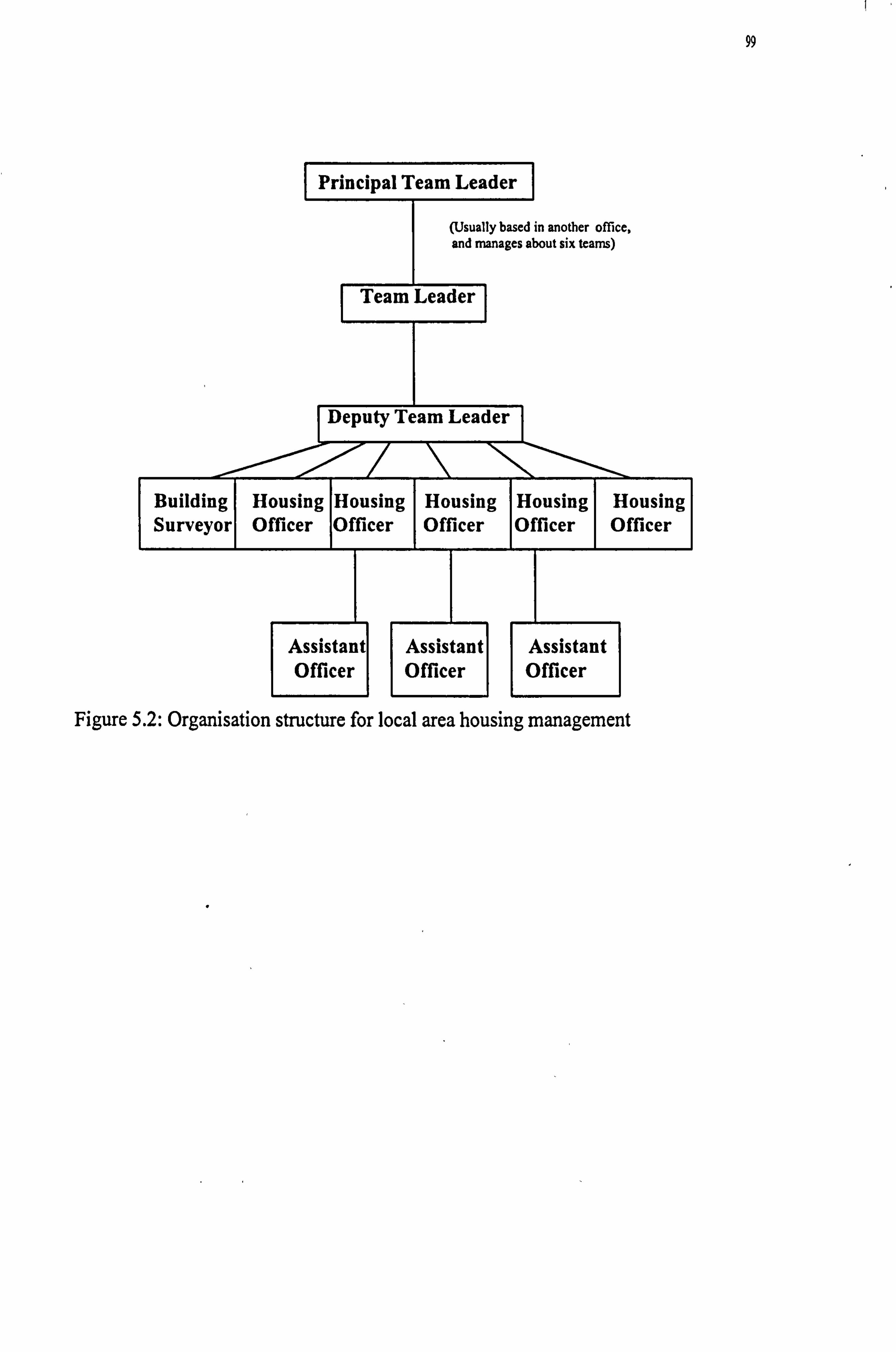
Principal Team Leader I
(Usually based in another office, and manages about six teams)
Team Leader
Deputy Team Leader
Building Housing Housing Housing Housing Housing Surveyor Officer Officer Officer Officer Officer
Assistant Assistant Assistant Officer Officer Officer
Figure 5.2: Organisation structure for local area housing management
100
5.12.2 Procedures for repair action 5.12.2.1 Defects reporting by tenants
A tenant is responsible for the behaviour of every person, including children living in or
visiting his home. Every tenant is obligated by the tenancy agreement to inform the
council about any defects or damage immediately.
When a repair is reported by a tenant, the receiving housing officer will immediately
order the repair as required following departmental laid down procedures once the
officer satisfies himself that the job has not already been ordered. Once ordered, a
computer generated confirmation slip is given or sent to the tenant confirming his
report. This receipt will show that the tenant had in fact met up with the requirement to
report repairs needs if there is a problem in the future.
Where damage is caused deliberately or by neglect, the tenant is expected to carry out
or pay for such repairs. Furthermore, the tenant is expected to do small repairs such as
unblocking sinks, replacing taps or internal door handles. It is however often too
difficult to prove where repair needs has been caused deliberately or by neglect. In the
end, the responsibility to do repairs falls upon the council.
5.12.2.2 Housing officer's inspection
Repairs which are not prioritised as emergency would normally require housing
officer's inspection. Such repairs are required to be inspected within five working days
of report being made by tenant. Where the housing officer could not obtain access to
the dwelling a `no access' card is left giving details of job and requesting the tenant to
reply within seven days and making arrangement for a mutually convenient time for a
repeat visit by the housing officer. This visit is simply to ensure that the repair has
been correctly ordered.
Once it has been decided that the repair is valid, the housing officer exercises his
discretion as to whether or not the defect requires the expertise of a building surveyor for accurate diagnosis.
101
Repairs are divided into two groups, namely; those that require a pre-inspection to
determine the work specification by building surveyors, and those which are routine
repairs an d can be ordered reasonably accurately without pre-inspection.
Where required, survey order request is raised by the housing officer for the surveyors'
group for the housing area, if not, the job is processed through the computer system for
the action of the DLO department. At this stage, a confirmation letter is sent to the
tenant informing him/her that repair works will be carried out. The deadline by which
the repair will be completed will either be 4 weeks from the day the repair order is sent
to the DLO or 12 weeks from the day the survey request is sent to the surveyors as
appropriate.
5.12.3 Local budgetary control
Each area housing team leader is allocated annual repairs budget and is responsible for
controlling expenditure within those cash limits. In order to exercise control, the team
leader requires an accurate estimate of their committed expenditure on a job by job and
summary basis. What is conspicuously lacking at the moment is a pre-planned estimate
of likely repair cost for a given year before the commencement of the financial year. This results in budget shortfalls and the most crucial repair needs have to be foregone in
most area offices. In some instances surplus budgets tend to be inefficiently spent-up
towards the end of the financial year in few area offices.
5.13 Summary
This chapter produced a review of related literature on factors determining or influencing maintenance needs namely; age, design, vandalism, construction type and
changing standards. The place of tenants in the repair of their home through the instrument of the Tenants' Charter was clearly identified. The subjectivity in defect
reporting culture on the part of both tenants and experts was discussed.
The influence of the mediatory role of local housing management in regulating and
responding to maintenance need and requirements was discussed. The decision as to
the validity of a tenant's report on defects rests with the housing officer, as well as
102
response time within which such defects are attended to. Control of local budgets as
they impact on responsiveness to repair was brought to the fore. Each area housing
team leader is allocated annual repairs budget and is responsible for controlling
expenditure within those cash limits. In order to exercise control, the team leader
requires an accurate estimate of their committed expenditure on a job by job and
summary basis. What is conspicuously lacking at the moment is a pre-planned estimate
of likely repair cost for a given year before the commencement of the financial year.
This results in budget shortfalls and the most crucial repair needs have to be foregone in
most area offices. In some instances surplus budgets tend to be inefficiently spent-up
towards the end of the financial year in few area offices.
103
CHAPTER 6
ANALYSIS OF SURVEYOR'S QUESTIONNAIRE
6.1 Introduction
The objective of this section is to analyse and interpret factors which bear upon building components and to explore underlying relationships among the number of building components forming construction entity from information provided by the
respondents. A multivariate statistical technique known as factor analysis was chosen
as the method of grouping the components into sub-patterns at exploratory level, and
regression statistical technique at the confirmatory level.
The chapter is divided into two main segments. Section one is the analysis of data from
the survey of building surveyors, which has been described as the primary analysis.
While section two is the second analysis which is intended to explore and detect
underlying relationships among the number of building components forming the
construction entity. The format of presentation for each analysis is hypothesis, data,
analysis and results, and interpretation.
6.2 Objective
Following from the literature review, authors are commonly agreed on factors
pertaining to the building structure. What is at dispute is the extent to which these
factors are important in causing defects. The impact of building structure family of factors is schematically illustrated in Figure 2.3 as derived from the literature. This
family of factors have been identified to include Age factors, construction factors,
Design factors, Changing Standard and Vandalism factors.
The objectives of this chapter are chiefly to:
1. Underscore the impact of each of the five criteria sets on the identified 28 building
components (see section 2.8.3.3 on how the components are obtained). In so doing,
it will be possible to appreciate the tangible influence of the factors in terms of how
they affect defect causation on building components for the sample population.
104
2. Establish the relative importance of each of the five criteria in terms of individual
contribution to overall defect. As a follow-up to this, the overall contribution to
maintenance generation of "Building Structure Family of Factors" will be
established in relation to other possible causes or factors.
6.3 The Thesis - Hypotheses
Three different hypotheses are explored in this chapter. The fourth is explored in
Chapter Seven as a follow-up to the questions raised in the exploration of the third
hypothesis. The hypotheses are set as follows:
A(i) Null hypothesis (Ho ): No agreement can be found among the building
surveyors in assessing the strength of each of design, construction, age,
changing standard and vandalism as a causative factor for defects on building
components, i. e. Kendall's Coefficient of Concordance is not significant at
5% level significance.
A(ii) Alternative hypothesis (H, ): There is agreement between the surveyors in
assessing the strength of each of design, construction, age, changing standard
and vandalism as a causative factor for defects on building components, i. e.
Kendall's Coefficient of Concordance is significant at 5% level significance.
B(i) Null Hypothesis (H0): Technical knowledge possessed by building surveyors,
of the building is the most important ingredient in tracking down maintenance in housing properties.
In essence, a knowledge of design and construction characteristics, evolving standards,
the level of exposure to vandalism and age of a dwelling will allow us to explain most
of the variations in its maintenance requirements.
B(ii) Alternative Hypothesis (H, ): Technical knowledge possessed by building
surveyors, of the building is not the most important ingredient in tracking down
maintenance in housing properties.
105
C(i) Null Hypothesis (Ho) : Of the five factors identified, none is more important
than the other for the prediction of housing maintenance requirements.
C(ii) Alternative Hypothesis (H, ): Of the five factors identified, some are more
important than others for the prediction of housing maintenance requirements.
D(i) Null Hypothesis (Ho ): There are no intercorrelations between component
defect causes, i. e. it is not plausible to localise defect causing factors to a
group of components.
D(ii) Alternative Hypothesis (H, ): There are intercorrelations between the
components defect causes
Tool for the last set of hypothesis is the factor analysis in the next chapter.
6.4 The survey
One hundred active building surveyors were selected from the survey population,
consisting of building surveyors and engineers employed by the Council. These all
have direct involvement with defects diagnosis on the housing stock. Of these, 52
surveyors responded by returning their questionnaire. This represents a 52% response
rate. However, of the returned questionnaire, seven were rejected for incomplete
information, thus the analysis is based on 45 satisfactorily returned questionnaire,
representing a final response rate of 45%. This response rate is still quite high for
surveys of this type and is considered satisfactory (Russell et al, 1992). It is worthy of
mention that the researcher's proximity to the population sample may have encouraged
such a high response rate. Furthermore, Forsgren's (1986) view that the respondent's
perception of the survey as touching on his field of interest very strongly influences
response rate, is here supported as the subject of the questionnaire directly impinges on
respondents' professional practice and field of employment.
106
6.5 Reasons for non-response
Forty-eight surveyors were believed to have declined to participate in the survey. In
actual fact, more than 40% of these returned their completed questionnaire two to three
months after the questionnaire was sent out. It was earlier decided before sending out
the questionnaire that returned questionnaires would be considered valid if they were
returned no later than six weeks after being sent out. It is believed that given the
number of responses complying with the set time limit, not including the late
questionnaires would not adversely affect the outcome of the survey. On the contrary,
it implies that the responses analysed in the first instance are those from a cross section
of participants possessing keen interest in the study and are indicative of deep interest
and enthusiasm for the subject.
The responses were analysed according to the hypothesis they were intended to test.
6.6 Data collection, manipulation, analysis and presentation 6.6.1 The data
The organisation of the questionnaire designed to elicit information from respondent for
the testing of the above hypothesis along with other related hypotheses is somewhat
complex. Complex as it was, the implementation of a pilot study (section 2.5.2.3)
alleviated any doubts as to understanding and clarity on the part of the participants.
The need to keep the questionnaire short so as to maintain interest and enthusiasm on
the part of the respondents was responsible for such complexity in the design of the
survey instrument.
Question No. 1 asked for the respondent's job title in order to know, at what level of expertise the participant is carrying out building surveying functions. Questions Nos. 2
and 3 seek to elicit information on the experience of survey participants in order to gain
some insight into the level of reliability the author can expect from the responses. Questions 4 and 5 are the very essence of the questionnaire. Question No. 4 asked
primarily for each of the identified building components to be scored on each of the five factors, namely: design, construction, age, changing standard and vandalism as a
0 107
defect causing influence. Question No. 5 asked respondents to rank the identified 28
building components according to how frequently defects show on them. This formed
the basis for the exploratory data reduction technique - factor analysis of the next
chapter. The suggested scores were: hardly ever [0], very occasional [1], occasional [2], frequent [3] and very frequent [4].
6.6.2 Missing values
An examination of the SPSS display of the results show that 431 scores (6.84% of the
total data set) are missing. The effect of the missing values will be to reduce to 17 the
number of valid cases having scores for all the variables. To correct for this
unwelcome effect; each missing score is substituted with the mean of the respondents
score for the variable; alternatively, the missing values can be substituted with random
scores (after Norusis 1994 and Nkado 1991). In this case, it was decided to opt for
`mean substitution' for missing values, as this is commonly believed to be the more
objective correction option.
6.6.3 Data Analysis
Each score given by a respondent represents the degree to which the occurrence of defects on a particular building component can be explained by the influence a
particular defect causing factor has on that component. In a survey of this nature,
incidence of repetitive scoring (Jobber 1986), which is an indication of lack of interest,
or an indication of boredom may be expected to a lesser or greater extent. A cursory inspection however, shows no apparent use of a particular rank across the variables by
any one respondent. A visual inspection of the pattern of scoring was done prior to the
various statistical analyses being conducted. From the inspection carried out, there is
nothing to suggest that thoughtful assessments have not been made and that
respondents did not express their candid and enthusiastic opinion in both the scoring for
Question No. 4 and ranking of components in Question No. 5.
108
6.6.3.1 Test for homogeneity across groupings
Whereas no validatory check-questions' were included in the building surveyor's
questionnaire, the issue of reliability of the responses was tested by conducting various
analyses to test for significant differences in the scorings between respondent groups.
A one-way analysis of variance was conducted for each of the 135 variables derived
from Questions Nos. 4 and 5 to test for differences between the mean scores of two
groups of surveyors, i. e. building surveyors and senior building surveyors. This
revealed the existence of significant differences (at the 5% level) between the groups
for six out of the 135 variables (after Fortune and Skitmore, 1994). An analysis of
variance (ANOVA) results print-out for six of the variables is shown in Table 6.1 It is
expected that the test could prove significant on up to seven variables by mere chance
occurrence, which is higher than the observed six in this case. On this evidence, it was
decided to proceed further with the analysis without regard to surveyor's title or
seniority. However, a similar analysis with length of experience as factor revealed that
21 out of the 135 variables proved to have significant `F' ratios. This is more than
would be expected by chance. Nevertheless, it is believed that this is not a strong
enough evidence against proceeding with further analysis using the respondent
groupings on length of experience. As shown in Table 6.4b, the distribution of
experience between the two groupings is not nearly balanced. Whereas 12
(representing 27% of the sample) claimed to have spent more than five years with the
technical consultancy unit, 33 (representing 73% of the sample) have not spent more
than five years. The effect of this imbalance in the distribution will have been to
distort the observed strength of significance in the analysis (after Champion, 1981).
This explains why up to 15 per cent of the variables prove to be significant (which is
considerably higher than the expected 5 per cent). The variation is underpinned by the
distribution rather than by length of service.
109
Table 6.1: Analysis of Variance results for selected variables on job title.
-----0 NEWA Y-----
Variable DAMPROFD DEFECTIVE DAMP PROOFING (DESIGN)
By Variable JOBTLE2 job tittle
Analysis of Variance
Sum of Mean FF
Source D. F. Squares Squares Ratio Prob.
Between Groups 1 2.6163 2.6163 2.0432 . 1605
Within Groups 41 52.5000 1.2805
Total 42 55.1163
Variable DEFRUFD defective roof structure (design)
By Variable JOBTLE2 job tittle
Analysis of Variance
Sum of Mean FF
Source D. F. Squares Squares Ratio Prob.
Between Groups 1 1.4901 1.4901 . 9098 . 3455
Within Groups 43 70.4211 1.6377
Total 44 71.9111
Variable RUTD dry/wet rot (design)
By Variable JOBTLE2 job tittle
Analysis of variance
Sum of Mean FF
Source D. F. Squares Squares Ratio Prob.
Between Groups 1 3.8413 3.8413 2.3183 . 1357
Within Groups 40 66.2778 1.6569
Total 41 70.1190
110
Table 6.1 (cont'd)
Variable WATINGD water ingress (design)
By Variable JOBTLE2 job tittle
Analysis of Variance
Sum of Mean FF
Source D. F. Squares Squares Ratio Prob.
Between Groups 1 . 5730 . 5730 . 3178 . 5760
Within Groups 41 73.9386 1.8034
Total 42 74.5116
Variable BUSTD broken pipe or appliance (design)
By Variable JOBTLE2 job tittle
Analysis of Variance
Sum of Mean FF
Source D. F. Squares Squares Ratio Prob.
Between Groups 1 . 3889 . 3889 . 8589 . 3596
Within Groups 40 18.1111 . 4528
Total 41 18.5000
Variable REGLAZD reglazing (design)
By Variable JOBTLE2 job title
Analysis of Variance
Sum of Mean FF
Source D. F. Squares Squares Ratio Prob.
Between Groups 1 . 0194 . 0194 . 0368 . 8488
Within Groups 42 22.1624 . 5277
Total 43 22.1818
111
The conclusion drawn from these two sets of analyses is largely that scores do not vary
with surveyors across job titles or length of service, i. e. that the scores are reasonably
homogeneous.
6.6.3.2 Methods
The purpose of this section is to present a statistical analysis of the manipulated sample
data on identified building component defect's assessment and tangible causes of defects, and to test the first three sets of hypotheses set out in section 6.3.
Before going into the details of the analyses carried out on the data, it is necessary to
explain the statistical tests and methods used. These methods are chosen as those most
applicable to the data sets.
6.6.3.2.1 The Kendall coefficient of concordance, W
Kendall's coefficient of concordance, W, measures the extent to which there is
agreement between the rankings on any number of variables. In essence, it determines
the significance of agreement between building surveyors in ranking the variables. It is
a method of determining the degree of agreement between `k' respondents on `n'
variables where each has been measured on an ordinal scale. In this study, it is used to
test the null hypothesis that the 45 sets of rankings on the 28 variables are independent
or unrelated at each of the five factor levels, at the 5% significance level.
There are three non-parametric rank correlation tests: Kendall's (t); Spearman's
(p)rank correlation coefficients; and Kendall's coefficient of concordance (w) (Hays
1988 and Siegel, 1956). The first two are impractical for large values of N since all
possible values of the coefficient for each pair of respondents must be averaged (Siegel,
1956). The third, Kendall's coefficient of concordance (w), was therefore the most
appropriate measure to apply in the case of this study.
112
Kendall's Coefficient of Concordance (x) is expressed by Siegel (1956), Champion
(1981) and Hays (1988) as:
Variance of Ranked Sums Maximum possible Variance of Rank Sums
Hence,
12S N2(n' -n)
where
N is the number of rankings (respondents)
n is the number of ranks (items ranked)
S is the observed sum of the squares of deviations of sums of ranks from the mean
value, -
N(n + 1).
There are two principal tests used to check the hypothesis that there is agreement between the judges in ranking n variables. These are as follows:
i) For n<7, a chi-square test is used (Hays, 1988)
where
XZ = N(n -1)w = 12S
Nn(n + 1)
ii) For n>7, the significance of the Kendall's Coefficient of Concordance may be determined by applying the formula for chi-
square given above, with degrees of freedom given by (n-1). A
significant chi-square confirms a significant (w) (Cohen and
Holliday, 1982; and Siegel and Castellan, 1988).
113
6.6.3.2.2 Chi-square test for independence
This statistic is a single-sample test of significance, which can be extended to two
independent-sample test. The procedures for chi-square statistic is commonly referred
to as goodness-of-fit tests. This label applies to the `fit' between an observed set of frequencies across a given number of categories or in a nominal crosstabulation of
variables, and an expected set of frequencies.
The statistic w proposes a hypothesis of independence or an approximation to
independence. Independence implies that knowing the value of one variable says
nothing about the values of the other. Conversely, the absence of independence
suggests that at least some categories are associated. The test rests upon the assumption
of asymptosis and multinomiality. By these, it is implied that the expected frequency
must be reasonably large not to produce misleading inferences. As a rule of thumb,
Champion (1981) suggested that the sample size must be 25 or larger, and randomly
selected. In our case, these two crucial conditions of asymptosis and multinominiality
are met as the sample size is 45 and fixed by the sample design in order to ensure that
the responses are independent. - The third and fundamental assumption of the test is that
the possible responses are mutually exclusive and of course, exhaustive. As a
respondent can not give more than one response to any of the variables, the condition of
mutual exclusiveness is met in the design of the questionnaire. To every intent and
purpose, it is believed that mutual exhaustiveness is ensured through the piloting of the
survey instrument.
6.6.3.2.3 Mean Rank
The development of a mean rank for each of the variables works upon the SPSS
recognising the pattern of scoring for each variable. In this study, the scores are
assigned to the variables as follows:
Hardly ever -0 Very occasional -1 Occasional -2
Frequent -3 Very frequent - 4.
114
These scores are treated as ranks for the computation of the Kendall's Coefficient of
Concordance (o) statistic. The highest score is assigned to the most popular variable
as perceived by the respondents. The mean rank is obtained by computing
28
Z R1 J-1 for each variable, that is building component (Siegel, 1956).
N
Where;
Rj is score assigned to the variable by each respondent and,
N is the number of rankings (respondents).
This quantity is automatically multiplied by 10 in SPSS software in every case in order
to ensure that every variable attains a figure of no less than 1.0. This quantity, here
referred to as mean rank (SPSS) measures the relative dominance of each variable
within the final statistic (o). In this study, the variable with the highest mean rank is
the most dominant while the variable with the least mean rank is the least dominant.
6.6.3.2.4 Multiple linear regression
The general form of a multiple linear regression can be written as: Y°
F'0 +PIXli +ß2X2i +1'3X31+""""+ßnXni +ri Eqn 1
Where Y is the predicted variable, ßo represents the constant term, X. represent the
independent variables and ß' represent the coefficient of each of the `n' variables in
the equation. The underlying assumption of the above equation is that the independent variables are
related to the dependent variable in a linear way. That is to say, the equations included
no variables as products or powers of itself.
Given a logarithmic transformation on the original data to convert it to an interval scale
measurement, the general form of the regression equation from equation 1 can be
changed as follows:
log Y= 10900 + log 1+ log X1, + log ß2+ log X2, +... + log ß�+ log X,, +, Eqn 2
115
According to Neal and Shone (1976), there is a systematic relationship between log Y
and log X. 3, - The variables are now log Y and log X;, while the parameters are log o and log
and c is normally distributed with X=0, S' =1 The advantage of the transformed equation lies in the fact that the variation in
maintenance need as a result of a possible change in each one of the independent
variables are the parameters of the equation.
6.6.3.2.5 Multiple Regression Statistics
The output of a regression analysis contains the following terms:
Multiple R: This is a measure of the linear relationship between the dependent variable
and the independent variables. It is described as the correlation between the observed
A dependent variable, Y and the fitted variable, }' from the independent regressor
variables in the equation (Gilchrist, 1984). It is the positive square root of R2 . As with
RZ from which it is derived, its value is 1.0 if all the observed values fall on the
regression line, and it assumes zero value if there is no linear relationship between the
dependent and independent variables.
R Square R2 : This is called the coefficient of determination and it is the proportion of
the variance of the values of Y explained by the regression equation (Norusis, 1990).
Accordingly, Gilchrist (1984) and Norusis (1990) have described at it as a measure of
the goodness of fit of a particular model.
R2 Residual sum of squares
Total sum of squares
Adjusted R square (Rä ): This expressed as:
116
(R2)= R2 p(1-R2) ° N-p-1
Where N is the number of cases and p is the number of independent variables in the
regression equation. It attempts to estimate for the population as against the sample
from which the statistic is derived. Whereas the sample R2 tends to be an optimistic
estimate of how well the model fits the population, Rö attempts to correct R2 for the
number of variables included in the model (Norusis, 1990). It does not automatically
increase as a new variable is added to the model, unlike R2 .
F- statistics: This is the standard deviation of the residuals.
The total observed variability in the dependent variable is subdivided into two
components, namely; that which is attributable to the regression and that which is not
(Norusis, 1991). The F-test is associated with the analysis of variance of the regression
model. It tests the null hypothesis that P. = 0. If this hypothesis is significant, it leads
us to reject the null hypothesis that RZ =0, in other words, it is a test of whether
there is a linear relationship between the dependent variable and the entire set of
independent variables.
P cofficients : These are the partial regression coefficients, partial because the
coefficient for each variable is adjusted for other regressor variables in the equation.
Beta: A way to make regression coefficients more comparable is to calculate the beta
weight, which are the coefficients of the independent variables when all variables are
standardised. It is computed as k=ßk Sk (Norusis, 1991) y
Where St is the standard deviation of the kth independent variable, SY is the standard
error of the estimate and ßk is the ß coefficient of the kth variable. Kinnear and Gray
(1994) interpreted this score as the proportion of one standard deviation change in the
dependent variable made by a one standard deviation change in the independent or kth
regressor variable. Beta scores are indicators of the relative importance of the variables
in the equation, and depend on the other independent variables in the equation.
117
Partial correlation coefficient: According to Norusis (1990), another way of
assessing the relative importance of independent variables is to consider the increase in
R2 when a variable is entered into an equation that already contains the other
independent variables. The square root of the increase is called the part correlation
coefficient. This coefficient is computed by as follows:
R2 -R2 Pr? _0 ' 1-R(; )
where Rr2 is the square of the multiple correlation coefficient when all independent
variables except the ith are in the equation.
Tolerance: This is the proportion of the variability in the ith variable which is not
explained or accounted for by the other variables in the equation. If the tolerance is
low, it indicates that multicollinearity is a problem.
t- test: This statistic is expressed as t=B SE(Bý
It is used to test the null hypothesis that the partial regression coefficient for the ith
variable, Pr, , is equal to zero. A significant t- test indicates the existence of a linear
relationship.
6.6.3.2.6 Mechanics of the scorings by respondents
The questionnaires were designed to allow all of the 28 building components to be
scored on the basis of respondent's perception on each of the five criteria of design,
age, construction, changing standard and vandalism as causative factors for defects. In
other words, a respondent is expected to score each component (between 0 and 4) on
the basis of his perception of the extent to which defect on the component is attributable
to Design factors. This process is then repeated for all the other four criteria, i. e. Age,
Construction, Changing Standard and Vandalism factors.
Each of the resulting groups (five in number) of data is analysed
118
6.7 Data Manipulation
Reynolds (1977) has criticised the widespread tendency among researchers to compress
variables into small, manageable number of categories, on the account that it may
produce erroneous conclusions. He suggested that such compression of variable should
not be done aimlessly, but should be dictated by statistical necessity where to do
otherwise may lead to an unsatisfactory application of a statistical model. One instance
where this is recommended according to Reynolds (1977) and Champion (1981) is
where there is the need to overcome the problem of few expected cell frequencies and logical combinations of cells are possible.
In this case, neither of these two conditions is violated. Further to Question No. 1
which asked for respondent's current job title, five categories of responses are possible.
However, as can be seen in the Tables, this will lead to an expected frequency of less
than five on all the 16 or 20 cells. This condition would result in a misleading chi-
square value. For the same reason, it was also decided to collapse the first and second
responses on Question No. 3 (which asked for how long the respondent has worked
with the Technical Department of the Council) as the actual cell frequency on the
category `Less than 1 year' is unacceptably too low. Tables 6.2a, 6.3a and 6.4a show
the frequency distribution for Question Nos. 1 to 3 respectively; and Tables 6.2b, 6.3b
and 6.4b show the corresponding collapsed categories for the same.
In line with Champion's (1981) and Reynolds' (1977) recommendations for
manipulating nominal data, it has been decided to collapse the variable categories
elicited from Question Nos. 1 to 3 as follows in Tables 6.2b, 6.3b and 6.4b.
119
6.8 Analysis of results on Building characteristics
6.8.1 Questionnaire responses by job title
Table 6.2a shows that 53% of the sample population are building surveyors (usually
without management responsibilities), 20% are senior building surveyors, 4%
compliance officer (responsible for monitoring defects on all repair works carried out),
about 18% are principal building surveyors (who are at the interface between executing
and managing surveys in each local office), and 4% surveying managers (they do not
have practical surveying roles, but are responsible for providing feedback information
on state of housing stock at each local office to senior management team for the
purpose of policy formulation). The job title distribution of the respondents indicates
that thoughtful assessments have been made and that the surveyors actually expressed
their opinion in scoring and ranking the variables on each factor criterion, as requested.
In the collapsed form, all surveyors without any management responsibility are grouped
into one category; namely, building surveyors and compliance officers are collapsed
into the building surveyor category. All the remaining three categories, i. e. senior and
principal surveyors, and surveying manager are grouped together into the senior
building surveyor category.
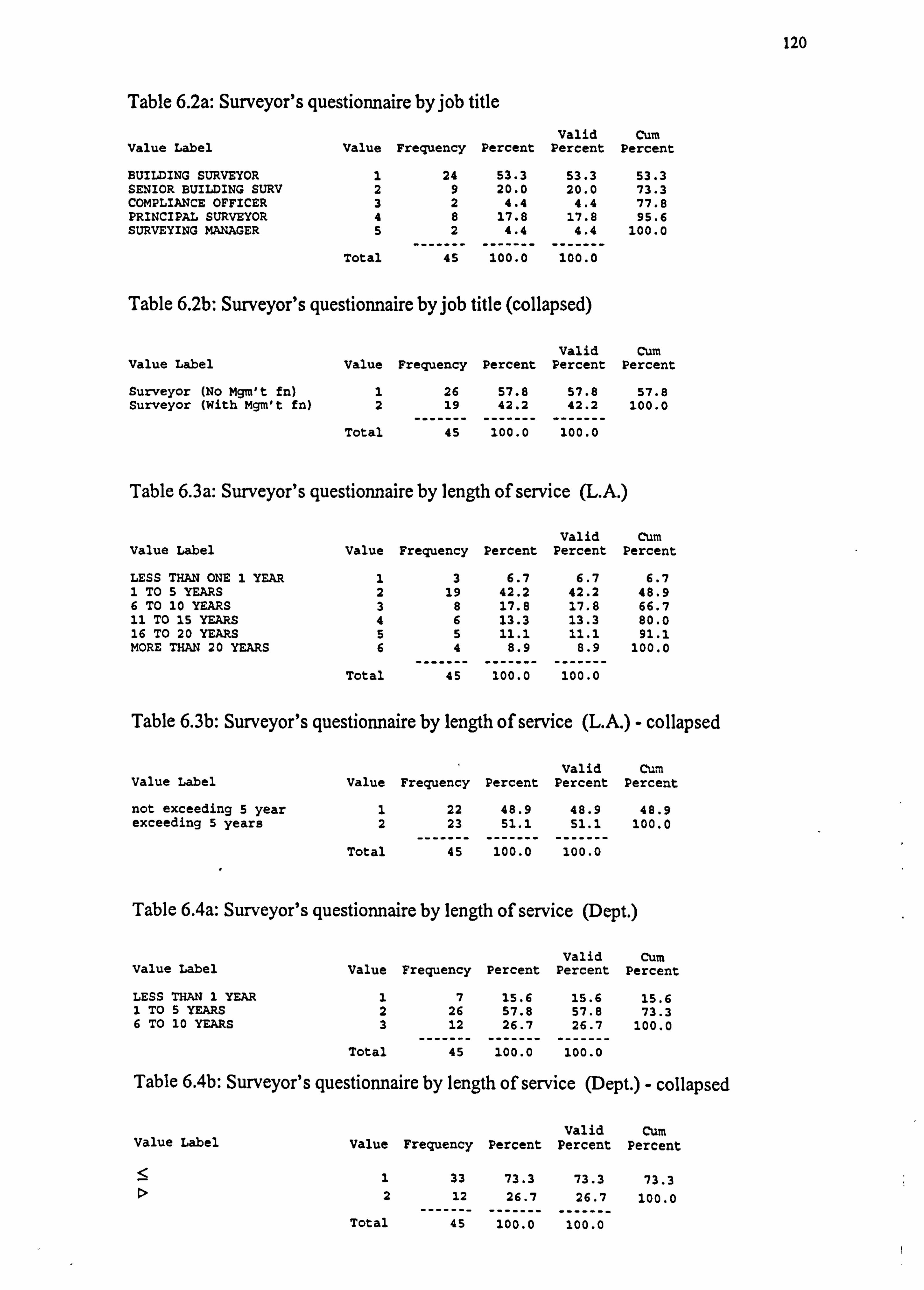
120
Table 6.2a: Surveyor's questionnaire by job title Valid Cum
Value Label Value Frequency Percent Percent Percent
BUILDING SURVEYOR 1 24 53.3 53.3 53.3 SENIOR BUILDING SURV 2 9 20.0 20.0 73.3 COMPLIANCE OFFICER 3 2 4.4 4.4 77.8 PRINCIPAL SURVEYOR 4 8 17.8 17.8 95.6 SURVEYING MANAGER 5 2 4.4 4.4 100.0
Total -------
45 -------
100.0 -------
100.0
Table 6.2b: Surveyor's questionnaire by job title (collapsed)
Valid Cum Value Label Value Frequency Percent Percent Percent
Surveyor (No Mgm't fn) 1 26 57.8 57.8 57.8 Surveyor (With Mgm't fn) 2 19
^ 42.2
- 42.2
-- 100.0
Total -----
45 --- ---
100.0 -----
100.0
Table 6.3a: Surveyor's questionnaire by length of service (L. A. )
Valid cum Value Label Value Frequency Percent Percent Percent
LESS THAN ONE 1 YEAR 1 3 6.7 6.7 6.7 1 TO 5 YEARS 2 19 42.2 42.2 48.9 6 TO 10 YEARS 3 8 17.8 17.8 66.7 11 TO 15 YEARS 4 6 13.3 13.3 80.0 16 TO 20 YEARS 5 5 11.1 11.1 91.1 MORE THAN 20 YEARS 6 4 8.9 8.9 100.0
Total -------
45 -------
100.0 ----- -100.0-
Table 6.3b: Surveyor's questionnaire by length of service (L. A. ) - collapsed
Valid Curn Value Label Value Frequency Percent Percent Percent
not exceeding 5 year 1 22 48.9 48.9 48.9 exceeding 5 years 2 23
-------
51.1 -------
51.1 -------
100.0
Total 45 100.0 100.0
Table 6.4a: Surveyor's questionnaire by length of service (Dept. )
Valid cum Value Label Value Frequency Percent Percent Percent
LESS THAN 1 YEAR 1 7 15.6 15.6 15.6 1 TO 5 YEARS 2 26 57.8 57.8 73.3 6 TO 10 YEARS 3 12 26.7 26.7 100.0
Total -------
45 -------
100.0 -------
100.0
Table 6.4b: Surveyor's questionnaire by length of service (Dept. ) - collapsed
Valid Cum Value Label Value Frequency Percent Percent Percent
1 33 73.3 73.3 73.3 2 12
------- 26.7 26.7 100.0
Total 45 -------
100.0 ----. --
100.0
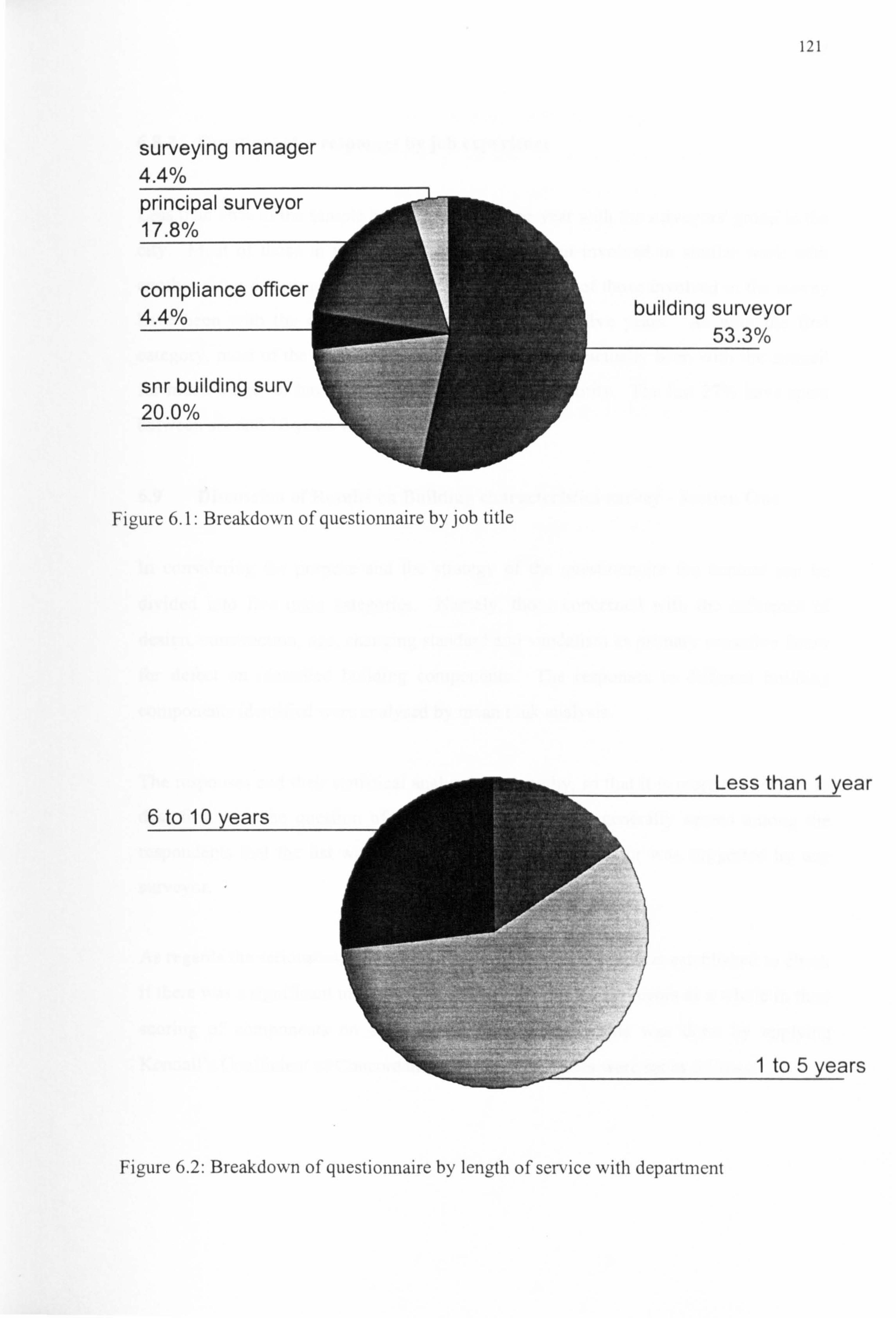
surveying manager 4.4% principal surveyor 17.8%
compliance officer 4.4%
snr building surv 20.0%
Figure 6.1: Breakdown of questionnaire by job title
121
? ar
rs
Figure 6.2: Breakdown of questionnaire by length of service with department
122
6.8.2 Questionnaire responses by job experience
Less than 16% of the sample has had less than one year with the surveyors' group in the
city. Most of those in this group have actually been involved in similar work with
another sister department of the council. The majority of those involved in the survey have been with the department for between one and five years. As with the first
category, most of the respondents in this category have actually been with the council for much longer or have come from another local authority. The last 27% have spent between six and 10 years with the department.
6.9 Discussion of Results on Building characteristics survey - Section One
In considering the purpose and the strategy of the questionnaire the content can be
divided into five main categories. Namely, those concerned with the influence of
design, construction, age, changing standard and vandalism as primary causative factor
for defect on identified building components. The responses to different building
components identified were analysed by mean rank analysis.
The responses and their statistical analyses are lengthy, so that it is more convenient to deal first with the question of comprehensives. It was generally agreed among the
respondents that the list was exhaustive, since no other factor was suggested by any
surveyor.
As regards the seriousness of the scoring, a statistical test was first established to check if there was a significant measure of agreement among the surveyors as a whole in their
scoring of components on each of the five factors. This was done by applying Kendall's Coefficient of Concordance, and the hypotheses were set as follows:
123
(i) Null hypothesis (Ho ): No agreement can be found among the building
surveyors in assessing the strength of each of design, construction, age,
changing standard and vandalism as a causative factor for defects on building
components, i. e. Kendall's Coefficient of Concordance is not significant at
5% level significance.
(ii) Alternative hypothesis (H, ): There is agreement between the surveyors in
assessing the strength of each of design, construction, age, changing standard
and vandalism as a causative factor for defects on building components, i. e.
Kendall's Coefficient of Concordance is significant at 5% level significance.
The statistical model for K related samples, the Kendal (o), in the Statistical Package
for Social Science (Windows) was used for the analysis. The results obtained are as
shown in Table 6.5 to Table 6.10b:
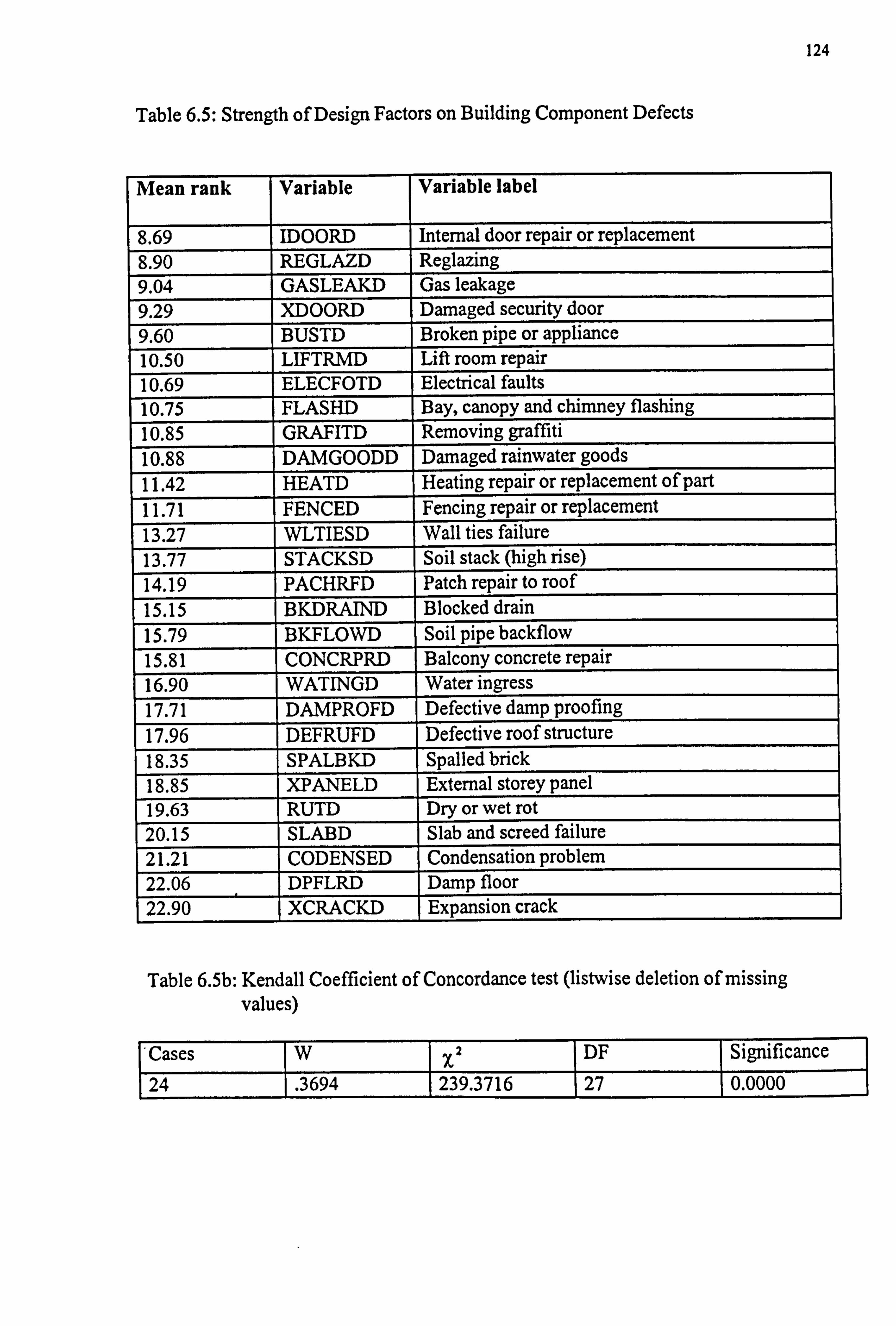
124
Table 6.5: Strength of Design Factors on Building Component Defects
Mean rank Variable Variable label
8.69 IDOORD Internal door repair or replacement 8.90 REGLAZD Reglazing 9.04 GASLEAKD Gas leakage
9.29 XDOORD Damaged security door 9.60 BUSTD Broken pipe or appliance 10.50 LIFTRMD Lift room repair 10.69 ELECFOTD Electrical faults
10.75 FLASHD Bay, canopy and chimney flashing 10.85 GRAFITD Removing graffiti 10.88 DAMGOODD Damaged rainwater goods 11.42 HEATD Heating repair or replacement of part 11.71 FENCED Fencing repair or replacement 13.27 WLTIESD Wall ties failure 13.77 STACKSD Soil stack (high rise) 14.19 PACHRFD Patch repair to roof 15.15 BKDRAIND Blocked drain 15.79 BKFLOWD Soil pipe backflow 15.81 CONCRPRD Balcony concrete repair 16.90 WATINGD Water ingress 17.71 DAMPROFD Defective damp proofing 17.96 DEFRUFD Defective roof structure 18.35 SPALBKD Spalled brick
18.85 XPANELD External storey panel 19.63 RUTD Dry or wet rot 20.15 SLABD Slab and screed failure
21.21 CODENSED Condensation problem 22.06 DPFLRD Damp floor 22.90 XCRACKD Expansion crack
Table 6.5b: Kendall Coefficient of Concordance test (listwise deletion of missing values)
Cases W 2 DF Significance
24 . 3694 239.3716 27 0.0000
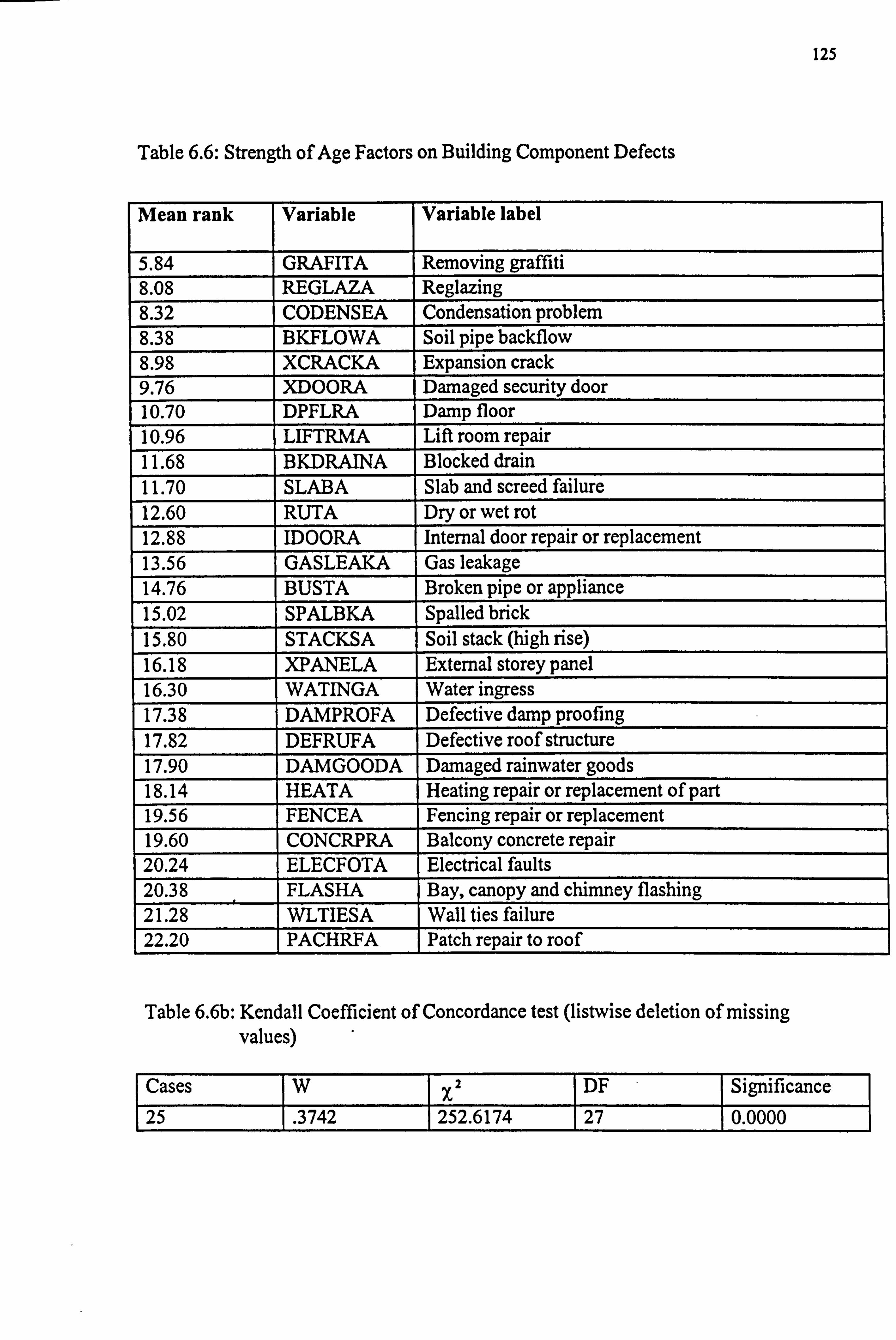
125
Table 6.6: Strength of Age Factors on Building Component Defects
Mean rank Variable Variable label
5.84 GRAFITA Removing graffiti 8.08 REGLAZA Reglazing 8.32 CODENSEA Condensation problem 8.38 BKFLOWA Soil pipe backflow 8.98 XCRACKA Expansion crack 9.76 XDOORA Damaged security door 10.70 DPFLRA Damp floor 10.96 LIFTRMA Lift room repair 11.68 BKDRAINA Blocked drain 11.70 SLABA Slab and screed failure 12.60 RUTA Dry or wet rot 12.88 IDOORA Internal door repair or replacement 13.56 GASLEAKA Gas leakage 14.76 BUSTA Broken pipe or appliance 15.02 SPALBKA Spalled brick 15.80 STACKSA Soil stack (high rise) 16.18 XPANELA External storey panel 16.30 WATINGA Water ingress 17.38 DAMPROFA Defective damp proofing 17.82 DEFRUFA Defective roof structure 17.90 DAMGOODA Damaged rainwater goods 18.14 HEATA Heating repair or replacement of part 19.56 FENCEA Fencing repair or replacement 19.60 CONCRPRA Balcony concrete repair 20.24 ELECFOTA Electrical faults 20.38 FLASHA Bay, canopy and chimney flashing 21.28 WLTIESA Wall ties failure 22.20 PACHRFA Patch repair to roof
Table 6.6b: Kendall Coefficient of Concordance test (listwise deletion of missing values)
Cases w x2 DF Significance
25 . 3742 252.6174 27 0.0000
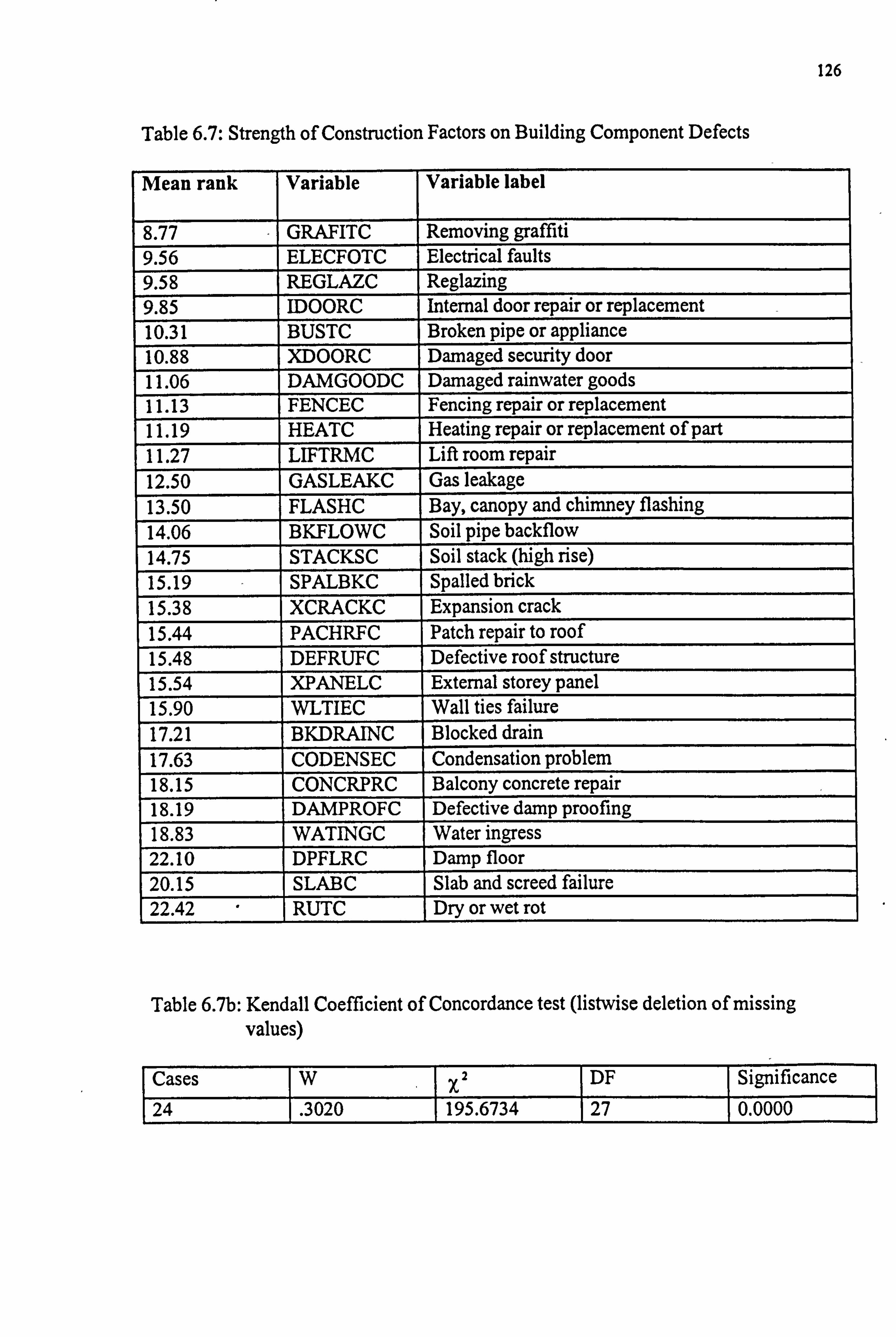
126
Table 6.7: Strength of Construction Factors on Building Component Defects
Mean rank Variable Variable label
8.77 GRAFITC Removing graffiti 9.56 ELECFOTC Electrical faults 9.58 REGLAZC Reglazing 9.85 IDOORC Internal door repair or replacement 10.31 BUSTC Broken pipe or appliance 10.88 XDOORC Damaged security door 11.06 DAMGOODC Damaged rainwater goods 11.13 FENCEC Fencing repair or replacement 11.19 HEATC Heating repair or replacement of part 11.27 LIFTRMC Lift room repair 12.50 GASLEAKC Gas leakage 13.50 FLASHC Bay, canopy and chimney flashing 14.06 BKFLOWC Soil pipe backflow 14.75 STACKSC Soil stack (high rise) 15.19 SPALBKC Spalled brick 15.38 XCRACKC Expansion crack 15.44 PACHRFC Patch repair to roof 15.48 DEFRUFC Defective roof structure 15.54 XPANELC External storey panel 15.90 WLTIEC Wall ties failure 17.21 BKDRAINC Blocked drain 17.63 CODENSEC Condensation problem 18.15 CONCRPRC Balcony concrete repair 18.19 DAMPROFC Defective damp proofing 18.83 WATINGC Water ingress 22.10 DPFLRC Damp floor 20.15 SLABC Slab and screed failure 22.42 RUTC Dry or wet rot
Table 6.7b: Kendall Coefficient of Concordance test (listwise deletion of missing values)
Cases w x2 DF Significance
24 . 3020 195.6734 27 0.0000
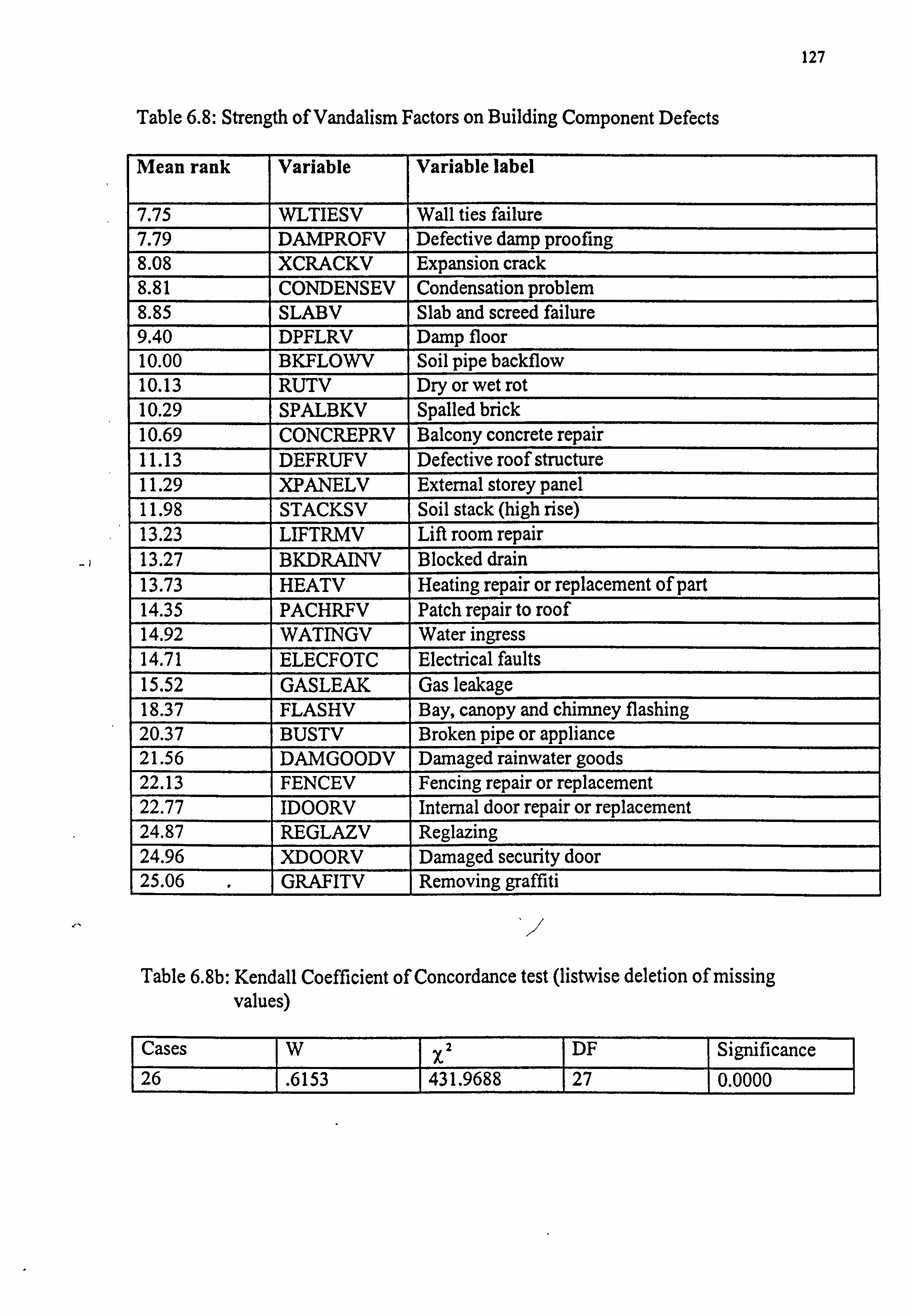
127
Table 6.8: Strength of Vandalism Factors on Building Component Defects
Mean rank Variable Variable label
7.75 WLTIESV Wall ties failure 7.79 DAMPROFV Defective damp proofing 8.08 XCRACKV Expansion crack 8.81 CONDENSEV Condensation problem 8.85 SLABV Slab and screed failure 9.40 DPFLRV Damp floor 10.00 BKFLOWV Soil pipe backflow 10.13 RUTV Dry or wet rot 10.29 SPALBKV Spalled brick 10.69 CONCREPRV Balcony concrete repair 11.13 DEFRUFV Defective roof structure 11.29 XPANELV External storey panel 11.98 STACKSV Soil stack (high rise) 13.23 LIFTRMV Lift room repair 13.27 BKDRAINV Blocked drain 13.73 HEATV Heating repair or replacement of part 14.35 PACHRFV Patch repair to roof 14.92 WATINGV Water ingress 14.71 ELECFOTC Electrical faults 15.52 GASLEAK Gas leakage 18.37 FLASHV Bay, canopy and chimney flashing 20.37 BUSTV Broken pipe or appliance 21.56 DAMGOODV Damaged rainwater goods 22.13 FENCEV Fencing repair or replacement 22.77 IDOORV Internal door repair or replacement 24.87 REGLAZV Reglazing 24.96 XDOORV Damaged security door 25.06 GRAFITV Removing graffiti
/
Table 6.8b: Kendall Coefficient of Concordance test (listwise deletion of missing values)
Cases wx2 DF Significance 26 . 6153 431.9688 27 0.0000
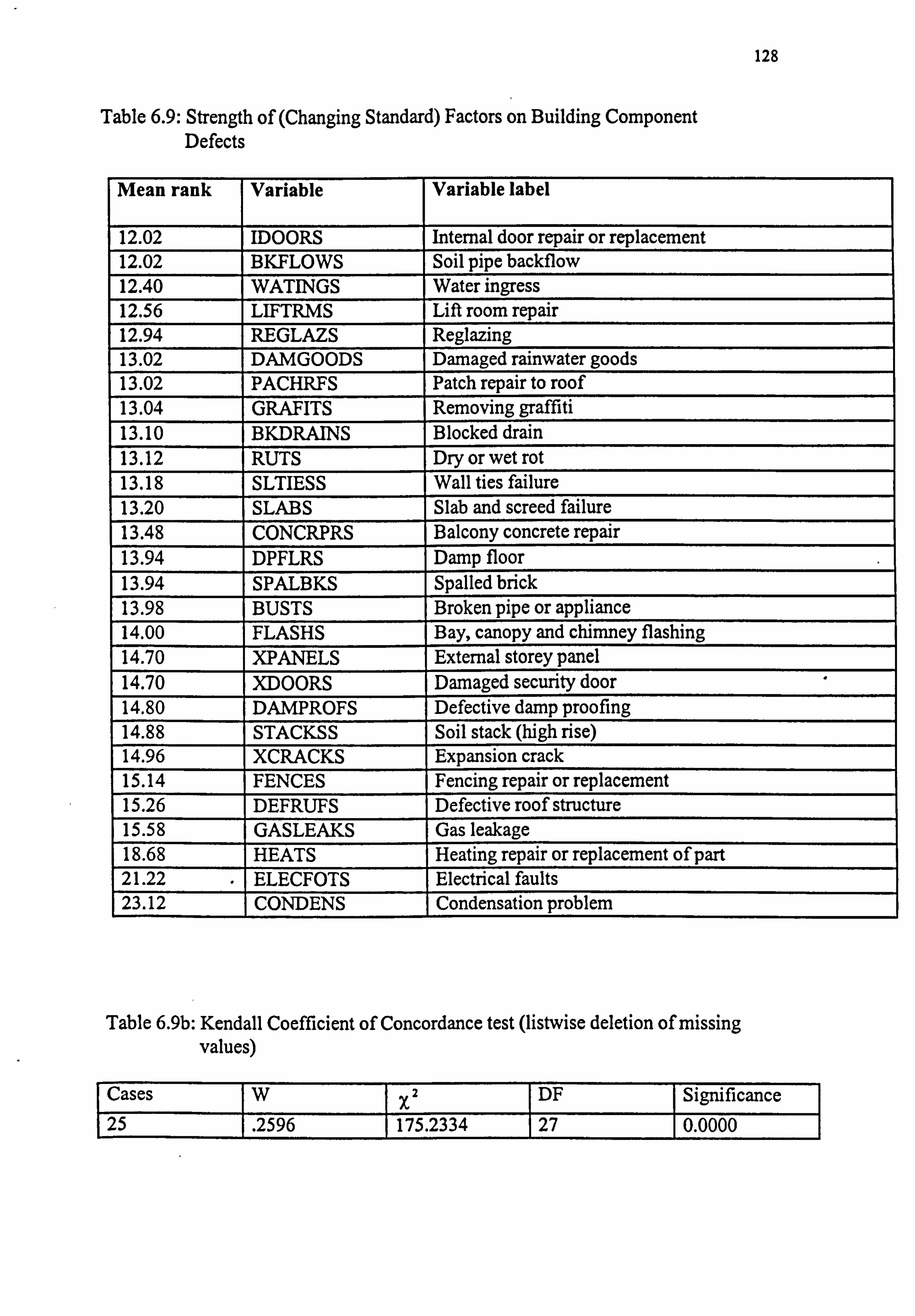
128
Table 6.9: Strength of (Changing Standard) Factors on Building Component Defects
Mean rank Variable Variable label
12.02 IDOORS Internal door repair or replacement 12.02 BKFLOWS Soil pipe backflow 12.40 WATINGS Water ingress 12.56 LIFTRMS Lift room repair 12.94 REGLAZS Reglazing 13.02 DAMGOODS Damaged rainwater goods 13.02 PACHRFS Patch repair to roof 13.04 GRAFITS Removing graffiti 13.10 BKDRAINS Blocked drain 13.12 RUTS Dry or wet rot 13.18 SLTIESS Wall ties failure 13.20 SLABS Slab and screed failure 13.48 CONCRPRS Balcony concrete repair 13.94 DPFLRS Damp floor 13.94 SPALBKS Spalled brick 13.98 BUSTS Broken pipe or appliance 14.00 FLASHS Bay, canopy and chimney flashing 14.70 XPANELS External storey panel 14.70 XDOORS Damaged security door 14.80 DAMPROFS Defective damp proofing 14.88 STACKSS Soil stack (high rise) 14.96 XCRACKS Expansion crack 15.14 FENCES Fencing repair or replacement 15.26 DEFRUFS Defective roof structure 15.58 GASLEAKS Gasleakage 18.68 HEATS Heating repair or replacement of part 21.22 . ELECFOTS Electrical faults 23.12 CONDENS Condensation problem
Table 6.9b: Kendall Coefficient of Concordance test (listwise deletion of missing values)
Cases w xz DF Significance 25 . 2596 175.2334 27 0.0000
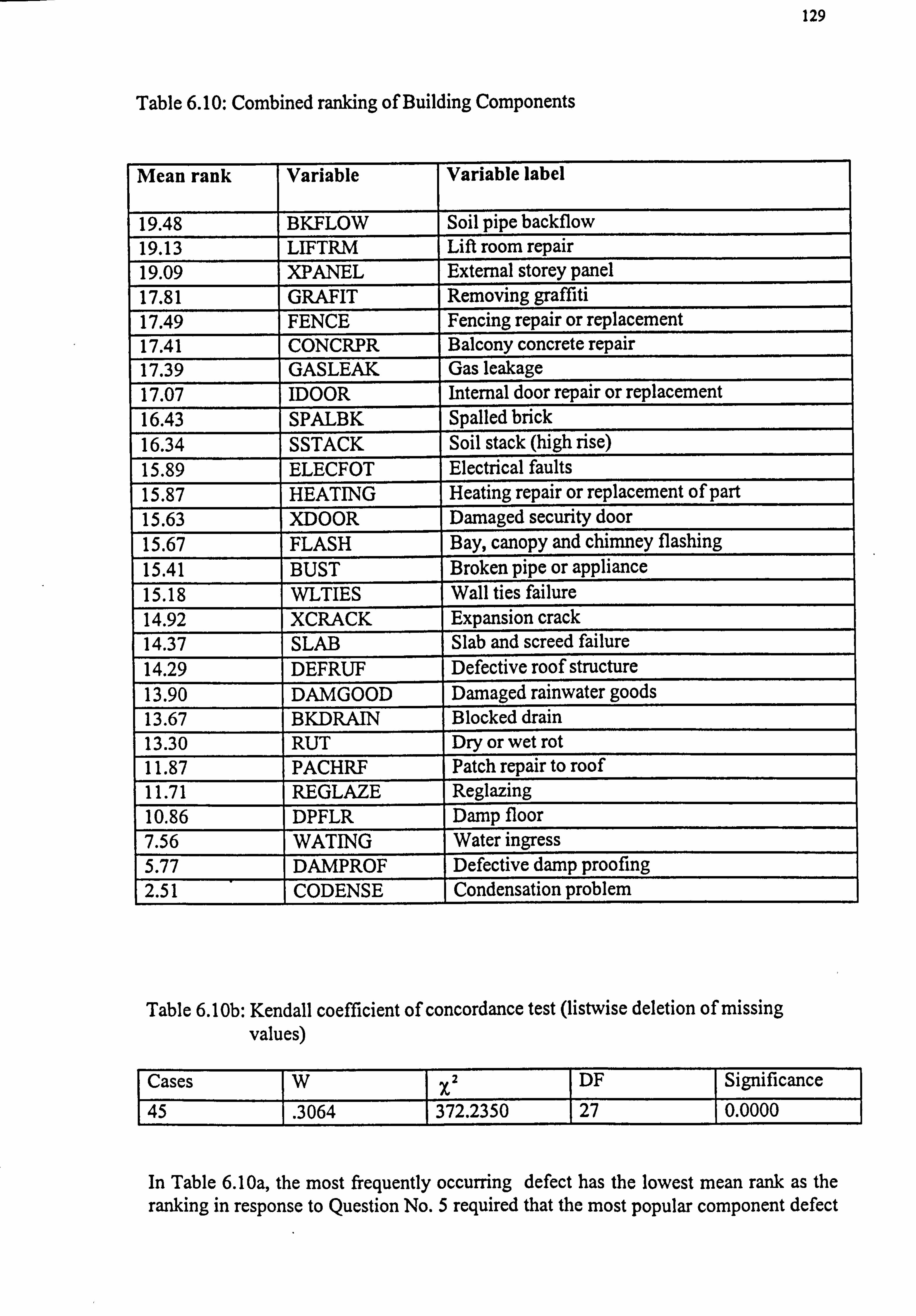
129
Table 6.10: Combined ranking of Building Components
Mean rank Variable Variable label
19.48 BKFLOW Soil pipe backflow 19.13 LIFTRM Lift room repair 19.09 XPANEL External storey panel 17.81 GRAFIT Removing graffiti 17.49 FENCE Fencing repair or replacement 17.41 CONCRPR Balcony concrete repair 17.39 GASLEAK Gas leakage 17.07 IDOOR Internal door repair or replacement 16.43 SPALBK Spalled brick 16.34 SSTACK Soil stack (high rise) 15.89 ELECFOT Electrical faults 15.87 HEATING Heating repair or replacement of part 15.63 XDOOR Damaged security door 15.67 FLASH Bay, canopy and chimney flashing 15.41 BUST Broken pipe or appliance 15.18 WLTIES Wall ties failure 14.92 XCRACK Expansion crack 14.37 SLAB Slab and screed failure 14.29 DEFRUF Defective roof structure 13.90 DAMGOOD Damaged rainwater goods 13.67 BKDRAIN Blocked drain 13.30 RUT Dry or wet rot 11.87 PACHRF Patch repair to roof 11.71 REGLAZE Reglazing 10.86 DPFLR Damp floor 7.56 WATING Water ingress 5.77 DAMPROF Defective damp proofing 2.51 CODENSE Condensation problem
Table 6.10b: Kendall coefficient of concordance test (listwise deletion of missing values)
Cases w xz DF Significance
45 . 3064 372.2350 27 0.0000
In Table 6.10a, the most frequently occurring defect has the lowest mean rank as the ranking in response to Question No. 5 required that the most popular component defect
130
is ranked 1 and the next, 2 and so on. This explains the observed disparity between this Table and the preceding Tables.
6.9.1 Criterion Impact on Building Component Defects
6.9.1.1 Design Factors
Tables 6.5 and 6.5b show the results of the building surveyors' responses to the scoring
of design influence on components. The five most affected components as a result of design faults appear to be `wall cracks' (including superficial and structural), dampness
in solid floor, condensation, slab failure and rot problems (which include wet and dry
rot).
Design generally has not only to do with building or housing morphology, but equally
with specification and construction methods. Cracks to walls are most frequent over
windows and doors (ranging from severe to hairline cracks), where there is failure of lintel. Damp floor is often associated with solid floors, frequently used in ground floor
back room and kitchen. In such instances, a case for misplaced design choices is
inferred. It is not unusual to find cases where damp proof membranes to solid floors
have failed, or even not been provided.
The problem of condensation is very much connected with overall climatic condition of the country. This necessitates the use of forms of housing designs which limit the
amount of air movements that can be allowed within the dwelling within comfort level
limits. This places unhealthy limits on window designer's provision for vents in
window units. Unfortunately this is rarely matched by the provision of the required
supplementary extract system to keep air changes within the internal environment at an
ambient level.
Slab failure, as with damp floor problems, is common with solid concrete floor. The
causes of failure may range from serious structural movement in the ground to inadequately protected services directly beneath the floor screed. Rusting of electric pipes have been known to result in swellings which cause the floor screed to crack up.
131
Wet rot is a more common problem than its counterpart dry rot. This finds its root in
dampness causing situations in the building, and has much to do with use rather than
design.
The implication of these observations is that the impact of design faults is most
poignantly revealed on these five components namely; wall cracks, dampness in solid
floor, condensation, slab failure and rot problems. If any of these components under
perform, the solution would most likely be found in the examination of the nature of
design and possible faults inherent in the design, or a combination of criteria which
consists of design criterion.
The five least affected components as a result of design faults are internal doors,
reglazing, gas leakage, security door and broken pipe or appliance. It is noteworthy
that none of these five relate to the actual fabric of the building, but all relate to fittings
of some kind to the main frame of the building. This leads one to suggest that design
improvement on housing should focus more on building frame and its morphology
rather than on fittings and fixtures.
6.9.1.2 Age Factors
Tables 6.6 and 6.6b show the results of the building surveyors' responses to the scoring
of age influence on components. The five most affected building components due to
age are minor damages to roof requiring patching up, wall tie failure, flashing
problems, 'electrical faults and concrete spalling. The inclusion of defective roof
patches and electrical faults in the top five components explains the rationale for the
commonness of wholesale electrical rewiring and roof renewal works on a number of
council dwellings. The observation constitutes a sound basis for preventative
programme works on each of these five components as a result of age. In other words,
re-roofing, wall tie replacement, flashing renewal, electrical re-wiring and general
concrete repairs should constitute priority preventative programme works on the
sampled dwellings. Such programmes should be decided on account of age and
estimated failure time of the components concerned.
132
The five least ̀ age vulnerable' components are graffiti related damage, broken panes,
condensation, backflow problems and Cracks to walls. It is surprising that `cracks to
walls' is one of these five components. Ordinarily, one would have posited that age
should be a strong factor in the `cracks to walls' defect (see section 6.10.7). It is
pertinent, however, to comment that there is nothing conclusive at this stage about this
observation, until the strength or weakness of each criterion in relation to the other four
criteria is established.
6.9.1.3 Construction Factors
Tables 6.7 and 6.7b show the results of the building surveyors' responses to the scoring
of construction influence on components. The five most influenced components as a
result of construction are rot (dry or wet), slab failure, dampness in solid floor, water in-
gress and damp proofing to wall. It is noteworthy that the first three of this list,
namely; rot, dampness in solid floor and damp proofing to wall are shared in common
with design criterion influence. It is therefore not out of place to propose a tentative
hypothesis that construction and design influences are reasonably correlated. This is
not surprising, as design invariably determines construction.
The five least `construction vulnerable' components appear to be graffiti related
damage, electrical faults, broken panes, internal door damages and burst pipes. The
inclusion of electrical faults in this list is interesting. This is not far fetched, as
installation of electrical works is regulated by a regulatory body, and is expected to pass
the required test on installation before use. Obviously, graffiti has nothing to do with
the quality of construction, and therefore not surprising that it tops this list. Glazing
works, internal door, and plumbing works are generally simple and straight forward
activities in a dwelling and therefore operatives are least likely to make mistakes in
installations.
As with the top five, the bottom five also share internal door damages, broken panes
and bust pipe with design criterion. This can be attributed to the twin relationship that
exists between design and construction. It is however note worthy that whilst graffiti is
133
the lowest item under construction influence, the same is not the case in design, thus
confirming that the two criteria are not completely interchangeable.
6.9.1.4 Vandalism Factors
Table 6.8 and 6.8b show the results of the building surveyors' responses to the scoring
of vandalism influence on components. The five most influenced components as a
result of vandalism are graffiti, damage to external door, broken pane, internal door
damage and damaged fence. This is not surprising as it is expected that the items of
prime importance under this criterion should be those external to the building fabric.
According to Armstrong and Wilson (1973) for instance, vandalism is commonly
believed to be external to the building. With internal door damage coming up in the
list, the suggestions (see chapter 4) that there could be a vandal within the building
itself is confirmed. This supports the notion that wilful damage on the part of the tenant
or his dependent is considered to mean vandalism by the surveyors in this sample
(Olubodun and Mole, 1996). Following from this finding, housing managers, in
planning for maintenance work should allow for vandalism budget variance on graffiti,
external door, glazing works, fencing and internal doors.
The five least `vandalism vulnerable' components are wall tie failure, damp proof failure, cracks to walls, condensation problem and concrete slab failure. The inclusion
of condensation problem on this list fails to support Olubodun and Mole's (1996)
notion that wilful neglect is tantamount to vandalism. It is common knowledge that
whilst there may be several factors at play in condensation, wilful neglect is far from
being an unimportant factor. It is however pre-mature to draw final conclusion on the
importance of vandalism in condensation until the overall strength or weakness of
vandalism in relation to the other criterion is known (see section 6.11.7).
134
6.9.1.5 Changing standard Factors
Table 6.9 and 6.9b show the results of the building surveyors' responses to the scoring
of changing standard influence on components. The five most influenced components
as a result of changing standard are condensation, electrical faults, heating failure,
gasleaks and defective roof structure. It is not surprising that electrical faults, heating
failure and gasleaks are symbols of improvement on a dwelling. A dwelling without
gas supply, heating and comprehensive rewiring work done on it, is anything but
modernised. As is expected, the effect of `modernisation' on an otherwise `old'
dwelling unit is condensation, which in this case tops the list.
The five least changing standard vulnerable components are internal door, backflow in
pipes, water ingress, lifts and glazing panes. The fact that glazing panes is included in
the bottom list reveals that respondents do not consider programmed work requiring
wholesale reglazing or window replacement not precipitated by immediate repair needs
as part of repairs or maintenance work in a true sense. This position accords with Mole
and Olubodun's (1995a) position which suggested that maintenance is widened to
include some aspects of programmed works of refurbishment and improvement.
6.9.2 Interpretation of Results
It can be seen from the concordance tests results in Tables 6.5b 6.6b, 6.7b, 6.8b, and
6.9b that the five coefficients of concordance are very highly significant. The low
probability in all the cases associated with the observed value of W enables us to reject
the null hypothesis in favour of the alternative hypothesis H,. In essence, surveyors in
the study sample were in agreement in assessing the strength of each of design,
construction, age, changing standard and vandalism as a causative factor for defects on
building components.
Given this general agreement, the study proceeded to establish the level of importance
of the five criteria, and of defects caused on building components. In seeking to
achieve the former objective, it was intended to establish from the combined scoring of the surveyors which of the causative factors presented was held to be the most
s 135
influential, which the second, which the third, etc. on overall defects/repair generation.
On first hand examination, it may be thought that this could be achieved by simply
summing up the scores on each factor column by the 45 building surveyors as
suggested by Mole and Olubodun (1995b). To do so will be fatuous as their model for
assessing criteria's importance presumes that all components are of equal weights of
occurrence. This is certainly not the case as evident by respondents' ranking in
response to question No. 5 (which asked respondents to rank all the 28 component
according to the frequency of defect on a general basis without isolating any one
criterion). As Table 6.10 shows, the building surveyors are significantly agreed in their
judgement.
Tables 6.5,6.6,6.7,6.8 and 6.9 reveal that the impact of each of the criteria, namely;
design, age, construction, changing standard and vandalism on a dwelling building can
be assessed on individual components rather than on the building as a whole.
Furthermore, the impact of individual criterion can be evaluated on identifiable
components on which such impact is strongest. Therefore, given certain defects in a
component, it becomes easier for building surveyors to begin the identification process
for the cause by the elimination of unlikely causes. For example, as in Table 6.7, damp
proof failure to wall is most likely to have its cause in bad construction which may have
been precipitated by damp proof course bridging. Similarly, damp floor problem (see
Tables 6.5 and 6.7) should require that design and construction would be the most
likely candidates for examination in order to identify the cause of such defect.
Table 6.10 shows the generalised consensual ordering of component defects. In
assessing overall maintenance requirements, building surveyors are generally of the
opinion that the five most important component defects are condensation, defective
damp proofing, water ingress, damp floors and broken panes.
The five least important component defects are soil pipe backflow, lift room repair,
external storey panels, graffiti and balcony concrete repairs. These components seem to
be restricted to certain class of housing construction typology rather than being
common to all typologies. Hence the need to proceed with further analysis to detect
any underlying patterns in component defects and causative criteria.
136
6.10 Relationships Between the Five Defect Criteria
1. Null Hypothesis: Technical knowledge possessed by building surveyors, of the
building is the most important ingredient in tracking down
maintenance in housing properties.
Alternative Hypothesis: Technical knowledge possessed by building surveyors, of
the building is not the most important ingredient in
tracking down maintenance in housing properties.
2. Null Hypothesis: Of the five factors identified, none is more important than
others for the prediction of housing maintenance requirements.
Alternative Hypothesis:
6.10.1 Generating the data
Of the five factors identified, some are more important
than others for the prediction of housing maintenance
requirements.
The original data collected with the help of the questionnaire were primarily based on
the Likert-type ordinal scaling method (Champion 1981; Black and Champion 1976).
In seeking to convert a lower order level data on ordinal scale to a higher order level
data on interval scale, it is certain that the resulting scores follow the order of the
original ordinal scores in magnitude (Reynolds, 1977). The most highly ranked attains
the highest interval score (representing the frequency of defect occurrence on a given
component as a result of the influence of an identified causative factor). What is not
certain is the extent to which a component ranked 1 is more frequent than 2, and 2 more
than 3, etc. In the final analysis, the case would be that we are arrogating constancy to
the difference between succeeding scores, which to a theoretical rather than practical
extent, is being corrected for by the transformation;
137
100In(30 - Rank).
Various transformation techniques that can be applied to the original data have been
identified by Yule and Kendall (1950). A necessary and important condition for the
regression model is `linearity'. Norusis (1990) noted that a commonly used
transformation to convert an otherwise non-linear variable to a linear one is the natural
logarithmic technique.
The criterion (30 - Rank) corrects for scoring the most frequent at 1, the second most
frequent at 2, etc. The constant 30 within the criterion was chosen to exceed the
maximum score by 2 points. The choice of two was to ensure that the resulting
transformation could not be zero. The multiplier, `100' is used to avoid handling
figures which are numerically too small to manage, without affecting the outcome of
the result either way.
The final criterion index developed from the original ranks is a form of weighted index
as it recognises building components which are believed to be more frequently
occurring than others in terms of defects along different lines of causation.
In the face of existing poor record keeping (Bird, 1987) in the building maintenance field, this may prove to be an important improvement on defects records, where any is
available.
In practice, where records of defects are being kept as in the Direct Labour
Organisation (DLO) computer system, the causes of defects are never recorded, and
hence practically non-existent. The theoretical data arrived at, based upon a
questionnaire research instrument can therefore be described as an inaugural theoretical
technique for quantifying defect-cause phenomenon. Inasmuch as there can be said to
be an independent variable, it is one whose existence must be inferred from whatever
patterns may exist in the resultant data. It is the raison d'etre of the transformation
technique to make such inference credible. This construct serves a similar purpose to Spedding et al's (1995) priority index which they defined as a method of ranking
138
anticipated maintenance and repair. The essence of their ranking being that the
`application of common standards would reduce the subjective element that has
featured so largely in maintenance decisions'.
It is important to compare this theoretical model with actual data when the culture of
defect-cause data recording is in place. However, this will require that the surveyor's
training and practice guidelines specify that systematic diagnosis and prognosis of
defects are given equal priority.
6.10.2 Weakness of the technique
There is a fundamental dubiety belying the manipulated sample data, which in this case
are made up of building elements as cases. It is impossible to attribute independence to
the data set of each variable much in the same way that `observations from each
member of a class that share certain features in common' are not truly independent.
However, such artificiality is an unavoidable characteristic of statistical control in
contrast to true experimental control (Kinnear and Gray, 1994).
6.10.3 The Dependent and Independent Variables.
The independent variables in the analysis that follows are age, design, construction
(CONSTRUT), standard (STANDARDI) and vandalism (VANDAL! ). The value on
each variable was obtained by developing ranks in each of Tables 6.5,6.6,6.7,6.8 and 6.9, so that the maximum rank corresponded with the total number of building
components included in the survey. This value was then converted to interval scale by
the transformation 100In(30- Rank)(section 6.10.1).
The dependent variable is labelled GENRANKI, and it measures the overall intensity
of defects across components as perceived by building surveyors within the sample.
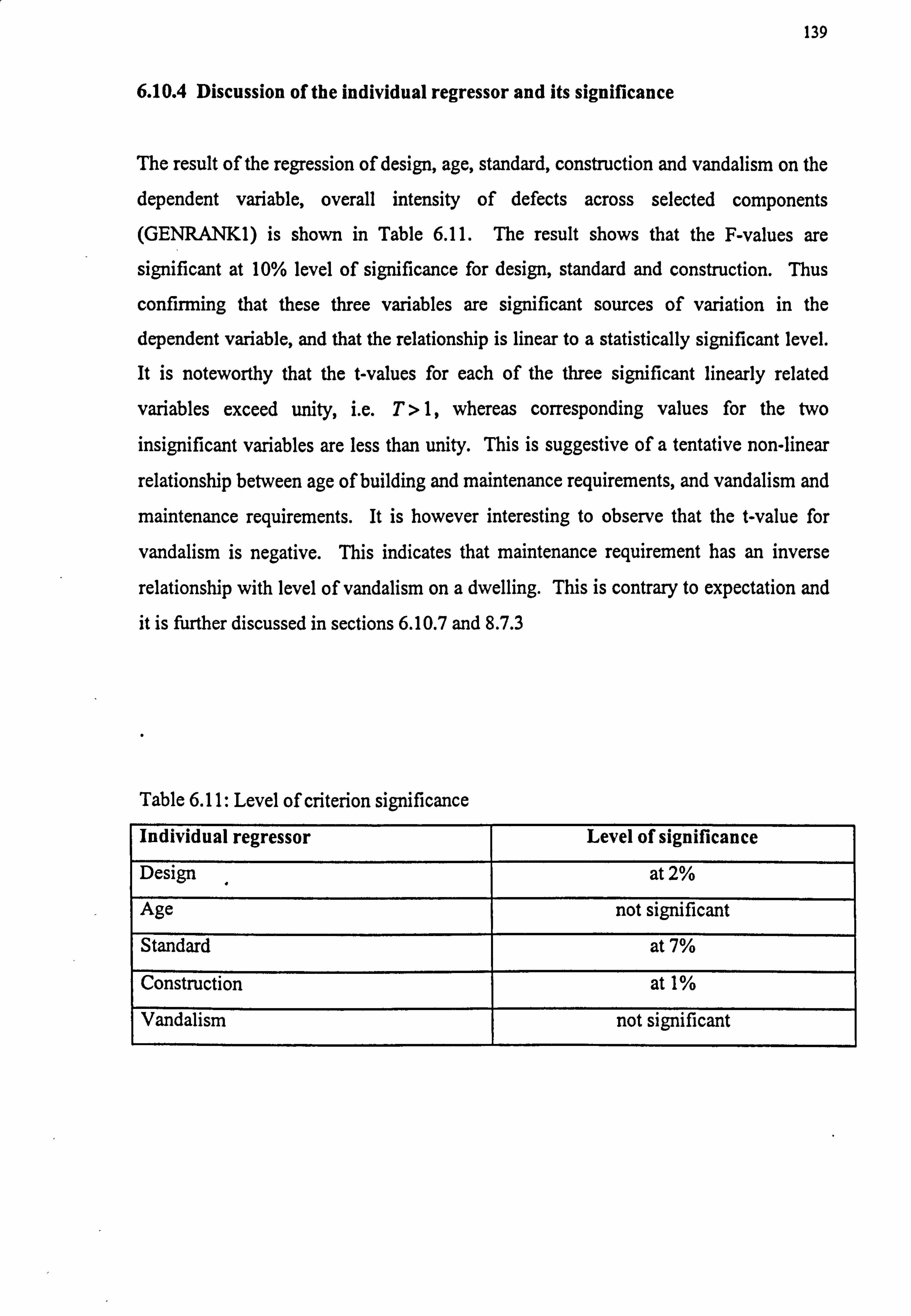
139
6.10.4 Discussion of the individual regressor and its significance
The result of the regression of design, age, standard, construction and vandalism on the
dependent variable, overall intensity of defects across selected components (GENRANKI) is shown in Table 6.11. The result shows that the F-values are
significant at 10% level of significance for design, standard and construction. Thus
confirming that these three variables are significant sources of variation in the
dependent variable, and that the relationship is linear to a statistically significant level.
It is noteworthy that the t-values for each of the three significant linearly related
variables exceed unity, i. e. T>1, whereas corresponding values for the two
insignificant variables are less than unity. This is suggestive of a tentative non-linear
relationship between age of building and maintenance requirements, and vandalism and
maintenance requirements. It is however interesting to observe that the t-value for
vandalism is negative. This indicates that maintenance requirement has an inverse
relationship with level of vandalism on a dwelling. This is contrary to expectation and it is further discussed in sections 6.10.7 and 8.7.3
Table 6.11: Level of criterion significance
Individual regressor Level of significance Design at 2%
Age not significant
Standard at 7%
Construction at 1%
Vandalism not significant
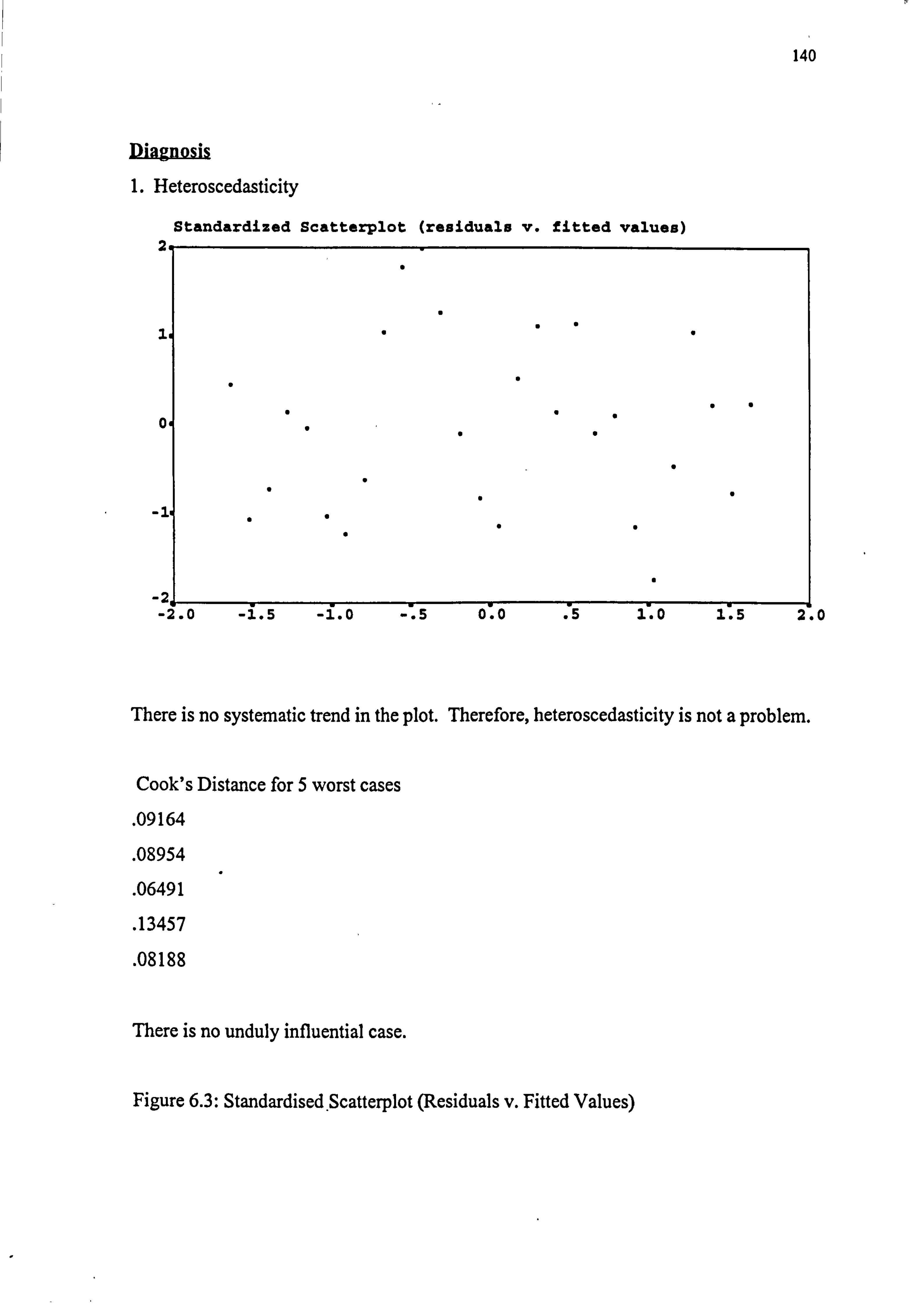
140
Diagnosis
1. Heteroscedasticity
Standardized Scatterplot (residuals v. fitted values)
0
0S
S
I
21 2.0 -1.5 -1.0 -. 5 0.0 .51.0 1.5 2,
There is no systematic trend in the plot. Therefore, heteroscedasticity is not a problem.
Cook's Distance for 5 worst cases
. 09164
. 08954
. 06491
. 13457
. 08188
There is no unduly influential case.
Figure 6.3: Standardised. Scatterplot (Residuals v. Fitted Values)
0
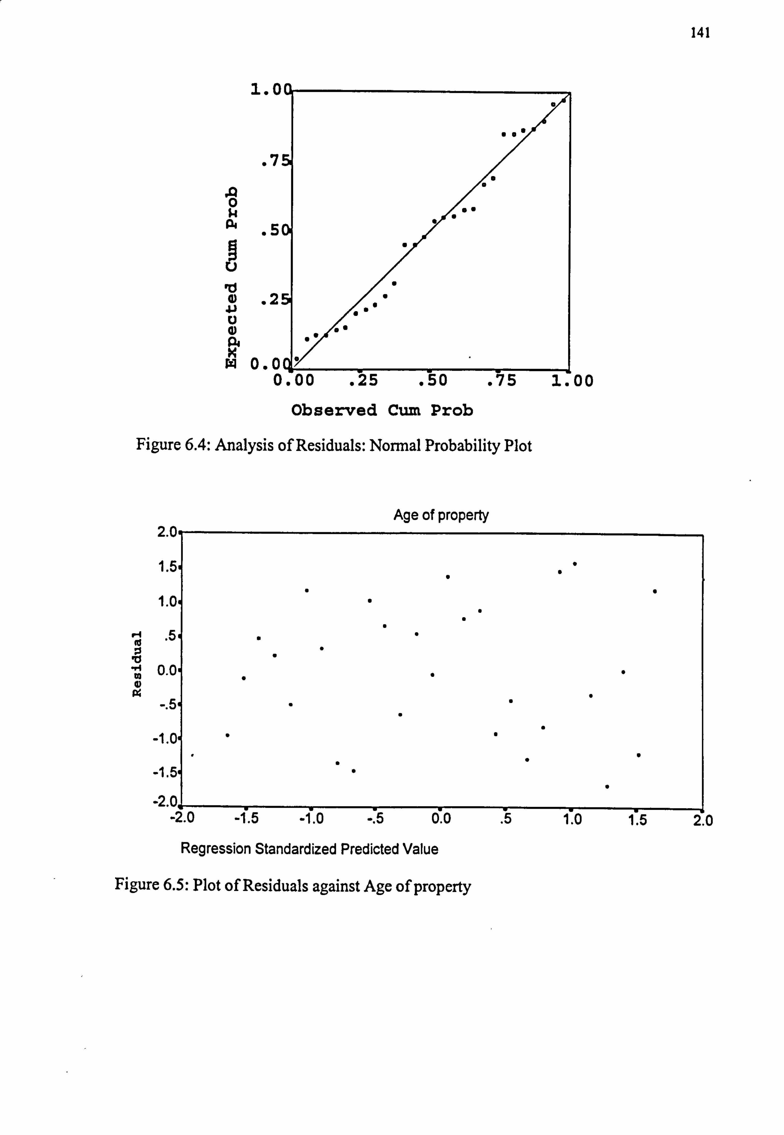
141
1.0
.7
0e
A 0
a5
o .2 4J U 0 P4 w 0.0
0
9
00 Observed Cum Prob
Figure 6.4: Analysis of Residuals: Normal Probability Plot
H
b
Regression Standardized Predicted Value
Figure 6.5: Plot of Residuals against Age of property
Age of property
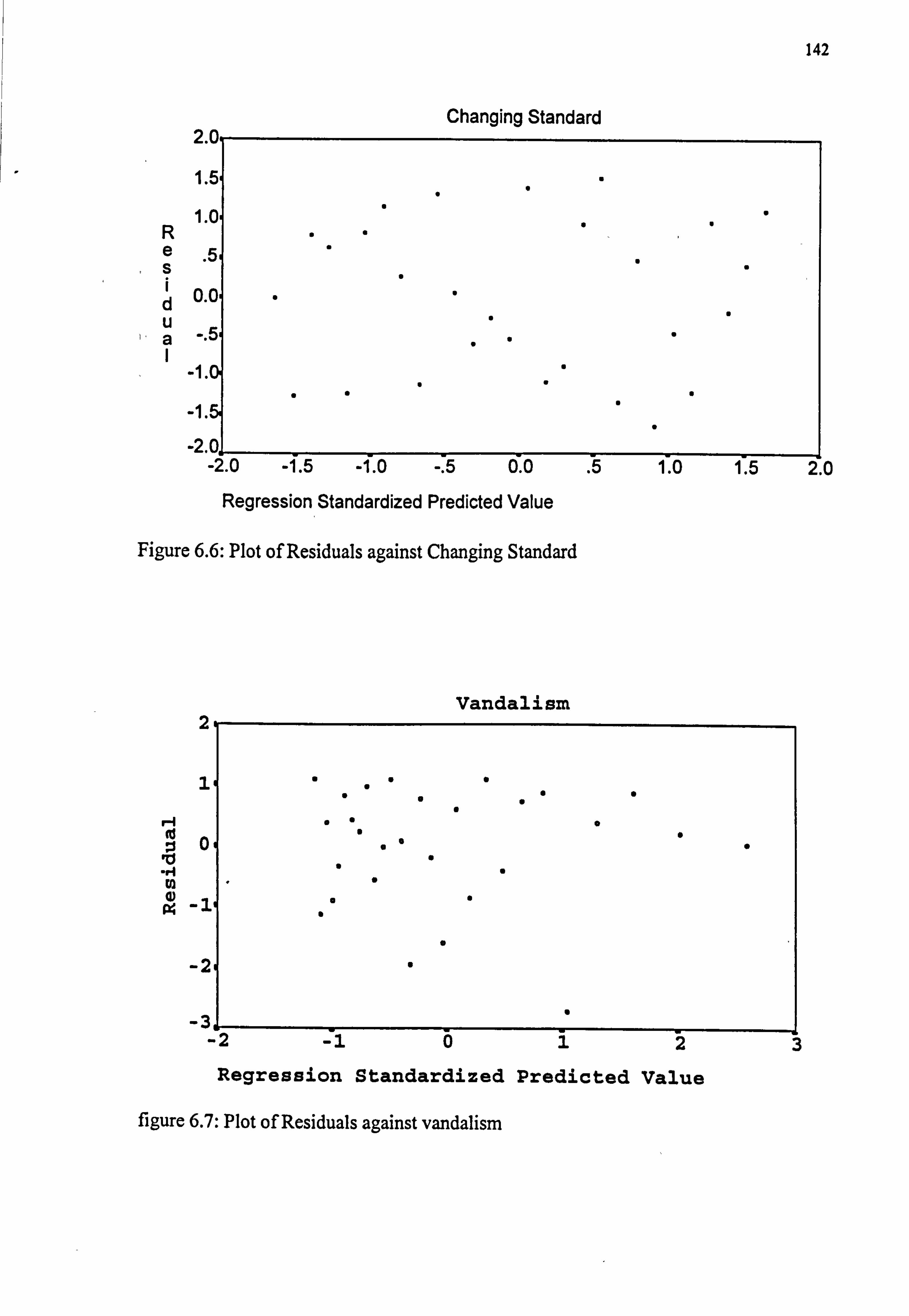
142
Changing Standard
R e s
d u a
-2.0 -1.5 -1.0 -. 5 0.0 .51.0 1.5 2.0
Regression Standardized Predicted Value
Figure 6.6: Plot of Residuals against Changing Standard
2
1
r-i ( b -. i
-1 P4
-2
Vandalism
. . . .
. . . . .
.
"" .
. °
.
. .
. .
"
.
.
"2 : 0 1 2 3
Regression Standardized Predicted Value
figure 6.7: Plot of Residuals against vandalism
143
6.10.5 Residuals Plotting
Figures 6.3 to 6.7 indicate the plotting of the standardized residual from the regression
analysis against the predictor variables (age, design, construction, standard and
vandalism, and dependent variable (overall intensity of defects across components). If
the assumptions of linearity and heteroscedasticity (homogeneity of variance) hold for
the data, it should show no pattern of relationship between the predicted and residual
values. Visual inspection of the figures shows that there is no pattern exhibited in the
plot of the residual values against the predicted values. Except for vandalism which
reveals that the variance of the residuals may decrease with increasing vandalism
measure. This confirms that the assumption of linearity and heteroscedasticity have
been met.
6.10.6 Normal Probability
The normal probability plot in Figure 6.4 shows the standardised residuals on the
vertical axis and the expected value (if the residuals were normally distributed) on the
horizontal axis. Simply put, normality is determined by how well the residuals lie
along a straight line along the diagonal.
It is expected that the residuals lie on a perfect straight line if the relationship between
the GENRANK1 (overall intensity of defect across components) and each of the five
independent variables DESIGN! (design), VANDAL! (vandalism), STANDRD I
(changing standard), CONSTRTI (construction) and AGE1 (age) is basically a straight
one. In each of the five cases, the condition of perfect normality is not confirmed. However, the departure from normality is not profound as to violate normality
condition (after Kinnear and Gray, 1994).
An examination of the F ratios for the five independent variables shows that only DESIGNI, CONSTRTI and STANDRDI are significantly linear with GENRANKI.
However it is expected that each of the five variables would bear an influence to a lesser or greater extent on the overall intensity of defect across components
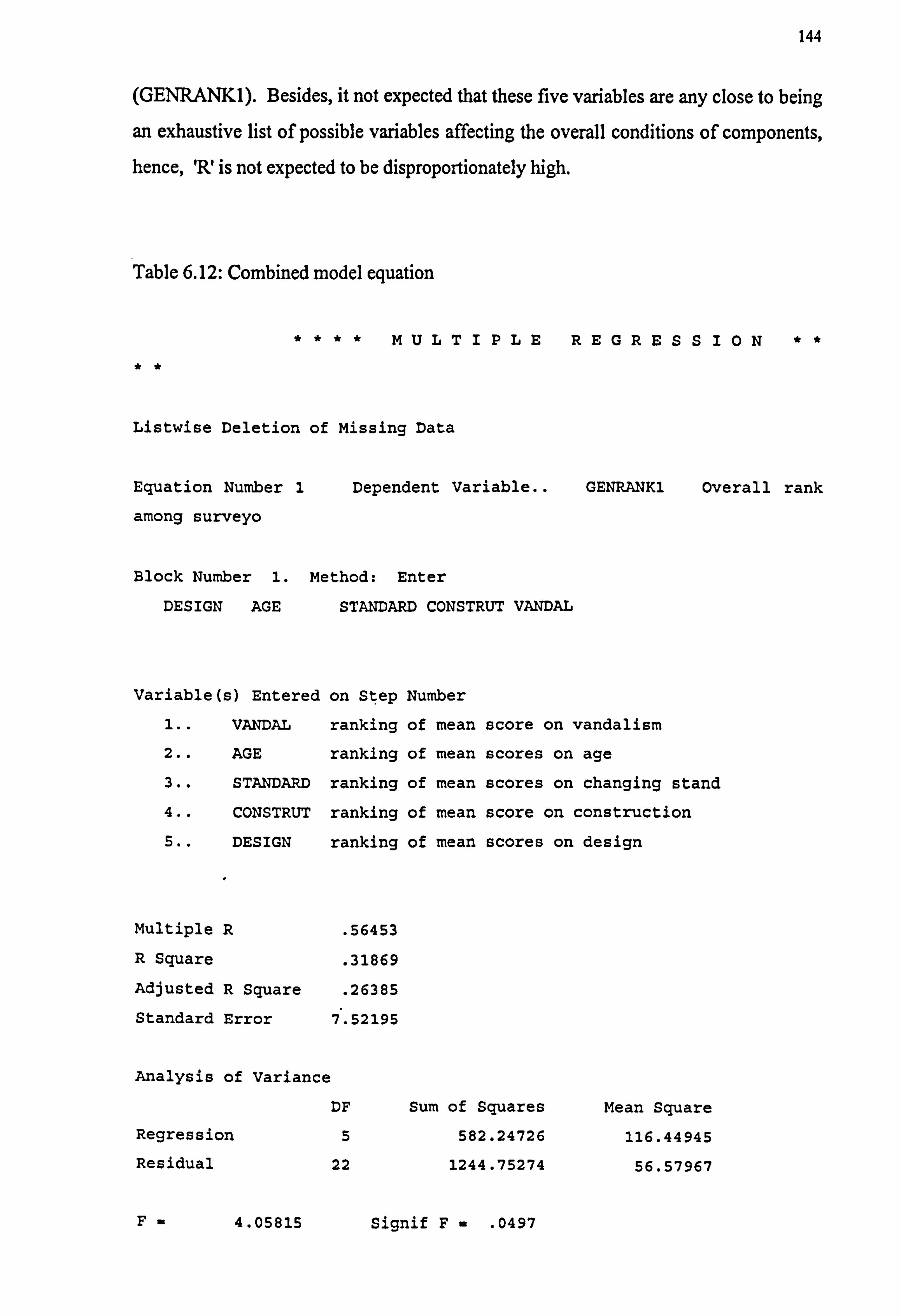
144
(GENRANK1). Besides, it not expected that these five variables are any close to being
an exhaustive list of possible variables affecting the overall conditions of components, hence, 'R' is not expected to be disproportionately high.
Table 6.12: Combined model equation
****MULTIPLEREGRESS10N **
**
Listwise Deletion of Missing Data
Equation Number 1 Dependent Variable.. GENRANK1 Overall rank
among surveyo
Block Number 1. Method: Enter
DESIGN AGE STANDARD CONSTRUT VANDAL
Variable(s) Entered on Step Number
l.. VANDAL ranking of mean score on vandalism
2.. AGE ranking of mean scores on age
3.. STANDARD ranking of mean scores on changing stand
4.. CONSTRUT ranking of mean score on construction
5.. DESIGN ranking of mean scores on design
Multiple R . 56453
R Square . 31869
Adjusted R Square . 26385
Standard Error 7.52195
Analysis of Variance
DF
Regression 5
Residual 22
Sum of Squares
582.24726
1244.75274
Mean Square
116.44945
56.57967
F=4.05815 Signif F= . 0497
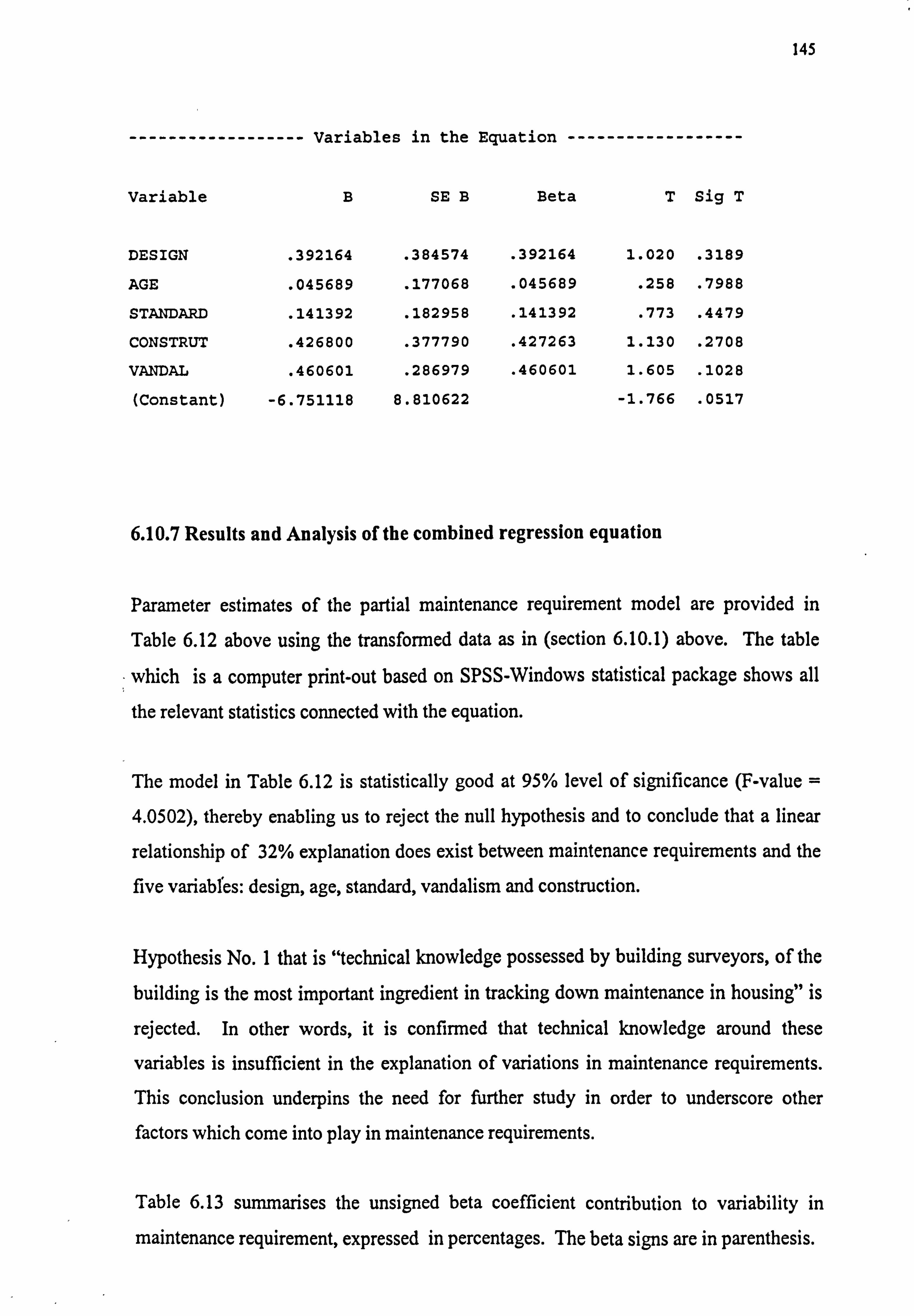
145
------------------ Variables in the Equation ------------------
Variable B SE B Beta T Sig T
DESIGN . 392164 . 384574 . 392164 1.020 . 3189
AGE . 045689 . 177068 . 045689 . 258 . 7988
STANDARD . 141392 . 182958 . 141392 . 773 . 4479
CONSTRUT . 426800 . 377790 . 427263 1.130 . 2708
VANDAL . 460601 . 286979 . 460601 1.605 . 1028
(Constant) -6.751118 8.810622 -1.766 . 0517
6.10.7 Results and Analysis of the combined regression equation
Parameter estimates of the partial maintenance requirement model are provided in
Table 6.12 above using the transformed data as in (section 6.10.1) above. The table
which is a computer print-out based on SPSS-Windows statistical package shows all
the relevant statistics connected with the equation.
The model in Table 6.12 is statistically good at 95% level of significance (F-value =
4.0502), thereby enabling us to reject the null hypothesis and to conclude that a linear
relationship of 32% explanation does exist between maintenance requirements and the
five variables: design, age, standard, vandalism and construction.
Hypothesis No. 1 that is "technical knowledge possessed by building surveyors, of the
building is the most important ingredient in tracking down maintenance in housing" is
rejected. In other words, it is confirmed that technical knowledge around these
variables is insufficient in the explanation of variations in maintenance requirements. This conclusion underpins the need for further study in order to underscore other factors which come into play in maintenance requirements.
Table 6.13 summarises the unsigned beta coefficient contribution to variability in
maintenance requirement, expressed in percentages. The beta signs are in parenthesis.
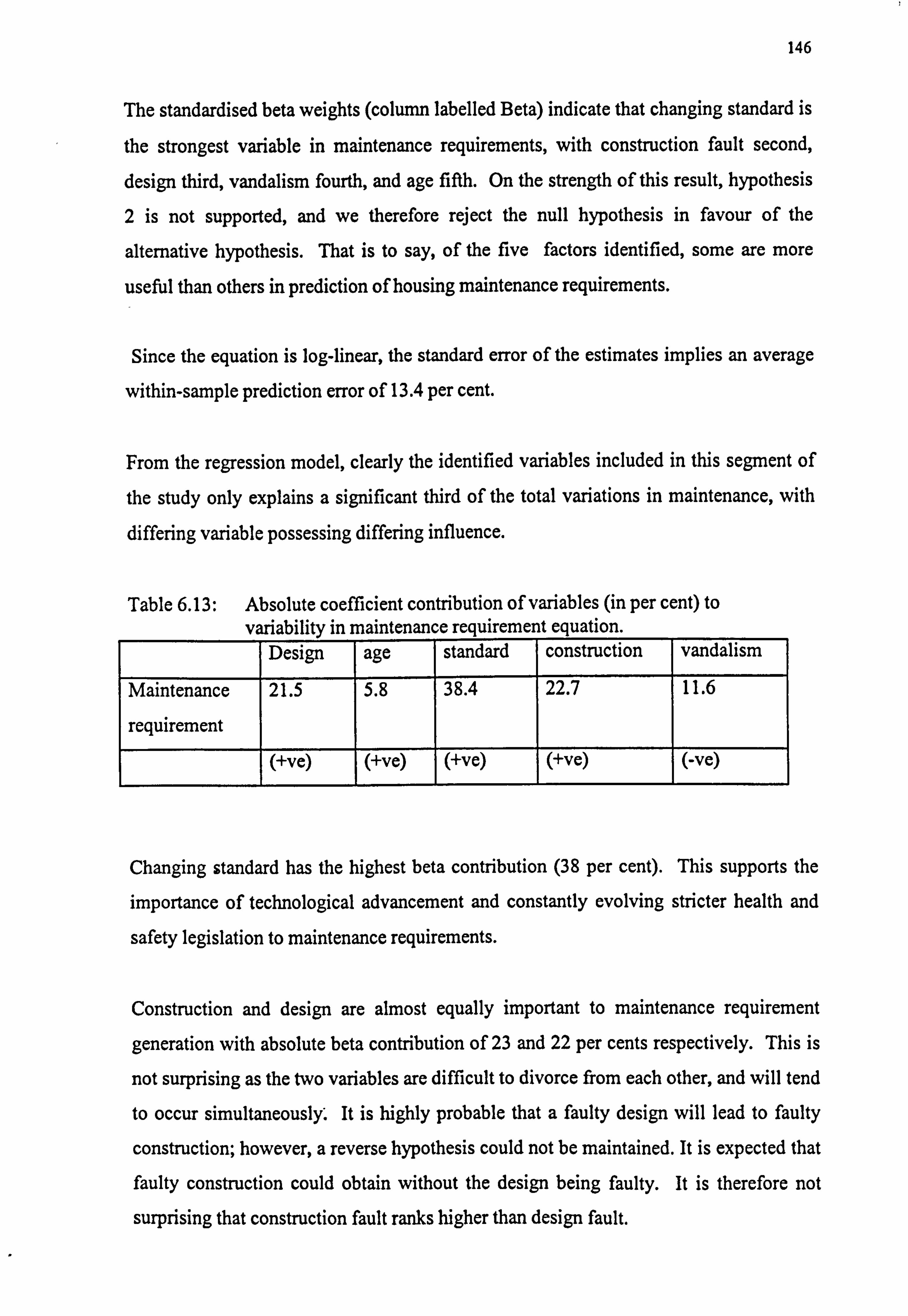
146
The standardised beta weights (column labelled Beta) indicate that changing standard is
the strongest variable in maintenance requirements, with construction fault second,
design third, vandalism fourth, and age fifth. On the strength of this result, hypothesis
2 is not supported, and we therefore reject the null hypothesis in favour of the
alternative hypothesis. That is to say, of the five factors identified, some are more
useful than others in prediction of housing maintenance requirements.
Since the equation is log-linear, the standard error of the estimates implies an average
within-sample prediction error of 13.4 per cent.
From the regression model, clearly the identified variables included in this segment of
the study only explains a significant third of the total variations in maintenance, with
differing variable possessing differing influence.
Table 6.13: Absolute coefficient contribution of variables (in per cent) to variability in maintenance requirement equation.
Design age standard construction vandalism
Maintenance
requirement
21.5 5.8 38.4 22.7 11.6
(+ve) (+ve) (+ve) (+ve) (-ve)
Changing standard has the highest beta contribution (38 per cent). This supports the
importance of technological advancement and constantly evolving stricter health and
safety legislation to maintenance requirements.
Construction and design are almost equally important to maintenance requirement
generation with absolute beta contribution of 23 and 22 per cents respectively. This is
not surprising as the two variables are difficult to divorce from each other, and will tend
to occur simultaneously. It is highly probable that a faulty design will lead to faulty
construction; however, a reverse hypothesis could not be maintained. It is expected that
faulty construction could obtain without the design being faulty. It is therefore not
surprising that construction fault ranks higher than design fault.
147
Age of dwelling has an unexpectedly low but positive correlation with maintenance
requirements. The beta coefficient contribution is under six per cent. This tends to
suggest that age is not a highly influential factor in maintenance requirement in the
housing stock within the sample, at least in relative terms. In this light, it is possible to
explain the unexpected low influence of age on `cracks to wall' defect in relation to the
other 21 components that precede it in importance. Because of the low contribution of
age criterion in relation to the other four criteria, the position is that the differences in
importance across all the components in Table 6.6 are not really as pronounced as
would have been the case with corresponding tables for criteria with higher beta
contribution. In any case, the inference drawn is that even the most important
components on age would not rank very highly in importance when a combined ranking
of components is carried out. This position is confirmed in Table 6.10 where none of
the five top most items on age (as in Table 6.6) feature in the top five most important
components on overall defect occurrence in Table 6.10.
Vandalism has an unexpectedly negative correlation with maintenance requirement.
The beta coefficient contribution is 12%. This may have two implications: (1) that
housing management team are less responsive to maintenance demands from socially deprived areas or households; and (2) that households in areas most vulnerable to
vandalism tend to care less for the condition of their dwellings, thus failing to report defects as and when they occur.
Vandalism is found to be the second lowest contributor to dwelling building object defect. Given that condensation problem is one of the five least affected components
on vandalism as causative factor, Olubodun and Moles' (1996) notion that wilful
neglect is tantamount to vandalism proves unsupported.
The ordering of the standardised beta weights as shown in Table 6.13 is supported by
consideration of the correlations between the dependent variable and each of these five
regressors: the correlation between GENRANK1 and design, age, standard,
construction and vandalism are 0.27,0.13,0.34,0.32 and -0.14 respectively as shown in Appendix 2A.
148
The extremely low tolerance for four of the five variables causes one to surmise that
multicollinearity is a problem with the regression model. The implications of this are
twofold: (1) it is possible in the presence of multicollinearity for a set of regressors
having no significant t-values to account for a significant variability in the dependent
variable; or (2) that there are intercorrelations between the regressors; which, in turn,
implies that defect occurrence on components are intercorrelated.
Whilst extremely low t-values are not desirable and suggest the possible existence of
multicolinearity, low tolerance does not distract from the integrity of the model
statistics. On the contrary, it suggests that further appraisal is required in order to fully
understand the extent of interactions between the independent variables.
6.11 Conclusion
This chapter has shown that components defects can be ordered according to frequency
of occurrence and hence prioritised for maintenance purpose.
Section One of the analysis demonstrates the reliability of the data upon which the
analyses are based by confirming the alternative hypothesis with significant coefficient
of concordance on everyone of the five criterion levels. In this segment of the analyses,
it was further demonstrated that different building components respond to varying
extent to different identifiable defect causing criteria, namely; age, construction, design,
standard and vandalism. Thus, in order to determine the effect of any of these criteria
on a dwelling building, attention should be focused on the most important components
on the criteria of interest. Table 6.14 shows the important component defects which
serve as strong indicators of the influence of each of the criteria, namely; age,
vandalism, design, construction, and changing standard in ascending order of
contribution to overall defect occurrence.
149
Table 6.14: Component Defect indicators for the five Defect Criteria
Defect-Cause Criteria Indicative component
Age Patch repair to roof; Wall ties failure; Bay, canopy and
chimney flashing; Electrical faults; Balcony concrete repair
Vandalism Removing graffiti; Damaged security door; Reglazing;
Internal door repair or replacement; Fencing repair or
replacement Design Expansion crack; Damp floor; Condensation problem; Slab
and screed failure; Dry or wet rot
Construction Dry or wet rot; Slab and screed failure; Damp floor; Water
ingress; Defective damp proofing
Changing Standard Condensation problem; Electrical faults; Heating repair or
replacement of part; Gas leakage; Defective roof structure
Section Two of the analysis sought to quantify the impact of these five criteria. To this
end, the analysis conclusively revealed that these five criteria are not exhaustive of all
the factors at play. To the extent that these five criteria influence maintenance
requirements, changing standard is the most influential at 38 per cent contribution,
followed by construction and design factors at 23 and 22 per cents, followed by
vandalism at 12 per cent, whilst age is least influential in terms of magnitude at only 6
per cent.
These findings support the rejection of the first two null hypotheses in favour of the
alternative hypotheses. That is to say;
1. "Technical knowledge possessed by building surveyors, of the building is the most
important ingredient in tracking down maintenance in housing properties" is
rejected. And the alternative hypothesis that "Technical knowledge possessed by
building surveyors, of the building is not the most important ingredient in tracking
down maintenance in housing properties" is accepted.
2. "Of the five factors identified, none is more important than others for the prediction
of housing maintenance requirements" is rejected. And the alternative hypothesis
that "Of the five factors identified, some are more important than others for the
prediction of housing maintenance requirements" is accepted.
150
From the regression analysis conducted, the explanation of variations in housing
maintenance requirements of the stock being studied (as a result of the features of the
building object) remains largely inconclusive because of the insignificance of four of
the five t-values. This calls for a further analysis. It requires that an attempt is made to
identify which (component-defects) are statistically correlated. In other words, to
identify which components are distinct and are principally influenced together by
common criterion. This forms the basis for the next chapter which sets out to proffer
answers to Hypothesis D(i) which states that "There are no intercorrelations between
the component defects, i. e. it is not plausible to localise defect causing factors to a
group of components" and its alternative.
151
CHAPTER 7
COMPONENTS DEFECTS ANALYSIS
7.1 Objective
This chapter deals with the fourth set of hypotheses set out in chapter Six, and which
emanated from questions raised about intercorrelations between defect-cause criteria in
the exploration of the third set of hypothesis (see section 6.3).
The analysis set out in this chapter is intended to explore and detect underlying
relationships among the defect-cause criteria namely; age, vandalism, design,
construction and changing standard, following from the generally low tolerance values
suggestive of the existence of intercorrelations between the criteria. Whilst these
principal defect-cause criteria are identifiable and known to the sample building
surveyors, the way these factors impact on component defects is through a combination
of different facets of the known criteria as revealed by the existence of intercorrelations
between the five criteria. A multi-variate statistical technique known as factor analysis
is chosen as the method of attempting to group the variables into clusters or
components with the help of SPSS/PC Factor Analysis Software programme.
7.2 Statement of Hypothesis to be tested
D(i) Null Hypothesis (Ho ): There is no intercorrelations between the component defects i. e. it is not plausible to localise defect causing factors to a group of
components.
D(ii) Alternative Hypothesis (H, ) : There are intercorrelations between the
components defects
152
7.3 Final Analysis of Building Surveyors Survey Data
The inclusiveness of the foregoing chapter on the regression analysis calls for further
analysis to identify which component-defects are statistically correlated. This will identify which components are distinct and principally influenced together by common
criteria. It is common knowledge among factor statisticians Kim and Muller (1978a
and 1987b), Tabachnick and Fidell (1989) and Kinnear and Gray (1994) that the
property of multicollinearity is highly undesirable for factor analysis. For the data
being dealt with, it should be noted that the identifiable multicollinearity in the linear
regression analysis which predicated the employment of factor analysis technique is
not, in this case, a problem. This problem has been side-tracked with the use of the data
resulting from Question No. 5 (which asked respondents to rank the identified 28
building components according to how frequently defects show on them) in the
`surveyor questionnaire' instrument, which sought to score each of the 28 building
components as variables, and hence suited for this analysis technique.
Data reduction allows an investigator to ascertain and isolate group(s) of components
(on which defects occur) that are meaningfully related. This procedure should benefit
architects and surveyors who are involved in various forms of design. It should assist
them in evaluating groups of components prone to certain defect causes within the
ambit of the building as a technical product.
In this chapter building surveyors' understanding and decipheration of components' defects and causes are explored. The intention is to investigate how, and to what
extent, each of the identified causative maintenance need factors affects the various
components of a dwelling and to identify which groups of building components are
statistically co-related on factorial level. The essence is to break down and identify
underlying considerations (sub-factors) which govern each of the identified principal factors in the survey instrument.
Factor analysis produces an `orderly simplification' (Burt, 1940) and is helpful in
isolating sets of building components that are meaningfully related on an individual
causative factor level. In doing so, professionals involved in the evaluation of building
153
(dwelling) life cycle will be able to meaningfully evaluate the impact of `stream of
influences' at various stages of a building life on maintenance need. The fundamental
assumption of the technique is that it is possible to explain complex phenomena by
identifying underlying factors. In essence, the technique facilitates the identification of `not-directly-observable' factors based on a set of observable variables.
The technique of factor analysis used is described by Kinner and Gary (1994) as data
reduction technique. Data reduction, in the context of the present study, means
statistical identification of groups of building components which share similar response
attributes to certain `causative phenomena' which bear upon the building fabric.
According to Norusis (1985) it is used to identify a number of factors which represent
the relationships among interelated variables. To describe in the words of Child (1990),
`all fields of study aspiring to scientific status endeavour to describe, to formulate
generalisations and ultimately to make predictions from the data observed'. Factor
analysis is a well documented technique for describing data, and it has long been
accepted as a data reduction technique (Thurstone 1947; Marman 1967; Cattell and Dickman; 1962).
Starting with an array of correlation coefficients for a set of variables, the technique
enables a researcher to see whether some underlying pattern of relationships exist such
that the data may be re-arranged or reduced to a smaller set of components that may be
taken as source variables accounting for the observed interrelations in the data as
indicated with low T-values in the regression analysis of chapter Six (see Table 6.12).
The use and application of factor analysis as a statistical reduction technique hinges
upon the following two theorems as enunciated by Guilford and Fruchter (1978).
Theorem 1: The variance of a variable is a composite of three component variances. These components are; 1) that contributed by one or more common factors i. e. factors which appear in
more than one variable. 2) that unique to the variable itself and, 3) error variance.
154
The above theorem can be mathematically expressed for a given variable on all
identifiable factor as follows:
Vt2 = Va2 + Vb2 ...... + Vr2 + V,, 2 + Vene Eqn 7.1
Where Vt2 =total variance of a variable
V, 2, Vb2, ...... V, 2 =variances in common factors A, B, ...., R
V�2 =variance specific to the variable Vent =error variance
For all practical purposes, Norusis (1988) has suggested that the sum of the error
variance Vene, and variance specific to the variable V,, 2 i. e. (V, n2 + Vv2) are assumed to
be uncorrelated with each other and with the common factors.
Theorem 2: The second theorem of factor analysis is that the correlation between two
variables is equal to the sum of the cross product of their common-factor loadings.
In summing up the two theorems, the standardised variance of the ih variable can be
expressed as:
X; = Ai1F1 + A12F2 + ...... + A;, F1 + Standardised(Ven. 2+V v 2)
Where F'S äre the common factors, the A's are the constants which are used to combine the k factors, and Standardised(Ve. 2 + Vv2) is described by Norusis (1988) as a unique factor. The estimate for the jth common factor is obtained by the general expression;
FF=E1`Wj; X; =Wj1X1+Wj2X2+...... +WA
The W; 'S are the factor coefficients, and ̀ r' is the number of variables (Norusis, 1988).
Where each of the `r' observed variables is described linearly in terms of `r' new un-
correlated components X1, X2 , ...., X, , each of which is, in turn defined as a linear
combination of the ̀ r' original variables.
155
Kinnear and Gray (1994) have suggested that factors of factor analysis are statistical
realities, but psychological fictions. This opinion is predicated by the fundamental
assumption that mathematical factors represent latent variables, the nature of which can
only be guessed at by examining the nature of tests.
7.4 Defect Criterion data analysis
Twenty-eight variables that relate to the components of a dwelling unit have been listed
in Table 6.10. The first stage of the analysis was to produce a correlation matrix as
shown in Table 7.2 based on product moment correlation coefficients. The correlation
coefficients express the degree of linear relationship between the row and the columns
of the matrix.
Essentially, factor analysis provides information on how many factors are necessary to
achieve a reconstruction of the initial coefficient matrix that is sufficiently good to
account satisfactorily for the correlations it contains.
Three important criteria must be satisfied by a credible factor analysis ( after Overall
and Klett, 1972; and Egbu, 1994). These are: 1) parsimony 2) orthogonality and, 3) conceptual meaningfulness.
A credible factor analysis should be parsimonious, that is the number of factor one ends
up with should be considerably less than the number of variables one started with. Orthogonality requires that factors are independent, and distinguishable one from
another (Norusis, 1990); and of course, each factor must be conceptually meaningful
and capable of identification.
An important indicator of the strength of the relationship among variables is the partial
correlation coefficient. According to Norusis (1988), if variables share common factors, the partial correlation coefficients between pairs of variables should be close to
zero when the linear effects of the other variables are eliminated.
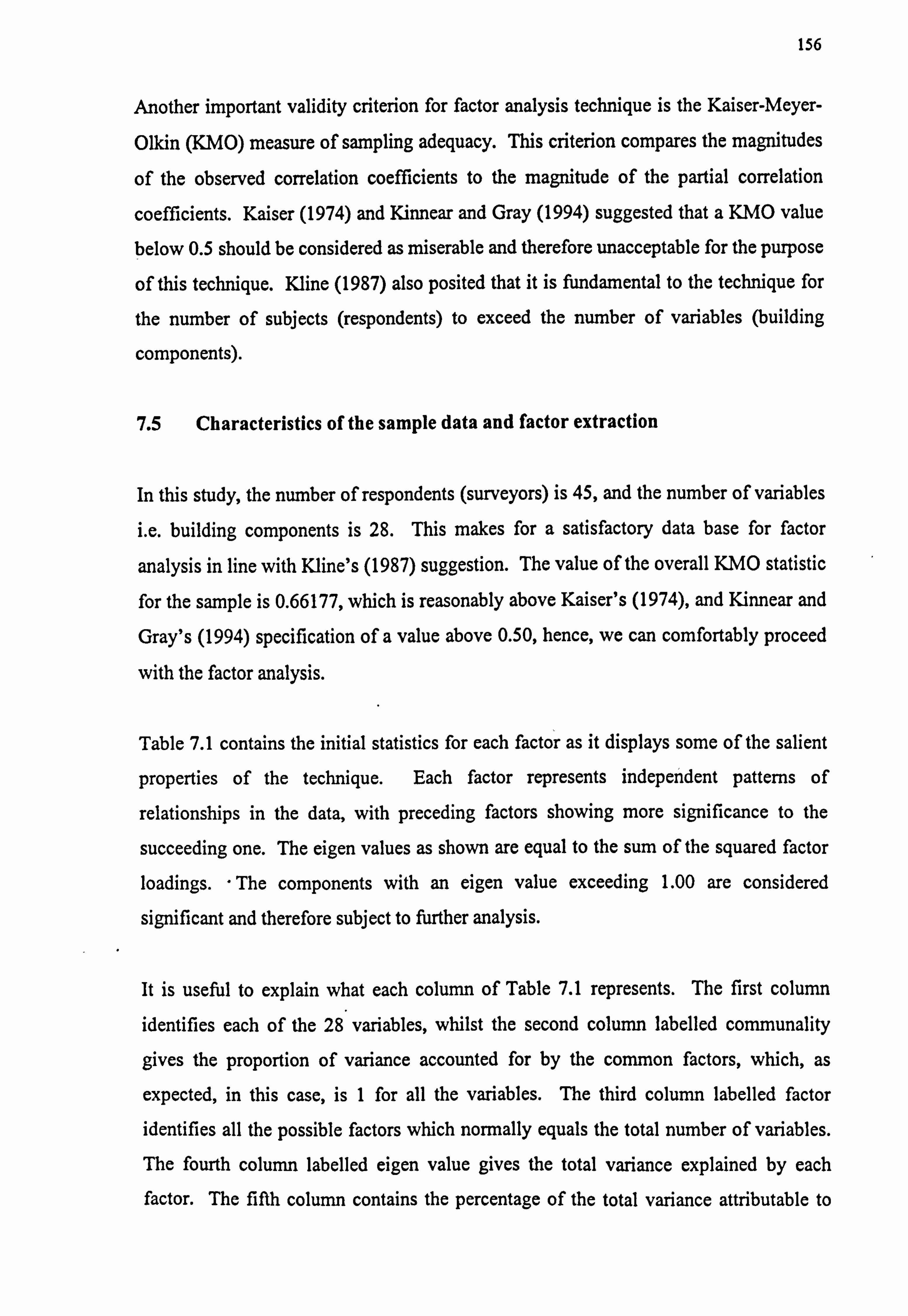
156
Another important validity criterion for factor analysis technique is the Kaiser-Meyer-
Olkin (KMO) measure of sampling adequacy. This criterion compares the magnitudes
of the observed correlation coefficients to the magnitude of the partial correlation
coefficients. Kaiser (1974) and Kinnear and Gray (1994) suggested that a KMO value
below 0.5 should be considered as miserable and therefore unacceptable for the purpose
of this technique. Kline (1987) also posited that it is fundamental to the technique for
the number of subjects (respondents) to exceed the number of variables (building
components).
7.5 Characteristics of the sample data and factor extraction
In this study, the number of respondents (surveyors) is 45, and the number of variables
i. e. building components is 28. This makes for a satisfactory data base for factor
analysis in line with Kline's (1987) suggestion. The value of the overall KMO statistic
for the sample is 0.66177, which is reasonably above Kaiser's (1974), and Kinnear and
Gray's (1994) specification of a value above 0.50, hence, we can comfortably proceed
with the factor analysis.
Table 7.1 contains the initial statistics for each factor as it displays some of the salient
properties of the technique. Each factor represents independent patterns of
relationships in the data, with preceding factors showing more significance to the
succeeding one. The eigen values as shown are equal to the sum of the squared factor
loadings. " The components with an eigen value exceeding 1.00 are considered
significant and therefore subject to further analysis.
It is useful to explain what each column of Table 7.1 represents. The first column
identifies each of the 28 variables, whilst the second column labelled communality
gives the proportion of variance accounted for by the common factors, which, as
expected, in this case, is 1 for all the variables. The third column labelled factor
identifies all the possible factors which normally equals the total number of variables. The fourth column labelled eigen value gives the total variance explained by each factor. The fifth column contains the percentage of the total variance attributable to
157
each factor. The sixth column gives the cumulative percentage, indicating the
percentage of variance attributable to that factor and those that precede it in the table.
A cursory look at the table shows that factorl which has a variance of 4.448 accounts for 15.9% of the total variance of the 28 factors. Similarly, 77.3% of the total variance is attributable to factors 1- 9 (inclusive).
Several procedures have been advanced for factor extraction in order to determine the
number of factors to use in the model (Norusis, 1990). One popular criterion suggests
that the eigen value for a factor must exceed 1.00 before the factor can be considered
significant and subject to factor analysis (Goddard and Kirby, 1976).
Figure 7.1 is a plot of the total variance associated with each factor, commonly referred
to as a scree plot. The name derives from its semblance to the rubble that forms at the
foot of a rock slope of a mountain (Cattel, 1966).
Experimental evidence shows that the gradual trailing off of the slope begins at the kth
factor, where k is the true number of factors (Norusis, 1990). It will be seen from the
scree plot that at factor 9, there is a break in the steady decreasing slope. A nine factor
model is therefore appropriate.
Having extracted and ascertained the appropriate factor model, the next step is to judge
how well the nine factor model describes the original 28 variables.
158
Table 7.1: Data Characteristics for the Analysis
Analysis number 1 Replacement of missing values with the mean
Kaiser-Meyer-Olkin Measure of Sampling Adequacy = . 66177
Bartlett Test of Sphericity = 831.58087, Significance = . 00000
Extraction 1 for analysis 1, Principal Components Analysis (PC)
Initial statistics:
Variable Communality * Factor Eigenvalue Pct of Var Cum Pct *
DAMPROF 1.00000 * 1 4.44843 15.9 15.9 DEFRUF 1.00000 * 2 3.66190 13.1 29.0 RUT 1.00000 * 3 3.17307 11.3 40.3 WATING 1.00000 * 4 2.46367 8.8 49.1 BUST 1.00000 * 5 2.17319 7.8 56.9 REGLAZE 1.00000 * 6 1.81386 6.5 63.3 PACHRF 1.00000 * 7 1.53282 5.5 68.8 DAMGOOD 1.00000 * 8 1.23678 4.4 73.2 FLASH 1.00000 * 9 1.14402 4.1 77.3 ELECFOT 1.00000 * 10 . 97814 3.5 80.8 GASLEAK 1.00000 * 11 . 81749 2.9 83.7 CODENSE 1.00000 * 12 . 69933 2.5 86.2 XDOOR 1.00000 * 13 . 60855 2.2 88.4 FENCE 1.00000 * 14 . 50798 1.8 90.2 BKDRAIN 1.00000 * 15 . 48782 1.7 92.0 GRAFIT 1.00000 * 16 . 41673 1.5 93.4 HEATING 1.00000 * 17 . 34133 1.2 94.7 IDOOR 1.00000 * 18 . 31674 1.1 95.8 SSTACK 1.00000 * 19 . 25723 .9 96.7 CONCRPR 1.00000 * 20 . 22757 .8 97.5 LIFTRM 1.00000 * 21 . 21791 .8 98.3 XPANEL 1.00000 * 22 . 14016 .5 98.8 BKFLOW 1.00000 * 23 . 11742 .4 99.2 XCRACK 1.00000 * 24 . 07530 .3 99.5 SPALBK 1.00000 * 25 . 06603 .2 99.7 WLTIES 1.00000 * 26 . 05342 .2 99.9 SLAB 1.00000 * 27 . 01805 .1 100.0 DPFLR 1.00000 * 28 . 00508 .0 100.0
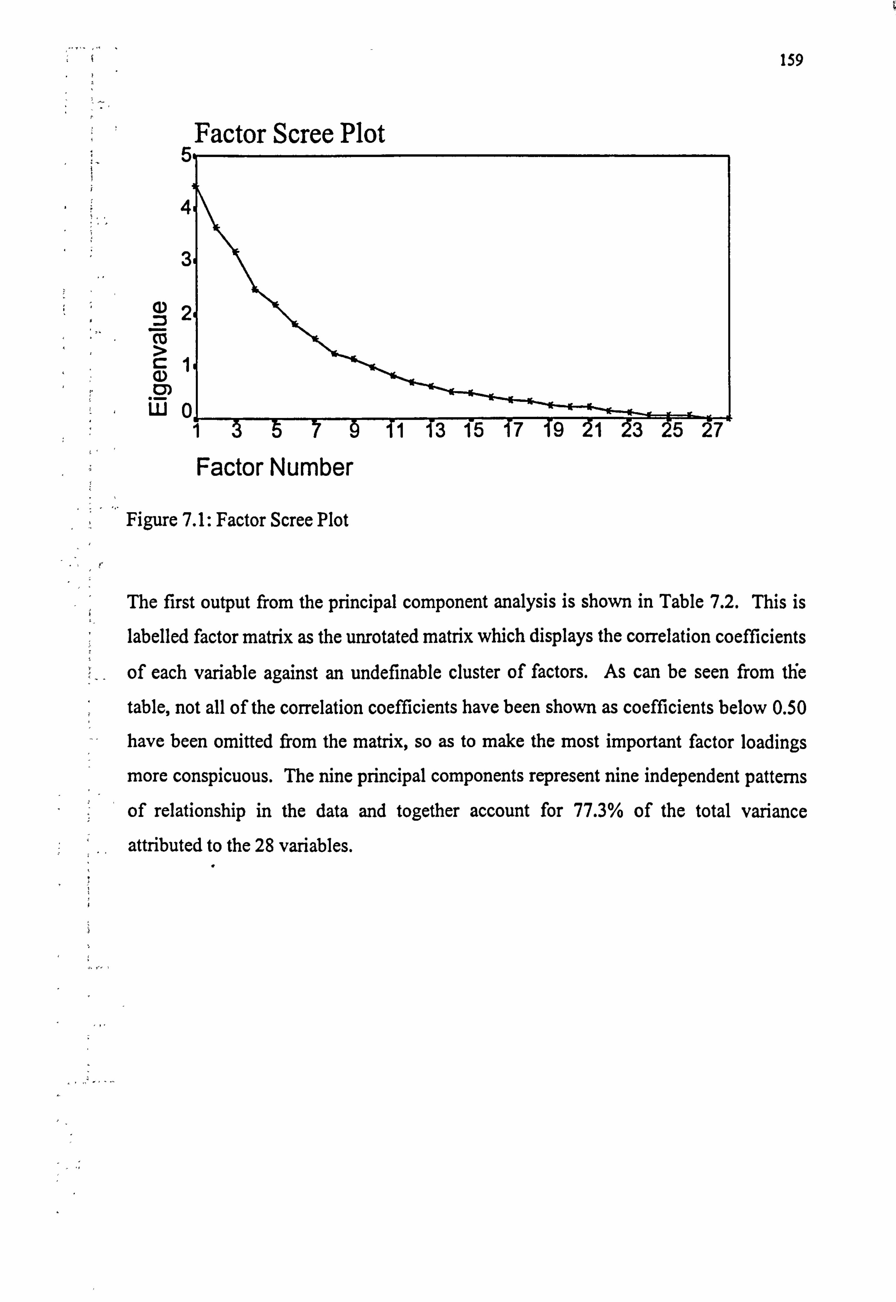
,,. {..
; - S i
U)
. CO > C N Q)
w
Factor Scree Plot 5
4
3
2
1
0 1 1 f3 f5 f7 f9 21 3 25 7
Factor Number
Figure 7.1: Factor Scree Plot
159
The first output from the principal component analysis is shown in Table 7.2. This is
labelled factor matrix as the unrotated matrix which displays the correlation coefficients
of each variable against an undefinable cluster of factors. As can be seen from the
table, not all of the correlation coefficients have been shown as coefficients below 0.50
have been omitted from the matrix, so as to make the most important factor loadings
more conspicuous. The nine principal components represent nine independent patterns
of relationship in the data and together account for 77.3% of the total variance
attributed to the 28 variables.
x
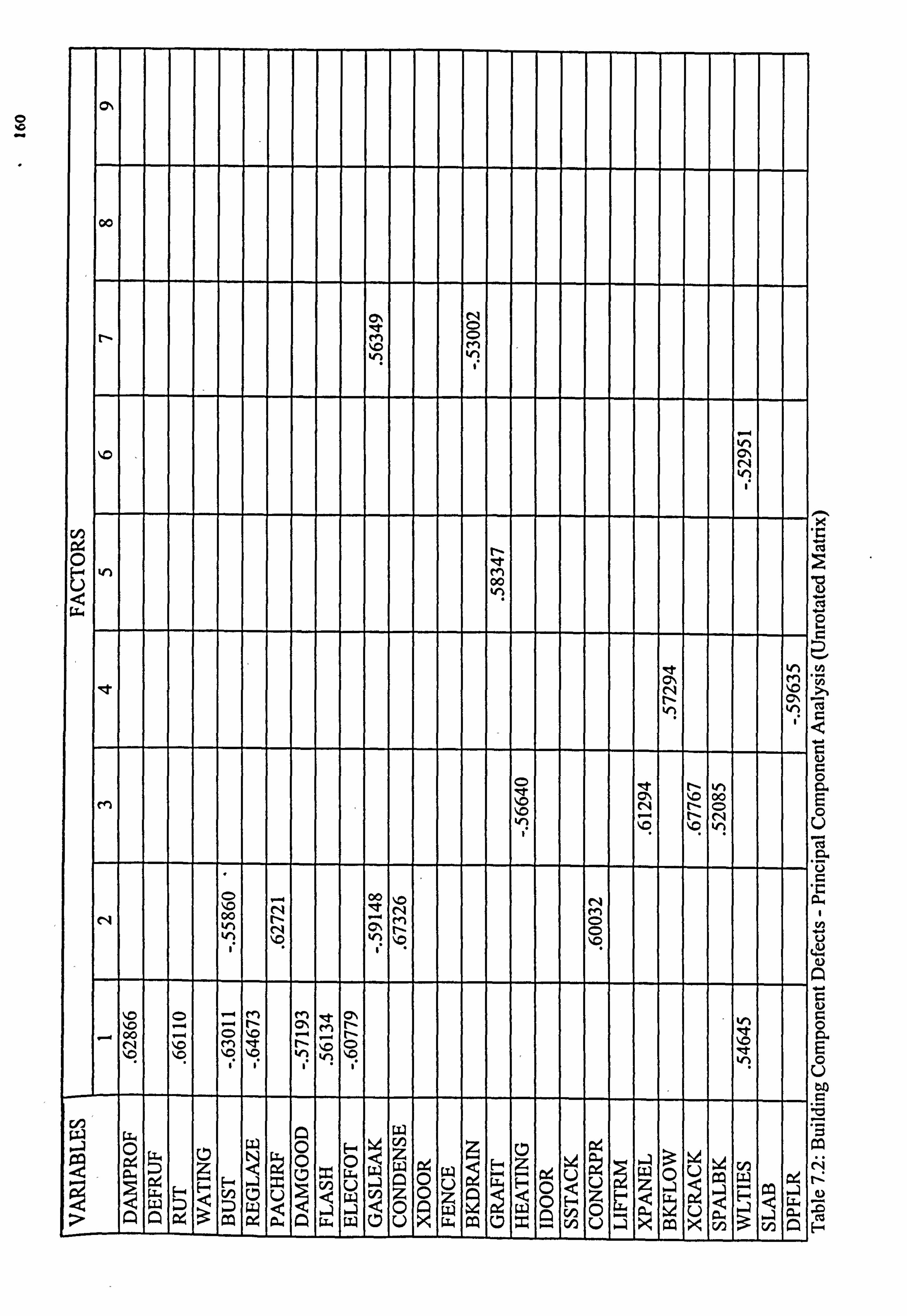
0
00
ýp M
IP1 N
N
C Ü kn
v M 00
C> N
rn
Im r- e
00 N KA
N n
N
ýo
00
-
*i
' M
N Ö
\Z \p 00
"0
0
"0
--4 " 0
'.
rn N "0
ýp
en C1
V1
M
yýj
r-
ýC
V1 let
ýt N
1 1 1 1
ä ö ý w
ý
ö H ý z
CD ý ý
ö `ý a z
Q
3 o
ý ¢
w_ ý
x
> A w A
A cZ
Q 3 A
m w x
¢ a A
ä w
ä w
¢ C7 U
q X
w w aý C7
w x
Ä ý
ý cn
ö v a
ýc aa
Ü X
ä v5
ä vn
ä A
.r Cd
b aý w cl 4- 2 0
.N
w 0 aý a 0 a E 0
U
0 a Ü C
a y
Ü
w aý A c aý 0 0 a E 0 U
0 b
N n
H
161
7.6 Component Analysis of the Extracted Factors
Having extracted and ascertained the appropriate factors, the next step is to assess how
well the nine factors explain the variations in the original 28 variables. This is achieved by a technique referred to as the principal component analysis. Table 7.3 shows the
results of principal component analysis and the conununalities and factor statistics after
the significant factors have been extracted. The proportion of variance explained by the
nine common factors is referred to as communality of the variable.
Communalities can range from 0 to 1, with 0 indicating that the common factors
explain none of the variance, and 1 indicating that all the variance is explained by the
common factors. The unexplained variance by the nine common factors can therefore
be attributed to the unique factor. For example, 88% of the variance in PACHRF is
accounted for, whereas only about 51% of the variance in SSTACK is accounted for.
7.7 Identification of the Significant Component Defects on the Factors
So far, it has been demonstrated with the help of the factor matrix, the relationships between the factors and the individual variables. However, it is still possible to
minimise the number of factors on which variables have high loading, and thereby
making the relationships between factors and variables conceptually meaningful. Whilst the "unrotated principal components successfully define the general pattern of
relationships in the data, it is possible to rotate the principal components so that they delineate any distinct clusters of relationships.
The final stage in the principal component analysis was to apply the Varimax
Orthogonal Rotation of component technique in order to simplify the rows in the factor
matrix. The axes of the components are rotated so as to maximise the variance of the
squared loading in each column. `To avoid bias against the contribution of the less
prominent component, each variable is weighted equally for the purposes of rotation' (Traynor, 1978). The objecive of rotation is always to achieve final component loadings which maximises the variance of the squared loading in each column.
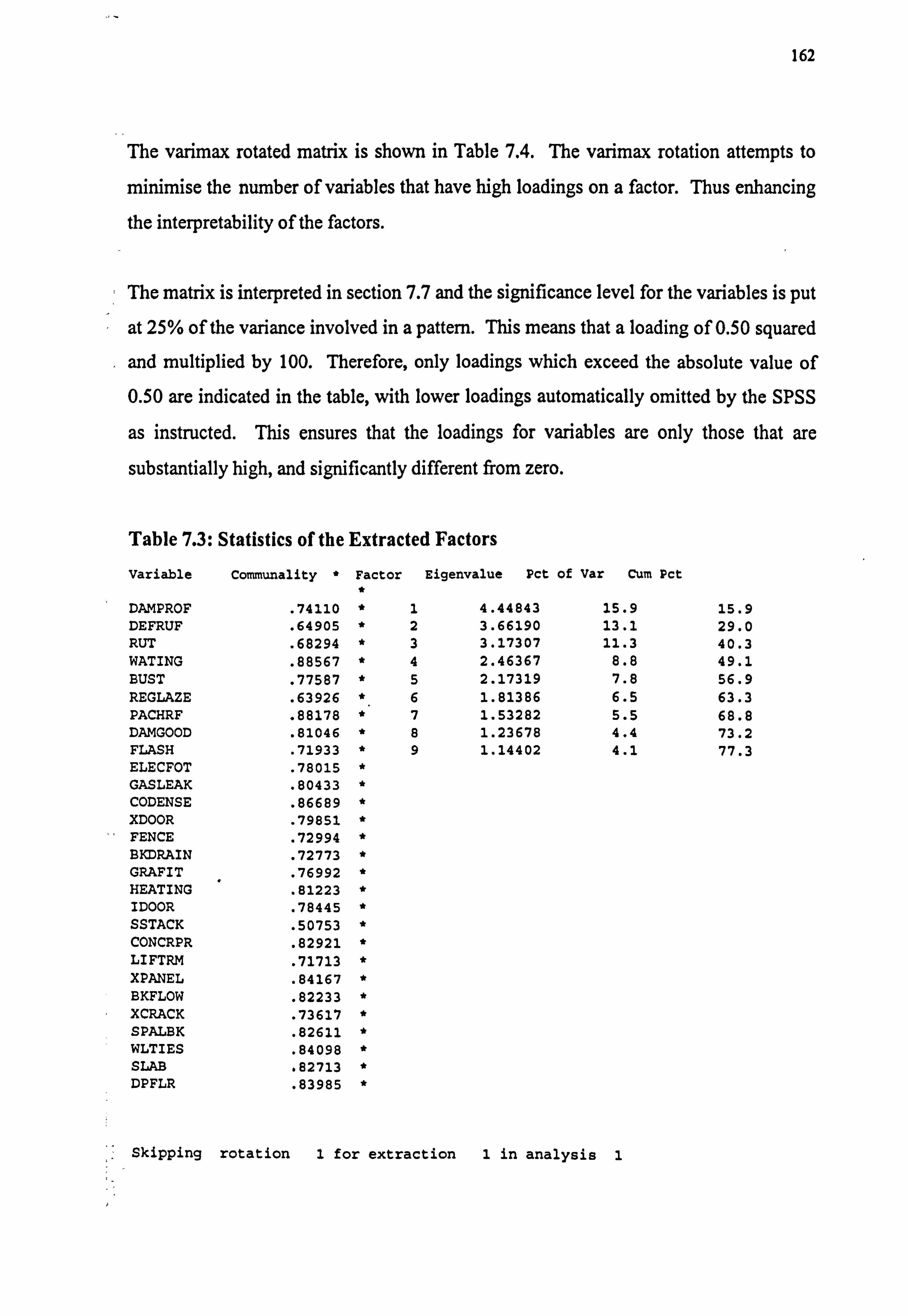
162
The varimax rotated matrix is shown in Table 7.4. The varimax rotation attempts to
minimise the number of variables that have high loadings on a factor. Thus enhancing
the interpretability of the factors.
The matrix is interpreted in section 7.7 and the significance level for the variables is put
at 25% of the variance involved in a pattern. This means that a loading of 0.50 squared
and multiplied by 100. Therefore, only loadings which exceed the absolute value of
0.50 are indicated in the table, with lower loadings automatically omitted by the SPSS
as instructed. This ensures that the loadings for variables are only those that are
substantially high, and significantly different from zero.
Table 7.3: Statistics of the Extracted Factors
Variable
DAMPROF DEFRUF RUT WATING BUST REGLAZE PACHRF DAMGOOD FLASH ELECFOT GASLEAK CODENSE XDOOR FENCE BKDRAIN GRAFIT HEATING IDOOR SSTACK CONCRPR LIFTRM XPANEL BKFLOW XCRACK SPALBK WLTIES SLAB DPFLR
Communality *
. 74110
. 64905
. 68294
. 88567
. 77587
. 63926
. 88178
. 81046
. 71933
. 78015
. 80433
. 86689
. 79851
. 72994
. 72773
. 76992
. 81223
. 78445
. 50753
. 82921
. 71713
. 84167
. 82233
. 73617
. 82611
. 84098
. 82713
. 83985
Factor " t
" w " "
" "
"
" "
"
Eigenvalue Pct of Var Cum Pct
1 4.44843 15.9 15.9 2 3.66190 13.1 29.0 3 3.17307 11.3 40.3 4 2.46367 8.8 49.1 5 2.17319 7.8 56.9 6 1.81386 6.5 63.3 7 1.53282 5.5 68.8 8 1.23678 4.4 73.2 9 1.14402 4.1 77.3
Skipping rotation 1 for extraction 1 in analysis 1
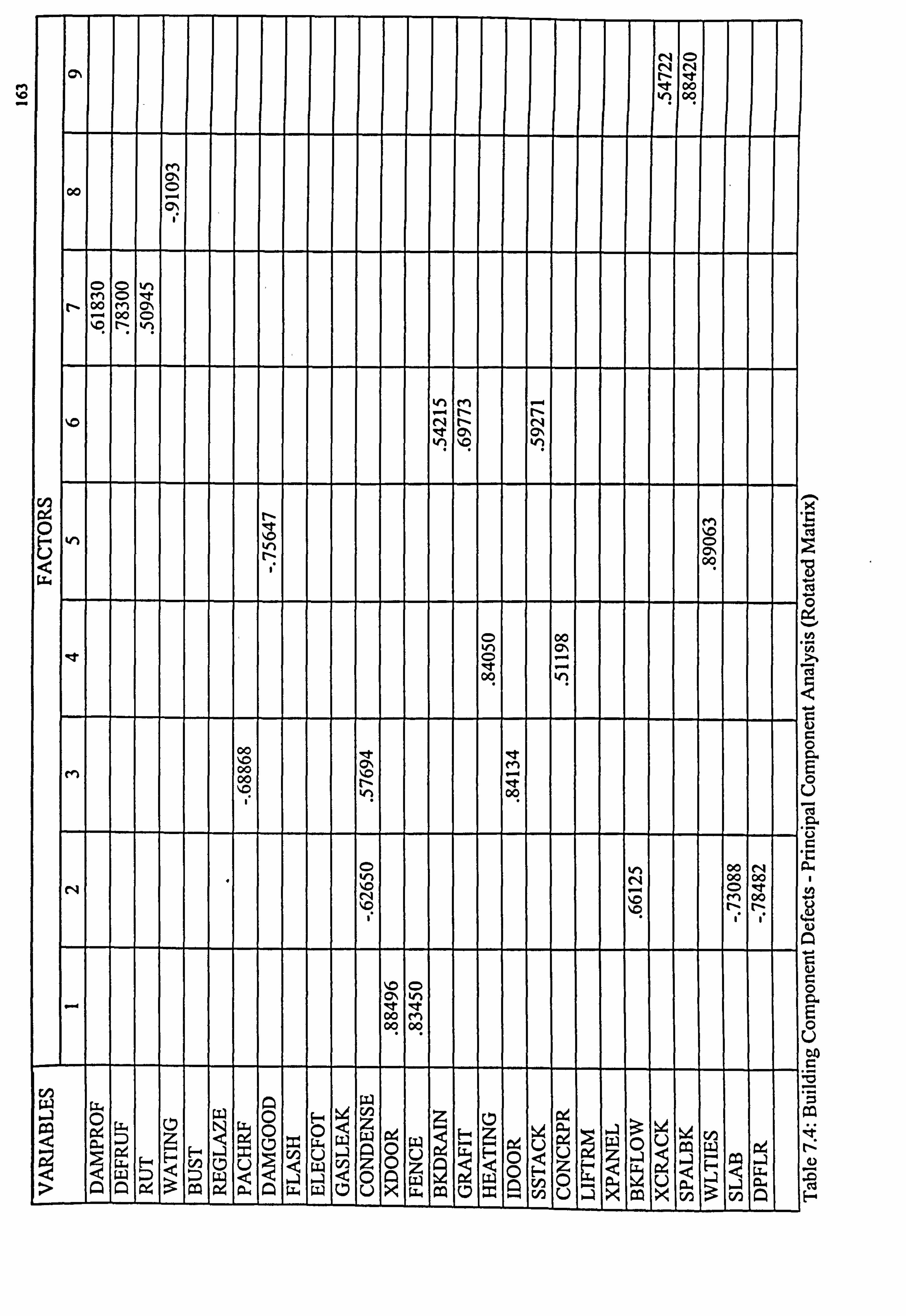
N O
00 W) 00
M O'
00
O O ý1 O ct 00
000 Ö
to en 1--4 - n N
0 N.
ýo 10 CD CN 00
00 In vý
v o . -" 00 'n
M
00 00 ON
N
vn
M
1-4 IRT
00
N N N -4
00
00
M
00 I 00
i i
00 M
ce. a
Ä ý 3
F-ý
rAa
.a
x a<.
C7 x
w
w
w w
a ¢ Ol
q o ul
C4 O
A
W
w Q
csý
E. w
t7
4
x
A~ Cv
U
U a
W
a, ýC
O
m U X
cý ä
rn
W_
3 tn
a!
A
K
cv
w cd
td
O
cu a
00
. Ei G4
164
7.8 Interpretation of the Factors
The information given in the rotated principal component analysis matrix is now
interpreted. Essentially, the principal components indicate the number of distinct
clusters of relationships. Each of the nine principal components are here reviewed in
turn and given an appropriate name.
To identify the factors, an attempt is made at grouping the variables that have large
loadings for the same factors as in Table 7.5 (manual shuffling of Table 7.4). For
example, the first factor shows strong positive correlation with defects in external doors
and fence. Thus implying that defect occurrence in external door and fence are
positively correlated. Similar inferences can be drawn for factors 2-9, with each factor
consisting of building components that are positively or negatively correlated.
It is noteworthy that seven of the 28 variables do not significantly correlate with any of
the factors, namely: BUST, REGLAZE, FLASH, ELECFOT, GASLEAK, LIFTRM,
and XPANEL. This suggests that among others, the bulk of their underlying factors are
found in the 22.7% unexplained factors outside of the nine significant factors.
To identify the factors, it is necessary to group the variables that have large loadings for
the same factors.
All the nine factors are listed below together with associated variable labels and full
component names (as in Table 7.6). Factors 1 through to 9 are distinct and capable of identity. Factor 1 relate to dwelling externality and thus might be interpreted as
measuring something like "dwelling external influence". The second factor is
negatively correlated with condensation, concrete bed/slab failure and dampness in
floor, but positively correlated with backflow. This factor describes the design integrity
standard of the dwelling. All the nine factors are listed below and classified under nine different defect causative characterisations.
165
Table 7.5: Significant Component Defects on the Factors
Variables Fl F2 F3 F4 F5 F6 F7 F8 F9
XDOOR . 88496 FENCE . 83450
CODENSE -. 62650 -. 57694 BKFLOW . 66125 SLAB -. 73088 DPFLR -. 78482
PACHRF -. 68868 IDOOR . 84134
HEATING . 84050 CONCRPR . 51198
DAMGOOD -. 75647 WLTIES . 89063
BKDRAIN . 54215 GRAFIT . 69773 SSTACK . 59271
DAMPROF . 61830
DEFRUF . 78300 RUT . 50945
WATING -. 91093
XCRACK . 54722
SPALBK . 88420
BUST REGLAZE FLASH ELECFOT GASLEAK LIFTRM XPANEL
166
Table 7.6: Groupings of the Factors and the Components Variable Labels Building component - Def
XDOOR Damaged security door FENCE Fencing repair or replacement
Facor 2
CODENSE Condensation problem BKFLOW Soil pipe backflow SLAB Slab and screed failure DPFLR Damp floor
Factor 3
PACHRF Patch repair to roof IDOOR Internal door repair or replacement
Factor 4
HEATING Heating repair or replacement of part CONCRPR Balcony concrete repair
Factor 5
DAMGOOD Damaged rain water goods WLTIES Wall ties failure
Factor 6
BKDRAIN Blocked drains
GRAFIT Grafitti SSTACK Soil stack (high rise)
Factor-2
DAMPROF Defective damp proofing DEFRUF Defective roof structure RUT Dry/Wet rot outbreak
Factor g
WATING Water ingress
Factor 9
XCRACK Expansion crack SPALBK Spallled bricks
167
Factor 1 Dwelling external influence
Factor 2 Design integrity standard of dwelling Factor 3 Tenant's lack of care index
Factor 4 Influence of changing and evolving standard
Factor 5 Ageing influence
Factor 6 Vandalism - Design pull effect Factor 7 Design - construction inadequacy
Factor 8 Accidental damage restricted to building envelope
Factor 9 Dwelling orientation and soil condition
7.9 Discussion of the maintenance requirement factors based on factor
analysis technique
Factor 1- Dwelling external influence
This component accounts for 16% of the total variance and two building component-
defect titles namely; damaged external door and fencing repair and replacement work
are shown with significant loadings on this cluster. The higher loading is given to the
defect in external door variable (XDOOR :r=0.8850) and this indicates the
overwhelming importance of external doors to overall maintenance profile.
The importance of external phenomenon upon the building fabric is reflected in the
loadings given to one other variable related to the externals of the building; defective
fences (FENCE :r=0.8345). From the primary analysis and the correlation matrix,
the patch repair to roof (PACHRF) does not appear significant, yet, this is as much an
external feature as the two significant variables. This leads us to infer that what bears
most heavily upon this component factor has more to do with the combination of the
vagaries of climatic exposure and human destructive instinct. As in roof tiles, the latter
influence is to a large extent totally absent and therefore not significant.
Factor 2- Design integrity standard of dwelling
This component absorbs 13% of the total variance with both positive and negative
significant loadings.
168
Negative loadings on condensation (CODENSE :r= -0.6265), floor bed/slab failure
(SLAB :r= -0.7309) and dampness in floor (DPFLR :r= -0.7848). This is indicative
of technical aspirations which future house designs must address.
A positive loading on backflow in waste disposal plumbing units (BKFLOW :r= 0.6613) shows that backflow problems are judged by the building surveyors to be of
secondary importance.
It can be inferred that this cluster measures respondents' opinions on the effectiveness
of the design. The component will be called the `Design Integrity Standard' factor and
as such measures a criterion of utmost importance for the housing maintenance market. This factor must be of vital concern to both designers (architects and building
surveyors), and housing managers.
Factor 3- Tenant's lack of care index
The third component includes significant positive and negative loadings which
incorporate approximately 11 % of the total variance. Whilst condensation and defects
requiring patching up of roof are both negative (CODENSE :r= -0.5769; PATCHRF
r= -0.6887), internal door is positively loaded (IDOOR :r=0.8413). Since
condensation variable is again given a negative loading as with PATCHRF, it implies
that respondents generally opined that condensation problem is a primary measure of tenant's care or lack of care in the same way as the overall condition of the roof
covering.
Whilst PATCHRF and CODENSE are both negatively loaded, it should be appreciated
that the two variables relate to the same factor from different perspectives. The level of
condensation measures tenant's `disposable care' towards the dwelling whilst roof defects requiring patch up measures his `inhibitive concern' for the dwelling. In both
cases, the tenant's readiness to exercise positive care on the dwelling is being
measured. The high positive loading on IDOOR places this variable as prime indicator
of "Tenant's Care Index" for the dwelling.
169
The positive loading for internal door shows that this variable is averse to the other two
significant variables on this factor component. It would be reasonable to infer that this
variable measures tenant's ̀ prohibitive care' for the dwelling.
Factor 4- Influence of changing and evolving standard The fourth component absorbs 9% of the total variance and two variables are shown
with significant loadings on this pattern. The higher loading is given to the defects in
heating installations (HEATING :r=0.8405), and the loading given to defects
requiring concrete repairs is (CONCRPR :r=0.5120).
Each of these two variables relate to changes in standards from different focal points.
On one hand, HEATING relates to changes in the maintenance need profile occasioned
by improved heating systems in comparison with erstwhile `coal fire place'. On the
other hand, CONCRPR relates to the bespoke flirting with concrete form of
construction of the 1960s (Wyatt, 1980).
The component measures the influence of standard on defects generation and can be
identified as "Changing and Evolving Standard".
Factor 5- Ageing influence
Component No. 5 describes the Ageing Influence factor on maintenance requirements. This component includes two significant loadings either of which is positive and
negative, and incorporates approximately eight per cent of the total variance.
The positive loading is on the wall ties defects (WLTIES :r=0.8906) which displays
to a large extent the influence of age since installation. The negative loading is on defective rain water goods (DAMGOOD :r= -0.6887) which indicates that it is seen
as a secondary measure of ageing. That is to say, the variable can be used to monitor
the effect of age when the other variable is not applicable to a particular building.
170
Factor 6- Vandalism - Design Pull effect
This component accounts for seven per cent of the total variance and three variables are
shown with significant loadings on this pattern. The highest loading is given to Graffiti
(GRAFIT :r=0.6977) which indicates the superiority of this variable on the factor
component.
The importance of systematic but conscious and insidious destruction of the built form
is reflected in the loading given to the one other variable related to what may be
described as vandalism, soil stack failure (SSTACK :r=0.5927).
Blocked drains was also given a positive loading (BKDRAIN :r=0.5422). Judging
from the concordance tests of the preceding chapter, it was observed that this defect
item ranks highest on age and second highest on vandalism. Component No. 6
therefore represents the significant effects of vandalism - design pull effect as
enunciated by (Cosby, 1985).
Factor 7- Design - construction inadequacy
The seventh component includes significant positive loadings which incorporate
approximately six per cent of the total variance.
The largest loading is on defective roof structure variable (DEFRUF : 'r = 0.7830)
which portrays the cause of failure in the structural integrity of roofs as against
cosmetic failure. The importance of timber as building material is reflected in the
loading given to dry or wet rot outbreak which is related to the same material (RUT
:r=0.5095). It would have been expected that since rot problems have more to do
with cosmetic rather than structural deficiencies the two variables should not co-relate.
However, the existence of structural failure inevitably leads to cosmetic failure in the
medium or long term.
Damp proof course failure, which inevitably leads to rising damp was also given a moderately high positive loading (DAMPROF :r=0.6183). This variable is vitally
related to dry or wet rot outbreak.
171
The three variables that are included in this factor component are most interestingly
related. Rot outbreaks in most house types where they occur are common in either loft
or sub-floor. The two locations are associated with each of the two variables which inter-link RUT, i. e. DEFRUF and DAMPROF.
It would be reasonable to infer that this component pattern measures the efficiency of both design and construction.
Factor 8- Accidental damage
This component accounts for about four per cent of the total variance. It shows one
significant highly negative loading on the variable for water ingress, (WATING :-
0.9109). The component apparently measures the tenant's propensity to accidental
damage on the building envelope. The negative sign of this loading suggests that
accidental damage to property would least likely result in either of penetrating damp or
flooding. That is to say, the factor component and the variable on which the factor is
significant are almost diametrically averse to each other (inverse relationship exists
between the two).
Because the factor informs of what it does not measure rather than measure, it is left to
conjecture as to the relevance of this component to overall framework of defect
generation and subsequent strategy for damage limitation. This result underpins the
generally prompt response that is often accorded any reports of penetrating water or flooding as- it would least likely be caused by user's neglect.
Factor 9- Dwelling orientation and soil condition
Component No. 9 is the last of the important components and includes four per cent of
the total variance. The first nine components have accounted for about 77% of the total
variance and therefore the 19 remaining components would be relatively insignificant
and together account for less than 23% of the variance.
This component shows two significant positive loadings on the variables for spalled bricks (SPALBK :r=0.5472) and cracks to walls (XCRACK :r=0.8842). The
component apparently measures what might be described as the building's reaction to
172
the vagaries of its situation. The two variables SPALBK and XCRACK are very
similar, and therefore it is no surprise that the two variables bear the effect of a
common pattern. .
The component is named Dwelling Orientation and Soil Condition and would be
important for maintenance managers when making maintenance budgets for dwellings.
In essence, variance in maintenance expenditure as a result of orientation and soil
condition should be reflected in the component of maintenance budget to cover spalling
bricks and expansion joints.
7.10 Conclusions
The chapter has shown that in relation to internal attributes of the building, the factors
at play are not simply those features commonly considered by designers, but involve
the inter-play of factorial combination phenomenon, which this segment of the study
has underscored.
The principal component analysis technique has allowed the data collected from
building surveyors through the questionnaire instrument (Appendix 1B) to be
simplified and interpreted into key component factors which influence maintenance
need of a dwelling on a broad basis. Thus addressing the part of the research
framework pertaining to Internal Attribute Component of the model in Figure 2.2.
From the point of view of a maintenance manager, each of the nine categories
represents strategic influences, an understanding of which surveyors must acquire in
order to proffer sound remedies to the defects encountered in survey of dwellings.
Through the factor analysis technique of data reduction, it has been established
statistically, the correlations between components-defects. In all, defects causative influences have been grouped into a nine-factor model according to their levels of importance.
173
This evidence, provides a basis to reject the null hypothesis in favour of the alternative
hypothesis, that is, the plausibility of localising defect causing factors to a group of
components is hereby confirmed on the basis of intercorrelations which exist between
component scores.
The use of the chosen statistical technique proved to be highly successful in detecting
the underlying patterns and reducing the mass of data into a brief yet coherent
statements. The set of component factors for housing maintenance needs gave an insight into the criteria available for those involved in determining maintenance budgets.
'1
174
CHAPTER 8
MAINTENANCE - TENANT MODEL
8.1 Introduction
This chapter focuses chiefly on the impact of tenants on dwelling maintenance need, and
in the process touches upon environmental and housing management impacts. The
chapter deals with the methodological framework for the measurement of maintenance
requirements and measurable variables that impact upon them. These entail the
exploration of tenants' characteristics, housing management responsiveness,
environmental stress and selected property characteristics on the sampled dwellings, and
how they affect maintenance need.
The aspect of tenants' characterisation has serious and complex social and policy
implications. An understudy of tenants and their characteristics may be seen to impinge
upon the policy of equal opportunity. However, without the proper integration of
information relating to property and the users of the dwelling, the phenomenon of housing
maintenance need prediction will remain an intractable problem for housing managers.
Whilst chapters Six and Seven show the results of building surveyor's questionnaire
survey, this chapter goes a step further by attempting to measure maintenance
requirement.
The hypothesis which this chapter seeks to explore is that dwellings within the same
estate and with similar architectural attribute in space and time will exhibit different
maintenance need profile as a result of differences in tenants' characteristics. In essence,
a significant proportion of the variation in maintenance requirement will have its
explanation in the differences in tenants' personalities and attributes. It is expected
therefore, that a housing manager will be able to predict a part of his maintenance budget
accurately given certain information about his tenants. In this vein, a housing manager
who discounts tenant information in the development of a maintenance strategy will not
apply resources to full effect.
175
8.2 Research Approach and Limitation
Whilst this section of the study sets out to test the hypothesis in relation to tenants'
influence, the choice of independent variables is decidedly broadened to encompass all
the measurable variables inherent in the theoretical model of chapter two. In so doing, the
study avoids the same limitation of which many studies into maintenance factors are
guilty. (This has been extensively discussed in chapter Five).
The mediatory role of the stockholder is essentially discounted in this study - policy and
budget matters are nebulous and do not lend themselves to direct measurement. They are
principally dictated by political dictum and nuances which are a function of both national
and international political and economic climates. From this family of variables
therefore, we have included for housing management responsiveness only.
8.3 The survey
The data for this aspect of the study was obtained in two parts. The first part of the data
was achieved by collecting data on repair costs for the sample dwellings from the
authority's Direct Labour Organisation (DLO) system. The second part was based
upon postal questionnaires which were distributed among tenants of the sample
dwellings. In total, 252 completed questionnaire on each of which computer DLO
records were obtainable provided quantitative data analysis. The 252 questionnaires
used for this part of the study represented a response rate of about 40%.
8.4 Data characteristics for the dependent variables
8.4.1 Maintenance requirements Indices
To assess some of the dimensions of maintenance requirements among our sample dwellings, it was decided to gather data on three indices as follows:
1. Historic maintenance measure;
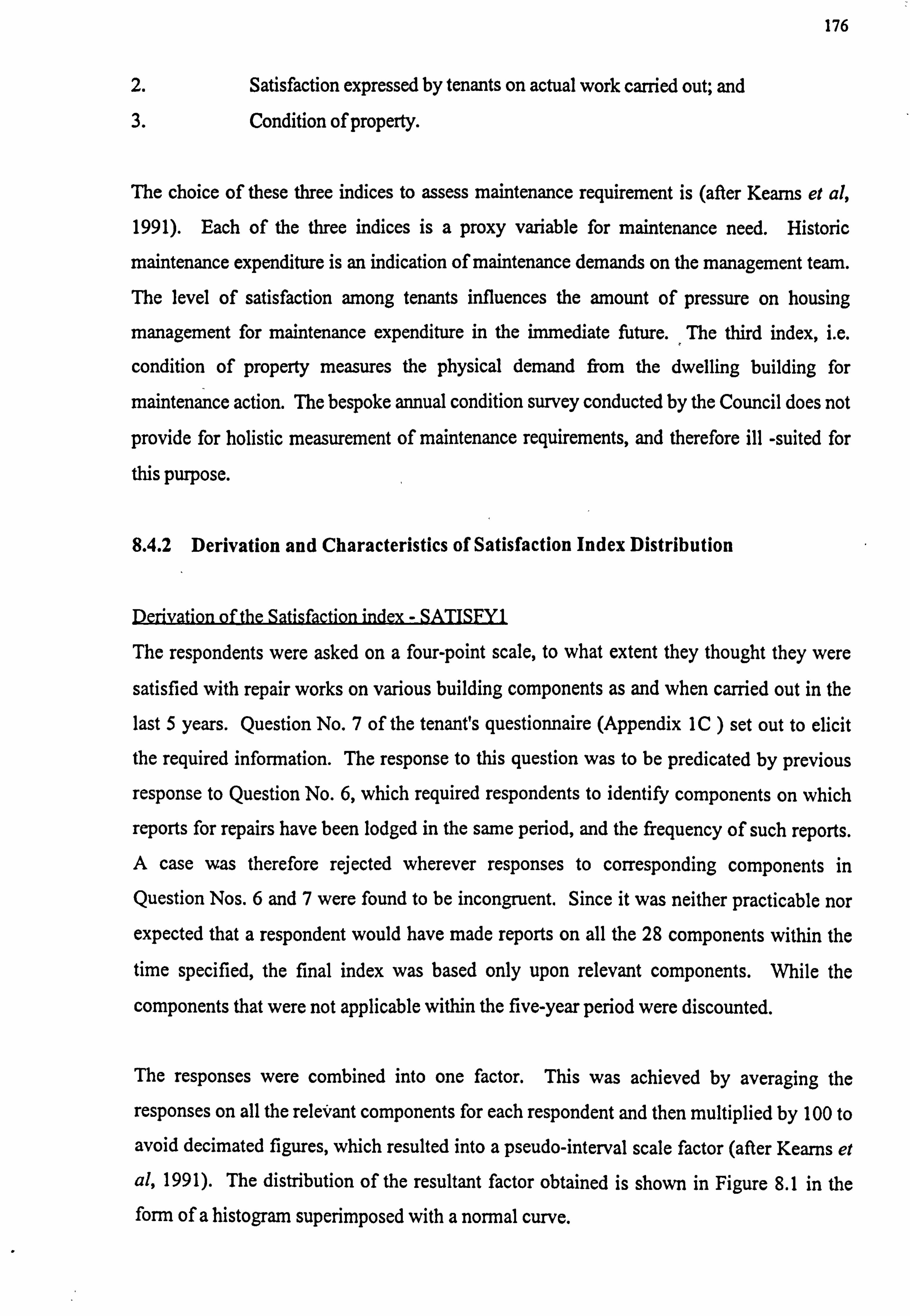
176
2. Satisfaction expressed by tenants on actual work carried out; and 3. Condition of property.
The choice of these three indices to assess maintenance requirement is (after Kearns et al,
1991). Each of the three indices is a proxy variable for maintenance need. Historic
maintenance expenditure is an indication of maintenance demands on the management team.
The level of satisfaction among tenants influences the amount of pressure on housing
management for maintenance expenditure in the immediate future. The third index, i. e.
condition of property measures the physical demand from the dwelling building for
maintenance action. The bespoke annual condition survey conducted by the Council does not
provide for holistic measurement of maintenance requirements, and therefore ill -suited for
this purpose.
8.4.2 Derivation and Characteristics of Satisfaction Index Distribution
Derivation of the Satisfaction index - SATISFYI
The respondents were asked on a four-point scale, to what extent they thought they were
satisfied with repair works on various building components as and when carried out in the
last 5 years. Question No. 7 of the tenant's questionnaire (Appendix 1C) set out to elicit the required information. The response to this question was to be predicated by previous
response to Question No. 6, which required respondents to identify components on which
reports for repairs have been lodged in the same period, and the frequency of such reports. A case was therefore rejected wherever responses to corresponding components in
Question Nos. 6 and 7 were found to be incongruent. Since it was neither practicable nor
expected that a respondent would have made reports on all the 28 components within the
time specified, the final index was based only upon relevant components. While the
components that were not applicable within the five-year period were discounted.
The responses were combined into one factor. This was achieved by averaging the
responses on all the relevant components for each respondent and then multiplied by 100 to
avoid decimated figures, which resulted into a pseudo-interval scale factor (after Kearns et al, 1991). The distribution of the resultant factor obtained is shown in Figure 8.1 in the form of a histogram superimposed with a normal curve.
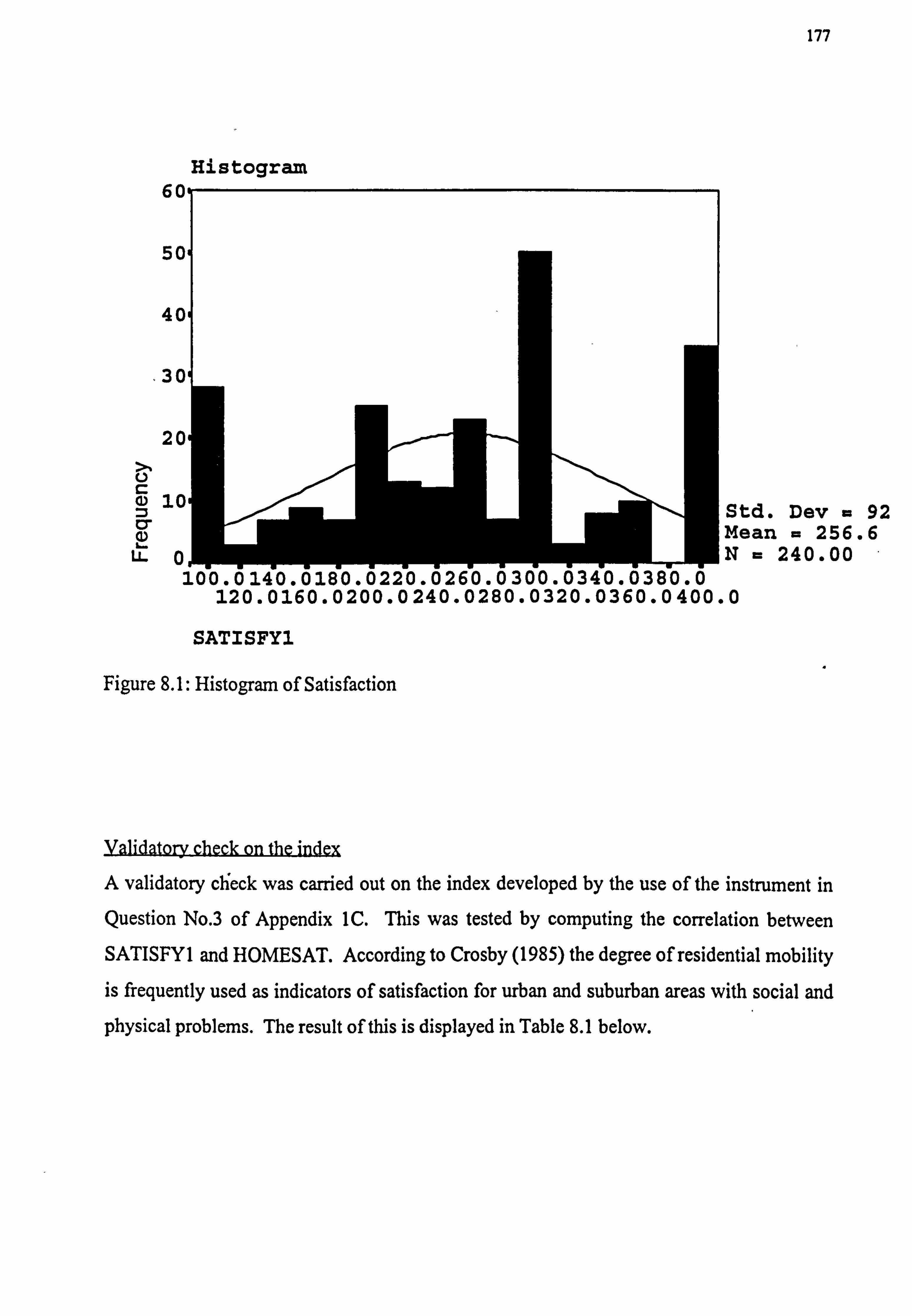
177
Histogram 6
5
4
3
2 A L) C 11 Q N L- LL
SATISFY1
Figure 8.1: Histogram of Satisfaction
Std. Dev = 92 Mean = 256.6 N= 240.00
Validatorv check on the index
A validatory clieck was carried out on the index developed by the use of the instrument in
Question No. 3 of Appendix 1C. This was tested by computing the correlation between
SATISFYI and HOMESAT. According to Crosby (1985) the degree of residential mobility is frequently used as indicators of satisfaction for urban and suburban areas with social and
physical problems. The result of this is displayed in Table 8.1 below.
120.0160.0200.0240.0280.0320.0360.0400.0
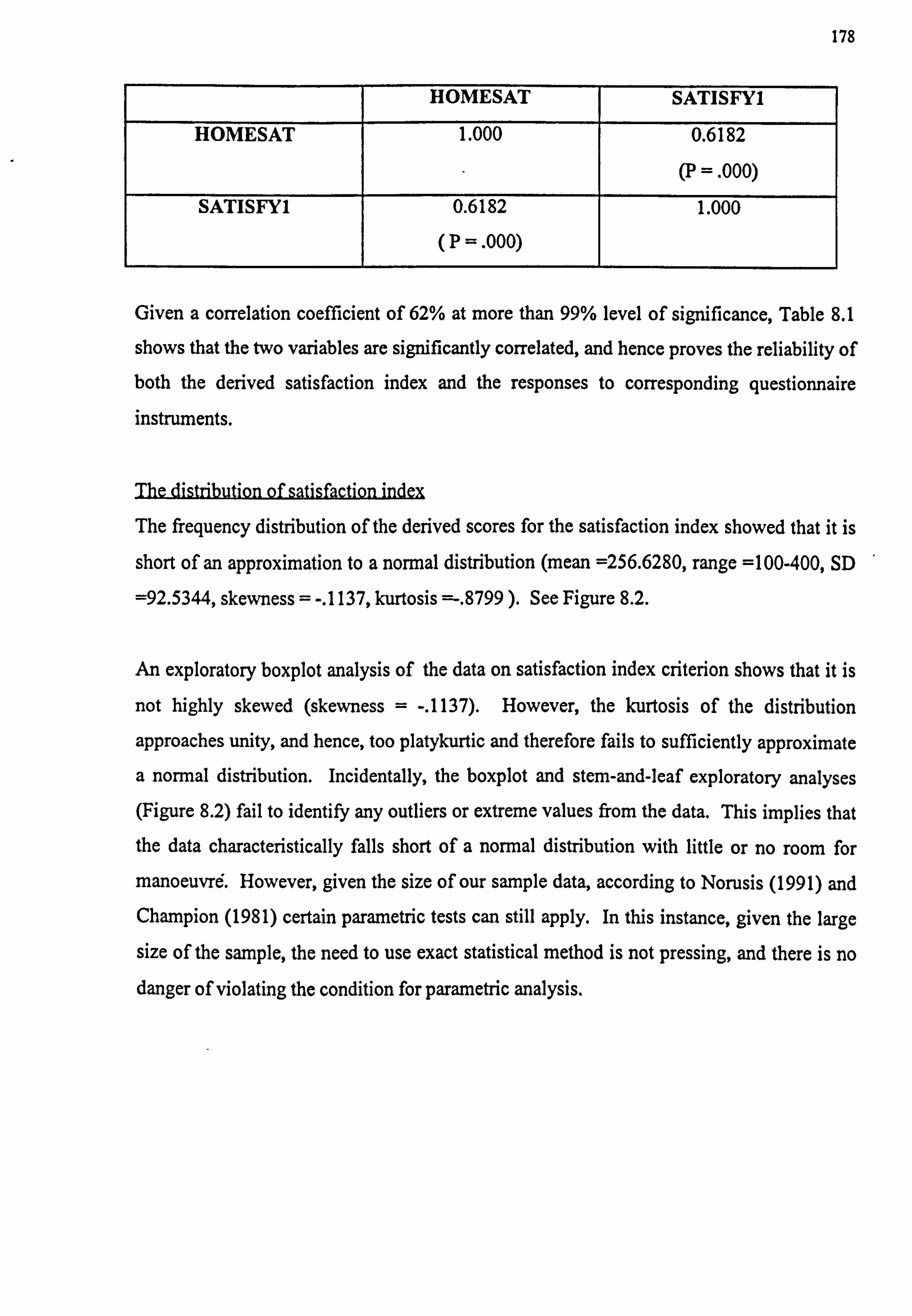
178
HOMESAT SATISFYI
HOMESAT 1.000 0.6182
(P =. 000)
SATISFY! 0.6182 1.000
(P =. 000)
Given a correlation coefficient of 62% at more than 99% level of significance, Table 8.1
shows that the two variables are significantly correlated, and hence proves the reliability of both the derived satisfaction index and the responses to corresponding questionnaire instruments.
The frequency distribution of the derived scores for the satisfaction index showed that it is
short of an approximation to a normal distribution (mean =256.6280, range =100-400, SD
=92.5344, skewness = -. 1137, kurtosis =-. 8799 ). See Figure 8.2.
An exploratory boxplot analysis of the data on satisfaction index criterion shows that it is
not highly skewed (skewness = -. 1137). However, the kurtosis of the distribution
approaches unity, and hence, too platykurtic and therefore fails to sufficiently approximate
a normal distribution. Incidentally, the boxplot and stem-and-leaf exploratory analyses (Figure 8.2) fail to identify any outliers or extreme values from the data. This implies that
the data characteristically falls short of a normal distribution with little or no room for
manoeuvre. However, given the size of our sample data, according to Norusis (1991) and Champion (1981) certain parametric tests can still apply. In this instance, given the large
size of the sample, the need to use exact statistical method is not pressing, and there is no danger of violating the condition for parametric analysis.
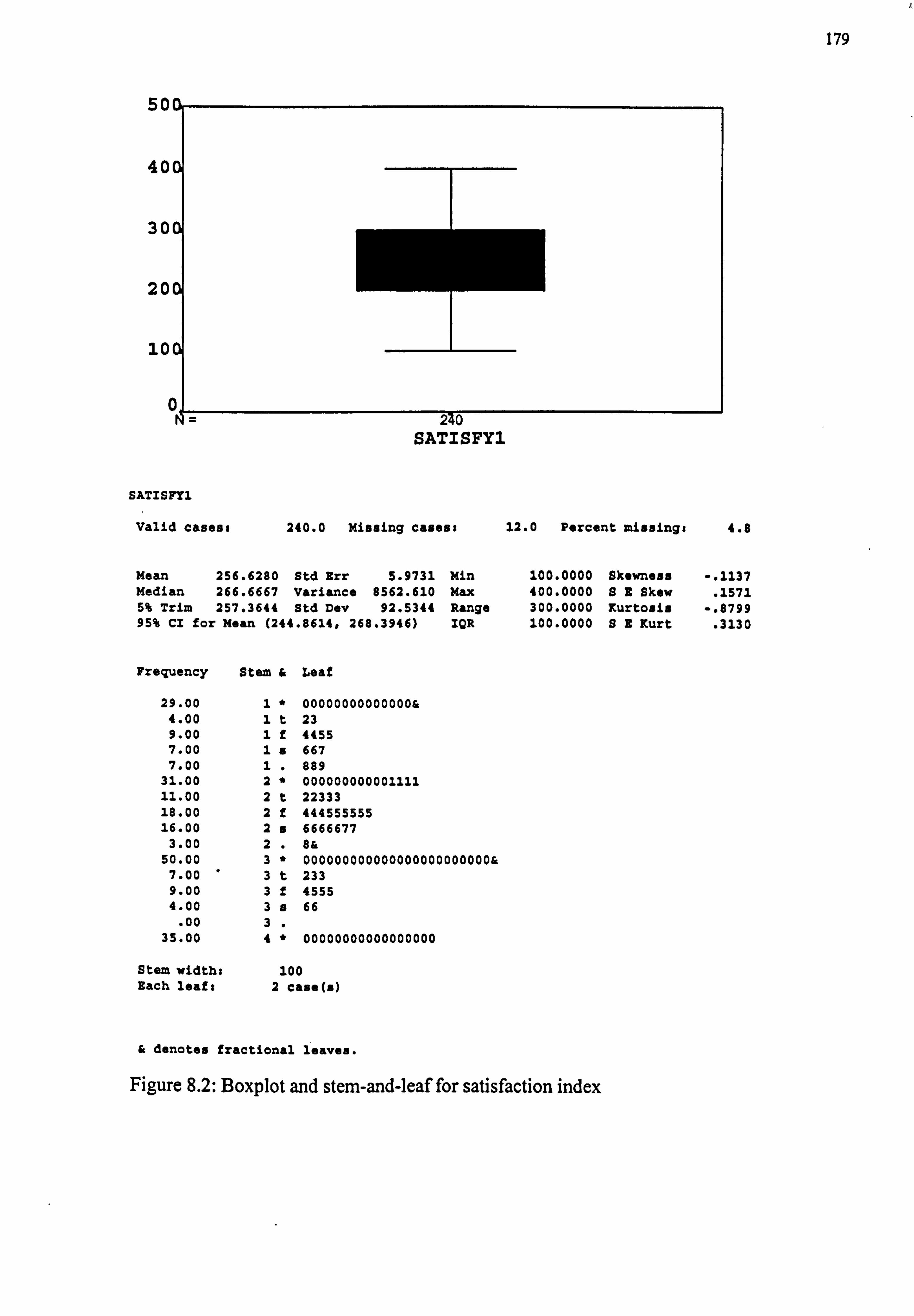
179
50
40
30
20
1o
SATISFY1
SATISFYi
Valid casess 240.0 Missing cases:
Mean 256.6280 Std Err 5.9731 Min Median 266.6667 Variance 8562.610 Max 5% Trim 257.3644 Std Dev 92.5344 Range 95% Cl for mean (244.8614,268.3946) IQR
Frequency Stem & Leaf
29.00 1 * 00000000000000& 4.00 1 t 23 9.00 1 f 4455 7.00 1 s 667 7.00 1 . 889
31.00 2 * 000000000001111 11.00 2 t 22333 18.00 2 f 444555555 16.00 2 s 6666677
3.00 2 . 8& 50.00 3 " 000000000000000000000000&
7.00 ' 3 t 233 9.00 3 f 4555 4.00 3 s 66
. 00 3 . 35.00 4 * 00000000000000000
Stem width: 10 0 Each leafs 2c ase(s)
12.0 Percent missings 4.8
100.0000 Skewness -. 1137 400.0000 88 Skew . 1571 300.0000 Kurtosis -. 8799 100.0000 SS Kurt . 3130
& denotes fractional leaves.
Figure 8.2: Boxplot and stem-and-leaf for satisfaction index
180
8.4.3 Maintenance Costs - (MAINTCST)
The collection of the data on this variable has been discussed in chapter Two. This criterion is one of the three indices employed in assessing maintenance need requirements. An
exploratory boxplot analysis of the data on historic maintenance cost criterion for
maintenance requirement shows that it is highly skewed (skewness = 2.0). Whilst this
feature may not pose a serious threat to further confirmatory analysis were the criterion an independent variable, the situation will change when the criterion is employed as a dependent variable, as it is in this case.
The boxplot in Figure 8.3 and stem & leaf frequency display in Table 8.2 show that there
are a total of 24 outliers and extreme values in the data set which have exerted an undue influence upon the values of the mean and standard deviation (after Hartwig and Dearing,
1979). As can be seen from Tables 8.2 and 8.3 the elimination of these outliers and
extreme values from the data reduces the mean from 1413 to 1014, and the standard error
from 96 to 56. It is better to have statistics that describe some 90% of the original data
well than having those that describe all of the data badly (Kinnear and Gray, 1994).
Therefore it was decided to adopt the approach of removing the outliers and repeating the
analysis with the remaining 227 subject as against the original 251 (after Kinnear and Gray, 1994). This resulted in Table 8.3.
The effect of removing outliers and extreme values
A comparison of Tables 8.2 and 8.3 reveals that the kurtosis (a coefficient which measures
a property of the single-humped distribution) is reduced from 4.1611 (indicates a leptokurtic curve for the distribution of the data set when the outliers are included) to
0.3620. This indicates that the new data set adequately approximates a normal distribution
(a vital assumption for parametric analysis technique). Thus improving the goodness of
the data for subsequent analysis.
Outliers
Table 8.2 shows the outlier and extreme values to the bottom of the stem-and-leaf.
The outliers and extreme values (24 in number) are quite many as they represent 10 per
cent of the data set, and are patterned. In other words, they do not exhibit the same random
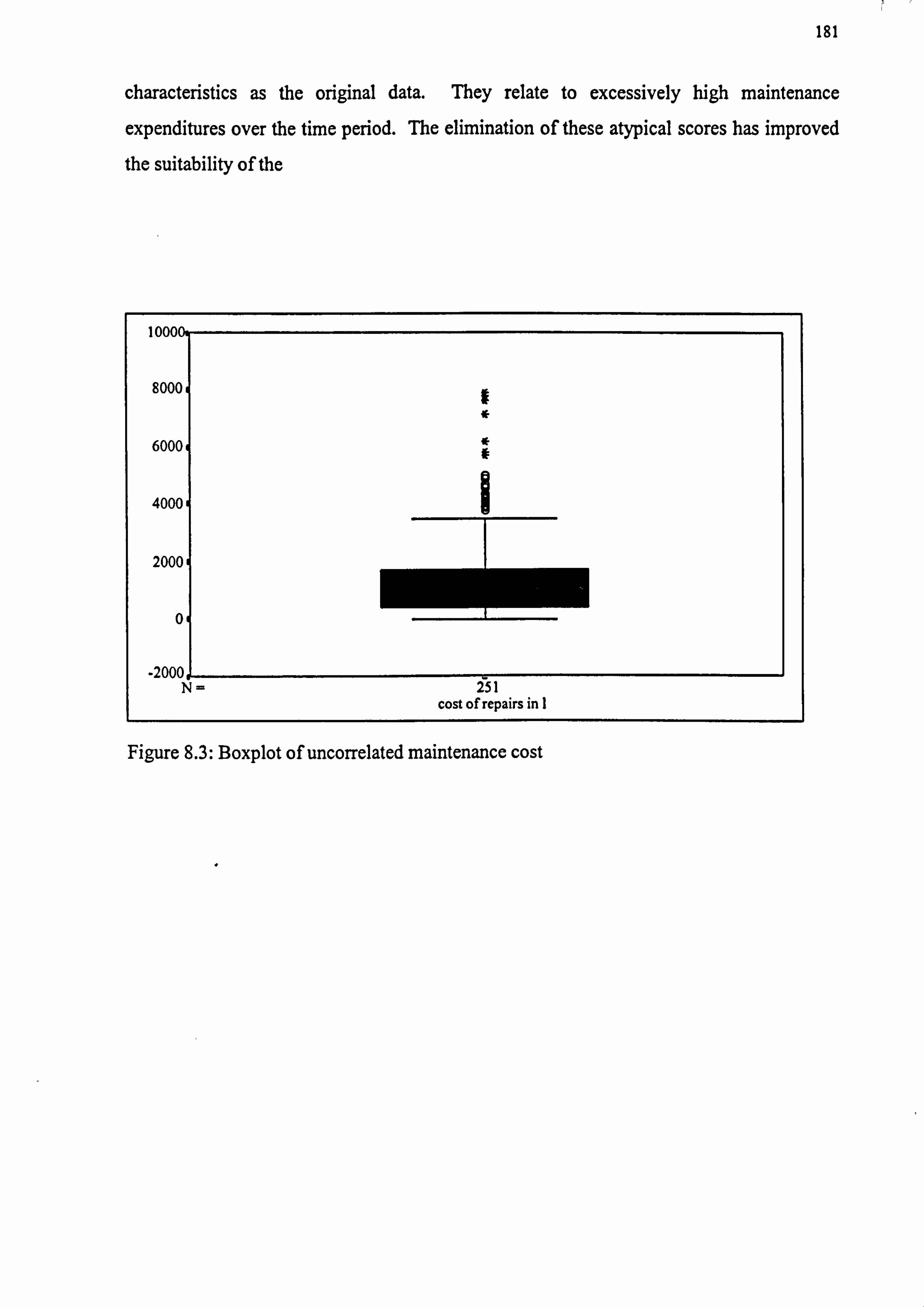
181
characteristics as the original data. They relate to excessively high maintenance
expenditures over the time period. The elimination of these atypical scores has improved
the suitability of the
I
8000
6000
4000
2000
0
-2000 251 cost of repairs in I
Figure 8.3: Boxplot of uncorrelated maintenance cost
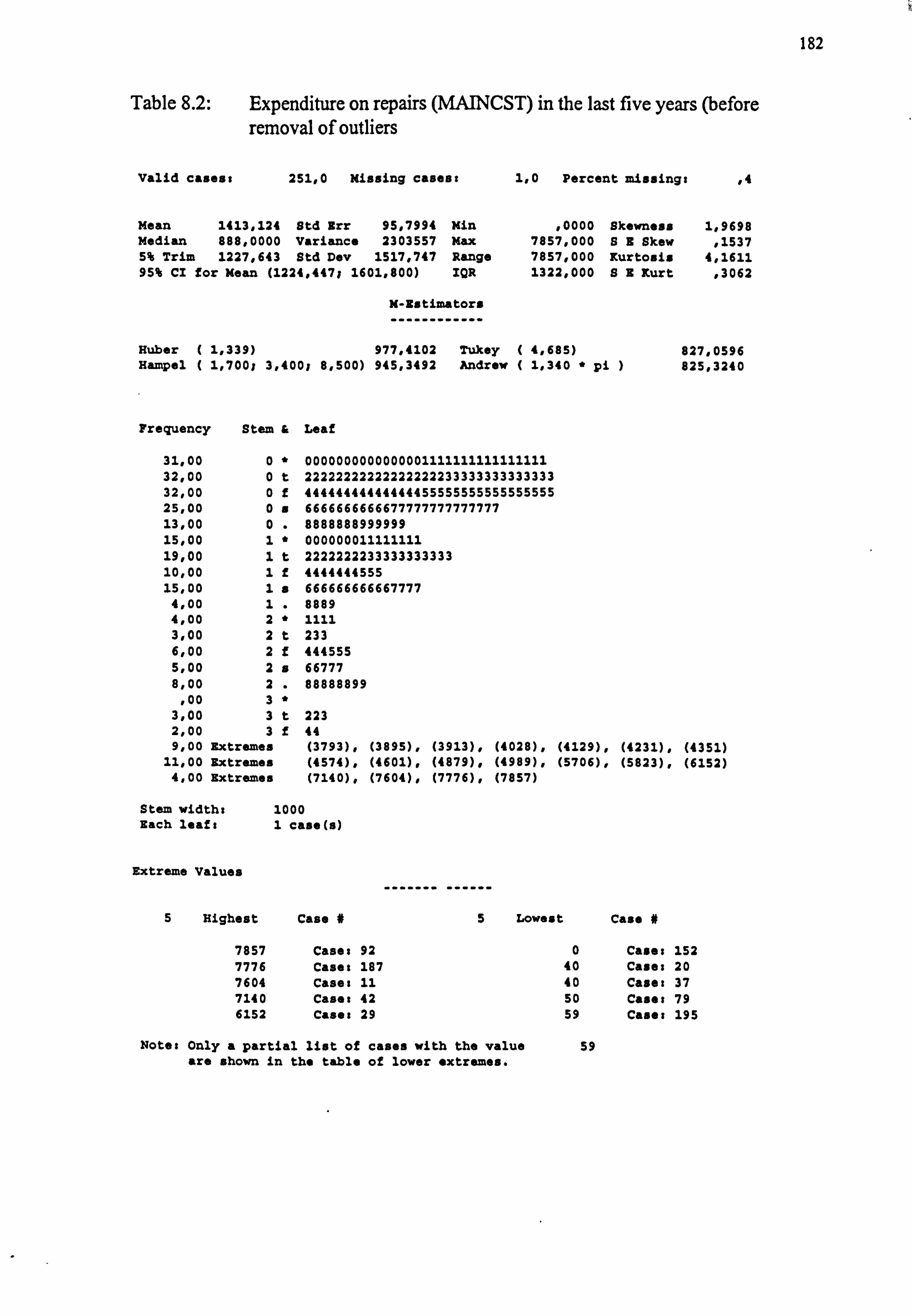
182
Table 8.2:
Valid casess
Expenditure on repairs (MAINCST) in the last five years (before removal of outliers
251,0 Missing cases: 1,0 Percent missing: ,4
Mean 1413,124 Std Err Median 888,0000 Variance 5% Trim 1227,643 Std Dev 95% Cl for Mean (1224,4471 16
Huber ( 1,339) Hampel ( 1,7001 3,400; 8,500)
Frequency Stem & Leaf
95,7994 2303557
1517,747 01,800)
M-Ei tu
977,4102 945,3492
Min , 0000 Skewness Max 7857,000 S8 Skew Range 7857,000 Kurtosis IQR 1322,000 8B Kurt
nators
Tukey ( 4,685) Andrew ( 1,340 * pi
1,9698
, 1537 4,1611
, 3062
837,0596 825,3240
31,00 0 * 0000000000000001111111111111111 32,00 0 t 22222222222222222233333333333333 32,00 0 f 44444444444444455555555555555555 25,00 0 s 6666666666677777777777777 13,00 0 . 8888888999999 15,00 1 * 000000011111111 19,00 1 t 2222222233333333333 10,00 1 f 4444444555 15,00 1 a 666666666667777
4,00 1 . 8889 4,00 2 * 1111 3,00 2 t 233 6,00 2 f 444555 5,00 2 a 66777 8,00 2 . 88888899
, 00 3 3,00 3 t 223 2,00 3 f 44 9,00 Extremes (3793), (3895), (3913), (4028), (4129), (4231), (4351)
11,00 Extremes (4574), (4601), (4879), (4989), (5706), (5823), (6152) 4,00 Extremes (7140), (7604), (7776), (7857)
Stem width: 100 0 Each leafs 1c ase(s)
Extreme Values
5 Highest Case *5 Lowest Case #
7857 Cases 92 0 Case: 152 7776 Cases 187 40 Cases 20 7604 Cases 11 40 Cases 37 7140 Case: 42 50 Cases 79 6152 Cases 29 59 Cases 195
Notes Only a partial list of cases with the value 59 are shown in the table of lower extremes.
183
Table 8.3:
Valid caress
Expenditure on repairs (MAINCST) in the last five years (after removal of outliers
227,0 Missing cases: 10 Percent missing, ,0
Mean 1014,441 Std Err 55,7891 Median 738,0000 Variance 706519,2 5% Trim 952,0573 Std Dev 840,5470 95% Cl for Mean (904,5073; 1124,374)
M-Estii
Huber ( 1,339) 839,6965 Hempel ( 1,7001 3,400; 8,500) 859,4752
Frequency Stem & Leaf
Min , 0000 Skewness Max 3495,000 S8 Skew Range 3495,000 Kurtosis IQR 1079,000 88 Kurt
rotors
Tukey ( 4,685) Andrew ( 1,340 * pi
31,00 0 * 0000000000000001111111111111111 32,00 0 t 22222222222222222233333333333333 32,00 0 f 44444444444444455555555555555555 25,00 0 a 6666666666677777777777777 13,00 0 . 8888888999999 15,00 1 * 000000011111111 19,00 1 t 2222222233333333333 10,00 1 f 4444444555 15,00 1 s 666666666667777
4,00 1 8889 4,00 2 " 1111 3,00 2 t 233 6,00 2 f 444555 5,00 2 a 66777 8,00 2 . 88888899 5,00 Extremes (3270), (3330), (3426)
Stem width: 10 00 Each leafs 1 case(s)
8xtreme Values ------- ------
5 Highest Case M5 Lowest
3495 Case: 209 0 3426 Cases 12 40 3330 Case: 189 40 3270 Case: 221 50 3270 Case: 223 59
Note: Only a partial list of cases with the value are shown in the table of lower extremes.
Hi-Res Chart N 2sDoxplot of maintcat
59
1,0634
, 1615
, 3620
, 3217
759,4013 753,6132
Case
Cases 152 Cases 20 Cases 37 Cases 79 Cases 168
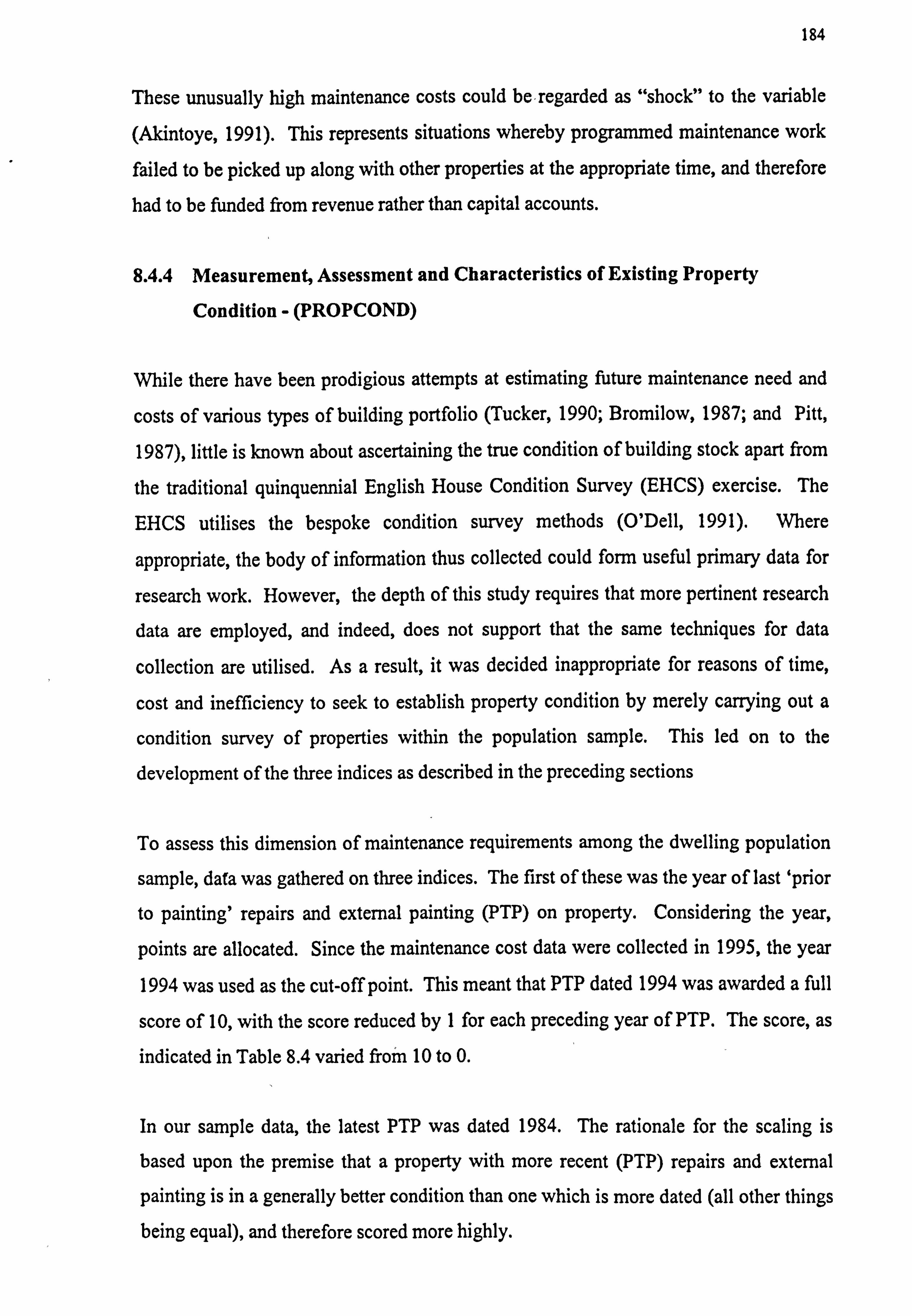
184
These unusually high maintenance costs could be regarded as "shock" to the variable
(Akintoye, 1991). This represents situations whereby programmed maintenance work
failed to be picked up along with other properties at the appropriate time, and therefore
had to be funded from revenue rather than capital accounts.
8.4.4 Measurement, Assessment and Characteristics of Existing Property
Condition - (PROPCOND)
While there have been prodigious attempts at estimating future maintenance need and
costs of various types of building portfolio (Tucker, 1990; Bromilow, 1987; and Pitt,
1987), little is known about ascertaining the true condition of building stock apart from
the traditional quinquennial English House Condition Survey (EHCS) exercise. The
EHCS utilises the bespoke condition survey methods (O'Dell, 1991). Where
appropriate, the body of information thus collected could form useful primary data for
research work. However, the depth of this study requires that more pertinent research
data are employed, and indeed, does not support that the same techniques for data
collection are utilised. As a result, it was decided inappropriate for reasons of time,
cost and inefficiency to seek to establish property condition by merely carrying out a
condition survey of properties within the population sample. This led on to the
development of the three indices as described in the preceding sections
To assess this dimension of maintenance requirements among the dwelling population
sample, data was gathered on three indices. The first of these was the year of last `prior
to painting' repairs and external painting (PTP) on property. Considering the year,
points are allocated. Since the maintenance cost data were collected in 1995, the year
1994 was used as the cut-off point. This meant that PTP dated 1994 was awarded a full
score of 10, with the score reduced by I for each preceding year of PTP. The score, as
indicated in Table 8.4 varied from 10 to 0.
In our sample data, the latest PTP was dated 1984. The rationale for the scaling is
based upon the premise that a property with more recent (PTP) repairs and external
painting is in a generally better condition than one which is more dated (all other things
being equal), and therefore scored more highly.
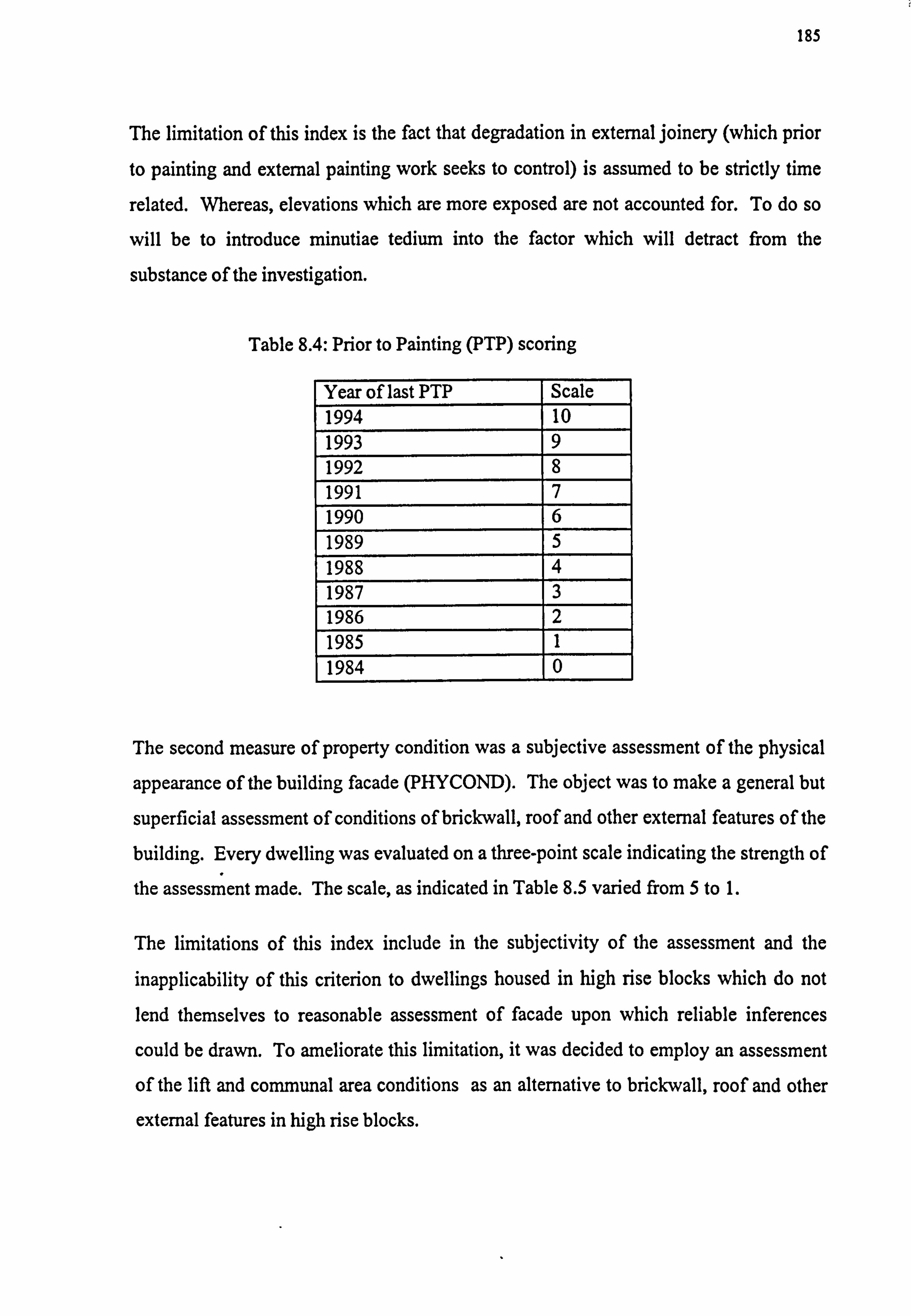
185
The limitation of this index is the fact that degradation in external joinery (which prior
to painting and external painting work seeks to control) is assumed to be strictly time
related. Whereas, elevations which are more exposed are not accounted for. To do so
will be to introduce minutiae tedium into the factor which will detract from the
substance of the investigation.
Table 8.4: Prior to Painting (PTP) scoring
Year of last PTP Scale 1994 10 1993 9 1992 8 1991 7 1990 6 1989 5 1988 4 1987 3 1986 2 1985 1 1984 0
The second measure of property condition was a subjective assessment of the physical
appearance of the building facade (PHYCOND). The object was to make a general but
superficial assessment of conditions of brickwall, roof and other external features of the
building. Every dwelling was evaluated on a three-point scale indicating the strength of
the assessment made. The scale, as indicated in Table 8.5 varied from 5 to 1.
The limitations of this index include in the subjectivity of the assessment and the
inapplicability of this criterion to dwellings housed in high rise blocks which do not
lend themselves to reasonable assessment of facade upon which reliable inferences
could be drawn. To ameliorate this limitation, it was decided to employ an assessment
of the lift and communal area conditions as an alternative to brickwall, roof and other
external features in high rise blocks.
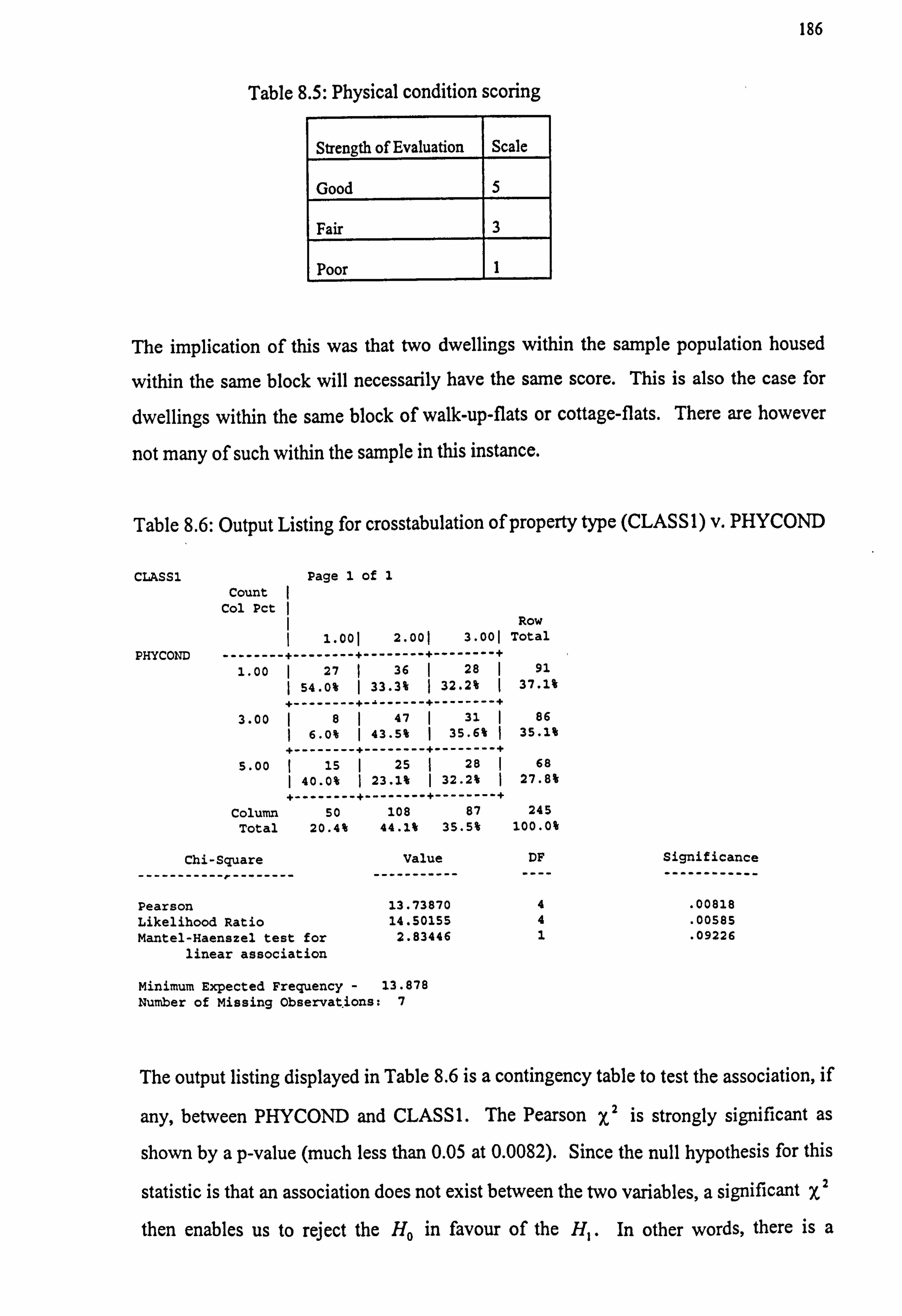
186
Table 8.5: Physical condition scoring
Strength of Evaluation Scale
Good 5
Fair 3
Poor I
The implication of this was that two dwellings within the sample population housed
within the same block will necessarily have the same score. This is also the case for
dwellings within the same block of walk-up-flats or cottage-flats. There are however
not many of such within the sample in this instance.
Table 8.6: Output Listing for crosstabulation of property type (CLASS 1) v. PHYCOND
CLASSI Page 1 of 1 Count
Col Pct Row
1.001 2.001 3.001 Total
PHYCOND ------------------------------------ 1.00 I 27 ý 36 I 28 I 91
54.0% 133.3% 32.2% ý 37.1%
---------------------------- 3.00 8ý 47 31 I 86
6.0% 143.5% 35.6% ý 35.1%
---------------------------- 5.00 ý 15 I 25 ý 28 I 68
40.0% 23.1% 132.2% ý 27.8%
---------------------------- Column 50 108 87 245
Total 20.4% 44.1% 35.5% 100.0%
Chi-Square Value -------------------- -----------
DF ----
Significance ------------
Pearson 13.73870 4 . 00818 Likelihood Ratio 14.50155 4 . 00585
Mantel-Haenszel test for 2.83446 1 . 09226
linear association
Minimum Expected Frequency - 13.878 Number of Missing observations: 7
The output listing displayed in Table 8.6 is a contingency table to test the association, if
any, between PHYCOND and CLASS 1. The Pearson x2 is strongly significant as
shown by a p-value (much less than 0.05 at 0.0082). Since the null hypothesis for this
statistic is that an association does not exist between the two variables, a significant x2
then enables us to reject the H. in favour of the H,. In other words, there is a
187
statistical association between PHYCOND and CLASS 1. This conclusion then requires
that the contingency table be closely studied to discover any underlying pattern of
association between the three classes of properties. The table reveals that 54% of high
rise dwellings are classified as poor whilst only about a third of both low rise flats and
houses are classified as poor. This accords, if not in magnitude, but at least in direction
with social expectation. On this account, the reliability of the scoring of the dwellings
on the variable is confirmed. Hence, the shortcomings of the index do not have
significant bearing upon its validity.
It is note worthy that the highest score on this index is 5 whilst the lowest is 1. It was decided not to maintain parity of score with the two other indices because of the
comparatively high subjectivity of the index.
A third measure of property condition, Propensity to carry out Repair (REPLIKE3) was
constructed from tenant's responses to Question No. 8 of the questionnaire in which
tenants were asked "how likely they were to carry out repairs identified in earlier Question No. 6" by themselves. Since the index, labelled REPLIKE3 is intended to
measure the willingness of tenants to repair, it is developed by the transformation of the
highest level of Likert scale shown by the respondent.
The transformation is given as follows:
REPLIKE3 = 3N -2
Where N is the numerical score assigned to a Likert response on the questionnaire instrument.
The object of the transformation is to achieve highest and lowest possible scores of 10
and 1 respectively. The limiting factor on this index is the fact that aged or disabled
tenants may not be able to repair, but may nevertheless possess attitude which enables
them to keep property in good condition.
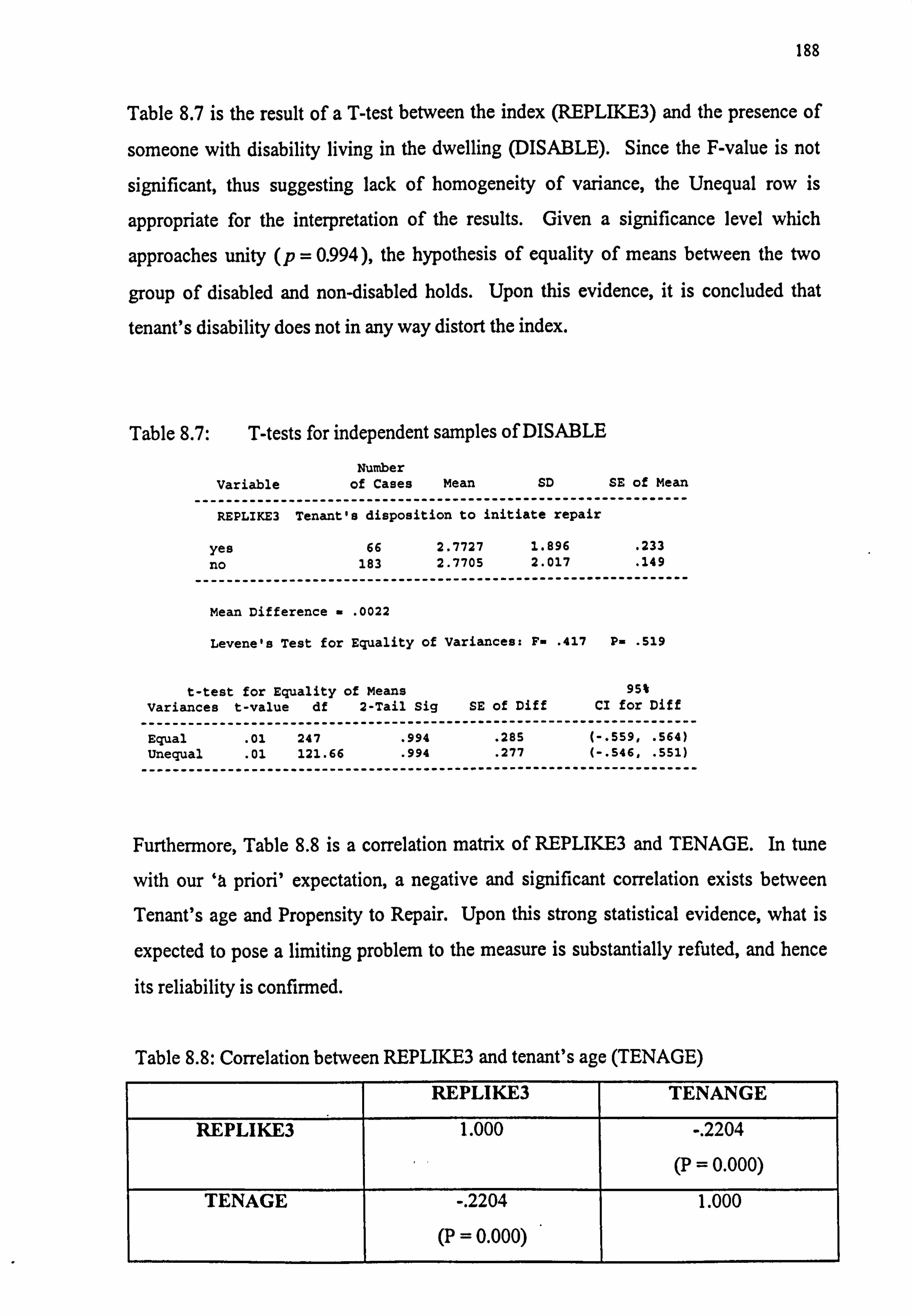
188
Table 8.7 is the result of a T-test between the index (REPLIKE3) and the presence of
someone with disability living in the dwelling (DISABLE). Since the F-value is not
significant, thus suggesting lack of homogeneity of variance, the Unequal row is
appropriate for the interpretation of the results. Given a significance level which
approaches unity (p = 0.994), the hypothesis of equality of means between the two
group of disabled and non-disabled holds. Upon this evidence, it is concluded that
tenant's disability does not in any way distort the index.
Table 8.7: T-tests for independent samples of DISABLE
Number Variable of Cases Mean SD SE of Mean
--------------------------------------------------------------- REPLIKE3 Tenant's disposition to initiate repair
yes 66 2.7727 1.696 . 233
no 183 2.7705 2.017 . 149
---------------------------------------------------------------
Mean Difference - . 0022
Levene's Test for Equality of Variances: F. . 417 P. . 519
t-test for Equality of Means 95% Variances t-value df 2-Tail Sig SE of Diff CI for Diff
----------------------------------------------------------------------- Equal . 01 247 . 994 . 285 (-. 559, . 564) Unequal . 01 121.66 . 994 . 277 (-. 546, . 551)
-----------------------------------------------------------------------
Furthermore, Table 8.8 is a correlation matrix of REPLIKE3 and TENAGE. In tune
with our ` priori' expectation, a negative and significant correlation exists between
Tenant's age and Propensity to Repair. Upon this strong statistical evidence, what is
expected to pose a limiting problem to the measure is substantially refuted, and hence
its reliability is confirmed.
Table 8.8: Correlation between REPLIKE3 and tenant's age (TENAGE)
REPLIKE3 TENANGE
REPLIKE3 1.000 -. 2204
(P = 0.000)
TENAGE -. 2204 1.000
(P = 0.000)
189
Limitation of the measure
One would surmise that if the three criteria namely; date of last PTP action, physical
(facade) condition and tenant's propensity to Repair severally contribute to a common
phenomenon as property condition being measured, then they should each be
independent one of another. In other words, any correlation between them should be
one of chance rather than of any systematic relationship. In this regard, the existence of
any association between REPLIKE3 (Tenant's propensity to repair) and any of the
other two can easily be discountenanced without proof. However, at face value, it is
not plausible to attribute a relationship of sort between PTP and PHYCOND to chance.
Indeed, the possibility exists that a more recent PTP action may have meant that more
repairs to the external elements, (which the index PHYCOND measures), have had to
be carried out as an adjunct to PTP action. If this proved to be the case, the
consequence is that the two criteria significantly measure the same attribute (covariance
is high), and hence an unwarranted statistical duplicity of measures. This position is
not supported by the Covariance matrix of the regression of PHYCOND on PTP, with a
low, though significant ß coefficient of 0.0664.
Similarly, the coefficient between PHYCOND and REPLIKE3 (tenant's propensity to
repair) is both sufficiently insignificant and low (ß = 0.0733, p=0.252) to support the
hypothesis of non-existence of co-relation. In practice, a systematic relationship is
unthinkable. How many tenants would take it upon themselves to provide an external
facelift to properties. This is practically unexpected. The results confirm this position.
Hence, there exists no valid basis for speculation as to the existence of a systematic
relationship between the three measures of existing property condition (PROPCOND).
Upon this moderately strong statistical evidence, it can be concluded that the construct
PROPCOND is a valid and reliable construct of maintenance requirements or need.
The distribution of the PROPCOND measure
The frequency distribution of the derived scores for Property Condition Index showed
that it is a good approximation to a normal distribution (mean =11.171, range =1-21, SD =3.854, skewness =0.013, kurtosis =-. 125).
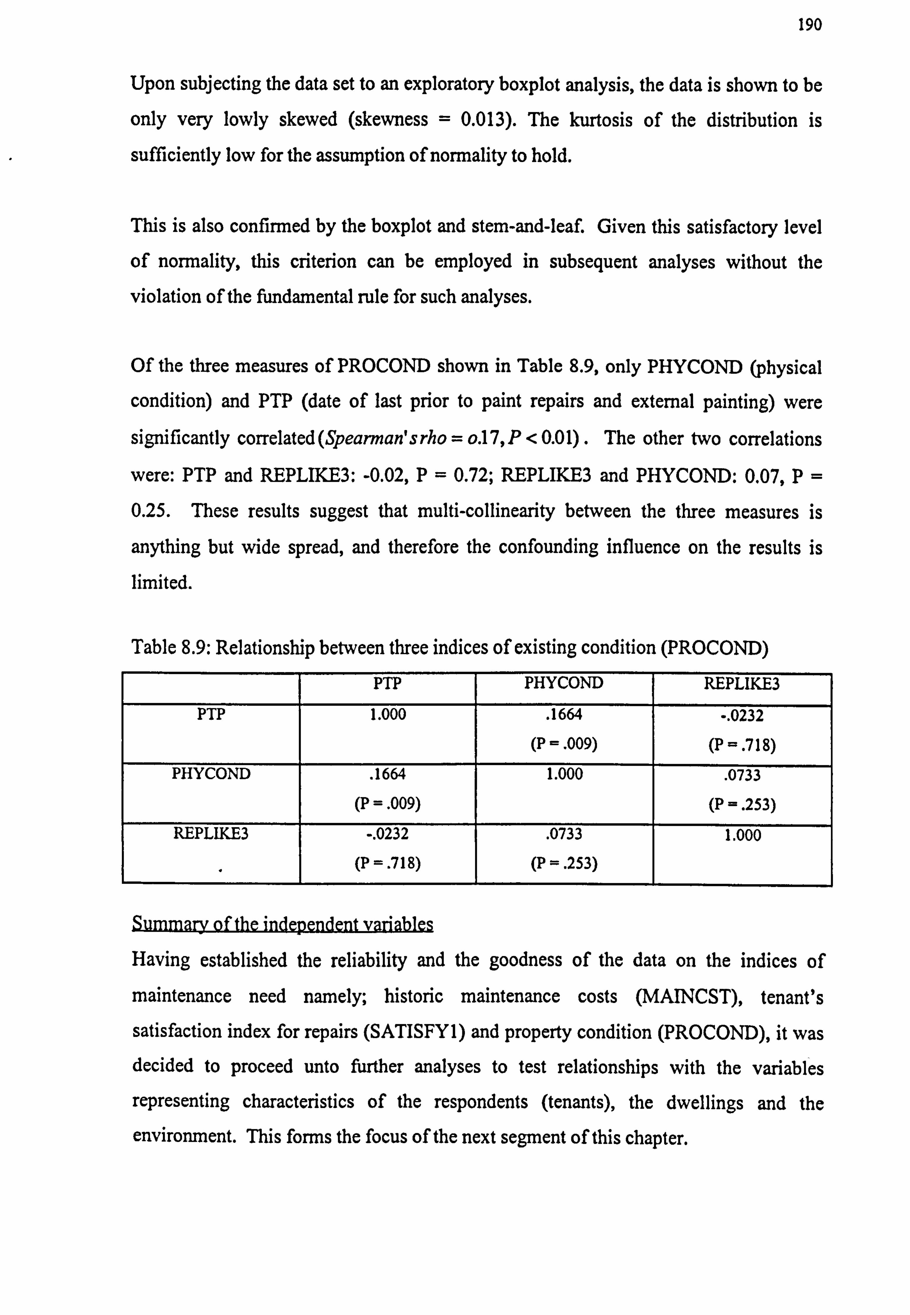
190
Upon subjecting the data set to an exploratory boxplot analysis, the data is shown to be
only very lowly skewed (skewness = 0.013). The kurtosis of the distribution is
sufficiently low for the assumption of normality to hold.
This is also confirmed by the boxplot and stem-and-leaf. Given this satisfactory level
of normality, this criterion can be employed in subsequent analyses without the
violation of the fundamental rule for such analyses.
Of the three measures of PROCOND shown in Table 8.9, only PHYCOND (physical
condition) and PTP (date of last prior to paint repairs and external painting) were
significantly correlated (Spearman's rho = o. 17, P<0.01) . The other two correlations
were: PTP and REPLIKE3: -0.02, P=0.72; REPLIKE3 and PHYCOND: 0.07, P=
0.25. These results suggest that multi-collinearity between the three measures is
anything but wide spread, and therefore the confounding influence on the results is
limited.
Table 8.9: Relationship between three indices of existing condition (PROCOND)
PTP PHYCOND REPLIKE3
PTP 1.000 . 1664 -. 0232
(P -. 009) (P =. 71 8)
PHYCOND . 1664 1.000 . 0733
(P =. 009) (P = . 253)
REPLIKE3 -. 0232 . 0733 1.000
(P =. 718) (P =. 253)
Having established the reliability and the goodness of the data on the indices of
maintenance need namely; historic maintenance costs (MAINCST), tenant's
satisfaction index for repairs (SATISFYI) and property condition (PROCOND), it was decided to proceed unto further analyses to test relationships with the variables
representing characteristics of the respondents (tenants), the dwellings and the
environment. This forms the focus of the next segment of this chapter.
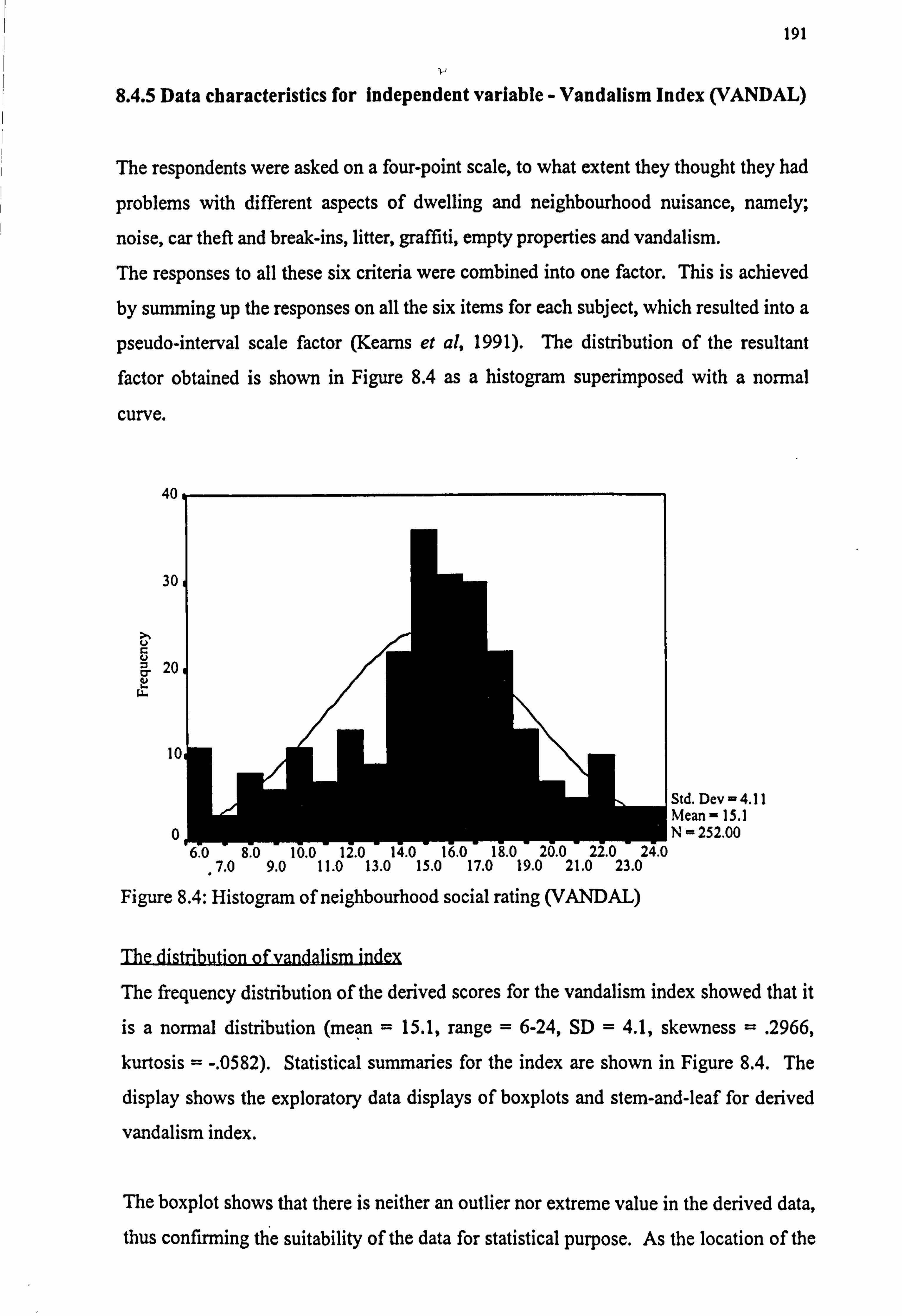
191
8.4.5 Data characteristics for independent variable - Vandalism Index (VANDAL)
The respondents were asked on a four-point scale, to what extent they thought they had
problems with different aspects of dwelling and neighbourhood nuisance, namely;
noise, car theft and break-ins, litter, graffiti, empty properties and vandalism. The responses to all these six criteria were combined into one factor. This is achieved
by summing up the responses on all the six items for each subject, which resulted into a
pseudo-interval scale factor (Kearns et al, 1991). The distribution of the resultant
factor obtained is shown in Figure 8.4 as a histogram superimposed with a normal
curve.
40
30
U
20 U P.
P.
10
0 7.0 9.0 11.0 13.0 15.0 17.0 19.0 21.0 23.0
Figure 8.4: Histogram of neighbourhood social rating (VANDAL)
Std. Dev = 4.11 Mean =15.1 N= 252.00
The distribution of vandalism index
The frequency distribution of the derived scores for the vandalism index showed that it
is a normal distribution (mean = 15.1, range = 6-24, SD = 4.1, skewness = . 2966,
kurtosis = -. 0582). Statistical summaries for the index are shown in Figure 8.4. The
display shows the exploratory data displays of boxplots and stem-and-leaf for derived
vandalism index.
The boxplot shows that there is neither an outlier nor extreme value in the derived data,
thus confirming the suitability of the data for statistical purpose. As the location of the
192
median within the box is non-eccentric, it expected that the skewness of the distribution
is minimal. This position is further corroborated by an extremely low absolute value of
the kurtosis (kurtosis = . 0582).
Validatorv check on the index
In statistical terms, the overall assessment of vandalism (an index of social location) is
significantly well-correlated with all of the six component items of social location (see
Appendix 3.1). These six items are car problem, noises problem, litter problem, graffiti
problem, empty properties and vandalism. Upon this evidence we have chosen to use
an aggregate measure composed of the scores on all of the components. All of the six
items had correlations stronger than 0.4 (at greater than 99% significance level). Given
this strong evidence, it is statistically improbable that the relationships between the
items are spurious.
In all, the six component items are significantly correlated with one another without
exception. This lends strong credence to the correctness of the choice of the social location stress indicator.
Combining all of the responses into one factor produced a Cronbach's alpha reliability
coefficient of 0.86. This suggests that the measure can act as a reasonably reliable scale to measure neighbourhood social rating index (see Appendix 3.3).
Locational consistency of the factor
Considering conventional wisdom, one would surmise that vandalism index should be
distinguishable along location. Indeed, the M22 category chosen for the survey is
believed to be safer for insurance purposes than the M8 category.
This position is unsupported by the analysis of the responses. As shown in Appendix
3.2, the chi-square is not significant (at 95% level of significance) between the two locations on any of the six component items. It is intriguing to note that none of the six
criteria possesses a significant chi-square on location. However, a probability of 0.06241 obtained for empty properties (EMPTPROB) is far from being unequivocal. Even though this is still not significant, it is useful to know in which `direction the lever
193
tilts'. This low probability purports that problem with empty properties, is more
rampant in M22/23 (South) than M8/9 (North).
The consistency of the index is further confirmed by a t-test analysis as follows: Car
theft problem in area (t-value = 1.59; P=0.113); Noise problem in area (t-value = . 90;
P=0.368); Litter problem in area (t-value = -. 94; P=0.347); Graffiti problem in area
(t-value = -. 21; P=0.835); Empty property problem in area (t-value = 1.7; P=0.092);
and vandalism problem in area (t-value =. 73; P=0.465). See Appendix 3.4 for details.
Going by the rule of probability, any observable difference between the two areas of the
city must be due to chance occurrence. In reality, it is not uncommon to have pockets
of areas which do not exhibit the same characteristics as the broader stereotypification
of the larger area. Considering this finding, it is concluded that the decision to assess
this criterion (social location vandalism rating) on individual dwelling basis is anything
but misplaced.
8.5 Variables selection
It is practically impossible, and in fact not very useful to include in each segment of the
investigation all measured variables (Sanders and Thomas, 1992). Rather, the set of
variables to be analysed in each case is selected from the total set of variables whilst
ensuring that the testing of the hypothesis is objective and thorough. This approach is
supported by Nkado (1991), Gilchrist (1984) and Beeston (1983). It has been indicated
by these exponents that the identification of potentially relevant variables is all a matter
of imagination and common sense.
8.5.1 The independent variables
The dependent variables can be classified into two categories for the purpose of this
study namely; interval and non-interval variables (all discussed in chapter two). These
variables belong to one or more of the following categories: tenant variables, variables
allowing the investigation of how the characteristics of the building object impacts on
maintenance requirements, environmental variables and variables describing housing
management.
194
8.5.1.1 Tenant Attributes
There are a number of variables that measure the characteristics of occupier of a
residential property including the number of children in dwelling (CHILDCT), attitude to repair problems (REPIRATT), Right-To-Buy speculation (RTBCOMP), gender (GENDER), restraints on physical mobility (DISABLE), move plan, i. e. residential
stability (MOVEPLAN), length lived in last home (LENTLAST) and length live in
current home (LENTLIVE), employment status (TEMPLOYI) and age (TENAGE).
Together, they give an insight into the behaviour and influence of the tenants as they
impact upon the dwelling and hence on maintenance need.
The following variables were included in the analysis and were subsequently entered on
step number.
1.. CHILDCT Number of children in dwelling
2.. VANDAL New variable derived from vandalism index
3.. RESREPIR council's response to repair
4.. REPIRATT attitude to repair problems 5.. PROPAGE age of property 6.. LOCATION
7.. RTBCOMP Right-to-buy speculation (RTB)
8.. HSGOFFS assessment of service from housing office 9.. GENDER
10.. DISABLE presence of disability or limiting illness
11.. RELETI
12.. MOVEPLAN likelihood of moving from present home
13.. RESVANDL council's response to vandalism 14.. LENTLAST length lived in last home
15.. LENTLIVE Length lived in current home
16.. FLAREA floor area 17.. TENAGE tenant's age 18.. CLASSI Class of dwelling (dwelling type)
19.. BED number of bedrooms
20.. SIZE size of property
195
8.5.1.2 Property Attributes
This family of variables has been dealt extensively with in chapters six and seven. As a
follow-up to these with other variables, we have nevertheless, because of the different
methodological framework employed for this segment of the analyses, included some
measurable property variables in the analysis. The conclusions arrived at confirm the
inference drawn from those analyses. The variables which are tested include the age of
dwelling, floor area, dwelling type and number of bedrooms, none of which eventually
proved to be significant.
8.5.1.3 Environmental Attributes
An environment inhabited by man is subject to wear, decay, attrition and destruction
(Ward, 1973). A major environmental influence which exacerbates degradation process
is labelled vandalism.
Architectural social theory contends that social behaviour of tenants is influenced by
the form of housing design, hence, vandalism as a social behaviour is inherent in the
design (Newman, 1972). This theory has been described by Ward (1973) as one of
social escapism seeking to shift the responsibility from the social deviant to the social
enhancer. A housing estate is a community of dwellings which share common
environmental characteristics prominent of which is geography. The characteristic of
an estate environment is an amalgam of complex inter-relationships. There exists the
danger of over-simplification in an attempt by social theorists to find meaning to what is typically a complex web of social and technological network. In reality, an
environment is constantly undergoing symbiotic processes. The individuals who live in
an environment constantly influence it, whilst the environment influences the
individuals. In the final analysis, it is this complex symbiosis that eventually determines what an estate is and will be in terms of its overall characteristics.
A useful index for assessing the quality of a human environment is possibly the extent
of damage to properties (built and otherwise) in the environment, which quite often does reflect on the general tidiness of the area. Thus portraying the result of the quality
196
of human interaction with that environment. To this end, Crosby (1985) attempted to
develop an environmental status index which essentially comprised of an evaluation of
social changes in the area and the physical environment.
In his study of user - responses to housing environments, Crosby (1985) demonstrated
that residential property conditions vary according to the environmental status of the
area in which property is located. The major environmental variables identified by him
are social changes in the area as well as the physical environment. It is therefore
possible that these two characteristics, in the main, will influence the maintenance
requirements of a property. The variables that could be tested under this grouping are Vandalism index and location.
8.5.1.4 Property Management Attribute
This group of variables is a measure of the attitude of the housing management team to
reported property defects or identification of these defects. Whilst it is possible to 4 argue that these attributes are not truly variable, they actually fall short of being `a
given' as every housing management team operates under some sorts of constraints be
it political, operational or financial. This group of variables includes Council's
response to repair (RESREPIR), quality of service from housing officers (HSGOFFS)
and councils response to vandalism (RESVANDL).
8.5.2 Characteristics of the Non-Interval variables
Table 8.13 shows the frequency distributions of the listed variables on the non-interval
scale.
The dwellings within the sample population are classified into flats in high rise;
constituting 21% of the sample size, flats in low rise 43%, and houses constituting 36%.
197
Table 8.10 shows that 74% of the tenants within the sample are unlikely to seek a move from dwelling in the future, whilst 26% hope to move sooner or later. Almost all (98%) the dwellings have central heating. In almost 77% of the dwellings, no child was
present. This appears to account for the high per cent of those who are unlikely to
move in comparison with those who are likely, which in turn may be accounted for by
the high average age of main tenants. This is coroborated by the fact that 74% of the
respondents are above the age of 45years.
In 73% of the cases, only one adult lives in dwelling with or without children. 48% of
the respondents are men whilst 52% are women. Sixty-eight per cent of the sample do
not express any Right-to-buy speculation on their property. Only a few, about 13% of dwellings have had relet work carried out on them. This indicates that tenants are
generally very stable.
Appendix 3.5 shows that the chi-square statistics on dwelling types for variables
MOVEPLAN, RESNUISE, RESREPIR, RESVANDL, HSGOFFS, REPIRATT,
GENDER, TENAGE and DISABLE are greater that 0.05; and therefore insignificant.
This is not surprising, as it is undesirable to have these variables exhibit characteristics
patterned along the line of dwelling type. Thus confirming the lack of bias within the
sample data. However, the relationship between dwelling type and the four other
variables, namely; LOCATION, RELET, RTBCOMP and CHILDCT are significant.
This implies that there is some dependence between dwelling type and each of the four
variables. Except for location, the results are expected. A significant relationship with
relet indicates that some dwelling types are more prone to being void than others. As
indicated in the crosstab of Appendix 3.5,53% of all relets relate to cottage flats, with
34% to high rise flats and 13% to houses. An underlying cause for this is partly in the
design and subsequent dampness problems which are more prevalent with cottage flats
(Housing NEWS, undated).
198
Table 8.10: Frequency tables for the dependent variables MOVEPLAN likelihood of moving from present home
Valid Cum Value Label Value Frequency Percent Percent Percent
very unlikely 1 100 39.7 44.8 44.8 unlikely 2 65 25.8 29.1 74.0 likely 3 28 11.1 12.6 86.5 very likely 4 30 11.9 13.5 100.0 don't know 9 29 11.5 Missing
Total -------
252 -------
100.0 -------
100.0
- ---------------------------------- RESREPIR council's response to repair
Valid Cum Value Label Value Frequency Percent Percent Percent
very bad 1 23 9.1 9.1 9.1 bad 2 41 16.3 16.3 25.4 well 3 114 45.2 45.2 70.6 very well 4 55 21.8 21.8 92.5 don't know 9 17 6.7 6.7 99.2
14 1 .4 .4 99.6 33 1 .4 .4 100.0
Total -------
252 -------
100.0 -------
100.0
RESVANDL council's response to vandalism
Valid Cum Value Label Value Frequency Percent Percent Percent
very bad 1 32 12.7 12.8 12.8 bad 2 36 14.3 14.4 27.2 well 3 33 13.1 13.2 40.4 very well 4 8 3.2 3.2 43.6 don't know 9 141 56.0 56.4 100.0
2 .8 Missing
Total -------
252 -------
100.0 -------
100.0
- ------------------- RESNUISE council's response to nuisance
Valid Cum Value Label Value Frequency Percent Percent Percent
very bad 1 42 16.7 16.8 16.8 bad 2 31 12.3 12.4 29.2 well 3 36 14.3 14.4 43.6 very well 4 11 4.4 4.4 48.0 don't know 9 130 51.6 52.0 100.0
2 .8 Missing
Total -------
252 -------
100.0 -------
100.0
199
HSGOFFS assessment of service from housing office
Valid Cum Value Label Value Frequency Percent Percent Percent
very poor 1 25 9.9 9.9 9.9 poor 2 46 18.3 18.3 28.2 good 3 100 39.7 39.7 67.9 very good 4 45 17.9 17.9 85.7 don't know 9 36 14.3 14.3 100.0
Total 252 100.0 100.0
------------------------------- RTBXISE exercising right to buy right
Valid Cum Value Label Value Frequency Percent Percent Percent
never would consider 1 160 63.5 67.8 67.8 may consider it one 2 32 12.7 13.6 81.4 considered it but do 3 29 11.5 12.3 93.6 still considering it 4 15 6.0 6.4 100.0
9 16 6.3 Missing
Total 252 100.0 100.0
------------------------- REPIRATT attitude to repair problems
Valid Cum Value Label Value Frequency Percent Percent Percent
I only repairs - thr 1 45 17.9 18.1 18.1 I would rather fix m 2 57 22.6 22.9 41.0 I take time in repor 3 64 25.4 25.7 66.7 I report repairs imm 4 83 32.9 33.3 100.0
9 3 1.2 Missing
Total -------
252 -------
100.0 -------
100.0
- ---------------------------------- GENDER
Valid Cum Value Label Value Frequency Percent Percent Percent
male 1 123 48.8 48.8 48.8 female 2 129 51.2 51.2 100.0
Total 252 100.0 100.0
CIRCUM occupant's circumstance
Valid Cum Value Label Value Frequency Percent Percent Percent
0 1 .4 .4 .4 single adult without 1 142 56.3 56.3 56.7 single adult with ch 2 41 16.3 16.3 73.0 2 or more adults wit 3 52 20.6 20.6 93.7 2 or more adults wit 4 16
----
6.3 6.3 100.0
Total ---
252 -------
100.0 -------
100.0
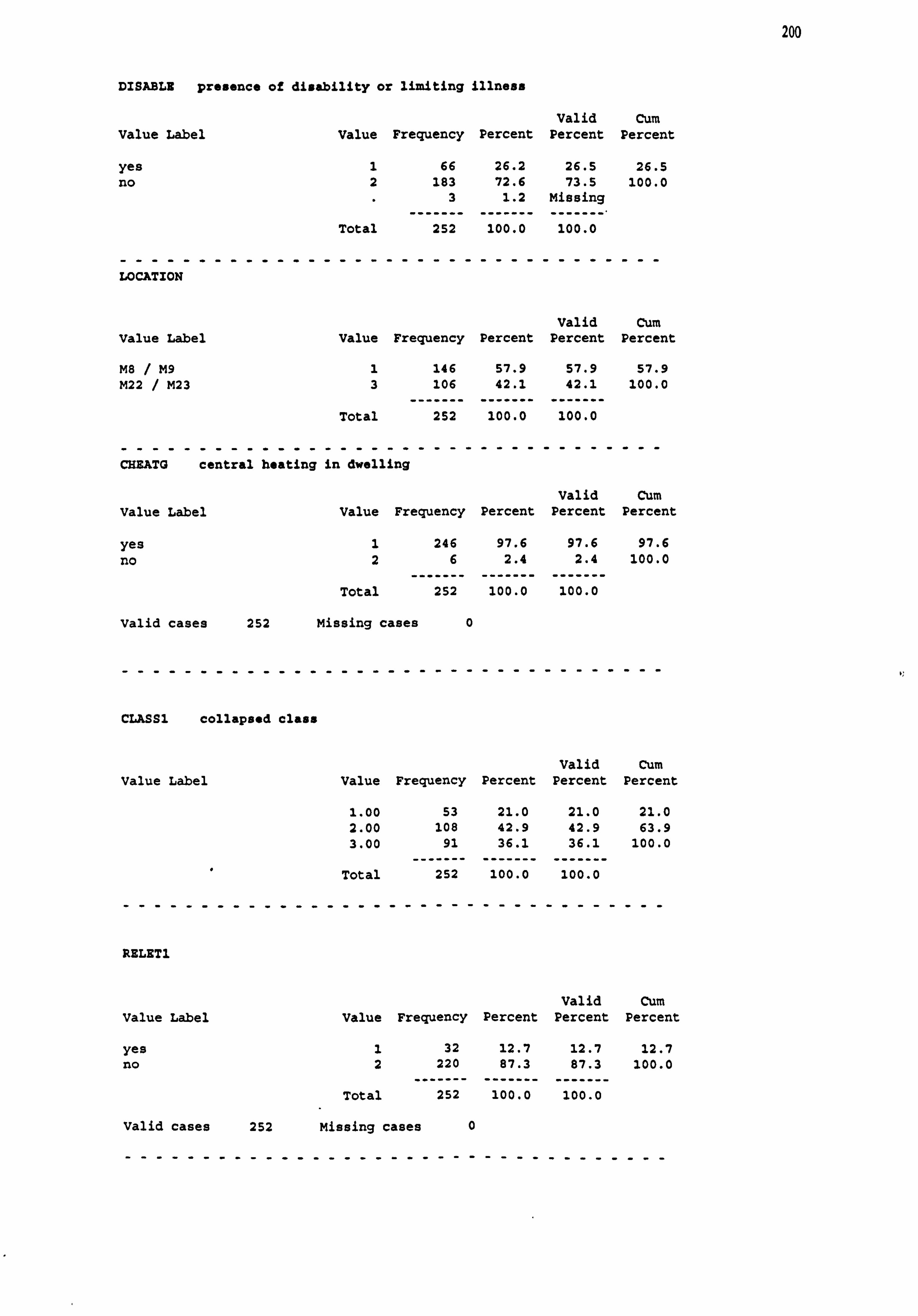
200
DISABLE presence of disability or limiting illness
Value Label Value Frequency
yes 1 66
no 2 183 3
Total 252
Percent
26.2 72.6
1.2
100.0
Valid Cum Percent Percent
26.5 26.5 73.5 100.0
Missing
100.0
LOCATION
Valid Cum Value Label Value Frequency Percent Percent Percent
M8 / M9 1 146 57.9 57.9 57.9 M22 / M23 3 106 42.1 42.1 100.0
------- ------- ------- Total 252 100.0 100.0
CHEATG central heating in dwelling
Valid Cum Value Label Value Frequency Percent Percent Percent
yes 1 246 97.6 97.6 97.6 no 26 2.4
------- 2.4
------- 100.0
------- Total 252 100.0 100.0
valid cases 252 Missing cases 0
CLASSI collapsed class
Value Label Value Frequency
1.00 53 2.00 108 3.00 91
Total 252
----------------------
Percent
21.0 42.9 36.1
100.0
Valid Cum Percent Percent
21.0 21.0 42.9 63.9 36.1 100.0
100.0
RELET1
Valid Cum Value Label Value Frequency Percent Percent Percent
yes 1 32 12.7 12.7 12.7 no 2 220
--
87.3 87.3 100.0
----- Total 252
------- 100.0
------- 100.0
Valid cases 252
-----------
Missing cases 0
------------ ---- ----- ---
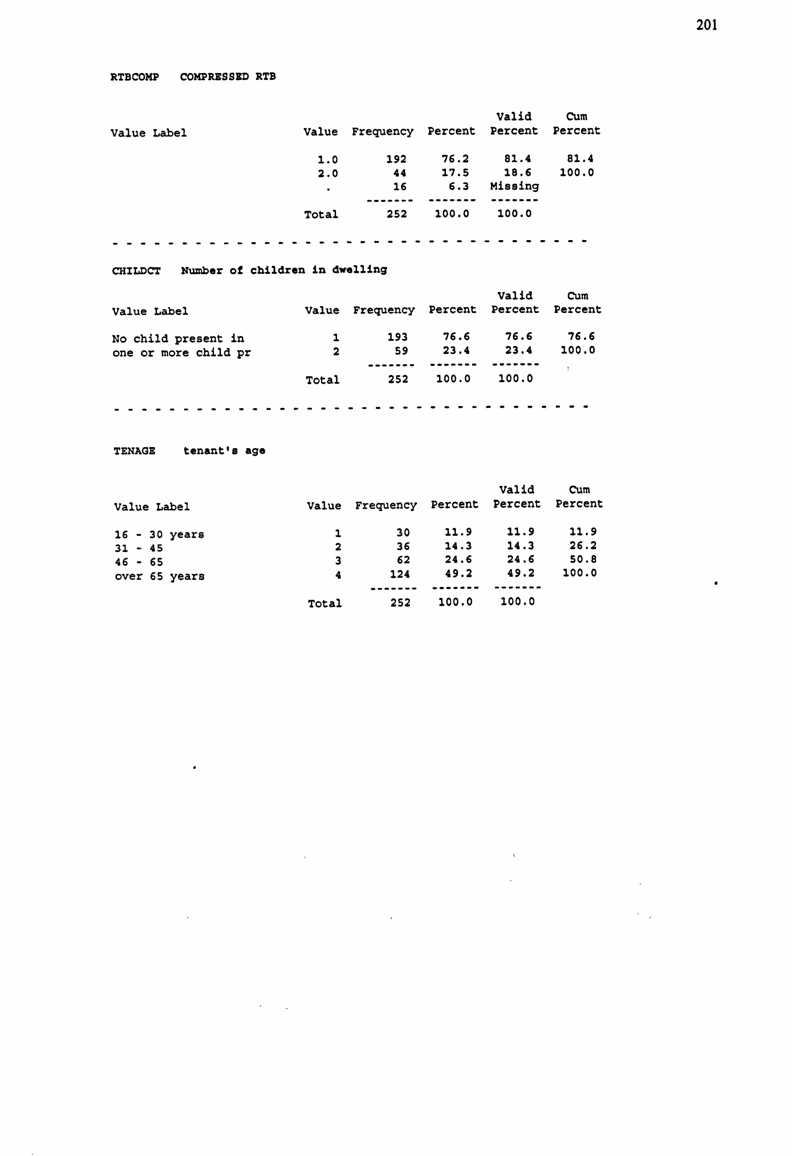
201
RTBCOMP COMPRESSED RTB
Value Label Value Frequency
1.0 192 2.0 44
16
Total 252
Percent
76.2 17.5
6.3
100.0
Valid Cum Percent Percent
81.4 81.4 18.6 100.0
Missing
100.0
CHILDCT Number of children in dwelling
Valid Cum
Value Label Value Frequency Percent Percent Percent
No child present in 1 193 76.6 76.6 76.6
one or more child pr 2 59 23.4 23.4 100.0
------- ------- ------- Total 252 100.0 100.0
TENAGE tenant's age
Valid Cum Value Label Value Frequency Percent Percent Percent
16 - 30 years 1 30 11.9 11.9 11.9
31 - 45 2 36 14.3 14.3 26.2
46 - 65 3 62 24.6 24.6 50.8
over 65 years 4 124
-
49.2
-------
49.2
-------
100.0
Total ------
252 100.0 100.0
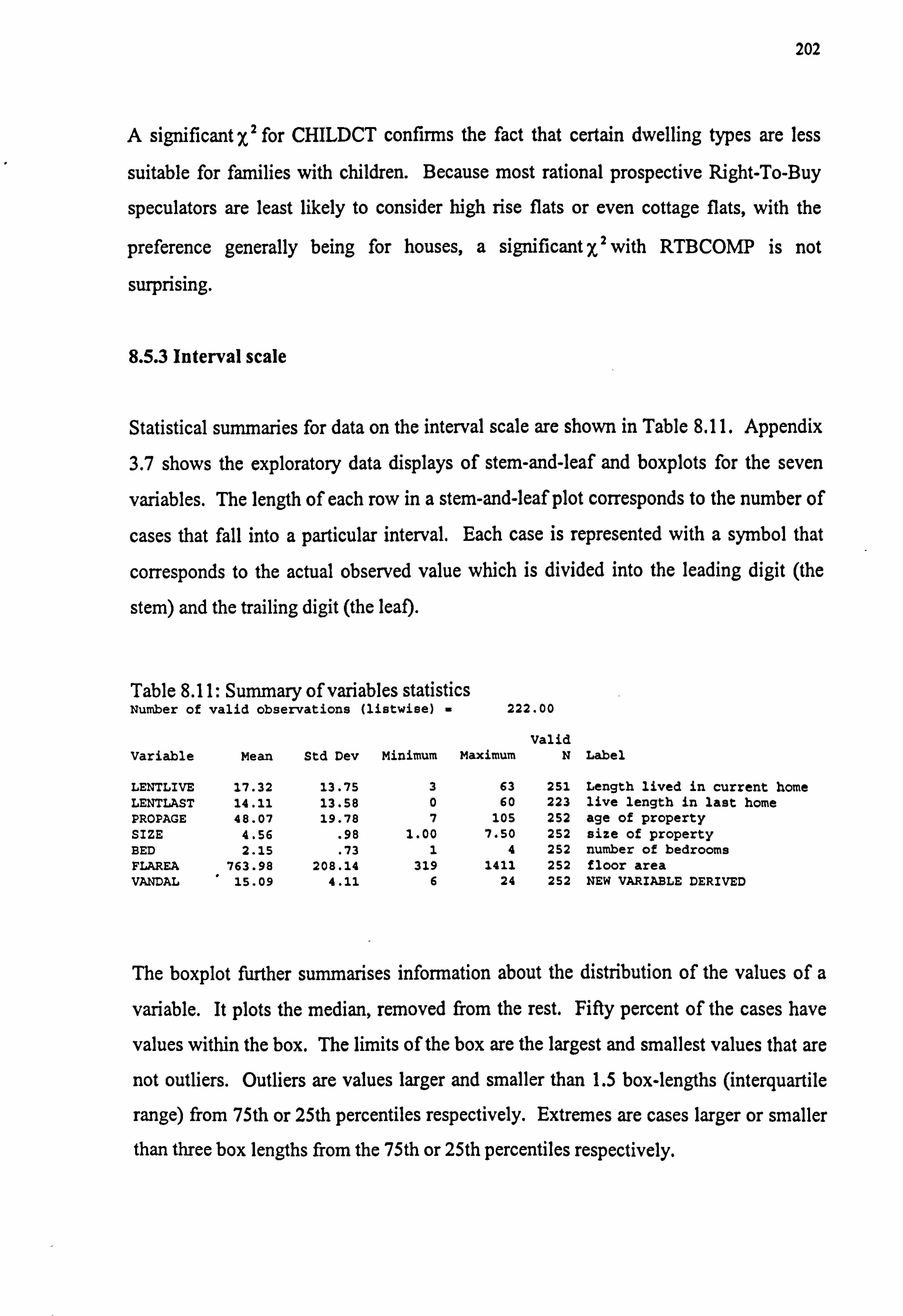
202
A significant X' for CHILDCT confirms the fact that certain dwelling types are less
suitable for families with children. Because most rational prospective Right-To-Buy
speculators are least likely to consider high rise flats or even cottage flats, with the
preference generally being for houses, a significant x2 with RTBCOMP is not
surprising.
8.5.3 Interval scale
Statistical summaries for data on the interval scale are shown in Table 8.11. Appendix
3.7 shows the exploratory data displays of stem-and-leaf and boxplots for the seven
variables. The length of each row in a stem-and-leaf plot corresponds to the number of
cases that fall into a particular interval. Each case is represented with a symbol that
corresponds to the actual observed value which is divided into the leading digit (the
stem) and the trailing digit (the leaf).
Table 8.11: Summary of variables statistics Number of valid observations (listwise) - 222.00
Valid Variable Mean Std Dev Minimum Maximum N Label
LENTLIVE 17.32 13.75 3 63 251 Length lived in current home LENTLAST 14.11 13.58 0 60 223 live length in last home PROPAGE 48.07 19.78 7 105 252 age of property SIZE 4.56 . 98 1.00 7.50 252 size of property BED 2.15 . 73 1 4 252 number of bedrooms FLAREA 763.98 208.14 319 1411 252 floor area VANDAL " 15.09 4.11 6 24 252 NEW VARIABLE DERIVED
The boxplot further summarises information about the distribution of the values of a
variable. It plots the median, removed from the rest. Fifty percent of the cases have
values within the box. The limits of the box are the largest and smallest values that are
not outliers. Outliers are values larger and smaller than 1.5 box lengths (interquartile
range) from 75th or 25th percentiles respectively. Extremes are cases larger or smaller
than three box lengths from the 75th or 25th percentiles respectively.
203
8.5.3.1 Interpretation of interval data
Three of the variables, VANDAL, FLAREA and PROPAGE are moderately normal,
whilst the remaining four show fairly skewed distributions. The sample comprises dwellings ranging in age from 7 to 105 years. The range of total gross floor area is 319
to 1411 m2 , with a mean of 766 m2 and a median value of 711 m2 .
The number of bedrooms in, and size of dwelling are discrete with very limited range. The range of number of bedrooms is 1 to 4, with mean and median value of 2. Whilst
the size ranges from 1 to 7 with mean value of 4.58, and median value of 5.38. This
explains the uniqueness of stem-and-leaf for these two variables.
8.5.4 Summary of Variables
In this section, the values of each measured variable has been considered as a separate
entity. The sample data comprises dwellings with just one and the same tenancy for
time period ranging from 3 to 62 years (µ =16.68 years). The chi-square display in
Appendix 3.5 generally accords with our a priori expectation with the exception of just
one variable - location. This has to do with sampling distribution rather than any
attribute which has to do with the validity or otherwise of the data collected. Given this
level of satisfactory interaction within the data set, detailed analysis to investigate the
relationships between these variables and other measured variables are carried out in
the next section.
8.6 Relationships between the three indices and selected variables
Analysis of the data begins with an investigation of the relationships between the three
indices and the independent variables. As the bivariate statistics in Table 8.15 indicate
location is significant only on PROPCOND. Properties in M8/9 area of the city are in
poorer condition. Surprisingly, this does not appear to affect the satisfaction of tenants in this area nor is there any evidence that this trend is predicated by differential
maintenance expenditure pattern on properties in the two areas.
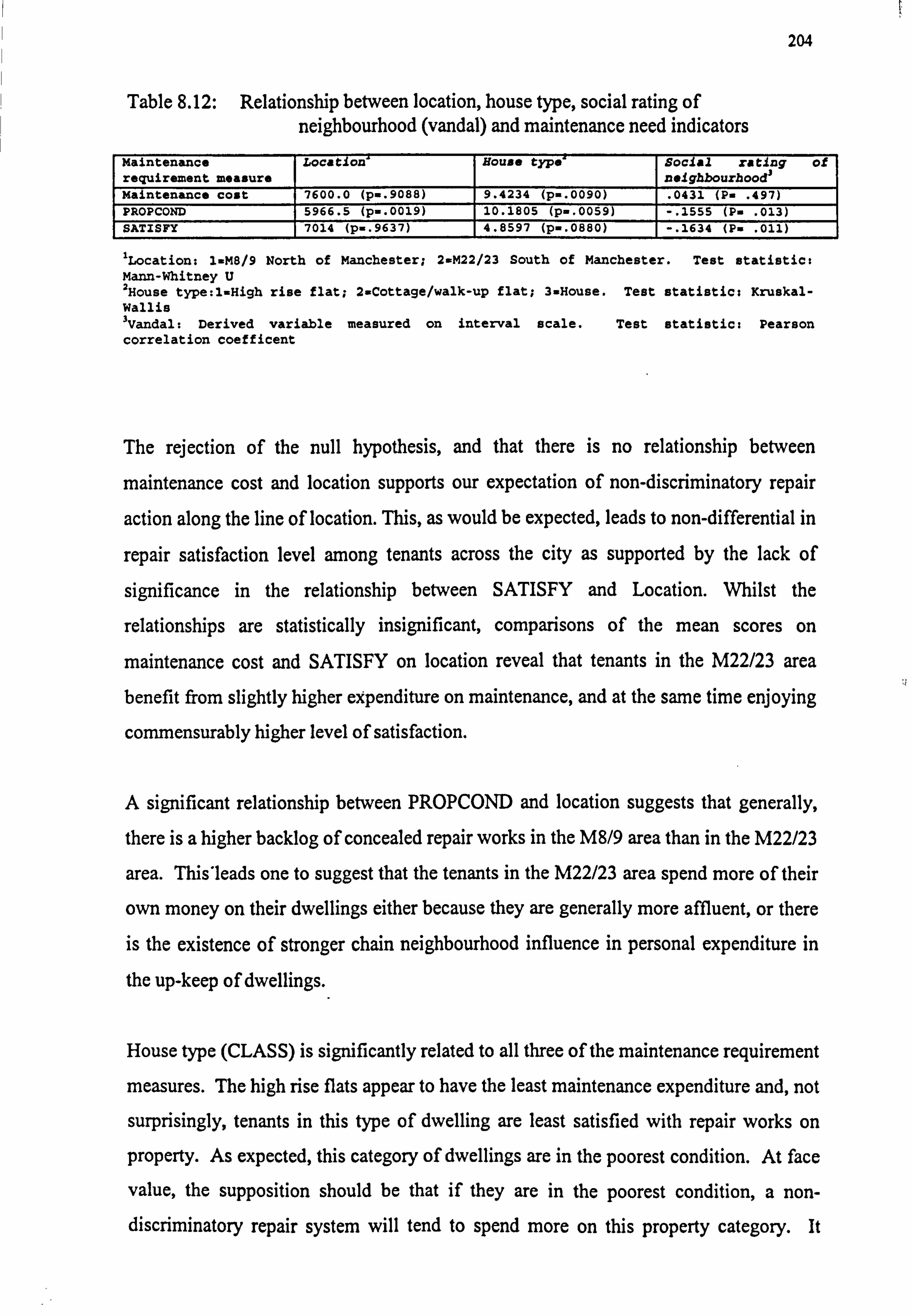
204
Table 8.12: Relationship between location, house type, social rating of neighbourhood (vandal) and maintenance need indicators
Maintenance requirement measure
Location House type Social rating of neighbourhood'
Maintenance cost 7600.0 (p.. 9088) 9.4234 (p.. 0090) . 0431 (P. . 497) PROPCOND 5966.5 (p-. 0019) 10.1805 (p-. 0059) -. 1555 (P. . 013) SATISFY 7014 (p.. 9637) 4.8597 (p-. 0880) -. 1634 (P. . 011)
1Location: 1.. M8/9 North of Manchester; 2.. M22/23 South of Manchester. Test statistic: Mann-Whitney U 2House type: l-High rise flat; 2=Cottage/walk-up flat; 3=House. Test statistic: Kruskal- Wallis 3vandal: Derived variable measured on interval scale. Test statistic: Pearson correlation coefficent
The rejection of the null hypothesis, and that there is no relationship between
maintenance cost and location supports our expectation of non-discriminatory repair
action along the line of location. This, as would be expected, leads to non-differential in
repair satisfaction level among tenants across the city as supported by the lack of
significance in the relationship between SATISFY and Location. Whilst the
relationships are statistically insignificant, comparisons of the mean scores on
maintenance cost and SATISFY on location reveal that tenants in the M22/23 area
benefit from slightly higher expenditure on maintenance, and at the same time enjoying
commensurably higher level of satisfaction.
A significant relationship between PROPCOND and location suggests that generally,
there is a higher backlog of concealed repair works in the M8/9 area than in the M22/23
area. Thisleads one to suggest that the tenants in the M22/23 area spend more of their
own money on their dwellings either because they are generally more affluent, or there
is the existence of stronger chain neighbourhood influence in personal expenditure in
the up-keep of dwellings.
House type (CLASS) is significantly related to all three of the maintenance requirement
measures. The high rise flats appear to have the least maintenance expenditure and, not
surprisingly, tenants in this type of dwelling are least satisfied with repair works on
property. As expected, this category of dwellings are in the poorest condition. At face
value, the supposition should be that if they are in the poorest condition, a non- discriminatory repair system will tend to spend more on this property category. It
205
would only be reasonable to expect this where property condition is not conditioned by
the attitude of the tenants or a group of tenants. Hence, it is unrealistic to expect that
every act of vandalism within the dwelling would qualify for immediate repair by the
housing management team.
Between the low rise flats and houses, the issue is more difficult to interpret. Whilst
houses generally score more highly on both maintenance expenditure and PROPCOND,
the low rise flats dwellers are generally more satisfied with repair works on properties.
This implies that house dwellers are generally more demanding on the repair system.
This may have an underlying explanation in the creation of artificial repair needs by
house tenants, who because of their circumstance are more disposed to having children
in dwelling and are generally of lower age brackets. These categories of tenants, as
shown by experience, tend to be `defect prone' and litigous by being more disposed to
using the legal aid facilities in `twisting the hands' of housing officers to carry out
repairs.
There are significant relationships between social rating of dwelling (VANDAL) and
two of the maintenance requirement measures (PROPCOND and SATISFYI). The
results of Table 8.15 show that these two measures are negatively correlated with
VANDAL. In other words, properties in more socially deprived locations are likely to
be in poorer conditions, with tenants being generally more difficult to please with the
repair systems. The relationship between VANDAL and maintenance cost is not
significant: The expectation however, would be that where properties are most
vulnerable to social menace, there would be a correspondingly higher response from the
housing team to rectify resultant defects in a non-discriminatory environment.
Although this may at first seem to be a surprising finding, it should be borne in mind
that only those acts of social menace which expose the dwelling to the direct influence
of the elements (such as broken panes) that command immediate, if any repair response from the housing management team.
As this part of the analysis has indicated, the M22/23 area in the sample have generally better conditioned dwellings. Across the two areas, it would appear that high rise flats
tend to be undermaintained.
206
8.7 PREDICTING MAINTENANCE NEED
There appears to be a link between maintenance need on the sample dwellings and their
location, house type and social index of neighbourhood. It is plausible, however, that
multi-collinearity between the three independent variables has contributed to
confounding the results. For example, given the concentration of high rise flats in the
M8/9 area of the city it is possible that what passes for a `house type effect' on
maintenance need may simply be a surrogate for M8/9 systematic undermaintenance in
relation to M22/23 area.
8.7.1 Repair cost record model
The results of repair cost regression are shown in Table 8.13. Full regression model
using all 20 independent variables has a multiple coefficient of determination (R2) of
0.6021 and an F ratio of 5.4465 which is significant at better than 99% level of
significance. This value of (R2) shows that the variables altogether explain 60 per cent
of the variations in repair costs.
As a first step in developing a better model, the variables with t-values of less than 1.6
(i. e. 90% significance level) were removed from the equation. The reason for including
variables at 90% significance level is that some of those variables may improve their
significance to the predicted 95% level when some of the weak variables are
eliminated., This resulted in the regression model shown in Table 8.14 which comprises
of four variables all of which satisfied the 95% level of significance. The (R) dropped
from 0.6021 to 0.4963, but the F ratio improved very substantially from 5.4465 to
25.4723, at better than 99% significance level. The improved F ratio indicates that the
latter model (Table 8.18) is yet still more highly significant than the former (Table
8.17). Hence, Table 8.18 results are the final model. The four variables in this final
model include RELETI, DISABLE, LENTLIVE and TENAGE.
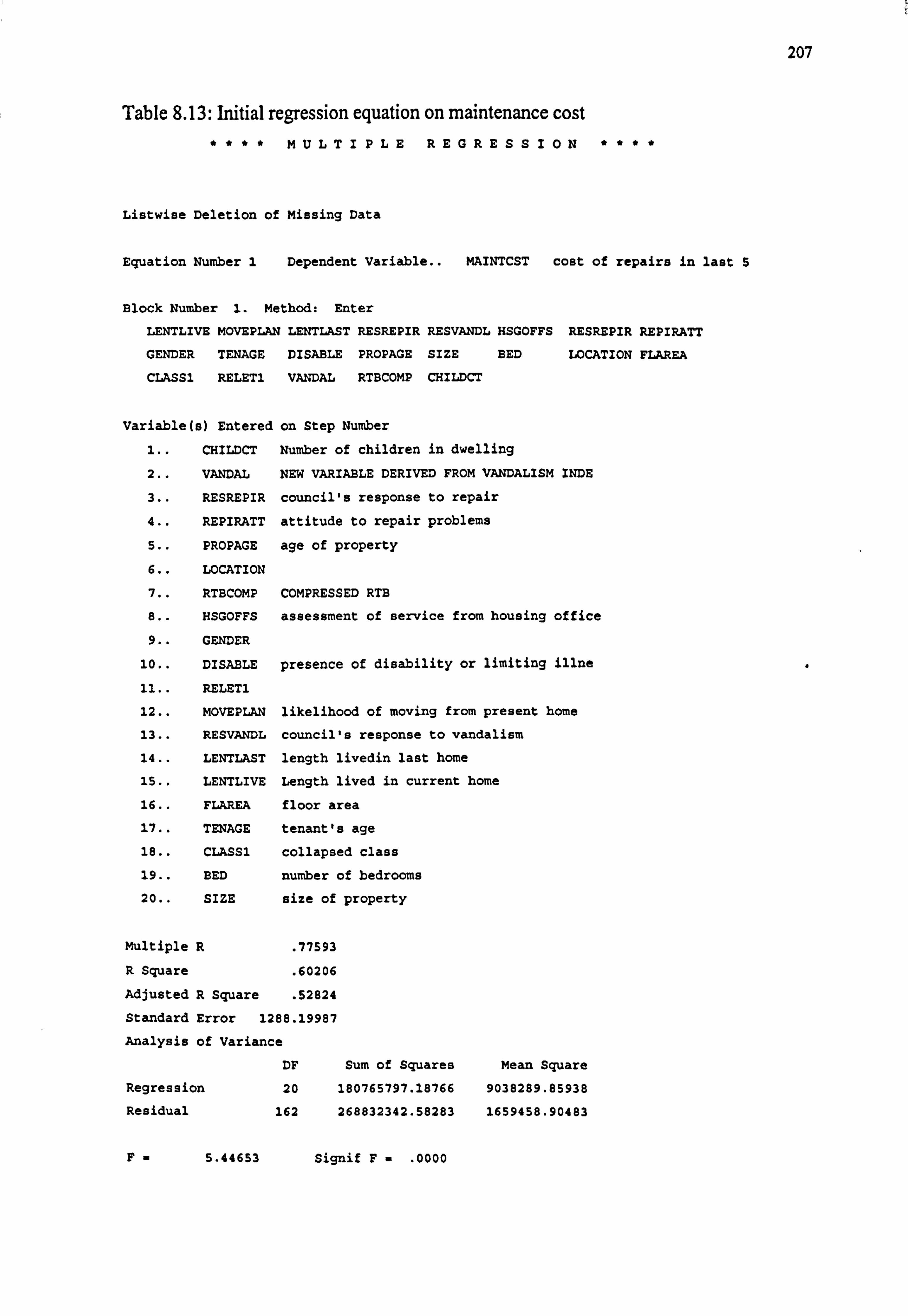
207
Table 8.13: Initial regression equation on maintenance cost ****MULTIPLER EGRESS 10N "**
Listwise Deletion of Missing Data
Equation Number 1 Dependent Variable.. MAINTCST cost of repairs in last 5
Block Number 1. Method: Enter
LENTLIVE MOVEPLAN LENTLAST RESREPIR RESVANDL HSGOFFS RESREPIR REPIRATT
GENDER TENAGE DISABLE PROPAGE SIZE BED LOCATION FLAREA
CLASSI RELET1 VANDAL RTBCOMP CHILDCT
Variable(s) Entered on Step Number
1.. CHILDCT Number of children in dwelling
2.. VANDAL NEW VARIABLE DERIVED FROM VANDALISM INDE
3.. RESREPIR council's response to repair
4.. REPIRATT attitude to repair problems
5.. PROPAGE age of property
6.. LOCATION
7.. RTBCOMP COMPRESSED RTB
8.. HSGOFFS assessment of service from housing office
9.. GENDER
10.. DISABLE presence of disability or limiting illne
11.. RELET1
12.. MOVEPLAN likelihood of moving from present home
13.. RESVANDL council's response to vandalism
14.. LENTLAST length livedin last home
15.. LENTLIVE Length lived in current home
16.. FLAREA floor area
17.. TENAGE tenant's age
18.. CLASS1 collapsed class
19.. BED number of bedrooms
20.. SIZE size of property
Multiple R . 77593
R Square . 60206
Adjusted R Square . 52824
Standard Error 1288.19987
Analysis of Variance
DF Sum of Squares Mean Square
Regression 20 180765797.18766 9038289.85938
Residual 162 268832342.58283 1659458.90483
F=5.44653 Signif F= . 0000
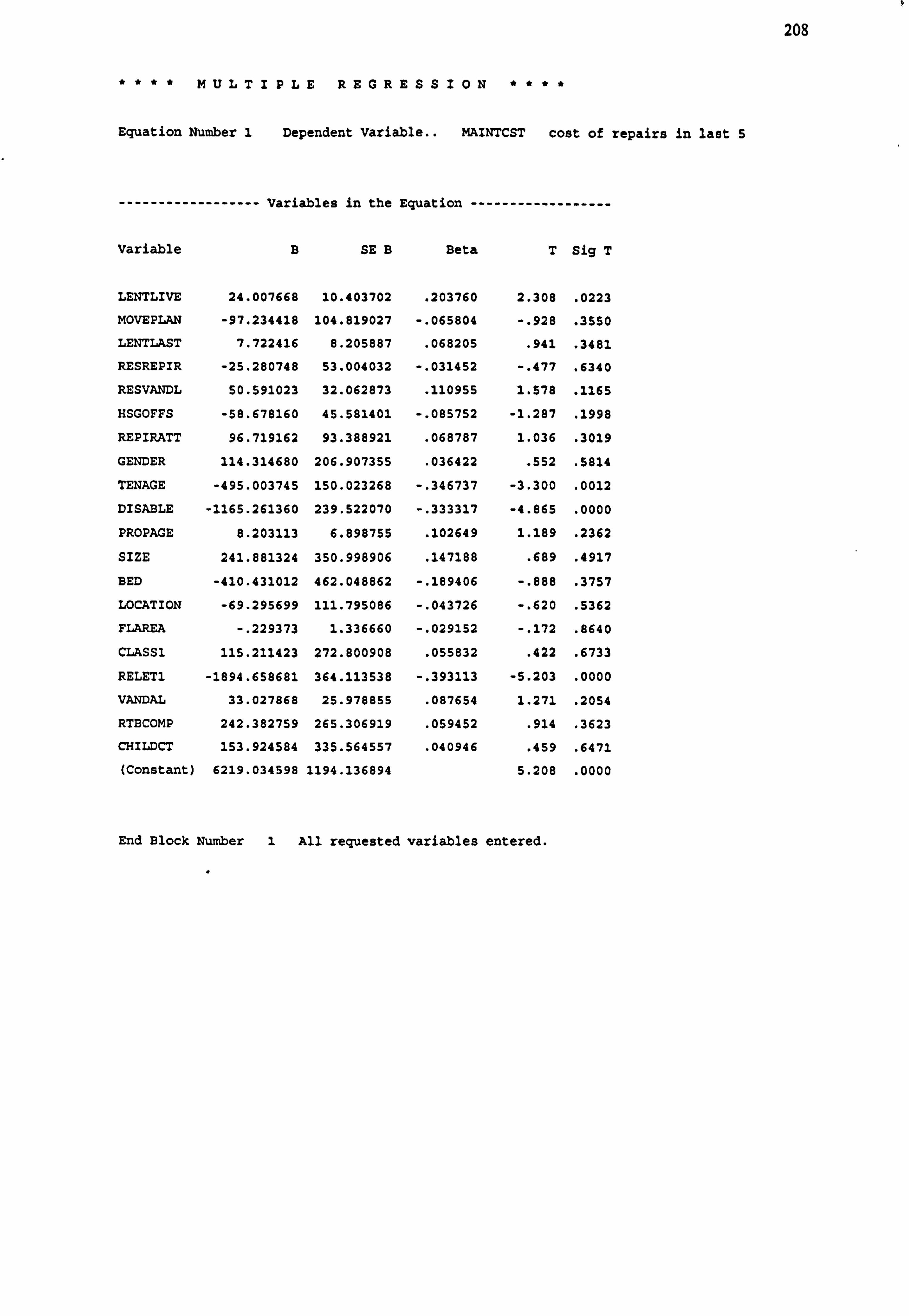
208
****MULTIPLEREGRESS10N****
Equation Number 1 Dependent Variable.. MAINTCST cost of repairs in last 5
------------------ Variables in the Equation ------------------
Variable B SE B Beta T Sig T
LENTLIVE 24.007668 10.403702 . 203760 2.308 . 0223
MOVEPLAN -97.234418 104.819027 -. 065804 -. 928 . 3550
LENTLAST 7.722416 8.205887 . 068205 . 941 . 3481
RESREPIR -25.280748 53.004032 -. 031452 -. 477 . 6340
RESVANDL 50.591023 32.062873 . 110955 1.578 . 1165
HSGOFFS -58.678160 45.581401 -. 085752 -1.287 . 1998
REPIRATT 96.719162 93.388921 . 068787 1.036 . 3019
GENDER 114.314680 206.907355 . 036422 . 552 . 5814
TENAGE -495.003745 150.023268 -. 346737 -3.300 . 0012
DISABLE -1165.261360 239.522070 -. 333317 -4.865 . 0000
PROPAGE 8.203113 6.898755 . 102649 1.189 . 2362
SIZE 241.881324 350.998906 . 147188 . 689 . 4917
BED -410.431012 462.048862 -. 189406 -. 888 . 3757
LOCATION -69.295699 111.795086 -. 043726 -. 620 . 5362
FLAREA -. 229373 1.336660 -. 029152 -. 172 . 8640
CLASS]. 115.211423 272.800908 . 055832 . 422 . 6733
RELET1 -1894.658681 364.113538 -. 393113 -5.203 . 0000
VANDAL 33.027868 25.978855 . 087654 1.271 . 2054
RTBCOMP 242.382759 265.306919 . 059452 . 914 . 3623
CHILDCT 153.924584 335.564557 . 040946 . 459 . 6471
(Constant) 6219.034598 1194.136894 5.208 . 0000
End Block Number 1 All requested variables entered.
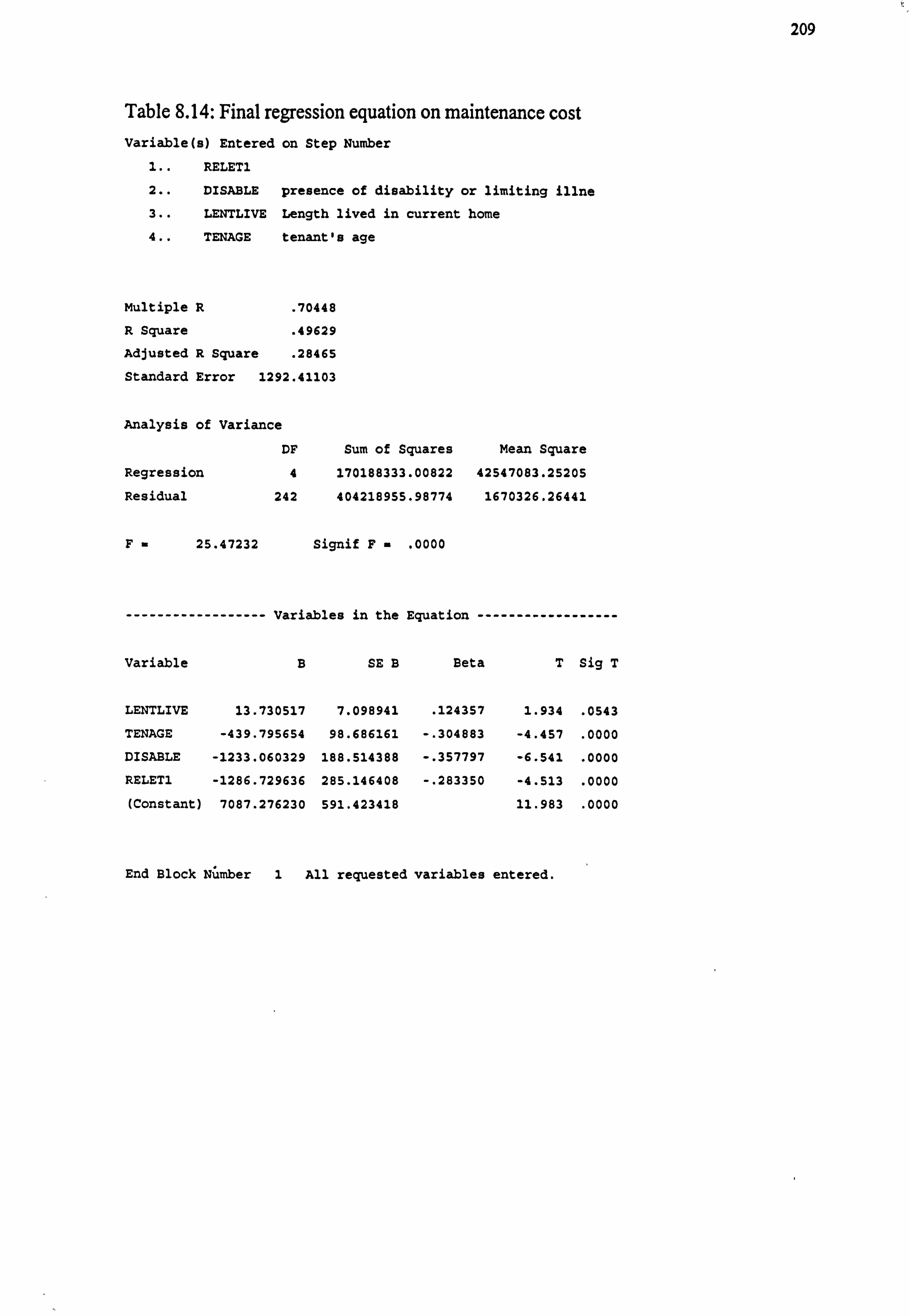
209
Table 8.14: Final regression equation on maintenance cost Variable(s) Entered on Step Number
1.. RELET1
2.. DISABLE presence of disability or limiting illne
3.. LENTLIVE Length lived in current home
4.. TENAGE tenant's age
Multiple R . 70448
R Square . 49629
Adjusted R Square . 28465
Standard Error 1292.41103
Analysis of Variance
DF
Regression 4
Residual 242
F- 25.47232
Sum of Squares Mean Square
170188333.00822 42547083.25205
404218955.98774 1670326.26441
Signif F- . 0000
------------------ Variables in the Equation ------------------
Variable B SE B Beta T Sig T
LENTLIVE 13.730517 7.098941 . 124357 1.934 . 0543
TENAGE -439.795654 98.686161 -. 304883 -4.457 . 0000
DISABLE -1233.060329 188.514388 -. 357797 -6.541 . 0000
RELETI -1286.729636 285.146408 -. 283350 -4.513 . 0000
(Constant) 7087.276230 591.423418 11.983 . 0000
End Block Number 1 All requested variables entered.
210
8.7.1.1 Inference from the Maintenance Cost Models
What this group of models seems to elicit is that all the 20 independent variables
account for about 60 per cent of the variation in repair costs within the local authority housing organisation. As the original 20 variables were fine-tuned on statistical
grounds, we were able to reduce them to just four variables which explain 50 per cent
of the total variation in the dependent variable.
The final model (Table 8.18) includes four variables which all fall into the category of
tenant attribute variables (RELETI, DISABLE, LENTLIVE and TENAGE). This
exclusive inclusion of variables in only one of the four areas of tenant, property,
environmental and property management attributes is surprising. It indicates that the
tenant characteristics are the dominant factors affecting day-to-day repair expenditure;
as a component of overall maintenance need of a residential property.
It is surprising because, on a priori grounds, it was expected that all the four areas
should inter-play in determining expenditure to a lesser or greater extent. Initial
speculation suggested that environmental factors should bear significantly upon MAINTCST (the dependent variable), which in this case has not been supported. This
confirms earlier finding, in chapter Six, which puts vandalism as one of least influential
on overall maintenance need; second only to age of property. It is worthy of note that
the Tolerance of the four variables are reasonably high, which enable us to reject any
suggestion of multi-collinearity as a problem within the models. Upon this evidence,
we could not explain away the features of the model on the grounds of inter-
correlations with other variables in the property, environmental and property
management domains.
The partial coefficients indicate that, in magnitude, DISABLE, is the strongest variable influencing repair expenditure, followed by TENAGE, RELETI and LENTLIVE. The
positive coefficient for the variable LENTLIVE is contrary to expectation. The
speculation would have been that the longer a tenant stayed in the dwelling, the less
would be his/her demands for repairs. However, this difference in impact can be
211
explained in three ways. Firstly, the awareness of tenants increases with length of
tenure, and as he becomes more aware of his rights, the higher the cost records
associated with his dwelling, especially where the tenant is likely to claim entitlement
to legal support. Secondly, the degree to which pressure is generated by the tenant on
local housing management team increases with tenant's self confidence which, in turn,
increases with length of tenure. Thirdly, whilst newer tenants become satisfied once
pre-occupation needs are met by the housing management team, when those needs
cease to be ̀ real needs' in the perception of the tenants, higher order needs are naturally
created by the tenants. Many of such needs may only be artificial. Therefore, the
longer the tenant is in occupation, the more demanding he is likely to be and hence may
generate more artificial defects which may, some of the time, have to be attended to by
the housing management group.
The negative coefficient for the variable RELET1 at (0.2834) indicates that repair
expenditure decreases where a property has had relet work carried out within the period
in question. This observation seems to contradict theoretical expectations since tenancy
turnover means more work being carried out on dwelling in order to secure replacement
tenants and hence increased maintenance expenditure. However, the contradiction
disappears where and if relet works constitute an encapsulation of all existing as well as
impending defects into one `big' repair action. Thus resulting in an `economies of
scale' which proves to be more cost efficient, as well as possessing some attribute of
pro-active and preventative maintenance. Hence, what is observed is that repair cost is
reduced in the medium or long term where there is tenancy turnover in so far as such a
turnover is not so frequent as to make the event itself short termed. The problem with
this trend however, lies in the time-value of such lump sum expenditure as well as the
management of day-to-day repair as a `revenue account' cost item.
The variable for DISABLE, which represents the physical well-being of tenants, has a
positive influence. What shows to be a negative partial coefficient is in actual sense a
positive coefficient since the scoring of the variable in the original data is in reverse
order with; 1- representing an existence of disabled person and a higher score
representing an absence of person with disability. It is also note worthy that some items of maintenance in dwellings occupied by disabled persons are carried out under
212
social services account rather than housing revenue account. Thus strengthening the
negative correlation, but the impact is not strong enough as to off-set additional
expenditure by housing department on disabled person's dwellings.
It is interesting that this variable has the strongest influence on repair expenditure. It is
useful to mention that repair expenditure profile does not include for ad-hoc social
services works carried out on properties for disabled persons, for, in the presence of
this, it becomes obvious why there would be a strongly positive inter-relationship. On
the contrary, it would appear that the strong influence is supported on account of the
sensitivity with which disabled persons are treated by housing officers, and therefore
any requests made by such persons. Therefore, a tenant's report for defects which may
pass for trifle in the case of non-disabled tenant, tends to receive more sympathetic and
urgent action when such a report comes from a disabled tenant. Secondly, one would
expect that disabled tenants are likely to spend more hours at home, and therefore,
likely to generate more work, especially condensation related problems. Furthermore,
because they tend to spend more time at home, they are in better position to identify at
much earlier stage, defects which other tenants will ignore or may not notice. Thirdly,
where the disabled person is a parent, the chances of do-it-yourself (DIY) works being
done on a dwelling become very remote, and hence, such defects fall to housing
management for rectification.
The negative partial coefficient for the variable TENAGE is interesting. What it
suggests is that the older the tenant is, the lower the repair costs. Anecdotal evidence as
well as findings by Alner and Fellows (1990) in their study of school buildings suggests
that age of property should be the strongly influencing factor in repair expenditure. In
this research, these findings are unsupported but appear to have been reversed. The
results suggest that PROPAGE is not a significant influencing factor, and that the age
of tenant (TENAGE) is more important in influencing residential property repair
expenditures. However, following from the preceding chapter, the ageing influence
exerts itself more significantly on some building components (damaged goods and wall
ties) rather than the whole, and possibly synergises with some other influence to exert
significant bearing on the building.
213
The direction of this influence can be explained in three ways. Firstly, older tenants are
least likely to have children leaving with them, and where they do, they are not likely to
be very young children, who may tend to generate more repairs by way of accidental
damage to vulnerable building components. Also, because dwellings with older tenants
are likely to be of lesser occupation density, condensation related problems associated
with higher density may not be more than off set by longer hours at home for this
category of tenants (older tenants). Secondly, even though MOVEPLAN is not here
found to be a significant variable, it is plausible that because younger household tend to
be more mobile, they are less likely than older ones to commit personal expenditure on dwelling, which is then passed on to housing management. Thirdly, with a major
proportion of their time devoted to work and tending younger children, younger
households would have less time at their disposal to carry out DIY duties on the
property in comparison with older households. Hence work which may well have been
carried out by the tenant for personal gratification (rather than for statutory
requirements) would end up being passed on to housing management team.
8.7.1.2 Excluded variables from Maintenance Expenditure Models
The regression model began with 20 independent variables, 16 of which failed the 95%
level of significance criterion and thus were excluded from the final regression equation in (Table 8.18). Their exclusion may be due to the variables' limited influence on
repair cost or that while they do affect repair expenditure, they do so less directly than
other variables for this particular purpose.
The variable (RESVANDL) was excluded from the final model even though the
response of the housing team to complaints generally is believed to have some
influence on repair expenditure. As seen in the regression model, this variable is the
strongest of all the 16 excluded variables in terms of t-value, which is significant at just
below 90% significance level. The exclusion may be due to possible effect of inter-area
transfer of housing staff. In which case, two or more respondents (tenants) in different
areas may actually be assessing one and the same housing staff. The housing officer
concerned may be the last direct contact with these respondents over the period in
question regarding the same subject matter. It is also possibly that tenants' personality
214
relating to their ages such as TENAGE have a more direct influence. The two variables
are significantly, though lowly, correlated (correlation coefficient = 0.1411).
The variable (HSGOFFS) was also excluded. It is possible that the exclusion of this
variable rests upon the same premise as with RESVANDL. Even though no significant
correlation exists between HSGOFFS and any of the four significantly influential
variables included in the final model, the strength of the correlation between
(RESVANDL) and (HSGOFFS) [Rho = 0.22] at 99% significance level enables us to
draw similar conclusion.
The fact that the partial coefficients of HSGOFFS and VANDAL are very close to
each other in magnitude, though in opposite directions at -0.0858 and 0.0877,
respectively indicates that the degree of responsiveness of housing officers and
vandalism index of area / dwelling have an equal but opposite impact on repair
expenditure profile.
Of the top most four influential variables excluded from the final model, the behaviour
of the variable PROPAGE appears to be most interesting. The age of property, though
not sufficiently significant to be included in the final model, the partial coefficient
suggests that its influence on repair cost is substantially greater than both HSGOFFS
and VANDAL, but failed the 95% criterion. The variable's failure of the t-test may be
that its contribution has been substantially represented by the two successful variables
with which it was proved to be significantly correlated, namely; RELET (Rho =
0.1329) and LENTLNE (Rho = 0.1963).
8.7.2 Property condition model
The results of property condition regression are shown in Table 8.15. Full regression
model using all 20 independent variables has a multiple coefficient of determination
(R2) of 0.2493 and an F ratio of 2.7065 which is significant at better than 99% level of
significance.
215
In an attempt to develop a better model, variables at less than 90% significance level
were excluded from the first model. This resulted in the regression model shown in
Table 8.16, leaving a model with just three of the original variables, namely; VANDAL, BED and SIZE, two of which satisfied the required 95% level of
significance. Although the final model satisfied the statistical criteria, and also showed
consistent improvement on the previous F values, due to the low explanatory power (R) = 0.0609 which is an excessively large drop from the original R2 at 0.2493, the
model was therefore rejected on the ground of spuriousness, and possible endogenous interference among the variables, thus distorting the various observed t-values which
are used in deciding the inclusion or exclusion of variables.
Table 8.15: Initial regression equation on property condition ****MULTIPLER EGRESS ION ***
Listwise Deletion of Missing Data
Equation Number 1 Dependent Variable.. PROPCOND Assessment of overall con
Block Number 1. Method: Enter
LENTLIVE MOVEPLAN LENTLAST RESREPIR RESVANDL HSGOFFS RESREPIR REPIRATT
GENDER TENAGE DISABLE PROPAGE SIZE BED LOCATION FLAREA
CLASS1 RELETI VANDAL RTBCOMP CHILDCT
Variable(s) Entered on Step Number
1.. CHILDCT Number of children in dwelling
2.. VANDAL NEW VARIABLE DERIVED FROM VANDALISM INDE
3.. RESREPIR council's response to repair
4.. REPIRATT attitude to repair problems
5.. PftOPAGE age of property
6.. LOCATION
7.. RTBCOMP COMPRESSED RTB
8.. HSGOFFS assessment of service from housing offic
9.. GENDER
10.. DISABLE presence of disability or limiting illne
11.. RELET1 12.. MOVEPLAN likelihood of moving from present home
13.. RESVANDL council's response to vandalism
14.. LENTLAST live length in last home
15.. LENTLIVE Length lived in current home
16.. FLAREA floor area
17.. TENAGE tenant's age
18.. CLASS1 collapsed class
19.. SIZE size of property
20.. BED number of bedrooms
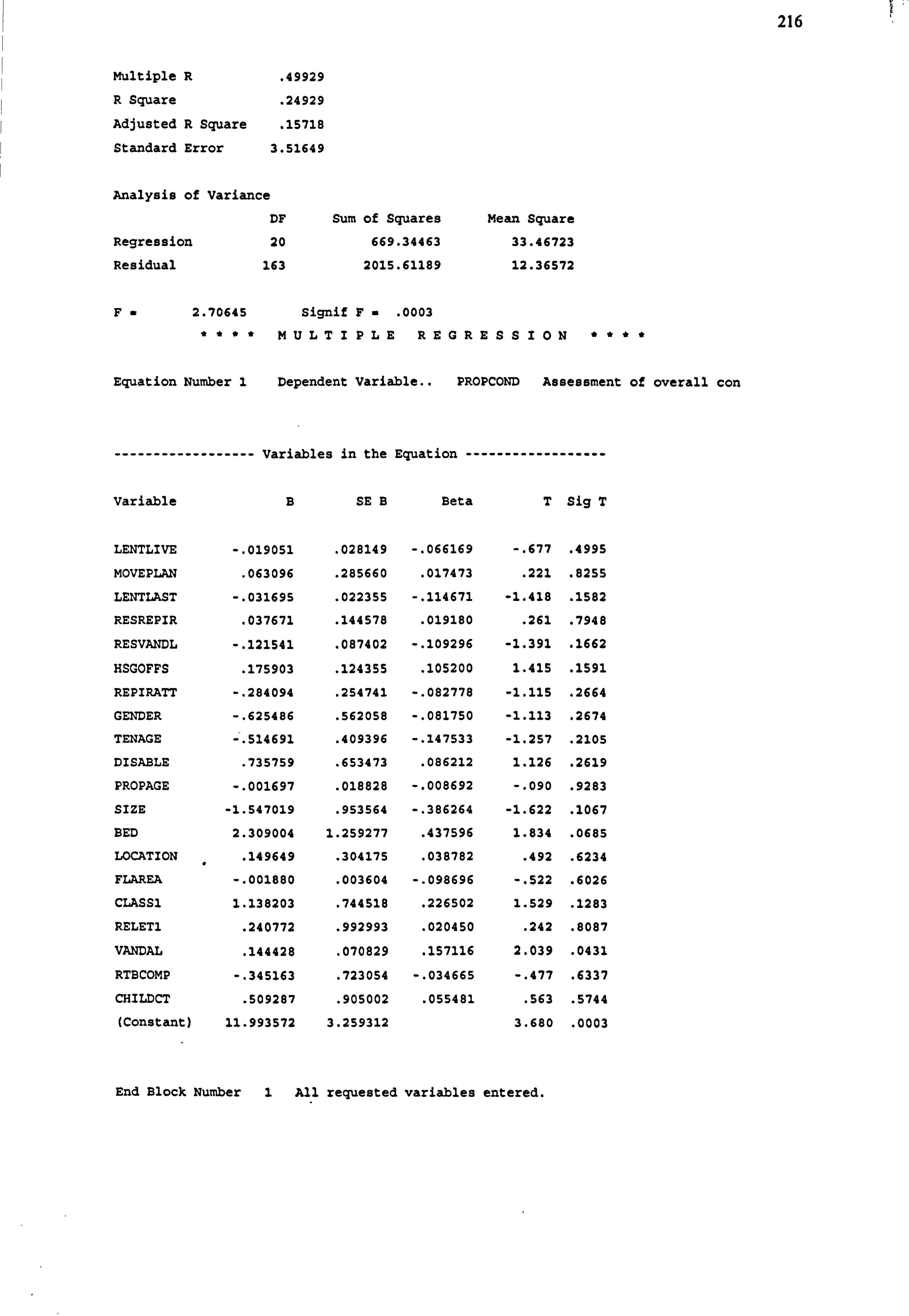
216
Multiple R . 49929
R Square . 24929
Adjusted R Square . 15718
Standard Error 3.51649
Analysis of Variance
DF
Regression 20
Residual 163
Sum of Squares Mean Square
669.34463 33.46723
2015.61189 12.36572
F"2.70645 Signif F" . 0003
***" MULTIPLEREGRESS10N ""*"
Equation Number 1 Dependent Variable.. PROPCOND Assessment of overall con
------------------ Variables in the Equation ------------------
Variable B SE B Beta T Sig T
LENTLIVE -. 019051 . 028149 -. 066169 -. 677 . 4995
MOVEPLAN . 063096 . 285660 . 017473 . 221 . 8255
LENTLAST -. 031695 . 022355 -. 114671 -1.418 . 1582
RESREPIR . 037671 . 144578 . 019180 . 261 . 7948
RESVANDL -. 121541 . 087402 -. 109296 -1.391 . 1662
HSGOFFS . 175903 . 124355 . 105200 1.415 . 1591
REPIRATT -. 284094 . 254741 -. 082778 -1.115 . 2664
GENDER -. 625486 . 562058 -. 081750 -1.113 . 2674
TENAGE -. 514691 . 409396 -. 147533 -1.257 . 2105
DISABLE . 735759 . 653473 . 086212 1.126 . 2619
PROPAGE -. 001697 . 018828 -. 008692 -. 090 . 9283
SIZE -1.547019 . 953564 -. 386264 -1.622 . 1067
BED 2.309004 1.259277 . 437596 1.834 . 0685
LOCATION . 149649 . 304175 . 038782 . 492 . 6234
FLAREA -. 001880 . 003604 -. 098696 -. 522 . 6026
CLASSI 1.138203 . 744518 . 226502 1.529 . 1283
RELET1 . 240772 . 992993 . 020450 . 242 . 8087
VANDAL . 144428 . 070829 . 157116 2.039 . 0431
RTBCOMP -. 345163 . 723054 -. 034665 -. 477 . 6337
CHILDCT . 509287 . 905002 . 055481 . 563 . 5744
(Constant) 11.993572 3.259312 3.680 . 0003
End Block Number 1 All requested variables entered.
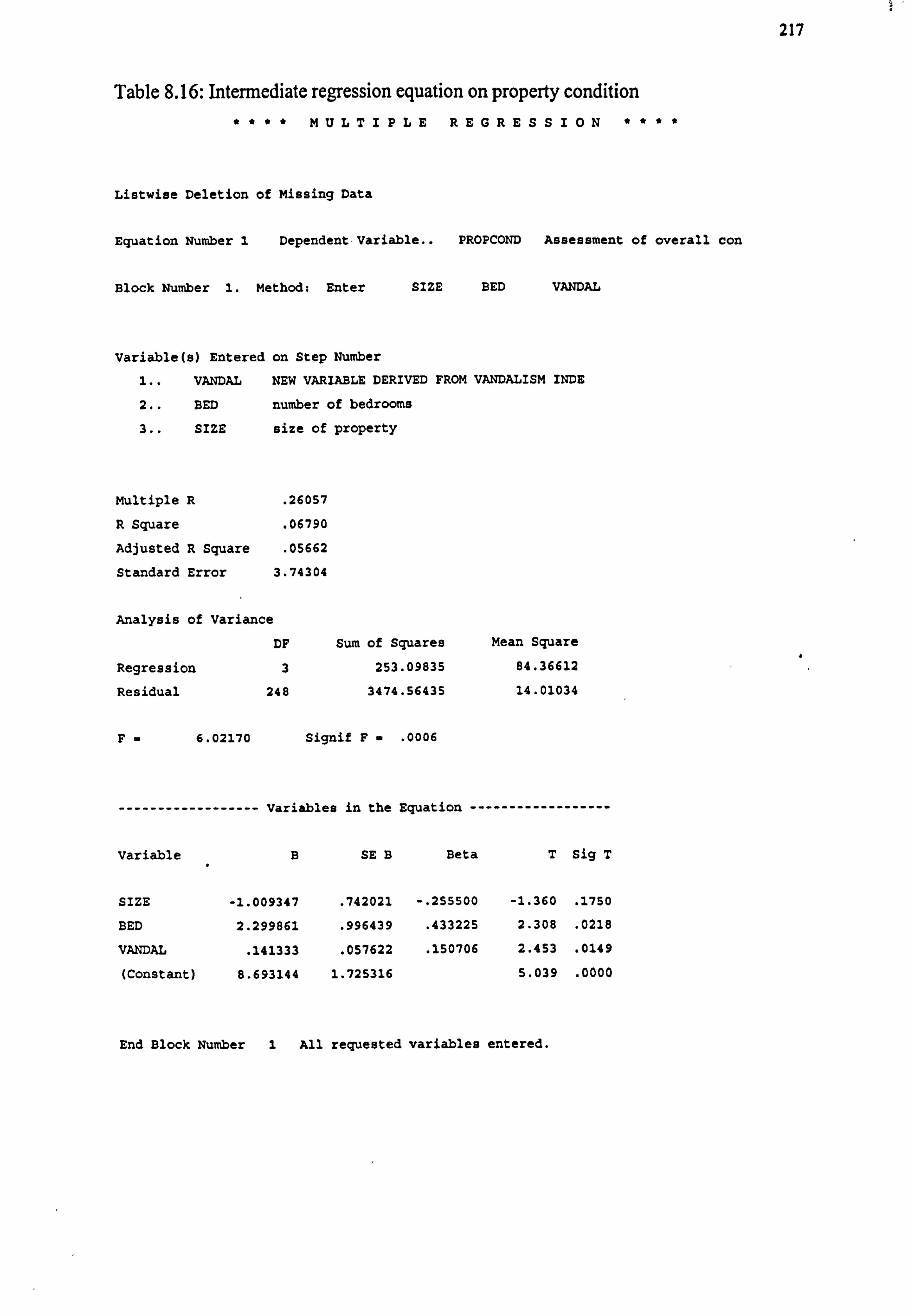
Table 8.16: Intermediate regression equation on property condition **"* MULTIPLEREGRESS10N ****
Listwise Deletion of Missing Data
Equation Number 1 Dependent-Variable.. PROPCOND Assessment of overall con
Block Number 1. Method: Enter SIZE BED VANDAL
Variable(s) Entered on Step Number
1.. VANDAL NEW VARIABLE DERIVED FROM VANDALISM INDE
2.. BED number of bedrooms
3.. SIZE size of property
217
Multiple R . 26057
R Square . 06790
Adjusted R Square . 05662
Standard Error 3.74304
Analysis of Variance
DF
Regression 3
Residual 248
Sum of Squares
253.09835
3474.56435
Mean Square
84.36612
14.01034
F=6.02170 Signif F. . 0006
------------------ Variables in the Equation ------------------
Variable B SE B Beta T Sig T
SIZE -1.009347 . 742021 -. 255500 -1.360 . 1750
BED 2.299861 . 996439 . 433225 2.308 . 0218
VANDAL . 141333 . 057622 . 150706 2.453 . 0149
(Constant) 8.693144 1.725316 5.039 . 0000
End Block Number 1 All requested variables entered.
' I
218
8.7.2.1 Correcting for Endogenous Interference in the Property Condition Model
The first step towards correcting for possible confounding influence on the model is to
compartmentalise the variables. The object being that if all the 20 variables explain
about 25% of the variation in property condition, any improved model from this, whilst
substantially improving on the F value and its significance, should not, nevertheless,
only so very marginally explain the variations in the dependent variable.
The most rational approach towards categorisation for this purpose appears to be along
the line shown under section 8.5.1 namely; tenant, property, environmental and
property management attributes.
The variables pertaining to each of these areas were isolated and subjected to regression
analysis whilst retaining the initial dependent variable. The regression runs show that
variables appertaining to three of the four identifiable areas, namely; property,
environmental and property management attributes are very weak models. However,
the regression run for the variables under `tenant' attributes proved almost equally as
strong as the original regression model consisting of all the 20 variables which
nevertheless failed the set 95% criterion.
The first model consists of 11 independent variables which proved to explain about 80% of the total variation accounted for by all the 20 variables put together. In the
modified property model, the full regression model is shown in Table 8.17a. The R2 of 0.1963 and the F ratio of 3.7745 are both significant at greater than 99% significance level. To further improve the model, the variables which did not meet the 90%
criterion for the t-values were excluded from the model. This resulted in Table 8.17c
model consisting of three variables all which now met the 95% criterion for the t-value.
The R2 dropped from 0.1936 to 0.1288, but the F ratio improved to 10.7962, which is
almost triple the previous value.
These results lead us to a similar inference as in the repair cost models, i. e. they indicate that tenant characteristics are the dominant factors affecting property condition to the exclusion of environmental and property attributes.
219
The negative coefficient for the variable TENAGE is in the same direction as its
influence on repair costs. In the first place, it was not expected that tenant's age should be a significant influential variable on property condition. This surprising observation
could however be explained on account of `cause and effect' phenomenon between
tenant's age (TENAGE) and vandalism (measured in the main by the variable VANDAL). An examination of the full property condition model reveals that these two
variables have opposite signs for the partial coefficients. This confirms that vandalism
occurs more frequently where tenants are younger. The validity of this inference is
confirmed by the fact that the variable VANDAL proved to be one of three factors
along with TENAGE that showed significant t-value in the final model, and in opposite
directions
The underlying cause for this trend lies in the fact that the presence of older children
within the dwelling in general and the neighbourhood in particular could act as a
catalyst for the general deterioration of property condition. As expected, such children
are more common with younger, rather than older families.
The negative coefficient for the variable LENTLAST indicates that tenants who lived
longer in previous dwellings are currently living in more `run down' properties within
the local authority. As revealed by the correlation matrix, LENTLAST is significantly
positively correlated with TENAGE (Rho = 0.40). This confirms conventional wisdom
which would seem to suggest that older tenants would more probably have lived
elsewhere and for longer period as well. The direction of the beta sign for LENTLAST
and TENAGE is negative whilst VANDAL is positive. Having said that, there is no
ground to suggest that the three variables are essentially measuring the same attribute,
as indeed they cannot, given their correlation matrix: LENTLAST and TENAGE at 0.3987'; LENTLAST and VANDAL at 0.0176; TENAGE and VANDAL at -0.0048 with just one of the three relationships being significant (as indicated with *).
The underlying explanation for this observation about the variable (PROPCOND) may be based purely on dogma for housing preference among older tenants who tend to
show preference for older dwelling types. Older people seem to believe that older
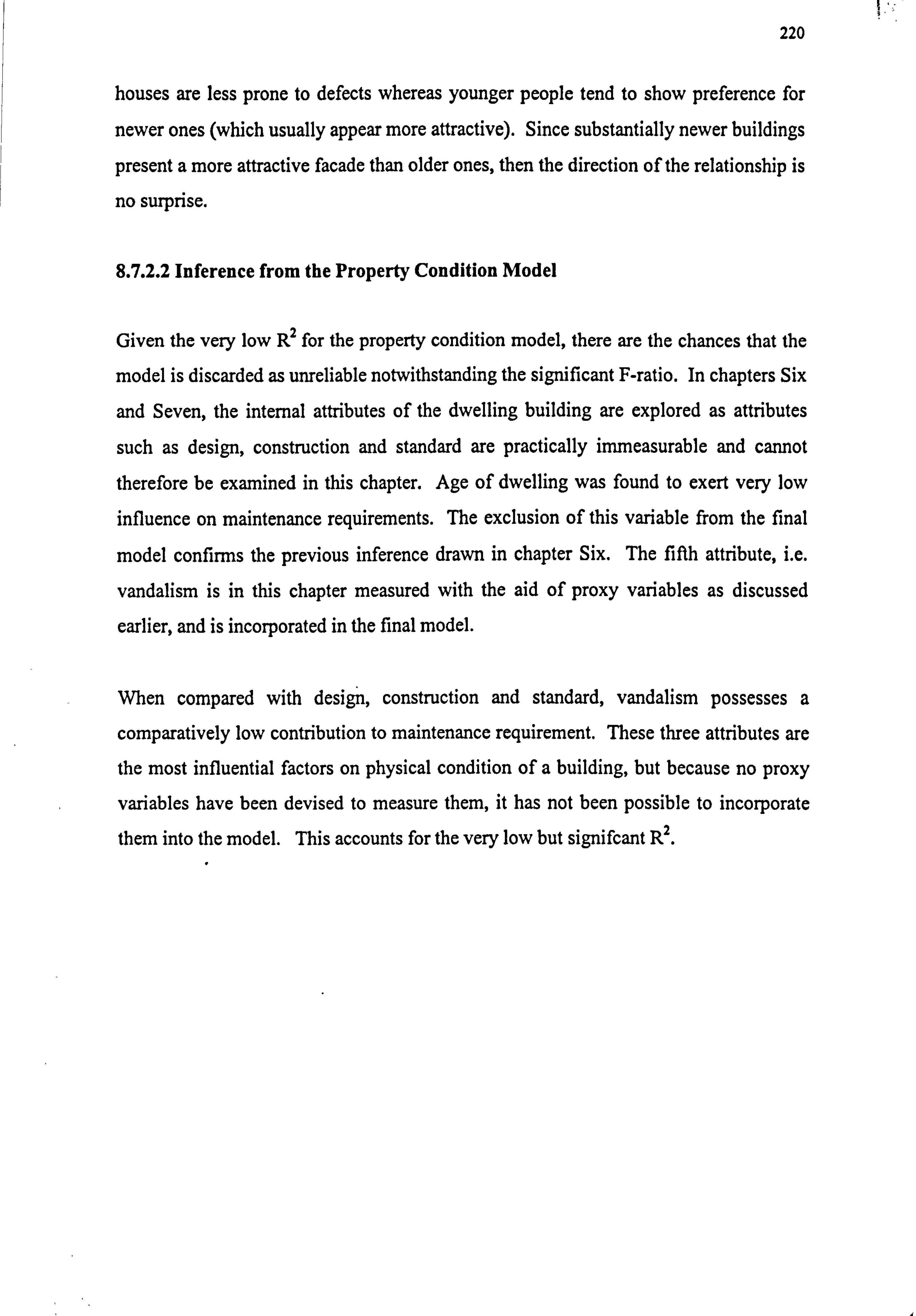
220
houses are less prone to defects whereas younger people tend to show preference for
newer ones (which usually appear more attractive). Since substantially newer buildings
present a more attractive facade than older ones, then the direction of the relationship is
no surprise.
8.7.2.2 Inference from the Property Condition Model
Given the very low R2 for the property condition model, there are the chances that the
model is discarded as unreliable notwithstanding the significant F-ratio. In chapters Six
and Seven, the internal attributes of the dwelling building are explored as attributes
such as design, construction and standard are practically immeasurable and cannot
therefore be examined in this chapter. Age of dwelling was found to exert very low
influence on maintenance requirements. The exclusion of this variable from the final
model confirms the previous inference drawn in chapter Six. The fifth attribute, i. e.
vandalism is in this chapter measured with the aid of proxy variables as discussed
earlier, and is incorporated in the final model.
When compared with design, construction and standard, vandalism possesses a
comparatively low contribution to maintenance requirement. These three attributes are
the most influential factors on physical condition of a building, but because no proxy
variables have been devised to measure them, it has not been possible to incorporate
them into the model. This accounts for the very low but signifcant R2.
ýr
Table 8.17: Final regression equations on property condition Table B. 17a: Variables in the Eauation
Variable B SE B Beta T Sig T
LENTLIVE . 010529 . 023712 . 036693 . 444 . 6576 MOVEPLAN -. 031975 . 277102 -. 008857 -. 115 . 9083 LENTLAST -. 040312 . 021241 -. 147185 -1.898 . 0594 REPIRATT -. 366057 . 250183 -. 107411 -1.463 . 1452 GENDER -. 885653 . 553509 -. 116214 -1.600 . 1114 TENAGE -. 753751 . 442257 -. 216742 -1.704 . 0901 DISABLE . 469599 . 610434 . 055110 . 769 . 4428 VANDAL . 169196 . 064898 . 184095 2.607 . 0099 RTBCOMP -. 131569 . 687908 -. 013383 -. 191 . 8485 CHILDCT 1.243394 . 803626 . 135627 1.547 . 1236 TEMPLOY1 . 237556 . 484157 . 050013 . 491 . 6243 (Constant) 11.184218 2.674504 4.182 . 0000
Multiple R . 43994 R Square . 19355 Adjusted R Square . 14227 Standard Error 3.53602
Analysis of Variance DF Sum of Squares Mean Square
Regression 11 519.13725 47.19430 Residual 173 2163.10058 12.50347
F=3.77450 Signif F. . 0001
Table 8.17b: Variables in the Equation
Variable B SE B Beta T Sig T
LENTLAST -. 046685 . 020034 -. 161919 -2.330 . 0207 TENAGE -. 885218 . 255503 -. 243134 -3.465 . 0006 VANDAL . 128410 . 060298 . 133895 2.130 . 0343 GENDER -. 792228 . 505534 -. 101201 -1.567 . 1185 (Constant) 13.812065 1.477600 9.348 . 0000
Multiple R . 37221 R Square . 13854 Adjusted R Square . 12274 Standard Error 3.66805
Analysis of Variance DF Sum of Squares Mean Square
Regression 4 471.71609 117.92902 Residual 218 2933.10005 13.45459
F=8.76497 Signif F" . 0000
Table 8.17c" Variables in the Equation
Variable B SE B Beta T Sig T
LENTLAST -. 051803 . 019832 -. 179668 -2.612 . 0096 TENAGE -. 799432 . 250398 -. 219572 -3.193 . 0016 VANDAL . 129221 . 060496 . 134741 2.136 . 0338 (Constant) 12.397120 1.173528 10.564 . 0000
Multiple R . 35894 R Square . 12884 Adjusted R Square . 11691 Standard Error 3.68022 Analysis of Variance
DF Sum of Squares Mean Square Regression 3 438.67382 146.22461 Residual 219 2966.14232 13.54403 F" 10.79624 Signif F" . 0000
221
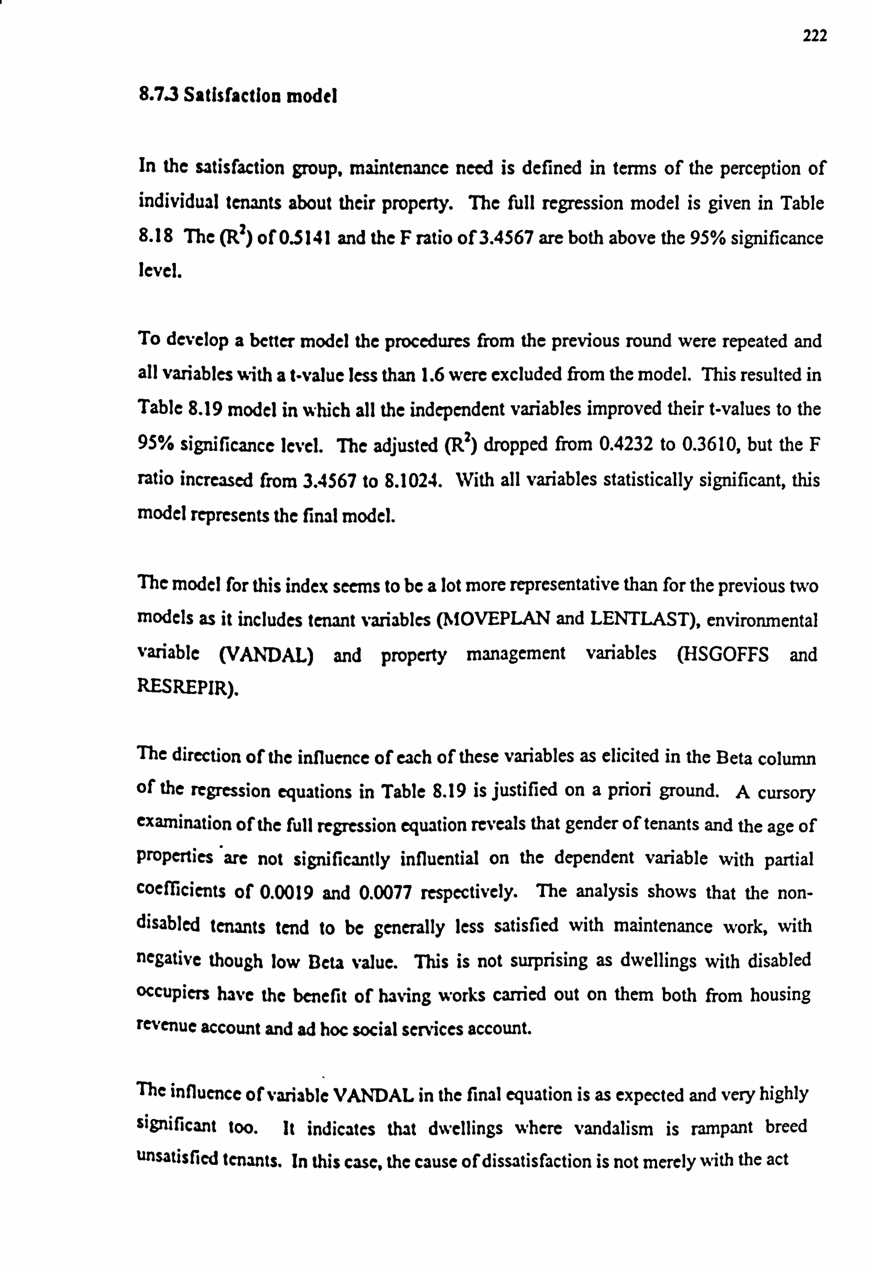
222
8.7.3 Satisfaction model
In the satisfaction group, maintenance need is defined in terms of the perception of individual tenants about their property. The full regression model is given in Table
8.18 The (It2) of 0.5141 and the F ratio of 3.4567 are both above the 95% significance level.
To develop a better model the procedures from the previous round were repeated and
all variables with a t-value less than 1.6 were excluded from the model. This resulted in
Table 8.19 model in which all the independent variables improved their t-values to the
9S% significance level. The adjusted (R2) dropped from 0.4232 to 0.3610, but the F
ratio increased from 3.4567 to 8.1024. With all variables statistically significant, this
model represents the final model.
The model for this index seems to be a lot more representative than for the previous two
models as it includes tenant variables (AfOVEPLAN and LENTLAST), environmental
variable (VANDAL) and property management variables (HSGOFFS and RESREPIR).
The direction of the influence of each of these variables as elicited in the Beta column of the regression equations in Table 8.19 is justified on a priori ground. A cursory examination of the full regression equation reveals that gender of tenants and the age of properties are not significantly influential on the dependent variable with partial coefficients of 0.0019 and 0.0077 respectively. The analysis shows that the non- disabled tenants tend to be generally less satisfied with maintenance work, with negative though low Beta value. This is not surprising as dwellings with disabled
occupicrs have the benefit of having works carried out on them both from housing
revenue account and ad hoc social services account.
The influence of variable VANDAL in the final equation is as expected and very highly
significant too. It indicates that dwellings where vandalism is rampant breed
unsatisfied tenants. In this case, the cause of dissatisfaction is not merely with the act
223
Table 8.18: Initial regression equation on tenant's satisfaction +"""MULTIPLER EGRESS 10N "+""
Listwise Deletion of Missing Data
Equation Number 1 Dependent Variable.. SATISFY1
Block Number 1. Method: Enter
LENTLIVE MOVEPLAN LENTLAST RESREPIR RESVANDL HSGOFFS RESREPIR REPIRATT
GENDER TENAGE DISABLE PROPAGE SIZE BED LOCATION FLAREA
CLASS1 RELET1 VANDAL RTBCOMP CHILDCT
Variable(s) Entered on Step Number
1.. CHILDCT Number of children in dwelling
2.. RESREPIR council's response to repair
3.. VANDAL NEW VARIABLE DERIVED FROM VANDALISM INDE
4.. REPIRATT attitude to repair problems
5.. PROPAGE age of property
6.. HSGOFFS assessment of service from housing offic
7.. LOCATION
8.. GENDER
9.. RTBCOMP COMPRESSED RTB
10.. DISABLE presence of disability or limiting illne
11.. RELET1
12.. MOVEPLAN likelihood of moving from present home
13.. LENTLAST live length in last home
14.. RESVANDL council's response to vandalism
15.. LENTLIVE Length lived in current home
16.. FLAREA floor area
17.. TENAGE tenant's age
18.. SIZE size of property 19.. CLASSI collapsed class 20.. BED number of bedrooms
Multiple R . 71697
R Square . 51405
Adjusted R Square . 42320
Standard Error 79.17288
Analysis of Variance
DF Sum of Squares Mean Square
Regression 20 433349.15756 21667.45788
Residual 151 946520.06400 6268.34479
F-3.45665 Signif F- . 0000
224
"***MULTIPLER EGRESS 10N ****
Equation Number 1 Dependent Variable.. SATISFY1
------------------ Variables in the Equation ------------------
Variable B SE B Beta T Sig T
LENTLIVE . 270603 . 645067 . 040382 . 419 . 6754
MOVEPLAN -12.123608 6.730705 -. 142617 -1.801 . 0737
LENTLAST 1.199754 . 526371 . 184849 2.279 . 0241
RESREPIR 14.668442 3.791723 . 277834 3.869 . 0002
RESVANDL -. 877377 2.097418 -. 033597 -. 418 . 6763
HSGOFFS 4.948273 3.012568 . 119959 1.643 . 1026
REPIRATT -4.680640 6.143145 -. 057432 -. 762 . 4473
GENDER -. 335821 13.258849 -. 001870 -. 025 . 9798
TENAGE 11.938181 9.514045 . 146981 1.255 . 2115
DISABLE -8.351086 15.081537 -. 042083 -. 554 . 5806
PROPAGE . 035902 . 444373 . 007713 . 081 . 9357
SIZE -13.605495 21.817215 -. 144138 -. 624 . 5338
BED 7.908106 29.056915 . 062600 . 272 . 7859
LOCATION 8.046796 7.135741 . 089102 1.128 . 2612
FLAREA -. 021816 . 083804 -. 048203 -. 260 . 7950
CLASS1 14.082570 17.874942 . 117931 . 788 . 4320
RELET1 4.765112 23.377527 . 017054 . 204 . 8388
VANDAL -3.084456 1.658267 -. 144915 -1.860 . 0648
RTBCOMP -23.074811 16.924600 -. 100252 -1.363 . 1748
CHILDCT -1.469432 20.762060 -. 006990 -. 071 . 9437
(Constant) 272.071498 74.414863 3.656 . 0004
End Block Number 1 All requested variables entered.
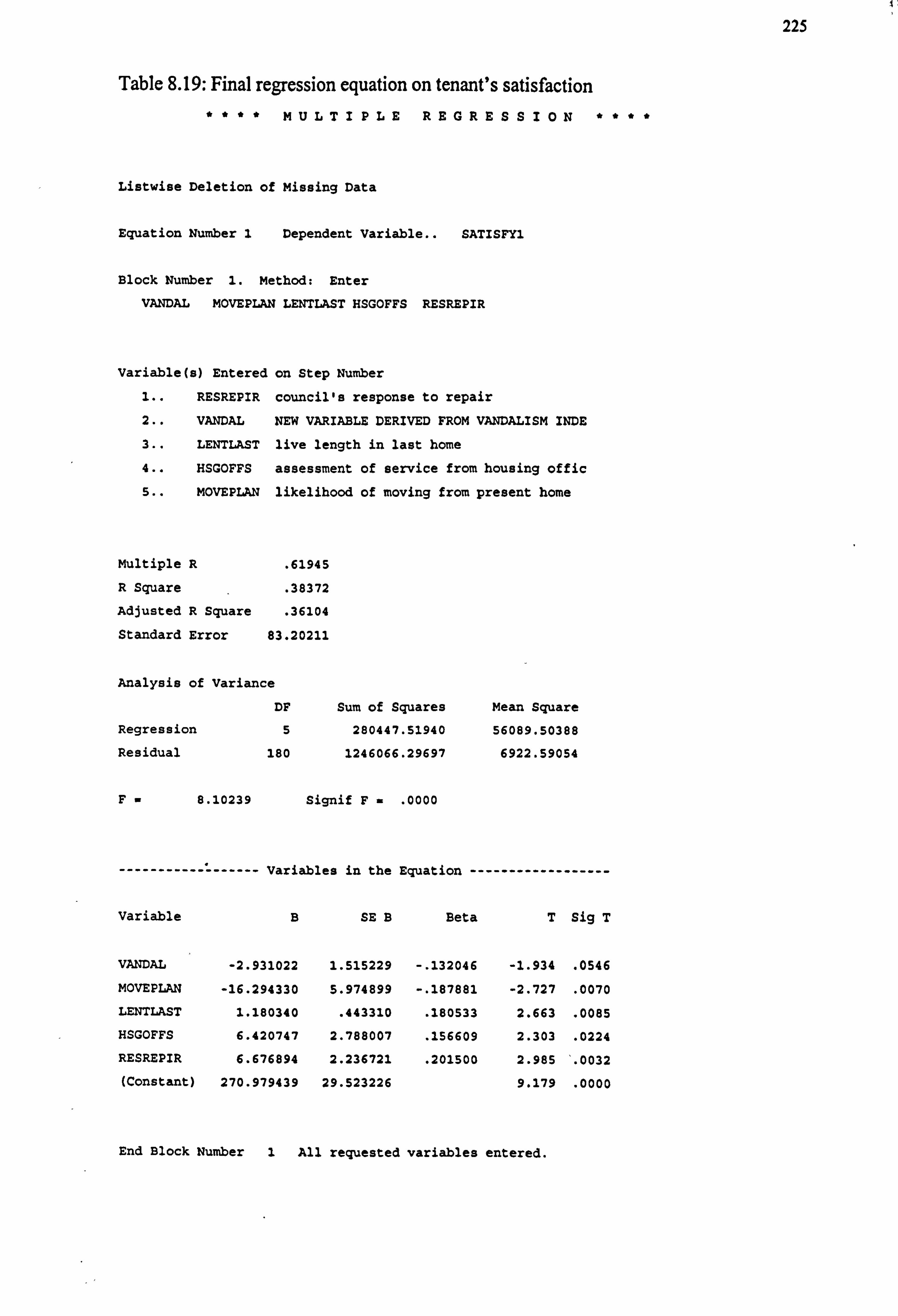
225
Table 8.19: Final regression equation on tenant's satisfaction **"* MULTIPLEREGRESS10N +*""
Listwise Deletion of Missing Data
Equation Number 1 Dependent Variable.. SATISFY1
Block Number 1. Method: Enter VANDAL MOVEPLAN LENTLAST HSGOFFS RESREPIR
Variable(s) Entered on Step Number
1.. RESREPIR council's response to repair
2.. VANDAL NEW VARIABLE DERIVED FROM VANDALISM INDE
3.. LENTLAST live length in last home
4.. HSGOFFS assessment of service from housing offic
5.. MOVEPLAN likelihood of moving from present home
Multiple R . 61945
R Square . 38372
Adjusted R Square . 36104
Standard Error 83.20211
Analysis of Variance
DF
Regression 5
Residual 180
Sum of Squares
280447.51940
1246066.29697
Mean Square
56089.50388
6922.59054
F-8.10239 Signif F- . 0000
-----------=------ Variables in the Equation ------------------
Variable B SE B Beta T Sig T
VANDAL -2.931022 1.515229 -. 132046 -1.934 . 0546
MOVEPLAN -16.294330 5.974899 -. 187881 -2.727 . 0070
LENTLAST 1.180340 . 443310 . 180533 2.663 . 0085
HSGOFFS 6.420747 2.788007 . 156609 2.303 . 0224
RESREPIR 6.676894 2.236721 . 201500 2.985 '. 0032
(Constant) 270.979439 29.523226 9.179 . 0000
End Block Number 1 All requested variables entered.
226
of vandalism as with the attitude of the housing management to repair works in such
vandalism prone dwellings and housing areas. This inference is borne out by the
significant contributions of HSGOFFS and RESREPIR to the model. The positive
directions of the latter two variables confirm that responsive housing management impacts on maintenance requirements to tenant's satisfaction. With the result that care
on the part of management is reinforced with concomitant care from satisfied tenants.
Most puzzling of all is the influence of length of tenure in previous accommodation.
Longer tenure in previous accommodation leads to reduced maintenance need. This is
accounted for by the fact that such tenants are more likely to have acquired `do-it-
yourself skills which allow them to carry out minor repairs at little cost to themselves.
Also, the correlation between TENAGE and LENTLAST is a positive one, and the
impact of the former on the latter may be at play in this instance, i. e. LENTLAST may
be a surrogate for TENAGE.
8.8 Conclusion
In this chapter three models dealing with maintenance needs have been developed. The
three models are statistically satisfactory. Combining the three models leads us to
suggest that nine out of the 20 independent variables are significant factors in the
determination of maintenance requirements for housing stock. These include
TENAGE, DISABLE, RELETI, VANDAL, LENTLAST, LENTLIVE, MOVEPLAN,
HSGOFFS, and RESREPIR. The direction of the influence of each of these variables is
clearly elicited in the Beta columns of the regression tables.
The apparent low explanatory power of the models is in line with our expectation. The
factors affecting maintenance requirements have elsewhere been established to be
multifaceted (see chapters Five, Six and Seven), and the attributes herein discussed are
some of the prominent variables which lend themselves to measurement of some sort. Hence, it is never anticipated that these families of variables should explain a disproportionately high percentage of the variation in maintenance requirements.
This chapter has brought to focus the strong influence of tenants' attributes upon
maintenance need. It also shows that it is insufficient for maintenance managers to
227
base their understanding of the subject purely on physical characteristics and attributes
of the building object. The manager must also build into any budgetary prediction an
allowance for variations in tenant profiles and their effects upon maintenance
generation.
228
CHAPTER 9
SUMMARY AND CONCLUSIONS
9.1 Summary
As stated in chapter One, the overall objective of the research was to develop a framework for isolating a group of factors influencing maintenance requirements in
public sector housing. It is expected that a factorial framework will enhance:
1. the awareness and knowledge of issues bearing upon maintenance which will be of
value to housing managers;
2. the development of maintenance strategies in housing which will help identify
optimum efficiencies and economics through the judicious allocation of resources;
3. the awareness of designers of new housing schemes of the factors influencing
maintenance generation and the performance of dwellings; and
4. the field of knowledge currently available because of the inadequacies of available
literature.
It can be seen from chapter Two that it is possible, from the literature search, to
establish a three-fold categorisation of the factors, i. e.:
" Internal attributes of the building object;
9 External attributes; and
" The mediatory role of the stockholder
This enabled a number of hypotheses to be formulated and tested. These hypotheses
revolve around the notion that maintenance requirements are influenced by:
(i) a number of precise building object attributes; (ii) the surrounding environment in which dwellings are located;
(iii) the characteristics of the tenants; and (iv) housing management responsiveness.
229
The obvious starting point in establishing a suitable methodology was an in-depth
survey of available information the Manchester Council housing records. An
examination of maintenance cost records over a five-year period for a sample of 66
dwellings showed an absence of patterned relationships. An analysis of variance of
maintenance expenditure between semi-detached houses and cottage flats revealed that
there is no significant difference between them. A scatter plot of the data revealed that
the size of dwellings both in terms of number of bedrooms and floor area does not have
significant bearing upon maintenance expenditure.
Following from this, some inadequacies were identified in the cost records and
therefore could not be relied upon totally as a principal yardstick for measuring
maintenance requirements. This is partly due to costs being distorted because some
tenants influenced the demand, priority and ordering of building maintenance through
their desire to use legal powers by way of the legal aid system, and partly due to their
forcefulness and determination to get work done.
However, it was felt that if the cost data was supported and enhanced by other data then
it was possible to provide a sound basis on which to establish the independent variables. Two complementary areas were identified; one being targeted at the tenants themselves,
and the other at the existing condition of the buildings.
Complementary information from tenants was aimed at determining how satisfied they
were with works carried out on their properties. Studies into tenants' satisfaction are
commonly agreed in their findings that dwellings with the least satisfied tenants tend to be
in poorer state of repairs than those with more satisfied tenants (Burbridge and Smith
1973; Shankland 1971; Stevenson et al 1967). Developing a measure for this attribute
clearly corrected some of the deficiencies found in the cost records.
From the literature search on the development of public housing in the UK, a common datum can be established for the tenants involved in the study. Exponents are generally
agreed on the fact that council housing tenants fall into the lowest 25 per cent income
brackets of the national population. This makes the sample a truly homogeneous sample, therefore enhancing the reliability of the index developed from the participants. A
230
strategy for the measurement of satisfaction expressed by tenants in relation to the
quality of repairs was devised from the tenant questionnaire. The resulting index
proved to be a highly reliable index with a reliability index of 0.8583.
The information on the existing condition of the building object was assembled on three
measures namely;
" The year of last prior to painting repairs and external painting;
" An assessment of the physical appearance of the building facade; and
" The propensity of tenants to carry out their own repair.
Our rejection of the popular condition survey approach to determining property
condition is advanced on account of time, expense, unpredictable subjectivity and
impracticality.
Having established a framework of independent variables for use in the statistical
process, it is apt to elucidate upon what constitute maintenance for the purpose of the
this study, bearing in mind the present lack of consensus among authors on the various
grades of work to existing buildings. One of the major requirements in dealing with
maintenance is to specify what the terms mean. A conceptual meaning of maintenance
that formed the basis for the study is figuratively illustrated in the Figure 9.1. It
illustrates that what is considered to be maintenance action could be a combination of
the different areas or categories of work namely; rehabilitation, improvement and
modernisation coupled with what is customarily referred to as repair action. This
combination can be quite loosely arranged and somewhat limited in extent.
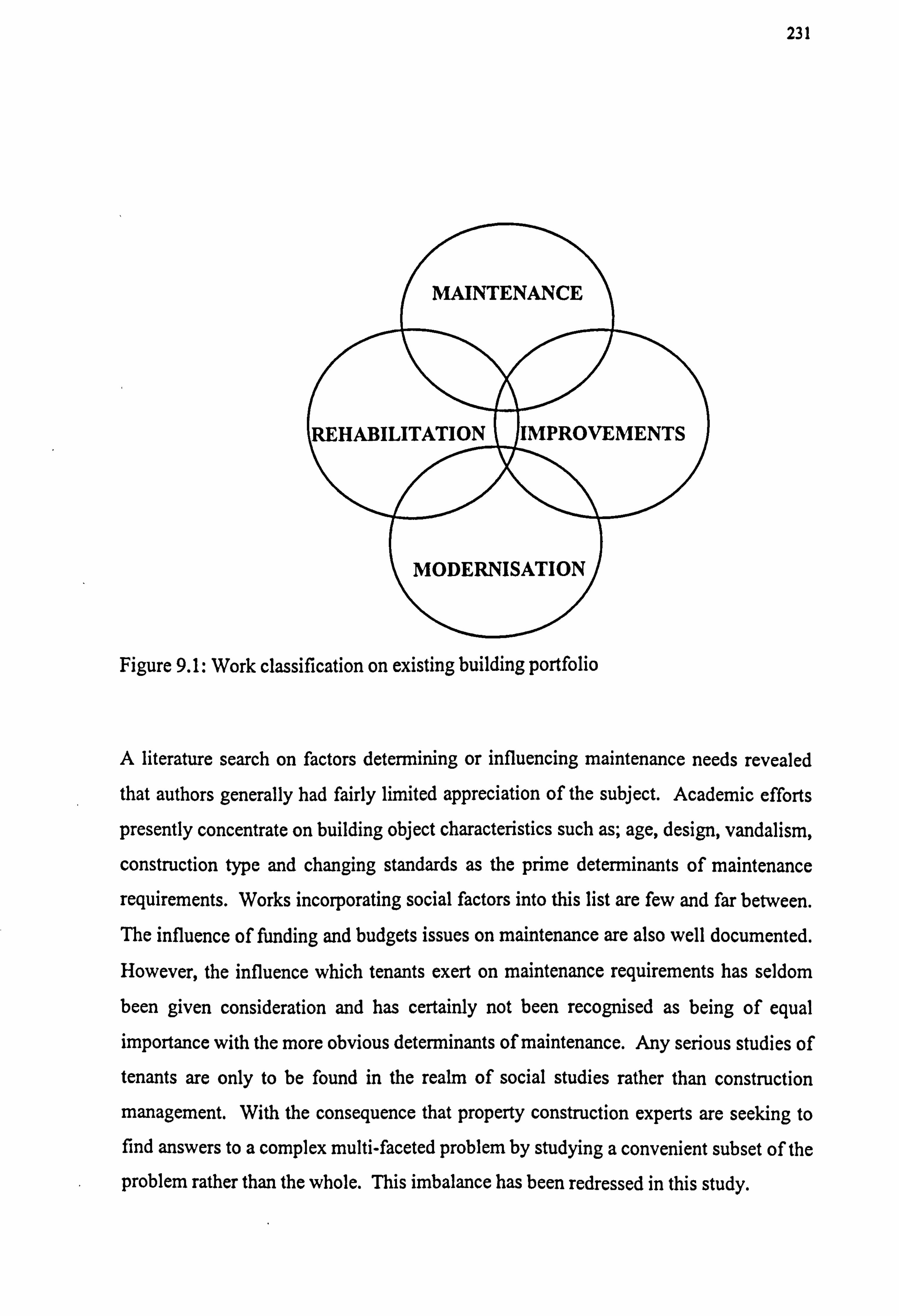
231
Figure 9.1: Work classification on existing building portfolio
A literature search on factors determining or influencing maintenance needs revealed
that authors generally had fairly limited appreciation of the subject. Academic efforts
presently concentrate on building object characteristics such as; age, design, vandalism,
construction type and changing standards as the prime determinants of maintenance
requirements. Works incorporating social factors into this list are few and far between.
The influence of funding and budgets issues on maintenance are also well documented.
However, the influence which tenants exert on maintenance requirements has seldom been given consideration and has certainly not been recognised as being of equal importance with the more obvious determinants of maintenance. Any serious studies of tenants are only to be found in the realm of social studies rather than construction
management. With the consequence that property construction experts are seeking to find answers to a complex multi-faceted problem by studying a convenient subset of the
problem rather than the whole. This imbalance has been redressed in this study.
232
The influence of the mediatory role of local housing management in regulating and
responding to maintenance need and requirements has hardly been acknowledged. It is
the housing officer who decides whether or not report made by a tenant is genuine and deserving of repair action. When that decision is made, it also rests with the housing
officer to determine response time for such defect.
Control of local budgets also influences maintenance requirements because it influences
'the response time of housing officers and building surveyors to defect reports made by
tenants. Each area housing team leader is allocated annual repairs budget and is
responsible for controlling expenditure within those cash limits. In order to exercise
control, the team leader requires an accurate estimate of their committed expenditure on
a job by job and summary basis. What is conspicuously lacking at the moment is a pre-
planned estimate of likely repair cost for a given year before the commencement of the
financial year. This results in budget shortfalls and the most crucial repair needs have
to be foregone in most area offices. In some instances surplus budgets tend to be
inefficiently spent-up towards the end of the financial year in few area offices.
Chapter Six presented the results and interpretations of data analyses following the
steps described in chapter two - with respect to building surveyor's questionnaire. The
response rate to the survey was 45%. A Kendall concordance test of the survey data
showed that defects causing criteria can be prioritised along component line as shown in the table below.
What Table 9.1 demonstrates is that if we wanted, for example, to determine the
soundness of a dwelling in terms of its design (which encompasses specifications and
detailing), we should concentrate any monitoring of performance processes on those
attributes identified, i. e. expansion cracks, dampness in floors, condensation, slab failure and rot. Whilst reliable in terms of design, the measures do not tell us to what
extent such defects impact upon the overall or total maintenance requirements.
233
Table 9.1: Indicative component defects on defect-cause criteria
Defect-Cause Criteria Indicative component
Age Patch repair to roof; Wall ties failure; Bay, canopy and
chimney flashing; Electrical faults; Balcony concrete repair
Vandalism Removing graffiti; Damaged security door; Reglazing;
Internal door repair or replacement; Fencing repair or
replacement
Design Expansion crack; Damp floor; Condensation problem; Slab
and screed failure; Dry or wet rot
Construction Dry or wet rot; Slab and screed failure; Damp floor; Water
ingress; Defective damp proofing
Changing Standard Condensation problem; Electrical faults; Heating repair or
replacement of part; Gas leakage; Defective roof structure
To do this it was necessary to determine the relationships which exist between the
defect-cause criteria namely; age, construction, design, changing standard and
vandalism from the data set. For statistical purpose, the data needed to be tested for
reliability. To achieve this, the analysis of the residuals showed that the data set is
statistically good with approximate normal shape and lack of pattern in the plots of
residual values against the predictor variables. Linear regression applied to the data on
individual predictor variables proved useful in that it showed that three of the five
defect-cause criteria were significant at 10% level of significance. The three significant
defect-cause criteria are construction, design and changing standard. Given these initial
results, it was considered worthwhile to undergo a combined regression analysis in
order to gain an insight into the characteristics of the data sets as a whole.
A combined regression model of the five variables proved to be significant at 95% level
with (F-ratio = 4.05815; P=0.0497; and R2= . 31869). A significant F-statistic as
shown confirms that linear relationships exist between the dependent and independent
variables included in the regression equation. Notwithstanding, the regression model
234
displayed strong characteristics of multicollinearity as shown by insignificant tolerance
values on four of the five variables. These four criteria are age, changing standard,
design, and construction.
The regression model showed that the features of the building object explain about 32%
of the variation in maintenance need. The order of importance of the five criteria was
as follows: 38.7% for standards, 22.7% for construction, 21.5% for design, 11.6% for
vandalism and 5.8% for age. This means that of the five defect-cause criteria identified,
changing standard is the most influential on maintenance requirements, construction
second, design third, vandalism fourth and age fifth. This result is most fascinating
especially with respect to age. What it shows is that the age of a dwelling property is
not very influential on maintenance requirements in comparison with the other four
factors. The obvious existence of multicollinearity shown by high tolerance values
required that further analysis be conducted with the aid of factor analysis technique
given in chapter seven.
In the light of these relationships between the five criteria, Table 9.1 could be
developed further to convey the level of importance of the indicative component defect.
This would help building surveyors to identify the cause of defects and thereby enhance
the determination of the correct remedies for such defects. Table 9.2 shows the level of impact the various building defects have. The darker the row in which a defect is
located, the greater the impact such a defect has on overall maintenance (the darker the
row, the greater the impact). In essence, the greater the impact of a defect, the greater
the probability of more serious problems occurring.
As illustrated, it is of much lesser consequence to ignore a wall tie failure than it is to
ignore a rot problem. The table does not however give any indication of the seriousness
of the chain reaction that could be triggered by the neglect of a defect from one
category to the other. It is noteworthy that defects are repeated across defect-cause.
For example, an electrical defect could be explained as being attributable to either age
or changing standard. The decision on where a particular electrical defect belongs will be best made in the light of other associated events linked with such defects. Such
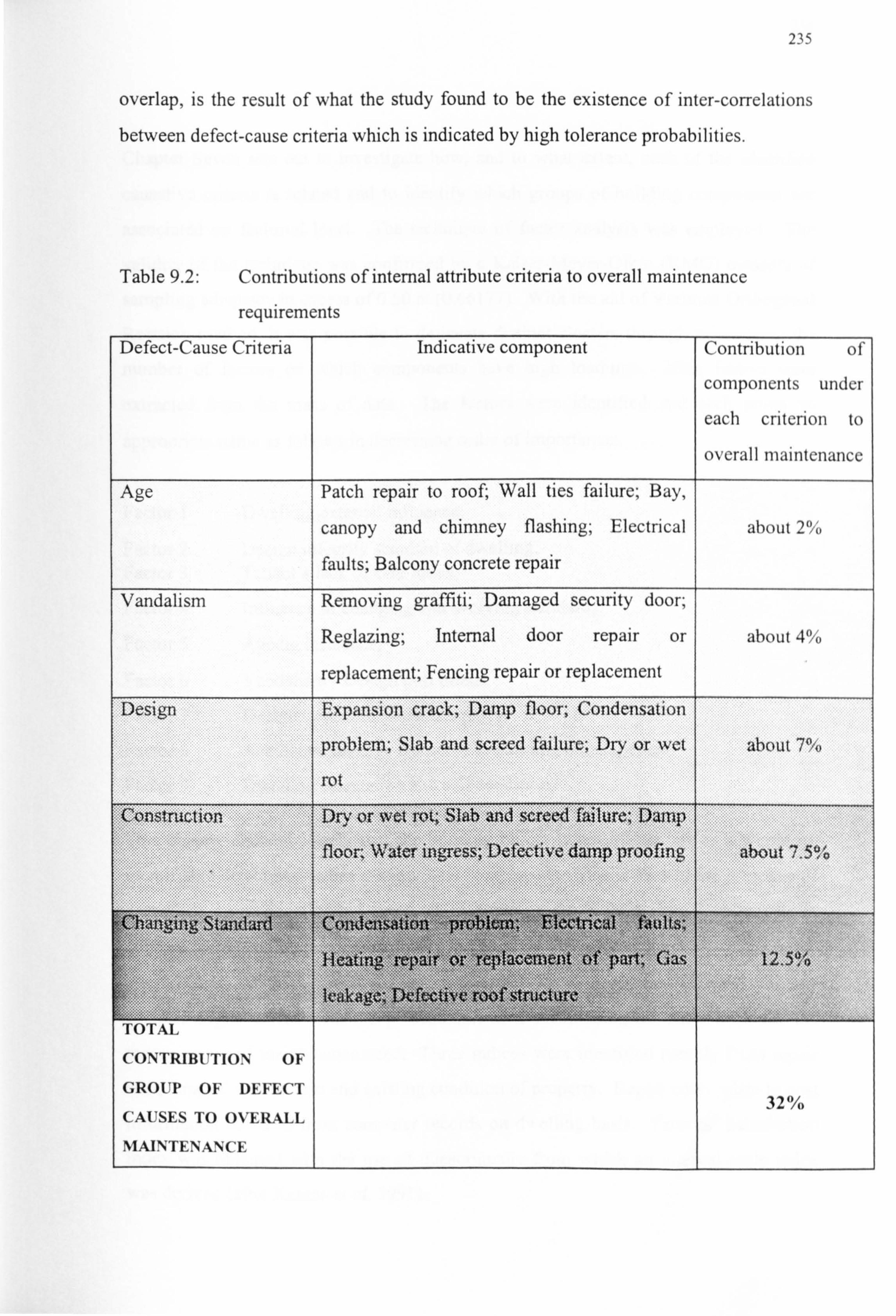
; ti 2
overlap, is the result of what the study found to be the existence of inter-correlations
between defect-cause criteria which is indicated by high tolerance probabilities.
Table 9.2: Contributions of internal attribute criteria to overall maintenance
requirements
Defect-Cause Criteria Indicative component Contribution of
components under
each criterion to
overall maintenance
TOTAL
CONTRIBUTION OF
GROUP OF DEFECT 32%
CAUSES TO OVERALL
MAINTENANCE
236
Chapter Seven sets out to investigate how, and to what extent, each of the identified
causative criteria is related and to identify which groups of building components are
associated on factorial level. The technique of factor analysis was employed. The
validity of the technique was confirmed by a Kaiser-Meyer-Olkin (KMO) measure of
sampling adequacy in excess of 0.50 at (0.66177). With the aid of Varimax Orthogonal
Rotation method, it was possible to delineate distinct clusters through minimising the
number of factors on which components have high loadings. Nine factors were
extracted from the mass of data. The factors were identified and each given an
appropriate name as follows in decreasing order of importance:
Factor 1 Dwelling external influence;
Factor 2 Design integrity standard of dwelling; Factor 3 Tenant's lack of care index;
Factor 4 Influence of changing and evolving standard;
Factor 5 Ageing influence;
Factor 6 Vandalism - Design pull effect;
Factor 7 Design - construction inadequacy;
Factor 8 Accidental damage restricted to building envelope; and
Factor 9 Dwelling orientation and soil condition.
This chapter showed clearly that the building object is not influenced as a whole by
identifiable defect causes but as individual components. This is akin to the principle of
cost planning in quantity surveying which splits up the building into its elements in
contrast to controlling the overall cost of the building as one lump sum.
Chapter Eight started with the presentation of a methodological framework for the
measurement of maintenance need. Three indices were identified namely DLO repair
cost, tenants' satisfaction and existing condition of property. Repair costs relate to cost information obtained from computer records on dwelling basis. Tenants' Satisfaction
index was obtained with the use of questionnaire from which an interval scale index
was derived (after Kearns et a1,1991).
237
Existing Condition of Property index was based upon an appropriate combination of three measures namely; the year of last prior to painting repairs and external paintings,
physical appearance of the building facade and tenant's propensity to carry out repair
work. This last measure has been incorporated because the tenant's disposition to care for his or her home impacts upon the attractiveness of the building to some extent. These three measures were combined to produce property condition index.
Rigorous validatory tests namely boxplot, stem-and-leaf plot, and normality test
analyses were conducted on the three indices which allowed manipulations to be made
to the data as necessary to ensure reliability, efficiency and validity as measures of dwelling maintenance requirement. Using the tenant's questionnaire survey instrument,
this process was followed by rigorous regression model testing to identify significant independent variables from a list of characteristics pertaining to tenant, property,
environmental and housing management attributes (20 in all). Of these groups of
variables, those relating to tenant's attribute proved to be most influential among the
significant factors.
In all, nine variables were significant at 95% level. This means that the variable
concerned have substantial impact (which cannot be merely attributed to chance) upon
one or more of the three indices of maintenance requirements. These variables are; Tenant's age, Presence of disability or limiting illness, Relet work carried out on
property in the last five years, Vandalism index of dwelling, Length lived in current home, Length lived in last home, Likelihood of moving from present home, Tenant's
assessment of service from housing office, and Council's response to repair need.
The models showed with their beta values the strength and direction of the relationship
of each variable to the index on which it proved to be significantly influential. Further
discussions of the implications of these values follow.
238
Table 9.3: Variables with substantial non-chance impact on the three indices
Significant variables on each of the index models showing strength and direction
Maintenance cost Property Condition Satisfaction
Length lived in current Length lived in last home Length lived in last home
home (+. 1244) (-. 1700) (+. 1805)
Tenant's age (-. 3049) Tenant's age (-. 2196) Likelihood of moving from
present home (-. 1880)
Presence of disability or Vandalism index of Vandalism index of
limiting illness (-. 3578) dwelling (+. 1347) dwelling (-. 1321)
Relet work carried out in Tenant's assessment of
the last five years (-. 2834) service from housing officer (+. 1566)
Council's response to repair
need (+. 2015)
50% of variations are 13% of variations are 38% of variations are
explained explained explained
Fifty per cent of the variation in reactive maintenance cost were accounted for, 38% and 13% in satisfaction and property condition indices respectively. The lowly proportion
of property condition explained by the group of significant variables finds explanation in the fact that this index is predominantly influenced by the intrinsic features of the
dwelling building identified in chapters Six and Seven, but which do not lend
themselves to interval or non-interval measurement within the property attribute group
of variables.
Under the maintenance cost index, Presence of disability or limiting illness is the most influential variable, although with an inverse relationship (i. e. negative beta value). The reason for this lies in the fact that some items of maintenance in dwellings
occupied by disabled persons are carried out under social service account rather than housing revenue account. The effect of this is to reduce maintenance spending by the housing department. The second most influential is tenant's age, and the third is relet
work, which is an indicator of tenancy turnover. It is interesting that the fourth, length

239
lived in current home, has a positive correlation. This means that the longer the tenant
has lived in his or her dwelling, the higher the maintenance spending will be.
Under the property condition index, tenant's age is negatively related to property
condition, i. e. the older the tenant, the poorer the property condition. The reason for
this is that older people tend to show more preference for older properties, as they often
believe they are less defect prone. This also explains the direction of variable, length
lived in last home as older people would more probably have lived longer in a previous
address. The positive beta sign of vandalism on property condition implies that the
higher the level of vandalism associated with a dwelling, the more attractive the
property condition appears to be. This suggests that housing management team respond
positively to rectify vandalistic damage, thus resulting in some face-lift to property, or
that dwellings preference by younger families with whom vandalism tends to be more
frequent present more attractive facade as they are generally of newer construction.
Under tenant's satisfaction index, it is interesting that tenants opinions of their housing
officer in particular and the council in general are positively related to how satisfied
they are with repair works. This is to be expected as tenants who consider works
carried out on their properties satisfactory would equally view the housing office as
efficient. In the same vein, those who plan to move from their current home are less
satisfied. It would appear that the desire to move is predicated by lack of satisfaction
rather than for other reasons. It is however intriguing that vandalism index is
negatively and significantly related to tenant's satisfaction. This does not support the
theoretical notion (Ward, 1973) that vandalism is almost always inherent in the built
form. Hence, the need for the construction of a vandalism index which sought to
incorporate some elements of vandalism inherent in the tenant along with
environmental vandalism.
Combining and comparing this group of factors with building object specific factors of
chapters Six and Seven, it is most interesting that none of the nine variables in Table
9.3 belong to internal attributes of building property. Most building object specific factors as detected in chapter Seven do not afford ready measurement and may not have
been included in the original 20 variables of chapter Eight safe in respect of property
t
240
age. The aspect of vandalism in the regression model does not in fact share exactly the
same features as that which is inherent in the building object, but more with the
environment and individuals living in it. In essence, there are two dimensions to
vandalism. According to Newman (1972) one of it is inherent in the nature of the built
form. While the other is dictated by the social attitude of the individuals who live in it
and their impact upon the immediate environment
9.2 Final Conclusion
The research has shown that building surveyors involved in the diagnosis and prognosis
of defects should consider the causes of defects found in buildings as a starting point
for remedial action. By sampling building surveyors from a specified survey
population, the research has established that the factors involved in a specific
component defect in local authority housing are often a combination of factors. It also
demonstrates that each of the specific factors namely; age, construction, design,
changing standard and vandalism affects some components more profoundly than
others. The result is that the elimination of defect causes by surveyors is simplified
depending on which component exhibits defect.
By sampling housing tenants of the local authority chosen for the study, it was revealed
that the influence of tenant's attributes is very strong upon maintenance requirements.
It revealed that it is insufficient for maintenance managers to base their understanding
of the subject purely on physical characteristics and attributes of the property itself.
Managers must also build into any budgetary prediction an allowance for variations in
tenant profiles and their effects upon maintenance generation.
The research also found that housing management responsiveness to repair needs and
report is a significant factor in maintenance need profile of Manchester Council housing
stock. The research has therefore provided a collection of factors in the realm of the
building object, tenants characteristics, housing management and environmental influence which have significant impact on maintenance need. These factors are identified as follows in Table 9.4.
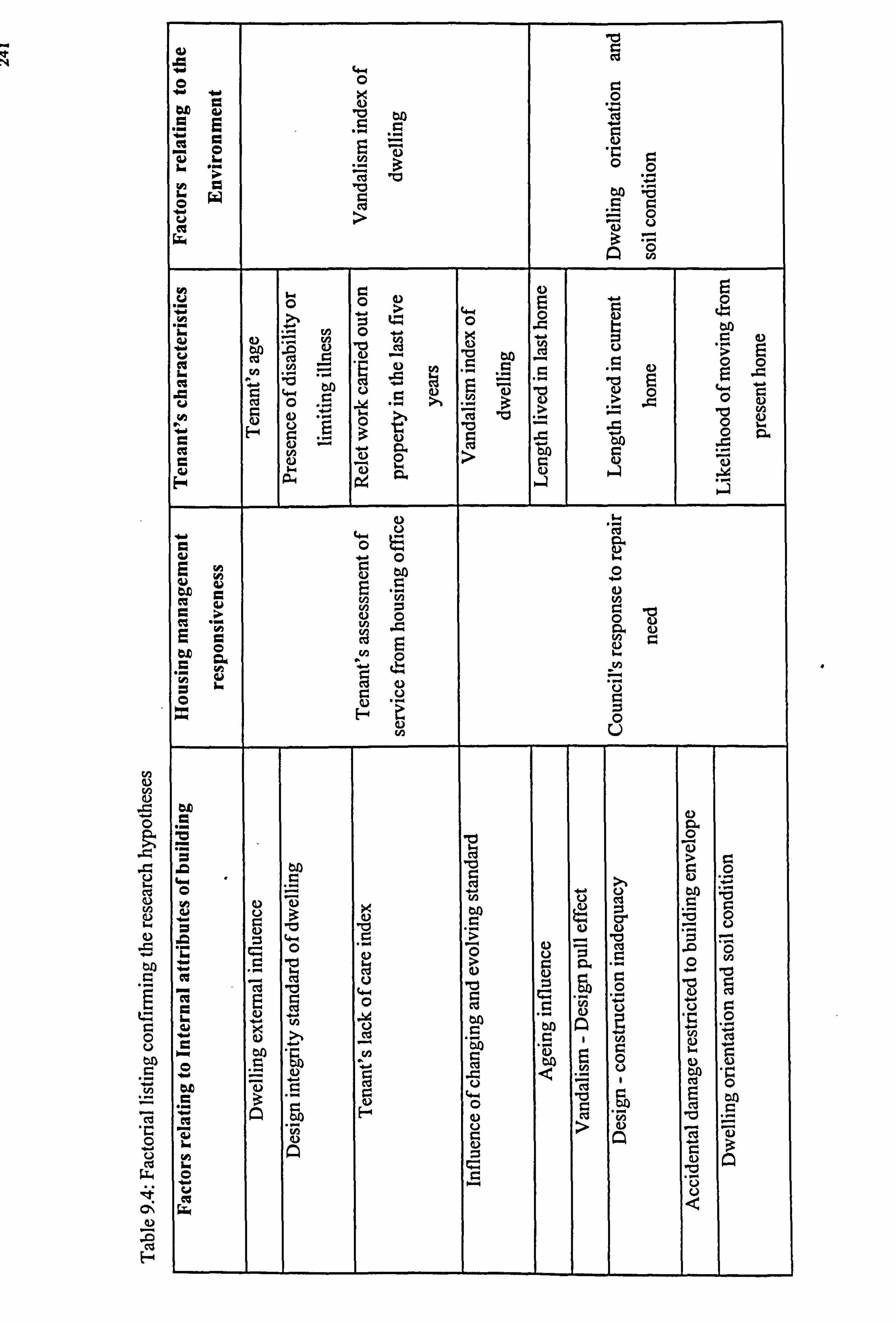
0
on
0 U to
cd
U CG
E-
10 - w
r
ice'. o
='
W
o
Ei
'O ý
3
ao ý
ö
'ýCý ö " U
A o
.M -
5
e4 . L7
m
y 0p
4- C" 9
.0 y
10 4-4 o
u
C
to
r
'O
V x
9. )
w_
.. r y
. -
R. KZ
N
ý,
ö
E
,m
,2 2
-
"C C)
V
r.
y >
Ö
=
man A
"'J
O FCE
o
Nýr E
O
Q
a,
Ü " ýp,,
CA
r
L7
rýv"
y
>
yý
y
vOi
.+
Er
pq
"y
0
w
N
O
N
O
N
O U
oo C)
bi) C) o o
O
vm "ý"
.. C°r
º""
*W
r.
G
cd E ''
3 Z
3 0
b
b
N ýq
Eh C A
IC
O c5
ö
v
y
. 5:
0 a)
Q
°n
ö
0 o -
y ý., E_ on pOq
V
p.
N
A
"0 9 >
v
v
-
Ü 2
o
-5 Ä
bA
e
O +-' b
Ü
C)
10 ä
v
N b
cd r. " o
aCi
bn . - ä 3
ü cq
f. )
242
9.3 Scope and limitations
The mediatory role of the stockholder is essentially discounted in this study - policy and
budget matters are nebulous and do not readily lend themselves to direct and objective
assessment, and for which no proxy variables have been devised. They are principally
dictated by political dictum and nuances which are a function of national and
international political and economic climate. Furthermore, no proportional strengths of
the indices of maintenance need are inferred in the study and hence, does not confirm to
what extent one variable is more or less important than the other. No account is taken of
the realism of repairs carried out without defects having occurred as in preventive
maintenance safe to the extent that such works (prior to painting repairs and external
painting) are incorporated into the property condition index.
9.4 Recommendation for further study
The following issues which emerged but could not be covered in the course of this work
are recognised as worthy of further investigation.
1. Further study can be conducted to establish more objective interval level
measurement criteria for variables measured on a rating scale and classified as
ordinal. variables in the research such as level of disability of tenant, housing
management responsiveness to repairs and building object features. Such interval
level measurement would enable the effects of these variables to be more precisely
investigated in a regression model.
2. This study can be replicated on additional public sector housing across the UK and
elsewhere using the methodology described so that the results can be pooled and
more dependable factorial framework can be developed.
3. It is recognised that this study does not constitute an end in its own right, it is only a
means towards the development of comprehensive and appropriate maintenance forecasting models in the sector, for which a comprehensive and measurable list of
significant factors are indispensable (Sanders and Thomas, 1992).
243
REFERENCES
Adams, J. S. (1956), An experiment on question and response bias, Public Opinion Quarterly, No. 20, Fall.
Aiken, L. R. (1991), Psychological testing and assessment, 7th edition, Boston: Allyn and Bacon
Akintoye, S. A. (1991), Construction tender price index: modelling and forecasting trends, unpublished PhD Thesis, Salford University.
Allen, R. T. (1986), Choosing a concrete repair system, Construction Repair & Maintenance, September.
ANON (1977), Start right; the road to better building, Building, 232,6985,13 May,
pp43.
Alner, G. R. and Fellows, R. F. (1990), Maintenance of local authority school buildings in UK: a case study, In Quah, L. K. (ed. ): Building Maintenance and Modernisation Worldwide, March, Singapore, Vol. 1, pp 90-99.
Armstrong, G. and Wilson, M. (1973), Delinquency and some aspects of housing. In Ward, W. (ed. ): Vandalism, London and St Austell: H. E. Warne.
Ashworth, A. and Au-Yeung, (1987), The usefulness of maintenance cost records in life
cycle cost prediction, In Spedding, A. (ed. ): Building Maintenance Economics and Management, E. & F. N. Spon, London, pp 141-150.
Association of Metropolitan Authorities, (1991), Refurbishing the Citizen's Charter.
Attenburrow, J. J. et al, (1978), The problems of some large local authority estates, pp9- 17.
Baker, A. J. (1976), `Valuing Information about Risks', University of Leicester Discussion Paper No. 51.
Black, J. A. and Champion, D. J, (1976), Methods and Issues in Social Research, New York: John Wiley & Sons, Inc.
Robertson, J. D. M. (1988), Maintenance audit, Building Maintenance Cost Information Service.
Barlow, R. E. and Proschan, F. (1965), Mathematical reliability, Wiley, New York.
Baldwin, J. (1974), Problem housing estate - perceptions of tenants, City Officials Criminologists, pp9-17.
Balchin, P. N. (1979), Housing improvement and social inequality: case study of an inner city, Westmead: Teakfiel Ltd.
244
Bargh, J. (1987) Increasing maintenance needs on limited budgets; A technique to assist the building manager in decision making, In Spedding, A. (ed. ): Building Maintenance, Economics and Management, E&F. N. Spon, pp321-326.
Bedale, C. (1980), Property relations and housing policy: Oldham in the late nineteenth and early twentieth centuries in Housing, In Melling, J. (ed. ): Social Policy and the State, Croom Helm Ltd. London.
Beeston, D. T. (1983), Statistical methods for building price data, Spon, London.
BRS, (1963), Cost comparisons in housing maintenance, Current paper design series 13, London: Institute of Municipal Treasurers and Accountants.
BRS, (1968), The maintenance and running costs of school buildings, Current paper 72/68, London: Institute of Municipal Treasurers and Accountants.
BRE, (1972), Costs in use: A guide to data and techniques, London: HMSO.
Bird, B. (1987), Cost-in-use: principles in the context of building procurement, Construction Management and Economics, Vol. 5 special issue, pp23-30.
Birks, D. F. and Southan, J. M. (1992), An evaluation of the rationale of tenant satisfaction surveys, Housing Studies, Vol. 7, No. 4, pp299-308.
Bishop, D. (1984), Some reflections on life cycle costing, In P. S. Brandon and J. A. Powell, (eds. ) Quality and Profit in Building Design, London: E. & F. N. Spon, pp385- 394.
BS 3811 (1984)
Bromilow, F. J. (1984), Economics of tall buildings, Proceedings International Conference on Tall Buildings, Singapore Institution of Engineers, Singapore, pp22-26.
Bromilow, F. J. and Pawsey, M. R. (1987), Life cycle cost of university buildings, Construction Management and Economics, Vol. 5 special issue, pp3-22
Brown, P. M. and Robertson, G. L. (1990), Comparative office building maintenance costs, In Quah, L. K. (ed. ): Building Maintenance and Modernisation Worldwide, March, Singapore, Vol 1, ppl72-181.
Bouchard, T. J. (1976), Field research methods: interviewing, questionnaires, participant observation, systematic observation, unobstructive measures, In Dunnette, M. D. (ed. ): Handbook of industrial and organisational psychology, University of Minnesota, pp363-413.
Bufaied, A. S. (1987), Risks in the construction industry: their causes and their effects at the project level, unpublished PhD Thesis, UMIST.
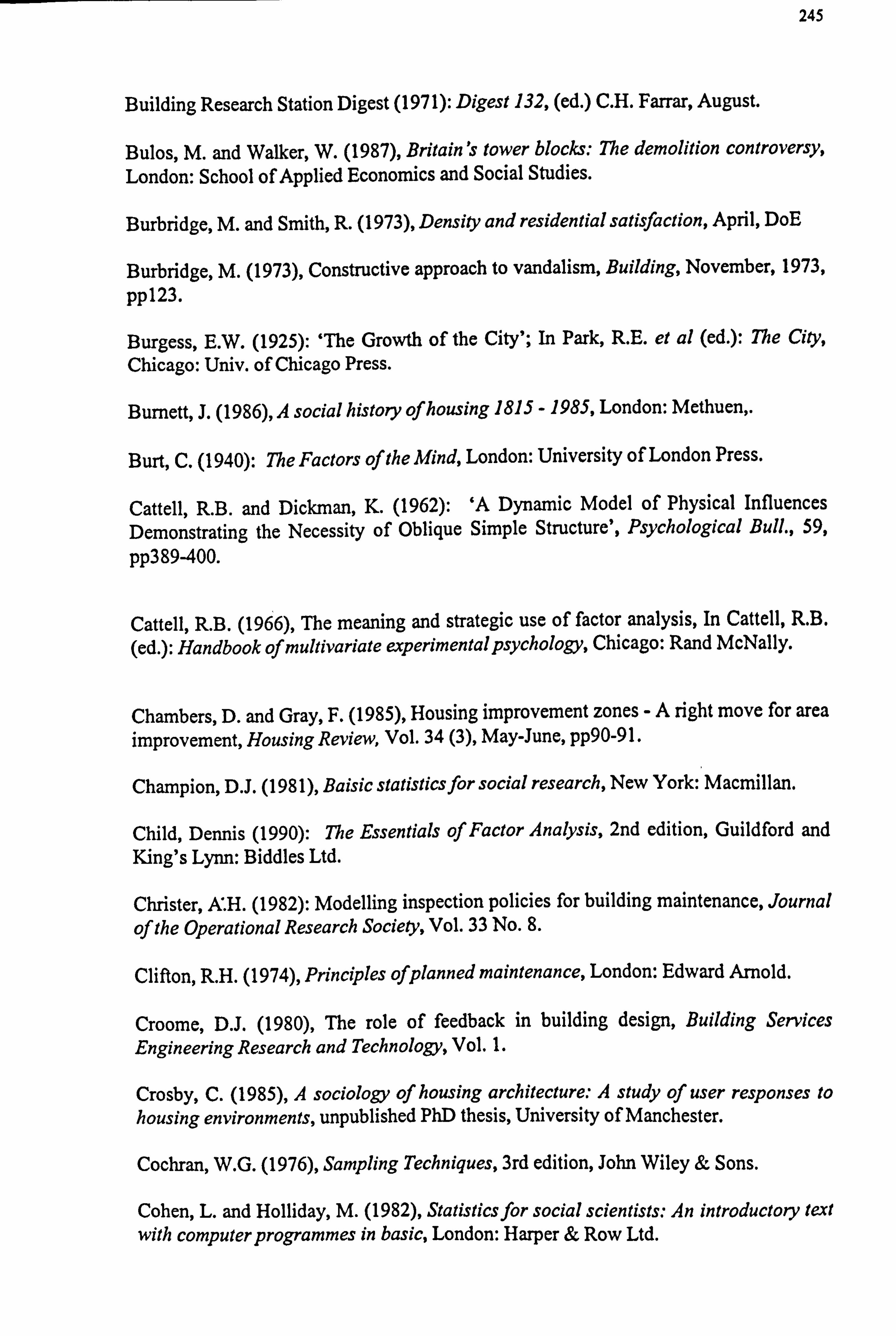
245
Building Research Station Digest (1971): Digest 132, (ed. ) C. H. Farrar, August.
Bulos, M. and Walker, W. (1987), Britain's tower blocks: The demolition controversy, London: School of Applied Economics and Social Studies.
Burbridge, M. and Smith, R. (1973), Density and residential satisfaction, April, DoE
Burbridge, M. (1973), Constructive approach to vandalism, Building, November, 1973,
pp123.
Burgess, E. W. (1925): `The Growth of the City'; In Park, R. E. et al (ed. ): The City, Chicago: Univ. of Chicago Press.
Burnett, J. (1986), A social history of housing 1815 - 1985, London: Methuen,.
Burt, C. (1940): The Factors of the Mind, London: University of London Press.
Cattell, R. B. and Dickman, K. (1962): `A Dynamic Model of Physical Influences Demonstrating the Necessity of Oblique Simple Structure', Psychological Bull., 59,
pp389-400.
Cattell, R. B. (1966), The meaning and strategic use of factor analysis, In Cattell, R. B. (ed. ): Handbook of multivariate experimental psychology, Chicago: Rand McNally.
Chambers, D. and Gray, F. (1985), Housing improvement zones -A right move for area improvement, Housing Review, Vol. 34 (3), May-June, pp90-91.
Champion, D. J. (1981), Baisic statistics for social research, New York: Macmillan.
Child, Dennis (1990): The Essentials of Factor Analysis, 2nd edition, Guildford and King's Lynn: Biddles Ltd.
Christer, A. H. (1982): Modelling inspection policies for building maintenance, Journal
of the Operational Research Society, Vol. 33 No. 8.
Clifton, R. H. (1974), Principles of planned maintenance, London: Edward Arnold.
Croome, D. J. (1980), The role of feedback in building design, Building Services Engineering Research and Technology, Vol. 1.
Crosby, C. (1985), A sociology of housing architecture: A study of user responses to housing environments, unpublished PhD thesis, University of Manchester.
Cochran, W. G. (1976), Sampling Techniques, 3rd edition, John Wiley & Sons.
Cohen, L. and Holliday, M. (1982), Statistics for social scientists: An introductory text with computer programmes in basic, London: Harper & Row Ltd.
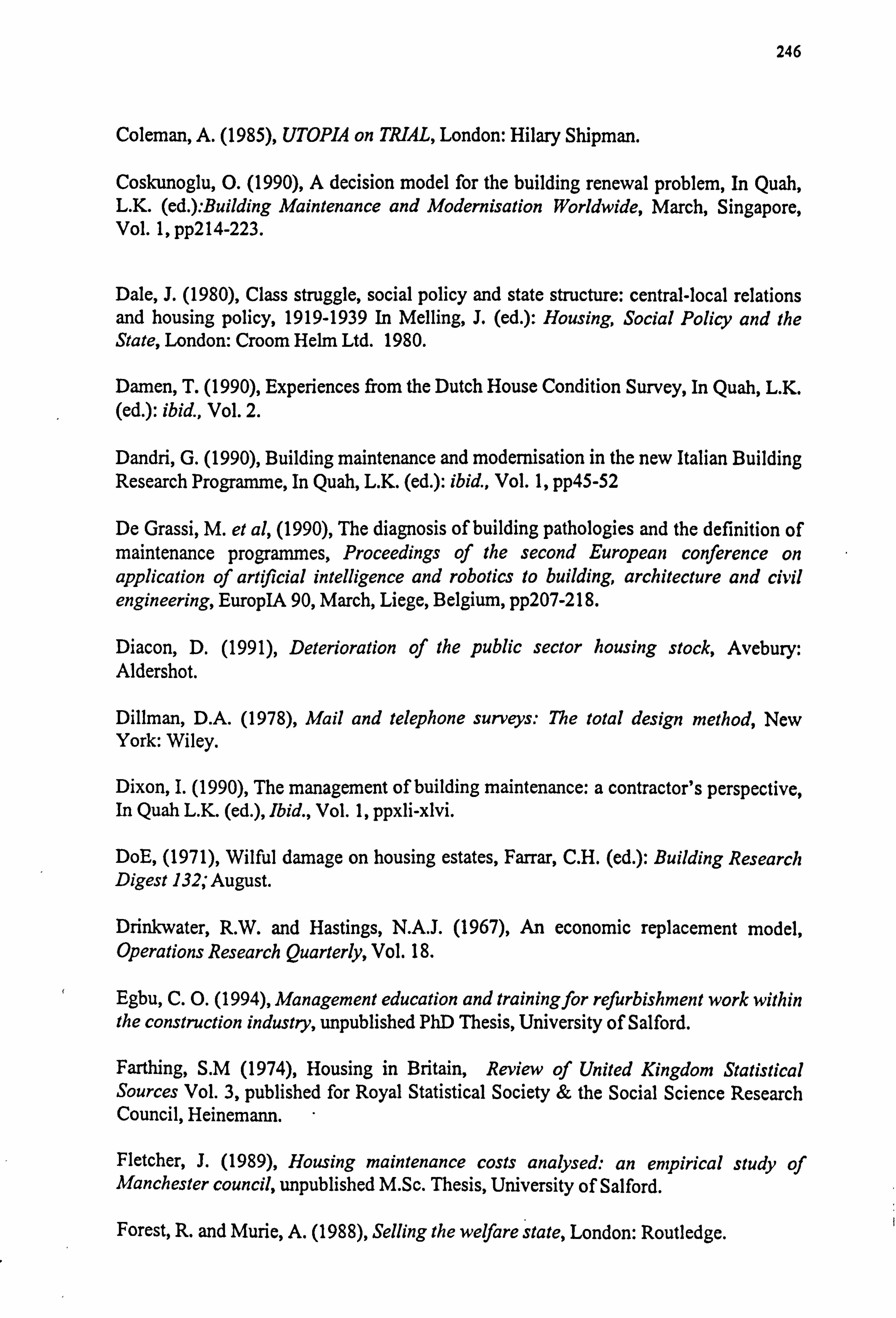
246
Coleman, A. (1985), UTOPIA on TRIAL, London: Hilary Shipman.
Coskunoglu, 0. (1990), A decision model for the building renewal problem, In Quah, L. K. (ed. ): Building Maintenance and Modernisation Worldwide, March, Singapore, Vol. 1, pp214-223.
Dale, J. (1980), Class struggle, social policy and state structure: central-local relations and housing policy, 1919-1939 In Melling, J. (ed. ): Housing, Social Policy and the State, London: Croom Helm Ltd. 1980.
Damen, T. (1990), Experiences from the Dutch House Condition Survey, In Quah, L. K. (ed. ): ibid., Vol. 2.
Dandri, G. (1990), Building maintenance and modernisation in the new Italian Building Research Programme, In Quah, L. K. (ed. ): ibid., Vol. 1, pp45-52
De Grassi, M. et al, (1990), The diagnosis of building pathologies and the definition of maintenance programmes, Proceedings of the second European conference on application of artificial intelligence and robotics to building, architecture and civil engineering, EuropIA 90, March, Liege, Belgium, pp207-218.
Diacon, D. (1991), Deterioration of the public sector housing stock, Avebury: Aldershot.
Dillman, D. A. (1978), Mail and telephone surveys: The total design method, New York: Wiley.
Dixon, I. (1990), The management of building maintenance: a contractor's perspective, In Quah L. K. (ed. ), Ibid., Vol. 1, ppxli-xlvi.
DoE, (1971), Wilful damage on housing estates, Farrar, C. H. (ed. ): Building Research Digest 132; August.
Drinkwater, R. W. and Hastings, N. A. J. (1967), An economic replacement model, Operations Research Quarterly, Vol. 18.
Egbu, C. 0. (1994), Management education and training for refurbishment work within the construction industry, unpublished PhD Thesis, University of Salford.
Farthing, S. M (1974), Housing in Britain, Review of United Kingdom Statistical Sources Vol. 3, published for Royal Statistical Society & the Social Science Research Council, Heinemann.
Fletcher, J. (1989), Housing maintenance costs analysed: an empirical study of Manchester council, unpublished M. Sc. Thesis, University of Salford.
Forest, R. and Murie, A. (1988), Selling the welfare state, London: Routledge.
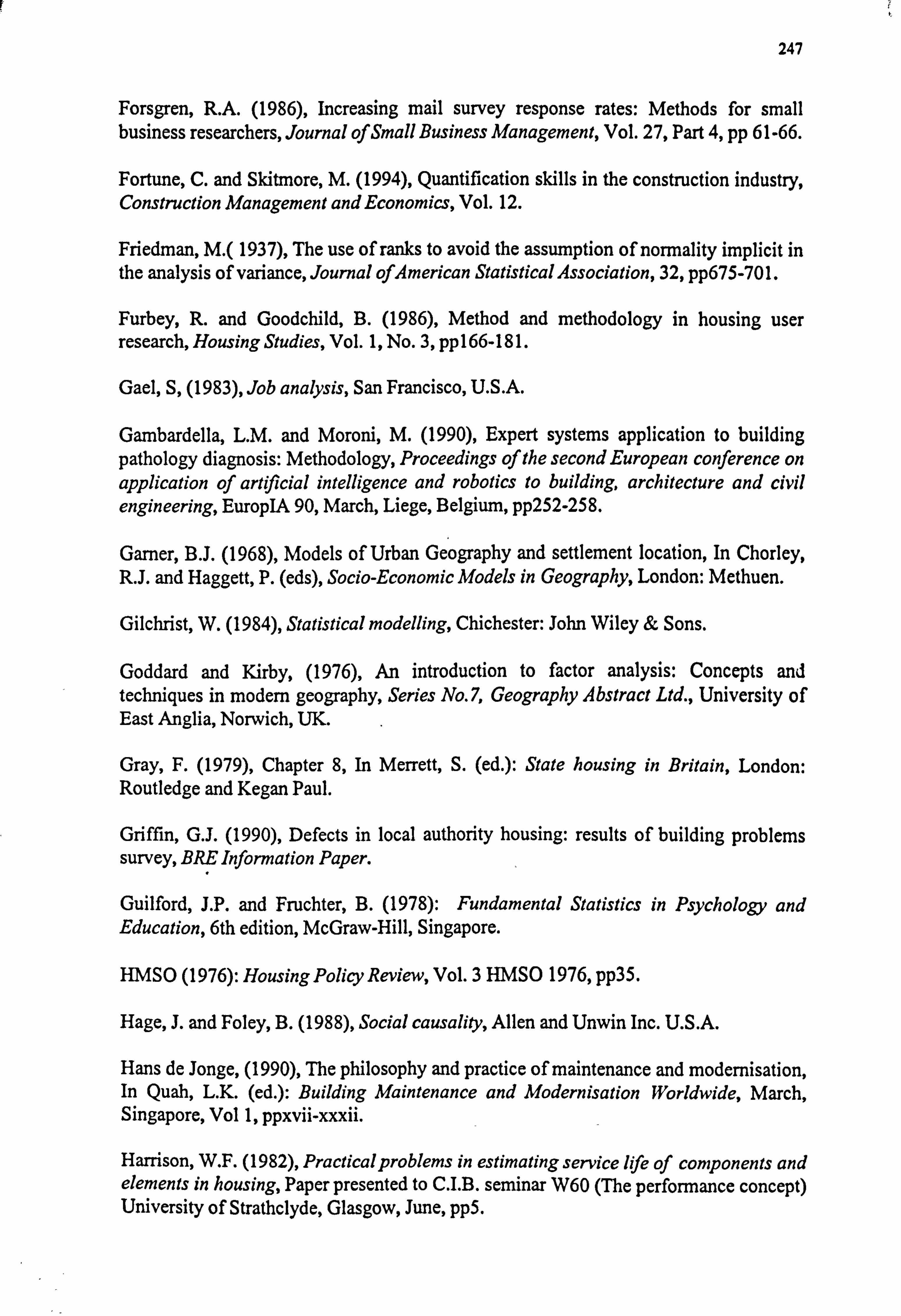
247
Forsgren, R. A. (1986), Increasing mail survey response rates: Methods for small business researchers, Journal of Small Business Management, Vol. 27, Part 4, pp 61-66.
Fortune, C. and Skitmore, M. (1994), Quantification skills in the construction industry, Construction Management and Economics, Vol. 12.
Friedman, M. ( 1937), The use of ranks to avoid the assumption of normality implicit in the analysis of variance, Journal ofAmerican Statistical Association, 32, pp675-701.
Furbey, R. and Goodchild, B. (1986), Method and methodology in housing user research, Housing Studies, Vol. 1, No. 3, pp166-181.
Gael, S, (1983), Job analysis, San Francisco, U. S. A.
Gambardella, L. M. and Moroni, M. (1990), Expert systems application to building pathology diagnosis: Methodology, Proceedings of the second European conference on application of artificial intelligence and robotics to building, architecture and civil engineering, EuropIA 90, March, Liege, Belgium, pp252-258.
Garner, B. J. (1968), Models of Urban Geography and settlement location, In Chorley, R. J. and Haggett, P. (eds), Socio-Economic Models in Geography, London: Methuen.
Gilchrist, W. (1984), Statistical modelling, Chichester: John Wiley & Sons.
Goddard and Kirby, (1976), An introduction to factor analysis: Concepts and techniques in modem geography, Series No. 7, Geography Abstract Ltd., University of East Anglia, Norwich, UK.
Gray, F. (1979), Chapter 8, In Merrett, S. (ed. ): State housing in Britain, London: Routledge and Kegan Paul.
Griffin, G. J. (1990), Defects in local authority housing: results of building problems survey, BRE Information Paper.
Guilford, J. P. and Fruchter, B. (1978): Fundamental Statistics in Psychology and Education, 6th edition, McGraw-Hill, Singapore.
HMSO (1976): Housing Policy Review, Vol. 3 HMSO 1976, pp35.
Hage, J. and Foley, B. (1988), Social causality, Allen and Unwin Inc. U. S. A.
Hans de Jonge, (1990), The philosophy and practice of maintenance and modernisation, In Quah, L. K. (ed. ): Building Maintenance and Modernisation Worldwide, March, Singapore, Vol 1, ppxvii-xxxii.
Harrison, W. F. (1982), Practical problems in estimating service life of components and elements in housing, Paper presented to C. I. B. seminar W60 (The performance concept) University of Strathclyde, Glasgow, June, pp5.
248
Harrison, J. D, (1990), Maintenance as an aspect of architectural design, In Quah, L. K. (ed. ): Building Maintenance and Modernisation Worldwide, March, Singapore, Vol. 2, pp1086-1096.
Hays, W. L. (1988), Statistics, 5th edition, Holt, Reinhart & Winston, New York.
Headley, B. (1978), Housing Policy in the Developed Economy, London: Croom Helm Ltd.
Hollis, M. and Gibson, C. (1991) Surveying Buildings, 3nd edition, London: RICS Books.
Holmes, R. and Droop, C. (1982), Factors affecting maintenance costs in L. A. housing, In Brandon, P. S. (ed. ): Building Cost Techniques New Directions.
Holmes, R. (1985), The evaluation of determinants in maintenance expenditure on L. A. dwellings, unpublished Ph. D. Thesis, University of Reading.
Holmes, R. (1987), Evaluation of determinants in maintenance expenditure on local authority dwellings. In Spedding, A. (ed. ): Building Maintenance Economics and Management, Spon, London, pp235-244.
Honstede, W. V. (1990), Research into the Quality of Housing Stock in the Netherlands, In Quah, L. K. (ed. ): Building Maintenance and Modernisation Worldwide, March, Singapore, Vol. 2, pp659-668.
Jobber, D. (1986), Improving response rates in industrial mail survey, Industrial Marketing Management, Vol. 15, No. 3, pp183-195
Kaiser, H. F. (1974), An index of factorial simplicity, Psychometrika, 39, pp31-36.
Kanuk, L and Berenson, C. (1975), Mail Surveys and Response Rates: A Literature Review, Journal of Marketing Research 12, Nov., pp440-453
Kearns, R. A. et al, (1991), Another day in paradise? Life on the margins, Urban New Zealand, Social Science Medical, Vol. 33, No. 4.
Kelly, A. (1988), A proposed framework for the analysis of maintenance systems, unpublished PhD Thesis, University of Manchester.
Kempen, E. V. and Musterd, S. (1991), High-rise housing reconsidered: some research and policy implications, Housing Studies, Vol. 6, No 2, April, pp83-95
Kendall, M. G. (1970), Rank correlation methods, 4th edition, Griffin & Co., London
249
Kerlinger, F. N. (1973), Foundations of behavioural research, Holt Rhinehart and Winston.
Kidder, L and Judd, C. (1981), Research methods in social relations, Holt Rinehart & winston inc. NY.
Kim, J& Mueller, C. W. (1978a): Introduction to factor analysis: What it is and how to do it, Sage university paper series on quantitative applications in the social sciences, 07-013. Newbury Park, CA: Sage.
Kim, J& Mueller, C. W. (1978b): Factor analysis: Statistical methods and practical issues, Sage university paper series on quantitative applications in the social sciences, 07-014. Newbury Park, CA: Sage.
Kinnear, P. R. and Gray, C. D. (1994), SPSS for Windows made simple, Hove: Lawrence Erlbaum Associates Ltd.
Kirby, D. A. (1972), The Inter- War Council Dwelling.
Klama, J. (1988), Aggression : Conflict in Animals and Humans Reconsidered, Longman.
Kline, P. (1987), Factor analysis and personality theory, Journal of Continuing Education, Vol. 2 Part 2, November.
Kondo et al, (1990), Simplified inspection method for long term maintenance to existing buildings, In Quah, L. K. (ed. ): Ibid., Vol. 2, pp650-658.
Labovitz, S. (1970), The assignment of numbers to rank order categories, American Sociological Review, 35: 515-524.
Latham, G. P. and Saari, L. M. (1984), Do People Do What They Say? Further Studies on the Situational Interview, The Statistical Review, American Psychological Association, Inc., vol 69 No. 4,1984 p 573 -
Lawson, R. B, Goldstein, S. G and Musty, R. E. (1975): Principles and methods of psychology, Oxford university press.
Lee, R. (1981), Building maintenance management, 2nd edition, Granada publishing, UK.
Leedy, P. D. (1989), Practical research planning and design, 4th edition, Macmillan.
Malpass, P. (1991), Books reviews, Housing Studies, Vol. 7, No. 1, pp75.
Malpass, P. (1993), Housing tenure and affordability: The British disease, In Graham Hallet (ed. ), The 'New Housing Shortages: housing affordability in Europe and the USA, London and NY: Routledge.

250
Malpass P. et al, (1993), Housing policy in action: The new financial regime for council housing, Bristol: SAUS Publications.
Manchester City Council (1986), Housing defects in Manchester, (Manchester City Housing Department)
Manchester City Council (1947), Manchester Housing, (Housing Committee)
Marman, HE (1967), Modern Factor Analysis, University of Chicago Press, Chicago.
McGeorge, D. and Betts, M. (1990), Systems approach to building maintenance forecasting, In Quah, L. K. (ed. ): ibid., Vol. 1, pp192-199.
McKennel, A. (1968), Some uses of factor analysis in social survey work, Government Social Survey No. M152, London.
Melville, I. A. and Gordon, I. A. (1979), The repair and maintenance of houses, Pitman Press.
Mole, T. (1991), Building maintenance policy: nebulous nevertheless necessary, In Proceedings of the Ist National Research Conference of the Royal Institution of Chartered Surveyors: Investment, Procurement and Performance in Construction, E& F. N. Spon, London, pp303-315.
Mole, T. and Olubodun, O. F. (1995a), A critique of definitional problems in building portfolio maintenance: International conference proceedings: Maintenance - Reliability
- Quality, April, Cambridge, pp123-127.
Mole, T. and Olubodun, O. F. (1995b), Principal factors in local authority housing maintenance need: survey of building surveyors' views; International conference proceedings: Maintenance - Reliability - Quality, April, Cambridge, pp 128-132.
Moser, C. A. and Kalton, G. (1971), Survey methods in social investigation, Heineman.
Nakagawa, T. and Osaka, S. (1982), The optimum repair limit replacement policies, Operations Research Quarterly, 25 No. 2.
National Income Statistics, (1976),
Neal, F. and Shone, R. (1976), Economic model building, London: Macmillan.
Newman, 0. (1972), Defensible space: People and design in the violent city, Architectural Press, London.
Ngo, M. (1990), Asset Management -A methodology for establishing maintenance standards, In Ireland, V. and Runeson, G. (eds. ): Building Economics and Construction Management, University of Sydney, Vol. 3, ppl49-157.
251
Ngo, M. et al, (1990), Establishment of standards in property maintenance -A pilot study. In Quah, L. K. (ed. ): Building Maintenance and Modernisation Worldwide, March, Singapore, Vol. 1, pp138-145.
Nireki, T. et al (1990), Trends in maintenance and modernisation of buildings in Japan, In Quah, L. K. (ed. ): Building Maintenance and Modernisation Worldwide, March, Singapore, Vol 1, pp1-10.
Nkado, R. N. (1991), A construction time information system for the building industry, unpublished PhD Thesis, University of Reading.
Norusis, M. J. (1985), SPSS-XAdvanced Statistics Guide, McGraw-Hill.
Norusis, M. J. (1988), SPSS-XAdvanced Statistics V2.0, Chicago: SPSS Inc.
Norusis, M. J. (1990), SPSS base system user's guide, Chicago: SPPS Inc.
Norusis, M. J. (1991), The SPSS Guide to data analysis for SPSS/PC+, 2nd edition, Chicago: SPSS Inc.
O'Dell, A. (1990), Development of the English house condition survey. In Quah, L. K. (ed. ): Building Maintenance and Modernisation Worldwide, March, Singapore, Vol. 2, pp595-604.
O'Dell, A. (1991), The English house condition survey and the national housing stock Part 1: The survey and the housing stock up to 1991, C. I. O. B. Construction Papers No. 52, Edited by P. Harlow.
O'Dell, A. (1995), The English house condition survey and the national housing stock Part 2: The housing stock in 1991, C. I. O. B. Construction Papers No. 53, Edited by P. Harlow.
Olubodun, O. F. and Mole, T. (1996), Helping housing managers understand the maintenance requirements of their stock - Tenant's issues, In The Construction and Building Research Conference of the Royal Institution of Chartered Surveyors, (COBRA), University of West England, Bristol, September.
Overall, J. E. and Klett, C. J., (1972), Applied multivariate analysis, McGraw-Hill, London.
Perin, C. (1970), With man in mind: An interdisciplinary prospectus for environmental design, Hoffeman Press.
Pitt, T. J. (1987), Using models to evaluate property maintenance strategy, In Brandon, P. S. (ed. ): Building Cost Modelling and Computers, E. & F. N. Spon, London, ppS3S- 544.
Phillips, C. (1986), Facilities renewal: the formula approach, In proc. 73rd annual meeting of the Association of physical plant administrators of universities and colleges, Boston, Mass.
252
Pollock, B. J. (1990), The economic aspects of buildings as assets, In Ireland, V. and Runeson, G. (eds. ): Ibid., Vol. 3
Porteous, W. A. (1982), Building failures, The Chartered Builder, Vol. 35.
Porteous, W. A. (1985), Perceived characteristics of building failure -A survey of the recent literature, Architectural Science Review, Vol. 28, June, pp53-56
Pullar- Strecker, P. (1990), Building defects: Are they avoidable?, In Quah, L. K. (ed. ): ibid., Vol. 1, ppxlvii-lii.
Pullen, L. M. (1987), Collection of property occupancy costs, In Brandon, P. S. (ed. ): Building Cost Modelling and Computers, E. & F. N. Spon, London, pp545-548.
Quah, L. K. (1991), Building maintenance and modernisation - research and practice trends, Transactions of the European symposium on management and economics in housing and other buildings, October, Lisbon.
Reece, I. and Walker, S. (1994), A practical guide to teaching and learning, 2nd edition.
Reiners, W. J. (1955), Maintenance costs of local authority, Housing Journal of the Institute of Municipal Engineers, No. 81.
Reynolds, H. T. (1977), The analysis of cross-classifications, The Free Press, NY.
Rowntree, D. (1987), Assessing students: How shall we know them? London, Kagan Page.
Russell, J. S. et al, (1992), Contractor prequalification data for construction owners; Construction Management and Economics, 10,117-135.
Sanders, SR and Thomas, H. R. (1992), H. R. Factors Affecting Masonry -Labour Productivity, Journal of Construction Engineering and Management.
Schieffelin, W. (1973): Anger and shame in the tropical forest: an affect as a cultural system in Paupau N. Guinea, ETHOS, 113, pp183-84.
Schuessler, K. (1971), Analysing social data: a statistical orientation, Boston (Mass). Houghton Mifflin Co.
Seeley, I. H. (1987), Building maintenance, 2nd ed., MacMillan.
Sherman, D. R. and Dergis, W. A. (1980), A funding model for building renewal, University of Michigan.
Short, J. R. (1982), Housing in Britain: the post-war. experience, London: Methuen.
253
Siegel, S. and Castellan, N. J. ( 1988), Nonparametric statistics for behavioural sciences, McGraw Hill.
Siegel, S. (1956), Nonparametric statistics for the behavioural sciences, McGraw Hill.
Smith, B. (1990) Effect of housing design on crime and crime prevention, Crime Prevention News (CPN), pp7.
Smith, C. J. et al, (1992), A tale of two cities: The experience of housing problems in Auckland and Christchurch, New Zealand Geographer, 48,1, pp2-10.
Spedding, A. (1987a), Management of maintenance - The need for and use of data, In Spedding, A. (ed. ): Building Maintenance Economics and Management, E. & F. N. Spon, London, pp37-48.
Spedding, A. (1987b), Building maintenance management and computers, In Brandon, P. S. (ed. ): Building Cost Modelling and Computers, E. & F. N. Spon, London, pp557- 566.
Spedding, A. (1990), Schools design and maintenance in England. In Quah, L. K. (ed. ): Building Maintenance and Modernisation Worldwide, March, Singapore, Vol. 2, ppl068-1076.
Spedding et al, (1995), Prioritising planned maintenance in county authorities, International conference proceedings: Maintenance - Reliability - Quality, April, Cambridge, pp 172-178.
Stevenson, A. et al, (1967), High living: A study of family life in flats, Melbourne Univ. Press.
Stoaling, D. (1985), The precast housing problems, Construction Repairs & Maintenance, July, pp6-7.
Stone, P. A. (1980), Building design evaluation - cost-in-use, London: Spons.
Tabachnick, B. G. and Fidell, L. S. (1989), Using multivariate statistics, 2nd edition, New York: Harper and Row.
Taylor, R. (1987), A computer based maintenance management system. In Spedding, A. (ed. ): Building Maintenance Economics and Management, E. & F. N. Spon, London, pp49-58.
Then, D. S. S. (1990), The impact of information technology on built asset management. In Ireland, V. and Runeson, G. (eds. ): Building Economics and Construction Management, University of Sydney, Vol. 3, pp195-203.
Thurstone, L. L (1947), Multiple Factor Analysis, University of Chicago Press, Chicago.

254
Traynor, E. (1978), Selection of Criteria for the determination of design standards in low rise housing, unpublished PhD Thesis, Salford University.
Tucker, S. N. (1990), Housing Portfolio cost analysis, In Ireland, V. and Runeson, G. (eds. ): Building Economics and Construction Management, University of Sydney, Vol. 3, pp204-214.
Tucker, S. N. (1992), Economics of maintenance and modernisation, Proceedings of CIB W70 Symposium on Management, Maintenance and Modernisation of Buildings, October, Rotterdam, Holland, pp53-64.
Tucker, S. N. and Rahilly, M. (1990), Life cycle costing of housing assets. In Quah, L. K. (cd. ): Building Maintenance and Modernisation Worldwide, March, Singapore, Vol. 1, pp162-171.
Walker, D. A. (1989), A simulation approach to modelling the degradation and deterioration of building components in local authority housing, unpublished M. Sc. Thesis, University of Salford.
Walker, Rob (1985): Doing Research; A Handbook For Teachers, London: Methuen & Co.
Walker, B. J., Kirchmann, W. and Conant, J. S. (1987): A Method to Improve Response to Industrial Mail Surveys; Industrial Marketing Management, 16,1987, pp305-314
Ward, C. (1973), Planners as vandals; In Ward, W. (ed. ): Vandalism, London and St Austell: H. E. Warne.
Weicher, J. C. (1989), Housing Quality: Measurement and progress, In Rosenberry, S and Hartman, C. (eds. ): Housing Issues of the 1990s, New York; London: Praeger pp9- 32.
Whites, D. J. (1969) Management science for maintenance, Conference on Building Maintenance, London.
Wyatt, D. P. (1980), The housing stock of G. B. 1800 - 2050, unpublished PhD Thesis, University of Salford.
Youngman, M. B. (1978), Designing and analysing questionnaires, Nottingham: University of Nottingham school of Education (Rediguide 12)
Yule, U. D. and Kendall, M. G, (1950), An introduction to the theory of statistics, 14th edition, London: Charles Griffin & Co.
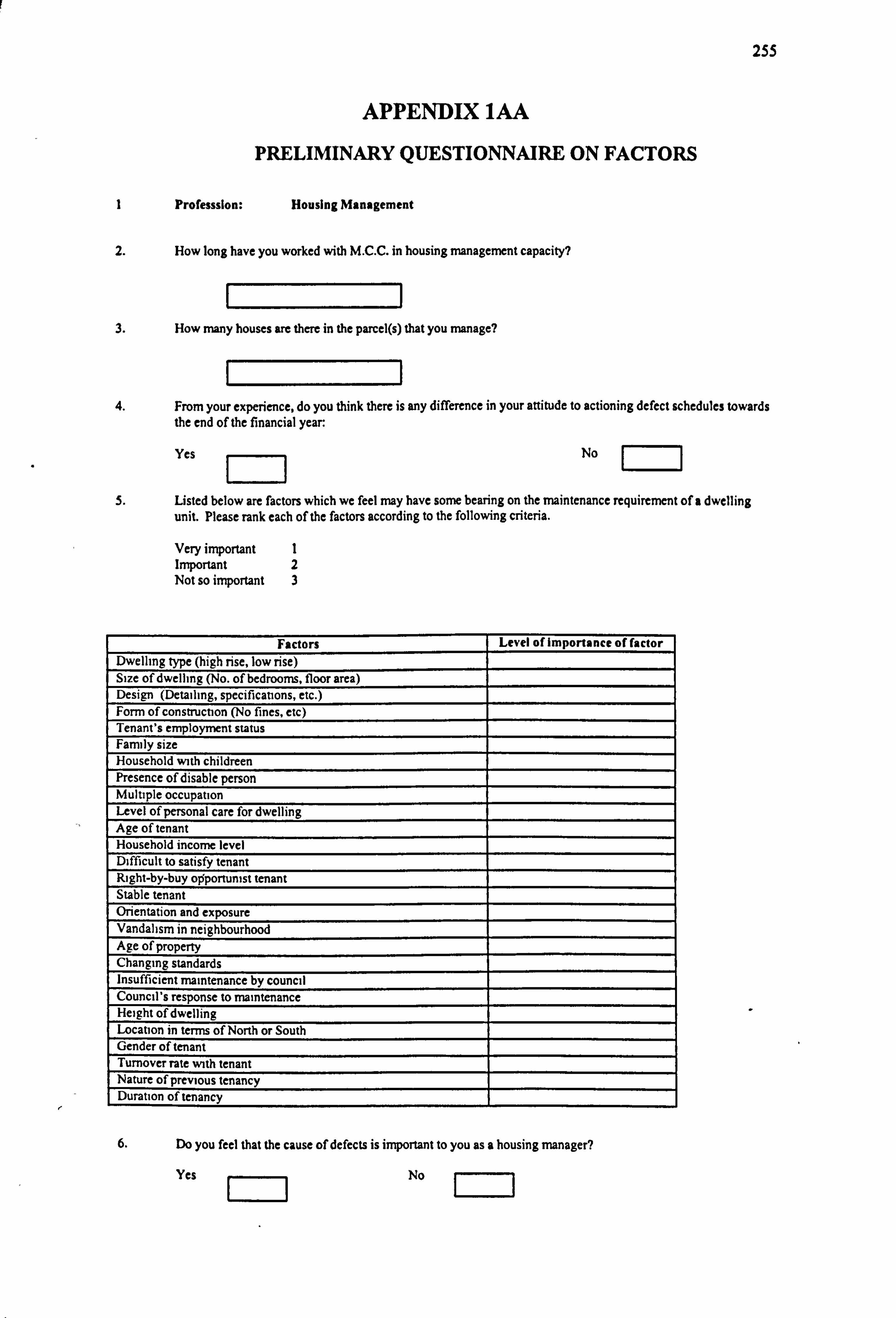
255
APPENDIX 1AA
PRELIMINARY QUESTIONNAIRE ON FACTORS
I Professsion: Housing Management
2. How long have you worked with M. C. C. in housing management capacity?
11
3. How many houses are there in the parcel(s) that you manage?
11
4. From your experience, do you think there is any difference in your attitude to actioning defect schedules towards the end of the financial year:
Yes i No
5. Listed below are factors which we feel may have some bearing on the maintenance requirement of a dwelling unit. Please rank each of the factors according to the following criteria.
Very important I Important 2 Not so important 3
nee
Form of construction (No fines, etc) Tenant's employment status Family size Household with childreen
i, eveº of personai care for aweºnng Age of tenant Household income level Difficult to satisfy tenant Right-by-buy opportunist tenant Stable tenant
Chan tnsutticlent maintenance by council Council's response to maintenance Height of dwelling Location in terms of North or South Gender of tenant Turnover rate with tenant
Duration
6. Do you feel that the cause of defects is important to you as a housing manager?
Yes ý No
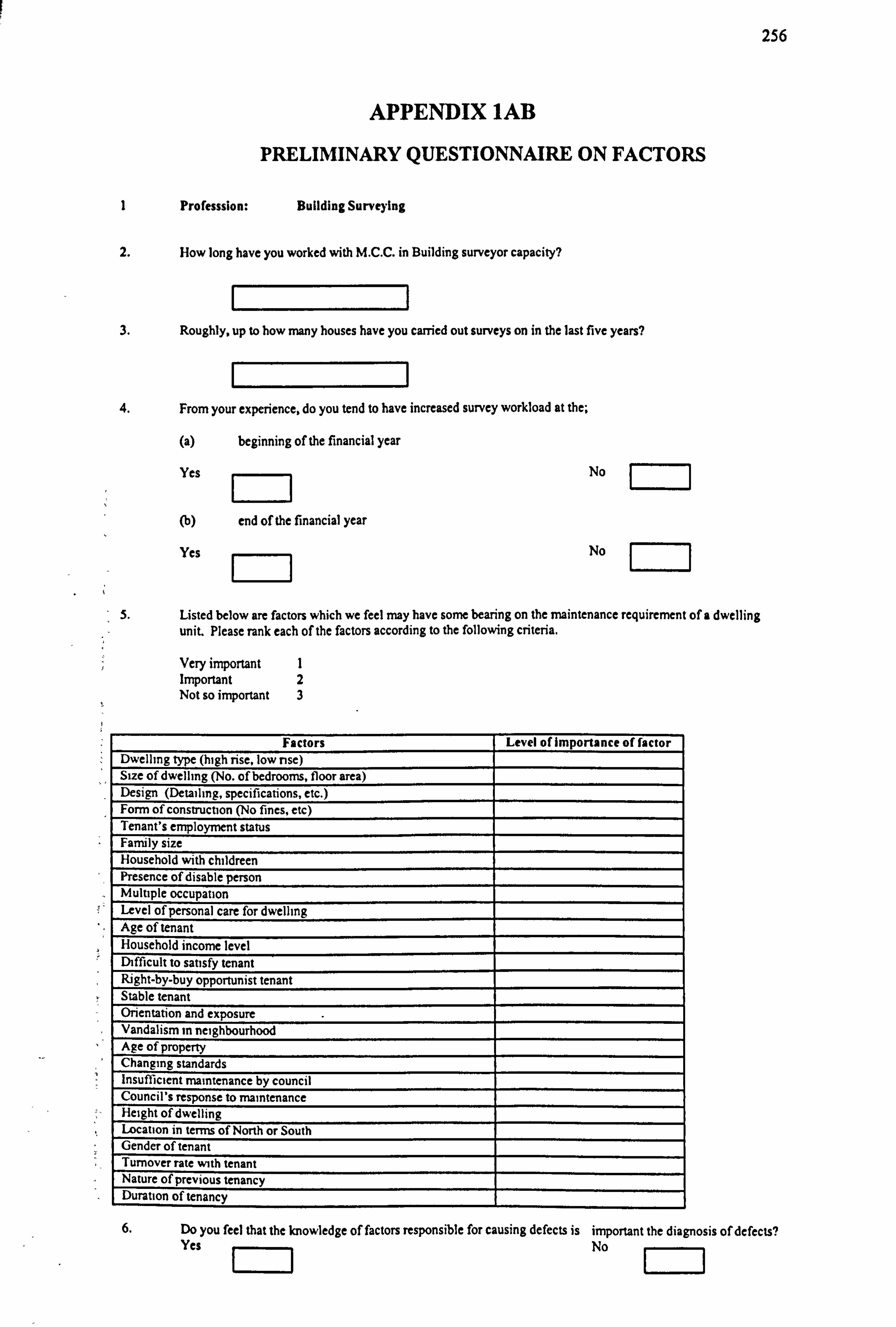
256
APPENDIX 1AB
PRELIMINARY QUESTIONNAIRE ON FACTORS
1 Professsion: Building Surveying
2. How long have you worked with M. C. C. in Building surveyor capacity?
11
3. Roughly, up to how many houses have you carried out surveys on in the last five years?
4. From your experience, do you tend to have increased survey workload at the;
(a) beginning of the financial year
Yes ý No
(b) end of the financial year
Yes ý No
5. Listed below are factors which we feel may have some bearing on the maintenance requirement of a dwelling unit. Please rank each of the factors according to the following criteria.
Very important 1 Important 2 Not so important 3
ctor
construction (No fü
employment status ize
Id with childreen
Dr personal care for aweui tenant hold income level lt to satisfy tenant by-buy opportunist tenant tenant ition and exposure lism in neighbourhood
etc.
tnsumcient maintenance by council Council's response to maintenance Height of dwelling Location in terms of North or South Gender of tenant Turnover rate with tenant Nature of previous tenancy
6. Do you feel that the knowledge of factors responsible for causing defects is important the diagnosis of defects? Yes ýý No

257
SURVEY QUESTIONNAIRE ON COUNCIL DWELLING MAINTENANCE NEED,
IDENTIFICATION, MANAGEMENT AND RESPONSIBILITY -A STUDY OF
MANCHESTER CITY COUNCIL HOUSING
NOTE ABOUT THE OUE_STIONNAIRE
Please be assured that your identity will remain strictly confidential and that all information supplied is strictly for academic
purposes and has nothing to do with any statutory rights and obligations.
As is the case with many, if not all surveys, there may be some questions which appear to be irrelevant or unimportant.
Nonetheless, it is necessary in this study that all questions are answered, as the questionnaire is designed to achieve particular
research objectives, and it is hoped not to offend respondents in anyway whatsoever. However, if there are questions which
you are unwilling or unable to answer, then it is my wish that you continue to answer the rest of the questionnaire.
GENERAL INFO MATION
Please tick the appropriate boxes
Q1 Please state your current job title:
1 Building surveyor
2 Compliance Officer
3 Senior Building Surveyor
4 Principal Surveyor
5 Surveying Manager
I Please specify if any other-
Q2 How ton have you worked with Manchester City Council?
1 Less than 1 year III Less than 1 year
2 1- 5 years
3 6 -10 years
4 11 -15 years
S 16 - 20 years
6 More than 20 years
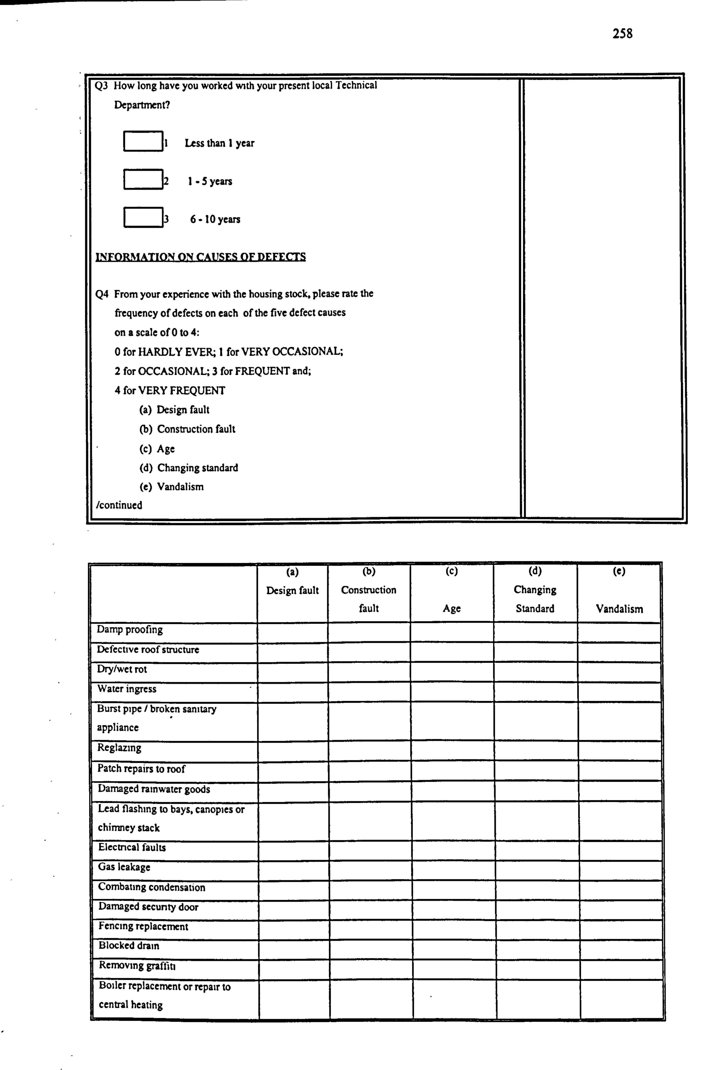
258
Q3 How long have you worked with your present local Technical
Department?
I Less than 1 year
1-5years
Q3 6-10 years
INFORMATION ON CAUSES OF DEFECTS
Q4 From your experience with the housing stock, please rate the
frequency of defects on each of the five defect causes
on a scale of 0 to 4:
0 for HARDLY EVER; I for VERY OCCASIONAL;
2 for OCCASIONAL; 3 for FREQUENT and;
4 for VERY FREQUENT
(a) Design fault
(b) Construction fault
(c) Age
(d) Changing standard
(e) Vandalism
/continued
(a)
Design fault
(b)
Construction
fault
(c)
Age
(d)
Changing
Standard
(e)
Vandalism
Damp proofing
Defective roof structure
Dry/wet rot
Water ingress
Burst pipe / broken sanitary
appliance
Reglazing
Patch repairs to roof
Damaged rainwater goods
Lead flashing to bays, canopies or
chimney stack
Electrical faults
Gas leakage
Combating condensation
Damaged security door
Fencing replacement
Blocked drain
Removing graffiti
Boiler replacement or repair to
central heating
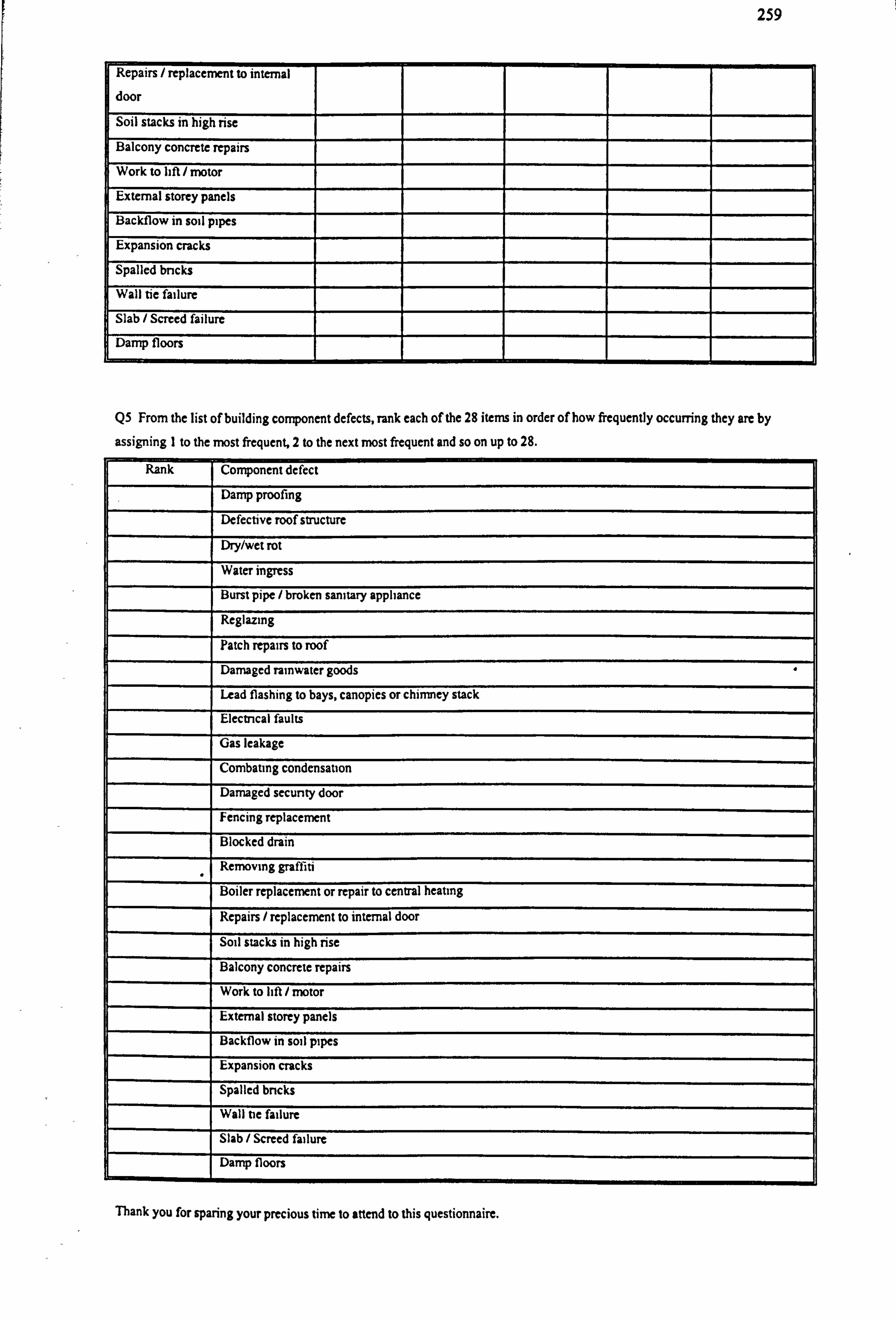
259
to internal
I door
Soil stacks in high rise
Balcony concrete repa
Work to lift / motor
External storey panels
Backflow in soil pipes
Q5 From the list of building component defects, rank each of the 28 items in order of how frequently occurring they are by
assigning Ito the most frequent, 2 to the next most frequent and so on up to 28.
Rank Component defect
Damp proofing
Defective roof structure
Dry/wet rot
Water ingress
Burst pipe / broken sanitary appliance
Reglazmg
Patch repairs to roof
Damaged rainwater goods
Lead flashing to bays, canopies or chimney stack
Electrical faults
Gas leakage
Combating condensation
Damaged security door
Fencing replacement
Blocked drain
Removing graffiti
Boiler replacement or repair to central heating
Repairs / replacement to internal door
Soil stacks in high rise
Balcony concrete repairs
Work to lift / motor
External storey panels
Backtow in soil pipes
Expansion cracks
Spalled bricks
Wall tie failure
Slab / Screed failure
Damp floors
Thank you for sparing your precious time to attend to this questionnaire.
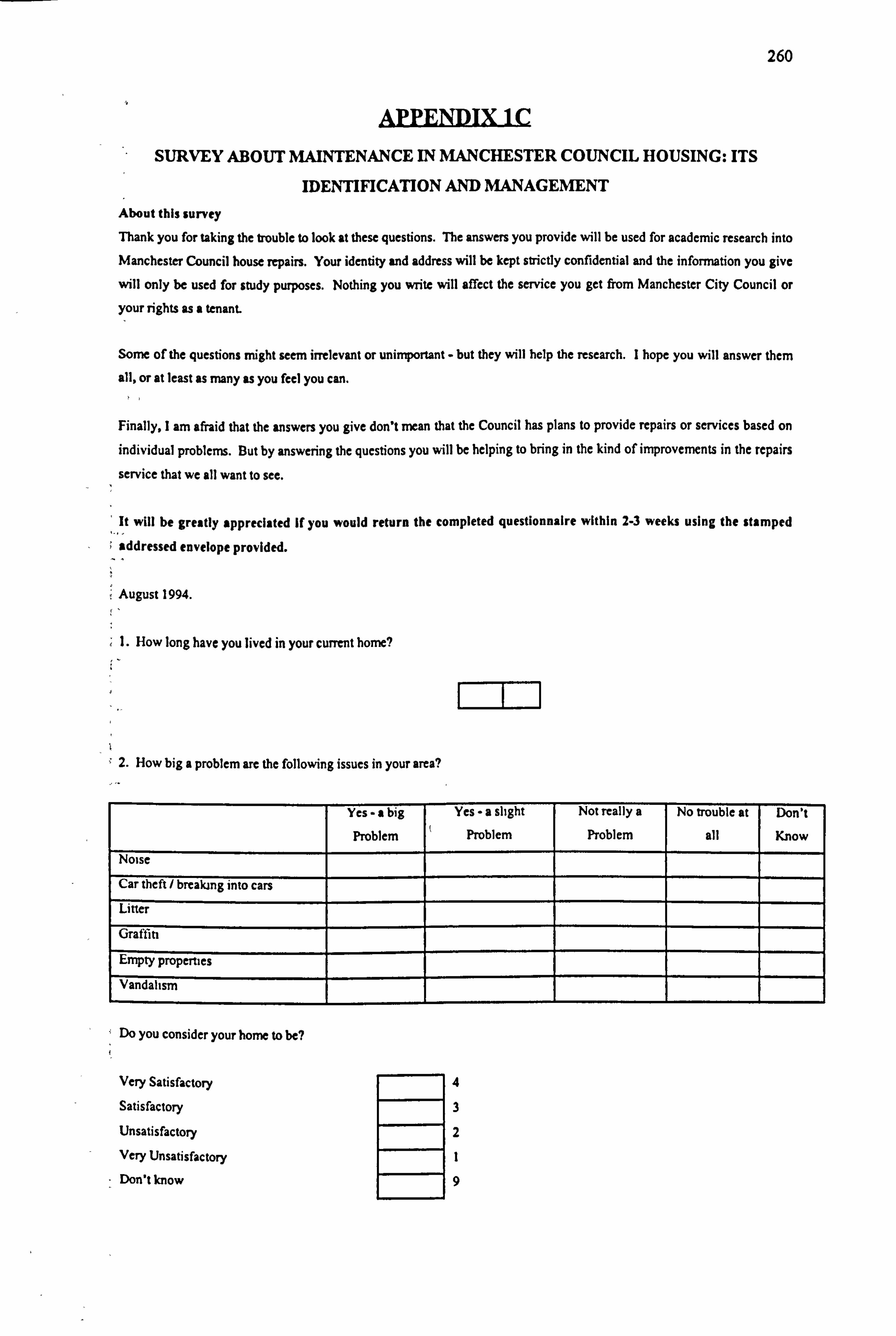
260
SURVEY ABOUT MAINTENANCE IN MANCHESTER COUNCIL HOUSING: ITS
IDENTIFICATION AND MANAGEMENT About this survey Thank you for taking the trouble to look at these questions. The answers you provide will be used for academic research into
Manchester Council house repairs. Your identity and address will be kept strictly confidential and the information you give
will only be used for study purposes. Nothing you write will affect the service you get from Manchester City Council or
your rights as a tenant.
Some of the questions might seem irrelevant or unimportant - but they will help the research. I hope you will answer them
all, or at least as many as you feel you can.
Finally, l am afraid that the answers you give don't mean that the Council has plans to provide repairs or services based on individual problems. But by answering the questions you will be helping to bring in the kind of improvements in the repairs
service that we all want to see.
It will be greatly appreciated if you would return the completed questionnaire within 2-3 weeks using the stamped
addressed envelope provided.
August 1994.
1. How long have you lived in your current home?
I
2. How big a problem are the following issues in your area?
Yes -a big
Problem
Yes -a slight
Problem
Not really a Problem
No trouble at
all
Don't
Know
Noise
Car theft / breaking into cars Litter
Graffiti
Empty properties
Vandalism
Do you consider your home to be?
Very Satisfactory 4
Satisfactory 3
Unsatisfactory 2
Very Unsatisfactory I
Don't know 9
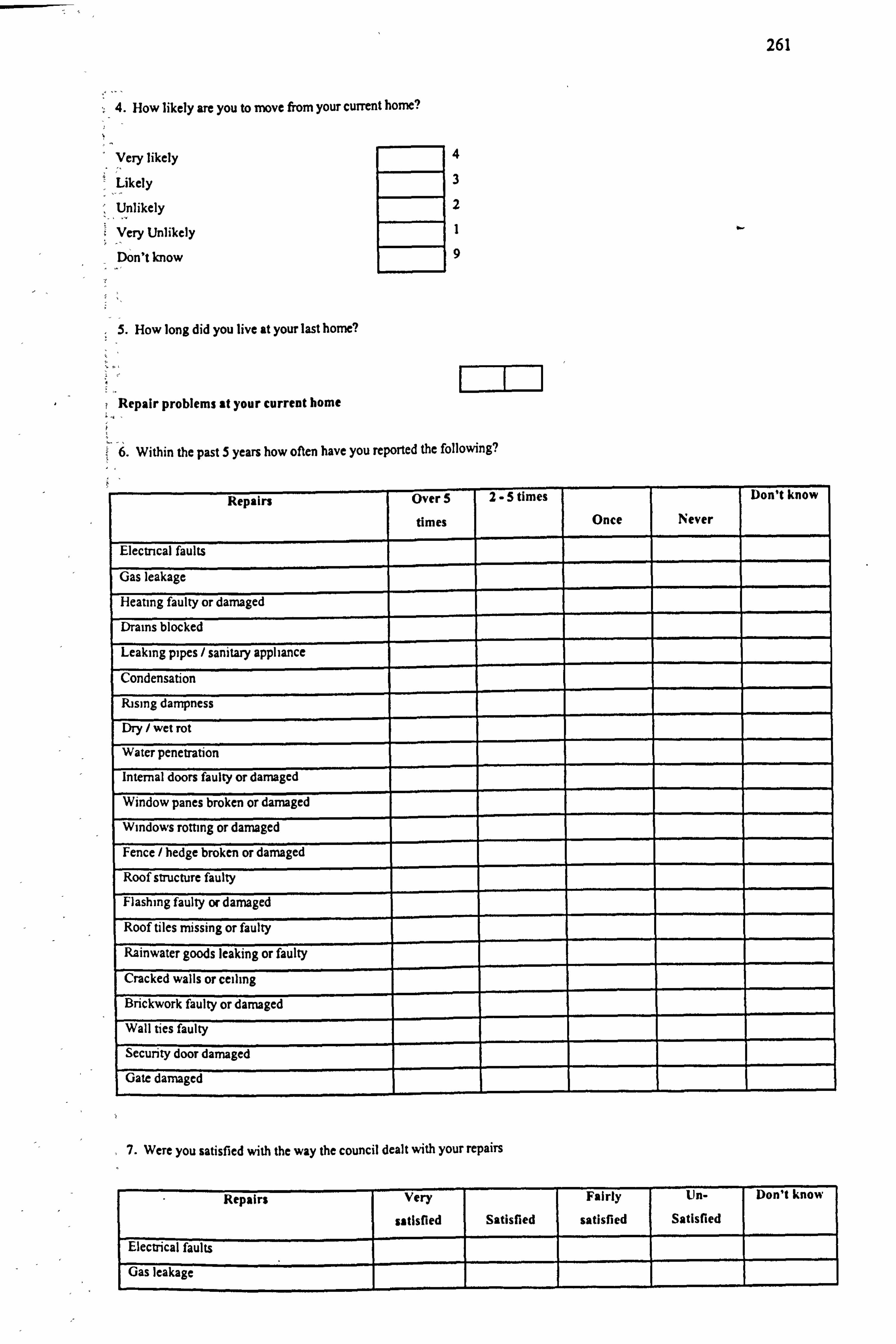
261
4. How likely are you to move from your current home?
Very likely 4
Likely 3
Unlikely 2
Very Unlikely 1
Don't know 9
5. How long did you live at your last home?
Repair problems at your current home
6. Within the past 5 years how often have you reported the following?
Repairs Over 5
times
2-5 times
Once Never
Don't know
Electrical faults
Gas leakage
Heating faulty or damaged
Drains blocked
Leaking pipes / sanitary appliance
Condensation
Rising dampness
Dry / wet rot
Water penetration
Internal doors faulty or damaged
Window panes broken or damaged
Windows rotting or damaged
Fence / hedge broken or damaged
Roof structure faulty
Flashing faulty or damaged
Roof tiles missing or faulty
Rainwater goods leaking or faulty
Cracked walls or ceiling
Brickwork faulty or damaged
Wall ties faulty
Security door damaged
Gate damaged
7. Were you satisfied with the way the council dealt with your repairs
Repairs Very Fairly Un- Don't know
satisfied Satisfied satisfied Satisfied
Electrical faults
Gas leakage
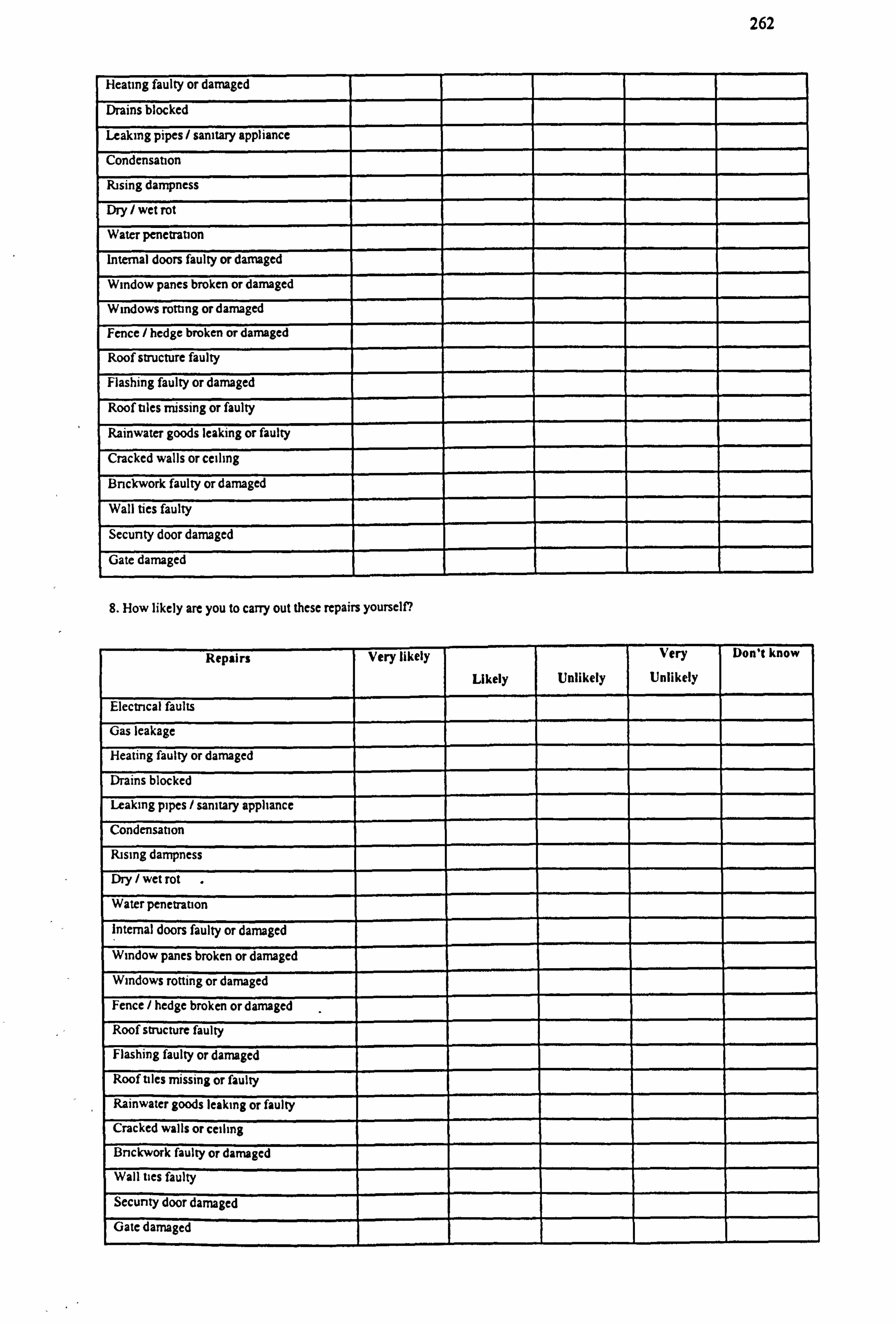
262
Heating faulty or damaged
Drains blocked
Leaking pipes / sanitary appliance
Condensation
Rising dampness
Dry / wet rot
Water penetration
Internal doors faulty or damaged
Window panes broken or damaged
Windows rotting or damaged
Fence / hedge broken or damaged
Roof structure faulty
Flashing faulty or damaged
Roof tiles missing or faulty
Rainwater goods leaking or faulty
Cracked walls or ceiling
Brickwork faulty or damaged
Wall ties faulty
Security door damaged
Gate damaged
8. How likely are you to carry out these repairs yourself?
Repairs Very likely
Likely Unlikely
Very
Unlikely
Don't know
Electrical faults
Gas leakage
Heating faulty or damaged
Drains blocked
Leaking pipes / sanitary appliance
Condensation
Rising dampness
Dry / wet rot . Water penetration
Internal doors faulty or damaged
Window panes broken or damaged
Windows rotting or damaged
Fence / hedge broken or damaged
Roof structure faulty
Flashing faulty or damaged
Roof tiles missing or faulty
Rainwater goods leaking or faulty
Cracked walls or ceiling Brickwork faulty or damaged
Wall ties faulty
Security door damaged
Gate damaged
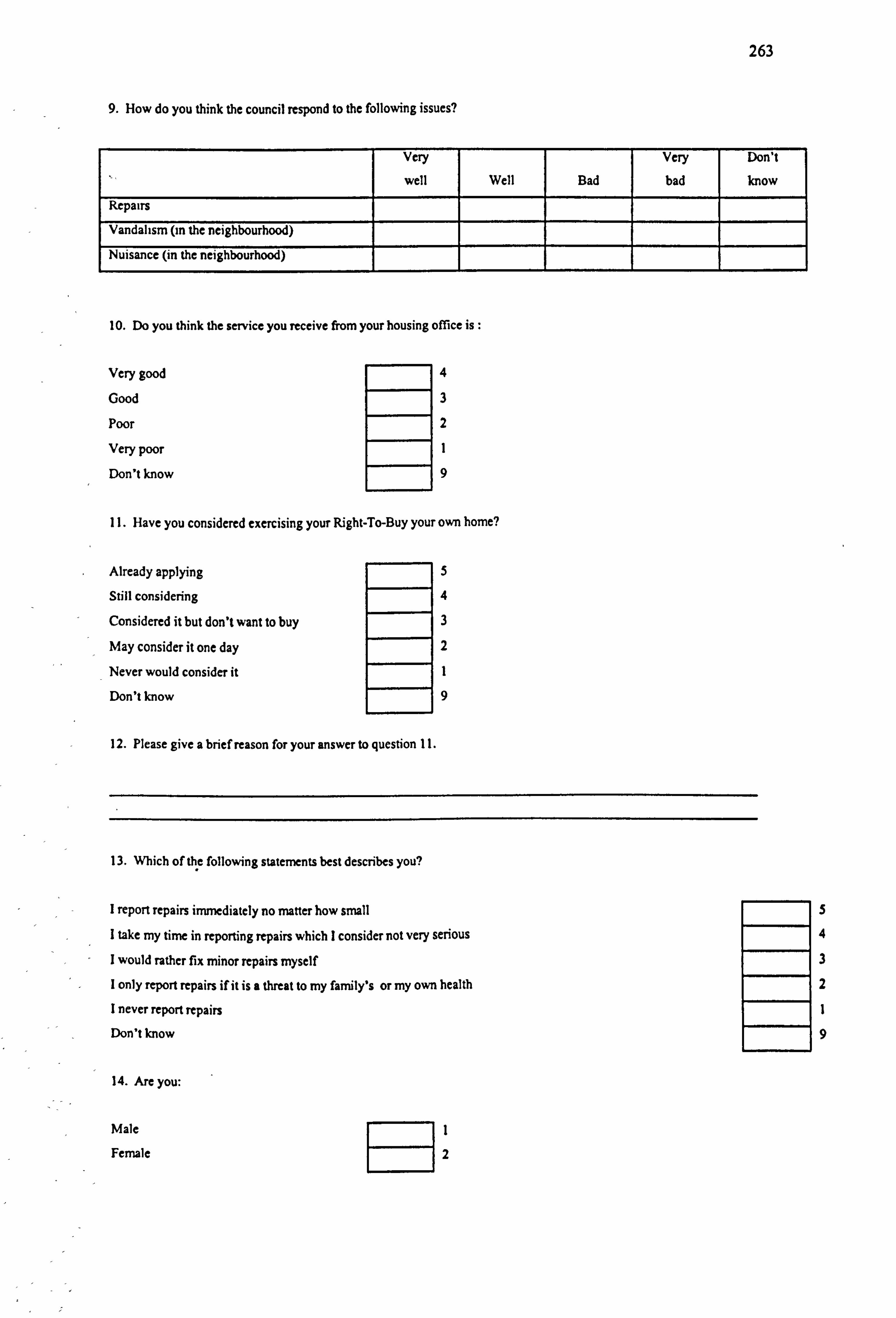
263
9. How do you think the council respond to the following issues?
Very
well Well Bad
Very
bad
Don't
know
Repairs
Vandalism (in the neighbourhood)
Nuisance (in the neighbourhood)
10. Do you think the service you receive from your housing office is :
Very good 4
Good 3
Poor 2
Very poor 1
Don't know 9
11. Have you considered exercising your Right-To-Buy your own home?
Already applying 5
Still considering 4
Considered it but don't want to buy 3
May consider it one day 2
Never would consider it FEI I
Don't know 9
12. Please give a brief reason for your answer to question 11.
13. Which of the following statements best describes you?
I report repairs immediately no matter how small S
I take my time in reporting repairs which I consider not very serious 4
I would rather fix minor repairs myself 3
I only report repairs if it is a threat to my family's or my own health 2
I never report repairs 1
Don't know 9
14. Are you:
Male 1
Female 2
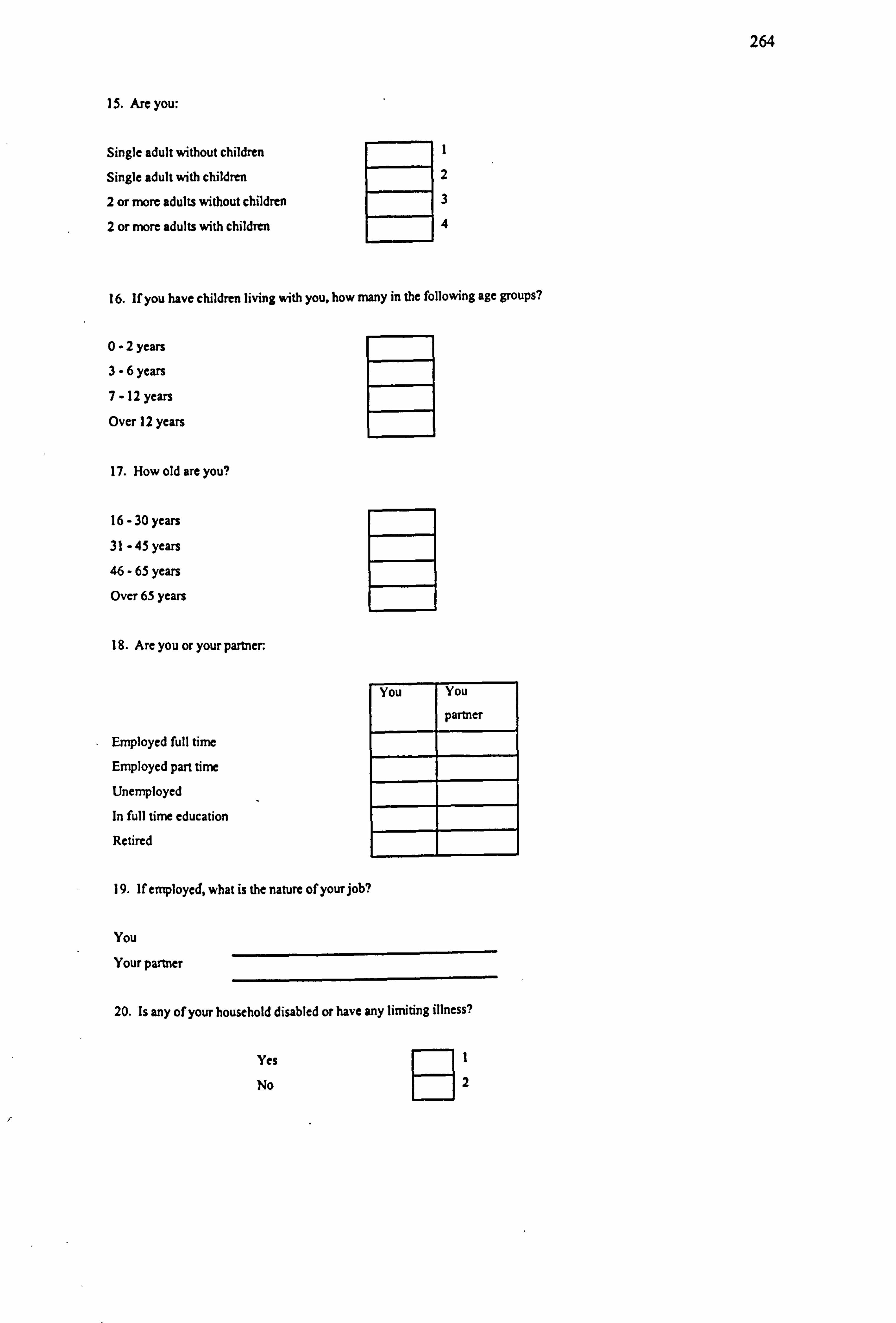
264
15. Are you:
Single adult without children 1
Single adult with children 2
2 or more adults without children 3
2 or more adults with children 4
16. If you have children living with you, how many in the following age groups?
0-2 years
3-6 years
7 -12 years
Over 12 years
17. How old are you?
16 - 30 years
31 - 45 years
46 - 65 years
Over 65 years
18. Are you or your partner.
You You
partner
Employed full time
Employed part time
Unemployed
In full time education
Retired
19. If employed, what is the nature of your job?
You
Your partner
20. Is any of your household disabled or have any limiting illness?
Yes RI No 2
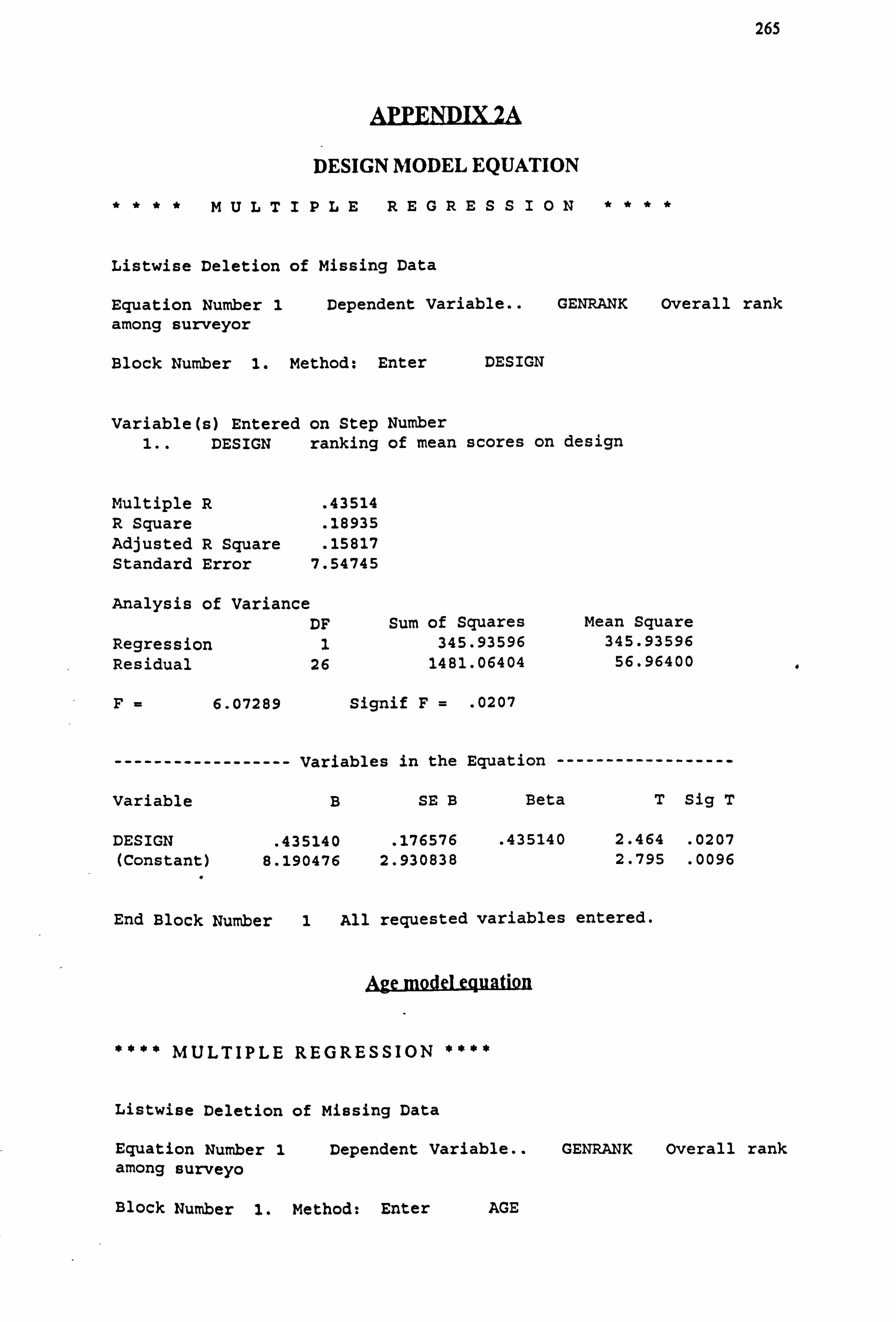
265
DESIGN MODEL EQUATION
**** MULTIPLEREGRESS10N
Listwise Deletion of Missing Data
Equation Number 1 Dependent Variable.. GENRANK Overall rank among surveyor
Block Number 1. Method: Enter DESIGN
Variable(s) Entered on Step Number 1.. DESIGN ranking of mean scores on design
Multiple R . 43514 R Square . 18935 Adjusted R Square . 15817 Standard Error 7.54745
Analysis of Variance DF
Regression 1 Residual 26
F=6.07289
Sum of Squares 345.93596
1481.06404
Signif F= . 0207
Mean Square 345.93596
56.96400
------------------ Variables in the Equation ------------
Variable B SE B Beta T Sig T
DESIGN . 435140 . 176576 . 435140 2.464 . 0207 (Constant) 8.190476 2.930838 2.795 . 0096
End Block Number 1 All requested variables entered.
**** MULTIPLE REGRESSION ****
Listwise Deletion of Missing Data
Equation Number 1 Dependent Variable.. GENRANK Overall rank among surveyo
Block Number 1. Method: Enter AGE
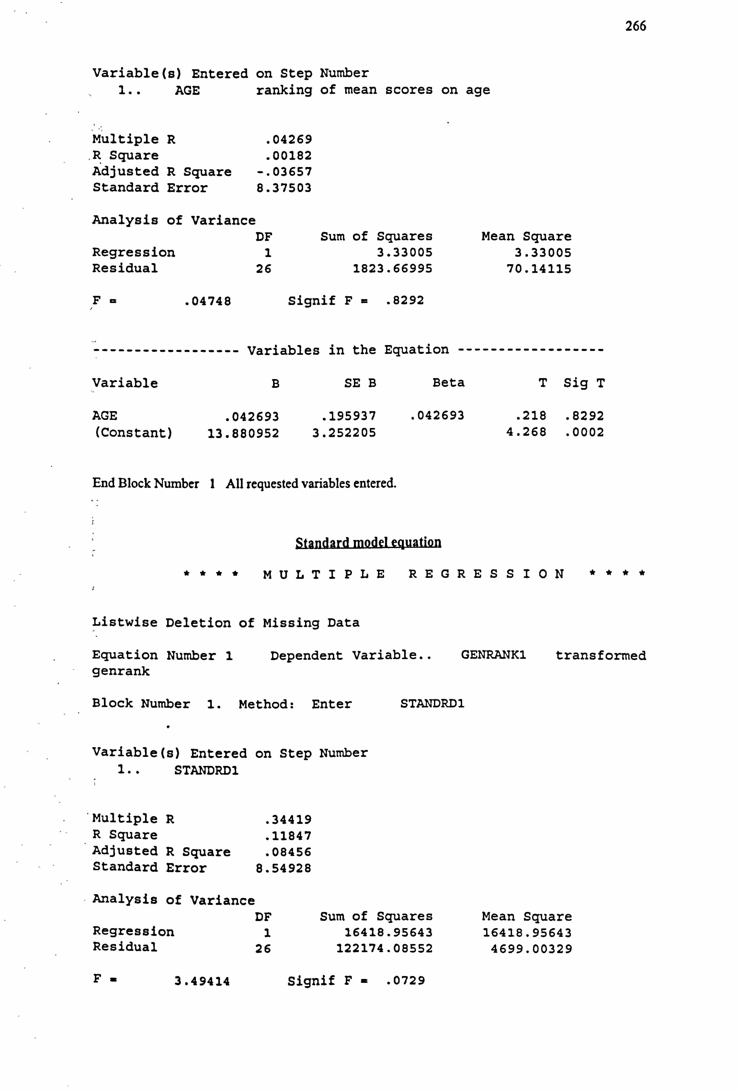
266
Variable(s) Entered on Step Number 1.. AGE ranking of mean scores on age
Multiple R . 04269 R Square . 00182 Adjusted R Square -. 03657 Standard Error 8.37503
Analysis of Variance DF
Regression 1 Residual 26
F= . 04748
Sum of Squares 3.33005
1823.66995
Signif F= . 8292
Mean Square 3.33005
70.14115
Variables in the Equation ------------------ ------------------
Variable B SE B Beta T Sig T
AGE . 042693 . 195937 . 042693 . 218 . 8292 (Constant) 13.880952 3.252205 4.268 . 0002
End Block Number 1 All requested variables entered.
Standard model equation
**** MULTIPLEREGRESS10N
Listwise Deletion of Missing Data
Equation Number 1 Dependent Variable.. GENRANK1 transformed genrank
Block Number 1. Method: Enter STANDRD1
Variable(s) Entered on Step Number 1.. STANDRD1
Multiple R . 34419 R Square
. 11847 Adjusted R Square . 08456 Standard Error 8.54928
Analysis of Variance DF
Regression 1 Residual 26
F-3.49414
Sum of Squares 16418.95643
122174.08552
Signif F- . 0729
Mean Square 16418.95643
4699.00329
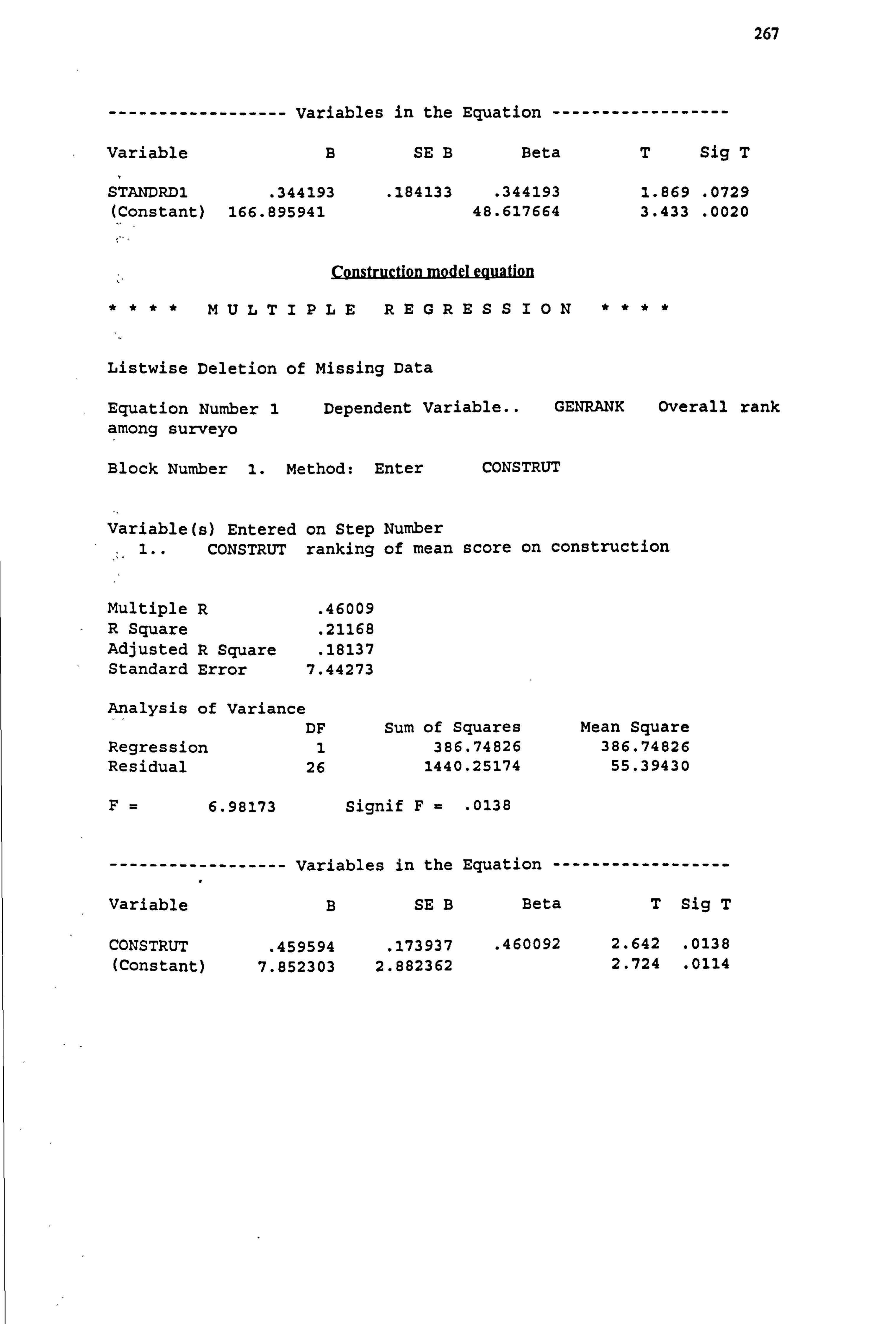
267
------------------ Variables in the Equation ------------------
Variable B SE B Beta T Sig T
STANDR. D1 . 344193 . 184133 . 344193 1.869 . 0729 (Constant) 166.895941 48.617664 3.433 . 0020
Construction model equation
**** MULTIPLEREGRESSION
Listwise Deletion of Missing Data
Equation Number 1 Dependent Variable.. GENRANK Overall rank among surveyo
Block Number 1. Method: Enter CONSTRUT
Variable(s) Entered on Step Number 1.. CONSTRUT ranking of mean score on construction
Multiple R . 46009 R Square
. 21168 Adjusted R Square . 18137 Standard Error 7.44273
Analysis of Variance DF
Regression 1 Residual 26
F=6.98173
Sum of Squares 386.74826
1440.25174
Signif F= . 0138
Mean Square 386.74826
55.39430
------------------ Variables in the Equation ------------------
Variable B SE B Beta T Sig T
CONSTRUT . 459594 . 173937 . 460092 2.642 . 0138
(Constant) 7.852303 2.882362 2.724 . 0114
268
Vandalism model equation
**** MULTIPLEREGRESS10N
Listwise Deletion of Missing Data
Equation Number 1 Dependent Variable.. GENRANKI transformed genrank
Block Number 1. Method: Enter VANDALI
Variable(s) Entered on Step Number 1.. VANDALI
Multiple R . 13994 R Square . 01958 Adjusted R Square -. 01813 Standard Error 72.29190
Analysis of Variance DF Sum of Squares Mean Square
Regression 1 2713.96809 2713.96809 Residual 26 135879.07385 5226.11823
F . 51931 Signif F= . 4776
------------------ Variables in the Equation ------------------
Variable B SE B Beta T Sig T
VA1DAL1 -. 139937 . 194186 -. 139937 -. 721 . 4776 (Constant) 290.101837 51.272067 5.658 . 0000
269
CORRELATIONS BETWEEN EACH OF THE SIX CRITERIA ON VANDALISM INDEX
NOISPROB noise problem in area by CARPROB car theft problem in area
CARPROB Page 1 of 1 Count
ono troub not real a slight a big pr is at al ly a pro problem oblem Row
11 21 31 41 Total NOISPROB ---------------------------------------------
11 21 I7ý7ý6I 41 no trouble at al 1 25,8
+------__+--------+-------_+--------+ 26ý 10 ý 12 13 I 41
not really a pro ýIIII 25,8
........................... 3I2I7 16 I 14 I 39
a slight problem 24,5 ------------------ ..................
4ý1I4I7ý 26 ý 38
a big problem 23,9
+__--_---+--------+--------+-----___+ Column 30 28 42 59 159
Total 18,9 17,6 26,4 37,1 100,0
Chi-Square Value DF Significance
Pearson Likelihood Ratio Mantel-Haenezel test for
linear association
Minimum Expected Frequency
Statistic
--------------------
Kendall's Tau-b
Pearson's R Spearman Cotrelation
56,01772 9 , 00000 53,00409 9 , 00000 39,25079 1 , 00000
6,692
Approximate value ASE1 Val/ASEO significance
--------- -------- -------- ---------"-.
, 42401 , 05946 7,06677
, 49842 . 06355 7,20375 , 00000 +4
, 48818 . 06627 7,00874 , 00000 "4
*4 VAL/ASKO is a t-value based on a normal approximation, as is the significance
Number of Missing Observationss 93
270
LITAPROB litter problem in area by CARPROB car theft problem in area
CARPROB Page 1 ox 1
Count I Ino trout not real a slight a big pr is at al ly a pro problem oblem Row
1 11 21 31 41 Total LITAPROB ---------------------------------------------
1ý 19 33 25
no trouble at al 15,6 -------------------------------------
2ý4ý9I86 27
not really a pro 16,9 -------------------------------------
371 12 1 22 18 1 59
a slight problem 1 36,9 -------------------------------------
42ý3 13 31 I 49
a big problem 30,6
------------------------------------- Column 32 27 43 58 160
Total 20,0 16,9 26,9 36,3 100,0
Chi-Square Value DF
-------------------- ----------- ----
Significance
............
Pearson 81,28717 9 , 00000 Likelihood Ratio 74,71645 9 100000 Mantel-Haenszel test for 49,90103 1 , 00000
linear association
Minimum Expected Frequency - 4,219 Cells with Expected Frequency <5-2 OF 16 ( 12,5%)
Approximate Statistic Value ASE1
-------------------- --------- -------- Val/ASEO --------
Significance ------------
Kendall's Tau-b , 46825 , 06043 7,51956
Pearson's R , 56022 , 06480 8,50106 , 00000 "4 Spearman Correlation , 52672 , 06608 7,78870 , 00000 "4
*4 VAL/ASEO is a t-value based on a normal approximation, as is the significance
Number of Missing Observations: 92
271
GRAPPROB graffitti problem in area by CARPROB car theft problem in area
CARPROB Page 1 of 1
Count Ino troub not real a slight a big pr le at al ly a pro problem oblem Row
11 21 31 41 Total GRAFPROB -------- -------------------------------------
1 23 1916( 13 51 no trouble at al I( 34,7
------------------------------------ 2 6 13 20 15 ý 54
not really a pro 36,7 ------------------------------------
3 ý13ý 10 12 26 a slight problem 17,7
------------------------------------- 4 3 13 ý 16
a big problem ýýII 10,9 -------------------------------------
Column 30 25 39 53 147 Total 20,4 17,0 26,5 36,1 100,0
Chi-Square -------------------
Value DF - ----------- ----
Significance ------------
Pearson 49,66003 9 100000 Likelihood Ratio 52,35710 9 100000 Mantel-Haenazel tes t for 31,81589 1 100000
linear association
Minimum Expected Frequency - 2,721 Cells with Expected Frequency <5-4 OF 16 ( 25,0%)
Approximate Statistic
------------------- Value ASE1
- --------- --------
Val/ASSO
-"------
Significance
-----------.
Kendall'a Tau-b , 39666 , 06422 6,00416
Pearson's R , 46682 , 06184 6,35628 , 00000 *4 Spearman Correlation , 44454 , 07243 5,97593 , 00000 *4
*4 VAL/ASEO*is a t-value based on a normal approximation, as is the significance
Number of Missing Observations: 105
0
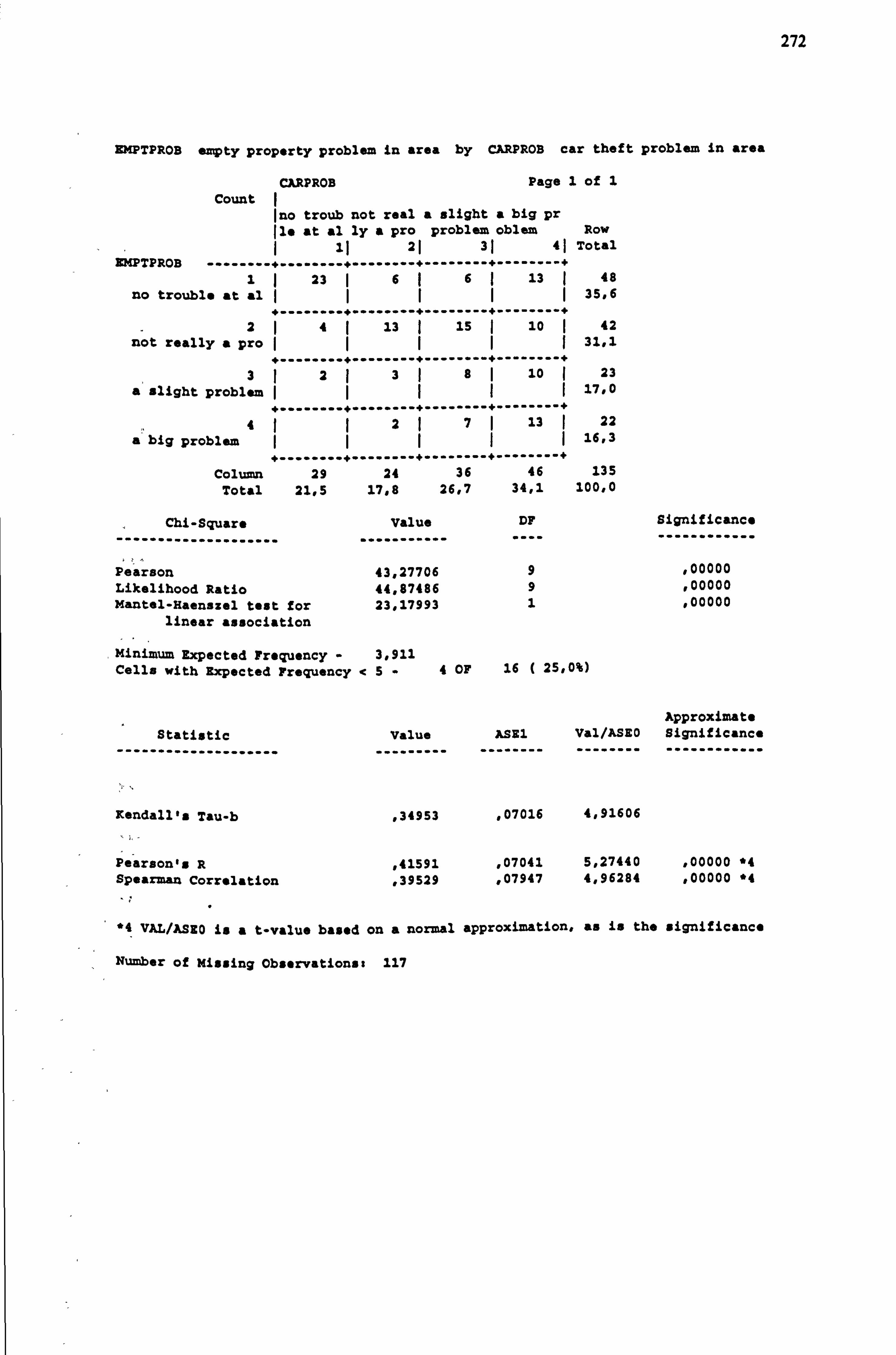
272
BMPTPROB empty property problem is area by CARPROB car theft problem in area
CARPROB Page 1 of 1
Count I Ino troub not real a slight a big pr is at al ly a pro problem oblem Row
11 21 31 41 Total BMPTPROB ---------------------------------------------
11 23 16161 13 ý 48 no trouble at al III1ý 35,6
+--------+"--"-""-+--------+--------+
2ý4 13 15 10 I 42 not really a pro 31.1
------------------------------------- 3ý2ý3ý8ý 10 ý 23
a slight problem 17,0
--------------------------- 42ý7ý 13 ý 22
a big problem 16,3
+--------+--------+--------+--------+ Column 29 24 36 46 135
Total 21,5 17.8 26,7 34,1 10010
Chi-Square Value DF
----"--------------- ........... ---- Significance ------------
Pearson 43,27706 9 , 00000 Likelihood Ratio 44,87486 9 , 00000 Mantel-Haenszel test for 23,17993 1 , 00000
linear association
Minimum Expected Frequency - 3,911 Cells with Expected Frequency <5-4 OF 16 ( 25,0%)
Approximate Statistic Value ASE1
----------------"--- ------"-- -------- Val/ASEO --------
Significance ............
Kendall's Tau-b , 34953 , 07016 4,91606
Pearson's R , 41591 , 07041 5,27440 , 00000 *4 Spearman Correlation , 39529 , 07947 4,96284 , 00000 "4
*4 VAL/AS80 is a t"value based on a normal approximation, as is the significance
Number of Missing Observations: 117
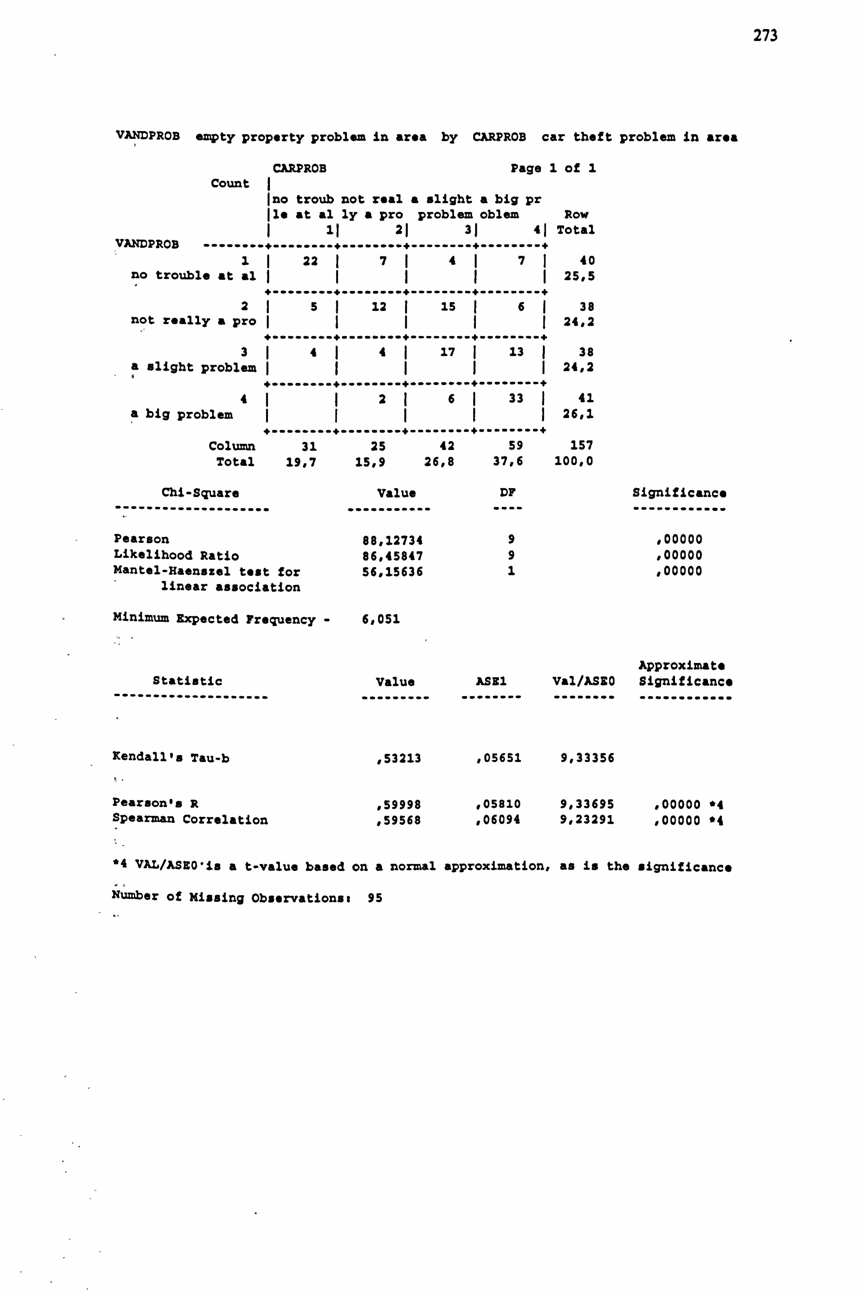
273
VANDPROB empty property problem in area by CARPROB car theft problem in area
CARPROB Page 1 of 1
Count ono trout not real a slight a big pr Ile at al ly a pro problem oblem Row
11 21 31 41 Total VANDPROB --------------------------------------------- 1 22 1714171 40
no trouble at al I1 25,5 +--------+--------+--------+--------+
25 12 ý 15 6I 38 not really a pro 24,2
------------------------------------- 3ý4I4 17 13 38
a alight problem (IýI 24,2
------------------------------------ 426I 33 41
a big problem 26,1
------------------------------------- Column 31 25 42 59 157
Total 19,7 15,9 26,8 37,6 100,0
Chi-Square
Pearson Likelihood Ratio Mantel-Haenazel teat for
linear association
Minimum Expected Frequency -
Statistic --------------------
Kendall'a Tau-b
Pearson'a R Spearman Correlation
Value -----------
DF ----
Significance ------------
88,12734 9 100000 86,45847 9 100000 56,15636 1 , 00000
6,051
Approximate Value ASE1 Val/ASEO Significance
, 53213 , 05651 9,33356
, 59998 , 05810 9,33695 , 00000 *4 , 59568 , 06094 9,23291 100000 "4
*4 VAL/ASEO"is a t-value based on a normal approximation, as is the significance
Number of Missing Observations, 95
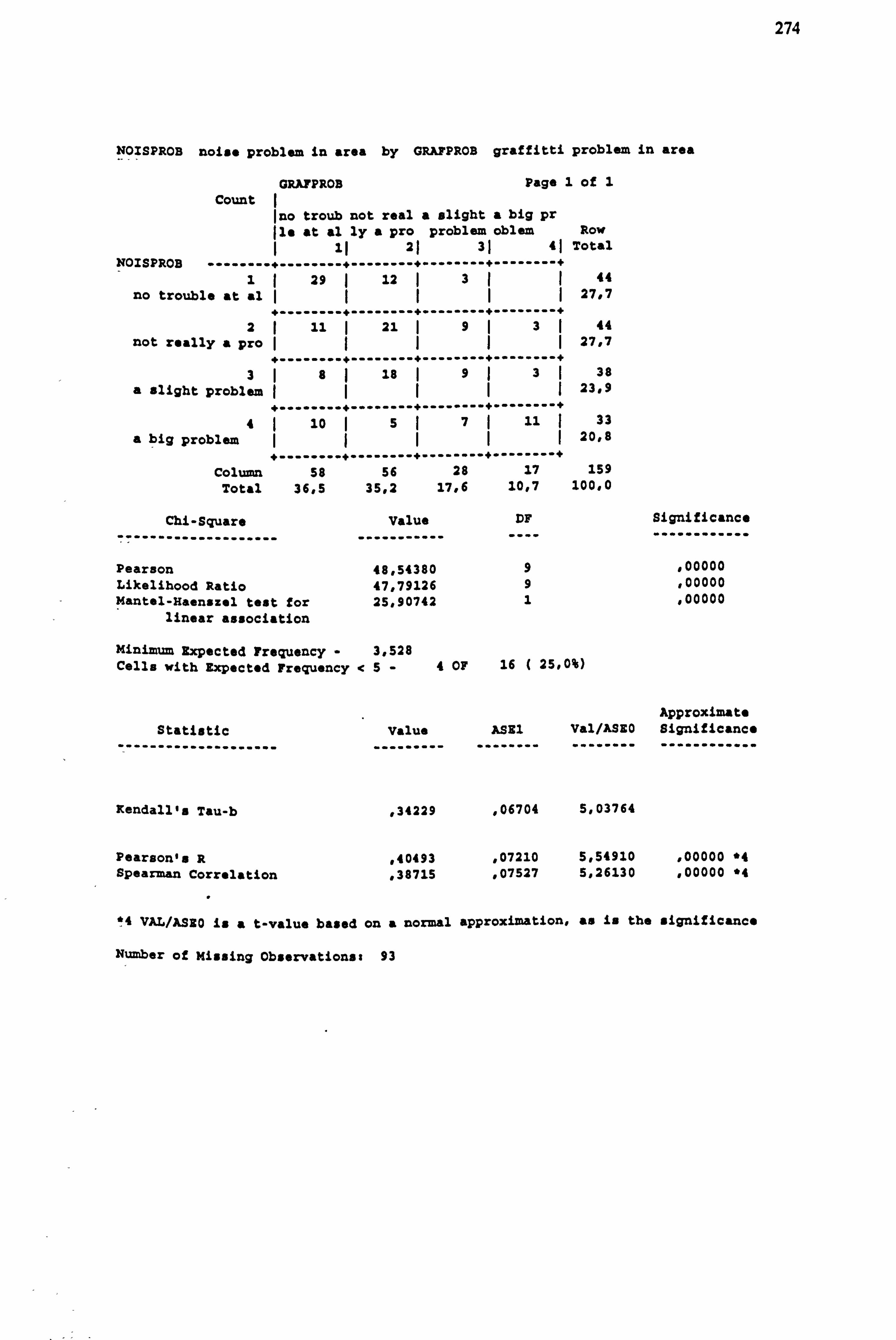
274
NOISPROB noise problem in area by GRAFPROB graffitti problem in area
GRA7PROB Page 1 of 1 Count
ono troub not real a alight a big pr (le at al ly a pro problem oblem Row
1 11 21 31 41 Total NOISPROB --------+--------+--------+--------+--------+
11 29 12 I3ýI 44 no trouble at al I1(I 27,7
+--------+--------+--------+--------+ 2 21 I9ý3ý 44
not really a pro ý(II 27,7
------------------------------------- 3I8ý 18 I9ý3 38
a alight problem 23.9
--------------------------- 4( 10 ý5ý7I 11 ý 33
a big problem 20,8
--------------------------- column 58 56 28 17 159
Total 36,5 35,2 17,6 10,7 10000
Chi-Square Value DF Significance
Pearson 48,54380 9 , 00000
Likelihood Ratio 47,79126 9 , 00000
Mantel-Haenszel test for 25,90742 1 , 00000 linear association
Minimum Expected Frequency - 3,528 Cells with Expected Frequency <5-4 OF 16 ( 25,0%)
Statistic --------------------
Kendall's Tau-b
Pearson's R Spearman correlation
Approximate Value ASE1 Val/ASEO Significance
, 34229 , 06704 5,03764
, 40493 , 07210 5,54910 , 00000 *4
, 38715 , 07527 5,26130 , 00000 *4
*4 VAL/AS O is a t-value based on a normal approximation, as is the significance
Number of Missing Observationsz 93
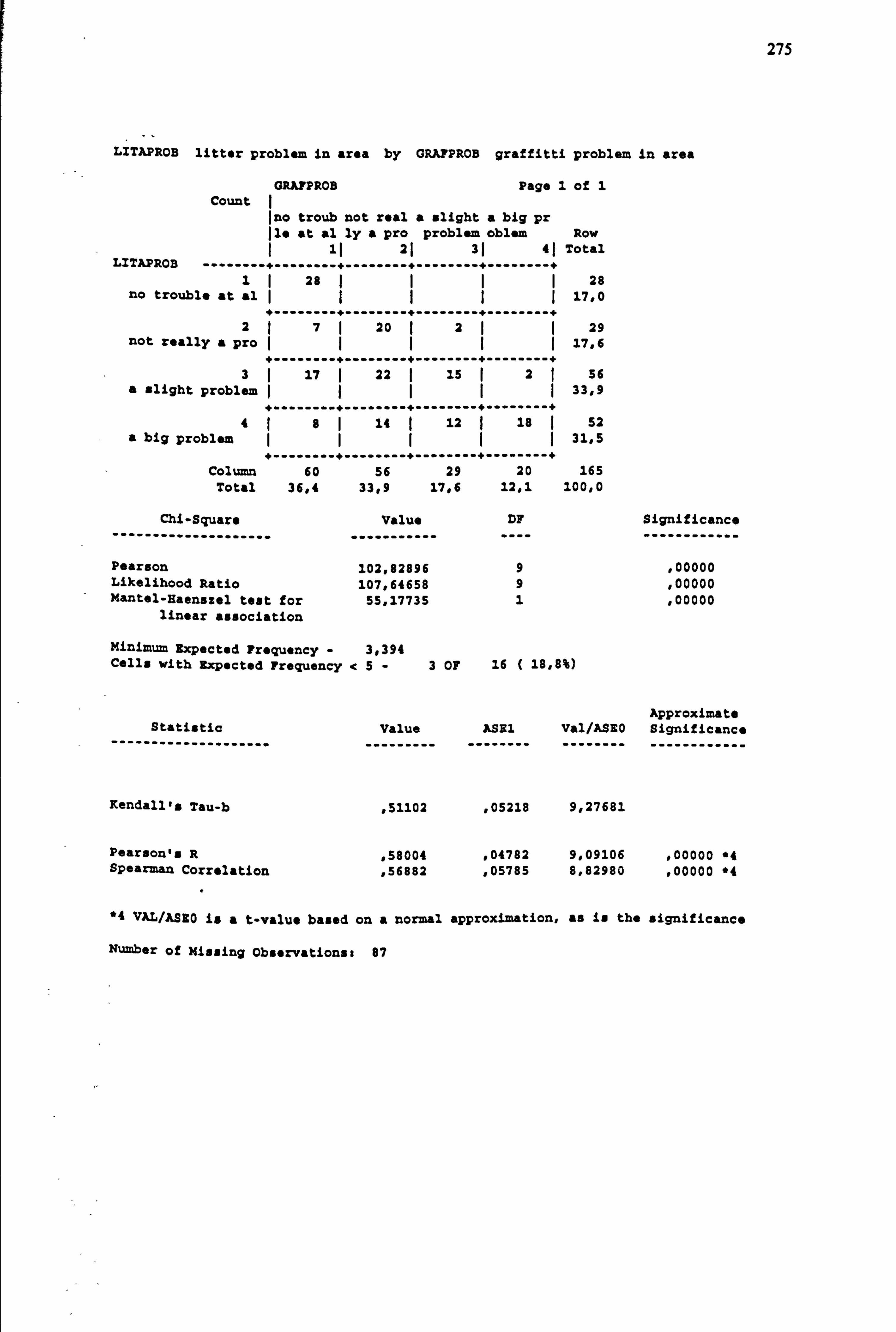
275
LITAPROB litter problem in area by GRAFPROB graffitti problem in area
GRAFPROB Page 1 of 1
Count I ono troub not real a slight a big pr 11e at al ly a pro problem oblem Row
11 21 31 41 Total LITAPROB .......................... +--------+--------+
11 28 1I11 28 no trouble at al II11 17,0
------------------------------------- 27ý 20 2ý 29
not really a pro 17,6 +--------+--------+--------+--------+
3( 17 ý 22 ý 15 ý2 56 a slight problem ýýII 33,9
+--------+--------+--------+.. ------+ 4(8I 14 ( 12 18 ý 52
a big problem 31,5
------------------------------------ Column 60 56 29 20 165
Total 36,4 33,9 17,6 12,1 100,0
Chi-Square Value DF Significance -------------------- ........... ---- ------------
Pearson 102,82896 9 100000 Likelihood Ratio 107,64658 9 100000 Mantel-Haenszel test for 55.17735 1 100000
linear association
Minimum Expected Frequency - 3,394 Cells with Expected Frequency <5-3 OF 16
Approximate Statistic Value ASE1 Val/ASEO Significance
-------------------- --------- -------- -------- ------------
Kendall's Tau-b , 51102 , 05218 9,27681
Pearson's R , 58004 , 04782 9,09106 100000 *4 Spearman Correlation , 56882 , 05785 8,82980 , 00000 *4
*4 VAL/ASKO is a t-value based on a normal approximation, as is the significance
Number of Missing Observations: 87
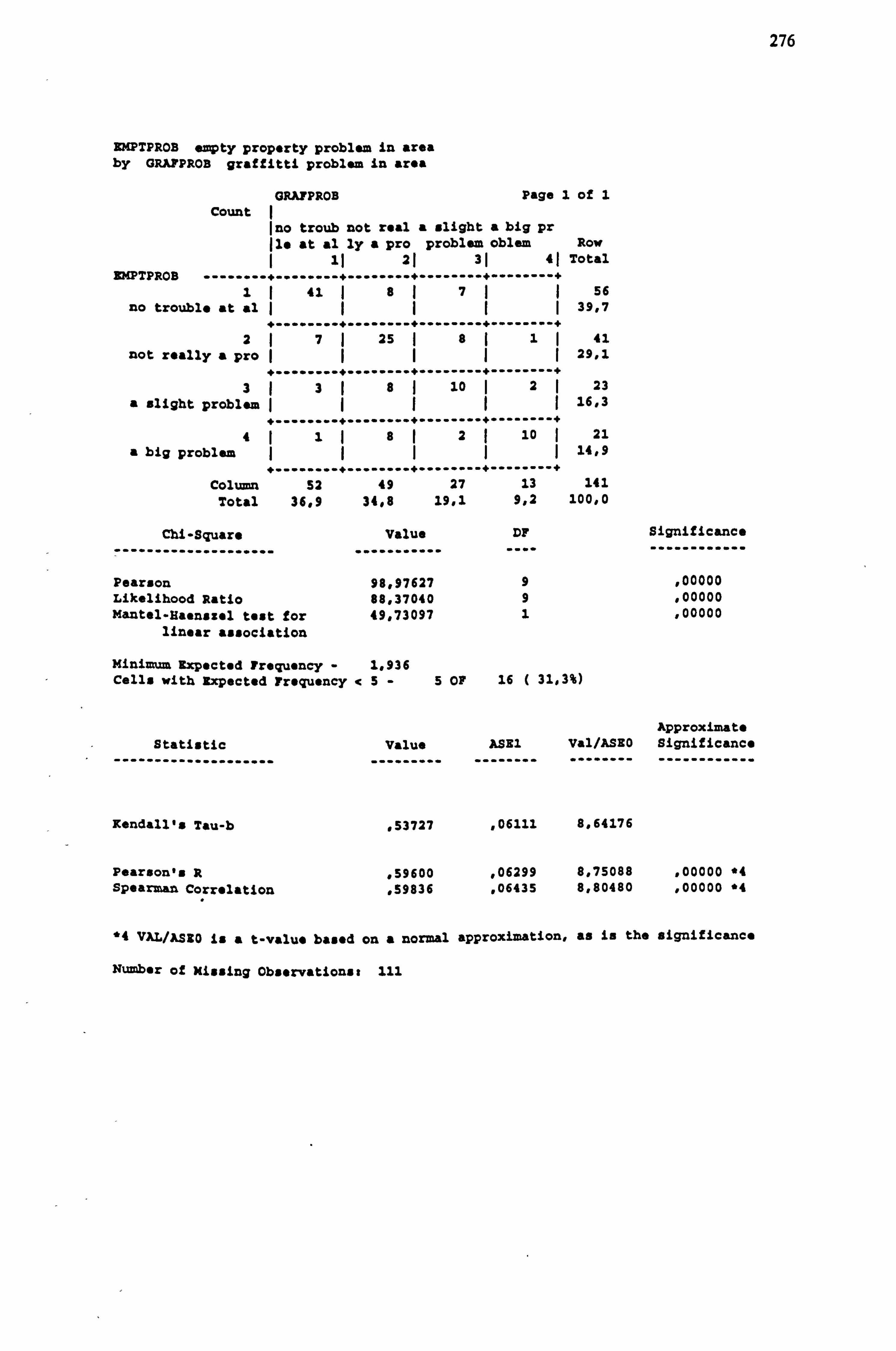
276
EMPTPROB empty property problem in area by ORAFPROB graffitti problem in area
GRAYPROB Page 1 of 1 Count I
ono troub not real a slight a big pr Ile at al ly a pro problem oblem Row
1 11 21 31 41 Total BMPTPROB -------------------------- ..................
1 41 8ý7 56 no trouble at al 1 39,7
+-"-""-""+--"-----+--"----"+--------+ 2ý7 25 ý8ý1ý 41
not really a pro 29,1
+........ +................. +--------+ 3ý3ý8 10 2ý 23
a slight problem 16,3
+----"............ +--------+--------+ 4ý1ý82 10 ý 21
a big problem IýýI 14,9
------------------ Column 52 49 27 13 141
Total 36,9 34,8 19,1 9,2 100,0
Chi-Square Value DF
Pearson 98,97627 9 Likelihood Ratio 88,37040 9 Mantel-Haenasel test for 49,73097 1
linear association
Minimum Expected Frequency - 1,936 Cells with Expected Frequency <5-5 OF 16 ( 31,3$)
Statistic
Kendall's Tau-b
Pearson's R Spearman Correlation
Significance
, 00000
, 00000
, 00000
Approximate Value ASE1 Val/ASSO Significance
--------- -------- --"--"-- ------------
, 53727 , 06111 8,64176
, 59600 , 06299 8,75088 , 00000 *4
, 59836 , 06435 8,80480 , 00000 *4
*4 VAL/A3g0 is a t-value based on a normal approximation, as is the significance
Number of kissing Obssrvationst 111
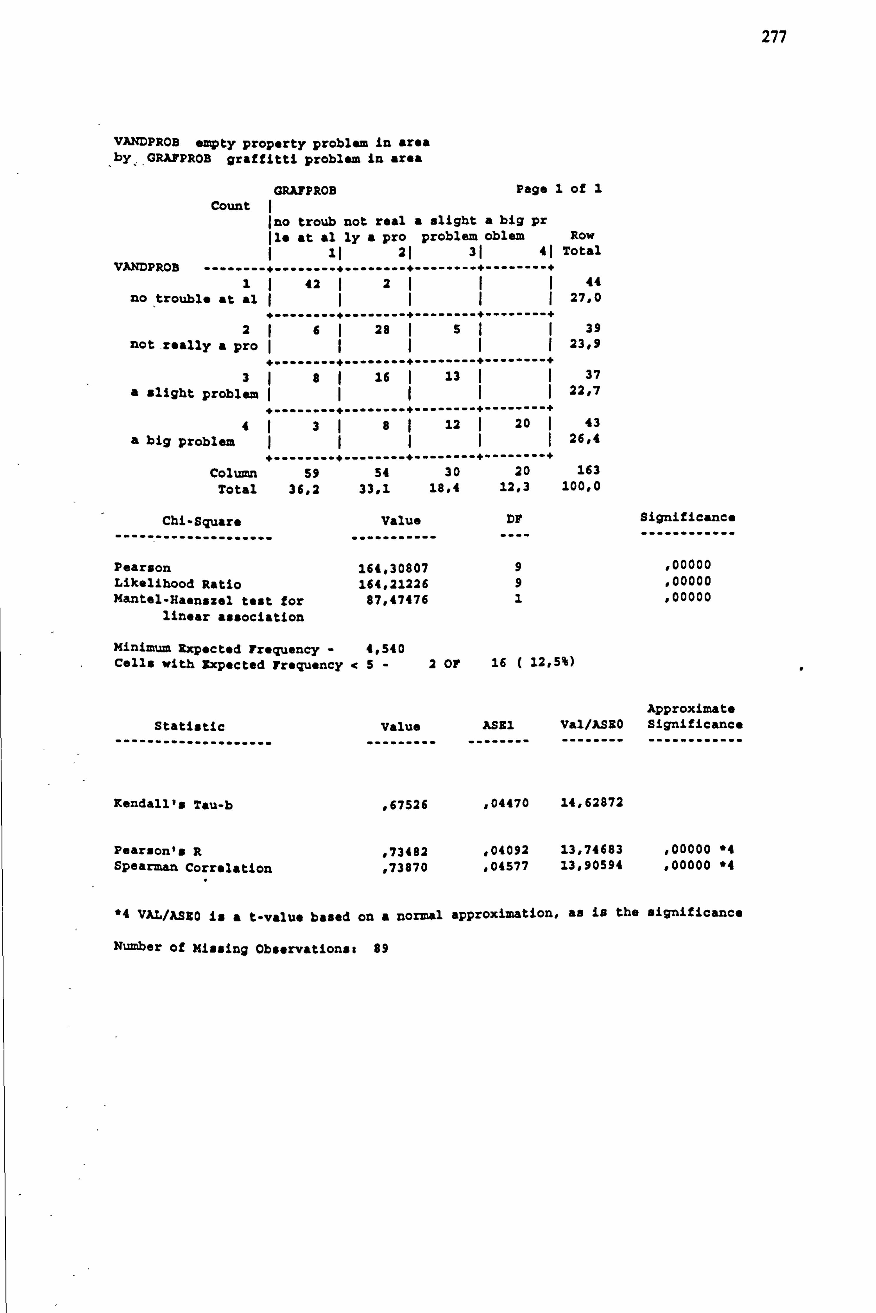
277
VANDPROB empty property problem in area by; GRAFPROB graftitti problem in area
GRAFPROB Page 1 of 1
Count ono trout not real a slight a big pr is at al ly a pro problem oblem Row
11 21 31 41 Total VANDPROB . _... ---+-.... __. +...........................
1 42 211 44
no trouble at al III11 27.0 +--------+--------+--------+--------+
216 28 (5 39
not really a pro III1I 23,9 .................. +-"------+--------+
38 16 I 13 II 37 a slight problem 22,7
------------------------------------- 4ý38( 12 20 43
a big problem 26,4 f"_-__... +--------+--------+--------+
Column 59 54 30 20 163 Total 36,2 33,1 18,4 12,3 100,0
Chi-Square Value DF Significance
Pearson 164,30807 9 , 00000 Likelihood Ratio 164,21226 9 , 00000
Mantel"Haenszel test for 87,47476 1 100000 linear association
Minimum Expected Frequency - 4,540 Cells with Expected Frequency <5-2 OF 16 ( 12,5%)
Approximate Statistic Value ASE1
-------------------" --------- -------- Val/AS80 --------
Significance ----------"-
Kendall's Tau-b , 67526 , 04470 14,62872
Pearson's R , 73482 , 04092 13,74683 , 00000 "4 Spearman Correlation , 73870 , 04577 13,90594 , 00000 *4
*4 VAL/A880 is a t-value based on a normal approximation, as is the significance
Number of Missing Observationss 89
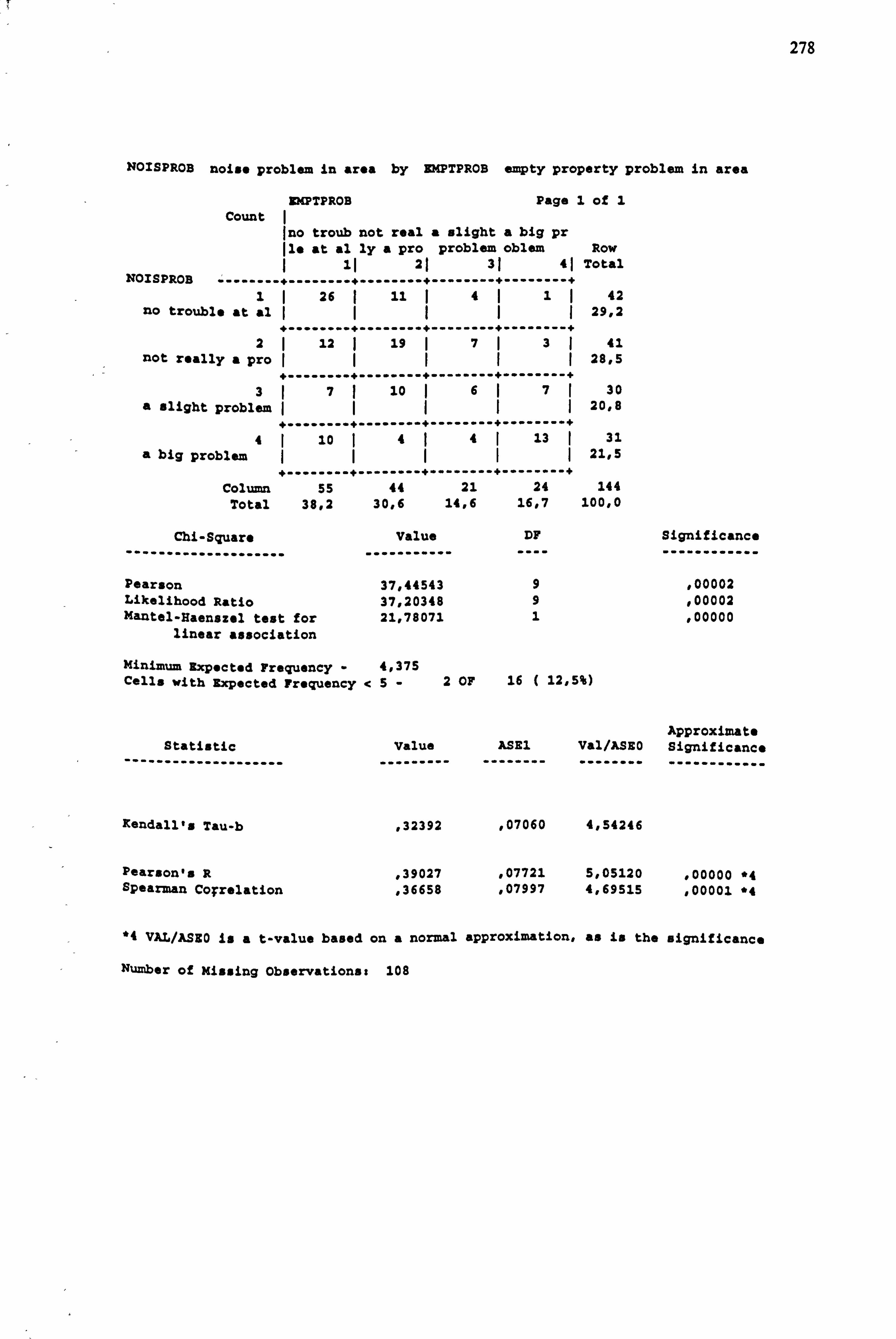
278
NOISPROB noise problem in area by ZMPTPROB empty property problem in area
Y? SPTPROB Page 1 of 1
Count Ino troub not real a slight a big pr is at al ly a pro problem oblem Row
1 11 21 31 41 Total NOISPROB --------------------------------------------- 1 26 11 411 42
no trouble at al I1 29,2
+--------+--------+--------+--------+ 2 12 ý 19 I7ý3 41
not really a pro 1IIýI 28,5
------------------------------------- 3I7ý 10 6I7I 30
a slight problem IIIý 20,8 -------------------------------------
4I 10 ý4ý4I 13 I 31 a big problem IIýý 21,5
------------------------------------- Column 55 44 21 24 144
Total 38,2 30,6 14,6 16,7 100,0
Chi-Square Value DF Significance
Pearson 37,44543 9 , 00002 Likelihood Ratio 37,20348 9 , 00002 Mantel-Raenszel test for 21,78071 1 100000
linear association
Minimum Expected Frequency - 4,375 Cells with Expected Frequency <5-2 OF 16 ( 12,5%)
Statistic --------------------
Rendall's Tau-b
Pearson's R Spearman Correlation
Approximate Value ASE1 Val/ASEO Significance
--------- -------- -------- ------------
, 32392 , 07060 4,54246
, 39027 , 07721 5,05120 . 00000 *4
, 36658 , 07997 4,69515 , 00001 *4
*4 VAL/ASzO is a t-value based on a normal approximation, as is the significance
Number of Missing observations: 108
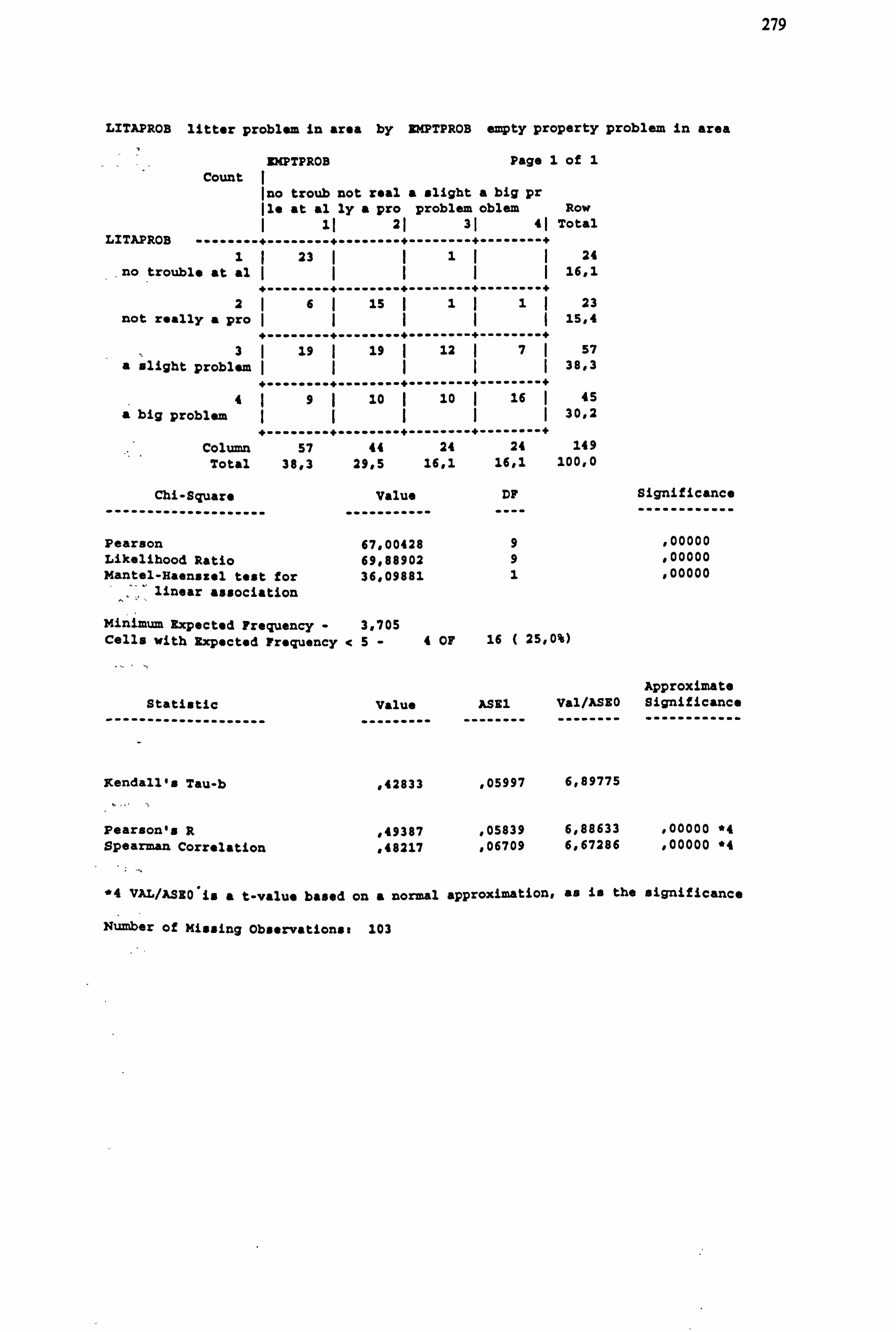
279
LITAPROB litter problem in area by W PTPROB empty property problem in area
EMPTPROB Page 1 of 1
Count Iao troub not real a slight a big pr Ile at al ly a pro problem oblem Row
11 21 31 41 Total LITAPROB ........ +-------- +........ +..................
1 23 1111 24 no trouble at al Iý11 16,1
------------------------------------- 26ý 15 ý11 23
not really a pro 15,4
+--------+--------+--------+--------+ 3I 19 19 ý 12 ý7ý 57
a slight problem 38,3
.................................... 4ý9( 10 I 10 I 16 I 45
a big problem 30,2
----------------------------------- Column 57 44 24 24 149
Total 38,3 29,5 16,1 16,1 100,0
Chi-Square Value DF -------------------- ----------- ----
Significance ------------
Pearson 67,00428 9 100000 Likelihood Ratio 69,88902 9 , 00000 Mantel-Haenazel test for 36,09881 1 , 00000
linear association
Minimum Expected Frequency - 3,705 Cells with Expected Frequency <5-4 OF 16 ( 25,0+ä)
Approximate Statistic Value ASS1 Va1/ASEO Significance
-------------------- --------- -------- -------- ------------
Kendall's Tau-b . 42833 , 05997 6,89775
Pearson's R , 49387 , 05839 6,88633 , 00000 *4 Spearman Correlation , 48217 , 06709 6,67286 , 00000 *4
*4 VAL/ASEO'is a t-value based on a normal approximation, as is the significance
Number of Missing Observations, 103
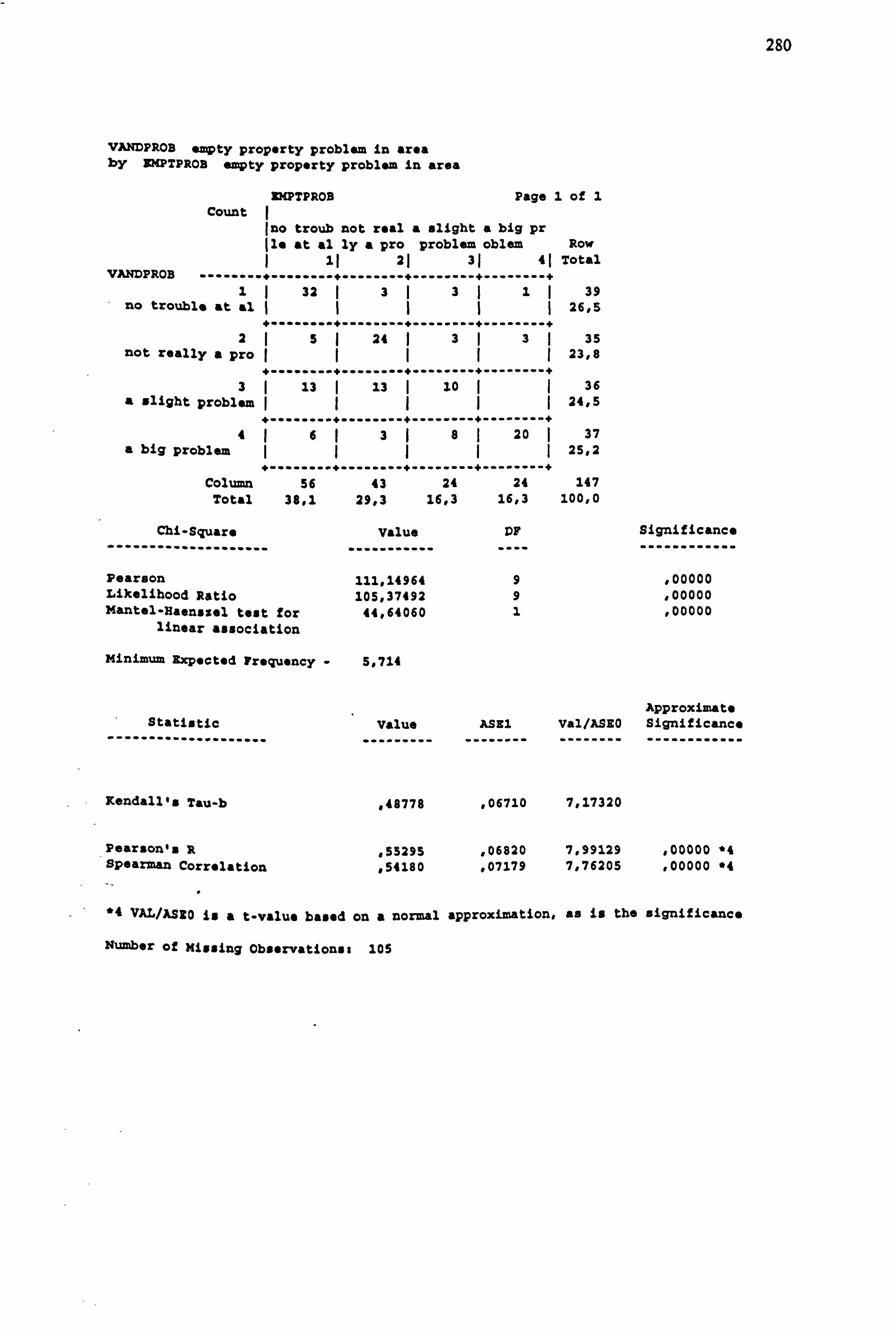
280
VANDPROB empty property problem in area by ZMPTPROB empty property problem in area
ZMPTPROB Page 1 of 1 Count I
ono troub not real a slight a big pr ale at al ly a pro problem oblem Row
1,21 31 41 Total VANDPROB ........ +................. +--------+--------+
1ý 32 13I311 39 no trouble at al ýII1 26,5
--------------------------- 2Sý 24 33 35
not really a pro I(1 23,8 +-------"+"""---""+..................
3ý 13 I 13 I 10 1 36 a slight problem 24,5
------------------ 4ý6ý38 20 I 37
a big problem 25,2 ---------------------------
Column 56 43 24 24 147 Total 38,1 29,3 16,3 16,3 100,0
Chi-Square Value DF -------------------- ----------- ---.
Pearson 111,14964 9 Likelihood Ratio 105,37492 9 Mantel"ßaenssel test for 44,64060 1
linear association
Minimum Zxp. Cted Frequency - 5.714
statistic ....................
Kendall's Tau-b
Significance
, 00000
, 00000
, 00000
Approximate Value ASS. Val/ASEO Significance
--------- -------- -------- ------------
, 48778 , 06710 7,17320
Pearson's R , 53295 , 06820 7,99129 , 00000 "4
Spearman Correlation , 54180 , 07179 7,76205 , 00000 *4
`4 VRL/ASYO is a t-value based on a normal approximation, as is the significance
Number of Missing Observations: 105
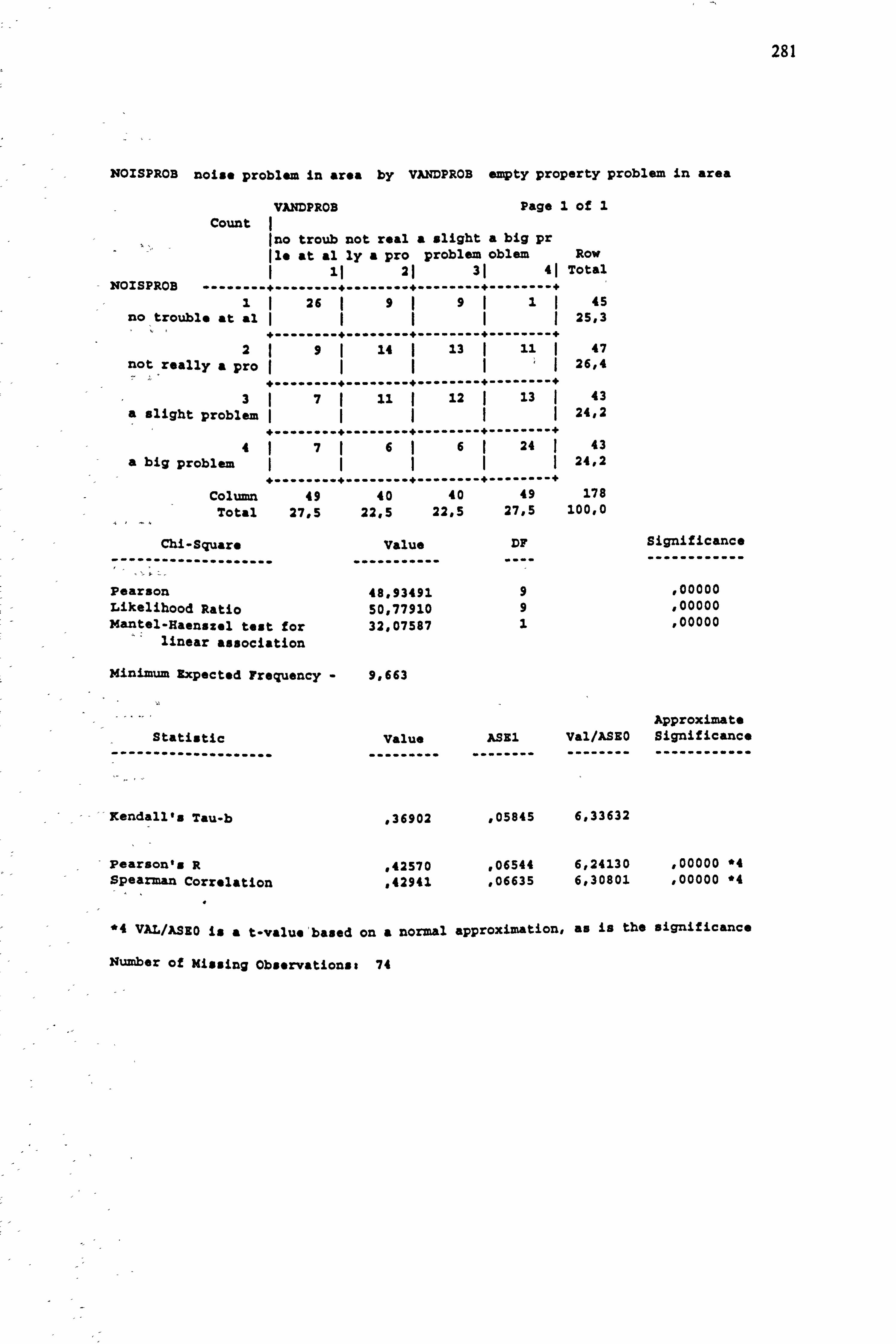
281
NOISPROB noise problem in area by VAIWPROB empty property problem in area
VANDPROB Page 1 of 1
Count I (no troub not real a slight a big pr ale at al ly a pro problem oblem Row
1 11 21 31 41 Total NOISPROB .......................... +---_----+--------+
1ý 26 (9ý9I11 45 no trouble at al IýII 25,3
+--------+--------+--------+--------+ 291 14 ý 13 ý 11 ý 47
not really a pro (1II 26,4 +........ +........ +--------+--------+
3ý7ý 11 ý 12 ý 13 ý 43
a slight problem 24,2
f--------+--------+--------+--------+ 476ý6ý 24 ý 43
a big problem 24,2
f........ +........ +....... _+....... _+ Column 49 40 40 49 178
Total 27,5 22,5 22,5 27,5 100,0
Chi-Square Value DF Significance
-------------------- ----------- ---- ------------
Pearson Likelihood Ratio Mantel-Haenszel test for
linear association
Minimum Expected Frequency
Statistic
Kendall's Tau-b
Pearson'. R Spearman Correlation
48,93491 9 , 00000
50,77910 9 , 00000
32,07587 1 , 00000
9,663
Approximate Value ASS1 Val/ASEO Significance
--------- -------- -------- ------------
, 36902 , 05845 6,33632
. 42570 . 06544 6,24130 , 00000 *4
, 42941 , 06635 6,30801 , 00000 "4
*4 VAL. /A380 is a t"value'based on a normal approximation, as is the significance
Number of Missing Observationss 74
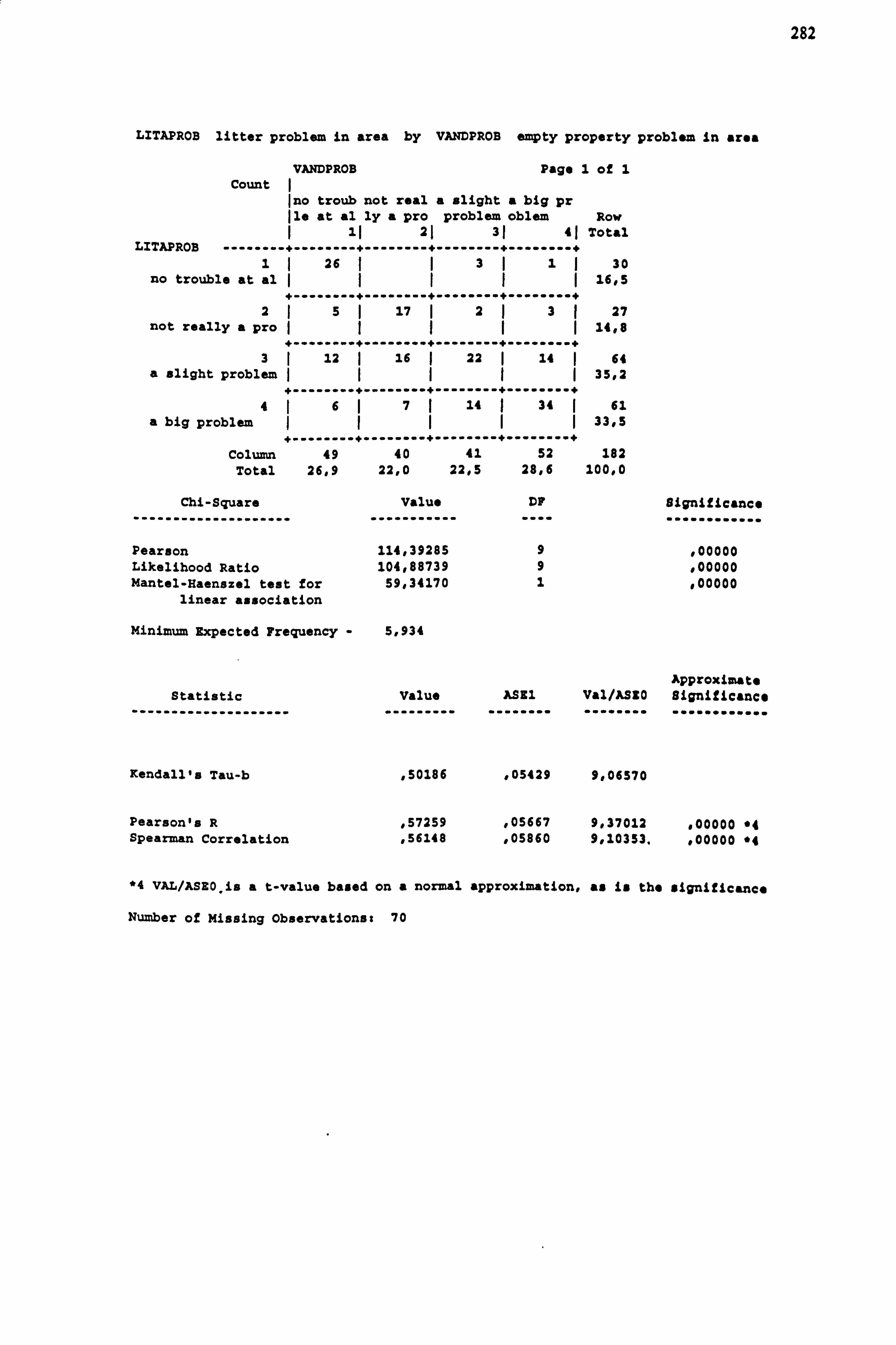
282
LITAPROB litter problem in area by VANDPROB empty property problem in area
VANDPROB Page 1 of 1
Count ono troub not real a slight a big pr lie at al ly a pro problem oblem Row
11 21 31 41 Total LITAPROB ---------------------------------------------
1 26 11311 30 no trouble at al II( 16,5
251 17 23 27 not really a pro 14,8
3ý 12 16 ý 22 ý 14 64 a slight problem 35,2
------------------------------------- 46ý7 14 ý 34 ý 61
a big problem IIIý 33,5 ...........................
Column 49 40 41 52 182 Total 26,9 22,0 22,5 28,6 100,0
Chi-Square Value De significance
------------------- ........... .... ............
Pearson Likelihood Ratio Mantel-Haenszel test for
linear association
Minimum Expected Frequency
Statistic --------------------
Kendall's Tau-b
Pearson's R Spearman Correlation
114,39285 9 100000 104,88739 9 100000
59,34170 1 000000
5,934
Approximate value ASE1 Val/ASEO Significance
, 50186 , 05429 9,06570
, 57259 , 05667 9,37012 800000 "4 , 56148 , 05860 9,10353,000000 "4
*4 VAL/ASEO, is a t-value based on a normal approximation, as is the significance
Number of Missing observations: 70
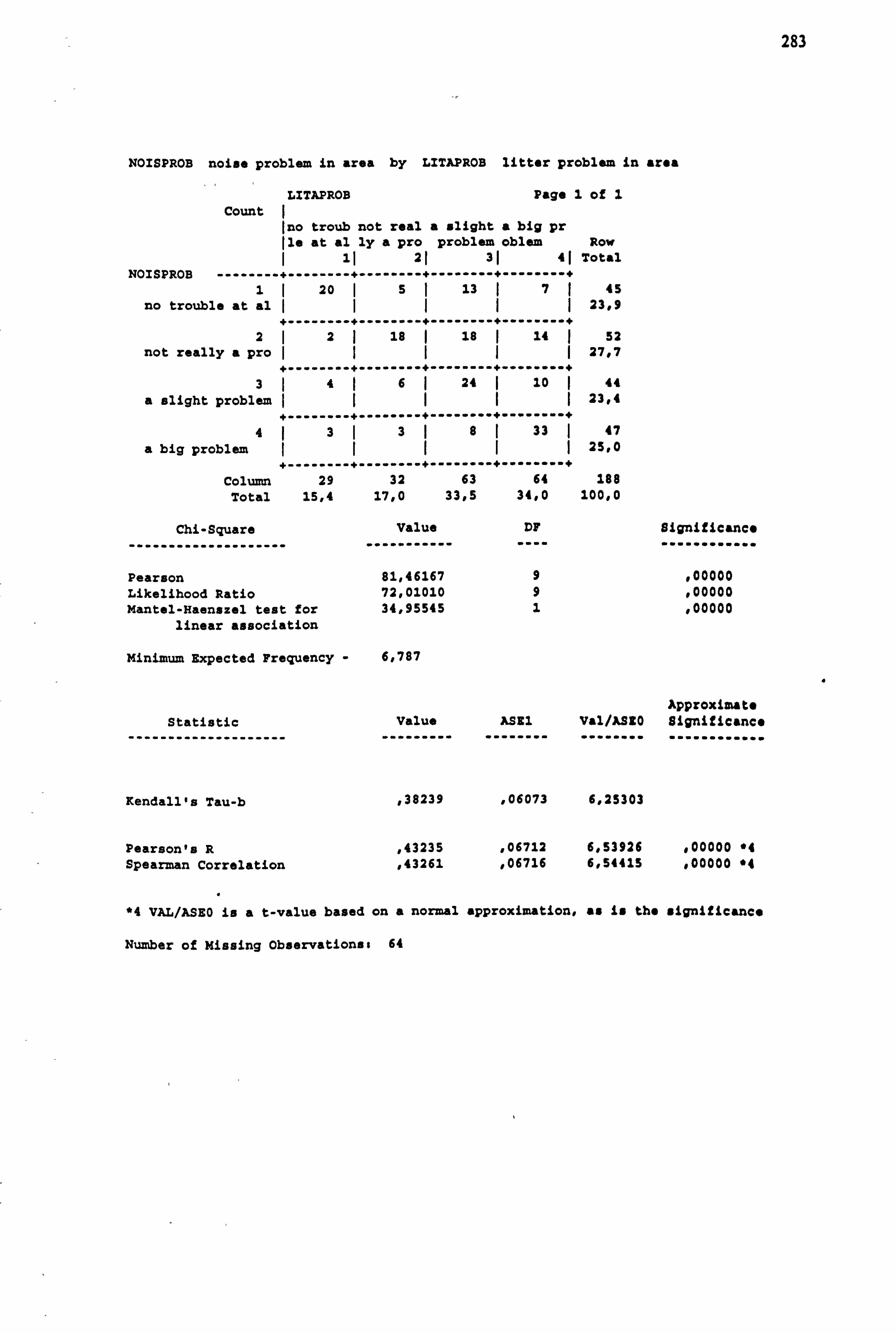
283
NOISPROB noise problem in area by LITAPROB litter problem in area
LITAPROB Page 1 of 1
Count (no trout not real a slight a big pr ale at al ly a pro problem oblem Row
11 21 31 41 Total NOISPROB ---------------------------------------------
11 20 51 13 ý7ý 45
no trouble at al II1I 23,9
------------------------------------- 2ý2ý 18 ý 18 ý 14 52
not really a pro IýýII 27,7
------------------------------------- 3I46I 24 ý 10 44
a slight problem ý(III 23,4
4ý3I3I8I 33 ý 47
a big problem IIIýI 25,0
Column 29 32 63 64 188 Total 15,4 17,0 33,5 34,0 100,0
Chi-Square Value D8 Significance
Pearson 81,46167 9 , 00000 Likelihood Ratio 72,01010 9 100000 Mantel-Haenszel test for 34,95545 1 , 00000
linear association
Minimum Expected Frequency - 6,787
Statistic --------------------
Kendall's Tau-b
Approximate Value ASE1 Val/ASYO Significance
, 38239 , 06073 6,25303
Pearson's R , 43235 , 06712 6,53926 000000 "4 Spearman Correlation , 43261 , 06716 6,54415 000000 "4
*4 VAL/ASEO is a t-value based on a normal approximation, as is the significance
Number of Missing Observationst 64
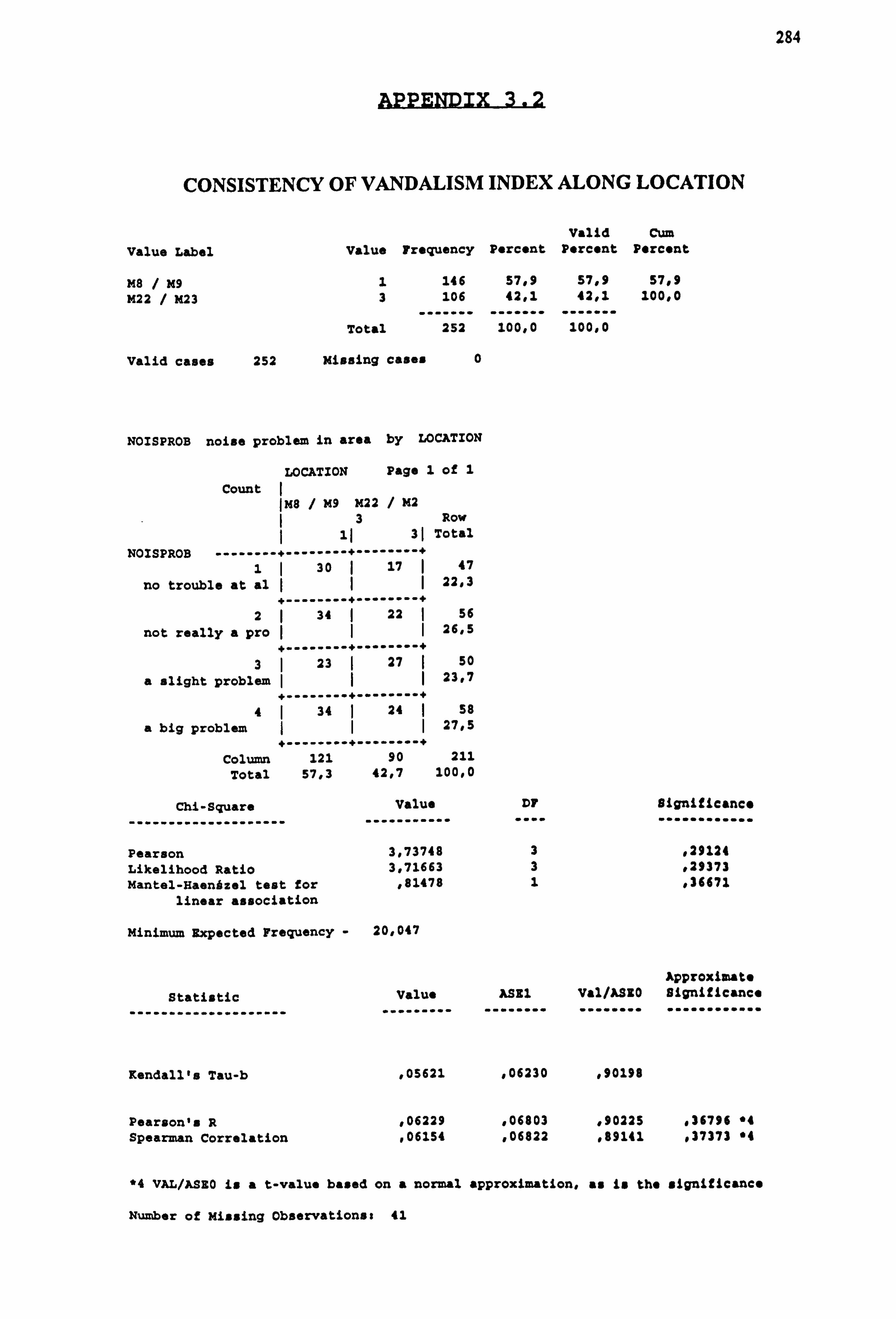
284
CONSISTENCY OF VANDALISM INDEX ALONG LOCATION
Valid Cum
Value Label Value Frequency Percent Percent Percent
M8 / M9 1 146 57,9 57,9 57,9 M22 / M23 3 106 42,1 42,1 100,0
Total 252 100,0 100,0
Valid cases 252 Missing cases 0
NOISPROB noise problem in area by LOCATION
LOCATION Page 1 of 1
Count IM8 / M9 M22 / M2
3 Row 31 Total
NOISPROS --------------------------- 1 30 1 17 ý 47
no trouble at al I1I 22,3
------------------- 2I 34 22 I 56
not really a pro II 26,5
------------------- 3 23 ý 27 ý 50
a alight problem ýI 23,7 -------------------
4I 34 24 58 a big problem ýI 27,5
------------------- Column 121 90 211
Total 57,3 42,7 100,0
Chi-Square Value
-------------------- ---"------"
DF _...
Significance ............
Pearson 3,73748 3 , 29124 Likelihood Ratio 3,71663 3 , 29373
Mantel-Haenhzel test for , 81478 1 , 36671
linear association
Minimum Expected Frequency - 20,047
Approximate
Statistic Value ASS1 Val/ASY0 significance
Kendall's Tau-b , 05621 , 06230 , 90198
Pearson's R , 06229 . 06803 , 90225 , 36796 "4 Spearman Correlation , 06154 , 06822 , 89141 , 37373 "4
*4 VAL/ASEO is a t-value based on a normal approximation, as is the significance
Number of Missing Observations: 41
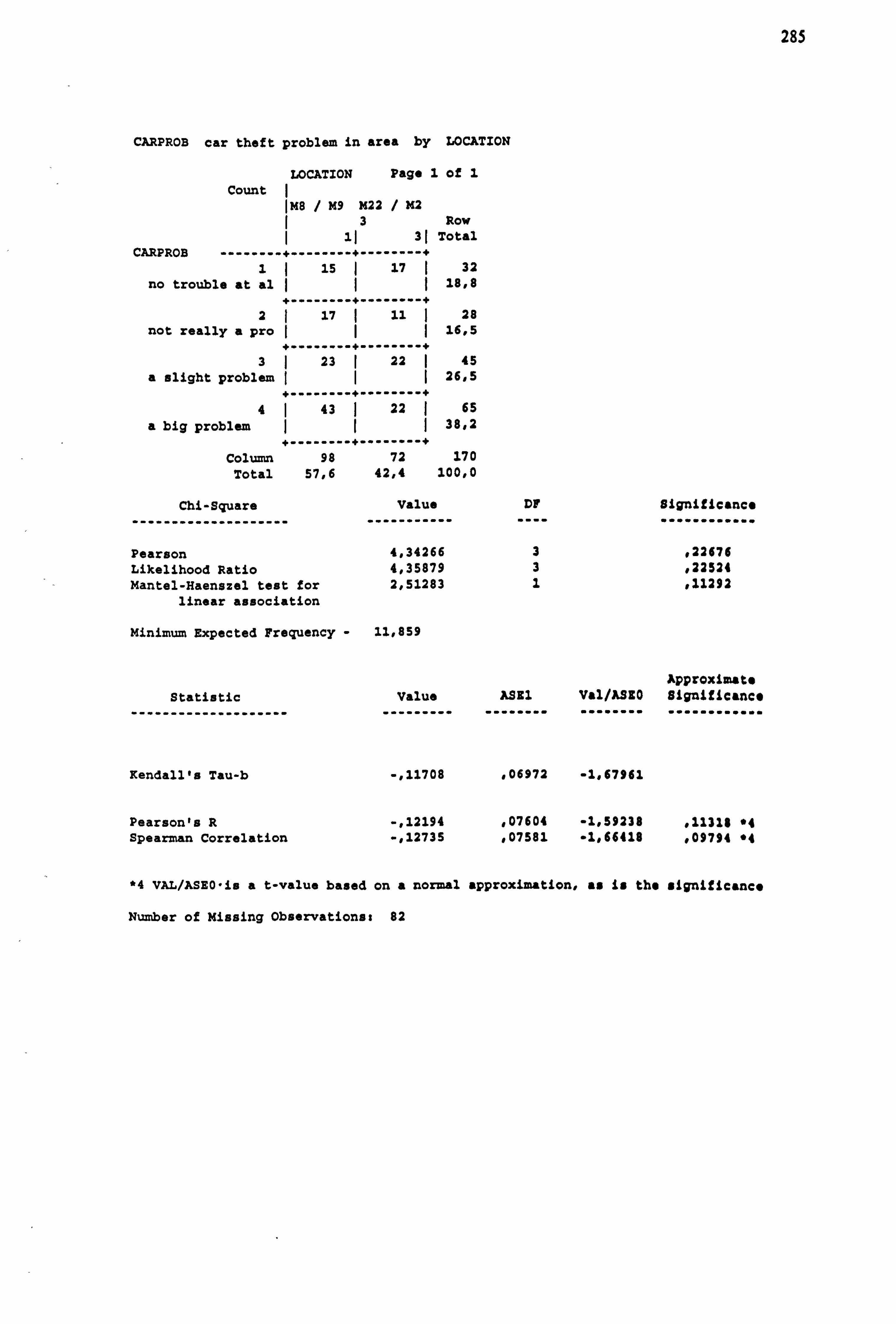
285
CARPROB car theft problem in area by LOCATION
LOCATION Page 1 of 1
Count IM8 / M9 M22 / M2
3 Row 1I 31 Total
CARPROB --------------------------- II 15 I 17 I 32
no trouble at al II 18,8 -------------------
2 17 I 11 I 28
not really a pro III 16,5
------------------- 3 23 I 22 45
a slight problem II 26,5 -------------------
4I 43 I 22 I 65 a big problem II 38,2
------------------- Column 98 72 170
Total 57,6 42,4 100,0
Chi-Square Value -------------------- -----------
DF ----
Significance ............
Pearson 4,34266 3 , 22676 Likelihood Ratio 4,35879 3 , 22524 Mantel-Haenszel test for 2,51283 1 , 11292
linear association
Minimum Expected Frequency - 11,859
Approximate Statistic Value
-------------------- --------- - ASE1
------- Val/ASEO --------
Significance ............
Kendall's Tau-b -, 11708 , 06972 -1,67961
Pearson's R -, 12194 , 07604 -1,59238 , 11318 "4 Spearman Correlation -, 12735 , 07581 -1,66418 , 09794 "4
*4 VAL/ASEO-is a t-value based on a normal approximation, as is the significance
Number of Missing Observations: 82
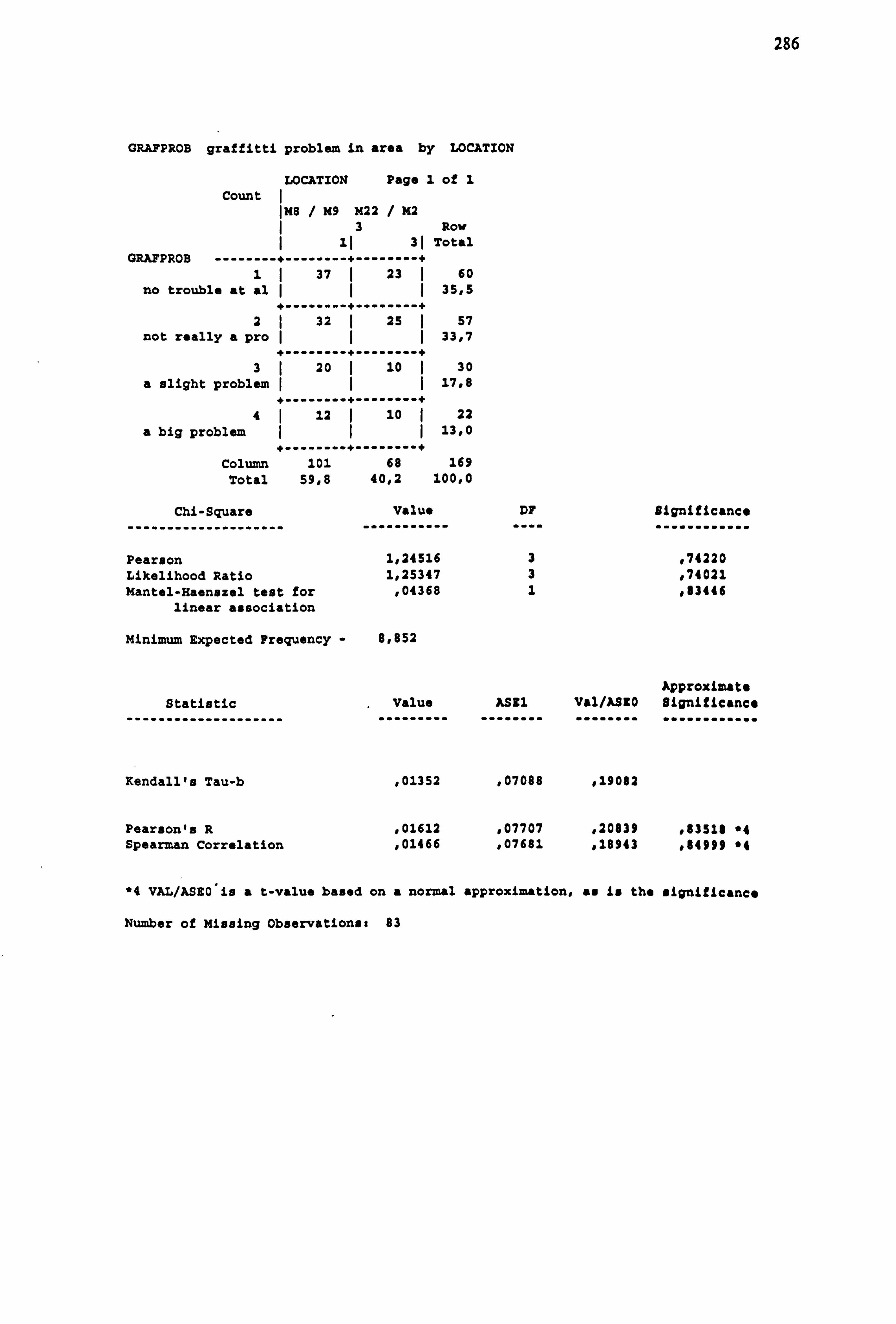
286
GRAFPROH graffitti problem in area by LOCATION
LOCATION Page 1 of 1
Count IM8 / M9 M22 / M2
3 Row 11 31 Total
GRAFPROB --------------------------- 11 37 23 60
no trouble at al I1 35,5 +........ +........ +
2 32 1 25 1 57 not really a pro 1 33,7
31 20 1 10 I 30 a slight problem I 17,8
4 12 ý 10 22 a big problem 13,0
................... Column 101 68 169
Total 5918 40,2 1 00,0
Chi-Square Value DF Significance
Pearson 1,24516 3 , 74220 Likelihood Ratio 1,25347 3 , 74021 Mantel-Hasnszel test for , 04368 1 , 83446
linear association
Minimum Expected Frequency - 8,852
Approximate Statistic Value
------------------- -------- -- ASH1
------- Val/ASZO --------
Significance ............
Kendall's Tau-b , 01352 , 07088 19082
Pearson's R , 01612 , 07707 . 20839 , 83518 *4 Spearman Correlation , 01466 , 07681 , 18943 , 84999 *4
*4 VAL/AS80'is a t-value based on a normal approximation, as is the significance
Number of Missing Observations 83
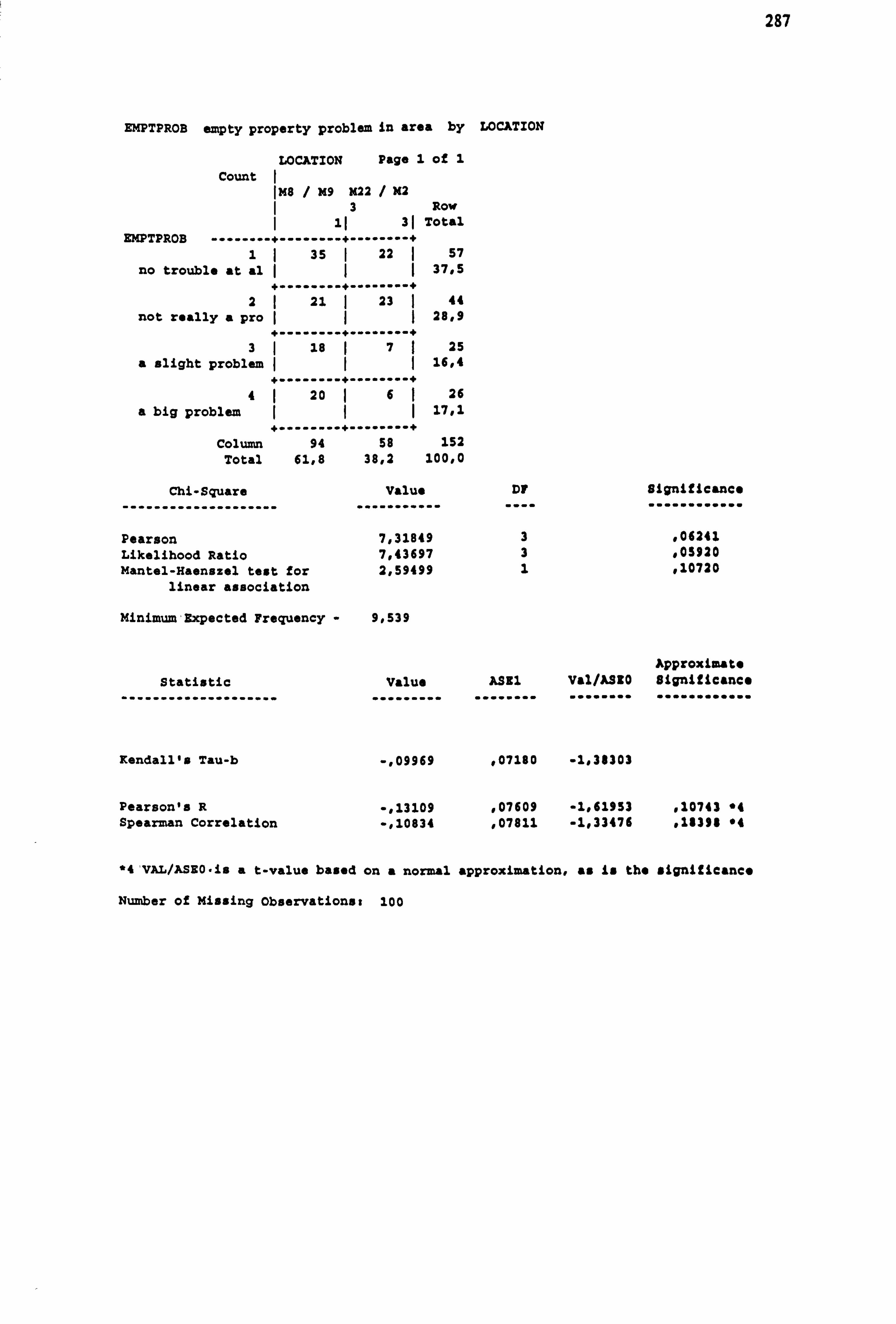
287
EMPTPROB empty property problem in area by LOCATION
LOCATION Page 1 of 1
Count IMS / M9 M22 / M2
3 Row 31 Total
EMPTPROB --------------------------- 1 35 1 22 1 57
no trouble at al I 37,5
21 21 ý 23 ý 44 not really a pro 28,9
------------------- 3ý 18 7 25
a alight problem 16,4
4 20 6ý 26 a big problem 17,1
Column 94 58 152 Total 61,8 38,2 100,0
Chi-Square value Dt
Pearson 7,31849 3 Likelihood Ratio 7,43697 3 Mantel-Hasnszel test for 2,59499 1
linear association
Minimum Expected Frequency - 9,539
Significance
, 06241
, 05920
, 10720
Approximate Statistic Value AS81 Val/ASYO significance
Kendall's Tau-b -, 09969 , 07180 -1,38303
Pearson's R -, 13109 , 07609 -1,61953 , 10743 "4 Spearman Correlation -, 10834 , 07811 -1,33476 . 18398 "4
*4'vAL/ASEO-is a t-value based on a normal approximation, as is the significance
Number of Missing Observations, 100
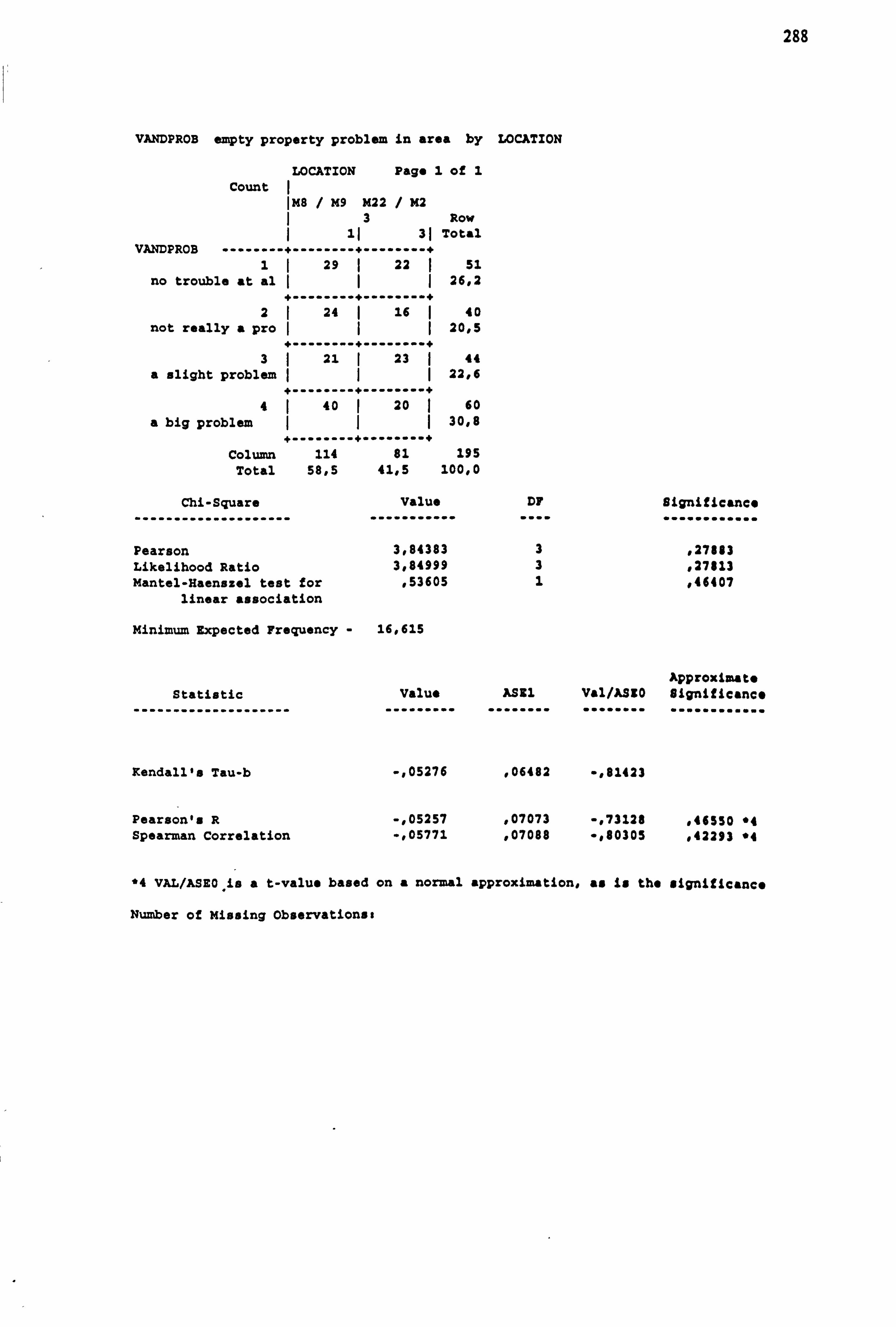
288
VANDPROB empty property problem in area by LOCATION
LOCATION Page 1 of 1
Count IMS / M9 M22 / M2
3 Row 1) 31 Total
VANDPROB --------------------------- 1 29 22 51
no trouble at al (1I 26,2 +--------+........ +
2I 24 16 40 not really a pro 20,5
------------------- 3 21 I 23 ý 44
a slight problem ýI 22,6 -------------------
4 40 20 ( 60 a big problem ýII 30,8
................... Column 114 81 195
Total 58,5 41,5 100,0
Chi-Square Value DB
Pearson 3,84383 3 Likelihood Ratio 3,84999 3 Mantel-Haenazel test for . 53605 1
linear association
Minimum Expected Frequency - 16,615
Significance
, 27113
, 27113
, 46407
Approximate Statistic Value ASH1 Val/ASiO Significance
Kendall's Tau-b -, 05276 , 06482 -, 81423
Pearson's R -, 05257 , 07073 -. 73128 146550 "4 Spearman Correlation -, 05771 , 07088 -, 80305 , 42293 "4
*4 VAL/ASEO, is a t-value based on a normal approximation, as is the significance
Number of Missing Observationst
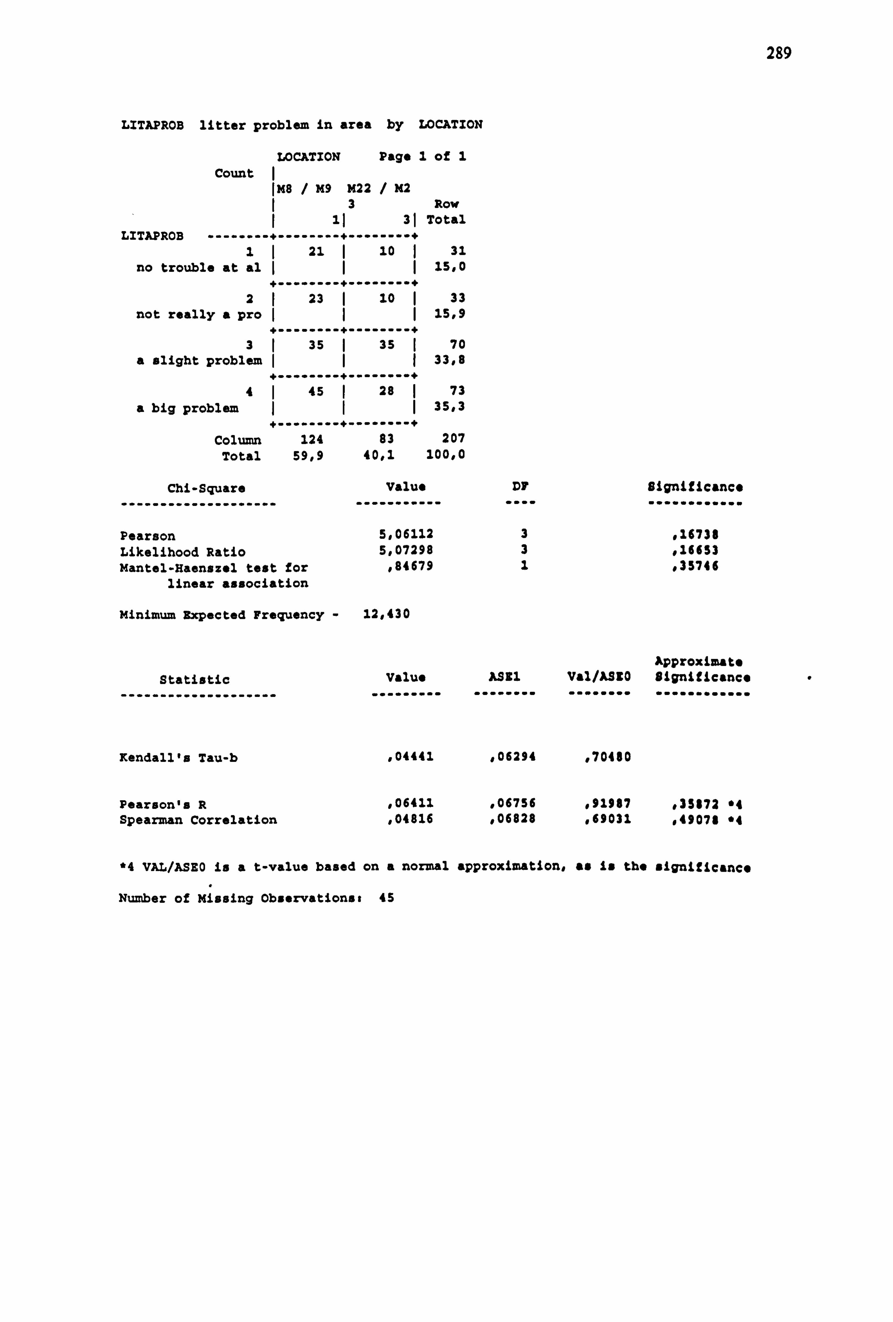
289
LITAPROB litter problem in area by LOCATION
LOCATION Page 1 of 1
Count IM8 / M9 M22 / M2
3 Row 11 31 Total
LITAPROB ------------------ --------- 1 21 ý 10 ý 31
no trouble at al I 15,0 ---------- --------
2I 23 I 10 I 33 not really a pro II I 15,9
---------- --------- 3ý 35 I 35 ý 70
a slight problem ýI 33,8
---------- --------- 4ý 45 28 ý 73
a big problem II I 35,3
Column 124 83 207 Total 59,9 40,1 1 00,0
Chi-Square
--------------------
Value
---------- -
DF
....
Significance
............
Pearson 5,06112 3 , 16738 Likelihood Ratio 5,07298 3 , 16653 Mantel-Haenszel test for , 84679 1 , 35746
linear association
Minimum Expected Frequency - 12,430
Approximate Statistic Value AS91 Val/ASYO Significance
Kendall's Tau-b , 04441 , 06294 , 70480
Pearson's R , 06411 , 06756 , 91987 , 35872 "4 Spearman Correlation , 04816 , 06828 , 69031 , 49078 "4
*4 VAL/ASEO is a t-value based on a normal approximation, as is the significance
Number of Missing Observations, 45
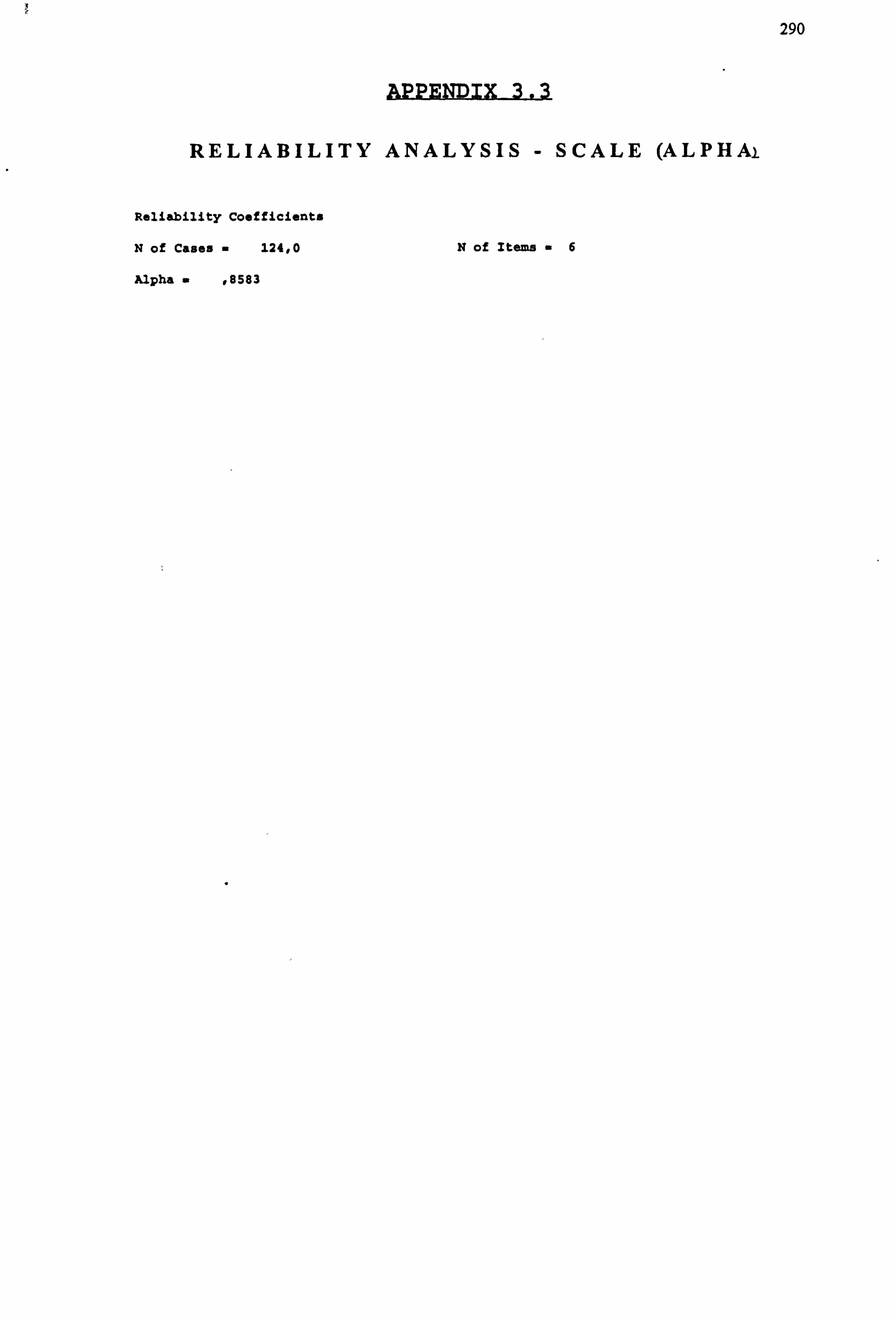
290
RELIABILITY ANALYSIS - SCALE (ALPHA)
Reliability Coefficients
N of Cases . 124,0 N of Items "6
Alpha . , 8583
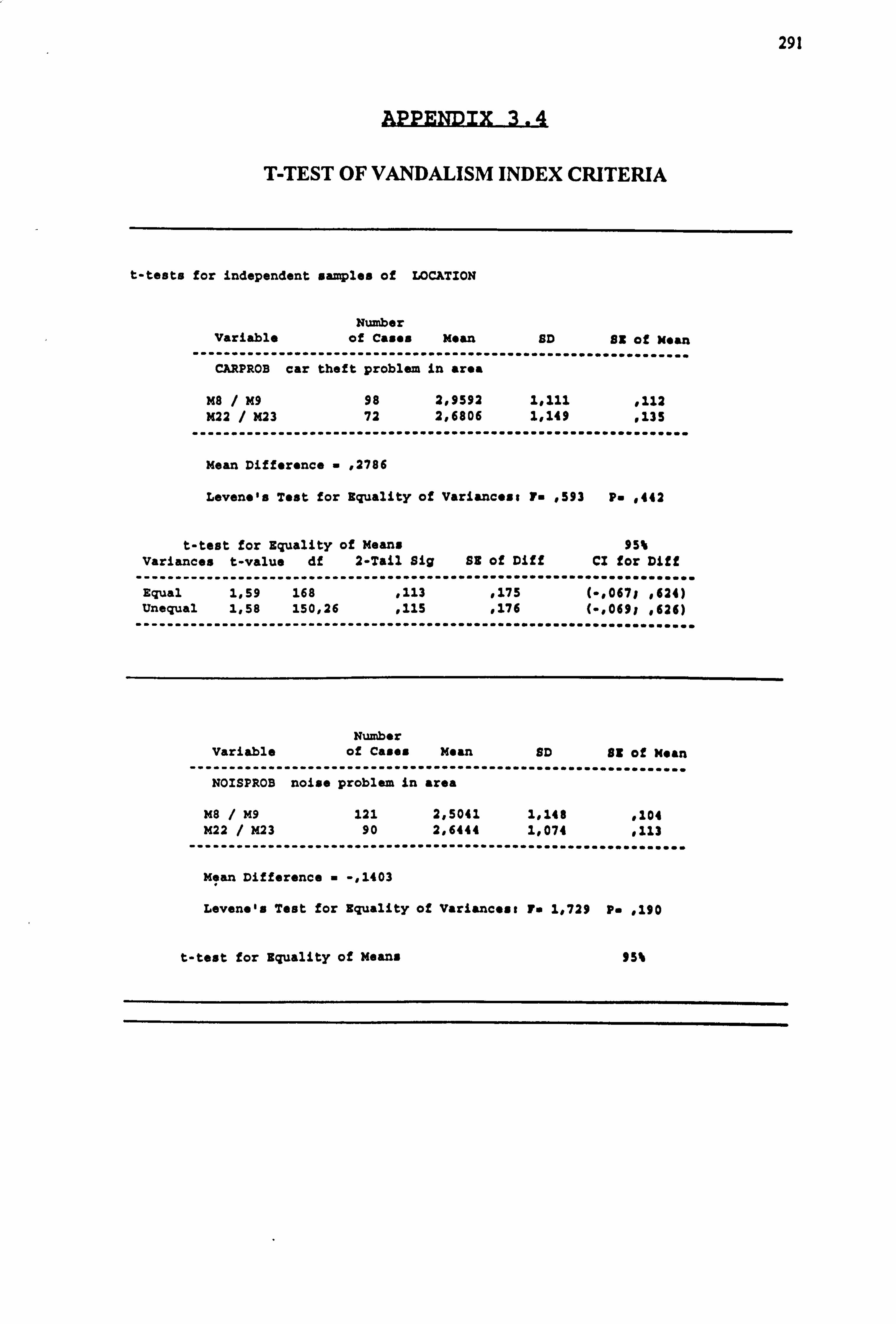
291
T-TEST OF VANDALISM INDEX CRITERIA
t-teats for independent samples of LOCATION
Number Variable of Cases Mean SD BE of Mean
............................................................... CARPROB car theft problem in area
M8 / M9 98 2,9592 1,111 , 112 M22 / M23 72 2,6806 1,149 , 135
Mean Difference - , 2786
Levene's Test for Equality of Variancest Y. , 593 P. , 442
t-test for Equality of Means 95% Variances t-value df 2-Tail Sig SE of Di!! C2 for Di! f
Equal 1,59 168 , 113 , 175 (-, 0671 , 624) Unequal 1,58 150,26 , 115 , 176 (-, 0691 0626)
.......................................................................
Number Variable of Cases Mean SD BE of mean
NOISPROB noise problem in area
M8 / M9 121 2,5041 1,148 , 104 M22 / X23 90 2,6444 1,074 , 113
Mean Difference - -, 1403
Levene's Test for Equality of Variances, 7.1,729 P. , 190
t-test for Equality of Means 95"
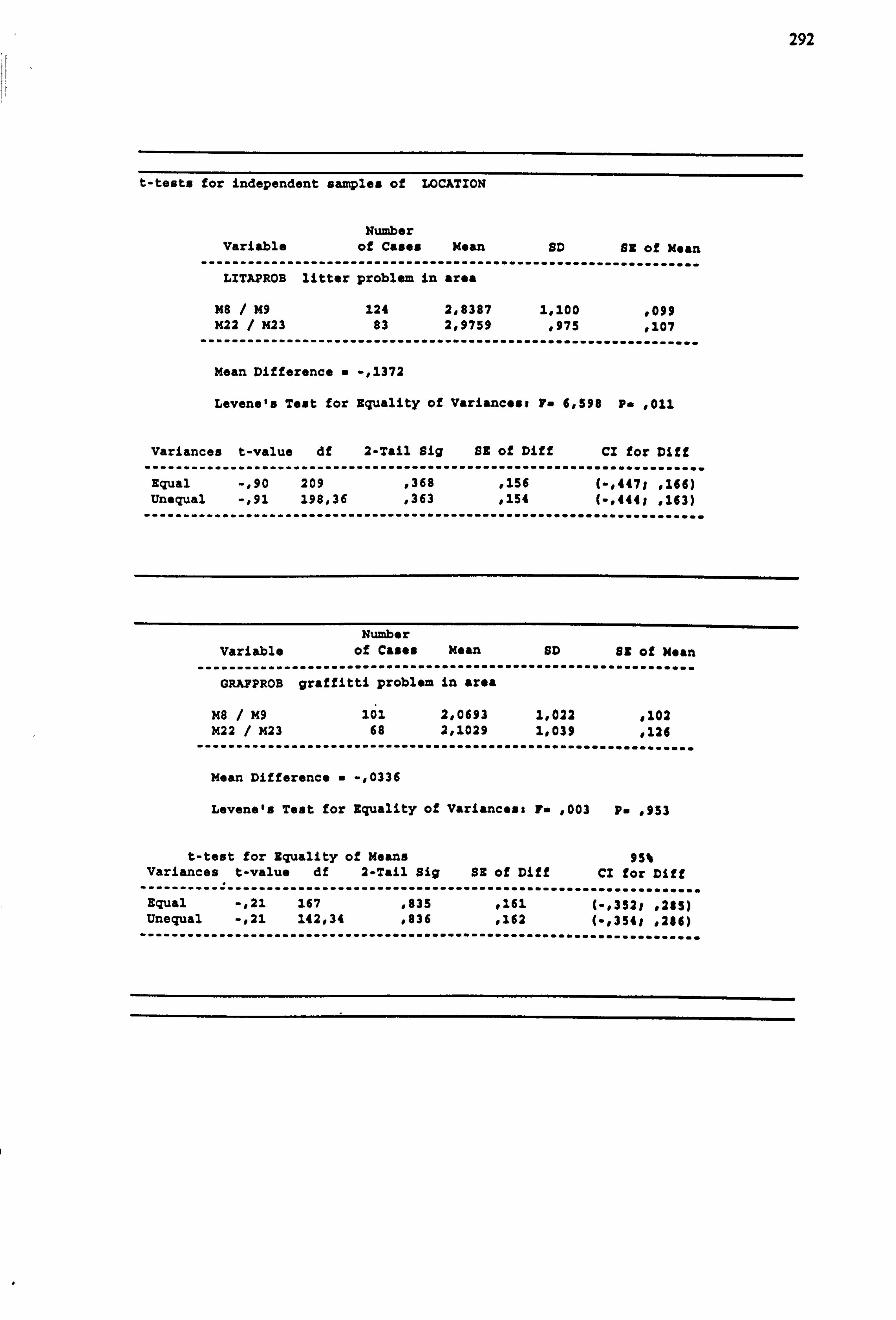
292
t-tests for independent samples of LOCATION
Number Variable of Cases Mean SD BE of Mean
--------------------------------------------------------------- LITAPROB litter problem in area
me / M9 124 2,8387 1,100 1099 M22 / M23 83 2,9759 , 975 , 107
---------------------------------------------------------------
Mean Difference . -, 1372
Levene's Test for Equality of Variances# 1.6,598 P. , 011
Variances t-value df 2-Tail Big SE of Diff CI for Diff
Equal -, 90 209 , 368 1156 (-, 4471 , 166) Unequal -, 91 198,36 , 363 , 154 (-, 444 , 163)
Number Variable of Cases Mean SD 89 of Mean
GRAPPROB graffitti problem in area
M8 / M9 101 2,0693 1,022 , 102 M22 / M23 68 2,1029 1,039 0126
Mean Difference . -, 0336
Levene'a Test for Equality of Variancesa 7. , 003 p. 0953
t-test for Equality of Means 95% Variances t-value df 2-Tail Sig BE of Diff CI for Diff
Equal -, 21 167 , 835 , 161 (-, 352, , 285) Unequal -, 21 142,34 , 836 , 162 (-, 3541 . 286)
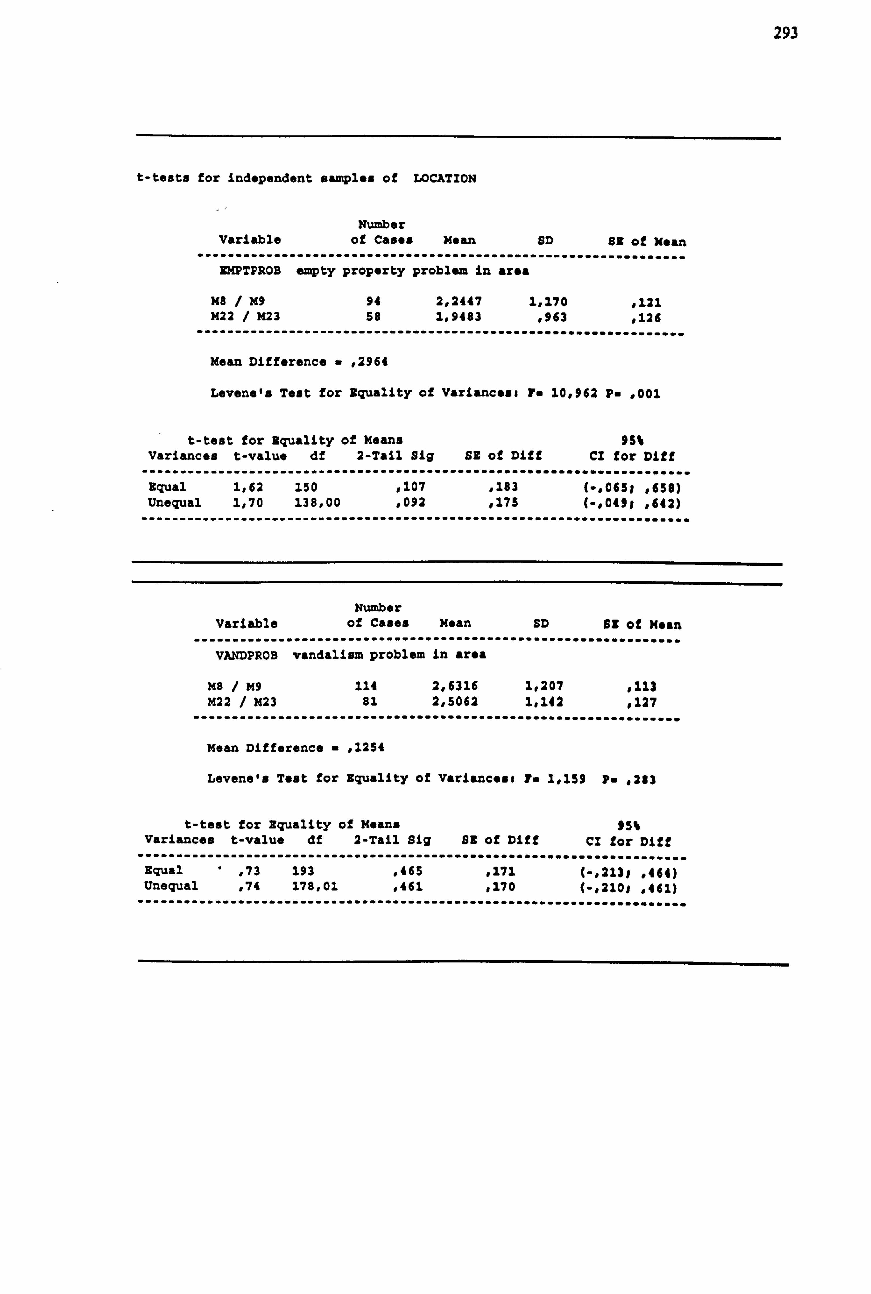
293
t-tests for independent samples of LOCATION
Number Variable of Cases Mean SD 8s of Kean
RMPTPROB empty property problem in area
M8 / X9 94 2,2447 1,170 , 121 M22 / M23 58 1,9483 , 963 , 226
Mean Difference . , 2964
Levene's Test for Equality of Variances, P. 10,962 P. , 001
t-teat for Equality of Means 95% Variances t-value df 2-Tail Big SE of Diff CI for Diff
Equal 1,62 150 , 107 , 183 (-1065, , 658) Unequal 1,70 138,00 , 092 , 175 (-, 049 , 642)
Number Variable of Cases Mean SD S! of Mean
VANDPROB vandalism problem in area
M8 / M9 114 2,6316 1,207 , 113 M22 / M23 61 2,5062 1.142 , 127
Mean Difference - , 1254
Levene'a Test for Equality of Variancess f. 1,159 P. , 283
t-test for Equality of Means 95% Variances t-value df 2-Tail Big BE of Diff Cr for Diff
Equal , 73 193 , 465 , 171 (-, 2131 . 464) Unequal , 74 178.01 , 461 , 170 (-, 210 . 461)
------------------ ---------------------- ...............................
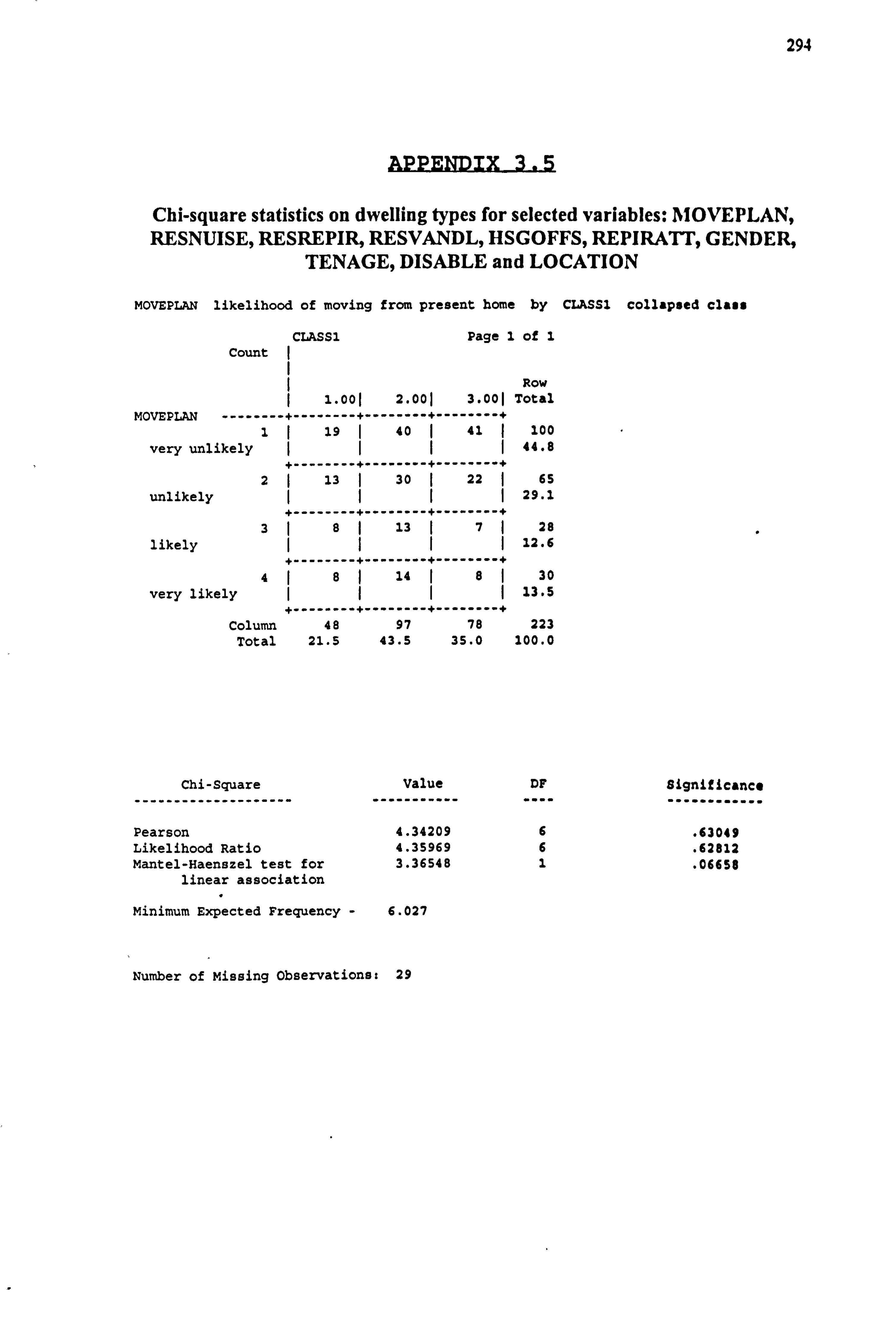
294
Chi-square statistics on dwelling types for selected variables: MOVEPLAN, RESNUISE, RESREPIR, RESVANDL, HSGOFFS, REPIRATT, GENDER,
TENAGE, DISABLE and LOCATION
MOVEPLAN likelihood of moving from present home by CLASSI collapsed class
Count CLASS1 Page 1 of 1
Row 1.00 2.001 3.001 Total
MOVEPLAN ------------------------------------ 1I 19 I 40 41 100
very unlikely 44.8 ----------------------------
2( 13 30 ý 22 ý 65
unlikely IýII 29.1
---------------------------- 3ý8ý 13 (7ý 28
likely 12.6
---------------------------- 48 14 8I 30
very likely 13.5 ----------------------------
Column 48 97 78 223 Total 21.5 43.5 35.0 100.0
Chi-square Value DF Significance -------------------- ----------- ---- ............
Pearson 4.34209 6 . 63049 Likelihood Ratio 4.35969 6 . 62812 Mantel-Haenszel test for 3.36548 1 . 06658
linear association
Minimum Expected Frequency - 6.027
Number of Missing observations: 29
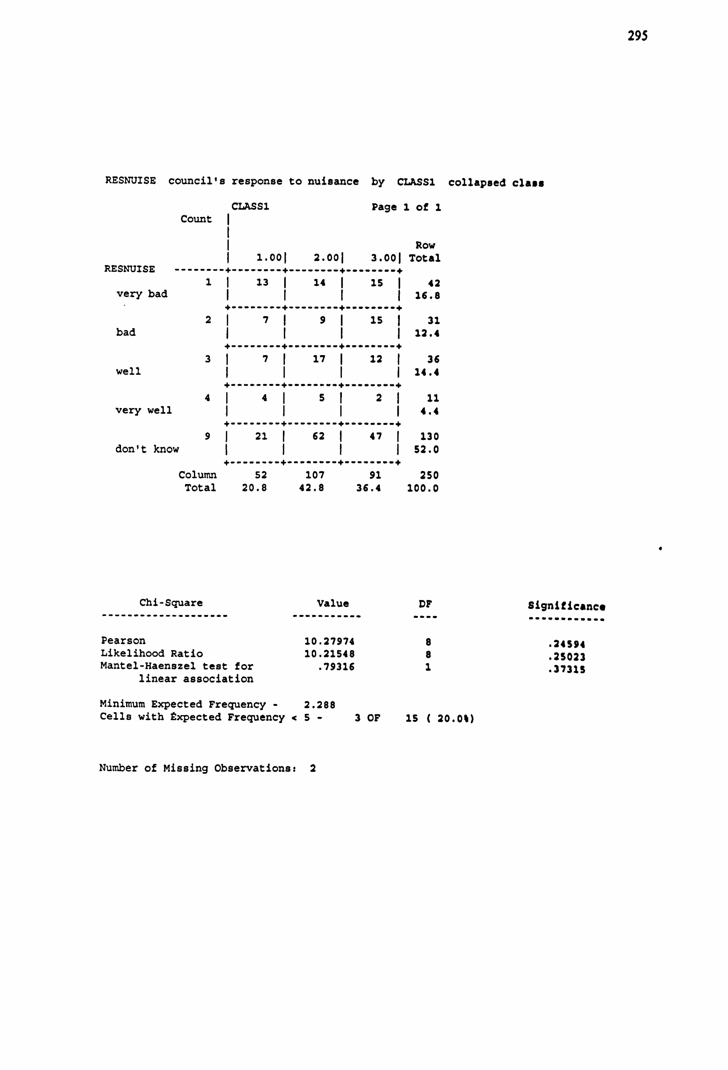
RESNUISE council's response to nuisance by CLASS1 collapsed class
CLASS1 Page 1 of 1 Count
Row
1.001 2.001 3.001 Total RESNUISE ------------------------------------
1i 13 i is i is 42 very bad
i 16.8
---------------------------- 2ý7ý9I 15 ý 31
bad 12.4 ----------------------------
3ý7ý 17 ý 12 ý 36
well 14.4 ----------------------------
4I4I5ý2ý 11 very well 4.4
---------------------------- 9ý 21 I 62 ý 47 ý 130
don't know ýIII 52.0 ----------------------------
Column 52 107 91 250 Total 20.8 42.8 36.4 100.0
295
Chi-Square Value DF -------------------- ----------- ----
Pearson 10.27974 8 Likelihood Ratio 10.21548 8 Mantel-Haenszel test for . 79316 1
linear association
Minimum Expected Frequency - 2.288 Cells with Expected Frequency <5-3 OF 15 ( 20.0%)
Significance
. 24594
. 25023
. 37315
Number of Missing observations: 2
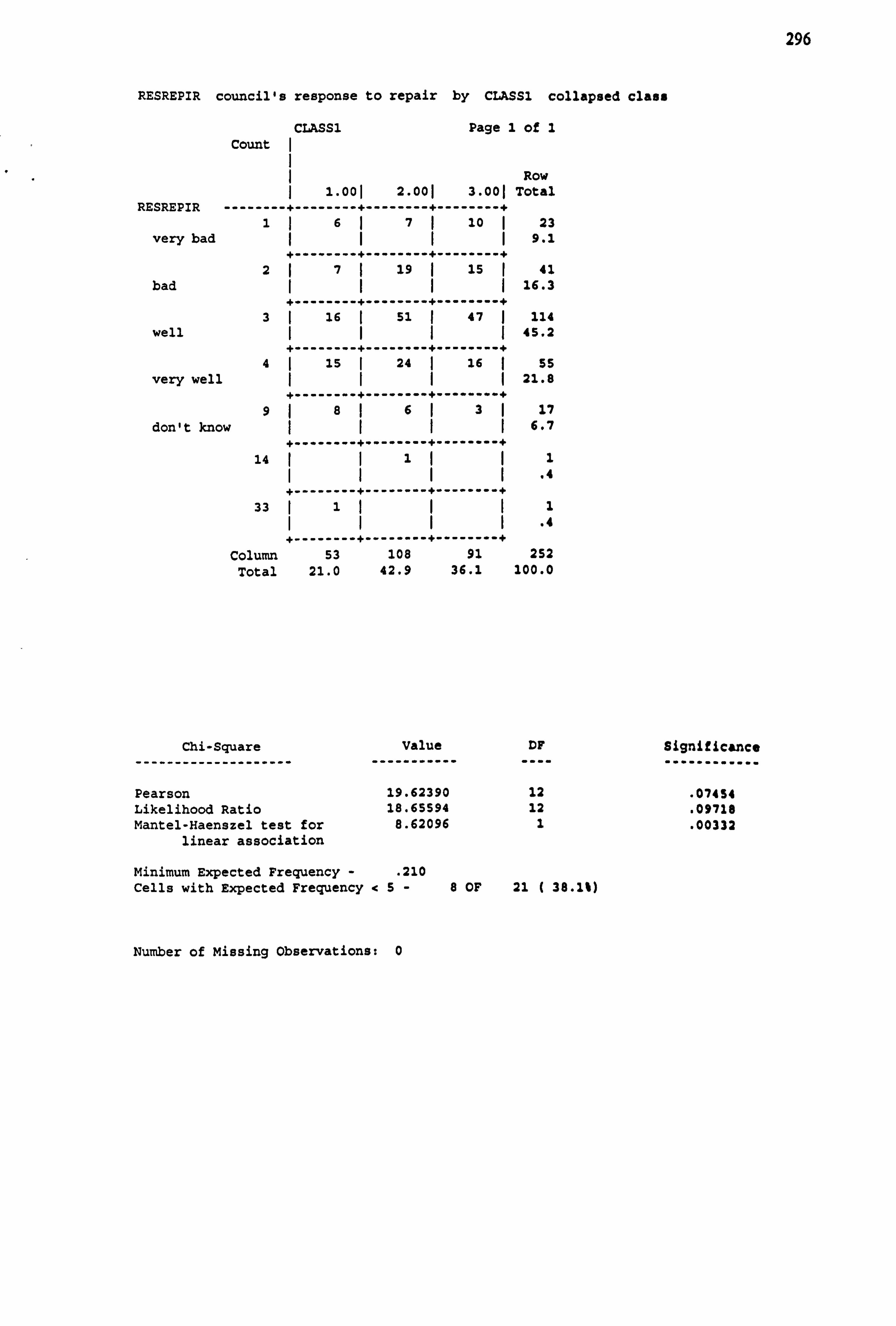
296
RESREPIR council's response to repair by CLASS1 collapsed class
Count CLASSI Page 1 of 1
I Row 1.001 2.001 3.001 Total
RESREPIR ------------------------------------ 1 1617 10 ý 23
very bad ý 9.1
---------------------------- 2 7 19 15 ý 41
bad 16.3 ----------------------------
3 I 16 ( 51 ý 47 114 well 45.2
---------------------------- 4 15 I 24 16 55
very well ýIII 21.8 ----------------------------
9 86ý3ý 17 don't know IIII 6.7
---------------------------- 14 I1II 1
.4 ----------------------------
33 1ýI 1
.4 ----------------------------
Column 53 108 91 252 Total 21.0 42.9 36.1 100.0
Chi-Square Value DF
-------------------- ----------- ----
Pearson 19.62390 12 Likelihood Ratio 18.65S94 12 Mantel-Haenszel test for 8.62096 1
linear association
Minimum Expected Frequency - . 210 Cells with Expected Frequency <5-8 OF 21 ( 38.11)
Significance
. 07454
. 09718
. 00332
Number of Missing Observations: 0
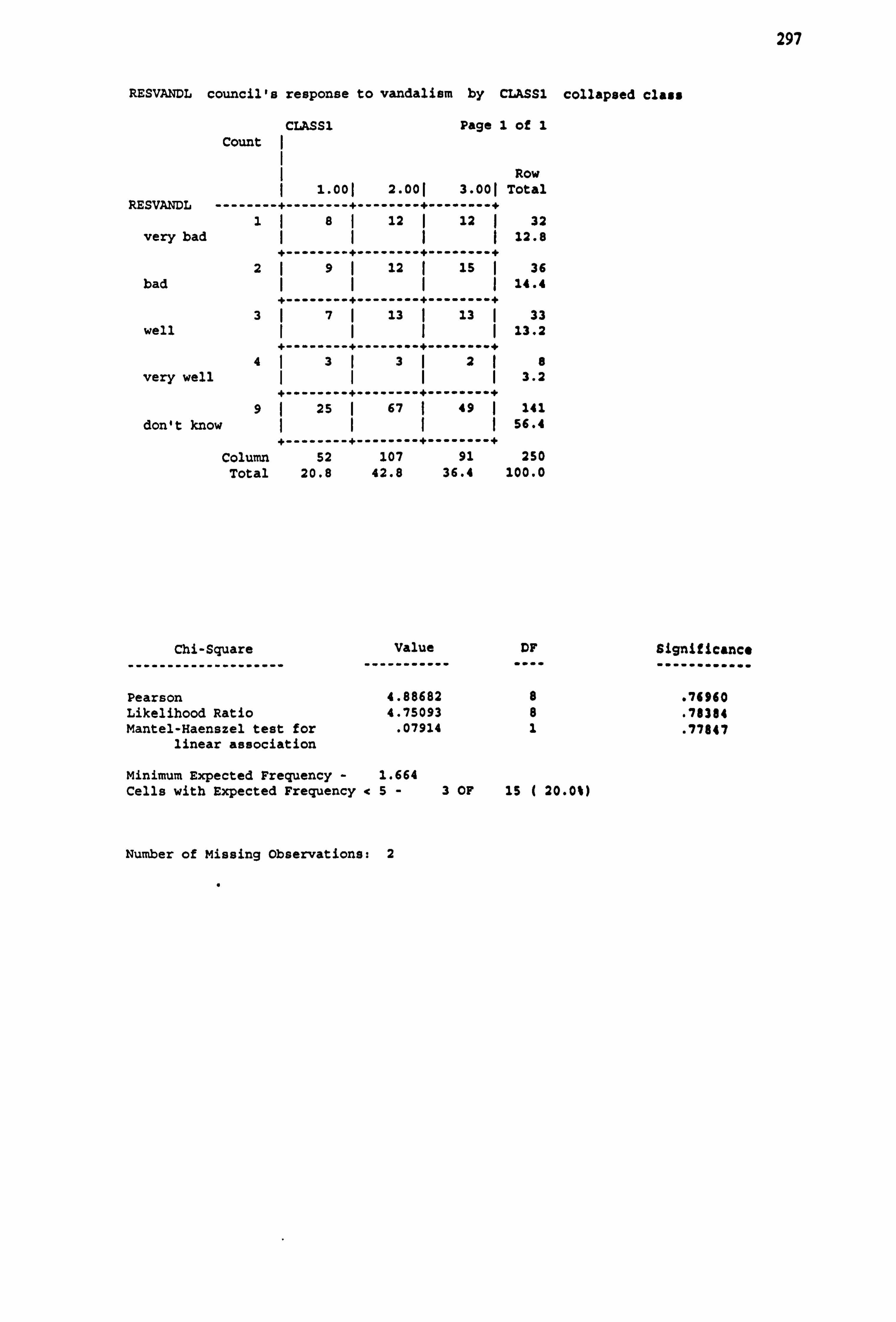
297
RESVANDL council's response to vandalism by CLASS1 collapsed class
CLASSI Page 1 of 1
Count
I Row 1.001 2.001 3.001 Total
RESVANDL ------------------------------------ 3. 18 12 ý 12 ý 32
very bad 12.8 ----------------------------
2 9I 12 15 36 bad IIý 14.4
---------------------------- 3 ý7ý 13 13 ý 33
well 13.2 ----------------------------
4 ý3ý3ý2 8
very well IIII 3.2 ----------------------------
9 ý 25 ý 67 49 141 don't know 56.4
---------------------------- Column 52 107 91 250
Total 20.8 42.8 36.4 100.0
Chi-Square Value DF
-------------------- ----------- _...
Pearson 4.88682 8 Likelihood Ratio 4.75093 8 Mantel-Haenszel test for . 07914 1
linear association
Minimum Expected Frequency - 1.664 Cells with Expected Frequency <5-3 OF 15 ( 20.0%)
Signiiicanct
. 76960
. 78784
. 77847
Number of Missing observations: 2
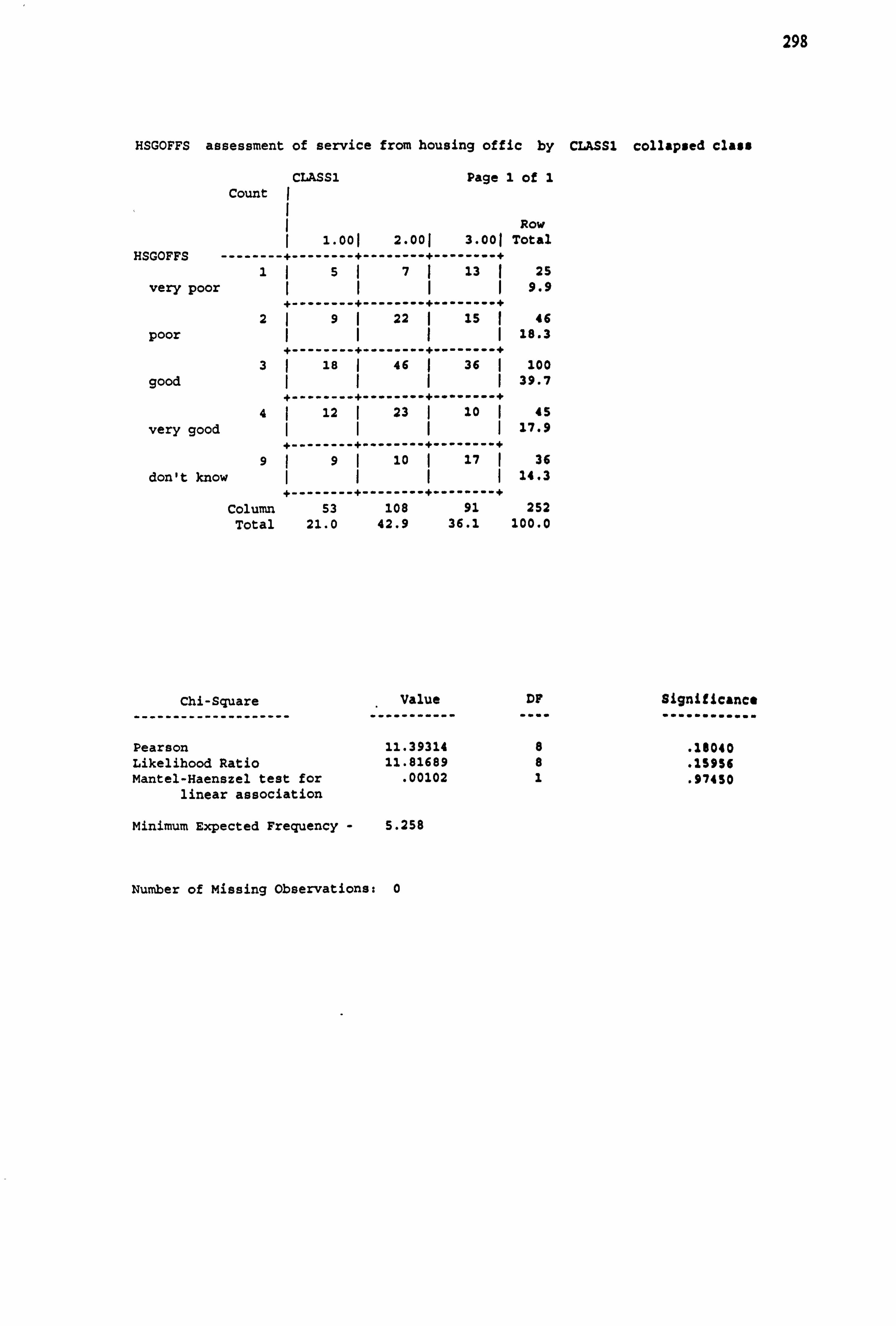
298
HSGOFFS assessment of service from housing offic by CLASSI collapsed class
CLASS1 Page 1 of 1
Count ý
Row 1.001 2.00 3.00 Total
HSGOFFS --------+--------+--------+--------+ 1 1517 13 ( 25
very poor II1I 9.9 ----------------------------
2 9I 22 ý 15 ý 46
poor IIII 18.3 ----------------------------
3 18 I 46 36 I 100
good 39.7 ----------------------------
4 12 ý 23 ý 10 ý 45 very good IIII 17.9
---------------------------- 9 ý9ý 10 17 ý 36
don't know IIII 14.3 ----------------------------
Column 53 108 91 252 Total 21.0 42.9 36.1 100.0
Chi-Square --------------------
Pearson Likelihood Ratio Mantel-Haenszel test for
linear association
Minimum Expected Frequency -
, Value DF Significance
11.39314 8 . 18040 11.81689 8 . 15956
. 00102 1 . 97450
5.258
Number of Missing Observations: 0
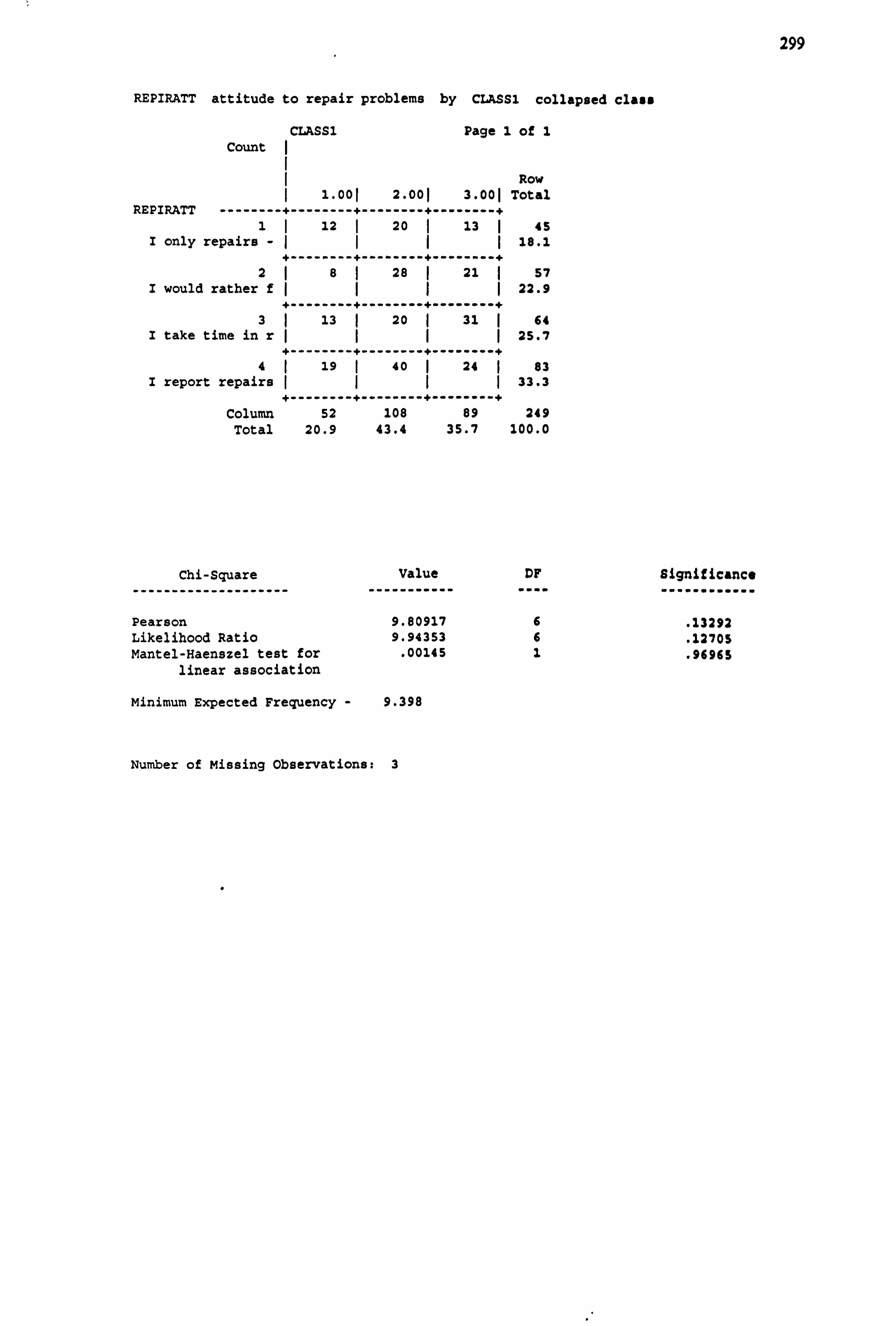
299
REPIRATT attitude to repair problems by CLASSI collapsed class
Count CLASS1 Page 1 of 1
I Row 1.001 2.001 3.001 Total
REPIRATT ------------------------------------ 3.1 12 ý 20 ý 13 ý 45
I only repairs -1ý 18.1 ----------------------------
2ý8ý 28 21 57 I would rather f 22.9
---------------------------- 3 13 ý 20 31 ( 64
I take time in r 25.7 ----------------------------
4ý 19 ý 40 24 ý 83 I report repairs (Iýý 33.3
---------------------------- Column 52 108 89 249
Total 20.9 43.4 35.7 100.0
Chi-Square Value DF Significance
Pearson 9.80917 6 . 13293 Likelihood Ratio 9.94353 6 . 12705 Mantel-Haenszel test for . 00145 1 . 96965
linear association
Minimum Expected Frequency - 9.398
Number of Missing Observations: 3
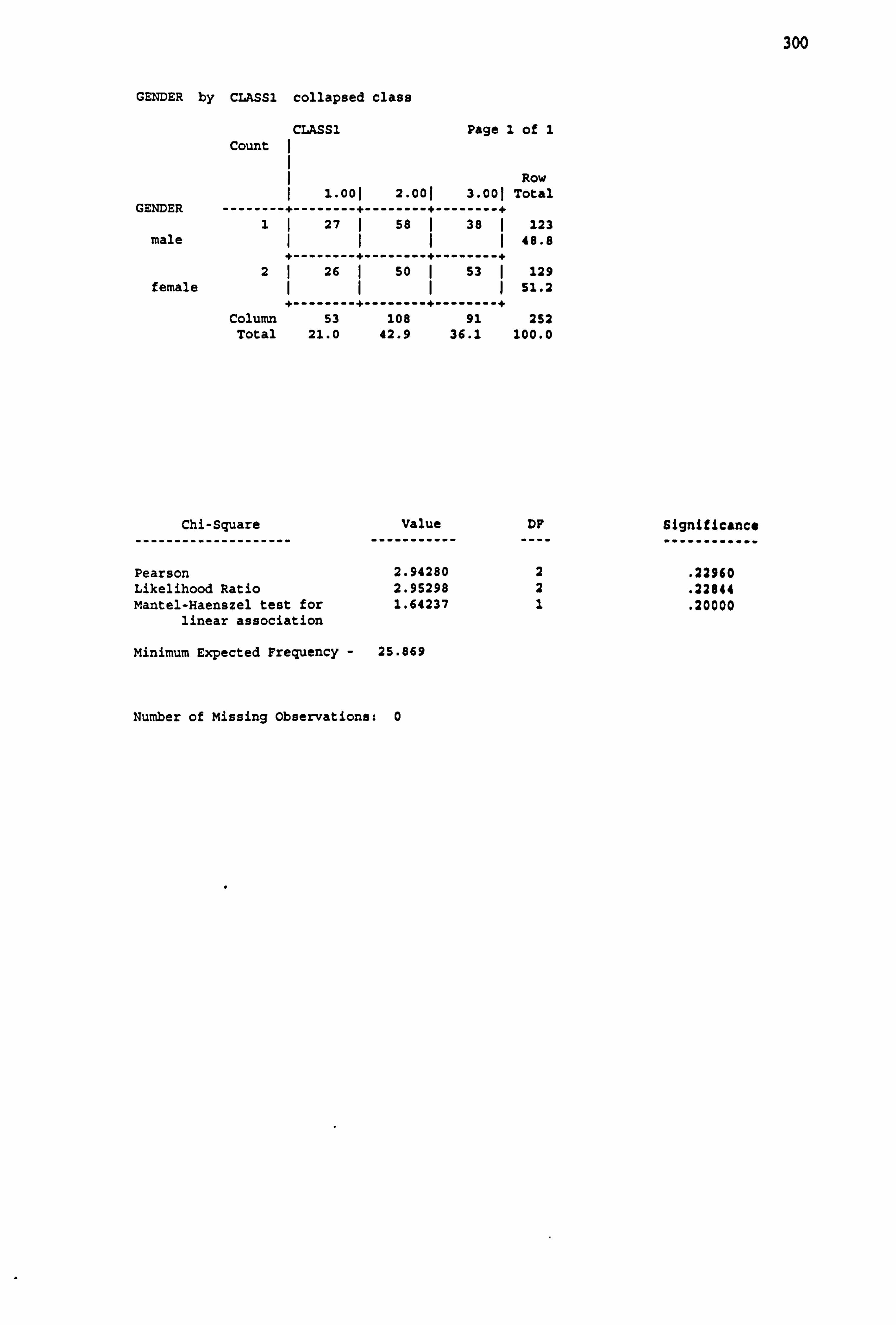
300
GENDER by CLASSI collapsed class
CLASSI Page 1 of 1 Count
Row 1.001 2.001 3.001 Total
GENDER ------------------------------------ 11 27 1 58 38 1 123
male I1 48.8 ----------------------------
2 26 50 I 53 ý 129 female 51.2
---------------------------- Column 53 108 91 252
Total 21.0 42.9 36.1 100.0
Chi-Square --------------------
Value -----------
DF ----
Significance ------------
Pearson 2.94280 2 . 22960 Likelihood Ratio 2.95298 2 . 22844 Mantel-Haenszel test for 1.64237 1 . 20000
linear association
Minimum Expected Frequency - 25.869
Number of Missing Observations: 0
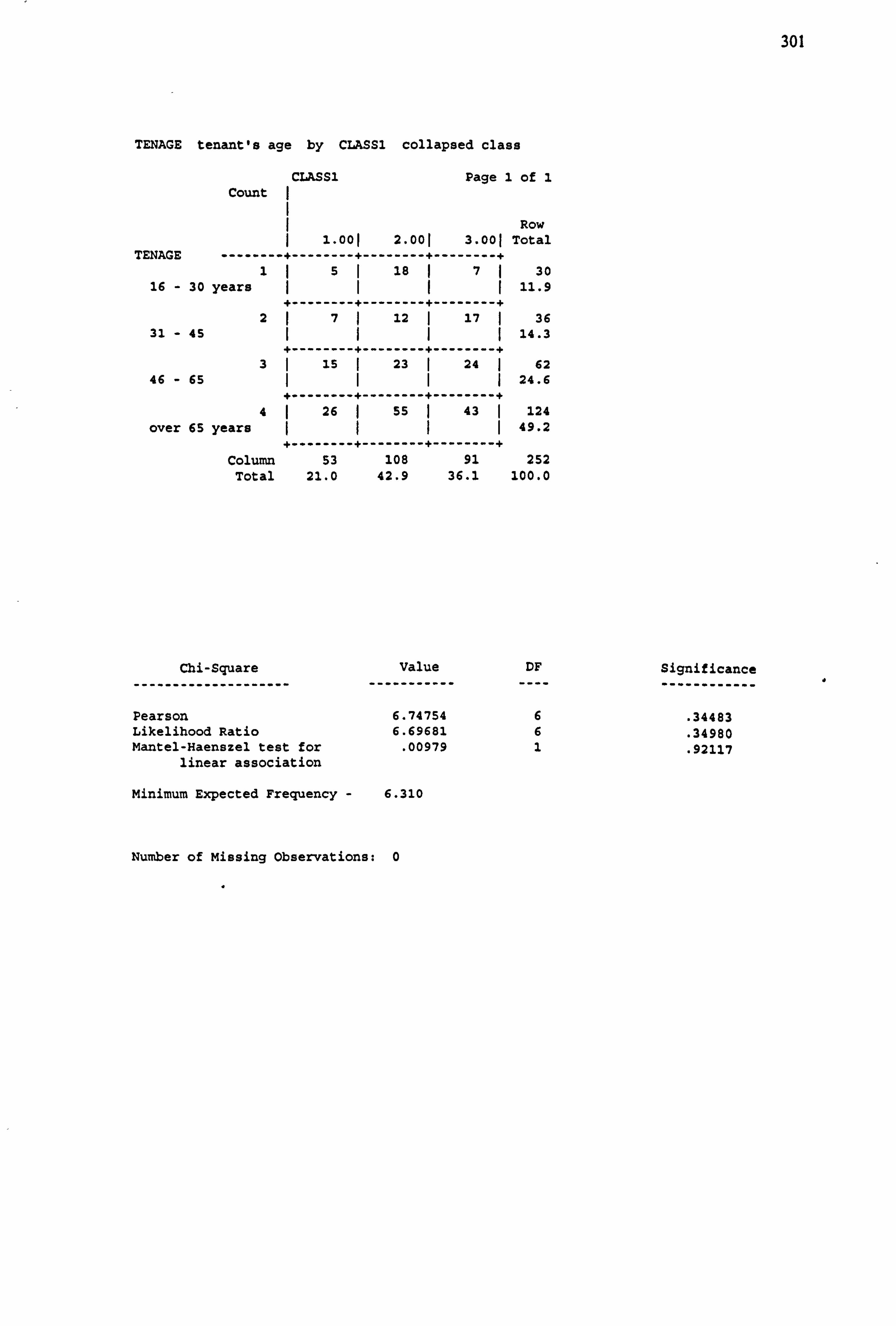
301
TENAGE tenant's age by CLASS1 collapsed class
CLASSI Page 1 of 1 Count
Row 1.001 2.001 3.001 Total
TENAGE ------------------------------------ 15I 18 171 30
16 - 30 years ýI 11.9 ----------------------------
27 12 ý 17 ý 36 31 - 45 14.3
---------------------------- 3I 15 ý 23 ý 24 62
46 - 65 ýIII 24.6 ----------------------------
4 26 55 ý 43 ý 124
over 65 years 49.2
---------------------------- Column 53 108 91 252
Total 21.0 42.9 36.1 100.0
Chi-Square Value DF Significance -------------------- ----------- ---- ------------
Pearson 6.74754 6 . 34483
Likelihood Ratio 6.69681 6 . 34980
Mantel-Haenszel test for . 00979 1 . 92117
linear association
Minimum Expected Frequency - 6.310
Number of Missing observations: 0
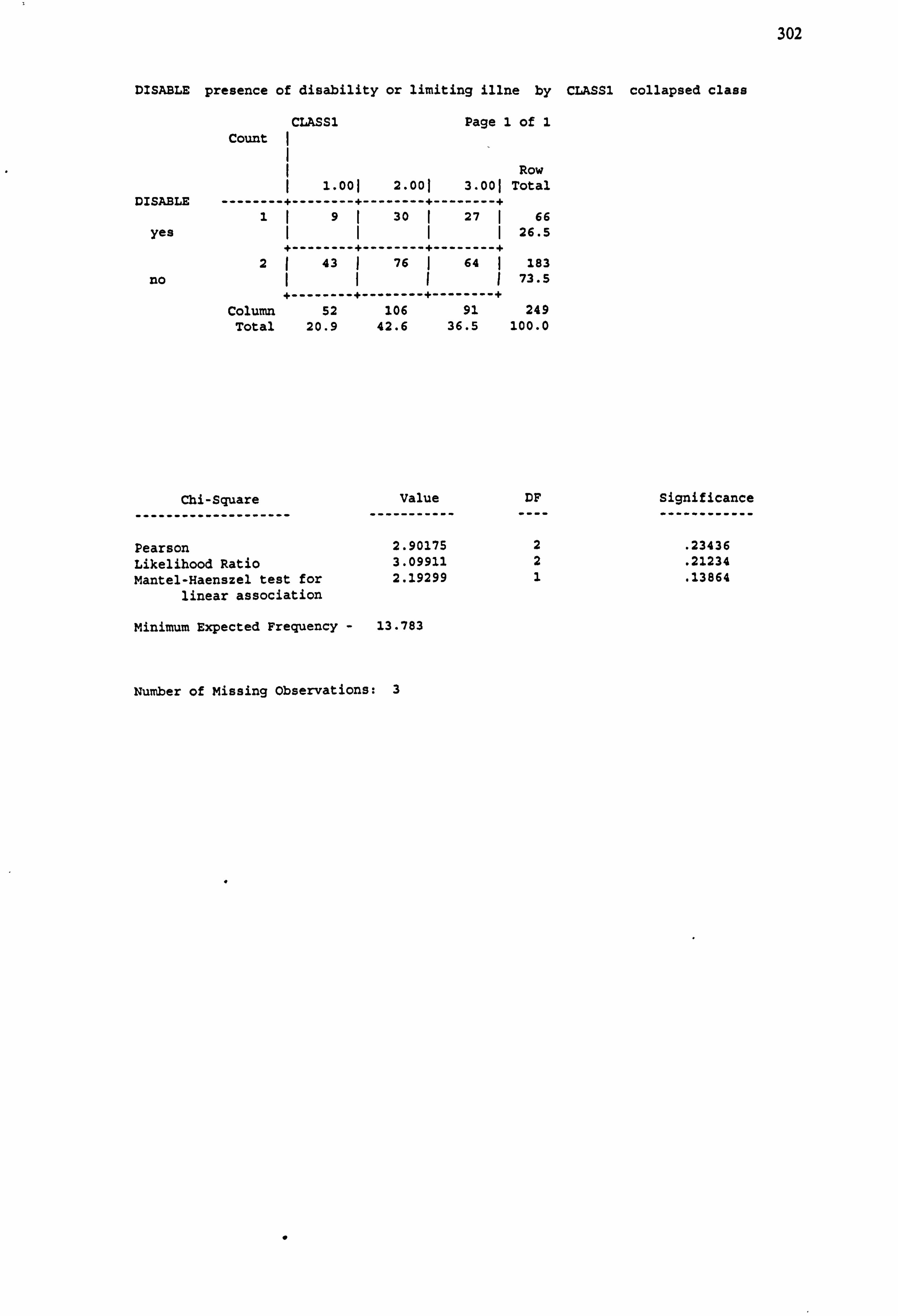
302
DISABLE presence of disability or limiting illne by CLASSI collapsed class
CLASS1 Page 1 of 1
Count
Row 1.001 2.001 3.001 Total
DISABLE ------------------------------------ 191 30 1 27 1 66
yes II11 26.5 ----------------------------
2 43 ý 76 1 64 1 183
no I11 73.5 ----------------------------
Column 52 106 91 249 Total 20.9 42.6 36.5 100.0
Chi-Square
--------------------
Value
-----------
DF
----
Significance
------------
Pearson 2.90175 2 . 23436 Likelihood Ratio 3.09911 2 . 21234
Mantel-Haenszel test for 2.19299 1 . 13864 linear association
Minimum Expected Frequency - 13.783
Number of Missing Observations: 3
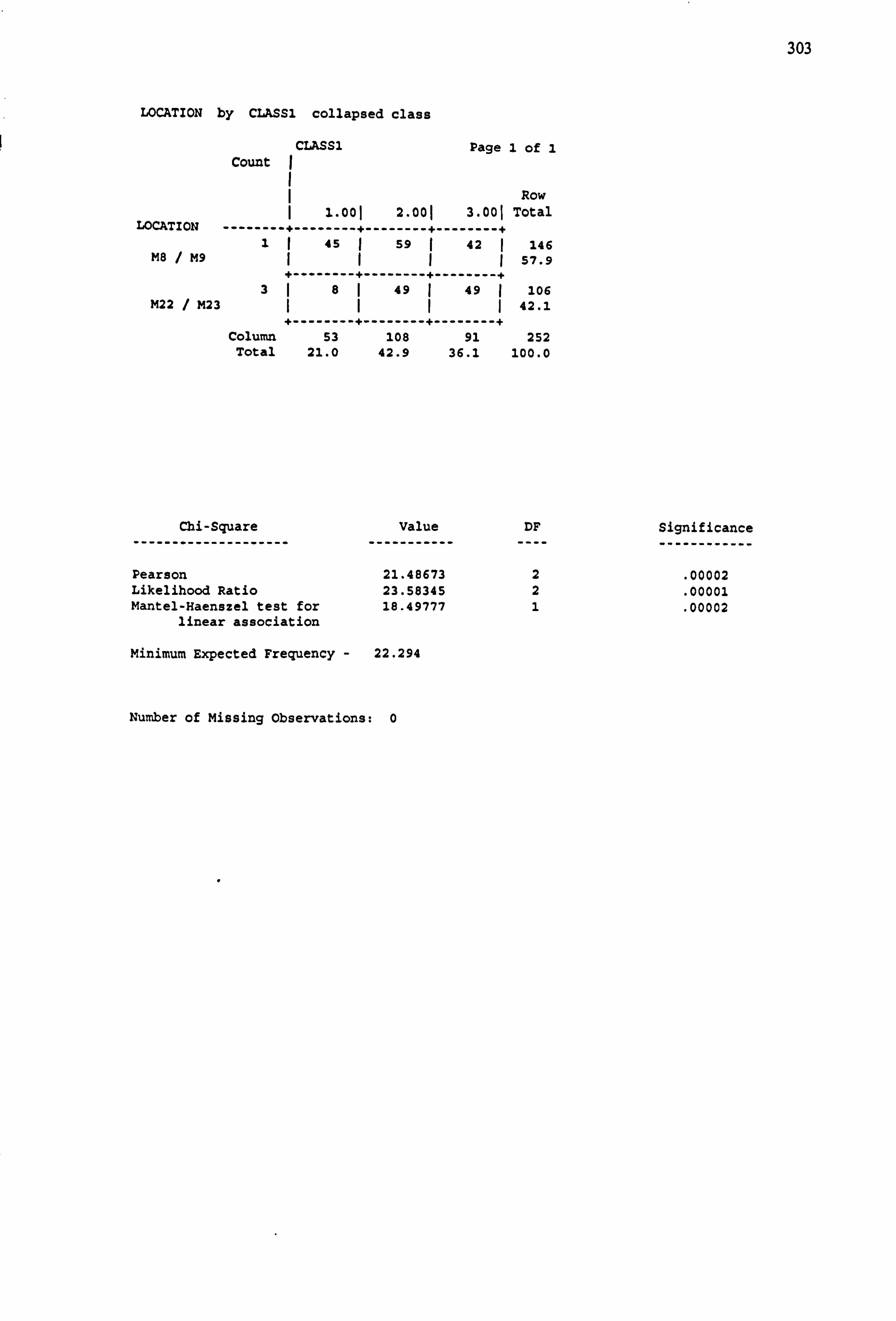
303
LOCATION by CLASS1 collapsed class
CLASS1 Page 1 of 1 Count
Row 1.001 2.001 3.00 Total
LOCATION ------------------------------------ 11 45 1 59 ( 42 146
M8 / M9 57.9 ----------------------------
3 49 ý 49 106 M22 / M23 42.1
---------------------------- Column 53 108 91 252
Total 21.0 42.9 36.1 100.0
Chi-Square --------------------
Value -----------
DF ----
Significance ------------
Pearson 21.48673 2 . 00002 Likelihood Ratio 23.58345 2 . 00001 Mantel-Haenszel test for 18.49777 1 . 00002
linear association
Minimum Expected Frequency - 22.294
Number of Missing observations: 0
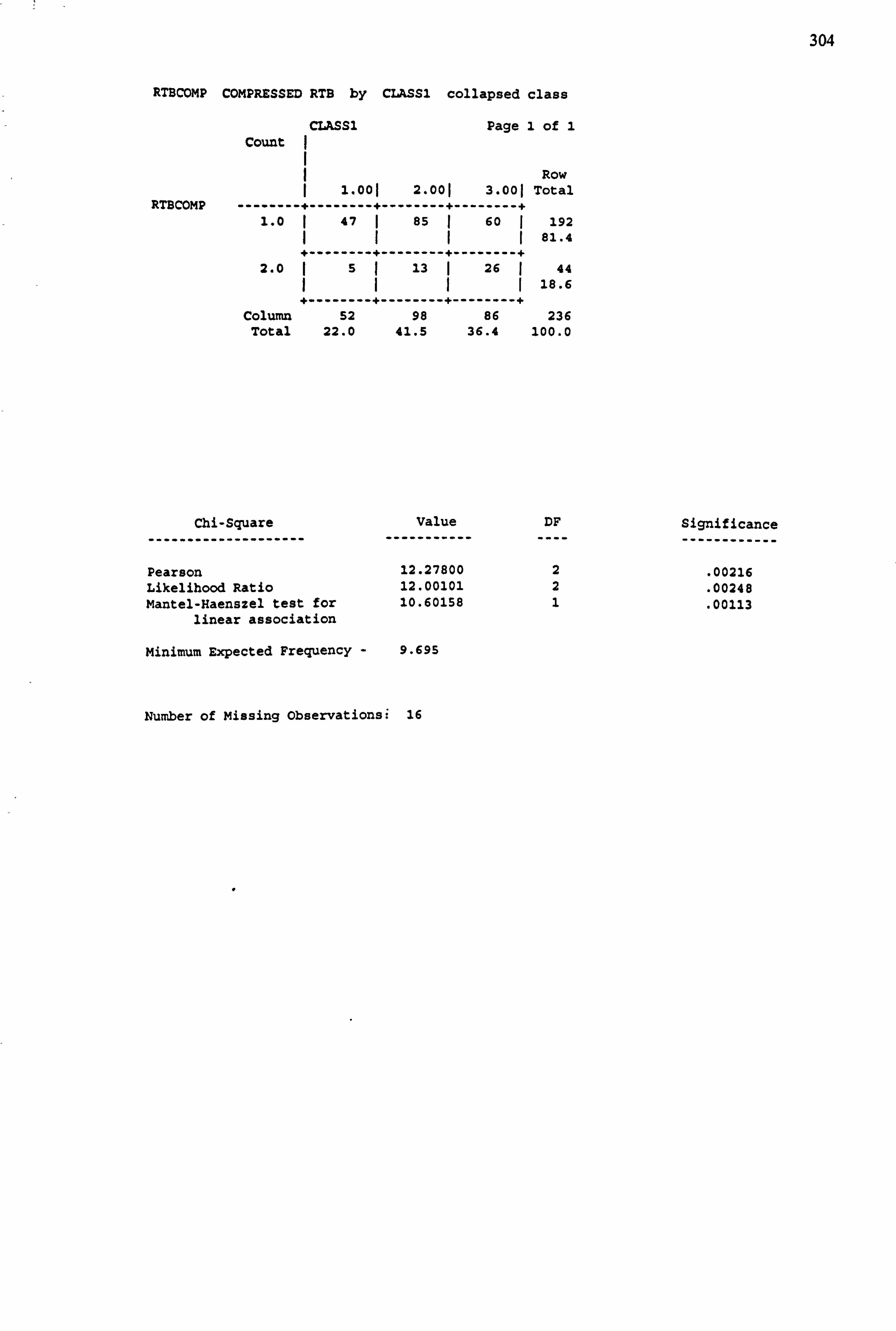
304
RTBCOMP COMPRESSED RTB by CLASSI collapsed class
CLASS1 Page 1 of 1 Count
Row 1.001 2.001 3.001 Total
RTBCOMP ------------------------------------ 1.0 1 47 85 60 1 192
111 81.4 ----------------------------
2.0 ý5 13 26 ý 44 18.6
---------------------------- Column 52 98 86 236
Total 22.0 41.5 36.4 100.0
Chi-Square --------------------
Value -----------
DF ----
Significance ------------
Pearson 12.27800 2 . 00216 Likelihood Ratio 12.00101 2 . 00248 Mantel-Haenszel test for 10.60158 1 . 00113
linear association
Minimum Expected Frequency - 9.695
Number of Missing Observations: 16
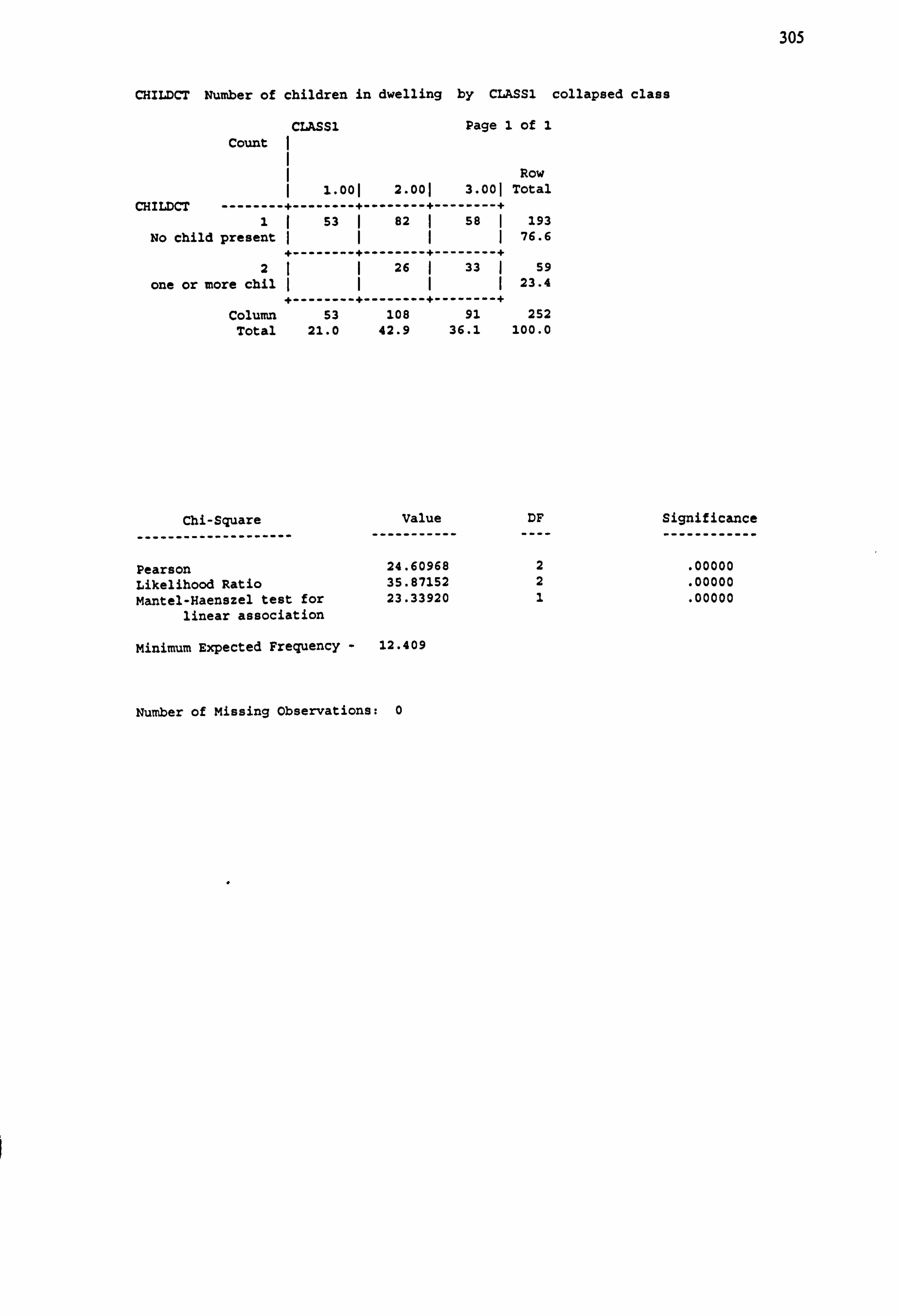
305
CHILDCT Number of children in dwelling by CLASS1 collapsed class
Count CLASSI Page 1 of 1
I Row 1 1.001 2.001 3.001 Total
CHILDCT ------------------------------------ 1 53 1 82 1 58 1 193
No child present II11 76.6
---------------------------- 2ýI 26 33 I 59
one or more chil ýIII 23.4 ----------------------------
column 53 108 91 252 Total 21.0 42.9 36.1 100.0
Chi-Square --------------------
Value -----------
DF ----
significance ------------
Pearson 24.60968 2 . 00000
Likelihood Ratio 35.87152 2 . 00000 Mantel-Haenszel test for 23.33920 1 . 00000
linear association
Minimum Expected Frequency - 12.409
Number of Missing Observations: 0
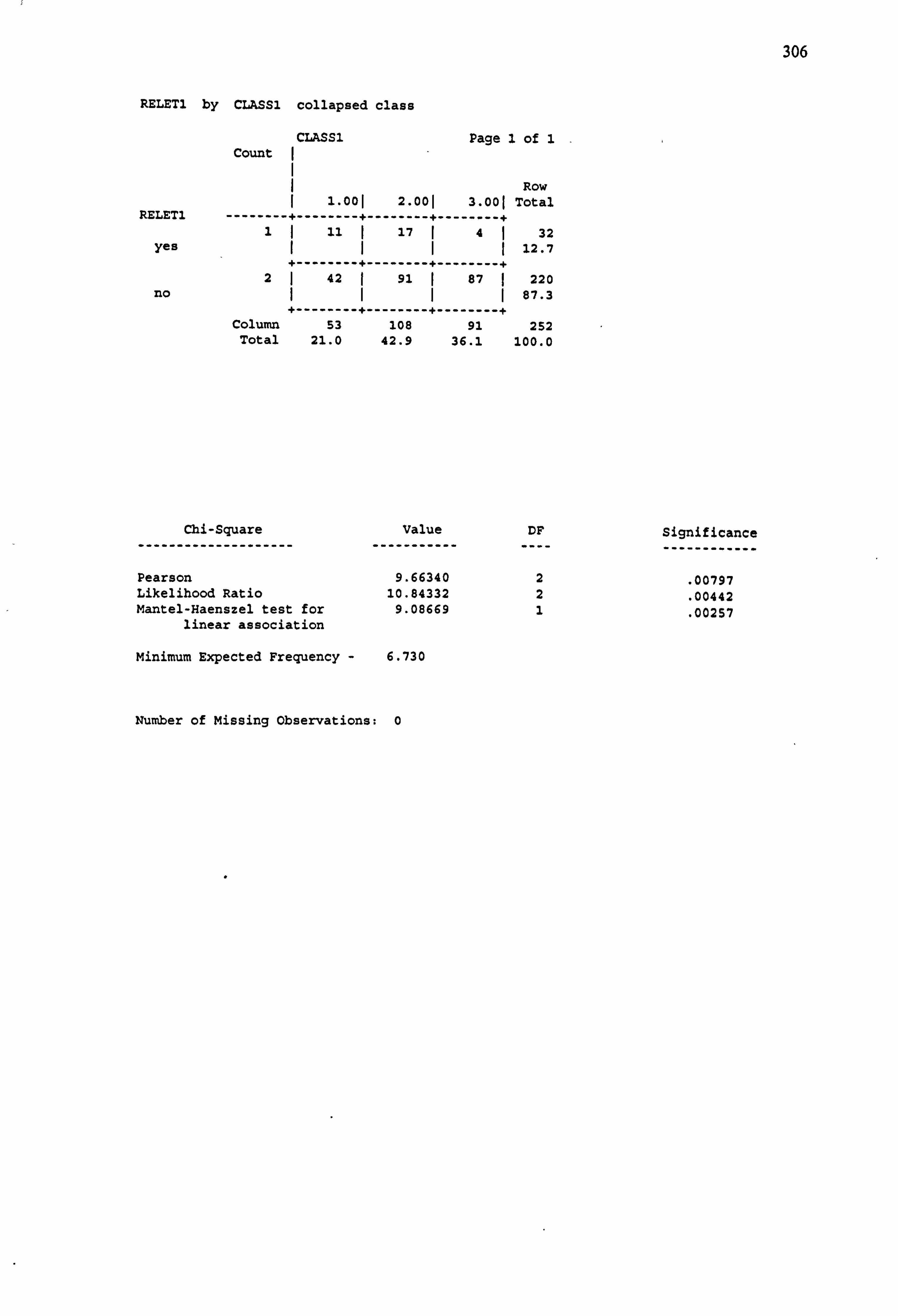
306
RELETI by CLASS1 collapsed class
CLASSI Page 1 of 1 Count
Row 1.001 2.001 3.001 Total
RELET1 ------------------------------------ 1ý 11 17 ý4ý 32
Yes IIII 12.7 ----------------------------
2 42 ( 91 ý 87 ý 220
no ýIII 87.3 ----------------------------
Column 53 108 91 252 Total 21.0 42.9 36.1 100.0
Chi-Square
--------------------
Value
-----------
DF
---- Significance ------------
Pearson 9.66340 2 . 00797
Likelihood Ratio 10.84332 2 . 00442
Mantel-Haenszel test for 9.08669 1 . 00257
linear association
Minimum Expected Frequency - 6.730
Number of Missing Observations: 0
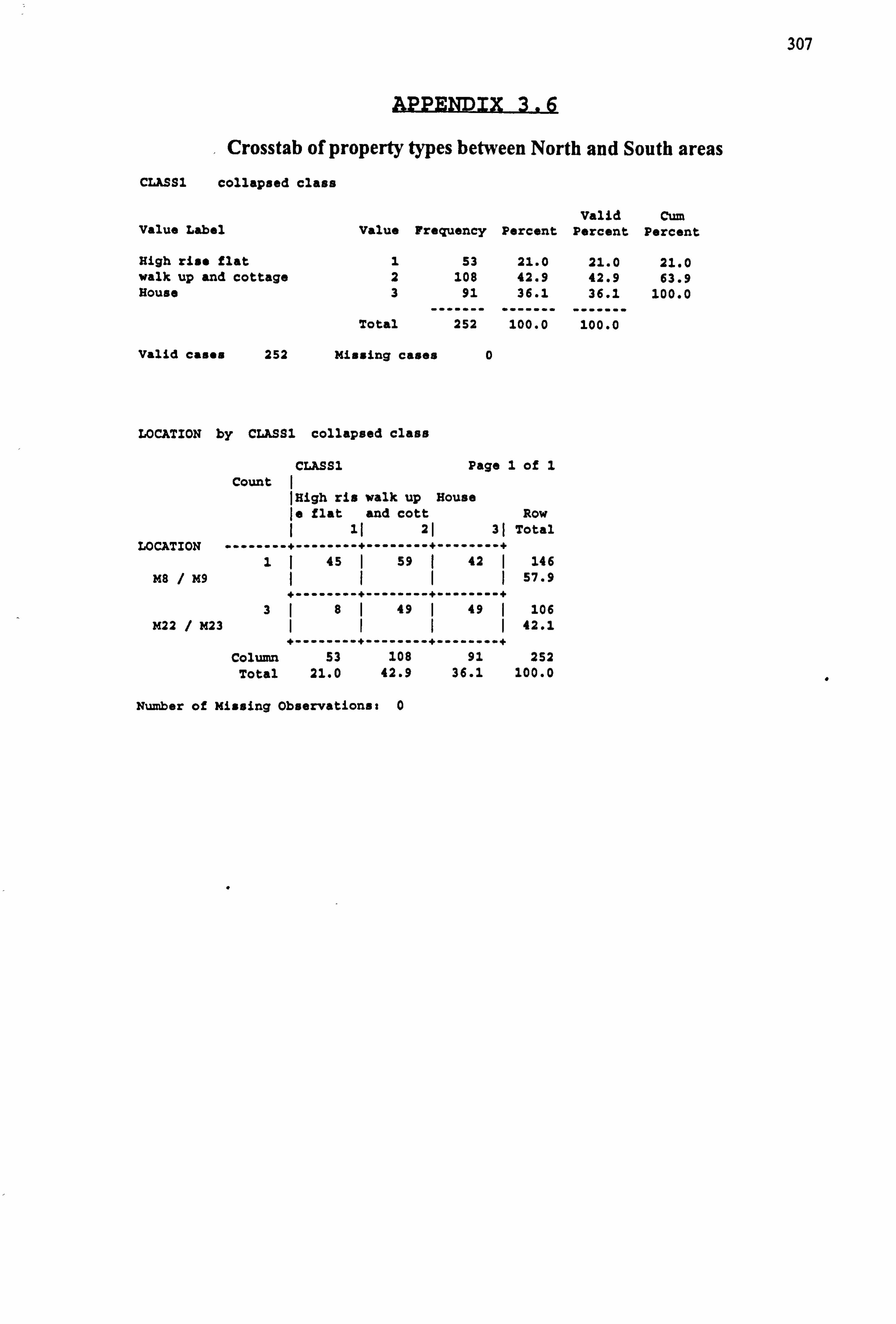
307
Crosstab of property types between North and South areas CLASSl collapsed class
Valid Cum Value Label Value Frequency Percent Percent Percent
High rise flat 1 53 21.0 21.0 21.0 walk up and cottage 2 108 42.9 42.9 63.9 House 3 91
-- - 36.1 36.1 100.0
Total 252 -
;2 -----
100.0 -------
100.0
Valid cases 252 Missing cases 0
LOCATION by CLASSI collapsed class
CLASS1 Page 1 of 1 Count I
High ris walk up House Is flat and cott Row
11 21 31 Total LOCATION ------------------------------------
1 45 1 59 ( 42 1 146 M8 / M9 (1 57.9
---------------------------- 3ý8I 49 ý 49 ý 106
M22 / M23 IIýý 42.1
---------------------------- Column 53 108 91 252
Total 21.0 42.9 36.1 100.0
Number of Missing Observations: 0
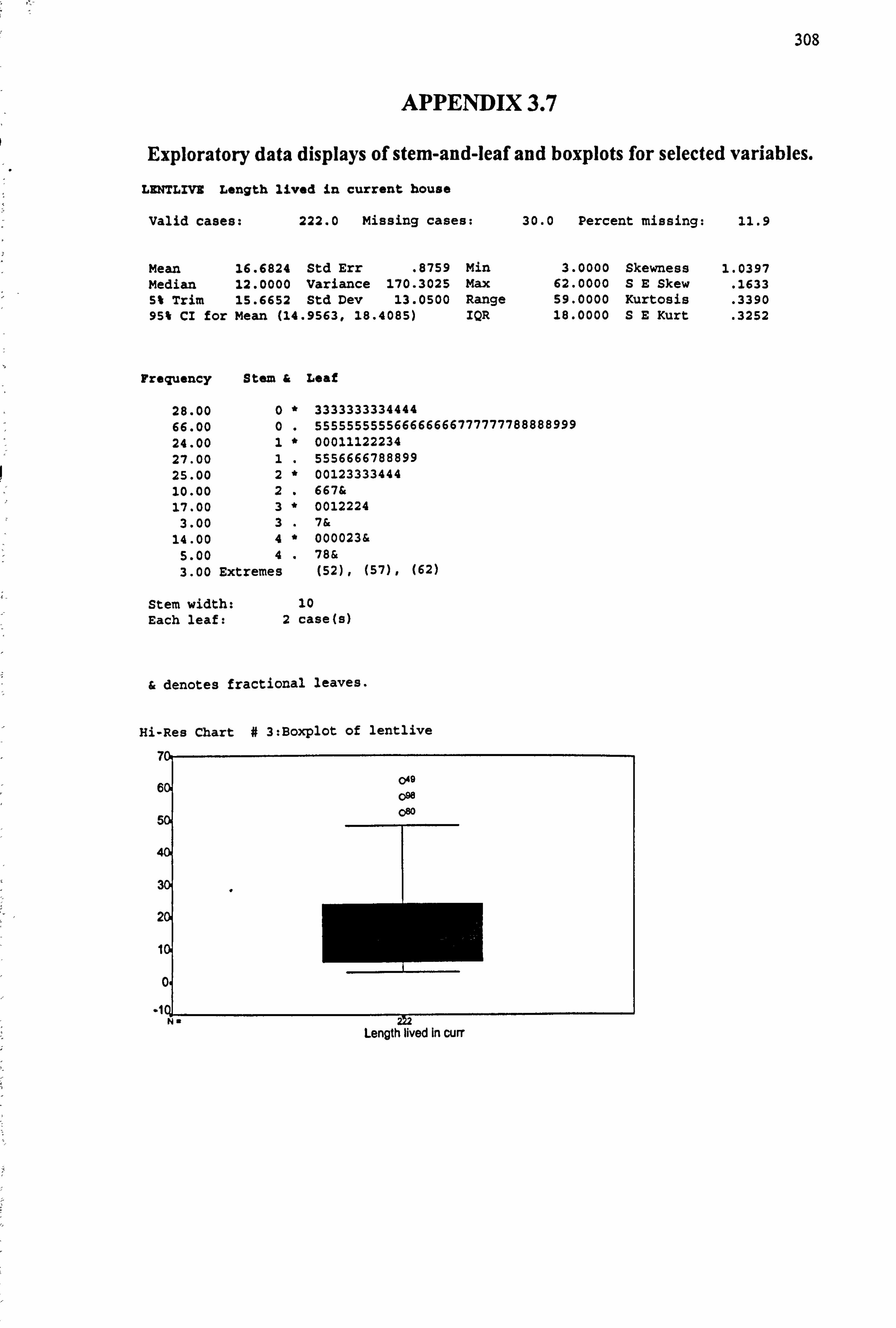
308
APPENDIX 3.7
Exploratory data displays of stem-and-leaf and boxplots for selected variables. LENTLIVB Length lived in current house
Valid cases: 222.0 Missing cases: 30.0 Percent missing: 11.9
Mean 16.6824 Std Err . 8759 Min 3.0000 Skewness Median 12.0000 Variance 170.3025 Max 62.0000 SE Skew 5% Trim 15.6652 Std Dev 13.0500 Range 59.0000 Kurtosis 95% CI for Mean (14.9563,18.4085) IQR 18.0000 SE Kurt
Frequency Stem & Leaf
28.00 0* 3333333334444 66.00 0. 555555555566666666777777788888999 24.00 1+ 00011122234 27.00 1. 5556666788899 25.00 2+ 00123333444 10.00 2. 667& 17.00 3+ 0012224
3.00 3. 7& 14.00 4" 000023&
5.00 4. 78& 3.00 Extremes (52), (57), (62)
Stem width: 10 Each leaf: 2 case(s)
& denotes fractional leaves.
Hi-Rea Chart # 3: BoxplOt of lentlive
7
049 6 o9e
080 50
40
3
2
1
0
1 N .
1.0397
. 1633
. 3390
. 3252
Length lived In curt
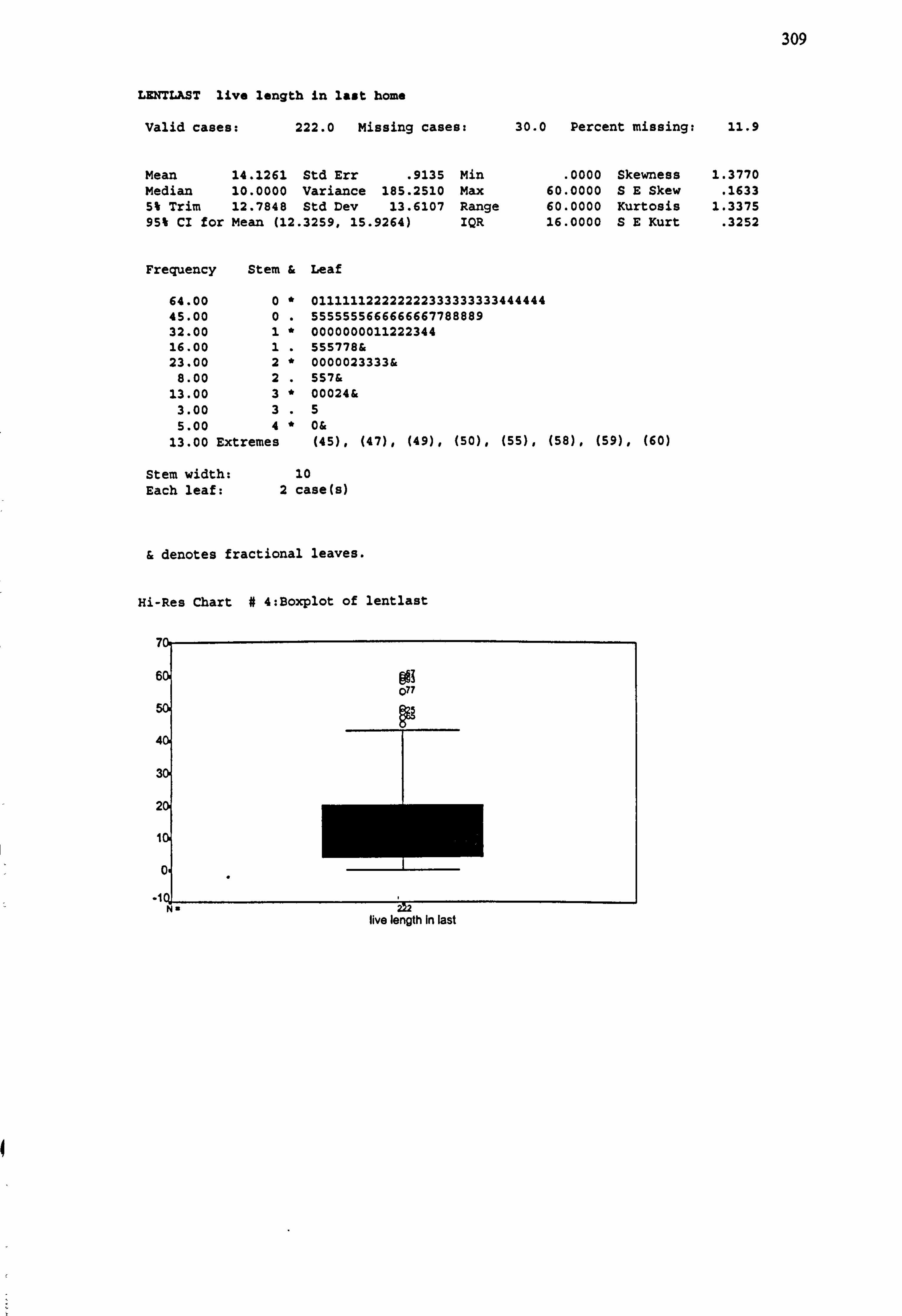
309
LENTLAST live length in last home
Valid cases: 222.0 Missing case s: 30.0 Percent missing: 11.9
Mean 14.1261 Std Err . 9135 Min . 0000 Skewness 1.3770 Median 10.0000 Variance 185.2510 Max 60.0000 SE Skew . 1633 5% Trim 12.7848 Std Dev 13.6107 Range 60.0000 Kurtosis 1.3375 95% CI for Mean (12.3259,15.9264) IQR 16.0000 SE Kurt . 3252
Frequency Stem & Leaf
64.00 0 " 011111122222222333333333444444 45.00 0 . 5555555666666667788889 32.00 1 " 0000000011222344 16.00 1 . 555778& 23.00 2 + 0000023333&
8.00 2 . 557& 13.00 3 " 00024&
3.00 3 .5 5.00 4 * 0&
13.00 Extremes (45), (47), (49), (50), (55), (58), (59), (60)
Stem width: 10 Each leaf: 2 case(s)
& denotes fractional leaves.
Hi-Res Chart # 4: Boxplot of lentlast
@13 o»
I 0J. - N- live length In last
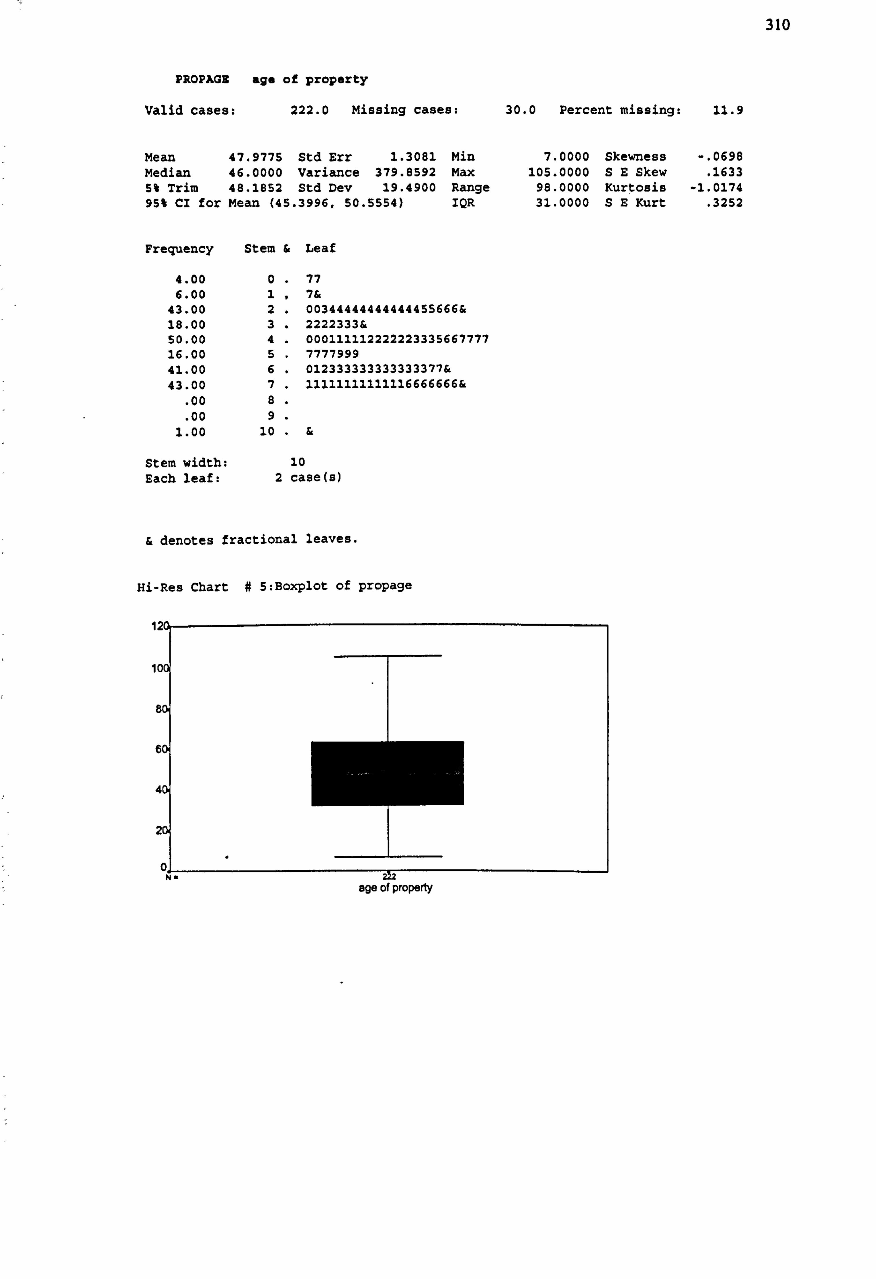
310
PROPkGE age of property
Valid cases: 222.0 Missing cases:
Mean 47.9775 Std Err 1.3081 Min Median 46.0000 Variance 379.8592 Max 5% Trim 48.1852 Std Dev 19.4900 Range 95% CI for Mean (45.3996,50.5554) IQR
Frequency Stem & Leaf
4.00 0. 77 6.00 1. 7&
43.00 2. 00344444444444455666& 18.00 3. 2222333& 50.00 4. 000111112222223335667777 16.00 5. 7777999 41.00 6. 012333333333333377& 43.00 7. 11111111111116666666&
. 00 8
. 00 9 1.00 10 . &
Stem width: 10
Each leaf: 2 case(s)
& denotes fractional leaves.
Hi-Res Chart # S: Boxplot of propage
30.0 Percent missing: 11.9
7.0000 Skewness -. 0698 105.0000 SE Skew . 1633
98.0000 Kurtosis -1.0174 31.0000 SE Kurt . 3252
I 2
0
8
6
4
2
N.
I
age of property
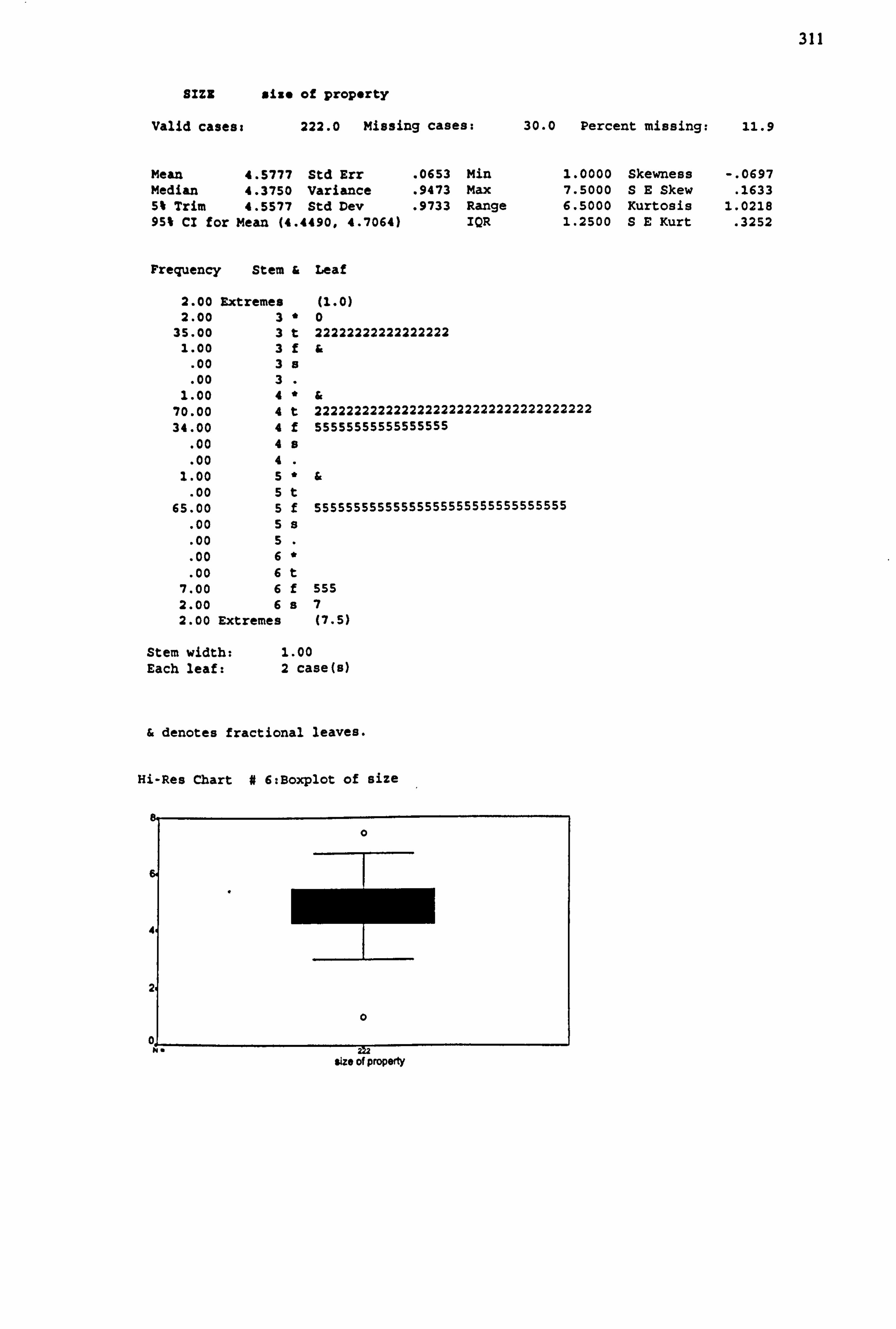
311
SIZE size of property
Valid cases: 222.0 Missing cases: 30.0 Percent missing: 11.9
Mean 4.5777 Std Err . 0653 Min 1.0000 Skewness -. 0697 Median 4.3750 Variance . 9473 Max 7.5000 SE Skew . 1633 5t Trim 4.5577 Std Dev . 9733 Range 6.5000 Kurtosis 1.0218 95% CI for Mean (4.4490,4.7064) IQR 1.2500 SE Kurt . 3252
Frequency Stem & Leaf
2.00 Extremes (1.0) 2.00 3"0
35.00 3t 22222222222222222 1.00 3f&
. 00 3s
. 00 3 1.00 4"&
70.00 4t 22222222222222222222222222222222222 34.00 4f 55555555555555555
. 00 4s
. 00 4 1.00 5"&
. 00 5t 65.00 5f 55555555555555555555555555555555
. 00 5s
. 00 5
. 00 6"
. 00 6t 7.00 6f 555 2.00 6s7 2.00 Extremes (7.5)
Stem width: 1.00 Each leaf: 2 case(s)
& denotes fractional leaves.
Hi-Res Chart # 6: Boxplot of size
T 0
ýý. N"
size of property
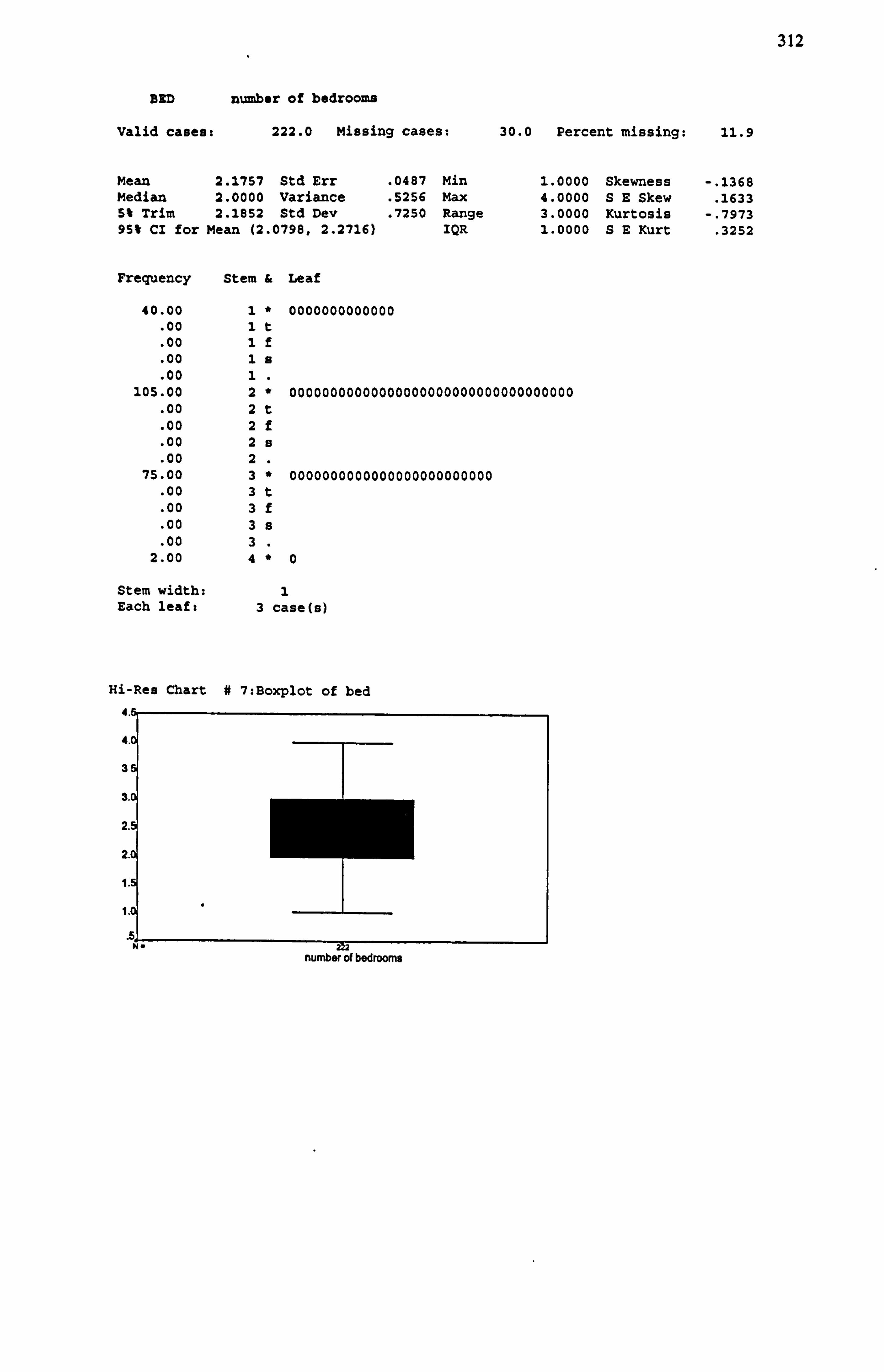
312
BED number of bedrooms
Valid cases: 222.0 Missing cases:
Mean 2.1757 Std Err . 0487 Min Median 2.0000 Variance . 5256 Max 5f Trim 2.1852 Std Dev . 7250 Range 95% Cl for Mean (2.0798,2.2716) IQR
Frequency Stem & Leaf
30.0 Percent missing: 11.9
1.0000 Skewness -. 1368 4.0000 SE Skew . 1633 3.0000 Kurtosis -. 7973 1.0000 SE Kurt . 3252
40.00 1 * 0000000000000
. 00 1 t
. 00 1 f
. 00 1 s
. 00 1 105.00 2 + 00000000000000000000000000000000000
. 00 2 t
. 00 2 f
. 00 2 s
. 00 2 75.00 3 " 0000000000000000000000000
. 00 3 t
. 00 3 f
. 00 3 s
. 00 3 . 2.00 4 " 0
Stem width: 1 Each leafs 3 case(s)
Hi-Rea Chart # 7: Boxplot of bed 4.
4.
3
S.
2.
2.
1.
1.
.5 N212 number of bedrooms
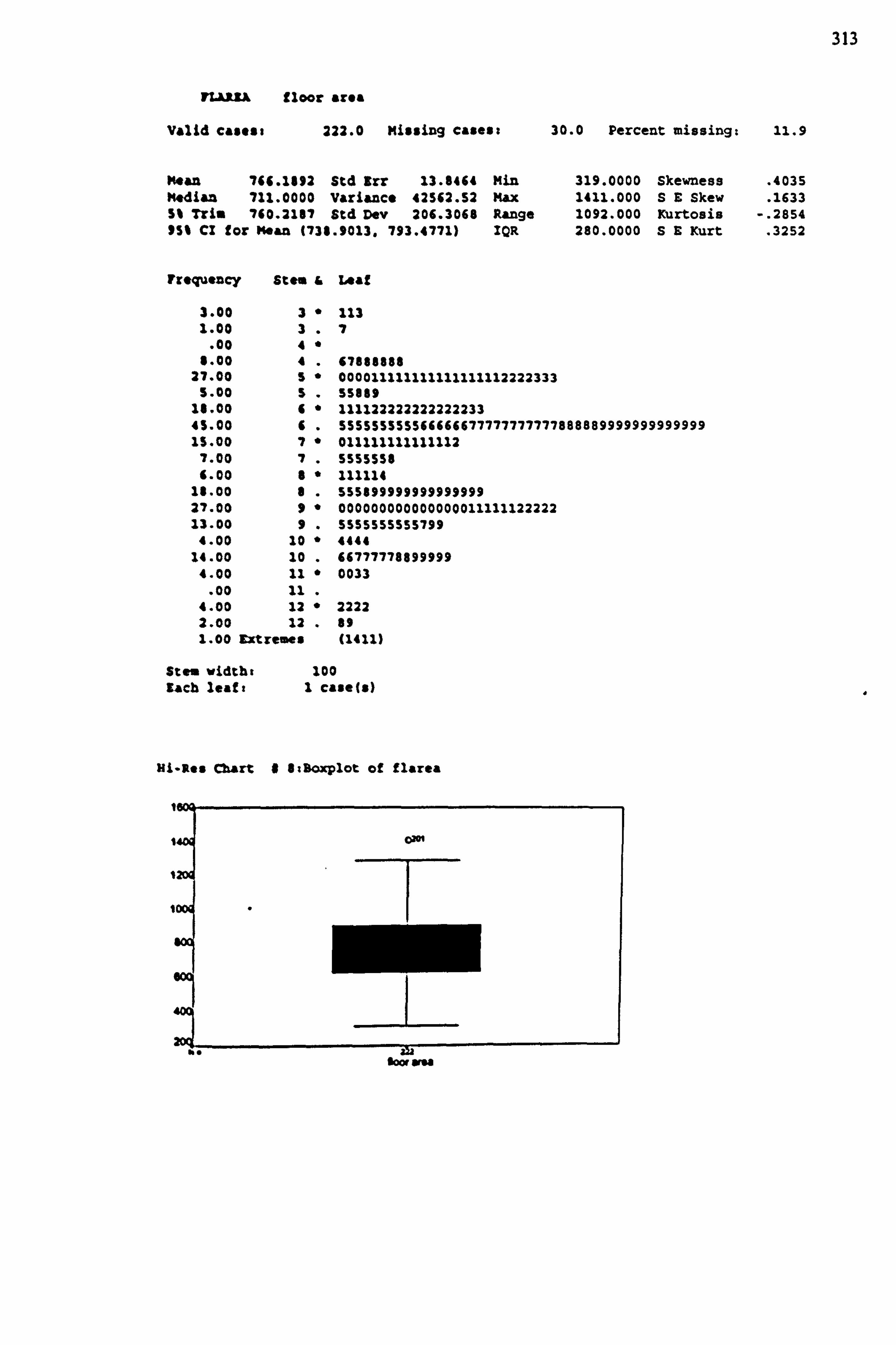
313
n&s. Jº floor area
Valid eases, 222.0 Missing eases: 30.0 Percent missing: 11.9
Mean 766.1892 Std Err 13.8464 Min 319.0000 Skewness K. dian 711.0000 Variance 42562.52 Max 1411.000 SE Skew St Tri 760.2187 Std Dev 206.3068 Range 1092.000 Kurtosis 9S% Cl for Mean (738.9013.793.4771) IQR 280.0000 SE Kurt
fr. qusacy Stcs & Leaf
3.00 3" 113 1.00 3. 7
. 00 4" 8.00 4. 67888888
27.00 S" 000011111111111111112222333 5.00 5. 55889
16.00 6" 112122222222222233 15.00 6. 555555S55566666677777777777888889999999999999 15.00 7" 011111111111112
7.00 7. 5555558 6.00 8* 111114
18.00 8. 555899999999999999 27.00 9" 000000000000000011111122222 13.00 9. 5555555555799
4.00 30 " 4444 14.00 30 . 66777778899999
4.00 11 " 0033
. 00 11 . 4.00 12 " 2222 2.00 12 . 89 1.00 Extr emes (1411)
Stem widths 100 Bach leaf: 1 case(s)
Hi-Res chart t 8: Boxplot of flarea
CM
. 4035
. 1633
-. 2854
. 3252
fooº vs.
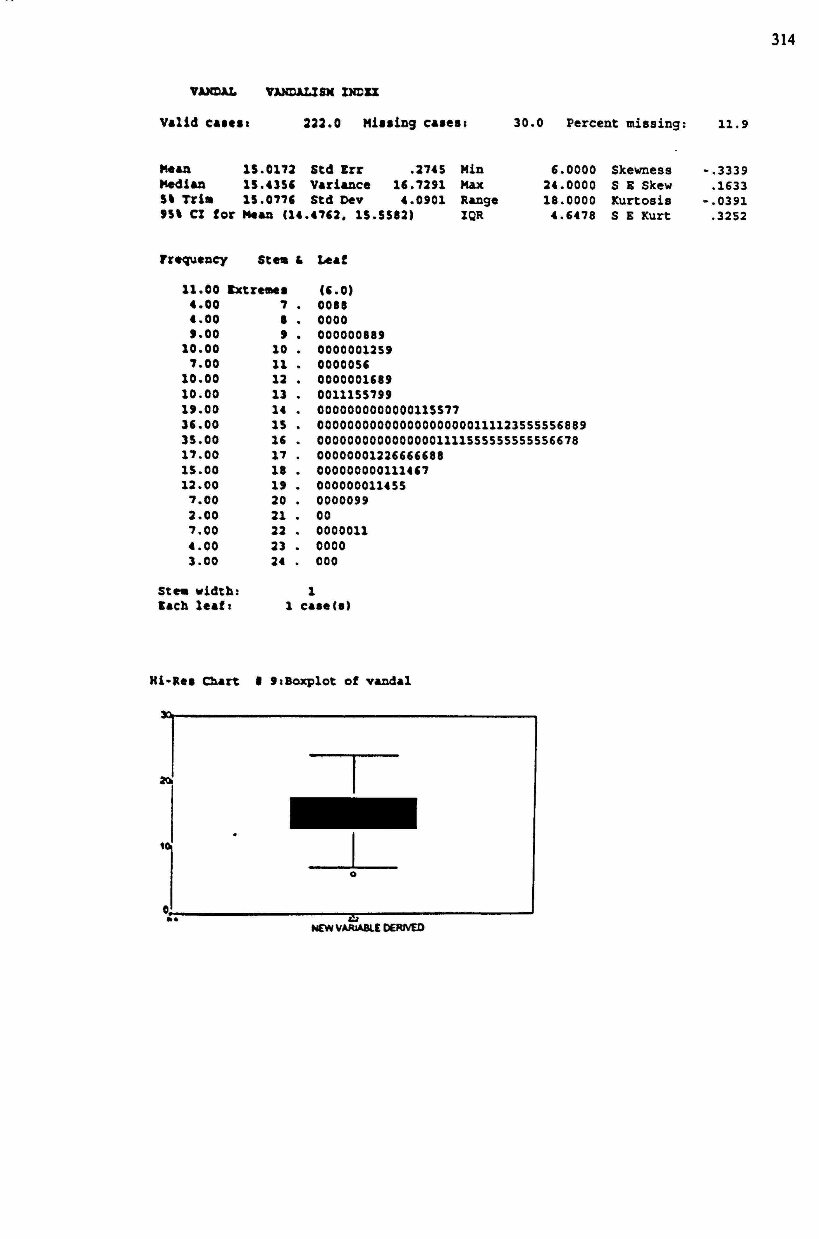
314
VANDAL VANDALZSX X MIX
valid cases: 222.0 Missing cases: 30.0 Percent missing: 11.9
Mean IS. 0172 Std Err . 2745 Min 6.0000 Skewness -. 3339 Median 15.4356 Variance 16.7291 Max 24.0000 SE Skew . 1633 St Trim 15.0776 Std Dev 4.0901 Range 18.0000 Kurtosis -. 0391 9S% Cl for Mean (14.4762.15.5582) IQR 4.6478 SE Kurt . 3252
frequency Stem L Leaf
11.00 Extremes (6.0) 4.00 7 . Cosa 4.00 s . 0000 9.00 9 . 000000889
10.00 10 . 0000001259 7.00 11 . 0000056
10.00 12 . 0000001689 10.00 13 . 0011155799 19.00 14 . 0000000000000115577 36.00 15 . 000000000000000000000111123555556889 35.00 16 . 00000000000000001111555555555556678 17.00 17 . 00000001226666688 15.00 18 . 000000000111467 12.00 19 . 000000011455
7.00 20 . 0000099 2.00 21 . 00 7.00 22 . 0000011 4.00 23 . 0000 3.00 24 . 000
Stem width: 1 Each leaf: 1 case(s)
Hi-Res Chart 19: Boxplot of vandal
C
w" to NEW VARL4K9 DERIVED
Top Related
Copyright © 2022 FDOKUMEN

