Download - An automated approach for reconstructing recent forest disturbance history using dense Landsat time series stacks

Remote Sensing of Environment 114 (2010) 183–198

Contents lists available at ScienceDirect

Remote Sensing of Environment

j ourna l homepage: www.e lsev ie r.com/ locate / rse

An automated approach for reconstructing recent forest disturbance history usingdense Landsat time series stacks

Chengquan Huang a,⁎, Samuel N. Goward a, Jeffrey G. Masek b, Nancy Thomas a,Zhiliang Zhu c, James E. Vogelmann d

a Department of Geography, University of Maryland, College Park, MD 20742, USAb Biospheric Sciences Branch, NASA Goddard Space Flight Center, Greenbelt, MD 20771, USAc U.S. Geological Survey, 12201 Sunrise Valley Drive, Reston, VA 20771, USAd USGS Earth Resources Observation and Science (EROS) Center, Sioux Falls, SD 57198, USA

⁎ Corresponding author.E-mail address: [email protected] (C. Huang).

0034-4257/$ – see front matter © 2009 Elsevier Inc. Aldoi:10.1016/j.rse.2009.08.017

a b s t r a c t
a r t i c l e i n f o
Article history:Received 17 April 2009Received in revised form 22 August 2009Accepted 29 August 2009

Keywords:Landsat time series stacks (LTSS)Vegetation change tracker (VCT)Forest z-score (FZ)Integrated forest z-score (IFZ)

A highly automated algorithm called vegetation change tracker (VCT) has been developed for reconstructingrecent forest disturbance history using Landsat time series stacks (LTSS). This algorithm is based on thespectral–temporal properties of land cover and forest change processes, and requires little or no fine tuningfor most forests with closed or near close canopy cover. It was found very efficient, taking 2–3 h on averageto analyze an LTSS consisting of 12 or more Landsat images using an average desktop PC. This LTSS-VCTapproach has been used to examine disturbance patterns with a biennial temporal interval from 1984 to2006 for many locations across the conterminous U.S. Accuracy assessment over 6 validation sites revealedthat overall accuracies of around 80% were achieved for disturbances mapped at individual year level.Average user's and producer's accuracies of the disturbance classes were around 70% and 60% in 5 of the 6sites, respectively, suggesting that although forest disturbances were typically rare as compared with no-change classes, on average the VCT detected more than half of those disturbances with relatively low levelsof false alarms. Field assessment revealed that VCT was able to detect most stand clearing disturbance events,including harvest, fire, and urban development, while some non-stand clearing events such as thinning andselective logging were also mapped in western U.S. The applicability of the LTSS-VCT approach depends onthe availability of a temporally adequate supply of Landsat imagery. To ensure that forest disturbance recordscan be developed continuously in the future, it is necessary to plan and develop observational capabilitiestoday that will allow continuous acquisition of frequent Landsat or Landsat-like observations.

l rights reserved.

© 2009 Elsevier Inc. All rights reserved.

1. Introduction

Forest disturbance and post-disturbance recovery are key processesin the developmentof forest ecosystems. The landscape pattern of forestage and structure, for example, is shaped in part by the history ofdisturbance and recovery processes (Peterken, 2001). Understandingthese processes over space and time is also crucial to studies of terres-trial and atmospheric carbon, as they are major processes modulatingcarbon flux between the biosphere and the atmosphere (Hirsch et al.,2004; Law et al., 2004). While North American forests, especially thosein the United States, have been proposed as a net carbon sink (Pacalaet al., 2001; Liu et al., 2004), estimates of themagnitude of the sink havesubstantial uncertainties. Reducing such uncertainties requires im-proved understanding of land use history, especially forest disturbance

history (Schimel & Braswell, 1997; Thornton et al., 2002; Houghton,2003).

The collection of Landsat images acquired through current andprevious Landsat missions (Goward et al., 2006) provide a unique datasource for reconstructing forest disturbance history for many areas ofthe globe. With the earliest Landsat images acquired in 1972, this col-lectionmakes it possible to document forest changes that have occurredsince then, while the fine spatial resolutions of Landsat images providethe spatial details necessary for characterizing many of the changesarising from both natural and anthropogenic disturbances (Townshend& Justice, 1988). Over the past 30+ years, Landsat images have beenwidely used in land cover and forest change analysis (Goward &Williams, 1997). While the Landsat Record has relatively denseacquisitions in many places of the world, especially in the United States(Goward et al., 2006), largely due to practical reasons, most previousstudies characterized land cover change at relatively sparse temporalintervals (Singh, 1989; Lu et al., 2004). For many of the Earth's forests,reestablishment of a new forest stand following a previous disturbance

mailto:[email protected]

http://dx.doi.org/10.1016/j.rse.2009.08.017

http://www.sciencedirect.com/science/journal/00344257

184 C. Huang et al. / Remote Sensing of Environment 114 (2010) 183–198

can occur in just a few years (e.g. Huang et al., 2009a, Fig. 1). As a result,some of those disturbances can become spectrally undetectable usingobservations acquired many years apart (Lunetta et al., 2004; Maseket al., 2008).

Within the framework of the North American Carbon Program(NACP), the North American Forest Dynamics (NAFD) project isevaluating forest disturbance and regrowth history for the contermi-nous U.S. by combining Landsat observations and field measurements(Goward et al., 2008). To minimize potential omission errors that mayarise from using temporally sparse observations, dense Landsat timeseries stacks (LTSS) are used in the NAFD study. About 30 LTSS havebeen assembled during the first phase of NAFD for locations selectedacross the U.S. (Goward et al., 2008; Huang et al., 2009a).

Two major steps are involved in mapping forest disturbance usingLTSS: development of imagery-ready-to-use (IRU) quality LTSS images,and forest disturbance detection. IRU quality LTSS images are defined ashaving minimum cloud and shadow contaminations and minimuminstrument or processing related errors. Such images should also havebeen corrected geometrically and radiometrically such that they havethe highest level of achievable geolocation accuracy and radiometricconsistency. Streamlined procedures for producing such IRU qualityLTSS images have been developed in a previous study (Huang et al.,2009a).

Over the last few decades of remote sensing history, numerousdigital change detection techniques have been developed for use withLandsat and other satellite images (see Singh, 1989; Coppin et al.,2004; Lu et al., 2004 for comprehensive reviews). These existingtechniques, however, are mostly bi-temporal in nature, i.e., they canbe used to analyze only one collocated image pair at a time. Whileeach LTSS could be divided into a sequence of image pairs and a bi-temporal technique could be used to analyze each image pair, such anapproach would be extremely inefficient. Furthermore, bi-temporaltechniques cannot take advantage of the rich temporal informationcontained in LTSS. As will be demonstrated in this study, temporalinformation is particularly useful for characterizing land cover andchange processes. While algorithms capable of analyzing three ormore images at a time have also been developed (e.g. Coppin & Bauer,1996; Cohen et al., 2002; Lunetta et al., 2004), most of them suffershortcomings similar to those of bi-temporal techniques for analyzingdense satellite observations.

To improve the efficiency of land cover change analysis using LTSS,Kennedy et al. (2007) developed a trajectory-based change detectionalgorithm. This algorithm takes all images in an LTSS into considera-

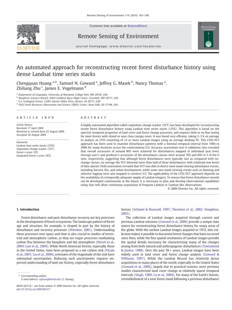
Fig. 1. Overall data flow and pro

tion, and uses idealized temporal trajectory of spectral values todetect and characterize changes. Here we develop a different changedetection algorithm called vegetation change tracker (VCT) formapping forest change using LTSS. This algorithm is similar to thetrajectory-based change detection algorithm of Kennedy et al. (2007)in that changes are detected through simultaneous analysis of allimages in an LTSS. But the mechanisms based on which changes aredetected are different. The VCT is based on the spectral–temporalcharacteristics of land cover and forest change processes. It consists oftwo major steps. In the first step, each image in an LTSS is analyzed tocreate masks and to calculate spectral indices that are measures offorest likelihood. Once this step is complete for all images in that LTSS,the derived indices and masks are analyzed in a time series analysisstep to map disturbances. A brief description of the VCT algorithm hasbeen provided before (Huang et al., 2009b). Some key components ofthe first step have also been detailed previously (Huang et al., 2008; inpress). The purpose of this paper is to provide a detailed, coherentdescription of all components of the VCT and to assess the disturbanceproducts derived using this algorithm.

The VCT has been used to produce disturbance products for the siteswhere LTSS were assembled during the first phase of the NAFD project(Goward et al., 2008;Huanget al., 2009a). Biennialdisturbanceproductshave also been produced using this approach for Mississippi (Li et al., inpress) and Alabama (Li et al., 2009) as part of an effort to update avegetation database developed through the LANDFIRE project (Rollins,2009). Those disturbance products have been evaluated using multipleapproaches, including ground-based assessment, visual assessment,designed-based accuracy assessment and assessment using field surveydata collected through the Forest Inventory and Analysis (FIA) programof the USDA Forest Service. Mainly for page limit considerations, only asummary of the results derived from field based assessment, visualevaluation, and design-based accuracy assessment is provided in thispaper. Full details on the design-based accuracy assessment andassessment using FIA field survey data will be provided in a follow-uppaper (Thomas, in preparation).

Because the VCT algorithm is designed for use with LTSS, a briefreview of the LTSS concept and the procedures for developing LTSS isdeemednecessaryhere, althoughdetails on thoseprocedureshave beenprovided previously (Huang et al., 2009a). Following this reviewSection 3 provides a detailed description of the VCT algorithm.Assessments of VCT disturbance products are provided in Section 4,followed by a summary and discussions on the properties of the VCTalgorithm and its requirement on satellite observations.

cesses of the VCT algorithm.

185C. Huang et al. / Remote Sensing of Environment 114 (2010) 183–198

2. LTSS development

A Landsat time series stack (LTSS) is defined as a temporalsequence of Landsat images acquired at a nominal temporal intervalfor an area defined by a path/row tile of the World Reference System(WRS). An annual LTSS consists of one image every year while abiennial LTSS consists of one image every 2 years. Due to limited dataavailability coupled with cloud contaminations, however, the actualtemporal intervals between consecutive acquisitions can be differentfrom the nominal interval (example acquisition dates of some LTSScan be found in Huang et al., 2009b, Table 2). Each image should haveminimal or no cloud contamination and should be acquired during thepeak growing season. Mainly due to data cost constraints,1 most LTSSused in the NAFD project were biennial stacks. Each LTSS had anominal starting year of 1984 and an ending year of 2006, consistingof Landsat Thematic Mapper (TM) and Enhanced Thematic MapperPlus (ETM+) images acquired between 1984 and 2006. To avoiddealing with data gaps resulting from a scan-line-corrector (SLC)problem that occurred to the Landsat 7 in May 2003, no ETM+ imagesacquired since then (i.e., SLC-off images) were used.

Most selected LTSS images were ordered from the USGS as level 1Gproduct, which typically had substantial geometric and radiometricerrors. To minimize spurious changes that often arise from misregis-tration errors in satellite images (Townshend et al., 1992), the level 1Gimages were processed using advanced correction algorithms imple-mented as automated modules in the Landsat Ecosystem DisturbanceAdaptive Processing System (LEDAPS). Specifically, each image wasregisteredprecisely to abase image thathadminimal geolocationerrors.Errors caused by terrain relief were then removed through orthorecti-fication using a digital elevation model (DEM) (Gao et al., 2009). ForLandsat 5 images we undid their original calibrations, which werereportedly out of date (Markham & Barker, 1986; Chander & Markham,2003; Chander et al., 2004; Markham et al., 2004), and re-calibratedthem using the most up-to-date coefficients to calculate top-of-atmospheric (TOA) radiance and reflectance (Chander et al., 2004).Such re-calibrations were not deemed necessary for Landsat 7 images,because the ETM+ sensor has been carefully monitored since launch(Markham et al., 2004). Finally, to compensate for atmosphericscatteringand absorption effects on theTOA reflectance, anatmosphericcorrection algorithmbased on the 6S radiative transfer codewasused toconvert TOA reflectance to surface reflectance (Vermote et al., 1997).More details on the LTSS concept and the advanced correctionalgorithms can be found in Huang et al. (2009a).

3. The VCT algorithm

3.1. Algorithm overview

Forest, disturbance, and post-disturbance recovery processes havea number of spectral–temporal properties that can be used todistinguish them from non-forest land cover types:

– Due to light absorption by green vegetation and canopy shadow-ing, forest is one of the darkest vegetated surfaces in satelliteimages acquired during the leaf-on growing season in visible andsome shortwave infrared bands (Colwell, 1974; Kauth & Thomas,1976; Goward et al., 1994; Huemmrich & Goward, 1997);

– During the mid-growing season, undisturbed forests typicallymaintain relatively stable spectral signatures over many years,while most non-forest land cover types have more spectralvariability, both seasonally and inter-annually;

1 When the NAFD study began in 2003, the costs for a TM and an ETM+ image fromthe USGS Center for EROS were $425 and $600 respectively. USGS did not open no-costaccess to its Landsat images until late 2008.

– Most forest disturbance events result in sudden reduction orremoval of forest canopy cover and woody biomass, and are oftenmanifested by abrupt spectral changes;

– Depending on the nature of a disturbance, the resultant changesignal in the spectral data can last several years or longer. This isbecause reestablishment of a new forest stand from a disturbancetakes time, or no forest stand will be reestablished if thatdisturbance results in a conversion from forest to a non-forestland cover type.

The vegetation change tracker (VCT) algorithm is developed basedon these spectral–temporal properties. It consists of two major steps(Fig. 1):

– Individual image masking and normalization: Each image in an LTSSis analyzed separately to mask water, cloud and cloud shadow, andto identify some forest samples. The identified forest samples arethen used to calculate several indices as measures of forestlikelihood.

– Time series analysis: The indices andmasks derived for all images ofan LTSS are used to form time series trajectories and to produceforest change products.

It should be noted that because VCT uses the spectral–temporalinformation as recorded in an LTSS to detect forest disturbance, thedetected disturbances are not necessarily limited to those defined inforestry or ecology. In VCT a disturbance refers to any event that canresult in significant reduction or removal of forest canopy cover andwoody biomass, including harvest, selective logging, tree reductionfor fuel treatment or other purposes, and damages due to fire, storm,insect or diseases, although, as will be discussed later, not all of theseevents can be detected reliably by the current version of the VCT. Also,throughout this paper, recovery, regrowth, and regeneration are usedinterchangeably. They all refer to the recovery process of a foreststand from a non-stand replacement disturbance, or the reestablish-ment of a new forest stand from a stand clearing disturbance.

3.2. Individual image masking and normalization

The purpose of this step is to analyze each image individually tocreate initial masks for water, cloud, and shadow, and to normalizethat image using known forest samples. This step has the followingmajor processes: creation of a land–water mask, identification offorest samples, calculation of forest indices, and masking of cloud andcloud shadow.

3.2.1. Land–water maskingWhile for the purpose of forest disturbance detection it is not

necessary to distinguish between water and other non-forest landcover types, it is useful to separate them for many other applications.Based on known spectral properties of typical water bodies (Jensen,1996), a pixel is flagged as a water pixel if it has low reflectance valuein the shortwave infrared band (band 5) and satisfies at least one ofthe following two conditions:

– It has a trend of decreasing reflectance values from the visible tothe infrared bands; or

– It has a low normalized difference vegetation index (NDVI) value,where NDVI is calculated using the reflectance value of the red(Rred) and near infrared (RNIR) bands:

NDVI =RNIR−Rred

RNIR + Rredð1Þ

Notice that turbid water or water with some surface vegetationmay not satisfy the above conditions and may not be flagged as waterat this step. Partial mitigation of this problemwill be achieved later on

Table 1Standard deviation values (% reflectance) used in Eqs. (2) and (3).

Band 1 Band 2 Band 3 Band 4 Band 5 B7

0.800 0.582 0.617 3.575 1.214 0.768

These values were the average of those derived using images acquired in different yearsfrom different places.


in the time series analysis step by using temporal information (seeSection 3.3).

3.2.2. Identification of forest samplesAlthough the LTSS images have been corrected to achieve high levels

of radiometric integrity, VCT uses forest samples to further normalizeimage radiometry and to calculate forest likelihood measures. Suchforest samples are identified based on known spectral properties offorest. Specifically, dense, mature forests typically appear dark andgreen in a true color composite imagery, and are among themost easilydistinguishable features in remote sensing imagery (Dodge & Bryant,1976). As such, someof themcan be identified reliably usinghistogramscreated from local image windows (e.g., 5 km by 5 km). Because forestpixels are typically the darkest vegetated pixels, they are generallylocated towards the lower end of each histogram. When a local imagewindow has a significant portion of forest pixels, those pixels form apeak called forest peak in the histogram. In the absence of water, darksoil, and other dark non-vegetated surfaces,which aremasked out usingappropriately defined NDVI and brightness threshold values, forestpixels are delineated using threshold values defined by the forest peak.Adetaileddescriptionof this approachhas beenprovidedbyHuang et al.(2008).

3.2.3. Calculation of forest indicesThe identified forest samples are used to calculate a number of

indices that are indicative of the likelihood of each pixel being a forestpixel. Suppose the mean and standard deviation of the band i spectralvalues of forest samples within an image are b̄i and SDi respectively,then for any pixel with a band i value of bi, a forest z-score (FZi) valuefor that band can be calculated as follows:

FZi =bi−biSDi

ð2Þ

Fig. 2. The IFZ values of different land cover types in eastern Virginia (a. left, WRS path 15/forests have IFZ values that are generally below 3 and are different from those of other lan

For multi-spectral satellite images, an integrated forest z-score(IFZ) value for that pixel is defined by integrating FZi over the spectralbands as follows:

IFZ =

ffiffiffiffiffiffiffiffiffiffiffiffiffiffiffiffiffiffiffiffiffiffiffiffiffiffiffi1NB

∑NB

i=1ðFZiÞ2

sð3Þ

where NB is number of bands used. For Landsat TM and ETM+images, bands 3, 5, and 7 are used to calculate the IFZ. Bands 1 and 2are not used because they are highly correlated with band 3. The nearinfrared band is not included in the IFZ calculation because: 1) it is lesssensitive to logging and other non-fire disturbances than the otherspectral bands; and 2) spectral changes in this band do not alwayscorrelate with disturbance events.

A major problem with using SDi calculated from forest sampleswithin each individual image is that the value can vary greatly as afunction of the forest type composition in that Landsat image. The SDi

calculated this way will be low for images consisting of forest pixelsthat are spectrally similar, but can be very high for images consistingof both open canopy forests with bright backgrounds and closedcanopy forests. Such a dependency of the SDi and hence the IFZ on thecomposition of forest types within each image makes it difficult todevelop generic change detection algorithms for use over a widerange of forest biomes. To mitigate this problem, the average standarddeviation values derived using images acquired in different years fromdifferent places of the U.S. are used in Eqs. (2) and (3) (Table 1).

The FZi and IFZ indices calculated using Eqs. (2) and (3) have anumber of appealing properties:

– IFZ is an inverse measure of the likelihood of a pixel being a forestpixel. Pixels having low IFZ value near 0 are close to the spectralcenter of forest samples, while those having high IFZ values arelikely non-forest pixels (Fig. 2).

– Assuming forest pixels have a normal distribution in the spectralspace, FZi could be directly related to the probability of a pixelbeing a forest pixel using the Standardized Normal DistributionTable (SDST) (e.g. Davis, 1986). As the root mean square of FZi, IFZcan be interpreted similarly. Specifically, over 99% of forest pixelslikely have IFZ values less than 3. Although in reality forestmay nothave a rigorous normal distribution, and the standard deviationvalues used here are not calculated from the image of interest,such an approximate probability interpretation makes it possible

row 34) and Oregon (b. right, WRS path 45/row 29) show that deciduous and coniferd cover types (except for some water).


to define probability based threshold values that might be appli-cable to images acquired on different dates over differentlocations.

– While deciduous and coniferous forests often have different spectralcharacteristics, during the growing season they have similar IFZvalues that are substantially more stable over time and are mostlylower than those of non-forest land cover types (Fig. 2). This obser-vation makes it possible to detect forest changes using the IFZ indexwithout knowing forest type, although the differences between theIFZ values of different forest types canbegreater than those shown inFig. 2 in many areas (e.g., see Section 3.3.2).

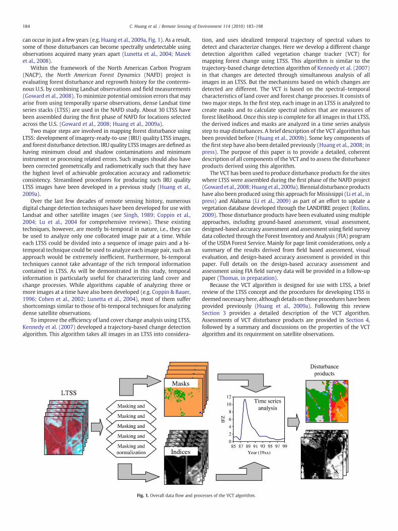
In addition, the calculation of FZi is essentially a normalization ofan image using forest pixels in that image. This normalization processcan substantially reduce the spatial and temporal variability of thespectral signature of forests caused by relatively homogeneousatmospheric conditions and instrument related issues (to be dis-cussed in more details later in Section 5, Fig. 10). Fig. 3(a) shows thatdue to atmospheric effect, a Landsat image can have substantiallyhigher top-of-atmospheric (TOA) reflectance values in the red bandthan surface reflectance (SR) values. For forest pixels, however, theIFZ values calculated using TOA and SR images are very close (Fig. 3(b)). In addition, some of the variation caused by vegetationphenology (during the summer growing season only) and sun angle(bi-directional reflectance effects) are also normalized through thecalculation of FZi and IFZ. As will be discussed later, the self-normalization property of these indices makes it possible for theVCT algorithm to be applicable to both TOA and SR images.

In addition to the FZi and IFZ indices, the VCT also calculates anormalized burn ratio index (NBRI) as follows:

NBRI =RNIR−R7

RNIR + R7ð4Þ

Where RNIR and R7 are reflectance in the near infrared band (band 4)and band 7. This index has been correlated with field measured burnseverity indices (e.g. Chen et al., 2008; Escuin et al., 2008), and is used toimprove detection of fire disturbance events by VCT.

3.2.4. Cloud and shadow maskingAlthough great effort has been taken to select imageswith the least

cloud cover for each LTSS, due to persisting cloudy conditions incertain areas some images inevitably contained cloudy pixels (Huanget al., 2009a, Table 3). Cloudy pixels generally have high brightnessvalues and low greenness values. If un-flagged, most likely they will

Fig. 3. Histograms of band 3 top-of-atmospheric (TOA) and surface reflectance (SR) (a. left(WRS path 15/row 33, acquired on July 6, 2001), showing that the IFZ values calculated from Teven though the TOA and SR values for those pixels are quite different.

be mapped as non-forest regardless of the actual surface conditionsbeneath the clouds. For forest change analysis, un-flagged clouds overforest likely will be mapped as forest disturbance. Cloud shadow overforest may also be mapped as disturbance as the spectral signature offorest under shadow can be quite different from that of sunlit forest.

Several cloudmasking algorithms have been developed for use withimages acquired by coarse resolution instruments (e.g. Simpson &Gobat, 1996; Ackerman et al., 1998; Stowe et al., 1999; Hutchison et al.,2005; Luo et al., 2008). For Landsat 7, an automated cloud coverassessment (ACCA) algorithm has also been developed for estimatingthe percentage of cloud coverwithin each image (Irish, 2000; Irish et al.,2006). The masking algorithm used in the VCT is based on observedcharacteristics of cloud and shadow. Clouds generally appear bright inthe reflective bands and cold in the thermal band (Fig. 4(a–b)). In thetemperature-red band space (Fig. 4(c)), a partly cloudy image forms anelongated cluster of points extending from the upper left to the lowerright. Vegetated, cloud-free observations are located near the upper lefttip and cloudy pixels are located towards the lower right tail. Cloudypixels are separated from cloud-free observations using thresholdvalues defined by a set of linear boundaries called cloud boundaries(Fig. 4(c–d)). Theseboundaries can be used to identifymost cloud types,including high altitude cirrus clouds, which are not necessarily verybright but are often very cold (Huang et al., in press).

For each cloud pixel, cloud height is calculated using its temperatureand a normal lapse rate (Smithson et al., 2008). The shadow location ofthat cloud is then predicted according to solar illumination geometryand the calculated cloud height. For large cloud patches, however, theshadow of some cloud pixels can be covered by other cloud pixels.Therefore, only predicted shadowpixels that are also dark are flagged asactual shadows. Details on this cloud and shadow algorithm have beenprovided by Huang et al. (in press).

3.3. Time series analysis

After the masking and normalization step is complete for all imagesin an LTSS, temporal interpolation is used to derive interpolated valuesfor pixels flagged as cloud, shadow, or other bad observation. Theresultantmasksand indices are thenused todeterminechange andnon-change classes, and to derive a suite of attributes to characterize themapped changes.

3.3.1. Temporal interpolationAs discussed earlier, because use of measurements contaminated

by cloud or shadow in land cover change analysis can result in false

) and those of the IFZ values calculated from TOA and SR (b. right) for a Landsat imageOA and SR are very close for forest pixels (identified by the first peak in the histograms)

Fig. 4. Clouds generally appear bright in the reflective bands (a) and cold in the thermal band (b). Cloudy pixels can be separated from cloud free observations using threshold valuesdefined by a set of linear boundaries called cloud boundary in the red-temperature space (c). Cloud edges are flagged using a 2-pixel buffer from identified cloudy pixels, andshadows are identified in the direction projected from identified cloud and cloud edge pixels according to illumination geometry (d).


changes, pixels flagged as cloud or cloud shadow should not be used inthe time series analysis. However, ignoring such pixels and leavingthem out from the analysis will result in holes in the derived changeproducts. To avoid this problem, VCT uses temporal interpolation toderive interpolated values for such pixels. Specifically, for each pixelmasked as cloud or cloud shadow in a particular year i, the temporallynearest non-cloud, non-shadow observations acquired before (p) andafter (n) year i are used to calculate its value as follows:

xi = xp + ði−pÞ × xn−xpn−p

ð5Þ

where x is any of the indices calculated in Section 3.2. If no non-cloud,non-shadow observation can be found in the years before (or after)the current acquisition year, then the value for the current year is setto that of the temporally nearest non-cloud, non-shadow observationacquired after (or before) year i. For each flagged cloudy or shadowpixel, temporal interpolation is applied to all the indices calculated inSection 3.2.

While we recognize that for pixels contaminated by cloud orshadow, there is no way to obtain their uncontaminated values, i.e., thevalues they would have if they were not contaminated, this temporalinterpolation can provide an informed guess of those uncontaminated

values. A pixel that was contaminated by cloud or shadow in a year butwas forested in the acquisition years before and after that year should beforested during that year, and Eq. (5) should give interpolated valuesclose to those of a forest pixel. Similarly, a pixel that was contaminatedby cloud or shadow in a year but was not forested in the acquisitionyears before and after that year should not be forested during that year,and the interpolated values from Eq. (5) likely will be different fromthose of a forest pixel. However, if a cloud or shadow contaminationhappened in the same year or the acquisition year immediately beforethe year when a disturbance occurred, the interpolated values can bevery different from the uncontaminated values, and that cloud/shadowcontamination may result in errors in the derived disturbance products(to be discussed in more details in Section 4).

3.3.2. Determining change and no-change classesTime series analysis of forest cover and change is based mainly on

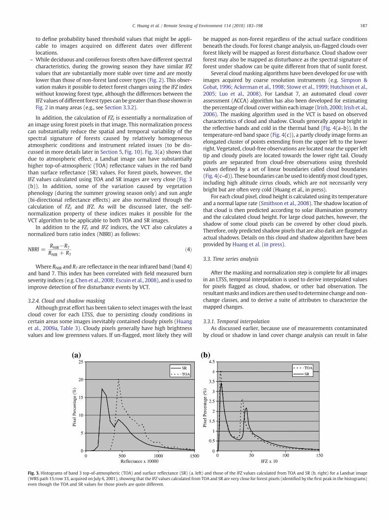
the physical interpretation of the IFZ. Because the IFZ measures thelikelihood of a pixel being a forest pixel, its value should change inresponse to forest change. Fig. 5 shows typical temporal profiles of theIFZ for major land cover and forest change processes. For persistingforest land where no major disturbance occurred during the yearsbeing monitored (throughout this paper the word “persisting”

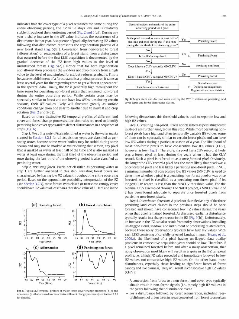
Fig. 6. Major steps and decision rules used by the VCT to determine persisting landcover types and forest disturbance classes.


indicates that the cover type of a pixel remained the same during theentire observing period), the IFZ value stays low and is relativelystable throughout the monitoring period (Fig. 2 and 5(a)). During anyyear a sharp increase in the IFZ value indicates the occurrence of adisturbance in that year. A sequence of gradually decreasing IFZ valuesfollowing that disturbance represents the regeneration process of anew forest stand (Fig. 5(b)). Conversion from non-forest to forest(afforestation) or regeneration of a forest stand from a disturbancethat occurred before the first LTSS acquisition is documented by thegradual decrease of the IFZ from high values to the level ofundisturbed forests (Fig. 5(c)). Notice that for both regenerationand afforestation processes the IFZ does not drop quickly from a highvalue to the level of undisturbed forest, but reduces gradually. This isbecause establishment of a forest stand is a gradual process; it takes atleast several years for the regrowing trees to get a “forest appearance”in the spectral data. Finally, the IFZ is generally high throughout thetime series for persisting non-forest pixels that remained non-forestduring the entire observing period. While certain crops may bespectrally similar to forest and can have low IFZ values during certainseasons, their IFZ values likely will fluctuate greatly as surfaceconditions change from one year to another due to harvest and croprotation (Fig. 2 and 5(d)).

Based on these distinctive IFZ temporal profiles of different landcover and forest change processes, decision rules are used to identifypersisting land cover types and to detect disturbances in a sequence ofsteps (Fig. 6).

Step 1, Persisting water. Pixels identified aswater by thewatermaskscreated in Section 3.2.1 for all acquisition years are classified as per-sisting water. Because some water bodies may be turbid during someseason and may not be masked as water during that season, any pixelthat is masked as water at least half of the time and is also masked aswater at least once during the first third of the observing period andonce during the last third of the observing period is also classified aspersisting water.

Step 2, Persisting forest. Pixels not classified as persisting water instep 1 are further analyzed in this step. Persisting forest pixels arecharacterized by having low IFZ values throughout the entire observingperiod. Based on the approximate probability interpretation of the IFZ(see Section 3.2.3), most forests with closed or near close canopy covershould have IFZ values of less thana threshold valueof 3.Here and in the

Fig. 5. Typical IFZ temporal profiles of major forest cover change processes (a–c) andnon-forest (d) that are used to characterize different change processes (see Section 3.3.2for details).

following discussions, this threshold value is used to separate low andhigh IFZ values.

Step 3, Persisting non-forest. Pixels not classified as persisting forestin step 2 are further analyzed in this step. While most persisting non-forest pixels have high and often temporally variable IFZ values, someof them can be spectrally similar to certain forest pixels and can havelow IFZ values during a particular season of a year. The likelihood ofmost non-forest pixels to have consecutive low IFZ values (CLIV),however, is low (Fig. 2). Therefore, if a pixel has a CLIV record, it likelywas a forest pixel at least during the years when it had the CLIVrecord. Such a pixel is referred to as a once forested pixel. Obviously,the longer the CLIV record a pixel has, the more likely that pixel was aonce forested pixel and less likely a persisting non-forest pixel. In VCT,a minimumnumber of consecutive low IFZ values (MNCLIV) is used todetermine whether a pixel is a persisting non-forest pixel or was onceforested. A pixel is classified as a persisting non-forest pixel if itslongest CLIV record is less than the MNCLIV threshold value. For thebiennial LTSS assembled through the NAFD project, a MNCLIV value of2 has been found adequate to separate once forested pixels frompersisting non-forest pixels.

Step 4, Disturbance detection. A pixel not classified as any of the threepersisting land cover classes in the previous steps should be onceforested and should have consecutive low IFZ values during the yearswhen that pixel remained forested. As discussed earlier, a disturbancetypically results in a sharp increase in the IFZ (Fig. 5(b)). Unfortunately,an increase in the IFZ can also result from noisy observations, includingun-flagged cloud, shadow, and instrument or processing related errors,because these noisy observations typically have high IFZ values. Witheach LTSS consisting of carefully selected Landsat images (Huang et al.,2009a), the likelihood of a pixel having un-flagged data qualityproblems in consecutive acquisition years should be low. Therefore, ifa pixel remained forested before and after a noisy observation, thatnoisy observation most likely will result in a spike in the IFZ temporalprofile, i.e., a high IFZ value preceded and immediately followed by lowIFZ values, not consecutive high IFZ values. On the other hand, mostdisturbances, especially those leading to significant losses of forestcanopy and live biomass, likelywill result in consecutive high IFZ values(CHIV):

– A conversion from forest to a non-forest land cover type typicallyshould result in non-forest signals (i.e., mostly high IFZ values) inthe years following that disturbance event.

– For a disturbance followed by forest regeneration, including rees-tablishment of urban trees in areas converted from forest to anurban


environment, the IFZ should remain high until the young trees growto a stage such that they spectrally look like forest.

Therefore, VCT uses the CHIV record following an IFZ hike todeterminewhether the increase was caused by a noisy observation or adisturbance. Only an IFZ hike followed by a CHIV record at least as longas a predefined minimum number of consecutive high IFZ values(MNCHIV) ismapped as a disturbance. For the biennial LTSS used by theNAFD, an MNCHIV value of 2 is used for most closed canopy forestecosystems in the U.S. A higher MNCHIV value can reduce the ability todetect disturbances, especially in the southeastern U.S. where treesplanted after a harvest can grow so rapidly that they can becomespectrally inseparable from undisturbed forest in just 4–6 years, or 2–3consecutive observations in a biennial LTSS, following that harvest(Huang et al., 2009a, Fig. 1). For open forests in the semiaridsouthwestern U.S., however, stress due to drought conditions can lastmanyyears, and can result in a CHIV record ofmore than 2. For theNAFDsuch a drought induced stress is not considered a disturbance. To avoidsucha stress beingmappedasdisturbance, theMNCHIV is increased to 3for open forest biomes.

It should be noted that open canopy forestswith bright backgroundstypically have IFZ values much higher than those of closed canopyforests and likely will be classified as persisting non-forest using the IFZthreshold value of 3 as defined in step 2. To minimize this problem, forimages consistingof both closed andopen canopy forest types, steps 2 to4 are performed twice. In the first time, the initial IFZ threshold value of3 is used to characterize forest and disturbances for areas having closedcanopy forests. Pixels classified as persisting non-forest in the firstiteration are reanalyzed in the second iteration, during which the IFZthreshold value in step 2 is relaxed for better characterization of forestand disturbances for areas having open canopy forests. Based onextensive examination of various sparse forests in the semiarid westernU.S., the IFZ threshold value is set to 6.5 in the second iteration.

We noticed that some fires, especially understory fires, did notalways result in high IFZ values. If such pixels did not have otherdisturbances during the observing period, they likely will be mappedas persisting forest in step 2. To reduce such omission errors the VCTalso checks the NBRI temporal profile for pixels mapped as persistingforest in step 2. Because fires typically result in low NBRI values(Escuin et al., 2008), they are detected by searching for significantdecreases on the NBRI temporal profile.

For disturbances that occurred at the beginning of the time series,there may not be a CLIV record that satisfies the MNCLIV criterion.Likewise, disturbances that occurred at the end of the time series willnot have a CHIV record that satisfies the MNCHIV criterion. Therefore,use of theMNCLIVandMNCHIV thresholdvalues asdescribed abovewillnot allow detection of such disturbances. To alleviate this problem, theMNCLIV is relaxed for disturbances that occurred at the beginning of thetime series, and theMNCHIV is relaxed for disturbances that occurred atthe end of the time series. Because of the relaxation of the MNCHIV andMNCLIV criteria, the disturbances detected at the beginning and end ofthe observing period of an LTSS likely will be less reliable than thosedetected in the middle of the observing period.

If a pixel reaches step 4 but its longest CHIV record is shorter thanthe MNCHIV and the CHIV record is not at the end of the time series, itis classified as persisting forest.

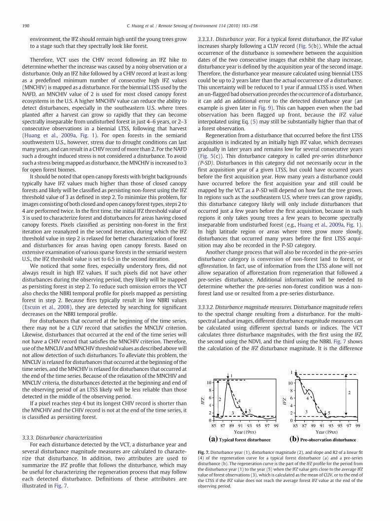
Fig. 7. Disturbance year (1), disturbance magnitude (2), and slope and R2 of a linear fit(4) of the regeneration curve for a typical forest disturbance (a) and a pre-seriesdisturbance (b). The regeneration curve is the part of the IFZ profile for the period fromthe disturbance year (1) to the year (5) when the IFZ value gets close to the average IFZvalue of forest observations (3), which is calculated as themean of CLIV, or to the end ofthe LTSS if the IFZ value does not reach the average forest IFZ value at the end of theobserving period.

3.3.3. Disturbance characterizationFor each disturbance detected by the VCT, a disturbance year and

several disturbance magnitude measures are calculated to characte-rize that disturbance. In addition, two attributes are used tosummarize the IFZ profile that follows the disturbance, which maybe useful for characterizing the regeneration process that may followeach detected disturbance. Definitions of these attributes areillustrated in Fig. 7.

3.3.3.1. Disturbance year. For a typical forest disturbance, the IFZ valueincreases sharply following a CLIV record (Fig. 5(b)). While the actualoccurrence of the disturbance is somewhere between the acquisitiondates of the two consecutive images that exhibit the sharp increase,disturbance year is defined by the acquisition year of the second image.Therefore, the disturbance year measure calculated using biennial LTSScould be up to 2 years later than the actual occurrence of a disturbance.This uncertainty will be reduced to 1 year if annual LTSS is used. Whenanun-flaggedbadobservationprecedes the occurrence of a disturbance,it can add an additional error to the detected disturbance year (anexample is given later in Fig. 9). This can happen even when the badobservation has been flagged up front, because the IFZ valueinterpolated using Eq. (5) may still be substantially higher than that ofa forest observation.

Regeneration from a disturbance that occurred before the first LTSSacquisition is indicated by an initially high IFZ value, which decreasesgradually in later years and remains low for several consecutive years(Fig. 5(c)). This disturbance category is called pre-series disturbance(P-SD). Disturbances in this category did not necessarily occur in thefirst acquisition year of a given LTSS, but could have occurred yearsbefore the first acquisition year. How many years a disturbance couldhave occurred before the first acquisition year and still could bemapped by the VCT as a P-SD will depend on how fast the tree grows.In regions such as the southeastern U.S. where trees can grow rapidly,this disturbance category likely will only include disturbances thatoccurred just a few years before the first acquisition, because in suchregions it only takes young trees a few years to become spectrallyinseparable from undisturbed forest (e.g., Huang et al., 2009a, Fig. 1).In high latitude region or areas where trees grow more slowly,disturbances that occurred many years before the first LTSS acqui-sition may also be recorded in the P-SD category.

Another change process that will also be recorded in the pre-seriesdisturbance category is conversion of non-forest land to forest, orafforestation. In fact, use of information from the LTSS alone will notallow separation of afforestation from regeneration that followed apre-series disturbance. Additional information will be needed todetermine whether the pre-series non-forest condition was a non-forest land use or resulted from a pre-series disturbance.

3.3.3.2. Disturbance magnitude measures. Disturbancemagnitude refersto the spectral change resulting from a disturbance. For the multi-spectral Landsat images, different disturbancemagnitudemeasures canbe calculated using different spectral bands or indices. The VCTcalculates three disturbance magnitudes, with the first using the IFZ,the second using the NDVI, and the third using the NBRI. Fig. 7 showsthe calculation of the IFZ disturbance magnitude. It is the difference


between the IFZ value in the disturbance year and themean IFZ value ofconsecutive forest observations, which are represented by CLIV (Fig. 7(a)). Here use of the mean IFZ value of consecutive forest observationsinsteadof the IFZ value of the pre-disturbance observation canminimizethe impact of inter-annual variations of forest signal on the calculateddisturbance magnitude value. For a pre-series disturbance, thedisturbance magnitude is calculated using the IFZ value of the firstLTSS acquisition and the mean IFZ value of CLIV (Fig. 7(b)). The NDVIandNBRI disturbancemagnitudes are calculated the samewayas the IFZdisturbance magnitude.

It should be noted that other spectral indices, such as the bandspecific FZi values or the tasseled cap indices (Crist & Cicone, 1984;Huang et al., 2002), can also be used to calculate disturbance magni-tudes. Further studies are needed to determine which of thesedisturbance magnitude measures can better characterize the natureand intensity of detected disturbances.

3.3.3.3. Regeneration characteristics. If forest regeneration occurredafter a disturbance, this regeneration process is tracked by a regenera-tion curve (Fig. 7). This curve refers to the portion of the IFZ profile fromthe disturbance year (point 1 in Fig. 7) to the point where the IFZ valuegets close to the average IFZ value of CLIV (point 5 in Fig. 7), or to the endof the LTSS if the IFZ value does not reach the average forest IFZ value atthe end of the observing period. To determinewhether this curve tracksforest regeneration and to characterize the regeneration rate, a line is fitusing this curve and the R2 of the fit and the slope of the line arecalculated. Regeneration of a new forest stand likely will yield high R2

values, and the slopeof the linemaybe an indicator of the growth rate ofthe regenerating forest. Of course, the linear fit will be statisticallymeaningful only when there are enough observations following adisturbance. For disturbances that occurred near the end of the LTSS,neither the slope nor theR2 is statisticallymeaningful and fill valueswillbe assigned to them. It should be noted that a spectral recovery asrepresented by the regeneration curve is not synonymous withecological definitions of forest recovery. Spectral recovery tends tooccur fairly quickly (within 5–15 years depending on forest type) suchthat even lowbiomass levelsmay give IFZ values comparable to those ofmature forests.

In areas like the southeastern U.S. where certain tree species growfast enough to allow more than one forest harvest during theobserving period of an LTSS, some fields may experience more thanone disturbance. In such cases the VCT will detect all disturbances andwill calculate the above described attributes for each detecteddisturbance.

4. Algorithm assessment

Asmentioned earlier, VCT has been tested inmany places in the U.S.,including Mississippi (Li et al., in press), Alabama (Li et al., 2009), andthe locations where LTSS have been assembled through the NAFDproject (Goward et al., 2008;Huanget al., 2009a). This highly automatedalgorithm was found very efficient. Except for a few parameters thatneeded fine tuning when both closed and open canopy forests arepresent within an image (see Section 3.3.2), universal or near-universalthreshold values were used for all other parameters. On average it took2–3 h to analyze an LTSS consisting of 12 or more Landsat images usingan average desktop PC available in today's market. Based on ourexperience, use of existing bi-temporal change detection techniques toanalyze such an image stack would take tens of working days,depending on the experience of an image analyst and the complexityof land cover and change processes within that image stack. Such anefficiency gap between the VCT and existing bi-temporal changedetection techniques likely will not reduce as computers become fasterin the future, because almost all the time required by VCT is CPU time,whereas many bi-temporal change detection techniques requiresignificant amount of human inputs.

Comprehensive validation of the entire suite of VCT products asdescribed in Section 4 has been found extremely challenging. Linkingthe disturbance magnitude measures to changes in biomass or otherbiophysical variables requires pre- and post-disturbance measure-ments obtained using methods that would allow reliable retrieval ofthose variables. Similarly, linking the regeneration characteristics tovegetation biophysical changes associated with regeneration process-es requires multi-temporal reference data sets on those biophysicalvariables. Such reference data sets likely will be scarce, especially forolder disturbances that occurred in the 1990s and 1980s, althoughtheir availability has yet to be better understood. Therefore, we havefocused on the disturbance year products in assessing the perfor-mance of the VCT algorithm, using both qualitative and quantitativemethods. Qualitative assessments include limited ground validationand comprehensive visual assessment. Quantitative assessmentsinclude a design-based accuracy assessment and comparison withfield measurement of forest age collected through the USDA ForestService Forest Inventory and Analysis (FIA) program. For page limitconsiderations, only qualitative evaluations and a summary of thedesign-based accuracy assessment are provided here. The assessmentusing FIA data and more details on the design-based accuracyassessment will be provided in a follow-up paper (Thomas, inpreparation).

4.1. Ground-based assessment

Ground-based assessment is often considered a preferred methodfor evaluating land cover classifications derived from remote sensing.Using this method to evaluate all the classes in a VCT disturbance yearmap, however, would require ground-based data collected in each ofthe acquisition years of the concerned LTSS, which likely do not existfor most disturbance classes. Nevertheless, checking the disturbancesmapped by the VCT on the ground would allow a better understand-ing of the nature of those disturbances and the processes thatoccurred following those disturbances. For this purpose we conductedlimited field trips in Virginia (path 15/row 34, in October 2005),Mississippi and Alabama (path 21/row 37 and path 21/row 39, in May2007), and Oregon (path 45/row 49, in July 2007). In each field trip,we visited a list of pre-selected sites where disturbances weremapped by the VCT. Field photos were taken along with GPScoordinates during each trip. Ground evidences were easy to findfor recent disturbance events that resulted in complete or nearcomplete removal of the forest canopy, including harvest (Fig. 8(a)),fire (Fig. 8(e)), and urban development (Fig. 8(d)). Older disturbancesthat occurred years before the field trips and were followed byregeneration of new forest stands were often evidenced by theexistence of young, even-aged forests, and the disturbance year wasroughly reflected by the height of the regenerating trees (Fig. 8(b and c)).Likely due to vigorous growth of understory vegetation in Virginia andMississippi/Alabama, evidence of less intensive disturbances such asstorm damage, insect/disease defoliation, and selective logging wasdifficult to find during the trips. Characterized by dry environmentalconditions and slow growth of both trees and understory vegetation, theeastern side of the Cascades in Oregon had many evidences of lessintensive disturbances, including some that occurred many years beforethe field trip. There we found that some less intensive disturbances, suchas selective logging and fuel treatment, were mapped successfully by theVCT (Fig. 8(f)), but many others were not.

4.2. Visual assessment

Compared with the ground-based assessment method, visualchecking of the disturbances mapped by the VCT against the inputLandsat images provides a more immediate and yet reliable way toevaluate those disturbances. In general, the spectral change signals ofmost forest disturbances can be identified reliably by experienced

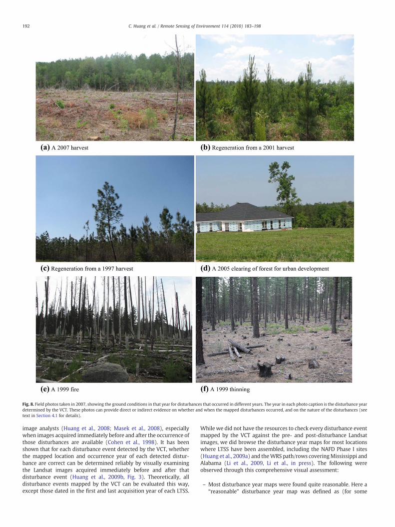
Fig. 8. Field photos taken in 2007, showing the ground conditions in that year for disturbances that occurred in different years. The year in each photo caption is the disturbance yeardetermined by the VCT. These photos can provide direct or indirect evidence on whether and when the mapped disturbances occurred, and on the nature of the disturbances (seetext in Section 4.1 for details).


image analysts (Huang et al., 2008; Masek et al., 2008), especiallywhen images acquired immediately before and after the occurrence ofthose disturbances are available (Cohen et al., 1998). It has beenshown that for each disturbance event detected by the VCT, whetherthe mapped location and occurrence year of each detected distur-bance are correct can be determined reliably by visually examiningthe Landsat images acquired immediately before and after thatdisturbance event (Huang et al., 2009b, Fig. 3). Theoretically, alldisturbance events mapped by the VCT can be evaluated this way,except those dated in the first and last acquisition year of each LTSS.

While we did not have the resources to check every disturbance eventmapped by the VCT against the pre- and post-disturbance Landsatimages, we did browse the disturbance year maps for most locationswhere LTSS have been assembled, including the NAFD Phase I sites(Huang et al., 2009a) and theWRS path/rows coveringMississippi andAlabama (Li et al., 2009, Li et al., in press). The following wereobserved through this comprehensive visual assessment:

– Most disturbance year maps were found quite reasonable. Here a“reasonable” disturbance year map was defined as (for some


graphic examples, see Huang et al., 2009b, Fig. 4): 1) the map hadminimum speckles; 2) for human disturbance events such asharvest and logging, themapped disturbance polygons had regularshapes or linear features that were indicative of the human originof those disturbances; and 3) for nature disturbances such as fireand storm damages, they had irregular shapes but were oftencontiguous. Disturbances that were mapped by the VCT but weredeemed “unreasonable” through this visual assessment werechecked against the pre- and post-disturbance images to deter-mine whether those disturbances were false alarms.

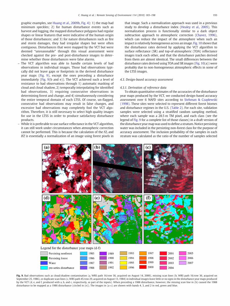
– The VCT algorithm was able to handle certain levels of badobservations in individual images. Those bad observations typi-cally did not leave gaps or footprints in the derived disturbanceyear maps (Fig. 9), except the ones preceding a disturbanceimmediately (Fig. 9(b and e)). The VCT achieved such a level ofresistance to bad observations through 1) automatic masking ofcloud and cloud shadow, 2) temporally interpolating for identifiedbad observations, 3) requiring consecutive observations indetermining forest and change, and 4) simultaneously consideringthe entire temporal domain of each LTSS. Of course, un-flagged,consecutive bad observations may result in false changes, andexcessive bad observations may completely fool the VCT algo-rithm. Therefore, it is still necessary to select high quality imagesfor use in the LTSS in order to produce satisfactory disturbanceproducts.

– While it is preferable to use surface reflectance in the VCT algorithm,it can still work under circumstances when atmospheric correctioncannot be performed. This is because the calculation of the FZi andIFZ is essentially a normalization of an image using forest pixels in

Fig. 9. Bad observations such as cloud/shadow contamination (a, WRS path 16/row 36, acSeptember 25, 1986), or duplicate scan lines (c,WRS path 45/row 29, acquired on August 13,by the VCT (d, e, and f, produced with a, b, and c, respectively, as part of the inputs). Whendisturbance to be mapped as a 1986 disturbance (circled in (e)). The images in (a–c) are sh

that image. Such a normalization approach was used in a previousstudy to develop a disturbance index (Healey et al., 2005). Thisnormalization process is functionally similar to a dark objectsubtraction approach to atmospheric correction (Chavez, 1996),which can reduce the impact of the atmosphere when such animpact is relatively homogeneousacross an image. Fig. 10 shows thatthe disturbance rates derived by applying the VCT algorithm tosurface reflectance (SR) and top-of-atmospheric (TOA) reflectanceimages track each other, and that the disturbance patches derivedfrom them are almost identical. The small differences between thedisturbance rates derived using TOAand SR images (Fig. 10(a))wereprobably due to non-homogeneous atmospheric effects in some ofthe LTSS images.

4.3. Design-based accuracy assessment

4.3.1. Derivation of reference dataTo obtain quantitative estimates of the accuracies of the disturbance

year maps produced by the VCT, we conducted design-based accuracyassessment over 6 NAFD sites according to Stehman & Czaplewski(1998). These sites were selected to represent different forest biomesand disturbance regimes in the U.S. (Table 2). For each site, validationsamples were selected using a stratified random sampling method,where each sample was a 28.5 m TM pixel, and each class (see thelegend of Fig. 9 for a complete list of those classes) in a draft version ofthedisturbanceyearmapwasused todefinea stratum.Noticepersistingwater was included in the persisting non-forest class for the purpose ofaccuracy assessment. The inclusion probability of the samples in eachstratum was calculated as the ratio of the number of samples selected

quired on August 14, 2000), missing scan lines (b, WRS path 16/row 36, acquired on1984) in individual images leave little or no signs in the disturbance yearmaps producedpreceding a 1988 disturbance, however, the missing scan line in (b) caused the 1988own with bands 4, 3, and 2 in red, green and blue.

Fig. 10. Disturbance rates for the Virginia site (path 15/row 34) derived by applying the VCT algorithm to surface reflectance (SR) and top-of-atmospheric (TOA) reflectance imagestrack each other, although the SR images yielded slightly higher disturbance rates in most years (a). A detailed checking of the disturbance year maps (b and c) reveals that the twomaps are almost identical at the patch level. See Fig. 9 for the legend for the disturbance year maps.


within that stratum over the total pixels of that stratum (Stehman et al.,2003). In order to achieve satisfactory precisions with the accuracyestimates we targeted 50 samples per stratum on average, with aminimum value of 20 for rare classes. A total of approximately 700validation samples were selected for each validation site (Table 2).

For each validation sample, all images of the target LTSS wereinspected visually to determine whether it belonged to one of the“persisting” classes or it had disturbances. If disturbances were found ata sample location, the disturbance years were recorded. As demon-strated in Section 4.2 and in many previous studies (e.g. Cohen et al.,1998; Healey et al., 2005; Kennedy et al., 2007; Huang et al., 2009b), thedisturbance year determined this way should be reliable and thereforecould be used as a reference for validating the disturbance yeardeterminedby theVCT. Tominimizepotential difficulties in interpretingthe Landsat images, for each validation sample we obtained a DigitalOrtho Quarter Quad (DOQQ) from the TerraServer (http://terraserver-usa.com/) to assist the analysis. Where necessary, the high resolution

Table 2Characteristics of the 6 validation sites where the VCT disturbance year products were eval

WRS path/row

Location Land cover and forest characteristics

12/31 Southeastern NewEngland

Mostly temperate deciduous forests, agriculture, ur

15/34 Virginia Pine plantation, deciduous or mixed forests, agricu21/37 Mississippi/Alabama Pine plantation, deciduous or mixed forests, agricu27/27 Minnesota Temperate deciduous and mixed forests, agricultur

37/34 Southern Utah Semiarid, mostly shrub and grassland, pinion/junipshort and sparse

45/29 Oregon Temperate evergreen forests to the west, dry grass aand to the east

imagery available from GoogleEarth was also checked. These imagestypically were not acquired immediately before or after the occurrenceof a disturbance, but their high spatial resolutions provided a localreference for the image analysts to separate forest, non-forest, anddisturbance at the Landsat level. Considering the fact that each LTSSimage could have subpixel misregistration errors, the compoundmisregistration errors from all Landsat images in that LTSS could beover one TM pixel. To minimize the impact of such misregistrationerrors on accuracy estimates, any validation sample thatwas located onthe edge of a land cover or change polygon was moved towards theinner part of that polygon such that it was at least 1 pixel away from theedge.

4.3.2. Accuracy estimatesFor each of the 6 validation sites, the above derived reference data

sets were used to create a confusion matrix. Accuracy measures,including overall accuracy, kappa coefficient, and per class user's, and

uated using a design-based accuracy assessment method.

Major disturbances Accuracy assessmentsample size

ban Urbanization, logging 697

lture Harvest, logging 650lture Harvest, logging 700e, wetlands Wind throw, ice damage,

harvest750

er forests are typically Fire 645

nd shrubs in the middle Fire, harvest, logging, fueltreatment

700

http://terraserver-usa.com/

http://terraserver-usa.com/


producer's accuracies, were calculated according to Stehman &Czaplewski (1998) and Congalton (1991), and the inclusion proba-bility of validation samples were incorporated according to Stehmanet al. (2003). Both the overall accuracy and kappa coefficient aremeasures of the overall agreement between a disturbance year mapand reference data, but kappa is often considered a better indicator ofalgorithm performance because chance agreement is excluded fromits calculation (Congalton & Mead, 1983). The user's accuracymeasures the proportion of pixels classified as belonging to a classthat are also labeled with that class in the reference data, while theproducer's accuracymeasures the proportion of pixels truly belongingto a class that are also classified as belonging to that class. User's andproducer's accuracies are related to commission (or false alarm) andomission errors as follows (Janssen & Wel, 1994):

Commissionerrorð%Þ = 100%−User’s accuracyð%Þ

Omissionerrorð%Þ = 100%−Producer’s accuracyð%Þ

Table 3 provides a summary of the accuracy measures for all 6validation sites, showing that the disturbance year maps had overallaccuracies ranging from 0.77 to 0.86. Except for the southern Utahsite (WRS path 37/row 34), the kappa values ranged from 0.67 to 0.76.The producer's and user's accuracies averaged over all classes rangedfrom 0.57 to 0.67 and 0.67 to 0.80, respectively, and were from 0.52to 0.63 and 0.63 to 0.79, respectively, when averaged over thedisturbance classes. The average accuracies of the disturbance classesindicate that although those classes were typically rare (up to 1%–3%of total area per disturbance year) as compared with no-changeclasses (Lunetta et al., 2004; Masek et al., 2008), on average the VCTwas able to detect more than half of the disturbances with relativelylow levels (i.e., 21%–37% for the 5 validation sites) of false alarm.Tables 4 and 5 provide the full confusion matrix along with variousaccuracy measures for a site where VCT had average performance(Virginia, WRS path 15/row 34) and a site where it performed worst(southern Utah, WRS path 37/row 34). In the Virginia site, thedisturbance year map had user's and producer's accuracies rangingfrom 65% to 96% and 46% to 94%, respectively (Table 4). In thesouthern Utah site, the user's and producer's accuracies were muchmore variable, largely because many disturbance classes had verysmall sample sizes (Table 5). In this site, the stratified randomsampling method failed to satisfy the minimum requirement of 20samples per class because disturbances in many acquisition yearswere extremely rare.

The errors in the disturbance year products can be attributed toseveral factors, many of which have been discussed in Huang et al.(2009b). The first is the difficulty to detect many non-stand clearingdisturbances by the current version of the VCT, although some ofthose disturbances were captured by the VCT (see Section 4.1, Fig. 8(f)). Due to lack of ground information or high resolution datacollected immediately after the occurrence of each disturbance, here

Table 3Overall accuracy, kappa, and average producer's and user's accuracy values of the VCTdisturbance year products assessed for all land cover and disturbance year classes ofthose products.

WRS2path/row

Overallaccuracy

Kappa Average accuracy of individual classes

All classes Disturbance classes

Producer's User's Producer's User's

12/31 0.85 0.76 0.67 0.67 0.63 0.6315/34 0.80 0.75 0.67 0.78 0.62 0.7721/37 0.78 0.74 0.64 0.79 0.59 0.7927/27 0.77 0.67 0.64 0.80 0.60 0.7937/34 0.86 0.43 0.31 0.55 0.24 0.5245/29 0.84 0.73 0.57 0.72 0.52 0.70

the distinction between stand clearing and non-stand clearingdisturbances was determined by visually checking the post-distur-bance Landsat images. After a non-stand clearing disturbance, thepost-disturbance pixels looked brighter and less green than the pre-disturbance pixels; but they still looked like forest pixels. For a standclearing disturbance resulting from clear cut or other stand replacingevents, however, the post-disturbance pixels did not look like forestsanymore. Most of the disturbed pixels that weremapped as persistingforest by VCT (omission error) were identified as non-stand clearingdisturbances by the analysts (Table 4). Many of the disagreements onthe disturbance year between the VCT and the analysts were alsoattributed to undetected thinning, which were typically followed bystand clearing harvests in later years.

The second type of errors are due to the fact that certain non-forestland cover types, including some crop fields and wetlands, had low IFZvalues in consecutive Landsat observations as represented by the LTSS ofinterest. As a result, they were mapped as persisting or disturbed forest(see Section 3.3.2). The third type of errors are due to the difficulty tomap marginal forests in a semiarid environment using remote sensingdata sets, because those forests typically had open canopy and consistedofmostly short tree species. The difficulty can be further exacerbated bylocal conditions including inter-annual variations in vegetation phe-nology due to changing precipitation patterns, and high terrain reliefcoupledwith changing solar angles. The substantially lower kappa valueand user's and producer's accuracies of the southern Utah site (WRSpath 37/row 34) as compared with the other 5 validation sites weremostlydue to the last factor. Specifically,more thanhalf of thepersistingforest samples in the reference data were classified as persisting non-forest by VCT, and for several disturbance classesmost of the samples inthe reference data were classified as persisting forest or persisting non-forest (Table 5). More detailed analysis of the errors in the disturbanceyear products along with the full confusion matrices for all 6 validationsites will be provided in a follow-up paper (Thomas, in preparation).

One may notice that most of the overall accuracy and kappa valueslisted in Table 3 are close to those reported by Kennedy et al. (2007)for the trajectory-based change detection (TBCD) method. However,because the sampling methods employed by this and the Kennedy etal. study are different, caution is needed in evaluating the comparativeperformance between VCT and TBCD using the accuracies reported inthe two studies.

5. Summary and discussions

With spatial resolutions suitable for reliable characterization ofmany natural and anthropogenic disturbances, a time series of Landsatacquisitions can provide a historical record of forest disturbance. Such arecord is critical for many earth science studies (Skole et al., 1998;Townshend et al., 2004). In this study we develop a vegetation changetracker (VCT) algorithm for reconstructing forest disturbance historyusing Landsat time series stacks (LTSS). This algorithm is based on thespectral–temporal properties of forest, disturbance, and post-distur-bance recovery processes. It first analyzes each individual image tocreate masks and spectral indices that measure forest likelihood. It thensimultaneously analyzes all images within an LTSS to detect distur-bances and uses the spectral trajectory following each disturbance totrack post-disturbance processes. Visual assessment of the disturbanceyear products revealed that most of them were reasonably reliable.Design-based accuracy assessment revealed that overall accuracies ofaround 80% were achieved for disturbances mapped at individual yearlevel. Averageuser's andproducer's accuracies of thedisturbanceclasseswere around 70% and 60% for 5 of the 6 validation sites, respectively,suggesting that although forest disturbances were typically rare ascomparedwithno-change classes, onaverage theVCTwasable todetectmore than half of those disturbances with relatively low levels of falsealarms. Field assessment revealed that VCT was able to detect moststand clearing disturbance events, including harvest, fire, and urban

Table 4Confusion matrix derived using the design-based accuracy assessment method for the Virginia site (15/34).

VCT Reference data n User'sacc.

PNF PF P-SD 86 88 90 92 94 96 98 00 02 05 Row total

PNF 29.23 0.65 0.26 0.26 0.07 0.07 0.05 30.59 122 95.56PF 0.78 27.83 2.60 0.34 1.24 1.16 0.66 1.14 0.36 1.30 0.29 0.37 0.77 38.84 175 71.65P-SD 0.88 0.44 4.38 0.42 0.04 0.10 0.10 0.10 6.46 56 67.7386 0.26 0.13 0.58 1.89 2.86 32 66.0888 0.26 0.06 0.06 2.34 0.26 2.97 35 78.7590 0.33 0.04 0.11 1.52 2.00 38 75.8192 0.07 0.07 0.13 0.07 1.37 0.07 1.76 24 77.7694 0.13 0.07 0.07 1.90 0.20 2.36 33 80.4996 0.10 0.14 0.07 2.55 2.86 36 89.2598 0.13 0.13 0.13 0.26 1.83 0.13 2.62 20 70.0000 0.26 0.10 0.10 2.81 3.26 32 86.1302 0.11 1.39 1.50 27 92.8005 0.10 0.21 0.16 0.21 1.25 1.92 20 65.08Column total 31.97 29.68 8.30 3.16 3.83 3.28 2.29 3.44 3.27 3.33 3.32 2.06 2.07 100.00No. sample (n) 127 131 63 35 41 46 25 37 39 21 34 31 20Producer's acc. 91.41 93.77 52.70 59.87 61.17 46.37 59.94 55.24 78.06 55.07 84.54 67.30 60.15 Overall acc. 80.28

The overall, user's, and producer's accuracies are in percentage (%). Values in the “n” row and column are number of reference samples (TM pixels) selected in this site. Values in allother cells are area percentages (e.g. 29.23 means 29.23% of the total area of the LTSS). Agreements between VCT and reference data are highlighted in bold face. Class codes are:PNF=persistent non-forest, PF = persistent forest, P-SD=pre-series disturbance (see Sections 3.3.2–3.3.3 for definitions). All other class labels correspond to disturbance year(86=1986).


development, while some non-stand clearing events such as thinningand selective logging were also mapped in the western U.S.

The VCT algorithm has several appealing properties. It is highlyautomated, requiring little or no fine tuning except when both closedand open canopy forests are present within an image. This algorithmis very efficient, taking 2–3 h on average to analyze an LTSS consistingof 12 or more Landsat images using an average desktop PC available intoday's market. It can handle certain levels of bad observations inindividual LTSS images such that those observations have minimumor no impact on the derived disturbance products. However,excessive, consecutive bad observations in an LTSS can still result insubstantial false alarms. If the LTSS images cannot be corrected foratmospheric effect due to practical difficulties, VCT can also normalizethe impact of relatively homogeneous atmospheric effect. The impactsof using images that have spatially variable atmospheric conditionsbut are not atmospherically corrected, however, have yet to beassessed.

In addition to the disturbance year products for characterizing theoccurrence of disturbances, the VCT algorithm also calculates severalchange magnitude measures and tracks post-disturbance processesusing spectral indices. Validation or calibration of these measures andindices requires time series of groundmeasurements or other types of

Table 5Confusion matrix derived using the design-based accuracy assessment method for the sout

VCT Reference data

PNF PF P-SD 87 89 91 93 95

PNF 80.00 6.18 0.41 0.01 0.95 0.02 0.42PF 2.59 5.28 0.82 0.03 0.01 0.02 0P-SD 0.03 0.0187 0.01 0.0089 0.0991 0.0593 0.0295 0.01 097 0.41 0.01 0.01 0.01 099 000 0.0302 0.83 0.11 0.0404Column total 83.86 11.60 1.23 0.04 1.06 0.13 0.48 0No. sample (n) 245 195 5 2 20 12 18 31Producer's acc. 95.40 45.50 0.58 0.00 8.87 37.26 4.25 12

Class labels, accuracy measures, and cell values are defined the same way as in Table 4.

reference data sets that match the LTSS acquisitions temporally.Existing reference data sets likely will not be adequate for thispurpose, although their availability has yet to be better understood. Toallow proper calibration and validation of the entire suite of VCTproducts, obtaining time series of reference data sets should be one ofthe goals in planning future reference data collection efforts.

The issues revealed through the assessment of the disturbanceyear products highlighted some future directions for improving VCT,including better detection of non-stand clearing disturbances,reducing commission errors due to certain non-forest land covertypes being mapped as disturbances, and better characterization ofdisturbances in marginal forests in semiarid regions. Furthermore,disturbances in non-forest ecosystems including rangeland andwetland are also of great concerns to various earth science studies.Whether the VCT algorithm concept can be adapted for monitoringthose disturbances has yet to be investigated.

5.1. Observational requirements

The LTSS-VCT approach provides an efficient approach for mappingforest disturbances at annual or biennial intervals. The ability to createsuch a disturbance record for a given area, however, depends on the

hern Utah site (37/34).

n User'sacc.

97 99 00 02 04 Row total

0.01 0.41 0.01 88.43 251 90.47.01 0.02 0.06 0.47 9.30 206 56.76

0.04 11 18.180.01 1 0.000.09 7 100.000.05 7 100.000.02 10 100.00

.01 0.01 0.00 0.03 14 39.22

.06 0.05 0.56 34 9.29

.01 0.06 0.00 0.01 0.09 22 70.380.04 0.08 0.01 0.16 17 27.36

0.12 1.09 40 10.660.00 0.10 0.10 25 96.62

.09 0.07 0.47 0.09 0.26 0.58 99.9514 17 10 41 35

.33 73.44 12.86 49.14 44.46 16.72 Overall acc. 85.83


availability of a long-term satellite data record consisting of quality,temporally frequent acquisitions for that area. With a caveat that theLandsat holdings at international ground receiving stations are stillunknown,an in-depth analysis of theUSGS Landsat archive revealed thatmany areas outside the U.S. did not have Landsat acquisitions duringmany years in the 1980s and 1990s (Goward et al., 2006). Thanks toacquisition strategies implemented for the Landsat 7 (Arvidson et al.,2001; Arvidson et al., 2006), at least one Landsat 7 image per year shouldhave been acquired since 1999 for all land areas of the globe. For manyareas characterized by frequent cloudy conditions, however, oneacquisition per year will not be adequate for assembling high qualityLTSS, especially when the images have gaps due to a scan-line-corrector(SLC) problem that occurred to the Landsat 7 in 2003. In such areas, thechance to obtain a cloud-free image is low, and multiple images mayhave to beused tomake cloud-free composites. To ensure that long-termrecords of global forest disturbance history can be reconstructed in thefuture, it is necessary to develop the satellite capabilities today that willallowacquisition of adequate Landsat or Landsat class images formakingat least one cloud-free composite during the peak growing season ofevery year. It may well be that for a global land observatory, a dailyrepeat frequency may be needed to resolve the cloud and phenologyissues encountered across the Earth. Such an observing frequency at theLandsat resolutions will require new observatory innovations includingwider swath widths and multiple satellites: a combination of nationaland international assets will likely provide a successful approach.

Looking back, change detection algorithms not requiring time seriesobservations may have to be used in areas where existing Landsatimages are inadequate for assembling LTSS. Alternatively, imagesacquired by other satellites, including the Satellite Pour l'Observationde la Terre (SPOT) and the Indian Remote Sensing (IRS) satellite, may beused together with available Landsat images to create time seriesobservations. These satellite series have spatial resolutions similar to theLandsat, and have been in operation since the 1980s (Kramer, 2002). Aninventory of the images acquired by Landsat and other satellites over anarea is needed in order to assess towhat extent time series observationscan be assembled for that area, andwhether the VCT can be adapted foranalyzing time series observations consisting ofmulti-sensor images, ora new, VCT-like algorithmcan bedeveloped for suchdata sets, has yet tobe investigated.

Acknowledgements

This study contributes to the North American Carbon Program, withgrant support from NASA's Terrestrial Ecology, Carbon Cycle Science,and Applied Sciences Programs. Funding support for developing andvalidating the VCT algorithm was also provided by the U.S. GeologicalSurvey and the LANDFIRE project, which was sponsored by theintergovernmental Wildland Fire Leadership Council of the UnitedStates. High level preprocessing of the Landsat images using the LEDAPSwas performed by Teng-Kui Lim of Science Systems and Applications,Inc. (SSAI). Donald Ohlen, Daniel Steinwand, Jay Kost, and Brian Tolk ofUSGS/EROS participated in the field trips for validating the deriveddisturbance products. The authors wish to thank the four anonymousreviewers for their detailed comments, which led to major improve-ments to the original manuscript.

References

Ackerman, S. A., Moeller, C. C., Gumley, L. E., Strabala, K. I., Menzel, W. P., & Frey, R. A. (1998).Discriminating clear sky from clouds with MODIS. Journal of Geophysical Research D:Atmospheres, 103, 32,141−32,157.

Arvidson, T., Gasch, J., & Goward, S. N. (2001). Landsat 7's long-term acquisition plan—An innovative approach to building a global imagery archive. Remote Sensing ofEnvironment, 78, 13−26.

Arvidson, T., Goward, S., Gasch, J., & Williams, D. (2006). Landsat-7 long-termacquisition plan: Development and validation. Photogrammetric Engineering andRemote Sensing, 72, 1137−1146.

Chander, G., Helder, D. L., Markham, B. L., Dewald, J. D., Kaita, E., Thome, K. J., Micijevic, E.,& Ruggles, T. A. (2004). Landsat-5 TM reflective-band absolute radiometriccalibration. IEEE Transactions on Geoscience and Remote Sensing, 42, 2747−2760.

Chander, G., & Markham, B. (2003). Revised Landsat-5 TM radiometric calibrationprocedures and postcalibration dynamic ranges. IEEE Transactions on Geoscienceand Remote Sensing, 41, 2674−2677.

Chavez, P. S. (1996). Image-based atmospheric corrections—Revisited and improved.Photogrammetric Engineering & Remote Sensing, 62, 1025−1036.

Chen, X., Zhu, Z., Ohlen, D., Huang, C., & Shi, H. (2008). Use of multiple spectral indices toestimate burn severity in the Black Hills of South Dakota. Pecora 17—The future ofland imaging ... going operational. November 18–20, 2008, Denver, Colorado.

Cohen, W. B., Fiorella, M., Bray, J., Helmer, E., & Anderson, K. (1998). An efficient andaccurate method for mapping forest clearcuts in the Pacific Northwest usingLandsat imagery. Photogrammetric Engineering & Remote Sensing, 64, 293−300.

Cohen,W. B., Maiersperger, T. K., Fiorella, M., Spies, T. A., Alig, R. J., & Oetter, D. R. (2002).Characterizing 23 years (1972–95) of stand replacement disturbance in westernOregon forests with Landsat imagery. Ecosystems, 5, 122−137.

Colwell, J. E. (1974). Vegetation canopy reflectance. Remote Sensing of Environment, 3,174−183.

Congalton, R. (1991). A review of assessing the accuracy of classifications of remotelysensed data. Remote Sensing of Environment, 37, 35−46.

Congalton, R. G., & Mead, R. A. (1983). A quantitative method to test for consistency andcorrectness in photo interpretation. Photogrammetric Engineering & Remote Sensing, 49,69−74.

Coppin, P., & Bauer, M. (1996). Digital change detection in forested ecosystems withremote sensing imagery. Remote Sensing Reviews, 13, 234−237.

Coppin, P., Lambin, E., Jonckheere, I., Nackaerts, K., & Muys, B. (2004). Digital changedetection methods in ecosystem monitoring: A review. International Journal ofRemote Sensing, 25, 1565−1596.

Crist, E. P., & Cicone, R. C. (1984). A physically-based transformation of ThematicMapper data —The TM Tasseled Cap. IEEE Trans. on Geosciences and Remote Sensing,GE-22, 256−263.

Davis, J. C. (1986). Statistics and data analysis in geology (pp. 646). New York: JohnWiley & Sons, Inc.

Dodge, A., & Bryant, E. (1976). Forest type mapping with satellite data. Journal ofForestry, 74, 23−40.

Escuin, S., Navarro, R., & Fernandez, P. (2008). Fire severity assessment by using NBR(Normalized Burn Ratio) and NDVI (Normalized Difference Vegetation Index)derived from LANDSAT TM/ETM images. International Journal of Remote Sensing, 29,1053−1073.

Gao, F., Masek, J., & Wolfe, R. (2009). An automated registration and orthorectificationpackage for Landsat and Landsat-like data processing. Journal of Applied RemoteSensing, 3, 033515, doi:10.1117/1.3104620.

Goward, S., Irons, J., Franks, S., Arvidson, T., Williams, D., & Faundeen, J. (2006). Historicalrecord of Landsat global coverage: Mission operations, NSLRSDA, and internationalcooperator stations. Photogrammetric Engineering and Remote Sensing, 72,1155−1169.

Goward, S. N., Huemmrich, K. F., & Waring, R. H. (1994). Visible-near infrared spectralreflectance of landscape components in western Oregon. Remote Sensing ofEnvironment, 47, 190−203.

Goward, S. N., Masek, J. G., Cohen, W., Moisen, G., Collatz, G. J., Healey, S., Houghton, R.,Huang, C., Kennedy, R., Law, B., Turner, D., Powell, S., & Wulder, M. (2008). Forestdisturbance and North American carbon flux. EOS Transactions, AmericanGeophysical Union, 89, 105−106.

Goward, S. N., & Williams, D. L. (1997). Landsat and earth systems science: Developmentof terrestrial monitoring. Photogrammetric Engineering & Remote Sensing, 63,887−900.

Healey, S. P., Cohen,W. B., Zhiqiang, Y., & Krankina, O. N. (2005). Comparison of tasseledcap-based Landsat data structures for use in forest disturbance detection. RemoteSensing of Environment, 97, 301.

Hirsch, A. I., Little, W. S., Houghton, R. A., Scott, N. A., & White, J. D. (2004). The netcarbon flux due to deforestation and forest re-growth in the Brazilian Amazon:Analysis using a process-based model. Global Change Biology, 10, 908−924.

Houghton, R. A. (2003). Why are estimates of the terrestrial carbon balance sodifferent? Global Change Biology, 9, 500−509.

Huang, C., Goward, S. N., Masek, J. G., Gao, F., Vermote, E. F., Thomas, N., Schleeweis, K.,Kennedy, R. E., Zhu, Z., Eidenshink, J. C., & Townshend, J. R. G. (2009). Developmentof time series stacks of Landsat images for reconstructing forest disturbancehistory. International Journal of Digital Earth, 2, 195−218.

Huang, C., Goward, S. N., Schleeweis, K., Thomas, N., Masek, J. G., & Zhu, Z. (2009).Dynamics of national forests assessed using the Landsat record: Case studies ineastern U.S. Remote Sensing of Environment, 113, 1430−1442.

Huang, C., Song, K., Kim, S., Townshend, J. R. G., Davis, P., Masek, J., & Goward, S. N. (2008).Use of a dark object concept and support vector machines to automate forest coverchange analysis. Remote Sensing of Environment, 112, 970−985.

Huang, C., Thomas, N., Goward, S.N., Masek, J., Zhu, Z., Townshend, J.R.G. & Vogelmann, J.E. (in press). Automated masking of cloud and cloud shadow for forest changeanalysis. International Journal of Remote Sensing.

Huang, C., Wylie, B., Homer, C., Yang, L., & Zylstra, G. (2002). Derivation of a tasseled captransformation based on Landsat 7 at-satellite reflectance. International Journal ofRemote Sensing, 23, 1741−1748.

Huemmrich, K. F., & Goward, S. N. (1997). Vegetation canopy PAR absorptance andNDVI: An assessment for ten tree species with the SAIL model. Remote Sensing ofEnvironment, 61, 254−269.

Hutchison, K. D., Roskovensky, J. K., Jackson, J.M., Heidinger, A. K., Kopp, T. J., Pavolonis,M. J., &Frey, R. (2005). Automated cloud detection and classification of data collected by the

http://dx.doi.org/10.1117/1.3104620


Visible Infrared Imager Radiometer Suite (VIIRS). International Journal of Remote Sensing,26, 4681−4706.

Irish, R. R. (2000). Landsat 7 automatic cloud cover assessment. Proceedings of SPIE:Algorithms for multispectral, hyperspectral, and ultraspectral imagery VI. April 24–26,2000, Orlando, U.S.A, 348−355.

Irish, R. R., Barker, J. L., Goward, S. N., & Arvidson, T. (2006). Characterization of thelandsat-7 ETM+automated cloud-cover assessment (ACCA) algorithm. Photo-grammetric Engineering and Remote Sensing, 72, 1179−1188.

Janssen, L. L. F., & Wel, F. (1994). Accuracy assessment of satellite derived land coverdata: a review. IEEE Photogrammetric Engineering & Remote Sensing, 60, 419−426.

Jensen, J. R. (1996). Introductory digital image processing: A remote sensingperspective. Englewood Cliffs, New Jersey: Prentice-Hall.

Kauth, R. J., & Thomas, G. S. (1976). The tasseled cap—A graphic description of thespectral–temporal development of agricultural crops as seen in Landsat. Proceed-ings on the Symposium onMachine Processing of Remotely Sensed Data. June 29 –- July1, 1976, West Lafayette, Indiana, 41−51.

Kennedy, R. E., Cohen, W. B., & Schroeder, T. A. (2007). Trajectory-based changedetection for automated characterization of forest disturbance dynamics. RemoteSensing of Environment, 110, 370−386.

Kramer, H. J. (2002). Observation of the earth and its environment: Survey of missions andsensors (pp. 1510). Berlin: Springer.

Law, B. E., Van Tuyl, S., Ritts,W. D., Cohen,W. B., Turner, D., Campbell, J., & Sun, O. J. (2004).Disturbance and climate effects on carbon stocks and fluxes across Western OregonUSA. Global Change Biology, 10, 1429−1444.

Li, M., Huang, C., Zhu, Z., Shi, H., Lu, H., & Peng, S. (2009). Assessing rates of forest changeand fragmentation in Alabama, USA, using the vegetation change tracker model.Forest Ecology & Management, 257, 1480−1488.

Li, M., Huang, C., Zhu, Z., Shi, H., Lu, H. & Peng, S. (in press). Use of remote sensingcoupled with a vegetation change trackermodel to assess rates of forest change andfragmentation in Mississippi, USA. International Journal of Remote Sensing.

Liu, S., Loveland, T. R., & Kurtz, R. M. (2004). Contemporary carbon dynamics interrestrial ecosystems in the Southeastern Plains of the United States. Environ-mental Management, 33, S442−S456.

Lu, D., Mausel, P., Brondízio, E., & Moran, E. (2004). Change detection techniques. In-ternational Journal of Remote Sensing, 25, 2365−2407.

Lunetta, R. S., Johnson, D. M., Lyon, J. G., & Crotwell, J. (2004). Impacts of imagerytemporal frequency on land-cover change detection monitoring. Remote Sensing ofEnvironment, 89, 444−454.

Luo, Y., Trishchenko, A. P., & Khlopenkov, K. V. (2008). Developing clear-sky, cloud andcloud shadow mask for producing clear-sky composites at 250-meter spatialresolution for the sevenMODIS land bands over Canada and North America. RemoteSensing of Environment, 112, 4167−4185.

Markham, B. L., & Barker, J. L. (1986). Landsat MSS and TM post-calibration dynamicranges, exoatmospheric reflectances and at-satellite temperatures. EOSAT LandsatTechnical Notes, 1, 3−8.

Markham, B. L., Storey, J. C., Williams, D. L., & Irons, J. R. (2004). Landsat sensorperformance: History and current status. Geoscience and Remote Sensing, IEEETransactions on, 42, 2691−2694.

Masek, J. G., Huang, C., Cohen, W., Kutler, J., Hall, F., & Wolfe, R. E. (2008). MappingNorth American forest disturbance from a decadal Landsat record: Methodologyand initial results. Remote Sensing of Environment, 112, 2914−2926.

Pacala, S. W., Hurtt, G. C., Baker, D., Peylin, P., Houghton, R. A., Birdsey, R. A., Heath, L.,Sundquist, E. T., Stallard, R. F., Ciais, P., Moorcroft, P., Caspersen, J. P., Shevliakova, E.,

Moore, B., Kohlmaier, G., Holland, E., Gloor, M., Harmon, M. E., Fan, S. M., Sarmiento,J. L., Goodale, C. L., Schimel, D., & Field, C. B. (2001). Consistent land- andatmosphere-based U.S. carbon sink estimates. Science, 292, 2316−2320.

Peterken, G. F. (2001). Structural dynamics of forest stands and natural processes. In J.Evans (Ed.), The forest handbook, Vol 1. (pp. 83−104)Malden, MA: Blackwell Science.

Rollins, M. G. (2009). LANDFIRE: A nationally consistent vegetation, wildland fire, andfuel assessment. International Journal of Wildland Fire, 18, 235−249.

Schimel, D. S., & Braswell, B. H. (1997). Continental scale variability in ecosystemprocesses: Models, data, and the role of disturbance. Ecological Monographs, 67,251−271.

Simpson, J. J., & Gobat, J. I. (1996). Improved cloud detection for daytime AVHRR scenesover land. Remote Sensing of Environment, 55, 21−49.

Singh, A. (1989). Digital change detection techniques using remotely-sensed data. In-ternational Journal of Remote Sensing, 10, 989−1003.

Skole, D. L., Salas, W. A., & Taylor, V. (1998). Global observation of forest cover: Fineresolution data and product design strategy, report of a workshop. Paris, France: CNES.

Smithson, P., Addison, K., & Atkinson, K. (2008). Fundamentals of the physical environment(pp. 776). London: Routledge.

Stehman, S. V., & Czaplewski, R. L. (1998). Design and analysis for thematic mapaccuracy assessment: Fundamental principles. Remote Sensing of Environment, 64,331−344.

Stehman, S. V., Wickham, J. D., Smith, J. H., & Yang, L. (2003). Thematic accuracy of the1992 National land-cover data for the eastern United States: Statistical method-ology and regional results. Remote Sensing of Environment, 86, 500−516.

Stowe, L. L., Davis, P. A., & McClain, E. P. (1999). Scientific basis and initial evaluation ofthe CLAVR-1 global clear/cloud classification algorithm for the advanced very highresolution radiometer. Journal of Atmospheric and Oceanic Technology, 16,656−681.

Thomas, N., Huang, C., Goward, S.N., Powell, S., Rishmawi, K., Schleeweis, K. & Hinds, A.(In preparation). Assessment of NAFD forest change products derived from LandsatTime Series Stacks (LTSS).

Thornton, P. E., Clark, K. L., Falge, E., Ellsworth, D. S., Goldstein, A. H., Monson, R. K.,Hollinger, D., Falk, M., Chen, J., Sparks, J. P., Law, B. E., & Gholz, H. L. (2002).Modeling and measuring the effects of disturbance history and climate on carbonand water budgets in evergreen needleleaf forests. Agricultural and ForestMeteorology, 113, 185−222.

Townshend, J. R., Justice, C. O., Skole, D. L., Belward, A., Janetos, A., Gunawan, I.,Goldammer, J. G., & Lee, B. (2004). Meeting the goals of GOFC. In G. Gutman, A. C.Janetos, C. O. Justice, E. F. Moran, J. F. Mustard, R. R. Rindfuss, D. Skole, B. L. TurnerII,& M. A. Cochrane (Eds.), Land Change Science (pp. 31−51). Dordrecht: KluwerAcademic Publishers.

Townshend, J. R. G., & Justice, C. O. (1988). Selecting the spatial resolution of satellitesensors required for global monitoring of land transformations. InternationalJournal of Remote Sensing, 9, 187−236.

Townshend, J. R. G., Justice, C. O., & McManus, J. (1992). The impact of misregistrationon change detection. IEEE Transactions on Geoscience and Remote Sensing, 30,1054−1060.

Vermote, E. F., Tanre, D., Deuze, J. L., Herman, M., & Morcrette, J. J. (1997). Secondsimulation of the satellite signal in the solar spectrum, 6S: An overview. IEEETransactions on Geoscience and Remote Sensing, 35, 675−686.