MANUFACTURING & SERVICEOPERATIONS MANAGEMENT

Vol. 7, No. 4, Fall 2005, pp. 360–378issn 1523-4614 �eissn 1526-5498 �05 �0704 �0360

informs ®

doi 10.1287/msom.1050.0084©2005 INFORMS

A Supply Chain Model with ReverseInformation Exchange

Apurva Jain, Kamran MoinzadehUniversity of Washington Business School, Seattle, Washington 98195-3200

{apurva@u.washington.edu, kamran@u.washington.edu}

We develop a model and analyze reverse information sharing, a growing business practice in supply chainmanagement in which a manufacturer shares information about supply with a retailer. We model the

manufacturer as a production queue with finished goods warehouse, the retailer as an inventory location, andother customers as an external demand stream. In our model, the manufacturer allows the retailer access toinventory status at the warehouse. To take advantage of this new information, the retailer changes from asingle-level base-stock policy to a two-level, state-dependent base-stock policy. We provide an exact method forcomputing performance and develop a procedure for evaluating optimal policy. We demonstrate the impact ofthe new policy on the manufacturer and other customers. Numerical computations lead to insights about thevalue of information to the retailer, and to guidelines for the manufacturer on sharing information.

Key words : information sharing; stochastic production-inventory system; state-dependent base stock; Markovchains

History : Received: November 16, 2003; accepted: June 8, 2005. This paper was with the authors 7 months for3 revisions.

1. IntroductionIn recent years, retailers and manufacturers haveshown increasing interest in cooperating to improvethe performance of the supply chain and increasetheir gains. Sharing information has emerged as oneof the most critical practices in improving the per-formance of supply chains. Most of the work oninformation sharing to date has focused on cases inwhich the retailer shares information about currentdemand with the manufacturer (for example, see Leeand Whang 1999, Cheung and Lee 2002, Chen 1998,Cachon and Fisher 2000, Moinzadeh 2002). A differentbut parallel trend calls for the manufacturer to shareinformation with the retailer. In these instances, infor-mation flows in reverse order; that is, instead of theretailer providing information about its demand andinventory status to the supplier, the supplier providesthe retailer with information about its inventory avail-ability status. While the practice appears to be grow-ing, its consequences have not been fully analyzed.Specifically, how can the retailer use this informationto its benefit, and what is the impact of the practiceon the performance of the manufacturer?

In this paper, we consider a supply chain inwhich the manufacturer shares information about cur-rent inventory with a retailer that satisfies externaldemand through inventory. The manufacturer sup-plies goods first come, first served (FCFS) to theretailer and other “walk-in” customers, using itsfinished-goods inventory. Finished-goods inventoryis replenished through production. Standard holdingand backorder costs apply at inventory locations, butno ordering/setup cost is incurred. At the time ofordering, the retailer can ask about the availability ofstock at the manufacturer’s finished-goods inventory.To take advantage of this information, the retaileruses a state-dependent base-stock policy. Our maingoals are to develop an exact evaluation of this sys-tem, and to develop insights for both the retailer andthe manufacturer.The new trend toward reverse information shar-

ing is driven by two factors: (i) availability of tech-nological capability for information sharing, and(ii) increased customer awareness of informationsharing in supply chains (and, as a consequence,increased customer pressure on the manufacturer to

360

Jain and Moinzadeh: A Supply Chain Model with Reverse Information ExchangeManufacturing & Service Operations Management 7(4), pp. 360–378, © 2005 INFORMS 361

share information). An example of new technolog-ical capability is the customer portal available inJ. D. Edwards’s software system. The portal allowsa retailer to log in to a manufacturer’s system. Afterlogging in, the retailer not only has the ability tocheck the status of its outstanding orders and itsfinancial account information, but can also choose“view inventory availability” option to get informa-tion on the manufacturer’s stock availability. Hereand in other examples, the manufacturer chooses toallow access to its system, and controls the amount ofinformation available to customers. These “customerportals” or similar features (the terminology is notstandard) are now available from most large businesssoftware application providers. They are the resultof a confluence of three technologies developed inrecent years: enterprise resource planning (ERP) sys-tems, customer relationship management (CRM) sys-tems, and business-to-business (B2B) exchanges.Valspar Corporation, a leading paint manufacturer,

offers an example of the second factor driving reverseinformation sharing, increased pressure from cus-tomers. Valspar Corporation administers a question-naire to any business seeking to become a regularsupplier. One of the qualifying questions determineswhether the supplier provides product availabilityinformation. This kind of pressure from customersis reflected by the supplier’s sales force. Hard datais difficult to come by, but in an informal U.S. Info-Tel survey, sales representatives said that they couldmake more sales if they were able to answer avail-ability questions in a customer’s office. The desireto answer such questions may be part of the rea-son for growth in salesforce automation software thatallows sales representatives to share inventory infor-mation with customers (Colombo 1994). Pressure forsharing information may also come from third-partytrading hubs, such as Exostar, that promise customers“improved access to product availability information”(Plyler and Shaw 2001).Driven by the availability of software applications

and working under competitive pressures to keepcustomers satisfied, many manufacturers and dis-tributors already employ customer portals in theirsupply chains. One such example (Smith 2002) isOsmonics Inc., a Minnesota-based manufacturer of

water purification systems serving soft drink man-ufacturers, bottled water companies, and originalequipment manufacturers. Osmonics uses the SAPAG R/3 ERP system for its internal data management,and HAHT Commerce’s HAHT Commerce Suite asan interface to share information with its customers.Many customers tap into the company’s ERP data andhave varying degrees of access and control, depend-ing in part on the sophistication of the customer’sown software systems. Among other features, cus-tomers using the system can check the status oforders and inventory. Another example (PeopleSoft2002) is Sager Electronics, one of the largest elec-tronics distributors in the United States. The com-pany upgraded its PeopleSoft ERP system to providepassword-protected access to customers so that theycan easily complete their supply chain managementfunctions. In addition, the system is designed to tailorthe portal for different users, and incorporates contentchanges for each user. In the business of spare parts,where base-stock policies are often used (Nahmias1981), Pratt and Whitney Canada provides informa-tion related to inventory availability to its customersonce they register on the Internet.In our abstract model of these business situations,

we consider a manufacturer who shares some pri-vate supply information with certain customers. Themanufacturer uses a base-stock policy to manage itsfinished-goods inventory, and its production processis modeled as a single-server queue. The manufac-turer shares information about product availabilityat its warehouse with the retailer. Other customers,called walk-ins, do not have access to this manufac-turer information. To take advantage of the productavailability information, the retailer employs a state-dependent base-stock ordering policy. Under this pol-icy, the retailer uses two different base-stock levels,each corresponding to whether or not the product isavailable at the manufacturer’s warehouse at the timethe order is placed. We use our model to demon-strate that this policy lets the retailer use the productavailability information opportunistically, sneaking inlarger orders when the product supply is unavailable.We develop insights on the magnitude of the retailer’scost reduction under various settings. We show thatthe retailer’s use of the information results in a bull-whip effect in the supply chain and investigate its

Jain and Moinzadeh: A Supply Chain Model with Reverse Information Exchange362 Manufacturing & Service Operations Management 7(4), pp. 360–378, © 2005 INFORMS

impact on the number of orders in the manufacturer’sproduction system, as well as on the on-hand inven-tory and backorder levels in the finished-goods ware-house. We then extend our model to consider thecase of two-way information exchange in which themanufacturer may know the retailer’s current inven-tory position. Finally, we use examples based on ourmodel to develop insights into the reasons manufac-turers are sharing their private supply information.We conclude with a discussion about the future ofsuch information sharing.Our contributions lie in two primary areas. First,

we extend the existing literature on inventory sys-tems with supply information. Among the literaturethat incorporates supply conditions in ordering pol-icy, Song and Zipkin (1996) is noteworthy. They studythis issue in a periodic setting by modeling the sup-ply system as an evolving Markov chain in which theretailer knows the current state of the chain beforeordering in each period. Their work builds on astream of research initiated by Kaplan (1970) for mod-eling stochastic lead times. In Kaplan (1970), lead-time distribution is known at the time of ordering.By design, however, it does not provide any informa-tion about the lead-time distribution at the next order-ing opportunity. Nahmias (1979) and Zipkin (1986)explain how to construct a supply system that pro-duces dependent lead times (orders do not cross) andyet provides no information for the next lead time. InSong and Zipkin (1996), the retailer knows the cur-rent state of the Markov chain, which not only leadsto the current lead-time distribution, but also pro-vides information about the lead-time distribution atthe next ordering opportunity. Thus, the dependencybetween consecutive lead times is explicitly modeledby Markov chain’s transition probabilities. The futurestate of the Markov chain, however, is independent ofthe ordering activities at any given time. That is, thetransition probabilities are independent of the ordersize. Chen and Yu (2002) provide a new algorithm forthe Song and Zipkin (1996) model, and analyze a sit-uation in which the retailer can use lead-time historydata to predict the next state, even when the currentstate is unknown.The focus of these studies is on determining opti-

mal policy in the periodic setting. In our work, wefocus on developing a model that captures the impact

of retailer ordering policy on the supply chain, andallows for exact analysis as well as the develop-ment of managerial insights. Most importantly, in ourmodel we allow the orders placed by the retailer toinfluence the supply system. This relaxes the assump-tion made in the earlier studies that retailer orders donot influence the supply system. By explicitly captur-ing the retailer orders’ impact on the state of the sup-ply system, we find that the value of information forthe retailer may be less than the value found in mod-els in which the retailer’s load is marginal to the sys-tem. We also identify situations in which the retailerwould not benefit from using this information.Our paper also makes a contribution to understand-

ing the propagation of variability in supply chains.Lee et al. (1997) have suggested several reasons forthe bullwhip effect in supply chains. One of these, thecapacity-rationing game (see Cachon and Lariviere1999), comes close to our situation. We demonstratethat reverse information sharing can actually createthe bullwhip effect in the supply chain. While ear-lier work is driven by shortage of capacity in a sin-gle period, we show the effect in a dynamic modelin which there is no shortage of capacity in the longterm. In addition, Lee et al. suggest that in theirmodel, the manufacturer sharing its inventory infor-mation with downstream members may prevent thebullwhip effect. In our model, however, it is the selec-tive sharing of information that creates the bullwhipeffect. We also present a rationale for the manufac-turer to allow reverse information sharing.In the next section, we describe our model and

the notation. Section 3 is devoted to the developmentand the analysis of the continuous-time Markov chain(CTMC) describing the state of the system. In §4,we focus on the retailer’s cost under the new pol-icy, and provide a procedure to compute optimal pol-icy parameters. We provide insights into the value ofinformation for the retailer. Section 5 provides resultson the manufacturer’s performance measures in suchsystems. Finally, we summarize our main results anddiscuss the possible extensions to this research.

2. The ModelConsider a supply chain consisting of a manufac-turer who supplies a finished good to a retailer andwalk-in customers. Demand generated by the walk-in

Jain and Moinzadeh: A Supply Chain Model with Reverse Information ExchangeManufacturing & Service Operations Management 7(4), pp. 360–378, © 2005 INFORMS 363

customers follows a Poisson process with rate �e (sub-script e for external arrivals). Demand at the retailer isassumed to follow a Poisson process with rate �r . Theretailer holds stock and satisfies its demand throughits on-hand inventory, and we assume that excessdemand at the retailer is backordered. To replenishits stock, the retailer places orders with the manu-facturer. We assume that orders placed by either theretailer or walk-in customers are satisfied immedi-ately if the manufacturer has stock; otherwise, theyare delayed and served in an FCFS manner. The man-ufacturer manages its finished-goods inventory usinga base-stock production policy. That is, for each orderit receives from its customers, the manufacturer issuesa production order. We model the manufacturer’s pro-duction system as a single-server queue with expo-nentially distributed processing times with a mean of1/�. In addition, we assume that the order transit timefrom the manufacturer to the retailer is constant, T .We assume that the manufacturer shares informa-

tion about stock availability only with the retailer.At the time of order placement, the manufacturerinforms the retailer whether the product is avail-able in the manufacturer’s finished-goods inventory.We acknowledge that manufacturers can share moredetailed information. However, limiting ourselvesto the simpler binary interpretation—stock is eitheravailable or unavailable—allows us to capture themain idea behind reverse information sharing whilekeeping the analysis tractable. Due to its limitedscope, this interpretation of reverse information shar-ing may be more practical. For example, many onlineretailers, such as Amazon.com, share information onstock availability with their customers. Manufactur-ers may find it easier to overcome their natural reluc-tance to let customers see private information if theamount of that information is limited. Finally, thisbinary model of information sharing is equivalent tothe manufacturer informing the retailer whether theproduct is backordered before the retailer places theorder.Because we observe differentiation between cus-

tomers in practice, we classify the manufacturer’s cus-tomers as retailers and walk-ins—those who haveaccess to reverse information and those who do not.At Osmonics Inc. (Smith 2002), for example, “nearly200 customers [are] actively accessing” its ERP data

out of a total of “3,000 or so customers.” Our mod-eling of walk-ins captures those customers who donot have access to information. Just like the retailer,walk-ins will carry inventory to satisfy their demand.In the absence of any supply information, how-ever, the walk-ins will employ a standard one-for-one policy. Therefore, the walk-in order streams tothe manufacturer will be exactly the same as theirdemand streams. It may be plausible that walk-inswill respond to any change in the supply chain bychanging their base-stock level, but that would notaffect their order stream. To keep matters simple, wedo not explicitly model the inventory system for thewalk-ins. Using the analysis presented here, incorpo-ration of the inventory model at the walk-in level isstraightforward. We believe, however, that it wouldnot offer further insights. We should point out that if awalk-in customer learns by observing the dependencein the lead times and this results in a state-dependentordering policy, it will be necessary to develop anexplicit inventory model for such customers. We donot consider that case in the study.The balance of the paper considers the impact

of reverse information exchange from either theretailer’s perspective or the manufacturer’s perspec-tive. In §4, we consider the retailer alone, and showthat service received by walk-in customers may dete-riorate as a result of the retailer’s actions. Section 5discusses the manufacturer’s response to the retailer’spolicy. We consider only those manufacturer policiesthat leave the service received by walk-in customersunaffected, and so do not motivate a change in cus-tomer behavior.

2.1. Retailer’s PolicyLet h and b denote the unit holding and backordercost rates at the retailer. Assuming that the retailer’sobjective is to minimize the sum of average hold-ing and backorder cost rates, we propose and dis-cuss the form of the retailer’s inventory policy. Wepresent an exact formulation of the cost functionin §4. Recall that the manufacturer allows the retaileraccess to information regarding stock availability atthe manufacturer’s finished-goods warehouse. So thatthe retailer can make use of this information, wepropose a state-dependent base-stock retailer order-ing policy as follows: When a demand occurs at the

Jain and Moinzadeh: A Supply Chain Model with Reverse Information Exchange364 Manufacturing & Service Operations Management 7(4), pp. 360–378, © 2005 INFORMS

retailer, the retailer checks the availability of the stockat the manufacturer. If the manufacturer has stockavailable, it orders enough to bring its inventory posi-tion (on-hand+on-order−backorders) up to the base-stock level Sl. Otherwise, it orders enough to bringits inventory position up to the base-stock level Su.Note that when the retailer’s inventory position isequal to or greater than the target base-stock level,the retailer does not order. Under this scenario, theretailer’s knowledge of the current state of the sup-ply system is binary, and there is a base-stock levelcorresponding to each state. We will refer to this state-dependent base-stock policy as �Sl Su� policy.Before we proceed, some discussion of the state-

dependent base-stock policy is helpful. Previousresearch suggests that in settings such as ours, thechoice of a state-dependent base-stock policy is areasonable one: Our model can be formulated as acontinuous-time Markov decision process, where thestate transition probability is a function of the actiontaken (order size) by the retailer. In a periodic set-ting, with transition probabilities independent of theaction, Song and Zipkin (1996) showed that the state-dependent base-stock policy is optimal. The depen-dence of transition probability on the form of thepolicy in our model makes it quite difficult to extendthe standard optimality arguments. On an intuitivelevel, it is difficult to argue that our proposed policymay not perform well. We also follow the tradition ofproposing simple-to-implement policies, especially incontinuous inventory models. See, for example, Rubioand Wein (1996).We assume that the retailer places an order only

at its demand epochs, and accesses the availabilityinformation only at those times. Order placementat demand epochs, while not necessarily optimal(Moinzadeh 2001), is a common and reasonableassumption that has been widely used in many previ-ous works (Axsäter 1990, Svoronos and Zipkin 1991).We also assume that the retailer knows the distribu-tion of the manufacturer’s processing time, its base-stock level and the total market demand. The retailermay have come to this knowledge based on historicaldata or by gathering business intelligence. This is akinto the retailer knowing the transition probabilities ofthe supply Markov chain in Song and Zipkin (1996)and in Chen and Yu (2002).

We assume that Sl ≤ Su. In studies of the periodicsystem, Song and Zipkin (1996) and Chen and Yu(2002) show that optimal state-dependent base-stocklevel is not necessarily nondecreasing in lead time.Based on their discussions and results, this counterin-tuitive phenomenon appears to occur when the leadtime is not monotonically increasing in the state vari-able describing the supply system (see Theorem 4 ofSong and Zipkin), and when lead time of zero is pos-sible. These conditions do not hold in our setting.Thus, we have primarily focused on the case Sl ≤ Su.Our evaluation technique, however, also lends itselfto the analysis of cases where Sl > Su. (The appendixpresents the case Sl = Su + 1�) In all of the instanceswe evaluated (see §4.2), Sl ≤ Su is always dominant.The manufacturer receives an order stream from

the retailer, and a second order stream, modeled asa Poisson process, from walk-in customers. If theretailer is using the information by following the pro-posed �Sl Su� policy, the retailer orders constitute astate-dependent bulk arrival process at the manufac-turer. We assume that even though a retailer’s ordermay consist of more than one unit, units in the sameorder do not wait for each other before being trans-ported (i.e., partial shipment is allowed).We assume that the manufacturer follows a base-

stock production policy with base-stock level Sm tomanage its finished-goods inventory. Thus, every unitdemanded by a customer gives rise to a productionorder to replenish the inventory. Again, the produc-tion system is modeled as a single-server, FCFS queuewith exponential service times with a mean rate of �.Our assumption of exponential service time allowsfor tractability of analysis, and is commonly used inproduction and inventory literature.The assumption of a base-stock policy for manu-

facturer finished-goods inventory is based on Sobel(1969), and Gavish and Graves (1980). In the absenceof any fixed start-up or shutdown costs, but withstandard holding and backorder cost rates, a base-stock policy is optimal when the order stream at themanufacturer is a renewal process. The assumptionof renewal arrivals is not met when Sl �= Su. It can beargued that when Sl �= Su, the manufacturer may antic-ipate the retailer’s ordering behavior and improve itscurrent base-stock policy. We will explore such animproved policy for the manufacturer in §5, and show

Jain and Moinzadeh: A Supply Chain Model with Reverse Information ExchangeManufacturing & Service Operations Management 7(4), pp. 360–378, © 2005 INFORMS 365

that the cost reduction for the manufacturer is minis-cule. Here, we continue to assume a base-stock policyfor the manufacturer.We close this section by defining all the relevant

parameters in the system.�e Mean arrival rate of external walk-in cus-

tomers�r Mean demand rate at the retailer� Mean unit production rate of the manufac-

turer’s production system�e Load in the production system due to external

arrivals= �e/��r Load in the production system due to retailer

arrivals= �r/�� Overall load in the production system= �e+�rSm Base-stock level for manufacturer’s inventory

in the finished-goods warehouseN Random variable representing the number of

orders in the manufacturer’s production sys-tem (also referred to as work in process)

Sl Retailer’s base-stock level when manufacturerhas stock �N < Sm�

Su Retailer’s base-stock level when manufactureris out of stock �N ≥ Sm�

� Su− Sl; �≥ 0IP Random variable representing retailer’s inven-

tory position�i�j Steady-state probability of �IP = Sl + i N = j�;

0≤ i≤�; j ≥ 0h Unit holding cost/timeb Retailer’s unit backorder cost/time

CSl�� Retailer’s expected cost for policy parame-ters Sl and �

E�X! Expected value of random variable X

3. Analysis of the ReverseInformation Sharing Model

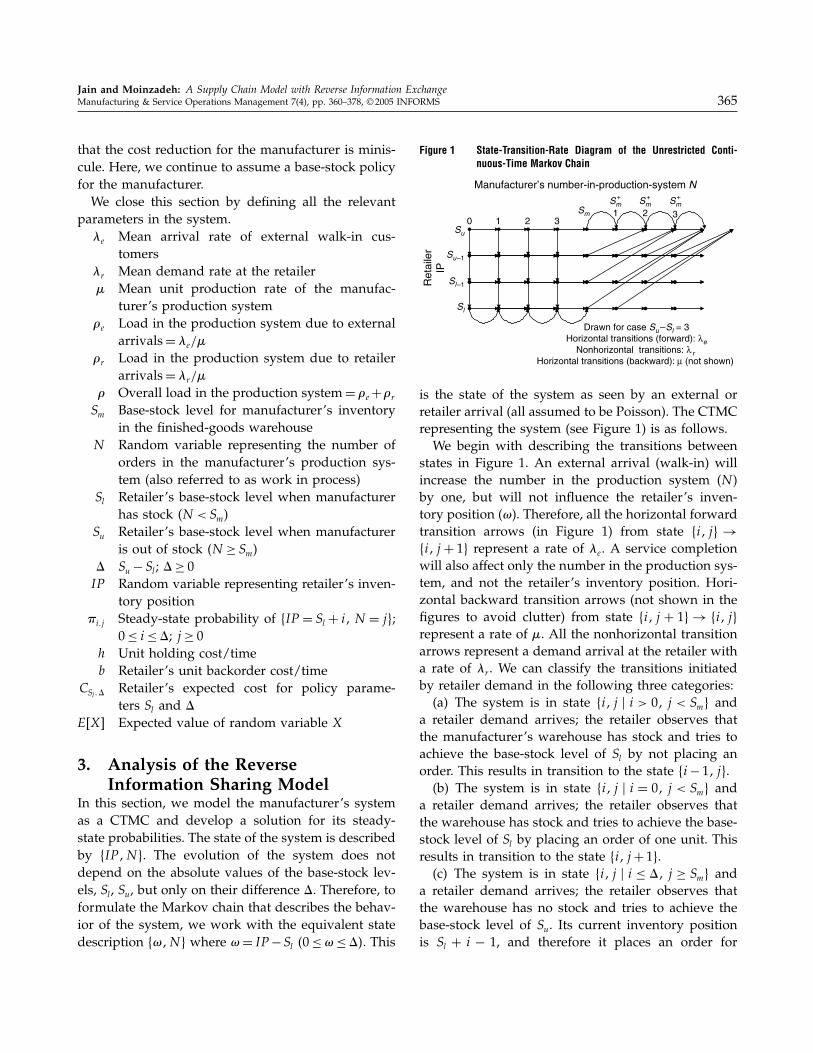
In this section, we model the manufacturer’s systemas a CTMC and develop a solution for its steady-state probabilities. The state of the system is describedby �IP N�. The evolution of the system does notdepend on the absolute values of the base-stock lev-els, Sl, Su, but only on their difference �. Therefore, toformulate the Markov chain that describes the behav-ior of the system, we work with the equivalent statedescription �" N� where "= IP −Sl �0≤"≤��. This

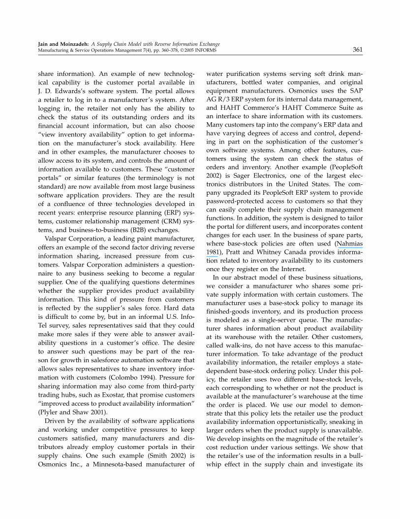
Figure 1 State-Transition-Rate Diagram of the Unrestricted Conti-nuous-Time Markov Chain

0 1 2 3Sm 1 2 3

Manufacturer’s number-in-production-system N

Ret

aile

rIP

Drawn for case Su–Sl = 3Horizontal transitions (forward): λe

Nonhorizontal transitions: λ rHorizontal transitions (backward): µ (not shown)

Su

Sl

Su–1

Sl–1

Sm+ Sm

+ Sm+

is the state of the system as seen by an external orretailer arrival (all assumed to be Poisson). The CTMCrepresenting the system (see Figure 1) is as follows.We begin with describing the transitions between

states in Figure 1. An external arrival (walk-in) willincrease the number in the production system (N )by one, but will not influence the retailer’s inven-tory position ("). Therefore, all the horizontal forwardtransition arrows (in Figure 1) from state �i j� →�i j + 1� represent a rate of �e. A service completionwill also affect only the number in the production sys-tem, and not the retailer’s inventory position. Hori-zontal backward transition arrows (not shown in thefigures to avoid clutter) from state �i j + 1�→ �i j�

represent a rate of �. All the nonhorizontal transitionarrows represent a demand arrival at the retailer witha rate of �r . We can classify the transitions initiatedby retailer demand in the following three categories:(a) The system is in state �i j � i > 0 j < Sm� and

a retailer demand arrives; the retailer observes thatthe manufacturer’s warehouse has stock and tries toachieve the base-stock level of Sl by not placing anorder. This results in transition to the state �i− 1 j�.(b) The system is in state �i j � i = 0 j < Sm� and

a retailer demand arrives; the retailer observes thatthe warehouse has stock and tries to achieve the base-stock level of Sl by placing an order of one unit. Thisresults in transition to the state �i j + 1�.(c) The system is in state �i j � i ≤ � j ≥ Sm� and

a retailer demand arrives; the retailer observes thatthe warehouse has no stock and tries to achieve thebase-stock level of Su. Its current inventory positionis Sl + i − 1, and therefore it places an order for

Jain and Moinzadeh: A Supply Chain Model with Reverse Information Exchange366 Manufacturing & Service Operations Management 7(4), pp. 360–378, © 2005 INFORMS

�− �i− 1� units. This results in the transition to thestate �� j +�− �i− 1��.We now develop a procedure for computing

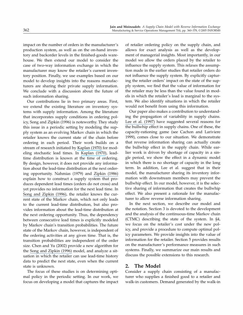
the steady-state joint probability mass function, �ij ,for this CTMC. The main idea is to exploit thedistinct patterns in two different portions of thestate-transition-rate diagram. We accomplish this bydecomposing the Markov chain into two parts. Theanalysis proceeds in five steps. The first step defineshow the process evolves over the reduced state spacein one of the two parts—we call it the “restrictedprocess.” The complete Markov chain is called “unre-stricted.” The second step solves for the steady-stateprobabilities in the restricted process. The third andfourth steps take the analysis back to the full CTMCand solves for the steady-state probabilities for therest of the states. The fifth step normalizes the stateprobabilities. We present the results of each step’sanalysis here. The details of the analysis are availablein the appendix.Step 1. Defining the Restricted Process. The

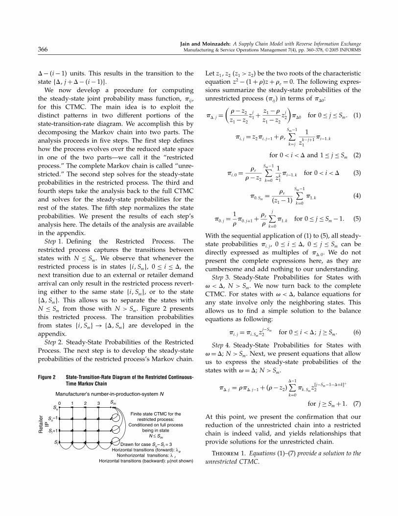
restricted process captures the transitions betweenstates with N ≤ Sm. We observe that whenever therestricted process is in states �i Sm�, 0 ≤ i ≤ �, thenext transition due to an external or retailer demandarrival can only result in the restricted process revert-ing either to the same state �i Sm�, or to the state�� Sm�. This allows us to separate the states withN ≤ Sm from those with N > Sm. Figure 2 presentsthis restricted process. The transition probabilitiesfrom states �i Sm� → �� Sm� are developed in theappendix.Step 2. Steady-State Probabilities of the Restricted

Process. The next step is to develop the steady-stateprobabilities of the restricted process’s Markov chain.

Figure 2 State-Transition-Rate Diagram of the Restricted Continuous-Time Markov Chain

0 1 2 3 Sm

Manufacturer’s number-in-production-system N

Finite state CTMC for therestricted process:

Conditioned on full processbeing in state

N ≤ Sm

Ret

aile

rIP

Su

Sl

Su–1

Sl+1

Drawn for case Su– Sl = 3Horizontal transitions (forward): λe

Nonhorizontal transitions: λ rHorizontal transitions (backward): µ(not shown)

Let z1 z2 �z1 > z2� be the two roots of the characteristicequation z2 − �1+ ��z+ �e = 0. The following expres-sions summarize the steady-state probabilities of theunrestricted process ��ij � in terms of ��0:

��� j =(�− z2z1− z2

zj1+

z1−�z1− z2

zj2

)��0 for 0≤ j ≤ Sm� (1)

�i� j = z2�i� j−1+�rSm−1∑k=j

1

zk−j+11

�i−1� k

for 0< i <� and 1≤ j ≤ Sm (2)

�i�0 =�r

�− z2Sm−1∑k=0

1zk1�i−1� k for 0< i <� (3)

�0� Sm =�r

�z1− 1�

Sm−1∑k=0

�1� k (4)

�0� j =1��0� j+1+

�r�

j∑k=0�1� k for 0≤ j ≤ Sm− 1� (5)

With the sequential application of (1) to (5), all steady-state probabilities �i� j , 0 ≤ i ≤ �, 0 ≤ j ≤ Sm can bedirectly expressed as multiples of ���0. We do notpresent the complete expressions here, as they arecumbersome and add nothing to our understanding.Step 3. Steady-State Probabilities for States with

" < �, N > Sm. We now turn back to the completeCTMC. For states with " < �, balance equations forany state involve only the neighboring states. Thisallows us to find a simple solution to the balanceequations as following:

�i� j =�i�Smzj−Sm2 for 0≤ i < �% j ≥ Sm� (6)

Step 4. Steady-State Probabilities for States with"=�; N > Sm. Next, we present equations that allowus to express the steady-state probabilities of thestates with "=�; N > Sm.

��� j = ���� j−1+ ��− z2��−1∑k=0�k�Smz

�j−Sm−1−�+k!+2

for j ≥ Sm+ 1� (7)

At this point, we present the confirmation that ourreduction of the unrestricted chain into a restrictedchain is indeed valid, and yields relationships thatprovide solutions for the unrestricted chain.

Theorem 1. Equations (1)–(7) provide a solution to theunrestricted CTMC.

Jain and Moinzadeh: A Supply Chain Model with Reverse Information ExchangeManufacturing & Service Operations Management 7(4), pp. 360–378, © 2005 INFORMS 367

Proof. See the appendix.Step 5. Determining ���0. Equations (1) to (7) allow

us to write all probabilities �i� j in terms of ���0. We cannow take the traditional normalization step of equat-ing the sum of probabilities �

∑�i=0

∑j=0�i� j � to 1 and

determining ���0. The following theorem provides asimplification of this step by showing that the sum ofprobability masses at states with N = 0 equals 1− �.Even though our model represents a queuing systemthat is controlled by the state-dependent actions of theretailer, the following relationship is similar to the oneobserved in a simple uncontrolled single-server queu-ing system, such as an M/M/1 queue.

Theorem 2.∑�i=0�i�0 = 1−�.

Proof. See the appendix.

4. Retailer’s Performance MeasuresIn this section, we determine the optimal policy andcost for the retailer under reverse information sharing.We also present computational results that providemanagerial insights into the value of this informationfor the retailer.

4.1. Retailer’s Optimal Policy and CostTo develop retailer’s cost, we follow the unit-costingconvention where each unit ordered by the retaileris assigned a cost incurred for satisfying the corre-sponding demand. Let C�i j k! denote the expectedcost assigned to the kth unit ordered when "= i andN = j . Let C�i j! be the expected total cost assigned toan ordering epoch when the state is "= i and N = j .

C�i j!=�−i+1∑k=1

C�i j k! for j ≥ Sm

C�i j!=C�i j 1! for i= 0% j < Sm

C�i j!= 0 for i > 0% j < Sm

We can write the average total cost per time unit forthe retailer as CSl�� = �r

∑�i=0

∑j=0�i� jC�i j!.

The average cost assigned to each unit ordered,C�i j k!, depends on the time difference between thearrival of the unit at the retailer and the occurrenceof the corresponding demand that will be satisfiedby this unit. For j < Sm, the ordered unit will arriveafter the transportation time T . When j ≥ Sm, in addi-tion to the fixed transportation time T , the ordered

units will each experience a delay at the manufactureras the manufacturer is out of stock at the time theretailer placed the order. In such cases, the delay expe-rienced by the kth unit in the order will be equal tothe time until j − Sm+ k units have been processed inthe production system. In either case, the correspond-ing demand, which will be satisfied by the kth unitin the order, will arrive after Sl+ i+ k− 1 subsequentdemands.First, consider the case j ≥ Sm. Let u = Sl + i +

k − 1 and v = j − Sm + k. The random variable rep-resenting the time until the corresponding demandoccurs is Erlang��r u�, and time until supply is avail-able is Erlang�� v�. Note that Erlang�' w� representsa random variable that is equal to the sum of wexponentially distributed random variables, each withrate '. Now

C�i j k! = hE�Erlang��r u�− T −Erlang�� v�!+

+ bE�T +Erlang�� v�−Erlang��r u�!+

= �h+ b�E�Erlang��r u�− T −Erlang�� v�!+

− b[u

�r− T − v

�

]

where �x!+ =max�0 x�. For the sake of completeness,when u≤ 0, the cost function is given by

C�i j k!= b[T + v

�+ u

�r

]�

Next, consider the case j < Sm. Clearly, for 1 ≤ i ≤ �,the retailer does not place an order, and therefore thecost assigned to the order epoch is zero. For i = 0,the retailer always orders one unit. Because the mate-rial is available in the warehouse, the lead time forthis order is always T , and therefore its correspondingaverage cost is always the same. Thus, C�i j 1! fori= 0; j < Sm has the same value; let us call it C�0 0 1!,which can be easily computed as

C�0 0 1!= �h+ b�E�Erlang��r Sl�− T !+ − b[Sl�r

− T]

for 0≤ j < Sm�The computational burden mainly consists of comput-ing C�i j k! values. The following observation helpsus ease this burden: C�i j k!=C�i+k−1 j+k−1 1!.We only need to evaluate C�i j 1! once for j < Sm,

Jain and Moinzadeh: A Supply Chain Model with Reverse Information Exchange368 Manufacturing & Service Operations Management 7(4), pp. 360–378, © 2005 INFORMS

and once for each state �i j�, j ≥ Sm. For the probabili-ties �i� j required for computing CSl��, we only need toknow the values of �i�Sm , 0≤ i≤�; because

∑Sm−1j=0 �0� j ,

as well as all �i� j 0≤ i≤�, j ≥ Sm+ 1, can be directlyexpressed in terms of �i�Sm , 0 ≤ i ≤ �. See proof ofTheorem 2 for the expression of

∑Sm−1j=0 �0� j .

For a given manufacturer base-stock Sm, and re-tailer’s ordering policy �Sl Su�, �= Su−Sl, the retailercost rate is denoted by CSl��. We now prove a propertyof CSl��.

Theorem 3. For a given � and Sm, CSl�� is convexin Sl.

Proof. See the appendix.This result allows us to efficiently search for the

optimal S∗l ��� for a given �. An observation based onextensive computations further simplifies the searchfor optimal policy: S∗l ��� is nonincreasing in �. Thealgorithm we present below arrived at the opti-mal policy parameters (confirmed by an exhaustivesearch) in all the cases in extensive experimentation.Step 1. Set �= 0, compute S∗l �0� and CS∗l �0� 0.Step 2. �=�+ 1. Find S∗l ��� as follows:2(a) Set S∗l ���= S∗l ��− 1�, compute CS∗l ��� �2(b) S∗l ��� = S∗l ��� − 1, If CS∗l ��� � < CS∗l ���+1 �, go

to Step 2(b) else, S∗l ���= S∗l ���+ 1, go to Step 3.Step 3. If CS∗l ��� � < CS∗l ��−1� �−1, go to Step 2, else

�∗ =�− 1, stop.Finally, it is evident intuitively that the retailer canbe no worse off using the information through astate-dependent base-stock policy. If current informa-tion suggests a congested supply system, the retailerhas an opportunity to order extra before the externalarrivals generated by walk-ins create further conges-tion. The retailer uses this information to opportunis-tically sneak in orders for extra units, and thus avoidspossibly longer lead times. As we discuss in the nextsection, however, we have identified instances whenthe retailer continues to use the single base-stock pol-icy after it obtains access to current information.

4.2. Computational Results for the RetailerIn this section, we study the impact of reverse infor-mation sharing on the retailer, using a numericalexperiment. We set the mean service rate, �, and hold-ing cost rate, h, to unity. Then, we vary the overallsystem utilization, �; the fraction of retailer load in

the total utilization, �r/�, the transportation time, T ;and the backorder cost rate at the retailer, b. The val-ues of the manufacturer’s base-stock level, Sm, areset to provide the service level, 'm, under the caseSl = Su. The values of T and b are chosen relative to �and h, respectively. We report our observations basedon computing the optimal policy and correspond-ing performance measures for a set of 216 probleminstances consisting of the following parameter val-ues: � ∈ �0�7 0�8 0�9�, �r/� ∈ �0�2 0�4 0�6 0�8�, 'm ∈�0�7 0�9 0�95� T ∈ �1 5�, b ∈ �7/3 9 19�. We chosethese values to reflect the range found in practice.For utilization �, the historical data in the FederalReserve Statistical Release (2004) suggests that ourchosen range represents a wide variety of industries.For relative retailer size �r/�, the chosen values repre-sent a wide range of possibilities. In the context of ourmodel, what matters is the relative size �r/� becausethe load imposed by a large retailer may constituteeither a large or a small portion of the manufacturer’stotal load. For example, a large retailer such as Wal-Mart is a major customer to Procter and Gamble, butit makes up only about 10% of Procter and Gamble’sdollar revenue. For a smaller manufacturer, on theother hand, Wal-Mart may be responsible for a largerportion of total load. To be complete, we focus on awide range of �r/� values in our numerical experi-ment. For manufacturer’s service level, 'm, we alsoconsider a wide range of values, as previous work hasreported and used service levels as low as 0.5 (Ernstand Cohen 1992) and as high as 0.99 (Cachon andFisher 1997). The values of b have been chosen to rep-resent the same range in the newsboy service levelsfor the retailer.

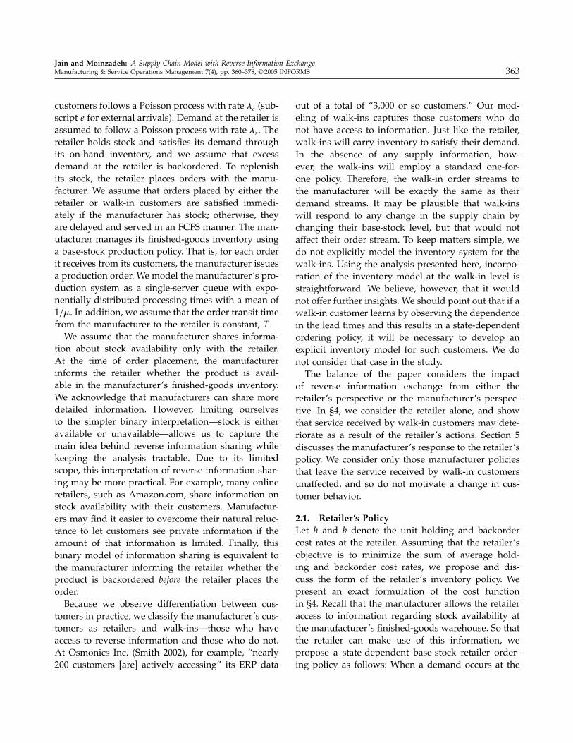
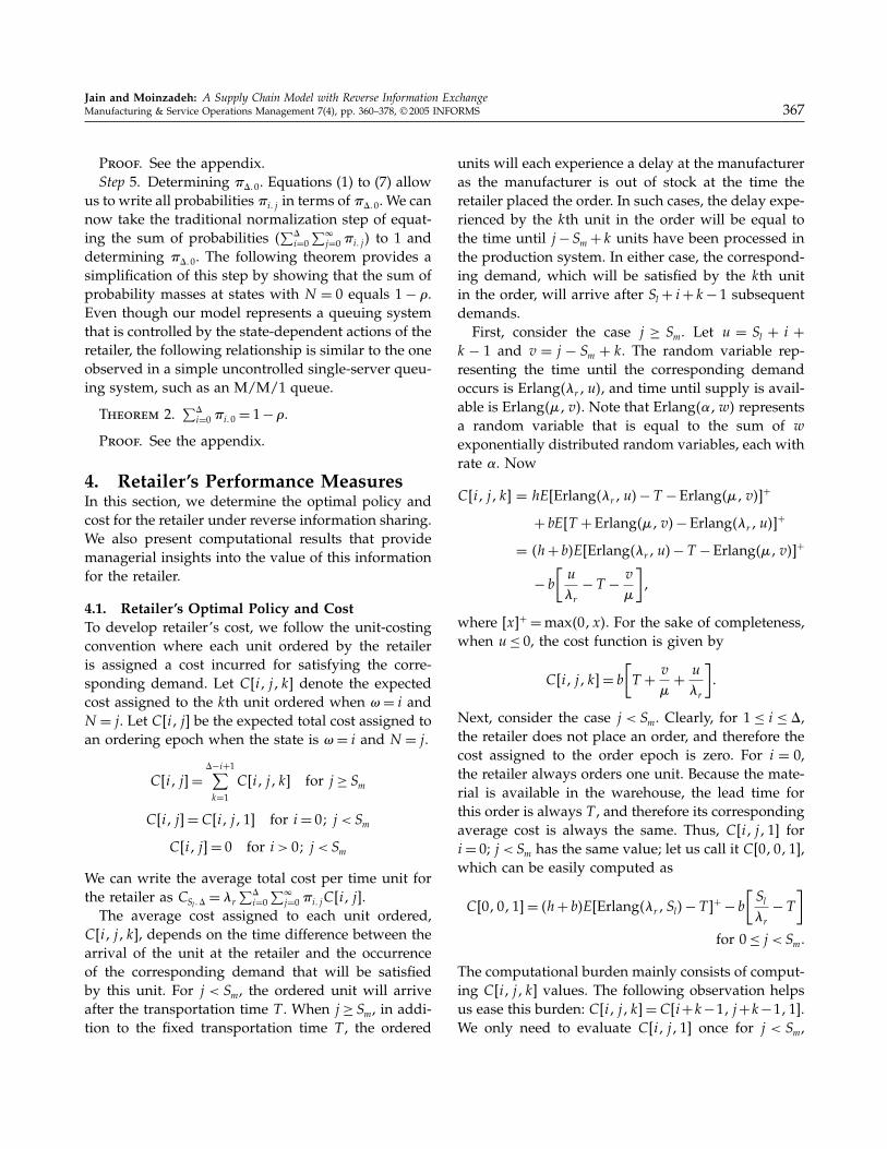
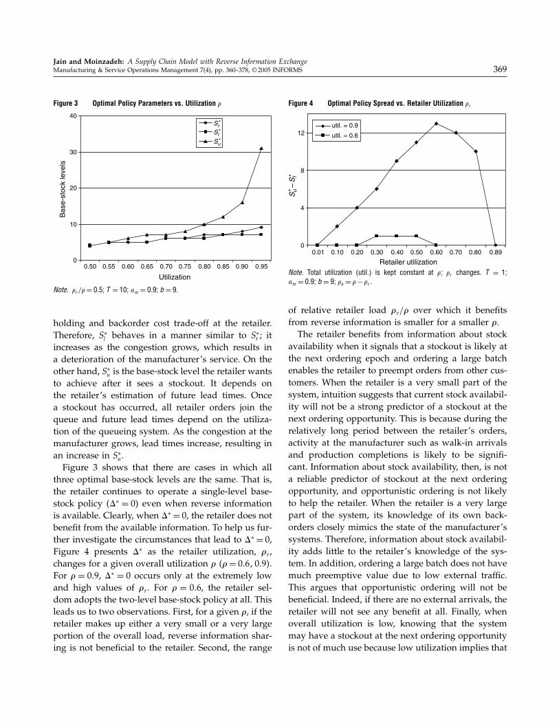
4.2.1. Retailer’s Optimal Policy Parameters. Wereport our observations by presenting results for aspecific combination of parameters. However, theseobservations hold for all problem instances we havedescribed previously. Figure 3 depicts the optimalpolicy parameters �S∗l S

∗u� as well as S

∗r , the optimal

base-stock level if the retailer does not use the infor-mation, as the overall utilization, �, is varied, whilethe ratio �r/� is fixed. Note that while S∗l tracks S∗rquite closely, S∗u increases as � increases. We can intu-itively explain this behavior by considering the rolesof each of the two base-stock levels S∗l and S

∗u. We sug-

gest that S∗l is mainly determined by considering the

Jain and Moinzadeh: A Supply Chain Model with Reverse Information ExchangeManufacturing & Service Operations Management 7(4), pp. 360–378, © 2005 INFORMS 369

Figure 3 Optimal Policy Parameters vs. Utilization �

0

10

20

30

40

0.50 0.55 0.60 0.65 0.70 0.75 0.80 0.85 0.90 0.95

Utilization

Bas

e-st

ock

leve

ls

Sr*

Sl*

Su*

Note. �r /�= 0�5; T = 10; �m = 0�9; b= 9.

holding and backorder cost trade-off at the retailer.Therefore, S∗l behaves in a manner similar to S∗r ; itincreases as the congestion grows, which results ina deterioration of the manufacturer’s service. On theother hand, S∗u is the base-stock level the retailer wantsto achieve after it sees a stockout. It depends onthe retailer’s estimation of future lead times. Oncea stockout has occurred, all retailer orders join thequeue and future lead times depend on the utiliza-tion of the queueing system. As the congestion at themanufacturer grows, lead times increase, resulting inan increase in S∗u.Figure 3 shows that there are cases in which all

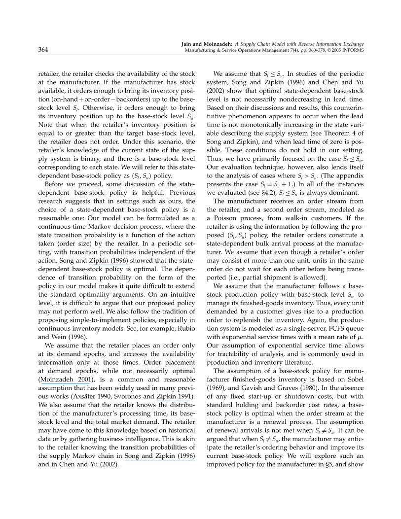
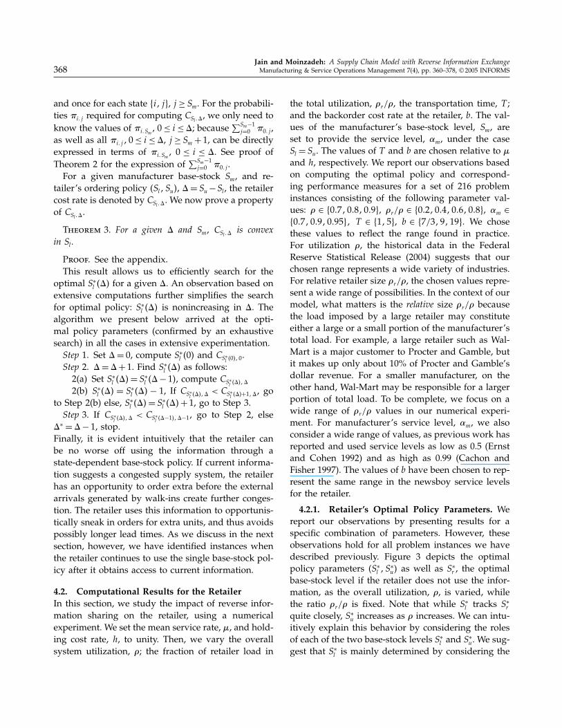
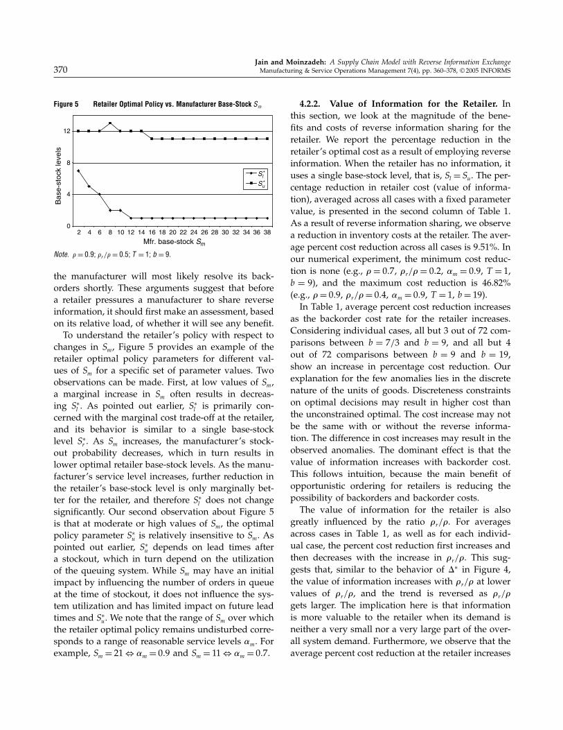
three optimal base-stock levels are the same. That is,the retailer continues to operate a single-level base-stock policy ��∗ = 0� even when reverse informationis available. Clearly, when �∗ = 0, the retailer does notbenefit from the available information. To help us fur-ther investigate the circumstances that lead to �∗ = 0,Figure 4 presents �∗ as the retailer utilization, �r ,changes for a given overall utilization � ��= 0�6 0�9�.For � = 0�9, �∗ = 0 occurs only at the extremely lowand high values of �r . For � = 0�6, the retailer sel-dom adopts the two-level base-stock policy at all. Thisleads us to two observations. First, for a given �, if theretailer makes up either a very small or a very largeportion of the overall load, reverse information shar-ing is not beneficial to the retailer. Second, the range

Figure 4 Optimal Policy Spread vs. Retailer Utilization �r

0

4

8

12

0.01 0.10 0.20 0.30 0.40 0.50 0.60 0.70 0.80 0.89

Retailer utilization

util. = 0.9

util. = 0.6

Su

–S

l**

Note. Total utilization (util.) is kept constant at �; �r changes. T = 1;�m = 0�9; b= 9; �e = �− �r .

of relative retailer load �r/� over which it benefitsfrom reverse information is smaller for a smaller �.The retailer benefits from information about stock

availability when it signals that a stockout is likely atthe next ordering epoch and ordering a large batchenables the retailer to preempt orders from other cus-tomers. When the retailer is a very small part of thesystem, intuition suggests that current stock availabil-ity will not be a strong predictor of a stockout at thenext ordering opportunity. This is because during therelatively long period between the retailer’s orders,activity at the manufacturer such as walk-in arrivalsand production completions is likely to be signifi-cant. Information about stock availability, then, is nota reliable predictor of stockout at the next orderingopportunity, and opportunistic ordering is not likelyto help the retailer. When the retailer is a very largepart of the system, its knowledge of its own back-orders closely mimics the state of the manufacturer’ssystems. Therefore, information about stock availabil-ity adds little to the retailer’s knowledge of the sys-tem. In addition, ordering a large batch does not havemuch preemptive value due to low external traffic.This argues that opportunistic ordering will not bebeneficial. Indeed, if there are no external arrivals, theretailer will not see any benefit at all. Finally, whenoverall utilization is low, knowing that the systemmay have a stockout at the next ordering opportunityis not of much use because low utilization implies that

Jain and Moinzadeh: A Supply Chain Model with Reverse Information Exchange370 Manufacturing & Service Operations Management 7(4), pp. 360–378, © 2005 INFORMS

Figure 5 Retailer Optimal Policy vs. Manufacturer Base-Stock Sm

0

4

8

12

2 4 6 8 10 12 14 16 18 20 22 24 26 28 30 32 34 36 38

Mfr. base-stock Sm

Bas

e-st

ock

leve

ls

Su*

Sl*

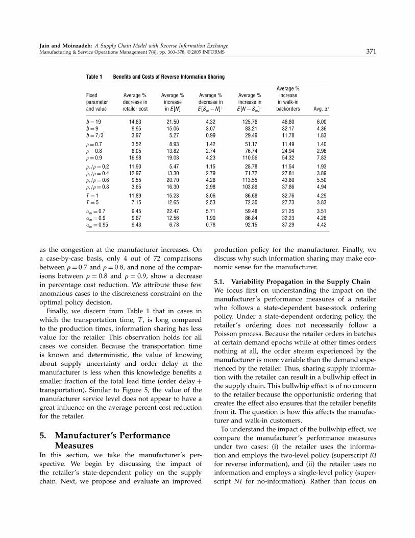
Note. �= 0�9; �r /�= 0�5; T = 1; b= 9.

the manufacturer will most likely resolve its back-orders shortly. These arguments suggest that beforea retailer pressures a manufacturer to share reverseinformation, it should first make an assessment, basedon its relative load, of whether it will see any benefit.To understand the retailer’s policy with respect to

changes in Sm, Figure 5 provides an example of theretailer optimal policy parameters for different val-ues of Sm for a specific set of parameter values. Twoobservations can be made. First, at low values of Sm,a marginal increase in Sm often results in decreas-ing S∗l . As pointed out earlier, S∗l is primarily con-cerned with the marginal cost trade-off at the retailer,and its behavior is similar to a single base-stocklevel S∗r . As Sm increases, the manufacturer’s stock-out probability decreases, which in turn results inlower optimal retailer base-stock levels. As the manu-facturer’s service level increases, further reduction inthe retailer’s base-stock level is only marginally bet-ter for the retailer, and therefore S∗l does not changesignificantly. Our second observation about Figure 5is that at moderate or high values of Sm, the optimalpolicy parameter S∗u is relatively insensitive to Sm. Aspointed out earlier, S∗u depends on lead times aftera stockout, which in turn depend on the utilizationof the queuing system. While Sm may have an initialimpact by influencing the number of orders in queueat the time of stockout, it does not influence the sys-tem utilization and has limited impact on future leadtimes and S∗u. We note that the range of Sm over whichthe retailer optimal policy remains undisturbed corre-sponds to a range of reasonable service levels 'm. Forexample, Sm = 21⇔ 'm = 0�9 and Sm = 11⇔ 'm = 0�7.

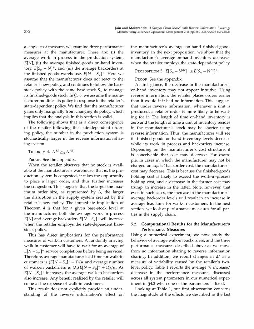
4.2.2. Value of Information for the Retailer. Inthis section, we look at the magnitude of the bene-fits and costs of reverse information sharing for theretailer. We report the percentage reduction in theretailer’s optimal cost as a result of employing reverseinformation. When the retailer has no information, ituses a single base-stock level, that is, Sl = Su. The per-centage reduction in retailer cost (value of informa-tion), averaged across all cases with a fixed parametervalue, is presented in the second column of Table 1.As a result of reverse information sharing, we observea reduction in inventory costs at the retailer. The aver-age percent cost reduction across all cases is 9.51%. Inour numerical experiment, the minimum cost reduc-tion is none (e.g., �= 0�7, �r/�= 0�2, 'm = 0�9, T = 1,b = 9), and the maximum cost reduction is 46.82%(e.g., �= 0�9, �r/�= 0�4, 'm = 0�9, T = 1, b= 19).In Table 1, average percent cost reduction increases

as the backorder cost rate for the retailer increases.Considering individual cases, all but 3 out of 72 com-parisons between b = 7/3 and b = 9, and all but 4out of 72 comparisons between b = 9 and b = 19,show an increase in percentage cost reduction. Ourexplanation for the few anomalies lies in the discretenature of the units of goods. Discreteness constraintson optimal decisions may result in higher cost thanthe unconstrained optimal. The cost increase may notbe the same with or without the reverse informa-tion. The difference in cost increases may result in theobserved anomalies. The dominant effect is that thevalue of information increases with backorder cost.This follows intuition, because the main benefit ofopportunistic ordering for retailers is reducing thepossibility of backorders and backorder costs.The value of information for the retailer is also

greatly influenced by the ratio �r/�. For averagesacross cases in Table 1, as well as for each individ-ual case, the percent cost reduction first increases andthen decreases with the increase in �r/�. This sug-gests that, similar to the behavior of �∗ in Figure 4,the value of information increases with �r/� at lowervalues of �r/�, and the trend is reversed as �r/�gets larger. The implication here is that informationis more valuable to the retailer when its demand isneither a very small nor a very large part of the over-all system demand. Furthermore, we observe that theaverage percent cost reduction at the retailer increases

Jain and Moinzadeh: A Supply Chain Model with Reverse Information ExchangeManufacturing & Service Operations Management 7(4), pp. 360–378, © 2005 INFORMS 371

Table 1 Benefits and Costs of Reverse Information Sharing

Average %Fixed Average % Average % Average % Average % increaseparameter decrease in increase decrease in increase in in walk-inand value retailer cost in E�N� E�Sm −N�+ E�N −Sm�

+ backorders Avg. �∗

b= 19 14�63 21�50 4.32 125�76 46.80 6.00b= 9 9�95 15�06 3.07 83�21 32.17 4.36b= 7/3 3�97 5�27 0.99 29�49 11.78 1.83

�= 0�7 3�52 8�93 1.42 51�17 11.49 1.40�= 0�8 8�05 13�82 2.74 76�74 24.94 2.96�= 0�9 16�98 19�08 4.23 110�56 54.32 7.83

�r /�= 0�2 11�90 5�47 1.15 28�78 11.54 1.93�r /�= 0�4 12�97 13�30 2.79 71�72 27.81 3.89�r /�= 0�6 9�55 20�70 4.26 113�55 43.80 5.50�r /�= 0�8 3�65 16�30 2.98 103�89 37.86 4.94

T = 1 11�89 15�23 3.06 86�68 32.76 4.29T = 5 7�15 12�65 2.53 72�30 27.73 3.83

�m = 0�7 9�45 22�47 5.71 59�48 21.25 3.51�m = 0�9 9�67 12�56 1.90 86�84 32.23 4.26�m = 0�95 9�43 6�78 0.78 92�15 37.29 4.42

as the congestion at the manufacturer increases. Ona case-by-case basis, only 4 out of 72 comparisonsbetween �= 0�7 and �= 0�8, and none of the compar-isons between � = 0�8 and � = 0�9, show a decreasein percentage cost reduction. We attribute these fewanomalous cases to the discreteness constraint on theoptimal policy decision.Finally, we discern from Table 1 that in cases in

which the transportation time, T , is long comparedto the production times, information sharing has lessvalue for the retailer. This observation holds for allcases we consider. Because the transportation timeis known and deterministic, the value of knowingabout supply uncertainty and order delay at themanufacturer is less when this knowledge benefits asmaller fraction of the total lead time (order delay+transportation). Similar to Figure 5, the value of themanufacturer service level does not appear to have agreat influence on the average percent cost reductionfor the retailer.

5. Manufacturer’s PerformanceMeasures

In this section, we take the manufacturer’s per-spective. We begin by discussing the impact ofthe retailer’s state-dependent policy on the supplychain. Next, we propose and evaluate an improved

production policy for the manufacturer. Finally, wediscuss why such information sharing may make eco-nomic sense for the manufacturer.

5.1. Variability Propagation in the Supply ChainWe focus first on understanding the impact on themanufacturer’s performance measures of a retailerwho follows a state-dependent base-stock orderingpolicy. Under a state-dependent ordering policy, theretailer’s ordering does not necessarily follow aPoisson process. Because the retailer orders in batchesat certain demand epochs while at other times ordersnothing at all, the order stream experienced by themanufacturer is more variable than the demand expe-rienced by the retailer. Thus, sharing supply informa-tion with the retailer can result in a bullwhip effect inthe supply chain. This bullwhip effect is of no concernto the retailer because the opportunistic ordering thatcreates the effect also ensures that the retailer benefitsfrom it. The question is how this affects the manufac-turer and walk-in customers.To understand the impact of the bullwhip effect, we

compare the manufacturer’s performance measuresunder two cases: (i) the retailer uses the informa-tion and employs the two-level policy (superscript RIfor reverse information), and (ii) the retailer uses noinformation and employs a single-level policy (super-script NI for no-information). Rather than focus on

Jain and Moinzadeh: A Supply Chain Model with Reverse Information Exchange372 Manufacturing & Service Operations Management 7(4), pp. 360–378, © 2005 INFORMS

a single cost measure, we examine three performancemeasures at the manufacturer. These are: (i) theaverage work in process in the production system,E�N !, (ii) the average finished-goods on-hand inven-tory, E�Sm − N!+, and (iii) the average backorders atthe finished-goods warehouse, E�N − Sm!+. Here weassume that the manufacturer does not react to theretailer’s new policy, and continues to follow the base-stock policy with the same base-stock Sm to manageits finished-goods stock. In §5.3, we assume the manu-facturer modifies its policy in response to the retailer’sstate-dependent policy. We find that the manufacturergains only marginally from changing its policy, whichimplies that the analysis in this section is valid.The following shows that as a direct consequence

of the retailer following the state-dependent order-ing policy, the number in the production system isstochastically larger in the reverse information shar-ing system.

Theorem 4. NRI ≥st NNI .

Proof. See the appendix.When the retailer observes that no stock is avail-

able at the manufacturer’s warehouse, that is, the pro-duction system is congested, it takes the opportunityto place a larger order, and thus further increasesthe congestion. This suggests that the larger the max-imum order size, as represented by �, the largerthe disruption in the supply system created by theretailer’s new policy. The immediate implication ofTheorem 4 is that for a given base-stock level atthe manufacturer, both the average work in processE�N ! and average backorders E�N −Sm!+ will increasewhen the retailer employs the state-dependent base-stock policy.This has direct implications for the performance

measures of walk-in customers. A randomly arrivingwalk-in customer will have to wait for an average ofE�N −Sm!+ service completions before being serviced.Therefore, average manufacturer lead time for walk-incustomers is �E�N − Sm!+ + 1�/� and average numberof walk-in backorders is ��e�E�N − Sm!+ + 1��/�. AsE�N − Sm!+ increases, the average walk-in backordersalso increase. Any benefit realized by the retailer willcome at the expense of walk-in customers.This result does not explicitly provide an under-

standing of the reverse information’s effect on

the manufacturer’s average on-hand finished-goodsinventory. In the next proposition, we show that themanufacturer’s average on-hand inventory decreaseswhen the retailer employs the state-dependent policy.

Proposition 5. E�Sm−NRI !+ ≤ E�Sm−NNI !+.

Proof. See the appendix.At first glance, the decrease in the manufacturer’s

on-hand inventory may not appear intuitive. Usingreverse information, the retailer places orders earlierthan it would if it had no information. This suggeststhat under reverse information, whenever a unit isproduced, a retailer order is more likely to be wait-ing for it. The length of time on-hand inventory iszero and the length of time a unit of inventory residesin the manufacturer’s stock may be shorter usingreverse information. Thus, the manufacturer will seeits finished-goods on-hand inventory levels decreasewhile its work in process and backorders increase.Depending on the manufacturer’s cost structure, itis conceivable that cost may decrease. For exam-ple, in cases in which the manufacturer may not becharged an explicit backorder cost, the manufacturer’scost may decrease. This is because the finished-goodsholding cost is likely to exceed the work-in-processholding cost, and a decrease in the former cost maytrump an increase in the latter. Note, however, thateven in such cases, the increase in the manufacturer’saverage backorder levels will result in an increase inaverage lead time for walk-in customers. In the nextsection, we look at performance measures for all par-ties in the supply chain.

5.2. Computational Results for the Manufacturer’sPerformance Measures

Using a numerical experiment, we now study thebehavior of average walk-in backorders, and the threeperformance measures described above as we movefrom no information sharing to reverse informationsharing. In addition, we report changes in �∗ as ameasure of variability caused by the retailer’s two-level policy. Table 1 reports the average % increase/decrease in the performance measures discussedacross all system parameters in our numerical exper-iment in §4.2 when one of the parameters is fixed.Looking at Table 1, our first observation concerns

the magnitude of the effects we described in the last

Jain and Moinzadeh: A Supply Chain Model with Reverse Information ExchangeManufacturing & Service Operations Management 7(4), pp. 360–378, © 2005 INFORMS 373

section. The retailer benefits by reverse informationsharing while walk-in customers see degradations inits performance measure. The manufacturer sees apercentage increase in its work in process, which isnumerically larger than the reduction it sees in itsfinished-goods on-hand inventory. From the manufac-turer’s perspective, the retailer’s push to share infor-mation results in degradation in the service walk-incustomers receive. The outcome, whether informationis shared or not, reflects a balance between these twoobservations. Clearly, our model does not capture allof the relevant aspects of the business situation thatmay influence the outcome, such as the power of theretailer versus the power of the walk-in customer, andthe profit function of the manufacturer. In the contextof our model, however, we can discuss how variousparameters may affect the outcome.Our second observation is that, as �r/� increases,

the percent increase in E�N !, percent decrease inE�Sm−N!+, and percent increase in E�N −Sm!+ all getlarger at first, and then decrease. Thus, the improve-ment in the retailer’s performance measure and thedegradation in walk-in customers’ performance mea-sure follow the same broad pattern.To further analyze this observation, we study the

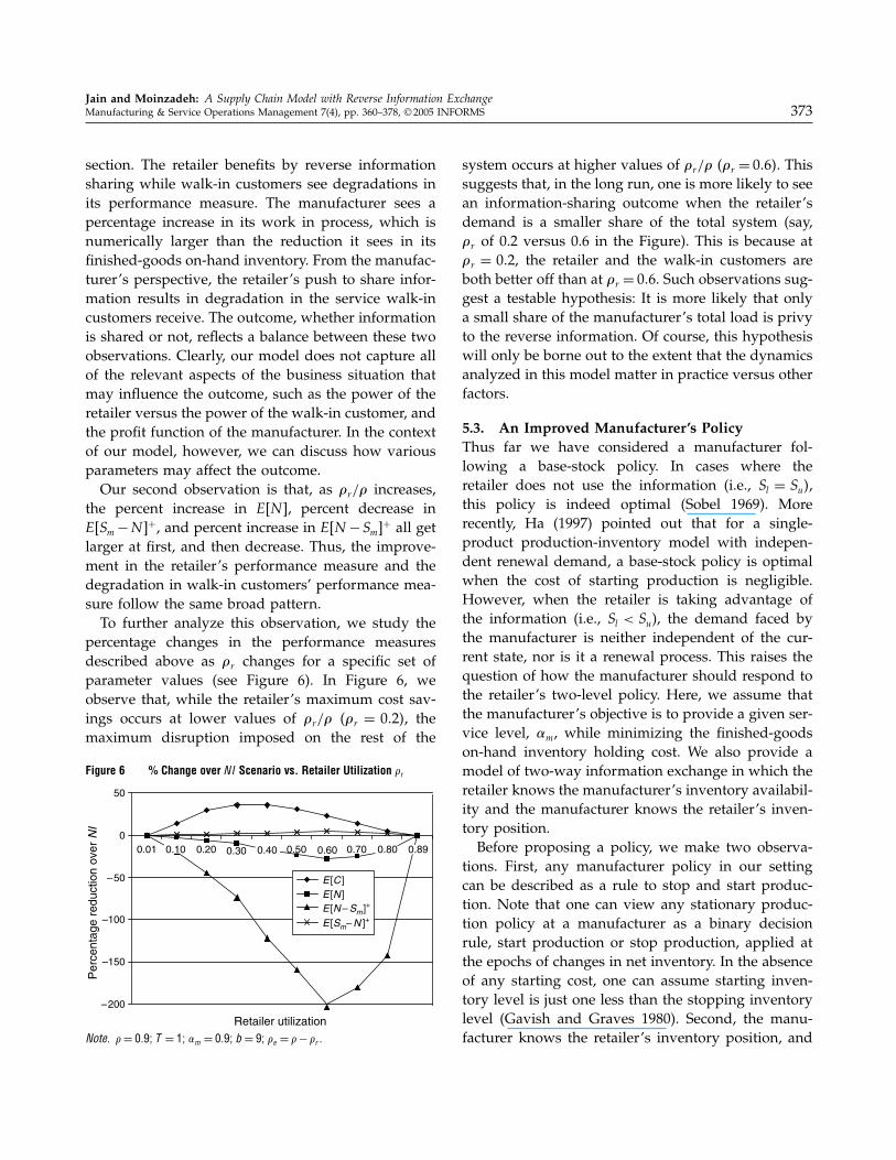
percentage changes in the performance measuresdescribed above as �r changes for a specific set ofparameter values (see Figure 6). In Figure 6, weobserve that, while the retailer’s maximum cost sav-ings occurs at lower values of �r/� ��r = 0�2�, themaximum disruption imposed on the rest of the

Figure 6 % Change over NI Scenario vs. Retailer Utilization �r

–100

–200

–150

–50

0

50

0.01 0.20 0.30 0.60 0.70

Retailer utilization

Per

cent

age

redu

ctio

n ov

erN

I

E [C ]E [N ]E [N – Sm]+

E [Sm– N ]+

0.10 0.40 0.50 0.80 0.89

Note. �= 0�9; T = 1; �m = 0�9; b= 9; �e = �− �r .

system occurs at higher values of �r/� ��r = 0�6�. Thissuggests that, in the long run, one is more likely to seean information-sharing outcome when the retailer’sdemand is a smaller share of the total system (say,�r of 0.2 versus 0.6 in the Figure). This is because at�r = 0�2, the retailer and the walk-in customers areboth better off than at �r = 0�6. Such observations sug-gest a testable hypothesis: It is more likely that onlya small share of the manufacturer’s total load is privyto the reverse information. Of course, this hypothesiswill only be borne out to the extent that the dynamicsanalyzed in this model matter in practice versus otherfactors.

5.3. An Improved Manufacturer’s PolicyThus far we have considered a manufacturer fol-lowing a base-stock policy. In cases where theretailer does not use the information (i.e., Sl = Su�,this policy is indeed optimal (Sobel 1969). Morerecently, Ha (1997) pointed out that for a single-product production-inventory model with indepen-dent renewal demand, a base-stock policy is optimalwhen the cost of starting production is negligible.However, when the retailer is taking advantage ofthe information (i.e., Sl < Su), the demand faced bythe manufacturer is neither independent of the cur-rent state, nor is it a renewal process. This raises thequestion of how the manufacturer should respond tothe retailer’s two-level policy. Here, we assume thatthe manufacturer’s objective is to provide a given ser-vice level, 'm, while minimizing the finished-goodson-hand inventory holding cost. We also provide amodel of two-way information exchange in which theretailer knows the manufacturer’s inventory availabil-ity and the manufacturer knows the retailer’s inven-tory position.Before proposing a policy, we make two observa-

tions. First, any manufacturer policy in our settingcan be described as a rule to stop and start produc-tion. Note that one can view any stationary produc-tion policy at a manufacturer as a binary decisionrule, start production or stop production, applied atthe epochs of changes in net inventory. In the absenceof any starting cost, one can assume starting inven-tory level is just one less than the stopping inventorylevel (Gavish and Graves 1980). Second, the manu-facturer knows the retailer’s inventory position, and

Jain and Moinzadeh: A Supply Chain Model with Reverse Information Exchange374 Manufacturing & Service Operations Management 7(4), pp. 360–378, © 2005 INFORMS

thus can anticipate the period when the retailer willnot be ordering in an effort to bring down its inven-tory position from Su to Sl. The manufacturer can takeadvantage of this anticipated low-demand period bycarrying lower on-hand inventory than it does duringperiods when the retailer is ordering. The proposedpolicy can be stated this way: If the retailer inventoryposition is less than or equal to Sip �Sl ≤ Sip < Su�, stopproduction when the manufacturer’s on-hand inven-tory reaches Smh; otherwise, stop production at Sml(where Sml < Smh�. Start production whenever on-handinventory drops below the stopping level. We notethat it is possible to implement a version of this policywith Sip = Sl, even if the manufacturer has no knowl-edge of the retailer’s inventory position. Our method-ology for Markov chain analysis, developed earlier, iseasily applicable here. (See the appendix for details.)Unfortunately, from the manufacturer’s perspective,

the cost saving of using this improved policy insteadof the standard single base-stock policy is miniscule.For example, let �e = �r = 0�4, �= 1, T = 1, h= 1 b =9 'm = 0�9. When the manufacturer is using a single-level base-stock policy, the retailer’s optimal policyis Sl = 1, Su = 5, and the manufacturer achieves thedesired service level at Sm = 12. We note that this isan equilibrium solution in the sense that, given oneparty’s policy, the other has no incentive to change itspolicy. The manufacturer provides a service level of90.64% with an average on-hand inventory, E�Sm−N!+of 8.1685. If the manufacturer uses the improved pol-icy, the optimal policy would be Sml = 6, Sip = 1, Smh =12, which would provide a service level of 90.07%with an average on-hand inventory of 8.0089. We notethat under both scenarios the retailer’s optimal policyremains Sl = 1, Su = 5 even as its cost increases slightlyunder the two-level policy at the manufacturer. Ourtwo observations—that the manufacturer’s cost reduc-tion is small and the retailer’s optimal �Sl Su� remainsunaffected—are verified across the parameter rangesdescribed in §4.2. This leads us to infer that evenin two-way information exchange, the managerialinsights drawn earlier will hold.Intuitively, the two-level policy increases the man-

ufacturer’s freedom to set policy, and allows it todeliver the required service level while reducingthe base-stock level. However, given that the manu-facturer’s supply system is a controlled productionqueue with finite production rate, and not the tradi-

tional outside supplier with infinite capacity and fixedlead times, the manufacturer’s decisions are limited to“when to stop production” instead of the traditional“when to place each order.” This explains the mod-est size of cost reduction. The manufacturer’s deci-sion space is constrained, and so it does not havemuch room to react to the current information. Giventhis limitation of the improved policy, we will limitourselves to a single-level policy at the manufacturer,while developing managerial insights into the manu-facturer’s actions in the next section.

5.4. Economic Rationale for ReverseInformation Sharing

We now investigate reverse information sharing froma purely economic point of view for manufacturers:Are there situations in which reverse informationsharing can benefit them? We suggest that sharingreverse information can be a tool to induce the retailerto increase its demand. For instance, if a retailerbuys only a portion of its demand from the man-ufacturer, providing reverse information may givethe retailer incentive to transfer a larger portion ofits demand to the manufacturer. This will gener-ate more revenues for the manufacturer, but willalso increase the congestion in the production sys-tem. These outcomes may justify reverse informationsharing for the manufacturer. Any such justificationmust also consider the impact of the retailer’s andthe manufacturer’s policies on walk-in customers. Inour study, we consider only those cases in whichthe service received by walk-in customers remainsthe same. Therefore, walk-in customers have no rea-son to change their behavior. We present an exampleand discuss the manufacturer’s incentive for sharingreverse information.Consider the situation in which the manufacturer

experiences an external demand rate of �e = 0�4 andits policy is to set the base-stock Sm to provide aservice level of 'm = 0�9. Other relevant parametersare � = 1, T = 1, h = 1, b = 9. The retailer decidesits demand rate. In the following, we consider theretailer’s problem under two scenarios, with andwithout reverse information.To keep the example simple, we assume a specific

demand-and-supply model for the retailer. Each of theretailer’s customers is assumed to be contributing .towards a total demand rate of /r . We assume dual

Jain and Moinzadeh: A Supply Chain Model with Reverse Information ExchangeManufacturing & Service Operations Management 7(4), pp. 360–378, © 2005 INFORMS 375

supply modes for the retailer. One mode is the man-ufacturer in our model, and the other is an externalsource exogenous to our model. The external sourcecharges a higher per-unit price we than the manufac-turer, but it has unlimited capacity, can deliver directlyto the retailer’s customers out of its own stock andagrees to compensate for any backorder cost incurredby the retailer due to delayed supplies. The manu-facturer charges a smaller price wm, but has a lim-ited capacity, can only deliver to the retailer with anadditional time lag T , and can only commit to a self-specified service level 'm. Both sources require a com-mitted order rate from the retailer. In such a situation,the retailer carries inventory only for the deliveriesfrom the manufacturer, assigns some customers (totaldemand rate �r ) to be supplied from its own inven-tory, and assigns other customers (total demand rate/r −�r ) to be supplied directly from the external sup-plier’s inventory.To find the optimal �r , the retailer uses a marginal

argument. Let C∗��r � be the optimal inventory costif the retailer satisfies an average of �r units of itsdemand from the manufacturer. For any �r , C∗��r � iscomputed at the equilibrium policy combination Sm,Sl, Su, under the condition Sl = Su to reflect no infor-mation sharing. Recall that the manufacturer’s policyis to set Sm to provide 'm = 0�9, and the retailer usesthe optimal single-level base-stock policy. The equilib-rium occurs when neither the retailer nor the manu-facturer has an incentive to deviate from its policy. Let�C∗��r �=C∗��r +.�−C∗��r � be the marginal increasein cost over an increase in the retailer’s demand of themanufacturer. The marginal argument suggests thatthe retailer would assign a customer’s demand streamto the manufacturer as long as wm.+ �C∗��r � ≤ we..In this example, we use . = 0�0001. We can numeri-cally confirm that �C∗��r � is positive and increasingin �r , and therefore there is a unique optimal solu-tion �∗r to the retailer’s problem. We note that there is aone-to-one correspondence between the two sources’price difference we − wm and optimal decision �∗r .Let us pick one case: we−wm = 33�0746⇔ �∗r = 0�4.The corresponding equilibrium policy combination isSm = 10, Sl = Su = 1. The retailer cost is 2.27743, and themanufacturer has an average finished-goods on-handinventory, E�Sm − N!+ of 6.4295, to provide a servicelevel of 89.2626%. The number of average walk-inbackorders is 0.5717.

Next, suppose reverse information is shared. Again,the retailer will decide its optimal �r by searchingfor the smallest �r to satisfy wm. + �C∗��r � ≤ we.

(we keep we −wm = 33�0746 to be consistent with theno-information case). Now, �C∗��r � is a different func-tion. For any �r , �C∗��r � is computed at the equilib-rium policy combination Sm, Sl, Su, without enforcingSl = Su. At the equilibrium, the manufacturer sets Smto provide 'm at lowest cost, the retailer sets Sl, Suto minimize its own cost, and given the other party’spolicy neither has any incentive to deviate from itsown policy. We numerically find the optimal decision�∗r = 0�46, with the corresponding equilibrium policy:Sm = 18, Sl = 1, Su = 8. We assume that /r is largeenough not to constrain the retailer’s choice of �r . Theretailer cost is 1.87877 and the manufacturer’s aver-age on-hand inventory is 12.0768. Clearly, the man-ufacturer has to increase Sm to maintain service. Theservice level 'm is 90.06% and the number of averagewalk-in backorders is 0.5425.Thus, the retailer’s cost rate decreases due to reverse

information from �we�/r − 0�40� + wm0�40 + 2�27743�to �we�/r − 0�46� + wm0�46 + 1�87877�, resulting in asavings of ��we − wm�0�06 + 0�39866�. The manufac-turer’s profit rate changes from �wm0�40 − xm0�40 −hm6�4295� to �wm0�46 − xm0�46 − hm12�0768�, wherexm is the production and material cost per unit andhm is the holding cost rate at the manufacturer’sfinished-goods inventory. The manufacturer’s profitwill increase using reverse information sharing if themanufacturer’s profit margin per unit �wm − xm� islarger than a critical value. This analysis suggests thatfor any given parameter combination, there may exista revenue and cost structure that would justify reverseinformation sharing for the manufacturer while reduc-ing the retailer’s cost and keeping the service levelfor walk-in customers the same. It also suggests thatsupply chains in which manufacturers have a highprofit margin are more likely to use reverse informa-tion sharing.Because we wish to highlight the issue in terms of

operating measures rather than exogenous parame-ters, in this discussion we have not assumed specificvalues for the per-unit cost parameters, we, wm, xm.Here, the manufacturer’s decision to share informa-tion depends on the trade-off between the increasein the retailer’s demand rate (benefit of additional

Jain and Moinzadeh: A Supply Chain Model with Reverse Information Exchange376 Manufacturing & Service Operations Management 7(4), pp. 360–378, © 2005 INFORMS

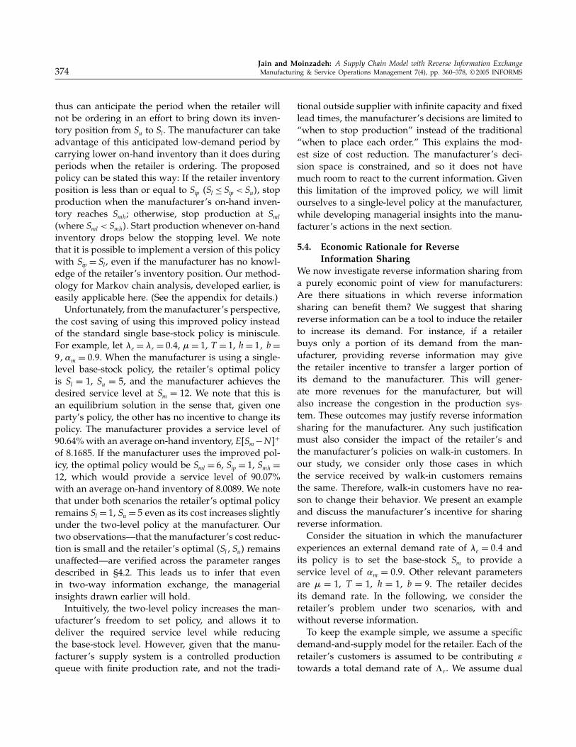
revenue) and the increase in finished-goods on-handinventory (cost of additional holding charges). Theincrease in the retailer’s rate is a consequence ofchange in the retailer’s cost due to information shar-ing. The increase in the finished-goods on-hand inven-tory is required to keep the service level fixed so thatexternal customers continue to experience the sameservice. Now we will focus on this operating measurestrade-off for the manufacturer.Figure 7 illustrates the trade-off by plotting the

retailer cost and manufacturer on-hand inventory bothbefore and after reverse information sharing. We notethat, for a given �r , reverse information sharing notonly reduces the retailer’s cost, but also reduces thegradient of the retailer cost ��C∗��r �/.�. This moti-vates the retailer to increase �r in order to keep thecost gradient unchanged at we−wm. The increase in �r(horizontal arrow) measures the benefit of informationsharing to the manufacturer, while the correspondingincrease in the holding cost (vertical arrow) measuresits cost to the manufacturer. Note that the graph isdrawn for a fixed �e, and any increase in �r increasesthe utilization at the manufacturer, as well as changesthe ratio of the two demand rates.The next graph, Figure 8, focuses on changing the

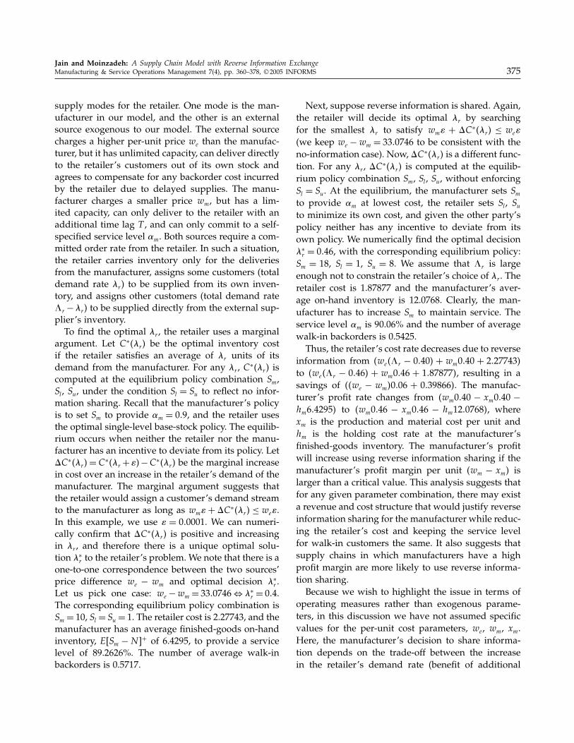
mix of two types of demand rate. The graph is con-structed for a constant utilization ��e + �r�/� whilechanging the mix of �e and �r . Consider each point onthe horizontal axis in Figure 8 as the retailer’s optimalorder rate under no information, corresponding to awe −wm value. A larger horizontal axis value reflects

Figure 7 Cost and Benefit of Information Sharing

1

3

5

7

0.30 0.32 0.34 0.36 0.38 0.40 0.42 0.44 0.46 0.48 0.501

3

5

7

9

11

13

15

17Cost, no-info.Cost, reverse-info.On-hand, no-info.On-hand, reverse-info.

Retailer order rate

Ret

aile

r co

st

Man

ufac

ture

r on

-han

d

Rate increase

On-

hand

incr

ease

Note. On-hand: E�Sm − N�+; �e = 0�4, � = 1, T = 1, hr = 1, br = 9,�m = 0�9.

Figure 8 Effect of Retailer Size on Information Sharing

0

0.02

0.04

0.06

0

2

4

6

util. = 0.8, order-rateutil. = 0.7, order-rateutil. = 0.8, on-handutil. = 0.7, on-hand

Retailer order rate

Incr

ease

in r

etai

ler

orde

r ra

te

Incr

ease

in m

fr.o

n-ha

nd

0.1 0.2 0.3 0.4 0.5 0.6 0.7

Note. Util.: �; on-hand: E�Sm − N�+, �e = ��− �r , �= 1, T = 1, hr = 1,br = 9, �m = 0�9�a larger we −wm. Now, for the manufacturer sharinginformation will lead to a benefit—increase in �r—anda cost—increase in holding cost. The benefit and costpair is plotted for two different utilization values.As the portion of the retailer’s demand in the total

grows, both the cost and the benefit of informationsharing first grow and then decline. The graph sug-gests that if the holding cost were negligible, the man-ufacturer should share information with retailers thatmake up about half of the workload. If the holdingcost is nonnegligible, we take the separation betweenthe cost and the benefit lines as a comparative mea-sure, and this suggests that retailers that constituteless than half of the workload are better candidatesfor information sharing than are those that consti-tute more than half of the workload. This makes intu-itive sense because, as we noted in §4.2.2, the percent-age cost reduction is smaller for the retailer when itsdemand is a larger part of the overall system. Thissuggests that the benefit to the manufacturer (increasein order rate) will be smaller if the retailer is larger.We do note, however, that while larger customers maybe able to exercise more pressure for sharing reverseinformation, the manufacturer’s economic interest isbetter served by sharing it with smaller customers.The graph shows another pair of cost benefit lines

for a lower utilization. We observe that the separa-tion is wider, and therefore that reverse informationsharing may make more sense for manufacturers withlower utilization. Again, this makes intuitive sensebecause the manufacturer’s cost will increase lessrapidly with utilization when utilization is small.

Jain and Moinzadeh: A Supply Chain Model with Reverse Information ExchangeManufacturing & Service Operations Management 7(4), pp. 360–378, © 2005 INFORMS 377

The example and analysis above highlight the man-ufacturer’s economic motivation to share information:releasing the information may result in the retailerincreasing its order rate. More detailed supply anddemand models for the retailer may suggest differentmechanisms for the increase in order rate. The retailermay lower its price to acquire new demand or, in thecase of two identical supply modes, may shift ordersfrom the mode that does not share reverse informationto the one that does. From the manufacturer’s perspec-tive, however, the end result is the same: an increase inthe retailer’s order rate. For the manufacturer, reverseinformation sharing is a way to differentiate itself fromits competitors, and thus attract larger demand. It isalso a tool that can be used to achieve nonprice dis-crimination among its customers, in favor of thosewho have the ability to increase their demand rate.

6. Extensions and ConclusionThis paper analyzes the implications of a growingbusiness practice called reverse information sharingfor different parties in a supply chain. We build andanalyze a manufacturer-retailer model that avoidsa limiting assumption made in earlier works. Wedemonstrate that a simple policy will enable theretailer to take advantage of reverse information toreduce its inventory cost. We also demonstrate howreverse information sharing may increase the manu-facturer’s profits. The model leads to insights that pro-vide guidance to managers on when to share reverseinformation and how to use it.On the modeling side, two questions stand out for

future research. First, what if the retailer has access tomore detailed current information, for example, if theretailer knows the number of orders outstanding atthe manufacturer, N , at the time of ordering? Second,what if the manufacturer shares current informationwith all customers? We believe that the infrastructurewe have developed in this model can be extendedto address these questions and others. It may also beextended to provide detailed models of the retailer’sstatic knowledge of the supply system. In this paperwe assume that the retailer possesses sufficient knowl-edge to develop �ij and to use our algorithm. Aninteresting avenue for future research is the study ofsituations in which the retailer does not have thisknowledge.

AppendixThis appendix provides brief sketches of the steps in theanalysis in §3 and of the proofs. Complete details are avail-able in the online appendix.Step 1. Defining the Restricted Process. The restricted

version observes the process only over states for whichN ≤ Sm. The state-transition-rate diagram is shown in Fig-ure 2. All the transition rates except those out of states �i Sm�remain the same as in the unrestricted process. To determinethe transition rates for �i Sm � i < ��→ �i Sm� and �i Sm � i <��→ �� Sm�, first definefij : Starting in a state �i j � i < � j ≥ Sm� and conditioned

on the next transition being due to external arrival, the prob-ability that the unrestricted process will return to state �i j�for the first time before it reaches state �� Sm�.Using conditioning arguments, we can write the recur-

sion fij = q∑k=0�pfi� j+1�

k where q = �/��e + �r +�� and p=�e/��e + �r + ��. Next, note that fij = fi� j+1 and therefore,fij = �1−

√1− 4pq�/�2p�= f . The transition rate attached to

�i Sm�→ �i Sm� for 0 ≤ i < � will be �ef and the rate for�i Sm�→ �� Sm�will be �r+�e�1−f �. The rate for �� Sm�→�� Sm� will be �e + �r . We will normalize these rates bydividing them by �.Steps 2, 3, and 4. In Steps 2 and 3 we formulate and solve

second-order homogeneous difference equations to obtainEquations (1) to (6). Further algebraic manipulation of thebalance equations yields Equation (7) in Step 4.

Proof of Theorem 1. We obtain this proof by showingthat Equations (1) to (7) in §3 satisfy all the balance equa-tions of the original process. �

Proof of Theorem 2. We first prove the following iden-tities (a) to (e).

(a)n∑j=0�1� j =

�∑i=1�i�n+1−�e

�∑i=1�i�n for 0≤ n≤ Sm− 1�

(b) �r

Sm−1∑j=0

�m� j = ��− z2�m−1∑i=0�i�Sm for 1≤m≤��

(c) �− z2 =�r

�1− z2��

(d) �1−���−1∑i=0

∑j=Sm

�i� j =�1−���1− z2�

�−1∑i=0�i�Sm �

(e) �1−��∑

j=Sm��� j =���Sm + ��− z2�

�−1∑i=0��− i��i� Sm

+ ��− z2��1− z2�

�−1∑i=0�i�Sm �

The last step in the proof begins with writing the balanceequations for the set of states ��0 j� � 0 ≤ j ≤ n� for all 0 ≤n ≤ Sm − 1 and then using (a) to (e) to show

∑�i=0�i�0 =

�1−��. �

Proof of Theorem 3. We separately prove the convexityof C�i j k! for j ≥ Sm and of C�0 0 1!. Combining the tworesults proves the convexity of CSl�� in Sl. �

Jain and Moinzadeh: A Supply Chain Model with Reverse Information Exchange378 Manufacturing & Service Operations Management 7(4), pp. 360–378, © 2005 INFORMS

Proof of Theorem 4. We will use the symbol �3� j todenote Pr�NRI = j! = ∑�

i=0�i� j = �3� j . In NI , Pr�NNI = j! =�1− ���j . We need to show that: Pr�NRI ≤ j!≤ Pr�NNI ≤ j!.From Theorem 2, we have �3�0 = 1 − �. Using theaggregation/disaggregation approach to analyze Markovchains (see Schweitzer 1991), we can write: �3�1 = ��e +�r ��0�0/�3�0���3�0 < ��3�0. We also show that �3� j < ��3� j−1for j ≤ Sm and that �3�Sm+1 = ��3�Sm . Therefore, Pr�NRI ≤ j!≤Pr�NNI ≤ j! for j ≤ Sm+ 1.Next, consider the balance equation for the group of

states ��i� j � 0 ≤ i ≤ �% j ≤ Sm�, which gives: �3�Sm+2 =��3�Sm+1 + �r

∑�i=0�i�Sm > ��3�Sm+1. Similarly, �3�Sm+j >

��3�Sm+j−1 for j ≥ 2. Therefore, �3�Sm+j > �j−k�3�Sm+k forj > k≥ 1.We will prove the rest by contradiction. Assume there

exists:

j∗ =Min{k∣∣∣ k∑j=0�3� j ≥ Pr�NNI ≤ k!% k≥ Sm+ 2

}�

From the definition of j∗4 Pr�NRI = j∗!=�3� j∗ > Pr�NNI =j∗!= �1−���j∗ . Now,

Limj→

Pr�NRI ≤ j! =j∗∑j=0�3� j +

∑j=j∗+1

�3� j

> Pr�NNI ≤ j∗!+∑

j=j∗+1�j−j

∗Pr�NNI = j∗!

= �1−�� �1−�j∗+1�

�1−�� + �1−���j∗ �

�1−�� = 1�

This is impossible. Therefore, no such j∗ exists and Pr�NRI ≤j!≤ Pr�NNI ≤ j! for all j ≥ 0. �

Proof of Proposition 5. Recall from Theorem 4 thatPr�NRI = j!≤ Pr�NNI = j! for j ≤ Sm. Thus

E�Sm−N!+RI =Sm−1∑j=0�Sm− j�Pr�NRI = j!

≤Sm−1∑j=0�Sm− j�Pr�NNI = j!= E�Sm−N!+NI � �

Two extensions of the basic model, discussed in §2and §5.3, are available in the online appendix (Jain andMoinzadeh 2005).

ReferencesAxsäter, S. 1990. Simple solution procedures for a class of two-

echelon inventory problems. Oper. Res. 38 64–69.Cachon, G., M. Fisher. 1997. Campbell’s Soup continuous prod-

uct replenishment program: Evaluation and enhanced decisionrules. Production Oper. Management 6 266–275.

Cachon, G. P., M. Fisher. 2000. Supply chain inventory manage-ment and the value of shared information. Management Sci. 461032–1048.

Cachon, G., M. Lariviere. 1999. Capacity allocation using past sales:When to turn-and-earn. Management Sci. 45(5) 685–703.

Chen, F. 1998. Echelon reorder points, installation reorder points,and the value of centralized demand information. ManagementSci. 44 S221–S234.

Chen, F., B. Yu. 2005. Quantifying the value of lead time infor-mation in a single-location inventory system. ManufacturingService Oper. Management 7(2) 144–151.

Cheung, K. L., H. Lee. 2002. The inventory benefit of shipmentcoordination and stock rebalancing in a supply chain. Man-agement Sci. 48 300–306.

Colombo, G. W. 1994. Sales Force Automation. McGraw-Hill,New York.

Ernst, R., M. A. Cohen. 1992. Coordination alternatives in a man-ufacturer/dealer inventory system under stochastic demand.Production Oper. Management 1 254–268.

Federal Reserve Statistical Release. 2004. G17. Industrial produc-tion and capacity utilization. http://www.federalreserve.gov/Releases/g17/download.htm.

Gavish, B., S. C. Graves. 1980. A one product production/inventoryproblem under continuous review policy. Oper. Res. 281128–1236.

Ha, A. Y. 1997. Optimal dynamic scheduling policy for a make-to-stock production system. Oper. Res. 45 42–53.

Jain, A., K. Moinzadeh. 2005. Online appendix to “A SupplyChain Model with Reverse Information Exchange.” http://www.informs.org/Pubs/Supplements/MSOM-1526-5498-2005-07-04-0360-app.pdf.

Kaplan, R. 1970. A dynamic inventory model with stochastic lead-times. Management Sci. 16 491–507.

Lee, H., S. Whang. 1999. Decentralized multi-echelon sup-ply chains: Incentives and information. Management Sci. 45633–640.

Lee, H., V. Padmanabhan, S. Whang. 1997. Information distortionin a supply chain: The bullwhip effect. Management Sci. 43(4)546–558.

Moinzadeh, K. 2001. An improved ordering policy for continuousreview inventory systems with arbitrary inter-demand distri-butions. IIE Trans. 33 111–118.

Moinzadeh, K. 2002. A multi-echelon inventory system with infor-mation exchange. Management Sci. 48 414–426.

Nahmias, S. 1979. Simple approximations for a variety of dynamicleadtime lost-sales inventory models. Oper. Res. 27 904–924.

Nahmias, S. 1981. Managing repairable inventory systems: A re-view. TIMS Stud. Management Sci. 16 253–277.

PeopleSoft. 2002. Sager launches customer portal. http://www.peoplesoft.com/media/en/pdf/success/sager_ss_0102.pdf.

Plyler, A., G. P. Shaw. 2001. Exostar: The trading exchange revolu-tionizing A&D. Achieving Supply Chain Excellence Through Tech-nology, Vol. 3. Montgomery Research Inc., San Francisco, CA.

Rubio, R., L. M. Wein. 1996. Setting base stock levels using product-form queueing networks. Management Sci. 42 259–268.

Schweitzer, P. J. 1991. A survey of aggregation-disaggregation inlarge Markov chains. Numerical Solution of Markov Chains.Probab. Pure Appl., Vol. 8. Dekker, New York, 63–88.

Smith, T. 2002. Cost conscious customer connections. InternetWeek.http://www.internetweek.com/newslead02/lead031102.htm.

Sobel, M. J. 1969. Optimal average cost policy for a queue withstart-up and shut-down costs. Oper. Res. 17 145–162.

Song, J., P. Zipkin. 1996. Inventory control with information aboutsupply conditions. Management Sci. 42 1409–1419.

Svoronos, A., P. Zipkin. 1991. Evaluation of one-for-one replenish-ment policies for multi-echelon inventory systems. Oper. Res.36 57–72.

Zipkin, P. 1986. Stochastic leadtimes in continuous-time inventorymodels. Naval Res. Logist. Quart. 33 763–774.