Computational Statistics & Data Analysis 14 (19’iZ) 489-498

North-Holland 489

Nam- Nguyen CSIRO-LAPP Biometrics Utzit, Claytovm 3168, Australia

CSIRO Division of Mathematics and Statistics, Claytorz 3168, Australia

Received October 1931, Revised June 1991

Abstract: For the past two decades, there has been increasing use of computers for the

construction of experimental designs which are ‘good’ in some well-defined sense. This paper reviews and compares some, well-known exchange algorithms for the construction of discrete D-optimal designs. An improved tmplementation of the Fedorov’s exchange algorithms is sug-

gested.

Keywords: Cholesky factorization; D-optimality; DETMAX; Exchange algorithm: Fedorov’s algo- rrthm; MD; Optimal design.

In ihe early stages of the development of experimental design as introduced by Sir R.A. Fisher and F. Yates, the emphasis on the construction of designs was mainly on devising orthogonal arrangements which yielded easy solutions to the normal equations and had some in-built symmetry. wever, over the ycarc, it has been realized that mere sy etry or easy stat al ComPutations do not necessarily guarantee that the which was developed from intui some given measure of go0 ness or optimahty. experimen was initiated by extent by efer in a series 0

Correspondence to: A.J. Miller, CSIRQ Division of athematics and Statistics. Clayton 3168, Australia.

0167..9473/92/$05.00 0 1992 - Elsevier Science Publishers B.V. All rights reserved

490 N.-K. Nguyen, A.J. Miller / Constructing discrete D-optimal designs

amount of literature dealing with theoretical as well as numeric results has accumulated in the area of optimal design.

The objective of all numerical methods for finding optimal or near-optimal designs is to choose n points to include in the design from a finite set of RI possible points called candidate points. The number of candidate points rnqv be quite large in a practical situation. n a recent oxygen delignification experir jF;nt on a given woodchip sample at the CSIRO Forest Product Division,, the 5 treatment factors to be examined were initial Kappa number, oxygen pressure, sodium hydroxide level, treatment temperature and treatment time. To fit a quadratic surface in 5 factors with 3 levels for each factor, the number of candidate points N is 35 = 243. Because of practical limitations, the experi- menter can only carry out rt = 30 experimental runs. The number of ways of choosing 30 design points out of the 243 is very large (about 2 x 1038), so it is not feasible to evaluate all alternatives. In this paper, we look at some heuristic algorithms which searches for ‘good’ designs, with particular emphasis upon designs which are D-optimal.

2. view 0 timality criteria

Consider the linear model 1 =Xp + e where y is an n-component column vector of observations, X is an 12 x p matrix of known elements, p is a p x 1 vector of unknown parameters and e is an n-component vector of random residual components with E(e) = 0 and D(e) = a21 where E and D stand for the expectation operator and the dispersion matrix respectively. The least squares normal equation for estimating p is X’XP = X’y. The task of construction of experimental designs then consists of choosing n rows of X out of N candidate rows in such a manner that the resultant information matrix X’X is good or optimal in some sense. The optimality criteria available in the literature centers around minimizing some special function of M = X’X, say G(M).

Let us assume that X’X is nonsingular and suppose pi,. . . ,p, are the eigenvalues of X’X. Three important criteria related to the minimization of some functions of these eigenvalues are:

(i) D-optimality: Q(M) = det( M- *) = l$[. ‘; (ii) A-optimality: Q(M) = trace( M- ') = Cp,: ';

(iii) E-optimality: Q(M) = max i( p,T l).

These three optimality criteria have the following statistical interpretations. A D-optimal design minimizes the generalize variance of the estimates of the components of p. Also, under normality, D-optimal design minimizes the

volume of the confidence ellipsoid for p. An A-optimal design minimizes the average variance of the estimates of the components of p. Finally, an E-optimal design minimize he maximum variance of the estimates of the components of

Ash and Hedayat (I978), Atkinson (1982, 1988) d bibliographies on the theory of optimal experi-

mental designs in a more general context.

N.-K. Nguyen, A.J. Miller / Constructing discrete D-optimal designs 491

Among the optimal&y criteria just mentioned, the D-optimality criterion, because of its simple updating formula, which will be discussed in the next section, has been used by many authors in the development of computer algorithms for the construction of optimal designs.

rix as

In this section, we give some results in matrix algebra which will be used in the following sections.

Let M = X'X and assume M to be nonsingular. The n rows of the matrix X are n p-dimensional vectors xl, i = 1,. . . , n. These n p-dimensional vectors can be considered as n points in R *. Note that there are N distinct candidates x’.

If x’ is a row vector to be augmented to X, we have

IM+xx'I = /M I(1 +x'M-lx), (3 1) .

(M+xu')-' =M-'+wuu', (3 2) .

where w = -l/(1 +x'M-lx) and u = M-k Let M, = M tm/. If XI is a row vector to be removed from the new X, we

have

IM x-~i~fl = l M, I(1 -xfML'xi),

(M x-xix'!)-'=M;l - WiUiU:,

where Wi = l/(1 _- X~MJ ‘xi) and Ui = M, 'Xi. Frcm (3.1) and (3.3) we have

(3 3) .

(3 4) .

I M+xx’--XiXlI = I M I(1 +x’M-‘x)(1 -xfM,*q) (35) .

= IM I(1 +A(xi, X)], (3 6) .

where

A(Xi, X) = (1 +x’M-‘x)(1 -XjM,-‘Xi) - 1 (3 7) .

-x’M-lx-q!M-lxi+(x’M-l+x’M-lx,,y;M-lxi, . (3 8)

using the following relation derived from (3.2):

x”M,- ‘Xi = x”M- ‘Xi - (X’M-lxi)Z/(l +x’M-‘X). (3 9) .

We refer to A( Xi, x) as Fedorov’s delta function.

XC gorit cti s

As mentioned in the previous section, designs consists 0: choosin? n rows x’ fro

of constructing optimal ate rows in such a manner

492 N.-K. Nguyen, A.J. Miller / Constructing discrete D-optimal designs

that the resultant matrix X’X or M is good or optimal in some sense. If replication of points is allowed there are N” possible choices or designs to be examined. If N is large, it is not feasible to examine all N” designs in order to find the most optimal one, even with the help of a computer. Several computer algorithms for the construction of D-optimal designs in n points are available in the literature. One of the most important classes in this direction is that of exchange algorithms (EAs). In this review, we will cover five EAs. The first EA is due to Fedorov (1969, 1972). The second EA is due to Mitchell and Miller (1970) and Wynn (1970). There are several variants of this EA. The third EA is due to Mitchell (1974). The fourth EA is due to Cook and Nachtsheim (1980). The fifth EA is due to Atkinson and Donev (1989). The first four EAs have been implemented in the SAS/QC module of SAS software (SAS Institute Inc., 1989). In addition, we also discuss some of our effort to improve Fedorov’s EA and Cook and Nachtsheim’s EA (Miller and Nguyen, 1993).

The Fedorov’s EA follows the following steps:

(i) Start with a randomly chosen n-point design. Compute ikl’, M-l and 1 M I.

iii) Find simultaneot_. ls!y a vector xi among yt vectors of the current n-point design and a vector x among N candidate vectors such that A(+ x) computed by (3.8) is maximum. Exchange Xi with x and update M-l by (3.2), (3.4) and I M 1 by (3.6).

Repeat step (ii) until A(Xi, x) is less than E, a chosen positive small number.

The purpose of E is to prevent cycling caused by rounding errors between designs with identical determinants. We found c = l.OE - 5 satisfactory.

In the EA of Mitchell and Miller (1970) and Wynn (1970) the delta function is first maximized with respect to x and then with respect to Xi. This EA works as follows:

(i) Start with a randomly chosen n-point design. Compute M, M- ’ and I M 1.

(ii) Find a vector x among N candidate vectors such that x’AK lx is maximum and add x to the current n-point design. Update M-r to M,- ’ to by (3.2).

(iii) Find a vector Xi amongst the n + P vectors of the current (n + D-point design such that x,!M, ‘Xi is minimum and remove Xi (Recall I&. =X + XK’). Update ML’ by (3.4) and 1 M 1 by (3.5).

Repeat steps (ii) and (iii) until A(Xi, x) calculated by (3.7) is less than E, a chosen positike small number.

Mitchell (1974) generalized his basic EA. to permit ‘excursions’. At each iteration, t points can be added to the n-point design and t points are removed from the (n + t&point designs. He called this EA, PIETMAX. When t = 1, DETMAX becomes his original EA. As computer time for each iteration is proportional to t, this EA is more time consuming particularly when t is large.

There are variants of Mitchell and iller’s basic EA. In the EA of Van Schalkwyk (1971), a point in tne design is deleted esig fore a new point is added, i.e. steps (ii) and (iii) in er’s are

N.-K. Ngtiyw, A.J. Miller / Constnrcting discrete D-optimal designs 493

interchanged. In Nguyen (1983) and Nguyen and ey (1989), point X, in step (iii) is found by maximizing the delta function using (3.8). As such, simultaneous exchange of x and xi is possible and the update of M-’ in step (ii) can be

postponed until point Xi is found. We note that the RHS of (3.9) can be written as xjM_*xi + ~(10~~)~ where = -l/(1 +x’M-lx) and u = M-lx as defined in Section 3. Galil and Kiefer

L980) use this simple relation for updating x !M- lx. to x !MT IX. (Recall Mx = M +xx’). A formula for updating x,fM-‘xi khen i point is rim&ed from the current (n + l)-point {design can be similarly defined. If we store all elements of XlM-‘xi (i = 1, l l l N) in a vector of length N, the problem of finding a point to add to (or delete from) the current n-point design becomes finding the biggest (or smallest) element of this vector. Galil and Kiefer also proposed the use of partially random designs instead of completely random designs as starting designs. For a partially random design, no points are randomly chosen from N candidate points (n, < n). n - n,, points are then sequentially added to this n,-point design. Their study did show the effect of amount of initial randomization on the success rate of the EA. They called their improved method modified DETMAX or MD.

From our experience Fedorov’s EA is far superior to DETMAX or a maximum-minimum EA type like MD in terms of producing ‘good’ designs. This view is also shared by Johnson and Nachtsheim (1983) and Atkinson and Donev (1989). It can easily be seen that once a design is constructed by Fedorov’s EA no maximum-minimum EA like MD can improve it. However, Fedorov’s ‘extravagant’ EA may not be feasible in terms of computer time for some design problems.

Cook and Nachtsheim (1980) proposed a modification of Fedorov’s EA. For convenience, we call their EA, MFEA. In MFEA, each iteration in Fedorov’s EA is broken into n stages. Each stage corresponds to a point in the n-point design. At each stage, a point Xi in the n-point design is exchanged with a point x among the N candidate points if A(Xi, x) is greater than zero. They found that the MFEA can produce designs comparable to the ones produced by Fedorov’s EA and is about twice as fast as Fedorov’s EA. Johnson and Nachtsheim (1983) generalized the original MFEA by permitting only t stages at each iteration (1 I t I n). These t stages correspond to t points in the n-point design with the smallest x;M-‘x,3. When t = 1, this EA becomes Van Schalk- wyk’s EA. When t = ~1, this EA becomes MFEA.

Atkinson and Donev (1989) proposed another modification of the rev’s

EA which they called the KL-exchage algorithm (KL-EA). In the A, a point xk (k 5 K 5 n) from the n-point design and xl (I 5 L I NJ from the candidate points are exchanged if A(x,, x,) is maximum. K corresponds to K points of the n-point design with the smallest xhM_‘x,‘s. L corresponds to L points of the N can dates points with the largest x;~~-~x~‘s. The exchange process ceases when smaller than a chosen positive small number. When K=n and L =N, th

It may be noted that whil tima

494 N.-K Nguyen, A.J. Miller / Constructing discrete D-optimal designs

designs proposed by Dykstra (1971) and Vuchkow et al. (1984) can be used for constructing ‘good’ starting designs, they are not expected to construct designs having maximum 1 X ‘X I. Also, while the branch-and-bound algorithm of (1982) can guarantee a catalogue of all global D-optimal designs for any specified linear model and design region, it can be computationally prohibitive, particularly if the number of candidate points exceeds about 30.

dorov’s exchange algawit

All the EAs we have discussed so far start with forming the sum of squares and cross products matrix M (Recall M = X'X), its inverse and determinant and use some forms of updating formulas mentioned in Section 3. We note that these calculations can be performed more quickly and accurately by using the Cholesky factorization. If we write

M=R'R, where R is the upper-triangular factorization of M, then we can verv quickly calculate the determinant of M, as the determinant of a triangular matrix is equal to the product of its diagonal elements. The Cholesky factor R can be formed without calculating M and it is easy to update or downdate R when a point (a row vector of X) is added to or deleted from X. An algorithm for doing this has been given by Gentleman (1974).

In calculating the Fedorov’s delta function A(Xi, x) for use in the Fedorov’s EA or MFEA, we need to calculate quantities of the form xrM-"xi and x'M-lx,. xlMvlxi can be written as

where Zi is the solution of R'Zi =q. Zi can be obtained by back-substitution without the need of inverting R'. We only need to calculate the xlM_‘xi’S in this way once. Update formulas like (3.9) are used to recalculate these quantities when a point is added or removed from the current design. Similarly, x'Mwlxi can be written as

x'(R'R)-'Xi=X'ui,

where Ui is the solution of Rui = Zi and zi is the solution of R'Zi =xi. Ui and Zi can be obtained by back-substitution without the need of inverting R and R'.

the Cauchy-Schwarz inequality, we have

( X' - 'Xi)2 - x ‘no- ‘xurM_ ‘xi I 0.

d x are a pair of ter than x'M-lx-

N.-K. Nguyerl, A.J. Miller / Comtrtrctirzg discrew D-optimal designs 3%

None of the EAs discussed above guarantees D-optimality as they may get ‘trapped’ in a local optimu n order to find a good design, several ‘tries’ should be made, each try with a different starting design. The starting design can be completely random or partially random. As mentioned, for a partially random design, n,, points are randomly chosen from W candidate points (n,, < n). n - N,, points are then sequentially added to this /j,I-point design. A point xi is added to the design if xjM_'x, is maximum. To avoid singularity when n,, is less than the number of parameters p, we work with a (M + EZ) matrix instead of M where E is a small positive number, say l.QE - 5. The effect of E is removed at a later stage. This simple method of constructing partially random starting design has been used by Vuchkow et al. (1984) and Atkinson and Donev (1989). In this paper we choose n,, = min(5, [$I). This choice of n,, is empirically based. We do not guarantee this is the best choice for all situations.

As mentioned, the D-optimality criterion, because of its simple updating formula, has been chosen by most authors for the construction of optimal designs. However, there is no reason why other optimality criteria should not be used with similar EAs. Welch (1984) generalized Mitchell’s DETMAX EA for searching G- and V-optimal designs. Nguyen and Dey (1990) used an EA similar to the ones discussed here to construct (M, S)-optimal incomplete block designs.

orw’s

In this section we make a comparison of Mitchell’s DETMAX, Galil and Kiefer’s MD, Atkinson and Donev’s KLEA and our implementation of Fe- dorov’s EA and Cook and Nachtsheim’s Modified Fedorov’s EA which we called MFEA, on a 16 MHz 80386 PC with a math co-processor. Our implemen- tation of the Fedorov’s EA and MFEA made use of our attempts to improve the speed and accuracy of these EAs whicn we discussed in the previous section.

The three examples we considered are a linear example, quadratic examples and quadratic examples with blocking. In the linear example, the design is a saturated one with p = n = 11. The ith row of the design matrix X is an 1 l-dimensional row vector xl

x! = (1, x1;, +i, l l l x*0;)

where X/Ii= +l, h = l,..., 10 and i= l,..., 11. The goal is to choose II 1 vectors out of 2”” = 1024 candidate vectors to form the X matrix such that 1 X'X 1 = 25 X 2” which is the known maximum. Table 1 gives a comparison of performance of various EAs in this linear e

AX program of of these EAs.

selected vectors n,, does have effect on time of successes out of a fi

D is a real ‘time-savi

496 N.-K. Nguyen, A.J. Miiler / Constructing discrete D-optimal designs

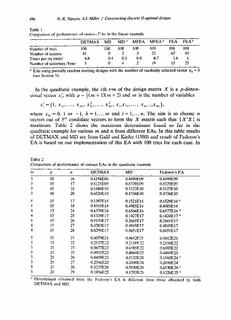
Table 1 Comparison of performance of variou> ZAs in the linear example

DETMAX MD MD a MFEA MFEA” FEA FEA”

Number of tries 100 100 100 100 100 100 100 Number of success 41 0 2 3 22 42 45 Timer per try (min) 4.8 0.4 0.3 0.8 0.7 1.6 1 Number of successes/hour 5 0 4 2 19 15 25

L1 EAs using partially random starting designs with the number of randomly selected vector n,, = 5 (see Section 5).

In the quadratic example, the ith row of the design matrix X is a p-dimen- sional vector x,!, with p = $( m + l)(m + 2) and m is the number of variables

Xl’= (1, xliY**V’, x,,li? Xfl,.**Y xl$i, xlix2j7 . ..$ x~n- lixmi)l

where x,,; = 0, 1 or - 1, h = Ii, *. . m and i = 1,. . . n. The aim is to choose n vectors out of 3”’ candidate vectors to form the X matrix such that 1 X’X 1 is maximum. Table 2 shows the maximum determinant found so far in the quadratic example for various m and rz from different EAs. In this table results of DETMAX and MD are from Galil and Kiefer (1980) and result of Fedorov’s EA is based on our implementation of this EA with 100 tries for each case. In

Table 2 Comparison of performance of various EAs in the quadratic example

IF? P n DETMAX MD Fedorov’s EA

10 16 10 17 10 I8 10 20

15 17 0.1397E14 15 18 0.4315E14 15 24 0.6379E16 15 25 0.1328E17 15 26 0.1970E17 15 27 0.3383E17 15 28 0.8296E 17

21 21 0.4079E2 1 ii 22 0.2! 37E22 21 23 0.5677E22 21 25 0.4052E23 21 26 6.8409E23 21 27 0.2566E24 21 28 0.523X24 21 29 0.1056E25

0.4 194EO9 0 8125E09 0.1488ElO 0.4529ElO

0.4499EO9 0.832OEO9 0.1527EiO 0.4736E 10

0.1521El4 0.4985E 14 0.6566E16 0.1427El7 0.2665E17 0.4819E17 0.8651E17

0.4612E21 0 31 C8F3-J -.-a_. --rut 0.6585E22 0.4869E23 0.1132E24 0.2698E24 0.5930E24 0.1283E25

0.4499E09 0.8320E09 0.1527ElO 0.4736ElO

0.1529E14 a 0.4985E 14 0.6577E 16 a 0.1424El7 a 0.266SE17 0.4819E17 0.865lE17

0.4612E21 0.2158E22 0.6585E22 0.4869E23 0.1168E24 a 0.2698E24 0.6130E24 a 0.1326E25 a

a Determinant obtained from the Fedorov’s EA is different from those obtained by both DETMAX and MD.

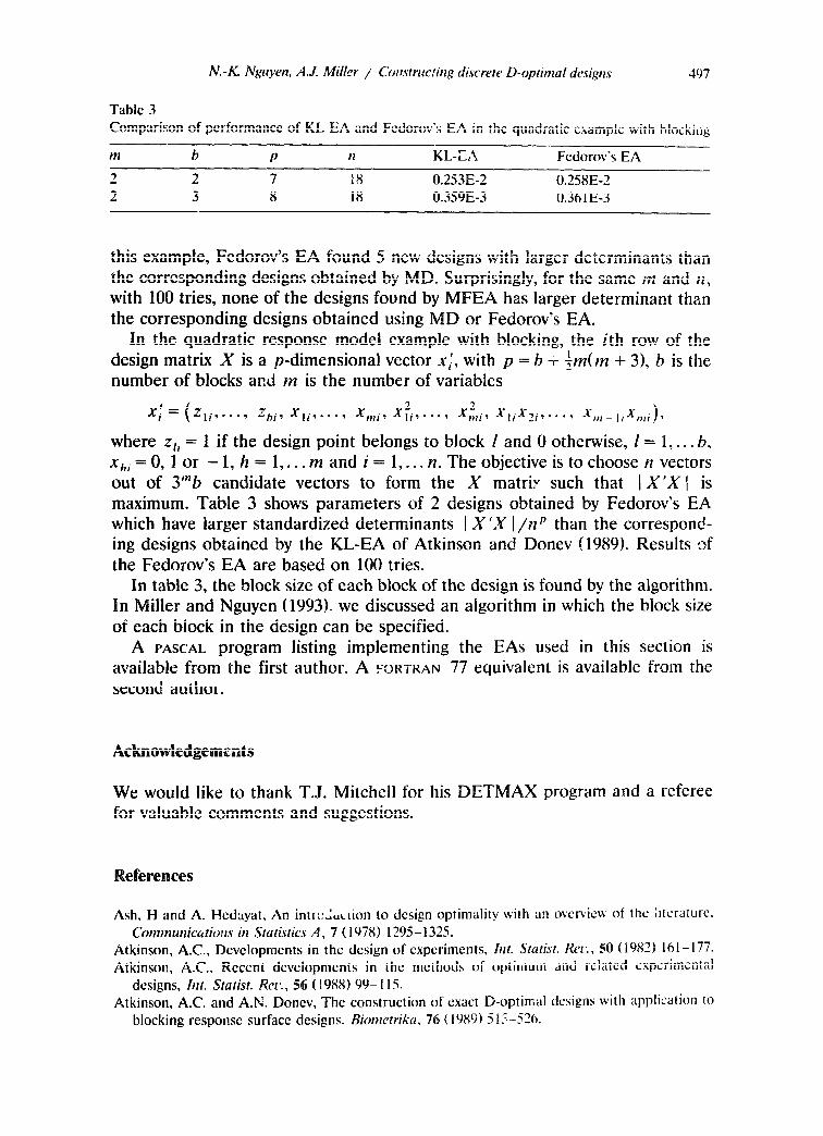
Table 3 Comparison of performance of KL-EA and Fedorov’s EA in the quadratic example with blocking

m b P il KL-;3,2 Fedorov’s EA

2 2 7 i8 0.253E-2 0.258E-2 2 3 8 18 0.359E-3 0.361 E-3

this

p = b -+ $dm + 3), b is the number of blocks and m is the number of variables

where Zli = 1 if the design point belongs to block I and 0 otherwise, I = 1,. . . b, Xhi=O, 1 or -1, 11 = l,... m and i= IL The is IZ vectors

of 3’nb to form X matrix such that 1 X’X 1 is maximum. Table 3 shows parameters of 2 designs obtained by Fedorov’s EA which have larger standardized determinants 1 X’X 1 /IP than the correspond- ing designs obtained by the KL-EA of Atkinson and Donev (1989). Results ,sf the Fedorov’s EA are based on 100 tries.

In table 3, the block size of each block of the design is found by the algorithm. In Miller and Nguyen (1993). we discussed an algorithm in which the block size of each block in the design can be specified.

A

Ash. H and A. Medayat. An intr cdtiction to &sign optimahty with an overvicu of the ;tteraturc.

Corlrlntrrzi~crtio~rs ill Statistics A, 7 ( 1978) 1295-1325.

Atkinson, A.C., Dcveiopments in the design of experiments,

in the methods of optimum and xl designs, ht. Statist. Rel,. ,

Atkinson, A.C. and A.N. Do tion of exact D-optimal designs with application to

blocking response surface designs. Riornctrika, ‘7

498 N.-K. Nguyen, A.J. Miller / Constrl!rting discrete D-optimal designs

Cook, R-D. and C.J. Nachtsheim, A comparison of algorithms for constructing exact D-optimal designs, Technometrics, 22 ( 1980) 3 15-324.

Dykstra, O., The augmentation of experimental data to maximize 1 X’X I, Technometrics, 13 (1971) 682-688.

Fedorov, V.V., Theory of optimal experiments, Preprint No. 7 LSM (Izd-vo Moscow State University, Moscow, 1969).

Fedorov, V.V., Theory of Optimal Experiments, Translated and edited by W.J. Studden and E.M. Klimko, eds. (Academic Press, New York, 1972).

Galil, Z. and J. Kiefer, Time- and space-saving computer methods, related to Mitchell’s DET- MAX, for finding D-optimal designs, Technometrics, 22 (1980) 301-313.

Gentleman, W.M., Algorithm AS 75, Basic procedures for large, sparse or weighted linear least squares problems, Applied Stat., 23 (1974) 448-1454.

Johnson, M.E. and C.J. Nachtsheim, Some guidelines for constructing exact D-optimal designs on convex design spaces, Technometrics, 25 (1983) 271-277.

Miller, A.J. and N.K. Nguyen, A Fedorov exchange algorithm for D-optimal design, To appear in Applied. Stat., ( 1993).

Mitchell, T.J., An algorithm for the construction of D-optimal designs, Technometrics, 20 (1974) 203-210.

Mitchell, T.J. and F.L. h .iller Jr., Use of ‘design repair’ to construct designs for special linear models, Math. Div. Ann. Progr. Rept. (ORNL-4661) (Tennessee, 1970) 130-131.

Nguyen, N.K., Computer-aided construction of optimal designs, Unpublished Ph.D. thesis (IARI, New Delhi, 1983).

Nguyen, N.K. and A. Dey, Computer-aided construction of Q-optimal 2”’ fractional factoriaf designs of resolution V, Aust. J. Stat., 31 (1989) 111-l 17.

Nguyen, N.K. and A. Dey, Computer-aided construction of small (M, S&optimal incomplete block designs, Aust. J. Stat., 32 (1990) 399-410.

SAS Institute Inc., SAS/QC Software: RP$ #ence, 1st ed. (SAS Institute, Cary, NC, 1989). St. John R.C. and N.R. Draper, D-sptimality for regression designs: A review, Technometrics, 17

(1975) 15-23. Van Schalkwyk, D.J., On the design of mixture experiments, Unpublished Ph.D. thesis (University

of London, London, 1971). Vuchkow, I.N., D.L. Damgaliew and A.N. Donev, Comparison of some algorithms for discrete

D-optimal design generation, COMPSTAT: Proceedings in Computational Statistics, (Physica Vet-lag, Vienna, 1984) 503-508.

Wald, A., On the efficient design of statistical investigations, Ann. Math. Stat., 14 (1943) 134-140. Welsh, W.J., branch-and-bound search for experimental designs based on D-optimality and other

criteria, Technometrics, 24 (1982) 41-48. Welsh, W.J., Computer-aided design experiments for response estimation, Technometrics, 26

(is)841 217-224. Wynn, H.P., The sequential generation of D-optimal experimental designs, Ann. Math. Stat., 41

(1970) 1644-1655.