


Bahasa
Halaman
Hukum


Journal of Global Positioning Systems (2011)
Vol.10, No.1 :89-99
DOI: 10.5081/jgps.10.1.89
© 2010 IEEE. Portions reprinted, with permission, from Knight NL, Almagbile A, Wang J, Ding W, Jiang Y,
Optimising Fault Detection and Exclusion in Positioning, Ubiquitous Positioning, Indoor Navigation and Location
Based Service (UPINLBS), 14-15 October, 2010.
A New Minimal Detectable Bias in Fault Detection for Positioning
Nathan L. Knight1, Jinling Wang
1 and Xiaochun Lu
2
1School of Surveying and Spatial Information Systems
University of New South Wales, Sydney, NSW2052, Australia 2The National Time Service Center (NTSC), Chinese Academy of Sciences,
Xi’an, Postcode 710600, Shaanxi, China
Abstract
The Minimal Detectable Bias method of Fault Detection
is frequently employed to determine if a position has
integrity. However, to provide integrity the Type I error
probability of the statistical tests is required to be preset.
Normally, this probability is set to avoid the unnecessary
rejection of measurements or to satisfy the continuity
requirements. In this paper, the Type I error probability
is set based on the integrity requirements by initially
setting the Protection Levels equal to the Alert Limit.
This new procedure of setting the Type I error
probability is compared with the more conventional
approach when there are different continuity
requirements and when multiple biases are considered.
From the results of this comparison, it is concluded that
the new procedure increases the availability rates
regardless of the continuity requirements and the number
of biases considered.
Keywords: Integrity, Continuity, Availability, Multiple
Biases
_____________________________________________
1. Introduction
The concept of integrity is based on the user specifying
the maximum amount of positioning error tolerated
which is commonly referred to as the Alert Limit. In
addition to the Alert Limit, the user is also required to set
the Probability of a Missed Detection, which is the
maximum probability of the position being in error
greater than the Alert Limit that will be forgiven by the
user. If the reported position is in error greater than the
Alert Limit more frequently than the Probability of a
Missed Detection, then the user is no longer forgiving
and considers that the integrity of the position has been
lost.
Whilst the Minimal Detectable Bias (MDB) method of
Fault Detection, based on either the chi-square test
(Baarda, 1967; Parkinson and Axelrad, 1988; Sturza,
1988; Brown, 1992) or the outlier test (Baarda, 1968;
Kelly, 1998), can be used to determine if a position has
sufficient integrity for a given Alert Limit. The
procedure is also dependent on the Type I error
probability of the statistical tests being preset in order to
determine the thresholds for the statistical tests and the
Protection Levels. Therefore, the question arises as how
to set the Type I error probability of the statistical tests?
In applications with continuity requirements, such as
aviation, the Type I error probability is traditionally set
to always satisfy the continuity requirements. Therefore,
to determine if the positioning system satisfies both
continuity and integrity requirements, that is available, it
is only required to monitor the position’s Protection
Level (Ober, 2000b). Since the applications that have
continuity requirements are adverse to continuity risks,
the Type I error probabilities that are set are very small.
Hence, the systems are inadvertently adverse to the
rejection of measurements.
In some applications, such as geodesy, where the
measurements are remeasured if they are rejected by the
statistical tests, the Type I error probability is set to
avoid such rejections. Since it is reasoned that due to the
high cost of remeasurement, the Type I error probability
should be set to avoid such unnecessary rejections.
Therefore, the Type I error probability in geodesy is
typically set to 1%, or 0.1%, such that only 1 in 100, or 1
in 1000, measurements are unnecessarily rejected
(Baarda, 1968).
The adverse impact of setting a small Type I error
probability, which avoids the rejection of measurements,
is that it increases the Protection Level. Therefore, by
increasing the Type I error probability, the Protection
Level can be reduced and the position can gain integrity.
However, this is at the expense of the continuity
probability and an increased probability of rejecting
measurements. Nevertheless, in applications that do not
have continuity requirements, or remeasure, this appears
to be a feasible strategy of increasing the percentage of
time that a position with integrity can be obtained.

Knight et al: New Minimal Detectable Bias in Fault Detection for Positioning
90
Another aspect of initially setting the Type I error
probability is that it also often results in the position’s
Protection Level being less than the Alert Limit. If the
Type I error probability was increased, then the
position’s Protection Level could be made equal to the
Alert Limit. Meaning that a position with integrity is
still obtained, but with a reduced continuity risk and a
reduced probability of measurements being rejected.
By initially setting the same Type I error probability, and
the same Probability of a Missed Detection, for each
measurement there are numerous different Protection
Levels that are obtained. To obtain the position’s
Protection Level, it is then conservatively assumed that
the bias always corresponds with the most difficult to
detect measurement that produces the largest Protection
Level (Lee et al., 1996; Lee and Van Dyke, 2002).
Whilst this is a conservative assumption, it is at the cost
of availability. In an attempt to address this, Lee and
Van Dyke (2002) assume that the bias can exist in any
one of the measurements and average the Missed
Detection Probabilities across all of the measurements.
However, it was found that this only results in a minor
improvement in availability. If the conservative
assumption is maintained, then when a statistical test
fails due to a measurement that does not correspond with
the largest Protection Level it may not actually be a
significant Missed Detection at all. Whilst this is the
only option when the chi-square test is employed, with
the outlier test it is possible make all of the
measurements have the same Missed Detection
Probability and the same Protection Level by changing
the Type I error probabilities. Such setting of the Type I
error probabilities will also result in a reduction in the
probability of a measurement being rejected and a
reduction in the continuity risk.
Besides the current procedure of applying the MDB
method that requires the Type I error probability to be
preset some, Fault Detection methods exist that initially
satisfy the integrity requirements and then monitor the
continuity risk. In general, these methods tend to be
position domain techniques whereas the methods that
require the Type I error probability to be preset are
measurement domain techniques (Ober, 2000b). They
include the multiple hypothesis method (Pervan et al.,
1998; Blanch et al., 2007) and the Bayesian approach
(Ober, 2000a).
In the multiple hypothesis method and the Bayesian
approach, it is expected that the positioning solution
using all of the measurements is equal to the positioning
solution with one of the measurements removed. If a
biased measurement is present, then the probability
density function of the solution using all of the
measurements is expected to be biased while the solution
with the biased measurement removed is expected to
correspond with the true position. Therefore, by
comparing the difference between all the positioning
solutions, and their distributions, with the Alert Limit it
can be determined if the positioning solution is
unreliable. However, in the multiple hypothesis method
the distributions are weighted by their a priori
probabilities while the Bayesian approach weights the
distributions by their a posteriori probabilities. The
problem with weighting the distributions with their a
posteriori probabilities is that the continuity probability
cannot be predicted (Ober, 2000b). Nevertheless,
comparing the multiple hypothesis method with the
Bayesian approach Ober (2000a) concludes that the
multiple hypothesis method produces optimistic
estimates to the Missed Detection Probability. The main
problem with both methods though is that when they are
extended to two or more dimensions numerical
integration of the probability density functions is
required. Therefore, they are generally not practical
methods of providing integrity.
Hence, this paper persists with the MDB method rather
than employing any of the existing position domain
techniques. The procedural operation of the MDB
method though is changed to set the Protection Level of
each measurement equal to the Alert Limit by changing
the Type I error probabilities. Therefore, placing
integrity as the first priority and simply maximising the
continuity probability with respect to integrity. In
addition, the developed operational procedure of the
MDB method is also extended to the case of two biases.
2. Fault Detection and Exclusion For a Single Bias
2.1 The Conventional MDB Procedure
In the conventional procedure of applying the MDB
method, using the outlier test, the continuity probability
is initially set. Then, using the continuity probability the
Probability of a False Alert, PFA, is obtained, and the
Type I error probabilities of the outliers tests are also
obtained as (Sĭdák, 1968; Kelly, 1998)
ni FAP11α (1)
where n is the number of measurements. Therefore, the
presence of a bias can be detected with the outlier
statistic (Baarda, 1968; Kelly, 1998)
2/α-1T
0
T
N(0,1)~σ
i
ii
iiw
PhPQh
PPQh
v
v (2)
where P is the weight matrix, 0σ is the a priori scale
factor, Qv is the cofactor matrix of the estimated
residuals, hi is a vector of zeros with a one in the ith
entry,
and ℓ is the measurement vector. If one or more of the

Knight et al: New Minimal Detectable Bias in Fault Detection for Positioning
91
outlier tests fails, then it is deduced that there are one or
more bias measurements. In the case of Fault Detection
and Exclusion (FDE), the measurement that corresponds
with the largest outlier statistic is rejected and the outlier
test is reapplied. This is continued until all the outlier
statistics pass, or there are an insufficient number of
measurements remaining.
Even if all of the outlier statistics pass, there is still a
possibility of a bias going undetected that causes the
positioning solution to be in error greater than the Alert
Limit. To ensure that the probability of such an event is
less than the Probability of a Missed Detection,
Protection Levels are formulated to indicate the region in
which this is not the case. In the MDB method, it is
initially assumed that the Probability of a Missed
Detection, PMD, is equal to the Type II error probability,
βi, of the outlier test (Kelly, 1998). With the set Type I
and Type II errors the corresponding shift in the outlier
statistic is normally approximated as (Baarda, 1968;
Kelly, 1998)
ii β2/α-10 N(0,1)-N(0,1)δ . (3)
While this is reasonable when the probabilities are small
(Oliveira and Tiberius, 2009), it becomes increasingly
errorous with larger probabilities. Conversely, the
correct δ0 can be obtained by converting the normal
distributions to chi-square distributions, as shown in
Fig. 1, which yields
20δ 1, ,β
21 ,α- 1
2ii . (4)
Figure 1: Chi-Squared Distributions of the Null and
Alternate Hypotheses
In the presence of a bias though the expected shift in the
ith
outlier test is given by (Baarda, 1968; Kelly, 1998)
0
T
σ
∇δ
iii
i
sPhPQh v (5)
where is∇ is the bias in the ith
measurement. Therefore,
on substitution of δ0 the MDB can be obtained as
(Baarda, 1968; Teunissen, 1990; Kelly, 1998)
ii
is
PhPQh v
T
00
0
σδ∇ . (6)
To determine the impact of the MDB on the final
position, it is initially required to notice that the expected
shift in the least squares solution caused by a bias is
given by (Baarda, 1968; Kelly, 1998)
iii s∇)(∇ T1-TPhAPAAx (7)
where ix∇ is a t by one vector and A is the design
matrix. Therefore, on substitution of Eq. (6) the impact
of the MDB on the least squares solution is given by
ii
ii
PhPQh
PhAPAAx
v
T
00T1-T
0
σδ∇ . (8)
With an appropriately constructed C matrix, to select the
coordinates of interest, the Protection Level for the ith
measurement can be obtained as (Chin et al., 1992;
Brown and Chin, 1997; Angus, 2006; Wang and Kubo,
2010)
iii xCCx 0
TT
0 ∇∇PL , (9)
which becomes
00T
T1-TT1-TT
δσPL
ii
ii
iPhPQh
PhAPAACCPAAPAh
v
.
(10)
Since there is a Protection Level corresponding with
each measurement and it is desired to obtain a single
Protection Level for the position, the largest PLi is
conservatively selected as the position’s Protection Level.
Even if the position passes outlier testing, it is still
considered unreliable for positioning if the Protection
Level is greater than the Alert Limit. It is often found
that this occurs when there is poor geometry and there is
a lack of redundant measurements.
2.2 The New MDB Procedure
From Eqs. (2) and (10) it can be seen that the threshold
for the outlier statistic and the Protection Level are
dependent on the set Type I error probability. However,
the Type I error probabilities can be made dependent on
the Alert Limit by setting the ith
Protection Level equal
to the Alert Limit, in Eq. (10), which yields
0
i βi
δ0

Knight et al: New Minimal Detectable Bias in Fault Detection for Positioning
92
ii
ii
i
PhAPAACCPAAPAh
PhPQh v
T1-TT1-TT
0
T
σ
ALδ . (11)
Then, with Eq. (4) the ith
Type I error probability, to be
employed with the ith
outlier statistic, can be obtained as
)1 ),((F-1α 2δ 1, ,β
2iii (12)
where F(x, v) is the cumulative distribution function of a
chi-squared distribution with v degrees of freedom. If all
the outlier statistics pass with respect to their αi values,
then it is concluded that the position has sufficient
integrity. Otherwise, the measurement that corresponds
with the largest outlier statistic is rejected and the αi
values are updated. This is continued until all the outlier
statistics pass, or there are an insufficient number of
measurements remaining.
Whilst the position has integrity when all of the outlier
statistics pass, the position may not have sufficient
continuity for the particular application. Nevertheless,
the Probability of a False Alert, and the continuity
probability, can be estimated via (Sĭdák, 1968)
n
i
i
1
FA )α1(-1≤P . (13)
If the computed continuity probability is insufficient for
the particular application, then the position is considered
unreliable on the grounds of continuity.
2.3 Comparing the MDB Procedures To demonstrate the benefits of the new FDE procedure
compared to the conventional FDE procedure, the ith
Protection Level was initially plotted against the Type I
error probability, in Fig. 2, to illustrate the reductions in
the Protection Level that can be achieved by simply
changing the Type I error probability.
From Fig. 2 it can be seen that the ith
Protection Level
can be reduced to zero by simply increasing the Type I
error probability. However, the most pronounced
reduction occurs when α is less than 10% and as α
approaches 1-β. In addition, the larger the β probability
initially set the greater the reduction in the Protection
Level that can be achieved with a small α value.
Further comparisons of the conventional and new FDE
procedures were also carried out by applying the
procedures to the 24 hours of GPS data shown in Fig. 3,
which contains between 6 and 11 satellites and has DOP
values that are less than five. In addition, the Probability
of a Missed Detection was set to 20%, the Probability of
a False Alert was set to 1%, and the Horizontal and
Vertical Alert Limits were set to 25m and 50m
respectively.
Figure 2: The Protection Level as α Increases for a
given β
If it is initially considered that there are no continuity
requirements, and that it is simply desired to obtain a
position with integrity, then in the conventional MDB
procedure based on the assumption of a single bias it was
found that all the positions pass statistical testing, with
Eq. (2). Therefore, the positions can be determined to
have sufficient integrity solely based on the comparisons
of the Protection Levels, from Eq. (10), and Alert Limits
that are shown in Figs. 4 and 6. When the new MDB
procedure was employed, it was found that 99% of the
positions successfully pass outlier testing with respect to
the Horizontal and Vertical Alert Limits. The
percentage of time that a position with horizontal and
vertical integrity was obtained is summarised in the first
row of Table 1.
Comparatively, it can be seen from Table 1 that the new
MDB procedure produces a significant increase in the
percentage of time that a position with integrity is
obtained. The reason for this can be explained with the
assistance of Figs. 5 and 7, which plot the horizontal and
vertical Probability of a False Alert for the new MDB
procedure. When the Protection Level in the
conventional procedure is greater than the Alert Limit,
the new procedure increases the Type I error
probabilities and the Probability of a False Alert. Since
the Type I error probabilities and the Probability of a
False Alert are often less than one, there is still a
reasonable chance of all the outlier statistics passing. As
a result, a position with the set Probability of a Missed
β

Knight et al: New Minimal Detectable Bias in Fault Detection for Positioning
93
Detection is more often obtained with the new MDB
procedure.
Another interesting scenario is to consider the case
where there is also a continuity requirement to be
satisfied. If the continuity requirement in this case
results in a required False Alert Probability of 1%, then
the conventional MDB procedure results in the same
availability rates as before. However, in the new MDB
procedure 1% of the positions fail outlier testing, with
respect to the Horizontal and Vertical Alert Limits,
which results in the Probability of a False Alert being
100%. Therefore, a position can be determined to have
sufficient integrity and continuity solely from a
comparison of the computed and required continuity in
Figure 3: Number of Satellites and DOPs
Table 1: Availability Rates of the Conventional and New MDB Procedures
Availability Horizontal Vertical
MDB Procedure Conventional New Conventional New
No Continuity Requirement 55% 99% 66% 99%
Continuity Requirement 55% 74% 66% 76%
Figure 4: Horizontal Protection Level Based On the Conventional MDB Procedure
Figure 5: The New MDB Procedure’s Horizontal Probability of a False Alert

Knight et al: New Minimal Detectable Bias in Fault Detection for Positioning
94
Figs. 5 and 7. The results of this comparison are also
summarised in Table 1.
Once again, from Table 1 it can be seen that there is a
significant increase in the availability rates with the new
MDB procedure compared to the conventional MDB
procedure. Whilst this may appear to be a surprising
result at first, it can be explained by the conventional
procedure setting the same Type I error probabilities, for
each of the outlier tests, and conservatively selecting the
largest of the Protection Levels as the position’s
Protection Level. However, the new MDB procedure
removes this conservative approximation by setting all
the Protection Levels equal to the Alert Limit, which on
average reduces the Type I error probabilities. Thus, a
smaller False Alert Probability is obtained which results
in the increased rates of availability.
3. Fault Detection and Exclusion For Two Biases
In determining if a position has sufficient integrity, it is
common to assume that there is at most a single bias.
Hence, it is from this perspective that the preceding
MDB method has been derived. However, it has been
demonstrated by Knight et al. (2009) that in the presence
of two or more biases the theories based on the
assumption of a single bias are incapable of providing a
position with the set level of integrity. Therefore, in
cases where there is a high probability of multiple biases
occurring it may be deemed necessary to provide
integrity based on the assumption of two biases.
3.1 The Conventional MDB Procedure
If two biases are considered, then in the conventional
MDB procedure the single outlier test is replaced with
the outlier test for two outliers, which is given by (Cook
and Weisberg, 1982; Förstner, 1983)
2 α,- 12
2
0
T1-TT
2 ~σ
)(
PPQHPHPQHPHPQ vvvw
(14)
where H is the n by two matrix
] [ ji hhH . (15)
Since there are n
2 combinations of the H matrix that
can be formed, then there is also an equal number of
outlier statistics and associated Type I error probabilities.
Therefore, with the continuity probability the Type I
error probabilities of the outlier tests can be obtained
with (Dykstra, 1980)
n2
FAP-1-1α . (16)
Figure 6: Vertical Protection Level Based On the Conventional MDB Procedure
Figure 7: The New MDB Procedure’s Vertical Probability of a False Alert

Knight et al: New Minimal Detectable Bias in Fault Detection for Positioning
95
If one or more of the outlier statistics fails, then it is
deduced that there are one or more biases within the
measurements. In the case of FDE, the measurements
that correspond with the largest outlier statistic are
rejected and the outlier tests are reapplied. This is
continued until all the outlier statistics pass or there are
an insufficient number of measurements remaining.
Like the single outlier case, even if all of the outlier
statistics pass there is still a possibility of multiple biases
going undetected that cause the positioning solution to
be in error greater than the Alert Limit. Therefore, the
MDB method is used to indicate the region in which the
Probability of a Missed Detection is unacceptable.
Hence, setting the Type II error probability of the outlier
test equal to the Probability of a Missed Detection the
corresponding shift in the outlier statistic can be obtained
as (Knight et al., 2009)
0δ 2, β,2
2 α,- 12
. (17)
In the presences of two biases though the expected shift
in the outlier statistic is given by
2
0
TT
σδ
sPHPQHs v (18)
where H corresponds with the bias vector, s∇ .
Therefore, substituting 0δ the MDB vector is obtained
as (Förstner, 1983; Knight et al., 2009)
2
0
0
TT
0
0σ
∇∇δ
sPHPQHs v , (19)
which defines a range of MDB vectors that correspond
with the H matrix. To determine the impact of the
MDBs on the positioning solution, it is initially required
to notice that the expected shift in the least squares
solution caused by two biases is given by
sPHAPAAx ∇)(∇ T-1T . (20)
Therefore, substituting the MDB vector, and removing
the parameters of interest, the Protection Level for a
given H matrix can be obtained as
sPHAPAACCPAAPAHs 0
T1-TT1-TTT
0 ∇∇PL .
(21)
Due to there being a range of MDB vectors for a given H
matrix, there is also a range of Protection Levels. Since
it is desired to place an upper bound on the region in
which the Probability of a Missed Detection is
unacceptable, Angus (2006) and Knight et al. (2009)
define the Protection Level, for a given H matrix, as the
maximum Protection Level obtainable subject to the
constraint of Eq. (19). Therefore, using Rayleigh-Ritz
quotient the maximum Protection Level is obtained as
Max00Max λδσPL (22)
where λMax is the maximum eigenvalue of
vPHvAPAAC
CPAAPAHPHPQH v
λ)(
)()(
T1-T
T-1TT1-T
. (23)
Since it is desired to obtain a single Protection Level for
the position, the largest of the PLMax values is
conservatively selected as the position’s Protection Level.
Therefore, the position is still considered unreliable if
the position’s Protection Level is greater than the Alert
Limit.
3.2 The New MDB Procedure When multiple outliers are considered, it can likewise be
seen that the threshold for the outlier test and the
Protection Level are dependent on the Type I error
probability. Therefore, setting the Protection Level
equal to the Alert Limit, in Eq. (22), yields
Max
2
0
2
0λσ
)AL(δ (24)
from which the Type I error probability is obtained as
)2 ),((F1α 0δ 2, β,2
. (25)
By employing this Type I error probability in the outlier
test, it can be determined that the position has integrity
when all the outlier tests pass. However, in the case
where one or more of the outlier statistics fails the
measurements corresponding with the largest outlier
statistic are rejected and the outlier test is reapplied.
If the particular application also has continuity
requirements, then the Probability of a False Alert, and
the continuity probability, can also be estimated via
(Dykstra, 1980)
n
k
k
2
1
FA )α1(-1≤P . (26)
3.3 Comparing the MDB Procedures To compare the conventional MDB procedure with the
new MDB procedure, when two biases are considered,

Knight et al: New Minimal Detectable Bias in Fault Detection for Positioning
96
the Protection Level was initially plotted against the
Type I error probability for a range of β values, in Fig. 8.
Figure 8: The Protection Level as α Increases for a
given β
From Fig. 8 it can be seen that when two biases are
considered, a significant reduction in the Protection
Level can be achieved by increasing the Type I error
probability. Further, comparing with the single outlier
case in Fig. 2 shows that the only difference is that the
Protection Level is slightly larger for the same α and β
values.
The conventional and new MDB procedures were also
applied to the 24 hours of GPS data shown in Fig. 3, but
considering that there are two biases. The resulting
Protection Levels are displayed in Figs. 9 and 11, and the
False Alert Probabilities are displayed in Figs. 10 and 12.
From Fig. 9 it can be seen that horizontally the
conventional MDB procedure is unable to provide a
position with integrity. In the vertical sense, only a
small percentage of the positions have Protection Levels
that are less than the Alert Limit. In addition, these
positions must also pass outlier testing. Comparing with
the single outlier case, it is clear that the more biases
considered the larger the Protection Levels become,
which agrees with the finding of Knight et al. (2009;
2010).
Figure 9: Horizontal Protection Level Based On the Conventional MDB Procedure
Figure 10: The New MDB Procedure’s Horizontal Probability of a False Alert
β
Knight et al: New Minimal Detectable Bias in Fault Detection for Positioning
97
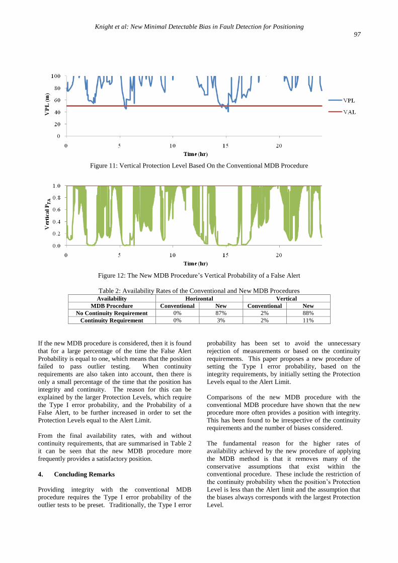
If the new MDB procedure is considered, then it is found
that for a large percentage of the time the False Alert
Probability is equal to one, which means that the position
failed to pass outlier testing. When continuity
requirements are also taken into account, then there is
only a small percentage of the time that the position has
integrity and continuity. The reason for this can be
explained by the larger Protection Levels, which require
the Type I error probability, and the Probability of a
False Alert, to be further increased in order to set the
Protection Levels equal to the Alert Limit.
From the final availability rates, with and without
continuity requirements, that are summarised in Table 2
it can be seen that the new MDB procedure more
frequently provides a satisfactory position.
4. Concluding Remarks
Providing integrity with the conventional MDB
procedure requires the Type I error probability of the
outlier tests to be preset. Traditionally, the Type I error
probability has been set to avoid the unnecessary
rejection of measurements or based on the continuity
requirements. This paper proposes a new procedure of
setting the Type I error probability, based on the
integrity requirements, by initially setting the Protection
Levels equal to the Alert Limit.
Comparisons of the new MDB procedure with the
conventional MDB procedure have shown that the new
procedure more often provides a position with integrity.
This has been found to be irrespective of the continuity
requirements and the number of biases considered.
The fundamental reason for the higher rates of
availability achieved by the new procedure of applying
the MDB method is that it removes many of the
conservative assumptions that exist within the
conventional procedure. These include the restriction of
the continuity probability when the position’s Protection
Level is less than the Alert limit and the assumption that
the biases always corresponds with the largest Protection
Level.
Figure 11: Vertical Protection Level Based On the Conventional MDB Procedure
Figure 12: The New MDB Procedure’s Vertical Probability of a False Alert
Table 2: Availability Rates of the Conventional and New MDB Procedures
Availability Horizontal Vertical
MDB Procedure Conventional New Conventional New
No Continuity Requirement 0% 87% 2% 88%
Continuity Requirement 0% 3% 2% 11%

Knight et al: New Minimal Detectable Bias in Fault Detection for Positioning
98
Since the proposed procedure increases the Availability
of a position with Integrity and is simple to apply, there
appears to be few reasons as to why the proposed
procedure should not be employed. The main reason
though appears to be in the case where the measurements
are remeasured since there is a higher probability of the
measurements being rejected. However, in other
applications, that may or may not have continuity
requirements, the main reason appears to be that the new
procedure is slightly more computationally intensive
than the conventional approach. Even considering this,
it appears that the new MDB procedure should still be
used in preference to the conventional approach.
Even though the new MDB procedure increases the
percentage of time that a position with integrity can be
obtained, there are still times when a position with
integrity cannot be obtained due to the very poor
geometry. Since the new MDB procedure, removes
many of the conservative assumptions that exist within
the conventional procedure. It appears that to further
increase the percentage of time that a position with
integrity can be obtained the new MDB procedure must
be extended to incorporate a dynamic model, via the use
of Kalman filter, and/or increase the number of
measurements, via sensor fusion.
References
Angus J. E. (2006), RAIM with Multiple Faults,
Navigation, Vol. 53, No. 4, pp. 249-257.
Baarda W. (1967), Statistical Concepts in Geodesy,
Netherlands Geodetic Commission, Publications on
Geodesy, New Series 2, No. 4, Delft, Netherlands.
Baarda W. (1968), A Testing Procedure for use in
Geodetic Networks, Netherlands Geodetic
Commission, Publications on Geodesy, New Series 2,
No. 5, Delft, Netherlands.
Blanch J., Ene A., Walter T. and Enge P. (2007), An
Optimized Multiple Hypothesis RAIM Algorithm
For Vertical Guidance, Proceedings of Institute of
Navigation GNSS 2007, Fort Worth, Texas, USA,
September 25-28, 2007, pp. 2924-2933.
Brown R. G. (1992), A Baseline GPS RAIM Scheme
and a Note on The Equivalence of Three RAIM
Methods, Navigation, Vol. 39, No. 3, pp. 301-316.
Brown R. G. and Chin G. Y. (1997), GPS RAIM:
Calculation of The Threshold and Protection
Radius Using Chi-Square Methods - A Geometric
Approach, In: Global Positioning System, Vol. 5,
The Institute of Navigation, Fairfax, Virginia, pp.
155-178.
Chin G. Y., Kraemer J. H. and Brown R. G. (1992), GPS
RAIM: Screening Out Bad Geometries Under
Worst-Case Bias Conditions, Navigation, Vol. 39,
No. 4, pp. 407-428.
Cook R. D. and Weisberg S. (1982), Residuals and
Influence in Regression, Chapman and Hall, New
York.
Dykstra R. L. (1980), Product Inequalities Involving
the Multivariate Normal Distribution, Journal of the
American Statistical Association, Vol. 75, No. 371,
pp. 646-650.
Förstner W. (1983), Reliability and Discernability of
Extended Gauss-Marko Models, In: Mathematical
Models of Geodetic/Photogrammetric Point
Determination with Regard to Outliers and
Systematic Errors, Deutsche Geodätische
Kommission, Reihe A, No. 98, Munchen, Germany.
Kelly R. J. (1998), The Linear Model, RNP, and the
Near-Optimum Fault Detection and Exclusion
Algorithm, In: Global Positioning System, Vol. 5,
The Institute of Navigation, Fairfax, Virginia, pp.
227-260.
Knight N. L., Wang J. and Rizos C. (2010), Generalised
Measures of Reliability for Multiple Outliers,
Journal of Geodesy, Vol. 84, No. 10, pp. 625-635.
Knight N. L., Wang J., Rizos C. and Han S. (2009),
GNSS Integrity Monitoring for Two Satellite Faults,
IGNSS Symposium 2009, Surfers Paradise, Australia,
December 1-3, 2009.
Lee Y. C. and Van Dyke K. L. (2002), Analysis
Performed in Support of the Ad-Hoc Working
Group of RTCA SC-159 on RAIM/FDE Issues,
Proceedings of Institute of Navigation NTM 2002,
San Diego, California, USA, January 28-30, 2002, pp.
639-654.
Lee Y., Van Dyke K., DeCleene B., Studenny J. and
Beckmann M. (1996), Summary of RTCA SC-159
GPS Integrity Working Group Activities, Navigation,
Vol. 43, No. 3, pp. 195-226.
Ober P. B. (2000a), LAAS Integrity The Bayesian Way,
Proceedings of Institute of Navigation NTM 2000,
Anaheim, California, USA, January 26-28, 2000, pp.
236-245.
Ober P. B. (2000b), Position Domain Integrity
Assessment, Proceedings of Institute of Navigation

Knight et al: New Minimal Detectable Bias in Fault Detection for Positioning
99
GPS 2000, Salt Lake City, Utah, USA, September
19-22, 2000, pp. 1948-1956.
Oliveira J. and Tiberius C. (2009), Quality Control in
SBAS: Protection Levels and Reliability Levels,
Journal of Navigation, Vol. 62, No. 3, pp. 509-522.
Parkinson B. W. and Axelrad P. (1988), Autonomous
GPS Integrity Monitoring Using the Pseudorange
Residual, Navigation, Vol. 35, No. 2, pp. 49-68.
Pervan B. S., Pullen S. P. and Christie J. R. (1998), A
Multiple Hypothesis Approach To Satellite
Navigation Integrity, Navigation, Vol. 45, No. 1, pp.
61-71.
Sĭdák Z. (1968), On Multivariate Normal Probabilities
of Rectangles: Their Dependence On Correlations,
The Annuals of Mathematical Statistics, Vol. 39, No.
5, pp. 1425-1434.
Sturza M. A. (1988), Navigation System Integrity
Monitoring Using Redundant Measurements,
Navigation, Vol. 35, No. 4, pp. 69-87.
Teunissen P. J. G. (1990), Quality Control in Integrated
Navigation Systems, IEEE Aerospace and Electronic
Systems Magazine, Vol. 5, No. 7, pp. 35-41.
Wang J. and Kubo Y. (2010), GNSS Receiver
Autonomous Integrity Monitoring, In: Sugimoto S.
and Shibasaki R. (Eds), GPS Handbook, Asakura,
Tokyo.
Biography
Nathan Knight is a PhD candidate at the School of
Surveying and Spatial Information Systems, at the
University of New South Wales. He holds a Bachelor in
Surveying from the University of Newcastle,
Australia. His current research interests are in the areas
of modelling and quality control, for positioning and
navigation with global navigation satellite
systems. Email: [email protected]
Top Related
Copyright © 2022 FDOKUMEN

