


Bahasa
Halaman
Hukum

Iranian Journal of Fisheries Sciences 15(1) 75-90 2016
Estimating catches with automatic identification system (AIS)
data: a case study of single otter trawl in Zhoushan fishing
ground, China
Wang Y.B.1*
; Wang Y.2
Received: June 2014 Accepted: February 2015
Abstract
The sailing tracks of single otter trawl vessels were simulated using cubic hermite
spline (cHs) interpolation method based on the automatic identification system (AIS)
data of 6 sampled vessels that were fishing in the Zhoushan fishing grounds after the
close of the fishing season from September 2012 to January 2013. The vessels’ status
(i.e. whether the vessels were fishing or not) were determined based on the integrated
information of speed method and the simulated tracks. Generalized additive model
(GAM) was built according to the logbook data of the 6 vessels in 2010, and then the
GAM was applied to the AIS data of the same 6 vessels from September 2012 to
January 2013 to estimate the monthly catches of these vessels in this period. The
results show that the error of the simulated tracks increase with the increase in time
interval, and the time interval of AIS data should be shorter than 30 minutes to prevent
low accurate results. GAM can give viable estimates of catches when they do not
greatly fluctuate over years. The step-by-step GAM analyses indicate that the factors,
which affect catch, are ordered by their importance as date, sea surface salinity (SSS),
latitude, sea surface temperature (SST), sea surface height (SSH) and longitude. This
research is a new attempt for the study of fisheries resources in China using new data
sources, which will be helpful for the improvement of fishery research in such data-
poor countries as China.
Keywords: AIS, cHs interpolation, Sailing track, GAM
1 -School of Fisheries, Zhejiang Ocean University, No. 1 Haida south road, Zhoushan, 316022,
China
2-Marine Fisheries Research Institute of Zhejiang, No. 28 sports road, Zhoushan, 316021,
China
*Corresponding author's email: [email protected]

76 Wang and Wang, Estimating catches with automatic identification system data: a case study of …
Introduction
Stock assessment methods for
quantifying the status of fishery
resources are critical to effective
fisheries management (Gobert, 1997;
Aubone, 2003; Wang et al., 2011).
Nowadays, stock assessment methods
have become more and more complex
because complex models are considered
to give a clearer picture of stock status
(Lapointe et al., 2012). Thus, more
data from different sources have to be
collected. Although only the traditional
statistics, such as catch and fishing
effort, cannot meet the needs of stock
assessment, they are still one of the
most important data that should be used
in fisheries stock assessment (Wang et
al., 2011; Anonymous, 2013).
In many countries, catch data
reported by their fisheries management
agencies are biased. They are under-
reported by 100-500% in many
developing countries and by 30-50% in
developed countries (Zeller et al., 2007;
Zeller et al., 2011). In China, the
problem might be more serious for its
over-reported catches have affected the
trend of global catches (Watson and
Pauly, 2001). Watson and Pauly (2001)
pointed out that China’s fishery data
have distorted analyses provided by the
FAO, and misled international fishery
investment and management. In 2008,
China revised the total fishery yield for
2006 based on the National Agriculture
Census (NAC) of 2006 (FAO, 2010),
and since 2009, China has treated the
statistics as one of the most important
works in fisheries management to
improve the quality of data (FAO,
2012). In view of the efforts made by
China, FAO did not separate the catches
of China from those of other countries
in the report of ―The state of word
fisheries and aquaculture 2012‖ (FAO,
2012). The quality of the reported
catch data in China has improved a lot,
but compared with the developed
countries, the current data collection
system in China is not sophisticated
enough to ensure the data (catches) to
be applied to stock assessment and
management (Wang et al, 2015).
Therefore, most of the fisheries in
China still belong to data-poor fisheries,
and other methods are needed to further
improve the quality of fishery statistics.
Since the last 15 years, the vessel
monitor system (VMS) has been
considered by many fishery managers
and scientists as an important technique
for fisheries monitoring, management
and surveillance (Chang, 2011). Now
VMS is generally used to track vessel
locations for fisheries which can be
applied to deter illegal fishing activity
(FAO, 1998; Wold et al., 2000) as well
as to study the impact of fishing gear on
the benthic communities (Piet et al.,
2000; Deng, 2005; Hiddink et al., 2006
a, b; Hintzen et al., 2010). In addition,
VMS data can also be used to provide
independent estimates of fishing
intensity (Gulin, 2005; Murawski et al.,
2005; Mills et al., 2007), analyze the
dynamics of fisheries (Kourti et al.,
2005.), and describe fish distribution
(Bertrand et al., 2005). It can be
expected that many potential functions
Iranian Journal of Fisheries Sciences 15(1) 2016 77
of VMS in fisheries studies will be
developed.
In 2008, Zhejiang became the first
province in China that installed AIS on
fishing vessels. It is required that
fishing vessels with main engine power
larger than 44kW install AIS, and those
with main engine power larger than
136kW install the terminal equipment
of satellite position information. AIS is
an automatic tracking system used on
ships for identifying and locating
vessels by electronically exchanging
data with other nearby ships and AIS
base stations. It can provide essential
information about the sailing of fishing
vessels, including the vessel’s name,
position (longitude and latitude), speed,
navigation heading, date and time.
Although VMS and AIS are quite
different on the technical level,
sometimes VMS is used as an informal
synonym for AIS, because both of them
can be applied to marine oversight and
navigation. In China, AIS only plays a
role in monitoring or surveying the
illegal fishing activities when the
fishing season is closed (each year from
June 1st to September 15th, the otter
trawls are forbidden to fish in the East
China Sea) and for safety command
when there is extreme weather
conditions. It has not been used as an
assistant tool, like the VMS does in
some developed countries, in the
research of fisheries science.
Both AIS and VMS are powerful
instruments. In China, the VMS data
consists of two parts: AIS data and
maritime satellite data. Because the
cost of maritime satellite is high, the
recording frequency of maritime
satellite data is low. Therefore, the
VMS data mainly come from AIS.
However, neither AIS nor VMS can
provide the catch, which is the key
information in stock assessment as
mentioned above. If the information,
including catch data, from logbooks can
be combined with the AIS data, the
usefulness of AIS can be increased.
The spatial distribution of catch, effort
and stocks at high resolution can be
explored, and the fishing activity that
cannot be clearly figured out from AIS
data may be verified based on logbooks
(Palmer and Wigley, 2009; Gerritsen
and Lordan, 2011).
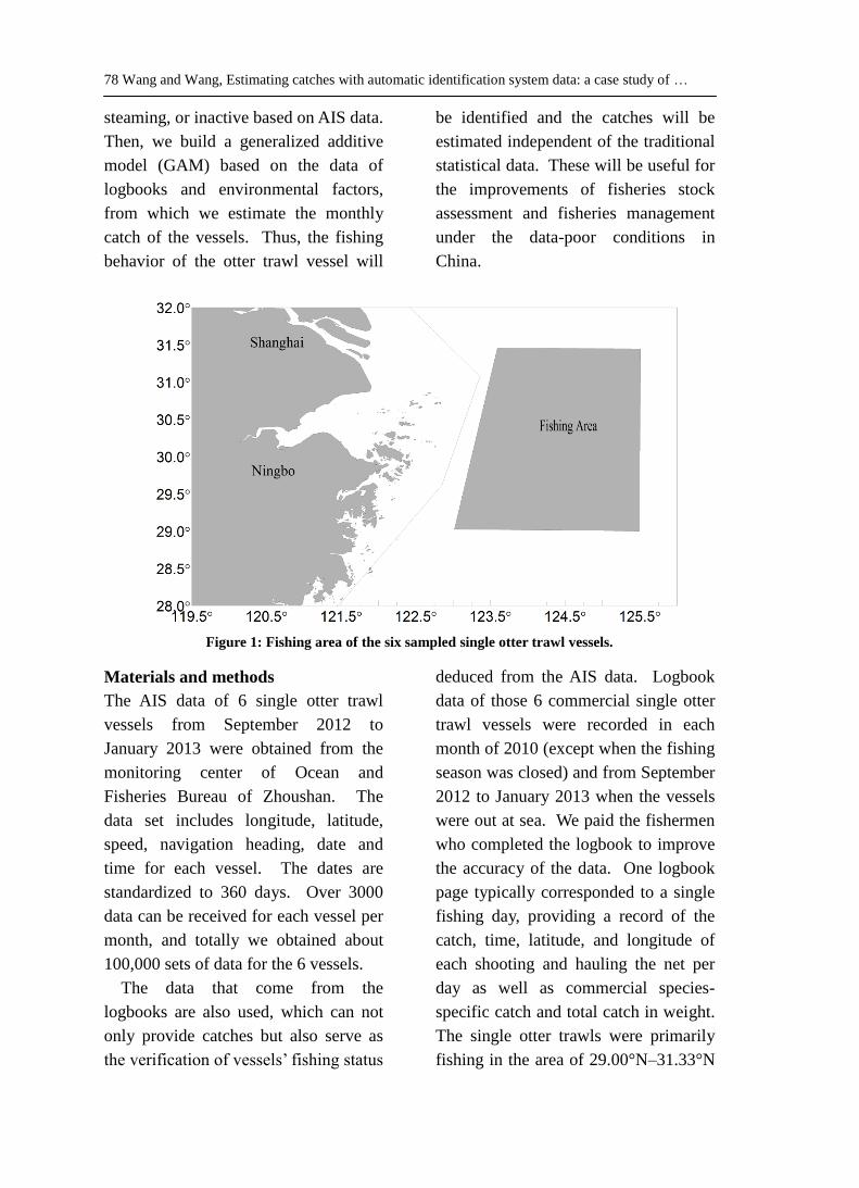
The Zhoushan fishing grounds,
located in the East China Sea, is the
largest near-shore fishing grounds in
China (Fig. 1). Mainland rivers
(including the Yangtze River)
continually flow into the East China
Sea, which bring a large amount of
nutritive salts into Zhoushan fishing
grounds and its adjacent waters. The
favorable geographical and
hydrological conditions make this sea
area a suitable habitat for fish
reproduction, growth, feeding, and
overwintering (Yu, 2011; Wang et al.,
2012). Thus, it is one of the most
important fishing areas in China, and
over thousands of vessels are fishing in
this area, which makes it also one of the
most representative fishing zones in
China.
In this paper, we firstly judge the
status of every single otter trawl vessel
fishing in the Zhoushan fishing
grounds, i.e. whether a vessel is fishing,
78 Wang and Wang, Estimating catches with automatic identification system data: a case study of …
steaming, or inactive based on AIS data.
Then, we build a generalized additive
model (GAM) based on the data of
logbooks and environmental factors,
from which we estimate the monthly
catch of the vessels. Thus, the fishing
behavior of the otter trawl vessel will
be identified and the catches will be
estimated independent of the traditional
statistical data. These will be useful for
the improvements of fisheries stock
assessment and fisheries management
under the data-poor conditions in
China.
Figure 1: Fishing area of the six sampled single otter trawl vessels.
Materials and methods
The AIS data of 6 single otter trawl
vessels from September 2012 to
January 2013 were obtained from the
monitoring center of Ocean and
Fisheries Bureau of Zhoushan. The
data set includes longitude, latitude,
speed, navigation heading, date and
time for each vessel. The dates are
standardized to 360 days. Over 3000
data can be received for each vessel per
month, and totally we obtained about
100,000 sets of data for the 6 vessels.
The data that come from the
logbooks are also used, which can not
only provide catches but also serve as
the verification of vessels’ fishing status
deduced from the AIS data. Logbook
data of those 6 commercial single otter
trawl vessels were recorded in each
month of 2010 (except when the fishing
season was closed) and from September
2012 to January 2013 when the vessels
were out at sea. We paid the fishermen
who completed the logbook to improve
the accuracy of the data. One logbook
page typically corresponded to a single
fishing day, providing a record of the
catch, time, latitude, and longitude of
each shooting and hauling the net per
day as well as commercial species-
specific catch and total catch in weight.
The single otter trawls were primarily
fishing in the area of 29.00°N–31.33°N
Iranian Journal of Fisheries Sciences 15(1) 2016 79
and 122.50°E–125.30°E (Fig. 1).
Usually the AIS data are not sent
back to the base stations in accordance
with the fixed frequency. Sometimes
data are received every few seconds,
but sometimes more than half an hour
apart. When the time interval between
two registration points is short, straight
lines can be used to describe the sailing
track. However, when the time interval
is large, the straight line will not be
viable since the headings of the vessel
on the two successive registration
points are not in the same direction
(Hedin et al., 1996; Jeffrey et al., 2001;
Hijmans et al., 2005; Tremblay et al.,
2006; Hedger et al., 2008). Thus, we
used cubic Hermite spline (cHs)
interpolation method for the estimation
of sailing tracks. It can pass through all
the registration points, and use more
information (like heading and speed) at
the same time, which will estimate the
sailing tracks with less deviation
(Hintzen et al., 2010). The cHs method
is based on four polynomials and it
considers heading and speed as two
points. Its interpolation curve passes all
the data points, and constructs a
simulative trajectory. (For more detailed
descriptions, refer to Hintzen et al.
(2010) and Wang et al. (2015).
When the sailing tracks are
determined, we still cannot clearly
know the fishing status (i.e. whether the
vessel is dragging or not) until some
features or the speed range of fishing
activity are known. It is important to
know this to avoid assigning catches or
effort to locations where the vessel was
not actually engaged in fishing
(Gerritsen and Lordan, 2011). We
firstly used the vessels’ speeds coming
from AIS to detect the fishing activity
(Eastwood, 2007; Mullowney and
Dawe, 2009; Lee et al., 2010). But
sometimes the speed method may
underestimate a vessel’s activity,
especially in the case of long intervals
between data. Thus we also relied on
the fishing features of the otter trawl
vessels at the same time to judge their
dragging behavior. Generally speaking,
when the single otter trawls are fishing,
they will show certain features, i.e. they
drag back and forth within a certain
range when they are fishing. Then, if
the sailing tracks, fishing features and
fishing speeds are estimated with less
deviation, we will get more accurate
spatial distribution characteristics of
fishing behaviors. At last, the status of
vessels are also validated by checking
the records in logbooks (Palmer and
Wigley, 2009). The percentage
frequency distributions of AIS speed
and the corresponding records in the
logbooks are compared to determine
whether and when a vessel is fishing.
With the criteria for judging the
characteristics of fishing status, we can
tell the locations where the net is shot
and hauled. Then we build a GAM to
predict the monthly catch total based on
the AIS and the environmental data.
Catch is log-transformed with errors
being assumed to be normally
distributed in the GAM (Tian et al.,
2009; Wang et al., 2012):
80 Wang and Wang, Estimating catches with automatic identification system data: a case study of …
)()()()()()()()ln( SSHsSSSsSSTslatitueslongitudestimetrawlingsdatescacth
(1),
where s is the spline smoother function,
and the variables in the brackets are the
factors that may have effects on catch
(Wang et al., 2012). Analysis of
deviance for the above GAM will be
done to screen the optimized model.
By using the optimized GAM we
estimate the catches of the 6 otter trawl
vessels from September 2012 to
January 2013 using the AIS data of the
6 vessels in 2010 and the corresponding
environmental data that come from the
Coriolis program of EU
(http://www.coriolis.eu.org/) and
Colorado Center for Astrodynamics
research
(http://eddy.colorado.edu/ccar/ssh/nrt_g
lobal_grid_viewer). The spatial
resolution was 11 . To verify the
accuracy of the estimates, we compared
the estimated catch with the recorded
catches in logbooks. R (Version 3.1.0)
was used for the analyses in the
research.
Results
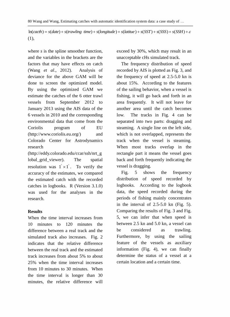
When the time interval increases from
10 minutes to 120 minutes the
difference between a real track and the
simulated track also increases. Fig. 2
indicates that the relative difference
between the real track and the estimated
track increases from about 5% to about
25% when the time interval increases
from 10 minutes to 30 minutes. When
the time interval is longer than 30
minutes, the relative difference will
exceed by 30%, which may result in an
unacceptable cHs simulated track.
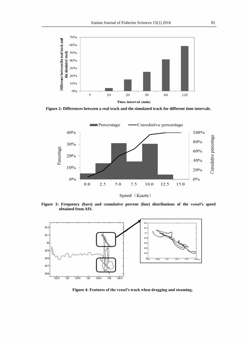
The frequency distribution of speed
recorded by AIS is plotted as Fig. 3, and
the frequency of speed at 2.5-5.0 kn is
about 15%. According to the features
of the sailing behavior, when a vessel is
fishing, it will go back and forth in an
area frequently. It will not leave for
another area until the catch becomes
low. The tracks in Fig. 4 can be
separated into two parts: dragging and
steaming. A single line on the left side,
which is not overlapped, represents the
track when the vessel is steaming.
When most tracks overlap in the
rectangle part it means the vessel goes
back and forth frequently indicating the
vessel is dragging.
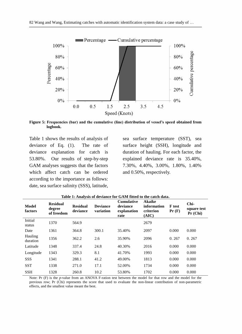
Fig. 5 shows the frequency
distribution of speed recorded by
logbooks. According to the logbook
data, the speed recorded during the
periods of fishing mainly concentrates
in the interval of 2.5-5.0 kn (Fig. 5).
Comparing the results of Fig. 3 and Fig.
5, we can infer that when speed is
between 2.5 kn and 5.0 kn, a vessel can
be considered as trawling.
Furthermore, by using the sailing
feature of the vessels as auxiliary
information (Fig. 4), we can finally
determine the status of a vessel at a
certain location and a certain time.
Iranian Journal of Fisheries Sciences 15(1) 2016 81
Figure 2: Differences between a real track and the simulated track for different time intervals.
Figure 3: Frequency (bars) and cumulative percent (line) distributions of the vessel’s speed
obtained from AIS.
Figure 4: Features of the vessel’s track when dragging and steaming.
82 Wang and Wang, Estimating catches with automatic identification system data: a case study of …
Figure 5: Frequencies (bar) and the cumulative (line) distribution of vessel’s speed obtained from
logbook.
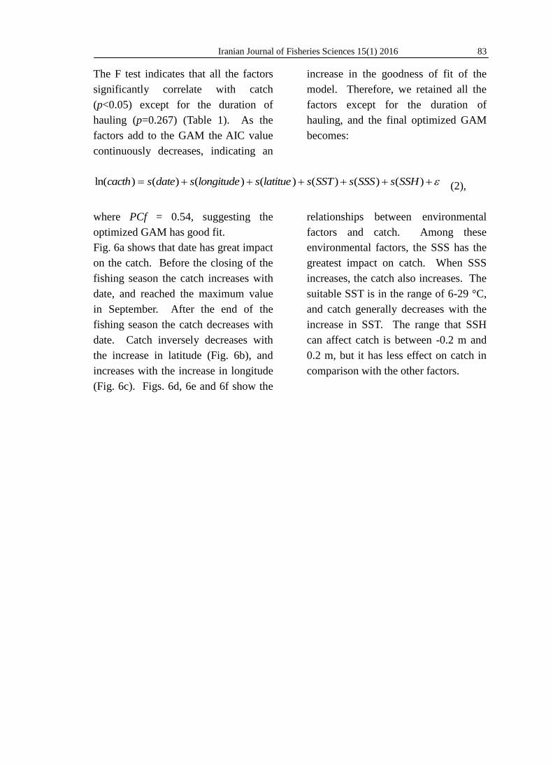
Table 1 shows the results of analysis of
deviance of Eq. (1). The rate of
deviance explanation for catch is
53.80%. Our results of step-by-step
GAM analyses suggests that the factors
which affect catch can be ordered
according to the importance as follows:
date, sea surface salinity (SSS), latitude,
sea surface temperature (SST), sea
surface height (SSH), longitude and
duration of hauling. For each factor, the
explained deviance rate is 35.40%,
7.30%, 4.40%, 3.00%, 1.80%, 1.40%
and 0.50%, respectively.
Table 1: Analysis of deviance for GAM fitted to the catch data.
Model
factors
Residual
degree
of freedom
Residual
deviance
Deviance
variation
Cumulative
deviance
explanation
rate
Akaike
information
criterion
(AIC)
F test
Pr (F)
Chi-
square test
Pr (Chi)
Initial
status 1370 564.9 2679
Date 1361 364.8 300.1 35.40% 2097 0.000 0.000
Hauling
duration 1356 362.2 2.6 35.90% 2096 0. 267 0. 267
Latitude 1348 337.4 24.8 40.30% 2016 0.000 0.000
Longitude 1343 329.3 8.1 41.70% 1993 0.000 0.000
SSS 1341 288.1 41.2 49.00% 1813 0.000 0.000
SST 1338 271.0 17.1 52.00% 1734 0.000 0.000
SSH 1328 260.8 10.2 53.80% 1702 0.000 0.000
Note: Pr (F) is the p-value from an ANOVA F-ration test between the model for that row and the model for the
previous row; Pr (Chi) represents the score that used to evaluate the non-linear contribution of non-parametric
effects, and the smallest value meant the best.
Iranian Journal of Fisheries Sciences 15(1) 2016 83
The F test indicates that all the factors
significantly correlate with catch
(p<0.05) except for the duration of
hauling (p=0.267) (Table 1). As the
factors add to the GAM the AIC value
continuously decreases, indicating an
increase in the goodness of fit of the
model. Therefore, we retained all the
factors except for the duration of
hauling, and the final optimized GAM
becomes:
)()()()()()()ln( SSHsSSSsSSTslatitueslongitudesdatescacth (2),
where PCf = 0.54, suggesting the
optimized GAM has good fit.
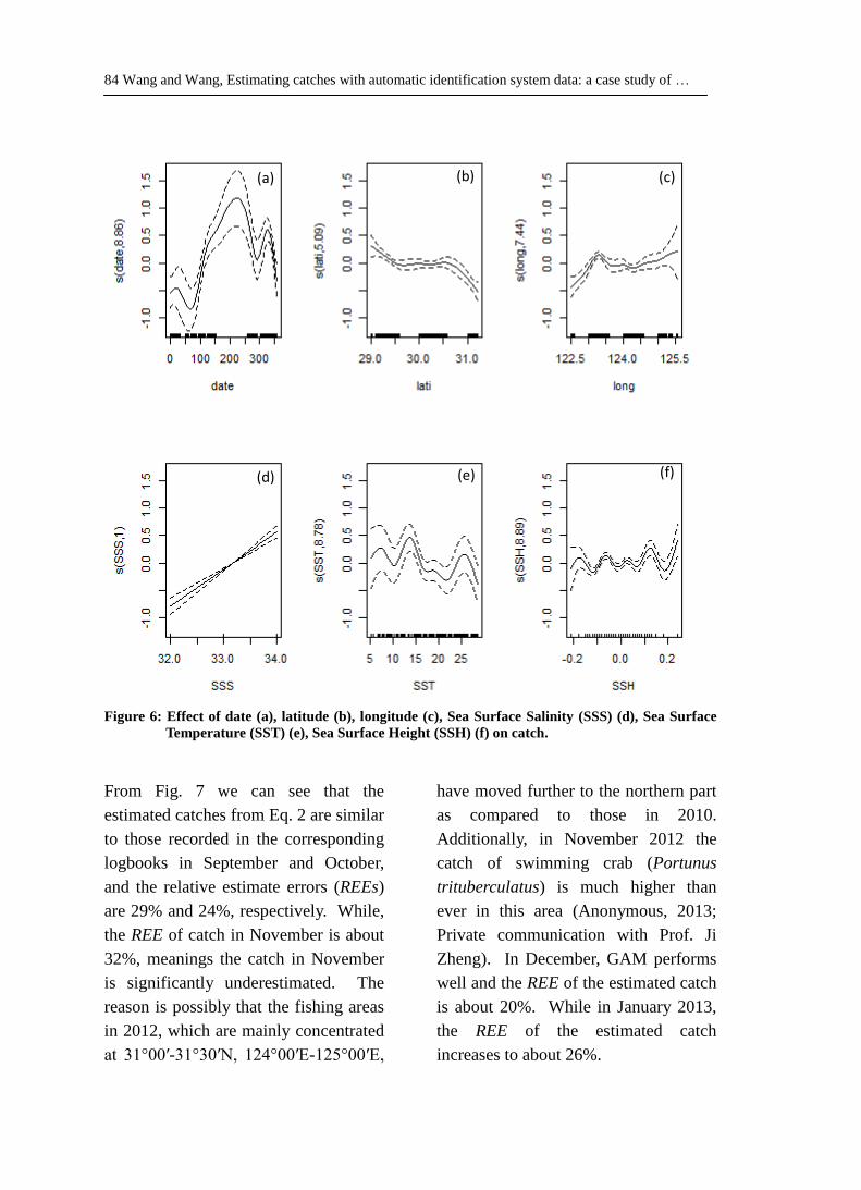
Fig. 6a shows that date has great impact
on the catch. Before the closing of the
fishing season the catch increases with
date, and reached the maximum value
in September. After the end of the
fishing season the catch decreases with
date. Catch inversely decreases with
the increase in latitude (Fig. 6b), and
increases with the increase in longitude
(Fig. 6c). Figs. 6d, 6e and 6f show the
relationships between environmental
factors and catch. Among these
environmental factors, the SSS has the
greatest impact on catch. When SSS
increases, the catch also increases. The
suitable SST is in the range of 6-29 °C,
and catch generally decreases with the
increase in SST. The range that SSH
can affect catch is between -0.2 m and
0.2 m, but it has less effect on catch in
comparison with the other factors.
84 Wang and Wang, Estimating catches with automatic identification system data: a case study of …
Figure 6: Effect of date (a), latitude (b), longitude (c), Sea Surface Salinity (SSS) (d), Sea Surface
Temperature (SST) (e), Sea Surface Height (SSH) (f) on catch.
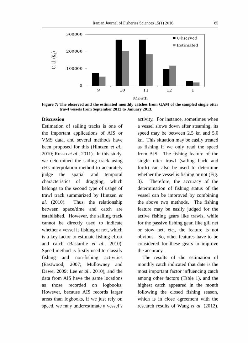
From Fig. 7 we can see that the
estimated catches from Eq. 2 are similar
to those recorded in the corresponding
logbooks in September and October,
and the relative estimate errors (REEs)
are 29% and 24%, respectively. While,
the REE of catch in November is about
32%, meanings the catch in November
is significantly underestimated. The
reason is possibly that the fishing areas
in 2012, which are mainly concentrated
at 31°00′-31°30′N, 124°00′E-125°00′E,
have moved further to the northern part
as compared to those in 2010.
Additionally, in November 2012 the
catch of swimming crab (Portunus
trituberculatus) is much higher than
ever in this area (Anonymous, 2013;
Private communication with Prof. Ji
Zheng). In December, GAM performs
well and the REE of the estimated catch
is about 20%. While in January 2013,
the REE of the estimated catch
increases to about 26%.
(f) (d) (e)
(b) (c) (a)
Iranian Journal of Fisheries Sciences 15(1) 2016 85
Figure 7: The observed and the estimated monthly catches from GAM of the sampled single otter
trawl vessels from September 2012 to January 2013.
Discussion
Estimation of sailing tracks is one of
the important applications of AIS or
VMS data, and several methods have
been proposed for this (Hintzen et al.,
2010; Russo et al., 2011). In this study,
we determined the sailing track using
cHs interpolation method to accurately
judge the spatial and temporal
characteristics of dragging, which
belongs to the second type of usage of
trawl track summarized by Hintzen et
al. (2010). Thus, the relationship
between space/time and catch are
established. However, the sailing track
cannot be directly used to indicate
whether a vessel is fishing or not, which
is a key factor to estimate fishing effort
and catch (Bastardie et al., 2010).
Speed method is firstly used to classify
fishing and non-fishing activities
(Eastwood, 2007; Mullowney and
Dawe, 2009; Lee et al., 2010), and the
data from AIS have the same locations
as those recorded on logbooks.
However, because AIS records larger
areas than logbooks, if we just rely on
speed, we may underestimate a vessel’s
activity. For instance, sometimes when
a vessel slows down after steaming, its
speed may be between 2.5 kn and 5.0
kn. This situation may be easily treated
as fishing if we only read the speed
from AIS. The fishing feature of the
single otter trawl (sailing back and
forth) can also be used to determine
whether the vessel is fishing or not (Fig.
3). Therefore, the accuracy of the
determination of fishing status of the
vessel can be improved by combining
the above two methods. The fishing
feature may be easily judged for the
active fishing gears like trawls, while
for the passive fishing gear, like gill net
or stow net, etc., the feature is not
obvious. So, other features have to be
considered for these gears to improve
the accuracy.
The results of the estimation of
monthly catch indicated that date is the
most important factor influencing catch
among other factors (Table 1), and the
highest catch appeared in the month
following the closed fishing season,
which is in close agreement with the
research results of Wang et al. (2012).
86 Wang and Wang, Estimating catches with automatic identification system data: a case study of …
The high catch may indicate the
increased abundance. This may owe to
the closed fishing season, which makes
the fisheries resources recover
temporarily. Duration of hauling is not
significantly correlated with catch,
which is inconsistent with previous
studies (Wang et al., 2012).
The criterion that is frequently used
to classify the vessel’s fishing and non-
fishing activities is speed (Eastwood,
2007; Mullowney and Dawe, 2009; Lee
et al., 2010). Unlike the previous study
that totally used logbooks, in this study
we used both the logbook and AIS data
to determine the fishing status by
analyzing the sailing speed and trawling
feature of the vessel. The range of the
duration of hauling determined by AIS
data is from 2.5 to 5 hours, which is
consistent with the observation that the
speed of bottom trawler is usually lower
than 3.6 kn (6.5 Km/h) (Murawski et
al., 2005) and the speed of fishing
activities falls within a narrow range
(Palmer and Wigley, 2009). But this is
narrower than those based on logbooks
(from 0.5 to 6 hours). The narrow
range results in similar catches, and
then their correlation may not be
significant. Although the range became
small, it still covers the optimal range
for catch and retention (Wang et al.,
2012). The spatial factors also affect
catch amounts (Figs. 6b and 6c). Catch
decreases with increasing latitude and
decreasing longitude. Catch is higher
in the southern area, most likely
because of the influence of the Taiwan
warm current and the upwelling caused
by complex submarine topography
(Wang et al., 2012). A greater number
of fish are captured in the eastern
region of the study area, most likely
because of declines in abundance in
coastal and inshore waters because of
overfishing, pollution, and habitat loss
(Wang et al., 2012). Environmental
factors are usually important when
GAM is applied to fisheries research
(Zhou et al., 2004; Walsh et al, 2005;
Chen and Tian, 2006; Tian et al., 2009).
The catches fluctuated under the
impacts of SST and SSH (Figs. 6e and
6f), indicating the seasonal variations in
catch is obvious. Catch increases with
increasing SSS, which is consistent
with the effects of longitude since the
SSS in the eastern region of the study
area is usually high (the west region of
the study area is affected by the diluted
water of Yangtze River).
Acknowledgements
This work was supported by the
National Natural Science Foundation of
China (grant number 40801225 and
31270527); the Natural Science
Foundation of Zhejiang Province (grant
number LY13D010005); Young
academic leaders climbing program of
Zhejiang Province (grant number
pd2013222). We wish to thank Ji
Zheng, who gave us great help in
renting sampled vessels and collecting
the AIS data.
References
Anonymous, 2013. China fishery
statistical yearbook. China
Iranian Journal of Fisheries Sciences 15(1) 2016 87
Agriculture Press, Beijing.
Anonymous, 2013. Does catch reflect
abundance? Nature, 494, 303–306.
Aubone, A., 2003. Threshold for
sustainable exploitation of an age-
structure fishery. Ecological
Modelling, 173, 95–107.
Bastardie, F.J., Nielsen, R., Ulrich,
C., Egekvist. J. and Degel H.,
2010. Detailed mapping of fishing
effort and landings by coupling
fishing logbooks with satellite
recorded vessel geo-location.
Fisheries Research, 106, 41–53.
Bertrand, S., Burgos, J.M., Gerlotto,
F. and Atiquipa, J., 2005. Levy
trajectories of Peruvianpurse-
seiners as an indicator of the spatial
distribution of anchovy (Engraulis
ringens). ICES Journal of Marine
Science, 62, 477–482.
Chang, S., 2011. Application of a
vessel monitoring system to
advance sustainable fisheries
management—Benefits received in
Taiwan. Marine Policy, 35, 116–
121.
Chen, X.J. and Tian, S.Q., 2006.
Temp-spatial distribution on
abundance index of nylon flying
squid Ommastrephes bartrami in
the Northwestern Pacific using
generalized additive models.
Journal of Jimei University, 11,
295–300.
Deng, R., 2005. Can vessel monitoring
system data also be used to study
trawling intensity and population
depletion? The example of
Australia’s northern prawn fishery.
Canadian Journal of Fisheries and
Aquaculture Science, 62, 611–622.
Eastwood, P., 2007. Human activities
in UK offshore waters: an
assessment of direct, physical
pressure on the seabed. ICES
Journal of Marine Science, 64,
453–463.
FAO., 1998. Fishing operations. Vessel
monitoring systems. FAO technical
guidelines for responsible
fisheries–Fishing Operations–1
Suppl. 1–1. Vessel Monitoring
Systems. Rome. FAO. pp.4–10.
FAO., 2010. The state of world
fisheries and aquaculture 2010.
FAO Fisheries and Aquaculture
Department, Rome. pp.5–6.
FAO., 2012. The state of world
fisheries and aquaculture 2012.
FAO Fisheries and Aquaculture
Department, Rome. pp.6–7.
Gerritsen, H. and Lordan, C., 2011.
Integrating vessel monitoring
systems (VMS) data with daily
catch data from logbooks to
explore the spatial distribution of
catch and effort at high resolution.
ICES Journal of Marne Science,
68, 245–252.
Gobert, B., 1997. Evaluating mortality
using length-frequency data when
growth parameters are poorly
known. Naga, the ICLARM
Quarterly, 20, 46–51.
Gulin, D., 2005. Fishing vessels
monitoring systems. In: ELMAR,
2005. The 47th
international
symposium, 8–10 June, 2005,
Zadar, Croatia; 2005. pp. 369–372.
Hedger, R.D., Martin, F., Dodson,
J.J., Hatin, D., Caron, F. and
88 Wang and Wang, Estimating catches with automatic identification system data: a case study of …
Whoriskey, F.G., 2008. The
optimized interpolation of fish
positions and speeds in an array of
fixed acoustic receivers. ICES
Journal of Marine Science, 65,
1248–1259.
Hedin, A.E., Fleming, E.L., Manson,
A.H., Schmidlin, F.J., Avery,
S.K., Clark, R.R., Franke, S.J.,
Fraser, G.J., Tsuda, T., Via, F.
and Vincent, R.A., 1996.
Empirical wind model for the
upper, middle and lower
atmosphere. Journal of
Atmospheric and Solar-Terrestrial
Physics, 58, 1421–1447.
Hiddink, J.G., Jennigs, S. and Kaiser,
M.J., 2006a. Indicators of the
ecological impact of bottom-trawl
disturbance on seabed
communities. Ecosystems, 9, 1190–
1199.
Hiddink, J.G., Jennigs, S., Kaiser, M.
J., Queiros, A.M., Duplisea, D.E.
and Piet, G.J., 2006b. Cumulative
impacts of seabed trawl disturbance
on benthic biomass, production,
and species richness in different
habitats. Canadian Journal of
Fisheries and Aquaculture Science,
63, 721–736.
Hijmans, R.J., Cameron, S.E., Parra,
J.L., Jones, P.G. and Jarvis, A.,
2005. Very high resolution
interpolated climate surfaces for
global land areas. International
Journal of Climatology, 25, 1965–
1978.
Hintzen, N.T., Piet, G.J. and Brunel,
T., 2010. Improved estimation of
trawling tracks using cubic Hermite
spline interpolation of position
registration data. Fisheries
Research, 101, 108–115.
Jeffrey, S.J., Carter, J.O., Moodie,
K.B. and Beswick, A.R., 2001.
Using spatial interpolation to
construct a comprehensive archive
of Australian climate data.
Environmental Modeling and
Software, 16, 309–330.
Kourti, N., Shepherd, I., Greidanus,
H., Alvarez, M., Aresu, E.,
Bauna, T., Chesworth, J.,
Lemoine, G. and Schwartz, G.,
2005. Integrating remote sensing in
fisheries control. Fisheries
Management and Ecology, 12,
295–307.
Lapointe, G., Mercer, L. and
Conathan, M., 2012. Counting
fish 101, an analysis of fish stock
assessments. Center for American
Progress, 9(2012), 15.
Lee, J., South, A.B. and Jennings, S.,
2010. Developing reliable,
repeatable, and accessible methods
to provide high-resolution
estimates of fishing-effort
distributions from vessel
monitoring system (VMS) data.
ICES Journal of Marine Science,
67, 1260–1271.
Mills, C.M., Townsend, S.E.,
Jennings, S., Eastwood, P.D. and
Houghton, C.A., 2007. Estimating
high resolution trawl fishing effort
from satellite-based vessel
monitoring system data. ICES
Journal of Marine Science 64,
Iranian Journal of Fisheries Sciences 15(1) 2016 89
248–255.
Mullowney, D.R. and Dawe, E.G.,
2009. Development of performance
indices for the Newfoundland and
Labrador snow crab (Chionoecetes
opilio) fishery using data from a
vessel monitoring system.
Fisheries Research, 100, 248–254.
Murawski, S.A., Wigley, S.E.,
Fogarty, M.J., Rago, P.J. and
Mountain, D.G., 2005. Effort
distribution and catch patterns
adjacent to temperate MPAs. ICES
Journal of Marine Science, 62,
1150–1167.
Palmer, M.C. and Wigley, S.E., 2009.
Using positional data from vessel
monitoring systems to validate the
logbook-reported area fished and
the stock allocation of commercial
fisheries landings. North American
Journal of Fisheries Management,
29, 928–942.
Piet, G.J., Rijnsdorp, A.D., Bergman,
M.J.N., van Santbrink, J.W.,
Craeymeersch, J. and Buijs, J.,
2000. A quantitative evaluation of
the impact of beam trawling on
ben-thic fauna in the southern
North Sea. ICES Journal of Marine
Science, 57, 1332–1339.
Russo, T., Parisi, A. and Cataudella,
S., 2011. New insights in
interpolating fishing tracks from
VMS data for different métiers.
Fisheries Research, 108, 184–194.
Tian, S.Q., Chen, X.J., Chen, Y., Xu,
L.X. and Dai, X.J., 2009.
Standardizing CPUE of
Ommastrephes bartramii for
Chinese squid-jigging fishery in
Northwest Pacific Ocean. Chinese
Journal of Oceanography
Limnology, 27, 729–739.
Tremblay, Y., Shaffer, S.A., Fowler, S.
L., Kuhn, C.E., McDonald, B.I.,
Weise, M.J., Bost, C.,
Weimerskirch, H., Crocker, D.E.,
Goebel, M.E. and Costa, D.P.,
2006. Interpolation of animal
tracking data in a fluid
environment. Journal of
Experimental Biology, 209, 128–
140.
Walsh, W.A., Ito, R.Y., Kawamoto,
K.E. and McCracken, M., 2005.
Analysis of logbook accuracy for
blue marlin (Makaira nigricans) in
the Hawaii-based longline fishery
with a generalized additive model
and commercial sales data.
Fisheries Research, 75, 175–192.
Wang, Y.B., Zheng, J. and Wang, Z.,
2011. The effects of distorted
fishery statistical data on fisheries
stock assessment. Chinese Journal
of Oceanography Limnology, 29,
270–276.
Wang, Y.B., Zheng, J., Wang, Y. and
Zheng X.Z., 2012. Spatiotemporal
factors affecting fish harvest and
their use in estimating the monthly
yield of single otter trawls in Putuo
district of Zhoushan, China.
Chinese Journal of Oceanography
Limnology, 30, 580–586.
Wang, Y.B., Wang, Y. and Zheng, J.,
2015. Analyses of trawling track
and fishing activity based on the
data of vessel monitoring system
(VMS): the single otter trawl
vessels in Zhoushan fishing ground
90 Wang and Wang, Estimating catches with automatic identification system data: a case study of …
as a case. Journal of Ocean
University of China, 14, in press.
Watson, R. and Pauly, D., 2001.
Systematic distortions in world
fisheries catch trends. Nature, 414,
534–536.
Wold, C., Arrigotti, S., Johnson, L.,
Horn, A.V. and White, L., 2000. A
review of monitoring, control, and
surveillance programs of
international fisheries agreements
with a view to the IWC’s
inspection and observation scheme
of the RMS. International
Environmental Law Project,
Northwestern School of Law of
Lewis & Clark College, 2000.
Yu, C.G., 2011. Zhoushan fishing
ground fishery ecology. Science
Press, Beijing, 2011.
Zeller, D., Booth, S., Davis, G. and
Pauly, D., 2007. Re-estimation of
small-scale fishery catches for U.S.
flag-associated island areas in the
western Pacific: the last 50 years.
Fishery Bulltein, 105, 266–277.
Zeller, D., Rossing, P., Harper, S.,
Persson, L., Booth, S. and Pauly,
D., 2011. The Baltic Sea: estimates
of total fisheries removals 1950–
2007. Fisheries Research, 108,
356–363.
Zhou, S.F., Fan, W., Cui, X.S. and
Cheng, Y.H., 2004. Effects of
environmental factors on catch
variation of main species of stow
net fisheries in East China Sea.
Chinese Journal of Applied
Ecology, 15, 1637–1640.
Top Related
Copyright © 2022 FDOKUMEN

