Download - A basis for variational calculations in d dimensions

arX

iv:m

ath-

ph/0

4100

35v1

12

Oct

200

4

CUQM-105

math-ph/0410035

October 2004

A basis for variational calculations in d dimensions

Richard L. Hall 1 , Qutaibeh D. Katatbeh 2 , and Nasser Saad 3

(1) Department of Mathematics and Statistics,

Concordia University,

1455 de Maisonneuve Boulevard West,

Montreal, Quebec, Canada H3G 1M8.


Faculty of Science and Arts,

Jordan University of Science and Technology,

Irbid 22110, Jordan.


University of Prince Edward Island,

550 University Avenue, Charlottetown,

PEI, Canada C1A 4P3.

Abstract

In this paper we derive expressions for matrix elements (φi, Hφj) for the Hamiltonian H =

−∆ +∑

q a(q)rq in d ≥ 2 dimensions. The basis functions in each angular momentum subspace

are of the form φi(r) = ri+1+(t−d)/2e−rp/2, i ≥ 0, p > 0, t > 0. The matrix elements are given in

terms of the Gamma function for all d . The significance of the parameters t and p and scale s are

discussed. Applications to a variety of potentials are presented, including potentials with singular

repulsive terms of the form β/rα , α, β > 0, perturbed Coulomb potentials −D/r + Br + Ar2,

and potentials with weak repulsive terms, such as −γr2 + r4, γ > 0.

PACS 03.65.Ge, 31.15.Bs, 02.30.Mv.

http://arXiv.org/abs/math-ph/0410035v1

A basis for variational calculations in d dimensions page 2

1. Introduction

We study quantum mechanical Hamiltonians H = −∆ + V (r) in d ≥ 2 dimensions, where

V is a spherically-symmetric potential that supports discrete eigenvalues, r = |r|, r ∈ ℜd. We

estimate the spectrum of H in an n -dimensional trial space lying inside an angular-momentum

subspace labelled by ℓ and spanned by radial functions with the form

φ(r) =

n−1∑

i=0

ciri+1+(t−d)/2e−

1

2rp

, t > 0. (1.1)

If the potential is chosen to be a linear combination of powers

V (r) =∑

q

a(q)rq , (1.2)

then all the matrix elements of H may be expressed explicitly in terms of the Gamma function.

The expressions obtained will be functions of the parameters t and p , and also of a scale parameter

s to be introduced later. If the potential V is highly singular, the parameter t must be chosen

sufficiently large so that 〈V 〉 exists. The advantages of the particular form chosen for the radial

functions will become clear in the development. Thus we have n + 3 variational parameters with

which to optimize upper estimates to the spectrum of H , with one degree of freedom being employed

for normalization.

Systems with Hamiltonians of this type have enjoyed wide attention in the literature of quantum

mechanics [1-62]. This interest arises particularly from the usefullness of these problems as models

in atomic and molecular physics. Many numerical and analytical techniques have been used to

tackle Hamiltonians of this form. In Section 2 we derive general matrix elements and show how the

minimization with respect to scale s can be easily included. In section 3 we discuss some numerical

issues not the least of which is the usefulness of the reduction of the matrix eigen equations to

symmetric form by first diagonalizing the ‘normalization’ matrix N = [(φi, φj)]. The dependence

of the eigenvalues on the parameters {p, t, s} may be rather complicated. Since changes to scale s

do not involve the recomputation of the basic matrix elements, a policy which emerges is to fix n ,

always optimize fully with respect to scale s, and, if necessary, optimize approximately with respect

to t and p by exploring a few values; if higher accuracy is required, a full optimization is undertaken,

or n is increased. In Section 4 the matrix elements are applied to a variety of problems and the

results are compared with those found in earlier work. We suppose that the Hamiltonian operators

in this paper have domains D(H) ⊂ L2(ℜd), they are bounded below, essentially self adjoint, and

have at least one discrete eigenvalue at the bottom of the spectrum. This, of course, implies that the

potential cannot be dominated by repulsive terms. Because the potentials are spherically symmetric,

the discrete eigenvalues Ednℓ can be labelled by two quantum numbers, the total angular momentum


ℓ = 0, 1, 2, . . . , and a ‘radial’ quantum number, n = 0, 1, 2, . . . , which counts the eigenvalues in each

angular-momentum subspace. These eigenvalues satisfy the relation Ednℓ ≤ Ed

mℓ, n < m. With our

labelling convention, the eigenvalue Ednℓ(q) in d ≥ 2 spatial dimensions has degeneracy 1 for ℓ = 0

and, for ℓ > 0, the degeneracy is given [63] by the function Λ(d, ℓ) , where

Λ(d, ℓ) = (2ℓ+ d− 2)(ℓ+ d− 3)!/{ℓ!(d− 2)!}, d ≥ 2, ℓ > 0. (1.3)

Many techniques have been applied to approximate the spectrum of singular potentials of the form

(1.2) using perturbation, variational, and geometrical approximation techniques [1-62]. Exact solu-

tions for the energy may be obtained in some special cases by first choosing a wave function with

parameters, and then finding a potential of the form (1.2) for which this wave function is an eigen-

function; this is possible only when certain constraints are satisfied between the parameters {a(q)} ,

as we shall discuss later.

2. Matrix elements

We consider first the action of the Laplacian in d dimensions on a wave function Ψ(r) =

ψ(r)Yℓ(θ0, θ1, . . . , θd−1) with a spherically-symmetric factor ψ(r) and a generalized spherical har-

monic factor Yℓ. If we remove the spherical harmonic factor after the action of the Laplacian on Ψ

we obtain [64]∆Ψ

Yℓ= ψ′′(r) +

d− 1

rψ′(r) − ℓ(ℓ+ d− 2)

r2ψ(r). (2.1)

The radial Schrodinger equation for a spherically symmetric potential V (r) in d -dimensional space

is therefore given by

−d2ψ

dr2− d− 1

r

dψ

dr+l(l + d− 2)

r2ψ + V (r)ψ = Eψ, ψ(r) ∈ L2([0,∞), rd−1dr) (2.2)

A correspondence to a problem on the half line in one dimension with a Dirichlet boundary condition

at r = 0 is obtained with the aid of a radial wave-function R(r) defined by

R(r) = r(d−1)/2ψ(r), d ≥ 2, R(0) = 0. (2.3)

If we now re-write (2.2) in terms of this new radial function, we obtain the following Schrodinger

equation for a problem on the half line

HR = −d2R

dr2+ UR = ER, R ∈ L2([0,∞), dr), (2.4)

where the effective potential U(r) is given by

U(r) = V (r) +(2ℓ+ d− 1)(2ℓ+ d− 3)

4r2, (2.5)


and H = − d2

dr2 + U is the effective Hamiltonian. We note that in (2.5), d and l enter into the

equation only in the combination 2l + d in U(r) : consequently, the solutions for a given central

potential V (r) are the same provided d + 2l remains unaltered. In this setting, our trial wave

functions now have the explicit form

Ri(r) = r(t+1)/2+i exp(−rp/2) ∈ L2([0,∞), dr). (2.6)

Thus we have for the general radial function in our trial space

R(r) =

d−1∑

i=0

ciRi(r). (2.7)

The matrix elements we seek (in a given angular momentum subspace) are given by

Hij =(

Ri,−R′′j

)

+∑

q

a(q) (Ri, rqRj) . (2.8)

For each potential term rq, if we everywhere omit the constant angular factor (equal to 4π in the

case d = 3 ), we find the following fomulae, expressed now in terms of the L2([0,∞), dr) inner

product:

Pij(q, p, t) = (Ri, rqRj) =

∫ ∞

0

ri+j+1+t+qe−rp

dr, i, j = 0, 1, 2, . . . ,

=1

pΓ

(

i+ j + t+ q + 2

p

)

, t > −(q + 2).

(2.9)

This type of integral is found by setting x = rp, and using the differential relation rkdr =

(1/p)x(k+1−p)/pdx and the definition of the Gamma function. The normalization integrals are special

cases of (2.9), namely

Nij(p, t) = (Ri, Rj) = Pij(0, p, t) =1

pΓ

(

i+ j + t+ 2

p

)

. (2.10)

After some algebraic simplifications we find that the corresponding kinetic energy matrix elements

Kij(p, t) = −(

Ri, R′′j

)

are given by

Kij(p, t) =1

4pΓ

(

i+ j + t

p

)

[

(2ℓ+ d− 1)(2ℓ+ d− 3) + 1 − (i− j)2 + p(i+ j + t)]

, t > 0.

(2.11)

We note that these terms of the Hamiltonian matrix elements Hij are all symmetric under the

permutation (ij) (because of Hermiticity), and invariant with respect to changes in d and ℓ that

leave the form 2ℓ+ d invariant. These formulae may be used as they stand for all dimensions d ≥ 2

provided that t > 0 is chosen sufficiently large t > −(2 + q) to control the most singular potential

term rq. We note, in addition, that the choice {d = 3, ℓ = 0} also provides the odd-parity solutions

in one dimension.


We now consider the problem of minimizing (R,HR) with respect to the vector v of coefficient

{ci}n−1i=0 subject to the constraint that (R,R) = 1 . We immediately obtain the necessary condition:

Hv = ENv (2.12)

By the min-max characterization of the spectrum [67], the eigenvalues of this matrix equation are

upper bounds to the unknown exact eigenvalues Eiℓ, i = 0, 1, 2, . . . n − 1. We assume that these

discrete eigenvalues of the underlying operator H are either known to exist, or indeed are demon-

strated to exist by the results of this variational estimate. By considering scaled radial wave functions

of the form

Rs(r) = R(r/s), (2.13)

we find that factors of s remain only according to the dimensions of the terms. In effect, when using

the scaled wave functions (2.13), we can leave the matrix N unchanged and replace the matrix for

H by

Hij(s) =1

s2Kij(p, t) +

∑

q

a(q)sqPij(q, p, t). (2.14)

Thus the upper bounds we seek are provided by the eigenvalues of the matrix equation

H(s)v = ENv, (2.15)

which now depend, for a given n and ℓ, on s, p and t and we write

Eiℓ ≤ Eiℓ = Eiℓ(p, t, s), i = 0, 1, 2 . . . n− 1. (2.17)

The problem now is to find these upper estimates and minimize them with respect to the three

parameters {p, t, s} .

3. Some numerical considerations

Rather than solving the general matrix eigenequation (2.7) directly, it is often desirable to

use the fact that N is positive definite to transform the problem to symmetric form. In physics

literature this is sometimes called a Lowdin transformation [65] and is equivalent analytically to

converting the basis functions to an orthonormal set by applying the Gram-Schmidt procedure. We

first diagonalize N with the aid of an orthogonal matrix, say S. We then get STNS = M−2 : the

square root M exists because N positive definite, which implies that the diagonal matrix has only

positive eigenvalues. The original problem (2.12) (or the scaled version (2.15)) may now be written

as

Hv = λNv → STHSST v = λSTNSST v = λM−2ST v (3.1)


If we multiply on the left by symmetric diagonal matrix M we obtain

MSTHSMM−1ST v = λM−1ST v (3.2)

If we now write H = MSTHSM, and u = M−1ST v, we obtain the reduction

Hu = λu, (3.3)

where HT = H. This is the symmetric alternative to our original eigenvalue problem. It has also

been shown that the Cholesky decomposition [66] in which the matrix N is written N = LTL,

where L is upper triangular, is often numerically faster and more stable than finding the square

root M . Computer algebra systems often allow one to solve these problems directly without knowing

which method is in fact implemented; the main purpose of our remarks is to show constructively

that solutions are always possible.

Another issue is to do with the Gamma function generating large numbers before (or without)

the symmetrization of H . To deal with this problem we have found it useful at an early stage to

divide all the matrix elements by (NiiNjj)1

2 .

Ideally the matrix eigenvalues should simply be optimized with respect to the parameters

{p, t, s}. In practice this is not always a trivially easy task. Typically, one chooses the basis di-

mension n and the angular momentum ℓ, and then finds the n eigenvalues. These numbers must

be sorted to find, say, the k th eigenvalue Ekℓ(p, t, s), and finally this function must be optimized

with respect to the three parameters. This appears to be straightforward until one realizes that the

matrix eigenvalue problem must be re-solved for each choice of the parameters and, of course, the

original ordering can be upset. Logically the k th always has the same numerical meaning but the

effect is to make the function Ekℓ(p, t, s) complicated. It is helpful to note that the basic matrices

N(p, t), P (q, p, t) and K(p, t) do not depend on s : the Hamiltonian matrix H depends on s by

the scaling equation (2.10). In order to reduce the difficulty of the search for a minimum we have

sometimes found it useful to fix p and t and to minimize at first only with respect to s; if neces-

sary a graph can be plotted of the dish-shaped function Ekℓ(s) to give a picture of the minimum.

This task may then be repeated for some other choices of p and t . In many cases an algorithm

such as Nelder-Mead tackles the full minimization problem very effectively and there is no more ado

concerning it. We shall make some comments concerning these matters along with the applications

described in section 4 below.

4. Applications


We may immediately employ the matrix elements found to solve the eigenvalue problems for

the general family of Hamiltonians given by

H = −∆ +∑

q

a(q)rq , (4.1)

One family we shall study in particular is the class of anharmonic singular Hamiltonians

H = − d2

dr2+ r2 +

N∑

q=0

λq

rαq, r ∈ [0,∞) (4.2)

where αq and λq are positive real numbers, and we assume that the exact wave function ψ

of H satisfies a Dirichlet boundary condition, namely ψ(0) = 0 . Inverse power-law potentials

V (r) =N∑

q=0

λq/rαq appear in many areas of physics and for this reason have been widely investigated.

The spiked harmonic oscillator Hamiltonian, for example,

H(α, λ) = − d2

dr2+ r2 +

λ

rα, α > 0, λ > 0 (4.3)

has been the subject of many mathematical studies which have greatly improved the understanding

of singular perturbation theory [1,47]. Many different methods [1-62] have been used to study the

anharmonic singular Hamiltonians (4.2), such as numerical integration of the differential equation,

perturbative schemes specifically developed for this class of Hamiltonian, and variational methods.

Among the various methods, the variational method is widely used for calculating energies and

wave functions since it has the advantage that the eigenvalue approximations are upper bounds [67].

Many variational techniques used in the literature were design to solve specific classes of Hamiltonian

such as (4.3). Aguilera-Navarro et al [31], for example, reported a variational study for the ground-

state energy of the spiked harmonic oscillator (4.3) valid only for α < 3 . Their study makes use

of the function space spanned by the exact solutions of the Schrodinger equation for the linear

harmonic oscillator Hamiltonian, supplemented by a Dirichlet boundary condition ψ(0) = 0 , namely,

ψn(r) = Ane−r2/2H2n+1(r), A

−2n = 4n(2n+1)!

√π, n = 0, 1, 2, . . . where H2n+1(r) are the Hermite

polynomials of odd degree. The matrix elements of the operator r−α, α < 3 , in this orthonormal

basis were given as

r−αmn = (−1)m+n

√

(2m+ 1)!(2n+ 1)!

2m+n m! n!

Γ(32 )

Γ(n+ 32 )

m∑

k=0

(−1)k

(

mk

)

Γ(k + 3−α2 )Γ(n+ α

2 − k)

Γ(k + 32 )Γ(α

2 − k), α < 3.

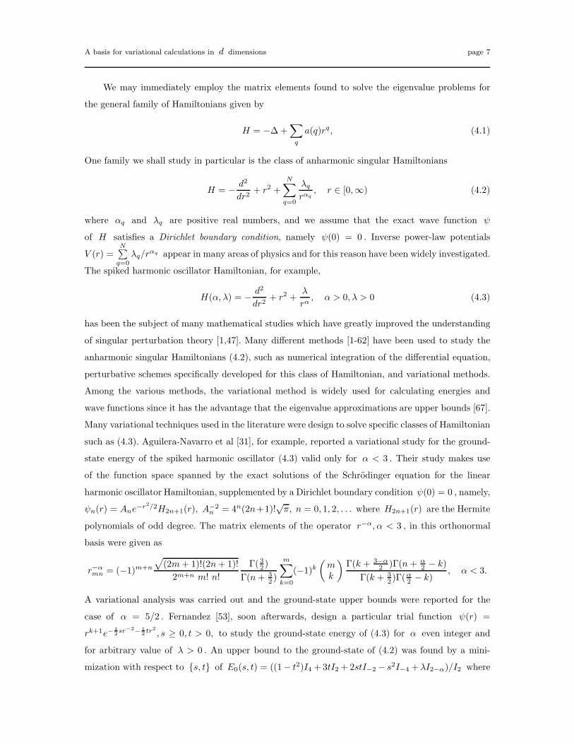
A variational analysis was carried out and the ground-state upper bounds were reported for the

case of α = 5/2 . Fernandez [53], soon afterwards, design a particular trial function ψ(r) =

rk+1e−1

2sr−2− 1

2tr2

, s ≥ 0, t > 0, to study the ground-state energy of (4.3) for α even integer and

for arbitrary value of λ > 0 . An upper bound to the ground-state of (4.2) was found by a mini-

mization with respect to {s, t} of E0(s, t) = ((1− t2)I4 + 3tI2 + 2stI−2 − s2I−4 +λI2−α)/I2 where


In(s, t) =∫ ∞0 rn exp(−s/r2 − tr2)dt,−∞ < n <∞ . These variational results however were not very

accurate, even for arbitrary large value of λ owing to the accumulated error in the computation of

In(s, t) . An interesting consequence of Fernandez’s work was, however, the exact solution of very

particular class of (4.3), namely H = −d2/dr2 + r2 +9/64r−6 , where the exact wavefunction in this

case reads ψ(r) = r3

2 e−3

16r−2− 1

2r2

and the exact ground-state energy is E0 = 4 . Aguilera-Navarro

et al [34] afterwards designed another trial function particularly devoted to analyze the ground-state

energy of the Hamiltonian H(4, λ) . Non-orthogonal basis set of trial wave functions were introduced

by means of ψn(r) = An 1F1(−n; 32 ; r2) exp(−ar2 − b

r ), n = 0, 1, 2, . . . where An is the normal-

ization constant and 1F1(−n; 3/2; r2) is the confluent hypergeometric function. The expressions for

the matrix elements Hmn(4, λ) were given by

Hmn =

n∑

q=0

m∑

q=0

(−n)p(−m)q

(32 )p(

32 )q

AmAn

p! q![(4m+3)I(2p+2q+4)+2

√λI(2p+2q+1)−4q

√λ(2p+2q−1)]

where the definite integrals I(u) =∫ ∞0ru exp(−r2 − (2

√λ/r))dr were computed by means of the

recursive relations (u+1)I(u) = (u−1)I(u−2)+2√λI(u−3) . The shifted factorial (a)n is defined

by

(a)0 = 1, (a)n = a(a+ 1)(a+ 2) . . . (a+ n− 1), for n = 1, 2, 3, . . . , (4.4)

which may be expressed in terms of the Gamma function by (a)n = Γ(a+ n)/Γ(a), when a is

not a negative integer −m , and, in these exceptional cases, (−m)n = 0 if n > m and otherwise

(−m)n = (−1)nm!/(m− n)!. The ground-state of (4.3) with α = 4 then follows by diagonalization

of H in the nonorthogonal basis. This particular study was then extended [36] to provide a global

analysis of the ground and excited states for the successive values of the orbital angular momentum

of the super-singular plus quadratic potential r2 + λ/r4 . Another variational study of the ground

state of (4.2) was introduced by Hall et al [38] where three parameters trial functions ψ(r) =

rp+ǫ exp(−βrq), p = (α − 1)/2 were used to approximate upper bounds of the ground-state of (4.3)

for arbitrary α and λ through the minimization of the right-side of the inequality E0 ≤ EU0 , where

EU0 = min

ǫ,β,q>0

[

q

2(2β)2/q

[

(2p+q+2ǫ−1)g1−2

q(p+ǫ)(p+ǫ−1)g2−

q

2g3

]

+

(

1

2β

)2/q

g4+λ(2β)α/qg5

]

/g6

and

g1 = Γ

(

2p+2ǫ+q−1q

)

, g2 = Γ

(

2p+2ǫ−1q

)

, g3 = Γ

(

2p+2ǫ+2q−1q

)

g4 = Γ

(

2p+2ǫ+3q

)

, g5 = Γ

(

2p+2ǫ−α+1q

)

, g6 = Γ

(

2p+2ǫ+1q

)

.

In attempt to provide a comprehensive variational treatment of the spiked harmonic oscillator Hamil-

tonian (4.3), for ground-state energy as well for excited states, independent of particular choices of

the parameters α and λ , Hall et al [40-48] based their variational analysis of the singular Hamilto-

nian (4.1) on an exact soluble model which itself has a singular potential term. They have suggested


and used trial wave functions constructed by means of the superposition of the orthonormal functions

of the exact solutions of the Gol’dman and Krivchenkov Hamiltonian

H0 = − d2

dr2+ r2 +

A

r2. (4.5)

The Hamiltonian is the generalization of the familiar harmonic oscillator in 3-dimension −d2/dr2 +

r2 + l(l + 1)/r2 where the generalization lies in the parameter A ranging over [ 0,∞) instead of

only values determined by the angular momentum quantum numbers l = 0, 1, 2, . . . . The energy

spectrum of the Schrodinger Hamiltonian H0 is given, in terms of parameter A as

En = 2(2n+ γ), n = 0, 1, 2, . . . , (4.6)

in which γ = 1 +√

A+ 14 and the normalized wavefunctions are

ψn(r) = (−1)n

√

2(γ)n

n!Γ(γ)rγ− 1

2 e−1

2r2

1F1(−n; γ; r2). (4.7)

Here 1F1 is the confluent hypergeometric function

1F1(−n; b; z) =

n∑

k=0

(−n)kzk

(b)kk!, ( n -degree polynomial in z ). (4.8)

Explicit matrix elements of the Hamiltonian (4.3) can often be found in this orthonormal basis. For

instance, the matrix elements of the singular operator λr−α assume the form

r−αmn = (−1)n+m (α

2 )n

(γ)n

Γ(γ − α2 )

Γ(γ)

√

(γ)n(γ)m

n!m!3F2

(

−m, γ − α2 , 1 − α

2γ, 1 − α

2 − n

∣

∣

∣

∣

1

)

, (4.9)

where the hypergeometric function 3F2 is defined by

3F2

(

−m, a, bc, d

∣

∣

∣

∣

1

)

=

m∑

k=0

(−m)k(a)k(b)k

(c)k(d)k k!, (m− degree polynomial).

Upper bounds to the energy levels of the Hamiltonian (4.3) then follow by diagonalization of H in

the orthonormal basis (4.5). In the case where α is a non-negative even number α = 2, 4, 6, . . . , the

hypergeometric function 3F2 in (4.9) can be regarded as a polynomial of degree α2 −1 instead of an

m -degree polynomial. Consequently the matrix elements assumes much simpler expressions which

are useful in numerical computational. For α 6= 2, 4, 6, . . . , the variational computational were then

based on direct use of the matrix elements in terms of the hypergeometric function 3F2 . According

to our discussion up to this point, it is clear that most of the variational methods developed in the

literature were specifically design to solve the eigenvalue problem of different classes of the singular

Hamiltonian (4.2). No basis set or trial wave function were design to treat a problem such as the

singular potentials which at the same time can be used, say, for Hamiltonians with polynomial type

potentials. The purpose of our basis introduced in section (2) and (3) is to have avaliable at our

disposal a working variational approach that can be used without a particular references to specific

potentials or special values for the parameters involve. In the next we apply the matrix elements

discussed in section (2) and (3) to solve a number of different eigenvalue problems.


4.1 Spiked Harmonic Oscillators

We start our applications by investigating the energy levels of the spiked Harmonic Oscillator

Hamiltonian (4.3). As we mentioned in section 3, the problem of finding the eigenvalues reduces to

diagnalizing the real symmetric matrix H = MSTHSM . For α = 2 , the Hamiltonian (4.3) admits

an exact solutions (4.6). Thus it serves as a benchmark for our variational approach. In Table (1),

we report our upper bounds for the ground-state of the spiked harmonic oscillator Hamiltonian (4.3)

for several values of the parameters λ and α = 12 , 1,

32 , 2,

52 along with some results obtained in the

literature. For α = 2 , with m = n = 0 , Table 1 shows that minimization over the three variables

{p, t, s} yields excellent agreement with the exact solutions (4.6). Such results can be explained by

observing that direct substitution of the trial wave function ψ0(r) into the eigenvalue problem

Hψ0 = −d2ψ0

dr2+ (r2 +

λ

rα)ψ0 = E0ψ0 (4.10)

yields for r → 0 that

t2 − 1

4r2+

p2

4r2−2p− (t+ 1)p

2r2−p− λ

rα= 0 (4.11)

Consequently, for α = 2 and p > 0 , the value t = 1 + |1 −√

1 + 4λ| yields the best possible

value of t . As for α < 2 , similar reasoning yields for r → 0 that t = 1 is an excellent initial

approximation for t, that is to say, suitable for starting the minimization process. In Table 2, we

present a comparison between different variational approaches for computing upper bounds to the

ground-state of the Hamiltonian H = −d2/dr2 + r2 + λr−5/2 for λ > 0 , where the diagonalization

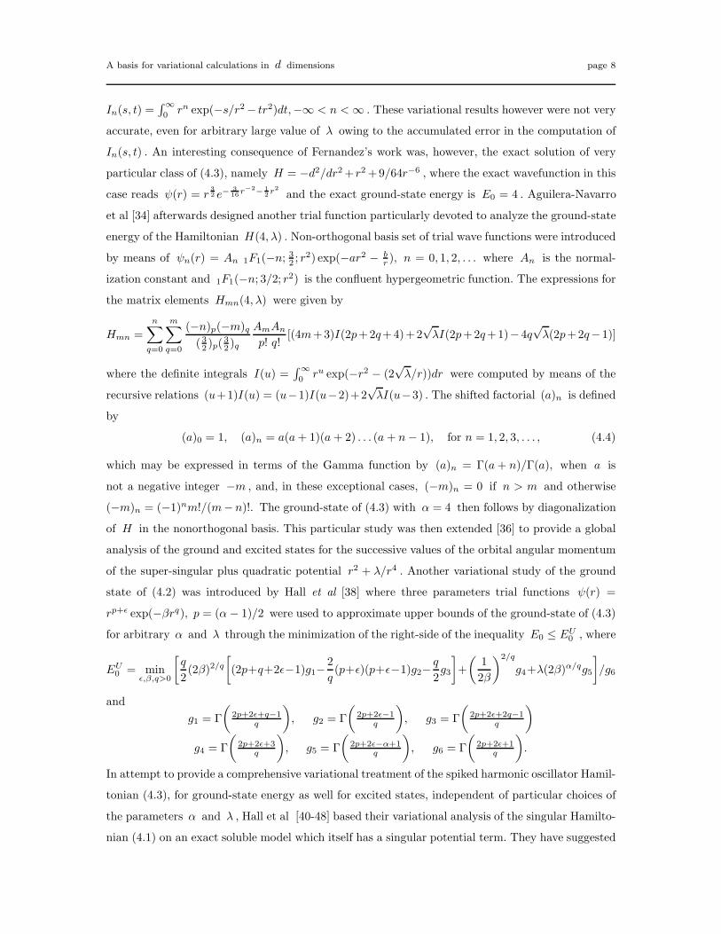
of H , Eq.(3.3), was carried out in variational spaces of different dimensions n . In Table 3, we

report our variational computation for upper bounds to the ground-state energy of the Hamiltonian

H = −d2/dr2 + r2 + λr−4 along with the eigenvalues reported in the literature. In Table 4, we

extended our variational analysis to study the Hamiltonian H = −d2/dr2 + r2 + l(l+ 1)/r2 + λ/r4

for λ≪ 1 and for several values of l . We compare our results with the those in the literature, along

with ‘exact’ eigenvalues obtained by direct numerical computation of the corresponding Schrodinger

equation. In order to keep the number of tables of results to a minimum, we first mention the case

of V (r) = r2 + 964

1r6 which yields the exact energy E = 4 : by using our variational approach we

obtain an upper bound of E = 4.0000006 for n = 15 with p = 0.73, t = 7.09, and s = 0.01 . The

reported results in the tables indicate the general usefulness of matrix elements for the investigation

of the entire spectrum of the spiked harmonic oscillator Hamiltonian for λ > 0 and arbitrary α

in any dimensions and for any angular momentum number l . It is also clear that we don’t need

a very large basis set to produce accurate bounds. It can be seen from the tables that the rate of

convergence is fast for moderate values of the coupling constant λ , while for very small values of

the coupling constant the rate of convergence is much slower. In general, however, throughout the


whole range of values of λ , the result from the introduced basis always gives very reliable upper

bounds. In summary, the basis provides a simple, uniform, and robust variational method.

4.2 Anharmonic Singular Hamiltonian

The anharmonic singular Hamiltonians

H = − d2

dr2+l(l+ 1)

r2+ ar2 +

b

r4+

c

r6, , a > 0, c > 0, l = 0, 1, 2, . . . (4.12)

have attracted considerable attention in part because conditionally exact solutions are possible.

From the mathematical point of view, this Hamiltonian is a non-trivial generalization of the spiked

harmonic oscillator (4.3). Znojil [7-8] employed a Laurent series ansatz for the eigenfunctions to

convert Schrodinger’s equation into a difference equation and then used continued fraction solutions

to obtain exact solutions for the ground-state and the first excited state. Kaushal and Parashar [68]

simplified Znojil’s ansatz to obtain exact ground-state expression

E0 =√a

(

4 +b√c

)

subject to the constraint (2√c+ b)2 = c(2l + 1)2 + 8c

√ac. (4.13)

Guardiola and Ros [37] then used a much simplifier trial wavefunction ψ(r) = r(b/√

c+3)/2 exp(−r2/2−√c/(2r2)) for the case of a = 1 and l = 0 to obtain the exact solution for the ground state as

E0 = 4 +b√c

subject to the constraint condition (2√c+ b)2 = c+ 8c

√c. (4.14)

For example with b = c = 1 , the ground-state is E0 = 5 and for b = c = 9 , E0 = 7 , etc.

Soon afterwards, Landtman [49] performed an accurate numerical calculation and showed that for

the parameters chosen by Kaushal and Parashar, although the ground-state energy they obtained

agreed with the numerical calculation, their first-excited energy did not. Varshni [51], in an attempt

to resolve this problem, obtained four sets of solutions, including one constraint equation for each set

and showed that the analytic expression for the energy agrees with the numerical result for any one

among the ground, the first and the second excited states, depending on the particular constraint

condition satisfied. For higher dimensions, by making use of certain ansatze for the eigenfunction,

Shi-Hai Dong and Zhong-Qi Ma [52] obtained exact closed-form solutions of (4.12) in two dimensions,

where the parameters of the potentials a, b, and c again satisfy certain constraints.

In order to compare our variational results with the exact eigenvalues, we have found for the

exact ground-state eigenvalue E0 = 5 of the Hamiltonian (4.12) with l = 0, a = b = c = 1 , an

upper bound of E0 = 5.000 006 obtained by the diagonalization of a 14 × 14 -matrix. Further,

the exact energies of 7, 7, 11, 11 corresponding to (a, b, c) = (1, 9, 9), (1,−7, 49), (1, 45, 225) , and

(1,−24.5125, 600.8623) respectively follow by the optimization of the matrix eigenvalues with ini-

tial guesses for the variational parameters and matrix dimensions given respectively by (p, t, s) =


(1.12, 16.09, 0.11), (1.03, 27.47, 0.07), (1.10, 31.00, 0.10), and (0.77, 40.82, 0.01), and 14×14 11×11 ,

8 × 8 , and 7 × 7 . These results indicate the generality and the efficiency of our approach. Note

(b, c) = (−7, 49), and (b, c) = (−24.5125, 600.8623) also shows the applicability of the method

in the case of b negative. We further illustrate the applicability of the matrix elements to obtain

accurate upper bounds to the ground-state of (4.12) for several values of a, b and c . Indeed, for

(a, b, c) = (1, 10, 1), (1, 10, 10), and (1, 100, 100) , we obtain 6.679 053, 7.138 261 , and 11.791 771

respectively which results are in excellent agreement with the exact eigenvalues obtained by direct

numerical integration of Schrodinger’s equation. The precision of the upper bounds to any number

of decimal places can be achieved by increasing n , the dimension of the matrix. The energies of the

excited states in arbitrary spatial dimension d are similarly straightforward to find.

4.3 Perturbed Coulomb Potentials

Hautot [60], in his solutions of Dirac’s equation in the presence of a magnetic field, introduced some

interesting methods of solving certain second-order differential equations. One of these methods

deals with the potential operator

V (r) = −D/r +Br +Ar2, A 6= 0. (4.15)

Hautot obtained exact solutions for only certain relations between the constants A,B, and D . He

achieved his results by applying the kinetic energy operator to an appropriate wavefunction and

using the standard procedure of comparing coefficients in the induced recurrence relations. More

precisely, by introducing [39]

ψ(r) = exp

(

− 1

2

(√Ar2 +

Br√A

)) n∑

k=0

akrk+l, n = 0, 1, 2, . . .

into the radial Schrodinger equation(

d2

dr2+

2

r

d

dr− l(l + 1)

r2+ E +

D

r−Br −Ar2

)

ψ(r) = 0

One obtains the following three-term recursion relation between the coefficients ak for (k =

0, 1, 2, . . .) :[

(k + 2)(k + 2l + 3)

]

ak+2 +

[

D − B√A

(k + 2 + l)

]

ak+1 +

[

E −√A(2k + 2l+ 3) +

B2

4A

]

ak = 0

This recurrence relation terminates if ak+1 = 0 , that is to say E = Enl =√A(2n + 2l + 3) − B2

4A

provided that the parameters A,B, and D satisfies the (n+ 1) × (n+ 1) -determinant

det

a0 b0c1 a1 b1

c2 a2 b2· · · ·

· · cn−1 an−1 bn−1

cn an

= 0, where

ak = D − B√A

(k + l + 1),

bk = (k + 1)(k + 2l+ 2),

ck = Enl −√A(2k + 2l+ 1) + B√

A.


For example, we have for the ground-state energy (i.e. k, l = 0 ) of

V (r) = −1

r+Ar + (Ar)2, E0 = (3 + 2l)A− 1

4, (4.16)

with the ground-state wavefunction given explicitly as ψ(r) = rl exp(− 12 (r+Ar2)) . This particular

case was studied by Killingbeck [17] who obtained the exact solution for the ground-state for β > 0 .

In order to test the variational approach discussed in section 2 and 3, we have employed the matrix

elements to obtain upper bounds to the exactly solvable cases such as β = 0.1, 1, and 2 , we found

that the upper bounds yields 0.05, 2.75, and 5.75 which are in excellent agrement with the exact

eigenvalues as given by (4.16). An important consequence of our variational approach are the upper

bounds that are easily obtained for unconstrained values of D,B , and A . In Table 5, we have

reported our variational results for D = 1 and several values of B and A where we compare

our results with the upper bounds obtained by the direct numerical integration of Schrodinger’s

equation [39]. In arbitrary dimensions, the matrix elements discussed in Sections 2 and 3 provide

a uniformly simple, straightforward, and efficient way of obtaining accurate energy bounds for the

entire spectrum. In order to compare our results with those in the literature, we consider in Table

6 the radial Schrodinger equation in d -dimensions in the form

−1

2

(

d2

dr2− Λ(Λ + 1)

r2

)

ψ + (−ar

+ br + cr2)ψ = Eψ (4.17)

where Λ = (d + 2ℓ − 3)/2 . The overall factor of 12 in the kinetic-energy was incorporate in our

calculations by multiplying the kinetic energy matrix elements (2.11) by this quantity. To analyze

the precision of the method, we again compare our results in Table 6 with some special cases for

which the eigenvalues are known [30]. Results for the excited states within each angular momentum

subspace (labelled by ℓ ) are automatically provided for (up to the dimension of the matrix used),

and arbitrary spatial dimension dimension d is allowed for in the general expressions for the matrix

elements.

4.4. The quartic double-well potential V (r) = −γr2 + r4, γ > 0

The quartic double-well potential

V (r) = −γr2 + r4, γ > 0, (4.18)

has a long history of numerical studies (see, for example, [61] and [62] and the references therein).

Apart from its intrinsic interest, the double-well potential also plays an important role in the quantum

study of the tunnelling time problem [69], in spectra of molecules such as ammonia and hydrogen-

bonded solids [70]. Broges et al [71], using supersymmetry techniques, constructed trial wave func-

tions for variational calculations of the ground-state, first, second, and third excited-states. In their


comparison with the literature, they have used the results obtained from direct numerical integra-

tion of the corresponding Schrodinger equation, as reported in [72]. Unfortunately, these numerical

eigenvalues were not very accurate and the errors are higher than appear in their reported tables. In

Table 7, we compare our results for the first- and third-exited states with those of Broges et al [71],

who considered the problem in one dimension; we also include accurate numerical values.

5. Conclusion

We have found matrix elements for Schrodinger operators in d spatial dimensions with

spherically-symmetric potentials of the form V (r) =∑

q a(q)rq . The matrix elements for a given

angular momentum ℓ are calculated with respect to a finite basis {φi}n−1i=0 comprising polynomials

in r with an overall factor of the form r1+(t−d)/2e−rp

. With the inclusion of a scale parameter s ,

the upper estimates are the eigenvalues E [n]i (p, t, s) of an n× n matrix eigen equation of the form

Hv = λNv, where N = [(φi, φj)]. For best results, these estimates are optimized with respect to

the three parameters {p, t, s} for a given n. For the class of problems considered, the basis has

the advantage that explicit analytic expressions in terms of the Gamma function are available for

all the matrix elements. The method is robust and flexible enough to yield excellent results for the

whole class of problems without the need to work with very large matrices.

https://www.researchgate.net/publication/243490849_An_Introduction_to_Computer_Simulation_Method_Applications_of_Physical_Systems?el=1_x_8&enrichId=rgreq-1a5c31b7-3c75-48c8-87b4-23a6f2acf6c1&enrichSource=Y292ZXJQYWdlOzIwOTE4NDM7QVM6MTAyNTI0MzA4Njg4OTEwQDE0MDE0NTUxMDg2OTU=


References

[1] E. M. Harrell, Ann. Phys. (NY) 105, (1977) 379.

[2] L. C. Detwiler and J. R. Klauder, Phys. Rev. D 11, (1975) 1436.

[3] H. Ezawa, J. R. Klauder, and L. A. Shepp, J. Math. Phys. 16, (1975) 783.

[4] J. R. Klauder, Science 199, (1978) 735.

[5] M. Znojil, J. Phys. A: Math. Gen. 15, 2111 (1982).

[6] M. Znojil, J. Phys. lett. 101A, 66 (1984).

[7] M. Znojil, J. Math. Phys. 30, 23 (1989).


[9] M. Znojil, Phys. Lett. A 169, 415 (1992).

[10] M. Znojil and P. G. L. Leach, J. Math. Phys. 33, 2785 (1992).


[12] M. Znojil and R. Roychoudhury, Czech. J. Phys. 48, (1998) 1.

[13] M. Znojil, Phys. Lett. A 255, (1999) 1 .

[14] J. Killingbeck, J. Phys. A: Math. Gen. 10, L99 (1977).

[15] J. Killingbeck, Phys. lett. A 67, 13 (1978).

[16] J. Killingbeck, Comp. Phys. Commun. 18, 211 (1979).

[17] J. Killingbeck, J. Phys. A: Math. Gen. 13, 49 (1980).

[18] J. Killingbeck, J. Phys. A: Math. Gen. 13, L231 (1980) .

[19] J. Killingbeck, J. Phys. A: Math. Gen. 14, 1005 (1981).

[20] J. Killingbeck, J. Phys. B: Mol. Phys. 15, 829 (1982).

[21] J. Killingbeck, G. Jolicard and A. Grosjean, J. Phys. A: Math. Gen. 34, L367 (2001).

[22] M. J. Jamieson, J. Phys. B: At. Mol. Phys. 16, L391 (1983).

[23] H. G. Miller, J. Math. Phys. 35, 2229 (1994).

[24] F. J. Hajj, J. Phys. B: At. Mol. Phys. 13, 4521 (1980).


[25] H. J. Korsch and H. Laurent, J. Phys. B: At. Mol. Phys. 14, 4213 (1981).

[26] W. Solano-Torres, G. A. Estevez, F. M. Fernandez, and G. C. Groenenboom, J. Phys. A: Math.

Gen. 25, 3427 (1992).

[27] E. Buendia, F.J.Galvez, A. Puertas, J. Phys. A: Math. Gen. 28, 6731 (1995).

[28] A. K. Roy, Phys. lett. A 321, 231 (2004).

[29] Peace Chang and Chen-Shiung Hsue, Phys. Rev. A 49, 4448 (1994).

[30] R. K. Roychoudhury and Y P Varshni, J. Phys. A: Math. Gen. 21, 3025 (1988).

[31] V. C. Aguilera-Navarro, G.A. Estevez, and R. Guardiola, J. Math. Phys. 31, 99 (1990).

[32] V. C. Aguilera-Navarro and R. Guardiola, J. Math. Phys. 32, 2135 (1991).

[33] V. C. Aguilera-Navarro, F. M. Fernandez, R. Guardiola and J. Ros, J.Phys. A: Math. Gen 25,

6379 (1992).

[34] V. C. Aguilera-Navarro, A. L. Coelho and Nazakat Ullah, Phys. Rev. A 49, 1477 (1994).

[35] V. C. Aguilera-Navarro and R. Guardiola, J. Math. Phys. 32, 2135 (1991).

[36] V. C. Aguilera-Navarro and Ley Koo, Int. J. Theo. Phys. 36, 157-1666. (1997)

[37] R. Guardiola and J. Rose, J. Phys. A: Math. Gen. 25, 1351 (1992).

[38] R. L. Hall and N. Saad, Can. J. Phys. 73, 493. (1995)

[39] R. L. Hall and N. Saad, J. Phys. A: Math. Gen. 29, 2127 (1996).

[40] R. L. Hall, N. Saad, and A. von Keviczky, J. Math. Phys. 39, 6345 (1998).

[41] R. L. Hall and N. Saad, J.Phys. A: Math. Gen. 33, 5531 (2000).

[42] R. L. Hall and N. Saad, J.Phys. A: Math. Gen. 34, 1169 (2001).

[43] R. L. Hall, N. Saad and A. von Keviczky, J. Phys. A 34, 1169 (2001).

[44] R. L. Hall, N. Saad, and A. von Kevicsky, J. Math. Phys. 43, 94(2002).

[45] N. Saad and R. L. Hall, J. Phys. A.: Math. Gen. 35, 4105 (2002).

[46] R. L Hall and N. Saad, J. Math. Phys. 43, 94 (2002).

[47] N. Saad, R.L. Hall, and A. von Keviczky, J. Math. Phys. 44, 5021 (2003).


[48] N. Saad, R. L. Hall, and A. von Keviczky, J. Phys. A: Math. Gen. 36, 487 (2003).

[49] M. Landtman, phys. lett. A 175, 335 (1993.

[50] E. Buendiia, F.J.Galvez, A. Puertas, J. Phys. A: Math. Gen. 28, 6731 (1995).

[51] Y. Varshni, phys. lett. A 183, 9 (1993).

[52] Shi-Hai Dong and Zhong-Qi Ma, J. Phys. A: Math. Gen. 31, 9855 (1998).

[53] F. M. Fernandez, Phys. Lett. A 160, 511 (1991).

[54] M. de Llano, Rev. Mex. Fis. 27, (1981) 243 .

[55] M. F. Flynn, R. Guardiola, and M. Znojil, Czech. J. Phys. 41, (1993) 1019.

[56] N. Nag and R. Roychoudhury, Czech. J. Phys. 46, (1996) 343.

[57] E. S. Estevez-Breton and G. A. Estevez-Breton, J. Math. Phys. 34, (1993) 437.

[58] O. Mustafa and M. Odeh, J. Phys. B 32, 3055 (1999).

[59] O. Mustafa and M. Odeh, J. Phys. A 33, 5207 (2000).

[60] A P Hautot, J. Math. Phys. 13, 710 (1972).

[61] P. Kumar, M. Rusiz-Altaba, and B. S. Thomas, Phys. Rev. Lett. 57, 2759 (1986).

[62] Wai-Yee Keung, Eve Kovacs, and Uday P. Sukhatme, Phys. Rev. Lett. 60, 41 (1988).

[63] H. A. Mavromatis, Exercises in Quantum Mechanics (Kluwer, Dordrecht, 1991).

[64] A. Sommerfeld, Partial Differential Equations in Physics (Academic, New York, 1949). The

Laplacian in N dimensions is discussed on pp. 227, 231

[65] P. -O. Lowdin, J. Chem. Phys. 18, 365 (1950).

[66] P. I. Davies, N. J. Higham, and F. Tisseur, Siam J. Matrix Anal. Apps. 23, 472 (2001).

[67] M. Reed and B. Simon, Methods of Modern Mathematical Physics IV: Analysis of Operators

(Academic, New York, 1978). The min-max principle for the discrete spectrum is discussed on

p75

[68] R. S. Kaushal and D Parashar, Phys. Lett. A 170, 335 (1992).

[69] D. K. Roy, Quantum Mechanics Tunneling and its applications (World Scientific, Singapore,

1986). ; L. A. MacColl, Phys. Rev. 40, 261 (1932)


[70] D. M. Dennison and G. E. Uhlenbeck, Phys. Rev. 41, 261 (1932). ; F. T. Wall and G. Glockler,

J. Chem. Phys. 5, 314 (1937).

[71] G. R. P. Broges, A. de Souza Dutra, Elso Drigo, and J. R. Ruggiero, Can. J. phys. 81, 1283

(2003).

[72] G. Harvey and J. Tobochnik, An introduction to computer simulation methods: applications to

physical systems, 2nd ed. (Addison-Wesley, Reading, Mass. 1996). p. 631

Acknowledgments

Partial financial support of this work under Grant Nos. GP3438 and GP249507 from the Natural

Sciences and Engineering Research Council of Canada is gratefully acknowledged by two of us

(respectively [RLH] and [NS]).


Table 1. Upper bounds EU to the ground-state eigenvalues of H = − d2

dr2 + r2 + λrα for different

values of λ , α . The eigenvalues for the case α = 2 are obtain for n = 1 and can be compared

with the exact formula 2 +√

1 + 4λ . The exponent refers to the dimension (n) of the matrix used

for the variational computations; the triples in parentheses refer to the approximate initial values of

the parameters {p, t, s} . The small letters indicate references where the same values were obtained

in the literature.

λ α = 0.5 α = 1 α = 1.5 α = 2 α = 2.5

0.0001 3.000 102 (1,a) 3.000 112 (1,a) 3.000 138 (1,a) 3.000 199 980 3.000 408 (14,a)

(2.00, 1.00, 1.00) (2.00,1.00,1.00) (2.00,1.00,1.00) (2.00,1.00,1.00) (2.00, 1.00, 0.79)

0.001 3.001 022 (1,d) 3.001 128 (1,b,d) 3.001 382 (1) 3.001 998 004 3.004 022 (14,c,e)

(2.00, 1.00, 1.00) (2.00,1.00,1.00) (2.00, 1.00, 1.00) (2.00,1.00,1.00) (2.01, 1.06, 0.78)

0.01 3.010 226 (1) 3.011 276 (1,b,d) 3.013 794 (3) 3.019 803 903 3.036 744 (15,c,e)

(2.00, 1.00, 1.00) (1.99,1.00,0.99) (1.99,1.00,0.99) (1.99,1.01,0.99) (0.75, 1.56, 0.01)

0.1 3.102 139 (3) 3.112 067 (5,b,d) 3.135 053 (13) 3.183 215 957 3.266 874 (18,c,e)

(2.00, 1.00, 1.00) (1.90,1.00,0.96) (1.59,1.00,0.47) (2.00,1.18,1.00) (0.57, 1.00, 0.00)

1 3.009 204 (13) 4.057 877 (14,b,d) 4.141 893 (14) 4.236 067 978 4.317 311 (16,c,e)

(2.18, 1.00, 0.98) (0.99,1.00,0.10) (1.80,1.06,0.56) (2.00,2.23,1.00) (0.69, 1.09, 0.009)

10 12.093 130 (14) 10.577 483 (14,b,d) 9.324 173 (14) 8.403 124 237 7.735 111 (6,c,e)

(1.99, 1.00, 0.9) (1.00,1.004,0.09) (2.12,1.69,1.00) (1.99,6.40,0.99) (1.70, 5.85, 0.73)

a Ref. [21]. b Ref. [33]. c Ref. [31]. d Ref. [44]. e Refs. [41], [59], and [29].

Table 2. Comparison of upper bounds for the ground state energy of the Hamiltonian H =

− d2

dr2 + r2 + λr5/2

by different variational techniques. The upper bounds EU are those obtained by

the present work. The exponent (n) refer to the dimensions of the matrix used for the variational

computations.

λ Ref. [31] Ref. [41] Ref. [41] Ref. [38] EU

0.001 3.004 075(30) 3.004 074 (30) 3.004 047 (5) 3.004 04 3.004 022 (14)

0.01 3.039 409 (30) 3.039 244 (30) 3.037 474 (5) 3.037 43 3.036 744 (15)

0.1 3.302 485 (30) 3.296 024 (30) 3.269 700 (5) 3.269 28 3.266 874 (18)

1 4.329 449 (30) 4.323 263 (30) 4.318 963 (5) 4.318 54 4.317 311 (16)

10 7.735 136 (30) 7.735 114 (30) 7.735 596 (5) 7.735 32 7.735 111 (8)

100 17.541 890 (30) 17.541 890 (30) 17.542 040 (5) 17.541 92 17.541 890 (11)

1000 44.955 485 (30) 44.955 485 (30) 44.955 517 (5) 44.955 49 44.955 485 (4)


Table 3. Upper bounds for the ground state energy EU for the Hamiltonain H = −∆ + r2 + λr4

for several values of λ . We compare our upper bounds EU with the literature. The superscript

numbers are the dimension of the matrix used; the triples in parentheses refer to the approximate

initial values of the parameters {p, t, s} .

λ EU E

0.0001 3.022 27522 3.022 275k

(0.30, 3.89, 0.00)

0.001 3.068 76320 3.068 763a,c, 3.06877b

(0.33, 8.00, 0.00)

0.005 3.148 35220 3.148352c, 3.14839h, 3.14835g

(0.44, 2.36, 0.001) 3.14664d, 3.148352d, 3.05319n

3.14835o

0.01 3.205 06920 3.205067a, 3.20508b, 3.20442d

(0.44, 2.10, 0.00) 3.20507k, 3.20527h, 3.20507g

3.205067d, 3.07522n, 3.23775k

3.20548m, 3.20507o, 3.24980p

0.1 3.575 55914 3.575552a,c, 3.57557b

(0.42, 9.30, 0.00) 3.57555k, 3.62644k, 3.60044p

0.4 4.031 97122 4.031971i, 4.031971f

(0.50, 3.89, 0.00)

1 4.494 17911 4.494178a, 4.49418b

(0.70, 11.00, 0.00) 4.49418k, 4.54879k

10 6.606 62514 6.606623a,c, 6.60662b, 6.60662k

(0.44, 18.00, 0.00) 6.64978k, 6.609 66p

100 11.265 0807 11.265080a, 11.26508b, 11.26508k

(0.49, 72.00, 0.00) 11.265 86p

1000 21.369 4646 21.369463a,c,l, 21.36946b

(0.62, 100.80, 0.00) 21.370 26p

a Ref. [28]. b Ref. [34]. c Ref. [28]. d Ref. [26]. e Ref. [21]. f Ref. [29].g Ref. [20]. h Ref. [2]. i Ref. [8]. j Ref. [53]. k Ref. [29]. l Ref. [20].m Ref. [2]. n Ref. [8]. o Ref. [44]. p Ref. [1]. q Ref. [25]. s Ref. [38].


Table 4. A comparison between the upper bounds for the Hamiltonian H = − d2

dr2 + r2 + Ar2 + λ

r4 ,

for a wide range of values of A = l(l + 1) and λ , using the present work EU and the bounds

EUa obtained by Aguilera-Navarro et al [36] (see also [48] and [28]). Accurate numerical results

E obtained by direct numerical solution of Schodinger’s equation are also presented. The exponent

refers to the dimension (n) of the matrix used for the variational computations; the triples in

parentheses refer to the approximate initial values of the parameters {p, t, s} .

λ l EUa EU E

0.001 3 9.000 114 279 9.000 114 279(11) (1.99, 7.00, 0.99) 9.000 114 279

4 11.000 063 490 11.000 063 490(11) (1.90, 9.00, 1.03) 11.000 063 490

5 13.000 040 403 13.000 040 403(11) (1.98, 9.00, 0.96) 13.000 040 403

0.01 3 9.001 142 268 9.001 142 199(11) (2.10, 7.22, 0.98) 9.001 142 199

4 11.000 634 795 11.000 634 788(11) (2.04, 6.91, 1.00) 11.000 634 788

5 13.000 404 001 13.000 404 000(11) (2.01, 7.00, 1.07) 13.000 404 000

0.1 3 9.011 370 328 9.011 364 024(13) (2.00, 5.00, 1.19) 9.011 364 024∗

4 11.006 336 739 11.006 336 013(13) (2.00, 3.99, 0.84) 11.006 336 013∗

5 13.004 036 546 13.004 036 433(8) (1.85, 5.97, 0.79) 13..004 036 433

1 3 9.109 013 250 38 9.108 657 991(14) (1.70, 4.00, 0.61) 9.108 657 991∗

4 11.062 293 143 4 11.062 241 722(11) (1.90, 8.99, 0.78) 11.062 241 719∗

5 13.040 025 483 8 13.040 015 183(8) (1.81, 7.19, 0.77) 13.040 015 183

Table 5. Upper bounds for the Hamiltonian H = − d2

dr2 − Dr + Br + Ar2 for different values

of the parameters B and A . The numerical results in the brackets are the exact eigenvalues as

obtained by direct numerical integration of Schrodinger equation. The triples in parentheses refer to

the approximate initial values of the parameters {p, t, s} .

D B A EU

1 1 2 3.656 525 (3.657)

8 × 8, (1.99, 1.00, 0.73)

1 0.1 1 1.885 424 (1.885)

11 × 11, (1.92, 1.00, 0.75)

1 0.5 1 2.277 581 (2.278)

10 × 10, (2.04, 1.00, 0.86)

1 0.1 0.1 0.378 305 (0.378)

12 × 12, (2.21, 1.00, 1.63)

1 0.01 1 1.795 268 (1.795)

8 × 8, (1.08, 1.00, 0.09)

1 0.001 1 1.786 212 (1.786)

8 × 8, (2.04, 1.00, 0.93)


Table 6. Comparison of the eigenvalues for H = − d2

dr2 − Dr + Br + Ar2 for different values

of D , B , and A where EN is calculated from the shifted 1/N expansion [30], the exact su-

persymmetric values Es [30] and the upper bounds EU obtained by the method of the present

paper (diagonalization of the d× d matrix elements then minimizing with repect to the parameters

{p, t, s} ).

l D B A EN Es EU

0 1 0.447 21 0.1 0.171 66 0.170 82 0.170 826

1 1 0.223 61 0.1 0.993 37 0.993 03 0.993 048

2 1 0.149 07 0.1 1.509 79 1.509 69 1.509 693

3 1 0.111 80 0.1 1.981 24 1.981 21 1.981 213

0 1 1.414 21 1.0 1.627 56 1.621 32 1.621 324

1 1 0.707 11 1.0 3.411 41 3.410 53 4.410 548

2 1 0.471 40 1.0 4.894 40 4.894 19 4.894 194

3 1 0.353 55 1.0 6.332 78 6.332 71 6.332 711

0 1 4.47214 10 6.226 80 6.208 20 6.208 224

1 1 2.23607 10 11.057 19 11.055 34 11.055 342

2 1 1.49071 10 15.59732 15.59692 15.596924

3 1 1.11803 10 20.093 49 20.093 36 20.093 3710

0 1 14.14214 100 20.753 21 20.713 20 20.713 204

1 1 7.07107 100 35.233 90 35.230 34 35.230 345

2 1 4.71405 100 49.442 67 49.441 92 49.441 929

3 1 3.535 53 100 63.608 60 63.608 36 63.608 378

0 1 44.721 36 1000 66.65904 66.58204 66.582 043

1 1 22.360 68 1000 111.685 01 111.678 40 111.678 407

2 1 14.907 12 1000 156.470 58 156.469 20 156.469 207

3 1 11.180 34 1000 201.215 30 201.214 87 201.214 877

Table 7. Upper bounds for the Hamiltonian H = − d2

dr2 − γr2 + r4 with different values of γ.

E1(V ) and E3(V ) represent the values obtained from the variational method discussed by Broges

et al, and EU1 and EU

3 are from the present work (with a 10× 10 -matrix). We have also included

accurate numerical results EN1 and EN

3 obtained by direct numerical integration of Schrodinger’s

equation.

γ E1(V ) EN1 EU

1 E3(V ) EN3 EU

3

0.1 3.710 64 3.708 93 3.708 93 11.542 58 11.488 48 11.488 480.2 3.618 90 3.617 01 3.617 01 11.386 92 11.331 27 11.331 270.3 3.525 96 3.523 87 3.523 87 11.230 45 11.173 10 11.173 100.4 3.431 79 3.429 47 3.429 47 11.073 07 11.013 97 11.013 970.5 3.336 36 3.333 78 3.333 78 10.914 77 10.853 87 10.853 870.6 3.239 62 3.236 76 3.236 76 10.755 56 10.692 80 10.692 800.7 3.141 55 3.138 37 3.138 37 11.595 47 10.530 74 10.530 740.8 3.042 10 3.038 56 3.038 56 10.434 48 10.367 70 10.367 700.9 2.941 23 2.937 30 2.937 30 10.272 58 10.203 67 10.203 671.0 2.838 91 2.834 54 2.834 54 10.109 78 10.038 65 10.038 652.0 1.726 29 1.713 03 1.713 03 8.433 95 8.332 87 8.332 87