BEN-GURION UNIVERSITY OF THE NEGEV

FACULTY OF NATURAL SCIENCES

DEPARTMENT OF MATHEMATICS

M. Ayzenberg-Stepanenko, T. Cohen, G. Osharovich and O. Timoshenko

Waves in Periodic Structures (mathematical models and computer simulations)

The manuscript contains the part “Waves in Periodic Structures” of the lecture course “Mathematical Modeling” done for students of the second degree of the Mathematical Department of Ben-Gurion University of the Negev (the direction: Applied and Industrial Mathematics) by Professor M.V. Ayzenberg-Stepanenko in 2003 – 2004. Lectures were written down and prepared for the manuscript by M.S. students T. Cohen, G. Osharovich and O. Timoshenko. They also adjusted mathematical formulas and calculation algorithms, elaborated computer programs and validated text and figures.

Be’er-Sheva, 2005

1

Abstract In the work, mathematical models, algorithms and computer programs are developed intended for analytical and computer analysis of hyperbolic systems with a specific kind of boundary conditions. In linear cases related to wave propagation problems in solids of periodic structure, dispersion equations are obtained and analyzed. Transient propagation of elastic waves and vibrations through layered composites and lattices is investigated. These structures are subjected by given pulse and/or vibration loadings. Mechanical features of structured waveguides and physical phenomena required to analysis bringing together result in set of necessary simplifications allowing a corresponding mechanical model to be designed. On the other hand, mathematical models are designed, allowing main features of the studied processes to be comprehensively explored. A coupled analytical-numerical approach is elaborated, consisting of

(i) revealing waveguide properties of periodical structures, (ii) obtaining time-dependent asymptotic solutions for certain spectral wave components, (iii) computer simulating a wide spectrum of perturbations in structured waveguides.

Quasi-steady state processes within the pass-bands and strongly transient processes within stop- bands (including pass/stop-band borders) are analyzed. As a basis of the numerical approach, explicit FDM schemes with mesh dispersion elimination, are used within computer simulations. A practical result of the work is a C++ − simulator designed for parametric analysis of linear and nonlinear dynamic processes in layered media and composite structures. Computer algorithms and the most interesting results of computer simulations are presented and discussed.

2

Content: Introduction 3 1.0 Brief historical review of the problem and the scope of the work 4 1.1 Work subjects and structure 9 1.1.1 Structured waveguides 9 1.1.2 Problem formulation, aims and methods of investigation 11 1.2 Wave dispersion 14 1.3 Infinite homogeneous rod (dispersionless waveguide) 14 1.4 A simple discrete mass-spring chain system 16 1.5 A thin cylindrical shell 17 1.6 Layered unidirectional composites loaded along the fiber direction 19 1.6.1 The simplest model: rod upon an elastic foundation 21 1.6.2 Fiber with amortized particles 22 2 1D steady and transient waves in dispersion waveguides 25 2.1 Mathematical models of mass-spring waveguides. Dispersion analysis 25 2.1.1 Simple mass-spring chain (MSC) 25 2.1.2 Two mode mass-spring waveguide (Born’s chain) 27 2.1.3 MSC with amortized masses 30 2.1.4 MSC upon an elastic foundation 33 2.1.5 Three-mode MSC 34 2.1.6 Four-mode MSC 37 2.2 Waveguides of material-bond elements. Dispersion analysis 38 2.2.1 Two-unit periodical waveguide. Associated problems 39 2.2.2 Units serially connected by inertial masses 45 2.2.3 Units connected by inertionless springs 48 2.2.4 Waveguide with periodically amortized particles 49 2.2.5 Material-bond lattice 52 2.2.6 Unidirectional composite loaded along fibers 53 2.3 Transient problem. Long-wave asymptotes 55 2.3.1 Long-wave asymptote of the wave propagation process 55 2.3.2 Resonance in a periodic waveguide under a monochromatic excitation 61 2.4 Transient problem. Numerical solutions. Pulse loading 63 2.4.1 MDM finite-difference explicit algorithms 63 2.4.2 Dispersionless waveguide 63 2.4.3 Simple MSC 65 2.4.4 Examples of continuous dispersion waveguides 89 2.4.5 Examples of periodically structured waveguides 70 2.5 Transient problem. Monochromatic loading. Numerical solutions 73 2.5.1 Simple MSC 74 2.5.2 Two-mode Born’s chain 80 2.5.3 Periodic waveguide: layered composite loaded across layers 82 2.6 Waveguide of a quasi periodic structure. Statistical approach 84

3

3 2D square-cell lattice 86 3.1 Peculiarities of wave propagations in 2D homogeneous square-cell lattices 87 3.1.1 Equations of motion and dispersion equation 87 3.1.2 Transient wave processes in a homogeneous square-cell lattice 88 3.2 Localized sinusoidal waves in square-cell lattices. Dispersion analysis 96 3.2.1 Infinite inhomogeneous lattice 96 3.2.2 Semi-infinite inhomogeneous lattice 100 3.2.3 Infinite inhomogeneous lattice with a layer upon an elastic foundation 100 3.2.4 Semi-infinite lattice bounded by a layer upon an elastic foundation 102 3.3 Steady-state solution. Comparison with computer simulations 102 3.4 Resonant excitation of a square lattice with an inner waveguide 104 4 Main results and conclusions 107

References 110

4

1 Introduction 1.0 Brief historical review of the problem and the scope of the work First, we try to briefly elucidate the history, the state-of-the-art and main subjects of the topic to show an original input (motivations and basis), following which chosen problems are formulated (they are selected below by the bold-italic font), and to define the place of the proposed work within the science field discussed. In this work, propagation of free waves in composite waveguides, steady-state and transient wave-vibration processes are investigated using mathematical models, known and designed within the work as well. Analytical and numerical solutions developed are presented. In practice, need arises to use such models and solutions within analyzing the dynamic behavior of engineering structures subjected by explosion or impact, seismic or acoustic emission from natural or artificial sources. Objects of our study are solids of piecewise constant physical and geometrical properties. Such objects include structures of periodical type − lattices and layered composites − and non-periodical those as wells (for example continuous waveguides interacting with external or filling media). By definition, a periodic structure is one that is made up of identical elements (sections) joined along their boundaries. So, if the volume of such sections, is large (or, in a limited case, − infinite), an initial-boundary problem is to be solved for a large (or infinite) system of hyperbolic equations. The right part of the system consists of diverse time-dependent generalized function, described impact, explosion, transient oscillations and other related pulse loading. Various models for the same objects will be designed depending on the loading type. Mathematical models and approaches to analysis of wave propagation in structured waveguides have a long history. Certainly, a great attention was attracted to a periodical mass-spring system (mass particles serially linked by inertionless springs, below the classic chain) due to its simplicity. The first work related to the topic was done by Isaac Newton, as early as the 17th century (I. Newton, "Principia", 1686). He used a model of the classic chain to derive a formula for the velocity of sound. The various aspects of wave propagation in the chain were studied by the all famous mathematicians and physicians of 18th – 19th centuries ( J. and D. Bernoulli, Taylor, Euler, Lagrange, Cauchy, Kelvin; a historical issue see in [2]). One of famous physician of 20th century Max Born explained such a strong interest to regular periodic models by the following words [2]: "… The striking feature is the number and the variety of subjects which are accessible to the same mathematical treatment: on one side problem of pure physics, like scattering of X-rays by crystals, thermal vibrations of crystal lattices, electronic motion in metals, and on the other side problems of electrical engineering, namely, propagation of electro-magnetic waves along periodic circuits and filtering properties of such systems …".

It was the pioneer work of Lord Rayleigh [1], in which models of periodic structures are formulated. The next fundamental work appears about of 70 years after [1] is a monograph by L. Brillouin [2] that formulized the mathematical aspects of the filter by using the Floquet theorem [Floquet, G., 1883, Sur les equation differentieles lineares a coefficients periodiques(4). Ann. Ecole Norm. Sup., Paris, 12, 47-89] to analyze wave propagation problems in crystal lattices and periodic electric filters. Sometimes, the definition “Floquet waves” also used; Floquet waves are waves that naturally propagate in periodic structures and are analogous to the waves that propagate in homogenous structures. They are best understood by recalling Floquet’s theorem for periodic structures (along, say, x-direction), which states that the amplitude of free response, v(x), obeys the identity v(x, …) = V(x, …)exp(iqx), where q is the (Floquet) wavenumber, and V(x, …) is a x-spatially dependent wave amplitude that is periodic with the same period as the structure. Later [see

5

3-10] his concept was extended to the analysis of similar problems in engineering periodic structures. First, the theory mentioned above was applied to wave analysis of layered and directional composites which were strongly developed in 50−70 years due to their practical importance. Periodically layered systems have been recognized by researchers to be a practical configuration to study the wave scattering at interfaces [3 – 7]. Theories on elastic harmonic wave propagation in periodically layered structures have been well developed. Various aspects of dispersion properties of elastic waves propagating in a stratified medium along the direction of the layering are described in [4 – 10, 12 − 16]. It was concluded that free wave propagatiion in infinite periodic structures occurs only in certain discrete bands of frequencies, known as “propagation bands” (or “pass-band”) which alternate with the bands of no propagation but spatial attenuation called “attenuation bands” or “stop-band”. Sengupta [8], for example, showed that the natural frequencies of finite periodic structures can be determined by suitably “discretizing” the propagation bands. In finite periodic structures the wave components are reflected at the end supports thereby producing “standing waves”. Thus the Brillouin zones (pass- and/or stop-bands) separate phase lags, which correspond to standing waves. The mentioned point requires the following improving, because it is of important interest to estimate the mentioned bands without solving dispersion equations, only using existing at hand parameters of the period section. This problem we try to elucidate in our work.

Some dispersion and reflection-refraction problems were described in [17 – 20] directed to revealing acoustical properties of complicated waveguides. Dispersion relations for SH-wave propagation in periodic piezoelectric composite layered structures are presented in [44]. In the last decades this topic has got the second wind when artificial "crystals" where revealed [22] as the band-gap materials allowing to control the propagation of waves of different nature: electronic waves ("electronic crystals"), electromagnetic waves ("photonic crystals") and waves of sound and vibration ("phononic crystals"). Monograghy [21] provides a broad and applications-oriented introduction to electromagnetic waves and antennas. “… Current interest in these areas is driven by the growth in wireless and fiber-optic communications, information technology, and materials science. Communications, antenna, radar, and microwave engineers must deal with the generation, transmission, propagation, and reception of electromagnetic waves. Computer and solid-state device engineers working on ever smaller integrated circuits and at ever higher frequencies must take into account wave propagation effects at the chip and circuit-board levels. Communication and computer network engineers routinely use waveguiding systems, such as transmission lines and optical fibers. Novel recent developments in materials, such as photonic band-gap structures, unidirectional dielectric mirrors, and birefringent multilayer films, promise a revolution in the control and manipulation of light”. The author comprehensively described a wide spectrum of problems:

• The propagation, reflection, and transmission of plane waves, and the analysis and design of multilayer films. • Waveguides, transmission lines, impedance matching, etc. • Antennas, scalar and vector diffraction theory, antenna array design, and coupled antennas.

Beginning from the late 80s the number of publications related to the topic has been growing exponentially It can be of interest to note a strong growth of publications related to band gaps in phononic and sonic materials, presented in http://phys.lsu.edu/~jdowling/pbgbib.html: Photonic & Sonic Band-Gap Bibliography Last Revised: 01 SEP 05. Compiled by Jonathan P. Dowling: Department of Physics and Astronomy, Louisiana State University.

6

We present some quotations from this work showing a serious work done by the author: ” … I try to update the references at the beginning of each month. History: The list began as

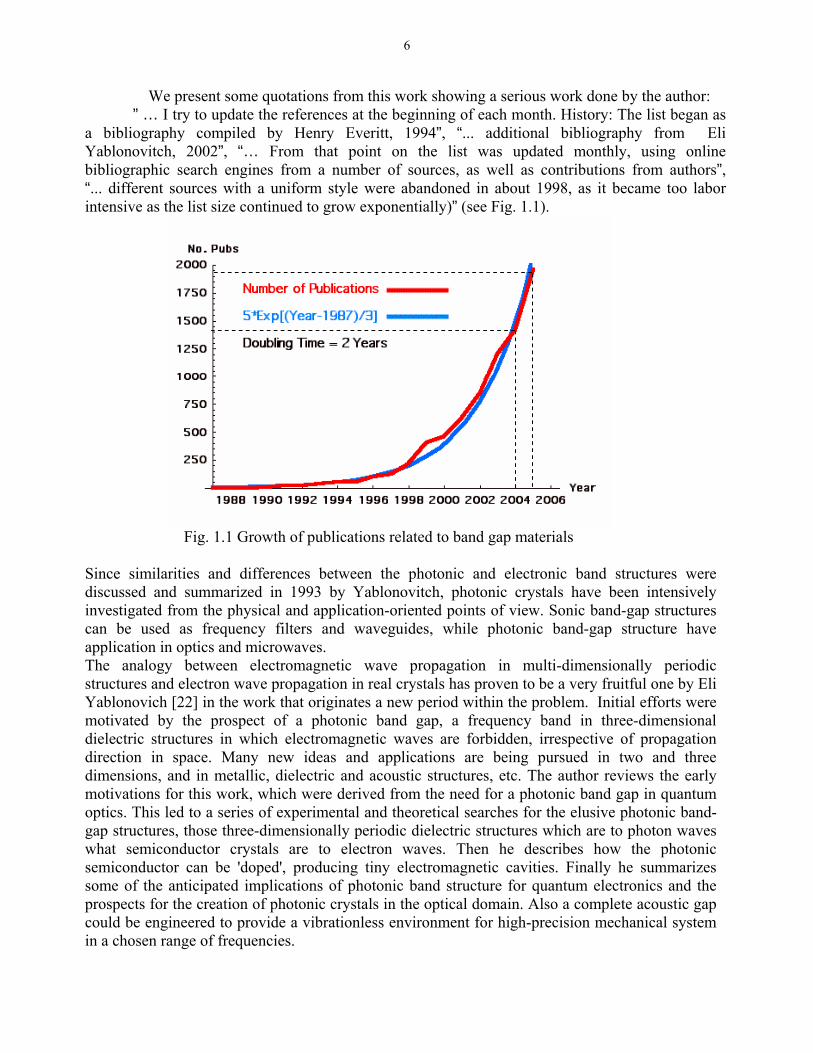
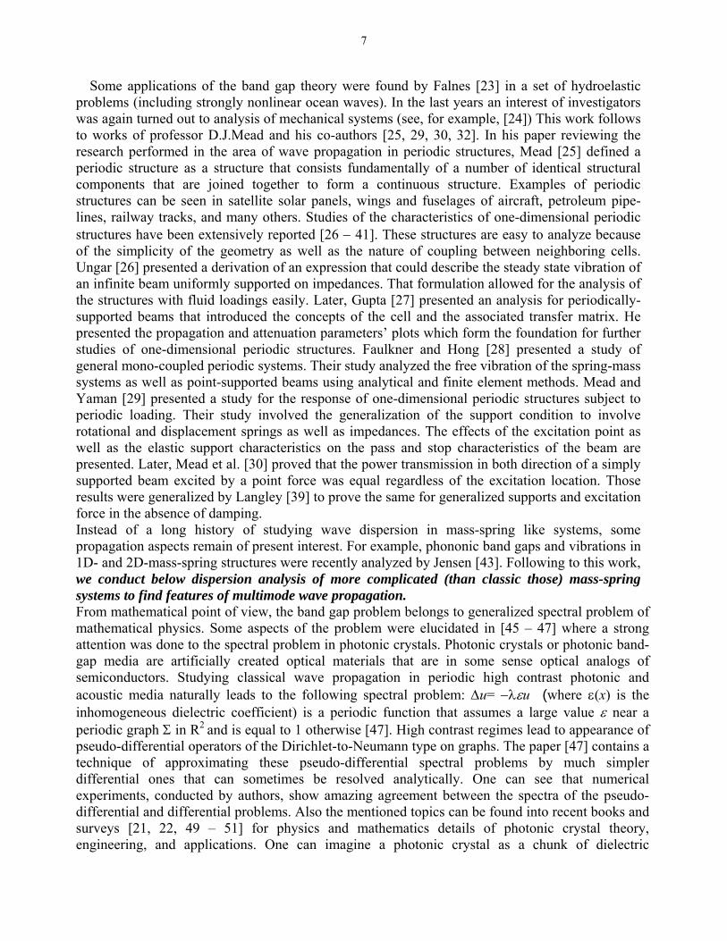
a bibliography compiled by Henry Everitt, 1994”, “... additional bibliography from Eli Yablonovitch, 2002”, “… From that point on the list was updated monthly, using online bibliographic search engines from a number of sources, as well as contributions from authors”, “... different sources with a uniform style were abandoned in about 1998, as it became too labor intensive as the list size continued to grow exponentially)” (see Fig. 1.1).

Fig. 1.1 Growth of publications related to band gap materials Since similarities and differences between the photonic and electronic band structures were discussed and summarized in 1993 by Yablonovitch, photonic crystals have been intensively investigated from the physical and application-oriented points of view. Sonic band-gap structures can be used as frequency filters and waveguides, while photonic band-gap structure have application in optics and microwaves. The analogy between electromagnetic wave propagation in multi-dimensionally periodic structures and electron wave propagation in real crystals has proven to be a very fruitful one by Eli Yablonovich [22] in the work that originates a new period within the problem. Initial efforts were motivated by the prospect of a photonic band gap, a frequency band in three-dimensional dielectric structures in which electromagnetic waves are forbidden, irrespective of propagation direction in space. Many new ideas and applications are being pursued in two and three dimensions, and in metallic, dielectric and acoustic structures, etc. The author reviews the early motivations for this work, which were derived from the need for a photonic band gap in quantum optics. This led to a series of experimental and theoretical searches for the elusive photonic band-gap structures, those three-dimensionally periodic dielectric structures which are to photon waves what semiconductor crystals are to electron waves. Then he describes how the photonic semiconductor can be 'doped', producing tiny electromagnetic cavities. Finally he summarizes some of the anticipated implications of photonic band structure for quantum electronics and the prospects for the creation of photonic crystals in the optical domain. Also a complete acoustic gap could be engineered to provide a vibrationless environment for high-precision mechanical system in a chosen range of frequencies.

7

Some applications of the band gap theory were found by Falnes [23] in a set of hydroelastic problems (including strongly nonlinear ocean waves). In the last years an interest of investigators was again turned out to analysis of mechanical systems (see, for example, [24]) This work follows to works of professor D.J.Mead and his co-authors [25, 29, 30, 32]. In his paper reviewing the research performed in the area of wave propagation in periodic structures, Mead [25] defined a periodic structure as a structure that consists fundamentally of a number of identical structural components that are joined together to form a continuous structure. Examples of periodic structures can be seen in satellite solar panels, wings and fuselages of aircraft, petroleum pipe-lines, railway tracks, and many others. Studies of the characteristics of one-dimensional periodic structures have been extensively reported [26 − 41]. These structures are easy to analyze because of the simplicity of the geometry as well as the nature of coupling between neighboring cells. Ungar [26] presented a derivation of an expression that could describe the steady state vibration of an infinite beam uniformly supported on impedances. That formulation allowed for the analysis of the structures with fluid loadings easily. Later, Gupta [27] presented an analysis for periodically-supported beams that introduced the concepts of the cell and the associated transfer matrix. He presented the propagation and attenuation parameters’ plots which form the foundation for further studies of one-dimensional periodic structures. Faulkner and Hong [28] presented a study of general mono-coupled periodic systems. Their study analyzed the free vibration of the spring-mass systems as well as point-supported beams using analytical and finite element methods. Mead and Yaman [29] presented a study for the response of one-dimensional periodic structures subject to periodic loading. Their study involved the generalization of the support condition to involve rotational and displacement springs as well as impedances. The effects of the excitation point as well as the elastic support characteristics on the pass and stop characteristics of the beam are presented. Later, Mead et al. [30] proved that the power transmission in both direction of a simply supported beam excited by a point force was equal regardless of the excitation location. Those results were generalized by Langley [39] to prove the same for generalized supports and excitation force in the absence of damping. Instead of a long history of studying wave dispersion in mass-spring like systems, some propagation aspects remain of present interest. For example, phononic band gaps and vibrations in 1D- and 2D-mass-spring structures were recently analyzed by Jensen [43]. Following to this work, we conduct below dispersion analysis of more complicated (than classic those) mass-spring systems to find features of multimode wave propagation. From mathematical point of view, the band gap problem belongs to generalized spectral problem of mathematical physics. Some aspects of the problem were elucidated in [45 – 47] where a strong attention was done to the spectral problem in photonic crystals. Photonic crystals or photonic band-gap media are artificially created optical materials that are in some sense optical analogs of semiconductors. Studying classical wave propagation in periodic high contrast photonic and acoustic media naturally leads to the following spectral problem: Δu= −λεu (where ε(x) is the inhomogeneous dielectric coefficient) is a periodic function that assumes a large value ε near a periodic graph Σ in R2 and is equal to 1 otherwise [47]. High contrast regimes lead to appearance of pseudo-differential operators of the Dirichlet-to-Neumann type on graphs. The paper [47] contains a technique of approximating these pseudo-differential spectral problems by much simpler differential ones that can sometimes be resolved analytically. One can see that numerical experiments, conducted by authors, show amazing agreement between the spectra of the pseudo-differential and differential problems. Also the mentioned topics can be found into recent books and surveys [21, 22, 49 – 51] for physics and mathematics details of photonic crystal theory, engineering, and applications. One can imagine a photonic crystal as a chunk of dielectric

8

(insulator) with cavities (“bubbles”) carved out in a periodic manner and filled with a different dielectric (e.g., air). The name photonic crystal comes from analogies with natural crystals that are also periodic media, and also from the idea that photonic crystals behave with respect to photon propagation similarly to the behavior of semi-conductors with respect to the electron propagation. Mathematical analysis of periodic structures have mostly employed two basic analysis methods, of which assume time-harmonic motions of the structure. The first method, which shall be referred to here as the eigenvalue method, solves an eigenvalue problem for the attenuation constant based on the analysis of one cell of the periodic structure. The eigenvalue problem is derived by applying Floquet theorem to the responses at the end of the cell. The second method, which shall be referred here as the wavenumber method, proceeds by taking the spatial Fourier transform of the differential equations of motion of the structure. Once in the wavenumber domain, the structural response is obtained by employing Poisson’s formula. In our work we describe systems in whish the mentioned above space function ε(x) has a step-wise nature. The main goal is to find transient solutions and then to link (where it is possible) dispersion properties and features of transient waves excited by local vibrating loads of frequencies lying within pass- and stop-bands. Transient solutions are described below also in the case of Heaviside-like pulses. Formation of quasi-fronts appeared with time instead of fronts is analyzed depending on the waveguide structure. Analytical approaches used in our work are based on ideas and formulations originally developed by Professor L. I. Slepyan (Tel-Aviv University) and on publications [54 – 62]. First of all we pay attention to dispersion properties of waves propagating in structured waveguides [54, 55, 61, 62, 63]. Note that existence of localized wave propagation without attenuation in 2D lattice (or, by another words, existence of 1D waveguides within 2D infinite structure) was recently shown in [62]. In our work we analyze a set of 2D lattices with properly designed inhomogeneities allowing existing an 1D waveguide to be proved. With the non-stationary problem in mind, used analytical approach [52, 54 58] intended for describing the transient wave propagation in waveguides of several structures includes - double integral transforms, - obtaining a formal solution for images, and - asymptotic analysis of this solutions within several spectral bands. We also use such an algorithm to find asymptotes for longwave components of the solution (in the case of a step loading of complicated waveguides) and short-wave those (in the case of resonance excitation), which were absent up to present. A numerical approach, called as MDM-technique [52, 53] are used in the work and developed here to precise numerical solutions of wave propagation processes saturated by front and high-gradient wave components. Resonance phenomena arising in structured waveguides subjected by local monochromatic or moving loads are described in [56, 59, 61, 63]. In the work we try to extend a range of resonance cases to be analyzed that appear in mass-spring and material bond lattices. Summarizing that was said above we note that in spite of a number aspects comprehensively revealed within the problem under consideration, some points require of further developing and improving. The main of those is a correspondence between steady-state and transient problems in the case of structured waveguides under action of different spectra loading. Besides, the influence has not yet been studied of broken symmetry (perturbed structures) intrinsic to actual structures. Development of resonant processes is required to be comprehensively studied with the aim to prove dangerous vibrations regimes. These points are studied in the work. At least three main aspects proved within these works, which can be serve of support points for the work, are the following:

9

• Dispersion properties of harmonic waves propagated in composite structures can be essentially informative applied to the problem of prediction of distinctive features of transient processes, notably for revealing quasi-steady state and resonant regimes of low-frequency spectrum in the case of relatively long external loading,

• Analytical technique, based on Slepyan's method of an asymptotical reversion of coupled Laplace-Fourier transforms, allows the mentioned above quasi-steady state and resonant regimes to be analyzed not only qualitatively but quantitatively as well,

• Computer algorithms, designed from explicit finite difference schemes (EFDS) with the use by the so called mesh dispersion minimization (MDM) method possess an unique possibility to obtain numerical solution of transient problems with the same (high) accuracy for low-frequency and high-frequency components. As is well known, besides the problem of EFDS computational stabilization, its serious drawback in pulse process calculations is the emergence of short-wave "parasite" oscillations in high-gradient solutions initiated by so-called mesh dispersion. The MDM serves to significantly decrease the above effect. It is a generalized concept of the well-known Courant condition that relates dispersion properties of discrete and continuous models. Generally speaking they have different domains of influence, and the idea behind MDM is to properly adjust these domains. Such a procedure results in requirements to parameters of an optimal mesh.

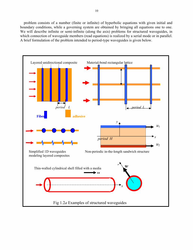
In our work we pay special attention to classic problems of wave propagation in chains and lattices, which could be simplest models for more complicated structures, bringing together discrete and continual elements. One of most interesting points of the classic theory is related to filter properties of periodic systems. At the so-called band-pass filters, energy dissipation is omitted, there is a sharp distinction between frequency bands exhibiting wave propagation without attenuation (passing bands) and those showing attenuation and no propagation (stopping bands). We use several models beginning from the classic one and including those proposed by us for description of waveguide properties and transient response in the wide spectrum of pulse-vibration excitations. The models and method designed would be applied to practical problems arising in calculations of elongated engineering structures subjected by explosion and seismic loadings. 1.1 Work subjects and structure 1.1.1 Structured waveguides. From engineering point of view, elastic waves are considered that propagated in stepwise composite structures under action of local or spatial pulse/harmonic loadings. Some examples of periodic-type and homogeneous-in-the-length waveguides and typical loadings, which are included into problems under our consideration, are shown in Fig. (1.2a): - an unidirectional composite, consisting on alternatively closed layers which can be presented by two families of diverse materials. Various structures made of glass-fiber-reinforced plastics (used, for example, in aircraft engineering) are modeled by this a way. - a lattice made on a number of families of material bonds (two families are shown here), - a thin cylindrical shell with fillings that model pipes and other structures where the boundary thickness is small compare to the radius - a sandwich structure made up of two beams with adhesive.

Periodicity, properties of elements and loading features [they are marked by thick red arrows in Fig.(1.2a)], allow 1D and 2D problems to be separated in a set of cases. We try to describe some common properties of structured waveguides of the shown above types. The main feature of a hypothetical generalized structure that could be built from its members connected serially or in parallel is existence of a direction, the waveguide axis (it is shown in Fig.1.2 by thin black arrows), along of which a significant part of wave energy is propagated. Mathematical formulation of the

10

problem consists of a number (finite or infinite) of hyperbolic equations with given initial and boundary conditions, while a governing system are obtained by bringing all equations one to one. We will describe infinite or semi-infinite (along the axis) problems for structured waveguides, in which connection of waveguide members (read equations) is realized by a serial mode or in parallel. A brief formulation of the problem intended to period-type waveguides is given below.

w u

r

x

Layered unidirectional composite Material-bond rectangular lattice

period L period L Fiber adhesive

yu1

x period H u2 Simplified 1D waveguides Non-periodic in-the-length sandwich structure modeling layered composites Thin-walled cylindrical shell filled with a media

Fig 1.2a Examples of structured waveguides

11

In Fig. (1.2b) a generalized model of period-type waveguide is depicted, in which linked by

nodes two families, I and II, are schematically shown. Nodes, in their turn, can be also structured.

1.1.2 Problem formulation, aims and methods of investigation. Let a periodic-type composite of such a structure consists of an infinite set of identical cells connected by periodically located nodes. Let the main direction of wave propagation is the structure axis x. Each cell can contain substructure bounded or unbounded along in the vertical axis y. The cell length is taken as the measurement unit, the node with no length can be inertial or massless as well. In some cross-section of the waveguide a non-stationary load Q(t) functions at t > 0. Propagation of waves through such a structure is examined. With the analysis of transient problem is mind, we study external actions of several types related to explosion and impact those: Heaviside-step, exponential, triangular, sinusoidal and mixed. A. Problem formulation

1. Wave propagation along layers (thin fibers and thick adhesive, see figure below) is described

Qm(t) u(x, t) m + 1 v(x, y, t) x m L L m − 1 y by the following infinite PDE system in which neighboring equations are linked by differential operators functioning in parallel: ( )I

yN (1.1) ( ) y

Here m is the number of the fiber-adhesive layer, u(x, t) and v(x, y, t) are longitudinal displacements in 1D-fiber and 2D-adhesive layers, Cm and cm are wave velocities in fiber and

( ) ( )[ ] ( ) ( ) ( ) ( ) ( )( ) 10c == ( )[ ] :loringlayer tai , , ,

,,

,2

1,2

mmLymmyymm

kmmmLymmI

mxxmm

m

mmtHtQtQtQNuCu

uvvv

vv

=±

−=++′′=

=

=+

′′ L

&&

&&

δ

L=1

n - 1 n n + 1 x

Q (t, x) e waveguid type-periodic 1D dGeneralize 1.2 Fig b

12

adhesive, is a first order differential operator with respect to vertical coordinate, y, Q( )IyN m(t) is

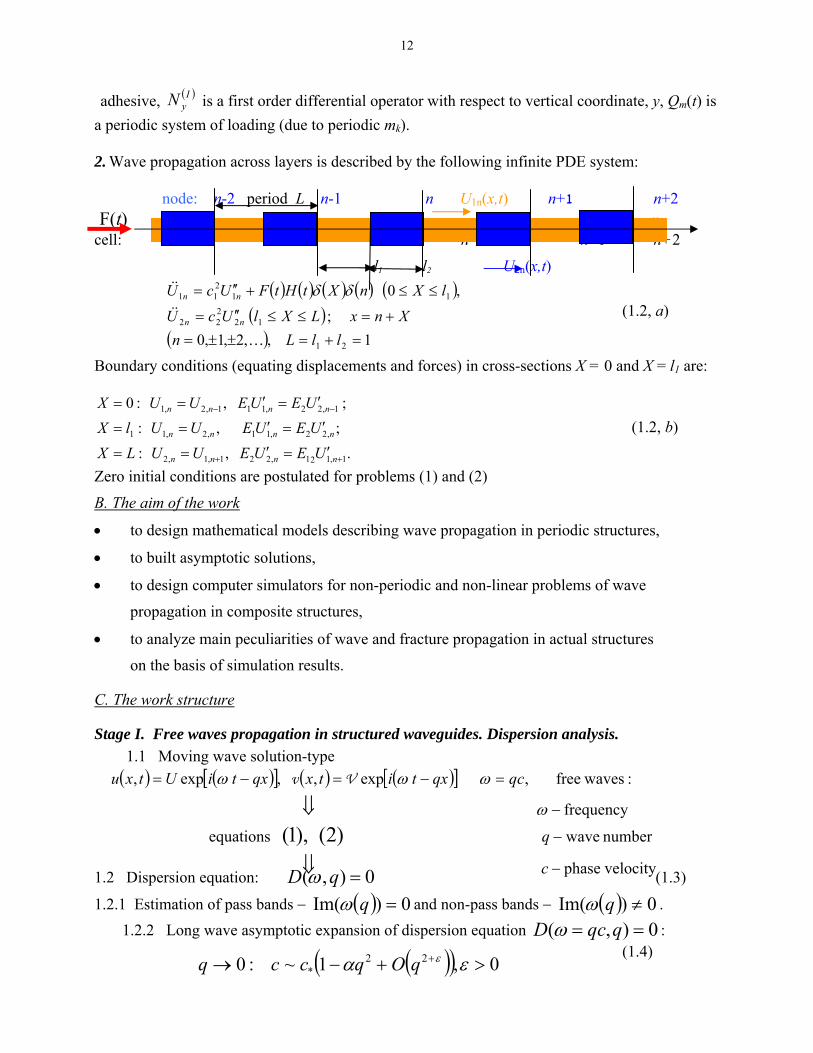
a periodic system of loading (due to periodic mk). 2. Wave propagation across layers is described by the following infinite PDE system:

node: n-2 period L n-1 n n+2 U1n(x,t) n+1

F(t) x cell: n-3 n-2 n-1 n n+1 n+2

l1 l2 U2n(x,t) ( ) ( ) ( ) ( ) ( )

( )( ) 1 ,,2,1,0

;

,0

21

12222

11211

=+=±±=+=≤≤′′=

≤≤+′′=

llLnXnxLXlUcU

lXnXtHtFUcU

nn

nn

K

&&

&& δδ (1.2, a) Boundary conditions (equating displacements and forces) in cross-sections X = 0 and X = l1 are:

. , :; , :; , :0

1,121,221,1,2

,22,11,2,11

1,22,111,2,1

++

−−

′=′==

′=′==

′=′==

nnnn

nnnn

nnnn

UEUEUULXUEUEUUlX

UEUEUUX (1.2, b)

Zero initial conditions are postulated for problems (1) and (2)

B. The aim of the work

• to design mathematical models describing wave propagation in periodic structures,

• to built asymptotic solutions,

• to design computer simulators for non-periodic and non-linear problems of wave

propagation in composite structures,

• to analyze main peculiarities of wave and fracture propagation in actual structures

on the basis of simulation results.

C. The work structure

Stage I. Free waves propagation in structured waveguides. Dispersion analysis. 1.1 Moving wave solution-type

( ) ( )[ ] ( ) (

1.2 Dispersion equation: 0),( =qD ω (1.3)

)[ ]

velocityphase

1.2.1 Estimation of pass bands − ( ) 0)Im( =qω and non-pass bands − ( ) 0)Im( ≠qω . 1.2.2 Long wave asymptotic expansion of dispersion equation 0),( == qqcD ω : (1.4)

number wave equations

frequency

wavesfree , , , ,

)2(),1(−

−

−

: expexp =−=−=

⇓

⇓

c

q

titxqxtiUtx

ω

qcqxu ωωω Vv

( )( ) 0,1~ :0 22* >+−→ + εα εqOqccq

13

0 ,cos22 :1

:chain spring-mass waveguideDispersion .2

12

0 =−−===

−

ω

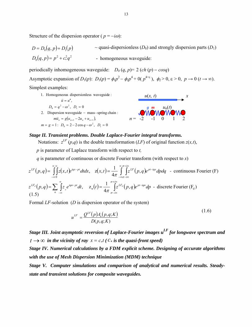
Structure of the dispersion operator ( p = −iω): ~ quasi-dispersionless (D0) and strongly dispersion parts (D1) ( ) (DD =

( )uuugum nnnn ,2 11 +−= +=&& n = -2 -1 0 1 2 DqDgm

DqD 0 , 122

0 =−= ω

uu , ′′=&& :e waveguidlessdispersion sHomogeneou .1

- homogeneous waveguide:

)10 , +22

*2

0 , qppq =

pDpq

( ) cD +

periodically inhomogeneous waveguide: D0 (q, p)= 2 (ch (p) − cosq)

Asymptotic expansion of D1(p): D1(p) = φ1p2 − φ2p4 + 0( p4+ε ), φ2 > 0, ε > 0, p → 0 (t → ∞).

Simplest examples:

u(x, t) x

g m un(t)

Stage II. Transient problems. Double Laplace-Fourier integral transforms. Notations: zLF (p,q) is the double transformation (LF) of original function z(x,t),

p is parameter of Laplace transform with respect to t,

q is parameter of continuous or discrete Fourier transform (with respect to x)

(1.5)

( ) ( ) ( ) ( )

( ) ( ) ( ) )(FFourier discrete - ,41z ,,

(F)Fourier continuous ,41,z ,,,

dn

0

∫∑ ∫

∫ ∫∫ ∫∞+

∞−

−−∞

∞−

∞

∞−

∞+

∞−

−−∞

∞−

∞

==

==

i

i

iqnptLF

n

ptiqnLF

i

i

iqxptLFptiqxLF

dpeqpztdtezqpz

-dqdpeqpztxdtdxetxzqpz

d

n

d

σ

σ

σ

σ

π

π

Formal LF-solution (D is dispersion operator of the system)

(1.6)

( ) ( ));,(;,

KDu =

qpKqpAp u

LFLF Q

Stage III. Joint asymptotic reversion of Laplace-Fourier images uLF for longwave spectrum and

∞→t in the vicinity of ray ( is the quasi-front speed) tcx *= *cStage IV. Numerical calculations by a FDM explicit scheme. Designing of accurate algorithms

with the use of Mesh Dispersion Minimization (MDM) technique

Stage V. Computer simulations and comparison of analytical and numerical results. Steady-

state and transient solutions for composite waveguides.

14

′′u&&

1.2 Wave Dispersion

Wave dispersion phenomenon is dependence of propagating wave velocity, c (or angular frequency, ω), on the wave length, λ. More precisely one defines dispersion of second and higher order via the Taylor expansion of the wave number q (q = 2π/λ) as a function ω (around some certain frequency ω0):

...)(61)(

21)()( 3

03

32

02

2

00 +−∂∂

+−∂∂

+−∂∂

+= ωωω

ωωω

ωωω

ω qqqqq

Dispersion causes wavelength-dependent refraction, it is also important for the propagation of pulses, because a pulse always has a finite spectral width, so the dispersion can cause it’s frequency components to propagate with different velocities If waves of various lengthes propagating along a waveguide have the same velocity such the waveguide is dispersionless one. Dispersionless waveguides are structures without characteristic measurement units, for example, homogeneous rod or string. Moving harmonic wave is described by the form ( ) 1 , −=± ie qxti ω , or,

that is the same, by . Dispersion dependences can be expressed by equations c = c(λ) linked c and λ, and also by equation c = c(q), where q = 2π/λ, or equavalently by equation ω = ω(q), ω = qc is the frequency of the moving wave. Dispersion dependence plays a significant role for obtaining and analysis of steady-state problem solutions for certain predictions which can be done for transient problems. In mathematical point of view, dependencies c = c(λ) are eigenvalues of a system, they also determine velocities of the so-called free waves, i.e. waves freely propagated along a waveguide.

( xctiqe ± )

1.3 Infinite homogeneous rod - dispersionless waveguide.

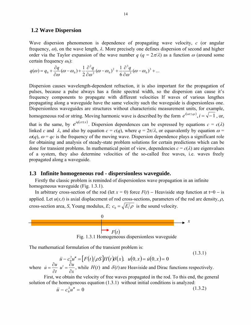
Firstly the classic problem is reminded of dispersionless wave propagation in an infinite homogeneous waveguide (Fig. 1.3.1).

In arbitrary cross-section of the rod (let x = 0) force F(t) − Heaviside step function at t=0 − is applied. Let u(x,t) is axial displacement of rod cross-sections, parameters of the rod are density, ρ, cross-section area, S, Young modulus, E; ρEc =0 is the sound velocity.

Fig. 1.3.1 Homogeneous dispersionless waveguide

0x

( )tF

The mathematical formulation of the transient problem is:

02 =− cu 0

( )[ ] ( ) ( ) ( ) ( ) 00020 ===′′− x,ux,u ,xtHStFucu &&& δρ

(1.3.1)

where xuu

tuu

∂∂

=′∂∂

= & , while )( and )( ttH δ are Heaviside and Dirac functions respectively.

First, we obtain the velocity of free waves propagated in the rod. To this end, the general solution of the homogeneous equation (1.3.1) without initial conditions is analyzed: (1.3.2)

15

As it can be seen Eqn. (1.3.2) can be transformed to the dimensionless equation, 0=′′− uu&& , by one of substitutions: t = tc0 or x = x/c0.

As it was said above, solution of (1.3.2) is represented by form ( )xctiqUeu −= (1.3.3)

in which c = ω/q is the phase speed of the free wave, ω is the frequency of oscillations in this wave, q can also be called as the spatial form frequency, λ = 2π/q is the wave length (spatial

0cc ±=

period). Solution (1.3.3) have the form of moving wave and results in the main conclusion: in homogeneous waveguide (rod) wave propagate independently on their lengths, with the same phase velocity

(1.3.4) Such a process as was said above is dispersionless one. Group velocity, dqdcqcdqdcg +== ω , proves the same (cg = c0) as in the dispersionless case.

At the examples below our first aim is to obtain dispersion equation c = c(q, K) (1.3.5) corresponding to wave propagating along composite waveguides (including periodic-like those) described above (here K is a set of characteristic parameters of the system), and to establish dispersion features of waveguides of different compositions depended on their parameters. Then we will study asymptotic solutions c = c(q, K) related to long wave propagation ( ∞→→ λ,0q ), which are to be very useful with respect to obtain simple asymptotic solutions of transient problems in this limiting case.

In this dispersionless case we have D’Alambert’s solution for transient problem (1.3.1) as follows:

( ) ( ) ( ) SxtcHxtcFtxu ρ||||, 00 −−= (1.3.6) Our aim is to obtain solutions of transient wave processes and to reveal similarities and

differences relized in various dispersion waveguides.

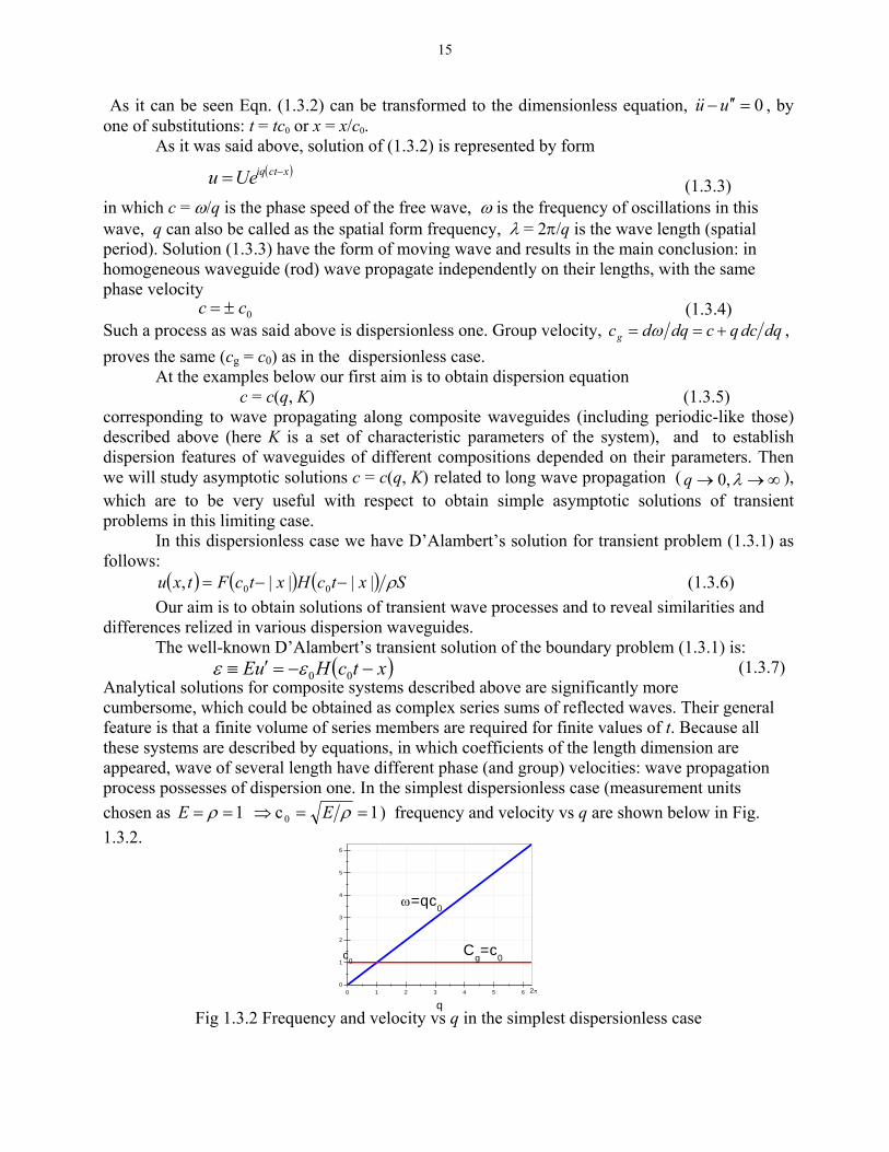
( ) xtcHuE 00 −−=′≡ εεThe well-known D’Alambert’s transient solution of the boundary problem (1.3.1) is:

(1.3.7) Analytical solutions for composite systems described above are significantly more

0 1 2 3 4 5 60

1

2

3

4

5

6

2π

c0Cg=c0

ω=qc0

cumbersome, which could be obtained as complex series sums of reflected waves. Their general feature is that a finite volume of series members are required for finite values of t. Because all these systems are described by equations, in which coefficients of the length dimension are appeared, wave of several length have different phase (and group) velocities: wave propagation process possesses of dispersion one. In the simplest dispersionless case (measurement units chosen as 1c 1 0 ==⇒== ρρ EE ) frequency and velocity vs q are shown below in Fig. 1.3.2. q

Fig 1.3.2 Frequency and velocity vs q in the simplest dispersionless case

16

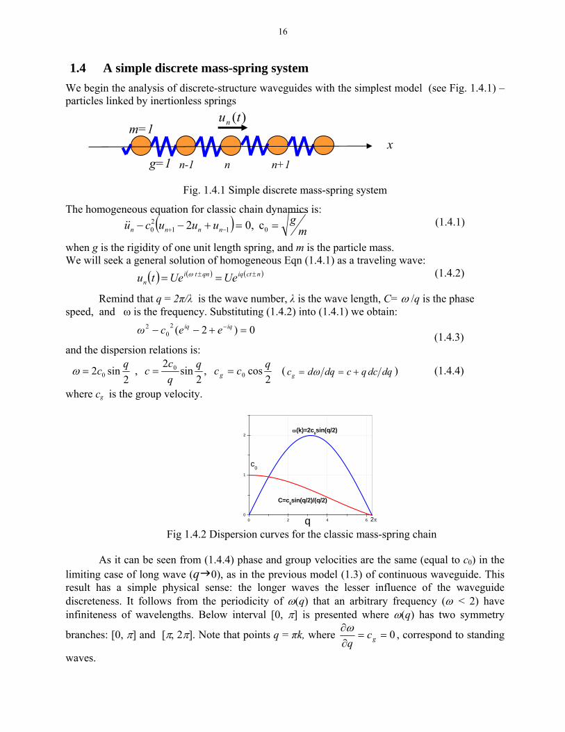
1.4 A simple discrete mass-spring system

We begin the analysis of discrete-structure waveguides with the simplest model (see Fig. 1.4.1) – particles linked by inertionless springs

( ) mguuucu nnnn ==+−− −+ 011

20 c 0,2 &&

( ) ( ) ( )nctiqqntin UeUeu ±t ± == ω

0 2 4 60

1

2

2π

c0

C=c0sin(q/2)/(q/2)

ω(k)=2c0sin(q/2)

q

n-1 n n+1

)(tunm=1

Fig. 1.4.1 Simple discrete mass-spring system

The homogeneous equation for classic chain dynamics is: (1.4.1)

when g is the rigidity of one unit length spring, and m is the particle mass. We will seek a general solution of homogeneous Eqn (1.4.1) as a traveling wave: (1.4.2)

Remind that q = 2π/λ is the wave number, λ is the wave length, C= ω /q is the phase speed, and ω is the frequency. Substituting (1.4.2) into (1.4.1) we obtain: (1.4.3) and the dispersion relations is:

2

sin2 0qc=ω ,

2cos ,

2sin

20

0 qccqqc

c g == ( dqdcqcdqdcg +== ω ) (1.4.4)

where cg is the group velocity.

Fig 1.4.2 Dispersion curves for the classic mass-spring chain

As it can be seen from (1.4.4) phase and group velocities are the same (equal to c0) in the limiting case of long wave (q 0), as in the previous model (1.3) of continuous waveguide. This result has a simple physical sense: the longer waves the lesser influence of the waveguide discreteness. It follows from the periodicity of ω(q) that an arbitrary frequency (ω < 2) have infiniteness of wavelengths. Below interval [0, π] is presented where ω(q) has two symmetry

branches: [0, π] and [π, 2π]. Note that points q = πk, where 0==∂∂

gcqω , correspond to standing

waves.

0)2(− cω 20

2 =+− −iqiq ee

g=1 x

17

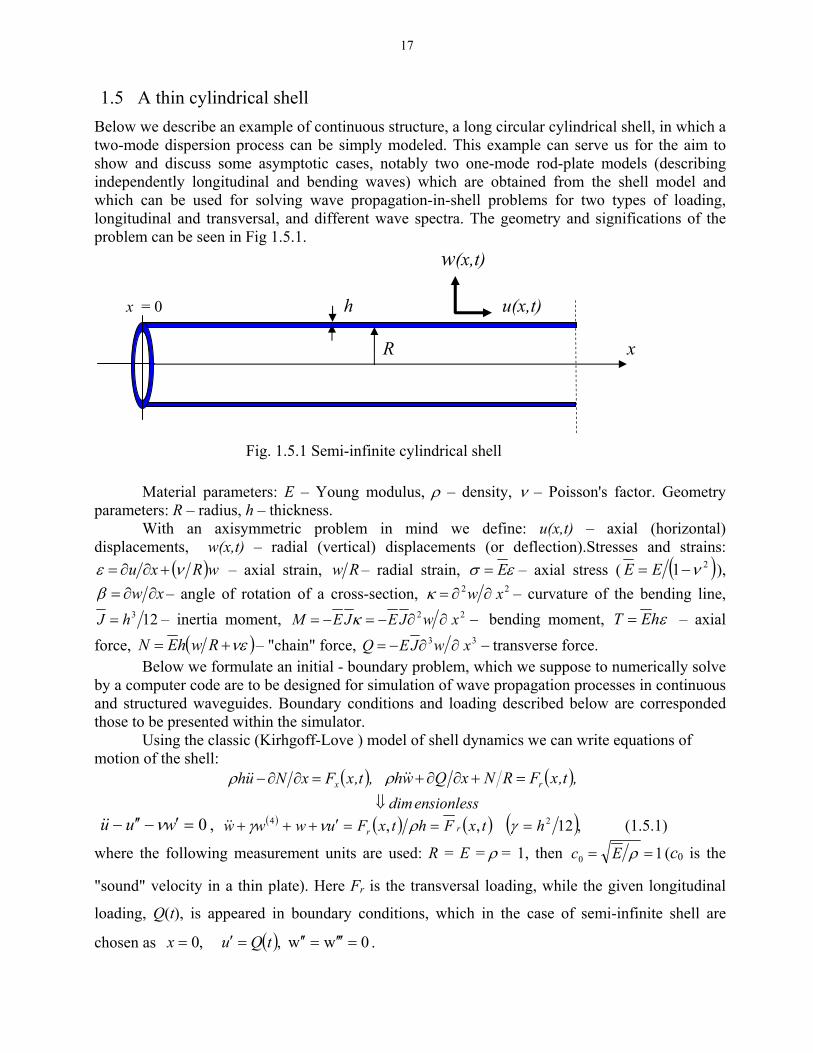
1.5 A thin cylindrical shell

Below we describe an example of continuous structure, a long circular cylindrical shell, in which a two-mode dispersion process can be simply modeled. This example can serve us for the aim to show and discuss some asymptotic cases, notably two one-mode rod-plate models (describing independently longitudinal and bending waves) which are obtained from the shell model and which can be used for solving wave propagation-in-shell problems for two types of loading, longitudinal and transversal, and different wave spectra. The geometry and significations of the problem can be seen in Fig 1.5.1.

w(x,t)

x = 0 h u(x,t) R x Fig. 1.5.1 Semi-infinite cylindrical shell

Material parameters: E – Young modulus, ρ – density, ν – Poisson's factor. Geometry parameters: R – radius, h – thickness.

With an axisymmetric problem in mind we define: u(x,t) – axial (horizontal) displacements, w(x,t) – radial (vertical) displacements (or deflection).Stresses and strains:

( )wRxu νε +∂∂= – axial strain, Rw – radial strain, εσ E= – axial stress ( ( )21 ν−= EE ), xw ∂∂=β – angle of rotation of a cross-section, 22 x w ∂∂=κ – curvature of the bending line,

123hJ = – inertia moment, −∂∂−=−= x wJEJEM 22κ bending moment, εhET = – axial force, ( νε+= RwhEN )– "chain" force, −∂∂−= x wJEQ 33 transverse force.

Below we formulate an initial - boundary problem, which we suppose to numerically solve by a computer code are to be designed for simulation of wave propagation processes in continuous and structured waveguides. Boundary conditions and loading described below are corresponded those to be presented within the simulator.

Using the classic (Kirhgoff-Love ) model of shell dynamics we can write equations of motion of the shell: ( ),t,xFxNuh x=∂∂−&&ρ ( ),t,xFRNxQwh r=+∂∂+&&ρ ensionlessdim⇓ , 0=′−′′− wuu ν&& ( ) ( ) ( ) ( ),12 ,, 24 htxFhtxFuwww rr ===′+++ γρνγ&& (1.5.1)

where the following measurement units are used: R = E = ρ = 1, then 10 == ρEc (c0 is the

"sound" velocity in a thin plate). Here Fr is the transversal loading, while the given longitudinal

loading, Q(t), is appeared in boundary conditions, which in the case of semi-infinite shell are

chosen as ( ) 0ww , ,0 =′′′=′′=′= tQux .

18

Initial conditions are: ( ) ( ) ( ) ( ) ( ) ( ) ( ) ( )x0000 00 Zx,0w ,xWx,0 w,xV,xu ,xU,xu = = == && ,

where are given functions. We seek the general solution of the

homogeneous system (1.5.1) in the form of the moving wave:

( ) ( ) ( ) ( )xZxWxVxU 0000 , , ,

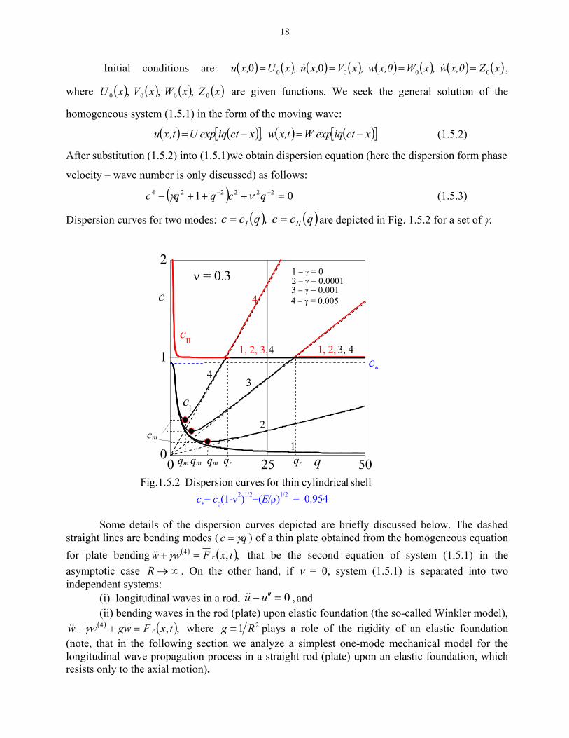
( ) ( )[ ] ( ) ( )[ ]xctiqexpWtx, w,xctiqexpUt,xu −=−= (1.5.2)

After substitution (1.5.2) into (1.5.1)we obtain dispersion equation (here the dispersion form phase

velocity – wave number is only discussed) as follows:

( ) 01 222224 =+++− −− qcqqc νγ (1.5.3)

Dispersion curves for two modes: ( ) ( )qcc ,qcc III == are depicted in Fig. 1.5.2 for a set of γ.

cm qm qm qm qr qr

Some details of the dispersion curves depicted are briefly discussed below. The dashed straight lines are bending modes ( qc γ= ) of a thin plate obtained from the homogeneous equation for plate bending ( ) ( ),,4 txFww r=+ γ&& that be the second equation of system (1.5.1) in the asymptotic case ∞→R . On the other hand, if ν = 0, system (1.5.1) is separated into two independent systems: (i) longitudinal waves in a rod, , 0=′′− uu&& and (ii) bending waves in the rod (plate) upon elastic foundation (the so-called Winkler model),

( ) ( ),,4 txFgwww r=++ γ&& where 21 Rg ≡ plays a role of the rigidity of an elastic foundation (note, that in the following section we analyze a simplest one-mode mechanical model for the longitudinal wave propagation process in a straight rod (plate) upon an elastic foundation, which resists only to the axial motion).

0 20

5 50

1

2

3, 41, 2,1, 2, 3,4

4 4 − γ = 0.0053 − γ = 0.0012 − γ = 0.00011 − γ = 0

43

2

1

c*

Dispersion curves for a cylindrical shell

q

c*= c0(1-ν2)1/2=(E/ρ)1/2 = 0.954

ν = 0.3

cI

c

cII

43

shell lcylindricafor thin curves Dispersion Fig.1.5.2

19

The curves 1 of mode I and mode II are non-interconnected (independent) those of so-called “membrane” theory of the shell. They can be formally obtained from (1.5.1) under the asymptotic condition , e.g. for too thin shells. Membrane model is used for description of a longwave spectrum propagated along the shell axis. In such a process, influence of radial oscillations arises with q (with decrease in λ). Asymptotic analysis of (1.5.3) shows that longwave velocity of the first mode, , is equal to the sound velocity in a rod:

0→h

*c ρEc* = , so radial oscillations of the shell does not exert influence on the wave (longitudinal) propagation process, which turned out the same as in an equivalent rod (i.e. in a rod having the same E, ρ and the square equal to 2πRh). Then, an asymptotic expression of the dispersion relation for long waves propagation is the following: :0→q ( )22501 q.c~c *I ν− (1.5.4)

It can be seen, that with rise of q first and second modes approach and transit one to one, so that remains less than c( )qcI 0 = 1 (it tend to 1 from below if ∞→q ). Such kind of long-wave asymptotes we will meet below for various continuous waveguides and waveguides of step-wise structures having a straight rod (or plate) as a basis and saturated by various adjoined elements fixed and periodically distributed on the basis. In the our case, if q increases and 0≠h , longitudinal form of propagating wave transits into the bending one for an equivalent rod (plate) after the passing of the critical point, the minimum of the dispersion curve (marked by solid circles, their abscissas are qm). So, the simplest rod model (axial motion) can be applied to solve the problem of longitudinal wave propagation if q is too large, the membrane model is applied to the spectrum q < qm, and the bending model (so-called classical Bernoulli model) of plate-rod transversal motion can be used within the interval qm < q < qr.

We note that coordinates of critical points (qm, cm) determine parameters of flexural resonant waves propagated along axis x (see [59]), the wavelength and the propagation velocity, if external force Fr is a moving load with velocity cm. Such a regime, however, isn’t investigated here. Indeed, we will meet with resonant regimes that are realized in periodical waveguides and propagated from a local (immobile) monochromatic source.

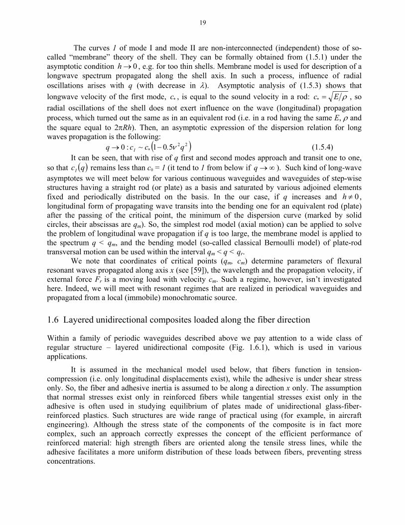
1.6 Layered unidirectional composites loaded along the fiber direction

Within a family of periodic waveguides described above we pay attention to a wide class of regular structure – layered unidirectional composite (Fig. 1.6.1), which is used in various applications.

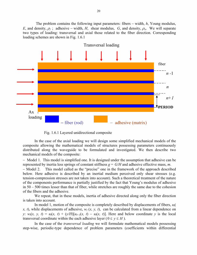
It is assumed in the mechanical model used below, that fibers function in tension-compression (i.e. only longitudinal displacements exist), while the adhesive is under shear stress only. So, the fiber and adhesive inertia is assumed to be along a direction x only. The assumption that normal stresses exist only in reinforced fibers while tangential stresses exist only in the adhesive is often used in studying equilibrium of plates made of unidirectional glass-fiber-reinforced plastics. Such structures are wide range of practical using (for example, in aircraft engineering). Although the stress state of the components of the composite is in fact more complex, such an approach correctly expresses the concept of the efficient performance of reinforced material: high strength fibers are oriented along the tensile stress lines, while the adhesive facilitates a more uniform distribution of these loads between fibers, preventing stress concentrations.

20

The problem contains the following input parameters: fibers − width, h, Young modulus, E, and density, ρf ; adhesive − width, H, shear modulus, G, and density, ρa. We will separate two types of loading: transversal and axial those related to the fiber direction. Corresponding loading schemes are shown in Fig. 1.6.1

. Transversal loading

fiber number

n -1 n –1 n n 1 n+1 PERIOD Axial loading

− fiber (rod) − adhesive (matrix) Fig. 1.6.1 Layered unidirectional composite

In the case of the axial loading we will design some simplified mechanical models of the composite allowing the mathematical models of structures possessing parameters continuously distributed along the waveguide to be formulated and investigated. We then describe two mechanical models of the composite: − Model 1. This model is simplified one. It is designed under the assumption that adhesive can be represented by inertia less springs of constant stiffness g = G/H and adhesive effective mass, m. − Model 2. This model called as the “precise” one in the framework of the approach described below. Here adhesive is described by an inertial medium perceived only shear stresses (e.g. tension-compression stresses are not taken into account). Such a theoretical treatment of the nature of the components performance is partially justified by the fact that Young’s modulus of adhesive in 50 – 500 times lesser than that of fiber, while stretches are roughly the same due to the cohesion of the fibers and the adhesive.

We repeat, that in these models, inertia of adhesive directed along only the fiber direction is taken into account.

In model 1, motion of the composite is completely described by displacements of fibers, ul( x, t), while displacements of adhesive, wl (x, y, t), can be calculated from a linear dependence on y: wl(x, y, t) = ul(x, t) + (y/H)[ul+1(x, t) − ul(x, t)]. Here and below coordinate y is the local transversal coordinate within the each adhesive layer ( Hy ≤≤0 ).

In the case of the transversal loading we will formulate mathematical models possessing step-wise, periodic-type dependence of problem parameters (coefficients within differential

21

equations) on the waveguide axis that is to be perpendicular to the fiber axis. This case will be described below beginning Section II.

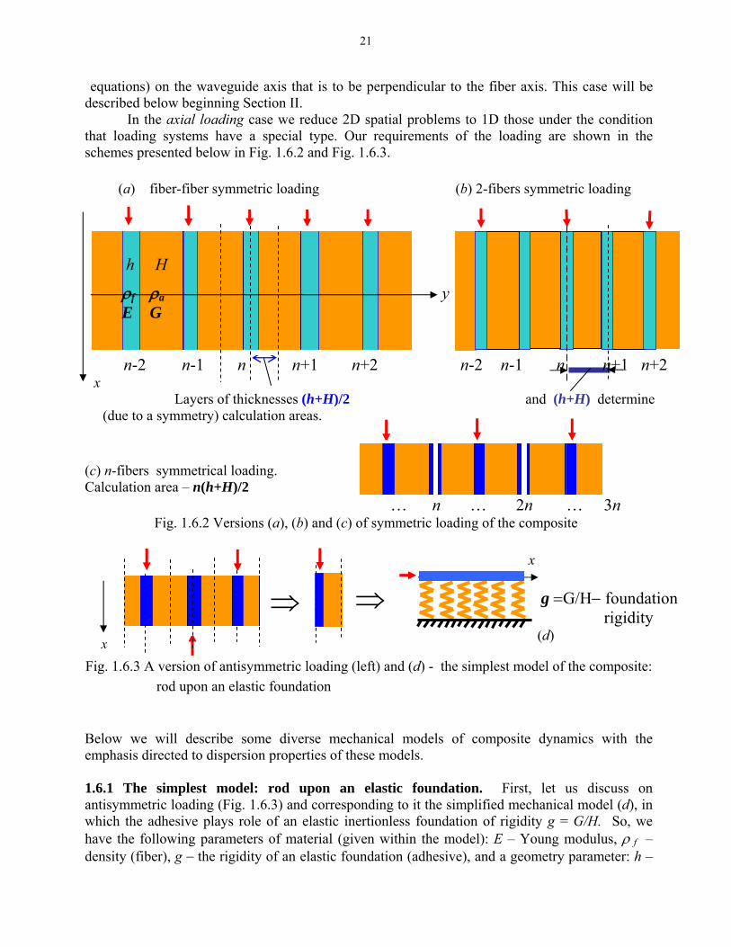
In the axial loading case we reduce 2D spatial problems to 1D those under the condition that loading systems have a special type. Our requirements of the loading are shown in the schemes presented below in Fig. 1.6.2 and Fig. 1.6.3.

(a) fiber-fiber symmetric loading (b) 2-fibers symmetric loading

h H

ρf ρa y E G n-2 n-1 n n+1 n+2 n-2 n-1 n n+1 n+2 x

Layers of thicknesses (h+H)/2 and (h+H) determine (due to a symmetry) calculation areas.

(c) n-fibers symmetrical loading. Calculation area – n(h+H)/2 … n … 2n … 3n

Fig. 1.6.2 Versions (a), (b) and (c) of symmetric loading of the composite

x g =G/H− foundation rigidity (d)

⇒⇒x

Fig. 1.6.3 A version of antisymmetric loading (left) and (d) - the simplest model of the composite: rod upon an elastic foundation Below we will describe some diverse mechanical models of composite dynamics with the emphasis directed to dispersion properties of these models. 1.6.1 The simplest model: rod upon an elastic foundation. First, let us discuss on antisymmetric loading (Fig. 1.6.3) and corresponding to it the simplified mechanical model (d), in which the adhesive plays role of an elastic inertionless foundation of rigidity g = G/H. So, we have the following parameters of material (given within the model): E – Young modulus, ρ f – density (fiber), g − the rigidity of an elastic foundation (adhesive), and a geometry parameter: h –

22

thickness. A single dependent variable is u(x,t) – displacements of the fiber xu ∂∂=ε – the axial strain in a fiber, εσ E= – the axial stress. Mathematical model of motion of the structure is: ( ).,f txFguuEhuh u=+′′−&&ρ (1.6.1) Its dimensionless version is ( ),, 2

0 txFuuu u=+′′− ω&& (1.6.2)

where measurement units are E = ρ f = h =1 (then c0 = (E/ρ f)1/2 =1) and hg fρω =0 is the frequency of an SDF-system having the mass equal to relative mass of the fiber and the spring rigidity equal to the rigidity of adhesive. Initial conditions: ( ) ( ) ( ) ( ).0, ,0, 00 xVxuxUxu == & To study the case of semi-infinite structure x ≥ 0 it is enough to set a boundary condition only in the origin cross-section, x = 0. Let ( ) ( ).x tQu 0==′ The general steady-state solution of the homogeneous system (1.6.1) can be present in the form of a moving wave: ( ) ( )[ ] ( )[ ] qcqxtiUxctiqUtxu =−=−= ωω , expexp, , (1.6.3) After substitution (1.6.3) into (1.6.2) we obtain the dispersion equations as the dependencies of frequency ω or phase velocity c vs wave number q (1.6.4) ( ). 1 0 ωωω qqq ±==+±= , 01

21

22 ωqqc =+ −

One can see that the phase velocity of long waves (q1 → 0) tends to infinity. This result has no physical sense (notably the finiteness of velocity must be proved) if we will associate the phase velocity with motion of material particles within the propagated wave. The discussed system has two faces: an oscillation face (rigidity of the fiber E → 0) and a wave face (rigidity of the adhesive g → 0). In the asymptotic case q1 → 0 the oscillation character of the motion overcomes and we have a steady-state oscillation process. This conclusion can be confirmed by the analysis of the group velocity ( ) 212

11 −−+±=∂=c ω qdqg which is responsible for the wave energy transfer: cg → 0 if q1→ 0. So long waves (more accurately: infinitely long waves) don’t propagate along the system. Their structure appears in the steady-state oscillation process. On the other hand, the short wave asymptote (q1 → ∞) results in an opposite conclusion: ( )∞→±== 1 1 qcc g , that is, elastic foundation of a limit rigidity is not detected by short waves, which have a small dispersion decreased along with q.

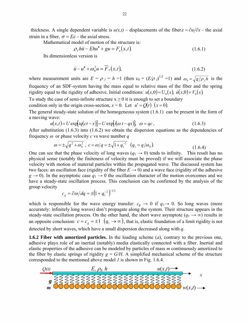
1.6.2 Fiber with amortized particles. In the loading scheme (a), contrary to the previous one, adhesive plays role of an inertial (notably) media elastically connected with a fiber. Inertial and elastic properties of the adhesive can be modeled by particles of mass m continuously amortized to the fiber by elastic springs of rigidity g = G/H. A simplified mechanical scheme of the structure corresponded to the mentioned above model 1 is shown in Fig. 1.6.4.

Q(t) E, ρf, h u(x,t) x g m w(x,t)

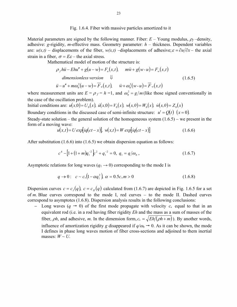
23

Fig. 1.6.4. Fiber with massive particles amortized to it Material parameters are signed by the following manner. Fiber: E – Young modulus, ρf –density, adhesive: g-rigidity, m-effective mass. Geometry parameter: h – thickness. Dependent variables are: u(x,t) – displacements of the fiber, w(x,t) –displacements of adhesive; xu ∂∂=ε – the axial strain in a fiber, εσ E= – the axial stress. Mathematical model of motion of the structure is:

( ) ( ) ( ) ( )

( ) ( ) ( ) ( )t,xFu-ww ,t,xFwumuu

version essdimensionl

t,xFu-wgwm ,t,xFwuguEhuh

wu

wuf

=+=−+′′−

⇓

=+=−+′′−

20

20 ωω

ρ

&&&&

&&&&

(1.6.5)

where measurement units are E = ρ f = h =1, and mg=20ω (like those signed conventionally in

the case of the oscillation problem). Initial conditions are: ( ) ( ) ( ) ( ) ( ) ( ) ( ) (xZx,0w ,xWx,0 w,xV,xu ,xU,xu 0000 00 = )=== && Boundary conditions in the discussed case of semi-infinite structure: ( ) ( ).x tQu 0==′ Steady-state solution – the general solution of the homogeneous system (1.6.5) − we present in the form of a moving wave: ( ) ( )[ ] ( ) ( )[ ]xctiqexpWtx, w,xctiqexpUt,xu −=−= (1.6.6) After substitution (1.6.6) into (1.6.5) we obtain dispersion equation as follows: ( )[ ] 01

21

221

4 ,011 ωqqqcqmc ==+++− −− , (1.6.7) Asymptotic relations for long waves (q1 → 0) corresponding to the mode I is ( ) 05.0 ,1~ :0 *

21* >=−→ mcqccq αα (1.6.8)

Dispersion curves ( ) ( )qccqcc III == , calculated from (1.6.7) are depicted in Fig. 1.6.5 for a set of m. Blue curves correspond to the mode I, red curves – to the mode II. Dashed curves correspond to asymptotes (1.6.8). Dispersion analysis results in the following conclusions:

− Long waves (q 0) of the first mode propagate with velocity equal to that in an equivalent rod (i.e. in a rod having fiber rigidity Eh and the mass as a sum of masses of the fiber, ρh, and adhesive, m. In the dimension form,

*c

( )mhEhc* += ρ ). By another words, influence of amortization rigidity g disappeared if q/ω0 0. As it can be shown, the mode I defines in phase long waves motion of fiber cross-sections and adjoined to them inertial masses: W ~ U.

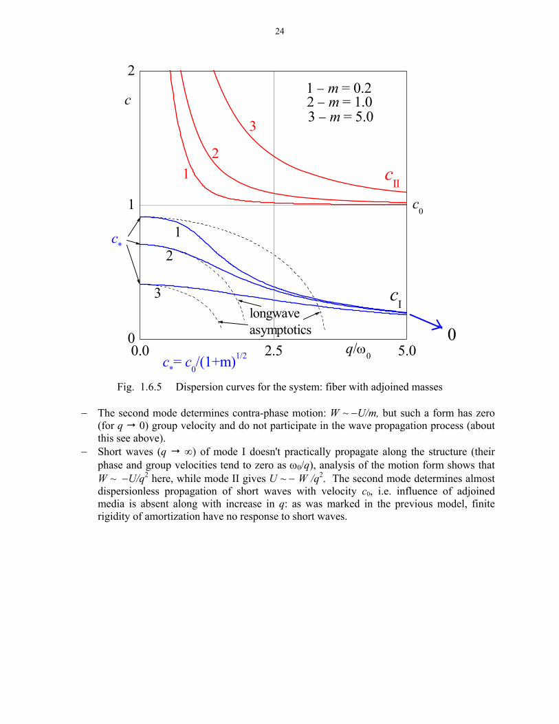
24

0.0 2.5 5.00

1

2

0

c0

longwave asymptotics

3 − m = 5.02 − m = 1.0

12

3

cII

1 − m = 0.2

3

21c*

q/ω0c*= c0/(1+m)1/2

cI

c

Fig. 1.6.5 Dispersion curves for the system: fiber with adjoined masses

− The second mode determines contra-phase motion: W ~ −U/m, but such a form has zero

(for q 0) group velocity and do not participate in the wave propagation process (about this see above).

− Short waves (q ∞) of mode I doesn't practically propagate along the structure (their phase and group velocities tend to zero as ω0/q), analysis of the motion form shows that W ~ −U/q2 here, while mode II gives U ~ − W /q2. The second mode determines almost dispersionless propagation of short waves with velocity c0, i.e. influence of adjoined media is absent along with increase in q: as was marked in the previous model, finite rigidity of amortization have no response to short waves.

- 25 -

2 1D steady and transient waves in dispersion waveguides

2.1 Mathematical models of mass-spring waveguides. Dispersion analysis.

2.1.1 Simple mass-spring chain (MSC). We begin the analysis of discrete-structure waveguides with the simplest model: mass-spring chain (MSC), Fig. 2.1.1, – massive particles linked by inertionless springs.

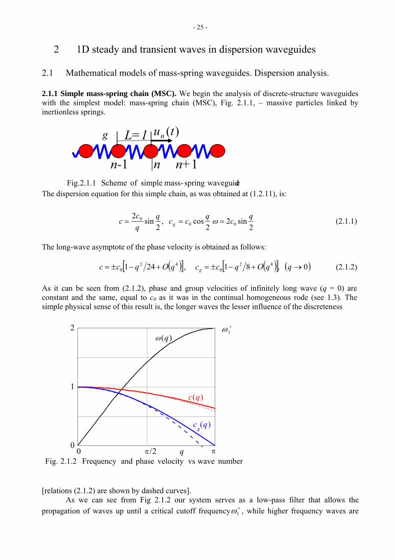
The dispersion equation for this simple chain, as was obtained at (1.2.11), is:

2

cos ,2

sin2

00 qccq

qc

c g ==2

sin2 0qc=ω (2.1.1)

The long-wave asymptote of the phase velocity is obtained as follows:

( )[ ] ( )[ ] ( ) 0 ,81 , 241 420

420 →+−±=+−±= qqOqccqOqcc g (2.1.2)

As it can be seen from (2.1.2), phase and group velocities of infinitely long wave (q = 0) are constant and the same, equal to c0 as it was in the continual homogeneous rode (see 1.3). The simple physical sense of this result is, the longer waves the lesser influence of the discreteness

[relations (2.1.2) are shown by dashed curves]. As we can see from Fig 2.1.2 our system serves as a low-pass filter that allows the propagation of waves up until a critical cutoff frequency , while higher frequency waves are +

1ω

0.0

0

1

2

cg(q)

π/2 π0 q

ω(q)+

1ω

number wavevs velocity phase andFrequency 2.1.2 Fig.

)(tung L=1

n-1 n n+1 e waveguidspring-mass simple of Scheme 2.1.1 Fig.

c(q)

- 26 -

fi out. We denote −iω and +

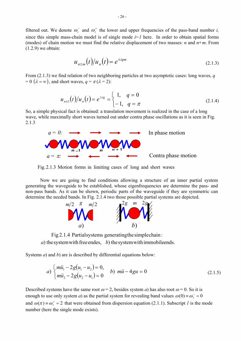
iω the lower and upper frequencies of the pass-band number i, since this simple mass-chain model is of single mode i=1 re. In order to obtain spatial forms (modes) of chain motion we must find the relative displacement of two masses: n and n+m. From (1.2.9) we obtain:

ltered he

( ) ( ) iqm±nm etut± = (2.1.3)

From (2.1.3) we find relation of two neighboring pa 0

nu

rticles at two asymptotic cases: long waves, q ( )∞=λ= , and short waves, q = π (λ = 2):

( ) ( )⎩⎨⎧±iq

=−=

==± πqq

etutu nn ,10 ,1

1 (2.1.4)

So, a simple physical fact is obtained: a translation moveme realized in the caswave, while maximally short waves turned out under contra

Now we are going to find conditions allowing a structure of an inner partial system ting the waveguide to be established, whose eigenfrequencies are determine the pass- and

non-pa

Systems a) and b) are is described by differential equations below:

02 122⎩ =−− uugum && (2.1.5)

Described systems have the same root ω = 2, besides system anough to use only system a) as the partial system for revealing band values

ode

nt is e of a long phase oscillations as it is seen in Fig.

2.1.3

q = 0: In phase motion

n + 1nn –1

generass bands. As it can be shown, periodic parts of the waveguide if they are symmetric can

determine the needed bands. In Fig. 2.1.4 two those possible partial systems are depicted.

( )04 )

,02 ) 211 =−⎨⎧ =−−

guumbuugum

a &&&&

( )

) has also root ω = 0. So it is e 0)0( 1 =≡ −ωω and 2)( 1 =≡ +ωπω that were obtained from dispersion equation (2.1.1). Subscript 1 is the mnumber (here the single mode exists).

esshort wav and long of cases limitingin formsMotion 2.1.3 Fig.

q = π: Contra phase motion

2m 2mg

)a

m g2g2

)b:chain simple thegenerating systems Partial 2.1.4 Fig

ends. immobile with system the) endes, free with system the) ba

- 27 -

2.1.2 Two mode mass-spring waveg

odel are two masses, m and m , connected by two springs of rigiditiesuide (Burn’s chain). Inside the period formatting this

1 2 g1 and g2, as is shown in

s it ca be seen from the chain structure, the length unit is determined by the chain .g. by he distance between two same masses. The system of homogenous equations used

elow f

mFig. 2.1.5

1 1 1g

nu nv 1+nu1−nv1−nu

1

m 2m1m 2m

1mg 2g 2g

L =

chain Borns 2.1.5 Fig

A neriod, e tp

b or the analysis of dispersion properties of the waveguide is:

( ) 0)( 1211

( ) 0)=++

1212 =−+−+ +nnnnn ugugm v(vv&& (2.1.6)

steady-state solution of the problem (2.1.6like to representation (1.2.9):

−nnnnn ugugum v-v-&&

We seek the ) by the form of a traveling wave

( ) ( )tqntiqnti

n Ueu −−= ωωn Ve= , v (2.1.7)

The obtained dispersion equation is:

( ) 02

sin4 2

21

21221

21

214 ⎜⎛ +

−mmω =++⎟⎟

⎠

⎞⎜⎝

qmmgggg

mmω (2.1.8)

Its roots are:

)( ,2

sin165.0 2121

212

21

2122 ggmmmmq

mmgg

+⎟⎟⎠

⎞⎜⎜⎝

⎛ +=⎟

⎟⎠

⎞⎜⎜⎝

⎛−±= βββω (2.1.9)

For each wave number q we get two frequencies ω, so dispersion curve ω(q) has two

ranches – first and second oscillation modes (known as the acoustical and optical branches) that escrib

21 ,0 0q , (2.1.10)

bd es all possible positional relationship (including phase and contra phase motions) of oscillating masses in the wave propagation process. In the limiting cases, q = 0 and q = π, we have:

−− βωω ==⇒=

⎟⎟⎠

⎞⎜⎜⎛1

⎝−+=⎟

⎟⎠

⎞⎜⎜⎝

⎛−−=⇒= ++

21

2122

21

2121 16

2 ,16

21

mmgg

mmggq ββωββωπ . (2.1.11)

- 28 -

0.0 31.5 63.00

1

2

c*= 0.51/2

m = 3, g = 1

c2

c1

π/2 q π

c

0.0 31.5 63.00

1

2

c*= 1.51/2

m = 1, g = 3

c2

c1

π/2 q π

c

0.0 31.5 63.00

1

2

m = 3, g = 3

c*= 0.751/2

c1

c2

c

π/2 q π

chain sBorn'for modes second andFirst 2.1.7 Fig. )( = qcc

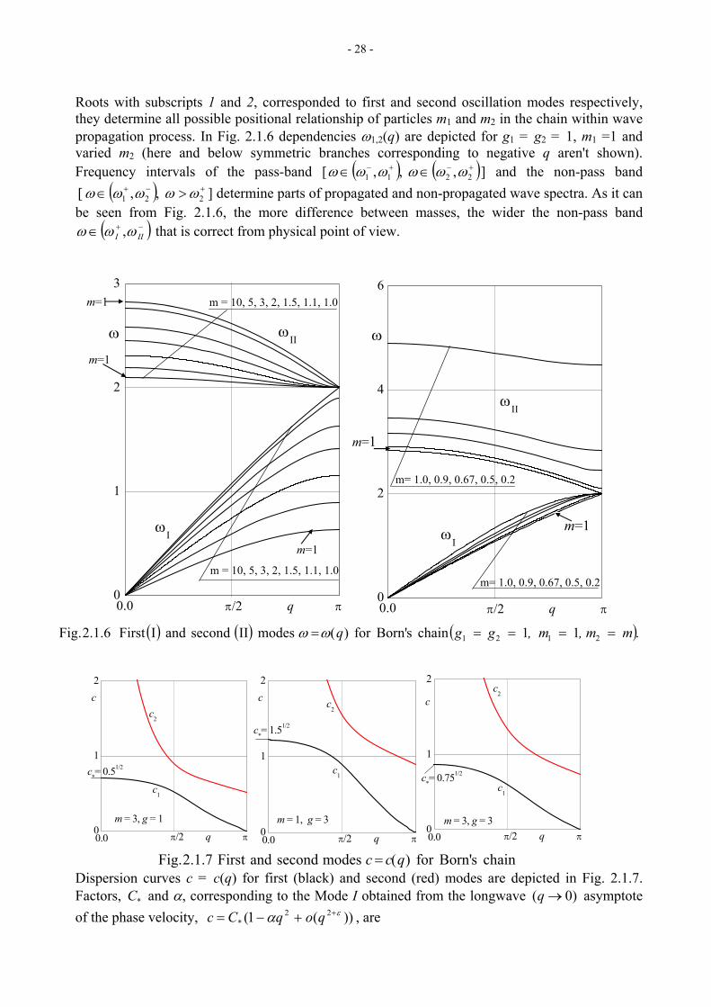
Roots with subscripts 1 and 2, corresponded to first and second oscillation modes respectively, they determine all possible positional relationship of particles m1 and m2 in the chain within wave

ropagation process. In Fig. 2.1.6 dependencies ω1,2(q) are depicted for g1 = g2 = 1, m1 =1 and pvaried m2 (here and below symmetric branches corresponding to negative q aren't shown). Frequency intervals of the pass-band [ ( ) ( )+−+− ∈∈ 2211 , ,, ωωωωωω ] and the non-pass band [ ( ) +−+ >∈ 221 ,, ωωωωω ] determine parts of propagated and non-propagated wave spectra. As it can be seen from Fig. 2.1.6, the more difference between ma ses, the wider the non-pass band s

( )−+∈ ωωω , that is correct from physical po

III int of view.

Dispersion curves c = c(q) for first (black) and second (red) modes are depicted in Fig. 2.1.7. actors, and α, corresponding to the Mode I obtained from the longwave asymptote

of the phase velocity, , are F *C )0( →q

))(1( 22*

εα ++−= qoqCc

0.00

1

2

3 6m = 10, 5, 3, 2, 1.5, 1.1, 1.0

m = 10, 5, 3, 2, 1.5, 1.1, 1.0

ωII

ωI

ω

π/2 q π 0.00

2

4

m= 1.0, 0.9, 0.67, 0.5, 0.2

m=1

m= 1.0, 0.9, 0.67, 0.5, 0.2

ωII

ωI

ω

π/2 q π

m=1

m=1 m=1

m=1

( ) ( ) ( ).11chain sBorn'for modes II second and IFirst 2.1.6Fig 2121 m , m , m g gq . ==== )( = ω ω

- 29 -

βα 1

2*21

*CggC ==212

,))(( 2121 ggmm

+++

(2.1.12)

As it is shown below in Subsection 2.3, long-wave asymptote factors a

needed for description of the transient solution within the long-wave spectrum. Besides, by these factors, an identity of different waveguides can be established with respect to their wave passing facilitie

*C nd α are

s. Let us explore oscillation forms of the system: relations of oscillating magnitudes of different masses, and dependences of magnitudes on the wavelength (or, that is the same, on wavenumber q). This analysis allows main physical peculiarities of the oscillation process to be

vealedre . Amplitude ratio of masses displacement within the same cell is:

2221

21

21

2121

ωω

mggegg

eggmgg

UV iq

iq −++

=+

−+= − (2.1.13)

It is of interest to built forms for two limiting cases: infinitely long waves, ( )∞== λ 0q , and

a ( )2 == λπqmaxim lly short waves, . t case of long waves, . 0→q(1) The firs

(1.1) for Mode I ( 0=−Iω ) we have: UV = , e.g. in this limiting case the t rm of

motion is realized lranslation fo

ikely to the case of the simple chain waveguide (remind, that the simple

e optichain has a single mode).

(1.2) for Mode II, th cal branch ( ), gives 12 UmVmβω =−II −= . So there are long-wave high

frequency contra-phase oscillation process, in which particle magnitudes are inversely proportional to masses.

π=q . (2) The second case: short waves, We seek forms for a particular case g

oscillation 1 = g2 = g to maximally simplify results and their physical interpretation. First, we get

frequencies of first and second modes. In this case Eqn. (2.1.9) is simplified to the following one:

( ) 042 22214 =+

+−

gmmg ωω (2.1.14) 2121 mmmm

with t

2g wo roots for ω 2: 1m and 22 mg . Let m1 > m2. Tbranch is

hen the frequency of lower (acoustical)

12 mgI =ω while the upper (optical) branch has 22 mgII =ω . Substitution of ωI and ω into Eqn. (2.1.14) results in the following oscillation forms: II

( ) 02

1

=−= mmm

gU − Mode I, ,21 V ( ) 0 ,212

2

=−= Ummm

gV − Mode II.

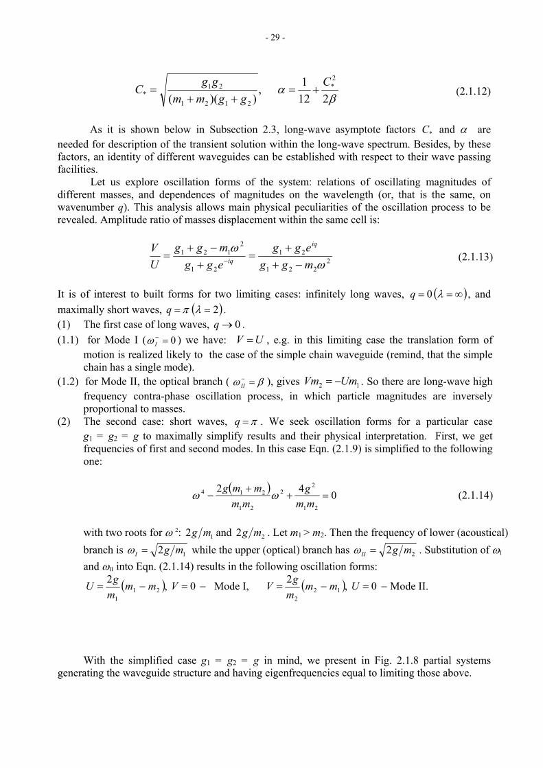
With the simplified case g1 = g2 = g in mind, we present in Fig. 2.1.8 partial systems

generating the waveguide structure and having eigenfrequencies equal to limiting those above.

- 30 -

Eigenfrequencies of system a) are ω = 0 and ω = β, of systems b) and c) − ωI and ωII. g that was said above on oscillating forms within modes I and II the following

conclusions can be done:

1

aller magn

more mass h

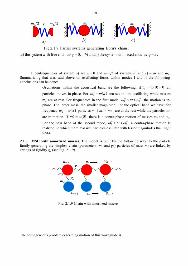
2.1.3 MSC family generating the simplest chain (parameters: m1 and g1) particles of mass m2 are linked by springs of rigidity g2 (see Fig. 2.1.9).

he homogeneous problem describing motion of this waveguide is:

Summarizin

Oscillations within the acoustical band are the following: if 0)0(1 ==− ωω all

particles moves in-phase. For )(πωω =+ masses m are oscillating while masses 1

m2 are at rest. For frequencies in the first mode, +− << 11 ωωω , the m in-phase. The larger mass, the sm itude. For the optical band we have: for frequency )(2 πωω =− particles m

otion is

1 ( m1 > m2 ) are at the rest while the particles m2

are in motion. If )0(2 ωω =+ , there is a contra-phase motion of masses m1 and m2.

For the pass band of the second mode, +− < 22 ωωω , a contra-phase motion is realized, in which ive particles oscillate with lesser magnitudes t an light those.

with amortized masses. The model is built by the following way: to the particle

<

T

m2

m1

g1

g2

vn vn+1 vn+1

un-1

Fig. 2.1.9 Chain with amortized masses

un un+1

:chain sBorn' generating systems Partial 2.1.8 Fig. ends fixed with system the) and ) 0, ends free with system the) π=⇒=⇒ qcbqa

21m g

)a

22m gg

)b

1m gg

)c

2m

- 31 -

⎩⎨⎧

=−++− 0)()()( 211111 nnnnnnn uguuguugum v&& =−+−+−+

0)(22 nnn ugm vv&& (2.1.17)

Dispersion equation is obtained as follows:

02

sin42

s4 12

214⎜⎜ +⎟⎟

⎞⎜⎜⎛ +

−mg

gmmmm

ω in 2

21

2122

121

=+⎟⎟⎠

⎞

⎝

⎛

⎠⎝

qmmggq

ω (2.1.18)

Its ro

ots,

,2

sin1621 2

21

21222,1 ⎟⎟

⎠

⎞⎜⎜⎝

⎛−±=

qmmggββω ,

2sin4 2

1

12

21

21 qmgg

mmmm

+⎟⎟⎠

⎞⎜⎜⎝

⎛ +=β (2.1.19)

result in the following band frequencies:

(2.1.20)

A set of dispersion pictures calculated from Eqn. (2.1.18) is shown in Fig. 2.1.9 (acoustical and

respectively) and Fig. 2.1.10 where the losymptote of phase velocity is depicted by shaded curves. Factors of the asymptote are:

( )

optical branches depicted by blue and red lines ng-wave a

2212

22

Group velocity obtained from dispersion equation (2.1.18) i

1

21

12* )(224

1 mmg

mgmm

gC+

+=+

= α (2.1.21)

s:

2cos122

2sin0C

C =∂

= mω

q

q

qg

±∂

(2.1.22)

Unlike Born’s chain where the group velocity of the second mode is negative, here it is positive for both modes, acoustical and optical as well.

⎟⎟⎠

⎞⎜⎜⎝

⎛−+=⎟

⎟⎠

⎞⎜⎜⎝

⎛−−=⇒= ++

21

21222

21

21221 165.0 ,165.0

mmgg

mmggq ββωββωπ

21

212

mmmmg

21 ,00q +==⇒= −− ωω

- 32 -

Let us describe partial systems corresponding to long and short waves. In Fig.2.1.11 such a system for the case of long waves . )0( →q

Equations of motion for one cell with free ends are:

⎩⎨⎧

=−+=−+

0)(0)(

22

21

uvgvmvugum

&&

&&

results in the dispersion equation:

, (2.1.23) 0)( 2212

421 =+− ωω mmgmm

Fig 2.1.11 Partial system corresponding to the long wave case

u g1 m1 /2

m2 /2

v

g2

0 1 2 30.0

0.5

1.0

m1=m2=g1=g2=1

c(q)

q

c1(q) c

1(q) asymptotic

c2(q)

0 1 2 30.0

0.5

1.0

m1=m2=g1=1g2=0.1

c(q)

q

c1(q) c1(q) asymptotic c2(q)

masses amortizedMSK with for modes second andFirst 2.1.10 Fig )( = qcc0 1 2 3

0.0

0.5

1.0

Non-pass band

m1=m2=g1=1g2=0.1

c(q)

q

c1(q) c1(q) asymptotic c2(q)

0 1 2 30

1

2 ω 2

+

ω 2-

ω 1+

ω (q)

q0 1 2 3

0

1

2

3

0 1 2 30

1

2

3

4

5

6

ω2+

-

ω1+

ω(q)

q

ω 2+

ω 2-

ω 1+

Non-pass band

m1=m2=g1=1; g2=10

ω (q)

q

q qq

ωω

ω+2ω

+2ω

+2ω

−2ω

+1ω

+1ω

+1ω

masses amortizedMSK with for modes second andFirst 2.1.9 Fig )

Non-pass m =m =

( = qωω

−2ω

Non-pass

Non-pass band Non-pass ban

g = g =1

d

1 2 1 2

−2ω

m1=m2=g1=1;

Non-pass

- 33 -

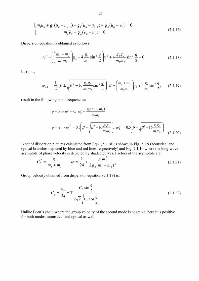
which roots are equal to limiting frequencies obtained in (2.1.20) as solutions of dispersion equation if q = 0. The partial system depicted in Fig. 2.1.12 can be served to determine the band frequencies corresponding to short waves

−−21 ,ωω

)( π→q .

12g

On the left and on the right of the particle m1 half of the spring g1 is rigidly fixed, so their rigidities are equal to 2g1. The cell also contains the particle of mass m2 (blue) adjoined in parallel to the waveguide (red) by the spring of rigidity g2. The equations of cell motion

⎩⎨⎧

=−+=−+−

0)(0)(4

22

211

nnn

nnnn

UVgvmVUgUgum

&&

&&,

result in the dispersion equation:

044)(

21

212

1

1

21

2124 =+⎟⎟⎠

⎞⎜⎜⎝

⎛+

+−

mmgg

mg

mmmmg

ωω (2.1.24)

Its roots are the limiting frequencies obtained in (2.1.20). ++

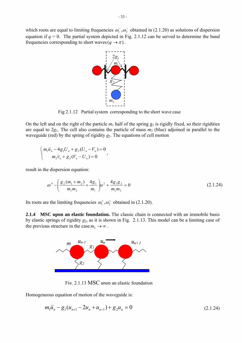
21 ,ωω 2.1.4 MSC upon an elastic foundation. The classic chain is connected with an immobile basis by elastic springs of rigidity g2, as it is shown in Fig. 2.1.13. This model can be a limiting case of the previous structure in the case ∞→2m .

2g

1m

2m

case short wave the toingcorrespond system Partial 2.1.12

un+1

Fig

Homogeneous equation of motion of the waveguide is:

0)2( 21111 =++−− −+ nnnnn uguuugum && (2.1.24)

un un-1 m g1

g2

Fig. 2.1.13 MSC upon an elastic foundation

- 34 -

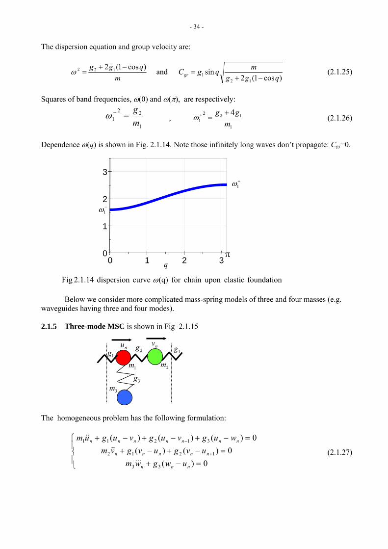
The dispersion equation and group velocity are:

mqgg )cos1(2 122 −+

=ω and )cos1(2

sin12

1 qggmqgCgr −+

= (2.1.25)

Squares of band frequencies, ω(0) and ω(π), are respectively:

1

221 m

g=−ω ,

1

1221

4m

gg +=+ω (2.1.26)

Dependence ω(q) is shown in Fig. 2.1.14. Note those infinitely long waves don’t propagate: Cgr=0.

0 1 2 30

1

2

3

Fig Below we consider more complicated mass-spring models of three and four masses (e.g. waveguides having three and four modes).

2.1.5 Three-mode MSC is shown in Fig 2.1.15 The homogeneous problem has the following formulation:

⎪⎩

⎪⎨

⎧

=−+=−+−+

=−+−+−+

+

−

0)(0)()(

0)()()(

33

1212

31211

nnn

nnnnn

nnnnnnn

uwgwmuvguvgvm

wugvugvugum

&&&

t&&

(2.1.27)

foundation elasticupon chain for (q) curve dispersion 2.1.14 ω

π

+1ω

q

−1ω

n2g

1gv

1m 2m

3m

1g

3g

nu

- 35 -

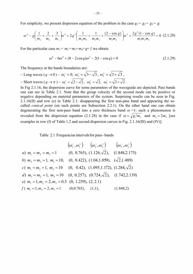
For simplicity, we present dispersion equation of the problem in the case g1 = g2 = g3 = g:

0)cos1(2)cos2(112321

321

32

213132

24

123

6 =−

+⎟⎟⎠

⎞⎜⎜⎝

⎛ −+++⎟⎟

⎠

⎞⎜⎜⎝

⎛++−

mmmqg

mmq

mmmmg

mmmg ωωω (2.1.28)

For the particular case m1 = m2 =m3=m4=g=1 we obtain:

0)cos1(2)cos28(6 246 =−−−+− qq ωωω (2.1.29) The frequency at the bands boundaries are:

− Long waves ( ) − 0→q 33 ,33 ,0 321 +=−== +−− ωωω ,

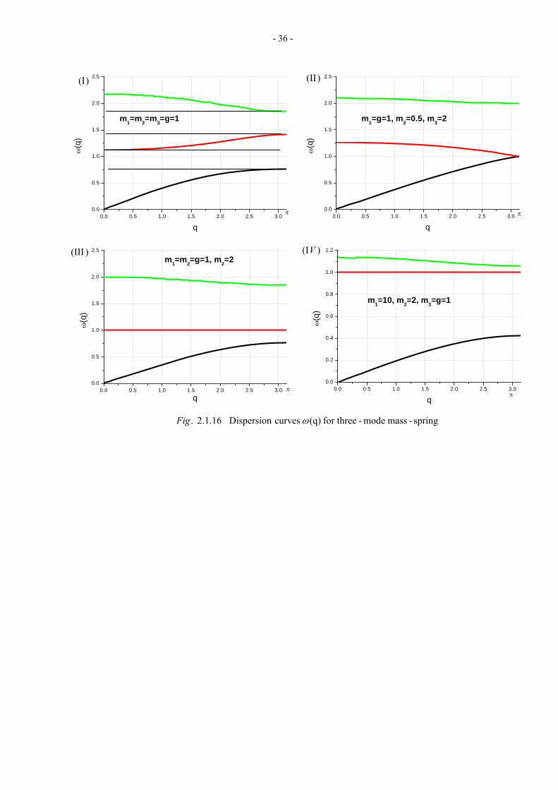
− Short waves ( π→q ) − 22 ,2 ,22 321 +==−= −++ ωωω . In Fig 2.1.16, the dispersion curve for some parameters of the waveguide are depicted. Pass bands one can see in Table 2.1. Note that the group velocity of the second mode can be positive or negative depending on material parameters of the system. Surprising results can be seen in Fig. 2.1.16(II) and row (e) in Table 2.1: disappearing the first non-pass band and appearing the so-called conical point (on such points see Subsection 2.2.1). On the other hand one can obtain degenerating the first non-pass band into a zero thickness band ω =1: such a phenomenon is revealed from the dispersion equation (2.1.28) in the case if 3mg=ω and [see examples in row (f) of Table 1.2 and second dispersion curves in Fig. 2.1.16(III) and (IV)].

32 2mm =

bands-passfor intervals sFrequencie 2.1 Table

( ) ( ) ( )

2.1) ,2( 1.259), (0, 5.0,2,1 ))139.2,742.1( ),2(0.724, 0.257), (0, 10 ,1 )

)2,284.1( ),72(1.095,1.1 0.42), (0, 10 ,1 )

)489.1,2( ),9(1.04,1.05 0.422), (0, ,10 ,1 )

)175.2,848.1( ),2(1.126, 0.765), (0, 1 )

, , ,

321

321

231

132

321

332211

======

===

===

===

+−+−+−

mmmemmmd

mmmc

mmmb

mmma

ωωωωωω

(1.848,2) (1,1), (0,0.765), 1 ,2 ,1 ) 321 === mmmf

- 36 -

0.0 0.5 1.0 1.5 2.0 2.5 3.00.0

0.5

1.0

1.5

2.0

2.5

m1=g=1, m2=0.5, m3=2

π

ω(q

)

q0.0 0.5 1.0 1.5 2.0 2.5 3.0

0.0

0.5

1.0

1.5

2.0

2.5

m1=m2=m3=g=1

π

ω(q

)

q

0.0 0.5 1.0 1.5 2.0 2.5 3.00.0

0.5

1.0

1.5

2.0

2.5

m1=m2=g=1, m2=2

π

ω(q

)

q0.0 0.5 1.0 1.5 2.0 2.5 3.0

0.0

0.2

0.4

0.6

0.8

1.0

1.2

m1=10, m2=2, m3=g=1

π

ω(q

)

q

spring-mass mode-for three (q) curves Dispersion 2.1.16 . ωFig

)(Ι

)(ΙΙΙ )( V

)(ΙΙ

Ι

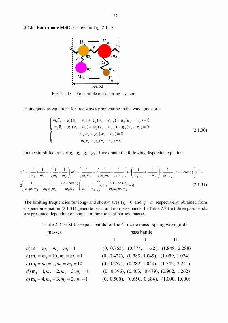
- 37 -

2.1.6 Four-mode MSC is shown in Fig 2.1.18

0)cos1(211)cos2(112

)cos27(1113112111311

4321

2

4321431432

4

214132314243

6

2143

8

=−

+⎟⎟⎠

⎞⎜⎜⎝

⎛⎟⎟⎠

⎞⎜⎜⎝

⎛+

−++

−⎟⎟⎠

⎞⎜⎜⎝

⎛−+⎟⎟

⎠

⎞⎜⎜⎝

⎛++⎟⎟

⎠

⎞⎜⎜⎝

⎛+++⎟

⎟⎠

⎞⎜⎜⎝

⎛⎟⎟⎠

⎞⎜⎜⎝

⎛+++−

mmmmq

mmmmq

mmmmmm

qmmmmmmmmmmmmmmmm

ω

ωωω

Homogeneous equations for free waves propagating in the waveguide are:

⎪⎪⎩

⎪⎪⎨

⎧

=−+=−+

=−+−+−+=−+−+−+

+

−

0)(0)(

0)()()(0)()()(

44

33

41212

31211

nnn

nnn

nnnnnnn

nnnnnnn

vrgrmuwgwm

rvguvguvgvmwugvugvugum

&&

&&&

t&&

(2.1.30)

In the simplified case of g1=g2=g3 =g4=1 we obtain the following dispersion equation:

(2.1.31)

The limiting frequencies for long- and short-waves ( 0=q and π=q respectively) obtained from dispersion equation (2.1.31) generate pass- and non-pass bands. In Table 2.2 first three pass bands are presented depending on some combinations of particle masses.

1.000) (1.000, 0.684), (0.650, 0.500), (0, 1,2,3,4m )1.262) (0.962, 0.479), (0.463, 0.396), (0, 4,3,2,1m )2.241) (1.742, 1.049), (0.282, 0.257), (0, 10, 1m )1.074) (1.059, 1.049), (0.589, 0.422), (0, 1, 10m )

)288.2 ,848.1( ),2 (0.874, 0.765), (0, 1m )

III II I bands pass masses

waveguidespring-mass mode-4 for the bands pass eFirst thre 2.2 Table

4321

4321

4321

4321

4321

========

========

====

mmmemmmd

mmmcmmmb

mmma

m2

m4

1g 2g

3g4g

nu nv

nwnr

2g

m1

m3

period Fig. 2.1.18 Four-mode mass-spring system

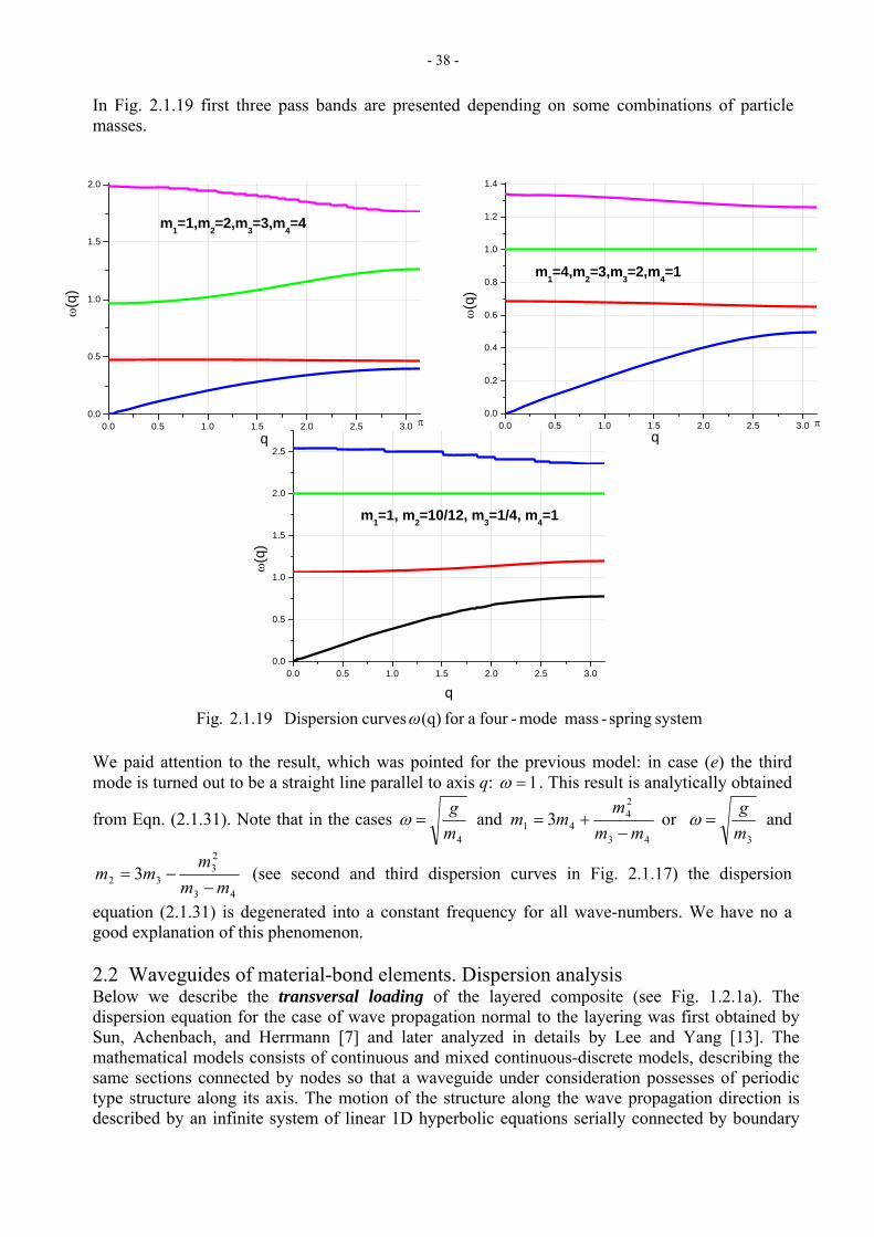
- 38 -

In Fig. 2.1.19 first three pass bands are presented depending on some combinations of particle masses.

We paid attention to the result, which was pointed for the previous model: in case (e) the third mode is turned out to be a straight line parallel to axis q: 1=ω . This result is analytically obtained

from Eqn. (2.1.31). Note that in the cases 4m

g=ω and

43

24

41 3mm

mmm

−+= or

3mg

=ω and

43

23

32 3mm

mmm

−−= (see second and third dispersion curves in Fig. 2.1.17) the dispersion

equation (2.1.31) is degenerated into a constant frequency for all wave-numbers. We have no a good explanation of this phenomenon. 2.2 Waveguides of material-bond elements. Dispersion analysis Below we describe the transversal loading of the layered composite (see Fig. 1.2.1a). The dispersion equation for the case of wave propagation normal to the layering was first obtained by Sun, Achenbach, and Herrmann [7] and later analyzed in details by Lee and Yang [13]. The mathematical models consists of continuous and mixed continuous-discrete models, describing the same sections connected by nodes so that a waveguide under consideration possesses of periodic type structure along its axis. The motion of the structure along the wave propagation direction is described by an infinite system of linear 1D hyperbolic equations serially connected by boundary

0.0 0.5 1.0 1.5 2.0 2.5 3.00.0

0.2

0.4

0.6

0.8

1.0

1.2

1.4

0.0 0.5 1.0 1.5 2.0 2.5 3.00.0

0.5

1.0

1.5

2.0

m1=4,m2=3,m3=2,m4=1

π

ω(q

)

qπ

m1=1,m2=2,m3=3,m4=4

ω(q

)

q

system spring-mass mode-four afor (q) curves Dispersion 2.1.19 .Fig

0.0 0.5 1.0 1.5 2.0 2.5 3.00.0

0.5

1.0

1.5

2.0

2.5

m1=1, m2=10/12, m3=1/4, m4=1

ω(q

)

q

ω

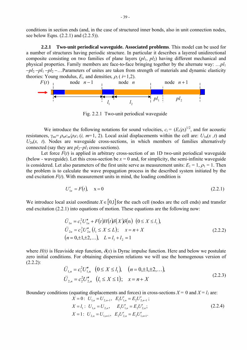
- 39 -

conditions in section ends (and, in the case of structured inner bonds, also in unit connection nodes, see below Eqns. (2.2.1) and (2.2.5)).

2.2.1 Two-unit periodical waveguide. Associated problems. This model can be used for a number of structures having periodic structure. In particular it describes a layered unidirectional composite consisting on two families of plane layers (pl1, pl2) having different mechanical and physical properties. Family members are face-to-face bringing together by the alternate way: …pl1

−pl2 −pl1 −pl2 −…Parameters of unites are taken from strength of materials and dynamic elasticity theories: Young modulus, Ei, and densities, ρi ( i=1,2).

1l 2l

Fig. 2.2.1 Two-unit periodical waveguide

1 node −n n node 1 node +n)(tF

2pl1pl

1/2= (E /ρWe introduce the following notations for sound velocities, c )i i i , and for acoustic resistances, γmi= ρmcm/ρ c (i, m=1, 2). Local axial displacements within the cell are: Ui i 1n(x ,t) and U2n(x, t). Nodes are waveguide cross-sections, in which members of families alternatively connected (say they are pl2−pl1 cross-sections). Let force F(t) is applied in arbitrary cross-section of an 1D two-unit periodical waveguide (below - waveguide). Let this cross-section be x = 0 and, for simplicity, the semi-infinite waveguide is considered. Let also parameters of the first unite serve as measurement units: E = 1, ρ1 1 = 1. Then the problem is to calculate the wave propagation process in the described system initiated by the end excitation F(t). With measurement units in mind, the loading condition is

(2.2.1) ( ) 0 x ,1 ==′ tFU n

[ ]1,0∈XWe introduce local axial coordinate for the each cell (nodes are the cell ends) and transfer

end excitation (2.2.1) into equations of motion. These equations are the following now:

( ) ( ) ( ) ( ) ( )( )

( ) 1 ,,2,1,0 ;

,0 n

21

12222

11211

=+=±±=+=≤≤′′=

≤≤+′′=

llLnXnxLXlUcU

lXXtHtFUcU

nn

nn

K

&&

&& δδ

(2.2.2)

where H(t) is Heaviside step function, δ(x) is Dyrac impulse function. Here and below we postulate zero initial conditions. For obtaining dispersion relations we will use the homogenous version of (2.2.2):

( ) ( )( ) XnxXlUcU

nlXUcU

nn

n

+=≤≤′′=

±±=≤≤′′=

; 1

,,2,1,0 ,0

1,222,2

1n1,21,1

&&

K&&

(2.2.3)

Boundary conditions (equating displacements and forces) in cross-sections X = 0 and X = l1 are:

. , :1; , :; , :0

1,12,221,1,2

,22,11,2,11

1,22,111,2,1

++

−−

′=′==

′=′==

′=′==

nnnn

nnnn

nnnn

UEUEUUXUEUEUUlX

UEUEUUX (2.2.4)

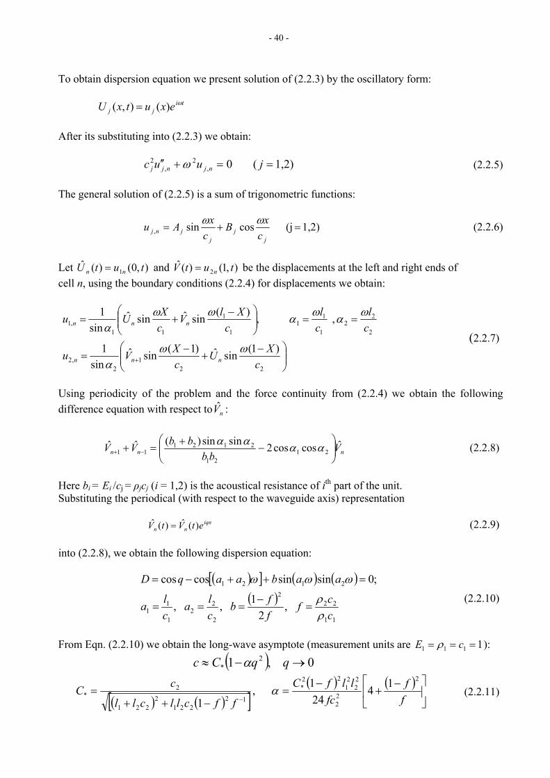
- 40 -

To obtain dispersion equation we present solution of (2.2.3) by the oscillatory form: ti

jj exutxU ω)(),( = After its substituting into (2.2.3) we obtain:

(2.2.5) 1,2)( 0,2

,2 ==+′′ juuc njnjj ω

The general solution of (2.2.5) is a sum of trigonometric functions:

1,2)(j cossin, =+=j

jj

jnj cxB

cxAu ωω (2.2.6)

Let and be the displacements at the left and right ends of ),0()(ˆ

1 tutU nn = ),1()(ˆ2 tutV n=

cell n, using the boundary conditions (2.2.4) for displacements we obtain:

)1(sinˆ)1(sinˆsin

1

, ,)(sinˆsinˆsin

1

221

2,2

2

22

1

11

1

1

11,1

⎟⎟⎠

⎞⎜⎜⎝

⎛ −+

−=

==⎟⎟⎠

⎞⎜⎜⎝

⎛ −+=

+ cXU

cXVu

cl

cl

cXlV

cXUu

nnn

nnn

ωωα

ωαωαωωα

(2.2.7)

Using periodicity of the problem and the force continuity from (2.2.4) we obtain the following difference equation with respect to : nV

ˆcoscos2sinsin)(ˆˆ21

21

212111 nnn V

bbbbVV ⎟⎟

⎠

⎞⎜⎜⎝

⎛−

+=+ −+ αααα (2.2.8)

Here bi = Ei /cj = ρjc (i = 1,2) is the acoustical resistance of ith part of the unit. jSubstituting the periodical (with respect to the waveguide axis) representation

(2.2.9) iqnnn etVtV )(ˆ)(ˆ =

into (2.2.8), we obtain the following dispersion equation:

( )[ ] ( ) ( )( )

11

222

2

22

1

11

2121

,2

1 , ,

;0sinsincoscos

ccf

ffb

cla

cla

aabaaqD

ρρ

ωωω

=−

===

=++−=

(2.2.10)

1111 === cE ρ ): From Eqn. (2.2.10) we obtain the long-wave asymptote (measurement units are

( ) 0 ,1 2* →−≈ qqCc α

( ) ( )[ ]( ) ( )

⎥⎦

⎤⎢⎣

⎡ −+

−=

−++=

− ff

fcllfC

ffcllcll

cC2

22

22

21

22*

12221

2221

2*

1424

1 ,1

α (2.2.11)

- 41 -

Below we present a set of dispersion curves calculated from (2.2.10), but first of all we will

explore partial systems of the waveguide to obtain frequencies of pass and non-pass bands. We are going to design partial systems (PS) generating our waveguide; PS-eigenfrequencies determine boundaries of pass- and non-pass bands. The eigenfrequencies discussed can be found as those for selecting partial systems with fixed and free ends what respectively result in obtaining the frequencies of long (q = 0) and short (q = π) waves. We begin our analysis with the PS depicted in Fig 2.2.2.

In the case of fixed boundaries at the cell ends, it’s enough (due to the symmetry) to consider half of the cell (say the right part of it). Two wave equations for u1 and u2 within two intervals:

0,2

,2

,21 11 ⎟

⎠⎞

⎜⎝⎛−⎟

⎠⎞

⎜⎝⎛ −−

ll describe motion of this PS:

0 ,0 22221

211 =′′−=′′− ucuucu &&&& (2.2.12)

1. Long waves. To obtain frequencies corresponded to the long waves we use

fixed boundary conditions at cell ends (the Dirichlet problem): )0( =q

( ) Ululuuu ˆ22

,00)21( 1

21

121 =⎟⎠⎞

⎜⎝⎛−=⎟

⎠⎞

⎜⎝⎛−==− (2.2.13)

Continuity of forces in contact cross-sections linking the layers results in the boundary condition:

+−=−−= ∂∂

=∂∂

2

22

2

11 11

|| lxlx xuE

xuE (2.2.14)

The most simple (with fast observation in mind) results can be obtained in the particular case: . Then solution of Dirichlet problem, (2.2.12) + (2.2.13) is: 121 == cc

U

21l− 0

x21l

21

−

V

⎟⎠⎞

⎜⎝⎛ +

=2

21 21 ll

waveguideperiodicallayer - two thegenerating systems Partial 2.2.2 Fig.

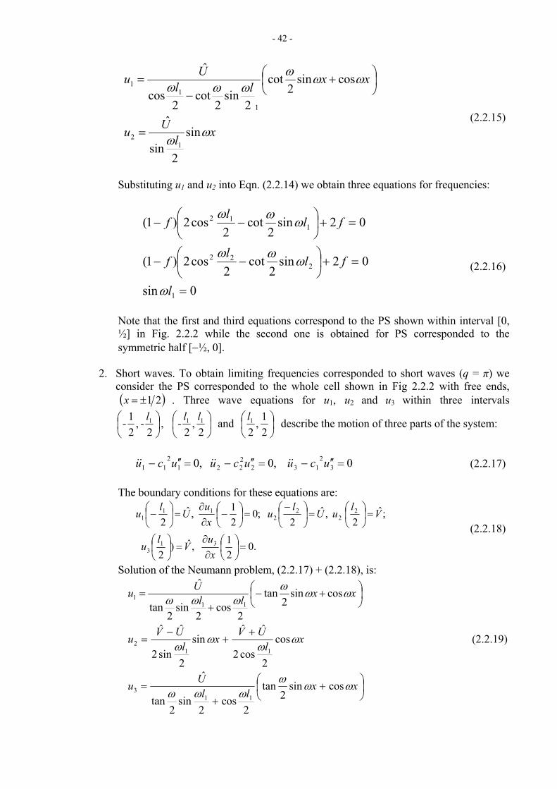
- 42 -

xl

Uu

xxll

Uu

ωω

ωωωωωω

sin

2sin

ˆ

cossin2

cot

2sin

2cot

2cos

ˆ

12

1

11

=

⎟⎠⎞

⎜⎝⎛ +

−=

(2.2.15)

and uSubstituting u into Eqn. (2.2.14) we obtain three equations for frequencies: 1 2

0sin

02sin2

cot2

cos2)1(

02sin2

cot2

cos2)1(

1

222

112

=

=+⎟⎠⎞

⎜⎝⎛ −−

=+⎟⎠⎞

⎜⎝⎛ −−

l

fllf

fll

f

ω

ωωω

ωωω

(2.2.16)

Note that the first and third equations correspond to the PS shown within interval [0, ½] in Fig. 2.2.2 while the second one is obtained for PS corresponded to the symmetric half [−½, 0].

2. Short waves. To obtain limiting frequencies corresponded to short waves (q = π) we

consider the PS corresponded to the whole cell shown in Fig 2.2.2 with free ends, ( 21 ±=x ) . Three wave equations for u1, u uand within three intervals 2 3

, 2

,21 1 ⎟

⎠⎞

⎜⎝⎛ l--

2 ,

2 11 ⎟

⎠⎞

⎜⎝⎛ ll-

21 ,

2 1 ⎟

⎠⎞

⎜⎝⎛ land describe the motion of three parts of the system:

0 ,0 ,0 3

2132

2221

211 =′′−=′′−=′′− ucuucuucu &&&&&& (2.2.17)

The boundary conditions for these equations are:

.021 ,ˆ)

2

;ˆ2

,ˆ2

;021 ,ˆ

2

313

22

22

111

=⎟⎠⎞

⎜⎝⎛

∂∂

=⎟⎠

⎞⎜⎝

⎛

=⎟⎠

⎞⎜⎝

⎛=⎟⎠

⎞⎜⎝

⎛ −=⎟

⎠⎞

⎜⎝⎛−

∂∂

=⎟⎠

⎞⎜⎝

⎛−

xu

Vl

u

Vl

uUl

uxu

Ul

u (2.2.18)

Solution of the Neumann problem, (2.2.17) + (2.2.18), is:

⎟⎠⎞

⎜⎝⎛ +−

+= xxll

Uu ωωωωωω cossin

2tan

2cos

2sin

2tan

ˆ

111

xl

UVxl

UVu ωω

ωω

cos

2cos2

ˆˆsin

2sin2

ˆˆ

112

++

−= (2.2.19)

⎟⎠⎞

⎜⎝⎛ +

+= xx

llUu ωω

ωωωω

cossin2

tan

2cos

2sin

2tan

ˆ

113

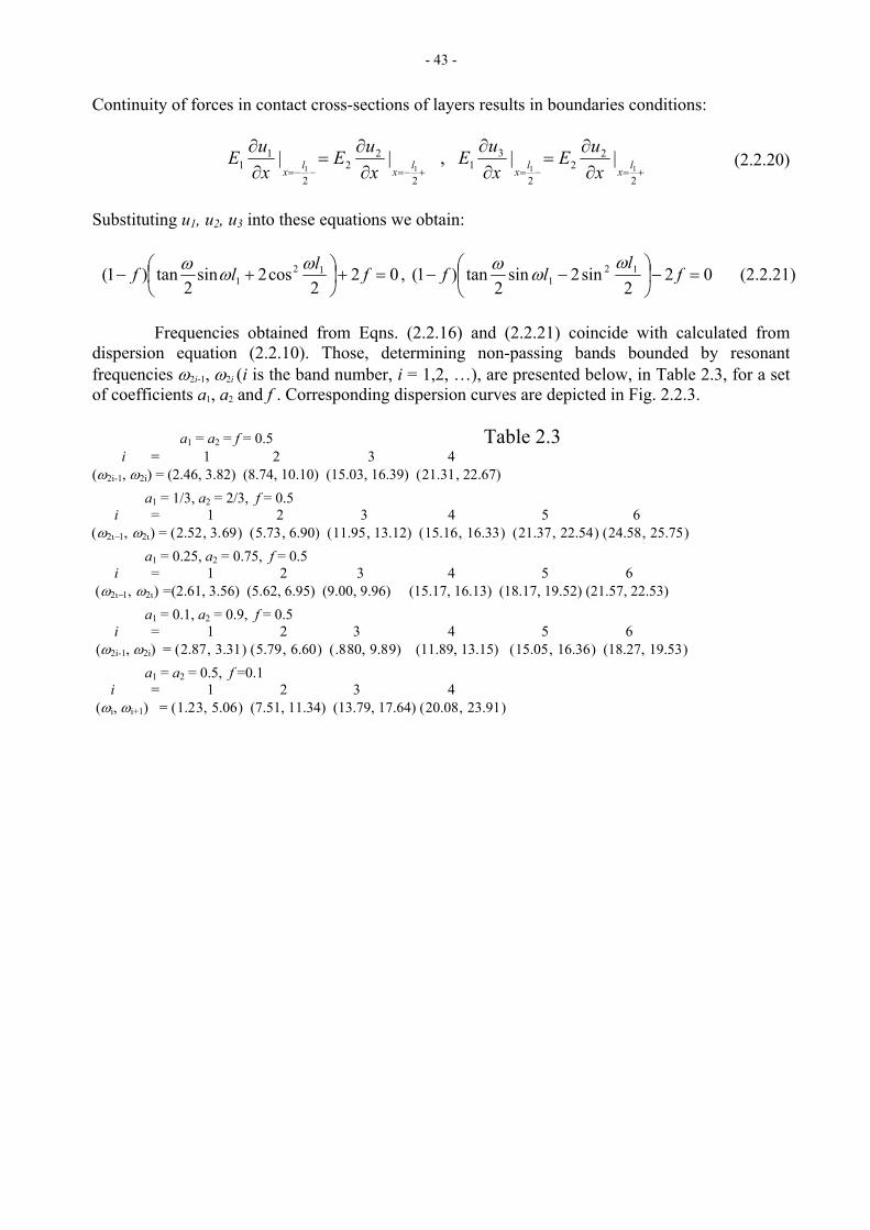
- 43 -

Continuity of forces in contact cross-sections of layers results in boundaries conditions:

+=−=+−=−−= ∂∂

=∂∂

∂∂

=∂∂

2

22

2

31

2

22

2

11 1111

|| , || lxlxlxlx xuE

xuE

xuE

xuE (2.2.20)

, uSubstituting u1 2, u into these equations we obtain: 3

022

sin2sin2

tan)1( 121 =−⎟

⎠

⎞⎜⎝

⎛ −− fl

lfω

ωω022

cos2sin2

tan)1( 121 =+⎟

⎠⎞

⎜⎝⎛ +− fllf ωωω , (2.2.21)

Frequencies obtained from Eqns. (2.2.16) and (2.2.21) coincide with calculated from

dispersion equation (2.2.10). Those, determining non-passing bands bounded by resonant frequencies ω2i-1, ω2i (i is the band number, i = 1,2, …), are presented below, in Table 2.3, for a set of coefficients a1, a2 and f . Corresponding dispersion curves are depicted in Fig. 2.2.3.

a1 = a2 = f = 0.5 Table 2.3 i = 1 2 3 4 (ω2i-1, ω2i) = (2.46, 3.82) (8.74, 10.10) (15.03, 16.39) (21.31, 22.67)

a1 = 1/3, a2 = 2/3, f = 0.5 i = 1 2 3 4 5 6

) = (2.52, 3.69) (5.73, 6.90) (11.95, 13.12) (15.16, 16.33) (21.37, 22.54) (24.58, 25.75 ) (ω , ω2ι−1 2ι

a1 = 0.25, a2 = 0.75, f = 0.5 i = 1 2 3 4 5 6

) =(2.61, 3.56) (5.62, 6.95) (9.00, 9.96) (15.17, 16.13) (18.17, 19.52) (21.57, 22.53) (ω , ω2ι−1 2ι

a1 = 0.1, a2 = 0.9, f = 0.5 i = 1 2 3 4 5 6 (ω2i-1, ω2i) = (2.87, 3.31) (5.79, 6.60) ( 8. 80, 9.89) (11.89, 13.15) (15.05, 16.36) (18.27, 19.53 )

a1 = a2 = 0.5, f =0.1 i = 1 2 3 4 (ωi, ωi+1) = (1.23, 5.06) (7.51, 11.34) (13.79, 17.64) (20.08, 23.91)

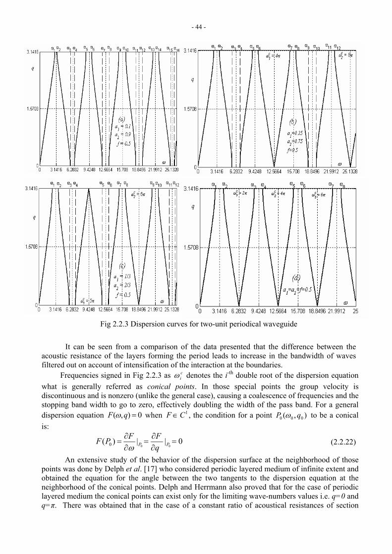
- 44 -

Fig 2.2.3 Dispersion curves for two-unit periodical waveguide

It can be seen from a comparison of the data presented that the difference between the

acoustic resistance of the layers forming the period leads to increase in the bandwidth of waves filtered out on account of intensification of the interaction at the boundaries.

-thFrequencies signed in Fig 2.2.3 as denotes the iciω double root of the dispersion equation

what is generally referred as conical points. In those special points the group velocity is discontinuous and is nonzero (unlike the general case), causing a coalescence of frequencies and the stopping band width to go to zero, effectively doubling the width of the pass band. For a general dispersion equation 0),( =qF ω when , the condition for a point 1CF ∈ ),( 000 qP ω to be a conical is:

0||)(000 =

∂∂

=∂∂

= PP qFFPF

ω (2.2.22)

An extensive study of the behavior of the dispersion surface at the neighborhood of those points was done by Delph et al. [17] who considered periodic layered medium of infinite extent and obtained the equation for the angle between the two tangents to the dispersion equation at the neighborhood of the conical points. Delph and Herrmann also proved that for the case of periodic layered medium the conical points can exist only for the limiting wave-numbers values i.e. q=0 and q=π. There was obtained that in the case of a constant ratio of acoustical resistances of section

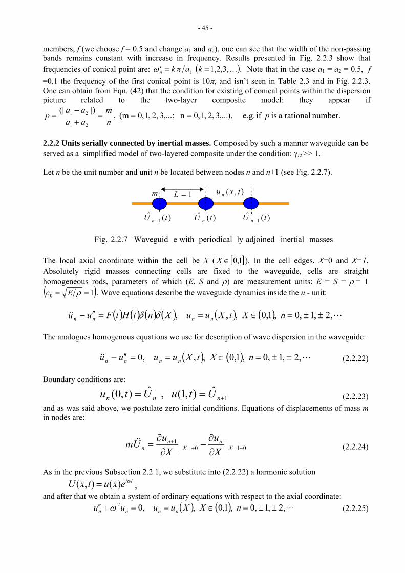
- 45 -

members, f (we choose f = 0.5 and change a and a1 2), one can see that the width of the non-passing bands remains constant with increase in frequency. Results presented in Fig. 2.2.3 show that frequencies of conical point are: ( )K1,2,3, 1 == kakc

n πω . Note that in the case a1 = a2 = 0.5, f =0.1 the frequency of the first conical point is 10π, and isn’t seen in Table 2.3 and in Fig. 2.2.3. One can obtain from Eqn. (42) that the condition for existing of conical points within the dispersion picture related to the two-layer composite model: they appear if

number. rational a is if e.g. ),,...3 ,2 ,1 ,0n ,...;3 ,2 ,1 ,0(m ,|)(|

21

21 pnm

aaaap ===

+−

=

2.2.2 Units serially connected by inertial masses. Composed by such a manner waveguide can be served as a simplified model of two-layered composite under the condition: γ12 >> 1. Let n be the unit number and unit n be located between nodes n and n+1 (see Fig. 2.2.7).

masses inertial adjoinedly periodical with e Waveguid2.2.7 Fig.

m 1=L ),( txu n

)(ˆ tU n )(ˆ1 tU n +)(ˆ

1 tU n −

The local axial coordinate within the cell be X ( [ ]1,0∈X ). In the cell edges, X=0 and X=1. Absolutely rigid masses connecting cells are fixed to the waveguide, cells are straight homogeneous rods, parameters of which (E, S and ρ) are measurement units: E = S = ρ = 1 ( )10 == ρEc . Wave equations describe the waveguide dynamics inside the n - unit:

( ) ( ) ( ) ( ) ( ) ( ) L&& ,2 ,1 ,0 ,1,0 ,, , ±±=∈==′′− nXtXuuXntHtFuu nnnn δδ The analogues homogenous equations we use for description of wave dispersion in the waveguide:

( ) ( ) L&& ,2 ,1 ,0 ,1,0 ,, ,0 ±±=∈==′′− nXtXuuuu nnnn (2.2.22)

Boundary conditions are:

ˆ),1( ,ˆ),0( 1 +== nnn UtuUtu (2.2.23) and as was said above, we postulate zero initial conditions. Equations of displacements of mass m in nodes are:

0101

−=+=+

∂∂

−∂

∂= X

nX

nn X

uX

uUm && (2.2.24)

As in the previous Subsection 2.2.1, we substitute into (2.2.22) a harmonic solution

, tiexutxU ω)(),( =and after that we obtain a system of ordinary equations with respect to the axial coordinate:

( ) ( ) L,2 ,1 ,0 ,1,0 , ,02 ±±=∈==+′′ nXXuuuu nnnn ω (2.2.25)

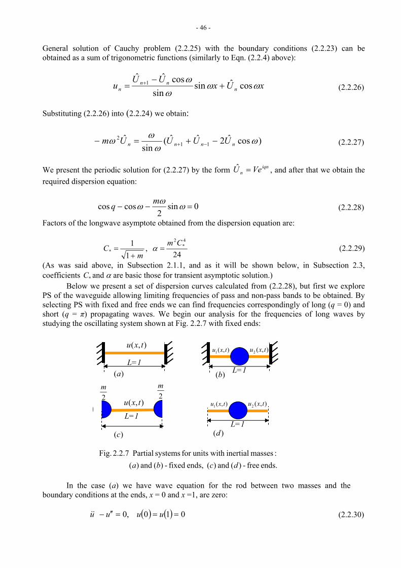
- 46 -

General solution of Cauchy problem (2.2.25) with the boundary conditions (2.2.23) can be obtained as a sum of trigonometric functions (similarly to Eqn. (2.2.4) above):

xUxUU

u nnn

n ωωω

ωcosˆsin

sincosˆˆ

1 +−

= + (2.2.26)

Substituting (2.2.26) into (2.2.24) we obtain:

)cosˆ2ˆˆ(sin

ˆ11

2 ωω

ωω nnnn UUUUm −+=− −+ (2.2.27)

We present the periodic solution for (2.2.27) by the form , and after that we obtain the required dispersion equation:

iqnn VeU =ˆ

0 sin2

coscos =−− ωωω mq (2.2.28)

Factors of the longwave asymptote obtained from the dispersion equation are:

24 ,

11 4

*2

*Cm

mC =

+= α (2.2.29)

(As was said above, in Subsection 2.1.1, and as it will be shown below, in Subsection 2.3, coefficients and α are basic those for transient asymptotic solution.) *C

Below we present a set of dispersion curves calculated from (2.2.28), but first we explore PS of the waveguide allowing limiting frequencies of pass and non-pass bands to be obtained. By selecting PS with fixed and free ends we can find frequencies correspondingly of long (q = 0) and short (q = π) propagating waves. We begin our analysis for the frequencies of long waves by studying the oscillating system shown at Fig. 2.2.7 with fixed ends:

In the case (a) we have wave equation for the rod between two masses and the boundary conditions at the ends, x = 0 and x =1, are zero:

( ) ( ) 010 ,0 ===′′− uuuu&& (2.2.30)

ends. free - )( and )( ends, fixed - )( and )( :masses inertial with unitsfor systems Partial 7.2.2 Fig.

dcba

L=1

),( txu

2m

L=1

),( txu2m

L=1

),(1 txu ),(2 txu

L=1

),(1 txu

)(a )(b

)(c )(d

),(2 txu

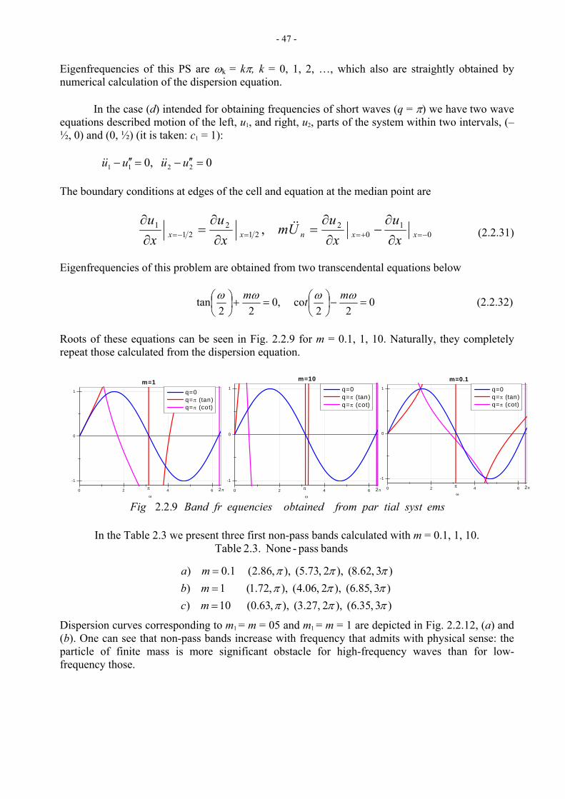
- 47 -

Eigenfrequencies of this PS are ωk = kπ, k = 0, 1, 2, …, which also are straightly obtained by numerical calculation of the dispersion equation.

In the case (d) intended for obtaining frequencies of short waves (q = π) we have two wave equations described motion of the left, u1, and right, u2, parts of the system within two intervals, (–½, 0) and (0, ½) (it is taken: c1 = 1):

0 ,0 2211 =′′−=′′− uuuu &&&&

The boundary conditions at edges of the cell and equation at the median point are

01

02

212

211 , −=+==−= ∂

∂−

∂∂

=∂

∂=

∂∂

xxnxx xu

xu

Umx

uxu && (2.2.31)

Eigenfrequencies of this problem are obtained from two transcendental equations below

02

2

co ,02

2

tan =−⎟⎠⎞

⎜⎝⎛=+⎟

⎠⎞

⎜⎝⎛ ωωωω mtm (2.2.32)

Roots of these equations can be seen in Fig. 2.2.9 for m = 0.1, 1, 10. Naturally, they completely repeat those calculated from the dispersion equation.

In the Table 2.3 we present three first non-pass bands calculated with m = 0.1, 1, 10.

Dispersion curves corresponding to m1 = m = 05 and m1 = m = 1 are depicted in Fig. 2.2.12, (a) and (b). One can see that non-pass bands increase with frequency that admits with physical sense: the particle of finite mass is more significant obstacle for high-frequency waves than for low-frequency those.

0 2 4 6

-1

0

1

π

m=1

2πω

q=0 q=π (tan) q=π (cot)

0 2 4 6

-1

0

1

π

m=0.1

2πω

q=0

0 2 4 6

-1

0

1

π

m=10

2πω

q=0 q=π (tan) q=π (tan) q=π (cot) q=π (cot)

emstial systfrom parobtained equencies Band fr..Fig 922

)3 ,35.6( ),2 ,27.3( ), ,63.0( 10 ))3 ,85.6( ),2 ,06.4( ), ,72.1( 1 ))3 ,62.8( ),2 ,73.5( ), ,86.2( 1.0 )

ππππππ

π π

===

mcmbma

bands pass-None 2.3. Table

π

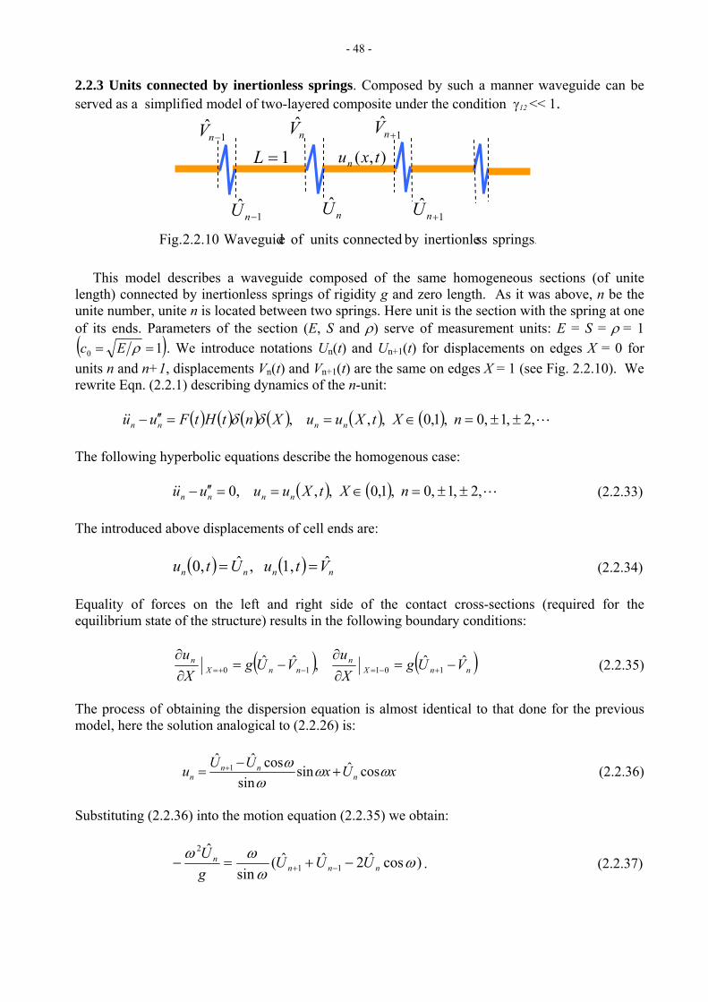
- 48 -

2.2.3 Units connected by inertionless springs. Composed by such a manner waveguide can be served as a simplified model of two-layered composite under the condition γ12 << 1.

nU 1ˆ

+nU1ˆ

−nU

1ˆ

−nV nV 1ˆ

+nV

1=L

),( txun

springs ssinertionleby connected units of e Waveguid2.2.10 Fig. . This model describes a waveguide composed of the same homogeneous sections (of unite length) connected by inertionless springs of rigidity g and zero length. As it was above, n be the unite number, unite n is located between two springs. Here unit is the section with the spring at one of its ends. Parameters of the section (E, S and ρ) serve of measurement units: E = S = ρ = 1 ( )10 == ρEc . We introduce notations U (t) and Un n+1(t) for displacements on edges X = 0 for units n and n+1, displacements V (t) and Vn n+1(t) are the same on edges X = 1 (see Fig. 2.2.10). We rewrite Eqn. (2.2.1) describing dynamics of the n-unit:

( ) ( ) ( ) ( ) ( ) ( ) L&& ,2 ,1 ,0 ,1,0 ,, , ±±=∈==′′− nXtXuuXntHtFuu nnnn δδ The following hyperbolic equations describe the homogenous case:

( ) ( ) L&& ,2 ,1 ,0 ,1,0 ,, ,0 ±±=∈==′′− nXtXuuuu nnnn (2.2.33)

The introduced above displacements of cell ends are:

( ) ( ) nnnn VtuUtu ˆ 1, ,ˆ0, == (2.2.34)

Equality of forces on the left and right side of the contact cross-sections (required for the equilibrium state of the structure) results in the following boundary conditions:

( ) ( )nnXn

nnXn VUg

Xu

VUgXu ˆˆ ,ˆˆ

10110 −=∂∂

−=∂∂

+−=−+= (2.2.35)

The process of obtaining the dispersion equation is almost identical to that done for the previous model, here the solution analogical to (2.2.26) is:

xUxUUu nnn

n ωωω

ω cosˆsinsin

cosˆˆ1 +−

= + (2.2.36)

Substituting (2.2.36) into the motion equation (2.2.35) we obtain:

)cosˆ2ˆˆ(sin

ˆ11

2

ωω

ωωnnn

n UUUgU

−+=− −+ . (2.2.37)

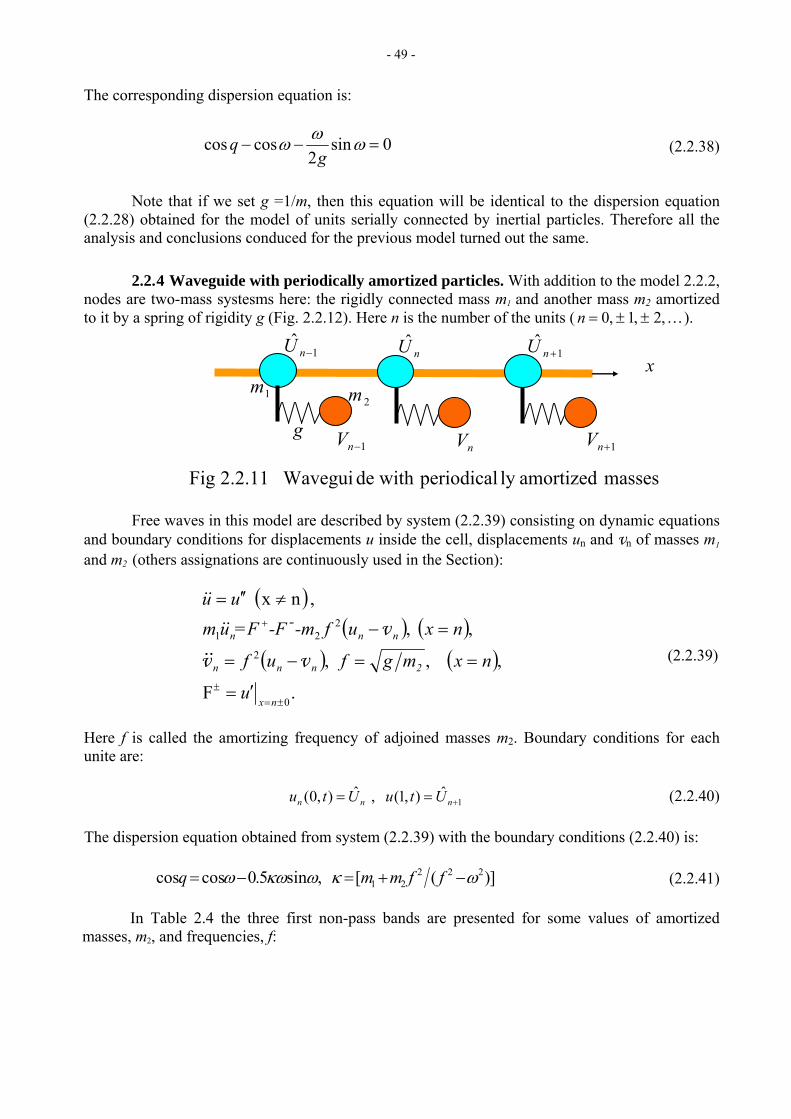
- 49 -

The corresponding dispersion equation is:

0 sin2

coscos =−− ωωωg

q (2.2.38)

Note that if we set g =1/m, then this equation will be identical to the dispersion equation (2.2.28) obtained for the model of units serially connected by inertial particles. Therefore all the analysis and conclusions conduced for the previous model turned out the same.

2.2.4 Waveguide with periodically amortized particles. With addition to the model 2.2.2, nodes are two-mass systesms here: the rigidly connected mass m1 and another mass m2 amortized to it by a spring of rigidity g (Fig. 2.2.12). Here n is the number of the units ( ). K ,2 ,1 ,0 ±±=n

x 1

ˆ+nUnU1

ˆ−nU

1−nV nV 1+nV

1m2m

g

masses amortizedly periodical with de Wavegui2.2.11 Fig Free waves in this model are described by system (2.2.39) consisting on dynamic equations and boundary conditions for displacements u inside the cell, displacements un and v of masses mn 1 and m (others assignations are continuously used in the Section): 2

( )( ) ( )

( ) ( ) .F

, , ,

, , , nx

0

2

221

±=±

+

′=

==−=

=−

≠′′=

nx

2nnn

nnn

u

nxmgfuf

nxuf-m-F=Fumuu

-

vvv

&&

&&

&&

(2.2.39)

Here f is called the amortizing frequency of adjoined masses m2. Boundary conditions for each unite are:

ˆ),1( ,ˆ),0( 1 +== nnn UtuUtu (2.2.40) The dispersion equation obtained from system (2.2.39) with the boundary conditions (2.2.40) is:

])([ ,sin5.0coscos 222

21 ωκωκωω −+=−= ffmmq (2.2.41)

In Table 2.4 the three first non-pass bands are presented for some values of amortized masses, m2, and frequencies, f:

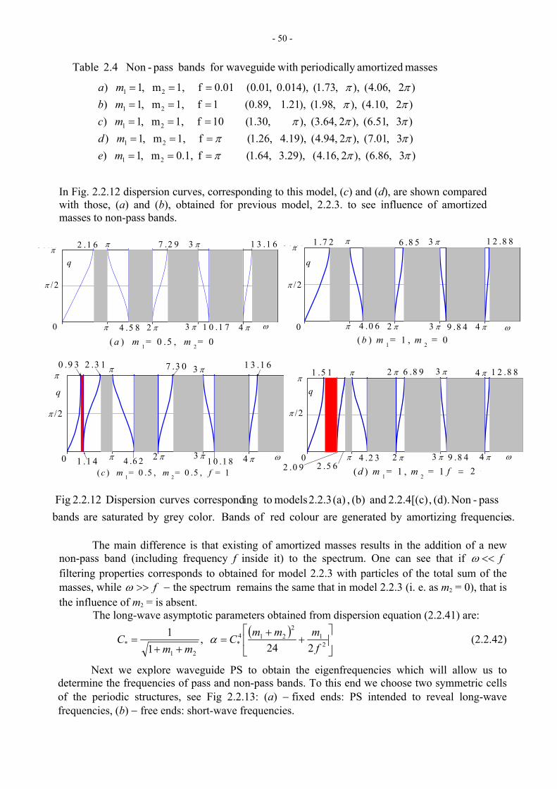
- 50 -

In Fig. 2.2.12 dispersion curves, corresponding to this model, (c) and (d), are shown compared with those, (a) and (b), obtained for previous model, 2.2.3. to see influence of amortized masses to non-pass bands.

The main difference is that existing of amortized masses results in the addition of a new

non-pass band (including frequency f inside it) to the spectrum. One can see that if f<<ω filtering properties corresponds to obtained for model 2.2.3 with particles of the total sum of the masses, while f>>ω − the spectrum remains the same that in model 2.2.3 (i. e. as m2 = 0), that is the influence of m2 = is absent. The long-wave asymptotic parameters obtained from dispersion equation (2.2.41) are:

( )⎥⎦

⎤⎢⎣

⎡+

+=

++= 2

12

214*

21* 224

,1

1f

mmmCmm

C α (2.2.42)

Next we explore waveguide PS to obtain the eigenfrequencies which will allow us to determine the frequencies of pass and non-pass bands. To this end we choose two symmetric cells of the periodic structures, see Fig 2.2.13: (a) − fixed ends: PS intended to reveal long-wave frequencies, (b) − free ends: short-wave frequencies.

0 .0 0 0 0 3 .1 4 1 6 6 .2 8 3 2 9 .4 2 4 8 1 2 .5 6 6 4

0 .0 0 0 0

1 .5 7 0 8

3 .1 4 1 6

( b ) m 1 = 1 , m 2 = 0

π 3 π

π /2

π

0

1 2 .8 8

9 .8 4

6 .8 5

4 π3 π2 π4 .0 6π

1 .7 2

ω

q

0 .0 0 0 0 3 .1 4 1 6 6 .2 8 3 2 9 .4 2 4 8 1 2 .5 6 6 4

0 .0 0 0 0

1 .5 7 0 8

3 .1 4 1 6

(c ) m 1= 0 .5 , m 2 = 0 .5 , f = 1

3 ππ2 .3 1|

0

π /2

π1 3 .1 6

4 π1 0 .1 83 π

7 .3 0

2 π4 .6 2π1 .1 4

0 .9 3

ω

q

0 .0 0 0 0 3 .1 4 1 6 6 .2 8 3 2 9 .4 2 4 8 1 2 .5 6 6 4

0 .0 0 0 0

1 .5 7 0 8

3 .1 4 1 6

( a ) m 1 = 0 .5 , m 2 = 0

3 πππ

π /2

0

1 3 .1 6

4 π1 0 .1 73 π

7 .2 9

2 π4 .5 8π

2 .1 6

ω

q

0 .0 0 0 0 3 .1 4 1 6 6 .2 8 3 2 9 .4 2 4 8 1 2 .5 6 6 4

0 .0 0 0 0

1 .5 7 0 8

3 .1 4 1 6

2 .5 62 .0 9 (d ) m 1 = 1 , m 2 = 1 , f 2 = π

3 π 4 π2 πππ

0

π /2

π

1 2 .8 8

9 .8 4

6 .8 9

4 π3 π2 π4 .2 3

1 .5 1

ω

q

2=f

s.frequencie amortizingby generated arecolour red of Bands color.grey by saturated are bands pass-Non (d). , 2.2.4[(c) and (b) , (a) 2.2.3 models toingcorrespond curves Dispersion 2.2.12 Fig

Table

)3 ,86.6( ),2 ,16.4( ),29.3 ,64.1( f 1,.0m ,1 ))3 ,01.7( ),2 ,94.4( ),19.4 ,26.1( f 1,m ,1 ))3 ,51.6( ),2 ,64.3( ), ,30.1( 10f 1,m ,1 ))2 ,10.4( ), ,98.1( ),21.)2 ,06.4( ), ,73.1( ),014

21

21

21

21

πππππππππππ

masses amortizedly periodical with idefor wavegu bands pass-Non 2.4

1 ,89.0( 1f 1,m ,1 ).0 ,01.0( 0.01f 1,m ,1 ) 21

===============

mbma π π

memdmc

- 51 -

Boundary conditions in the case of fixed ends, (a) (remind that this system defines

frequencies at ) are: 0→q0)1()0( == uu (2.2.43)

and the frequency equation is the simple one: 0,1,2..... ,0sin ==⇒= kkπωω (2.2.44)

The partial system with free ends, (b), includes two wave equations for u1 and u2 within two intervals (–½, 0) and (0, ½)

0 ,0 2211 =′′−=′′− uuuu &&&& , (2.2.45,a) boundaries conditions

0,21 ,

21 ,),0(),0( 2121 =⎟

⎠⎞

⎜⎝⎛′=⎟

⎠⎞

⎜⎝⎛−′== tutuUtutu (2.2.45,b)

and the following conditions tailoring the left and right parts of the system:

( )2

22

22

02

01

1

/ )(

),(||

mgfVUfV

VUmfx

uxuUm

nnn

nnxxn

=−=

−−∂

∂−

∂∂

= +=−=

&&

&& (2.2.45,c)

g

particles amortizedly periodical with idefor wavegu systems Partial 2.2.13 Fig

m1

m2

0x2

12

1−

U),(2 txu),(1 txu

V

x0 1

)(b22m

g

u(x, t) nU 1ˆ

+nU

V

21m

)(a

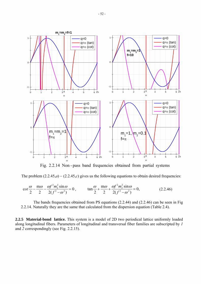
- 52 -

The problem (2.2.45,a) − (2.2.45,c) gives us the following equations to obtain desired frequencies:

0 )(2

sin2

m2

c 22

22

2

=−

−−ω

ωωωωfmfot , 0,

)(2sin

2m

2tan 22

22

2

=−

++ω

ωωωωfmf

(2.2.46)

The bands frequencies obtained from PS equations (2.2.44) and (2.2.46) can be seen in Fig 2.2.14. Naturally they are the same that calculated from the dispersion equation (Table 2.4).

2.2.5 Material-bond lattice. This system is a model of 2D two periodical lattice uniformly loaded along longitudinal fibers. Parameters of longitudinal and transversal fiber families are subscripted by 1 and 2 correspondingly (see Fig. 2.2.15).

0 1 2 3 4 5 6

-1

0

1

π

m1=m2=f=1

2πω

q=0 q=π (tan) q=π (cot)

0 1 2 3 4 5 6

-1

0

1

0 1 2 3 4 5 6

-1

0

1

π

m1=m2=1f=π

2πω

q=0 q=π (tan) q=π (cot)

π

m1=m2=1f=10

2πω

q=0 q=π (tan) q=π (cot)

0 1 2 3 4 5 6

-1

0

1 q=0 q=π (tan)

π

m1=1, m2=0.1f=π

2πω

q=π (cot)

systems partial from obtained sfrequencie band pass-Non 2.2.14 Fig.

- 53 -

y

Equations of the model are:

( ) ( ) ( )( ) ( ) 2,1 , ; , ,0

)()(22

12

2

12

1

==∈±==″−

+−=″−

iEcNnnLxc

xtQnLxxFucu

iiiyn

xnn

ρ

δδ

vv n&&

&& (2.2.47)

where F(x) is the longitudinal force acting from transversal fibers to longitudinal those in junction cross-sections x = nL1

. ,)(0

NnFxFy

n ∈∂∂

=≡+=

yv n (2.2.48)

(below parameters of the x-family are chosen as measurement units, we denote additionally: { } { }12121212 ,, ,=,,, LLccSSLcS ρρρ ) Boundary conditions for fibers of the y-family are:

( ) 0 ,,),0,(22

=∂

∂=

=Ly

nn y

tnutx vv (2.2.49)

With use Eqns (2.2.47) – (2.2.49) one can obtain the dispersion equation:

.tansin2coscos ⎟⎠⎞

⎜⎝⎛−=

cLScq ωωρω (2.2.50)

Parameters of long-wave asymptotic of the dispersion equation are ( ) 2

*

20

20

4*

00

* 624 ,

11

CLmmCLSm

mC +==

+= αρ (2.2.51)

2.2.6 Unidirectional composite loaded along fibers. This system is a model (a) of unidirectional composite in the case of fiber-fiber anti-symmetric loading (see Fig 1.2.4a). Contrary to the all previous models this one is the non-periodic in the direction of the waveguide axis. Problem conditions, notably structure periodicity in the transversal direction and the same periodicity of acting loads allow the waveguide shown in Fig. 2.2.16 to be selected and an infinitely elongated (in the transversal direction) structure to be inversed into the finite one. There is assumed that fibers function by tension-compression mode, while adhesive functions only in shear, so displacements of fibers, u(x,t), and adhesive, w(x,y,t), directed only along the x-axis. For a fiber a 1D rod model is used, while adhesive described by the 2D “string” model of theory of elasticity [58]. Parameters of the model are shown in Fig. 2.2.16.

E1, ρ1, S1 E2, ρ2, S2

n-1 n n+1 x

1L

2L

elements bond-material of lattice periodic- twoa of e Waveguid2.2.15 Fig.

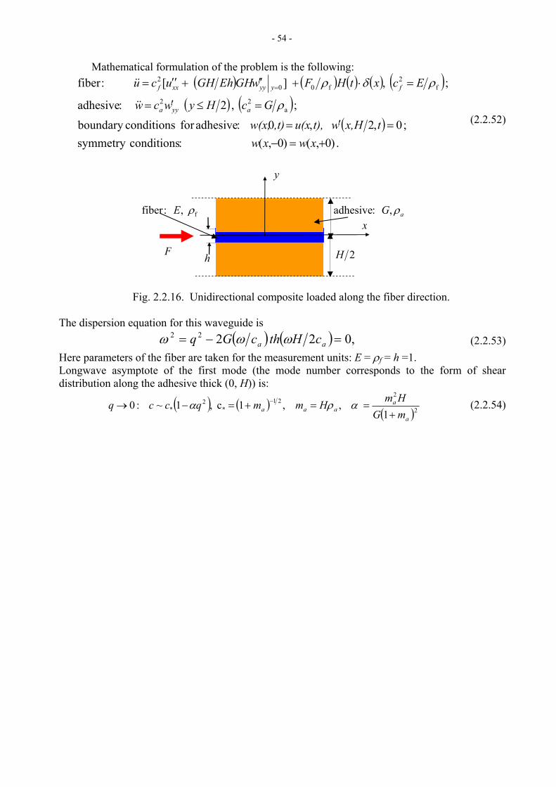
- 54 -

Mathematical formulation of the problem is the following: ( ) ( ) ( ) ( ) ( )

( ) ( )( )

. )0,()0,( :conditions symmetry ; 0,2,0 :adhesivefor conditionsboundary

; , 2 :adhesive

; ,][ :fiber

a22

f2

f002

+=−=′=

=≤′=

=⋅+′′+′′= =

xwxwtHx,wt), u(x,t)w(x,

GcHywcw

EcxtHF wGHEhGH ucu

ayya

fyyyxxf

ρ

ρδρ

&&

&&

(2.2.52)

y

Fig. 2.2.16. Unidirectional composite loaded along the fiber direction. The dispersion equation for this waveguide is

( ) ( ) 0, 2 222 =−= aa cHthcGq ωωω (2.2.53) Here parameters of the fiber are taken for the measurement units: E = ρf = h =1. Longwave asymptote of the first mode (the mode number corresponds to the form of shear distribution along the adhesive thick (0, H)) is:

( ) ( )( )2

221

*2

* 1 ,,1 c ,1~ :0

a

aaaa mG

HmHmmqccq+

= = +=−→ − αρα (2.2.54)

F

x

2H

, :adhesive , :fiber f aGE ρ ρ

h

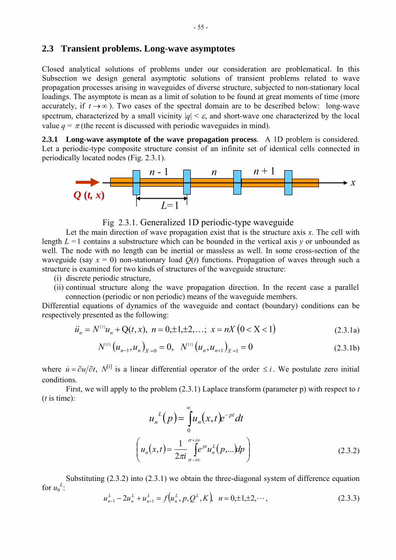
- 55 -

2.3 Transient problems. Long-wave asymptotes Closed analytical solutions of problems under our consideration are problematical. In this Subsection we design general asymptotic solutions of transient problems related to wave propagation processes arising in waveguides of diverse structure, subjected to non-stationary local loadings. The asymptote is mean as a limit of solution to be found at great moments of time (more accurately, if ). Two cases of the spectral domain are to be described below: long-wave spectrum, characterized by a small vicinity |q| < ε, and short-wave one characterized by the local value q = π (the recent is discussed with periodic waveguides in mind).

∞→t

2.3.1 Long-wave asymptote of the wave propagation process. A 1D problem is considered. Let a periodic-type composite structure consist of an infinite set of identical cells connected in periodically located nodes (Fig. 2.3.1).

L=1

n - 1 n n + 1 x

Q (t, x)

Fig 2.3.1. Generalized 1D periodic-type waveguide Let the main direction of wave propagation exist that is the structure axis x. The cell with length L =1 contains a substructure which can be bounded in the vertical axis y or unbounded as well. The node with no length can be inertial or massless as well. In some cross-section of the waveguide (say x = 0) non-stationary load Q(t) functions. Propagation of waves through such a structure is examined for two kinds of structures of the waveguide structure:

(i) discrete periodic structure, (ii) continual structure along the wave propagation direction. In the recent case a parallel

connection (periodic or non periodic) means of the waveguide members. Differential equations of dynamics of the waveguide and contact (boundary) conditions can be respectively presented as the following:

( 1X0 ;,2,1,0 ,),Q(]2[ <<=±±=+= nXxnxtuNu nn K&& ) (2.3.1a)

( ) ( ) 0, 0,, 1 10 1]1[]1[ == =+=− XnnXnn uuNuuN (2.3.1b)

N[i] i≤,tuu ∂∂=& is a linear differential operator of the order where . We postulate zero initial

conditions. First, we will apply to the problem (2.3.1) Laplace transform (parameter p) with respect to t

(t is time):

( ) ( ) dtetxupu ptn

Ln

−∞

∫=0

,

( ) ( ) ⎟⎟⎠

⎞⎜⎜⎝

⎛= ∫

∞+

∞−

dppuei

txui

i

Ln

ptn

σ

σπ,...

21, (2.3.2)

Substituting (2.3.2) into (2.3.1) we obtain the three-diagonal system of difference equation

for u L: n

( ) L,2,1,0 ,,,,2 11 ±±==+− +− nKQpufuuu LLn

Ln

Ln

Ln , (2.3.3)

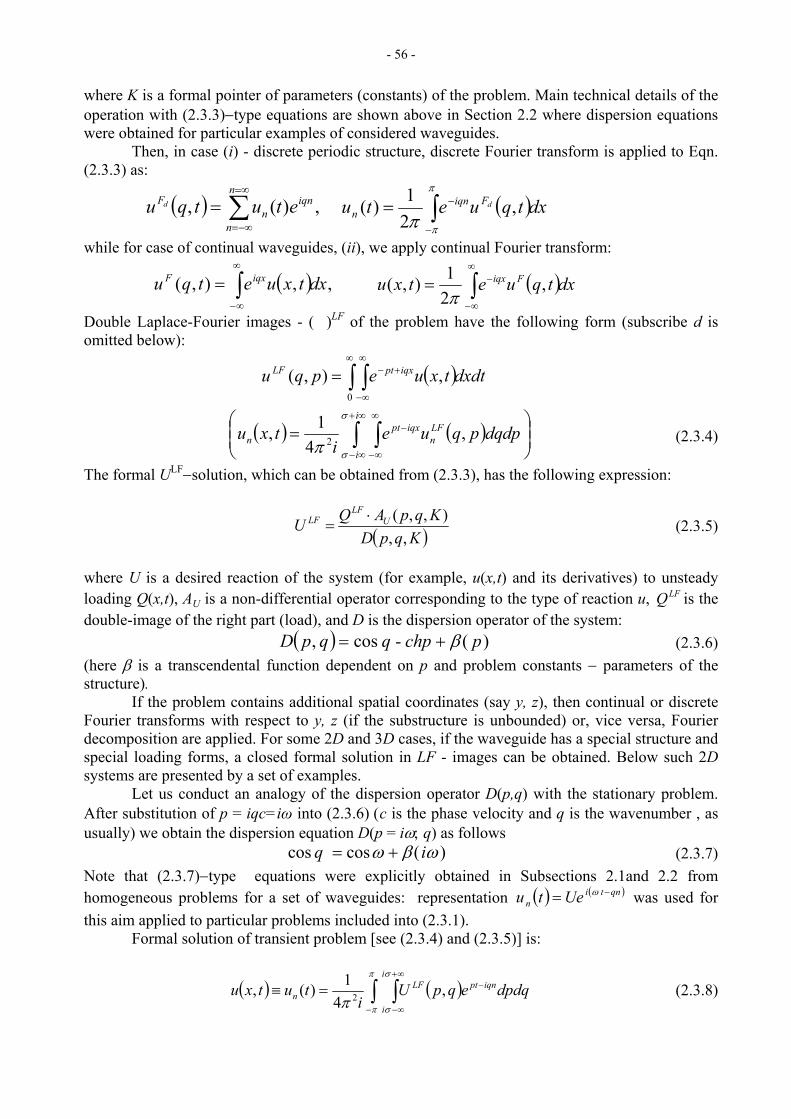
- 56 -

where K is a formal pointer of parameters (constants) of the problem. Main technical details of the operation with (2.3.3)−type equations are shown above in Section 2.2 where dispersion equations were obtained for particular examples of considered waveguides.

Then, in case (i) - discrete periodic structure, discrete Fourier transform is applied to Eqn. (2.3.3) as:

( )dxtquetu dFiqnn ∫

−

−=π

ππ,

21)(( ) ,)(, ∑

∞=

−∞=

=n

n

iqnn

F etutqu d

while for case of continual waveguides, (ii), we apply continual Fourier transform:

( ) ,,),( dxtxuetqu iqxF ∫∞

∞−

= ( )dxtquetxu Fiqx∫∞

∞−

−= ,21),(π

Double Laplace-Fourier images - ( )LF of the problem have the following form (subscribe d is omitted below):

( )dxdttxuepqu iqxptLF ∫ ∫∞ ∞

∞−

+−=0

,),(

( ) ( ) ⎟⎟⎠

⎞⎜⎜⎝

⎛= ∫ ∫

∞+

∞−

∞

∞−

− dpdqpquei

txui

i

LFn

iqxptn

σ

σπ,

41, 2 (2.3.4)

The formal ULF−solution, which can be obtained from (2.3.3), has the following expression:

( ) ,,

),,( KqpD

KqpAQU ULF

LF ⋅= (2.3.5)

where U is a desired reaction of the system (for example, u(x,t) and its derivatives) to unsteady loading Q(x,t), AU is a non-differential operator corresponding to the type of reaction u, is the double-image of the right part (load), and D is the dispersion operator of the system:

LFQ

( ) )( + = pchpq -qpD βcos, (2.3.6) (here β is a transcendental function dependent on p and problem constants − parameters of the structure). If the problem contains additional spatial coordinates (say y, z), then continual or discrete Fourier transforms with respect to y, z (if the substructure is unbounded) or, vice versa, Fourier decomposition are applied. For some 2D and 3D cases, if the waveguide has a special structure and special loading forms, a closed formal solution in LF - images can be obtained. Below such 2D systems are presented by a set of examples.

Let us conduct an analogy of the dispersion operator D(p,q) with the stationary problem. After substitution of p = iqc=iω into (2.3.6) (c is the phase velocity and q is the wavenumber , as usually) we obtain the dispersion equation D(p = iω; q) as follows

)( + = ωβω iq coscos (2.3.7) Note that (2.3.7)−type equations were explicitly obtained in Subsections 2.1and 2.2 from homogeneous problems for a set of waveguides: representation ( ) ( qnti

n Uetu −= ω ) was used for this aim applied to particular problems included into (2.3.1). Formal solution of transient problem [see (2.3.4) and (2.3.5)] is:

( ) ( )∫ ∫−

∞+

∞−

−=≡π

π

σ

σπdpdqeqpU

itutxu

i

i

iqnptLFn ,

41)(, 2 (2.3.8)

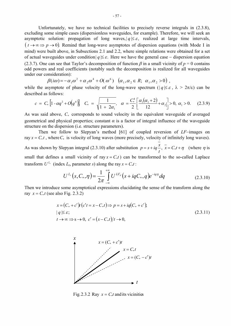
- 57 -

Unfortunately, we have no technical facilities to precisely reverse integrals in (2.3.8), excluding some simple cases (dispersionless waveguides, for example). Therefore, we will seek an asymptotic solution: propagation of long waves, ,|| ε≤q realized at large time intervals,

Remind that long-wave asymptotes of dispersion equations (with Mode I in mind) were built above, in Subsections 2.1 and 2.2, where simple relations were obtained for a set of actual waveguides under condition

( .0 →⇒∞→ pt )

.|| ε≤q Here we have the general case − dispersion equation (2.3.7). One can see that Taylor’s decomposition of function β in a small vicinity of p = 0 contains odd powers and real coefficients (notably such the decomposition is realized for all waveguides under our consideration):

( )0 > ∈ )( + + − = )( 42

22121

61 , ;, ααααωωαωαωβ ROi ,

ε≤|| qwhile the asymptote of phase velocity of the long-wave spectrum ( , λ > 2π/ε) can be described as follows:

( )[ ] ( ) .0 ,012

2221

11 1211

4*

1

42 >>⎥⎦⎤

⎢⎣⎡ +

+ =

+= ,+ = ααααα

αα C ,

CqOq - Cc ** (2.3.9)

As was said above, corresponds to sound velocity in the equivalent waveguide of averaged geometrical and physical properties; constant α is a factor of integral influence of the waveguide structure on the dispersion (i.e. structure parameters).

*C

Then we follow to Slepyan’s method [61] of coupled reversion of LF−images on ray , where is velocity of long waves (more precisely, velocity of infinitely long waves).

As was shown by Slepyan integral (2.3.10) after substitution

tCx *= *C

, * η+=+= tCxtxiqsp (where η is

small that defines a small vicinity of ray tCx *= ) can be transformed to the so-called Laplace transform (index LrLU r, parameter s) along the ray tCx *= :

( ) ( )∫+∞

∞−

−+= dqeqiqCsUCsU iqLFL dr η

πη ,

21,, ** (2.3.10)

Then we introduce some asymptotical expressions elucidating the sense of the transform along the ray (see also Fig. 2.3.2) tCx *=

( ) ( ) ( )

( ) ,0 ,0 s ;||

;

*

***

→−=′→⇒∞→≤

′++=⇒−=′′+=

ttCxctq

cCiqsptCxtctcCxε (2.3.11)

x′= + t cCx * )(

= t Cx *

′= −

t

t cCx * )(

s vicinitieits and Ray 2.3.2 Fig. *tCx

=

- 58 -

which show that

( ), valuesmall a is * ctCx ′=- we operate in a small vicinity of the ray ε≤|| q- we analyze long waves ( ) in this vicinity, and

∞→t- the time-asymptotic solution ( ) is under our consideration. ( ) ~,qpD ( )qiqCsD ,*+ Time asymptote of dispersion operator (2.3.6), , is found as its

Taylor’s decomposition in small vicinity |q| < δ, and with taken into account (that defines originals at

0→p∞→t ):

(2.3.13) ( ) )+′+( 3

**2~ qCiciqsiqCs,qD α By such the way, the nominator of formal solution (2.3.5) also is decomposed with accounting (2.3.11), so that the solution has the following asymptote:

( ))+′+(

+3

**

*

2;,~

qCiciqsiqCKqiqCsAQu U

LFLF

dd

α (2.3.14)

The LF − transform of the local (x = 0) external loading, Q(t)δ(x), is under our analysis now. Here we don’t differ cases (i) and (ii), because discrete or continual Fourier transforms applied to Dirac functions δ(n) or δ(x) correspondingly results in the same value: δ(n)LFd LF = δ(x) = 1. We are separate three cases of loading:

1. Heaviside step:

( ) ( )pQQxtHQQ LF 0

022 =⇒= δ (2.3.15)

2. Finite pulse [F(t) – form of the pulse, t0 − its duration]:

( ) ( ) ( )[ ] ( ) ( ) dtetFQQxtHttHtFQQ ptt

LF −∫=⇒−−=0

0000 22 δ (2.3.16)

3. Infinite harmonic loading of frequency ω and initial phaseϕ:

( ) ( )[ ] ( ) 2200cossin2sin2

ωϕωϕδϕω

++

=⇒+=p

pQQxtHtQQ LF (2.3.17)

1. Heaviside step loading. Asymptotical solution in this case we obtain by the following way. Asymptote of LF − transform (2.3.15) with accounting (2.3.11) is:

*

00 2~2iqCsQ

pQQ dLF

+= (2.3.18)

( ) 1~;,* OBKqiqCsA UU ≡ ( )+Using (2.3.14) and (2.3.19) and taking into account that , we obtain asymptotical expression of particle velocity as follows:

( )( )[ 13***02~ −

+′++≡ qiCciqsiqCsCBQu vv& ] (2.3.19)

ε≤|| qBecause asymptotic representation (2.3.20) is proved within small vicinity , we change integration limits in (2.3.12). Taking into account (2.3.19) we obtain

( ) ( )( )∫− +′++

e

e

L

qiCciqsiqCsdqCBQ

Csr3

**

*0* ~,,

πη vv (2.3.20)

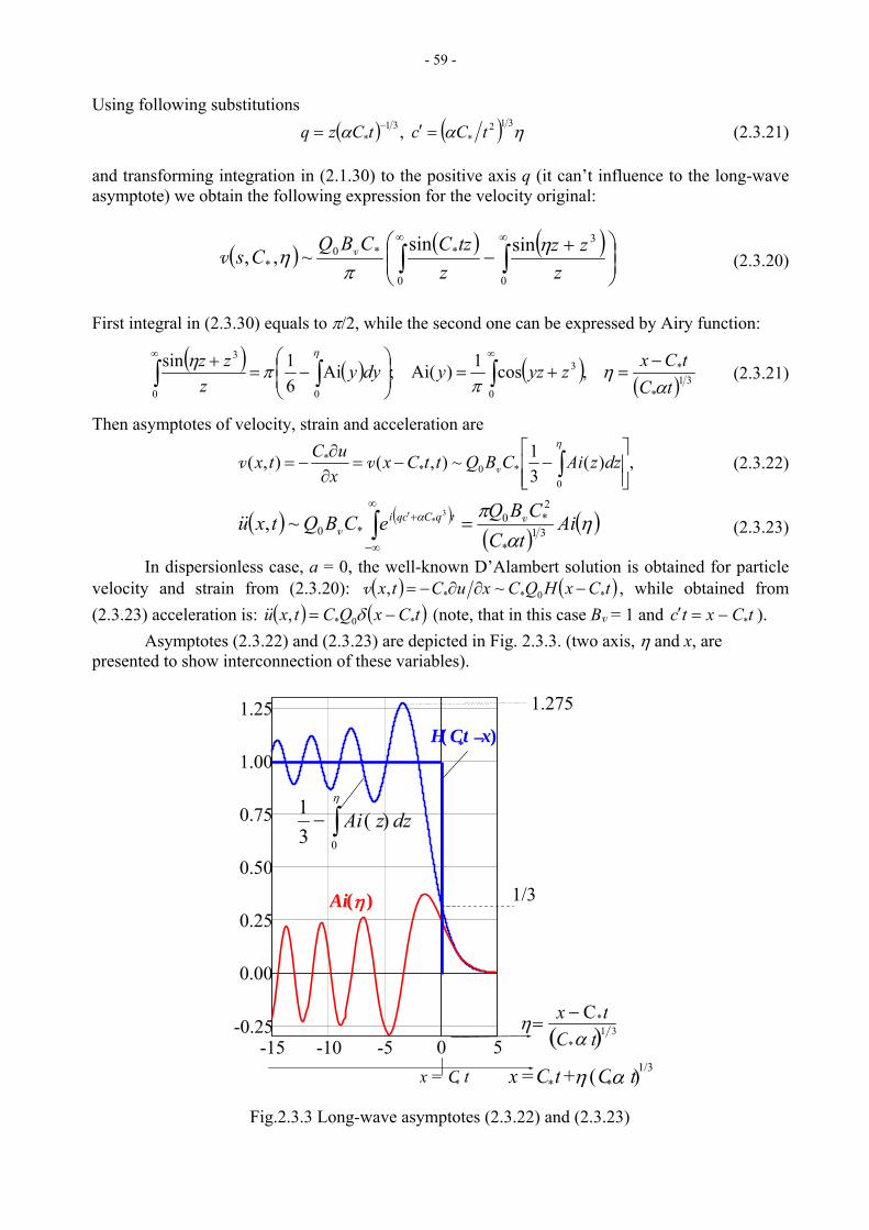
- 59 -

Using following substitutions ( ) ( ) ηαα

312*

31* , tCctCzq =′= − (2.3.21)

and transforming integration in (2.1.30) to the positive axis q (it can’t influence to the long-wave asymptote) we obtain the following expression for the velocity original:

( ) ( ) ( )⎟⎟⎠

⎞⎜⎜⎝

⎛ +−∫ ∫

∞ ∞

0 0

3**0

*sinsin

~,,z

zzz

tzCCBQCs η

πη vv (2.3.20)

First integral in (2.3.30) equals to π/2, while the second one can be expressed by Airy function:

( ) ( ) ( )( ) 31

*

*

0

3

00

3

,cos1)Ai( ;Ai61sin

tCtCxzyzydyy

zzz

αη

ππη η −

=+=⎟⎟⎠

⎞⎜⎜⎝

⎛−=

+∫∫∫∞∞

(2.3.21)

Then asymptotes of velocity, strain and acceleration are

,)(31~),(),(

0*0*

*

⎥⎥⎦

⎤

⎢⎢⎣

⎡−−=

∂∂

−= ∫η

dzzAiCBQttCxxuCtx vvv (2.3.22)

( ) ( )( )

( )ηα

πα AitCCBQeCBQtxu tqCcqi

31*

2*0

*0

3*~, v

v =∫∞

∞−

+′&& (2.3.23)

In dispersionless case, a = 0, the well-known D’Alambert solution is obtained for particle velocity and strain from (2.3.20): ( ) ( )tCxHQCxuCtx *0** ~, −∂∂−=v , while obtained from (2.3.23) acceleration is: ( ) ( )tCxQCtxu *0*, −= δ&& tCxtc *−=′ (note, that in this case B = 1 and ). Bv

Asymptotes (2.3.22) and (2.3.23) are depicted in Fig. 2.3.3. (two axis, η and x, are presented to show interconnection of these variables).

-15 -10 -5 0 5-0.25

0.00

0.25

0.50

0.75

1.00

1.25

1/3

1.275

x = C* t x = C*t + η (C*α t)1/3

H C

Fig.2.3.3 Long-wave asymptotes (2.3.22) and (2.3.23)

Ai(η)

( ) 31*

*CtC

txα

η −=

∫−η

0

)(31 dzzAi

( *t − x)

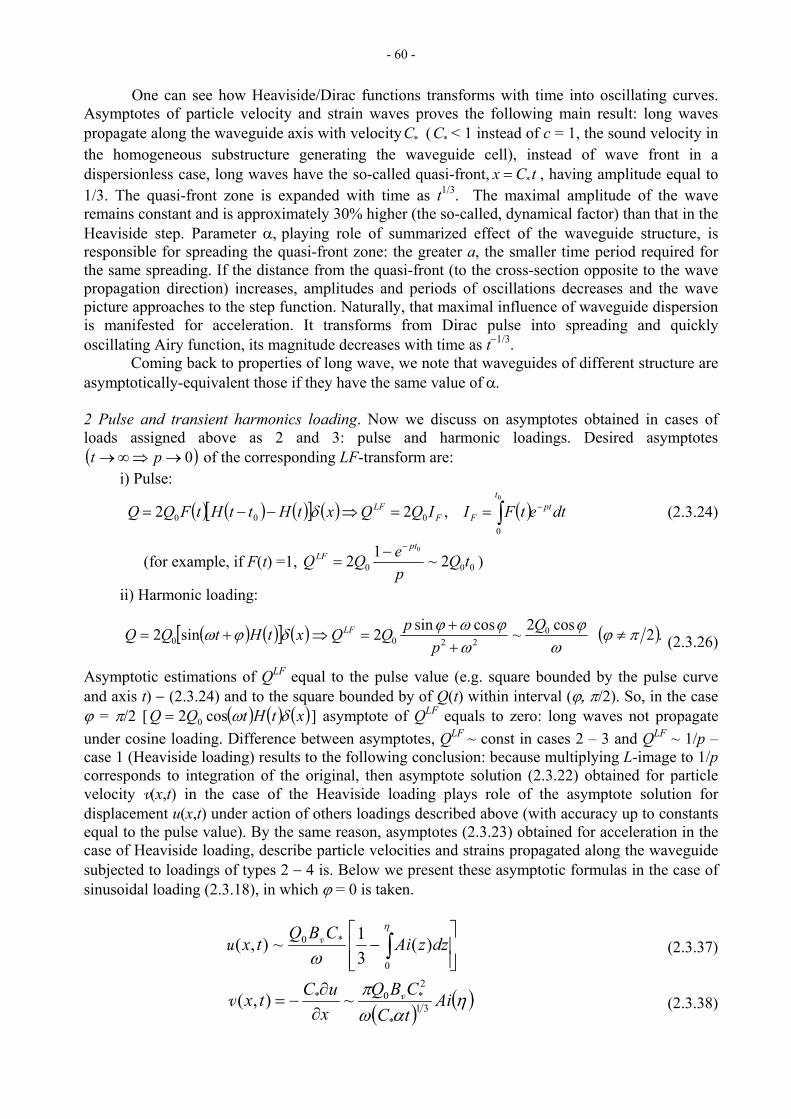
- 60 -

One can see how Heaviside/Dirac functions transforms with time into oscillating curves. Asymptotes of particle velocity and strain waves proves the following main result: long waves propagate along the waveguide axis with velocity ( < 1 instead of c = 1, the sound velocity in the homogeneous substructure generating the waveguide cell), instead of wave front in a dispersionless case, long waves have the so-called quasi-front,

*C *C

tCx *= , having amplitude equal to 1/3. The quasi-front zone is expanded with time as t1/3. The maximal amplitude of the wave remains constant and is approximately 30% higher (the so-called, dynamical factor) than that in the Heaviside step. Parameter α, playing role of summarized effect of the waveguide structure, is responsible for spreading the quasi-front zone: the greater a, the smaller time period required for the same spreading. If the distance from the quasi-front (to the cross-section opposite to the wave propagation direction) increases, amplitudes and periods of oscillations decreases and the wave picture approaches to the step function. Naturally, that maximal influence of waveguide dispersion is manifested for acceleration. It transforms from Dirac pulse into spreading and quickly oscillating Airy function, its magnitude decreases with time as t−1/3.

Coming back to properties of long wave, we note that waveguides of different structure are asymptotically-equivalent those if they have the same value of α.

2 Pulse and transient harmonics loading. Now we discuss on asymptotes obtained in cases of loads assigned above as 2 and 3: pulse and harmonic loadings. Desired asymptotes

of the corresponding LF-transform are: ( 0 →⇒∞→ pt )i) Pulse:

( ) ( ) ( )[ ] ( ) ( ) dtetFIIQQxtHttHtFQQ ptt

FFLF −∫==⇒−−=

0

0000 ,22 δ (2.3.24)

000 2~120

tQpeQQ

ptLF

−−=(for example, if F(t) =1, )

ii) Harmonic loading:

( ) ( )[ ] ( ) ( .2 cos2~cossin2sin2 02200 πϕ

ω)ϕ

ωϕωϕδϕω ≠

++

=⇒+=Q

ppQQxtHtQQ LF

(2.3.26)

Asymptotic estimations of QLF equal to the pulse value (e.g. square bounded by the pulse curve and axis t) − (2.3.24) and to the square bounded by of Q(t) within interval (ϕ, π/2). So, in the case ϕ = π/2 [ ( ) ( ) (xtHtQQ )δωcos2 0= ] asymptote of QLF equals to zero: long waves not propagate under cosine loading. Difference between asymptotes, QLF ~ const in cases 2 – 3 and QLF ~ 1/p – case 1 (Heaviside loading) results to the following conclusion: because multiplying L-image to 1/p corresponds to integration of the original, then asymptote solution (2.3.22) obtained for particle velocity v(x,t) in the case of the Heaviside loading plays role of the asymptote solution for displacement u(x,t) under action of others loadings described above (with accuracy up to constants equal to the pulse value). By the same reason, asymptotes (2.3.23) obtained for acceleration in the case of Heaviside loading, describe particle velocities and strains propagated along the waveguide subjected to loadings of types 2 − 4 is. Below we present these asymptotic formulas in the case of sinusoidal loading (2.3.18), in which ϕ = 0 is taken.

)(31~),(

0

*0

⎥⎥⎦

⎤

⎢⎢⎣

⎡− ∫

η

ωdzzAi

CBQtx vu (2.3.37)

( )( )η

αωπ Ai

tCCBQ

xuCtx 31

*

2*0* ~),( vv

∂∂

−= (2.3.38)

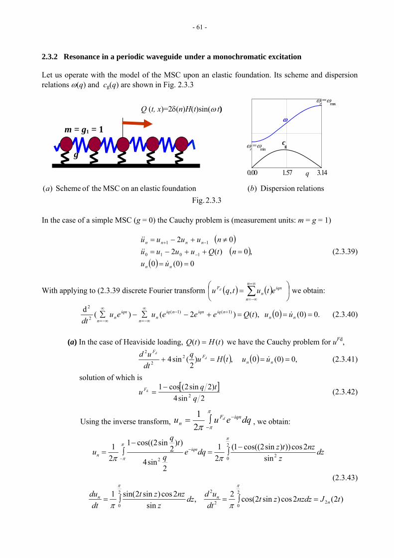
- 61 -

2.3.2 Resonance in a periodic waveguide under a monochromatic excitation Let us operate with the model of the MSC upon an elastic foundation. Its scheme and dispersion relations ω(q) and c (q) are shown in Fig. 2.3.3 g

In the case of a simple MSC (g = 0) the Cauchy problem is (measurement units: m = g = 1)

( )(

( ) 0)0(0,0 )(2

0 2

1010

11

===++−=

≠+−=

−

−+

nn

nnnn

uuntQuuuu

nuuuu

&

&&

&&

) (2.3.39)

With applying to (2.3.39 discrete Fourier transform we obtain: ( ) ( ) ⎟⎠

⎞⎜⎝

⎛= ∑

∞=

−∞=

,n

n

iqnn

F etutqu d

( ) .0)0(0 ),()2()(d )1()1(2

2

===+−∑−∑ +−∞

−∞=

∞

−∞=nn

niqiqnniqn

n

iqnn

nuutQeeeueu

dt& (2.3.40)

(a) In the case of Heaviside loading, )()( tHtQ = we have the Cauchy problem for uFd,

( ) ( ) ,0)0(0 ,)2

(sin4 22

2

===+ nnF

F

uutHuqdtud

dd

& (2.3.41)

solution of which is

[ ]2sin4

)2sin2(cos1 2d

qtqu F −

= (2.3.42)

Using the inverse transform, dqeuu iqnFn

d −

−∫=π

ππ21

, we obtain:

dzz

nztzdqeq

tq

u iqnn 2

2

02 sin2cos)))sin2cos((1(

21

2sin4

))2

sin2cos((1

21 −

∫=−

∫= −

−

ππ

π ππ

(2.3.43)

)2(2cos)sin2cos(2 ,sin

2cos)sin2sin(12

2

02

22

0tJnzdzzt

dtuddz

znzzt

dtdu

nnn =∫=∫=

ππ

ππ

0.00 1.57 3.14

ωr = ωmincg

ω

ωr = ωmax

q

Q (t, x)=2δ(n)H(t)sin(ω t)

g

m = g1 = 1

2.3.3 Fig. relations Dispersion )( foundation elastican on MSC theof Scheme )( ba

- 62 -

where J2n(z) is the first kind Bessel function of order 2n [55] (here and below table integrals are taken from [56]).

dtdun(b) For Dirac impulse, )()( ttQ δ= , displacements, u , and velocities, n , are

respectively velocities and accelerations obtained below for the Heaviside step (2.3.43):

)2( ,sin

2cos)sin2sin(12

2

0tJ

dtdu

dzz

nzztu nn

n ==∫=

π

π (2.3.44)

(c) Solution for monochromatic loading, ttQ ωsin)( = , is obtained by the convolution

integral from sinωt and (2.3.44) (below we show the solution for the particle velocity),

τττω djtdt

dun

tn )2()(sin 2

0−∫= . (2.3.45)

Then our aim is to find solution corresponding to the resonance case: ω=2 in the monochromatic loading. Remind, that notably ω=2 is the boundary between pass and non-pass bands in the problem under consideration. With using table of integrals (see [56]) we obtain:

⎥⎦⎤

⎢⎣⎡ −∑−−−+=

=+ )2()1(2)2()2cos(*||)1()2( 2

101||2 tJtJtnttJ

dtdu

mm

n

m

nn

n (2.3.46)

Using asymptotic representation Jm(z) for (see [55]) ∞→>> zm ,z 2

),42

cos(2)( πππ

−−=mz

zzjm (2.3.47)

dtdun : we obtain the following asymptotic estimation for

)4

3)12(2cos( πππ

−+−≈ nttdt

dun 0,|| →<< ttn, (2.3.48)

For the particle to which the loading is applied (n = 0) we obtain the following asymptote:

( ) ( ) ( ) ⎟⎠⎞

⎜⎝⎛ =−≈−≈∞→ ttutt

dtdu t

472sin

21 ,2cos: 0

0 πϕϕπ

ϕπ

(2.3.49)

- 63 -

2.4 Transient problem. Numerical solutions. Pulse loading

In this Subsection, designing of calculation algorithms and computer simulations are described for transient processes arising in diverse waveguides considered above.

2.4.1 MDM finite-difference explicit algorithms. The Mesh Dispersion Minimization (MDM) technique within the explicit Finite Difference (FD) schemes is applied to precise solving various hyperbolic problems. This technique is intended to maximally close the original continual problem and its discrete (mesh) analog. The MDM approach was originally created for linear hyperbolic problems manifested in solid mechanics (see [52, 53, 58]), and then it has been upgraded to computation of nonlinear hyperbolic equations with unknown boundaries arising in fracture dynamics (see [62, 63]). The technique is based on a generalized concept of the Courant condition that links temporal and spatial mesh lengths with the wave velocity, which reflects properties of the material at hand. Difference presentation of original differential equations exhibits some typical domains of influence, and the idea behind MDM is to properly adjust these domains so as to improve convergence. To this end, phase velocities of high-frequency components of the continuous models have to be considered, and the mesh to be set so that the propagation velocities induced by them approximate the former as closely as possible. An important technical advantage of MDM is that it utilizes the same grid for both high-gradient and smoothed components of solution. Firstly, to reveal main points of MDM algorithms, we introduce the following classic problem: 1D wave propagation in dispersionless waveguide (a mechanical analog is straight elastic rod).

2.4.2 Dispersionless waveguide. In this example, the Fourier-Neumann problem is formulated for a semi-infinite homogeneous dispersionless waveguide (see Subsection 1.2): ( ) ( ) ( ) .0)0,()0,( , ,0 , ;, ==−=′′′== xuxutHtuuutxuu &&& (2.4.1) A mechanical analog of the problem can be chosen as the following: semi-infinite thin elastic rod is subjected to the Heaviside step loading in the cross-section x = 0; parameters of waveguide serve measurement units.

A discrete model of the problem we describe by an explicit finite difference scheme (the cross-type version). The FD analog of the problem can be described as follows. In rectangular domain with coordinates x = jΔx, and t = kΔt (Δx and Δt are spatial and temporal steps of the), continual function, u(x,t), is transformed to the discrete one: . Below we will discuss on two solutions: (a) general solution of the homogeneous problem,

, and (b) partial solution of the initial-boundary problem (with zero initial conditions).

{ TtXxD ≤≤≤≤ 0 ,0 }kjutxu =),(

0=′′− uu&&

1=c

The dispersion relation and the D’Alambert solution for wave propagated along the positive direction of x-axis are:

(2.4.2)

( ) ( )xHu tuxtu −=−′ =−= δ&&& , (2.4.3)

The FD analog of the problem (2.4.1) can be written as follows:

( ) ( ) ( ) ; ,22 22211

211 xtuuuuuuuu (2.4.1,a) kj

kj

kj

kj

kj

kj ΔΔ=+−+−=⇒′′= −+

−+ λλ&&

( ) ( ) ,,0 01 xuutHtu kk Δ+=⇒=′ − .00)0,()0,( 10 ==⇒== −jj uuxuxu &

We seek the general solution of the homogenous problem (first equation in (2.4.1a)) as

that result in the dispersion equation: ( )xj-tckiqk

j Ueu ΔΔ=

- 64 -

xqtq

c ⎟⎠⎞

⎜⎝⎛ Δ

⋅Δ

±=2

sinarcsin2 λ (2.4.2,a)

Comparing Eqns (2.4.2 a) and (2.4.2 a) one can see that in the discrete problem waves propagate dispersionally. The dispersion equation (2.4.2 a) has infinity of modes that relate to multivalent arcsine. If λ = 1 (Δx = Δt), domains of influence of initial conditions in the continual problem, x = t, and in the discrete one, j = k, coincide that results in coincidence of (2.4.2) and (2.4.2 a). So, the mesh dispersion is eliminated in this case. Note that equality λ = 1 is the limiting value of Currant’s stability criterion: 1≤λ . Condition λ = 1 transforms Eqn. (2.4.1 a) into the following algorithm (here and below Δx = 1 is taken):

1 0, , 01011

111 +===−+= −

−−−+

+ kkjj

kj

kj

kj

kj uuuuuuuu (2.4.1,b)

Solution of (2.4.1b) obtained by the method of mathematical induction,

, (2.4.3,a) ( )⎩⎨⎧

≠=

=−=′−=−

jkjkΔt

u jkHuu ,0

, ,

1

&&&

coincides with is the analytical one (2.4.3) in integer points of x,t-coordinates: in mesh nodes (Δt−1 plays role of the discrete analog of the Dirac’s function). Dispersion curves and transient solutions (we present particle velocities) calculated for several λ are shown in Fig. 2.4.1. So mesh dispersion is eliminated in algorithm (2.4.1b) with λ = 1.

Fig. 2.4.1 Dispersion of the explicit finite-difference scheme:

(a) dispersion curves of the wave equation discrete analog; (b) computer solution ( u&=v − the particle velocity) of a step propagation in a dispersionless waveguide.

Dispersion curves (Fig. 2.4.1a) tend to dispersionless relation ω = q with 1 → λ and mode branches come straight lines prolonging this relation with growth of q. If λ < 1 phase velocities (c = ω/q) of short waves decrease with increasing q in interval (0, π) and wave process consists of long-waves running ahead and short waves reaching the same point of the waveguide later than long those (see Fig. 2.4.1b). As it can be seen from comparison of dispersion curves and calculation results presented in Fig. 2.4.1, difference between results is practically insignificant in

0.0000000000.5000000171.0000000331.5000000502.0000000670

2

4

6

Δx = 1, c0= 1

ππ

Δt = 0.5Δt = 1.00

Δt = 1.00

Mode IIMode II

Mode I

Δt = 0.95

210

Mode IΔt = 0.01

ω

q/π

Δt = 0.95

0 25 50 75 100 1250

Δt = 1Δt = 0.9Δt = 0.5Δt < 0.1

x

1

1

0

0

1v

t = 100

t = 20

t = 50

( )xtHuu&&(a) (b) ′′ δ)(2− =

- 65 -

the interval 0 < λ < 0.1. What was said above was related to facilities of FD schemes to approximate the continual problem (2.4.1). This simple example lies in the basis for the MDM technique. Below we construct dispersionless and small-dispersion FD explicit schemes intended for numerical simulation of transient wave processes in waveguides of diverse structure. In the case of 1D and such degenerative 2D and 3D problems when it is possible to confirm the unique direction of wave propagation, mesh dispersion is completely eliminated from the numerical solution: resent can be defined as the accurate one in the mesh nodes. With this fact in mind we call it “the accurate numerical solution”. In the case of really non-1D problems, especially designed algorithms allow the mesh dispersion to be minimized in the numerical solution. The maximally suppress mesh dispersion the domains of influence in continual and discrete equations must be as close as possible. Note that this condition is impossible for implicit algorithms in which the influence domain equals to infinity regardless of the size of mesh steps.

2.4.3 Simple MSC. Let us discuss results shown in Fig. 2.4.1 with point of view of the originally discrete problem: wave propagation in the simple MSC. Motion equations of the chain (c0 = 1) and dispersion relations are (see Subsection 1.2):

( ) 0,2 11 =+−− −+ nnnn uuuu&& (2.4.4) ( ) 2sin2 q=ω (2.4.5)

Asymptotically the same equation (2.4.5) is obtained from dispersion equation (2.4.2 a) if

→ 0λ (remind that Δx = 1). So, if we use FD algorithms (discrete time and discrete space) to calculate waves in a spatially discrete waveguide, the requirement to mesh dispersion minimization is . One can obtain that the maximal error for phase velocity calculated by (2.4.2 a) lesser than . Results in Fig. (2.4.1,b) calculated for

→ Δ 0t2)(2.0 tΔ ≤ Δ 1.0t have that error (in this example the

absolute error and relative one are the same). 2.4.4 Examples of continuous dispersion waveguides. Below we present examples of calculations and analyze wave processes in more complicate waveguides for which design of MDM algorithms is the principal point. We mean that FD solutions based on algorithms possessing the mesh dispersion can include serious drawbacks, notably in the case of sharp fronts and large gradients. Firstly we describe solutions for continuous dispersion waveguides. (a) Long rod upon an elastic foundation. Linear and non-linear problems. We discuss the waveguide, homogeneous model of which can be described by linear Klein-Gordon equation, (1.2.16):

, guuu −′′=&& (2.4.6) where g is the foundation rigidity. The corresponding dispersion equation is

. 1 2qgc +±= (2.4.7)

Discrete analogs of (2.4.6) and (2.4.7), with using of standard significations within difference algorithms, are

( ) ( ) )1(22 11211 k

jkj

kj

kj

kj

kj uugutuuu −+

−+ ++−Δ+−= , (2.4.8) and

gqttq

c ⎟⎟⎠

⎞⎜⎜⎝

⎛+Δ

Δ±=

42sinarcsin2 2 (2.4.9)

The recent results in the following stability condition of the algorithm (2.4.8):

- 66 -

+≤ Δ 411 gt (2.4.10) which shows that the coincidence of influence domains for continual and discrete models isn’t reached . So, mesh dispersion undoubtedly appears within algorithm (2.4.7). To pass over this obstacle, in [53] was proposed the following (non classic) approximation of the term gu in Eqn. (2.4.6):

)required is 1 for this( = Δt

( )( ) 24 11

kj

kj

kj uuuggu −+ ++⇒ ,

that can’t change the approximation order of the FD scheme. After that, dispersion equation (2.4.8) are rewritten as

qgqttq

c ⎟⎟⎠

⎞⎜⎜⎝

⎛+Δ

Δ±=

2cos

42sinarcsin2 22 (2.4.11)

It was proved in [54] that Eqn. (2.4.11) has maximal approximation to the continual one (2.4.7). On the other hand, the stability condition with using (2.4.10) instead of the conventional approximation, , remains as Courant one: k

jgu 1≤ Δt . If now we define , then the limiting case (q = π) for the discrete model (i.e. maximally short waves) coincides with one

1= Δt)( ∞→ q

corresponding to the continual model: c = 1. So, with approximation (2.4.10) and condition we get the following dispersionless algorithm for calculation the linear Klein-Gordon

problem (initial and boundary conditions are taken from (2.4.1)): 1= Δt

( )( ) 1 0, ,241 01

01111

1 +===−−+−= −−−

−++ kk

jjkj

kj

kj

kj

kj uuuuuguuugu (2.4.12)

We will calculate continual Klein-Gordon problem with a step loading in cross-section x = 0, ( ) ( ) ( ) ( ) ,00,0, ,2 ===+′′− xuxuxtHguuu &&& δ that has the following analytical solution [see (44)] (we present it for velocity, ): ( txuv ,&= )

( )( ) ( xtHxtgJu −−= 220& ) (2.4.13)

where J0(z) is the first kind Bessel function of the zero order. In Fig. 2.4.2, (a) and (b), black and red lines are respectively particle velocities, u&=v , and strains, xu ∂∂=ε , calculated by algorithms (2.4.12) and coincided with analytical solution (2.4.13), while (c) and (d) are the same functions calculated by the conventional scheme (2.4.8). One can see significant difference of recent results and former those, notably in the front zone: due to analytical (and MDM) solutions, the front amplitude is continuous: , a high-frequency package follows behind it. Algorithm (2.4.8) can’t find the front and generates high-frequency oscillations related to the mesh dispersion.

( xtu == 1& )

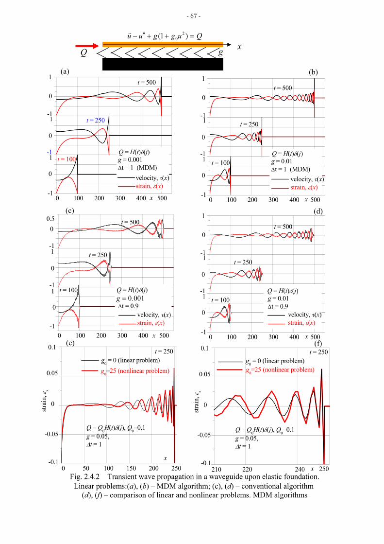
- 67 -

Fig. 2.4.2 Transient wave propagation in a waveguide upon elastic foundation. Linear problems:(a), (b) – MDM algorithm; (c), (d) – conventional algorithm

(d), (f) – comparison of linear and nonlinear problems. MDM algorithms

0 100 200 300 400 500

velocity, v(x)strain, ε(x)

1

-11

-1

-1

g = 0.001Δt = 1 (MDM)

Q = H(t)δ(j)

0

t = 250

x

0

0

t = 5001

t = 100

0 100 200 300 400 500

1

velocity, v(x)strain, ε(x)

-1

1

1

-1

-1

g = 0.01Δt = 1 (MDM)

Q = H(t)δ(j)

0

t = 250

x

0

0

t = 500

t = 100

0 100 200 300 400 500

velocity, v(x)

1

strain, ε(x)

-1

1

1

-1

-1

g = 0.01Δt = 0.9

Q = H(t)δ(j)

0

t = 250

x

0

0

t = 500

t = 100

0 100 200 300 400 500

velocity, v(x)

1

strain, ε(x)

-1

0.5

1

-1

-1

g = 0.01Δt = 0.9

Q = H(t)δ(j)

0

t = 250

x

0

0

t = 500

t = 100

Q g

Qugguu =++′′− )1( 20&&

x

0 50 100 150 200 250

g0 = 0 (linear problem) g0=25 (nonlinear problem)

0.1

x

-0.05

0.05

-0.1

Q = Q0H(t)δ(j), Q0=0.1 g = 0.05, Δt = 1

0

t = 250

strai

n, ε x

220 240

g0 = 0 (linear problem) g0=25 (nonlinear problem)

210

0.1

250x

.05

0.05

-0.1

Q = Q0H(t)δ(j), Q0=0.1 g = 0.05, Δt = 1

0

t = 250

strai

n, ε

001.0=g

(a) (b)

(c) (d)

(e) (f)

x

-0

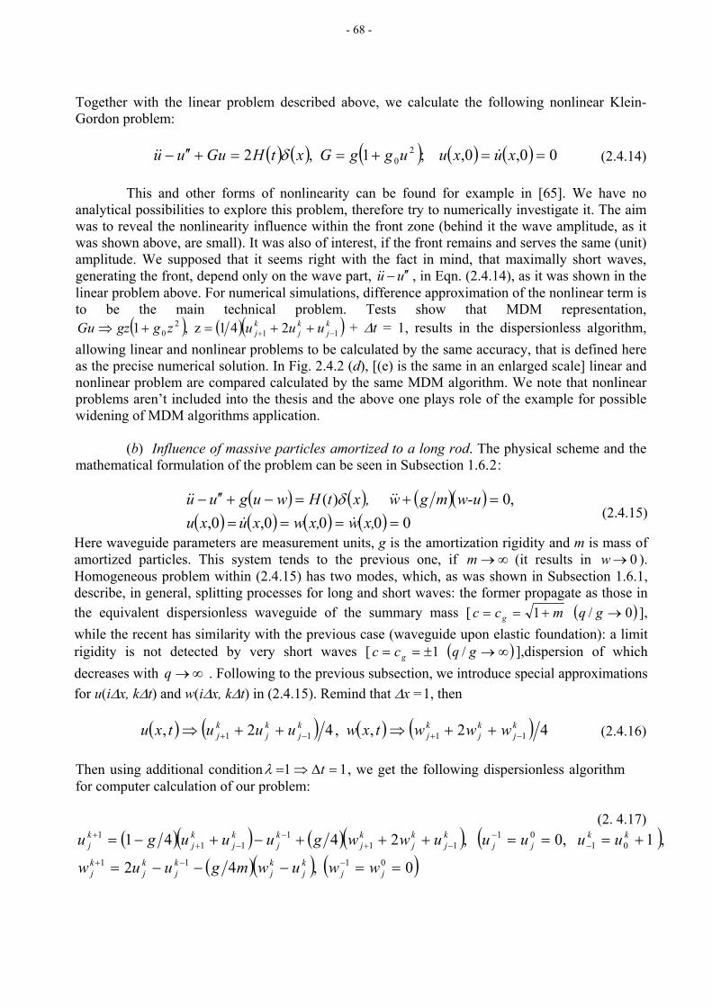
- 68 -

Together with the linear problem described above, we calculate the following nonlinear Klein-Gordon problem:

( ) ( ) ( ) ( ) ( ) 00,0, ;1 ,2 20 ==+==+′′− xuxuugg GxtHGuuu &&& δ (2.4.14)

This and other forms of nonlinearity can be found for example in [65]. We have no analytical possibilities to explore this problem, therefore try to numerically investigate it. The aim was to reveal the nonlinearity influence within the front zone (behind it the wave amplitude, as it was shown above, are small). It was also of interest, if the front remains and serves the same (unit) amplitude. We supposed that it seems right with the fact in mind, that maximally short waves, generating the front, depend only on the wave part, uu ′′−&& , in Eqn. (2.4.14), as it was shown in the linear problem above. For numerical simulations, difference approximation of the nonlinear term is to be the main technical problem. Tests show that MDM representation,

( ) ( )( ) 241z ,1 112

0kj

kj

kj uuuzggzGu −+ ++=+⇒ + Δt = 1, results in the dispersionless algorithm,

allowing linear and nonlinear problems to be calculated by the same accuracy, that is defined here as the precise numerical solution. In Fig. 2.4.2 (d), [(e) is the same in an enlarged scale] linear and nonlinear problem are compared calculated by the same MDM algorithm. We note that nonlinear problems aren’t included into the thesis and the above one plays role of the example for possible widening of MDM algorithms application. (b) Influence of massive particles amortized to a long rod. The physical scheme and the mathematical formulation of the problem can be seen in Subsection 1.6.2:

( ) ( ) ( )( )

( ) ( ) ( ) ( ) 0000, 0,,0)(

=====+=−+′′−

x,wx,wxuxuw-umgw, xtHwuguu

&&

&&&& δ (2.4.15)

Here waveguide parameters are measurement units, g is the amortization rigidity and m is mass of amortized particles. This system tends to the previous one, if ∞→m (it results in ). Homogeneous problem within (2.4.15) has two modes, which, as was shown in Subsection 1.6.1, describe, in general, splitting processes for long and short waves: the former propagate as those in the equivalent dispersionless waveguide of the summary mass [

0 →w

( )0/ 1 →+== gqmcc g ], while the recent has similarity with the previous case (waveguide upon elastic foundation): a limit rigidity is not detected by very short waves [ ( )∞→±== gqcc g / 1 ],dispersion of which decreases with . Following to the previous subsection, we introduce special approximations for u(iΔx, kΔt) and w(iΔx, kΔt) in (2.4.15). Remind that Δx =1, then

∞→q

( ) ( ) ( ) ( ) 42, ,42, 1111

kj

kj

kj

kj

kj

kj wwwtxwuuutxu −+−+ ++⇒++⇒ (2.4.16)

Then using additional condition 1=Δ⇒ 1 = tλ , we get the following dispersionless algorithm for computer calculation of our problem:

(2. 4.17) ( )( ) ( )( ) ( )

( )( ) ( )0 ,4 2

, 1 0, ,24 410111

0101

111

111

==−−−=

+===+++−+−=−−+

−−

−+−

−++

jjkj

kj

kj

kj

kj

kkjj

kj

kj

kj

kj

kj

kj

kj

wwuwmguuw

uuuuuwwguuugu

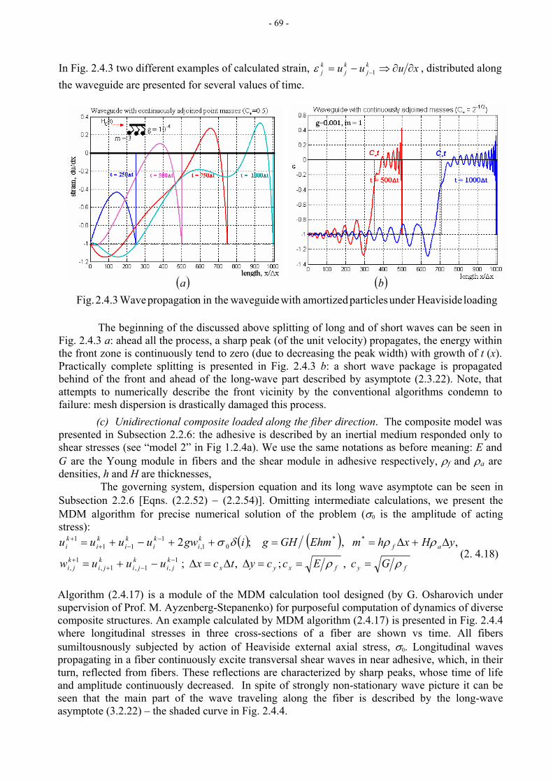
- 69 -

In Fig. 2.4.3 two different examples of calculated strain, xuuu kj

kj

kj ∂∂⇒−= −1ε , distributed along

the waveguide are presented for several values of time.

( ) ( )loading Heavisideunder particles amortized with waveguidein then propagatio Wave2.4.3 Fig.

ba

The beginning of the discussed above splitting of long and of short waves can be seen in Fig. 2.4.3 a: ahead all the process, a sharp peak (of the unit velocity) propagates, the energy within the front zone is continuously tend to zero (due to decreasing the peak width) with growth of t (x). Practically complete splitting is presented in Fig. 2.4.3 b: a short wave package is propagated behind of the front and ahead of the long-wave part described by asymptote (2.3.22). Note, that attempts to numerically describe the front vicinity by the conventional algorithms condemn to failure: mesh dispersion is drastically damaged this process.

(c) Unidirectional composite loaded along the fiber direction. The composite model was presented in Subsection 2.2.6: the adhesive is described by an inertial medium responded only to shear stresses (see “model 2” in Fig 1.2.4a). We use the same notations as before meaning: E and G are the Young module in fibers and the shear module in adhesive respectively, ρf and ρa are densities, h and H are thicknesses,

The governing system, dispersion equation and its long wave asymptote can be seen in Subsection 2.2.6 [Eqns. (2.2.52) − (2.2.54)]. Omitting intermediate calculations, we present the MDM algorithm for precise numerical solution of the problem (σ0 is the amplitude of acting stress):

( ) ( ) , ; , ;

, , ; 21

,1,1,1

,

**01,

111

1

fyfxyxk

jik

jik

jik

ji

afki

ki

ki

ki

ki

GcEccytcxuuuw

yHxhmEhmGHgigwuuuu

ρρ

ρρδσ

===ΔΔ=Δ−+=

Δ+Δ==++−+=−

−++

−−+

+

(2. 4.18)

Algorithm (2.4.17) is a module of the MDM calculation tool designed (by G. Osharovich under supervision of Prof. M. Ayzenberg-Stepanenko) for purposeful computation of dynamics of diverse composite structures. An example calculated by MDM algorithm (2.4.17) is presented in Fig. 2.4.4 where longitudinal stresses in three cross-sections of a fiber are shown vs time. All fibers sumiltousnously subjected by action of Heaviside external axial stress, σ0. Longitudinal waves propagating in a fiber continuously excite transversal shear waves in near adhesive, which, in their turn, reflected from fibers. These reflections are characterized by sharp peaks, whose time of life and amplitude continuously decreased. In spite of strongly non-stationary wave picture it can be seen that the main part of the wave traveling along the fiber is described by the long-wave asymptote (3.2.22) – the shaded curve in Fig. 2.4.4.

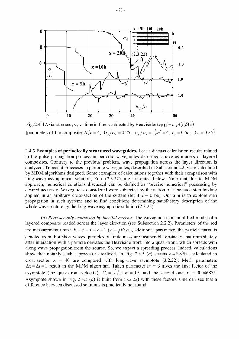
- 70 -

(6)

σ 0 0.5

x = 20h

x =10h

x = 5h

20h 10h x = 5h

H

h

0

1.0

0

0

2.4.5 Examples of periodically structured waveguides. Let us discuss calculation results related to the pulse propagation process in periodic waveguides described above as models of layered composites. Contrary to the previous problem, wave propagation across the layer direction is analyzed. Transient processes in periodic waveguides, described in Subsection 2.2, were calculated by MDM algorithms designed. Some examples of calculations together with their comparison with long-wave asymptotical solution, Eqn. (2.3.22), are presented below. Note that due to MDM approach, numerical solutions discussed can be defined as “precise numerical” possessing by desired accuracy. Waveguides considered were subjected by the action of Heaviside step loading applied in an arbitrary cross-section of the system (let it x = 0 be). Our aim is to explore step propagation in such systems and to find conditions determining satisfactory description of the whole wave picture by the long-wave asymptotic solution (2.3.22). (a) Rods serially connected by inertial masses. The waveguide is a simplified model of a layered composite loaded across the layer direction (see Subsection 2.2.2). Parameters of the rod are measurement units: 1==== cLE ρ ( ρEc = ), additional parameter, the particle mass, is denoted as m. For short waves, particles of finite mass are insuperable obstacles that immediately after interaction with a particle deviates the Heaviside front into a quasi-front, which spreads with along wave propagation from the source. So, we expect a spreading process. Indeed, calculations show that notably such a process is realized. In Fig. 2.4.5 (a) strains, xu ∂∂=ε , calculated in cross-section x = 40 are compared with long-wave asymptote (3.2.22). Mesh parameters

result in the MDM algorithm. Taken parameter m = 3 gives the first factor of the asymptote (the quasi-front velocity),

1=Δ=Δ tx5.011* =+= mC and the second one, α = 0.046875.

Asymptote shown in Fig. 2.4.5 (a) is built from (3.2.22) with these factors. One can see that a difference between discussed solutions is practically not found.

0 10 20 30 40 50 60

1.0

1.0 σ/σ

tc f

/h

)22.3.2(

0σ

σ

0σ

htc f

( ) ( )( )]0.25 ,0.5 4, 1 0.25, 4, :composite theof s[parameter

H step Heavisideby subjected fibersin time vs, , stresses Axial 2.4.4 Fig.

**

0

======

=

CccmEGhH

xtQ

xyxyxy ρρ

σ σ δ

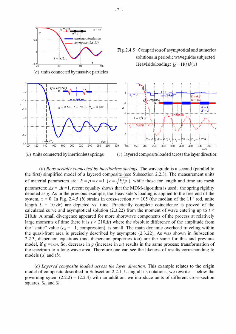
- 71 -

(b) Rods serially connected by inertionless springs. The waveguide is a second (parallel to

the first) simplified model of a layered composite (see Subsection 2.2.3). The measurement units of material parameters are: 1=== cE ρ ( ρEc = ), while those for length and time are mesh parameters: Δx = Δt =1, recent equality shows that the MDM-algorithm is used; the spring rigidity denoted as g. As in the previous example, the Heaviside’s loading is applied to the free end of the system, x = 0. In Fig. 2.4.5 (b) strains in cross-section x = 105 (the median of the 11th rod, unite length L = 10 Δx) are depicted vs. time. Practically complete coincidence is proved of the calculated curve and asymptotical solution (2.3.22) from the moment of wave entering up to t < 210Δt. A small divergence appeared for more shortwave components of the process at relatively large moments of time (here it is t > 210Δt) where the absolute difference of the amplitude from the “static” value (εst = −1, compression), is small. The main dynamic overhead traveling within the quasi-front area is precisely described by asymptote (2.3.22). As was shown in Subsection 2.2.3, dispersion equations (and dispersion properties too) are the same for this and previous model, if g =1/m. So, decrease in g (increase in m) results in the same process: transformation of the spectrum to a long-wave area. Therefore one can see the likeness of results corresponding to models (a) and (b).

(c) Layered composite loaded across the layer direction. This example relates to the origin

model of composite described in Subsection 2.2.1. Using all its notations, we rewrite below the governing sytem (2.2.2) − (2.2.4) with an addition: we introduce units of different cross-section squares, S1, and S2.

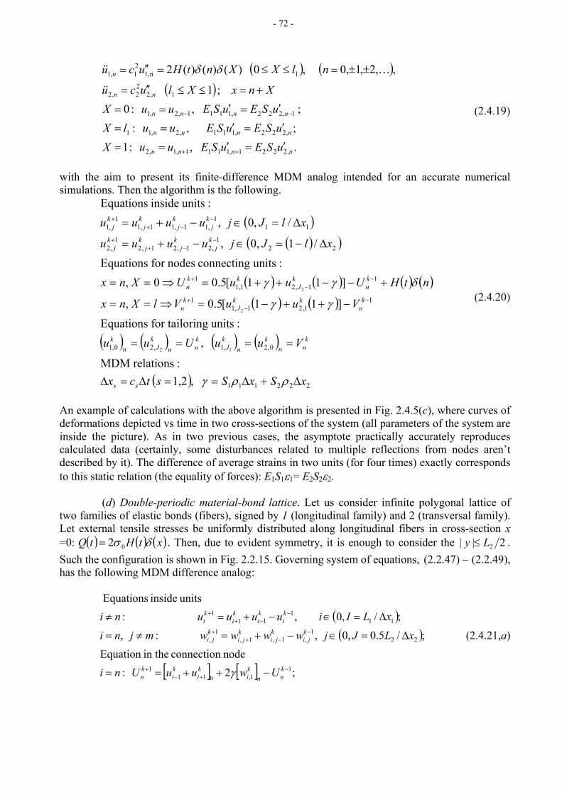
- 72 -

( ) ( )( )

. , :1; , :; , :0

; 1

,,2,1,0 ,0 )()()(2

,2221,1111,1,2

,222,111,2,11

1,222,1111,2,1

1,222,2

1n1,21,1

nnnn

nnnn

nnnn

nn

n

uSEuSEuuXuSEuSEuulX

uSEuSEuuXXnxXlucu

nlXXntHucu

′=′==

′=′==

′=′==

+=≤≤′′=

±±=≤≤=′′=

++

−−

&&

K&& δδ

(2.4.19)

with the aim to present its finite-difference MDM analog intended for an accurate numerical simulations. Then the algorithm is the following.

(2.4.20)

( )( )( )

( ) ( ) ( ) (( ) ( )

( ) ( ) ( ) ( )

( ) 222111

0,2,1,20,1

11,21,1

1

11,21,1

1

221

,21,21,21

,2

111

,11,11,11

,1

,1,2 :relations MDM

,:units ingfor tailor Equations

]11[5.0 ,

]11[5.00 ,:units connecting nodesfor Equations

/1,0 ,

/,0 ,:units inside Equations

12

2

2

xSxSstcx

VuuUuu

VuuVlXnx

ntHUuuUXnx

xlJjuuuu

xlJjuuuu

ss

knn

kn

kJ

knn

kJn

k

kn

kkJ

kn

kn

kJ

kkn

kj

kj

kj

kj

kj

kj

kj

kj

Δ+Δ==Δ=Δ

====

−++−=⇒==

+−−++=⇒==

Δ−=∈−+=

Δ=∈−+=

−−

+

−−

+

−−+

+

−−+

+

ρργ

γγ

δγγ )

An example of calculations with the above algorithm is presented in Fig. 2.4.5(c), where curves of deformations depicted vs time in two cross-sections of the system (all parameters of the system are inside the picture). As in two previous cases, the asymptote practically accurately reproduces calculated data (certainly, some disturbances related to multiple reflections from nodes aren’t described by it). The difference of average strains in two units (for four times) exactly corresponds to this static relation (the equality of forces): E1S1ε1= E2S2ε2.

(d) Double-periodic material-bond lattice. Let us consider infinite polygonal lattice of

two families of elastic bonds (fibers), signed by 1 (longitudinal family) and 2 (transversal family). Let external tensile stresses be uniformly distributed along longitudinal fibers in cross-section x =0: ( ) ( ) ( )xtHtQ δσ 02= . Then, due to evident symmetry, it is enough to consider the 2|| 2Ly ≤ . Such the configuration is shown in Fig. 2.2.15. Governing system of equations, (2.2.47) − (2.2.49), has the following MDM difference analog:

(2.4.21,a)

( )(

[ ] [ ] ; 2 :node connection in theEquation

;/5.0,0 , : ,

;/,0 , :units inside Equations

11,n11

1

221

,1,1,1

,

111

111

−+−

+

−−+

+

−−+

+

−++==

Δ=∈−+=≠=

Δ=∈−+=≠

knn

ki

ki

ki

kn

kji

kji

kji

kji

ki

ki

ki

ki

UwuuUni

xLJjwwwwmjni

xLIiuuuuni

γ

)

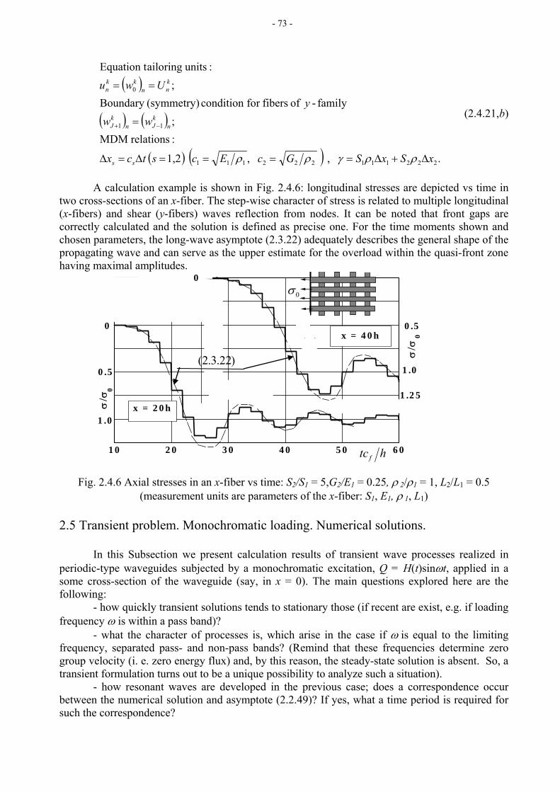
- 73 -

( )

( ) ( )

( ) ( ) . , , 1,2

:relations MDM;

family - of fibersfor condition (symmetry)Boundary ;

:units ailoringEquation t

222111222111

11

0

xSxSGcEcstcx

wwy

Uwu

ss

nkJn

kJ

knn

kkn

Δ+Δ====Δ=Δ

=

==

−+

ρργρρ

(2.4.21,b)

A calculation example is shown in Fig. 2.4.6: longitudinal stresses are depicted vs time in

two cross-sections of an x-fiber. The step-wise character of stress is related to multiple longitudinal (x-fibers) and shear (y-fibers) waves reflection from nodes. It can be noted that front gaps are correctly calculated and the solution is defined as precise one. For the time moments shown and chosen parameters, the long-wave asymptote (2.3.22) adequately describes the general shape of the propagating wave and can serve as the upper estimate for the overload within the quasi-front zone having maximal amplitudes.

1 0 2 0 3 0 4 0 5 0 6 0

σ/σ

0

0σ

/σ

0

0 .5σ

0

x = 4 0 h

x = 2 0 h

(6 )

1 .2 5

(6 )

1 .0

0 .5

0

1 .0

0

tc /h

)22.3.2(

0σ

htcf

Fig. 2.4.6 Axial stresses in an x-fiber vs time: S2/S1 = 5,G2/E1 = 0.25, ρ 2/ρ1 = 1, L2/L1 = 0.5 (measurement units are parameters of the x-fiber: S1, E1, ρ 1, L1)

2.5 Transient problem. Monochromatic loading. Numerical solutions.

In this Subsection we present calculation results of transient wave processes realized in periodic-type waveguides subjected by a monochromatic excitation, Q = H(t)sinωt, applied in a some cross-section of the waveguide (say, in x = 0). The main questions explored here are the following:

- how quickly transient solutions tends to stationary those (if recent are exist, e.g. if loading frequency ω is within a pass band)?

- what the character of processes is, which arise in the case if ω is equal to the limiting frequency, separated pass- and non-pass bands? (Remind that these frequencies determine zero group velocity (i. e. zero energy flux) and, by this reason, the steady-state solution is absent. So, a transient formulation turns out to be a unique possibility to analyze such a situation).

- how resonant waves are developed in the previous case; does a correspondence occur between the numerical solution and asymptote (2.2.49)? If yes, what a time period is required for such the correspondence?

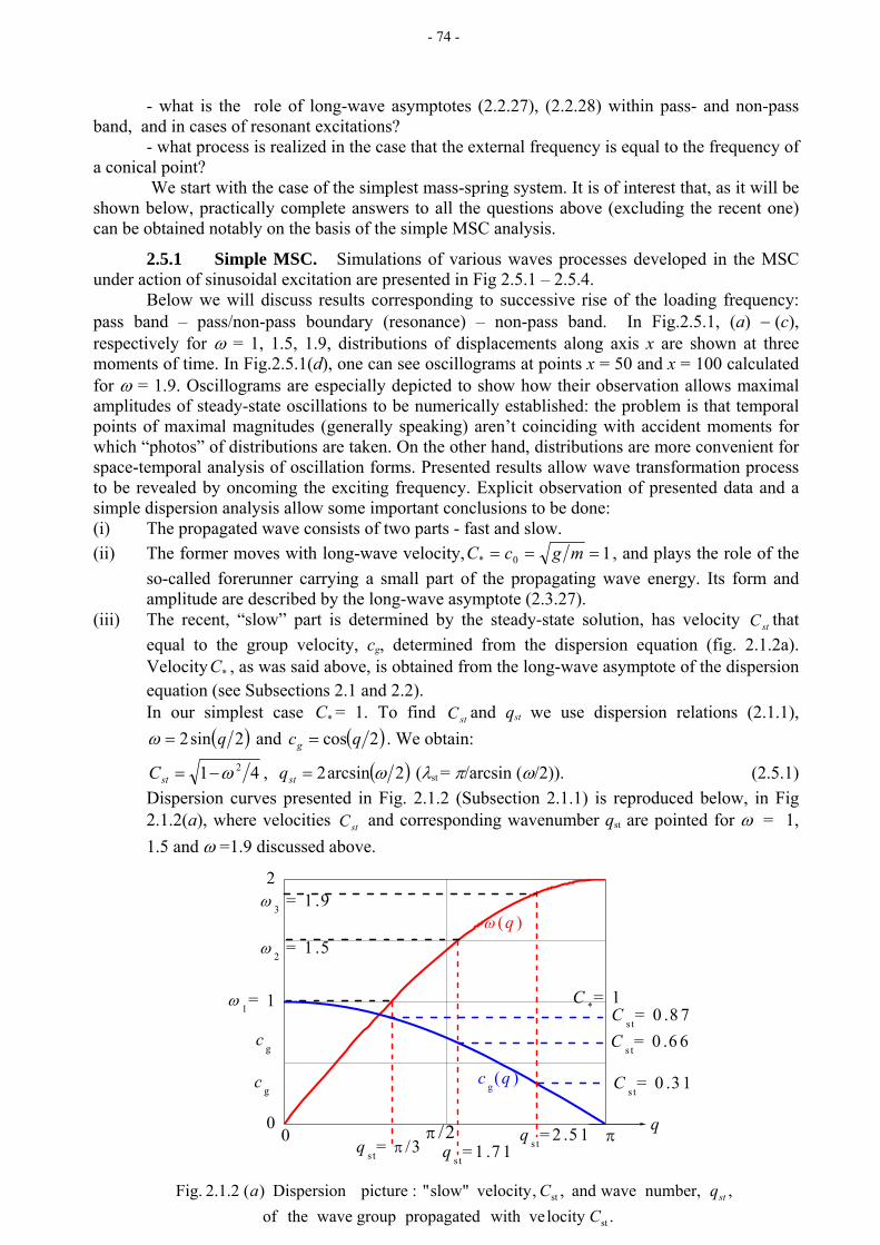
- 74 -

- what is the role of long-wave asymptotes (2.2.27), (2.2.28) within pass- and non-pass band, and in cases of resonant excitations?

- what process is realized in the case that the external frequency is equal to the frequency of a conical point?

We start with the case of the simplest mass-spring system. It is of interest that, as it will be shown below, practically complete answers to all the questions above (excluding the recent one) can be obtained notably on the basis of the simple MSC analysis.

2.5.1 Simple MSC. Simulations of various waves processes developed in the MSC under action of sinusoidal excitation are presented in Fig 2.5.1 – 2.5.4.

Below we will discuss results corresponding to successive rise of the loading frequency: pass band – pass/non-pass boundary (resonance) – non-pass band. In Fig.2.5.1, (a) − (c), respectively for ω = 1, 1.5, 1.9, distributions of displacements along axis x are shown at three moments of time. In Fig.2.5.1(d), one can see oscillograms at points x = 50 and x = 100 calculated for ω = 1.9. Oscillograms are especially depicted to show how their observation allows maximal amplitudes of steady-state oscillations to be numerically established: the problem is that temporal points of maximal magnitudes (generally speaking) aren’t coinciding with accident moments for which “photos” of distributions are taken. On the other hand, distributions are more convenient for space-temporal analysis of oscillation forms. Presented results allow wave transformation process to be revealed by oncoming the exciting frequency. Explicit observation of presented data and a simple dispersion analysis allow some important conclusions to be done: (i) The propagated wave consists of two parts - fast and slow. (ii) The former moves with long-wave velocity, 10* === mgcC , and plays the role of the

so-called forerunner carrying a small part of the propagating wave energy. Its form and amplitude are described by the long-wave asymptote (2.3.27).

(iii) The recent, “slow” part is determined by the steady-state solution, has velocity that equal to the group velocity, c

stCg, determined from the dispersion equation (fig. 2.1.2a).

Velocity , as was said above, is obtained from the long-wave asymptote of the dispersion equation (see Subsections 2.1 and 2.2).

*C

In our simplest case = 1. To find and q*C stC st we use dispersion relations (2.1.1), ( 2sin2 q= )ω and ( 2cos qcg = ) . We obtain:

41 2ω−=stC , ( )2arcsin2 ω=stq (λst = π/arcsin (ω/2)). (2.5.1) Dispersion curves presented in Fig. 2.1.2 (Subsection 2.1.1) is reproduced below, in Fig 2.1.2(a), where velocities and corresponding wavenumber qstC st are pointed for ω = 1, 1.5 and ω =1.9 discussed above.

0 .0

0

1

2

Cs t

= 0 .3 1

Cs t

= 0 .6 6C

s t= 0 .8 7

qs t

= 2 .5 1q

s t= π /3

ω1=

ω3 = 1 .9

cg

cg

q = 1 .7 1st

ω2 = 1 .5

C*= 1

cg(q )

π /2 π0 q

ω (q )

.locity with vepropagated group wave theof , number, waveand , , velocityslow"" :picture Dispersion )( 2.1.2 Fig.

st

st

CqCa st

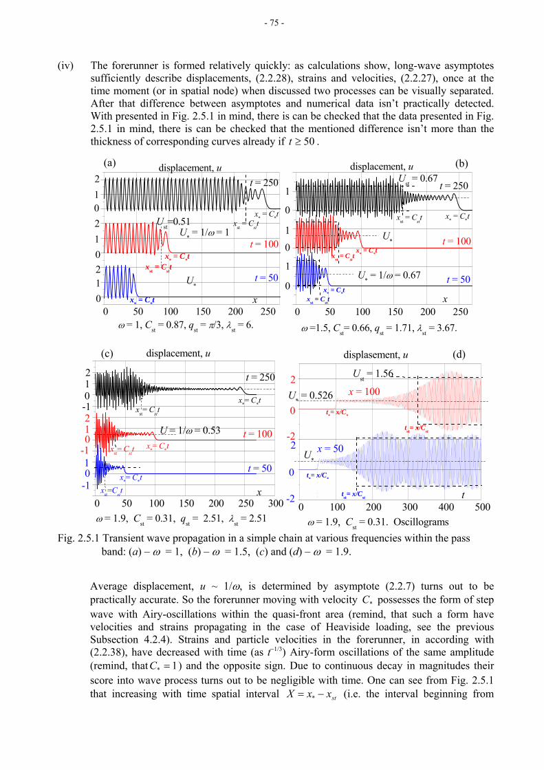
- 75 -

(iv) The forerunner is formed relatively quickly: as calculations show, long-wave asymptotes sufficiently describe displacements, (2.2.28), strains and velocities, (2.2.27), once at the time moment (or in spatial node) when discussed two processes can be visually separated. After that difference between asymptotes and numerical data isn’t practically detected. With presented in Fig. 2.5.1 in mind, there is can be checked that the data presented in Fig. 2.5.1 in mind, there is can be checked that the mentioned difference isn’t more than the thickness of corresponding curves already if . 50≥t

0 50 100 150 200 250

Ust = 0.671

1

0

0U*

xst = Cstt

xst = Csttx

* = C

*t

xst = Cstt x* = C*t

1

x* = C

*t

U* = 1/ω = 0.67

ω =1.5, Cst= 0.66, qst = 1.71, λst = 3.67.

displacement, u

x0

t = 250

t = 50

t = 100

0 50 100 150 200 250

Ust=0.51

2102

2U*

xst = C

sttx* = C*t

1

1

xst = C

stt

x* = C

*t

x* = C*t

U* = 1/ω = 1

ω = 1, Cst = 0.87, qst = π/3, λst = 6.

0

displacement, u

x0

t = 250

t = 50

t = 100

0 100 200 300 400 500

U* = 0.526

Ust = 1.56

tst= x/C

st

U*

t*= x/C

*

tst= x/C

st

x = 100

-2

2

t*= x/C

*0

2

ω = 1.9, Cst = 0.31. Oscillograms

0

displasement, u

t-2

x = 50

0 50 100 150 200 250 300

x*= C

*t

1

-10

-1

1

xst= C

stt

2

-101

x*= C

*tx

st= C

stt

2

xst=C

stt

U = 1/ω = 0.53

x*= C

*t

ω = 1.9, Cst = 0.31, q

st = 2.51, λ

st = 2.51

displacement, u

x

0

t = 250

t = 50

(a) (b)

(c) (d)

t = 100

Fig. 2.5.1 Transient wave propagation in a simple chain at various frequencies within the pass band: (a) – ω = 1, (b) – ω = 1.5, (c) and (d) – ω = 1.9.

Average displacement, u ~ 1/ω, is determined by asymptote (2.2.7) turns out to be practically accurate. So the forerunner moving with velocity possesses the form of step wave with Airy-oscillations within the quasi-front area (remind, that such a form have velocities and strains propagating in the case of Heaviside loading, see the previous Subsection 4.2.4). Strains and particle velocities in the forerunner, in according with (2.2.38), have decreased with time (as t

*C

−1/3) Airy-form oscillations of the same amplitude (remind, that 1* =C ) and the opposite sign. Due to continuous decay in magnitudes their score into wave process turns out to be negligible with time. One can see from Fig. 2.5.1 that increasing with time spatial interval stxxX −= * (i.e. the interval beginning from

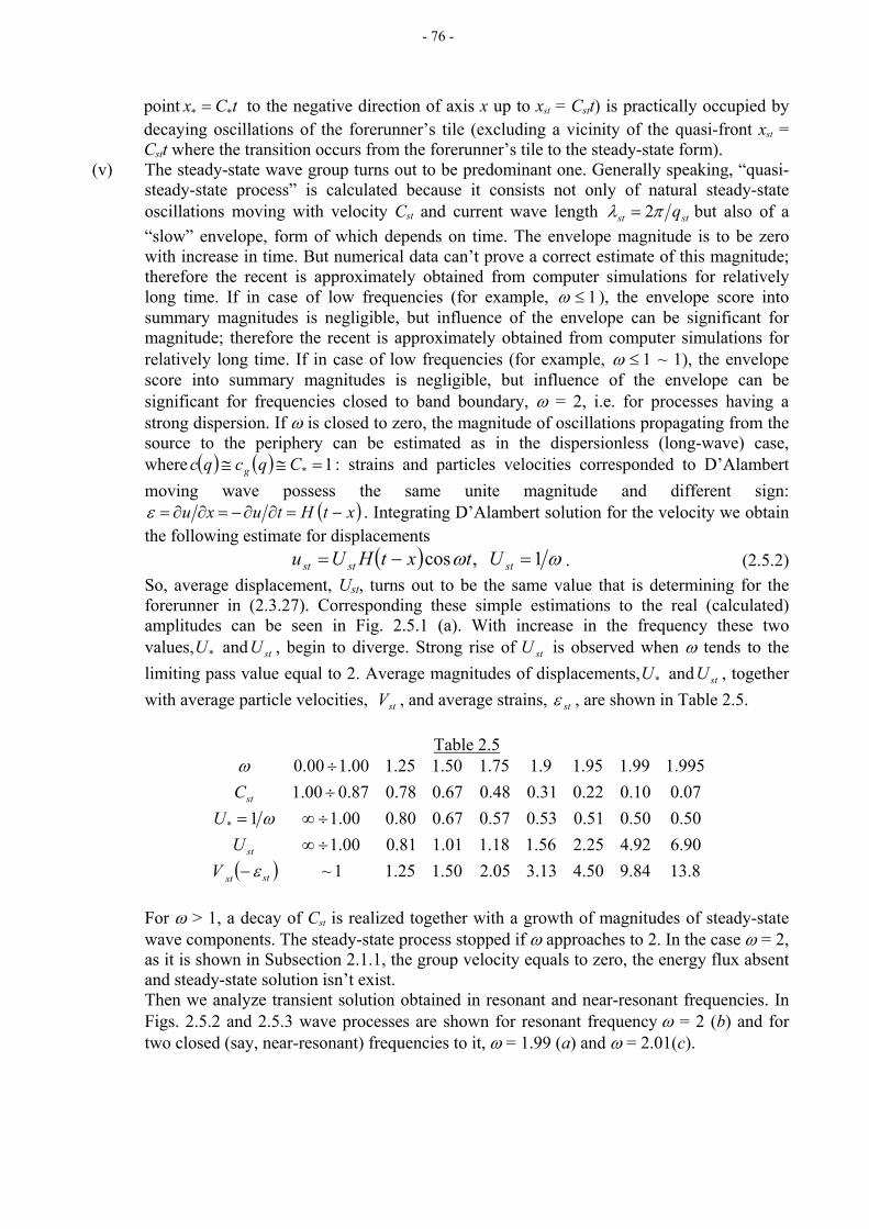
- 76 -

point to the negative direction of axis x up to xtCx ** = st = Cstt) is practically occupied by decaying oscillations of the forerunner’s tile (excluding a vicinity of the quasi-front xst = Cstt where the transition occurs from the forerunner’s tile to the steady-state form).

(v) The steady-state wave group turns out to be predominant one. Generally speaking, “quasi-steady-state process” is calculated because it consists not only of natural steady-state oscillations moving with velocity Cst and current wave length stst qπλ 2= but also of a “slow” envelope, form of which depends on time. The envelope magnitude is to be zero with increase in time. But numerical data can’t prove a correct estimate of this magnitude; therefore the recent is approximately obtained from computer simulations for relatively long time. If in case of low frequencies (for example, 1≤ω ), the envelope score into summary magnitudes is negligible, but influence of the envelope can be significant for magnitude; therefore the recent is approximately obtained from computer simulations for relatively long time. If in case of low frequencies (for example, 1≤ω ~ 1), the envelope score into summary magnitudes is negligible, but influence of the envelope can be significant for frequencies closed to band boundary, ω = 2, i.e. for processes having a strong dispersion. If ω is closed to zero, the magnitude of oscillations propagating from the source to the periphery can be estimated as in the dispersionless (long-wave) case, where : strains and particles velocities corresponded to D’Alambert moving wave possess the same unite magnitude and different sign:

( ) ( ) 1* =≅≅ Cqcqc g

( xtHtuxu −= )∂∂−=∂∂=ε . Integrating D’Alambert solution for the velocity we obtain the following estimate for displacements

( ) ωω 1 ,cos =−= ststst UtxtHUu . (2.5.2) So, average displacement, Ust, turns out to be the same value that is determining for the forerunner in (2.3.27). Corresponding these simple estimations to the real (calculated) amplitudes can be seen in Fig. 2.5.1 (a). With increase in the frequency these two values, , begin to diverge. Strong rise of is observed when ω tends to the limiting pass value equal to 2. Average magnitudes of displacements, , together with average particle velocities, , and average strains,

stUU and * stU

stUU and *

stV stε , are shown in Table 2.5.

Table 2.5

( ) 8.1384.950.413.305.250.125.11~90.692.425.256.118.101.181.000.150.050.051.053.057.067.080.000.1107.010.022.031.048.067.078.087.000.1

995.199.195.19.175.150.125.100.100.0

*

stst

st

st

VU

C

ε

ω

ω

−÷∞÷∞=÷÷

U

For ω > 1, a decay of Cst is realized together with a growth of magnitudes of steady-state wave components. The steady-state process stopped if ω approaches to 2. In the case ω = 2, as it is shown in Subsection 2.1.1, the group velocity equals to zero, the energy flux absent and steady-state solution isn’t exist. Then we analyze transient solution obtained in resonant and near-resonant frequencies. In Figs. 2.5.2 and 2.5.3 wave processes are shown for resonant frequency ω = 2 (b) and for two closed (say, near-resonant) frequencies to it, ω = 1.99 (a) and ω = 2.01(c).

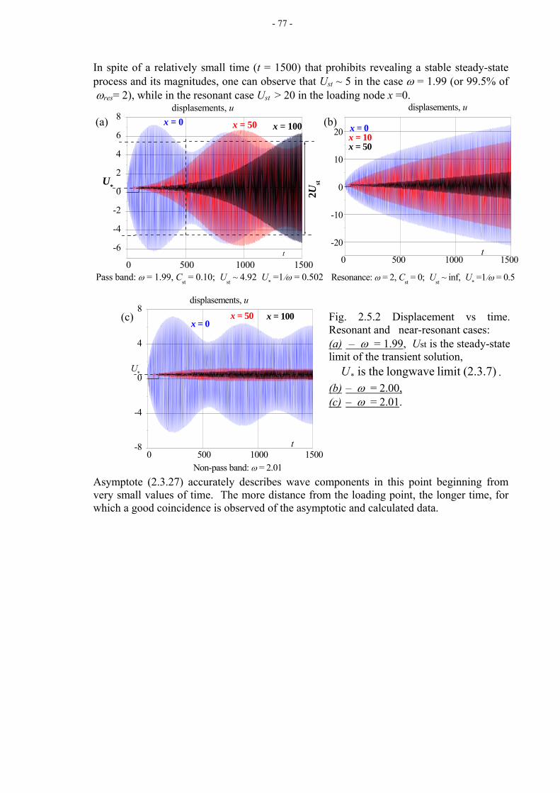
- 77 -

In spite of a relatively small time (t = 1500) that prohibits revealing a stable steady-state process and its magnitudes, one can observe that Ust ~ 5 in the case ω = 1.99 (or 99.5% of ωres= 2), while in the resonant case Ust > 20 in the loading node x =0.

0 500 1000 1500-8

-4

0

4

8x = 100x = 50

U*

Non-pass band: ω = 2.01

displasements, u

t

x = 0

0 500 1000 1500

-20

-10

0

10

20x = 50

Resonance: ω = 2, Cst = 0; Ust ~ inf, U* =1/ω = 0.5

displasements, u

t

x = 0

0 500 1000 1500

-6

-4

-2

0

2

4

6

8x = 50 x = 100

x = 10

2UstU*

Pass band: ω = 1.99, Cst = 0.10; Ust ~ 4.92 U* =1/ω = 0.502

displasements, u

t

x = 0(a) (b)

Fig. 2.5.2 Displacement vs time. Resonant and near-resonant cases: (a) – ω = 1.99, Ust is the steady-state limit of the transient solution, . (2.3.7)limit longwave theis *U(b) – ω = 2.00, (c) – ω = 2.01.

(c)

Asymptote (2.3.27) accurately describes wave components in this point beginning from very small values of time. The more distance from the loading point, the longer time, for which a good coincidence is observed of the asymptotic and calculated data.

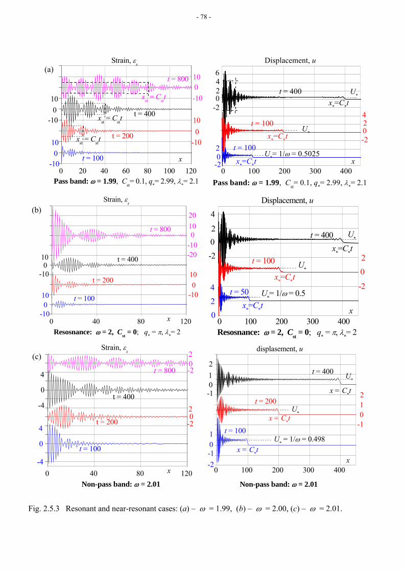
- 78 -

Fig. 2.5.3 Resonant and near-resonant cases: (a) – ω = 1.99, (b) – ω = 2.00, (c) – ω = 2.01.

0 20 40 60 80 100 120

xst = Cstt

xst = Cstt

xst = Cstt0-10

10

t = 400-10

10

Pass band: ω = 1.99, Cst= 0.1, q*= 2.99, λ*= 2.1

-10

10

t = 800

Strain, εx

x

0

0 t = 100

t = 200

10

-100

0 40 80 120Resosnance: ω = 2, Cst = 0; q* = π, λ*= 2

-20

0-10

1020

t = 400

-10

10

-10

10

t = 800

Strain, εx

x

0

0t = 100

t = 20010

-100

0 40 80 120

0-2

2

t = 400-4

4

Non-pass band: ω = 2.01

-4

4

t = 800

Strain, εx

x

0

0 t = 100

t = 200

2

-20

0 100 200 300 400

x = C*t

x = C*t

U*

U* = 1/ω = 0.498

U*

2

1

-2-1

x = C*t

21

-1

10-1

0

0

Non-pass band: ω = 2.01

t = 400

displasement, u

x

t = 100

t = 200

0 100 200 300 400

U*

U*

x*=C*t

20x*=C*t-2

-2

4

2

2

U*= 1/ω = 0.5

x*=C*t

Resosnance: ω = 2, Cst = 0; q* = π, λ*= 2

4

Displacement, u

x

0

0

t = 400

t = 50

t = 100

0 100 200 300 400

6

Pass band: ω = 1.99, Cst= 0.1, q*= 2.99, λ*= 2.1

U*

U*

x*=C

*t

420

x*=C*t -2

-2

42

-2

U*= 1/ω = 0.5025

x*=C*t

2

Displacement, u

x

0

0

t = 400

t = 100

(a)

t = 100

(b)

(c)

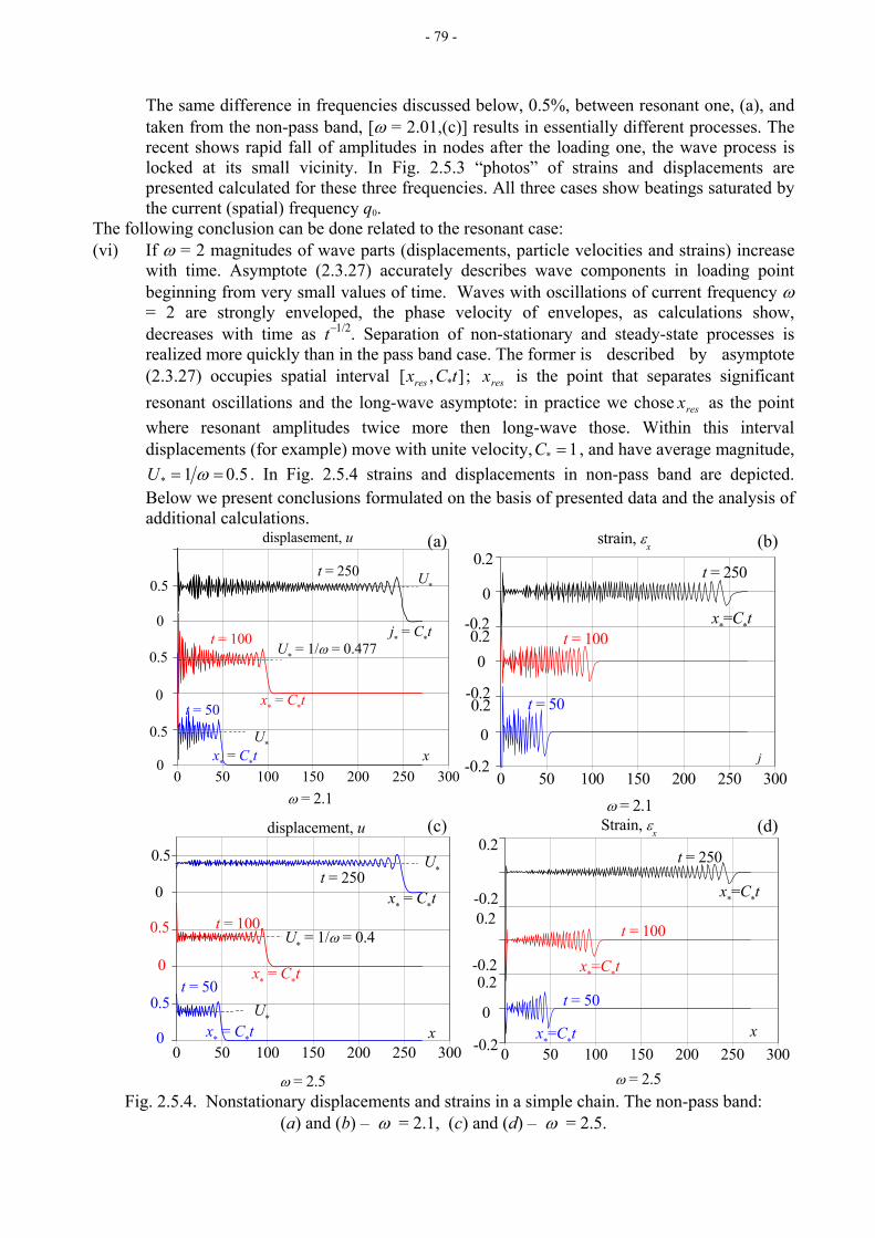
- 79 -

The same difference in frequencies discussed below, 0.5%, between resonant one, (a), and taken from the non-pass band, [ω = 2.01,(c)] results in essentially different processes. The recent shows rapid fall of amplitudes in nodes after the loading one, the wave process is locked at its small vicinity. In Fig. 2.5.3 “photos” of strains and displacements are presented calculated for these three frequencies. All three cases show beatings saturated by the current (spatial) frequency q0.

The following conclusion can be done related to the resonant case: (vi) If ω = 2 magnitudes of wave parts (displacements, particle velocities and strains) increase

with time. Asymptote (2.3.27) accurately describes wave components in loading point beginning from very small values of time. Waves with oscillations of current frequency ω = 2 are strongly enveloped, the phase velocity of envelopes, as calculations show, decreases with time as t−1/2. Separation of non-stationary and steady-state processes is realized more quickly than in the pass band case. The former is described by asymptote (2.3.27) occupies spatial interval ; is the point that separates significant resonant oscillations and the long-wave asymptote: in practice we chose as the point where resonant amplitudes twice more then long-wave those. Within this interval displacements (for example) move with unite velocity,

],[ *tCxres resx

resx

1* =C , and have average magnitude, 5.01* == ωU . In Fig. 2.5.4 strains and displacements in non-pass band are depicted.

Below we present conclusions formulated on the basis of presented data and the analysis of additional calculations.

0 50 100 150 200 250 300

U* = 1/ω = 0.477

x* = C

*t

x* = C*t

U*

ω = 2.1

displasement, u

0.5

0.5

0.5 U*

j* = C

*t

0

x

0

0

t = 250

t = 50

t = 100

0 50 100 150 200 250 300x* = C*t

x* = C*t

0.5

0.5

0.5

U*

U* = 1/ω = 0.4

U*

x* = C*t

ω = 2.5

0

displacement, u

x

0t = 250

t = 50

t = 100

0

0 50 100 150 200 250 300

0

0.2

0.2

0.2

-0.2

-0.2

x*=C

*t

x*=C*t

-0.2

ω = 2.5

t = 50

Strain, εx

x

t = 250

x*=C*t

t = 100

0 50 100 150 200 250 300

x*=C*t

t = 250

0.2

0.2

0.2

-0.2

-0.2

-0.2

ω = 2.1

0

strain, εx

j

0

0

t = 50

(a) (b)

t = 100

(c) (d)

Fig. 2.5.4. Nonstationary displacements and strains in a simple chain. The non-pass band:

(a) and (b) – ω = 2.1, (c) and (d) – ω = 2.5.

- 80 -

(vii) Very quickly (the more distant from ω = 2 the more quickly) the long-wave part, described by asymptote (2.3.27) becomes dominant: others non-stationary perturbations have chaotic type and practically not revealed if the frequency relatively distant from ω = 2. Accordingly to calculations and asymptote (2.3.27) strains and particle velocities decrease with time (distance) as t−1/3 (x−1/3), while displacements have constant average magnitude,

5.01* == ωU , moving with unite velocity, 1* =C . In the discussed case of the simple SMC, the conclusions (i) − (vii) above give comprehensive answers for the questions formulated at the beginning Subsection 2.5. 2.5.2 Two-mode Born’s chain. The model is described in Subsection 2.1.2 where sufficiently complete information is presented related to dispersion properties of the chain. A set of questions including waves propagated in pass- and non-pass bands could be covered by the approach was used in the previous case. We omit results looking like to described above excluding resonant cases, where Born’s chain has some differences. Firstly, we have two shortwave resonances here (corresponding to the each mode) and secondly, formation of resonant waves of corresponding mode depends on the loaded node number (having masses m1 or m2).

In Fig. 2.5.5 strains 1) ( ,)1]([])([ =Δ−−= xxuxuε , are depicted. Chosen masses of particles generating the chain are ,2 ,1 21 == mm while springs have the same rigidity: 121 == gg (i.e. beginning from particle j = 0 of mass m1 = 1, masses of all even particles are m1, and of odd those – m2). Particle j = 0 is taken as the loading point. As it can be obtained from dispersion equation (2.1.8), see also Fig. 2.1.6, the parameters above result in resonant frequencies

2,1 =resω and 2,2 =resω . Analysis of partial systems (see Eqn. 2.1.14 and Fig. 2.1.18) proves that the spatial wave form corresponding to frequency res,1ω determines contra-phase oscillations of heavy particles, while light those are at rest.

0 50 100 150 200

t = 500

t = 325

t = 250

ε

105

5

5

5

-5

-5

-50

0

0

0-5

x0 100 200 300 400 500

-15

-10

-5

0

5

10

15ε

j = 6 (m = 1)t

t = 125j = 5 (m = 2)

(a) Strains vs time (b) Strains vs spatial coordinate, x

Fig. 2.5.5 Second resonance in the Born’s chain: ,121 == gg .2 ,2 ,1 ,221 ==== resmm ωω The alternate form is revealed in the case res,2ωω = : heavy particles are at rest and light those

belong at contra-phase oscillations. So, the resonant rise is realized for odd particles. Strain growth with time (growth of particle velocities and displacements as well) has the same degree that was realized in the simple MSC ~ t1/2 that can be observed in Fig. 2.5.5 (a). Strains distributed along

- 81 -

axis x are structured by the current wavelength (λ = 2, corresponding to q = π), and two envelopes: the inner one has frequency increasing along axis x, the outer one seems to an exponentially decaying (with respect to positive direction of axis x) dependence. In Fig.2.5.6 strain ocsillograms are presented for four events of diverse loadings: light and heavy particles are successively loaded by force Q = sin(ωt) with frequencies 2,1 == resωω and 2,1 == resωω . One can see that resonant oscillations are formed in cases (b) and (c), while a practically dispersionless wave transmission is observed for (a) and (d).

0 100 200 300 400 500

-20

-10

0

10

20

j = 0

t

j = 10

... 2 1 0 =j

0 100 200 300 400 500-15

-10

-5

0

5

10

15

0 100 200 300 400 500-1.5

-1.0

-0.5

0.0

0.5

1.0

1.5j = 0

t

j = 0,

t

j = 100,

j = 10

300

j = 10 ... 2 1 0 =j ... 2 1 0 j =

(a) Transmission m1=0.5, m2=1 ( )2,1 == resωω (b) Resonance: m1=1, m2=0.5 ( )2,1 == resωω

0 100 200 300 400 500 -1.5

-1.0

-0.5

0.0

0.5

1.0

1.5 ... 2 1 0 =j j = 0 j = 10

t (c) Resonance: m1=0.5, m2=1 (ω = ω2,res = 2) (d) Transmission: m1=1, m2=0.5 (ω =ω2,res= 2)

Fig.2.5.6. Excitation of the Born’s chain (g1 = g2 = 1) by force F = sin(ωt) applied to particle j =0.

- 82 -

2.5.3 Periodic waveguide: layered composite loaded across layers. We discuss the model in the title above several times: in Subsection 2.2, where its dispersion features were explored, in Subsection 2.3, where this model was taken as a basis for designing long-wave asymptotes, and, at last, in Subsection 2.4, where wave propagation processes under step loading were numerically investigated and applicability of the long-wave asymptote was revealed. Here we analyze numerical results corresponding to a monochromatic excitation of the system within a wide spectral interval of loading. Because we have no analytical formulas for describing time dependent waves of arbitrary spectrum, numerical simulations remain a unique possibility to obtain transient solutions. In Fig. 2.5.7 and 2.5.8 presented calculation results are related to the composite, characterized by parameters: E1 = ρ1 = 0.5, E2 = ρ 2 = 1, l = 0.5L. In the calculation algorithm period L consists of 10 spatial steps (L = 10Δx), step, Δx is taken as the length unite, the time unite be 22 ρExΔ . Dispersion picture for the chosen composite is shown in Fig. 2.2.3, pass band boundaries can be seen in Table 2.3. In according with the abovementioned data, first two pass bands are (0 - 2.46) (3.82 – 8.74). Note that ω =2π (the frequency falls within the second pass band) is the so called conical point, ωc [see Subsection 2.2 and definition (2.2.21)], whose role in transient processes has not yet been elucidated.

( )a ( )b

( )c( )d ( )e

point conical at the and bands pass -non pass-, within structures Wave2.5.7 Fig.

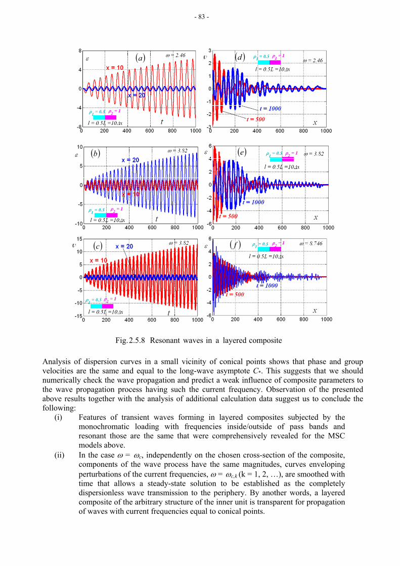
- 83 -

( )a

( )b

( )c ( )f

( )e

( )d

composite layered ain wavesResonant 2.5.8 Fig. Analysis of dispersion curves in a small vicinity of conical points shows that phase and group velocities are the same and equal to the long-wave asymptote C*. This suggests that we should numerically check the wave propagation and predict a weak influence of composite parameters to the wave propagation process having such the current frequency. Observation of the presented above results together with the analysis of additional calculation data suggest us to conclude the following:

(i) Features of transient waves forming in layered composites subjected by the monochromatic loading with frequencies inside/outside of pass bands and resonant those are the same that were comprehensively revealed for the MSC models above.

(ii) In the case ω = ωc, independently on the chosen cross-section of the composite, components of the wave process have the same magnitudes, curves enveloping perturbations of the current frequencies, ω = ωc,k (k = 1, 2, …), are smoothed with time that allows a steady-state solution to be established as the completely dispersionless wave transmission to the periphery. By another words, a layered composite of the arbitrary structure of the inner unit is transparent for propagation of waves with current frequencies equal to conical points.

- 84 -

2.6 Waveguides of a quasi periodic structure. Statistical approach

In practice, waveguide structures have a spread of characteristics probabilistic in nature. In this subsection we describe a probabilistic version of the waveguide structure, rod with adjoined masses referred in Subsection 2.2.2. We simulate propagation of Heaviside step by a set of numerical simulations with the aim to compare the obtained results with the asymptotic estimate (2.3.22) corresponding to the periodic structure described by equation (2.2.4). A dispersionless continuous waveguide (rod) is considered with periodically attached pointed particles of variable masses. The total sum of masses is invariant for all possible versions of the mass distributions along the waveguide length. It is assumed that the masses are random variables distributed uniformly in the interval )]1()],1([ δδ +− mm where the maximal deviation is m⋅δ . If δ = 0 we get the same homogenous model as in 2.2.2.

For numerical experiment we consider a rod with periodically attached inertial particles

(period, L = 1), the total weight of masses − . Below we discuss results obtained

for m =1, N = 20 (hence the rod length is 20) and for three versions of 1

NmM i

N

i=∑=

=∑

δ (δ = 0.1, 0.25, 1). The sampling amount in the each case is equal to n = 30. For the above mentioned comparison of the periodic and randomly non periodic models, the maximal amplitude of the particle velocity vi is chosen which attained in the small vicinity of the quasi-front area.

In accordance with asymptote (2.3.22), the maximal amplitude is .898.0227.127.1 * ≈≈≈ Cmaxv With the assumption of normal distribution

),( 2,, kikik N σμ∈v )30....2,1( =i , the mean value

30,

30

1,

1ik

iik

n

ik n

Xvv

==∑

=∑

= is a consistence, unbiased

and asymptotically normal estimate for the expectancy μk, and

29

)(

1

)( 21,

30

1

21,

12X

n

XS

iki

ik

n

ik

−∑=

−

−∑= ==

μμ is a consistence unbiased estimate for the variance . 2

kσ

Using the definition the mean square error (MSE) estimator is: (2.6.1) 2))(()( θτθ θθ −+== TETVMSER TT

since both estimators are unbiased TVMSET θ= , for variance

29

21

2 44 σσ=

−=

nMSES (2.6.2)

and for expectancy

nXVMSE X

2σ== (2.6.3)

Confident ranges for the expectancy and the variance are:

),(2

1,12

1,1ααμ

−−−−+−∈

nnt

nSXt

nSX , ))1(,)1((

2,1

2

21,1

22

αα χχσ

−−−

−−∈

nn

SnSn (2.6.4)

By χ and tn we will define the cumulative, χ2 = ))

2( 2

(0 2

222

dxn

exx

n

xn

∫Γ

−−

,

- 85 -

and Student, tn = ))1( )

2(

)2

1((

212∫

∞−+

+Γ

+Γx

n

nxnn

n

π, distributions.

Then we are going to find the estimations, confident range and MSE for various values of δ: a) δ=0.1:

89762.030

,1

30

11 ≈

∑= =

ii

uX is the estimate for the expectancy μ1, and

00001.029

)( 21,1

30

121 ≈

−∑= =

XS

ii

μ is the estimate for the variance . The confident ranges,

(2.6.4), of 99.9% (α=0.1) for both parameters μ and σ

21σ

2 are: ) 898601.0 , 896639.0 (∈μ and , the MSE values, (2.6.2)-(2.6.3), are: ) 000016.0 , 000007.0 (2 ∈σ XMSE =0.0000003 and MSES=6.89*10-12.

b) δ = 0.25:

90012.030

,2

30

12 ≈

∑= =

ii

uX is an estimate for the expectancy μ2,

00005.029

)( 22,2

29

122 ≈

−∑= =

XS

ii

μis a consistence unbiased estimate for variance .

Confident ranges, computed for α=0.1 are:

22σ

) 9001963.0 , 898037.0 (∈μ and , the MSE values are ) 000065.0 , 000027.0 (2 ∈σ XMSE =0.0000017 and MSES=1.66*10-10.

c) δ = 1: 90535.03 ≈X is an estimate for the expectancy μ3, and is a consistence

unbiased estimate for the variance . Confident ranges, computed for α=0.1 are:

00091.023 ≈S

23σ

) 915066.0 , 895634.0 (∈μ and , the MSE values are ) 001605.0 , 000666.0 (2 ∈σ

XMSE =0.0000303 and MSES=5.5*10-8

Calculations show that it should be expected for 1≤δ that the wave process in the quasi-front area will be maximized by asymptote (2.3.22) corresponding to m=1. The maximal value of the longitudinal velocity isn’t lesser than 90% of the asymptotic one. So, the chosen imperfections of the periodic structure of the waveguide have insignificant influence, and asymptotic estimates obtained for definitely periodic waveguide describe main parameters of the wave process in considered systems.

- 86 -

3 Two-dimensional square-cell lattice In this Section we consider 2D infinite square-cell lattices consisted of point particles (mass M) that are connected by elastic bonds of rigidity g1 and g2 (Fig. 3.0).

0=m 1

2

1−

1

21−2−

2−

0=nM 1g

2g

3−

m

n

lattice elastic cell-square 2D Infinite 3.0 Fig. Some 2D problems were investigated above (at Section 2) in such degenerative cases that due to geometrical and loading symmetry – external sources have needed periodicity − originally 2D infinite structure can be described as an 1D infinite waveguide (say, elongated to x-direction) having the finite length with respect to y-direction. Then, if the energy flux associated with wave propagation is absent in this direction, we have no wave attenuation within pass bands. With this sense in mind, we can say that a 1D waveguide exists within 2D infinite structure. In other hand, it seems natural that waves excited by a local source propagate at a periphery of 2D structures have geometrical attenuation depended on parameters of structure, on the loading type and on the direction in plane (m, n) as well. So, if aren’t arguments for existence of waveguides within homogeneous infinite lattices (of constant masses and rigidities). We have no analytical possibilities to check this thesis, therefore it was decided to conduct numerical experiments and analyze results for a set of loading frequencies located in pass/non-pass bands and in the boundary point. Such an investigation we present in Subsection 3.1.2. Existence of waveguides within 2D infinite lattice (or, by another words, existence of waves localized along a some direction) was recently revealed in [62] where the particular case is described: anti-symmetric response, um,−1 = − um, 0 and a special relation for bond rigidities: horizontal those are the same (g2 = G), while vertical bonds also have the same rigidity (g1 = G) excluding layer n = − 1, 0 for which inequality g1 = G0 > G is satisfied. It was revealed that as in the case of Rayleigh waves, solution for propagating (along m-axis) waves exponentially decayed. However, some questions associated to the problem, remain to be open. Among them are the following:

- what the peculiarities of transient processes are in such a waveguide under a local harmonic action? - what the types of lattices are in which waveguides exist? - how the stabilization process (from transient regime to the steady-state one) can be described?

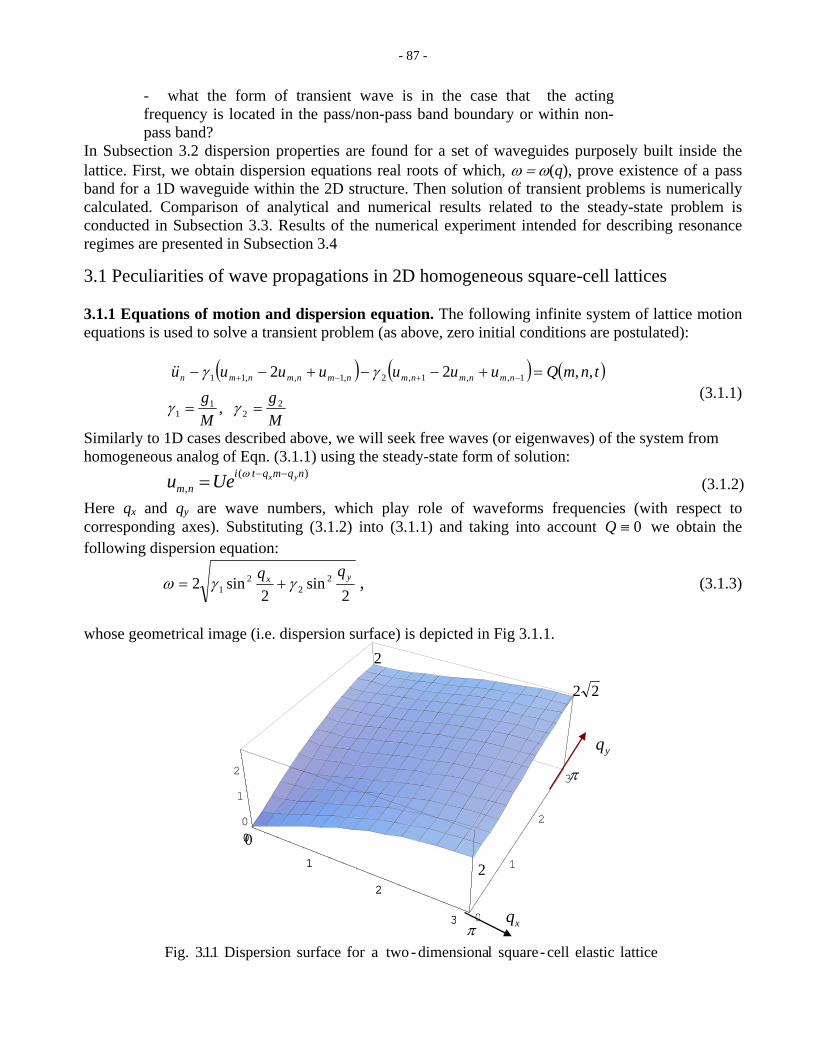
- 87 -

- what the form of transient wave is in the case that the acting frequency is located in the pass/non-pass band boundary or within non-pass band?

In Subsection 3.2 dispersion properties are found for a set of waveguides purposely built inside the lattice. First, we obtain dispersion equations real roots of which, ω = ω(q), prove existence of a pass band for a 1D waveguide within the 2D structure. Then solution of transient problems is numerically calculated. Comparison of analytical and numerical results related to the steady-state problem is conducted in Subsection 3.3. Results of the numerical experiment intended for describing resonance regimes are presented in Subsection 3.4

3.1 Peculiarities of wave propagations in 2D homogeneous square-cell lattices 3.1.1 Equations of motion and dispersion equation. The following infinite system of lattice motion equations is used to solve a transient problem (as above, zero initial conditions are postulated):

( ) ( ) ( )

,

,,22

22

11

1,,1,2,1,,11

Mg

Mg

tnmQuuuuuuu nmnmnmnmnmnmn

==

=+−−+−− −+−+

γγ

γγ&&

(3.1.1)

Similarly to 1D cases described above, we will seek free waves (or eigenwaves) of the system from homogeneous analog of Eqn. (3.1.1) using the steady-state form of solution:

(3.1.2) ) (,

nqmqtinm

yxUeu −−= ω

Here qx and qy are wave numbers, which play role of waveforms frequencies (with respect to corresponding axes). Substituting (3.1.2) into (3.1.1) and taking into account we obtain the following dispersion equation:

0≡Q

2

sin2

sin2 22

21

yx qqγγω += , (3.1.3)

whose geometrical image (i.e. dispersion surface) is depicted in Fig 3.1.1.

0

1

2

3 0

1

2

3

0

1

2

0

1

2

3

22

π

2

0

2

π

xk

yq

xq

lattice elastic cell-square ldimensiona- twoafor surface Dispersion 113 Fig. ..

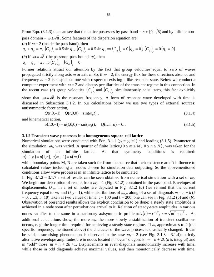
- 88 -

From Eqn. (3.1.3) one can see that the lattice possesses by pass-band − )8 ,0[ ∈ω and by infinite non-pass domain − 8 ≥ω . Some features of the dispersion equation are: (a) if ω = 2 (inside the pass band), then

( ) ( ) ( ) ( ) ( ) ( )0 0 ,0 0sin5.0 ,sin5.0 , ====⇒===+ xygyxgxygxxgyx qCqCqCqCqq π .

(b) if 8 =ω (the pass/non-pass boundary), then ( ) ( ) 0 , ==⇒==

ygxgyx CCqq π

Former relations attract our attention by the fact that group velocities equal to zero of waves propagated strictly along axis m or axis n. So, if ω = 2, the energy flux for these directions absence and frequency ω = 2 is suspicious one with respect to existing a like-resonant state. Below we conduct a computer experiment with ω = 2 and discuss peculiarities of the transient regime in this connection. In the recent case (b) group velocities ( ) ( )

ygxg CC and simultaneously equal zero, this fact explicitly

show that 8 =ω is the resonant frequency. A form of resonant wave developed with time is discussed in Subsection 3.1.2. In our calculations below we use two types of external sources: antisymmetric force action,

)sin()0,0,()1,0,( 0ttQtQ ω==− , (3.1.4) and kinematical action,

.0),,( ),sin()0,0,()1,0,( 0 ===− nmtQttutu ω . (3.1.5)

3.1.2 Transient wave processes in a homogeneous square-cell lattice Numerical simulations were conducted with Eqn. 3.1.1 (γ1 = γ2 =1) and loading (3.1.5). Parameter of the simulation, ω0, was varied. A quarter of finite lattice, ( )NnMm ≤≤≤≤ 0 ,0 , was taken for the simulation of an infinite lattice. At that symmetry conditions is required:

( ) ( ) ( ) ( 1,1, ,,1,1 mumununu =−=− )while boundary points M, N are taken such far from the source that their existence aren’t influence to calculated values including all nodes chosen for simulation data outputting. So the abovementioned conditions allow wave processes in an infinite lattice to be simulated In Fig. 3.1.2 – 3.1.7 a set of results can be seen obtained from numerical simulation with a set of ω0. We begin our description of results from ω0 = 1 (Fig. 3.1.2) contained in the pass band. Envelopes of displacements, Um,n, in a set of nodes are depicted in Fig. 3.1.2 (a) (we remind that the current frequency equal to ω0 and U0,0 = 1), while distributions of um,n, along of a set of diagonals m = n + k (k = 0, …,3, 5, 10) taken at two values of time, t = 100 and t = 200, one can see in Fig. 3.1.2 (a) and (b). Observation of presented results allows the explicit conclusion to be done: a steady state amplitude is achieved in a node soon after perturbations arrival to it. Relation of steady-state amplitudes in various nodes satisfies to the same in a stationary axisymmetric problem: ( ) ,~ 21−rrU 22 nmr += . As additional calculations show, the more ω0, the more slowly a stabilization of transient oscillations occurs, e. g. the longer time required for achieving a steady state regime. If ω0 approximates to 2 (the specific frequency, mentioned above) the character of the wave process is drastically changed. It can be said, a surprising phenomenon is observed in the case ω0 = 2 (see Fig. 3.1.3 - 3.1.4): strictly alternative envelope amplitudes are in nodes located in “even” diagonals: m = n + 2k (k is integral) and in “odd” those: m = n + 2k +1. Displacements in even diagonals monotonically increase with time, while those in odd diagonals achieve maximal values, and then monotonically decrease with time.

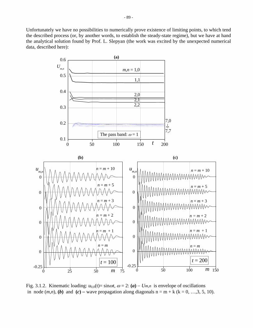
- 89 -

Unfortunately we have no possibilities to numerically prove existence of limiting points, to which tend the described process (or, by another words, to establish the steady-state regime), but we have at hand the analytical solution found by Prof. L. Slepyan (the work was excited by the unexpected numerical data, described here):

0 25 50 75

0

n = m + 1

n = m + 5

n = m + 2

n = m + 3

0

0

0

0

0

-0.25

n = m + 10

n = m

t = 100m

um,n

0 50 100 150 2000.1

0.2

0.3

0.4

0.5

0.6

The pass band: ω = 1

.|.

Um,n

7,7

7,0

2,22,12,0

t

1,1

m,n = 1,0

0 50 100 150

0

n = m + 1

n = m + 5

n = m + 2

n = m + 3

0

0

0

0

0

-0.25

n = m + 10

n = m

t = 200m

um,n

(a)

(b) (c)

Fig. 3.1.2. Kinematic loading: u0,0(t)= sinωt, ω = 2: (a) − Um,n is envelope of oscillations in node (m,n), (b) and (c) − wave propagation along diagonals n = m + k (k = 0, …,3, 5, 10).

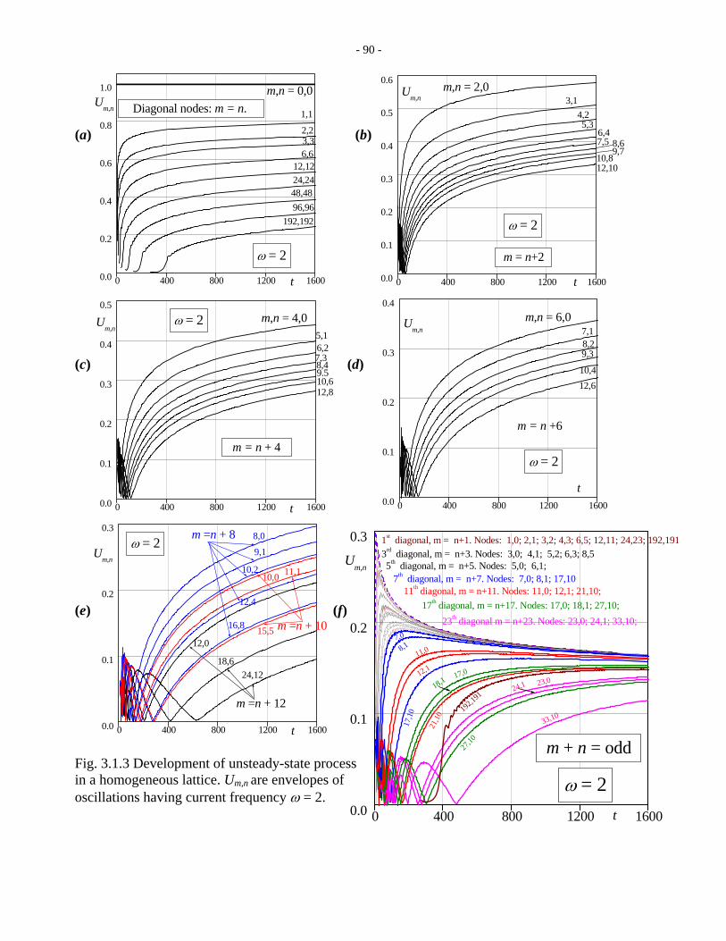
- 90 -

0 400 800 1200 16000.0

0.1

0.2

0.3

23th diagonal m = n+23. Nodes: 23,0; 24,1; 33,10;17th diagonal, m = n+17. Nodes: 17,0; 18,1; 27,10;

7th diagonal, m = n+7. Nodes: 7,0; 8,1; 17,105th diagonal, m = n+5. Nodes: 5,0; 6,1;

11th diagonal, m = n+11. Nodes: 11,0; 12,1; 21,10;

1st diagonal, m = n+1. Nodes: 1,0; 2,1; 3,2; 4,3; 6,5; 12,11; 24,23; 192,191

ω = 2

7,0

192,1

91

33,10

27,10

17,1

0

18,117,0

21,10

118,1

23,0

3rd diagonal, m = n+3. Nodes: 3,0; 4,1; 5,2; 6,3; 8,5

24,1

,0

12,1

m + n = odd

t

Um,n

0 400 800 1200 16000.0

0.1

0.2

0.3

0.4

Um,n

ω = 2

12,610,4

8,29,3

7,1

m = n +6

m,n = 6,0

t0 400 800 1200 16000.0

0.1

0.2

0.3

0.4

0.5

Um,n

ω = 2

12,810,6

5,16,2

9.57,38,4

m = n + 4

m,n = 4,0

t

0 400 800 1200 16000.0

0.1

0.2

0.3

Um,n

ω = 2

m =n + 1015,5

11,110,0

m =n + 12

m =n + 89,1

10,2

18,6

16,8

12,0

8,0

24,12

t

12,4

0 400 800 1200 16000.0

0.2

0.4

0.6

1.0

0.8

ω = 2

192,192

48,4896,96

12,12

m,n = 0,0

3,3

Diagonal nodes: m = n.

24,24

6,6

1,1

t

Um,n

2,2

0 400 800 1200 16000.0

0.1

0.2

0.3

0.4

0.5

0.6

ω = 2

Um,n

12,1010,8

9,78,6

6,47,5

5,34,2

3,1

m = n+2

m,n = 2,0

t

(a) (b) (c) (d) (e) (f)

Fig. 3.1.3 Development of unsteady-state process in a homogeneous lattice. Um,n are envelopes of oscillations having current frequency ω = 2.

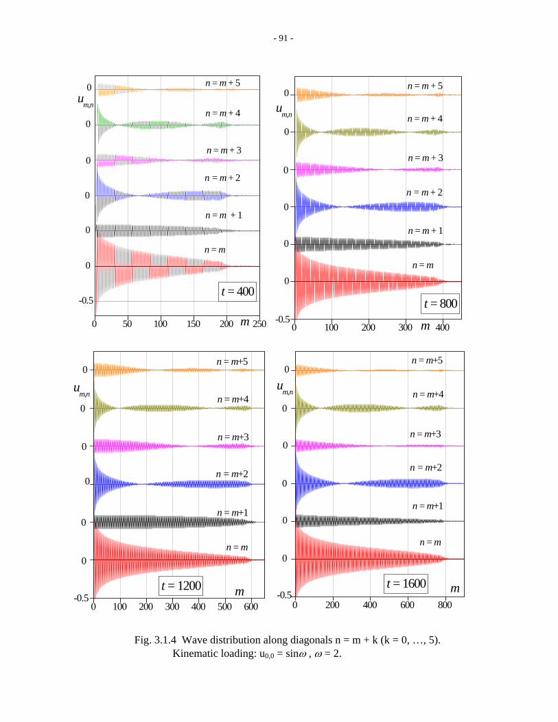
- 91 -

Fig. 3.1.4 Wave distribution along diagonals n = m + k (k = 0, …, 5).

Kinematic loading: u0,0 = sinω , ω = 2.

0 100 200 300 400

n = m + 1

n = m + 4

n = m + 2

n = m + 3

0

0

0

0

0

0

-0.5

n = m + 5

n = m

t = 800

m

um,n

0 50 100 150 200 250

n = m + 1

n = m + 4

n = m + 2

n = m + 3

0

0

0

0

0

0

-0.5

n = m + 5

n = m

t = 400

m

um,n

0 100 200 300 400 500 600

n = m+1

n = m+4

n = m+2

n = m+3

0

0

0

0

0

0

-0.5

n = m+5

n = m

t = 1200 m

um,n

0 200 400 600 800

n = m+1

n = m+4

n = m+2

n = m+3

0

0

0

0

0

0

-0.5

n = m+5

n = m

t = 1600 m

um,n

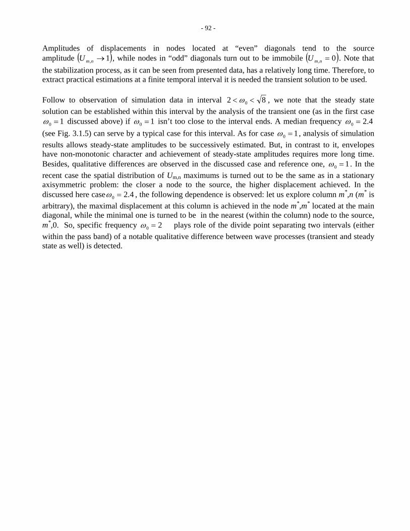
- 92 -

Amplitudes of displacements in nodes located at “even” diagonals tend to the source amplitude ( )1 , →nmU , while nodes in “odd” diagonals turn out to be immobile ( )0 , =nmU . Note that the stabilization process, as it can be seen from presented data, has a relatively long time. Therefore, to extract practical estimations at a finite temporal interval it is needed the transient solution to be used. Follow to observation of simulation data in interval 8 2 0 << ω , we note that the steady state solution can be established within this interval by the analysis of the transient one (as in the first case

1 0 =ω discussed above) if 1 0 =ω isn’t too close to the interval ends. A median frequency 4.2 0 =ω (see Fig. 3.1.5) can serve by a typical case for this interval. As for case 1 0 =ω , analysis of simulation results allows steady-state amplitudes to be successively estimated. But, in contrast to it, envelopes have non-monotonic character and achievement of steady-state amplitudes requires more long time. Besides, qualitative differences are observed in the discussed case and reference one, 1 0 =ω . In the recent case the spatial distribution of Um,n maximums is turned out to be the same as in a stationary axisymmetric problem: the closer a node to the source, the higher displacement achieved. In the discussed here case 4.2 0 =ω , the following dependence is observed: let us explore column m*,n (m* is arbitrary), the maximal displacement at this column is achieved in the node m*,m* located at the main diagonal, while the minimal one is turned to be in the nearest (within the column) node to the source, m*,0. So, specific frequency 2 0 =ω plays role of the divide point separating two intervals (either within the pass band) of a notable qualitative difference between wave processes (transient and steady state as well) is detected.

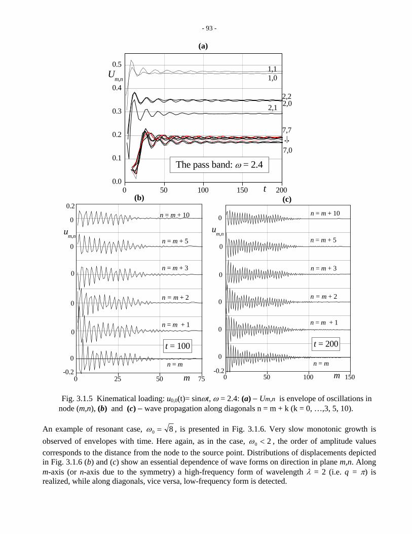
- 93 -

(a)

0 50 100 150 2000.0

0.1

0.2

0.3

0.4

0.5

The pass band: ω = 2.4

.|.

Um,n

7,7

7,0

2,22,1 2,0

t

1,11,0

0 25 50 75

0.2

0

n = m + 1

n = m + 5

n = m + 2

n = m + 3

0

0

0

0

0

-0.2

n = m + 10

n = m

t = 100

m

um,n

0 50 100 150-0.2

0

n = m + 1

n = m + 5

n = m + 2

n = m + 3

0

0

0

0

0

n = m + 10

n = m

t = 200

m

um,n

(b) (c)

Fig. 3.1.5 Kinematical loading: u0,0(t)= sinωt, ω = 2.4: (a) − Um,n is envelope of oscillations in

node (m,n), (b) and (c) − wave propagation along diagonals n = m + k (k = 0, …,3, 5, 10). An example of resonant case, 8 0 =ω , is presented in Fig. 3.1.6. Very slow monotonic growth is observed of envelopes with time. Here again, as in the case, 20 <ω , the order of amplitude values corresponds to the distance from the node to the source point. Distributions of displacements depicted in Fig. 3.1.6 (b) and (c) show an essential dependence of wave forms on direction in plane m,n. Along m-axis (or n-axis due to the symmetry) a high-frequency form of wavelength λ = 2 (i.e. q = π) is realized, while along diagonals, vice versa, low-frequency form is detected.

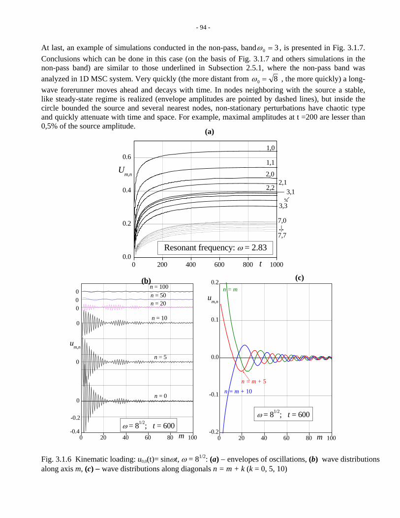
- 94 -

At last, an example of simulations conducted in the non-pass, band 30 =ω , is presented in Fig. 3.1.7. Conclusions which can be done in this case (on the basis of Fig. 3.1.7 and others simulations in the non-pass band) are similar to those underlined in Subsection 2.5.1, where the non-pass band was analyzed in 1D MSC system. Very quickly (the more distant from 8 0 =ω , the more quickly) a long-wave forerunner moves ahead and decays with time. In nodes neighboring with the source a stable, like steady-state regime is realized (envelope amplitudes are pointed by dashed lines), but inside the circle bounded the source and several nearest nodes, non-stationary perturbations have chaotic type and quickly attenuate with time and space. For example, maximal amplitudes at t =200 are lesser than 0,5% of the source amplitude.

0 200 400 600 800 10000.0

0.2

0.4

0.6

.|.3,1

3,3

Resonant frequency: ω = 2.83

.|.

Um,n

7,7

7,0

2,22,1

2,0

t

1,1

1,0

0 20 40 60 80 100-0.2

-0.1

0.0

0.1

0.2

n = m + 10

(a)

n = m + 5

n = m

ω = 81/2; t = 600

m

um,n

0 20 40 60 80 100

-0.2

0n = 5

n = 10

n = 20

10000

0

0

0

-0.4

= 50

n = 0

n =n

ω = 81/2; t = 600m

um,n

(b) (c)

Fig. 3.1.6 Kinematic loading: u0,0(t)= sinωt, ω = 81/2: (a) − envelopes of oscillations, (b) wave distributions along axis m, (c) − wave distributions along diagonals n = m + k (k = 0, 5, 10)

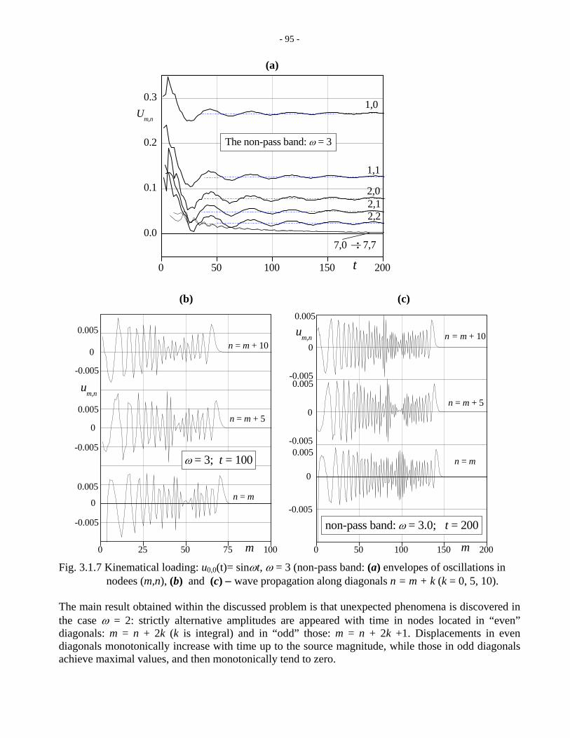
- 95 -

(a)

0 50 100 150 200

0.0

0.1

0.2

0.3

The non-pass band: ω = 3

.|.

Um,n

7,77,0

2,22,12,0

t

1,1

1,0

0 50 100 150 200

0.005

0.005

0.005

-0.005

-0.005

n = m + 10 0

0

0

-0.005

n = m + 5

n = m

non-pass band: ω = 3.0; t = 200

m

um,n

0 25 50 75 100

0.005

0.005

0.005

-0.005

-0.005

n = m + 5

0

0

0

-0.005

n = m + 10

n = m

ω = 3; t = 100

m

um,n

(b) (c)

Fig. 3.1.7 Kinematical loading: u0,0(t)= sinωt, ω = 3 (non-pass band: (a) envelopes of oscillations in nodees (m,n), (b) and (c) − wave propagation along diagonals n = m + k (k = 0, 5, 10). The main result obtained within the discussed problem is that unexpected phenomena is discovered in the case ω = 2: strictly alternative amplitudes are appeared with time in nodes located in “even” diagonals: m = n + 2k (k is integral) and in “odd” those: m = n + 2k +1. Displacements in even diagonals monotonically increase with time up to the source magnitude, while those in odd diagonals achieve maximal values, and then monotonically tend to zero.

- 96 -

3.2 Localized sinusoidal waves in square-cell lattices. Dispersion analysis In order to design a lattice containing a waveguide we will investigate two cases:

(i) x ,y − infinite lattice , ( )LL 2, ,1 ,0 ; 2, ,1 ,0 ±±=±±= mn , and (ii) y − semi-infinite lattice (lattice bounded by y = 0), ( )LL 2, ,1 ,0 ; 2, ,1 ,0 ±±== mn .

3.2.1 Infinite inhomogeneous lattice. Let all bonds of the lattice have the same rigidities (which together with the particle mass serve by measurement units: M = g1 = g2 = 1) excluding bonds within layer (0, −1), as it is shown in Fig.3.2.1: horizontal rigidities for chains n = 0, −1 are γm, while vertical rigidities between these chains are γn (in the common case 1≠≠ nm γγ ).

0=m 1

1

Equations for free waves in terms of displacement are:

(3.2.1) ( ) ( ) ( )( ) ( ) ( )1,0,1,2,1,11,11,

0,1,0,1,0,10,10,

n,1,1,,1,1,

1212

1) 0,-1(n 4

−−−−+−−−

−+−

−+−+

−++−++=

−++−++=

==⇒≠−+++=

mmnmmmmmmm

mmnmmmmmmm

mnmnmnmnmnmnm

uuuuuuuuuuuuuu

uuuuuu

γγγγγγ

γγ

&&

&&

&&

Their solution we seek by the asymmetric (with respect to axis y) form:

( ) ( )[ ] ( )( ) ( )[ ] ( 1 iexp

0 iexp)1(

,

,

−≤−−=

≥−=+− ntmqtu

ntmqtun

nm

nnm

ωξ

ωξ

) (3.2.2)

when |ξ| < 1, that is, the solution vanishes for ±∞→n (i.e. the finite energy density per unit of length). Our aim is to obtain the dispersion equation, ω = ω(q) and associated relations. We obtain after substitution (3.2.2) into (3.2.1):

( ) ( )( ) nmQqQQ γξωγξ

ξω 21 ,2/sin4 1 222

2 −−=−=−

=− , (3.2.3)

from which we get two possible values ξ = ξ1,2.

−

1

21−2−

2

n

n

−

0=γ

mγ

mγ

(-1,0)layer within rigidities Bond 3.2.1 .

nγ

Fig

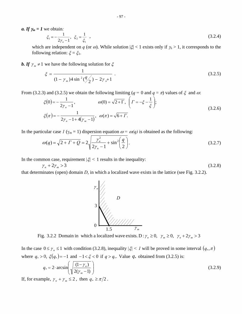
- 97 -

a. If γm = 1 we obtain:

1 ,12

1ξ −=1

21 ξξ

γ=

−n

, (3.2.4)

which are independent on q (or ω). While solution |ξ| < 1 exists only if γn > 1, it corresponds to the

. If

following relation: ξ = ξ1.

b 1≠mγ we have the following solution for ξ

12)2(sin4)1(

1=ξ

2 +−− nmq γγ

. (3.2.5)

rom (3.2.3) and (3.2.5) we obtain the following limiting (q = 0 and q = π) values of ξ and ω:

F

( )

( ) ( ) .6)( ,1412

1

; 1 ,2(0) ,10 Γ ⎟⎞

⎜⎛

−−=Γ+=−= ξωξ12

Γmn

n

+=−+−

−=

⎟⎠

⎜⎝−

πωγγ

πξ

ξγ (3.2.6)

the particular case 1 (γ = 1) dispersion equation ω = ω(q) is obtained as the following:

In m

⎟⎠⎞⎛2

2 qnγ⎜⎝

+−

=++=2

sin12

22)( QΓqnγ

ω . (3.2.7)

the common case, requirement |ξ| < 1 results in the inequality: In

32 >+ mn γγ (3.2.8) that determinates (open

the case

) domain D, in which a localized wave exists in the lattice (see Fig. 3.2.2).

nγ

3

5.10

D

mγ

In 10 ≤≤ nγ with condition (3.2.8), inequality |ξ| < 1 will be proved in some interval ( ) ,* πq

where . if 01and 1 qq q ><<−−> ( ) ,0 *** q = ξξ Value *q obtained from (3.2.5) is:

⎟⎟⎠

⎞⎜⎜⎝

⎛

−−

⋅= 2*q)1(2

)1(arcsinm

n

γγ (3.2.9)

If, for example, 2≤+ mn γγ , then 2* π≥q .

32 ,0 ,0:D exists. wavelocalized ain which Domain 3.2.2 .Fig >+≥≥ mnmnγ γ γ γ

- 98 -

Below, for comp teady st raarison of s ate and t nsient solutions, together with relation ω(q) we also will need the dispersion relation for group velocity Cg = q∂∂ω . It is the following:

ξξ

γξγ 2 ))1((sin −−⋅=

qC mm 2)1( −

−Qg

(3.2.10)

One can see that if0→gC π→q − e.g., as in the case of 1D waveguides above, standing waves are

appeared in the waveguide if π=q . Note that 1 if 0 ≤≥ ξgC . Depicted In Fig 3.2.3 dispersion curves ω = ω(q) are calculated for the case 1 (γm = 1, γn > 1) . Note that

in the case γm = γn = 1 localized wave doesn’t exist (here |ξ| = 1), and is shown only as a limiting curve that bounds (from below) the family of dispersion curves. These limiting frequencies are:

( ) ( ) 8 ,20 == πωω (3.2.11) As it can be seen from analysis 2.7) (of (3.2.6) and (3. and also from Fig. 3.2.3) the pass-band width, Δω, and group velocities decreased if γn increased: ( ) ( ) , 00 →−=Δ ωπωω ) ( 0 ∞→→ ngrc γ ; their upper

limits are: ,28max −=Δω ( ) ( )1 12max −=c )n =γgr . Pass bands ( ) ([ ]πωωωω == +− ,0 calculated for γn =1.5, 2 50, 3.20], [3.02, 3.63], and [3.33, 3.89]. .5, 4, 5 are correspondingly: [2.12, 2.92], [2.

0 1 2 31.5

2.0

2.5

3.0

3.5

4.0

0.0 0.5 1.0 1.5 2.0 2.5 3.00.0

0.1

0.2

0.3

0.4γn=1

γn=1.5γn=5

γn=4

γn=2.5

γn=1.5

γn=1

ω(q

)

q

γn=5

γn=2.5

γn=4

Cg(q

)

q

( )1 5 ,4 ,5.2 ,5.1 ,1for )(C and curves Dispersion 3.2.3 .Fig mg =ω γ = γnq(q)

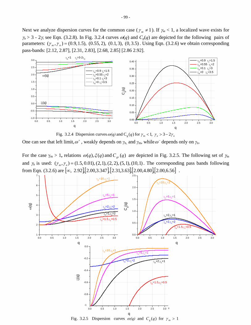
- 99 -

0.0 0.5 1.0 1.5 2.0 2.5 3.01

2

3

4

5

6

7

γm=5,γn=1

γm=2,γn=2

γm=1,γn=2

γm=10,γn=1

Next we analyze dispersion curves for the common case ( 1≠mγ ). If γm < 1, a localized wave exists for γn > 3 - 2γ, see Eqn. (3.2.8). In Fig. 3.2.4 curves ω(q) and Cg(q) are depicted for the following pairs of parameters: )5.3 ,0( ),3 ,1.0( ),2 ,55.0( ),5.1 ,9.0(),( =nm γγ . Using Eqn. (3.2.6) we obtain corresponding pass-bands: [2.12, 2.87], [2.31, 2.83], [2.68, 2.85] [2.86 2.92].

0.0 0.5 1.0 1.5 2.0 2.5 3.0-1.0

-0.5

0.0

0.5

1.0

1.5

2.0

2.5

3.0

ω(q)

ξ(q)

γm<1 γn>3-2γm

q

γm=0.9 γn=1.5 γm=0.55 γn=2 γm=0.1 γn=3 γm=0 γn=3.5

0.0 0.5 1.0 1.5 2.0 2.5 3.00.00

0.05

0.10

0.15

0.20

0.25

0.30

0.35

0.40

Cg(q

)q

γm=0.9 γn=1.5 γ

m=0.55 γ

n=2

γm=0.1 γn=3 γ

m=0 γ

n=3.5

nnq(q) γγγω 23 ,1for )(C and curves Dispersion 3.2.4 .Fig mg −>< One can see that left limit, , weakly depends on γ+ω n, and γm, while depends only on γ−ω n. For the case γm > 1, relations )( and )( ),( qCqq grξω are depicted in Fig. 3.2.5. The following set of γm and γn is used: ( )1 ,10( ),1 ,5( ),2 ,2( ),1 ,2( ),.010 ,5.1(), =nm γγ . The corresponding pass bands following from Eqn. (3.2.6) are [ ] [ ] [ ] [ ] [ ] .566,00.2,.804,00.2,.633,31.2 ,.3473,00.2,92.2 ,∞ .

0.0 0.5 1.0 1.5 2.0 2.5 3.00.0

0.5

1.0

1.5

2.0

2.5

ω(q

)

q

γm=1.5,γn=0.5

γm=10,γn=1

γm=5,γn=1

γm=2,γn=1

γm=2,γn=2

Cg(q

)

q

1 for )( and curves Dispersion 3.2.5 .Fig mg >

γm=1.5,γn=0.5

0.0 0.5 1.0 1.5 2.0 2.5 3.0

-0.8

-0.6

-0.4

-0.2

0.0

γω qC(q)

γm=10,γn=1γm=5,γn=1

γm=2,γn=2 γm=2,γn=1

π-1

ξ(q)

q

γm=1.5,γn=0.5

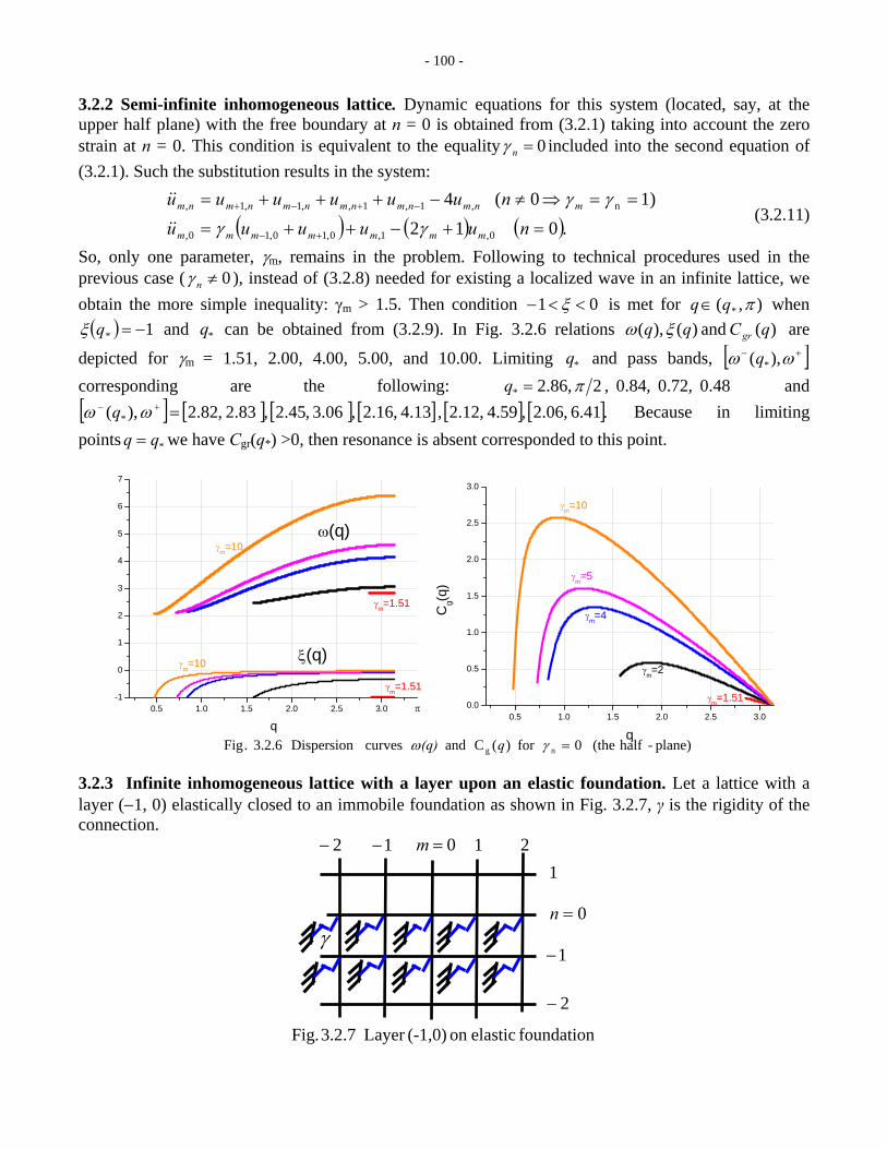
- 100 -

3.2.2 Semi-infinite inhomogeneous lattice. Dynamic equations for this system (located, say, at the upper half plane) with the free boundary at n = 0 is obtained from (3.2.1) taking into account the zero strain at n = 0. This condition is equivalent to the equality 0=nγ included into the second equation of (3.2.1). Such the substitution results in the system:

(3.2.11) ( ) ( ) ( ).0 12 1) 0( 4

0,1,0,10,10,

n,1,1,,1,1,

=+−++=

==⇒≠−+++=

+−

−+−+

nuuuuunuuuuuu

mmmmmmm

mnmnmnmnmnmnm

γγγγ

&&

&&

So, only one parameter, γm, remains in the problem. Following to technical procedures used in the previous case ( 0≠nγ ), instead of (3.2.8) needed for existing a localized wave in an infinite lattice, we obtain the more simple inequality: γm > 1.5. Then condition 01 <<− ξ is met for ),( * πqq ∈ when

( ) 1* −=qξ and can be obtained from (3.2.9). In Fig. 3.2.6 relations *q )( and )( ),( qCqq grξω are

depicted for γm = 1.51, 2.00, 4.00, 5.00, and 10.00. Limiting and pass bands, *q [ ]+− ωω ),( *q corresponding are the following: 48.0 ,72.0 ,84.0 , 2 ,86.2* π=q and [ ] [ ] [ ] [ ] [ ] [ ].6.41 ,06.2 ,.594 ,12.2 , .134 ,16.2 , .063 ,.452 , 83.2 ,82.2 ),( * =+− ωω q Because in limiting points we have C*qq = gr(q*) >0, then resonance is absent corresponded to this point.

0.5 1.0 1.5 2.0 2.5 3.0-1

0

1

2

3

4

5

6

7

π0.5 1.0 1.5 2.0 2.5 3.0

0.0

0.5

1.0

1.5

2.0

2.5

3.0

γm=10

γm=10 ξ(q)

ω(q)

q

γm=1.51

γm=1.51γ

m=2

γm=4

γm=5

γm=10

Cg(q

)

qplane)-half (the 0for )(C and curves Dispersion 3.2.6 .Fig ng =γω q(q)

γm=1.51

3.2.3 Infinite inhomogeneous lattice with a layer upon an elastic foundation. Let a lattice with a layer (−1, 0) elastically closed to an immobile foundation as shown in Fig. 3.2.7, γ is the rigidity of the connection.

foundation elasticon (-1,0)Layer 3.2.7 .Fig

0=m 1 21−2−

1−

1

2−

0=nγ

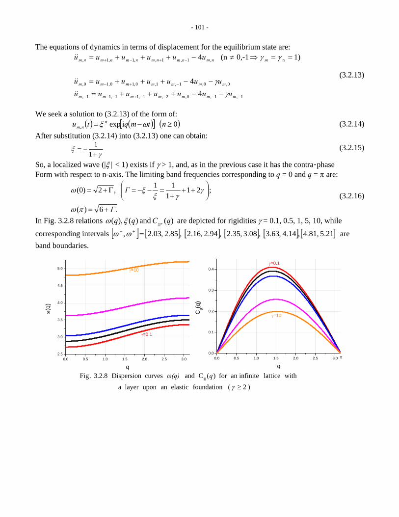
- 101 -

The equations of dynamics in terms of displacement for the equilibrium state are:

(3.2.13)

1,1,0,2,1,11,11,

0,0,1,1,0,10,10,

n,1,1,,1,1,

44

1) 0,-1(n 4

−−−−+−−−

−+−

−+−+

−−+++=

−−+++=

==⇒≠−+++=

mmmmmmm

mmmmmmm

mnmnmnmnmnmnm

uuuuuuuuuuuuuu

uuuuuu

γγ

γγ

&&

&&

&&

We seek a solution to (3.2.13) of the form of:

(3.2.14) ( ) ( )[ ] ( 0 iexp, ≥−= ntmqtu nnm ωξ )

After substitution (3.2.14) into (3.2.13) one can obtain:

11

γξ

+−= (3.2.15)

So, a localized wave (|ξ | < 1) exists if γ > 1, and, as in the previous case it has the contra phase -

Form with respect to n-axis. The limiting band frequencies corresponding to q = 0 and q = π are:

.6)(

; 211

11 ,2(0)

Γ

Γ

+=

⎟⎟⎠

⎞⎜⎜⎝

⎛++

+=−−=Γ+=

πω

γγξ

ξω (3.2.16)

In Fig. 3.2.8 relations )( and )( ),( qCqq grξω are depicted for rigidities γ = 0.1, 0.5, 1, 5, 10, while

corresponding intervals [ ] [ ] [ ] [ ] [ ] [ ] .215 .81,4 ,.144 ,.633 ,.083 ,35.2 ,94.2 ,16.2 ,85.2 ,03.2 , =+− ωω are band boundaries.

0.0 0.5 1.0 1.5 2.0 2.5 3.00.0

0.1

0.2

0.3

0.4

γ=10

γ=0.1

0.0 0.5 1.0 1.5 2.0 2.5 3.02.5

3.0

3.5

4.0

4.5

5.0

π

Cg(q

)

q

γ=10

ω(q

)

q

) 2 ( foundation elastican upon layer a withlattice infinitean for )(C and curves Dispersion 3.2.8 .Fig g

≥γ

γ=0.1

ω q(q)

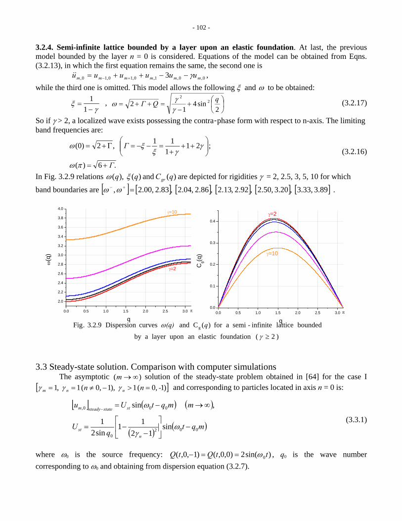
- 102 -

3.2.4. Semi-infinite lattice bounded by a layer upon an elastic foundation. At last, the previous model bounded by the layer n = 0 is considered. Equations of the model can be obtained from Eqns. (3.2.13), in which the first equation remains the same, the second one is 0,0,1,0,10,10, 3 mmmmmm uuuuuu γ−−++= +−&& , while the third one is omitted. This model allows the following ξ and ω to be obtained:

1

1γ

ξ−

= , ⎟⎠⎞

⎜⎝⎛+

−=++=

2sin4

12 2

2 qQΓγγω (3.2.17)

So if γ > 2, a localized wave exists possessing the contra-phase form with respect to n-axis. The limiting band frequencies are:

.6)(

; 211

11 ,2(0)

Γ

Γ

+=

⎟⎟⎠

⎞⎜⎜⎝

⎛++

+=−−=Γ+=

πω

γγξ

ξω (3.2.16)

In Fig. 3.2.9 relations )( and )( ),( qCqq grξω are depicted for rigidities γ = 2, 2.5, 3, 5, 10 for which

band boundaries are [ ] [ ] [ ] [ ] [ ] [ ] .893 .33,3 ,.203 ,50.2 ,.922 ,13.2 ,.862 ,04.2 ,83.2 ,00.2 , =+− ωω .

0.0 0.5 1.0 1.5 2.0 2.5 3.0

2.0

2.2

2.4

2.6

2.8

3.0

3.2

3.4

3.6

3.8

4.0γ=10

π

γ=2

ω(q

)

q0.0 0.5 1.0 1.5 2.0 2.5 3.0

0.0

0.1

0.2

0.3

0.4

γ=2

γ=10

π

Cg(q

)

q

) 2 ( foundation elastican upon layer aby

bounded lattice infinite-semi afor )(C and curves Dispersion 3.2.9 .Fig g

≥γ

ω q(q)

]

3.3 Steady-state solution. Comparison with computer simulations

The asymptotic solution of the steady-state problem obtained in [64] for the case I )( ∞→m[ )1 ,0( 1 ),1 ,0( 1 ,1 -nn nnm =>−≠== γγγ and corresponding to particles located in axis n = 0 is:

[ ] ( ) ( )

( )( ) sin

1211

sin21

, sin

0020

000,

mqtq

U

mmqtUu

nst

ststatesteadym

−⎥⎦

⎤⎢⎣

⎡

−−=

∞→−=−

ωγ

ω

(3.3.1)

where ω0 is the source frequency: )sin(2)0,0,()1,0,( 0ttQtQ ω==− , q0 is the wave number corresponding to ω0 and obtaining from dispersion equation (3.2.7).

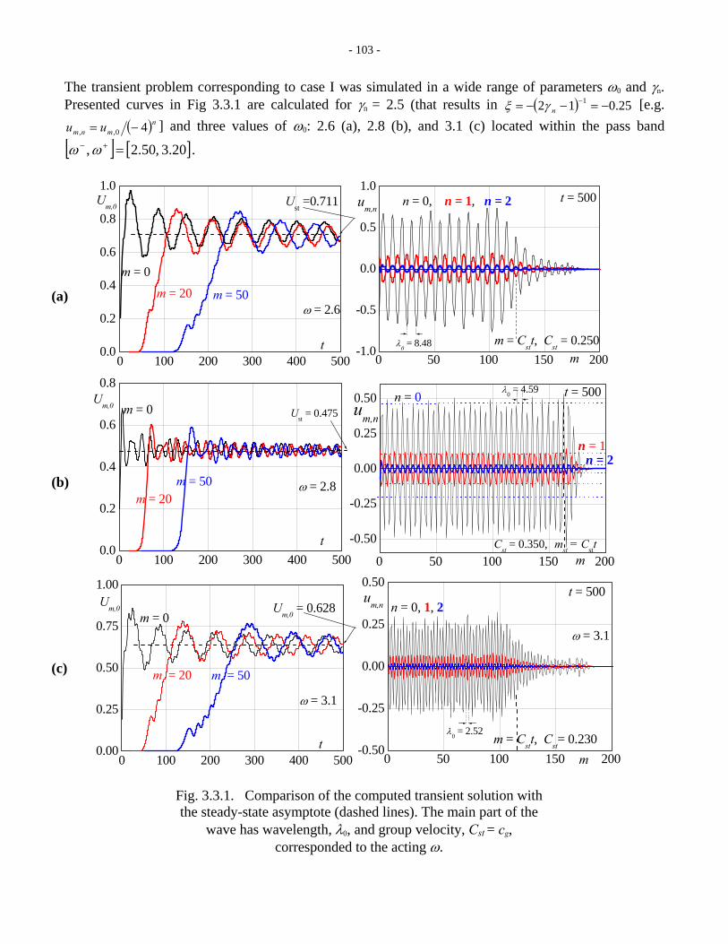
- 103 -

The transient problem corresponding to case I was simulated in a wide range of parameters ω0 and γn. Presented curves in Fig 3.3.1 are calculated for γn = 2.5 (that results in [e.g. ( ) 25.012 1 −=−−= −

nγξ

( )nmnm uu 40,, −= ] and three values of ω0: 2.6 (a), 2.8 (b), and 3.1 (c) located within the pass band

[ ] [ ]20.3 ,50.2 , =+− ωω .

0 100 200 300 400 5000.0

0.2

0.4

0.6

0.8

1.0Um,0

m = 50

0 50 100 150 200-1.0

-0.5

0.0

0.5

1.0

m = 20

m = 0

Ust =0.711

ω = 2.6

t λ0 = 8.48 m = Cstt, Cst = 0.250

um,nt = 500n = 0, n = 2

m

n = 1,

0 100 200 300 400 5000.0

0.2

0.4

0.6

0.8

Ust = 0.475

m = 50

m = 0

m = 20

Um,0

ω = 2.8

t

0 50 100 150 200-0.50

-0.25

0.00

0.25

0.50

λ0 = 2.52m = Cstt, Cst= 0.230

um,n

ω = 3.1

t = 500n = 0, 2

m

1,

0 50 100 150 200

-0.50

-0.25

0.00

0.25

0.50

Cst = 0.350,

n = 2n = 1

λ0 = 4.59

mst = Cstt

um,n

t = 500n = 0

m

0 100 200 300 400 5000.00

0.25

0.50

0.75

1.00

Um,0 = 0.628

m = 50

m = 0

m = 20

Um,0

ω = 3.1

t

(a)

(b)

(c)

Fig. 3.3.1. Comparison of the computed transient solution with the steady-state asymptote (dashed lines). The main part of the

wave has wavelength, λ0, and group velocity, Cst = cg, corresponded to the acting ω.

- 104 -

Pictures in left columns are envelopes (their positive parts) of displacements in nodes: n = 0 and m = 0, 20, 50, while the right columns are “photos” of displacements taken at t = 500. Results in left columns are to be implicitly enough to experimentally estimate magnitudes of the steady-state part of the wave process, while those in the right column serve to establish wave forms (with respect to axes), peculiarities of the transient process propagation and the speed of its stabilization (passing into the steady state one). Dashed straight lines are the steady-state amplitude, U

2,1,0, ,, mmm uuu

st, calculated from analytical asymptote (3.3.1). One can see that wavy character of calculated envelopes has a tendency to spread with time; the stabilization speed is maximal for the frequency ω0 (in this figure and below subscript, 0, omitted) located at the median part of the band where the group velocity (it denoted as Cst at the right column) is maximal. At the same time, the steady-state amplitudes can also be sufficiently estimated (as median lines of envelopes) in the two other cases where frequencies are relatively closed to band boundaries. The photos presented above and a number of other simulation data allow the following features of transient and steady state waves to be established:

− numerical simulations of the transient process allow the magnitude of the steady state wave to be estimated,

− the main part of propagating waves move with the group velocity corresponding to the source frequency,

− the transient waveform with respect to transversal axis n is sufficiently determined by the steady-state estimate: . The waveform with respect to waveguide axis m possesses by the frequency equal to wave number q

0,, mn

nm uu ξ=

0. − the maximal Cg is obtained in small vicinity 2~)max( π

gcqq = ,

− the higher Cg, the lesser the median amplitude of the transient wave (or, that is the same, the steady state amplitude) and the lesser time required for stabilization of the transient process,

− the waveform with respect to waveguide axis m possesses the frequency equal to q0, − the main attributes of the wave package moving with velocity Cst is sufficiently determined by

the steady-state estimate if loading frequency is located within the pass band and isn’t too close to band boundaries, ω− and ω+.

3.4 Resonant excitation of a square lattice with an inner waveguide

Below we present an example of numerical simulation of resonant excitations realized for two values of the source frequency: ω = ω− and ω = ω+. The former frequency excites the long-wave resonant process, while the recent one − the shortwave resonant process (such the process was already investigated in Subsection 2.5.1 on the basis of the simple MSC waveguide). As in Subsection 2.5.1 we will compare really resonant waves and near-resonant those possessing by the steady state solution. Besides the fact that the nonstationary − steady-state transition requires relatively long time, the mentioned comparison allows peculiarities of the resonance development to be elucidated in detail. In Fig. 3.4.1 results of numerical simulation are presented related to the first resonance, (a), − ω = ω− , to the second one, (d), − ω = ω+, and for two near-resonant cases: (b) − ω = 1.004 ω− , and (c) − ω = 0.997ω+. As in the previous Fig. 3.3.1, curves in left columns are positive parts of displacement envelopes in pointed nodes (inside the figure), dashed straight lines are the amplitude of asymptote (3.3.1).

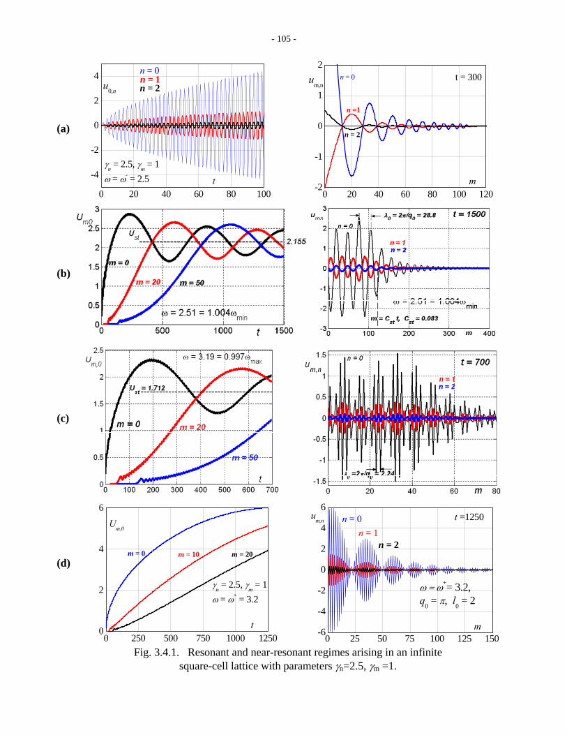
- 105 -

Fig. 3.4.1. Resonant and near-resonant regimes arising in an infinite

square-cell lattice with parameters γn=2.5, γm =1.

(a)

(b)

(c)

(d)

0 250 500 750 1000 12500

2

4

6

m = 20m = 0

γn = 2.5, γm = 1ω = ω+ = 3.2

Um,0

t

m = 10

0 20 40 60 80 100

-4

-2

0

2

4

γn = 2.5, γm = 1ω = ω- = 2.5

n = 0u0,n

t0 20 40 60 80 100 120

-2

-1

0

1

2

n = 2

um,nt = 300n = 0

m

n = 2n = 1

n =1

0 25 50 75 100 125 150-6

-4

-2

0

2

4

6t =1250

ω = ω+= 3.2, q0 = π, l0 = 2

n = 2

n = 0um,n

m

n = 1

- 106 -

In right columns one can see “photos” of displacements , taken at various values of time allowing spatial-temporal pictures for these three strips to be sufficiently described. One can observe the contra-phase transverse form of the resonant and near resonant processes. Resonant and near-resonant processes coincide practically up to time when the recent reach maximums (see the right column). Then envelopes of near-resonant processes acquire an oscillation character, while resonant those monotonically increase as t

2,1,0, ,, mmm uuu

½, the same growth that was analytically estimated for the case of the MSC waveguide. So, resonant processes excited in 2D lattices (and in 1D composite waveguides as well, see Subsection 2.5) have the same nature that arising in the MSC. The recent can be used for the preliminary analysis of wave processes in more complicated systems. The needed condition for justification of such a procedure is a correspondence dispersion relation within required spectrum intervals.

- 107 -

4. Main results and conclusions

I Dispersion properties of composite waveguides Dispersion properties of harmonic waves propagated in composite waveguides are significantly informative not only for steady state problem but also for prediction of distinctive features of transient processes, notably for revealing the existence of resonant regimes. For example, the longwave expansion of the dispersion operator is essentially used for estimates of quasi-steady state regimes. Below we present main results of the dispersion analysis conducted in the thesis and conclusions having mathematical, physical and applied sense. 1.1 Physical models of composite waveguides of diverse structure have been described and corresponding mathematical models of steady state and transient wave processes have been formulated. 1.2 Dispersion properties have been revealed of a general type periodic waveguide and particular peculiarities have been analyzed. Among them are the following:

− distribution of pass and non-pass band within the frequency spectrum depending on the waveguide structure, common and partial

− introducing of the so-called Partial Systems (PS) – mechanical structures generating the composite waveguide − allowing boundaries of pass bands to be obtained as PS eigenvalues.

− degeneration of a pass band into a local frequency has been revealed in multimode mass-spring waveguides: the dispersion curve of the corresponding mode turns out to be a straight line. In such a case zero group velocity is proved for the whole spectrum: there is no a steady state solution.

− bringing together neighboring pass bands (i.e. elimination of the non-pass band separating them) and appearing so-called conical points, frequencies of tailoring the pass bands. Such points, as in the previous case, determine transparent facilities of the waveguide.

− asymptotic formulas for simplified dispersion relations in a long wave spectrum has been obtained in the general case of a composite waveguide: ( ) 0 ,1~ 2

* >− ααqCc , 0→q( ∞→= q )πλ 2 where q and λ are the wave number and the wave length, c and are phase and group velocities. Factors and α have a simple physical sense: the former is the quasi-front speed, while the recent is the dispersion factor, integrated into a single number in the case of long waves.

*C

*C

II Asymptotes of long and short waves propagated in composite waveguides. 2.1 The analytical approach to describing the transient waves of chosen spectra has been used. In the case of a pulse loading the method applied to the long wave analysis consists of obtaining a formal solution in terms of double Laplace-Fourier integral transforms, and using a joint asymptotic reversion of Laplace-Fourier images at ∞→t in the vicinity of ray tCx *= . As a result, asymptotic formulas have been obtained for quasi-steady state components of the long wave, which, in the case of the Heaviside loading, can be used as precise one (as has been shown by numerical simulations). 2.2 An asymptotical formula has been obtained describing resonant growth realized in the mass-spring chain (MSC). Its corollary is that magnitudes of oscillation of MSC particles increase with time as t1/2, if

∞→t . Computer simulations showed that for oscillations of the loaded particle, the asymptotical formula obtained is turned out to be precise practically beginning the small moments of time.

- 108 -

III Waves propagation in 2D square-cell lattices Localized sinusoidal waves in infinite and semi-infinite inhomogeneous square-cell lattices have been investigated. In the case of lattices having a layer with properly changed parameters (the particle mass or the string rigidity) a localized waveguide is appeared within the lattice with this layer as a basis. In transversal directions wave exponentially decays (similarly to Rayleigh waves in elastic halfspace), while in the defected layer direction steady state wave propagation is proved. Dispersion equations have been obtained for a set of waveguides of especially designed structures when:

− longitudinal and/or transversal rigidities vary in an infinite lattice, − a semi-infinite lattice with varied longitudinal and/or transversal rigidities, − the layer within an infinite lattice is elastically connected with a rigid foundation, − the previous case for a semi-infinite lattice.

Dispersion equations have been obtained in the abovementioned cases, group velocities of the whole spectrum and resonant frequencies corresponding to the limiting points of the spectrum have been revealed. Comparison of analytical and numerical (on the recent see below) data result in

− computer simulations of the transient process allow the magnitude of the steady state wave to be estimated,

− the main part of propagating waves move with the group velocity corresponding to the source frequency,

− the waveform with respect to waveguide axis m possesses by the frequency equal to wave number q0 corresponding to the source frequency,

− maximal group velocity, (Cg)max, is reached in the small vicinity 2~)max( πgcqq = ,

− the higher Cg, the lesser the steady state amplitude of the transient wave and the lesser time required for stabilization of the transient process,

− the main attributes of the wave package moving with velocity Cst is sufficiently determined by the steady-state estimate if loading frequency is located within the pass band and isn’t too close to band boundaries, ω− and ω+,

− resonances appeared if the source frequency is equal to ω− and ω+, − resonant perturbations monotonically increase with time as t½ that is the same growth that was

analytically estimated for the case of the MSC waveguide. Resonant processes excited in waveguides within 2D lattices have the same nature that arising in the MSC. The recent can be used for the preliminary analysis of wave processes in more complicated systems. The needed condition making justification of such a procedure is a correspondence dispersion relations within chosen spectrum intervals.

IV Computer simulations A numerical approach, called as MDM-technique has been extended in the thesis to a wide range of hyperbolic systems describing composite waveguides of a step-like structure. Designed MDM algorithms allow numerous computer solutions of wave propagation processes saturated by fronts and high-gradient components to use as precise those. The accurate numerical solutions have been obtained in the following problems: 4.1 Wave propagation in 1D waveguides of diverse structure subjected by pulse and monochromatic excitations. Comparison of numerical and analytical solutions allows the applicability of asymptotic formulas to be established. Resonant processes have been comprehensively analyzed. Forms of transient wave have been obtained in the case when the frequency of the monochromatic loading is located in a non-pass band.

- 109 -

4.2 Wave propagation in homogeneous and inhomogeneous 2D lattices subjected by monochromatic excitations. Correspondence of steady state and transient solutions has been revealed in the case of inhomogeneous lattices when a 1D waveguide exists within the lattice structure. Surprising phenomena have been discovered in the case when a homogeneous lattice excited by a monochromatic source with frequency ω = 2 ( masses and rigidities of the lattice serve by measurement units) located at the origin m = n = 0 (m and n are particle numbers, L,2,1,0, ±±=nm ): strongly alternative amplitudes are appeared with time in nodes located in “even” diagonals: m = n + 2k (k is integral) and in “odd” those: m = n + 2k +1. Displacements in even diagonals monotonically increase with time up to the source magnitude, while those in odd diagonals achieve maximal values, and then monotonically tend to zero. 4.3 Statistical approach has been used to study a waveguide of slightly perturbed symmetry and to obtain parameter intervals allowing the longwave asymptotes finding for strongly symmetric models) to be applied to the mentioned case. Such intervals were revealed in the case of the waveguide with periodically adjoined particles of masses randomly distributed in the interval )]1( )],1([ δδ +− mm . The total sum of masses is invariant for all δ. On the basis of computer simulation data (with the assumption of normal distribution) all required statistical parameters have been obtained: consistence, unbiased and asymptotically normal expectancies and variances ( )2 and σμ , their confident ranges ( ) and MSE estimators2

22121 , and , σσμμ ( )σμ EE and . For example, in the case of the Heaviside stress

loading of the unite amplitude and m = 1, the maximal stress (independent on time) is estimated by the asymptote as . In the case δ = 1 and after 30 tests, once the propagating wave has been passed 20 periods, following data have been obtained by simulations:

8980.0≈

9054.0≈μ , 9151.0 ,8956.0 21 == μμ , and , , 103.03 5−⋅=μE 0009.02 ≈σ 000666.0 21 =σ

22σ = 0.001605, ES = 5.5010 .810−⋅

- 110 -

References

1. Lord Rayleigh (1887) , On the maintenance of vibrations by forces of double frequency, and the propagation of waves through a medium endowed with periodic structure, Philosophical Magazine, 24 145-159

2. Brillouin L. (1953) Wave Propagation in Periodic Structures. Dover Publication, Inc. NY

3. Miles J.W (1956) Vibrations of beams on many supports , Proceedings of the American Society of Civil Engineering, Engineering Mechanics Division, EM 1 p. 1-9

4. Hecky M. (1961) Wave propagation on beam-plate systems. J. Acoust. Soc. Am. 33, 640-651

5. T.J Delph,,G.Hermann , R.K Kaul (1966) Harmonic wave propagation in a periodically layered, infinite elastic body: Antiplane strain. Journal of Applied Mechanics 45 p. 343-34

6. Rytov, S. (1968) Acoustical properties of a thinly laminated medium, Soviet Physics and Acoustics, 2, pp. 68–80

7. C. Sun, J. Achenbach, and G. Herrmann, (1968) Time harmonic waves in a stratified medium propagating in the direction of the layering, Journal of Applied Mechanics, 90 E, pp. 408– 411 8. G.Sengupta (1970) Natural flexural waves and the normal modes of periodically supported beams and plates. Journal of Sound and Vibration 13, 89-101 9. D.J Mead (1970) Free wave propagation in periodically supported infinite beams. Journal of Sound and Vibration 11, 181-197

10. D.J Mead (1971) Vibration response and wave propagation in periodic structures. Journal of Engineering for Industry 93, 783-792

11. Slepyan L.I. (1972). Time Dependent ElasticWaves. Sudostroenie. Leningrad (in Russian).

12. C. Sve (1972) Stress wave attenuation in composite materials, Journal of Applied Mechanics, pp. 1151–1153 13. E.H Lee and W.H. Yang (1973) on waves in composite materials with periodic structure. Siam Journal of Applied Mathematics 25 No 3 p.492-499 14. Mal A. S (1974) Elastic waves in a fiber-reinforced composite. Journal of the Mechanics and Physics of Solids 22, pp. 217–229

15. Achenbach, J. (1975) Vibrations and waves in directional composites. In: Mechanics of Composite Materials 2. Academic Press. N-Y

16. M. Ben-Amoz (1975) On wave propagation in laminated composites. I. Propagation parallel to the laminates. International Journal of Engineering Science 13, pp. 43–56

17. S. Datta, H. Ledbetter, and R. Kriz (1984) Calculated elastic constants of composites containing anisotropic fibers. International Journal of Solids and Structures 20, pp. 429–438

18. Achenbach, J. Lu, Y., and M. Kitahara (1988) 3-D reflection and transmission of sound by an array of rods. Journal of Sound and Vibrations 125, pp. 463–476

19. Mal A. S. (1988) Wave propagation in layered composite laminates under periodic surface loads. Wave Motion 10, pp. 257–266

- 111 -

20. D.J. Mead (1995) Wave propagation in continuous periodic structures. Journal of Sound and Vibration 190(3) p. 495-524

21. S. J. Orfanidis. Electromagnetic Waves & Antennas –– June 21, 2004 http://www.ece.rutgers.edu/%7Eorfanidi/ewa

22. E. Yablonovitch (1993). Photonic band-gap crystals. J. Phys. Condens. Matter, 5, 2443-2460.

23. Falnes, J. (2002) Ocean waves and oscillating systems. Cambridge University Press. Cambridge, UK

24. Tawfik, M., Chung J., and A. Baz (2004) Wave attenuation in periodic helicopter blade. In: Jordan International Mechanical Engineering Conference (JIMEC), Balkaa University, Amman, Jordan. http://math.guc.edu.eg/Tawfik/JIMEC2004.pdf

25. Mead, D.J. (1996) Wave Propagation in Continuous Periodic Structures: Research Contributions from Southampton, 1964-1995, Journal of Sound and Vibration, Vol. 190, No. 3, pp. 495-524

26. Ungar, E.E. (1966) Steady-State Response of One-Dimensional Periodic Flexural Systems, The Journal of The Acoustic Society of America, Vol. 39, No. 5, pp. 887-894

27. Gupta, G.S. (1970) Natural Flexural Waves and The Normal Modes of Periodically-Supported Beams and Plates, Journal of Sound and Vibration, Vol. 13, No. 1, pp. 89-101

28. Faulkner, M.G. and Hong, D.P., Free Vibration of Mono-Coupled Periodic System, Journal of Sound and Vibration, Vol. 99, No. 1, pp. 29-42, 1985

29. Mead, D. J. and Yaman, Y. (1991) The Response of Infinite Periodic Beams to Point Harmonic Forces: A Flexural Wave Analysis, Journal of Sound and Vibration, Vol. 144, No. 3, pp. 507-530

30. Mead, D. J., White, R. G., and Zhang, X. M. (1994) Power Transmission In a Periodically Supported Infinite Beam Excited at A Single Point, Journal of Sound and Vibration, Vol. 169, No. 4, pp. 558-561

31. Langeley, R. S. (1995) Power Transmission in a One-Dimensional Periodic Structure Subjected to Single-Point Excitation, Journal of Sound and Vibration, Vol. 185, No. 3, pp. 552-558

32. Mead, D. J. (1975) Wave Propagation and Natural Modes in Periodic Systems: II. Multi-Coupled Systems, With and Without Damping, Journal of Sound and Vibration, Vol. 40, No. 1, pp. 19-39

33. Kissel, G. J. (1991) Localization Factor for Multichannel Disordered Systems, Physical ReviewA, Vol. 44, No. 2, pp. 1008-1034

34. 10 Gry, L. and Gontier, C. (1997). Dynamic Modeling of Railway Track: A Periodic Model Based onGeneralized Beam Formulation, Journal of Sound and Vibration, Vol. 199, No. 4, pp. 531-558

35. Ariaratnam, S. T. and Xie, W. C. (1995) Wave Localization in Randomly Disordered Nearly Periodic Long Continuous Beams, Journal of Sound and Vibration, 181, 7-22

36. Cetinkaya, C., (1999) Localization of Longitudinal Waves in Bi-Periodic Elastic Structures With Disorders, Journal of Sound and Vibration, Vol. 221, No. 1, 49-66

37. Ruzzene, M. and Baz, A. (2000) Attenuation and Localization of Wave Propagation in Periodic Rods Using Shape Memory Inserts. Smart Materials and Structures, 9, 805-816

38. Ruzzene, M. and Baz, A. (2001) Active Control of Wave Propagation in Periodic Fluid-Loaded Shells. Smart Materials and Structures, 10, 893-906.

- 112 -

39. Langley, R. S. (1994).On The ForcedResponse of One-Dim ensional Periodic Structures Vibration Localization by Damping, Journal of Sound and Vibration, 178, 411-428.

40. Cetinkaya, C. (1999).Localiza tion of Longitudinal Waves in Bi-Periodic Elastic Structures With Disorders, Journal of Sound and Vibration, 221, 49-66,

41. Thorp, O., Ruzzene, M., and Baz, A. (2001) Attenuation and Localization of Waves in Rods With Periodic Shunted Piezo, Smart Materials and Structures, 10,. 979-989

42. S.Mukherjee and S. Parthan (1994) Wave propagation in one-dimensional multi-bay periodically supported panels under supersonic fluid flow. Journal of Sound and Vibrations 186(1) 71-86

43. J.S Jensen (2003) Phononic band gaps and vibrations in one- and two-dimensional mass-spring structures. Journal of Sound and Vibration, 226, 1053-1078

44. Zhenghua Qian, Feng Jin, Zikun Wang, Kikuo Kishimoto (2003) Dispersion relations for SH-wave propagation in periodic piezoelectric composite layered structures. Int. J. Engng Sci. 42, 673-689

45. P. Kuchment, The Mathematics of Photonic Crystals (2001) Ch. 7 in Mathematical Modeling in Optical Science”, G. Bao, L. Cowsar, and W. Masters(Editors), Frontiers in Applied Mathematics SIAM, v. 22, , 207 - 272.

46. Kuchment, P. (2003) On some spectral problems of mathematical physics. Pan-American Advanced Studies Institute (PASI) on Partial Differential Equations, Inverse Problems and NonLinear Analysis, Universidad de Chile, Santiago, Chile. http://www.math.tamu.edu/~kuchment/kuch_pasi.pdf

47. P. Kuchment and L. Kunyansky (2002) Differential operators on graphs and photonic crystals. Ad.vances in Computational Mathematics 16: 263–290.

48. S. G. Johnson and J. D. Joannopoulos (2002) Photonic Crystals. The Road from Theory to Practice, Kluwer Acad. Publ., Boston

49. K. Sakoda (2003) Optical Properties of Photonic Crystals. Springer Verlag, Berlin

50. R. E. Slusher and B. J. Eggleton (Editors), Nonlinear Photonic Crystals. Springer Verlag, Berlin.

51. J. D. Joannopoulos, R. D. Meade, and J. N. Winn (1995) Photonic Crystals, Molding the Flow of Light, Princeton Univ. Press, Princeton, N.J.

52. Ayzenberg-Stepanenko, M. V. (1981) Numerical experiment on fracture dynamics of a layered composite. Mechanics of Composites, 1, 53 – 60.

53. Abdukadyrov S.A., Ayzenberg-Stepanenko M.V. and Alexandrova N. I. (1984). On MDM Approach to Calculation of Solid and Structure Dynamics. Sov. Mining Sci. 6, 34-40.

54. Ayzenberg-Stepanenko M. and Tsareva, O. (1987) Evolution of Shock Pulse Propagated through a Composite Elastic System. Sov. Mining Sci. 24, 43-52.

55. Ayzenberg-Stepanenko M. and T. Kadyrov T. (1988) On Particular Features of Elastic Waves Propagation in a Layer Halfspace. J.Appl. Mech. Techn. Phys. 18, 109-115.

56. Slepyan L.I. and Tsareva O.V. (1988) Energy Flux for Zero Group Velocity of the Carrying Wave. Sov. Phys. Dokl. 32, 522-524

57. Ayzenberg-Stepanenko M.V., Saraykin V. A. and Tsareva O.V. (1988) Evolution of Shock Pulse Propagated through an Elastic Waves in a Medium of a Block Structure. Sov. Mining Sci. 25, 14-21.

- 113 -

58. Ayzenberg-Stepanenko, M. V. (1992) Non-steady state wave propagation in composite structures. Proc. 24th Israel Conf. Mech. Engng., Technion. Haifa, sec. 4.8.2, 1-3

59. Ayzenberg-Stepanenko, M. (1994) Resonance Waves in Elastic Waveguides. Proc. 25th Israel Conf. on Mech. Engng. Technion. Haifa. 241-244

60. Slepyan L.I. and Ayzenberg-Stepanenko M.V. (2002) Some Surprising Phenomena in Weak-Bond Fracture of a Triangular Lattice. J Mech Phys Solids, 50 (8) p.1591-1625

61. Slepyan L.I. (2002) Waves: Chapter 3 in book: Models and Phenomena in Fracture Mechanics. Springer, 71-110.

62. Slepyan L.I. and Ayzenberg-Stepanenko M.V. (2004) Localized Transition Waves in Bistable-Bond Lattices. J Mech Phys Solids, 52 (7) 1447-1479.

63. Ayzenberg-Stepanenko M. V. (2004) Resonant Waves in a Structured Elastic Halfspace. In: Surface Waves in Anisotropic and Laminated Bodies and Defects Detection. Eds: R.V.Goldstein and G.A. Maugin: Proceedings of NATO Workshop. pp.45-59. Kluwer WB/Nato Publishing Unit. Dordrecht, Netherlands.

64. Slepyan L.I. Localized sinusoidal wave in lattices. (2005) (Private communication)