August 14, 2006

Why Have Business Cycle Fluctuations Become Less Volatile?

Andres Arias

Ministerio de Agricultura y Desarrollo Rural, Republic of Colombia

Gary D. Hansen UCLA & NBER

Lee E. Ohanian

UCLA, Federal Reserve Bank of Minneapolis, & NBER

Abstract This paper shows that a standard Real Business Cycle model driven by productivity shocks can successfully account for the 50 percent decline in cyclical volatility of output and its components, and labor input that has occurred since 1983. The model is successful because the volatility of productivity shocks has also declined significantly over the same time period. We then investigate whether the decline in the volatility of the Solow Residual is due to changes in the volatility of some other shock operating through a channel that is absent in the standard model. We therefore develop a model with variable capacity and labor utilization. We investigate whether government spending shocks, shocks that affect the household’s first order condition for labor, and shocks that affect the household’s first order condition for saving can plausibly account for the change in TFP volatility and in the volatility of output, its components, and labor. We find that none of these shocks are able to do this. This suggests that successfully accounting for the post-1983 decline in business cycle volatility requires a change in the volatility of a productivity-like shock operating within a standard growth model.

* We thank Stephen Parente, Ed Prescott, John Taylor, and two anonymous referees for helpful comments and suggestions.

1

1. Introduction

Kydland and Prescott (1982) and Prescott (1986) established that productivity shocks

could account for most post-World War II business cycle volatility. Business cycle volatility was

roughly constant up through the period studied by Kydland and Prescott, but has changed

substantially since then. Kim and Nelson (1999), McConnell and Perez-Quiros (2000) and Stock

and Watson (2002) all identify a large and statistically significant permanent decline in U.S.

GDP volatility beginning in the first quarter of 1984.

This paper examines this decreased volatility through the lens of neoclassical business

cycle theory. We focus our analysis on changes in the variance of the Hodrick-Prescott cyclical

component of real GDP, its components, labor input, and total factor productivity (TFP). All of

these variances are about 30-50 percent smaller in the post-1983 period compared to the 1955-83

period.

Within the neoclassical framework, changes in cyclical volatility are the result of either

changes in the volatility of the exogenous shocks that are fed into the model, and/or changes in

the structure of the model that maps the exogenous shocks into the endogenous variables. We

focus our analysis on changes in the exogenous shock volatility.

We first evaluate the impact of changes in the volatility of TFP shocks. We find that the

volatility of this shock declines about 50 percent after 1983. We find that this volatility change

reduces the volatility of output and its components, and labor input also by 50 percent in the

Hansen (1985) model. This finding suggests that lower productivity shock volatility can be a

significant factor underlying lower cyclical volatility. Some economists will question this

finding, however, because they argue that TFP shocks are not productivity shocks per se, but

rather the endogenous consequence of other shocks operating through unmeasured capital and

2

labor utilization. This “mis-measurement” view of TFP would suggest that the change in TFP

volatility is due to the change in the volatility of some other shock, combined with unmeasured

changes in factor utilization. We therefore pursue this possibility using the model of Burnside et

al. (1996) that features both variable capital and labor utilization. We follow Chari, Kehoe, and

McGrattan (2002, 2006) and Cole and Ohanian (2002) who focus on three other shocks for

understanding fluctuations in the growth model: a shock to the household’s static first order

condition, a shock to the household’s dynamic first order condition, and an additive shock to the

resource constraint, such as government spending shocks.

We test whether changes in the volatility of these other shocks can account for both the

change in TFP volatility and the change in the volatility of the output, its components and labor.

Our main finding is that none of these shocks do this. The volatility of the static preference

shocks is roughly unchanged between the two periods. The volatility of the shock to the resource

constraint changes significantly, but this change is quantitatively unimportant for the volatility of

TFP and the other variables. The volatility of the shock to the Euler equation changes

significantly, but generates business cycle statistics that are grossly counterfactual. We conclude

that the most promising candidate for understanding lower post-1983 business cycle volatility is

a shock that operates like TFP in a standard stochastic growth model. The change in the

correlation structure between the two periods provides some additional evidence on this issue.

The paper is organized as follows. Section 2 discusses the literature. Section 3 presents

changes in volatility of macroeconomic variables and the impact of lower volatility of

technology shocks in a standard real business cycle model. Section 4 describes how we identify

multiple shocks in this model and Section 5 studies the change in TFP volatility in the model

3

with variable capital and labor utilization. Section 6 considers the impact of a change in the

volatility of technology shocks on business cycle correlations and Section 7 concludes.

2. Connection with the Literature

The existing literature offers several explanations for the fall in business cycle volatility,

though currently there is no generally accepted explanation of lower cyclical volatility. Kahn,

McConnell and Perez-Quiros (2002) argue that the “information revolution” has changed the

way shocks are propagated. In particular, they argue that the volatility reduction resulting

largely from improvements in inventory management techniques, using a model that differs

substantially from the standard neoclassical model. Their approach thus focuses on changes in a

specific model’s propagation mechanism with a focus on inventory management. More recently,

Campbell and Hercowitz (2005) argue that financial reforms of the early 1980’s have changed

the propagation mechanism by relaxing collateral constraints on household borrowing. Other

authors, for example Clarida, Galí and Gertler (2000), maintain that improved monetary policy

since the early 1980’s has stabilized the U.S. economy. Blanchard and Simon (2001) argue that

changes in inventory management techniques, monetary policy, and also the volatility of

government spending all have been significant contributing factors to lower volatility.

In contrast, Stock and Watson (2002) conduct a comprehensive statistical examination

and find that the volatility reduction is primarily due to “good luck.” That is, there has been a

fall in the variance of the structural shocks that impact the economy, rather than improved

monetary policy or improved inventory control techniques. Ahmed, Levin, and Wilson (2002)

also conclude that lower volatility is largely a matter of “good luck” in the post-1983 period.

Finally, Gordon (2005) also finds that the reduced variance of shocks was the dominant source of

4

reduced business cycle volatility. We accept the “good luck” conclusions of these papers, that

the shocks hitting the U.S. economy since 1984 have been smaller. Our paper complements these

latter three studies by providing an assessment of the contribution of lower shock volatility to the

business cycle using a DSGE framework. Our DSGE analysis allows us to make progress on

understanding which shocks are important for the change in cyclical volatility, and on

understanding the structural mechanisms through which these shocks operate. We therefore

develop a simple RBC model and we evaluate how changes in the volatility of different shocks

affect business cycle volatility. Comin and Phillipon (2005) argue that microeconomic volatility

(among listed corporations) has increased recently, and Phillipon (2003) argues that increases in

competition can jointly account for higher microeconomic volatility and lower macroeconomic

volatility.1 The closest study to ours is by Leduc and Sill (2005) who study the contribution of

TFP shocks and monetary shocks to lower volatility. They find that changes in monetary policy

are relatively unimportant.2

3. Volatility in a Basic Real Business Cycle Model

In Table 1, we present a measure of business cycle volatility for a variety of U.S.

aggregate time series.3 Here, the business cycle is defined by deviations from a Hodrick-Prescott

1 We do not address the possible increase in firm-level volatility, as this is beyond the scope of this paper. It is worth noting, however, that within our framework, improved access to asset markets would tend to increase microeconomic volatility. There is evidence that asset markets have become more efficient (see Krueger and Perri (2006)). 2 Other analyses of changes in volatility within a fully articulated model include Posch and Waelde (2005), and Justiano and Primiceri (2005). Both analyses differ considerably from this analysis. Posch and Waelde find that changes in tax rates can be stability-enhancing in a model with endogenous cycles, while Justiano and Primiceri find that changes in the variance of investment-specific technological change is key in a Bayesian analysis of a model with time-varying mark-ups, sticky prices and wages, habit formation, investment-specific technological change, and investment adjustment costs. 3 We use quarterly data from 1955:3 – 2003:2. The beginning date is the first for which hours based on the household survey are available. Data has been logged before applying the Hodrick-Prescott filter. All National Income and Product Account data is in 1996 dollars. Hours (HS) is total hours worked based on data from the

5

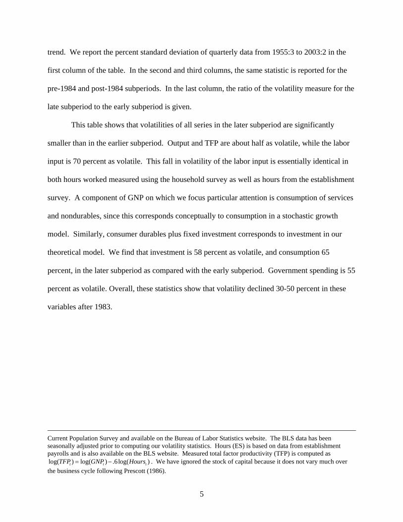
trend. We report the percent standard deviation of quarterly data from 1955:3 to 2003:2 in the

first column of the table. In the second and third columns, the same statistic is reported for the

pre-1984 and post-1984 subperiods. In the last column, the ratio of the volatility measure for the

late subperiod to the early subperiod is given.

This table shows that volatilities of all series in the later subperiod are significantly

smaller than in the earlier subperiod. Output and TFP are about half as volatile, while the labor

input is 70 percent as volatile. This fall in volatility of the labor input is essentially identical in

both hours worked measured using the household survey as well as hours from the establishment

survey. A component of GNP on which we focus particular attention is consumption of services

and nondurables, since this corresponds conceptually to consumption in a stochastic growth

model. Similarly, consumer durables plus fixed investment corresponds to investment in our

theoretical model. We find that investment is 58 percent as volatile, and consumption 65

percent, in the later subperiod as compared with the early subperiod. Government spending is 55

percent as volatile. Overall, these statistics show that volatility declined 30-50 percent in these

variables after 1983.

Current Population Survey and available on the Bureau of Labor Statistics website. The BLS data has been seasonally adjusted prior to computing our volatility statistics. Hours (ES) is based on data from establishment payrolls and is also available on the BLS website. Measured total factor productivity (TFP) is computed as log( ) log( ) .6log( )t t tTFP GNP Hours= − . We have ignored the stock of capital because it does not vary much over the business cycle following Prescott (1986).

6

Table 1—Volatility of U.S. Data

Percent Standard Deviation Series 1955:3-2003:2 1955:3-1983:4 1984:1-2003:2 Late/Early GNP 1.59 1.78 0.93 0.53Hours (HS) 1.51 1.58 1.12 0.71 Employment 1.02 1.08 0.73 0.68 Hours per worker 0.69 0.74 0.58 0.79Hours (ES) 1.72 1.82 1.29 0.71Labor Productivity (HS) 1.01 1.15 0.75 0.65Labor Productivity (ES) 0.79 0.86 0.67 0.78TFP (HS) ( 0.6GNP Hours= ) 1.04 1.21 0.62 0.51TFP (ES) 0.83 0.95 0.46 0.49 Consumption Expenditures 1.23 1.38 0.80 0.57 Nondurables 1.10 1.23 0.79 0.64 Services 0.71 0.74 0.54 0.74 Durables 4.54 5.08 3.07 0.60 Nondurables + Services 0.80 0.88 0.57 0.65 Investment Expenditures 7.06 7.66 4.41 0.58 Fixed Investment 4.87 5.29 3.20 0.61 Fixed Investment + Consumer Durables 4.53 4.97 2.88 0.58

Government Expenditures 1.50 1.73 0.96 0.55

7

We first assess the impact of lower TFP volatility on output and its components, and

labor. We do this using the following real business cycle model. The equilibrium of this model

economy is characterized by the solution to a social planner’s problem (where the initial capital

stock, 0k , is given):

1 , 0

log(1 )max logt t

tt tk h t

hE c hh

β θ+

∞

=

⎡ ⎤−+⎢ ⎥

⎣ ⎦∑

subject to

11 (1 )tz

t t t t tc k e k h kα α δ−++ = + −

2

1 1 1, 1 1 1, ~ (0, )t t tz z Nρ ε ε σ+ += + In this economy, labor is indivisible (individuals work h or not at all), and the labor

market allows trade in employment lotteries—contracts that specify a probability of working h

hours (see Hansen (1985) for details). In this problem, tz is the log of TFP, tc is consumption,

and th is aggregate hours worked. The log of TFP follows a first order autoregressive process.

The model is calibrated in way that is standard in the real business cycle literature (see

Cooley and Prescott (1995)). In particular, the value of the discount factor, β , is determined so

that the average quarterly k/y ratio for the model is the same as in U.S. data. The depreciation

rate is calibrated to the average investment to output ratio and the reduced form preference

parameter, log(1 )hh

θ − , is chosen so that individuals spend on average 31 percent of their

substitutable time working. The parameter α is set equal to average labor’s share in the U.S.

national income accounts, and 1ρ is set close to one in order to match the autocorrelation of

measured TFP (additional details provided in the next section). These criteria lead us to assign

8

the following parameter values: β = .988, δ = 0.018, log(1 )hh

θ − = 2.547, α = 0.6, and

1 .95ρ = .

We now use the model to quantify the contribution of changes in TFP volatility to the

volatility of the other variables. We first calculate the volatility of the endogenous variables

when 1σ is set to its value over the entire 1955:1 – 2003:2 period. We then calculate the

volatilities for the endogenous variables for the 1955-1983 subperiod when 1σ is calibrated so

that TFP volatility in the model is equal to actual TFP volatility in that subperiod , and we

analogously do this for the 1984-2003 subperiod. The TFP volatilities we calibrate to are listed in

Table 14.

The results of this experiment are shown in Table 2.

Table 2—Volatility in a Standard Real Business Cycle Economy Percent Standard Deviations Series Entire Period Early Subperiod Late Subperiod Late/Early Output 1.57 1.80 0.87 0.49Hours 1.25 1.43 0.69 0.49Capital 0.36 0.40 0.19 0.49Investment 5.61 6.45 3.07 0.49Consumption 0.40 0.46 0.22 0.49Labor Productivity 0.40 0.45 0.22 0.49 TFP 0.83 0.95 0.46 0.49Calibrated 1σ 0.0065 0.0075 0.0037

The fall in the volatility of GNP and other aggregate variables is not a puzzle from

perspective of “pure” real business cycle theory. In addition, because there is only one shock in

4 We use the establishment survey measure of hours worked for calibrating TFP in our model.

9

this model and the propagation mechanism is close to linear, the volatility of all variables falls by

the same amount. This would not be the case if we introduced additional shocks to the model.

Several researchers, however, [Basu (1996) and Burnside, Eichenbaum and Rebelo

(1995)] have argued that aggregate procyclical TFP fluctuations are due primarily to unmeasured

changes in factor utilization. According to these studies, once unmeasured utilization is taken

into account, there is little in the way of exogenous technology shocks to be accounted for by

exogenous shocks. Hence, in Section 5, we consider the impact of changes in the volatility of

shocks other than technology shocks in a model with endogenous movements in TFP due to

labor hording and capital utilization. Before doing that, we describe how we identify these other

shock in the following section.

4. Identifying Multiple Shocks

Our approach for identifying shocks is similar to that of Chari, Kehoe, and McGrattan

(2004) and Cole and Ohanian (2001) in that fluctuations in the endogenous variables from their

steady state values is due to one or more deviations in the equations that characterize the solution

to the planner's problem. In both our case, and in the case of these other papers, the goal is to

determine which deviations are central for understanding the fluctuations in the endogenous

variables. It is worth noting that there is a slight difference in terminology, however, but not in

substance. Whereas Chari et.al. refer to these deviations as “wedges” which can be mapped into

a variety of shocks, we refer to these deviations as shocks: a technology shock, a government

expenditure shock, a shock to preference for leisure, and a shock to the discount factor. Note that

as in the case of Chari et.al., the deviations (shocks) that we specify can be mapped into different

classes of deeper shocks. For example, the shock to the preference for leisure can be modeled

more deeply as a shock to home production, or a shock to changes in union power. The key point

10

is that our investigation, as in the case of Chari et.al., identifies plausible broad classes of shocks

that may—or may not—be important for the question of interest.

The following planner’s problem incorporates all of shocks considered in this paper:

1, 0

log(1 )max logt t

t t t tk h t

hE c hh

β θ+

∞

=

⎡ ⎤−+⎢ ⎥

⎣ ⎦∑

subject to 1 1

1 (1 )tzt t t t t tc k g e k h kα α δ−

++ + = + − 2 tz

tg ge= 3tz

t eθ θ= 4

1 0, 1tzt t eβ β β β+ = =

2

, 1 , , 1log log , ~ (0, ) for 1 4i t i i t i t i iz z N iρ ε ε σ+ += + = − 0k given.

There are four types of stochastic shocks in this economy, which we denote by 1 4to z z .

The first is the same technology shock as in the previous section. The second shock is an

additive shock to the resource constraint. Following Christiano and Eichenbaum (1992), we

measure this as a government spending shock. The third shock is a preference shock that distorts

the labor-leisure decision. The importance of this class of shocks for business cycles has been

argued by Hall (1997) and a number of others. The last is a shock to the subjective discount

factor and introduces a stochastic wedge in the intertemporal Euler equation.

Each of these shocks is identified from the data as follows:

1 log logt t tz y hα= −

2 logt tz g=

11

3 log log logt t t tz y c h= − −

4 1 1 2 2 3 3t t t t tz Ac B z B z B z= + + +

The first equation is the log of TFP, measured using establishment hours. As in Table 1,

since we are interested in cyclical fluctuations, we ignore capital because it does not vary

significantly over the business cycle. The second shock is computed from the log of government

expenditures.5 To compute the third shock, we take the first order condition for hours worked,

3log(1 )

tz t

t t

h yeh c h

αθ − −= , and solve for 3tz (ignoring constants). Finally, the fourth shock is

computed from the intertemporal first order condition, 4 1 1

1

1 (1 )( ) 1tz t t

tt t

y ke Ec c

α δβ + +

+

⎡ ⎤− + −= ⎢ ⎥

⎣ ⎦.

Solving a log-linearized version of this model enables us to express the conditional expectation

on the right hand side as a linear function of itz (i = 1,..,4) and log tk . Next, this linearized first

order condition can be solved for 4tz , where 1 2, ,A B B , and 3B are the resulting coefficients.

Again, as in the case of 1z , our empirical measure of 4z ignores capital (the coefficient on log tk

is set equal to zero).

The autoregressive parameters of the first three shocks ( 1 2,ρ ρ , and 3ρ ) are estimated by

removing a linear time trend from our measures of 1 2,z z , 3z and computing an autoregression

using OLS. From this, we obtained 1 .95ρ = , 2 .98ρ = , and 3 .99ρ = . In order to compute the

empirical counterpart to the fourth shock, we needed to guess a value for 4ρ so that we could

solve for the conditional expectation. Using this value, we constructed a time series for 4z and

estimated 4ρ from this time series. We solve for the fixed point where the guessed value for 4ρ

5 As pointed out by a referee, we are ignoring net exports in this identification of the additive shock.

12

used to compute the 4z time series and the autoregressive coefficient estimated from this time

series are identical. This procedure led us to set 4 .99ρ = .

5. Volatility in Model with Endogenous Factor Utilization

In this section, we use the model of Burnside and Eichenbaum (1996) to study the impact

of changes in the size of alternative shocks on business cycle volatility in a model with

unmeasured factor utilization. This model incorporates two sources of factor utilization in a real

business cycle model similar to the one studied in the previous section. These include labor

hording as modeled in Burnside, Eichenbaum and Rebelo (1993) and capital utilization as

modeled in Greenwood, Hercowitz and Huffman (1988) and Taubman and Wilkinson (1970).

The equilibrium of this model is characterized by the solution to a social planner’s

problem like the one in the previous section except with two additional choice variables: labor

effort, e, and the rate of capital utilization, u. Labor hording is introduced by assuming that

employment ( tn ) is chosen before period t shocks are observed. The remaining choices ( 1, ,t tk u+

and te ) are made after the shocks are observed. The planner’s problem is the following subject

to this timing restriction:

1 , , , 0max log log(1 )

t t t tt t t t tk n e u t

E c n h eβ θ ω+

∞

=

⎡ ⎤+ − −⎣ ⎦∑

subject to

( ) ( )11

1 (1 ( ))tzt t t t t t t t tc k g e u k e n h u k

αα δ−++ + = + −

( ) , 1t tu uφδ γ φ= > 2 tz

tg ge= 3tz

t eθ θ=

13

4

1 0, 1tzt t eβ β β β+ = =

2

, 1 , , 1log log , ~ (0, ) for 1 4i t i i t i t i iz z N iρ ε ε σ+ += + = − 0k given. Capital utilization, tu , affects both production and the rate of depreciation. The higher

capital is utilized in production, the larger is the rate of depreciation. As discussed in Burnside

and Eichenbaum (1996), this feature and labor hoarding have important implication for the way

shocks are propagated.

The model is calibrated in a similar manner as in the previous section. In particular, the

value of β is chosen to target the k/y ratio, φ chosen to target the i/y ratio, and g chosen to

target the g/y ratio. The parameter θ is chosen so that the average time devoted to market

activities, ( )tn hω + , is equal to 0.31 and γ is chosen so that the average utilization rate is 0.9.6

The length of a work shift, h , is set so that effort (e) is 1 in steady state. Labor’s share is set

equal to 0.6 and the fraction of time spent commuting (ω ) is set equal to 6/98. The

autoregressive coefficients for the shock processes are not re-estimated for this model and are the

same as reported in the pervious section: 1 .95ρ = ; 2 .98ρ = ; 3 .99ρ = , and 4 .99ρ = .

Our goal in the following three experiments is to determine if changes in the volatility of

(i) the government spending shock, (ii), the static preference shock, and (iii), the intertemporal

preference shock, can plausibly account for both the change in the volatility of TFP and the

change in the volatility of output and its components, and labor. We begin with the government

spending shock. The volatility of government spending in the data falls by almost half after

6 The cyclical properties of the model do not depend on the value of the parameter γ .

14

1983. To measure the impact of reducing the volatility of government spending, we simulate the

model as follows, setting 3 4 0σ σ= = ( tθ θ= and tβ β= ):

1. Set 1σ and 2σ to match the volatility of TFP and government spending for the entire

1955-2003 period shown in Table 1.

2. Keep 1σ at the same value, but choose 2σ to match the volatility of g during the early

subperiod.

3. Keep 1σ at the same value, but choose 2σ to match the volatility of g during the late

subperiod.

The percent standard deviations associated with each of these parameterizations are given

in the first three columns of Table 3.

Table 3—Volatility in a Model with Variable Factor UtilizationThe Role of Government Spending Shocks ( 3 4 0σ σ= = )

Percent Standard Deviations

Series Entire PeriodEarly

Subperiod Late

Subperiod Late/Early Output 1.40 1.40 1.32 0.94Hours 1.26 1.29 1.15 0.89Capital 0.25 0.25 0.24 0.98Investment 5.17 5.11 4.94 0.97Consumption 0.31 0.31 0.28 0.90Labor Productivity 0.65 0.66 0.62 0.94 TFP 0.83 0.82 0.80 0.97Government Expenditure 1.50 1.73 0.96 0.55 Calibrated 1σ 0.00311 0.00311 0.00311 Calibrated 2σ 0.01173 0.01378 0.00773

The key finding from Table 3 is that, although government spending is 55 percent as

volatile in the second subperiod as the first, this has relatively little effect on the volatility of any

15

of the endogenous variables. Thus the impact of an additive resource constraint shock is

quantitatively much too small to account for changes in the volatility of the other variables in the

model.

Perhaps a reduction in the variance of the preference shock will have a more important

quantitative effect on business cycle volatility. In order to conduct an empirically relevant

experiment, we need to calibrate 3σ . To do so, we use the first order condition for choosing te

(labor effort), which can be written as follows:

(1 )

t t t

t t t

y ec n h he

θα ω

=− −

(1)

The volatility of the left hand side can be computed from data, but the right hand side is a

function of unobservable effort. This is not a problem, because we can choose 3σ so that

simulations of the model imply volatility of the left hand side of this equation that is the same as

that measured in U.S. data.

More precisely, Table 4 gives results from the following experiment

(assume 2 4 0σ σ= = ):

1. Set 1σ and 3σ to match the volatility of TFP and the “theta target” for the entire

1955-2003 period shown in Table 1.

2. Keep 1σ at the same value, but choose 3σ to match the volatility of the target during

the early subperiod.

3. Keep 1σ at the same value, but choose 3σ to match the volatility of the target during

the late subperiod.

16

Table 4—Volatility in a Model with Variable Factor Utilization

The Role of Taste Shocks ( 2 4 0σ σ= = ) Percent Standard Deviations

Series Entire PeriodEarly

Subperiod Late

Subperiod Late/Early Output 1.78 1.77 1.67 0.94Hours 2.10 2.10 1.96 0.94Capital 0.30 0.30 0.28 0.94Investment 6.34 6.25 5.94 0.95Consumption 0.68 0.68 0.63 0.93Labor Productivity 0.85 0.85 0.81 0.95 TFP 0.83 0.82 0.79 0.96Theta target 1.10 1.10 1.03 0.93 Calibrated 1σ 0.00258 0.00258 0.00258 Calibrated 3σ 0.00822 0.00834 0.00784 Table 4 shows very little change in business cycle volatility from the calibrated change in

the variance of the taste shock. The volatility in the model variables falls between 4 and 7

percent, compared to the 30-50 percent declines in the data. This finding that the change in the

shock volatility cannot account for the volatility changes in the other variables is similar to the

first case of the resource constraint shock in table 3, but for a very different reason. Here, the

volatility of the left hand side of (1) falls by only 7 percent from the early to the late subperiod.

This implies relatively little change in the value of 3σ . If the variance of the left hand side of (1)

had fallen more substantially, we would find a bigger change in business cycle volatility between

the early and late subperiods. Thus, the taste shock is not a useful candidate factor for

17

understanding changing cyclical volatility in the indivisible labor model because its volatility is

similar between the two periods.7

Our next experiment considers the potential of the intertemporal shock to account for the

change in volatility. This shock enters the intertemporal first order condition, which can be

written as follows:

4 1 1 1

1

(1 )( / ) 11tz t t t

t t

y k ue Ec c

φα γβ + + +

+

⎡ ⎤− + −= ⎢ ⎥

⎣ ⎦.

A natural way to calibrate the standard deviation of this shock is to target the volatility of

consumption. If we employ this criterion, the value of 4σ we obtain using data for the entire

period, turns out to be 0.000403. While this is a considerably smaller value than our estimates of

the other shock volatilities, it turns out to imply considerable volatility in the endogenous

variables. In particular, the percent volatility of TFP implied by our model turns out to be 0.85.

This is actually larger than TFP volatility computed from U.S. data for this same period (0.83).

Because of the considerable volatility generated by this shock, we report results for an

experiment where the other shock volatilities are set equal to zero. That is, Table 6 gives results

from the following experiment (assume 1 2 3 0σ σ σ= = = ):

1. Set 4σ to match the volatility of consumption for the entire 1955-2003 period shown

in Table 1.

2. Choose 4σ to match the volatility of consumption during the early subperiod.

3. Choose 4σ to match the volatility of consumption during the late subperiod.

7 We stress that this finding is for the indivisible labor model, and may be sensitive to alternative formulations. This is because the household static first order condition which we used to identify the variance of the shock depends on the preference specification that is used.

18

Table 6—Volatility in a Model with Variable Factor UtilizationThe Role of Intertemporal Shocks ( 1 2 3 0σ σ σ= = = )

Percent Standard Deviations

Series Entire PeriodEarly

Subperiod Late

Subperiod Late/Early Output 2.49 2.73 1.77 0.65Hours 3.34 3.67 2.38 0.65Capital 0.67 0.73 0.47 0.64Investment 16.58 17.90 9.04 0.50Consumption 0.80 0.88 0.57 0.65Labor Productivity 1.15 1.29 0.84 0.65 TFP 0.85 0.94 0.61 0.65 Calibrated 4σ 0.000403 0.000453 0.000296

We find that considerable volatility reduction can be accounted for by the intertemporal

shock. In particular, unlike the government spending or preference shock, this shock appears to

be able to account for the reduction in volatility of TFP and other endogenous variables once

endogenous factor utilization is taken into account.

While this intertemporal shock may be capable of potentially accounting for much of the

change in the volatility of TFP and the other variables, its contribution in this one-shock model is

flawed, because with only this one shock the model is seriously deficient as a positive business

cycle model. Specifically, it generates several business cycle statistics that are grossly

counterfactual. For example, as shown in Table 6, the fluctuations in hours worked are

significantly larger than the output fluctuations, and investment is much too volatile. An even

more striking shortcoming of this model is the fact that consumption in this model economy is

counter-cyclical, while it is highly pro-cyclical in the U.S. economy. These findings indicate that

this one-shock model is not a reasonable specification for evaluating the potential contribution of

19

the change in the volatility of the intertemporal shock. Doing this requires adding productivity

shocks, as it is well known that models with productivity shocks tend to produce reasonable

volatility and co-movement patterns compared to actual data.

We now consider the contribution of the change in the volatility of the intertemporal

shock in an economy where technology shocks are important. Specifically, to generate a model

with potentially reasonable business cycle properties, we maximize the possible contribution of

technology shocks as follows. The value of 1σ is chosen so that it completely accounts for TFP

volatility in the second (low volatility) subperiod. The same value of 1σ is used in the first (high

volatility) subperiod, and we choose 4σ in the first subperiod to account for the change in the

volatility of 1σ between the two subperiods. Specifically, the experiment is conducted as

follows:

1. Set 4 0σ = and choose 1σ to match the volatility of TFP in later subperiod (results

are shown in the second column of Table 7).

2. For the early subperiod, maintain the same value of 1σ as in step 1. Choose 4σ to

match the much higher volatility of TFP during the early subperiod.

Hence, in this experiment, we are allowing for a significant role for technology shocks in both

subperiods, but we are allowing a change in the volatility of the intertemporal shock ( 4σ ) to

account for one hundred percent of the change in the TFP volatility between the two subperiods.

20

Table 7—Volatility in a Model with Variable Factor Utilization The Role of Intertemporal Shocks ( 2 3 0σ σ= = )

Percent Standard Deviations

Series Early

Subperiod Late

Subperiod Late/Early Output 2.51 0.75 0.30Hours 3.29 0.64 0.19Capital 0.66 0.14 0.21Investment 14.38 2.83 0.20Consumption 0.79 0.16 0.20Labor Productivity 1.18 0.84 0.30 TFP 0.95 0.46 0.48 Calibrated 1σ 0.00183 0.00183 Calibrated 4σ 0.000398 0

The results of this experiment tell basically the same story as Table 6. A change in the

variance of the intertemporal shock can account for the reduced variance of TFP, but the implied

business cycle properties when the intertemporal shock is active (the early subperiod in Table 7)

are substantially at variance with the business cycle properties of the U.S. economy.

Specifically, hours worked fluctuates more than output, and consumption is highly counter-

cyclical (the correlation of output and consumption is -0.7).

This experiment indicates that a change in the volatility of an intertemporal shock that

shifts the Euler equation is a very unlikely candidate for understanding changing cyclical

volatility because the business cycle properties in this model are significantly at variance with

the data. This suggests that investigating this shock seems to require a model which deviates

considerably from the growth model.

21

6. Changes in Correlations

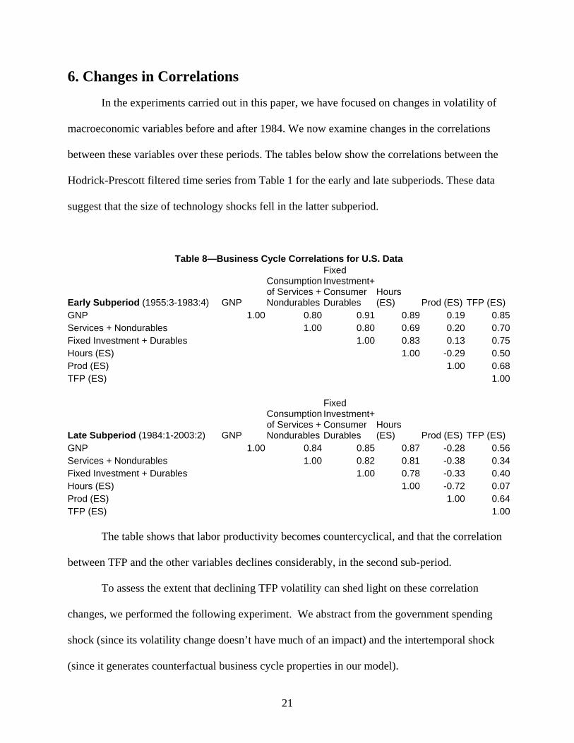
In the experiments carried out in this paper, we have focused on changes in volatility of

macroeconomic variables before and after 1984. We now examine changes in the correlations

between these variables over these periods. The tables below show the correlations between the

Hodrick-Prescott filtered time series from Table 1 for the early and late subperiods. These data

suggest that the size of technology shocks fell in the latter subperiod.

Table 8—Business Cycle Correlations for U.S. Data

Early Subperiod (1955:3-1983:4) GNP

Consumption of Services + Nondurables

Fixed Investment+Consumer Durables

Hours (ES) Prod (ES) TFP (ES)

GNP 1.00 0.80 0.91 0.89 0.19 0.85Services + Nondurables 1.00 0.80 0.69 0.20 0.70Fixed Investment + Durables 1.00 0.83 0.13 0.75Hours (ES) 1.00 -0.29 0.50Prod (ES) 1.00 0.68TFP (ES) 1.00

Late Subperiod (1984:1-2003:2) GNP

Consumption of Services + Nondurables

Fixed Investment+Consumer Durables

Hours (ES) Prod (ES) TFP (ES)

GNP 1.00 0.84 0.85 0.87 -0.28 0.56Services + Nondurables 1.00 0.82 0.81 -0.38 0.34Fixed Investment + Durables 1.00 0.78 -0.33 0.40Hours (ES) 1.00 -0.72 0.07Prod (ES) 1.00 0.64TFP (ES) 1.00 The table shows that labor productivity becomes countercyclical, and that the correlation

between TFP and the other variables declines considerably, in the second sub-period.

To assess the extent that declining TFP volatility can shed light on these correlation

changes, we performed the following experiment. We abstract from the government spending

shock (since its volatility change doesn’t have much of an impact) and the intertemporal shock

(since it generates counterfactual business cycle properties in our model).

22

1. Set 2 4 0σ σ= = and 3 0.00822σ = . The latter is the value of 3σ required to match

the volatility of the “theta target” for the entire sample (see Table 4). Set 1σ to match

the volatility of TFP for the early subperiod.

2. Hold 2 3 4, ,and σ σ σ constant and set 1σ to match the volatility of TFP for the later

subperiod.

The following table shows the correlation matrix corresponding to each of the two cases

described above:

Table 9—Correlations in a Model with Variable Factor Utilization

The Role of Technology Shocks ( 2 4 0σ σ= = ) Early Subperiod Output Consumption Investment Hours

Labor Productivity TFP

Output 1.00 0.83 0.98 0.90 -0.05 0.79Consumption 1.00 0.74 0.71 0.05 0.69Investment 1.00 0.90 -0.07 0.77Hours 1.00 -0.46 0.47Labor Productivity 1.00 0.55TFP 1.00

Late Subperiod Output Consumption Investment Hours Labor Productivity TFP

Output 1.00 0.87 0.98 0.95 -0.60 0.67Consumption 1.00 0.79 0.71 -0.19 0.86Investment 1.00 0.98 -0.69 0.57Hours 1.00 -0.81 0.42Labor Productivity 1.00 0.18TFP 1.00

We see that our model with the change in TFP volatility, and the volatility of the taste

shock held constant, indeed generates countercyclical labor productivity in the later subperiod. It

does not, however, predict the large changes in the correlations with TFP seen in Table 8.

23

7. Conclusion

We find that the approximately 50 percent decline in business cycle volatility that has

occurred since 1983 can be accounted for by the observed decline in the volatility of productivity

shocks. This finding is robust to allowing for endogenous TFP volatility operating in a model

with variable capital and labor utilization. In particular, we found that neither changes in the

volatility of an additive resource constraint shock, changes in the volatility of a static taste shock,

nor changes in the volatility of a dynamic taste shock can plausibly account for the change in

TFP volatility, the change in the volatility of output and its components, and labor. We see two

avenues for future research in this area. One is to develop theories for why the TFP shock

volatility had declined so much. Another is to test whether other plausible modifications to the

model generate very different results.

24

References Ahmed, S., A. Levin and B. A. Wilson. 2002. “Recent U.S. macroeconomic stability: good

policies, good practices, or good luck?” International Financial Discussion Paper No. 730. Board of Governors of the Federal Reserve System.

Basu, S. 1996. “Procyclical Productivity: Increasing Returns or Cyclical Utilization?” The Quarterly Journal of Economics Vol. 111, No. 3, 719-751.

Blanchard, O. and J. Simon. 2001. “The long and large decline in U.S. output volatility.” Brookings Papers on Economic Activity, 1, 135-164.

Burnside C. and M. Eichenbaum. 1996. “Factor-hoarding and the propagation of business-cycle shocks.” American Economic Review 86, 1154-1174.

Burnside, Craig, Martin Eichenbaum and Sergio Rebelo. 1993. “Labor Hoarding and the Business Cycle.” Journal of Political Economy, Vol. 101, No. 2. 245-273.

Burnside, Craig, Martin Eichenbaum, and Sergio Rebelo, 1995. “Capital Utilization and Returns to Scale,” in NBER Macroeconomics Annual 1995, pages 67-110.

Campbell, J.R. and Z. Hercowitz. 2005. “The Role of Collateralized Household Debt in Macroeconomic Stabilization,” Working Paper, Federal Reserve Bank of Chicago.

Chari, V.V., P.J. Kehoe and E.R. McGrattan. 2004. “Business Cycle Accounting.” Federal Reserve Bank of Minneapolis Staff Report 328.

Christiano, L.J. and M. Eichenbaum. 1992, ‘Current Real Business Cycle Theories and Aggregate Labor Market Fluctuations,’ American Economic Review.

Clarida, R., J. Galí and M. Gertler. 2000. “Monetary Policy Rules and Macroeconomic Stability: Evidence and Some Theory.” Quarterly Journal of Economics, February, 147-180.

Cole, Harold, and Lee E. Ohanian, 2001, “The Great U.S. and U.K. Depressions Through the Lens of Neoclasical Theory”, American Economic Review, May, pp. 28-32.

Comin, Diego and Thomas Philippon, 2005, “The Rise in Firm-Level Volatility: Causes and Consequences”, forthcoming NBER Macroeconomics Annual.

Cooley, T. F. and E. C. Prescott. 1995. “Economic growth and business cycles.” In T. F. Cooley, ed., Frontiers of Business Cycle Research. Princeton University Press, 1-38.

Gordon, R. J. 2005. “What Caused the Decline in U.S. Business Cycle Volatility?” NBER Working Paper 11777.

Greenwood, Jeremy, Zvi Hercowitz and Gregory W. Huffman. 1988. “Investment, Capacity Utilization, and the Real Business Cycle” American Economic Review, Vol. 78, No. 3, 402-417.

Hansen, G. D. 1985. “Indivisible labor and the business cycle.” Journal of Monetary Economics 16, 309-327.

Hall, R.E. 1997. “Macroeconomic Fluctuations and the Allocation of Time.” Journal of Labor Economics 15 No. 1 Pt. 2, S223-S250.

25

Justiano, A. and G. Primiceri. 2005. “The Time-Varying Volatility of Macroeconomic Fluctuations”, Discussion Paper, Northwestern University, Evanston, IL.

Kahn, J. A., M. M. McConnell and G. Perez-Quiros. 2002. “On the causes of the increased stability of the U.S. economy.” Federal Reserve Bank of New York Economic Policy Review, May, 183-202.

Kim, C.-J. and C. Nelson. 1999. “Has the US Economy Become More Stable? A Bayesian Approach Based on a Markov Switching Model of the Business Cycle.” Review of Economics and Statistics 81, 608-616.

Leduc, Sylvain and Keith Sill. 2005. “Monetary Policy, Oil Shocks, and TFP: Accounting for the Decline in U.S. Volatility,” Working Paper, FRB Philadelphia.

McConnell, M. M. and G. Perez-Quiros. 2000. “Output fluctuations in the United States: what has changed since the early 1980’s?” American Economic Review 90, No. 5, 1464-1476.

Philippon, T. 2003. “An Explanation for the Joint Evolution of Firm and Aggregate Volatility”, Stern School of Business, NYU, Working Paper.

Posch, O. and K. Waelde. 2005. “Natural Volatility, Welfare, and Taxation”, Discussion Paper, University of Hamburg, Hamburg, Germany.

Prescott, E. C. 1986. “Theory Ahead of Business Cycle Measurement,” Federal Reserve Bank of Minneapolis Quarterly Review 10, 9–22.

Rogerson, R. 1988. “Indivisible labor, lotteries and equilibrium.” Journal of Monetary Economics 21, 3-16.

Stock, J.H. and M.W. Watson. 2002. “Has the Business Cycle Changed and Why?” NBER Macroeconomics Annual 2002.

Taubman, Paul and Maurice Wilkinson. 1970. “User Cost, Capital Utilization and Investment Theory.” International Economic Review, Vol. 11, No. 2. 209-215.