What Comes Beyond the Standard Models - COSMOVIA

ii

“proc17” — 2017/12/11 — 19:44 — page I — #1 ii

ii

ii

BLEJSKE DELAVNICE IZ FIZIKE LETNIK 18, ST. 2BLED WORKSHOPS IN PHYSICS VOL. 18, NO. 2

ISSN 1580-4992

Proceedings to the 20th Workshop

What Comes Beyond theStandard Models

Bled, July 9–17, 2017

Edited by

Norma Susana Mankoc BorstnikHolger Bech Nielsen

Dragan Lukman

DMFA – ZALOZNISTVO

LJUBLJANA, DECEMBER 2017

ii

“proc17” — 2017/12/11 — 19:44 — page II — #2 ii

ii

ii

The 20th Workshop What Comes Beyond the Standard Models, 9.–17. July 2017, Bled

was organized by

Society of Mathematicians, Physicists and Astronomers of Slovenia

and sponsored by

Department of Physics, Faculty of Mathematics and Physics, University of Ljubljana

Society of Mathematicians, Physicists and Astronomers of Slovenia

Beyond Semiconductor (Matjaz Breskvar)

Scientific Committee

John Ellis, CERNRoman Jackiw, MIT

Masao Ninomiya, Yukawa Institute for Theoretical Physics, Kyoto University andMathematical Institute, Osaka-city University

Organizing Committee

Norma Susana Mankoc BorstnikHolger Bech NielsenMaxim Yu. Khlopov

The Members of the Organizing Committee of the International Workshop “WhatComes Beyond the Standard Models”, Bled, Slovenia, state that the articles

published in the Proceedings to the 20th Workshop “What Comes Beyond theStandard Models”, Bled, Slovenia are refereed at the Workshop in intense

in-depth discussions.

ii

“proc17” — 2017/12/11 — 19:44 — page III — #3 ii

ii

ii

Workshops organized at Bled

. What Comes Beyond the Standard Models(June 29–July 9, 1998), Vol. 0 (1999) No. 1(July 22–31, 1999)(July 17–31, 2000)(July 16–28, 2001), Vol. 2 (2001) No. 2(July 14–25, 2002), Vol. 3 (2002) No. 4(July 18–28, 2003) Vol. 4 (2003) Nos. 2-3(July 19–31, 2004), Vol. 5 (2004) No. 2(July 19–29, 2005) , Vol. 6 (2005) No. 2(September 16–26, 2006), Vol. 7 (2006) No. 2(July 17–27, 2007), Vol. 8 (2007) No. 2(July 15–25, 2008), Vol. 9 (2008) No. 2(July 14–24, 2009), Vol. 10 (2009) No. 2(July 12–22, 2010), Vol. 11 (2010) No. 2(July 11–21, 2011), Vol. 12 (2011) No. 2(July 9–19, 2012), Vol. 13 (2012) No. 2(July 14–21, 2013), Vol. 14 (2013) No. 2(July 20–28, 2014), Vol. 15 (2014) No. 2(July 11–19, 2015), Vol. 16 (2015) No. 2(July 11–19, 2016), Vol. 17 (2016) No. 2(July 9–17, 2017), Vol. 18 (2017) No. 2

. Hadrons as Solitons (July 6–17, 1999)

. Few-Quark Problems (July 8–15, 2000), Vol. 1 (2000) No. 1

. Selected Few-Body Problems in Hadronic and Atomic Physics (July 7–14, 2001),Vol. 2 (2001) No. 1

. Quarks and Hadrons (July 6–13, 2002), Vol. 3 (2002) No. 3

. Effective Quark-Quark Interaction (July 7–14, 2003), Vol. 4 (2003) No. 1

. Quark Dynamics (July 12–19, 2004), Vol. 5 (2004) No. 1

. Exciting Hadrons (July 11–18, 2005), Vol. 6 (2005) No. 1

. Progress in Quark Models (July 10–17, 2006), Vol. 7 (2006) No. 1

. Hadron Structure and Lattice QCD (July 9–16, 2007), Vol. 8 (2007) No. 1

. Few-Quark States and the Continuum (September 15–22, 2008),Vol. 9 (2008) No. 1

. Problems in Multi-Quark States (June 29–July 6, 2009), Vol. 10 (2009) No. 1

. Dressing Hadrons (July 4–11, 2010), Vol. 11 (2010) No. 1

. Understanding hadronic spectra (July 3–10, 2011), Vol. 12 (2011) No. 1

. Hadronic Resonances (July 1–8, 2012), Vol. 13 (2012) No. 1

. Looking into Hadrons (July 7–14, 2013), Vol. 14 (2013) No. 1

. Quark Masses and Hadron Spectra (July 6–13, 2014), Vol. 15 (2014) No. 1

. Exploring Hadron Resonances (July 5–11, 2015), Vol. 16 (2015) No. 1

. Quarks, Hadrons, Matter (July 3–10, 2016), Vol. 17 (2016) No. 1

. Advances in Hadronic Resonances (July 2–9, 2017), Vol. 18 (2017) No. 1

. Statistical Mechanics of Complex Systems (August 27–September 2, 2000) Studies of Elementary Steps of Radical Reactions in Atmospheric Chemistry

(August 25–28, 2001)

ii

“proc17” — 2017/12/11 — 19:44 — page IV — #4 ii

ii

ii

ii

“proc17” — 2017/12/11 — 19:44 — page V — #5 ii

ii

ii

Contents

Preface in English and Slovenian Language . . . . . . . . . . . . . . . . . . . . . . . . . . . . VII

Talk Section . . . . . . . . . . . . . . . . . . . . . . . . . . . . . . . . . . . . . . . . . . . . . . . . . . . . . . . . 1

1 Texture Zero Mass Matrices and Their ImplicationsG. Ahuja . . . . . . . . . . . . . . . . . . . . . . . . . . . . . . . . . . . . . . . . . . . . . . . . . . . . . . . . . . . . 1

2 Search for Double Charged Particles as Direct Test for Dark AtomConstituentsO.V. Bulekov, M.Yu. Khlopov, A.S. Romaniouk and Yu.S. Smirnov . . . . . . . . . . 11

3 Eightfold Way for Composite Quarks and LeptonsJ.L. Chkareuli . . . . . . . . . . . . . . . . . . . . . . . . . . . . . . . . . . . . . . . . . . . . . . . . . . . . . . . 25

4 A Deeper Probe of New Physics Scenarii at the LHCA. Djouadi . . . . . . . . . . . . . . . . . . . . . . . . . . . . . . . . . . . . . . . . . . . . . . . . . . . . . . . . . . 44

5 ∆F = 2 in Neutral Mesons From a Gauged SU(3)F Family SymmetryA. Hernandez-Galeana . . . . . . . . . . . . . . . . . . . . . . . . . . . . . . . . . . . . . . . . . . . . . . . 56

6 Phenomenological Mass Matrices With a Democratic TextureA. Kleppe . . . . . . . . . . . . . . . . . . . . . . . . . . . . . . . . . . . . . . . . . . . . . . . . . . . . . . . . . . . 72

7 Fermions and Bosons in the Expanding Universe by the Spin-charge-family theoryN.S. Mankoc Borstnik . . . . . . . . . . . . . . . . . . . . . . . . . . . . . . . . . . . . . . . . . . . . . . . . 83

8 Why Nature Made a Choice of Clifford and not Grassmann Coordi-natesN.S. Mankoc Borstnik and H.B.F. Nielsen . . . . . . . . . . . . . . . . . . . . . . . . . . . . . . . 100

9 Reality from Maximizing Overlap in the Future-included theoriesK. Nagao and H.B. Nielsen . . . . . . . . . . . . . . . . . . . . . . . . . . . . . . . . . . . . . . . . . . . . 132

10 Bosons Being Their Own Antiparticles in Dirac FormulationH.B. Nielsen and M. Ninomiya . . . . . . . . . . . . . . . . . . . . . . . . . . . . . . . . . . . . . . . . 144

11 UV complete Model With a Composite Higgs Sector for Baryogene-sis, DM, and Neutrino massesT. Shindou . . . . . . . . . . . . . . . . . . . . . . . . . . . . . . . . . . . . . . . . . . . . . . . . . . . . . . . . . . 190

ii

“proc17” — 2017/12/11 — 19:44 — page VI — #6 ii

ii

ii

VI Contents

12 Structure of Quantum Corrections in N = 1 Supersymmetric GaugeTheoriesK.V. Stepanyantz . . . . . . . . . . . . . . . . . . . . . . . . . . . . . . . . . . . . . . . . . . . . . . . . . . . . 197

Discussion Section . . . . . . . . . . . . . . . . . . . . . . . . . . . . . . . . . . . . . . . . . . . . . . . . . . 215

13 The Symmetry of 4 × 4 Mass Matrices Predicted by the Spin-charge-family Theory — SU(2)×SU(2)×U(1) — Remains in All Loop CorrectionsN.S. Mankoc Borstnik and A. Hernandez-Galeana . . . . . . . . . . . . . . . . . . . . . . . 217

14 Fermionization, Number of FamiliesN.S. Mankoc Borstnik and H.B.F. Nielsen . . . . . . . . . . . . . . . . . . . . . . . . . . . . . . . 244

Virtual Institute of Astroparticle Physics Presentation . . . . . . . . . . . . . . . . . . . 271

15 Scientific-Educational Platform of Virtual Institute of AstroparticlePhysics and Studies of Physics Beyond the Standard ModelM.Yu. Khlopov . . . . . . . . . . . . . . . . . . . . . . . . . . . . . . . . . . . . . . . . . . . . . . . . . . . . . . 273

ii

“proc17” — 2017/12/11 — 19:44 — page VII — #7 ii

ii

ii

Preface

The series of annual workshops on ”What Comes Beyond the Standard Models?”started in 1998 with the idea of Norma and Holger for organizing a real workshop,in which participants would spend most of the time in discussions, confrontingdifferent approaches and ideas. Workshops take place in the picturesque townof Bled by the lake of the same name, surrounded by beautiful mountains andoffering pleasant walks and mountaineering.This year was the 20th anniversary workshop. We celebrated this by offering atalk to the general audience of Bled with the title ”How far do we understandthe Universe in this moment?”, given by Holger Bech Frits Nielsen in the lecturehall of the Bled School of Management. The lecture hall was kindly offered by thefounder of the school Danica Purg.In our very open minded, friendly, cooperative, long, tough and demanding dis-cussions several physicists and even some mathematicians have contributed. Mostof topics presented and discussed in our Bled workshops concern the proposalshow to explain physics beyond the so far accepted and experimentally confirmedboth standard models — in elementary particle physics and cosmology — inorder to understand the origin of assumptions of both standard models and beconsequently able to make predictions for future experiments. Although mostof participants are theoretical physicists, many of them with their own sugges-tions how to make the next step beyond the accepted models and theories, andseveral knowing running experiments in details, the participants from the experi-mental laboratories were very appreciated, helping a lot to understand what domeasurements really tell and which kinds of predictions can best be tested.The (long) presentations (with breaks and continuations over several days), fol-lowed by very detailed discussions, have been extremely useful, at least for theorganizers. We hope and believe, however, that this is the case also for most ofparticipants, including students. Many a time, namely, talks turned into very ped-agogical presentations in order to clarify the assumptions and the detailed steps,analyzing the ideas, statements, proofs of statements and possible predictions,confronting participants’ proposals with the proposals in the literature or withproposals of the other participants, so that all possible weak points of the propos-als showed up very clearly. The ideas therefore seem to develop in these yearsconsiderably faster than they would without our workshops.This year the gravitational waves were again confirmed, this time from two merg-ing neutron stars — the predicted possible source of heavy elements in the universe— measured also with the for a few second delayed electromagnetic signal. Suchevents offer new opportunity to be explained by theories, proposed and discussedin our workshops, showing the way beyond the standard models.This year particle physics experiments have not brought much new, although a lotof work and effort has been put in, but the news will hopefully come when further

ii

“proc17” — 2017/12/11 — 19:44 — page VIII — #8 ii

ii

ii

analyses of the data gathered with 13 TeV on the LHC will be done. The analysesmight show whether there are the new family to the observed three and the newscalar fields, which determine the higgs and the Yukawa couplings, as well asthe heavy fifth family explaining the dark matter content, all these predicted bythe spin-charge-family theory and discussed in this proceedings. Such analysismight provide a test also of the hypothesis that dark atoms, composed of newstable double charged particles, can explain the puzzling excess of slow positrons,annihilating in the center of Galaxy, as well as the excess of high energy cosmicpositrons.The new data might answer the question, whether laws of nature are elegant (aspredicted by the spin-charge-family theory and also — up to the families — otherKaluza-Klein-like theories and the string theories) or ”she is just using gaugegroups when needed” (what many models assume, some of them with additionaldiscrete symmetries, as in several in this proceedings).Shall the study of Grassmann space in confrontation with Clifford space for thedescription of the internal degrees of freedom for fermions, discussed in thisproceedings in the first and second quantization of fields, help to better understandthe “elegance of the laws of nature” and consequently the laws of nature? Willthe complex action including future and past, also studied in this proceedings,help? Both studies have for the working hypotheses that “all the mathematicsis a part of nature”. Will the assumption that ”nature started” with bosons (ascommuting fields) only, fermionizing bosons to obtain anti commuting fermionfields, as discussed in this proceedings, help? Might the extension of the Dirac seato bosons (which are their own antiparticles), also presented in this proceedings,help as well to understand better the elegance of nature?Although the supersymmetry might not be confirmed in the low energy regime,yet the regularization by higher derivatives in N = 1 supersymmetric gaugetheories, in some cases to all the orders, might speak for the “elegance of thenature”.The fact that the spin-charge-family theory offers the explanation for all the as-

sumptions of the standard model, predicting the symmetry SU(2)× SU(2)×U(1)of mass matrices for four rather than three observed families, explaining also otherphenomenas, like the dark matter existence and the matter/antimatter asymmetry(even “miraculous” cancellation of the triangle anomaly in the standard modelseems natural in the spin-charge-family theory), it might very well be that thereis the fourth family. New data on mixing matrices of quarks and leptons, whenaccurate enough, will help to determine in which interval can masses of the fourthfamily members be expected. There are several papers in this proceedings man-ifesting that the more work is put into the spin-charge-family theory the moreexplanations for the observed phenomena and the better theoretical grounds forthis theory offers.There are attempts in this proceedings to recognize the origin of families byguessing symmetries of the 3 × 3 mass matrices (this would hardly work if the3× 3mass matrices are indeed the submatrices of the 4× 4mass matrices). Thereare also attempts in this proceedings to understand the appearance of families byguessing new degrees of freedom at higher energies.

ii

“proc17” — 2017/12/11 — 19:44 — page IX — #9 ii

ii

ii

The idea of compositeness of quarks and leptons are again coming back in a newcontext, presented in this proceedings, opening again the question whether thecompositness exists at all — could such clusters be at all massless — and how farcan one continue with compositness.As every year also this year there has been not enough time to mature the verydiscerning and innovative discussions, for which we have spent a lot of time,into the written contributions, although some of the ideas started in previousworkshops and continued through several years. Since the time to prepare theproceedings is indeed very short, less than two months, authors did not have atime to polish their contributions carefully enough, but this is compensated by thefresh content of the contributions.Questions and answers as well as lectures enabled by M.Yu. Khlopov via VirtualInstitute of Astroparticle Physics (viavca.in2p3.fr/site.html) of APC have in amplediscussions helped to resolve many dilemmas. Google Analytics, showing morethan 226 thousand visits to this site from 152 countries, indicates world wideinterest to the problems of physics beyond the Standard models, discussed at BledWorkshop.The reader can find the records of all the talks delivered by cosmovia since Bled2009 on viavca.in2p3.fr/site.html in Previous - Conferences. The three talks de-livered by: Norma Mankoc Borstnik (Spin-charge-family theory explains all theassumptions of the standard model, offers explanation for the dark matter, forthe matter/antimatter asymmetry, explains miraculous triangle anomaly cancel-lation,...making several predictions), Abdelhak Djouadi (A deeper probe of newphysics scenarii at the LHC) and M. Yu. Khlopov and Yu. S. Smirnov (Searchfor double charged particles as direct test for Dark Atom Constituents), can beaccessed directly athttp://viavca.in2p3.fr/what comes beyond the standard model 2017.htmlMost of the talks can be found on the workshop homepagehttp://bsm.fmf.uni-lj.si/.Bled Workshops owe their success to participants who have at Bled in the heart ofSlovene Julian Alps enabled friendly and active sharing of information and ideas,yet their success was boosted by videoconferences.Let us conclude this preface by thanking cordially and warmly to all the partici-pants, present personally or through the teleconferences at the Bled workshop, fortheir excellent presentations and in particular for really fruitful discussions andthe good and friendly working atmosphere.

Norma Mankoc Borstnik, Holger Bech Nielsen, Maxim Y. Khlopov,(the Organizing comittee)

Norma Mankoc Borstnik, Holger Bech Nielsen, Dragan Lukman,(the Editors)

Ljubljana, December 2017

ii

“proc17” — 2017/12/11 — 19:44 — page X — #10 ii

ii

ii

1 Predgovor (Preface in Slovenian Language)

Serija delavnic ,,Kako preseci oba standardna modela, kozmoloskega in elek-trosibkega” (”What Comes Beyond the Standard Models?”) se je zacela leta 1998 zidejo Norme in Holgerja, da bi organizirali delavnice, v katerih bi udelezenci vizcrpnih diskusijah kriticno soocili razlicne ideje in teorije. Delavnicapoteka naBledu ob slikovitem jezeru, kjer prijetni sprehodi in pohodi na cudovite gore, kikipijo nad mestom, ponujajo priloznosti in vzpodbudo za diskusije.To leto smo imeli jubilejno 20. delavnico. To smo proslavili s predavanjem zasplosno obcinstvo na Bledu z naslovom “Kako dobro razumemo nase Vesolje v temtrenutku ?”, ki ga je imel Holger Bech Frits Nielsen v predavalnici IEDC (Blejskasola za management). Predavalnico nam je prijazno odstopila ustanoviteljica tesole, gospa Danica Purg.K nasim zelo odprtim, prijateljskim, dolgim in zahtevnim diskusijam, polnimiskrivega sodelovanja, je prispevalo veliko fizikov in celo nekaj matematikov.Vecina predlogov teorij in modelov, predstavljenih in diskutiranih na nasih Ble-jskih delavnicah, isce odgovore na vprasanja, ki jih v fizikalni skupnosti sprejetain s stevilnimi poskusi potrjena standardni model osnovnih fermionskih in bo-zonskih polj ter kozmoloski standardni model puscata odprta. Ceprav je vecinaudelezencev teoreticnih fizikov, mnogi z lastnimi idejami kako narediti naslednjikorak onkraj sprejetih modelov in teorij, in tudi taki, ki poznajo zelo dobro potekposkusov, so se posebej dobrodosli predstavniki eksperimentalnih laboratorijev,ki nam pomagajo v odprtih diskusijah razjasniti resnicno sporocilo meritev inugotoviti, kaksne napovedi so potrebne, da jih lahko s poskusi dovolj zanesljivopreverijo.Organizatorji moramo priznati, da smo se na blejskih delavnicah v (dolgih) pred-stavitvah (z odmori in nadaljevanji cez vec dni), ki so jim sledile zelo podrobnediskusije, naucili veliko, morda vec kot vecina udelezencev. Upamo in verjamemo,da so veliko odnesli tudi studentje in vecina udelezencev. Velikokrat so se pre-davanja spremenila v zelo pedagoske predstavitve, ki so pojasnile predpostavkein podrobne korake, soocile predstavljene predloge s predlogi v literaturi ali spredlogi ostalih udelezencev ter jasno pokazale, kje utegnejo ticati sibke tockepredlogov. Zdi se, da so se ideje v teh letih razvijale bistveno hitreje, zahvaljujocprav tem delavnicam.To leto so ponovno zaznali gravitacijske valove, tokrat iz zlitja dveh nevtronskihzved — verjame se, da se pri takih pojavih tvori vecina zelo tezkih elementov,ki so prisotni v vesolju — kar je omogocilo spremljanje posledic zlitja tudi zelektromagnetnimi valovi. Taksni pojavi ponujajo nove moznosti za razlago steorijami, ki jih predstavljamo in o katerih razpravljamo na nasih delavnicah inkazejo pot onkraj standardnih modelov.To leto poskusi niso prinesli veliko novega, cetudi je bilo v eksperimente vlozenegaogromno dela, idej in truda. Nove rezultate in z njimi nova spoznanja je pricakovati

ii

“proc17” — 2017/12/11 — 19:44 — page XI — #11 ii

ii

ii

sele, ko bodo narejene podrobnejse analize podatkov, pridobljenih na posodoblje-nem trkalniku (the Large Hadron Collider) pri 13 TeV. Tedaj bomo morda izvedeliali obstajajo nova druzina in nova skalarna polja, ki dolov cajo Higgsove in Yukaw-ine sklopitve, pa tudi tezka peta druzina, ki razlaga temno snov (kar napovedujeteorija spinov-nabojev-druzin obravnavana v vec prispevkih in diskusijah v temzborniku). Take analize bi lahko omogocile preveritev hipoteze, da obstoj tem-nih atomov, ki jih sestavljajo novi nabiti delci z dvojnim nabojem, lahko pojasnipresezek pocasnih pozitronov, ki se anihilirajo v centru Rimske Ceste in presezekkozmicnih pozitronov visokih energij.Novi podatki bodo morda dali odgovor na vprasanje, ali so zakoni narave pre-prosti (kot napove teorija spinov-nabojev-druzin kakor tudi — razen druzin —ostale teorije Kaluza-Kleinovega tipa, pa tudi teorije strun), ali pa narava preprosto“uporabi umeritvene grupe, kadar jih potrebuje” (kar pocne veliko modelov, neka-teri z dodatnimi diskretnimi simetrijami, kot v tem zborniku).Bo studij uporabe Grassmannovega prostora v namesto Cliffordovega prostora zaopis vseh notranjih prostostnih stopenj fermionov ter prva in druga kvantizacijapolj v vsakem od obeh prostorov, kar obravnavamo v temzborniku, pripomogla kboljsemu razumevanju “elegance naravnih zakonov” ter posledicno zakonov? Bopripomoglo k ugotovitvi, kaksi so zakoni narave, proucevanje enacb gibanja, kisledijo iz kompleksne akcije, ki vkljucuje preteklost in prihodnost, kar je prav takopredstavljeno v tem zborniku? Oba pristopa privzameta kot delovno hipotezo,da je “vsa matematika del narave”. Ali bo pomagala predpostavka, da je “naravazacela” samo z bozoni (ki so komutirajoca polja), nato fermionizirala bozone, karje dalo antikomutirajoca fermionska polja (prav tako predstavljeno v zborniku)?Lahko razsiritev Diracovega morja na bozone (ki so sami sebi antidelci), tudipredstavljena v zborniku, pomaga bolje razumeti eleganco narave?Ceprav supersimetrije pri nizkih energijah morda ne bo opazili, lahko regular-izacijo supersimetricnih umeritvenih teorij za N = 1, v nekaterih primerih v vsehredih, razumemo kot argument za “eleganco narave”.Dejstvo, da teorija spinov-nabojev-druzin ponuja razlago predpostavk standard-

nega modela, napove simetrijo SU(2)×SU(2)×U(1) masnih matrik za stiri druzine,namesto opazenih treh druzin, ter pojasni se druge pojave, kot je obstoj temnesnovi in asimetrija snovi/antisnovi (celo “cudezno” odpravo trikotniske anomalijev standardnem modelu), je argument za mozen obstoj cetrte druzine. Novi podatkio mesalnih matrikah kvarkov in leptonov bodo, ce bodo dovolj natancni, pomagalidolociti interval pricakovanih mas za clane cetrte druzine. V tem zborniku je nekajprispevkov, ki kazejo, da z vec vlozenem delu ter napoveduje nove pojave.V zborniku predstavimo tudi pristope, v katerih poskusajo pojasniti izvor druzinz ugibanjem simetrij masnih matrik za tri druzine (kar v primeru, da so te matrikev resnici podmatrike 3× 3matrik 4× 4 ne bo dosti pomagalo). V zborniku so pred-stavljeni tudi poskusi, da bi razumeli pojav druzin z ugibanjem novih prostostnihstopenj pri visokih energijah.Poskusi, da bi lastnosti leptonov in kvarkov razlozili kot gruco delcev, se znovapojavljajo, tokrat v zborniku v novem kontekstu, ki znova odpira vprasanje, ali solahko taksne gruce sploh lahko (skoraj) brez mase in kako dalec lahko s podstruk-turo strukture smiselno nadaljujemo.

ii

“proc17” — 2017/12/11 — 19:44 — page XII — #12 ii

ii

ii

Kot vsako leto nam tudi letos ni uspelo predstaviti v zborniku kar nekaj zeloobetavnih diskusij, ki so tekle na delavnici in za katere smo porabili veliko casa.Premalo je bilo casa do zakljucka redakcije, manj kot dva meseca, zato avtorjiniso mogli povsem izpiliti prispevkov, vendar upamo, da to nadomesti svezinaprispevkov.Cetudi so k uspehu ,,Blejskih delavnic” najvec prispevali udelezenci, ki so naBledu omogocili prijateljsko in aktivno izmenjavo mnenj v osrcju slovenskihJulijcev, so k uspehu prispevale tudi videokonference, ki so povezale delavnice zlaboratoriji po svetu. Vprasanja in odgovori ter tudi predavanja, ki jih je v zadnjihletih omogocil M.Yu. Khlopov preko Virtual Institute of Astroparticle Physics(viavca.in2p3.fr/site.html, APC, Pariz), so v izcrpnih diskusijah pomagali razcistitimarsikatero dilemo. Storitev Google Analytics pokaze vec kot 226 tisoc obiskovte spletne strani iz vec kot 152 drzav sveta, kar kaze na sirok interes v svetu zaprobleme fizke onkraj standardnih modelov, ki jih obravanavamo na blejskihdelavnicah.Bralec najde zapise vseh predavanj, objavljenih preko ”cosmovia” od leta 2009,na viavca.in2p3.fr/site.html v povezavi Previous - Conferences. Troje letosnjihpredavanj,Norma Mankoc Borstnik (Spin-charge-family theory explains all the assump-tions of the standard model, offers explanation for the dark matter, for the mat-ter/antimatter asymmetry, explains miraculous triangle anomaly cancellation, ...making several predictions), Abdelhak Djouadi (A deeper probe of new physicsscenarii at the LHC) in M. Yu. Khlopov ter Yu. S. Smirnov (Search for doublecharged particles as direct test for Dark Atom Constituents), je dostopnih nahttp://viavca.in2p3.fr/what comes beyond the standard model 2017.htmlVecino predavanj najde bralec na spletni strani delavnice nahttp://bsm.fmf.uni-lj.si/.

Naj zakljucimo ta predgovor s prisrcno in toplo zahvalo vsem udelezencem, pris-otnim na Bledu osebno ali preko videokonferenc, za njihova predavanja in seposebno za zelo plodne diskusije in odlicno vzdusje.

Norma Mankoc Borstnik, Holger Bech Nielsen, Maxim Y. Khlopov,(Organizacijski odbor)

Norma Mankoc Borstnik, Holger Bech Nielsen, Dragan Lukman,(uredniki)

Ljubljana, grudna (decembra) 2017

ii

“proc17” — 2017/12/11 — 19:44 — page 1 — #13 ii

ii

ii

Talk Section

All talk contributions are arranged alphabetically with respect to the authors’names.

ii

“proc17” — 2017/12/11 — 19:44 — page 2 — #14 ii

ii

ii

ii

“proc17” — 2017/12/11 — 19:44 — page 1 — #15 ii

ii

ii

BLED WORKSHOPSIN PHYSICSVOL. 18, NO. 2

Proceedings to the 20th WorkshopWhat Comes Beyond . . . (p. 1)

Bled, Slovenia, July 9–20, 2017

1 Texture Zero Mass Matrices and Their Implications

G. Ahuja ?

Department of Physics, Panjab University, Chandigarh, India

Abstract. We have made an attempt to briefly address the issue of texture zero fermionmass matrices from the ‘bottom-up’ perspective. Essentials pertaining to texture zero massmatrices have been summarized and using the facility of Weak Basis transformations, theimplications of the texture zero mass matrices so obtained have been examined for thequark as well as the lepton sector.

Povzetek. Avtorica obravnava masne matrike za kvarke in leptone, ki imajo nicelne ele-mente razporejene po dolocenih vzorcih. Povzame bistvene znacilnosti takih masnih matrik,ki jih transformira v sibko bazo ter doloci proste parametre iz eksperimentalnih podatkov.

Keywords: Texture zero mass matrices, Weak Basis transformations, Quark massmatrices, Lepton mass matrices

1.1 Introduction

Understanding fermion masses and mixings is of paramount importance in thefield of High Energy Physics. Regarding the quark case, at present one has afairly good idea of the masses as well as the mixing angles [1]. In particular, onefinds that both the quark masses as well as the mixing angles exhibit a clear cuthierarchy. For the case of neutrinos, although, recently refinements of the reactormixing angle s13 [2,3], the solar mixing angle s12 and the atmospheric mixingangle s23 have been carried out, however, regarding the neutrino masses, in theabsence of their absolute measurements, one has their interpretation only in termsof the neutrino mass-squared differences [4].

In order to understand the underlying pattern of fermion masses and flavormixings, experimental efforts in the form of continuous refinements of the fermionmixing data are being carried out regularly. Along with these attempts, largeamounts of efforts at the phenomenological end are also being made. In thepresent context, we have followed the “bottom-up” approach which involvesphenomenological formulation of mass matrices which may eventually provideclues for the efforts carried out through the “top-down” approach. In this context,an interesting idea being investigated in the quark as well as leptonic sector isthat of the texture zero mass matrices [5]-[8]. In the present paper, after presentinga brief outline of the essentials pertaining to the texture zero mass matrices in

? E-mail: [email protected]

ii

“proc17” — 2017/12/11 — 19:44 — page 2 — #16 ii

ii

ii

2 G. Ahuja

Section 2, the details of the analyses corresponding to the quark and leptonicsectors have been presented in Sections 3.1 and 3.2 respectively. Finally, Section 4,summarizes our conclusions.

1.2 Essentials pertaining to texture zero mass matrices

Fermion masses, along with fermion mixings, provide a good opportunity tohunt for physics beyond the SM. In view of the relationship of fermion mixingphenomenon with that of the fermion mass matrices, understanding flavor physicsessentially implies formulating fermion mass matrices. The lack of a viable ap-proach from the top-down perspective brings up the need for formulating fermionmass matrices from a bottom-up approach. In this context, initially, incorporatingthe texture zero approach, several ansatze were suggested for quark mass matrices.

1.2.1 Quark mass matrices

In the Standard Model (SM), the fermion mass matrices, having their origin inthe Higgs fermion couplings, are completely arbitrary, therefore, the number offree parameters available with a general mass matrix is larger than the physicalobservables. For example, if no restrictions are imposed, there are 36 real freeparameters in the two 3× 3 general complex mass matrices,MU andMD, whichin the quark sector need to describe 10 physical observables, i.e., 6 quark masses, 3mixing angles and 1 CP violating phase. Similarly, in the leptonic sector, physicalobservables described by lepton mass matrices are 6 lepton masses, 3 mixingangles and 1 CP violating phase for Dirac neutrinos (2 additional phases in caseneutrinos are Majorana particles). Therefore, to develop viable phenomenologicalfermion mass matrices, as a first step, one needs to constrain the number of freeparameters associated with the mass matrices so as to obtain valuable clues fordeveloping an understanding of fermion mixing phenomenology.

In the SM and its extensions in which righthanded quarks are singlets, theabove mentioned task is accomplished by considering the fermion mass matricesto be Hermitian. This brings down the number of real free parameters from 36 to18, which however, is still a large number compared to the number of observables.To this end, Weinberg implicitly and Fritzsch [9,10] explicitly proposed the ideaof texture zero mass matrices which imparted considerable predictability to thefermion mass matrices. This approach involves assuming certain elements of theHermitian quark mass matrices to be zero, e.g., the typical Fritzsch texture zeroHermitian quark mass matrices are given by

MU =

0 AU 0

A∗U 0 BU0 B∗U CU

, MD =

0 AD 0

A∗D 0 BD0 B∗D CD

, (1.1)

whereMU andMD refer to the mass matrices in the up and down sector respec-tively. Such matrices were named as texture zero mass matrices with a particularmatrix defined as texture ‘n’ zero if the sum of the number of diagonal zeros and

ii

“proc17” — 2017/12/11 — 19:44 — page 3 — #17 ii

ii

ii

1 Texture Zero Mass Matrices and Their Implications 3

half the number of the symmetrically placed off diagonal zeros is ‘n’. Each ofthe above matrix is texture three zero type, together these are known as texturesix zero Fritzsch mass matrices. On lines of these ansatze, by considering lessernumber of texture zeros, several possible Fritzsch like texture zero mass matricescan be formulated. Also, one can get non Fritzsch like mass matrices by shiftingthe position of Ci(i = U,D) on the diagonal as well as by shifting the position ofzeros among the non diagonal elements. One can thus obtain a very large numberof possible texture zero mass matrices.

An analysis of these mass matrices involves firstly diagonalizing them usingbi-unitary orthogonal transformations and then obtaining the fermion mixingmatrix using the relationship between the mass matrices and the mixing matrices.The corresponding mixing matrix is compared with the experimentally availablemixing matrix which then determines the viability of a given texture zero massmatrix. As an example, we present here essentials pertaining to the diagonalizationof texture 4 zero mass matrices. A general Fritzsch-like texture 2 zero mass matrixcan be expressed as

Mk =

0 Ak 0

A∗k Dk Bk0 B∗k Ck

, (1.2)

where k = l, νD, for neutrino case and k = U,D, for quark case. Consideringboth the matrices of either the up and the down sector for quarks or the chargedlepton or neutrino sector for leptons to be the texture 2 zero type, one essentiallyobtains the case of texture 4 zero mass matrices. Texture 6 zero mass matricescan be obtained from the above mentioned matrices by taking both Dk to be zeroin both sets of mass matrices. Texture 5 zero matrices can be obtained by takingDk = 0 in one of the two mass matrices.

To fix the notations and conventions, we detail the formalism connecting themass matrix to the mixing matrix. The mass matrices, for Hermitian as well assymmetric case, can be exactly diagonalized. To facilitate diagonalization, the massmatrixMk can be expressed as

Mk = QkMrkPk, (1.3)

orMrk = Q†kMkP

†k, (1.4)

where Mrk is a real symmetric matrix with real eigenvalues and Qk and Pk are

diagonal phase matrices. For the Hermitian case Q†k = Pk, whereas for the sym-metric case under certain conditions Qk = Pk. In general, the real matrix Mr

k isdiagonalized by the orthogonal transformation Ok, e.g.,

Mdiagk = OTkM

rkOk, (1.5)

which on using equation (4) can be written as

Mdiagk = OTkQ

†kMkP

†kOk. (1.6)

ii

“proc17” — 2017/12/11 — 19:44 — page 4 — #18 ii

ii

ii

4 G. Ahuja

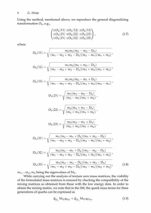
Using the method, mentioned above, we reproduce the general diagonalizingtransformation Ok, e.g.,±Ok(11) ±Ok(12) ±Ok(13)±Ok(21) ∓Ok(22) ±Ok(23)

∓Ok(31) ±Ok(32) ±Ok(33)

, (1.7)

where

Ok(11) =

√m2m3(m3 −m2 −Dk)

(m1 −m2 +m3 −Dk)(m3 −m1)(m1 +m2),

Ok(12) =

√m1m3(m1 +m3 −Dk)

(m1 −m2 +m3 −Dk)(m3 +m2)(m1 +m2),

Ok(13) =

√m1m2(m2 −m1 +Dk)

(m1 −m2 +m3 −Dk)(m3 +m2)(m3 −m1),

Ok(21) =

√m1(m3 −m2 −Dk)

(m3 −m1)(m1 +m2),

Ok(22) =

√m2(m3 +m1 −Dk)

(m2 +m3)(m1 +m2),

Ok(23) =

√m3(m2 −m1 +Dk)

(m3 +m2)(m1 +m2),

Ok(31) =

√m1(m2 −m1 +Dk)(m1 +m3 −Dk)

(m1 −m2 +m3 −Dk)(m3 −m1)(m1 +m2),

Ok(32) =

√m2(m2 −m1 +Dk)(m3 −m2 −Dk)

(m1 −m2 +m3 −Dk)(m3 +m2)(m1 +m2),

Ok(33) =

√m3(m3 −m2 −Dk)(m1 +m3 −Dk)

(m1 −m2 +m3 −Dk)(m3 −m1)(m3 +m2), (1.8)

m1,−m2,m3 being the eigenvalues ofMk.While carrying out the analysis of texture zero mass matrices, the viability

of the formulated mass matrices is ensured by checking the compatibility of themixing matrices so obtained from these with the low energy data. In order toobtain the mixing matrix, we note that in the SM, the quark mass terms for threegenerations of quarks can be expressed as

qULMUqUR + qD

LMDqDR , (1.9)

ii

“proc17” — 2017/12/11 — 19:44 — page 5 — #19 ii

ii

ii


where qUL(R)and qDL(R)

are the left (right) handed quark fields for the up sector(u, c, t) and down sector (d, s, b) respectively.MU andMD are the mass matricesfor the up and the down sector of quarks. In order to re-express above equation interms of the physical quark fields, one can diagonalize the mass matrices by thefollowing bi-unitary transformations

V†ULMUVUR =Mdiag

U ≡ Diag(mu,mc,mt), (1.10)

V†DLMDVDR =Mdiag

D ≡ Diag(md,ms,mb), (1.11)

whereMdiagU,D are real and diagonal, while VU

L, VU

Retc. denote the eigenvalues

of the mass matrices, i.e., the physical quark masses. Using the above equations,one can rewrite equation (9) as

qULVU

LMdiagU V†U

RqUR + qD

LVD

LMdiagD V†D

RqDR (1.12)

which can be re-expressed in terms of physical quark fields as

qphysULMdiagU qphysU

R+ qphysD

LMdiagD qphysD

R, (1.13)

where qphysUL

= V†ULqUL and qphysD

L= V†D

LqDR and so on. The mismatch of

diagonalizations of up and down quark mass matrices leads to the quark mixingmatrix VCKM, referred to as the Cabibbo-Kobayashi-Maskawa (CKM) matrix [11]given as

VCKM = V†ULVU

R. (1.14)

Over the past few years, both in the quark as well as lepton sector, a largenumber of analyses [5]-[8] have been carried out which establish the texture zeroapproach as a viable one for explaining the fermion mixing data. However, asmentioned earlier, since the number of possible texture zero mass matrices is verylarge, one has to carry out an exhaustive analysis of all possible texture zero massmatrices. To account for this limitation, therefore, Branco et al. [12,13] and Fritzschand Xing [14,15] have proposed the concept of ‘Weak Basis (WB) transformations’.

Within the SM and some of its extensions, one has the facility of makingWeak Basis (WB) transformations W on the quark fields, e.g., qL →WqL, qR →WqR, q′L → Wq′L, q

′R → Wq′R. These are unitary transformations which leave

the gauge currents real and diagonal but transform the mass matrices as

MU →W†MUW, MD →W†MDW. (1.15)

Without loss of generality, this approach introduces zeros in the quark massmatrices leading to a reduction in the number of parameters defining the massmatrices. Following this, one can arrive at two kinds of structures of the massmatrices, e.g., Branco et al. [12,13] give

Mq =

0 ∗ 0∗ ∗ ∗0 ∗ ∗

, Mq′ =

0 ∗ ∗∗ ∗ ∗∗ ∗ ∗

, q, q′= U,D, (1.16)

ii

“proc17” — 2017/12/11 — 19:44 — page 6 — #20 ii

ii

ii

6 G. Ahuja

whereas Fritzsch and Xing [14,15] give

Mq =

∗ ∗ 0∗ ∗ ∗0 ∗ ∗

, q = U,D. (1.17)

The mass matrices so obtained can thereafter be considered texture zero massmatrices and same methodology can be used to analyze these. Interestingly, onenow has an additional advantage that the large number of possible structures arenot all independent. Several of these are related through WB transformations andtherefore yield the same structure of the diagonalizing transformations leadingto similar mixing matrices, making the number of matrices to be analyzed muchless than before. However, there is a limitation too, i.e, this idea does not resultin constraining the parameter space of the elements of the mass matrices. Toovercome this, one can further impose a condition on the elements of the massmatrices by considering the following hierarchy for these [8]

(1, i) . (2, j) . (3, 3); i = 1, 2, 3, j = 2, 3. (1.18)

1.2.2 Lepton mass matrices

Keeping in mind the quark lepton universality [16], similar to the case of texturezero quark mass matrices discussed in the previous section, it becomes desirableto carry out a corresponding analysis in the lepton sector also. In the case ofleptons, several attempts have been made to formulate the phenomenologicalmass matrices considering charged leptons to be diagonal, usually referred to asthe flavor basis case [17]. However, in the present work, we have considered thenon flavor basis [18], wherein, texture is imposed on both the charged lepton massmatrix as well as on the neutrino mass matrix. The ‘smallness’ of the neutrinomasses is best described in terms of ‘seesaw mechanism’ [19] given by

Mν = −MTνDM

−1R MνD, (1.19)

withMν,MνD andMR corresponding to the light Majorana neutrino mass matrix,the Dirac neutrino mass matrix and the heavy right handed Majorana neutrinomass matrix respectively.

The methodology of analyzing the texture zero lepton mass matrices remainsessentially the same as that for the case of quarks. One can impose texture onthe charged lepton mass matrixMl and on the Dirac neutrino mass matrixMνD.Equation (1.19) can then be used to obtain the Majorana neutrino matrix Mν

which along with the matrixMl allows the construction of the Pontecorvo MakiNakagawa Sakata (PMNS) matrix [20] for examining the viability of the massmatrices. Using these ideas, in the following we have briefly summarized theresults of the analyses in the case of quarks [21] as well as leptons [22].

ii

“proc17” — 2017/12/11 — 19:44 — page 7 — #21 ii

ii

ii


1.3 Results and discussion

1.3.1 Texture zero quark mass matrices

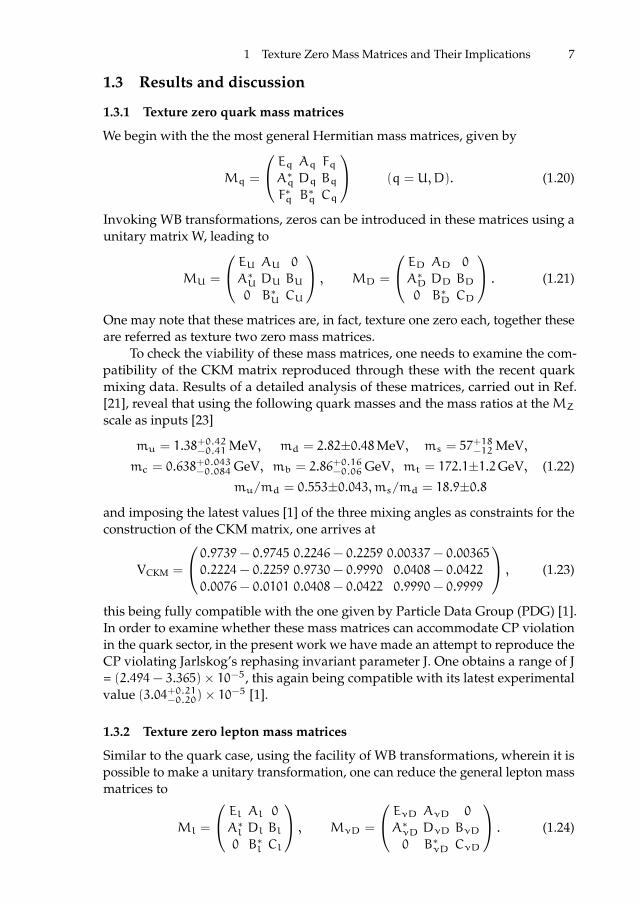
We begin with the the most general Hermitian mass matrices, given by

Mq =

Eq Aq FqA∗q Dq BqF∗q B

∗q Cq

(q = U,D). (1.20)

Invoking WB transformations, zeros can be introduced in these matrices using aunitary matrix W, leading to

MU =

EU AU 0

A∗U DU BU0 B∗U CU

, MD =

ED AD 0

A∗D DD BD0 B∗D CD

. (1.21)

One may note that these matrices are, in fact, texture one zero each, together theseare referred as texture two zero mass matrices.

To check the viability of these mass matrices, one needs to examine the com-patibility of the CKM matrix reproduced through these with the recent quarkmixing data. Results of a detailed analysis of these matrices, carried out in Ref.[21], reveal that using the following quark masses and the mass ratios at theMZ

scale as inputs [23]

mu = 1.38+0.42−0.41MeV, md = 2.82±0.48MeV, ms = 57+18−12MeV,

mc = 0.638+0.043−0.084GeV, mb = 2.86+0.16−0.06GeV, mt = 172.1±1.2GeV, (1.22)

mu/md = 0.553±0.043,ms/md = 18.9±0.8

and imposing the latest values [1] of the three mixing angles as constraints for theconstruction of the CKM matrix, one arrives at

VCKM =

0.9739− 0.9745 0.2246− 0.2259 0.00337− 0.003650.2224− 0.2259 0.9730− 0.9990 0.0408− 0.0422

0.0076− 0.0101 0.0408− 0.0422 0.9990− 0.9999

, (1.23)

this being fully compatible with the one given by Particle Data Group (PDG) [1].In order to examine whether these mass matrices can accommodate CP violationin the quark sector, in the present work we have made an attempt to reproduce theCP violating Jarlskog’s rephasing invariant parameter J. One obtains a range of J= (2.494− 3.365)× 10−5, this again being compatible with its latest experimentalvalue (3.04+0.21−0.20)× 10−5 [1].

1.3.2 Texture zero lepton mass matrices

Similar to the quark case, using the facility of WB transformations, wherein it ispossible to make a unitary transformation, one can reduce the general lepton massmatrices to

Ml =

El Al 0

A∗l Dl Bl0 B∗l Cl

, MνD =

EνD AνD 0

A∗νD DνD BνD0 B∗νD CνD

. (1.24)

ii

“proc17” — 2017/12/11 — 19:44 — page 8 — #22 ii

ii

ii

8 G. Ahuja

A detailed analysis of these mass matrices has been carried out in Ref. [22]. In thepresent work, for the normal and inverted ordering of neutrino masses, we havefirst examined the viability of these mass matrices and then we have investigatedtheir implications for CP violation in the leptonic sector.

The latest situation regarding neutrinos masses and mixing angles at 3σ C.L.is summarized as follows [24]

∆m221 = (7.02− 8.09)× 10−5eV2; ∆m223 = (2.325− 2.599)× 10−3eV2; (1.25)

sin2 θ12 = 0.270− 0.344; sin2 θ23 = 0.385− 0.644; sin2 θ13 = 0.0188− 0.0251.(1.26)

The 3σ C.L. ranges of the PMNS matrix elements recently constructed by Garcia etal.[24] are as follows

UPMNS =

0.801− 0.845 0.514− 0.580 0.137− 0.1580.225− 0.517 0.441− 0.699 0.164− 0.793

0.246− 0.529 0.464− 0.713 0.590− 0.776

. (1.27)

For the inverted and normal neutrino mass orderings, the mass matrices men-tioned in equation (1.24) yield the following magnitudes of the correspondingPMNS matrix elements [22] respectively

UIOPMNS =

0.034− 0.859 0.0867− 0.593 0.135− 0.9960.250− 0.971 0.068− 0.812 0.043− 0.808

0.103− 0.621 0.395− 0.822 0.088− 0.810

. (1.28)

UNOPMNS =

0.444− 0.993 0.123− 0.837 0.004− 0.2880.061− 0.816 0.410− 0.941 0.047− 0.872

0.012− 0.848 0.049− 0.779 0.460− 0.992

. (1.29)

For both the mass orderings, one finds that the 3σ C.L. ranges of the PMNSmatrix elements given by Garcia et al. are inclusive in the ranges of the PMNSmatrix elements found here, thereby ensuring the viability of texture two zeromass matrices considered here. Further, analogous to the case of quarks, we havemade an attempt to find constraints for the CP violating Jarlskog’s rephasinginvariant parameter in the leptonic sector also. For the inverted mass ordering, oneobtains a range of J from −0.05− 0.05, whereas, for the normal mass ordering the,parameter J is obtained in the range −0.03− 0.03. These observations, therefore,lead one to conclude that the texture two zero leptonic mass matrices are notonly compatible with the recent leptonic mixing data but also provide interestingbounds for the Jarlskog’s rephasing invariant parameter.

1.4 Summary and Conclusions

To summarize, in the present work, we have made an attempt to provide anoverview of texture zero fermion mass matrices. For the case of both quarks andleptons, incorporating the texture zero approach as well as using the WB transfor-mations, analyses of the “general” fermion mass matrices have been discussed.

ii

“proc17” — 2017/12/11 — 19:44 — page 9 — #23 ii

ii

ii


After examining the viability of these mass matrices, we have obtained interestingbounds on the Jarlskog’s rephasing invariant parameter in the quark and leptonicsector.

AcknowledgementsThe author would like to thank the organizers of the 20th International work-shop “What Comes Beyond The Standard Models” held at Bled, Slovenia forproviding an opportunity to present this work. Thanks are due to M.Gupta foruseful discussions. The author acknowledges DST, Government of India (GrantNo: SR/FTP/PS-017/2012) for financial support.

References

1. C. Patrignani et al., Particle Data Group, Chin. Phys. C 40, 100001 (2016).2. F. P. An et al., DAYA-BAY Collaboration, Phys. Rev. Lett. 108, 171803 (2012).3. J. K. Ahn et al., RENO Collaboration, Phys. Rev. Lett. 108, 191802 (2012).4. F. Capozzi et al., Nucl. Phys. B 908, 218 (2016).5. H. Fritzsch, Z. Z. Xing, Nucl. Phys. B 556, 49 (1999) and references therein.6. Z. Z. Xing, H. Zhang, J. Phys. G 30, 129 (2004) and refrences therein.7. N. G. Deshpande, M. Gupta, P. B. Pal, Phys. Rev. D 45, 953 (1992); P. S. Gill, M. Gupta,

Pramana 45, 333 (1995); M. Gupta, G. Ahuja, Int. J. Mod. Phys. A 26, 2973 (2011).8. M. Gupta, G. Ahuja, Int. J. Mod. Phys. A 27, 1230033 (2012) and references therein.9. H. Fritzsch, Phys. Lett. B 70, 436 (1977).

10. H. Fritzsch, Phys. Lett. B 73, 317 (1978).11. N. Cabibbo, Phys. Rev. Lett. 10, 531 (1963); M. Kobayashi, T. Maskawa, Prog. Theor.

Phys. 49, 652 (1973).12. G. C. Branco, D. Emmanuel-Costa, R. G. Felipe, Phys. Lett. B 477, 147 (2000).13. G. C. Branco, D. Emmanuel-Costa, R. G. Felipe, H. Serodio, Phys. Lett. B 670, 340 (2009).14. H. Fritzsch, Z. Z. Xing, Phys. Lett. B 413, 396 (1997) and references therein.15. H. Fritzsch, Z. Z. Xing, Nucl. Phys. B 556, 49 (1999) and references therein.16. M. A. Schmidt, A. Yu. Smirnov, Phys. Rev. D 74, 113003 (2006).17. P. H. Frampton, S. L. Glashow, D. Marfatia, Phys. Lett. B 536, 79 (2002); Z. Z. Xing, Phys.

Lett. B 530, 159 (2002); B. R. Desai, D. P. Roy, A. R. Vaucher, Mod. Phys. Lett. A 18, 1355(2003); Z. Z. Xing, Int. J. Mod. Phys. A 19, 1 (2004); A. Merle, W. Rodejohann, Phys. Rev.D 73, 073012 (2006); S. Dev, S. Kumar, S. Verma, S. Gupta, R. R. Gautam, Phys. Rev. D81, 053010 (2010) and references therein.

18. M. Fukugita, M. Tanimoto, T. Yanagida, Prog. Theor. Phys. 89, 263 (1993); ibid. Phys.Lett. B 562, 273 (2003), hep-ph/0303177; M. Randhawa, G. Ahuja, M. Gupta, Phys. Rev.D 65, 093016 (2002); G. Ahuja, S. Kumar, M. Randhawa, M. Gupta, S. Dev, Phys. Rev.D 76, 013006 (2007); G. Ahuja, M. Gupta, M. Randhawa, R. Verma, Phys. Rev. D 79,093006 (2009); M. Fukugita, et al., Phys. Lett. B 716, 294 (2012), arXiv:1204.2389; P. Fakay,S. Sharma, R. Verma, G. Ahuja, M. Gupta, Phys. Lett. B 720, 366 (2013).

19. H. Fritzsch, M. Gell-Mann, P. Minkowski, Phys Lett. B 59, 256 (1975); P. Minkowski,Phys. Lett. B 67, 421 (1977); T. Yanagida, proceedings of the Workshop on Unified Theoriesand Baryon Number in the Universe, Tsukuba, 1979, eds. A. Sawada, A. Sugamoto, KEKReport No. 79-18, Tsukuba; M. Gell-Mann, P. Ramond, R. Slansky, in Supergravity, editedby F. van Nieuwenhuizen, D. Freedman (North Holland, Amsterdam, 1979) 315; S. L.Glashow, in Quarks and Leptons, edited by M. Levy et al. (Plenum, New York, 1980) 707;R. N. Mohapatra, G. Senjanovic, Phys. Rev. Lett. 44, 912 (1980); J. Schechter, J. W. F.Valle, Phys. Rev. D 22, 2227 (1980).

ii

“proc17” — 2017/12/11 — 19:44 — page 10 — #24 ii

ii

ii

10 G. Ahuja

20. B. Pontecorvo, Zh. Eksp. Theor. Fiz. (JETP) 33, 549 (1957); ibid. 34, 247 (1958); ibid. 53,1771 (1967); Z. Maki, M. Nakagawa, S. Sakata, Prog. Theor. Phys. 28, 870 (1962).

21. S. Sharma, P. Fakay, G. Ahuja, M. Gupta, Phys. Rev. D 91, 053004 (2015).22. S. Sharma, G. Ahuja, M. Gupta, Phys. Rev. D 94, 113004 (2016).23. Z. Z. Xing, H. Zhang, S. Zhou, Phys. Rev. D 86, 013013 (2012).24. M.C. Gonzalez-Garcia, M. Maltoni, T. Schwetz, Nucl. Phys. B 908, 199 (2016).

ii

“proc17” — 2017/12/11 — 19:44 — page 11 — #25 ii

ii

ii




2 Search for Double Charged Particles as Direct Testfor Dark Atom Constituents

O.V. Bulekov1, M.Yu. Khlopov1,2,3?,A.S. Romaniouk1,4 and Yu.S. Smirnov1??

1National Research Nuclear University ”MEPHI”(Moscow Engineering Physics Institute),115409 Moscow, Russia2 Centre for Cosmoparticle Physics “Cosmion”115409 Moscow, Russia3 APC laboratory 10, rue Alice Domon et Leonie Duquet75205 Paris Cedex 13, France4 CERN, Geneva, Switzerland

Abstract. The nonbaryonic dark matter of the Universe is assumed to consist of new stableparticles. Stable particle candidates for cosmological dark matter are usually consideredas neutral and weakly interacting. However stable charged leptons and quarks can alsoexist hidden in elusive dark atoms and can play a role of dark matter. Such possibility isstrongly restricted by the constraints on anomalous isotopes of light elements that formpositively charged heavy species with ordinary electrons. This problem might be avoided,if stable particles with charge -2 exist and there are no stable particles with charges +1 and-1. These conditions cannot be realized in supersymmetric models, but can be satisfied inseveral alternative scenarios, which are discussed in this paper. The excessive -2 chargedparticles are bound with primordial helium in O-helium atoms, maintaining specific nuclear-interacting form of the dark matter. O-helium dark matter can provide solution for thepuzzles of dark matter searches. The successful development of composite dark matterscenarios appeals to experimental search for doubly charged constituents of dark atoms.Estimates of production cross section of such particles at LHC are presented and discussed.Signatures of double charged particles in the ATLAS experiment are outlined.

Povzetek. Avtorji predpostavijo, da temno snov, ki ni iz barionov poznanih treh druzin,sestavljajo novi stabilni delci. Obicajno za njih predlagajo nevtralne delce s sibko interakcijo,pa tudi stabilne nabite leptone in kvarke, vezane v “temne atome”. To zadnjo moznost soposkusi mocno omejili.Tem omejitvam se lahko izognemo, ce privzamemo, da obstajajostabilni (temni) delci z nabojem −2, ni pa stabilnih (temnih) delcev z naboji +1 in −1.Tega privzetka ne moremo narediti v modelih s supersimetrijo, lahko pa ga naredimo valternativnih modelih, ki jih avtorji obravnavajo. Visek delcev z nabojem −2 se veze sprvotnim helijem v “atome” O-helija, katerega interakcija je posledicno obicajna jedrska.Taka temna snov pojasni rezultate tistih poskusov iskanja temne snovi, ki je se niso zaznali.Obravnavajo preseke za te delce pri poskusih na LHC in predvidijo rezultate meritev naATLASu.? Presented first part of talk at Bled

?? Presented second part of talk by VIA teleconference

ii

“proc17” — 2017/12/11 — 19:44 — page 12 — #26 ii

ii

ii

12 O.V. Bulekov, M.Yu. Khlopov, A.S. Romaniouk and Yu.S. Smirnov

Keywords: Elementary particles, Dark matter, Dark atoms, Stable double chargedparticles

2.1 Introduction

The observation of exotic stable multi-charge objects would represent strikingevidence for physics beyond the Standard Model. Cosmological arguments putsevere constraints on possible properties of such objects. Such particles (see e.g.Ref. [1] for review and reference) should be stable, provide the measured darkmatter density and be decoupled from plasma and radiation at least before thebeginning of matter dominated stage. The easiest way to satisfy these conditions isto involve neutral elementary weakly interacting massive particles (WIMPs). SUSYModels provide a list of possible WIMP candidates: neutralino, axino, gravitinoetc., However it may not be the only particle physics solution for the dark matterproblem.

One of such alternative solutions is based on the existence of heavy stablecharged particles bound in neutral dark atoms. Dark atoms offer an interestingpossibility to solve the puzzles of dark matter searches. It turns out that even stableelectrically charged particles can exist hidden in such atoms, bound by ordinaryCoulomb interactions (see [1–3] and references therein). Stable particles withcharge -1 are excluded due to overproduction of anomalous isotopes. However,there doesn’t appear such an evident contradiction for negatively doubly chargedparticles.

There exist several types of particle models where heavy stable -2 chargedspecies, O−−, are predicted:

(a) AC-leptons, predicted as an extension of the Standard Model, based on theapproach of almost-commutative geometry [4–7].

(b) Technileptons and anti-technibaryons in the framework of Walking Technicolor(WTC) [8–14].

(c) stable ”heavy quark clusters” UUU formed by anti-U quark of 4th generation[4,15–19]

(d) and, finally, stable charged clusters u5u5u5 of (anti)quarks u5 of 5th familycan follow from the approach, unifying spins and charges[20].

All these models also predict corresponding +2 charge particles. If these posi-tively charged particles remain free in the early Universe, they can recombinewith ordinary electrons in anomalous helium, which is strongly constrained interrestrial matter. Therefore a cosmological scenario should provide a mechanismwhich suppresses anomalous helium. There are two possible mechanisms thancan provide a suppression:

(i) The abundance of anomalous helium in the Galaxy may be significant, but interrestrial matter a recombination mechanism could suppress this abundancebelow experimental upper limits [4,6]. The existence of a new U(1) gaugesymmetry, causing new Coulomb-like long range interactions between chargeddark matter particles, is crucial for this mechanism. This leads inevitably tothe existence of dark radiation in the form of hidden photons.

ii

“proc17” — 2017/12/11 — 19:44 — page 13 — #27 ii

ii

ii

2 Search for Double Charged Particles as Direct Test. . . 13

(ii) Free positively charged particles are already suppressed in the early Universeand the abundance of anomalous helium in the Galaxy is negligible [2,16].

These two possibilities correspond to two different cosmological scenarios of darkatoms. The first one is realized in the scenario with AC leptons, forming neutralAC atoms [6]. The second assumes a charge asymmetry of the O−− which formsthe atom-like states with primordial helium [2,16].

If new stable species belong to non-trivial representations of the SU(2) elec-troweak group, sphaleron transitions at high temperatures can provide the relationbetween baryon asymmetry and excess of -2 charge stable species, as it was demon-strated in the case of WTC [8,21–23].

After it is formed in the Standard Big Bang Nucleosynthesis (BBN), 4Hescreens the O−− charged particles in composite (4He++O−−) OHe “atoms” [16].In all the models of OHe, O−− behaves either as a lepton or as a specific “heavyquark cluster” with strongly suppressed hadronic interactions. The cosmologicalscenario of the OHe Universe involves only one parameter of new physics − themass of O−−. Such a scenario is insensitive to the properties of O−− (except forits mass), since the main features of the OHe dark atoms are determined by theirnuclear interacting helium shell. In terrestrial matter such dark matter speciesare slowed down and cannot cause significant nuclear recoil in the undergrounddetectors, making them elusive in direct WIMP search experiments (where detec-tion is based on nuclear recoil) such as CDMS, XENON100 and LUX. The positiveresults of DAMA experiments (see [24] for review and references) can find inthis scenario a nontrivial explanation due to a low energy radiative capture ofOHe by intermediate mass nuclei [2,1,3]. This explains the negative results of theXENON100 and LUX experiments. The rate of this capture is proportional to thetemperature: this leads to a suppression of this effect in cryogenic detectors, suchas CDMS.

OHe collisions in the central part of the Galaxy lead to OHe excitations, andde-excitations with pair production in E0 transitions can explain the excess of thepositron-annihilation line, observed by INTEGRAL in the galactic bulge [1,3,21,27].

One should note that the nuclear physics of OHe is in the course of develop-ment and its basic element for a successful and self-consistent OHe dark matterscenario is related to the existence of a dipole Coulomb barrier, arising in the pro-cess of OHe-nucleus interaction and providing the dominance of elastic collisionsof OHe with nuclei. This problem is the main open question of composite darkmatter, which implies correct quantum mechanical solution [28]. The lack of sucha barrier and essential contribution of inelastic OHe-nucleus processes seem tolead to inevitable overproduction of anomalous isotopes [29].

Production of pairs of elementary stable doubly charged heavy leptons ischaracterized by a number of distinct experimental signatures that would provideeffective search for them at the experiments at the LHC and test the atom-likestructure of the cosmological dark matter. Moreover, astrophysical consequencesof composite dark matter model can reproduce experimentally detected excess inpositron annihilation line and high energy positron fraction in cosmic rays onlyif the mass of double charged X particles is in the 1 TeV range (Section 2). Wediscuss confrontation of these predictions and experimental data in Section 3. The

ii

“proc17” — 2017/12/11 — 19:44 — page 14 — #28 ii

ii

ii


current status and expected progress in experimental searches for stable doublecharged particles as constituents of composite dark matter are summarized in theconcluding Section 4.

2.2 Indirect effects of composite dark matter

The existence of such form of matter as O-helium should lead to a number ofastrophysical signatures, which can constrain or prove this hypothesis. One of thesignatures of O-helium can be a presence of an anomalous low Z/A componentin the cosmic ray flux. O-helium atoms that are present in the Galaxy in the formof the dark matter can be destroyed in astrophysical processes and free X can beaccelerated as ordinary charged particles. O-helium atoms can be ionized due tonuclear interaction with cosmic rays or in the front of a shock wave in the Super-nova explosions, where they were effectively accumulated during star evolution[16]. If the mechanisms of X acceleration are effective, the low Z/A componentwith charge 2 should be present in cosmic rays at the level of FX/Fp ∼ 10−9m−1

o

[21], and might be observed by PAMELA and AMS02 cosmic ray experiments.Heremo is the mass of O-helium in TeV, FX and Fp are the fluxes of X and protons,respectively.

2.2.1 Excess of positron annihilation line in the galactic bulge

Another signature of O-helium in the Galaxy is the excess of the positron annihila-tion line in cosmic gamma radiation due to de-excitation of the O-helium after itsinteraction in the interstellar space. If 2S level of O-helium is excited, its direct one-photon transition to the 1S ground state is forbidden and the de-excitation mainlygoes through direct pair production. In principle this mechanism of positronproduction can explain the excess in positron annihilation line from the galacticbulge, measured by the INTEGRAL experiment. Due to the large uncertainty ofDM distribution in the galactic bulge this interpretation of the INTEGRAL data ispossible in a wide range of masses of O-helium with the minimal required centraldensity of O-helium dark matter atmo = 1.25TeV [25,26]For the smaller valuesofmo on needs larger central density to provide effective excitation of O-heliumin collisions Current analysis favors lowest values of central dark matter density,making possible O-helium explanation for this excess only for a narrow windowaround this minimal value (see Fig. 2.1)

2.2.2 Composite dark matter solution for high energy positron excess

In a two-component dark atom model, based on Walking Technicolor, a sparseWIMP-like component of atom-like state, made of positive and negative doublycharged techniparticles, is present together with the dominant OHe dark atom andthe decays of doubly positive charged techniparticles to pairs of same-sign leptonscan explain the excess of high-energy cosmic-ray positrons, found in PAMELA andAMS02 experiments [17]. This explanation is possible for the mass of decaying

ii

“proc17” — 2017/12/11 — 19:44 — page 15 — #29 ii

ii

ii


Fig. 2.1. Dark matter is subdominant in the central part of Galaxy. It strongly suppresses itdynamical effect and causes large uncertainty in dark matter density and velocity distribu-tion. At this uncertainty one can explain the positron line excess, observed by INTERGRAL,for a wide range of mo given by the curve with minimum at mo = 1.25TeV. However,recent analysis of possible dark matter distribution in the galactic bulge favor minimalvalue of its central density.

Fig. 2.2. Best fit high energy positron fluxes from decaying composite dark matter in con-frontation with the results of AMS02 experiment.

ii

“proc17” — 2017/12/11 — 19:44 — page 16 — #30 ii

ii

ii


+2 charged particle below 1 TeV and depends on the branching ratios of leptonicchannels (See Fig. 2.2).

Since even pure lepton decay channels are inevitably accompanied by gammaradiation the important constraint on this model follows from the measurement ofcosmic gamma ray background in FERMI/LAT experiment. The multi-parameter

Fig. 2.3. Gamma ray flux accompanying the best fit high energy positron fluxes from decay-ing composite dark matter reproducing the results of AMS02 experiment, in confrontationwith FERMI/LAT measurement of gamma ray background.

analysis of decaying dark atom constituent model determines the maximal modelindependent value of the mass of decaying +2 charge particle, at which thisexplanation is possible

mo < 1TeV.

One should take into account that according to even in this range hypothesison decaying composite dark matter, distributed in the galactic halo, can lead togamma ray flux exceeding the measured by FERMI/LAT.

2.2.3 Sensitivity of indirect effect of composite dark matter to the mass oftheir double charged constituents

We see that indirect effects of composite dark matter strongly depend on the massof its double charged constituents.

To explain the excess of positron annihilation line in the galactic bulge massof double charged constituent of O-helium should be in a narrow window around

mo = 1.25TeV.

ii

“proc17” — 2017/12/11 — 19:44 — page 17 — #31 ii

ii

ii


To explain the excess of high energy cosmic ray positrons by decays of con-stituents of composite dark matter with charge +2 and to avoid overproductionof gamma background, accompanying such decays, the mass of such constituentshould be in the range

mo < 1TeV.

These predictions should be confronted with the experimental data on theaccelerator search for stable double charged particles.

2.3 Searches for stable multi-charged particles

A new charged massive particle with electric charge 6= 1ewould represent a dra-matic deviation from the predictions of the Standard Model, and such a spectaculardiscovery would lead to fundamental insights and critical theoretical develop-ments. Searches for such kind of particles were carried out in many cosmic rayand collider experiments (see for instance review in [38]). Experimental search fordouble charged particles is of a special interest because of important cosmologicalsequences discussed in previous sections. In a tree approximation, such particlescannot decay to pair of quarks due to electric charge conservation and only decaysto the same sign leptons are possible. The latter implies lepton number noncon-servation, being a profound signature of new physics. In general, it makes suchstates sufficiently long-living in a cosmological scale.

Obviously, such experiments are limited to look only for the “long-lived”particles, which do not decay within a detector, as opposed to truly stable particles,which do not decay at all. Since the kinematics and cross sections for doublecharged particle production processes cannot be reliably predicted, search resultsat collider experiments are usually quoted as cross section limits for a range ofcharges and masses for well-defined kinematic models. In these experiments,the mass limit was set at the level of up to 100 GeV(see e.g. for review [38]).

The CDF experiment collaboration performed a search for long-lived doublecharged Higgs bosons (H++, H−−) with 292 pb−1 of data collected in pp collisionsat√s = 1.96 TeV [39]. The dominant production mode considered was pp →

γ?/Z+ X→ H++H−− + X.Background sources include jets fragmenting to high-pT tracks, Z → ee,

Z→ µµ, and Z→ ττ, where at least one τ decays hadronically. Number of eventsexpected from these backgrounds in the signal region was estimated to be < 10−5

at 68% confidence level (CL).Not a single event with a H++ or H−− was found in experimental data. This

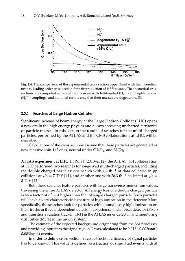
allows to set cross-section limit shown in Fig. 2.4 as a horizontal solid line. Next-to-leading order theoretical calculations of the cross-section for pair production ofH±± bosons for left-handed and right-handed couplings are also shown in thisfigure. Comparison of expected and observed cross-section limits gives the follow-ing mass constrains: 133 and 109 GeV on the masses of long-lived H±±L and H±±R ,respectively, at 95% CL as shown in Fig. 2.4. In case of degenerate H±±L and H±±Rbosons, the mass limit was set to 146 GeV.

ii

“proc17” — 2017/12/11 — 19:44 — page 18 — #32 ii

ii

ii


with a flat prior for the signal cross section and Gaussianpriors for the uncertainties on acceptance, background, andintegrated luminosity (6%) [24]. The 95% C.L. upper limiton the cross section (which varies from 39.7 fb at mH 90 GeV=c2 to 32.6 fb at mH 160 GeV=c2, see Fig. 2)is converted into an H mass limit by comparing to thetheoretical p p ! =Z X ! HH X cross sec-tion at next-to-leading order [25] using the CTEQ6 [22] setof PDFs. We include uncertainties in the theoretical crosssections due to PDFs (5%) [22] and higher-order QCDcorrections (7.5%) [25] in the extraction of the mass limit,for a total systematic uncertainty of 14%. The theoreticalcross sections are computed separately for H

L and HR

bosons that couple to left- and right-handed particles,respectively. When only one of these states is accessible,we exclude the long-lived H

L boson below a mass of133 GeV=c2 and the long-lived H

R boson below a massof 109 GeV=c2, both at the 95% C.L. When the two statesare degenerate in mass, we exclude mH < 146 GeV=c2

at the 95% C.L.In conclusion, we have searched for long-lived doubly

charged particles using their signatures of high ionizationand muonlike penetration. No evidence is found for pair-production of such particles, and we set the individuallower limits of 133 GeV=c2 and 109 GeV=c2, respec-tively, on the masses of long-lived H

L and HR bosons.

The mass limit for the case of degenerate HL and H

Rbosons is 146 GeV=c2.

We thank M. Muhlleitner and M. Spira for calculatingthe next-to-leading order H production cross section.We thank the Fermilab staff and the technical staffs of theparticipating institutions for their vital contributions. Thiswork was supported by the U.S. Department of Energy andNational Science Foundation; the Italian Istituto Nazionaledi Fisica Nucleare; the Ministry of Education, Culture,Sports, Science, and Technology of Japan; the NaturalSciences and Engineering Research Council of Canada;the National Science Council of the Republic of China; the

Swiss National Science Foundation; the A. P. SloanFoundation; the Bundesministerium fuer Bildung undForschung, Germany; the Korean Science andEngineering Foundation and the Korean ResearchFoundation; the Particle Physics and AstronomyResearch Council and the Royal Society, UK; theRussian Foundation for Basic Research; the CommissionInterministerial de Ciencia y Tecnologia, Spain; and in partby the European Community’s Human PotentialProgramme under Contract No. HPRN-CT-2002-00292,Probe for New Physics.

[1] T. P. Cheng and L.-F. Li, Phys. Rev. D 22, 2860 (1980).[2] R. N. Mohapatra and J. C. Pati, Phys. Rev. D 11, 566

(1975); G. Senjanovic and R. N. Mohapatra, Phys.Rev. D 12, 1502 (1975); R. N. Mohapatra and G.Senjanovic, Phys. Rev. D 23, 165 (1981).

[3] C. S. Aulakh, A. Melfo, and G. Senjanovic, Phys. Rev. D57, 4174 (1998); Z. Chacko and R. N. Mohapatra, Phys.Rev. D 58, 015003 (1998).

[4] C. S. Aulakh, K. Benakli, and G. Senjanovic, Phys. Rev.Lett. 79, 2188 (1997).

[5] Y. Ashie et al. (Super-Kamiokande Collaboration), Phys.Rev. Lett. 93, 101801 (2004), and references therein.

[6] R. N. Mohapatra and G. Senjanovic, Phys. Rev. Lett. 44,912 (1980).

[7] B. Bajc, G. Senjanovic, and F. Vissani, Phys. Rev. D 70,093002 (2004), and references therein; S. F. King, Rep.Prog. Phys. 67, 107 (2004), and references therein.

[8] T. Han, H. E. Logan, B. McElrath, and L.-T. Wang, Phys.Rev. D 67, 095004 (2003).

[9] D. Acosta et al. (CDF Collaboration), Phys. Rev. Lett. 93,221802 (2004).

[10] The range 105 > hll0 > 108 corresponds to the H

boson decaying within the detector, and requires othertriggering and tracking methods.

[11] G. Abbiendi et al. (OPAL Collaboration), Phys. Lett. B526, 221 (2002).

[12] J. Abdallah et al. (DELPHI Collaboration), Phys. Lett. B552, 127 (2003).

[13] D. Acosta et al., Phys. Rev. D 71, 032001 (2005).[14] T. Affolder et al., Nucl. Instrum. Methods Phys. Res., Sect.

A 526, 249 (2004).[15] F. Abe et al. (CDF Collaboration), Nucl. Instrum. Methods

Phys. Res., Sect. A 271, 387 (1988).[16] G. Ascoli et al., Nucl. Instrum. Methods Phys. Res., Sect.

A 268, 33 (1988).[17] CDF uses a cylindrical coordinate system in which is

the azimuthal angle, r is the radius from the nominalbeamline, and z points in the direction of the protonbeam and is zero at the center of the detector. Thepseudorapidity lntan!=2, where ! is the polarangle with respect to the z axis. Calorimeter energy (trackmomentum) measured transverse to the beam is denotedas ETpT. Track pT is evaluated from its curvatureassuming a singly charged particle, and is half of thetrue pT for a doubly charged particle.

) 2 Mass (GeV/c±±H90 100 110 120 130 140 150 160

Cro

ss S

ecti

on

(p

b)

0

0.1

0.2

L±±H

R±±H

R±± & HL

±±degenerate H

experimental limit(95% C.L.)

FIG. 2. The comparison of the experimental cross sectionupper limit with the theoretical next-to-leading order crosssection [25] for pair production of H bosons. The theoreticalcross sections are computed separately for bosons with left-handed (H

L ) and right-handed (HR ) couplings, and summed

for the case that their masses are degenerate.

PRL 95, 071801 (2005) P H Y S I C A L R E V I E W L E T T E R S week ending12 AUGUST 2005

071801-6

Fig. 2.4. The comparison of the experimental cross section upper limit with the theoreticalnext-to-leading order cross section for pair production of H±± bosons. The theoretical crosssections are computed separately for bosons with left-handed (H±±L ) and right-handed(H±±R ) couplings, and summed for the case that their masses are degenerate, [39].

2.3.1 Searches at Large Hadron Collider

Significant increase of beam energy at the Large Hadron Collider (LHC) opensa new era in the high energy physics and allows accessing uncharted territoriesof particle masses. In this section the results of searches for the multi-chargedparticles, performed by the ATLAS and the CMS collaborations at LHC, will bedescribed.

Calculations of the cross sections assume that these particles are generated asnew massive spin-1/2 ones, neutral under SU(3)C and SU(2)L.

ATLAS experiment at LHC In Run 1 (2010–2012), the ATLAS [40] collaborationat LHC performed two searches for long-lived multi-charged particles, includingthe double charged particles: one search with 4.4 fb−1 of data collected in ppcollisions at

√s = 7 TeV [41], and another one with 20.3 fb−1 collected at

√s =

8 TeV [42].Both these searches feature particles with large transverse momentum values,

traversing the entire ATLAS detector. An energy loss of a double charged particleis by a factor of q2 = 4 higher than that of single charged particle. Such particleswill leave a very characteristic signature of high ionization in the detector. Morespecifically, the searches look for particles with anomalously high ionization ontheir tracks in three independent detector subsystems: silicon pixel detector (Pixel)and transition radiation tracker (TRT) in the ATLAS inner detector, and monitoringdrift tubes (MDT) in the muon system.

The estimate of the expected background originating from the SM processesand providing input into the signal region D was calculated to be 0.013±0.002(stat.)±0.003(syst.) events.

In order to define cross section, a reconstruction efficiency of signal particleshas to be known. This value is defined as a fraction of simulated events with at

ii

“proc17” — 2017/12/11 — 19:44 — page 19 — #33 ii

ii

ii


Fig. 2.5. The signal efficiencies for different masses and charges of the multi-charged parti-cles for the DY production model. Double charged particles are denoted as “z = 2” (redpoints and line). The picture is taken from [42].

least one multi-charged particle satisfying all of the aforementioned criteria overthe number of all generated events. In other words, it is a search sensitivity to finda hypothetical particle with the ATLAS experiment. These values are shown inFig. 2.5 for each considered signal sample containing particles with charges from 2

to 6.

Fig. 2.6. Observed 95% CL cross-section upper limits and theoretical cross-sections asfunctions of the multi-charged particles mass. Again, the double charged particles aredenoted as “z = 2” (red points and lines). The picture is taken from [42].

ii

“proc17” — 2017/12/11 — 19:44 — page 20 — #34 ii

ii

ii


No events with double charged particles were found in neither 2011 or 2012experimental data sets, setting the lower mass limits to 430 and 660 GeV, respec-tively, at 95% CL. The comparison of observed cross-section upper limits andtheoretically predicted cross-sections is shown in Fig. 2.6.

CMS experiment at LHC In parallel to the ATLAS experiment, the CMS [43]collaboration at LHC performed a search for double charged particles, using5.0 fb−1 of data collected in pp collisions at

√s = 7 TeV and 18.8 fb−1 collected at√

s = 8 TeV [44].The search features particles with high ionization along their tracks in the in-

ner silicon pixel and strip tracker. Tracks with specific ionization Ih > 3 MeV/cmwere selected. The muon system was used to measure the time-of-flight values.Tracks with 1/β > 1.2were considered.

For the part of the search based on the√s = 7 TeV data, the number of events

in the signal region, expected from SM processes, was estimated to be 0.15± 0.04,whereas for the

√s = 8 TeV part it was 0.52±0.11 events. The uncertainties include

both statistical and systematical contributions. 0 and 1 events were observed inthe signal regions for the 7 and 8 TeV analyses, respectively, which is consistentwith the predicted event rate.

Comparison between observed upper cross section limits and theoreticallypredicted cross section values for the 8 TeV is shown in Fig. 2.7.

For the 8 TeV search, the mass limit of 665 GeV was obtained. This result(within uncertainties) is very close to the ATLAS limit of 660 GeV for the 8 TeVdata set. Also, CMS treated the results obtained at 7 and 8 TeV as combined. Thisallowed to push the lower mass limit to 685 GeV at 95% CL. A combination ofthe results of two experiments for 8 TeV would mean an increase of statistics bya factor of 2. Having said that, one can conclude that the mass limit based onthe results of both experiment for double charged particles can be set at the levelof about 730 GeV.

What one expects from LHC Run 2 Considering a recent CMS Physics AnalysisSummary [45] and an ATLAS paper in preparation, both on the searches for doublecharged particles in data delivered by LHC to these experiments in 2015–2016,we may conclude that each of these two experiments will be able to set a lowermass limit on the double charged particles atm = 1000± 50 GeV. Going furtherand considering the data taking periods of ATLAS and CMS until the end ofRun 2 (end of 2018), we can estimate a low limit on the double charged particlesmass corresponding to the Run 2 data set. Several assumptions are made in thesespeculations:

• by the end of 2018, ATLAS and CMS will each record about 120 fb−1 of√s = 13 TeV data;

• signal efficiency will remain at a present level in both experiments, withoutbeing compromised by high detector occupancy or any other effects;

• no double charged particle candidates will be in observed in the first place.

ii

“proc17” — 2017/12/11 — 19:44 — page 21 — #35 ii

ii

ii


Fig. 2.7. Observed 95% CL cross-section upper limits and theoretical cross-sections asfunctions of the multi-charged particles mass in CMS search at the

√s = 8 TeV. The double

charged particles are denoted as “|Q| = 2e”. The picture is taken from [44].

Considering all of the above, the ATLAS and CMS collaborations may eachbe expected to set the lower mass limits at the level of 1.2 TeV based on theiranalyses of the entire 13 TeV data set. If these two experiments combined theirindependently gathered statistics together for this kind of search, the limits wouldgo as high as up to 1.3 TeV.

2.4 Conclusions

The existence of heavy stable neutral particles is one of the popular solutionsfor the dark matter problem. However, DM considered to be electrically neutral,potentially can be formed by stable heavy charged particles bound in neutral atom-like states by Coulomb attraction. Analysis of the cosmological data and atomiccomposition of the Universe gives the constrains on the particle charge showingthat only -2 charged constituents, being trapped by primordial helium in neutralO-helium states, can avoid the problem of overproduction of the anomalousisotopes of chemical elements, which are severely constrained by observations.Cosmological model of O-helium dark matter can even explain puzzles of directdark matter searches.

Stable charge -2 states (X−−) can be elementary like AC-leptons or technilep-tons, or look like technibaryons. The latter, composed of techniquarks, reveal their

ii

“proc17” — 2017/12/11 — 19:44 — page 22 — #36 ii

ii

ii


structure at much higher energy scale and should be produced at colliders andaccelerators as elementary species. They can also be composite like “heavy quarkclusters” UUU formed by anti-U quark in one of the models of fourth generation[16] or u5u5u5 of (anti)quarks u5 of stable 5th family in the approach [20].

In the context of composite dark matter scenario accelerator search for stabledoubly charged leptons acquires the meaning of direct critical test for existence ofcharged constituents of cosmological dark matter.

The signature for AC leptons and techniparticles is unique and distinctivewhat allows to separate them from other hypothetical exotic particles. Compos-ite dark matter models can explain observed excess of high energy positronsand gamma radiation in positron annihilation line at the masses of X−− in therange of 1 TeV, it makes search for double charged particles in this range directexperimental test for these predictions of composite dark matter models.

Test for composite X−− can be only indirect: through the search for heavyhadrons, composed of single U or U and light quarks (similar to R-hadrons).

The ATLAS and CMS collaborations at the Large Hadron Collider are search-ing for the double charged particles since 2011. The most stringent results achievedso far exclude the existence of such particles up to their mass of 680 GeV. Thisvalue was obtained by both ATLAS and CMS collaborations independently. Itis expected that if these two collaborations combine their independently gath-ered statistics of LHC Run 2 (2015–2018), the lower mass limit of double chargedparticles could reach the level of about 1.3 TeV.

Acknowledgements

We thank K.Belotsky, J.-R. Cudell, C. Kouvaris, M.Laletin for collaboration indevelopment of the presented approach. The work was supported by RussianScience Foundation and fulfilled in the framework of MEPhI Academic ExcellenceProject (contract 02.a03.21.0005, 27.08.2013)..

References

1. M. Yu. Khlopov, Fundamental Particle Structure in the Cosmological Dark Matter Int. J.Mod. Phys. A 28 (2013) 1330042 .

2. M. Y. Khlopov,Physics of Dark Matter in the Light of Dark Atoms Mod. Phys. Lett. A26 (2011) 2823 [arXiv:1111.2838 [astro-ph.CO]].

3. M. Yu. Khlopov, Dark Atoms and Puzzles of Dark Matter Searches Int. J. Mod. Phys. A29 (2014) 1443002 .

4. M. Y. Khlopov, “New symmetries in microphysics, new stable forms of matter aroundus”, arXiv:astro-ph/0607048.

5. C. A. Stephan,Almost-commutative geometries beyond the standard model, arXiv:hep-th/0509213.

6. D. Fargion, M. Khlopov and C. A. Stephan,Cold dark matter by heavy double chargedleptons?, Class. Quantum Grav. 23 (2006) 7305 .

7. A. Connes Noncommutative Geometry (Academic Press, London and San Diego, 1994).8. M. Y. Khlopov and C. Kouvaris, Strong Interactive Massive Particles from a Strong

Coupled Theory, Phys. Rev. D 77 (2008) 065002 .

ii

“proc17” — 2017/12/11 — 19:44 — page 23 — #37 ii

ii

ii


9. F. Sannino and K. Tuominen, Orientifold Theory Dynamics and Symmetry Breaking,Phys. Rev. D 71 (2005) 051901 .

10. D. K. Hong, S. D. Hsu and F. Sannino, Composite Higgs from higher representations,Phys. Lett. B 597 (2004) 89 .

11. D. D. Dietrich, F. Sannino and K. Tuominen, Light composite Higgs from higher repre-sentations versus electroweak precision measurements: Predictions for LHC, Phys. Rev.D 72 (2005) 055001 .

12. D. D. Dietrich, F. Sannino and K. Tuominen, Light composite Higgs and precisionelectroweak measurements on the Z resonance: An update, Phys. Rev. D 73 (2006)037701 .

13. S. B. Gudnason, C. Kouvaris and F. Sannino, Towards working technicolor: Effectivetheories and dark matter, Phys. Rev. D 73 (2006) 115003 .

14. S. B. Gudnason, C. Kouvaris and F. Sannino, Dark matter from new technicolor theories,Phys. Rev. D 74 (2006) 095008 .

15. K.M.Belotsky et al, Heavy hadrons of 4th family hidden in our Universe and close todetection? Gravitation and Cosmology 11 (2005) 3 .

16. M.Yu. Khlopov, Composite dark matter from 4th generation JETP Lett. 83 (2006) 1 .17. K. Belotsky, M. Khlopov and K. Shibaev, “Stable matter of 4th generation: Hidden in

the Universe and close to detection?”, arXiv:astro-ph/0602261.18. K. Belotsky, M. Khlopov and K. Shibaev, Composite dark matter and its charged

constituents, Gravitation and Cosmology 12 (2006) 1 .19. K. Belotsky, M.Yu.Khlopov,K.I.Shibaev, Stable quarks of the 4th family? in Eds. N. L.

Watson and T. M. Grant: ”The Physics of Quarks: New Research.” ( Horizons in WorldPhysics, V.265), NOVA Publishers, Hauppauge NY, 2009, PP.19-47; arXiv:0806.1067[astro-ph].

20. N. Mankoc-Borstnik, Unification of spins and charges in Grassmann space?, Mod. Phys.Lett.A 10, 587 (1995).

21. M. Y. Khlopov and C. Kouvaris, Composite dark matter from a model with compositeHiggs boson, Phys. Rev. D 78 (2008) 065040

22. M. Y. Khlopov,The puzzles of dark matter searches, AIP Conf. Proc. 1241 (2010) 38823. M. Y. Khlopov, A. G. Mayorov and E. Y. Soldatov,Composite Dark Matter and Puzzles

of Dark Matter Searches, Int. J. Mod. Phys. D 19 (2010) 1385.24. R. Bernabei, et al. Dark Matter investigation by DAMA at Gran Sasso Int. J. Mod. Phys.

A 2013, 28, 1330022 [71 pages]25. D. P. Finkbeiner and N. Weiner, Exciting Dark Matter and the INTEGRAL/SPI 511 keV

signal,Phys. Rev. D76 083519 (2007).26. B. J. Teegarden et al., INTEGRAL/SPI Limits on Electron-Positron Annihilation Radia-

tion from the Galactic Plane, Astrophys. J. 621 296300 (2005).27. J.-R. Cudell, M.Yu.Khlopov and Q.Wallemacq Dark atoms and the positron-annihilation-

line excess in the galactic bulge. Advances in High Energy Physics, vol. 2014, Article ID869425, 5 pages, 2014; e-Print: arXiv: 1401.5228.

28. J.-R. Cudell, M.Yu.Khlopov and Q.Wallemacq, The nuclear physics of OHe. BledWorkshops in Physics 13 (2012) 10

29. J.-R. Cudell, M.Yu.Khlopov and Q.Wallemacq, Some Potential Problems of OHe Com-posite Dark Matter, Bled Workshops in Physics 15 (2014) 66

30. K. Belotsky, M. Khlopov, C. Kouvaris, M. Laletin, Decaying Dark Atom constituentsand cosmic positron excess, Advances in High Energy Physics, vol. 2014, Article ID214258, 10 p., arXiv:1403.1212.

31. PAMELA Collaboration, Phys. Rev. Lett. 111 (2013) 081102, arXiv:1308.0133.32. AMS collaboration, Phys. Rev. Lett, 110 (2013), 141102.33. M. Aguilar et al., Phys. Rev. Lett. 113, 121102 (2014).

ii

“proc17” — 2017/12/11 — 19:44 — page 24 — #38 ii

ii

ii


34. L. Accardo et al., Phys. Rev. Lett. 113, 121101 (2014).35. M. Ackermann et al. (Fermi/LAT Collaboration), Phys.Rev. D86 (2012),

arXiv:1205.2739v136. T. Sjostrand, S. Mrenna and P. Skands, JHEP 0605, 026 (2006)37. E. A. Baltz and J. Edsjo, Phys.Rev. D 59, 023511 (1999)38. M. Fairbairn, et al., Stable Massive Particles at Colliders, Phys. Rep. 438 (2007) 1.39. CDF Collaboration, D. Acosta et al., Search for long-lived doubly-charged Higgs bosons

in pp collisions at√s = 1.96 TeV, Phys. Rev. Lett. 95 071801 (2005).

40. ATLAS Collaboration, G. Aad et al., The ATLAS Experiment at the CERN Large HadronCollider, JINST 3 S08003 (2008).

41. ATLAS Collaboration, G. Aad et al., Search for long-lived, multi-charged particles inpp collisions at

√s = 7 TeV using the ATLAS detector, Phys. Lett. B 722 305 (2013).

42. ATLAS Collaboration, G. Aad et al., Search for heavy long-lived multi-charged particlesin pp collisions at

√s = 8 TeV using the ATLAS detector, Eur. Phys. J. C 75 362 (2015).

43. CMS Collaboration, S. Chatrchyan et al., The CMS Experiment at the CERN LHC, JINST3 S08004 (2008).

44. CMS Collaboration, S. Chatrchyan et al., Searches for long-lived charged particles in ppcollisions at

√s = 7 and 8 TeV, JHEP 1307 122 (2013).

45. CMS Collaboration, Search for heavy stable charged particles with 12.9 fb−1 of 2016data, CMS-PAS-EXO-16-036.

ii

“proc17” — 2017/12/11 — 19:44 — page 25 — #39 ii

ii

ii




3 Eightfold Way for Composite Quarks and Leptons

J.L. Chkareuli ?

Center for Elementary Particle Physics, ITP, Ilia State University0162 Tbilisi, Georgia

To memory of V.N. Gribov (1930-1997)

Abstract. The L-R symmetric composite model for quarks and leptons where constituentpreons are bound by the SO(n)L × SO(n)R gauge forces is reconsidered. We find that justthe eight left-handed and right-handed preons, their local metaflavor symmetry SU(8)MFand accompanying global chiral symmetry SU(8)L×SU(8)R may determine physical worldat small distances. This result for an admissible number of preons filling the fundamentalmultiplet of some SU(N)MF symmetry group appears as a solution to the ’t Hooft’s anomalymatching condition precisely for N = 8, provided that this condition is satisfied separatelyfor the L-preon and R-preon composites which fill individually a single multiplet of theSU(N) rather than a set of its multiplets. We next show that an appropriate L-R symmetryviolation reduces an initially emerged vectorlike SU(8) theory down to the conventionalSU(5) GUT with an extra local family symmetry SU(3)F and three standard generations ofquarks and leptons. Though the tiny radius of compositeness for universal preons compos-ing both quarks and leptons makes it impossible to immediately confirm their compositenature, theory predicts the several extra heavy SU(5) × SU(3)F multiplets located at thescales from O(1) TeV up to the Planck mass scale that may appear of actual experimentalinterest.

Povzetek. Avtor obravnava model sestavljenih kvarkov in leptonov s simetrijo L-R, vkaterem sestavne delce (preone) veze sila umeritve SO(n)L × SO(n)R. Fiziko na majhnihrazdaljah v tem primeru doloca samo osem levorocnih in desnorocnih preonov z njihovolokalno meta-okusno simetrijo SU(N)MF in ustrezno globalno kiralno simetrijo SU(N)L ×SU(N)R. Ta rezultat za N = 8 zadosti ’t Hooftovemu pogoju za ujemanje anomalij, ce veljaposebej za gruce levorocnih in posebej za gruce desnorocnih preonov, ce vsako od grucdoloca bodisi levorocni bodisi desnrocni multiplet. Avtor pokaze, da priblizna zlomitevsimetrije L − R vodi do GUT SU(5), ki pa ima dodatno lokalno simetrijo SU(3)F, s kateroopise tri druzine druzine kvarkov in leptonov. Teorija napove vec zelo tezkih multipletovSU(5) × SU(3)F, ki imajo mase od O(1) TeV do Planckove skale, kar bi lahko opazili priposkusih.

Keywords: Composite, Preon, Family, Grand unified theory


ii

“proc17” — 2017/12/11 — 19:44 — page 26 — #40 ii

ii

ii

26 J.L. Chkareuli

3.1 Preamble

It has long recognized that there is no meaningful internal symmetry schemebeyond the known Grand Unified Theories like as the SU(5), SO(10), or E(6)GUTs which could be well suited for classification of all observed quarks and lep-tons. Any attempt to describe all three quark-lepton families in the grand unifiedframework leads to higher symmetries with enormously extended representationswhich also contain lots of exotic states that never been detected in an experiment.This may motivate us to continue seeking a solution in some subparticle or preonmodels for quark and leptons just like as in the nineteen-sixties the spectroscopyof hadrons had required to seek a solution in the quark model for hadrons inthe framework of the so-called Eightfold Way. This term was coined by MurrayGell-Mann in 1961 to describe a classification scheme for hadrons, that he haddevised, according to which the known baryons and mesons are grouped intothe eight-member families of some global hadron flavor symmetry SU(3) [1]. Thisconcept had finally led to the hypothesis of quarks locating in the fundamentaltriplet of this symmetry, and consequently to a compositeness of baryons andmesons observed. We try to show now that the Eightfold Way idea looks muchmore adequate when it is applied to a next level of the matter elementarity, namely,to elementary preons and composite quarks and leptons. Remarkably, just theeight preons and their generic SU(8) symmetry seem to determine in a somewhatspecial way the fundamental entities of the physical world and its total internalsymmetry. Interestingly, not only the number ”eight” for preons but also its break-down into some special subdivisions corresponds to the spirit of the EightfoldWay that will be seen from a brief sketch given below.

In more detail, the Eightfold Way or Noble Eightfold Path [2] is a summary ofthe path of Buddhist practices leading, as supposed, to a true liberation. Keepingin mind the particle physics we propose that the eight spoke Dharma wheelwhich symbolizes the Noble Eightfold Path could be associated with eight preonfields (or superfields, in general) Pi (i = 1, . . . , 8) being the fundamental octetof the basic flavor symmetry SU(8). They may carry out the eight fundamentalquantum numbers which has been detected so far. These numbers are relatedto the weak isospin, color and families of quarks and leptons. Accordingly, wewill refer to these preons as a collection of ”isons” Pw (w = 1, 2), ”chromons” Pc(c = 1, 2, 3) and ”famons” Pf (f = 1, 2, 3). Surprisingly, the Noble Eightfold Path isalso originally divided into three similar basic divisions. They are:

(1) The Insight consisting of the Right view and the Right resolve,(2) The Moral virtue consisting of the Right speech, the Right action and the

Right livelihood,(3) The Meditation consisting of the Right effort, the Right mindfulness and

the Right Concentration.This analogy with a similar decomposition of the sacred number eight, 8 =

2+ 3+ 3, which appears in the expected breakdown of the generic preon SU(8)symmetry

SU(8)→ SU(2)W × SU(3)C × SU(3)F , (3.1)

looks indeed rather impressive.

ii

“proc17” — 2017/12/11 — 19:44 — page 27 — #41 ii

ii

ii

3 Eightfold Way for Composite Quarks and Leptons 27

In principle, it is not necessary to generically relate the Eightfold Way conceptto preons and composite quarks and leptons. First of all, it is related to the eightfundamental quantum charges of particle physics presently observed. They corre-spond in fact to the two weak isospin orientations, the three types of colors andthe three species of quark-lepton families, all of which may be accommodated inthe unified SU(8) theory. Their carriers could be or could not be the elementarypreons, though the preon model composing the observed quark and leptons atappropriate distances seems to reflect this concept in the most transparent way.

We find, resurrecting to an extent the old Eightfold Way idea in an initially L-Rsymmetric and SU(N) invariant physical world, that just the eight left-handed andright-handed preons and their basic flavor symmetry SU(8) appear as a solutionto the ’t Hooft’s anomaly matching condition [3] providing the chiral symmetrypreservation at all distances involved and, therefore, masslessness of emergedcomposite fermions. We show that this happens if (1) this condition is satisfied sep-arately for the L-preon and R-preon composites and (2) each of these two series ofcomposites fill only one irreducible representation of the starting SU(N) symmetrygroup rather than a set of its representations. We next show that an appropriateL-R symmetry violation reduces an emerged vectorlike SU(8) theory down toone of its chiral remnants being of significant physical interest. Particularly, thisviolation implies that, while there still remains the starting chiral symmetry for theleft-handed preons and their composites, for the right-handed states we only havethe broken chiral symmetry [SU(5)×SU(3)]R. Therefore, whereas nothing changesfor the left-handed preon composites still filling the total multiplet of the SU(8),the right-handed preon composites will fill only some particular submultipletsin it. As a result, we eventually come to the conventional SU(5) GUT with anextra local family symmetry SU(3)F and three standard generations of quarksand leptons. Moreover, the theory has the universal gauge coupling constant run-ning down from the SU(8) unification scale, and also predicts some extra heavySU(5) × SU(3)F multiplets located at the scales from O(1) TeV up to the Planckmass that may appear of actual experimental interest. For simplicity, we largelywork in an ordinary spacetime framework, though extension to the conventionalN = 1 supersymmetry with preons and composites treated as standard scalarsuperfields could generally be made. All these issues are successively consideredin the subsequent sections 3.2–3.7, and in the final section 3.8 we present ourconclusion.

Some attempt to classify quark-lepton families in the framework of the SU(8)GUT with composite quarks and leptons had been made quite a long ago [4],though with some special requirements which presently seem not necessary orcould be in principle derived rather than postulated. Since then also many otherthings became better understood, especially the fact that the chiral family symme-try subgroup SU(3)F of the SU(8), taken by its own, was turned out to be rathersuccessful in description of quark-lepton generations. At the same time, there havenot yet appeared, as mentioned above, any other meaningful internal symmetryfor an appropriate classification of all the observed quarks and leptons. All thatmotivates us to address this essential problem once again.

ii

“proc17” — 2017/12/11 — 19:44 — page 28 — #42 ii

ii

ii

28 J.L. Chkareuli

3.2 Preons - metaflavors and metacolors

We start formulating a few key elements of preon models (for some significantreferences, see [5,6]), partially refining some issues given in our old paper [4].

• We propose that there is an exact L-R symmetry at small distances whereN elementary massless left-handed and right-handed preons, PiL and PiR(i = 1, . . . ,N), possess a local metaflavor symmetry SU(N)MF including theknown physical charges, such as weak isospin, color, and family number. Thepreons, both PiL and PiR, are located in its fundamental representation.• The preons also possess a local metacolor symmetry GMC = GLMC × GRMC

with n metacolors (n is odd) which bind preons into composites - quarks,leptons and other states. In contrast to their common metaflavors, preons havedifferent metacolors for the left-right and left-handed components, PαiL andPα′

iR, where α and α′ are indices of the corresponding metacolor subgroupsGLMC (α = 1, ..., n) and GRMC (α′ = 1, ..., n), respectively. As a consequence,there are two types of composites at large distances being composed fromthem separately with a radius of compositeness, RMC ∼ 1/ΛMC, where ΛMCcorresponds to the scale of the preon confinement for the asymptotically free(or infrared divergent) GL,RMC symmetries. Obviously, the preon condensate⟨PLPR

⟩which could cause theΛMC order masses for composites is principally

impossible. This is in sharp contrast to an ordinary QCD case where the left-handed and right-handed quarks forms the 〈qLqR〉 condensate thus leadingto the ΛC order masses (ΛC ∼ (0.1÷ 1)GeV) for mesons and baryons. Due tothe L-R symmetry, the metacolor symmetry groups GLMC and GRMC are takenidentical with a similar confinement for both of sets of preons. If one alsoproposes that the preon metacolor symmetry GMC is generically anomaly-free for any matter content involved, then for independent left-handed andright-handed preons one comes to an input chiral orthogonal symmetry of thetype

GMC = SO(n)LMC × SO(n)RMC, n = 3, 5, ... (3.2)

for the n-preon configurations of composites. For reasons of economy, it isusually proposed that fermion composites have the minimal 3-preon configu-ration.

• Apart from the local symmetries, metacolors and metaflavors, the preons PαiLand Pα

′

iR possess an accompanying chiral global symmetry

K(N) = SU(N)L × SU(N)R (3.3)

being unbroken at the small distances. We omitted above the Abelian chiralU(1)L,R symmetries in K(N) since the corresponding currents have Adler-Bell-Jackiw anomalies in the triangle graph where they couple to two metagluons[7]. In fact, their divergences for massless preons are given by

∂µJµL,R = n

g2L,R16π2

GµνL,RGρσL,Rεµνρσ (3.4)

where GµνL,R are the metagluon field strengths for the SO(n)L,RMC metacolors,respectively, while gL,R are the appropriate gauge coupling constants. Thereby,

ii

“proc17” — 2017/12/11 — 19:44 — page 29 — #43 ii

ii

ii


the chiral symmetries U(1)L,R, which would present the conserved chiral hy-percharges in the classical Lagrangian with massless preons, appear brokenby the quantum corrections (3.4) that make us to leave only the non-Abelianchiral symmetry (3.3) in the theory. Nevertheless, one could presumably stilluse these symmetries at the small distances, r RMC, where the corrections(3.4) may become unessential due to asymptotic freedom in the metacolortheory considered. We will refer to this regime as the valent preon approxi-mation in which one may individually recognize each preon no matter it isfree or bound in a composite fermion. Therefore, the chiral preon numbersor hypercharges YL,R related to the symmetries U(1)L,R may be consideredin this approximation as the almost conserved classical charges according towhich the preon and composite states are allowed to be classified.• The fact that the left-handed and right-handed preons do not form the

⟨PLPR

⟩condensate may be generally considered as a necessary but not yet a suffi-cient condition for masslessness of composites. The genuine massless fermioncomposites are presumably only those which preserve chiral symmetry ofpreons (3.3) at large distances that is controlled by the ’t Hooft’s anomalymatching (AM) condition [3]. For reasons of simplicity, we do not considerbelow boson composites, the effective scalar or vector fields. Generally, theybeing no protected by any symmetry will become very heavy (with massesof the order of the compositeness scale ΛMC) and decouple from a low-lyingparticle spectrum.

3.3 AM conditions for N metaflavors

The AM condition [3] states in general that triangle anomalies related to Nmass-less elementary preons, both left-handed and right-handed, have to match thosefor massless fermions (including quarks and leptons) being composed by themetacolor forces arranged by the proposed local symmetry SO(n)LMC× SO(n)RMC.Based on the starting L-R symmetry in our model we will require, in some contrastto the original AM condition [3], that fermions composed from the left-handed andright-handed preons with their own metacolors, SO(n)LMC and SO(n)RMC, have tosatisfy the AM condition separately, whereas the metaflavor triangle anomaliesof the L-preon and R-preon composites may in general compensate each other.Therefore, in our L-R symmetric preon model one does not need to specially intro-duce elementary metacolor singlet fermions, called the ”spectator fermions” [3],to cancel these anomalies both at the small and large distances.

The AM condition puts in general powerful constraints on the classificationof massless composite fermions with respect to the underlying local metaflavorsymmetry SU(N)MF or some of its subgroups, depending on the extent to whichthe accompanying global chiral symmetry (3.3) of preons remains at large distances.In one way or another, the AM condition∑

r

ira(r) = na(N) (3.5)

for preons (the right side) and composite fermions (the left side) should be satisfied.Here a(N) and a(r) are the group coefficients of triangle anomalies related to the

ii

“proc17” — 2017/12/11 — 19:44 — page 30 — #44 ii

ii

ii

30 J.L. Chkareuli

groups SU(N)L or SU(N)R in (3.3) whose coefficients are calculated in an ordinaryway,

a(r)dABC = Tr(TATBTC)r , Tr(TATB) =1

2δAB (3.6)

where TA (A,B,C = 1, . . . ,N2 − 1) are the SU(N) generators taken in the corre-sponding representation r. The a(N) corresponds a fundamental representationand is trivially equal to±1 (for left-handed and right-handed preons, respectively),while a(r) is related to a representation r for massless composite fermions. Thevalues of the factors ir give a number of times the representation r appears in aspectrum of composite fermions and are taken positive for the left-handed statesand negative for the right-handed ones.

The anomaly coefficients for composites a(r) contain an explicit dependenceon the number of preons N, due to which one could try to find this numberfrom the AM condition. However, in general, there are too many solutions to thecondition (3.5) for any value of N. Nevertheless, for some special, though natural,requirements an actual solution may only appear for N = 8, as we will see below.

Indeed, to strengthen the AM condition one could think that it would moreappropriate to have all composite quarks and leptons in a single representation ofthe unified symmetry group rather than in some set of its representations. This,though would not largely influence the gauge sector of the unified theory, couldmake its Yukawa sector much less arbitrary. Apart from that, the compositesbelonging to different representations would have in general different preonnumbers that could look rather unnatural. Let us propose for the moment that weonly have the minimal three-preon fermion composites formed by the metacolorforces which correspond to the SO(3)LMC × SO(3)RMC symmetry case in (3.2). Wewill, therefore, require that only some single representation r0 for massless three-preon states has to satisfy the AM condition that simply gives in (3.5)

a(r0) = 3 (3.7)

individually for L-preon and R-preon composites.Now, calculating the anomaly coefficients for all possible three L-preon and

three R-preon composites one respectively has (see also [4,8])

ΨijkL,R , N2/2+ 9N/2+ 9,

Ψ[ijk]L,R , N2/2− 9N/2+ 9,

Ψ[ij]kL,R, N2 − 9,

ΨijkL,R , N2/2+ 7N/2− 1,

Ψi[jk]L,R , N2/2− 7N/2− 1 (3.8)

with all appropriate SU(N)L,R representations listed (anomaly coefficients forright-handed composites have to be taken with an opposite sign). Putting theneach of the above anomaly coefficients in (3.8) into the AM condition (3.7) onecan readily find that there is a solution with an integer N only for the last tensorsΨi[jk]L,R , and this is in fact the unique ”eightfold” solution

N2/2− 7N/2− 1 = 3, N = 8 . (3.9)

ii

“proc17” — 2017/12/11 — 19:44 — page 31 — #45 ii

ii

ii


Remarkably, the same solution N = 8 independently appears if one requiresthat the SU(N) symmetry has to possess the right SU(5) GUT assignment [5]for the observed quark-lepton families in order to be in fact in accordance withobservations. This means that one of its specified representations has to containan equal numbers of the SU(5) anti-quintets 5

kand decuplets 10[k,l] (k, l are the

SU(5) indices). Indeed, decomposing SU(N) into SU(5)× SU(N− 5) one find thatthis equality does not exist for any 3-index representation (3.8) but the last oneΨi[jk], for which it reads as

(N− 5)(N− 6)/2 = N− 5, N = 8 (3.10)

thus leading again to the ”eightfold” SU(8) metaflavor symmetry.Let us note that, apart the minimal 3-preon states, there are also possible some

alternative higher preon configurations for composite quarks and leptons. More-over, the SO(3)L,RMC metacolors providing the three-preon structure of compositequarks and leptons may appear insufficient for the preon confinement, unless oneinvokes some special strong coupling regime [9]. For the asymptotically free SO(n)metacolor, one must generally require n > 2+ 2N/11, due to which the compositequarks and leptons have to appear at least as five-preon states. Checking generallyall possible n-index representations of SU(N) we find that the AM condition onlyworks for some combination of its ”traced” tensors Ψi[jk]L,R and ΨiL,R obtainedafter taking traces out of the proper n-index tensors Ψi...[jk...]L,R. This eventuallyleads to the equation generalizing the above anomaly matching condition (3.9)

N2/2− 7N/2− 1+ p = n (3.11)

where p is a number of the traced fundamental multiplets ΨiL,R for composites.One can see that there appear some reasonable solutions only for n− p = 3 and,therefore, one has again solutions for the ”eightfold” metaflavor symmetry SU(8).

Apart from the AM condition (3.5) there would be in general another kindof constraint on composite models which has been also proposed in [3]. This con-straint requires the anomaly matching for preons and composites, even if some ofintroduced N preons become successively heavier than the scale of compositenessand consequently decouple from the entire theory. As a result, the AM conditionshould work for any number of preons remained massless (thus basically beingindependent of N) that could make generally classification of composite fermionsquite arbitrary. Fortunately, such an extra constraint is not applicable to our L-Rsymmetric model where the Dirac masses for preons are not possible by definition,whereas the Majorana masses would mean breaking of the input local metaflavorSU(N)MF symmetry1.

Most importantly, the orthogonal symmetry for metacolor (3.2) allows toconsider more possible composite configurations than it is in the case of an unitarymetacolor symmetry, as in the conventional SU(3) color for QCD. The abovestrengthening of the AM condition, according to which composites only fill a

1 Apart from that, it has been generally argued [5] that the nonperturbative effects may notbe analytic in the preon mass so that for the large and small preon masses the theoriesmay be quite different, thus avoiding this additional constraint.

ii

“proc17” — 2017/12/11 — 19:44 — page 32 — #46 ii

ii

ii

32 J.L. Chkareuli

single multiplet of the metaflavor SU(N)MF symmetry group, has unambiguouslyled us to the composite multiplets Ψi[jk]L,R having the same classical U(1)L,Rfermion numbers or hypercharges YL,R as the preons themselves. We argued in theprevious section that these hypercharges may be considered in the valent preonapproximation as the almost conserved classical charges according to which thepreon and composite states could be classified. With all that in mind, one couldassume that there may work some extra selection rule according to which onlycomposites satisfying the condition

YL,R(preons) = YL,R(composites) (3.12)

appear in physical spectrum in the orthogonal left-right metacolor case.We can directly see that the condition (3.12) trivially works for the simplest

composite states which could be constructed out of a single preon PαiL or Pα′

iR, whosemetacolor charge is screened by the metagluon fields AαLµ and Aα

′

Rµ of SO(n)LMCand SO(n)RMC, respectively. These composites will also satisfy the general AMcondition (3.5) provided that one admits the n left-handed and right-handed fun-damental multiplets of the SU(N)MF to participate (iN = n). In our L-R symmetricmodel, however, such massless composites will necessarily pair up, thus becomingvery massive and decoupling from the low-lying particle spectrum, no matterthe starting L-R symmetry becomes later broken or not. This in sharp contrast tothe models [8] with the orthogonal metacolor group SO(n) for the single chiralitypreons, where such massless composite generally appear to be in contradictionwith observations. Moreover, in this case the composite multi-preon states forquarks and leptons seem hardly to be stable, since they could freely dissociate intothree screened preon states.

One could wonder why the condition (3.12) does not work in the familiar QCDcase with elementary quarks and composite baryons. The point is that, despitesome conceptual similarity, QCD is the principally different theory. The first andimmediate is that the unitary color SU(3)C, in contrast to the orthogonal ones,allows by definition no other quark number for baryons but YB = 3Yq. The mostimportant aspect of this difference is, however, that the color symmetry SU(3)C isvectorlike due to which chiral symmetry in QCD is broken by quark-antiquarkcondensates with the corresponding zero-mass Goldstone bosons (pions, kaonsetc.) providing the singularity of the three-point function. As a consequence, theAM condition implies in this case that dynamics requires spontaneous breakdownof chiral symmetry rather than an existence of massless composite fermions, ashappens in the orthogonal metacolor case discussed above.

We find below in section 3.5 that, though the proposed condition (3.12) looksrather trivial in the L-R symmetry phase of the theory, it may become rathersignificant when this symmetry becomes spontaneously broken.

3.4 Composites - the L-R symmetry phase

So, we have at small distances the preons given by the Weil fields

PαiL , Pα′

iR (i = 1, . . . , 8; α = 1, 2, 3; α′ = 1, 2, 3) (3.13)

ii

“proc17” — 2017/12/11 — 19:44 — page 33 — #47 ii

ii

ii


belonging to the fundamental octet of the local metaflavor symmetry SU(8)MFand to triplets of the metacolor symmetry SO(3)LMC × SO(3)RMC which are local,and there is also the accompanying global chiral symmetry

K(8) = SU(8)L × SU(8)R (3.14)

of the eight preon species (3.13). At large distances, on the other hand, we havecomposites located, respectively, in the left-handed and right-handed multipletsof the SU(8)MF

Ψi[jk]L(216) , Ψi[jk]R(216) , (3.15)

where their dimensions are explicitly indicated. The chiral symmetry (3.14), ac-cording to the AM condition taken, remains at large distances. Due to a total L-Rsymmetry of preons and composites the triangle anomalies both at small andlarge distances appears automatically compensated. Decomposing the SU(8)MFcomposite multiplets (3.15) into the SU(5)× SU(3)F components one has

216L,R =[(5+ 10, 3) + (45, 1) + (5, 8) + (24, 3) + (1, 3) + (1, 6)

]L,R

(3.16)

where the first term for the left-handed composites, (5+10, 3)L, could be associatedwith the standard SU(5) GUT assignment for quarks and leptons [5] extended bysome family symmetry SU(3)F, while other multiplets are somewhat exotic and,hopefully, could be made heavy to decouple them from an observed low-lyingparticle spectrum.

The determination of the explicit form of the wave function for compositestates (3.15) is a complicated dynamical problem related to the yet unknowndynamics of the preon confinement. We propose that some basic feature of thesecomposites are simply given by an expression

Ψi[jk]L(x) ∝ εαβγ(Pαi

L γµPβL[j

)γµPγ

k]L(x) (3.17)

where indices α, β, γ belong to the metacolor symmetry SO(3)LMC. In the valentpreon approximation, the preon current (3.17) corresponds to a bound state ofthree left-handed preons with zero mass (p2 = (p1 + p2 + p3)

2 = 0) being formedby massless preons (p21 = p

22 = p

23 = 0) which are moving in a common direction.

It is then clear that a state with a spin of 1/2 (and a helicity −1/2) can be onlyobtained by assembling two preons and one antipreon into a quark or lepton. Ina similar way one can construct the preon current Ψi[jk]R which corresponds to amultiplet of states again with a spin of 1/2 (but a helicity +1/2) composed fromright-handed preons. This is simply achieved by making the proper replacementsin (3.17) leading to the composite states

Ψi[jk]R(x) ∝ εα′β′γ′(Pα′i

R γµPβ′

R[j

)γµPγ

′

k]R(x) (3.18)

where indices α′, β′, γ′ belong now to the metacolor symmetry SO(3)RMC. For thesimplest composite states which can be constructed out of a single preon PαiL orPα′

iR , whose metacolor charge is screened by the metagluon fields AαLµ and Aα′

Rµ ofSO(3)LMC and SO(3)RMC, the wave functions may be written as

ΨiL(x) ∝ AαLµγµPαiL(x) , ΨiR(x) ∝ Aα′

RµγµPα

′

iR(x) , (3.19)

ii

“proc17” — 2017/12/11 — 19:44 — page 34 — #48 ii

ii

ii

34 J.L. Chkareuli

respectively.Let us remark in conclusion that the whole theory so far considered is certainly

vectorlike with respect to preons (3.13), as well as composites (3.15). This meansthat, while preons are left massless being protected by their metacolors, all theL-preon and R-preon composites being metacolor singlets will pair up due to somequantum gravitational transitions and, therefore, acquire some Dirac masses. Wefind below that due to closeness of the compositeness scale ΛMC to the Planckscale MPl the masses of all composites appear very heavy that has nothing incommon with reality. It is rather clear that such a theory is meaningless unlessthe L-R symmetry is somehow broken that seems to be in essence a basic pointin our model. One could expect that such breaking may somehow exclude theright-handed submultiplet (5 + 10, 3)R in the composite spectrum (3.16), whileleaving there its left-handed counterpart, (5+ 10, 3)L, which can be then uniquelyassociated with the observed three families of ordinary quarks and leptons.

3.5 Composites - partially broken L-R symmetry

We propose that there a partial breaking of the chiral symmetry (3.14) in theright-handed preon sector of the type

K(8)→ SU(8)L × [SU(5)× SU(3)]R (3.20)

For convenience, we consider a supersymmetric model where this breaking maybe caused presumably due to the asymmetric preon condensation

εαβγ

⟨PαiLP

βjLP

γkL

⟩= 0 , εα′β′γ′

⟨Pα′

iRPβ′

jRPγ′

kR

⟩= δai δ

bj δckεabcΛ

4MC (3.21)

emerging for preon superfields with their fermion and scalar field componentsinvolved. Here antisymmetric third-rank tensors εαβγ and εα′β′γ′ belong to themetacolor symmetries SO(3)LMC and SO(3)RMC, respectively, while εabc (a, b, c =1, 2, 3) to the symmetry SU(3)R. Remarkably, the breaking (3.20) is only possiblewhen the number of metacolors n is equal 3 or 5, as is actually implied in ourmodel. For the minimal case, n = 3, the vacuum configurations (3.21) couldspontaneously appear in some L-R symmetric model with the properly arrangedhigh-dimensional preon interactions2

∞∑n=1

GLLn[(PLPLPL

)(PLPLPL)

]n+ GRRn

[(PRPRPR

)(PRPRPR)

]n+GLRn

[(PLPLPL

)(PRPRPR)

]n+ GRLn [

(PRPRPL

)(PLPLPL)]

n (3.22)

with coupling constants satisfying the conditions GLLn = GRRn and GLRn = GRLn .This model is evidently non-renormalizable and can be only considered as aneffective theory valid at sufficiently low energies. The dimensionful couplings Gn

2 This L-R symmetry breaking model looks somewhat similar to the well-known multi-fermion interaction schemes used in the other contexts for chiral symmetry breaking [10]or spontaneous Lorentz violation [11].

ii

“proc17” — 2017/12/11 — 19:44 — page 35 — #49 ii

ii

ii


are proportional to appropriate powers of some UV cutoff Λwhich in our case canbe ultimately related to the preon confinement energy scaleΛMC, Gn ∼ Λ4−8nMC . Forsome natural choice of these coupling constants one may come to the asymmetricsolution (3.21).

A more conventional way of getting the L-R asymmetry may follow from thesymmetric scalar field potential [5]

U =M2(Φ2L +Φ2R) + h(Φ

2L +Φ

2R)2 + h′Φ2LΦ

2R + P(ΦL, ΦR) (3.23)

containing two elementary third-rank antisymmetric scalar fields,Φ[ijk]L andΦ[ijk]

R ,interacting with L- and R-preons, respectively. For some natural area of the param-eters in the potential, M2 < 0 and h, h′ > 0, and properly chosen couplings forscalars Φ[ijk]

L and Φ[ijk]R in the polynomial P(ΦL, ΦR) they may readily develop

the totally asymmetric VEV configuration⟨Φ

[ijk]L

⟩= 0 ,

⟨Φ

[ijk]R

⟩= δiaδ

jbδkcεabcMLR (a, b, c = 1, 2, 3) (3.24)

where the mass MLR corresponds to the L-R symmetry breaking scale and indicesa, b, c belong to the SU(3)R. Due to these VEVs, the higher dimension terms in theeffective superpotential induced generally by gravity

GLMPl

(PiLPjLPkL)Φ[ijk]L +

GRMPl

(PiRPjRPkR)Φ[ijk]R (3.25)

(GL,R are dimensionless coupling constants) will change the AM conditions forright-handed states leaving those for the left-handed ones intact. This modificationis related to an appearance of a new Yukawa interaction for preons

G′Rεabc(P

(f)aRCP

(f)bR)P

(s)cR , G′R = GR

MLR

MPl(3.26)

where P(f,s)iR are, respectively, the fermion and scalar field components of theright-handed preon superfield PiR. This interaction will give some extra radiativecorrections to the triangle graphs with circulating ”family” preons P(f)aR (a =

1, 2, 3) and their composites. As a result, the triangle anomalies correspondingto all generators of the SU(8)R, besides those of the [SU(5) × SU(3)]R, are leftuncompensated, that causes the proper decreasing of the chiral symmetry, just asis indicated in (3.20).

Eventually, while there still remains the starting chiral symmetry for the left-handed preons and their composites, for the right-handed states we only havethe broken symmetry given in (3.20). Therefore, whereas nothing changes forthe L-preon composites filling the total multiplet 216L in (3.16), the R-preons willonly compose some particular submultiplets in 216R (3.16) which in general maynot include the three right-handed quark-lepton families (5 + 10, 3)R. We cansimply postulate it as some possible ansatz being allowed by the different chiralsymmetries in the L-preon and R-preon sectors in the L-R symmetry broken phase.Nonetheless, it would be interesting to argue it using the preon number matching

ii

“proc17” — 2017/12/11 — 19:44 — page 36 — #50 ii

ii

ii

36 J.L. Chkareuli

condition (3.12) which we discussed in section 3.3. Note first that the U(1)R sym-metry in the right-handed sector reduces after the L-R symmetry breaking (3.21,3.24) to

U(1)R → U(1)(5)R × Z(3)

(3)R (3.27)

while the U(1)L symmetry is left intact. Here, U(1)(5)R and Z(3)(3)R stand for thesurvived continuous and discrete symmetries of quintet preons PsR (s = 1, ..., 5)of SU(5)R and triplet preons PaR (a = 1, 2, 3) of SU(3)R, respectively, which arethereby separated. Namely, the R-preon hypercharge group in the broken L-Rsymmetry phase is given by the product (3.27) rather than the universal U(1)Rfor all eight preons, as was in its unbroken phase. Now, if we require the preonnumber matching for preons and composites the states collected in (5 + 10, 3)Rwill never appear in physical spectrum. Indeed, as one can easily check, boththe U(1)(5)R hypercharge and discrete Z(3)(3)R symmetry values for these statesare quite different from those for the preons PsR and PaR, respectively. At thesame time, all other composite submultiplets in 216R (3.16) readily match the bothsymmetry values for preons.

One way or another, the simplest combination of the 216R submultipletswhich may simultaneously satisfy the AM conditions for the [SU(5) × SU(3)]Rsymmetry, as well as the above preon number matching condition is in fact givenby the collection

(45, 1)R + (5, 8+ 1)R + 3(1, 3)R (3.28)

where the submultiplet (1, 3)R has to appear three times in (3.28) in order toappropriately restore the anomaly coefficient balance for the R-preon composites.Of course, this collection of states can also appear by its own without any referenceto the preon number matching condition that we have used above as some merelyheuristic argument.

3.6 Physical sector - quarks and leptons

We can see that after chiral symmetry breaking in the sector of the right-handedpreon composites the starting metaflavor symmetry SU(8)MF at large distances isreduced to the product of the standard SU(5) GUT and chiral family symmetrySU(3)F

SU(8)MF → SU(5)× SU(3)F (3.29)

presumably with the equal gauge coupling constants g5 and g3F at the grandunification scale. This is in essence the chiral remnant of the initially emergedvectorlike SU(8)MF symmetry. The massless composite fermions, due to pairingup of the similar L-preon and R-preon composites and decoupling them froma low-energy spectrum, are given now by the collection of the SU(5) × SU(3)Fmultiplets

(5+ 10, 3)L + (24, 3)L + 2(1, 3)R + (1, 6)R (3.30)

which automatically appear free from both the SU(5) and SU(3)F anomalies. Theycontain just three conventional families of quarks and leptons plus massive multi-plets located on the family symmetry scaleMF. In order to sufficiently suppress

ii

“proc17” — 2017/12/11 — 19:44 — page 37 — #51 ii

ii

ii


all flavor-changing transitions, which would induce the family gauge boson ex-changes, this scale should be at least of the order 105÷6 GeV , though in principleit could be as large as the SU(5) GUT scale. In the latter case, some of the heavystates in (3.30) could be considered as candidates for the superheavy right-handedneutrinos. One can argue that the physical composite multiplets (3.30) appear notonly for the triple metacolor, n = 3, but in general case as well. Indeed, using theremark concerning the generalized AM condition (3.11) and properly extendingthe left-handed multiplets in (3.16) and the right-handed multiplets in (3.28) bythe new n − 3 fundamental composite octets [(5, 1) + (1, 3)]L,R to have anomalymatching for any number n of metacolors, one comes after pairing of the identicalmultiplets to the same physical remnant (3.30) as in the triple metacolor case.

It is important to note that the tiny radius of compositeness for universalpreons composing both quarks and leptons makes it impossible to directly observetheir composite nature [12]. Indeed, one can readily see that the quark pair u+ d

contains the same preons as the antiquark-antilepton pair u+ e+ that will lead tothe process

u+ d→ u+ e+ (3.31)

and consequently to the proton decay p → π0 + e+ just due to a simple rear-rangement of preons in a proton. To prevent this one should take the compos-iteness scale ΛMC of the order of the scale of the SU(5) GUT or even larger,ΛMC &MGUT ≈ 2 · 1016 GeV, and, respectively, RMC ≤ 5 · 10−31 sm.

This limit on the radius of compositeness may in turn cause limits on thecomposite fermions masses appearing as a result of the quantum gravitationaltransitions of the identical states in the left-handed multiplets (3.15) and right-handed multiplets (3.28),

(45, 1)L,R + (5, 8+ 1)L,R + (1, 3)L,R , (3.32)

into each other. From dimensional arguments related to a general structure of thecomposites proposed above (3.17), these masses could be of the order

(ΛMC/MPl)5ΛMC

(that corresponds in fact to the 6-fermion interaction of the left-handed and right-handed preons) and, in fact, are very sensitive to the confinement scale ΛMC.Actually, for the metacolor scales, MGUT ≤ ΛMC ≤ MPl, the heavy fermionmasses may be located at the scales from O(1) TeV up to the Planck mass scale.Therefore, the heavy composite states may be of direct observation interest if theyare located near the low limit, or otherwise they will populate the SU(5) GUTdesert. Interestingly, the screened preon states (3.19)

(5, 1)L,R + (1, 3)L,R (3.33)

acquire much heavier masses when being pairing with each other. Again, from thedimensional arguments one may conclude that these masses has a natural order(ΛMC/MPl)ΛMC that is significantly larger than masses of the 3-preon states (3.17,3.18).

ii

“proc17” — 2017/12/11 — 19:44 — page 38 — #52 ii

ii

ii

38 J.L. Chkareuli

Note that some of the heavy states (3.32) can mix with ordinary quarks andleptons given by the multiplet (5 + 10, 3)L in (3.30). Particularly, there could bethe large mixing term of the part (5, 3)L containing the lepton doublet and downantiquarks with the multiplet (5, 8+ 1)R in (3.32). This term has a form

(5, 3)L(5, 8+ 1)R(1, 3) (3.34)

where (1, 3) stands for some pure ”horizontal” scalar field being a triplet of thefamily symmetry SU(3)F. Actually, this mixing is related again to the 6-fermiongravitational interaction of the left-handed and right-handed preons, thus leadingto the nondiagonal masses of the order (ΛMC/MPl)

5MF. Thereby, in order not tosignificantly disturb the masses of quarks and leptons in (3.30) one has to generallypropose MF ΛMC. This in fact is readily satisfied even for high family scales,namely, in the case when the scale MF is taken near the grand unification scaleMGUT , while the scaleΛMC near the Planck scaleMPl. The more liberal limitationsappears when that part (5, 3)L mixes with the screen preon states (5, 1)R in (3.33)due to the same scalar triplet (1, 3) of the SU(3)F. Now, this mixing caused by the4-fermion interaction leads to the nondiagonal mass of the order (ΛMC/MPl)

2MF

that may be naturally much lesser than diagonal mass (ΛMC/MPl)ΛMC derivedabove for the screened preon state. Nevertheless, depending on real values of thescales ΛMC and MF there could be expected some violation of unitarity in theconventional 3× 3mass matrices of leptons and down quarks which may be of aspecial interest for observations. Other mixings of quarks and leptons with heavystates (3.32) and (3.33) will necessarily include an ordinary Higgs quintet of thegrand unified SU(5) (or a doublet of the SM) and, therefore, are negligibly small.

To conclude, our preon model predicts three types of states which are (1)three families of ordinary quarks and leptons (5+ 10, 3)L in (3.30) with masses atthe electroweak scale, (2) the heavy chiral multiplets (24, 3)L + 2(1, 3)R + (1, 6)R(3.30) with the Majorana type masses at the family scaleMF = 10

6÷16 GeV and (3)the heavy paired multiplets (3.32) with masses in the interval 103÷19 GeV whichare related to the gravitational transition amplitudes of the L-preon compositesinto the R-preon ones. However, the most important prediction of the left-rightpreon model considered here is, indeed, an existence of the local chiral family(or horizontal) symmetry SU(3)F for quark-lepton generations which is brieflypresented below.

3.7 The chiral family symmetry SU(3)F

The flavor mixing of quarks and leptons is certainly one of the major problems thatpresently confront particle physics. Many attempts have been made to interpretthe pattern of this mixing in terms of various family symmetries - discrete orcontinuous, global or local. Among them, the chiral family symmetry SU(3)Fderived first in the similar preon framework [4] and developed then by its ownby many authors [13-22] seems most promising. As was shown, the spontaneousbreaking of this symmetry gives some guidance to the observed hierarchy betweenelements of the quark-lepton mass matrices, on the one hand, and to presence

ii

“proc17” — 2017/12/11 — 19:44 — page 39 — #53 ii

ii

ii


of texture zeros in them, on the other, that leads to relationships between themass and mixing parameters. In the framework of the supersymmetric StandardModel, it leads, at the same time, to an almost uniform mass spectrum for thesuperpartners, with a high degree of flavor conservation, that makes its existenceeven more significant in the SUSY case.

Generically, the chiral family symmetry SU(3)F possesses four basically at-tractive features:

(i) It provides a natural explanation of the number three of observed quark-lepton families, correlated with three species of massless or light (mν < MZ/2)neutrinos contributing to the invisible Z boson partial decay width;

(ii) Its local nature conforms with the other local symmetries of the StandardModel, such as the weak isospin symmetry SU(2)w or color symmetry SU(3)c,thus leading to the family-unified SM with a total symmetry SM× SU(3)F;

(iii) Its chiral nature, according to which both left-handed and right-handedfermions are proposed to be fundamental triplets of the SU(3)F, provides thehierarchical mass spectrum of quark-lepton families as a result of a spontaneoussymmetry breaking at some high scaleMF which could in principle located in thearea from 105÷6 GeV (to properly suppress the flavor-changing processes) up tothe grand unification scaleMGUT and even higher. Actually, any family symmetryshould be completely broken in order to conform with reality at lower energies.This symmetry should be chiral, rather than a vectorlike, since a vectorlike sym-metry would not forbid the invariant mass, thus leading in general to degeneraterather than hierarchical mass spectra. Interestingly, both known examples of localvectorlike symmetries, electromagnetic U(1)EM and color SU(3)C, appear to beexact symmetries, while all chiral symmetries including conventional grand uni-fications [5] SU(5), SO(10) and E(6) (where fermions and antifermions lie in thesame irreducible representations) appear broken;

(iv) Thereby, due to its chiral structure, the SU(3)F admits a natural unificationwith all known GUTs in a direct product form, both in an ordinary and super-symmetric framework, thus leading to the family-unified GUTs, GUT × SU(3)F,beyond the Standard Model.

So, if one takes these naturality criteria seriously, all the candidates for flavorsymmetry can be excluded except for local chiral SU(3)F symmetry. Indeed, theU(1) family symmetry does not satisfy the criterion (i) and is in fact applicableto any number of quark-lepton families. Also, the SU(2) family symmetry cancontain, besides two light families treated as its doublets, any number of additional(singlets or new doublets of SU(2)) families. All the global non-Abelian symmetriesare excluded by criterion (ii), while the vectorlike symmetries are excluded by thelast criteria (iii) and (iv).

Among applications of the SU(3)F symmetry, the most interesting ones arethe description of the quark and lepton masses and mixings in the StandardModel and GUTs [13], neutrino masses and oscillations [15] and rare processes[16] including their astrophysical consequences [22]. Remarkably, the SU(3)Finvariant Yukawa coupling are always accompanied by an accidental global chiralU(1) symmetry, which can be identified with the Peccei-Quinn symmetry [18]provided it is not explicitly broken in the Higgs sector, thus giving a solution to

ii

“proc17” — 2017/12/11 — 19:44 — page 40 — #54 ii

ii

ii

40 J.L. Chkareuli

the strong CP problem [17]. In the SUSY context [19], the SU(3)F model leads toa special relation between (s)fermion masses and the soft SUSY breaking termsat the GUT scale in a way that all the dangerous flavor-changing processes arenaturally suppressed. The special sector of applications is related to a new typeof topological defects - flavored cosmic strings and monopoles appearing duringthe spontaneous violation of the SU(3)F which may be considered as possiblecandidates for the cold dark matter in the Universe [20].

Let us note in conclusion that if the family symmetry SU(3)F arises from thepreon model proposed above one can expect that in the emerged SU(5)× SU(3)FGUT the gauge coupling constants g5 and g3F should be equal at the SU(8)MFunification scale. The study of flavor changing processes µ → e + γ, D0 − D

0,

B0−B0

and others caused by the SU(3)F gauge boson exchanges could in principleshow whether the family symmetry has an origin in the preon model or it is,rather, independently postulated. However, the most crucial difference betweenthese two cases is related to the existence in the preon model of some heavySU(5)× SU(3)F multiplets located at scales from O(1) TeV up to the Planck mass.If they are relatively light, they may be of direct observational interest by themown. If they are heavy, they still strongly affect the quark-lepton mass matricesdue to their large mixings with the down quarks and leptons, as was shown in(3.34). Remarkably, even if the family symmetry SU(3)F is taken at the GUT scalethe difference between these cases is still left. Indeed, now all flavor-changingtransitions due to the family gauge boson exchange will be extremely suppressed,while for the independently introduced family symmetry these transitions maysignificantly contribute into rates of the nondiagonal processes. Moreover, forthe high scale family symmetry one has some natural candidates for massiveright-handed neutrinos in terms of the extra heavy states given in (3.30).

3.8 Conclusion and outlook

We have shown that, apart from somewhat inspirational religious and philosophi-cal aspects ensured by the Eightfold Way, the SU(8) symmetry as a basic internalsymmetry of the physical world is indeed advocated by preon model for compositequarks and leptons.

In fact, many preon models have been discussed and considered in the past(some significant references can be found in [5,6]), though they were not turnedout to be too successful and attractive, especially compared with other theorydevelopments, like as supersymmetry and supergravity, appeared at almost thesame time. However, there is still left a serious problem in particle physics withclassification of all observed quark-lepton families. As in the hadron spectroscopycase, this may motivate us to continue seeking a solution in some subparticleor preon models for quarks and leptons, rather than in the less definitive extradimension or superstring theories.

Let us briefly outline the main results presented here. We have started with theL-R symmetric preon model and found that an admissible metaflavor symmetrySU(8)MF appears as a solution to the ’t Hooft’s anomaly matching condition

ii

“proc17” — 2017/12/11 — 19:44 — page 41 — #55 ii

ii

ii


providing preservation of the accompanying chiral symmetry SU(8)L × SU(8)Rat all scales involved. In contrast to a common point of view, we require thatstates composed from the left-handed and right-handed preons with their ownmetacolors, SO(3)LMC×SO(3)RMC, have to satisfy AM condition separately, thoughtheir triangle anomalies may compensate each other. The point is, however, thisSU(8)MF theory emerges as the vectorlike theory with respect both to preons andcomposites. As a consequence, while preons are left massless being protected bytheir metacolors, all L-preon and R-preon composites being metacolor singlets willpair up and, therefore, acquire superheavy Dirac masses. It is rather clear that sucha theory is meaningless unless the L-R symmetry is partially broken that seemsto be a crucial point in our model. In this connection, the natural mechanismsfor spontaneous L-R symmetry breaking have been proposed according to whichsome R-preons, in contrast to L-preons, may be condensed or such asymmetry maybe caused by the properly arranged scalar field potential. As result, an initiallyemerged vectorlike SU(8) theory reduces down to the conventional SU(5) GUTwith an extra local family symmetry SU(3)F and three standard generations ofquarks and leptons. Though the tiny radius of compositeness for universal preonscomposing both quarks and leptons makes it impossible to immediately confirmtheir composite nature, the theory necessarily predicts a few special SU(5)×SU(3)Fmultiplets of composite fermions located at the scales from O(1) TeV up to thePlanck mass scale that may appear of actual experimental interest. Some of themmay be directly observed, the others populate the SU(5) GUT desert. Due to theirmixing with ordinary quark-lepton families there may be expected some violationof unitarity in the mass matrices for leptons and down quarks depending on theinterplay between the compositeness scale ΛMC and scale of the family symmetrySU(3)F.

For the reasons of simplicity, we have not considered here boson compositeswhich could appear as the effective scalar or vector fields in the theory. Generally,they will become very heavy (with masses of the order of the compositeness scaleΛMC) unless their masses are specially protected by the low-scale supersymmetry.The point is, however, that some massless composite vector fields could nonethe-less appear in a theory as the Goldstone bosons related to spontaneous violationof Lorentz invariance through the multi-preon interactions similar to those givenin the section 3.5 (3.22). In principle, one could start with a global metaflavorsymmetry SU(N)MF which is then converted into the local one through the con-tact multi-preon interactions [11] or some nonlinear constraint put on the preoncurrents (see in this connection [23] and the later works [24]). If so, the quarksand leptons, on the one hand, and the gauge fields (photons, weak bosons, gluonsetc.), on the other, could be composed at the same order distances determinedby the preon confinement scale ΛMC. In other words, there may be a lower limitto the division of matter beyond which one can not go. Indeed, a conventionaldivision of matter from atoms to quarks is naturally related to the fact that mat-ter is successively divided, whereas the mediator gauge fields (photons, gluons,gravitons etc.) are left intact. However, situation may be drastically changed ifthese spontaneously emerging gauge fields become composite as well. We willaddress this and other related questions elsewhere.

ii

“proc17” — 2017/12/11 — 19:44 — page 42 — #56 ii

ii

ii

42 J.L. Chkareuli

Acknowledgments

I am grateful to many people who had significantly contributed to the ideaspresented here during the years when they were developed, especially to A.A.Anselm, V.N. Gribov, O.V. Kancheli, S.G. Matinyan and V.I. Ogievetsky. I wouldalso like to thank the organizers and participants of the 20th International Work-shop ”What Comes Beyond the Standard Model?” (9-17 July 2017, Bled, Slovenia)M.Yu. Khlopov, N.S. Mankoc Borstnik, H.B.F. Nielsen and K.V. Stepanyantz for awarm hospitality and interesting discussions.

References

1. M. Gell-Mann and Y. Ne’eman, The Eightfold Way (W.A. Benjamin, New York, 1964).2. https://en.wikipedia.org/wiki/Noble Eightfold Path.3. G. ’t Hooft, in Recent Developments in Gauge Theories, edited by G.’t Hooft et al (Plenum,

New-York, 1980).4. J.L. Chkareuli, JETP Lett. 32 (1980) 671;

J.L. Chkareuli , Composite Quarks And Leptons: From Su(5) To Su(8) Symmetry, In Proc. ofthe Int. Seminar QUARKS-82, pp 149-156, edited by A.L. Kataev (INR, Moscow, 1982).

5. R.N. Mohapatra, Unification and Supersymmetry (Springer-Verlag, New-York, 2003).6. I.A. D’Souza and C.S. Kalman, Preons: Models of Leptons, Quarks and Gauge Bosons as

Composite Objects (World Scientific, Singapore, 1992);H. Terazawa, Y. Chikashige and K. Akama, Phys. Rev. D 15 (1977) 480 ; H. Terazawa,ibid. 22 (1980) 184.

7. G. ’t Hooft, Phys. Rev. Letters 37 (1976) 8.8. R. Barbieri, L. Maiani and R. Petronzio, Phys. Lett. B 96 (1980) 63.9. K.G. Wilson, Phys. Rev. 10 (1974) 2245;

M. Creutz, Phys. Rev. Lett. 43 (1979) 553.10. Y. Nambu and G. Jona-Lasinio, Phys. Rev. 122 (1961) 345.11. J.D. Bjorken, Ann. Phys. (N.Y.) 24 (1963) 174;

Per Kraus and E.T. Tomboulis, Phys. Rev. D 66 (2002) 045015.12. A.A. Anselm, Sov. Phys. JETP 53 (1981) 23.13. Z.G. Berezhiani and J.L. Chkareuli, Sov. J. Nucl. Phys. 37 (1983) 618;

Z.G. Berezhiani, Phys. Lett. B129 (1983) 99; ibid B150 (1985) 177;Z. Berezhiani and M. Yu.Khlopov, Sov. J. Nucl. Phys. 51(1990) 935;T. Appelquist, Y. Bai and M. Piai, Phys. Lett. B 637 (2006) 245 .

14. F. Wilczek, AIP Conf. Proc. 96 (1983) 313.15. Z. G. Berezhiani, J. L. Chkareuli, JETP Lett. 37 (1983) 338;

Z.G. Berezhiani and J.L. Chkareuli, Sov. Phys. Usp. 28 (1985) 104;T. Appelquist, Y. Bai and M. Piai, Phys. Rev. D 74 (2006) 076001 .

16. J.L. Chkareuli, Phys. Lett. B246 (1990) 498; ibid B 300 (1993) 361.17. Z.G. Berezhiani and J.L. Chkareuli , Horizontal Unification Of Quarks And Leptons, In

Proc. of the Int. Seminar QUARKS-84, vol. 1, pp 110-121, edited by A.N. Tavkhelidze etal (INR, Moscow, 1984);Z. Berezhiani and M. Yu.Khlopov, Sov. J. Nucl. Phys. 51(1990) 739;T. Appelquist, Y. Bai and M. Piai, Rev. D 75(2007) 073005.

18. R.D. Peccei and H.R. Quinn, Phys. Rev. D16 (1977) 1891.

ii

“proc17” — 2017/12/11 — 19:44 — page 43 — #57 ii

ii

ii


19. Z.G. Berezhiani, J.L. Chkareuli, G.R. Dvali and M.R. Jibuti, Supersymmetry and genera-tions of quarks and leptons, In Proc. of the Int. Seminar QUARKS-86, pp 209-223, editedby A.N. Tavkhelidze et al (INR, Moscow, 1986);Z. Berezhiani, Phys. Lett. B 417 (1998) 287;S.F. King and G.G. Ross, Phys. Lett. B 520 (2001) 243;J.L. Chkareuli, C.D. Froggatt and H.B. Nielsen, Nucl. Phys. B 626 (2002) 307.

20. J.L. Chkareuli, Phys. Lett. B272 (1991) 207;G. Dvali and G. Senjanovic, Phys. Rev. Lett. 72 (1994) 9;D. Spergel and U.-Li Pen, Astrophys. J. 491 (1997) L67;S.M. Carroll and M. Trodden , Phys. Rev. D57 (1998) 5189.

21. P. Ramond, hep-ph/9809459.22. M. Yu. Khlopov, Cosmoparticle Physics (World Scientific, Singapore, 1999).23. Y. Nambu, Progr. Theor. Phys. Suppl. E 68 (1968) 190.24. J.L. Chkareuli, C.D. Froggatt, J.G. Jejelava and H.B. Nielsen, Nucl. Phys. B 796 (2008)

211;J.L. Chkareuli, C.D. Froggatt and H.B. Nielsen, Nucl. Phys. B 848 (2011) 498.

ii

“proc17” — 2017/12/11 — 19:44 — page 44 — #58 ii

ii

ii




4 A Deeper Probe of New Physics Scenarii at theLHC

A. Djouadi ?

Laboratoire de Physique Theorique, Universite Paris–Sud and CNRS,F–91405 Orsay, France

Abstract. The implications of the discovery of a Higgs boson at the LHC with a mass of125 GeV are summarised in the context of the Standard Model of particle physics andin new physics scenarios beyond it, taking the example of the minimal supersymmetricStandard Model extension, the MSSM. The perspectives for Higgs and new physics searchesat the next LHC upgrades as well as at future hadron and lepton colliders are then brieflysummarized.

Povzetek. Avtor povzame posledice odkritja higgsovega bozona z maso 125 GeV napospesevalniku LHC v kontekstu standardnega modela osnovnih delcev in scenarijevmozne nove fizike onkraj tega modela. Kot primer vzame minimalno supersimetricnorazsiritev standardnega modela znano kot MSSM. Pregleda obete za iskanje znakov novefizike v naslednji nadgradnji LHC in na bodocih leptonskih in hadronskih pospesevalnikih.

Keywords: Higgs boson, new physics scenarios, supersymmetry, MSSM

4.1 Introduction

The ATLAS and CMS historical discovery of a particle with a mass of 125 GeV [1]and properties that are compatible with those of a scalar Higgs boson [2,3] hasfar reaching consequences not only for the Standard Model (SM) but also for newphysics models beyond it. In the SM, electroweak symmetry breaking is achievedspontaneously via the Brout–Englert–Higgs mechanism [2], wherein the neutralcomponent of an isodoublet scalar field acquires a non–zero vacuum expectationvalue v. This gives rise to nonzero masses for the fermions and the electroweakgauge bosons while preserving the SU(2)×U(1) gauge symmetry. One of the fourdegrees of freedom of the original isodoublet field, corresponds to a physicalparticle [3]: a scalar boson with JPC = 0++ quantum numbers under parity andcharge conjugation. The couplings of the Higgs boson to the fermions and gaugebosons are related to the masses of these particles and are thus decided by thesymmetry breaking mechanism. In contrast, the Higgs mass itselfMH, althoughexpected to be in the vicinity of the weak scale v≈250 GeV, is undetermined. Let

? [email protected]

ii

“proc17” — 2017/12/11 — 19:44 — page 45 — #59 ii

ii

ii

4 A Deeper Probe of New Physics Scenarii at the LHC 45

us summarise the known information on this parameter before the start of theLHC.

A direct information was the lower limit MH>∼ 114 GeV at 95% confidence

level (CL) established at LEP2 [4]. Furthermore, a global fit of the electroweakprecision data to which the Higgs boson contributes, yields the valueMH = 92+34−26

GeV, corresponding to a 95% CL upper limit of MH<∼ 160 GeV [4]. From the

theoretical side, the presence of this new weakly coupled degree of freedom isa crucial ingredient for a unitary electroweak theory. Indeed, the SM withoutthe Higgs particle leads to scattering amplitudes of the W/Z bosons that growwith the square of the center of mass energy and perturbative unitarity wouldbe lost at energies above the TeV scale. In fact, even in the presence of a Higgsboson, theW/Z bosons could interact very strongly with each other and, imposingthe unitarity requirement leads to the important mass boundMH

<∼ 700 GeV [5],

implying that the particle is kinematically accessible at the LHC.Another theoretical constraint emerges from the fact that the Higgs self–

coupling, λ ∝ M2H, evolves with energy and at some stage, becomes very large

and even infinite and the theory completely looses its predictability. If the energyscale up to which the couplings remains finite is of the order of MH itself, oneshould have MH

<∼ 650 GeV [6]. On the other hand, for small values of λ and

hence MH, the quantum corrections tend to drive the self–coupling to negativevalues and completely destabilize the scalar Higgs potential to the point where theminimum is not stable anymore [6]. Requiring λ ≥ 0, up to the TeV scale impliesthatMH

>∼ 70 GeV. If the SM is to be extended to the Planck scale MP ∼ 1018 GeV,

the requirements on λ from finiteness and positivity constrain the Higgs mass tolie in the range 130 GeV <∼ MH

<∼ 180 GeV [6]. This narrow margin is close to the

one obtained from the direct and indirect experimental constraints.The discovery of the Higgs particle with a mass of 125 GeV, a value that makes

the SM perturbative, unitary and extrapolable to the highest possible scales, istherefore a consecration of the model and crowns its past success in describing allexperimental data available. In particular, the average mass value measured bythe ATLAS and CMS teams, MH=125.1± 0.24 GeV [7], is remarkably close to thebest–fit of the precision data which should be considered as a great achievementand a triumph for the SM. In addition, a recent analysis that includes the state-of-the-art quantum corrections [8] gives for the condition of absolute stability of theelectroweak vacuum, λ(MP) ≥ 0, the bound MH

>∼ 129 GeV for the present value

of the top quark mass and the strong coupling constant,mexpt = 173.2± 0.9 GeV

and αs(MZ) = 0.1184 ± 0.0007 [4]. Allowing for a 2σ variation of mexpt , one

obtainsMH≥125.6 GeV that is close to the measuredMH value [7]. In fact, for anunambiguous and well-defined determination of the top mass, one should ratheruse the total cross section for top pair production at hadron colliders which canunambiguously be defined theoretically; this mass has a larger error, ∆mt≈3 GeV,which allows more easily absolute stability of the SM vacuum up toMP [9].

Nevertheless, the SM is far from being perfect in many respects. It does notexplain the proliferation of fermions and the large hierarchy in their mass spectraand does not say much about the small neutrino masses. The SM does not unifyin a satisfactory way the electromagnetic, weak and strong forces, as one has

ii

“proc17” — 2017/12/11 — 19:44 — page 46 — #60 ii

ii

ii

46 A. Djouadi

three different symmetry groups with three coupling constants which shortly failto meet at a common value during their evolution with the energy scale; it alsoignores the fourth force, gravitation. Furthermore, it does not contain a particlethat could account for the cosmological dark matter and fails to explain the baryonasymmetry in the Universe.

However, the main problem that calls for beyond the SM is related to thespecial status of the Higgs boson which, contrary to fermions and gauge bosonshas a mass that cannot be protected against quantum corrections. Indeed, theseare quadratic in the new physics scale which serves as a cut–off and hence,tend to drive MH to very large values, ultimately to MP, while we need MH =

O(100 GeV). Thus, the SM cannot be extrapolated beyond O(1 TeV) where somenew physics should emerge. This is the reason why we expect something new tomanifest itself at the LHC.

There are three avenues for the many new physics scenarios beyond the SM.There are first theories with extra space–time dimensions that emerge at the TeVscale (the cut–off is then not so high) and, second, composite models inspired fromstrong interactions also at the TeV scale (and thus the Higgs is not a fundamentalspin–zero particle). Some versions of these scenarios do not incorporate any Higgsparticle in their spectrum and are thus ruled out by the Higgs discovery. However,the option that emerges in the most natural way is Supersymmetry (SUSY) [10] asit solves most of the SM problems discussed above. In particular, SUSY protectsMH as the quadratically divergent radiative corrections from standard particlesare exactly compensated by the contributions of their supersymmetric partners.These new particles should not be much heavier than 1 TeV not to spoil thiscompensation [11] and, thus, they should be produced at the LHC.

The Higgs discovery is very important for SUSY and, in particular, for itssimplest low energy manifestation, the minimal supersymmetric SM (MSSM) thatindeed predicts a light Higgs state. In the MSSM, two Higgs doublet fields Hu andHd are required, leading to an extended Higgs consisting of five Higgs bosons,two CP–even h and H, a CP–odd A and two charged H± states [12]. Nevertheless,only two parameters are needed to describe the Higgs sector at tree–level: oneHiggs mass, which is generally taken to be that of the pseudoscalar boson MA,and the ratio of vacuum expectation values of the two Higgs fields, tanβ = vd/vu,expected to lie in the range 1<∼ tanβ<∼ 60. The masses of the CP–even h,H and thechargedH± states, as well as the mixing angle α in the CP–even sector are uniquelydefined in terms of these two inputs at tree-level, but this nice property is spoiledat higher orders [13]. ForMAMZ, one is in the so–called decoupling regime inwhich the h state is light and has almost exactly the SM–Higgs couplings, while theother CP–even H and the charged H± bosons become heavy, MH≈MH± ≈MA,and decouple from the massive gauge bosons. In this regime, the MSSM Higgssector thus looks almost exactly as the one of the SM with its unique Higgs boson.

Nevertheless, contrary to the SM Higgs boson, the lightest MSSM CP–even hmass is bounded from above and, depending on the SUSY parameters that enterthe important quantum corrections, is restricted to Mmax

h<∼ 130 GeV [13] if one

assumes a SUSY breaking scale that is not too high, MS<∼O (1 TeV), in order to

avoid too much fine-tuning in the model. Hence, the requirement that the MSSM

ii

“proc17” — 2017/12/11 — 19:44 — page 47 — #61 ii

ii

ii


h boson coincides with the one observed at the LHC, i.e. with Mh ≈ 125 GeV andalmost SM–like couplings as the LHC data seem to indicate, would place verystrong constraints on the MSSM parameters, in particular the SUSY–breaking scaleMS. This comes in addition to the LHC limits obtained from the search of theheavier Higgs states and the superparticles.

In this talk, the implications of the discovery of the Higgs boson at the LHCand the measurement of its properties will be summarised and the prospects forthe searches of new physics, in particular in the SUSY context, in the future will bediscussed.

4.2 Implications: Standard Model and beyond

In many respects, the Higgs particle was born under a very lucky star as the massvalue of ≈ 125 GeV allows to produce it at the LHC in many redundant channelsand to detect it in a variety of decay modes. This allows detailed studies of theHiggs properties.

4.2.1 Higgs production and decay

We start by summarizing the production and decay at the LHC of a light SM–likeHiggs particle, which should correspond to the lightest MSSM h boson in thedecoupling regime. First, for MH ≈ 125 GeV, the Higgs mainly decays [14] intobb pairs but the decays into WW∗ and ZZ∗ final states, before allowing the gaugebosons to decay leptonicallyW→`ν and Z→`` (`=e, µ), are also significant. TheH→τ+τ− channel (as well as the gg and cc decays that are not detectable at theLHC) is also of significance, while the clean loop induced H→ γγ mode can beeasily detected albeit its small rates. The very rare H→ Zγ and even H→ µ+µ−

channels should be accessible at the LHC but only with a much larger data sample.On the other hand, many Higgs production processes have significant cross

sections [15–17]. While the by far dominant gluon fusion mechanism gg→ H (ggF)has extremely large rates (≈20 pb at

√s=7–8 TeV), the subleading channels, i.e.

the vector boson fusion (VBF) qq→ Hqq and the Higgs–strahlung (HV) qq→ HV

with V = W,Z mechanisms, have cross sections which should allow for Higgsstudies of the already at

√s >∼ 7 TeV with the ≈ 25 fb−1 data collected by each

experiment. The associated process pp→ ttH (ttH) would require higher energyand luminosity.

This pattern already allows the ATLAS and CMS experiments to observethe Higgs boson in several channels and to measure some of its couplings in areasonably accurate way. The channels that have been searched are H→ZZ∗→4`±, H→WW∗→2`2ν,H→γγ where the Higgs is mainly produced in ggF withsubleading contributions from Hjj in the VBF process, H→ ττ where the Higgsis produced in association with one (in ggF) and two (in VBF) jets, and finallyH → bb with the Higgs produced in the HV process. One can ignore for themoment the low sensitivity H→µµ and H→Zγ channels.

A convenient way to scrutinize the couplings of the produced H boson is tolook at their deviation from the SM expectation. One then considers for a given

ii

“proc17” — 2017/12/11 — 19:44 — page 48 — #62 ii

ii

ii

48 A. Djouadi

search channel the signal strength modifier µwhich for the H→XX decay modemeasures the deviation compared to the SM expectation of the Higgs productioncross section times decay branching fraction µXX. ATLAS and CMS have providedthe signal strengths for the various final states with a luminosity of ≈ 5 fb−1 forthe 2011 run at

√s = 7 TeV and ≈ 20 fb−1 for the 2012 run at

√s = 8 TeV. The

constraints given by the two collaborations, when combined, lead to a globalsignal strength µATLAS

tot = 1.18± 0.15 and µCMStot = 1.00± 0.14 [7]. The global value

being very close to unity implies that the observed Higgs is SM–like.Hence, already with the rather limited statistics at hand, the accuracy of the

ATLAS and CMS measurements is reaching the 15% level. This is at the sametime impressive and worrisome. Indeed, the main Higgs production channel isthe top and bottom quark loop mediated gluon fusion mechanism and, at

√s=7

or 8 TeV, the three other mechanisms contribute at a total level below 15%. Themajority of the signal events observed at LHC, in particular in the search channelsH→ γγ,H→ ZZ∗ → 4`,H→WW∗ → 2`2ν and to some extent H→ ττ, thuscome from the ggF mechanism which is known to be affected by large theoreticaluncertainties.

Indeed, although σ(gg → H) is known up next–to–next–to–leading order(NNLO) in perturbative QCD (and at least at NLO for the electroweak interaction)[15,16], there is a significant residual scale dependence which points to the possi-bility that still higher order contributions cannot be totally excluded. In addition,as the process is of O(α2s) at LO and is initiated by gluons, there are sizable uncer-tainties due to the gluon parton distribution function (PDF) and the value of thecoupling αs. A third source of theoretical uncertainties, the use of an effective fieldtheory (EFT) approach to calculate the radiative corrections beyond NLO shouldalso be considered [15]. In addition, large uncertainties arise when σ(gg→H) isbroken into the jet categories H+0j,H+1j and H+2j [18]. In total, the combinedtheoretical uncertainty is estimated to be ∆th ≈ ±15% [16] and would increaseto ∆th≈ ±20% if the EFT uncertainty is also included. The a priori cleaner VBFprocess will be contaminated by the gg→H+2j mode making the total error inthe H+jj “VBF” sample also rather large [18].

Hence, the theoretical uncertainty is already at the level of the accuracy of thecross section measured by the ATLAS and CMS collaborations. Another drawbackof the analyses is that they involve strong theoretical assumptions on the totalHiggs width since some contributing decay channels not accessible at the LHC areassumed to be SM–like and possible invisible Higgs decays in scenarios beyondthe SM do not to occur.

In Ref. [17], following earlier work [19] it has been suggested to consider theratio Dp

XX = σp(pp → H → XX)/σp(pp → H → VV) for a specific productionprocess p and for a given decay channel H→ XXwhen the reference channel H→VV is used. In these ratios, the cross sections and hence, their significant theoreticaluncertainties will cancel out, leaving out only the ratio of partial decay widthswhich are better known. The total decay width which includes contributions fromchannels not under control such as possible invisible Higgs decays, do not appearin the ratios Dp

XX. Some common experimental systematical uncertainties suchas the one from the luminosity measurement and the small uncertainties in the

ii

“proc17” — 2017/12/11 — 19:44 — page 49 — #63 ii

ii

ii


Higgs decay branching ratios also cancel out. We are thus left with only with thestatistical and some (non common) systematical errors [17].

The ratiosDXX involve, up to kinematical factors and known radiative correc-tions, only the ratios |cX|2/ |cV |2 of the Higgs reduced couplings to the particlesX and V compared to the SM expectation, cX ≡ gHXX/gSM

HXX. For the time being,three independent ratios can be considered: Dγγ, Dττ and Dbb. In order to deter-mine these ratios, the theoretical uncertainties have to be treated as a bias (andnot as if they were associated with a statistical distribution) and the fit has to beperformed for the two µ extremal values: µi|exp± δµi/µi|th with δµi/µi|th ≈ ±20%[20].

A large number of analyses of the Higgs couplings from the LHC data havebeen performed and in most cases, it is assumed that the couplings of the Higgsboson to the massiveW,Z gauge bosons are equal to gHZZ = gHWW = cV and thecouplings to all fermions are also the same gHff = cf. However, as for instanceadvocated in Ref. [21] to characterize the Higgs particle at the LHC, at least threeindependent H couplings should be considered, namely ct, cb and cV . While thecouplings toW,Z, b, τ particles are derived by considering the decays of the Higgsboson to these particles, the Htt coupling is derived indirectly from σ(gg→H)and BR(H→γγ), two processes that are generated by triangular loops involvingthe top quarks in the SM. One can assume, in a first approximation, that cc = ctand cτ = cb and possible invisible Higgs decays are absent. In Ref. [21], a three–dimensional fit of the H couplings was performed in the space [ct, cb, cV ], whenthe theory uncertainty is taken as a bias and not as a nuisance. The best-fit valuefor the couplings, with the

√s = 7+8 TeV ATLAS and CMS data turns out to be

ct = 0.89, cb = 1.01 and cV = 1.02, ie very close to the SM values.

4.2.2 Implications of the Higgs couplings measurement

The precise measurements of Higgs couplings allow to draw several importantconclusions.

i) A fourth generation fermions is excluded. Indeed, in addition to the direct LHCsearches that exclude heavier quarksmb ′ ,mt ′<∼ 600 GeV [23], strong constraintscan be also obtained from the loop induced Higgs–gluon and Higgs-photonvertices in which any heavy particle coupling to the Higgs proportionally toits mass will contribute. For instance the additional 4th generation t ′ and b ′

contributions increase σ(gg → H) by a factor of ≈ 9 at LO but large O(GFm2f ′)electroweak corrections should be considered. It has been shown [23] that with afourth family, the Higgs signal would have not been observable and the obtainedHiggs results unambiguously rule out this possibility.

ii) The invisible Higgs decay width should be small. Invisible decays would affectthe properties of the observed Higgs boson and could be constrained if the totaldecay width is determined. But for a 125 GeV Higgs, Γ tot

H = 4 MeV, is too smallto be resolved experimentally. Nevertheless, in pp → VV → 4f, a large fractionof the Higgs cross section lies in the high–mass tail [24] allowing to to put looseconstrains Γ tot

H /ΓSMH ≈ 5–10 [25]. The invisible Higgs decay width Γ inv

H can be betterconstrained indirectly by a fit of the Higgs couplings and in particular with the

ii

“proc17” — 2017/12/11 — 19:44 — page 50 — #64 ii

ii

ii

50 A. Djouadi

signal strength in the H→ZZ process: µZZ∝Γ(H→ZZ)/Γ totH with Γ tot

H =Γ invH +Γ SM

H ;one obtains Γ inv

H /Γ SMH<∼ 50% at 95% CL with the assumption cf = cV = 1 [20].

A more model independent approach would be to perform direct searchesfor missing transverse energy. These have been conducted in pp → HV withV→ jj, `` and in VBF, qq → qqET/. leading to BRinv <∼ 50% at 95%CL for SM–likeHiggs couplings [7]. A more promising search for invisible decays is the monojetchannel gg→Hj which has large rates [26]. While the most recent monojet ATLASand CMS searches are only sensitive to BRinv ∼ 1, more restrictive results can beobtained in the future.

The Higgs invisible rate and the dark matter detection rate in direct astro-physical searches are correlated in Higgs portal models and it turns out that LHCconstraints are competitive [27] with those derived from direct dark matter searchexperiments [28].

iii) The spin–parity quantum numbers are those of a standard Higgs. One also needsto establish that the observed Higgs state is indeed a CP even scalar and hencewith JPC = 0++ quantum numbers. For the spin, the observation of the H → γγ

decay rules out the spin–1 case [29]. The Higgs parity can be probed by studyingkinematical distributions in the H→ ZZ∗ → 4` decay channel and in the VH andVBF production modes [30] and with the 25 fb−1 data collected so far, ATLASand CMS found that the observed Higgs is more compatible with a 0+ state andthe 0− possibility is excluded at the 98%CL [7]. Other useful diagnostics of theHiggs CP nature that also rely on the tensorial structure of the HVV coupling canbe made in the VBF process [31]. Nevertheless, there is a caveat in the analysesrelying on the HVV couplings: a CP–odd state has no tree–level VV couplings [32].In fact, a better way to measure the Higgs parity is to study the signal strengthin the H → VV channels and in Ref. [20] it was demonstrated that the observedHiggs has indeed a large CP component, >∼ 50% at the 95%CL. In fact, the lessunambiguous way to probe the Higgs CP nature would be to look at final states inwhich the particle decays hadronically, e.g. pp→ HZ→ bb`` [32]. These processesare nevertheless extremely challenging even at the upgraded LHC.

4.2.3 Implications for Supersymmetry

We turn now to the implications of the LHC Higgs results for the MSSM Higgssector and first make a remark on the Higgs masses and couplings, which at tree–level depend only onMA and tanβ, when the important radiative corrections areincluded. In this case many parameters such as the masses of the third generationsquarksmti ,mbi and their trilinear couplings At, Ab enterMh andMH throughquantum corrections. These are introduced by a general 2 × 2 matrix ∆M2

ij butthe leading one is controlled by the top Yukawa coupling and is proportional tom4t , logMS with MS =

√mt1mt2 the SUSY–breaking scale and the stop mixing

parameter Xt [13]. The maximal value Mmaxh is then obtained for a decoupling

regimeMA∼ O(TeV), large tanβ, largeMS that implies heavy stops and maximalmixing Xt =

√6MS [33]. If the parameters are optimized as above, the maximal

Mh value reaches the level of 130 GeV.It was pointed out in Refs. [34,35,21] that when the measured valueMh=125

GeV is taken into account, the MSSM Higgs sector with only the largely dominant

ii

“proc17” — 2017/12/11 — 19:44 — page 51 — #65 ii

ii

ii


correction discussed above, can be again described with only the two parameterstanβ andMA; in other words, the loop corrections are fixed by the value ofMh.This observation leads to a rather simple but accurate parametrisation of theMSSM Higgs sector, called hMSSM.

The reduced couplings of the CP–even h state (as is the case for the heavierH) depend in principle only on the angles β and α (and hence tanβ and MA),c0V =sin(β−α), c0t=cosα/ sinβ, c0b=−sinα/ cosβ, while the couplings of A andH± (as well as H in the decoupling regime) to gauge boson are zero and those tofermions depend only on β: for tanβ > 1, they are enhanced (∝ tanβ) for b, τ andsuppressed (∝ 1/ tanβ) for tops.

i) Implications from the Higgs mass value: In the so–called “phenomenologicalMSSM” (pMSSM) [37] in which the model involves only 22 free parameters, a largescan has been performed [36] using the RGE program Suspect [38] that calculatesthe maximalMh value and the result confronted to the measured massMh ∼ 125

GeV. ForMS<∼ 1 TeV, only scenarios with Xt/MS values close to maximal mixing

Xt/MS ≈√6 survive. The no–mixing scenario Xt ≈ 0 is ruled out for MS

<∼ 3

TeV, while the typical mixing scenario, Xt ≈MS, needs large MS and moderateto large tanβ values. In constrained MSSM scenarios (cMSSM) such the minimalsupergravity (mSUGRA) model and the gauge and anomaly mediated SUSY–breaking scenarios, GMSB and AMSB, only a few basic inputs are needed andthe mixing parameter cannot take arbitrary values. A scan in these models withMS

<∼ 3 TeV not to allow for too much fine-tuning [11] leadsMmax

h<∼ 122 GeV in

AMSB and GMSB thus disfavoring these scenarios while one has Mmaxh =128 GeV

in mSUGRA. In high–scale SUSY scenarios,MS 1TeV, the radiative correctionsare very large and need to be resumed [39]. For low tanβ values, large scales, atleastMS

>∼ 10

4 GeV, are required to obtainMh = 125GeV and even higher in mostcases

ii) Implications from the production rates of the observed state. Besides the correc-tions to the Higgs masses and couplings discussed above, there are also directcorrections to the Higgs couplings and the most ones are those affecting the hbbvertex [40] and the stop loop contributions to the gg→h production and h→γγdecay rates [41]. A fit of the ct, cb and cV couplings shows that the latter are small[20]. In turn, ignoring the direct corrections and using the input Mh≈ 125 GeV,one can make a fit in the plane [tanβ,MA]. The best-fit point is tanβ = 1 andMA=550 GeV which implies a large SUSY scale,MS = O(100) TeV. In all, casesone also hasMA

>∼ 200–350 GeV.

iii) Implications from heavy Higgs boson searches. At high tanβ values, the strongenhancement of the b, τ couplings makes that the Φ = H/A states decay domi-nantly into τ+τ− and bb pairs and are mainly produced in gg→Φ fusion withthe b–loop included and associated production with b–quarks, gg/qq→bb+Φ[42]. The most powerful LHC search channel is thus pp→gg+bb→Φ→ τ+τ−.For the charged Higgs, the dominant mode is H±→τνwith the H± light enoughto be produced in top decays t→H+b→τνb. In the low tanβ regime, tanβ <∼ 3,the phenomenology of the A,H,H± states is richer [34]. For the production, onlygg→ Φ process with the dominant t and sub-dominant b contributions provideslarge rates. The H/A/H± decay pattern is in turn rather involved. Above the

ii

“proc17” — 2017/12/11 — 19:44 — page 52 — #66 ii

ii

ii

52 A. Djouadi

tt (tb) threshold H/A→ tt and H+ → tb are by far dominant. Below threshold,the H→WW,ZZ decays are significant. For 2Mh

<∼ MH

<∼ 2mt (MA

>∼ Mh +MZ),

H → hh (A → hZ) is the dominant H(A) decay mode. But the A → ττ channelis still important with rates >

∼ 5%. In the case of H±, the channel H+ →Wh isimportant forMH±

<∼ 250 GeV, similarly to the A→hZ case.

In Ref. [34] an analysis of these channels has been performed using currentinformation given by ATLAS and CMS in the context of the SM, MSSM [43] orother scenarios. The outcome is impressive. The ATLAS and CMS H/A→ τ+τ−

constraint is extremely restrictive andMA<∼ 250 GeV, it excludes almost the entire

intermediate and high tanβ regimes. The constraint is less effective for a heavierAbut even forMA ≈ 400GeV the high tanβ >∼ 10 region is excluded and one is evensensitive toMA ≈ 800 GeV for tanβ >∼ 50. For H±, almost the entireMH±

<∼ 160

GeV region is excluded by the process t → H+b with the decay H+ → τν. Theother channels, in particular H→ VV and H/A→ tt, are very constraining as theycover the entire low tanβ area that was previously excluded by the LEP2 boundup toMA ≈ 500 GeV. Even A→ hZ and H→ hhwould be visible at the currentLHC in small portions of the parameter space.

4.3 Perspectives for Higgs and New Physics

The last few years were extremely rich and exciting for particle physics. Withthe historical discovery of a Higgs boson by the LHC collaborations ATLASand CMS, crowned by a Nobel prize in fall 2013, and the first probe of its basicproperties, they witnessed a giant step in the unraveling of the mechanism thatbreaks the electroweak symmetry and generates the fundamental particle masses.They promoted the SM as the appropriate theory, up to at least the Fermi energyscale, to describe three of Nature’s interactions, the electromagnetic, weak andstrong forces. However, it is clear that these few years have also led to somefrustration as no signal of physics beyond the SM has emerged from the LHCdata. The hope of observing some signs of the new physics models that wereput forward to address the hierarchy problem, that is deeply rooted in the Higgsmechanism, with Supersymmetric theories being the most attractive ones, did notmaterialize.

The Higgs discovery and the non–observation of new particles has neverthe-less far reaching consequences for supersymmetric theories and, in particular, fortheir simplest low energy formulation, the MSSM. The mass of approximately125 GeV of the observed Higgs boson implies that the scale of SUSY–breakingis rather high, at least O(TeV). This is backed up by the limits on the masses ofstrongly interacting SUSY particles set by the ATLAS and CMS searches, which inmost cases exceed the TeV range. This implies that if SUSY is indeed behind thestabilization of the Higgs mass against very high scales that enter via quantumcorrections, it is either fine–tuned at the permille level at least or its low energymanifestation is more complicated than expected.

The production and decay rates of the observed Higgs particles, as well asits spin and parity quantum numbers, as measured by ATLAS and CMS with the≈ 25 fb−1 data collected at

√s=7+8 TeV, indicate that its couplings to fermions

ii

“proc17” — 2017/12/11 — 19:44 — page 53 — #67 ii

ii

ii


and gauge bosons are almost SM–like. In the context of the MSSM, this impliesthat we are close to the decoupling regime and this particle is the lightest h boson,while the other H/A/H± states must be heavier than approximately the Fermiscale. This last feature is also backed up by LHC direct searches of these heavierHiggs states.

This drives up to the question that is now very often asked: what to do next?The answer is, for me, obvious: we are only in the beginning of a new era. Indeed,it was expected since a long time that the probing of the electroweak symmetrybreaking mechanism will be at least a two chapters story. The first one is thesearch and the observation of a Higgs–like particle that will confirm the scenarioof the SM and most of its extensions, that is, a spontaneous symmetry breakingby a scalar field that develops a non–zero vev. This long chapter has just beenclosed by the ATLAS and CMS collaborations with the spectacular observation of aHiggs boson. This observation opens a second and equally important chapter: theprecise determination of the Higgs profile and the unraveling of the electroweaksymmetry breaking mechanism itself.

A more accurate measurement of the Higgs couplings to fermions and gaugebosons will be mandatory to establish the exact nature of the mechanism and,eventually, to pin down effects of new physics if additional ingredients beyondthose of the SM are involved. This is particularly true in weakly interacting theo-ries such as SUSY in which the quantum effects are expected to be small. Thesemeasurements could be performed at the upgraded LHC with an energy close to√s=14 TeV, in particular if a very high luminosity, a few ab−1, is achieved [43,44].

At this upgrade, besides improving the measurements performed so far, rarebut important channels such as associated Higgs production with top quarks,pp→ttH, and Higgs decays into µ+µ− and Zγ states could be probed. Above all,a determination of the self–Higgs coupling could be made by searching for doubleHiggs production e.g. in the gluon fusion channel gg→ HH [45]; this would be afirst step towards the reconstruction of the scalar potential that is responsible ofelectroweak symmetry breaking. This measurement would be difficult at the LHCeven with high–luminosity but a proton collider with

√s=30 to 100 TeV could do

the job [44].In a less near future, a high–energy lepton collider, which is nowadays dis-

cussed in various options (ILC, TLEP, CLIC, µ–collider) would lead to a moreaccurate probing of the Higgs properties [46], promoting the scalar sector tothe very high–precision level of the gauge and fermion sectors achieved by theLEP and SLC colliders in the 1990s [4]. At electron-positroncolliders, the processe+e− → HZ, just looking at the recoiling Z boson allows to measure the Higgsmass, the CP parity and the absolute HZZ coupling, allowing to derive the totaldecay width Γ tot

H . One can then measure precisely, already at√s ≈ 250 GeV where

σ(e+e− → HZ) is maximal, the absolute Higgs couplings to gauge bosons andlight fermions from the decay branching ratios. The important couplings to topquarks and the Higgs self–couplings can measured at the 10% level in the higher-order processes e+e− → ttH and e+e− → HHZ at energies of at least 500 GeVwith a high–luminosity.

ii

“proc17” — 2017/12/11 — 19:44 — page 54 — #68 ii

ii

ii

54 A. Djouadi

Besides the high precision study of the already observed Higgs, one shouldalso continue to search for the heavy states that are predicted by SUSY, not only thesuperparticles but also the heavier Higgs bosons. The energy upgrade to ≈14 TeV(and eventually beyond) and the planed order of magnitude (or more) increasein luminosity will allow to probe much higher mass scales than presently. In fact,more generally, one should continue to search for any sign of new physics ornew particles, new gauge bosons and fermions, as predicted in most of the SMextensions.

In conclusion, it is not yet time to give up on SUSY and more generally onNew Physics but, rather, to work harder to be fully prepared for the more preciseand larger data set that will be delivered by the upgraded LHC. It will be soonenough to “philosophize” then as the physics landscape will become more clear.

Acknowledgements:I thank the organisers for their invitation to give a talk at the conference. This workis supported by the ERC Advanced Grant Higgs@LHC.

References

1. ATLAS collaboration, Phys. Lett. B716 (2012) 1; CMS collaboration, Phys. Lett. B716(2012) 30.

2. F. Englert and R. Brout, Phys. Rev. Lett. 13 (1964) 321; P. Higgs, Phys. Rev. Lett. 13 (1964)508; P. Higgs, Phys. Lett. 12 (1964) 132; G. Guralnik, C. Hagen, T. Kibble, Phys. Rev. Lett.13 (1964) 585.

3. For a review of SM Higgs, see: A. Djouadi, Phys. Rept. 457 (2008) 1.4. K. Olive et al., Particle Data Group, Chin. Phys. C38 (2014) 090001.5. B.W. Lee, C. Quigg and H.B. Thacker, Phys. Rev. D16 (1977) 1519.6. N. Cabibbo et al., Nucl. Phys. B158 (1979) 295; M. Sher, Phys. Rept. 179 (1989) 273;

G. Altarelli and G. Isidori, Phys. Lett. B337 (1994) 141.7. See the talks given at the summer conferences.8. G. Degrassi et al., JHEP 1208 (2012) 098; F. Bezrukov et al., JHEP 1210 (2012) 140.9. S. Alekhin, A. Djouadi and S. Moch, Phys. Lett. B716 (2012) 214.10. M. Drees, R. Godbole, P. Roy, Theory and phenomenology of sparticles, World Sci., 2005.11. E. Witten, Nucl. Phys. B188 (1981) 513; R. Barbieri and G. Giudice, Nucl. Phys. B306

(1988) 63; M. Papucci, J. Ruderman and A. Weiler, JHEP 1209 (2012) 035.12. A. Djouadi, Phys. Rept. 459 (2008) 1; Eur. Phys. J. C74 (2014) 2704.13. S. Heinemeyer, W. Hollik and G. Weiglein, Phys. Rept. 425 (2006) 265; M. Carena and H.

Haber, Prog. Part. Nucl.P hys. 50 (2003) 63; B. Allanach et al., JHEP 0409 (2004) 044.14. A. Djouadi, J. Kalinowski and M. Spira, Comput. Phys. Commun. 108 (1998) 56;

A.Djouadi, M.Muhlleitner and M.Spira, Acta. Phys. Polon. B38 (2007) 635.15. J. Baglio and A. Djouadi, JHEP 1103 (2011) 055; JHEP 1010 (2010) 064; J. Baglio et al.,

Phys. Lett. B716 (2012) 203.16. S. Dittmaier et al., the LHC Higgs xsWG, arXiv:1101.0593 [hep-ph].17. A. Djouadi, Eur. Phys. J. C73 (2013) 2498; A. Djouadi, J. Quevillon and R. Vega-Morales,

arXiv:1509.03913 [hep-ph].18. S. Dittmaier et al., the LHC Higgs xsWG, arXiv:1201.3084 [hep-ph].19. D. Zeppenfeld et al. Phys. Rev. D62 (2000) 013009; A. Djouadi et al., hep-ph/0002258;

M. Duhrssen et al., Phys. Rev. D70 (2004) 113009.

ii

“proc17” — 2017/12/11 — 19:44 — page 55 — #69 ii

ii

ii


20. A. Djouadi and G. Moreau, Eur. Phys. J. C73 (2013) 2512.21. A. Djouadi, L. Maiani, G. Moreau, A. Polosa, J. Quevillon, V. Riquer, Eur. Phys. J. C73

(2013) 2650; JHEP 1506 (2015) 168.22. A. Djouadi and A. Lenz, Phys. Lett. B715 (2012) 310; E. Kuflik, Y. Nir and T. Volansky,

Phys. Rev.Lett. 110 (2013) 091801; A. Denner et al., Eur.Phys.J. C72 (2012) 1992; A. Djouadi,P. Gambino, B. Kniehl, Nucl. Phys. B523 (1998) 17; A. Djouadi and P. Gambino, Phys. Rev.Lett. 73 (1994) 2528.

23. CMS collaboration, Phys. Rev. D86 (2012) 112003; ATLAS collaboration, Phys. Rev. Lett.109 (2012) 032001.

24. See e.g., N. Kauer and G. Passarino, JHEP 1208 (2012) 116.25. ATLAS collaboration, ATLAS-CONF-2014-042; CMS collaboration, Phys. Lett. B736

(2014) 64.26. A. Djouadi, A. Falkowski, Y. Mambrini and J. Quevillon, Eur. Phys. J. C73 (2013) 2455.27. A. Djouadi, O. Lebedev, Y. Mambrini and J. Quevillon, Phys. Lett. B709 (2012) 65.28. M. Goodman and E. Witten, Phys. Rev. D31 (1985) 3059; M. Drees and M. Nojiri, Phys.

Rev. D48 (1993) 3483; A. Djouadi and M. Drees, Phys. Lett. B484 (2000) 183.29. L. Landau, Dokl. Akad. Nauk Ser. Fiz. 60 (1948) 207; C. Yang, Phys. Rev. 77 (1950) 242.30. For a review, see e.g. S. Kraml (ed.) et al., hep-ph/0608079.31. T. Plehn, D. Rainwater and D. Zeppenfeld, Phys. Rev. Lett. 88 (2002) 051801; A. Djouadi,

R. Godbole, B. Mellado, K. Mohan, Phys. Lett. B723 (2013) 307.32. V. Barger et al., Phys. Rev. D49 (1994) 79; B. Grzadkowski, J. Gunion and X. He, Phys.

Rev. Lett. 77 (1996) 5172; J. Gunion and J. Pliszka, Phys. Lett. B444 (1998) 136; P. BhupalDev et al., Phys. Rev. Lett. 100 (2008) 051801; J. Ellis, V. Sanz, T. You, Phys. Lett. B726(2013) 244.

33. M. Carena et al., Eur. J. Phys. C26 (2003) 601; Eur. Phys. J. C73 (2013) 2552.34. A. Djouadi and J. Quevillon, JHEP 1310 (2013) 028.35. L. Maiani, A. Polosa, V. Riquer, Phys. Lett. B718 (2012) 465; ibid. B724 (2013) 274.36. A. Arbey et al., Phys. Lett. B708 (2012) 162; JHEP 1209 (2012) 107; Phys. Lett. B720 (2013)

153.37. A. Djouadi et al. (MSSM working group), hep-ph/9901246.38. A. Djouadi, J.L. Kneur and G. Moultaka, Comput. Phys. Commun. 176 (2007) 426; M.

Muhlleitner et al., Comput. Phys. Commun. 168 (2005) 46.39. L. Hall and Y. Nomura, JHEP 03 (2010) 076; G. Giudice and A. Strumia, Nucl. Phys.

B858 (2012) 63; N. Bernal, A. Djouadi, P. Slavich, JHEP 0707 (2007) 016.40. See e.g., M. Carena et al., Nucl. Phys. B577 (2000) 88.41. A. Djouadi et al., Phys. Lett. B435 (1998) 101; Eur. Phys. J. C1 (1998) 149; Eur. Phys.

J. C1 (1998) 163; A. Arvanitaki, G. Villadoro, JHEP 02 (2012) 144; A. Delgado et al.,Eur.Phys.J.C73 (2013) 2370.

42. M. Spira et al., Phys. Lett. B264 (1991) 440; Phys. Lett. B318 (1993) 347; Nucl. Phys. B453(1995) 17; R. Harlander and W. Kilgore, Phys. Rev. D68 (2003) 013001; R. Harlander, S.Liebler and H. Mantler, Comp. Phys. Comm. 184 (2013) 1605.

43. ATLAS coll., arXiv:1307.7292; CMS coll., arXiv:1307.7135.44. SN. Arkani-Hamed et al. arXiv:1511.06495 [hep-ph]; J. Baglio, A. Djouadi and J. Quevil-

lon, arXiv:1511.07853 [hep-ph].45. See e.g., J. Baglio et al., JHEP 1304 (2013) 151.46. M. Bicer et al., arXiv:1308.6176; H. Baer et al., arXiv:1306.6352; G. Arons et al.,

arXiv:0709.1893; G. Weiglein et al. Phys. Rept. 426 (2006) 47; J. Aguilar-Saavedra, hep-ph/0106315; E. Accomando et al., Phys. Rept. 299 (1998) 1; A. Djouadi, Int. J. Mod. Phys.A10 (1995) 1.

ii

“proc17” — 2017/12/11 — 19:44 — page 56 — #70 ii

ii

ii




5 ∆F = 2 in Neutral Mesons From a Gauged SU(3)FFamily Symmetry

A. Hernandez-Galeana ?

Departamento de Fısica, ESFM - Instituto Politecnico Nacional.U. P. ”Adolfo Lopez Mateos”. C. P. 07738, Ciudad de Mexico, Mexico

Abstract. Within a broken local gauge vector-like SU(3)F family symmetry, we study some∆F = 2 processes induced by the tree level exchange of the new massive horizontal gaugebosons, which introduce flavor-changing couplings. We find out that some of the dangerousFCNC processes, like for instance; Ko − Ko , Do − Do mixing, may be properly suppressedif the first stage of the Spontaneous Symmetry Breaking (SSB), SU(3)F → SU(2)F, occurs ata high scale Λ ∼ 1011 GeV , with the SU(2)F gauge bosons acting on the light families. Weprovide a parameter space region where this framework can accommodate the hierarchicalspectrum of quark masses and mixing and simultaneously suppress properly the contri-bution to Ko − Ko mixing as well as the OLL and ORR effective operators for the ∆C = 2

processes.

Povzetek. Avtor obravnava procese, pri katerih se druzinsko kvantno stevilo spremeni za2. Uporabi model, v katerem opise druzinsko kvantno stevilo kvarkov in leptonov z grupoSU3, lokalna umeritvena polja grupe SU3 pa poskrbijo za interakcijo med fermioni, ki nosijoustrezna kvantna stevila. Masivni umeritveni bozoni dopuscajo sicer nevtralne prehode(FCNC) med fermioni iste druzine, vendar so taki prehodi, kot primer navaja mesanjeKo − Ko ter Do − Do, dovolj malo verjetni, ce le pride do spontane zlomitve druzinskesimetrije SU(3)F → SU(2)F pri energijiΛ ∼ 1011GeV . Poisce obmocje parametrov, v kateremimajo kvarki opazljive lastnosti.

Keywords: Quark and lepton masses and mixing, Flavor symmetry, ∆F = 2

Processes.Pacs: 14.60.Pq, 12.15.Ff, 12.60.-i

5.1 Introduction

Flavor physics and rare processes play an important role to test any BeyondStandard Model(BSM) physics proposal, and hence, it is crucial to explore thepossibility to suppress properly these type of flavor violating processes.

Within the framework of a vector-like gauged SU(3)F family symmetrymodel[1,2], we study the contribution to ∆F = 2 processes[3]-[6] in neutral mesons


ii

“proc17” — 2017/12/11 — 19:44 — page 57 — #71 ii

ii

ii

5 ∆F = 2 in Neutral Mesons From a Gauged SU(3)F Family Symmetry 57

at tree level exchange diagrams mediated by the gauge bosons with masses ofthe order of some TeV’s, corresponding to the lower scale of the SU(3)F familysymmetry breaking.

The reported analysis is performed in a scenario where light fermions obtainmasses from radiative corrections mediated by the massive bosons associated tothe broken SU(3)F family symmetry, while the heavy fermions; top and bottomquarks and tau lepton become massive from tree level See-saw mechanisms.Previous theories addressing the problem of quark and lepton masses and mixingwith spontaneously broken SU(3) gauge symmetry of generations include theones with chiral local SU(3)H family symmetry as well as other SU(3) familysymmetries. See for instance [7]-[20] and references therein.

5.2 SU(3)F flavor symmetry model

The model is based on the gauge symmetry

G ≡ SU(3)F ⊗ SU(3)C ⊗ SU(2)L ⊗U(1)Y (5.1)

where SU(3)F is a completely vector-like and universal gauged family symme-try. That is, the corresponding gauge bosons couple equally to Left and RightHanded ordinary Quarks and Leptons, with gH, gs, g and g′ the correspondingcoupling constants. The content of fermions assumes the standard model quarksand leptons:

Ψoq = (3, 3, 2,1

3)L , Ψol = (3, 1, 2,−1)L

Ψou = (3, 3, 1,4

3)R , Ψod(3, 3, 1,−

2

3)R , Ψoe = (3, 1, 1,−2)R

where the last entry is the hypercharge Y, with the electric charge defined byQ = T3L +

12Y.

The model includes two types of extra fermions:

• Right Handed Neutrinos: ΨoνR = (3, 1, 1, 0)R ,introduced to cancel anomalies [21],

• and a new family of SU(2)L weak singlet vector-like fermions:

UoL, UoR = (1, 3, 1,

4

3) , DoL, D

oR = (1, 3, 1,−

2

3) (5.2)

Vector Like electrons: EoL, EoR = (1, 1, 1,−2)

and

New Sterile Neutrinos: NoL, NoR = (1, 1, 1, 0) ,

ii

“proc17” — 2017/12/11 — 19:44 — page 58 — #72 ii

ii

ii

58 A. Hernandez-Galeana

The particle content and gauge symmetry assignments are summarized inTable 5.1. Notice that all SU(3)F non-singlet fields transform as the fundamentalrepresentation under the SU(3)F symmetry.

SU(3)F SU(3)C SU(2)L U(1)Y

ψoq 3 3 2 13

ψouR 3 3 1 43

ψodR 3 3 1 - 23

ψol 3 1 2 -1ψoeR 3 1 1 -2ψoνR 3 1 1 0

Φu 3 1 2 -1Φd 3 1 2 +1ηi 3 1 1 0

UoL,R 1 3 1 43

DoL,R 1 3 1 - 23

EoL,R 1 1 1 -2NoL,R 1 1 1 0

Table 5.1. Particle content and charges under the gauge symmetry

5.3 SU(3)F family symmetry breaking

To implement the SSB of SU(3)F, we introduce the flavon scalar fields: ηi, i = 2, 3,

ηi = (3, 1, 1, 0) =

ηoi1ηoi2ηoi3

, i = 2, 3

with the ”Vacuum ExpectationValues” (VEV’s):

〈η2〉T = (0,Λ2, 0) , 〈η3〉T = (0, 0,Λ3) . (5.3)

It is worth to mention that these two scalars in the fundamental representation isthe minimal set of scalars to break down completely the SU(3)F family symme-try. The interaction Lagrangian of the SU(3)F gauge bosons to the SM masslessfermions is

iLint,SU(3)F = gH(fo1 f

o2 fo3

)γµ

Zµ1

2+

Zµ2

2√3

Y+µ1√2

Y+µ2√2

Y−µ1√2

−Zµ1

2+

Zµ2

2√3

Y+µ3√2

Y−µ2√2

Y−µ3√2

−Zµ2√3

fo1

fo2

fo3

ii

“proc17” — 2017/12/11 — 19:44 — page 59 — #73 ii

ii

ii


where gH is the SU(3)F coupling constant, Z1, Z2 and Y±j =Y1j ∓iY

2j√

2, j = 1, 2, 3 are

the eight gauge bosons.Thus, the contribution to the horizontal gauge boson masses from the VEV’s

in Eq.(5.3) read

• 〈η2〉 :g2H2

Λ222

(Y+1 Y−1 + Y+3 Y

−3 ) +

g2H2Λ224

(Z21 +Z223

− 2Z1Z2√3)

• 〈η3〉 :g2H3

Λ232

(Y+2 Y−2 + Y+3 Y

−3 ) + g

2H3Λ23

Z223

The ”Spontaneous Symmetry Breaking” (SSB) of SU(3)F occurs in two stages

SU(3)F ×GSM〈η3〉−−−→ SU(2)F ?×GSM

〈η2〉−−−→ GSM

FCNC ?

Λ3: 5 very heavy boson masses (≥ 100 TeV ′s)

Λ2: 3 heavy boson masses (may be a few TeV ′s).

Notice that the hierarchy of scales Λ3 Λ2 define an ”approximate SU(2) globalsymmetry” in the spectrum of SU(2)F gauge boson masses. To suppress properlythe FCNC like, for instance: µ→ eγ , µ→ e e e , Ko− Ko, andDo− Do, it is crucialto choose properly the SU(2)F symmetry at the lower scale.

Therefore, neglecting tiny contributions from electroweak symmetry breaking, weobtain the gauge boson mass terms.

M22 Y

+1 Y

−1 +M2

3 Y+2 Y

−2 + (M2

2 +M23) Y

+3 Y

−3 +

1

2M22 Z

21

+1

2

M22 + 4M

23

3Z22 −

1

2(M2

2)2√3Z1 Z2 (5.4)

M22 =

g2HΛ22

2, M2

3 =g2HΛ

23

2, y ≡ M3

M2=Λ3

Λ2(5.5)

Z1 Z2

Z1 M22 −

M22√3

Z2 −M22√3

M22+4M23

3

Table 5.2. Z1 − Z2 mixing mass matrix

Diagonalization of the Z1 − Z2 squared mass matrix yield the eigenvalues

ii

“proc17” — 2017/12/11 — 19:44 — page 60 — #74 ii

ii

ii


M2− =

2

3

(M22 +M

23 −

√(M2

3 −M22)2 +M2

2M23

)(5.6)

M2+ =

2

3

(M22 +M

23 +

√(M2

3 −M22)2 +M2

2M23

)(5.7)

and finally

M22 Y

+1 Y

−1 +M2

3 Y+2 Y

−2 + (M2

2 +M23) Y

+3 Y

−3 +M2

−

Z2−2

+M2+

Z2+2, (5.8)

where (Z1Z2

)=

(cosφ − sinφsinφ cosφ

)(Z−

Z+

)(5.9)

cosφ sinφ =

√3

4

M22√

M42 +M

23(M

23 −M

22)

Z1 = cosφ Z− − sinφ Z+ , Z2 = sinφ Z− + cosφ Z+ (5.10)

5.4 Electroweak symmetry breaking

For electroweak symmetry breaking we introduction two triplets of SU(2)L Higgsdoublets, namely;

Φu = (3, 1, 2,−1) , Φd = (3, 1, 2,+1) ,

and the VEV?s

Φu〉 =

〈Φu1 〉〈Φu2 〉〈Φu3 〉

, 〈Φd〉 =

〈Φd1 〉〈Φd2 〉〈Φd3 〉

,

where

Φui 〉 =1√2

(vui0

), 〈Φdi 〉 =

1√2

(0

vdi

).

The contributions from 〈Φu〉 and 〈Φd〉 yield theW and Zo gauge boson massesand mixing with the SU(3)F gauge bosons

g2

4(v2u + v2d)W

+W− +(g2 + g′

2)

8(v2u + v2d)Z

2o

+ tiny contribution to the SU(3)F gauge boson masses and mixing with

the gauge boson Zo ,

ii

“proc17” — 2017/12/11 — 19:44 — page 61 — #75 ii

ii

ii


v2u = v21u + v22u + v23u , v2d = v21d + v22d + v

23d. So, if we defineMW = 1

2gv, we may

write v =√v2u + v2d ≈ 246 GeV.

5.5 Fermion masses

5.5.1 Dirac See-saw mechanisms

The scalars and fermion content allow the gauge invariant Yukawa couplings

Hu ψoq Φu UoR + hiu ψ

ouR ηi U

oL + MU U

oL U

oR + h.c (5.11)

Hd ψoq Φd DoR + hid ψ

odR ηi D

oL + MD D

oL D

oR + h.c (5.12)

He ψol Φ

d EoR + hie ψoeR ηi E

oL + ME E

oL E

oR + h.c (5.13)

Hν ψol Φ

u NoR + hiν ψoνR ηi N

oL + MND N

oL N

oR + h.c (5.14)

hL ψol Φ

u (NoL)c + mL N

oL (N

oL)c + h.c (5.15)

hiR ψoνR ηi (N

oR)c + mR N

oR (NoR)

c + h.c (5.16)

MU ,MD ,ME ,MND ,mL ,mR are free mass parameters andHu,Hd,He,Hν, hiu,hid, hie, hiν, hL, hiR are Yukawa coupling constants. When the involved scalarfields acquire VEV’s, we get in the gauge basis ψoL,R

T = (eo, µo, τo, Eo)L,R, themass terms ψoLMoψoR + h.c, where

Mo =

0 0 0 h v10 0 0 h v20 0 0 h v30 h2Λ2 h3Λ3 M

≡0 0 0 a10 0 0 a20 0 0 a30 b2 b3 M

. (5.17)

Mo is diagonalized by applying a biunitary transformation ψoL,R = VoL,R χL,R.Using the possible parametrizations for the orthogonal matrices VoL and VoR arewritten explicitly in the Appendix A, Using one obtains

VoLTMo VoR = Diag(0, 0,−λ3, λ4) (5.18)

VoLTMoMoT VoL = VoR

TMoTMo VoR = Diag(0, 0, λ23, λ24) . (5.19)

where λ3 and λ4 are the nonzero eigenvalues defined in Eqs.(5.56-5.58), λ4 beingthe fourth heavy fermion mass, and λ3 of the order of the top, bottom and tau

ii

“proc17” — 2017/12/11 — 19:44 — page 62 — #76 ii

ii

ii


mass for u, d and e fermions, respectively. We see from Eqs.(5.18,5.19) that fromtree level the See-saw mechanism yields two massless eigenvalues associated tothe light fermions:

It is worth to mention that the Yukawa couplings in Eqs.5.11–5.16 are invariantunder the global symmetryU(1)B×U(1)Y×U(1)α×U(1)β, where B is the baryonnumber, Y is the hypercharge, and U(1)α, U(1)β are two additional symmetries,and one of them could play the role of a Peceei-Quinn symmetry to address thestrong CP problem[22].

5.6 One loop contribution to fermion masses

After tree level contributions the first two generations remain massless. Therefore,in this scenario light fermion masses, including neutrinos, may get small massesfrom radiative corrections mediated by the SU(3)F heavy gauge bosons.

The one loop diagram of Fig. 1 gives the generic contribution to the mass termmij e

oiLe

ojR, where

eojR eokR

Y

EoL Eo

R eofL eoiL

M

< ηk > < Φd >

Fig. 5.1. Generic one loop diagram contribution to the mass termmij eoiLe

ojR

mij = cYαH

π

∑k=3,4

mok (VoL )ik(V

oR)jkf(MY ,m

ok) , αH ≡

g2H4π, (5.20)

MY being the mass of the gauge boson, cY is a factor coupling constant, Eq.(5.3),mo3 = −λ3 and mo4 = λ4 are the See-saw mass eigenvalues, Eq.(5.18), f(x, y) =x2

x2−y2ln x2

y2, and∑k=3,4

mok (VoL )ik(V

oR)jkf(MY ,m

ok) =

ai bjM

λ24 − λ23

F(MY) , (5.21)

i = 1, 2, 3 , j = 2, 3, and F(MY) ≡ M2Y

M2Y−λ24

ln M2Y

λ24

−M2Y

M2Y−λ23

ln M2Y

λ23

. Adding up all

possible the one loop contributions, we get the mass terms ψoLMo1 ψ

oR + h.c.,

ii

“proc17” — 2017/12/11 — 19:44 — page 63 — #77 ii

ii

ii


Mo1 =

D11 D12 D13 0

0 D22 D23 0

0 D32 D33 0

0 0 0 0

αH

π, (5.22)

D11 =1

2(µ22F1 + µ33F2) , D12 = µ12(−

FZ14

+FZ212

) , D13 = −µ13(FZ26

+ Fm) ,

D22 = µ22(FZ14

+FZ212

− Fm) +1

2µ33F3 , D23 = −µ23(

FZ26

− Fm) ,

D32 = −µ32(FZ26

− Fm) , D33 = µ33FZ23

+1

2µ22F3 ,

αH =g2H4 π

, F1 ≡ F(MY1) , F2 ≡ F(MY2) , F3 ≡ F(MY3)

FZ1 = cos2φF(M−) + sin2φF(M+) , FZ2 = sin2φF(M−) + cos2φF(M+)

Fm =cosφ sinφ2√3

[ F(M−) − F(M+) ] .

FZ1 , FZ2 are the contributions from the diagrams mediated by the Z1 , Z2 gaugebosons, Fm comes from the Z1 − Z2 mixing diagrams, withM2,M3,M−,M+ thehorizontal boson masses, Eqs.(5.5-5.7),

µij =ai bjM

λ24 − λ23

=ai bj

a bλ3 cα cβ , (5.23)

with cα = cosα, cβ = cosβ, sα = sinα, sβ = sinβ the mixing angles comingfrom the diagonalization ofMo. Therefore, up to one loop corrections the fermionmasses are

ψoLMo ψoR + ψoLMo1 ψ

oR = χLM χR , (5.24)

where ψoL,R = VoL,R χL,R, and M ≡[Diag(0, 0,−λ3, λ4) + V

oLTMo

1 VoR

]can be

written as:

M =

m11 m12 cβm13 sβm13

m21 m22 cβm23 sβm23

cαm31 cαm32 (−λ3 + cαcβm33) cαsβm33

sαm31 sαm32 sαcβm33 (λ4 + sαsβm33)

, (5.25)

ii

“proc17” — 2017/12/11 — 19:44 — page 64 — #78 ii

ii

ii


The explicit expression for themij mass terms depends on the used parametriza-tion for VoL , VoR .The diagonalization ofM, Eq.(5.25) gives the physical masses for u and d quarks,e charged leptons and ν Dirac neutrino masses.Using a new biunitary transformation

χL,R = V(1)L,R ΨL,R; χLM χR = ΨL V

(1)L

TM V

(1)R ΨR,

with ΨL,RT = (f1, f2, f3, F)L,R the mass eigenfields, that is

V(1)L

TMMT V

(1)L = V

(1)R

TMTM V

(1)R = Diag(m21,m

22,m

23,M

2F) , (5.26)

m21 = m2e, m22 = m2µ, m23 = m2τ and M2F = M2

E for charged leptons. So, therotations from massless to mass fermions eigenfields in this scenario reads

ψoL = VoL V(1)L ΨL and ψoR = VoR V

(1)R ΨR (5.27)

5.6.1 Quark Mixing Matrix VCKM

We recall that vector like quarks, Eq.(5.2), are SU(2)L weak singlets, and theydo not couple toW boson in the interaction basis. In this way, the interaction ofL-handed up and down quarks; fouL

T = (uo, co, to)L and fodLT = (do, so, bo)L, to

theW charged gauge boson is

g√2fouLγµf

odLW

+µ =

g√2ΨuL [(VouL V

(1)uL )3×4]

T (VodL V(1)dL )3×4 γµΨdL W

+µ , (5.28)

Hence, in this scenario the non-unitary VCKM of dimension 4× 4 is identified as

(VCKM)4×4 = [(VouL V(1)uL )3×4]

T (VodL V(1)dL )3×4 (5.29)

5.7 Numerical results for quark masses and mixing

As an example of the possible spectrum of quark masses and mixing from thisscenario, we consider the following set of parameters at theMZ scale [23]

Using the input values for the horizontal boson masses, Eq.(5.5), and the couplingconstant of the SU(3)F symmetry:

M2 = 6.0TeV , M3 = 1.5× 108 TeV ,αH

π= 0.2 , (5.30)

we show in the interaction basis the following tree levelMoq, and one loopMo

q1

quark mass matrices, and the corresponding mass eigenvalues and mixing:

ii

“proc17” — 2017/12/11 — 19:44 — page 65 — #79 ii

ii

ii


u-quarks:

Tree level see-saw mass matrix:

Mou =

0 0 0 5573.43

0 0 0 23883.8

0 0 0 397346.

0 −1.931× 108 5.193× 106 2.470× 108

MeV , (5.31)

the mass matrix up to one loop corrections:

Mou1 =

1.42 −220.786 34.6742 0

0 −944.713 148.589 0

0 −91921.3 11631.6 0

0 0 0 0

MeV (5.32)

the u-quark mass eigenvalues

(mu , mc , mt , MU) = (1.382 , 633.289 , 172968 , 313.606× 106) MeV (5.33)

and the mixing matrices:

VuL = VouL V(1)uL:

0.973838 −0.226464 −0.0188217 0.0000144353

−0.227244 −0.970491 −0.080663 0.0000618569

9.34208× 10−7 0.0828299 −0.996563 0.0011792

−2.14837× 10−9 −0.0000343726 0.00118041 0.999999

(5.34)

VuR = VouR V(1)uR:

1. 0.000507791 1.54519× 10−7 0

−7.6088× 10−6 0.0147444 0.787788 −0.61577

0.000507462 −0.999362 0.0316481 0.0165598

−0.0000166153 0.0325336 0.615132 0.787752

(5.35)

d-quarks:

Mod =

0 0 0 0

0 0 0 3102.75

0 0 0 61977.5

0 −9.805× 107 2.837× 106 6.046× 108

MeV (5.36)

Mod1 =

2.82 0 0 0

0 −130.851 10.43 0

0 −7200.83 664.801 0

0 0 0 0

MeV (5.37)

ii

“proc17” — 2017/12/11 — 19:44 — page 66 — #80 ii

ii

ii


the d-quark mass eigenvalues

(md , ms , mb , MD ) = ( 2.82 , 52.087 , 2861.96 , 612.541× 106 ) MeV (5.38)

the mixing matrices:

VdL = VodL V(1)dL :

1. 0 0 0

0 0.991883 −0.127155 5.03428× 10−60 −0.127155 −0.991883 0.000101762

0 7.94612× 10−6 0.000101576 1.

(5.39)

VdR = VodR V(1)dR:

1. 0 0 0

0 −0.127762 0.9788 −0.160083

0 0.99148 0.130175 0.00463162

0 −0.0253722 0.158128 0.987093

(5.40)

and the quark mixing matrix

VCKM =

0.97383 0.2254 0.02889 −1.14× 10−6−0.22646 0.97314 0.04124 3.54× 10−6−0.01882 −0.04670 0.99873 −0.00010

1.44× 10−5 8.85× 10−5 −0.00117 1.20× 10−7

(5.41)

5.8 ∆F = 2 Processes in Neutral Mesons

Here we study the tree level FCNC interactions that contribute to Ko−Ko,Do−Do

mixing via Z1 , Y±1 exchange from the depicted diagram in Fig. 2.

Y

s

d

d

s

Ko Ko

Fig. 5.2. Generic tree level exchange contribution to Ko − Ko from the SU(3) horizontalgauge bosons.

The Z1 , Y±1 gauge bosons have flavor changing couplings in both left- andright-handed fermions, and then contribute the ∆S = 2 effective operators

ii

“proc17” — 2017/12/11 — 19:44 — page 67 — #81 ii

ii

ii


OLL = (dLγµsL)(dLγµsL) , ORR = (dRγµsR)(dRγ

µsR) (5.42)

OLR = (dLγµsL)(dRγµsR) (5.43)

The SU(3)F couplings to fermions, Eq.5.3, when written in the mass basisyield the gauge couplings

Lint,Z1 =gH

2

(CLZ1 dLγµsL + CRZ1 dRγµsR

)Zµ1 (5.44)

Lint,Y11=gH

2

(CLY1

1dLγµsL + CRY1

1dRγµsR

)Y1µ1 (5.45)

Lint,Y21=gH

2

(CLY2

1dLγµsL + CRY2

1dRγµsR

)i Y2µ1 (5.46)

with the coefficients

CLZ1 = L11 L12 − L21 L22 , CRZ1 = R11 R12 − R21 R22

CLY11= L12 L21 + L11 L22 , CRY1

1= R12 R21 + R11 R22

CLY21= (L12 L21 − L11 L22) , CRY2

1= (R12 R21 − R11 R22)

(5.47)

where Lij = VL ij and Rij = VR ij. For each gauge boson, the effective four-fermionhamiltonian at the scale of the gauge boson mass is

HZ1 =g2H4M2

Z1

(C2LZ1 OLL + 2CLZ1CRZ1OLR + C2RZ1 ORR

)(5.48)

HY11=

g2H4M2

2

(C2LY1

1OLL + 2CLY1

1CRY1

1OLR + C2RY1

1ORR

)(5.49)

HY21= −

g2H4M2

2

(C2LY2

1OLL + 2CLY2

1CRY1

1OLR + C2RY2

1ORR

)(5.50)

with MY1 = MY2 = M2. Therefore, the total four-fermion hamiltonian HSU(2) =

HZ1 +HY11 +HY21

can be written as

HSU(2) =g2H4M2

2

[(C2LZ1 + C

2LY1

1− C2LY2

1)OLL + (C2RZ1 + C

2RY1

1+ C2RY2

1)ORR

+2(CLZ1CRZ1 + CLY11CRY11 − CLY21CRY2

1)OLR

]

+g2H4

(1

M2Z1

−1

M22

)[C2LZ1OLL + C

2RZ1ORR + 2CLZ1CRZ1OLR)

](5.51)

ii

“proc17” — 2017/12/11 — 19:44 — page 68 — #82 ii

ii

ii


From the coefficients in Eq.5.47 we get:

C2LZ1 + C2LY1

1− C2LY2

1= δ2L , C2RZ1 + C

2RY1

1− C2RY2

1= δ2R , ,

CL,Z1 CR,Z1 + CL,Y11 CR,Y11 − CL,Y21CR,Y2

1= δL δR

+ 2(L11 R21 − L21 R11)(L22 R12 − L12 R22) ,

and finally we can write

HSU(2) =g2H4M2

1

[δ2L OLL + δ2R ORR + δ2LR OLR

](5.52)

+g2H4

(1

M2Z1

−1

M21

)[(L11L12 − L21L22)

2 OLL + (R11R12 − R21R22)2 ORR

+2(L11L12 − L21L22)(R11R12 − R21R22) OLR)] (5.53)

with

δL = L11 L12 + L21 L22 , δR = R11 R12 + R21 R22

δLR =√2(δL δR + 2(L11 R21 − L21 R11)(L22 R12 − L12 R22))

5.8.1 Ko − Ko meson mixing

The numerical fit of parameters provided in section 7 yield the mixing anglesVd12 = Vd21 = 0 for left- and right-handed d-quarks, and then all the contribu-tions to the effective operators, Eqs.5.42–5.43, for ∆S = 2 vanish.

5.8.2 Do − Do meson mixing

The reported parameter space region in section 7 generateMZ1 =M2 with verygood approximation, and then only the four-fermion Hamiltonian in Eq.5.52contribute. For this case we compute the numerical values

δL = −7.73804× 10−8 , M2gH2δL

= −5.51894× 107 TeV

δR = 5.07679× 10−4 , M2gH2δR

= 8411.97 TeV

δLR = 0.0508636 , M2gH2δLR

= 83.9614 TeV

(5.54)

Accordingly to the Review ”The CKM quark - mixing matrix” in PDG2016[24],the ∆C = 2 effective operators OLL and ORR are within suppression limits.

ii

“proc17” — 2017/12/11 — 19:44 — page 69 — #83 ii

ii

ii


5.9 Conclusions

Horizontal gauge bosons from the local SU(3)F introduce flavor changing cou-plings, and in particular mediate ∆F = 2 processes at tree level. We reportedthe analytic contribution to Ko − Ko and Do − Do meson mixing from tree levelexchange diagrams mediated by the SU(2)F gauge bosons Z1 , Y±1 with massesin the TeV region. We provide a particular parameter space region in in section 7where this scenario can accommodate the hierarchy spectrum of quark masses andsimultaneously suppress properly the Ko − Ko meson mixing, and the effectiveoperators OLL and ORR for the ∆C = 2 processes.

Acknowledgements

It is my pleasure to thank the organizers N.S. Mankoc-Borstnik, H.B. Nielsen, M.Y. Khlopov, and participants for the stimulating Workshop at Bled, Slovenia. Theauthor is grateful for the warm hospitality at the APC Laboratory, Paris, France,during sabbatical staying, and the financial support of the Cosmology groupto attend this conference. This work was partially supported by the ”InstitutoPolitecnico Nacional”, (Grants from EDI and COFAA) and ”Sistema Nacional deInvestigadores” (SNI) in Mexico.

5.10 APPENDIX: Diagonalization of the generic Dirac See-sawmass matrix

Mo =

0 0 0 a10 0 0 a20 0 0 a30 b2 b3 c

(5.55)

The tree levelMo 4× 4 See-saw mass matrix is diagonalized by a biunitarytransformation ψoL = VoL χL and ψoR = VoR χR. The diagonalization of MoMoT

(MoTMo) yield the nonzero eigenvalues

λ23 =1

2

(B−

√B2 − 4D

), λ24 =

1

2

(B+

√B2 − 4D

)(5.56)

and rotation mixing angles

cosα =

√λ24 − a

2

λ24 − λ23

, sinα =

√a2 − λ23λ24 − λ

23

,

(5.57)

cosβ =

√λ24 − b

2

λ24 − λ23

, sinβ =

√b2 − λ23λ24 − λ

23

.

ii

“proc17” — 2017/12/11 — 19:44 — page 70 — #84 ii

ii

ii


B = a2 + b2 + c2 = λ23 + λ24 , D = a2b2 = λ23λ

24 , (5.58)

a2 = a21 + a22 + a

23 , b2 = b21 + b

22 + b

23

The rotation matrices VoL , VoR admit several parametrizations related to the two

zero mass eigenstates.

5.10.1 Parametrization P12

VoL =

c1 c2 s1 s1 s2 cα s1 s2 sα−s1 c1 c2 c1 s2 cα c1 s2 sα0 −s2 c2 cα c2 sα0 0 −sα cα

, VoR =

1 0 0 0

0 cr sr cβ sr sβ0 −sr cr cβ cr sβ0 0 −sβ cβ

ap =√a21 + a

22 , bp =

√b21 + b

22 , a =

√ap2 + a23 , b =

√bp2 + b23 ,

s1 =a1

ap, c1 =

a2

ap, s2 =

ap

a, c2 =

a3

a, sr =

b2

b, cr =

b3

b


VoL =

c1 −s1 s2 s1 c2 cα s1 c2 sα0 c2 s2 cα s2 sα

−s1 −c1 s2 c1 c2 cα c1 c2 sα0 0 −sα cα

, VoR =

1 0 0 0


an =√a21 + a

23 , bn =

√b21 + b

23 , a =

√a2n + a22 , b =

√b2n + b22 ,

s1 =a1

an, c1 =

a3

an, s2 =

a2

a, c2 =

an

a, sr =

b2

b, cr =

b3

b(5.59)


VoL =

c1 0 s1 cα s1 sα

−s1 s2 c2 c1 s2 cα c1 s2 sα−s1 c2 −s2 c1 c2 cα c1 c2 sα0 0 −sα cα

, VoR =

1 0 0 0


an =√a22 + a

23 , bn =

√b22 + b

23 , a =

√a2n + a21 , b =

√b2n + b21 ,

s1 =a1

a, c1 =

an

a, s2 =

a2

an, c2 =

a3

an, sr =

b2

b, cr =

b3

b(5.60)

ii

“proc17” — 2017/12/11 — 19:44 — page 71 — #85 ii

ii

ii


References

1. A. Hernandez-Galeana, Rev. Mex. Fis. Vol. 50(5), (2004) 522. hep-ph/0406315.2. A. Hernandez-Galeana, Bled Workshops in Physics, (ISSN:1580-4992), Vol. 17,

No. 2, (2016) Pag. 36; arXiv:1612.07388[hep-ph]; Vol. 16, No. 2, (2015) Pag. 47;arXiv:1602.08212[hep-ph]; Vol. 15, No. 2, (2014) Pag. 93; arXiv:1412.6708[hep-ph];Vol. 14, No. 2, (2013) Pag. 82; arXiv:1312.3403[hep-ph]; Vol. 13, No. 2, (2012) Pag. 28;arXiv:1212.4571[hep-ph]; Vol. 12, No. 2, (2011) Pag. 41; arXiv:1111.7286[hep-ph]; Vol.11, No. 2, (2010) Pag. 60; arXiv:1012.0224[hep-ph]; Bled Workshops in Physics,Vol. 10,No. 2, (2009) Pag. 67; arXiv:0912.4532[hep-ph];

3. E. Golowich, J. Hewett, S. Pakvasa, and A. Petrov, Phys. Rev. D 76, 095009 (2007).4. E. Golowich, J. Hewett, S. Pakvasa, and A. Petrov, Phys. Rev. D 79, 114030 (2009).5. M. Kirk, A. Lenz, and T. Rauh, arXiv:1711.02100[hep-ph]; T. Jubb, M. Kirk, A. Lenz, and

G. Tetlalmatzi-Xolocotzi, arXiv:1603.07770[hep-ph];6. C. Bobeth, A. J. Buras, A. Celis, and M. Junk, arXiv:1703.04753[hep-ph]; A. J. Buras,

arXiv:1611.06206[hep-ph]; arXiv:1609.05711[hep-ph];7. Z. Berezhiani and M. Yu.Khlopov: Theory of broken gauge symmetry of families,

Sov.J.Nucl.Phys. 51, 739 (1990).8. A. S. Sakharov and M. Yu. Khlopov: Horizontal unification as the phenomenology of

the theory of everything, Phys.Atom.Nucl. 57, 651 (1994).9. M. Yu. Khlopov: Cosmoparticle physics, World Scientific, New York -London-Hong Kong

- Singapore, 1999.10. Maxim Khlopov, Fundamentals of Cosmic Particle physics, CISP-SPRINGER, Cambridge,

2012.11. M. Yu. Khlopov: Fundamental Particle Structure in the Cosmological Dark Matter, J. of

Mod. Phys. A 28 1330042 (60 pages) (2013).12. Z. Berezhiani and M. Yu.Khlopov: Physical and astrophysical consequences of breaking

of the symmetry of families, Sov.J.Nucl.Phys. 51, 935 (1990).13. Z. Berezhiani, M. Yu.Khlopov and R. R. Khomeriki: On the possible test of quantum

flavor dynamics in the searches for rare decays of heavy particles, Sov.J.Nucl.Phys. 52,344 (1990).

14. T. Appelquist, Y. Bai and M. Piai: SU(3) Family Gauge Symmetry and the Axion, Phys.Rev. D 75, 073005 (2007).

15. T. Appelquist, Y. Bai and M. Piai: Neutrinos and SU(3) family gauge symmetry, Phys.Rev. D 74, 076001 (2006).

16. T. Appelquist, Y. Bai and M. Piai: Quark mass ratios and mixing angles from SU(3)family gauge symmetry, Phys. Lett. B 637, 245 (2006).

17. J. L. Chkareuli: Quark-Lepton families: From SU(5) to SU(8) symmetry, JETP Lett. 32,671 (1980).

18. Z. G. Berezhiani, J. L. Chkareuli: Mass of the T quark and the number of quark leptongenerations, JETP Lett. 35, 612 1982.

19. Z. G. Berezhiani, J. L. Chkareuli: Neutrino oscillations in grand unified models with ahorizontal symmetry, JETP Lett. 37, 338 1983.

20. Z.G. Berezhiani: The weak mixing angles in gauge models with horizontal symmetry:A new approach to quark and lepton masses, Phys. Lett. B 129, 99 (1983).

21. T. Yanagida, Phys. Rev. D 20, 2986 (1979).22. A. Hernandez-Galeana and M. Yu.Khlopov, work in progress.23. Zhi-zhong Xing, He Zhang and Shun Zhou, Phys. Rev. D 86, 013013 (2012).24. The Review of Particle Physics (2016), C. Patrignani et al. (Particle Data Group), Chin.

Phys. C, 40, 100001 (2016).25. See PDG review: The CKM quark-mixing matrix, by A. Ceccucci (CERN), Z. Ligeti

(LBNL), and Y. Sakai (KEK).

ii

“proc17” — 2017/12/11 — 19:44 — page 72 — #86 ii

ii

ii




6 Phenomenological Mass Matrices With aDemocratic Texture

A. Kleppe ?

SACT, Oslo

Abstract. Taking into account all available data on the mass sector, we obtain unitaryrotation matrices that diagonalize the quark matrices by using a specific parametrization ofthe Cabibbo-Kobayashi-Maskawa mixing matrix. The form of the resulting mass matricesis consistent with a democratic scheme with a well-defined, stepwise breaking of the initialflavour symmetry.

Povzetek. Avtorica izbere parametrizacijo mesalne matrike Cabibba, Kobayashija in Mas-kawe, poisce zanjo unitarne rotacijske matrike, ki pri tej parametrizaciji diagonalizirajomasne matrike kvarkov. Izmerjene mase kvarkov zavrti v startni masni matriki, ki staskladni z demokraticno shemo matrik z dobro definirano in postopno zlomljeno zacetnosimetrije.

Keywords: Mass matrices, CKM matrix, Democratic texture

6.1 Mass states and flavour states

In this work, we take a very phenomenological approach on the fermion massmatrices, by assuming that the quark mass matrices can be derived from a (naive)factorization of the Cabbibo-Kobayashi-Maskawa (CKM) mixing matrix V [1],which appears in the charged current Lagrangian

Lcc = −g

2√2ϕLγ

µVϕ ′LWµ + h.c. (6.1)

where ϕ and ϕ ′ are quark fields with charges Q and Q− 1, correspondingly.From the perspective of weak interactions, Lcc describes an interaction be-

tween left-handed flavour states. From the point of view of all other interactions,the interaction takes place between mixed physical particle states - where “physi-cal particles” refer to mass eigenstates of the mass matricesM andM ′ appearingin the mass Lagrangian

Lmass = fMf+ f ′M ′f ′

where f, f ′ are fermion flavour states of charge 2/3 and -1/3, respectively, with thecorresponing mass matrices denoted as M =M(2/3) and M ′ =M ′(−1/3). Our


ii

“proc17” — 2017/12/11 — 19:44 — page 73 — #87 ii

ii

ii

6 Phenomenological Mass Matrices With a Democratic Texture 73

dilemma is in a way how to understand the relation between physical particlesand flavour states.

We imagine that all the flavour states live in the same “weak basis” in flavourspace, while the mass states of the 2/3-sector and the -1/3-sector live in theirseparate “mass bases”. We go between the weak basis and the mass bases of thetwo charge sectors by rotating with the unitary matrices U and U ′, which arefactors of the CKM-matrix, V = UU ′†.

M→ UMU† = D = diag(mu,mc,mt) (6.2)

M ′ → U ′M ′U ′† = D ′ = diag(md,ms,mb)

Since V 6= 1, the up-sector mass basis is different from the down-sector mass basis,the CKM matrix thus bridges the two mass bases.

The mass Lagagrangian reads

Lmass = fMf+ f ′M ′f ′ = ψDψ+ ψ ′D ′ψ ′ (6.3)

where f, f ′ are the flavour states and ψ,ψ ′ are the mass states. We of course knowthe diagonal mass matricesD(2/3) andD ′(−1/3), it isM(2/3) andM ′(−1/3) thatwe are looking for, in the hope that their form can shed light on (the mechanismbehind) the mysterious, hierarchical fermion mass spectra.

Whereas the quark mass eigenstates are perceived as “physical”, and theweakly interacting flavour states are percieved as mixings of physical particles, inthe lepton sector the situation is somewhat different, due to the fact that neutrinomass eigenstates don’t ever appear in interactions - they merely propagate in freespace. In the realm of neutral leptons it is actually the flavour states νe, νµ, ντ

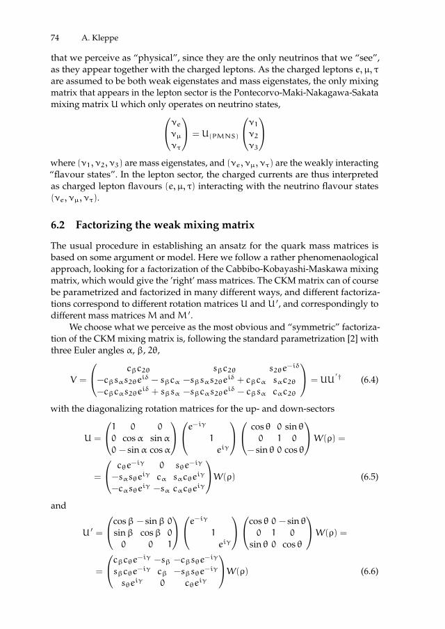
ii

“proc17” — 2017/12/11 — 19:44 — page 74 — #88 ii

ii

ii

74 A. Kleppe

that we perceive as “physical”, since they are the only neutrinos that we “see”,as they appear together with the charged leptons. As the charged leptons e, µ, τare assumed to be both weak eigenstates and mass eigenstates, the only mixingmatrix that appears in the lepton sector is the Pontecorvo-Maki-Nakagawa-Sakatamixing matrix Uwhich only operates on neutrino states,νeνµ

ντ

= U(PMNS)

ν1ν2ν3

where (ν1, ν2, ν3) are mass eigenstates, and (νe, νµ, ντ) are the weakly interacting“flavour states”. In the lepton sector, the charged currents are thus interpretedas charged lepton flavours (e, µ, τ) interacting with the neutrino flavour states(νe, νµ, ντ).

6.2 Factorizing the weak mixing matrix

The usual procedure in establishing an ansatz for the quark mass matrices isbased on some argument or model. Here we follow a rather phenomenaologicalapproach, looking for a factorization of the Cabbibo-Kobayashi-Maskawa mixingmatrix, which would give the ’right’ mass matrices. The CKM matrix can of coursebe parametrized and factorized in many different ways, and different factoriza-tions correspond to different rotation matrices U and U ′, and correspondingly todifferent mass matricesM andM ′.

We choose what we perceive as the most obvious and “symmetric” factoriza-tion of the CKM mixing matrix is, following the standard parametrization [2] withthree Euler angles α, β, 2θ,

V =

cβc2θ sβc2θ s2θe−iδ

−cβsαs2θeiδ − sβcα −sβsαs2θe

iδ + cβcα sαc2θ−cβcαs2θe

iδ + sβsα −sβcαs2θeiδ − cβsα cαc2θ

= UU′† (6.4)

with the diagonalizing rotation matrices for the up- and down-sectors

U =

1 0 0

0 cosα sinα0 − sinα cosα

e−iγ 1eiγ

cos θ 0 sin θ0 1 0

− sin θ 0 cos θ

W(ρ) =

=

cθe−iγ 0 sθe

−iγ

−sαsθeiγ cα sαcθe

iγ

−cαsθeiγ −sα cαcθe

iγ

W(ρ) (6.5)

and

U ′ =

cosβ − sinβ 0sinβ cosβ 0

0 0 1

e−iγ 1eiγ

cos θ 0 − sin θ0 1 0

sin θ 0 cos θ

W(ρ) =

=

cβcθe−iγ −sβ −cβsθe−iγ

sβcθe−iγ cβ −sβsθe

−iγ

sθeiγ 0 cθe

iγ

W(ρ) (6.6)

ii

“proc17” — 2017/12/11 — 19:44 — page 75 — #89 ii

ii

ii


respectively, whereW(ρ) is a unitary matrix which is chosen is such a way that γis the only phase in either of the mass matrices,0 cos ρ ± sin ρ

1 0 0

0 ∓ sin ρ cos ρ

, cos ρ 0 ± sin ρ

0 1 0

∓ sin ρ 0 cos ρ

, cos ρ ± sin ρ 0

0 0 1

∓ sin ρ cos ρ 0

Here ρ is unknown, whereas α, β, θ and γ correspond to the parameters in thestandard parametrization, with γ = δ/2, δ = 1.2±0.08 rad, and 2θ = 0.201±0.011,while α = 2.38± 0.06 and β = 13.04± 0.05. In this factorization scheme, α andβ are rotation angles operating in the up-sector and the down-sector, respectively.

With the rotation matrices U(α, θ, γ, ρ) and U ′(β, θ, γ, ρ), we obtain the theup- and down-sector mass matrices

M = U†diag(mu,mc,mt)U and M ′ = U ′†diag(md,ms,mb)U′,

such that

M =

M11 M12 M13

M21 M22 M23

M31 M32 M33

=

=W†(ρ)

Xc2θ + Ys2θ Zsθ e

−iγ (X− Y)cθsθZsθ e

iγ Y − 2Z cot 2α −Zcθ eiγ

(X− Y)cθsθ −Zcθ e−iγ Xs2θ + Yc

2θ

W(ρ) (6.7)

where X = mu, Z = (mt −mc) sinα cosα and Y = mc sin2 α+mt cos2 α; and

M ′ =

M ′11 M ′12 M ′13M ′21 M′22 M

′23

M ′31 M′32 M

′33

=

=W†(ρ)

X ′s2θ + Y′c2θ Z ′cθ e

iγ (X ′ − Y ′)cθsθZ ′cθ e

−iγ Y ′ + 2Z ′ cot 2β −Z ′sθ e−iγ

(X ′ − Y ′)cθsθ −Z ′sθ eiγ X ′c2θ + Y

′s2θ

W(ρ) (6.8)

where X ′ = mb, Z ′ = (ms −md) sinβ cosβ and Y ′ = md cos2 β+ms sin2 β. Thetwo mass matrices thus have similar textures.

From Y = mc sin2 α+mt cos2 α, Z = (mt−mc) sinα cosα, Y ′ = md cos2 β+ms sin2 β and Z ′ = (ms −md) sinβ cosβ, we moreover have

mu = X, mc = Y − Z cotα, mt = Y + Z tanαmd = Y ′ − Z ′ tanβ, ms = Y

′ + Z ′ cotβ, mb = X ′(6.9)

6.3 The matrix W

We choose the matrixW(ρ) as

W(ρ) =

cos ρ − sin ρ 00 0 1

sin ρ cos ρ 0

, (6.10)

ii

“proc17” — 2017/12/11 — 19:44 — page 76 — #90 ii

ii

ii

76 A. Kleppe

which gives the up-sector mass matrix

M =W†

Xc2θ + Ys2θ Zsθ e

−iγ (X− Y)cθsθZsθ e

iγ Y − 2Z cot 2α −Zcθ eiγ

(X− Y)cθsθ −Zcθ e−iγ Xs2θ + Yc

2θ

W =

=W†

A Zsθ e−iγ H

Zsθ eiγ F −Zcθ e

iγ

H −Zcθ e−iγ K

W =

=

Ac2ρ + Ks2ρ +H sin 2ρ 1

2(K−A) sin 2ρ+H cos 2ρ −Ze−iγ sin(ρ− θ)

12(K−A) sin 2ρ+H cos 2ρ As2ρ + Kc

2ρ −H sin 2ρ −Ze−iγ cos(ρ− θ)

−Zeiγ sin(ρ− θ) −Zeiγ cos(ρ− θ) F

,(6.11)

With

A = Xc2θ + Ys2θ, H = (X− Y)cθsθ and K = Xs2θ + Yc

2θ,

we get

M =

X cos2 µ+ Y sin2 µ (Y − X) sinµ cosµ −Z sinµ e−iγ

(Y − X) sinµ cosµ X sin2 µ+ Y cos2 µ −Z cosµ e−iγ

−Z sinµ eiγ −Z cosµ eiγ F

(6.12)

where µ = ρ−θ, and as before, X = mu, Z = (mt−mc) sinα cosα, Y = mc sin2 α+mt cos2 α, and F = Xs2θ + Yc

2θ = Y − 2Z cot 2α = trace(M) − X− Y.

Now, depending on the value of µ = ρ− θ, we get different matrix textures,e.g.

µ = ρ− θ 0 or π π/4 π/2

M11 = Xc2µ + Ys2µ X (X+ Y)/2 Y

M12 =12(Y − X)s2µ 0 (Y − X)/2 0

M13 = −Zsµ e−iγ 0 −Ze−iγ/

√2 −Ze−iγ

M22 = Xs2µ + Yc2µ Y (X+ Y)/2 X

M23 = −Zcµ e−iγ −Ze−iγ −Ze−iγ/

√2 0

M33 = F Y − 2Z cot 2α Y − 2Z cot 2α Y − 2Z cot 2α

So for ρ− θ = 0 or π, we get the simple form

M(0, π) =

X 0 0

0 Y −Ze−iγ

0 −Zeiγ F

, (6.13)

and for ρ− θ = π/2, equally simple

M(π/2) =

Y 0 −Ze−iγ

0 X 0

−Zeiγ 0 F

(6.14)

ii

“proc17” — 2017/12/11 — 19:44 — page 77 — #91 ii

ii

ii


Applying the same procedure on the down-sector, we get the down-sector massmatrix

M ′ =W(ρ)†

X ′s2θ + Y′c2θ Z ′cθ e

iγ (X ′ − Y ′)cθsθZ ′cθ e

−iγ Y ′ + 2Z ′ cot 2β −Z ′sθ e−iγ

(X ′ − Y ′)cθsθ −Z ′sθ eiγ X ′c2θ + Y

′s2θ

W(ρ) =

=

X ′ sin2 µ ′ + Y ′ cos2 µ ′ (X ′ − Y ′) sinµ ′ cosµ ′ Z ′ cosµ ′ eiγ

(X ′ − Y ′) sinµ ′ cosµ ′ X ′ cos2 µ ′ + Y ′ sin2 µ ′ −Z ′ sinµ ′ eiγ

Z ′ cosµ ′ e−iγ −Z ′ sinµ ′ e−iγ F ′

(6.15)

where µ ′ = ρ + θ, and as before, X ′ = mb, Z ′ = (ms − md) sinβ cosβ, Y ′ =md cos2 β+ms sin2 β, and F ′ = Y ′ + 2Z ′ cot 2β = trace(M ′) − X ′ − Y ′.

Depending on the value of µ ′ = ρ+ θ, we get different matrix textures.

µ ′ = ρ+ θ 0 or π π/4 π/2

M ′11 = X′s2µ ′ + Y

′c2µ ′ Y ′ (X ′ + Y ′)/2 X ′

M ′12 =12(X ′ − Y ′)s2µ ′ 0 (X ′ − Y ′)/2 0

M ′13 = Z′cµ ′ e

iγ Z ′eiγ Z ′eiγ/√2 0

M ′22 = X′c2µ ′ + Y

′s2µ ′ X ′ (X ′ + Y ′)/2 Y ′

M ′23 = −Z ′sµ ′ eiγ 0 −Z ′eiγ/

√2 −Z ′eiγ

M ′33 = F′ Y ′ + 2Z ′ cot 2β Y ′ + 2Z ′ cot 2β Y ′ + 2Z ′ cot 2β

So for µ ′ = ρ+ θ = 0 or π, we get

M ′(0, π) =

Y ′ 0 Z ′eiγ

0 X ′ 0

Z ′e−iγ 0 F ′

(6.16)

and for µ ′ = ρ+ θ = π/2, we get

M ′(π/2) =

X ′ 0 0

0 Y ′ −Z ′eiγ

0 −Z ′e−iγ F ′

(6.17)

6.4 Texture Zero Mass Matrices

The textures (6.13) and (6.14), as well as (6.16) and (6.17), make us wonder if ourscheme implies quark mass matrices of texture zero.

Texture zero matrices can be said to have come about because of the need toreduce the number of free parameters, since the fermion mass matrices are 3x3complex matrices, which without any constraints contain 36 real free parameters.It is however always possible to perform a unitary transformation that rendersan arbitrary mass matrix Hermitian [5], so there is no loss of generality to assumethat the mass matrices be Hermitian, reducing the number of free parameters to 18.This is still a very big number, which in the end of the 1970-ies prompted Fritzsch

ii

“proc17” — 2017/12/11 — 19:44 — page 78 — #92 ii

ii

ii

78 A. Kleppe

[4], [6] to introduce “texture zero matrices”, mass matrices where a certain numberof the entries are zero.

Since then, a huge amount of articles have appeared, with analyses of the verylarge number of (different types of) texture zero matrices and their phenomenology.In the course of this work, a number of of texture zero matrices has been ruled out,singling out a smaller subset of matrices as viable [7]. Among the texture 4 zeromatrices the only matrices that are found to be viable are:A B 0

B∗ D C

0 C∗ 0

,A B C

B∗ D 0

C∗ 0 0

,A 0 B

0 0 C

B∗ C∗ D

, 0 C 0

C∗ A B

0 B∗ D

, 0 0 C

0 A B

C∗ B∗ D

,D C B

C∗ 0 0

B∗ 0 A

while A 0 0

0 C B

0 B∗ D

and

A 0 B

0 C 0

B∗ 0 D

are among the matrices that are ruled out. In our scheme this precisely correspondsto the matrices (6.13), (6.14), (6.16) and (6.17), which means that our mass matricesM and M ′ are not of texture zero. This can be expressed as a constraint on thevalues of the angle ρ,

ρ 6= 1

2Nπ± θ (6.18)

whereN ∈ Z , ruling out the matricesM(12Nπ− θ) andM ′(1

2Nπ+ θ), so our mass

matrices M and M ′ are not of texture zero. Instead, they display a democratictexture.

6.5 Democratic mass matrices

Initially, we were looking for mass matrices with a democratic structure [3], wherethe assumption is that both the up- and down-sector mass matrices start out froma form of the typeM0 = kN andM ′0 = k

′N where

N =

1 1 11 1 1

1 1 1

The underlying philosophy is that in the Standard Model, where the fermionsget their masses from the Yukawa couplings by the Higgs mechanism, there is noreason why there should be a different Yukawa coupling for each fermion. Thecouplings to the gauge bosons of the strong, weak and electromagnetic interactionsare identical for all the fermions in a given charge sector, it thus seems like a naturalassumption that they should also have identical Yukawa couplings. The differenceis that the weak interactions take place in a specific flavour space basis, while theother interactions are flavour independent.

A matrix of the form M = kN moreover has the mass spectrum (0, 0, 3k),reflecting the phenomenology of the fermion mass spectra with one very big, andtwo much smaller mass values. In the weak basis M = kN is however totally

ii

“proc17” — 2017/12/11 — 19:44 — page 79 — #93 ii

ii

ii


flavour symmetric, which means that the (weak) flavours fi are indistinguishible(“absolute democracy”).

In the assumed initial stage, since the up-sector mass matrix and the downsector mass matrix are identical except for the dimensional coefficients k and k ′,the mixing matrix is equal to unity, so there is no CP-violation. In order to obtainthe final mass spectra with the three hierarchical non-zero values, the initial flavoursymmetry displayed by the matricesM0 andM ′0 must be broken, in such a waythat the mixing matrix becomes the observed CKM matrix (with a CP-violatingphase).

An “ansatz” within the democratic scenario then consists of a specific choiceof a flavour symmetry breaking scheme. And it is precisely what we are lookingfor: a credible flavour symmetry breaking scheme that gives the observed massspectra.

Our initial assumption is that the rotation matrices (6.5), (6.6) which diagonal-ize the up-sector and down-sector mass matrices, are given by the factorizationof the Cabibbi-Koabayashi-Maskawa matrix (6.4), with well-known angles. Theonly “steering-parameter parameter” is then ρ, in the sense that different valuesof ρ correspond to mass matrices of different form.

6.5.1 A democratic substructure

We now reparametrize the mass matrices (6.12) and (6.15),

M =

Xc2µ + Ys2µ (Y − X)sµcµ −Zsµ e−iγ

(Y − X)sµcµ Xs2µ + Yc2µ −Zcµ e−iγ

−Zsµ eiγ −Zcµ e

iγ F

and

M ′ =

X ′s2µ ′ + Y′c2µ ′ (X ′ − Y ′)sµ ′cµ ′ Z

′cµ ′ eiγ

(X ′ − Y ′)sµ ′cµ ′ X′c2µ ′ + Y

′s2µ ′ −Z ′sµ ′ eiγ

Z ′cµ ′ e−iγ −Z ′sµ ′ e

−iγ F ′

,in a way that reveals their “democratic substructure”:

M =

P RSeiγ

1 1 11 1 1

1 1 1

P RSe−iγ

+

X XQ

(6.19)

and

M ′ =

P ′ R ′S ′e−iγ

1 1 11 1 1

1 1 1

P ′ R ′S ′eiγ

+

X ′ X ′Q ′

(6.20)

where

P =√|Y − X| sin(ρ− θ), R =

√|Y − X| cos(ρ− θ), S = −Z√

|Y−X|, Q = F− S2,

and

ii

“proc17” — 2017/12/11 — 19:44 — page 80 — #94 ii

ii

ii

80 A. Kleppe

P ′ =√|Y ′ − X ′| cos(ρ+ θ), R ′ = −

√|Y ′ − X ′| sin(ρ+ θ), S ′ = Z ′√

|Y ′−X ′|, Q ′ =

F ′ − S ′2.

These matrices can in their turn be rewritten as

M = B

sinµcosµ

Geiγ

1 1 11 1 1

1 1 1

sinµcosµ

Ge−iγ

+

X XQ

(6.21)

where

µ = ρ− θ, B = Y − X, G = −Z/(Y − X), Q = F− BG2.

Likewise,

M ′ = B ′

cosµ ′

− sinµ ′

G ′e−iγ

1 1 11 1 1

1 1 1

cosµ ′

− sinµ ′

G ′eiγ

+

X ′ X ′Q ′

(6.22)

where

µ ′ = ρ+ θ, B ′ = Y ′ − X ′, G ′ = Z ′/(Y ′ − X ′), Q ′ = F ′ − B ′G ′2.

So without any assumptions about an initial democratic texture, we get a massmatrix structure that can be interpreted as originating from a democratic massmatrix, where the flavour symmetry has subsequently been broken in a veryspecific manner.

6.6 Flavour symmetry breaking mechanisms

The goal of our investigation is to get some hint about the form that the quarkmass matrices take in the weak basis - and the hint we get from the matrices (6.21)and (6.22) is that the mass matrices come about from a kind of democratic scenariowhere the initial flavour symmetry is broken in a stepwise fashion.

Flavour symmetries relate the different flavours fj, and in the democraticscenario, where the initial form of the mass matrices is taken to be

M0 = kN = k

1 1 11 1 1

1 1 1

, (6.23)

the mass Lagrangian reads

Lmass = kfNf =3∑

i=1,j=1

k fifj

This means that in the democratic scheme, all the flavours fj are initially indistin-guishible, with the same Yukawa coupling for all the flavours: a totally flavoursymmetric situation.

ii

“proc17” — 2017/12/11 — 19:44 — page 81 — #95 ii

ii

ii


Following the hint given by our approach, we now postulate that the massmatrices originate from a democratic form (6.23), and that the initial overall flavoursymmetries have subsequently undergone a stepwise breaking. To show how thisworks, we start with a generic matrixM0, and take the first symmetry breakingstep to be

M0 = kN→M1 =

E EJ

1 1 11 1 1

1 1 1

E EJ

(6.24)

Here the mass spectrum is basically unchanged even though the flavour symmetryis partially broken, with the mass Lagrangian

Lmass = kfM1f = E2χχ+ EJ(χf3 + f3χ) + J

2f3f3

where χ = f1+ f2; thus the flavour symmetry f1 ⇔ f2 is still unbroken. In the nextstep, we lift the remaining flavour symmetry by rotating the two equal terms,

(E, E)→ (L sinη, L cosη),

which gives

M1 = kN→M2 = L2

sinηcosη

T

1 1 11 1 1

1 1 1

sinηcosη

T

, (6.25)

where L2 is the only dimensional parameter, and T = J/L. In order to accountfor CP-violation, we moreover introduce a phase γ, in a way that reflects thatCP-violation is connected to the presence of three families (with only two familiesthere is no CP-violation):

M2 →M3 = L2

sinηcosη

Teiγ

1 1 11 1 1

1 1 1

sinηcosη

Te−iγ

, (6.26)

where the CP-breaking phase is connected to the third family, as it should. Weknow nothing about the values of L, η, T , but by the assumption that the trace ofthe mass matrix is constant through all the flavour symmetry breaking steps, weget

L2 + T2 = 3k

But the matrix M3 still has determinant zero, and a mass spectrum with twovanishing and one non-zero mass value. We therefore add an extra term to M3,which like in (6.21) and (6.22), is of diagonal form. This gives us the final massmatrix

M3 →M4 = L2

sinηcosη

Teiγ

1 1 11 1 1

1 1 1

sinηcosη

Te−iγ

+Λ (6.27)

where Λ is a diagonal matrix.Our scheme thus reads:

ii

“proc17” — 2017/12/11 — 19:44 — page 82 — #96 ii

ii

ii

82 A. Kleppe

• We start with the democratic matrix M0 = kN, k = Trace(M)/3, with totalflavour symmetry f1 ⇔ f2 ⇔ f3 in the weak basis.

• Assumption: the trace of the matrixM is constant throughout every flavoursymmetry breaking step.

• First flavour breaking step (6.24):M0 →M1. The flavour symmetry f1 ⇔ f2still remains, and there is still only one non-zero mass value, but f3 is singledout.

• Next flavour breaking step (6.25): M1 → M2, lifting the flavour symmetryf1 ⇔ f2.

• Introducing a CP-violating phase (6.26):M2 →M3.• Last step (6.27): adding a diagonal matrix to M3, M3 → M4 = M3 + Λ,

whereby we get the three observed non-zero mass values.

6.7 Conclusion

Without introducing any new assumptions, by just factorizing the “standardparametrization” of the CKM weak mixing matrix in a specific way, we obtainmass matrices with a specific type of democratic texture and a well-defined schemefor breaking the initial flavour symmetry. Our approach thus hints at a democraticscenario, which comes from the formalism without any other assumptions than avery natural and straightforward way of factorizing the weak mixing matrix.

References

1. M. Kobayashi, T. Maskawa; Maskawa (1973), “CP-Violation in the RenormalizableTheory of Weak Interaction”, Progress of Theoretical Physics 49 (2): 652657.

2. L.L. Chau and W.-Y. Keung (1984), “Comments on the Parametrization of the Kobayashi-Maskawa Matrix”, Phys. Rev. Letters 53 (19): 1802.

3. A. Kleppe, “A democratic suggestion”, hep-ph/1608.08988.4. H. Fritzsch, Phys. Lett. B 70, 436 (1977), Phys. Lett. B 73, 317 (1978).5. D. Emmanuel-Costa and C. Simoes, Phys. Rev. D 79, 073006 (2009).6. H. Fritzsch, “Texture Zero Mass Matrices and Flavor Mixing of Quarks and Leptons”,

hep-ph/1503.07927v1.7. S. Sharma, P. Fakay, G. Ahuja, M. Gupta, Phys. Rev. D 91, 053004 (2015).

ii

“proc17” — 2017/12/11 — 19:44 — page 83 — #97 ii

ii

ii




7 Fermions and Bosons in the Expanding Universeby the Spin-charge-family theory ?

N.S. Mankoc Borstnik ??

Department of Physics, University of Ljubljana,SI-1000 Ljubljana, Slovenia

Abstract. The spin-charge-family theory, which is a kind of the Kaluza-Klein theories ind = (13 + 1) — but with the two kinds of the spin connection fields, the gauge fieldsof the two Clifford algebra objects, Sab and Sab — explains all the assumptions of thestandard model: The origin of the charges of fermions appearing in one family, the originand properties of the vector gauge fields of these charges, the origin and properties ofthe families of fermions, the origin of the scalar fields observed as the Higgs’s scalar andthe Yukawa couplings. The theory explains several other phenomena like: The origin ofthe dark matter, of the matter-antimatter asymmetry, the ”miraculous” triangle anomalycancellation in the standard model and others. Since the theory starts at d = (13 + 1) thequestion arises how and at which d had our universe started and how it came down tod = (13 + 1) and further to d = (3 + 1). In this short contribution some answers to thesequestions are presented.

Povzetek. Avtorica obravnava teorijo spinov-nabojev-druzin, ki sodi v druzino Kaluza-Kleinovih teorij v d = (13 + 1) — vendar z dvema vrstama polj spinskih povezav, ki soumeritvena polja dveh vrst objektov v Cliffordovih algebrah — in pojasni predpostavkestandardnega modela: izvor nabojev fermionov v posamezni druzini, izvor in lastnosti vek-torskih umeritvenih polj teh nabojev, izvor in lastnosti druzin fermionov in izvor skalarnihpolj, ki se kazejo kot Higgsov skalar in Yukavine sklopitve. Teorija pojasni tudi drugepojave: izvor temne snovi, izvor asimetrije snov-antisnov, “cudezno” izginotje trikotniskeanomalije v standardnem modelu. Ker teorija izhaja iz d = (13 + 1), se pojavi vprasanje, kaoin pri katerem d se je vesolje zacelo in kako je prislo so d = (13 + 1) in nato se naprej dod = (3 + 1). Avtorica predlaga nekaj odgovorov na ta vprasanja.

Keywords:Unifying theories; Beyond the standard model; Kaluza-Klein-like the-ories; Vector and scalar gauge fields and their origin; Fermions, their families intheir properties in the expanding universe.

? This talk was presented also in the Conference on Cosmology, Gravitational Waves andParticles in Singapore 6 – 10 of February, 2017 and published in the Proceedings to thisconference.

?? E-mail: [email protected]

ii

“proc17” — 2017/12/11 — 19:44 — page 84 — #98 ii

ii

ii

84 N.S. Mankoc Borstnik

7.1 Introduction

Both standard models, the standard model of elementary fermion and boson fieldsand the standard cosmological model, have quite a lot of assumptions, guessed fromthe properties of observables. Although in the history physics was and still is(in particular when many degrees of freedom are concerned) relying on smalltheoretical steps, confirmed by experiments, there are also a few decisive steps,without which no real further progress would be possible. Among such steps thereare certainly the general theory of relativity and the standard model of elementaryfermion and boson fields. Both theories enabled much better understanding of ouruniverse and its elementary fields — fermions and bosons.

With more and more accurate experiments is becoming increasingly clear thata new decisive step is again needed in the theory of elementary fields as well as incosmology.

Both theories rely on observed facts built into innovative mathematical mod-els. However, the assumptions remain unexplained.

Among the non understood assumptions of the standard model of the elemen-tary fields of fermions and bosons are: i. The origin of massless family memberswith their charges related to spins. ii. The origin of families of fermions. iii. Theorigin of the massless vector gauge fields of the observed charges. iv. The originof masses of family members and heavy bosons. v. The origin of the Higgs’s scalarand the Yukawa couplings. vi. The origin of matter-antimatter asymmetry. vii.The origin of the dark matter. viii. The origin of the electroweak phase transitionscale. ix. The origin of the colour phase transition scale. And others.

Among the non understood assumptions of the cosmological model are: a. Thedifferences in the origin of the gravity, of the vector gauge fields and the (Higgs’s)scalars. b. The origin of the dark matter, of the matter-antimatter asymmetry ofthe (ordinary) matter. c. The appearance of fermions. d. The origin of the inflationof the universe. e. While it is known how to quantize vector gauge fields, thequantization of gravity is still an open problem.

The L(arge) H(adron) C(collider) and other accelerators and measuring appa-ratus produce a huge amount of data, the analyzes of which should help to explainthe assumptions of both standard models. But it looks like so far that the proposedmodels, relying more or less on small extensions of the standard models, can notoffer much help. The situation in elementary particle physics is reminiscent of thesituation in the nuclear physics before the standard model of the elementary fieldswas proposed, opening new insight into physics of elementary fermion and bosonfields.

The deeper into the history of our universe we are succeeding to look bythe observations and experiments the more both standard models are becomingentangled, dependent on each other, calling for the next step which would offerthe explanation for most of the above mentioned non understood assumptions ofboth standard models.

The spin-charge-family theory [1,2,4,3,5–8] does answer open questions of thestandard model of the elementary fields and also several of cosmology.

ii

“proc17” — 2017/12/11 — 19:44 — page 85 — #99 ii

ii

ii

7 Fermions and Bosons in the Expanding Universe. . . 85

The spin-charge-family theory [1,2,4,3] is promising to be the right next stepbeyond the standard model of elementary fermion and boson fields by offering theexplanation for all the assumptions of this model. By offering the explanationalso for the dark matter and matter-antimatter asymmetry the theory makes anew step also in cosmology, in particular since it starts at d ≥ 5 with spinorsand gravitational fields only — like the Kaluza-Klein theories (but with the twokinds of the spin connection fields, which are the gauge fields of the two kindsof the Clifford algebra objects). Although there are still several open problemswaiting to be solved, common to most of proposed theories — like how do theboundary conditions influence the breaking of the starting symmetry of space-timeand how to quantize gravity in any d, while we know how to quantize at leastthe vector gauge fields in d = (3 + 1) — the spin-charge-family theory is makingseveral predictions (not just stimulated by the current experiments what most ofpredictions do).

The spin-charge-family theory (Refs. [1,2,4,3,5–11,13,15,12] and the referencestherein) starts in d = (13+ 1): i. with the simple action for spinors, Eq. (7.1), whichcarry two kinds of spins, i.a. the Dirac one described by γa and manifesting atlow energies in d = (3+ 1) as spins and all the charges of the observed fermionsof one family, Table 7.1, i.b. the second one named [15] (by the author of thispaper) γa (γa, γb+ = 0, Eq. (7.2)), and manifesting at low energies the familyquantum numbers of the observed fermions. ii. Spinors interact in d = (13+1) withthe gravitational field only, ii.a. the vielbeins and ii.b. the two kinds of the spinconnection fields (Refs. [1,4] and the references therein). Spin connection fields —ωstm ((s, t) ≥ 5,m = (0, 1, 2, 3, 4)), Eq. (7.1) — are the gauge fields of Sst, Eq. (7.7),and manifest at low energies in d = (3+ 1) as the vector gauge fields (the colour,weak and hyper vector gauge fields are directly or indirectly observed vector gaugefields). Spin connections ωsts ′ ((s, t) ≥ 5, s ′ = (7, 8)) manifest as scalar gaugefields, contributing to the Higgs’s scalar and the Yukawa couplings together withthe scalar spin connection gauge fields — ωabs ′ ((a, b) = (m, s, t), s ′ = (7, 8)),Eq. (7.1) — which are the gauge fields of Sab, Eq. (7.7) [4,3,1,2]. Correspondinglythese (several) scalar gauge fields determine after the electroweak break masses ofthe families of all the family members and of the heavy bosons (Refs. [2,4,3,1], andthe references therein).

Scalar fields ωsts ′ ((s, t) ≥ 5, s ′ = (9, · · · , 14)), Ref. [4] (and the referencestherein), cause transitions from anti-leptons to quarks and anti-quarks into quarksand back. In the presence of the condensate of two right handed neutrinos [2,4]the matter-antimatter symmetry breaks.

7.2 Short presentation of the spin-charge-family theory

The spin-charge-family theory [3,2,4,7–10] assumes a simple action, Eq. (7.1), in aneven dimensional space (d = 2n, d > 5). d is chosen to be (13 + 1), what makesthe simple starting action in d to manifest in d = (3+ 1) in the low energy regimeall the observed degrees of freedom, explaining all the assumptions of the standardmodel as well as other observed phenomena. Fermions interact with the vielbeinsfαa and the two kinds of the spin-connection fields — ωabα and ωabα — the

ii

“proc17” — 2017/12/11 — 19:44 — page 86 — #100 ii

ii

ii


gauge fields of Sab = i4(γa γb−γb γa) and Sab = i

4(γa γb− γb γa), respectively,

where:

A =∫ddx E 1

2(ψ γap0aψ) + h.c.+∫

ddx E (αR+ α R) , (7.1)

here p0a = fαa p0α + 12E

pα, Efαa−, p0α = pα − 1

2Sabωabα − 1

2Sab ωabα

1,

R =1

2fα[afβb] (ωabα,β −ωcaαω

cbβ)+ h.c.,

R =1

2fα[afβb] (ωabα,β − ωcaα ω

cbβ)+ h.c..

The action introduces two kinds of the Clifford algebra objects, γa and γa,

γa, γb+ = 2ηab = γa, γb+ . (7.2)

fαa are vielbeins inverted to eaα, Latin letters (a, b, ..) denote flat indices, Greekletters (α,β, ..) are Einstein indices, (m,n, ..) and (µ, ν, ..) denote the correspond-ing indices in (0, 1, 2, 3), (s, t, ..) and (σ, τ, ..) denote the corresponding indices ind ≥ 5:

eaαfβa = δβα , eaαf

αb = δab , (7.3)

E = det(eaα) 2.The action A offers the explanation for the origin and all the properties of the

observed fermions (of the family members and families), of the observed vectorgauge fields, of the Higgs’s scalar and of the Yukawa couplings, explaining theorigin of the matter-antimatter asymmetry, the appearance of the dark matter andpredicts the new scalars and the new (fourth) family coupled to the observed threeto be measured at the LHC ([2,4] and the references therein).

The standard model groups of spins and charges are the subgroups of theSO(13, 1) group with the generator of the infinitesimal transformations expressiblewith Sab — for spins

~N±(= ~N(L,R)) : =12(S23 ± iS01, S31 ± iS02, S12 ± iS03) , (7.4)

— for the weak charge, SU(2)I, and the second SU(2)II, these two groups are theinvariant subgroups of SO(4)

~τ1 : = 12(S58 − S67, S57 + S68, S56 − S78) ,

~τ2 : = 12(S58 + S67, S57 − S68, S56 + S78) , (7.5)

1 Whenever two indexes are equal the summation over these two is meant.2 This definition of the vielbein and the inverted vielbein is general, no specification about

the curled space is assumed yet, but is valid also in the low energies regions, when thestarting symmetry is broken [1].

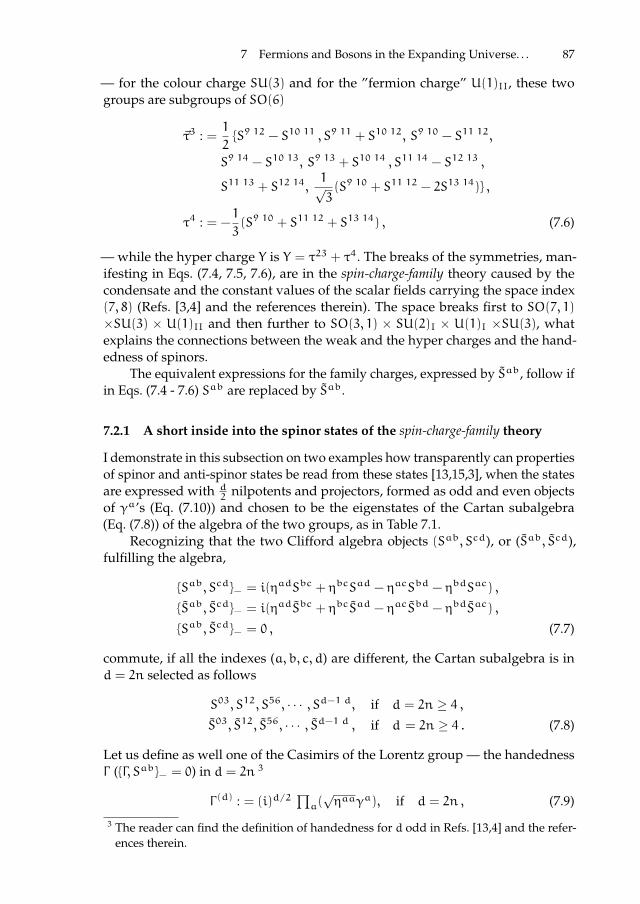
ii

“proc17” — 2017/12/11 — 19:44 — page 87 — #101 ii

ii

ii


— for the colour charge SU(3) and for the ”fermion charge” U(1)II, these twogroups are subgroups of SO(6)

~τ3 : =1

2S9 12 − S10 11 , S9 11 + S10 12, S9 10 − S11 12,

S9 14 − S10 13, S9 13 + S10 14 , S11 14 − S12 13 ,

S11 13 + S12 14,1√3(S9 10 + S11 12 − 2S13 14) ,

τ4 : = −1

3(S9 10 + S11 12 + S13 14) , (7.6)

— while the hyper charge Y is Y = τ23 + τ4. The breaks of the symmetries, man-ifesting in Eqs. (7.4, 7.5, 7.6), are in the spin-charge-family theory caused by thecondensate and the constant values of the scalar fields carrying the space index(7, 8) (Refs. [3,4] and the references therein). The space breaks first to SO(7, 1)×SU(3) × U(1)II and then further to SO(3, 1) × SU(2)I × U(1)I ×SU(3), whatexplains the connections between the weak and the hyper charges and the hand-edness of spinors.

The equivalent expressions for the family charges, expressed by Sab, follow ifin Eqs. (7.4 - 7.6) Sab are replaced by Sab.

7.2.1 A short inside into the spinor states of the spin-charge-family theory

I demonstrate in this subsection on two examples how transparently can propertiesof spinor and anti-spinor states be read from these states [13,15,3], when the statesare expressed with d

2nilpotents and projectors, formed as odd and even objects

of γa’s (Eq. (7.10)) and chosen to be the eigenstates of the Cartan subalgebra(Eq. (7.8)) of the algebra of the two groups, as in Table 7.1.

Recognizing that the two Clifford algebra objects (Sab, Scd), or (Sab, Scd),fulfilling the algebra,

Sab, Scd− = i(ηadSbc + ηbcSad − ηacSbd − ηbdSac) ,

Sab, Scd− = i(ηadSbc + ηbcSad − ηacSbd − ηbdSac) ,

Sab, Scd− = 0 , (7.7)

commute, if all the indexes (a, b, c, d) are different, the Cartan subalgebra is ind = 2n selected as follows

S03, S12, S56, · · · , Sd−1 d, if d = 2n ≥ 4 ,S03, S12, S56, · · · , Sd−1 d , if d = 2n ≥ 4 . (7.8)

Let us define as well one of the Casimirs of the Lorentz group — the handednessΓ (Γ, Sab− = 0) in d = 2n 3

Γ (d) : = (i)d/2∏a(√ηaaγa), if d = 2n , (7.9)

3 The reader can find the definition of handedness for d odd in Refs. [13,4] and the refer-ences therein.

ii

“proc17” — 2017/12/11 — 19:44 — page 88 — #102 ii

ii

ii


which can be written also as Γ (d) = id−1 · 2d2 S03 · S12 · · ·S(d−1)d. The product ofγa’s must be taken in the ascending order with respect to the index a: γ0γ1 · · ·γd.It follows from the Hermiticity properties of γa for any choice of the signature ηaa

that Γ (d)† = Γ (d), (Γ (d))2 = I. One proceeds equivalently for Γ (d), substitutingγa’s by γa’s. We also find that for d even the handedness anticommutes with theClifford algebra objects γa (γa, Γ + = 0).

Spinor states can be, as in Table 7.1, represented as products of nilpotents andprojectors defined by γa’s

ab

(k): = 12(γa + ηaa

ikγb) ,

ab

[k]:= 12(1+ i

kγaγb) , (7.10)

where k2 = ηaaηbb.

It is easy to check that the nilpotentab

(k) and the projectorab

[k] are ”eigenstates”of Sab and Sab

Sabab

(k)= 12kab

(k) , Sabab

[k]= 12kab

[k] ,

Sabab

(k)= 12kab

(k) , Sabab

[k]= −12kab

[k] , (7.11)

where in Eq. (7.11) the vacuum state |ψ0〉 is meant to stay on the right hand sidesof projectors and nilpotents. This means that one gets when multiplying nilpotentsab

(k) and projectorsab

[k] by Sab the same objects back multiplied by the constant 12k,

while Sab multiplyab

(k) by k andab

[k] by (−k) rather than k.One can namely see, taking into account Eq. (7.2), that

γaab

(k)= ηaaab

[−k], γbab

(k)= −ikab

[−k], γaab

[k]=ab

(−k), γbab

[k]= −ikηaaab

(−k) ,

γaab

(k)= −iηaaab

[k], γbab

(k)= −kab

[k], γaab

[k]= iab

(k), γbab

[k]= −kηaaab

(k) .(7.12)

One recognizes also that γa transformab

(k) intoab

[−k], never toab

[k], while γa trans-

formab

(k) intoab

[k], never toab

[−k].In Table 7.1 [2,5,3] the left handed (Γ (13,1) = −1, Eq. (7.9)) massless multiplet

of one family (Table 7.3) of spinors — the members of the fundamental representa-tion of the SO(13, 1) group — is presented as products of nilpotents and projectors,Eq. (7.10). All these states are eigenstates of the Cartan sub-algebra (Eq. (7.8)).Table 7.1 manifests the subgroup SO(7, 1) of the colour charged quarks and anti-quarks and the colourless leptons and anti-leptons [13,15]. The multiplet containsthe left handed (Γ (3,1) = −1) weak (SU(2)I) charged (τ13 = ±1

2, Eq. (7.5)), and

SU(2)II chargeless (τ23 = 0, Eq. (7.5)) quarks and leptons and the right handed(Γ (3,1) = 1) weak (SU(2)I) chargeless and SU(2)II charged (τ23 = ±1

2) quarks

and leptons, both with the spin S12 up and down (±12

, respectively). Quarks andleptons (and separately anti-quarks and anti-leptons) have the same SO(7, 1) part.They distinguish only in the SU(3)×U(1) part: Quarks are triplets of three colours(ci = (τ33, τ38) = [(1

2, 1

2√3), (−1

2, 1

2√3), (0,− 1√

3)], Eq. (7.6)) carrying the ”fermion

ii

“proc17” — 2017/12/11 — 19:44 — page 89 — #103 ii

ii

ii


charge” (τ4 = 16

, Eq. (7.6)). The colourless leptons carry the ”fermion charge”(τ4 = −1

2).

The same multiplet contains also the left handed weak (SU(2)I) chargeless andSU(2)II charged anti-quarks and anti-leptons and the right handed weak (SU(2)I)charged and SU(2)II chargeless anti-quarks and anti-leptons. Anti-quarks areanti-triplets, carrying the ”fermion charge” (τ4 = −1

6). The anti-colourless anti-

leptons carry the ”fermion charge” (τ4 = 12

). S12 defines the ordinary spin ±12

.Y = (τ23 + τ4) is the hyper charge, the electromagnetic charge is Q = (τ13 + Y).The vacuum state, on which the nilpotents and projectors operate, is not shown.

All these properties of states can be read directly from the table. Example 1.and 2. demonstrate how this can be done.

The states of opposite charges (anti-particle states) are reachable from theparticle states (besides by Sab) also by the application of the discrete symmetryoperator CN PN , presented in Refs. [12] and in the footnote of this subsection.

In Table 7.1 the starting state is chosen to be03

(+i)12

(+) |56

(+)78

(+) ||9 10

(+)11 12

(−)13 14

(−) . We could make any other choice of products of nilpotents and projectors, let

say the state03

[−i]12

(+) |56

(+)78

[−] ||9 10

(+)11 12

(−)13 14

(−) , which is the state in the seventhline of Table 7.1. All the states of one representation can be obtained from thestarting state by applying on the starting state the generators Sab. From the firststate, for example, we obtain the seventh one by the application of S0 7 (or of S0 8,S3 7, S3 8).

Let us make a few examples to get inside how can one read the quantumnumbers of states from 7 products of nilpotents and projectors. All nilpotents andprojectors are eigen states, Eq. (7.11), of Cartan sub-algebra, Eq. (7.8).

Example 1.: Let us calculate properties of the two states: The first state —03

(+i)12

(+) |56

(+)78

(+) ||9 10

(+)11 12

(−)13 14

(−) |ψ0〉— and the seventh state —03

[−i]12

(+) |56

(+)78

[−]

||9 10

(+)11 12

(−)13 14

(−) |ψ0〉— of Table 7.1.The handedness of the whole one Weyl representation (64 states) follows from

Eqs. (7.9,7.8): Γ (14) = i1327S03S12 · · ·S13 14. This operator gives, when appliedon the first state of Table 7.1, the eigenvalue = i1327 i

2(12)4(−1

2)2 = −1 (since the

operator S03 applied on the nilpotent03

(+i) gives the eigenvalue k2= i2

, the restfour operators have the eigenvalues 1

2, and the last two −1

2, Eq. (7.11)).

In an equivalent way we calculate the handedness Γ (3,1) of these two statesin d = (3 + 1): The operator Γ (3,1) = i322S03S12, applied on the first state, gives1 — the right handedness, while Γ (3,1) is for the seventh state −1 — the lefthandedness.

The weak charge operator τ13(= 12(S56 − S78)), Eq. (7.5), applied on the first

state, gives the eigenvalue 0: 12(12− 12), The eigenvalue of τ13 is for the seventh

state 12

: 12(12− (−1

2)), τ23 (= 1

2(S56 + S78)), applied on the first state, gives as its

eigenvalue 12

, while when τ23 applies on the seventh state gives 0. The ”fermioncharge” operator τ4 (= −1

3(S9 10 + S11 12 + S13 14), Eq. (7.6)), gives when applied

on any of these two states, the eigenvalues −13(12− 12− 12) = 1

6. Correspondingly is

ii

“proc17” — 2017/12/11 — 19:44 — page 90 — #104 ii

ii

ii


i |aψi >, Γ(7,1) = (−1) 1 , Γ(6) = (1) − 1 Γ(3,1) S12 τ13 τ23 τ33 τ38 τ4 Y Q

(Anti)octetof (anti)quarks and (anti)leptons

1 uc1R

03(+i)

12(+) |

56(+)

78(+) ||

9 10(+)

11 12(−)

13 14(−) 1 1

20 1

212

12√3

16

23

23

2 uc1R

03[−i]

12[−] |

56(+)

78(+) ||

9 10(+)

11 12(−)

13 14(−) 1 − 1

20 1

212

12√3

16

23

23

3 dc1R

03(+i)

12(+) |

56[−]

78[−] ||

9 10(+)

11 12(−)

13 14(−) 1 1

20 − 1

212

12√3

16

− 13

− 13

4 dc1R

03[−i]

12[−] |

56[−]

78[−] ||

9 10(+)

11 12(−)

13 14(−) 1 − 1

20 − 1

212

12√3

16

− 13

− 13

5 dc1L

03[−i]

12(+) |

56[−]

78(+) ||

9 10(+)

11 12(−)

13 14(−) -1 1

2− 12

0 12

12√3

16

16

− 13

6 dc1L

03(+i)

12[−] |

56[−]

78(+) ||

9 10(+)

11 12(−)

13 14(−) -1 − 1

2− 12

0 12

12√3

16

16

− 13

7 uc1L

03[−i]

12(+) |

56(+)

78[−] ||

9 10(+)

11 12(−)

13 14(−) -1 1

212

0 12

12√3

16

16

23

8 uc1L

03(+i)

12[−] |

56(+)

78[−] ||

9 10(+)

11 12(−)

13 14(−) -1 − 1

212

0 12

12√3

16

16

23

9 uc2R

03(+i)

12(+) |

56(+)

78(+) ||

9 10[−]

11 12[+]

13 14(−) 1 1

20 1

2− 12

12√3

16

23

23

10 uc2R

03[−i]

12[−] |

56(+)

78(+) ||

9 10[−]

11 12[+]

13 14(−) 1 − 1

20 1

2− 12

12√3

16

23

23

11 dc2R

03(+i)

12(+) |

56[−]

78[−] ||

9 10[−]

11 12[+]

13 14(−) 1 1

20 − 1

2− 12

12√3

16

− 13

− 13

12 dc2R

03[−i]

12[−] |

56[−]

78[−] ||

9 10[−]

11 12[+]

13 14(−) 1 − 1

20 − 1

2− 12

12√3

16

− 13

− 13

13 dc2L

03[−i]

12(+) |

56[−]

78(+) ||

9 10[−]

11 12[+]

13 14(−) -1 1

2− 12

0 − 12

12√3

16

16

− 13

14 dc2L

03(+i)

12[−] |

56[−]

78(+) ||

9 10[−]

11 12[+]

13 14(−) -1 − 1

2− 12

0 − 12

12√3

16

16

− 13

15 uc2L

03[−i]

12(+) |

56(+)

78[−] ||

9 10[−]

11 12[+]

13 14(−) -1 1

212

0 − 12

12√3

16

16

23

16 uc2L

03(+i)

12[−] |

56(+)

78[−] ||

9 10[−]

11 12[+]

13 14(−) -1 − 1

212

0 − 12

12√3

16

16

23

17 uc3R

03(+i)

12(+) |

56(+)

78(+) ||

9 10[−]

11 12(−)

13 14[+] 1 1

20 1

20 − 1√

316

23

23

18 uc3R

03[−i]

12[−] |

56(+)

78(+) ||

9 10[−]

11 12(−)

13 14[+] 1 − 1

20 1

20 − 1√

316

23

23

19 dc3R

03(+i)

12(+) |

56[−]

78[−] ||

9 10[−]

11 12(−)

13 14[+] 1 1

20 − 1

20 − 1√

316

− 13

− 13

20 dc3R

03[−i]

12[−] |

56[−]

78[−] ||

9 10[−]

11 12(−)

13 14[+] 1 − 1

20 − 1

20 − 1√

316

− 13

− 13

21 dc3L

03[−i]

12(+) |

56[−]

78(+) ||

9 10[−]

11 12(−)

13 14[+] -1 1

2− 12

0 0 − 1√3

16

16

− 13

22 dc3L

03(+i)

12[−] |

56[−]

78(+) ||

9 10[−]

11 12(−)

13 14[+] -1 − 1

2− 12

0 0 − 1√3

16

16

− 13

23 uc3L

03[−i]

12(+) |

56(+)

78[−] ||

9 10[−]

11 12(−)

13 14[+] -1 1

212

0 0 − 1√3

16

16

23

24 uc3L

03(+i)

12[−] |

56(+)

78[−] ||

9 10[−]

11 12(−)

13 14[+] -1 − 1

212

0 0 − 1√3

16

16

23

25 νR

03(+i)

12(+) |

56(+)

78(+) ||

9 10(+)

11 12[+]

13 14[+] 1 1

20 1

20 0 − 1

20 0

26 νR

03[−i]

12[−] |

56(+)

78(+) ||

9 10(+)

11 12[+]

13 14[+] 1 − 1

20 1

20 0 − 1

20 0

27 eR

03(+i)

12(+) |

56[−]

78[−] ||

9 10(+)

11 12[+]

13 14[+] 1 1

20 − 1

20 0 − 1

2−1 −1

28 eR

03[−i]

12[−] |

56[−]

78[−] ||

9 10(+)

11 12[+]

13 14[+] 1 − 1

20 − 1

20 0 − 1

2−1 −1

29 eL

03[−i]

12(+) |

56[−]

78(+) ||

9 10(+)

11 12[+]

13 14[+] -1 1

2− 12

0 0 0 − 12

− 12

−1

30 eL

03(+i)

12[−] |

56[−]

78(+) ||

9 10(+)

11 12[+]

13 14[+] -1 − 1

2− 12

0 0 0 − 12

− 12

−1

31 νL

03[−i]

12(+) |

56(+)

78[−] ||

9 10(+)

11 12[+]

13 14[+] -1 1

212

0 0 0 − 12

− 12

0

32 νL

03(+i)

12[−] |

56(+)

78[−] ||

9 10(+)

11 12[+]

13 14[+] -1 − 1

212

0 0 0 − 12

− 12

0

Table 7.1. The left handed (Γ (13,1) = −1, Eq. (7.9)) multiplet of spinors — the members of(one family of) the fundamental representation of the SO(13, 1) group of the colour chargedquarks and anti-quarks and the colourless leptons and anti-leptons, with the charges, spinand handedness manifesting in the low energy regime — is presented in the massless basisusing the technique [2,5,3], explained in the text and in Examples 1.,2..

ii

“proc17” — 2017/12/11 — 19:44 — page 91 — #105 ii

ii

ii


i |aψi >, Γ(7,1) = (−1) 1 , Γ(6) = (1) − 1 Γ(3,1) S12 τ13 τ23 τ33 τ38 τ4 Y Q

(Anti)octetof (anti)quarks and (anti)leptons

33 dc1L

03[−i]

12(+) |

56(+)

78(+) ||

9 10[−]

11 12[+]

13 14[+] -1 1

20 1

2− 12

− 12√3

− 16

13

13

34 dc1L

03(+i)

12[−] |

56(+)

78(+) ||

9 10[−]

11 12[+]

13 14[+] -1 − 1

20 1

2− 12

− 12√3

− 16

13

13

35 uc1L

03[−i]

12(+) |

56[−]

78[−] ||

9 10[−]

11 12[+]

13 14[+] -1 1

20 − 1

2− 12

− 12√3

− 16

− 23

− 23

36 uc1L

03(+i)

12[−] |

56[−]

78[−] ||

9 10[−]

11 12[+]

13 14[+] -1 − 1

20 − 1

2− 12

− 12√3

− 16

− 23

− 23

37 dc1R

03(+i)

12(+) |

56(+)

78[−] ||

9 10[−]

11 12[+]

13 14[+] 1 1

212

0 − 12

− 12√3

− 16

− 16

13

38 dc1R

03[−i]

12[−] |

56(+)

78[−] ||

9 10[−]

11 12[+]

13 14[+] 1 − 1

212

0 − 12

− 12√3

− 16

− 16

13

39 uc1R

03(+i)

12(+) |

56[−]

78(+) ||

9 10[−]

11 12[+]

13 14[+] 1 1

2− 12

0 − 12

− 12√3

− 16

− 16

− 23

40 uc1R

03[−i]

12[−] |

56[−]

78(+) ||

9 10[−]

11 12[+]

13 14[+] 1 − 1

2− 12

0 − 12

− 12√3

− 16

− 16

− 23

41 dc2L

03[−i]

12(+) |

56(+)

78(+) ||

9 10(+)

11 12(−)

13 14[+] -1 1

20 1

212

− 12√3

− 16

13

13

42 dc2L

03(+i)

12[−] |

56(+)

78(+) ||

9 10(+)

11 12(−)

13 14[+] -1 − 1

20 1

212

− 12√3

− 16

13

13

43 uc2L

03[−i]

12(+) |

56[−]

78[−] ||

9 10(+)

11 12(−)

13 14[+] -1 1

20 − 1

212

− 12√3

− 16

− 23

− 23

44 uc2L

03(+i)

12[−] |

56[−]

78[−] ||

9 10(+)

11 12(−)

13 14[+] -1 − 1

20 − 1

212

− 12√3

− 16

− 23

− 23

45 dc2R

03(+i)

12(+) |

56(+)

78[−] ||

9 10(+)

11 12(−)

13 14[+] 1 1

212

0 12

− 12√3

− 16

− 16

13

46 dc2R

03[−i]

12[−] |

56(+)

78[−] ||

9 10(+)

11 12(−)

13 14[+] 1 − 1

212

0 12

− 12√3

− 16

− 16

13

47 uc2R

03(+i)

12(+) |

56[−]

78(+) ||

9 10(+)

11 12(−)

13 14[+] 1 1

2− 12

0 12

− 12√3

− 16

− 16

− 23

48 uc2R

03[−i]

12[−] |

56[−]

78(+) ||

9 10(+)

11 12(−)

13 14[+] 1 − 1

2− 12

0 12

− 12√3

− 16

− 16

− 23

49 dc3L

03[−i]

12(+) |

56(+)

78(+) ||

9 10(+)

11 12[+]

13 14(−) -1 1

20 1

20 1√

3− 16

13

13

50 dc3L

03(+i)

12[−] |

56(+)

78(+) ||

9 10(+)

11 12[+]

13 14(−) -1 − 1

20 1

20 1√

3− 16

13

13

51 uc3L

03[−i]

12(+) |

56[−]

78[−] ||

9 10(+)

11 12[+]

13 14(−) -1 1

20 − 1

20 1√

3− 16

− 23

− 23

52 uc3L

03(+i)

12[−] |

56[−]

78[−] ||

9 10(+)

11 12[+]

13 14(−) -1 − 1

20 − 1

20 1√

3− 16

− 23

− 23

53 dc3R

03(+i)

12(+) |

56(+)

78[−] ||

9 10(+)

11 12[+]

13 14(−) 1 1

212

0 0 1√3

− 16

− 16

13

54 dc3R

03[−i]

12[−] |

56(+)

78[−] ||

9 10(+)

11 12[+]

13 14(−) 1 − 1

212

0 0 1√3

− 16

− 16

13

55 uc3R

03(+i)

12(+) |

56[−]

78(+) ||

9 10(+)

11 12[+]

13 14(−) 1 1

2− 12

0 0 1√3

− 16

− 16

− 23

56 uc3R

03[−i]

12[−] |

56[−]

78(+) ||

9 10(+)

11 12[+]

13 14(−) 1 − 1

2− 12

0 0 1√3

− 16

− 16

− 23

57 eL

03[−i]

12(+) |

56(+)

78(+) ||

9 10[−]

11 12(−)

13 14(−) -1 1

20 1

20 0 1

21 1

58 eL

03(+i)

12[−] |

56(+)

78(+) ||

9 10[−]

11 12(−)

13 14(−) -1 − 1

20 1

20 0 1

21 1

59 νL

03[−i]

12(+) |

56[−]

78[−] ||

9 10[−]

11 12(−)

13 14(−) -1 1

20 − 1

20 0 1

20 0

60 νL

03(+i)

12[−] |

56[−]

78[−] ||

9 10[−]

11 12(−)

13 14(−) -1 − 1

20 − 1

20 0 1

20 0

61 νR

03(+i)

12(+) |

56[−]

78(+) ||

9 10[−]

11 12(−)

13 14(−) 1 1

2− 12

0 0 0 12

12

0

62 νR

03[−i]

12[−] |

56[−]

78(+) ||

9 10[−]

11 12(−)

13 14(−) 1 − 1

2− 12

0 0 0 12

12

0

63 eR

03(+i)

12(+) |

56(+)

78[−] ||

9 10[−]

11 12(−)

13 14(−) 1 1

212

0 0 0 12

12

1

64 eR

03[−i]

12[−] |

56(+)

78[−] ||

9 10[−]

11 12(−)

13 14(−) 1 − 1

212

0 0 0 12

12

1

Table 7.2. Table 7.1 continued.

the hyper charge Y (= τ23 + τ4) of these two states Y = (23, 16), respectively, what

the standard model assumes for uR and uL, respectively.One finds for the colour charge of these two states, (τ33, τ38) (= (1

2(S9 10 −

S11 12), 1√3(S9 10 + S11 12 − 2S13 14)) the eigenvalues (1/2, 1/(2

√3)).

The first and the seventh states differ in the handedness Γ (3,1) = (1,−1), inthe weak charge τ13 =(0, 1

2) and the hyper charge Y = (2

3, 16

), respectively. Allthe states of this octet — SO(7, 1) — have the same colour charge and the same

ii

“proc17” — 2017/12/11 — 19:44 — page 92 — #106 ii

ii

ii


”fermion charge” (the difference in the hyper charge Y is caused by the differencein τ23 = (1

2, 0)).

The states for the dR-quark and dL-quark of the same octet follow from thestate uR and uL, respectively, by the application of S57 (or S58, S67, S68).

All the SO(7, 1) (Γ (7,1) = 1) part of the SO(13, 1) spinor representation are thesame for either quarks of all the three colours (quarks states appear in Table 7.1from the first to the 24th line) or for the colourless leptons (leptons appear inTable 7.1 from the 25th line to the 32nd line).

Leptons distinguish from quarks in the part represented by nilpotents andprojectors, which is determined by the eigenstates of the Cartan subalgebra of(S9 10, S11 12, S13 14). Taking into account Eq. (7.11) one calculates that (τ33, τ38) is

for the colourless part of the lepton states (νR,L, eR,L) — (· · · ||9 10

(+)11 12

[+]13 14

[+] ) —equal to = (0, 0), while the ”fermion charge” τ4 is for these states equal to −1

2(just

as assumed by the standard model).Let us point out that the octet SO(7, 1) manifests how the spin and the weak

and hyper charges are related.

Example 2.: Let us look at the properties of the anti-quark and anti-leptonstates of one fundamental representation of the SO(13, 1) group. These states arepresented in Table 7.1 from the 33rd line to the 64th line, representing anti-quarks(the first three octets) and anti-leptons (the last octet).

Again, all the anti-octets, the SO(7, 1) (Γ (7,1) = −1) part of the SO(13, 1)representation, are the same either for anti-quarks or for anti-leptons. The lastthree products of nilpotents and projectors (the part appearing in Table 7.1 after”||”) determine anti-colours for the anti-quarks states and the anti-colourless statefor anti-leptons.

Let us add that all the anti-spinor states are reachable from the spinor states(and opposite) by the application of the operator [12] CNPN 4. The part of thisoperator, which operates on only the spinor part of the state (presented in Table 7.1),is CNPN |spinor = γ0

∏d=γs,s=5 γ

s. Taking into account Eq. (7.12) and this operatorone finds that CNPN |spinor transforms uc1R from the first line of Table 7.1 intouc1L from the 35th line of the same table. When the operator CNPN |spinor applieson νR (the 25th line of the same table, with the colour chargeless part equal to

· · · ||9 10

(+)11 12

[+]13 14

[+] ), transforms νR into νL (the 59th line of the table, with the

colour anti-chargeless part equal to (· · · ||9 10

[−]11 12

(−)13 14

(−) ).

4 Discrete symmetries in d = (3 + 1) follow from the corresponding defini-tion of these symmetries in d- dimensional space [12]. This operator is de-fined as: CNPN = γ0

∏d=γs,s=5 γ

s I~x3 Ix6,x8,...,xd , where γ0 and γ1 are real,γ2 imaginary, γ3 real, γ5 imaginary, γ6 real, alternating imaginary and realup to γd, which is in even dimensional spaces real. γa’s appear in the as-cending order. Operators I operate as follows: Ix0x

0 = −x0 ; Ixxa = −xa ;Ix0x

a = (−x0,~x) ; I~x~x = −~x ; I~x3xa = (x0,−x1,−x2,−x3, x5, x6, . . . , xd) ;

Ix5,x7,...,xd−1 (x0, x1, x2, x3, x5, x6, x7, x8, . . . , xd−1, xd) =

(x0, x1, x2, x3,−x5, x6,−x7, . . . ,−xd−1, xd); Ix6,x8,...,xd (x0, x1, x2, x3, x5, x6, x7, x8, . . . ,

xd−1, xd) = (x0, x1, x2, x3, x5,−x6, x7,−x8, . . . , xd−1,−xd), d = 2n.

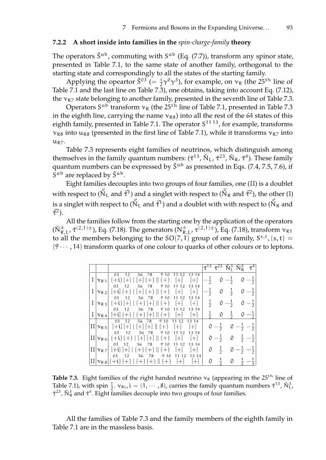
ii

“proc17” — 2017/12/11 — 19:44 — page 93 — #107 ii

ii

ii


7.2.2 A short inside into families in the spin-charge-family theory

The operators Sab, commuting with Sab (Eq. (7.7)), transform any spinor state,presented in Table 7.1, to the same state of another family, orthogonal to thestarting state and correspondingly to all the states of the starting family.

Applying the opeartor S03 (= i2γ0γ3), for example, on νR (the 25th line of

Table 7.1 and the last line on Table 7.3), one obtains, taking into account Eq. (7.12),the νR7 state belonging to another family, presented in the seventh line of Table 7.3.

Operators Sab transform νR (the 25th line of Table 7.1, presented in Table 7.3in the eighth line, carrying the name νR8) into all the rest of the 64 states of thiseighth family, presented in Table 7.1. The operator S11 13, for example, transformsνR8 into uR8 (presented in the first line of Table 7.1), while it transforms νR7 intouR7.

Table 7.3 represents eight families of neutrinos, which distinguish amongthemselves in the family quantum numbers: (τ13, NL, τ23, NR, τ4). These familyquantum numbers can be expressed by Sab as presented in Eqs. (7.4, 7.5, 7.6), ifSab are replaced by Sab.

Eight families decouples into two groups of four families, one (II) is a doubletwith respect to ( ~NL and ~τ1) and a singlet with respect to ( ~NR and ~τ2), the other (I)is a singlet with respect to ( ~NL and ~τ1) and a doublet with with respect to ( ~NR and~τ2).

All the families follow from the starting one by the application of the operators(N±R,L, τ(2,1)±), Eq. (7.18). The generators (N±R,L, τ(2,1)±), Eq. (7.18), transform νR1to all the members belonging to the SO(7, 1) group of one family, Ss,t, (s, t) =

(9 · · · , 14) transform quarks of one colour to quarks of other colours or to leptons.

τ13 τ23 N3L N3R τ4

I νR 103

(+i)12

[+] |56

[+]78

(+) ||9 10

(+)11 12

[+]13 14

[+] − 12

0 − 12

0 − 12

I νR 203

[+i]12

(+) |56

[+]78

(+) ||9 10

(+)11 12

[+]13 14

[+] − 12

0 12

0 − 12

I νR 303

(+i)12

[+] |56

(+)78

[+] ||9 10

(+)11 12

[+]13 14

[+] 12

0 − 12

0 − 12

I νR 403

[+i]12

(+) |56

(+)78

[+] ||9 10

(+)11 12

[+]13 14

[+] 12

0 12

0 − 12

II νR 503

[+i]12

[+] |56

[+]78

[+] ||9 10

(+)11 12

[+]13 14

[+] 0 − 12

0 − 12− 12

II νR 603

(+i)12

(+) |56

[+]78

[+] ||9 10

(+)11 12

[+]13 14

[+] 0 − 12

0 12− 12

II νR 703

[+i]12

[+] |56

(+)78

(+) ||9 10

(+)11 12

[+]13 14

[+] 0 12

0 − 12− 12

II νR 803

(+i)12

(+) |56

(+)78

(+) ||9 10

(+)11 12

[+]13 14

[+] 0 12

0 12− 13

Table 7.3. Eight families of the right handed neutrino νR (appearing in the 25th line ofTable 7.1), with spin 1

2. νRi, i = (1, · · · , 8), carries the family quantum numbers τ13, N3L,

τ23, N3R and τ4. Eight families decouple into two groups of four families.

All the families of Table 7.3 and the family members of the eighth family inTable 7.1 are in the massless basis.

ii

“proc17” — 2017/12/11 — 19:44 — page 94 — #108 ii

ii

ii


The scalar fields, which are the gauge scalar fields of ~NR and ~τ2, couple onlyto the four families which are doublets with respect to these two groups. The scalarfields which are the gauge scalars of ~NL and ~τ1 couple only to the four familieswhich are doublets with respect to these last two groups.

After the electroweak phase transition, caused by the scalar fields with thespace index (7, 8) [5,11,3,4], the two groups of four families become massive. Thelowest of the two groups of four families contains the observed three, while thefourth family remains to be measured. The lowest of the upper four families is thecandidate to form the dark matter [4,10].

7.2.3 Vector gauge fields and scalar gauge fields in the spin-charge-familytheory

In the spin-charge-family theory [4,2,3], like in all the Kaluza-Klein like theories,either vielbeins or spin connections can be used to represent the vector gaugefields in d = (3 + 1) space, when space with d ≥ 5 has large enough symmetryand no strong spinor source is present. This is proven in Ref. [1] and the referencestherein. There are the superposition ofωstm,m = (0, 1, 2, 3), (s, t) ≥ 5, which areused in the spin-charge-family theory to represent vector gauge fields — AAim (=∑s,t c

Aistω

stm) — in d = (3+1) in the low energy regime. HereAi represent the

quantum numbers of the corresponding subgroups, expressed by the operatorsSst in Eqs. (7.5, 7.6). Coefficients cAist can be read from Eqs. (7.5,7.6). These vectorgauge fields manifest the properties of all the directly and indirectly observedgauge fields 5.

In the spin-charge-family theory also the scalar fields [2,4,3,9,11,1] have theorigin in the spin connection field, in ωsts ′ and ωsts ′ , (s, t, s ′) ≥ 5. These scalarfields offer the explanation for the Higgs’s scalar and the Yukawa couplings of thestandard model [9,4].

Both, scalar and vector gauge fields, follow from the simple starting action ofthe spin-charge-family presented in Eq. (7.1).

The Lagrange function for the vector gauge fields follows from the action forthe curvature R in Eq. (7.1) and manifests in the case of the flat d = (3+ 1) spaceas assumed by the standard model: Lv = −1

4

∑A,i,m,n

FAimnFAimn, FAimn =

∂mAAin − ∂nA

Aim − ifAijkAAjm AAkn , with

AAim =∑s,t

cAistωstm ,

τAi =∑s,t

cAistMst , Mst = Sst + Lst . (7.13)

5 In the spin-charge-family theory there are, besides the vector gauge fields of (~τ1, ~τ3),Eqs. (7.5,7.6), also the vector gauge fields of ~τ2, Eq. (7.5), and τ4, Eq. (7.6). The vectorgauge fields of τ21, τ22 and Y ′ = τ23 − tan θ2 gain masses when interacting with thecondensate [4] (and the references therein) at around 1016 GeV, while the vector gaugefield of the hyper charge Y = τ23 + τ4 remains massless, together with the gauge fields of~τ1 and ~τ3, manifesting at low energies properties, postulated by the standard model.

ii

“proc17” — 2017/12/11 — 19:44 — page 95 — #109 ii

ii

ii


In the low energy regime only Sst manifest. These expressions can be found inRef. [1], Eq. (25), for example, and the references therein.

From Eq. (7.1) we read the interaction between fermions, presented in Ta-ble 7.1, and the corresponding vector gauge fields in flat d = (3+ 1) space.

Lfv = ψγm(pm −∑A,i

τAiAAim )ψ . (7.14)

Particular superposition of spin connection fields, either ωsts ′ or ωabs ′ ,(s, t, s ′) ≥ 5, (a, b) = (0, · · · , 8), with the scalar space index s ′ = (7, 8), mani-fest at low energies as the scalar fields, which contribute to the masses of thefamily members. The superposition of the scalar fieldsωstt" with the space indext ′′ = (9, · · · , 14) contribute to the transformation of matter into antimatter andback, causing in the presence of the condensate [2,4] the matter-antimatter asym-metry of our universe. The interactions of all these scalar fields with fermionsfollow from Eq. (7.1)

Lfs = ∑s=7,8

ψγsp0s ψ+

∑

t=5,6,9,...,14

ψγtp0t ψ , (7.15)

where p0s = ps − 12Ss′s"ωs ′s"s −

12Sabωabs, p0t = pt − 1

2St′t"ωt ′t"t −

12Sabωabt,

with m ∈ (0, 1, 2, 3), s ∈ (7, 8), (s ′, s") ∈ (5, 6, 7, 8), (a, b) (appearing in Sab)run within either (0, 1, 2, 3) or (5, 6, 7, 8), t runs ∈ (5, . . . , 14), (t ′, t") run either∈ (5, 6, 7, 8) or ∈ (9, 10, . . . , 14). The spinor function ψ represents all family mem-bers of all the 2

7+12

−1 = 8 families presented in Table 7.3.There are the superposition of the scalar fieldsωs ′s"s — (AQ± , AQ

′

± , AY′

± ) 6 —

and the superposition of ωs ′s ′′s — (~ANL± , ~A1±, ~ANR± , ~A2±) 7 — which determine massterms of family members of spinors after the electroweak break. I shall use AAi±to represent all the scalar fields, which determine masses of family members, theYukawa couplings and the weak boson vector fields,AAi± = (

∑A,i,a,b c

Aist(ωst7±iωst8) as well as =

∑A,i,a,b c

Aist(ωab7 ± iωab8).The part of the second term of Eq. (7.15), in which summation runs over the

space index s = (7,8) —∑s=7,8 ψγ

sp0sψ — determines after the electroweakbreak masses of the two groups of four families. The highest of the lower fourfamilies is predicted to be observed at the L(arge)H(adron)C(ollider) [11], thelowest of the higher four families is explaining the origin of the dark matter [10].

The scalar fields in the part of the second term of Eq. (7.15), in which sum-mation runs over the space index t = (9, · · · , 14) —

∑t=9,··· ,14 ψγ

tp0tψ— cause

6 Q := τ13 + Y, Q ′ := −Y tan2 ϑ1 + τ13, Q ′ := − tan2 ϑ1Y + τ13, Y := τ4 + τ23, Y ′ :=− tan2 ϑ2τ4+τ23,Q := τ13+Y, and correspondinglyAQs = sin ϑ1A13s +cos ϑ1AYs ,AQ

′s =

cos ϑ1A13s − sin ϑ1AYs ,AY′s = cos ϑ2A23s − sin ϑ2A4s ,A4s = −(ω9 10 s+ω11 12 s+ω13 14 s),

A13s = (ω56s −ω78s), A23s = (ω56s +ω78s), with (s ∈ (7, 8)) (Re. [3], Eq. (A9)).7 ~A1s = (ω58s − ω67s, ω57s + ω68s, ω56s − ω78s),

~ANLs = (ω23s + i ω01s, ω31s +

i ω02s, ω12s + i ω03s),~A2s = (ω58s + ω67s, ω57s − ω68s, ω56s + ω78s) and ~A

NRs =

(ω23s − i ω01s, ω31s − i ω02s, ω12s − i ω03s) , where (s ∈ (7, 8)) (Ref. [3], Eq. (A8)).

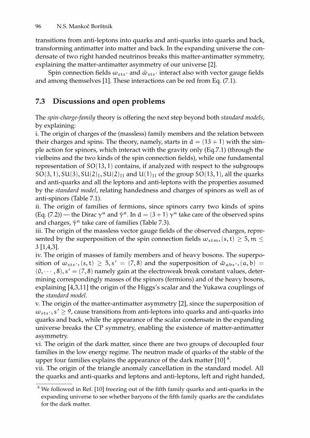
ii

“proc17” — 2017/12/11 — 19:44 — page 96 — #110 ii

ii

ii


transitions from anti-leptons into quarks and anti-quarks into quarks and back,transforming antimatter into matter and back. In the expanding universe the con-densate of two right handed neutrinos breaks this matter-antimatter symmetry,explaining the matter-antimatter asymmetry of our universe [2].

Spin connection fieldsωsts ′ and ωsts ′ interact also with vector gauge fieldsand among themselves [1]. These interactions can be red from Eq. (7.1).

7.3 Discussions and open problems

The spin-charge-family theory is offering the next step beyond both standard models,by explaining:i. The origin of charges of the (massless) family members and the relation betweentheir charges and spins. The theory, namely, starts in d = (13 + 1) with the sim-ple action for spinors, which interact with the gravity only (Eq.7.1) (through thevielbeins and the two kinds of the spin connection fields), while one fundamentalrepresentation of SO(13, 1) contains, if analyzed with respect to the subgroupsSO(3, 1), SU(3), SU(2)I, SU(2)II and U(1)II of the group SO(13, 1), all the quarksand anti-quarks and all the leptons and anti-leptons with the properties assumedby the standard model, relating handedness and charges of spinors as well as ofanti-spinors (Table 7.1).ii. The origin of families of fermions, since spinors carry two kinds of spins(Eq. (7.2)) — the Dirac γa and γa. In d = (3+ 1) γa take care of the observed spinsand charges, γa take care of families (Table 7.3).iii. The origin of the massless vector gauge fields of the observed charges, repre-sented by the superposition of the spin connection fields ωstm, (s, t) ≥ 5,m ≤3 [1,4,3].iv. The origin of masses of family members and of heavy bosons. The superpo-sition of ωsts ′ , (s, t) ≥ 5, s ′ = (7, 8) and the superposition of ωabs ′ , (a, b) =

(0, · · · , 8), s ′ = (7, 8) namely gain at the electroweak break constant values, deter-mining correspondingly masses of the spinors (fermions) and of the heavy bosons,explaining [4,3,11] the origin of the Higgs’s scalar and the Yukawa couplings ofthe standard model.v. The origin of the matter-antimatter asymmetry [2], since the superposition ofωsts ′ , s

′ ≥ 9, cause transitions from anti-leptons into quarks and anti-quarks intoquarks and back, while the appearance of the scalar condensate in the expandinguniverse breaks the CP symmetry, enabling the existence of matter-antimatterasymmetry.vi. The origin of the dark matter, since there are two groups of decoupled fourfamilies in the low energy regime. The neutron made of quarks of the stable of theupper four families explains the appearance of the dark matter [10] 8.vii. The origin of the triangle anomaly cancellation in the standard model. Allthe quarks and anti-quarks and leptons and anti-leptons, left and right handed,

8 We followed in Ref. [10] freezing out of the fifth family quarks and anti-quarks in theexpanding universe to see whether baryons of the fifth family quarks are the candidatesfor the dark matter.

ii

“proc17” — 2017/12/11 — 19:44 — page 97 — #111 ii

ii

ii


appear within one fundamental representation of SO(13, 1) [4,3].viii. The origin of all the gauge fields. The spin-charge-family theory unifies thegravity with all the vector and scalar gauge fields, since in the starting action thereis only gravity (Eq. (7.1)), represented by the vielbeins and the two kinds of thespin connection fields, which in the low energy regime manifests in d = (3 + 1)

as the ordinary gravity and all the directly and indirectly observed vector andscalar gauge fields [1]. If there is no spinor condensate present, only one of thethree fields is the propagating field (both spin connections are expressible with thevielbeins). In the presence of the spinor fields the two spin connection fields differamong themselves (Ref. [1], Eq. (4), and the references therein).

The more work is done on the spin-charge-family theory, the more answers tothe open questions of both standard models is the theory offering.

There are, of course, still open questions (mostly common to all the models)like:

a. How has our universe really started? The spin-charge-family theory assumesd = (13 + 1), but how ”has the universe decided” to start with d = (13 + 1)?If starting at d = ∞, how can it come to (13 + 1) with the massless Weyl repre-sentation of only one handedness? We have studied in a toy model the break ofsymmetry from d = (5 + 1) into (3 + 1) [14], finding that there is the possibilitythat spinors of one handedness remain massless after this break. This study givesa hope that breaking the symmetry from (d− 1)+ 1, where d is even and∞, couldgo, if the jump of (d− 1) + 1 to ((d− 4) − 1) + 1would be repeated as twice thebreak suggested in Ref. [14]. These jumps should then be repeated all the wayfrom d =∞ to d = (13+ 1).b. What did ”force” the expanding universe to break the symmetry of SO(13, 1)to SO(7, 1) ×SU(3)×U(1)II and then further to SO(3, 1) ×SU(2)× SU(3)×U(1)Iand finally to SO(3, 1)× SU(3)×U(1)?From phase transitions of ordinary matter we know that changes of temperatureand pressure lead a particular matter into a phase transition, causing that con-stituents of the matter (nuclei and electrons) rearrange, changing the symmetry ofspace.In expanding universe the temperature and pressure change, forcing spinorsto make condensates (like it is the condensate of the two right handed neutri-nos in the spin-charge-family theory [3,2,4], which gives masses to vector gaugefields of SU(2)II, breaking SU(2)II × U(1)II into U(1)I). There might be alsovector gauge fields causing a change of the symmetry (like does the colourvector gauge fields, which ”dress” quarks and anti-quarks and bind them tomassive colourless baryons and mesons of the ordinary, mostly the first fam-ily, matter). Also scalar gauge fields might cause the break of the symmetry ofthe space (as this do the superposition of ωs ′t ′s and the superposition of ωabs,s = (7, 8), (s ′, t") ≥ 5, (a, b) = (0, · · · , 8) in the spin-charge-family theory [4,3] bygaining constant values in d = (3 + 1) and breaking correspondingly also thesymmetry of the coordinate space in d ≥ 5).All these remain to be studied.c. What is the scale of the electroweak phase transition? How higher is this scale in

ii

“proc17” — 2017/12/11 — 19:44 — page 98 — #112 ii

ii

ii


comparison with the colour phase transition scale? If the colour phase transitionscale is at around 1 GeV (since the first family quarks contribute to baryons massesaround 1 GeV), is the electroweak scale at around 1 TeV (of the order of the massof Higgs’s scalar) or this scale is much higher, possibly at the unification scale(since the spin-charge-family theory predicts two decoupled groups of four familiesand several scalar fields — twice two triplets and three singlets [3,11,4])?

d. There are several more open questions. Among them are the origin of thedark energy, the appearance of fermions, the origin of inflation of the universe,quantization of gravity, and several others. Can the spin-charge-family theory be— while predicting the fourth family to the observed three, several scalar fields,the fifth family as the origin of the dark matter, the scalar fields transforminganti-leptons into quarks and anti-quarks into quarks and back and the condensatewhich break this symmetry — the first step, which can hopefully show the way tonext steps?

7.4 APPENDIX: Some useful formulas and relations arepresented [4,5]

Sacab

(k)cd

(k) = − i2ηaaηcc

ab

[−k]cd

[−k] , Sacab

(k)cd

(k)= i2ηaaηcc

ab

[k]cd

[k] ,

Sacab

[k]cd

[k] = i2

ab

(−k)cd

(−k) , Sacab

[k]cd

[k]= − i2

ab

(k)cd

(k) ,

Sacab

(k)cd

[k] = − i2ηaa

ab

[−k]cd

(−k) , Sacab

(k)cd

[k]= − i2ηaa

ab

[k]cd

(k) ,

Sacab

[k]cd

(k) = i2ηcc

ab

(−k)cd

[−k] , Sacab

[k]cd

(k)= i2ηcc

ab

(k)cd

[k] . (7.16)

ab

(k)ab

(k) = 0 ,ab

(k)ab

(−k)= ηaaab

[k] ,ab

(−k)ab

(k)= ηaaab

[−k] ,ab

(−k)ab

(−k)= 0 ,ab

[k]ab

[k] =ab

[k] ,ab

[k]ab

[−k]= 0 ,ab

[−k]ab

[k]= 0 ,ab

[−k]ab

[−k]=ab

[−k] ,ab

(k)ab

[k] = 0 ,ab

[k]ab

(k)=ab

(k) ,ab

(−k)ab

[k]=ab

(−k) ,ab

(−k)ab

[−k]= 0 ,ab

(k)ab

[−k] =ab

(k) ,ab

[k]ab

(−k)= 0,ab

[−k]ab

(k)= 0 ,ab

[−k]ab

(−k)=ab

(−k) .(7.17)

N±+ = N1+ ± iN2+ = −03

(∓i)12

(±) , N±− = N1− ± iN2− =03

(±i)12

(±) ,

N±+ = −03˜(∓i)

12˜(±) , N±− =

03˜(±i)

12˜(±) ,

τ1± = (∓)56

(±)78

(∓) , τ2∓ = (∓)56

(∓)78

(∓) ,

τ1± = (∓)56˜(±)

78˜(∓) , τ2∓ = (∓)

56˜(∓)

78˜(∓) . (7.18)

ii

“proc17” — 2017/12/11 — 19:44 — page 99 — #113 ii

ii

ii


References

1. D. Lukman, N.S. Mankoc Borstnik, Eur. Phys. J. C (2017) 33, DOI: 10.1140/epjc/s10052-017-4804-y.

2. N.S. Mankoc Borstnik, Phys. Rev. D 91, 6 (2015) 065004 ID: 0703013; doi:10.1103[arXiv:1409.7791, arXiv:1502.06786v1].

3. N.S. Mankoc Borstnik, J. of Mod. Phys. 6 (2015) 2244–2274, doi:10.4236/jmp.2015.615230[arxiv:1409.4981].

4. N.S. Mankoc Borstnik, ”Spin-charge-family theory is offering next step in under-standing elementary particles and fields and correspondingly universe”, to appearin Proceedings to The 10th Biennial Conference on Classical and Quantum Relativis-tic Dynamics of Particles and Fields, IARD conference, Ljubljana 6-9 of June 2016[arXiv:1607.01618v2].

5. A. Borstnik Bracic and N.S. Mankoc Borstnik, Phys. Rev. D 74, 073013 (2006) [hep-ph/0301029; hep-ph/9905357, p. 52-57; hep-ph/0512062, p.17-31; hep-ph/0401043, p.31-57].

6. N.S. Mankoc Borstnik, Phys. Lett. B 292, 25-29 (1992).7. N.S. Mankoc Borstnik, J. Math. Phys. 34, 3731-3745 (1993).8. N.S. Mankoc Borstnik, Int. J. Theor. Phys. 40, 315-338 (2001).9. G. Bregar, M. Breskvar, D. Lukman and N.S. Mankoc Borstnik, New J. of Phys. 10,

093002 (2008), [arXiv:0606159, arXiv:07082846, arXiv:0612250, p.25-50].10. G. Bregar and N.S. Mankoc Borstnik, Phys. Rev. D 80, 1 (2009), 083534 (2009).11. G. Bregar, N.S. Mankoc Borstnik, ”The new experimental data for the quarks mixing

matrix are in better agreement with the spin-charge-family theory predictions”, Proceed-ings to the 17th Workshop ”What comes beyond the standard models”, Bled, 20-28 ofJuly, 2014, Ed. N.S. Mankoc Borstnik, H.B. Nielsen, D. Lukman, DMFA Zaloznistvo,Ljubljana December 2014, p.20-45 [ arXiv:1502.06786v1, arXiv:1412.5866].

12. N.S. Mankoc Borstnik, H.B. Nielsen, JHEP 04 (2014) 165-174, doi:10.1007[arXiv:1212.2362v3].

13. N.S. Mankoc Borstnik, H.B. Nielsen, J. of Math. Phys. 43 (2002) 5782 [hep-th/0111257].14. D. Lukman, N.S. Mankoc Borstnik, H.B. Nielsen, New J. Phys. 13 (2011) 103027 [hep-

th/1001.4679v5].15. N.S. Mankoc Borstnik, H. B. Nielsen, J. of Math. Phys. 44 (2003) 4817, [hep-th/0303224].

ii

“proc17” — 2017/12/11 — 19:44 — page 100 — #114 ii

ii

ii




8 Why Nature Made a Choice of Clifford and notGrassmann Coordinates ?

N.S. Mankoc Borstnik1 and H.B.F. Nielsen2

1Department of Physics, University of Ljubljana,SI-1000 Ljubljana, Slovenia2Niels Bohr Institute, University of Copenhagen, Blegdamsvej 17,Copenhagen Ø, Denmark

Abstract. This is a discussion on fields, the internal degrees of freedom of which areexpressed by either the Grassmann or the Clifford ”coordinates”. Since both ”coordinates”fulfill anticommutation relations, both fields can be second quantized so that their creationand annihilation operators fulfill the requirements of the commutation relations for fermionfields. However, while the internal spin, determined by the generators of the Lorentz groupof the Clifford objects Sab and Sab (in the spin-charge-family theory Sab determine the spindegrees of freedom and Sab the family degrees of freedom) have half integer spin, have Sab

(expressible with Sab + Sab) integer spin. Nature made obviously a choice of the Cliffordalgebra.

We discuss here the quantization — first and second — of the fields, the internaldegrees of freedom of which are functions of the Grassmann coordinates θ and theirconjugate momentum, as well as of the fields, the internal degrees of freedom of which arefunctions of the Clifford γa. Inspiration comes from the spin-charge-family theory [[1,2,9,3],and the references therein], in which the action for fermions in d-dimensional space isequal to

∫ddx E 1

2(ψ γap0aψ) + h.c., with p0a = fαap0α + 1

2Epα, Ef

αa−, p0α = pα −

12Sabωabα − 1

2Sabωabα. We write the basic states of the Grassmann fields and the Clifford

fields as a function of products of either Grassmann or Clifford objects, trying to understandthe choice of nature. We look for the action for free fields which are functions of either theGrassmann coordinates or of the Clifford coordinates in order to understand why Cliffordalgebra ”win” in the competition for the physical degrees of freedom (at least in ourobservable world).

Povzetek. Avtorja obravnavata polja, pri katerih so notranje prostostne stopnje izrazeneali z Grassmannovimi ali pa s Cliffordovimi “koordinatami”. Ker obe vrsti “koordinat”zadoscata antikomutacijskim relacijam, lahko za obe vrsti polj naredimo drugo kvanti-zacijo tako, da kreacijski in anihilacijski operatorji zadoscajo komutacijskim relacijam zafermionska polja. Za razliko od internih spinov, ki jih dolocajo generatorji Lorentzovegrupe Cliffordovih objektov Sab in Sab (v teoriji spinov-nabojev-druzin Sab dolocajo spinskeprostostne stopnje, Sab pa druzinske prostostne stopnje) in imajo polstevilcni spin), imajoSab (ki jih lahko izrazimo z Sab + Sab) celostevilski spin. “Narava se je ocitno odlocila” zaCliffordovo algebro.

? This is the part of the talk presented by N.S. Mankoc Borstnik at the 20th Workshop”What Comes Beyond the Standard Models”, Bled, 09-17 of July, 2017, and published inthe Proceedings to this workshop.

ii

“proc17” — 2017/12/11 — 19:44 — page 101 — #115 ii

ii

ii

8 Why Nature Made a Choice of Clifford and not Grassmann Coordinates 101

Avtorja obravnavata kvantizacijo — prvo in drugo — za polja, pri katerih so notranjeprostostne stopnje funkcije Grassmannovih koordinat θ in ustreznih konjugiranih momen-tov, pa tudi za polja, kjer so interne prostostne stopnje funkcije Cliffordovih koordinatγa. Navdih najdeta v teoriji spinov-nabojev-druzin [[1,2,9,3], in reference v teh clankih], vkateri je akcija za fermione v d razseznem prostoru enaka

∫ddx E 1

2(ψ γap0aψ) + h.c.,

with p0a = fαap0α + 12E


2Sabωabα − 1

2Sabωabα. Da bi razumela

“izbiro narave”, zapiseta osnovna stanja Grassmannovih in Cliffordovih polj kot produkteGrassmannovih ali Cliffordovih objektov. Isceta akcijo za prosta polja, ki so funkcije Grass-mannovih ali pa Cliffordovih koordinat, da bi bolje razumela, zakaj Cliffordova algebra“zmaga” v tekmi za fizikalne prostostne stopnje (vsaj v opazljivem svetu).

Keywords: Spinor representations, Kaluza-Klein theories, Discrete symmetries,Higher dimensional spaces, Beyond the standard modelPACS: 11.30.Er,11.10.Kk,12.60.-i, 04.50.-h

8.1 Introduction

This paper is to look for the answers to the questions like: Why our universe”uses” the Clifford rather than the Grassmann coordinates, although both leadin the second quantization procedure to the anticommutation relations requiredfor fermion degrees of freedom? Does the answer lay on the fact that the Clifforddegrees of freedom offers the appearance of the families, the half integer spin andthe charges as observed so far for fermions, while the Grassmann coordinatesoffer the groups of (isolated) integer spin states and to charges in the adjointrepresentations? Can this explain why the simple starting action of the spin-charge-family theory of one of us (N.S.M.B.) [9,3,5,8,4,6,7] is doing so far extremely wellin manifesting the observed properties of the fermion and boson fields in the lowenergy regime?

The working hypothesis is that ”Nature knows” all the mathematics, accord-ingly therefore ”she knows” for the Grassmann and the Clifford coordinates. Tounderstand why Grassmann space ”was not chosen” – we see that the use of theDirac γa’s enabled to understand the fermions in the first and second quntizedtheory of fields – or better, to understand why the Clifford algebra (in the spin-charge-family theory of two kinds – γa’s and γa’s) is succesfully applicable at leastin the low enery regime, we work in this paper with both types of spaces.

This work is a part of the project of both authors, which includes the fermion-ization procedure of boson fields or the bosonization procedure of fermion fields,discussed in Refs. [10] and in this proceedings for any dimension d (by the authorsof this contribution, while one of them, H.B.F.N. [11], has succeeded with anotherauthor to do the fermionization for d = (1+ 1))), and which would hopefully helpto better understand the content and dynamics of our universe.

In the spin-charge-family theory [9,3,5,8,4,6,7] — which offers the explanationof all the assumptions of the standard model, with the appearance of families, thescalar higgs and the Yukawa couplings included, offering also the explanation forthe matter-antimatter asymmetry in our universe and for the appearance of thedark matter — a very simple starting action for massless fermions and bosons in

ii

“proc17” — 2017/12/11 — 19:44 — page 102 — #116 ii

ii

ii

102 N.S. Mankoc Borstnik and H.B.F. Nielsen

d = (1+ 13) is assumed, in which massless fermions interact with only gravity, thevielbeins fαa (the gauge fields of momentums pa) and the two kinds of the spinconnections (ωabα and ωabα, the gauge fields of the two kinds of the Cliffordalgebra objects γa and γa, respectively).

A =

∫ddx E

1


ddx E (αR+ α R) , (8.1)

with p0a = fαap0α + 12E


2Sabωabα − 1

2Sabωabα and

R = 12fα[afβb] (ωabα,β − ωcaαω

cbβ) + h.c., R = 1

2fα[afβb] (ωabα,β −

ωcaα ωcbβ)+ h.c.. The two kinds of the Clifford algebra objects, γa and γa,

γa, γb+ = 2ηab = γa, γb+ ,

γa, γb+ = 0 . (8.2)

anticommute, γa, γb+ = 0 (γa and γb are connected with the left and the rightmultiplication of the Clifford objects, there is no third kind of operators). One ofthe objects, the generators Sab = i

4(γa γb − γb γa) , determine spins and charges

of spinors of any families, another, Sab = i4(γa γb − γb γa) , determine the family

quantum numbers. Here 1 fα[afβb] = fαafβb− fαbfβa. There are correspondinglytwo kinds of infinitesimal generators of the Lorentz transformations in the internaldegrees of freedom - Sab for SO(13, 1) and Sab for SO(13, 1), arranging states intorepresentations.

The curvature R and R determine dynamics of the gauge fields — the spinconnections and the vielbeins, which manifest in d = (1+ 3) all the known vectorgauge fields as well as the scalar fields [5] which explain the appearance of higgsand the Yukawa couplings, provided that the symmetry breaks from the startingone to SO(3, 1)× SU(3)×U(1).

The infinitesimal generators of the Lorentz transformations for the gaugefields – the two kinds of the Clifford operators and the Grassmann operators –operate as follows

Sab, γe− = −i (ηae γb − ηbe γa) ,

Sab, γe− = −i (ηae γb − ηbe γa) ,

Sab, θe− = −i (ηae θb − ηbe θa) ,

Mab, Ad...e...g− = −i (ηaeAd...b...g − ηbeAd...a...g) , (8.3)

where Mab are defined by a sum of Lab plus any of Sab or Sab, in the Grassmanncase Mab is Lab + Sab, which appear to be Mab= Lab + Sab + Sab, as presentedlater in Eq. (8.22).

1 fαa are inverted vielbeins to eaα with the properties eaαfαb = δab, eaαfβa = δβα, E =

det(eaα). Latin indices a, b, ..,m, n, .., s, t, .. denote a tangent space (a flat index), whileGreek indices α, β, .., µ, ν, ..σ, τ, .. denote an Einstein index (a curved index). Letters fromthe beginning of both the alphabets indicate a general index (a, b, c, .. and α, β, γ, .. ),from the middle of both the alphabets the observed dimensions 0, 1, 2, 3 (m,n, .. andµ, ν, ..), indexes from the bottom of the alphabets indicate the compactified dimensions(s, t, .. and σ, τ, ..). We assume the signature ηab = diag1,−1,−1, · · · ,−1.

ii

“proc17” — 2017/12/11 — 19:44 — page 103 — #117 ii

ii

ii


We discuss in what follows the first and the second quantization of the fieldswhich depend on the Grassmann coordinates θa, as well as of the fields whichdepend on the Clifford coordinates γa (or γa) in order to try to understand why”nature has made a choice” of fermions of spins and charges (describable in thespin-charge-family theory by subgroups of the Lorentz group expressible with thegenerators Sab) in the fundamental representations of the groups, which interactin the spin-charge-family theory through the boson gauge fields (the vielbeins andthe spin connections of two kinds). We choose correspondingly either θa’s or γa’s(or γa’s, either γa’s or γa’s [6,7,9]) to describe the internal degrees of freedom offields to clarify the ”choice of nature” and correspondingly also the meaning offermionization of bosons (or bosonization of fermions) discussed in Refs. [10] and inthis proceedings for any dimension d.

In all these cases we treat free massless boson and fermion fields; masses ofthe fields which manifest in d = (1 + 3) are in the spin-charge-family theory dueto their interactions with the gravitational fields in d > 4, described by the scalarvielbeins or spin connection fields

8.2 Observations which might be of some help whenfermionizing boson fields or bosonizing fermion fields

We present in this section properties of fields with the integer spin in d-dimensionalspace, expressed in terms of the Grassmann algebra objects, and the fermion fields,expressed in terms of the Clifford algebra objects. Since the Clifford algebra objectsare expressible with the Grassmann algebra objects (Eqs. (8.14, 8.15)), the norms ofboth are determined by the integral in the Grassmann space, Eqs. (8.24, 8.27).

a. Fields with the integer spin in the Grassmann space

A point in d-dimensional Grassmann space of real anticommuting coordinatesθa, (a = 0, 1, 2, 3, 5, . . . , d), is determined by a vector θa = (θ1, θ2, θ3, θ5, . . . , θd).A linear vector space over the coordinate Grassmann space has correspondinglythe dimension 2d, due to the fact that (θai)2 = 0 for any ai ∈ (0, 1, 2, 3, 5, . . . , d).

Correspondingly are fields in the Grassmann space expressed in terms of theGrassmann algebra objects

B =

d∑k=0

aa1a2...ak θa1θa2 . . . θak |φog > , ai ≤ ai+1 , (8.4)

where |φog > is the vacuum state, here assumed to be |φog >= |1 >, so that∂∂θa

|φog >= 0 for any θa. The Kalb-Ramond boson fields aa1a2...ak are antisym-metric with respect to the permutation of indexes, since the Grassmann coordinatesanticommute

θa, θb+ = 0 . (8.5)

ii

“proc17” — 2017/12/11 — 19:44 — page 104 — #118 ii

ii

ii


The left derivative ∂∂θa

on vectors of the space of monomials B(θ) is defined asfollows

∂

∂θaB(θ) =

∂B(θ)∂θa

,∂

∂θa,∂

∂θb

+

B = 0 , for all B . (8.6)

Defining pθa

= i ∂∂θa

it correspondingly follows

pθa, pθb+ = 0 , pθa, θb+ = i ηab , (8.7)

The metric tensor ηab (= diag(1,−1,−1, . . . ,−1)) lowers the indexes of a vectorθa: θa = ηab θ

b, the same metric tensor lowers the indexes of the ordinary vectorxa of commuting coordinates.

Defining 2

(θa)† =∂

∂θaηaa = −i pθaηaa , (8.8)

it follows

(∂

∂θa)† = ηaa θa , (pθa)† = −iηaaθa . (8.9)

By introducing [2] the generators of the infinitesimal Lorentz transformations inthe Grassmann space as

Sab = θapθb − θbpθa ,

(8.10)

one finds

Sab,Scd− = iSadηbc + Sbcηad − Sacηbd − Sbdηac ,

Sab† = ηaaηbbSab . (8.11)

The basic states in Grassmann space can be arrange into representations [2] withrespect to the Cartan subalgebra of the Lorentz algebra, as presented in App. 8.4.The state in d-dimensional space with all the eigenvalues of the Cartan subalgebraof the Lorentz group of Eq. (8.67) equal to either i or 1 is (θ0 − θ3)(θ1 + iθ2)(θ5 +iθ6) · · · (θd−1 + iθd)|φog >, with |φog >= |1 >.

b. Fermion fields and the Clifford objects

Let us present as well the properties of the fermion fields with the half integerspin, expressed by the Clifford algebra objects

F =

d∑k=0

aa1a2...ak γa1γa2 . . . γak |ψoc > , ai ≤ ai+1 , (8.12)

2 In Ref. [2] the definition of θa† was differently chosen. Correspondingly also the scalarproduct needed different weight function in Eq. (8.24) is different.

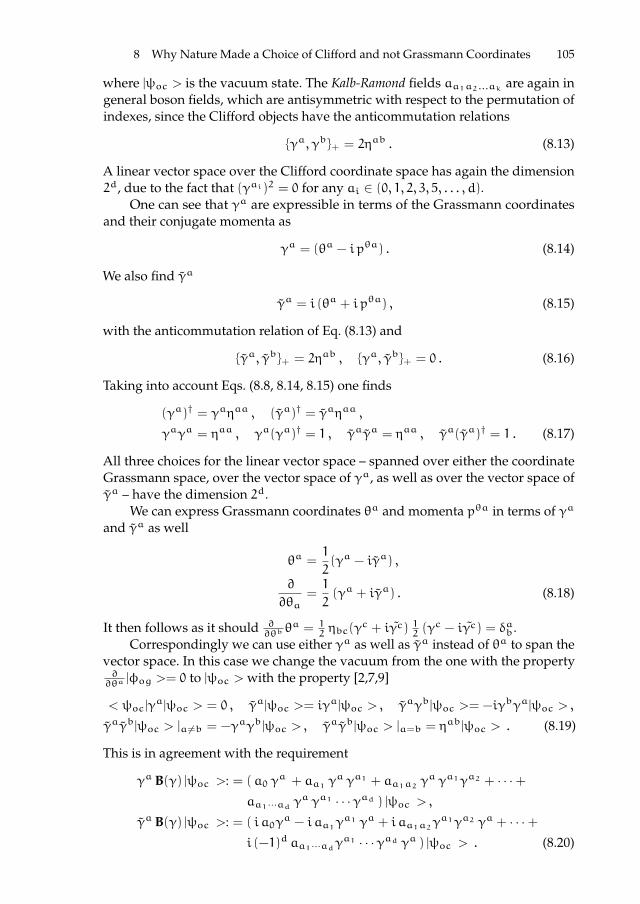
ii

“proc17” — 2017/12/11 — 19:44 — page 105 — #119 ii

ii

ii


where |ψoc > is the vacuum state. The Kalb-Ramond fields aa1a2...ak are again ingeneral boson fields, which are antisymmetric with respect to the permutation ofindexes, since the Clifford objects have the anticommutation relations

γa, γb+ = 2ηab . (8.13)

A linear vector space over the Clifford coordinate space has again the dimension2d, due to the fact that (γai)2 = 0 for any ai ∈ (0, 1, 2, 3, 5, . . . , d).

One can see that γa are expressible in terms of the Grassmann coordinatesand their conjugate momenta as

γa = (θa − i pθa) . (8.14)

We also find γa

γa = i (θa + i pθa) , (8.15)

with the anticommutation relation of Eq. (8.13) and

γa, γb+ = 2ηab , γa, γb+ = 0 . (8.16)

Taking into account Eqs. (8.8, 8.14, 8.15) one finds

(γa)† = γaηaa , (γa)† = γaηaa ,

γaγa = ηaa , γa(γa)† = 1 , γaγa = ηaa , γa(γa)† = 1 . (8.17)

All three choices for the linear vector space – spanned over either the coordinateGrassmann space, over the vector space of γa, as well as over the vector space ofγa – have the dimension 2d.

We can express Grassmann coordinates θa and momenta pθa in terms of γa

and γa as well

θa =1

2(γa − iγa) ,

∂

∂θa=1

2(γa + iγa) . (8.18)

It then follows as it should ∂∂θb

θa = 12ηbc(γ

c + iγc) 12(γc − iγc) = δab.

Correspondingly we can use either γa as well as γa instead of θa to span thevector space. In this case we change the vacuum from the one with the property∂∂θa

|φog >= 0 to |ψoc >with the property [2,7,9]

< ψoc|γa|ψoc > = 0 , γa|ψoc >= iγ

a|ψoc > , γaγb|ψoc >= −iγbγa|ψoc > ,

γaγb|ψoc > |a 6=b = −γaγb|ψoc > , γaγb|ψoc > |a=b = ηab|ψoc > . (8.19)

This is in agreement with the requirement

γa B(γ) |ψoc >: = (a0 γa + aa1 γ

a γa1 + aa1a2 γa γa1γa2 + · · ·+

aa1···ad γa γa1 · · ·γad ) |ψoc > ,

γa B(γ) |ψoc >: = ( i a0γa − i aa1γ

a1 γa + i aa1a2γa1γa2 γa + · · ·+

i (−1)d aa1···adγa1 · · ·γad γa ) |ψoc > . (8.20)

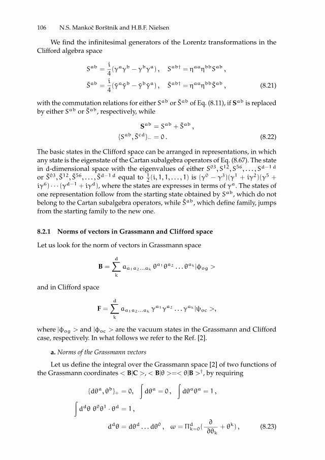
ii

“proc17” — 2017/12/11 — 19:44 — page 106 — #120 ii

ii

ii


We find the infinitesimal generators of the Lorentz transformations in theClifford algebra space

Sab =i

4(γaγb − γbγa) , Sab† = ηaaηbbSab ,

Sab =i

4(γaγb − γbγa) , Sab† = ηaaηbbSab , (8.21)

with the commutation relations for either Sab or Sab of Eq. (8.11), if Sab is replacedby either Sab or Sab, respectively, while

Sab = Sab + Sab ,

Sab, Scd− = 0 . (8.22)

The basic states in the Clifford space can be arranged in representations, in whichany state is the eigenstate of the Cartan subalgebra operators of Eq. (8.67). The statein d-dimensional space with the eigenvalues of either S03, S12, S56, . . . , Sd−1d

or S03, S12, S56, . . . , Sd−1d equal to 12(i, 1, 1, . . . , 1) is (γ0 − γ3)(γ1 + iγ2)(γ5 +

iγ6) · · · (γd−1 + iγd), where the states are expresses in terms of γa. The states ofone representation follow from the starting state obtained by Sab, which do notbelong to the Cartan subalgebra operators, while Sab, which define family, jumpsfrom the starting family to the new one.

8.2.1 Norms of vectors in Grassmann and Clifford space

Let us look for the norm of vectors in Grassmann space

B =

d∑k

aa1a2...ak θa1θa2 . . . θak |φog >

and in Clifford space

F =

d∑k

aa1a2...ak γa1γa2 . . . γak |ψoc >,

where |φog > and |φoc > are the vacuum states in the Grassmann and Cliffordcase, respectively. In what follows we refer to the Ref. [2].

a. Norms of the Grassmann vectors

Let us define the integral over the Grassmann space [2] of two functions ofthe Grassmann coordinates < B|C >, < B|θ >=< θ|B >†, by requiring

dθa, θb+ = 0,

∫dθa = 0 ,

∫dθaθa = 1 ,∫

ddθ θ0θ1 · θd = 1 ,

ddθ = dθd . . . dθ0 , ω = Πdk=0(∂

∂θk+ θk) , (8.23)

ii

“proc17” — 2017/12/11 — 19:44 — page 107 — #121 ii

ii

ii


with ∂∂θa

θc = ηac. The scalar product is defined by the weight function ω =

Πdk=0(∂∂θk

+ θk). It then follows for a scalar product < B|C >

< B|C > =

∫ddxddθa ω < B|θ >< θ|C >=

d∑k=0

∫ddxb∗b1...bkcb1...bk ,(8.24)

where according to Eq. (8.8) follows:

< B|θ >=< φog|d∑p=0

(−i)p a∗a1...appθap ηapap · · ·pθa1 ηa1a1 .

The vacuum state is chosen to be |φog >= |1 >, Eq. (8.4).The norm < B|B > is correspondingly always nonnegative.

b. Norms of the Clifford vectors

Let us look for the norm ofvectors, expressed with the Clifford objects F =∑dk aa1a2...ak γ

a1γa2 . . . γak |ψoc >, where |φog > and |ψoc > are the two vac-uum states when the Grassmann and the Clifford objects are concerned, respec-tively. By taking into account Eq. (8.17) it follows that

(γa1γa2 . . . γak)† = γakηakak . . . γa2ηa2a2γa1ηa1a1 , (8.25)

while γa γa = ηaa.We can use Eqs. (8.23, 8.24) to evaluate the scalar product of two Clifford

algebra objects < γa|F >=< (θa − ipθa)|F > and < (θb − ipθb)|G >. Theseexpressions follow from Eqs. (8.14, 8.15, 8.17)). We must then choose for thevacuum state the one from the Grassmann case – |ψoc >= |φog >= |1 >. Weobtain

< F|G > =

∫ddxddθa ω < F|γ >< γ|G >=

d∑k=0

∫ddxa∗a1...akbb1...bk .

(8.26)

Similarly we obtain, if we express F =∑dk=0 aa1a2...ak γ

a1 γa2 . . . γak |φoc >

and G =∑dk=0 bb1b2...bk γ

b1 γb2 . . . γbk |φoc > and take |ψoc >= |φog >= |1 >,the scalar product

< F|G > =

∫ddxddθa ω < F|γ >< γ|G >=

d∑k=0

∫ddxa∗a1...akab1...bk .

(8.27)

Correspondingly we can write

(aa1a2...ak γa1γa2 . . . γak)†(aa1a2...ak γ

a1γa2 . . . γak)

= a∗a1a2...ak aa1a2...ak . (8.28)

ii

“proc17” — 2017/12/11 — 19:44 — page 108 — #122 ii

ii

ii


The norm of each scalar term in the sum of F is nonnegative.c. We have learned that in both spaces – Grassmann and Clifford – the norms

of basic states can be defined so that the states, which are eigenvectors of the Cartansubalgebra, are orthogonal and normalized using the same integral. Studying thesecond quantization procedure in Subsect. 8.2.3 we learn that not all 2d states canbe generated by the creation and annihilation operators fullfilling the requirementsfor the second quantized operators, either for states with integer spins or for stateswith half integer spin. We also learn that the vacuum state must in the Cliffordalgebra case be different the one assumed in the first quantization case.

8.2.2 Actions in Grassmann and Clifford space

Let us construct actions for states in the Grassmann space, as well as in the Cliffordspace. While the action in the Clifford space is well known since long [17], theaction in the Grassmann space must be found. In both cases we look for actionsfor free massless states only.

States in Grassmann space as well as states in Clifford space are organized tobe – within each of the two spaces – orthogonal and normalized with respect toEq. (8.23). We choose the states in each of two spaces to be the eigenstates of theCartan subalgebra – with respect to Sab in Grassmann space and with respect toSab and Sab in Clifford space, Eq. (8.67).

In both spaces the requirement that states are obtained by the application ofcreation operators on vacuum states – bθi obeying the commutation relations ofEq. (8.40) on the vacuum state |φog > for Grassmann space, and bαi obeying thecommutation relation of Eq. (8.52) on the vacuum states |ψoc >, Eq. (8.59), forClifford space – reduces the number of states, in the Clifford space more than inthe Grassmann space. But while in the Clifford space all physically applicablestates are reachable by either Sab or by Sab, the states in the Grassmann space,belonging to different representations with respect to the Lorentz generators, seemnot to be connected.

a. Action in Clifford space

In Clifford space we expect that the action for a free massless object

A =

∫ddx

1

2(ψ†γ0 γapaψ) + h.c. , (8.29)

is Lorentz invariant, and that it leads to the equations of motion

γapa|ψαi > = 0 , (8.30)

which fulfill also the Klein-Gordon equation

γapaγbpb|ψ

αi > = papa|ψ

αi >= 0 .

(8.31)

ii

“proc17” — 2017/12/11 — 19:44 — page 109 — #123 ii

ii

ii


Correspondingly γ0 appears in the action since we pay attantion that

Sab† γ0 = γ0 Sab ,

S†γ0 = γ0S−1 ,

S = e−i2ωab(S

ab+Lab) . (8.32)

We choose the basic states to be the eigenstates of all the members of theCartan subalgebra, Eq. (8.67). Correspondingly all the states, belonging to differentvalues of the Cartan subalgebra – at least they differ in one value of either theset of Sab or the set of Sab, Eq. (8.67) – are orthogonal with respect to the scalarproduct for a chosen vacuum state, defined as the integral over the Grassmanncoordinates, Eq. (8.23). Correspondingly the states generated by the creation oper-ators, Eq. (8.57), on the vacuum state, Eq. (8.59), are orthogonal as well (both lastequations will appear later).

b. Action in Grassmann space

In Grassmann space we require – similarly as in the Clifford case – that theaction for a free massless object

A =1

2

∫ddx ddθ ω (φ†(1− 2θ0

∂

∂θ0) θapaφ)+ h.c. , (8.33)

is Lorentz invariant. pa = i ∂∂xa

. We use the integral also over θa coordinates, withthe weight functionω from Eq. (8.23). Requiring the Lorentz invariance we addafter φ† the operator (1 − 2θ0 ∂

∂θ0), which takes care of the Lorentz invariance.

Namely

Sab† (1− 2θ0∂

∂θ0) = (1− 2θ0

∂

∂θ0)Sab ,

S† (1− 2θ0∂

∂θ0) = (1− 2θ0

∂

∂θ0)S−1 ,

S = e−i2ωab(L

ab+Sab) . (8.34)

We also require that the action leads to the equations of motion

θapa|φθi > = 0 ,

∂

∂θapa |φ

θi > = 0 , (8.35)

both equations leading to the same solution, and also to the Klein-Gordon equation

θapa,∂

∂θbpb+|φ

θi > = papa|φ

θi >= 0 . (8.36)

c. We learned:In both spaces – in the Clifford and in the Grassmann space – there exists the action,which leads to the equationsof motion and to the corresponding Klein-Gordonequation.

We shall see that creation and annihilation operators in both spaces fulfill theanticommutation relations, required for fermions. But while the Clifford algebra

ii

“proc17” — 2017/12/11 — 19:44 — page 110 — #124 ii

ii

ii


defines spinors with the half integer eigenvalues of the Cartan subalgebra opera-tors of the Lorentz algebra, the Grassmann algebra defines states with the integereigenvalues of the Cartan subalgebra.

8.2.3 Second quantization of Grassmann vectors and Clifford vectors

States in the Grassmann space as well as states in the Clifford space are organizedto be – within each of the two spaces – orthogonal and normalized with respect toEq. (8.23). All the states in each of spaces are chosen to be eigenstates of the Cartansubalgebra – with respect to Sab in the Grassmann space, and with respect to Sab

and Sab in the Clifford space, Eq. (8.67).In both spaces the requirement that states are obtained by the application

of creation operators on vacuum states – bθi obeying the commutation relationsof Eq. (8.40) on the vacuum state |φog >= |1 > for the Grassmann space, andbαi obeying the commutation relation of Eq. (8.52) on the vacuum states |ψoc >,Eq. (8.59), for the Clifford space – reduces the number of states, in the Clifford spacemore than in the Grassmann space. But while in the Clifford space all physicallyapplicable states are reachable either by Sab or by Sab, the states, belonging todifferent groups with respect to the Lorentz generators, seems not to be connectedby the Lorentz operators in the Grassmann space.

Let us construct the creation and annihilation operators for the cases that weuse a. the Grassmann vector space, or b. the Clifford vector space. We shall see thatfrom 2d states in either the Grassmann or the Clifford space (all are orthogonalamong themselves with respect to the integral, Eq. (8.23)) – separately in each ofthe two spaces – there are reduced number of sates generated by the correspondingcreation and annihilation operators, when products of Grassmann coordinates θa’sand momenta ∂

∂θaare required to represent creation and annihilation operators,

and only 2d2−1 · 2d2−1, Eq.(8.60), when products of nilpotents and projectors,

Eq. (8.46), are chosen to generate creation and annihilation operators.

a. Quantization in Grassmann space

There are 2d states in Grassmann space, orthogonal to each other with respectto Eq. (8.23). To any coordinate there exists the conjugate momentum. We payattention in this paper to 2

d2−1(2

d2−1 + 1) states, Eq. (8.43), when products of

the superposition of the Grassmann coordinates, which are eigenstates of theCartan subalgebra operators, are used to represent creation and their Hermitianconjugatde objects the annihilation operators. Let us see how it goes.

If bθ†i is a creation operator, which creates a state in the Grassmann space,when operating on a vacuum state |ψog > and bθi = (bθ†i )† is the corresponding an-nihilation operator, then for a set of creation operators bθ†i and the correspondingannihilation operators bθi it must be

bθi |φog > = 0 ,

bθ†i |φog > 6= 0 . (8.37)

We first pay attention on only the internal degrees of freedom - the spin.

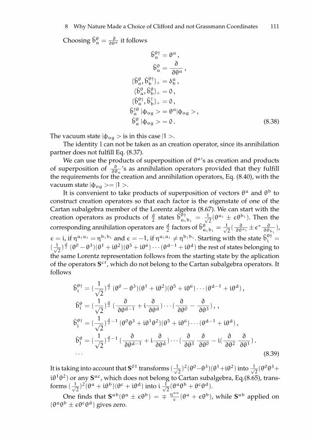
ii

“proc17” — 2017/12/11 — 19:44 — page 111 — #125 ii

ii

ii


Choosing bθa = ∂∂θa

it follows

bθ†a = θa ,

bθa =∂

∂θa,

bθa, bθ†b + = δab ,

bθa, bθb+ = 0 ,

bθ†a , b†b+ = 0 ,

b†θa |φog > = θa|φog > ,

bθa |φog > = 0 . (8.38)

The vacuum state |φog > is in this case |1 >.The identity I can not be taken as an creation operator, since its annihilation

partner does not fulfill Eq. (8.37).We can use the products of superposition of θa’s as creation and products

of superposition of ∂∂θa

’s as annihilation operators provided that they fulfillthe requirements for the creation and annihilation operators, Eq. (8.40), with thevacuum state |φog >= |1 >.

It is convenient to take products of superposition of vectors θa and θb toconstruct creation operators so that each factor is the eigenstate of one of theCartan subalgebra member of the Lorentz algebra (8.67). We can start with thecreation operators as products of d

2states bθ†aibi = 1√

2(θai ± εθbi). Then the

corresponding annihilation operators are d2

factors of bθaibi =1√2( ∂∂θai

±ε∗ ∂∂θbi

),

ε = i, if ηaiai = ηbibi and ε = −1, if ηaiai 6= ηbibi . Starting with the state bθ†i =

( 1√2)d2 (θ0 − θ3)(θ1 + iθ2)(θ5 + iθ6) · · · (θd−1 + iθd) the rest of states belonging to

the same Lorentz representation follows from the starting state by the aplicationof the operators Scf, which do not belong to the Cartan subalgebra operators. Itfollows

bθ†i = (1√2)d2 (θ0 − θ3)(θ1 + iθ2)(θ5 + iθ6) · · · (θd−1 + iθd) ,

bθi = (1√2)d2 (

∂

∂θd−1+ i

∂

∂θd) · · · ( ∂

∂θ0−

∂

∂θ3) , ,

bθ†j = (1√2)d2−1 (θ0θ3 + iθ1θ2)(θ5 + iθ6) · · · (θd−1 + iθd) ,

bθj = (1√2)d2−1 (

∂

∂θd−1+ i

∂

∂θd) · · · ( ∂

∂θ3∂

∂θ0− i(

∂

∂θ2∂

∂θ1) .

· · · (8.39)

It is taking into account that S01 transforms ( 1√2)2(θ0−θ3)(θ1+iθ2) into 1√

2(θ0θ3+

iθ1θ2) or any Sac, which does not belong to Cartan subalgebra, Eq.(8.65), trans-forms ( 1√

2)2(θa + iθb)(θc + iθd) into i 1√

2(θaθb + θcθd).

One finds that Sab(θa ± εθb) = ∓ ηaa

ε(θa + εθb), while Sab applied on

(θaθb ± εθcθd) gives zero.

ii

“proc17” — 2017/12/11 — 19:44 — page 112 — #126 ii

ii

ii


Although all the states, generated by creation operators, which include one(I±εθaθb) or several (I±εθa1θb1) · · · (I±εθakθak), are orthogonal with respectto the scalar product, Eq.(8.24), such creation operators do not have appropriateannihilation operators since (I ± εθaθb) and (I ± ε∗ ∂

∂θb∂∂θa

) (or several (I ±εθa1θb1) · · · (I ± εθakθbk) and (I ± ε∗ ∂

∂θbk∂∂θak

) · · · (I ± ε∗ ∂∂θb1

∂∂θa1

)) do notfulfill Eqs. (8.37, 8.38), since I has no annihilation partner. However, creationoperators which are products of one or several, let say n, of the kind θaiθbi (atmost d

2, each factor of them is the ”eigenstate” of one of the Cartan subalgebra

operators – Sabθaθb|1 >= 0), while the rest, d2− n, have the ”eigenvalues” either

(+1 or −1) or (+i or −i), fulfill relations

bθi , bθ†j +|φog > = δij |φog > ,

bθi , bθj +|φog > = 0 |φog > ,

bθ†i , b†j +|φog > = 0|φog > ,

bθ†j |φog > = |φj >

bθj |φog > = 0 |φog > . (8.40)

There are in (d = 2) two creation ((θ0 ∓ θ1, for ηab = diag(1,−1)) and corre-spondingly two annihilation operators ( ∂

∂θ0∓ ∂

∂θ1), and one creation operator

θ0θ1 and the corresponding annihilation operator ∂∂θ1

∂∂θ0

, each belonging to itsown group with respect to the Lorentz transformation operators, which fulfillEq. (8.40), in (d = 4) there are two triplets of the kind presented in Eq. (8.39)of creation and correspondingly two triplets of annihilation operators, and fourcreation operators with one product of θaiθbi multiplied by (θci ± θdi ) and fourcorresponding annihilation operators as well as the creation operator θ0θ3θ1θ2

with the corresponding annihilation operator, they all fulfill Eq. (8.40).Let us count the number of creation operators, when one starts with the

creator, which is the product of d2

factors, each with the ”eigenvalue” of the Cartansubalgebra operators, Eq. (8.67), equal to either +i or +1, Eq. (8.39):

bθ†0 = (θ0 − θ3)(θ1 + iθ2)(θ5 + iθ6) · · · (θd−3 + iθd−2)(θd−1 + iθd) . (8.41)

There are 2d2−1 creation operators of this type (θ0−θ3)(θ1+iθ2)(θ5+iθ6) · · · (θd−3+

iθd−2)(θd−1 + iθd), (θ0 + θ3)(θ1 − iθ2)(θ5 + iθ6) · · · (θd−3 + iθd−2)(θd−1 + iθ5),(θ0 + θ3)(θ1 + iθ2)(θ5 − iθ6) · · · (θd−3 + iθd−2)(θd−1 + iθd), · · · , (θ0 − θ3)(θ1 +iθ2)(θ5−iθ6) · · · (θd−1−iθ5) with the eigenvalues of the Cartan subalgebra equalto (+i,+1,+1, . . . ,+1,+1), (−i,−1,+1, . . . ,+1+ 1), (−i,+1,−1, . . . ,+1,+1),· · · ,(+i,+1,+1 . . . ,−1,−1), each of the operators distinguishing from the others inone pair of factors with the opposite eigenvalues of the Cartan subalgebra opera-tors.

There are in addition 2d2−1(2

d2−1 − 1)/2 Grassmann odd operators obtained

when Sef apply on (θ0 − θ3)(θ1 + iθ2)(θ5 + iθ6) · · · (θd−3 + iθd−2)(θd−1 + iθd),(θ0 + θ3)(θ1 − iθ2)(θ5 + iθ6) · · · (θd−3 + iθd−2)(θd−1 + iθd) and on the rest of2d2−1 − 1 operators. S01 applied on (θ0 − θ3)(θ1 + iθ2)(θ5 + iθ6) · · · (θd−3 +

iθd−2)(θd−1 + iθd), (θ0 + θ3)(θ1 − iθ2)(θ5 + iθ6) · · · (θd−3 + iθd−2)(θd−1 + iθd)gives ∝ (θ0θ3 + iθ1θ2)(θ5 + iθ6) · · · (θd−3 + iθd−2)(θd−1 + iθd), (θ0 + θ3)(θ1 −

ii

“proc17” — 2017/12/11 — 19:44 — page 113 — #127 ii

ii

ii


iθ2)(θ5 + iθ6) · · · (θd−3 + iθd−2)(θd−1 + iθ5)). Each of these operators have two”eigenvalues” of the Cartan subalgebra equal to zero and all the rest equal to either±i (if one of the two summands has ηaa = 1) or ±1 (otherwise). All these creationoperators are connected by Seg.

There are correspondingly all together 2d2−1(2

d2−1 + 1)/2 creation operators

and the same number of annihilation operators (they follow from the creationoperators by Hermitian conjugation, Eq. (8.8)), belonging to one group, so that allthe operators follow from the starting one by the application of Saf.

There is additional group of creation and annihilation operators, which followfrom the starting one

bθ†0 = (θ0 + θ3)(θ1 + iθ2)(θ5 + iθ6) · · · (θd−3 + iθd−2)(θd−1 + iθd) . (8.42)

(one can chose in the starting creation operator with changed sign in any offactors in the product, in each case the same group will follow). All the rest2d2−1(2

d2−1 + 1)/2 creation operators can be obtained from the starting one as in

the case of the first group.There is therefore

2d2−1(2

d2−1 + 1) (8.43)

creation and the same number of annihilation operators, which are built on twostarting states, presented in Eqs. (8.41, 8.42), divided in two groups, each gener-ating or annihilating states belonging to the same representation of the Lorentzalgebra.

The rest of creators (and the corresponding annihilators) have opposite Grass-mann character than the ones studied so far – like θ0θ1 ( ∂

∂θ1∂∂θ0

) in d = (1+1) andin d = (1+3) θ0θ3(θ1±iθ2) ( ∂

∂θ1∓i ∂

∂θ2) ∂∂θ3

∂∂θ0

), θ1θ2(θ0∓iθ3) (( ∂∂θ0±i ∂

∂θ3) ∂∂θ1

∂∂θ2

) and θ0θ3θ1θ2 ( ∂∂θ2

∂∂θ1

∂∂θ3

∂∂θ0

), which also fulfill the relations of Eq. (8.40).All the states |φθi >, generated by the creation operators (presented in Eq. (8.40))

on the vacuum state |φog > are the eigenstates of the Cartan subalgebra operatorsand are orthogonal and normalized with respect to the norm of Eq. (8.23)

< φθi |φθj > = δij . (8.44)

If we now extend the creation and annihilation operators to the ordinarycoordinate space, the relation among creation and annihilation operators at onetime read

bθi (~x), bθ†j (~x ′)+|φog > = δij δ(~x− ~x ′)|φog > ,

bθi (~x), bθj (~x′)+|φog > = 0 |φog > ,

bθ†i (~x), bθ†j (~x ′)+|φog > = 0 |φog > ,

bθ†j (~x)|φog > = 0 |φog >

|φog > = |1 > . (8.45)

b. Quantization in Clifford space

ii

“proc17” — 2017/12/11 — 19:44 — page 114 — #128 ii

ii

ii


In Grassmann space the requirement that products of eigenstates of the Cartansubalgebra operators represent the creation and annihilation operators, obeyingthe relation Eq. (8.40), reduces the number of states. Let us study what happens,when, let say, γa’s are used to create the basis and correspondingly also to createthe creation and annihilation operators.

Let us point out that γa is expressible with θa and its its deriative (γa =

(θa + ∂∂θa

)), Eq. (8.14), and that we again require that creation (annihilation)operators create (annihilate) states, which are eigenstates of the Cartan subalgebra,Eq. (8.67). We could as well make a choice of γa = i(θa − ∂

∂θa) 3. We shall follow

here to some extend Ref. [15].Making a choice of the Cartan subalgebra eigenstates of Sab, Eq. (8.67),

ab

(k): =1

2(γa +

ηaa

ikγb) ,

ab

[k]: =1

2(1+

i

kγaγb) , (8.46)

where k2 = ηaaηbb, recognizing that the Hermitian conjugate values ofab

(k) andab

[k] are

ab

(k)

†

= ηaaab

(−k),ab

[k]

†

=ab

[k] , (8.47)

while the corresponding eigenvalues of Sab, Eq. (8.48), and Sab, Eq. (8.85), are

Sabab

(k) =1

2kab

(k) , Sabab

[k]=1

2kab

[k]

Sabab

(k) =k

2

ab

(k) , Sabab

[k]= −k

2

ab

[k] . (8.48)

We find in d = 2(2n+ 1) that from the starting state with products of odd numberof only nilpotents

|ψ11 > |2(2n+1) =03

(+i)12

(+)35

(+) · · ·d−3 d−2

(+)d−1 d

(+) |ψoc > , (8.49)

having correspondingly an odd Clifford character 4, all the other states of the sameLorentz representation, there are 2

d2−1 members, follow by the application of Scd 5,

which do not belong to the Cartan subalgebra, Eq. (8.67): Scd |ψ11 > |2(2n+1) =

|ψ1i > |2(2n+1). The operators Scd, which do not belong to the Cartan subalgebra of

3 We choose γa’s, Eq.(8.14) to create the basic states. We could instead make a choice ofγa’s, Eq.(8.15) to create the basic states. In the case of this latter choice the role of γa andγa should be correspondingly exchanged in Eq. (8.74).

4 We call the starting state in d = 2(2n + 1) |ψ11 > |2(2n+1), and the starting state in d = 4n

|ψ11 > |4n.5 The smallest number of all the generators Sac, which do not belong to the Cartan subal-

gebra, needed to create from the starting state all the other members is 2d2−1 − 1. This is

true for both even dimensional spaces – 2(2n + 1) and 4n.

ii

“proc17” — 2017/12/11 — 19:44 — page 115 — #129 ii

ii

ii


Sab, Eq. (8.67), generate states with different eigenstates of the Cartan subalgebra(S03, S12, S56, · · · , Sd−1d), we call the eigenvalues of their eigenstates the ”family”quantum numbers. There are 2

d2−1 families. From the starting new member with

a different ”family” quantum number the whole Lorentz representation withthis ”family” quantum number follows by the application of Sef: Sef Scd|ψ11 >|2(2n+1) = |ψji > |2(2n+1). All the states of one Lorentz representation of anyparticular ”family” quantum number have an odd Clifford character, since neitherScd nor Scd, both with an even Clifford character, can change this character. Weshall comment our limitation of states to only those with an odd Clifford characterafter defining the creation and annihilation operators.

For d = 4n the starting state must be the product of one projector and 4n− 1

nilpotents, since we again limit states to those with an odd Clifford character. Letus start with the state

|ψ11 > |4n =03

(+i)12

(+)35

(+) · · ·d−3 d−2

(+)d−1 d

[+] |ψoc > , (8.50)

All the other states belonging to the same Lorentz representation follow again bythe application of Scd on this state |ψ11 > |4n, while a new family starts by theapplication of Scd|ψ11 > |4n and from this state all the other members with thesame ”family” quantum number can be generated by SefScd on |ψ11 > |4n: SefScd

|ψ11 > |4n = |ψji > |4n.All these states in either d = 2(2n+ 1) space or d = 4n space are orthogonal

with respect to Eq. (8.23).However, let us point out that (γa)† = γaηaa. Correspondingly it follows,

Eq. (8.47), thatab

(k)

†

= ηaaab

(−k), andab

[k]

†

=ab

[k].Since any projector is Hermitian conjugate to itself, while to any nilpotent

ab

(k) the Hermitian conjugated one has an opposite k, it is obvious that Hermitianconjugated product to a product of nilpotents and projectors can not be acceptedas a new state 6.

The vacuum state |ψoc > ought to be chosen so that < ψoc|ψoc >= 1,

while all the states belonging to the physically acceptable states, like03

[+i]12

[+]56

[−]78

[−]

· · ·d−3 d−2

(+)d−1 d

(+) |ψoc >, must not give zero for either d = 2(2n+ 1) or for d = 4n.We also want that the states, obtained by the application of ether Scd or Scd orboth, are orthogonal. To make a choice of the vacuum it is needed to know the

6 We could as well start with the state |ψ11 > |2(2n+1) =03

(+i)12

(+)35

(+) · · ·d−3 d−2

(+)d−1 d

(+) |ψoc >

for d = 2(2n + 1) and with |ψ11 > |4n =03

(+i)12

(+)35

(+) · · ·d−3 d−2

(+)d−1 d

[+] |ψoc > in the case ofd = 4n. Then creation and annihilation operators will exchange their roles.

ii

“proc17” — 2017/12/11 — 19:44 — page 116 — #130 ii

ii

ii


relations of Eq. (8.71). It must be

< ψoc| · · ·ab

(k)

†

· · · | · · ·ab

(k ′) · · · |ψoc > = δkk ′ ,

< ψoc| · · ·ab

[k]

†

· · · | · · ·ab

[k ′] · · · |ψoc > = δkk ′ ,

< ψoc| · · ·ab

[k]

†

· · · | · · ·ab

(k ′) · · · |ψoc > = 0 . (8.51)

Our experiences in the case, when states with the integer values of the Cartansubalgebra operators were expressed by Grassmann coordinates, teach us that therequirements, which creation and annihilation operators must fulfill, influence thechoice of the number of states, as well as of the vacuum state.

Let us first repeat therefore the requirements which the creation and annihila-tion operators must fulfill

bαγi , bβγ†k +|ψoc > = δαβ δik|ψoc > ,

bαγi , bβγk +|ψoc > = 0|ψoc > ,

bαγ†i , bβγ†k +|ψoc > = 0|ψoc > ,

bαγ†i |ψoc > = 0|ψoc > , (8.52)

paying attention at this stage only at the internal degrees of freedom of the states,that is on their spins. Here (α,β, . . . ) represent the family quantum number de-termined by Sac and (i, j, . . . ) the quantum number of one representation, deter-mined by Sac. From Eqs. (8.49, 8.50) is not difficult to extract the creation operatorswhich, when applied on the two vacuum states, generate the starting states.

i. One Weyl representationWe define the creation b1†1 – and the corresponding annihilation operator b11,

(b1†1 )† = b11 – which when applied on the vacuum state |ψoc > create a vector ofone of the two equations (8.49, 8.50), as follows

b1†1 : =03

(+i)12

(+)56

(+) · · ·d−1 d

(+) ,

b11 : =d−1 d

(−) · · ·56

(−)12

(−)03

(−i) ,

for d = 2(2n+ 1) ,

b1†1 : =03

(+i)12

(+)56

(+) · · ·d−3 d−2

(+)d−1 d

[+] ,

b11 : =d−1,d

[+]d−2 d−3

(−) · · ·56

(−)12

(−)03

(−i) ,

for d = 4n . (8.53)

We shall call this vector the starting vector of the starting ”family”.

ii

“proc17” — 2017/12/11 — 19:44 — page 117 — #131 ii

ii

ii


Now we can make a choice of the vacuum state for this particular ”family”taking into account Eq. (8.71)

|ψoc > =03

[−i]12

[−]56

[−] · · ·d−1 d

[−] |0 > ,

for d = 2(2n+ 1) ,

|ψoc > =03

[−i]12

[−]56

[−] · · ·d−3 d−2

[−]d−1 d

[+] |0 > ,

for d = 4n , (8.54)

n is a positive integer, so that the requirements of Eq. (8.52) are fulfilled. Wesee: The creation and annihilation operators of Eq. (8.53) (both are nilpotents,(b1†1 )2 = 0 and (b11)

2 = 0), b1†1 (generating the vector |ψ11 >when operating on thevacuum state) gives b1†1 |ψoc > 6= 0, while the annihilation operator annihilates thevacuum state b11|ψ0 >= 0, giving b11, b

1†1 +|ψoc >= |ψoc >, since we choose the

appropriate normalization, Eq. (8.46).All the other creation and annihilation operators, belonging to the same

Lorentz representation with the same family quantum number, follow from thestarting ones by the application of particular Sac, which do not belong to theCartan subalgebra (8.65).

We call b1†2 the one obtained from b1†1 by the application of one of the fourgenerators (S01, S02, S31, S32). This creation operator is for d = 2(2n+ 1) equal to

b1†2 =03

[−i]12

[−]35

(+) · · ·d−1 d

(+) , while it is for d = 4n equal to b1†2 =03

[−i]12

[−]56

(+) · · ·d−1 d

[+] .All the other family members follow from the starting one by the application ofdifferent Sef, or by the product of several Sgh.

We accordingly have

b1†i ∝ Sab..Sefb1†1 ,

b1i ∝ b11Sef..Sab , (8.55)

with Sab† = ηaaηbbSab. We shall make a choice of the proportionality factors sothat the corresponding states |ψ11 >= b

1†i |ψoc >will be normalized.

We recognize that [15]:i.a. (b1†i )2 = 0 and (b1i )

2 = 0, for all i.

To see this one must recognize that Sac (or Sbc, Sad, Sbd) transformsab

(+)cd

(+) toab

[−]cd

[−], that is an even number of nilpotents (+) in the starting state is transformedinto projectors [−] in the case of d = 2(2n+ 1). For d = 4n, Sac (or Sbc, Sad, Sbd)

transformsab

(+)cd

[+] intoab

[−]cd

(−). Therefore for either d = 2(2n + 1) or d = 4n atleast one of factors, defining a particular creation operator, will be a nilpotent. Ford = 2(2n+ 1) there is an odd number of nilpotents, at least one, leading from the

starting factor (dg

(+)) in the creator. For d = 4n a nilpotent factor can also bed−1 d

(−)

(sinced−1d

[+] can be transformed by Sed−1, for example intod−1 d

(−) ). A square ofat least one nilpotent factor (we started with an odd number of nilpotents, andoddness can not be changed by Sab), is enough to guarantee that the square of

ii

“proc17” — 2017/12/11 — 19:44 — page 118 — #132 ii

ii

ii


the corresponding (b1†i )2 is zero. Since b1i = (b1†i )†, the proof is valid also forannihilation operators.i.b. b1†i |ψoc > 6= 0 and b1i |ψoc >= 0, for all i.To see this in the case d = 2(2n+1) one must recognize that b1†i distinguishes fromb1†1 in (an even number of) those nilpotents (+), which have been transformed

into [−]. Whenab

[−] from b1†i meetsab

[−] from |ψoc >, the product givesab

[−] back,

and correspondingly a nonzero contribution. For d = 4n also the factord−1 d

[+] can

be transformed. It is transformed intod−1 d

(−) which, when applied to a vacuum

state, gives again a nonzero contribution (d−1 d

(−)d−1 d

[+] =d−1 d

(−) , Eq.(8.71)).In the case of b1i we recognize that in b1†i at least one factor is nilpotent; that of the

same type as in the starting b†1 – (+) – or in the case of d = 4n it can be alsod−1 d

(−) .

Performing the Hermitian conjugation (b1†i )†, (+) transforms into (−), whiled−1 d

(−)

transforms intod−1 d

(+) in b1i . Since (−)[−] gives zero andd−1 d

(+)d−1 d

[+] also gives zero,b1i |ψoc >= 0.i.c. b1†i , b

1†j + = 0, for each pair (i, j).

There are several possibilities, which we have to discuss. A trivial one is, if bothb1†i and b1†j have a nilpotent factor (or more than one) for the same pair of indexes,

saykl

(+). Then the product of such twokl

(+)kl

(+) gives zero. It also happens, that b1†i

has a nilpotent at the place (kl) (03

[−] · · ·kl

(+) · · ·mn

[−] · · · ) while b1†j has a nilpotent

at the place (mn) (03

[−] · · ·kl

[−] · · ·mn

(+) · · · ). Then in the term b1†i b1†j the product

mn

[−]mn

(+) makes the term equal to zero, while in the term b1†j b1†i the product

kl

[−]kl

(+)

makes the term equal to zero. There is no other possibility in d = 2(2n + 1). In

the case that d = 4n, it might appear also that b1†i =03

[−] · · ·ij

(+) · · ·d−1 d

[+] and

b1†j =03

[−] · · ·ij

[−] · · ·d−1 d

(−) . Then in the term b1†i b1†j the factor

d−1 d

[+]d−1 d

(−) makes

it zero, while in b1†j b1†i the factor

ij

[−]ij

(+) makes it zero. Since there are no furtherpossibilities, the proof is complete.i.d. b1i , b

1j + = 0, for each pair (i, j).

The proof goes similarly as in the case with creation operators. Again we treatseveral possibilities. b1i and b1j have a nilpotent factor (or more than one) with the

same indexes, saykl

(−). Then the product of such twokl

(−)kl

(−) gives zero. It also

happens, that b1i has a nilpotent at the place (kl) (· · ·mn

[−] · · ·kl

(−) · · ·03

[−]) while b1j

has a nilpotent at the place (mn) (· · ·mn

(−) · · ·kl

[−] · · ·03

[−]). Then in the term b1i b1j the

productkl

(−)kl

[−] makes the term equal to zero, while in the term b1j b1i the product

mn

(−)mn

[−] makes the term equal to zero. In the case that d = 4n, it appears also that

ii

“proc17” — 2017/12/11 — 19:44 — page 119 — #133 ii

ii

ii


b1i =d−1 d

[+] · · ·ij

(−) · · ·03

[−] and b1j =d−1 d

(+) · · ·ij

[−] · · ·03

[−]. Then in the term b1i b1j the

factorij

(−)ij

[−] makes it zero, while in b1j b1i the factor

d−1 d

(+)d−1 d

[+] makes it zero.i.e. b1i , b

1†j +|ψoc >= δij|ψoc > .

To prove this we must recognize that b1i = b1Sef..Sab and b1†i = Sab..Sefb1.

Since any b1i |ψoc >= 0, we only have to treat the term b1i b1†j . We find b1i b

1†j ∝

· · ·lm

(−) · · ·03

(−)Sef · · ·SabSlm · · ·Spr03

(+) · · ·lm

(+) · · · . If we treat the term b1i b1†i ,

generators Sef · · ·SabSlm · · ·Spr are proportional to a number and we normalize< ψ0|b

1i b1†i |ψoc > to one. When Sef · · ·SabSlm · · ·Spr are proportional to several

products of Scd, these generators change b1†1 into03

(+) · · ·kl

[−] · · ·np

[−] · · · , making

the product b1i b1†j equal to zero, due to factors of the type

kl

(−)kl

[−]. In the case of

d = 4n also a factord−1 d

[+]d−1 d

(−) might occur, which also gives zero.We saw and proved that for the definition of the creation and annihilation operators

in Eqs.(8.49,8.50) all the requirements of Eq. (8.52) are fulfilled, provided that creationand correspondingly also the annihilation operators have an odd Clifford character, that isthat the number of nilpotents in the product is odd.

For an even number of factors of the nilpotent type in the starting state and accord-ingly in the starting b1†1 , an annihilation operator b1i would appear with all factors of thetype [−], which on the vacuum state (Eq.(8.54)) would not give zero.

ii. Families of Weyl representationsLet bα†i be a creation operator, fulfilling Eq. (8.52), which creates one of the

(2d/2−1) Weyl basic states of an α−th ”family”, when operating on a vacuum state|ψoc > and let bαi = (bα†i )† be the corresponding annihilation operator. We shallnow proceed to define bα†i and bαi from a chosen starting state (8.49, 8.50), whichb1†1 creates on the vacuum state |ψoc >.

When treating more than one Weyl representation, that is, more than one”family”, we must take into account that: i. The vacuum state chosen to fulfillrequirements for second quantization of the starting family might not and it willnot be the correct one when all the families are taken into account. ii. The productsof Sab, which do not belong to the Cartan subalgebra set of the generators Sab

(2d/2−1 − 1 of them), when being applied on the starting family ψ11, generate thestarting members ψα1 of all the rest of the families. There are correspondinglythe same number of ”families” as there is the number of vectors of one Weylrepresentation, namely 2d/2−1. Then the whole Weyl representations of a particularfamily ψα1 follows again with the application of Sef, which do not belong to theCartan subalgebra of Sab on this starting family.

Any vector |ψαi > follows from the starting vector (Eqs.8.49, 8.50) by theapplication of either Sef, which change the family quantum number, or Sgh, whichchange the member of a particular family (as it can be seen from Eqs. (8.73, 8.86))or with the corresponding product of Sef and Sef

|ψαi > ∝ Sab · · · Sef|ψ1i >∝ Sab · · · SefSmn · · ·Spr|ψ11 > . (8.56)

ii

“proc17” — 2017/12/11 — 19:44 — page 120 — #134 ii

ii

ii


Correspondingly we define bα†i (up to a constant) to be

bα†i ∝ Sab · · · SefSmn · · ·Sprb1†1

∝ Smn · · ·Sprb1†1 Sab · · ·Sef . (8.57)

This last expression follows due to the property of the Clifford object γa andcorrespondingly of Sab, presented in Eqs. (8.74, 8.75).

For bαi = (bα†i )† we accordingly have

bαi = (bα†i )† ∝ Sef · · ·Sabb11Spr · · ·Smn . (8.58)

The proportionality factor will be chosen so that the corresponding states |ψαi >=bα†i |ψoc >will be normalized.

We ought to generalize the vacuum state from Eq. (8.54) so that bα†i |ψoc > 6= 0

and bαi |ψoc >= 0 for all the members i of any family α. Since any Seg changesef

(+)gh

(+) intoef

[+]gh

[+] and (ab

[+])† =ab

[+], while (ab

(+))†ab

(+)=ab

[−], the vacuum state |ψoc >

from Eq. (8.54) must be replaced by

|ψoc >=03

[−i]12

[−]56

[−] · · ·d−1 d

[−] +03

[+i]12

[+]56

[−] · · ·d−1 d

[−] +03

[+i]12

[−]56

[+] · · ·d−1 d

[−] + · · · |0 > ,for d = 2(2n+ 1),

|ψoc >=03

[−i]12

[−]35

[−] · · ·d−3 d−2

[−]d−1 d

[+] +03

[+i]12

[+]56

[−] · · ·d−3 d−2

[−]d−1 d

[+] + · · · |0 > ,for d = 4n, (8.59)

n is a positive integer. There are 2d2−1 summands. since we step by step replace all

possible pairs ofab

[−] · · ·ef

[−] in the starting part03

[−i]12

[−]35

[−] · · ·d−1 d

[−] (or03

[−i]12

[−]35

[−]

· · ·d−3 d−2

[−]d−1 d

[+] ) intoab

[+] · · ·ef

[+] and include new terms into the vacuum state sothat the last 2n+ 1 summands have for d = 2(2n+ 1) case, n is a positive integer,only one factor [−] and all the rest [+], each [−] at different position. For d = 4n

also the factord−1 d

[+] in the starting term03

[−i]12

[−]35

[−] · · ·d−3 d−2

[−]d−1 d

[+] changes tod−1 d

[−] . The vacuum state has then the normalization factor 1/√2d/2−1.

There is therefore

2d2−1 2

d2−1 (8.60)

number of creation operators, defining the orthonormalized states when applayingon the vacuum state of Eqs. (8.59) and the same number of annihilation operators,which are defined by the creation operators on the vacuum state of Eqs. (8.59).Sab connect members of different families, Sab generates all the members of onefamily.

We recognize that:ii.a. The above creation and annihilation operators are nilpotent – (ba†i )2 = 0 =

ii

“proc17” — 2017/12/11 — 19:44 — page 121 — #135 ii

ii

ii


(bai )2 – since the ”starting” creation operator b1†1 and annihilation operator bai are

both made of the product of an odd number of nilpotents, while products of eitherSab or Sab can change an even number of nilpotents into projectors. Any ba†i iscorrespondingly a factor of an odd number of nilpotents (at least one) (and aneven number of projectors) and its square is zero. The same is true for bai .ii.b. All the creation operators operating on the vacuum state of Eq.(8.59) give anon zero vector – ba†i |ψoc > 6= 0 – while all the annihilation operators annihilatethis vacuum state – bai |ψ0 > for any α and any i.It is not difficult to see that bai |ψoc >= 0, for any α and any i. First we recognizethat whatever the set of factors Smn · · ·Spr appear on the right hand side of theannihilation operator b11 in Eq.(8.58), it lives at least one factor [−] unchanged.

Since b11 is the product of only nilpotents (−) and sinceab

(−)ab

[−]= 0, this part of theproof is complete.Let us prove now that bα†i |ψoc > 6= 0 for each α, i. According to Eq.(8.57) theoperation Smn on the left hand side of b1†1 , withm,n, which does not belong to

the Cartan subalgebra set of indices, transforms the term03

[−i]12

[−] · · ·lm

[−] · · ·nk

[−]

· · ·d−1 d

[−] (or the term03

[−i]12

[−] · · ·lm

[−] · · ·nk

[−] · · · · · ·d−1 d

[+] ) into the term03

[−i]12

[−]

· · ·lm

(+) · · ·nk

(+) · · ·d−1 d

[−] (or the term03

[−i]12

[−] · · ·lm

(+) · · ·nk

(+) · · · · · ·d−1 d

[+] ) and b1†1

on such a term gives zero, sincelm

(+)lm

(+)= 0 andnk

(+)nk

(+)= 0. Let us first assume thatSmn is the only term on the right hand side of b1†1 and that none of the operatorsfrom the left hand side of b1†1 in Eq.(8.57) has the indicesm,n. It is only one termamong all the summands in the vacuum state (Eq.8.59), which gives non zero

contribution in this particular case, namely the term03

[−i]12

[−] · · ·lm

[+] · · ·nk

[+] · · ·d−1 d

[−]

(or the term03

[−i]12

[−] · · ·lm

[+] · · ·nk

[+] · · · · · ·d−1 d

[+] ). Smn transforms the part · · ·lm

[+]

· · ·nk

[+] · · · into · · ·lm

(−) · · ·nk

(−) · · · and sincelm

(+)lm

(−) gives ηlllm

[+], while for the restof factors it was already proven that such a factor on b1†1 forms a b1†i giving nonzero contribution on the vacuum (8.54).We also proved that what ever other Sab but Smn operate on the left hand side ofb1†1 the contribution of this particular part of the vacuum state is nonzero. If theoperators on the left hand side have the indexesm or n or both, the contribution onthis term of the vacuum will still be nonzero, since then such a Smp will transform

the factorlm

(+) in b1†1 intolm

[−] andlm

[−]lm

(−) is nonzero, Eq. (8.71).The vacuum state has a term which guarantees a non zero contribution for anypossible set of Smn · · ·Spr operating from the right hand side of b1†1 (that is foreach family) (which we achieved just by the transformation of all possible pairs

ofcd

[−],gh

[−] intocd

[+],gh

[+]), the proof that bα†i operating on the vacuum |ψoc > of

Eq. (8.59) gives nonzero contribution. Among [−] also03

[−i] is understood.It is not difficult to see that for each ”family” of 2

d2−1 families it is only one term

among all the summands in the vacuum state |ψoc > of Eq. (8.59), which givea nonzero contribution, since when ever [+] appears on a wrong position, that

ii

“proc17” — 2017/12/11 — 19:44 — page 122 — #136 ii

ii

ii


is on the position, so that the product ofab

(+) from b1† andab

[+] from the vacuumsummand appears, the contribution is zero.ii.b. Any two creation operators anti commute — bα†i , b

β†j + = 0.

According to Eq.8.57 we can rewrite bα†i , bb†j +, up to a factor, as

Smn · · ·Sprb1†1 Sab · · ·Sef, Sm

′n ′ · · ·Sp′r ′ b1†1 S

a ′b ′ · · ·Se′f ′ +.

Whatever the product Sab · · ·SefSm ′n ′ · · ·Sp ′r ′ (or Sa′b ′ · · ·Se ′f ′Smn · · ·Spr) is, it

always transforms an even number of (+) in b1†1 into [−]. Since an odd number ofnilpotents (+) (at least one) stays unchanged in this right b1†1 , after the application

of all the Sab in the product in front of it ord−1 d

[ +] transforms intod−1 d

( −),and since the left b1†1 is a product of only nilpotents (+) or an odd number ofnilpotents and [+] for d = 2(2n+1) and d = 4n, n is an integer, respectively, whiled−1 d

[+]d−1 d

(−) = 0, the anticommutator for any two creation operators is zero.ii.c.. Any two annihilation operators anticommute – bαi , β

bj + = 0.

According to Eq.8.58 we can rewrite bαi , bβj +, up to a factor, as

Sab · · ·Sefb11Smn · · ·Spr, Sa′b ′ · · ·Se

′f ′ b11Sm ′n ′ · · ·Sp

′r ′ +.

What ever the product Smn · · ·SprSa ′b ′ · · ·Se ′f ′ (or Sm′n ′ · · ·Sp ′r ′Sab · · ·Sef) is,

it always transforms an even number of (−) in b11 into [+]. Since an odd number ofnilpotents (−) (at least one) stays unchanged in this b11, after the application of all

the Sab in the product in front of it ord−1 d

[ +] transforms intod−1 d

( −), and sinceb11 in the left hand side is a product of only nilpotents (−) or an odd number ofnilpotents and [+] for d = 2(2n+1) and d = 4n, n is an integer, respectively, whileab

(−)ab

(−)= 0 andab

[+]ab

[−]= 0, the anti commutator of any two annihilation operatorsis zero.ii.d. For any creation and any annihilation operators it follows: bαi , b

β†j +|ψ− >=

δabδij|ψ0 > .

Let us prove this. According to Eqs. (8.57,8.58) we may rewrite bαi , bβ†j + up

to a factor as Sab · · ·Sefb11Smn · · ·Spr, Sm′n ′ · · ·Sp ′r ′ b1†1 Sa

′b ′ · · ·Se ′f ′ +. We dis-tinguish between two cases. It can be that both Smn · · ·SprSm ′n ′ · · ·Sp ′r ′ andSa′b ′ · · ·Se ′f ′Sab · · ·Sef are numbers. This happens when α = β and i = j. Then

we follow i.b.. We normalize the states so that < ψαi |ψαi >= 1.

The second case is that at least one of

Smn · · ·SprSm′n ′ · · ·Sp

′r ′ and Sa′b ′ · · ·Se

′f ′Sab · · ·Sef

is not a number. Then the factors likeab

(−)ab

[−] orab

[+]ab

(−) orab

(+)ab

[+] make the anticom-mutator equal zero. And the proof is completed.

iii. We learned:iii.a. From 2d internal states expressed with Grassmann coordinates, which areall orthogonal with respect to the scalar product, Eq.(8.24), not all of 2d fulfill re-quirements that the states should be written as product of Grassmann coordinates

ii

“proc17” — 2017/12/11 — 19:44 — page 123 — #137 ii

ii

ii


on the vacuum state. We payed particular attention on 2d2−1 (2

d2−1 + 1), states,

Eqs. (8.41, 8.42). To these creation operators the same number, (2d2−1(2

d2−1 + 1)),

of the corresponding annihilation operators belong, fulfilling the relation for thecreation and annihilation operators (8.40), for which we expect that the creationand annihilation operators have to. These states form two (separate) groups ofthe Lorentz representation: The members of each group are reachable by Sab

(which do not belong to the Cartan subalgebra (8.65)) from one of the state of eachgroup, each with (2

d2−1(2

d2−1 + 1))/2members. The second quantized states have

in d = 4n an even Grassmann caharacter, while in d = 2(2n + 1) they have anodd Grassmann character. There are in addition creation operators of oppositeGrassmann character then these 2

d2−1(2

d2−1 + 1)) states either in d = 4n or in

d = 2(2n+ 1). They are products of two, four or at most product of d θa.iii.b. From 2d internal states expressed with Clifford coordinates, which againare orthogonal with respect to the scalar product, Eq.(8.24), only 2

d2−1 (2

d2−1)

fulfill requirements that the second quantized states are expressed by productsof nilpotents and projectors, which apply on the vacuum state. The products ofnillpotents and projectors have to have an odd Clifford character in either d = 4n

or d = 2(2n + 1). They form creation operators and annihilation operators, full-filling Eq.(8.52), for which we expect that the creation and annihilation operatorshave to.The corresponding states form families of states. Each family members are reach-able from any one by Sab, while any family can be reached by Sab.iii.c. We pay attention on even-dimensional spaces only.

8.3 Conclusions

We have started the present study to understand, why ”nature made a choice” ofthe Clifford algebra, rather than the Grassmann algebra, to describe the internaldegrees of freedom of fermion fields, although both spaces enable the secondquantization of the internal degrees of freedom of the fermion type. We studyas well how to fermionize boson fields (or bosonize fermion fields) in any d(the reader can find the corresponding contribution in this proceedings) to betterunderstand why and how ”nature made choices of the theories and models” inthe expansion of the universe.

The creation and annihilation operators fulfill anticommutation relations,desired for fermions either in Grassmann space or in Clifford space, althoughstates in Grassmann space carry integer spins, what leads in the spinn-charge-familytheory (since spins in d ≥ 5 manifest as charges in d = (1+ 3)) to the charges inthe adjoint representations of the charge groups (the subgroups of the Lorentzgroup SO(1, 13)) while states in the Clifford space carry half integer spin andcorrespondingly are all the charges in the fundamental representations of thegroups.

We want to understand as well how does this choice of whether takingGrassmann or Clifford space, manifest in the breaking of the starting symmetryin d-dimension down to d = (1+ 3). The spin-charge-family theory namely startsat d = (1+ 13) with the simple action in which massless fermions carry only two

ii

“proc17” — 2017/12/11 — 19:44 — page 124 — #138 ii

ii

ii


kinds of spin described by two kinds of the Clifford algebra objects – γa and γa

– and interact with the gravity only – through vielbeins, the gauge fields of thePoincare algebra and the two kinds of the spin connection fields, the gauge fieldsof these two kinds of the Clifford algebra objects. The theory offers the explanationfor all the assumptions of the standard model of elementary fields, fermions andbosons, with the appearance of families including, explaining also the phenomenalike the existence of the dark matter, of the matter-antimatter asymmetry, offeringcorrespondingly the next step beyond both standard models – cosmological oneand the one of the elementary fields.

To come to the low energy regime the symmetry must break, first fromSO(13, 1) to SO(7, 1)× SU(3)×U(1) and then further to SO(3, 1) ×SU(3)×U(1).Further study is needed to understand whether the ”nature could start” at allwith Grassmann space while ”recognizing”, when breaking symmetry in steps,the ”advantage” of the Clifford degrees of freedom with respect to the Grassmannones: The covariant momentum of the starting action of the spin-charge-familytheory, Eq. (8.1), would in the case that the Grassmann coordinates describe theinternal degrees of freedom of massless objects with the anticommutation relationof the creation and annihilation operators (Eq.(8.40)) read: p0α = pα−

12

SabΩabα,whereΩabα are the spin connection gauge fields of Sab (of the generators of theLorentz transformations in the Grassmann space) and fαa p0α would replace theordinary momentum, when massless objects start to interact with the gravitationalfield, through the vielbeins and the spin connections in Eq. (8.33).

This contribution is a step towards understanding better the open problemsof the elementary particle physics and cosmology.

Although we have not yet learned enough to be able to answer the four ques-tions – a. Why is the simple starting action of the spin-charge-family theory doing sowell in manifesting the observed properties of the fermion and boson fields? b. Un-der which condition can more general action lead to the starting action of Eq. (8.1)?c. What would more general action, if leading to the same low energy physics,mean for the history of our Universe? d. Could the fermionization procedure ofboson fields or the bosonization procedure of fermion fields, discussed in thisProceedings for any dimension d (by the authors of this contribution, while one ofthem, H.B.F.N. [11], has succeeded with another author to do the fermionizationfor d = (1+ 1)), tell more about the ”decisions” of the universe in the history.

8.4 APPENDIX: Lorentz algebra and representations inGrassmann and Clifford space

A Lorentz transformation on vector components θa, γa, or γa, which are usedto describe internal degrees of freedom of fields with the fermion nature, and onvector components xa, which are real (ordinary) commuting coordinates:θ ′a = Λab θ

b, γ ′a = Λab γb, γ ′a = Λab γ

b and xa = Λab xb,

leaves forms

aa1a2...aiθa1θa2 . . . θai , aa1a2...aiγ

a1γa2 . . . γai , aa1a2...ai γa1 γa2 . . . γai

ii

“proc17” — 2017/12/11 — 19:44 — page 125 — #139 ii

ii

ii


andba1a2...ai x

a1xa2 . . . xai , i = (1, . . . , d)

invariant.While ba1a2...ai (= ηa1b1ηa2b2 . . . ηaibi b

b1b2...bi) is a symmetric tensorfield, aa1a2...ai (= ηa1b1ηa2b2 . . . ηaibi a

b1b2...bi) are antisymmetric tensor Kalb-Ramond fields. The requirements that x

′a x′bηab = xc xdηcd, θ ′aθ ′bεab = θcθdεcd,

γ ′aγ ′bεab = γcγdεcd and γ ′aγ ′bεab = γcγdεcd, where the metric tensor ηab

(in our case ηab = diag(1,−1,−1, . . . ,−1)) lowers the indices of vectors xa

(= ηabxb), θa: (θa = ηab θb), γa: (γa = ηab γb) and γa: (γa = ηab γb),εab is the antisymmetric tensor, lead to ΛabΛcd ηac = ηbd. An infinitesimalLorentz transformation for the case with detΛ = 1,Λ00 ≥ 0 can be written asΛab = δab +ωab, whereωab +ωba = 0.

According to Eqs. (8.14, 8.15, 8.21) one finds

γa, Scd− = 0 = γa, Scd− ,

γa,Scd− = γa, Scd− =i

2(ηacγd − ηadγc) ,

γa,Scd− = γa, Scd− =i

2(ηacγd − ηadγc) . (8.61)

Comments: In the cases with either the basis θa or with the basis of γa or γa thescalar products — the norms — < B|B > < F|F > are non negative and equal to∑dk=0

∫ddxb∗b1...bkbb1...bk .

To have the norm which would have fields with the positive and the negativenorm one could define the norm as< φ0|bb1...bkγ

bk . . . γb1cc1...ckγc1 . . . γck |φ0 >,

as it is used in Ref. [21] to obtain the generalized Stueckelberg equation.

8.4.1 Lorentz properties of basic vectors

What follows is taken from Ref. [2] and Ref. [9], Appendix B.Let us first repeat some properties of the anticommuting Grassmann coordi-

nates.An infinitesimal Lorentz transformation of the proper ortochronous Lorentz

group is then

δθc = −i

2ωabSabθc = ωcaθa ,

δγc = −i

2ωabS

abγc = ωcaγa ,

δγc = −i

2ωabS

abγc = ωcaγa ,

δxc = −i

2ωabL

abxc = ωcaxa , (8.62)

whereωab are parameters of a transformation and γa and γa are expressed by θa

and ∂∂θa

in Eqs. (8.14, 8.15).Let us write the operator of finite Lorentz transformations as follows

U = ei2ωab(Sab+Lab) . (8.63)

ii

“proc17” — 2017/12/11 — 19:44 — page 126 — #140 ii

ii

ii


We see that the Grassmann θa and the ordinary xa coordinates and the Cliffordobjects γa and γa transform as vectors Eq.(8.63)

θ ′c = e−i2ωab(Sab+Lab) θc e

i2ωab(Sab+Lab)

= θc −i

2ωabSab, θc− + · · · = θc +ωcaθa + · · · = Λcaθa ,

x ′c = Λcaxa , γ ′c = Λcaγ

a , γ ′c = Λcaγa . (8.64)

Correspondingly one finds that compositions like γapa and γapa, here pa arepxa (= i ∂

∂xa), transform as scalars (remaining invariants), while Sabωabc and

Sab ωabc transform as vectors: U−1 Sabωabc U = ΛcdSabωabd, U−1 Sab ωabc U =

ΛcdSab ωabd.

Also objects like

R =1


cbβ)

andR =

1

2fα[afβb] (ωabα,β − ωcaαω

cbβ)

from Eq. (8.1) transform with respect to the Lorentz transformations as scalars.Making a choice of the Cartan subalgebra set of the algebra Sab, Sab and Sab,

Eqs. (8.10, 8.14, 8.15),

S03,S12,S56, · · · ,Sd−1 d ,S03, S12, S56, · · · , Sd−1 d ,S03, S12, S56, · · · , Sd−1 d , (8.65)

one can arrange the basic vectors so that they are eigenstates of the Cartan subal-gebra, belonging to representations of Sab, or of Sab and Sab.

8.5 APPENDIX: Technique to generate spinor representationsin terms of Clifford algebra objects

We shall briefly repeat the main points of the technique for generating spinorrepresentations from Clifford algebra objects, following the reference[12]. We askthe reader to look for details and proofs in this reference.

We assume the objects γa, Eq. (8.14), which fulfill the Clifford algebra, Eq (8.13).

γa, γb+ = I 2ηab, for a, b ∈ 0, 1, 2, 3, 5, · · · , d, (8.66)

for any d, even or odd. I is the unit element in the Clifford algebra, while γa, γb± =

γaγb ± γbγa.We accept the “Hermiticity” property for γa’s, Eq. (8.17), γa† = ηaaγa. lead-

ing to γa†γa = I.The Clifford algebra objects Sab close the Lie algebra of the Lorentz group of

Eq. (8.21) Sab, Scd− = i(ηadSbc + ηbcSad − ηacSbd − ηbdSac). One finds fromEq.(8.17) that (Sab)† = ηaaηbbSab and that Sab, Sac+ = 1

2ηaaηbc.

ii

“proc17” — 2017/12/11 — 19:44 — page 127 — #141 ii

ii

ii


Recognizing that two Clifford algebra objects Sab, Scd with all indexes dif-ferent commute, we select (out of infinitely many possibilities) the Cartan subalgebra set of the algebra of the Lorentz group as follows

S0d, S12, S35, · · · , Sd−2 d−1, if d = 2n,

S12, S35, · · · , Sd−1 d, if d = 2n+ 1. (8.67)

To make the technique simple, we introduce the graphic representation[12] asfollows

ab

(k): =1

2(γa +

ηaa

ikγb),

ab

[k]: =1

2(1+

i

kγaγb), (8.68)

where k2 = ηaaηbb. One can easily check by taking into account the Cliffordalgebra relation (Eq.8.66) and the definition of Sab that if one multiplies from the

left hand side by Sab the Clifford algebra objectsab

(k) andab

[k], it follows that

Sabab

(k)=1

2kab

(k),

Sabab

[k]=1

2kab

[k] . (8.69)

This means thatab

(k) andab

[k] acting from the left hand side on anything (on avacuum state |ψ0〉, for example) are eigenvectors of Sab.

We further find

γaab

(k) = ηaaab

[−k],

γbab

(k) = −ikab

[−k],

γaab

[k] =ab

(−k),

γbab

[k] = −ikηaaab

(−k) (8.70)

It follows that Sacab

(k)cd

(k)= − i2ηaaηcc

ab

[−k]cd

[−k], Sacab

[k]cd

[k]= i2

ab

(−k)cd

(−k), Sacab

(k)cd

[k]=

− i2ηaa

ab

[−k]cd

(−k), Sacab

[k]cd

(k)= i2ηcc

ab

(−k)cd

[−k] . It is useful to deduce the followingrelations

ab

(k)ab

(k) = 0,ab

(k)ab

(−k)= ηaaab

[k],ab

(−k)ab

(k)= ηaaab

[−k],ab

(−k)ab

(−k)= 0ab

[k]ab

[k] =ab

[k],ab

[k]ab

[−k]= 0,ab

[−k]ab

[k]= 0,ab

[−k]ab

[−k]=ab

[−k]ab

(k)ab

[k] = 0,ab

[k]ab

(k)=ab

(k),ab

(−k)ab

[k]=ab

(−k),ab

(−k)ab

[−k]= 0ab

(k)ab

[−k] =ab

(k),ab

[k]ab

(−k)= 0,ab

[−k]ab

(k)= 0,ab

[−k]ab

(−k)=ab

(−k) .

(8.71)

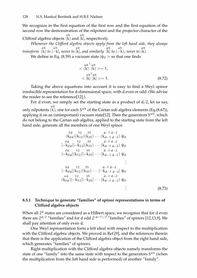
ii

“proc17” — 2017/12/11 — 19:44 — page 128 — #142 ii

ii

ii


We recognize in the first equation of the first row and the first equation of thesecond row the demonstration of the nilpotent and the projector character of the

Clifford algebra objectsab

(k) andab

[k], respectively.Whenever the Clifford algebra objects apply from the left hand side, they always

transformab

(k) toab

[−k], never toab

[k], and similarlyab

[k] toab

(−k), never toab

(k).We define in Eq. (8.59) a vacuum state |ψ0 > so that one finds

<ab

(k)

†ab

(k) >= 1,

<ab

[k]

†ab

[k] >= 1. (8.72)

Taking the above equations into account it is easy to find a Weyl spinorirreducible representation for d-dimensional space, with d even or odd. (We advisethe reader to see the reference[12].)

For d even, we simply set the starting state as a product of d/2, let us say,

only nilpotentsab

(k), one for each Sab of the Cartan sub algebra elements (Eq.(8.67)),applying it on an (unimportant) vacuum state[12]. Then the generators Sab, whichdo not belong to the Cartan sub algebra, applied to the starting state from the lefthand side, generate all the members of one Weyl spinor.

0d

(k0d)12

(k12)35

(k35) · · ·d−1 d−2

(kd−1 d−2) ψ00d

[−k0d]12

[−k12]35

(k35) · · ·d−1 d−2

(kd−1 d−2) ψ00d

[−k0d]12

(k12)35

[−k35] · · ·d−1 d−2

(kd−1 d−2) ψ0...

0d

[−k0d]12

(k12)35

(k35) · · ·d−1 d−2

[−kd−1 d−2] ψ0od

(k0d)12

[−k12]35

[−k35] · · ·d−1 d−2

(kd−1 d−2) ψ0... (8.73)

8.5.1 Technique to generate ”families” of spinor representations in terms ofClifford algebra objects

When all 2d states are considered as a Hilbert space, we recognize that for d eventhere are 2d/2 ”families” and for d odd 2(d+1)/2 ”families” of spinors [12,13,9]. Weshall pay attention of only even d.

One Weyl representation form a left ideal with respect to the multiplicationwith the Clifford algebra objects. We proved in Ref.[9], and the references thereinthat there is the application of the Clifford algebra object from the right hand side,which generates ”families” of spinors.

Right multiplication with the Clifford algebra objects namely transforms thestate of one ”family” into the same state with respect to the generators Sab (whenthe multiplication from the left hand side is performed) of another ”family”.

ii

“proc17” — 2017/12/11 — 19:44 — page 129 — #143 ii

ii

ii


We defined in refs.[13] the Clifford algebra objects γa’s as operations whichoperate formally from the left hand side (as γa’s do) on any Clifford algebra objectA as follows

γaA = i(−)(A)Aγa, (8.74)

with (−)(A) = −1, if A is an odd Clifford algebra object and (−)(A) = 1, if A is aneven Clifford algebra object.

Then it follows that γa obey the same Clifford algebra relation as γa.

(γaγb + γbγa)A = −ii((−)(A))2A(γaγb + γbγa) = 2ηabA (8.75)

and that γa and γa anticommute

(γaγb + γbγa)A = i(−)(A)(−γbAγa + γbAγa) = 0. (8.76)

We may write

γa, γb+ = 0, while γa, γb+ = 2ηab. (8.77)

One accordingly finds

γaab

(k): = −iab

(k) γa = −iηaaab

[k], (8.78)

γbab

(k): = −iab

(k) γb = −kab

[k],

γaab

[k]: = iab

[k] γa = iab

(k), (8.79)

γbab

[k]: = iab

[k] γb = −kηaaab

(k) . (8.80)

If we define

Sab =i

4[γa, γb] =

1

4(γaγb − γbγa), (8.81)

it follows

SabA = A1

4(γbγa − γaγb), (8.82)

manifesting accordingly that Sab fulfil the Lorentz algebra relation as Sab do.Taking into account Eq.(8.74), we further find

Sab, Sab− = 0, Sab, γc− = 0, Sab, γc− = 0. (8.83)

One also finds

Sab, Γ − = 0, γa, Γ − = 0, for d even,

Sab, Γ − = 0, γa, Γ + = 0, for d odd, (8.84)

which means that in d even transforming one ”family” into another with eitherSab or γa leaves handedness Γ unchanged. (The transformation to another ”family”

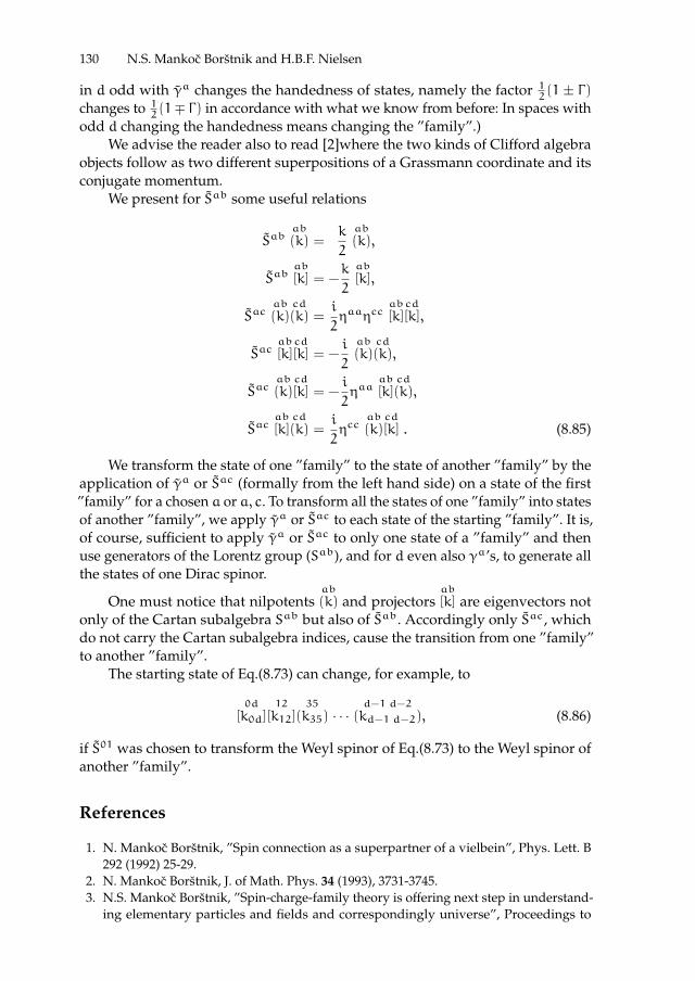
ii

“proc17” — 2017/12/11 — 19:44 — page 130 — #144 ii

ii

ii


in d odd with γa changes the handedness of states, namely the factor 12(1 ± Γ)

changes to 12(1∓ Γ) in accordance with what we know from before: In spaces with

odd d changing the handedness means changing the ”family”.)We advise the reader also to read [2]where the two kinds of Clifford algebra

objects follow as two different superpositions of a Grassmann coordinate and itsconjugate momentum.

We present for Sab some useful relations

Sabab

(k) =k

2

ab

(k),

Sabab

[k] = −k

2

ab

[k],

Sacab

(k)cd

(k) =i

2ηaaηcc

ab

[k]cd

[k],

Sacab

[k]cd

[k] = −i

2

ab

(k)cd

(k),

Sacab

(k)cd

[k] = −i

2ηaa

ab

[k]cd

(k),

Sacab

[k]cd

(k) =i

2ηcc

ab

(k)cd

[k] . (8.85)

We transform the state of one ”family” to the state of another ”family” by theapplication of γa or Sac (formally from the left hand side) on a state of the first”family” for a chosen a or a, c. To transform all the states of one ”family” into statesof another ”family”, we apply γa or Sac to each state of the starting ”family”. It is,of course, sufficient to apply γa or Sac to only one state of a ”family” and thenuse generators of the Lorentz group (Sab), and for d even also γa’s, to generate allthe states of one Dirac spinor.

One must notice that nilpotentsab


[k] are eigenvectors notonly of the Cartan subalgebra Sab but also of Sab. Accordingly only Sac, whichdo not carry the Cartan subalgebra indices, cause the transition from one ”family”to another ”family”.

The starting state of Eq.(8.73) can change, for example, to

0d

[k0d]12

[k12]35

(k35) · · ·d−1 d−2

(kd−1 d−2), (8.86)

if S01 was chosen to transform the Weyl spinor of Eq.(8.73) to the Weyl spinor ofanother ”family”.

References

1. N. Mankoc Borstnik, ”Spin connection as a superpartner of a vielbein”, Phys. Lett. B292 (1992) 25-29.

2. N. Mankoc Borstnik, J. of Math. Phys. 34 (1993), 3731-3745.3. N.S. Mankoc Borstnik, ”Spin-charge-family theory is offering next step in understand-

ing elementary particles and fields and correspondingly universe”, Proceedings to

ii

“proc17” — 2017/12/11 — 19:44 — page 131 — #145 ii

ii

ii


the Conference on Cosmology, Gravitational Waves and Particles, IARD conferences,Ljubljana, 6-9 June 2016, The 10th Biennial Conference on Classical and QuantumRelativistic Dynamics of Particles and Fields, J. Phys.: Conf. Ser. 845 (2017) 012017[arXiv:1607.01618v2]

4. N.S. Mankoc Borstnik, Phys. Rev. D 91 065004 (2015) [arxiv:1409.7791].5. N.S. Mankoc Borstnik, D. Lukman, Eur. Phys. J. C 77 (2017) 231.6. N.S. Mankoc Borstnik, ”Do we have the explanation for the Higgs and Yukawa cou-

plings of the standard model” [arXiv:1212.3184v2, arXiv:1207.6233), in Proceedings to the15th Workshop ”What comes beyond the standard models”, Bled, 9-19 of July, 2012, Ed. N.S.Mankoc Borstnik, H.B. Nielsen, D. Lukman, DMFA Zaloznistvo, Ljubljana, December2012, p.56-71 [arXiv.1302.4305].

7. N.S. Mankoc Borstnik N S, J. of Modern Phys. 4 (2013) 823 [arxiv:1312.1542].8. N.S. Mankoc Borstnik, H.B.F. Nielsen, Fortschrite der Physik, Progress of Physics (2017)

1700046.9. N.S. Mankoc Borstnik, J.of Mod. Physics 6 (2015) 2244-2274,

http://dx.org./10.4236/jmp.2015.615230 [arXiv:1409.4981].10. N.S. Mankoc Borstnik, H.B.F. Nielsen, ”Fermionization in an Arbitrary Num-

ber of Dimensions”, Proceedings to the 18th Workshop ”What comes beyondthe standard models”, Bled, 11-19 of July, 2015, Ed. N.S. Mankoc Borstnik, H.B.Nielsen, D. Lukman, DMFA Zaloznistvo, Ljubljana December 2015, p. 111-128[http://arxiv.org/abs/1602.03175]

11. H. Aratyn, H.B. Nielsen, ”Constraints On Bosonization In Higher Dimensions”, NBI-HE-83-36, Conference: C83-10-10.2 (Ahrenshoop Sympos.1983:0260), p.0260 Proceed-ings.

12. N.S. Mankoc Borstnik, H.B.F. Nielsen, J. of Math. Phys. 43, 5782 (2002) [hep-th/0111257].13. N.S. Mankoc Borstnik, H.B.F. Nielsen, J. of Math. Phys. 44 4817 (2003) [hep-th/0303224].14. N.S. Mankoc Borstnik and H.B. Nielsen, Phys. Rev. D 62, 044010 (2000) [hep-

th/9911032].15. N.S. Mankoc Borstnik and H.B. Nielsen, Proceedings to the 8th Workshop ”What Comes

Beyond the Standard Models”, Bled, July 19 - 29, 2005, Ed. by Norma Mankoc Borstnik,Holger Bech Nielsen, Colin Froggatt, Dragan Lukman, DMFA Zaloznistvo, LjubljanaDecember 2005, p.63-71, hep-ph/0512061.

16. N.S. Mankoc Borstnik and H.B.F. Nielsen, JHEP 04:165, 2014 [arXiv:1212.2362].17. P.A/M. Dirac, Proc. Roy. Soc. (London), A 117 (1928) 610.18. D. Lukman, N.S. Mankoc Borstnik and H.B. Nielsen, New J. Phys. 13:103027, 2011.19. D. Lukman and N.S. Mankoc Borstnik, J. Phys. A: Math. Theor. 45:465401, 2012

[arxiv:1205.1714, arxiv:1312.541, hep-ph/0412208 p.64-84].20. D. Lukman, N.S. Mankoc Borstnik and H.B. Nielsen, ”Families of spinors in d = (1+ 5)

with a zweibein and two kinds of spin connection fields on an almost S2”, Proceedingsto the 15th Workshop ”What comes beyond the standard models”, Bled, 9-19 of July,2012, Ed. N.S. Mankoc Borstnik, H.B. Nielsen, D. Lukman, DMFA Zaloznistvo, LjubljanaDecember 2012, 157-166, arxiv.1302.4305.

21. M. Pavsic, ”Quantized fields a la Clifford and unification” [arXiv:1707.05695].

ii

“proc17” — 2017/12/11 — 19:44 — page 132 — #146 ii

ii

ii




9 Reality from Maximizing Overlap in theFuture-included theories

K. Nagao1 ? ?? and H.B. Nielsen2 ??? †

1 Faculty of Education, Ibaraki University, Bunkyo 2-1-1,Mito, Ibaraki 310-8512, Japan,2Niels Bohr Institute, University of Copenhagen, Blegdamsvej 17,Copenhagen Ø, Denmark

Abstract. In the future-included complex and real action theories whose paths run over notonly the past but also the future, we briefly review the theorem on the normalized matrixelement of an operator O, which is defined in terms of the future and past states with aproper inner product IQ that makes a given Hamiltonian normal. The theorem states that,provided that the operator O isQ-Hermitian, i.e. Hermitian with regard to the proper innerproduct IQ, the normalized matrix element becomes real and time-develops under a Q-Hermitian Hamiltonian for the past and future states selected such that the absolute valueof the transition amplitude from the past state to the future state is maximized. Discussingwhat the theorem implicates, we speculate that the future-included complex action theorywould be the most elegant quantum theory.

Povzetek. Avtorja obravnavata teorijo z realno in kompleksno akcijo, ki poleg preteklostivkljuci tudi prihodnost. Na kratko predstavita izrek o normaliziranih matricnih elemen-tih operatorja O, ki operira na stanja preteklosti in prihodnosti tako, da je v primernoizbranem skalarnem produktu IQ hamiltonka normalna. Ce je operator O hermitski gledena ta skalarni produkt, so normalizirani matricni elementi realni, njihov casovni razvoj papoteka po tistih preteklih in prihodnjih stanjih, za katere je absolutna vrednost amplitudeprehoda iz preteklega v prihodnje stanje maksimizirana. Obravnavata posledice izrekain domevata, da je najbolj elegantna kvantna teorija prav teorija kompleksne akcije, kivkljucuje prihodnost.

Keywords: Complex action theories, Future-included action theories, Influencefrom the future

9.1 Introduction

Quantum theory is formulated via the Feynman path integral (FPI). Usually anaction in the FPI is taken to be real. However, there is a possibility that the action? email: [email protected]

?? Presented the talk at a previous Bled worshop??? email: [email protected]† Presented the talk at Bled workshop. Talk was also discussed at length at previous Bled

workshops.

ii

“proc17” — 2017/12/11 — 19:44 — page 133 — #147 ii

ii

ii

9 Reality from Maximizing Overlap in the Future-included theories 133

is complex at the fundamental level but looks real effectively. If we pursue afundamental theory, it is better to require less conditions imposed on it at first.In this sense such a complex action theory (CAT) is preferable to the usual realaction theory (RAT), because the former has less conditions at least by one: thereis no reality condition on the action. Based on this speculation the CAT has beeninvestigated with the expectation that the imaginary part of the action wouldgive some falsifiable predictions [1–4], and various interesting suggestions havebeen made for Higgs mass [5], quantum mechanical philosophy [6–8], some fine-tuning problems [9,10], black holes [11], de Broglie-Bohm particles and a cut-off inloop diagrams [12]. Also, in Ref. [13], introducing what we call the proper innerproduct IQ so that a given non-normal Hamiltonian becomes normal with respectto it, we proposed a mechanism to effectively obtain a Hamiltonian which is Q-Hermitian, i.e., Hermitian with respect to the proper inner product, after a longtime development. Furthermore, using the complex coordinate formalism [14], weexplicitly derived the momentum relation p = mq, where m is a complex mass,via the FPI [15]. In general, the CAT1 could be classified into two types: one is thefuture-not-included theory [21]2, i.e., the theory including only a past time as anintegration interval of time, and the other one is the future-included theory[1], inwhich not only the past state |A(TA)〉 at the initial time TA but also the future state|B(TB)〉 at the final time TB is given at first, and the time integration is performedover the whole period from the past to the future.

In the future-included theory, the normalized matrix element [1] 〈O〉BA ≡〈B(t)|O|A(t)〉〈B(t)|A(t)〉 , where t is an arbitrary time (TA ≤ t ≤ TB), seems to have a role of an

expectation value of the operator O. Indeed, in Refs. [23,24] we argued in the caseof the action being complex that, if we regard 〈O〉BA as an expectation value in thefuture-included theory, we obtain the Heisenberg equation, Ehrenfest’s theorem,and a conserved probability current density. So 〈O〉BA is a strong candidate for theexpectation value in the future-included theory. The normalized matrix element〈O〉BA is called the weak value [25] in the context of the future-included RAT, andit has been intensively studied. The details are found in Ref. [26] and referencestherein.

In Ref. [27], we considered a slightly modified normalized matrix element〈O〉BAQ ≡ 〈B(t)|QO|A(t)〉

〈B(t)|QA(t)〉 , where 〈B(t)|Q ≡ 〈B(t)|Q, and Q is a Hermitian operatorthat is appropriately chosen to define the proper inner product IQ. This matrixelement is obtained just by changing the notation of 〈B(t)| as 〈B(t)|→ 〈B(t)|Q in〈O〉BA. We proposed a theorem in the future-included CAT, which states that, pro-vided that an operator O is Q-Hermitian, 〈O〉BAQ becomes real and time-developsunder aQ-Hermitian Hamiltonian for the future and past states selected such thatthe absolute value of the transition amplitude defined with IQ from the past state

1 The corresponding Hamiltonian H is generically non-normal. So the set of the Hamiltoni-ans we consider is much larger than that of the PT-symmetric non-Hermitian Hamiltoni-ans, which has been intensively studied [16–20].

2 In our recent study [22], we have pointed out that, if a theory is described with a complexaction, then such a theory is suggested to be the future-included theory rather than thefuture-not-included theory.

ii

“proc17” — 2017/12/11 — 19:44 — page 134 — #148 ii

ii

ii

134 K. Nagao and H.B. Nielsen

to the future state is maximized. We call this way of thinking the maximizationprinciple. This theorem applies to not only the CAT but also the RAT. In Ref. [27],we proved this theorem only in the CAT, i.e., in the case of non-Hermitian Hamilto-nians, by finding that essentially only terms associated with the largest imaginaryparts of the eigenvalues of the Hamiltonian H3 contribute significantly to the abso-lute value of the transition amplitude defined with IQ, and that 〈O〉BAQ for suchmaximizing states becomes an expression similar to an expectation value definedwith IQ in the future-not-included theory. This proof is based on the existenceof imaginary parts of the eigenvalues of H, so it cannot be applied to the RAT.In Ref. [28], we presented another theorem particular to the case of HermitianHamiltonians, i.e., the RAT case for simplicity, and proved it. In this paper, wereview the maximization principle and clarify what the theorems implicate basedon Refs. [27–29].

This paper is organized as follows. In section 2 we briefly review the properinner product and the future-included theory. In section 3 we present the theorems,and prove them in section 4. Section 5 is devoted to discussion.

9.2 Proper inner product and future-included complex actiontheory

We suppose that our system that could be the whole world is described bya non-normal diagonalizable Hamiltonian H such that [H, H†] 6= 0. Based onRefs.[13,14,29], we first review the proper inner product for H which makes Hnormal with respect to it. We define the eigenstates |λi〉(i = 1, 2, · · · ) of H suchthat

H|λi〉 = λi|λi〉, (9.1)

where λi(i = 1, 2, · · · ) are the eigenvalues of H, and introduce the diagonalizingoperator P = (|λ1〉, |λ2〉, . . .), so that H is diagonalized as H = PDP−1, where D isgiven by diag(λ1, λ2, · · · ). Let us consider a transition from an eigenstate |λi〉 toanother |λj〉 (i 6= j) fast in time ∆t. Since |λi〉 are not orthogonal to each other in theusual inner product I, I(|λi〉, |λj〉) ≡ 〈λi|λj〉 6= δij, the transition can be measured,i.e., |I(|λj〉, exp

(− i

~ H∆t)|λi〉)|2 6= 0, though H cannot bring the system from |λi〉

to |λj〉 (i 6= j). In any reasonable theories, such an unphysical transition from aneigenstate to another one with a different eigenvalue should be prohibited. Inorder to have reasonable probabilistic results, we introduce a proper inner product[13,14]4 for arbitrary kets |u〉 and |v〉 as

IQ(|u〉, |v〉) ≡ 〈u|Qv〉 ≡ 〈u|Q|v〉, (9.2)

where Q is a Hermitian operator chosen as Q = (P†)−1P−1, so that |λi〉 get orthog-onal to each other with regard to IQ,

〈λi|Qλj〉 = δij. (9.3)

3 In the CAT the imaginary parts of the eigenvalues of H are supposed to be bounded fromabove to avoid the Feynman path integral

∫ei~SDpath being divergently meaningless.

4 Similar inner products are studied also in refs.[30,19,20].

ii

“proc17” — 2017/12/11 — 19:44 — page 135 — #149 ii

ii

ii


This implies the orthogonality relation∑i |λi〉〈λi|Q = 1. In the special case of H

being hermitian,Q is the unit operator. We introduce the “Q-Hermitian” conjugate†Q of an operator A by 〈u|QA|v〉∗ ≡ 〈v|QA†

Q

|u〉, so

A†Q

≡ Q−1A†Q. (9.4)

If A obeys A†Q

= A, A is Q-Hermitian. We also define †Q for kets and bras as

|u〉†Q ≡ 〈u|Q and (〈u|Q)†Q

≡ |u〉. In addition, P−1 =

〈λ1|Q〈λ2|Q...

satisfies P−1HP =

D and P−1H†Q

P = D†, so H is “Q-normal”, [H, H†Q

] = P[D,D†]P−1 = 0. Thusthe inner product IQ makes H Q-normal. We note that H can be decomposed as

H = HQh + HQa, where HQh = H+H†Q

2and HQa = H−H†

Q

2are Q-Hermitian and

anti-Q-Hermitian parts of H respectively.In Refs.[1,23,24], the future-included theory is described by using the future

state |B(TB)〉 at the final time TB and the past state |A(TA)〉 at the initial time TA,where |A(TA)〉 and |B(TB)〉 time-develop as follows,

i~d

dt|A(t)〉 = H|A(t)〉, (9.5)

−i~d

dt〈B(t)| = 〈B(t)|H, (9.6)

and the normalized matrix element 〈O〉BA ≡ 〈B(t)|O|A(t)〉〈B(t)|A(t)〉 is studied. The quantity

〈O〉BA is called the weak value[25,26] in the RAT. In refs.[23,24], we investigated〈O〉BA and found that, if we regard 〈O〉BA as an expectation value in the future-included theory, then we obtain the Heisenberg equation, Ehrenfest’s theorem,and a conserved probability current density. Therefore, 〈O〉BA seems to have arole of an expectation value in the future-included theory.

In the following, we adopt the proper inner product IQ for all quantities.Hence we change the notation of the final state 〈B(TB)| as 〈B(TB)|→ 〈B(TB)|Q sothat the Hermitian operator Q pops out and the usual inner product I is replacedwith IQ. Then 〈B(TB)| time-develops according not to eq.(9.6) but to

−i~d

dt〈B(t)|Q = 〈B(t)|QH ⇔ i~

d

dt|B(t)〉 = H†

Q

|B(t)〉, (9.7)

and the normalized matrix element is expressed as

〈O〉BAQ ≡ 〈B(t)|QO|A(t)〉〈B(t)|QA(t)〉

. (9.8)

In addition, we suppose that |A(TA)〉 and 〈B(TB)| areQ-normalized by 〈A(TA)|QA(TA)〉 =1 and 〈B(TB)|QB(TB)〉 = 1. In the RAT, since Q = 1, 〈O〉BAQ corresponds to 〈O〉BA.

9.3 Theorems of the maximization principle

In Ref. [27] we proposed the following theorem :

ii

“proc17” — 2017/12/11 — 19:44 — page 136 — #150 ii

ii

ii


Theorem 1. Maximization principle in the future-included CATAs a prerequisite, assume that a given Hamiltonian H is non-normal but diagonalizableand that the imaginary parts of the eigenvalues of H are bounded from above, and define amodified inner product IQ by means of a Hermitian operatorQ arranged so that H becomesnormal with respect to IQ. Let the two states |A(t)〉 and |B(t)〉 time-develop according tothe Schrodinger equations with H and H†

Q

respectively: |A(t)〉 = e− i~ H(t−TA)|A(TA)〉,

|B(t)〉 = e− i~ H†Q(t−TB)|B(TB)〉, and be normalized with IQ at the initial time TA and the

final time TB respectively: 〈A(TA)|QA(TA)〉 = 1, 〈B(TB)|QB(TB)〉 = 1. Next determine|A(TA)〉 and |B(TB)〉 so as to maximize the absolute value of the transition amplitude|〈B(t)|QA(t)〉| = |〈B(TB)|Q exp(−iH(TB − TA))|A(TA)〉|. Then, provided that an opera-tor O isQ-Hermitian, i.e., Hermitian with respect to the inner product IQ, O†Q = O, thenormalized matrix element of the operator O defined by 〈O〉BAQ ≡ 〈B(t)|QO|A(t)〉

〈B(t)|QA(t)〉 becomesreal and time-develops under a Q-Hermitian Hamiltonian.

We call this way of thinking the maximization principle. This theorem meansthat the normalized matrix element 〈O〉BAQ , which is taken as an average for anoperator O obeying O†Q = O, turns out to be real almost unavoidably. Also,in the case of non-normal Hamiltonians, it is nontrivial to obtain the emergingQ-hermiticity for the Hamiltonian by the maximization principle. The theorem isgiven for systems defined with such general Hamiltonians that they do not evenhave to be normal, so it can also be used for normal Hamiltonians in addition tonon-normal Hamiltonians. For a normal Hamiltonian H, Q is the unit operator.In such a case the above theorem becomes simpler with Q = 1. There are twopossibilities for such a case: one is that H is non-Hermitian but normal, and theother is that H is Hermitian. In both casesQ = 1, but there is a significant differencebetween them. In the former case, there are imaginary parts of the eigenvalues ofH, Imλi, and the eigenstates having the largest Imλi blow up and contribute mostto the the absolute value of the transition amplitude |〈B(t)|QA(t)〉|. In the lattercase, there are no Imλi, and the full set of the eigenstates of H can contribute to|〈B(t)|A(t)〉|. So we need to investigate them separately.

In the special case where the Hamiltonian is Hermitian, i.e., in the future-included RAT, we can consider three possibilities: One is that |A(TA)〉 is given atfirst, and |B(TB)〉 is chosen by the maximization principle. Another is the reverse.The other is that both |A(TA)〉 and |B(TB)〉 are partly given and chosen. Sincewe know empirically the second law of thermodynamics, we choose the firstoption in the future-included RAT. We suppose that |A(t)〉 is a given fixed state,and only |B(t)〉 is a random state, which should be chosen appropriately by themaximization principle, though in the future-included CAT both |A(t)〉 and |B(t)〉are supposed to be random states at first. In addition, in the future-includedRAT the hermiticity of the Hamiltonian is given at first, so we write the theoremparticular to the case of Hermitian Hamiltonians as follows:

Theorem 2. Maximization principle in the future-included RATAs a prerequisite, assume that a given Hamiltonian H is diagonalizable and Hermitian.Let the two states |A(t)〉 and |B(t)〉 time-develop according to the Schrodinger equation

ii

“proc17” — 2017/12/11 — 19:44 — page 137 — #151 ii

ii

ii


with H: |A(t)〉 = e−i~ H(t−TA)|A(TA)〉, |B(t)〉 = e−

i~ H(t−TB) |B(TB)〉, and be nor-

malized at the initial time TA and the final time TB respectively: 〈A(TA)|A(TA)〉 = 1,〈B(TB)|B(TB)〉 = 1. Next determine |B(TB)〉 for the given |A(TA)〉 so as to maximizethe absolute value of the transition amplitude |〈B(t)|A(t)〉| = |〈B(TB)| exp(− i

~ H(TB −

TA))|A(TA)〉|. Then, provided that an operator O is Hermitian, O† = O, the normalizedmatrix element of the operator O defined by 〈O〉BA ≡ 〈B(t)|O|A(t)〉

〈B(t)|A(t)〉 becomes real andtime-develops under the given Hermitian Hamiltonian.

We investigate the above theorems separately.

9.4 Proof of the theorems

To prove the theorems we expand |A(t)〉 and |B(t)〉 in terms of the eigenstates |λi〉as follows:

|A(t)〉 =∑i

ai(t)|λi〉, (9.9)

|B(t)〉 =∑i

bi(t)|λi〉, (9.10)

where

ai(t) = ai(TA)e− i

~λi(t−TA), (9.11)

bi(t) = bi(TB)e− i

~λ∗i (t−TB). (9.12)

We express ai(TA) and bi(TB) as

ai(TA) = |ai(TA)|eiθai , (9.13)

bi(TB) = |bi(TB)|eiθbi , (9.14)

and introduce

T ≡ TB − TA, (9.15)

Θi ≡ θai − θbi −1

~TReλi, (9.16)

Ri ≡ |ai(TA)||bi(TB)|e1~T Imλi . (9.17)

Then, since 〈B(t)|QA(t)〉 is expressed as

〈B(t)|QA(t)〉 =∑i

RieiΘi , (9.18)

|〈B(t)|QA(t)〉|2 is calculated as

|〈B(t)|QA(t)〉|2 =∑i

R2i + 2∑i<j

RiRj cos(Θi −Θj). (9.19)

The normalization conditions for |A(TA)〉 and |B(TB)〉 are expressed as∑i

|ai(TA)|2 =∑i

|bi(TB)|2 = 1. (9.20)

We proceed with this study separately according to whether the given Hamil-tonian H is non-Hermitian or Hermitian.

ii

“proc17” — 2017/12/11 — 19:44 — page 138 — #152 ii

ii

ii


9.4.1 Non-Hermitian Hamiltonians case

In the case of non-Hermitian Hamiltonians, there exist imaginary parts of theeigenvalues of the Hamiltonian, Imλi, which are supposed to be bounded fromabove to avoid the Feynman path integral

∫ei~SDpath being divergently mean-

ingless. We can imagine that some of Imλi take the maximal value B, and denotethe corresponding subset of i as A. Then, since Ri ≥ 0, |〈B(t)|QA(t)〉| can take amaximal value only under the following conditions:

|ai(TA)| = |bi(TB)| = 0 for ∀i /∈ A, (9.21)

Θi ≡ Θc for ∀i ∈ A, (9.22)∑i∈A

|ai(TA)|2 =∑i∈A

|bi(TB)|2 = 1, (9.23)

and |〈B(t)|QA(t)〉|2 is estimated as

|〈B(t)|QA(t)〉|2 =

(∑i∈A

Ri

)2

= e2BT~

(∑i∈A

|ai(TA)||bi(TB)|

)2

≤ e 2BT~∑i∈A

(|ai(TA)|+ |bi(TB)|

2

)22= e

2~BT , (9.24)

where the third equality is realized for

|ai(TA)| = |bi(TB)| for ∀i ∈ A. (9.25)

In the last equality we have used this relation and Eq.(9.23). The maximizationcondition of |〈B(t)|QA(t)〉| is represented by Eqs.(9.21)-(9.23) and (9.25). That is tosay, the states to maximize |〈B(t)|QA(t)〉|, |A(t)〉max and |B(t)〉max, are expressed as

|A(t)〉max =∑i∈A

ai(t)|λi〉, (9.26)

|B(t)〉max =∑i∈A

bi(t)|λi〉, (9.27)

where ai(t) and bi(t) obey Eqs.(9.22), (9.23), and (9.25).To evaluate 〈O〉BAQ for |A(t)〉max and |B(t)〉max, utilizing the Q-Hermitian part

of H, HQh ≡ H+H†Q

2, we define the following state:

|A(t)〉 ≡ e− i~ (t−TA)HQh |A(TA)〉max, (9.28)

which is normalized as 〈A(t)|QA(t)〉 = 1 and obeys the Schrodinger equation

i~d

dt|A(t)〉 = HQh|A(t)〉. (9.29)

ii

“proc17” — 2017/12/11 — 19:44 — page 139 — #153 ii

ii

ii


Using Eqs.(9.21)-(9.23) and (9.25), we obtain

max〈B(t)|QA(t)〉max = eiΘc∑i∈A

Ri = eiΘce

BT~ , (9.30)

and

max〈B(t)|QO|A(t)〉max

= eiΘceBT~∑i,j∈A

aj(TA)∗ai(TA)e

i~ (t−TA)(Reλj−Reλi)〈λj|QO|λi〉

= eiΘceBT~ 〈A(t)|QO|A(t)〉. (9.31)

Thus 〈O〉BAQ for |A(t)〉max and |B(t)〉max is evaluated as

〈O〉BmaxAmaxQ = 〈A(t)|QO|A(t)〉 ≡ 〈O〉AAQ . (9.32)

Since〈O〉AAQ

∗= 〈O†Q〉AAQ , 〈O〉BAQ for |A(t)〉max and |B(t)〉max has been shown

to be real for Q-Hermitian O.Next we study the time development of 〈O〉AAQ . We express 〈O〉AAQ as 〈O〉AAQ =

〈A(TA)|QOH(t, TA)|A(TA)〉, where we have introduced the Heisenberg operatorOH(t, TA) ≡ e

i~ HQh(t−TA)Oe− i

~ HQh(t−TA). This operator OH(t, TA) obeys theHeisenberg equation i~ d

dtOH(t, TA) = [OH(t, TA), HQh], so we find that 〈O〉AAQ

time-develops under the Q-Hermitian Hamiltonian HQh as

d

dt〈O〉AAQ =

i

~〈[HQh, O

]〉AAQ . (9.33)

Thus Theorem 1 has been proven, and the maximization principle providesboth the reality of 〈O〉BAQ for Q-Hermitian O and the Q-Hermitian Hamiltonian.

9.4.2 Hermitian Hamiltonians case

Theorem 2 can be proven more simply than Theorem 1. Since the norms of |A(t)〉and |B(t)〉 are constant in time in the case of Hermitian Hamiltonians,

〈A(t)|A(t)〉 = 〈A(TA)|A(TA)〉 = 1, (9.34)

〈B(t)|B(t)〉 = 〈B(TB)|B(TB)〉 = 1, (9.35)

we can directly use an elementary property of linear space, and find that the finalstate to maximize |〈B(t)|A(t)〉|, |B(TB)〉max, is the same as |A(t)〉 up to a constantphase factor:

|B(t)〉max = e−iΘc |A(t)〉. (9.36)

This phase factor presents the ambiguity of the maximizing state |B(t)〉max, andshows that |B(t)〉max is not determined uniquely. We note that this is quite incontrast to the case of non-Hermitian Hamiltonians, where only a unique class of

ii

“proc17” — 2017/12/11 — 19:44 — page 140 — #154 ii

ii

ii


|A(t)〉 and |B(t)〉 is chosen by the maximization principle. The normalized matrixelement 〈O〉BA for the given |A(t)〉 and |B(t)〉max becomes

〈O〉BmaxA =max〈B(t)|O|A(t)〉

max〈B(t)|A(t)〉= 〈A(t)|O|A(t)〉≡ 〈O〉AA, (9.37)

where in the second equality we have used Eqs.(9.36) and (9.34). Thus 〈O〉BA forthe given |A(t)〉 and |B(t)〉max has become the form of a usual average 〈O〉AA, andso it becomes real for Hermitian O. In addition, 〈O〉AA time-develops under theHermitian Hamiltonian H as

d

dt〈O〉AA =

i

~〈[H, O

]〉AA. (9.38)

We emphasize that the maximization principle provides the reality of 〈O〉BA forHermitian O, though 〈O〉BA is generically complex by definition.

To see the differences from the case of non-Hermitian Hamiltonians moreexplicitly, we investigate Theorem 2 by expanding |A(t)〉 and |B(t)〉 in the sameway as Eqs.(9.9)-(9.12). Then we can make use of Eqs.(9.13)-(9.20) just by notingthat Eqs.(9.17)-(9.19) are expressed as

Ri ≡ |ai(TA)||bi(TB)|, (9.39)

〈B(t)|A(t)〉 =∑i

RieiΘi , (9.40)

|〈B(t)|A(t)〉|2 =∑i

R2i + 2∑i<j

RiRj cos(Θi −Θj), (9.41)

since Imλi = 0 and Q = 1. Then, since Ri ≥ 0, |〈B(t)|A(t)〉| can take a maximalvalue only under the condition:

Θi = Θc for ∀i, (9.42)

and |〈B(t)|A(t)〉|2 is estimated as

|〈B(t)|A(t)〉|2 =

(∑i

Ri

)2

=

(∑i

|ai(TA)||bi(TB)|

)2

≤

∑i

(|ai(TA)|+ |bi(TB)|

2

)22= 1, (9.43)

where the third equality is realized for

|ai(TA)| = |bi(TB)| for ∀i. (9.44)

ii

“proc17” — 2017/12/11 — 19:44 — page 141 — #155 ii

ii

ii


In the last equality we have used this relation and Eq.(9.20). The condition formaximizing |〈B(t)|A(t)〉| is represented by Eqs.(9.42) and (9.44). In the case ofnon-Hermitian Hamiltonians, the condition for maximizing |〈B(t)|QA(t)〉| is rep-resented by Eqs.(9.21)-(9.23) and (9.25), and essentially only the subset having thelargest imaginary parts of the eigenvalues of H contributes most to the absolutevalue of the transition amplitude |〈B(t)|QA(t)〉|, as we saw in Subsection 9.4.1.This is quite in contrast to the present study in the case of Hermitian Hamiltonians,where the full set of the eigenstates of H can contribute to |〈B(t)|A(t)〉|. Thus thefinal state to maximize |〈B(t)|A(t)〉|, |B(TB)〉max, is expressed as

|B(TB)〉max =∑i

bmaxi (TB)|λi〉, (9.45)

where

bmaxi (TB) ≡ |ai(TA)|e

i(θai−1~Tλi−Θc) (9.46)

obeys ∑i

|bmaxi (TB)|

2 = 1. (9.47)

Hence |B(t)〉max is expressed as

|B(t)〉max = e−i~ H(t−TB)|B(TB)〉max =

∑i

bmaxi (t)|λi〉, (9.48)

where bmaxi (t) is given by

bmaxi (t) = bmax

i (TB)e− i

~λi(t−TB) = ai(t)e−iΘc . (9.49)

In the second equality we have used Eq.(9.46). Consequently, |B(t)〉max is found tobe the same as |A(t)〉 up to the constant phase factor, as we saw in Eq.(9.36).

9.5 Discussion

In this paper, after briefly explaining the proper inner product IQ, which makesa given non-normal Hamiltonian normal, and also the future-included CAT, wehave reviewed the theorem on the normalized matrix element of O, 〈O〉BAQ , whichseems to have a role of an expectation value in the future-included CAT andRAT. Assuming that a given Hamiltonian H is non-normal but diagonalizable,and that the imaginary parts of the eigenvalues of H are bounded from above,we presented a theorem that states that, provided that O is Q-Hermitian, i.e.,O†Q = O, and that |A(t)〉 and |B(t)〉 time-develop according to the Schrodingerequations with H and H†

Q

and are Q-normalized at the initial time TA and atthe final time TB, respectively, 〈O〉BAQ becomes real and time-develops under aQ-Hermitian Hamiltonian for |A(t)〉 and |B(t)〉 such that the absolute value of thetransition amplitude |〈B(t)|QA(t)〉| is maximized. First we proved the theorem inthe case of non-Hermitian Hamiltonians based on Refs. [27,29]. Next we provided

ii

“proc17” — 2017/12/11 — 19:44 — page 142 — #156 ii

ii

ii


another theorem particular to the case of Hermitian Hamiltonians, and proved it,based on Refs. [28,29]. It is noteworthy that, both in the future-included CAT andRAT, we have obtained a real average for O at any time t by means of the simpleexpression 〈O〉BAQ , though it is generically complex by definition. In addition, weemphasize that, in the case of non-Hermitian Hamiltonians, we have obtained aQ-Hermitian Hamiltonian.

In the usual theory, i.e., the future-not-included RAT, the expectation valueof O, 〈O〉AA, is constructed to be real for a Hermitian operator O by definition.Similarly, even in the future-not-included CAT, 〈O〉AAQ is real for a Q-Hermitianoperator O. On the other hand, in the future-included CAT and RAT, 〈O〉BAQ is notadjusted so, but it becomes real by our natural way of thinking, the maximiza-tion principle. In addition, 〈O〉BAQ is expressed more elegantly than 〈O〉AAQ in thefunctional integral form:

〈O〉BAQ =

∫Dpath ψ∗BψAQOe

i~S[path]∫

Dpath ψ∗BψAQei~S[path]

. (9.50)

In the future-not-included theories 〈O〉AAQ does not have such a full functionalintegral expression for all time. Therefore, 〈O〉BAQ seems to be more natural than〈O〉AAQ , and we can speculate that the fundamental physics is given by 〈O〉BAQ in thefuture-included theories rather than by 〈O〉AAQ in the future-not-included theories.This interpretation provides a more direct connection of functional integrals tomeasurable physics.

In such future-included theories we are naturally motivated to consider themaximization principle. If we do not use it, 〈O〉BAQ , which is expected to have a roleof an expectation value in the future-included theories, is generically complex bydefinition not only in the CAT but also in the RAT. This situation is analogous to theusual classical physics, where classical solutions are generically complex, unlesswe impose an initial condition giving the reality. Therefore, the maximizationprinciple could be regarded as a special type of initial (or final) condition. Indeed,in the case of the future-included CAT, it specifies a unique class of combinationsof |A(TA)〉 and |B(TB)〉. On the other hand, in the case of the future-included RAT,the maximization principle does not specify such a unique class, but only givesthe proportionality relation: Eq.(9.36), and thus leaves the initial condition to bechosen arbitrarily. This is in contrast to the case of the future-included CAT. Thusthe specification of the future and past states by the maximization principle ismore ambiguous in the RAT than in the CAT. In this sense, the future-includedCAT seems to be nicer than the future-included RAT, though it still requires abit of phenomenological adjustment of the imaginary part of the action to geta cosmologically or experimentally good initial condition, and also suggests aperiodic universe.

Therefore, we speculate that the functional integral formalism of quantumtheory would be most elegant in the future-included CAT. Though the future-included CAT looks very exotic, it cannot be excluded from a phenomenologicalpoint of view[23,24]. Only the maximization principle would be needed in additionto the imaginary part of the action. The future-included CAT supplemented with

ii

“proc17” — 2017/12/11 — 19:44 — page 143 — #157 ii

ii

ii


the maximization principle could provide a unification of an initial conditionprediction and an equation of motion.

Acknowledgements

K.N. would like to thank the members and visitors of NBI for their hospitalityduring his visits to Copenhagen, and the organizers of the workshop Bled 2017for giving him the opportunity to contribute to the proceedings of the workshop.H.B.N. is thankful to NBI for allowing him to work at the institute as emeritus,and Matjaz Breskvar for economic support to visit the Bled Conference.

References

1. H. B. Nielsen and M. Ninomiya, Proc. Bled 2006: What Comes Beyond the StandardModels, pp.87-124 (2006) [arXiv:hep-ph/0612250].

2. H. B. Nielsen and M. Ninomiya, Int. J. Mod. Phys. A 23, 919 (2008).3. H. B. Nielsen and M. Ninomiya, Int. J. Mod. Phys. A 24, 3945 (2009).4. H. B. Nielsen and M. Ninomiya, Prog. Theor. Phys. 116, 851 (2007).5. H. B. Nielsen and M. Ninomiya, Proc. Bled 2007: What Comes Beyond the Standard

Models, pp.144-185 (2007) [arXiv:0711.3080 [hep-ph]].6. H. B. Nielsen and M. Ninomiya, arXiv:0910.0359 [hep-ph].7. H. B. Nielsen, Found. Phys. 41, 608 (2011) [arXiv:0911.4005[quant-ph]].8. H. B. Nielsen and M. Ninomiya, Proc. Bled 2010: What Comes Beyond the Standard

Models, pp.138-157 (2010) [arXiv:1008.0464 [physics.gen-ph]].9. H. B. Nielsen, arXiv:1006.2455 [physic.gen-ph].

10. H. B. Nielsen and M. Ninomiya, arXiv:hep-th/0701018.11. H. B. Nielsen, arXiv:0911.3859 [gr-qc].12. H. B. Nielsen, M. S. Mankoc Borstnik, K. Nagao, and G. Moultaka, Proc. Bled 2010: What

Comes Beyond the Standard Models, pp.211-216 (2010) [arXiv:1012.0224 [hep-ph]].13. K. Nagao and H. B. Nielsen, Prog. Theor. Phys. 125, 633 (2011).14. K. Nagao and H. B. Nielsen, Prog. Theor. Phys. 126, 1021 (2011); 127, 1131 (2012)

[erratum].15. K. Nagao and H. B. Nielsen, Int. J. Mod. Phys. A27, 1250076 (2012).16. C. M. Bender and S. Boettcher, Phys. Rev. Lett. 80, 5243 (1998).17. C. M. Bender, S. Boettcher, and P. Meisinger, J. Math. Phys. 40, 2201 (1999).18. C. M. Bender and P. D. Mannheim, Phys. Rev. D 84, 105038 (2011).19. A. Mostafazadeh, J. Math. Phys. 43, 3944 (2002).20. A. Mostafazadeh, J. Math. Phys. 44, 974 (2003).21. K. Nagao and H. B. Nielsen, Prog. Theor. Exp. Phys. 2013, 073A03 (2013).22. K. Nagao and H. B. Nielsen, arXiv:1709.10179 [quant-ph].23. K. Nagao and H. B. Nielsen, Prog. Theor. Exp. Phys. 2013, 023B04 (2013).24. K. Nagao and H. B. Nielsen, Proc. Bled 2012: What Comes Beyond the Standard Models,

pp.86-93 (2012) [arXiv:1211.7269 [quant-ph]].25. Y. Aharonov, D. Z. Albert, and L. Vaidman, Phys. Rev. Lett. 60, 1351 (1988).26. Y. Aharonov, S. Popescu, and J. Tollaksen, Phys. Today 63, 27 (2010).27. K. Nagao and H. B. Nielsen, Prog. Theor. Exp. Phys. 2015, 051B01 (2015).28. K. Nagao and H. B. Nielsen, Prog. Theor. Exp. Phys. 2017, 081B01 (2017).29. K. Nagao and H. B. Nielsen, “Fundamentals of Quantum Complex Action Theory”, to

be published by Lambert Academic Publishing.30. F. G. Scholtz, H. B. Geyer, and F. J. W. Hahne, Ann. Phys. 213, 74 (1992).

ii

“proc17” — 2017/12/11 — 19:44 — page 144 — #158 ii

ii

ii




10 Bosons Being Their Own Antiparticles in DiracFormulation ?

H.B. Nielsen1 ?? ??? and M. Ninomiya2 †

1 Niels Bohr Institute, Copenhagen University,Blegdamsvej 17, 2100 Copenhagen φ, Denmark2 Okayama Institute for Quantum Physics,Kyoyama 1-9-1 Kita-ku, Okayama-city 700-0015, Japan

Abstract. Using our earlier formalism of extending the idea of the Dirac sea (negativeenergy states) to also for Bosons, we construct a formalism for Bosons which are their ownantiparticles. Since antiparticles in formalisms with a Dirac sea are at first formulated asholes, they are a priori formally a bit different from the particles themselves. To set up aformalism/a theory for Majorana fermions and for Bosons in which particles are their ownantiparticles is thus at first non-trivial. We here develop this not totally trivial formalism forwhat one could call extending the name for the fermions, “Majorana-bosons”. Because inour earlier work had what we called “different sectors” we got there some formal extensionsof the theory which did not even have positive definite metric. Although such unphysicalsectors may a priori be of no physical interest one could hope that they could be helpful forsome pedagogical deeper understanding so that also the formalism for particles in suchunphysical sectors of their own antiparticles would be of some “academic” interest.

Povzetek. Avtorja razsirita pojm Diracovega morja (stanj z negativno energijo) na bozone,ki so sami sebi antidelci. V kontekstu Diracovega morja so antidelci vrzeli v morju, tedajformalno razlicni od delcev. Konstrukcija formalizma za Majoranine fermione in bozone, vkateri so delci enaki antidelcem, je zato vsaj na prvi pogled netrivialna. V tem prispevkuavtorja napravita ta netrivialni korak in gledata fermione kot “Majoranine bozone”. Vpredhodnem delu avtorjev definirata “sektorje”, v katerih metrika ni pozitivno definitna.Taki sektorji sicer morda nimajo fizikalnega pomena, lahko pa pomagajo pedagosko globljerazumeti obravnavani formalizem.

Keywords:Dirac sea, Majorana fermion, Dirac sea for Bosons, Quantum fieldtheory, String field theoryPACS: 11.10.-z, 11.25.-w, 14.80.-j, 03.70.+K

? OIQP-15-9?? Presented the talk at several Bled workshops

??? E-mail: [email protected], [email protected]† E-mail: [email protected]

ii

“proc17” — 2017/12/11 — 19:44 — page 145 — #159 ii

ii

ii

10 Bosons Being Their Own Antiparticles in Dirac Formulation 145

10.1 Introduction

Majorana [1] put forward the idea of fermions having the property of being theirown antiparticles and such fermions are now usually called Majorana fermions orMajorana particles.

The Majorana field ψM is defined in general as real or hermitean ψ†M = ψM.Among the known bosons we have more commonly bosons, which are their

own antiparticles, and which we could be tempted to call analogously “Majoranabosons” (a more usual name is “real neutral particles” [2]), such as the photon,Z0, π0, . . . particles. Now the present authors extended [3,4] the Dirac sea idea [5]of having negative energy electron single particle states in the second quantizedtheory being already filled in vacuum, also to Bosons. This extension of the Diracsea idea to Bosons has a couple of new features:

1) We had to introduce the concept of having a negative number of bosons ina single particle state. We described that by considering the analogy of asingle particle state in which a variable number of bosons can be present toa harmonic oscillator, and then extend their wave functions from normal-izable to only be analytical. The harmonic oscillator with wave functionsallowed to be non-normalizable and only required to be analytical has in-deed a spectrum of energies En = (n+ 1

2)ωwhere now n can be all integers

n = . . . ,−3,−2,−1, 0, 1, 2, . . .. So it corresponds to that there can be a negativenumber of bosons in a single particle state.

2) It turns out though that these states - of say the “analytical wave functionharmonic oscillator” corresponding to negative numbers of bosons have al-ternating norm square: For n ≥ 1 we have as usual 〈n|n〉 = 1 for n ≥ 0 (bynormalization) but for n ≤ −1we have instead 〈n|n〉 = c · (−1)n for n nega-tive. (c is just a constant we put say c = +1.) This variation of norm squareis needed to uphold the usual rules for the creation a+ and annihilation aoperators

a+|n〉 =√1+ n|n+ 1〉

a|n〉 =√n|n− 1〉 (10.1)

to be valid also for negative n.3) With the relations (10.1) it is easily seen that there is a “barrier” between n = −1

and n = 0 in the sense that the creation and annihilation operators a+, and acannot bring you across from the space spanned by the n = 0, 1, 2, . . . statesto the one spanned by the n = −1,−2, . . . one or opposite. It is indeed bestto consider the usual space spanned by the |n〉 ′s with n = 0, 1, 2, . . . as oneseparate “sector” the “positive sector” and the one spanned by the |n〉 stateswith n = −1,−2, . . . as another “sector” called the “negative sector”. Since inthe harmonic oscillator with the wave functions only required to be analyticalbut not normalizable the states in the “positive sector” are not truly orthogonalto those in the “negative sector” but rather have divergent or ill-defined innerproducts with each other, it is best not even to (allow) consider inner productslike say

ii

“proc17” — 2017/12/11 — 19:44 — page 146 — #160 ii

ii

ii

146 H.B. Nielsen and M. Ninomiya

〈0|− 1〉 = ill defined

〈n|p〉 = ill defined (10.2)

when n ≤ −1 and p ≥ 0 or opposite.Basically we shall consider only one sector at a time.

4) The use of our formalism with negative number of particles to connect to theusual and physically correct description of bosons with some charge or at leastan (at first) conserved particle number comes by constructing a “Dirac sea forbosons”. That is to say one first notes that e.g. the free Klein-Gordon equation

φ = 0

has both positive and negative energy solutions, and that the inner product

〈ϕ1|ϕ2〉 =∫ϕ∗1←→∂ 0ϕ2d

3~X (10.3)

gives negative norm square for negative energy eigenstates and positive normsquare for positive energy eigenstates.Then the physical or true world is achieved by using for the negative energysingle particle states the “negative sector” (see point 3) above) while one forthe positive energy single particle states use the “positive sector”. That is tosay that in the physical world there is (already) a negative number of bosonsin the negative energy single particle states. In the vacuum, for example, thereis just −1 boson in each negative energy single particle state.This is analogous to that for fermions there is in the Dirac sea just +1 fermionin each negative energy single particle state. For bosons – where we have −1

instead +1 particle– we just rather emptied Dirac sea by one boson in eachsingle particle negative energy state being removed from a thought uponsituation with with 0 particles everywhere. (Really it is not so nice to thinkon this removal because the “removal” cross the barrier from the “positivesector” to the “negative sector” and strictly speaking we should only look atone sector at a time (as mentioned in 3).)

5) It is rather remarkable that the case with the “emptied out Dirac sea” describedin 4) – when we keep to positive sector for positive energy and negativesector for negative energy– we obtain a positive definite Fock space. This Fockspace also has only positive energy of its excitations as possibilities. Indeedwe hereby obtained exactly a Fock space for a theory with bosons, that aredifferent from their antiparticles.

In the present paper we like to study how to present a theory for bosonswhich are their own antiparticles, Majorana bosons so to speak, in this formalismwith the “emptied” Dirac sea.

Since in the Dirac sea formalisms – both for fermions and for bosons – anantiparticle is the removal of a particle from the Dirac sea, an antiparticle a priori

ii

“proc17” — 2017/12/11 — 19:44 — page 147 — #161 ii

ii

ii


is something quite different from a particle with say positive energy. Thereforeto make a theory / a formalism for a theory with particle being identified withits antiparticles – as for Majorana fermions or for the photon, Z0, π0 – is in our orDirac’s Dirac sea formalisms a priori not trivial. Therefore this article. Of courseit is at the end pretty trivial, but we think it has value for our understanding todevelop the formalism of going from the Dirac sea type picture to the theorieswith particles being their own antiparticles (“Majorana theories”).

One point that makes such a study more interesting is that we do not have toonly consider the physical model in the boson case with using positive sector forpositive single particle energy states and negative sector for negative energy singleparticle states. Rather we could – as a play– consider the sectors being chosen ina non-physical way. For example we could avoid “emptying” the Dirac sea inthe boson-case and use the positive sector for both negative and positive energysingle boson eigenstates. In this case the Fock space would not have positive normsquare. Rather the states with an odd number of negative energy bosons wouldhave negative norm square, and of course allowing a positive number of negativeenergy bosons leads to their being no bottom in the Hamiltonian for such a Fockspace.

The main point of the present article is to set up a formalism for particles thatare their own antiparticles (call them “Majorana”) on the basis of a formalism forsomehow charged particles further formulated with the Dirac sea. That is to saywe consider as our main subject how to restrict the theory with the Dirac sea –and at first essentially charged particle – to a theory in which the particles andantiparticles move in the same way and are identified with each other.

For example to describe a one-particle state of a “Majorana” particle onewould naturally think that one should use a state related to either the particle orthe antiparticle for instance being a superposition of a particle and antiparticlestate.

So the states of the Fock space HMaj for describing the particles which aretheir own antipatricles shall be below identified with some corresponding states inthe theory with Dirac sea. However, there are more degrees of freedom in a theorywith charged particles (as the Dirac sea one) than in a corresponding theory forparticles which are their own antiparticle. Thus the states in the with Dirac seaFock space cannot all be transfered to the Fock space from “Majorana” particles.So only a certain subspace of the Fockspace for the with Dirac sea theory can beidentified with states of some number of Majorana particles.

To develop our formalism for this transition from the Dirac sea theory to theone for Majorana particles, we therefore need a specification of which subspace isthe one to be used to describe the “Majorana particles”. Below we shall argue forthat this subspace HMaj becomes

HMaj =| 〉|(a(~p, E > 0) + a†(−~p, E < 0)

)| 〉 = 0, for all ~p

(10.4)

where we used the notation of a(~p, E < 0) for the annihilation operator for aparticle with momentum ~p and energy E corresponding to that being positive i.e.

E > 0⇒ E =

√m2 + ~p2. Correspondingly the annihilation operator a(~p, E < 0)

ii

“proc17” — 2017/12/11 — 19:44 — page 148 — #162 ii

ii

ii


annihilates a particle with energy E = −

√m2 + ~p2. The corresponding creation

operators just have the dagger † attached to the annihilation operator, as usual.We define

r(~p) =1√2

(a(~p, E > 0) + a†(−~p, E < 0)

)(10.5)

This then shall mean, that we should identify a basis, the basis elements ofwhich have a certain number of the “Majorana bosons”, say, with some momenta –in a physical world we only expect conventional particles with positive energy –for the subspace HMaj contained in the full space with Dirac sea.

We thus have to construct below creation b†(~p) and annihilation b(~p) opera-tors for the particles which are their own antiparticles (“Majoranas”). These b†(~p)and b(~p) should now in our work be presented by formulas giving them in termsof the creation and annihilation operators for the theory with Dirac sea (and thusacting on the Fock space H of this “full” theory). In fact we shall argue for (below)

b†n =

(a†(a†~p,E>0)−a(−~p,E<0))√

2(on pos. sec for pos. E, neg sec for neg E)

(a†(a†~p,E>0)+a(−~p,E<0))√2

for both sectors

· · ·(10.6)

and then of course it has to be so that these b†(~p) and b(~p) do not bring a Hilbertvector out of the subspace HMaj but let it stay there once it is there. It would bethe easiest to realize such a keeping inside HMaj by action with b†(~p) – and weshall have it that way – if we arrange the commutation rules[

r(~p), b†( ~p ′)]= 0[

r(~p), b( ~p ′)]= 0 (10.7)

(Here the commutation for ~p 6= ~p ′ is trivial because it then concerns differentd.o.f. but the

[r(~p), b†( ~p ′)

]= 0 and

[r(~p), b( ~p ′)

]= 0 are the nontrivial relations

to be arranged (below))Indeed we shall find below

b†(~p) =1√2

(a†(~p, E > 0) + a(−~p, E < 0)

)(defined on both pos.)

b(~p) =1√2

(a(~p, E > 0) + a†(−~p, E < 0

)(10.8)

It is then that we shall arrange that if we extrapolate to define also theb(†)(~p, E < 0) and not only for positive energy b(†)(~p, E > 0) = b(†)(~p) we shouldobtain the formula usual in conventional description of Majorana particle theories

b†(~p) = b†(~p, E > 0) = b(−~p, E < 0)

b(~p) = b(~p, E > 0) = b†(−~p, E < 0) (10.9)

ii

“proc17” — 2017/12/11 — 19:44 — page 149 — #163 ii

ii

ii


For fermions we simply do construct these r(~p) and b(~p) rather trivially andit must be known in some notation to everybody. For bosons, however almostnobody but ourselves work with Dirac sea at all, and therefore it must be a bitmore new to get particles which are their own antiparticles into such a scheme. Forbosons also we have already alluded to the phenomenon of different “sectors” (see3) above) being called for due to our need for negative numbers of particles. Wetherefore in the present article as something also new have to see what becomes ofthe theory with bosons being their own antiparticles when we go to the unphysicalsector-combinations. (The physical combination of sectors means as described inpoint 4) above, but if we e.g. have the positive sector both for negative and positiveenergy single particle states, this is a unphysical sector-combination.) This is apriori only a discussion though of academic interest, since the truly physical worldcorresponds to the physical combination described in point 4) with the Dirac sea“emptied out”.

However, in our attempts to describe string field theory in a novel way weraised to a problem that seemed formally to have solution using such on unphysi-cal sector-combination.

In the following section 10.2 we just, as a little warm up, discuss the introduc-tion in the Majorana fermion theory on a subspace of the Fock space of a fermiontheory in Dirac sea formulation.

In section 10.3 we then review with more formalism our “Dirac sea for bosons”theory.

Then in section 10.4 we introduce the formalism r(~p), b†(~p) and b(~p) relevantfor the Majorana rather theory or for particles which are their own antiparticles.The operators r(~p) defined in (10.5) are the operators defined to be used for singlingout the Majorana subspace, and b†(~p) and b(~p) are the creation and annihilationoperators for “Majorana-bosons”.

In section 10.5 we go to the unphysical sector combinations to study thepresumably only of acdemic interest problems there.

In section 10.6 we bring conclusion and outlook.

10.2 Warming up by Fermion

10.2.1 Fermion Warm Up Introduction

As the warming up consider that we have a fermion theory at first describedby making naively (as if nonrelativistically, but we consider relativity) creationa†(n,~p, E > 0) and a†(n,~p, E < 0) for respectively positive and negative energyE of the single particle state. Also we consider the corresponding annihilationoperators a(σ,~p, E > 0) and a(σ,~p, E < 0)The physically relevant second quantized system takes its outset in the physicalvacuum in which all the negative energy E < 0 single particle states are filledwhile the positive energy ones are empty.

| vac phys〉 =∏σ,~p

a†(σ,~p, E < 0) | 0 totally empty〉 (10.10)

ii

“proc17” — 2017/12/11 — 19:44 — page 150 — #164 ii

ii

ii


Of course in modern practice you may ignore the Dirac sea and just startfrom the physical vacuum | vac phys〉 and operate on that with creation andannihilation operators. If you want to say create on antiparticle with momentum~p (and of course physically wanted positive energy) you operate on | vac phys〉with

a†anti(σ,~p, E > 0) = a(σ1,−~p, E < 0) (10.11)

i.e. the antiparticle creation operator a†anti(σ,~p, E > 0) is equal to the annihilationoperator a(σ1,−~p, E < 0) with the “opposite” quantum numbers.

10.2.2 Constructing Majorana

Now the main interest of the present article is how to construct a theory of particlesbeing their own antiparticle (“Majorana”) from the theory with essentially chargedparticles – carrying at least a particle-number “charge”– by appropriate projectionout of a sub-Fock space and by constructing creation and annihilation operatorsfor the Majorana –in this section– fermions.

Let us remark that this problem is so simple, that we can do it for momentumvalue, and if we like to simplify this way we could decide to consider only onesingle value of the momentum ~p and spin. Then there would be only two creationand two annihilation operators to think about

a†(E > 0) = a†(σ,~p, E > 0)

a†(E < 0) = a†(σ,~p, E < 0) (10.12)

and thus the whole Fock space, we should play with would only have 2 · 2 = 4

states, defined by having filled or empty the two single particle states being theonly ones considered in this simplifying description just denoted by “E > 0” and“E < 0”.

In fact the construction of a full Majorana-formalism will namely be obtainedby making the construction of the Majorana Fock (or Hilbert) space for eachmomentum ~p and spin and then take the Cartesian product of all the obtainedMajorana-Fock spaces, a couple for each spin and momentum combination.

The four basis states in the Fock space after throwing away all but one mo-mentum and one spin-state are:

| 1 antiparticle〉 =| vac totally empty〉| vac phys〉 = a†(E < 0) | vac totally empty〉

| 1 fermion in phys〉 = a†(E > 0)a†(E < 0) | vac totally empty〉| both particle and antip.〉 = a†(E > 0) | vac totally empty〉 (10.13)

Considering the situation from the point of view of the physical vacuum

| vac phys〉 = a†(E < 0) | vac totally empty〉 (10.14)

ii

“proc17” — 2017/12/11 — 19:44 — page 151 — #165 ii

ii

ii


creating a Majorana particle should at least either a particle or an antiparticle orsome superposition of the two (but not both).

So the one Majorana particle state shoule be a superpositon of

| 1 fermion in phys〉 = a†(E > 0)a†(E < 0) | vac totally empty〉 (10.15)

and| 1 antiferm in phys〉 =| vac totally empty〉 (10.16)

The most symmetric state would natutally be to take with coefficients 1√2

these two states with equal amplitude:

| 1 Majorana〉 = 1√2

(a†(E > 0)a†(E < 0) + 1

)| vac totally empty〉 (10.17)

We should then construct a creation operators b†(σ,~p) or just b† so that

b† | vac phys〉 =| 1 Majorana〉 (10.18)

Indeed we see thatb† =

1√2

(a†(E > 0) + a(E < 0)

)(10.19)

will do the job.If we use b† and

b =1√2

(a(E > 0) + a†(E < 0)

)(10.20)

it turns out that states needed are the – superpositoins of –

| vac phys〉 = a†(E < 0) | vac totally empty〉 (10.21)

andb† | vac phys〉 =| 1 Majorana〉 (10.22)

This subspace which in our simplyfication of ignoring all but one momentumand spin state actually represents the whole space HMaj used to describe theMajorana theory has only 2 dimensions contrary to the full Hilbert space H whichin our only one momentum and spin consideration has 4 dimensions.

So it is a genuine subspace and we shall look for an operator r = r(h,~p) whichgives zero when acting on HMaj but not when it acts on the rest of H.

It is easily seen that

r =1√2

(a(E > 0) − a†(E < 0)

)(10.23)

ii

“proc17” — 2017/12/11 — 19:44 — page 152 — #166 ii

ii

ii


will do the job. Thus we can claim that

HMaj = |〉 | r |〉 = 0 (10.24)

Written for the full theory with all the momenta and spins we rather have

HMaj = | 〉 ∈ H | ∀h~p[r(~p, h) |〉 = 0] (10.25)

wherer(~p, h) =

1√2

(a(~p, h, E > 0) − a†(−~p, h, E < 0)

)(10.26)

and a(~p, h, E > 0) is the annihilation operator for a fermion with momentum ~p

and eigenstate h of the normalized helicity

h ∼ ~Σ · ~p/ | ~p | (10.27)

where ~Σ is the spin angular momentum, and the energy E = +

√~p2 +m2.

The fully described creation opperator for a Majorana particle fermion withmomentum ~p and helicity h,

b†(~p, h) =1√2

(a†(~p, h, E > 0) + a(−~p, h, E < 0)

)(10.28)

and the corresponding annihilation operator

b(~p, h) =1√2

(a(~p, h, E > 0) + a†(−~p, h, E < 0)

)(10.29)

One easily checks that the operation with these operators b(~p, h) and b+(~p, h)map HMaj on HMaj because

r( ~p ′, h ′), b(~p, h)+= 0

r( ~p ′, h ′), b†(~p, h)+= 0 (10.30)

10.3 Review of Dirac Sea for Bosons

Considering any relativistically invariant dispersion relation for a single particle itis, by analyticity or better by having a finite order differential equation, impossibleto avoid that there will be both negative and positive energy (eigen) solutions. Thisis true no matter whether you think of integer or half integer spin or on bosonsor fermions(the latter of course cannot matter at all for a single particle theory).In fact this unavoidability of also negative energy single particle states is what isbehind the unavoidable CPT-theorem.

ii

“proc17” — 2017/12/11 — 19:44 — page 153 — #167 ii

ii

ii


There is for each type of equation a corresponding inner product for sin-gle particle states, so that for instance the Klein-Gordon equation and the Diracequation have respectively

〈ϕ1 | ϕ2〉 =∫ϕ∗1

←→∂

∂tϕ2d

3~X (Klein Gordon) (10.31)

and

〈ψ1 | ψ2〉 =∫ψ†1ψ2d

3~X =

∫~ψ1γ

0ψ2d3~X (for Dirac equation) (10.32)

( see e.g. [7])At least in these examples –but it works more generally– the inner product of

a single particle state with itself, the norm square, gets negative for integer spinand remains positive for the half integer spin particles, when going to the negativeenergy states.

For integer spin particles (according to spin statistics theorem taken to bebosons) as for example a scalar we thus have negative norm square for the negativeenergy single particle states. This means that for all the states for which we wantto make an analogy to the filling of the Dirac sea, we have to have in mind, thatwe have this negative norm square.

That is to say, that thinking of second quantizing the norm square of a multipleparticle state in the Fock space would a priori alternate depending on whether thenumber of particles (bosons) with negative energy is even or odd.

Physically we do not want such a Fock space, which has non-positive-definitenorm –since for the purpose of getting positive probabilities we need a positivedefinite inner product –.

The resolution to this norm square problem in our “Dirac sea for bosons” –model is to compensate the negative norm square by another negative norm squarewhich appears, when one puts into a single particle state a negative number ofbosons.

This is then the major idea of our ‘Dirac sea for bosons”-work, that we formally–realy of course our whole model in this work is a formal game – assume that it ispossible to have a negative number of particles (bosons) in a single particle state.That is to say we extend the usual idea of the Fock space so as to not as usual haveits basic vectors described by putting various non-negative numbers of bosonsinto each single particle state, but allow also to have a negative number of bosons.

Rather we allow also as Fock-space basis vector states corresponding to thatthere could be negative integer numbers of bosons. So altogether we can haveany integer number of bosons in each of the single particle states (whether ithas positive or negative energy at first does not matter, you can put any integernumber of bosons in it anyway).

In our “Dirac-sea for Bosons” –paper [3] we present the development toinclude negative numbers of particles via the analogy with an harmonic oscillator.It is well-known that a single particle state with a non-negative number of bosonsin it is in perfect correspondance with a usual harmonic oscillator[6] in which

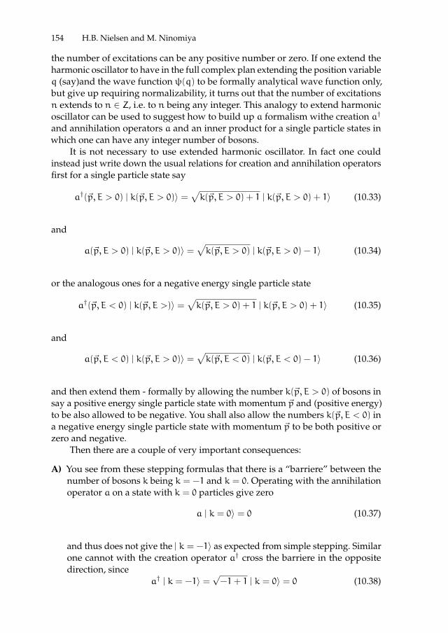
ii

“proc17” — 2017/12/11 — 19:44 — page 154 — #168 ii

ii

ii


the number of excitations can be any positive number or zero. If one extend theharmonic oscillator to have in the full complex plan extending the position variableq (say)and the wave function ψ(q) to be formally analytical wave function only,but give up requiring normalizability, it turns out that the number of excitationsn extends to n ∈ Z, i.e. to n being any integer. This analogy to extend harmonicoscillator can be used to suggest how to build up a formalism withe creation a†

and annihilation operators a and an inner product for a single particle states inwhich one can have any integer number of bosons.

It is not necessary to use extended harmonic oscillator. In fact one couldinstead just write down the usual relations for creation and annihilation operatorsfirst for a single particle state say

a†(~p, E > 0) | k(~p, E > 0)〉 =√k(~p, E > 0) + 1 | k(~p, E > 0) + 1〉 (10.33)

and

a(~p, E > 0) | k(~p, E > 0)〉 =√k(~p, E > 0) | k(~p, E > 0) − 1〉 (10.34)

or the analogous ones for a negative energy single particle state

a†(~p, E < 0) | k(~p, E >)〉 =√k(~p, E > 0) + 1 | k(~p, E > 0) + 1〉 (10.35)

and

a(~p, E < 0) | k(~p, E > 0)〉 =√k(~p, E < 0) | k(~p, E < 0) − 1〉 (10.36)

and then extend them - formally by allowing the number k(~p, E > 0) of bosons insay a positive energy single particle state with momentum ~p and (positive energy)to be also allowed to be negative. You shall also allow the numbers k(~p, E < 0) ina negative energy single particle state with momentum ~p to be both positive orzero and negative.

Then there are a couple of very important consequences:

A) You see from these stepping formulas that there is a “barriere” between thenumber of bosons k being k = −1 and k = 0. Operating with the annihilationoperator a on a state with k = 0 particles give zero

a | k = 0〉 = 0 (10.37)

and thus does not give the | k = −1〉 as expected from simple stepping. Similarone cannot with the creation operator a† cross the barriere in the oppositedirection, since

a† | k = −1〉 =√−1+ 1 | k = 0〉 = 0 (10.38)

ii

“proc17” — 2017/12/11 — 19:44 — page 155 — #169 ii

ii

ii


Thus we have that the states describing the number of bosons k in a givensingle particle state are not connected by –a finite number of operations – ofcreation and annihilation operatiors.Really this means that we make best by considering the positive sector of thespace of positive or zero number of bosons and another sector formed fromthe | k〉 states with k = −1,−2,−3, ... being a negative number of bosons. Byordinary creation and annihilation operators, as they would occur in someinteraction Hamiltonian, one cannot cross the barriere. This means that if tobeign with one has say a negative number of boson in a given single particlestate, then an ordinary interaction cannot change that fact.Thus we take it that one can choose once forever to put some single particlesstates in their positive sector and others in their negative sector, and theythen will stay even under operation of an interaction Hamiltonian. If one forexample make the ansatz that all the negative energy single particle stateshave a negative number of bosons while the positive energy states have zeroor a positive number of bosons in them, then this ansatz can be kept forever.This special choice we call the “physical choice” and we saw already[3] –andshall see very soon here – that this choice gives us a positive definite Fockspace.

B) The norm square of the states | k〉 (with k = −1,−2, . . .) i.e. with negativenumbers k of bosons have to vary alternatingly with k even, k odd.Using the writing of a negative k

| k〉 ∼ a|k|−1 | k = −1〉 (10.39)

We may evaluate 〈k | k〉 ∼< −1 | (a†)|k|−1a|k|−1 | −1〉 for k ≤ −1.Now using still the usual commutation rule

[a†, a] = −1 (10.40)

you easily see that we normalize by putting

| k〉 = 1√(|k|− 1)!

a|k|−1 | −1〉 (10.41)

and〈k | k〉 = (−1)|k| (10.42)

say for k ≤ −1 (having taken 〈−1 | −1〉 = −1.) while of course for k =

0, 1, 2, . . . you have 〈k | k〉 = 1.The major success of our “Dirac sea for bosons” is that one can arrange thesign alternation with (10.42) with the total number of negative energy bosonsto cancel against the sign from in (10.31) so as to achieve, if we choose the“physical sector”, to get in total the Fock space, which has positive norm square.This “physical sector” corresponds to that negative energy single particle statesare in the negative sectors, while the positive energy single particle states arein the positive sector.

ii

“proc17” — 2017/12/11 — 19:44 — page 156 — #170 ii

ii

ii


The basis vectors of the full Fock space for the physical sector are thus of theform

| . . . , k(~p, E > 0), . . . ; . . . , k(~p, E < 0), . . .〉 (10.43)

where the dots . . . denotes that we have one integer number for every mo-mentum vector –value (~p or ~p ′), but now the numbers k(~p, E > 0) of particlesin a positive energy are– in the physical sector-combination– restricted tobe non-negative while the numbers of bosons in the negative energy singleparticle states are restricted to be negative

k(~p, E > 0) = 0, 1, 2, . . .

k(~p, E < 0) = −1,−2,−3, . . . (10.44)

These basis vectors (10.43) are all orthogonal to each other, and so the innerproduct is alone given by their norm squares

〈. . . , k(~p, E > 0), . . . ; . . . , k( ~p ′, E < 0), . . . || . . . , k(~p, E > 0), . . . ; . . . , k( ~p ′, E < 0), . . .〉

= (−1)](neg energy b)∏~p ′

(−1)|k(~p ′,E<0)| = 1 (10.45)

Here ](neg energy b) means the total number of negative energy bosons i.e.

](neg energy b) =∑~p ′

k(~p, E < 0) (10.46)

(a negative number in our physical sector-combination). The factor

(−1)](neg energy b.)

comes from (10.31) which gives negative norm square for single particle stateswith negative energy, because

←→∂∂t

is essentially the energy. The other factor∏~p ′(−1)

|k( ~p ′,E<0)| comes from (10.42) one factor for each negative single par-ticle energy state, i.e. each ~p ′. Had we here chosen another sector-combination,e.g. to take k(~p, E < 0) non-negative as well as k(~p, E > 0), then we wouldhave instead

k(~p, E > 0) = 0, 1, 2, . . .

k( ~p ′, E < 0) = 0, 1, 2, . . .

(both pos sectors.) (10.47)

and the inner with themselves, norm squares product for the still mutuallyorthogonal basis vectors would be

〈. . . , k(~p, E > 0), . . . ; . . . , k( ~p ′, E < 0), . . .| . . . , k(~p, E > 0), . . . ; . . . , k( ~p ′, E < 0), . . .〉

= (−1)](neg energy b)

(for both positive sectors) (10.48)

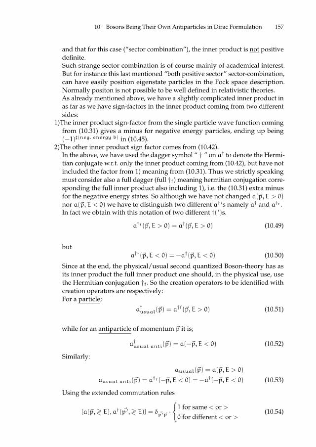
ii

“proc17” — 2017/12/11 — 19:44 — page 157 — #171 ii

ii

ii


and that for this case (“sector combination”), the inner product is not positivedefinite.Such strange sector combination is of course mainly of academical interest.But for instance this last mentioned “both positive sector” sector-combination,can have easily position eigenstate particles in the Fock space description.Normally positon is not possible to be well defined in relativistic theories.As already mentioned above, we have a slightly complicated inner product inas far as we have sign-factors in the inner product coming from two differentsides:

1)The inner product sign-factor from the single particle wave function comingfrom (10.31) gives a minus for negative energy particles, ending up being(−1)](neg. energy b) in (10.45).

2)The other inner product sign factor comes from (10.42).In the above, we have used the dagger symbol “ † ” on a† to denote the Hermi-tian conjugate w.r.t. only the inner product coming from (10.42), but have notincluded the factor from 1) meaning from (10.31). Thus we strictly speakingmust consider also a full dagger (full †f) meaning hermitian conjugation corre-sponding the full inner product also including 1), i.e. the (10.31) extra minusfor the negative energy states. So although we have not changed a(~p, E > 0)nor a(~p, E < 0) we have to distinguish two different a† ′s namely a† and a†f .In fact we obtain with this notation of two different †( ′)s.

a†f(~p, E > 0) = a†(~p, E > 0) (10.49)

buta†f(~p, E < 0) = −a†(~p, E < 0) (10.50)

Since at the end, the physical/usual second quantized Boson-theory has asits inner product the full inner product one should, in the physical use, usethe Hermitian conjugation †f. So the creation operators to be identified withcreation operators are respectively:For a particle;

a†usual(~p) = a†f(~p, E > 0) (10.51)

while for an antiparticle of momentum ~p it is;

a†usual anti(~p) = a(−~p, E < 0) (10.52)

Similarly:

ausual(~p) = a(~p, E > 0)

ausual anti(~p) = a†f(−~p, E < 0) = −a†(−~p, E < 0) (10.53)

Using the extended commutation rules

[a(~p,>< E), a†( ~p ′, >< E)] = δ ~p ′~p ·

1 for same < or >0 for different < or >

(10.54)

ii

“proc17” — 2017/12/11 — 19:44 — page 158 — #172 ii

ii

ii


so that for instance[a(~p,< E), a†( ~p ′, < E)] = δ~p ~p ′ (10.55)

We quickly derive the correspondingcommutation rules using the “full dag-ger”

[a(~p, E > 0), a†f( ~p ′, E > 0)] = δ~p ~p ′ (10.56)

and[a(~p, E < 0), a†f( ~p ′, E < 0)] = δ~p ~p ′ (10.57)

10.4 “Majorana-bosons”

We shall now in this section analogously to what we did in sections 10.2 forFermions as a warm up excercise from our Fock space defined in section 10.3 fore.g. the physical sector- combination extract a subspace HMaj and on that finda description of now bosons which are their own antiparticles. There would besome meaning in analogy to the Fermion case to call such bosons which are theirown antiparticles by the nickname “Majorana-bosons”.

As for the fermions we shall expect a state with say kMaj(~p) “Majorana-bosons”with momentum equal to ~p to be presented as a superposition of a numberof the “essentially charged” bosons or antibosons of the type discussed in forego-ing section. Here an antiparticle of course means that one has made the numberof bosons in a negative energy single particle state one unit more negative. Typ-ically since the physical vacuum has k(~p, E < 0) = −1 for all momenta and anantiparticle of momentum ~pwould mean that k(−~p, E < 0) gets decreased from−1 to −2. If you have several antiparticles l say in the same state with momentum~p of course you decrease k(−~p, E < 0) to −1 − l, k(−~p, E < 0) = −1 − l (for lantiparticles).

In other words we expect a state with say lMaj “Majorana-bosons” withmomentum ~p to be a superposition of states in the Fock space with the number ofantiparticles running from l = 0 to l = lMaj while correspondingly the numberwith momentum ~p is made to lMaj−l so that there are together in the representingstate just equally many particles or antiparticles as the number of “Majorana-bosons” lMaj wanted.

We actually hope –and we shall see we shall succeed– that we can construct a“Majorana-boson” creation operator for say a “Majorana-boson” with momentum~p,b†(~p) analogously to the expressions (10.19) and (10.20)b†(~p) = 1√

2

(a†(~p, E > 0) + a(−~p, E < 0)

)and b(~p) = 1√

2

(a(E > 0) + a†(E < 0)

).

Since an extra phase on the basis states does not matter so much we could alsochoose for the boson the “Majorana boson” creation and annihilation operators to

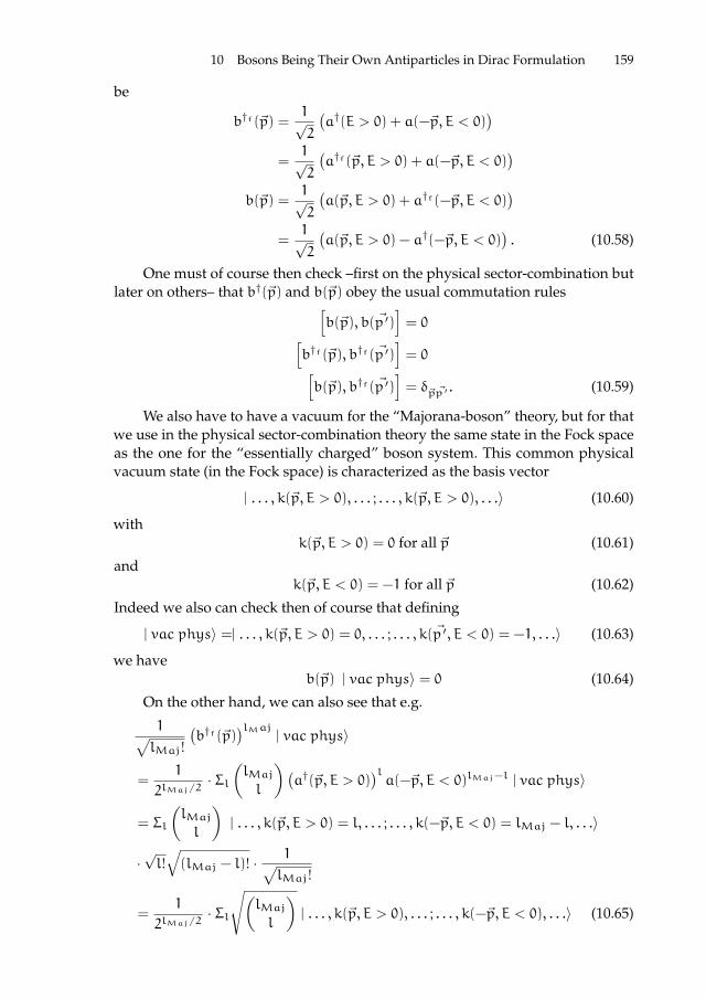
ii

“proc17” — 2017/12/11 — 19:44 — page 159 — #173 ii

ii

ii


be

b†f(~p) =1√2

(a†(E > 0) + a(−~p, E < 0)

)=

1√2

(a†f(~p, E > 0) + a(−~p, E < 0)

)b(~p) =

1√2

(a(~p, E > 0) + a†f(−~p, E < 0)

)=

1√2

(a(~p, E > 0) − a†(−~p, E < 0)

). (10.58)

One must of course then check –first on the physical sector-combination butlater on others– that b†(~p) and b(~p) obey the usual commutation rules[

b(~p), b( ~p ′)]= 0[

b†f(~p), b†f( ~p ′)]= 0[

b(~p), b†f( ~p ′)]= δ~p ~p ′ . (10.59)

We also have to have a vacuum for the “Majorana-boson” theory, but for thatwe use in the physical sector-combination theory the same state in the Fock spaceas the one for the “essentially charged” boson system. This common physicalvacuum state (in the Fock space) is characterized as the basis vector

| . . . , k(~p, E > 0), . . . ; . . . , k(~p, E > 0), . . .〉 (10.60)

withk(~p, E > 0) = 0 for all ~p (10.61)

andk(~p, E < 0) = −1 for all ~p (10.62)

Indeed we also can check then of course that defining

| vac phys〉 =| . . . , k(~p, E > 0) = 0, . . . ; . . . , k( ~p ′, E < 0) = −1, . . .〉 (10.63)

we haveb(~p) | vac phys〉 = 0 (10.64)

On the other hand, we can also see that e.g.

1√lMaj!

(b†f(~p)

)lMaj| vac phys〉

=1

2lMaj/2· Σl

(lMajl

)(a†(~p, E > 0)

)la(−~p, E < 0)lMaj−l | vac phys〉

= Σl

(lMajl

)| . . . , k(~p, E > 0) = l, . . . ; . . . , k(−~p, E < 0) = lMaj − l, . . .〉

·√l!√(lMaj − l)! ·

1√lMaj!

=1

2lMaj/2· Σl

√(lMajl

)| . . . , k(~p, E > 0), . . . ; . . . , k(−~p, E < 0), . . .〉 (10.65)

ii

“proc17” — 2017/12/11 — 19:44 — page 160 — #174 ii

ii

ii


If we only put the Majorana-boson particles into the momentum ~p state ofcourse only k(~p, E > o) and k(−~p, E < 0) will be different from their | phys vac〉values 0 and −1 respectively for E > 0 and E < 0. But really the extension to put“Majorana-bosons” in any number of momentum states is trivial.

We now have also to construct the analogous operator to the r(~p) for thefermions so that we can characterize the subspace HMaj to be for the boson case

HMaj = |〉 | r(~p) |〉 = 0 . (10.66)

We in fact shall see that the proposal

r(~p) =1√2(a(+~p, E > 0) + a†(−~p, E < 0))

=1√2(a(~p, E > 0) − a†f(−~p, E < 0) (10.67)

does the job.Now we check (using (10.58))[

r(~p), b†f(~p)]=

=

[1√2

(a(~p), E > 0) + a†(−~p, E < 0)

),1√2

(a†(~p), E > 0) + a(−~p, E < 0)

)]or

=1

2

[(a(~p, E > 0) − a†f(−~p, E < 0)), (a†f(~p, E > 0) + a(−~p, E < 0)

)]=1

2(1− 1) = 0 (10.68)

and also

[r(~p), b(~p)] =

=

[1√2

(a(~p), E > 0) − a†f(−~p, E < 0)

),1√2

(a(~p), E > 0) + a†f(−~p, E < 0)

)]=

[1√2

(a(~p), E > 0) + a†(−~p, E < 0)

),1√2

(a(~p), E > 0) − a†(−~p, E < 0)

)]= 0 (10.69)

We should also check that the physical vacuum

| phys vac〉 =| . . . , k(~p, E > 0) = 0, . . . ; . . . , k( ~p ′, E < 0) = −1, . . .〉 (10.70)

in which there is in all negative energy (with momentum ~p ′ say) single particlestates k( ~p ′, E < 0) = −1 bosons, and in all positive energy single particle statesk(~p, E > 0) = 0 bosons is annihilated by the r(~p) operators.

ii

“proc17” — 2017/12/11 — 19:44 — page 161 — #175 ii

ii

ii


Now indeed

r(~p) | phys vac〉

=1

2

(a(~p, E > 0) − a†f(−~p, E, 0)

)| phys vac〉

=1

2

(a(~p, E > 0) + a†(−~p, E, 0)

)· | . . . , k(~p, E > 0) = 0, . . . ; . . . , k(~p, E < 0)

= −1, . . .〉= 0 (10.71)

basically because of the barriere, meaning the square roots in the formulas (10.34,10.35)became zero.

The result of this physical section for the most attractive formalism with b(~p)and b†f(~p) annihilating and creating operators for the Boson-type particle beingits own antiparticle (=Majorana Boson) and to them corresponding useful statecondition operator rf(~p) is summarized as:

b(~p) =1√2

(a(~p, E > 0) − a†f(−~p, E < 0)

)b†f(~p) =

1√2

(a†f(~p, E > 0) − a(−~p, E < 0)

)| phys vac〉 =| . . . , k(all ~p, E > 0) = 0, . . . ; . . . , k(all ~p, E < 0) = −1, . . .〉

rf(~p) =1√2

(a(~p, E > 0) + a†f(−~p, E < 0)

)(10.72)

the useful subspace for bosons being their own antiparticles being

HMaj f =| 〉 | ∀~prf(~p) | 〉 = 0

(10.73)

(One should note that whether one chooses our r( ~p ′) ′s or the rf(~p) ′s to de-fine makes no difference for the space HMaj f rather than Hf, since we actuallyhave r(~p) = rf(~p) the two expressions being just expressed in terms of differenta†(~p, E < 0) and a†f(~p, E < 0) say)

We can easily check that our explicit state expressions (10.65) indeed areannihilated by r(~p) It were formally left out theE > 0 or E < 0 for the b(~p) andb†f(~p) it being understood that E > 0, but formally we can extrapolate also toE < 0 and it turns of b(~p, E > 0) = b†f(−~p, E < 0)?

10.4.1 Charge Conjugation Operation

Since we discuss so much bosons being their own antiparticles coming out of aformalism in which the bosons –at first– have antiparticles different from them-selves, we should here define a charge conjugation operator C that transform aboson into its antiparticle:

ii

“proc17” — 2017/12/11 — 19:44 — page 162 — #176 ii

ii

ii


That is to say we want this operator acting on the Fock space to have the commu-tation properties with our creation and annihilation operators

C−1a(~p, E > 0)C = a†f(−~p, E < 0) (10.74)

andC−1a†f(~p, E > 0)C = a(−~p, E < 0). (10.75)

We also haveC−1a(~p, E < 0)C = a†f(−~p, E > 0) (10.76)

andC−1a†f(~p, E < 0)C = a(−~p, E > 0) (10.77)

These requirements suggest that we on the basis of (10.43) for the Fock spacehave the operation

C | . . .∼

k (~p, E > 0), . . . ; . . . ,∼

k ( ~p ′, E < 0), . . .〉

=| . . . , k(~p, E > 0) = −∼

k (− ~p ′, E < 0) + 1, . . . ; (10.78)

. . . , k( ~p ′, E < 0) = −1−∼

k (− ~p ′, E > 0), . . .〉.

Using the “full inner product” this C operation conserves the norm, and infact it is unitary under the full inner product corresponding hermitean conjugation†f i.e.

C†fC = 1 = CC†f (10.79)

But if we used the not full inner product, so that the norm squares for basisvector would be given by (10.81) and therefore corresponding hermitean conjuga-tion †, then if C acts on a state in which the difference of the number of positiveand negative energy bosons is odd, the norm square would change sign under theoperation with C.

So under † the charge conjugation operator could not possibly be unitary:

C†C 6= 1 6= CC† (10.80)

10.5 “Majorana boson” in unphysical sector-combination

As an example of one of the unphysical sector-combination we could take what inour earlier work “Dirac sea for Bosons” were said to be based on the naive vacuum.This naive vacuum theory means a theory in which we do not make any emptyingvacuum but rather let there be in both positive and negative single particle energystates a positive or zero number of particles. So in this naive vacuum attachedsector combination we can completely ignore the extrapolated negative numberof boson possibilities; we so to speak could use the analogue of the harmonicoscillator with normalized states only.

ii

“proc17” — 2017/12/11 — 19:44 — page 163 — #177 ii

ii

ii


This means that the inner product excluding the negative single particle statenormalization using (10.31) will be for this naive vacuum sector combinationcompletely positive definite.

However, including the negative norm factor for the negative energy statesfrom (10.31) so as to get the full inner product we do no longer have the positivedefinite Hilbert inner product on the Fock space. Now rather we have for basisvectors (10.43) instead of (10.45) that the norm squares

〈. . . , k(~p, E > 0), . . . ; . . . , k( ~p ′, E < 0), . . . | . . . , k(~p, E > 0), . . . ; . . . , k( ~p ′, E < 0), . . .〉= (−1)](neg. energy b.) (10.81)

This means that the norm square of a basis vector is positive when the numberof negative energy bosons is even, but negative when the number of negativeenergy bosons is odd.

In the naive vacuum sector combination the vacuum analogue Fock spacestate is the “naive vacuum”,

| naive vac.〉 =| . . . , k(~p, E > 0) = 0, . . . ; . . . , k(~p, E < 0) = 0, . . .〉. (10.82)

In analogy to what we did in the foregoing section 10.4, we should thenconstruct the states with various numbers of bosons of the Majorana type beingtheir own antiparticles by means of some creation and annihilation operatorsb†f(~p) and b(~p), but first one needs a vacuum that is its own “anti state” so tospeak, meaning that the charge conjugation operator C acting on it gives it back.i.e. one need a vacuum | vac?〉 so that

C | vac?〉 =| vac?〉 (10.83)

But this is a trouble! The “naive vacuum” | naive vac.〉 in not left invariant un-der the charge conjugation operator C defined in the last subsection of Section 10.4by (10.78).

Rather this naive vacuum is by C transformed into a quite different sectorcombination, namely in that sector combination, in which there is a negativenumber of bosons in both positive and negative energy single particle eigenstates.i.e. the charge conjugation operates between one sector combination and anotherone! But this then means, that we cannot make a representation of a theory with(only) bosons being their own antiparticles unless we use more than just the naivevacuum sector combination. i.e. we must include also the both number of particlesbeing negative sector combination.

In spite of this need for having the two sector combinations –both the naiveall positive particle number and the opposite all negative numbers of particles– inorder that the charge conjugation operator should stay inside the system –Fockspace, we should still have in mind that the creation and annihilation operatorscannot pass the barriers and thus can not go from sectors, also the inner productbetween different sector combinations are divergent and ill defined (and we shouldeither avoid such inner products or define them arbitrarily).

So if we construct “Majorana boson” creation and annihilation operatorsanalogoulsy to the b(~p) and b†f(~p) in foregoing section as a linear combination of

ii

“proc17” — 2017/12/11 — 19:44 — page 164 — #178 ii

ii

ii


a(†)(~p,>< E) operators operating with such b(~p) and b†f( ~p ′)swill stay inside onesector combination. For instance such b(~p) and b†f(~p) constructed analogouslyto the physical sector ones formally would operate arround staying inside thenaive vacuum sector combination if one starts there, e.g. on the naive vacuum| naive vac.〉. In this –slightly cheating way– we could then effectively build upa formalism for bosons which are their own antiparticles inside just one sectorcombination. When we say that it is “slightly cheating” to make this constructionon only one sector combination it is because we cannot have the true antiparticles ifwe keep to a sector combination only, which is not mapped into itself by the chargeconjugation operator C. It namely then would mean that the true antiparticlecannot be in the same sector combination.

Nevertheless let us in this section 5 study precisely this “slightly cheating”formalism of keeping to the naive vacuum sector combination with positivenumbers of particles only.

We then after all simply use the naive vacuum | naive vac.〉 defined by (10.82)as the “Majorana boson”-vacuum although it is not invariant under C, which wemust ignore or redefine, if this shall be o.k.

We may e.g. build up a formalism for the slightly cheating Majorana bosonsby starting from the | naive vac.〉 (10.82) and build up with b†f(~p) taken to be thesame as

b†f(~p) =1√2

(a†f(~p, E > 0) + a(−~p, E < 0)

)(10.84)

and

b(~p) =1√2

(a(~p, E > 0) + a†f(−~p, E < 0)

)=

1√2

(a(~p, E > 0) − a†(−~p, E < 0)

)(10.85)

We have already checked that for all sector combinations we have[b(~p, b†f( ~p ′)

]= δ~p ~p ′ (10.86)

and of course [b(~p, b( ~p ′

]= 0

=[b†f(~p), b†f( ~p ′)

](10.87)

So we see that we can build up using b(~p) and b†f(~p) a tower of stateswith any nonnegative number of what we can call the Majorana bosons for anymomentum ~p.

We can also in all the sector combinations use the already constructed

r(~p) =1

2

(a(~p, E > 0) − a†f(−~p, E < 0)

)=1

2

(a(~p, E > 0) + a†(−~p, E < 0)

)(10.88)

ii

“proc17” — 2017/12/11 — 19:44 — page 165 — #179 ii

ii

ii


to fullfill the commutation conditions[r(~p), b†f(~p)

]= 0[

r(~p), b( ~p ′)]= 0 (10.89)

and we even haver(~p) | naive vac.〉 = 0 (10.90)

So indeed we have gotten a seemingly full theory of “Majorana Bosons” insidethe naive vacuum sector combination subspace

HMaj = |〉 | ∀~p (r(~p) |〉 = 0) (10.91)

but it is not kept under the C as expected.But really what we ended up constructing were only a system of positive

energy particle states since the creation with b†f(~p) = b†(~p) starting from thenaive vacuum only produces positive energy particles in as far as the a(−~p, E < 0)contained in b†f(~p) just gives zero on the naive vacuum.

So this a “bit cheating” formalism really just presented for us the “essentiallycharged” positive energy particles as “the Majorana-bosons”.

That is to say this a bit cheating formalism suggests us to use in the naivevacuum sector combination the “essentially charged particles” as were they theirown antiparticles.

If we similarly built a Majorana boson Fock space system of the

C | naive vac.〉 =| vac. with both E > 0 and E < 0 emptied out〉=| . . . , k(~p, E > 0) = −1, . . . ; . . . , k(~p, E < 0) = −1, . . .〉, (10.92)

we would obtain a series of essentially antiparticles (with positive energies) con-structed in the “both numbers of bosons negative” sector combination.

What we truly should have done were to start from the superposition

| self copy vac.〉= 1√2(| naive vac.〉+ C | naive vac.〉)

=1√2(| . . . , k(~p, E > 0) = 0, . . . ; . . . , k(~p, E < 0) = 0, . . .〉

+ | . . . , k(~p, E > 0) − 1, . . . ; . . . , k(~p, E < 0) = −1, . . .〉)(10.93)

and then as we would successively go up the latter with b†f(~p) operators we wouldsuccessively fill equally many positive energy particles into the | naive vac.〉 andpositive energy antiparticles in C | naive vac.〉. Note that analogously to the abovecalled “a bit cheating” Majorana-boson construction using only the positive energysingle particle states we obtain here only use of the positive energy states for the

ii

“proc17” — 2017/12/11 — 19:44 — page 166 — #180 ii

ii

ii


naive vacuum sector combination and only the negative energy single particlestates for the Charge conjugation to the naive vacuum sector combination. Also itshould not be misunderstood: The filling in is not running parallel in the sense thatthe sectors truly follow each other. Rather one has to look for if there is Majoranaboson by looking into both sector-combination- projections.

So we see that what is the true Majorana boson theory built on the twounphysical sector combinations having respectively nonzero numbers of particles(the naive vacuum construction) and negative particles number in both positiveand negative energies is the following:

A basis state with n(~p) Majorana bosons with momentum ~p, -and as wealways have for Majorana’s positive energy- gets described as a superpositionot two states –one from each of the two sector combinations– with just n(~p)ordinary (positive energy) essentially charged bosons (of the original types of ourconstruction created by a†..) and a corresponding Fock space state from the othersector, now with n(~p) antiparticles in the other sector combination (the one builtfrom C | naive vac.〉).

Both of these separate sector combinations have for the used states a positivedefinite Hilbert space.

As already stated the overlap between different sector combinaions vectorsare divergent and illdefined.

We can check this rather simple way of getting the Majorana bosons describedin our on the state 1

2(| naive vac.〉+ C | naive vac.〉) built system of states by

noting what the condition r(~p) |〉 = 0 tells us the two sector combinations:On a linear combination of basis vectors of the naive vacuum construction

type

|〉 = Σ | k(~p, E > 0) ≥ 0, . . . ; . . . , k(~p, E < 0) ≥ 0, . . .〉C...k(~p,E>0)...;...k(~p,E<0)... (10.94)

the requirementr(~p) |〉 = 0 (10.95)

relates coefficients which correspond to basis states being connected by k(~p, E > 0)going one up while k(−~p, E < 0) going one unit down or opposite. As we get therelation √

1+ k(~p, E > 0)C...k(~p,E>0)+1,...;...,k(−~p,E<0),...

+C...,k( ~p ′,E>0),...;...,k(−~p,E<0)−1,...·

√k(−~p, E < 0) = 0 (10.96)

we can easily see that the states being annihilated are of the form

∑(−1)k(~p,E>0)

√k(−~p, E < 0)!√k(~p, E > 0)!

· | . . . , k(~p, E > 0), . . . ; . . . , k(−~p, E < 0), . . .〉,

(10.97)

ii

“proc17” — 2017/12/11 — 19:44 — page 167 — #181 ii

ii

ii


where we sum over k(~p, E > 0) and the difference d = k(~p, E > 0) − k(−~p, E < 0)

is FIXED.As a special case we might look at possibility that the difference

d = k(~p, E > 0) − k(−~p, E < 0) (10.98)

were 0. In this case the | naive vac.〉 itself would be in the series. In this case thesolution (10.97) reduces to∑

k=0

(−1)k | . . . , k(~p, E > 0) = k, . . . ; . . . , k(−~p, E < 0) = k, . . .〉 (10.99)

But it is now the problem that this series does not converge. But for appropri-ate values of the difference d,

d ≥ 2, (10.100)

the series (10.97)converge.For the convergent cases we can estimate the norm square of a state (10.97) to

go proportional to

‖ |〉‖2 ∝∞∑k=0

(k− d)!

k!(−1)k−d (10.101)

where the (−1)k−d now comes from the alternating “full” norm square due to thefactor (−1)](neg. energy b.). This expression in turn is proportional to

∞∑k=0

(k− d

−d

)(−1)k−d =

∑n=−d

(n

−d

)(−1)n (n = k− d)

=(−1)−d

(1− (−1))−d+1

(10.102)

which is zero for d− 1 ≥ 1.So indeed it is seen that the basis states in HMaj part inside the naive vacuum

sector combination has zero norm. Since the states with different numbers ofMajorana-bosons are represented by mutually orthogonal it means that the wholepart of the naive vacuum sector combination used to represent the Majorana-bosons has totally zero inner product. Basically that means that the inner producttransfered from the original theory with its “essentially charged bosons” to the forMajorana bosons in subspace HMaj turns out to be zero.

This result means –extrapolating to suppose zero norm also in the divergentcases– that in the unphysical sector combination we get no non-trivial innerproduct for the Majorana-bosons.

If ones use the true Majorana boson description by as necessary combiningtwo sector combinations, one could use the ambiguity (and divergence) of theinner product of states from different sectors to make up instead a non trivial innerproduct.

ii

“proc17” — 2017/12/11 — 19:44 — page 168 — #182 ii

ii

ii


10.5.1 Overview of All four Sector Combinations

Strictly speaking we could make an infinite number of sector combinations, be-cause we for every single particle state – meaning for every combination of aspin state and a momentum say ~p – could choose for just that single particlestate to postulate the second quantized system considered to be started at sucha side of the “barriers” that just this special single particle state had always anegative number of bosons in it. For another one we could instead choose tohave only a non-negative numbe of bosons. Using all the choice possibilities ofthis type would lead us so to speak to the infinite number of sector combina-tions 2#“single particle states”, where #“single particle states” means the numberof single particle states. But most of these enormously many sector combinationswould not be Lorentz invariant nor rotational invariant. Really, since the sectorcombination should presumably rather be considered a part of the initial statecondition than of the laws of Nature, it might be o.k. that it be not Lorentz norrotational invariant. Nevertheless we strongly suspect that it is the most impor-tant to consider the Lorentz and rotational invariant sector-combination-choices.Restricting to the latter we can only choose a seprate sector for the positive enegrystates and for the negative energy sector, and then there would be only 22 = 4

sector combinations.Quite generally we have the usual rules for creation and annihilation oper-

ators,but you have to have in mind that we have two different hermitean con-jugations denoted respectively by † and by †f, and that the creation operatorsconstructed from the same annihilation operators are related

a†f(~p, E > 0) = a†(~p, E > 0)

a†f(~p, E < 0) = −a†(~p, E < 0) (10.103)

These “usual” relations are[a(~p, E > 0), a†( ~p ′, E > 0)

]= δ~p ~p ′[

a(~p, E < 0), a†( ~p ′, E < 0)]= δ~p ~p ′[

a(~p, E > 0), a†f( ~p ′, E > 0)]= δ~p ~p ′[

a(~p, E < 0), a†f( ~p ′, E < 0)]= −δ~p ~p ′ (10.104)

while we have exact commutation for awith a or for a† or a†f with a† or a†f . Eacha(~p, E >< 0) or a†f or a† act changing only the number of particle in just the singlerelevant single particle state, meaning it changes only k(~p, E >< 0); the rules are as

ii

“proc17” — 2017/12/11 — 19:44 — page 169 — #183 ii

ii

ii


seen analytical continuations generally

a†(~p, E > 0) | . . . , k(~p, E > 0), . . . ; . . . , k( ~p ′, E < 0), . . .〉

=√k(~p, E > 0) + 1 | . . . , k(~p, E > 0) + 1, . . . ; . . . , k( ~p ′, E < 0), . . .〉

a†( ~p ′, E < 0) | . . . , k(~p, E > 0), . . . ; . . . , k( ~p ′, E < 0), . . .〉

=

√k( ~p ′, E < 0) + 1 | . . . , k(~p, E > 0), . . . ; . . . , k( ~p ′, E < 0) + 1, . . .〉

a†f(~p, E > 0) | . . . , k(~p, E > 0), . . . ; . . . , k( ~p ′, E < 0), . . .〉

=√k(~p, E > 0) + 1 | . . . , k(~p, E > 0) + 1, . . . ; . . . , k( ~p ′, E < 0), . . .〉

a†f( ~p ′, E < 0) | . . . , k(~p, E > 0), . . . ; . . . , k( ~p ′, E < 0), . . .〉

=−

√k( ~p ′, E < 0) + 1 | . . . , k(~p, E > 0), . . . ; . . . , k( ~p ′, E < 0) + 1, . . .〉

a(~p, E > 0) | . . . , k(~p, E > 0), . . . ; . . . , k( ~p ′, E < 0), . . .〉

=√k(~p, E > 0) | . . . , k(~p, E > 0) − 1, . . . ; . . . , k( ~p ′, E < 0), . . .〉

a( ~p ′, E < 0) | . . . , k(~p, E > 0), . . . ; . . . , k( ~p ′, E < 0), . . .〉

=

√k( ~p ′, E < 0) | . . . , k(~p, E > 0) + 1, . . . ; . . . , k( ~p ′, E < 0) − 1, . . .〉 (10.105)

The four sector combination with the same sector for the same sign of theenergy E of the single particle states were called:

1)The “physical sector” has

k(~p, E > 0) = 0, 1, 2, . . .

k(~p, E < 0) = −1,−2,−3 . . . (10.106)

2)The “sector-combination constructed from the naive vacuum” has

k(~p, E > 0) = 0, 1, 2, . . .

k(~p, E < 0) = 0, 1, 2, . . . (10.107)

3)The “both sectors with negative numbers” sector-combination has

k(~p, E > 0) = −1,−2,−3 . . .

k(~p, E < 0) = −1,−2,−3 . . . (10.108)

4)The “a positive number with negative energy and vise versa” has

k(~p, E > 0) = −1,−2,−3 . . .

k(~p, E < 0) = 0, 1, 2, . . . (10.109)

In the physical sector combination the Fock space ends up having positivedefinite norm square and so this sector-combination is the one usual taken forbeing the in nature realized one.

ii

“proc17” — 2017/12/11 — 19:44 — page 170 — #184 ii

ii

ii


10.5.2 Formulas for “Majorana particles”

The theory of Majorana fermions may be so well known that we had nothing tosay, but it were written about it in section 2.

For the boson case we introduced for each (vectorial) value of the momentuman operator acting on the Fock space called r(~p) defined by (10.88)

r(~p) =1√2

(a(~p, E > 0) − a†f(−~p, E < 0)

)=

1√2

(a(~p, E > 0) + a†(−~p, E < 0)

)(10.110)

with the properties [r(~p), b( ~p ′)

]= 0[

r(~p), b†( ~p ′)]= 0[

r(~p), b†f( ~p ′)]= 0 (10.111)

where the creation b†f(~p)(= b†f(~p

)and annihilation b(~p) operators for the “Ma-

jorana bosons” (i.e. boson being its own antiparticle) were defined in terms of thea’s as

b†f(~p) =1√2

(a†f(~p, E > 0) + a(−~p, E < 0)

)(10.112)

and

b(~p) =1√2

(a(~p, E > 0) + a†f(−~p, E < 0)

)(10.113)

=1√2

(a(~p, E > 0) − a†(−~p, E < 0

)(10.114)

These operators obey (see(10.86) and (10.87))[b(~p, b†f( ~p ′)

]= δ~p ~p ′[

b(~p, b( ~p ′]= 0[

b†f(~p), b†f( ~p ′)]= 0 (10.115)

and so these operators are suitable for creating and annihilation of particles, andindeed these particles are the “Majorana bosons”. As a replacement for the inusual formalism for “Majorana bosons” say

b(~p, E) = b†f(−~p,−E) (10.116)

ii

“proc17” — 2017/12/11 — 19:44 — page 171 — #185 ii

ii

ii


we have in our notationb(−~p) |with

>↔<= b†f(~p) (10.117)

as is easily seen from (10.113) and (10.112) just above.But now we need also a vacuum from which to start the creation of the

“Majorana bosons” with b†f(~p). In the two sector-combinations 1) the physicalone and 4) “a positive number with negative energy and vice versa” there are thesuitable vacua:

In 1)

| physical vac〉 =| . . . , k(~p, E > 0) = 0, . . . ; . . . , k(~p, E < 0) = −1, . . .〉 (10.118)

and in 4)

|pos in E < 0

neg in E > 0〉 = 1 . . . , k(~p, E > 0) = −1, . . . ; . . . , k(~p, E < 0) = 0, . . .〉 (10.119)

In the sector-combinations 2) and 3), however, there are no charge conjugationsymmetric states to use as the vacuum state for a “Majorana-boson” formalism. Inthis case the vacuum of 2) goes under charge conjugation C into that of 3).

10.6 Outlook on String Field Theory Motivation

One of our own motivations for developping the sort of boson Dirac sea theoryfor bosons being their own antiparticles, i.e. a theory with Dirac sea, were to use itin our own so called “novel string field theory”[8–11].

In this “novel string field theory” we sought to rewrite the whole of stringtheory[12–15,28,29] (see also modified cubic theory [24])- although we did notyet come to superstrings[25,17,26] although that should be relatively easy - into aformalism in which there seems a priori to be no strings. The strings only comeout of our novel string field theory [18–23] by a rather complicated special wayof looking at it. In fact our basic model in this novel string field theory is ratherlike a system of /a Fock space for massless scalar particles, which we call “objects”in our formulation, but they have much although not all properties similar toscalar massless particles. These particles/objects we think must be in an abstractway what we here called Majorana bosons. This means they should be their ownantiparticles to the extend that they have antiparticles.

But their being put into cyclically ordered orientable chains may put a needfor a deeper understanding of the Majorananess for these “objects”.

The reason for the objects, that in our novel string field theory are a kindof constituents, for the strings being supposed to a nature reminiscent of theMajorana particles or being their own antiparticles, is that they carry in themselvesno particle number or charge, except that they can have (26)-momentum. (Forcomplete consistency of the bosonic string theory it is wellknown that 26 spacetime dimensions are required.) The bulk of the string (in string theory) can namely

ii

“proc17” — 2017/12/11 — 19:44 — page 172 — #186 ii

ii

ii


be shrunk or expanded ad libitum, and it is therefore not in itself charged, althoughit can carry some conserved quantum numbers such as the momentum densities.

We take this to mean that the string as just bulk string should be consideredto be equal to its own antimaterial. If we think of splitting up the string into smallpieces like Thorn[27], or we split the right and left mover parts separately like wedid ourselves, one would in both cases say that the pieces of Thorn’s or the objectsof ours should be their own antiparticles. With our a bit joking notation: theyshould be Majorana. Thus we a priori could speculate that, if for some reason weshould also like to think our objects as particles, then from the analytical propertiesof the single particle in relativistic theories must have both positive and negativeenergy states. Then a treatment of particles being their own antiparticles in theDirac sea formulation could - at least superficially -look to be relevant.

One could then ask, what we learned above, that could be of any help sug-gesting, how to treat long series of “objects”, if these objects are to be consideredbosons that are their own antiparticles:

• 1. In the novel string field theory of ours it is important for the associationto the strings, that one considers ring shaped chains of objects. We calledsuch ring shaped chains of objects for “cyclically ordered chains”. Now suchordering of our “objects” (as we call them), or of any type of particles, intochains in which each particle (or “object”) can be assigned a number (althoughin our special model only a number modulo some large number N) is o.k. forparticles with an individuality. However, if we have particles (or “objects”) thatare say bosons, then all particles are identical - or one could say any allowedstate is a superposition of states in which all possible permutations on theparticles have been performed and a superposition of the results of all thesepermutations with same amplitude only is presented as the final state -. Butthis then means that one cannot order them, because you cannot say, which isbefore which in the ordering, because you cannot name the single particle.You could only say, that some particle A is, say, just before some particleB in a (cyclic) ordering, if you characterize A as being the particle with acertain combination of coordinates (or other properties) and B as being theone with a certain other combination of coordinates (and other properties).Unless you somehow specify by e.g. some approximate coordinates (or othercharacteristic) which particle you think about, it has no meaning to expresssome relation involving the relative ordering, say, of two bosons.

• 2. The problem just mentioned in assigning order to bosons means, that theconcept of “cyclically ordered chains” of objects - or for that matter buildingup any string from particle pieces like Thorn say - cannot be done once theparticles or objects are bosons, but rather should be preferably formulatedbefore one symmetrize the wave function under the particle permutation so asto implement that they are bosons. One shall so to speak go back in the“pedagogical” development of boson-theory and think in the way before thesymmetry principle under permutations making the particles bosons wereimposed. In this earlier stage of the description the cyclically ordered chains,or any type of ordering, which one might wish, makes sense. So here it looks

ii

“proc17” — 2017/12/11 — 19:44 — page 173 — #187 ii

ii

ii


that going back and postponing the boson constraint is needed for orderingchains.

• 3. But seeking to go back prior to boson or fermion formulation makes aproblem for the Dirac sea - in both boson and fermion cases -: If we want toconsider the case of individual particles or objects fully, we have to imaginethat we have given names (or numbers) to all the particles in the Dirac sea!For this problem we may think of a couple of solutions:

– a. We could imagine an interaction that would organize the particles inthe ground state (to be considered a replacement for the physical vacuum)or that some especially important state for the Fock space obtained byimposing some other principle is postulated to make up a kind of vacuumstate. Then one could hope or arrange for the interaction or state-selectingprinciple chosen, that the vacuum state becomes such, that the objects (orparticles) in the Dirac sea goes into such a state, that these objects havesuch positions or momenta, that it due to this state becomes possible torecognize such structure that their ordering in the wanted chain becomesobvious. If so, then the (cyclic) ordering can come to make sense.This solution to the problem may be attractive a priori, because we thenin principle using the now somewhat complicated state of the vacuumcan assign orderings to the whole Dirac sea, and thus in principle give anindividuality even to the Dirac sea particles and missing particles / theholes can make sense, too. They so to speak can inherit their individualityfrom the particles missing, which before being removed were sitting in thechains of the vacuum. We have thus at least got allowance to talk about achain ordering for pieces of chains for the holes. There is so to speak anordering of the holes given by the ordering of the particles removed fromthe Dirac sea originating from the chain postulated to have appeared fromthe interaction or from some special selection principle for the vacuumstate.A little technical worry about the “gauge choice” in our novel string fieldtheory: In our novel string field theory we had made a gauge choice forthe parametrization of the strings, that led to the objects having a specialcomponent of their momenta p+, or in the language of our papers on thisstring field theory J+(I) for the Ith object in the chain fixed to a chosensmall value aα ′/2. Since the argument for there having to be negativeenergy solutions(to say the Dirac equation) and thus a need for a Dirac seaat all is actually analyticity of the equation of motion, we would supposethat also for our objects one should keep “analyticity” in developing onespicture of the “negative energy states” and thereby of the Dirac sea. Butthen the p+ or J+, which is fixed to constant could hardly get continuedto anything else than the same constant ? This sounds a bit unpleasant,if we imagine the p+ be lightlike or timelike, because then we cannotfind the negative energy state with the chosen gauge condition, and thewhole reason for the Dirac sea seems to have disappeared. And thus thediscussion of Majorana may also have lost its ground. But if we imaginethe gauge choice fixed component to be spacelike, then we obtain, that

ii

“proc17” — 2017/12/11 — 19:44 — page 174 — #188 ii

ii

ii


the gauge condition surface intersects the light cone in two disconnectedpieces that are actually having respectively positive and negative energy.So assumming the gauge choice done with a space-like component wehave indeed the possibility of the Majorananess discussion! And also inthis case of a spacelike p or J component being fixed (by gauge choice) ourconstruction of the Majorana bosons makes perfect sense.Now it gets again severely complicated by the chains postulated in thevaccuum. In the space-like gauge fixing case it also becomes of coursecomplicated, but the complication is due to the complicated state ratherthan to the gauge fixing alone.Let us, however, stress again: To make a ordering of the objects in the Diracsea into say cyclically ordered chains a much more complicated state inthe Fock space is needed than the simple say physical vacuum.To figure out how to think about such a situation with a “complicated”vacuum state replacing the, say, “physical vacuum” as discussed above,we might think about the analogous situation with the fermions. When onehas a quantum field theory with fermions having interactions, it means thatthe interaction part of the Hamiltonian has caused that the ground state forthe full Hamiltonian is no longer the state with just the Dirac sea fillied andthe positive energy single particle states empty. Rather it is a “complicated”superposition of states in the Fock space, most of which would in the freetheory have positive energy. These are states which can be described asstates with some - infinite - number of positive energy fermions and someanti-fermions present (in addition to the vacuum with just the Dirac seafilled). The presence of anti-fermions (holes) means, that if one acts witha creation operators b†(~p, E < 0) for inserting a fermion with a negativeenergy (E < 0), then one shall not necessarily get 0 as in the free theoryvacuum, because one has the possibility(chance) of hitting a single particlestate in which there is a hole. The Fock-space state created by such an actionwill have higher full Hamiltonian energy than the “interaction vacuum”,because the latter is by definition the lowest energy state, but one hasanyway succeeded in inserting a fermion in a state which from the freetheory counted has a negative energy. It should be absolutely possiblethat such an inserted in the just mentioned sense negative energy particlecould be part of the construction of say a bound state or some compositeobject resonance or so. Similarly it could on top of a “complicated vacuum”(meaning a ground state e.g. for the full Hamiltonian but not for the freeone) be possible to remove with an annihilation operator a(~p, E > 0) aparticle from a single particle state (having with the free Hamiltonian)positive energy (E > 0). One could namely have the chance of hitting apositve energy single particle state, in which there already is a particle inthe “complicated vacuum”. Such a removal or hole in a positive singleparticle state is what we ought to call a “negative energy anti-particle”.We here sought to argue, that if one for some reason or another (becauseof interaction and taking the ground state, or because one has postuletedsome “complicated vacuum” just to make ordering make sense) use a

ii

“proc17” — 2017/12/11 — 19:44 — page 175 — #189 ii

ii

ii


“complicated vacuum”, then it becomes possible formally to add particlesor anti-particles with negative energy.Especially we want to stress the possibility that, if one wants to describeproperly a resonance or a bound state composed or several particles (e.g.fermions) then one might need to assign some of the constituents negativeenergy in the sense just alluded to here.Strictly speaking it comes to look in the “complicated vacuum” as if onehas got doubled the number of species of effective particle, because one nowby acting with e.g. a†(~p, E > 0) both can risk to produce a positive energyparticle, and can risk to fill in a hole in positive energy single particle stateand thereby creating a negative energy anti-particle. So operating withthe same operator we risk two different results, which may be interpretedas if one had effectively had two different types of operators and therebydoubly as many types of particles as we started with. We have so to speak- in the case of non-Majorana particles - gotten both positive and negativeenergy particles and also both positve and negative anti-particles effectiveon the “complicated vacuum”.If we go to make our particles Majorana, we reduce the number of speciesby a factor two (as expected in as far as Majorana means that particle andanti-particle gets identified.)In the case of the “complicated vacuum” the transition to Majorana alsoreduce the number of species by a factor 2 and thus compensates for theeffect of the “complicated vacuum”. With Majorana the particles and anti-particles are no longer distinguished, but with the “complicated vacuum”we obtain both positive and negative energy (Majorana)particles. It essen-tially functions as if the particle were no more Majorana. The “complicatedvacuum”, so to speak, removed the Majorananess.We hope in later publication to be able to check that the just delivered storyof the interaction vacuum increasing the number of species effectively bythe factor two, is found when using the Bethe-Salpeter equation to describebound states. Then there ought according to the just said to be effectivelyboth negative and positive states relevant for the “constituent” particles inthe Bethe-Salpeter equation.Applying the just put forward point of view on the objects in our novelstring field theory we should imagine that in this formulation with the“complicated vacuum” being one with chains in it it is possible for someobjects to have their energy negative. Nevertheless a whole chain formedfrom them might end up with positive energy by necessity.Such a possibility of negative energy for single objects that can neverthelessbe put onto the vacuum might be very important for complete annihilationof pieces of one chain put onto the vacuum with part on an other one alsoput onto that vacuum. If we did not have such possibility for both signsalong the chains, then we could not arrange that two incomming cyclicallyordered chains could partly annihilate, because energy conservation locallyalong the chains would prevent that.

ii

“proc17” — 2017/12/11 — 19:44 — page 176 — #190 ii

ii

ii


At least in principle it must though be admitted, that such a picture basedon an interaction or by some restriction of the state of the whole worldmakes a complicated vacuum is a bit complicated technically.But physically it is wellknown, that the vacuum in quantum field theoriesis a very complicated state, and so we might also expect that in stringtheory a similarly complicated vacuum would be needed. And that shouldeven be the case in our novel string field theory in spite of the statement,often stated about this theory, that it has no interaction properly; all theseeming interactions being fake. But we could circumvent the need foran interaction to produce the complicated vacuum, we seemingly needby claiming that we instead have a restriction on the Fock space states ofthe system of objects, that is allowed. Such a constraint could force thevacuum to be more complicated, and thus in succession lead to that itbecomes allowed in the more complicated vacuum to have some of theobjects having even negative energy, which in turn could allow a completeannihilation of objects from one cyclicaally ordered chain and another setup in the same state (built on the complicated vacuum)

– b. We give up seeing any chain structure in the vacuum as a whole, butrather attempt to be satisfied with ordering the missing particles, (or maybe the antiparticles?).Naturally we would start imagining that we can have a Majorana boson, ifwe wish, represented by -1 negative energy boson, because the Majoranaboson is a superposiotion of a particle and an antiparticle, and the latterreally can be considered -1 particle of negative energy.At first one might think that having two bound states or two strings,which would like to partially annihilate -as it seems that we need in ourderivation of Venezianoamplitude in our novel string field theory - couldbe indeed achieved by having part of one of these composed structurestreated or thought upon as consisting of antiparticles, since one wouldsay that particle and anti-particle can annihilate. However, when anti-particle and particle both with positive energy annihilate, then at leastsome energy is in excess and they therefore cannot annihilate completelyinto nothing. Rather there would have to some emmitted material leftover to take away the energy. If we therefore as it seems that we wouldto get the terms missing in our novel string field theory t get the correctthree term Veneziano amplitude should have a total annihilaton withoutleft over such positive energy particles and antiparticles are not sufficient.Therefore this b. alternative seems not to truly help us with the problem ofour novel string field theory to reproduce the Veneziano model fully.

• 4. In our formalism above - taken in the physical vacuum - the “Majorana-boson” became a superposition of being a hole and a genuine positive enrgyparticle. The hole meant it were in part of the superposition - i.e. with someprobability 50 % - −1 particle with negative energy. So one would with signifi-cant probability be able to consider that the “Majoran-boson” were indeed alack of a negative energy original particle. For calculating amplitudes of some

ii

“proc17” — 2017/12/11 — 19:44 — page 177 — #191 ii

ii

ii


sort one would then imagine that we might even have to add up contributionsfrom the holes and contributions from the positive energy particles.For each object, say, we should think we should have both a contribution inwhich it is considered a particle (with positive energy) and one in which it is ahole.

• 5. From the construction of the creation and annihilation operators for the“Bosons being their own antiparticles ” - the b’s - being constructed as contain-ing the quite analogous contributions from a hole part and a particle part, itlooks that in building up states with many Majorana- bosons one gets an anal-ogous built up for both the holes and the particles and with say the analogousmomenta.Here analogous means that the holes are holes for states with opposite mo-mentum, but since it is holes it becomes the same net momentum for the holeas from the particle analogous to it.

• 6. With any sort of even formal interaction one would think that a hole and aparticle can annihilate as stuff annihilate anti-matter. But if you have a pairof positive energy particles or anti-particles, they can only annihilate intosome other particles of some sort. They cannot just disappear together. That ishowever, possible, if you have a negative energy particle and a positive energyone of just opposite four(or 26) momenta.

• 7. If one would say choose a gauge so that the particles get as in our gaugechoice in our papers on the novel string theory that a certain momentumcomponent, p+ say, is specified to be a fixed value aα ′/2 as we choose, thenone would have to let the particle, the state of which is made the hole have itsp+ = −aα ′/2, i.e. the opposite value. (Then if one has negative numbers ofsuch particles, of course they contribute a positive p+ again.) If one has indeedcompletely opposite four momenta - including energy - then an anihilationwithout left over is possible, otherwise not. It is therefore it is so crucial withnegative energy constituents, if any such total disappearance of a pair isneeded/wanted.But if we have physically only the free simple vacuum in which one has justfor bosons emptied the negative energy states and for fermions just filled thenegative energy states and no more, then all modifications will even particlefor particle have positive energy. It will either be a removal of a negative energyparticle meaning an antiparticle created or an insertion of a positive energyparticle. Both these modifications would mean insertion of positive energyand they could not annihilate with each other without leaving decay material.So to have a piece of a cyclically ordered chain annihilate without decay materialwith another piece, it is needed that we do not just have the free theory vacuum.We need instead something like a “complicated vacuum” such as can be gottenby the effect of either interactions, or from some more complicated postulateas to what the vacuum state should be.In our novel string field theory, in which it is claimed that there are no in-teractions in the object formulation, we cannot refer to interactions. Ratherwe must refer to making a postulate about what the “complicated vacuumstate” should be. As already mentioned above we need in order that ordering

ii

“proc17” — 2017/12/11 — 19:44 — page 178 — #192 ii

ii

ii


into the cyclically ordered chains can make sense to have as the (vacuum)state a state in which the various objects can have so different single particlestates that we can use their single particle state characteristic to mark themso as to give them sufficient individuality. Really we should postulate such a“complicated vacuum state” that there would for each object be an effectivelyunique successor lying as neighbor for the first one. But such restrictions tosomewhat welldefined positions relative to neighbors in a chain must meanthat it cannot at all be so, that there are just, 1 for fermions, -1 for bosons,particels in the negative energy states and zero in the positive ones. Rather itmeans, that considering such a free vacuum as starting point the state withthe chains organized into the “compicated vacuum” is strongly excited. Sothere are many both particles and anti particles present in this “complicatedvacuum ” needed to have chains inside the vacuum.But as already said such “complicated vacuum” can give the possibility ofhaving effectively negative energy constituents. Since our objects are essen-tially constituents, this also means that our objects in a complicated vacuumcan get allowed to be of negative energy. We must arrange that by allowingthem in our gauge choice to get the J+ have both signs. If so we may enjoy thefull annihilation without left over material.

• 8. To construct an operator creating a chain (or series) of Majorana particlesin our novel SFT we mean the objects - we strictly speaking should use aspecific linear combination of the hole and the positive energy particle (orobject) for every Majorana particle created along the chain, but if we projectout at the end the constructed Fock space state into the subspace used for theMajorana boson description, it is not so important to use precisely the correctlinear combination. We shall namely obtain the right linear combination, sincein that case it comes out of such a projection automatically.But trusting that projecting into the Majorana-describing sub-space will dothe job, we can just choose at will whether we use a series of positive energyparticle (or object) creation operator or instead the corresponding hole creating(destruction of negative energy) operator.

Since our objects are a priori Majorana ones, it may at the end due to thedoubling of state-types mentioned get them rather described effective as non-Majorana, in the way that they can be in both positive and negative energy singleparticle states. This actually reminds us more about the “naive vacuum” sectorcombination. But now it is the result of the “complicated vacuum” and of thethereby associated “doubling of the number of species effectively”.

10.6.1 The “Rough Dirac Sea” in General

Let us extract and stress the idea, which we suppose will be very important forour formulation of the scattering amplitude for strings in our novel string fieldtheory, but which could also be imagined to deliver an approximation that couldbe useful especially for bound states with many constituents, “the (very) roughDirac sea”. This rough Dirac sea is really the same as what we called above the“complicated vacuum”.

ii

“proc17” — 2017/12/11 — 19:44 — page 179 — #193 ii

ii

ii


The picture of true rough sea (a rough sea is the opposite of a calm sea,and it means that there lots of high waves may actually) be a very good one topedagogically promote the idea of the effects of the “complicated vacuum” or the“rough Dirac sea” leading to that we effectively get negative energy particles andantiparticles.

In this picture the “calm Dirac sea” means the free approximation vacuum, inwhich - in the physical choice of sector combination, which is what one normallywill have in mind - the negative energy states are filled for the fermion case, while“emptied out” in the boson case. In any case this calm Dirac sea is the picture forthe theory vacuum in the unperturbed approximation (the free vacuum). But ininteracting quantum field theories the vacuum gets perturbed by the interactionand becomes a more complicated state “the complicated vacuum”, and it is for this“complicated vacuum” that the analogy with the rough sea is very good. Thereshould have been near the surface -at the average surface height - a region inheights, in which you find with some probability water and with some probabilityair. Just at the should-have-been surface (= average surface) one expects that theprobability for finding water is 50 % and for finding air in a given point is 50 %.

Now imagine: we come with an extra water molecule (or may be just a tiny bitof water) and want to insert it into the sea or the air not too far from the “should-have-been surface”. Now if there happen to be a wave of water present, where youwant to or attempt to insert such an extra tiny bit of water, you will not succeed,and that is analogous to getting zero, when you want to create a particle with acreation operator into a state that is already filled (say, we think for simplicity onthe fermion case). If, however, there happen to be a valley in the waves, you willsucceed in inserting a tiny bit of water even if it is under the average water height!This corresponds to inserting a negative energy particle into the “rough Dirac sea”or the “complicated vacuum”. You may also think about removing a droplet ofwater. That will of course only succeed, if there is some water in the point in space,wherein you want to do it. Again it is not guaranteed that you can remove a bit ofwater in the rough sea, even if you attempt to remove it deeper than the averagewater height, because there might be a valley among the waves. Also if you hit awave you might be able to remove a bit of water from a height above the averageheight.

In this way we see that you can produce sometimes a hole in the water bothwith positive and negative height (analogous to the both positive and negative(single particle) energy). Similarly you may produce both above and below extrabubbles of water.

This means that we have got a kind of doubling: While in the calm Dirac seayou can only make droplets ( particles) above the average surface and only holes( antiparticles) below, we now in the rough sea can do all four combinations.

10.6.2 Infinite Momentum Frame Wrong, in Rough Dirac Sea?

With “rough Dirac sea”-thinking we arrived at the idea, that one might describefor instance a bound state or resonance as composed of constituent particles not allhaving positive energy; but some of the constituents could have negative energy.

ii

“proc17” — 2017/12/11 — 19:44 — page 180 — #194 ii

ii

ii


It must be legal to choose to describe a bound state or resonance state by alinear combination - weighted with what is essentially a wave function for theconstituents in the bound state or resonance - of creation operators and annihila-tion operators (for describing the contained anti-particles among the constituentparticles) and let it act on the vacuum. We might, say, think of an operator of theform

A†(bound state) = (10.120)

=

∫Ψ(~p1, h1, s1; ...;~pN, hN, sN)

∗∏h1,s1

(a†(~p1, h1, s1)d3~p1,h1,s1) · · ·

∏hN,sN

(a†(~pn, hN, sN)d3~pN); (10.121)

|bound state (Fock)state〉 = (10.122)

= A†(bound state)|“complicated vacuum”〉 (10.123)

=

∫Ψ(~p1, h1, s1; ...;~pN, hN, sN) (10.124)∏

h1,s1

(a†(~p1, h1, s1)d3~p1,h1,s1) · · ·

∏hN,sN

(a†(~pn, hN, sN)d3~pN) (10.125)

|“complicated vacuum”〉 (10.126)

where Ψ(~p1, h1, s1; ...;~pN, hN, sN) is (essentially) the wave function for a boundsstate of N constituents numbered from 1 to N. The momenta of the constituentsare denoted by ~pi with i = 1, 2, ..., N, while the internal quantum numbers aredenoted hi, and then there is the symbol si that can be si = “positive”= (E > 0) orsi =“negative” = (E < 0) , meaning that the single particle energy of the constituenthere is allowed to be both positive and negative, it being denoted by si, whichof these two possibilities is realized for constituent number i. In this expression(10.126) we took just N constituents, but it is trivial to write formally also thepossibillity of the bound state being in a state, that is a superposition of states withdifferent values of the number N of constituents:

A†(bound state) = (10.127)

=∑

N=1,2,...

∫ΨN(~p1, h1, s1; ...;~pN, hN, sN)

∗∏h1,s1

(a†(~p1, h1, s1)d3~p1,h1,s1) · · ·

∏hN,sN

(a†(~pn, hN, sN)d3~pN). (10.128)

In this way we could describe a (bound) state inserted on the background ofthe true (“complicated”) vacuum with a superposition of different numbers ofconstituents. In principle we could find a wave function set, ΨN(~p1, h1, s1; ...;~pN, hN, sN) for N = 1, 2, ..., that could precisely produce the (bound) state orresonace in question. It might because of the allowance of both negative andpositive energy constituents be possible to construct in this way a given state inmore than one way. But one could well imagine, that if we would like to havethe wave function reasonably smooth, then it would be hard to quite avoid the

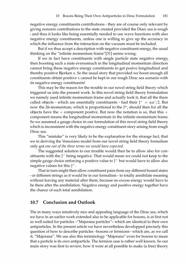
ii

“proc17” — 2017/12/11 — 19:44 — page 181 — #195 ii

ii

ii


negative energy constituents contributions - they are of course only relevant bygiving nonzero contributions to the state created provided the Diarc sea is rough- and thus it looks like being essentially needed to use wave functions with alsonegative energy constituents, unless one is willing to give up the accuracy inwhich the influence from the interaction on the vacuum must be included.

But if we thus accept a description with negative constituent energy, the usualthinking on the “infinite momentum frame”[31] seems wrong:

If we in fact have constituents with single particle state negative energy,then boosting such a state eversomuch in the longitudinal momentum directioncannot bring these negative energy constituents to get posive longitudinal andthereby positive Bjorken x. So the usual story that provided we boost enough allconstituents obtain positive x cannot be kept in our rough Dirac sea scenario withits negative energy constituents!

This may be the reason for the trouble in our novel string field theory whichtriggered us into the present work. In this novel string field theory formulationwe namely used infinite momentum frame and actually took it, that all the therecalled objects - which are essentially constituents - had their J+ = aα ′/2. Butnow the 26-momentum, which is proportional to the Jµ, should then for all theobjects have the + component positve. But now the notation is so, that this +

component means the longitudinal momentum in the infinite momentum frame.So we assumed a gauge choice in our formulation of this novel string field theorywhich is inconsistent with the negative energy constituent story arising from roughDirac sea.

This “mistake” is very likely to be the explanation for the strange fact, thatwe in deriving the Veneziano model from our novel string field theory formalismonly got one out of the three terms we would have expected.

The suggested solution to our trouble would then be to allow also for con-stituents with the J+ being negative. That would mean we could not keep to thesimple gauge choice enforcing a positive value to J+ but would have to allow alsonegative values for this J+.

That in turn might then allow constituent pairs from say different bound states- or different strings as it would be in our formalism - to totally annihilate meaningwithout leaving any material after them, because no excess energy would have tobe there after the annihilation. Negative energy and positive energy together havethe chance of such total annihilation.

10.7 Conclusion and Outlook

The in many ways intuitively nice and appealing language of the Dirac sea, whichwe have in an earlier work extended also to be applicable for bosons, is at first notso well suited for particles –“Majorana particles”– which are identical to their ownantiparticles. In the present article we have nevertheless developped precisely thisquestion of how to describe particles –bosons or fermions– which are, as we callit, “Majorana”. We use also this terminology “Majorana” even for bosons to meanthat a particle is its own antiparticle. The fermion case is rather well known. So ourmain story was first to review, how it were at all possible to make (a free) theory

ii

“proc17” — 2017/12/11 — 19:44 — page 182 — #196 ii

ii

ii


for bosons based on a Dirac sea, and secondly the new features of this Dirac seafor boson theory as follows:

a)negative norm squaresb)negative number of particles.

The main point then became how to get what we call a Majorana-bosontheory through these new features. This comes about by constructing in terms ofthe creation and annihilation operators a†f(~p, E > 0) and a(~p, E < 0) for a type ofboson that might have a charge, some creation and annihilation operators b(~p)and b†f(~p) for the Majorana boson, which is really a superposition of a boson andan anti-boson of the type described by a and a†.

10.7.1 The old Dirac sea for bosons

The Dirac sea for boson theory is based on having a Fock space, for which a basisconsists of states with a number of bosons k(~p, E >< 0), which can be both positive,zero and negative integer, in both positive and negative energy E single particlestates for each 3−momentum ~p,

| . . . , k(~p, E > 0), . . . ; . . . , k( ~p ′, E < 0), . . .〉 ∈ Fock space. (10.129)

Because of the complication that the inner product

〈ϕ1 |(f) ϕ2〉 =∫ϕ∗1

←→∂

∂tϕ2d

3~X (10.130)

for a (single particle) boson is not positive definite we have to distinguish twodifferent inner products | and |f say and thus also the two thereto respondinghermitean conjugations † and †f, meaning respectively without and with the∫ϕ∗1←→∂∂tϕ2d

3~X included. In fact we have for the norm square for these two innerproducts

〈. . . , k(~p, E > 0), . . . ; . . . , k( ~p ′, E < 0), . . . |f. . . , k(~p, E > 0), . . . ; . . . , k( ~p ′, E < 0), . . .〉

=(−1)](neg. energy b.〈. . . , k(~p, E > 0), . . . ; . . . , k( ~p ′, E < 0), . . . |

. . . , k(~p, E > 0), . . . ; . . . , k( ~p ′, E < 0), . . .〉

=(−1)](neg. energy b. ·∏

(~p,E><0)for which k≤−1

(−1)|k| (10.131)

10.7.2 Main Success of Our Previous Dirac Sea (also) for Bosons:

The remarkable feature of the sector with the emptied out Dirac sea for bosons -what we called the physical sector - is that one has arranged the sign alternation(10.42) with the total number of negative energy bosons to cancel the sign from(10.31) so as to achieve that the total Fock space has positive norm square. This

ii

“proc17” — 2017/12/11 — 19:44 — page 183 — #197 ii

ii

ii


“physical sector” corresponds to that negative energy single particle states arein the negative sectors, while the positive energy single particle states are in thepositive sector.

Thus the basis vectors of the full Fock space for the physical sector are of theform

| . . . , k(~p, E > 0), . . . ; . . . , k(~p, E < 0), . . .〉 (10.132)

where the dots . . . denotes that we have one integer number for every momentumvector –value (~p or ~p ′), but now the numbers k(~p, E > 0) of particles in a positiveenergy are– in the physical sector-combination– restricted to be non-negative whilethe numbers of bosons in the negative energy single particle states are restrictedto be negative

k(~p, E > 0) = 0, 1, 2, . . .

k(~p, E < 0) = −1,−2,−3, . . . (10.133)

In this physical sector our Dirac Sea formalism is completely equivalent tothe conventional formalism for quantizing Bosons with “charge” (i.e. Bosonsthat are not their own antiparticles), say e.g. π+ and π−.

But let us remind ourselves that this idea of using Dirac sea allows one to notfill the Dirac sea, if one should wish to think of such world. With our extension ofthe idea of the Dirac sea to also include Bosons one also gets allowed to not emptyout to have −1 boson in each negative energy single particle state. But for bosonsyou have the further strange feature of the phantasy world with the Dirac sea nottreated as it should be to get physical, that one even gets negative norm squarestates, in addition to like in the fermion case having lost the bottom in the energy.

10.7.3 Present Article Main Point were to Allow for Bosons being their ownAntiparticles also in Dirac sea Formalism

We could construct a “Majorana-boson” creation operator for say a “Majorana-boson” with momentum ~p, b†(~p) analogously to the expressions (10.19) and(10.20).b†(~p) = 1√

2

(a†(~p, E > 0) + a(−~p, E < 0)

)and b(~p) = 1√

2

(a(E > 0) + a†(E < 0)

)Since an extra phase on the basis states does not matter so much we could also

choose for the bosons the “Majorana boson” creation and annihilation operatorsto be

b†f(~p) =1√2

(a†(E > 0) + a(−~p, E < 0)

)=

1√2

(a†f(~p, E > 0) + a(−~p, E < 0)

)b(~p) =

1√2

(a(~p, E > 0) + a†f(−~p, E < 0)

)=

1√2

(a(~p, E > 0) − a†(−~p, E < 0)

)(10.134)

ii

“proc17” — 2017/12/11 — 19:44 — page 184 — #198 ii

ii

ii


Such creation operators b†f(~p) and their corresponding annihilation operatorsb(~p) make up the completely usual creation and annihilation operator algebrafor Bosons that are their own antiparticles in the case of the “physical sectorcombination”. This “physical sector combination” means that we emptied out theDirac sea in the sense that in the “vacuum” put just −1 boson in each negativeenergy single particle state. This correspondence means that our formalism isfor this “physical sector combination” completely equivalent to how one usuallydescribes Bosons - naturally without charge - which are their own antiparticles.But our formalism is to put into the framework of starting with a priori “charged”Bosons which then quite analogously to fermions have the possibility of havingnegative energy (as single particles). We then treat the analogous problem(s) tothe Dirac sea for Fermions, by “putting minus one boson in each of the negativeenergy single particle states. That a bit miraculously solves both the problem ofnegative norm squares and negative second quantized energy, and even we canon top of that restrict the theory, if we so wish,to enforce the bosons to be identified withtheir own antiparticles.

We saw above that

• 1. We obtain the Fock-space (Hilbert-space) for the Bosons being their ownantiparticles by restriction to a subspace

HMaj = |〉 | r(~p) |〉 = 0 , (10.135)

where we have defined

r(~p) =1√2(a(+~p, E > 0) + a†(−~p, E < 0))

=1√2(a(~p, E > 0) − a†f(−~p, E < 0). (10.136)

Of course when one forces in the original Dirac sea formalism the antiparticlesdiffernt from the particles to behave the same way in detail it means a drasticreduction of the degrees of freedom for the second quantized system - the Fockspace-, and thus it is of course quite natural that we only use the subspaceHMaj being of much less (but still infinite) dimension than the original one.

• 2. In our formalism - since we use to write the creation operator for the bosonbeing its own antiparticle as a sum of creation of a particle and of a hole (10.134)- a “Majorana-boson”is physically described as statistically or in superpositionbeing with some chanse a particle and with some chance a hole. Really it isobvious, that it is 50 % chance for each. So the physical picture is that the“Majorana-boson” is a superposition of a hole and an original positive energyparticle in the “physical sector combination”.• 3. We could construct a charge conjugation operation C which on our Fock

space with both negative and positive energy states present as possibilitiesobtained the definition:

C | . . .∼

k (~p, E > 0), . . . ; . . . ,∼

k ( ~p ′, E < 0), . . .〉

=| . . . , k(~p, E > 0) = −∼

k (− ~p ′, E < 0) + 1, . . . ; (10.137)

. . . , k( ~p ′, E < 0) = −1−∼

k (− ~p ′, E > 0), . . .〉.

ii

“proc17” — 2017/12/11 — 19:44 — page 185 — #199 ii

ii

ii


Of course the state of the system of negative single particle comes to depend onthat of the positive energy system after the charge conjugation and oppositely.With (10.58) or (10.134) one sees that on the whole system or Fock spaceof Bosons being their own antiparticles is left invariant under the chargeconjugation operator C. This is as expected since these “Majorana Bosons”should be invariant under C.

10.7.4 The Unphysical Sector Combinations and Boson-theories therein withBosons being their own antiparticles

As a curiosity - but perhaps the most new in the present article - we have notonly the physical sector combination, which so successfully just gives the usualformalism for both “charged” bosons and for what we called Majorana-bososns(the ones of their own antiparticles) but three more “sector-combinations” meaningcombinations of whether one allows only negative numbers of bosons, or onlynon-negative numbers for the positive and the negative single particle states. Thereader should have in mind that there is what we called the barier, meaning thatthe creation and annihilation operators cannot cross from a negative number ofparticles in a single particle state to a positive one or opposite, and thus we canconsider the theories in which a given single particle state has a positive or zeronumber of particles in it as a completely different theory from one in which onehas a negative number of bosons in that single particle state. For simplicity wehad chosen to only impose that we only considered that all single particle stateswith one sign of the single particle energy would have their number of particlesbeing on the same side of the barrier. But even with this simplifying choice thereremained 22 = 4 different sector-combinations. One of these sector-combinations -and of course the most important one because it matches the usual and physicalformalism - were the “physical sector combination” characterized by their being anon-negative number k of bosons in all the positive energy single particle states(i.e. for E > 0), while the number k of bosons in the negative energy single particlestates (i.e. for E < 0) is restricted to be genuinely negative −1,−2,−3, ....

The sector combination possibility 4) in our enumeration above the Fockspace gets negative definite instead of as the one for the physical sector combi-nation which gets positive definite. But these sector combinations are analogousor isomorphic with the appropriate sign changes allowed. Also our charge con-jugation operator C operates inside both the “physical sector combination” andinside the sector combination number 4), which is characterized as having just theopposite to those of the physical sector, meaning that in sector combination 4) onehas a negative number of particles in each positive energy (single particle)state,while there is a positive or zero number in the negative energy states. Thus theconstruction of particles being their own antiparticles would be rather analogousto that in the physical sector combination.

Less trivial is it to think about the two sector combinations 2) and 3) becausenow the charge conjugation operator C goes between them:Acting with the chargeconjugation operator C on a state in the section combination 2) which we called the“naive vacuum sector combination” one gets a result of the operation in the different

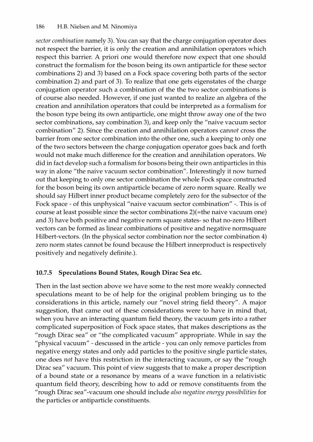
ii

“proc17” — 2017/12/11 — 19:44 — page 186 — #200 ii

ii

ii


sector combination namely 3). You can say that the charge conjugation operator doesnot respect the barrier, it is only the creation and annihilation operators whichrespect this barrier. A priori one would therefore now expect that one shouldconstruct the formalism for the boson being its own antiparticle for these sectorcombinations 2) and 3) based on a Fock space covering both parts of the sectorcombination 2) and part of 3). To realize that one gets eigenstates of the chargeconjugation operator such a combination of the the two sector combinations isof course also needed. However, if one just wanted to realize an algebra of thecreation and annihilation operators that could be interpreted as a formalism forthe boson type being its own antiparticle, one might throw away one of the twosector combinations, say combination 3), and keep only the “naive vacuum sectorcombination” 2). Since the creation and annihilation operators cannot cross thebarrier from one sector combination into the other one, such a keeping to only oneof the two sectors between the charge conjugation operator goes back and forthwould not make much difference for the creation and annihilation operators. Wedid in fact develop such a formalism for bosons being their own antiparticles in thisway in alone “the naive vacuum sector combination”. Interestingly it now turnedout that keeping to only one sector combination the whole Fock space constructedfor the boson being its own antiparticle became of zero norm square. Really weshould say Hilbert inner product became completely zero for the subsector of theFock space - of this unphysical “naive vacuum sector combination” -. This is ofcourse at least possible since the sector combinations 2)(=the naive vacuum one)and 3) have both positive and negative norm square states- so that no-zero Hilbertvectors can be formed as linear combinations of positive and negative normsquareHilbert-vectors. (In the physical sector combination nor the sector combination 4)zero norm states cannot be found because the Hilbert innerproduct is respectivelypositively and negatively definite.).

10.7.5 Speculations Bound States, Rough Dirac Sea etc.

Then in the last section above we have some to the rest more weakly connectedspeculations meant to be of help for the original problem bringing us to theconsiderations in this article, namely our “novel string field theory”. A majorsuggestion, that came out of these considerations were to have in mind that,when you have an interacting quantum field theory, the vacuum gets into a rathercomplicated superposition of Fock space states, that makes descriptions as the“rough Dirac sea” or “the complicated vacuum” appropriate. While in say the“physical vacuum” - descussed in the article - you can only remove particles fromnegative energy states and only add particles to the positive single particle states,one does not have this restriction in the interacting vacuum, or say the “roughDirac sea” vacuum. This point of view suggests that to make a proper descriptionof a bound state or a resonance by means of a wave function in a relativisticquantum field theory, describing how to add or remove constituents from the“rough Dirac sea”-vacuum one should include also negative energy possibilities forthe particles or antiparticle constituents.

ii

“proc17” — 2017/12/11 — 19:44 — page 187 — #201 ii

ii

ii


These considerations are also hoped to be helpful for the problems we havefor the moment with obtaining the full Veneziano model amplitude from our novelstring field theory.

Acknowledgement

One of us (H.B.N.) wishes to thank the Niels Bohr Institute to allow him to workas emeritus there, with room and some support for travel etc. The other (M.N.)acknowledges the Niels Bohr Institute and the Niels Bohr International Academy,where the present work started; He wishes to thank there for their hospitalityextended to hime during his stay. M.N. also acknowledges the Okayama Institutefor Quantum Physics and the Okayama local government for providing him travelexpences. He also acknowledges that present research is supported by the J.S.P.S.Grant-in-Aid for Scientific Research No. 23540332.

References

1. Majorana, Ettore; Maiani, Luciano (2006). ”A symmetric theory of electrons andpositrons”. In Bassani, Giuseppe Franco. Ettore Majorana Scientific Papers. pp. 201E3.doi:10.1007/978-3-540-48095 -2 10. ISBN 978-3-540-48091-4. Translated from: Majorana,Ettore (1937). ”Teoria simmetrica dell’elettrone e del positrone”. Il Nuovo Cimento (inItalian) 14 (4): 171E4. doi:10.1007/bf02961314.

2. Griffiths, David J. (2008). Elementary Particles (Second, Revised ed.). WILEY-VCH. p.149. ISBN 978-3-527-40601-2)

3. Nielsen, H. B.; Ninomiya, M., Dirac Sea for Bosons. I —Formulation of Negative EnergySea for Bosons— Progress of Theoretical Physics, Vol. 113, No. 3, pp. 603-624 DOI:10.1143/PTP.113.603 Bibliographic Code: 2005PThPh.113..603NHolger B. Nielsen and Masao Ninomiya, Progress of Theoretical Physics Volume 113,Issue 3 pp. 625-643.Dirac Sea for Bosons. II E Study of the Naive Vacuum Theory for the Toy Model WorldPrior to Filling the Negative Energy Sea

4. Yoshinobu Habara, Yukinori Nagatani, Holger B. Nielsen and Masao NinomiyaDirac Sea and Hole Theory for Bosons II: Renormalization ApproachInt. J. Mod. Phys. A 23, 2771 (2008). DOI: 10.1142/S0217751X08040354

5. Dirac, P A M - 1931 - Quantized Singularities In The Electromagnetic Fields (Publishedby api-3773171) P.A.M. Dirac, Proc. Roy. Soc.A 133, 60 1931.See also e.g. Alvarez-Gaume, Luis; Vazquez-Mozo, Miguel A. (2005). ”IntroductoryLectures on Quantum Field Theory”. CERN Yellow Report CERN-, pp. - 1 (96): 2010001.arXiv:hep-th/0510040. Bibcode:2005hep.th...10040A.

6. Feynman, Richard P. (1998) [1972]. Statistical Mechanics: A Set of Lectures (2nd ed.).Reading, Massachusetts: Addison-Wesley. ISBN 978-0-201-36076-9.

7. arXiv:quant-ph/0602151v2 19 Feb 2006 Quantum Mechanics of Klein-Gordon Fields I:Hilbert Space, Localized States, and Chiral Symmetry A. Mostafazadeh and F. Zamani

8. H. B. Nielsen and M. Ninomiya, An Idea of New String Field Theory – Liberating Right andLeft movers –, in Proceedings of the 14th Workshop, “What Comes Beyond the StandardModels” Bled, July 11-21, 2011, eds. N. M. Borstnik, H. B. Nielsen and D. Luckman;arXiv: 1112. 542[hep-th].

ii

“proc17” — 2017/12/11 — 19:44 — page 188 — #202 ii

ii

ii


9. H. B. Nielsen and M. Ninomiya, A New Type of String Field Theory, in Proceedings of the10th Tohwa International Symposium in String Theory”, July 3-7, 2001, Fukuoka Japan,AIP conference Proc vol.607, p.185-201; arXiv: hep-th/0111240.v1, Nov.2001

10. H.B. Nielsen and M. Ninomiya, “A Novel String Field Theory Solving String Theory byLiberating Left and Right Movers” JHEP 202P 05131 v2 (2013)

11. H. B. Nielsen and M. Ninomiya, “Deriving Veneziano Model in a Novel String FieldTheory Solving String Theory by Liberating Right and Left Movers,” arXiv:1410.1048[hep-th].

12. String references are cited in References [12]-[15], [17]H. B. Nielsen, A Physical interpretation of the integrand of the n-point Veneziano model,(1969)(Nordita preprint...); a later version “An almost Physical interpretation of theintegrand of the n-point Veneziano model” preprint at Niels Bohr Institute; a paperpresented at the 15th International Conference on High Energy Physics, Kiev 1970 (seep.445 in Veneziano’s talk.)

13. Y. Nambu, Quark Model and the factorization of the Veneziano amplitude, in Proceedingsof the International Conference on Symmetries and Quark Models, June 18-20, 1969ed. by Chand, R. (Gordon and Breach), New York, 269-277; reprinted in Broken Sym-metry Selected Papers of Y. Nambu eds. T. Eguchi and K. Nishijima, (World Scientific,Singapore, 1995)258-277.

14. Y. Nambu, Duality and hadrondynamics, Lecture notes prepared for Copenhagen summerschool, 1970; It is reproduced in “Broken Symmetry”, Selected Papers of Y. Nambu eds.T. Eguchi, and K. Nishijima, (World Scientific, Singapore, 1995)280.

15. L. Susskind, Structure of hadrons implied by duality, Phys. Rev. D1(1970)1182-1186(1970):L. Susskind, Dual symmetric theory of hadrons, 1. Nuovo Cimento A69,457-496(1970).

16. For many original papers of early string theory found inThe Birth of String Theory” eds. by Andrea Cappeli, Elena Castellani, Flippo Colomo andPaolo Di Vecchia, Cambridge University Press 2012. Cambridge, New York, Melbourne.

17. M. B. Green, J. H. Schwarz and E. Witten, Superstring theory, 1-2, Cambridge UniversityPress 1987.

18. As for bosonic string field theory in the light-cone gauge:M. Kaku and K. Kikkawa, Phys. Rev. D10(1974)1110; M. Kaku and K. Kikkawa, Phys.Rev. D10(1974)1823; S. Mandelstam, Nucl. Phys. B64(1973)205; E. Cremmer and J.-L.Gervais, Nucl. Phys. B90(1975)410.

19. Witten type mid-point interaction of covariant bosonic string field theory: for openstringE. Witten, Nucl. Phys. B268(1986)253.

20. Closed string version of ref.[19] of the Witten theory:M. Saadi and B. Zwiebach, Ann. Phys. 192(1989)213; T. Kugo, H. Kunitomo and K. Sue-hiro, Phys. Lett. B226(1989)48; T. Kugo and K. Suehiro, Nucl. Phys. B337(1990)434;B. Zwiebach, Nucl. Phys. B390(1993)33.

21. Joining-Splitting light-cone type: for open stringH. Hata, K. Itoh, T. Kugo, H. Kunitomo and K. Ogawa, Phys. Rev. D34(1986)2360.

22. Closed string of Joining-Splitting light-cone type:H. Hata, K. Itoh, H. Kunitomo and K. Ogawa, Phys. Rev. D35(1987)1318;H. Hata, K. Itoh, T. Kugo, H. Kunitomo and K. Ogawa, Phys. Rev. D35(1987)1356.

23. Supersymmetrized covariant open Witten theoryE. Witten, Nucl. Phys. B276(1986)291; I. Arefeva and P. Medvedev, Phys. Lett.B212(1988)299; C. Wendt, Nucl. Phys.B314(1989)209; N. Berkovits, Nucl. Phys.B450(1995)90 [Errata, B459(1996)439] hepth/9503099.

ii

“proc17” — 2017/12/11 — 19:44 — page 189 — #203 ii

ii

ii


24. Modified cubic theory:I. Arefeva, P. Medvedev and A. Zubarev, Nucl. Phys. B341(1990)464; C. R. Preitschopf,C. B. Thorn and S. A. Yost, Nucl. Phys. B337(1990)363.

25. Supersymmetrized Green-Schwarz theory in the light-cone gauge:M. B. Green and J. H. Schwarz, Nucl. Phys. B218(1983)43; M. B. Green, J. H. Schwarzand L. Brink, Nucl. Phys. B219(1983)437; M. B. Green, and J. H. Schwarz, Nucl. Phys.B243(1984)437; J. Greensite and F. R. Klinkhamer, Nucl. Phys. B281(1987)269; Nucl.Phys. B291(1987)557; Nucl. Phys. B304(1988)108; M. B. Green and N. Seiberg, Nucl.Phys. B299(1988)559; S.-J. Sin, Nucl. Phys. B313(1989)165.

26. For review articles of string field theory:W. Taylor and B. Zwiebach, D-branes, Tachyons, and String Field Theory, hep-th/0311017http://jp.arxiv.org/abs/hep-th/0311017; K. Ohmori, A Review on Tachyon Condensationin Open String Theories, hep-th/0102085 http://jp.arxiv.org/abs/hep-th/0102085.

27. C. B. Thorn, Derivational model from field theory II, Phys. Rev. D17(1978)1037, and refer-ences therein.

28. G. Veneziano, Construction of a crossing-symmetric, Regge behaved amplitude for linearlyrising trajectories, Nuovo Cimento A57 190(1968).

29. For comprehensive reviews of string theory seee.g. J. Polchinski, String Theory, vol.I-II, Cambridge University Press 1998.

30. H. Bethe, E. Salpeter (1951). ”A Relativistic Equation for Bound-State Problems”. Physi-cal Review 84 (6): 1232. Bibcode:1951PhRv...84.1232S. doi:10.1103/PhysRev.84.1232.

31. S. Fubini and G. Furlan, Physicsi, 229.S. Weinberg, Phys. Rev. 150, 1313.L. Susskind, Phys. Rev. 165, 1535.L. Susskind, Infinite Momentum Frames and Particle Dynamics, in Lectures in Theoret-ical Physics, Vol. XI-D: Mathematical Methods in Theoretical Physics, K. Mahanthappaand W. Brittin, ed.; Gordon and Breach, New York.

ii

“proc17” — 2017/12/11 — 19:44 — page 190 — #204 ii

ii

ii




11 UV complete Model With a Composite HiggsSector for Baryogenesis, DM, and Neutrino masses

T. Shindou ?

Division of Liberal-Arts, Kogakuin University,Nakanomachi 2665-1, Hachioji, 192-0015, Tokyo, Japan

Abstract. We propose a UV complete model based on SUSY SU(2)H gauge theory withconfinement. New Z2 discrete symmetry and Z2-odd right-handed neutrino superfieldsare also introduced to the model. Its low-energy effective theory can provide solutions forBaryogenesis, DM candidate, and origin of neutrino masses. Below a confinement scale, theHiggs sector is described in terms of mesonic superfields of fundamental SU(2)H doublets.We also discuss how to test the scenario by the future collider experiments in a benchmarkscenario.

Povzetek. Avtor predlaga model za konfinirane kvarke, ki temelji na supersimetricni umer-itveni teoriji SU(2)H, dopolnjeni z diskretno simetrijo Z2. Tudi za nevtrinska superpoljauporabi Z2 diskretno simetrijo. V limiti nizkih energij lahko model ponudi odgovore zanastanek barionov, kandidate za temno snov in pojasni izvor nevtrinskih mas. Na energijskiskali pod kromodinamskim faznim prehodom opise Higgsove skalarje z mezonskimi su-perpolji osnovnega dubleta SU(2)H. Obravnava tudi moznosti preverbe modela na bodocihposkusih na pospesevalnikih.

Keywords: New Physics, Composite Higgs sector, SUSY

11.1 Introduction

A Higgs boson was discovered in 2012 at LHC experiments, and it has beenconfirmed that its properties are consistent with the Higgs boson in the StandardModel (SM). However, it is not the end of the story. The SM has still serousproblems. For example, there is no successful mechanism of Baryogenesis, thereis no candidate of the Dark Matter (DM), there is no natural explanation of tinyneutrino masses, and so on. On the other hand, we have not fully understoodthe Higgs sector yet. There are still several fundamental questions. For example,how many Higgs bosons are there?, Whether is the Higgs boson a elementaryscalar or a composite state? What is the origin of the negative mass squared ofthe Higgs boson? and so on. In many models, extension of the SM for explainingunsolved problems, such as Baryogenesis, DM, neutrino masses, etc lead to an


ii

“proc17” — 2017/12/11 — 19:44 — page 191 — #205 ii

ii

ii

11 UV complete Model With a Composite Higgs Sector. . . 191

extended Higgs sector. Thus, we can say that the Higgs sector will be a probe ofnew physics.

In this talk, we consider a SUSY model[1,2] with additional SU(2)H gaugesymmetry to the SM gauge group and three matter fields (and three anti-matterfields) which are fundamental representations under the SU(2)H. In the low energyeffective theory of this model, the Higgs sector is described by mesonic fieldsof those six fields. We then show that this effective theory can provide enoughenhancement of the first order electroweak phase transition (1stOPT) which isrequired by successful electroweak baryogenesis scenario[3], DM candidates, andmechanism to generate tiny neutrino masses through radiative corrections.

11.2 Model

In SUSY SU(Nc) gauge theory with Nc + 1 flavour fields, confinement occursat some scale[6]. The simplest example is Nc = 2 case. Utilising this setup, wepropose a model with SU(2)H symmetry with three flavour fields which are fun-damental representations of SU(2)H. There should also be three anti-matter fieldsfor each fundamental representation matter fields. We described these six fieldsas Ti(i = 1, · · · , 6). This setup is almost same as one in the minimal SUSY fatHiggs model[7]. In the minimal SUSY fat Higgs model, two doublets and onesinglet mesonic fields are light in the low energy effective theory by introducingadditional fields. In our model, in contrast, all the mesonic fields appears in thelow energy effective theory.

We here introduce a right-handed neutrino (RHN) which is singlet underSU(2)H as well as the SM gauge symmetry. The model also has an unbrokendiscrete symmetry Z2 in order to forbid tree level contributions to neutrino masses.The RHN has an odd charge under the Z2 parity. We show the charge assignmentof Ti and the RHN NcR under the SM gauge symmetry, SU(2)H, and the Z2 parityin Table 11.1-(I). The fifteen mesonic fields below a certain scale ΛH which arecanonically normalized as Hij ' 1

4πΛHTiTj(i 6= j) are listed in the Table 11.1-(II).

The superpotential of the Higgs sector below ΛH is given by

Weff =λN(HuHd + v20

)+ λNΦ

(ΦuΦd + v2Φ

)+ λNΩ

(Ω+Ω− − ζη+ v2Ω

)+ λζHdΦu + ηHuΦd −Ω+HdΦd −Ω−HuΦu −NNΦNΩ

. (11.1)

ii

“proc17” — 2017/12/11 — 19:44 — page 192 — #206 ii

ii

ii

192 T. Shindou

(I)

Superfield SU(2)H SU(3)C SU(2)L U(1)Y Z2(T1T2

)2 1 2 0 +1

T3 2 1 1 +1/2 +1

T4 2 1 1 −1/2 +1

T5 2 1 1 +1/2 −1

T6 2 1 1 −1/2 −1

NcR 1 1 1 0 −1

(II)

Superfield SU(3)C SU(2)L U(1)Y Z2

Hd ≡(H14H24

)1 2 −1/2 +1

Hu ≡(H13H23

)1 2 +1/2 +1

Φd ≡(H15H25

)1 2 −1/2 −1

Φu ≡(H16H26

)1 2 +1/2 −1

Ω− ≡ H46 1 1 −1 −1

Ω+ ≡ H35 1 1 +1 −1

N ≡ H56, NΦ ≡ H34, NΩ = H12 1 1 0 +1

ζ ≡ H36, η ≡ H45 1 1 0 −1

Table 11.1. (I) The charge assignment of the SU(2)H doublets Ti and the RHN NcR underthe SM gauge group (SU(3)c×SU(2)L×U(1)Y and the Z2 parity. (II) The field content of theextended Higgs sector in the low energy effective theory below the scale ΛH.

By the Naive Dimensional Analysis, λ ' 4π is naively expected at the confinementscale ΛH. The relevant soft SUSY breaking Lagrangian terms are given by

LH =−m2HuH†uHu −m2HdH

†dHd −m2ΦuΦ

†uΦu −m2ΦdΦ

†dΦd

−m2NN∗N−m2NΦN

∗ΦNΦ −m2NΩN

∗ΩNΩ −m2Ω+

Ω∗+Ω+ −m2Ω−Ω∗−Ω−

−m2ζζ∗ζ−m2ηη

∗η−

m2ζηη

∗ζ+B2ζ2ζ2 +

B2η

2η2 + h.c.

−Cλv20N+ CΦλv

2ΦNΦ + CΩλv

2ΩNΩ + h.c.

− BµHuHd + BΦµΦΦuΦd + BΩµΩ(Ω+Ω− + ζη) + h.c.

− λANHuHdN+ANΦΦuΦdNΦ +ANΩ(Ω+Ω− − ηζ)NΩ +AζHdΦuζ

+AηHuΦdη+AΩ−HuΦuΩ− +AΩ+

HdΦdΩ+ + h.c.. (11.2)

By the vacuum expectation values (vev’s) of Z2-even singlet fieldsN,NΦ andNΩ,the mass parameters µ = λ〈N〉, µΦ = λ〈NΦ〉 and µΩ = λ〈NΩ〉 are induced. The

ii

“proc17” — 2017/12/11 — 19:44 — page 193 — #207 ii

ii

ii


RHN has Yukawa couplings and the Majorana mass term given by

WN =yiNNcRLiΦu + hiNN

cREciΩ− +

MR

2NcRN

cR +

κ

2NNcRN

cR . (11.3)

11.3 Benchmark point and its phenomenology

For successful electroweak baryogenesis, the condition ϕc/Tc > 1 should besatisfied, which means that the 1stOPT is strong enough. Though new CP violationphases are required in order to reproduce the correct amount of Baryon asymmetryof the Universe, we here focus only on the 1stOPT. It is naively expected that we canintroduce several CP phases relevant to Baryogenesis as in the case of MSSM[8]. Inour model, the 1stOPT can be enhanced by the loop contributions of extra Z2-oddscalar particles strongly enough.

Since our low energy effective theory keeps both Z2-parity and R-parityunbroken, there are potentially three kinds of the DM candidates, i.e. the lightestparticles with the parity assignments of (−,+), (+,−), and (−,−). However, inthe case that one of them is heavier than the sum of the masses of the others, theheaviest one decays into the other two particles so that the heaviest particle cannotbe a DM.

In our model, tiny neutrino masses are generated via loop contributionsshown in Fig. 11.1. There are one-loop and three-loop contributions. The one-loopand three-loop diagrams correspond to the SUSY versions of Ma model[4] andAKS[5], respectively. It is interesting that the one-loop diagrams are driven bythe coupling yN and the three-loop diagrams are controlled by another couplinghN. Both one-loop and three-loop contributions can be significant if hN yN.Therefore, two different mass squared differences can be generated even if onlyone RHN is introduced.

Φu

νjνiνR νR

mνR

η, ζ η, ζ

B2η , B

2ζ , m

2∗ζη

HuHu

Φu

yiN yjN

νjνi

Hu Hu

ζ ζ

B2ζ

νR νR

mνR

Hd

eRi eRj

hiN hj

N

Hd

Ω− Ω−νjνi

Hu Hu

ζ ζ

B2ζ

νR νR

mνRΩ− Ω−

Hd

eRi eRj

hiN hj

N

Φd Φd

HdΩ+ Ω+

(I) (II) (III)

Fig. 11.1. (I) A one-loop diagram and (II) three-loop diagrams which contribute to theneutrino mass matrix. The figures are taken from [1]

A benchmark scenario is provided in Table 3 of Ref. [1] and some predictionsare shown in Table 4 of the same reference, where the condition ϕc/Tc > 1 issatisfied, the neutrino masses and the mixing angles given by neutrino oscillationdata can be reproduced, and the relic abundance of the DM can be explained withsatisfying the constraints from the experiments such as LFV searches.

ii

“proc17” — 2017/12/11 — 19:44 — page 194 — #208 ii

ii

ii

194 T. Shindou

Fig. 11.2. The mass spectrum of the relevant particles in the bench mark scenario. The figureis taken from Ref.[1].

Though this point is already excluded by the direct detection experimentof the DM[9], we discuss phenomenological consequences of this benchmarkscenario, because we can see some general features of our model in the scenario. InFig. 11.2, the mass spectrum of the relevant particles in this benchmark scenario isshown. The Z2-even part of the spectrum is similar to one in nMSSM. A significantsize of mass splitting between the charged Higgs boson and the heavy Higgsbosons is required for obtaining the large mixing between doublet fields and asinglet field, which is necessary to reproduce the relic abundance of the DM. Bylooking at such a large splitting in the spectrum of extra Higgs bosons, the Z2-evenpart of our scenario can be distinguished from the MSSM. In this benchmarkscenario, ϕc/Tc is enhanced by the loop effect of Φu andΩ−. The loop effect canalso significantly affect the h-γ-γ coupling and the triple Higgs boson coupling asshown in Table 11.2. By using precise measurement of the SM-like Higgs bosoncouplings at future collider experiment such as ILC[10], our benchmark scenariocan be distinguished from nMSSM too.

Couplings hWW hZZ huu hdd h¯` hγγ hhh

κhφφ = ghφφ/gSMhφφ 0.990 0.990 0.990 0.978 0.978 0.88 1.2

Table 11.2. The deviations in the coupling constants from the SM values in the benchmarkscenario defined in Ref. [1].

ii

“proc17” — 2017/12/11 — 19:44 — page 195 — #209 ii

ii

ii


It is also interesting to discuss phenomenology in the Z2-odd sector. By thedirect search of inert doublet particles[11] and inert charged singlet searches[12] atILC, it is expected to get a strong hint on the Z2-odd sector of the scenario.

11.4 Conclusion

We have attempted to construct a simple model to solve the three problems suchas baryogenesis, DM, and tiny neutrino mass, which cannot be explained in theSM. We have succeeded to find such a UV model based on SUSY SU(2)H gaugetheory with confinement. In its low energy effective theory, we have shown thatthe 1stOPT is enhanced strongly enough for successful electroweak baryogenesis,multi-components DM scenario is realised, and tiny neutrino masses are generatedvia one-loop and three-loop diagrams. We have also introduced a benchmarkscenario and we have discussed how to test it at future collider experiments. Inthis benchmark scenario, the spin-independent cross section of DM’s are abovethe latest result of the DM direct detection experiments, so that we should lookfor a new benchmark scenario. In addition, we focus only on the 1stOPT for thebaryogenesis. For complete analysis, new CP violation phases should be takeninto account.

Recently, effects of CP violation in the singlet-doublet dark matter model isdiscussed and it is shown that the spin-independent cross section can be sup-pressed with a certain CP violation in the dark sector[13]. Therefore, it will beimportant to take CP phases in to account for evading the strong constraint fromthe direct detection of DMs as well as for complete analysis of the baryogenesisscenario.

Acknowledgements

This work is supported in part by JSPS KAKENHI, Grant Number 17H05408.

References

1. S. Kanemura, N. Machida and T. Shindou, Phys. Lett. B 738 (2014) 1782. S. Kanemura, T. Shindou and T. Yamada, Phys. Rev. D 86 (2012) 055023; S. Kanemura,

E. Senaha, T. Shindou and T. Yamada, JHEP 1305 (2013) 066; S. Kanemura, N. Machida,T. Shindou and T. Yamada, Phys. Rev. D 89 (2014) 1, 013005.

3. V. A. Kuzmin, V. A. Rubakov and M. E. Shaposhnikov, Phys. Lett. B 155 (1985) 36;A. G. Cohen, D. B. Kaplan and A. E. Nelson, Ann. Rev. Nucl. Part. Sci. 43 (1993) 27;M. Quiros, Helv. Phys. Acta 67 (1994) 451; V. A. Rubakov and M. E. Shaposhnikov, Usp.Fiz. Nauk 166 (1996) 493 [Phys. Usp. 39 (1996) 461]; K. Funakubo, Prog. Theor. Phys.96 (1996) 475; M. Trodden, Rev. Mod. Phys. 71 (1999) 1463; W. Bernreuther, Lect. NotesPhys. 591 (2002) 237; J. M. Cline, hep-ph/0609145; D. E. Morrissey and M. J. Ramsey-Musolf, New J. Phys. 14 (2012) 125003.

4. E. Ma, Phys. Rev. D 73 (2006) 077301.

ii

“proc17” — 2017/12/11 — 19:44 — page 196 — #210 ii

ii

ii

196 T. Shindou

5. M. Aoki, S. Kanemura and O. Seto, Phys. Rev. Lett. 102 (2009) 051805; M. Aoki, S. Kane-mura and O. Seto, Phys. Rev. D 80 (2009) 033007; M. Aoki, S. Kanemura and K. Yagyu,Phys. Rev. D 83 (2011) 075016.

6. K. A. Intriligator and N. Seiberg, Nucl. Phys. Proc. Suppl. 45BC (1996) 1.7. R. Harnik, G. D. Kribs, D. T. Larson and H. Murayama, Phys. Rev. D 70 (2004) 015002.8. M. Dine, P. Huet, R. L. Singleton, Jr and L. Susskind, Phys. Lett. B 257 (1991) 351;

A. G. Cohen and A. E. Nelson, Phys. Lett. B 297 (1992) 111.9. D. S. Akerib et al. [LUX Collaboration], Phys. Rev. Lett. 118 (2017) no.2, 021303.

10. H. Baer, T. Barklow, K. Fujii, Y. Gao, A. Hoang, S. Kanemura, J. List and H. E. Logan etal., arXiv:1306.6352 [hep-ph]; D. M. Asner, T. Barklow, C. Calancha, K. Fujii, N. Graf,H. E. Haber, A. Ishikawa and S. Kanemura et al., arXiv:1310.0763 [hep-ph].

11. M. Aoki, S. Kanemura and H. Yokoya, Phys. Lett. B 725 (2013) 302.12. M. Aoki and S. Kanemura, Phys. Lett. B 689 (2010) 28.13. T. Abe, Phys. Lett. B 771 (2017) 125.

ii

“proc17” — 2017/12/11 — 19:44 — page 197 — #211 ii

ii

ii




12 Structure of Quantum Corrections inN = 1

Supersymmetric Gauge Theories

K.V. Stepanyantz ?

Moscow State University, Physical Faculty, Department ofTheoretical Physics, 119991, Moscow, Russia

Abstract. Some recent research of quantum corrections inN = 1 supersymmetric theoriesis briefly reviewed. The most attention is paid to the theories regularized by higher covariantderivatives. In particular, we discuss, how the NSVZ and NSVZ-like relations appear withthis regularization and how one can construct the NSVZ scheme in all orders.

Povzetek. Avtor na kratko poroca o nedavnih raziskavah kvantnih popravkov v super-simetricnih teorijah tipaN = 1 s posebnim poudarkom na teorijah regulariziranih z visjimikovariantnimi odvodi. Predstavi, kaj se zgodi z relacijami tipa NSVZ in tej podobnimi v tejregularizaciji in kako poteka konstrukcija NSVZ sheme v vseh redih.

Keywords: Supersymmetric theories, Quantum corrections, Regularization,N = 1

sypersymmetric extensions of the Standard Model

12.1 Introduction

N = 1 sypersymmetric extensions of the Standard Model (SM) are very inter-esting candidates for describing physics beyond it [1]. In these theories there areno quadratically divergent quantum corrections to the Higgs mass, the runningof coupling constants agrees with the predictions of the Grand Unified Theories,and the proton lifetime (proportional to M4

X) is much larger than in the non-supersymmetric case. This makes them very attractive from the phenomenologicalpoint of view. However, the supersymmetric extensions of SM predict a lot ofnew particles, which are superpartners of quarks, leptons, gauge bosons andHiggs bosons. Supersymmetry also requires two Higgs doublets, which produces2× 2× 2− 3 = 5Higgs bosons. To make masses of superpartners sufficiently large,it is necessary to break supersymmetry. Although it is highly desirable to break su-persymmetry spontaneously, the simplest models (like MSSM) include soft terms,which explicitly break supersymmetry, but do not produce quadratic divergences.Investigation of quantum corrections in supersymmetric theories and theorieswith softly broken sypersymmetry and comparing them with experimental datacan provide information about physics beyond SM.? E-mail: [email protected]

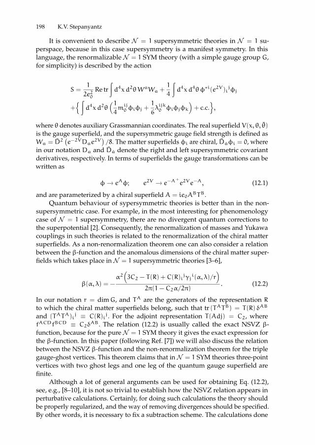
ii

“proc17” — 2017/12/11 — 19:44 — page 198 — #212 ii

ii

ii

198 K.V. Stepanyantz

It is convenient to describe N = 1 supersymmetric theories in N = 1 su-perspace, because in this case supersymmetry is a manifest symmetry. In thislanguage, the renormalizable N = 1 SYM theory (with a simple gauge group G,for simplicity) is described by the action

S =1

2e20Re tr

∫d4xd2θWaWa +

1

4

∫d4xd4θφ∗i(e2V)i

jφj

+ ∫

d4xd2θ(14mij0 φiφj +

1

6λijk0 φiφjφk

)+ c.c.

,

where θ denotes auxiliary Grassmannian coordinates. The real superfield V(x, θ, θ)is the gauge superfield, and the supersymmetric gauge field strength is defined asWa = D2

(e−2VDae

2V)/8. The matter superfields φi are chiral, Daφi = 0, where

in our notation Da and Da denote the right and left supersymmetric covariantderivatives, respectively. In terms of superfields the gauge transformations can bewritten as

φ→ eAφ; e2V → e−A+

e2Ve−A, (12.1)

and are parameterized by a chiral superfield A = ie0ABTB.

Quantum behaviour of sypersymmetric theories is better than in the non-supersymmetric case. For example, in the most interesting for phenomenologycase of N = 1 supersymmetry, there are no divergent quantum corrections tothe superpotential [2]. Consequently, the renormalization of masses and Yukawacouplings in such theories is related to the renormalization of the chiral mattersuperfields. As a non-renormalization theorem one can also consider a relationbetween the β-function and the anomalous dimensions of the chiral matter super-fields which takes place in N = 1 supersymmetric theories [3–6],

β(α, λ) = −α2(3C2 − T(R) + C(R)i

jγji(α, λ)/r

)2π(1− C2α/2π)

. (12.2)

In our notation r = dimG, and TA are the generators of the representation Rto which the chiral matter superfields belong, such that tr (TATB) = T(R) δAB

and (TATA)ij ≡ C(R)i

j. For the adjoint representation T(Adj) = C2, wherefACDfBCD ≡ C2δ

AB. The relation (12.2) is usually called the exact NSVZ β-function, because for the pure N = 1 SYM theory it gives the exact expression forthe β-function. In this paper (following Ref. [7]) we will also discuss the relationbetween the NSVZ β-function and the non-renormalization theorem for the triplegauge-ghost vertices. This theorem claims that in N = 1 SYM theories three-pointvertices with two ghost legs and one leg of the quantum gauge superfield arefinite.

Although a lot of general arguments can be used for obtaining Eq. (12.2),see, e.g., [8–10], it is not so trivial to establish how the NSVZ relation appears inperturbative calculations. Certainly, for doing such calculations the theory shouldbe properly regularized, and the way of removing divergences should be specified.By other words, it is necessary to fix a subtraction scheme. The calculations done

ii

“proc17” — 2017/12/11 — 19:44 — page 199 — #213 ii

ii

ii

12 Structure of Quantum Corrections inN = 1. . . 199

with the dimensional reduction [11] in the DR-scheme in the three- and four-loopapproximations [12–14,16] demonstrated that Eq. (12.2) does not take place startingfrom the three-loop approximation. However, one can explain the disagreementby the scheme dependence of the NSVZ relation [17,18]. A possibility of thisexplanation is non-trivial due to some scheme-independent consequences of theNSVZ relation [18,19]. Thus, with the dimensional reduction the NSVZ equationshould be obtained by a special tuning of the subtraction scheme in every order,while the general all-order prescription giving the NSVZ scheme is absent.

Also it should be noted that the dimensional reduction is not mathematicallyconsistent [20], and can break supersymmetry in higher orders [21,22]. That is whythe use of other regularizations is also reasonable and interesting. In this paper wewill mostly discuss various application of the Slavnov higher covariant derivativeregularization [23,24] to calculating quantum corrections inN = 1 supersymmetrictheories. Unlike the dimensional reduction, this regularization is consistent andcan be formulated in a manifestly N = 1 supersymmetric way [25,26]. It is alsoapplicable to theories with N = 2 supersymmetry [27–29]. The main idea ofthis regularization is to add a term with higher degrees of covariant derivativesto the action of a theory. Then divergences beyond the one-loop approximationdisappear, while the remaining one-loop divergences are regularized by insertingthe Pauli–Villars determinants into the generating functional [30]. In this paper wewill demonstrate that this regularization allows to reveal some interesting featuresof quantum corrections in supersymmetric theories which are missed in the caseof using the dimensional technique.

12.2 NSVZ relation inN = 1 SQED

12.2.1 Higher derivative regularization in the Abelian case

We will start with the simplest N = 1 supersymmetric gauge theory, namely,the N = 1 supersymmetric electrodynamics (SQED) with Nf flavors. In the mass-less case this theory is described by the action

S =1

4e20Re∫d4xd2θWaWa +

Nf∑f=1

1

4

∫d4xd4θ

(φ∗fe

2Vφf + φ∗fe

−2V φf

), (12.3)

which is written in terms of N = 1 superfields. In this formalism supersymmetryis a manifest symmetry of the theory. The usual gauge field is now a component ofthe real gauge superfield V . The terms containing the chiral matter superfields φfand φf produce Dirac fermions and the other terms needed for supersymmetry in-variance. In the Abelian case the supersymmetric gauge field strength is describedby the chiral spinor superfield Wa = D2DaV/4. For the theory (12.3) the NSVZβ-function (12.2) takes the form [31,32]

β(α) =α2Nf

π

(1− γ(α)

). (12.4)

ii

“proc17” — 2017/12/11 — 19:44 — page 200 — #214 ii

ii

ii


To regularize the theory (12.3) by the Slavnov higher derivatives method, weadd the term

SΛ =1

4e20Re∫d4xd2θWa

(R(∂2/Λ2) − 1

)Wa (12.5)

to the classical action, where the function R(∂2/Λ2) contains higher degrees ofderivatives. Note that for Abelian theories one should use the usual deriva-tives (instead of the covariant ones). In the simplest case it is possible to chooseR = 1 + ∂2n/Λ2n. Due to the presence of the higher derivative term, the propa-gator of the gauge superfield contains higher degrees of the momentum in thedenominator, and all diagrams beyond the one-loop approximation become finite.For removing the remaining one-loop divergences, following Ref. [30], we insertinto the generating functional the Pauli–Villars determinants,

Z =

∫Dµ∏I

(detPV(V,MI)

)NfcIexpiSreg + iSgf + iSSources

, (12.6)

with the constants cI satisfying the conditions∑I cI = 1;

∑I cIM

2I = 0. Here

MI = aIΛ (where aI are constants independent of α0) are masses of the Pauli–Villars superfields proportional to the parameter Λ which enters the regulatorfunction R.

Below we will see that the NSVZ equation follows from the underlyingrelation between the two-point Green functions. In N = 1 SQED these two-pointGreen functions are related to the corresponding part of the effective action by theequation

Γ (2) =

∫d4p

(2π)4d4θ

(−

1

16πV(−p)∂2Π1/2V(p)d

−1(α0, Λ/p)

+1

4

Nf∑f=1

(φ∗f(−p, θ)φf(p, θ) + φ

∗f(−p, θ)φf(p, θ)

)G(α0, Λ/p)

). (12.7)

Here ∂2Π1/2 ≡ −DaD2Da/8 is a supersymmetric transversal projection operator,and the transversality of the gauge superfield two-point function follows from theSlavnov–Taylor identities.

The function d−1 expressed in terms of the renormalized coupling constantα(α0, Λ/µ) should be finite in the limit Λ→∞. The charge renormalization con-stant Z3 is then defined as Z3(α,Λ/µ) ≡ α/α0. To construct the renormalizationconstant Z for the chiral matter superfields, we require finiteness of the functionZ(α,Λ/µ)G(α0, Λ/p) in the limit Λ→∞.

According to [33], it is important to distinguish the renormalization groupfunctions (RGF) defined in terms of the bare coupling constant and the onesdefined in terms of the renormalized coupling constant. In terms of the barecoupling constant RGF are defined by the equations

β(α0) ≡dα0

d lnΛ

∣∣∣α=const

; γ(α0) ≡ −d lnZd lnΛ

∣∣∣α=const

. (12.8)

ii

“proc17” — 2017/12/11 — 19:44 — page 201 — #215 ii

ii

ii


They are independent of a renormalization prescription for a fixed regularization,see, e.g., [33], but depend on the regularization. Below we will see that for thetheory (12.3) these RGF satisfy the NSVZ relation in all loops in the case of usingthe above described version of the higher derivative regularization.

12.2.2 Charge renormalization in the lowest loops

Explicit calculations in the lowest loops made with the higher covariantderivative regularization demonstrated that loop integrals giving a β-functiondefined in terms of the bare coupling constant are integrals of total derivatives[34]. They can be also presented as integrals of double total derivatives [35]. Theβ-function of N = 1 SQED with Nf flavours, regularized by higher derivatives, iscalculated by the help of the equation

β(α0)

α20=

d

d lnΛ

(d−1(α0, Λ/p) − α

−10

)∣∣∣p=0

. (12.9)

By other words, we calculate the two-point Green function of the gauge superfieldand differentiate it with respect to lnΛ in the limit of the vanishing externalmomentum. For example, the two-loop result for the β-function written as theintegral of double total derivatives has the form

β(α0)

α20= 2πNf

d

d lnΛ

∫d4q

(2π)4∂

∂qµ∂

∂qµ

∑I

cIln(q2 +M2

I )

q2+

∫d4k

(2π)4

× 2e2

k2Rk

( 1

q2(k+ q)2−∑I

cI1

(q2 +M2I )((k+ q)

2 +M2I )

)+O(e4). (12.10)

The (essentially larger) three-loop expression can be found, e.g., in [36]. Note thatthe β-function does not vanish because of integrand singularities. This can beillustrated by a simple example: consider a nonsingular function f(q2) rapidlydecreasing at infinity. Then∫

d4q

(2π)4∂

∂qµ

(qµq4f(q2)

)= −

1

8π2f(0). (12.11)

Doing similar calculations it is possible to decrease the number of integrations inEq. (12.10) and reduce this expression to the integral giving the one-loop anoma-lous dimension of the matter superfield (also defined in terms of the bare couplingconstant),

β(α0)

α20=Nf

π

(1−

d

d lnΛlnG(α0, Λ/q)

∣∣∣q=0

)=Nf

π

(1− γ(α0)

). (12.12)

ii

“proc17” — 2017/12/11 — 19:44 — page 202 — #216 ii

ii

ii


12.2.3 NSVZ relation in all loops

The all-loop derivation of the NSVZ relation for RGF defined in terms of thebare coupling constant by the direct summing of supergraphs for N = 1 SQEDregularized by higher derivatives has been made in [37,38] and verified at thethree-loop level in [39]. Here we briefly explain the main ideas of the method ofRef. [37].

First, it is necessary to prove that all loop integrals for the β-function definedin terms of the bare coupling constant are integrals of double total derivatives. Forthis purpose it is convenient to use the background field method which (in theAbelian case) is introduced by making the replacement V → V +V, where V is thebackground gauge superfield, in the action. Then we make the formal substitutionV → θ4, after which

d∆Γ(2)V

d lnΛ

∣∣∣V=θ4

=1

2πV4 ·

d

d lnΛ

(d−1(α0, Λ/p) − α

−10

)=1

2πV4 ·

β(α0)

α20, (12.13)

where V4 is the (properly regularized) volume of the space-time.For N = 1 SQED the functional integrals over the matter superfield are Gaus-

sian and can be calculated exactly. This allows operating with some expressionsvalid in all loops. In particular, it is possible to find the formal expression for thetwo-point function of the background gauge superfield. Then after the substitutionV → θ4 we try to present the result as an integral of double total derivatives. Inthe coordinate representation an integral of a total derivative is written as

Tr([xµ, Something]

)− Singularities = −Singularities. (12.14)

After some non-trivial transformations the result for the expression (12.13) canbe presented as a trace of double commutator, i.e. as an integral of a double totalderivative. The details of this calculation are described in Ref. [37]. The resultdoes not vanish due to singularities of the integrand, which can be summed in allorders. This gives

d∆Γ (2)

d lnΛ

∣∣∣V=θ4

=Nf

2π2V4(1−

d lnGd lnΛ

∣∣∣q=0

)=Nf

2π2V4(1− γ(α0)

), (12.15)

and we obtain the exact all-order result

β(α0)

α20=Nf

π

(1− γ(α0)

). (12.16)

Note that this equation is valid for an arbitrary renormalization prescription inthe case of using the higher derivative regularization, because RGF entering it aredefined in terms of the bare coupling constant.

In graphical language, this result can be explained as follows [35] (see also[40]): If we have a supergraph without external lines, then a contribution to the

ii

“proc17” — 2017/12/11 — 19:44 — page 203 — #217 ii

ii

ii


β-function can be constructed by attaching two external lines of the backgroundgauge superfield V to it, while a contribution to the anomalous dimension isobtained by cutting matter lines in the considered supergraph. The equation(12.16) relates both these contributions.

12.2.4 How to construct the NSVZ scheme inN = 1 SQED

Eq. (12.16) is valid for RGF defined in terms of the bare coupling constant.However, RGF are standardly defined by a different way, in terms of the renormal-ized coupling constant,

β(α) ≡ dα

d lnµ

∣∣∣α0=const

; γ(α) ≡ d lnZd lnµ

∣∣∣α0=const

, (12.17)

and are scheme-dependent. However, both definitions of RGF give the samefunctions, if the conditions

Z3(α, x0) = 1; Z(α, x0) = 1 (12.18)

are imposed on the renormalization constants, in which x0 is a fixed value ofx = lnΛ/µ [18,19,33]: β(α0) = β(α0); γ(α0) = γ(α0).

β and γ are scheme-dependent and satisfy the NSVZ equation only in acertain (NSVZ) scheme. Now, from Eq. (12.16) and the above arguments it isevident that for the theory regularized by higher derivatives this NSVZ scheme isfixed in all loops by the boundary conditions (12.18).

The general statements discussed above can be verified by explicit calculationsin the lowest loops. They are non-trivial starting from the three-loop approxima-tion, because the β-function and the anomalous dimension are scheme-dependentstarting from the three- and two-loop order, respectively.

For the higher derivative regulator Rk = 1+ k2n/Λ2n

1

α0=1

α−Nf

π

(lnΛ

µ+ b1

)−αNf

π2

(lnΛ

µ+ b2

)−α2Nf

π3

(Nf2

ln2Λ

µ

− lnΛ

µ

(Nf∑I

cI lnaI +Nf +1

2−Nfb1

)+ b3

)+O(α3); (12.19)

Z = 1+α

π

(lnΛ

µ+ g1

)+α2(Nf + 1)

2π2ln2

Λ

µ−α2

π2lnΛ

µ

×(Nf∑I

cI lnaI −Nfb1 +Nf +1

2− g1

)+α2g2

π2+O(α3), (12.20)

where bi and gi are arbitrary finite constants, which fix a subtraction scheme.Differentiating Eqs. (12.19) and (12.20) with respect to lnΛ we construct RGFdefined in terms of the bare coupling constant,

ii

“proc17” — 2017/12/11 — 19:44 — page 204 — #218 ii

ii

ii


β(α0)

α20=Nf

π+α0Nf

π2−α20Nf

π3

(Nf∑I

cI lnaI +Nf +1

2

)+O(α30); (12.21)

γ(α0) = −α0

π+α20π2

(Nf∑I

cI lnaI +Nf +1

2

)+O(α30), (12.22)

which appear to be independent of the constants bi and gi and to satisfy the NSVZrelation. However, RGF defined in terms of the renormalized coupling constant,

β(α)

α2=Nf

π+αNf

π2−α2Nf

π3

(Nf∑I

cI lnaI +Nf +1

2+Nf(b2 − b1)

)+O(α3); (12.23)

γ(α) = −α

π+α2

π2

(Nf +

1

2+Nf

∑I

cI lnaI −Nfb1 +Nfg1)+O(α3) (12.24)

depend on these constants and, therefore, on a subtraction scheme. This sub-traction scheme can be fixing, e.g., by imposing the conditions (12.18). Choosingx0 = 0, from these equations we obtain g2 = b1 = b2 = b3 = 0. Therefore, in thisscheme only powers of lnΛ/µ are included into the renormalization constants,while all finite constants vanish. Thus, the considered scheme looks very similarto the minimal subtractions. However, now we use the higher derivative regu-larization, so that it is reasonable to call this scheme HD + MSL, where MSL isthe abbreviation for Minimal Subtraction of Logarithms. Substituting the abovevalues of the finite constants into Eqs. (12.23) and (12.24), it is easy to see that inthis scheme these RGF satisfy the NSVZ relation.

12.2.5 Quantum corrections with the dimensional reduction

It is well known [12–14] that in the DR-scheme the NSVZ relation is notvalid starting from the three-loop approximation. However, to obtain it, onecan specially tune a subtraction scheme in each order. It is also possible to trymaking calculations similarly to the higher derivative case [41,42]. However, thecorresponding relation between the functions d−1 and G (which is at presentobtained only in the lowest orders) has a more complicated form, than for thehigher derivative case. The boundary conditions analogous to (12.18) can also bewritten, but the right hand side of one of them is a series in α. It was demonstratedthat such a structure agrees with the results obtained in [13,14].

12.2.6 NSVZ-like relation in softly broken N = 1 SQED regularized byhigher derivatives

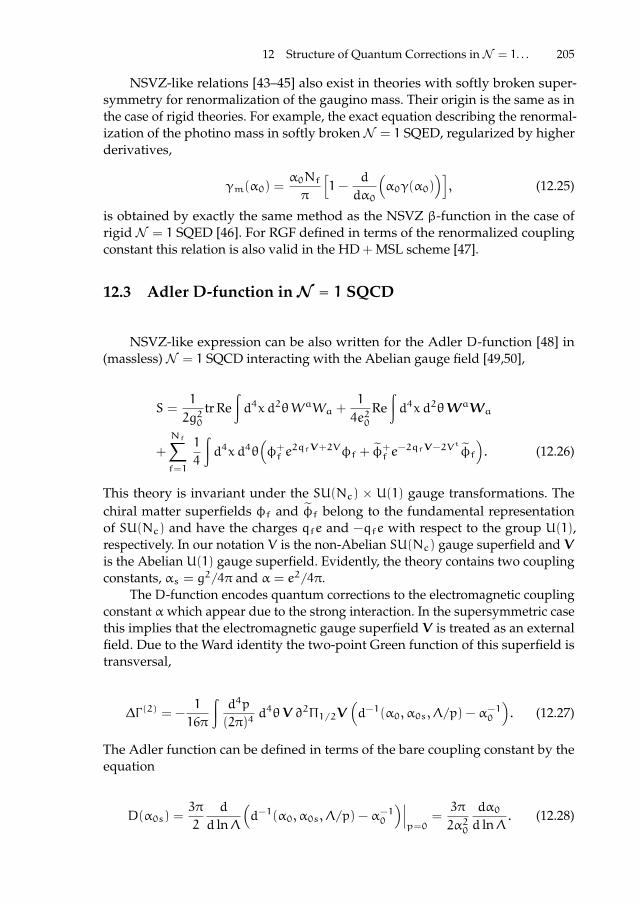
ii

“proc17” — 2017/12/11 — 19:44 — page 205 — #219 ii

ii

ii


NSVZ-like relations [43–45] also exist in theories with softly broken super-symmetry for renormalization of the gaugino mass. Their origin is the same as inthe case of rigid theories. For example, the exact equation describing the renormal-ization of the photino mass in softly broken N = 1 SQED, regularized by higherderivatives,

γm(α0) =α0Nf

π

[1−

d

dα0

(α0γ(α0)

)], (12.25)

is obtained by exactly the same method as the NSVZ β-function in the case ofrigid N = 1 SQED [46]. For RGF defined in terms of the renormalized couplingconstant this relation is also valid in the HD + MSL scheme [47].

12.3 AdlerD-function inN = 1 SQCD

NSVZ-like expression can be also written for the Adler D-function [48] in(massless) N = 1 SQCD interacting with the Abelian gauge field [49,50],

S =1

2g20tr Re

∫d4xd2θWaWa +

1

4e20Re∫d4xd2θWaWa

+

Nf∑f=1

1

4

∫d4xd4θ

(φ+f e2qfV+2Vφf + φ

+f e

−2qfV−2Vtφf

). (12.26)

This theory is invariant under the SU(Nc) × U(1) gauge transformations. Thechiral matter superfields φf and φf belong to the fundamental representationof SU(Nc) and have the charges qfe and −qfe with respect to the group U(1),respectively. In our notation V is the non-Abelian SU(Nc) gauge superfield and Vis the Abelian U(1) gauge superfield. Evidently, the theory contains two couplingconstants, αs = g2/4π and α = e2/4π.

The D-function encodes quantum corrections to the electromagnetic couplingconstant αwhich appear due to the strong interaction. In the supersymmetric casethis implies that the electromagnetic gauge superfield V is treated as an externalfield. Due to the Ward identity the two-point Green function of this superfield istransversal,

∆Γ (2) = −1

16π

∫d4p

(2π)4d4θV ∂2Π1/2V

(d−1(α0, α0s, Λ/p) − α

−10

). (12.27)

The Adler function can be defined in terms of the bare coupling constant by theequation

D(α0s) =3π

2

d

d lnΛ

(d−1(α0, α0s, Λ/p) − α

−10

)∣∣∣p=0

=3π

2α20

dα0

d lnΛ. (12.28)

ii

“proc17” — 2017/12/11 — 19:44 — page 206 — #220 ii

ii

ii


Again, this function depends on regularization, but is independent of a renormal-ization prescription for a fixed regularization.

According to [49,50], in the case of using the higher covariant derivativeregularization1 the exact expression for the Adler function for the consideredtheory can be written in the NSVZ-like form

D(α0s) =3

2

∑f

q2f ·Nc(1− γ(α0s)

). (12.29)

It looks very similar to the NSVZ β-function in N = 1 SQED and is derived in allloops by exactly the same method. However, Eq. (12.29) contains the anomalousdimension of the non-Abelian theory, and this is a very essential difference fromthe N = 1 SQED case. Recently this expression has been confirmed by an explicitthree-loop calculation in Ref. [51].

12.4 Non-AbelianN = 1 supersymmetric theories

12.4.1 Regularization and renormalization

Let us consider the theory described by the action (12.1) in the massless limit.It is convenient to do calculations using the background field method introducedby replacement e2V → eΩ

+

e2VeΩ. The background gauge superfield V is thenrelated toΩ andΩ+ by the equation e2V = eΩ

+

eΩ. The higher derivative termin this case can be written in the form

SΛ =1

2e20Re tr

∫d4xd2θ eΩeΩWae−Ωe−Ω

[R(−∇2∇2

16Λ2

)− 1]Adj

eΩeΩ

×Wae−Ωe−Ω +1

4

∫d4xd4θφ+eΩ

+

eΩ+[F(−∇2∇2

16Λ2

)− 1]eΩeΩφ, (12.30)

where the functions R(x) and F(x) rapidly increase at infinity and satisfy thecondition R(0) = F(0) = 1. It is convenient to fix a gauge without breaking thebackground gauge invariance. For this purpose it is possible to use the gaugefixing term

Sgf = −1

16ξ0e20

tr∫d4xd4θ∇2VK

(−∇2∇2

16Λ2

)Adj∇2V, (12.31)

where K(0) = 1 and K(x) also rapidly grows at infinity. The corresponding actionsfor ghosts and the Pauli–Villars determinants can be found in Ref. [52], where theyare discussed in all details. The renormalization constants are introduced by theequations

1 The higher derivative term for the considered theory should contain covariant derivatives∇a = e−Ω

+

DaeΩ+

; ∇a = eΩDae−Ω, where e2V = eΩ

+

eΩ.

ii

“proc17” — 2017/12/11 — 19:44 — page 207 — #221 ii

ii

ii


1

α0=Zα

α; V = ZVZ

−1/2α VR; cc = ZcZ

−1α cRcR; φi = (

√Zφ)i

j(φR)j,

(12.32)where c and c are the chiral Faddeev–Popov ghost superfields.

12.4.2 Finiteness of the triple gauge-ghost vertices

InN = 1 gauge supersymmetric theories the three-point gauge-ghost vertices(c Vc, c+Vc, c Vc+, and c+Vc+) with two ghost legs and a single leg of the quantumgauge superfield are finite [7], so that

d

d lnΛ(Z−1/2α ZcZV) = 0. (12.33)

(At the one-loop level it was found in [52].) This theorem is derived by the help ofthe Slavnov–Taylor identities, which can be obtained using the standard methods[53,54]. To write the identity for the considered three-point functions, we introducethe chiral source J and the source term

−e0

2

∫d4xd2θ fABCJAcBcC + c.c. (12.34)

Then using the superspace Feynman rules it is possible to prove that the effectivevertex

δ3Γ

δcCz δcDwδJ By

=e0

4fBCD

∫d4p

(2π)4d4q

(2π)4H(p, q)D2zδ

8zy(q+ p)D2wδ

8yw(q) (12.35)

is finite in all orders. Really, we can present the corresponding superdiagrams asintegrals over the total superspace, which include integration over

∫d4θ = −

1

2

∫d2θD2 + total derivatives in the coordinate space. (12.36)

Consequently, due to chirality of all external legs the non-vanishing result can beobtained only if two right spinor derivatives also act to the external legs. Thus,commuting supersymmetric covariant derivatives, we see that the result shouldbe proportional to, at least, second degree of the external momenta and is finite inthe ultraviolet region.

From dimensional and chirality considerations one can write the followingexpression for the one of triple gauge-ghost Green functions,

δ3Γ

δc∗Ax δVBy δcCz

= −ie0

16fABC

∫d4p

(2π)4d4q

(2π)4

(f(p, q)∂2Π1/2

−Fµ(p, q)(γµ)a

bDaDb + F(p, q))y

(D2xδ

8xy(q+ p) D2zδ

8yz(q)

), (12.37)

ii

“proc17” — 2017/12/11 — 19:44 — page 208 — #222 ii

ii

ii


where δ8xy(p) ≡ δ4(θx − θy)eipα(xα−yα). Then the Slavnov–Taylor identity can be

written in the form

Gc(q)F(q, p) +Gc(p)F(p, q) = 2Gc(q+ p)H(−q− p, q), (12.38)

where Gc(q) is the two-point Green function for the Faddeev–Popov ghosts. Mul-tiplying this equation to Zc, differentiating the result with respect to lnΛ andsetting p = −qwe obtain finiteness of the function F(−q, q), which follows fromthe finiteness of (Gc)R and H in the limit Λ→∞. This means that the correspond-ing renormalization constant is finite, see Eq. (12.33). Consequently, all three-pointghost-gauge vertices are also finite.

12.4.3 Vcc-vertices in the one-loop approximation

In the one-loop approximation (after the Wick rotation)

F(p, q) = 1+e20C2

4

∫d4k

(2π)4

−

(q+ p)2

Rkk2(k+ p)2(k− q)2−

ξ0 p2

Kkk2(k+ q)2

× 1

(k+ q+ p)2+

ξ0 q2

Kkk2(k+ p)2(k+ q+ p)2+( ξ0Kk

−1

Rk

)(−

1

k2(k+ q)2

−1

k2(k+ p)2+

2

k2(k+ q+ p)2−

2(q+ p)2

k4(k+ q+ p)2

)+O(α20, α0λ

20). (12.39)

It is easy to see that this expression is finite in the UV region. The other functionsin Eq. (12.37) are also finite, see [7]. The finiteness of the function H, defined in Eq.(12.35), at the one-loop level has also been demonstrated,

H(p, q) = 1−e20C2

4

∫d4k

(2π)4

p2

Rkk2(k+ q)2(k+ q+ p)2+

(q+ p)2

k4(k+ q+ p)2

×( ξ0Kk

−1

Rk

)+

q2

k4(k+ q)2

( ξ0Kk

−1

Rk

)+O(e40, e

20λ20). (12.40)

12.4.4 New form of the NSVZ relation

Let write the NSVZ relation (12.2) for RGF defined in terms of the barecouplings (see the definitions in Ref. [7]) in the form

β(α0, λ0)

α20= −

3C2 − T(R) + C(R)ij(γφ)j

i(α0, λ0)/r

2π+C2

2π· β(α0, λ0)

α0(12.41)

and take into account that the β-function can be related to the renormalizationconstant Zα,

ii

“proc17” — 2017/12/11 — 19:44 — page 209 — #223 ii

ii

ii


β(α0, λ0) =dα0(α, λ,Λ/µ)

d lnΛ

∣∣∣α,λ=const

= −α0d lnZαd lnΛ


. (12.42)

Then the right hand side of Eq. (12.41) can be expressed in terms of γc and γV bythe help of Eq. (12.33),

β(α0, λ0) = −2α0d ln(ZcZV)d lnΛ


= 2α0

(γc(α0, λ0) + γV(α0, λ0)

). (12.43)

Substituting this identity into Eq. (12.41) we rewrite the exact NSVZ β-function ina different form,

β(α0, λ0)

α20= −

1

2π

(3C2 − T(R) − 2C2γc(α0, λ0) − 2C2γV(α0, λ0)

+C(R)ij(γφ)j

i(α0, λ0)/r). (12.44)

Eq. (12.44) admits a simple graphical interpretation similar to the Abelian case.Consider a supergraph without external lines. By attaching two external legsof the superfield V we obtain a set of diagrams contributing to the β-function.From the other side, cutting internal lines gives superdiagrams contributing tothe anomalous dimensions of the Faddeev–Popov ghosts, of the quantum gaugesuperfield, and of the matter superfields. Eq. (12.44) relates these two sets ofsuperdiagrams.

12.4.5 The NSVZ scheme for non-Abelian gauge theories

The RGF standardly defined in terms of the renormalized couplings (weagain denote them by tildes) are scheme-dependent and satisfy the NSVZ relationonly in a certain (NSVZ) subtraction scheme. Let us suggest that, similar to theAbelian case, RGF defined in terms of the bare couplings satisfy the NSVZ relation(12.44) in the case of using the higher covariant derivative regularization. Really,the qualitative way of its derivation looks exactly as in N = 1 SQED and thefactorization into total derivatives [55,56] and double total derivatives [57] alsotakes place at least in the lowest orders. Then, repeating the argumentation of Ref.[33], one can prove that in the non-Abelian case both definitions of RGF give thesame result (for coinciding arguments) if the renormalization constants satisfy theconditions

Zα(α, λ, x0) = 1; (Zφ)ij(α, λ, x0) = δi

j; Zc(α, λ, x0) = 1. (12.45)

Thus, under the assumption that the NSVZ relation is valid for RGF defined interms of the bare couplings with the higher derivative regularization, the NSVZscheme is given by the boundary conditions (12.45). Again, it is easy to see that forx0 = 0 in this scheme only powers of lnΛ/µ are included into the renormalizationconstants, so that the NSVZ scheme coincides with HD + MSL. Certainly, it is alsoassumed that ZV = Z

1/2α Z−1

c due to the non-renormalization of the Vcc-vertices.

ii

“proc17” — 2017/12/11 — 19:44 — page 210 — #224 ii

ii

ii


12.4.6 Checking the new form of the NSVZ relation by explicit calculations

To check the above results, we consider terms quartic in the Yukawa couplings[58] corresponding to the graphs presented in Fig. 12.1.

Fig. 12.1. The terms in the NSVZ relation which are investigated here are obtained fromthese two graphs.

Attaching two external lines of the background gauge superfield gives alarge number of two- and three-loop diagrams contributing to the β-function. Thecorresponding diagrams for the anomalous dimension are obtained by cuttinginternal lines in the considered graphs. The result for the considered part of theβ-function defined in terms of the bare couplings can be presented as an integralof double total derivatives,

∆β(α0, λ0)

α20= −

2π

rC(R)i

j d

d lnΛ

∫d4k

(2π)4d4q

(2π)4λimn0 λ∗0jmn

∂

∂qµ

∂

∂qµ

×( 1

k2Fk q2Fq (q+ k)2Fq+k

)+4π

rC(R)i

j d

d lnΛ

∫d4k

(2π)4d4l

(2π)4d4q

(2π)4

×

(λiab0 λ∗0kabλ

kcd0 λ∗0jcd

( ∂

∂kµ

∂

∂kµ−

∂

∂qµ

∂

∂qµ

)+ 2λiab0 λ∗0jacλ

cde0 λ∗0bde

× ∂

∂qµ

∂

∂qµ

)1

k2F2k q2Fq (q+ k)2Fq+k l2Fl (l+ k)2Fl+k

. (12.46)

Taking one of loop integrals it is possible to relate this expression to the correspond-ing contribution to the anomalous dimension of the matter superfield (defined interms of the bare couplings),

∆β(α0, λ0)

α20= −

1

2πrC(R)i

j∆γφ(λ0)ji. (12.47)

This equation completely agrees with Eq. (12.44), so that the NSVZ relation issatisfied for terms of the considered structure.

For F(k2/Λ2) = 1+ k2/Λ2 all loop integrals can be calculated,

∆γφ(α0, λ0)ji =

1

4π2λiab0 λ∗0jab −

1

16π4λiab0 λ∗0jacλ

cde0 λ∗0bde. (12.48)

ii

“proc17” — 2017/12/11 — 19:44 — page 211 — #225 ii

ii

ii


Scheme-dependent RGF defined in terms of the renormalized couplings have beencalculated in Ref. [58]. The contribution to the β-function depends on some finiteconstants g1 and b2, which appear due to arbitrariness of choosing a subtractionscheme,

γφ(α, λ)ji =

1

4π2λiabλ∗jab −

1

16π4λiabλ∗jacλ

cdeλ∗bde +O(α) +O(λ6); (12.49)

β(α, λ)

α2= −

1

2π

(3C2 − T(R)

)+

1

2πrC(R)i

j[−

1

4π2λiabλ∗jab +

1

16π4

×λiabλ∗kabλkcdλ∗jcd(b2 − g1

)+

1

16π4λiabλ∗jacλ

cdeλ∗bde

(1+ 2b2 − 2g1

)]+O(α) +O(λ6). (12.50)

We see that for an arbitrary values of g1 and b2 the NSVZ relation is not valid.However, the values of g1 and b2 can be fixed by imposing the conditions (12.45).In this case g1 = b2 = −x0, so that b2 − g1 = 0. Therefore, in this scheme

β(α, λ)

α2= −

1

2π

(3C2 − T(R)

)−

1

2πrC(R)i

jγφ(α, λ)ij +O(α) +O(λ6). (12.51)

This confirms the guess that Eq. (12.45) gives the NSVZ scheme in the non-Abeliancase.

Note that recently [59] the identity (12.44) has been completely checked inthe two-loop approximation in the case of using the non-invariant version of thehigher covariant derivative regularization supplemented by a special subtractionprocedure which restores the Slavnov–Taylor identities [60].

12.5 Conclusion

The β-function defined in terms of the bare coupling constant for N = 1

supersymmetric gauge theories regularized by higher derivatives is given byintegrals of double total derivatives. In some cases it has been proved in allloops, but for general non-Abelian SYM theories at present there are only strongevidences in favour of this. Such a structure of quantum corrections naturallyleads to the NSVZ relation for RGF defined in terms of the bare coupling constant,which is obtained after taking the integral of the total derivative and is validindependently of the subtraction scheme. Note that in the non-Abelian case animportant ingredient of the derivation is the finiteness of the three-point ghost-gauge vertices, which allows rewriting the NSVZ equation in a different form.

The RGF defined in terms of the renormalized couplings satisfy the NSVZrelation only in a certain (NSVZ) scheme, which is obtained with the higherderivative regularization by minimal subtraction of logarithms. This means thatonly powers of lnΛ/µ are included into various renormalization constants. This

ii

“proc17” — 2017/12/11 — 19:44 — page 212 — #226 ii

ii

ii


prescription can be also reformulated by imposing simple boundary conditions onthe renormalization constants.

All general statements considered here are confirmed by explicit perturbativecalculations. Note that some of them are made in the three-loop approximationand are highly non-trivial.

Acknowledgements

I am very grateful to the organizers of the twentieth workshop ”What ComesBeyond the Standard Model” (July 9-17, 2017, Bled, Slovenia) for kind hospitalityand to all participants for very helpful discussions. Also I would like to express mydeep thanks to A.L.Kataev for numerous discussions of various topics consideredin this paper.

References

1. R.N.Mohapatra, “Unification And Supersymmetry. The Frontiers Of Quark - Lepton Physics:The Frontiers Of Quark-lepton Physics,” New York, USA: Springer (2003) 421 p.

2. M.T.Grisaru, W.Siegel and M.Rocek, Nucl. Phys. B 159 (1979) 429.3. V.A.Novikov, M.A.Shifman, A.I.Vainshtein and V.I.Zakharov, Nucl. Phys. B 229, (1983)

381.4. D.R.T.Jones, Phys. Lett. B 123, (1983) 45.5. V.A.Novikov, M.A.Shifman, A.I.Vainshtein and V.I.Zakharov, Phys. Lett. B 166, (1986)

329; Sov. J. Nucl. Phys. 43 (1986) 294.6. M.A.Shifman and A.I.Vainshtein, Nucl. Phys. B 277, (1986) 456; Sov. Phys. JETP 64,

(1986) 428.7. K.V.Stepanyantz, Nucl. Phys. B 909, (2016) 316.8. M.A.Shifman and A.I.Vainshtein, “Instantons versus supersymmetry: Fifteen years later,”

In *Shifman, M.A.: ITEP lectures on particle physics and field theory, vol. 2* 485-647.9. N.Arkani-Hamed and H.Murayama, JHEP 0006, (2000) 030.

10. E.Kraus, C.Rupp and K.Sibold, Nucl. Phys. B 661, (2003) 83.11. W.Siegel, Phys. Lett. B 84, (1979) 193.12. L.V.Avdeev and O.V.Tarasov, Phys. Lett. 112B, (1982) 356.13. I.Jack, D.R.T.Jones and C.G.North, Phys. Lett. B 386, (1996) 138.14. I.Jack, D.R.T.Jones and C.G.North, Nucl. Phys. B 486, (1997) 479.15. I.Jack, D.R.T.Jones and A.Pickering, Phys. Lett. B 435, (1998) 61.16. R.V.Harlander, D.R.T.Jones, P.Kant, L.Mihaila and M.Steinhauser, JHEP 0612, (2006)

024.17. D.Kutasov and A.Schwimmer, Nucl. Phys. B 702, (2004) 369.18. A.L.Kataev and K.V.Stepanyantz, Theor. Math. Phys. 181, (2014) 1531.19. A.L.Kataev and K.V.Stepanyantz, Phys. Lett. B 730, (2014) 184.20. W.Siegel, Phys. Lett. B 94, (1980) 37.21. L.V.Avdeev, Phys. Lett. B 117, (1982) 317.22. L.V.Avdeev and A.A.Vladimirov, Nucl. Phys. B 219, (1983) 262.23. A.A.Slavnov, Nucl. Phys. B 31, (1971) 301.24. A.A.Slavnov, Theor.Math.Phys. 13, (1972) 1064.25. V.K.Krivoshchekov, Theor. Math. Phys. 36, (1978) 745.26. P.C.West, Nucl. Phys. B 268, (1986) 113.

ii

“proc17” — 2017/12/11 — 19:44 — page 213 — #227 ii

ii

ii


27. V.K.Krivoshchekov, Phys. Lett. B 149, (1984) 128.28. I.L.Buchbinder and K.V.Stepanyantz, Nucl. Phys. B 883, (2014) 20.29. I.L.Buchbinder, N.G.Pletnev and K.V.Stepanyantz, Phys. Lett. B 751, (2015) 434.30. A.A.Slavnov, Theor. Math. Phys. 33, (1977) 977.31. A.I.Vainshtein, V.I.Zakharov and M.A.Shifman, JETP Lett. 42, (1985) 224.32. M.A.Shifman, A.I.Vainshtein and V.I.Zakharov, Phys. Lett. B 166 (1986) 334.33. A.L.Kataev and K.V.Stepanyantz, Nucl. Phys. B 875, (2013) 459.34. A.A.Soloshenko and K.V.Stepanyantz, Theor. Math. Phys. 140, (2004) 1264.35. A.V.Smilga and A.Vainshtein, Nucl. Phys. B 704, (2005) 445.36. K.V.Stepanyantz, J. Phys. Conf. Ser. 343, (2012) 012115.37. K.V.Stepanyantz, Nucl. Phys. B 852, (2011) 71.38. K.V.Stepanyantz, JHEP 1408, (2014) 096.39. A.E.Kazantsev and K.V.Stepanyantz, J. Exp. Theor. Phys. 120, (2015) 618.40. A.B.Pimenov and K.V.Stepanyantz, Theor. Math. Phys. 147, (2006) 687.41. S.S.Aleshin, A.L.Kataev and K.V.Stepanyantz, JETP Lett. 103, (2016) no.2, 77.42. S.S.Aleshin, I.O.Goriachuk, A.L.Kataev and K.V.Stepanyantz, Phys. Lett. B 764, (2017)

222.43. J.Hisano and M.A.Shifman, Phys. Rev. D 56, (1997) 5475.44. I.Jack and D.R.T.Jones, Phys. Lett. B 415, (1997) 383.45. L.V.Avdeev, D.I.Kazakov and I.N.Kondrashuk, Nucl. Phys. B 510, (1998) 289.46. I.V.Nartsev and K.V.Stepanyantz, JHEP 1704, (2017) 047.47. I.V.Nartsev and K.V.Stepanyantz, JETP Lett. 105, (2017) no.2, 69.48. S.L.Adler, Phys. Rev. D 10, (1974) 3714.49. M.Shifman and K.Stepanyantz, Phys. Rev. Lett. 114, (2015) 051601.50. M.Shifman and K.V.Stepanyantz, Phys. Rev. D 91, (2015) 105008.51. A.L.Kataev, A.E.Kazantsev and K.V.Stepanyantz, arXiv:1710.03941 [hep-th].52. S.S.Aleshin, A.E.Kazantsev, M.B.Skoptsov and K.V.Stepanyantz, JHEP 1605, (2016)

014.53. J.C.Taylor, Nucl. Phys. B 33, (1971) 436.54. A.A.Slavnov, Theor. Math. Phys. 10, (1972) 99.55. A.B.Pimenov, E.S.Shevtsova and K.V.Stepanyantz, Phys. Lett. B 686, (2010) 293.56. K.V.Stepanyantz, Proceedings of the Steklov Institute of Mathematics, 272, (2011) 256.57. K.V.Stepanyantz, arXiv:1108.1491 [hep-th].58. V.Y.Shakhmanov and K.V.Stepanyantz, Nucl. Phys. B 920, (2017) 345.59. V.Y.Shakhmanov and K.V.Stepanyantz, arXiv:1711.03899 [hep-th].60. A.A.Slavnov and K.V.Stepanyantz, Theor. Math. Phys. 139, (2004) 599.

ii

“proc17” — 2017/12/11 — 19:44 — page 214 — #228 ii

ii

ii

ii

“proc17” — 2017/12/11 — 19:44 — page 215 — #229 ii

ii

ii

Discussion Section

The discussion section is reserved for those open problems presented and dis-cussed during the workshop, that they might start new collaboration amongparticipants or at least stimulate participants to start to think about possible solu-tions of particular open problems in a different way, or to invite new collaboratorson the problems. Since the time between the workshop and the deadline for con-tributions for the proceedings is very short and includes for most of participantsalso their holidays, it is not so easy to prepare there presentations or besides theirpresentations at the workshop also the common contributions to the discussionsection.

However, the discussions, even if not presented as a contribution to thissection, influenced participants’ contributions, published in the main section.Contributions in this section might not be written yet in a shape that look like anormal paper, although they even might be very innovative and correspondinglyvaluable.

As it is happening every year also this year quite a lot of started discussionshave not succeeded to appear in this proceedings. Organizers hope that they willbe developed enough to appear among the next year talks, or will just stimulatethe works of the participants.

There are two contributions in this section this year. One contribution is treat-ing the fermionization of bosons of the Kalb-Ramond type boson fields to better”understand why Nature” has decided to use fermions besides bosons. It is extend-ing the old theorem of Aratyn and Nielsen. Another is proving that the symmetryof the 4× 4 family matrix, predicted by the spin-charge-family theory of one ofthe authors on the tree level, is keept in all orders of loop corrections, loweringthe number of free parameters of the mass matrices and enabling correspondinglyto predict the masses and the mixing matrix elements of the fourth family to theobserved three.

All discussion contributions are arranged alphabetically with respect to theauthors’ names.

ii

“proc17” — 2017/12/11 — 19:44 — page 216 — #230 ii

ii

ii

Ta razdelek je namenjen odprtim vprasanjem, o katerih smo med delavnicoizcrpno razpravljali. Problemi, o katerih smo razpravljali, bodo morda privedli donovih sodelovanj med udelezenci, ali pa so pripravili udelezence, da razmislijo omoznih resitvah odprtih vprasanj na drugacne nacine, ali pa bodo k sodelovanjupritegnili katerega od udelezencev. Ker je cas med delavnico in rokom za oddajoprispevkov zelo kratek, vmes pa so poletne pocitnice, je zelo tezko pripravitiprispevek in se tezje poleg prispevka, v katerem vsak udelezenec predstavi lastnodelo, pripraviti se prispevek k temu razdelku.

Tako se velik del diskusij ne bo pojavil v letosnjem zborniku. So pa gotovovplivale na prispevek marsikaterega udelezenca. Organizatorji upamo, da bodote diskusije do prihodnje delavnice dozorele do oblike, da jih bo mogoce na njejpredstavit.

Prispevki v tem razdelku niso nujno napisani v obicajni obliki clanka, kar pane pomeni, da niso zelo inovativni in posledicno dragoceni.

Letos sta v tem razdelku dva prispevka. Eden isce pot, kako bozone tipa Kalb-Ramond ”predstaviti” kot fermione z namenom, da bi avtorja prispevka boljerazumela, zakaj se je ”narava odlocila” uporabiti poleg bozonov tudi fermione.Prinasa posplositev teorema Aratyna in Nielsena. Drugi prispevek dokazuje, dase simetrija masne matrike 4× 4, ki jo napove teorija spina-nabojev-druzin ene odavtorjev prispevka, ohranja v popravkih v vseh redih ter tako omeji stevilo prostihparametrov masnih matrik vsakega clana druzine, kar omogoci napovedi mase inmatricnih elementov cetrte druzine.

Prispevki v tej sekciji so, tako kot prispevki v glavnem delu, urejeni po abeced-nem redu priimkov avtorjev.

ii

“proc17” — 2017/12/11 — 19:44 — page 217 — #231 ii

ii

ii




13 The Symmetry of 4× 4Mass Matrices Predictedby the Spin-charge-family Theory —SU(2)× SU(2)×U(1) — Remains in All LoopCorrections

N.S. Mankoc Borstnik1 and A. Hernandez-Galeana2 ?

1University of Ljubljana,Jadranska 19, SI-1000 Ljubljana, Slovenia2Departamento de Fısica, ESFM - Instituto Politecnico NacionalU. P. ”Adolfo Lopez Mateos”. C. P. 07738, Ciudad de Mexico, Mexico.

Abstract. The spin-charge-family theory [1–11,14–22] predicts the existence of the fourthfamily to the observed three. The 4 × 4 mass matrices manifest the symmetry SU(2) ×SU(2) × U(1), determined on the tree level by the nonzero vacuum expectation valuesof several scalar fields – the three singlets with the family members quantum numbers(belonging to U(1)) and the two triplets with the family quantum numbers (belongingto SU(2) × SU(2)) with the weak and the hyper charge of the standard model higgs field(± 1

2,∓ 1

2, respectively). It is demonstrated, using the massless spinor basis, on several cases

that (why) the symmetry of 4× 4mass matrices remains the same in all loop corrections.

Povzetek. Teorija spinov-nabojev-druzin [1–11,14–22] napove obstoj cetrte druzine k opazzenimtrem. Masne matrike 4×4 kazejo simetrijo SU(2)×SU(2)×U(1), ki je na drevesnem nivojudolocena z nenicelnimi vakuumskimi pricakovanimi vrednostmi vec skalarnih polj — trehsingletov s kvantnimi stevili druzin (v U(1)) in dveh tripletov s kvantnimi stevili druzin (vSU(2)× SU(2)), ki imajo sibki in hipernaboj higgsovega polja standardnega modela, (enak± 12

in ∓ 12

). Avtorja pokazeta, da (zakaj) se v bazi brezmasnih spinorjev, v vec primerih,simetrija masnih matrik 4× 4 ohranja v vseh redih.

Keywords: Unifying theories, Beyond the standard model, Origin of families,Origin of mass matrices of leptons and quarks, Properties of scalar fields, Thefourth family, Origin and properties of gauge bosons, Flavour symmetry, Kaluza-Klein-like theoriesPACS:12.15.Ff 12.60.-i 12.90.+b 11.10.Kk 11.30.Hv 12.15.-y 12.10.-g 11.30.-j 14.80.-j

13.1 Introduction

The spin-charge-family theory [1–11,14–22] predicts before the electroweak breakfour - rather than the observed three - coupled massless families of quarks andleptons.? E-mail: [email protected]

ii

“proc17” — 2017/12/11 — 19:44 — page 218 — #232 ii

ii

ii

218 N.S. Mankoc Borstnik and A. Hernandez-Galeana

The 4× 4mass matrices of all the family members demonstrate in this theorythe same symmetry [1,5,4,19,20], determined by the scalar fields: the two triplets —the gauge fields of the two family groups SU(2)×SU(2) operating among families— and the three singlets — the gauge fields of the three charges (Q,Q ′ and Y ′)distinguishing among family members. All these scalar fields carry the weak andthe hyper charge as does the scalar of the standard model: (±1

2and ∓1

2, respec-

tively) [1,4,22].Although there is no direct observations of the fourth family quarks masses

below 1 TeV, while the fourth family quarks with masses above 1 TeV wouldcontribute according to the standard model (the standard model Yukawa couplingsof the quarks with the scalar higgs is proportional to mα4

v, wheremα4 is the fourth

family member (α = u, d) mass and v the vacuum expectation value of the scalar)to either the quark-gluon fusion production of the scalar field (the higgs) or to thescalar field decay too much in comparison with the observations, the high energyphysicists do not expect the existence of the fourth family members at all [23,24].

One of the authors (N.S.M.B) discusses in Refs. ([1], Sect. 4.2.) that the standardmodel estimation with one higgs scalar might not be the right way to evaluatewhether the fourth family, coupled to the observed three, does exist or not. Theui-quarks and di-quarks of an ith family, namely, if they couple with the oppositesign (with respect to the ”±” degree of freedom) to the scalar fields carrying thefamily (A, i) quantum numbers and have the same masses, do not contributeto either the quark-gluon fusion production of the scalar fields with the familyquantum numbers or to the decay of these scalars into two photons:

The strong influence of the scalar fields carrying the family members quantumnumbers to the masses of the lower (observed) three families manifests in the hugedifferences in the masses of the family members, let say ui and di, i = (1, 2, 3),and families (i). For the fourth family quarks, which are more and more decoupledfrom the observed three families the higher are their masses [20,19], the influenceof the scalar fields carrying the family members quantum numbers on their massesis expected to be much weaker. Correspondingly the u4 and d4 masses becomecloser to each other the higher are their masses and the weaker are their couplings(the mixing matrix elements) to the lower three families. For u4-quarks and d4-quarks with the similar masses the observations might consequently not be incontradiction with the spin-charge-family theory prediction that there exists thefourth family coupled to the observed three ([26], which is in preparation).

We demonstrate in the main Sect. 13.2 why the symmetry, which the massmatrices demonstrate on the tree level, keeps the same in all loop corrections.

We present shortly the spin-charge-family theory and its achievements so far inSect. 13.4. All the mathematical support appears in appendices.

Let be here stressed what supports the spin-charge-family theory to be theright next step beyond the standard model. This theory can not only explain - whilestarting from the very simple action in d ≥ (13+ 1), Eqs. (13.20) in App. 13.4, withthe massless fermions (with the spin of the two kinds γa and γa , one kind takingcare of the spin and of the charges of the family members (Eq. (13.2)), the secondkind taking care of the families (Eqs. (13.19, 13.35))) coupled only to the gravity(through the vielbeins and the two kinds of the corresponding spin connections

ii

“proc17” — 2017/12/11 — 19:44 — page 219 — #233 ii

ii

ii

13 The Symmetry of 4× 4Mass Matrices Predicted by. . . 219

fields ωabαfαc and ωabαfαc, the gauge fields of Sab and Sab (Eqs. (13.20)) - allthe assumptions of the standard model, but also answers several open questionsbeyond the standard model. It offers the explanation for [4–6,1,7–11,14–22]:a. the appearance of all the charges of the left and right handed family membersand for their families and their properties,b. the appearance of all the corresponding vector and scalar gauge fields and theirproperties (explaining the appearance of higgs and Yukawa couplings),c. the appearance and properties of the dark matter,d. the appearance of the matter/antimatter asymmetry in the universe.

The theory predicts for the low energy regime:i. The existence of the fourth family to the observed three.ii. The existence of twice two triplets and three singlets of scalars, all with theproperties of the higgs with respect to the weak and hyper charges, what explainsthe origin of the Yukawa couplings.iii. There are several other predictions, not directly connected with the topic ofthis paper.

The fact that the fourth family quarks have not yet been observed - directly orindirectly - pushes the fourth family quarks masses to values higher than 1 TeV.

Since the experimental accuracy of the (3× 3 submatrix of the 4× 4) mixingmatrices is not yet high enough [30], it is not possible to calculate the mixingmatrix elements among the fourth family and the observed three. Correspondinglyit is not possible to estimate masses of the fourth family members by fittingthe experimental data to the parameters of mass matrices, determined by thesymmetry predicted by the spin-charge-family [20,19].

But assuming the masses of the fourth family members the matrix elementscan be estimated from the existing 3× 3 subamtrix of the 4× 4matrix.

The more effort and work is put into the spin-charge-family theory, the moreexplanations of the observed phenomena and the more predictions for the futureobservations follow out of it. Offering the explanation for so many observed phe-nomena - keeping in mind that all the explanations for the observed phenomenaoriginate in a simple starting action - qualifies the spin-charge-family theory as thecandidate for the next step beyond the standard model.

The reader is kindly asked to learn more about the spin-charge-family theoryin Refs. [2–4,1,5,6] and the references there in. We shall point out sections in thesereferences, which might be of particular help, when needed.

13.2 The symmetry of family members mass matrices keepsunchanged in all orders of loop corrections

It is demonstrated in this main section that the symmetry SU(2)× SU(2)×U(1) ofthe mass term, which manifests in the starting action 13.20 of the spin-charge-familytheory [4,1,5,6], remains unchanged in all orders of loop corrections. The masslessbasis will be used for this purpose.

Let us rewrite formally the fermion part of the starting action, Eq. (13.20),in the way that it manifests, Eq. (13.1), the kinetic and the interaction term in

ii

“proc17” — 2017/12/11 — 19:44 — page 220 — #234 ii

ii

ii


d = (3+1) (the first line,m = (0, 1, 2, 3)), the mass term (the second line, s = (7, 8))and the rest (the third line, t = (5, 6, 9, 10, · · · , 14)).

Lf = ψγm(pm −∑A,i

gAiτAiAAim )ψ+

∑s=7,8

ψγsp0s ψ+

∑

t=5,6,9,...,14

ψγtp0t ψ , (13.1)

where p0s = ps− 12Ss′s"ωs ′s"s−

12Sabωabs, p0t = pt− 1

2St′t"ωt ′t"t−

12Sabωabt

1,with m ∈ (0, 1, 2, 3), s ∈ (7, 8), (s ′, s") ∈ (5, 6, 7, 8), (a, b) (appearing in Sab)run within either (0, 1, 2, 3) or (5, 6, 7, 8), t runs ∈ (5, . . . , 14), (t ′, t") run either∈ (5, 6, 7, 8) or ∈ (9, 10, . . . , 14). The spinor function ψ represents all family mem-bers, presented on Table 13.3 of all the 2

7+12

−1 = 8 families, presented on Table 13.4.The first line of Eq. (13.1) determines (in d = (3 + 1)) the kinematics and

dynamics of spinor (fermion) fields, coupled to the vector gauge fields. The gener-ators τAi of the charge groups are expressible in terms of Sab through the complexcoefficients cAiab (the coefficients cAiab of τAi can be found in Eqs. (13.23, 13.24) 2,

τAi =∑a,b

cAiab Sab , (13.2)

fulfilling the commutation relations

τAi, τBj− = iδABfAijkτAk . (13.3)

They represent the colour (τ3i), the weak (τ1i) and the hyper (Y) charges, as wellas the SU(2)II (τ2i) and U(1)II (τ4) charges, the gauge fields of these last twogroups gain masses interacting with the condensate, Table 13.5. The condensateleaves massless, besides the colour and gravity gauge fields, the weak and thehyper charge vector gauge fields. The corresponding vector gauge fields AAim areexpressible with the spin connection fieldsωstm Eq. (13.29)

AAim =∑s,t

cAist ωstm . (13.4)

The scalar gauge fields of the charges, Eq. (13.30), are expressible with the spinconnections and vielbeins [2].

1 If there are no fermions present, then either ωabc or ωabc are expressible by vielbeinsfαa [[2,5], and the references therein]. We assume that there are spinor fields whichdetermine spin connection fields – ωabc and ωabc. In general one would have [6]:p0a = fαap0α + 1

2Epα, Ef

αa−, p0α = pα − 1

2Ss′s"ωs ′s"α − 1

2Sabωabα. Since the term

12E

pα, Efαa− does not influece the symmetry of mass matrices, we do not treat it in this

paper.2 Before the electroweak break there are the conserved charges ~τ1, ~τ3 and Y := τ4 + τ23 ,

and the non conserved charge Y ′ := −τ4 tan2 ϑ2 + τ23 , where θ2 is the angle of thebreak of SU(2)II from SU(2)I×SU(2)II×U(1)II to SU(2)I×U(1)I. After the electroweakbreak the conserved charges are ~τ3 and Q := Y + τ13, the non conserved charge isQ ′ := −Y tan2 ϑ1 + τ13, where θ1 is the electroweak angle.

ii

“proc17” — 2017/12/11 — 19:44 — page 221 — #235 ii

ii

ii


The groups SO(3, 1), SU(3), SU(2)I, SU(2)II and U(1)II determine spin andcharges of fermions, the groups SO(3, 1), SU(2)I, SU(2)II and U(1)II determinefamily quantum numbers 3.

The generators of these groups are expressible by ˜Sab

τAi =∑a,b

cAiab Sab , (13.5)

fulfilling again the commutation relations

τAi, τBj− = iδABfAijkτAk , (13.6)

while

τAi, τBj− = 0 . (13.7)

The scalar gauge fields of the groups SU(2)I, SU(2)I and U(1) are presentedin Eq. (13.30), the application of the generators of ~τ1, Eq. (13.26), ~NL, Eq. (13.25),which distinguish among families and are the same for all the family members,are presented in Eq. (13.12). The application of the family members generatorsQ, Y, τ4 and Y ′ on the family members of any family is presented on Table 13.1.

R QL,R Y τ4L,R Y ′ Q ′ L Y Y ′ Q ′

uiR23

23

16

12(1 − 1

3tan2 θ2) − 2

3tan2 θ1 uiL

16− 16

tan2 θ2 12(1 − 1

3tan2 θ1)

diR − 13− 13

16− 12(1 + 1

3tan2 θ2) 1

3tan2 θ1 diL

16− 16

tan2 θ2 − 12(1 + tan2 θ1)

νiR 0 0 − 12

12(1 + tan2 θ2) 0 νiL − 1

212

tan2 θ2 12(1 + tan2 θ1)

eR −1 −1 − 12

12(−1 + tan2 θ2) tan2 θ1 eL − 1

212

tan2 θ2 − 12(1 − tan2 θ1)

Table 13.1. The quantum numbersQ, Y, τ4, Y ′, Q ′, Eq. (13.28), of the members of one family(anyone) [6]. Left and right handed members of any family have the same Q and τ4, theright handed members have τ13 = 0 and τ23 = 1

2, while the left handed members have

τ13 = 12

and τ23 = 0.

There are in the spin-charge-family theory 2(1+7)2

−1 = 8 families, which split intwo groups of four families, due to the break of the symmetry from SO(1, 7) intoSO(1, 3)×SO(4). Each of these two groups manifests SU(2)

SO(1,3)×SU(2)

SO(4)[6].

These decoupled twice four families are presented in Table 13.4The lowest of the upper four families, forming neutral clusters with respect

to the electromagnetic and colour charges, is the candidate to forms the darkmatter [18].

We discuss in this paper symmetry properties of the lower four families,presented in Table 13.4 in the first four lines. We repeat in Table 13.2 the represen-tation and the family quantum numbers of the left and right handed members ofthe lower four families. Since any of the family members (uiL,R, diL,R, νiL,R, eiL,R)

3 SU(3) do not contribute to the families at low energies [34].

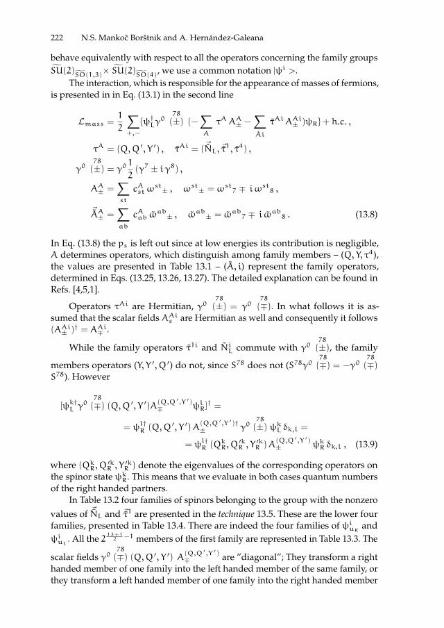
ii

“proc17” — 2017/12/11 — 19:44 — page 222 — #236 ii

ii

ii


behave equivalently with respect to all the operators concerning the family groupsSU(2)

SO(1,3)× SU(2)

SO(4), we use a common notation |ψi >.

The interaction, which is responsible for the appearance of masses of fermions,is presented in in Eq. (13.1) in the second line

Lmass =1

2

∑+,−

ψ†Lγ078

(±) (−∑A

τAAA± −∑Ai

τAiAAi± )ψR+ h.c. ,

τA = (Q,Q ′, Y ′) , τAi = ( ~NL, ~τ1, τ4) ,

γ078

(±) = γ0 12(γ7 ± i γ8) ,

AA± =∑st

cAstωst± , ωst± = ωst7 ∓ iωst8 ,

~AA± =∑ab

cAab ωab± , ωab± = ωab7 ∓ i ωab8 . (13.8)

In Eq. (13.8) the ps is left out since at low energies its contribution is negligible,A determines operators, which distinguish among family members – (Q, Y, τ4),the values are presented in Table 13.1 – (A, i) represent the family operators,determined in Eqs. (13.25, 13.26, 13.27). The detailed explanation can be found inRefs. [4,5,1].

Operators τAi are Hermitian, γ078

(±) = γ078

(∓). In what follows it is as-sumed that the scalar fields AAis are Hermitian as well and consequently it follows(AAi± )† = AAi∓ .

While the family operators τ1i and NiL commute with γ078

(±), the family

members operators (Y, Y ′, Q ′) do not, since S78 does not (S78γ078

(∓) = −γ078

(∓)S78). However

[ψk†L γ078

(∓) (Q,Q ′, Y ′)A(Q,Q ′,Y ′)∓ ψlR]

† =

= ψl†R (Q,Q ′, Y ′)A(Q,Q ′,Y ′)†± γ0

78

(±) ψkL δk,l =

= ψl†R (QkR, Q′kR , Y

′kR )A

(Q,Q ′,Y ′)± ψkR δk,l , (13.9)

where (QkR, Q′kR , Y

′kR ) denote the eigenvalues of the corresponding operators on

the spinor state ψkR. This means that we evaluate in both cases quantum numbersof the right handed partners.

In Table 13.2 four families of spinors belonging to the group with the nonzerovalues of ~NL and ~τ1 are presented in the technique 13.5. These are the lower fourfamilies, presented in Table 13.4. There are indeed the four families of ψiuR andψiuL . All the 2

13+12

−1 members of the first family are represented in Table 13.3. The

scalar fields γ078

(∓) (Q,Q ′, Y ′) A(Q,Q ′,Y ′)∓ are ”diagonal”; They transform a right

handed member of one family into the left handed member of the same family, orthey transform a left handed member of one family into the right handed member

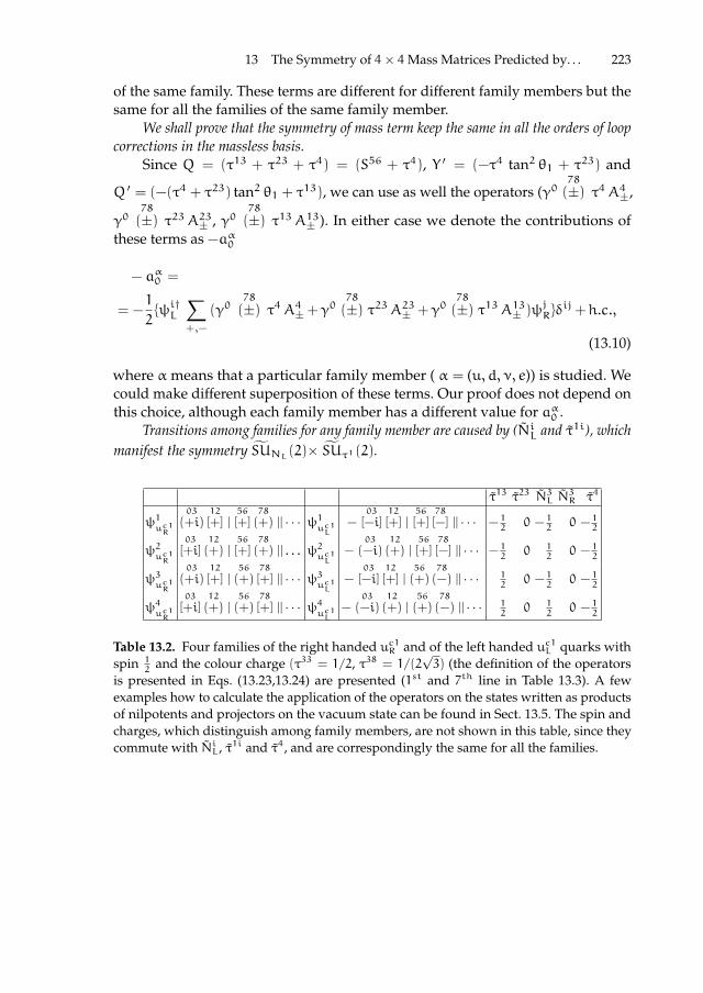
ii

“proc17” — 2017/12/11 — 19:44 — page 223 — #237 ii

ii

ii


of the same family. These terms are different for different family members but thesame for all the families of the same family member.

We shall prove that the symmetry of mass term keep the same in all the orders of loopcorrections in the massless basis.

Since Q = (τ13 + τ23 + τ4) = (S56 + τ4), Y ′ = (−τ4 tan2 θ1 + τ23) and

Q ′ = (−(τ4 + τ23) tan2 θ1 + τ13), we can use as well the operators (γ078

(±) τ4A4±,

γ078

(±) τ23A23± , γ078

(±) τ13A13± ). In either case we denote the contributions ofthese terms as −aα0

− aα0 =

= −1

2ψi†L

∑+,−

(γ078

(±) τ4A4±+γ078

(±) τ23A23± +γ078

(±) τ13A13± )ψjRδij+h.c.,

(13.10)

where α means that a particular family member ( α = (u, d, ν, e)) is studied. Wecould make different superposition of these terms. Our proof does not depend onthis choice, although each family member has a different value for aα0 .

Transitions among families for any family member are caused by (NiL and τ1i), whichmanifest the symmetry SUNL(2)× SUτ1(2).

τ13 τ23 N3L N3R τ4

ψ1uc1R

03

(+i)12

[+] |56

[+]78

(+) || · · · ψ1uc1L

−03

[−i]12

[+] |56

[+]78

[−] || · · · − 12

0 − 12

0 − 12

ψ2uc1R

03

[+i]12

(+) |56

[+]78

(+) || . . . ψ2uc1L

−03

(−i)12

(+) |56

[+]78

[−] || · · · − 12

0 12

0 − 12

ψ3uc1R

03

(+i)12

[+] |56

(+)78

[+] || · · · ψ3uc1L

−03

[−i]12

[+] |56

(+)78

(−) || · · · 12

0 − 12

0 − 12

ψ4uc1R

03

[+i]12

(+) |56

(+)78

[+] || · · · ψ4uc1L

−03

(−i)12

(+) |56

(+)78

(−) || · · · 12

0 12

0 − 12

Table 13.2. Four families of the right handed uc1R and of the left handed uc1L quarks withspin 1

2and the colour charge (τ33 = 1/2, τ38 = 1/(2

√3) (the definition of the operators

is presented in Eqs. (13.23,13.24) are presented (1st and 7th line in Table 13.3). A fewexamples how to calculate the application of the operators on the states written as productsof nilpotents and projectors on the vacuum state can be found in Sect. 13.5. The spin andcharges, which distinguish among family members, are not shown in this table, since theycommute with NiL, τ1i and τ4, and are correspondingly the same for all the families.

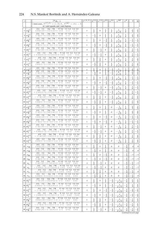
ii

“proc17” — 2017/12/11 — 19:44 — page 224 — #238 ii

ii

ii


i |aψi > Γ(3,1) S12 τ13 τ23 τ33 τ38 τ4 Y Q

(Anti)octet, Γ(7,1) = (−1) 1 , Γ(6) = (1) − 1

of (anti)quarks and (anti)leptons

1 uc1R

03(+i)

12[+] |

56[+]

78(+) ||

9 10(+)

11 12[−]

13 14[−] 1 1

20 1

212

12√3

16

23

23

2 uc1R

03[−i]

12(−) |

56[+]

78(+) ||

9 10(+)

11 12[−]

13 14[−] 1 − 1

20 1

212

12√3

16

23

23

3 dc1R

03(+i)

12[+] |

56(−)

78[−] ||

9 10(+)

11 12[−]

13 14[−] 1 1

20 − 1

212

12√3

16

− 13

− 13

4 dc1R

03[−i]

12(−) |

56(−)

78[−] ||

9 10(+)

11 12[−]

13 14[−] 1 − 1

20 − 1

212

12√3

16

− 13

− 13

5 dc1L

03[−i]

12[+] |

56(−)

78(+) ||

9 10(+)

11 12[−]

13 14[−] -1 1

2− 12

0 12

12√3

16

16

− 13

6 dc1L

−03

(+i)12(−) |

56(−)

78(+) ||

9 10(+)

11 12[−]

13 14[−] -1 − 1

2− 12

0 12

12√3

16

16

− 13

7 uc1L

−03

[−i]12[+] |

56[+]

78[−] ||

9 10(+)

11 12[−]

13 14[−] -1 1

212

0 12

12√3

16

16

23

8 uc1L

03(+i)

12(−) |

56[+]

78[−] ||

9 10(+)

11 12[−]

13 14[−] -1 − 1

212

0 12

12√3

16

16

23

9 uc2R

03(+i)

12[+] |

56[+]

78(+) ||

9 10[−]

11 12(+)

13 14[−] 1 1

20 1

2− 12

12√3

16

23

23

10 uc2R

03[−i]

12(−) |

56[+]

78(+) ||

9 10[−]

11 12(+)

13 14[−] 1 − 1

20 1

2− 12

12√3

16

23

23

11 dc2R

03(+i)

12[+] |

56(−)

78[−] ||

9 10[−]

11 12(+)

13 14[−] 1 1

20 − 1

2− 12

12√3

16

− 13

− 13

12 dc2R

03[−i]

12(−) |

56(−)

78[−] ||

9 10[−]

11 12(+)

13 14[−] 1 − 1

20 − 1

2− 12

12√3

16

− 13

− 13

13 dc2L

03[−i]

12[+] |

56(−)

78(+) ||

9 10[−]

11 12(+)

13 14[−] -1 1

2− 12

0 − 12

12√3

16

16

− 13

14 dc2L

−03

(+i)12(−) |

56(−)

78(+) ||

9 10[−]

11 12(+)

13 14[−] -1 − 1

2− 12

0 − 12

12√3

16

16

− 13

15 uc2L

−03

[−i]12[+] |

56[+]

78[−] ||

9 10[−]

11 12(+)

13 14[−] -1 1

212

0 − 12

12√3

16

16

23

16 uc2L

03(+i)

12(−) |

56[+]

78[−] ||

9 10[−]

11 12(+)

13 14[−] -1 − 1

212

0 − 12

12√3

16

16

23

17 uc3R

03(+i)

12[+] |

56[+]

78(+) ||

9 10[−]

11 12[−]

13 14(+) 1 1

20 1

20 − 1√

316

23

23

18 uc3R

03[−i]

12(−) |

56[+]

78(+) ||

9 10[−]

11 12[−]

13 14(+) 1 − 1

20 1

20 − 1√

316

23

23

19 dc3R

03(+i)

12[+] |

56(−)

78[−] ||

9 10[−]

11 12[−]

13 14(+) 1 1

20 − 1

20 − 1√

316

− 13

− 13

20 dc3R

03[−i]

12(−) |

56(−)

78[−] ||

9 10[−]

11 12[−]

13 14(+) 1 − 1

20 − 1

20 − 1√

316

− 13

− 13

21 dc3L

03[−i]

12[+] |

56(−)

78(+) ||

9 10[−]

11 12[−]

13 14(+) -1 1

2− 12

0 0 − 1√3

16

16

− 13

22 dc3L

−03

(+i)12(−) |

56(−)

78(+) ||

9 10[−]

11 12[−]

13 14(+) -1 − 1

2− 12

0 0 − 1√3

16

16

− 13

23 uc3L

−03

[−i]12[+] |

56[+]

78[−] ||

9 10[−]

11 12[−]

13 14(+) -1 1

212

0 0 − 1√3

16

16

23

24 uc3L

03(+i)

12(−) |

56[+]

78[−] ||

9 10[−]

11 12[−]

13 14(+) -1 − 1

212

0 0 − 1√3

16

16

23

25 νR

03(+i)

12[+] |

56[+]

78(+) ||

9 10(+)

11 12(+)

13 14(+) 1 1

20 1

20 0 − 1

20 0

26 νR

03[−i]

12(−) |

56[+]

78(+) ||

9 10(+)

11 12(+)

13 14(+) 1 − 1

20 1

20 0 − 1

20 0

27 eR

03(+i)

12[+] |

56(−)

78[−] ||

9 10(+)

11 12(+)

13 14(+) 1 1

20 − 1

20 0 − 1

2−1 −1

28 eR

03[−i]

12(−) |

56(−)

78[−] ||

9 10(+)

11 12(+)

13 14(+) 1 − 1

20 − 1

20 0 − 1

2−1 −1

29 eL

03[−i]

12[+] |

56(−)

78(+) ||

9 10(+)

11 12(+)

13 14(+) -1 1

2− 12

0 0 0 − 12

− 12

−1

30 eL −03

(+i)12(−) |

56(−)

78(+) ||

9 10(+)

11 12(+)

13 14(+) -1 − 1

2− 12

0 0 0 − 12

− 12

−1

31 νL −03

[−i]12[+] |

56[+]

78[−] ||

9 10(+)

11 12(+)

13 14(+) -1 1

212

0 0 0 − 12

− 12

0

32 νL

03(+i)

12(−) |

56[+]

78[−] ||

9 10(+)

11 12(+)

13 14(+) -1 − 1

212

0 0 0 − 12

− 12

0

33 dc1L

03[−i]

12[+] |

56[+]

78(+) ||

9 10[−]

11 12(+)

13 14(+) -1 1

20 1

2− 12

− 12√3

− 16

13

13

34 dc1L

03(+i)

12(−) |

56[+]

78(+) ||

9 10[−]

11 12(+)

13 14(+) -1 − 1

20 1

2− 12

− 12√3

− 16

13

13

35 uc1L

−03

[−i]12[+] |

56(−)

78[−] ||

9 10[−]

11 12(+)

13 14(+) -1 1

20 − 1

2− 12

− 12√3

− 16

− 23

− 23

36 uc1L

−03

(+i)12(−) |

56(−)

78[−] ||

9 10[−]

11 12(+)

13 14(+) -1 − 1

20 − 1

2− 12

− 12√3

− 16

− 23

− 23

37 dc1R

03(+i)

12[+] |

56[+]

78[−] ||

9 10[−]

11 12(+)

13 14(+) 1 1

212

0 − 12

− 12√3

− 16

− 16

13

38 dc1R

−03

[−i]12(−) |

56[+]

78[−] ||

9 10[−]

11 12(+)

13 14(+) 1 − 1

212

0 − 12

− 12√3

− 16

− 16

13

39 uc1R

03(+i)

12[+] |

56(−)

78(+) ||

9 10[−]

11 12(+)

13 14(+) 1 1

2− 12

0 − 12

− 12√3

− 16

− 16

− 23

Continued on next page

ii

“proc17” — 2017/12/11 — 19:44 — page 225 — #239 ii

ii

ii


i |aψi > Γ(3,1) S12 τ13 τ23 τ33 τ38 τ4 Y Q

(Anti)octet, Γ(7,1) = (−1) 1 , Γ(6) = (1) − 1

of (anti)quarks and (anti)leptons

40 uc1R

03[−i]

12(−) |

56(−)

78(+) ||

9 10[−]

11 12(+)

13 14(+) 1 − 1

2− 12

0 − 12

− 12√3

− 16

− 16

− 23

41 dc2L

03[−i]

12[+] |

56[+]

78(+) ||

9 10(+)

11 12[−]

13 14(+) -1 1

20 1

212

− 12√3

− 16

13

13

42 dc2L

03(+i)

12(−) |

56[+]

78(+) ||

9 10(+)

11 12[−]

13 14(+) -1 − 1

20 1

212

− 12√3

− 16

13

13

43 uc2L

−03

[−i]12[+] |

56(−)

78[−] ||

9 10(+)

11 12[−]

13 14(+) -1 1

20 − 1

212

− 12√3

− 16

− 23

− 23

44 uc2L

−03

(+i)12(−) |

56(−)

78[−] ||

9 10(+)

11 12[−]

13 14(+) -1 − 1

20 − 1

212

− 12√3

− 16

− 23

− 23

45 dc2R

03(+i)

12[+] |

56[+]

78[−] ||

9 10(+)

11 12[−]

13 14(+) 1 1

212

0 12

− 12√3

− 16

− 16

13

46 dc2R

−03

[−i]12(−) |

56[+]

78[−] ||

9 10(+)

11 12[−]

13 14(+) 1 − 1

212

0 12

− 12√3

− 16

− 16

13

47 uc2R

03(+i)

12[+] |

56(−)

78(+) ||

9 10(+)

11 12[−]

13 14(+) 1 1

2− 12

0 12

− 12√3

− 16

− 16

− 23

48 uc2R

03[−i]

12(−) |

56(−)

78(+) ||

9 10(+)

11 12[−]

13 14(+) 1 − 1

2− 12

0 12

− 12√3

− 16

− 16

− 23

49 dc3L

03[−i]

12[+] |

56[+]

78(+) ||

9 10(+)

11 12(+)

13 14[−] -1 1

20 1

20 1√

3− 16

13

13

50 dc3L

03(+i)

12(−) |

56[+]

78(+) ||

9 10(+)

11 12(+)

13 14[−] -1 − 1

20 1

20 1√

3− 16

13

13

51 uc3L

−03

[−i]12[+] |

56(−)

78[−] ||

9 10(+)

11 12(+)

13 14[−] -1 1

20 − 1

20 1√

3− 16

− 23

− 23

52 uc3L

−03

(+i)12(−) |

56(−)

78[−] ||

9 10(+)

11 12(+)

13 14[−] -1 − 1

20 − 1

20 1√

3− 16

− 23

− 23

53 dc3R

03(+i)

12[+] |

56[+]

78[−] ||

9 10(+)

11 12(+)

13 14[−] 1 1

212

0 0 1√3

− 16

− 16

13

54 dc3R

−03

[−i]12(−) |

56[+]

78[−] ||

9 10(+)

11 12(+)

13 14[−] 1 − 1

212

0 0 1√3

− 16

− 16

13

55 uc3R

03(+i)

12[+] |

56(−)

78(+) ||

9 10(+)

11 12(+)

13 14[−] 1 1

2− 12

0 0 1√3

− 16

− 16

− 23

56 uc3R

03[−i]

12(−) |

56(−)

78(+) ||

9 10(+)

11 12(+)

13 14[−] 1 − 1

2− 12

0 0 1√3

− 16

− 16

− 23

57 eL

03[−i]

12[+] |

56[+]

78(+) ||

9 10[−]

11 12[−]

13 14[−] -1 1

20 1

20 0 1

21 1

58 eL

03(+i)

12(−) |

56[+]

78(+) ||

9 10[−]

11 12[−]

13 14[−] -1 − 1

20 1

20 0 1

21 1

59 νL −03

[−i]12[+] |

56(−)

78[−] ||

9 10[−]

11 12[−]

13 14[−] -1 1

20 − 1

20 0 1

20 0

60 νL −03

(+i)12(−) |

56(−)

78[−] ||

9 10[−]

11 12[−]

13 14[−] -1 − 1

20 − 1

20 0 1

20 0

61 νR

03(+i)

12[+] |

56(−)

78(+) ||

9 10[−]

11 12[−]

13 14[−] 1 1

2− 12

0 0 0 12

12

0

62 νR −03

[−i]12(−) |

56(−)

78(+) ||

9 10[−]

11 12[−]

13 14[−] 1 − 1

2− 12

0 0 0 12

12

0

63 eR

03(+i)

12[+] |

56[+]

78[−] ||

9 10[−]

11 12[−]

13 14[−] 1 1

212

0 0 0 12

12

1

64 eR

03[−i]

12(−) |

56[+]

78[−] ||

9 10[−]

11 12[−]

13 14[−] 1 − 1

212

0 0 0 12

12

1

Table 13.3. The left handed (Γ(13,1) = −1, Eq. (13.38)) multiplet of spinors — the members of the fundamental representation of theSO(13, 1)

group, manifesting the subgroup SO(7, 1) of the colour charged quarks and anti-quarks and the colourless leptons and anti-leptons — is presented in the

massless basis using the technique presented in App. 13.5. It contains the left handed (Γ(3,1) = −1) weak (SU(2)I ) charged (τ13 = ± 12

, Eq. (13.23)),

and SU(2)II chargeless (τ23 = 0, Eq. (13.23)) quarks and leptons and the right handed (Γ(3,1) = 1, Sect. 13.5) weak (SU(2)I ) chargeless and

SU(2)II charged (τ23 = ± 12

) quarks and leptons, both with the spin S12 up and down (± 12

, respectively). Quarks distinguish from leptons only

in the SU(3) × U(1) part: Quarks are triplets of three colours (ci = (τ33, τ38) = [( 12, 12√3

), (− 12, 12√3

), (0,− 1√3

)], Eq. (13.24))

carrying the ”fermion charge” (τ4 = 16

, Eq. (13.24)). The colourless leptons carry the ”fermion charge” (τ4 = − 12

). The same multiplet contains also the lefthanded weak (SU(2)I) chargeless and SU(2)II charged anti-quarks and anti-leptons and the right handed weak (SU(2)I ) charged and SU(2)IIchargeless anti-quarks and anti-leptons. Anti-quarks distinguish from anti-leptons again only in theSU(3)×U(1) part: Anti-quarks are anti-triplets, carrying

the ”fermion charge” (τ4 = − 16

). The anti-colourless anti-leptons carry the ”fermion charge” (τ4 = 12

). Y = (τ23 + τ4) is the hyper charge, the

electromagnetic charge isQ = (τ13 +Y). The states of opposite charges (anti-particle states) are reachable from the particle states (besides bySab ) also bythe application of the discrete symmetry operatorCN PN , presented in Refs. [41,42] and in Sect. 13.5. The vacuum state, on which the nilpotents and projectorsoperate, is not shown. The reader can find this Weyl representation also in Refs. [5,14,15,4] and in the references therein.

Taking into account Table 13.3 and Eqs. (13.34, 13.43) one easily finds what

do operators γ078

(±) do on the left handed and the right handed members of any

ii

“proc17” — 2017/12/11 — 19:44 — page 226 — #240 ii

ii

ii


family i = (1, 2, 3, 4).

γ078

(−) |ψiuR,νR > = −|ψiuL,νL > ,

γ078

(+) |ψiuL,νL > = |ψiuR,νR > ,

γ078

(+) |ψidR,eR > = |ψidL,eL > ,

γ078

(−) |ψidL,eL > = |ψidR,eR > . (13.11)

We need to know also what do operators (τ1± = τ11 ± i τ12, τ13) and (N±L =

N1L ± i N2L, N3L) do when operating on any member (uL,R, νL,R, dL,R, eL,R) of aparticular family ψi, i = (1, 2, 3, 4).

Taking into account, Eqs. (13.32, 13.33, 13.43, 13.45, 13.36, 13.25, 13.26),

N±L = −

03

(∓i)12

(±) , τ1± = (∓)56

(±)78

(∓) ,

N3L =1

2(S12 + i S03) , τ13 =

1

2(S56 − S78) ,

ab

(−k)ab

(k) = −i ηaaab

[k] ,

ab

(k)ab

(k)= 0 ,

ab

(k)ab

[k] = iab

(k) ,

ab

(k)ab

[−k]= 0 ,

ab

(k) =1

2(γa +

ηaa

ikγb) ,

ab

[k] =1

2(1+

i

kγaγb) , (13.12)

one finds

N+L |ψ1 > = |ψ2 > , N+

L |ψ2 >= 0 ,

N−L |ψ2 > = |ψ1 > , N−

L |ψ1 >= 0 ,

N+L |ψ3 > = |ψ4 > , N+

L |ψ4 >= 0 ,

N−L |ψ4 > = |ψ3 > , N−

L |ψ3 >= 0 ,

τ1+ |ψ1 > = |ψ3 > , τ1+ |ψ3 >= 0 ,

τ1− |ψ3 > = |ψ1 > , τ1− |ψ1 >= 0 ,

τ1− |ψ4 > = |ψ2 > , τ1− |ψ2 >= 0 ,

τ1+ |ψ2 > = |ψ4 > , τ1+ |ψ4 >= 0 ,

N3L |ψ1 > = −

1

2|ψ1 > , N3L |ψ

2 >= +1

2|ψ2 > ,

N3L |ψ3 > = −

1

2|ψ3 > , N3L |ψ

4 >= +1

2|ψ4 > ,

τ13 |ψ1 > = −1

2|ψ1 > , τ13 |ψ2 >= −

1

2|ψ2 > ,

τ13 |ψ3 > = +1

2|ψ3 > , τ13 |ψ4 >= +

1

2|ψ4 > . (13.13)

Let the scalars (ANL±(±) , ANL3(±) , A

1±(±), A

13(±)) be the scalar gauge fields of the operators

(N±L , N3L, τ1±, τ13), respectively. Here A(±) = A7 ∓ i A8 for all the scalar gauge

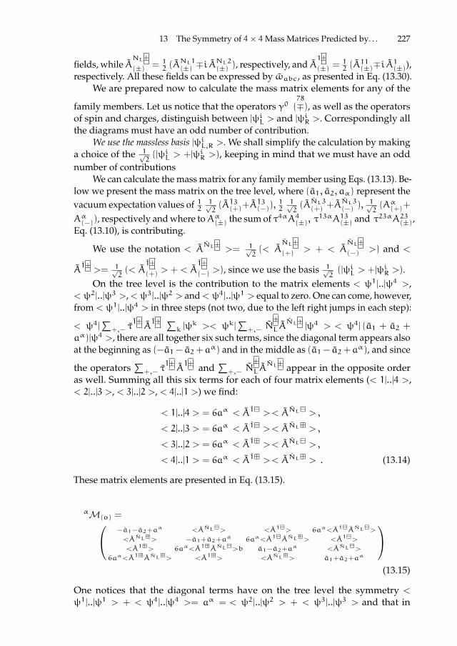
ii

“proc17” — 2017/12/11 — 19:44 — page 227 — #241 ii

ii

ii


fields, while ANL±(±) = 1

2(ANL1(±) ∓i A

NL2(±) ), respectively, and A

1±(±) =

12(A11(±)∓i A

1(±)),

respectively. All these fields can be expressed by ωabc, as presented in Eq. (13.30).We are prepared now to calculate the mass matrix elements for any of the

family members. Let us notice that the operators γ078

(∓), as well as the operatorsof spin and charges, distinguish between |ψiL > and |ψiR >. Correspondingly allthe diagrams must have an odd number of contribution.

We use the massless basis |ψiL,R >. We shall simplify the calculation by makinga choice of the 1√

2(|ψiL > +|ψiR >), keeping in mind that we must have an odd

number of contributionsWe can calculate the mass matrix for any family member using Eqs. (13.13). Be-

low we present the mass matrix on the tree level, where (a1, a2, aα) represent thevacuum expectation values of 1

21√2(A13(+)+A

13(−)),

121√2(ANL3(+) +ANL3(−) ), 1√

2(Aα(+)+

Aα(−)), respectively and where toAα(±) the sum of τ4αA4(±), τ13αA13(±) and τ23αA23(±),

Eq. (13.10), is contributing.

We use the notation < ANL± >= 1√

2(< A

NL±(+) > + < A

NL±(−) >) and <

A1±>= 1√

2(< A

1±(+) > + < A

1±(−) >), since we use the basis 1√

2(|ψiL > +|ψiR >).

On the tree level is the contribution to the matrix elements < ψ1|..|ψ4 >,< ψ2|..|ψ3 >,< ψ3|..|ψ2 > and< ψ4|..|ψ1 > equal to zero. One can come, however,from < ψ1|..|ψ4 > in three steps (not two, due to the left right jumps in each step):

< ψ4|∑

+,− τ1±A1± ∑

k |ψk >< ψk|

∑+,− N

±L A

NL± |ψ4 > < ψ4| (a1 + a2 +

aα)|ψ4 >, there are all together six such terms, since the diagonal term appears alsoat the beginning as (−a1− a2+aα) and in the middle as (a1− a2+aα), and since

the operators∑

+,− τ1±A1± and

∑+,− N

±L A

NL± appear in the opposite orderas well. Summing all this six terms for each of four matrix elements (< 1|..|4 >,< 2|..|3 >, < 3|..|2 >, < 4|..|1 >) we find:

< 1|..|4 > = 6aα < A1 >< ANL > ,

< 2|..|3 > = 6aα < A1 >< ANL > ,

< 3|..|2 > = 6aα < A1 >< ANL > ,

< 4|..|1 > = 6aα < A1 >< ANL > . (13.14)

These matrix elements are presented in Eq. (13.15).

αM(o) = −a1−a2+aα <ANL> <A1> 6aα<A1ANL>

<ANL> −a1+a2+aα 6aα<A1ANL> <A1>

<A1> 6aα<A1ANL>b a1−a2+aα <ANL>

6aα<A1ANL> <A1> <ANL> a1+a2+aα

(13.15)

One notices that the diagonal terms have on the tree level the symmetry <ψ1|..|ψ1 > + < ψ4|..|ψ4 >= aα = < ψ2|..|ψ2 > + < ψ3|..|ψ3 > and that in

ii

“proc17” — 2017/12/11 — 19:44 — page 228 — #242 ii

ii

ii


the off diagonal elements in next order to zero the contribution of the fields,which depend on particular family member α = (u, d, ν, e) enter. We also noticethat < ψi|..|ψj >†=< ψj|..|ψi >. In the case that < A1 >=< A1 >= e and< ANL >=< ANL >= d, which would mean that all the matrix elements arereal, the mass matrix simplifies to

Mα(o) =

−a1 − a2 + a

α d e 6aαed

d −a1 + a2 + aα 6aαed e

e 6aαed a1 − a2 + aα d

6aαed e d a1 + a2 + aα

.

(13.16)

13.2.1 Mass matrices beyond the tree level

To make a proof that the symmetry SU(2)× SU(2) × U(1) of the mass matrix,presented in Eq. (13.15), is kept in all orders of loop corrections, we need to proofonly that at each order the matrix element, let say, < 1|..|2 > (in Eq. (13.15) thismatrix element is equal to < ANL >) remains equal to < 3|..|4 > in all orders,while < 2|..|1 > remains to be equal to < 1|..|2 >†=< 4|..|3 > (=< ANL >). Theseshould be done for all the matrix elements appearing in Eq. (13.15.

a. It is not difficult to see that each of the diagonal terms (τ13 < A13 >,N3L < A

NL3 >, τA < AA >, with τA = τ4, τ13, τ23) have the property that thesum of the contributions x+ xxx+ xxxxx+ ... (in all orders) keeps the symmetryof the tree level. Let us check for τ13 < A13 >. One obtains for each of the fourfamilies i = [1, 2, 3, 4] the values [−a1(1+(−a1)2+(−a1)4+. . . ),−a1(1+(−a1)2+

(−a1)4+. . . ), a1(1+(a1)2+(a1)4+. . . ), a1(1+(a1)2+(a1)4+. . . )], which we call[−a1, −a1, a1, a1] for the four families i = [1, 2, 3, 4], respectively. Correspondinglyone finds for the same kind of diagrams for N3L < A

NL3 > the four values [−a2,a2, −a2, a2] for the four families i = [1, 2, 3, 4], respectively. While for τAAA weobtain, when summing over the diagrams x+ xxx+ xxxxx+ ..., the same value aα

for a particular family member α = (u, d, ν, e) all four families. Family membersproperties enter in the left/right basis 1√

2(|ψiL > +|ψiR > into the mass matrix only

through aα.One reproduces that the sum of < 1|..|1 > + < 4|..|4 >=< 2|..|2 > + < 3|..|3 >

Correspondingly it is not difficult to see that all the matrix elements, notonly diagonal but also off diagonal, keep the symmetry of the mass matrix ofEq. (13.15) in all orders of corrections, provided that the matrix elements of thekind αa1 + βa2 + aα — or of the kind in the αa1 + βa2 + aα — appears inthe diagrams in first power only. Here (α,β) are ±1, they are determined bythe eigenvalues of the operators τ13 (for a1) and N3L (for a2), respectively, on aparticular family, Eq. (13.13).

ii

“proc17” — 2017/12/11 — 19:44 — page 229 — #243 ii

ii

ii


b. Let us add to the diagonal terms the loop corrections. Let us evaluate,using the massless basis |ψi >= 1√

2(|ψiL > +|ψiR >), the contribution:

< ψi|∑

−,+,,,j

γ078

(±) [N±L A

NL± + τ1±A1±

]|ψj >

< ψj|∑−,+

γ078

(±) [N3LANL3 + τ13A13 +

∑A

τAAA]|ψj >

< ψj|∑

−,+,,

γ078

(±) [N∓L A

NL∓ + τ1∓A1∓

]|ψi > . (13.17)

One finds for i = [1, 2, 3, 4] the values [A1A1(a1−a2+aα) +ANLANL(−a1+a2+aα), A1A1(a1+a2+aα) +ANLANL(−a1−a2+aα), A1A1(−a1−a2+aα) +ANLANL(+a1+ a2+aα), A1A1(−a1+ a2+aα) +ANLANL(+a1−a2 + aα)], respectively, which again has the symmetry of the tree level state< 1| . . . |1 > + < 4| . . . |4 >=< 2| . . . |2 > + < 3| . . . |3 >.

One can make three such loops, or any kind of loops in any order of loopcorrections with one (αa1 + βa2 + aα) and the symmetry of tree level state< 1| . . . |1 > + < 4| . . . |4 >=< 2| . . . |2 > + < 3| . . . |3 > is manifested.

c. Let us look at the loop corrections to the off diagonal terms < 1| . . . |2 >,<1| . . . |3 >,< 2| . . . |4 >,< 3| . . . |4 >, as well as their complex conjugate values.

Let us evaluate, using the massless basis |ψi >= 1√2(|ψiL > +|ψiR >), the

contribution:

< ψ4|∑

−,+,,,j,k

γ078

(±) [N±L A

NL± + τ1±A1±

]|ψj >

< ψj|∑−,+

γ078

(±) [N±L A

NL± + τ1±A1±

]|ψk >

< ψk|∑

−,+,,

γ078

(±) [N∓L A

NL∓ + τ1∓A1∓

]|ψ2 >

+ < ψ4|∑

−,+,,,j

γ078

(±) [N3LANL3 + τ13A13 +

∑A

τAAA]|ψ4 >

< ψ4|∑

−,+,,

γ078

(±) [N∓L A

NL∓ + τ1∓A1∓

]|ψj >

< ψj|∑

−,+,,

γ078

(±) [N3LANL3 + τ13A13 +

∑A

τAAA]|ψ2 > . (13.18)

One obtains for this term < 4|...|2 >= < A1 > ANLANL + |ANL3|2 +

|A13|2 + |τAAA|2, which is equal to the equivalent loop correction term for thematrix element < 3|...|1 >.

Checking the loop corrections for the off diagonal elements < 1| . . . |2 >

,< 1| . . . |3 >,< 2| . . . |4 >,< 3| . . . |4 > in all loop corrections one finds that thesymmetry of these off diagonal terms is kept in all orders.

ii

“proc17” — 2017/12/11 — 19:44 — page 230 — #244 ii

ii

ii


d. There are still the terms < 1| . . . |4 >,< 2| . . . |3 >,< 3| . . . |2 > and< 4| . . . |1 > to be checked in loop corrections. Adding loop corrections in theway we did in c. we find that also these matrix elements keep the symmetry ofEq. (13.15).

13.3 Conclusions

We demonstrate in this contribution on several cases that the matrix elements ofmass matrices 4 × 4, predicted by the spin-charge-family theory for each familymember α = (u, d, ν, e) to have the symmetry SU(2) ˜SO(4)1+3

× SU(2) ˜SO(4)"weak"×

U(1) on the tree level, keeps this symmetry in all loop corrections. The first togroups concern the family groups, the last one concern the family members group.

The only dependence of the mass matrix on the family member (α = (u, d, ν, e))quantum numbers is on the tree level through the vacuum expectation values

of the operators γ078

(±) QAQ± , γ078

(±) Q ′AQ′

± and γ078

(±) τ4A4±, appearing ona tree level in the diagonal terms of the mass matrix only and are the same foreach of four families — I4×4a

α, I is the unite matrix. In the loop corrections theseoperators enter into all the off diagonal matrix elements, causing the difference inthe masses of the family members. The right handed neutrino, which is the regularmember of the four families, Table 13.3, has the nonzero value of the operatorτ4A4± only (while the family part of the mass matrix is on the tree level the samefor all the members).

We demonstrate on several cases, why does the symmetry of the mass matrix,which shows up on the tree level, remain in the loop corrections in all orders.

Although we are not (yet) able to calculate these matrix elements, the pre-dicted symmetry will enable to predict masses of the fourth family (to the ob-served three), since the 3× 3 submatrix of the 4× 4matrix determines 4× 4matrixuniquely [19,4]. We only must wait for accurate enough data for mixing matricesof quarks and leptons to predict, using the symmetry of mass matrices predictedby the spin-charge-family, the masses of the fourth family quarks and leptons.

13.4 APPENDIX: Short presentation of the spin-charge-familytheory

This subsection follows similar sections in Refs. [1,4–7].The spin-charge-family theory [1–11,14–22] assumes:

A. A simple action (Eq. (13.20)) in an even dimensional space (d = 2n, d > 5), dis chosen to be (13+ 1). This choice makes that the action manifests in d = (3+ 1)

in the low energy regime all the observed degrees of freedom, explaining all theassumptions of the standard model, as well as other observed phenomena.

There are two kinds of the Clifford algebra objects, γa’s and γa’s in this theorywith the properties.

γa, γb+ = 2ηab , γa, γb+ = 2ηab , , γa, γb+ = 0 . (13.19)

ii

“proc17” — 2017/12/11 — 19:44 — page 231 — #245 ii

ii

ii


Fermions interact with the vielbeins fαa and the two kinds of the spin-connectionfields -ωabα and ωabα - the gauge fields of Sab = i

4(γa γb − γb γa) and Sab =

i4(γa γb − γb γa), respectively.

The action

A =

∫ddx E

1


ddx E (αR+ α R) , (13.20)

in which p0a = fαa p0α + 12E


2Sabωabα − 1

2Sab ωabα,

andR =

1


cbβ)+ h.c.,

R =1

2fα[afβb] (ωabα,β − ωcaα ω

cbβ)+ h.c.

4, introduces two kinds of the Clifford algebra objects, γa and γa, γa, γb+ =

2ηab = γa, γb+. fαa are vielbeins inverted to eaα, Latin letters (a, b, ..) denoteflat indices, Greek letters (α,β, ..) are Einstein indices, (m,n, ..) and (µ, ν, ..) de-note the corresponding indices in (0, 1, 2, 3), while (s, t, ..) and (σ, τ, ..) denote thecorresponding indices in d ≥ 5:

eaαfβa = δβα , eaαf

αb = δab , (13.21)

E = det(eaα).B. The spin-charge-family theory assumes in addition that the manifoldM(13+1)

breaks first into M(7+1) × M(6) (which manifests as SO(7, 1) ×SU(3) ×U(1)),affecting both internal degrees of freedom - the one represented by γa and the onerepresented by γa. Since the left handed (with respect toM(7+1)) spinors coupledifferently to scalar (with respect toM(7+1)) fields than the right handed ones, thebreak can leave massless and mass protected 2((7+1)/2−1) families [34]. The rest offamilies get heavy masses 5.C. There is additional breaking of symmetry: The manifold M(7+1) breaksfurther intoM(3+1)×M(4).D. There is a scalar condensate (Table 13.5) of two right handed neutrinos withthe family quantum numbers of the upper four families, bringing masses of thescale ∝ 1016 GeV or higher to all the vector and scalar gauge fields, which interactwith the condensate [5].E. There are the scalar fields with the space index (7, 8) carrying the weak (τ1i)and the hyper charges (Y = τ23+τ4, τ1i and τ2i are generators of the subgroups of

4 Whenever two indexes are equal the summation over these two is meant.5 A toy model [34,35] was studied in d = (5 + 1) with the same action as in Eq. (13.20).

The break from d = (5 + 1) to d = (3 + 1)× an almost S2 was studied. For a particularchoice of vielbeins and for a class of spin connection fields the manifoldM(5+1) breaksinto M(3+1) times an almost S2, while 2((3+1)/2−1) families remain massless and massprotected. Equivalent assumption, although not yet proved how does it really work, ismade in the d = (13 + 1) case. This study is in progress.

ii

“proc17” — 2017/12/11 — 19:44 — page 232 — #246 ii

ii

ii


SO(4), τ4 and τ3i are the generators of U(1)II and SU(3), respectively, which aresubgroups of SO(6)), which with their nonzero vacuum expectation values changethe properties of the vacuum and break the weak charge and the hyper charge.Interacting with fermions and with the weak and hyper bosons, they bring massesto heavy bosons and to twice four groups of families. Carrying no electromagnetic(Q = τ13 + Y) and colour (τ3i) charges and no SO(3, 1) spin, the scalar fields leavethe electromagnetic, colour and gravity fields in d = (3+ 1) massless.

The assumed actionA and the assumpions offer the explanation for the originand all the properties o. of the observed fermions:

o.i. of the family members, on Table 13.3 the family members, belonging toone Weyl (fundamental) representation of massless spinors of the group SO(13, 1)are presented in the ”technique” [9–11,14–16,12,13] and analyzed with respect tothe subgroups SO(3, 1), SU(2)I, SU(2)II, SU(3), U(1)II), Eqs. (13.22, 13.23, 13.24),with the generators τAi =

∑s,t c

Aist S

st,o.ii.of the families analyzed with respect to the subgroups SO(3, 1), SU(2)I,

SU(2)II, U(1)II), with the generators τAi =∑ab c

Aiab S

st, Eqs. (13.25, 13.26,13.27), are presented on Table 13.4, all the families are singlets with respect toSU(3),

oo.i. of the observed vector gauge fields of the charges

SU(2)I, SU(2)II, SU(3), U(1)II)

discussed in Refs. ([1,4,2], and the references therein), all the vector gauge fieldsare the superposition of theωstm, AAim =

∑s,t c

Aistωstm, Eq. vect

oo.ii. of the Higgs’s scalar and of the Yukawa couplings, explainable with thescalar fields with the space index (7, 8), there are two groups of two triplets, whichare scalar gauge fields of the charges τAi, expressible with the superposition ofthe ωabs,AAim =

∑a,b c

Aiabωabs and three singlets, the gauge fields ofQ,Q ′, S ′,

Eqs. (13.28), all with the weak and the hyper charges as assumed by the standardmodel for the Higgs’s scalars,

oo.iii. of the scalar fields explaining the origin of the matter-antimatter asym-metry, Ref. [5],

oo.iv. of the appearance of the dark matter, there are two decoupled groupsof four families, carrying family charges ( ~NL, ~τ1) and ( ~NR, ~τ2), Eqs. (13.25, 13.26),both groups carry also the family members charges (Q,Q ′, Y ′), Eq. (13.28).

The standard model groups of spins and charges are the subgroups of theSO(13, 1) group with the generator of the infinitesimal transformations expressiblewith Sab (= i

2(γaγb − γbγa), Sab, Scd− = −i(ηadSbc + ηbcSad − ηacSbd −

ηbdSac)) for the spin

~N±(= ~N(L,R)) : =1

2(S23 ± iS01, S31 ± iS02, S12 ± iS03) , (13.22)

ii

“proc17” — 2017/12/11 — 19:44 — page 233 — #247 ii

ii

ii


for the weak charge, SU(2)I, and the second SU(2)II, these two groups are theinvariant subgroups of SO(4),

~τ1 : =1

2(S58 − S67, S57 + S68, S56 − S78) ,

~τ2 : =1

2(S58 + S67, S57 − S68, S56 + S78) , (13.23)

for the colour charge SU(3) and for the ”fermion charge” U(1)II, these two groupsare subgroups of SO(6),

~τ3 :=1

2S9 12 − S10 11 , S9 11 + S10 12, S9 10 − S11 12,

S9 14 − S10 13, S9 13 + S10 14 , S11 14 − S12 13 ,

S11 13 + S12 14,1√3(S9 10 + S11 12 − 2S13 14) ,

τ4 := −1

3(S9 10 + S11 12 + S13 14) , (13.24)

τ4 is the ”fermion charge”, while the hyper charge Y = τ23 + τ4.The generators of the family quantum numbers are the superposition of

the generators Sab (Sab = i4γa, γb−, Sab, Scd− = −i(ηadSbc + ηbcSad −

ηacSbd − ηbdSac), Sab, Scd− = 0. One correspondingly finds the generators ofthe subgroups of SO(7, 1),

~NL,R : =1

2(S23 ± iS01, S31 ± iS02, S12 ± iS03) , (13.25)

which determine representations of the two SU(2) invariant subgroups of SO(3, 1),while

~τ1 : =1

2(S58 − S67, S57 + S68, S56 − S78) ,

~τ2 : =1

2(S58 + S67, S57 − S68, S56 + S78) , (13.26)

determine representations of SU(2)I× SU(2)II of SO(4). Both, SO(3, 1) and SO(4),are the subgroups of SO(7, 1). One finds for the infinitesimal generator τ4 of U(1)originating in SO(6) the expression

τ4 := −1

3(S9 10 + S11 12 + S13 14) . (13.27)

The operators for the charges Y and Q of the standard model, together withQ ′ and Y ′, and the corresponding operators of the family charges Y, Y ′, Q, Q ′ aredefined as follows:

Y := τ4 + τ23 , Y ′ := −τ4 tan2 ϑ2 + τ23 , Q := τ13 + Y , Q ′ := −Y tan2 ϑ1 + τ13 ,

Y := τ4 + τ23 , Y ′ := −τ4 tan2 ϑ2 + τ23 , Q := Y + τ13 , Q ′ = −Y tan2 ϑ1 + τ13 .

(13.28)

ii

“proc17” — 2017/12/11 — 19:44 — page 234 — #248 ii

ii

ii


The families split into two groups of four families, each manifesting the

SU(2)× SU(2)×U(1),

with the generators of of the infinitesimal transformations ( ~NL, ~τ1, Q,Q ′, Y ′) and( ~NR, ~τ2, Q,Q ′, Y ′), respectively. The generators ofU(1) group (Q,Q ′, Y ′), Eq. 13.28,distinguish among family members and are the same for both groups of fourfamilies, presented on Table 13.4, taken from Ref. [4].

The vector gauge fields of the charges ~τ1, ~τ2, ~τ3 and τ4 follow from therequirement

∑Ai τ

AiAAim =∑s,t

12Sstωstm and the requirement that τAi =∑

a,b cAiab Sab, Eq. (13.2), fulfilling the commutation relations τAi, τBj− =

iδABfAijkτAk, Eq. (13.3). Correspondingly we find AAim =∑s,t cAist ω

stm,

Eq. (13.4), with (s, t) either in (5, 6, 7, 8) or in (9, . . . , 14).The explicit expressions for these vector gauge fields in terms ofωstm are as

follows

~A1m = (ω58m −ω67m,ω57m +ω68m,ω56m −ω78m) ,

~A2m = (ω58m +ω67m,ω57m −ω68m,ω56m +ω78m) ,

AQm = ω56m − (ω9 10m +ω11 12m +ω13 14m) ,

AYm = (ω56m +ω78m) − (ω9 10m +ω11 12m +ω13 14m) ,

~A3m = (ω9 12m −ω10 11m,ω9 11m +ω10 12m,ω9 10m −ω11 12m,

ω9 14m −ω10 13m,ω9 13m +ω10 14m,ω11 14m −ω12 13m,

ω11 13m +ω12 14m,1√3(ω9 10m +ω11 12m − 2ω13 14m)) ,

A4m = (ω9 10m +ω11 12m +ω13 14m) . (13.29)

Allωstm vector gauge fields are real fields. Here the fields contain the couplingconstants which are not necessarily the same for all of them. In the case that thecoupling constants would be the same, than the angles θ22 and θ21 would be equalto one, which is not the case (at least sin21 ≈ 0.22.)

One obtains in a similar way the scalar gauge fields, which determine massmatrices of family members. They carry the space index s = (7, 8).

~A1s = (ω58s − ω67s, ω57s + ω68s, ω56s − ω78s) ,

~A2s = (ω58s + ω67s, ω57s − ω68s, ω56s + ω78s) ,

~ANLs = (ω23s + iω01s, ω31s + iω02s, ω12s + ω03s) ,

~ANRs = (ω23s − iω01s, ω31s − iω02s, ω12s − iω03s) ,

AQs = ω56s − (ω9 10s +ω11 12s +ω13 14s) ,

AYs = (ω56s +ω78s) − (ω9 10s +ω11 12s +ω13 14s)

A4s = −(ω9 10s +ω11 12s +ω13 14s) . (13.30)

All ωsts ′ , ωsts ′ , (s, t, s ′) = (5, ·, 14), ωi,j,s ′ and i ω0,s ′ , (i, j) = (1, 2, 3) scalargauge fields are real fields.

ii

“proc17” — 2017/12/11 — 19:44 — page 235 — #249 ii

ii

ii


τ13τ23N3 LN3 Rτ4

Iuc1R1

03

(+i)12

[+]|56

[+]78

(+)||910

(+)1112

[−]1314

[−]νR1

03

(+i)12

[+]|56

[+]78

(+)||910

(+)1112

(+)1314

(+)

−1 2

0−1 2

0−1 2

Iuc1R2

03

[+i]12

(+)|56

[+]78

(+)||910

(+)1112

[−]1314

[−]νR2

03

[+i]12

(+)|56

[+]78

(+)||910

(+)1112

(+)1314

(+)

−1 2

01 2

0−1 2

Iuc1R3

03

(+i)12

[+]|56

(+)78

[+]||910

(+)1112

[−]1314

[−]νR3

03

(+i)12

[+]|56

(+)78

[+]||910

(+)1112

(+)1314

(+)

1 20−1 2

0−1 2

Iuc1R4

03

[+i]12

(+)|56

(+)78

[+]||910

(+)1112

[−]1314

[−]νR4

03

[+i]12

(+)|56

(+)78

[+]||910

(+)1112

(+)1314

(+)

1 20

1 20−1 2

IIuc1R5

03

[+i]12

[+]|56

[+]78

[+]||910

(+)1112

[−]1314

[−]νR5

03

[+i]12

[+]|56

[+]78

[+]||910

(+)1112

(+)1314

(+)

0−1 2

0−1 2−1 2

IIuc1R6

03

(+i)

12

(+)|56

[+]78

[+]||910

(+)1112

[−]1314

[−]νR6

03

(+i)

12

(+)|56

[+]78

[+]||910

(+)1112

(+)1314

(+)

0−1 2

01 2−1 2

IIuc1R7

03

[+i]12

[+]|56

(+)78

(+)||910

(+)1112

[−]1314

[−]νR7

03

[+i]12

[+]|56

(+)78

(+)||910

(+)1112

(+)1314

(+)

01 2

0−1 2−1 2

IIuc1R8

03

(+i)

12

(+)|56

(+)78

(+)||910

(+)1112

[−]1314

[−]νR8

03

(+i)

12

(+)|56

(+)78

(+)||910

(+)1112

(+)1314

(+)

01 2

01 2−1 2

Tabl

e13

.4.

Eigh

tfam

ilies

ofth

eri

ghth

ande

duc1R

(13.

3)qu

ark

with

spin1 2

,the

colo

urch

arge

(τ33=1/2

,τ38=1/(2√3)

(the

defin

ition

ofth

eop

erat

ors

isp

rese

nted

inE

qs.(

13.2

3,13

.24)

,afe

wex

amp

les

how

toca

lcu

late

the

app

licat

ion

ofth

ese

oper

ator

son

the

stat

esca

nbe

fou

ndin

Subs

ect.

13.5

.

The

defi

niti

onof

the

oper

ator

s,ex

pre

ssib

lew

ithSab

is:~ NL,R

=1 2(S23±iS01,S31±iS02,S12±iS03),~ τ1=1 2(S58−S67,S57+S68,S56−S78),~ τ2

=1 2(S58+S67,S57−S68,S56+S78)

andτ4=

−1 3(S910+S1112+S1314))

,and

ofth

eco

lour

less

righ

than

ded

neut

rinoνR

ofsp

in1 2

are

pres

ente

din

the

left

and

inth

eri

ghtc

olum

n,re

spec

tivel

y.Th

eybe

long

totw

ogr

oups

offo

urfa

mili

es,o

ne(II)

isa

doub

letw

ithre

spec

tto

(~ NL

and~ τ1)a

nda

sing

let

wit

hre

spec

tto

(~ NR

and~ τ2),

the

othe

r(I

)is

asi

ngle

twit

hre

spec

tto

(~ NL

and~ τ1)

and

ad

oubl

etw

ith

wit

hre

spec

tto

(~ NR

and~ τ2).

All

the

fam

ilies

follo

wfr

omth

est

arti

ngon

eby

the

app

licat

ion

ofth

eop

erat

ors

( N± R,L

,τ(2,1

)±),

Eq.

(13.

45).

The

gene

rato

rs(N± R,L

,τ(2,1

)±)

(Eq.

(13.

45))

tran

sfor

muRi,i

=(1,···,8),

toal

lth

em

embe

rsof

the

sam

eco

lou

rof

thef

amily

.The

sam

ege

nera

tors

tran

sfor

meq

uiv

alen

tly

the

righ

tha

nded

neu

trin

oνRi,i

=(1,···,8),

toal

lthe

colo

urle

ssm

embe

rsof

theith

fam

ily.

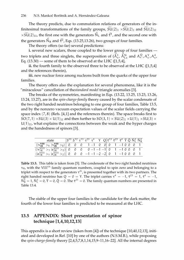
ii

“proc17” — 2017/12/11 — 19:44 — page 236 — #250 ii

ii

ii


The theory predicts, due to commutation relations of generators of the in-finitesimal transformations of the family groups, SU(2)I ×SU(2)I and SU(2)II×SU(2)II, the first one with the generators ~NL and ~τ1, and the second one withthe generators ~NR and ~τ2, Eqs. (13.25,13.26), two groups of four families.

The theory offers (so far) several predictions:i. several new scalars, those coupled to the lower group of four families —

two triplets and three singlets, the superposition of (~A1s , ~ANLs and AQs , AYs , A4s ,Eq. (13.30) — some of them to be observed at the LHC ([1,5,4],

ii. the fourth family to the observed three to be observed at the LHC ([1,5,4]and the references therein),

iii. new nuclear force among nucleons built from the quarks of the upper fourfamilies.

The theory offers also the explanation for several phenomena, like it is the”miraculous” cancellation of thestandard model triangle anomalies [3].

The breaks of the symmetries, manifesting in Eqs. (13.22, 13.25, 13.23, 13.26,13.24, 13.27), are in the spin-charge-family theory caused by the scalar condensate ofthe two right handed neutrinos belonging to one group of four families, Table 13.5,and by the nonzero vacuum expectation values of the scalar fields carrying thespace index (7, 8) (Refs. [4,1] and the references therein). The space breaks first toSO(7, 1) ×SU(3)×U(1)II and then further to SO(3, 1)× SU(2)I ×U(1)I ×SU(3)×U(1)II, what explains the connections between the weak and the hyper chargesand the handedness of spinors [3].

state S03 S12 τ13 τ23 τ4 Y Q τ13 τ23 τ4 Y Q N3L N3R

(|νVIII1R >1 |νVIII

2R >2) 0 0 0 1 −1 0 0 0 1 −1 0 0 0 1

(|νVIII1R >1 |eVIII2R >2) 0 0 0 0 −1 −1 −1 0 1 −1 0 0 0 1

(|eVIII1R >1 |eVIII2R >2) 0 0 0 −1 −1 −2 −2 0 1 −1 0 0 0 1

Table 13.5. This table is taken from [5]. The condensate of the two right handed neutrinosνR, with the VIIIth family quantum numbers, coupled to spin zero and belonging to atriplet with respect to the generators τ2i, is presented together with its two partners. Theright handed neutrino has Q = 0 = Y. The triplet carries τ4 = −1, τ23 = 1, τ4 = −1,N3R = 1, N3L = 0, Y = 0, Q = 0. The τ31 = 0. The family quantum numbers are presented inTable 13.4.

The stable of the upper four families is the candidate for the dark matter, thefourth of the lower four families is predicted to be measured at the LHC.

13.5 APPENDIX: Short presentation of spinortechnique [1,4,10,12,13]

This appendix is a short review (taken from [4]) of the technique [10,40,12,13], initi-ated and developed in Ref. [10] by one of the authors (N.S.M.B.), while proposingthe spin-charge-family theory [2,4,5,7,8,1,14,15,9–11,16–22]. All the internal degrees

ii

“proc17” — 2017/12/11 — 19:44 — page 237 — #251 ii

ii

ii


of freedom of spinors, with family quantum numbers included, are describablewith two kinds of the Clifford algebra objects, besides with γa’s, used in thistheory to describe spins and all the charges of fermions, also with γa’s, used inthis theory to describe families of spinors:

γa, γb+ = 2ηab , γa, γb+ = 2ηab , γa, γb+ = 0 . (13.31)

We assume the “Hermiticity” property for γa’s (and γa’s) γa† = ηaaγa (andγa† = ηaaγa), in order that γa (and γa) are compatible with (13.31) and formallyunitary, i.e. γa † γa = I (and γa †γa = I). One correspondingly finds that (Sab)† =ηaaηbbSab (and (Sab)† = ηaaηbbSab).

Spinor states are represented as products of nilpotents and projectors, formedas odd and even objects of γa’s, respectively, chosen to be the eigenstates of aCartan subalgebra of the Lorentz groups defined by γa’s

ab

(k): =1

2(γa +

ηaa

ikγb) ,

ab

[k]:=1

2(1+

i

kγaγb) , (13.32)

where k2 = ηaaηbb. We further have [4]

γaab

(k): =1

2(γaγa +

ηaa

ikγaγb) = ηaa

ab

[−k] ,

γaab

[k]: =1

2(γa +

i

kγaγaγb) =

ab

(−k) ,

γaab

(k): = −i1

2(γa +

ηaa

ikγb)γa = −iηaa

ab

[k] ,

γaab

[k]: = i1

2(1+

i

kγaγb)γa = −i

ab

(k) ,

(13.33)

where we assume that all the operators apply on the vacuum state |ψ0〉. We define

a vacuum state |ψ0 > so that one finds <ab

(k)

†ab

(k) >= 1 , <ab

[k]

†ab

[k] >= 1.

We recognize that γa transformab

(k) intoab

[−k], never toab

[k], while γa transformab

(k) intoab

[k], never toab

[−k]

γaab

(k)= ηaaab

[−k], γbab

(k)= −ikab

[−k], γaab

[k]=ab

(−k), γbab

[k]= −ikηaaab

(−k) ,

γaab

(k)= −iηaaab

[k], γbab

(k)= −kab

[k], γaab

[k]= iab

(k), γbab

[k]= −kηaaab

(k) .

(13.34)

The Clifford algebra objects Sab and Sab close the algebra of the Lorentzgroup

Sab : = (i/4)(γaγb − γbγa) ,

Sab : = (i/4)(γaγb − γbγa) , (13.35)

Sab, Scd− = 0 , Sab, Scd− = i(ηadSbc+ηbcSad−ηacSbd−ηbdSac) , Sab, Scd−= i(ηadSbc + ηbcSad − ηacSbd − ηbdSac) .

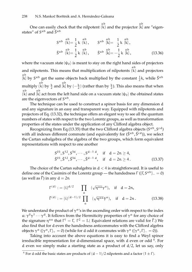
ii

“proc17” — 2017/12/11 — 19:44 — page 238 — #252 ii

ii

ii


One can easily check that the nilpotentab

(k) and the projectorab

[k] are ”eigen-states” of Sab and Sab

Sabab

(k)=1

2kab

(k) , Sabab

[k]=1

2kab

[k] ,

Sabab

(k)=1

2kab

(k) , Sabab

[k]= −1

2kab

[k] , (13.36)

where the vacuum state |ψ0〉 is meant to stay on the right hand sides of projectors

and nilpotents. This means that multiplication of nilpotentsab


[k] by Sab get the same objects back multiplied by the constant 12k, while Sab

multiplyab

(k) by k2

andab

[k] by (−k2) (rather than by k

2). This also means that when

ab

(k) andab

[k] act from the left hand side on a vacuum state |ψ0〉 the obtained statesare the eigenvectors of Sab.

The technique can be used to construct a spinor basis for any dimension dand any signature in an easy and transparent way. Equipped with nilpotents andprojectors of Eq. (13.32), the technique offers an elegant way to see all the quantumnumbers of states with respect to the two Lorentz groups, as well as transformationproperties of the states under the application of any Clifford algebra object.

Recognizing from Eq.(13.35) that the two Clifford algebra objects (Sab, Scd)with all indexes different commute (and equivalently for (Sab, Scd)), we selectthe Cartan subalgebra of the algebra of the two groups, which form equivalentrepresentations with respect to one another

S03, S12, S56, · · · , Sd−1 d, if d = 2n ≥ 4,S03, S12, S56, · · · , Sd−1 d, if d = 2n ≥ 4 . (13.37)

The choice of the Cartan subalgebra in d < 4 is straightforward. It is useful todefine one of the Casimirs of the Lorentz group — the handedness Γ (Γ, Sab− = 0)(as well as Γ ) in any d = 2n

Γ (d) : = (i)d/2∏a

(√ηaaγa), if d = 2n,

Γ (d) : = (i)(d−1)/2∏a

(√ηaaγa), if d = 2n . (13.38)

We understand the product of γa’s in the ascending order with respect to the indexa: γ0γ1 · · ·γd. It follows from the Hermiticity properties of γa for any choice ofthe signature ηaa that Γ † = Γ, Γ2 = I.( Equivalent relations are valid for Γ .) Wealso find that for d even the handedness anticommutes with the Clifford algebraobjects γa (γa, Γ + = 0) (while for d odd it commutes with γa (γa, Γ − = 0)).

Taking into account the above equations it is easy to find a Weyl spinorirreducible representation for d-dimensional space, with d even or odd 6. Ford even we simply make a starting state as a product of d/2, let us say, only

6 For d odd the basic states are products of (d − 1)/2 nilpotents and a factor (1± Γ).

ii

“proc17” — 2017/12/11 — 19:44 — page 239 — #253 ii

ii

ii


nilpotentsab

(k), one for each Sab of the Cartan subalgebra elements (Eqs.(13.37,13.35)), applying it on an (unimportant) vacuum state. Then the generators Sab,which do not belong to the Cartan subalgebra, being applied on the starting statefrom the left hand side, generate all the members of one Weyl spinor.

0d

(k0d)12

(k12)35

(k35) · · ·d−1 d−2

(kd−1 d−2) |ψ0 >0d

[−k0d]12

[−k12]35

(k35) · · ·d−1 d−2

(kd−1 d−2) |ψ0 >0d

[−k0d]12

(k12)35

[−k35] · · ·d−1 d−2

(kd−1 d−2) |ψ0 >

...0d

[−k0d]12

(k12)35

(k35) · · ·d−1 d−2

[−kd−1 d−2] |ψ0 >od

(k0d)12

[−k12]35

[−k35] · · ·d−1 d−2

(kd−1 d−2) |ψ0 >

... (13.39)

All the states have the same handedness Γ , since Γ, Sab− = 0. States, belongingto one multiplet with respect to the group SO(q, d− q), that is to one irreduciblerepresentation of spinors (one Weyl spinor), can have any phase. We could makea choice of the simplest one, taking all phases equal to one. (In order to have theusual transformation properties for spinors under the rotation of spin and underCN PN ,some of the states must be multiplied by (−1).)

The above representation demonstrates that for d even all the states of oneirreducible Weyl representation of a definite handedness follow from a starting

state, which is, for example, a product of nilpotentsab

(kab), by transforming all

possible pairs ofab

(kab)mn

(kmn) intoab

[−kab]mn

[−kmn]. There are Sam, San, Sbm, Sbn,which do this. The procedure gives 2(d/2−1) states. A Clifford algebra object γa

being applied from the left hand side, transforms a Weyl spinor of one handednessinto a Weyl spinor of the opposite handedness.

We shall speak about left handedness when Γ = −1 and about right handed-ness when Γ = 1.

While Sab, which do not belong to the Cartan subalgebra (Eq. (13.37)), gen-erate all the states of one representation, Sab, which do not belong to the Cartansubalgebra (Eq. (13.37)), generate the states of 2d/2−1 equivalent representations.

Making a choice of the Cartan subalgebra set (Eq. (13.37)) of the algebra Sab

and Sab: (S03, S12, S56, S78, S9 10, S11 12, S13 14 ), (S03, S12, S56, S78, S9 10, S11 12,S13 14 ), a left handed (Γ (13,1) = −1) eigenstate of all the members of the Cartansubalgebra, representing a weak chargeless uR-quark with spin up, hyper charge(2/3) and colour (1/2 , 1/(2

√3)), for example, can be written as

03

(+i)12

(+) |56

(+)78

(+) ||9 10

(+)11 12

(−)13 14

(−) |ψ0〉 =1

27(γ0 − γ3)(γ1 + iγ2)|(γ5 + iγ6)(γ7 + iγ8)||

(γ9 + iγ10)(γ11 − iγ12)(γ13 − iγ14)|ψ0〉 . (13.40)

ii

“proc17” — 2017/12/11 — 19:44 — page 240 — #254 ii

ii

ii


This state is an eigenstate of all Sab and Sab which are members of the Cartansubalgebra (Eq. (13.37)).

The operators Sab, which do not belong to the Cartan subalgebra (Eq. (13.37)),generate families from the starting uR quark, transforming the uR quark fromEq. (13.40) to the uR of another family, keeping all of the properties with respectto Sab unchanged. In particular, S01 applied on a right handed uR-quark fromEq. (13.40) generates a state which is again a right handed uR-quark, weak charge-less, with spin up, hyper charge (2/3) and the colour charge (1/2 , 1/(2

√3))

S0103

(+i)12

(+) |56

(+)78

(+) ||910

(+)1112

(−)1314

(−)= −i

2

03

[ +i]12

[ + ] |56

(+)78

(+) ||910

(+)1112

(−)1314

(−) .

(13.41)

One can find both states in Table 13.4, the first uR as uR8 in the eighth line of thistable, the second one as uR7 in the seventh line of this table.

Below some useful relations follow. From Eq.(13.34) one has

Sacab

(k)cd

(k) = −i

2ηaaηcc

ab

[−k]cd

[−k] , Sacab

(k)cd

(k)=i

2ηaaηcc

ab

[k]cd

[k] ,

Sacab

[k]cd

[k] =i

2

ab

(−k)cd

(−k) , Sacab

[k]cd

[k]= −i

2

ab

(k)cd

(k) ,

Sacab

(k)cd

[k] = −i

2ηaa

ab

[−k]cd

(−k) , Sacab

(k)cd

[k]= −i

2ηaa

ab

[k]cd

(k) ,

Sacab

[k]cd

(k) =i

2ηcc

ab

(−k)cd

[−k] , Sacab

[k]cd

(k)=i

2ηcc

ab

(k)cd

[k] . (13.42)

We conclude from the above equation that Sab generate the equivalent representa-tions with respect to Sab and opposite.

We recognize in Eq. (13.43) the demonstration of the nilpotent and the projec-

tor character of the Clifford algebra objectsab

(k) andab

[k], respectively.

ab

(k)ab

(k) = 0 ,ab

(k)ab

(−k)= ηaaab

[k] ,ab

(−k)ab

(k)= ηaaab

[−k] ,ab

(−k)ab

(−k)= 0 ,ab

[k]ab

[k] =ab

[k] ,ab

[k]ab

[−k]= 0 ,ab

[−k]ab

[k]= 0 ,ab

[−k]ab

[−k]=ab

[−k] ,ab

(k)ab

[k] = 0 ,ab

[k]ab

(k)=ab

(k) ,ab

(−k)ab

[k]=ab

(−k) ,ab

(−k)ab

[−k]= 0 ,ab

(k)ab

[−k] =ab

(k) ,ab

[k]ab

(−k)= 0,ab

[−k]ab

(k)= 0 ,ab

[−k]ab

(−k)=ab

(−k) .

(13.43)

Defining

ab˜(±i)= 1

2(γa ∓ γb) ,

ab˜(±1)= 1

2(γa ± iγb) ,

ab˜[±i]= 1

2(1± γaγb),

ab˜[±1]= 1

2(1± iγaγb).

ii

“proc17” — 2017/12/11 — 19:44 — page 241 — #255 ii

ii

ii


one recognizes that

ab˜(k)ab

(k) = 0 ,ab˜(−k)

ab

(k)= −iηaaab

[k] ,ab˜(k)ab

[k]= iab

(k) ,ab˜(k)

ab

[−k]= 0 .

(13.44)

Below some more useful relations [14] are presented:

N±+ = N1+ ± iN2+ = −03

(∓i)12

(±) , N±− = N1− ± iN2− =03

(±i)12

(±) ,

N±+ = −03˜(∓i)

12˜(±) , N±− =

03˜(±i)

12˜(±) ,

τ1± = (∓)56

(±)78

(∓) , τ2∓ = (∓)56

(∓)78

(∓) ,

τ1± = (∓)56˜(±)

78˜(∓) , τ2∓ = (∓)

56˜(∓)

78˜(∓) . (13.45)

In Table 13.4 [4] the eight families of the first member in Table 13.3 (membernumber 1) of the eight-plet of quarks and the 25th member in Table 13.3 of theeight-plet of leptons are presented as an example. The eight families of the righthanded u1R quark are presented in the left column of Table 13.4 [4]. In the rightcolumn of the same table the equivalent eight-plet of the right handed neutrinosν1R are presented. All the other members of any of the eight families of quarks orleptons follow from any member of a particular family by the application of theoperators N±R,L and τ(2,1)±, Eq. (13.45) on this particular member.

The eight-plets separate into two group of four families: One group containsdoublets with respect to ~NR and ~τ2, these families are singlets with respect to ~NL

and ~τ1. Another group of families contains doublets with respect to ~NL and ~τ1,these families are singlets with respect to ~NR and ~τ2.

The scalar fields which are the gauge scalars of ~NR and ~τ2 couple only to thefour families which are doublets with respect to these two groups. The scalar fieldswhich are the gauge scalars of ~NL and ~τ1 couple only to the four families whichare doublets with respect to these last two groups.

After the electroweak phase transition, caused by the scalar fields with thespace index (7, 8), the two groups of four families become massive. The lowestof the two groups of four families contains the observed three, while the fourthremains to be measured. The lowest of the upper four families is the candidate forthe dark matter [1].

References

1. N.S. Mankoc Borstnik, ”Spin-charge-family theory is offering next step in understand-ing elementary particles and fields and correspondingly universe”, Proceedings tothe Conference on Cosmology, Gravitational Waves and Particles, IARD conferences,Ljubljana, 6-9 June 2016, The 10th Biennial Conference on Classical and QuantumRelativistic Dynamics of articles and Fields, J. Phys.: Conf. Ser. 845 (2017) 012017

2. D. Lukman, N.S. Mankoc Borstnik, Eur. Phys. J. C 77 (2017) 231.

ii

“proc17” — 2017/12/11 — 19:44 — page 242 — #256 ii

ii

ii


3. N.S. Mankoc Borstnik, H.B.F. Nielsen, Fortschrite der Physik, Progress of Physics (2017)1700046.

4. N.S. Mankoc Borstnik, J. of Mod. Phys. 6 (2015) 2244-2274.5. N.S. Mankoc Borstnik, Phys. Rev. D 91 (2015) 6, 065004 ID: 0703013. doi:10.1103;

[arxiv:1409.7791, arXiv:1502.06786v1].6. N.S. Mankoc Borstnik, J. of Modern Phys. 4, 823-847 (2013) [arxiv:1312.1542].7. N.S. Mankoc Borstnik, ”Spin-charge-family theory is explaining appearance of families

of quarks and leptons, of Higgs and Yukawa couplings”, in Proceedings to the 16th Work-shop ”What comes beyond the standard models”, Bled, 14-21 of July, 2013, eds. N.S. MankocBorstnik, H.B. Nielsen and D. Lukman (DMFA Zaloznistvo, Ljubljana, December 2013)p.113 -142, [arxiv:1312.1542].

8. N.S. Mankoc Borstnik, ”Do we have the explanation for the Higgs andYukawa couplings of the standard model”, http://arxiv.org/abs/1212.3184v2,(http://arxiv.org/abs/1207.6233), in Proceedings to the 15 th Workshop ”What comes be-yond the standard models”, Bled, 9-19 of July, 2012, Ed. N.S. Mankoc Borstnik,H.B. Nielsen,D. Lukman, DMFA Zaloznistvo, Ljubljana, December 2012, p.56-71, [arxiv.1302.4305].

9. N.S. Mankoc Borstnik, Phys. Lett. B 292, 25-29 (1992).10. N.S. Mankoc Borstnik, J. Math. Phys. 34, 3731-3745 (1993).11. N.S. Mankoc Borstnik, Int. J. Theor. Phys. 40, 315-338 (2001).12. N.S. Mankoc Borstnik, H.B.F. Nielsen, J. of Math. Phys. 43, 5782 (2002) [hep-th/0111257].13. N.S. Mankoc Borstnik, H.B.F. Nielsen, J. of Math. Phys. 44 4817 (2003) [hep-th/0303224].14. A. Borstnik Bracic and N.S. Mankoc Borstnik, Phys. Rev. D 74, 073013 (2006) [hep-

ph/0301029; hep-ph/9905357, p. 52-57; hep-ph/0512062, p.17-31; hep-ph/0401043 ,p.31-57].

15. A. Borstnik Bracic, N.S. Mankoc Borstnik, “The approach Unifying Spins and Chargesand Its Predictions”, Proceedings to the Euroconference on Symmetries Beyond theStandard Model, Portoroz, July 12 - 17, 2003, Ed. by N.S. Mankoc Borstnik, H.B. Nielsen,C. Froggatt, D. Lukman, DMFA Zaloznistvo, Ljubljana December 2003, p. 31-57, [hep-ph/0401043, hep-ph/0401055.

16. N.S. Mankoc Borstnik, Modern Phys. Lett. A 10, 587 -595 (1995).17. G. Bregar, M. Breskvar, D. Lukman and N.S. Mankoc Borstnik, New J. of Phys. 10,

093002 (2008), [arXiv:0606159, arXiv:07082846, arXiv:0612250, p.25-50].18. G. Bregar and N.S. Mankoc Borstnik, Phys. Rev. D 80, 083534 (2009) 1-16.19. G. Bregar, N.S. Mankoc Borstnik, ”Can we predict the fourth family masses for quarks

and leptons?”, Proceedings to the 16 th Workshop ”What comes beyond the standardmodels”, Bled, 14-21 of July, 2013, Ed. N.S. Mankoc Borstnik, H.B. Nielsen, D. Lukman,DMFA Zaloznistvo, Ljubljana December 2013, p. 31-51, [arxiv:1403.4441].

20. G. Bregar, N.S. Mankoc Borstnik, ”The new experimental data for the quarks mixingmatrix are in better agreement with the spin-charge-family theory predictions”, Proceed-ings to the 17th Workshop ”What comes beyond the standard models”, Bled, 20-28 ofJuly, 2014, Ed. N.S. Mankoc Borstnik, H.B. Nielsen, D. Lukman, DMFA Zaloznistvo,Ljubljana December 2014, p.20-45 [ arXiv:1502.06786v1] [arxiv:1412.5866]

21. N.S. Mankoc Borstnik, ”Do we have the explanation for the Higgs and Yukawa cou-plings of the standard model”, [arxiv:1212.3184, arxiv:1011.5765].

22. N.S. Mankoc Borstnik, ”The spin-charge-family theory explains why the scalar Higgscarries the weak charge ± 1

2and the hyper charge ∓ 1

2”, Proceedings to the 17th Work-

shop ”What Comes Beyond the Standard Models”, Bled, July 20 - 28, 2014, p.163-182,[arxiv:1409.7791, arxiv:1212.4055].

23. A. Ali in discussions and in private communication at the Singapore Conference onNew Physics at the Large Hadron Collider, 29 February - 4 March 2016.

24. M. Neubert, in discussions at the Singapore.

ii

“proc17” — 2017/12/11 — 19:44 — page 243 — #257 ii

ii

ii


25. A. Lenz, Advances in High Enery Physics 2013, ID 910275.26. N.S. Mankoc Borstnik, H.B.F. Nielsen, ”Do the present experiments exclude the exis-

tence of the fourth family members?”, Proceedings to the 19th Workshop ”What comesbeyond the standard models”, Bled, 11-19 of July, 2016, Ed. N.S. Mankoc Borstnik,H.B. Nielsen, D. Lukman, DMFA Zaloznistvo, Ljubljana December 2016, p.128-146[arXiv:1703.09699].

27. T. P. Cheng and Marc Sher, Phys. Rev. D 35 (1987), 3484.28. F. Mahmoudi and O. Stal, Phys. Rev. D 81 (2010) 035016.29. C. Anastasioua, R. Boughezalb and F. Petrielloc, J. of High Energy Phys. 04 (2009) 003.30. C. Patrignani et al. (Particle Data Group), Chin. Phys. C 40 (2016) 100001.31. A. Hoecker, ”Physics at the LHC Run-2 and beyond”, [arXiv:1611v1[hep-ex]].32. N.S. Mankoc Borstnik, ”The Spin-Charge-Family theory offers the explanation for all the

assumptions of the Standard model, for the Dark matter, for the Matter-antimatter asym-metry, making several predictions”, Proceedings to the Conference on New Physicsat the Large Hadron Collider, 29 Februar - 4March, 2016, Nanyang Executive Centre,NTU, Singapore, to be published, [arXiv: 1607.01618v1].

33. N.S. Mankoc Borstnik, D. Lukman, ”Vector and scalar gauge fields with respect tod = (3+1) in Kaluza-Klein theories and in the spin-charge-family theory”, Proceedings tothe 18th Workshop ”What comes beyond the standard models”, Bled, 11-19 of July, 2015,Ed. N.S. Mankoc Borstnik, H.B. Nielsen, D. Lukman, DMFA Zaloznistvo, LjubljanaDecember 2015, p. 158-164 [arXiv:1604.00675].

34. D. Lukman, N.S. Mankoc Borstnik, H.B. Nielsen, New J. Phys. 13 (2011) 103027, hep-th/1001.4679v5.

35. D. Lukman and N.S. Mankoc Borstnik, J. Phys. A: Math. Theor. 45, 465401 (2012),[arxiv:1205.1714, arxiv:1312.541, hep-ph/0412208 p.64-84].

36. R. Franceshini, G.F. Giudice, J.F. Kamenik, M. McCullough, A.Pomarol, R. Rattazzi, M.Redi, F. Riva, A. Strumia, R. Torre, ArXiv:1512.04933.

37. CMS Collaboration, CMS-PAS-EXO-12-045.38. CMS Collaboration, Phys. Rev. D 92 (2015) 032004.39. N.S. Mankoc Borstnik, D. Lukman, ”Vector and scalar gauge fields with respect to

d = (3+1) in Kaluza-Klein theories and in the spin-charge-family theory”, Proceedings tothe 18th Workshop ”What comes beyond the standard models”, Bled, 11-19 of July, 2015,Ed. N.S. Mankoc Borstnik, H.B. Nielsen, D. Lukman, DMFA Zaloznistvo, LjubljanaDecember 2015, p. 158-164 [arXiv:1604.00675].

40. N.S. Mankoc Borstnik, H. B. Nielsen, Phys. Rev. D 62, 044010, (2000)1-14, hep-th/9911032.

41. N.S. Mankoc Borstnik, H.B. Nielsen, Jour. of High Energy Phys. 04 (2014)165-174[arXiv:1212.2362v3].

42. T. Troha, D. Lukman and N.S. Mankoc Borstnik, Int. J. of Mod. Phys. A 29 1450124(2014), [arXiv:1312.1541].

43. N.S. Mankoc Borstnik, H.B.F. Nielsen, ”Fermionization in an arbitrary number ofdimensions”, Proceedings to the 18th Workshop ”What comes beyond the standardmodels”, Bled, 11-19 of July, 2015, Ed. N.S. Mankoc Borstnik, H.B. Nielsen, D. Lukman,DMFA Zaloznistvo, Ljubljana December 2015, p. 111-128 [arXiv.1602.03175].

44. T. Kaluza, Sitzungsber. Preuss. Akad. Wiss. Berlin, Math. Phys. 96 (1921) 69, O. Klein,Z.Phys. 37 (1926) 895.

45. The authors of the works presented in An introduction to Kaluza-Klein theories, Ed. byH. C. Lee, World Scientific, Singapore 1983, T. Appelquist, A. Chodos, P.G.O. Freund(Eds.), Modern Kaluza-Klein Theories, Reading, USA: Addison Wesley, 1987.

46. D. Lukman, N. S. Mankoc Borstnik, H. B. Nielsen, New J. Phys. 13 (2011) 10302[arXiv:1001.4679v4].

ii

“proc17” — 2017/12/11 — 19:44 — page 244 — #258 ii

ii

ii




14 Fermionization, Number of Families

N.S. Mankoc Borstnik1 and H.B.F. Nielsen2 ?

1Department of Physics, University of Ljubljana,SI-1000 Ljubljana, Slovenia2Niels Bohr Institute, University of Copenhagen, Blegdamsvej 17,Copenhagen Ø, Denmark

Abstract. We investigate bosonization/fermionization for free massless fermions beingequivalent to free massless bosons with the purpose of checking and correcting the oldrule by Aratyn and one of us (H.B.F.N.) for the number of boson species relative to thenumber of fermion species which is required to have bosonization possible. An importantapplication of such a counting of degrees of freedom relation would be to invoke restric-tions on the number of families that could be possible under the assumption, that all thefermions in nature are the result of fermionizing a system of boson species. Since a theoryof fundamental fermions can be accused for not being properly local because of havinganticommutativity at space like distances rather than commutation as is more physicallyreasonable to require, it is in fact called for to have all fermions arising from fermionizationof bosons. To make a realistic scenario with the fermions all coming from fermionizingsome bosons we should still have at least some not fermionized bosons and we are driventowards that being a gravitational field, that is not fermionized. Essentially we reach thespin-charge-families theory by one of us (N.S.M.B.) with the detail that the number offermion components and therefore of families get determined from what possibilities forfermionization will finally turn out to exist. The spin-charge-family theory has long beplagued by predicting 4 families rather than the phenomenologically more favoured 3.Unfortunately we do not yet understand well enough the unphysical negative norm squarecomponents in the system of bosons that can fermionize in higher dimensions because wehave no working high dimensional case of fermionization. But suspecting they involvegauge fields with complicated unphysical state systems the corrections from such statescould putatively improve the family number prediction.

Povzetek. Avtorja diskutirata bozonizacijo/fermionizacijo za proste brezmasne fermione,ki jih obravnavata kot ekvivalentne prostim brezmasnim bozonom. Namen je preveritiin popraviti staro pravilo Aratyna in H.B.F.N. za stevilo vrst bozonov glede na stevilovrst fermionov kot pogoj za obstoj fermionizacije bozonov. Pomembna uporaba takegapravila bi bil pogoj na stevilo moznih druzin, ce privzamemo, da so vsi fermioni v naravirezultat fermionizacije vrst bozonov. Teoriji fermionov kot fundamentalnih delcev lahkoocitamo, da nima pravilne lokalnosti, ker zahtevamo za fermione antikomutativnost, nepa komutativnosti. Temu ocitku bi se lahko izognili, ce vsi fermioni izhajajo iz fermion-izacije bozonov. Za realisticen opis v modelu, v katerem fermione dobimo s fermionizacijobozonov, mora vsaj nekaj bozonov ostati nefermioniziranih. Avtorja predlagata, da so tinefermionizirani bozoni gravitacijska polja. Zelita na ta nacin reproducirati teorijo Spina-nabojev-druzin enega od avtorjev (S.N.M.B.), kjer bi stevilo fermionskih komponent in

? H.B.F. Nielsen presented the talk.

ii

“proc17” — 2017/12/11 — 19:44 — page 245 — #259 ii

ii

ii

14 Fermionization, Number of Families 245

stevilo druzin dolocale moznosti za fermionizacijo. Teorija spina-nabojev-druzin napove4 druzine, namesto doslej opazenih 3. Avtorja se ne razumeta dovolj dobro nefizikalnihkomponent z negativnim kvadratom norm v sistemu bozonov, ki se fermionizira v visjih di-menzijah, ker jima fermionizacije v visjih dimenzijah se ni uspelo zares izpeljati. Domnevata,da bodo spoznanja o vlogi nefizikalnih stanj pomagala pri napovedi stevila druzin.

Keywords: Fermionization, Bosonization, Number of families

14.1 Introduction

One of the general requirements for quantum field theories is microcausality [1,2],the requirement of causality, which in its form as suggested from tensor productdeduction says, that for two relative to each other spacelikely placed events x1and x2 in Minkowski space-time a couple of quantum field operators O1 and O2taken at these events will commute

O1(x1),O2(x2)− = 0 for spacelike x1 − x2. (14.1)

This is so for the O1 and O2 being boson fields, but if they are both fermionfields, one would have instead to let them anticommute

O1(x1),O2(x2)+ = 0 for spacelike x1 − x2. (14.2)

Such anticommutation is, however, from the tensor product way of arguing forthe relation completely wrong. We could therefore claim that it is not truly allowedto have fermions in the usual way, because it leads to a “crazy” locality axiom. It isone of the purposes of the present proceedings article to suggest to investigate theconsequences of such an attitude, that fermions as fundamental particles are notgood, but that one should rather seek to obtain fermions, not as fundamental, butrather only by fermionization of some boson fields instead. But then it becomesvery important what combinations - what systems - of fermions can be obtainedfrom appropriate bosonic models. For the existence of quite nontrivial restrictionson the number of fermions, we can expect to be obtainable by fermionizationfrom a system bosons, the theorem [3] by Aratyn and one of us (H.B.F.N.) isquite suggestive. In fact this theorem tells, that the ratio between the numberof fermion spin components for all the species (families) counted together andthe corresponding number of boson spin components counted together must be2dspatial

2dspatial−1

. A priori this theorem seems to enforce that in say the experimentalnumber of dimensions, dspatial = 3 and 1 time, the collective number of fermionscomponents must be divisible by 23 = 8. If we count the components as real fieldsa Weyl fermion has 2*2 = 4 such real components, and thus the number of Weylfermions must be divisible by 8/4 =2.

Let us immediately include the remark, that although we shall below mainlygo for the presumably simplest case of non-interacting massless bosons - presum-ably Kalb-Ramond fields - being fermionized into also free massless fermions, thatdoes NOT mean that we seriously suggest Nature to have no interactions. Rather

ii

“proc17” — 2017/12/11 — 19:44 — page 246 — #260 ii

ii

ii


the hope is that gravitational degrees of freedom couple in a way specified aloneby the flow of energy and momentum, so that we can hope that having a freetheory it should be very easy and almost unique how to add a gravitational inter-action. Let us say, that by the spin-charge-family theory by one of us, the interactingfields are the gravitational ones (vielbeins and spin connections) [5–7] only, but ind > (1+ 3), fermions manifesting in (1+ 3) as spins and all the observed charges,as well as families, gravity manifesting all the observed gauge fields as well as thescalar fields, explaining higgs and the Yukawa couplings.

In analogy to, how one sometimes says that the electromagnetic interactionis added to a system of particles or fields with a global charge is “minimallycoupled”, if one essentially just replace the derivatives by the correspondingcovariant ones, we shall imagine that our free theory, which has energy andmomentum as global charges could be made to contain gravity by some sortof “minimal coupling”. To introduce other extra interactions than just gravity is,however, expected to be much more complicated: Especially higher order Kalb-Ramond fields couple naturally to strings and branes, which in any case wouldtend to have disappeared in the present status of the universe. So effectivelyto day the Kalb-Ramond fields [13] should be free except for their “minimalcoupling to gravity”. This would mean that allowing such a “later” rather trivialinclusion of gravity, which should be relatively easy, would make our at first freemodel be precisely the since long beloved model of one of us, the-spin-charge-family theory [5–7]. Fundamentally we have thus in our picture some series ofKalb-Ramond fields together with gravity coupling to them in the minimal way.Then we fermionize only this series of Kalb-Ramond fields, but keep bosonic thegravitational field, which probably cannot be fermionized even, if we wanted to.The resulting theory thus becomes precisely of similar type as the one by one ofus, the spin-charge-family theory.

Now, however, the Kalb-Ramond fields are plagued by a lot of gauge sym-metry and “unphysical” degrees of freedom, some of which even show up witheven negative norm squared inner products. In principle these unphysical degreesof freedom must also somehow be treated in the fermionization procedure. Es-pecially, if we want to use our theorem of counting degrees of freedom underbosonization [3], we should have such a theorem allowed to be used also whenthe “unphysical” d.o.f. are present.

In fact it is the main new point in the present article, that we put forward aslightly more complicated Aratyn-Nielsen-theorem - an extended Aratyn-Nielsentheorem -, allowing for theories with negative norm squared normalizations.

It is the true motivation of the present work, that once when we shall find somegenuinely working case(s) of theories that bosonize/fermionize into each other inhigh dimensions, they will almost certainly turn out to involve gauge theories onthe bosonic side. That is to say it will be combinations of various Kalb-Ramondfields [13] (among which we can formally count also electromagnetic fields andeven a scalar field), and such Kalb-Ramond fields often have lots of negative normsquare components. Thus once we know what is the boson theory that can befermionized we need an extended Aratyn-Nielsen theorem to calculate the correctnumber of fermion components matching the fermionization correspondance.

ii

“proc17” — 2017/12/11 — 19:44 — page 247 — #261 ii

ii

ii


Well really, if we know it well, we can just read off how many fermion componentsthere are. It is namely this number of fermion components, that translates into thenumber of families, on which they are to be distributed. It means that knowingthe detailed form of the boson system and the rule - the extended Aratyn-Nielsentheorem - for translating the number of boson components into the number offermion components is crucial for obtaining the correct number of families. Willso to speak the number of fermion-families remain 4 as claimed by one of us inher model, which has reminiscent of being a fermionization, or will it be correctedsomehow from the true bosonization requirement including the negative normsquare components for the bosons? The reliability of the model would of course -according to the judgement of one of us (H.B.F.N.) - be much bigger, if it turnedout that the true prediction were 3 families rather than the 4 as usually claimed,except, of course, if the fourth family, predicted by the spin-charge-family theory,will be measured.

With the old Aratyn-Nielsen theorem (the unextended version) it does crudelynot look promising to get the number 3 rather than 4 as H.B.F.N would hopephenomenologically in as far this version implies that the number of fermioncomponents is divisible by a rather high power of the number 2. Such a number-theoretic property of the number of families seems a priori to favor 4 much over3.

The works of major importance for the present talk are:

• Aratyn & Nielsen We made a theorem [3] about the ratio of the number ofbosons needed to represent a number of fermions based on statistical mechan-ics in the free case, under the provision that a bosonization exists.

• Kovner & Kurzepa They[8,9] present an explicit bosonization of two complexfermion fields in 2+1 dimensions being equivalent to QED3 meaning 2+1dimensional quantum electrodynamics.

• Mankoc-Borstnik [5–7] The spin-charge-family unification theory explains thenumber of families from the number of fermion components appeared in thistheory.

In the next section 14.2 we put forward the main hope or point of view of ourapplication of bosonization to make prediction of the number of families. In section14.3 we give a loose argument for what we think should our picture for nature tocope with the investigations in the present article. Then we shall in section 14.4and 14.5 review both Kalb Ramond fields and and our old Aratyn-Nielsen theoremabout the number fermion components needed to make an equivalent theory witha number of boson components. In section 14.6 we look at the problem, that thecomponents of a Kalb-Ramond field with an index being 0 are on the one handto be a conjugate momentum to the other components and on the the other hand,if we use Lorentz invariance, have to lead to states with negative norm square.The latter is of course simply a reflection of the signature of the Minkowski metrictensor. It is for the application on such negative norm square components - thecomponents with an index 0 - that our extension of our Aratyn-Nielsen theoremto negative norm square components become relevant.

In section 14.8 we review the work by Kovner and Kurzepa[8], who proposeda concrete bosonization including explicit expressions for the fermion fields in

ii

“proc17” — 2017/12/11 — 19:44 — page 248 — #262 ii

ii

ii


terms of the boson fields - actually simply electrodynamics - in the case of 2 spacedimensions and one time, 1+ 2. Next in 14.9 we seek to check our Aratyn-Nielsentheorem on this special case of 1+2 both by counting the particle species includingspin states 14.10 and by counting the fields 14.11.

Towards the end, section 14.12, we seek to reduce away some of the degreesof freedom from the Kovner and Kurzepa model to obtain a reduced case withfewer particles on which we - if it is also a case of bosonization - would be againable to check our counting theorem (Aratyn-Nielsen).

14.2 Hope

Use of Bosonization/Fermionization Justifying Number of FamiliesThe governing philosophy and motivation for the present study is:

• Fermions do NOT exist fundamentally (because they do not have propercausal/local property) .

• Some boson degrees of freedom are rewritten by bosonization (better fermion-ization) to fermionic ones, which then make up the fermions in the world,we see. (but some other boson degrees of freedom, hopefully gravity, are notbosonized).

• We work here only with an at first free theory - for our presentation, it mightbe best if only bosonization worked for FREE theories in higher dimensions -i.e. free bosons can be rewritten as free fermions.

• We though suggest - hope- that exterior to both bosons and/or fermions, wecan add a GRAVITATIONAL theory. So fundamentally: gravity with matterbosons. It gets rewritten to fermions in a gravitational field, just similar to thetheory [5–7] of one of us called spin-charge-family unification theory.

Let us be more specific about the dream or hope behind the present project:By using say ideas from the below discussed paper by Kovner and Kurzepa [8]

or by our own earlier article in last years Bled Proceedings about bosonization,we hope to find at least a case of fermionizing some series of Kalb-Ramond fields(i.e. Boson fields) - and electrodynamics is of course considered here a specialKalb-Ramond one - into some system of fermions. Presumably it is easiest - andperhaps only possible - for free theories or only theories interacting in a veryspecial way. We therefore are most eagerly going for such a free and even masslesscase.

But now if indeed we can find such a case, or if exists, then it is very likelythat we can extend it to interact with gravity in a minimal way. In fact we all thetime require our hoped for fermionization cases to have the same energy andmomentum for the bosonic and the fermionic theories that shall be equivalent.Thus the fermionization procedure, if it exist at all, is compatible with energy andmomentum.

If we therefore let our boson-theory interact with gravity, that couples to theenergy and momentum - specifically to the energy momentum tensor Tµν(x) -we have some hope that this coupling of the boson fields to gravity will simplytransfer to a coupling of the fermionized theory, too.

ii

“proc17” — 2017/12/11 — 19:44 — page 249 — #263 ii

ii

ii


As procedure we might have in mind writing the free massless fermionizationprocedure in arbitrary coordinates. That should of course be possible, but althoughthe theory would now look as a gravitational theory, it would only have beenderived for the case of the gravitational fields having zero curvature, i.e. for theRiemann tensor being zero all over. However, if the fermionization procedurecould be described by a local expression for the Kalb-Ramond fields - or otherboson fields - expressed in terms of fermion currents or the like, then the corre-spondence would in that formulation be local and lead to the energy momentumtensor being also related in such simple local way. I.e. we would have in thisspeculation

Tµν(x)|boson = Tµν(x)|fermion. (14.3)

Here of course the two energy momentum tensors are the ones in respectively thefermion and the boson theory being equivalent by the dream for fermionization.

It is further our hope for further calculation that we may argue that in generalit is very difficult to have interaction with Kalb-Ramond fields except for

• The appropriate branes,• Some general gauge-theory coupling to the charges (think of global ones)

conserved by the Kalb-Ramond- theory in question. But since the alwaysconserved global charges are the energy and momentum this suggests thecoupling to gravitational field.

We thus want to say that this starting form fundamental Klab-Ramond fieldssupposedly difficult to make interact points towards a theory at the end withgravity as the only interaction. Gravity namely is suggested to be hard to excludeas possibility even for otherwise difficult to make interact Kalb-Ramond fields.

If we manage to fermionize the Kalb-Ramond fields as just suggested, wetherefore tend to end up with the spin-charge-family unification model of one ofus in the sense that we get ONLY gravity interaction, and otherwise a free theory.

But it shall of course be understood here that we only fermionize some ofthe boson fields in as far as we leave the assumed fundamental gravity field nonfermionized.

14.3 Guiding and Motivation

The reader might ask why we choose - and suppose Nature to choose - theseKalb-Ramond-type fields which are to be explained a bit more below in section(14.5). Let us therefore put forward a few wish-thinking arguments for our bosonicfundamental model:

• We have no way to make fermionization/bosonization conserving angular-momentum truly (at the same time keeping the spin statistics theorem): Thebosons namely necessarily can only produce Fock space states with integerangular momentum, but the fermion sates should for an odd number offermions in the the Fock state have half integer angular momentum. So clearlyfermionization/bosonization conserving angular momentum is impossible!

ii

“proc17” — 2017/12/11 — 19:44 — page 250 — #264 ii

ii

ii


• The trick to overcome this angular-momentum-problem is to reinterprete a spin1/2 index on the fermions as a family index instead. That is to say we accept at firstthat the fermions come out of the fermionization with bosonic integer spinindex combination, and then seek to reinterprete part of the spin polarisationinformation as instead being a family information.

• In fact we shall be inspired by the spin-charge-family unification model to gofor that the fermions come out from the fermionization at first with two spinorindices, so that they have indeed formally at this tage integer spin. Then wemake the interpretation that one of these spinor indices is indeed a family index.That of course means, that we let one of the two indices be taken as a scalarindex i.e. being not transformed under Lorentz transformations.

• So we decide to go for a system of fermions at the “first interpretation” beinga two-spinor-indexed field. But now such a field Bαβ, where α and β are thespinor indices, is indeed a Clifford algebra element, or we could say a Diracmatrix (or a Weyl matrix only if we use only the Weyl components). In anycase we can expand it on antisymmetrized products of gamma-matrices:

Bαβ =(a1 + aµγ

µ + · · ·+ aµν...ργµγν · · ·γρ + . . .

+ a0,1,...,(d−1)γ0γ1 · · ·γ(d−1)

)αβ, (14.4)

and thus the boson fields suggested to by fermionization leading to suchfermion fields should be a series of antisymmetric tensor fields of all thedifferent orders from the scalar a and the d-vector aµ all the way up to themaximal antisymmetric order tensor a0,1,...,(d−1).

• With random coefficients on a Lagrange-density expansion for a theory withboson fields, which have d-vectorial indices one unavoidably loose the bottomin the Hamiltonian as one can see from e.g. just a term like

c ∗ (∂µ · · ·∂νaρ...τ)2 . (14.5)

Think for instance on the terms for which the series of the derivative indicesare spatial so that we have to do with a potential energy term. If the coefficientc is adjusted to let the contribution with the indices on aρ...τ being spatialto the Hamiltonian be positive, then the contributions with a 0 among theseindices will from Lorentz invariance have to be of the wrong sign. So it is atbest exceedingly hard to organize a positive definite Hamiltonian density.Consider only the free part - meaning bilinear part in the field aρ...τ - inthe Lagrangian. For simplicity let us consider the situation of a field aρ...τbeing constant as function of the time coordinate x0, and that the number ofderivatives acting on the field is so low that some of the indices- say ρ - on theaρ...τ has to be contracted with another one or the same index on this fieldin order to cope with Lorentz invariance. Then if this (sum of) squares of thefield in some combination shall get a for the hamiltonian positive contributionfrom a spatial value of the index ρ, it will get the opposite sign for ρ = 0. So itlooks that we cannot avoid the Hamiltonian having both signs for a “free term”in the Lagrangian, unless all the indices on aρ...τ are in the term contractedwith derivatives. But with the antisymmetry this would be zero for more than

ii

“proc17” — 2017/12/11 — 19:44 — page 251 — #265 ii

ii

ii


one index on aρ...τ. So indeed it seems that unless one gets the fields restrictedin some way, so that these fields or their conjugate variables are somehownot allowed to take independent values, then the Hamiltonian will loose itsbottom and (presumably infinite) negative energy values will be allowed.

• We are thus driven towards theories with constraints!• Such constraints are typically obtained by means of some gauge symmetry,

and thus we are driven towards theories with gauge symmetry, if we wantto uphold a positive definite Hamiltonian for the by the constraints allowedstates of the field and its conjugate momenta.

• The obvious candidate for such a gauge theory with antisymmetrised tensorfields is of course the Kalb-Ramond fields. (Personally we suspect, that we canshow that ONLY Kalb-Ramond-fields will solve this problem of positivity byproviding enough constraints.)• Thus it seems that it is very hard to hope for our to be used fermionization

unless we make use of presumably a whole series of Kalb-Ramond fields!

14.4 Review

In theoretical condensed matter physics and particle physics, Bosonization/fermio-nization is a mathematical procedure by which a system of possibly interactingfermions in (1+1) dimensions can be transformed to a system of massless, non-interacting bosons. In the present article we shall dream about extending suchbosonization to higher dimensions, and we shall be most interested in the casewhen even the fermions do not interact. The method of bosonization was conceivedindependently by particle physicists Sidney Coleman and Stanley Mandelstam;and condensed matter physicists Daniel Mattis and Alan Luther in 1975. [4]The progress to higher dimensions has been less developed [11] than the 1+1dimensional case, but there has been some works also on higher dimensions.especially we shall below review a bit a work[8] by Kovner and Kurzepa for thenext to simplest case, namely 2+1 dimensions. There has also been developmentsbased on Chern-Simon type action[11], but we suspect that the type of bosonizationwe are hoping for in the present article should rather be of the Kovner Kurzepatype than of the Chern-Simon one, although we have difficulty in explainingrationally why we believe so.

When we have such transformation and thus two equivalent theories, onewith fermions and one with bosons, one will of course expect that the number ofdegrees of freedom should in some way be the same for the boson and for thefermion theory. Otherwise of course they could not be equivalent. In the moststudied case of 1+1 dimensions it has turned out in the cases known that there aretwo fermion components per boson component. This ratio is in accord with thetheorem by Aratyn and one of us [3] - which we call the Aratyn-Nielsen theorem- in as far as this theorem predicts the ratio to be 2

dspatial

2dspatial−1

where dspatial isthe dimension of space ( not including time) so that we talk about the dimensiondspatial + 1. In fact of course for the case 1+1 we have thus dspatial = 1 andthe fraction predicted becomes 21

21−1= 2 times as many fermion components as

boson components. This is really assuming that a “component” corresponds to a

ii

“proc17” — 2017/12/11 — 19:44 — page 252 — #266 ii

ii

ii


polarization state of a particle. What we - one of us and Aratyn - really derivedwas that for a theory with massless interacting there ahd to be the mentioned ratiobetween the number of polarization states for the fermion(s) relative to that for thebosons. It were namely the contributions of such polarization states to the averageenergy in a Boltzmann distribution calculation that was used to derive the theorem.Although derived for this non-interacting massless case there could be reasonsto believe that by taking a couple of limits in an imagined case of interactingand perhaps massive bosonization it could be argued, that the theorem of ourswould have to hold anyway. For instance going to a very small distance scaleapproximation an approximately massless theory would arrive and the theoremshould be applicable even if there is a mass. Since we are concerned in this theoremreally with a counting of degrees of freedom a very general validity is in fact, whatwould be expected. As already said, we are, however, in the present article moreconcentrating on the generalization to include some unphysical degrees of freedomwith possibly wrong signature,

14.5 AratynN

Aratyn-Nielsen Theorem for massless free BosonizationIf there exist two free massless quantum field theories respectively with

Boson, and Fermion particles and they are equivalent w.r.t. to the number of statesof given momenta and energies, then the two theories must have the same averageenergy densities for a given temperature T , or simply same average energies, if wetake them with the same infrared cut off(a quantisation volume V):

< Uboson > = < Ufermion > where (14.6)

< Uboson > =∑~p

E(~p)

1− exp (E(~p)/T)(14.7)

< Ufermion > =∑~p

E(~p)

1+ exp (E(~p)/T). (14.8)

(14.9)

Here ~p runs through the by the infrared cut off allowed momentum eigenstates,and E(~p) are the corresponding single particle energies. Of course the singleparticle energy for a mass-less theory is

E(~p) = |~p|, (14.10)

when c=1, and in dspatial dimensions and with an infrared cut off spatial volumeV the sum gets replaced in the continuum limit by the integral∑

~p

...→ ∫ ∑components

...V

(2π)dspatial, (14.11)

where∑components ... stands for the sum over the different polarization com-

ponents of the particles in question. So effectively in the simplest case of all the

ii

“proc17” — 2017/12/11 — 19:44 — page 253 — #267 ii

ii

ii


particles having the same “spin”/the same set of components we have the replace-ment ∑

components

...→ Nfamilies ∗Nc... (14.12)

where Nc is the number of components for each particle and Nfamilies is thenumber of families. Some formulas for deriving Aratyn-Nielsen

< Uboson > =∑~p

E(~p)

1− exp (E(~p)/T)(14.13)

= ‘‘Nfamilies ∗N ′′c ∗ V/(2π)dspatial ∗ (14.14)∫O(dspatial)|~p|

dspatialE(~p)∑

n=0,1,...

exp (nE(~p)/Td|~p|

(14.15)

Simple Aratyn-Nielsen Relation For a given temperature must the averageenergies of respectively the boson and the with it equivalent fermion theories

Our Realization Suggestion

• FermionsFor the fermions we shall use the needed number of say Weyl fermions, i.e.we must adjust the number of families hoping that we get an integer number.• Bosons

For the bosons we let the number 2dspatial − 1 suggest that we take a seriesof all Kalb-Ramond fields, one combination of fields for each value of thenumber p of indices on the “potential field” Aab...k (where then there are justp symbols in the chain ab...k). At first we take these symbols a, b, ..., k to beonly spatial coordinate numbers.

Free Kalb-Ramond A Kalb-Ramond field[13] with p indices on the “po-tential” and p+1 indices on the strength

Fµνρ...τ(x) = ∂[µAνρ...τ](x), (14.16)

where [...] means antisymmetrizing, and the “potential” Aνρ...τ is antisymmetricin its p indices νρ...τ, is defined to have an action invariant under the gaugetransformation:

Aνρ...τ(x)→ Aνρ...τ(x) + ∂[νλρ...τ](x) (14.17)

for any arbitrary antisymmetric gauge function λρ...τ(x) with p− 1 indices.Free Kalb-Ramond Action:Note that the strength Fµνρ...τ = ∂[µAνρ...τ] is gauge invariant, and that thus

we could have a gauge invariant Lagrangian density as a square of this fieldstrength

L(x) = Fµν...τFµ ′ν ′...τ ′gµµ′∗ gνν

′∗ ... ∗ gττ

′. (14.18)

ii

“proc17” — 2017/12/11 — 19:44 — page 254 — #268 ii

ii

ii


Then the conjugate momentum of the potential becomes(formally):

Πνρ...τ = ΠAνµ...τ =∂L

∂(∂0Aνρ...τ)

= F0νρ...τ. (14.19)

A Lorentz gauge choice:

∂µAνρ...τgµν = 0, (14.20)

allows to write the Lagrange density instead as

Lmodified(x) = 1/2 ∗ ∂µAµν...τ∂µ ′Aµ ′ν ′...τ ′ ∗ gµµ′gνν

′· · ·gττ

′, (14.21)

which leads to the very simple equations of motion letting each component of the“potential” Aνρ...τ independently obey the Dalambertian equation of motion

gµµ′∂µ∂µ ′Aνρ...τ = 0. (14.22)

Lorentz Invariance Requires Indefinite Inner Product!:Lorentz invariant norm square for the states generated by the creation oper-

ators a†νρ...τ(p), i.e. a†νρ...τ(p)|0 >, must have different sign of the norm squaredepending on whether there is an even (i.e. no) 0’s among the indices or whetherthere is an odd number (i.e. 1). A priori we are tempted to take

< 0|aνρ...τ(p)a†νρ...τ(p)|0 > > 0 for no 0 among the indices,

< 0|aνρ...τ(p)a†νρ...τ(p)|0 > < 0 for one 0 among the indices,

(14.23)

14.6 Time-index

Problem with Components with the time index 0:But full Kalb-Ramond fields require also components a 0 among the in-

dices.(This is the main new thing in the present article to treat this problem of thecomponents with one 0 among the indices.)

Remember about these components with a 0 index:

• Using a usual Minkowskian metric tensor gµν in constructing an inner productbetween Kalb-Ramond fields, say

gµνgρσ · · ·gτκAµρ...τ(potentially an ∂0)Aνσ...κ, (14.24)

we get the opposite signature (=sign of the square norm) depending onwhether there is a 0 or not!This means that if particles produced by the components without the 0 in-dex have normal positive norm square, then those produced by the oneswith the 0 have negative norm-square!

ii

“proc17” — 2017/12/11 — 19:44 — page 255 — #269 ii

ii

ii


Good Luck We Removed the Kalb-Ramond A with p = 0 Indices! We couldnamely not have replaced on A one among its indices by a 0 because it has noindices. So we would not have known what to do for the fields Awith 0 indices.

We correspondingly also have to leave out the Kalb-Ramond-field with p =

dspatial + 1 indices, because for that there would be no components without anindex 0.

For the unexceptional index numbers p = 1, 2, ..., dspatial there are somecomponents both with and without the 0.

For the two exceptions p = 0 and d = dspatial + 1 we have chosen notto have a Kalb-Ramond-field in our scheme, using it to get the −1 in the fromAratyn-Nielsen required 2dspatial − 1.

Simplest (Naive) Norm Square AssignmentNote that for each Kalb-Ramond-field we can choose an overall extra sign on

the inner product, because we simply can define the overall inner product with anextra minus sign, if we so choose. But the simplest choice is to just let the particlescorresponding to fields with only spatial indices (i.e. all p indices different from 0)to have positive norm square, while then those with one 0 have negative normsquare.

This simple rule would lead to equally many components/particles withpositive as with negative norm square, so that dreaming about imposing a con-straint that removes equally many negative and positive norm square at a timewould leave us with nothing.

Numbers of Components with and without 0. An of course totally antisym-metric field Aµν...τ with p indices has

# componentsKR pindices =

(d

p

)=

(dspatial + 1

p

)# no 0 components

KR pindices =

(dspatial

p

)=

(d− 1

p

)# cmps. with 0 & p-1 non-0

KR pindices =

(dspatial

p− 1

)=

(d− 1

p− 1

).

and so one must have as is easily checked(d

p

)=

(d− 1

p

)+

(d− 1

p− 1

)corresponding to

“All components” = “Without 0” + “With 0”

Using ONLY the Components WITHOUT 0 would fit 2dspatial Nicely !Having decided to leave out the number of indices p values p = 0 and p = d thenumber of components without any component indices being 0 just makes up

# without 0 for all p = 1, 2, ..., d− 1 =∑

p=1,2,...,d−1

(d− 1

p

)= 2d−1 − 1

so these “only with spatial indices components” could elegantly correspond to2d−1 = 2dspatial fermion components.

ii

“proc17” — 2017/12/11 — 19:44 — page 256 — #270 ii

ii

ii


But problem: Kalb- Ramond fields need also the component with an indexbeing 0.

Using ONLY the Components WITH 0 could also fit 2dspatial Nicely ! Hav-ing decided to leave out the number of indices p values p = 0 and p = d thenumber of components with the 0 just makes up

# with 0 for all p = 1, 2, ..., d− 1 =∑

p=1,2,...,d−1

(d− 1

p− 1

)= 2d−1 − 1

also, so these “only with 0 index components” could elegantly correspond to 2d−1

= 2dspatial fermion components, also!But problem: Kalb- Ramond fields need also the components without an

index being 0, and these with 0 usually come with wrong norm square.The Trick Suggested is to use for Some KR-fields Opposite Hilbert Norm

SquareIn other words we shall look along the chain of all the allowed p-values

p = 1, 2, ..., d− 1; and for each of these p-values we can choose whether

• Normal: The states associated with the polarization components without the0 among the indices shall be of positive norm square, as usual, and then fromLorentz invariance essentially the ones with the 0 shall have negative normsquare, or

• Opposite The states with 0 shall have positive norm square, while the com-ponents without 0 negative norma square.

Our proposal: Choose so that we get the largest number of positive norm squarecomponents. How to get Maximal Number of Positive over Negative NormSquare Single Boson States

For each value of p (=the number of indices on the Kalb Ramond “potential”)p = 1, 2, ..., dspace decided to be used in the bosonization ansatz a priori, weinvestigate whether the number of (independent) components with or without a0 is the bigger:

# no 0 componentsKR pindices =

(dspatial

p

)=

(d− 1

p

)# cmps. with 0 & p-1 non-0

KR pindices =

(dspatial

p− 1

)=

(d− 1

p− 1

).

So if there are most components without 0, i.e. if(dspatialp−1

)<(dspatial

p

), then we

give the particle states corresponding to the without 0 “potentials” have positivenorm square. And opposite if

(dspatialp−1

)>(dspatial

p

).

But if there are most components with 0, i.e. if(dspatialp−1

)>(dspatial

p

), then

we give the particle states corresponding to the with 0 “potentials” have positivenorm square.

To Maximize Positive Norm Square we Choose:

ii

“proc17” — 2017/12/11 — 19:44 — page 257 — #271 ii

ii

ii


• When p < d2

, choose without 0 positive norm squared, while “with 0” nega-tive;

• but when p > d2

, choose with 0 positive norm squared, while “without 0”negative;

For e.g. p < d/2 the excess of positive norm square “components ” over thenegative norm ones becomes:(

dspace

p

)−

(dspace

p− 1

)=

(dspace

p

)(1−

p

dspace − p+ 1)

=dspace!(dspace + 1− 2p)

(dspace − p+ 1)!p!=

(d− 1)!(d− 2p)

(d− p)!p!, (14.25)

However, for p > d/2 the excess is(dspace

p− 1

)−

(dspace

p

)=

(dspace

p− 1

)(1−

dspace − p+ 1

p)

=dspace!(2p− dspace − 1)

(dspace − p+ 1)!p!=

(d− 1)!(2p− d)

(d− p)!p!, (14.26)

Adding up Positive Norm Square over Negative Excess:The sums over p “ telescopes” from each of the two cases of p bigger or smaller

than d/2, and gives by symmetry the same excess of positive over negative normsquare states, namely for each for say d even (i.e. dspace odd)(

d− 1

d/2− 1

)− 1 =

(d− 1)!

(d/2− 1)!(d/2+ 1)!− 1, (14.27)

where we used that the middle value p = d/2 contribution vanishes. Including aswe shall both “sides” smaller than d/2 and also bigger than d/2 we get the doubleof this.

Example Excesses States for even d for Bosons

Excess(d = 2) = 2(

(2− 1

2/2− 1

)− 1) = 0

Excess(d = 4) = 2(

(4− 1

4/2− 1

)− 1) = 2

Excess(d = 6) = 2(

(6− 1

6/3− 1

)− 1) = 18

Excess(d = 14) = 2(

(14− 1

14/2− 1

)− 1) (14.28)

Contribution from a Negative Norm square ComponentOne shall count the Hilbert space states with the negative norm square into

the Boltzmann weighted averaging with a minus extra.This extra minus for a negative norm square boson functions accidentally

just like the fermi-statistics versus bose statistics. And thus e.g. a small p timelikepolarization contributes to the average energy just like a fermion, though with anover all minus sign.

ii

“proc17” — 2017/12/11 — 19:44 — page 258 — #272 ii

ii

ii


14.7 Extension of Our Theorem on Counting

It is a major purpose of the present talk to present an extension of the Aratyn-Nielsen theorem[3] on the numbers of bosons versus fermions in a bosonization toinclude the just above discussed negative norm square states associated with theKalb-Ramond components having an index 0. Since such states obtaining at firstnegative norm squares are seemingly enforced by Lorentz invariance, it seems tobe important to extend our Aratyn-Nielsen theorem to the case, where some ofthe components of the fields are quantized with a negative norm square.

We take such a negative norm square mode to mean, that whenever there ina Fock space state is an odd number of particles with the component in question,then such a Fock-space basis vector is in the “Hilbert norm” given a negative normsquare. Of course that means that strictly speaking our Fock space is no longera genuine Hilbert space, but rather just an (infinite dimensional) space with anindefinite inner product, |, giving the inner product between two Focks, |a > and|b > say, as < b|a >. But now the point is just that we have no sign restriction on< a|a >; it can easily be negative.

The in usual Hilbert spaces used expansion on an orthonormal basis

1 =∑a

|a >< a| (usual), (14.29)

cannot now be applied. Now we rather have to use

1 =∑a

(−1)Nneg(a)|a >< a| (with negative norm square also), (14.30)

where Nneg(a) denotes the number of particles in the various negative normsquare single particle states together. If for instance a basis state |a > for the Fockspace has 3 particle in the states with 0 index all together (and we have used thechoice of letting the components with a 0-index be the ones with negative norm,rather than the more complicated possibilities discussed above), Nneg(a) = 3

and thus such a state would come with a minus sign in the expansion of the unitoperator 1.

Let us now calculate the average energy for a system described by a Fockspace with only one single particle state present, so it really is the system withonly one single particle state, that may be filled or empty according the rule forit being bosonic or fermionic and having negative or positive norm square. Forthis purpose we have to think about how one shall define the concept of a trace -which goes into the average procedure to provide us with such a an average of theenergy, and we claim that we must indeed in the case with negative norm squarestates take the trace definition:

Tr(O) =∑a

(−1)Nneg(a) < a|O|a > . (14.31)

ii

“proc17” — 2017/12/11 — 19:44 — page 259 — #273 ii

ii

ii


With this definition we easily check some usual rule for traces:

Tr(OP) =∑a

(−1)Nneg(a) < a|OP|a > (14.32)

=∑a

∑b

(−1)Nneg(a) < a|O|b >< b|(−1)Nneg(b)P|a > (14.33)

= Tr(PO). (14.34)

Using this definition of the trace Tr we can then put in the quite analogousway to the usual case for Boltzmann distribution in quantum mechanics

< E > =Tr(exp(−H/T)H)Tr(exp(−H/T))

, (14.35)

where the Boltzmann-Constant k has been absorbed into the temperature T , andwhere now we use in the case of negative norm square the expression (14.31).Let us enumerate the single particle states with the letter n and denote the singleparticle energy of the state n as En. Then the free HamiltonianH is given by meansof the number operators

Nn = a†nan (14.36)

asH =

∑n

EnNn =∑n

Ena†nan, (14.37)

and we immediately see that

< EnNn > |bosonpos. =

∑Nn=0,1,...

EnNn exp(−EnNn/T)∑Nn=0,1,2,...

exp(−EnNn/T)

=−d(

11−exp(−En/T)

)d(1/T)

11−exp(−En/T)

=En

exp(En/T) − 1(boson; pos. norm sq.) (14.38)

< EnNn > |bosonneg. =

∑Nn=0,1,...

(−1)NnEnNn exp(−EnNn/T)∑Nn

(−1)Nn exp(−EnNn/T)

=−d(

11+exp(−En/T)

)d(1/T)

11+exp(−En/T)

= −En

exp(En/T) + 1(boson; neg. norm sq.) (14.39)

< EnNn > |fermionpos. =

∑Nn=0,1

EnNn exp(−EnNn/T)∑Nn=0,1

exp(−EnNn/T)

=−d(1+exp(−En/T))

d(1/T)

1+ exp(−En/T)=

En

exp(En/T) + 1(fermion; pos. norm sq.) (14.40)

< EnNn > |fermionneg. =

∑Nn=0,1

(−1)NnEnNn exp(−EnNn/T)∑Nn=0,1

(−1)Nn exp(−EnNn/T)

=−d(1−exp(−En/T))

d(1/T)

1− exp(−En/T)= −

En

exp(En/T) − 1(fermion; neg. norm sq.) (14.41)

ii

“proc17” — 2017/12/11 — 19:44 — page 260 — #274 ii

ii

ii


We notice that - by accident - the contribution from a negative norm squarefermion mode happens to be just the opposite of that of a positive norm squareboson mode with the same energy En. And also the positive fermion mode contri-bution is just minus one time the negative boson contribution. Thus we can getthe requirement for the theory of fermions and that of bosons to provide the sameaverage energy: ∑

E ′nsfor (pos.)fermionsplus neg. bosons

En

exp(En/T) + 1=

∑E ′nsfor (pos.)bosonsplus neg. fermions

. (14.42)

14.7.1 Free Massless

The simplest case to consider is the one in which both the fermions and the bosons- on their respective sides of the identification of the theories - are supposed tobe both free and massless relativistic particles. In this case - which is the one weshall keep to in the present article - we introduce for definiteness an infra redcut off so that we get discretized momentum eigenstates, and the above n nowreally becomes a pair of a discretized momentum ~p and an index denoting thecomponent, which means typically the vector or spinor index including also thefamily index, all put together say to t, standing for the word “total component”,meaning that both family and genuine component is included. The number ofpossible values for this total component enumeration is of course for what weare indeed obtaining restrictions for. Let us therefore immediately define the fournumbers

Nt ferm pos. = Nfamilies ferm pos. ∗Nc ferm pos,

Nt ferm neg. = Nfamilies ferm neg. ∗Nc ferm neg.,

Nt boson pos. = Nfamilies boson pos. ∗Nc boson pos,

Nt boson neg. = Nfamilies boson neg. ∗Nc boson neg.,

to denote the total numbers of components of the respective types of particles w.r.t.statistics and normsquare sign.

One technique for calculating the integrals over the momentum space consistsin first Taylor expanding the expressions to be integrated

En

exp(En/T) − 1=

En

exp(En/T)∗ (1+ exp(−En/T) + exp(−2En/T) + ...)

= En

∑j=1,2,...

exp(−jEn/T)

(14.43)

En

exp(En/T) + 1=

En

exp(En/T)∗ (1− exp(−En/T) + exp(−2En/T) − ...)

= En

∑j=1,2,...

(−1)j−1 exp(−jEn/T)

, (14.44)

ii

“proc17” — 2017/12/11 — 19:44 — page 261 — #275 ii

ii

ii


and then using ∑~l∈integer lattice

exp(−j|~l ∗ 2π/L|) =∫

exp(−j|~x2π/L|)ddspatial~x (14.45)

=

(L

2π ∗ j

)dspatial ∫exp(−|~x|)ddspatial~x (14.46)

=

(L

2π ∗ j

)dspatialO(dspatial − 1)

∫∞0

exp(−x)xdspatialdx (14.47)

=

(L

2π ∗ j

)dspatialO(dspatial − 1)/dspatial!. (14.48)

Here we denoted the surface area of the unit sphere in dspatial dimensions byO(dspatial − 1) because this surface then has the dimension dspatial − 1. In fact

O(dsurface) =2πdsurface/2

Γ(dsurface/2). (14.49)

We then finally shall use

ζ(dspatial) =∑

j=0,1,2,...

1

jdspatial. (14.50)

ζ(dspatial)

(1−

1

2dspatial

)=

∑j=0,1,2,...

(−1)j

jdspatial. (14.51)

When we compare the different expressions for bosons versus for fermions,most factors drop out and the only important factor is the factor

(1− 1

2dspatial

).

It is then easy to see that we obtain the extended Aratyn-Nielsen theorem:

Nt ferm pos. +Nt boson neg. =2dspatial

2dspatial − 1∗ (Nt boson pos. +Nt ferm neg.).

(14.52)

14.7.2 Properties and Examples

Let us first of all call attention to that this extended Aratyn-Nielsen theorem likethe original one has the property of “additivity” meaning that if we have twocases of functioning bosonization - i.e. two cases of a system of fermions beingequivalent to a system of bosons - and thus by combining them formally a systemwith both sets of bosons making up its set of bosons and similarly construct a setof fermions by combing the fermions then the combined system will automatically- just algebraically - come to obey the requirement from our theorem.

Let us also remark that the old Aratyn-Nielsen theorem[3] just is the specialcase, in which there are no negative norm square components.

In the Bled workshop in 2015 [12] we presented speculations, that one couldmake a free massless case of bosonization/fermionization in an arbitrary num-ber of dimensions. This attempt were indeed already strongly inspired from our

ii

“proc17” — 2017/12/11 — 19:44 — page 262 — #276 ii

ii

ii


theorem and counted just 2dspatial − 1 boson particle components and 2dspatialfermionic components. There were no negative norm square components and thethere suggested case of bosonization should thus be an example on the use ofthe “old” Aratyn-Nielsen theorem. The ratio of the number 2dspatial of fermioncomponents equivalent to 2dspatial − 1 bosonic components is namely of coursejust equal to 2

dspatial

2dspatial−1

as it should according to our theorem(s). The specialfeature of that proposal [12] was that we imagined having chosen such infraredcut off periodicity or antiperiodicity conditions, that these (anti)periodicity condi-tions specified the components of the fields. Indeed there were just one fermioncomponent for each combination of a choice of periodicity versus antiperiodicityfor each of the dspatial spatial dimensions. That makes up of course 2dspatialcombinations of periodicity antiperiodicity choices and thus so many fermioncomponents. Similarly almost all such combinations gave rise to a boson compo-nent, except that we deleted so to speak the boson components, that should havecorresponded to being periodic in all dspatial coordinates (taken with infraredcut off). Thus there were just 2dspatial − 1 boson components in the in this Bledproceeding speculated case of bosonization.

14.7.3 A speculative semi-trivial example

Starting from the example[12] we would now highly suggestively - but really a bitspeculatively - construct a not completely trivial although not so very physicallyinteresting at first example with negative norm square components. Since we haveanyway broken in this model full rotational invariance, it is no longer a catastropheto treat one of coordinate axis - say x1 in a different way from the other ones.

We modify the model in the 2015 Bled proceedings by:

• On the fermionic side we take all the components specified by having oddmomentum along say the x1-axis or equivalently have antiperiodic boundarycondition in x1 to have negative norm square. They make up just half - andthus 2dspatial−1 - of all the fermionic components.

• On the bosonic side we also change the norm-square to be negative for thecomponents antiperiodic in the x1-coordinate. This is for even more than halfof the components in as far as it is again for 2dspatial−1, but now only out ofthe 2dspatial − 1 bosonic components.

Both of these two modifications have in the Fock-space the same effect in as faras they both just lead to shifting the norm square form positive to negative for allthe states with the total p1-momentum odd. So the two modifications suggestedfor respectively the bosons and the fermions seem to be the same one in the Fockspace. At least speculatively then we expect, that the modified model will havefunctioning bosonization - provided we trust that the original model from the Bled2015 proceeding were indeed consistently a case of bosonization.

Now we want to test, if this suggestive speculative case of bosonization willobey our extended Aratyn-Nielsen requirement(14.52):

We have in this modified model/case of bosonization:

ii

“proc17” — 2017/12/11 — 19:44 — page 263 — #277 ii

ii

ii


• We are left with 2dspatial−1 − 1 bosonic positive norm square components, i.e.Nt boson pos. = 2

dspatial−1 − 1.• While 2dspatial−1 of the bosonic components were made to have negative

norm squared. So Nt boson neg. = 2dspatial−1.• Of the fermionic components 2dspatial−1 remained of positive norm-square;

so Nt ferm pos. = 2dspatial−1.

• Also 2dspatial−1 components had the odd momentum in the x1-direction andwere made to have negative norm square. So Nt ferm neg. = 2

dspatial−1.

Inserting these numbers of components into (14.52) is easily seen to make itsatisfied. The point really is, that we made the same number of boson componentsand of fermion components negative norm square. This sign of norm square in ourformula makes them move from one side to the other, but since the two groupswere of the same number at the end nothing were changed and the formula stillsatisfied.

14.8 Kovner...

Kovner and Kurzepa made 2+1 The article by these authors [8] containsthe expression

ψα(x) = kΛVα(x)Φ(x)Uα(x) (14.53)

for the fermion fields expressed in terms of the boson fields in their fermionizationin 2+1 dimensions. Here the expressions Vα(x), Φ(x), and Uα(x) are exponentialsof integrals over the boson field, which are indeed electromagnetic fields in 2+1dimensions. The variants of expressions are denoted by the index α, which takestwo values. There are thus (a priori) two complex fermion fields defined here.

14.9 Match?

Does the Kovner Kurzepa Bosonization Match with the Aratyn-Nielsen Counting Rule?

First look at number of hermitean counted fields: Kovner and Kurzepagets two complex meaning 4 real fermion fields Reψ1(x), Imψ1(x), Reψ2(x),and Imψ2(x) out of the for the construction relevant boson-fields A1(x), A2(x),∂iEi = ∂1E1 + ∂2E2. This looks agreeing with the Aratyn Nielsen prediction thatthe ratio shall be

#bosons#fermions

=2ds − 1

2ds=22 − 1

22for the spatial dimension beingds = d− 1 = 2

(14.54)Four real fermion fields bosonize to three real boson-fields! o.k.

What about the conjugate momenta to the fields? While the fermion fieldsare normally each others conjugate variables(fields) in as far as they anticommutewith each other having only no-zero anticommutators with themselves, the boson-fields typically are taken each to have associated an extra field - its conjugate -

ii

“proc17” — 2017/12/11 — 19:44 — page 264 — #278 ii

ii

ii


with which it does not commute, while of course any variable must commute withitself. But a field, that depends on an x-point or on a momentum, need NOT tocommute with itself, though.

But then the question: Shall we for bosons somehow also count the conjugatemomentum fields, when we shall compare the number of fermion and bosonfields equivalent through bosonization ? For the fermions the conjugate fieldsare unavoidable already included into the set of fields describing the fermions,because the it is the field in question itself, but for bosons we could easily get thenumber of fields doubled, if we include for each field also its conjugate.

Conjugate Momentum Fields NOT to be Included in Counting.Let us argue that it is enough in the counting to count the number of fields,

from which you by Fourier resolution can extract the annihilation and creationoperators needed to annihilate or create the particles, the species of which are tobe counted:

• Normally we could extract the conjugate field by differentiating w.r.t. to timethe field because usually you can replace the fields and their conjugate by thefields and their time derivatives.

• Using equations of motion these time derivatives can in turn be obtained bysome way - also some sort of differentiation - from the field itself.

• Thus at the end the information on the conjugate is extractable from the fielditself!

Further Support for NOT including also Conjugate Momentum FieldsWe could very easily construct linear (or more complicated) combinations of

boson fields and their conjugate fields. Such combinations would like the fermionfields typically not commute/anticommute with themselves.

So provided we can extra the particle creation and annihilation operatorsfrom the combined field we would have no rule to tell that we should includemore. Thus we would need only the combined field, and with that rule have quiteanalogy to the fermion case.

Meaning of NOT Counting also the Conjugate FieldInQED3 sayA1(x) andA2(x) would be enough to represent both longitudinal

and transversely polarized photons. It would NOT be needed also to have theessentially conjugate electric fields E1(x) and E2(x).

The field ∂iEi is in fact the conjugate A0 so that we - having the symmetrybetween a field and its conjugate, it being conjugate of its conjugate - can considerthat timelike photons are described by this ∂iEi field combination.

14.10 Particles

But in terms of Particles, How??Usually one thinks of electrodynamics in 2+1 dimensions as having only one

particle polarisation, since there is only one transversely polarisation for a photon.So seemingly only one component of boson. This transversely polarized photon iseven its own antiparticle, so even the anti-particle is not new.

ii

“proc17” — 2017/12/11 — 19:44 — page 265 — #279 ii

ii

ii


On the contrary the fermions after the fermionization counts two complexfields meaning two different fermion components (ψ1 and ψ2) each with an apriori different antiparticle in as far as the fields ψ1 and ψ2 both are complex(non-Hermitean). That seems NOT to match!

Where have the two missing photon-polarizations gone?Suggestion for How 3 photons.To count independently both Ai (i=1,2.) as real fields, we need to consider it

that we have not only the transverse photon, but also a longitudinal photon !The third of the real fields ∂iEi = div~E is actually the conjugate variable to

the time component A0(x) of the fourcomponent photon field. So if we take it thatconjugate or not does not matter it could correspond to the timelike polarizedphoton.

This would mean that we could hope for interpreting the three photon polar-izations as being

• 1) The transverse photon.• 2) The longitudinal photon.• 3) The time-like photon.

But the time like photon has wrong signature ?!Better Suggestion for the 3 particles ?To avoid the problem with the ltime-like photon form Lorentz invariance

having the signature with negative norm square states we can instead take a furtherscalar. If so we could have 3 bosons corresponding to the four (real) fermions.

In any case if we want a fermion system with positive definite Hilbert spacewe better have the bosons also give positive definite Hilbert space if they shallmatch in their Hilbert spaces.

14.11 Fields

How to count Hermitean Boson fields ?To exercise we shall for the moment even begin with a 1+1 dimensional

only right moving Hermitean field constructed as a superposition of momentumstate creation a†(p) and annihilation operators a(p) for say a series discretizedmomentum values, which we for “elegance”( and later interest) shall take to beodd integers in some unit:

φ(x) =∑

p odd,p>0

√pa(p) exp (ipx) +

∑p odd,p<0

√|p|a†(|p|) exp (ipx)

=∑p odd

√|p|a(p), (14.55)

where we have puta(p) = a†(−p) for all the odd p (14.56)

ii

“proc17” — 2017/12/11 — 19:44 — page 266 — #280 ii

ii

ii


Properties of the Hermitean field A Hermitean field of the form (in 1+1dimension say)

φ(x) =∑

p odd,p>0

√pa(p) exp (ipx) +

∑p odd,p<0

√|p|a†(|p|) exp (ipx)

=∑p odd

√|p|a(p) (14.57)

obeys

φ(x)† = φ(x) (Hermiticity) and (14.58)

[φ(x), φ(y)] =∑p odd

∑p ′ odd

√|p|√|p ′|[a(p), a(p ′)] exp (ipx+ ip ′y) (14.59)

=∑p odd

p exp (ip(x− y)) = 2πd

id(x− y)δ(x− y) (14.60)

= −i2π∂δ(x− y) (local commutation rule). (14.61)

14.12 New

New, Reduce the Kovner Kurzepa model.We claim, that in a way the Kovner and Kurzepa bosonization in 2 + 1 dimen-

sions has included a kind of “funny extra bosonic degree of freedom” the chargedensity compared to our own plan of doing a completely free model.

Really we want to say: In a truly free electrodynamics “free QED3” (in 2 +1dimensions) the divergence of the electric field is zero:

∂iEi ≈ 0 (on physical states). (14.62)

When we use ≈ instead of = it is because we may need the divergence ∂iEi as anoperator even though we may take it to be zero on the “physical states”.

Reduction of Kovner Kurzepa model w.r.t. degrees of freedomInserting formally our claim of a constraint equation

∂iEi ≈ 0 (on physical states). (14.63)

into the expressions of Kovner and Kurzepa

V1(x) = −i exp (i

2e

∫(θ(x− y) − π)∂iEi) (14.64)

U1(x) = exp (−i

2eθ(y− x)∂iEi) (14.65)

we get

V1(x) ≈ −i (14.66)

U1(x) ≈ 1. (14.67)

ii

“proc17” — 2017/12/11 — 19:44 — page 267 — #281 ii

ii

ii


Using the constraint equation formally on Kovner and Kurzepa In Kovner andKurzepa one finds

ψα(x) = kΛVα(x)Φ(x)Uα(x) (14.68)

Φ(x) = exp (ie

∫ei(y− x)Ai(y)d

2y);ei(y− x) =yi − xi(y− x)2

(14.69)

V1(x) = −i exp (i

2e

∫(θ(x− y) − π)∂iEi);V2(x) = −iV†1(x) (14.70)

U1(x) = exp (−i

2eθ(y− x)∂iEi);U2(x) = V

†1(x) (14.71)

and thus with the constraint formally included

ψ2(x) ≈ iψ1(x) (14.72)

Our Constraint would Spoil Rotation Symmetry A constraint equation

ψ2(x) ≈ iψ1(x) (14.73)

would not be consistent with the rotation symmetry and the transformation prop-erty for the fermion field suggested in Kovner and Kurzepa

ψ1 → exp (iφ/2)ψ1;ψ2 → exp (−iφ/2)ψ2. (14.74)

So including the constraint would make the bosonization/fermionization becomenon-rotational invariant. But it is our philosophy not to take that as a so seriousproblem, because it is in any case impossible to get in a rotational invariant wayspin 1/2 fermions from a purely bosonic theory with only integer spin!

Rotation symmetry broken in reduced model!

14.13 Conclusion

We have extended the previous “Aratyn-Nielsen-thorem” relating the numberof degrees of freedom / number of components / number of particle (orthogo-nal) polarizations for a set of bosons that by bosonization/fermionization is incorrespondance with each other. The extension consists in also allowing negativenorm square single particle states. We only considered yet the case of masslessnoninteracting both bosons and fermions, but expect that by thinking of the limitof small distances the relation of the theorem would also have to hold for massiveparticles. If there existed a common for both bosons and fermions weak interactionlimit you would also expect that the noninteraction assumption could be avoided.

The main result is the relation (14.52):

Nt ferm pos. +Nt boson neg. =2dspatial

2dspatial − 1∗ (Nt boson pos. +Nt ferm neg.),

where the “normal” boson and fermion component numbers are denoted withNt boson pos. and Nt ferm pos. respectively for bosons and for fermions, and

ii

“proc17” — 2017/12/11 — 19:44 — page 268 — #282 ii

ii

ii


where the corresponding numbers of components with negative norm squareare Nt boson neg. and Nt ferm neg..

We have also looked at some examples where one might apply and test ourtheorem, but the problem is that we do not know the higher dimensional examplesso well. Basically the dimension limit where the examples basically stop is nothigh. Googling you find mainly at most 2+1. The case 3+1 is very rare.

14.13.1 Outlook Dream

Our motivation, which has not quite ran out to be realized yet is that we shallfind in literature or develop bosonization case(s) for the dimensions of interest asdimension of the space time, such as the experimental dimension 3+1 or the inthe spin-charge-family theory practical starting dimension 13 +1. That is to saywe hope to find a set of boson fields that is equivalent to a set of fermion fieldsin the bosonization way. If we have a valid theorem as the one we just extendedwe strictly speaking only need to know one side, i.e. either the bosons or thefermions, because then we can calculate the number of components for the otherside. Without the “extension ” of our theorem it looks that the number of fermioncomponents must always be a number divisible by 2dspatial , which e.g. for thecase of the experimental dimension is 23 = 8. It makes it especially difficult toavoid the number of families being even, because if we think of Weyl fermions atleast and even count real components so that we get twice as many as if we usedcomplex components, we still need a multiplum of 2 families of Weyl particle. WithDirac fermions we could use up a factor 2 more and we would get no predictionthan just the number of families being integer. But in the Standard model weknow that we have the weak interactions and the components put together toDirac fermions have separate gauge quantum numbers are are hardly suitable forcoming from the same fermionization.

With an extended theorem relating the two sides fermions and bosons, how-ever, the situation gets less clear and the hope for even getting somehow a phe-nomenologically good number is not excluded yet.

Acknowledgement

One of us HBN thanks the Niels Bohr Institute for allowing him to stay as emeritus,and Matjaz Breskvar, BS storitve d.o.o., for partly economic support to visit theBled-conference.

References

1. Daniel Ranard, An introduction to rigorous formulations of quantum field theory, PerimeterInstitute for Theoretical Physics, Advisors: Ryszard Kostecki and Lucien Hardy May2015.

2. D. Iagolnitzer, “Causality in Local Quantum Field Theory: Some General Results”,Commun. Math. Phys. 144,235-255 (1992) Springer-Verlag 1992.

ii

“proc17” — 2017/12/11 — 19:44 — page 269 — #283 ii

ii

ii


3. Aratyn, H.B. Nielsen, “Constraints On Bosonization In Higher Dimensions”, NBI-HE-83-36, Conference: C83-10-10.2 (Ahrenshoop Sympos.1983:0260), p.0260 Proceedings.

4. Coleman, S. (1975). ”Quantum sine-Gordon equation as the massive Thirring model”Physical Review D11 2088; Witten, E. (1984). ”Non-abelian bosonization in two dimen-sions”, Communications in Mathematical Physics 92 455-472. E. Lieb, D. Mattis, J. Math.Phys. 6 (1965), 304; S. Coleman, Phys. Rev. D11 (1975) 2088; A. Luther, I. Peschel, Phys.Rev. B12 (1975), 3908; S. Mandelstam, Phys. Rev. D11 (1975), 3026.

5. N.S. Mankoc Borstnik, ”Spin-charge-family theory is offering next step in understand-ing elementary particles and fields and correspondingly universe”, Proceedings to theConference on Cosmology, Gravitational Waves and Particles, IARD conferences, Ljubl-jana, 6-9 June 2016, The 10th Biennial Conference on Classical and Quantum RelativisticDynamics of articles and Fields, J. Phys.: Conf. Ser. 845 012017 [arXiv:1607.01618v2],and the references therein.

6. N. Mankoc Borstnik, ”Spin connection as a superpartner of a vielbein”, Phys. Lett. B292 (1992) 25-29.N. Mankoc Borstnik, ”Spinor and vector representations in four dimensional Grass-mann space”, J. of Math. Phys. 34 (1993), 3731-3745. N.S. Mankoc Borstnik, ”Matter-antimatter asymmetry in the spin-charge-family theory”, Phys. Rev. D 91 065004 (2015)[arxiv:1409.7791].

7. N.S. Mankoc Borstnik, ”The explanation for the origin of the Higgss scalar and forthe Yukawa couplings by the spin-charge-family theory”, J.of Mod. Physics 6 (2015)2244-2274, http://dx.org./10.4236/jmp.2015.615230 [http://arxiv.org/abs/1409.4981],and the references therein.N.S. Mankoc Borstnik, D. Lukman, ”Vector and scalar gauge fields with respect tod = (3+ 1) in Kaluza-Klein theories and in the spin-charge-family theory”, Eur. Phys. J. C77 (2017) 231.N.S. Mankoc Borstnik, H.B.F. Nielsen, ”The spin-charge-family theory offers under-standing of the triangle anomalies cancellation in the standard model”, Fortschrite derPhysik, Progress of Physics (2017) 1700046.

8. A. Kovner and P. S. Kurzepa, “Fermions from photons: Bosonization of QED in (2+1)-dimensions,” Int. J. Mod. Phys. A 9 (1994) 4669 doi:10.1142/S0217751X94001862 [hep-th/9306065].

9. A. Kovner and P. Kurzepa, “Bosonization in (2+1)-dimensions without Chern-Simons attached,” Phys. Lett. B 321 (1994) 129 doi:10.1016/0370-2693(94)90338-7 [hep-th/9303145].

10. Andrea Cappelli, INFN Florence, “Topological Insulators in 3D and Bosonization”11. Phys.Lett.B336:18-24,1994, M. Luscher, Nuclear Physics B Volume 326, Issue 3, 13

November 1989, Pages 557-582 Nuclear Physics B “Bosonization in 2 + 1 dimensions”12. “Fermionization in an Arbitrary Number of Dimensions” N.S. Mankoc Bor stnik and

H.B.F. Nielsen in Proceedings, 18th Workshop on “What Comes Beyond the StandardModels?” : Bled, Slovenia, July 11-19, 2015 Norma Susana Mankoc Borstnik (ed.) ,Holger Bech Nielsen (ed.) , Dragan Lukman (ed.)(2015)

13. M. Kalb and Pierre Ramond, ”Classical direct interstring action.” Phys. Rev. D 9 (1974),2273–2284.

ii

“proc17” — 2017/12/11 — 19:44 — page 270 — #284 ii

ii

ii

ii

“proc17” — 2017/12/11 — 19:44 — page 271 — #285 ii

ii

ii

Virtual Institute of Astroparticle PhysicsPresentation

ii

“proc17” — 2017/12/11 — 19:44 — page 272 — #286 ii

ii

ii

ii

“proc17” — 2017/12/11 — 19:44 — page 273 — #287 ii

ii

ii




15 Scientific-Educational Platform of VirtualInstitute of Astroparticle Physics and Studies ofPhysics Beyond the Standard Model

M.Yu. Khlopov1,2,3

1 Centre for Cosmoparticle Physics ”Cosmion”2 National Research Nuclear University ”Moscow Engineering Physics Institute”, 115409Moscow, Russia3 APC laboratory 10, rue Alice Domon et Leonie Duquet75205 Paris Cedex 13, France

Abstract. Being a unique multi-functional complex of science and education online, VirtualInstitute of Astroparticle Physics (VIA) operates on website http://viavca.in2p3.fr/site.html.It supports presentation online for the most interesting theoretical and experimental results,participation online in conferences and meetings, various forms of collaborative scientificwork as well as programs of education at distance, combining online videoconferences withextensive library of records of previous meetings and Discussions on Forum. Since 2014VIA online lectures combined with individual work on Forum acquired the form of OpenOnline Courses. Aimed to individual work with students it is not Massive, but the accountfor the number of visits to VIA site converts VIA in a specific tool for MOOC activity. VIAsessions are now a traditional part of Bled Workshops’ programme. At XX Bled Workshopit provided a world-wide discussion of the open questions of physics beyond the standardmodel, supporting world-wide propagation of the main ideas, presented at this meeting.

Povzetek. Virtual Institute of Astroparticle Physics (VIA) je vecnamensko spletisce zaznanost in izobrazevanje na naslovu http://viavca.in2p3.fr/site.html. Podpira neposrednepredstavitve najbolj zanimivih teoreticnih in eksperimentalnih rezultatov, sodelovanje vneposrednih konferencah in srecanjih, podporo za razlicne oblike znanstvenega sodelo-vanja, programe za izobrazevanje na daljavo, pri cemer ponuja kombinacije videokon-ferenc z obsirno knjiznico zapisov prejsnjih srecanj in diskusije na Forumu. Po letu 2014so predavanja VIA na daljavo, kombinirana z individualnim delom na forumu, dobilaobliko odprtih tecajev na daljavo. Ker cilja na individualno delo s posameznimi studenti,ni mnozicna, vendar je, glede na stevilo obiskov spletisca VIA, le to postalo orodje zamnozicne aktivnosti ucenja na daljavo (MOOC). Seje VIA so postale tradicionalen del pro-grama te blejske delavnice. Na letosni (jubilejni) dvajseti delavnici so omogocila diskusije oodprtih vprasanjih fizike onkraj standardnih modelov za udelezence iz vseh koncev svetain razsirjanje idej, predstavljenih na delavnici, po vsem svetu.

Keywords: Astroparticle physics, Physics beyond the Standard model, E-learning,E-science, MOOC

ii

“proc17” — 2017/12/11 — 19:44 — page 274 — #288 ii

ii

ii

274 M.Yu. Khlopov

15.1 Introduction

Studies in astroparticle physics link astrophysics, cosmology, particle and nuclearphysics and involve hundreds of scientific groups linked by regional networks(like ASPERA/ApPEC [1,2]) and national centers. The exciting progress in thesestudies will have impact on the knowledge on the structure of microworld andUniverse in their fundamental relationship and on the basic, still unknown, physi-cal laws of Nature (see e.g. [3,4] for review). The progress of precision cosmologyand experimental probes of the new physics at the LHC and in nonacceleratorexperiments, as well as the extension of various indirect studies of physics beyondthe Standard model involve with necessity their nontrivial links. Virtual Instituteof Astroparticle Physics (VIA) [5] was organized with the aim to play the role ofan unifying and coordinating plarform for such studies.

Starting from the January of 2008 the activity of the Institute takes place onits website [6] in a form of regular weekly videoconferences with VIA lectures,covering all the theoretical and experimental activities in astroparticle physicsand related topics. The library of records of these lectures, talks and their pre-sentations was accomplished by multi-lingual Forum. Since 2008 there were 180VIA online lectures, VIA has supported distant presentations of 92 speakers at23 Conferences and provided transmission of talks at 61 APC Colloquiums.

In 2008 VIA complex was effectively used for the first time for participationat distance in XI Bled Workshop [7]. Since then VIA videoconferences became anatural part of Bled Workshops’ programs, opening the virtual room of discus-sions to the world-wide audience. Its progress was presented in [8–15]. Here thecurrent state-of-art of VIA complex, integrated since 2009 in the structure of APCLaboratory, is presented in order to clarify the way in which discussion of openquestions beyond the standard model at the XX Bled Workshop were presentedwith the of VIA facility to the world-wide audience.

15.2 VIA structure and its activity

15.2.1 VIA activity

The structure of VIA complex is illustrated by the Fig. 15.1. The home page, pre-sented on this figure, contains the information on the coming and records of thelatest VIA events. The menu links to directories (along the upper line from leftto right): with general information on VIA (About VIA), entrance to VIA virtualrooms (Rooms), the library of records and presentations (Previous) of VIA Lectures(Previous→ Lectures), records of online transmissions of Conferences(Previous→Conferences), APC Colloquiums (Previous→ APC Colloquiums), APC Seminars(Previous → APC Seminars) and Events (Previous → Events), Calender of thepast and future VIA events (All events) and VIA Forum (Forum). In the upperright angle there are links to Google search engine (Search in site) and to contactinformation (Contacts). The announcement of the next VIA lecture and VIA onlinetransmission of APC Colloquium occupy the main part of the homepage withthe record of the most recent VIA events below. In the announced time of the

ii

“proc17” — 2017/12/11 — 19:44 — page 275 — #289 ii

ii

ii

15 Scientific-Educational Platform of VIA. . . 275

Fig. 15.1. The home page of VIA site

event (VIA lecture or transmitted APC Colloquium) it is sufficient to click on ”toparticipate” on the announcement and to Enter as Guest (printing your name) inthe corresponding Virtual room. The Calender shows the program of future VIAlectures and events. The right column on the VIA homepage lists the announce-ments of the regularly up-dated hot news of Astroparticle physics and relatedareas.

ii

“proc17” — 2017/12/11 — 19:44 — page 276 — #290 ii

ii

ii

276 M.Yu. Khlopov

In 2010 special COSMOVIA tours were undertaken in Switzerland (Geneva),Belgium (Brussels, Liege) and Italy (Turin, Pisa, Bari, Lecce) in order to test stabilityof VIA online transmissions from different parts of Europe. Positive results of thesetests have proved the stability of VIA system and stimulated this practice at XIIIBled Workshop. The records of the videoconferences at the XIII Bled Workshopare available on VIA site [16].

Since 2011 VIA facility was used for the tasks of the Paris Center of Cos-mological Physics (PCCP), chaired by G. Smoot, for the public programme ”Thetwo infinities” conveyed by J.L.Robert and for effective support a participationat distance at meetings of the Double Chooz collaboration. In the latter case, theexperimentalists, being at shift, took part in the collaboration meeting in such avirtual way.

The simplicity of VIA facility for ordinary users was demonstrated at XIV BledWorkshop in 2011. Videoconferences at this Workshop had no special technicalsupport except for WiFi Internet connection and ordinary laptops with theirinternal video and audio equipments. This test has proved the ability to use VIAfacility at any place with at least decent Internet connection. Of course the qualityof records is not as good in this case as with the use of special equipment, but stillit is sufficient to support fruitful scientific discussion as can be illustrated by therecord of VIA presentation ”New physics and its experimental probes” given byJohn Ellis from his office in CERN (see the records in [17]).

In 2012 VIA facility, regularly used for programs of VIA lectures and transmis-sion of APC Colloquiums, has extended its applications to support M.Khlopov’stalk at distance at Astrophysics seminar in Moscow, videoconference in PCCP,participation at distance in APC-Hamburg-Oxford network meeting as well as toprovide online transmissions from the lectures at Science Festival 2012 in Univer-sity Paris7. VIA communication has effectively resolved the problem of referee’sattendance at the defence of PhD thesis by Mariana Vargas in APC. The refereesmade their reports and participated in discussion in the regime of VIA videoconfer-ence. In 2012 VIA facility was first used for online transmissions from the ScienceFestival in the University Paris 7. This tradition was continued in 2013, whenthe transmissions of meetings at Journes nationales du Dveloppement Logiciel(JDEV2013) at Ecole Politechnique (Paris) were organized [19].

In 2013 VIA lecture by Prof. Martin Pohl was one of the first places at whichthe first hand information on the first results of AMS02 experiment was presented[18].

In 2014 the 100th anniversary of one of the foundators of Cosmoparticlephysics, Ya. B. Zeldovich, was celebrated. With the use of VIA M.Khlopov couldcontribute the programme of the ”Subatomic particles, Nucleons, Atoms, Universe:Processes and Structure International conference in honor of Ya. B. Zeldovich 100thAnniversary” (Minsk, Belarus) by his talk ”Cosmoparticle physics: the Universeas a laboratory of elementary particles” [20] and the programme of ”ConferenceYaB-100, dedicated to 100 Anniversary of Yakov Borisovich Zeldovich” (Moscow,Russia) by his talk ”Cosmology and particle physics” [21].

In 2015 VIA facility supported the talk at distance at All Moscow Astrophysi-cal seminar ”Cosmoparticle physics of dark matter and structures in the Universe”

ii

“proc17” — 2017/12/11 — 19:44 — page 277 — #291 ii

ii

ii


by Maxim Yu. Khlopov and the work of the Section ”Dark matter” of the Interna-tional Conference on Particle Physics and Astrophysics (Moscow, 5-10 October2015). Though the conference room was situated in Milan Hotel in Moscow all thepresentations at this Section were given at distance (by Rita Bernabei from Rome,Italy; by Juan Jose Gomez-Cadenas, Paterna, University of Valencia, Spain and byDmitri Semikoz, Martin Bucher and Maxim Khlopov from Paris) and its work waschaired by M.Khlopov from Paris [26]. In the end of 2015 M. Khlopov gave hisdistant talk ”Dark atoms of dark matter” at the Conference ”Progress of RussianAstronomy in 2015”, held in Sternberg Astronomical Institute of Moscow StateUniversity.

In 2016 distant online talks at St. Petersburg Workshop ”Dark Ages and WhiteNights (Spectroscopy of the CMB)” by Khatri Rishi (TIFR, India) ”The informationhidden in the CMB spectral distortions in Planck data and beyond”, E. Kholupenko(Ioffe Institute, Russia) ”On recombination dynamics of hydrogen and helium”,Jens Chluba (Jodrell Bank Centre for Astrophysics, UK) ”Primordial recombinationlines of hydrogen and helium”, M. Yu. Khlopov (APC and MEPHI, France andRussia)”Nonstandard cosmological scenarios” and P. de Bernardis (La SapiencaUniversity, Italy) ”Balloon techniques for CMB spectrum research” were givenwith the use of VIA system [27]. At the defense of PhD thesis by F. Gregis VIAfacility made possible for his referee in California not only to attend at distance atthe presentation of the thesis but also to take part in its successive jury evaluation.

The discussion of questions that were put forward in the interactive VIAevents is continued and extended on VIA Forum. Presently activated in English,French and Russian with trivial extension to other languages, the Forum representsa first step on the way to multi-lingual character of VIA complex and its activity.Discussions in English on Forum are arranged along the following directions:beyond the standard model, astroparticle physics, cosmology, gravitational waveexperiments, astrophysics, neutrinos. After each VIA lecture its pdf presentationtogether with link to its record and information on the discussion during it areput in the corresponding post, which offers a platform to continue discussion inreplies to this post.

15.2.2 VIA e-learning, OOC and MOOC

One of the interesting forms of VIA activity is the educational work at distance. Forthe last eight years M. Khlopov’s course ”Introduction to cosmoparticle physics”is given in the form of VIA videoconferences and the records of these lecturesand their ppt presentations are put in the corresponding directory of the Forum[22]. Having attended the VIA course of lectures in order to be admitted to examstudents should put on Forum a post with their small thesis. In this thesis studentsare proposed to chose some BSM model and to analyze its cosmological conse-quences. The list of possible topics for such thesis is proposed to students, butthey are also invited to chose themselves any topic of their own on possible linksbetween cosmology and particle physics. Professor’s comments and proposedcorrections are put in a Post reply so that students should continuously present onForum improved versions of work until it is accepted as satisfactory. Then they are

ii

“proc17” — 2017/12/11 — 19:44 — page 278 — #292 ii

ii

ii

278 M.Yu. Khlopov

admitted to pass their exam. The record of videoconference with their oral examis also put in the corresponding directory of Forum. Such procedure providescompletely transparent way of evaluation of students’ knowledge.

Since 2014 the second semester of this course is given in English and convertedin an Open Online Course. It was aimed to develop VIA system as a possibleaccomplishment for Massive Online Open Courses (MOOC) activity [23]. In 2016not only students from Moscow, but also from France and Sri Lanka attended thiscourse. In 2017 students from Moscow were accompanied by participants fromFrance, Italy, Sri Lanka and India [24]. The students pretending to evaluation oftheir knowledge must write their small thesis, present it and being admitted toexam pass it in English. The restricted number of online connections to video-conferences with VIA lectures is compensated by the wide-world access to theirrecords on VIA Forum and in the context of MOOC VIA Forum and videoconfer-encing system can be used for individual online work with advanced participants.Indeed Google analytics shows that since 2008 VIA site was visited by more than226 thousand visitors from 152 countries, covering all the continents by its ge-ography (Fig. 15.2). According to this statistics more than half of these visitorscontinued to enter VIA site after the first visit. Still the form of individual educa-

Fig. 15.2. Geography of VIA site visits according to Google statistics

tional work makes VIA facility most appropriate for PhD courses and it is plannedto be involved in the International PhD program on Fundamental Physics to be inoperation on the basis of Russian-French collaborative agreement. In 2017 the testfor the ability of VIA to support fully distant education and evaluation of students(as well as for work on PhD thesis and its distant defense) was undertaken. SteveBranchu from France, who attended the Open Online Course and presented onForum his small thesis has passed exam at distance. The whole procedure, start-ing from a stochastic choice of number of examination ticket, answers to ticket

ii

“proc17” — 2017/12/11 — 19:44 — page 279 — #293 ii

ii

ii


questions, discussion by professors in the absence of student and announcementof result of exam to him was recorded and put on VIA Forum [25].

15.2.3 Organisation of VIA events and meetings

First tests of VIA system, described in [5,7–9], involved various systems of video-conferencing. They included skype, VRVS, EVO, WEBEX, marratech and adobeConnect. In the result of these tests the adobe Connect system was chosen andproperly acquired. Its advantages are: relatively easy use for participants, a possi-bility to make presentation in a video contact between presenter and audience, apossibility to make high quality records, to use a whiteboard tools for discussions,the option to open desktop and to work online with texts in any format.

Initially the amount of connections to the virtual room at VIA lectures anddiscussions usually didn’t exceed 20. However, the sensational character of theexciting news on superluminal propagation of neutrinos acquired the numberof participants, exceeding this allowed upper limit at the talk ”OPERA versusMaxwell and Einstein” given by John Ellis from CERN. The complete record ofthis talk and is available on VIA website [28]. For the first time the problem ofnecessity in extension of this limit was put forward and it was resolved by creationof a virtual ”infinity room”, which can host any reasonable amount of participants.Starting from 2013 this room became the only main virtual VIA room, but forspecific events, like Collaboration meetings or transmissions from science festivals,special virtual rooms can be created. This solution strongly reduces the price of thelicence for the use of the adobeConnect videoconferencing, retaining a possibilityfor creation of new rooms with the only limit to one administrating Host for all ofthem.

The ppt or pdf file of presentation is uploaded in the system in advanceand then demonstrated in the central window. Video images of presenter andparticipants appear in the right window, while in the lower left window thelist of all the attendees is given. To protect the quality of sound and record, theparticipants are required to switch out their microphones during presentation andto use the upper left Chat window for immediate comments and urgent questions.The Chat window can be also used by participants, having no microphone, forquestions and comments during Discussion. The interactive form of VIA lecturesprovides oral discussion, comments and questions during the lecture. Participantshould use in this case a ”raise hand” option, so that presenter gets signal to switchout his microphone and let the participant to speak. In the end of presentationthe central window can be used for a whiteboard utility as well as the wholestructure of windows can be changed, e.g. by making full screen the window withthe images of participants of discussion.

Regular activity of VIA as a part of APC includes online transmissions ofall the APC Colloquiums and of some topical APC Seminars, which may be ofinterest for a wide audience. Online transmissions are arranged in the manner,most convenient for presenters, prepared to give their talk in the conferenceroom in a normal way, projecting slides from their laptop on the screen. Havinguploaded in advance these slides in the VIA system, VIA operator, sitting in the

ii

“proc17” — 2017/12/11 — 19:44 — page 280 — #294 ii

ii

ii

280 M.Yu. Khlopov

conference room, changes them following presenter, directing simultaneouslywebcam on the presenter and the audience.

15.3 VIA Sessions at XX Bled Workshop

VIA sessions of XX Bled Workshop have developed from the first experience atXI Bled Workshop [7] and their more regular practice at XII, XIII, XIV, XV, XVI,XVII, XVIII and XIX Bled Workshops [8–15]. They became a regular part of theBled Workshop’s program.

In the course of XX Bled Workshop meeting the list of open questions wasstipulated, which was proposed for wide discussion with the use of VIA facility.The list of these questions was put on VIA Forum (see [29]) and all the participantsof VIA sessions were invited to address them during VIA discussions. Duringthe XX Bled Workshop the announcement of VIA sessions was put on VIA homepage, giving an open access to the videoconferences at VIA sessions. Though theexperience of previous Workshops principally confirmed a possibility to provideeffective interactive online VIA videoconferences even in the absence of any specialequipment and qualified personnel at place, VIA Sessions were directed at XXWorkshop by M.Khlopov at place. Only laptop with microphone and webcamtogether with WiFi Internet connection was proved to support not only attendance,but also VIA presentations and discussions.

In the framework of the program of XX Bled Workshop, M. Khlopov, gavehis part of talk ”Search for double charged particles as direct test for Dark AtomConstituents” (Fig. 15.3), being at Bled, while his co-author Yu.Smirnov continuedthe talk from Moscow. VIA session also included talk of distant participants of theWorkshop A.Djouadi ”A deeper probe of new physics scenarii at the LHC” (Fig.15.4). It provided an additional demonstration of the ability of VIA to support thecreative non-formal atmosphere of Bled Workshops (see records in [30]).

The talk ”Do no observations so far of the fourth family quarks speak againstthe spin-charge-family theory?” by Norma Mankoc-Borstnik (Fig. 15.5) was givenat Bled, inviting distant participants to join the discussion.

The records of all these lectures and discussions can be found in VIA library[30].

15.4 Conclusions

The Scientific-Educational complex of Virtual Institute of Astroparticle physicsprovides regular communication between different groups and scientists, workingin different scientific fields and parts of the world, the first-hand information onthe newest scientific results, as well as support for various educational programs atdistance. This activity would easily allow finding mutual interest and organizingtask forces for different scientific topics of astroparticle physics and related topics.It can help in the elaboration of strategy of experimental particle, nuclear, astro-physical and cosmological studies as well as in proper analysis of experimentaldata. It can provide young talented people from all over the world to get the

ii

“proc17” — 2017/12/11 — 19:44 — page 281 — #295 ii

ii

ii


Fig. 15.3. VIA talk ”Search for double charged particles as direct test for Dark Atom Con-stituents” was started by M.Khlopov in Bled and continued by Yu.Smirnov from Moscowat XX Bled Workshop

Fig. 15.4. VIA talk from Paris by A.Djouadi ”A deeper probe of new physics scenarii at theLHC” at XX Bled Workshop

highest level education, come in direct interactive contact with the world knownscientists and to find their place in the fundamental research. These educationalaspects of VIA activity is now being evolved in a specific tool for InternationalPhD programme for Fundamental physics. VIA applications can go far beyondthe particular tasks of astroparticle physics and give rise to an interactive systemof mass media communications.

VIA sessions became a natural part of a program of Bled Workshops, main-taining the platform of discussions of physics beyond the Standard Model fordistant participants from all the world. This discussion can continue in posts andpost replies on VIA Forum. The experience of VIA applications at Bled Workshops

ii

“proc17” — 2017/12/11 — 19:44 — page 282 — #296 ii

ii

ii

282 M.Yu. Khlopov

Fig. 15.5. VIA talk ”Spin-charge-family theory explains all the assumptions of the standardmodel, offers explanation for the dark matter, for the matter/antimatter asymmetry, explainsmiraculous triangle anomaly cancellation,...making several predictions” by N. Mankoc-Borstnik at XX Bled Workshop

plays important role in the development of VIA facility as an effective tool ofe-science and e-learning.

Acknowledgements

The initial step of creation of VIA was supported by ASPERA. I am grateful toP.Binetruy, J.Ellis and S.Katsanevas for permanent stimulating support, to J.C.Hamilton for support in VIA integration in the structure of APC laboratory, toK.Belotsky, A.Kirillov, M.Laletin and K.Shibaev for assistance in educational VIAprogram, to A.Mayorov, A.Romaniouk and E.Soldatov for fruitful collaboration,to M.Pohl, C. Kouvaris, J.-R.Cudell, C. Giunti, G. Cella, G. Fogli and F. DePaolisfor cooperation in the tests of VIA online transmissions in Switzerland, Belgiumand Italy and to D.Rouable for help in technical realization and support of VIAcomplex. I express my gratitude to N.S. Mankoc Borstnik, D. Lukman and allOrganizers of Bled Workshop for cooperation in the organization of VIA Sessionsat XX Bled Workshop.

References

1. http://www.aspera-eu.org/2. http://www.appec.org/3. M.Yu. Khlopov: Cosmoparticle physics, World Scientific, New York -London-Hong Kong

- Singapore, 1999.4. M.Yu. Khlopov: Fundamentals of Cosmic Particle Physics, CISP-Springer, Cambridge,

2012.5. M. Y. Khlopov, Project of Virtual Institute of Astroparticle Physics, arXiv:0801.0376

[astro-ph].

ii

“proc17” — 2017/12/11 — 19:44 — page 283 — #297 ii

ii

ii


6. http://viavca.in2p3.fr/site.html7. M. Y. Khlopov, Scientific-educational complex - virtual institute of astroparticle physics,

Bled Workshops in Physics 9 (2008) 81–86.8. M. Y. Khlopov, Virtual Institute of Astroparticle Physics at Bled Workshop, Bled Work-

shops in Physics 10 (2009) 177–181.9. M. Y. Khlopov, VIA Presentation, Bled Workshops in Physics 11 (2010) 225–232.

10. M. Y. Khlopov, VIA Discussions at XIV Bled Workshop, Bled Workshops in Physics 12(2011) 233–239.

11. M. Y. .Khlopov, Virtual Institute of astroparticle physics: Science and education online,Bled Workshops in Physics 13 (2012) 183–189.

12. M. Y. .Khlopov, Virtual Institute of Astroparticle physics in online discussion of physicsbeyond the Standard model, Bled Workshops in Physics 14 (2013) 223–231.

13. M. Y. .Khlopov, Virtual Institute of Astroparticle physics and ”What comes beyond theStandard model?” in Bled, Bled Workshops in Physics 15 (2014) 285-293.

14. M. Y. .Khlopov, Virtual Institute of Astroparticle physics and discussions at XVIII BledWorkshop, Bled Workshops in Physics 16 (2015) 177-188.

15. M. Y. .Khlopov, Virtual Institute of Astroparticle Physics Scientific-Educational Platformfor Physics Beyond the Standard Model Bled Workshops in Physics 17 (2016) 221-231.

16. In http://viavca.in2p3.fr/ Previous - Conferences - XIII Bled Workshop17. In http://viavca.in2p3.fr/ Previous - Conferences - XIV Bled Workshop18. In http://viavca.in2p3.fr/ Previous - Lectures - Martin Pohl19. In http://viavca.in2p3.fr/ Previous - Events - JDEV 201320. In http://viavca.in2p3.fr/ Previous - Conferences - Subatomic particles, Nucleons,

Atoms, Universe: Processes and Structure International conference in honor of Ya. B.Zeldovich 100th Anniversary

21. In http://viavca.in2p3.fr/ Previous - Conferences - Conference YaB-100, dedicated to100 Anniversary of Yakov Borisovich Zeldovich

22. In http://viavca.in2p3.fr/ Forum - Discussion in Russian - Courses on Cosmoparticlephysics

23. In http://viavca.in2p3.fr/ Forum - Education - From VIA to MOOC24. In http://viavca.in2p3.fr/ Forum - Education - Lectures of Open Online VIA Course

201725. In http://viavca.in2p3.fr/ Forum - Education - Small thesis and exam of Steve Branchu26. http://viavca.in2p3.fr/ Previous - Conferences - The International Conference on

Particle Physics and Astrophysics27. http://viavca.in2p3.fr/ Previous - Conferences - Dark Ages and White Nights (Spec-

troscopy of the CMB)28. In http://viavca.in2p3.fr/ Previous - Lectures - John Ellis29. In http://viavca.in2p3.fr/ Forum - CONFERENCES BEYOND THE STANDARD

MODEL - XX Bled Workshop ”What comes beyond the Standard model?”30. In http://viavca.in2p3.fr/ Previous - Conferences - XX Bled Workshop ”What comes

beyond the Standard model?”

ii

“proc17” — 2017/12/11 — 19:44 — page 284 — #298 ii

ii

ii

BLEJSKE DELAVNICE IZ FIZIKE, LETNIK 18, ST. 2, ISSN 1580-4992

BLED WORKSHOPS IN PHYSICS, VOL. 18, NO. 2

Zbornik 20. delavnice ‘What Comes Beyond the Standard Models’, Bled, 9. –17. julij 2017

Proceedings to the 20th workshop ’What Comes Beyond the Standard Models’,Bled, July 9.–17., 2017

Uredili Norma Susana Mankoc Borstnik, Holger Bech Nielsen in Dragan Lukman

Izid publikacije je financno podprla Javna agencija za raziskovalno dejavnost RSiz sredstev drzavnega proracuna iz naslova razpisa za sofinanciranje domacihznanstvenih periodicnih publikacij

Brezplacni izvod za udelezence

Tehnicni urednik Matjaz Zaversnik

Zalozilo: DMFA – zaloznistvo, Jadranska 19, 1000 Ljubljana, Slovenija

Natisnila tiskarna Itagraf v nakladi 100 izvodov

Publikacija DMFA stevilka 2052

What Comes Beyond the Standard Models - COSMOVIA

Documents

Transcript of What Comes Beyond the Standard Models - COSMOVIA