University of Alberta Stephanie Yuen Yee Wong Doctor of ...

University of Alberta

AB INITIO SEMICLASSICAL INITIAL VALUE REPRESENTATION:DEVELOPMENT OF NEW METHODS

by

Stephanie Yuen Yee Wong

A thesis submitted to the Faculty of Graduate Studies and Researchin partial fulfillment of the requirements for the degree of

Doctor of Philosophy

Department of Chemistry

c©Stephanie Yuen Yee WongFall 2013

Edmonton, Alberta

Permission is hereby granted to the University of Alberta Libraries to reproduce singlecopies of this thesis and to lend or sell such copies for private, scholarly or scientific

research purposes only. Where the thesis is converted to, or otherwise made available indigital form, the University of Alberta will advise potential users of the thesis of these terms.

The author reserves all other publication and other rights in association with the copyright inthe thesis, and except as herein before provided, neither the thesis nor any substantialportion thereof may be printed or otherwise reproduced in any material form whatever

without the author’s prior written permission.

Abstract

Between the world of classical and quantum mechanics there lies a region where both

are used to provide an accurate (quantum) but computationally tractable (classical)

description of motion: semiclassical mechanics. The heart of semiclassical theory is

the use of the classical path (or, alternatively, the classical trajectory), in a way to

elucidate quantum mechanical properties. At the heart of this theory is the semiclas-

sical expression of the quantum mechanical propagator: e−iHt/~. By reexpressing

the propagator in semiclassical form (specifically, the Herman-Kluk initial value

representation), we are able to use classical trajectories to determine the vibrational

energies of molecules. We first develop the software tools for ab initio molecular

dynamics in MMTK. In the process of doing so, we have examined the ground

and excited state dynamics of the methyl hypochlorite CH3OCl molecule. Vertical

excitation energies and transition dipole moments are calculated at the complete

active space self-consistent field (CASSCF)/6-31+G(d) level of theory. With these

proven tools, the semiclassical initial value representation (SC-IVR) method for the

calculation of vibrational state energies is implemented into this framework. This is

the main focus of the thesis. A thorough analysis of the vibrational energies for some

of the fundamental, overtone and combination modes of H2CO is completed. Then,

the time-averaged variant of SC-IVR is implemented on the same molecular system.

Through this study, we have discovered many caveats of SC-IVR calculations which

we discuss. We have shown that ab initio SC-IVR is a useful method to calculate

vibrational energies and that its values approach that of quantum mechanical meth-

ods such as vibrational self-consistent field (VSCF) and vibrational configuration

interaction (VCI).

Acknowledgements

I would like to thank all the friends and family who have supported me throughout

my studies. Your camaraderie, friendship and scientific discussions are greatly

appreciated. Much thanks to Bilkiss Issack, whom I am following the footsteps after,

who provided me with tremendous guidance at the start of my PhD. Thanks to Jose-

Luis Carreon Macedo who worked with me on this project during its infancy. I would

also like to thank the other members of the Brown Group, especially Ryan Zaari,

who as my contemporary, went through this graduate school experience alongside

me. Of course I must thank my supervisors, Alex Brown and Pierre-Nicholas Roy.

P.-N.’s enthusiasm for his work is what led me to research in this field. Alex has

always been a constant source of supervisory support. I am indebted to my friends

who have kept my optimism strong through these past few years.

AB, PNR and SYYW thank the Natural Sciences and Engineering Research

Council of Canada (NSERC) and the University of Alberta for financial support

and the Canadian Foundation for Innovation for funding of computational resources.

SYYW acknowledges the support of NSERC through the award of an NSERC

Canada Graduate Scholarship. AB thanks Chen Liang for performing preliminary

calculations for CH3OCl. This research has been (partially) enabled by the use

of computing resources provided by WestGrid and Compute/Calcul Canada. Con-

tributions by DMB was partly supported by a grant (“SFB-569/TP-N1”) from the

Deutsche Forschungsgemeinschaft (DFG).

Table of Contents1 INTRODUCTION 1

1.1 The Big Picture . . . . . . . . . . . . . . . . . . . . . . . . . . . . 1

1.2 Quantum Mechanical Simulations . . . . . . . . . . . . . . . . . 3

1.3 Electronic Structure Methods . . . . . . . . . . . . . . . . . . . . 5

1.4 Quantum Dynamics . . . . . . . . . . . . . . . . . . . . . . . . . 6

1.5 Why not Classical? . . . . . . . . . . . . . . . . . . . . . . . . . . 8

1.5.1 Semiclassical dynamics - the best of both worlds . . . . . . 10

2 THEORY 12

2.1 The Semiclassical Wavefunction . . . . . . . . . . . . . . . . . . 13

2.2 The Semiclassical Propagator . . . . . . . . . . . . . . . . . . . . 16

2.3 Molecular dynamics simulations and electronic potentials . . . . 21

2.4 Photochemical Studies . . . . . . . . . . . . . . . . . . . . . . . . 22

2.5 Vibrational States . . . . . . . . . . . . . . . . . . . . . . . . . . 23

2.6 Time-averaged SC-IVR . . . . . . . . . . . . . . . . . . . . . . . 24

2.7 Vibrational Configuration Interaction technique for calculatingvibrational states . . . . . . . . . . . . . . . . . . . . . . . . . . . 26

2.8 Goal . . . . . . . . . . . . . . . . . . . . . . . . . . . . . . . . . . 28

3 Ab initio MOLECULAR DYNAMICS 29

3.1 Introduction . . . . . . . . . . . . . . . . . . . . . . . . . . . . . 29

3.2 Experimental/Theoretical Background . . . . . . . . . . . . . . . 31

3.3 Computational Methods . . . . . . . . . . . . . . . . . . . . . . . 33

3.3.1 Electronic Structure . . . . . . . . . . . . . . . . . . . . . . 33

3.3.2 Molecular Dynamics . . . . . . . . . . . . . . . . . . . . . 37

5

3.4 Results and Discussion . . . . . . . . . . . . . . . . . . . . . . . . 39

3.4.1 Static electronic structure . . . . . . . . . . . . . . . . . . . 39

3.4.2 Ground and Excited State Dynamics . . . . . . . . . . . . . 45

3.5 Conclusions . . . . . . . . . . . . . . . . . . . . . . . . . . . . . . 51

4 VIBRATIONAL STATES OF H2CO USING THE SEMICLASSICAL INITIALVALUE REPRESENTATION 53

4.1 Introduction . . . . . . . . . . . . . . . . . . . . . . . . . . . . . 54

4.2 Theory . . . . . . . . . . . . . . . . . . . . . . . . . . . . . . . . 57

4.3 Computational Methods . . . . . . . . . . . . . . . . . . . . . . . 59

4.3.1 Electronic Structure and Harmonic Frequencies . . . . . . . 59

4.3.2 Trajectories for Phase Space Average . . . . . . . . . . . . 60

4.3.3 Reference Wavefunctions and Overlaps . . . . . . . . . . . 62

4.4 Results and Discussion . . . . . . . . . . . . . . . . . . . . . . . . 64

4.5 Concluding remarks . . . . . . . . . . . . . . . . . . . . . . . . . 77

5 TIME-AVERAGED SEMICLASSICAL INITIAL VALUE REPRESENTATION 79

5.1 Introduction . . . . . . . . . . . . . . . . . . . . . . . . . . . . . 79

5.2 Single-Trajectory Simulations on H2CO . . . . . . . . . . . . . . 82

5.3 Time-Averaging: Equivalent Ensembles? . . . . . . . . . . . . . 98

6 CONCLUSION AND FUTURE OUTLOOK 102

6.1 Conclusions . . . . . . . . . . . . . . . . . . . . . . . . . . . . . . 102

6.1.1 Ab initio Molecular Dynamics . . . . . . . . . . . . . . . . 103

6.1.2 Semiclassical Initial-Value Representation of H2CO . . . . . 104

6.2 Future Outlook . . . . . . . . . . . . . . . . . . . . . . . . . . . . 104

6.2.1 Immediate Questions and Discussions . . . . . . . . . . . . 104

6.2.2 Ultimate Aim . . . . . . . . . . . . . . . . . . . . . . . . . 105

6.3 Other Applications of SC-IVR . . . . . . . . . . . . . . . . . . . 107

BIBLIOGRAPHY 109

APPENDICES 116

A VAN VLECK’S SEMICLASSICAL PROPAGATOR 116

B ELECTRONIC STRUCTURE METHODS USED - OVERVIEW 117

B.1 Hartree-Fock . . . . . . . . . . . . . . . . . . . . . . . . . . . . . 117

B.2 Density Functional Theory . . . . . . . . . . . . . . . . . . . . . 117

B.3 Configuration Interaction . . . . . . . . . . . . . . . . . . . . . . 117

B.4 Complete Active Space Self Consistent Field . . . . . . . . . . . 118

B.5 Multi-Reference Configuration Interaction . . . . . . . . . . . . 118

List of Tables

3.1 Equilibrium geometry of CH3OCl at the B3LYP/6-31G(d) level oftheory as compared to previous benchmark results. Bond lengthsare given in A and bond/dihedral angles in degrees. Ha refers to theH-atom lying on the same plane as C-O-Cl, while Hb,c are the twoout-of-plane hydrogen atoms. . . . . . . . . . . . . . . . . . . . . 34

3.2 Vibrational frequencies and assignments (cm−1) at the B3LYP/6-31G(d) level of theory compared to experimental results and previousbenchmark calculations. . . . . . . . . . . . . . . . . . . . . . . . . 35

3.3 Vertical excitation energies (eV) and, when determined, transitiondipole moments (Debye) from the ground (X1A′) to the first (11A′′)and second (21A′) excited states. Present results determined at theCCSD(T)/6-311G(2df,2p) equilibrium geometry [1]. . . . . . . . . 40

4.1 Equilibrium geometry of H2CO at the HF/3-21G level of theory.Bond lengths are given in A and the bond angle in degrees. . . . . . 60

4.2 Harmonic normal mode labelling and frequencies (cm−1). Frequen-cies are determined at the HF/3-21G level of theory. . . . . . . . . . 63

4.3 Fundamental vibrational states involving the A1 normal modes ofH2CO at the HF/3-21G level as determined using various compu-tational methods. Units are in cm−1. The SC-IVR values weredetermined by the location of the point of the highest intensity peakof one or more spectra (average), where each point was separated by< 0.5 cm−1. The mean absolute error (MAE) and root mean squaredeviation (RMSD) with respect to the curvilinear-VSCF/VCIPSI-PT2 method are shown for the fundamental overtones. . . . . . . . 71

4.4 Vibrational combination states involving the A1 normal modes ofH2CO at the HF/3-21G level as determined using various compu-tational methods. Units are in cm−1. The SC-IVR values weredetermined by the location of the point of the highest intensity peakof one or more spectra (average), where each point was separatedby < 0.5 cm−1. Values with a (*) indicate that the assignment isuncertain. . . . . . . . . . . . . . . . . . . . . . . . . . . . . . . . 76

5.1 Fundamental vibrational states involving the A1 normal modes ofH2CO at the HF/3-21G level. Units are in cm−1. . . . . . . . . . . 83

8

5.2 Fundamental and overtone vibrational state energies of H2CO at theHF/3-21G level. Units are in cm−1. . . . . . . . . . . . . . . . . . 98

List of Figures

2.1 The difference between a path (a) and a trajectory (b). . . . . . . . . 19

2.2 A long trajectory (curved arrow) can be split into multiple segments.Each segment can be considered its own trajectory with a differentinitial condition in phase space. . . . . . . . . . . . . . . . . . . . . 25

3.1 The ground state structure of CH3OCl. . . . . . . . . . . . . . . . 31

3.2 The CASSCF study consisted of 34 electrons and 20 orbitals. Ofthe 20 orbitals, 10 are active and the remaining 14 electrons candistribute within them. . . . . . . . . . . . . . . . . . . . . . . . . 36

3.3 The ground state trajectory represents the ground state configura-tions of the molecule. When a configuration is photoexcited, themolecule is raised to the electronic excited state, keeping its originalconfiguration. Then, excited state dynamics on the new electronicpotential surface may be completed. . . . . . . . . . . . . . . . . . 39

3.4 Energies at the CASSCF/6-31+G(d) level of the first three singletstates of CH3OCl as a function of the ROCl bond length. All otherbond parameters fixed at those of the B3LYP/6-31G(d) ground stateequilibrium geometry. Calculations are carried out in C1 symmetryand, therefore, the states (along with their Cs symmetries) illustratedare 11A = X1A′ (solid line + circles), 21A = 11A′′ (dashed line +squares), and 31A = 21A′ (dotted line + diamonds). . . . . . . . . . 42

3.5 Gradient projections of the first excited state (21A = 11A′′) onto theO-Cl bond vector as a function of the ROCl bond length: CASSCF/6-31+G(d) (circles), MRCI/aug-cc-pVDZ (squares), and MRCI/aug-cc-pVTZ (triangles). Other coordinates are fixed at the B3LYP/6-31G(d)optimized geometry. . . . . . . . . . . . . . . . . . . . . . . . . . . 44

3.6 Gradient projections of the second excited state (31A = 21A′) onto theO-Cl bond vector as a function of the ROCl bond length: CASSCF/6-31+G(d) (circles), MRCI/aug-cc-pVDZ (squares), and MRCI/aug-cc-pVQZ (triangles). Other coordinates are fixed at the B3LYP/6-31G(d) optimized geometry. . . . . . . . . . . . . . . . . . . . . . 45

10

3.7 The canonical distribution of C-O bond lengths (RCO) for uncon-strained and constrained (with C-H bond lengths fixed at their equilib-rium values) dynamics. Both trajectories are at the B3LYP/6-31G(d)level of theory. Trajectory length is 9.6 ps for both unconstrained(dt = 2 fs) and constrained (dt = 4 fs) dynamics. The vertical linerepresents the equilibrium value. . . . . . . . . . . . . . . . . . . . 47

3.8 The canonical distribution of O-Cl bond lengths (ROCl) for uncon-strained and constrained (with C-H bond lengths fixed at their equilib-rium values) dynamics. Both trajectories are at the B3LYP/6-31G(d)level of theory. Trajectory length is 9.6 ps for both unconstrained(dt = 2 fs) and constrained (dt = 4 fs) dynamics. The vertical linerepresents the equilibrium value. . . . . . . . . . . . . . . . . . . . 48

3.9 The canonical distribution of the C-O-Cl bond angle (θCOCl) forunconstrained and constrained (with C-H bond lengths fixed at theirequilibrium values) dynamics. Both trajectories are at the B3LYP/6-31G(d) level of theory. Trajectory length is 9.6 ps for both uncon-strained (dt = 2 fs) and constrained (dt = 4 fs) dynamics. Thevertical line represents the equilibrium value. . . . . . . . . . . . . 49

3.10 The canonical distribution of the Ha-C-O-Cl dihedral angle (τHaCOCl)for unconstrained and constrained (with C-H bond lengths fixed attheir equilibrium values) dynamics. Both trajectories are at theB3LYP/6-31G(d) level of theory. Trajectory length is 9.6 ps for bothunconstrained (dt = 2 fs) and constrained (dt = 4 fs) dynamics. . . 50

4.1 Correlation is highest when the coherent state (state at time t) ismost similar to that of the reference state. . . . . . . . . . . . . . . 63

4.2 Correlation functions where the ν1 mode is displaced by variousamounts d when constructing the reference wavefunction. The signaldecays after very short time. . . . . . . . . . . . . . . . . . . . . . 66

4.3 Variation of the spectral density (displaced in ν1) with respect to thetype of HK prefactor used. The dashed (blue) line indicates use ofthe absolute value of ω, the dotted (red) line sums only the positivefrequencies and the solid (black) line has a complex-valued ω (nofurther approximations). . . . . . . . . . . . . . . . . . . . . . . . . 68

4.4 Intensity (spectral density) plots from SC-IVR given symmetry-adapted reference state overlaps with displacements along the threeA1 normal modes, (a) ν1, (b) ν2 and (c) ν3, respectively. The curvesare the SC-IVR results. d represents the magnitude of displacement(energy ∝ d2) of each mode (see text for details). The verticallines represent the curvilinear-VSCF/VCIPSI-PT2 reference boundstate calculation. In each panel, the leftmost vertical line representsthe ground vibrational state (000000), and in the case of the firstpanel, the subsequent lines are the (100000), (200000), (300000)and (400000) vibrational states. The other two panels are similarlylabelled. . . . . . . . . . . . . . . . . . . . . . . . . . . . . . . . . 70

4.5 Spectral density plots where the ν1 and ν2 A1 modes are displacedsimultaneously when constructing the reference wavefunction. Thevertical lines represent the reference curvilinear-VSCF/VCIPSI-PT2values (see Table 4.3 for labelling.) (a) d = 1, (b) d = 2 . . . . . . . 73



5.1 PES cut along the normal mode coordinate ν1 of H2CO. The hori-zontal lines represent the first few vibrational states calculated withVSCF/VCIPSI-PT2. . . . . . . . . . . . . . . . . . . . . . . . . . . 84






5.7 The zero point energy calculated with various single trajectories.Each trajectory was displaced along a particular normal mode coor-dinate equivalent to the energy on the x-axis. The horizontal line isthe “exact” curvilinear-VSCF/VCIPSI-PT2 zero point energy. . . . . 92

5.8 The summation of the local frequencies for a trajectory with 12~ω4

of energy in mode ν4. In this case, all of the frequencies are real. . . 93

5.9 Correlation function of a single-trajectory SC-IVR calculation with asingle quanta displacement in mode ν4 and a reference wavefunction|p = 0,q = eq〉. . . . . . . . . . . . . . . . . . . . . . . . . . . . . 94

5.10 Power spectrum of a single-trajectory SC-IVR calculation with asingle quanta displacement in mode ν4 and a reference wavefunction|p = 0,q = eq〉. The spectrum shows the single highly-resolvedZPE peak. . . . . . . . . . . . . . . . . . . . . . . . . . . . . . . . 95

5.11 Power spectra of H2CO determined by trajectory and reference wave-function displacements along modes νj Each peak represents a single-mode excitation of the form (· · ·n · · · ). Up to 2-quanta excitation isachieved from these particular trajectories. . . . . . . . . . . . . . . 97

List of Symbols

A solution of differential Riccati equation

a acceleration

α Hessian eigenvalue matrix

C survival amplitude (auto-correlation function)

E, C, σ symmetry operators

E total energy

Eij transition energy

e charge of electron

ε0 permittivity of vacuum

F force constant matrix

F force

f oscillator strength

g coherent state (or atomic gradient)

γ coherent-state width

H Hamiltonian operator

~ reduced Planck constant

I intensity

i imaginary unit

K propagator (quantum time-evolution operator)

K kinetic energy

k spring constant

kB Boltzmann constant

L Hessian eigenvector matrix

L Lagrangian

λ de Broglie wavelength

m mass

µ transition dipole moment (or reduced mass)

ν vibrational mode

ω angular frequency

p momentum (or mass-weighted momentum)

Φ wavefunction

ϕ basis function

Ψ general wavefunction

Ψref reference wavefunction

Q normal mode coordinates

q position (or mass-weighted position or curvilinear coordinates)

R Hamilton principal function

Rp0,q0,t Herman-Kluk prefactor

r, R position (or bond length)

S classical action

σ absorption cross section

T length of trajectory, temperature

Tcorr correlation time

t time

τ dihedral angle

θ bond angle

ϑ mean-field potential

V electronic potential

v velocity

W window function

x, y, z Cartesian coordinates

Z nuclear charge

List of Abbreviations

2MR-QFF Two-Mode Coupling Representation – Quartic Force Field

AIMD Ab initio Molecular Dynamics

AMBER Assisted Model Building with Energy Refinement

CAS Complete Active Space

CASSCF Complete Active Space Self Consistent Field

CCSD Coupled Cluster Singles and Doubles

CCSD(T) Coupled Cluster Singles and Doubles with Perturbative Triples

CCSDT Coupled Cluster Singles, Doubles and Triples

cc-VSCF Correlation Corrected Vibrational Self-Consistent Field

CHARMM Chemistry at HARvard Molecular Mechanics

CISD Configuration Interaction Singles and Doubles

CISDT Configuration Interaction Singles, Doubles and Triples

DFT Density Functional Theory

DL POLY Daresbury Laboratory [Polymer] Package

DMC Diffusion Monte Carlo

FB-IVR Forward-Backward Initial Value Representation

FT Fourier Transform

GAMESS General Atomic and Molecular Electronic Structure System

GROMACS GROningen MAchine for Chemical Simulations

HF Hartree-Fock

HK Herman-Kluk

HO Harmonic Oscillator

IR Infrared

IVR Initial Value Representation

MCTDH Multiconfiguration Time Dependent Hartree

MD Molecular Dynamics

MMTK Molecular Modelling Toolkit

MO Molecular Orbital

MP2 2nd order Møller-Plesset perturbation theory

MRCI Multireference Configuration Interaction

NVE [Constant] Number, Volume, Energy

NVT [Constant] Number, Volume, Temperature

PES Potential Energy Surface

PIMC Path Integral Monte Carlo

PIMD Path Integral Molecular Dynamics

QMC Quantum Monte Carlo

QM/MM Quantum Mechanics/Molecular Mechanics

RPMD Ring Polymer Molecular Dynamics

SA-CASSCF State-Averaged Complete Active Space Self Consistent Field

SC-IVR Semiclassical Initial Value Representation

TA Time Averaged

TIP4P Transferable Intermolecular Potential 4 Point

TISE Time-Independent Schrodinger Equation

VCI Vibrational Configuration Interaction

VCIPSI Vibrational Configuration Interaction with Perturbation SelectedInteractions – Second Order Perturbation

VMC Variational Monte Carlo

VSCF Vibrational Self-Consistent Field

WKB Wentzel-Kramers-Brillouin

ZPE Zero Point Energy

Chapter 1

Introduction

1.1 The Big Picture

Since the discovery of the laws of motion by the famed polymath Isaac Newton in

the 17th century, humans have been able to use classical mechanics to transform all

facets of life. From the development of the tallest buildings and amazingly-complex

machines and the mathematical foundation of celestial mechanics, to the launch of

a moonbound rocket, classical mechanics had been able to describe almost every

then-evident problem. However, when scientists began to probe nature at the atomic

and molecular level, including electromagnetic radiation, evidence arose that, in

these regimes, classical mechanics breaks down. One of the most famous of these

discoveries is the “ultraviolet catastrophe”, which results from the failure of the

Rayleigh-Jeans Law to describe blackbody radiation at short wavelengths [2, 3]. So,

too, was the explanation of the photoelectric effect [4] which demonstrated that light

was quantized in what is called a photon. Quantization is a fundamental principle

in quantum but not classical physics. Through macroscopic eyes, the world is a

continuum, but when one zooms into the microscopic regime, the energy spectrum

reveals its multitude of “states”. The existing laws were ineffectual at explaining

these phenomena. Rapid work in the early 20th century led to the new scientific

field of quantum mechanics, whose most widely used and known equation is the

1

time-independent Schrodinger equation:

HΨ = EΨ. (1.1)

The Hamiltonian operator, H , when acting upon the wavefunction Ψ and giving EΨ,

creates an eigenvalue equation. The wavefunction has the property that when acted

upon by H gives itself multiplied by a scalar. This scalar is the total energy of the

system the wavefunction represents. The time-independent Schrodinger equation

can be used when H is time-independent and when one is not interested in the

time-dependence of the wavefunction (it is a phase factor) and only interested in

stationary states. When the wavefunction is explicitly time-dependent (and possibly

the Hamiltonian), the Schrodinger equations becomes

i~∂

∂tΨ = HΨ. (1.2)

The wavefunction, Ψ, can describe all properties of a system. Using the time-

independent form, H can be explicitly expressed in Cartesian coordinates for N

particles as

H = −~2

2

N∑n=1

1

mn

(∂2

∂x2n+

∂2

∂y2n+

∂2

∂z2n

)+ V (r1, r2, · · · , rN), (1.3)

where (r1, r2, · · · , rN) = (x1, y1, z1, x2, y2, z2, · · · , xN , yN , zN), mn is the mass of

particle n and V is the global potential describing the interaction of all particles. This

is a multidimensional second-order partial differential equation. Most often, this

equation (or set of equations, as we are realistically dealing with multiple particles

and dimensions) is expressed in matrix notation. The Hamiltonian, which is an

N × N matrix, where N is the number of degrees of freedom in the system of

interest, requires a diagonalization of order N3 .

To this point, we have only referred to systems and “particles”. As this is chem-

istry, we would like to treat a system of molecules. Therefore, Ψ is a wavefunction

that determines all properties of the chemical system. Solution of the Schrodinger

2

equation is computationally non-trivial and so, much of theoretical/computational

chemistry and molecular physics research has been to find alternate ways to solve

this equation approximately. The contents of this thesis cover a specific way to solve

this type of equation.

1.2 Quantum Mechanical Simulations

The Schrodinger equation can be specifically applied to a chemical system. A full

quantum mechanical description of a molecular system involves all the degrees of

freedom of the nuclei and electrons. Each nucleus is in motion and surrounding it is a

varying electronic distribution. Even before considering the form of the Hamiltonian,

the number of degrees of freedom is already overwhelming. There are 3N nuclear

degrees of freedom and they are all coupled with one another. In general, they are

not separable. One of the first approximations most quantum mechanical simulations

begin with is the Born-Oppenheimer approximation. The justification behind it is

simple. The masses of the nuclei in a molecule are much larger than those of the

electrons. As such, the electrons move much faster than the nuclei. To a very good

approximation, the nuclei are stationary with respect to the motion of the electrons.

The advantage of this approximation is that the nuclear and electronic problems can

be separated. The general Hamiltonian can be expressed as a sum of the electronic

(first 3 terms) and nuclear (last 2 terms) Hamiltonians:

H = Hel + HN (1.4)

= − ~2

2me

∑i

∇2i +

e2

4πε0

∑i<j

1

|rj − ri|− e

4πε0

∑i,A

ZA|ri −RA|

−∑A

~2

2mA

∇2A +

1

4πε0

∑A<B

ZAZB|RB −RA|

,

where me and ri are electronic mass and positions, respectively, mA and RA are

nuclear masses and positions, respectively, ε0 is the permittivity of vacuum, e is

the charge of an electron and ZA is the charge of the nucleus A. The first term

3

represents the kinetic energy of the electrons, the second term the two-body potential

interactions between the electrons, the third term the two-body interactions between

the nuclei and electrons, the fourth term the kinetic energy of the nuclei, and the

final term the two-body potential interactions between the nuclei. When the nuclei

are fixed by assuming the Born-Oppenheimer approximation, the nuclear kinetic

term can be ignored and the electronic Schrodinger equation can be solved. The

nuclear geometry coordinates are now parameters ~R. The electronic coordinates, ~r,

are the only variables. Then, the electronic Schrodinger equation is

Helψ(~r;R) = Eelψ(~r; ~R), (1.5)

where

Hel = − ~2

2me

∑i

(∂2

∂x2i+

∂2

∂y2i+

∂2

∂z2i

)+ V ({x, y, z}; ~R). (1.6)

The electronic Schrodinger equation can be solved separately, and the study of

quantum chemistry and electronic structure methods is an entire field in its own

right [5, 6]. In a strict “electronic structure program”, the positions of the atoms

are fixed at a given geometry. There, the electronic Schrodinger equation is solved

through various quantum mechanical electronic structure methods (see Appendix

B). For instance, the determination of potential energies V for a set of geometries

produces a potential energy surface (PES). The forces on a fixed configuration of

nuclei are governed by this potential field. Provided that the molecular system stays

on a single adiabatic electronic quantum state, the Born-Oppenheimer approximation

is valid. That is, we assume there is no change in electronic state.

With the electronic solution being (hopefully) obtainable, one can now focus

on the nuclear problem. In most cases, a brute force exact solution of the nuclear

Schrodinger equation is impractical. While classical molecular methods can be used,

especially for more massive particles (beyond He), in some circumstances, there

is a necessity for developing approximate quantum methods. Despite fundamental

4

approximations like the Born-Oppenheimer one, almost all problems need to be

solved numerically. The Schrodinger equation is not separable. Dimensionality soon

becomes an issue because of the diagonalization of the Hamiltonian matrix which is

required to solve for the wavefunction. In some situations, expedient diagonalization

methods [7] may be used; otherwise, one may rely on other quantum mechanical

formulations [8, 9] such as path integrals [10], semiclassical mechanics [11] or

quasi-classical mechanics [12].

1.3 Electronic Structure Methods

In Eq. 1.5, the electronic wavefunction was introduced. To describe the electronic

distribution in a molecular system, quantum mechanics must be used. Quantum

effects dominate all cases due to the presence of electrons and their large de Broglie

wavelength. The myriad of electronic structure methods used in computational

chemistry today span the whole gamut of computational accuracy [5, 6, 13].

Commonly-used are methods such as Hartree-Fock (HF) [14] and Density Func-

tional Theory (DFT) [15, 16]. For expedient and approximate ground state calcula-

tions, these are often sufficient. DFT is widely used for many-atom systems and is

a satisfactory choice for including electron correlation with advantages over some

post-HF methods. High-level electronic structure methods are abundant and, in

theory, the exact answer can be approached, although the timescale (infinite) for such

a simulation is obviously prohibitive. Among these methods are the perturbation

theories (Møller-Plesset second-order perturbation theory [MP2]), configuration

interaction (CI singles and doubles [CISD], CI singles, doubles and triples [CISDT]),

multireference (complete active space [CAS], multi-reference configuration inter-

action [MRCI]) and coupled-cluster (CC singles, doubles and perturbative triples

[CCSD(T)], CC singles, doubles and triples [CCSDT]) methods. These have all

been well-documented in many textbooks [5, 6, 13]. Numerous quantum chem-

5

istry programs have been developed to calculate energies, spectroscopic values and

thermodynamic properties. These programs [17–20] provide the ability to conduct

many electronic structure calculations in a somewhat black box fashion, although

substantial knowledge of the models/implementation is required for an educated

interpretation of most results.

1.4 Quantum Dynamics

Assuming the electronic Schrodinger equation is solved with the tools mentioned

above such that the PES (or single ab initio points) can be obtained, the focus

turns from the static problem with fixed nuclei to nuclear motion. Treatment of

the nuclear problem may be classical or quantum mechanical, depending on the

system at hand and the dynamical accuracy required. For phenomena that are a result

of quantum mechanical effects, such as those involving light atoms (e.g., proton

transfer), quantum mechanical treatments are needed. Of course, solution of the

full quantum nuclear Schrodinger equation requires solving a multidimensional

partial differential equation. While brute force methods exist, there are many other

approaches. Whole fields of study have been developed [21,22] to solve this equation.

Some are techniques to simplify brute force methods, while others reformulate the

original problem.

Richard Feynman developed an exact method of quantum dynamics through

classical intuition. He used the concept of polymer beads to represent delocalized

atoms, which he called the path integral [10]. In this sense, it preserves the uncer-

tainty and delocalization of quantum particles, yet the mathematical implementation

through the use of beads is classical. Many flavours of path integrals have been

implemented to calculate equilibrium and dynamical properties of molecular systems.

The guiding principle is the expression of the partition function in terms of a division

of time slices (or beads). The matrix element of the quantum mechanical propagator,

6

⟨x′∣∣∣e−iHt/~∣∣∣x⟩ is segmented into time slices so that instead of a propagation from

x′ to x, the propagator is a sum of short-time propagators from x′ → x1, x1 → x2,

..., xN−1 → xN , xN → x [22]. The short-time propagator is desired because then,

the propagator may be simplified through Trotter factorization, whereby the kinetic

and potential terms in the Hamiltonian may separated and factorized.

Quantum Monte Carlo (QMC) techniques [23] have been widely used in molecu-

lar simulations. With a scalability on the order of N3 or less (where N is the number

of degrees of freedom) and the intrinsic ability for parallelization, many advances

and flavours of QMC have been developed. Variational Monte Carlo (VMC) is

based on the variational principle. The expectation value of the Hamiltonian is

variationally-obtained after rewriting it in terms of the probability density function,

which is randomly sampled. Like any variational method, the choice of trial wave-

function has a large effect on the convergence of the simulation. Another QMC

method is Diffusion Monte Carlo (DMC) [24]. This exploits the similarity between

the diffusion equation/branching process with the kinetic and potential terms in the

Hamiltonian. It is highly successful in calculating ground vibrational states and

properties of anharmonic systems and weakly-bound complexes [25]. To go beyond

the ground state limitation and calculate excited states, there are other expanded

approaches such as fixed-node DMC [26].

There are also other approaches to solving the time-dependent Schrodinger

equation; for instance, the Multiconfiguration Time Dependent Hartree (MCTDH)

[27] method which often uses an approximate Hamiltonian. It is a variational-type

method that expresses the wavefunction in terms of products of single particle

functions. MCTDH is computationally efficient for systems from about 4-12 degrees

of freedom, although has been used for much larger model problems. The primary

limitation, though, is the need to express the Hamiltonian in product form; so, in

particular, there needs to be a potential expressible in such a form.

7

1.5 Why not Classical?

Classical simulations can be used to model macroscopic systems, and to a lesser

extent, microscopic systems. The dynamics of a classical system follows the New-

tonian equations of motion. Each “particle” is localized in coordinate space and

momentum. Being very practical and intuitive, it would be desired to use ideas

and methods from classical mechanics to solve the quantum problem. It is possible

to bring in some of its concepts (and even equations). The reason is due to the

the correspondence principle. In the limit of large quantum numbers, quantum

mechanics reduces to classical mechanics. In fact, assuming the limit, Hamilton’s

principal function (described later) [28, 29] will give rise to the Hamilton-Jacobi

equation, which is just another formulation of classical mechanics. So, Newtonian

mechanics can, in part, describe well enough some aspects of molecular motion.

The study of molecular motion with classical mechanics is called classical

molecular dynamics (MD). Its central equation is Newton’s Second Law:

F = ma, (1.7)

which is the famous equation (in 1-D) stating force is proportional to mass and

acceleration. Knowing that the acceleration can be expressed as a derivative of

potential energy V with respect to position x:

a = −dVdx

, (1.8)

the equation implies that the acceleration (or force) placed on the nucleus is caused by

the electronic potential acting on it. That is, the slope on the potential energy surface

corresponding to the nuclear coordinates gives the acceleration on the nucleus.

The solution of the position and momentum of point particles (or single atoms)

can be analytically solved with simple potentials. For more complex (realistic)

problems, the solution of these integrals requires using numerical integrators, which

8

are adaptations of the standard kinematic equations. One of the common integrators

is Velocity-Verlet [30]:

x(t+ ∆t) = x(t) + v(t)∆t+1

2a(t)∆t2

v(t+ ∆t) = v(t) +a(t) + a(t+ ∆t)

2∆t.

(1.9)

At time t or an infinitesimal time later t+ ∆t, there is a corresponding position x,

velocity (momentum) v (p = mv) and acceleration a for each Cartesian degree of

freedom (3N ). The acceleration is obtained from the potential as described above

while the continual application of this set of equations for every timestep will produce

a series of positions x and momenta p, forming a MD trajectory (momentum is the

more practical variable to use in this context). The complexity or time-constraint

of the otherwise simple calculation above is the determination of the electronic

potential for the acceleration. Once the potential is known – including effects such

as periodic boundary conditions (Ewald summation) or solvent effects – the rest

of the classical dynamics is straightforward. The need for an accurate PES that

can be computed in a reasonable amount of time is the bottleneck for a classical

simulation. Therefore, crafting feasible classical molecular dynamics simulations

usually involves finding ways to calculate the quantum electronic forces.

Model analytic potential energy surfaces are abundant and in fact, many molec-

ular dynamics programs (AMBER [31], GROMACS [32], DL POLY [33]) take

advantage of these ready-made surfaces (TIP4P [34], AMBER, Lennard-Jones,

CHARMM [35], Morse). A substantial number of potentials are geared towards

biological or organic molecules. Also, empirically-derived parameters are limited

in scope. While the availability of potentials is growing, in many cases, a “pre-

generated” potential energy surface may not be desirable. These include reactions

and processes such as non-adiabatic surface hopping and avoided crossings that are

not dealt with well on a single energy surface. It is desirable to use an ab initio

approach, where the potential for the dynamics algorithm is computed “on-the-fly”.

9

This means that ab initio points are calculated as needed. No interpolation or ap-

proximation from an existing grid (PES) is used. Then, the dynamics may respond

to changes in the electronic Hamiltonian in an immediate fashion.

1.5.1 Semiclassical dynamics - the best of both worlds

As alluded to earlier in Sec. 1.5, quantum mechanics has a classical limit. Since

the solution of the quantum mechanical wavefunction is “difficult” while classical

mechanics is “easy”, it would be wise to merge the two to obtain a semiclassical

theory. Then one may conduct quantum dynamics (or at least approach its results)

while using classical tools. The heart of semiclassical theory is the use of the classical

path (or, alternatively, classical trajectory), from which quantum mechanics can be

developed. Rather than dealing with a delocalized wavefunction from the start,

semiclassical mechanics begins with the localized classical trajectory. These are

computed in classical Newtonian fashion. Then, through valid approximations made

to the quantum mechanical propagator e−iHt/~, this semiclassical propagator readily

receives as “inputs” these classical trajectories. The quantum propagator originates

from Eq. 1.2, where the general solution is: Ψ(t) = e−iHt/~Ψ(0). Therefore, the

propagator (also called the time-evolution operator) gives the current state of a system

initially in an original state (in this case, t = 0). Conceptually, the complexity greatly

diminishes because of the localized picture. This is our choice of methodology and

the subsequent chapters of this thesis will develop the tools and explore the aspects

of a particular type of semiclassical dynamics.

This thesis endeavours to develop tools based on the semiclassical initial variable

representation technique to provide accurate stationary and dynamical information

of chemical systems, with the goal of boosting the arsenal of quantum dynamics

methodologies. Since the specific purpose of the present research is to develop a

methodology of semiclassical vibrational state calculations rather than reproducing

10

exact experimental results, the electronic structure methods we use are relatively

low-level and the results are only to be compared to other computational results

calculated at the same level of theory. The research begins at the classical mechanics

stage, developing the specific tools to do our own ab initio molecular dynamics

simulations. Then, the semiclassical aspect is introduced. Chapter 2 describes

all the theory behind the classical and semiclassical simulations. Chapter 3 is

about the development of ab initio molecular dynamics simulations tools and and

applications to the ground and excited dynamics simulations of methyl hypochlorite.

Chapter 4 describes the vibrational state energy calculations of formaldehyde with

the semiclassical initial value representation method and its comparison to some

other techniques. This study is the main aspect of our research. In Chapter 5, an

alternate form of this method (time-averaged SC-IVR) is discussed. The vibrational

states of formaldehyde are obtained with this method and are compared to the results

in Chapter 4. Chapter 6 contains our conclusions and future outlook.

11

Chapter 2

Theory

The first step in approximating full quantum mechanics is to choose the method of

approach. One such method is the semiclassical approximation [36]. The premise of

semiclassical theory is to reintroduce localized position and momentum (the concept

of a particle) in order to use molecular information obtained classically, namely the

classical path (or trajectory). There are a handful of derivations [21, 28, 29] that lead

to the same semiclassical expressions. They depend on how classical mechanics is

perceived. Classical mechanics may be viewed as its own independent theory (after

all, it was discovered first and is essentially correct for macroscopic objects) with

an isomorphic quantum equivalent; or, one can consider classical mechanics as just

the classical limit of quantum mechanics, with its equations simply resulting from

approximations to the quantum ones. Either way, there has to be a criterion that

links the two theories [28]. The “classical limit” may be the large quantum number,

the Planck constant approaching zero (~ does not exist in classical mechanics), the

de Broglie wavelength (a classical macroscopic object has a very small wavelength

so that it is for all intents and purposes a particle), etc. Semiclassical expressions

have been derived using all these criteria and it would be a large (and unnecessary)

undertaking to discuss here [21, 28, 29]. Therefore, below will be a brief outline of

the basic assumptions of semiclassical theory as it pertains to this thesis.

12

2.1 The Semiclassical Wavefunction

The Wentzel-Kramers-Brillouin (WKB) approximation is a particularly useful

method to solve partial differential equations, and its use in deriving the WKB

semiclassical wavefunction will be shown to provide a basis for the later deriva-

tion of the semiclassical propagator. We begin with the (1-D) time-independent

Schrodinger equation (TISE):

− ~2

2m

d2Ψ(q)

dq2+ V (q)Ψ(q) = EΨ(q). (2.1)

At present, q is a one-dimensional position coordinate. It will be generalized later to

many dimensions. In terms of wave mechanics, the TISE may be expressed as

~2d2Ψ(q)

dq2+ p2(q)Ψ(q) = 0, (2.2)

where

p(q) =√

2m(E − V (q)), (2.3)

which comes from the 1-D particle moving in a potential V (q). It is important to

note that it is assumed that the potential V is slowly-varying and the de Broglie

wavelength is small.

An ansatz to the differential equation in Eq. 2.2 is then

Ψ = A(q)ei~S(q). (2.4)

A and S are real-valued functions and are the amplitude and phase of the wavefunc-

tion, respectively. This polar form of the wavefunction is very useful. The WKB

approximation is applied in the following subset of partial differential equations.

Taking the general wavefunction above (Eq. 2.4) and expanding the exponential part

in powers of ~:

S(q) = S0(q) + ~S1(q) + ~2S2(q) + · · · , (2.5)

13

we notice that since ~ is small, terms involving higher powers of ~ are negligible.

In fact, in the limit of classical mechanics, ~ approaches zero. Therefore, the terms

involving higher powers of ~ can be neglected. Inserting this expansion into Eq. 2.2

and equating powers of ~ gives

d2S0(q)

dq2+ p2 = 0 (2.6a)

and

−2

(dS0(q)

dq

)(dS1(q)

dq

)± i(d2S0(q)

dq2

)= 0. (2.6b)

Rearranging, this gives the equation for S0 and S1:

S0(q) = ±∫

[2m(E − V (q))]1/2dq (2.7a)

S1(q) =i

4ln[2m(E − V (q))]. (2.7b)

The use of the assumption that the potential is slowly-varying and that the de

Broglie wavelength (λ = 2π~/p) is small can be more easily exemplified with an

alternate, but equivalent derivation. Inserting Eq. 2.4 into Eq. 2.2, we get

(Ae

i~S)′′

+ k2Aei~S = 0, (2.8)

where k = p/~. If the real and imaginary parts are equated separately, the following

equations emerge:

(S ′)2 = p2 + ~2A′′

A(2.9)

and

S ′′A+ 2S ′A′ =1

A

d

dq(S ′A2) = 0. (2.10)

The WKB approximation assumes the amplitudeA of the wavefunction varies slowly.

This means the curvature (A′′) is very small. So, assuming the A′′/A term vanishes,

we end up with:

S ′ = p (2.11)

14

which can be readily integrated to obtain

S =

q2∫q1

p(q) dq. (2.12)

The integration limit is between q1 and q2, meaning S = S(q1, q2). Eq. 2.10 may be

solved by observing that ddq

(S ′A2) = 0 and that when integrated,

A(q) =C

|p(q)| 12=

C

|√

2m(E − V (q))| 12. (2.13)

The resulting time-independent wavefunction is

ΨWKB =C

|√

2m(E − V (q))| 12ei~S(q). (2.14)

However, as is well-known, there is a time-dependent component in the full wave-

function (stemming from the time-dependent part of the Schrodinger equation). So,

after adding this “phase” component, e−iEt/~, the time-dependent WKB wavefunc-

tion is

ΨWKB =C

|√

2m(E − V (q))| 12ei~ [S(q)−Et]. (2.15)

Note that a potential problem with Eq. 2.15 is that there is a division by the momen-

tum (see Eq. 2.3), meaning there are discontinuities at the turning points where p = 0.

Therefore, to have a valid wavefunction at all points, one must use a Fourier trans-

form between position and momentum representations, which adds a phase factor

to wavefunction. Provided that the phase is accounted for, the WKB wavefunction

serves as a semiclassical approximation to the exact wavefunction.

What is important to remember from this WKB wavefunction is that S is a

critical part in the theory. First, we must note the two terms in the exponential in

Eq. 2.15: S(q)− Et. In cases where the time-dependent wavefunction is used, the

−Et term will be in the exponential and so it is customary to incorporate it into S.

This means that S is now time-dependent.1 This more general S will be used from1In fact, S(q) is sometimes called the abbreviated action and S(q, t) the action. Notation for the

action is not consistent.

15

now on in the following derivations. The relevance of S to classical mechanics may

be gleaned from the classical Hamilton-Jacobi equation:

H +dS

dt= 0. (2.16)

The Hamilton-Jacobi equation is just an alternate formulation of classical mechanics

and shows how interrelated the equations for classical mechanics and semiclassical

mechanics are. S(q, t) is actually the time-integral of the Lagrangian, L, which is

just kinetic energy (K) minus the potential energy (V ):

S =

∫p(t)q(t)−H(p(t), q(t)) dt =

∫K(p(t))− V (q) dt =

∫L(p(t), q(t)) dt

(2.17)

and is related to Hamilton’s Principal Function:

R(q, q′, (t− t′)) = S(q, q′, E)− E(t− t′). (2.18)

2.2 The Semiclassical Propagator

We now go back to quantum mechanics and begin with the definition of the single-

particle propagator (quantum time-evolution operator):

K(t) = e−iHt/~. (2.19)

This operator, when it acts on a wavefunction, gives the wavefunction at a later time

t:

|Ψf〉 = e−iHt/~ |Ψi〉 . (2.20)

The propagator (also called Green’s function) determines the time-evolution of a

molecular system. It must be expressed in a particular representation (in this instance,

the position q). The propagation from configuration qi to qf in matrix form is

K(qi,qf , t) =⟨qf |e−iHt/~|qi

⟩. (2.21)

16

The propagator acting on a state Ψ and overlapped with itself generates the wave-

function auto-correlation function:

C(t) =⟨

Ψ|e−iHt/~|Ψ⟩. (2.22)

Eq. 2.22 is called the quantum mechanical survival amplitude (or correlation func-

tion2). What this equation gives us is the overlap of the current state at time t with a

reference state Ψ (if the Ψs were different, it would give the transition amplitude3).

In integral form, the survival amplitude may be expressed as a double integral (for

each degree of freedom) over the positions of the system (insertion of 1’s):

C(t) =

∫dqf

∫dqi⟨Ψ|qf

⟩ ⟨qf |e−iHt/~|qi

⟩〈qi|Ψ〉 . (2.23)

The integrals are paths joining two spacetime points (i, f) [28].4 If the current

wavefunction state (as it traverses along the path in time) has high overlap with Ψ,

then the magnitude of the survival amplitude is large. For a fully harmonic system,

the survival amplitude will oscillate and be periodic. In an anharmonic system, there

will be loss of correlation and the correlation will approach zero at long time.

Under the assumption that the potential of a quantum system is slowly varying

(also assumed in the WKB wavefunction derivation discussed in Sec. 2.1), van

Vleck [37] proposed and proved that the propagator may be written semiclassically

under two assumptions. The wavefunction is assumed to be of the form in Eq. 2.4

and the propagator is of the form

K = A1/2∆1/2eS/ih, (2.24)2Note: We call this the “correlation function”, although this is a misnomer. Real correlation

functions will be discussed in Future Outlook in Sec. 6.2.3The propagator acting on a state Ψi and overlapped by state Ψf generates the transition amplitude

between the two states.4Equivalently, the transition amplitude would be

Cfi(t) =

∫dqf

∫dqi

⟨Ψf |qf

⟩ ⟨qf |e−iHt/~|qi

⟩〈qi|Ψi〉 .

17

where A is a constant, S is the classical action and ∆ is a functional stemming from

the classical Hamilton-Jacobi equation (Eq. 2.16). In a more explicit form,

K(q0,qt, t) = (2πi~)−3N/2

√det

∂2S

∂qt∂q0

ei~St . (2.25)

Gutzwiller [38] rederived the propagator above from a Feynman path integral point

of view. He noticed, however, that an extra phase term needed to be added to

the exponential. The exponential term is oscillatory and thus, when integrated in

Eq. 2.23, C(t) only has significant amplitude when S is stationary (δS = 0). This

only happens in the classical limit. The assumption that S is stationary is called the

stationary phase approximation.5

In Eq. 2.23, the survival amplitude is a double integral incorporating all paths

from configuration i to f . To determine all paths joining them involves a root search

(boundary value) problem. In other words, all classical paths that link point i to point

f must be found. This “primitive” semiclassical equation can be solved with the use

of the stationary phase approximation, but there is a simpler solution without further

approximation. Through the works of many including Herman, Heller, Miller and

others [39–42], a transformation from the double-ended boundary condition (qi,qf )

in the integral to an initial phase space (qi,pi) integral eliminates the path search.

This new integral leaves the final coordinates ambiguous and requires, rather, the

initial conditions. A classical trajectory is constructed this way, as once the initial

conditions are specified, the dynamics according to the potential takes it to the final

coordinates (see Fig. 2.1). Therefore, Eq. 2.23 may be now written as

C(t) =

∫dpi∫dqi⟨Ψ|gpt,qt

⟩ ⟨gpt,qt |e

−iHt/~|gpi,qi⟩ ⟨

gpi,qi |Ψ⟩. (2.26)

5This approximation implies that the path (connecting two coordinate points) of a particle is onethat yields a stationary value of the action. Classical paths exist only if S is stationary. Similarly,it implies that the trajectory that a particle takes is one that has a stationary phase. Its relevance toquantum mechanics is that the trajectories move along “wavefronts” of constant S (time-independentform). Thus, S serves as a “link” between classical and quantum mechanics.

18

(a)

(b)

Figure 2.1: The difference between a path (a) and a trajectory (b).

When using these phase space integrals, it is amenable to use a coherent state

representation of the propagator matrix and wavefunction [43, 44]. Coherent states

are “hybrid” [45] states between the position and momentum eigenstates and resem-

19

ble a frozen multidimensional Gaussian wavepacket. They have the property that

the centre of the Gaussian evolves according to the classical equations of motion,

which makes it easy to implement and conceptually visualize. |gpt,qt〉 and 〈gp0,q0|

are coherent state representations of the minimum-uncertainty wavepacket, which is

a multivariate Gaussian function of coherent-state width γ [39, 43, 44].

To transform the Hamiltonian operator into a semiclassical form, the quantum

propagator can be replaced with the semiclassical Herman-Kluk (HK) propagator [39,

46–48]. Expanding upon the works by van Vleck and others mentioned previously,

Herman and Kluk proposed this form of the propagator:

e−iHt/~ = (2π~)−3N∫ ∫

dp0dq0Rp0,q0,teiSp0,q0,t/~|gpt,qt〉〈gp0,q0|. (2.27)

The integrals are over the mass-weighted phase space variables, p0 and q0, and are

determined through Monte Carlo sampling. Since these phase space variables are

initial conditions, they are so-called initial value representations (thus the name

SC-IVR). Now, similar to the semiclassical WKB wavefunction, the time-dependent

classical action (Eq. 2.17) appears in Eq. 2.27. Also, a term Rp0,q0,t manifests

itself, called the Herman-Kluk prefactor. The prefactor resolves many of the issues

that plagued previous semiclassical propagators (e.g., the root search problem and

discontinuities at turning points). The form of the prefactor is

Rp0,q0,t =

√det

[1

2

(∂qt∂q0

+∂pt∂p0

− i~γ ∂qt∂p0

+i

γ~∂pt∂q0

)], (2.28)

which is a determinant of monodromy stability matrices, requiring the derivatives

of the time-evolved (pt,qt) variables with respect to the initial variables (p0,q0).

The classical action S, explicitly, is the time-integral of the Lagrangian along the

trajectory:

Sp0,q0,t =

t∫0

dt′(p2t′

2m− V (qt′)

). (2.29)

20

With the propagator now known, adding in the wavefunction results in the initial

value representation (IVR) form of the semiclassical survival amplitude:

C(t) = (2π~)−3N∫ ∫

dp0dq0Rp0,q0,teiSp0,q0,t/~〈Ψref |gpt,qt〉〈gp0,q0|Ψref〉.

(2.30)

In the above, the “ref” in Ψref is used to clearly denote that this is an arbitrary

reference state.

Previously, we described the WKB wavefunction (Eq. 2.15). In practice, there

are numerous forms [49] of the semiclassical wavepacket possible. These include the

above “primitive” form [37], cellular dynamics [41], frozen Gaussians [43], thawed

Gaussians [50], etc. The coherent state [51] has been extensively used in SC-IVR

applications. In tandem with the HK propagator, which uses the coherent state

representation, we represent the wavefunction as a multivariate Gaussian function:

〈gp,q|Ψref〉 = exp

[−1

4(q− qref)

T γ (q− qref) (2.31)

− 1

4~2(p− pref)

T γ−1 (p− pref)

+i

2~(p + pref)

T (q− qref)

].

pref and qref are the reference state mass-weighted momenta and positions, respec-

tively. The overlaps have a general Gaussian form.

2.3 Molecular dynamics simulations and electronicpotentials

As explained in the above section, the quantum dynamical equations are expressed in

an approximate semiclassical form which takes in classical inputs. The primary input

is the classical trajectory. In the survival amplitude integral (Eq. 2.30), the terms

are integrated over multiple trajectories. These trajectories are chosen statistical

mechanically. The basics of classical mechanics and molecular dynamics were

21

explained in Section 1.5. Of greatest import (and computationally demanding) is

the calculation of the potential. An accurate depiction of the potential interactions

in the molecular system is vital for a correct dynamical description. The advantage

of using an ab initio trajectory is the fact that it is more flexible than a predefined

potential, making it advantageous for cases in which the system is situated far from

equilibrium.

Quantum chemistry calculations of the electronic potential are a complete study

in itself, and a fully accurate description requires benchmarking over many electronic

theories and basis sets. Each method used in this thesis is briefly described in

Appendix B.

2.4 Photochemical Studies

In a photochemical study where molecules are excited by light, the molecules may

be in various positional configurations prior to excitation. For instance, they can

be on the electronic ground state potential surface, possessing any value of kinetic

energy. Therefore, it is common to generate an ensemble of configurations which

are used as starting points for the excited state dynamics. An ensemble may be

generated by Monte Carlo or it may be assumed that all configurations are at the same

temperature; thus, in a canonical (NVT) ensemble. An NVT molecular dynamics

simulation follows the standard MD (NVE) procedure as given before, but the system

is also in contact with an external bath. This bath regulates the average energy of the

system after a number of timesteps, maintaining a constant temperature.

After the initial conditions are computed, they may be used for microcanonical

(or NVE) dynamics on the excited state surface. In our case, we chose to examine the

lowest electronic potential surfaces of CH3OCl. It is a well-studied system [52, 53]

and a good photoexcitation model. Upon photoexcitation, the system is immediately

raised to an excited electronic state, without any change in the nuclear positions

22

(Franck-Condon principle). The state that the system ends up in depends on the

energy of excitation, and the intensity of the transition based on the relative overlap

of the wavefunctions of the initial and excited state. While on these excited surfaces,

the molecule is on a dissociative path. The resultant products of the dissociation are

the main interest in such a study.

2.5 Vibrational States

Returning to semiclassical dynamics, the techniques developed to do the above ab

initio dynamical studies are directly applicable here. Only NVE trajectories on the

potential ground state are required as the focus is on the vibrational states (rotational

states are not considered). How these trajectories are chosen for the integration

will be discussed in Chapter 4. Because of the extensive number of trajectories and

the length of each trajectory, it is advantageous to reduce the number of electronic

structure calls for the potential and its derivatives. The problematic term in Eq. 2.30

is the Herman-Kluk prefactor, Rp0,q0,t, for it involves derivatives at each timestep

of pt and qt with respect to p0 and q0 (see Eq. 2.28). While calculable, this is

not desirable. The first method of improving the efficiency of this calculation is

re-expressing Rp0,q0,t in a log-derivative form [54]:

Rp0,q0,t =

√det

[1

2

(1 +

i

~γ−1At

)]exp

1

2

t∫0

Tr(At′)dt′

, (2.32)

where A is the solution of the differential Riccati equation:

∂At

∂t= −Ft −A2

t . (2.33)

F is the force constant matrix. The initial value A0 is ~γ/i. This form of Rp0,q0,t

is exactly equivalent to Eq. 2.28. Since the log-derivative form still requires the

solution of a numerical differential equation, an approximation is sought. Johnson’s

23

WKB approximation [54, 55] reduces the prefactor to

Rp0,q0,t = exp

− i~

t∫0

dt′3N−6∑j=1

~ωj(t′)2

, (2.34)

where ωj corresponds to the angular frequency of each vibrational mode j at time

t′. This is the local harmonic frequency (a frequency calculation not necessarily

at a stationary point) of each timestep of the trajectory. It may be calculated at

the same time as the dynamics step, reducing the electronic structure calculation

overhead. This prefactor has been successfully used in studies of the vibrational

states of weakly-bound trimers and the water dimer [56–59].

The reference state constitutes a chosen “trial” wavefunction, which is the

desired state of interest. Eq. 2.26 is the correlation of the state of the system with this

reference function, meaning the chosen reference function serves as an “extractor”

for eigenstates near it. Note that, in practice, |Ψref〉 is also symmetry-adapted.

Therefore, to determine specific vibrational states, reference states are chosen that

overlap as much as possible with the real eigenstate. The form of the reference

function is of great import and part of ongoing research [60].

The Fourier Transform (FT) of the survival amplitude into energy-space:

I (ω) =1

2π

∞∫−∞

dt eiωtC (t) , (2.35)

gives the energy spectrum. The peaks of this spectrum are the vibrational state

energies. The intensities of the resultant spectra are not quantitative, as they only

represent the magnitude of overlap (i.e., based on the reference state). However, a

strong and narrow signal allows for precise determination of the energy levels.

2.6 Time-averaged SC-IVR

The double integral over the phase space may span tens of thousands of trajectories.

Each of these trajectories are independent, serially-determined computations (the

24

trajectory and force constant calculations are serial processes, but the actual com-

putation of the integral can be parallelized). The electronic structure bottleneck is

huge, even for a computationally efficient method like Hartree-Fock. To correctly

interpret experimental results (i.e., requiring the use of the best available high-level

accurate quantum chemistry), the solution may become intractable. Since SC-IVR is

being developed as an alternative approach to other quantum dynamical methods, it

should be at least equally as efficient as these methods. Miller et al. [61] introduced

a modification to the SC-IVR equation by using the ergodic hypothesis; the particle

traversal at the limit of long t equals the traversal in phase space:

Aobs = Aphase space = limtobs→∞

1

tobs

tobs∫0

A(p(t), q(t)) dt. (2.36)

This “time-averaged” SC-IVR method [59, 61, 62] takes advantage of longer, but

fewer trajectories. The assumption is that the Monte Carlo initial conditions from

the original SC-IVR equation (Eq. 2.26) are equivalent to random points along a

very long trajectory (see Fig. 2.2).

Figure 2.2: A long trajectory (curved arrow) can be split into multiple segments.Each segment can be considered its own trajectory with a different initial conditionin phase space.

The survival amplitude includes an extra time-integral term, yet, since significant

parts of trajectories are being reused, as long as all trajectory and Hessian (second

derivative of the potential) data are saved, total computational time drops. In the

extreme case, a single very long trajectory is used and the double phase space integral

25

vanishes. The time-averaged form of the survival amplitude is

CTA(t) = (2π~)−3N∫ ∫

dp0dq01

T

∫ T

0

dt1Rpt1qt1 t2(2.37)

× eiSpt1qt1

t2/~〈Ψ|gpt2qt2 〉〈gpt1qt1 |Ψ〉.

This variant of SC-IVR will be investigated in Chapter 5.

2.7 Vibrational Configuration Interaction techniquefor calculating vibrational states

[This section is an excerpt reprinted with permission from The Journal of Chemical

Physics: S.Y.Y. Wong, D.M. Benoit, M. Lewerenz, A. Brown and P.-N. Roy, Deter-

mination of molecular vibrational state energies using the ab initio semiclassical

initial value representation: Application to formaldehyde, JCP, 134, 094110 (2011).

Copyright 2011, American Institute of Physics. Contribution to this section of the

article was provided by D.M. Benoit [63, 64].]

To determine the accuracy of semiclassical SC-IVR vibrational state results, we used

a number of computational methods for comparison: correlation-corrected vibra-

tional self-consistent field/two-mode coupling representation of a quartic force field

(cc-VSCF/2MR-QFF), direct cc-VSCF, vibrational self-consistent field/vibrational

configuration interaction with perturbation selected interactions-second order pertur-

bation (VSCF/VCIPSI-PT2) and curvilinear-VSCF/VCIPSI-PT2.

The vibrational self-consistent field (VSCF) procedure provides a variational

solution to the vibrational Schrodinger equation [65, 66]. It uses a separable product

of one-coordinate functions to represent the total vibrational wavefunction, such that

Φn(Q) =N∏j=1

ϕ(n)nj

(Qj), (2.38)

where (n) is a collective index representing the vibrational state of interest, be it the

ground state or any singly excited state, overtone or combination band. GAMESS-

26

US [17] implements a correlation-corrected VSCF where the potential energy surface

including up to 2-mode couplings can either be computed using a quartic force field

(cc-VSCF/2MR-QFF) [67] or by computing the PES on a grid using single-point

calculations (direct cc-VSCF) [68].

In the methodology developed by Benoit and co-workers, [63, 64] a variation-

perturbative approach, perturbative screening is used to iteratively update the initial

VCI active space (VSCF/VCIPSI-PT2). This calculation can be performed for a PES

expressed either in rectilinear or curvilinear coordinates (curvilinear-VSCF/VCIPSI-

PT2), which lends to more efficient computation. The advantage of using curvilinear

coordinates is that it is amenable to systems of multiple local minima and that it

reduces mode–mode coupling, leading to a more accurate representation of the vibra-

tional states. Rectilinear coordinates, on the contrary, often expand the wavefunction

over a single minimum and can introduce artificially large mode–mode couplings.

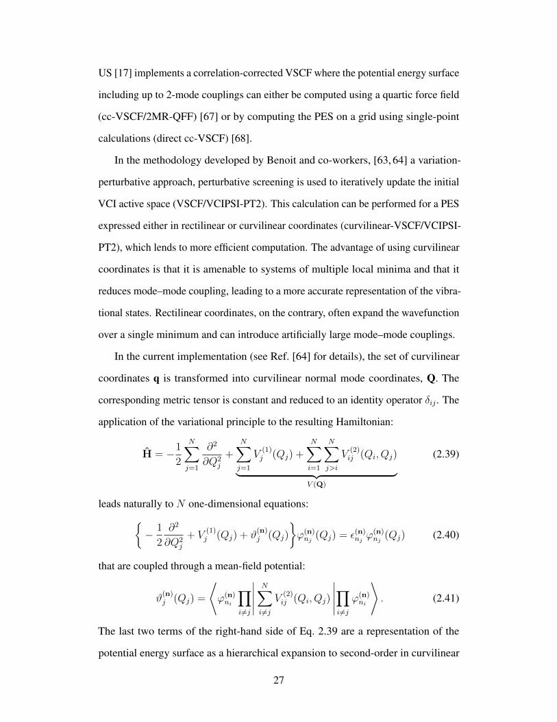
In the current implementation (see Ref. [64] for details), the set of curvilinear

coordinates q is transformed into curvilinear normal mode coordinates, Q. The

corresponding metric tensor is constant and reduced to an identity operator δij . The

application of the variational principle to the resulting Hamiltonian:

H = −1

2

N∑j=1

∂2

∂Q2j

+N∑j=1

V(1)j (Qj) +

N∑i=1

N∑j>i

V(2)ij (Qi, Qj)︸︷︷︸

V (Q)

(2.39)

leads naturally to N one-dimensional equations:{− 1

2

∂2

∂Q2j

+ V(1)j (Qj) + ϑ

(n)j (Qj)

}ϕ(n)nj

(Qj) = ε(n)njϕ(n)nj

(Qj) (2.40)

that are coupled through a mean-field potential:

ϑ(n)j (Qj) =

⟨ϕ(n)ni

∏i 6=j

∣∣∣∣∣N∑i 6=j

V(2)ij (Qi, Qj)

∣∣∣∣∣∏i 6=j

ϕ(n)ni

⟩. (2.41)

The last two terms of the right-hand side of Eq. 2.39 are a representation of the

potential energy surface as a hierarchical expansion to second-order in curvilinear

27

normal modes. Each term of the potential expansion is computed on a grid of points

(direct approach), providing a simple and automatic way of generating the PES

directly from ab initio data without requiring an analytic expression for V (Q). Note

that, for a curvilinear coordinate system, an extra potential term may appear in the

kinetic energy operator when a non-Euclidian normalization convention is used. We

neglect this contribution as it is typically very small compared to the potential energy

term.

The set of Eqns. 2.40 are solved self-consistently until convergence of the total

VSCF energy. We then compute the correlated vibrational eigenstates by diagonalis-

ing the full Hamiltonian of Eq. 2.39 in a virtual VSCF basis, as suggested originally

by Bowman et al. [69–71] We perform this type of vibrational configuration interac-

tion (VCI) calculation for each VSCF-optimised state and use virtual excitations to

construct the VCI matrix in each case:

〈Φr| H |Φs〉 =N∑i=1

εri∏k 6=i

δrksk + 〈Φr|∆V (n) |Φs〉 , (2.42)

where the state-specific vibrational correlation operator, ∆V (n) is defined as:

∆V (n) =N∑i=1

N∑j>i

V(2)ij (Qi, Qj)−

N∑j=1

ϑ(n)j (Qj). (2.43)

Note that index (n) indicates that the effective potential is computed for optimised

VSCF state |Φn〉. The resulting VCI matrix is diagonalised using our iterative

VCIPSI-PT2 procedure based on a Davidson algorithm [72–74] adapted for vibra-

tional calculations by Carter et al. [71].

2.8 Goal

We now embark on developing our computational and analysis tools for molecular

and semiclassical dynamics. New implementations and results will be discussed.

The existing methods in this chapter are critically analyzed. Novel approaches will

be discussed and summarized in the final chapter of this thesis.

28

Chapter 3

Ab initio Molecular Dynamics

This chapter is based upon S.Y.Y. Wong, P.-N. Roy and A. Brown, Ab initio Elec-

tronic Structure and Direct Dynamics Simulations of CH3OCl. Reused with per-

mission, Canadian Journal of Chemistry, 87 1022 (2009). Copyright 2009 NRC

Research Press. It has been expanded upon and modified.

3.1 Introduction

The first part of this research work consisted of developing the molecular dynamics

tools so that one can later calculate vibrational state energies of small molecules

using SC-IVR techniques. The first requirement for an SC-IVR calculation is its

classical inputs, which are the molecular dynamics trajectories. The Molecular

Modeling software package MMTK [75] has been used in numerous instances,1

although largely for systems with only pre-existing integrated model potentials or

parametrized force fields. At the time, direct dynamics had not been introduced into

the program (either internally or as an external add-on). Therefore, it was desirable

to develop this tool and to choose a chemically-interesting problem to investigate.

A direct dynamics study of an atmospherically-interesting molecule, CH3OCl, was

chosen. The basic dynamics tools were found in MMTK already. However, the

potentials found in the software were only models or empirically-derived, and most

1http://dirac.cnrs-orleans.fr/MMTK/publications/publications-citing-mmtk/

29

of those available were for biochemically-relevant molecules. The outset of this

research program was to write an interface between the the MMTK package with

that of existing electronic structure programs in order to conduct direct dynamics

simulations. The advantage is that potentials are calculated “on-the-fly” using ab

initio electronic structure techniques and, therefore, are more exact and can adapt

better to molecular or electronic changes (reactions, surface hopping, etc.). At

the time of this research, this had not been implemented before in MMTK. In this

particular chapter, we discuss the interface of MMTK with the electronic structure

package MOLPRO [18].

In this chapter, we compute the excited state energies, gradients and transi-

tion dipole moments for the UV photoexcitation CH3OCl molecule, determined

using computational methods tractable for ab initio molecular dynamics. Density

functional theory (DFT) for the ground state and CASSCF for the excited states

are validated against high-level internally-contracted MRCI results. These lay the

groundwork for future studies of the photodissociation of CH3OCl. This chapter

also reports the first implementation of ab initio molecular dynamics (AIMD) using

MMTK and illustrates its use with both ground and excited state dynamics for

CH3OCl. Sections 3.2 and 3.3.1 detail the previous and present ab initio methods

used to explore the electronic structure of CH3OCl. The AIMD techniques are

discussed in Sec. 3.3.2. The static electronic structure properties are reported in

Sec. 3.4.1 and a comparison is made between those from methods viable for AIMD

and high-level benchmark results. Ground electronic state configurational sampling

from AIMD for unconstrained and constrained dynamics is discussed in Sec. 3.4.2.

Sec. 3.4.2 also contains a brief discussion of AIMD for excited states of CH3OCl.

Finally, some conclusions and an outlook on future uses of AIMD with MMTK are

presented in Sec. 3.5.

30

3.2 Experimental/Theoretical Background

Figure 3.1: The ground state structure of CH3OCl.

The stratospheric molecule CH3OCl (see Fig. 3.1) has been shown to be important

in ozone chemistry through its role as a reservoir for chlorine [53]. Therefore,

it is important to understand the loss mechanisms for CH3OCl, including its UV

absorption and subsequent decomposition. Gas-phase experiments have shown

there to be two CH3OCl absorption peaks between the range of 200-400 nm. The

absorption peak at 236 nm is strong and narrow while the one at 310 nm is weaker

31

and broader.2 Due to its structural and spectral similarities to HOCl [76, 77], it

has been predicted that CH3O· and Cl· would be the photolysis products [53, 76].

The dominant reaction upon photolysis via either absorption peak was confirmed

experimentally [78, 79] as:

CH3OCl + hν → CH3O(X2E) + Cl(2P), (3.1)

where the chlorine atom is produced in either its spin-orbit ground (2P3/2) or excited

(2P1/2) state. Theoretical determination of the excited states [52] demonstrated the

highly repulsive electronic excited states along the Cl-O coordinate. Butler and

co-workers [78] measured the velocity distributions of the photofragments resulting

from photodissociation at 248 nm. All their data could be fit assuming Cl· and

CH3O· as the only photoproducts. They determined that the CH3O· fragments had

a narrow range of internal energies (vibration and primarily rotation). Schindler

et al. [79] used resonantly enhanced multiphoton ionization time-of-flight mass

spectrometry to measure the Cl· radical fragments produced following excitation

at 308 nm and 235/237 nm - different wavelengths were used to detect Cl(2P3/2)

versus Cl(2P1/2). The chlorine atoms were formed with nearly equal probability

at both wavelengths. Interestingly, the ratio of spin-orbit excited to ground state

chlorine atoms, Cl(2P1/2)/Cl(2P3/2), was strongly wavelength dependent with a value

of 0.31 ± 0.02 at 308 nm and 1.45 ± 0.05 at 235 nm. Clearly, the photodissociation

dynamics of CH3OCl is quite rich, and thus, it is a useful model molecule for our

study.

Francisco [1] completed an equilibrium structure and vibrational frequency

study of CH3OCl with density functional theory B3LYP/6-31++G(3df,3pd) and

coupled-cluster theory CCSD(T)/6-311G(2df,2p) where the results show a structure

similar to that of methanol. Li and Francisco [52] have determined energetics for

2JPL-97, JPL-2002 and JPL-2005 recommended the mean values of Crowley et al. [53] andJungkamp et al. [76].

32

low-lying singlet and triplet excited electronic states using complete active space

self-consistent field (CASSCF) followed by internally-contracted multi-reference

configuration interaction (MRCI) with cc-pVTZ and/or cc-pVTZ+sp basis sets.

Peyerimhoff and co-workers [80, 81] have examined similar properties for CH3OCl

using CCSD(T)/cc-pVTZ (equilibrium structure and vibrational frequencies) and

MRCI/cc-pVTZ+sp (vertical excitation energies). The goal of the present study is

not to reproduce these results, but to demonstrate that a computationally efficient

method will provide an energetically-correct characterization of CH3OCl, consistent

with the previously reported findings above. The necessity for a merely “sufficient”

method is to be able to practically conduct direct dynamics simulations. To this

effect, single-point calculations along the O-Cl bond coordinate are demonstrated

to provide semi-quantitatively the potential energy surface and energy gradients of

the first three singlet states. In the present study, we neglect the roles that low-lying

triplet states and spin-orbit coupling play in the dissociation process. In the Franck-

Condon region, the singlet ground-to-triplet excited state transitions are essentially

forbidden, and, thus, the triplet states play no role in the initial excitation process.

As the molecule dissociates, coupling between the singlet and triplet states becomes

important as the states approach the asymptote and are energetically similar. The

coupling manifests itself in the production of both Cl(2P3/2) and Cl(2P1/2) fragments.

Therefore, if one wants to interpret the experimental measurements [79] of the

branching ratio for these photoproducts, the spin-orbit coupling will have to be taken

into account - this is not the purpose of the present study.

3.3 Computational Methods

3.3.1 Electronic Structure

There have been several previous theoretical studies of the ground state structure

and vibrational frequencies of CH3OCl [1, 81–83]. In particular, there have been

33

two benchmark studies by Francisco [1] and by Peyerimhoff and co-workers [81] at

the CCSD(T)/6-311G(2df,2p) and at the CCSD(T)/cc-pVTZ levels of theory, respec-

tively. Unless otherwise specified, all single-point calculations reported in this article

have been carried out at the equilibrium geometry determined by Francisco (see Ta-

ble 3.1) using Cs symmetry. Since the CCSD(T) methodology is too computationally

expensive for dynamics calculations, a B3LYP/6-31G(d) geometry optimization and

vibrational frequency analysis were performed to assess the suitability of this level

of theory for ground state configurational sampling (see the discussion in Sec. 3.3.2).

The B3LYP/6-31G(d) ground state structure (Table 3.1) and vibrational frequencies

(Table 3.2) as compared to the benchmark CCSD(T) results indicate that this method

and basis set provide a suitable representation for the ground state potential energy

surface, including the equilibrium structure, with respect to both bases mentioned

above. For example, the bond lengths differ by less than 0.05 A and the angles by

less than 1.3 degrees. Importantly, the frequencies also differ by a maximum of 5%

and, in most cases, are within 1% of the benchmark results.

Table 3.1: Equilibrium geometry of CH3OCl at the B3LYP/6-31G(d) level of theoryas compared to previous benchmark results. Bond lengths are given in A andbond/dihedral angles in degrees. Ha refers to the H-atom lying on the same plane asC-O-Cl, while Hb,c are the two out-of-plane hydrogen atoms.

Parameter This work Ref. [1] Ref. [81] Ref. [84]B3LYP/ CCSD(T)/ CCSD(T)/ Expt.6-31G(d) 6-311G(2df,2p) cc-pVTZ

rCO 1.425 1.425 1.425 1.389rOCl 1.736 1.709 1.689 1.674rCHa 1.096 1.089 1.089 1.068rCHb,c 1.097 1.091 1.089 1.111θCOCl 110.4 109.2 109.3 112.8θHaCO 103.3 104.4 — —θHb,cCO 111.9 111.4 — —τHb,cCOCl 62.0 61.5 — —

34

Table 3.2: Vibrational frequencies and assignments (cm−1) at the B3LYP/6-31G(d)level of theory compared to experimental results and previous benchmark calcula-tions.

Assignment This work Ref. [76] Ref. [1] Ref. [81]B3LYP/ Experiment CCSD(T)/ CCSD(T)/6-31G(d) 6-311G(2df,2p) cc-pVTZ

CH3 Torsion 260 — 254 261C-O-Cl Bend 365 — 373 365O-Cl Stretch 659 680 692 661C-O Stretch 1023 1002 1046 1020

Hb,c-C-O Rock 1183 1150 1180 1181Ha-C-O Rock 1206 1170 1201 1284CH3 Umbrella 1477 1424 1467 1475

C-H Asymm. Bend 1487 1456 1479 1488Hb-C-Hc Scissor 1538 1471 1516 1537

CH3 Symm. Stretch 3035 2820 3040 3038Hb-C-Hc Asymm. Stretch 3109 2904 3117 3113Ha-C-Hb Asymm. Stretch 3131 2920 3144 3133

There have only been two theoretical studies focused on surveying the lowest-

lying singlet and triplet excited states for CH3OCl [52, 80]. In these studies, the

authors have determined the energies for the lowest six singlet and triplet states (three

A′ and three A′′ for each spin multiplicity). From these works, the two lowest energy

absorptions observed experimentally at 310 nm and 236 nm [76] are identified with

excitation to the 11A′′ and 21A′ states, respectively. These two low-lying electronic

states are the focus of this work. Benchmark calculations of both vertical excitation

energies and transition dipole moments have been carried out using the augmented

correlation consistent family of basis sets (aug-cc-pVXZ, X = D, T, and Q) [85–87].

In order to determine the energies and transition dipole moments, state-averaged

complete active space self-consistent field (SA-CASSCF) calculations [88–90] were

carried out including two A′ and one A′′ states. Following the work of Li and

Francisco [52], the active space consisted of fourteen electrons in ten active orbitals

(7 and 3 active MO’s in A′ and A′′ symmetry, respectively). The CASSCF method is

briefly explained in Sec. B.4. Essentially, a 20-orbital region is chosen to represent

35

the occupied and potentially occupied orbitals. The lower (closed) orbitals are, of

course, fully occupied in all states of excitation in the study; the rest (virtual) are

available for potential electron occupation (see Fig. 3.2).

Figure 3.2: The CASSCF study consisted of 34 electrons and 20 orbitals. Of the 20orbitals, 10 are active and the remaining 14 electrons can distribute within them.

The resulting CASSCF orbitals and wavefunctions were then used for internally-

contracted multi-reference configuration interaction (MRCI) [91, 92] calculations.

For the MRCI calculations, the effect of higher-order excitations on the energies was

estimated using the Davidson correction [93]. All electronic structure calculations

reported in this article were carried out using the MOLPRO ab initio electronic

structure program [18].

The MRCI method is suitable for single-point calculations (or even potential

energy scans) but it is far too computationally intensive to be utilized for a direct

dynamics study. The benchmark calculations used were used to gauge the accuracy

of SA-CASSCF calculations using the same (14,10) active space as described above

but with the much more modest 6-31+G(d) basis set [94–97]. The major difference

36

was that these calculations were carried out with C1 symmetry as they will form

the basis for future excited state dynamical studies, where the planar symmetry of

the molecule will be broken. We would like to use a moderate level of theory since

efficiency (speed) is of critical importance for dynamics but we would like to retain a

quantitative description of the excited states. In order to do this, the vertical excitation

energies were determined, as they provide information on the energetic accessibility

of the two excited states. The transition dipoles were used to gather information

about the relative probability of accessing either state. Finally, and perhaps most

importantly, the energy gradients must be determined since they govern the classical

dynamics. In order to assess the accuracy of the SA-CASSCF/6-31+G(d) gradients,

they are compared with numerical MRCI gradients at a small number of geometries

– note that analytic MRCI gradients are not available in MOLPRO. The comparison

of the gradients we make involves a projection onto the O-Cl bond vector, i.e., the

primary “reaction” channel, defined by

gOCl =(~gO − ~gCl) · (~rO − ~rCl)

‖~rOCl‖, (3.2)

where ~gi and ~ri are Cartesian vectors of the atomic gradients and positions, respec-

tively. The numerical MRCI gradients are computed by four-point finite difference

using a displacement length of 0.01 bohr along the rOCl bond coordinate.

3.3.2 Molecular Dynamics

Ab initio molecular dynamics simulations on the ground electronic state were carried

out using MMTK [75]. MMTK is a simulation and modelling program library written

in Python and C which has been proven to be useful for atomic systems to large

bio-molecules. Most of the procedures needed in conducting the dynamics is self-

contained in program classes which can be called from a main code. Significantly

for us, MMTK allows the ready implementation of constrained dynamics, where

the bond lengths can be fixed. A proper choice of constraints can “freeze out” high-

37

frequency vibrations, permitting the use of larger integration timesteps. In order

to perform AIMD using MMTK, an ab initio force field class that obtains energies

and gradients directly from electronic structure calculations was implemented. The

electronic structure calculations were performed using the MOLPRO package [18].

The present implementation allows the use of Hartree-Fock (HF), Møller-Plesset

second-order perturbation theory, density functional theory (DFT) and CASSCF

classical trajectories – methods where analytic gradients are available in MOLPRO.

An ab initio force field determined using GAMESS [17] has also been developed

for HF and DFT trajectories (results not presented here). The computer code for

interfacing these ab initio electronic structure packages with MMTK is available

upon request from the authors.

To generate initial conditions for examining the excited state dynamics (see

Fig. 3.3), one requires a sampling of geometries and initial velocities from the ground

electronic state. One can do this through Monte Carlo sampling or by running a

canonical NVT classical trajectory on the ground state potential energy surface to

sample both positions and momenta. In this paper, we chose the latter in order to

demonstrate our implementation of AIMD in MMTK. A single long NVT ground

state trajectory was generated at the B3LYP/6-31G(d) level of theory and can serve

as a sampling of initial conditions of the molecule prior to photoabsorption. The

initial conditions of the trajectory consisted of the equilibrium geometry determined

at the B3LYP/6-31G(d) level of theory (see Table 3.1) and velocities obtained from

a Boltzmann distribution at 300 K. Dynamics were conducted using the Velocity-

Verlet integrator [30]. To maintain the constant temperature, a Nose thermostat [98]

with a time constant of 0.2 ps was used. The proper timestep was determined from

NVE dynamics and the length of simulation determined from proper phase space

coverage. These NVT trajectories were determined for both unconstrained and

constrained systems. In the constrained dynamics, the rCH distances were fixed at

38

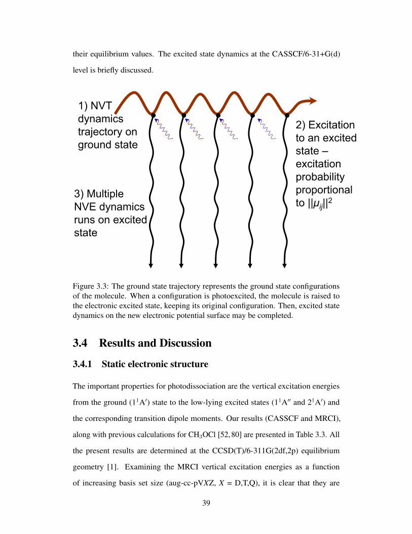
their equilibrium values. The excited state dynamics at the CASSCF/6-31+G(d)

level is briefly discussed.

1) NVT dynamics trajectory on ground state

3) Multiple NVE dynamics runs on excited state

2) Excitation to an excited state –excitation probability proportional to || ij||2

Figure 3.3: The ground state trajectory represents the ground state configurationsof the molecule. When a configuration is photoexcited, the molecule is raised tothe electronic excited state, keeping its original configuration. Then, excited statedynamics on the new electronic potential surface may be completed.

3.4 Results and Discussion

3.4.1 Static electronic structure

The important properties for photodissociation are the vertical excitation energies

from the ground (11A′) state to the low-lying excited states (11A′′ and 21A′) and

the corresponding transition dipole moments. Our results (CASSCF and MRCI),

along with previous calculations for CH3OCl [52, 80] are presented in Table 3.3. All

the present results are determined at the CCSD(T)/6-311G(2df,2p) equilibrium

geometry [1]. Examining the MRCI vertical excitation energies as a function

of increasing basis set size (aug-cc-pVXZ, X = D,T,Q), it is clear that they are

39

converging to the values of 4.13 eV and 5.27 eV for the 11A′′← X1A′ and 21A′←

X1A′ excitations, respectively. The present CASSCF and MRCI excitation energies

are consistent with those determined previously [52,80] and with the experimentally-

determined absorption spectra [53, 76] that exhibit maxima at 4.00 eV (310 nm) and

5.25 eV (236 nm). Importantly, the CASSCF/6-31+G(d) energies, upon which we

plan to base the direct dynamics, are within 0.180 eV and 0.513 eV of the MRCI/aug-

cc-pVQZ results. The comparison between these two differing methods/bases is

necessary as the desired dynamics method (CASSCF/ 6-31+G(d)) must be consistent

with the benchmark (MRCI/aug-cc-pVQZ).

Table 3.3: Vertical excitation energies (eV) and, when determined, transition dipolemoments (Debye) from the ground (X1A′) to the first (11A′′) and second (21A′) ex-cited states. Present results determined at the CCSD(T)/6-311G(2df,2p) equilibriumgeometry [1].

Transition Energy (transition dipole moment)Reference Basis Method 11A′′← X1A′ 21A′← X1A′

Present work aug-cc-pVDZ CASSCF 4.826 (0.262) 5.957 (0.430)MRCI 4.136 (0.052) 5.317 (0.257)

aug-cc-pVTZ CASSCF 4.364 (0.283) 5.804 (0.338)MRCI 4.132 (0.079) 5.268 (0.264)

aug-cc-pVQZ CASSCF 4.371 (0.324) 5.802 (0.417)MRCI 4.133 (0.089) 5.269 (0.270)

6-31+G(d) CASSCFa 4.313 (0.282) 5.782 (0.331)CASSCFb 4.373 (0.317) 5.867 (0.388)

Ref. [52] cc-pVTZ CASSCF 4.19 5.90MRCI 4.17 5.65

cc-pVTZ+sp CASSCF 4.53 6.00MRCI 4.24 5.58

Ref. [80] cc-pVTZ+spc MRCI 4.13 (0.07)d 5.50 (0.12)da CASSCF(14,10)b Full valence, i.e., CASSCF(20,15)c Both the basis set and active space used differ from that in Ref. [52].d Converted from oscillator strengths, f , using µ =

√3f

2E10

The square of the magnitudes of the transition dipole moments can be used

to determine the probability of a transition to each excited state – presently, the

transition dipole moments are treated as scalars rather than as vectors. Examining

40

the CASSCF versus MRCI transition dipole moments for a given basis set (see Table

3.3), it is clear that the inclusion of dynamic correlation plays a significant role in de-

termining their magnitudes. For example, the CASSCF/6-31+G(d) transition dipoles

as compared to the MRCI/aug-cc-pVQZ results are reduced from 0.282 D (11A′′

← X1A′) and 0.331 D (21A′← X1A′) to 0.089 D and 0.270 D, respectively. More

importantly, the ratio of the square of the dipole moments, which is proportional to

the absorption cross section, changes significantly, e.g., for the aug-cc-pVQZ basis

set, (µ2/µ1)2 = 1.38 for CASSCF and 9.30 for MRCI. In order to assess the relia-

bility of the computed transition dipole moments, we can compare as a first-order

approximation to the ratio of the experimentally-determined maximum absorption

cross sections [53, 76], where σ236/σ310 = 9.99. Clearly, the ratios predicted by

the CASSCF calculations are incorrect while the MRCI results for the triple- and

quadruple-zeta basis sets agree fairly well with experiment. For future excited state

direct dynamics work, the CASSCF results will be unable to predict correctly the

relative populations of the 11A′′ and 21A′ states. Therefore, a geometry-independent

dipole will be assumed and the populations in the states will be weighted 1:9 if both

states are energetically accessible.

The CASSCF/6-31+G(d) energies also need to be considered away from the

ground state equilibrium geometry as the eventual goal of the research is to examine

the photodissociation dynamics, where the molecule will access geometries far from

equilibrium. Figure 3.4 shows the potential energy curves for the first three singlet

states of CH3OCl as determined using the CASSCF/6-31+G(d) level of theory. As

expected from previous investigations [52,80], the excited states are highly repulsive

in the rOCl coordinate. Since the dynamics will break the Cs symmetry of the

molecule, the CASSCF calculations have been performed using C1 symmetry, i.e.,

no symmetry. One difficulty with carrying out the calculations in C1 symmetry is

that root-flipping problems can occur in the asymptotic region of the potentials.

41

1 1.5 2 2.5 3 3.5ROCl/Å

-1.0

0.0

1.0

2.0

3.0

4.0

Ener

gy/ ×

104

cm

-1

Figure 3.4: Energies at the CASSCF/6-31+G(d) level of the first three singlet statesof CH3OCl as a function of the ROCl bond length. All other bond parameters fixedat those of the B3LYP/6-31G(d) ground state equilibrium geometry. Calculations arecarried out inC1 symmetry and, therefore, the states (along with theirCs symmetries)illustrated are 11A = X1A′ (solid line + circles), 21A = 11A′′ (dashed line + squares),and 31A = 21A′ (dotted line + diamonds).

Gradients serve the purpose of providing the acceleration term in the Velocity-

Verlet integration scheme used for molecular dynamics. Therefore, obtaining accu-

rate forces is more important than the potential energy curves (relative energetics) –

although they are, of course, intimately related. The gradients for the first excited

state (11A′′ in Cs symmetry = 21A in C1 symmetry) as a function of the rOCl bond

length (all other coordinates are fixed at the B3LYP/6-31G(d) optimized geometry)

are shown in Fig. 3.5. The CASSCF/6-31+G(d) gradients are compared to those

from MRCI/aug-cc-pVDZ and MRCI/aug-cc-pVTZ determinations at four bond

lengths (rOCl = 1.536, 1.736, 1.936, and 2.136 A). The MRCI results are noticeably

smaller in magnitude than the corresponding CASSCF results – the ratio of the

MRCI/aug-cc-pVTZ to the CASSCF results is approximately 0.4 for all four rOCl

42

bond lengths considered. The gradients for the second excited state ([21A′ in Cs

symmetry = 31A in C1 symmetry], see Fig. 3.6) are qualitatively similar to those of

Fig. 3.5, where now the MRCI/aug-cc-pVTZ to CASSCF ratio is approximately 0.5.

Hence, we conclude that the CASSCF/6-31+G(d) gradients provide a qualitative

picture for guiding the excited state dynamics – a semi-quantitative picture could be

obtained through simple scaling of the CASSCF/6-31+G(d) gradients. Importantly,

the CASSCF/6-31+G(d) energy and analytic gradient calculations are reasonable in

computational time (approximately 2 minutes per geometry) for performing AIMD

while those using MRCI/aug-cc-pVXZ are prohibitive. Note that for rOCl > 2.5

A, there is a problem with root-flippping as the 21A′ (31A) state becomes lower in

energy than 1A′′ (21A); this is obvious due to the observation of a discontinuity in

the original gradient calculations. Therefore, the potentials, Fig. 3.4, and gradients,

Figs. 3.5 and 3.6, present results where the root-flipping has been accounted for “by

hand”. When AIMD is determined in the excited states, the root-flipping must be

accounted for automatically or trajectories must be terminated before rOCl > 2.5 A.

43

1 1.5 2 2.5 3 3.5 4R

OCl/Å

-1.5

-1.0

-0.5

0.0

Gra

dien

t (E

H/Å

)

Figure 3.5: Gradient projections of the first excited state (21A = 11A′′) onto theO-Cl bond vector as a function of the ROCl bond length: CASSCF/6-31+G(d)(circles), MRCI/aug-cc-pVDZ (squares), and MRCI/aug-cc-pVTZ (triangles). Othercoordinates are fixed at the B3LYP/6-31G(d) optimized geometry.

44

1 1.5 2 2.5 3 3.5 4R

OCl/Å

-1.5

-1.0

-0.5

0.0

Gra

dien

t (E

H/Å

)

Figure 3.6: Gradient projections of the second excited state (31A = 21A′) ontothe O-Cl bond vector as a function of the ROCl bond length: CASSCF/6-31+G(d)(circles), MRCI/aug-cc-pVDZ (squares), and MRCI/aug-cc-pVQZ (triangles). Othercoordinates are fixed at the B3LYP/6-31G(d) optimized geometry.

3.4.2 Ground and Excited State Dynamics

Presented here are NVT ground state trajectories at the B3LYP/6-31G(d) level. In the

first case, motion in all 3N − 6 internal degrees of freedom is allowed. In the second

case, to remove high frequency vibrational motions, all three C-H bonds are fixed

at their equilibrium bond lengths. To determine an appropriate timestep, equivalent

NVE simulations with various timesteps (dt) are run. Equilibration occurs within

a few femtoseconds. By applying constraints, we are able to increase the timestep

about three-fold (from ∼2 fs in unconstrained dynamics to ∼5 fs with constrained

dynamics) before energy conservation is violated or SCF non-convergence occurs in

the electronic structure calculation, when large timesteps lead to significant geometric

and, hence, electronic, changes. The latter point is of particular importance in AIMD

simulations. Therefore, the energy convergence tests are merely to show the general

45

upper limit on dt for the unconstrained and constrained systems. As a prescription,

we suggest that actual production runs should be performed at smaller timesteps.

Figs. 3.7-3.10 present histograms of the RCO and ROCl bond lengths, the COCl

bond angle, θCOCl, and the torsional angle, τHaCOCl, respectively, from 9.6 ps uncon-

strained and constrained NVT trajectories (dt = 2 fs and dt = 4 fs, respectively).

As expected, in the ground state at this temperature, the harmonic-like C-O bond

exhibits a Gaussian distribution centred about the equilibrium bond length. Similarly,

the O-Cl bond, COCl bond angle and torsional angle exhibit canonical behaviour.

The Cl fragment neither diverges too far from its equilibrium distance to the O nor

changes exceedingly from its orientation with respect to the C-O. For the constrained

simulation, note that the methyl group isomerizes and Ha occupies equivalent min-

ima at 60◦, 180◦ and 300◦. Taking all the above into consideration, the use of a

canonical NVT trajectory to sample initial ground state distributions is certainly

feasible, although it should be implemented with care. A small enough timestep

needs to be taken to prevent integrator problems that can adversely affect ab ini-

tio calculations. Yet, the simulation must be long enough for all modes to reach

the canonical limit. The use of a Monte Carlo sampling scheme may allow us to

circumvent such difficulties.

46

1.3 1.35 1.4 1.45 1.5 1.55 1.6R

CO/Å

unconstrainedconstrained

Figure 3.7: The canonical distribution of C-O bond lengths (RCO) for unconstrainedand constrained (with C-H bond lengths fixed at their equilibrium values) dynamics.Both trajectories are at the B3LYP/6-31G(d) level of theory. Trajectory length is 9.6ps for both unconstrained (dt = 2 fs) and constrained (dt = 4 fs) dynamics. Thevertical line represents the equilibrium value.

47

1.6 1.7 1.8R

OCl/Å


Figure 3.8: The canonical distribution of O-Cl bond lengths (ROCl) for unconstrainedand constrained (with C-H bond lengths fixed at their equilibrium values) dynamics.Both trajectories are at the B3LYP/6-31G(d) level of theory. Trajectory length is 9.6ps for both unconstrained (dt = 2 fs) and constrained (dt = 4 fs) dynamics. Thevertical line represents the equilibrium value.

48

100 110 120 130θ

COCl/degrees


Figure 3.9: The canonical distribution of the C-O-Cl bond angle (θCOCl) for uncon-strained and constrained (with C-H bond lengths fixed at their equilibrium values)dynamics. Both trajectories are at the B3LYP/6-31G(d) level of theory. Trajectorylength is 9.6 ps for both unconstrained (dt = 2 fs) and constrained (dt = 4 fs)dynamics. The vertical line represents the equilibrium value.

49

0 60 120 180 240 300 360τ

HaCOCl

/degrees


Figure 3.10: The canonical distribution of the Ha-C-O-Cl dihedral angle (τHaCOCl)for unconstrained and constrained (with C-H bond lengths fixed at their equilibriumvalues) dynamics. Both trajectories are at the B3LYP/6-31G(d) level of theory.Trajectory length is 9.6 ps for both unconstrained (dt = 2 fs) and constrained(dt = 4 fs) dynamics.

Positions and momenta sampled from the constrained ground state trajectory

will serve as initial conditions for future excited state dynamics studies. To test

AIMD for excited electronic states, a short 20 fs constant energy excited state

trajectory is determined on the first excited electronic state (21A in C1 symmetry)

at the CASSCF/6-31+G(d) level of theory. The trajectory starts at the ground state

equilibrium geometry with no initial kinetic energy (in practice, NVT ground state

initial conditions would be used). The molecule quickly reaches the asymptotic

dissociation limit (ROCl > 2.5 A) in about 100 timesteps (dt = 0.2 fs). Thus, a

single trajectory would take only (approximately) 300 minutes with the present

50

technology, pointing to the computational feasibility of exploring ensembles of

trajectories on the excited electronic states. The entire ensemble of excited state

trajectories can then be easily parallelized.

3.5 Conclusions

The three lowest-lying singlet states of methyl hypochlorite have been examined

using electronic structure methods for which direct dynamics studies would be

computationally feasible, i.e., B3LYP/6-31G(d) for the ground state and CASSCF/6-

31+G(d) for the excited states. From this, potential energy scans and energy gradients

along the O-Cl bond were obtained with an accuracy comparable to that of MRCI

with the aug-cc-pVXZ (X = D,T,Q) family of basis sets. In particular, the CASSCF

gradients are related to the MRCI gradients by only a factor, allowing for appropriate

dynamics. Thus, this moderate method is capable of semi-quantitatively representing

the benchmark calculations of the CH3OCl system at a fraction of the computational

cost. We have successfully implemented direct dynamics into MMTK using the

electronic structure packages MOLPRO (results presented here) and also GAMESS

(results not presented here). The power of using an ab initio on-the-fly method is

that any system – provided electronic structure calculations are computationally

feasible – can be studied. Implementing this method with a modular molecular

dynamics package lends to portability, generalization and great potential. Note,

however, careful analysis of the single-point calculations must be done. In our case,

we encountered root-flipping problems and the potential for electronic structure non-

convergence of systems far from equilibrium. We have also shown that constrained

dynamics can markedly decrease simulation time.

A full dynamical study of CH3OCl dissociation is the direct next step. In theory,

a large set of trajectories generated from a Boltzmann distribution of initial states

can be used to produce the sampling pool of ground state configurations from

51

which photoexcitation (vertical excitation) can occur. However, a Monte Carlo

sampling approach may be more practical. One could for instance sample the

ground state NVT distribution in the harmonic approximation yielding a Monte

Carlo sampling scheme where no rejection step is required. In this case, the Monte

Carlo sampling would be more efficient than the MD sampling. The dissociative

nature of CH3OCl in its excited states was demonstrated with our AIMD algorithm,

and for this type of process, is highly computationally practical at this level of theory.

Further investigations will involve calculating ensemble averages and other structural

properties. Quantum dynamical properties are also currently being investigated

based on the present tool along with semiclassical initial value representation (SC-

IVR) techniques [8, 99–101]. The present work opens the door to the development

of semiclassical dynamics with constraints using ab initio force fields. This is

an advancement over earlier work where the quantum dynamics of rigid water

clusters [58, 59] was studied using model potentials. Very recent work has shown

the practicality of on-the-fly AIMD-based semiclassical calculations [60, 102–105]

and the aforementioned inclusion of constraints is therefore quite timely.

52

Chapter 4

Vibrational States of H2CO using theSemiclassical Initial ValueRepresentation

This chapter is based upon S.Y.Y. Wong, D.M. Benoit, M. Lewerenz, A. Brown

and P.-N. Roy, Determination of molecular vibrational state energies using the

ab initio semiclassical initial value representation: Application to formaldehyde.

Reprinted with permission from The Journal of Chemical Physics, 134, 094110

(2011). Copyright 2011, American Institute of Physics. It has been expanded upon

and modified.

In the previous chapter, the basis of our molecular dynamics recipe was developed.

Molecular dynamics is purely classical (other than the potential, of course) in

nature. Here, we introduce semiclassical dynamics, which is a form of simulation to

approximately reflect quantum dynamics. The semiclassical (not to be confused with

“quasiclassical” [9]) techniques will build upon the tools in Chapter 3. In this chapter,

we will demonstrate the use of ab initio molecular dynamics (AIMD) trajectories

to compute the vibrational energy levels of molecular systems in the context of the

semiclassical initial value representation (SC-IVR).

53

4.1 Introduction

Classical MD simulations are successful in many situations where quantum effects

are negligible or not of interest. However, when quantum effects are important,

standard MD fails. Properties such as quantized molecular energy states, interfer-

ence and coherence are non-classical phenomena and are computed from quantum

mechanical equations or their isomorphic equivalent, the path integral. The difficulty

with solving quantum mechanical equations directly is that of exponential scaling.

Therefore, a variety of different approaches have been suggested to circumvent

this scaling problem. Depending on the method, certain properties are more easily

attainable (or accurate) than others. For example, one may use the multiconfiguration

time-dependent Hartree (MCTDH) [27, 106, 107] approach to approximate the full

quantum mechanical solution. While a very powerful approach, the MCTDH method

in general necessitates a full-dimensional PES fit to product form and, hence, has

only been used for modest-sized systems of 3-7 atoms. MULTIMODE [107,108]

is another software code that can calculate ro-vibrational energies of polyatomic

molecules by using vibrational self-consistent field (VSCF) and vibrational configu-

ration interaction (VCI). From the path integral formulation, the diffusion Monte

Carlo (DMC) method [24] can obtain ground state properties to very good accu-

racy. Its basis is the expression of the solution to the Schrodinger equation as a

sum of exponentials in imaginary time. Unfortunately, DMC works only when the

wavefunction is positive, meaning any wavefunction that has nodes (i.e., excited

states) will not work. To deal with node-crossing in DMC, one has to apply a

fixed-node approach where each region of the wavefunction is treated separately [26]

(node-release DMC [109] is a variant). Ring polymer molecular dynamics (RPMD)

is another method which can compute dynamical properties. One can then obtain

real-time Kubo-transformed time-correlation functions [110]. In practice, however,

as system size increases, these methods may become intractable, as either basis set,

54

dimensionality or convergence issues multiply. For example, we are often limited to

using pair potentials for DMC and RPMD or require a full-dimensional PES.

Semiclassical dynamics is another method for obtaining quantum-mechanical

properties by representing the system in terms of definite positions and momenta [40].

The framework of computation is then classical. The semiclassical propagator

developed by van Vleck [37] has been the basis of many practical advancements

in semiclassical theory [11, 43, 111] and has been recently reviewed by Thoss and

Wang [99] and by Kay [100]. In particular, a semiclassical initial value representation

(SC-IVR) propagator was developed in 1984 by Herman and Kluk [39,46,47] which

expresses the quantum time-propagation correlation function as a semiclassical

expression in terms of coherent states. Unlike its predecessors, [37, 111] an initial

value representation eliminates root search and singularity problems. Instead of

finding all possible paths between two coordinate-space points, one only needs initial

value information. This means the use of classical molecular dynamics trajectories

is possible. The only other information required in addition to the classical trajectory

itself is Hessian information from the dynamics.

In the last decade many developments in the SC-IVR method have been un-

dertaken [45, 56–61, 102–105, 112–118]. Among them have been prescriptions for

the calculation of vibrational states [56–62, 119], vibronic absorption spectra [102],

reactive processes [112], quantum coherence [116], response functions [120] and

internal conversion rates [121]. Over the past few years, research groups have inves-

tigated ab initio SC-IVR, where the trajectories are calculated on-the-fly. Tatchen

and Pollak [102] computed the absorption spectrum of the S0 → S1 transition of

formaldehyde using the time-dependent density functional theory (TD-DFT) [122]

method with the Perdew-Burke-Ernzerhof (PBE) [123] functional. They used a

unity-valued Herman-Kluk prefactor to calculate the Herzberg-Teller correlation

function. In 2009, Aspuru-Guzik and co-workers [60, 103] employed AIMD in the

55

study of the vibrational states of CO2, which can be computed from the survival

amplitude function. Here, they used the time-averaged variant of SC-IVR, which

utilizes a significantly-reduced number of trajectories. Comparisons were made to

states determined from fitted potential surfaces and the accuracy of state energies

was examined. In a later study, they also calculated the eigenfunctions of CO2 [104].

Since the Hessian is a vital part of an AIMD-SC-IVR study, effort have also been de-

veloped to reduce the number of Hessian evaluations, as shown by Hase et al. [105].

There have also been a number of other studies based on fitted PESs using SC-IVR

to examine molecular vibrational states. Kaledin and Miller [61, 62] have obtained

the vibrational states of H2, H2O, NH3, CH4, CH2D2 and H2CO with SC-IVR as

well as time-averaged SC-IVR [61]. Roy and co-workers [56–59, 114] developed a

reduced-dimensionality approach through Cartesian geometric constraints [applying

it to Ar3 and (H2O)2], which is amenable for the computation of larger systems. The

focus of this chapter is to determine accurate molecular vibrational states through a

semiclassical approach.

Determination of vibrational state energies within the harmonic approximation

is trivial for even very large systems. However, when anharmonic corrections are

introduced, the computational effort is much more considerable. What is possible

to do — through the use of classical-based dynamics — is to use spectral densities

from ab initio SC-IVR to compute vibrational state energies. By incorporating

terms accounting for probability amplitudes, SC-IVR reintroduces the quantum

contribution into the classical simulation. Here, we provide further insight into ab

initio-based SC-IVR using H2CO as a model system and address several points

that have not been considered in previous studies [56–58, 60–62, 103]. As opposed

to time-averaged SC-IVR [61], we use standard SC-IVR (i.e., full phase space

averaging) and an approximation of the Herman-Kluk prefactor. Previous work [62]

has utilized reference wavefunctions chosen on the basis of symmetry, but here, we

56

separate them on a normal-mode basis. Careful analysis of the results as a function of

the chosen reference wavefunction is done. We also demonstrate a practical tool for

performing ab initio SC-IVR within the Molecular Modelling Toolkit (MMTK) [75],

a molecular dynamics software package. The low-lying vibrational states of H2CO

are determined and compared to harmonic, quartic force field correlation-corrected

vibrational self consistent field (cc-VSCF) [67], direct cc-VSCF [68,124,125], direct

rectilinear-vibrational self-consistent field/vibrational configuration interaction with

perturbation selected interactions-second order perturbation theory (VSCF/VCIPSI-

PT2) as well as reference direct curvilinear-VSCF/VCIPSI-PT2 method results

[63, 64].

Sec. 4.2 presents a brief review of the mathematical formulation of SC-IVR.

Sec. 4.3 covers the details regarding the computation of the spectral density of H2CO.

In Sec. 4.3.1, we introduce the electronic structure methods used to produce the ab

initio energies and frequencies. The most important component of the method is the

phase space integral, which is obtained from the classical dynamics trajectories, as

detailed in Sec. 4.3.2. The final spectral density depends largely on the reference

wavefunction and so the prescription for determining the reference wavefunction

and its overlaps are discussed in Sec. 4.3.3. Results and discussion of the obtained

vibrational states follow in Sec. 4.4. Sec. 4.5 presents our final conclusions.

4.2 Theory

The quantum mechanical survival amplitude, C(t), was introduced in Chapter 2:

C(t) =⟨

Ψ|e−iHt/~|Ψ⟩. (4.1)

This autocorrelation function has largest amplitude when H − E = 0. The Fourier

transform of C(t) generates the vibrational state energy peaks. That is, in ket

57

notation, its Fourier transform is

I(E) =⟨

Ψ|δ(H − E)|Ψ⟩, (4.2)

which clearly indicates that peaks should occur at quantized states En. To solve this

equation, the propagator is rewritten in Herman and Kluk’s semiclassical formulation

[39–42] mentioned previously in Sec. 2.2:

e−iHt/~ = (2π~)−3N∫ ∫

dp0dq0Rp0,q0,teiSp0,q0,t/~|gpt,qt〉〈gp0,q0|. (4.3)

The integrals run over p0 and q0, which are the phase space variables. Rp0,q0,t is

the so-called Herman-Kluk (HK) prefactor stability matrix, Sp0,q0,t/~ the classical

action specifying the phase of the Gaussian wavepacket and the gs are coherent

states. The prefactor (Eq. 2.28) contains numerous terms involving derivatives of

the phase space variables. To numerically solve this with finite difference would

require a very small timestep. The Johnson approximation (Eq. 2.34) avoids this

by requiring only the local frequencies at each timestep along the trajectory. The

coherent state representation of the minimum-uncertainty wavepacket (|gpt,qt〉 and

〈gp0,q0|) is a multivariate Gaussian function of coherent state width [39, 43, 44]

γ = 2LαLT , (4.4)

where L is the eigenvector matrix and α the eigenvalue matrix from the Hessian.

Coherent states have the property that the centre of the Gaussian evolves according

to the classical equations of motion. Both the coherent states at the initial (0)

and current (t) times are required. The coherent state may be expressed in terms

of various representations (such as the position representation). Our form of the

coherent state wavepacket is

〈x|gpt,qt〉 =(γπ

)3N/4exp

[−γ

2(qc − q)2 +

i

~p(qc − q)

], (4.5)

where c indicates the coherent state Gaussian is centered. The phase term, eiSp0,q0,t/~,

comes from the Lagrangian equations of motion. Combining Eqs. 4.1 and 4.3, we

58

obtain a semiclassical expression for the survival amplitude, i.e.,

C(t) = (2π~)−3N∫ ∫

dp0dq0Rp0,q0,teiSp0,q0,t/~〈Ψref |gpt,qt〉〈gp0,q0|Ψref〉, (4.6)

where the overlap of Ψref with the coherent state produces:

〈gp,q|Ψref〉 = exp

[−1

4(q− qref)

T γ (q− qref)−1

4~2(p− pref)

T γ−1 (p− pref)

+i

2~(p + pref)

T (q− qref)

]. (4.7)

pref and qref are the reference state mass-weighted momenta and positions, respec-

tively. The overlaps have a general Gaussian form. The reference state constitutes

a chosen “trial” wavefunction, which is the desired state of interest. C(t) is the

correlation of the state of the system with this reference function, meaning the

chosen reference function serves as an “extractor” for eigenstates near it. Note that

in practice, the above overlap is also symmetry-adapted, which will be explained in

Sec. 4.3.3.

Now, the Fourier transform of this semiclassical survival amplitude gives the

resultant power spectrum. That is,

I (ω) =1

2π

∞∫−∞

dt eiωtC (t) (4.8)

produces the energy eigenvalues of the Hamiltonian H . The intensities of the peaks

are directly related to the choice of reference wavefunction.

4.3 Computational Methods

4.3.1 Electronic Structure and Harmonic Frequencies

In order to benchmark our SC-IVR approach, the ab initio electronic structure

calculations were carried out at the HF/3-21G level of theory [14, 126] for ease of

production. The equilibrium geometry of H2CO is given in Table 4.1. Energies at

which the simulation was run are far below that of the HF transition state (37,700

59

cm−1) [127]. The availability of analytic gradients and Hessians, for the classical

dynamics and HK prefactor evaluation, respectively, is a major asset and guided,

along with its computational efficiency, the choice of the Hartree-Fock level of

theory. In principle, any electronic structure theory methodology for which analytic

gradients and Hessians are available can be utilized. Our calculations made use of

the GAMESS-US 2007 and 2009 quantum chemistry packages [17].

Table 4.1: Equilibrium geometry of H2CO at the HF/3-21G level of theory. Bondlengths are given in A and the bond angle in degrees.

Parameter ValuerCO 1.207rCH 1.083θHCO 122.5

4.3.2 Trajectories for Phase Space Average

To determine the initial conditions for the ensemble of trajectories, a Monte Carlo

sampling of M = 20,000 sets of initial geometric configurations and momenta

was produced, corresponding to a coherent state Gaussian wavepacket centered at

the HF/3-21G equilibrium geometry and with zero momentum. The phase space

sampled represents |〈gp0,q0|Ψeq〉|2, whose form is identical to that of Eq. 2.31.

The coordinate and momentum widths of Eq. 2.31 are√

2/γ and ~√

2γ, respec-

tively. Of these initial conditions, only motion in the 3N − 6 internal degrees of

freedom is allowed, and so the original values are adjusted, fixing the molecule’s

centre of mass and spatial orientation. Note that only one set of initial conditions is

used for the various reference wavefunctions and therefore, a re-weighting procedure

is required (in other words, the integral over phase space isn’t uniform). Eq. 4.6 can

60

be rewritten with the insertion of unity 1 = |〈gp0,q0|Ψeq〉|2/|〈gp0,q0|Ψeq〉|2 as

C(t) = (2π~)−3N∫ ∫

dp0dq0Rp0,q0,teiSp0,q0,t/~ (4.9)

× 〈Ψref |gpt,qt〉〈gp0,q0|Ψref〉|〈gp0,q0|Ψeq〉|2

|〈gp0,q0|Ψeq〉|2.

The initial conditions essentially impose a bias of |〈gp0,q0|Ψeq〉|2 (the numerator in

1) in the phase space distribution which must be accounted for by division of the

bias. The Monte Carlo estimate is therefore

C(t) =1

M

M∑m=1

[Rp0,q0,te

iSp0,q0,t/~〈Ψref |gpt,qt〉〈gp0,q0 |Ψref〉〈Ψeq|gp0,q0〉〈gp0,q0|Ψeq〉

]m

. (4.10)

This choice of sampling greatly reduces the computational cost as only one set of ab

initio trajectories is required instead of a full phase space distribution.

Approximately 38% of the 20,000 generated initial geometries and momenta had

a total energy less than 300 kJ/mol (∼25,000 cm−1). Initial conditions with energies

above 300 kJ/mol were discarded. Energies below 300 kJ/mol place the molecule

well below the transition state, which is important in the numerical stability of the

Herman-Kluk prefactor. Additionally, the semiclassical survival amplitude, C(t),

was computed only when |〈gp0,q0|Ψeq〉|2 > 10−10 (low overlap leads to negligible

contribution to the average of the survival amplitude). From each of these initial

conditions, a 244 fs constant energy molecular dynamics trajectory was determined

using MMTK. These trajectories constitute the phase space average, which is the

multidimensional integral in C(t). The equations of motion were computed with

Velocity-Verlet integration [30]. During the dynamics, the Hessian at each timestep

(0.5 fs) was saved and diagonalized. The resultant eigenvalues are necessary for the

calculation of the HK prefactor which requires the local harmonic zero point energy

(ZPE) (see Eq. 2.34).

61

4.3.3 Reference Wavefunctions and Overlaps

The coherent state overlaps are functions of mass-weighted geometry and momentum.

A choice of reference wavefunction where qref is located at the equilibrium geometry

and pref = 0, will produce the highest overlap with the lowest vibrational state (zero

point energy). In all cases we choose pref to be zero, for simplicity, and we vary

only qref . The width is chosen to be γ as previously defined, meaning that Ψref is

the exact harmonic ground state wavefunction, and there is no appreciable overlap

with any state other than the ground state. When another reference wavefunction is

chosen, it will be those coherent states (i.e., phase space points along the trajectory)

that have highest overlap with this wavefunction which will contribute the most to

the survival amplitude. Fig. 4.1 demonstrates this graphically. One way to vary

the wavefunction in order to obtain additional states is to apply a technique where

the atoms are spatially displaced along a normal mode coordinate. As a result, it

is easy to interpret the magnitude of displacement (c) with the energy put “into”

a mode νj (in this work, we use ν to denote the mode itself). For instance, by

letting c =√~/ωj displacement of mode νj , this means that the molecule has been

displaced from equilibrium along νj and has 12~ωj of potential energy (assuming the

motion is perfectly harmonic). Essentially, this provides a vibrational excited state

reference wavefunction. The normal modes are as assigned in Table 4.2. By allowing

just single normal mode displacements, this should effectively produce a spectrum

with peaks only at the fundamental frequencies and overtones, i.e., (n1 · · ·nj · · ·nN )

: nj 6=k = 0, nk ∈ Z>0.

62

Figure 4.1: Correlation is highest when the coherent state (state at time t) is mostsimilar to that of the reference state.

Table 4.2: Harmonic normal mode labelling and frequencies (cm−1). Frequenciesare determined at the HF/3-21G level of theory.

Mode Assignment Frequencyν1(A1) CH2 Symmetric Stretch 3162ν2(A1) CO Stretch 1916ν3(A1) CH2 Scissor 1693ν4(B1) CH2 Wag 1337ν5(B2) CH2 Asymmetric Stretch 3233ν6(B2) CH2 Rock 1378

A Monte Carlo procedure is used to estimate the phase space integrals and

therefore, all eigenstates can contribute to the survival amplitudes. The normal mode

displacements in the reference wavefunction are also not pure symmetry states. To

remedy this problem, we explicitly symmetrize the reference wavefunction. To

do so, we project out specific symmetries by constructing a projection operator

corresponding to a specific irreducible representation of the C2v group. For the case

of symmetric A1 states, an unsymmetrized reference wavefunction, |Ψref〉, becomes,

|ΨA1ref〉 =

1

4

[E|Ψref〉+ C2|Ψref〉+ σv|Ψref〉+ σ′v|Ψref〉

]. (4.11)

The use of the above wavefunction will ensure that energy levels of a specific

symmetry are extracted (cf. Ref. [62], where a product of coherent states is used

instead, with a symmetrizer to extract states of particular molecular symmetry).

Because the width γ (see Eq. 4.4) is identical to that of the ground state wave-

function, one may visualize the displaced reference wavefunction (prior to sym-

63

metrization) as simply a shift of the ground state wavefunction along a single normal

mode coordinate. For a given mode j, the new atom positions in Cartesian coor-

dinates is represented as the vector ~xj (we call this x to differentiate this from the

mass-weighted coordinate q). For each individual coordinate α, the elements of the

vector ~xj are:

xjα = Xα − cjLαjµα

, (4.12)

where Xα is an element of the Cartesian equilibrium geometry vector, µα is the

square root of the mass of the atom associated with Cartesian component α, and

Lαj is the eigenvector element associated with displaced mode νj . In this work, cj

is varied by a factor d to adjust the magnitude of the normal mode displacement

(cj = d ·√

~/ωj).

4.4 Results and Discussion

Here, we present the results of the calculation of the spectral density of H2CO

as determined by SC-IVR. The SC-IVR solution of C(t) by Eq. 4.10 leads to a

signal which decays rapidly (see Fig. 4.2 for an example). This shows that the

the total simulation length, T , is satisfactory. The peaks of the spectral density

are the low-lying vibrational eigenstates. It is possible for SC-IVR to determine

more states, albeit at a substantial cost of more trajectories. The survival amplitude

would improve. In this particular case, since the correlation function decays to a

great extent within the timespan of the simulation, a longer trajectory would make

minimal difference in the spectra. The symmetry-adapted reference wavefunction

of Eq. 4.11 is used for all the SC-IVR results. The SC-IVR values are compared

to the harmonic approximation, cc-VSCF/2MR-QFF, direct-cc-VSCF, (rectilinear)

VSCF/VCIPSI-PT2 and curvilinear-VSCF/VCIPSI-PT2 methods1 described earlier1The main contribution by D.M. Benoit to the current study were the calculations with the

VSCF/VCI methods.

64

in Chapter 2 (Sec. 2.7). While vibrational states in the harmonic approximation

are trivially obtained to the nth state, anharmonic terms are increasingly difficult to

compute. In all four VSCF implementations, only two-mode couplings were utilized

and three-mode (and higher) couplings were neglected. To make sure that the VSCF

results used in the the VSCF/VCIPSI-PT2 methods are fully converged, we include

up to 4-mode excitations in the VCI basis and allow up to 8-quanta excitation per

mode. This leads to a large vibrational basis (about 70,000 states) that is more

appropriate for describing combination bands and overtones. Given the large size of

the basis, we performed the calculations with a slightly different technique than VCI

called vibrational configuration interaction with perturbation selected interactions-

second-order perturbation (VCIPSI-PT2). It has been shown [64] that this method

gives virtually the same results as a standard VCI/VSCF calculation. Of the four

reference calculation types being considered, the curvilinear approach is the most

accurate.

65

Figure 4.2: Correlation functions where the ν1 mode is displaced by various amountsd when constructing the reference wavefunction. The signal decays after very shorttime.

As detailed in Sec. 4.2, we use an alternate form of the Herman-Kluk prefactor.

Johnson’s approximation [54] has been shown to be effective for weakly-bound

systems [56–59]. This approximation eliminates branch cut problems as well as

the need to calculate phase space derivatives. Instead, one only needs to calculate

the Hessian matrix at each geometry along the trajectories. Diagonalization of the

Hessian matrix gives the eigenvalues, whose square roots are the local harmonic

frequencies. These ωjs are similar to frequencies calculated at stationary points

(i.e., at the equilibrium or transition state geometries). Since the frequencies are

calculated at any point on the potential energy surface, they are naturally complex-

valued. The consequence is a highly-oscillatory exponential term that increases noise

in the survival amplitude function. In Fig. 4.3, we present results comparing spectra

66

obtained with Johnson’s WKB approach along with several further approximations.

Issack and Roy [56–59] took the approach of taking the absolute value of all the

frequencies (|ω|) to eliminate the oscillating phase. This simplification results in

a larger magnitude term in the exponential of Eq. 2.34 since it is taking a sum

over additional positive real numbers. The HK prefactor, Rp0,q0,t, becomes a larger

negative complex exponent. This appears to lead to overestimating the energy of

the vibrational states (see Fig. 4.3). As well, the decay of the survival amplitude

is much slower. Alternatively, if one encounters an imaginary frequency, one can

simply neglect it, so that only the real frequencies are taken into account (ω ∈ R).

The different summations do provide minor differences in the spectral density, with

the peak positions between ω ∈ R and a complex ω being negligible. In fact, ω ∈ C

appears to reduce signal noise. However, the signal intensity of the peaks is slightly

diminished compared to ω ∈ R. The difference between the use of complex-, real-

or absolute-valued frequencies can be in the tens of wavenumbers, which may be

significant for the accuracy of SC-IVR, although the width of the spectral peaks is

comparable to the shift due to the type of prefactor. In the present work, we see

no reason not to use the complex-valued frequencies, since there appears to be no

benefit in simplifying the WKB approximation further (whether it is more difficult to

converge the prefactor in other systems, such as weakly-bound complexes, warrants

further investigation). In all the following calculations we maintain the complex

value of the frequencies (ω ∈ C). Note that all 12 eigenvalues of the Hessian are

non-zero, including the rotational and translational modes. As seen in Eq. 2.34, the

summation is only over 3N − 6 modes (cf. previous literature), so the extraneous

non-vibrational frequencies must be removed in the prefactor evaluation — we do

so in the present work by neglecting the 6 lowest magnitude frequencies.

67

6000 7000 8000 9000 10000 11000Energy [cm-1]

I(ω

) [ar

b. u

nits

]|ω|ω ∈Rω ∈C

Figure 4.3: Variation of the spectral density (displaced in ν1) with respect to the typeof HK prefactor used. The dashed (blue) line indicates use of the absolute value ofω, the dotted (red) line sums only the positive frequencies and the solid (black) linehas a complex-valued ω (no further approximations).

Following Sec. 4.3.3, we examine the spectral density as a function of the

reference state chosen. We show the results of simulations with normal mode

displacements along the A1 modes of vibration, ν1, ν2 and ν3. Since the wavefunction

is symmetry-adapted for A1, in theory, all A1 vibrational states should be obtained.

Yet, as solely the A1 normal modes are excited, we only expect to obtain their

fundamentals, overtones and, to a certain extent, their combination bands, the others

being of negligible amplitude.

68

The spectral density as determined by SC-IVR is shown in Fig. 4.4. Three values

of configurational displacement along the normal mode (magnitude specified by

d), are shown. As can be seen, the further the reference wavefunction is displaced

from the equilibrium geometry, the larger the overlap with higher energy states.

Therefore, increasing the reference wavefunction displacement is a systematic way

to determine vibrational states of increasing energy. The ground state (000000) is

resolved in all figures. Each of the curves in Figs. 4.4(a), (b) and (c) resolves one

set of vibrational states (· · ·n · · · ) due the overlap with a single normal mode (in

the harmonic limit). The benefit of such “filtering” is that a cleaner spectrum is

obtained, so that close-lying eigenstates are unequivocally differentiated. Spectral

noise and uncertainty are major issues for many-dimensional systems and states of

higher excitation. The intensities in Fig. 4.4(a) have the broadest peaks because the

reference wavefunction energy (i.e., displacement) is largest, since it is proportional

to ω1. It is more difficult to extract states higher in energy (phase space coverage

decreases, meaning the overlap term is often zero and therefore has no contribution

to the overall survival amplitude integral). Table 4.3 lists the A1 fundamental and

overtone vibrational state peak positions up to 4-quanta excitation and also the

mean absolute errors and root mean square deviations as compared to curvilinear-

VSCF/VCIPSI-PT2. The assignments are quite close to the curvilinear bound state

calculations (vertical lines) for low excitation, and, in general, are well within

100 cm−1. As expected, errors and deviations become larger as one goes higher in

energy. The results show that the SC-IVR results are systematically more accurate

than the cc-VSCF/2MR-QFF (i.e., a VSCF-type method), direct cc-VSCF and the

rectilinear-VSCF/VCIPSI-PT2 (i.e., a VSCF/VCI method) results when compared

to the more accurate curvilinear-VSCF/VCIPSI-PT2 reference calculations.

69

d=1d=2d=3

(a)

I(ω

) [ar

b. u

nits

]

d=1d=2d=3

(b)

6000 8000 10000 12000 14000 16000Energy [cm-1]

d=1d=2d=3

(c)

Figure 4.4: Intensity (spectral density) plots from SC-IVR given symmetry-adaptedreference state overlaps with displacements along the three A1 normal modes, (a)ν1, (b) ν2 and (c) ν3, respectively. The curves are the SC-IVR results. d representsthe magnitude of displacement (energy ∝ d2) of each mode (see text for details).The vertical lines represent the curvilinear-VSCF/VCIPSI-PT2 reference boundstate calculation. In each panel, the leftmost vertical line represents the groundvibrational state (000000), and in the case of the first panel, the subsequent lines arethe (100000), (200000), (300000) and (400000) vibrational states. The other twopanels are similarly labelled.

70

Tabl

e4.

3:Fu

ndam

enta

lvib

ratio

nals

tate

sin

volv

ing

the

A1

norm

alm

odes

ofH

2C

Oat

the

HF/

3-21

Gle

vela

sde

term

ined

usin

gva

riou

sco

mpu

tatio

nalm

etho

ds.U

nits

are

incm−1.T

heSC

-IV

Rva

lues

wer

ede

term

ined

byth

elo

catio

nof

the

poin

toft

hehi

ghes

tint

ensi

type

akof

one

orm

ore

spec

tra

(ave

rage

),w

here

each

poin

twas

sepa

rate

dby<

0.5

cm−1.T

hem

ean

abso

lute

erro

r(M

AE

)and

root

mea

nsq

uare

devi

atio

n(R

MSD

)with

resp

ectt

oth

ecu

rvili

near

-VSC

F/V

CIP

SI-P

T2

met

hod

are

show

nfo

rthe

fund

amen

talo

vert

ones

.

Stat

eH

arm

onic

cc-V

SCF/

2MR

-QFF

dire

ctcc

-VSC

FV

SCF/

VC

IPSI

-PT

2cu

rvi-

VSC

F/V

CIP

SI-P

T2

SC-I

VR

(000

000)

6360

6271

6268

6268

6309

6311

(100

000)

9522

9265

9254

9251

9320

9303

(010

000)

8276

8155

8152

8152

8198

8208

(001

000)

8053

7924

7922

7921

7980

8013

(200

000)

1268

512

183

1213

612

259

1223

212

297

(020

000)

1019

110

029

1002

410

023

1007

410

089

(002

000)

9745

9574

9571

9571

9650

9587

(300

000)

1584

715

071

1495

515

103

1525

415

209

(030

000)

1210

711

893

1188

511

881

1193

611

961

(003

000)

1143

811

164

1121

611

216

1132

111

269

(400

000)

1901

0—

1772

117

938

1799

617

848

(040

000)

1402

2—

1373

513

727

1378

713

853

(004

000)

1313

1—

1285

112

851

1298

612

904

MA

E25

774

104

72—

48R

MSD

370

8913

380

—61

71

Figs. 4.5, 4.6 and 4.7 show spectral densities consisting of reference state dis-

placements of two modes simultaneously. That is, they are a linear combination

of single mode displacements. Like those of Fig. 4.4, the fundamental bands are

obtained, although with somewhat less accuracy. Many combination bands are also

visible, although given the width of the peaks and that they are often near other states,

assignments can be made with less certainty. In most cases, the location of the high-

est peak was the value tabulated in Table 4.4 and if the peaks were clearly defined

or equally ambiguous in more than one spectrum, the average of these locations

were chosen. This uncertainty may be rectified with a more detailed procedure of

displacing the reference wavefunction (here, we place a single quanta of energy into

each normal mode) and potentially increasing the number of trajectories involved in

the calculation.

72

8000 12000 16000Energy [cm-1]

I(ω

) [ar

b. u

nits

]

(a)

8000 12000 16000Energy [cm-1]

I(ω

) [ar

b. u

nits

]

(b)

Figure 4.5: Spectral density plots where the ν1 and ν2 A1 modes are displacedsimultaneously when constructing the reference wavefunction. The vertical linesrepresent the reference curvilinear-VSCF/VCIPSI-PT2 values (see Table 4.3 forlabelling.) (a) d = 1, (b) d = 2

73

8000 12000 16000Energy [cm-1]

I(ω

) [ar

b. u

nits

]

(a)

8000 12000 16000Energy [cm-1]

I(ω

) [ar

b. u

nits

]

(b)


74

6000 8000 10000 12000 14000Energy [cm-1]

I(ω

) [ar

b. u

nits

]

(a)

6000 8000 10000 12000 14000Energy [cm-1]

I(ω

) [ar

b. u

nits

]

(b)


75

Tabl

e4.

4:V

ibra

tiona

lcom

bina

tion

stat

esin

volv

ing

the

A1

norm

alm

odes

ofH

2C

Oat

the

HF/

3-21

Gle

vela

sde

term

ined

usin

gva

riou

sco

mpu

tatio

nalm

etho

ds.

Uni

tsar

ein

cm−1.

The

SC-I

VR

valu

esw

ere

dete

rmin

edby

the

loca

tion

ofth

epo

into

fth

ehi

ghes

tint

ensi

type

akof

one

orm

ore

spec

tra

(ave

rage

),w

here

each

poin

twas

sepa

rate

dby<

0.5

cm−1.V

alue

sw

itha

(*)i

ndic

ate

that

the

assi

gnm

enti

sun

cert

ain.

Stat

eH

arm

onic

cc-V

SCF-

2MR

-QFF

cc-V

SCF

VSC

F/V

CIP

SI-P

T2

curv

i-V

SCF/

VC

IPSI

-PT

2SC

-IV

R(1

1000

0)11

438

1116

411

133

1112

611

211

1119

1(2

1000

0)14

600

1407

214

006

1412

014

126

1405

5*(1

2000

0)13

354

1302

512

997

1298

713

088

1308

6(2

2000

0)16

516

—15

860

1596

716

004

1595

2(1

0100

0)11

215

1091

310

885

1087

610

981

1089

6(2

0100

0)14

377

1379

513

735

1384

413

884

1411

5(1

0200

0)12

908

1252

512

511

1249

812

642

1248

8*(2

0200

0)16

070

—15

329

1543

015

533

1559

1*(0

1100

0)99

6898

0198

0597

9498

5898

58(0

2100

0)11

884

1166

511

672

1165

311

722

1169

0(0

1200

0)11

661

1143

911

453

1143

211

517

1156

2(0

2200

0)13

576

—13

316

1327

913

370

1354

4*

76

4.5 Concluding remarks

We have shown, using ab initio trajectory data, that the vibrational eigenstates of

H2CO can be determined with reasonable accuracy through the use of SC-IVR and

that it is systematically more accurate than VSCF and VSCF/VCI methods. The

curvilinear-VSCF/VCIPSI-PT2 bound state approach is used as our exact reference.

Our semiclassical description comes at an acceptable computational cost, but does

have limitations. The vibrational states determined are highly sensitive to the

reference wavefunction chosen. As such, for a complete description of a range of

eigenstates, multiple carefully-constructed reference wavefunctions are required to

extract them. In this work, we chose symmetry-adapted reference wavefunctions

that had excitations along 1 and 2 normal modes only. This prescription allows us

to independently and accurately determine fundamental states and some two-state

combination bands of A1 symmetry. This symmetrizing enables easier assignment

of states. The major bottleneck in these simulations is the trajectory and Hessian

computation. However, once done, the phase space average for the survival amplitude

is readily calculated. An important outcome of the present study is that in utilizing

our newly proposed phase space re-weighting procedure, only a single set of ab

initio trajectories is required to obtain several power spectra.

In addition, we have examined the various implementations of Johnson’s WKB

approximation for the calculation of the HK prefactor. We have concluded that

the local harmonic frequencies require no further simplification (i.e., can remain

complex) since, at least in the case of H2CO, it is not computationally advantageous.

SC-IVR is an effective method for determining energy levels beyond the harmonic

limit. However, it remains to be seen whether results would be as accurate for a

more anharmonic system: at low energy, H2CO is very harmonic. Therefore, the

resolution of the data is a significant factor if the anharmonic correction for the

eigenstates lies within the width of the spectral peaks. As anharmonicity increases,

77

it may also be more difficult to obtain accurate results due to the nature of the

method (especially with the harmonic WKB approximation). However, previous

results on the strongly anharmonic water dimer suggest that the approximation

is reasonable [58, 59]. The challenge in obtaining higher excitations is another

limitation, yet the solution might be simply increasing the number of trajectories.

How many more remains to be investigated. Ab initio SC-IVR appears promising

for extracting some quantum effects in molecular systems and its practicality will

be important for larger molecules where full quantum simulations are not currently

possible.

78

Chapter 5

Time-Averaged Semiclassical InitialValue Representation

5.1 Introduction

In the previous chapter, the survival amplitude was in the form of a phase space

integral over the semiclassical propagator. The phase space integral allows for a

delocalized view of the wavepacket in terms of an ensemble of localized trajectories.

The grid of this integral must be fine enough for convergence. As indicated in

Eq. 4.10, the initial conditions of the trajectories are obtained through Monte Carlo

sampling. In the SC-IVR approach, for each timestep of each trajectory, we are

required to compute the potential energy and Hessian matrix (and in our case,

followed by diagonalization). Given that thousands of trajectories are needed for

convergence for each degree of freedom [105], an improvement whereby some of

those values are reused is highly desired. In Sec. 2.6, the time-averaged SC-IVR

technique was introduced [61, 128].

The Liouville theorem states that along a trajectory, the phase space distribution

function is uniform. The ergodic principle, coming from this, states that given

enough time, a system will occupy all possible configurations. That is, a long time

average will equal a (uniform) phase space average. A time average will cover all of

79

phase space that is energetically accessible. Mathematically, this is∫ ∫dp0dq0 → lim

T→∞

1

T

∫ T

0

dt. (5.1)

The integrals over phase space (p0,q0) are eliminated and replaced by a time integral.

This is valid provided that T is long enough to sample well phase space.

Kaledin and Miller [61, 62] previously drew the same conclusion by explicitly

realizing that (p0,q0)→ (pt,qt). They show that the correlation function (spectral

density) now becomes

CTA =

∫ ∫dp0dq0

1

T

T∫0

dtA(pt,qt) (5.2)

=1

T

T∫0

dt

∫ ∫dp0dq0A(pt,qt),

where A is the integrand. Liouville’s theorem then makes the following substitution:

CTA =1

T

T∫0

dt

∫ ∫dptdqtA(pt,qt). (5.3)

But, the double integral is equivalent to the standard full phase space SC-IVR

equation. So,

CTA = C1

T

T∫0

dt (5.4)

= C.

If Liouville’s substitution applies for this equation, then time-averaged SC-IVR is

equivalent to SC-IVR. One may note, however, that the Liouville theorem applies to

a uniform phase space average. In practice, a uniform phase space average is not

the case. The first time-averaged expression of the IVR equation is due to Kay et

al. [128]. Specifically, they took the full SC-IVR equation:

C(t2) = (2π~)−3N∫ ∫

dp0dq01

Tcorr

∫ Tcorr

0

dt1Rpt1 ,qt1 ,t2(5.5)

× eiSpt1,qt1

,t2/~〈Ψref |gpt2 ,qt2 〉〈gpt1 ,qt1 |Ψref〉,

80

whereN is the number of atoms, Tcorr the correlation time of each segment,Rpt1 ,qt1 ,t2

the Herman-Kluk prefactor in Eq. 2.28, Spt1 ,qt1 ,t2/~ the classical action in Eq. 2.29,

Ψref the reference wavefunction, and |gp,q〉 the coherent states. The time variables

are now t1 and t2, denoting the beginning and current time, respectively. Here, the

problem seems to be more complicated with the extra time integral, but it is, in

fact, easier (faster) to compute. Looking back at Fig. 2.2 as reference, the above

equation implies that fewer trajectories are computed (fewer points of p0 and q0).

Each trajectory is divided up into correlation segments whereby for each segment, a

correlation function is obtained. Therefore, there are still many correlation functions

to average over, but, since each segment overlaps with adjacent segments, there is an

improved signal with less overhead. It has been stated that spectra up to 1 cm−1 in

precision can be achieved [129].

In the limiting case where only one trajectory is used, the integral over phase

space completely disappears. The phase space average is replaced by a very long

trajectory which can be divided into many segments. The attractiveness of the single-

trajectory approach is that it dramatically reduces the total number of dynamics

steps needed to be computed. An additional benefit to single-trajectory SC-IVR

is reported in Ref. [62]; the averaging over multiple segments smooths out the

correlation function, leading to considerably sharper spectral peaks. The reason why

the correlation function is smoother is because of the numerical stability of the HK

prefactor.

As with a standard full SC-IVR calculation, the Herman-Kluk prefactor may

be rewritten in a more concise form or approximated (discussion in Sec. 2.5). To

restate, the form of the HK prefactor we use is the Johnson WKB approximation:

Rpt1 ,qt1 ,t2= exp

− i~

t2∫t1

dt′3N−6∑j=1

~ωj(t′)2

, (5.6)

The following section is an analysis of the single-trajectory time-averaged SC-

81

IVR methods, using the H2CO system, which can be compared directly with the

results of the previous chapter.

5.2 Single-Trajectory Simulations on H2CO

In a single-trajectory SC-IVR calculation, much thought should be taken into choos-

ing the trajectory (after all, the assumption is that time-averaged SC-IVR is equivalent

to a full phase space average), meaning the trajectory should cover a similar or equiv-

alent phase space area. Analogous to the work of the previous chapter, energy is

imparted into one of the normal mode coordinates. We give each trajectory an initial

displacement along a single normal mode. The initial momentum for all atoms is set

to zero. The trajectory coherent state is thus

|p0,q0〉 = |p = 0,q = normal mode displacement〉. (5.7)

The range of energies go from zero to a little over the total zero point energy. To

examine the area of the potential sampled with such a trajectory, one examines the

PES along 1-D cuts of the potential. Figs. 5.1-5.6 show the potential energy cuts

(HF/3-21G) along all six vibrational modes, νi, while keeping the other coordinates

fixed at equilibrium. The horizontal red line represents the zero point energy. The

other lines are various vibrational states and includes the transition state [127]. These

vibrational state values come from the curvilinear-VSCF/VCIPSI-PT2 results from

Table 4.3. A subset of that table is shown below:

82

Table 5.1: Fundamental vibrational states involving the A1 normal modes of H2COat the HF/3-21G level. Units are in cm−1.

State Harmonic Curvilinear- FullVSCF/VCIPSI-PT2 [130] SC-IVR [130]

(000000) 6360 6309 6311(100000) 9522 9320 9303(010000) 8276 8198 8208(001000) 8053 7980 8013(200000) 12685 12232 12297(020000) 10191 10074 10089(002000) 9745 9650 9587(300000) 15847 15254 15209(030000) 12107 11936 11961(003000) 11438 11321 11269(400000) 19010 17996 17848(040000) 14022 13787 13853(004000) 13131 12986 12904

83

-0.1

-0.0

50

0.0

50.1

0.1

5N

orm

al m

ode

coord

inat

e fo

r ν

1

0

1000

2000

3000

4000

5000

6000

7000

8000

9000

10000

Energy (cm-1

)

ZP

E(0

00100)

(000001)

(001000)

(010000)

(100000)

(000010)

Figu

re5.

1:PE

Scu

talo

ngth

eno

rmal

mod

eco

ordi

nateν 1

ofH

2CO

.The

horiz

onta

llin

esre

pres

entt

hefir

stfe

wvi

brat

iona

lsta

tes

calc

ulat

edw

ithV

SCF/

VC

IPSI

-PT

2.

84

-0.2

-0.1

00

.10

.2N

orm

al m

od

e co

ord

inat

e fo

r ν

2

0

10

00

0

20

00

0

30

00

0

40

00

0

Energy (cm-1

)

ZP

E(0

00

10

0)

(00

00

01

)

(00

10

00

)

(01

00

00

)

(10

00

00

)

(00

00

10

)

Tra

nsi

tio

n S

tate

Figu

re5.

2:PE

Scu

talo

ngth

eno

rmal

mod

eco

ordi

nateν 2

ofH

2CO

.The

horiz

onta

llin

esre

pres

entt

hefir

stfe

wvi

brat

iona

lsta

tes

calc

ulat

edw

ithV

SCF/

VC

IPSI

-PT

2.

85

-0.5

00

.5N

orm

al m

od

e co

ord

inat

e fo

r ν

3

0

10

00

0

20

00

0

30

00

0

40

00

0

Energy (cm-1

)

ZP

E(0

00

10

0)

(00

00

01

)

(00

10

00

)

(01

00

00

)

(10

00

00

)

(00

00

10

)

Tra

nsi

tio

n S

tate

Figu

re5.

3:PE

Scu

talo

ngth

eno

rmal

mod

eco

ordi

nateν 3

ofH

2CO

.The

horiz

onta

llin

esre

pres

entt

hefir

stfe

wvi

brat

iona

lsta

tes

calc

ulat

edw

ithV

SCF/

VC

IPSI

-PT

2.

86

-1-0

.50

0.5

1N

orm

al m

ode

coord

inat

e fo

r ν

4

0

10000

20000

30000

40000

50000

Energy (cm-1

)

ZP

E(0

00100)

(000001)

(001000)

(010000)

(100000)

(000010)

Tra

nsi

tion S

tate

Figu

re5.

4:PE

Scu

talo

ngth

eno

rmal

mod

eco

ordi

nateν 4

ofH

2CO

.The

horiz

onta

llin

esre

pres

entt

hefir

stfe

wvi

brat

iona

lsta

tes

calc

ulat

edw

ithV

SCF/

VC

IPSI

-PT

2.

87

-0.5

00

.5N

orm

al m

od

e co

ord

inat

e fo

r ν

5

0

10

00

0

20

00

0

30

00

0

40

00

0

50

00

0

Energy (cm-1

)

ZP

E(0

00

10

0)

(00

00

01

)

(00

10

00

)

(01

00

00

)

(10

00

00

)

(00

00

10

)

Tra

nsi

tio

n S

tate

Figu

re5.

5:PE

Scu

talo

ngth

eno

rmal

mod

eco

ordi

nateν 5

ofH

2CO

.The

horiz

onta

llin

esre

pres

entt

hefir

stfe

wvi

brat

iona

lsta

tes

calc

ulat

edw

ithV

SCF/

VC

IPSI

-PT

2.

88

-0.1

-0.0

50

Norm

al m

ode

coord

inat

e fo

r ν

6

0

10000

20000

30000

40000

50000

60000

70000

Energy (cm-1

)

ZP

E(0

00100)

(000001)

(001000)

(010000)

(100000)

(000010)

Tra

nsi

tion S

tate

Figu

re5.

6:PE

Scu

talo

ngth

eno

rmal

mod

eco

ordi

nateν 6

ofH

2CO

.The

horiz

onta

llin

esre

pres

entt

hefir

stfe

wvi

brat

iona

lsta

tes

calc

ulat

edw

ithV

SCF/

VC

IPSI

-PT

2.

89

VSCF/VCIPSI-PT2 [64] is a variational quantum method for determining vibrational

eigenstates of molecules. Similar to electronic variational methods (e.g., SCF and

CI), these solve the vibrational Schrodinger equation. They have been shown to be

successful in calculating eigenstates of molecules of 4 or more atoms (generally,

the computational bottleneck begins here). Therefore, we consider their vibrational

energies “exact” for our purposes. Clearly, the trajectories sample regions around

these lowest vibrational states or very near the bottom of the potential. Sampling

above this region where the curvature of the potential changes would lead to instabil-

ities in the Herman-Kluk prefactor (Eq. 5.6). This is because the prefactor, which

is imaginary, would be highly variable as the local frequencies along a curvature

change region of the PES will change sign and/or become complex.

In Chapter 4, with a trajectory length of 244 fs and timestep of 0.5 fs, a total

number of 488 gradient and Hessian calculations must be done. About 10,000

trajectories were used to calculate the correlation function. That amounts to about

5 million gradient and Hessian calculations. In these single-trajectory calculations,

the trajectory length is 2.4 ps, with the same timestep size of 0.5 fs. So, while

the trajectory is an order of magnitude longer, it is only a single calculation on a

single processor (only 4880 gradients and Hessians). This is a drastic reduction

of computational resources, taking about a day’s worth of computational time on

a single processor compared to a few weeks on a hundred processors. For each

trajectory, we divide it into “segments” of correlation time (Tcorr) of 0.3 ps length,

which is a little over the period of the slowest vibrational mode. From this, we get the

correlation function and determine the zero point energy, an equivalent procedure as

done in Chapter 4 with full SC-IVR. For the strongest zero point signal, the reference

wavefunction is kept at:

Ψref = |p = 0,q = qeq〉, (5.8)

which is the Gaussian approximation of the ground state. Fig. 5.7 shows results for

90

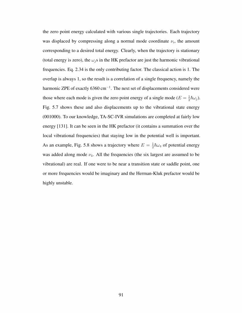
the zero point energy calculated with various single trajectories. Each trajectory

was displaced by compressing along a normal mode coordinate νi, the amount

corresponding to a desired total energy. Clearly, when the trajectory is stationary

(total energy is zero), the ωjs in the HK prefactor are just the harmonic vibrational

frequencies. Eq. 2.34 is the only contributing factor. The classical action is 1. The

overlap is always 1, so the result is a correlation of a single frequency, namely the

harmonic ZPE of exactly 6360 cm−1. The next set of displacements considered were

those where each mode is given the zero point energy of a single mode (E = 12~ωj).

Fig. 5.7 shows these and also displacements up to the vibrational state energy

(001000). To our knowledge, TA-SC-IVR simulations are completed at fairly low

energy [131]. It can be seen in the HK prefactor (it contains a summation over the

local vibrational frequencies) that staying low in the potential well is important.

As an example, Fig. 5.8 shows a trajectory where E = 12~ω4 of potential energy

was added along mode ν4. All the frequencies (the six largest are assumed to be

vibrational) are real. If one were to be near a transition state or saddle point, one

or more frequencies would be imaginary and the Herman-Kluk prefactor would be

highly unstable.

91

0 1000 2000 3000 4000 5000 6000 7000 8000 9000 10000

Energy in Trajectory [cm-1

]

6175

6200

6225

6250

6275

6300

6325

6350

Zer

o P

oin

t E

ner

gy [

cm-1

]

ν1

ν2

ν3

ν4

ν5

ν6

Figure 5.7: The zero point energy calculated with various single trajectories. Eachtrajectory was displaced along a particular normal mode coordinate equivalent to theenergy on the x-axis. The horizontal line is the “exact” curvilinear-VSCF/VCIPSI-PT2 zero point energy.

92

0 500 1000Timesteps

2360

2370

2380

2390

2400

2410

2420

Su

m o

f F

req

uen

cies

[cm

-1]

Figure 5.8: The summation of the local frequencies for a trajectory with 12~ω4 of

energy in mode ν4. In this case, all of the frequencies are real.

Going into more detail, the correlation function that is used in the Fourier

transform consists of an average of 600 segments of 0.3 ps correlation length. This

is similar to the averaging done in a multi-trajectory SC-IVR simulation. In this case,

instead of separate trajectories, the segments come from the same single trajectory.

The correlation function has both a real and imaginary part, and the two parts are

shown in Fig. 5.9. The correlation function of this trajectory (same as that in Fig. 5.8)

is highly periodic and of a single frequency. There is no loss of correlation, meaning

there is little coupling of this mode, at least for this simulation length. The single

frequency is due to the the coherent state of the trajectory strongly overlapping with

the coherent state at the equilibrium geometry and no other states.

93

0 0.05 0.1 0.15 0.2 0.25Time [ps]

Co

rrel

atio

n [

dim

ensi

on

less

]

realimaginary

Figure 5.9: Correlation function of a single-trajectory SC-IVR calculation with asingle quanta displacement in mode ν4 and a reference wavefunction |p = 0,q =eq〉.

The power spectrum is obtained by a Fourier transform of the correlation function.

Since the signal here does not decay, an exponential window function is applied:

W = exp

[−C

(t

T

)2], (5.9)

where C is a constant, t is time and T is the total length of the correlation function.

This is because a Fourier transform by definition is an integration over the interval

(−∞,∞) so the signal needs to decay to zero by the integration limits. In cases where

the trajectory is less harmonic and the reference wavefunction is not at equilibrium,

the correlation does decay quite rapidly. The power spectrum of the above correlation

function is shown in Fig. 5.10. It is highly-resolved and characteristic of time-

averaged spectra. A similar result is found in the H2CO simulations by Kaledin

and Miller [62]. In their findings, the single-trajectory spectra are highly-peaked

and narrow, while their full phase space spectra are relatively broad. This is due

to - in their words - the “quenching” of the IVR integrand. However, they report

the relative errors between the two methods and single time-averaged SC-IVR has a

slightly higher error, with it increasing for higher vibrational states. It would seem

logical that noise is quenched with repetitive data, yet because there are less data,

results may not be as accurate.

94

6000 8000 10000 12000 14000

Energy [cm-1

]

Inte

nsi

ty

Figure 5.10: Power spectrum of a single-trajectory SC-IVR calculation with a singlequanta displacement in mode ν4 and a reference wavefunction |p = 0,q = eq〉. Thespectrum shows the single highly-resolved ZPE peak.

Fig. 5.7 shows that the power spectra may be fairly dependent on the trajectory

chosen. Within a particular mode displacement, there appears to be some trend,

especially for displacement energies lower than the total zero point energy. For

example, ν2 remains relatively constant. The other modes have somewhat linear

and decreasing trends, with ν3, ν4 and ν6 being fairly similar. However, it is unclear

why there is a turnaround at higher energies. More strikingly is that with increasing

energies, the values become divergent. At around x = 3250 cm−1, where 3 different

displacements coincide, it is very near the “exact” zero point.

Ψref may also be be chosen to extract states of higher energy. Analogous to

the displacement of the Gaussian along normal modes in Chapter 4, we employed

displaced reference wavefunctions and were able to easily extract the fundamentals

95

and first overtones. Fig. 5.11 shows power spectra where both the trajectories and

reference wavefunctions were Gaussians displaced along a normal mode by an

amount E = 12~ωj . As can be seen, all simulations were able to determine the

zero point energy, with a similar discrepancy to that of Fig. 5.7. A trajectory with

a displacement along νj with an equivalently-displaced Ψref will produce peaks of

the variety (· · ·n · · · ). For instance, the first fundamental peak is (000100) from

a trajectory and reference wavefunction of displacement along ν4. These power

spectra are much more resolved and easier for assignment compared to the standard

SC-IVR spectra. Table 5.2 compiles all the SC-IVR vibrational state calculations in

Chapter 4 with those of Chapter 5 (Figs. 5.7 and 5.11) as well as TA-SC-IVR of eight

trajectories by Ceotto et al. [129], which is discussed in the next section. Ceotto

undershoots the exact energies, which is of interest, as that means that method is

finding more anharmonicity than the “exact” results. On the other hand, our single-

trajectory SC-IVR energies are larger (closer to harmonic) than that of the standard

SC-IVR.

96

6000 7000 8000 9000 10000

Energy [cm-1

]

Inte

nsi

ty [

arb

. u

nit

s]

ν1

ν2

ν3

ν4

ν5

ν6

Figure 5.11: Power spectra of H2CO determined by trajectory and reference wave-function displacements along modes νj Each peak represents a single-mode exci-tation of the form (· · ·n · · · ). Up to 2-quanta excitation is achieved from theseparticular trajectories.

97

Table 5.2: Fundamental and overtone vibrational state energies of H2CO at theHF/3-21G level. Units are in cm−1.

State Harmonic Exact SC-IVR TA(1)-SC-IVR TA(8)-SC-IVR[130] [130] [129]

(000000) 6360 6309 6311 6336* 6258(000100) 7697 7640 — 7682 —(000001) 7738 7672 — 7726 —(001000) 8053 7980 8013 8039 7911(010000) 8276 8198 8208 8262 8152(100000) 9522 9320 9303 9454 9300(000010) 9593 9384 — 9519 —(000200) 9034 8987 — 9018 —(000002) 9117 9037 — 9103 —(002000) 9745 9650 9587 9732 9598(020000) 10191 10074 10089 10174 10020(200000) 12685 12232 12297 12595 12352(000020) 12827 12418 — 12724 —

5.3 Time-Averaging: Equivalent Ensembles?

The Monte Carlo estimate of the phase space as shown in Eq. 4.9 is a distribution

centred upon a given position and momentum. This is a canonical distribution.

While we account for this non-uniform sampling in Eq. 4.10, in a single-trajectory

time-averaged SC-IVR, the canonical distribution is intrinsically eliminated. In

fact, since segments (p1,q1) are obtained from the single trajectory, the distribution

actually sampled is microcanonical (that is, it is a constant energy ensemble). This

becomes a concern for the integral in the correlation function. In the extreme limit

where the integral over (p0,q0) reduces to a single value, the phase space SC-IVR

and time-averaged SC-IVR are not equivalent.

Thinking along that line, we look back at the original time-averaged SC-IVR

equation (Eq. 5.5). Here, in addition to time-averaging, there is still the integral over

phase space. If we take the (unaveraged) correlation functions from multiple single-

trajectory calculations, which all have a different total energy, we conjecture that

98

we will recover some of the phase space average. In single-trajectory time-averaged

SC-IVR, the “final” correlation function is an average of all the correlations in each

segment. Each segment is a single NVE trajectory. Now, taking these correlations

and then averaging them with other segments from a different (energy) trajectory,

it would be an approximation to making a proper phase space average. It could

provide a more accurate power spectrum (cf. Ref. [129]). We take the average of

6 different trajectories (E = 12~ωj for each νj) and the result for the ZPE is 6336

cm−1. Contrast this between the reference VSCF/VCIPSI-PT2 calculation (6309

cm−1) and the full SC-IVR calculation (6311 cm−1). It is between these results

and the harmonic value. It is necessary to compare numerous single trajectories

and see whether they produce consistent results or determine the outliers. Further

investigation into whether a single-trajectory calculation is equivalent is warranted,

as it is found in literature without much explanation.

Of recent interest [60, 103, 129, 130] has been the informed construction of

the reference state. As said before, the correlation is highest when the coherent

state of the trajectory is similar to that of the reference state. A reference state is a

representation (guess) of the true wavefunction. So, when the reference wavefunction

is a Gaussian at equilibrium, it represents the true ground state wavefunction, and a

high overlap with this state will produce a strong signal for the ground vibrational

state. Similarly, reference wavefunctions similar to the true wavefunction of other

vibrational states will allow for the determination of those vibrational states in the

power spectrum. Of course, all wavefunctions overlap in some manner with each

other unless forbidden by symmetry. Generally, the issue with SC-IVR is the overlap

with too many states, making for a very indeterminate spectrum. In Ref. [62], the

reference state was expressed in a symmetry-adapted form. For H2CO, there are four

symmetric states: A1, A2, B1 and B2. In our previous study in Chapter 4, we used

this concept (see Eq. 4.11) to extract states of A1 symmetry. Most recently, Ceotto

99

et al. [60] reported a “multiple coherent” states method, where the reference state is

of the form:

Ψref =states∑i=1

|piqi〉. (5.10)

The “states” they consider are points on the (p, 0) or (0, q) phase space surface that

are located at the peaks of the harmonic power spectrum. For maximum overlap, they

also suggest using trajectories that are on the same phase space orbit. They state that

the trajectories are “close to the modes associated with the desired vibrational energy

peaks.” This appears to mean imparting either momenta or displacement along all

the normal modes with a total energy equal to that of the (harmonic) vibrational

states. Therefore, multiples of quanta are imparted to each vibrational mode. Their

results show that multiple trajectories (i.e., time-averaged SC-IVR not at the single-

trajectory limit) produces energies that are more anharmonic than single-trajectory

SC-IVR. In terms of their multiple coherent reference states, they are effective

at producing a wide range of peaks yet they show that selecting reference states

favouring a single vibrational state will produce more precise (higher, sharper peak)

states. Using symmetric combinations of this multiple coherent state, choosing peaks

with specific symmetries is possible as well. Another modification to the correlation

function that they used (originally found in Ref. [61]) is the separable approximation.

In this approximation, the HK prefactor is assumed to be separable. The prefactor

contains two time variables (t1 and t2) and assuming it can be factored, would be of

form:

R(t1, t2) ≈ f(t1)g(t2). (5.11)

It can be shown then, that one only needs to calculate the phase of R. The integrand

becomes positive definite and improves the prefactor accuracy at long time. For

H2CO, they note that the separable approximation makes for a smoother power

spectrum and does not affect peak location. While it is possible to implement, we

have not found the need to use this approximation, given that we already use the

100

Johnson approximation of the prefactor.

From our results of the ZPE calculation, it is evident that the choice of trajectory

affects the location of the ZPE. While the choice of reference state may affect

the strength of the spectral density, it appears that the choice of trajectory may be

critical for a single-trajectory calculation. For a very low energy trajectory, one

seems to approach the harmonic zero point. Fig. 5.7 shows that as the energy of

the trajectory increases, the calculated ZPE diverges. It would be useful to know

the exact trajectories used in previous studies, whether the spectra are hand-picked

from select trajectories or whether a single trajectory with significant spectral peaks

was chosen. Further investigations into model systems would be beneficial. The

higher vibrational states, when considered individually, give very resolved peaks,

considerably easier to assign than for the standard SC-IVR calculation. If the location

of the peaks can be reproduced with other trajectories, then the existing prescription

is successful. If not, then the reason for the discrepancies due to trajectory choice

will have to be examined.

The analysis of our implementation of the single-trajectory SC-IVR reveals that

the approach is practical and can yield useful results with much reduced computa-

tional effort, providing a very efficient ab initio SC-IVR option.

101

Chapter 6

Conclusion and Future Outlook

6.1 Conclusions

The ultimate goal of theoretical chemistry is the ability to find solutions to describe

nature at its most accurate, yet, as with all things, there is compromise. The real world

is inherently quantum mechanical in nature, i.e., following the rules of quantum

mechanics. The mathematics used to solve its equations are fairly simple. Yet,

the solutions for most systems are computationally intractable. So, it is the job

of the theoretical chemist to find ways to make these problems easier to solve.

This involves creating an acceptable model for the molecular system and using

a good approximation/representation of the Schrodinger equation. The former

involves determining the subsystem of interest (or of importance) and the latter

finding ways to circumvent the “brute force” method. One of the far-reaching

areas of quantum dynamics is semiclassical dynamics. Semiclassical mechanics

lies in between quantum and classical mechanics, in that it proceeds to solve the

quantum mechanical equations in such a way that it takes information from classical

mechanics. Specifically, we can utilize information from a classical (molecular

dynamics) trajectory and use it in semiclassical forms of quantum mechanical

equations in order to describe quantum mechanical effects, e.g., tunnelling, zero

point energy, scattering, etc.

In this thesis, we have endeavoured to develop tools for and investigate problems

102

with the semiclassical initial value representation (SC-IVR). The first part of the

work (Chapter 3) involved developing the ability to perform ab initio molecular

dynamics in the software package MMTK. An interface between electronic structure

programs (e.g., Molpro, GAMESS) and MMTK means that one can do on-the-fly

molecular dynamics simulations in the simple and powerful framework of MMTK.

With this tool established, we investigated the electronic ground and excited state

dynamics of the CH3OCl molecule. It is an important molecule in atmospheric

chemistry and we have laid the groundwork for an intensive investigation into its

photodissociation dynamics. Next, we began the primary focus of our research,

which was creating a method to compute molecular vibrational state energies using

the ab initio SC-IVR. With the tools developed in MMTK, we were able to conduct

molecular dynamics simulations (and obtain second derivatives) which provided the

classical inputs for our semiclassical algorithm (in Python, with some integration

into the MMTK code), which is entirely in Cartesian coordinates. We determined the

vibrational state energies of H2CO and these were shown to be very accurate when

compared to benchmark results (see Chapter 4). The final part of this thesis (Chapter

5) details similar calculations using time-averaged SC-IVR, a more computationally

efficient technique. Our findings show that the energies obtained via this method are

comparable to those obtained with full phase space SC-IVR.

6.1.1 Ab initio Molecular Dynamics

Methyl hypochlorite (CH3OCl) has two low-lying electronic excited states from

which the resulting dissociation products are known to contribute to the atmospheric

chlorine cycle. Photoexcited CH3OCl primarily goes into two dissociative excited

states that produce the Cl· radical. We have modelled the distribution of the ground

state molecule which would be vertically excited into one of two excited states.

Transition probabilities were computed from equilibrium and a preliminary excited

103

state analysis was done. The primary purpose of this study was to test the integration

of ab initio dynamics in MMTK.

6.1.2 Semiclassical Initial-Value Representation of H2CO

H2CO is a well-studied molecule in terms of its vibrational states, including highly

accurate PES surfaces [132]. Use of methods such as vibrational self-consistent

field or vibrational configuration interaction to determine its vibrational energies

including anharmonicity (for a certain electronic method/basis set) makes it a good

system for observing the accuracy of vibrational states calculated using SC-IVR.

With the ab initio tools established, we applied it to the SC-IVR technique and have

reported on the numerous intricacies involved in such simulations (e.g., reference

state selection). The fundamental, overtone and two-mode coupled vibrational states

of H2CO were determined. Finally, we examined the time-averaged variant of

SC-IVR and performed similar calculations on the same system.

6.2 Future Outlook

6.2.1 Immediate Questions and Discussions

The immediate questions to be addressed are the validity and accuracy of time-

averaged SC-IVR calculations. A full comparison of the results for standard SC-

IVR with time-averaged SC-IVR calculations would be desired, and an analysis

of whether any trends in the spectra with respect to trajectory selection should be

done. As well, examining the use of a combination of reference states would be

beneficial to see if any artifacts due to dynamics along a single mode remain. This

could show whether the tradeoff between using single trajectories over multiple

(time-averaged) trajectories is worth the extra scrutiny the single trajectory chosen

must be. Choice of an inappropriate single trajectory may skew results. In fact,

the exact prescription for each trajectory should be reported in any SC-IVR results.

104

Time-averaging over multiple trajectories has been shown to be more accurate [61]

than single-trajectory SC-IVR. Unless the ab initio energy and Hessian evaluations

are extremely computationally costly, there is most likely little reason not to use

multiple-trajectory time-averaging.

In the meantime, it would be very beneficial to examine the phase space distribu-

tion between a full SC-IVR integral (NVT) and a time-averaged (NVE) integral. A

weighting procedure of the trajectories similar to Eq. 4.10 would ensure the phase

space distribution is uniform (i.e., a uniform grid). Then, the two methods would be

mathematically equivalent. The simplest model is the 1-D harmonic oscillator (HO).

Because the diagonalization of the Hessian for a harmonic system will just give the

frequency of the HO, its power spectrum is actually analytic, and has been derived

in Ref. [129]. Then, the most immediate models to investigate would be the single

1-D Morse oscillator, which is an ideal model system with actual anharmonicity.

Ref. [129] has looked at uncoupled Morse oscillators. However, the determination

of the equivalency of these systems with full phase space integrals is desired.

Other than work by Roy and co-workers [56–59, 114], the approximate Johnson

WKB prefactor [54, 55] has not been used in the literature except for when it was

originally proposed. Others have used the original prefactor and its alternate but

equivalent form, the log-derivative. To that end, we have started implementing the

log-derivative form for the 1-D models. Any discrepancies between that and the

WKB approximation can then be precisely identified.

6.2.2 Ultimate Aim

Ultimately, SC-IVR would show its power not through small systems, but through

large and/or strongly anharmonic systems such as small clusters, complexes in water

or proteins. Surface chemistry using SC-IVR is also possible [133]. Smaller systems

can already be analyzed relatively computationally efficiently using vibrational SCF

105

methods. So, ways to improve SC-IVR to be more advantageous than these methods

would be of immediate interest to examine. Ensuring that, notwithstanding SC-

IVR’s natural slow convergence [134], these chemically-interesting systems can be

accessible. We know that despite increasing degrees of freedom, SC-IVR can take

advantage of using geometric constraints [56]. Then, for example, parts of a system

(say, an amino acid of interest in a protein, or the active region of proton transfer)

may treated with all degrees of freedom while the “unimportant” parts may be

constrained. Geometric constraints in MTTK is a straightforward process. SC-IVR

also requires the Hessian in this limited degree of freedom frame, so employing

projection techniques is necessary [56]. Also, it would be worth to take advantage

of some of the force fields that are natively built into MMTK. A force field such

as AMBER [135] has many atomic parameters for bio-molecular systems readily

usable in MMTK.

Another way to realize the full potential of SC-IVR is to reduce the number of

Hessian calculations. The improvement of integrators through the use of Hessians

is not new [136, 137]. However, bringing Hessians into an integrator (we only use

gradient data in Velocity-Verlet, for example) means those calculations have to be

efficient or sparse. Bringing this idea into SC-IVR would be highly-desirable, as

Hessian information is already required. Barring efficiencies in the integrator algo-

rithm that would make the number of timesteps more sparse, there is the technique

called Hessian updating [105, 138], where while the dynamics integration timestep

doesn’t change, the need for a Hessian at each timestep is not necessary. For example,

compact finite difference schemes are stepwise ways to determine the Hessian using

other data (e.g., gradients). Therefore, a “true” Hessian is only obtained after a few

timesteps, while the interim points are numerically obtained through an updating

scheme. Ceotto and co-workers have shown that ab initio MD calculations can be

two orders of magnitude more efficient [138]. He and other co-workers applied this

106

scheme to ab initio time-averaged SC-IVR on the CO2 molecule. As the number

of timesteps before a real Hessian calculation increases, the accuracy of the power

spectrum remains surprisingly good. Only after about 20 steps of approximate Hes-

sians does the spectra start to show a significant degradation in the lower-intensity

peaks. This is encouraging news for studying larger systems.

6.3 Other Applications of SC-IVR

Vibrational states are only a single type of information which can be obtained

from SC-IVR. In fact, SC-IVR has been used to determine a variety of molecular

information. The quantum propagator is the root of many quantum-mechanical

equations, so having a semiclassical propagator allows for an analysis of other

properties provided the observable (or eigenstate) can be expressed in semiclassical

variables. For instance, we have referred to the survival amplitude C(t) as the

“correlation” function. In several applications, one is interested in studying the

effects of temperature, T , on the correlation between two physical quantities, A and

B, for a system with Hamiltonian H . This is achieved by computing the so-called

canonical time correlation function defined as [139]:

〈AB(t)〉 =1

ZTr{e−βHAB(t)

}, (6.1)

where β = 1/(kBT ), kB is Boltzmann’s constant, and Z = Tr {exp(−βH)} is the

canonical partition function of the system. Note that the B(t) represents the time

dependence of the operator B. More specifically,

B(t) = eiHt/~Be−iHt/~ (6.2)

is the Heisenberg representation of the operator B and defines the time dependence.

Note that both the forward and backward propagators appear in the definition of B(t).

This means that in a SC-IVR implementation, two sets of integrals over phase space

107

must be inserted. This can lead to serious sampling issues and various approximate

methods have been developed to overcome these problems [140].

There are a variety of problems that can benefit from our SC-IVR for vibrational

states. Most related to vibrational states would be the determination of vibrational

eigenfunctions. Ceotto et al. [104] have determined the eigenstates of H2CO with an

equation very similar to that of the survival amplitude. Quantum thermal correlation

functions such as vibrational relaxation [115] can be studied. Vibronic transitions of

H2CO [102] via ab initio SC-IVR have also been investigated.

Overall, ab initio semiclassical techniques are promising and have been shown

to be another effective tool in the arsenal of a quantum dynamicist.

108

Bibliography

[1] J. S. Francisco, International Journal of Quantum Chemistry 73 29 (1999).

[2] D. A. McQuarrie and J. D. Simon, Physical Chemistry: A Molecular Ap-proach, University Science Books, Sausalito, CA (1997).

[3] Rayleigh, Baron (J. W. Strutt), Nature 72 54 (1975).

[4] A. Einstein, Ann. Phys. (Berlin) 17 132 (1905).

[5] C. J. Cramer, Essentials of Computational Chemistry: Theories and Models,Wiley, West Sussex (2004).

[6] T. Helgaker, P. Jørgensen, and J. Olsen, Molecular Electronic-StructureTheory, Wiley, West Sussex (2000).

[7] J. K. Cullum and R. A. Willoughby, Lanczos Algorithms for Large SymmetricEigenvalue Computations, Birkhauser, Boston (1985).

[8] W. H. Miller, Proc. Natl. Acad. Sci. 102 6660 (2005).

[9] B. Balzer, S. Dilthey, G. Stocka, and M. Thoss, J. Chem. Phys. 119 5795(2003).

[10] R. P. Feynman and A. R. Hibbs, Quantum Mechanics and Path Integrals,McGraw-Hill, New York (1965).

[11] K. G. Kay, J. Chem. Phys. 100 4377 (1994).

[12] H.-W. Lee and M. O. Scully, J. Chem. Phys. 73 2238 (1980).

[13] F. Jensen, Introduction to Computational Chemistry, 2nd Ed., Wiley, WestSussex (2007).

[14] C. C. J. Roothaan, Rev. Mod. Phys. 23 69 (1951).

[15] P. Hohenberg and W. Kohn, Phys. Rev. B136 864 (1964).

[16] W. Kohn and L. J. Sham, Phys. Rev. A140 1133 (1965).

[17] M. W. Schmidt, K. K. Baldridge, J. A. Boatz, S. T. Elbert, M. S. Gordon,J. H. Jensen, S. Koseki, N. Matsunaga, K. A. Nguyen, S. J. Su, T. L. Windus,M. Dupuis, and J. A. Montgomery, J. Comput. Chem. 14 1347 (1993).

109

[18] H.-J. Werner, P. J. Knowles, R. Lindh, F. R. Manby, M. Schutz, P. Celani,T. Korona, G. Rauhut, R. D. Amos, A. Bernhardsson, A. Berning, D. L.Cooper, M. J. O. Deegan, A. J. Dobbyn, F. Eckert, C. Hampel, G. Het-zer, A. W. Lloyd, S. J. McNicholas, W. Meyer, M. E. Mura, A. Nicklass,P. Palmieri, R. Pitzer, U. Schumann, H. Stoll, A. J. Stone, R. Tarroni, andT. Thorsteinsson, Molpro, version 2006.1, a package of ab initio programs(2006), see http://www.molpro.net.

[19] M. J. Frisch, G. W. Trucks, H. B. Schlegel, G. E. Scuseria, M. A. Robb, J. R.Cheeseman, G. Scalmani, V. Barone, B. Mennucci, G. A. Petersson, H. Nakat-suji, M. Caricato, X. Li, H. P. Hratchian, A. F. Izmaylov, J. Bloino, G. Zheng,J. L. Sonnenberg, M. Hada, M. Ehara, K. Toyota, R. Fukuda, J. Hasegawa,M. Ishida, T. Nakajima, Y. Honda, O. Kitao, H. Nakai, T. Vreven, J. A. Mont-gomery, Jr., J. E. Peralta, F. Ogliaro, M. Bearpark, J. J. Heyd, E. Brothers,K. N. Kudin, V. N. Staroverov, R. Kobayashi, J. Normand, K. Raghavachari,A. Rendell, J. C. Burant, S. S. Iyengar, J. Tomasi, M. Cossi, N. Rega, J. M.Millam, M. Klene, J. E. Knox, J. B. Cross, V. Bakken, C. Adamo, J. Jaramillo,R. Gomperts, R. E. Stratmann, O. Yazyev, A. J. Austin, R. Cammi, C. Pomelli,J. W. Ochterski, R. L. Martin, K. Morokuma, V. G. Zakrzewski, G. A. Voth,P. Salvador, J. J. Dannenberg, S. Dapprich, A. D. Daniels, . Farkas, J. B.Foresman, J. V. Ortiz, J. Cioslowski, and D. J. Fox, Gaussian 09 RevisionA.1, Gaussian Inc. Wallingford CT 2009.

[20] TURBOMOLE V6.3 2011, a development of University of Karlsruhe andForschungszentrum Karlsruhe GmbH, 1989-2007, TURBOMOLE GmbH,since 2007; available from http://www.turbomole.com.

[21] P. Atkins and R. Friedman, Molecular Quantum Mechanics, 5th Ed., OUP,Oxford (2011).

[22] D. J. Tannor, Introduction to Quantum Mechanics - A Time-DependentPerspective, University Science Books, Sausalito, California (2007).

[23] B. M. Austin, D. Y. Zubarev, and W. A. Lester, Jr., Chem. Rev. 112 263(2012).

[24] J. B. Anderson, J. Chem. Phys. 63 1499 (1975).

[25] D. C. Clary, D. M. Benoit, and T. van Mourik, Acc. Chem. Res. 33 441 (2000).

[26] P. J. Reynolds, D. M. Ceperley, B. J. Adler, and W. A. Lester, J. Chem. Phys.77 5593 (1982).

[27] H.-D. Meyer, F. Gatti, and G. A. Worth, Multidimensional Quantum Dynam-ics: MCTDH Theory and Applications, Wiley-VCH, Weinheim (2009).

[28] P. R. Holland, The Quantum Theory of Motion, Cambridge University Press,Cambridge (1993).

[29] M. Brack and R. K. Bhaduri, Semiclassical Physics, Addison-Wesley, DonMills, Ontario (1997).

[30] W. C. Swope, H. C. Andersen, P. H. Berens, and K. R. Wilson, J. Chem. Phys.76 637 (1982).

110

[31] D. A. Case, T. E. Cheatham, III, T. Darden, H. Gohlke, R. Luo, K. M. Merz,Jr., A. Onufriev, C. Simmerling, B. Wang, and R. Woods, J. Comput. Chem.26 1668 (2005).

[32] H. J. C. Berendsen, D. Van Der Spoel, and R. Van Drunen, Comp. Phys.Comm. 91 43 (1995).

[33] W. Smith, T. R. Forester, and I. T. Todorov, The DLPOLY Classic UserManual, Daresbury Laboratory, Cheshire, UK (2010).

[34] W. L. Jorgensen, J. Chandrasekhar, J. D. Madura, R. W. Impey, and M. L.Klein, J. Chem. Phys. 79 926 (1983).

[35] B. R. Brooks, R. E. Bruccoleri, B. D. Olafson, D. J. States, S. Swaminathan,and M. Karplus, J. Comput. Chem. 4 187 (1983).

[36] P. Cvitanovic, R. Artuso, R. Mainieri, G. Tanner, and G. Vattay, Chaos:Classical and Quantum, Niels Bohr Institute, Copenhagen (2010), Chaos-Book.org.

[37] J. H. van Vleck, Proc. Nat. Acad. Sci. 14 178 (1928).

[38] M. C. Gutzwiller, J. Math. Phys. 8 1979 (1967).

[39] M. F. Herman and E. Kluk, Chem. Phys. 91 27 (1984).

[40] M. F. Herman, Annu. Rev. Phys. Chem. 45 83 (1994).

[41] E. J. Heller, J. Chem. Phys. 94 2723 (1991).

[42] W. H. Miller, J. Chem. Phys. 95 9428 (1991).


[44] C. Cohen-Tannoudji, B. Diu, and F. Laloe, Quantum Mechanics, John Wiley& Sons and Hermann, Paris (1977).

[45] W. H. Miller, J. Phys. Chem. A 105 2942 (2001).

[46] W. H Miller, Mol. Phys. 100 397 (2002).

[47] S. A. Deshpande and G. S. Ezra, J. Phys. A 39 5067 (2006).

[48] K. G. Kay, Chem. Phys. 322 3 (2006).

[49] E. J. Heller, Acc. Chem. Res. 39 127 (2006).


[51] R. J. Glauber, Phys. Rev. 130 2529 (1963).

[52] Y. Li and J. S. Francisco, J. Chem. Phys. 111 8384 (1999).

[53] J. N. Crowley, F. Helleis, R. Muller, G. K. Moortgat, and P. J. Crutzen, J.Geophys. Res 99 20683 (1994).

[54] R. Gelabert, X. Gimenez, M. Thoss, H. Wang, and W. H. Miller, J. Phys.Chem. A 104 10321 (2000).

111

[55] B. R. Johnson, Chem. Phys. 381 1973 (1973).

[56] B. B. Issack and P.-N. Roy, J. Chem. Phys. 123 84103 (2005).




[60] M. Ceotto, S. Atahan, G. F. Tantardini, and A. Aspuru-Guzik, J. Chem. Phys.130 234113 (2009).

[61] A. L. Kaledin and W. H. Miller, J. Chem. Phys. 118 7174 (2003).

[62] A. L. Kaledin and W. H. Miller, J. Chem. Phys. 119 3078 (2003).

[63] Y. Scribano and D. M. Benoit, Chem. Phys. Lett. 458 384 (2008).

[64] Y. Scribano, D. M. Lauvergnat, and D. M. Benoit, J. Chem. Phys. 133 94103(2010).

[65] G. C. Carney, L. L. Sprandel, and C. W. Kern, Adv. Chem. Phys. 37 305(1978).

[66] J. M. Bowman, J. Chem. Phys. 68 608 (1978).

[67] K. Yagi, K. Hirao, T. Taketsugu, M. W. Schmidt, and M. S. Gordon, J. Chem.Phys. 121 1383 (2004).

[68] G. M. Chaban, J. O. Jung, and R. B. Gerber, J. Chem. Phys. 111 1823 (1999).

[69] J. M. Bowman, K. M. Christoffel, and F. L. Tobin, J. Phys. Chem. 83 905(1979).

[70] K. M. Christoffel and J. M. Bowman, Chem. Phys. Lett. 85 220 (1982).

[71] S. Carter, J. M. Bowman, and N. C. Handy, Theor. Chem. Acc. 100 191(1998).

[72] E. R. Davidson, J. Comput. Phys. 17 87 (1975).

[73] E. R. Davidson, Comp. Phys. Commun. 53 49 (1989).

[74] C. W. Murray, S. C. Racine, and E. R. Davidson, J. Comput. Phys. 103 382(1992).

[75] K. Hinsen, J. Comput. Chem. 21 79 (2000).

[76] T. P. W. Jungkamp, U. Kirchner, M. Schmidt, and R. N. Schindler, J. Pho-tochem. Photobiol. A 91 1 (1995).

[77] S. Nanbu and S. Iwata, J. Phys. Chem. 96 2103 (1992).

[78] M. J. Krisch, L. R. McCunn, K. Takematsu, L. J. Butler, F. R. Blase, andJ. Shu, J. Phys. Chem. A 108 1650 (2004).

[79] R. N. Schindler, M. Liesner, S. Schmidt, U. Kirchner, and T. Benter, J.Photochem. Photobiol. A 107 9 (1997).

112

[80] M. Muhlhauser, M. Schnell, and S. D. Peyerimhoff, Mol. Phys. 100 509(2002).

[81] E. Drougas, A. M. Kosmas, M. Schnell, M. Muhlhauser, and S. D. Peyer-imhoff, Mol. Phys. 100 2653 (2002).

[82] T. J. He, D. M. Chen, F. C. Liu, and L. S. Sheng, Chem. Phys. Lett. 332 545(2000).

[83] D. Jung, C. J. Chen, and J. W. Bozzelli, J. Phys. Chem. A 104 9581 (2000).

[84] J. S. Rigden and S. S. Butcher, J. Chem. Phys. 40 2109 (1964).

[85] T. H. Dunning, J. Chem. Phys. 90 1007 (1989).

[86] D. E. Woon and T. H. Dunning, J. Chem. Phys. 98 1358 (1993).

[87] R. A. Kendall, T. H. Dunning, and R. J. Harrison, J. Chem. Phys. 96 6796(1992).

[88] H.-J. Werner and P. J. Knowles, J. Chem. Phys. 82 5053 (1985).

[89] P. J. Knowles and H.-J. Werner, Chem. Phys. Letters 115 259 (1985).

[90] H.-J. Werner and W. Meyer, J. Chem. Phys. 74 5794 (1981).

[91] H.-J. Werner and P. J. Knowles, J. Chem. Phys. 89 5803 (1988).

[92] P. J. Knowles and H.-J. Werner, Chem. Phys. Lett. 145 514 (1988).

[93] E. R. Davidson and D. W. Silver, Chem. Phys. Lett. 52 403 (1977).

[94] W. J. Hehre, R. Ditchfield, and J. A. Pople, J. Chem. Phys. 56 2257 (1972).

[95] M. M. Francl, W. J. Pietro, W. J. Hehre, J. J. Binkley, M. S. Gordon, D. J.Defrees, and J. A. Pople, J. Chem. Phys. 77 3654 (1982).

[96] P. C. Harihara and J. A. Pople, Theor. Chim. Acta 28 213 (1973).

[97] T. Clark, J. Chandrasekhar, G. W. Spitznagel, and P. V. Schleyer, J. Comp.Chem. 4 294 (1983).

[98] S. Nose, Mol. Phys. 52 255 (1984).

[99] M. Thoss and H. Wang, Annu. Rev. Phys. Chem. 55 299 (2004).

[100] K. G. Kay, Annu. Rev. Phys. Chem. 56 255 (2005).


[102] J. Tatchen and E. Pollak, J. Chem. Phys. 130 041103 (2009).

[103] M. Ceotto, S. Atahan, S. Shim, G. F. Tantardini, and A. Aspuru-Guzik, Phys.Chem. Chem. Phys. 11 3861 (2009).

[104] M. Ceotto, S. Valleau, G. F. Tantardini, and A. Aspuru-Guzik, J. Chem. Phys.134 234103 (2011).

[105] M. Ceotto, Y. Zhuang, and W. L. Hase, J. Chem. Phys. 138 054116 (2013).

113

[106] H.-D. Meyer, U. Manthe, and L. S. Cederbaum, Chem. Phys. Lett. 165 73(1990).

[107] J. M. Bowman, T. Carrington, and H.-D. Meyer, Mol. Phys. 106 2145 (2008).

[108] J. M. Bowman, S. Carter, and X. Huang, Int. Rev. Phys. Chem. 22 533 (2003).

[109] D. M. Ceperley and B. J. Adler, J. Chem. Phys. 81 5833 (1984).

[110] I. R. Craig and D. E. Manolopoulos, J. Chem. Phys. 121 3368 (2004).


[112] X. Sun and W. H. Miller, J. Chem. Phys. 110 6635 (1999).

[113] W. H. Miller, J. Phys. Chem. A 113 1405 (2009).

[114] B. B. Harland and P.-N. Roy, J. Chem. Phys. 118 4791 (2003).

[115] J. M. Moix and E. Pollak, J. Chem. Phys. 129 064515 (2008).

[116] G. Tao and W. H. Miller, J. Chem. Phys. 130 184108 (2009).

[117] N. Makri and W. H. Miller, J. Chem. Phys. 116 9207 (2002).

[118] E. Bukhman and N. Makri, J. Phys. Chem. A 111 11320 (2007).

[119] X. Sun and W. H. Miller, J. Chem. Phys. 108 8870 (1998).

[120] M. Ovchinnikov, V. A. Apkarian, and G. A. Voth, J. Chem. Phys. 114 7130(2001).

[121] R Ianconescu and E. Pollak, J. Chem. Phys. 134 234305 (2011).

[122] Y. Tawada, T. Tsuneda, S. Yanagisawa, Y. Yanai, and K. Hirao, J. Chem. Phys.120 8425 (2004).

[123] J. P. Perdew, K. Burke, and M. Ernzerhof, Phys. Rev. Lett. 77 3865 (1996).

[124] J. O. Jung and R. B. Gerber, J. Chem. Phys. 105 10332 (1996).

[125] L. Pele, B. Brauer, and R. B. Gerber, Theo. Chem. Acc. 117 69 (2007).

[126] J. S. Binkley, J. A. Pople, and W. J. Hehre, J. Am. Chem. Soc. 102 939 (1980).

[127] G. H. Peslherbe and W. L. Hase, J. Chem. Phys. 104 7882 (1996).

[128] Y. Elran and K. G. Kay, J. Chem. Phys. 110 8912 (1999).

[129] M. Ceotto, G. F. Tantardini, and A. Aspuru-Guzik, J. Chem. Phys. 135 214108(2011).

[130] S. Y. Y. Wong, D. M. Benoit, M. Lewerenz, A. Brown, and P.-N. Roy, J.Chem. Phys. 134 094110 (2011).

[131] Private correspondence with M. Ceotto.

[132] K. Yagi, C. Oyanagi, T. Taketsugu, and K. Hirao, J. Chem. Phys. 118 1653(2003).

114

[133] M. Ceotto, D. Dell’Angelo, and G. F. Tantardini, J. Chem. Phys. 133 054701(2010).

[134] J. C. Burant and V. Batista, J. Chem. Phys. 116 2748 (2002).

[135] R. Salomon-Ferrer, D. A. Case, and R. C. Walker, WIREs Comput. Mol. Sci.3 198 (2013).

[136] U. Lourderaj, K. Song, T. L. Windus, Y. Zhuang, and W. L. Hase, J. Chem.Phys. 126 044105 (2007).

[137] J. M. Millam, V. Bakken, W. Chen, W. L. Hase, and H. B. Schlegel, J. Chem.Phys. 111 3800 (1999).

[138] Y. Zhuang, M. R. Siebert, W. L. Hase, K. G. Kay, and M. Ceotto, J. Chem.Theo. Comp. 9 54 (2013).

[139] D. A. McQuarrie, Statistical Mechanics, University Science Books, Sausalito,CA (2000).

[140] N. Makri and K. Thompson, Chem. Phys. Lett. 291 101 (1998).

115

Appendix A

van Vleck’s Semiclassical Propagator

The propagator is assumed to be in this general form:

e−iHt/~ ≡ A(x, x′, dt)ei~S(x,x

′,δt). (A.1)

S is now the time-dependent form of the action (integral of Lagrangian) as found inthe Hamilton-Jacobi equation. Through some algebra, one gets:

e−iHt/~ ≈( m

2πi~δt

)3N/2ei~

(m(q−q′)2

2δt−V (q)δt

). (A.2)

As can be seen, the amplitude and phase are entirely classical quantities. Van Vleck’sfinal form is:

e−iHt/~ =∑roots

∫dxf

∫dxiΨ

∗f (x2)Ψi(x1)

[(2πi~)3N

∣∣∣∣∂x2∂p1

∣∣∣∣]−1/2 eiSt(x2,x1)/~.(A.3)

In terms of an initial value representation, it can be written as

eiHt/~ =

∫dx0

∫dp0

[∣∣∣∣∂xt(x0,p0)

∂p0

∣∣∣∣ /(2πi~)3N]1/2

eiSt(x0,p0)/~|xt〉〈x0|. (A.4)

This form has also been rederived by Gutzwiller [38].

116

Appendix B

Electronic Structure Methods Used -Overview

Further information about electronic structure methods may be found in Refs. [5, 6,13].

B.1 Hartree-FockThe simplest electronic structure method used in this work is the Hartree-Fock (HF)method [14]. Molecular orbitals (MOs) are expressed as linear combinations ofatomic orbitals. For each molecular orbital, the coefficients are determined througha self-consistent field procedure. These molecular orbitals linear combinations area result of a single Slater determinant (single configuration). The product of thesesingle-particle orbitals make up the total wavefunction. HF is approximate at best fordetermining the ground state of a molecule but it can be a first step for the applicationof more complex electronic structure methods.

B.2 Density Functional TheoryDensity Functional Theory (DFT) [15, 16], instead of working with the electroniccoordinates directly, uses a functional of the electron density. It includes someelectron correlation (missing in HF). Like HF, it is an independent-particle model soscales in time similarly to it.

B.3 Configuration InteractionThe HF method is a starting point for many investigations and its self-consistentfield orbitals are used as a basis for advanced methods. Most systems consist ofelectronic states that are a combination of a number of configuration states. Insteadof solely occupying the lowest MOs, the virtual orbitals may also be populated.Each configuration is represented by a determinant. The total wavefunction is asummation of all these excited Slater determinants; in the case of an infinite numberof excitations, it is called a full CI (configuration interaction).

117

B.4 Complete Active Space Self-Consistent FieldIn addition to determining the wavefunction coefficients, each MO may be optimized.This becomes a huge computational effort, so the MOs are split into active andinactive types. The active space generally contains the upper occupied orbitalsand lower unoccupied orbitals where excitations occur to/from. This restricts thetotal number of configuration state functions involved in the calculation. The activespace, taken from an HF reference calculation, is chosen as small as possible whileensuring an accurate description of the system. If multiple states are optimized inthe CASSCF at the same time, it is state-averaged [90].

B.5 Multi-Reference Configuration InteractionIf the reference wavefunction does not come from a HF calculation but rather fromCASSCF, then the configuration state functions are generated from these orbitals(multiple determinants). Because of the number of configurations generated, thechoice of which functions to include into calculations is also important.

118

University of Alberta Stephanie Yuen Yee Wong Doctor of ...

Documents

Transcript of University of Alberta Stephanie Yuen Yee Wong Doctor of ...