UNIVERSIDAD DE CHILEFACULTAD DE CIENCIAS FÍSICAS Y MATEMÁTICASDEPARTAMENTO DE CIENCIAS DE LA COMPUTACIÓN

COMPACT DATA STRUCTURES FOR INFORMATION RETRIEVALON NATURAL LANGUAGE

TESIS PARA OPTAR AL GRADO DE DOCTOR EN CIENCIAS,MENCIÓN COMPUTACIÓN

ROBERTO DANIEL KONOW KRAUSE

PROFESOR GUÍA:GONZALO NAVARRO BADINO

MIEMBROS DE LA COMISIÓN:JORGE PÉREZ ROJAS

BÁRBARA POBLETE LABRAALISTAIR MOFFAT

Este trabajo ha sido parcialmente financiado por Millennium Nucleus Information andCoordination in Networks ICM/FIC P10-024F, Fondecyt Grant 1-140796, Basal Center for

Biotechnology and Bioengineering (CeBiB) y Beca de Doctorado Nacional Conicyt

SANTIAGO DE CHILE2016

ResumenEl principal objetivo de los sistemas de recuperación de información (SRI) es encontrar, lomás rápido posible, la mejor respuesta para una consulta de un usuario. Esta no es unatarea simple: la cantidad de información que los SRI manejan es típicamente demasiadogrande como para permitir búsquedas secuenciales, por lo que es necesario la construcción deíndices. Sin embargo, la memoria es un recurso limitado, por lo que estos deben ser eficientesen espacio y al mismo tiempo rápidos para lidiar con las demandas de eficiencia y calidad.La tarea de diseñar e implementar un índice que otorgue un buen compromiso en velocidady espacio es desafiante tanto del punto de vista teórico como práctico. En esta tesis nosenfocamos en el uso, diseño e implementación de estructuras de datos compactas para crearnuevos índices que sean más rápidos y consuman menos espacio, pensando en ser utilizadosen SRI sobre lenguaje natural.

Nuestra primera contribución es una nueva estructura de datos que compite con el índiceinvertido, que es la estructura clásica usada en SRIs por más de 40 años. Nuestra nuevaestructura, llamada Treaps Invertidos, requiere espacio similar a las mejores alternativas enel estado del arte, pero es un orden de magnitud más rápido en varias consultas de interés,especialmente cuando se recuperan unos pocos cientos de documentos. Además presentamosuna versión incremental que permite actualizar el índice a medida que se van agregandonuevos documentos a la colección. También presentamos la implementación de una ideateórica introducida por Navarro y Puglisi, llamada Dual-Sorted, implementando operacionescomplejas en estructuras de datos compactas.

En un caso más general, los SRI permiten indexar y buscar en colecciones formadaspor secuencias de símbolos, no solamente palabras. En este escenario, Navarro y Nekrichpresentaron una solución que es óptima en tiempo, que requiere de espacio lineal y es capazde recuperar los mejores k documentos de una colección. Sin embargo, esta solución teóricarequiere más de 80 veces el tamaño de la colección, haciéndola poco atractiva en la práctica.En esta tesis implementamos un índice que sigue las ideas de la solución óptima. Diseñamos eimplementamos nuevas estructuras de datos compactas y las ensamblamos para construir uníndice que es órdenes de magnitud más rápido que las alternativas existentes y es competitivoen términos de espacio. Además, mostramos que nuestra implementación puede ser adaptadafácilmente para soportar colecciones de texto que contengan lenguaje natural, en cuyo casoel índice es más poderoso que los índices invertidos para contestar consultas de frases.

Finalmente, mostramos cómo las estructuras de datos, algoritmos y técnicas desarrolladasen esta tesis pueden ser extendidas a otros escenarios que son importantes para los SRI. Eneste sentido, presentamos una técnica que realiza agregación de información de forma eficienteen grillas bidimensionales, una representación eficiente de registros de accesos a sitios web quepermite realizar operaciones necesarias para minería de datos, y un nuevo índice que mejoralas herramientas existentes para representar colecciones de trazas de paquetes de red.

i

AbstractThe ultimate goal of modern Information Retrieval (IR) systems is to retrieve, as quickly aspossible, the best possible answer given a user’s query. This is not a simple task: the amountof data that IR systems handle is typically too large to admit sequential query processing,so IR systems need to build indexes to speed up queries. However, memory resources arelimited, so indexes need to be space-efficient and, at the same time, fast enough to copewith current efficiency and quality standards. The task of designing and implementing anindex that provides good trade-offs in terms of space and time is challenging from both atheoretical and a practical point of view. In this thesis we focus on the use, design andimplementation of compact data structures to assemble new faster and smaller indexes forinformation retrieval on natural language.

We start by introducing a new data structure that competes with the inverted index, thestructure that has been used for 40 years to implement IR system. We call this new indexInverted Treaps and show that it uses similar space as state-of-the-art alternatives, but itis up to an order of magnitude faster at queries, particularly when less than a few hundreddocuments are returned. In addition, we introduce an incremental version that supportsonline indexing of new documents as they are added to the collection. We also present theimplementation of a theoretical idea introduced by Navarro and Puglisi, dubbed Dual-Sorted,by engineering complex query processing algorithms on compact data structures.

In a more general scenario, IR systems are required to handle collections containing ar-bitrary sequences of symbols instead of just words. On general string collections Navarroand Nekrich introduced a time-optimal and linear-space solution for retrieving the top-k bestdocuments from a string collection given a pattern. However, in practice, the theoreticalsolution requires more than 80 times the size of the collection, making it unpractical. Inthis thesis, we implement an index following the ideas of the optimal solution. We designand engineer new compact data structures and assemble them to construct a compact indexthat is orders of magnitude faster than state-of-the-art alternatives and is competitive interms of space. We also show that our implementation can be easily adapted to support textcollections of natural language, in which case the index is much more powerful than invertedindexes to handle phrase queries.

Finally, we show how the data structures, algorithms and techniques developed in thisthesis can be extended to other scenarios that are important for IR. We present a techniqueto perform efficient aggregated queries on two-dimensional grids. We also present a space-efficient representation of web access logs, which supports fast operations required by webusage mining processes. Finally, we introduce a new space-efficient index that performsfast query processing on network packet traces and outperforms similar existing networkingtools.

ii

Dedicated to my grandmotherHayra Díaz (1917-2016)

iii

AcknowledgementsEvery PhD student usually thanks his advisor for his academic talent, patience and knowl-edge. What most students don’t do, is to thank their advisors for what they did besides theacademic aspects. I would like thank Gonzalo for everything else that is not reflected inthis thesis: his friendship, the humongous amount of time he spent listening to my personalmatters and giving me advices, for the amazing and crazy black-sheep email conversations at4 AM, for letting me to try getting him drunk in so many occasions, but utterly failed, and ofcourse, for the best barbecues ever. I had a blast doing the work presented in this documentand none of that fun would have been possible without him. I will be always grateful forthese amazing years.

I am very grateful to have such amazing friends like Luciano Ahumada and FranciscoClaude. It would have been impossible for me to even consider doing a PhD without thehelp and support from Luciano, who has helped me in every possible way. Francisco, hisfriendship, talent and patience over the last 13 years never end to amaze me, thank you bothfor all the support and help you gave during this process and others.

To Nelson Baloian, for teaching me what research meant, for being one of the first ones inbelieving in me, for his friendship and advices over the years, and of course, gambate kudazai.

I would like to thank the committee, Jorge Peréz, Bárbara Poblete and Alistair Moffatfor their time and dedication in reviewing my thesis. I would also like to thank Simon Gog,Diego Seco, Guillermo de Bernardo and Yung-Hwan Kim for their awesome work and helpin various papers where we worked together.

Big thanks to my friends: Jorge Lanzarotti, Cristián Valdés, Cristián Tala, MarceloFrías, Philippe Pavez, Fernanda Palacios, Christopher Espinoza, Giorgio Botto, Pablo Cristi,Waldemar Vildoso, Benjamín Sepúlveda, Paulina Jara, Rodrigo Mellado, Ximena Geoffroy,Jonathan Frez, Felipe Stein, Cristián Vera, Domenico Tavano, Valentina Concha, TámaraAvil’es, Carolina Claude, Ingrid Faust, Francisco Claude (father), OMA, Carolina Bascuñan,Luis Loyola, Leandro Llanza, Rodrigo Canóvas, Alberto “Negro” Ordoñez, Susana Ladra andSimon Gog, for all the fun, alcohol and good times we shared together :).

To the most important people in my life, my family: Werner Konow for all his support andteaching me what the word effort really means, I would not ever achieve anything withouthis example of hard work and patience. Sylvia Krause for providing me all her love andteaching me the desire of learning every day something new about life with her example ofpatience and kindness. Andrés Konow for teaching me the passion of Computer Science,and for always believing in me. Carolina Konow for such great advices, friendship and helpwith everything I can imagine. Fabiola Konow for teaching me the luck of being healthy, to

iv

appreciate simple things of life and special thanks for providing me with rock solid patience.

And finally, and most importantly, to my wife, Nadia Eger, who had to struggle withme at every step in this crazy, yet incredibly fun process. Without her it would have beenimpossible for me to be alive after all the nights without sleep while working on this. Youdeserve credit for every single page of this document. Thanks for being with me in the mostdarkest and hardest times. I (still) cannot believe how lucky I am to be able to share my lifewith such a beautiful person like you. Thank you for loving me even after everything thisthesis might have caused <3.

v

Contents

I What, Why and How 1

1 Introduction 21.1 Publications derived from the Thesis . . . . . . . . . . . . . . . . . . . . . . 41.2 Awards . . . . . . . . . . . . . . . . . . . . . . . . . . . . . . . . . . . . . . . 61.3 Research Stays and Internships . . . . . . . . . . . . . . . . . . . . . . . . . 6

2 Basic Concepts 72.1 Computation model . . . . . . . . . . . . . . . . . . . . . . . . . . . . . . . . 72.2 Sequences, Documents and Collections . . . . . . . . . . . . . . . . . . . . . 72.3 Empirical Entropy . . . . . . . . . . . . . . . . . . . . . . . . . . . . . . . . 82.4 Huffman Codes . . . . . . . . . . . . . . . . . . . . . . . . . . . . . . . . . . 82.5 Integer Encoding Mechanisms . . . . . . . . . . . . . . . . . . . . . . . . . . 9

2.5.1 Bit-aligned Codes . . . . . . . . . . . . . . . . . . . . . . . . . . . . . 102.5.2 Byte-aligned Codes . . . . . . . . . . . . . . . . . . . . . . . . . . . . 11

2.6 Rank, Select and Access . . . . . . . . . . . . . . . . . . . . . . . . . . . . . 132.6.1 Binary Sequences . . . . . . . . . . . . . . . . . . . . . . . . . . . . . 132.6.2 General Sequences . . . . . . . . . . . . . . . . . . . . . . . . . . . . 15

2.7 Wavelet Tree . . . . . . . . . . . . . . . . . . . . . . . . . . . . . . . . . . . 162.7.1 Data Structure . . . . . . . . . . . . . . . . . . . . . . . . . . . . . . 162.7.2 Rank, Select and Access . . . . . . . . . . . . . . . . . . . . . . . . . 162.7.3 Wavelet Trees and Grids . . . . . . . . . . . . . . . . . . . . . . . . . 182.7.4 Two-Dimensional Range Queries . . . . . . . . . . . . . . . . . . . . . 19

2.8 Directly Addressable Codes . . . . . . . . . . . . . . . . . . . . . . . . . . . 202.9 K2-tree . . . . . . . . . . . . . . . . . . . . . . . . . . . . . . . . . . . . . . 212.10 Compact Trees . . . . . . . . . . . . . . . . . . . . . . . . . . . . . . . . . . 242.11 Differentially Encoded Search Trees . . . . . . . . . . . . . . . . . . . . . . 252.12 Range Maximum Queries . . . . . . . . . . . . . . . . . . . . . . . . . . . . . 262.13 Treaps and Priority Search Trees . . . . . . . . . . . . . . . . . . . . . . . . 272.14 Text Indexes . . . . . . . . . . . . . . . . . . . . . . . . . . . . . . . . . . . . 27

2.14.1 Generalized Suffix Tree and Suffix Array . . . . . . . . . . . . . . . . 282.14.2 Self Indexes . . . . . . . . . . . . . . . . . . . . . . . . . . . . . . . . 302.14.3 Inverted Indexes . . . . . . . . . . . . . . . . . . . . . . . . . . . . . 33

2.15 Muthukrishnan’s Algorithm . . . . . . . . . . . . . . . . . . . . . . . . . . . 332.16 Information Retrieval Concepts . . . . . . . . . . . . . . . . . . . . . . . . . 35

2.16.1 Scoring . . . . . . . . . . . . . . . . . . . . . . . . . . . . . . . . . . . 352.16.2 Top-k Query Processing and Two-stage Ranking Process . . . . . . . 37

vi

II Inverted Indexes 38

3 Query Processing and Compression of Posting Lists 393.1 Query Processing . . . . . . . . . . . . . . . . . . . . . . . . . . . . . . . . . 39

3.1.1 Early Termination . . . . . . . . . . . . . . . . . . . . . . . . . . . . 403.1.2 Index Organization . . . . . . . . . . . . . . . . . . . . . . . . . . . . 403.1.3 Query Processing Strategies . . . . . . . . . . . . . . . . . . . . . . . 40

3.2 Algorithms for Top-k Ranked Retrieval . . . . . . . . . . . . . . . . . . . . . 413.2.1 Weak-And (WAND) . . . . . . . . . . . . . . . . . . . . . . . . . . . 423.2.2 Block-Max WAND . . . . . . . . . . . . . . . . . . . . . . . . . . . . 443.2.3 Persin et al.’s Algorithm . . . . . . . . . . . . . . . . . . . . . . . . . 463.2.4 Other Approaches . . . . . . . . . . . . . . . . . . . . . . . . . . . . . 46

3.3 Dual-Sorted Inverted Lists . . . . . . . . . . . . . . . . . . . . . . . . . . . . 483.3.1 Basic operations . . . . . . . . . . . . . . . . . . . . . . . . . . . . . . 483.3.2 Complex Operations . . . . . . . . . . . . . . . . . . . . . . . . . . . 50

3.4 Compression of Posting Lists . . . . . . . . . . . . . . . . . . . . . . . . . . . 52

4 Inverted Treaps 544.1 Inverted Index Representation . . . . . . . . . . . . . . . . . . . . . . . . . . 55

4.1.1 Construction . . . . . . . . . . . . . . . . . . . . . . . . . . . . . . . 554.1.2 Compact Treap Representation . . . . . . . . . . . . . . . . . . . . . 564.1.3 Representing the Treap Topology . . . . . . . . . . . . . . . . . . . . 574.1.4 Practical Improvements . . . . . . . . . . . . . . . . . . . . . . . . . 61

4.2 Query Processing . . . . . . . . . . . . . . . . . . . . . . . . . . . . . . . . . 634.2.1 General Procedure . . . . . . . . . . . . . . . . . . . . . . . . . . . . 634.2.2 Intersections . . . . . . . . . . . . . . . . . . . . . . . . . . . . . . . . 644.2.3 Unions . . . . . . . . . . . . . . . . . . . . . . . . . . . . . . . . . . . 674.2.4 Supporting Different Score Schemes . . . . . . . . . . . . . . . . . . . 67

4.3 Incremental Treaps . . . . . . . . . . . . . . . . . . . . . . . . . . . . . . . . 694.3.1 Supporting Insertions . . . . . . . . . . . . . . . . . . . . . . . . . . . 704.3.2 Gradual Growth . . . . . . . . . . . . . . . . . . . . . . . . . . . . . 71

5 Experimental Evaluation 735.1 Datasets and Test Environment . . . . . . . . . . . . . . . . . . . . . . . . . 73

5.1.1 Baselines and Setup . . . . . . . . . . . . . . . . . . . . . . . . . . . 745.1.2 Dual-Sorted Implementation . . . . . . . . . . . . . . . . . . . . . . . 745.1.3 Inverted Treaps Implementation . . . . . . . . . . . . . . . . . . . . . 75

5.2 Results . . . . . . . . . . . . . . . . . . . . . . . . . . . . . . . . . . . . . . . 755.2.1 Index Size . . . . . . . . . . . . . . . . . . . . . . . . . . . . . . . . . 755.2.2 Construction Time . . . . . . . . . . . . . . . . . . . . . . . . . . . . 775.2.3 Ranked Union Query Processing . . . . . . . . . . . . . . . . . . . . . 785.2.4 Ranked Intersection Query Processing . . . . . . . . . . . . . . . . . 805.2.5 One-word Queries . . . . . . . . . . . . . . . . . . . . . . . . . . . . . 895.2.6 Incremental Treaps . . . . . . . . . . . . . . . . . . . . . . . . . . . . 89

5.3 Discussion . . . . . . . . . . . . . . . . . . . . . . . . . . . . . . . . . . . . . 91

vii

III Practical Top-k on General Sequences 94

6 Top-k Document Retrieval on General Sequences 956.1 Linear Space Solutions . . . . . . . . . . . . . . . . . . . . . . . . . . . . . . 96

6.1.1 Hon et al. solution . . . . . . . . . . . . . . . . . . . . . . . . . . . . 966.1.2 Optimal solution . . . . . . . . . . . . . . . . . . . . . . . . . . . . . 97

6.2 Practical Implementations . . . . . . . . . . . . . . . . . . . . . . . . . . . . 986.2.1 Hon et al. . . . . . . . . . . . . . . . . . . . . . . . . . . . . . . . . . 986.2.2 GREEDY . . . . . . . . . . . . . . . . . . . . . . . . . . . . . . . . . 1006.2.3 NPV . . . . . . . . . . . . . . . . . . . . . . . . . . . . . . . . . . . . 1006.2.4 SORT . . . . . . . . . . . . . . . . . . . . . . . . . . . . . . . . . . . 1016.2.5 Patil et al. . . . . . . . . . . . . . . . . . . . . . . . . . . . . . . . . . 1016.2.6 Other aproaches . . . . . . . . . . . . . . . . . . . . . . . . . . . . . . 1026.2.7 Summary . . . . . . . . . . . . . . . . . . . . . . . . . . . . . . . . . 102

7 Top-k on Grids 1047.1 Wavelet Trees and RMQ . . . . . . . . . . . . . . . . . . . . . . . . . . . . . 1047.2 K2-treap . . . . . . . . . . . . . . . . . . . . . . . . . . . . . . . . . . . . . . 106

7.2.1 Local Maximum Coordinates . . . . . . . . . . . . . . . . . . . . . . 1077.2.2 Local Maximum Values . . . . . . . . . . . . . . . . . . . . . . . . . . 1087.2.3 Tree Structure . . . . . . . . . . . . . . . . . . . . . . . . . . . . . . . 1087.2.4 Top-k Query Processing . . . . . . . . . . . . . . . . . . . . . . . . . 1097.2.5 Other Supported Queries . . . . . . . . . . . . . . . . . . . . . . . . . 109

8 Practical Implementations 1108.1 A Basic Compact Implementation . . . . . . . . . . . . . . . . . . . . . . . . 110

8.1.1 Searching for Patterns . . . . . . . . . . . . . . . . . . . . . . . . . . 1108.1.2 Mapping to the Grid . . . . . . . . . . . . . . . . . . . . . . . . . . . 1108.1.3 Finding Isolated Documents . . . . . . . . . . . . . . . . . . . . . . . 1118.1.4 Representing the Grid . . . . . . . . . . . . . . . . . . . . . . . . . . 1118.1.5 Representing Labels and Weights . . . . . . . . . . . . . . . . . . . . 1118.1.6 Summing Up . . . . . . . . . . . . . . . . . . . . . . . . . . . . . . . 1128.1.7 Answering Queries . . . . . . . . . . . . . . . . . . . . . . . . . . . . 112

8.2 An Improved Index . . . . . . . . . . . . . . . . . . . . . . . . . . . . . . . . 1148.2.1 Mapping the Suffix Tree to the Grid . . . . . . . . . . . . . . . . . . 1148.2.2 Smaller Grid Representations . . . . . . . . . . . . . . . . . . . . . . 1168.2.3 Efficient Construction for Large Collections . . . . . . . . . . . . . . 1178.2.4 Summing Up . . . . . . . . . . . . . . . . . . . . . . . . . . . . . . . 117

9 Experimental Evaluation 1189.1 Datasets and Test Environment . . . . . . . . . . . . . . . . . . . . . . . . . 1189.2 Implementations . . . . . . . . . . . . . . . . . . . . . . . . . . . . . . . . . 119

9.2.1 Baselines . . . . . . . . . . . . . . . . . . . . . . . . . . . . . . . . . . 1199.2.2 Implementation of WRMQ . . . . . . . . . . . . . . . . . . . . . . . . 1209.2.3 Implementation of K2TreapH . . . . . . . . . . . . . . . . . . . . . . 1219.2.4 Implementation of W1RMQH . . . . . . . . . . . . . . . . . . . . . . 121

9.3 Results . . . . . . . . . . . . . . . . . . . . . . . . . . . . . . . . . . . . . . . 121

viii

9.3.1 Space . . . . . . . . . . . . . . . . . . . . . . . . . . . . . . . . . . . 1229.3.2 Retrieval Speed Varying k . . . . . . . . . . . . . . . . . . . . . . . . 1249.3.3 Varying Pattern Length . . . . . . . . . . . . . . . . . . . . . . . . . 1299.3.4 Word Alphabet Collections . . . . . . . . . . . . . . . . . . . . . . . . 131

9.4 Discussion . . . . . . . . . . . . . . . . . . . . . . . . . . . . . . . . . . . . . 133

IV Extensions and Evangelization 139

10 Aggregated 2D Queries on Clustered Points 14010.1 Motivation . . . . . . . . . . . . . . . . . . . . . . . . . . . . . . . . . . . . . 14010.2 Augmenting the K2-tree . . . . . . . . . . . . . . . . . . . . . . . . . . . . . 142

10.2.1 Supporting Counting Queries . . . . . . . . . . . . . . . . . . . . . . 14310.3 Experiments and Results . . . . . . . . . . . . . . . . . . . . . . . . . . . . . 145

10.3.1 Experiment Setup . . . . . . . . . . . . . . . . . . . . . . . . . . . . . 14610.3.2 Space Comparison . . . . . . . . . . . . . . . . . . . . . . . . . . . . 14710.3.3 Query Processing . . . . . . . . . . . . . . . . . . . . . . . . . . . . . 148

10.4 Discussion . . . . . . . . . . . . . . . . . . . . . . . . . . . . . . . . . . . . . 150

11 Web Access Logs 15211.1 Motivation . . . . . . . . . . . . . . . . . . . . . . . . . . . . . . . . . . . . . 15211.2 Our Index . . . . . . . . . . . . . . . . . . . . . . . . . . . . . . . . . . . . . 154

11.2.1 Construction . . . . . . . . . . . . . . . . . . . . . . . . . . . . . . . 15411.2.2 Queries . . . . . . . . . . . . . . . . . . . . . . . . . . . . . . . . . . 155

11.3 Experiments and Results . . . . . . . . . . . . . . . . . . . . . . . . . . . . . 15711.3.1 Setup and Implementations . . . . . . . . . . . . . . . . . . . . . . . 15711.3.2 Experimental Data . . . . . . . . . . . . . . . . . . . . . . . . . . . . 15711.3.3 Space Usage . . . . . . . . . . . . . . . . . . . . . . . . . . . . . . . . 15811.3.4 Time Performance . . . . . . . . . . . . . . . . . . . . . . . . . . . . 158

11.4 Discussion . . . . . . . . . . . . . . . . . . . . . . . . . . . . . . . . . . . . . 160

12 PcapWT: Indexing Network Packet Traces 16112.1 Motivation . . . . . . . . . . . . . . . . . . . . . . . . . . . . . . . . . . . . . 16112.2 Related Work . . . . . . . . . . . . . . . . . . . . . . . . . . . . . . . . . . . 16212.3 The Design of pcapWT . . . . . . . . . . . . . . . . . . . . . . . . . . . . . . 163

12.3.1 Building Index Data . . . . . . . . . . . . . . . . . . . . . . . . . . . 16312.3.2 Packet Lookup and Extraction . . . . . . . . . . . . . . . . . . . . . . 163

12.4 Performance Evaluation . . . . . . . . . . . . . . . . . . . . . . . . . . . . . 16612.4.1 Packet Traces Datasets . . . . . . . . . . . . . . . . . . . . . . . . . . 16612.4.2 Baselines . . . . . . . . . . . . . . . . . . . . . . . . . . . . . . . . . . 16812.4.3 Space . . . . . . . . . . . . . . . . . . . . . . . . . . . . . . . . . . . 16812.4.4 Multi-threaded File I/O . . . . . . . . . . . . . . . . . . . . . . . . . 16912.4.5 Packet Extraction . . . . . . . . . . . . . . . . . . . . . . . . . . . . . 169

12.5 Discussion . . . . . . . . . . . . . . . . . . . . . . . . . . . . . . . . . . . . . 171

ix

V And Finally... 174

13 Conclusions and Future Work 17513.1 Summary of Contributions . . . . . . . . . . . . . . . . . . . . . . . . . . . . 17513.2 Future Work . . . . . . . . . . . . . . . . . . . . . . . . . . . . . . . . . . . . 176

Bibliography 177

x

List of Tables

2.1 Encoding positive integers using different bit-aligned encoding techniques. . . 112.2 Different configurations for Simple9 depending on the selector value b . . . . 122.3 List of compact tree operations . . . . . . . . . . . . . . . . . . . . . . . . . 25

5.1 Ranked union results grouped by percentiles. . . . . . . . . . . . . . . . . . . 805.2 Ranked intersection results grouped by percentiles. . . . . . . . . . . . . . . 85

6.1 Comparison of practical results. . . . . . . . . . . . . . . . . . . . . . . . . 103

9.1 Collection Statistics for top-k document retrieval experiments . . . . . . . . 120

10.1 Real datasets used, and space required to represent them. . . . . . . . . . . 147

11.1 Space usage, in bytes, of the data structures used in our index . . . . . . . . 15711.2 Comparison of the space consumption of the SSA, CSA, and CST. . . . . . . . 158

12.1 Description of four sample pcap files. . . . . . . . . . . . . . . . . . . . . . . 16712.2 Comparison of the index data size. . . . . . . . . . . . . . . . . . . . . . . . 16912.3 Packet filtering queries and specifications. . . . . . . . . . . . . . . . . . . . 172

xi

List of Figures

1.1 Outline of the thesis . . . . . . . . . . . . . . . . . . . . . . . . . . . . . . . 5

2.1 Concatenation C of our 3-document example collection D. . . . . . . . . . . 82.2 Huffman tree example . . . . . . . . . . . . . . . . . . . . . . . . . . . . . . 102.3 Example of rank and select operations on a binary sequence S[1, 11]. . . . 132.4 Example of a wavelet tree. . . . . . . . . . . . . . . . . . . . . . . . . . . . . 182.5 Huffman shaped wavelet tree of an example sequence S = 1511863875743288. 182.6 Example of grid representation using a wavelet tree . . . . . . . . . . . . . . 202.7 Example of a DAC representation of integers . . . . . . . . . . . . . . . . . . 222.8 Example of a K2-tree . . . . . . . . . . . . . . . . . . . . . . . . . . . . . . . 222.9 Example of compact representation of a tree using BP, LOUDS and DFUDS . . 252.10 Example of a differentially encoded search tree . . . . . . . . . . . . . . . . . 262.11 Example of a Cartesian tree to support RMQ over S . . . . . . . . . . . . . 272.12 Example of a treap . . . . . . . . . . . . . . . . . . . . . . . . . . . . . . . . 282.13 Example of a generalized suffix tree . . . . . . . . . . . . . . . . . . . . . . . 292.14 Suffix array of collection C . . . . . . . . . . . . . . . . . . . . . . . . . . . . 292.15 Matrix of all the cyclic rotations of “ATA#TAAA#TATA#$” . . . . . . . . 312.16 Example of positional inverted index. . . . . . . . . . . . . . . . . . . . . . . 342.17 Example of a Document array and C-Array . . . . . . . . . . . . . . . . . . 35

3.1 Example of Dualsorted inverted list . . . . . . . . . . . . . . . . . . . . . . . 49

4.1 An example of posting list representation using a treap. . . . . . . . . . . . . 564.2 Compact treap using BP topology. . . . . . . . . . . . . . . . . . . . . . . . . 584.3 Compact treap using LOUDS . . . . . . . . . . . . . . . . . . . . . . . . . . . 594.4 Compact treap using HEAP. . . . . . . . . . . . . . . . . . . . . . . . . . . . . 624.5 Separating frequencies below f0 = 2 in our example treap. . . . . . . . . . . 634.6 The left-to-right construction of an example treap. . . . . . . . . . . . . . . . 72

5.1 Total sizes of the indexes depending on the scoring scheme. . . . . . . . . . . 765.2 Total sizes of the indexes depending on the scoring scheme. . . . . . . . . . . 765.3 Sizes of the topology components depending on the scoring scheme. . . . . . 775.4 Construction time of the indexes depending on the scoring scheme, in minutes. 775.5 Ranked union times for distinct k values, in milliseconds. . . . . . . . . . . . 795.6 Ranked union times grouped by number of terms per query using tf-idf. . . . 815.7 Ranked union times grouped by number of terms per query using BM25. . . 825.8 Ranked union times for distinct k values as a function of the query length. . 83

xii

5.9 Ranked intersection times for distinct k values, in milliseconds. . . . . . . . . 845.10 Ranked intersection times grouped by number of terms per query, using tf-idf. 865.11 Ranked intersection times grouped by number of terms per query, using BM25. 875.12 Ranked intersection times for distinct k values as a function of the query length. 885.13 One-word query times as a function of k. . . . . . . . . . . . . . . . . . . . . 905.14 Times for incremental versus static construction of treaps. . . . . . . . . . . 915.15 Ranked union and intersection times as a function of k. . . . . . . . . . . . . 92

6.1 Example of the Hon et al. mapping . . . . . . . . . . . . . . . . . . . . . . . 986.2 Example of Navarro and Nekrich mapping. . . . . . . . . . . . . . . . . . . . 99

7.1 Wavelet tree and RMQ combination for top-k two-dimensional queries . . . . 1067.2 Example of K2-treap construction from the matrix in Fig. 10.1 . . . . . . . . 1087.3 Storage of the conceptual tree in our data structures . . . . . . . . . . . . . 109

8.1 H-mapping of Navarro and Nekrich’s Solution. . . . . . . . . . . . . . . . . . 115

9.1 Space usage decomposition as fraction of the input, for each structure employedin WRMQ. . . . . . . . . . . . . . . . . . . . . . . . . . . . . . . . . . . . . 122

9.2 Space usage decomposition for each structure employed in K2TreapH . . . . 1239.3 Space required of grid G using single level Wavelet tree . . . . . . . . . . . . 1249.4 Space requirements for small character alphabet collection . . . . . . . . . . 1259.5 Detailed breakdown of average query time for the different indexes . . . . . . 1269.6 Query times for IDX_GN on enwiki-bigcwith m = 5 . . . . . . . . . . . . . 1279.7 Comparison of the average time per query required to retrieve the top-k results

using a K2-treap or the wavelet tree for representing G. . . . . . . . . . . . . 1289.8 Comparison of query time of K2-treap and wavelet tree for representing grid G 1299.9 Average time per query for different k values on small character alphabet

collections . . . . . . . . . . . . . . . . . . . . . . . . . . . . . . . . . . . . . 1309.10 Average time per query for varying k and m = 5 on big character alphabet

collections. . . . . . . . . . . . . . . . . . . . . . . . . . . . . . . . . . . . . . 1319.11 Average time per query in microseconds for different pattern lengths and fixed

k = 10 value. . . . . . . . . . . . . . . . . . . . . . . . . . . . . . . . . . . . 1329.12 Average time per query in microseconds for different pattern lengths and fixed

k = 10 value for enwiki-bigc. . . . . . . . . . . . . . . . . . . . . . . . . . . 1339.13 Detailed breakdown of average query time for index K2TreapH on word al-

phabet collections. . . . . . . . . . . . . . . . . . . . . . . . . . . . . . . . . 1349.14 Query times on gov2w for index IDX_GN . . . . . . . . . . . . . . . . . . . 1359.15 Results of different grid representations on word alphabet collections . . . . . 1369.16 Query time for varying k and m = 1 on word alphabet collections . . . . . . 1379.17 Time per query for different pattern lengths . . . . . . . . . . . . . . . . . . 138

10.1 Weighted matrix. . . . . . . . . . . . . . . . . . . . . . . . . . . . . . . . . . 14110.2 Binary matrix. . . . . . . . . . . . . . . . . . . . . . . . . . . . . . . . . . . 14110.3 Range query. . . . . . . . . . . . . . . . . . . . . . . . . . . . . . . . . . . . 14110.4 Storage of the conceptual tree in our data structures. . . . . . . . . . . . . . 14410.5 Space overhead in GIS and WEB datasets. . . . . . . . . . . . . . . . . . . . 14810.6 Query times of range counting queries in real datasets. . . . . . . . . . . . . 149

xiii

10.7 Space-time trade-offs of the compared range counting variants. . . . . . . . . 150

11.1 Layout of our index organization for representing Web Access Logs . . . . . 15511.2 Average microseconds to perform access and user_path. . . . . . . . . . . 15911.3 Average microseconds to perform count (P ) and the most_frequent . . 15911.4 Average microseconds to list distinct users and retrieve top-10 most common

path. . . . . . . . . . . . . . . . . . . . . . . . . . . . . . . . . . . . . . . . . 160

12.1 Extracting index data from a source packet trace file. . . . . . . . . . . . . . 16412.2 Mapping between the extracted index data and positive integers. . . . . . . . 16412.3 Building wavelet tree chunks. . . . . . . . . . . . . . . . . . . . . . . . . . . 16512.4 Listing the final matched packets. . . . . . . . . . . . . . . . . . . . . . . . . 16612.5 Retrieving the packets using multi-threaded file I/O. . . . . . . . . . . . . . 16712.6 Comparison of the index size. . . . . . . . . . . . . . . . . . . . . . . . . . . 17012.7 Comparison of the building time of index data. . . . . . . . . . . . . . . . . . 17012.8 Comparison of the packet lookup time for different sampling sizes. . . . . . . 17112.9 Comparison of packet extraction with various number of threads for parallel

file I/O. . . . . . . . . . . . . . . . . . . . . . . . . . . . . . . . . . . . . . . 17212.10A performance comparison of packet extraction using RT-2/3. . . . . . . . . 173

xiv

List of Algorithms

1 Basic wavelet tree algorithms . . . . . . . . . . . . . . . . . . . . . . . . . . . 172 Method range_report on a wavelet tree . . . . . . . . . . . . . . . . . . . 213 Method K2_range on a K2-tree. . . . . . . . . . . . . . . . . . . . . . . . . 234 Method backward_search on the SSA . . . . . . . . . . . . . . . . . . . . 325 Method locate on the SSA . . . . . . . . . . . . . . . . . . . . . . . . . . . . 326 Method document_listing returns the distinct documents . . . . . . . . . 35

7 Method svs . . . . . . . . . . . . . . . . . . . . . . . . . . . . . . . . . . . . . 428 Method wand . . . . . . . . . . . . . . . . . . . . . . . . . . . . . . . . . . . 449 Method evaluate . . . . . . . . . . . . . . . . . . . . . . . . . . . . . . . . . 4510 Method try_report . . . . . . . . . . . . . . . . . . . . . . . . . . . . . . . 4511 Method block-max-wand . . . . . . . . . . . . . . . . . . . . . . . . . . . . 4712 Method range_intersect on a wavelet tree . . . . . . . . . . . . . . . . . 51

13 Method treap_intersect using treaps. . . . . . . . . . . . . . . . . . . . . 6514 Method report using treaps . . . . . . . . . . . . . . . . . . . . . . . . . . . 6615 Method changev using treaps. . . . . . . . . . . . . . . . . . . . . . . . . . . 6616 Method changed using treaps. . . . . . . . . . . . . . . . . . . . . . . . . . . 6617 Method treap_union using treaps. . . . . . . . . . . . . . . . . . . . . . . . 6818 Method changed_union using treaps. . . . . . . . . . . . . . . . . . . . . . 69

19 Method wt_greedy returns the top-k most frequent symbols . . . . . . . . 101

20 Top-k algorithm using WRMQ index . . . . . . . . . . . . . . . . . . . . . . . 11321 Top-k algorithm using H-mapping index . . . . . . . . . . . . . . . . . . . . . 116

xv

Part I

What, Why and How

1

Chapter 1

Introduction

We are facing an information overload problem [6]. The huge amount of information gener-ated by users on the Internet is making the task of storing, searching and retrieving relevantinformation a big challenge for computer scientists and engineers. Modern Information Re-trieval (IR) systems [40, 50, 17] have to deal with this humongous amount of data whileserving millions of queries per day on billions of Web pages. The most prominent challengeswhen building IR systems are (1) quality, (2) time, and (3) space. The quality problem boilsdown to defining a suitable score scheme that returns the best possible answer to a user’squery. Score functions range from very simple (such as “term frequency”, the number of timesthe query appears in the document) to very sophisticated ones. In many cases, a simple scorefunction is used to filter a few hundred candidate documents and more sophisticated rankingsare then computed on those [40, 105]. This is because of the second concern, time. Textcollections are usually too large to admit a sequential query processing. Indexes are datastructures built on the text to speed up queries, and this is connected with the third chal-lenge: space. Designing and implementing an index that provides a good trade-off in termsof space and time is a challenging problem from both a theoretical and a practical point ofview.

Compact Data Structures is a Computer Science research field motivated by the needto handle increasing amounts of data in main memory while taking advantage of the largeperformance gap between the different levels of the memory hierarchy. It has achieved impor-tant theoretical and practical breakthroughs, such as representing trees of n nodes using just2n + o(n) bits while supporting powerful constant-time navigation [14], representing textswithin their high-order entropy space while supporting fast extraction of arbitrary segmentsand pattern searches [118, 66] or representing Web graphs within about 1 bit per edge [29],just to name a few. An area that has surprisingly remained outside of this recent virtuouscircle of achievements is IR. IR is precisely where most of the early research on compressedtext and index representations focused. The combination of text and index compression isa classical topic treated in IR textbooks over the past decade [17, 166]. It might be arguedthat IR has not been included in recent research because space efficiency is a closed problemin this area, but this is not the case.

The inverted index is the central data structure in every IR system. No matter if the index

2

is stored on disk or in main memory, reducing its size is crucial. On disk, it reduces transfertime. In main memory, it increases the size of the collections that can be managed withina given RAM budget, or alternatively reduces the number of servers that must be allocatedin a cluster to hold the index, the energy they consume, and the amount of communicationin the network. Compression of inverted indexes is possibly the oldest and most successfulapplication of compressed data structures (e.g., see Witten et al. [166]).

Inverted indexes have been designed for so-called Natural Language scenarios, that is,where queryable terms are predefined and are not too numerous as compared to the size ofthe collection. For example, they work very well on collections where the documents can beeasily tokenized into “words”, and queries are also formed by words. This scenario is commonfor documents written in most Western languages. However, inverted indexes are not suitablefor documents where words are difficult to segment, such as documents written in East Asianlanguages, or in agglutinating languages such as Finnish and German, where one needs tosearch for particles inside the words. There are also sequence collections with no concept ofwords such as software source repositories, MIDI streams, DNA and protein sequences. Wewill refer to these sequences as general sequences. These scenarios are more complicated tohandle, since virtually any text substring is a potential query.

IR systems have to provide very precise results in response to user queries, often identifyinga few relevant documents among increasingly larger collections. These requirements can beaddressed via a two-stage ranking process [163, 40]. In the first stage, a fast and simplefiltration procedure extracts a subset of a few hundred or thousand candidates from thepossibly billions of documents forming the collection. In the second stage, more complexlearned ranking algorithms are applied to the reduced candidate set to obtain a handful ofhigh-quality results. In this thesis, we focus on improving the efficiency of the first stage,freeing more resources for the second stage and thus increasing the overall performance. Top-k query processing is the key operation for solving the first stage. Given a query, the idea isto retrieve the k most “relevant” documents associated to that query for some definition ofrelevance.

In the case of solving top-k query processing on natural language collections, the invertedindex requires extra data structures and complex algorithms in order to avoid having toperform a full evaluation of all documents. Authors in the past [152, 12, 59, 131, 13] proposeddifferent algorithms, index organizations, and compression techniques to reduce the amountof work that a top-k query requires, and hopefully, reduce the size of the index at the sametime. Despite the existing findings, we show that with a combination of recent well-engineeredcompact data structures and new algorithms, there is still room for improvement.

In order to handle the case of indexing a general sequence, traditional solutions build asuffix tree [164] or a suffix array [107], which are both indexes that can count and list allthe individual occurrences of a string in the collection, in optimal or near-optimal time. Stillthis functionality is not sufficient to solve top-k query processing efficiently. The problem offinding top-k documents containing a substring, even with a simple relevance measure liketerm frequency, is challenging. Current state of the art solutions are complex to implementand their solutions demand 3 to 5 times the size of the data, making them impractical forlarge-scale scenarios.

3

In this thesis we present new compact indexes for IR on natural language, and also showextensions of these techniques to other relevant IR scenarios. In the first part we provide acomprehensive study of the basic concepts, compact data structures, and techniques that areemployed.

In the second part, we present two new representations of the inverted index and newquery algorithms for solving the top-k problem. The first technique is dubbed Dual-Sortedand is based on the work of Navarro and Puglisi [122]. We present this data structure andthe implementation details for making it space-efficient and competitive in terms of queryprocessing times. The second technique is dubbed inverted treaps, which is based on the treapdata structure for representing the key elements of an inverted index and allows performingefficient top-k query processing algorithms. We also present an incremental version of thisdata structure, that can be applied in more complex scenarios. We performed comprehensiveexperiments and compared these new approaches to existing state-of-the-art techniques.

In the third part, we show a new compact index for solving top-k document retrievalproblem on general sequences, based on an optimal theoretical solution presented by Navarroand Nekrich [119]. In this part we also present two techniques that are fundamental for anefficient implementation of the theoretical solution, for solving top-k two-sided queries ontwo-dimensional grids. For solving these queries, we introduce a new data structure, namedthe K2-treap. At the end of this part, we present an experimental study of this index forgeneral sequences and also for natural language. Our index is considerably faster than otherapproaches that are within the same space requirements.

In the fourth part we show how these techniques can be extended to other scenarios thatare relevant for IR systems such as web access logs, indexing network packet traces and forsolving aggregated two-dimensional queries on OLAP databases.

Finally, in the fifth part, we conclude with the main contributions of this thesis and discussthe future work.

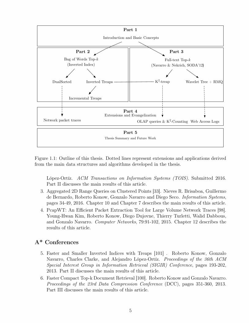
Figure 1.1 shows the outline of this thesis, separated by parts and their main contributions.

1.1 Publications derived from the Thesis

The main contributions of this thesis have appeared in the following articles. We categorizethe conference articles according to the CORE conference ranking (http://core.edu.au/index.php/conference-rankings).

Journals

1. Practical Compact Indexes for Top-k Document Retrieval. Simon Gog, Roberto Konowand Gonzalo Navarro. ACM Journal of Experimental Algorithms (JEA). Submitted2016. The main results of this article are discussed in Part III.

2. Inverted Treaps. Roberto Konow, Gonzalo Navarro, Charles L.A Clarke and Alex

4

Part 1

Part 4

Part 3Part 2

Introduction and Basic Concepts

Bag of Words Top-k(Inverted Index)

Full-text Top-k(Navarro & Nekrich, SODA’12)

DualSorted Inverted Treaps K2-treap Wavelet Tree + RMQ

OLAP queries & K2-Counting Web Access LogsNetwork packet traces

Incremental Treaps

Extensions and Evangelization

Part 5Thesis Summary and Future Work

Figure 1.1: Outline of this thesis. Dotted lines represent extensions and applications derivedfrom the main data structures and algorithms developed in the thesis.

López-Ortíz. ACM Transactions on Information Systems (TOIS). Submitted 2016.Part II discusses the main results of this article.

3. Aggregated 2D Range Queries on Clustered Points [33]. Nieves R. Brisaboa, Guillermode Bernardo, Roberto Konow, Gonzalo Navarro and Diego Seco. Information Systems,pages 34-49, 2016. Chapter 10 and Chapter 7 describes the main results of this article.

4. PcapWT: An Efficient Packet Extraction Tool for Large Volume Network Traces [98].Young-Hwan Kim, Roberto Konow, Diego Dujovne, Thierry Turletti, Walid Dabbous,and Gonzalo Navarro. Computer Networks, 79:91-102, 2015. Chapter 12 describes theresults of this article.

A* Conferences

5. Faster and Smaller Inverted Indices with Treaps [101] . Roberto Konow, GonzaloNavarro, Charles Clarke, and Alejandro López-Ortíz. Proceedings of the 36th ACMSpecial Interest Group in Information Retrieval (SIGIR) Conference, pages 193-202,2013. Part II discusses the main results of this article.

6. Faster Compact Top-k Document Retrieval [100]. Roberto Konow and Gonzalo Navarro.Proceedings of the 23rd Data Compression Conference (DCC), pages 351-360, 2013.Part III discusses the main results of this article.

5

B Conferences

7. K2-Treaps: Range Top-k Queries in Compact Space [32]. Nieves Brisaboa, Guillermode Bernardo, Roberto Konow, and Gonzalo Navarro. Proceedings of the 21st StringProcessing and Information Retrieval conference (SPIRE), pages 215-226. LNCS 8799,2014. Chapter 10 describes the results of this article.

8. Efficient Representation of Web Access Logs [45]. Francisco Claude, Roberto Konow,and Gonzalo Navarro. Proceedings of the 21st String Processing and Information Re-trieval conference (SPIRE), pages 65-76. LNCS 8799, 2014. Chapter 11 describes theresults of this article.

9. Dual-Sorted Inverted Lists in Practice[99]. Roberto Konow and Gonzalo Navarro. Pro-ceedings of 19th the String Processing and Information Retrieval conference (SPIRE),pages 295-306. LNCS 7608, 2012. Section 3.3 and Chapter 5 describes the main resultsof this article.

1.2 Awards

1. Capocelli Prize, Data Compression Conference 2013 for the presentation of the workFaster Compact Top-k Document Retrieval.

1.3 Research Stays and Internships

1. Research stay at the David R. Cheriton School of Computer Science,University of Wa-terloo. Advisors: Charles L.A Clarke and Alex López-Ortíz. June 2012 to December2012.

2. Internship at eBay inc. Search Backend, Query Service Stack Group. Mentor: RaffiTutundjian. Manager: Anand Lakshminath. June 2014 to September 2014.

6

Chapter 2

Basic Concepts

In this chapter, we define and explain the main concepts, data structures, and algorithmsthat are employed in the development of this thesis.

2.1 Computation model

All data structures used in this thesis work in the word-RAM model. In this model, thememory is divided into cells storing words of w = Θ(log n) bits, where n is the size ofthe data. Any cell can be accessed and modified in constant time and is able to representany integer in the set 0, . . . , 2w − 1. In addition, other operations such as arithmeticoperations, comparisons, and bitwise Boolean operations (and, or, exclusive-or, <<, >>),are also considered to require constant time.

2.2 Sequences, Documents and Collections

We define a sequence S of length n that contains symbols over an alphabet Σ of size σ. Wedefine a collection of D documents D = d1, d2, . . . , dD containing symbols from an alphabetΣ of size σ, and |di| denotes the number of symbols of document di. The total length of thecollection is

∑Di=1 |di| = n and we call C the concatenation of its documents, where at the

end of each di a special symbol # is used to mark the end of that document and the symbol$ marks the end of the collection. It holds $ < # < c for all c ∈ Σ. Figure 2.1 shows anexample of a collection containing 3 documents with a total length of n = 15.

Another scenario is when a collection of documents contains text of Natural Language.In this case, the alphabet Σ can be divided into two disjoint sets: separators (i.e., space,tab) that separate words, and symbols that belong to the words. The set of distinct wordsform what is called the vocabulary of the collection. Natural language collections follow twoempirical laws that are well accepted in IR [17]: Heaps’ Law and Zipf’s law. Heaps’ law

7

d1 d2 d3

C = A T A # T A A A # T T A # $1 2 3 4 5 6 7 8 9 10 11 12 13 14i =

A15

Figure 2.1: Concatenation C of our 3-document example collection D.

states that the vocabulary of a text of n words is of size V = Knβ = O(nβ), where K and βdepends on the text and 0 < β < 1. On the other hand, Zipf’s law attempts to capture thedistribution of the frequencies, that is, the number of occurrences of the words in the text.It states that the i−th most frequent word in the collection has frequency f1/i

α, where f1

is the frequency of the most frequent word and α is a text dependent parameter. In otherwords, these two laws establish that the number of distinct terms (the size of the vocabulary)is much smaller than the collection, and that natural language documents contain few wordsthat occur frequently and many words that rarely occur in the text.

2.3 Empirical Entropy

A widely used measure of the compressibility of a fixed sequence is the empirical entropy[137]. For a sequence S of length n containing symbols from an alphabet Σ of size σ, thezero-order entropy is defined as follows 1

H0(S) =∑c∈Σ

ncn

logn

nc(2.1)

where nc is the number of occurrences of symbol c in S. H0(S) gives the average number ofbits needed to represent a symbol in S if the same symbol always receives the same code.

If we take into account the context in which the symbol appears, we can achieve bettercompression ratios by extending the definition to the kth order empirical entropy:

Hk(S) =∑c∈Σk

|Sc|nH0(Sc). (2.2)

where Sc is the sequence of symbols preceded by the context c in S. It can be proved that0 ≤ Hk(S) ≤ Hk−1(S) ≤ · · · ≤ H0(S) ≤ log σ.

2.4 Huffman Codes

Given a sequence S[1, n] = x1, x2, . . . , xn containing n elements from an alphabet of size σ, wecan encode each value of the sequence using blog2 σc+ 1 bits 2. However, this representation

1We will always use log x to denote log2 x, unless otherwise stated.2Assuming it is possible to map any symbol to an integer in [1..σ].

8

does not take into account that some elements may appear more frequently than others andthus we can represent the sequence in a more efficient way. One way to reduce the spaceis to use variable-length codes, that is, employ codes that have different amounts of bits fordifferent symbols. One family of variable-length codes are the ones that take advantage ofstatistical properties of the sequences and are referred to as statistical codes. The idea isto assign smaller codes to the symbols that occur more frequently and larger codes for theinfrequent symbols. However, the task of assigning codes is not trivial: on the one hand, theyhave to be as small as possible, on the other hand, they have to be prefix-free. Prefix-freecodes are uniquely decodable codes, since there is no code that is a prefix of another one.

Huffman codes [89] are prefix-free codes and belong to the family of statistical encoders.They represent a sequence S[1, n] using less than H0(S)+1 bits per symbol, which is optimal(among methods that encode symbols separately). The algorithm to generate the codesbuilds what is known as a Huffman tree and is used to assign different codes to the symbols.The procedure to generate such codes and building the tree is as follows: first, one node foreach distinct symbol is created; these are regarded as leaf nodes and store the symbol andits frequency of occurrences in S. The two least frequent nodes, x and y, are then taken outof the set of nodes and merged together into a new internal node v, which is assigned as theparent of x and y. The frequency of v is the sum of the frequencies of its children. Thisprocedure is repeated as long as two or more nodes remain without merging. The processfinishes when a unique node remains, which is the root of the Huffman tree. Every left branchis labeled as 0 and the right one is labeled as 1. The code for each symbol is generated asthe concatenation of the labels of the traversal path from the root to its leaf. The Huffmantree can be constructed in O(σ log σ) time if the symbols are not sorted according to theirfrequencies and in O(σ) time if the symbols are sorted. The encoding procedure has to storethe codeword lengths. An example of the Huffman tree and the generated codes are shownin Figure 2.2.

2.5 Integer Encoding Mechanisms

Given a sequence of positive integers S[1, n] = x1, . . . , xn, and letting M be the maximuminteger in that sequence, it is possible to be represented using dlog2Me bits per element andhave access to any position in constant time. One problem with this representation is thatit is not space-efficient if many integers are much smaller than others, so it is possible torepresent the sequence more efficiently. For instance, we can use statistical compression suchas Huffman codes. However, in some applications smaller values are more frequent, so inthis case one can directly encode the numbers with codes that give shorter codes to smallernumbers. The advantage with this idea is that it is not necessary to store a mapping ofthe symbols to their codes, which can be prohibitive when the set of distinct numbers is toolarge.

In this section we briefly describe the most used and popular encoding mechanisms forinteger sequences. We assume that the integer to be encoded is positive (x > 0) and wedefine binary(x, `) as a function that returns the binary representation of a positive integerx using ` bits by adding leading zeroes as needed. We will refer to |x| as the number of bits

9

S = 1 5 1 1 8 6 3 8 7 5 7 4 3 2 81 2 3 4 5 6 7 8 9 10 11 12 13 14i = 15

816

8 1 5 3 7 2 4 6

0

0 1

1

0

0 1

1

1

1010

0

1234

5678

0 1 1 1 0 11 0 11 1 1 0

1 0 0 1 1 1 1 1 1 0 00 0

Huffman Tree

Huffman Codes

4 3 2 2 2 1 1 1

234

5

7

9

16

Figure 2.2: Top: A sequence over Σ = [1, 8]. The Huffman tree and the resulting Huffmancodes are shown below. Numbers next to the tree nodes represent the accumulated frequencyof that node.

that are needed to represent x in binary.

2.5.1 Bit-aligned Codes

Bit-aligned codes are used in the case of representing sequences containing small integers.We describe here the most representative codes of this family of encodings. We show anexample of the encodings in Table 2.1.

Unary Codes [143]. An integer x ≥ 1 is coded as a binary sequence with x− 1 one bitsfollowed by a zero bit, unary(x) = 1x−10. For example, the integer 4 is represented asunary(4) = 1110. This encoding mechanism is usually only suitable for very small x values.

Gamma Codes (γ) [143]. Gamma codes represent |x| using unary code and then con-catenate it with the binary representation of x−2blog xc or, in other words, x without its mostsignificant bit. It is defined as γ(x) = unary(|x|)binary(x− 2blog xc, |x| − 1). For example,consider the number x = 7, and the binary length of the binary code is |x| = 1 + blog 7c = 3(110 in unary) and 7 − 22 = 3 (11 in binary), the concatenation is the binary sequenceγ(7) = 11011. The amount of bits required for coding any x using γ codes is 1 + 2blog xcbits.

10

Delta Codes [143]. The idea is to represent the length of the code using γ encodingand then concatenate it with the binary representation of the symbol x without its mostsignificant bit. That is δ(x) = γ(|x|)binary(x− 2blog xc, |x| − 1). For x = 7, the length of thebinary code is |x| = 3, so it is represented as 101 using γ encoding. The final representationis 10111. Encoding a number using Delta codes uses 1 + 2blog log(x+ 1)c+ blog xc bits andit may be of interest when x is too large to be efficiently represented by γ codes.

Rice Codes [138, 143]. Rice Codes receive two values as inputs: the symbol x and aparameter b. The encoding is performed by representing q = b(x− 1)/2bc in unary and thenrepresenting r = n−q2b−1 in binary using b bits. The final code is the concatenation of r andq as rice(x) = unary(b(x− 1)/2bc)binary(n− q2b − 1, b). Consider the same example asbefore with x = 7 and choosing b = 2. unary(b6/4c) = 10 and binary((7− 4− 1), b) = 10,therefore rice(7) = 1010. Rice codes require b(x− 1)/2bc+ b+ 1 bits in total.

Integer Unary γ δ Rice(b = 2)1 0 0 0 0002 10 100 1000 0013 110 101 1001 0104 1110 11000 10100 0115 11110 11001 10101 10006 111110 11010 10110 10017 1111110 11011 10111 10108 11111110 1110000 11000000 10119 111111110 1110001 11000001 1100010 1111111110 1110010 11000010 11001

Table 2.1: Encoding positive integers using different bit-aligned encoding techniques.

2.5.2 Byte-aligned Codes

Bit-aligned codes can be inefficient at decoding since they require several bitwise operationswhich are not always efficiently implemented. Therefore, byte-aligned [147] or word-alignedcodes [168, 11] are preferred when the speed is the main concern. Examples of this familyof techniques are Variable Byte (VByte), Simple9, and PForDelta. We briefly describe themost representative methods of this family below:

Simple-9 [11]. Simple-9 is a 32-bit word-aligned encoding scheme. This mechanism packsas many numbers as possible into a 32-bit word by assigning an equal number of bits to eachsymbol. A selector value (b) has to be chosen and is encoded using 4 bits in a 32 bit word.The rest of the 28 bits from the 32-bit word will store as many integers as possible using afixed amount of bits that depends on the selector value. We show in Table 2.2 the numberof integers in a 32-bit word for different selector b values, the bits per integer (bpi) that areused and amount of bits that are not used. Other versions [13] extend this approach to makeuse of 64-bit words, having 60 bits instead of 28 bits available for data.

11

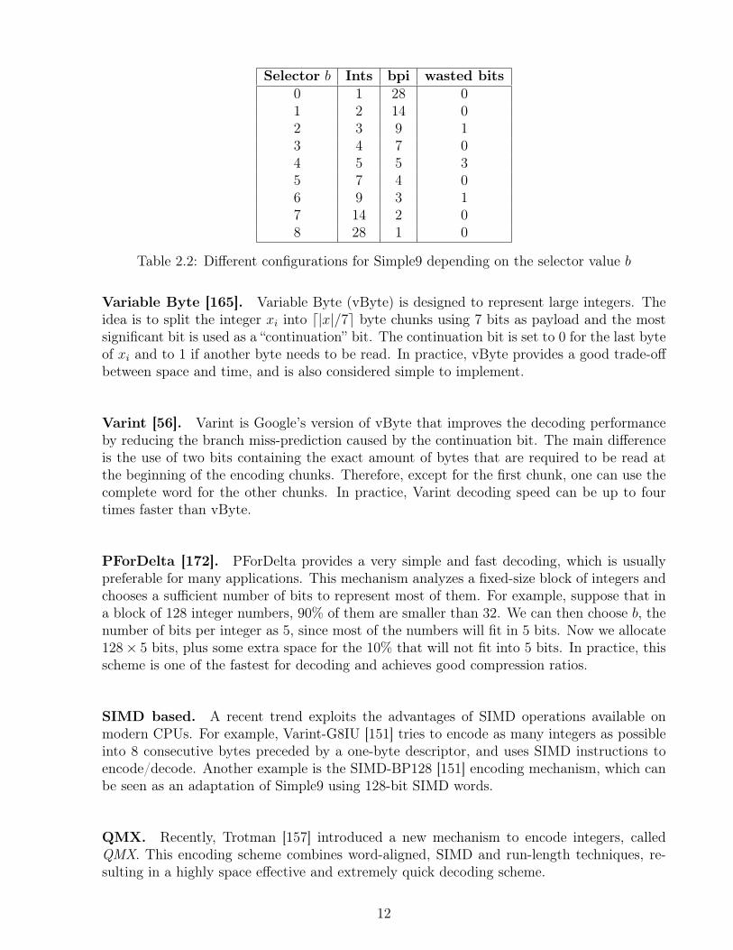
Selector b Ints bpi wasted bits0 1 28 01 2 14 02 3 9 13 4 7 04 5 5 35 7 4 06 9 3 17 14 2 08 28 1 0

Table 2.2: Different configurations for Simple9 depending on the selector value b

Variable Byte [165]. Variable Byte (vByte) is designed to represent large integers. Theidea is to split the integer xi into d|x|/7e byte chunks using 7 bits as payload and the mostsignificant bit is used as a “continuation” bit. The continuation bit is set to 0 for the last byteof xi and to 1 if another byte needs to be read. In practice, vByte provides a good trade-offbetween space and time, and is also considered simple to implement.

Varint [56]. Varint is Google’s version of vByte that improves the decoding performanceby reducing the branch miss-prediction caused by the continuation bit. The main differenceis the use of two bits containing the exact amount of bytes that are required to be read atthe beginning of the encoding chunks. Therefore, except for the first chunk, one can use thecomplete word for the other chunks. In practice, Varint decoding speed can be up to fourtimes faster than vByte.

PForDelta [172]. PForDelta provides a very simple and fast decoding, which is usuallypreferable for many applications. This mechanism analyzes a fixed-size block of integers andchooses a sufficient number of bits to represent most of them. For example, suppose that ina block of 128 integer numbers, 90% of them are smaller than 32. We can then choose b, thenumber of bits per integer as 5, since most of the numbers will fit in 5 bits. Now we allocate128× 5 bits, plus some extra space for the 10% that will not fit into 5 bits. In practice, thisscheme is one of the fastest for decoding and achieves good compression ratios.

SIMD based. A recent trend exploits the advantages of SIMD operations available onmodern CPUs. For example, Varint-G8IU [151] tries to encode as many integers as possibleinto 8 consecutive bytes preceded by a one-byte descriptor, and uses SIMD instructions toencode/decode. Another example is the SIMD-BP128 [151] encoding mechanism, which canbe seen as an adaptation of Simple9 using 128-bit SIMD words.

QMX. Recently, Trotman [157] introduced a new mechanism to encode integers, calledQMX. This encoding scheme combines word-aligned, SIMD and run-length techniques, re-sulting in a highly space effective and extremely quick decoding scheme.

12

2.6 Rank, Select and Access

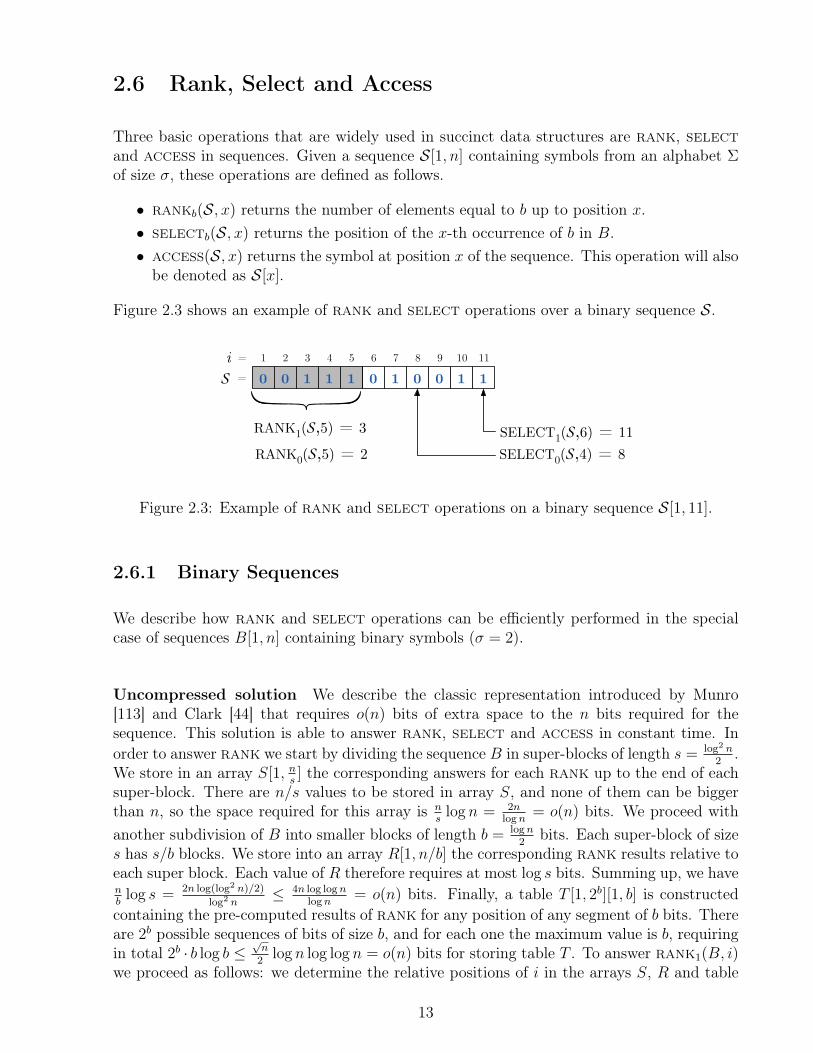
Three basic operations that are widely used in succinct data structures are rank, selectand access in sequences. Given a sequence S[1, n] containing symbols from an alphabet Σof size σ, these operations are defined as follows.

• rankb(S, x) returns the number of elements equal to b up to position x.• selectb(S, x) returns the position of the x-th occurrence of b in B.• access(S, x) returns the symbol at position x of the sequence. This operation will also

be denoted as S[x].

Figure 2.3 shows an example of rank and select operations over a binary sequence S.

S = 0 0 1 1 1 0 1 0 0 1 11 2 3 4 5 6 7 8 9 10 11i =

RANK1(S,5) = 3RANK0(S,5) = 2 SELECT0(S,4) = 8

SELECT1(S,6) = 11

Figure 2.3: Example of rank and select operations on a binary sequence S[1, 11].

2.6.1 Binary Sequences

We describe how rank and select operations can be efficiently performed in the specialcase of sequences B[1, n] containing binary symbols (σ = 2).

Uncompressed solution We describe the classic representation introduced by Munro[113] and Clark [44] that requires o(n) bits of extra space to the n bits required for thesequence. This solution is able to answer rank, select and access in constant time. Inorder to answer rank we start by dividing the sequence B in super-blocks of length s = log2 n

2.

We store in an array S[1, ns] the corresponding answers for each rank up to the end of each

super-block. There are n/s values to be stored in array S, and none of them can be biggerthan n, so the space required for this array is n

slog n = 2n

logn= o(n) bits. We proceed with

another subdivision of B into smaller blocks of length b = logn2

bits. Each super-block of sizes has s/b blocks. We store into an array R[1, n/b] the corresponding rank results relative toeach super block. Each value of R therefore requires at most log s bits. Summing up, we havenb

log s = 2n log(log2 n)/2)

log2 n≤ 4n log logn

logn= o(n) bits. Finally, a table T [1, 2b][1, b] is constructed

containing the pre-computed results of rank for any position of any segment of b bits. Thereare 2b possible sequences of bits of size b, and for each one the maximum value is b, requiringin total 2b · b log b ≤

√n

2log n log log n = o(n) bits for storing table T . To answer rank1(B, i)

we proceed as follows: we determine the relative positions of i in the arrays S, R and table

13

T , such that i is decomposed as i = j · s+ k · b+ r. To obtain the final result we continue bysumming S[j] +R[j( s

b) + k] + T [B[j · s+ k · b, j · s+ (k + 1) · b]][r]. Note that we can answer

rank0(B, i) by performing i − rank1(B, i).

In order to support select in constant-time a similar procedure is performed: insteadof dividing the sequence into blocks and super-blocks of fixed size, we divide the sequenceaccording to the number of bits that are set. This way, we have blocks of variable length butevery block will contain a fixed amount of 1’s inside them. As before, a similar table T withprecomputed values is constructed and stored.

An implementation of this solution was introduced by González et al. [80] supportingrank and access in constant time and select in O(log n) time 3. Experimental resultsshow that this implementation requires only 5% extra space of the original sequence tosupport these operations. We will refer to this implementation as RG. In practice, operationselectb(B, x) is answered by performing a binary search on the values from the arrays S[1, n

s]

and R[1, n/b] and then sequentially scanning until the the position where the number of onesequals x.

Compressed solution. A compressed representation of the bitmap B that is able to an-swer rank and select operations was presented by Raman et al. [135, 136]. Their solutionreduces the space required to represent the bitmap to nH0(B) + o(n) bits.

The idea is to divide the sequence into blocks of size b = logn2

. A block will be assigned toa class ci if it contains exactly ci 1s. Since each block has b bits, we have at most b+1 classes.However, each class ci has at most

(bci

)different shuffles of its bits. We can represent any

block Bi as a pair (ci, oi), where ci indicates the class and oi is the offset within that class. Forexample, the class c2 for blocks of length b = 3 containing 2 ones is c2 = 011, 101, 110 andtheir offsets are o2 = 0, 1, 2. The binary representation of each class ci requires dlog(b+1)ebits. We will store in a sequence C[1, dn/be] the class of each block, requiring a total ofdn/bedlog(b + 1)e = (n/b) log b + O(n/b) bits. The offsets oi are stored separately in asequence O[1, n/b], and each oi component requires dlog

(bci

)e bits, so the total space in bits

for representing sequence O[1, n/b] is:

dn/be∑i=1

⌈log

(b

ci

)⌉≤dn/be∑i=1

log

(b

ci

)+ dn/be = log

dn/be∏i=1

(b

ci

)+ dn/be ≤

log

(n

m

)+ dn/be ≤ nH0(B) + dn/be

where m is the number of 1’s in the sequence [128].

In order to support rank and select operations we still need to add additional arraysstoring relative results, pointers and precomputed tables, similarly to the uncompressed so-lution. Raman et al. [136] solution obtains a final space bound of nH0(B) + o(n). We willrefer to practical implementations of this approach as RRR. In practice, the cost of handling

3Please note, that even though select can be solved in O(1), most implementations use a binary searchto solve select, thus making the implementation of selectO(log n) time

14

a reduced-space bitmap is that queries are up to two times slower than the uncompressedalternative (RG).

Other solutions. Several other practical implementations have been proposed. Okahonaraand Sadakane [126] presented a data structure called SDArray that requires nH0(B) + 2m+o(m) bits for representing a bitmap with m 1s. It is able to support select in constant time,and rank and access in time O(log(n/m)). Vigna [160] introduced an implementation thatuses SIMD words to improve the space and speed of rank and access operations. Navarroand Providel [134, 121] presented a new representation that improved the space/time tradeoffsfor select operations. Recently, Kärkkäinen et al. [97] introduced the hybrid bit vector whichdivides the bitmap into blocks and then chooses the best encoding of each block separatelyfrom the techniques previously described. Most of the techniques previously described wereimplemented and improved to support large bit sequences by Gog et al. [77].

2.6.2 General Sequences

There are different approaches for solving rank, select and access for the case of generalsequences (i.e., σ > 2). A naive solution consists in creating a bitmap Bi[1, n] for eachdistinct symbol i ∈ Σ, by setting Bi[x] = 1 iff S[x] = i. The operations rank and selectcan then be solved by querying the corresponding bitmap Bi. However, this solution requiresnσ + o(nσ) bits if an uncompressed solution is used (i.e., RG). Another drawback of thissolution is that one has to traverse σ bitmaps in order to answer access in the worst case,making it unpractical for sequences having large alphabets. We can improve the size by usingthe SDArray, where the space becomes nH0(S) +O(n) bits, however method access is stillinefficient.

The most popular data structure employed to solve rank, select and access operationson general sequences is the wavelet tree [81, 117] . We describe in detail the properties andvirtues of this structure in Section 2.7. Other very competitive alternatives are GMR [79] andAlphabet Partitioning (AP) [19] solutions. We briefly describe these solutions below, howeverwe do not explain how the inner mechanisms work.

GMR. Golynski et al. [79] presented a data structure that uses n log σ+o(n log σ) bits andanswers select in constant time. This data structure requires O(log log σ) time to answeraccess and rank operations. GMR is of interest when the speed of the operations is the mainconcern and for big alphabets, since the size of the final structure is not compressed.

Alphabet Partitioning. In the case where the alphabet of the sequence is big and thesize is the main concern, the technique called alphabet partitioning is preferred. It supportsrank, select, and access operations in O(log log σ) time and represents the sequence Sin nH0(S) + o(nH0(S) + n) bits.

15

2.7 Wavelet Tree

In this section we describe the main properties and operations of the wavelet tree [81, 117].We start by describing the composition of the data structure and then explain how the wavelettree answers rank, select and access operations. We then describe other applications ofthe wavelet trees when representing grids.

2.7.1 Data Structure

Let S[1, n] be a sequence of symbols from a finite alphabet Σ of size σ. For simplicity we willassume that Σ = [1..σ]. The wavelet tree over an alphabet [a..b] ⊆ [1..σ] is a balanced binarytree that stores a bit sequence in every node except the leaves. It has b − a + 1 leaves andif a 6= b it has at least an internal node, vroot that represents S[1, n]. The root of the tree isrepresented by a bit sequence, Bvroot [1, n], and is defined as follows: if S[i] ≤ (a + b)/2 thenBvroot [i] is marked with a ‘0’, and if S[i] > (a + b)/2 then Bvroot [i] is marked with a ‘1’. Wedefine Sleft[1, nleft] as the subsequence of symbols from S[1, n] that were marked with a ‘0’in Bvroot , that is, all symbols c in S[1, n] such that c ≤ (a + b)/2. Let Sright[1, nright] be thesequence of symbols that were marked with a ‘1’ in Bvroot , that is, all symbols c such thatc > (a+ b)/2. The left child of vroot is going to be a wavelet tree of a sequence Sleft[1, nleft]over an alphabet [a..b(a+ b)/2c] and the right child of vroot is a wavelet tree of the sequenceSright[1, nright] over an alphabet [1 + b(a + b)/2c..b]. This decomposition is done recursivelyuntil the alphabet of the subsequence is a single symbol. The tree has σ leaves and each levelof the tree requires n bits. The height of the tree is dlog σe, thus we need ndlog σe bits torepresent the tree.

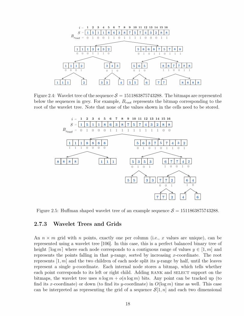
Each bit sequence at every level must be capable of answering access, rank and selectqueries, thus we can use the RG or RRR representation to represent the bit sequences. If RG isemployed, the wavelet tree requires n log σ+o(n log σ) bits. On the other hand, if we use RRRto represent the bit sequences at each level, the wavelet tree uses nH0(S) + o(n log σ) bits ofspace. If we want to compress the data structure even more, we can change the shape of thetree to the shape of the Huffman tree of the symbols frequencies appearing in S. Figure 2.4shows an example of a regular wavelet tree and a Huffman shaped wavelet tree is shown onFigure 2.5.

2.7.2 Rank, Select and Access

The regular wavelet tree answers rank, select and access in O(log σ) time, that is tosay, the execution time depends only on the size of the alphabet, not on the length of thesequence. If a Huffman shaped wavelet tree is employed, the average time required of theseoperations is O(1 +H0(S)).

We define labels(v) as a method that returns the set of symbols that belong to thesubrange [a..b] ⊆ [1..σ] from the sequence represented by node v and we will refer to vl or vr

16

as the left or right child of node v respectively.

We will explain how to perform access operation through an example based on thewavelet tree from Figure 2.4. Let us assume that we want to perform access(S, 6), thatis, return the symbol located at position 6. We start at position 6 of the root bit sequence(Bvroot) and ask if the corresponding bit is marked as ‘1’ or ‘0’. If the bit is ‘0’, we go to theleft branch, if not, to the right. In this case Bvroot [6] = 1, so we go to the right branch of thetree. Now we have to map the original position (x = 6) to the corresponding position at theright branch. In other words, we want to know how many 1′s were at the root bit sequence upto position 6. We can easily do this in constant time by performing the operation supportedby RG and RRR bit sequences: rank1(Bvroot , 6), which returns the value 3. Using this valuewe can now go to the right node of the root, v, and execute the same procedure. The valueat Bvroot [3] is 0 so we know we have to go to the left and count how many values to the leftexist in Bv by executing rank0(Bv, 3) = 2. This process is done recursively until we reacha leaf. Algorithm 1 shows this procedure as acc(v, x). Note that we do not need to storethe label at the leaves; they are deduced as we successively restrict the subrange [a..b] as wedescend down the tree.

Algorithm 1: Basic wavelet tree algorithms: On the wavelet tree of sequence S,acc(vroot, x) returns S[x]; rnk(vroot, j, b) returns rankb(S, x); and sel(vroot, x, b) re-turns selectb(S, x).

acc(v, x)01 if v is a leaf then02 return labels(v)03 if Bv[x] = 0 then04 x← rank0(v, x)05 return acc(vl, x)06 else07 x← rank1(v, x)08 return acc(vr, x)

rnk(v, x, b)if v is a leaf then

return xif b ∈ labels (vl) thenx← rank0(Bv, x)return rnk(vl, x, b)

elsex← rank1(Bv, x)return rnk(vr, x, b)

sel(v, x, b)if v is a leaf then

return xif b ∈ labels (vl) thenx← sel(vl, x, b)return select0(Bv, x)

elsex← sel(vr, x, b)return select1(Bv, x)

A similar procedure is performed for rankb(S, x). We start at the root of the tree andcheck if the symbol b belongs to the left or right child of the root. If the symbol belongs to theleft subtree, we transform the position x to a position in the the left subtree by performingx = rank0 (Bvroot , x) or x = rank1 (Bvroot , x) if the symbol belongs to the right subtree.This is done recursively until we reach a leaf, where the final answer is x. Algorithm 1 showsthis procedure as rnk(v, x, b).

The case of selectb(S, x) is different: instead of starting at the root, we start at positionx of the leaf that represents symbol b in the wavelet tree. If the leaf is the left child of anode v, then the x-th occurrence of symbol b in v is at position x = select0(Bv, x), andif the leaf is the right child of v the x-th occurrence of b in v is located at the positionx = select1(Bv, x). We continue this procedure until we reach the root bit sequence of thewavelet tree Bvroot and return position x. Algorithm 1 shows this procedure as sel(v, x, b).

17

S = 1 5 1 1 8 6 3 8 7 5 7 4 3 2 8

1 1 1 3 4 3 2 5 8 6 8

6

5

1 1 2 3 4 3

1 1 1 2 43 3

5 5

7

78 8

655 8 87

0 1 0 0 1 1 0 1 1 1 1 0 0 0 1 1

0 0 0 1 1 1 0 0 1 0 1 1 0 1 1 1

0 0 0 1 0 1 0 0 1 0 1 1 0 0 1 1

1 2 3 4 5 6 7 8 9 10 11 12 13 14i = 15

Bv =816

7 88

7 88

7 8 8

1

root

Figure 2.4: Wavelet tree of the sequence S = 1511863875743288. The bitmaps are representedbelow the sequences in grey. For example, Broot represents the bitmap corresponding to theroot of the wavelet tree. Note that none of the values shown in the cells need to be stored.

S = 1 5 1 1 8 6 3 8 7 5 7 4 3 2 8

1 1 1 8 8 8 8 5 6 3 7

3

7

1 18 8 8 5 5

5

76 7

355 6 47

0 1 0 0 0 1 1 1 1 1 1 1 1 1 0 0

1 1 1 0 0 0 0 0 1 0 1 0 1 1 0 1

0 1 0 1 1 0 0 1 0

1 2 3 4 5 6 7 8 9 10 11 12 13 14i = 15

=816

4 23

4 2

7

64

18 3

3 21 0 0 0 1

77 2

Bvroot

Figure 2.5: Huffman shaped wavelet tree of an example sequence S = 1511863875743288.

2.7.3 Wavelet Trees and Grids

An n × m grid with n points, exactly one per column (i.e., x values are unique), can berepresented using a wavelet tree [106]. In this case, this is a perfect balanced binary tree ofheight dlogme where each node corresponds to a contiguous range of values y ∈ [1,m] andrepresents the points falling in that y-range, sorted by increasing x-coordinate. The rootrepresents [1,m] and the two children of each node split its y-range by half, until the leavesrepresent a single y-coordinate. Each internal node stores a bitmap, which tells whethereach point corresponds to its left or right child. Adding rank and select support on thebitmaps, the wavelet tree uses n logm + o(n logm) bits. Any point can be tracked up (tofind its x-coordinate) or down (to find its y-coordinate) in O(logm) time as well. This casecan be interpreted as representing the grid of a sequence S[1, n] and each two dimensional

18

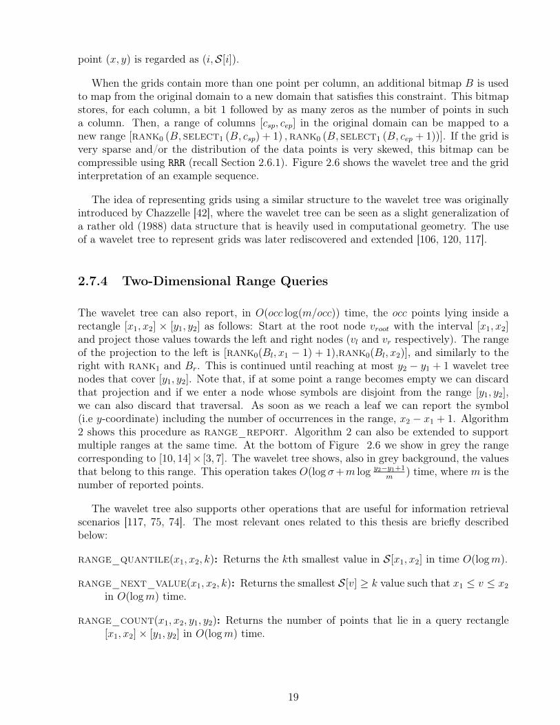
point (x, y) is regarded as (i,S[i]).

When the grids contain more than one point per column, an additional bitmap B is usedto map from the original domain to a new domain that satisfies this constraint. This bitmapstores, for each column, a bit 1 followed by as many zeros as the number of points in sucha column. Then, a range of columns [csp, cep] in the original domain can be mapped to anew range [rank0 (B, select1 (B, csp) + 1) ,rank0 (B, select1 (B, cep + 1))]. If the grid isvery sparse and/or the distribution of the data points is very skewed, this bitmap can becompressible using RRR (recall Section 2.6.1). Figure 2.6 shows the wavelet tree and the gridinterpretation of an example sequence.

The idea of representing grids using a similar structure to the wavelet tree was originallyintroduced by Chazzelle [42], where the wavelet tree can be seen as a slight generalization ofa rather old (1988) data structure that is heavily used in computational geometry. The useof a wavelet tree to represent grids was later rediscovered and extended [106, 120, 117].

2.7.4 Two-Dimensional Range Queries

The wavelet tree can also report, in O(occ log(m/occ)) time, the occ points lying inside arectangle [x1, x2] × [y1, y2] as follows: Start at the root node vroot with the interval [x1, x2]and project those values towards the left and right nodes (vl and vr respectively). The rangeof the projection to the left is [rank0(Bl, x1 − 1) + 1),rank0(Bl, x2)], and similarly to theright with rank1 and Br. This is continued until reaching at most y2 − y1 + 1 wavelet treenodes that cover [y1, y2]. Note that, if at some point a range becomes empty we can discardthat projection and if we enter a node whose symbols are disjoint from the range [y1, y2],we can also discard that traversal. As soon as we reach a leaf we can report the symbol(i.e y-coordinate) including the number of occurrences in the range, x2 − x1 + 1. Algorithm2 shows this procedure as range_report. Algorithm 2 can also be extended to supportmultiple ranges at the same time. At the bottom of Figure 2.6 we show in grey the rangecorresponding to [10, 14]× [3, 7]. The wavelet tree shows, also in grey background, the valuesthat belong to this range. This operation takes O(log σ+m log y2−y1+1

m) time, where m is the

number of reported points.

The wavelet tree also supports other operations that are useful for information retrievalscenarios [117, 75, 74]. The most relevant ones related to this thesis are briefly describedbelow:

range_quantile(x1, x2, k): Returns the kth smallest value in S[x1, x2] in time O(logm).

range_next_value(x1, x2, k): Returns the smallest S[v] ≥ k value such that x1 ≤ v ≤ x2

in O(logm) time.

range_count(x1, x2, y1, y2): Returns the number of points that lie in a query rectangle[x1, x2]× [y1, y2] in O(logm) time.

19

1 2 3 4 5 6 7 8 9 11 12 13 14 1512345678

x

y10 16

S = 1 5 1 1 8 6 3 8 7 5 7 4 3 2 8

1 1 1 3 4 3 2 5 8 6 8

6

5

1 1 2 3 4 3

1 1 1 2 43 3

5 5

7

78 8

655 8 87

0 1 0 0 1 1 0 1 1 1 1 0 0 0 1 1

0 0 0 1 1 1 0 0 1 0 1 1 0 1 1 1

0 0 0 1 0 1 0 0 1 0 1 1 0 0 1 1

1 2 3 4 5 6 7 8 9 10 11 12 13 14i = 15

=816

7 88

7 88

7 8 8

1

x range

y ra

nge

Bvroot

Figure 2.6: Top: The wavelet tree for the sequence S = 1511863875743288. Bottom: Thegrid representation of the sequence. The x− and y−ranges are shown in light grey, while theirintersection is shown in darker grey. The highlighted values on the wavelet tree correspondto the ones that belong to the range [10, 14]× [3, 7].

2.8 Directly Addressable Codes

Directly Addressable Codes (DAC) [34] is a variable-length encoding that is inspired byvByte. Given a chunk length b and a sequence of positive integers S[1, n] = x1, x2, . . . , xn,DAC divides each integer xi into d|xi|/be chunks. Similar to vByte, DAC employs a ‘con-tinuation’ bit, but instead of concatenating the encoding of xi+1 after that of xi, it builds amulti-layer data structure. LetM be the maximum element in the sequence, a DAC encodingwill contain ` = dblog(M)c+(1/b)e layers consisting of two parts: (1) the lowest b bits of eachchunk, which are stored contiguously in an array Ak with 1 ≤ k ≤ `, using b bits per element,and (2) the ‘continuation’ bits, which are concatenated into a bitmap Bk. Any integer xi willrequire exactly d(|xi|)/be layers. For example, say we want to encode the integer x = 5 andwe set the chunk length b = 2. The lowest b bits of 5 are 01 and we append them to the firstlayer of array A1. Since we still require more bits to represent the number, we need to setthe continuation bit to 1, and this is appended to the bit sequence B, again, at first layer.The next b lowest bits for representing x are now located in the next layer A2, and since we

20

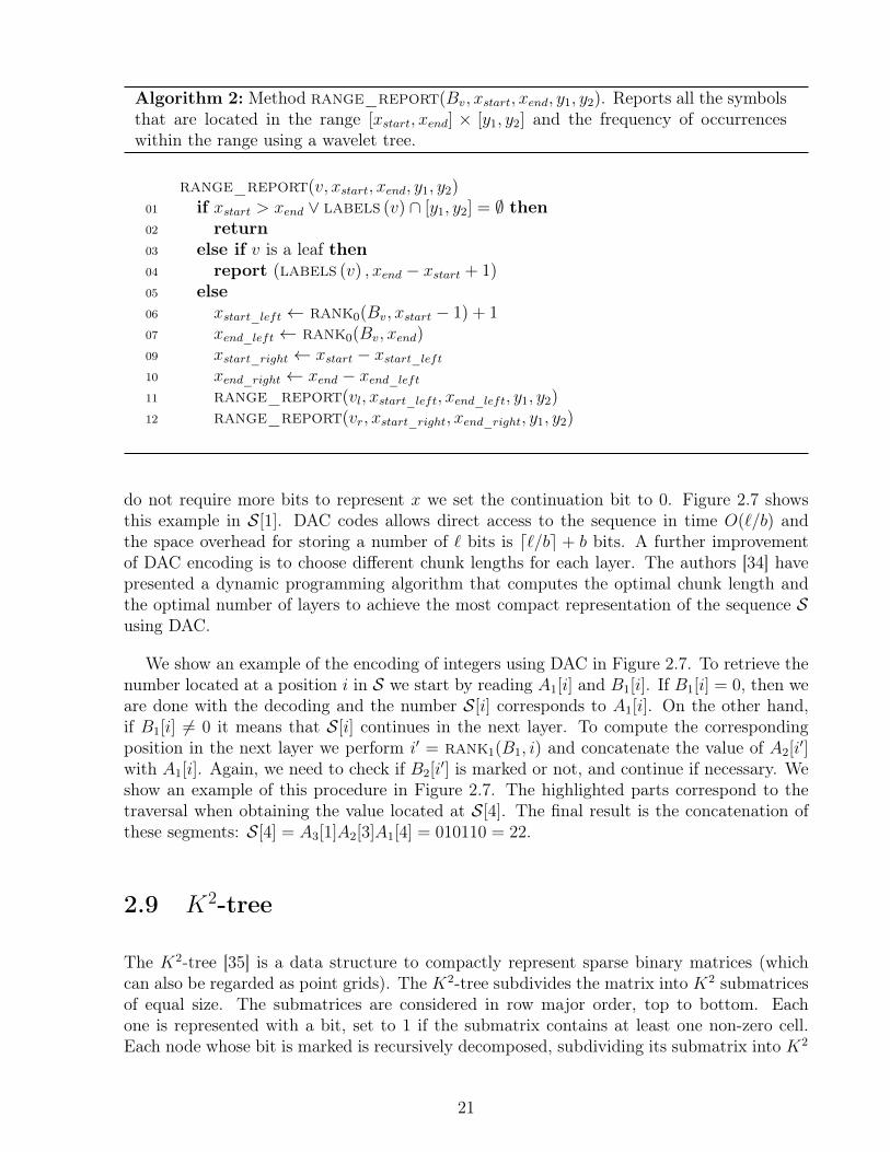
Algorithm 2: Method range_report(Bv, xstart, xend, y1, y2). Reports all the symbolsthat are located in the range [xstart, xend] × [y1, y2] and the frequency of occurrenceswithin the range using a wavelet tree.

range_report(v, xstart, xend, y1, y2)01 if xstart > xend ∨ labels (v) ∩ [y1, y2] = ∅ then02 return03 else if v is a leaf then04 report (labels (v) , xend − xstart + 1)05 else06 xstart_left ← rank0(Bv, xstart − 1) + 107 xend_left ← rank0(Bv, xend)09 xstart_right ← xstart − xstart_left10 xend_right ← xend − xend_left11 range_report(vl, xstart_left, xend_left, y1, y2)12 range_report(vr, xstart_right, xend_right, y1, y2)

do not require more bits to represent x we set the continuation bit to 0. Figure 2.7 showsthis example in S[1]. DAC codes allows direct access to the sequence in time O(`/b) andthe space overhead for storing a number of ` bits is d`/be + b bits. A further improvementof DAC encoding is to choose different chunk lengths for each layer. The authors [34] havepresented a dynamic programming algorithm that computes the optimal chunk length andthe optimal number of layers to achieve the most compact representation of the sequence Susing DAC.

We show an example of the encoding of integers using DAC in Figure 2.7. To retrieve thenumber located at a position i in S we start by reading A1[i] and B1[i]. If B1[i] = 0, then weare done with the decoding and the number S[i] corresponds to A1[i]. On the other hand,if B1[i] 6= 0 it means that S[i] continues in the next layer. To compute the correspondingposition in the next layer we perform i′ = rank1(B1, i) and concatenate the value of A2[i′]with A1[i]. Again, we need to check if B2[i′] is marked or not, and continue if necessary. Weshow an example of this procedure in Figure 2.7. The highlighted parts correspond to thetraversal when obtaining the value located at S[4]. The final result is the concatenation ofthese segments: S[4] = A3[1]A2[3]A1[4] = 010110 = 22.

2.9 K2-tree

The K2-tree [35] is a data structure to compactly represent sparse binary matrices (whichcan also be regarded as point grids). The K2-tree subdivides the matrix into K2 submatricesof equal size. The submatrices are considered in row major order, top to bottom. Eachone is represented with a bit, set to 1 if the submatrix contains at least one non-zero cell.Each node whose bit is marked is recursively decomposed, subdividing its submatrix into K2

21

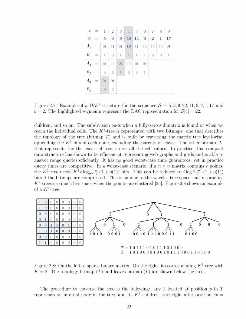
B1 =

S = 5 3 9 22 11 6 21 2 3 4 5 6 7i =

A1 = 01

1

11 01 10 11 10 10

0 1 1 1 1 0

B2 =

A2 = 01

0

10 01 10 01

0 1 0 0

B3 =

A3 = 01

0

18

179

10

0

01

1

01

0

00

1

Figure 2.7: Example of a DAC structure for the sequence S = 5, 3, 9, 22, 11, 6, 2, 1, 17 andb = 2. The highlighted segments represent the DAC representation for S[4] = 22.

children, and so on. The subdivision ends when a fully-zero submatrix is found or when wereach the individual cells. The K2-tree is represented with two bitmaps: one that describesthe topology of the tree (bitmap T ) and is built by traversing the matrix tree level-wise,appending the K2 bits of each node, excluding the parents of leaves. The other bitmap, L,that represents the the leaves of tree, stores all the cell values. In practice, this compactdata structure has shown to be efficient at representing web graphs and grids and is able toanswer range queries efficiently. It has no good worst-case time guarantees, yet in practicequery times are competitive. In a worst-case scenario, if a n × n matrix contains t points,the K2-tree needs K2 t logK2

n2

t(1 + o(1)) bits. This can be reduced to t log n2·K2

t(1 + o(1))

bits if the bitmaps are compressed. This is similar to the wavelet tree space, but in practiceK2-trees use much less space when the points are clustered [35]. Figure 2.8 shows an exampleof a K2-tree.

1 0 0 0 0 0 0 01 0 0 0 0 0 0 00 0 0 0 0 0 0 00 1 0 0 0 0 0 00 0 1 1 0 1 0 01 0 1 0 0 0 0 00 0 0 0 0 0 0 01 1 0 0 0 0 0 0

1 0 1 1

1 0 1 0

1 0 1 0

1 0 0 0

0 0 0 1 0 1 0 0

1 1 0

0 0 1 0 1 1 1 0

1

0 0 1 1

T = 1 0 1 1 1 0 1 0 1 1 1 0 1 0 0 0L = 1 0 1 0 0 0 0 1 0 0 1 0 1 1 1 0 0 0 1 1 0 1 0 0

Figure 2.8: On the left, a sparse binary matrix. On the right, its corresponding K2-tree withK = 2. The topology bitmap (T ) and leaves bitmap (L) are shown below the tree.

The procedure to traverse the tree is the following: any 1 located at position p in Trepresents an internal node in the tree, and its K2 children start right after position sp =

22

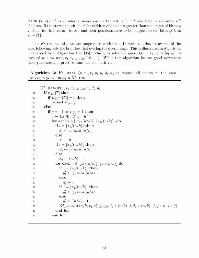
rank1(T, p) ·K2 as all internal nodes are marked with a 1 in T and they have exactly K2

children. If the starting position of the children of a node is greater than the length of bitmapT , then its children are leaves, and their positions have to be mapped to the bitmap L assp− |T |.

The K2-tree can also answer range queries with multi-branch top-down traversal of thetree, following only the branches that overlap the query range. This is illustrated in Algorithm3 (adapted from Algorithm 1 in [35]), which, to solve the query Q = [x1, x2] × [y1, y2], isinvoked as range(n, x1, x2, y1, y2, 0, 0,−1). While this algorithm has no good worst-casetime guarantees, in practice times are competitive.

Algorithm 3: K2_range(n, x1, x2, y1, y2, dp, dq, p) reports all points in the area[x1, x2]× [y1, y2] using a K2-tree.

K2_range(n, x1, x2, y1, y2, dp, dq, p)01 if p ≥ |T | then02 if L[p− |T |] = 1 then03 report 〈dp, dq〉04 else05 if p = −1 or T [p] = 1 then06 y ← rank1 (T, p) ·K2

07 for each i ∈ [bx1/(n/k)c..bx2/(n/k)]c do08 if i = bx1/(n/k)c then09 x′1 ← x1 mod (n/k)10 else11 x′1 ← 012 if i = bx2/(n/k)c then13 x′2 ← x2 mod (n/k)14 else15 x′2 ← (n/k)− 116 for each j ∈ [by1/(n/k)c..by2/(n/k)c do17 if j = by1/(n/k)c then18 y′1 ← y1 mod (n/k)19 else20 y′1 ← 021 if j = by2/(n/k)c then22 y′1 ← y2 mod (n/k)23 else24 y′2 ← (n/k)− 125 K2_range(n/k, x′1, x

′2, y′1, y′2, dp + (n/k) · i, dq + (n/k) · j, y + k · i+ j)

26 end for27 end for

23

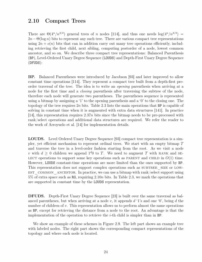
2.10 Compact Trees

There are Θ(4n/n3/2) general trees of n nodes [114], and thus one needs log(4n/n3/2) =2n−Θ(log n) bits to represent any such tree. There are various compact tree representationsusing 2n + o(n) bits that can in addition carry out many tree operations efficiently, includ-ing retrieving the first child, next sibling, computing postorder of a node, lowest commonancestor, and so on. We describe three compact tree representations: Balanced Parenthesis(BP), Level-Ordered Unary Degree Sequence (LOUDS) and Depth-First Unary Degree Sequence(DFUDS):

BP. Balanced Parentheses were introduced by Jacobson [93] and later improved to allowconstant time operations [114]. They represent a compact tree built from a depth-first pre-order traversal of the tree. The idea is to write an opening parenthesis when arriving at anode for the first time and a closing parenthesis after traversing the subtree of the node,therefore each node will generate two parentheses. The parentheses sequence is representedusing a bitmap by assigning a ‘1’ to the opening parenthesis and a ‘0’ to the closing one. Thetopology of the tree requires 2n bits. Table 2.3 lists the main operations that BP is capable ofsolving in constant time when it is augmented with extra data structures [141]. In practice[14], this representation requires 2.37n bits since the bitmap needs to be pre-processed withrank/select operations and additional data structures are required. We refer the reader tothe work of Arroyuelo et al. [14] for implementation details.

LOUDS. Level Ordered Unary Degree Sequence [93] compact tree representation is a sim-pler, yet efficient mechanism to represent ordinal trees. We start with an empty bitmap Tand traverse the tree in a level-order fashion starting from the root. As we visit a nodev with d ≥ 0 children we append 1d0 to T . We need to augment T with rank and se-lect operations to support some key operations such as parent and child in O(1) time.However, LOUDS constant-time operations are more limited than the ones supported by BP.This representation does not support complex operations such as subtree_size or low-est_common_ancestor. In practice, we can use a bitmap with rank/select support using5% of extra space such as RG, requiring 2.10n bits. In Table 2.3, we mark the operations thatare supported in constant time by the LOUDS representation.

DFUDS. Depth-First Unary Degree Sequence [23] is built over the same traversal as bal-anced parentheses, but when arriving at a node v, it appends d ‘1’s and one ‘0’, being d thenumber of children of v. This representation allows us to perform almost the same operationsas BP, except for retrieving the distance from a node to the root. An advantage is that theimplementation of the operation to retrieve the i-th child is simpler than in BP.

We show an example of these schemes in Figure 2.9. The left part shows an example treewith labeled nodes. The right part shows the corresponding compact representations of thetopology and where each node is located.

24

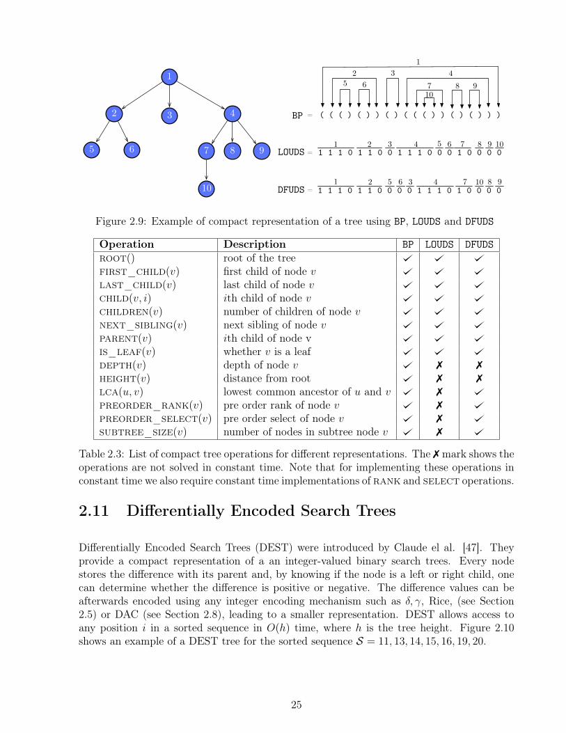
1

2

7

3 4

65 8

10

9

BP

LOUDS

DFUDS

=

=

( ( ( ) ( ) ) ( ) ( ( ( ) ) ( ) ( ) ) )

= 1 1 1 0 1 1 0 0 1 1 1 0 0 0 1 0 0 0 0

1 1 1 0 1 1 0 0 0 0 1 1 1 0 1 0 0 0 0

12 43

5 6 7 8 910

1 2 54 6 7 8 9 103

1 2 46 73 8105 9

Figure 2.9: Example of compact representation of a tree using BP, LOUDS and DFUDS

Operation Description BP LOUDS DFUDSroot() root of the treefirst_child(v) first child of node vlast_child(v) last child of node vchild(v, i) ith child of node vchildren(v) number of children of node vnext_sibling(v) next sibling of node vparent(v) ith child of node vis_leaf(v) whether v is a leafdepth(v) depth of node v 7 7

height(v) distance from root 7 7

lca(u, v) lowest common ancestor of u and v 7

preorder_rank(v) pre order rank of node v 7

preorder_select(v) pre order select of node v 7

subtree_size(v) number of nodes in subtree node v 7

Table 2.3: List of compact tree operations for different representations. The 7 mark shows theoperations are not solved in constant time. Note that for implementing these operations inconstant time we also require constant time implementations of rank and select operations.

2.11 Differentially Encoded Search Trees

Differentially Encoded Search Trees (DEST) were introduced by Claude el al. [47]. Theyprovide a compact representation of a an integer-valued binary search trees. Every nodestores the difference with its parent and, by knowing if the node is a left or right child, onecan determine whether the difference is positive or negative. The difference values can beafterwards encoded using any integer encoding mechanism such as δ, γ, Rice, (see Section2.5) or DAC (see Section 2.8), leading to a smaller representation. DEST allows access toany position i in a sorted sequence in O(h) time, where h is the tree height. Figure 2.10shows an example of a DEST tree for the sorted sequence S = 11, 13, 14, 15, 16, 19, 20.

25

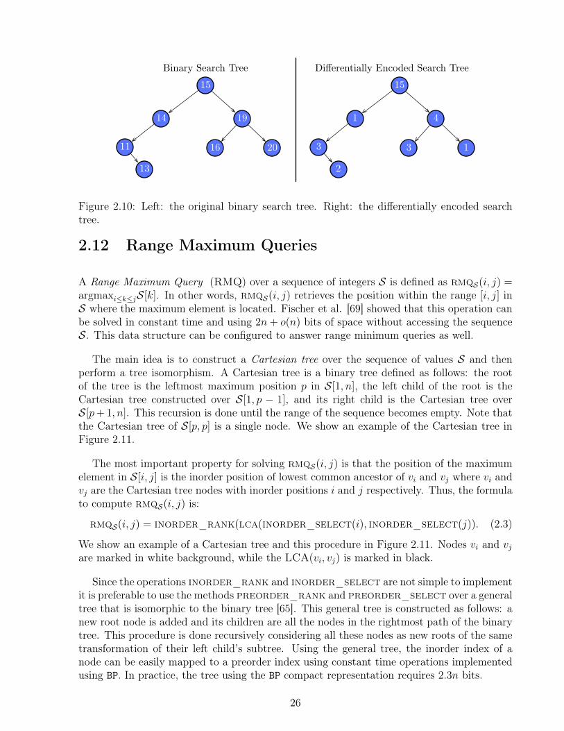
15

14

16

19

13

11 20

15

1

3

4

2

3 1

Binary Search Tree Differentially Encoded Search Tree

Figure 2.10: Left: the original binary search tree. Right: the differentially encoded searchtree.

2.12 Range Maximum Queries

A Range Maximum Query (RMQ) over a sequence of integers S is defined as rmqS(i, j) =argmaxi≤k≤jS[k]. In other words, rmqS(i, j) retrieves the position within the range [i, j] inS where the maximum element is located. Fischer et al. [69] showed that this operation canbe solved in constant time and using 2n+ o(n) bits of space without accessing the sequenceS. This data structure can be configured to answer range minimum queries as well.

The main idea is to construct a Cartesian tree over the sequence of values S and thenperform a tree isomorphism. A Cartesian tree is a binary tree defined as follows: the rootof the tree is the leftmost maximum position p in S[1, n], the left child of the root is theCartesian tree constructed over S[1, p − 1], and its right child is the Cartesian tree overS[p+ 1, n]. This recursion is done until the range of the sequence becomes empty. Note thatthe Cartesian tree of S[p, p] is a single node. We show an example of the Cartesian tree inFigure 2.11.

The most important property for solving rmqS(i, j) is that the position of the maximumelement in S[i, j] is the inorder position of lowest common ancestor of vi and vj where vi andvj are the Cartesian tree nodes with inorder positions i and j respectively. Thus, the formulato compute rmqS(i, j) is:

rmqS(i, j) = inorder_rank(lca(inorder_select(i), inorder_select(j)). (2.3)

We show an example of a Cartesian tree and this procedure in Figure 2.11. Nodes vi and vjare marked in white background, while the LCA(vi, vj) is marked in black.

Since the operations inorder_rank and inorder_select are not simple to implementit is preferable to use the methods preorder_rank and preorder_select over a generaltree that is isomorphic to the binary tree [65]. This general tree is constructed as follows: anew root node is added and its children are all the nodes in the rightmost path of the binarytree. This procedure is done recursively considering all these nodes as new roots of the sametransformation of their left child’s subtree. Using the general tree, the inorder index of anode can be easily mapped to a preorder index using constant time operations implementedusing BP. In practice, the tree using the BP compact representation requires 2.3n bits.

26

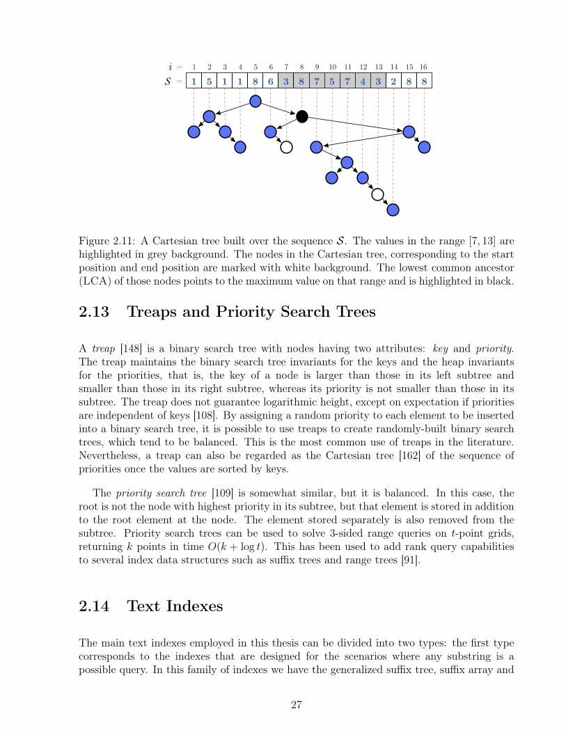
S = 1 5 1 1 8 6 3 8 7 5 7 4 3 2 81 2 3 4 5 6 7 8 9 10 11 12 13 14i = 15

816

Figure 2.11: A Cartesian tree built over the sequence S. The values in the range [7, 13] arehighlighted in grey background. The nodes in the Cartesian tree, corresponding to the startposition and end position are marked with white background. The lowest common ancestor(LCA) of those nodes points to the maximum value on that range and is highlighted in black.

2.13 Treaps and Priority Search Trees

A treap [148] is a binary search tree with nodes having two attributes: key and priority.The treap maintains the binary search tree invariants for the keys and the heap invariantsfor the priorities, that is, the key of a node is larger than those in its left subtree andsmaller than those in its right subtree, whereas its priority is not smaller than those in itssubtree. The treap does not guarantee logarithmic height, except on expectation if prioritiesare independent of keys [108]. By assigning a random priority to each element to be insertedinto a binary search tree, it is possible to use treaps to create randomly-built binary searchtrees, which tend to be balanced. This is the most common use of treaps in the literature.Nevertheless, a treap can also be regarded as the Cartesian tree [162] of the sequence ofpriorities once the values are sorted by keys.

The priority search tree [109] is somewhat similar, but it is balanced. In this case, theroot is not the node with highest priority in its subtree, but that element is stored in additionto the root element at the node. The element stored separately is also removed from thesubtree. Priority search trees can be used to solve 3-sided range queries on t-point grids,returning k points in time O(k + log t). This has been used to add rank query capabilitiesto several index data structures such as suffix trees and range trees [91].

2.14 Text Indexes

The main text indexes employed in this thesis can be divided into two types: the first typecorresponds to the indexes that are designed for the scenarios where any substring is apossible query. In this family of indexes we have the generalized suffix tree, suffix array and

27

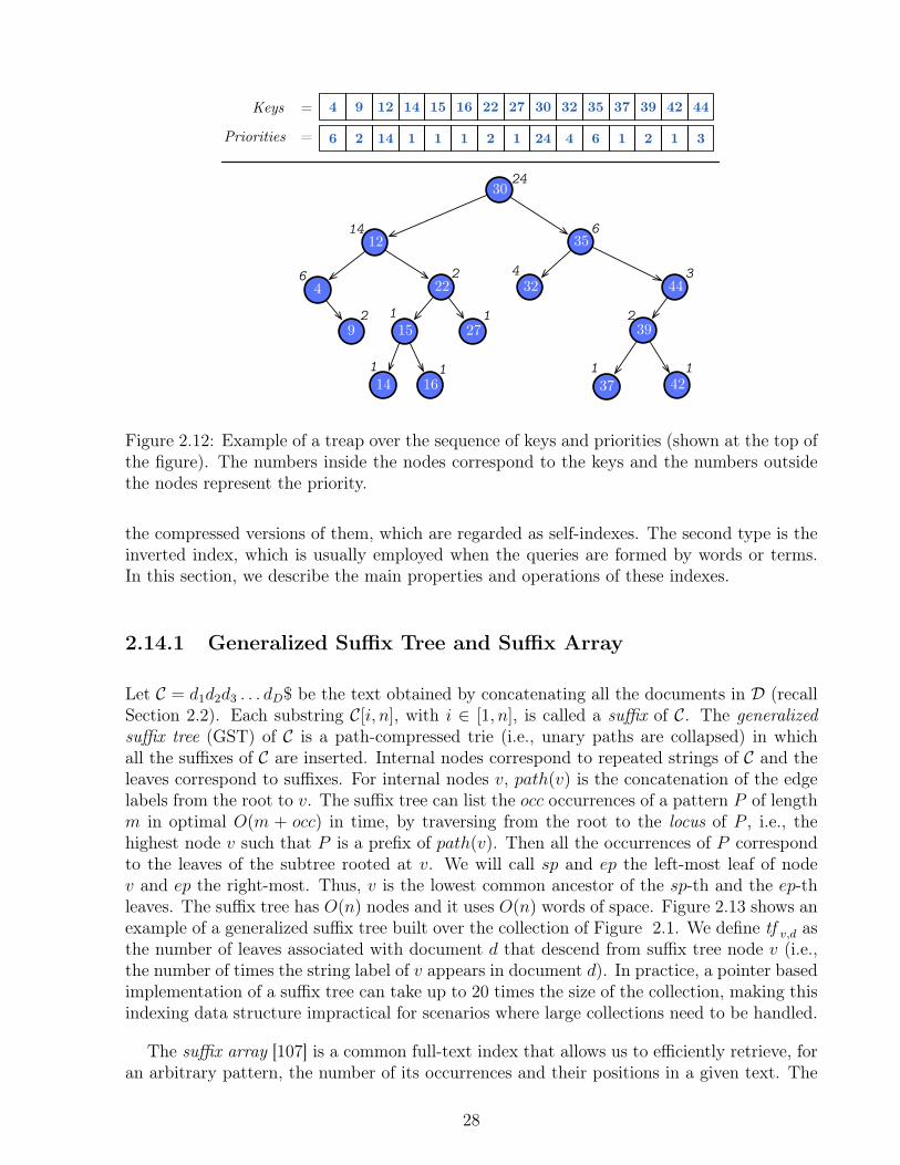
30

12

39

35

9

4 44

37

22

2715

16

Keys = 4 9 12 14 16 22 27 30 35 37 39 42

6 2 14 1 1 2 1 24 6 1 2 1Priorities =

24

6

3

2

1

32

1411

1

15

1

32

4

4

14

6

2

2

1

421

44

3

Figure 2.12: Example of a treap over the sequence of keys and priorities (shown at the top ofthe figure). The numbers inside the nodes correspond to the keys and the numbers outsidethe nodes represent the priority.

the compressed versions of them, which are regarded as self-indexes. The second type is theinverted index, which is usually employed when the queries are formed by words or terms.In this section, we describe the main properties and operations of these indexes.

2.14.1 Generalized Suffix Tree and Suffix Array

Let C = d1d2d3 . . . dD$ be the text obtained by concatenating all the documents in D (recallSection 2.2). Each substring C[i, n], with i ∈ [1, n], is called a suffix of C. The generalizedsuffix tree (GST) of C is a path-compressed trie (i.e., unary paths are collapsed) in whichall the suffixes of C are inserted. Internal nodes correspond to repeated strings of C and theleaves correspond to suffixes. For internal nodes v, path(v) is the concatenation of the edgelabels from the root to v. The suffix tree can list the occ occurrences of a pattern P of lengthm in optimal O(m + occ) in time, by traversing from the root to the locus of P , i.e., thehighest node v such that P is a prefix of path(v). Then all the occurrences of P correspondto the leaves of the subtree rooted at v. We will call sp and ep the left-most leaf of nodev and ep the right-most. Thus, v is the lowest common ancestor of the sp-th and the ep-thleaves. The suffix tree has O(n) nodes and it uses O(n) words of space. Figure 2.13 shows anexample of a generalized suffix tree built over the collection of Figure 2.1. We define tf v,d asthe number of leaves associated with document d that descend from suffix tree node v (i.e.,the number of times the string label of v appears in document d). In practice, a pointer basedimplementation of a suffix tree can take up to 20 times the size of the collection, making thisindexing data structure impractical for scenarios where large collections need to be handled.

The suffix array [107] is a common full-text index that allows us to efficiently retrieve, foran arbitrary pattern, the number of its occurrences and their positions in a given text. The

28

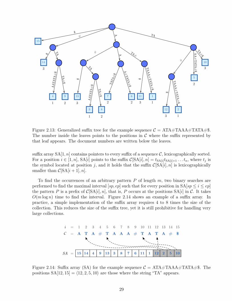
15

14

4 9 13

3 8

7 6

12 2

5

10

3

1 2 3

1 2

2 2

3 1

2

3

111

3 1

TATA#$

AA#TATA

#$

TAAA#TATA#

$

$

#

TAAA#TATA#

$

$

A#TATA#

$TATA#$

TA#$

AATATA#$

TA

#

$

A

TA#$

AATATA#$

TA$

#$

TA#A

Figure 2.13: Generalized suffix tree for the example sequence C = ATA#TAAA#TATA#$.The number inside the leaves points to the positions in C where the suffix represented bythat leaf appears. The document numbers are written below the leaves.

suffix array SA[1, n] contains pointers to every suffix of a sequence C, lexicographically sorted.For a position i ∈ [1, n], SA[i] points to the suffix C[SA[i], n] = tSA[i]tSA[i]+1 . . . tn, where tj isthe symbol located at position j, and it holds that the suffix C[SA[i], n] is lexicographicallysmaller than C[SA[i+ 1], n].

To find the occurrences of an arbitrary pattern P of length m, two binary searches areperformed to find the maximal interval [sp, ep] such that for every position in SA[sp ≤ i ≤ ep]the pattern P is a prefix of C[SA[i], n], that is, P occurs at the positions SA[i] in C. It takesO(m log n) time to find the interval. Figure 2.14 shows an example of a suffix array. Inpractice, a simple implementation of the suffix array requires 4 to 8 times the size of thecollection. This reduces the size of the suffix tree, yet it is still prohibitive for handling verylarge collections.

C = A T A # T A A A # T T A # $

SA = 15 14 4 9 13 3 8 7 6 11 1 12 2

A

5 10

1 2 3 4 5 6 7 8 9 10 11 12 13 14i = 15

Figure 2.14: Suffix array (SA) for the example sequence C = ATA#TAAA#TATA#$. Thepositions SA[12, 15] = 〈12, 2, 5, 10〉 are those where the string “TA” appears.

29

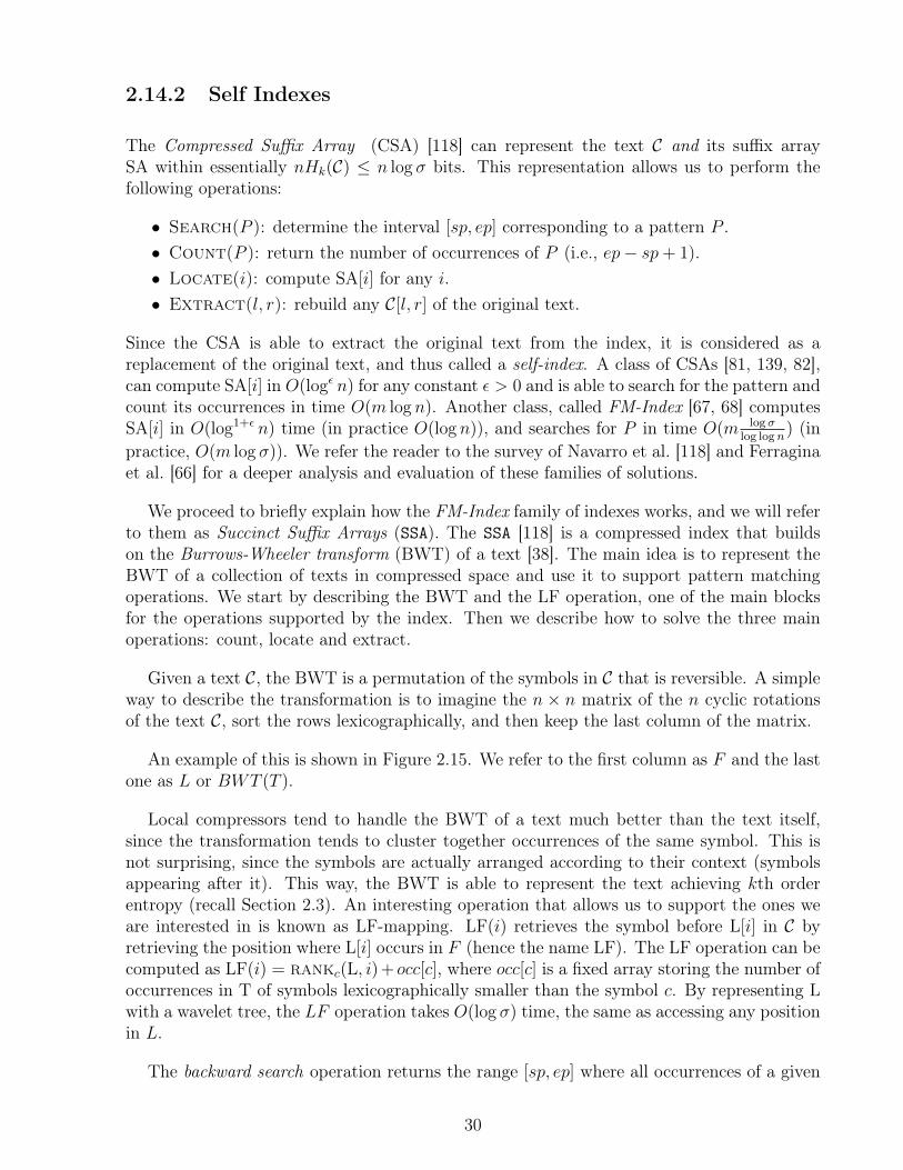
2.14.2 Self Indexes

The Compressed Suffix Array (CSA) [118] can represent the text C and its suffix arraySA within essentially nHk(C) ≤ n log σ bits. This representation allows us to perform thefollowing operations:

• Search(P ): determine the interval [sp, ep] corresponding to a pattern P .• Count(P ): return the number of occurrences of P (i.e., ep− sp+ 1).• Locate(i): compute SA[i] for any i.• Extract(l, r): rebuild any C[l, r] of the original text.

Since the CSA is able to extract the original text from the index, it is considered as areplacement of the original text, and thus called a self-index. A class of CSAs [81, 139, 82],can compute SA[i] in O(logε n) for any constant ε > 0 and is able to search for the pattern andcount its occurrences in time O(m log n). Another class, called FM-Index [67, 68] computesSA[i] in O(log1+ε n) time (in practice O(log n)), and searches for P in time O(m log σ

log logn) (in

practice, O(m log σ)). We refer the reader to the survey of Navarro et al. [118] and Ferraginaet al. [66] for a deeper analysis and evaluation of these families of solutions.

We proceed to briefly explain how the FM-Index family of indexes works, and we will referto them as Succinct Suffix Arrays (SSA). The SSA [118] is a compressed index that buildson the Burrows-Wheeler transform (BWT) of a text [38]. The main idea is to represent theBWT of a collection of texts in compressed space and use it to support pattern matchingoperations. We start by describing the BWT and the LF operation, one of the main blocksfor the operations supported by the index. Then we describe how to solve the three mainoperations: count, locate and extract.

Given a text C, the BWT is a permutation of the symbols in C that is reversible. A simpleway to describe the transformation is to imagine the n × n matrix of the n cyclic rotationsof the text C, sort the rows lexicographically, and then keep the last column of the matrix.

An example of this is shown in Figure 2.15. We refer to the first column as F and the lastone as L or BWT (T ).

Local compressors tend to handle the BWT of a text much better than the text itself,since the transformation tends to cluster together occurrences of the same symbol. This isnot surprising, since the symbols are actually arranged according to their context (symbolsappearing after it). This way, the BWT is able to represent the text achieving kth orderentropy (recall Section 2.3). An interesting operation that allows us to support the ones weare interested in is known as LF-mapping. LF(i) retrieves the symbol before L[i] in C byretrieving the position where L[i] occurs in F (hence the name LF). The LF operation can becomputed as LF(i) = rankc(L, i) + occ[c], where occ[c] is a fixed array storing the number ofoccurrences in T of symbols lexicographically smaller than the symbol c. By representing Lwith a wavelet tree, the LF operation takes O(log σ) time, the same as accessing any positionin L.

The backward search operation returns the range [sp, ep] where all occurrences of a given

30

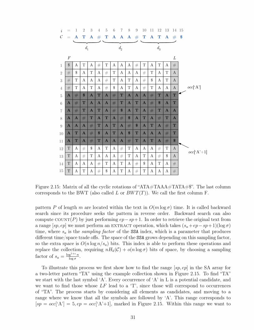
d1 d2 d3

C = A T A # T A A A # T T A # $1 2 3 4 5 6 7 8 9 10 11 12 13 14i =

A15

$ A T A # T A A A # T A T A #

# $ A T A # T A A A # T A T A

# T A A A # T A T A # $ A T A

# T A T A # $ A T A # T A A A

A # $ A T A # T A A A # T A T

A A # T A T A # $ A T A # T A

A T A # $ A T A $ T A A A # T

T A # $ A T A # T A A A # T A

T A # T A A A # T A T A # $ A

T A A A # T A T A # $ A T A #

T A T A # $ A T A # T A A A #

F L

A A A # T A T A # $ A T A # T

A T A # T A A A # T A T A # $

occ[‘A’]

occ[‘A’+1]

1

2

3

4

5

6

7

8

9

10

11

12

13

1415

A # T A A A # T A T A # $ A TA # T A T A # $ A T A # T A A

Figure 2.15: Matrix of all the cyclic rotations of “ATA#TAAA#TATA#$”. The last columncorresponds to the BWT (also called L or BWT (T )). We call the first column F.

pattern P of length m are located within the text in O(m log σ) time. It is called backwardsearch since its procedure seeks the pattern in reverse order. Backward search can alsocompute count(P ) by just performing ep−sp+1. In order to retrieve the original text froma range [sp, ep] we must perform an extract operation, which takes (sa+ep−sp+1)(log σ)time, where sa is the sampling factor of the SSA index, which is a parameter that producesdifferent time/space trade offs. The space of the SSA grows depending on this sampling factor,so the extra space is O(n log n/sa) bits. This index is able to perform these operations andreplace the collection, requiring nHk(C) + o(n log σ) bits of space, by choosing a samplingfactor of sa = log1+ε n

log σ.

To illustrate this process we first show how to find the range [sp, ep] in the SA array fora two-letter pattern “TA” using the example collection shown in Figure 2.15. To find “TA”we start with the last symbol ‘A’. Every occurrence of ‘A’ in L is a potential candidate, andwe want to find those whose LF lead to a ‘T’, since those will correspond to occurrencesof “TA”. The process starts by considering all elements as candidates, and moving to arange where we know that all the symbols are followed by ‘A’. This range corresponds to[sp = occ[‘A’] = 5, ep = occ[‘A’+1], marked in Figure 2.15. Within this range we want to

31

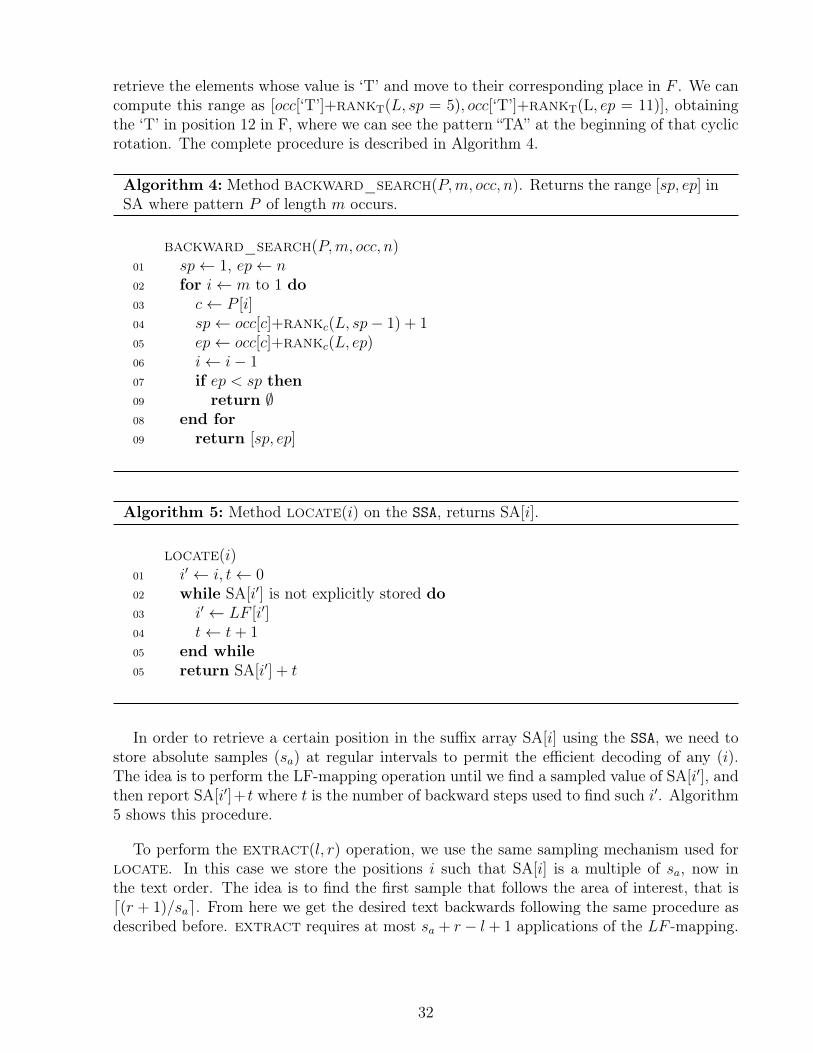
retrieve the elements whose value is ‘T’ and move to their corresponding place in F . We cancompute this range as [occ[‘T’]+rankT(L, sp = 5), occ[‘T’]+rankT(L, ep = 11)], obtainingthe ‘T’ in position 12 in F, where we can see the pattern “TA” at the beginning of that cyclicrotation. The complete procedure is described in Algorithm 4.

Algorithm 4: Method backward_search(P,m, occ, n). Returns the range [sp, ep] inSA where pattern P of length m occurs.

backward_search(P,m, occ, n)01 sp← 1, ep← n02 for i← m to 1 do03 c← P [i]04 sp← occ[c]+rankc(L, sp− 1) + 105 ep← occ[c]+rankc(L, ep)06 i← i− 107 if ep < sp then09 return ∅08 end for09 return [sp, ep]

Algorithm 5: Method locate(i) on the SSA, returns SA[i].

locate(i)01 i′ ← i, t← 002 while SA[i′] is not explicitly stored do03 i′ ← LF [i′]04 t← t+ 105 end while05 return SA[i′] + t

In order to retrieve a certain position in the suffix array SA[i] using the SSA, we need tostore absolute samples (sa) at regular intervals to permit the efficient decoding of any (i).The idea is to perform the LF-mapping operation until we find a sampled value of SA[i′], andthen report SA[i′]+ t where t is the number of backward steps used to find such i′. Algorithm5 shows this procedure.

To perform the extract(l, r) operation, we use the same sampling mechanism used forlocate. In this case we store the positions i such that SA[i] is a multiple of sa, now inthe text order. The idea is to find the first sample that follows the area of interest, that isd(r + 1)/sae. From here we get the desired text backwards following the same procedure asdescribed before. extract requires at most sa + r− l + 1 applications of the LF -mapping.

32

2.14.3 Inverted Indexes

The inverted index is an old and simple, yet efficient, data structure that is at the heartof every modern information retrieval system, and plays a central role in any book on thetopic [166, 40, 17, 50]. Given a collection of text containing a set of D documents D =d1, d2, . . . , dD. A document di can be regarded as a sequence of terms or words and thenumber of words in the document is denoted by |di|. The total length of the collection isthen

∑Di=1 |di| = n. Each document has a unique document identifier (docid) ∈ [1, D]. The

set of distinct terms in the collection is called the vocabulary, which is comparatively smallin most cases [84], more precisely of size O(nβ), for some constant 0 < β < 1 that dependson the text type. The inverted index can be seen as an array of lists or postings, where eachentry of the array corresponds to a different term or word in the vocabulary of the collection,and the lists contain one element per distinct document where the term appears. For eachterm, the index stores in the list the document identifier (docid), the weight of the term inthe document and, if needed, the positions where the term occurs in the document. Theweight of the term in the document is a utility function that represents the importance ofthat word inside the document. The main components of the inverted index are then definedas the vocabulary and the inverted lists:

• The Vocabulary. The vocabulary stores all distinct terms contained in the collectionof documents D. This is commonly implemented with a dictionary data structure suchas hash tables or tries. In practice, the vocabulary stores two elements associated witheach term: an integer value dft, that is, the amount of documents that contain the termt, and a pointer to the start of its corresponding inverted list.• Inverted Lists. A non-positional inverted list stores a list of elements containing

pairs 〈d, w(t, d)〉, where d is the document identifier (docid) and w(t, d) is a relevancemeasure of the term t in document d. A positional inverted list contains a list of triples〈d, w(t, d), 〈p1, p2, · · · , pk〉〉, where the third component is a vector of positions wherethe occurrences term t are located in the document d. An inverted index that makesuse of positional inverted lists is also commonly referred to as full-text inverted index.

Figure 2.16 shows a example of a positional inverted index for a collection consisting ofthree documents. The inverted index from the example shows a docid-sorted organization,where each posting list is in increasing docid order. The posting lists could also follow aweight-sorted organization

2.15 Muthukrishnan’s Algorithm

The inverted index is not suitable for the case where the query is any possible text substringand we want to retrieve the document identifiers that contain a string pattern P . This isa common scenario for text collections written in East Asian languages such as Chinese orKorean, where words are difficult to segment, or in agglutinating languages such as Finnishand German, where one needs to search for particles inside words.

Muthukrishnan [115] introduced the first solution for retrieving the documents containing

33

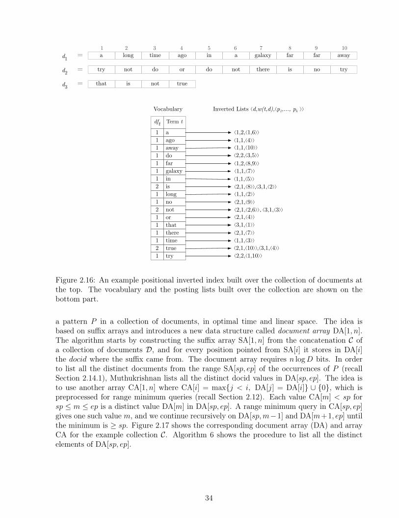
a long time ago in a galaxy far far awayd1 1 2 3 4 5 6 7 8 9 10

=

try not do or do not there is no tryd2 =

that is not trued3 =

aago

dofargalaxyinislongnonotorthattheretimetruetry

Term t

⟨1,2,⟨1,6⟩⟩ ⟨1,1,⟨4⟩⟩

⟨2,2,⟨3,5⟩⟩ ⟨1,2,⟨8,9⟩⟩ ⟨1,1,⟨7⟩⟩ ⟨1,1,⟨5⟩⟩ ⟨2,1,⟨8⟩⟩,⟨3,1,⟨2⟩⟩ ⟨1,1,⟨2⟩⟩

⟨2,1,⟨2,6⟩⟩, ⟨3,1,⟨3⟩⟩ ⟨2,1,⟨4⟩⟩⟨3,1,⟨1⟩⟩

⟨2,1,⟨9⟩⟩

Inverted Lists ⟨d,w(t,d),⟨p1,…, pk ⟩⟩

⟨2,1,⟨7⟩⟩⟨1,1,⟨3⟩⟩⟨2,1,⟨10⟩⟩,⟨3,1,⟨4⟩⟩⟨2,2,⟨1,10⟩⟩

away ⟨1,1,⟨10⟩⟩

dft11111112112111121

Vocabulary

Figure 2.16: An example positional inverted index built over the collection of documents atthe top. The vocabulary and the posting lists built over the collection are shown on thebottom part.

a pattern P in a collection of documents, in optimal time and linear space. The idea isbased on suffix arrays and introduces a new data structure called document array DA[1, n].The algorithm starts by constructing the suffix array SA[1, n] from the concatenation C ofa collection of documents D, and for every position pointed from SA[i] it stores in DA[i]the docid where the suffix came from. The document array requires n logD bits. In orderto list all the distinct documents from the range SA[sp, ep] of the occurrences of P (recallSection 2.14.1), Muthukrishnan lists all the distinct docid values in DA[sp, ep]. The idea isto use another array CA[1, n] where CA[i] = maxj < i, DA[j] = DA[i] ∪ 0, which ispreprocessed for range minimum queries (recall Section 2.12). Each value CA[m] < sp forsp ≤ m ≤ ep is a distinct value DA[m] in DA[sp, ep]. A range minimum query in CA[sp, ep]gives one such value m, and we continue recursively on DA[sp,m−1] and DA[m+1, ep] untilthe minimum is ≥ sp. Figure 2.17 shows the corresponding document array (DA) and arrayCA for the example collection C. Algorithm 6 shows the procedure to list all the distinctelements of DA[sp, ep].

34

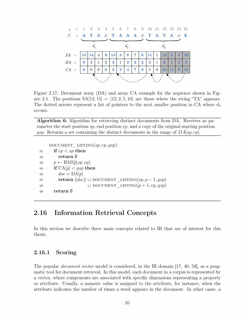
DA = 0 3 1 2 3 1 2 2 2 3 1 3

d1 d2 d3

CA = 0 0 0 0 2 3 4 7 8 5 6 10111

29

C = A T A # T A A A # T T A # $1 2 3 4 5 6 7 8 9 10 11 12 13 14i =

A15

SA = 15 14 4 9 13 3 8 7 6 11 1 12 2 5 10312

Figure 2.17: Document array (DA) and array CA example for the sequence shown in Fig-ure 2.1. The positions SA[12, 15] = 〈12, 2, 5, 10〉 are those where the string “TA” appears.The dotted arrows represent a list of pointers to the next smaller position in CA where d3

occurs.

Algorithm 6: Algorithm for retrieving distinct documents from DA. Receives as pa-rameter the start position sp, end position ep, and a copy of the original starting positiongsp. Returns a set containing the distinct documents in the range of DA[sp, ep].

document_listing(sp, ep, gsp)01 if ep < sp then02 return ∅03 p← RMQ(sp, ep)04 if CA[p] < gsp then05 doc = DA[p]07 return doc ∪ document_listing(sp, p− 1, gsp)08 ∪ document_listing(p+ 1, ep, gsp)09 return ∅

2.16 Information Retrieval Concepts

In this section we describe three main concepts related to IR that are of interest for thisthesis.

2.16.1 Scoring

The popular document vector model is considered, in the IR domain [17, 40, 50], as a prag-matic tool for document retrieval. In this model, each document in a corpus is represented bya vector, where components are associated with specific dimensions representing a propertyor attribute. Usually, a numeric value is assigned to the attribute, for instance, when theattribute indicates the number of times a word appears in the document. In other cases, a

35

vector entry may be a bit value where the value 1 indicates that a property is present in thedocument, or 0 otherwise. A document vector model represents any document di as a vector~di = (w(t1, di), ..., w(tk, di)) where tj is a term (usually a word) and the function w(tj, di) isthe weight of the term tj in the document di. The weight of the term is a utility functionthat represents the importance of that word inside the document. Another model is thebag-of-words. In this model, a collection of documents is represented as a set (bag) of thewords contained in the collection, not taking into consideration the word ordering, grammaror other properties from the text.

Most IR systems that are based on these models define the score of a document d for aquery Q as

score(Q, d) =∑t∈Q

w(t, d), (2.4)

where the query Q is a set of terms and thus considered as a “bag of words”.

For example, in the well-known tf-idf scoring scheme, the weight is computed as w(t, d) =tf t,d · idft. Here, tf t,d is the term frequency of t in d, that is, the number of times t occurs in d.The second term is idft = log D

dft, where dft is the document frequency, that is, the number of

documents where the term t appears, and D is the total number of documents. Since idft (ordft) depends only on t, an efficient way to store w(t, d) in an inverted index is to store idft ordft together with each distinct vocabulary term, and store the values tf t,d in the posting listof term t, together with each docid d. Recent state- of-the-art information retrieval systemsemploy more complex ranking formulas such as the Okapi BM25 [95]:

score(Q, d) =∑t∈Q

tf t,d · (k1 + 1)

tf t,d + k1 · (1− b+ b · |d|/avg_dlength)· idft, (2.5)

where k1 and b are tuning parameters and avg_dlength is the average document length inthe collection D.

Computing the ranking score can be a major bottleneck of the system’s query processingroutines. One idea to improve speed is to pre-compute the scores and store them as floating-point numbers in 24 to 32 bits. This alternative is usually not possible, since it increases thesize of the index significantly. If we want to speed up the score calculation process and alsomaintain a reasonable size of the index we can discretize the range of possible scores into apredefined set of buckets. Anh et al. [12] proposed a uniform quantization method that isan index-wide linear scaling of the term weights, in other words, the idea is to precomputeand store the impact score for the term weight as I(d, t) using the following formula:

I(t, d) =

⌊w(t, d)−min(w(t, d))

max(w(t, d))−min(w(t, d))× 2b

⌋, (2.6)

where b is the number of bits that we are willing to reserve for each score contribution. Anhet al. [9] showed that by setting b = 8, quantization methods achieves effectiveness that isindistinguishable from using exact term weights, this has been also been further explored inthe work of Anh and Moffat [10, 12].

36

2.16.2 Top-k Query Processing and Two-stage Ranking Process

In the case of natural language collections, we define a query Q as a set of q words or termst ∈ Q. In the case of general sequences, we define the query as a pattern P , which is asequence of symbols from an alphabet Σ of size σ and its length is |P | = m.

The problem with retrieving a fixed amount of k documents with the highest “score” to aquery Q (natural language case) or a pattern P (general sequence case) for some definitionof score, is known as the top-k document retrieval problem. This problem is of interest forthe two-stage ranking process that is performed in modern Web search engines and other IRsystems. The two-stage ranking process is a technique that copes with the huge amounts ofdata and enables IR systems to deliver precise results in response to the user queries [163, 40].In the first stage, a fast and simple filtration procedure extracts a subset of a few hundred orthousand of candidates from the possibly billions of documents forming the collection. In thesecond stage, more complex learned ranking algorithms are applied to the reduced candidateset in order to obtain a handful of high-quality results. In general, improving the efficiencyof the first stage frees more resources for the second stage, and this way increases the overallperformance. In contexts where traditional ranking methods are sufficient, the goal of thefirst stage is to directly convey a few top-quality results to the final user.

In distributed main-memory systems, documents are usually distributed across indexes,and each index contributes with a few results to the final top-k list. Therefore, it is mostinteresting that individual indexes solve top-k queries efficiently for k values in the range10–100 [40].

37

Part II

Inverted Indexes

38

Chapter 3

Query Processing and Compression ofPosting Lists

In this chapter we survey the main techniques to perform top-k query processing on invertedindexes. As previously discussed in Section 2.16.2, complex IR systems requirements arehandled via a two-stage ranking process [163, 40]. The first stage aims to return a set ofthe highest ranked documents containing either all the query terms (a ranked intersection) orsome of the most important query terms (a ranked union). In most cases, ranked intersectionsare solved via a Boolean intersection followed by the computation of scores for the resultingdocuments. Ranked unions are generally solved only in approximate form, avoiding a costlyBoolean union. In order to avoid a complete traversal of all lists, there are query processingtechniques that make use of early termination mechanisms. Different organizations of theposting lists have been proposed and it has been shown that they can assist early terminationmechanisms. Moreover, there are different ways to traverse the posting lists to improve queryprocessing. We cover these concepts in this chapter.

Another important issue is compression. The inverted index can be stored on disk or inmain memory, and in both cases reducing its size is crucial. On disk, it reduces transfertime when reading the lists of the query terms. In main memory, it increases the size ofthe collections that can be managed within a given RAM budget, or alternatively reducesthe number of servers that must be allocated in a cluster to hold the index, the energy theyconsume, and the amount of communication. In this chapter, we also cover compressiontechniques that are typically employed to reduce the size of the index

3.1 Query Processing

Query processing involves a number of phases such as query parsing, query rewriting andthe computation of complex machine-learned ranking functions that may include hundreds offeatures from the documents. At the same time, IR systems need to serve as many queries aspossible, needing to execute huge amounts of queries per second. To do this efficiently, search

39

engines commonly separate the ranking process into two or more phases. In the first phase, asimple and fast ranking function such as BM25 is used to get the top 100 or 1000 documents.Then in the second and following phases, increasingly more complicated ranking functionswith more features are applied to documents that pass through the earlier phases. Thus, thelater phases only examine a fairly small number of candidates, therefore a significant amountof computation is spent in the first phase.

3.1.1 Early Termination

When processing simple ranked queries on large document collections, the main performancechallenge is caused by the lengths of the inverted lists and the large number of candidates thatpass the Boolean filter. Early termination is a set of techniques that address this problem.We say that a query processing algorithm is exhaustive if it fully evaluates all the documentsthat satisfy the Boolean filter condition. Any other algorithm uses early termination (ET).In general, early termination techniques can be categorized by the use of one or more of thefollowing approaches:

1. Stopping early. Each inverted list is arranged from the most to the least promisingposting and traversal is stopped once enough good results are found.

2. Skipping. Inverted lists are sorted by docids, so promising documents are spread outover the lists. The idea is to skip over uninteresting parts of a list using additionalinformation.

3. Partial scoring. Documents are partially or approximately scored.

3.1.2 Index Organization

Early termination techniques may require inverted index structures to be arranged in specificways. In particular, some techniques assume a specific organization such that the mostpromising documents appear early in the inverted lists, which can be done by either reorderingthe postings in a list, or partitioning the index into several layers. In general, most queryprocessing techniques use one of the following index organizations [59]:

• Document-Sorted Indexes: The standard approach for exhaustive query processing,where postings in each inverted list are sorted by docid.• Frequency-Sorted Indexes: Postings in each list are sorted by their frequency.• Impact-Sorted Indexes: Postings in each list are sorted by decreasing impact (or

term score), that is, their contribution to the document score.

3.1.3 Query Processing Strategies

There are different query evaluation strategies that exhibit affinities to different index or-ganizations. They are classified in three different categories: Document-at-a-time (DAAT),

40

Term-at-a-time (TAAT) and Score-at-a-time (SAAT) [159].

Document-at-a-time. DAAT processing is more popular for Boolean intersections andunions. Given a query containing q terms, all lists are processed in parallel, looking for thesame document in all of them. Posting lists must be sorted by increasing docid, and we keepa pointer to the current position in each of the q lists. Once a document is processed, thepointers move forward. Much research has been carried out on Boolean intersections [57,18, 145, 51, 20]. While DAAT processing is always used to intersect two lists, experimentalresults suggest that the most efficient way to handle more lists is to intersect the two shortestones, then the result with the third list, and so on [20].

Term-at-a-time. TAAT processes one posting list after the other. The lists are consideredfrom shortest to longest, starting with the first one as a candidate answer set, and refining itas we consider the next lists. TAAT is especially popular for processing ranked unions [131,12, 152, 111], as the successive lists have decreasing idft value and thus a decreasing impacton the result, not only for the tf-idf scoring, but also for BM25 and other scorings. Thus,heuristic thresholds can be used to obtain an approximate ranked union efficiently by pruningthe processing of lists earlier, or avoiding complete posting lists, as we reach less relevantdocuments and our candidate set becomes stronger [131, 12]. A more sophisticated approachbased on similar ideas can be used to guarantee that the answer is exact [152]. TAATapproaches usually make use of an accumulator data structure that holds the intermediatescores for candidate documents.

Score-at-a-time. SAAT mechanism can be seen as a hybrid between DAAT and TAAT inwhich multiple index lists are open. This strategy opens all index pointers simultaneously,and start reading from the posting list that has the score with the largest impact [12]. InImpact-ordered indexes the actual score contributions of each term are precomputed andquantized into what are known as impact scores [9, 10, 12]. The idea is that a complete im-pact block is processed at each step, and the results are obtained using a set of accumulatorvariables.

3.2 Algorithms for Top-k Ranked Retrieval

Boolean query processing is probably the simplest form of resolving queries. A query withthe form “force AND awakens” is dubbed intersection or conjunctive query, while the query“episode OR viii ” is referred to as union or disjunctive query. In its basic form, union queriesare solved by linearly traversing all posting lists from all terms involved in the correspondingquery and marking all documents that have those terms. On the other hand, intersectionqueries have been a field of study for decades [20, 52, 96]. It can be proved that the optimalintersection algorithm for two sets of length m and n with m ≤ n is O(m log n

m). The most

popular algorithm for solving intersections is dubbed Set Versus Set, or also Small Versus

41

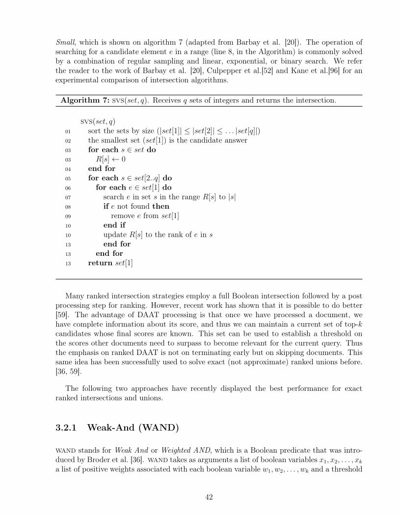
Small, which is shown on algorithm 7 (adapted from Barbay et al. [20]). The operation ofsearching for a candidate element e in a range (line 8, in the Algorithm) is commonly solvedby a combination of regular sampling and linear, exponential, or binary search. We referthe reader to the work of Barbay et al. [20], Culpepper et al.[52] and Kane et al.[96] for anexperimental comparison of intersection algorithms.

Algorithm 7: svs(set, q). Receives q sets of integers and returns the intersection.

svs(set, q)01 sort the sets by size (|set[1]| ≤ |set[2]| ≤ . . . |set[q]|)02 the smallest set (set[1]) is the candidate answer03 for each s ∈ set do03 R[s]← 004 end for05 for each s ∈ set[2..q] do06 for each e ∈ set[1] do07 search e in set s in the range R[s] to |s|08 if e not found then09 remove e from set[1]10 end if10 update R[s] to the rank of e in s13 end for13 end for13 return set[1]

Many ranked intersection strategies employ a full Boolean intersection followed by a postprocessing step for ranking. However, recent work has shown that it is possible to do better[59]. The advantage of DAAT processing is that once we have processed a document, wehave complete information about its score, and thus we can maintain a current set of top-kcandidates whose final scores are known. This set can be used to establish a threshold onthe scores other documents need to surpass to become relevant for the current query. Thusthe emphasis on ranked DAAT is not on terminating early but on skipping documents. Thissame idea has been successfully used to solve exact (not approximate) ranked unions before.[36, 59].

The following two approaches have recently displayed the best performance for exactranked intersections and unions.

3.2.1 Weak-And (WAND)

wand stands for Weak And or Weighted AND, which is a Boolean predicate that was intro-duced by Broder et al. [36]. wand takes as arguments a list of boolean variables x1, x2, . . . , xka list of positive weights associated with each boolean variable w1, w2, . . . , wk and a threshold

42

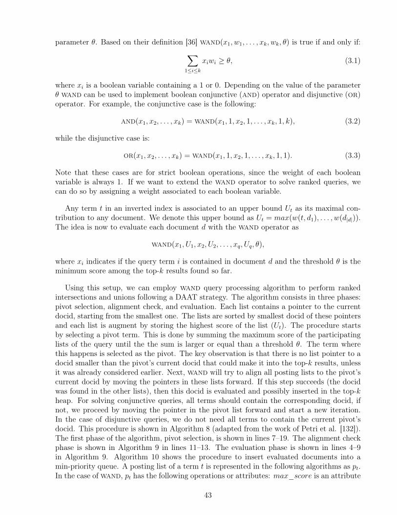
parameter θ. Based on their definition [36] wand(x1, w1, . . . , xk, wk, θ) is true if and only if:∑1≤i≤k

xiwi ≥ θ, (3.1)

where xi is a boolean variable containing a 1 or 0. Depending on the value of the parameterθ wand can be used to implement boolean conjunctive (and) operator and disjunctive (or)operator. For example, the conjunctive case is the following:

and(x1, x2, . . . , xk) = wand(x1, 1, x2, 1, . . . , xk, 1, k), (3.2)

while the disjunctive case is:

or(x1, x2, . . . , xk) = wand(x1, 1, x2, 1, . . . , xk, 1, 1). (3.3)

Note that these cases are for strict boolean operations, since the weight of each booleanvariable is always 1. If we want to extend the wand operator to solve ranked queries, wecan do so by assigning a weight associated to each boolean variable.

Any term t in an inverted index is associated to an upper bound Ut as its maximal con-tribution to any document. We denote this upper bound as Ut = max(w(t, d1), . . . , w(d|d|)).The idea is now to evaluate each document d with the wand operator as

wand(x1, U1, x2, U2, . . . , xq, Uq, θ),

where xi indicates if the query term i is contained in document d and the threshold θ is theminimum score among the top-k results found so far.

Using this setup, we can employ wand query processing algorithm to perform rankedintersections and unions following a DAAT strategy. The algorithm consists in three phases:pivot selection, alignment check, and evaluation. Each list contains a pointer to the currentdocid, starting from the smallest one. The lists are sorted by smallest docid of these pointersand each list is augment by storing the highest score of the list (Ut). The procedure startsby selecting a pivot term. This is done by summing the maximum score of the participatinglists of the query until the the sum is larger or equal than a threshold θ. The term wherethis happens is selected as the pivot. The key observation is that there is no list pointer to adocid smaller than the pivot’s current docid that could make it into the top-k results, unlessit was already considered earlier. Next, wand will try to align all posting lists to the pivot’scurrent docid by moving the pointers in these lists forward. If this step succeeds (the docidwas found in the other lists), then this docid is evaluated and possibly inserted in the top-kheap. For solving conjunctive queries, all terms should contain the corresponding docid, ifnot, we proceed by moving the pointer in the pivot list forward and start a new iteration.In the case of disjunctive queries, we do not need all terms to contain the current pivot’sdocid. This procedure is shown in Algorithm 8 (adapted from the work of Petri et al. [132]).The first phase of the algorithm, pivot selection, is shown in lines 7–19. The alignment checkphase is shown in Algorithm 9 in lines 11–13. The evaluation phase is shown in lines 4–9in Algorithm 9. Algorithm 10 shows the procedure to insert evaluated documents into amin-priority queue. A posting list of a term t is represented in the following algorithms as pt.In the case of wand, pt has the following operations or attributes: max_score is an attribute

43

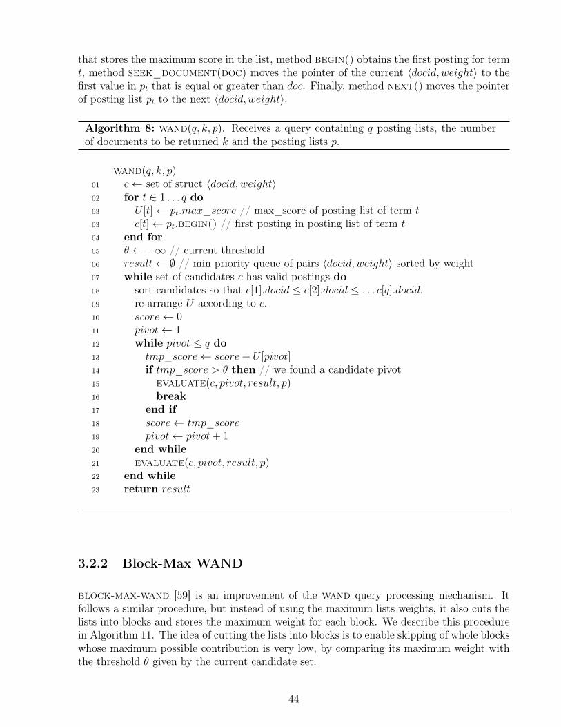
that stores the maximum score in the list, method begin() obtains the first posting for termt, method seek_document(doc) moves the pointer of the current 〈docid, weight〉 to thefirst value in pt that is equal or greater than doc. Finally, method next() moves the pointerof posting list pt to the next 〈docid, weight〉.

Algorithm 8: wand(q, k, p). Receives a query containing q posting lists, the numberof documents to be returned k and the posting lists p.

wand(q, k, p)01 c← set of struct 〈docid, weight〉02 for t ∈ 1 . . . q do03 U [t]← pt.max_score // max_score of posting list of term t03 c[t]← pt.begin() // first posting in posting list of term t04 end for05 θ ← −∞ // current threshold06 result← ∅ // min priority queue of pairs 〈docid, weight〉 sorted by weight07 while set of candidates c has valid postings do08 sort candidates so that c[1].docid ≤ c[2].docid ≤ . . . c[q].docid.09 re-arrange U according to c.10 score← 011 pivot← 112 while pivot ≤ q do13 tmp_score← score+ U [pivot]14 if tmp_score > θ then // we found a candidate pivot15 evaluate(c, pivot, result, p)16 break17 end if18 score← tmp_score19 pivot← pivot+ 120 end while21 evaluate(c, pivot, result, p)22 end while23 return result

3.2.2 Block-Max WAND

block-max-wand [59] is an improvement of the wand query processing mechanism. Itfollows a similar procedure, but instead of using the maximum lists weights, it also cuts thelists into blocks and stores the maximum weight for each block. We describe this procedurein Algorithm 11. The idea of cutting the lists into blocks is to enable skipping of whole blockswhose maximum possible contribution is very low, by comparing its maximum weight withthe threshold θ given by the current candidate set.

44

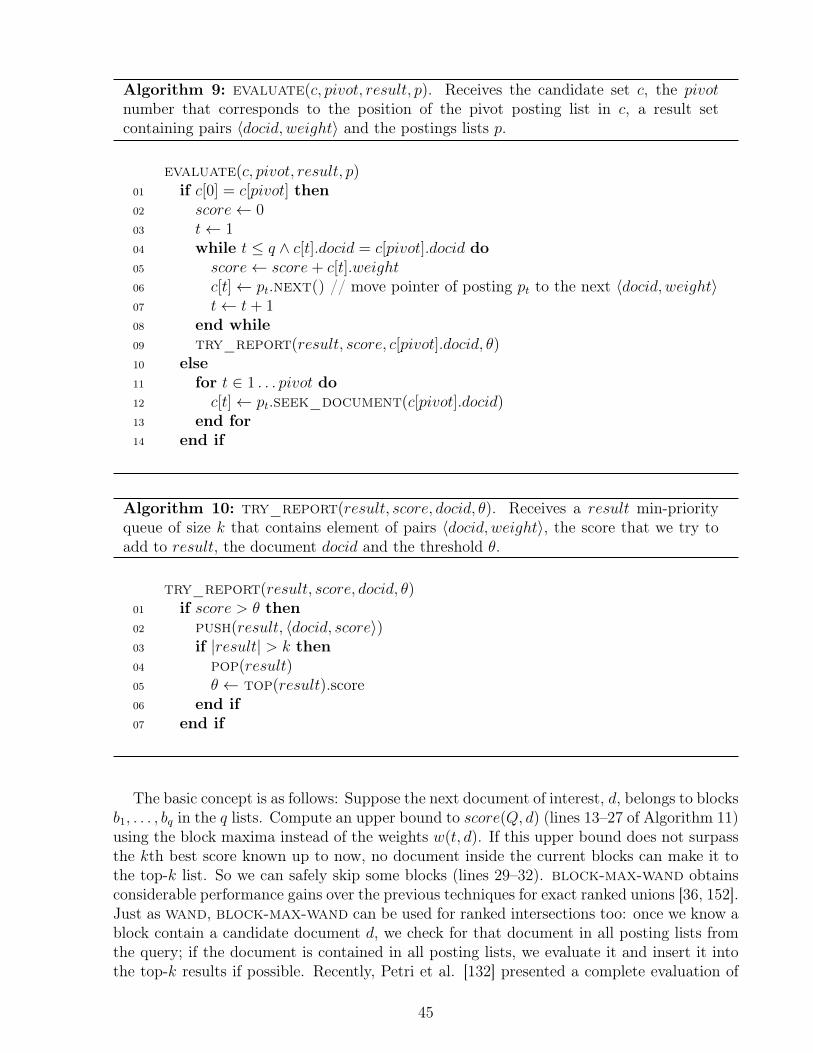
Algorithm 9: evaluate(c, pivot, result, p). Receives the candidate set c, the pivotnumber that corresponds to the position of the pivot posting list in c, a result setcontaining pairs 〈docid, weight〉 and the postings lists p.

evaluate(c, pivot, result, p)01 if c[0] = c[pivot] then02 score← 003 t← 104 while t ≤ q ∧ c[t].docid = c[pivot].docid do05 score← score+ c[t].weight06 c[t]← pt.next() // move pointer of posting pt to the next 〈docid, weight〉07 t← t+ 108 end while09 try_report(result, score, c[pivot].docid, θ)10 else11 for t ∈ 1 . . . pivot do12 c[t]← pt.seek_document(c[pivot].docid)13 end for14 end if

Algorithm 10: try_report(result, score, docid, θ). Receives a result min-priorityqueue of size k that contains element of pairs 〈docid, weight〉, the score that we try toadd to result, the document docid and the threshold θ.

try_report(result, score, docid, θ)01 if score > θ then02 push(result, 〈docid, score〉)03 if |result| > k then04 pop(result)05 θ ← top(result).score06 end if07 end if

The basic concept is as follows: Suppose the next document of interest, d, belongs to blocksb1, . . . , bq in the q lists. Compute an upper bound to score(Q, d) (lines 13–27 of Algorithm 11)using the block maxima instead of the weights w(t, d). If this upper bound does not surpassthe kth best score known up to now, no document inside the current blocks can make it tothe top-k list. So we can safely skip some blocks (lines 29–32). block-max-wand obtainsconsiderable performance gains over the previous techniques for exact ranked unions [36, 152].Just as wand, block-max-wand can be used for ranked intersections too: once we know ablock contain a candidate document d, we check for that document in all posting lists fromthe query; if the document is contained in all posting lists, we evaluate it and insert it intothe top-k results if possible. Recently, Petri et al. [132] presented a complete evaluation of

45

wand and block-max-wand methods, supporting other more complex scoring formulas.

For implementing block-max-wand, the posting lists pt requires extra methods andattributes in addition to the ones required by wand: method seek_block(doc) re-turns a pointer to the block whose smallest docid is greater or equal to doc, the attributecur_block.mac_weight contains the maximum weight of the current block being examinedand cur_block.maxdoc is an attribute that contains the maximum docid that lies in thecurrent block.

3.2.3 Persin et al.’s Algorithm

Persin et al.’s algorithm [131] is one of the most famous TAAT query processing algorithms.The idea is to solve bag-of-word queries without scanning all of the lists. The algorithmrequires the lists of each term to be sorted by decreasing weight. While the algorithm isdescribed for the tf-idf model, it can be easily adapted to many variants, with lists sorted byimpact [12].

The first step of the algorithm creates an accumulator accd for each document d in thedataset (in practice, one can dynamically add a new accumulator when a candidate documentis found). The second step will store into the corresponding accumulators accd the weightsof the documents of the shortest among the lists of the query terms, that is, the one withthe highest idft. The third step processes the rest of the lists in increasing length order,where the weight of each document is accumulated in its corresponding accd. In order toavoid processing the complete lists, they enforce a minimum threshold such that if the w(t, d)values fall below it, the list is abandoned. Since the longer lists have a lower idft multiplyingthe term frequencies, it turns out that a lower proportion of the longer lists is traversed. Theyalso apply a stricter threshold that limits the insertion of new documents as candidates. Thesethresholds provide a time/quality tradeoff.

3.2.4 Other Approaches

Buckley and Lewit [37] introduced one of the earliest query optimization techniques. Theidea follows a TAAT strategy, from the least frequent term to the most frequent one. Duringthe query evaluation, it is possible to show that is not necessary to evaluate any more terms,since it is impossible for the document at rank k+ 1 to surpass the score of the document atrank k. This technique has the advantage that it is not required to load from disk to mainmemory some of the posting lists involved in the query.

Moffat and Zobel [111] proposed another technique that also follows a TAAT traversal,and introduced two heuristics: Quit and Continue. The idea behind the Quit heuristicis to dynamically add accumulators for the documents until the amount of them meetssome fixed value. The documents are ranked by the partial scores from the accumulatorsand are reported to the user. On the other hand, the Continue heuristic follows a similarprocedure. It also uses a fixed number of accumulators, however, when the threshold is

46

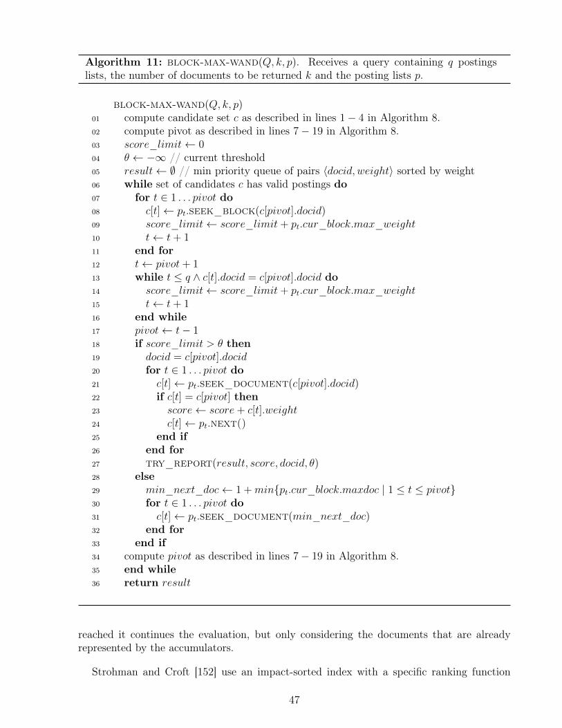
Algorithm 11: block-max-wand(Q, k, p). Receives a query containing q postingslists, the number of documents to be returned k and the posting lists p.

block-max-wand(Q, k, p)01 compute candidate set c as described in lines 1− 4 in Algorithm 8.02 compute pivot as described in lines 7− 19 in Algorithm 8.03 score_limit← 004 θ ← −∞ // current threshold05 result← ∅ // min priority queue of pairs 〈docid, weight〉 sorted by weight06 while set of candidates c has valid postings do07 for t ∈ 1 . . . pivot do08 c[t]← pt.seek_block(c[pivot].docid)09 score_limit← score_limit+ pt.cur_block.max_weight10 t← t+ 111 end for12 t← pivot+ 113 while t ≤ q ∧ c[t].docid = c[pivot].docid do14 score_limit← score_limit+ pt.cur_block.max_weight15 t← t+ 116 end while17 pivot← t− 118 if score_limit > θ then19 docid = c[pivot].docid20 for t ∈ 1 . . . pivot do21 c[t]← pt.seek_document(c[pivot].docid)22 if c[t] = c[pivot] then23 score← score+ c[t].weight24 c[t]← pt.next()25 end if26 end for27 try_report(result, score, docid, θ)28 else29 min_next_doc← 1 +minpt.cur_block.maxdoc | 1 ≤ t ≤ pivot30 for t ∈ 1 . . . pivot do31 c[t]← pt.seek_document(min_next_doc)32 end for33 end if34 compute pivot as described in lines 7− 19 in Algorithm 8.35 end while36 return result

reached it continues the evaluation, but only considering the documents that are alreadyrepresented by the accumulators.

Strohman and Croft [152] use an impact-sorted index with a specific ranking function

47

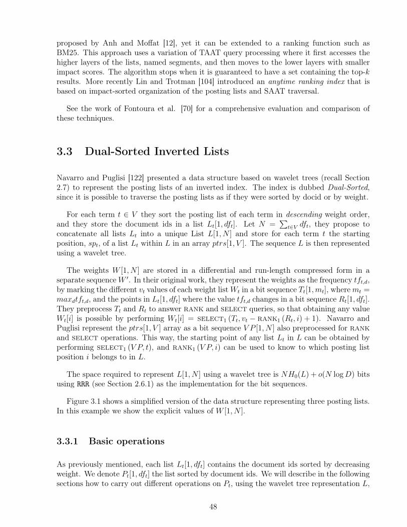
proposed by Anh and Moffat [12], yet it can be extended to a ranking function such asBM25. This approach uses a variation of TAAT query processing where it first accesses thehigher layers of the lists, named segments, and then moves to the lower layers with smallerimpact scores. The algorithm stops when it is guaranteed to have a set containing the top-kresults. More recently Lin and Trotman [104] introduced an anytime ranking index that isbased on impact-sorted organization of the posting lists and SAAT traversal.

See the work of Fontoura et al. [70] for a comprehensive evaluation and comparison ofthese techniques.

3.3 Dual-Sorted Inverted Lists

Navarro and Puglisi [122] presented a data structure based on wavelet trees (recall Section2.7) to represent the posting lists of an inverted index. The index is dubbed Dual-Sorted,since it is possible to traverse the posting lists as if they were sorted by docid or by weight.

For each term t ∈ V they sort the posting list of each term in descending weight order,and they store the document ids in a list Lt[1, dft]. Let N =

∑t∈V dft, they propose to

concatenate all lists Lt into a unique List L[1, N ] and store for each term t the startingposition, spt, of a list Lt within L in an array ptrs[1, V ]. The sequence L is then representedusing a wavelet tree.

The weights W [1, N ] are stored in a differential and run-length compressed form in aseparate sequenceW ′. In their original work, they represent the weights as the frequency tft,d,by marking the different vt values of each weight listWt in a bit sequence Tt[1,mt], wheremt =maxdtft,d, and the points in Lt[1, dft] where the value tft,d changes in a bit sequence Rt[1, dft].They preprocess Tt and Rt to answer rank and select queries, so that obtaining any valueWt[i] is possible by performing Wt[i] = select1 (Tt, vt − rank1 (Rt, i) + 1). Navarro andPuglisi represent the ptrs[1, V ] array as a bit sequence V P [1, N ] also preprocessed for rankand select operations. This way, the starting point of any list Lt in L can be obtained byperforming select1 (V P, t), and rank1 (V P, i) can be used to know to which posting listposition i belongs to in L.

The space required to represent L[1, N ] using a wavelet tree is NH0(L) + o(N logD) bitsusing RRR (see Section 2.6.1) as the implementation for the bit sequences.

Figure 3.1 shows a simplified version of the data structure representing three posting lists.In this example we show the explicit values of W [1, N ].

3.3.1 Basic operations

As previously mentioned, each list Lt[1, dft] contains the document ids sorted by decreasingweight. We denote Pt[1, dft] the list sorted by document ids. We will describe in the followingsections how to carry out different operations on Pt, using the wavelet tree representation L,

48

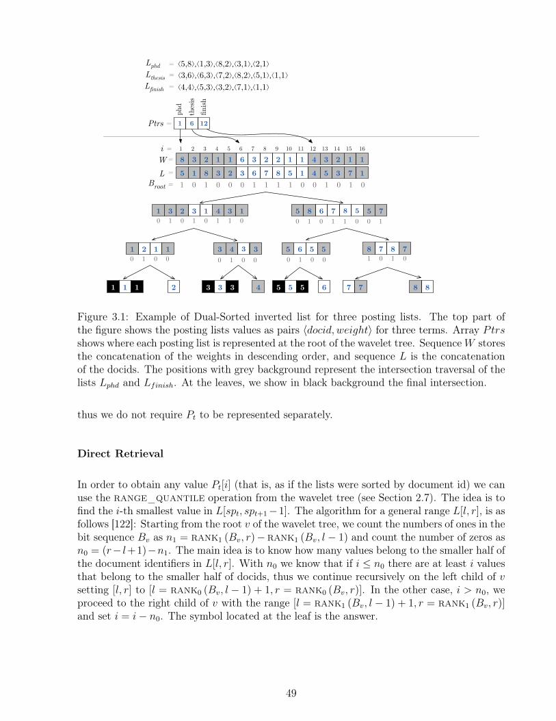
L = 5 1 8 3 2 3 6 7 8 5 1 4 5 3 7

1 3 2 3 1 4 3 5 8 6 7

6

5

2 1 1 3 4 3

1 1 1 2 43 3

5 5

8

88 7

655 8 87

1 0 1 0 0 0 1 1 1 1 0 0 1 0 1 0

0 1 0 1 0 1 1 0 0 1 0 1 1 0 0 1

0 1 0 0 0 1 0 0 0 1 0 0 1 0 1 0

1 2 3 4 5 6 7 8 9 10 11 12 13 14i = 15

Broot =1

16

5 7

7

7

1

LphdLthesisLfinish

W= 8 3 2 1 1 6 3 2 2 1 1 4 3 2 1 1

= ⟨5,8⟩,⟨1,3⟩,⟨8,2⟩,⟨3,1⟩,⟨2,1⟩ = ⟨3,6⟩,⟨6,3⟩,⟨7,2⟩,⟨8,2⟩,⟨5,1⟩,⟨1,1⟩

⟨4,4⟩,⟨5,3⟩,⟨3,2⟩,⟨7,1⟩,⟨1,1⟩

Ptrs

=

= 1 6 12

1

5

5

3

3

finish

thes

isph

d

Figure 3.1: Example of Dual-Sorted inverted list for three posting lists. The top part ofthe figure shows the posting lists values as pairs 〈docid, weight〉 for three terms. Array Ptrsshows where each posting list is represented at the root of the wavelet tree. SequenceW storesthe concatenation of the weights in descending order, and sequence L is the concatenationof the docids. The positions with grey background represent the intersection traversal of thelists Lphd and Lfinish. At the leaves, we show in black background the final intersection.

thus we do not require Pt to be represented separately.

Direct Retrieval

In order to obtain any value Pt[i] (that is, as if the lists were sorted by document id) we canuse the range_quantile operation from the wavelet tree (see Section 2.7). The idea is tofind the i-th smallest value in L[spt, spt+1−1]. The algorithm for a general range L[l, r], is asfollows [122]: Starting from the root v of the wavelet tree, we count the numbers of ones in thebit sequence Bv as n1 = rank1 (Bv, r)−rank1 (Bv, l − 1) and count the number of zeros asn0 = (r− l+1)−n1. The main idea is to know how many values belong to the smaller half ofthe document identifiers in L[l, r]. With n0 we know that if i ≤ n0 there are at least i valuesthat belong to the smaller half of docids, thus we continue recursively on the left child of vsetting [l, r] to [l = rank0 (Bv, l − 1) + 1, r = rank0 (Bv, r)]. In the other case, i > n0, weproceed to the right child of v with the range [l = rank1 (Bv, l − 1) + 1, r = rank1 (Bv, r)]and set i = i− n0. The symbol located at the leaf is the answer.

49

Retrieving a Range

It is also possible to extract a range Pt[i, i′], in docid order, in time O((i′−i+1)(1+log Di′−i+1

)).The procedure is similar to the one previously described: we go to the same branch whenboth i and i′ tell us to do it, and we split the interval into two separate ranges when they donot. The worst case is when we arrive at i′ − i+ 1 leaves of the wavelet tree, but part of thework of arriving at these leave is shared.

3.3.2 Complex Operations

Intersection

Given a candidate document d, an important operation for intersecting posting lists is tofind the first position j such that Pt[j] ≥ d. This is commonly solved with a combination ofregular samplings and linear, binary or exponential search (recall Section 3.2). In order tosolve this operation using the wavelet tree, we start at the root node v, the root bit sequenceBv and the interval L[l, r] that represents the docids of term t, with l = stt and r = stt+1−1.In the case that the number d belongs to the first half, we descend to the left, otherwise wedescend to the right. In both cases we need to update the corresponding ranges l and r asin the procedure to obtain any value Pt[i]. If the interval [l, r] becomes empty, this meansthat there is no value d in the subtree and we return without a value. On the other hand,if we arrive at a leaf with l = r, the leaf represents the document that we are searching forand we return this value. If at some point during the recursion, we return no result, we haveto look for the first result to the right, searching for the smallest document d′ > d. If therecursion was to the right child, or the left but there was no 1 marked in Bv[l, r], we knowthat there is no document d′ bigger than d. Otherwise, we enter to the right child lookingfor the smallest value. From there we follow the leftmost path if there is some 0 in Bv[l, r],otherwise we descend to the right. This way, in at most two root-to-leaf traversals we findthe first d′ ≥ d value in Pt. To obtain j, the position of d′ in Pt, we must perform the sumof all n0 values from all the nodes that were traversed to reach d′ where we have gone to theright. This operation can be carried out in O(logD) time, which is not far from the timerequired to perform a binary search on Pt. In the case that Pt[j] = d, we must look for thefirst value Pt[j′] ≥ d′, that can be done in amortized time proportional to O(log(d′ − d+ 1).

The wavelet tree is capable of performing the Boolean intersection of multiple lists effi-ciently by traversing all list at the same time. We refer to this procedure as range_intersectionand is described in Algorithm 12. Given a set of k x-ranges [xs1, x

e1], [xs2, x

e2]...[xsk, x

ek], this op-

eration returns the y-coordinates that are common to all the x-ranges. The idea is to startfrom the k ranges at the root of the wavelet tree, and as before, project those ranges to theleaves. We map the ranges to the left child and right child of the root using rank0 andrank1. We continue recursively on the branches where all of the k sub-intervals are notempty. If we are able to reach a leaf, then its corresponding symbol is in the intersection.In the worst-case, this operation takes O(

∑ki=1 x

ei − xsi + 1), however there are more detailed

time complexity measures for this operation, see for example the work of Gagie et al. [74,Theorem 8] for a more detailed analysis.

50

Using this operation, this data structure also allows us to carry out another intersectionalgorithm: Let us say that we want to intersect all values that are shared by Pt and P ′t ,we know that the ranges in the wavelet tree for these postings lists are [stt, stt+1 − 1] and[stt′ , stt′+1 − 1]. Now we can apply Algorithm 12. Recall that this algorithm allows us tointersect k ranges, so we can perform the intersection of k posting lists at the same time.

Algorithm 12: Method range_intersect(v, [xs1, . . . , xsk], [x

e1, . . . , x

ek]). Reports all

the symbols that are common in the k x-ranges [xs1, xe1], [xs2, x

e2]...[xsk, x

ek]. We denote xsi

the starting position of the i-th (1 ≤ i ≤ k) range and xei its ending position.

range_intersect(v, [xs1, . . . , xsk], [x

e1, . . . , x

ek])

01 if xs1 > xe1 ∨ . . . xsk > xek then02 return03 if v is a leaf then04 report labels (v)05 return06 rstart_left, rend_left, rstart_right, rend_left ← ∅07 for each xstart ∈ [xs1, . . . , x

sk], xend ∈ [xe1, . . . , x

ek] do

08 rstart_left ← rstart_left ∪ rank0(Bv, xstart − 1) + 1)09 rend_left ← rend_left ∪ rank0(Bv, xend)10 rstart_right ← rstart_right ∪ xstart − xstart_left11 rend_right ← rend_right ∪ xend − xend_left12 end for13 range_intersect(vl, rstart_left, rend_left)14 range_intersect(vr, rstart_right, rend_right)

Union

We can use a similar procedure as the one described in Algorithm 12 for the union. Recallfrom the algorithm that, for reporting a document, all ranges have to reach a leaf. In the caseof the Boolean union, we can relax this condition and allow that some ranges could becomeempty, and we only report the ones that reached the leaves. The cost of this procedure isO(M(1 + log D

m)) , where m is the size of the output and M is the sum, over the returned

documents, of the number of intervals where they appeared.

Ranked Unions

It is possible to support ranked union operations on this data structure by implementingPersin et al.’s algorithm [131]. We use the operation described to extract a range L[i, j] inorder to obtain the whole shortest list, and to extract a prefix of the next lists. The extensionof the prefix to be extracted (according to the threshold on w(t, d) given by the algorithm)is computed by an exponential search on W . Note that the range operation obtains the

51

documents of the lists sorted by docid, which makes it convenient to merge into our set ofaccumulators accd if they are also sorted by docid. Note that W stores tf values; these aremultiplied by idft before accumulating them.

Ranked Intersections

Ranked intersections can be handled by first performing the complete Boolean intersectionand then proceeding to score documents. First, we find the q intervals [st, et] of the querywords using the pointers from the vocabulary to the inverted lists Lt, and sort them byincreasing lengths. Then we use Algorithm 12 for tracking the ranges within the wavelettree. We track all the q ranges simultaneously, stopping as soon as any of those becomesempty. Every time we reach a leaf, it corresponds to a document d that participates inthe intersection. Their term frequencies are available by first obtaining the original positionin sequence L. This can be done by performing select operation using the docid as thesymbol and the leaf position as the number of occurrences. This way we can compute thedocument score, by traversing the tree upwards and obtaining the weight using sequence W .As we obtain each document that belongs to the intersection, we retain the k highest scoreddocuments in a min priority queue containing pairs 〈docid, weight〉 prioritized by weight.

3.4 Compression of Posting Lists

Compression of the postings lists is essential for efficient retrieval, on disk and in mainmemory [166]. The main idea to achieve compression is to differentially encode the docids,whereas the weights are harder to compress. A list of docids 〈d1, d2, d3, . . . dn〉 is representedas a sequence of d-gaps 〈d1, d2 − d1, d3 − d2, . . . , dn − dn−1〉, and variable-length encoding isused to encode the differences (see Section 2.5) Extracting a single list or merging lists is doneoptimally by traversing lists from the beginning, but query processing schemes can be donemuch faster if random access to the sequences is possible. This can be obtained by cuttingthe lists into blocks that are differentially encoded, while storing in a separate sequence theabsolute values of the block headers and pointers to the encoded blocks [51, 145].The resultis a two-level structure: the first contains the sampled values and the second stores theencoded sequence itself. For example, Culpepper and Moffat [51] extract a sample everyp′ = p log n values from the compressed list, where p is a space/time tradeoff parameter.Direct access requires a binary search on the samples list plus the decompression of a within-samples block. Sanders and Transier [145], instead, sample regularly the domain values: allthe values differing only in their p = log(B/n) lowest bits (for a parameter B, typically 8),form a block. The advantages are that binary searches on the top structure, and storingabsolute values in it, are not necessary. A disadvantage is that the blocks are of varyinglength and more values might have to be scanned on average for a given number of samples.

Since bit-aligned codes can be inefficient at decoding as they require several bitwise oper-ations, byte-aligned [147] or word-aligned codes [168, 11] are preferred when the speed is themain concern. Examples of this family of techniques are Variable Byte (VByte), Simple9 and

52

Simple16 (recall Section 2.5). Another approach is to encode blocks of integers at the sametime, this way trying to improve both compression and decoding speed. The most popularblock-based encoding mechanism is known as PForDelta. Any other integer compressionmechanism can be employed to compress the posting lists, providing different space/timetradeoffs. See the work of Trotman [157] for a comprehensive study and comparison of thesetechniques.

Vigna [161] explored an Elias-Fano representation of monotone sequences to representthe docids of the posting lists. Different from the traditional approach, it is not necessaryto represent the list as a sequence of d-gaps. Vigna showed how to perform random accessdirectly over the compressed sequence and implement efficient operators that are useful forskipping when performing intersections. The usage of this compression scheme showed that itis possible to achieve competitive space and time when compared to state-of-the-art methodssuch as γ-δ-Rice and even PForDelta. Ottaviano and Venturini [127] extended this idea byperforming an (1 + ε)-optimal partitioning of the list into chunks, for any ε > 0, and thenencoding both the chunks and their endpoints with Elias-Fano. Their results show that thepartitioned approach offers significantly better compression and similar performance in termsof query time efficiency.

When the lists are sorted by decreasing weight (for approximate ranked unions), thedifferential compression of docids is not possible, in principle. Instead, term weights can bestored differentially. When storing tf values, one can take advantage of the fact that longruns of equal tf values (typically low ones) are frequent, and thus not only perform run-lengthencoding of them, but also sort the corresponding docids increasingly, so as to encode themdifferentially [16, 171].

53

Chapter 4

Inverted Treaps

In this chapter we introduce a new compressed representation for the lists of the invertedindex, which performs ranked intersections and (exact) ranked unions directly. Our repre-sentation is based on the treap data structure (See Section 2.13) , a binary tree that simul-taneously represents a left-to-right and a top-to-bottom ordering. We use the left-to-rightordering for document identifiers (which supports fast Boolean operations) and the top-to-bottom ordering for term weights (which supports the thresholding of results simultaneouslywith the intersection process). Using this data structure, we can obtain the top-k results fora ranked intersection/union without having to produce the full Boolean result first.

We explore different alternatives to engineer the new list representation using state-of-the-art compact data structures to represent the treap topology. The classical differentialrepresentation of docids becomes less efficient in the treap, but in exchange the treap repre-sentation allows us to differentially encode both docids and weights, which compensates forloss. We also present novel algorithms for processing the queries on the treap structure, andcompare their performance against well-known approaches such as WAND [36], Block-Max[59], and Dual-Sorted [99]. Our experiments under the classical tf-idf scoring scheme showthat the space usage of our treap-based inverted index representation is competitive withthe state-of-the-art compressed representations: our faster variant is around 25% larger thanWAND, as large as Block-Max, and 15% smaller than Dual-Sorted. In terms of time, thefastest inverted treap variant outperforms previous techniques in many cases: on ranked one-word queries it is 20 times faster than Dual-Sorted and 25–200 times faster than Block-Max;WAND is even slower. On ranked unions it is from 10 times (for k = 10) to 3 times (fork = 1000) faster than Block-Max, and similarly from 45–50 times to 6–7 times faster thanWAND and Dual-Sorted. It is always the fastest index for one-word and two-word queries,which are the most popular. On ranked intersections, our fastest treap alternative is twice asfast as Block-Max for k = 10, converging to similar times for k = 1000. In the same range ofk, it goes from twice as fast to 40% faster than WAND, and from 80% faster to 10% slowerthan Dual-Sorted. Our inverted treap is always the fastest index up to k = 100. We alsoexperimented under a quantized BM25 scoring scheme, where the fastest inverted treap uses35%–40% more space than Block-Max or Dual-Sorted. It is still slightly better than all thealternatives on ranked unions. For ranked intersections, it is from twice as fast (for k = 10)to 15% slower (for k = 1000) on ranked intersections, still being the fastest for k = 100. On

54

one-word queries, the inverted treap is 20 times faster than Dual-Sorted and 40–300 timesfaster than Block-Max.

Those ranges of k values make this result very relevant both for a first stage retrievinga few hundreds or thousands of documents, or for directly conveying a handful of final re-sults to the user. We also show how to support incremental updates on the treap, makingthis representation a useful alternative for scenarios where new documents must be avail-able immediately. The overhead of allowing for incremental updates compared to our staticalternatives, in terms of space, construction and query times, ranges from 50% to 100%.

The first version of this work appeared in the proceedings of the 36th ACM Special InterestGroup in Information Retrieval (SIGIR) Conference held in Dublin, Ireland on August 2013.An extended version has been submitted for revision to the ACM Transactions on InformationSystems in March 2016. This work has been developed in collaboration with Charles L.AClarke and Alejandro López-Ortíz from the University of Waterloo, Canada.

4.1 Inverted Index Representation

We consider the posting list of each term as a sequence sorted by docids (which act as keys),each with its own term frequency (which act as priorities). Term impacts, or any otherterm weights, may also be used as priorities. We then use a treap to represent this sequence.Therefore the treap will be binary searchable by docid, whereas it will satisfy a heap orderingon the frequencies. This means, in particular, that if a given treap node has a frequency belowa desired threshold, then all the docids below it in the treap can be discarded as well.

Figure 4.1 illustrates a treap representation of a posting list. This treap will be used as arunning example. Ignore for now the differential arrays on the bottom.

4.1.1 Construction

A treap on a list 〈(d1, w1), . . . , (dn, wn)〉 of documents and weights can be built in O(n) timein a left-to-right traversal [27, 22, 69]. Initially, the treap is just a root node (d1, w1). Now,assume we have processed (d1, w1), . . . , (di−1, wi−1) and the rightmost path of the treap, rootto leaf, is v′1, . . . , v′`, each v′j representing the posting (d′j, w

′j). Then we traverse the path

from v′` to v′1, until finding the first node v′j with w′j ≥ wi (assume the treap is the right childof a fake root with weight w′0 = +∞, to avoid special cases). Then, (di, wi) is set as the rightchild of v′j and the former right child of v′j becomes the left child of (di, wi), which becomesthe lowest node in the rightmost path.

Since for every step in this traversal the rightmost path decreases in length, and it cannotincrease in length by more than 1 per posting, the total number of steps is O(n). Underreasonable assumptions (i.e., the weight and the docid are statistically independent and theinput list is already sorted by docid) the height of a treap is O(log n) [108], and so is thelength of its rightmost path. Therefore, the maximum time per insertion is O(log n) expected

55

30

12

39

35

9

4 44

37

22

2715

16

docids = 4 9 12 14 16 22 27 30 35 37 39 42

6 2 14 1 1 2 1 24 6 1 2 1freqs =

24

6

3

2

1

32

1411

1

15

1

32

4

4

14

6

2

2

1

diff docids = 8 5 18 1 1 10 7 30 5 2 5 3

8 4 10 0 0 12 1 24 18 1 1 1diff freqs =7

1

3

2

421

44

3

9

3

Figure 4.1: An example posting list with docids and frequencies and the corresponding treaprepresentation in our scheme. Note that docids (inside the nodes) are sorted inorder andfrequencies (outside the nodes) are sorted top to bottom. The differentially encoded docidsand frequencies are shown below the tree.

(but O(1) worst-case when amortized over all the insertions on the treap).

4.1.2 Compact Treap Representation

To represent this treap compactly we must encode the tree topology, the docids, and theterm frequencies. We discuss only the docids and frequencies in this subsection. Our plan isnot to access the posting lists in sequential form as in classical schemes, thus a differentialencoding for each docid with respect to the previous one is not directly applicable. Instead,we make use of the invariants of the treap data structure.

Let id(v) be the docid of a treap node v, and f(v) its frequency. We represent id(v)and f(v) for the root in plain form, and then represent those of its left and right childrenrecursively. For each node v that is the left child of its parent u, we represent id(u)− id(v)instead of id(v). If, on the other hand, v is the right child of its parent u, we representid(v) − id(u) [47]. In both cases, we represent f(u) − f(v) instead of f(v). Those numbersget smaller as we move downwards in the treap.

The sequence of differentially encoded id(v) and f(v) values is represented according toan inorder traversal of the treap, as show on the bottom of Figure 4.1. As we move downthe treap, we can easily maintain the correct id(v) and f(v) values for any node arrived at,and use it to compute the values of the children as we descend.

56

To do this we need to randomly access a differential value in the sequence, given a node.We store those values in an array indexed by node inorders and use the Direct AddressableCodes (DACs) described in Section 2.8 to directly access the values while taking advantageof their small size.

4.1.3 Representing the Treap Topology

We have shown that if we use a treap to represent posting lists we can differentially encodeboth docids and frequencies, however, we still need to represent the topology. A pointer-basedrepresentation of a treap topology of n nodes requires O(n log n) bits, which is impractical forlarge-scale data. Still, space is not the only concern: we need a compact topology represen-tation that supports fast navigation in order to implement the complex algorithms derivingfrom ranked intersections and unions. In this subsection we introduce three representationsdesigned to be space-efficient and to provide fast navigation over the topology.

Compact Treap using BP

This representation uses the balanced parentheses (BP) described in Section 2.10. However,this representation is designed for general ordinal trees, not for binary trees. For example, ifa node has only one child, general trees cannot distinguish between it being the “left” or the“right” child.

A well-known isomorphism [114] allows us represent a binary tree of n nodes using ageneral tree of n+ 1 nodes: First, a fake root node vroot for the general tree is created. Thechildren of vroot are the nodes in the rightmost path of the treap, from the root to the leaf.Then each of those nodes is converted recursively. The general tree is then represented asa BP sequence SBP[1, 2n + 2]. With this transformation, the original treap root is the firstchild of vroot. The left child of a treap node v is its first child in the general tree and the rightchild of v is its next sibling in the general tree. Moreover, the inorder in the original treap,which we use to access docids and frequencies, corresponds to the preorder in the generaltree, which is easy to compute with parentheses. Figure 4.2 shows the transformed treap forour running example.

Each treap node i is identified with its corresponding opening parenthesis. Thus the rootof the treap is node 2. The inorder of a node i is simply rank1(SBP, i) − 1, the number ofopening parentheses up to i excluding the fake root. The left child of i in the treap, or itsfirst child in the general tree, is simply first_child(i) = i+ 1. If, however, SBP[i+ 1] = 0,this means that i has no first child. For the right child of node i in the treap, or its nextsibling in the general tree, we use next_sibling(i) =close(i)+1, where close returns theclosing parenthesis that matches a given opening parenthesis. If SBP has a 0 in the resultingposition, this means that i has no right child.

Therefore, in addition to rank, we need to implement operation close in constant time.This is achieved with a few additional data structures of size o(n), as described in Section 2.10.

57

30

12

39

35

9

4 44

37

22

2715

16

24

6

3

2

1

32

1411

1

4

14

6

2

2

1

SBP

42

( ( ( ( ) ( ) ) ( ( ( ) ) ( ) ) ( ) ) ( ( ) ) ( ( ( ) ) ( ) ) )1 2 3 4 5 6 7 8 9 1011121314151617181920212223242526272829303132

v1

v1v3

v2 v3

v2

vroot

=

Figure 4.2: The original binary tree edges (dashed) are replaced by a general tree, whosetopology is represented with parentheses. The opening and closing parentheses of nodes v1,v2 and v3 in SBP are shown on the bottom part.

As an example, we demonstrate this procedure using the treap from Figure 4.2. We seethat v1 (the treap’s original root) starts at position i = 2 in SBP. If we want to retrievethe index of its left child, which is node v2, we perform first_child(2). The procedurechecks that SBP[3] is an opening parenthesis, so we can return 3 as the answer for the startingposition of the left node of v1. On the other hand, if want to obtain the position where theright child of v1 begins, which is v3, we perform close(2) + 1 and obtain position 20, whichcontains a 1 and thus corresponds to the starting position of v3.

Compact treap using LOUDS

The LOUDS representation (recall Section 2.10) can be adapted to support binary treesefficiently: for every node in a level-order traversal we append two bits to the bit sequence,setting the first bit to ‘1’ iff the node contains a left child and setting the second to ‘1’ iffthe node contains a right child. For example, a leaf node will be represented as 00, while abinary tree node containing both children is represented as 11. The concatenation of thesebits builds a bit sequence SLOUDS[1, 2n]. Since every node adds two bits to this sequence,we can use the levelwise order i of a node as its identifier, knowing that its two bits are atSLOUDS[2i− 1, 2i].

The LOUDS representation is simpler than BP, as it can be navigated downwards usingonly rank operations. In addition, it does not require the tree isomorphism. Given thesequence SLOUDS representing the treap topology as a binary tree and a node i, we navigate

58

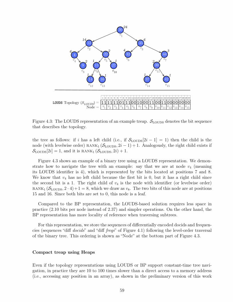
1 3 5 12 11 14 13 18 17 2019 6 7 8 9 10 21 22 23 24 25 26 27 28 29 30

v1 v2

30

12

39

35

9

4 44

37

22

2715

16

24

6

3

2

1

32

1411

1

4

14

6

2

2

1

LOUDS Topology (SLOUDS) =

v1

v2 v3

v4 v5 v6 v7

v8 v9 v10 v11

v12 v13 v14

v3

42v15

1

1111 1101v4 v5 v6 v7 v9 v10 v12 v13

110010 11 001100v14 v15v11

00 000042 16 15

v800

Node =

Figure 4.3: The LOUDS representation of an example treap. SLOUDS denotes the bit sequencethat describes the topology.

the tree as follows: if i has a left child (i.e., if SLOUDS[2i − 1] = 1) then the child is thenode (with levelwise order) rank1 (SLOUDS, 2i− 1) + 1. Analogously, the right child exists ifSLOUDS[2i] = 1, and it is rank1 (SLOUDS, 2i) + 1.

Figure 4.3 shows an example of a binary tree using a LOUDS representation. We demon-strate how to navigate the tree with an example: say that we are at node v4 (meaningits LOUDS identifier is 4), which is represented by the bits located at positions 7 and 8.We know that v4 has no left child because the first bit is 0, but it has a right child sincethe second bit is a 1. The right child of v4 is the node with identifier (or levelwise order)rank1 (SLOUDS, 2 · 4)+1 = 8, which we draw as v8. The two bits of this node are at positions15 and 16. Since both bits are set to 0, this node is a leaf.

Compared to the BP representation, the LOUDS-based solution requires less space inpractice (2.10 bits per node instead of 2.37) and simpler operations. On the other hand, theBP representation has more locality of reference when traversing subtrees.

For this representation, we store the sequences of differentially encoded docids and frequen-cies (sequences “diff docids” and “diff freqs” of Figure 4.1) following the level-order traversalof the binary tree. This ordering is shown as “Node” at the bottom part of Figure 4.3.

Compact treap using Heaps

Even if the topology representations using LOUDS or BP support constant-time tree navi-gation, in practice they are 10 to 100 times slower than a direct access to a memory address(i.e., accessing any position in an array), as shown in the preliminary version of this work

59

[101]. In order to avoid these costly operations, we designed a new compact binary tree rep-resentation that is inspired by binary heaps. The main idea is to take advantage of the factthat a complete binary tree of n nodes does not require any extra information to representits topology, since the values can be represented using just an array of size n. In order tonavigate the tree, we can use traditional binary heap operations: the left child of node i islocated at position 2i and the right child at position 2i + 1. However, a treap posting listrepresentation will rarely be a complete binary tree. Therefore, we take the maximal toppart of the tree that is complete and represent it as a heap. We then recursively representthe subtrees that sprout from the bottom of the complete part. The motivation is to avoidthe use of rank or more complex operations every time we need to navigate down the tree.

We start at the root of the treap and traverse it in levelwise order, looking for the firstnode that does not contain a left or a right child. Say that this happens at level ` of the tree,so we know that all the nodes up to level ` have both left and right children. In other words,the subtree formed by all the nodes starting from the root up to level ` forms a completetree T1 that contains 2` − 1 nodes. Figure 4.4 shows an example, where the first node thatdoes not have a left or right child (v4) is located at level ` = 3, therefore |T1| = 23 − 1 = 7.We then append the differential values of the nodes (docid and frequency) of the completesubtree to the sequences “diff docids” and “diff freqs” (see Figure 4.1), in levelwise order.

For each of the 2`−1 leaves of T1 we write in a bit sequence SHEAP two bits, indicating ifthe corresponding leaf contains a left or a right child, similarly to LOUDS.

We continue this procedure by considering each node located at level `+ 1 as a new root,for further trees Tj. The trees yet to process are appended to a queue, so the trees Tj arealso deployed levelwise. Note that any of these new roots (including the original root) couldlack a left or a right node, in which case we will have a complete subtree of only one node.

We also need a sequence P where P [j] is the starting point of Tj in the sequences of docidsand frequencies. This also serves to compute |Tj| = P [j + 1] − P [j]. Since there may be aconsiderable number of small complete trees, P may require up to n log n bits. To reduce itssize, and considering that P [j+1]−P [j] is of the form 2`−1, we store another array instead,P ′, that stores the number of levels in the corresponding complete binary tree, P ′[0] = 0 andP ′[j + 1] = ` − 1 = log2(|Tj| + 1) − 1. This reduces the space to at most n log log n bits,and the starting position of the sequences of Tj can be obtained as P [j] =

∑j−1i=0 (2P

′[i]+1− 1).To compute this sum faster, we divide P ′ into blocks of fixed size b and store in a separatesequence the sums up to the beginning of each block. This way, we limit to b the number ofelements that are summed up. A similar trick, computing −1 +

∑j−1i=0 2P

′[i]+1 = P [j] + j − 1,gives the starting position of Tj in the bitvector SHEAP.

Figure 4.4 shows our representation. The grey triangles represent the complete trees T1

to T5. On the bottom of the figure we show the extra structures discussed.

In order to navigate the tree we proceed as follows: we represent a node v as a pair 〈j, pos〉,so that v is the node at levelwise-order position pos inside the subtree Tj. To move to theleft child, we just set pos′ = 2 ·pos, and to move to the right child we set pos′ = 2 ·pos+ 1. Ifpos′ ≤ |Tj| we are within the same complete subtree Tj, so we are done. On the other hand,if pos′ > |Tj|, we know two things: first, node v is a leaf within its complete subtree Tj, and

60

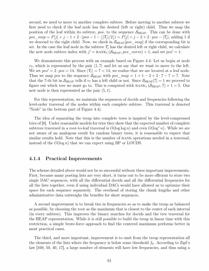
second, we need to move to another complete subtree. Before moving to another subtree wefirst need to check if the leaf node has the desired (left or right) child. Thus we map theposition of the leaf within its subtree, pos, to the sequence SHEAP. This can be done withpos_map = P [j] + j − 1 + 2 · (pos− 1− b|Tj|/2c) = P [j] + j − 2 + 2 · pos− |Tj|, adding 1 ifwe descend to the right child. Now, we check in SHEAP[pos_map] if the corresponding bit isset. In the case the leaf node in the subtree Tj has the desired left or right child, we calculatethe new node subtree index with j′ = rank1 (SHEAP, pos_norm) + 1, and set pos′ = 1.

We demonstrate this process with an example based on Figure 4.4: Let us begin at nodev7, which is represented by the pair 〈1, 7〉 and let us say that we want to move to the left.We set pos′ = 2 · pos = 14. Since |T1| = 7 < 14, we realize that we are located at a leaf node.Thus we map pos to the sequence SHEAP with pos_map = 1 + 1 − 2 + 2 · 7 − 7 = 7. Notethat the 7-th bit in SHEAP tells if v7 has a left child or not. Since SHEAP[7] = 1 we proceed tofigure out which tree we must go to. This is computed with rank1 (SHEAP, 7) + 1 = 5. Ournew node is then represented as the pair 〈5, 1〉.

For this representation, we maintain the sequences of docids and frequencies following thelevel-order traversal of the nodes within each complete subtree. This traversal is denoted“Node” in the bottom part of Figure 4.4).

The idea of separating the treap into complete trees is inspired by the level-compressedtries of [8]. Under reasonable models for tries they show that the expected number of completesubtrees traversed in a root-to-leaf traversal is O(log log n) and even O(log∗ n). While we arenot aware of an analogous result for random binary trees, it is reasonable to expect thatsimilar results hold. Note that this is the number of rank operations needed in a traversal,instead of the O(log n) that we can expect using BP or LOUDS.

4.1.4 Practical Improvements

The scheme detailed above would not be so successful without three important improvements.First, because many posting lists are very short, it turns out to be more efficient to store twosingle DAC sequences, with all the differential docids and all the differential frequencies forall the lists together, even if using individual DACs would have allowed us to optimize theirspace for each sequence separately. The overhead of storing the chunk lengths and otheradministrative data outweighs the benefits for short sequences.

A second improvement is to break ties in frequencies so as to make the treap as balancedas possible, by choosing the root as the maximum that is closest to the center of each interval(in every subtree). This improves the binary searches for docids and the tree traversal forthe HEAP representation. While it is still possible to build the treap in linear time with thisrestriction, a simple brute-force approach to find the centered maximum performs better inmost practical cases.

The third, and more important, improvement is to omit from the treap representation allthe elements of the lists where the frequency is below some threshold f0. According to Zipf’slaw [169, 50, 40, 17], a large number of elements will have low frequencies, and thus using a

61

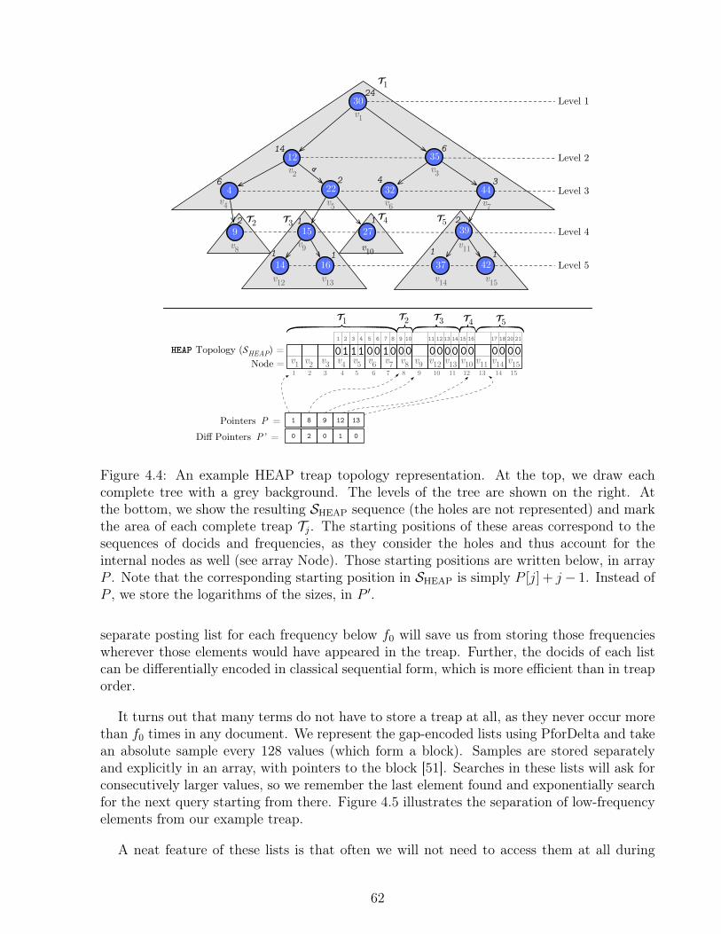
1 3 5 1211 1615 6 7 8 9 10 17 18 20 2142 14 13

30

12

9

4

24

6

3

2

114

11

1

4

14

6

2

2

1

HEAP Topology (SHEAP) =

d

v1

v2 v3

v4 v5 v6 v7

v8 v9 v10v11

v12 v13 v14 v15

1

v1 v2 v301v4 v5 v6 v7 v9 v12 v10 v11

00 10 00 00v14 v15v130000

v800

1 8 9 12 13

11 00

0 2 0 1 0

Pointers P =Diff Pointers P’ =

Node =

T1

T2 T3 T4 T5

T1 T2 T3 T4 T5

Level 1

Level 2

Level 3

Level 4

35

3222 44

392715

Level 516 37 42

1 2 3 4 5 6 7 8 9 10 11 12 13 14 15

Figure 4.4: An example HEAP treap topology representation. At the top, we draw eachcomplete tree with a grey background. The levels of the tree are shown on the right. Atthe bottom, we show the resulting SHEAP sequence (the holes are not represented) and markthe area of each complete treap Tj. The starting positions of these areas correspond to thesequences of docids and frequencies, as they consider the holes and thus account for theinternal nodes as well (see array Node). Those starting positions are written below, in arrayP . Note that the corresponding starting position in SHEAP is simply P [j] + j − 1. Instead ofP , we store the logarithms of the sizes, in P ′.

separate posting list for each frequency below f0 will save us from storing those frequencieswherever those elements would have appeared in the treap. Further, the docids of each listcan be differentially encoded in classical sequential form, which is more efficient than in treaporder.

It turns out that many terms do not have to store a treap at all, as they never occur morethan f0 times in any document. We represent the gap-encoded lists using PforDelta and takean absolute sample every 128 values (which form a block). Samples are stored separatelyand explicitly in an array, with pointers to the block [51]. Searches in these lists will ask forconsecutively larger values, so we remember the last element found and exponentially searchfor the next query starting from there. Figure 4.5 illustrates the separation of low-frequencyelements from our example treap.

A neat feature of these lists is that often we will not need to access them at all during

62

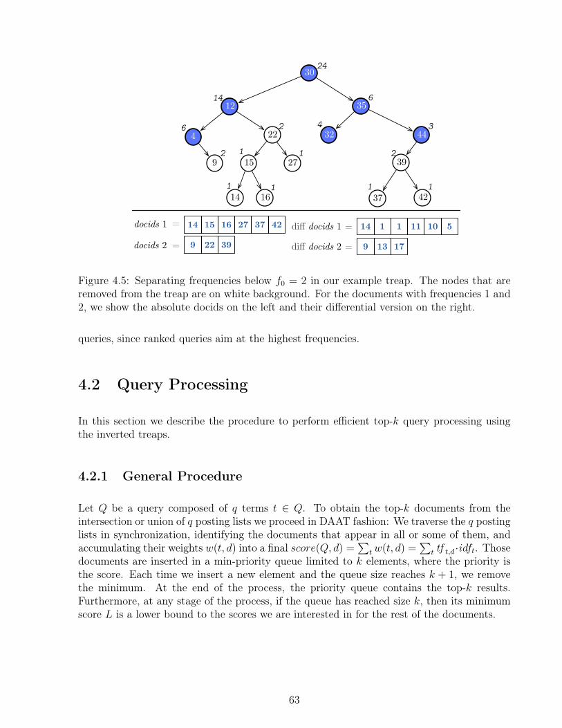
30

12

39

35

9

4 44

37

22

2715

16

24

6

3

2

1

32

1411

1

4

14

6

2

2

1

docids 1 =14 15 16 27 4237

421

docids 2 = 9 22 39

diff docids 1 14 1 1 11 510=

= diff docids 2 9 13 17

Figure 4.5: Separating frequencies below f0 = 2 in our example treap. The nodes that areremoved from the treap are on white background. For the documents with frequencies 1 and2, we show the absolute docids on the left and their differential version on the right.

queries, since ranked queries aim at the highest frequencies.

4.2 Query Processing

In this section we describe the procedure to perform efficient top-k query processing usingthe inverted treaps.

4.2.1 General Procedure

Let Q be a query composed of q terms t ∈ Q. To obtain the top-k documents from theintersection or union of q posting lists we proceed in DAAT fashion: We traverse the q postinglists in synchronization, identifying the documents that appear in all or some of them, andaccumulating their weights w(t, d) into a final score(Q, d) =

∑tw(t, d) =

∑t tf t,d ·idft. Those

documents are inserted in a min-priority queue limited to k elements, where the priority isthe score. Each time we insert a new element and the queue size reaches k + 1, we removethe minimum. At the end of the process, the priority queue contains the top-k results.Furthermore, at any stage of the process, if the queue has reached size k, then its minimumscore L is a lower bound to the scores we are interested in for the rest of the documents.

63

4.2.2 Intersections

Let d be the smallest docid not yet considered (initially d = 1). Every treap t involved in thequery Q maintains a stack of nodes (initially holding just a sentinel value element ut withid(ut) = +∞ and f(ut) = +∞), and a cursor vt (initially the treap root). The stack willcontain the nodes in the path from the root to vt where we descend by the left child. We willalways call ut the top of the stack, thus ut is an ancestor of vt and it holds id(ut) > id(vt).

We advance in all the treaps simultaneously towards a node v with docid id(v) = d, whileskipping nodes using the current lower bound L. In all the treaps t we maintain the invariantthat, if v is in the treap, it must appear in the subtree rooted at vt. In particular, this impliesd < id(ut).

Because of the decreasing frequency property of treaps, if d is in a node v within thesubtree rooted at vt, then f(v) ≤ f(vt). Therefore, we can compute an upper bound U to thescore of document d by using values f(vt) instead of f(v), for example U =

∑t∈Q f(vt) · idft

for a tf-idf scoring1. If this upper bound is U ≤ L, then there is a valid top-k answer whered does not participate, so we can discard d. Further, no node that is below all the currentvt nodes can qualify. Therefore, we can safely compute a new target d← mint(id(ut)). Eachtime the value of d changes (it always increases), we must update the stack of all the treaps tto restore the invariants: While id(ut) ≤ d, we assign vt ← ut and remove ut from the stack.We then resume the global intersection process with this new target d. The upper bound Uis recomputed incrementally each time any vt value changes (U may increase or decrease).

When U > L, it is still feasible to find d with sufficiently high score. In this case we haveto advance towards the node containing d in some treap. We obtained the best results bychoosing the treap t of the shortest list. We must choose a treap where we have not yetreached d; if we have reached d in all the treaps then we can output d as an element of theintersection, with a known score (the current U value is the actual score of d), insert it inthe priority queue of top-k results as explained (which may increase the lower bound L),and resume the global intersection process with d← d+ 1 (we must update stacks, as d haschanged).

In order to move towards d 6= id(vt) in a treap t, we proceed as follows. If d < id(vt), wemove to the left child of vt, lt, push vt in the stack, and make vt ← lt. Instead, if d > id(vt),we move to the right child of vt, rt, and make vt ← rt. We then recompute U with the newvt value.

If we have to move to the left and there is no left child of vt, then d does not belong tothe intersection. We stay at node vt and redefine a new target d ← id(vt). If we have tomove to the right and there is no right child of vt, then again d is not in the intersection. Wemake vt ← ut, remove ut from the stack, and redefine d ← id(ut). In both cases we adjustthe stacks of the other treaps to the new value of d, as before, and resume the intersectionprocess.

1Replacing f(v) by f(vt) will yield an upper bound whenever the scoring function is monotonic with thefrequencies. This is a reasonable assumption and holds for most weighting formulas, including tf-idf andBM25.

64

Algorithm 13 gives pseudocode for the intersection. The auxiliary methods report,changev and changed are shown in Algorithms 14,15 and 16 respectively.

Algorithm 13: Method treap_intersect(Q, k). Performs a ranked intersection fromquery terms Q and returns the top-k documents and scores.

treap_intersect(Q, k)01 results← ∅ // priority queue of pairs 〈key, priority〉02 for t ∈ Q do03 stackt ← 〈⊥〉 // stack of treap t, id(⊥) = f(⊥) = +∞04 vt ← root of treap t05 end for06 d← 1, L← −∞07 while d < +∞ do08 while U ≤ L do09 changed(mint∈Q id(top(stackt)), stack, U, d)10 end while11 if ∀t ∈ Q, d = id(vt)12 report(d, U, k, results)13 changed(d+ 1, stack, U, d)14 else15 t← treap of shortest list such that d 6= id(vt)16 if d < id(vt) then17 lt ← left child of vt18 if lt is not null then19 push(stackt,vt), changev(t, lt, U)20 else21 changed(id(vt), stack, U, d)22 end if23 else24 rt ← right child of vt25 if rt is not null26 changev(t, rt, U)27 else28 changev(t,pop(stackt), U)29 changed(id(vt), stack, U, d)30 end if31 end if32 end if33 end while34 return results

65

Algorithm 14: Method report(d, s, k, results). Maintains the top-k candidates in themin-priority queue results, d is the document to be inserted, s is the correspondingscore, k is the top-k variable, and results is the min priority queue.

report(d, s, k, results)01 results← results ∪ (d, s)02 if |results| > k do03 remove minimum from results, L← minimum priority in results04 end if

Algorithm 15: Method changev(t, v, U). Changes the contribution in U according tothe current node in v in t.

changev(t, v)01 remove contribution of f(vt) from U , e.g. U − f(vt) · idft02 vt ← v03 add contribution of f(vt) to U , e.g. U + f(vt) · idft

Algorithm 16: Method changed(newd, stack, U). Changes the current documentcandidate to be evaluated.

changed(newd, stack, d)01 d← newd02 for t ∈ Q do03 v ← vt04 while d ≥ id(top(stackt)) do05 v ←top(stackt)06 pop(stackt)07 end while08 changev(t, v, U)09 end for

Handling low-frequency lists

We have not yet considered the lists of documents with frequencies up to f0, which arestored separately, one per frequency, outside the treap. While a general solution is feasible(but complicated), we describe a simple strategy for the case f0 = 1, which is the case weimplemented.

Recall that we store the posting lists in gap-encoded blocks. Together with the treapcursor, we will maintain a list cursor, which points inside some block that has been previously

66

decompressed. Each time there is no left or right child in the treap, we must search the listfor potential elements omitted in the treap. More precisely, we look for elements in the range[d, id(vt)− 1] if we cannot go left, or in the range [d, id(ut)− 1] if we cannot go right. Thoseelements must be processed as if they belonged to the treap before proceeding in the actualtreap. Finding this new range [l, r] in the list may imply seeking and decompressing a newblock.

The cleanest way to process range [l, r] is to search as if it formed a subtree fully skewedto the right, descending from vt. If we descended to the left of vt towards the range, we pushvt into the stack. Since all the elements in the list have the same frequency, when we arerequired to advance towards (a new) d we simply scan the interval until reaching or exceedingd, and the docid found acts as our new id(vt) value. When the interval [l, r] is exhausted, wereturn to the treap. Note that the interval [l, r] may span several physical list blocks, whichmay be subsequently decompressed.

4.2.3 Unions

The algorithm for ranked unions requires a few changes on the algorithm for intersections.First, in the two lines that call changed(id(vt)), we do not change the d for all the treapswhen the current treap does not find it. Rather, we keep values nextdt where each treap storesthe minimum d′ ≥ d it contains, thus those lines are changed by nextdt ← id(vt). Second, wewill choose the treap t to advance only among those where id(vt) 6= d and nextdt = d, as ifnextdt > d we cannot find d in treap t. Third, when all the treaps t where id(vt) 6= d satisfynextdt > d, we have found exactly the treaps where d appears. We add up score(Q, d) overthose treaps where id(vt) = d, report d, and advance to d+ 1. If, however, this happens butno treap t satisfies id(vt) = d, we know that d is not in the union and we can advance dwith changed(mint∈Q nextdt). Finally, changed(newd) should not only update d but alsoupdate, for all the treaps t, nextdt to max(nextdt, newd).

Algorithm 17 gives the detailed pseudocode. A special case for the method changed hasto be implemented for this case, which is depicted in Algorithm 18.

4.2.4 Supporting Different Score Schemes

Arguably the simplest scoring scheme is to use the sum of term frequencies tft,d of the wordsinvolved in a bag-of-words union or intersection query. This case is easy to implement usinginverted treaps, since the topology is constructed employing the term frequency as the priorityand the term frequencies are represented differentially. A trivial extension is tf-idf scoring:every time we need to calculate U , we multiply the term frequency by the corresponding idft,as shown in Algorithm 13 and Algorithm 17. However, in order to support more complexscoring schemes, such as BM25, additional information is required (i.e., document length) andthe resulting relative order of documents inside a list may be different from tf . In these cases,creating the treap topology based on the the term frequency tft,d is not useful. Moreover,if we actually use the exact score, we would require float or double precision numbers, thus

67

Algorithm 17: Method treap_union(Q, k). Performs a ranked intersection fromquery terms Q and returns the top-k documents and scores.

treap_union(Q, k)01 results← ∅ // priority queue of pairs 〈key, priority〉02 for t ∈ Q do03 stackt ← 〈⊥〉 // stack of treap t, id(⊥) = f(⊥) = +∞04 vt ← root of treap t05 nextdt ← 1 // next possible value in treap t06 end for06 d← 1, L← −∞07 while d < +∞ do08 while U ≤ L do09 changed_union(mint∈Q id(top(stackt)), stack, U, d)10 end while11 if ∀t ∈ Q, d = id(vt) ∨ nextdt > d then12 if ∃t ∈ Q, d = id(vt) then12 report(d, U, k, results)13 changed_union(d+ 1, stack, U, d)14 else16 changed_union(mint∈Qnextdt, stack, U, d)17 end if18 else19 t← treap of shortest list such that d 6= id(vt)16 if d < id(vt) then17 lt ← left child of vt18 if lt is not null then19 push(stackt,vt), changev(t, lt, U)20 else21 nextdt ← id(vt)22 end if23 else24 rt ← right child of vt25 if rt is not null26 changev(t, rt), U27 else28 changev(t,pop(stackt), U)29 nextdt ← id(vt)30 end if31 end if32 end if33 end while34 return results

68

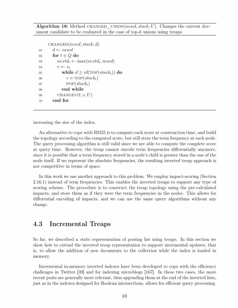
Algorithm 18: Method changed_union(newd, stack, U). Changes the current doc-ument candidate to be evaluated in the case of top-k unions using treaps.

changed(newd, stack, d)01 d← newd02 for t ∈ Q do03 nextdt ← max(nextdt, newd)04 v ← vt05 while d ≥ id(top(stackt)) do06 v ←top(stackt)07 pop(stackt)08 end while09 changev(t, v, U)10 end for

increasing the size of the index.

An alternative to cope with BM25 is to compute each score at construction time, and buildthe topology according to the computed score, but still store the term frequency at each node.The query processing algorithm is still valid since we are able to compute the complete scoreat query time. However, the treap cannot encode term frequencies differentially anymore,since it is possible that a term frequency stored in a node’s child is greater than the one of thenode itself. If we represent the absolute frequencies, the resulting inverted treap approach isnot competitive in terms of space.

In this work we use another approach to this problem. We employ impact-scoring (Section2.16.1) instead of term frequencies. This enables the inverted treaps to support any type ofscoring scheme. The procedure is to construct the treap topology using the pre-calculatedimpacts, and store them as if they were the term frequencies in the nodes. This allows fordifferential encoding of impacts, and we can use the same query algorithms without anychange.

4.3 Incremental Treaps

So far, we described a static representation of posting list using treaps. In this section weshow how to extend the inverted treap representation to support incremental updates, thatis, to allow the addition of new documents to the collection while the index is loaded inmemory.

Incremental in-memory inverted indexes have been developed to cope with the efficiencychallenges in Twitter [39] and for indexing microblogs [167]. In these two cases, the morerecent posts are generally more relevant, thus appending them at the end of the inverted lists,just as in the indexes designed for Boolean intersections, allows for efficient query processing.

69

In main memory, the problem of maintaining such an inverted index up to date is simpler,because the price for non-contiguous storage of the inverted lists is not so high. In a thoroughrecent study, Asadi and Lin [15] show that the difference in query performance between listscut into many short isolated blocks versus fully contiguous lists is only 10%–20% for Booleanintersections and 3%–6% for ranked intersections.

However, there are cases where we require immediate updating of the index but have nopreference for the most recent posts. Obvious examples are online stores like Ebay or Amazon,where new products must be immediately available but they are not necessarily better thanprevious ones. In those cases, we are interested in ranked retrieval using traditional relevancemeasures, which are mostly independent of the insertion time.

While this form of dynamization is simple for the WAND and Block-Max formats [15],it is much more challenging for the treaps, because postings are not physically stored inincreasing document identifier order, and therefore one cannot simply append the insertedpostings at the end of the inverted lists.

4.3.1 Supporting Insertions

Our solution is inspired by the linear-time algorithms for building treaps offline (recall Section4.1.1). We maintain the rightmost path of the tree in uncompressed form, and their leftsubtrees are organized into progressively larger compressed structures. This allows for smoothinsertion times without large sudden reconstructions, reasonable compression performanceand search times.

The main idea is to maintain a treap for each inverted list, as in the static case. How-ever, this treap is only gradually converted into a compressed static structure, and nevercompletely. Some nodes are represented with classical pointers (we call those free nodes),whereas some subtrees are represented in the form of static treaps.

The rightmost path is always composed of free nodes. Some nodes descending from theleft children of those nodes may also be free, but not many. Each free node v stores thenumber F(v) of free nodes in its subtree; these always form a connected subtree rooted atthe node. We use a blocking parameter b, so that when a left child v of a rightmost pathnode has b free nodes or more, all those free nodes are converted into a static treap.

Precisely, when a rightmost node v′j is converted into the left child of a new incoming nodevi, we check if F(v′j) ≥ b (since v′j belonged to the rightmost path, the limit to free nodesdid not apply to it, so if v′j has ` rightmost descendants, it could have up to f(v′j) = b` freenodes descending from it). If F(v′j) ≥ b, all those F(v′j) free nodes are converted into a statictreap and we set F(vi)← 1 for the new node. Otherwise, we set F(vi)← F(v′j) + 1.

Hence, the maximum time per insertion is O(b`), which is O(b log n) in expectation. This,however, does not add up to more than O(n), since static treaps are built in linear time andeach node becomes part of a static tree only once.

70

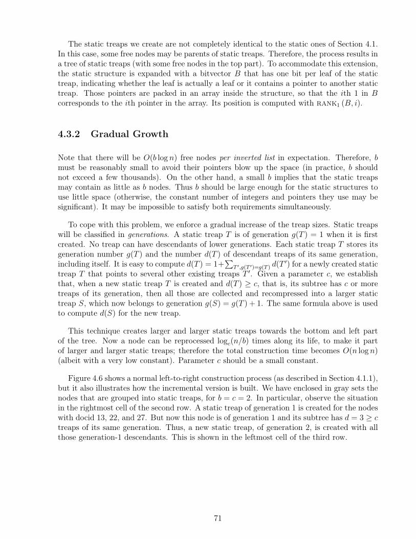
The static treaps we create are not completely identical to the static ones of Section 4.1.In this case, some free nodes may be parents of static treaps. Therefore, the process results ina tree of static treaps (with some free nodes in the top part). To accommodate this extension,the static structure is expanded with a bitvector B that has one bit per leaf of the statictreap, indicating whether the leaf is actually a leaf or it contains a pointer to another statictreap. Those pointers are packed in an array inside the structure, so that the ith 1 in Bcorresponds to the ith pointer in the array. Its position is computed with rank1 (B, i).

4.3.2 Gradual Growth

Note that there will be O(b log n) free nodes per inverted list in expectation. Therefore, bmust be reasonably small to avoid their pointers blow up the space (in practice, b shouldnot exceed a few thousands). On the other hand, a small b implies that the static treapsmay contain as little as b nodes. Thus b should be large enough for the static structures touse little space (otherwise, the constant number of integers and pointers they use may besignificant). It may be impossible to satisfy both requirements simultaneously.

To cope with this problem, we enforce a gradual increase of the treap sizes. Static treapswill be classified in generations. A static treap T is of generation g(T ) = 1 when it is firstcreated. No treap can have descendants of lower generations. Each static treap T stores itsgeneration number g(T ) and the number d(T ) of descendant treaps of its same generation,including itself. It is easy to compute d(T ) = 1+

∑T ′,g(T ′)=g(T ) d(T ′) for a newly created static

treap T that points to several other existing treaps T ′. Given a parameter c, we establishthat, when a new static treap T is created and d(T ) ≥ c, that is, its subtree has c or moretreaps of its generation, then all those are collected and recompressed into a larger statictreap S, which now belongs to generation g(S) = g(T ) + 1. The same formula above is usedto compute d(S) for the new treap.

This technique creates larger and larger static treaps towards the bottom and left partof the tree. Now a node can be reprocessed logc(n/b) times along its life, to make it partof larger and larger static treaps; therefore the total construction time becomes O(n log n)(albeit with a very low constant). Parameter c should be a small constant.

Figure 4.6 shows a normal left-to-right construction process (as described in Section 4.1.1),but it also illustrates how the incremental version is built. We have enclosed in gray sets thenodes that are grouped into static treaps, for b = c = 2. In particular, observe the situationin the rightmost cell of the second row. A static treap of generation 1 is created for the nodeswith docid 13, 22, and 27. But now this node is of generation 1 and its subtree has d = 3 ≥ ctreaps of its same generation. Thus, a new static treap, of generation 2, is created with allthose generation-1 descendants. This is shown in the leftmost cell of the third row.

71

4 9 13 14 15 22 27 30 35 37 39 44

freqs 6 2 14 1 1 2 1 24 6 1 2 3

docids

13

14

4

6

22

2

9

2

14

1

15

1

13

14

4

6

22

2

9

2

14

1

15

1

27

1

2430

13

14

4

6

22

2

9

2

14

1

15

1

27

1

2430

13

1435

6

4

6

22

2

9

2

14

1

15

1

27

1

137

2430

13

1435

6

4

6

22

2

9

2

14

1

15

1

27

1

13

14

4

6

9

2

114

13

14

4

6

9

2

114

15

1

13

14

4

6

9

2

4

6

9

2

4

6

2430

13

1435

6

4

6

22

2

9

2

14

1

15

1

27

1

239

137

2430

13

1435

6

4

6

22

244

3

9

2

14

1

39

2

15

137

1

27

1

Figure 4.6: The left-to-right construction of an example treap. We show in bold the rightmostpath and shade the node that is added in each iteration. Sets of nodes with gray bordersindicate static treaps that are built.

72

Chapter 5

Experimental Evaluation

In this chapter we describe the experimental setup, in terms of the collections used and theenvironment employed for the experiments. We also explain the engineering details requiredto implement the indexes and the baselines, and discuss the space/time results obtained.

5.1 Datasets and Test Environment

We use the TREC GOV2 collection, parsed using the Indri search engine1, and Porter’sstemming algorithm. The collection contains about 25.2 million documents and about 39.8million terms in the vocabulary. The inverted lists contain about 4.9 billion postings in total.After pre-processing and filtering, a plain representation of the GOV2 collection requiresabout 72GB. The average posting list length is 76 and the average document contains 932words.

We also performed experiments using other collections, such as the English Wikipediadump, containing about 5 million documents and 6 million terms. An average Wikipediaarticle contains 352 words and the average number of elements in a posting list is 132. We alsoperformed experiments on the Weblogs collection2, containing about 50 million documentsand requiring 120GB of space. For queries, we used the 50,000 TREC2005 and TREC2006Efficiency Queries dataset with distinct numbers of terms, from q = 2 to 5. We omitted thosenot appearing in our collection, thus we actually have 48,583 queries.

In this work we only show the results obtained using the TREC GOV2 collection, sincethe results over the others do not change significantly.

1http://www.lemurproject.org/indri/2http://www.icwsm.org/data/

73

5.1.1 Baselines and Setup

We compare our results with five baselines: (1) Elias Fano WAND implementation [127],(2) Block-compressed WAND Implementation [36], (3) Block-Max [59], (4) Dual-Sorted [100]and (5) ATIRE [158].

For Elias Fano WAND, we use the implementation 3 provided by the authors [127]; we de-note this implementation EF in the charts. For PforDelta WAND, we use the implementationobtained from the SURF framework4, we denote this implementation WAND in the charts.For Block-Max, we adapted the implementation of [132] by extending it to support rankedintersections and including it into the SURF framework. For both WAND and Block-Max weuse the optimal PForDelta encoding for the docids and Simple9 encoding for the frequencies,as these gave the smallest indexes. The encoding implementations were obtained from theFastPFor library5. In both cases the posting lists were encoded using blocks of 128 values.In the case of Block-Max, we also store the maximum value for every block. We denoteBlock-Max as BMAX in the charts.

We use ATIRE 6 as our baseline for impact-sorted indexes. ATIRE is an open-sourcesearch engine that supports different early termination algorithms based on impact or fre-quency sorted posting lists. We constructed both, frequency-sorted and quantized BM25(q = 8) impact-sorted indexes for our experiments. All baselines were modified when needed,to support both quantized impact BM25 scores (Section 2.16.1) and tf-idf scoring. Our exper-iments were run on a dedicated server with 16 processors Intel Xeon E5-2609 at 2.4GHz, with256 GB of RAM and 10 MB of cache. The operating system is Linux with kernel 3.11.0-1564 bits. We used GNU g++ compiler version 4.8.1 with full optimizations (-O3) flags.

5.1.2 Dual-Sorted Implementation

In the case of Dual-Sorted (see Section 3.3), we make the following practical considerationsto implement this data structure. The wavelet tree is represented using a pointerless version[46] because D is considerably large compared to n. We use the RRR (recall Section 2.6.1) bitsequence representation for the wavelet tree, in order to save space.

We do not use the complex mapping of the bit sequence st; this is replaced by an arrayusing V logN bits, we call it Ptrs (see Figure 3.1) from the terms t to the starting positionsof the lists Lt in L. The weights within the range of each list Lt, which are decreasing, arerepresented in differential form using Rice codes (recall Section 2.5). Absolute values aresampled every K positions, where K is a space/time tradeoff parameter. In fact, as there aremany runs of equal weights, we store only the nonzero differences, and store a bitmapW ′[1, n]indicating which differences are nonzero. So we actually access position W [rank1 (W ′, i)]instead of W [i]. We use the RG representation that uses 5% extra space on top of the bit

3http://github.com/ot/partitioned_elias_fano4http://github.com/simongog/surf5https://github.com/lemire/FastPFor6http://atire.org/index.php?title=Main_Page

74

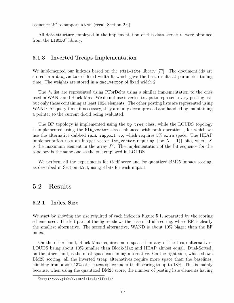
sequence W ′ to support rank (recall Section 2.6).

All data structure employed in the implementation of this data structure were obtainedfrom the LIBCDS7 library.

5.1.3 Inverted Treaps Implementation

We implemented our indexes based on the sdsl-lite library [77]. The document ids arestored in a dac_vector of fixed width 6, which gave the best results at parameter tuningtime. The weights are stored in a dac_vector of fixed width 2.

The f0 list are represented using PForDelta using a similar implementation to the onesused in WAND and Block-Max. We do not use inverted treaps to represent every posting list,but only those containing at least 1024 elements. The other posting lists are represented usingWAND. At query time, if necessary, they are fully decompressed and handled by maintaininga pointer to the current docid being evaluated.

The BP topology is implemented using the bp_tree class, while the LOUDS topologyis implemented using the bit_vector class enhanced with rank operations, for which weuse the alternative dubbed rank_support_v5, which requires 5% extra space. The HEAPimplementation uses an integer vector int_vector requiring dlog(X + 1)e bits, where Xis the maximum element in the array P ′. The implementation of the bit sequence for thetopology is the same one as the one employed in LOUDS.

We perform all the experiments for tf-idf score and for quantized BM25 impact scoring,as described in Section 4.2.4, using 8 bits for each impact.

5.2 Results

5.2.1 Index Size

We start by showing the size required of each index in Figure 5.1, separated by the scoringscheme used. The left part of the figure shows the case of tf-idf scoring, where EF is clearlythe smallest alternative. The second alternative, WAND is about 10% bigger than the EFindex.

On the other hand, Block-Max requires more space than any of the treap alternatives,LOUDS being about 10% smaller than Block-Max and HEAP almost equal. Dual-Sorted,on the other hand, is the most space-consuming alternative. On the right side, which showsBM25 scoring, all the inverted treap alternatives require more space than the baselines,climbing from about 13% of the text space under tf-idf scoring to up to 18%. This is mainlybecause, when using the quantized BM25 score, the number of posting lists elements having

7http://www.github.com/fclaude/libcds/

75

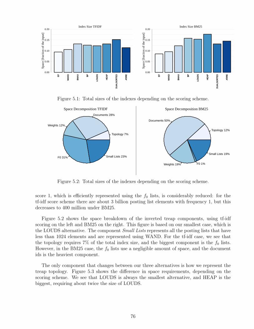
EF

WA

ND

BM

AX

BP

LOU

DS

HE

AP

DU

ALS

OR

TE

D

ATIR

E

Spa

ce [f

ract

ion

of th

e in

put]

0.00

0.05

0.10

0.15

0.20

EF

WA

ND

BM

AX

BP

LOU

DS

HE

AP

DU

ALS

OR

TE

D

ATIR

E

Index Size TFIDF

EF

WA

ND

BM

AX

BP

LOU

DS

HE

AP

DU

ALS

OR

TE

D

ATIR

E

Spa

ce [f

ract

ion

of th

e in

put]

0.00

0.05

0.10

0.15

0.20

EF

WA

ND

BM

AX

BP

LOU

DS

HE

AP

DU

ALS

OR

TE

D

ATIR

E

Index Size BM25

Figure 5.1: Total sizes of the indexes depending on the scoring scheme.

Topology 7%

Documents 28%

Weights 12%

F0 31% Small Lists 23%

Space Decomposition TFIDF

Topology 12%

Documents 50%

Weights 19% F0 1%

Small Lists 19%

Space Decomposition BM25

Figure 5.2: Total sizes of the indexes depending on the scoring scheme.

score 1, which is efficiently represented using the f0 lists, is considerably reduced: for thetf-idf score scheme there are about 3 billion posting list elements with frequency 1, but thisdecreases to 400 million under BM25.

Figure 5.2 shows the space breakdown of the inverted treap components, using tf-idfscoring on the left and BM25 on the right. This figure is based on our smallest case, which isthe LOUDS alternative. The component Small Lists represents all the posting lists that haveless than 1024 elements and are represented using WAND. For the tf-idf case, we see thatthe topology requires 7% of the total index size, and the biggest component is the f0 lists.However, in the BM25 case, the f0 lists use a negligible amount of space, and the documentids is the heaviest component.

The only component that changes between our three alternatives is how we represent thetreap topology. Figure 5.3 shows the difference in space requirements, depending on thescoring scheme. We see that LOUDS is always the smallest alternative, and HEAP is thebiggest, requiring about twice the size of LOUDS.

76

BP

TF

IDF

LOU

DS

TF

IDF

HE

AP

TF

IDF

BP

BM

25

LOU

DS

BM

25

HE

AP

BM

25

BP

TF

IDF

LOU

DS

TF

IDF

HE

AP

TF

IDF

BP

BM

25

LOU

DS

BM

25

HE

AP

BM

25

0.000.020.040.060.080.100.120.140.160.180.200.220.24

Spa

ce [f

ract

ion

of in

dex

size

]

Topology Comparison

Figure 5.3: Sizes of the topology components depending on the scoring scheme.

EF

WA

ND

BM

AX

BP

LOU

DS

HE

AP

ATIR

E

EF

WA

ND

BM

AX

BP

LOU

DS

HE

AP

ATIR

E

0

10

20

30

40

50

60

70

Min

utes

Construction Times TFIDF

EF

WA

ND

BM

AX

BP

LOU

DS

HE

AP

ATIR

E

EF

WA

ND

BM

AX

BP

LOU

DS

HE

AP

ATIR

E

0

10

20

30

40

50

60

70M

inut

es

Construction Times BM25

Figure 5.4: Construction time of the indexes depending on the scoring scheme, in minutes.

5.2.2 Construction Time

Figure 5.4 shows the time required to build each index. We see that the construction timesof the inverted treap alternatives are not so distant from those of the baseline inverted indexrepresentations. This holds except for the HEAP alternative, which is about twice as slow tobuild than the fastest baseline. It is interesting to note that the Elias-Fano WAND approachis 1.4 to 1.8 times slower than the block-compressed WAND implementation. ATIRE wasthe slowest alternative in both cases. We do not include the time required to build theDual-Sorted index, since the construction is not optimized and was above 200 minutes.

77

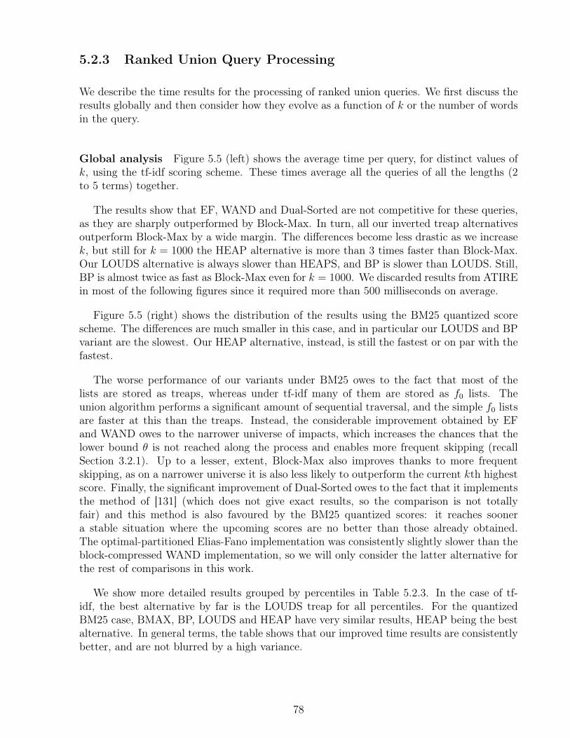
5.2.3 Ranked Union Query Processing

We describe the time results for the processing of ranked union queries. We first discuss theresults globally and then consider how they evolve as a function of k or the number of wordsin the query.

Global analysis Figure 5.5 (left) shows the average time per query, for distinct values ofk, using the tf-idf scoring scheme. These times average all the queries of all the lengths (2to 5 terms) together.

The results show that EF, WAND and Dual-Sorted are not competitive for these queries,as they are sharply outperformed by Block-Max. In turn, all our inverted treap alternativesoutperform Block-Max by a wide margin. The differences become less drastic as we increasek, but still for k = 1000 the HEAP alternative is more than 3 times faster than Block-Max.Our LOUDS alternative is always slower than HEAPS, and BP is slower than LOUDS. Still,BP is almost twice as fast as Block-Max even for k = 1000. We discarded results from ATIREin most of the following figures since it required more than 500 milliseconds on average.

Figure 5.5 (right) shows the distribution of the results using the BM25 quantized scorescheme. The differences are much smaller in this case, and in particular our LOUDS and BPvariant are the slowest. Our HEAP alternative, instead, is still the fastest or on par with thefastest.

The worse performance of our variants under BM25 owes to the fact that most of thelists are stored as treaps, whereas under tf-idf many of them are stored as f0 lists. Theunion algorithm performs a significant amount of sequential traversal, and the simple f0 listsare faster at this than the treaps. Instead, the considerable improvement obtained by EFand WAND owes to the narrower universe of impacts, which increases the chances that thelower bound θ is not reached along the process and enables more frequent skipping (recallSection 3.2.1). Up to a lesser, extent, Block-Max also improves thanks to more frequentskipping, as on a narrower universe it is also less likely to outperform the current kth highestscore. Finally, the significant improvement of Dual-Sorted owes to the fact that it implementsthe method of [131] (which does not give exact results, so the comparison is not totallyfair) and this method is also favoured by the BM25 quantized scores: it reaches soonera stable situation where the upcoming scores are no better than those already obtained.The optimal-partitioned Elias-Fano implementation was consistently slightly slower than theblock-compressed WAND implementation, so we will only consider the latter alternative forthe rest of comparisons in this work.

We show more detailed results grouped by percentiles in Table 5.2.3. In the case of tf-idf, the best alternative by far is the LOUDS treap for all percentiles. For the quantizedBM25 case, BMAX, BP, LOUDS and HEAP have very similar results, HEAP being the bestalternative. In general terms, the table shows that our improved time results are consistentlybetter, and are not blurred by a high variance.

78

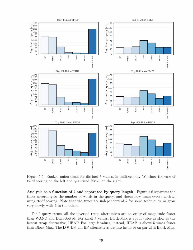
Avg

. tim

e pe

r qu

ery

[ms]

0255075

100125150175200225250275

EF

WA

ND

BM

AX

BP

LOU

DS

HE

AP

DU

ALS

OR

TE

D

Top 10 Union TFIDF

Avg

. tim

e pe

r qu

ery

[ms]

0

25

50

75

100

125

150

175

EF

WA

ND

BM

AX

BP

LOU

DS

HE

AP

DU

ALS

OR

TE

D

Top 10 Union BM25

Avg

. tim

e pe

r qu

ery

[ms]

0255075

100125150175200225250275

EF

WA

ND

BM

AX

BP

LOU

DS

HE

AP

DU

ALS

OR

TE

D

Top 100 Union TFIDF

Avg

. tim

e pe

r qu

ery

[ms]

0

25

50

75

100

125

150

175

EF

WA

ND

BM

AX

BP

LOU

DS

HE

AP

DU

ALS

OR

TE

D

Top 100 Union BM25

Avg

. tim

e pe

r qu

ery

[ms]

0255075

100125150175200225250275

EF

WA

ND

BM

AX

BP

LOU

DS

HE

AP

DU

ALS

OR

TE

D

Top 1000 Union TFIDF

Avg

. tim

e pe

r qu

ery

[ms]

0

25

50

75

100

125

150

175

EF

WA

ND

BM

AX

BP

LOU

DS

HE

AP

DU

ALS

OR

TE

D

Top 1000 Union BM25

Figure 5.5: Ranked union times for distinct k values, in milliseconds. We show the case oftf-idf scoring on the left and quantized BM25 on the right.

Analysis as a function of k and separated by query length Figure 5.6 separates thetimes according to the number of words in the query, and shows how times evolve with k,using tf-idf scoring. Note that the times are independent of k for some techniques, or growvery slowly with k in the others.

For 2 query terms, all the inverted treap alternatives are an order of magnitude fasterthan WAND and Dual-Sorted. For small k values, Block-Max is about twice as slow as thefastest treap alternative, HEAP. For large k values, instead, HEAP is about 5 times fasterthan Block-Max. The LOUDS and BP alternatives are also faster or on par with Block-Max.

79

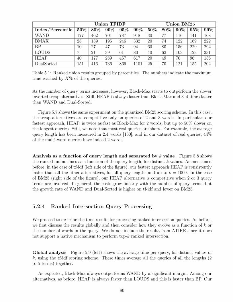
Union TFIDF Union BM25Index/Percentile 50% 80% 90% 95% 99% 50% 80% 90% 95% 99%WAND 177 462 701 787 918 30 77 116 141 168BMAX 28 139 195 246 332 20 74 122 169 222BP 10 27 47 73 94 60 80 156 229 294LOUDS 7 21 39 61 80 40 62 103 123 231HEAP 40 177 289 457 617 20 49 76 96 156DualSorted 151 416 736 866 1101 25 70 121 155 202

Table 5.1: Ranked union results grouped by percentiles. The numbers indicate the maximumtime reached by X% of the queries.

As the number of query terms increases, however, Block-Max starts to outperform the slowerinverted treap alternatives. Still, HEAP is always faster than Block-Max and 3–4 times fasterthan WAND and Dual-Sorted.

Figure 5.7 shows the same experiment on the quantized BM25 scoring scheme. In this case,the treap alternatives are competitive only on queries of 2 and 3 words. In particular, ourfastest approach, HEAP, is twice as fast as Block-Max for 2 words, but up to 50% slower onthe longest queries. Still, we note that most real queries are short. For example, the averagequery length has been measured in 2.4 words [150], and in our dataset of real queries, 44%of the multi-word queries have indeed 2 words.

Analysis as a function of query length and separated by k value Figure 5.8 showsthe ranked union times as a function of the query length, for distinct k values. As mentionedbefore, in the case of tf-idf (left side of the figure), our fastest approach HEAP is consistentlyfaster than all the other alternatives, for all query lengths and up to k = 1000. In the caseof BM25 (right side of the figure), our HEAP alternative is competitive when 2 or 3 queryterms are involved. In general, the costs grow linearly with the number of query terms, butthe growth rate of WAND and Dual-Sorted is higher on tf-idf and lower on BM25.

5.2.4 Ranked Intersection Query Processing

We proceed to describe the time results for processing ranked intersection queries. As before,we first discuss the results globally and then consider how they evolve as a function of k orthe number of words in the query. We do not include the results from ATIRE since it doesnot support a native mechanism to perform top-k ranked intersection.

Global analysis Figure 5.9 (left) shows the average time per query, for distinct values ofk, using the tf-idf scoring scheme. These times average all the queries of all the lengths (2to 5 terms) together.

As expected, Block-Max always outperforms WAND by a significant margin. Among ouralternatives, as before, HEAP is always faster than LOUDS and this is faster than BP. Our

80

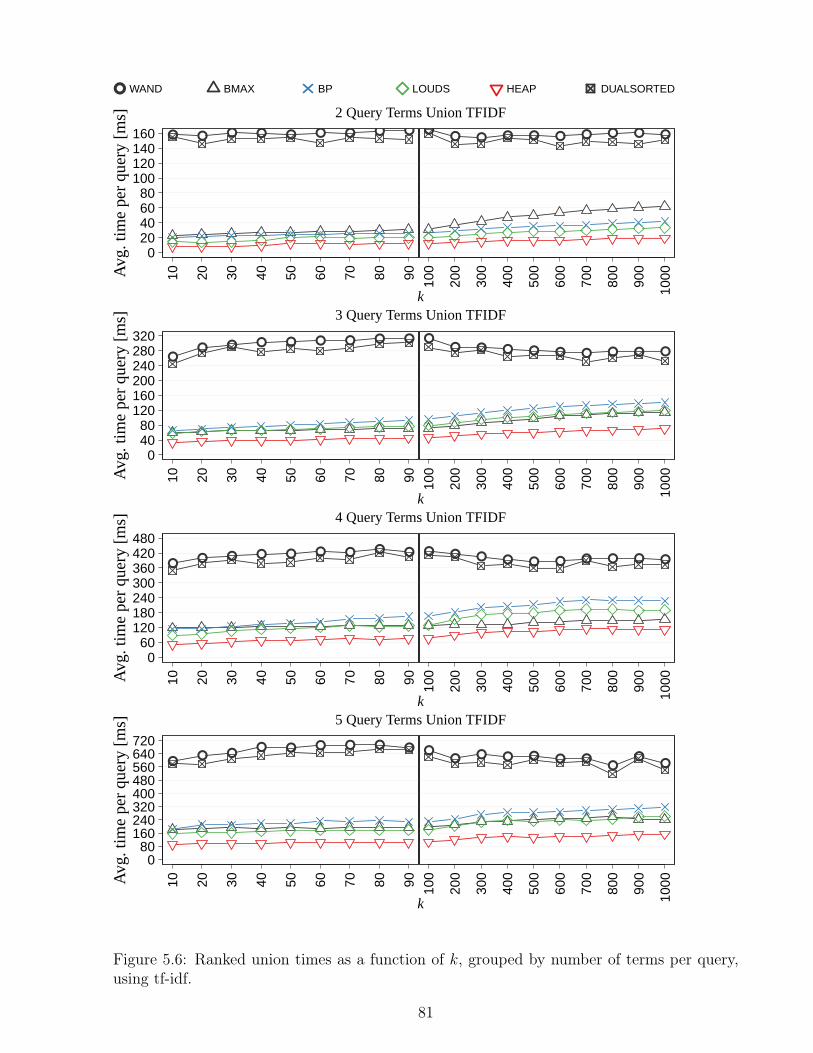
WAND BMAX BP LOUDS HEAP DUALSORTED

A

vg. t

ime

per

quer

y [m

s]

020406080

100120140160

10 20 30 40 50 60 70 80 90

100

200

300

400

500

600

700

800

900

1000

2 Query Terms Union TFIDF

k

Avg

. tim

e pe

r qu

ery

[ms]

04080

120160200240280320

10 20 30 40 50 60 70 80 90

100

200

300

400

500

600

700

800

900

1000

3 Query Terms Union TFIDF

k

Avg

. tim

e pe

r qu

ery

[ms]

060

120180240300360420480

10 20 30 40 50 60 70 80 90

100

200

300

400

500

600

700

800

900

1000

4 Query Terms Union TFIDF

k

Avg

. tim

e pe

r qu

ery

[ms]

080

160240320400480560640720

10 20 30 40 50 60 70 80 90

100

200

300

400

500

600

700

800

900

1000

5 Query Terms Union TFIDF

k

Figure 5.6: Ranked union times as a function of k, grouped by number of terms per query,using tf-idf.

81

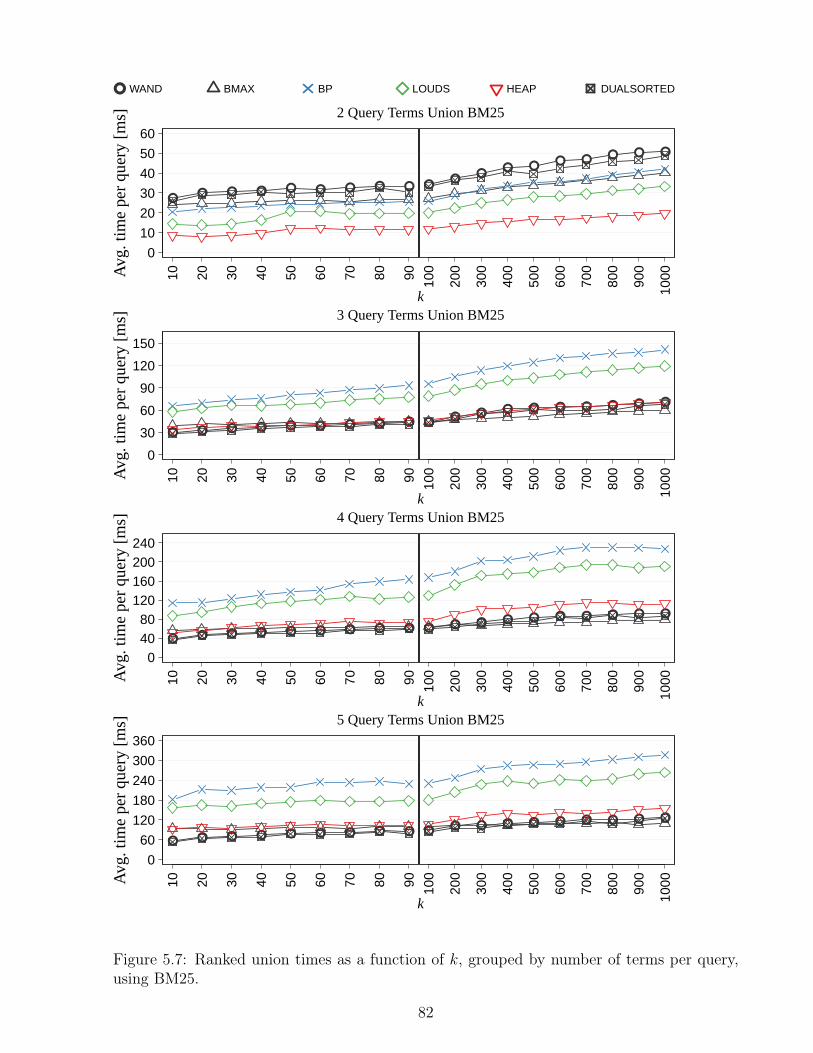
WAND BMAX BP LOUDS HEAP DUALSORTED

Avg

. tim

e pe

r qu

ery

[ms]

0

10

20

30

40

50

60

10 20 30 40 50 60 70 80 90

100

200

300

400

500

600

700

800

900

1000

2 Query Terms Union BM25

k

Avg

. tim

e pe

r qu

ery

[ms]

0

30

60

90

120

150

10 20 30 40 50 60 70 80 90

100

200

300

400

500

600

700

800

900

1000

3 Query Terms Union BM25

k

Avg

. tim

e pe

r qu

ery

[ms]

04080

120160200240

10 20 30 40 50 60 70 80 90

100

200

300

400

500

600

700

800

900

1000

4 Query Terms Union BM25

k

Avg

. tim

e pe

r qu

ery

[ms]

0

60

120

180

240

300

360

10 20 30 40 50 60 70 80 90

100

200

300

400

500

600

700

800

900

1000

5 Query Terms Union BM25

k

Figure 5.7: Ranked union times as a function of k, grouped by number of terms per query,using BM25.

82

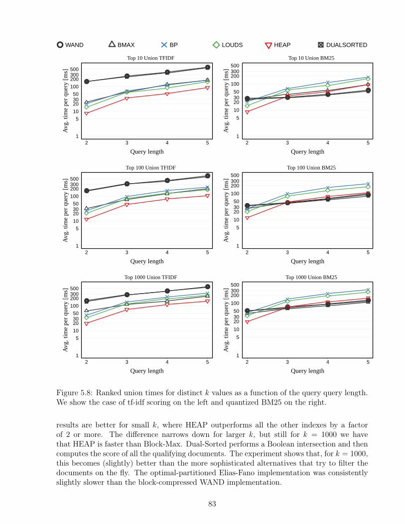
WAND BMAX BP LOUDS HEAP DUALSORTED

A

vg. t

ime

per

quer

y [m

s]

Query length

1

5

10

203050

100

200300500

2 3 4 5

Top 10 Union TFIDF

Avg

. tim

e pe

r qu

ery

[ms]

Query length

1

5

10

203050

100

200300500

2 3 4 5

Top 10 Union BM25

Avg

. tim

e pe

r qu

ery

[ms]

Query length

1

5

10

203050

100

200300500

2 3 4 5

Top 100 Union TFIDF

Avg

. tim

e pe

r qu

ery

[ms]

Query length

1

5

10

203050

100

200300500

2 3 4 5

Top 100 Union BM25

Avg

. tim

e pe

r qu

ery

[ms]

Query length

1

5

10

203050

100

200300500

2 3 4 5

Top 1000 Union TFIDF

Avg

. tim

e pe

r qu

ery

[ms]

Query length

1

5

10

203050

100

200300500

2 3 4 5

Top 1000 Union BM25

Figure 5.8: Ranked union times for distinct k values as a function of the query query length.We show the case of tf-idf scoring on the left and quantized BM25 on the right.

results are better for small k, where HEAP outperforms all the other indexes by a factorof 2 or more. The difference narrows down for larger k, but still for k = 1000 we havethat HEAP is faster than Block-Max. Dual-Sorted performs a Boolean intersection and thencomputes the score of all the qualifying documents. The experiment shows that, for k = 1000,this becomes (slightly) better than the more sophisticated alternatives that try to filter thedocuments on the fly. The optimal-partitioned Elias-Fano implementation was consistentlyslightly slower than the block-compressed WAND implementation.

83

Avg

. tim

e pe

r qu

ery

[ms]

0

5

10

15

20

25

30

35

40

EF

WA

ND

BM

AX

BP

LOU

DS

HE

AP

DU

ALS

OR

TE

D

Top 10 Intersection TFIDF

Avg

. tim

e pe

r qu

ery

[ms]

0

5

10

15

20

25

30

EF

WA

ND

BM

AX

BP

LOU

DS

HE

AP

DU

ALS

OR

TE

D

Top 10 Intersection BM25

Avg

. tim

e pe

r qu

ery

[ms]

0

5

10

15

20

25

30

35

40

EF

WA

ND

BM

AX

BP

LOU

DS

HE

AP

DU

ALS

OR

TE

D

Top 100 Intersection TFIDF

Avg

. tim

e pe

r qu

ery

[ms]

0

5

10

15

20

25

30

EF

WA

ND

BM

AX

BP

LOU

DS

HE

AP

DU

ALS

OR

TE

D

Top 100 Intersection BM25

Avg

. tim

e pe

r qu

ery

[ms]

0

5

10

15

20

25

30

35

40

EF

WA

ND

BM

AX

BP

LOU

DS

HE

AP

DU

ALS

OR

TE

D

Top 1000 Intersection TFIDF

Avg

. tim

e pe

r qu

ery

[ms]

0

5

10

15

20

25

30

EF

WA

ND

BM

AX

BP

LOU

DS

HE

AP

DU

ALS

OR

TE

D

Top 1000 Intersection BM25

Figure 5.9: Ranked intersection times for distinct k values, in milliseconds. We show thecase of tf-idf scoring on the left and quantized BM25 on the right.

Figure 5.9 (right) shows the distribution of the results using the BM25 quantized scorescheme. Unlike in the case of unions, the powerful filtration enabled by the treaps outweighsits slowness compared to traversing an f0 list. As a result, the inverted treaps are faster onBM25 than on tf-idf scores. The methods WAND and Block-Max also improve thanks to thequantized scores. Dual-Sorted also improves: even if it always performs the same Booleanintersection and then computes the scores of the surviving candidates, this computationis faster because it uses the stored quantized scores, whereas for tf-idf it must multiplyeach stored tf by the idf associated with the query term. The comparisons between all thealternatives stay, overall, similar as in the case of tf-idf scoring.

84

Intersection TFIDF Intersection BM25Index/Percentile 50% 80% 90% 95% 99% 50% 80% 90% 95% 99%WAND 4 43 93 178 451 9 35 89 128 223BMAX 29 146 209 260 321 3 29 62 93 156BP 17 42 58 68 77 18 43 67 85 101LOUDS 13 22 34 47 60 12 29 44 56 67HEAP 3 12 18 23 34 9 21 32 42 51DualSorted 24 132 230 287 386 9 33 84 122 212

Table 5.2: Ranked intersection results grouped by percentiles. The numbers indicate themaximum time reached by X% of the queries.

We show detailed results grouped by percentiles in Table 5.2 for all alternatives that wereconsidered. In both cases, tf-idf and BM25, the best alternative is the treap using the HEAPtopology. In general terms, the table shows that our improved time results are consistentlybetter, and are not blurred by a high variance.

Analysis as a function of k and separated by query length Figure 5.10 shows howtimes evolve with k, using tf-idf scoring. As in the ranked unions, some techniques areindependent of k and others (in this case, the inverted treaps with 2 or 3 words) grow slowlywith k.

For 2 query terms, the HEAP alternative is the fastest up to k = 300, from where Block-Max takes over. For 3 and 4 words, HEAP is either the fastest choice or very close to it,and for 5-word queries it takes over again. As mentioned by [59], the performance of Block-Max is considerably affected by the number of terms participating in the query. For 4 queryterms, it is one of the slowest alternatives, together with the BP inverted treap variant. For5 query terms, it is definitely the slowest. This explains the poor performance of Block-Maxcompared to WAND when considering all the queries together.

Figure 5.11 shows the results for ranked intersections on the quantized BM25 scoringscheme. While the general picture is similar to the case of tf-idf, HEAP is overcomed morefrequently. For few-word queries it is outperformed sooner by Block-Max, for k = 200 on 2words and for k = 80 on 3 words. On 4-word queries, it is almost always outperformed bya small margin. It is again the fastest alternative on 5 words, but by a smaller margin thanfor tf-idf. Block-Max is also heavily affected as the number of words increases.

Analysis as a function of query length and separated by k value Figure 5.12 showsthe ranked intersection times as a function of the query length, for distinct k values. Onthe left side of the figure we show the results of the tf-idf scoring scheme. We can see moreclearly how Block-Max is heavily affected by the query length. The others stay unaltered orfluctuate as a function of the number of words. This is because, as this number increases,more lists have to be handled, but it is also more likely to filter out portions of the lists. Theinteraction of the two effects produces increments and decrements in the query times. Recallthat WAND and Dual-Sorted perform a Boolean intersection followed by the evaluation of

85

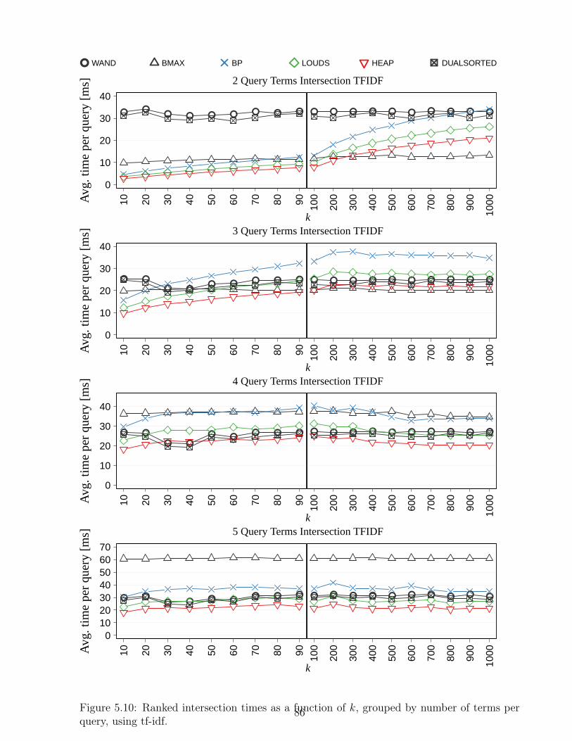
WAND BMAX BP LOUDS HEAP DUALSORTED

Avg

. tim

e pe

r qu

ery

[ms]

0

10

20

30

40

10 20 30 40 50 60 70 80 90

100

200

300

400

500

600

700

800

900

1000

2 Query Terms Intersection TFIDF

k

Avg

. tim

e pe

r qu

ery

[ms]

0

10

20

30

40

10 20 30 40 50 60 70 80 90

100

200

300

400

500

600

700

800

900

1000

3 Query Terms Intersection TFIDF

k

Avg

. tim

e pe

r qu

ery

[ms]

0

10

20

30

40

10 20 30 40 50 60 70 80 90

100

200

300

400

500

600

700

800

900

1000

4 Query Terms Intersection TFIDF

k

Avg

. tim

e pe

r qu

ery

[ms]

010203040506070

10 20 30 40 50 60 70 80 90

100

200

300

400

500

600

700

800

900

1000

5 Query Terms Intersection TFIDF

k

Figure 5.10: Ranked intersection times as a function of k, grouped by number of terms perquery, using tf-idf.

86

WAND BMAX BP LOUDS HEAP DUALSORTED

Avg

. tim

e pe

r qu

ery

[ms]

0

5

10

15

20

25

30

10 20 30 40 50 60 70 80 90

100

200

300

400

500

600

700

800

900

1000

2 Query Terms Intersection BM25

k

Avg

. tim

e pe

r qu

ery

[ms]

0

5

10

15

20

25

30

10 20 30 40 50 60 70 80 90

100

200

300

400

500

600

700

800

900

1000

3 Query Terms Intersection BM25

k

Avg

. tim

e pe

r qu

ery

[ms]

0

5

10

15

20

25

30

10 20 30 40 50 60 70 80 90

100

200

300

400

500

600

700

800

900

1000

4 Query Terms Intersection BM25

k

Avg

. tim

e pe

r qu

ery

[ms]

0

5

10

15

20

25

30

10 20 30 40 50 60 70 80 90

100

200

300

400

500

600

700

800

900

1000

5 Query Terms Intersection BM25

k

Figure 5.11: Ranked intersection times as a function of k, grouped by number of terms perquery, using BM25.

87

all the resulting scores, so their behavior is very similar. Note that our HEAP alternative isgenerally the best on tf-idf, whereas on BM25 it is the best for k = 10 and in some cases forlarger k.

WAND BMAX BP LOUDS HEAP DUALSORTED

Avg

. tim

e pe

r qu

ery

[ms]

Query length

0

10

20

30

40

50

60

70

2 3 4 5

Top 10 Intersection TFIDF

Avg

. tim

e pe

r qu

ery

[ms]

Query length

0

10

20

30

40

2 3 4 5

Top 10 Intersection BM25

Avg

. tim

e pe

r qu

ery

[ms]

Query length

0

10

20

30

40

50

60

70

2 3 4 5

Top 100 Intersection TFIDF

Avg

. tim

e pe

r qu

ery

[ms]

Query length

0

10

20

30

40

2 3 4 5

Top 100 Intersection BM25

Avg

. tim

e pe

r qu

ery

[ms]

Query length

0

10

20

30

40

50

60

70

2 3 4 5

Top 1000 Intersection TFIDF

Avg

. tim

e pe

r qu

ery

[ms]

Query length

0

10

20

30

40

2 3 4 5

Top 1000 Intersection BM25

Figure 5.12: Ranked intersection times for distinct k values as a function of the query length.We show the case of tf-idf scoring on the left and quantized BM25 on the right.

88

5.2.5 One-word Queries

We have not yet considered the simplest one-word queries, which account for a significantpercentage of typical queries (almost 24% in our query set). For these queries, we mustobtain the k highest-ranked documents from a single inverted list. In the case of WAND,this requires traversing the whole list and retaining the k highest scores. Block-Max speedsthis up by skipping blocks where the maximum score is not higher than the kth score wealready know. Dual-Sorted, instead, simply requires to extract the first k elements from thelist of the query term, as its lists are sorted by decreasing frequency. Therefore the Dual-Sorted time is bounded by O(k logD), as it is implemented on a wavelet tree. This is thebest scenario for ATIRE, since the posting lists are sorted by either frequencies or quantizedscores, so returning the k best documents is done simply by traversing the first k postings.

For our inverted treaps, we use a simplification of the procedures for ranked unions andintersections. We insert the root of the treap in a heap that sorts by decreasing score.We then iteratively extract the top of the heap, report its document, and insert its twochildren. Therefore we require O(k) operations on the treap and the heap, leading to totaltime O(k log k).

Figure 5.13 shows the time performance. The time differences are so significant that wehave used logarithmic scale. Our fastest variant, HEAP, requires from 5–10 microsecondsper query with k = 10 to 100–200 with k = 1000, whereas our slower variant, BP, requires10–20 to 200–500 microseconds. Dual-Sorted, instead, goes from 100–200 to 2000–5000 mi-croseconds, that is, around 20 times slower than HEAP. The slowest technique in the plotsis Block-Max, which requires 1–5 milliseconds per query, that is, 25–200 times slower thanHEAPS. This is because its time is not bounded in terms of k. Still, the time of Block-Maxincreases with k because its ability to filter blocks decreases as k grows. On the other hand,the times of the other indexes grows more or less linearly with k after a query initializationtime: A rough fitting gives, for HEAP, 0.15k + 6.5 microseconds on tf-idf and 0.10k + 5 onBM25; for BP it gives 0.5k+ 10 on tf-idf and 0.3k+ 5 on BM25; and for DualSorted it climbsto 4k+ 100 on tf-idf and 2k+ 80 on BM25. ATIRE is clearly the fastest alternative for singleterm queries, as it takes 0.5k microseconds on both cases. We have not included the times ofWAND as they are much higher, 15000 microseconds almost independently of k (note thatWAND needs to decompress the whole list, independently of k, and then find the k largestscores).

5.2.6 Incremental Treaps

Figure 5.14 shows the time required to insert increasing prefixes of the GOV2 collection onour incremental inverted treaps. For these experiments, we use the block parameter b = 1024and recompress any subtree that has generation c = 16 into a new larger static treap (recallSection 4.3.1). These values were chosen by parameter tuning experiments. As a baseline,we consider the static inverted treap construction, for LOUDS and HEAP, on the sameprefixes. The figure shows that the time for incremental treap construction grows slightlysuperlinearly, as expected from its O(n log n) time complexity. The static construction,

89

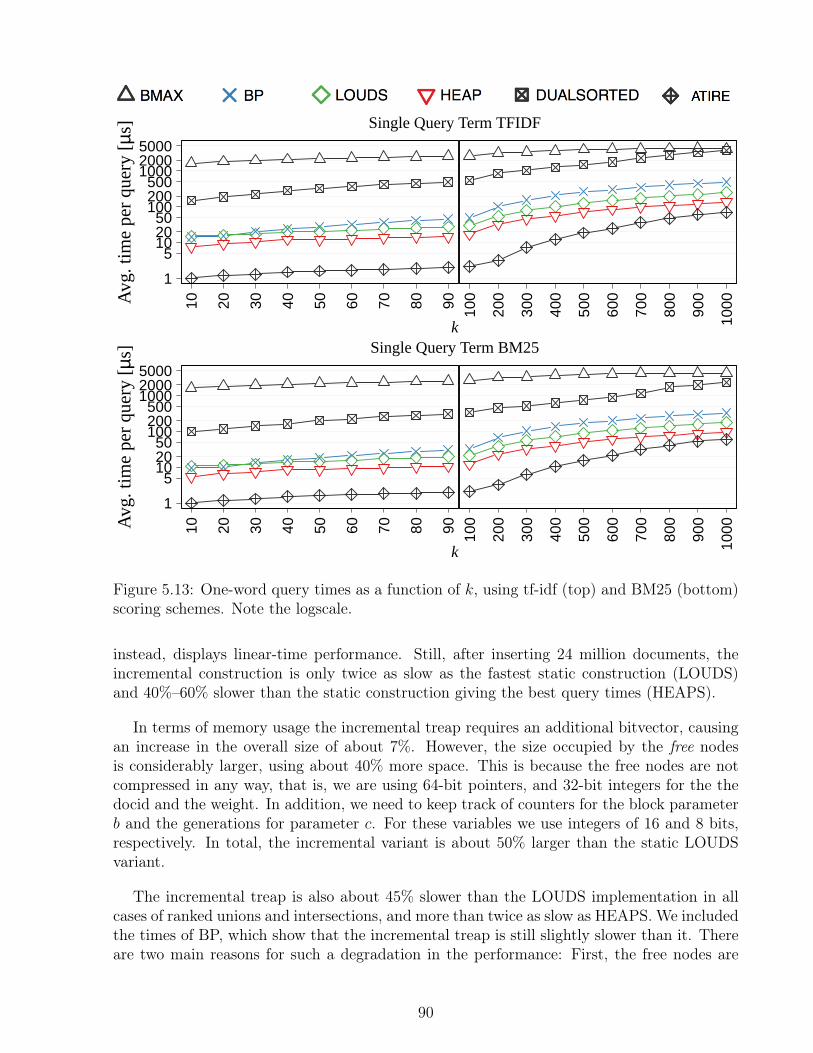
Avg

. tim

e pe

r qu

ery

[µs]

1

5102050

100200500

100020005000

10 20 30 40 50 60 70 80 90 100

200

300

400

500

600

700

800

900

1000

Single Query Term TFIDF

k

Avg

. tim

e pe

r qu

ery

[µs]

1

5102050

100200500

100020005000

10 20 30 40 50 60 70 80 90 100

200

300

400

500

600

700

800

900

1000

Single Query Term BM25

k

Figure 5.13: One-word query times as a function of k, using tf-idf (top) and BM25 (bottom)scoring schemes. Note the logscale.

instead, displays linear-time performance. Still, after inserting 24 million documents, theincremental construction is only twice as slow as the fastest static construction (LOUDS)and 40%–60% slower than the static construction giving the best query times (HEAPS).

In terms of memory usage the incremental treap requires an additional bitvector, causingan increase in the overall size of about 7%. However, the size occupied by the free nodesis considerably larger, using about 40% more space. This is because the free nodes are notcompressed in any way, that is, we are using 64-bit pointers, and 32-bit integers for the thedocid and the weight. In addition, we need to keep track of counters for the block parameterb and the generations for parameter c. For these variables we use integers of 16 and 8 bits,respectively. In total, the incremental variant is about 50% larger than the static LOUDSvariant.

The incremental treap is also about 45% slower than the LOUDS implementation in allcases of ranked unions and intersections, and more than twice as slow as HEAPS. We includedthe times of BP, which show that the incremental treap is still slightly slower than it. Thereare two main reasons for such a degradation in the performance: First, the free nodes are

90

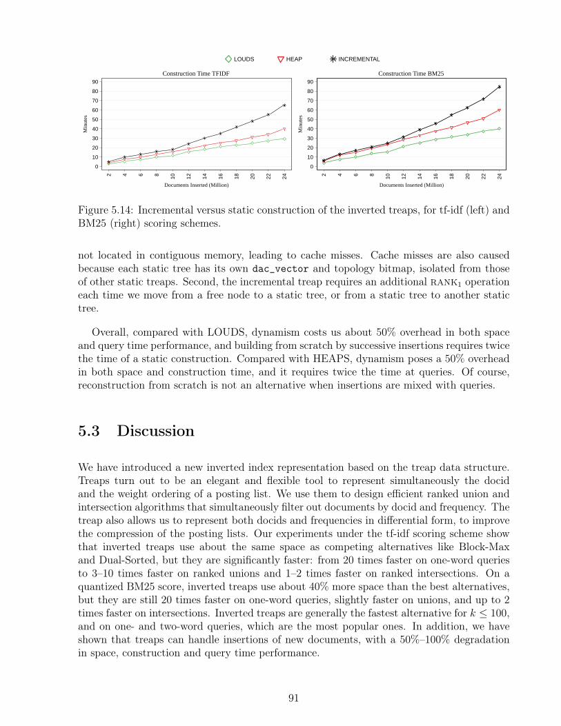
LOUDS HEAP INCREMENTAL

2 4 6 8 10 12 14 16 18 20 22 24

0

10

20

30

40

50

60

70

80

90M

inut

es

Documents Inserted (Million)

Construction Time TFIDF

2 4 6 8 10 12 14 16 18 20 22 24

0

10

20

30

40

50

60

70

80

90

Min

utes

Documents Inserted (Million)

Construction Time BM25

Figure 5.14: Incremental versus static construction of the inverted treaps, for tf-idf (left) andBM25 (right) scoring schemes.

not located in contiguous memory, leading to cache misses. Cache misses are also causedbecause each static tree has its own dac_vector and topology bitmap, isolated from thoseof other static treaps. Second, the incremental treap requires an additional rank1 operationeach time we move from a free node to a static tree, or from a static tree to another statictree.

Overall, compared with LOUDS, dynamism costs us about 50% overhead in both spaceand query time performance, and building from scratch by successive insertions requires twicethe time of a static construction. Compared with HEAPS, dynamism poses a 50% overheadin both space and construction time, and it requires twice the time at queries. Of course,reconstruction from scratch is not an alternative when insertions are mixed with queries.

5.3 Discussion

We have introduced a new inverted index representation based on the treap data structure.Treaps turn out to be an elegant and flexible tool to represent simultaneously the docidand the weight ordering of a posting list. We use them to design efficient ranked union andintersection algorithms that simultaneously filter out documents by docid and frequency. Thetreap also allows us to represent both docids and frequencies in differential form, to improvethe compression of the posting lists. Our experiments under the tf-idf scoring scheme showthat inverted treaps use about the same space as competing alternatives like Block-Maxand Dual-Sorted, but they are significantly faster: from 20 times faster on one-word queriesto 3–10 times faster on ranked unions and 1–2 times faster on ranked intersections. On aquantized BM25 score, inverted treaps use about 40% more space than the best alternatives,but they are still 20 times faster on one-word queries, slightly faster on unions, and up to 2times faster on intersections. Inverted treaps are generally the fastest alternative for k ≤ 100,and on one- and two-word queries, which are the most popular ones. In addition, we haveshown that treaps can handle insertions of new documents, with a 50%–100% degradationin space, construction and query time performance.

91

BP LOUDS HEAP INCREMENTAL

Avg

. tim

e pe

r qu

ery

[ms]

0102030405060708090

10 20 30 40 50 60 70 80 90 100

200

300

400

500

600

700

800

900

1000

Union TFIDF

k

Avg

. tim

e pe

r qu

ery

[ms]

020406080

100120140160

10 20 30 40 50 60 70 80 90 100

200

300

400

500

600

700

800

900

1000

Union BM25

k

Avg

. tim

e pe

r qu

ery

[ms]

05

10152025303540

10 20 30 40 50 60 70 80 90 100

200

300

400

500

600

700

800

900

1000

Intersection TFIDF

k

Avg

. tim

e pe

r qu

ery

[ms]

05

10152025303540

10 20 30 40 50 60 70 80 90 100

200

300

400

500

600

700

800

900

1000

Intersection BM25

k

Figure 5.15: Ranked union and intersection times as a function of k, using tf-idf and BM25,for our static and incremental variants.

92

A future research line is to study the effect of reassigning docids. Some results [59] showthat reassignment can significantly improve both space and processing time. How muchwould treaps improve with such schemes? Can we optimize the reassignment for a treaplayout?

An important part of our gain owed to separating lists with frequency f0 = 1 (this is themain explanation why our scheme performs better on tf-idf than on quantized BM25). Howto efficiently separate lists with higher frequencies or impacts is a challenge, and it can leadto important gains. It is also interesting to explore how this idea could impact on schemeslike Block-Max and Dual-Sorted.

Finally, we have used DAAT processing on our inverted treaps. Such an approach penalizeslong queries, as already noted before in Block-Max [59]. We believe the time would becomealmost nonincreasing with the query length if we used treaps under a TAAT scheme, wherethe longer lists were processed after determining good lower bounds with the shorter lists.This constitutes another interesting line of future work.

93

Part III

Practical Top-k on General Sequences

94

Chapter 6

Top-k Document Retrieval on GeneralSequences

In this chapter we focus on indexing a collection of generic strings to support top-k querieson it. The top-k document retrieval problem can then be defined as follows: a collectionD of D documents, consisting of sequences of total length n over an alphabet of size σ, ispreprocessed so that given a query string P of length m, the system retrieves k documentswith the highest “score” to P , for some definition of score.

The basic solutions to this general problem build a suffix tree [164] or a suffix array [107],which are indexes that can count and list all the individual occurrences of P in the collection,in optimal or near-optimal time. Still this functionality is not sufficient to solve top-k docu-ment retrieval efficiently. The problem of finding top-k documents containing the pattern asa substring, even with a simple relevance measure like term frequency, is challenging. Honet al. [87] presented the first efficient solution, achieving O(m+ log n log log n+ k) time, yetwith super-linear space usage, O(n log2 n) bits. Then Hon et al. [88] improved the solution toO(m+k log k) time and linear space, O(n log n) bits. The problem was then essentially closedby Navarro and Nekrich [119], who achieved optimal O(m+k) time using O(n(log σ+logD))bits.

In practice, however, those solutions are far from satisfactory. Implemented directly fromthe theory, the constants involved in the optimal (and previous) solutions are not small,especially in space: The index can be as large as 80 times the size of the collection, making itunfeasible in practice. Just a part of the solution, the suffix tree, can be 20 times larger thanthe text, and the suffix array, 4 times. There has also been a line of research aiming at optimalspace [116]. While they achieved important theoretical results, a verbatim implementationis likely to be equally unsatisfactory.

The most practical implementations [53, 124, 77] have followed an intermediate path interms of space, using 2–5 times the text size and answering queries within milliseconds.Still, they are toy implementations, limited to relatively small collections of a few hundredmegabytes. They are also restricted to sequences with over small alphabets (usually σ = 255distinct symbols), which prevents using them on sequences of words, for example.

95

In this work, we show that a carefully engineered implementation of the optimal-timeproposal [119] is competitive in space with current implementations and performs ordersof magnitude faster. Our new top-k index implementation uses 2.5–3.0 times the text sizeand answers queries within microseconds, in collections of hundreds of gigabytes and overalphabets of up to millions of symbols. Our experimental comparison shows that our index isorders of magnitude faster than previous heuristics [53], naive solutions [77], and compressedsolutions [124], whereas only the latter uses less space than ours. We also present results oncollections of 500 GB, where the previous structures cannot be built.

Our ability to handle large alphabets allows us apply our index on collections of naturallanguage text, which are regarded as sequences of words (not characters), so that our indexoffers a functionality similar to an inverted index. In this case our index takes up aboutthe same space of the tokenized collection (i.e., one integer per word, and still including thestorage of the collection itself).

An initial version of this work was published in the Data Compression Conference (DCC),2013, held in Salt Lake City, USA. An extended version of this work was submitted forrevision to the ACM Journal on Experimental Algorithms (JEA) on January 2016. Theextended version was developed in collaboration with Simon Gog from Karlsruhe Instituteof Technology (KIT), Germany. Simon Gog provided a faster and smaller re-implementationof the work published in DCC and included the implementation from ALENEX’15 [78]. Healso implemented part of the new indexes presented here.

The first version of this work, published in the DCC conference had an error in themeasurements of the size of the index 1.

6.1 Linear Space Solutions

This section describes in detail the top-k framework of Hon et al. [88] and the subsequentoptimal-time solution of Navarro and Nekrich [119], which is the one we implement in thiswork.

6.1.1 Hon et al. solution

Let T be the suffix tree of the concatenation C of a collection of documents d1, d1, . . . , dD.This tree contains the nodes corresponding to all the suffix trees Ti of the documents di: foreach node u ∈ Ti, there is a node v ∈ T such that path(v) = path(u). We will say thatv = map(u, i). Also, let parent(u) be the parent of u and depth(u) be its depth. The ideaof Hon et al. [88] is to store T with additional information about the trees Ti. For eachv = map(u, i), they store a pointer ptr(v, i) = v′ = map(parent(u), i), noting where theparent of u maps in T . These pointers are stored at the target nodes v′ in a so-called F-list.Together with the pointers ptr(v, i) they also store a weight w(v, i), which is the relevance of

1http://dcc.uchile.cl/~gnavarro/fixes/dcc13.1.html

96

path(u) in di. This relevance can be any function that depends on the set of starting positionsof path(u) in di. In this Part of the thesis, we will focus on a simple one: the number ofleaves of u in Ti, that is, tf(P, d). Let v be the locus in T of a pattern P . They proved that,for each distinct document di where P appears, there is exactly one pointer ptr(v′′, i) = v′

going from a descendant v′′ of v (v itself included) to a (strict) ancestor v′ of v, and w(v′′, i)is the relevance of P in di. Obtaining the top-k documents using this structure boils downto identifying all the pointers in the F-lists of the ancestors of v that come from the subtreeof v, and then selecting k corresponding documents with the highest scores. This task canbe carried out in O(m+ k log k) time and the index requires linear space.

Figure 6.1 shows this structure on our example collection C. The top left part of thefigure shows the the suffix tree T3 corresponding to document d3. The bottom part showsthe generalized suffix tree T of the collection C. The numbers inside the nodes correspond tothe preorder number and the dark nodes are those mapped from T3 to T . The dotted linescorrespond to the pointers ptr(v, i) = map(parent(u), i).

We store the documents and weights as pairs (di, w(v, i)) and append them to the F-lists,which are associated with the node where the pointer arrives. These lists are shown on thetop right part of the figure.

6.1.2 Optimal solution

Navarro and Nekrich [119] presented an optimal O(m+ k) time solution that requires linearspace, O(n log n) bits, for solving the top-k document retrieval problem. They represent thestructure of Hon et al. [88] as a grid of size O(n) × O(n) with labeled weighted points.Each pointer v′ = ptr(v, i) is represented as a point in the grid, whose x-coordinate is thepreorder number of the source v, and whose y-coordinate is the depth of the target v′. Then,the pointers going from the subtree of v to an ancestor of v correspond to the points whosex-coordinate is the preorder range of the subtree of v, and whose y-coordinates are smallerthan the depth of v. By giving weights w(v, i) to the points, the problem boils down toretrieving the k heaviest points in that 3-sided query range.

The construction procedure is the following: they traverse T in preorder, where they addfor each node v ∈ T and pointer ptr(v, i) = v′, a new rightmost x-coordinate with only onepoint, with a y-coordinate value set to depth(v′), weight equal to w(v, i) and label equalto i. To solve a query, they find the locus v of P , determine the range [x1, x2] of all the x-coordinates filled by v or its descendants, find the k heaviest points in [x1, x2]×[0, depth(v)−1],and report their labels. A linear-space representation allows them to carry out this task inoptimal time. Figure 6.2 shows an example of this procedure: the top part

shows the generalized suffix tree T . The grey area corresponds to the locus of the pattern“TA” and the corresponding subtree. The bottom part of the figure shows a two-dimensionalgrid that maps the content of the F-lists. The grey area shows the mapping from the querypattern to a range [x1, x2] in this grid corresponding to the subtree of the locus. The darkgrey area is the final range [x1, x2]× [0, depth(v)−1] from where the procedure finally selectsthe top-k highest-weighted points.

97

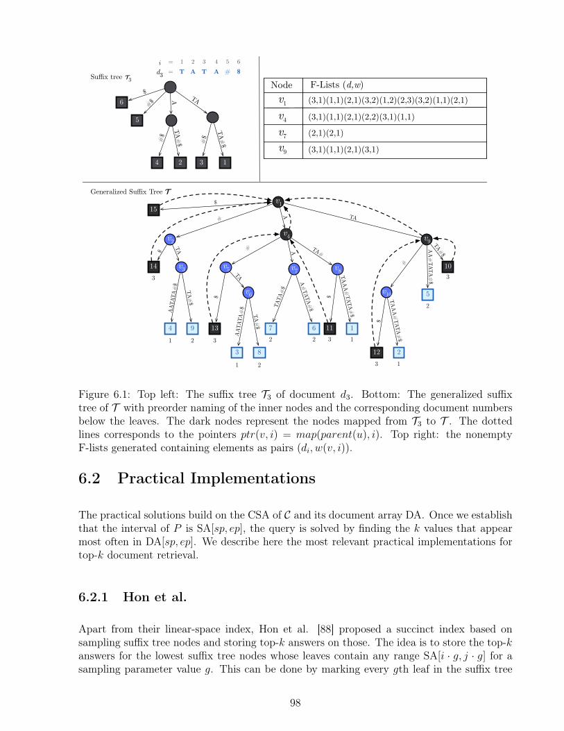
5

3 14 2

d3 T T AA #=1 2 3 4i = 5

Suffix tree T3

Generalized Suffix Tree T

F-Lists (d,w)v1 (3,1)(1,1)(2,1)(3,2)(1,2)(2,3)(3,2)(1,1)(2,1)

(3,1)(1,1)(2,1)(2,2)(3,1)(1,1)

(2,1)(2,1)

Node

(3,1)(1,1)(2,1)(3,1)

$

6

6

v115

v2

14 v3

4 9 13

v6

3 8

v5

7 6

v7

v4

12 2

v10 5

10

v9

3

1 2 3

1 2

2 2

3 1

2

3v8

1113 1

TA

TA#$

AA

#TATA

#$

TAAA#TATA#

$

$

#

TAAA#TATA#

$

$

A#TATA#

$TATA

#$

TA#$

AATA

TA#

$

TA

#

$

A

TA#$

AATA

TA#

$

TA$

#

$

TA#A

TA

TA#$#

$

ATA#

$#$

$

#$

v4

v7

v9

Figure 6.1: Top left: The suffix tree T3 of document d3. Bottom: The generalized suffixtree of T with preorder naming of the inner nodes and the corresponding document numbersbelow the leaves. The dark nodes represent the nodes mapped from T3 to T . The dottedlines corresponds to the pointers ptr(v, i) = map(parent(u), i). Top right: the nonemptyF-lists generated containing elements as pairs (di, w(v, i)).

6.2 Practical Implementations

The practical solutions build on the CSA of C and its document array DA. Once we establishthat the interval of P is SA[sp, ep], the query is solved by finding the k values that appearmost often in DA[sp, ep]. We describe here the most relevant practical implementations fortop-k document retrieval.

6.2.1 Hon et al.

Apart from their linear-space index, Hon et al. [88] proposed a succinct index based onsampling suffix tree nodes and storing top-k answers on those. The idea is to store the top-kanswers for the lowest suffix tree nodes whose leaves contain any range SA[i · g, j · g] for asampling parameter value g. This can be done by marking every gth leaf in the suffix tree

98

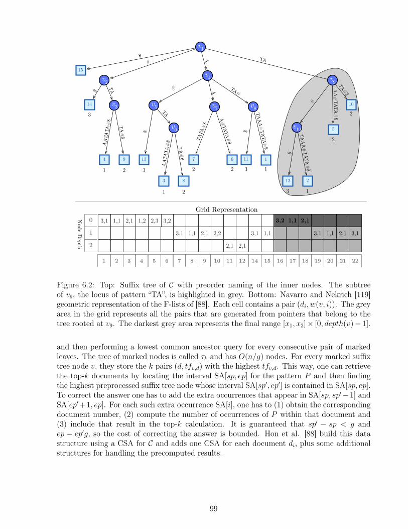
Grid Representation3,1 1,1 2,1 1,2 2,3 3,2

3,1

Node D

epth

1,1 2,1 2,2

2,1 2,1

3,1 1,1

3,2 1,1 2,1

3,1 1,1 2,1 3,1

v1

15

v2

14 v3

4 9 13

v6

3 8

v5

7 6

v7

v4

12 2

v10 5

10

v9

3

1 2 3

1 2

2 2

3 1

2

3v8

111

3 1

TATA#$

AA

#TATA

#$

TAAA#TATA#

$

$

#

TAAA#TATA#

$

$

A#TATA#

$TATA

#$

TA#$

AATA

TA#

$

TA

#

$

A

TA#$

AATA

TA#

$

TA$

#$

TA#A

1 2 3 4 5 6 7 8 9 10 11 12 14 15 16 17 18 19 20 21 22

0

1

2

Figure 6.2: Top: Suffix tree of C with preorder naming of the inner nodes. The subtreeof v9, the locus of pattern “TA”, is highlighted in grey. Bottom: Navarro and Nekrich [119]geometric representation of the F-lists of [88]. Each cell contains a pair (di, w(v, i)). The greyarea in the grid represents all the pairs that are generated from pointers that belong to thetree rooted at v9. The darkest grey area represents the final range [x1, x2]× [0, depth(v)− 1].

and then performing a lowest common ancestor query for every consecutive pair of markedleaves. The tree of marked nodes is called τk and has O(n/g) nodes. For every marked suffixtree node v, they store the k pairs (d, tfv,d) with the highest tfv,d. This way, one can retrievethe top-k documents by locating the interval SA[sp, ep] for the pattern P and then findingthe highest preprocessed suffix tree node whose interval SA[sp′, ep′] is contained in SA[sp, ep].To correct the answer one has to add the extra occurrences that appear in SA[sp, sp′−1] andSA[ep′+1, ep]. For each such extra occurrence SA[i], one has to (1) obtain the correspondingdocument number, (2) compute the number of occurrences of P within that document and(3) include that result in the top-k calculation. It is guaranteed that sp′ − sp < g andep − ep′g, so the cost of correcting the answer is bounded. Hon et al. [88] build this datastructure using a CSA for C and adds one CSA for each document di, plus some additionalstructures for handling the precomputed results.

99

6.2.2 GREEDY

Culpepper et al. [53] studied various heuristics to solve top-k queries on top of a CSA and awavelet tree of the document array DA. They introduced two solutions: Quantile probing andGreedy traversal, both of them based on properties obtained by representing the documentarray using a wavelet tree.

• Quantile probing is based on the observation that in a sorted array A, if there is an itemd with frequency larger than f , then there exists at least one j such that A[j · f ] = d.Culpepper et al. use range quantile queries on the wavelet tree (recall Section 2.7) toretrieve the (j ·f)th document in the sorted DA[sp, ep] without actually sorting it. Thealgorithm makes successive passes using this observation, refining the results at eachstep while storing the candidates in a min-heap of size k.• Greedy traversal. This technique relies on the fact if P appears many times in a doc-

ument d, then the [sp, ep] interval on the path to that document leaf in the wavelettree should also be long. The wavelet tree is traversed the in a greedy fashion, that is,selecting the longest [sp, ep] interval first. Then the algorithm will first reach the leafwith the highest term frequency value. The next document reported will be the second-highest score and so on. This procedure continues until k documents are reported. Weshow this procedure in Algorithm 19.

In practice, the greedy variant outperforms quantile probing.

Culpepper et al. [92] adapted the scheme to large natural language text collections (whereeach word is taken as an atomic symbol), showing that it was competitive with invertedindexes for some queries (see previous work on this line by Patil et al.[129]). The solution,however, resorts to approximations when handling ranked Boolean queries.

6.2.3 NPV

Apart from their linear-space index, Hon et al.[88] proposed a succinct index based on sam-pling suffix tree nodes and storing top-k answers on those. When the locus of P reachesa non-sampled node, they choose the highest sampled node below the locus and correct itsprecomputed answer by considering the additional leaves of the locus. The sampling ensuresthat this work is bounded.

Navarro et al. [124] implemented a practical version of the proposal of Hon et al. [88]and also combined it with the greedy algorithm (see Algorithm 19) of Culpepper et al. [53]to speed up the correction process. They also studied compressed representations of thewavelet tree of DA, by using grammar compression [102] on its bitmaps. They carried out athorough experimental study of these approaches and previous ones, establishing one of thefirst baselines for future comparisons of top-k indexes.

100

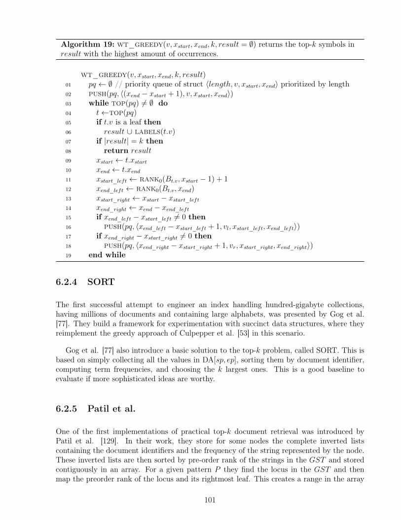
Algorithm 19: wt_greedy(v, xstart, xend, k, result = ∅) returns the top-k symbols inresult with the highest amount of occurrences.

wt_greedy(v, xstart, xend, k, result)01 pq ← ∅ // priority queue of struct 〈length, v, xstart, xend〉 prioritized by length02 push(pq, 〈(xend − xstart + 1), v, xstart, xend〉)03 while top(pq) 6= ∅ do04 t←top(pq)05 if t.v is a leaf then06 result ∪ labels(t.v)07 if |result| = k then08 return result09 xstart ← t.xstart10 xend ← t.xend11 xstart_left ← rank0(Bt.v, xstart − 1) + 112 xend_left ← rank0(Bt.v, xend)13 xstart_right ← xstart − xstart_left14 xend_right ← xend − xend_left15 if xend_left − xstart_left 6= 0 then16 push(pq, 〈xend_left − xstart_left + 1, vl, xstart_left, xend_left〉)17 if xend_right − xstart_right 6= 0 then18 push(pq, 〈xend_right − xstart_right + 1, vr, xstart_right, xend_right〉)19 end while

6.2.4 SORT

The first successful attempt to engineer an index handling hundred-gigabyte collections,having millions of documents and containing large alphabets, was presented by Gog et al.[77]. They build a framework for experimentation with succinct data structures, where theyreimplement the greedy approach of Culpepper et al. [53] in this scenario.

Gog et al. [77] also introduce a basic solution to the top-k problem, called SORT. This isbased on simply collecting all the values in DA[sp, ep], sorting them by document identifier,computing term frequencies, and choosing the k largest ones. This is a good baseline toevaluate if more sophisticated ideas are worthy.

6.2.5 Patil et al.

One of the first implementations of practical top-k document retrieval was introduced byPatil et al. [129]. In their work, they store for some nodes the complete inverted listscontaining the document identifiers and the frequency of the string represented by the node.These inverted lists are then sorted by pre-order rank of the strings in the GST and storedcontiguously in an array. For a given pattern P they find the locus in the GST and thenmap the preorder rank of the locus and its rightmost leaf. This creates a range in the array

101

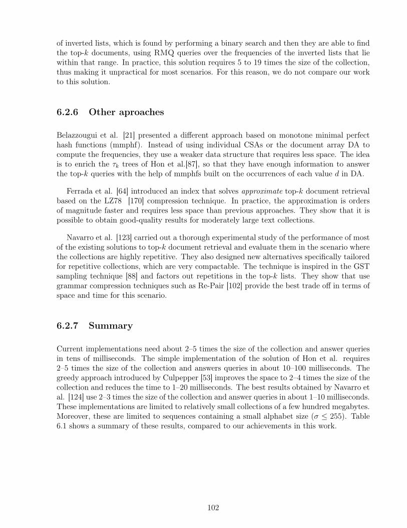
of inverted lists, which is found by performing a binary search and then they are able to findthe top-k documents, using RMQ queries over the frequencies of the inverted lists that liewithin that range. In practice, this solution requires 5 to 19 times the size of the collection,thus making it unpractical for most scenarios. For this reason, we do not compare our workto this solution.

6.2.6 Other aproaches

Belazzougui et al. [21] presented a different approach based on monotone minimal perfecthash functions (mmphf). Instead of using individual CSAs or the document array DA tocompute the frequencies, they use a weaker data structure that requires less space. The ideais to enrich the τk trees of Hon et al.[87], so that they have enough information to answerthe top-k queries with the help of mmphfs built on the occurrences of each value d in DA.

Ferrada et al. [64] introduced an index that solves approximate top-k document retrievalbased on the LZ78 [170] compression technique. In practice, the approximation is ordersof magnitude faster and requires less space than previous approaches. They show that it ispossible to obtain good-quality results for moderately large text collections.

Navarro et al. [123] carried out a thorough experimental study of the performance of mostof the existing solutions to top-k document retrieval and evaluate them in the scenario wherethe collections are highly repetitive. They also designed new alternatives specifically tailoredfor repetitive collections, which are very compactable. The technique is inspired in the GSTsampling technique [88] and factors out repetitions in the top-k lists. They show that usegrammar compression techniques such as Re-Pair [102] provide the best trade off in terms ofspace and time for this scenario.

6.2.7 Summary

Current implementations need about 2–5 times the size of the collection and answer queriesin tens of milliseconds. The simple implementation of the solution of Hon et al. requires2–5 times the size of the collection and answers queries in about 10–100 milliseconds. Thegreedy approach introduced by Culpepper [53] improves the space to 2–4 times the size of thecollection and reduces the time to 1–20 milliseconds. The best results obtained by Navarro etal. [124] use 2–3 times the size of the collection and answer queries in about 1–10 milliseconds.These implementations are limited to relatively small collections of a few hundred megabytes.Moreover, these are limited to sequences containing a small alphabet size (σ ≤ 255). Table6.1 shows a summary of these results, compared to our achievements in this work.

102

Index Max. Max. |C| Size Timeσ in MB (times |C|) in µs

Hon et al. implementation [124] 28 − 1 137 2− 5 104 − 105

GREEDY [53] 28 − 1 100 2− 4 103 − 104

NPV [124] 28 − 1 137 2− 3 103 − 104

Patil et al. [129] 28 − 1 100 5− 19 102 − 103

SORT [77] 264 − 1 72,000 2− 3 104 − 106

Ours 264 − 1 72,000 2− 3 101 − 103

Table 6.1: Comparison of practical results.

103

Chapter 7

Top-k on Grids

Top-k queries on multidimensional weighted point sets ask for the k heaviest points in arange. These type of queries arises most prominently in data mining and OLAP processing(e.g., find the sellers with most sales in a time period) and in GIS applications (e.g., find thecheapest hotels in a city area), but also in less obvious document retrieval applications [119].In the example of sales, one coordinate is the seller id, which is arranged hierarchically toallow queries for sellers, stores, areas, cities, states, etc., and the other is time (in periods ofhours, days, weeks, etc.). Weights are the number of sales made by a seller during a timeslice. Thus the query asks for the k heaviest points in some range Q = [x1, x2] × [y1, y2] ofthe grid.

The optimal solution proposed by Navarro and Nekrich (recall Section 6.1) considers theproblem of top-k document retrieval on general sequences as a geometrical problem: locatethe top-k heaviest points from a two-dimensional query on a grid. In order to develop practicalimplementations of this theoretical work, we need to address the geometrical problem usingdata structures that take into consideration both space and time constraints.

In this chapter we present two data structures to solve this geometrical problem, and theyare a fundamental component that is used for our practical solutions that are detailed inthis part. The first data structure is based on the work of Navarro et al. [120] and makesuse of wavelet trees and RMQ (Section 2.7 and Section 2.12). The second data structure,K2-treap, is a new data structure based on the K2-tree (see Section 2.9) and the Treap (seeSection 2.13) that was developed in collaboration with Nieves R. Brisaboa and Guillermo deBernardo [32].

7.1 Wavelet Trees and RMQ

Recall from Section 2.7 that the wavelet trees can be used to represent a two-dimensionalgrid [1, n]× [1,m] and that it can be regarded as sequence S[1, n] since it has only one pointper column. Now, let us enhance this grid by adding another dimension to each point: aweight. Thus, the sequence now contains pairs as S[i] = 〈si, wi〉. The operation that is of

104

interest to the development of this thesis is to retrieve the top-k maximum points accordingto their weights, that are located within a rectangle Q = [x1, x2]× [y1, y2].

Navarro et al. [120] introduced a solution for two-dimensional range top-k queries basedon wavelet trees. The idea is to enhance the bitmaps of each node of the wavelet tree asfollows: Let p1, . . . , pr be the points represented at a node v, and w(p) be the weight of pointp. Then a range maximum query (RMQ) data structure built on w(p1), . . . , w(pr) is storedtogether with the bitmap. Recall from Section 2.12 that such structure requires 2r+o(r) bitsand finds the maximum weight in any range [w(pi), . . . , w(pj)] in constant time and withoutaccessing the weights themselves. Therefore, the total space becomes 3n logm + o(n logm)bits.

To solve top-k queries on a grid range Q = [x1, x2]× [y1, y2], we first traverse the wavelettree to identify the O(logm) bitmap intervals where the points in Q lie. The heaviest pointin Q in each bitmap interval is obtained with an RMQ, but we need to obtain the actualpriorities in order to find the heaviest among the O(logm) candidates. The priorities arestored sorted by the x- or y-coordinate, so we obtain each one in O(logm) time by trackingthe point with maximum weight at each interval. Thus a top-1 query is solved in O(log2m)time. For a top-k query, we must maintain a priority queue of the candidate intervals and,each time the next heaviest element is found, we remove it from its interval and reinsert it inthe queue with the two resulting subintervals. The total query time is O((k+logm) log(km)).

It is possible to reduce the time to O((k+ logm) logεm) for any constant ε > 0 [119], butthe space usage is much higher, even if linear. A better result, not using wavelet trees, wasintroduced by Prosenjit et al. [112], who presented a succinct data structure matching theoptimal O(log n/ log log n) time using just n+ o(n) integers. This is for n points on an n×ngrid.

We demonstrate this procedure with an example in Figure 7.1. At the top of the tree, weshow the weights of each point in a sequence W [1, n]. At each level of the wavelet tree weshow how the weight sequence is permuted according to the values of the grid points; theyare displayed with grey borders and grey fonts. Let us say that we want to retrieve the top-1value from the range [10, 14] × [3, 7]. We start at the root of the wavelet tree and projectthe values to its left and right child. For all nodes, we do not store the permutation of theweights, instead, we store a RMQ data structure of the permutations. Since the left node ofthe root does not belong completely to the query range, we continue with the traversal untilwe find a node that is fully contained. We perform an RMQ query over projected ranges ofthe suitable nodes. For example, we perform a RMQ query over the range [2, 3] on the nodecontaining the values 343 on the left side of the tree, and obtain the first position of the rangethat contains the maximum value, as shown on the Figure. On the other hand, we perform aRMQ query over the range [6, 7] for the right child of the root, since it is fully contained in thequery range and obtain the second position, which corresponds to the maximum weight valueof the range. We show in black background, the RMQ query results over the ranges. Notethat, since we do not store explicitly the weights at these nodes, we need to traverse down thetree until the last level where we actually store the permutation of W [1, n] according to theleaves in an explicit way. The final step is to obtain the corresponding weight and compareit to the other branches that might have reached a leaf. In this case, the final result is the

105

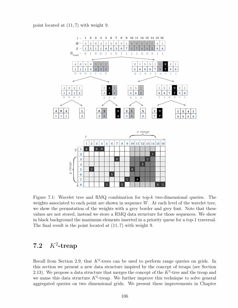
point located at (11, 7) with weight 9.

4 8 41

8 23

2 65

1 91 5 4

1 2 3 4 5 6 7 8 9 11 12 13 14 1512345678

x

y10 16

1

S = 1 5 1 1 8 6 3 8 7 5 7 4 3 2 8

1 1 1 3 4 3 2 5 8 6 8

6

5

1 1 2 3 4 3

1 1 1 2 43 3

5 5

7

78 8

655 8 87

0 1 0 0 1 1 0 1 1 1 1 0 0 0 1 1

0 0 0 1 1 1 0 0 1 0 1 1 0 1 1 1

0 0 0 1 0 1 0 0 1 0 1 1 0 0 1 1

1 2 3 4 5 6 7 8 9 10 11 12 13 14i = 15

=8

16

7 88

7 88

7 8 8

1

x range

y ra

nge

Bvroot

W = 4 2 8 4 1 5 8 5 1 6 9 3 2 1 4 1

4 8 4 8 3 2 1 2 1 5 5 61 9 14

8 4 14 8 3 2 52 1 11 5 9 14

1 5 4 1914 8 4 1 38 2 512

Figure 7.1: Wavelet tree and RMQ combination for top-k two-dimensional queries. Theweights associated to each point are shown in sequence W . At each level of the wavelet tree,we show the permutation of the weights with a grey border and grey font. Note that thesevalues are not stored, instead we store a RMQ data structure for those sequences. We showin black background the maximum elements inserted in a priority queue for a top-1 traversal.The final result is the point located at (11, 7) with weight 9.

7.2 K2-treap

Recall from Section 2.9, that K2-trees can be used to perform range queries on grids. Inthis section we present a new data structure inspired by the concept of treaps (see Section2.13). We propose a data structure that merges the concept of the K2-tree and the treap andwe name this data structure K2-treap. We further improve this technique to solve generalaggregated queries on two dimensional grids. We present these improvements in Chapter

106

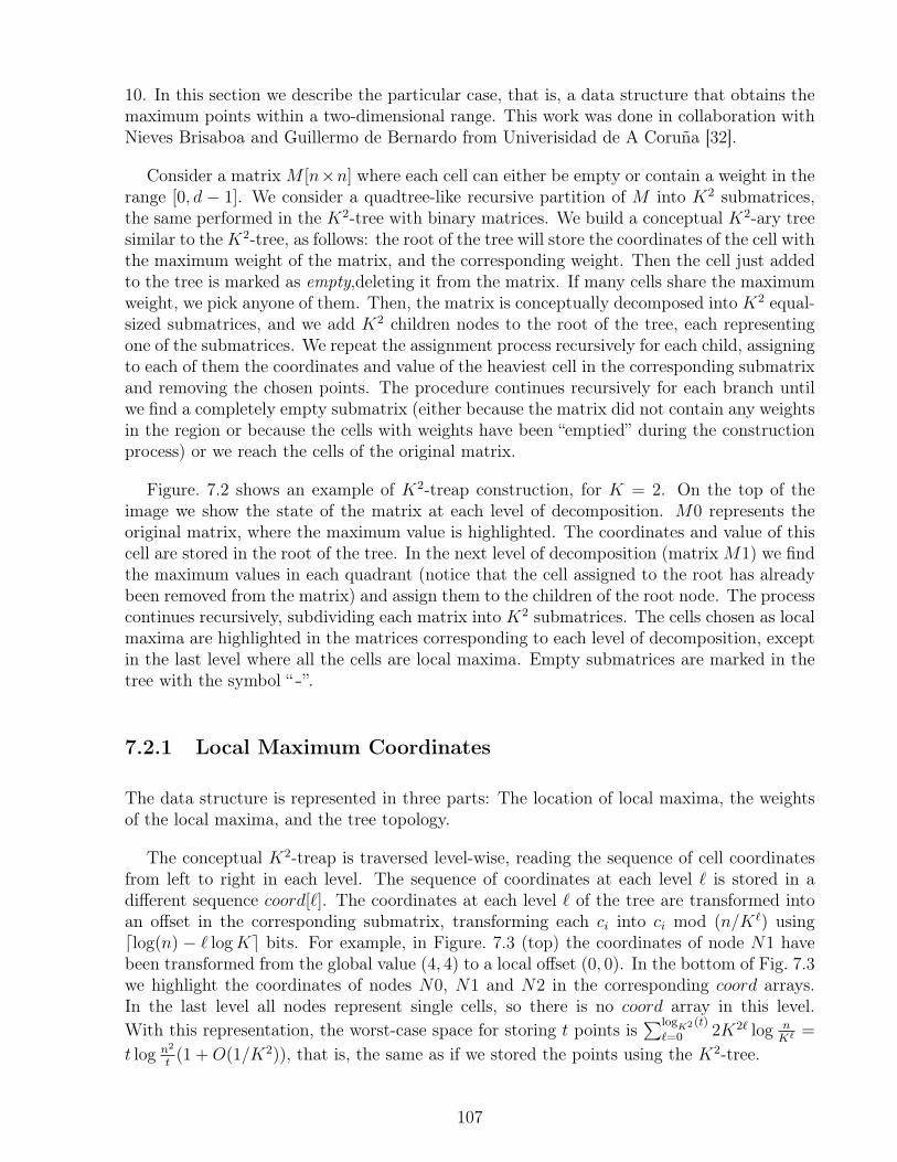
10. In this section we describe the particular case, that is, a data structure that obtains themaximum points within a two-dimensional range. This work was done in collaboration withNieves Brisaboa and Guillermo de Bernardo from Univerisidad de A Coruña [32].

Consider a matrixM [n×n] where each cell can either be empty or contain a weight in therange [0, d − 1]. We consider a quadtree-like recursive partition of M into K2 submatrices,the same performed in the K2-tree with binary matrices. We build a conceptual K2-ary treesimilar to theK2-tree, as follows: the root of the tree will store the coordinates of the cell withthe maximum weight of the matrix, and the corresponding weight. Then the cell just addedto the tree is marked as empty,deleting it from the matrix. If many cells share the maximumweight, we pick anyone of them. Then, the matrix is conceptually decomposed into K2 equal-sized submatrices, and we add K2 children nodes to the root of the tree, each representingone of the submatrices. We repeat the assignment process recursively for each child, assigningto each of them the coordinates and value of the heaviest cell in the corresponding submatrixand removing the chosen points. The procedure continues recursively for each branch untilwe find a completely empty submatrix (either because the matrix did not contain any weightsin the region or because the cells with weights have been “emptied” during the constructionprocess) or we reach the cells of the original matrix.

Figure. 7.2 shows an example of K2-treap construction, for K = 2. On the top of theimage we show the state of the matrix at each level of decomposition. M0 represents theoriginal matrix, where the maximum value is highlighted. The coordinates and value of thiscell are stored in the root of the tree. In the next level of decomposition (matrixM1) we findthe maximum values in each quadrant (notice that the cell assigned to the root has alreadybeen removed from the matrix) and assign them to the children of the root node. The processcontinues recursively, subdividing each matrix into K2 submatrices. The cells chosen as localmaxima are highlighted in the matrices corresponding to each level of decomposition, exceptin the last level where all the cells are local maxima. Empty submatrices are marked in thetree with the symbol “-”.

7.2.1 Local Maximum Coordinates

The data structure is represented in three parts: The location of local maxima, the weightsof the local maxima, and the tree topology.

The conceptual K2-treap is traversed level-wise, reading the sequence of cell coordinatesfrom left to right in each level. The sequence of coordinates at each level ` is stored in adifferent sequence coord[`]. The coordinates at each level ` of the tree are transformed intoan offset in the corresponding submatrix, transforming each ci into ci mod (n/K`) usingdlog(n) − ` logKe bits. For example, in Figure. 7.3 (top) the coordinates of node N1 havebeen transformed from the global value (4, 4) to a local offset (0, 0). In the bottom of Fig. 7.3we highlight the coordinates of nodes N0, N1 and N2 in the corresponding coord arrays.In the last level all nodes represent single cells, so there is no coord array in this level.With this representation, the worst-case space for storing t points is

∑logK2 (t)

`=0 2K2` log nK` =

t log n2

t(1 +O(1/K2)), that is, the same as if we stored the points using the K2-tree.

107

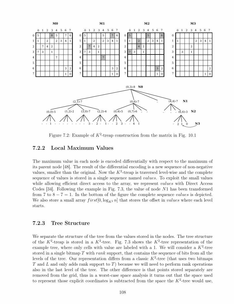
Figure 7.2: Example of K2-treap construction from the matrix in Fig. 10.1

7.2.2 Local Maximum Values

The maximum value in each node is encoded differentially with respect to the maximum ofits parent node [48]. The result of the differential encoding is a new sequence of non-negativevalues, smaller than the original. Now the K2-treap is traversed level-wise and the completesequence of values is stored in a single sequence named values. To exploit the small valueswhile allowing efficient direct access to the array, we represent values with Direct AccessCodes [34]. Following the example in Fig. 7.3, the value of node N1 has been transformedfrom 7 to 8 − 7 = 1. In the bottom of the figure the complete sequence values is depicted.We also store a small array first[0, logK2 n] that stores the offset in values where each levelstarts.

7.2.3 Tree Structure

We separate the structure of the tree from the values stored in the nodes. The tree structureof the K2-treap is stored in a K2-tree. Fig. 7.3 shows the K2-tree representation of theexample tree, where only cells with value are labeled with a 1. We will consider a K2-treestored in a single bitmap T with rank support, that contains the sequence of bits from all thelevels of the tree. Our representation differs from a classic K2-tree (that uses two bitmapsT and L and only adds rank support to T ) because we will need to perform rank operationsalso in the last level of the tree. The other difference is that points stored separately areremoved from the grid, thus in a worst-case space analysis it turns out that the space usedto represent those explicit coordinates is subtracted from the space the K2-tree would use,

108

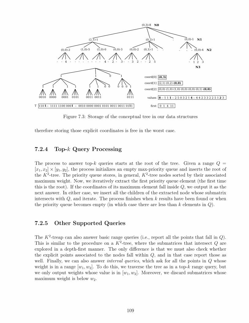
Figure 7.3: Storage of the conceptual tree in our data structures

therefore storing those explicit coordinates is free in the worst case.

7.2.4 Top-k Query Processing

The process to answer top-k queries starts at the root of the tree. Given a range Q =[x1, x2]× [y1, y2], the process initializes an empty max-priority queue and inserts the root ofthe K2-tree. The priority queue stores, in general, K2-tree nodes sorted by their associatedmaximum weight. Now, we iteratively extract the first priority queue element (the first timethis is the root). If the coordinates of its maximum element fall inside Q, we output it as thenext answer. In either case, we insert all the children of the extracted node whose submatrixintersects with Q, and iterate. The process finishes when k results have been found or whenthe priority queue becomes empty (in which case there are less than k elements in Q).

7.2.5 Other Supported Queries

The K2-treap can also answer basic range queries (i.e., report all the points that fall in Q).This is similar to the procedure on a K2-tree, where the submatrices that intersect Q areexplored in a depth-first manner. The only difference is that we must also check whetherthe explicit points associated to the nodes fall within Q, and in that case report those aswell. Finally, we can also answer interval queries, which ask for all the points in Q whoseweight is in a range [w1, w2]. To do this, we traverse the tree as in a top-k range query, butwe only output weights whose value is in [w1, w2]. Moreover, we discard submatrices whosemaximum weight is below w2.

109

Chapter 8

Practical Implementations

In this chapter, we present our practical implementations of the solution proposed by Navarroand Nekrich (recall Section 6.1) for solving, in optimal time, top-k queries on general se-quences. As discussed before, the main constraints of the implementation of this solution isspace, so we make use of the wavelet tree combined with RMQ solution (see Section 7.1) andthe K2-treap (see Section 7.2). We show how we engineered different alternatives, in orderto obtain indexes that are practical in terms of size and faster than other solutions from thestate of the art.

8.1 A Basic Compact Implementation

In this section we describe a basic compact implementation of the optimal-time solution [119],which will be labeled WRMQ.

8.1.1 Searching for Patterns

In order to search for patterns in the collection, we use a CSA, which computes the interval[sp, ep] corresponding to P in time O(tsearch(m)). We also add a compact representation ofthe topology of the suffix tree, seeing it as an ordinal tree. Note that this is just the topology,not a full suffix tree, so we need to search using the CSA. We will use the suffix tree topologyto obtain the locus v of P from sp and ep, and then to map it to the grid.

8.1.2 Mapping to the Grid

The grid G is of width∑

i |Ti| ≤ 2n, as we add one coordinate per node in the suffix tree ofeach document. To save space, we will consider a virtual grid just as defined, but will store anarrower physical grid. In the physical grid, the entries corresponding to leaves of T (which

110

contain exactly one pointer ptr(v, i)) will not be represented. Thus the physical grid is ofwidth at most n. This frequency thresholding is a key idea, as it halves the space of moststructures in our index.

A bitmap B[1, 2n] will be used to map between the suffix tree and the grid. Bitmap Bwill mark starting positions of nodes of T in the physical grid: along the grid constructionprocess, each time we arrive at an internal node v we add a 1 to B, and each time we adda new x-coordinate to the grid (due to a pointer ptr(v, i)) we add a 0 to B. This structurewill be called MAP.

8.1.3 Finding Isolated Documents

Due to frequency thresholding, the information on the grid may be insufficient to answertop-k queries when the result includes documents where P appears only once. For thispurpose, we store the RMQ structure on top of the array CA of Muthukrishnan [115] (recallSection 2.15) (the array itself is not stored). This structure, RMQC, allows us list k distinctdocuments in any interval SA[sp, ep].

To determine the identity of a document found at position i of CA, we will use the CSAto compute p = SA[i] and then determine to which document position C[p] belongs. For thissake we store a sparse bitmap DOCBITMAP, that marks beginnings of documents in C. Thedocument is then rank1(DOCBITMAP, p).

8.1.4 Representing the Grid

In the grid there is exactly one point per x-coordinate. We represent with a wavelet tree[81] the sequence of corresponding y-coordinates. Each node v of the wavelet tree representsa subsequence of the original sequence of y-coordinates. We consider the (virtual) sequenceof the weights associated to the points represented by v, W (v), and build an RMQ datastructure for each node W (v), as explained, to support top-k queries on the grid.

8.1.5 Representing Labels and Weights

The labels of the points, that is, the document identifiers, are represented directly as asequence of at most n logD bits, aligned to the bottom of the wavelet tree. Given any pointto report, we descend to the leaf and retrieve the aligned document identifier.

The weights are stored similarly, but using direct access codes, to take advantage of thefact that most weights (term frequencies) are small.

111

8.1.6 Summing Up

TheWRMQ index consists of eight components: the compressed suffix array (CSA), the suffixtree topology (TREE), the suffix tree to grid mapping (MAP), the wavelet tree over the gridG (WT) including the RMQ structures at each node, the document ids associated with thegrid elements (DOC), in the same order of leaves of the wavelet tree, the weights associatedto the documents (FREQ), the RMQ structure to retrieve documents occurring once overthe CA array (RMQC), and the bitmap marking document borders (DOCBITMAP).

If the height of the suffix tree is O(log n), as is the case in many reasonable distributions[155], then WT requires 3n log log n + O(n) bits. The other main components are |CSA| ≤n log σ bits, the array DOC, which uses n logD bits, and the array FREQ, which in the worstcase needs n log n bits but uses much less in practice. The other elements add up to O(n)bits, with a constant factor of about 8–10.

8.1.7 Answering Queries

The first step to answer a query is to use the CSA to determine the range [sp, ep]. To find thelocus v of P in the topology of the suffix tree, we compute l and r, the spth and epth leavesof the tree, respectively, using l = leaf_select(sp) and r = leaf_select(ep); then wehave v = lca(l, r).

To determine the horizontal extent [x1, x2] of the grid that corresponds to the locus nodev, we first compute p1 = preorder(v) and p2 = p1+subtree_size(v). This gives the pre-order range [p1, p2) including leaves. Now l1 = leaf_rank(p1) and l2 = leaf_rank(p2−1)give the number of leaves up to those preorders. Then, since we have omitted the leaves inthe physical grid, we have x1 = select1(B, p1− l1)− (p1− l1) + 1 and x2 = select1(B, p2−l2)− (p2− l2). The limits in the y axis are just [0,depth(v)−1]. Thus the grid area to queryis determined with a constant amount of operations on bitmaps and trees.

Once the range [x1, x2] × [y1, y2] to query is determined, we proceed to the grid. Wedetermine the wavelet tree nodes that cover the interval [y1, y2], and map the interval [x1, x2]to all of them.

We now use the top-k algorithm for wavelet trees we described. Let v1, v2, . . . , vs be thewavelet tree nodes that cover [y1, y2] and let [xi1, x

i2] be the interval [x1, x2] mapped to vi. For

each of them we compute rmqW (vi)(xi1, x

i2) to find the position xi with the largest weight

among the points in vi, and find out that weight and the corresponding document, wi anddi. We set up a max-priority queue that will hold at most k elements (elements smallerthan the kth are discarded by the queue). We initially insert the tuples (vi, x

i1, x

i2, xi, wi, di),

being wi the sort key. Now we iteratively extract the tuple with the largest weight, say(vj, x

j1, x

j2, xj, wj, dj). We report the document dj with weight wj, and create two new ranges

in vj: [xj1, xj−1] and [xj +1, xj2]. We compute their RMQ, find the corresponding documentsand weights, and reinsert them in the queue. After k steps, we have reported the top-kdocuments. We will refer to this procedure as topk_grid_query.

112

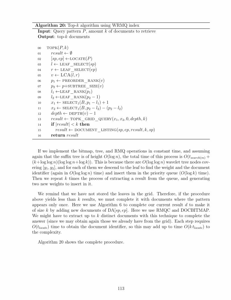
Algorithm 20: Top-k algorithm using WRMQ indexInput: Query pattern P , amount k of documents to retrieveOutput: top-k documents

00 topk(P, k)01 result← ∅02 [sp, ep]←locate(P )03 l← leaf_select(sp)04 r ← leaf_select(ep)05 v ← LCA(l, r)06 p1 ← preorder_rank(v)07 p2 ← p+subtree_size(v)08 l1 ←leaf_rank(p1)09 l2 ←leaf_rank(p2 − 1)10 x1 ← select1(B, p1 − l1) + 111 x2 ← select1(B, p2 − l2)− (p2 − l2)12 depth← depth(v)− 113 result← topk_grid_query(x1, x2, 0, depth, k)14 if |result| < k then15 result← document_listing(sp, ep, result, k, sp)16 return result

If we implement the bitmap, tree, and RMQ operations in constant time, and assumingagain that the suffix tree is of height O(log n), the total time of this process is O(tsearch(m) +(k+log log n)(log log n+log k)). This is because there are O(log log n) wavelet tree nodes cov-ering [y1, y2], and for each of them we descend to the leaf to find the weight and the documentidentifier (again in O(log log n) time) and insert them in the priority queue (O(log k) time).Then we repeat k times the process of extracting a result from the queue, and generatingtwo new weights to insert in it.

We remind that we have not stored the leaves in the grid. Therefore, if the procedureabove yields less than k results, we must complete it with documents where the patternappears only once. Here we use Algorithm 6 to complete our current result d to make itof size k by adding new documents of DA[sp, ep]. Here we use RMQC and DOCBITMAP.We might have to extract up to k distinct documents with this technique to complete theanswer (since we may obtain again those we already have from the grid). Each step requiresO(tlocate) time to obtain the document identifier, so this may add up to time O(k tlocate) tothe complexity.

Algorithm 20 shows the complete procedure.

113

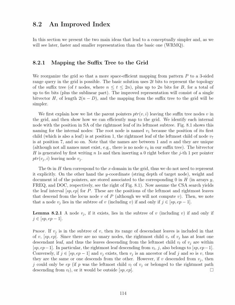
8.2 An Improved Index

In this section we present the two main ideas that lead to a conceptually simpler and, as wewill see later, faster and smaller representation than the basic one (WRMQ).

8.2.1 Mapping the Suffix Tree to the Grid

We reorganize the grid so that a more space-efficient mapping from pattern P to a 3-sidedrange query in the grid is possible. The basic solution uses 2t bits to represent the topologyof the suffix tree (of t nodes, where n ≤ t ≤ 2n), plus up to 2n bits for B, for a total ofup to 6n bits (plus the sublinear part). The improved representation will consist of a singlebitvector H, of length 2(n − D), and the mapping from the suffix tree to the grid will besimpler.

We first explain how we list the parent pointers ptr(v, i) leaving the suffix tree nodes v inthe grid, and then show how we can efficiently map to the grid. We identify each internalnode with the position in SA of the rightmost leaf of its leftmost subtree. Fig. 8.1 shows thisnaming for the internal nodes: The root node is named v1 because the position of its firstchild (which is also a leaf) is at position 1, the rightmost leaf of the leftmost child of node v7

is at position 7, and so on. Note that the names are between 1 and n and they are unique(although not all names must exist, e.g., there is no node v4 in our suffix tree). The bitvectorH is generated by first writing n 1s and then inserting a 0 right before the j-th 1 per pointerptr(vj, i) leaving node vj.

The 0s in H then correspond to the x-domain in the grid, thus we do not need to representit explicitly. On the other hand the y-coordinate (string depth of target node), weight anddocument id of the pointers, are stored associated to the corresponding 0 in H (in arrays y,FREQ, and DOC, respectively, see the right of Fig. 8.1). Now assume the CSA search yieldsthe leaf interval [sp, ep] for P . These are the positions of the leftmost and rightmost leavesthat descend from the locus node v of P (although we will not compute v). Then, we notethat a node vj lies in the subtree of v (including v) if and only if j ∈ [sp, ep− 1].

Lemma 8.2.1 A node vj, if it exists, lies in the subtree of v (including v) if and only ifj ∈ [sp, ep− 1].

Proof. If vj is in the subtree of v, then its range of descendant leaves is included in thatof v, [sp, ep]. Since there are no unary nodes, the rightmost child vr of vj has at least onedescendant leaf, and thus the leaves descending from the leftmost child vl of vj are within[sp, ep−1]. In particular, the rightmost leaf descending from vl, j, also belongs to [sp, ep−1].Conversely, if j ∈ [sp, ep− 1] and vj exists, then vj is an ancestor of leaf j and so is v, thusthey are the same or one descends from the other. However, if v descended from vj, thenj could only be ep (if p was the leftmost child vl of vj or belonged to the rightmost pathdescending from vl), or it would be outside [sp, ep].

114

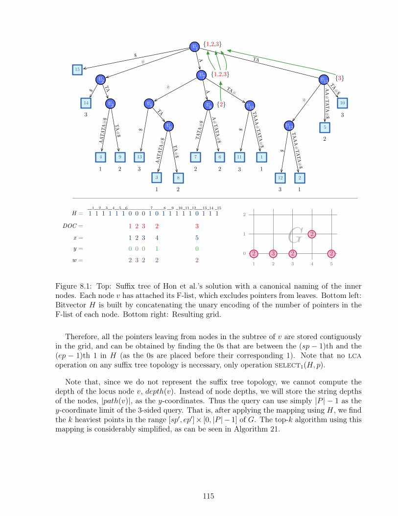
G

v1

15

v2

14 v3

4 9 13

v6

3 8

v5

7 6

v8

v7

12 2

v12 5

10

v13

3

1 2 3

1 2

2 2

3 1

2

3v10

111

3 1

TATA#$

AA#TATA

#$

TAAA#TATA#

$

$

#

TAAA#TATA#

$

$

A#TATA#

$TATA#$

TA#$

AATATA#$

TA

#

$

A

TA#$

AATATA#$

TA$

#$

TA#A

1 1 1 1 1 1 0 0 0 1 0 1 1 1 1 1 0 1 1 1

2

1,2,3 3

1,2,3

H =__2__1 __3__4__5__6____________7_____8 __9 _10_11_12___13_14 _15

DOC =

x =y =

w =

1 1 1 1 1 1 1 2 3 1 2 1 1 1 1 1 3 1 1 11 1 1 1 1 1 1 2 3 1 4 1 1 1 1 1 5 1 1 11 1 1 1 1 1 0 0 0 1 1 1 1 1 1 1 0 1 1 11 1 1 1 1 1 2 3 2 1 2 1 1 1 1 1 2 1 1 1 1 2 3 4 5

0

1

2

2 3 2

2

2

Figure 8.1: Top: Suffix tree of Hon et al.’s solution with a canonical naming of the innernodes. Each node v has attached its F-list, which excludes pointers from leaves. Bottom left:Bitvector H is built by concatenating the unary encoding of the number of pointers in theF-list of each node. Bottom right: Resulting grid.

Therefore, all the pointers leaving from nodes in the subtree of v are stored contiguouslyin the grid, and can be obtained by finding the 0s that are between the (sp − 1)th and the(ep − 1)th 1 in H (as the 0s are placed before their corresponding 1). Note that no lcaoperation on any suffix tree topology is necessary, only operation select1(H, p).

Note that, since we do not represent the suffix tree topology, we cannot compute thedepth of the locus node v, depth(v). Instead of node depths, we will store the string depthsof the nodes, |path(v)|, as the y-coordinates. Thus the query can use simply |P | − 1 as they-coordinate limit of the 3-sided query. That is, after applying the mapping using H, we findthe k heaviest points in the range [sp′, ep′]× [0, |P | − 1] of G. The top-k algorithm using thismapping is considerably simplified, as can be seen in Algorithm 21.

115

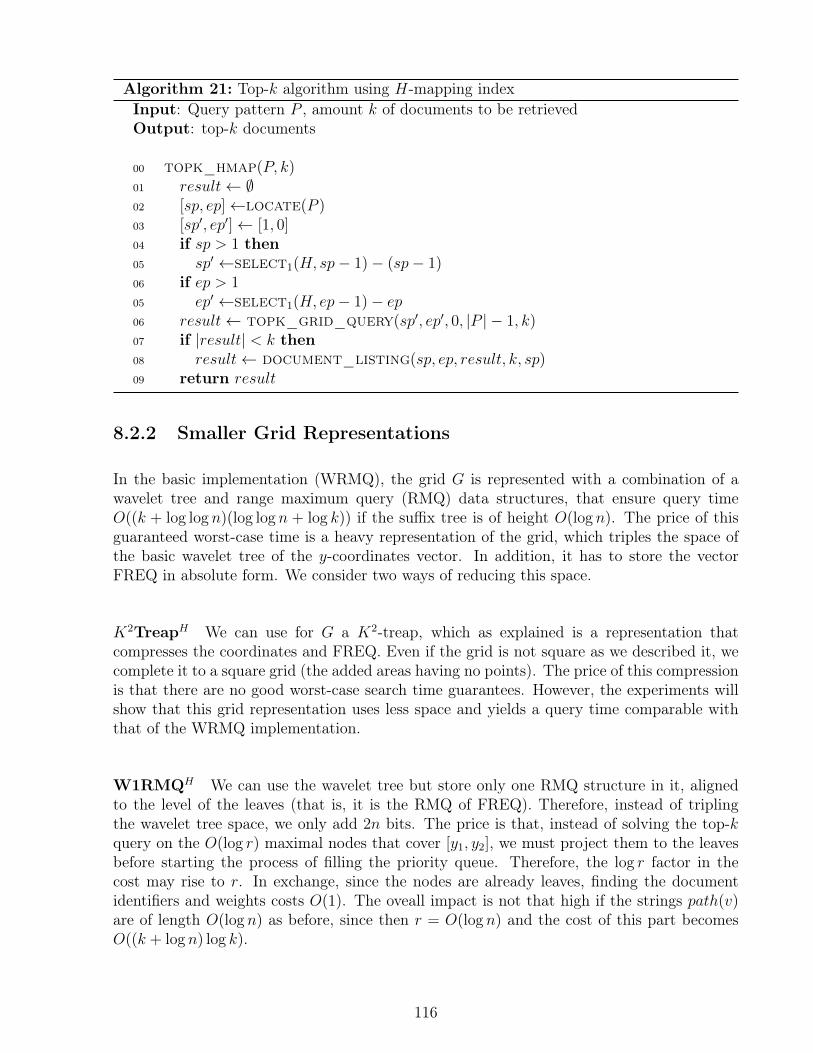
Algorithm 21: Top-k algorithm using H-mapping indexInput: Query pattern P , amount k of documents to be retrievedOutput: top-k documents

00 topk_hmap(P, k)01 result← ∅02 [sp, ep]←locate(P )03 [sp′, ep′]← [1, 0]04 if sp > 1 then05 sp′ ←select1(H, sp− 1)− (sp− 1)06 if ep > 105 ep′ ←select1(H, ep− 1)− ep06 result← topk_grid_query(sp′, ep′, 0, |P | − 1, k)07 if |result| < k then08 result← document_listing(sp, ep, result, k, sp)09 return result

8.2.2 Smaller Grid Representations

In the basic implementation (WRMQ), the grid G is represented with a combination of awavelet tree and range maximum query (RMQ) data structures, that ensure query timeO((k + log log n)(log log n + log k)) if the suffix tree is of height O(log n). The price of thisguaranteed worst-case time is a heavy representation of the grid, which triples the space ofthe basic wavelet tree of the y-coordinates vector. In addition, it has to store the vectorFREQ in absolute form. We consider two ways of reducing this space.

K2TreapH We can use for G a K2-treap, which as explained is a representation thatcompresses the coordinates and FREQ. Even if the grid is not square as we described it, wecomplete it to a square grid (the added areas having no points). The price of this compressionis that there are no good worst-case search time guarantees. However, the experiments willshow that this grid representation uses less space and yields a query time comparable withthat of the WRMQ implementation.

W1RMQH We can use the wavelet tree but store only one RMQ structure in it, alignedto the level of the leaves (that is, it is the RMQ of FREQ). Therefore, instead of triplingthe wavelet tree space, we only add 2n bits. The price is that, instead of solving the top-kquery on the O(log r) maximal nodes that cover [y1, y2], we must project them to the leavesbefore starting the process of filling the priority queue. Therefore, the log r factor in thecost may rise to r. In exchange, since the nodes are already leaves, finding the documentidentifiers and weights costs O(1). The oveall impact is not that high if the strings path(v)are of length O(log n) as before, since then r = O(log n) and the cost of this part becomesO((k + log n) log k).

116

8.2.3 Efficient Construction for Large Collections

A bottleneck not addressed by the WRMQ implementation is the efficient construction ofthe index1. Both time-and space- efficiency have to be considered. We will concentrate hereon the construction of H, the grid G, and its K2-treap representation, suffix tree (CST) ofC and a wavelet tree over the document array, WTD, of n logD bits. We perform a depth-first-search traversal on the CST and calculate, for each node vj, the list of its document idmarks, by intersecting the document array ranges of v’s children. This can be done usingthe intersection on wavelet trees [74]. Since we can calculate the nodes in the order of theirnames, we can write H and the document ids (DOC) directly to disk. In a second traversalwe calculate the pointers. For each document i we use a stack to maintain the string depthof the last occurrence of i in the tree. For a node v marked with i we push the string depthof v at the first visit and pop it after all the subtree of v is traversed. Note that this time wecan read H and DOC from disk (in streamed mode) and avoid the intersection. In the sametraversal we can calculate the weight array FREQ by performing counting queries on WTD.Again, arrays y and FREQ can be streamed to disk.

Finally, the K2-treap is constructed in-place by a top-down level by level process. Letthe input be stored as a sequence of triples (x, y, w) and let 1 be the root level and b be thebottom level. First, we determine the heaviest element by a linear scan, stream its weightout to disk and mark the element as deleted. We then partition the elements of the rootlevel into K2 ranges, such that all elements in range r (0 ≤ r ≤ K2) have the property thatx/Kb−` mod K = r mod K and y/Kb−` mod K = r/K. For each non-empty (resp. empty)range r we add a 1 (resp. 0) to the bitvector T , which is streamed to disk. On the nextlevel ` − 1 we can detect nodes by checking the partitioning condition of the last level, findand mark the maximum weighted entry and apply the partitioning in the node. The timecomplexity of the process is O(K2 logK n) and does not use extra space.

8.2.4 Summing Up

We introduce new indexes, K2TreapHand W1RMQH , that simplify WRMQ by convertingits MAP and TREE components into a single bitmap H. In addition, they reduce the spaceof the grid representation, by trading it for weaker time guarantees. The experiments willshow that this does not translate into markedly reduced performance.

1For example, the liner-time LCA-based index construction method takes 1.5 hours for an 80MBWikipediacollection, where their peak main memory usage is 12.25 GB.

117

Chapter 9

Experimental Evaluation

In this chapter we describe the experimental setup in terms of the collections where the indexwere evaluated, query generation and environment employed. We also explain the engineeringdetails required to implement the indexes.

9.1 Datasets and Test Environment

We will split the collections into two categories depending on the alphabet type: characteralphabet and word alphabet. For the character alphabet, we have four “small” collections,that have been used as baselines in previous work [124], and a “big” collection containingnatural language text. We describe and label the collections as follows:

• kgsc. Consists of a collection of 18,839 sgf-formmated Go game records from year 2009(http://www.u-go.net/gamerecords), containing 52,721,176 characters.• proteinsc. A collection of 143,244 sequences of Human and Mouse proteins (http://www.ebi.ac.uk/swissport), containing 59,103,058 symbols.• enwiki-smlc. A sample of a Wikipedia dump, consisting of 4,390 English articles,

containing 68,210,334 symbols.• dnac. A sequence of 10,000 highly repetitive (0.05% difference between documents)

synthetic DNA sequences with 100,030,016 bases in total.• enwiki-bigc. A bigger sample of English Wikipedia articles, consisting of 8.5GB of

natural text and 3.8 million documents.

In the case of word alphabets we use three collections of documents containing naturallanguage. We preprocessed these collections using the Indri search engine (http://www.lemurproject.org/indri/) for generating a sequence of stemmed words and excluding allhtml tags.

• enwiki-smlw. A word parsing of enwiki-smlc, containing 281,577 distinct words.• enwiki-bigw. A collection containing 8,289,354 words obtained from regarding the

118

text as a sequence of words from enwiki-bigc.• gov2w. Probably the most frequently used natural text collection for comparing effi-

ciency of IR systems. The parsed collection consists of more than 72GB of data, around40 million terms and more than 25 million documents.

Table 9.1 summarizes properties of the collections that are used. For queries, we selected40,000 random substrings of length m obtained from the top-k documents for m = 5. Weincrease k exponentially from 1 to 256.

For all experimental comparisons, the relevance measure used is the term frequency andthe query is a single pattern string. All experiments were run on a server equipped with anIntel(R) Xeon(R) E5-4640 CPU clocking at 2.40GHz. All experiments use a single core and atmost 150GB of the installed 512GB of RAM. All programs were compiled with optimizationsusing g++ version 4.9.0.

9.2 Implementations

In this section we describe the implementation details for each engineered index. Our im-plementation and benchmarks are publicly available at https://github.com/rkonow/surf/tree/wt_topk.

9.2.1 Baselines

As baselines we use the GREEDY solution [53] and the SORT approach [77], which is in-cluded in the Succinct Data Structure Library (SDSL, https://github.com/simongog/sdsl-lite). Baseline SORT uses the CSA and document array DA. It first gets the range [sp, ep] ofall occurrences of P from the CSA. Then it copies all documents from DA[sp, ep] and extractsthe top-k most relevant documents by sorting and accumulating the occurrences. BaselineGREEDY also gets the range [sp, ep] from the CSA, but then does a greedy traversal of thewavelet tree over DA to get the top-k documents. As an additional baseline we also ran theexperiments using the original source code of Navarro et al. [124] (NPV). This implemen-tation consists of more than 24 alternative configurations, including grammar compressedwavelet trees using different bitmap representations and improvements to the GREEDY al-gorithm. For the experimental time-related results, we will always show the points thatcorrespond to the pareto-optimal border in terms of space and time considering all possibleconfigurations. We refer to this index as as NPVopt. We will not compare to the work of Patilet al. [129] since the space requirements of this solution is considerably bigger (see Table 6.1)than the ones that are being evaluated in this work.

119

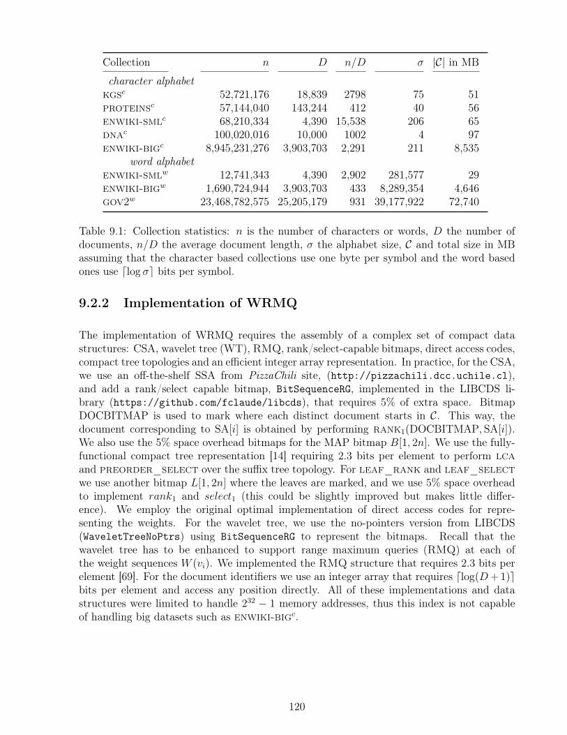
Collection n D n/D σ |C| in MB

character alphabetkgsc 52,721,176 18,839 2798 75 51proteinsc 57,144,040 143,244 412 40 56enwiki-smlc 68,210,334 4,390 15,538 206 65dnac 100,020,016 10,000 1002 4 97enwiki-bigc 8,945,231,276 3,903,703 2,291 211 8,535

word alphabetenwiki-smlw 12,741,343 4,390 2,902 281,577 29enwiki-bigw 1,690,724,944 3,903,703 433 8,289,354 4,646gov2w 23,468,782,575 25,205,179 931 39,177,922 72,740

Table 9.1: Collection statistics: n is the number of characters or words, D the number ofdocuments, n/D the average document length, σ the alphabet size, C and total size in MBassuming that the character based collections use one byte per symbol and the word basedones use dlog σe bits per symbol.

9.2.2 Implementation of WRMQ

The implementation of WRMQ requires the assembly of a complex set of compact datastructures: CSA, wavelet tree (WT), RMQ, rank/select-capable bitmaps, direct access codes,compact tree topologies and an efficient integer array representation. In practice, for the CSA,we use an off-the-shelf SSA from PizzaChili site, (http://pizzachili.dcc.uchile.cl),and add a rank/select capable bitmap, BitSequenceRG, implemented in the LIBCDS li-brary (https://github.com/fclaude/libcds), that requires 5% of extra space. BitmapDOCBITMAP is used to mark where each distinct document starts in C. This way, thedocument corresponding to SA[i] is obtained by performing rank1(DOCBITMAP, SA[i]).We also use the 5% space overhead bitmaps for the MAP bitmap B[1, 2n]. We use the fully-functional compact tree representation [14] requiring 2.3 bits per element to perform lcaand preorder_select over the suffix tree topology. For leaf_rank and leaf_selectwe use another bitmap L[1, 2n] where the leaves are marked, and we use 5% space overheadto implement rank1 and select1 (this could be slightly improved but makes little differ-ence). We employ the original optimal implementation of direct access codes for repre-senting the weights. For the wavelet tree, we use the no-pointers version from LIBCDS(WaveletTreeNoPtrs) using BitSequenceRG to represent the bitmaps. Recall that thewavelet tree has to be enhanced to support range maximum queries (RMQ) at each ofthe weight sequences W (vi). We implemented the RMQ structure that requires 2.3 bits perelement [69]. For the document identifiers we use an integer array that requires dlog(D+ 1)ebits per element and access any position directly. All of these implementations and datastructures were limited to handle 232 − 1 memory addresses, thus this index is not capableof handling big datasets such as enwiki-bigc.

120

9.2.3 Implementation of K2TreapH

The set of data structures required for implementing K2TreapH is smaller: We need a CSA,RMQ, rank/select capable bitmaps, direct access codes, a K2-treap, and an efficient inte-ger array representation. We based our implementation on structures from SDSL and willuse the SDSL class names in the following. For character based indexes, we use a CSAbased on a wavelet tree (csa_wt) which is parametrized by a Huffman-shaped wavelet tree(wt_huff) which uses a compressed bitmap (rrr_vector). For word based indexes, weopted for a CSA based on the Ψ function (csa_sada) which is compressed with Elias-δcodes (coder::elias_delta). The latter provided a better time-space trade-off for largealphabet pattern matching. For the mapping we store the bitmap H using a compressedbitmap rrr_vector. The select1 performance of rrr_vector is slow compared to a plainbitmap representation but negligible in our case, where only two select1 queries are doneper top-k query (recall Algorithm 21). The RMQC structure is realized by a MinMax-treeimplementation rmq_succinct_sct which uses about 2.3 bits per element. The documentids, DOC, are stored in an integer vector (int_vector) using dlog(D+ 1)e bits per element.For this work we have implemented the K2-treap structure and added it to SDSL (availablenow as k2_treap). The K2-treap implementation is generic (the value K, the bitmap rep-resentation of the K2-ary tree, and the representation of the vector of relative weights, canbe parametrized) and complements the description of Brisaboa et al.[32] with an efficientin-place construction described in Section 8.2.3. For the relative weights we use direct accesscodes (dac_vector) with a fixed width of 4.

9.2.4 Implementation of W1RMQH

The only difference between K2TreapH and W1RMQH is the grid implementation. TheW1RMQH solution uses a wavelet tree and an RMQ data structure to represent the grid. Weopted for a wt_int parametrized with rrr_vector. The compressed bitvector decreased thesize considerably since the grid contains many small y-values. The absolute weights are storedin a dac_vector of fixed width 4, which gave the most practical result when performing pa-rameter tuning experiments. The RMQ structure was again realized by rmq_succinct_sctusing 2.3 bits per element.

9.3 Results

In this section we study the practical properties of the different index implementations. Wefirst analyze the space consumption of the structures; both total space and the space ofsubstructures – like the grid – are considered. Then the query time is analyzed. Again,we consider total query time and also study the time for the different phases of the queryprocess. To get a precise picture about the performance we vary various parameters: thenumber of results k, the pattern length m, and collections. The latter are from differentapplication domains, cover different scales of magnitude – from 50 MB to 72 GB –, and varyin alphabets size from 4 to almost 40 million. Note that some non-SDSL based baselines did

121

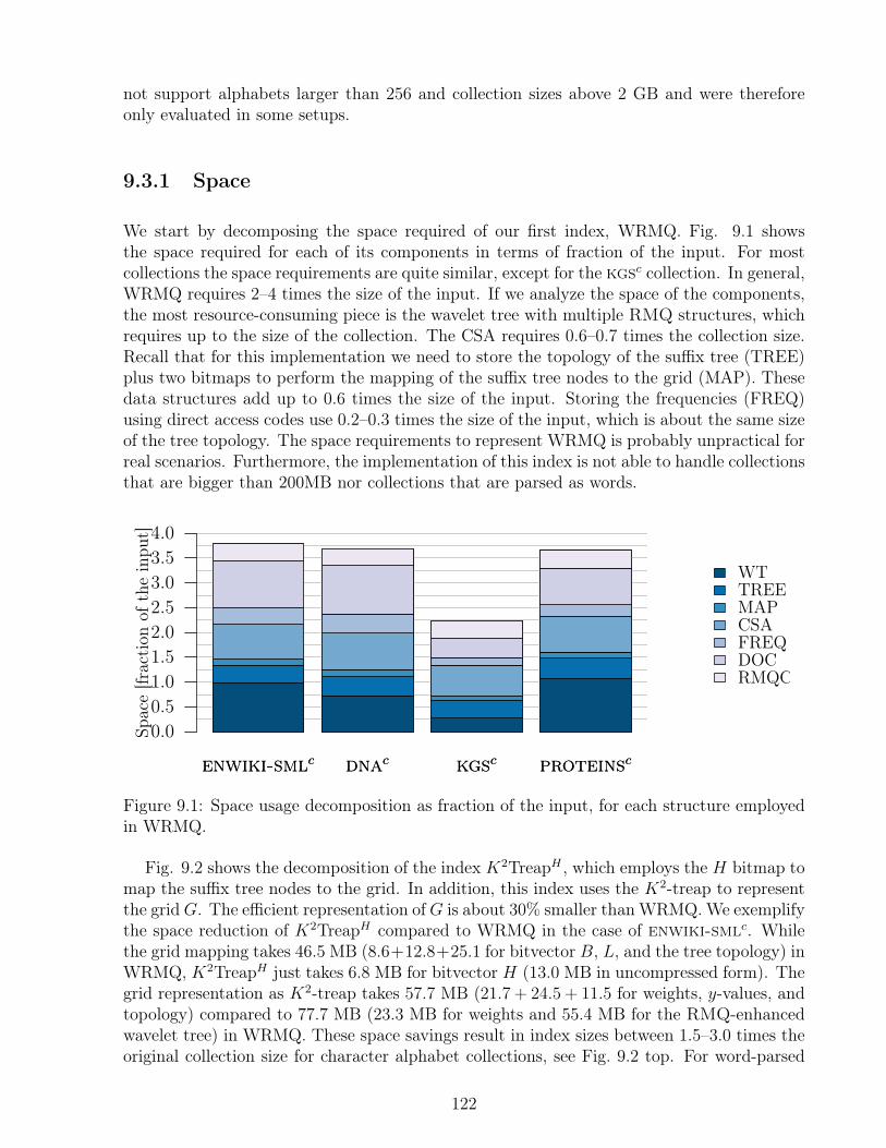
not support alphabets larger than 256 and collection sizes above 2 GB and were thereforeonly evaluated in some setups.

9.3.1 Space

We start by decomposing the space required of our first index, WRMQ. Fig. 9.1 showsthe space required for each of its components in terms of fraction of the input. For mostcollections the space requirements are quite similar, except for the kgsc collection. In general,WRMQ requires 2–4 times the size of the input. If we analyze the space of the components,the most resource-consuming piece is the wavelet tree with multiple RMQ structures, whichrequires up to the size of the collection. The CSA requires 0.6–0.7 times the collection size.Recall that for this implementation we need to store the topology of the suffix tree (TREE)plus two bitmaps to perform the mapping of the suffix tree nodes to the grid (MAP). Thesedata structures add up to 0.6 times the size of the input. Storing the frequencies (FREQ)using direct access codes use 0.2–0.3 times the size of the input, which is about the same sizeof the tree topology. The space requirements to represent WRMQ is probably unpractical forreal scenarios. Furthermore, the implementation of this index is not able to handle collectionsthat are bigger than 200MB nor collections that are parsed as words.

enwiki-smlc dnac kgsc proteinscenwiki-smlc dnac kgsc proteinsc

Space[fraction

oftheinpu

t]

0.00.51.01.52.02.53.03.54.0

WTTREEMAPCSAFREQDOCRMQC

Figure 9.1: Space usage decomposition as fraction of the input, for each structure employedin WRMQ.

Fig. 9.2 shows the decomposition of the index K2TreapH , which employs the H bitmap tomap the suffix tree nodes to the grid. In addition, this index uses the K2-treap to representthe gridG. The efficient representation ofG is about 30% smaller thanWRMQ.We exemplifythe space reduction of K2TreapH compared to WRMQ in the case of enwiki-smlc. Whilethe grid mapping takes 46.5 MB (8.6+12.8+25.1 for bitvector B, L, and the tree topology) inWRMQ, K2TreapH just takes 6.8 MB for bitvector H (13.0 MB in uncompressed form). Thegrid representation as K2-treap takes 57.7 MB (21.7 + 24.5 + 11.5 for weights, y-values, andtopology) compared to 77.7 MB (23.3 MB for weights and 55.4 MB for the RMQ-enhancedwavelet tree) in WRMQ. These space savings result in index sizes between 1.5–3.0 times theoriginal collection size for character alphabet collections, see Fig. 9.2 top. For word-parsed

122

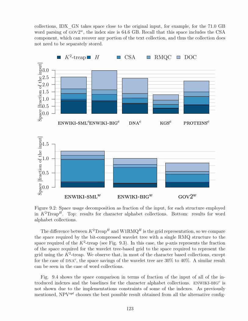
collections, IDX_GN takes space close to the original input, for example, for the 71.0 GBword parsing of gov2w, the index size is 64.6 GB. Recall that this space includes the CSAcomponent, which can recover any portion of the text collection, and thus the collection doesnot need to be separately stored.

enwiki-smlcenwiki-bigc dnac kgsc proteinscenwiki-smlcenwiki-bigc dnac kgsc proteinscSpace[fraction

oftheinpu

t]

0.00.51.01.52.02.53.0

enwiki-smlw enwiki-bigw gov2wenwiki-smlw enwiki-bigw gov2wSpace[fraction

oftheinpu

t]

0.0

0.5

1.0

1.5

K2-treap H CSA RMQC DOC

Figure 9.2: Space usage decomposition as fraction of the input, for each structure employedin K2TreapH . Top: results for character alphabet collections. Bottom: results for wordalphabet collections.

The difference betweenK2TreapH andW1RMQH is the grid representation, so we comparethe space required by the bit-compressed wavelet tree with a single RMQ structure to thespace required of the K2-treap (see Fig. 9.3). In this case, the y-axis represents the fractionof the space required for the wavelet tree-based grid to the space required to represent thegrid using the K2-treap. We observe that, in most of the character based collections, exceptfor the case of dnac, the space savings of the wavelet tree are 30% to 40%. A similar resultcan be seen in the case of word collections.

Fig. 9.4 shows the space comparison in terms of fraction of the input of all of the in-troduced indexes and the baselines for the character alphabet collections. enwiki-bigc isnot shown due to the implementations constraints of some of the indexes. As previouslymentioned, NPVopt chooses the best possible result obtained from all the alternative config-

123

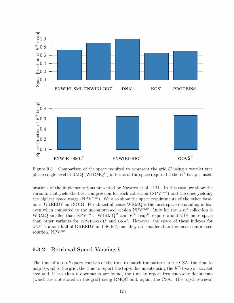
enwiki-smlcenwiki-bigc dnac kgsc proteinscenwiki-smlcenwiki-bigc dnac kgsc proteinsc

Space[fraction

ofK

2-treap

]

0.0

0.2

0.4

0.6

0.8

1.0

enwiki-smlw enwiki-bigw gov2wenwiki-smlw enwiki-bigw gov2w

Space[fraction

ofK

2-treap

]

0.0

0.2

0.4

0.6

0.8

Figure 9.3: Comparison of the space required to represent the grid G using a wavelet treeplus a single level of RMQ (W1RMQH) in terms of the space required if the K2-treap is used.

urations of the implementations presented by Navarro et al. [124]. In this case, we show thevariants that yield the best compression for each collection (NPVmin) and the ones yieldingthe highest space usage (NPVmax). We also show the space requirements of the other base-lines, GREEDY and SORT. For almost all cases WRMQ is the most space-demanding index,even when compared to the uncompressed version NPVmax. Only for the kgsc collection isWRMQ smaller than NPVmax. W1RMQH and K2TreapH require about 20% more spacethan other variants for enwiki-smlc and dnac. However, the space of these indexes forkgsc is about half of GREEDY and SORT, and they are smaller than the most compressedsolution, NPVopt.

9.3.2 Retrieval Speed Varying k

The time of a top-k query consists of the time to match the pattern in the CSA, the time tomap [sp, ep] to the grid, the time to report the top-k documents using theK2-treap or wavelettree and, if less than k documents are found, the time to report frequency-one documents(which are not stored in the grid) using RMQC and, again, the CSA. The top-k retrieval

124

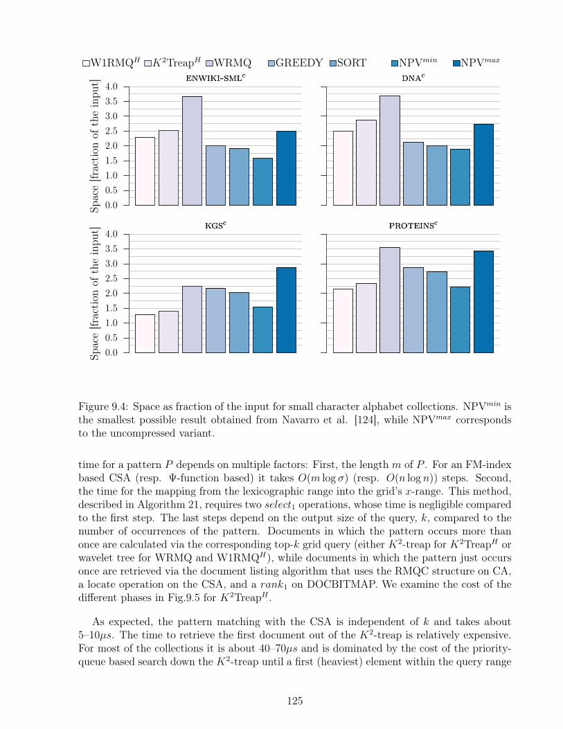
enwiki-smlcenwiki-smlc

Space[fraction

oftheinpu

t]

0.00.51.01.52.02.53.03.54.0

dnacdnac

kgsckgsc

Space[fraction

oftheinpu

t]

0.00.51.01.52.02.53.03.54.0

proteinscproteinsc

W1RMQH K2TreapH WRMQ GREEDY SORT NPVmin NPVmax

Figure 9.4: Space as fraction of the input for small character alphabet collections. NPVmin isthe smallest possible result obtained from Navarro et al. [124], while NPVmax correspondsto the uncompressed variant.

time for a pattern P depends on multiple factors: First, the length m of P . For an FM-indexbased CSA (resp. Ψ-function based) it takes O(m log σ) (resp. O(n log n)) steps. Second,the time for the mapping from the lexicographic range into the grid’s x-range. This method,described in Algorithm 21, requires two select1 operations, whose time is negligible comparedto the first step. The last steps depend on the output size of the query, k, compared to thenumber of occurrences of the pattern. Documents in which the pattern occurs more thanonce are calculated via the corresponding top-k grid query (either K2-treap for K2TreapH orwavelet tree for WRMQ and W1RMQH), while documents in which the pattern just occursonce are retrieved via the document listing algorithm that uses the RMQC structure on CA,a locate operation on the CSA, and a rank1 on DOCBITMAP. We examine the cost of thedifferent phases in Fig.9.5 for K2TreapH .

As expected, the pattern matching with the CSA is independent of k and takes about5–10µs. The time to retrieve the first document out of the K2-treap is relatively expensive.For most of the collections it is about 40–70µs and is dominated by the cost of the priority-queue based search down the K2-treap until a first (heaviest) element within the query range

125

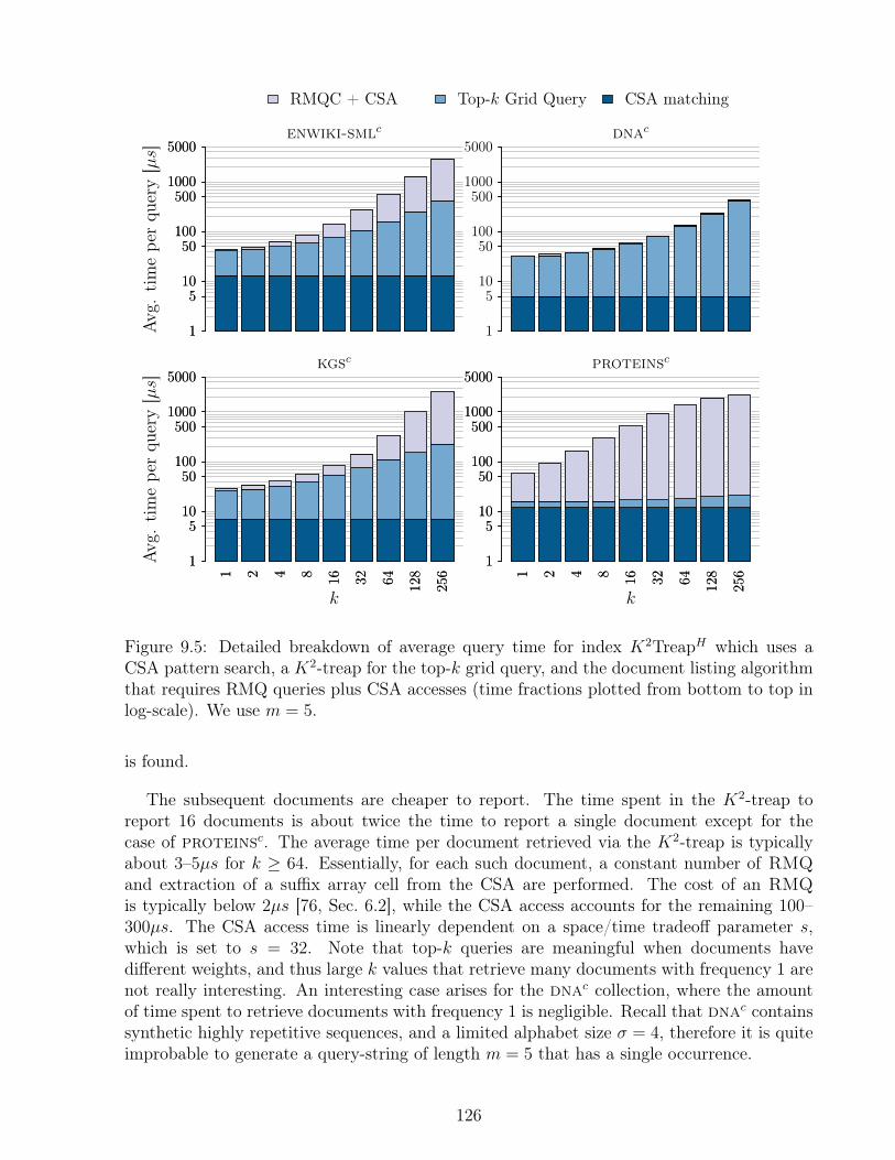
enwiki-smlc

Avg.

timepe

rqu

ery[µs]

1

510

50100

5001000

5000

1

510

50100

5001000

5000Av

g.timepe

rqu

ery[µs]

dnac

1

5

10

50

100

500

1000

5000

1

510

50100

5001000

5000

1 2 4 8 16 32 64 128

256

kgsc

Avg.

timepe

rqu

ery[µs]

1

510

50100

5001000

5000

1 2 4 8 16 32 64 128

256

1

510

50100

5001000

5000

k

Avg.

timepe

rqu

ery[µs]

1 2 4 8 16 32 64 128

256

proteinsc

1

510

50100

5001000

5000

1 2 4 8 16 32 64 128

256

1

510

50100

5001000

5000

k

RMQC + CSA Top-k Grid Query CSA matching

Figure 9.5: Detailed breakdown of average query time for index K2TreapH which uses aCSA pattern search, a K2-treap for the top-k grid query, and the document listing algorithmthat requires RMQ queries plus CSA accesses (time fractions plotted from bottom to top inlog-scale). We use m = 5.

is found.

The subsequent documents are cheaper to report. The time spent in the K2-treap toreport 16 documents is about twice the time to report a single document except for thecase of proteinsc. The average time per document retrieved via the K2-treap is typicallyabout 3–5µs for k ≥ 64. Essentially, for each such document, a constant number of RMQand extraction of a suffix array cell from the CSA are performed. The cost of an RMQis typically below 2µs [76, Sec. 6.2], while the CSA access accounts for the remaining 100–300µs. The CSA access time is linearly dependent on a space/time tradeoff parameter s,which is set to s = 32. Note that top-k queries are meaningful when documents havedifferent weights, and thus large k values that retrieve many documents with frequency 1 arenot really interesting. An interesting case arises for the dnac collection, where the amountof time spent to retrieve documents with frequency 1 is negligible. Recall that dnac containssynthetic highly repetitive sequences, and a limited alphabet size σ = 4, therefore it is quiteimprobable to generate a query-string of length m = 5 that has a single occurrence.

126

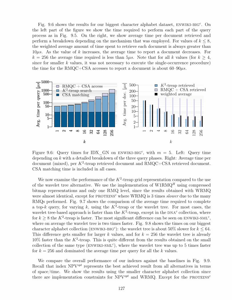
Fig. 9.6 shows the results for our biggest character alphabet dataset, enwiki-bigc. Onthe left part of the figure we show the time required to perform each part of the queryprocess as in Fig. 9.5. On the right, we show average time per document retrieved andperform a breakdown depending on the mechanism that was employed. For values of k ≤ 8,the weighted average amount of time spent to retrieve each document is always greater than10µs. As the value of k increases, the average time to report a document decreases. Fork = 256 the average time required is less than 5µs. Note that for all k values (for k ≥ 4,since for smaller k values, it was not necessary to execute the single-occurrence procedure)the time for the RMQC+CSA accesses to report a document is about 60–90µs.

1 2 4 8 16 32 64 128

256

k

Avg.

timepe

rqu

ery[µs]

1

510

50100

5001000

5000

1 2 4 8 16 32 64 128

256

k

Avg.

timepe

rqu

ery[µs]

1

510

50100

5001000

5000RMQC + CSA accessK2-treap searchCSA matching

125102050100200500

k

Avg.

timepe

rdo

c.[µs]

1 2 4 8 16 32 64 128

256

K2-treap retrievedRMQC + CSA retrievedweighted average

Figure 9.6: Query times for IDX_GN on enwiki-bigc, with m = 5. Left: Query timedepending on k with a detailed breakdown of the three query phases. Right: Average time perdocument (mixed), per K2-treap retrieved document and RMQC+CSA retrieved document.CSA matching time is included in all cases.

We now examine the performance of the K2-treap grid representation compared to the useof the wavelet tree alternative. We use the implementation of W1RMQH using compressedbitmap representations and only one RMQ level, since the results obtained with WRMQwere almost identical, except for proteinsc where WRMQ is 3 times slower due to the manyRMQs performed. Fig. 9.7 shows the comparison of the average time required to completea top-k query, for varying k, using the K2-treap or the wavelet tree. For most cases, thewavelet tree-based approach is faster than the K2-treap, except in the dnac collection, wherefor k ≥ 8 the K2-treap is faster. The most significant difference can be seen on enwiki-smlc,where on average the wavelet tree is two times faster. Fig. 9.8 shows the times on our biggestcharacter alphabet collection (enwiki-bigc): the wavelet tree is about 50% slower for k ≤ 64.This difference gets smaller for larger k values, and for k = 256 the wavelet tree is already10% faster than the K2-treap. This is quite different from the results obtained on the smallcollection of the same type (enwiki-smlc), where the wavelet tree was up to 5 times fasterfor k = 256 and dominated the average time per query for all the k values.

We compare the overall performance of our indexes against the baselines in Fig. 9.9.Recall that index NPVopt represents the best achieved result from all alternatives in termsof space/time. We show the results using the smaller character alphabet collection sincethere are implementation constraints for NPVopt and WRMQ. Except for the proteinsc

127

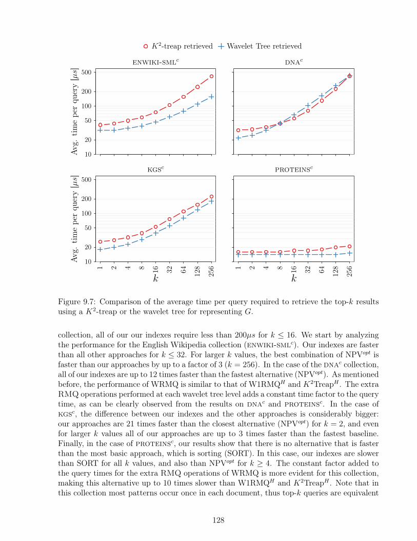
enwiki-smlc

Avg.

timepe

rqu

ery[µs]

10

20

50

100

200

500

1 2 4 8 16 32 64 128

256

dnac

1 2 4 8 16 32 64 128

256

kgsc

Avg.

timepe

rqu

ery[µs]

k

10

20

50

100

200

500

1 2 4 8 16 32 64 128

256

proteinsc

k

1 2 4 8 16 32 64 128

256

K2-treap retrieved Wavelet Tree retrieved

Figure 9.7: Comparison of the average time per query required to retrieve the top-k resultsusing a K2-treap or the wavelet tree for representing G.

collection, all of our our indexes require less than 200µs for k ≤ 16. We start by analyzingthe performance for the English Wikipedia collection (enwiki-smlc). Our indexes are fasterthan all other approaches for k ≤ 32. For larger k values, the best combination of NPVopt isfaster than our approaches by up to a factor of 3 (k = 256). In the case of the dnac collection,all of our indexes are up to 12 times faster than the fastest alternative (NPVopt). As mentionedbefore, the performance of WRMQ is similar to that of W1RMQH and K2TreapH . The extraRMQ operations performed at each wavelet tree level adds a constant time factor to the querytime, as can be clearly observed from the results on dnac and proteinsc. In the case ofkgsc, the difference between our indexes and the other approaches is considerably bigger:our approaches are 21 times faster than the closest alternative (NPVopt) for k = 2, and evenfor larger k values all of our approaches are up to 3 times faster than the fastest baseline.Finally, in the case of proteinsc, our results show that there is no alternative that is fasterthan the most basic approach, which is sorting (SORT). In this case, our indexes are slowerthan SORT for all k values, and also than NPVopt for k ≥ 4. The constant factor added tothe query times for the extra RMQ operations of WRMQ is more evident for this collection,making this alternative up to 10 times slower than W1RMQH and K2TreapH . Note that inthis collection most patterns occur once in each document, thus top-k queries are equivalent

128

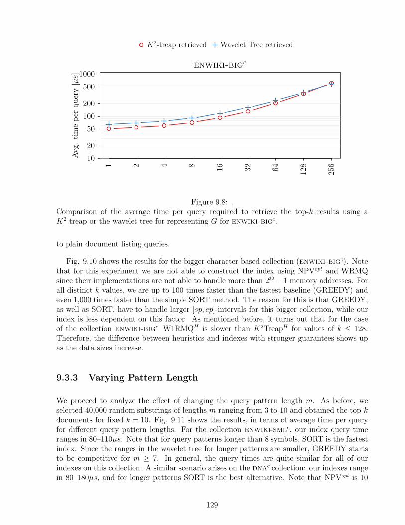
enwiki-bigcAv

g.timepe

rqu

ery[µs]

1020

50100200

5001000

1 2 4 8 16 32 64 128

256

K2-treap retrieved Wavelet Tree retrieved

Figure 9.8: .Comparison of the average time per query required to retrieve the top-k results using aK2-treap or the wavelet tree for representing G for enwiki-bigc.

to plain document listing queries.

Fig. 9.10 shows the results for the bigger character based collection (enwiki-bigc). Notethat for this experiment we are not able to construct the index using NPVopt and WRMQsince their implementations are not able to handle more than 232− 1 memory addresses. Forall distinct k values, we are up to 100 times faster than the fastest baseline (GREEDY) andeven 1,000 times faster than the simple SORT method. The reason for this is that GREEDY,as well as SORT, have to handle larger [sp, ep]-intervals for this bigger collection, while ourindex is less dependent on this factor. As mentioned before, it turns out that for the caseof the collection enwiki-bigc W1RMQH is slower than K2TreapH for values of k ≤ 128.Therefore, the difference between heuristics and indexes with stronger guarantees shows upas the data sizes increase.

9.3.3 Varying Pattern Length

We proceed to analyze the effect of changing the query pattern length m. As before, weselected 40,000 random substrings of lengths m ranging from 3 to 10 and obtained the top-kdocuments for fixed k = 10. Fig. 9.11 shows the results, in terms of average time per queryfor different query pattern lengths. For the collection enwiki-smlc, our index query timeranges in 80–110µs. Note that for query patterns longer than 8 symbols, SORT is the fastestindex. Since the ranges in the wavelet tree for longer patterns are smaller, GREEDY startsto be competitive for m ≥ 7. In general, the query times are quite similar for all of ourindexes on this collection. A similar scenario arises on the dnac collection: our indexes rangein 80–180µs, and for longer patterns SORT is the best alternative. Note that NPVopt is 10

129

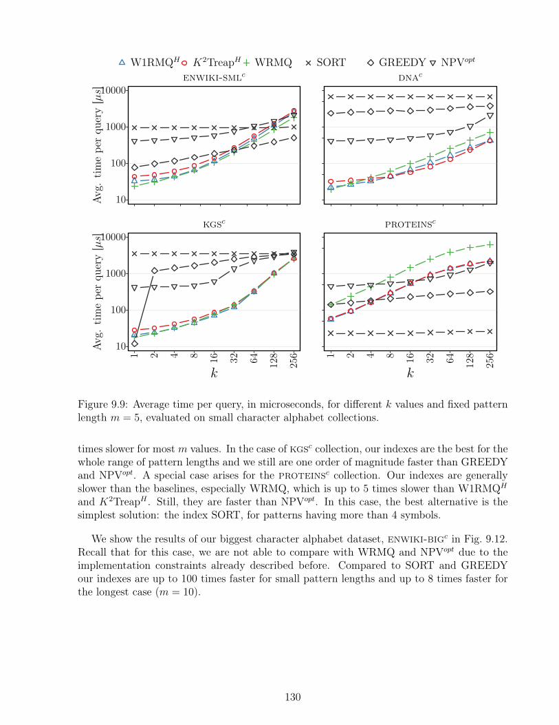
enwiki-smlc

Avg.

timepe

rqu

ery[µs]

10

100

1000

10000dnac

kgsc

Avg.

timepe

rqu

ery[µs]

k

10

100

1000

10000

1 2 4 8 16 32 64 128

256

proteinsc

k

1 2 4 8 16 32 64 128

256

W1RMQH K2TreapH WRMQ SORT GREEDY NPVopt

Figure 9.9: Average time per query, in microseconds, for different k values and fixed patternlength m = 5, evaluated on small character alphabet collections.

times slower for most m values. In the case of kgsc collection, our indexes are the best for thewhole range of pattern lengths and we still are one order of magnitude faster than GREEDYand NPVopt. A special case arises for the proteinsc collection. Our indexes are generallyslower than the baselines, especially WRMQ, which is up to 5 times slower than W1RMQH

and K2TreapH . Still, they are faster than NPVopt. In this case, the best alternative is thesimplest solution: the index SORT, for patterns having more than 4 symbols.

We show the results of our biggest character alphabet dataset, enwiki-bigc in Fig. 9.12.Recall that for this case, we are not able to compare with WRMQ and NPVopt due to theimplementation constraints already described before. Compared to SORT and GREEDYour indexes are up to 100 times faster for small pattern lengths and up to 8 times faster forthe longest case (m = 10).

130

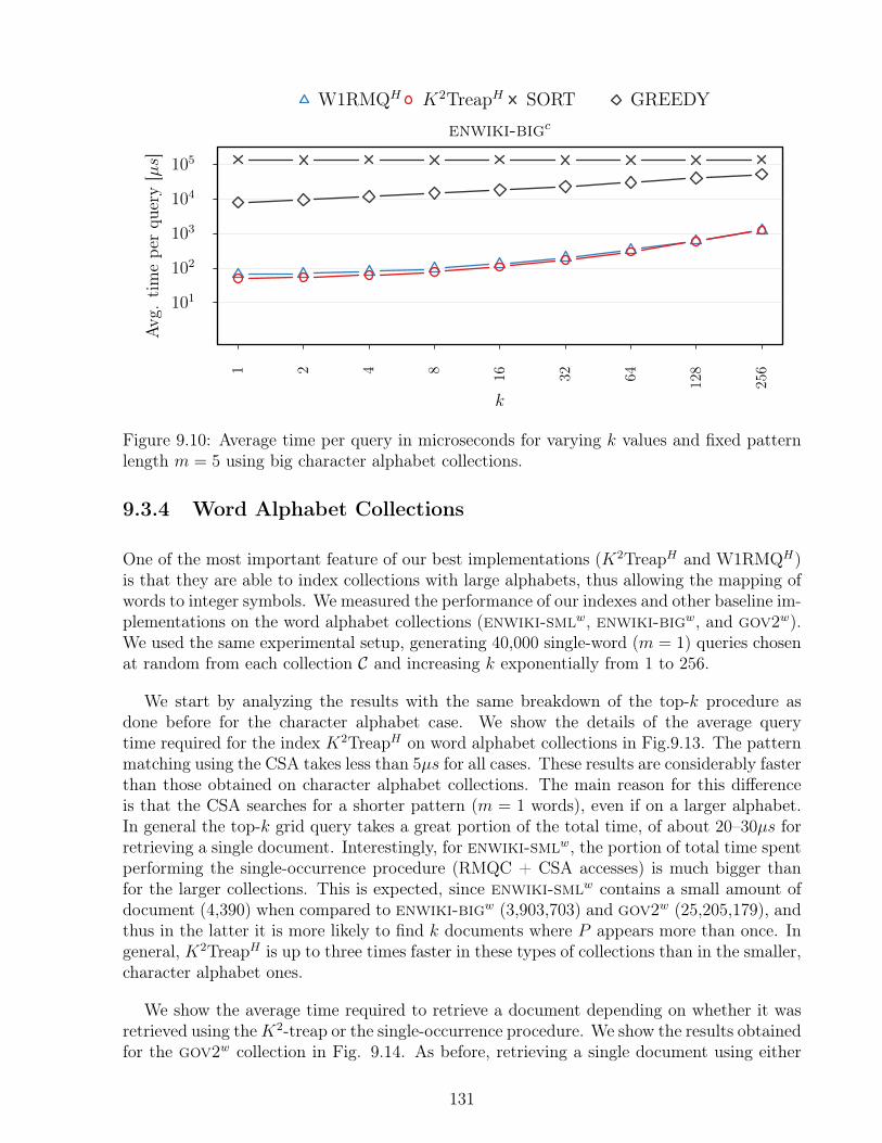
enwiki-bigc

Avg.

timepe

rqu

ery[µs]

k

101

102

103

104

105

1 2 4 8 16 32 64 128

256

W1RMQH K2TreapH SORT GREEDY

Figure 9.10: Average time per query in microseconds for varying k values and fixed patternlength m = 5 using big character alphabet collections.

9.3.4 Word Alphabet Collections

One of the most important feature of our best implementations (K2TreapH and W1RMQH)is that they are able to index collections with large alphabets, thus allowing the mapping ofwords to integer symbols. We measured the performance of our indexes and other baseline im-plementations on the word alphabet collections (enwiki-smlw, enwiki-bigw, and gov2w).We used the same experimental setup, generating 40,000 single-word (m = 1) queries chosenat random from each collection C and increasing k exponentially from 1 to 256.

We start by analyzing the results with the same breakdown of the top-k procedure asdone before for the character alphabet case. We show the details of the average querytime required for the index K2TreapH on word alphabet collections in Fig.9.13. The patternmatching using the CSA takes less than 5µs for all cases. These results are considerably fasterthan those obtained on character alphabet collections. The main reason for this differenceis that the CSA searches for a shorter pattern (m = 1 words), even if on a larger alphabet.In general the top-k grid query takes a great portion of the total time, of about 20–30µs forretrieving a single document. Interestingly, for enwiki-smlw, the portion of total time spentperforming the single-occurrence procedure (RMQC + CSA accesses) is much bigger thanfor the larger collections. This is expected, since enwiki-smlw contains a small amount ofdocument (4,390) when compared to enwiki-bigw (3,903,703) and gov2w (25,205,179), andthus in the latter it is more likely to find k documents where P appears more than once. Ingeneral, K2TreapH is up to three times faster in these types of collections than in the smaller,character alphabet ones.

We show the average time required to retrieve a document depending on whether it wasretrieved using theK2-treap or the single-occurrence procedure. We show the results obtainedfor the gov2w collection in Fig. 9.14. As before, retrieving a single document using either

131

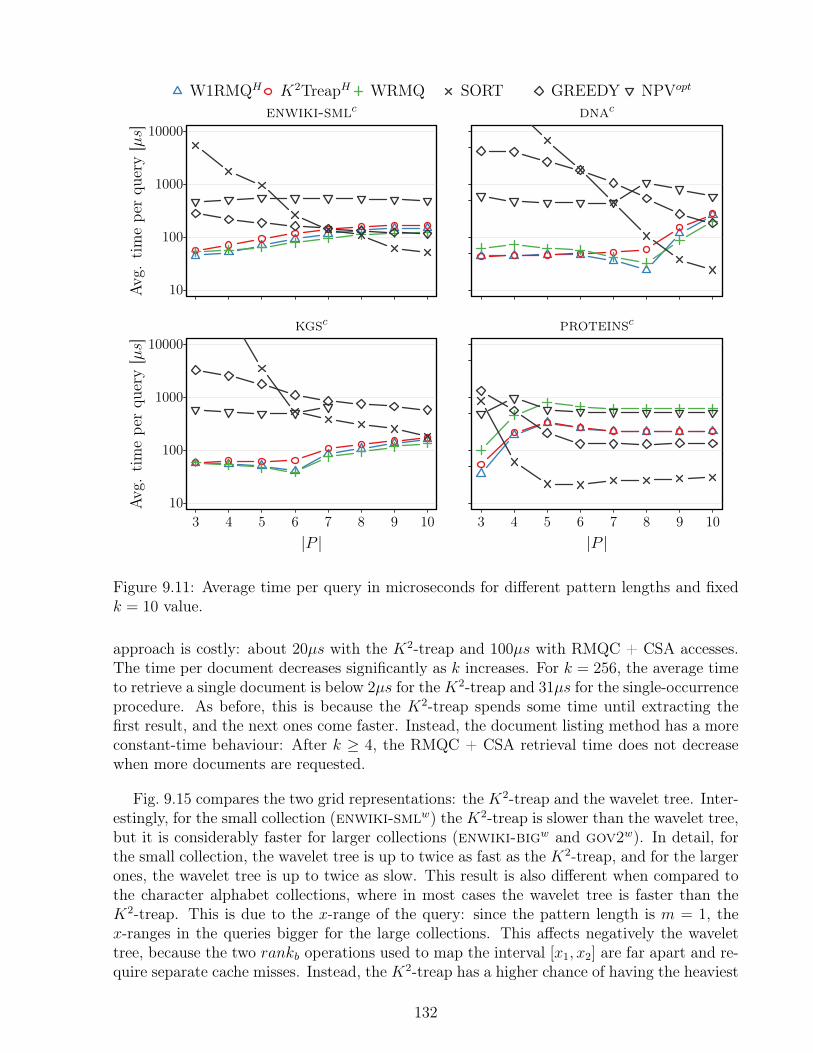
enwiki-smlc

Avg.

timepe

rqu

ery[µs]

10

100

1000

10000dnac

kgsc

Avg.

timepe

rqu

ery[µs]

|P |

10

100

1000

10000

3 4 5 6 7 8 9 10

proteinsc

|P |3 4 5 6 7 8 9 10

W1RMQH K2TreapH WRMQ SORT GREEDY NPVopt

Figure 9.11: Average time per query in microseconds for different pattern lengths and fixedk = 10 value.

approach is costly: about 20µs with the K2-treap and 100µs with RMQC + CSA accesses.The time per document decreases significantly as k increases. For k = 256, the average timeto retrieve a single document is below 2µs for the K2-treap and 31µs for the single-occurrenceprocedure. As before, this is because the K2-treap spends some time until extracting thefirst result, and the next ones come faster. Instead, the document listing method has a moreconstant-time behaviour: After k ≥ 4, the RMQC + CSA retrieval time does not decreasewhen more documents are requested.

Fig. 9.15 compares the two grid representations: the K2-treap and the wavelet tree. Inter-estingly, for the small collection (enwiki-smlw) the K2-treap is slower than the wavelet tree,but it is considerably faster for larger collections (enwiki-bigw and gov2w). In detail, forthe small collection, the wavelet tree is up to twice as fast as the K2-treap, and for the largerones, the wavelet tree is up to twice as slow. This result is also different when compared tothe character alphabet collections, where in most cases the wavelet tree is faster than theK2-treap. This is due to the x-range of the query: since the pattern length is m = 1, thex-ranges in the queries bigger for the large collections. This affects negatively the wavelettree, because the two rankb operations used to map the interval [x1, x2] are far apart and re-quire separate cache misses. Instead, the K2-treap has a higher chance of having the heaviest

132

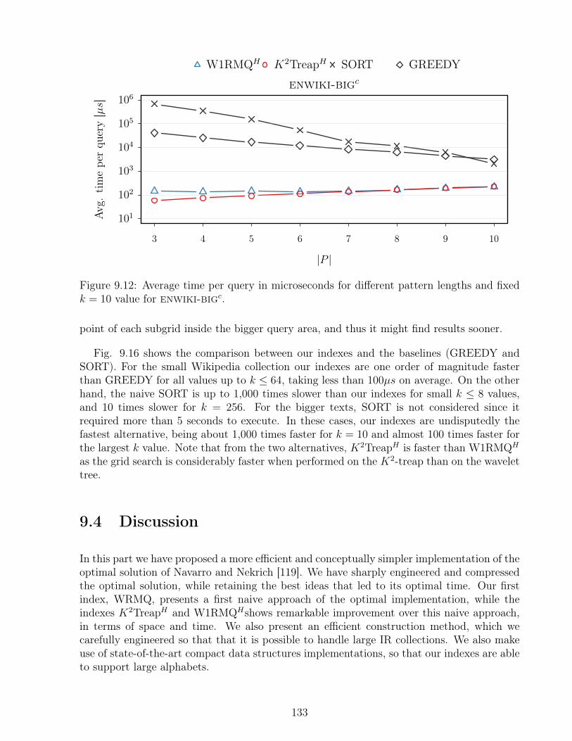
enwiki-bigcAv

g.timepe

rqu

ery[µs]

|P |

101

102

103

104

105

106

3 4 5 6 7 8 9 10

W1RMQH K2TreapH SORT GREEDY

Figure 9.12: Average time per query in microseconds for different pattern lengths and fixedk = 10 value for enwiki-bigc.

point of each subgrid inside the bigger query area, and thus it might find results sooner.

Fig. 9.16 shows the comparison between our indexes and the baselines (GREEDY andSORT). For the small Wikipedia collection our indexes are one order of magnitude fasterthan GREEDY for all values up to k ≤ 64, taking less than 100µs on average. On the otherhand, the naive SORT is up to 1,000 times slower than our indexes for small k ≤ 8 values,and 10 times slower for k = 256. For the bigger texts, SORT is not considered since itrequired more than 5 seconds to execute. In these cases, our indexes are undisputedly thefastest alternative, being about 1,000 times faster for k = 10 and almost 100 times faster forthe largest k value. Note that from the two alternatives, K2TreapH is faster than W1RMQH

as the grid search is considerably faster when performed on the K2-treap than on the wavelettree.

9.4 Discussion

In this part we have proposed a more efficient and conceptually simpler implementation of theoptimal solution of Navarro and Nekrich [119]. We have sharply engineered and compressedthe optimal solution, while retaining the best ideas that led to its optimal time. Our firstindex, WRMQ, presents a first naive approach of the optimal implementation, while theindexes K2TreapH and W1RMQHshows remarkable improvement over this naive approach,in terms of space and time. We also present an efficient construction method, which wecarefully engineered so that that it is possible to handle large IR collections. We also makeuse of state-of-the-art compact data structures implementations, so that our indexes are ableto support large alphabets.

133

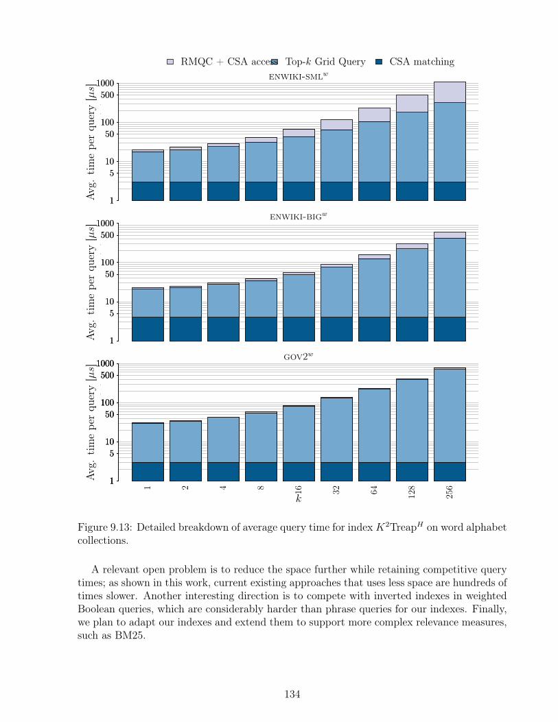
1 2 4 8 16 32 64 128 256

enwiki-smlw

Avg.

timepe

rqu

ery[µs]

1

510

50100

5001000

1 2 4 8 16 32 64 128 256

1

510

50100

5001000

Avg.

timepe

rqu

ery[µs]

1 2 4 8 16 32 64 128 256

enwiki-bigw

Avg.

timepe

rqu

ery[µs]

1

510

50100

5001000

1 2 4 8 16 32 64 128 256

1

510

50100

5001000

Avg.

timepe

rqu

ery[µs]

1 2 4 8 16 32 64 128 256

gov2w

Avg.

timepe

rqu

ery[µs]

1

510

50100

5001000

1 2 4 8 16 32 64 128 256

1

510

50100

5001000

k

1 2 4 8 16 32 64 128

256

1

510

50100

5001000

Avg.

timepe

rqu

ery[µs]

RMQC + CSA access Top-k Grid Query CSA matching

Figure 9.13: Detailed breakdown of average query time for indexK2TreapH on word alphabetcollections.

A relevant open problem is to reduce the space further while retaining competitive querytimes; as shown in this work, current existing approaches that uses less space are hundreds oftimes slower. Another interesting direction is to compete with inverted indexes in weightedBoolean queries, which are considerably harder than phrase queries for our indexes. Finally,we plan to adapt our indexes and extend them to support more complex relevance measures,such as BM25.

134

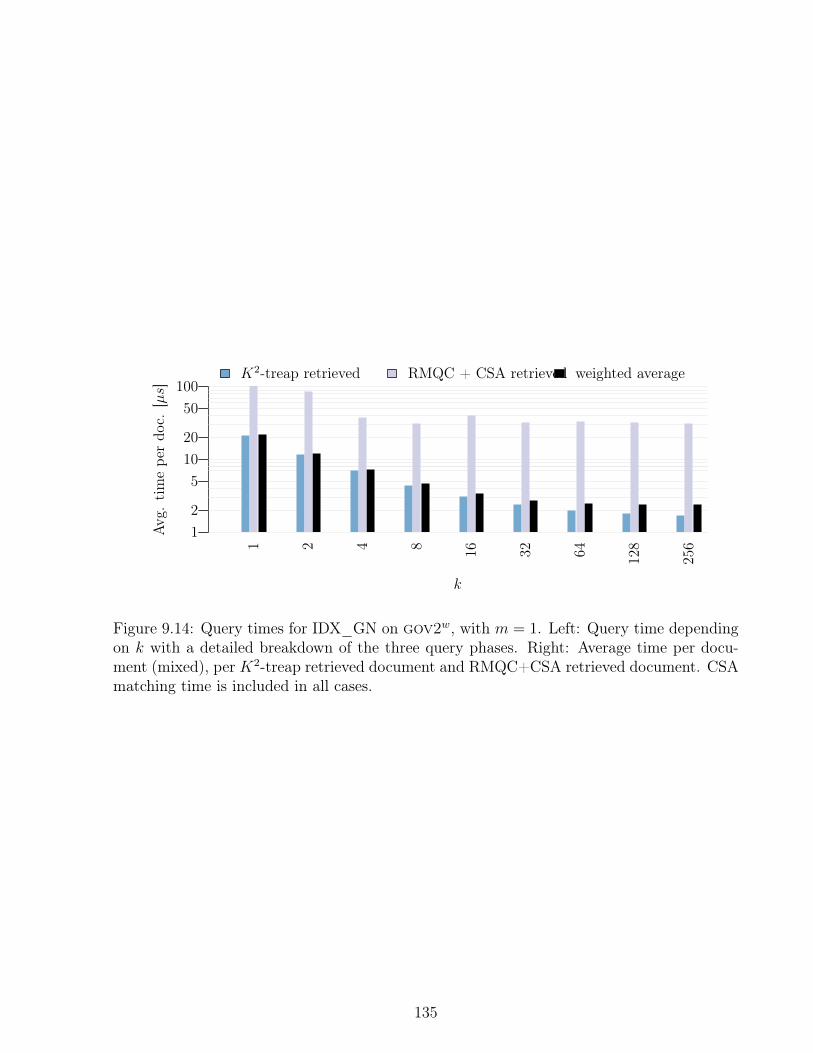
12

51020

50100

k

Avg.

timepe

rdo

c.[µs]

1 2 4 8 16 32 64 128

256

K2-treap retrieved RMQC + CSA retrieved weighted average

Figure 9.14: Query times for IDX_GN on gov2w, with m = 1. Left: Query time dependingon k with a detailed breakdown of the three query phases. Right: Average time per docu-ment (mixed), per K2-treap retrieved document and RMQC+CSA retrieved document. CSAmatching time is included in all cases.

135

enwiki-smlw

Avg.

timepe

rqu

ery[µs]

1020

50100200

50010002000

enwiki-bigw

Avg.

timepe

rqu

ery[µs]

1020

50100200

50010002000

gov2w

Avg.

timepe

rqu

ery[µs]

1020

50100200

50010002000

1 2 4 8 16 32 64 128

256

k

K2-treap retrieved Wavelet Tree retrieved

Figure 9.15: Comparison of the average time per query to retrieve the top-k results using aK2-treap or the wavelet tree for representing G in word alphabet collections.

136

enwiki-bigw

Avg.

timepe

rqu

ery[µs]

101

102

103

104

105

106

enwiki-bigw

Avg.

timepe

rqu

ery[µs]

101

102

103

104

105

106

gov2w

Avg.

timepe

rqu

ery[µs]

k

101

102

103

104

105

106

1 2 4 8 16 32 64 128

256

W1RMQH K2TreapH SORT GREEDY

Figure 9.16: Average time per query in microseconds for different k values and fixed patternlength m = 1 on word alphabet collections. Results that required more than 5 seconds forSORT are not shown.

137

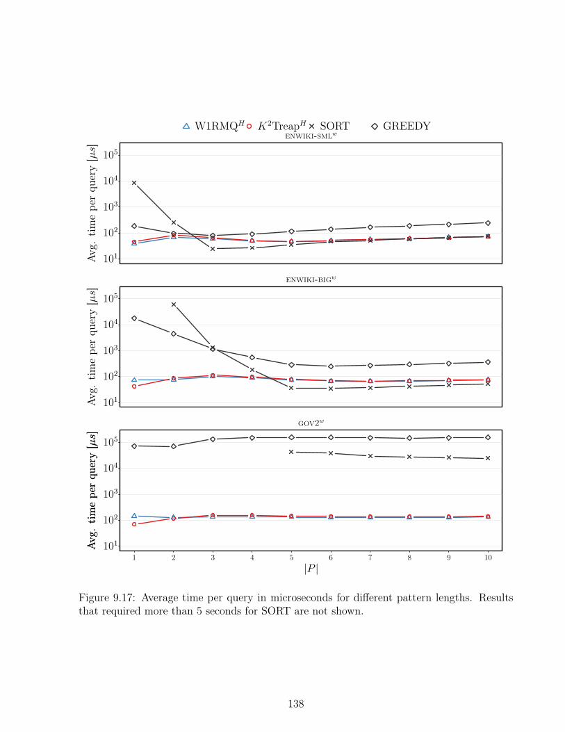
enwiki-smlw

Avg.

timepe

rqu

ery[µs]

101

102

103

104

105

enwiki-bigw

Avg.

timepe

rqu

ery[µs]

101

102

103

104

105

gov2w

Avg.

timepe

rqu

ery[µs]

101

102

103

104

105

Avg.

timepe

rqu

ery[µs]

|P |1 2 3 4 5 6 7 8 9 10

W1RMQH K2TreapH SORT GREEDY

Figure 9.17: Average time per query in microseconds for different pattern lengths. Resultsthat required more than 5 seconds for SORT are not shown.

138

Part IV

Extensions and Evangelization

139

Chapter 10

Aggregated 2D Queries on ClusteredPoints

In this chapter we present a generalization of the technique that was used in the designof the K2-treap data structure (see Section 7.2) to support other types of two-dimensionalaggregated queries. We show how to extend the K2-tree to solve the problem of efficientlyretrieving the number of points that lie in a two-dimensional range [x1, x2] × [y1, y2]. Ourexperimental evaluation shows that by using little space overhead (less than a 30%) on topof the K2-tree, the modified version of the data structure performs queries several orders ofmagnitude faster than the original K2-tree, especially when the query ranges are large.

The K2-treap data structure appears in the proceedings of the 21st String Processingand Information Retrieval conference (SPIRE), 2014, held in Ouro Preto, Brazil. The gen-eralization of the K2-treap as a technique that employs the K2-tree to perform aggregatedtwo-dimensional queries over clustered set of points has been published in the journal Infor-mation Systems, in March of 2016. This work was developed in collaboration with Nieves R.Brisaboa, Guillermo de Bernardo from University of A. Coruña, Spain and Diego Seco, fromUniversity of Concepción.

10.1 Motivation

Many problems in different domains can be interpreted geometrically by modeling datarecords as multidimensional points and transforming queries about the original records intoqueries on the point sets [26, Chapter 5]. In 2D, for example, orthogonal range queries ona grid can be used to solve queries of the form “report all employees born between y0 andy1 who earn between s1 and s2 dollars”, which are very common in databases. By the sametoken, other range aggregated queries (e.g., top-k, counting, quantile, majority, etc.) haveproven to be useful for analyses about the data in various domains, such as OLAP databases,Geographic Information Systems, Information Retrieval, Data Mining, among others [120].For example, top-k queries on a OLAP database of sales can be used to find the sellers with

140

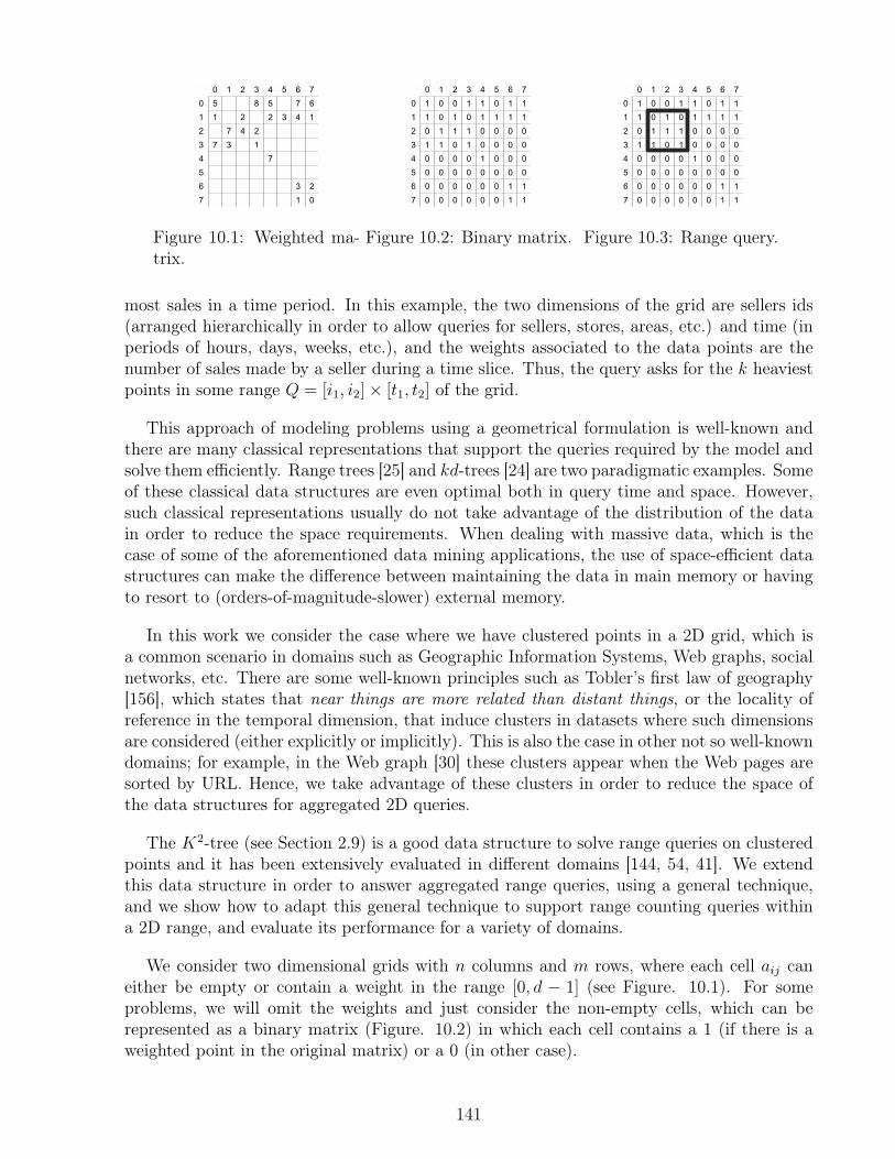
Figure 10.1: Weighted ma-trix.

Figure 10.2: Binary matrix. Figure 10.3: Range query.

most sales in a time period. In this example, the two dimensions of the grid are sellers ids(arranged hierarchically in order to allow queries for sellers, stores, areas, etc.) and time (inperiods of hours, days, weeks, etc.), and the weights associated to the data points are thenumber of sales made by a seller during a time slice. Thus, the query asks for the k heaviestpoints in some range Q = [i1, i2]× [t1, t2] of the grid.

This approach of modeling problems using a geometrical formulation is well-known andthere are many classical representations that support the queries required by the model andsolve them efficiently. Range trees [25] and kd-trees [24] are two paradigmatic examples. Someof these classical data structures are even optimal both in query time and space. However,such classical representations usually do not take advantage of the distribution of the datain order to reduce the space requirements. When dealing with massive data, which is thecase of some of the aforementioned data mining applications, the use of space-efficient datastructures can make the difference between maintaining the data in main memory or havingto resort to (orders-of-magnitude-slower) external memory.

In this work we consider the case where we have clustered points in a 2D grid, which isa common scenario in domains such as Geographic Information Systems, Web graphs, socialnetworks, etc. There are some well-known principles such as Tobler’s first law of geography[156], which states that near things are more related than distant things, or the locality ofreference in the temporal dimension, that induce clusters in datasets where such dimensionsare considered (either explicitly or implicitly). This is also the case in other not so well-knowndomains; for example, in the Web graph [30] these clusters appear when the Web pages aresorted by URL. Hence, we take advantage of these clusters in order to reduce the space ofthe data structures for aggregated 2D queries.

The K2-tree (see Section 2.9) is a good data structure to solve range queries on clusteredpoints and it has been extensively evaluated in different domains [144, 54, 41]. We extendthis data structure in order to answer aggregated range queries, using a general technique,and we show how to adapt this general technique to support range counting queries withina 2D range, and evaluate its performance for a variety of domains.

We consider two dimensional grids with n columns and m rows, where each cell aij caneither be empty or contain a weight in the range [0, d − 1] (see Figure. 10.1). For someproblems, we will omit the weights and just consider the non-empty cells, which can berepresented as a binary matrix (Figure. 10.2) in which each cell contains a 1 (if there is aweighted point in the original matrix) or a 0 (in other case).

141

Let t be the number of 1s in the binary matrix (i.e., the number of weighted points). Ifwe can partition the t points into c clusters, not necessarily disjoint and c << t, we will saythe points are clustered. This definition is used in Gagie et al. [73] to show that a quadtreein such case has O(c log u+

∑i ti log li), where u = max(n,m), and ti and li are the number

of points and the diameter of cluster i, respectively.

A range query Q = [x1, x2]× [y1, y2] defines a query rectangle with all the columns in therange [x1, x2] and the rows in [y1, y2] (see Fig. 10.3). An aggregated range query defines, inaddition to the range, an aggregate function that must be applied to the data points in therange query. Examples of aggregated queries are count(Q), which counts the number of datapoints in the range query, max/min(Q), which computes the maximum (alt. minimum) valuein the query range, and its generalization top-k, which retrieves the k lightest (alt. heaviest)points in the query range. These top-k queries are also referred in the literature as rankedrange queries. For the range query q in Fig. 10.3 the result of count(q) is 6, max(q) returns7, min(q) returns 1, and the top-3 heaviest elements are 7, 4 and 3.

There are other interesting data-analysis queries on two-dimensional grids. For example,quantile(Q, k), which returns the k-th smallest value in Q, or majority(Q,α), whichretrieves those values in Q that appear with relative frequency larger than α. These andmore have been studied in [120], where the authors propose space-efficient data structureswith good time performance. We restrict ourselves to an emblematic subset of these queries,and propose data structures that are even more space-efficient when the points in the set areclustered.

10.2 Augmenting the K2-tree

LetM [n×n] be a matrix in which cells can be empty or contain weight in the range [0, d−1]and let BM [n × n] be a binary matrix in which each cell contains a zero or a one. We saythat BMM represents the topology of M if BMM [i][j] = 1 when M [i][j] is not empty, andBMM [i][j] = 0, otherwise.

On the one hand, we store the topology of the data. On the other hand, we store theweights associated with each non-empty cell. For the topology, which can be regarded as abinary matrix, we use a K2-tree. Recall from Section 2.9 that this data structure requireslittle space when the data points are clustered. The K2-tree performs a recursive divisionof the space into K2 submatrices until it reaches an individual cell or a completely emptysubmatrix, and each of these submatrices is represented in the data-structure with a bit.Therefore, each bit in the K2-tree represents a submatrix of the original matrix which sizedepends on its depth on the recursive division.

A level-wise traversal of the K2-tree can be used to map each node to an aggregatedvalue that summarizes the weights in the corresponding submatrix. The specific value of thissummary depends on the operation. For example, for ranked range queries (see Section 7.2)the summary represents the maximum weight in the corresponding submatrix, whereas forcounting queries, it represents the number of non-empty cells in the submatrix. However, a

142

common property is that the value associated with a node aggregates information about itsK2 children. Therefore, we use a sort of differential encoding [48] to encode the values of eachnode with respect to the value of its parent. In other words, the information of a node (suchas its summary and number of children) is used to represent the information of its childrenin a more compact way. In order to access the original (non-compressed) information of anode we need to access its parent first (i.e., the operations in this technique are restricted toroot-to-leaves traversals).

To summarize, we use a K2-tree to represent the topology of the data and augment eachnode of such a tree with additional values that represents the aggregate information relatedwith the operation to be supported. These aggregated values are differentially encoded withrespect to information of the parent node in order to reduce the space necessary to storethem. In the following two sections we show how both the K2-tree and the differentialencoded values can be tuned to efficiently solve two types of aggregated queries.

Finally, note that we present our results for matrices of size n × n. This is not a lossof generality, as we can extend a matrix M ′[n ×m] with zeros to complete a square matrixM [n × n] (w.l.o.g. we assume m ≤ n). As the topology of the matrix is represented with aK2-tree, this does not cause a significant overhead because the K2-tree is efficient to handlelarge areas of zeros. Actually, we round n up to the next power of K [35].

10.2.1 Supporting Counting Queries

In addition to the K2-tree, the augmented data structure stores additional information tosupport range counting queries efficiently. In Figure 10.4 we show a conceptual K2-treein which each node has been annotated with the number of elements in its correspondingsubmatrix. Note that this is the same example of Figure 7.2 considering as non-empty cellsthose with weight larger than 0.

This conceptual tree is traversed level-wise, reading the sequence of counts from left toright in each level. All these counts are stored in a sequence counts using a variant ofthe differential encoding technique presented in Section 10.2. Let v be a node of the K2-tree, children(v) the number of children of v, and count(v) the number of elements in thesubmatrix represented by v. Then, count(v′) = count(v)

children(v)represents the expected number of

elements in the submatrix associated with each child v′ of v, assuming an uniform distribution.Thus, the count of each node v′ is stored as the difference of the actual count and its expectedvalue. In the running example, the root has three children and there are 22 elements in thematrix. Each of the corresponding submatrices is expected to contain b22/3c = 7 elementswhereas they actually contain 10, 7 and 5 elements, respectively. Hence, the differentialenconding stores 10− 7 = 3, 7− 7 = 0, and 5− 7 = −2.

The result of this differential encoding is a new sequence of values smaller than the original,but which may contain negative values. In order to map this sequence, in a unique andreversible way, to a sequence of non-negative values we use the folklore overlap and interleavescheme, which maps a negative number −i to the ith-odd number (2i − 1) and a positivenumber j to the jth even number (2j). Finally, to exploit the small values while allowing

143

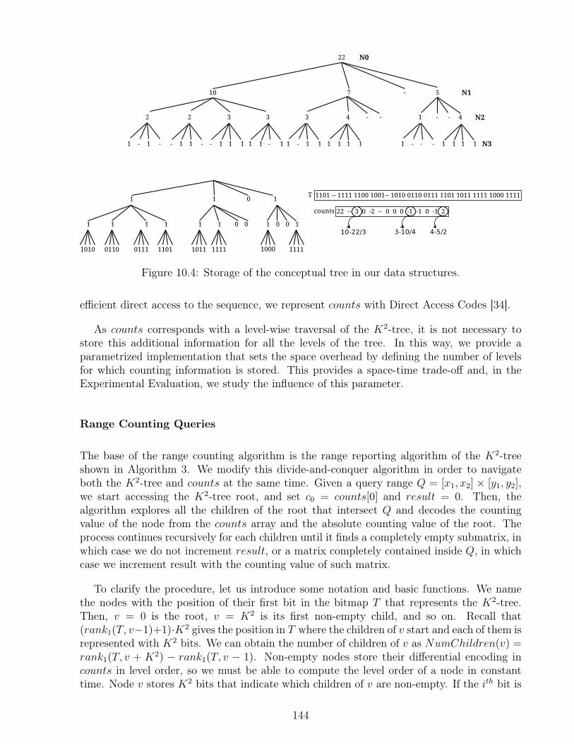
Figure 10.4: Storage of the conceptual tree in our data structures.

efficient direct access to the sequence, we represent counts with Direct Access Codes [34].

As counts corresponds with a level-wise traversal of the K2-tree, it is not necessary tostore this additional information for all the levels of the tree. In this way, we provide aparametrized implementation that sets the space overhead by defining the number of levelsfor which counting information is stored. This provides a space-time trade-off and, in theExperimental Evaluation, we study the influence of this parameter.

Range Counting Queries

The base of the range counting algorithm is the range reporting algorithm of the K2-treeshown in Algorithm 3. We modify this divide-and-conquer algorithm in order to navigateboth the K2-tree and counts at the same time. Given a query range Q = [x1, x2] × [y1, y2],we start accessing the K2-tree root, and set c0 = counts[0] and result = 0. Then, thealgorithm explores all the children of the root that intersect Q and decodes the countingvalue of the node from the counts array and the absolute counting value of the root. Theprocess continues recursively for each children until it finds a completely empty submatrix, inwhich case we do not increment result, or a matrix completely contained inside Q, in whichcase we increment result with the counting value of such matrix.

To clarify the procedure, let us introduce some notation and basic functions. We namethe nodes with the position of their first bit in the bitmap T that represents the K2-tree.Then, v = 0 is the root, v = K2 is its first non-empty child, and so on. Recall that(rank1(T, v−1)+1)·K2 gives the position in T where the children of v start and each of them isrepresented with K2 bits. We can obtain the number of children of v as NumChildren(v) =rank1(T, v + K2) − rank1(T, v − 1). Non-empty nodes store their differential encoding incounts in level order, so we must be able to compute the level order of a node in constanttime. Node v stores K2 bits that indicate which children of v are non-empty. If the ith bit is

144

set to 1, then the level order of that child node is rank1(T, v + i), with i ∈ [0, K2 − 1].

Given a node v with absolute counting value cv and NumChildren(v) children, we expecteach child v′ to represent count(v′) = cv

NumChildren(v)elements. Let p be the level order

number of child v′. Then, the absolute counting value of v′ can be computed as cv′ =counts[p] + count(v′). Note that counts is stored using DACs, which support efficient directaccess. By updating cv′ before visiting each node v′, we can complete the recursive procedure.

Let us consider a query example q = [0, 1] × [0, 2]. We start at the root with c0 = 22and result = 0. The root has three children, but only the first one, stored at position4 in T , intersects q. Each child is expected to represent b22/3c = 7 elements, so we setc4 = counts[rank1(T, 0 + 0)] + 7 = 3 + 7 = 10. Similarly, we recurse on the first and thirdchildren of this node. On the first branch of the recursion, we process node 16 and setc16 = counts[rank1(T, 4 + 0)] + b10/4c = counts[4] + 2 = 2. As the submatrix correspondingwith this node is contained inside q, we add 2 to the result and stop the recursion on thisbranch. On the other one, we have to recurse until the leaves to sum the other element tothe result, and obtain the final count of three.

Other Supported Queries

This data structure obviously supports all the queries that can be implemented on a K2-tree,such as range reporting or emptiness queries. More interesting is that it can also supportother types of queries with minor modifications. A natural generalization of range countingqueries are aggregated sum queries. In this case, we consider a matrix M [n× n] where eachcell can either be empty or contain a weight in the range [0, d−1]. We perform the same datapartitioning on the conceptual binary matrix that represents the non-empty cells. In otherwords, we use a K2-tree to represent the topology of the matrix. Then, instead of augmentingthe nodes with the count of the non-empty cells in the corresponding submatrix, we storethe sum of the weights contained in such submatrix. The same differential encoding used forrange counting can be used to store these sums. In this case, however, the space-efficiencyachieved by the data structure depends not only on the clustering of the data, but also onthe distribution of the weights. The encoding achieves its best performance when the sumsof the weights of all the children of a node are similar.

10.3 Experiments and Results

In this section we present the conducted empirical evaluation of range counting queries. Wefirst present the experiment setup (baselines and datasets), then an evaluation in terms ofthe space required by the different solutions, and finally a comparison of the running timesof such solutions.

We ran all our experiments on a dedicated server with 4 Intel(R) Xeon(R) E5520 CPUcores at 2.27GHz 8MB cache and 72GB of RAM memory. The machine runs UbuntuGNU/Linux version 9.10 with kernel 2.6.31-19-server (64 bits) and gcc 4.4.1. All the data

145

structures were implemented in C/C++ and compiled with full optimizations.

All bitmaps that are employed use a bitmap representation that supports rank and se-lect using 5% of extra space. The wavelet tree that was employed to implement the solutionof [120] is a pointer less version obtained from LIBCDS1. This wavelet tree is augmented witha RMQ data structure (recall Section 2.12 at each level.

10.3.1 Experiment Setup

We use grid datasets coming from three different real domains: Geographic InformationSystems (GIS), Social Networks (SN) and Web Graphs (WEB). For GIS data we use theGeonames dataset2, which contains the geographic coordinates (latitude and longitude) ofmore than 6 million populated places, and converted it into three grids with different res-olutions: Geo-sparse, Geo-med, and Geo-dense. The higher the resolution, the sparser thematrix. These datasets allow for evaluating the influence of data sparsity in the differentproposals. For SN we use three social networks (dblp-2011, enwiki-2013 and ljournal-2008)obtained from the Laboratory for Web Algorithmics3 [31, 28]. Finally, in the WEB domainwe consider the grid associated with the adjacency matrix of three Web graphs (indochina-2004, uk-2002 and uk-2007-5) obtained from the same Web site. The existence of clustersin these datasets is very dissimilar. In general, GIS datasets do not preset many clusterswhereas data points in the WEB datasets are very clustered. SN represent an intermediatecollection in terms of clustering.

In this experiment, we compare our proposal to speed up range counting queries on aK2-tree, named rck2tree, with the original K2-tree. In this evaluation we show the space-time trade-off offered by the rck2tree structure, which is parametrized by the number oflevels of the original K2-tree augmented with counting information. As a baseline from thesuccinct data structures area, we include a representation of grids based on wavelet trees(recall Section 7.1), named wtgrid in the following discussion. As explained in Section 2.7.4,this representation requires a bitmap to map from a general grid to a grid with at most onepoint per column. In our experiments we store this bitmap with either plain bitmaps or RRR,the one that requires less space. As for the wavelet tree itself, we use a balanced tree withjust one pointer per level and the bitmaps of each level are compressed with RRR. In otherwords, we use a configuration of this representation that aims to reduce the space. Note,however, that we use the implementation available in Libcds [46], which uses O(σ) countersto speed up queries. As we will show in the experiments, this data structure, even with thecompression of the bitmaps that represent the nodes of the wavelet tree, does not take fulladvantage of the existence of clusters in the data points.

Table 10.1 shows the main characteristics of the datasets used: name of the dataset, size ofthe grid (u)4, number of points it contains (n) and the space achieved by the baseline wtgrid,

1http://www.github.com/fclaude/libcds/2http://www.geonames.org/3http://law.di.unimi.it4Note that, unlike the grids used in the previous scenario, these are square grids, and thus u represents

both the number of rows and columns.

146

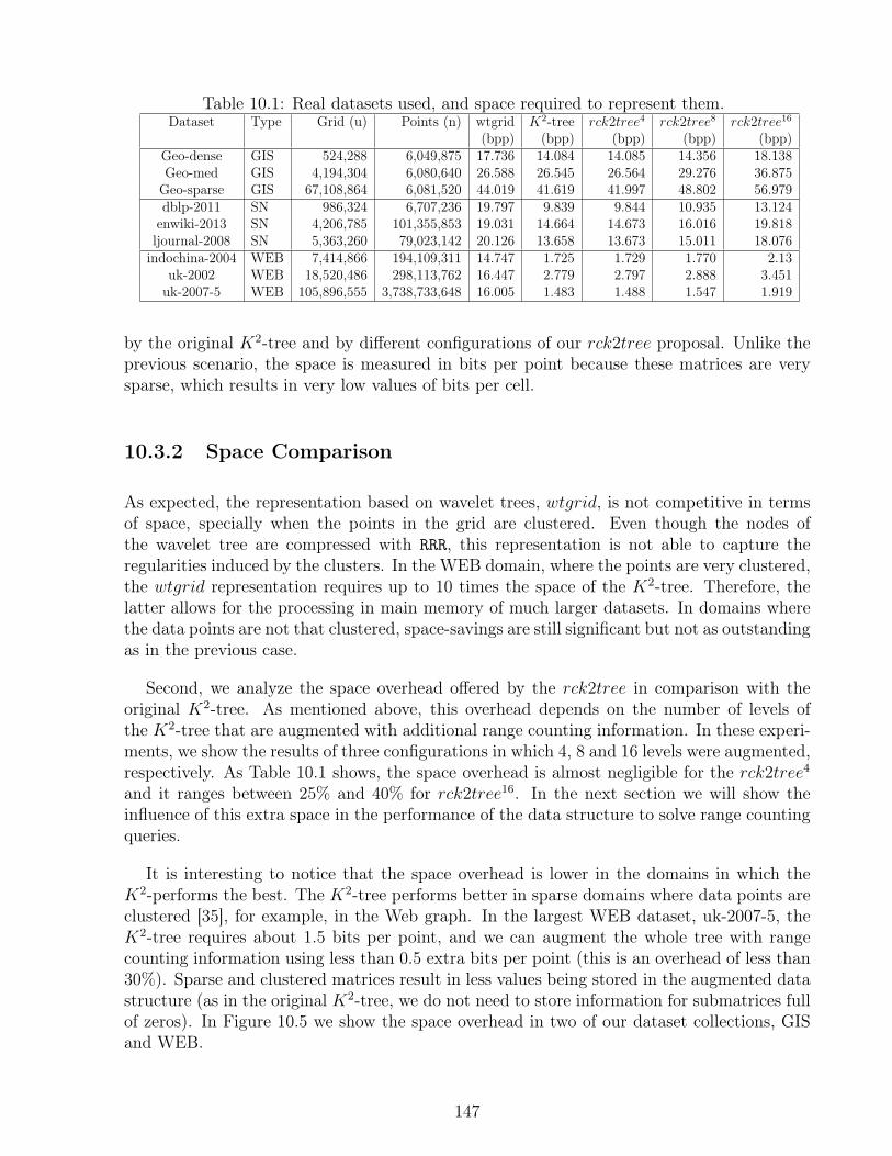
Table 10.1: Real datasets used, and space required to represent them.Dataset Type Grid (u) Points (n) wtgrid K2-tree rck2tree4 rck2tree8 rck2tree16

(bpp) (bpp) (bpp) (bpp) (bpp)Geo-dense GIS 524,288 6,049,875 17.736 14.084 14.085 14.356 18.138Geo-med GIS 4,194,304 6,080,640 26.588 26.545 26.564 29.276 36.875Geo-sparse GIS 67,108,864 6,081,520 44.019 41.619 41.997 48.802 56.979dblp-2011 SN 986,324 6,707,236 19.797 9.839 9.844 10.935 13.124enwiki-2013 SN 4,206,785 101,355,853 19.031 14.664 14.673 16.016 19.818ljournal-2008 SN 5,363,260 79,023,142 20.126 13.658 13.673 15.011 18.076indochina-2004 WEB 7,414,866 194,109,311 14.747 1.725 1.729 1.770 2.13

uk-2002 WEB 18,520,486 298,113,762 16.447 2.779 2.797 2.888 3.451uk-2007-5 WEB 105,896,555 3,738,733,648 16.005 1.483 1.488 1.547 1.919

by the original K2-tree and by different configurations of our rck2tree proposal. Unlike theprevious scenario, the space is measured in bits per point because these matrices are verysparse, which results in very low values of bits per cell.

10.3.2 Space Comparison

As expected, the representation based on wavelet trees, wtgrid, is not competitive in termsof space, specially when the points in the grid are clustered. Even though the nodes ofthe wavelet tree are compressed with RRR, this representation is not able to capture theregularities induced by the clusters. In the WEB domain, where the points are very clustered,the wtgrid representation requires up to 10 times the space of the K2-tree. Therefore, thelatter allows for the processing in main memory of much larger datasets. In domains wherethe data points are not that clustered, space-savings are still significant but not as outstandingas in the previous case.

Second, we analyze the space overhead offered by the rck2tree in comparison with theoriginal K2-tree. As mentioned above, this overhead depends on the number of levels ofthe K2-tree that are augmented with additional range counting information. In these experi-ments, we show the results of three configurations in which 4, 8 and 16 levels were augmented,respectively. As Table 10.1 shows, the space overhead is almost negligible for the rck2tree4

and it ranges between 25% and 40% for rck2tree16. In the next section we will show theinfluence of this extra space in the performance of the data structure to solve range countingqueries.

It is interesting to notice that the space overhead is lower in the domains in which theK2-performs the best. The K2-tree performs better in sparse domains where data points areclustered [35], for example, in the Web graph. In the largest WEB dataset, uk-2007-5, theK2-tree requires about 1.5 bits per point, and we can augment the whole tree with rangecounting information using less than 0.5 extra bits per point (this is an overhead of less than30%). Sparse and clustered matrices result in less values being stored in the augmented datastructure (as in the original K2-tree, we do not need to store information for submatrices fullof zeros). In Figure 10.5 we show the space overhead in two of our dataset collections, GISand WEB.

147

0

10

20

30

40

50

GEO_dense GEO_med GEO_sparse

Sp

ace

(b

its/p

oin

t)

Dataset

rck2tree16

rck2tree8

rck2tree4

K2-tree

0

0.5

1

1.5

2

2.5

3

3.5

indochina-2004 uk-2002 uk-2007-5

Sp

ace

(b

its/p

oin

t)

Dataset

rck2tree16

rck2tree8

rck2tree4

K2-tree

Figure 10.5: Space overhead in GIS and WEB datasets.

Note also that, unlike the K2-tree, the space overhead is not drastically increased insparse, but not clustered, datasets (for example, Geo-sparse). Isolated points are representedin the original K2-tree with K2 bits per level, which results in a strong degradation of suchrepresentation. The K2-tree uses more than 40 bits per point in the Geo-sparse dataset,which is a lot more than the about 2 bits per point in the, also sparse, WEB datasets.However, the space overhead of the rck2tree16 (with respect to the K2-tree) is about 40% inGeo-sparse and 30% in uk-2007-5 (i.e., a difference of 10 percentage points). Isolated pointsare represented with approximately two bits per level in the range counting data structure,as it represents the difference between the expected number of elements in the submatrix,one, and the actual number, which is also one5. If we consider the other configurations thatstore range counting values for less levels of the K2-tree the difference is even smaller. Thisis expected because there are less isolated points in higher levels of the K2-tree.

10.3.3 Query Processing

In this section we analyze the efficiency of range counting queries, comparing our augmentedK2-tree with the original data structure and with the wtgrid. For each dataset, we buildmultiple sets of queries with different query selectivities (i.e., size of spatial ranges). All thequery sets were generated for fixed query selectivity. A query selectivity of X% means thateach query in the set covers X% of the cells in the dataset. Each query set contains 1,000queries where the spatial window is placed at a random position within the matrix.

As in the space comparison, we show the results of three different configurations of ouraugmented data structure, in which 4, 8 and 16 levels were augmented with range countingdata. Fig. 10.4 shows the time required to perform range counting queries in some of our realdatasets, for different values of query selectivity. For each domain (GIS, SN and WEB), weonly show the results of the two most different datasets, as the other datasets do not changethe conclusions of this comparison.

5Recall that these data are represented using DACs, which require at least two bits, one two encode thedifference and one two indicate that such value is encoded using just one block.

148

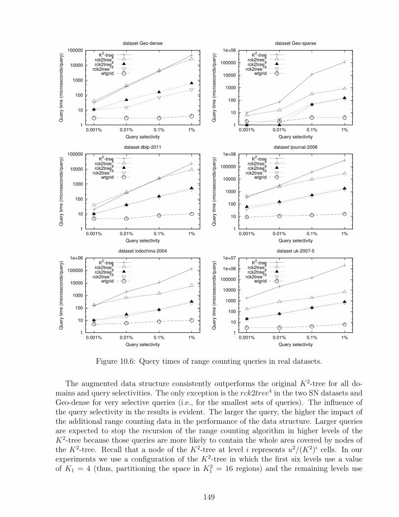
1

10

100

1000

10000

100000

0.001% 0.01% 0.1% 1%

Qu

ery

tim

e (

mic

rose

co

nd

s/q

ue

ry)

Query selectivity

dataset Geo-dense

K2-tree

rck2tree4

rck2tree8

rck2tree16

wtgrid

1

10

100

1000

10000

100000

1e+06

0.001% 0.01% 0.1% 1%

Qu

ery

tim

e (

mic

rose

co

nd

s/q

ue

ry)

Query selectivity

dataset Geo-sparse

K2-tree

rck2tree4

rck2tree8

rck2tree16

wtgrid

1

10

100

1000

10000

100000

0.001% 0.01% 0.1% 1%

Qu

ery

tim

e (

mic

rose

co

nd

s/q

ue

ry)

Query selectivity

dataset dblp-2011

K2-tree

rck2tree4

rck2tree8

rck2tree16

wtgrid

1

10

100

1000

10000

100000

1e+06

0.001% 0.01% 0.1% 1%

Qu

ery

tim

e (

mic

rose

co

nd

s/q

ue

ry)

Query selectivity

dataset ljournal-2008

K2-tree

rck2tree4

rck2tree8

rck2tree16

wtgrid

1

10

100

1000

10000

100000

1e+06

0.001% 0.01% 0.1% 1%

Qu

ery

tim

e (

mic

rose

co

nd

s/q

ue

ry)

Query selectivity

dataset indochina-2004

K2-tree

rck2tree4

rck2tree8

rck2tree16

wtgrid

1

10

100

1000

10000

100000

1e+06

1e+07

0.001% 0.01% 0.1% 1%

Qu

ery

tim

e (

mic

rose

co

nd

s/q

ue

ry)

Query selectivity

dataset uk-2007-5

K2-tree

rck2tree4

rck2tree8

rck2tree16

wtgrid

Figure 10.6: Query times of range counting queries in real datasets.

The augmented data structure consistently outperforms the original K2-tree for all do-mains and query selectivities. The only exception is the rck2tree4 in the two SN datasets andGeo-dense for very selective queries (i.e., for the smallest sets of queries). The influence ofthe query selectivity in the results is evident. The larger the query, the higher the impact ofthe additional range counting data in the performance of the data structure. Larger queriesare expected to stop the recursion of the range counting algorithm in higher levels of theK2-tree because those queries are more likely to contain the whole area covered by nodes ofthe K2-tree. Recall that a node of the K2-tree at level i represents u2/(K2)i cells. In ourexperiments we use a configuration of the K2-tree in which the first six levels use a valueof K1 = 4 (thus, partitioning the space in K2

1 = 16 regions) and the remaining levels use

149

a value of K2 = 2. Therefore, for the rck2tree4 to improve the performance of the rangecounting queries, those queries must contain at least u2/(42)4 = u2/216 cells. In the rck2tree8

and rck2tree16, which contain range counting data for more levels of the K2-tree, this valueis much lower and thus, even small queries are likely to stop the recursion of the query al-gorithm. For larger queries, the improvement in the performance reaches several orders ofmagnitude in some datasets (note the logarithmic scale).

In most datasets, the performance of rck2tree8 and rck2tree16 is very similar, thereforethe former is preferable as it requires less extra space. Hence, in general, we can recommendthe use of the rck2tree8 configuration to speed up range counting queries. If the queries arenot very selective, and there are strong memory consumption constraints, the rck2tree4 canbe an alternative as it requires almost the same space of the original K2-tree.

The wtgrid is consistently not only faster than the data structures based on the K2-tree,but also less sensitive to the size of the query. However, as we showed above, it also requiresmore space. To reinforce these conclusions, Figure 10.7 shows the space-time trade-offs ofthe different configurations. We selected two representative datasets that were not used inthe previous experiment, enwiki-2013 (SN) and uk-2002 (WEB), and two query selectivitiesfor each of them, 0.001% and 0.1%. Each point in the lines named rck2tree represents adifferent configuration with 4, 8 and 16 levels augmented with range counting information,respectively from left to right.

1

10

100

1000

10000

100000

14 15 16 17 18 19 20

Qu

ery

tim

e (

mic

rose

co

nd

s/q

ue

ry)

Space (bits/point)

dataset enwiki-2013

K2-tree (0.001%)K

2-tree (0.1%)

rck2tree (0.001%)rck2tree (0.1%)wtgrid (0.001%)

wtgrid (0.1%)

1

10

100

1000

10000

100000

2 4 6 8 10 12 14 16 18

Qu

ery

tim

e (

mic

rose

co

nd

s/q

ue

ry)

Space (bits/point)

dataset uk-2002

K2-tree (0.001%)K

2-tree (0.1%)

rck2tree (0.001%)rck2tree (0.1%)wtgrid (0.001%)

wtgrid (0.1%)

Figure 10.7: Space-time trade-offs of the compared range counting variants.

These graphs show that the rck2tree8 configuration offers the most interesting trade-offas it requires just a bit more space than the original K2-tree and it speeds up range countingqueries significantly. This effect is more evident for larger queries, but even for very selectivequeries the improvement is significant. The wtgrid competes in a completely different areaof the trade-off, being the fastest data structure, but also the one that requires more space.

10.4 Discussion

We have introduced a technique to solve aggregated 2D range queries on grids, which requireslittle space when the data points in the grid are clustered. We use a K2-tree to represent the

150

topology of the data (i.e., the positions of the data points) and augment each node of thetree with additional aggregated information that depends on the operation to be supported.The aggregated information in each node is differentially encoded with respect to its parentin order to reduce the space overhead.

Our experimental evaluation shows that with a little space overhead (less than a 30%) ontop of the K2-tree, this data structure performs queries several orders of magnitude fasterthan the original K2-tree, specially when the query ranges are large. These results areconsistent in the different databases tested, which included domains with different levels ofclustering in the data points. For example, in Web graphs the data points are very clustered,which is not the case in GIS applications. We also compared our proposal with a wavelettree-based solution and the experiments show that, although the wavelet tree is faster, ourproposal requires less space (up to 10 times less space when the points are clustered). Thus,we provide a new point in the space-time trade-off which allows for the processing of muchlarger datasets.

Although we have presented the two types of queries separately, this does not mean thatan independent data structure would be required for each type of aggregated query. Thetopology of the data can be represented by a unique K2-tree and each type of aggregatedquery just adds additional aggregated and differentially encoded information. However, somespecific optimizations on the K2-tree, such as the one presented for ranked range queries,may not be possible for all types of queries.

The technique can be generalized to represent grids in higher dimensions, by replacingour underlying K2-tree with its generalization to d dimensions, the Kd-tree [55] (not to beconfused with kd-trees [24]). The algorithms stay identical, but an empirical evaluation isleft for future work. In the worst case, a grid of t points on [n]d will require O(t log nd

t) bits,

which is of the same order of the data, and much less space will be used on clustered data.Instead, an extension of the wavelet tree will require O(n logd n) bits, which quickly becomesimpractical. Indeed, any structure able to report the points in a range in polylogarithmictime requires Ω(n(log n/ log log n)d−1) words of space [43], and with polylogarithmic space oneneeds time at least Ω(log n(log n/ log log n)bd/2c−2) [7]. As with top-k queries one can reportall the points in a range, there is no hope to obtain good worst-case time and space boundsin high dimensions, and thus heuristics like Kd-treaps are the only practical approaches (kd-trees do offer linear space, but their time guarantee is rather loose, O(n1−1/d) for n points on[n]d).

151

Chapter 11

Web Access Logs

This chapter describes how to extend the ideas from top-k query processing (see Part III)to other scenarios that are of interest for IR. In this case, we explore the idea of using acompressed text representation (SSA) to represent the server logs that are formed when anyuser visits a website. In order to support IR operations, while being space-efficient, we designan index that makes use different compact data structures and document retrieval algorithms,and we adapt them to this particular scenario. The result is a space-efficient data structurethat is able to process a set of operations that are of interest to web usage mining processes.

This work appears in the proceedings of 21st String Processing and Information Retrievalconference (SPIRE), held in Ouro Preto, Brazil, and was developed in collaboration withFrancisco Claude from Universidad Diego Portales, Chile.

11.1 Motivation

Web Usage Mining (WUM) [90] is the process of extracting useful= information from webserver access logs, which allows web site administrators, designers and engineers to under-stand the users’ interaction with their web site. This process is used to improve the layoutof the web site to better suit their users, or to analyze the performance of their systems inorder to apply smart prefetching techniques for faster response, among other applications.

One particular WUM task is to predict the path of web pages that the user is going totraverse within a website. Accurately predicting the web user access behavior can minimizethe user perception of latency, which is an important measure of the website quality of service[153, 61, 60]. This is achieved by fetching the web page before the user requests it. Anotherapplication is as a recommendation technique [154, 146]: the prediction can be displayed tothe user, giving insight as to what the user might be looking for, therefore improving theuser’s experience. Other relevant mining operations include determining how frequently thepath has been followed, which users have followed the path, and so on.

The prediction problem can be formalized as follows. Access logs obtained from web

152

servers are used to extract the user’s website visit path as an ordered sequence of web pagesSu = 〈v1, v2, v3, . . . , vm〉 (several sessions of the same user u might be concatenated into Su).Therefore the system records the set S = S1, S2, . . . , Sn of the accesses of each user. Givena new visit sequence (or path) P that is currently being performed by a user, the predictingtask has to predict which page will be visited next. One näive approach to this problem is tofirst return the k web pages that have been visited most commonly by users after followingthe same path P , that is, we consider each time P appears as a substring of some Su, andpick the most common symbols following those occurrences of P . After this process is done,more complex recommendation or machine learning algorithms [110] can be employed toaccurately predict the next web page that is going to be visited. One particular challengeis that this operation needs to be done in an on-line manner, that is, we have to efficientlyupdate our results as new requests are appended at the end of P . The system will eventuallyadd those requests S ′ to the corresponding Su sequences in S, via periodic updates. At querytime, the set S can be taken as static. The other mining operations are defined analogously.

Another interesting operation coming from WUM and general data mining is to retrievethe top-k most frequent sequences [83, 130] of a certain length. These are commonly used inretailing, add-on sales, customer satisfaction and in many other fields. On the other hand,least frequent sequences can be used to identify outliers or sets of suspicious activities on asite.

We present a space-efficient data structure for representing web access logs, based on theBurrows-Wheeler Transform (BWT) [38] (see Section 2.14.1). Our index is able to efficientlyprocess various queries of interest, while representing the data in compressed form. In thiswork we focus on the following key operations; others are described in the Conclusions.

• access(u, i) : Access the i-th web page visited by user u.• userpath(u) : Return the complete path done by user u.• count(P ) : Count the number of times that path P has been done by any user.• most_common(P, k) : Return the k most common web pages visited after a path P .• list_users(P, k) : Return k distinct users that have followed path P .• most_frequent(k, q) : Return the k most frequent paths of length q done by the

users.

Our experimental results show that our index is able to represent the web access logs using0.85–1.03 the size of their plain representations, thereby replacing them by a representationthat uses about the same space but efficiently answers various queries, within microsecondsin most cases. Our index can be easily deployed in other types of applications that handleordered sequences, such as GPS trajectories, stock price series, customer buying history, andso on.

To our knowledge, this is the first compressed representation of logs that answers queriesspecific of WUM applications.

153

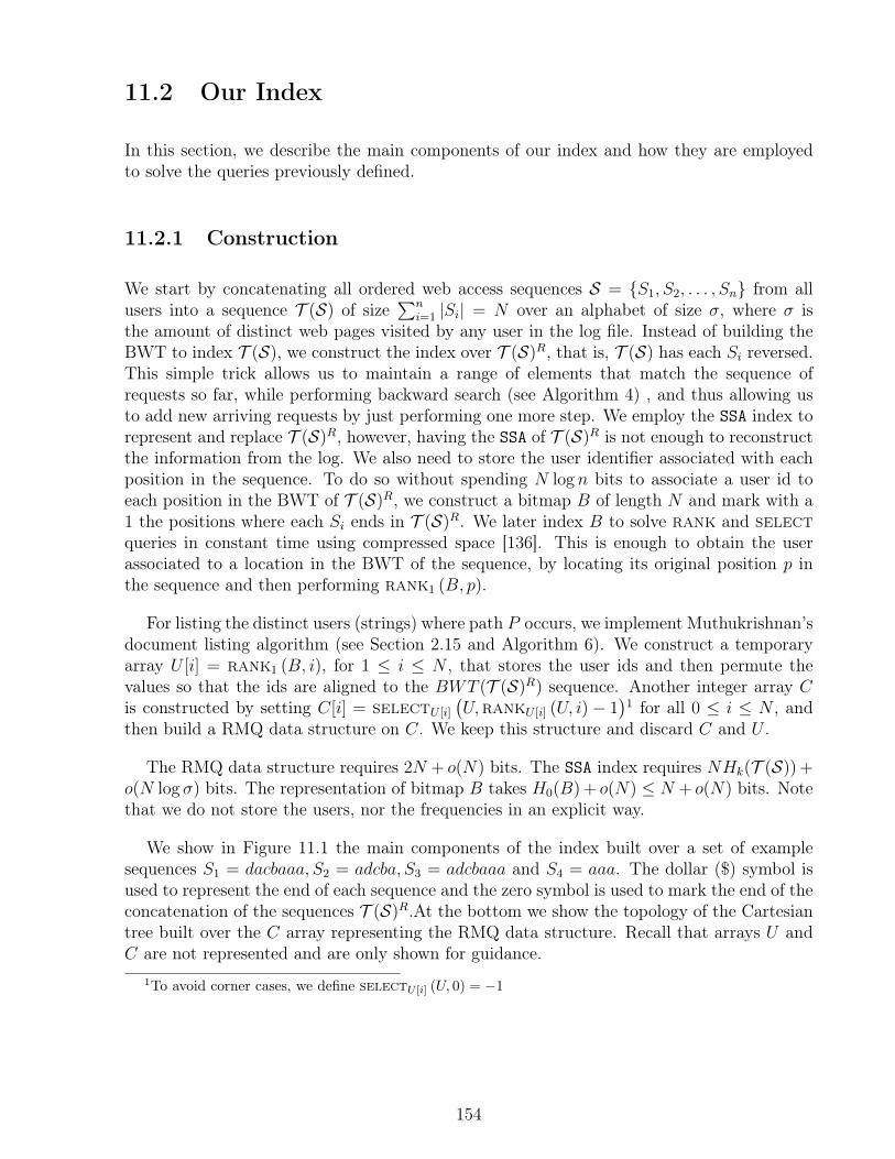
11.2 Our Index

In this section, we describe the main components of our index and how they are employedto solve the queries previously defined.

11.2.1 Construction

We start by concatenating all ordered web access sequences S = S1, S2, . . . , Sn from allusers into a sequence T (S) of size

∑ni=1 |Si| = N over an alphabet of size σ, where σ is

the amount of distinct web pages visited by any user in the log file. Instead of building theBWT to index T (S), we construct the index over T (S)R, that is, T (S) has each Si reversed.This simple trick allows us to maintain a range of elements that match the sequence ofrequests so far, while performing backward search (see Algorithm 4) , and thus allowing usto add new arriving requests by just performing one more step. We employ the SSA index torepresent and replace T (S)R, however, having the SSA of T (S)R is not enough to reconstructthe information from the log. We also need to store the user identifier associated with eachposition in the sequence. To do so without spending N log n bits to associate a user id toeach position in the BWT of T (S)R, we construct a bitmap B of length N and mark with a1 the positions where each Si ends in T (S)R. We later index B to solve rank and selectqueries in constant time using compressed space [136]. This is enough to obtain the userassociated to a location in the BWT of the sequence, by locating its original position p inthe sequence and then performing rank1 (B, p).

For listing the distinct users (strings) where path P occurs, we implement Muthukrishnan’sdocument listing algorithm (see Section 2.15 and Algorithm 6). We construct a temporaryarray U [i] = rank1 (B, i), for 1 ≤ i ≤ N , that stores the user ids and then permute thevalues so that the ids are aligned to the BWT (T (S)R) sequence. Another integer array Cis constructed by setting C[i] = selectU [i]

(U,rankU [i] (U, i)− 1

)1 for all 0 ≤ i ≤ N , and

then build a RMQ data structure on C. We keep this structure and discard C and U .

The RMQ data structure requires 2N + o(N) bits. The SSA index requires NHk(T (S)) +o(N log σ) bits. The representation of bitmap B takes H0(B) + o(N) ≤ N + o(N) bits. Notethat we do not store the users, nor the frequencies in an explicit way.

We show in Figure 11.1 the main components of the index built over a set of examplesequences S1 = dacbaaa, S2 = adcba, S3 = adcbaaa and S4 = aaa. The dollar ($) symbol isused to represent the end of each sequence and the zero symbol is used to mark the end of theconcatenation of the sequences T (S)R.At the bottom we show the topology of the Cartesiantree built over the C array representing the RMQ data structure. Recall that arrays U andC are not represented and are only shown for guidance.

1To avoid corner cases, we define selectU [i] (U, 0) = −1

154

a a a b c a d $ a b c d a $ a a a b c d a $ a a a $ 01 0 0 0 0 0 0 0 1 0 0 0 0 0 1 0 0 0 0 0 0 0 1 0 0 0 1

T (S)RB

$ a a a d a d d a $ 0 $ a a a a $ c a a a b b b a c c4 4 3 2 1 4 3 2 4 3 2 1 3 1 3 1 1 1 3 2 1 3 2 1 3 2-1 0 -2 -3 -4 1 2 3 5 6 7 4 9 12 13 14 16 17 15 11 18 19 20 21 22 23

BWT

UC

RMQ

Figure 11.1: Layout of our index organization for representing Web Access Logs over anexample set of sequences.

11.2.2 Queries

access(u, i). To obtain the i-th web page visited by user u within the sequence, we need tolocate the position in the original sequence T (S)R where the user’s session begins. Wecan do this by computing p = select1(B, u+ 1)− 1− i and then applying extract asT (S)R[p, p] on the SSA index, in O(sa log σ) time.

userpath(u). To obtain the path done by user u, we compute p1 = select1 (B, u) andp2 = select1 (B, u+ 1)− 1 and then extract on T (S)R[p1, p2] using the SSA index.This takes O((`+ sa) log σ) time, where ` = p2− p1 is the length of the extracted path.

count(P ). Given a path P of length m we can count its occurrences, by just performingcount (P ) on the SSA index in O(m log σ) time.

most_common(P, k). We describe this operation incrementally. Assume we have alreadyprocessed the sequence of requests P = r1, r2, . . . , rm−1. Our invariant is that we knowthe interval [sp, ep] corresponding to path P , and this is sufficient to answer querymost_commonP, k. Now a new request rm arrives at the end of P . Then we proceedas follows:

1. Update the range [sp, ep] in BWT (T (S)) using rm, in O(log σ) time [67].2. Retrieve the k most frequent symbols in BWT [sp, ep], which are precisely those

preceding the occurrences of PR in T (S)R, or following P in T (S).

The second step is done with the heuristic proposed by Culpepper et al. [53] to retrievethe k most frequent symbols in a range of a sequence represented with a wavelet tree.

155

It is a greedy algorithm that starts at the wavelet tree root and maps the range (inconstant time, using rank on the bitmap of the wavelet tree node) to its children, untilreaching the leaves. The traversal is prioritized by visiting the longest ranges first, andreporting the symbols corresponding to the first k leaves found in the process. Theworst-case performance of this algorithm is bounded by the number of different symbolspresent in the string range. This is smaller than both σ and the size of the range. Byusing more sophisticated data structures (that nevertheless do not add much space)[88, 125], a worst case of O(k + polylog n) time can be guaranteed. Note that, if wewant to list all the request that have followed P , we can use an optimal algorithm basedon depth-first traversal of the wavelet tree [74]. We show the details of this procedurein Algorithm 19.

list_users(P ). To list k (or all) distinct users that have followed path P we first locate thestarting and ending points [sp, ep] for the given path, using the SSA index in O(m log σ)time (we can also proceed incrementally as in operation most_common. Then weapply the optimal document listing algorihtm [115, 140]. Each value C[p] < sp, forsp ≤ p ≤ ep, signals a distinct value of U [p] in U [sp, ep]. Recall that we do not haveC or U anymore, but the procedure for extracting the list of users can be emulatedwith the RMQ data structure over array C and the bitmap B. Listing k distinct usersfor path P takes O((k · sa + p) log σ) time, since for each user u we need to take aposition in the BWT and map it to the corresponding position in the original T (S)R,in O(sa log σ) time. Figure 11.1 shows an example of listing users. The framed regionrepresents the range sp, ep. Red nodes in the RMQ tree represent the position of theretrieved users, while the blue node represents the last visited node before returning.

most_frequent(k, n). We want to retrieve the k most frequent paths of a certain lengthq done by the users in the system. We start by pushing into a priority queue all rangesobtained by performing a backward-search of paths of length 1 for each possible symbol(σ at most). Now, we extract the biggest range from the priority queue as well as thepath that created that range. We execute the same procedure again, creating newpaths by appending to the extracted path one further symbol (trying the σ possibleones in the worst case) and we push the ranges obtained by performing the backwardsearch on these new paths into the priority queue. When we extract a path of length q,we report it and remove it from the priority queue. The procedure ends when k pathsare reported or when the priority queue is empty. In the worst case, this operation cantake O(σq).

This method may perform poorly when the alphabet σ is large. An optimization is toavoid trying out all the σ characters to extend the current path, but just those symbolsthat do appear in the current range. Those are found by traversing the wavelet treefrom the root towards all the leaves that contain some symbol in the current range [74].

156

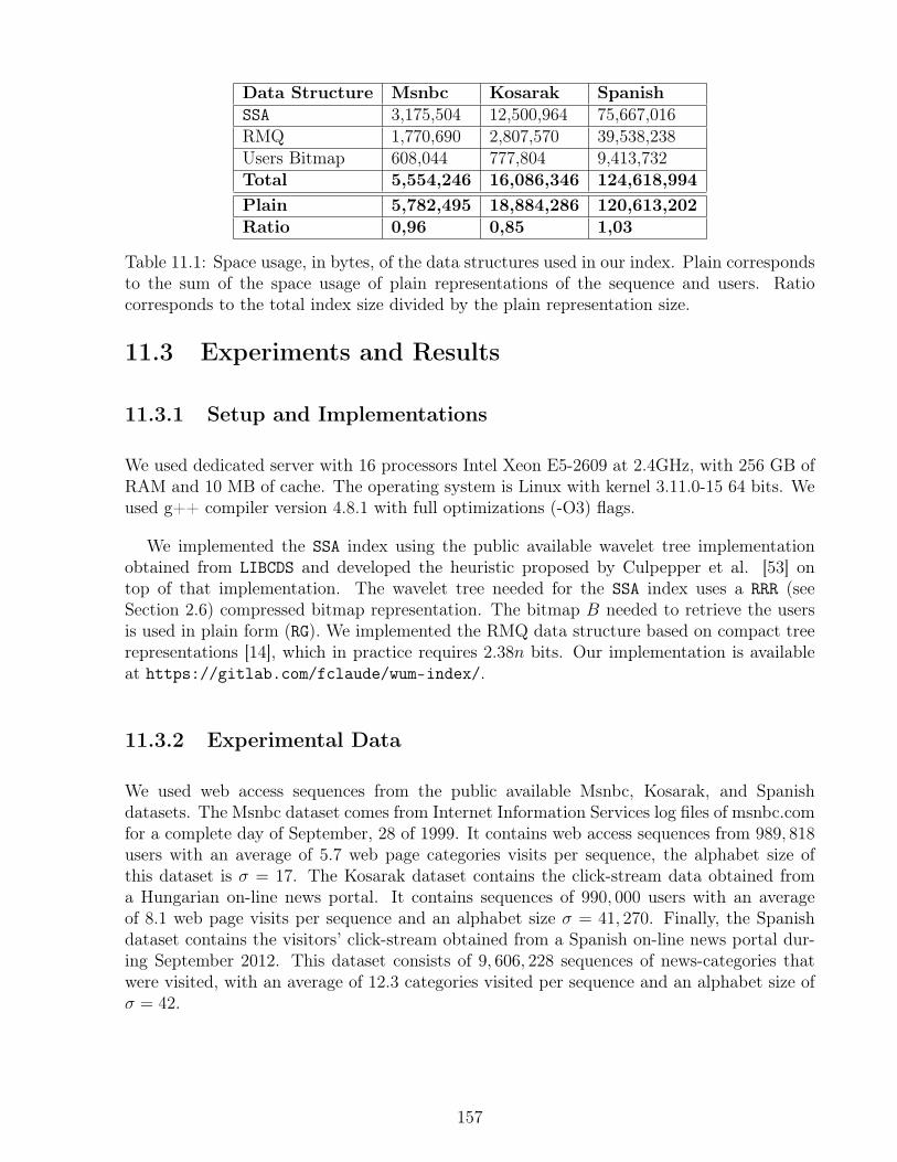
Data Structure Msnbc Kosarak SpanishSSA 3,175,504 12,500,964 75,667,016RMQ 1,770,690 2,807,570 39,538,238Users Bitmap 608,044 777,804 9,413,732Total 5,554,246 16,086,346 124,618,994Plain 5,782,495 18,884,286 120,613,202Ratio 0,96 0,85 1,03

Table 11.1: Space usage, in bytes, of the data structures used in our index. Plain correspondsto the sum of the space usage of plain representations of the sequence and users. Ratiocorresponds to the total index size divided by the plain representation size.

11.3 Experiments and Results

11.3.1 Setup and Implementations

We used dedicated server with 16 processors Intel Xeon E5-2609 at 2.4GHz, with 256 GB ofRAM and 10 MB of cache. The operating system is Linux with kernel 3.11.0-15 64 bits. Weused g++ compiler version 4.8.1 with full optimizations (-O3) flags.

We implemented the SSA index using the public available wavelet tree implementationobtained from LIBCDS and developed the heuristic proposed by Culpepper et al. [53] ontop of that implementation. The wavelet tree needed for the SSA index uses a RRR (seeSection 2.6) compressed bitmap representation. The bitmap B needed to retrieve the usersis used in plain form (RG). We implemented the RMQ data structure based on compact treerepresentations [14], which in practice requires 2.38n bits. Our implementation is availableat https://gitlab.com/fclaude/wum-index/.

11.3.2 Experimental Data

We used web access sequences from the public available Msnbc, Kosarak, and Spanishdatasets. The Msnbc dataset comes from Internet Information Services log files of msnbc.comfor a complete day of September, 28 of 1999. It contains web access sequences from 989, 818users with an average of 5.7 web page categories visits per sequence, the alphabet size ofthis dataset is σ = 17. The Kosarak dataset contains the click-stream data obtained froma Hungarian on-line news portal. It contains sequences of 990, 000 users with an averageof 8.1 web page visits per sequence and an alphabet size σ = 41, 270. Finally, the Spanishdataset contains the visitors’ click-stream obtained from a Spanish on-line news portal dur-ing September 2012. This dataset consists of 9, 606, 228 sequences of news-categories thatwere visited, with an average of 12.3 categories visited per sequence and an alphabet size ofσ = 42.

157

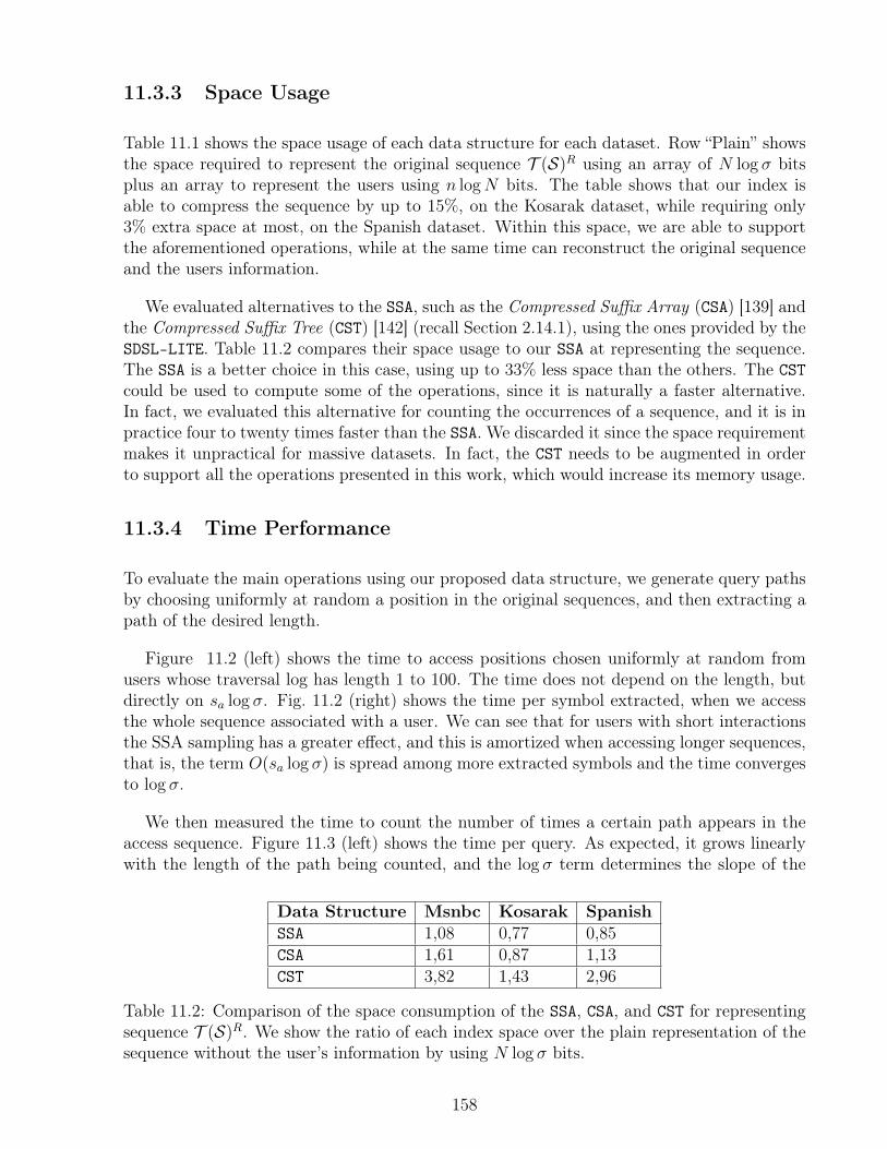
11.3.3 Space Usage

Table 11.1 shows the space usage of each data structure for each dataset. Row “Plain” showsthe space required to represent the original sequence T (S)R using an array of N log σ bitsplus an array to represent the users using n logN bits. The table shows that our index isable to compress the sequence by up to 15%, on the Kosarak dataset, while requiring only3% extra space at most, on the Spanish dataset. Within this space, we are able to supportthe aforementioned operations, while at the same time can reconstruct the original sequenceand the users information.

We evaluated alternatives to the SSA, such as the Compressed Suffix Array (CSA) [139] andthe Compressed Suffix Tree (CST) [142] (recall Section 2.14.1), using the ones provided by theSDSL-LITE. Table 11.2 compares their space usage to our SSA at representing the sequence.The SSA is a better choice in this case, using up to 33% less space than the others. The CSTcould be used to compute some of the operations, since it is naturally a faster alternative.In fact, we evaluated this alternative for counting the occurrences of a sequence, and it is inpractice four to twenty times faster than the SSA. We discarded it since the space requirementmakes it unpractical for massive datasets. In fact, the CST needs to be augmented in orderto support all the operations presented in this work, which would increase its memory usage.

11.3.4 Time Performance

To evaluate the main operations using our proposed data structure, we generate query pathsby choosing uniformly at random a position in the original sequences, and then extracting apath of the desired length.

Figure 11.2 (left) shows the time to access positions chosen uniformly at random fromusers whose traversal log has length 1 to 100. The time does not depend on the length, butdirectly on sa log σ. Fig. 11.2 (right) shows the time per symbol extracted, when we accessthe whole sequence associated with a user. We can see that for users with short interactionsthe SSA sampling has a greater effect, and this is amortized when accessing longer sequences,that is, the term O(sa log σ) is spread among more extracted symbols and the time convergesto log σ.

We then measured the time to count the number of times a certain path appears in theaccess sequence. Figure 11.3 (left) shows the time per query. As expected, it grows linearlywith the length of the path being counted, and the log σ term determines the slope of the

Data Structure Msnbc Kosarak SpanishSSA 1,08 0,77 0,85CSA 1,61 0,87 1,13CST 3,82 1,43 2,96

Table 11.2: Comparison of the space consumption of the SSA, CSA, and CST for representingsequence T (S)R. We show the ratio of each index space over the plain representation of thesequence without the user’s information by using N log σ bits.

158

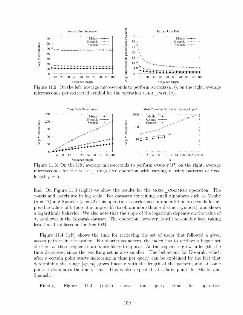
0

20

40

60

80

100

120

140

10 20 30 40 50 60 70 80 90 100

Av

g.

Mic

rose

con

ds

Sequence length

Access User Sequence

MsnbcKosarakSpanish

0

5

10

15

20

25

30

35

10 20 30 40 50 60 70 80 90 100

Av

g.

Mic

rose

con

ds

per

Ex

trac

ted

Sy

mb

ol

Sequence length

Extract User Path

MsnbcKosarakSpanish

Figure 11.2: On the left, average microseconds to perform access (u, i); on the right, averagemicroseconds per extracted symbol for the operation user_path (u).

0

50

100

150

200

250

4 8 12 16 20 24 28 32 36 40

Av

g.

Mic

rose

con

ds

Sequence length

Count Path Occurrences

MsnbcKosarakSpanish

1

10

100

1000

1 2 4 8 16 32 64 128 256 512 1024

Av

g.

Mic

rose

con

ds

k

Most Common Next Visit, varying k, p=5

MsnbcKosarakSpanish

Figure 11.3: On the left, average microseconds to perform count (P ) on the right, averagemicroseconds for the most_frequent operation with varying k using patterns of fixedlength p = 5.

line. On Figure 11.3 (right) we show the results for the most_common operation. Thex-axis and y-axis are in log scale. For datasets containing small alphabets such as Msnbc(σ = 17) and Spanish (σ = 42) this operation is performed in under 30 microseconds for allpossible values of k (note it is impossible to obtain more than σ distinct symbols), and showsa logarithmic behavior. We also note that the slope of the logarithm depends on the value ofσ, as shown in the Kosarak dataset. The operation, however, is still reasonably fast, takingless than 1 millisecond for k = 1024.

Figure 11.4 (left) shows the time for retrieving the set of users that followed a givenaccess pattern in the system. For shorter sequences, the index has to retrieve a bigger setof users, as these sequences are more likely to appear. As the sequences grow in length, thetime decreases, since the resulting set is also smaller. The behaviour for Kosarak, whichafter a certain point starts increasing in time per query, can be explained by the fact thatdetermining the range [sp, ep] grows linearly with the length of the pattern, and at somepoint it dominates the query time. This is also expected, at a later point, for Msnbc andSpanish.

Finally, Figure 11.4 (right) shows the query time for operation

159

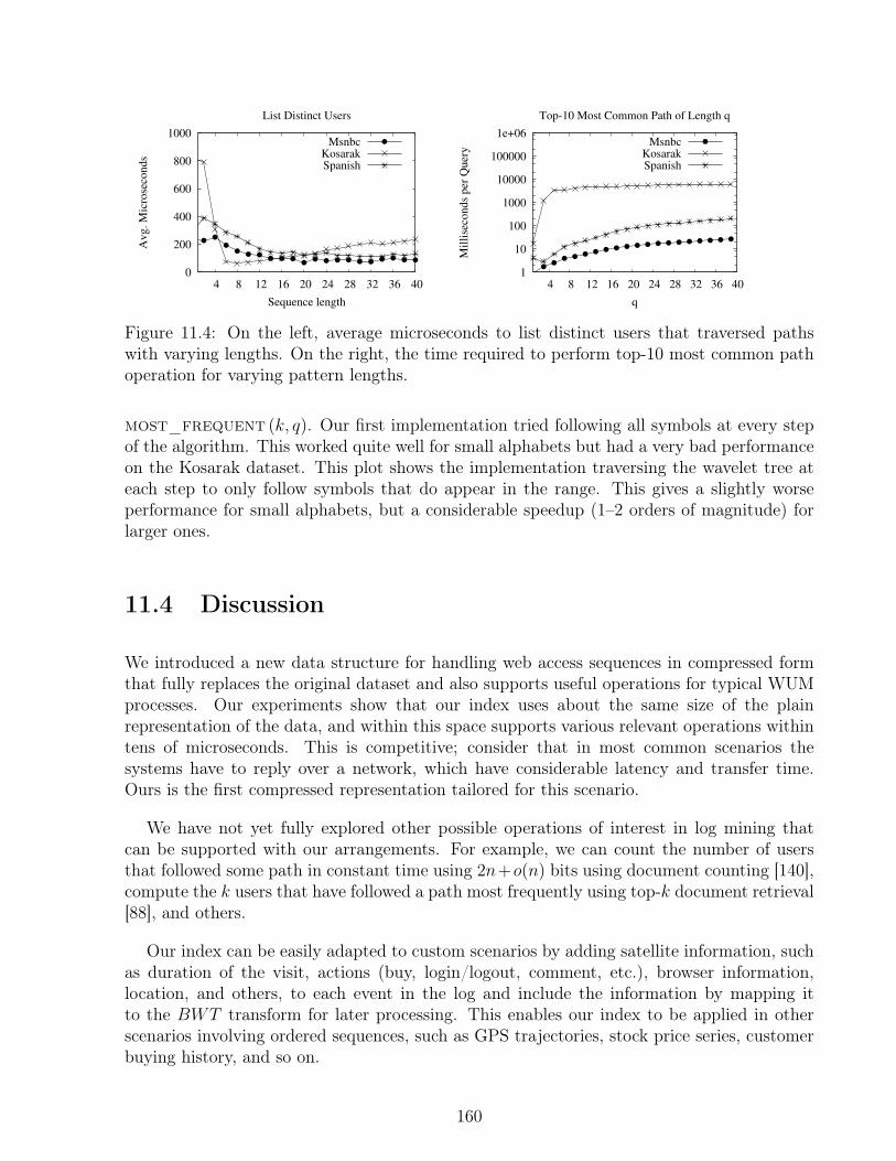
0

200

400

600

800

1000

4 8 12 16 20 24 28 32 36 40

Av

g.

Mic

rose

con

ds

Sequence length

List Distinct Users

MsnbcKosarakSpanish

1

10

100

1000

10000

100000

1e+06

4 8 12 16 20 24 28 32 36 40

Mil

lise

con

ds

per

Qu

ery

q

Top-10 Most Common Path of Length q

MsnbcKosarakSpanish

Figure 11.4: On the left, average microseconds to list distinct users that traversed pathswith varying lengths. On the right, the time required to perform top-10 most common pathoperation for varying pattern lengths.

most_frequent (k, q). Our first implementation tried following all symbols at every stepof the algorithm. This worked quite well for small alphabets but had a very bad performanceon the Kosarak dataset. This plot shows the implementation traversing the wavelet tree ateach step to only follow symbols that do appear in the range. This gives a slightly worseperformance for small alphabets, but a considerable speedup (1–2 orders of magnitude) forlarger ones.

11.4 Discussion

We introduced a new data structure for handling web access sequences in compressed formthat fully replaces the original dataset and also supports useful operations for typical WUMprocesses. Our experiments show that our index uses about the same size of the plainrepresentation of the data, and within this space supports various relevant operations withintens of microseconds. This is competitive; consider that in most common scenarios thesystems have to reply over a network, which have considerable latency and transfer time.Ours is the first compressed representation tailored for this scenario.

We have not yet fully explored other possible operations of interest in log mining thatcan be supported with our arrangements. For example, we can count the number of usersthat followed some path in constant time using 2n+o(n) bits using document counting [140],compute the k users that have followed a path most frequently using top-k document retrieval[88], and others.

Our index can be easily adapted to custom scenarios by adding satellite information, suchas duration of the visit, actions (buy, login/logout, comment, etc.), browser information,location, and others, to each event in the log and include the information by mapping itto the BWT transform for later processing. This enables our index to be applied in otherscenarios involving ordered sequences, such as GPS trajectories, stock price series, customerbuying history, and so on.

160

Chapter 12

PcapWT: Indexing Network PacketTraces

In this chapter we present a solution that is inspired by the dual sorted inverted index datastructure introduced in Section 3.3. We explore the idea of indexing large network packettraces using wavelet trees, and we show that our index is competitive in terms of space andtime to the state of the art tools that network administrators use regularly.

The results of this work appear in the IEEE Journal on Computer Networks, 2015 andwas done in collaboration with Young-Hwan Kim from INRIA, France, Diego Dujovne fromUniversidad Diego Portales, Chile, Thierry Turletti and Walid Dabbous from INRIA, France.

12.1 Motivation

The volume of network packet traces becomes larger and larger, and much more complexthan before. The reason is that the speed and size of networks have increasingly expanded.Thus, much more H/W resources (e.g., massive storage space, stronger computing power, andso on) are necessary to deal with big traces including numerous packets and complex trafficpatterns. Furthermore, efficient tools are required to analyze the data effectively. However,traditional tools such as tcpdump [94], tcpflow [62], or tcpstat [85] are inefficient at handlingvery large packet traces.

In order to enhance packet trace analysis, a number of contributions have been published,such as fast packet filtering [58], packet trace compression [86, 133], and network statisticsinformation extraction [63]. Moreover, a few practical tools have also been recently pro-posed, such as PCAP-Index [4], Compressed Pcap Packet Indexing Program (CPPIP) [1],and pcapIndex [71, 5]. Overall, they use extra data sets for fast search, which are extractedfrom the original trace.

However, these tools result in poor performance, as we show in Section 12.4.2. PCAP-

161

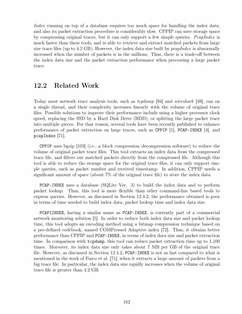
Index running on top of a database requires too much space for handling the index data,and also its packet extraction procedure is considerably slow. CPPIP can save storage spaceby compressing original traces, but it can only support a few simple queries. PcapIndex ismuch faster than these tools, and is able to retrieve and extract matched packets from largesize trace files (up to 4.2 GB). However, the index data size built by pcapIndex is abnormallyincreased when the number of packets is in the millions. Thus, there is a trade-off betweenthe index data size and the packet extraction performance when processing a large packettrace.

12.2 Related Work

Today most network trace analysis tools, such as tcpdump [94] and wireshark [49], run ona single thread, and their complexity increases linearly with the volume of original tracefiles. Possible solutions to improve their performance include using a higher processor clockspeed, replacing the SSD by a Hard Disk Drive (HDD), or splitting the large packet traceinto multiple pieces. For that reason, several tools have been recently published to enhanceperformance of packet extraction on large traces, such as CPPIP [1], PCAP-INDEX [4], andpcapIndex [71].

CPPIP uses bgzip [103] (i.e., a block compression/decompression software) to reduce thevolume of original packet trace files. This tool extracts an index data from the compressedtrace file, and filters out matched packets directly from the compressed file. Although thistool is able to reduce the storage space for the original trace files, it can only support sim-ple queries, such as packet number and received timestamp. In addition, CPPIP needs asignificant amount of space (about 7% of the original trace file) to store the index data.

PCAP-INDEX uses a database (SQLite Ver. 3) to build the index data and to performpacket lookup. Thus, this tool is more flexible than other command-line based tools toexpress queries. However, as discussed in Section 12.4.2, the performance obtained is poorin terms of time needed to build index data, packet lookup time and index data size.

PCAPIINDEX, having a similar name as PCAP-INDEX, is currently part of a commercialnetwork monitoring solution [5]. In order to reduce both index data size and packet lookuptime, this tool adopts an encoding method using a bitmap compression technique based ona pre-defined codebook, named COMPressed Adaptive index [72]. Thus, it obtains betterperformance than CPPIP and PCAP-INDEX, in terms of index data size and packet extractiontime. In comparison with tcpdump, this tool can reduce packet extraction time up to 1,100times. Moreover, its index data size only takes about 7 MB per GB of the original tracefile. However, as discussed in Section 12.4.2, PCAP-INDEX is not as fast compared to what ismentioned in the work of Fusco et al. [71], when it extracts a large amount of packets from abig trace file. In particular, the index data size rapidly increases when the volume of originaltrace file is greater than 4.2 GB.

162

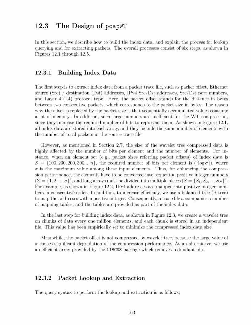
12.3 The Design of pcapWT

In this section, we describe how to build the index data, and explain the process for lookupquerying and for extracting packets. The overall processes consist of six steps, as shown inFigures 12.1 through 12.5.

12.3.1 Building Index Data

The first step is to extract index data from a packet trace file, such as packet offset, Ethernetsource (Src) / destination (Dst) addresses, IPv4 Src/Dst addresses, Src/Dst port numbers,and Layer 4 (L4) protocol type. Here, the packet offset stands for the distance in bytesbetween two consecutive packets, which corresponds to the packet size in bytes. The reasonwhy the offset is replaced by the packet size is that sequentially accumulated values consumea lot of memory. In addition, such large numbers are inefficient for the WT compression,since they increase the required number of bits to represent them. As shown in Figure 12.1,all index data are stored into each array, and they include the same number of elements withthe number of total packets in the source trace file.

However, as mentioned in Section 2.7, the size of the wavelet tree compressed data ishighly affected by the number of bits per element and the number of elements. For in-stance, when an element set (e.g., packet sizes referring packet offsets) of index data isS = 100, 200, 200, 300..., n, the required number of bits per element is (dlog σe), whereσ is the maximum value among these input elements. Thus, for enhancing the compres-sion performance, the elements have to be converted into sequential positive integer numbers(Σ = 1, 2, ..., σ), and long arrays must be divided into multiple pieces (S = S1, S2, ..., SN).For example, as shown in Figure 12.2, IPv4 addresses are mapped into positive integer num-bers in consecutive order. In addition, to increase efficiency, we use a balanced tree (B-tree)to map the addresses with a positive integer. Consequently, a trace file accompanies a numberof mapping tables, and the tables are provided as part of the index data.

In the last step for building index data, as shown in Figure 12.3, we create a wavelet treeon chunks of data every one million elements, and each chunk is stored in an independentfile. This value has been empirically set to minimize the compressed index data size.

Meanwhile, the packet offset is not compressed by wavelet tree, because the large value ofσ causes significant degradation of the compression performance. As an alternative, we usean efficient array provided by the LIBCDS package which removes redundant bits.

12.3.2 Packet Lookup and Extraction

The query syntax to perform the lookup and extraction is as follows,

163

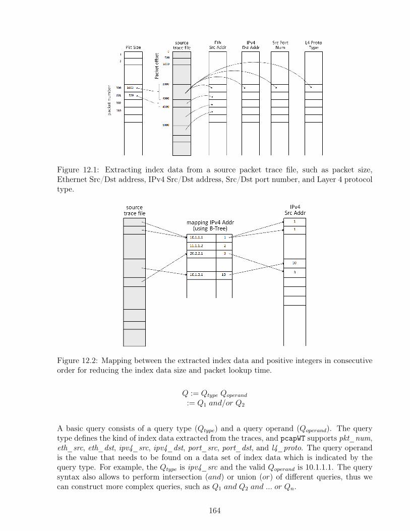
Figure 12.1: Extracting index data from a source packet trace file, such as packet size,Ethernet Src/Dst address, IPv4 Src/Dst address, Src/Dst port number, and Layer 4 protocoltype.

Figure 12.2: Mapping between the extracted index data and positive integers in consecutiveorder for reducing the index data size and packet lookup time.

Q := Qtype Qoperand

:= Q1 and/or Q2

A basic query consists of a query type (Qtype) and a query operand (Qoperand). The querytype defines the kind of index data extracted from the traces, and pcapWT supports pkt_num,eth_src, eth_dst, ipv4_src, ipv4_dst, port_src, port_dst, and l4_proto. The query operandis the value that needs to be found on a data set of index data which is indicated by thequery type. For example, the Qtype is ipv4_src and the valid Qoperand is 10.1.1.1. The querysyntax also allows to perform intersection (and) or union (or) of different queries, thus wecan construct more complex queries, such as Q1 and Q2 and ... or Qn.

164

Figure 12.3: Building wavelet tree chunks from the mapped index data once every one millionpackets. This partitioning can reduce the size of index data.

Recall the basic functions described in Section 2.7. The main idea is that we can getthe number of matched packets (m) containing the query operand by performing rank ofthe wavelet tree. Next, we can figure out indexing numbers of matched packets by iterativeexecuting of select.

First, the procedure to perform the lookup has to reconstruct the packet offset by accumu-lating the packet sizes. For example, if the packet sizes are P = 100, 200, 200, 300, ..., pn,their offsets are O = 0, 100, 300, 500, 800, ..., on. Then, it loads an index data related to thequery. At this step, the index data is located in main memory, however it does not need tobe decompressed to execute a lookup.

The matched packets are marked on a matching table, which is composed of a Booleanarray with the same number of entries as the number of packets included in the source pcapfile. If there are multiple queries concatenated by and/or operators, those steps are repeated-from loading related index data- through updating the matching table. As shown in Figure12.4, the matching table assigns 1 to its entries for the matched packets which are found bythe first query or queries located after the or operator. On the other hand, if the packetsare found by queries located after the and operator, the table assigns 1 only to entries kept1, otherwise 0. Once the lookup procedure is completed, two lists are created where offsetsand packet sizes for the final matched packets are marked 1 on the matching table.

The performance of packet extraction highly depends on the capability of storage devices.In particular, this function performs random read and sequential write from/to files. Therandom access performance is significantly degraded in comparison with sequential access, interms of read and write throughput. Therefore, we need an efficient way to compensate theperformance degradation. SSDs have a very short access delay (e.g., below 1 millisecond)compared to HDDs, thus we can reduce the idle time by distributing the I/O requests intomultiple processes, without significant delay overhead. Consequently, the proposed designuses multiple threads to handle multiple requests simultaneously, which are performed byOpenMP provided by gcc [3].

As shown in Figure 12.5, a number of threads are used to balance the overall workload

165

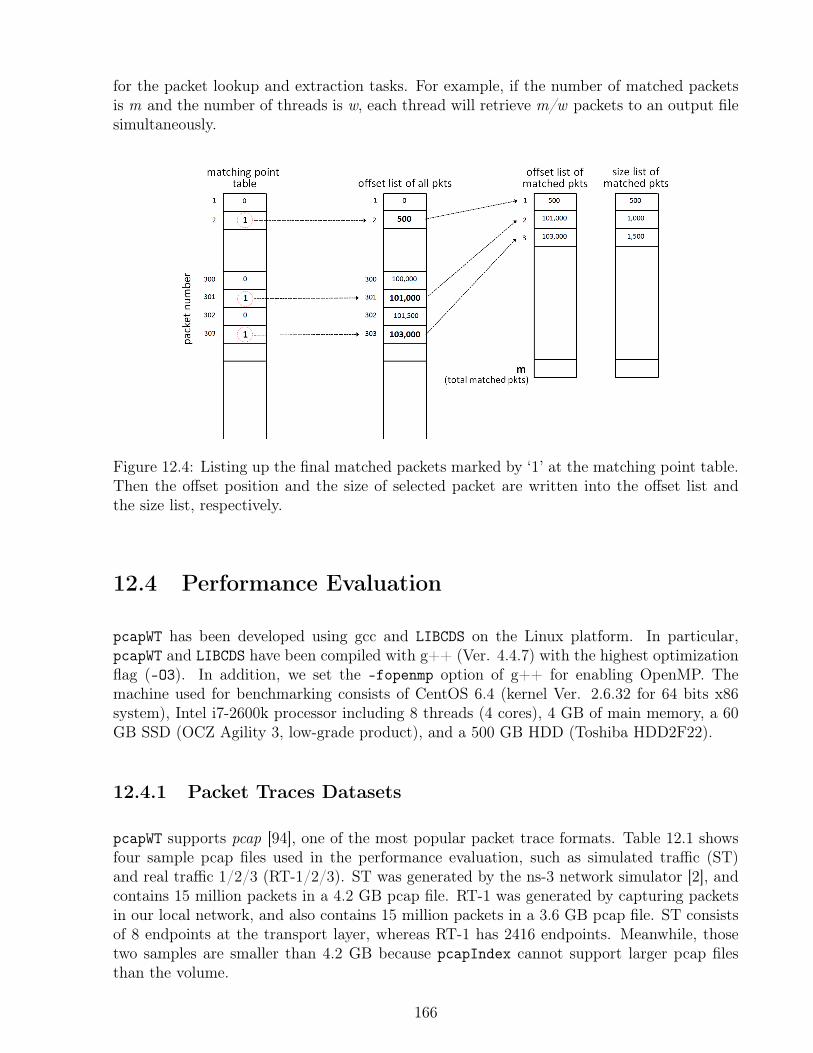
for the packet lookup and extraction tasks. For example, if the number of matched packetsis m and the number of threads is w, each thread will retrieve m/w packets to an output filesimultaneously.

Figure 12.4: Listing up the final matched packets marked by ‘1’ at the matching point table.Then the offset position and the size of selected packet are written into the offset list andthe size list, respectively.

12.4 Performance Evaluation

pcapWT has been developed using gcc and LIBCDS on the Linux platform. In particular,pcapWT and LIBCDS have been compiled with g++ (Ver. 4.4.7) with the highest optimizationflag (-O3). In addition, we set the -fopenmp option of g++ for enabling OpenMP. Themachine used for benchmarking consists of CentOS 6.4 (kernel Ver. 2.6.32 for 64 bits x86system), Intel i7-2600k processor including 8 threads (4 cores), 4 GB of main memory, a 60GB SSD (OCZ Agility 3, low-grade product), and a 500 GB HDD (Toshiba HDD2F22).

12.4.1 Packet Traces Datasets

pcapWT supports pcap [94], one of the most popular packet trace formats. Table 12.1 showsfour sample pcap files used in the performance evaluation, such as simulated traffic (ST)and real traffic 1/2/3 (RT-1/2/3). ST was generated by the ns-3 network simulator [2], andcontains 15 million packets in a 4.2 GB pcap file. RT-1 was generated by capturing packetsin our local network, and also contains 15 million packets in a 3.6 GB pcap file. ST consistsof 8 endpoints at the transport layer, whereas RT-1 has 2416 endpoints. Meanwhile, thosetwo samples are smaller than 4.2 GB because pcapIndex cannot support larger pcap filesthan the volume.

166

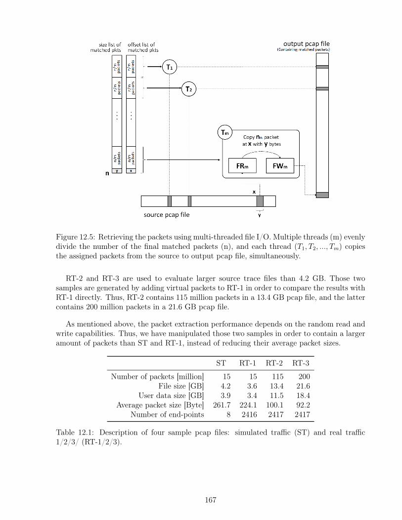
Figure 12.5: Retrieving the packets using multi-threaded file I/O. Multiple threads (m) evenlydivide the number of the final matched packets (n), and each thread (T1, T2, ..., Tm) copiesthe assigned packets from the source to output pcap file, simultaneously.

RT-2 and RT-3 are used to evaluate larger source trace files than 4.2 GB. Those twosamples are generated by adding virtual packets to RT-1 in order to compare the results withRT-1 directly. Thus, RT-2 contains 115 million packets in a 13.4 GB pcap file, and the lattercontains 200 million packets in a 21.6 GB pcap file.

As mentioned above, the packet extraction performance depends on the random read andwrite capabilities. Thus, we have manipulated those two samples in order to contain a largeramount of packets than ST and RT-1, instead of reducing their average packet sizes.

ST RT-1 RT-2 RT-3

Number of packets [million] 15 15 115 200File size [GB] 4.2 3.6 13.4 21.6

User data size [GB] 3.9 3.4 11.5 18.4Average packet size [Byte] 261.7 224.1 100.1 92.2

Number of end-points 8 2416 2417 2417

Table 12.1: Description of four sample pcap files: simulated traffic (ST) and real traffic1/2/3/ (RT-1/2/3).

167

12.4.2 Baselines

We analyze the performances of other tools based on packet indexing, such as CompressedPcap Packet Indexing Program (CPPIP) [1], PCAP-INDEX [4], and pcapIndex [5].

In order to build the index data from RT-1, pcapIndex and CPPIP need 27 MB (0.8%1) and 289 MB (8.0%) of storage, respectively. However, PCAP-INDEX needs around 2.6GB (72%), even though PCAP-INDEX deals with a few simple fields (e.g., addresses, portnumbers, protocol types, and so on). This is due to the database, which is not configured touse data compression. Moreover, PCAP-INDEX needs around 265 seconds to complete, whereaspcapIndex and CPPIP take only around 25 and 40 seconds, respectively. The reason is thatPCAP-INDEX requires a lot of time to inject the index data into the database.

CPPIP and pcapIndex take around 20 and 30 seconds to extract the largest traffic cor-responding to 48% of the volume and 36% of the total number of the packets of RT-1,respectively. However, the available operations are not the same ones used as in the priorcase, since this tool supports only simple filtering queries using a range of packet timestampsand striding (e.g., selecting every n-th packets). Moreover, PCAP-INDEX takes about 80 sec-onds (packet lookup time from the database about 30 seconds and file writing time about 50seconds), which is significantly slower compared to the other tools. Even tcpdump takes lessthan 32 seconds in the same use case.

CPPIP affords the advantage of being able to extract packets directly from a compressedtrace file. However, some efforts are needed to support more complex filtering queries and toreduce the index data size as much as that of pcapIndex. PCAP-INDEX is not satisfactory frommany points of views, even though it uses a database. In contrast, pcapIndex is the onlyreliable one among those tools, since it provides not only comprehensive query operations,as well as remarkable performances in terms of index data size and packet extraction time.Therefore, we select pcapIndex to compare performance with pcapWT in the following.

12.4.3 Space

pcapWT aims to minimize the index data size, for example to compress it below 1% of thevolume of original trace files. As shown in Table 12.4.3, pcapWT is successful for all samplefiles.

More precisely, as mentioned in Section 2.7, wavelet trees supports different bitmap rep-resentation methods (i.e., RG and RRR) and its encoding unit size that can be set by the user.Figure 12.6 shows that RRR is slightly better at reducing index data size than RG. On theother hand, according to Figures 12.7 and 12.8, RG is more efficient than RRR, in terms ofindex data building time and the packet lookup time. Especially, as shown in Figure 12.6, RGusing a wide sampling provides mostly complementary performance between those features.Thus, we decided to use RG(50) as the default configuration.

1a percentage of the volume of original trace file.

168

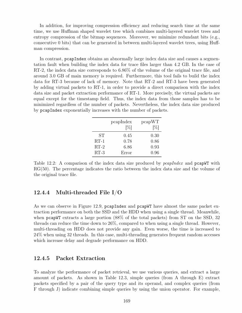
In addition, for improving compression efficiency and reducing search time at the sametime, we use Huffman shaped wavelet tree which combines multi-layered wavelet trees andentropy compression of the bitmap sequences. Moreover, we minimize redundant bits (e.g.,consecutive 0 bits) that can be generated in between multi-layered wavelet trees, using Huff-man compression.

In contrast, pcapIndex obtains an abnormally large index data size and causes a segmen-tation fault when building the index data for trace files larger than 4.2 GB. In the case ofRT-2, the index data size corresponds to 6.86% of the volume of the original trace file, andaround 3.0 GB of main memory is required. Furthermore, this tool fails to build the indexdata for RT-3 because of lack of memory. Note that RT-2 and RT-3 have been generatedby adding virtual packets to RT-1, in order to provide a direct comparison with the indexdata size and packet extraction performance of RT-1. More precisely, the virtual packets areequal except for the timestamp field. Thus, the index data from those samples has to beminimized regardless of the number of packets. Nevertheless, the index data size producedby pcapIndex exponentially increases with the number of packets.

pcapIndex[%]

pcapWT[%]

ST 0.45 0.30RT-1 0.78 0.86RT-2 6.86 0.93RT-3 Error 0.96

Table 12.2: A comparison of the index data size produced by pcapIndex and pcapWT withRG(50). The percentage indicates the ratio between the index data size and the volume ofthe original trace file.

12.4.4 Multi-threaded File I/O

As we can observe in Figure 12.9, pcapIndex and pcapWT have almost the same packet ex-traction performance on both the SSD and the HDD when using a single thread. Meanwhile,when pcapWT extracts a large portion (88% of the total packets) from ST on the SSD, 32threads can reduce the time down to 26%, compared to when using a single thread. However,multi-threading on HDD does not provide any gain. Even worse, the time is increased to24% when using 32 threads. In this case, multi-threading generates frequent random accesseswhich increase delay and degrade performance on HDD.

12.4.5 Packet Extraction

To analyze the performance of packet retrieval, we use various queries, and extract a largeamount of packets. As shown in Table 12.3, simple queries (from A through E) extractpackets specified by a pair of the query type and its operand, and complex queries (fromF through J) indicate combining simple queries by using the union operator. For example,

169

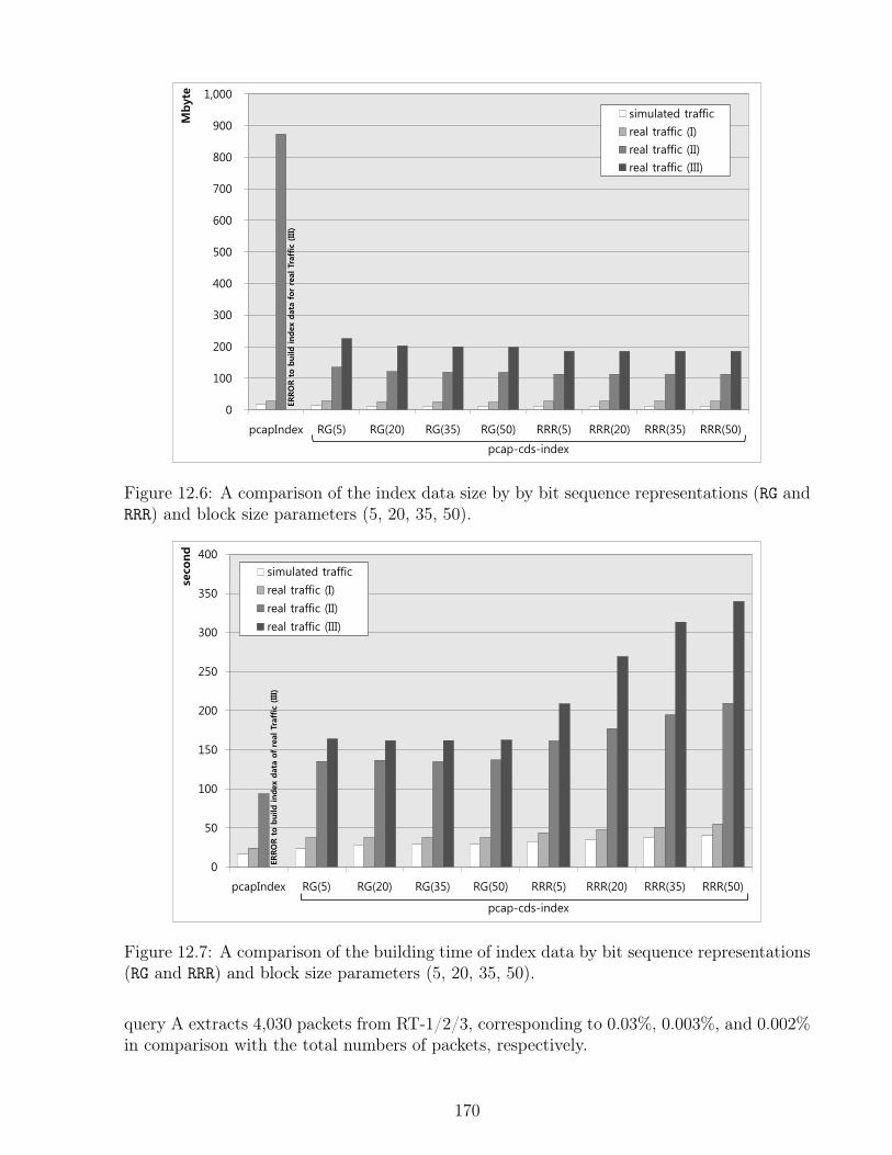
0

100

200

300

400

500

600

700

800

900

1,000

pcapIndex RG(5) RG(20) RG(35) RG(50) RRR(5) RRR(20) RRR(35) RRR(50)

Mbyt

e

simulated traffic

real traffic (I)

real traffic (II)

real traffic (III)

ERRO

R t

o b

uild

index

dat

a fo

r re

al T

raff

ic (

III)

pcap-cds-index

Figure 12.6: A comparison of the index data size by by bit sequence representations (RG andRRR) and block size parameters (5, 20, 35, 50).

0

50

100

150

200

250

300

350

400

pcapIndex RG(5) RG(20) RG(35) RG(50) RRR(5) RRR(20) RRR(35) RRR(50)

seco

nd

simulated traffic

real traffic (I)

real traffic (II)

real traffic (III)

ERRO

R t

o b

uild

index

dat

a of

real

Tra

ffic

(III)

pcap-cds-index

Figure 12.7: A comparison of the building time of index data by bit sequence representations(RG and RRR) and block size parameters (5, 20, 35, 50).

query A extracts 4,030 packets from RT-1/2/3, corresponding to 0.03%, 0.003%, and 0.002%in comparison with the total numbers of packets, respectively.

170

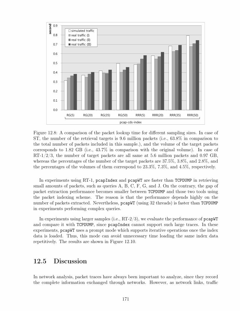
0.0

0.1

0.2

0.3

0.4

0.5

0.6

0.7

0.8

0.9

RG(5) RG(20) RG(35) RG(50) RRR(5) RRR(20) RRR(35) RRR(50)

seco

nd

simulated traffic real traffic (I) real traffic (II) real traffic (III)

pcap-cds-index

Figure 12.8: A comparison of the packet lookup time for different sampling sizes. In case ofST, the number of the retrieval targets is 9.6 million packets (i.e., 63.8% in comparison tothe total number of packets included in this sample.), and the volume of the target packetscorresponds to 1.82 GB (i.e., 43.7% in comparison with the original volume). In case ofRT-1/2/3, the number of target packets are all same at 5.6 million packets and 0.97 GB,whereas the percentages of the number of the target packets are 37.5%, 3.8%, and 2.8%, andthe percentages of the volumes of them correspond to 23.3%, 7.3%, and 4.5%, respectively.

In experiments using RT-1, pcapIndex and pcapWT are faster than TCPDUMP in retrievingsmall amounts of packets, such as queries A, B, C, F, G, and J. On the contrary, the gap ofpacket extraction performance becomes smaller between TCPDUMP and those two tools usingthe packet indexing scheme. The reason is that the performance depends highly on thenumber of packets extracted. Nevertheless, pcapWT (using 32 threads) is faster than TCPDUMPin experiments performing complex queries.

In experiments using larger samples (i.e., RT-2/3), we evaluate the performance of pcapWTand compare it with TCPDUMP, since pcapIndex cannot support such large traces. In theseexperiments, pcapWT uses a prompt mode which supports iterative operations once the indexdata is loaded. Thus, this mode can avoid unnecessary time loading the same index datarepetitively. The results are shown in Figure 12.10.

12.5 Discussion

In network analysis, packet traces have always been important to analyze, since they recordthe complete information exchanged through networks. However, as network links, traffic

171

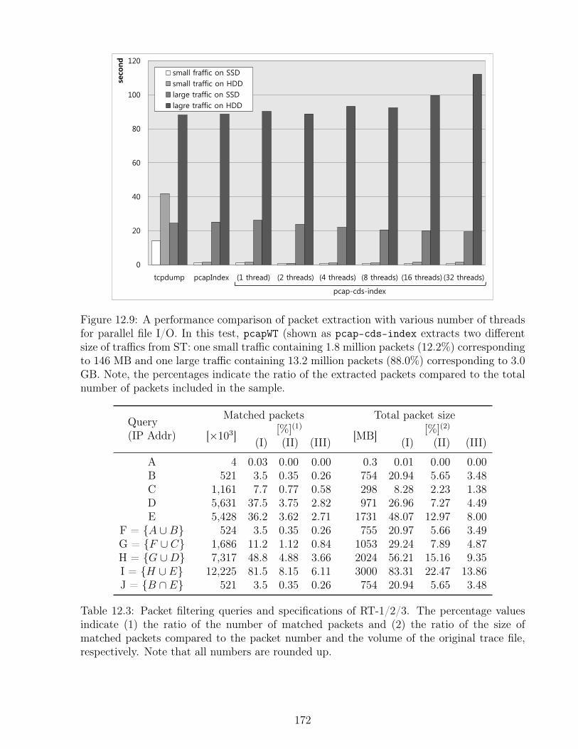
0

20

40

60

80

100

120

tcpdump pcapIndex (1 thread) (2 threads) (4 threads) (8 threads) (16 threads) (32 threads)

seco

nd

small fraffic on SSD small traffic on HDD large traffic on SSD lagre traffic on HDD

pcap-cds-index

Figure 12.9: A performance comparison of packet extraction with various number of threadsfor parallel file I/O. In this test, pcapWT (shown as pcap-cds-index extracts two differentsize of traffics from ST: one small traffic containing 1.8 million packets (12.2%) correspondingto 146 MB and one large traffic containing 13.2 million packets (88.0%) corresponding to 3.0GB. Note, the percentages indicate the ratio of the extracted packets compared to the totalnumber of packets included in the sample.

Query(IP Addr)

Matched packets Total packet size

[×103] [%](1)

[MB] [%](2)

(I) (II) (III) (I) (II) (III)

A 4 0.03 0.00 0.00 0.3 0.01 0.00 0.00B 521 3.5 0.35 0.26 754 20.94 5.65 3.48C 1,161 7.7 0.77 0.58 298 8.28 2.23 1.38D 5,631 37.5 3.75 2.82 971 26.96 7.27 4.49E 5,428 36.2 3.62 2.71 1731 48.07 12.97 8.00

F = A ∪B 524 3.5 0.35 0.26 755 20.97 5.66 3.49G = F ∪ C 1,686 11.2 1.12 0.84 1053 29.24 7.89 4.87H = G ∪D 7,317 48.8 4.88 3.66 2024 56.21 15.16 9.35I = H ∪ E 12,225 81.5 8.15 6.11 3000 83.31 22.47 13.86J = B ∩ E 521 3.5 0.35 0.26 754 20.94 5.65 3.48

Table 12.3: Packet filtering queries and specifications of RT-1/2/3. The percentage valuesindicate (1) the ratio of the number of matched packets and (2) the ratio of the size ofmatched packets compared to the packet number and the volume of the original trace file,respectively. Note that all numbers are rounded up.

172

Figure 12.10: A performance comparison of packet extraction using RT-2/3.

complexity, and applications throughput have significantly increased, the analysis of hugeamounts of those traces is becoming a challenging task, and traditional analysis tools are notefficient at dealing with such traces. Even though a few tools have been recently publishedfor fast packet extraction, their performance is still not satisfactory in terms of index datasize, and packet extraction delay.

In this work, we propose a new tool designed to process efficiently very large networktraces, which allows not only enhancing packet extraction performance on large traces, butalso reducing storage requirements. pcapWT uses a wavelet tree data structure and a multi-threading scheme for parallel file I/O. Our benchmarks including SSD show that pcapWT isabout 10 to 20% faster than pcapIndex in the worst case scenario and about 200% in thebest cases. Moreover, this tool allows reducing the storage space required to store the indexdata by about 10 to 35% compared to pcapIndex.

173

Part V

And Finally...

174

Chapter 13

Conclusions and Future Work

13.1 Summary of Contributions

In this thesis we have addressed the problem of speeding up queries at the first stage of queryprocessing in Information Retrieval systems: given a user’s query, retrieve as fast as possiblethe top-k most relevant candidate documents using a fast and simple ranking scheme. Wehave designed, implemented and evaluated new compact data structures and algorithms,and showed how to assemble them to create space-efficient indexes for information retrievalon natural language. We experimentally showed that these new indexes obtain interestingspace/time tradeoffs when compared to the current state-of-the-art.

This section summarizes the main contributions of this thesis:

• We have presented a new representation of inverted indexes, dubbed Inverted Treaps.Inverted Treaps are able to simultaneously represent the docid and the weight orderingof a posting list. We use them to design efficient ranked union and intersection algo-rithms that simultaneously filter out documents by docid and frequency. The treapalso allows us to represent both docids and frequencies in differential form, to improvethe compression of the posting lists.We have also presented an engineered version of the theoretical index dubbed Dual-Sorted [122], and compared it against inverted index alternatives, including the invertedtreaps.Experimental results show that under the tf-idf scoring scheme, inverted treaps useabout the same space as competing alternatives like Block-Max and Dual-Sorted, butthey are significantly faster: from 20 times faster on one-word queries to 3–10 timesfaster on ranked unions and 1–2 times faster on ranked intersections. Inverted treapsare generally the fastest alternative for k ≤ 100, and on one-word and two-word queries,which are the most popular ones. In addition, we have shown that treaps can handleinsertions of new documents, with a 50%–100% degradation in space, construction andquery time performance.• We proposed a more efficient and conceptually simpler implementation of the optimal

175

solution introduced by Navarro and Nekrich [119] for the top-k document retrieval prob-lem. We presented three new indexes: WRMQ is a first naive approach to the optimalimplementation, our second index, K2TreapH , is a remarkable improvement over thefirst approach thanks to the use of a new compact data structure, the K2-treap, and bysimplifying components of the optimal solution. Finally, our third index, W1RMQH ,can be regarded as merged version of the first and second alternatives, which providessimilar space/time tradeoffs. Although top-k document retrieval indexes traditionallyconsider the collection as general sequences, we show how these indexes can be usedin natural language collections, in which case the index is much more powerful thaninverted indexes at handling phrase queries. We also present an efficient constructionmethod so that it is possible to handle large IR collections. Our experimental resultsshowed that these indexes are orders of magnitude faster than the current state-of-the-art for most types of collections. Remarkably, our indexes are within the same spacerequirements as the best alternatives.• We have extended the main ideas previously developed in this thesis, and make exten-

sive use of compact data structure for tackling other scenarios that are important forIR.We presented a generalization of the technique used in the design of the K2-treap datastructure (based on the treap data structure introduced in Part II) to support othertypes of two-dimensional aggregated queries. We showed a particular case that solvesthe problem of counting the points that lie in a two-dimensional range [x1, x2]× [y1, y2].Our experimental evaluation showed that using little space overhead (less than a 30%)on top of the K2-tree, this data structure performs queries several orders of magnitudefaster than the original K2-tree, especially when the query ranges are large.Based on the work developed for top-k document retrieval on general sequences, wepresented an index for handling web access sequences in compressed form that fullyreplaces the original dataset and also supports useful operations for typical web usagemining. Our experiments showed that our index uses about the same size of the plainrepresentation of the data, and within this space supports various relevant operationswithin tens of microseconds.Finally, we proposed a new tool to efficiently process very large network traces, whichallows enhancing packet extraction performance on large traces while reducing the stor-age requirements. This tool is based on the idea of the Dual-Sorted index, introducedin Part II. Our index, dubbed pcapWT, uses a wavelet tree data structure and a multi-threading scheme for parallel file I/O. Our experimental evaluation showed that pcapWTis 10% to 20% faster than existing networking tools in the worst case and about 200%in the best scenarios. Finally, our index reduces the space required to store the indexeddata by about 10% to 35% when compared to the space required by other typical tools.

13.2 Future Work

In this section we detail some future plans after this thesis. We describe the most interestingones for each contribution.

176

• A future research line for experimenting with the inverted treap representation of in-verted indexes is to study the effect of reassigning docids. Some results [59] show thatreassignment can significantly improve both space and processing time. Another line ofresearch is to introduce a mechanism to efficiently separate lists with higher frequenciesor impacts. We believe that, since an important part of our gain owes to the separationof lists with frequency f0 = 1, this can lead to important gains. It is also interestingto explore how this idea could impact on schemes like Block-Max and Dual-Sorted.• An interesting direction to investigate is to evaluate if our efficient top-k document

retrieval indexes for general string collections are able to compete with inverted in-dexes for weighted Boolean queries, which are considerably harder than phrase queriesfor our indexes. In addition, our current implementation supports term frequency asthe relevance score. A possible next step is to support more complex relevance mea-sures, such as BM25. Finally, A relevant open problem is to reduce the space furtherwhile retaining competitive query times; as shown in our experiments, current existingapproaches that use less space are hundreds of times slower.• The generalized technique to support aggregated queries presented in Chapter 10 can

be generalized to represent grids in higher dimensions, by replacing our underlying K2-tree with its generalization to d dimensions, the Kd-tree [55] (not to be confused withkd-trees [24]). The algorithms remain identical, but an empirical evaluation is left forfuture work.• Our space-efficient web access logs index, can be further extended to support more

complex scenarios by adding satellite information, such as duration of the visit, actions,browser information, location, and others, to each event in the log. How our indexperforms in practice for these extended scenarios remains uncertain.• Compact data structures is an active field of research, yet, many computer science

research areas have not taken advantage of the new developments coming from thisarea. We have shown that wavelet trees (Chapter 12) or top-k document retrievalindexes (Chapter 11) can be employed to assemble new indexes that offer interestingspace/time tradeoffs in other scenarios of interest for IR. We believe that there are evenmore IR-related problems that will benefit from the use of compact data structures.An example is the representation of the item/user matrix employed in traditional col-laborative filtering performed in recommender systems. The use of wavelet-trees orK2-trees arises as natural, space-efficient alternatives to current space-demanding rep-resentations. Another case is the use of compact top-k document retrieval indexes(Part III) to efficiently represent large language models while providing fast access andoperations on them. As an example of this line of research, Shareghi et al. [149] haverecently showed that it is possible to use compressed suffix trees to represent languagemodels that supports fast operations.

177

Bibliography

[1] Cppip. URL http://blogs.cisco.com/tag/pcap/. Last visited on 18/12/2015.

[2] Ns-3 Network Simulator. URL http://www.nsnam.org/. Last visited on 18/12/2015.

[3] Openmp. URL http://gcc.gnu.org/projects/gomp/. Last visited on 18/12/2015.

[4] Pcap-index. URL https://github.com/taterhead/PCAP-Index/. Last visited on18/12/2015.

[5] PcapIndex. URL http://www.ntop.org/products/n2disk/. Last visited on18/12/2015.

[6] D. Abhishek and J. Ankit. Indexing the world wide web: The journey so far. In NextGeneration Search Engines: Advanced Models for Information Retrieval, pages 1–28,2012.

[7] P. Afshani, L. Arge, and K. G. Larsen. Higher-dimensional orthogonal range reportingand rectangle stabbing in the pointer machine model. In Proceedings of the Twenty-eighth Annual Symposium on Computational Geometry, pages 323–332, 2012.

[8] A. Andersson and S. Nilsson. Faster searching in tries and quadtrees - an analysis oflevel compression. In Proc. of the 2nd Annual European Symposium on Algorithms(ESA), LNCS 855, pages 82–93, 1994.

[9] V. Anh, O. Kretser, and A. Moffat. Vector-space ranking with effective early termina-tion. In Proc. of the 24th Annual International ACM SIGIR Conference on Researchand Development in Information Retrieval, SIGIR ’01, pages 35–42. ACM, 2001.

[10] V. Anh and A. Moffat. Impact transformation: Effective and efficient web retrieval.In Proc. of the 25th Annual International ACM SIGIR Conference on Research andDevelopment in Information Retrieval, SIGIR ’02, pages 3–10, 2002.

[11] V. Anh and A. Moffat. Inverted index compression using word-aligned binary codes.Information Retrieval, 8(1):151–166, 2005.

[12] V. Anh and A. Moffat. Pruned query evaluation using pre-computed impacts. InProceedings of the 29th Annual International ACM SIGIR Conference on Research andDevelopment in Information Retrieval (SIGIR), pages 372–379, 2006.

178

[13] V. Anh and A. Moffat. Index compression using 64-bit words. Software Practice andExperience, 40(2):131–147, 2010.

[14] D. Arroyuelo, R. Cánovas, G. Navarro, and K. Sadakane. Succinct trees in practice.In Proc. 11th Workshop on Algorithm Engineering and Experiments (ALENEX), pages84–97, 2010.

[15] N. Asadi and J. Lin. Fast, incremental inverted indexing in main memory for Web-scalecollections. CoRR, abs/1305.0699, 2013.

[16] R. Baeza-Yates, A. Moffat, and G. Navarro. Searching large text collections. In Hand-book of Massive Data Sets, pages 195–244. Kluwer, 2002.

[17] R. Baeza-Yates and B. Ribeiro-Neto. Modern Information Retrieval. Addison-Wesley,2nd edition, 2011.

[18] R. Baeza-Yates and A. Salinger. Experimental analysis of a fast intersection algorithmfor sorted sequences. In Proc. 12th International Symposium on String Processing andInformation Retrieval (SPIRE), pages 13–24, 2005.

[19] J. Barbay, F. Claude, T. Gagie, G. Navarro, and Y. Nekrich. Efficient fully-compressedsequence representations. Algorithmica, 69(1):232–268, 2014.

[20] J. Barbay, A. López-Ortiz, T. Lu, and A. Salinger. An experimental investigation of setintersection algorithms for text searching. ACM Journal of Experimental Algorithmics,14:art. 7, 2009.

[21] D. Belazzougui, G. Navarro, and D. Valenzuela. Improved compressed indexes forfull-text document retrieval. Journal of Discrete Algorithms, 18:3–13, 2013.

[22] M. Bender and M. Farach-Colton. The LCA problem revisited. In Proceedings of the9th Latin American Theoretical Informatics (LATIN), LNCS 1776, pages 88–94, 2000.

[23] D. Benoit, E. Demaine, I. Munro, R. Raman, and S. Rao V. Raman. Representingtrees of higher degree. Algorithmica, 43(4):275–292, December 2005.

[24] J. Bentley. Multidimensional binary search trees used for associative searching. Com-munications of the ACM, 18(9):509–517, 1975.

[25] J. Bentley. Decomposable searching problems. Information Processing Letters,8(5):244–251, 1979.

[26] M. Berg, O. Cheong, M. Kreveld, and M. Overmars. Computational Geometry: Algo-rithms and Applications. Springer-Verlag TELOS, 3rd edition, 2008.

[27] O. Berkman and U. Vishkin. Recursive star-tree parallel data structure. SIAM Journalon Computing, 22(2):221–242, 1993.

[28] P. Boldi, M. Rosa, M. Santini, and S. Vigna. Layered label propagation: A multireso-

179

lution coordinate-free ordering for compressing social networks. In Proceedings of the20th international conference on World Wide Web (WWW). ACM Press, 2011.

[29] P. Boldi, M. Santini, and S. Vigna. Permuting web graphs. In Proceedings of the 6thInternational Workshop on Algorithms and Models for the Web-Graph, pages 116–126,2009.

[30] P. Boldi and S. Vigna. The webgraph framework i: Compression techniques. In Proc. ofthe 13th International Conference on World Wide Web (WWW), pages 595–602, 2004.

[31] P. Boldi and S. Vigna. The WebGraph framework I: Compression techniques. In Proc.of the 13th International World Wide Web Conference (WWW), pages 595–601, 2004.

[32] N. Brisaboa, G. de Bernardo, R. Konow, and G. Navarro. k2-treaps: Range top-kqueries in compact space. In Proc. 21st International Symposium on String Processingand Information Retrieval (SPIRE), LNCS 8799, pages 215–226, 2014.

[33] N. Brisaboa, G. de Bernardo, R. Konow, G. Navarro, and D. Seco. Aggregated 2drange queries on clustered points. Information Systems, 60:34–49, 2016.

[34] N. Brisaboa, S. Ladra, and G. Navarro. DACs: Bringing direct access to variable-lengthcodes. Information Processing Management., 49(1):392–404, 2013.

[35] N. Brisaboa, S. Ladra, and G. Navarro. Compact representation of web graphs withextended functionality. Information Systems, 39(1):152–174, 2014.

[36] A. Broder, D. Carmel, M. Herscovici, A. Soffer, and J. Zien. Efficient query evaluationusing a two-level retrieval process. In Proc. 12th CIKM, pages 426–434, 2003.

[37] C. Buckle and A. Lewit. Optimization of inverted vector searches. In Proc. of the8th Annual International ACM SIGIR Conference on Research and Development inInformation Retrieval (SIGIR), pages 97–110, 1985.

[38] M. Burrows and D. J. Wheeler. A block-sorting lossless data compression algorithm.Technical report, Digital Equipment Corporation, 1994.

[39] M. Busch, K. Gade, B. Larson, P. Lok, S. Luckenbill, and J. Lin. Earlybird: Real-timesearch at Twitter. In Proceedings of the 28th IEEE conference on Data Engineering(ICDE), pages 1360–1369, 2012.

[40] S. Büttcher, C. Clarke, and G. Cormack. Information Retrieval: Implementing andEvaluating Search Engines. MIT Press, 2010.

[41] D. Caro, M. Rodríguez, and N. Brisaboa. Data structures for temporal graphs basedon compact sequence representations. Information Systerms, 51:1–26, 2015.

[42] B. Chazelle. Functional approach to data structures and its use in multidimensionalsearching. SIAM Journal of Computation, 17(3):427–462, 1988.

180

[43] B. Chazelle. Lower bounds for orthogonal range searching I: The reporting case. Journalof the ACM, 37(2):200–212, 1990.

[44] D. Clark. Compact PAT trees. PhD thesis, University of Waterloo, 1997.

[45] F. Claude, R. Konow, and G. Navarro. Efficient representation of web access logs. InProc. 21st International Symposium on String Processing and Information Retrieval(SPIRE), LNCS 8799, pages 65–76, 2014.

[46] F. Claude and G. Navarro. Practical rank/select queries over arbitrary sequences. InProc. 15th International Symposium on String Processing and Information Retrieval(SPIRE), LNCS 5280, pages 176–187, 2008.

[47] F. Claude, P. Nicholson, and D. Seco. Differentially encoded search trees. In Proc.22nd Data Compression Conference (DCC), pages 357–366, 2012.

[48] F. Claude, P. Nicholson, and D. Seco. On the compression of search trees. InformationProcessing Management, 50(2):272–283, 2014.

[49] G. Combs. Wireshark. pages 12–02, 2007. Last visited on 18/12/2015.

[50] B. Croft, D. Metzler, and T. Strohman. Search Engines: Information Retrieval inPractice. Pearson Education, 2009.

[51] J. Culpepper and A. Moffat. Compact set representation for information retrieval. InProceedings of the 14th International Symposium on String Processing and InformationRetrieval (SPIRE), pages 137–148, 2007.

[52] S. Culpepper and A. Moffat. Efficient set intersection for inverted indexing. ACMTransactions on Information Systems, 29(1):1:1–1:25, 2010.

[53] S. Culpepper, G. Navarro, S. Puglisi, and A. Turpin. Top-k ranked document searchin general text databases. In Proc. 18th Annual European Symposium on Algorithms(ESA B), LNCS 6347, pages 194–205 (part II), 2010.

[54] G. de Bernardo, S. Alvarez-García, N. Brisaboa, G. Navarro, and O. Pedreira. Compactquerieable representations of raster data. In Proc. 20th International Symposium onString Processing and Information Retrieval (SPIRE), LNCS 8214, pages 96–108, 2013.

[55] G. de Bernardo, S. Álvarez-García, N. Brisaboa, G. Navarro, and O. Pedreira. Compactquerieable representations of raster data. In Proc. 20th International Symposium onString Processing and Information Retrieval (SPIRE), LNCS 8214, pages 96–108, 2013.

[56] J. Dean. Challenges in building large-scale information retrieval systems. In ACMWorkshop on Web Search and Data Mining, 2009.

[57] E. Demaine, A. López-Ortiz, and I. Munro. Adaptive set intersections, unions, anddifferences. In Proc. 11th Annual ACM-SIAM Symposium on Discrete Algorithms(SODA), pages 743–752, 2000.

181

[58] L. Deri. High-speed Dynamic Packet Filtering. Journal of Network and Systems Man-agement, 15(3):401–415, 2007.

[59] S. Ding and T. Suel. Faster top-k document retrieval using block-max indexes. In Proc.34th SIGIR, pages 993–1002, 2011.

[60] J. Domènech, J. Gil, J. Sahuquillo, and A. Pont. Web prefetching performance metrics:a survey. Performance and Evaluation, 63(9):988–1004, 2006.

[61] X. Dongshan and S. Junyi. A new markov model for web access prediction. Computingin Science and Engg., 4(6):34–39, 2002.

[62] J. Elson. Tcpflow. URL http://www.circlemud.org/jelson/software/tcpflow/,2009. Last visited on 18/12/2013.

[63] C. Estan, K. Keys, D. Moore, and G. Varghese. Building A Better NetFlow. ACMSIGCOMM Computer Communication Review, 34(4):245–256, 2004.

[64] H. Ferrada and G. Navarro. Efficient compressed indexing for approximate top-k stringretrieval. In Proc. 21st International Symposium on String Processing and InformationRetrieval (SPIRE), LNCS 8799, pages 18–30, 2014.

[65] H. Ferrada and G. Navarro. Improved range minimum queries. In Proc. 26th DataCompression Conference (DCC), pages 516–525, 2016.

[66] P. Ferragina, R. González, G. Navarro, and R. Venturini. Compressed text indexes:From theory to practice. ACM Journal of Experimental Algorithmics, 13(12), 2009.

[67] P. Ferragina and G. Manzini. Indexing compressed text. Journal of the ACM,52(4):552–581, 2005.

[68] P. Ferragina, G. Manzini, V. Mäkinen, and G. Navarro. Compressed representations ofsequences and full-text indexes. ACM Transactions on Algorithms (TALG), 3(2):20–45,2007.

[69] J. Fischer and V. Heun. Space-efficient preprocessing schemes for range minimumqueries on static arrays. SIAM J. Comput., 40(2):465–492, 2011.

[70] M. Fontoura, V. Josifovski, J. Liu, S. Venkatesan, X. Zhu, and J. Zien. Evaluationstrategies for top-k queries over memory-resident inverted indexes. Proceedings of theVLDB Endowment, 4(12):1213–1224, 2011.

[71] F. Fusco, X. Dimitropoulos, and M. Vlachos L. Deri. PcapIndex: An ndex for NetworkPacket Traces with Legacy Compatibility. ACM SIGCOMM Computer CommunicationReview, 42(1):47–53, 2012.

[72] F. Fusco and M. Vlachos M. Stoecklin. NET-FLi: On-the-fly Compression, Archivingand Indexing of Streaming Network Traffic. Proc. of the VLDB Endowment, 3(1-2):1382–1393, 2010.

182

[73] T. Gagie, J. González-Nova, S. Ladra, G. Navarro, and D. Seco. Faster compressedquadtrees. In Proc. 25th Data Compression Conference (DCC), pages 93–102, 2015.

[74] T. Gagie, G. Navarro, and S. J. Puglisi. New algorithms on wavelet trees and applica-tions to information retrieval. Theoretical Computer Science, 426-427:25–41, 2012.

[75] T. Gagie, S. Puglisi, and A. Turpin. Range quantile queries: Another virtue of wavelettrees. In Proc. 16th International Symposium on String Processing and InformationRetrieval (SPIRE), pages 1–6, 2009.

[76] S. Gog. Compressed Suffix Trees: Design, Construction, and Applications. PhD thesis,Univ. of Ulm, Germany, 2011.

[77] S. Gog, T. Beller, A. Moffat, and M. Petri. From theory to practice: Plug and playwith succinct data structures. In Proc. 13th International Symposium on ExperimentalAlgorithms, (SEA), pages 326–337, 2014.

[78] S. Gog and G. Navarro. Improved single-term top-k document retrieval. In Proc. 17thWorkshop on Algorithm Engineering and Experiments (ALENEX), pages 24–32. SIAMPress, 2015.

[79] A. Golynski, I. Munro, and S. Rao. Rank/select operations on large alphabets: A toolfor text indexing. In Proc. 17th Annual ACM-SIAM Symposium on Discrete Algorithms(SODA), pages 368–373, 2006.

[80] R. González, Sz. Grabowski, V. Mäkinen, and G. Navarro. Practical implementationof rank and select queries. In Poster Proc. Volume of 4th Workshop on Efficient andExperimental Algorithms (WEA), pages 27–38, 2005.

[81] R. Grossi, A. Gupta, and J. Vitter. High-order entropy-compressed text indexes. InProc. 14th SODA, pages 841–850, 2003.

[82] R. Grossi and J. Vitter. Compressed suffix arrays and suffix trees with applications totext indexing and string matching. SIAM Journal on Computing, 35(2):378–407, 2005.

[83] Jiawei Han, Hong Cheng, Dong Xin, and Xifeng Yan. Frequent pattern mining: currentstatus and future directions. Data Mining and Knowledge Discovery, 15(1):55–86, 2007.

[84] H. Heaps. Information Retrieval - Computational and Theoretical Aspects. AcademicPress, NY, 1978.

[85] P. Herman. Tcpstat tool. URL http://www.frenchfries.net/paul/tcpstat/, 2001.Last visited on 18/12/2013.

[86] R. Holanda, J. Verdu, J. Garcıa, and M. Valero. Performance Analysis of A NewPacket Trace Compressor Based on TCP Flow Clustering. Proc. of IEEE InternationalSymposium on Performance Analysis of Systems and Software (ISPASS), pages 219–225, 2005.

183

[87] W. Hon, M. Patil, R. Shah, and S.-B. Wu. Efficient index for retrieving top-k mostfrequent documents. Journal of Discrete Algorithms, 8(4):402–417, 2010.

[88] W. Hon, R. Shah, and J. S. Vitter. Space-efficient framework for top-k string retrievalproblems. In Proc. 50th FOCS, pages 713–722, 2009.

[89] D. Huffman. A method for the construction of minimum-redundancy codes. Proc. ofthe IRE, 40(9):1098–1101, Sept.

[90] T. Hussain, S. Asghar, and N. Masood. Web usage mining: A survey on preprocessingof web log file. In Proc. of the Information and Emerging Technologies conference(ICIET), pages 1–6, 2010.

[91] B. Iwona and R. Grossi. Rank-sensitive data structures. In Proc. 11th InternationalSymposium on String Processing and Information Retrieval (SPIRE), pages 79–90,2005.

[92] M. Petri J. Culpepper and F. Scholer. Efficient in-memory top-k document retrieval.In Proc. 35th International ACM Conference on Research and Development in Infor-mation Retrieval (SIGIR), pages 225–234, 2012.

[93] G. Jacobson. Space-efficient static trees and graphs. In Proceedings of the 30th AnnualSymposium on Foundations of Computer Science, SFCS ’89, pages 549–554, 1989.

[94] V. Jacobson, C. Leres, and S. McCanne. Tcpdump. URL http://www.tcpdump.org/,2003. Last visited on 18/12/2013.

[95] K. Jones, S. Walker, and S. Robertson. A probabilistic model of information retrieval:development and comparative experiments: Part 2. Information Processing & Man-agement, 36(6):809–840, 2000.

[96] A. Kane and F. Tompa. Skewed partial bitvectors for list intersection. In Proc. of the37th International ACM SIGIR Conference on Research and Development in Informa-tion Retrieval, SIGIR ’14, pages 263–272, 2014.

[97] J. Karkkainen, D. Kempa, and S. Puglisi. Hybrid compression of bitvectors for thefm-index. In Proceeding of the Data Compression Conference (DCC), pages 302–311,2014.

[98] Y Kim, R. Konow, D. Dujovne, T. Turletti, W. Dabbous, and G. Navarro. PcapWT:An efficient packet extraction tool for large volume network traces. Computer Networks,79:91–102, 2015.

[99] R. Konow and G. Navarro. Dual-sorted inverted lists in practice. In Proc. 19th SPIRE,LNCS 7608, pages 295–306, 2012.

[100] R. Konow and G. Navarro. Faster compact top-k document retrieval. In Proc. 23rdData Compression Conference (DCC), pages 351–360, 2013.

184

[101] R. Konow, G. Navarro, C. Clarke, and A. López-Ortíz. Faster and smaller invertedindices with treaps. In Proc. 36th Annual International ACM Conference on Researchand Development in Information Retrieval (SIGIR), pages 193–202, 2013.

[102] N. J. Larsson and A. Moffat. Off-line dictionary-based compression. Proc. of the IEEE,88(11):1722–1732, 2000.

[103] H. Li, B. Handsaker, A. Wysoker, T. Fennell, J. Ruan, G. Marth N. Homer, andG. Abecasis R. Durbin. The Sequence Alignment/Map Format and SAMtools. Bioin-formatics, 25(16):2078–2079, 2009.

[104] J. Lin and A. Trotman. Anytime ranking for impact-ordered indexes. In Proceedingsof the ACM SIGIR International Conference on the Theory of Information Retrieval(ICTIR), pages 25–36, 2015.

[105] T. Liu. Learning to rank for information retrieval. Foundations and Trends in Infor-mation Retrieval, 3(3):225–331, 2009.

[106] V. Mäkinen and G. Navarro. Position-restricted substring searching. In Proceedings ofthe 7th Latin American Theoretical Informatics Symposium (LATIN’06), LNCS 3887,pages 703–714, 2006.

[107] U. Manber and E. W. Myers. Suffix arrays: A new method for on-line string searches.SIAM Journal on Computing, 22(5):935–948, 1993.

[108] C. Martínez and S. Roura. Randomized binary search trees. J. ACM, 45(2):288–323,1997.

[109] E. McCreight. Priority search trees. SIAM J. Comp., 14(2):257–276, 1985.

[110] B. Mobasher. Data mining for web personalization. In The adaptive web, pages 90–135.2007.

[111] A. Moffat and J. Zobel. Self-indexing inverted files for fast text retrieval. ACM Trans-actions on Information Systems, 14(4):349–379, 1996.

[112] B. Prosenjit H. Meng M. Aniland P. Morin. Succinct orthogonal range search struc-tures on a grid with applications to text indexing. In Proc. of the 11th InternationalSymposium on Algorithms and Data Structures, WADS, pages 98–109, 2009.

[113] I. Munro. Tables. In Proc. 16th Conference on Foundations of Software Technologyand Theoretical Computer Science (FSTTCS), LNCS 1180, pages 37–42, 1996.

[114] I. Munro and V. Raman. Succinct representation of balanced parentheses and statictrees. SIAM Journal on Computation, 31(3):762–776, 2002.

[115] S. Muthukrishnan. Efficient algorithms for document retrieval problems. In Proc. ofthe thirteenth annual ACM-SIAM symposium on Discrete algorithms, SODA ’02, pages657–666, 2002.

185

[116] G. Navarro. Spaces, trees and colors: The algorithmic landscape of document retrievalon sequences. ACM Computing Surveys, 46(4):article 52, 2014. 47 pages.

[117] G. Navarro. Wavelet trees for all. Journal of Discrete Algorithms, 25:2–20, 2014.

[118] G. Navarro and V. Mäkinen. Compressed full-text indexes. ACM Computing Surveys,39(1), 2007.

[119] G. Navarro and Y. Nekrich. Top-k document retrieval in optimal time and linear space.In Proc. 23rd Annual ACM-SIAM Symposium on Discrete Algorithms (SODA), pages1066–1078, 2012.

[120] G. Navarro, Y. Nekrich, and L. Russo. Space-efficient data-analysis queries on grids.Theoretical Computer Science, 482:60–72, 2013.

[121] G. Navarro and E. Providel. Fast, small, simple rank/select on bitmaps. In Proc 13thInternational Symposium on Experimental Algorithms (SEA), pages 295–306, 2012.

[122] G. Navarro and S. Puglisi. Dual-sorted inverted lists. In Proceedings of the 17thinternational conference on String processing and information retrieval (SPIRE), LNCS6393, pages 309–321, 2010.

[123] G. Navarro, S. J. Puglisi, and J. Sirén. Document retrieval on repetitive collections. InProc. 22nd Annual European Symposium on Agorithms (ESA B), LNCS 8737, pages725–736, 2014.

[124] G. Navarro, S. J. Puglisi, and D. Valenzuela. General document retrieval in compactspace. ACM Journal of Experimental Algorithmics, 19(2):article 3, 2014. 46 pages.

[125] G. Navarro and D. Valenzuela. Space-efficient top-k document retrieval. In Proc. 11thSEA, pages 307–319, 2012.

[126] D. Okanohara and K. Sadakane. Practical entropy-compressed rank/select dictionary.In Proc. 8th ALENEX, 2007.

[127] G. Ottaviano and R. Venturini. Partitioned elias-fano indexes. In Proceedings of the37th international ACM SIGIR conference on Research and development in informationretrieval, pages 273–282, 2014.

[128] R. Pagh. Low redundancy in static dictionaries with constant query time. SIAMJournal on Computing, 31(2):353–363, 2001.

[129] M. Patil, S. Thankachan, R. Shah, W. Hon, J. Vitter, and S. Chandrasekaran. In-verted indexes for phrases and strings. In Proc. of the 34th International ACM SIGIRConference on Research and Development in Information Retrieval, SIGIR ’11, pages555–564. ACM, 2011.

[130] Jian Pei, Jiawei Han, Behzad Mortazavi-Asl, and Hua Zhu. Mining access patternsefficiently from web logs. In Knowledge Discovery and Data Mining. Current Issues

186

and New Applications, pages 396–407. Springer, 2000.

[131] M. Persin, J. Zobel, and R. Sacks-Davis. Filtered document retrieval with frequency-sorted indexes. Journal of the American Society for Information Science, 47(10):749–764, 1996.

[132] M. Petri, S. Culpepper, and A. Moffat. Exploring the magic of WAND. In Proceedingsof the rhe Australasian Document Computing Symposium (ADCS), pages 58–65, 2013.

[133] P. Politopoulos, E. Markatos, and S. Ioannidis. Evaluation of Compression of Re-mote Network Monitoring Data Streams. In Proc. of IEEE Network Operations andManagement Symposium (NOMS) Workshops, pages 109–115, 2008.

[134] E. Providel. Efficient solutions for select operations in binary sequences. MSc. Thesis,2011. Department of Computer Science, University of Chile.

[135] R. Raman, V. Raman, and S. Rao. Succinct indexable dictionaries with applicationsto encoding k-ary trees and multisets. In Proc. of the thirteenth annual ACM-SIAMsymposium on Discrete algorithms (SODA’02), pages 233–242, 2002.

[136] R. Raman, V. Raman, and S. Rao. Succinct indexable dictionaries with applicationsto encoding k-ary trees, prefix sums and multisets. ACM Transactions on Algorthms,3(4), 2007.

[137] F. Reza. An Introduction to Information Theory. Dover Books on Mathematics Series.1961.

[138] R. Rice and J. Plaunt. Adaptive variable-length coding for efficient compressionof spacecraft television data. IEEE Transactions on Communication Technology,19(6):889 –897, 1971.

[139] K. Sadakane. New text indexing functionalities of the compressed suffix arrays. ACMJournal on Algoritms, 48(2):294–313, 2003.

[140] K. Sadakane. Compressed suffix trees with full functionality. Theoretical ComputerSystems, 41(4):589–607, 2007.

[141] K. Sadakane and G. Navarro. Fully-functional succinct trees. In Proc. 21st AnnualACM-SIAM Symposium on Discrete Algorithms (SODA), pages 134–149, 2010.

[142] Kunihiko Sadakane. Succinct data structures for flexible text retrieval systems. J.Discrete Algorithms, 5(1):12–22, 2007.

[143] D. Salomon. Data Compression: The Complete Reference. Springer Verlag, 4th edition,2007.

[144] S.Álvarez-García, N. Brisaboa, J. Fernández, M. Martínez-Prieto, and G. Navarro.Compressed vertical partitioning for efficient RDF management. Knowledge and Infor-mation Systems, 44(2):439–474, 2015.

187

[145] P. Sanders and F. Transier. Intersection in integer inverted indices. In Proc. 9thWorkshop on Algorithm Engineering and Experiments (ALENEX), 2007.

[146] S. Nadiand M. Saraee and M. Davarpanah-Jazi. A fuzzy recommender system fordynamic prediction of user’s behavior. In Proc. ICITST, pages 1–5, 2010.

[147] F. Scholer, H. Williams, J. Yiannis, and J. Zobel. Compression of inverted indexes forfast query evaluation. In Proc. 25th SIGIR, pages 222–229, 2002.

[148] R. Seidel and C. Aragon. Randomized search trees. Algorithmica, 16(4/5):464–497,1996.

[149] E. Shareghi, M. Petri, G. Haffari, and T. Cohn. Compact, efficient and unlimited capac-ity: Language modeling with compressed suffix trees. In Proceedings of the Conferenceon Empirical Methods in Natural Language Processing, (EMNLP), pages 2409–2418,2015.

[150] A. Spink, D. Wolfram, M. Jansen, and S. Tefko. Searching the web: The public andtheir queries. Journal of the Society of Information Science Technology, 52(3):226–234,2001.

[151] A. Stepanov, A. Gangolli, D. Rose, R. Ernst, and P. Oberoi. Simd-based decoding ofposting lists. In Proc. of the 20th ACM International Conference on Information andKnowledge Management, pages 317–326, 2011.

[152] T. Strohman and B. Croft. Efficient document retrieval in main memory. In Proc.30th Annual International ACM SIGIR Conference on Research and Development inInformation Retrieval (SIGIR), pages 175–182, 2007.

[153] Z. Su, Q. Yang, Y. Lu, and H. Zhang. Whatnext: A prediction system for web requestsusing n-gram sequence models. In Proc. of the First International Conference on WebInformation Systems Engineering (WISE), pages 214–224, 2000.

[154] C. Sumathi, R. Valli, and T. Santhanam. Automatic recommendation of web pages inweb usage mining. Intl. J. Comp. Sci. Eng., 2:3046–3052, 2010.

[155] W. Szpankowski. A generalized suffix tree and its (un)expected asymptotic behaviors.SIAM Journal on Computing, 22(6):1176–1198, 1993.

[156] W. Tobler. A computer movie simulating urban growth in the detroit region. EconomicGeography, 46(2):234–240, 1970.

[157] A. Trotman. Compression, simd, and postings lists. In Proceedings of the 2014 Aus-tralasian Document Computing Symposium (ADCS), pages 50:50–50:57, 2014.

[158] A. Trotman, X. Jia, and M. Crane. Towards an efficient and effective search engine. InSIGIR 2012 Workshop on Open Source Information Retrieval, pages 40–47, 2012.

[159] H. Turtle and J. Flood. Query evaluation: Strategies and optimizations. Information

188

Processing Management, 31(6):831–850, 1995.

[160] S. Vigna. Broadword implementation of rank/select queries. In Experimental Algo-rithms, pages 154–168. Springer, 2008.

[161] S. Vigna. Quasi-succinct indices. In Proc. of the Sixth ACM International Conferenceon Web Search and Data Mining (WSDM), pages 83–92, 2013.

[162] J. Vuillemin. A unifying look at data structures. Communications of the ACM,23(4):229–239, 1980.

[163] L. Wang, J. Lin, and D. Metzler. A cascade ranking model for efficient ranked re-trieval. In Proc. 34th International ACM Conference on Research and Development inInformation Retrieval (SIGIR), pages 105–114, 2011.

[164] P. Weiner. Linear pattern matching algorithms. In Proc. Switching and AutomataTheory, pages 1–11, 1973.

[165] H. Williams and J. Zobel. Compressing integers for fast file access. ACM ComputingJournal, 42(3):193–201, 1999.

[166] I. Witten, A. Moffat, and T. Bell. Managing Gigabytes. Morgan Kaufmann, 2nd edition,1999.

[167] L. Wu, W. Lin, X. Xiao, and Y. Xu. LSII: an indexing structure for exact real-timesearch on microblogs. In Proceedings of the 29th IEEE conference on Data Engineering(ICDE), pages 482–493, 2013.

[168] H. Yan, S. Ding, and T. Suel. Inverted index compression and query processing withoptimized document ordering. In Proc. of the 18th international conference on Worldwide web (WWW), pages 401–410, 2009.

[169] G. Zipf. Human Behaviour and the Principle of Least Effort. Addison-Wesley, 1949.

[170] J. Ziv and A. Lempel. Compression of individual sequences via variable-rate coding.IEEE Transactions on Information Theory, 24(5):530–536, 1978.

[171] J. Zobel and A. Moffat. Inverted files for text search engines. ACM Computing Surveys,38(2):art. 6, 2006.

[172] M. Zukowski, H. Sandor, N. Niels, and P. Boncz. Super-scalar ram-cpu cache compres-sion. In Proc. of the 22nd International Conference on Data Engineering, pages 59–.IEEE Computer Society, 2006.

189