undergraduate texts in computer science - Zenodo
407
-
Upload
khangminh22 -
Category
Documents
-
view
0 -
download
0
Transcript of undergraduate texts in computer science - Zenodo
UNDERGRADUATE TEXTS IN COMPUTER SCIENCE
Editors David Gries
Fred B. Schneider
UNDERGRADUATE TEXTS IN COMPUTER SCIENCE
Beidler, Data Structures and Algorithms
Bergin, Data Structure Programming
Brooks, C Programming: The Essentials for Engineers and Scientists
Brooks, Problem Solving with Fortran 90
Dandamudi, Introduction to Assembly Language Programming
Gril/meyer, Exploring Computer Science with Scheme
Jalote, An Integrated Approach to Software Engineering, Second Edition
Kizza, Ethical and Social Issues in the Information Age
Kozen, Automata and Computability
Merritt and Stix, Migrating from Pascal to C++
Pearce, Programming and Meta-Programming in Scheme
Zeigler, Objects and Systems
Dexter C. Kozen
Automata and Computability
~ Springer
Dexter C. Kozen Department of Computer Science Cornell Uni versity Ithaca, NY 14853-7501 USA
Series Edirors DavidGries Department of Computer Science 415 Boyd Studies Research Center The University of Georgia Athens, Georgia 30602 USA
Fred B. Schneider Department of Computer Science Cornell University 4115C Upson Hall Ithaca, NY 14853-7501 USA
On rIUl cover: Cover photo taken by John Still/Photonica.
With 1 figure.
Library of Congress Cataloging-in-Publication Data Kozen, Dexter, 1951-
Automata IOd computability/Dexter C. Kozen. p. cm. - (Undergraduate texts in computer science)
Includes bibliographical references IOd index. ISBN 978-1-4612-7309-7 ISBN 978-1-4612-1844-9 (eBook) DOI 10.1007/978-1-4612-1844-9 1. Machine theory. 2. Computable functions. I. Title.
II. Series. QA267.K69 1997 511.3 - dc21 96-37409
Printed on acid-frec paper.
© 1997 Springer Science+Business Media New York Originally published by Springer-Verlag New York,lnc. in 1997 Softcover reprint ofthe hardcover lst edition 1997 AII rights reserved. This work may not be translated or copied in whole or in part withoot the written pennission of the publisher (Springer ScieDce+Business Media, LLC, 233 Spring Street, New York, NY 10013, USA), except for briefexcerpts in connection with reviews or scholarly analysis. Use in connection with any fOnD of information storage and retrieval, electronic adaptation, computer software, ar by similar ar dissimilar methodology now know ar hereafter developed is forbidden. The use in this publication of trade names, trademarks, service marks and similar terms, even if the are not identified as such, is notto be taken as an expression of opinion as ta whether ar not they are subject ta proprietary rights.
987
ISBN 978-1-4612-7309-7
springeronline.com
To Juris
Preface
These are my lecture notes from C8381/481: Automata and Computability Theory, a one-semester senior-level course I have taught at Cornell University for many years. I took this course myself in the fall of 1974 as a first-year Ph.D. student at Cornell from Juris Hartmanis and have been in love with the subject ever since.
The course is required for computer science majors at Cornell. It exists in two forms: C8481, an honors version; and C8381, a somewhat gentlerpaced version. The syllabus is roughly the same, but C8481 goes deeper into the subject, covers more material, and is taught at a more abstract level. Students are encouraged to start off in one or the other, then switch within the first few weeks if they find the other version more suitable to their level of mathematical skill.
The purpose of the course is twofold: to introduce computer science students to the rich heritage of models and abstractions that have arisen over the years; and to develop the capacity to form abstractions of their own and reason in terms of them.
The course is quite mathematical in flavor, and a certain degree of previous mathematical experience is essential for survival. 8tudents should already be conversant with elementary discrete mathematics, including the notions of set, function, relation, product, partial order, equivalence relation, graph, and tree. They should have a repertoire of basic proof techniques at their disposal, including a thorough understanding of the principle of mathematical induction.
viii Preface
The material covered in this text is somewhat more than can be covered in a one-semester course. It is also a mix of elementary and advanced topics. The basic course consists of the lectures numbered 1 through 39. Additionally, I have included several supplementary lectures numbered A through K on various more advanced topics. These can be included or omitted at the instructor's discretion or assigned as extra reading. They appear in roughly the order in which they should be covered.
At first these notes were meant to supplement and not supplant a textbook, but over the years they gradually took on a life of their own. In addition to the notes, I depended on various texts at one time or another: Cutland [30], Harrison [55], Hopcroft and Ullman [60], Lewis and Papadimitriou [79], Machtey and Young [81], and Manna [82]. In particular, the Hopcroft and Ullman text was the standard textbook for the course for many years, and for me it has been an indispensable source of knowledge and insight. All of these texts are excellent references, and I recommend them highly.
In addition to the lectures, I have included 12 homework sets and several miscellaneous exercises. Some of the exercises come with hints and/or solutions; these are indicated by the annotations "H" and "S," respectively. In addition, I have annotated exercises with zero to three stars to indicate relative difficulty.
I have stuck with the format of my previous textbook [72], in which the main text is divided into more or less self-contained lectures, each 4 to 8 pages. Although this format is rather unusual for a textbook, I have found it quite successful. Many readers have commented that they like it because it partitions the subject into bite-sized chunks that can be covered more or less independently.
I owe a supreme debt of gratitude to my wife Frances for her constant love, support, and superhuman patience, especially during the final throes of this project. I am also indebted to the many teachers, colleagues, teaching assistants, and students who over the years have shared the delights of this subject with me and from whom I have learned so much. I would especially like to thank Rick Aaron, Arash Baratloo, Jim Baumgartner, Steve Bloom, Manuel Blum, Amy Briggs, Ashok Chandra, Wilfred Chen, Allan Cheng, Francis Chu, Bob Constable, Devdatt Dubhashi, Peter van Emde Boas, Allen Emerson, Andras Ferencz, Jeff Foster, Sophia Georgiakaki, David Gries, Joe Halpern, David Harel, Basil Hayek, Tom Henzinger, John Hopcroft, Nick Howe, Doug Ierardi, Tibor Janosi, Jim Jennings, Shyam Kapur, Steve Kautz, Nils Klarlund, Peter Kopke, Vladimir Kotlyar, Alan Kwan, Georges Lauri, Michael Leventon, Jake Levirne, David Liben-Nowell, Yvonne Lo, Steve Mahaney, Nikolay Mateev, Frank McSherry, Albert Meyer, Bob Milnikel, Francesmary Modugno, Anil Nerode, Damian Niwinski, David de la Nuez, Dan Oberlin, Jens Palsberg, Rohit
Preface ix
Parikh, David Pearson, Paul Pedersen, Vaughan Pratt, Zulfikar Ramzan, Jon Rosenberger, Jonathan Rynd, Erik Schmidt, Michael Schwartzbach, Amitabh Shah, Frederick Smith, Kjartan Stefansson, Colin Stirling, Larry Stockmeyer, Aaron Stump, Jurek Tiuryn, Alex Tsow, Moshe Vardi, Igor Walukiewicz, Rafael Weinstein, Jim Wen, Dan Wineman, Thomas Yan, Paul Zimmons, and many others too numerous to mention. Of course, the greatest of these is Juris Hartmanis, whose boundless enthusiasm for the subject is the ultimate source of my own.
I would be most grateful for suggestions and criticism from readers.
Note added for the third printing. I am indebted to Chris Jeuell for pointing out several typographical errors, which have been corrected in this printing.
Ithaca, New York Dexter C. Kozen
Contents
Preface vii
Lectures 1
Introduction 1 Course Roadmap and Historical Perspective . 3 2 Strings and Sets .................. 7
Finite Automata and Regular Sets 3 Finite Automata and Regular Sets 14 4 More on Regular Sets ....... 19 5 Nondeterministic Finite Automata 25 6 The Subset Construction. . . . . . 32 7 Pattern Matching. . . . . . . . . . 40 8 Pattern Matching and Regular Expressions 44 9 Regular Expressions and Finite Automata . 49 A Kleene Algebra and Regular Expressions. 55 10 Homomorphisms . . . . . . . . . . 61 11 Limitations of Finite Automata . . 67 12 Using the Pumping Lemma 72 13 DFA State Minimization. . 77 14 A Minimization Algorithm. 84 15 Myhill-Nerode Relations. . 89 16 The Myhill-Nerode Theorem 95
xii Contents
B Collapsing Nondeterministic Automata. . . . . . . . . .. 100 C Automata on Terms . . . . . . . . . . . . . . . . . . . .. 108 D The Myhill-Nerode Theorem for Term Automata ..... 114 17 Two-Way Finite Automata ................. 119 18 2DFAs and Regular Sets . . . . . . . . . . . . . . . . . .. 124
Pushdown Automata and Context-Free Languages 19 Context-Free Grammars and Languages . . . . . . . . .. 129 20 Balanced Parentheses .................... 135 21 Normal Forms. . . . . . . . . . . . . . . . . . . . . . . .. 140 22 The Pumping Lemma for CFLs . . . . . . . . . . . . . .. 148 23 Pushdown Automata. . . . . . . . . . . . . . . . . . . 157 E Final State Versus Empty Stack. . . . . . . . . . . . . .. 164
24 PDAs and CFGs . . . . . . . . . . . . . . . . . . . . . .. 167 25 Simulating NPDAs by CFGs ................ 172 F Deterministic Pushdown Automata. . . . . . . . . . . .. 176
26 Parsing ............................ 181 27 The Cocke-Kasami-Younger Algorithm . . . . . . . . 191 G The Chomsky-Schiitzenberger Theorem . . . . . . . . 198 H Parikh's Theorem. . . . . . . . . . . . . . . . . . . . . 201
Turing Machines and Effective Computability 28 Turing Machines and Effective Computability . . . . . .. 206 29 More on Turing Machines . . . . . . . . . . . . . . . . . . 215 30 Equivalent Models .................... " 221 31 Universal Machines and Diagonalization . . . . . . . . .. 228 32 Decidable and Undecidable Problems. . . . . . . . . . .. 235 33 Reduction........................... 239 34 Rice's Theorem . . . . . . . . . . . . . . . . . . . . . . . . 245 35 Undecidable Problems About CFLs. . . . . . . . . . . .. 249 36 Other Formalisms ...................... 256 37 The A-Calculus . . . . . . . . . . . . . . . . . . . . . . 262
I While Programs . . . . . . . . . . . . . . . . . . . . . 269 J Beyond Undecidability. . . . . . . . . . . . . . 274
38 Godel's Incompleteness Theorem . . . . . . . . . . . . 282 39 Proof of the Incompleteness Theorem ......... 287 K GOdel's Proof . . . . . . . . . . . . . . . . . . . . . . . .. 292
Exercises 299
Homework Sets Homework 1 Homework 2
301 302
Homework 3 Homework 4 Homework 5 Homework 6 Homework 7 Homework 8 Homework 9 Homework 10 Homework 11 Homework 12
Miscellaneous Exercises
Contents xiii
303 304 306 307 308 309 310 311 312 313
Finite Automata and Regular Sets. . . . . . . . . . . . . . .. 315 Pushdown Automata and Context-Free Languages. . . . . 333 Turing Machines and Effective Computability ....... 340
Hints and Solutions Hints for Selected Miscellaneous Exercises. . . . . Solutions to Selected Miscellaneous Exercises . . . .
References
Notation and Abbreviations
Index
351 357
373
381
389
Lectures
Lecture 1
Course Roadmap and Historical Perspective
The goal of this course is to understand the foundations of computation. We will ask some very basic questions, such as
• What does it mean for a function to be computable?
• Are there any noncomputable functions?
• How does computational power depend on programming constructs?
These questions may appear simple, but they are not. They have intrigued scientists for decades, and the subject is still far from closed.
In the quest for answers to these questions, we will encounter some fundamental and pervasive concepts along the way: state, transition, nondeterminism, redu.ction, and u.ndecidability, to name a few. Some of the most important achievements in theoretical computer science have been the crystallization of these concepts. They have shown a remarkable persistence, even as technology changes from day to day. They are crucial for every good computer scientist to know, so that they can be recognized when they are encountered, as they surely will be.
Various models of computation have been proposed over the years, all of which capture some fundamental aspect of computation. We will concentrate on the following three classes of models, in order of increasing power:
4 Lecture 1
(i) finite memory: finite automata, regular expressions;
(ii) finite memory with stack: pushdown automata;
(iii) unrestricted:
• Turing machines (Alan Turing [120]),
• Post systems (Emil Post [99, 100]),
• It-recursive functions (Kurt GOdel [51), Jacques Herbrand),
• A-calculus (Alonzo Church [23), Stephen C. Kleene [66]),
• combinatory logic (Moses Schonfinkel [111), Haskell B. Curry [29]).
These systems were developed long before computers existed. Nowadays one could add PASCAL, FORTRAN, BASIC, LISP, SCHEME, C++, JAVA, or any sufficiently powerful programming language to this list.
In parallel with and independent of the development of these models of computation, the linguist Noam Chomsky attempted to formalize the notion of grammar and language. This effort resulted in the definition of the Chomsky hierarchy, a hierarchy of language classes defined by grammars of increasing complexity:
(i) right-linear grammars;
(ii) context-free grammars;
(iii) unrestricted grammars.
Although grammars and machine models appear quite different on a superficiallevel, the process of parsing a sentence in a language bears a strong resemblance to computation. Upon closer inspection, it turns out that each of the grammar types (i), (il), and (iii) are equivalent in computational power to the machine models (i), (il), and (iii) above, respectively. There is even a fourth natural class called the context-sensitive grammars and languages, which fits in between (ii) and (iii) and which corresponds to a certain natural class of machine models called linear bounded automata.
It is quite surprising that a naturally defined hierarchy in one field should correspond so closely to a naturally defined hierarchy in a completely different field. Could this be mere coincidence?
Course Roadmap and Historical Perspective 5
Abstraction
The machine models mentioned above were first identified in the same way that theories in physics or any other scientific discipline arise. When studying real-world phenomena, one becomes aware of recurring patterns and themes that appear in various guises. These guises may differ substantially on a superficial level but may bear enough resemblance to one another to suggest that there are common underlying principles at work. When this happens, it makes sense to try to construct an abstract model that captures these underlying principles in the simplest possible way, devoid of the unimportant details of each particular manifestation. This is the process of abstraction. Abstraction is the essence of scientific progress, because it focuses attention on the important principles, unencumbered by irrelevant details.
Perhaps the most striking example of this phenomenon we will see is the formalization of the concept of effective compu.tability. This quest started around the beginning of the twentieth century with the development of the formalist school of mathematics, championed by the philosopher Bertrand Russell and the mathematician David Hilbert. They wanted to reduce all of mathematics to the formal manipulation of symbols.
Of course, the formal manipulation of symbols is a form of computation, although there were no computers around at the time. However, there certainly existed an awareness of computation and algorithms. Mathematicians, logicians, and philosophers knew a constructive method when they saw it. There followed several attempts to come to grips with the general notion of effective compu.tability. Several definitions emerged (Turing machines, Post systems, etc.), each with its own peculiarities and differing radically in appearance. However, it turned out that as different as all these formalisms appeared to be, they could all simulate one another, thus they were all computationally equivalent.
The formalist program was eventually shattered by Kurt GOdel's incompleteness theorem, which states that no matter how strong a deductive system for number theory you take, it will always be possible to construct simple statements that are true but unprovable. This theorem is widely regarded as one of the crowning intellectual achievements of twentieth century mathematics. It is essentially a statement about computability, and we will be in a position to give a full account of it by the end of the course.
The process of abstraction is inherently mathematical. It involves building models that capture observed behavior in the simplest possible way. Although we will consider plenty of concrete examples and applications of these models, we will work primarily in terms of their mathematical properties. We will always be as explicit as possible about these properties.
6 Lecture 1
We will usually start with definitions, then subsequently reason purely in terms of those definitions. For some, this will undoubtedly be a new way of thinking, but it is a skill that is worth cultivating.
Keep in mind that a large intellectual effort often goes into coming up with just the right definition or model that captures the essence of the principle at hand with the least amount of extraneous baggage. After the fact, the reader often sees only the finished product and is not exposed to all the misguided false attempts and pitfalls that were encountered along the way. Remember that it took many years of intellectual struggle to arrive at the theory as it exists today. This is not to say that the book is closed-far from it!
Lecture 2
Strings and Sets
Decision Problems Versus Functions
A decision problem is a function with a one-bit output: "yes" or "no." To specify a decision problem, one must specify
• the set A of possible inputs, and
• the subset B ~ A of ''yes'' instances.
For example, to decide if a given graph is connected, the set of possible inputs is the set of all (encodings of) graphs, and the "yes" instances are the connected graphs. To decide if a given number is a prime, the set of possible inputs is the set of all (binary encodings of) integers, and the "yes" instances are the primes.
In this course we will mostly consider decision problems as opposed to functions with more general outputs. We do this for mathematical simplicity and because the behavior we want to study is already present at this level.
Strings
Now to our first abstraction: we will always take the set of possible inputs to a decision problem to be the set of finite-length strings over some fixed finite
8 Lecture 2
Definition 2.1
alphabet (formal definitions below). We do this for uniformity and simplicity. Other types of data-graphs, the natural numbers N = {O, 1,2, ... }, trees, even programs---can be encoded naturally as strings. By making this abstraction, we have to deal with only one data type and a few basic operations.
• An alphabet is any finite set. For example, we might use the alphabet {O, 1, 2, ... ,9} if we are talking about decimal numbers; the set of all ASCII characters if talking about text; {O, I} if talking about bit strings. The only restriction is that the alphabet be finite. When speaking about an arbitrary finite alphabet abstractly, we usually denote it by the Greek letter E. We call elements of E letters or symbols and denote them by a, b, c, .... We usually do not care at all about the nature of the elements of E, only that there are finitely many of them.
• A string over E is any finite-length sequence of elements of E. Example: if E = {a, b}, then aabab is a string over E of length five. We use x, y, z, ... to refer to strings.
• The length of a string x is the number of symbols in x. The length of x is denoted Ix!- For example, laababl = 5.
• There is a unique string of length 0 over E called the null string or empty string and denoted by e (Greek epsilon, not to be confused with the symbol for set containment E). Thus lei = O.
• We write an for a string of a's of length n. For example, a5 = aaaaa, a1 = a, and aD = e. Formally, an is defined inductively:
D def a = e,
n+l def n a = a a.
• The set of all strings over alphabet E is denoted E*. For example,
{a,b}* = {e,a,b,aa,ab,ba,bb,aaa,aab, ... }, {a}* = {e,a,aa,aaa, aaaa, ... }
= {an I n ~ O}.
By convention, we take
0* ~ {e},
o
where 0 denotes the empty set. This may seem a bit strange, but there is good mathematical justification for it, which will become apparent shortly.
Definition 2.2
Strings and Sets 9
If ~ is nonempty, then ~* is an infinite set of finite-length strings. Be careful not to confuse strings and sets. We won't see any infinite strings until much later in the course. Here are some differences between strings and sets:
• {a,b} = {b,a}, but ab i= baj
• {a,a,b} = {a,b},butaabi=ab.
Note also that 0, {f}, and f are three different things. The first is a set with no elementsj the second is a set with one element, namely fj and the last is a string, not a set.
Operations on Strings
The operation of concatenation takes two strings x and y and makes a new string xy by putting them together end to end. The string xy is called the concatenation of x and y. Note that xy and yx are different in general. Here are some useful properties of concatenation.
• concatenation is associative: (xy)z = x(yz)j
• the null string f is an identity for concatenation: fX = Xf = Xj
• Ixyl = Ixl + Iyl· A special case of the last equation is aman = am +n for all m, n ~ O.
A monoid is any algebraic structure consisting of a set with an associative binary operation and an identity for that operation. By our definitions above, the set ~* with string concatenation as the binary operation and f as the identity is a monoid. We will see some other examples later in the course.
• We write xn for the string obtained by concatenating n copies of x. For example, (aab)5 = aabaabaabaabaab, (aabF = aab, and (aab)O = f. Formally, xn is defined inductively:
° def X = f,
Xn+l ~f XnX.
• If a e E and x e ~*, we write #a(x) for the number of a's in x. For example, #0(001101001000) = 8 and #1(00000) = O.
• A prefiz of a string x is an initial substring of Xj that is, a string y for which there exists a string z such that x = yz. For example, abaab is a prefix of abaababa. The null string is a prefix of every string, and
10 Lecture 2
every string is a prefix of itself. A prefix y of x is a proper prefix of x if y # E and y # x. 0
Operations on Sets
We usually denote sets of strings (subsets of I:*) by A, B, C, .... The cardinality (number of elements) of set A is denoted IAI. The empty set 0
is the unique set of cardinality O.
Let's define some useful operations on sets. Some of these you have probably seen before, some probably not.
• Set union:
AU B ~f {x I x e A or x e B}.
In other words, x is in the union of A and B iffl either x is in A or x is in B. For example, {a,ab} U {ab,aab} = {a,ab,aab}.
• Set intersection:
An B ~ {x I x e A and x e B}.
In other words, x is in the intersection of A and B iff x is in both A and B. For example, {a,ab} n {ab,aab} = {ab}.
• Complement in I:*:
..... A ~ {x e I:* I x ¢ A}.
For example,
..... {strings in I:* of even length} = {strings in I:* of odd length}.
Unlike U and n, the definition of ..... depends on I:*. The set ..... A is sometimes denoted I:* - A to emphasize this dependence.
• Set concatenation:
AB d,g {xy I x e A and y e B}.
In other words, z is in AB iff z can be written as a concatenation of two strings x and y, where x e A and y e B. For example, {a, ab}{ b, ba} = {ab, aba, abb, abba}. When forming a set concatenation, you include all strings that can be obtained in this way. Note that AB and BA are different sets in general. For example, {b, ba}{ a, ab} = {ba, bab, baa, baab}.
1 iff = if and only if.
Strings and Sets 11
• The powers An of a set A are defined inductively as follows:
AO ~f {€},
An+l ~f AAn.
In other words, An is formed by concatenating n copies of A together. Taking AO = {€} makes the property Am+n = AmAn hold, even when one of m or n is O. For example,
{ab,aab}O = {€}, {ab,aab}l = {ab,aab},
{ab,aab}2 = {abab,abaab,aabab,aabaab}, {ab,aab}3 = {ababab,ababaab,abaabab,aababab,
abaabaab,aababaab,aabaabab,aabaabaab}.
Also,
{a,b}n = {X.E {a,b}* Ilxl = n} = {strings over {a, b} oflength n}.
• The asterate A * of a set A is the union of all finite powers of A:
A*~ U An n;::O
= AO U Al U A2 U A3 U ....
Another way to say this is
A * = {Xl X2 ... Xn I n ~ 0 and Xi E A, 1 ::; i ::; n}.
Note that n can be OJ thus the null string € is in A * for any A.
We previously defined I;* to be the set of all finite-length strings over the alphabet I;. This is exactly the asterate of the set I;, so our notation is consistent.
• We define A + to be the union of all nonzero powers of A:
A+ ~f AA* = U An. n;::l
Here are some useful properties of these set operations:
• Set union, set intersection, and set concatenation are associative:
(A U B) U C = Au (B U C),
(AnB) nc = An (B nc), (AB)C = A(BC).
12 Lecture 2
• Set union and set intersection are commutative:
AUB=BUA, AnB=BnA.
As noted above, set concatenation is not.
• The null set 0 is an identity for U:
AU0= 0UA=A.
• The set {f} is an identity for set concatenation:
• The null set 0 is an annihilator for set concatenation:
A0=0A=0.
• Set union and intersection distribute over each other:
Au (Bn G) = (AUB) n (AUG), An (B U G) = (AnB) U (An G).
• Set concatenation distributes over union:
A(B U G) = AB U AG, (AUB)G=AGUBG.
In fact, concatenation distributes over the union of any family of sets. If {B. liE I} is any family of sets indexed by another set I, finite or infinite, then
A(U BI ) = U AB., lEI 'EI
(U B.)A = U B.A. iEI 'EI
Here UiEI Bi denotes the union of all the sets Bi for i E I. An element x is in this union iff it is in one of the Bi.
Set concatenation does not distribute over intersection. For example, take A = {a,ab}, B = {b}, G = {f}, and see what you get when you compute A(B n G) and AB nAG.
• The De Morgan laws hold:
",(AUB) = ",An"'B,
",(AnB) = "'Au"'B.
Strings and Sets 13
• The asterate operation * satisfies the following properties:
A*A*=A*,
A** = A*,
A * = {f} U AA * = {f} U A * A,
0* = {fl.
Lecture 3
Finite Automata and Regular Sets
States and Transitions
Intuitively, a state of a system is an instantaneous description of that system, a snapshot of reality frozen in time. A state gives all relevant information necessary to determine how the system can evolve from that point on. Transitions are changes of state; they can happen spontaneously or in response to external inputs.
We assume that state transitions are instantaneous. This is a mathematical abstraction. In reality, transitions usually take time. Clock cycles in digital computers enforce this abstraction and allow us to treat computers as digital instead of analog devices.
There are innumerable examples of state transition systems in the real world: electronic circuits, digital watches, elevators, Rubik's cube (54!/9!6 states and 12 transitions, not counting peeling the little sticky squares off), the game of Life (211 states on a screen with k cells, one transition).
A system that consists of only finitely many states and transitions among them is called a finite-state transition system. We model these abstractly by a mathematical model called a finite automaton.
Finite Automata and Regular Sets 15
Finite Automata
Formally, a deterministic finite automaton (DFA) is a structure
M= (Q,~, 6, s, F),
where
• Q is a finite set; elements of Q are called statesj
• ~ is a finite set, the input alphabet;
• 6 : Q x ~ -+ Q is the transition function (recall that Q x ~ is the set of ordered pairs {( q, a) I q E Q and a E ~}). Intuitively, 6 is a function that tells which state to move to in response to an input: if M is in state q and sees input a, it moves to state 6(q, a).
• SEQ is the start statej
• F is a subset of Qj elements of F are called accept or final states.
When you specify a finite automaton, you must give all five parts. Automata may be specified in this set-theoretic form or as a transition diagram or table as in the following example.
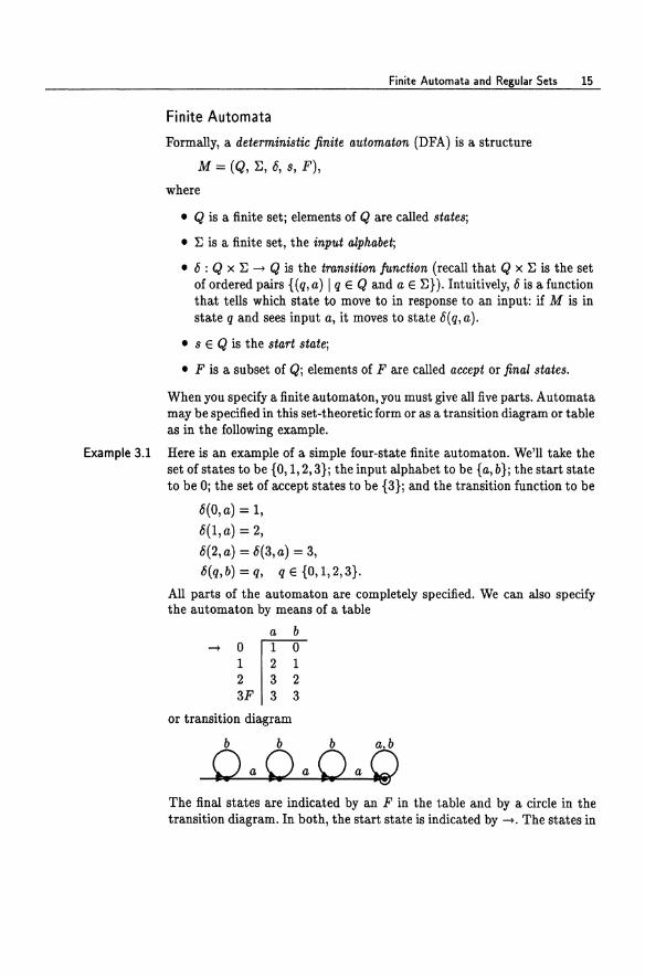
Example 3.1 Here is an example of a simple four-state finite automaton. We'll take the set of states to be {O, 1,2, 3}j the input alphabet to be {a, b}j the start state to be OJ the set of accept states to be {3}j and the transition function to be
6(0, a) = 1,
6(I,a) = 2,
o(2,a) = 6(3,a) = 3, 6(q, b) = q, q E {O, 1,2, 3}.
All parts of the automaton are completely specified. We can also specify the automaton by means of a table
a b
~ fITl ~ 2 3 2 3F 3 3
or transition diagram
The final states are indicated by an F in the table and by a circle in the transition diagram. In both, the start state is indicated by -+. The states in
16 Lecture 3
the transition diagram from left to right correspond to the states 0, 1,2,3 in the table. One advantage of transition diagrams is that you don't have to name the states. 0
Another convenient representation of finite automata is transition matrices; see Miscellaneous Exercise 7.
Informally, here is how a finite automaton operates. An input can be any string x e E*. Put a pebble down on the start state s. Scan the input string x from left to right, one symbol at a time, moving the pebble according to 6: if the next symbol of x is b and the pebble is on state q, move the pebble to 6(q, b). When we come to the end of the input string, the pebble is on some state p. The string x is said to be accepted by the machine M if p e F and rejected if p rt F. There is no formal mechanism for scanning or moving the pebble; these are just intuitive devices.
For example, the automaton of Example 3.1, beginning in its start state 0, will be in state 3 after scanning the input string baabbaab, so that string is acceptedj however, it will be in state 2 after scanning the string babbbab, so that string is rejected. For this automaton, a moment's thought reveals that when scanning any input string, the automaton will be in state 0 if it has seen no a's, state 1 if it has seen one a, state 2 if it has seen two a's, and state 3 if it has seen three or more a's.
This is how we do formally what we just described informally above. We first define a function
6: Q x E* -+ Q
from 6 by induction on the length of x:
~ def O(q,f) = q,
- def-o(q,xa) = O(O(q,x),a).
(3.1)
(3.2)
The function 6 maps a state q and a string x to a new state 6(q,x). Intuitively, 6 is the multistep version of o. The state 6(q, x) is the state Mends up in when started in state q and fed the input x, moving in response to each symbol of x according to o. Equation (3.1) is the basis of the inductive definition; it says that the machine doesn't move anywhere under the null input. Equation (3.2) is the induction stepj it says that the state reachable from q under input string xa is the state reachable from p under input symbol a, where p is the state reachable from q under input string x.
Note that the second argument to 6 can be any string in E*, not just a string of length one as with OJ but 6 and 0 agree on strings of length one:
6(q, a) = 6(q, fa) since a = fa
= 0(6(q, f), a) by (3.2), taking x = f
Finite Automata and Regular Sets 17
= 8(q,a) by (3.1).
Formally, a string x is said to be accepted by the automaton M if
6(s, x) E F
and rejected by the automaton M if
6(s, x) ¢ F,
where s is the start state and F is the set of accept states. This captures formally the intuitive notion of acceptance and rejection described above.
The set or language accepted by M is the set of all strings accepted by M and is denoted L(M):
def * ~ L(M) = {xE~ 18(s,X)EF}.
A subset A ~ ~* is said to be regular if A = L(M) for some finite automaton M. The set of strings accepted by the automaton of Example 3.1 is the set
{x E {a, b} * I x contains at least three a's},
so this is a regular set.
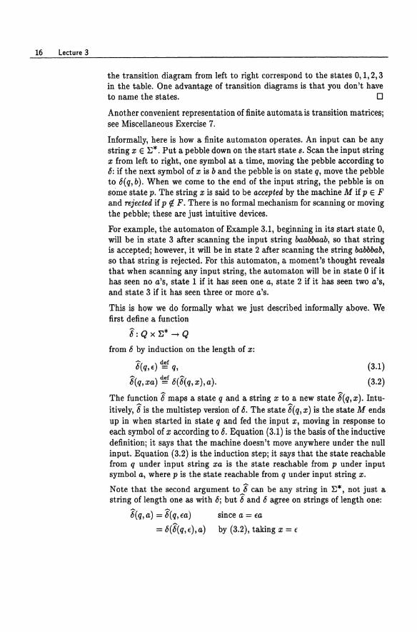
Example 3.2 Here is another example of a regular set and a finite automaton accepting it. Consider the set
{xaaay I x,y E {a,b}*}
= {x E {a,b}* I x contains a substring ofthree consecutive a's}.
For example, baabaaaab is in the set and should be accepted, whereas babbabab is not in the set and should be rejected (because the three a's are not consecutive). Here is an automaton for this set, specified in both table and transition diagram form:
a b
~ fITl ~ 2 3 0 3F 3 3
o
18 Lecture 3
The idea here is that you use the states to count the number of consecutive a's you have seen. If you haven't seen three a's in a row and you see a b, you must go back to the start. Once you have seen three a's in a row, though, you stay in the accept state.
Lecture 4
More on Regular Sets
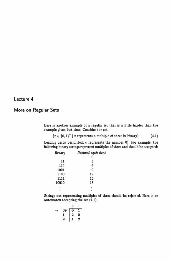
Here is another example of a regular set that is a little harder than the example given last time. Consider the set
{x E {O, 1} * I x represents a multiple of three in binary} (4.1)
(leading zeros permitted, f represents the number 0). For example, the following binary strings represent multiples of three and should be accepted:
Binary o
11
Decimal equivalent o
110 1001 1100 1111
10010
3 6 9
12 15 18
Strings not representing multiples of three should be rejected. Here is an automaton accepting the set (4.1):
o 1
-+ OF 1fT1 1 2 0 2 1 2
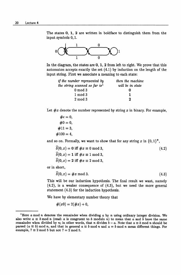
20 Lecture 4
The states 0, 1, 2 are written in boldface to distinguish them from the input symbols 0, 1.
° d_1_x __ O_yo 1 1 °
In the diagram, the states are 0, 1, 2 from left to right. We prove that this automaton accepts exactly the set (4.1) by induction on the length of the input string. First we associate a meaning to each state:
if the number represented by then the machine the string scanned so far is l will be in state
° mod 3 ° 1 mod 3 1 2 mod 3 2
Let #x denote the number represented by string x in binary. For example,
#e=O, #0=0,
#11 =3, #100 = 4,
and so on. Formally, we want to show that for any string x in {O, 1 } * , 6(0, x) = ° iff #x == ° mod 3,
6(0, x) = 1 iff #x == 1 mod 3,
6(0, x) = 2 iff #x == 2 mod 3,
or in short,
6(0, x) = #x mod 3.
(4.2)
(4.3)
This will be our induction hypothesis. The final result we want, namely (4.2), is a weaker consequence of (4.3), but we need the more general statement (4.3) for the induction hypothesis.
We have by elementary number theory that
#(xO) = 2(#x) + 0,
1 Here a mod n denotes the remainder when dividing a by n using ordinary integer division. We also write a == b mod n (read: a is congruent to b modulo n) to mean that a and b have the same remainder when divided by nj in other words, that n divides b - a. Note that a == b mod n should be parsed (a == b) mod n, and that in general a == b mod n and a = b mod n mean different things. For example, 7 == 2 mod 5 but not 7 = 2 mod 5.
More on Regular Sets 21
#(x1) = 2(#x) + 1,
or in short,
#(xc) = 2(#x) + c (4.4)
for c E {O,1}. From the machine above, we see that for any state q E {O, 1, 2} and input symbol c E {O, 1},
6(q, c) = (2q+c) mod 3. (4.5)
This can be verified by checking all six cases corresponding to possible choices of q and c. (In fact, (4.5) would have been a great way to define the transition function formally-then we wouldn't have had to prove it!) Now we use the inductive definition of 8 to show (4.3) by induction on Ixl.
Basis
For x = 10,
8(0,10)=0
=#10
by definition of 6
since #€ = 0
= #€ mod 3.
Induction step
Assuming that (4.3) is true for x E {O, 1} *, we show that it is true for xc, where c E {O,1}.
8(0, xc) = 6(8(0,x),c) = 6(#x mod 3,c) = (2(#x mod 3) + c) mod 3
= (2(#x) + c) mod 3
= #xcmod3
definition of 8 induction hypothesis
by (4.5)
elementary number theory
by (4.4).
Note that each step has its reason. We used the definition of 6, which is specific to this automaton; the definition of 8 from 6, which is the same for all automata; and elementary properties of numbers and strings.
Some Closure Properties of Regular Sets
For A, B ~ r;*, recall the following definitions:
AU B = {x I x E A or x E B} An B = {x I x E A and x E B}
"'A = {x E r;* I x (j. A}
union
intersection
complement
22 Lecture 4
AB = {xy I X E A and y E B} concatenation
A* = {XIX2'" Xn In;::: 0 and Xi E A, 1 :$ i :$ n}
= AO U Al U A2 U Aa U··· asterate.
Do not confuse set concatenation with string concatenation. Sometimes'" A is written 1:* - A.
We show below that if A and B are regular, then so are Au B, An B, and '" A. We'll show later that AB and A * are also regular.
The Product Construction
Assume that A and B are regular. Then there are automata
Ml = (Ql> 1:,151,81, Fl)'
M2 = (Q2, 1:, 152 , 82, F2)
with L(Ml) = A and L(M2) = B. To show that An B is regular, we will build an automaton Ma such that L(Ma) = An B.
Intuitively, Ma will have the states of Ml and M2 encoded somehow in its states. On input x E 1:*, it will simulate Ml and M2 simultaneously on X, accepting iff both Ml and M2 would accept. Think about putting a pebble down on the start state of Ml and another on the start state of M2 • As the input symbols come in, move both pebbles according to the rules of each machine. Accept if both pebbles occupy accept states in their respective machines when the end of the input string is reached.
Formally, let
M3 = (Q3, ~, 153, 83, F3),
where
Q3 = Ql X Q2 = {(p,q) I p E Ql and q E Q2},
F3 = Fl X F2 = {(p,q) I p E Fl and q E F2},
83 = (81) 82),
and let
ba : Q3 x 1: -+ Qa
be the transition function defined by
b3((p,q),a) = (b1(p,a),b2(q,a)).
The automaton Ma is called the product of Ml and M2. A state (p,q) of Ma encodes a configuration of pebbles on Ml and M2.
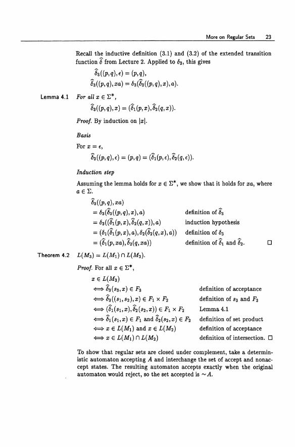
More on Regular Sets 23
Recall the inductive definition (3.1) and (3.2) of the extended transition function 6 from Lecture 2. Applied to 03, this gives
6s(p,q),e) = (p,q),
63«(p,q),xa) = oa(6a«p,q),x),a).
Lemma 4.1 For all x e r:*, 63«p,q),x) = (61(P,x),62(q,x)).
Proof. By induction on Ixl.
Basis
For x = e,
63«(P, q), e) = (P, q) = (~(P, e).62(q, e)).
Induction 8tep
Assuming the lemma holds for x e r:*, we show that it holds for xa, where a e r:.
63«(p,q),xa)
= os(6s«(P,q),x),a)
= Os «61 (p, X).62(q, x)), a)
= (01 (61(P, x), a), 02 (62(q, x), a))
= (61(P,xa).62(q,xa))
Theorem 4.2 L(Ms) = L(Ml) n L(M2).
Proof. For all x e r:*, x E L(Ms)
definition of 6s
induction hypothesis
definition of oa definition of 61 and 62.
¢:::} 63 ( 8S, x) E Fs definition of acceptance
¢:::} 63«81,82),X) e Fl x F2 definition of 83 and F3
¢:::} (61 (81, X),62(82, x)) E Fl x F2 Lemma 4.1
¢:::} 61 (81. x) E Fl and 62(82,X) E F2 definition of set product
¢:::} x e L(Ml) and x e L(M2) definition of acceptance
o
¢:::} x E L(Ml) n L(M2 ) definition of intersection. 0
To show that regular sets are closed under complement, take a deterministic automaton accepting A and interchange the set of accept and nonaccept states. The resulting automaton accepts exactly when the original automaton would reject, so the set accepted is N A.
24 lecture 4
Once we know regular sets are closed under n and "", it follows that they are closed under U by one of the De Morgan laws:
AUB = ""(""An ""B).
If you use the constructions for nand"" given above, this gives an automaton for AU B that looks exactly like the product automaton for An B, except that the accept states are
F3 = {(p,q) I p e FI or q e F2} = (FI x Q2) U (QI x F2)
instead of FI x F2•
Historical Notes
Finite-state transition systems were introduced by McCulloch and Pitts in 1943 [84]. Deterministic finite automata in the form presented here were studied by Kleene [70]. Our notation is borrowed from Hopcroft and Ullman [60].
Lecture 5
Nondeterministic Finite Automata
Nondeterm i n ism
Nondetermini8m is an important abstraction in computer science. It refers to situations in which the next state of a computation is not uniquely determined by the current state. Nondeterminism arises in realUfe when there is incomplete information about the state or when there are external forces at work that can affect the course of a computation. For example, the behavior of a process in a distributed system might depend on messages from other processes that arrive at unpredictable times with unpredictable contents.
Nondeterminism is also important in the design of efficient algorithms. There are many instances of important combinatorial problems with efficient nondeterministic solutions but no known efficient deterministic solution. The famous P = NP problem-whether all problems solvable in nondeterministic polynomial time can be solved in deterministic polynomial time-is a major open problem in computer science and arguably one of the most important open problems in all of mathematics.
In nondeterministic situations, we may not know how a computation will evolve, but we may have some idea of the range of possibilities. This is modeled formally by allowing automata to have multiple-valued transition functions.
26 Lecture 5
In this lecture and the next, we will show how nondeterminism is incorporated naturally in the context of finite automata. One might think that adding nondeterminism might increase expressive power, but in fact for finite automata it does not: in terms of the sets accepted, nondeterministic finite automata are no more powerful than deterministic ones. In other words, for every nondeterministic finite automaton, there is a deterministic one accepting the same set. However, nondeterministic machines may be exponentially more succinct.
Nondeterministic Finite Automata
A nondeterministic finite automaton (NFA) is one for which the next state is not necessarily uniquely determined by the current state and input symbol. In a deterministic automaton, there is exactly one start state and exactly one transition out of each state for each symbol in ~. In a nondeterministic automaton, there may be one, more than one, or zero. The set of possible next states that the automaton may move to from a particular state q in response to a particular input symbol a is part of the specification of the automaton, but there is no mechanism for deciding which one will actually be taken. Formally, we won't be able to represent this with a function 6 : Q x ~ -+ Q anymore; we will have to use something more general. Also, a nondeterministic automaton may have many start states and may start in anyone of them.
Informally, a nondeterministic automaton is said to accept its input x if it is possible to start in some start state and scan x, moving according to the transition rules and making choices along the way whenever the next state is not uniquely determined, such that when the end of x is reached, the machine is in an accept state. Because the start state is not determined and because of the choices along the way, there may be several possible paths through the automaton in response to the input x; some may lead to accept states while others may lead to reject states. The automaton is said to accept x if at least one computation path on input x starting from at least one start state leads to an accept state. The automaton is said to reject x if no computation path on input x from any start state leads to an accept state. Another way of saying this is that x is accepted iff there exists a path with label x from some start state to some accept state. Again, there is no mechanism for determining which state to start in or which of the possible next moves to take in response to an input symbol.
It is helpful to think about this process in terms of guessing and verifying. On a given input, imagine the automaton guessing a successful computation or proof that the input is a "yes" instance of the decision problem, then verifying that its guess was indeed correct.
Nondeterministic Finite Automata 27
For example, consider the set
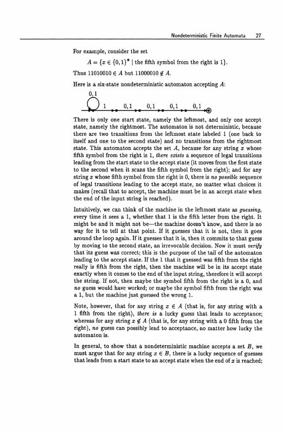
A = {x E {0,1}* I the fifth symbol from the right is I}.
Thus 11010010 E A but 11000010 rt A.
Here is a six-state nondeterministic automaton accepting A:
o 1
(2 1 0, 1 0, 1 0, 1 0, 1 t::\ - ~. .. ... ... .~
There is only one start state, namely the leftmost, and only one accept state, namely the rightmost. The automaton is not deterministic, because there are two transitions from the leftmost state labeled 1 (one back to itself and one to the second state) and no transitions from the rightmost state. This automaton accepts the set A, because for any string x whose fifth symbol from the right is 1, there exists a sequence of legal transitions leading from the start state to the accept state (it moves from the first state to the second when it scans the fifth symbol from the right); and for any string x whose fifth symbol from the right is 0, there is no possible sequence of legal transitions leading to the accept state, no matter what choices it makes (recall that to accept, the machine must be in an accept state when the end of the input string is reached).
Intuitively, we can think of the machine in the leftmost state as guessing, every time it sees a 1, whether that 1 is the fifth letter from the right. It might be and it might not be-the machine doesn't know, and there is no way for it to tell at that point. If it guesses that it is not, then it goes around the loop again. If it guesses that it is, then it commits to that guess by moving to the second state, an irrevocable decision. Now it must verify that its guess was correct; this is the purpose of the tail of the automaton leading to the accept state. If the 1 that it guessed was fifth from the right really is fifth from the right, then the machine will be in its accept state exactly when it comes to the end of the input string, therefore it will accept the string. If not, then maybe the symbol fifth from the right is a 0, and no guess would have worked; or maybe the symbol fifth from the right was a 1, but the machine just guessed the wrong 1.
Note, however, that for any string x E A (that is, for any string with a 1 fifth from the right), there is a lucky guess that leads to acceptance; whereas for any string x rt A (that is, for any string with a 0 fifth from the right), no guess can possibly lead to acceptance, no matter how lucky the automaton is.
In general, to show that a nondeterministic machine accepts a set B, we must argue that for any string x E B, there is a lucky sequence of guesses that leads from a start state to an accept state when the end of x is reached;
28 Lecture 5
but for any string x ¢ B, no sequence of guesses leads to an accept state when the end of x is reached, no matter how lucky the automaton is.
Keep in mind that this process of guessing and verifying is just an intuitive aid. The formal definition of nondeterministic acceptance will be given in Lecture 6.
There does exist a deterministic automaton accepting the set A, but any such automaton must have at least 25 = 32 states, since a deterministic machine essentially has to remember the last five symbols seen.
The Subset Construction
We will prove a rather remarkable fact: in terms of the sets accepted, nondeterministic finite automata are no more powerful than deterministic ones. In other words, for every nondeterministic finite automaton, there is a deterministic one accepting the same set. The deterministic automaton, however, may require more states.
This theorem can be proved using the subset construction. Here is the intuitive idea; we will give a formal treatment in Lecture 6. Given a nondeterministic machine N, think of putting pebbles on the states to keep track of all the states N could possibly be in after scanning a prefix of the input. We start with pebbles on all the start states of the nondeterministic machine. Say after scanning some prefix y of the input string, we have pebbles on some set P of states, and say P is the set of all states N could possibly be in after scanning y, depending on the nondeterministic choices that N could have made so far. If input symbol b comes in, pick the pebbles up off the states of P and put a pebble down on each state reachable from a state in P under input symbol b. Let pI be the new set of states covered by pebbles. Then pI is the set of states that N could possibly be in after scanning yb.
Although for a state q of N, there may be many possible next states after scanning b, note that the set pI is uniquely determined by b and the set P. We will thus build a deterministic automaton M whose states are these sets. That is, a state of M will be a set of states of N. The start state of M will be the set of start states of N, indicating that we start with one pebble on each of the start states of N. A final state of M will be any set P containing a final state of N, since we want to accept x if it is possible for N to have made choices while scanning x that lead to an accept state of N.
It takes a stretch of the imagination to regard a set of states of N as a single state of M. Let's illustrate the construction with a shortened version of the example above.
Nondeterministic Finite Automata 29
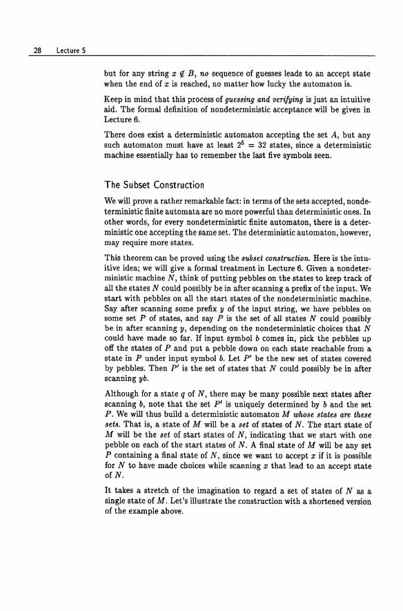
Example 5.1 Consider the set
A = {x E {O, I} * I the second symbol from the right is I}.
o 1
~ 1 0,1 t::\ ~ .... .. ~ p q r
Label the states p, q, r from left to right, as illustrated. The states of M will be subsets of the set of states of N. In this example there are eight such subsets:
0, {p}, {q}, {r}, {p,q}, {p,r}, {q,r}, {p,q,r}.
Here is the deterministic automaton M:
0 1 0 0 0 - {p} {P} {p,q}
{q} {r} {r} {r}F 0 0
{p,q} {p,r} {p,q,r} {p,r}F {P} {p,q} {q,r}F {r} {r}
{p,q,r}F {p,r} {p,q,r}
For example, if we have pebbles on p and q (the fifth row of the table), and if we see input symbol 0 (first column), then in the next step there will be pebbles on p and r. This is because in the automaton N, p is reachable from p under input 0 and r is reachable from q under input 0, and these are the only states reachable from p and q under input o. The accept states of M (marked F in the table) are those sets containing an accept state of N. The start state of Mis {p}, the set of all start states of N.
Following 0 and 1 transitions from the start state {P} of M, one can see that states {q,r}, {q}, {r}, 0 of M can never be reached. These states of M are inaccessible, and we might as well throw them out. This leaves
o 1
- {P} p {p, q} {p, r} {p,r}F {p}
{p,q,r}F {p,r}
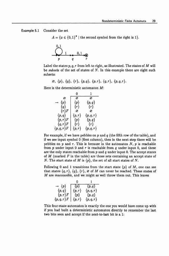
This four-state automaton is exactly the one you would have come up with if you had built a deterministic automaton directly to remember the last two bits seen and accept if the next-to-last bit is a 1:
30 Lecture 5
1 [01] 1
°cEl :~: 11'~} 0 [10] 0
Here the state labels [be] indicate the last two bits seen (for our purposes the null string is as good as having just seen two O's). Note that these two automata are isomorphic (Le., they are the same automaton up to the renaming of states):
{P} ~ [00], {p,q} ~ [01], {p, r} ~ [10],
{p,q,r} ~ [11]. o
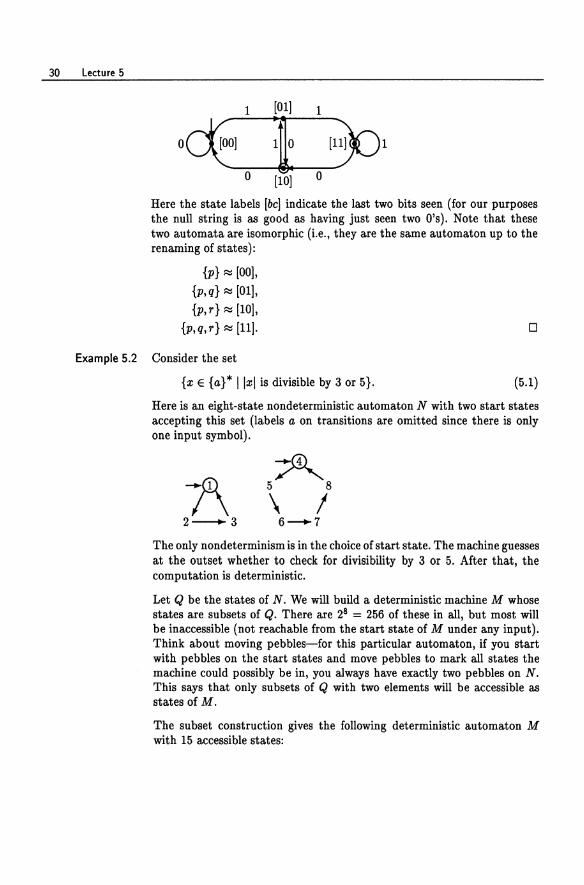
Example 5.2 Consider the set
{x E {a}* Ilxl is divisible by 3 or 5}. (5.1)
Here is an eight-state nondeterministic automaton N with two start states accepting this set (labels a on transitions are omitted since there is only one input symbol).
1\ 2-3
The only nondeterminism is in the choice of start state. The machine guesses at the outset whether to check for divisibility by 3 or 5. After that, the computation is deterministic.
Let Q be the states of N. We will build a deterministic machine M whose states are subsets of Q. There are 28 = 256 of these in all, but most will be inaccessible (not reachable from the start state of M under any input). Think about moving pebbles-for this particular automaton, if you start with pebbles on the start states and move pebbles to mark all states the machine could possibly be in, you always have exactly two pebbles on N. This says that only subsets of Q with two elements will be accessible as states of M.
The subset construction gives the following deterministic automaton M with 15 accessible states:

Nondeterministic Finite Automata 31
{3,8}_{2,7}~{3,5}~{3,7}_{2,6}
~{2'5}"'{3'6}~{2'8}~ 0
In the next lecture we will give a formal definition of nondeterministic finite automata and a general account of the subset construction.
Lecture 6
The Subset Construction
Formal Definition of Nondeterministic Finite Automata
A nondeterministic finite au.tomaton (NFA) is a five-tuple
N = (Q, 1:, d, S, F),
where everything is the same as in a deterministic automaton, except for the following two differences.
• S is a set of states, that is, S ~ Q, instead of a single state. The elements of S are called start states.
• d is a function
d : Q x 1: -+ 2Q ,
where 2Q denotes the power set of Q or the set of all subsets of Q:
2Q ~f {A I A !; Q}.
Intuitively, d(p, a) gives the set of all states that N is allowed to move to from p in one step under input symbol a. We often write
a p--+ q
The Subset Construction 33
if q E ~(p,a). The set ~(p,a) can be the empty set 0. The function ~ is called the transition function.
Now we define acceptance for NFAs. The function ~ extends in a natural way by induction to a function
& : 2Q x E* -+ 2Q
according to the rules ~ def ~(A,€) = A,
~ def U ~(A,xa) = ~(q,a).
(6.1)
(6.2)
Intuitively, for A ~ Q and x E E*, &(A, x) is the set of all states reachable under input string x from some state in A. Note that ~ takes a single state as its first argument and a single symbol as its second argument, whereas & takes a set of states as its first argument and a string of symbols as its second argument.
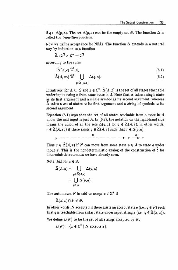
Equation (6.1) says that the set of all states reachable from a state in A under the null input is just A. In (6.2), the notation on the right-hand side means the union of all the sets ~(q,a) for q E &(A,x); in other words, r E &(A,xa) if there exists q E &(A,x) such that r E ~(q,a).
x a p -----------------+ q _ r
Thus q E &(A,x) if N can move from some state pEA to state q under input x. This is the nondeterministic analog of the construction of (; for deterministic automata we have already seen.
Note that for a E E,
&(A,a) = U ~(p,a) PEa(A,<)
= U ~(p,a). pEA
The automaton N is said to accept x E E* if
&(8,x)nF:;60.
In other words, N accepts x if there exists an accept state q (i.e., q E F) such that q is reachable from a start state under input string x (i.e., q E &(8, x)).
We define L(N) to be the set of all strings accepted by N:
L(N) = {x E E* I N accepts x}.
34 Lecture 6
Under this definition, every DFA
(Q, E, 8, s, F)
is equivalent to an NFA
(Q, E, ~, {s}, F),
where ~(p,a) ~ {8(p, a)}. Below we will show that the converse holds as well: every NFA is equivalent to some DFA.
Here are some basic lemmas that we will find useful when dealing with NFAs. The first corresponds to Exercise 3 of Homework 1 for deterministic automata.
Lemma 6.1 For any x,y E E* and A ~ Q,
&(A,xy) = &(&(A,x),y).
Proof. The proof is by induction on Iyl.
Basis
For y = EO,
&(A,u) = &(A,x)
= &(&(A,X),i) by (6.1).
Induction step
For any y E E* and a E E,
&(A,xya) = U ~(q,a) by (6.2) qE~(A,,,,y)
= U ~(q,a) induction hypothesis
qE~(~(A,,,,),y)
= &(&(A,x),ya) by (6.2). o
Lemma 6.2 The function & commutes with set union: for any indexed family Ai of subsets of Q and x E E*,
&(UAi,x) = U &(Ai'X). i i
Proof. By induction on Ixl.
The Subset Construction
Basis
By (6.1),
~(U Ai, f) = U Ai = U ~(Ai' f). iii
Indu.ction step
~(UAi,xa) = U d(p, a) by (6.2)
PEA(U. A., .. )
= U d(p,a) induction hypothesis
PEU. A(A., .. )
=U U d(p, a) basic set theory
i PEA(A., .. )
= U~(Ai,xa) by (6.2).
In particular, expressing a set as the union of its singleton subsets,
~(A,x) = U ~({P},x). pEA
The Subset Construction: General Account
The subset construction works in general. Let
N = (QN, E, dN, SN, FN)
35
0
(6.3)
be an arbitrary NFA. We will use the subset construction to produce an equivalent DFA. Let M be the DFA
M = (QM, E, OM, SM, FM),
where
Q ~f2QN M- , def ~
t5M(A,a) = dN(A,a), def S SM = N.
FM ~f {A S;; QN I AnFN '" 0}.
Note that 15M is a function from states of M and input symbols to states of M, as it should be, because states of M are sets of states of N.
36 Lecture 6
Lemma 6.3 For any A ~ QN and x e E*,
6M(A,x) = ~N(A,x). Proof. Induction on Ixl.
Basis
For x = f, we want to show
6M(A, f) = ~N(A, f). But both of these are A, by definition of ~ and ~N'
Induction step
Assume that
6M(A,x) = ~N(A,x). We want to show the same is true for xa, a e E.
6M(A,xa) = oM(6M(A,x),a)
= OM(~N(A,x),a) = ;&N(~N(A,x),a) = ;&N(A,xa)
definition of 6 M
induction hypothesis
definition of OM
Lemma 6.1. o Theorem 6.4 The automata M and N accept the same set.
Proof. For any x e E*,
x e L(M)
<==:} 6M(SM'X) e FM
<==:} ~N(SN'X) n FN i= 0
<==:} x e L(N)
f-Transitions
definition of acceptance for M
definition of SM and FM, Lemma 6.3
definition of acceptance for N. 0
Here is another extension of finite automata that turns out to be quite useful but really adds no more power.
An f-transition is a transition with label E, a letter that stands for the null string f:
E p~q.
The automaton can take such a transition anytime without reading an input symbol.
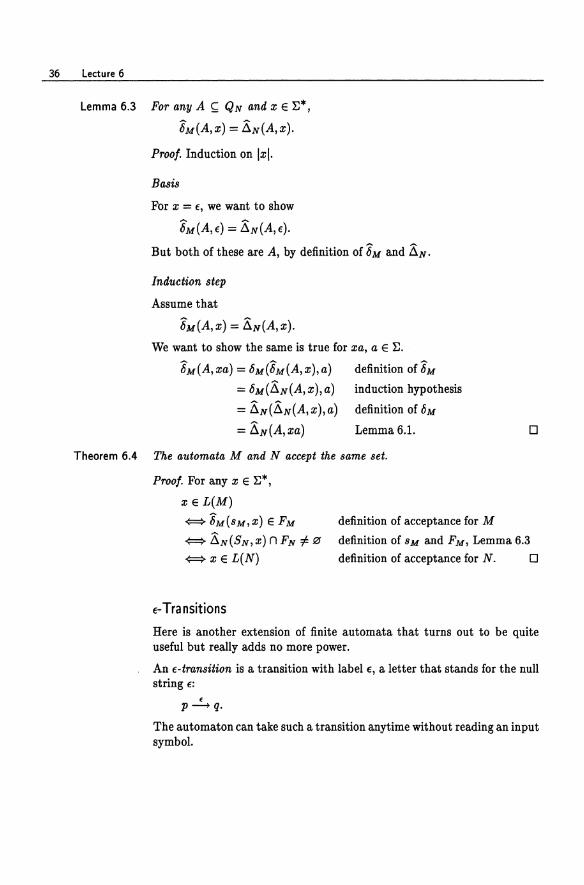
Example 6.5
The Subset Construction 37
-lb/ib/ib P q ~
If the machine is in state 8 and the next input symbol is b, it can nondeterministically decide to do one of three things:
• read the b and move to state Pi
• slide to t without reading an input symbol, then read the b and move to state qj or
• slide to t without reading an input symbol, then slide to 1.1 without reading an input symbol, then read the b and move to state r.
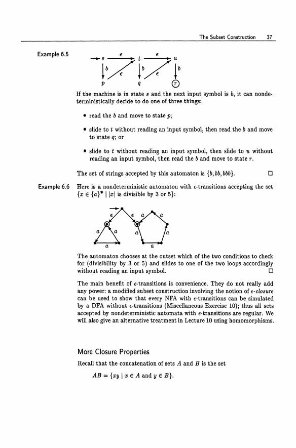
The set of strings accepted by this automaton is {b, bb, bbb}. o Example 6.6 Here is a nondeterministic automaton with f-transitions accepting the set
{x E {a}* Ilxl is divisible by 3 or 5}:
The automaton chooses at the outset which of the two conditions to check for (divisibility by 3 or 5) and slides to one of the two loops accordingly without reading an input symbol. 0
The main benefit of f-transitions is convenience. They do not really add any power: a modified subset construction involving the notion of f-clostiTe can be used to show that every NFA with f-transitions can be simulated by a DFA without f-transitions (Miscellaneous Exercise 10)j thus all sets accepted by nondeterministic automata with f-transitions are regular. We will also give an alternative treatment in Lecture 10 using homomorphisms.
More Closure Properties
Recall that the concatenation of sets A and B is the set
AB = {xy I x E A and y E B}.
38 Lecture 6
For example,
{a,ab}{b,ba} = {ab,aba,abb,abba}.
If A and B are regular, then so is AB. To see this, let M be an automaton for A and N an automaton for B. Make a new automaton P whose states are the union of the state sets of M and N, and take all the transitions of M and N as transitions of P. Make the start states of M the start states of P and the final states of N the final states of P. Finally, put f-transitions from all the final states of M to all the start states of N. Then L(P) = AB.
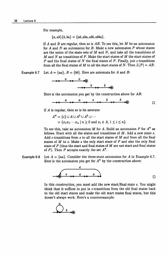
Example 6.7 Let A = {aa}, B = {bbl. Here are automata for A and B:
a ~ . ..
b •• •• Here is the automaton you get by the construction above for AB:
~. a~. a •• E •• b~. b .®
If A is regular, then so is its asterate:
A* = {f} U A U A2 U A3 U···
= {XIX2· ··Xn I n ~ 0 and Xi E A, 1 ~ i ~ n}.
o
To see this, take an automaton M for A. Build an automaton P for A * as follows. Start with all the states and transitions of M. Add a new state s. Add f-transitions from s to all the start states of M and from all the final states of M to s. Make s the only start state of P and also the only final state of P (thus the start and final states of M are not start and final states of P). Then P accepts exactly the set A*.
Example 6.8 Let A = {aa}. Consider the three-state automaton for A in Example 6.7. Here is the automaton you get for A * by the construction above:
f
~iE .. a •• o
In this construction, you must add the new start/final state s. You might think that it suffices to put in E-transitions from the old final states back to the old start states and make the old start states final states, but this doesn't always work. Here's a counterexample:
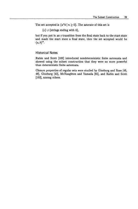
The Subset Construction 39
The set accepted is {an bin ~ o}. The asterate of this set is
{e} U {strings ending with b},
but if you put in an e-transition from the final state back to the start state and made the start state a final state, then the set accepted would be {a,b}*.
Historical Notes
Rabin and Scott [102] introduced nondeterministic finite automata and showed using the subset construction that they were no more powerful than deterministic finite automata.
Closure properties of regular sets were studied by Ginsburg and Rose [46, 48], Ginsburg [43], McNaughton and Yamada [851, and Rabin and Scott [1021, among others.
Lecture 7
Pattern Matching
What happens when one types rm * in UNIX? (If you don't know, don't try it to find out!) What if the current directory contains the files
a.tex be.tex a.dvi bc.dvi
and one types rm *. dvi? What would happen if there were a file named .dvi?
What is going on here is pattern matching. The * in UNIX is a pattern that . matches any string of symbols, including the null string.
Pattern matching is an important application of finite automata. The UNIX commands grep, fgrep, and egrep are basic pattern-matching utilities that use finite automata in their implementation.
Let ~ be a finite alphabet. A pattern is a string of symbols of a certain form representing a (possibly infinite) set of strings in ~*. The set of patterns is defined formally by induction below. They are either atomic patterns or compound patterns built up inductively from atomic patterns using certain operators. We'll denote patterns by Greek letters a, (3, ,,/, ....
As we define patterns, we will tell which strings a: E ~* match them. The set of strings in ~* matching a given pattern a will be denoted L(a). Thus
L(a) = {a: E ~* I a: matches a}.
Pattern Matching 41
In the following, forget the UNIX definition of *. We will use the symbol * for something else.
The atomic patterns are
• a for each a E ~, matched by the symbol a only; in symbols, L(a) = {a};
• E, matched only by E, the null string; in symbols, L(E) = {E};
• f/t, matched by nothing; in symbols, L(f/t) = 0, the empty set;
• #, matched by any symbol in 'E; in symbols, L( #) = ~; • @, matched by any string in ~*; in symbols, L(@) = ~*.
Compound patterns are formed inductively using binary operators +, n, and· (usually not written) and unary operators +, *, and <V. If a and (3 are patterns, then so are 01+(3, an /3, 01*, 01+, <va, and 01/3. The last of these is short for a . /3. We also define inductively which strings match each pattern. We have already said which strings match the atomic patterns. This is the basis of the inductive definition. Now suppose we have already defined the sets of strings L(a) and L(/3) matching a and /3, respectively. Then we'll say that
• x matches a + /3 if x matches either a or (3:
L(a + /3) = L(a) U L(/3);
• x matches a n /3 if x matches both a and (3:
L(o: n f3) = L(o:) n L(f3);
• x matches 01/3 if x can be broken down as x = yz such that y matches a and z matches /3:
L(a/3) = L(a)L(/3) = {yz lyE L(a) and z E L(/3)};
• x matches <va if x does not match a:
L( <va) = <v L(a) = 'E* - L(a);
• x matches 01* if x can be expressed as a concatenation of zero or more strings, all of which match 0::
L(o:*) = {XIX2··· Xn In;::: 0 and Xi E L(o:), 1 SiS n} = L(a)O U L(a)l U L(a)2 U···
42 Lecture 7
Example 7.1
Example 7.2
= L(a)*.
The null string € always matches a*, since € is a concatenation of zero strings, all of which (vacuously) match a.
• x matches a+ if x can be expressed as a concatenation of one or more strings, all of which match a:
L(a+) = {X1X2'" Xn In 2: 1 and Xi e L(a), 1 :::; i :::; n} = L(a)l U L(a)2 U L(a)3 u··· =L(a)+.
Note that patterns are just certain strings of symbols over the alphabet
E U { e, ft, #, @, +, n, "', *, +, (, ) }.
Note also that the meanings of #, @, and,..., depend on E. For example, if E = {a,b,c} then L(#) = {a,b,c}, but if E = {a} then L(#) = {a}.
• E* = L(@) = L(#*).
• Singleton sets: if x e E*, then x itself is a pattern and is matched only by the string Xj i.e., {x} = L(x).
• Finite sets: if Xl, ... ,Xm e E*, then
{Xl,X2, ... ,xm} = L(X1 + X2 + ... + Xm). o Note that we can write the last pattern Xl + X2 + ... + Xm without parentheses, since the two patterns (a + {3) + 1 and a + ({3 + 1) are matched by the same set of stringsj i.e.,
L«a + {3) + 1) = L(a + ({3 + 1))·
Mathematically speaking, the operator + is associative. The concatenation operator' is associative, too. Hence we can also unambiguously write a{31 without parentheses.
• strings containing at least three occurrences of a:
@a@a@a@j
• strings containing an a followed later by a bj that is, strings of the form xaybz for some x, y, z:
@a@b@j
• all single letters except a:
# n "'aj
• strings with no occurrence of the letter a:
(# n "'a)*;
Pattern Matching 43
• strings in which every occurrence of a is followed sometime later by an occurrence of b; in other words, strings in which there are either no occurrences of a, or there is an occurrence of b followed by no occurrence of a; for example, aab matches but boo doesn't:
(# n "'a)* +@b(#n"'a)*.
If the alphabet is {a,b}, then this takes a much simpler form:
E+@b. o Before we go too much further, there is a subtlety that needs to be mentioned. Note the slight difference in appearance between E and to and between 11I and 0. The objects E and 11I are symbols in the language of patterns, whereas to and 0 are metasymbols that we are using to name the null string and the empty set, respectively. These are different sorts of things: E and 11I are symbols, that is, strings of length one, whereas to is a string of length zero and 0 isn't even a string.
We'll maintain the distinction for a few lectures until we get used to the idea, but at some point in the near future we'll drop the boldface and use to and 0 exclusively. We'll always be able to infer from context whether we mean the symbols or the metasymbols. This is a little more convenient and conforms to standard usage, but bear in mind that they are still different things.
While we're on the subject of abuse of notation, we should also mention that very often you will see things like x E a*b* in texts and articles. Strictly speaking, one should write x E L(a*b*), since a*b* is a pattern, not a set of strings. But as long as you know what you really mean and can stand the guilt, it is okay to write x e a*b*.
Lecture 8
Pattern Matching and Regular Expressions
Here are some interesting and important questions:
• How hard is it to determine whether a given string x matches a given pattern a.? This is an important practical question. There are very efficient algorithms, as we will see.
• Is every set represented by some pattern? Answer: no. For example, the set
is not represented by any pattern. We'll prove this later.
• Patterns 0. and f3 are equivalent if L(o.) = L(f3). How do you tell whether 0. and f3 are equivalent? Sometimes it is obvious and sometimes not.
• Which operators are redundant? For example, we can get rid of E since it is equivalent to "'(#@) and also to fij*. We can get rid of@ since it is equivalent to #*. We can get rid of unary + since 0.+ is equivalent to 0.0.*. We can get rid of #, since if E = {ab ... ,an} then # is equivalent to the pattern
Pattern Matching and Regular Expressions 45
The operator n is also redundant, by one of the De Morgan laws:
0: n 13 is equivalent to "" ("" 0: + "" 13).
Redundancy is an important question. From a user's point of view, we would like to have a lot of operators since this lets us write more succinct patterns; but from a programmer's point of view, we would like to have as few as possible since there is less code to write. Also, from a theoretical point of view, fewer operators mean fewer cases we have to treat in giving formal semantics and proofs of correctness.
An amazing and difficult-to-prove fact is that the operator"" is redundant. Thus every pattern is equivalent to one using only atomic patterns a E ~, e, fl, and operators +, " and *. Patterns using only these symbols are called regular ezpressions. Actually, as we have observed, even e is redundant, but we include it in the definition of regular expressions because it occurs so often.
Our goal for this lecture and the next will be to show that the family of subsets of ~* represented by patterns is exactly the family of regular sets. Thus as a way of describing subsets of ~*, finite automata, patterns, and regular expressions are equally expressive.
Some Notational Conveniences
Since the binary operators + and· are associative, that is,
L(o: + (13 + 'Y)) = L((o: + 13) + 'Y), L(a({j-y)) = L«a,8h),
we can write
without ambiguity. To resolve ambiguity in other situations, we assign precedence to operators. For example,
could be interpreted as either
0: + (13'Y) or (0: + 13)-Y,
which are not equivalent. We adopt the convention that the concatenation operator' has higher precedence than +, so that we would prefer the former interpretation. Similarly, we assign * higher precedence than + or " so that
0: +,8*
46 Lecture 8
is interpreted as
a + (13*)
and not as
(a+f3)*.
All else failing, use parentheses.
Equivalence of Patterns, Regular Expressions, and Finite Automata
Patterns, regular expressions (patterns built from atomic patterns a E I:, E, fiS, and operators +, *, and· only), and finite automata are all equivalent in expressive power: they all represent the regular sets.
Theorem 8.1 Let A ~ I:*. The following three statements are equivalent:
(i) A is regular; that is, A = L(M) for some finite automaton M;
(ii) A = L(a) for some pattern a;
(iii) A = L(a) for some regular expression a.
Proof. The implication (iii) ::} (ii) is trivial, since every regular expression is a pattern. We prove (ii) ::} (i) here and (i) ::} (iii) in Lecture 9.
The heart of the proof (ii) ::} (i) involves showing that certain basic sets (corresponding to atomic patterns) are regular, and the regular sets are closed under certain closure operations corresponding to the operators used to build patterns. Note that
• the singleton set {a} is regular, a E I:,
• the singleton set {f} is regular, and
• the empty set 0 is regular,
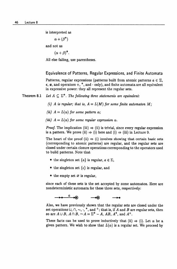
since each of these sets is the set accepted by some automaton. Here are nondeterministic automata for these three sets, respectively:
Also, we have previously shown that the regular sets are closed under the set operations U, n, "', ., *, and +j that is, if A and B are regular sets, then so are AUB, AnB, "'A = I:* - A, AB, A*, and A+.
These facts can be used to prove inductively that (ii) ::} (i). Let a be a given pattern. We wish to show that L(a) is a regular set. We proceed by
Pattern Matching and Regular Expressions 47
induction on the structure of 0:. The pattern 0: is of one of the following forms:
(i) a, where a e ~j (vi) P + 'Yj
(ii) e· , (vii) P n 'Yj
(iii) 16j (viii) P'Yj
(iv) #j (ix) "" pj
(v) @lj (x) p*j
(xi) P+.
There are five base cases (i) through (v) corresponding to the atomic patterns and six induction cases (vi) through (xi) corresponding to compound patterns. Each of these cases uses a closure property of the regular sets previously observed.
For (i), (ii), and (iii), we have L(a) = {a} for a e ~, L(e) = {E}, and L(16) = 0, and these are regular sets.
For (iv), (v), and (xi), we observed earlier that the operators #, @I, and + were redundant, so we may disregard these cases since they are already covered by the other cases.
For (vi), recall that L(P+'Y) = L(P)UL('Y) by definition of the + operator. By the induction hypothesis, L(P) and L( 'Y) are regular. Since the regular sets are closed under union, L(P + 'Y) = L(P) U L( 'Y) is also regular.
The arguments for the remaining cases (vii) through (x) are similar to the argument for (vi). Each of these cases uses a closure property of the regular sets that we have observed previously in Lectures 4 and 6. 0
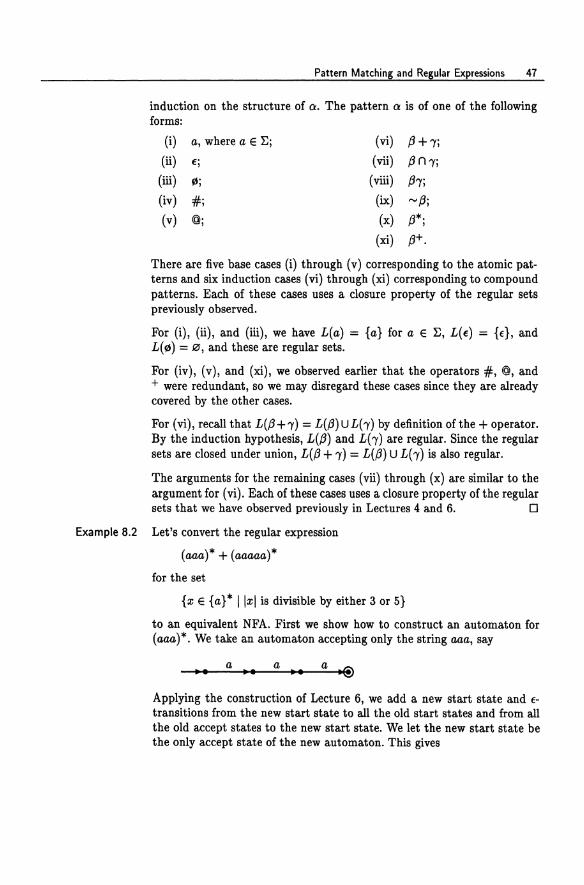
Example 8.2 Let's convert the regular expression
(aaa)* + (aaaaa)*
for the set
{x e {a}* Ilxl is divisible by either 3 or 5}
to an equivalent NFA. First we show how to construct an automaton for (aaa)*. We take an automaton accepting only the string aaa, say
• • a •• a ... Applying the construction of Lecture 6, we add a new start state and etransitions from the new start state to all the old start states and from all the old accept states to the new start state. We let the new start state be the only accept state of the new automaton. This gives
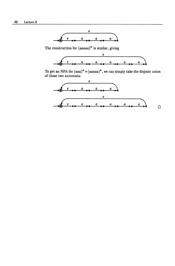
48 Lecture 8
a a ~. ~ .
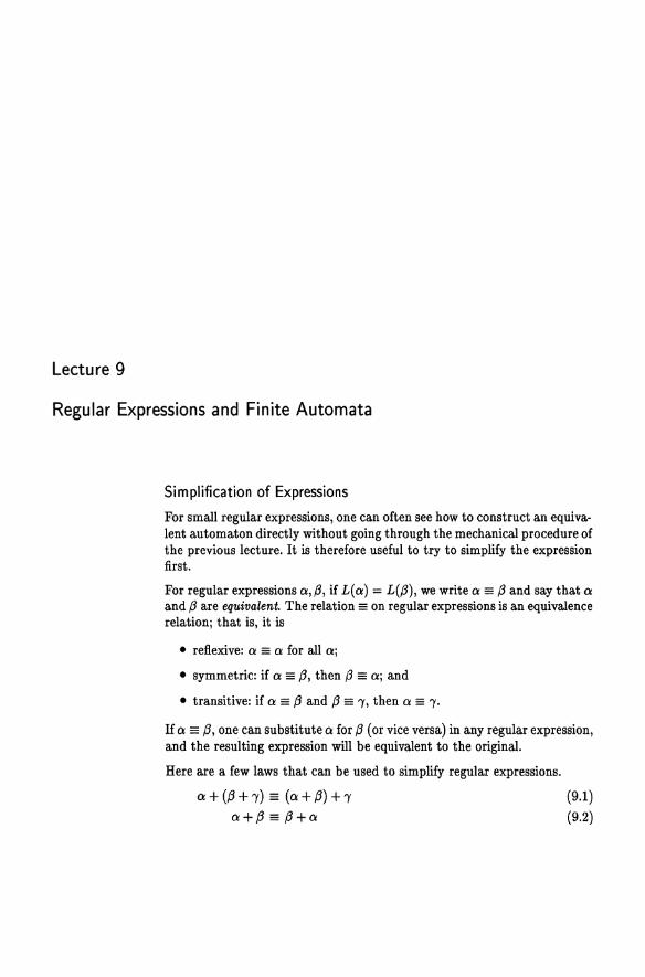
The construction for (aaaaa)* is similar, giving
a a a a •• ... . . ~.
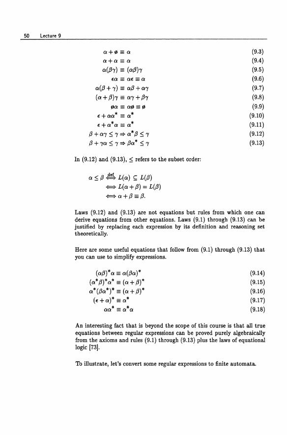
To get an NFA for (aaa)* + (aaaaa)* , we can simply take the disjoint union of these two automata: £
~(£ a a a,:\ ~. ~ . ~ .
£ ~(£ a a a a a,:\ .. . ~. ~. ~ . ~ . 0
Lecture 9
Regular Expressions and Finite Automata
Simplification of Expressions
For small regular expressions, one can often see how to construct an equivalent automaton directly without going through the mechanical procedure of the previous lecture. It is therefore useful to try to simplify the expression first.
For regular expressions 0.,(3, if L(a) = L«(3), we write 0. == (3 and say that 0. and (3 are equivalent. The relation == on regular expressions is an equivalence relation; that is, it is
• reflexive: 0. == 0. for all 0.;
• symmetric: if 0. == (3, then (3 == 0.; and
• transitive: if 0. == (3 and (3 == " then 0. == ,.
If 0. == (3, one can substitute 0. for (3 (or vice versa) in any regular expression, and the resulting expression will be equivalent to the original.
Here are a few laws that can be used to simplify regular expressions.
0. + «(3 +,) == (0. + (3) +,
0.+(3 == (3+0.
(9.1) (9.2)
50 Lecture 9
a+fij== a
a+a == a a{{J'Y) == (a{Jh
Ea == aE ==a a{{J + 'Y) == a{J + a'Y
{a + {Jh == a'Y + {J'Y fija == af6 == f6
E+aa* == a* E+a*a == a*
{J + a'Y ~ 'Y ~ a* {J ~ 'Y
{J + 'Ya ~ 'Y ~ {Ja* ~ 'Y
In (9.12) and (9.13), ~ refers to the subset order:
a ~ (J ~ L(a) ~ L({J) {:::::} L( a + (J) = L({J) {:::::} a + {J == {J.
(9.3)
(9.4) (9.5) (9.6)
(9.7) (9.8) (9.9)
(9.10) (9.11) (9.12) (9.13)
Laws (9.12) and (9.13) are not equations but rules from which one can derive equations from other equations. Laws (9.1) through (9.13) can be justified by replacing each expression by its definition and reasoning set theoretically.
Here are some useful equations that follow from (9.1) through (9.13) that you can use to simplify expressions.
(a{J)*a == a({Ja)* (a*{J)*a* == (a+{J)* a*({Ja*)* == (a + (J)*
(E+a)* == a* aa* == a*a
(9.14) (9.15) (9.16)
(9.17) (9.18)
An interesting fact that is beyond the scope of this course is that all true equations between regular expressions can be proved purely algebraically from the axioms and rules (9.1) through (9.13) plus the laws of equational logic [73].
To illustrate, let's convert some regular expressions to finite automata.
Regular Expressions and Finite Automata 51
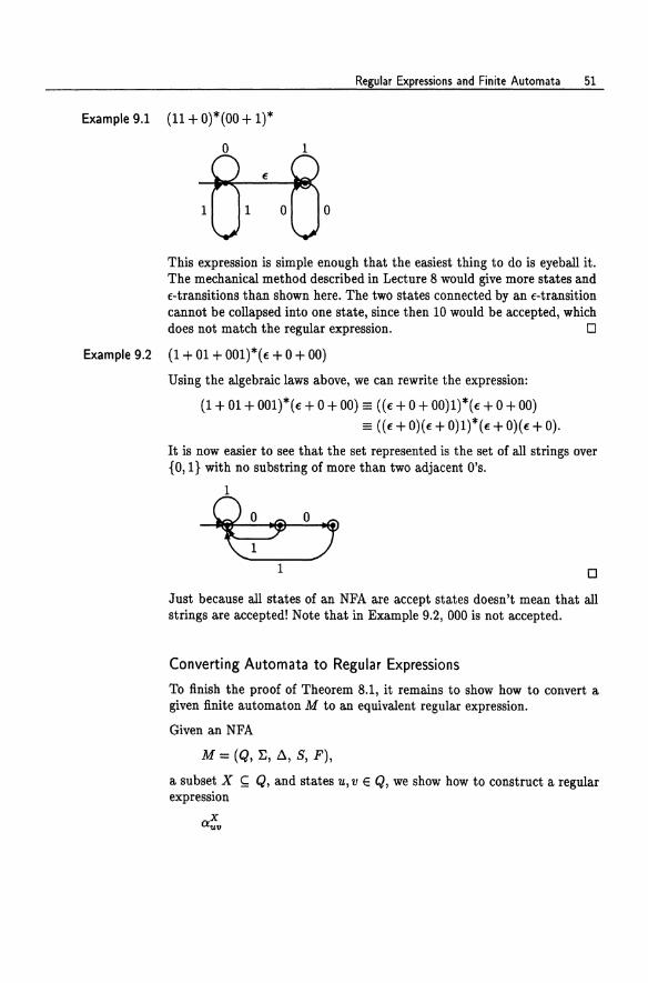
Example 9.1 (11 + 0)*(00 + 1)*
1 o
This expression is simple enough that the easiest thing to do is eyeball it. The mechanical method described in Lecture 8 would give more states and €-transitions than shown here. The two states connected by an €-transition cannot be collapsed into one state, since then 10 would be accepted, which does not match the regular expression. 0
Example 9.2 (1 + 01 + 001)*(e + 0 + 00)
Using the algebraic laws above, we can rewrite the expression:
(1 + 01 + 001)*(e+ 0+00) == ((e+O+ OO)l)*(e + 0+00)
== ((€ + O)(e + O)l)*(e + O)(e + 0).
It is now easier to see that the set represented is the set of all strings over {O, 1} with no substring of more than two adjacent O's.
~OJ 1 o
Just because all states of an NFA are accept states doesn't mean that all strings are accepted! Note that in Example 9.2, 000 is not accepted.
Converting Automata to Regular Expressions
To finish the proof of Theorem 8.1, it remains to show how to convert a given finite automaton M to an equivalent regular expression.
Given an NFA
M = (Q, ~, D., S, F),
a subset X ~ Q, and states '11., V E Q, we show how to construct a regular expression
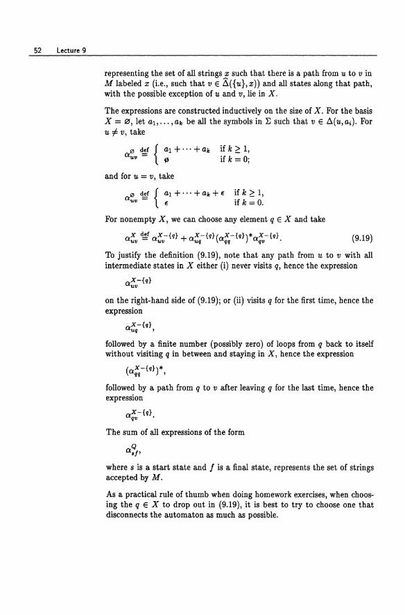
52 Lecture 9
representing the set of all strings x such that there is a path from 'It to v in M labeled x (i.e., such that v E 6.( {'It}, x)) and all states along that path, with the possible exception of u and v, lie in X.
The expressions are constructed inductively on the size of X. For the basis X = 0, let al, ... ,ale be all the symbols in ~ such that v E 6.(u,a.). For u:j:. v, take
and for u = v, take
if k ~ 1, if k = 0;
" c!!:.f { al + ... + ale + E 0:"" - E
if k ~ 1, if k = o.
For nonempty X, we can choose any element q E X and take
x c!!f X-{q} + X-{q}( X-{q})* X-{q} 0:,.." - 0:,.." O:,..q O:qq O:q" • (9.19)
To justify the definition (9.19), note that any path from 'It to v with all intermediate states in X either (i) never visits q, hence the expression
o:x-{q} ""
on the right-hand side of (9.19); or (ii) visits q for the first time, hence the expression
o:x-{q} "q ,
followed by a finite number (possibly zero) of loops from q back to itself without visiting q in between and staying in X, hence the expression
(o:x-{q})* qq ,
followed by a path from q to v after leaving q for the last time, hence the expression
,..X-{q} .... q" •
The sum of all expressions of the form
Q 0:."
where 8 is a start state and I is a final state, represents the set of strings accepted by M.
As a practical rule of thumb when doing homework exercises, when choosing the q E X to drop out in (9.19), it is best to try to choose one that disconnects the automaton as much as possible.
Regular Expressions and Finite Automata 53
Example 9.3 Let's convert the automaton
o~: ~
r to an equivalent regular expression. The set accepted by this automaton will be represented by the inductively defined regular expression
o:{p,q,r} pp ,
since p is the only start and the only accept state. Removing the state q (we can choose any state we like here), we can take
o:{p,q,r} - o:{p,r} + o:{p,r} (o:{p,r})*o:{p,r} pp - pp pq qq qp'
Looking at the automaton, the only paths going from p to p and staying in the states {p, r} are paths going around the single loop labeled 0 from p to p some finite number of times; thus we can take
",{p,r} - 0* "'pp - •
By similar informal reasoning, we can take
o:{p,r} = 0*1 pq ,
o:{p,r} = E + 01 + 000*1 qq
= E + O( E + 00*)1 = E+OO*l,
Q~V} = 000*.
Thus we can take
o:~~,q,r} = 0* + O*l(E + 00*1)*000*.
This is matched by the set of all strings accepted by the automaton. We can further simplify the expression using the algebraic laws (9.1) through (9.18):
0* + O*l(E + 00*1)*000* =0*+0*1(00*1)*000* = E + 00* + 0*10(0*10)*00* = E + (E + 0*10(0*10)*)00* = E + (0*10)*00* = E + (0*10)*0*0
= E + (0 + 10)*0
by (9.17) by (9.10) and (9.14) by (9.8) by (9.10)
by (9.18)
by (9.15). o
54 Lecture 9
Historical Notes
Kleene [70] proved that deterministic finite automata and regular expressions are equivalent. A shorter proof was given by McNaughton and Yamada [85].
The relationship between right- and left-linear grammars and regular sets (Homework 5, Exercise 1) was observed by Chomsky and Miller [21].
Supplementary Lecture A
Kleene Algebra and Regular Expressions
In Lecture 9, we gave a combinatorial proof that every finite automaton has an equivalent regular expression. Here is an algebraic proof that generalizes that argument. It is worth looking at because it introduces the notion of Kleene algebra and the use of matrices. We will show how to use matrices and Kleene algebra to solve systems of linear equations involving sets of strings.
Kleene algebra is named after Stephen C. Kleene, who invented the regular sets [70j.
Kleene Algebra
We have already observed in Lecture 9 that the set operations U, " and * on subsets of I;*, along with the distinguished subsets fZJ and {f}, satisfy certain important algebraic properties. These were listed in Lecture 9, axioms (9.1) through (9.13). Let us call any algebraic structure satisfying these properties a Kleene algebra. In general, a Kleene algebra 1C consists of a nonempty set with two distinguished constants 0 and 1, two binary operations + and . (usually omitted in expressions), and a unary operation * satisfying the following axioms.
a + (b + c) = (a + b) + c associativity of + a+b=b+a commutativity of +
(A. 1) (A.2)
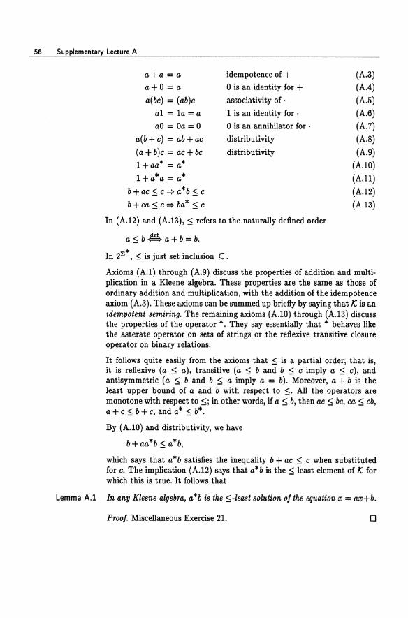
56 Supplementary Lecture A
a+a = a a+O = a a(bc) = (ab)e
al = Ia = a
aO=Oa=O
a(b+e) = ab+ac
(a + b)e = ac+be I +00* = a* I+a*a = a*
b + ae :::; e => a*b :::; e
b + ea :::; e => ba* :::; e
idempotence of + o is an identity for + associativity of .
I is an identity for .
o is an annihilator for·
distributivity
distributivity
In (A.12) and (A.13), :::; refers to the naturally defined order
a:::;b~a+b=b.
In 2lJ*, :::; is just set inclusion ~.
(A.3)
(A A)
(A.5) (A.6) (A.7) (A.B) (A.9)
(A.IO)
(A.H)
(A.12)
(A.13)
Axioms (A.I) through (A.9) discuss the properties of addition and multiplication in a Kleene algebra. These properties are the same as those of ordinary addition and multiplication, with the addition of the idempotence axiom (A.3). These axioms can be summed up briefly by saying that 1C is an idempotent semiring. The remaining axioms (A.lO) through (A.13) discuss the properties of the operator *. They say essentially that * behaves like the asterate operator on sets of strings or the reflexive transitive closure operator on binary relations.
It follows quite easily from the axioms that :5 is a partial order; that is, it is reflexive (a :5 a), transitive (a :5 b and b :5 e imply a :5 c), and antisymmetric (a :::; b and b :5 a imply a = b). Moreover, a + b is the least upper bound of a and b with respect to :::;. All the operators are monotone with respect to :::;j in other words, if a :::; b, then ae :::; be, ea :::; eb, a + e :5 b + e, and a* :5 b*.
By (A.IO) and distributivity, we have
b+aa*b:::; a*b,
which says that a*b satisfies the inequality b + ac :::; c when substituted for c. The implication (A.12) says that a*b is the :::;-least element of 1C for which this is true. It follows that
Lemma A.I In any Kleene algebra, a*b is the :::;-least solution of the equation x = ax+b.
Proof. Miscellaneous Exercise 21. o
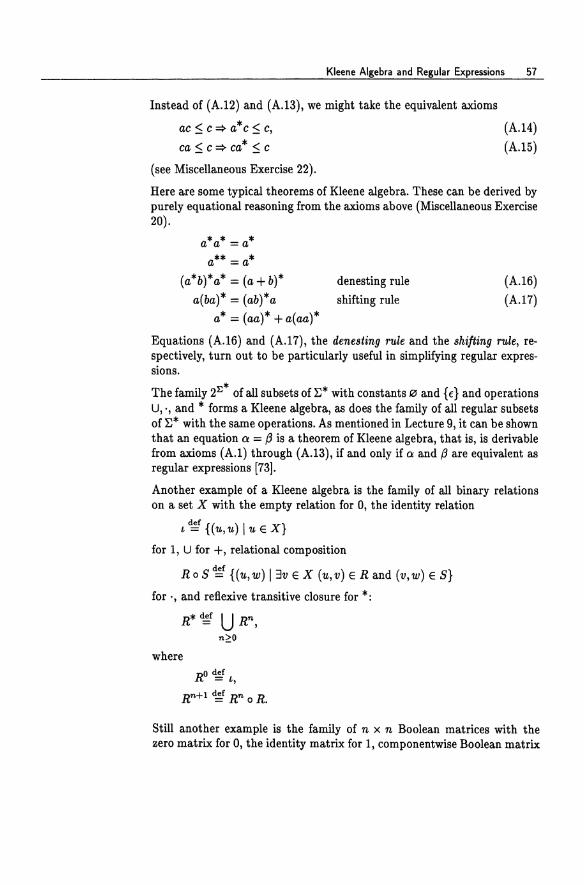
Kleene Algebra and Regular Expressions 57
Instead of (A.12) and (A.13), we might take the equivalent axioms
ac $ c ~ a*c $ c, (A.14)
ca $ c ~ ca* $ c (A.15)
(see Miscellaneous Exercise 22).
Here are some typical theorems of Kleene algebra. These can be derived by purely equational reasoning from the axioms above (Miscellaneous Exercise 20).
a*a* = a* a** = a*
(a*b)*a* = (a + b)* denesting rule
a(ba)* = (ab)*a shifting rule
a* = (00)* + a(oo)*
(A.16)
(A.17)
Equations (A.16) and (A.17), the denesting rule and the shifting rule, respectively, turn out to be particularly useful in simplifying regular expressions.
The family 2'E* of all subsets of r:* with constants fi!J and {€} and operations U,', and * forms a Kleene algebra, as does the family of all regular subsets of r:* with the same operations. As mentioned in Lecture 9, it can be shown that an equation a = /3 is a theorem of Kleene algebra,that is, is derivable from axioms (A.1) through (A.13), if and only if a and /3 are equivalent as regular expressions [73].
Another example of a Kleene algebra is the family of all binary relations on a set X with the empty relation for 0, the identity relation
L dg {( u, u) I u E X}
for 1, U for +, relational composition
Ro S ~f {(u,w) 13v E X (u,v) E R and (v,w) E S}
for " and reflexive transitive closure for *:
R*~ U R", ,,~o
where
Still another example is the family of n x n Boolean matrices with the zero matrix for 0, the identity matrix for 1, componentwise Boolean matrix
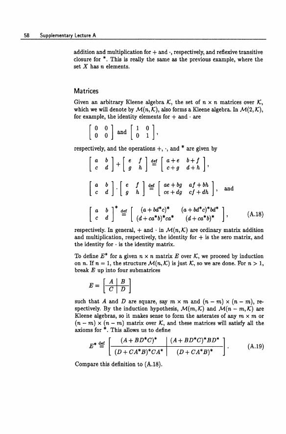
58 Supplementary Lecture A
addition and multiplication for + and·, respectively, and reflexive transitive closure for *. This is really the same as the previous example, where the set X has n elements.
Matrices
Given an arbitrary Kleene algebra JC, the set of n x n matrices over JC, which we will denote by M(n,JC), also forms a Kleene algebra. In M(2,JC), for example, the identity elements for + and· are
respectively, and the operations +, ., and * are given by
b+ f ] d+h '
[: :].[: f ] ~ [ ae + bg af + bh] and h - ce + dg cf + dh '
[ ac db] * <I,g [ (a + bd*c)* (d + ca*b)*ca*
(a + bd*c)*bd* ] (d+ ca*b)* ,
(A.18)
respectively. In general, + and . in M(n, JC) are ordinary matrix: addition and multiplication, respectively, the identity for + is the zero matrix:, and the identity for . is the identity matrix:.
To define E* for a given n x n matrix: E over JC, we proceed by induction on n. If n = 1, the structure M( n, JC) is just JC, so we are done. For n > 1, break E up into four submatrices
E=[~I~] such that A and D are square, say m x m and (n - m) x (n - m), respectively. By the induction hypothesis, M( m, JC) and M( n - m, JC) are Kleene algebras, so it makes sense to form the asterates of any m x m or (n - m) x (n - m) matrix over JC, and these matrices will satisfy all the axioms for *. This allows us to define
[ (A+BD*C)*
E*~ (D + CA*B)*CA*
Compare this definition to (A.18).
(A + BD*C)* BD* ] .
(D+CA*B)* (A.19)
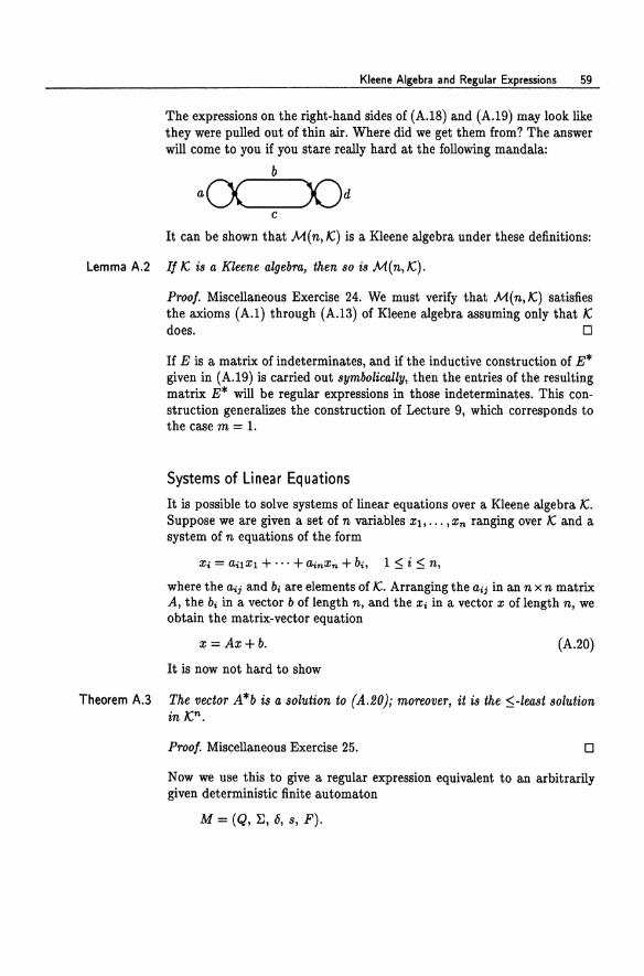
Kleene Algebra and Regular Expressions 59
The expressions on the right-hand sides of (A.18) and (A.19) may look like they were pulled out of thin air. Where did we get them from? The answer will come to you if you stare really hard at the following mandala:
b
c
It can be shown that M(n,.q is a Kleene algebra under these definitions:
Lemma A.2 If /C is a Kleene algebra, then so is M(n,/C).
Proof. Miscellaneous Exercise 24. We must verify that M(n,/C) satisfies the axioms (A.I) through (A.13) of Kleene algebra assuming only that /C ~_ 0
If E is a matrix of indeterminates, and if the inductive construction of E* given in (A.19) is carried out symbolically, then the entries of the resulting matrix E* will be regular expressions in those indeterminates. This construction generalizes the construction of Lecture 9, which corresponds to the case m = 1.
Systems of Linear Equations
It is possible to solve systems of linear equations over a Kleene algebra /C. Suppose we are given a set of n variables Xl, ••• ,Xn ranging over /C and a system of n equations of the form
Xi = ailXl + ... + ainXn + bi, 1 ~ i ~ n,
where the aij and bi are elements of /C. Arranging the aij in an n x n matrix A, the bi in a vector b of length n, and the Xi in a vector X of length n, we obtain the matrix-vector equation
X = Ax+b. (A.20)
It is now not hard to show
Theorem A.3 The vector A*b is a solution to (A.20)i moreover, it is the ~-least solution in /Cn •
Proof. Miscellaneous Exercise 25. o
Now we use this to give a regular expression equivalent to an arbitrarily given deterministic finite automaton
M = (Q, I}, 6, s, F).
60 Supplementary Lecture A
Assume without loss of generality that Q = {I, 2, ... , n}. For each q e Q, let Xq denote the set of strings in ~* that would be accepted by M if q were the start state; that is,
Xq ~f {x e ~* I 6(q, x) e F}.
The Xq satisfy the following system of equations:
X - { L:aEIl aX6(q,a) if q ¢ F, q - L:aEE aX6(q,a) + 1 if q e F.
Moreover, the Xq give the least solution with respect to ~. As above, these equations can be arranged in a single matrix-vector equation of the form
X=AX+b, (A.21)
where A is an n x n matrix containing sums of elements of ~, b is a 0-1 vector of length n, and X is a vector consisting of Xl, ... ,Xn • The vector X is the least solution of (A.21). By Theorem A.3,
X=A*b.
Compute the matrix A* symbolically according to (A.19), so that its entries are regular expressions, then multiply by b. A regular expression for L(M) can then be read off from the 8th entry of A*b, where 8 is the start state ofM.
Historical Notes
Salomaa [108] gave the first complete axiomatization of the algebra of regular sets. The algebraic theory was developed extensively in the monograph of Conway [27]. Many others have contributed to the theory, including Redko [103], Backhouse [6], Bloom and Esik [10], Boffa [11, 12], Gecseg and Peak [41], Krob [74], Kuich and Salomaa [76], and Salomaa and Soittola [109]. The definition of Kleene algebra and the complete axiomatization given here is from Kozen [731.
Lecture 10
Homomorph isms
A homomorphism is a map h : ~* -+ r* such that for all x, y E ~*,
h(xy) = h(x)h(y), h(f) = f.
Actually, (10.2) is a consequence of (10.1):
Ih(f)1 = Ih(ff)1 = Ih(f)h(f)1 = Ih(f)1 + Ih(f)l;
(10.1) (10.2)
subtracting Ih(f)1 from both sides, we have Ih(f)1 = 0, therefore h(f) = f.
It follows from these properties that any homomorphism defined on ~* is uniquely determined by its values on ~. For example, if h( a) = ccc and h(b) = dd, then
h(abaab) = h(a)h(b)h(a)h(a)h(b) = cccddccccccdd.
Moreover, any map h : ~ -+ r* extends uniquely by induction to a homomorphism defined on all of ~*. Therefore, in order to specify a homomorphism completely, we need only say what values it takes on elements of ~.
62 Lecture 10
If A ~ ~*, define
h{A) ~ {h{x) I x E A} ~ r*, and if B ~ r*, define
h-1(B) d,g {x I h(x) E B} ~ ~*.
The set h(A) is called the image of A under h, and the set h-1(B) is called the preimage of B under h.
We will show two useful closure properties of the regular sets: any homomorphic image or homomorphic preimage of a regular set is regular.
Theorem 10.1 Let h : ~* - r* be a homomorphism. If B ~ r* is regular, then 80 is its preimage h-l(B) under h.
Proof. Let M = (Q, r, 6, 8, F) be a DFA such that L{M) = B. Create a new DFA M' = (Q, ~, 6', 8, F) for h-1{B) as follows. The set of states, start state, and final states of M' are the same as in M. The input alphabet is ~ instead of r. The transition function 6' is defined by
6'(q,a) ~f 6(q,h(a)).
Note that we have to use 6 on the right-hand side, since h(a) need not be a single letter.
Now it follows by induction on Ixl that for all x E ~*, ..,., ~
6 (q, x) = 6(q, h(x)). (10.3)
For the basis x = e, using (10.1), ..,., ~ ~
6 (q,e) = q = 6(q, e) = 6(q,h(e)).
For the induction step, assume that 6'(q,x) = 6(q,h(x)). Then
6'(q,xa) = 6'(6'(q,x),a) definition of 6' = 6'(6(q,h(x)),a) induction hypothesis
= 6(6(q, h(x)), h(a)) definition of 6'
= 6(q,h(x)h(a)) Homework 1, Exercise 3
= 6(q, h(xa)) property (10.2) of homomorphisms.
Now we can use (10.3) to prove that L(M') = h-1(L(M)). For any z E ~*,
x E L(M') ¢:::::> 6'(8,Z) E F definition of acceptance
¢:::::> 6(8,h(x)) E F by (10.3)
¢:::::> h(x) E L(M) definition of acceptance
¢:::::> x E h-1(L(M)) definition of h-1(L(M)). 0
Homomorphisms 63
Theorem 10.2 Let h : I:* ..... r* be a homomorphism. II A ~ I:* is regular, then so is its image h(A) under h.
Prool. For this proof, we will use regular expressions. Let a be a regular expression over I: such that L(a) = A. Let a' be the regular expression obtained by replacing each letter a e I: appearing in a with the string h(a) e r*. For example, if h(a) = ccc and h(b) = dd, then
«a + b)*ab)' = (ccc + dd)*cccdd.
Formally, a' is defined by induction:
a' = h(a), a e I:, f'J'=f'J,
(13 + ,)' = 13' + 1, (13,)' = 13',',
13*' = 13'*. We claim that for any regular expression 13 over I:,
L(13') = h(L(13»; (10.4)
in particular, L(a') = h(A). This can be proved by induction on the structure of 13. To do this, we will need two facts about homomorphisms: for any pair of subsets C, D ~ I:* and any family of subsets Ci ~ I:*, i e I,
h(CD) = h(C)h(D),
h(U Ci) = U h(Ci). iEl iel
To prove (10.5),
h(CD) = {h(w) I we CD} = {h(yz) lye C, ZED} = {h(y)h(z) lye C, zeD} = {uv I U E h(C), v E h(D)} = h(C)h(D).
To prove (10.6),
h(UCi) = {h(w) I we UCi} i i
= {h(w) 13i w E Ci}
= U{h(w) I w E Ci} i
(10.5)
(10.6)
64 Lecture 10
Now we prove (lOA) by induction. There are two base cases:
L(a') = L(h(a)) = {h(a)} = h({a}) = h(L(a))
and
L(f/J') = L(f/J) = 10 = h(fO) = h(L(f/J)).
The case of E is covered by the other cases, since € = 10*.
There are three induction cases, one for each of the operators +, ., and *. For +,
L«f3 + 1)') = L(f3' + 1') = L(f3') U L( 1') = h(L(f3)) U h(L(-y)) = h(L(f3) U L(-y)) = h(L(f3 + 1))
definition of '
definition of + induction hypothesis
property (10.6)
definition of +.
The proof for· is similar, using property (10.5) instead of (10.6). Finally, for *,
L(f3*')
= L((3'*) = L(f3')* = h(L(f3))*
= U h(L(f3))n n2:0
= U h(L(f3)") n2:0
= h(U L(f3)") n2:0
= h(L(f3)*) = h(L(f3*))
definition of '
definition of regular expression operator * induction hypothesis
definition of set operator *
property (10.5)
property (10.6)
definition of set operator * definition of regular expression operator *. o
Warning: It is not true that A is regular whenever h(A) is. This is not what Theorem 10.1 says. We will show later that the set {anbn I n 2: O} is not regular, but the image of this set under the homomorphism h(a) = h(b) = a is the regular set {an I n is even}. The preimage h-l({an I n is even}) is not {anbn I n 2: O}, but {x E {a,b}* Ilxl is even}, which is regular.
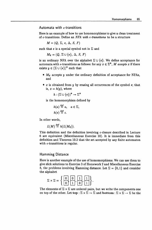
Homomorphisms 65
Automata with f-transitions
Here is an example of how to use homomorphisms to give a clean treatment of f-transitions. Define an NFA with f-transitions to be a structure
M = (Q, I:, e, t:., S, F)
such that e is a special symbol not in I: and
Me = (Q, I: u {e}, t:., S, F)
is an ordinary NFA over the alphabet I: U {e}. We define acceptance for automata with f-transitions as follows: for any x e I:*, M accepts x if there exists y e (I: U {e})* such that
• Me accepts y under the ordinary definition of acceptance for NFAs, and
• x is obtained from y by erasing all occurrences of the symbol ej that is, x = h(y), where
h: (I: U {e})* -+ I:*
is the homomorphism defined by
( ) def h a = a, a e I:,
( ) def he = f.
In other words,
L(M) dg h(L(Me)).
This definition and the definition involving f-closure described in Lecture 6 are equivalent (Miscellaneous Exercise 10). It is immediate from this definition and Theorem 10.2 that the set accepted by any finite automaton with f-transitions is regular.
Hamming Distance
Here is another example of the use of homomorphisms. We can use .them to give slick solutions to Exercise 3 of Homework 2 and Miscellaneous Exercise 8, the problems involving Hamming distance. Let I: = {0,1} and consider the alphabet
The elements of I: x I: are ordered pairs, but we write the components one on top of the other. Let top: I: x I: -+ I: and bottom: I: x I: -+ I: be the
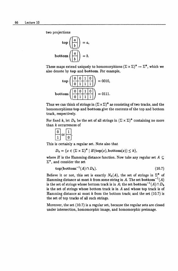
66 Lectu re 10
two projections
top (~) =a,
bottom (~) = b.
These maps extend uniquely to homomorphisms (E x E)* - E*, which we also denote by top and bottom. For example,
top (CililiIQJ) = 0010, CiliIiliJ bottom (CililiIQJ) = 0111.
CiliIiliJ Thus we can think of strings in (E x E)* as consisting of two tracks, and the homomorphisms top and bottom give the contents of the top and bottom track, respectively.
For fixed k, let Die be the set of all strings in (E x E)* containing no more than k occurrences of
This is certainly a regular set. Note also that
Die = {x E (E x E)* I H(top(x), bottom(x» S k},
where H is the Hamming distance function. Now take any regular set A ~ E*, and consider the set
top(bottom-1(A) n Die)' (10.7)
Believe it or not, this set is exactly NIe(A), the set of strings in E* of Hamming distance at most k from some string in A. The set bottom-1(A) is the set of strings whose bottom track is in Aj the set bottom-1(A) nDIe is the set of strings whose bottom track is in A and whose top track is of Hamming distance at most k from the bottom trackj and the set (10.7) is the set of top tracks of all such strings.
Moreover, the set (10.7) is a regular set, because the regular sets are closed under intersection, homomorphic image, and homomorphic preimage.
Lecture 11
Limitations of Finite Automata
We have studied what finite automata can do; let's see what they cannot do. The canonical example of a nonregular set (one accepted by no finite automaton) is
B = {a" b" In;::: O} = {€, ab, aabb, aaabbb, aaaabbbb, ... },
the set of all strings of the form a*b* with equally many a's and b's.
Intuitively, in order to accept the set B, an automaton scanning a string of the form a*b* would have to remember when passing the center point between the a's and b's how many a's it has seen, since it would have to compare that with the number of b's and accept iff the two numbers are the same.
aaaaaaaaaaaaaaaaaaaaaaaaaaaaabbbbbbbbbbbbbbbbbbbbbbbbbbbbb i q
Moreover, it would have to do this for arbitrarily long strings of a's and b's, much longer than the number of states. This is an unbounded amount of information, and there is no way it can remember this with only finite memory. All it "knows" at that point is represented in the state q it is in, which is only a finite amount of information. You might at first think there may be some clever strategy, such as counting mod 3, 5, and 7, or something similar. But any such attempt is doomed to failure: you cannot
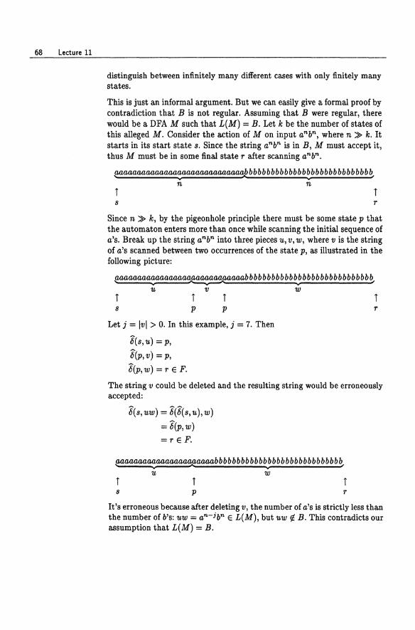
68 Lecture 11
distinguish between infinitely many different cases with only finitely many states.
This is just an informal argument. But we can easily give a formal proof by contradiction that B is not regular. Assuming that B were regular, there would be a DFA M such that L(M) = B. Let k be the number of states of this alleged M. Consider the action of M on input anbn, where n :> k. It starts in its start state s. Since the string anbn is in B, M must accept it, thus M must be in some final state r after scanning anbn.
paaaaaaaaaaaaaaaaaaaaaaaaaaaaPbbbbbbbbbbbbbbbbbbbbbbbbbbb~ y y
n n i i s r
Since n :> k, by the pigeonhole principle there must be some state p that the automaton enters more than once while scanning the initial sequence of a's. Break up the string anbn into three pieces 1.1., v, w, where v is the string of a's scanned between two occurrences of the state p, as illustrated in the following picture:
paaaaaaaeaaaaaaa~aaaaabbbbbbbbbbbb!bbbbbbbbbbbbbbb~
i s
1.1. v W
i p
i p
Let j = Ivl > O. In this example, j = 7. Then
6(8,1.1.) =p,
6(p,v) = p,
6(P,w) = reF.
i r
The string v could be deleted and the resulting string would be erroneously accepted:
6(s,uw) = 6(6(s,u),w)
= 6(p,w) =r eF.
paaaaaaaaaaaaaaaa~aaaaabbbbbbbbbbbbbbbbbbbbbbbbbbbb~
i s
:y ..,.
1.1. W i p
i r
It's erroneous because after deleting v, the number of a's is strictly less than the number of b's: uw = an-ibn e L(M), but uw ¢ B. This contradicts our assumption that L(M) = B.
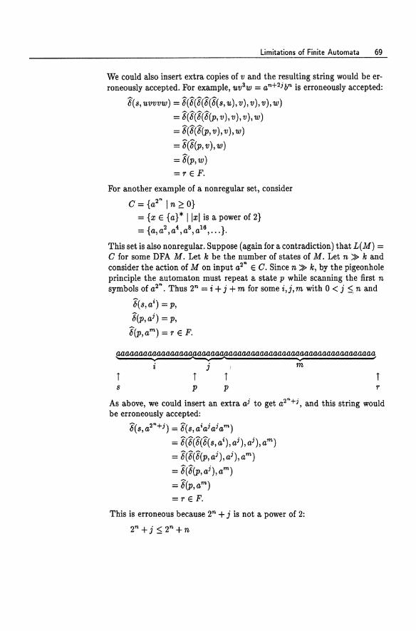
Limitations of Finite Automata 69
We could also insert extra copies of v and the resulting string would be erroneously accepted. For example, uv3w = an+2j bn is erroneously accepted:
8(s,uvvvw) = 8(8(8(8(8(s,u),v),v),v),w)
= 8(8(8(8(p,v),v),v),w)
= 8(8(8(p,v),v),w)
= 8(8(p,v),w)
= 8(p,w)
=r E F.
For another example of a nonregular set, consider
C={a2n In2::0} = {x E {a}* Ilxl is a power of 2}
= {a, a2 , a4 , as, a16 , ••• }.
This set is also nonregular. Suppose (again for a contradiction) that L(M) = C for some DFA M. Let k be the number of states of M. Let n ~ k and consider the action of M on input a2" E C. Since n ~ k, by the pigeonhole principle the automaton must repeat a state p while scanning the first n symbols of a2n . Thus 2n = i + j + m for some i,j, m with 0 < j ~ nand
8(s,ai ) = p,
8(p,aj ) = p,
8(p, am) = rEF.
~aaaaaaa~aaaaaaaa~aaaaaaaaaaaaaaaaa~aaaaaaaaaaaaaaa~
i s
i j m i p
i p
i r
As above, we could insert an extra aj to get a2n+i , and this string would be erroneously accepted:
8(s,a2"+i) = 8(s,ai ai ai am)
= 8(8(8(8(s,atai ),ai ),am)
= 8(8(8(p,aj ),ai ), am)
= 8(8(p,ai ),am)
= 8(p,am)
=r E F.
This is erroneous because 2n + j is not a power of 2:
2n + j::; 2n +n
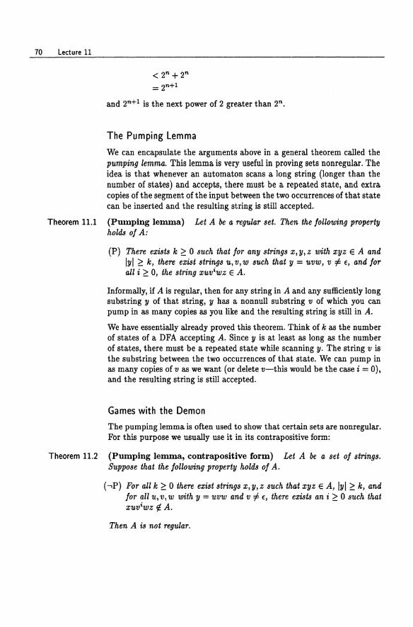
70 Lecture 11
< 2n + 2n
= 2n +1
and 2n+1 is the next power of 2 greater than 2n.
The Pumping Lemma
We can encapsulate the arguments above in a general theorem called the pumping lemma. This lemma is very useful in proving sets nonregular. The idea is that whenever an automaton scans a long string (longer than the number of states) and accepts, there must be a repeated state, and extra copies of the segment of the input between the two occurrences of that state can be inserted and the resulting string is still accepted.
Theorem 11.1 (Pumping lemma) Let A be a regular set. Then the following property holds of A:
(P) There exists k ~ 0 such that for any strings x, y, z with xyz E A and Ivi ~ k, there exist strings u,v,w such that V = uvw, v i= f, and for all i ~ 0, the string xuv'wz E A.
Informally, if A is regular, then for any string in A and any sufficiently long substring V of that string, V has a nonnull substring v of which you can pump in as many copies as you like and the resulting string is still in A.
We have essentially already proved this theorem. Think of k as the number of states of a DFA accepting A. Since V is at least as long as the number of states, there must be a repeated state while scanning v. The string v is the substring between the two occurrences of that state. We can pump in as many copies of vas we want (or delete v-this would be the case i = 0), and the resulting string is still accepted.
Games with the Demon
The pumping lemma is often used to show that certain sets are nonregular. For this purpose we usually use it in its contrapositive form:
Theorem 11.2 (Pumping lemma, contrapositive form) Let A be a set of strings. Suppose that the following property holds of A.
(..,P) For all k ~ 0 there exist strings x, y, z such that xyz E A, Iyl ~ k, and for all u, v, w with y = uvw and v i= E, there exists an i ~ 0 such that xuv'wz if. A.
Then A is not regular.
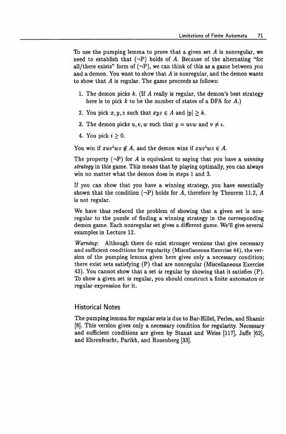
Limitations of Finite Automata 71
To use the pumping lemma to prove that a given set A is nonregular, we need to establish that (.,P) holds of A. Because of the alternating "for all/there exists" form of (.,P), we can think of this as a game between you and a demon. You want to show that A is nonregular, and the demon wants to show that A is regular. The game proceeds as follows:
1. The demon picks k. (If A really is regular, the demon's best strategy here is to pick k to be the number of states of a DFA for A.)
2. You pick x, y, z such that xyz E A and Iyl ~ k.
3. The demon picks 11., v, w such that y = uvw and v ::I E.
4. You pick i ~ O.
You win if xuviwz ¢ A, and the demon wins if xuviwz E A.
The property (.,P) for A is equivalent to saying that you have a winning strategy in this game. This means that by playing optimally, you can always win no matter what the demon does in steps 1 and 3.
If you can show that you have a winning strategy, you have essentially shown that the condition (.,P) holds for A, therefore by Theorem 11.2, A is not regular.
We have thus reduced the problem of showing that a given Bet is nonregular to the puzzle of finding a winning strategy in the corresponding demon game. Each nonregular set gives a different game. We'll give several examples in Lecture 12.
Warning: Although there do exist stronger versions that give necessary and sufficient conditions for regularity (Miscellaneous Exercise 44), the version of the pumping lemma given here gives only a necessary condition; there exist sets satisfying (P) that are nonregular (Miscellaneous Exercise 43). You cannot show that a set is regular by showing that it satisfies (P). To show a given set is regular, you should construct a finite automaton or regular expression for it.
Historical Notes
The pumping lemma for regular sets is due to Bar-Hillel, Perles, and Shamir [8]. This version gives only a necessary condition for regularity. Necessary and sufficient conditions are given by Stanat and Weiss [117], Jaffe [62], and Ehrenfeucht, Parikh, and Rozenberg [33].
Lecture 12
Using the Pumping Lemma
Example 12.1 Let's use the pumping lemma in the form of the demon game to show that the set
A = {anbm In?: m}
is not regular. The set A is the set of strings in a*b* with no more b's than a's. The demon, who is betting that A is regular, picks some number k. A good response for you is to pick z = ak , y = bk , and z = f. Then xyz = akbk E A and Iyl = k; so far you have followed the rules. The demon must now pick u, v, w such that y = uvw and v ::/; f. Say the demon picks U,V,w of length j,m,n, respectively, with k = j + m + nand m > O. No matter what the demon picks, you can take i = 2 and you win:
xuv2wz = akbibmbmbn
= akbi+2m+n
= akbk+m,
which is not in A, because the number of b's is strictly larger than the number of a's.
This strategy always leads to victory for you in the demon game associated with the set A. As we argued in Lecture 11, this is tantamount to showing that A is nonregular. 0
Using the Pumping Lemma 73
Example 12.2 For another example, take the set
C = {an! I n ~ a}.
We would like to show that this set is not regular. This one is a little harder. It is an example of a nonregular set over a single-letter alphabet. Intuitively, it is not regular because the differences in the lengths of the successive elements of the set grow too fast.
Suppose the demon chooses k. A good choice for you is x = z = E and y = ak!. Then xyz = ak! E C and Iyl = k! ~ k, so you have not cheated. The demon must now choose u, v, w such that y = uvw and v f= E. Say the demon chooses u, v, w of length j, m, n, respectively, with k! = j + m + n and m > O. You now need to find i such that xuviwz ¢ Cj in other words, Ixuviwzl f= p! for any p. Note that for any i,
Ixuviwzl = j + im + n = k! + (i - 1)m,
so you will win if you can choose i such that k! + (i - 1)m f= p! for any p. Take i = (k + 1)! + 1. Then
k! + (i -l)m = k! + (k+ l)!m = k!(l +m(k+ 1)),
and we want to show that this cannot be p! for any p. But if
p! = k!(l + m(k + 1)),
then we could divide both sides by k! to get
p(p - l)(p - 2) ... (k + 2)(k + 1) = 1 + m(k + 1),
which is impossible, because the left-hand side is divisible by k + 1 and the right-hand side is not. 0
A Trick
When trying to show that a set is nonregular, one can often simplify the problem by using one of the closure properties of regular sets. This often allows us to reduce a complicated set to a simpler set that is already known to be nonregular, thereby avoiding the use of the pumping lemma.
To illustrate, consider the set
D = {x E {a,b}* I #a(x) = #b(x)}.
To show that this set is nonregular, suppose for a contradiction that it were regular. Then the set
D na*b*
74 Lecture 12
would also be regular, since the intersection of two regular sets is always regular (the product construction, remember?). But
D n L(a*b*) = {anbn I n ~ D},
which we have already shown to be nonregular. This is a contradiction.
For another illustration of this trick, consider the set A of Example 12.1 above:
A={anbm In~m},
the set of strings x E L(a*b*) with no more b's than a's. By Exercise 2 of Homework 2, if A were regular, then so would be the set
rev A = {bman I n ~ m},
and by interchanging a and b, we would get that the set
A' = {ambn I n ~ m}
is also regular. Formally, "interchanging a and b" means applying the homomorphism a ...... b, b ...... a. But then the intersection
AnA' = {anbn I n ~ D}
would be regular. But we have already shown using the pumping lemma that this set is nonregular. This is a contradiction.
Ultimate Periodicity
Let U be a subset of N = {D, 1, 2, 3, ... }, the natural numbers.
The set U is said to be ultimately periodic if there exist numbers n ~ D and p > D such that for all m ~ n, m E U if and only if m + p E U. The number p is called a period of U.
In other words, except for a finite initial part (the numbers less than n), numbers are in or out of the set U according to a repeating pattern. For example, consider the set
{D,3,7,11,19,20,23,26,29,32,35,38,41,44,47,50, ... }.
Starting at 20, every third element is in the set, therefore this set is ultimately periodic with n = 20 and p = 3. Note that neither n nor p is unique; for example, for this set we could also have taken n = 21 and p = 6, or n = 100 and p = 33.
Regular sets over a single-letter alphabet {a} and ultimately periodic subsets of N are strongly related:
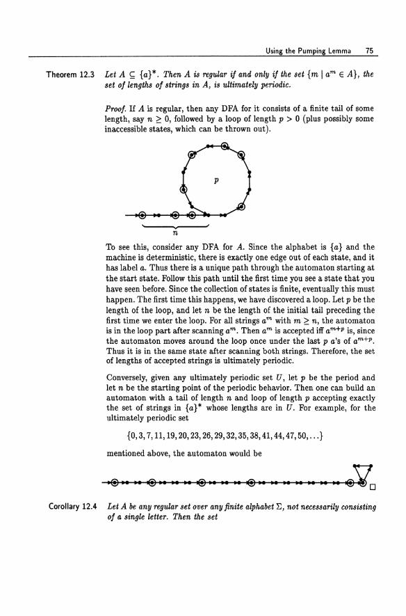
Using the Pumping Lemma 75
Theorem 12.3 Let A S;;; {a}*. Then A is regular i/ and only i/ the set {m I am E A}, the set o/lengths 0/ strings in A, is ultimately periodic.
Proof. If A is regular, then any DFA for it consists of a finite tail of some length, say n ;:: 0, followed by a loop of length p > ° (plus possibly some inaccessible states, which can be thrown out).
To see this, consider any DFA for A. Since the alphabet is {a} and the machine is deterministic, there is exactly one edge out of each state, and it has label a. Thus there is a unique path through the automaton starting at the start state. Follow this path until the first time you see a state that you have seen before. Since the collection of states is finite, eventually this must happen. The first time this happens, we have discovered a loop. Let p be the length of the loop, and let n be the length of the initial tail preceding the first time we enter the loop. For all strings am with m ;:: n, the automaton is in the loop part after scanning am. Then am is accepted iff am+p is, since the automaton moves around the loop once under the last p a's of am+p•
Thus it is in the same state after scanning both strings. Therefore, the set of lengths of accepted strings is ultimately periodic.
Conversely, given any ultimately periodic set U, let p be the period and let n be the starting point of the periodic behavior. Then one can build an automaton with a tail of length n and loop of length p accepting exactly the set of strings in {a}* whose lengths are in U. For example, for the ultimately periodic set
{0,3,7,11,19,20,23,26,29,32,35,38,41,44,47,50, ... }
mentioned above, the automaton would be
.@.. .• @.. .. .. @.. •• .. @.. .. .. .. •• .. •• .:lo Corollary 12.4 Let A be any regular set over any finite alphabet~, not necessarily consisting
0/ a single letter. Then the set
76 Lecture 12
lengths A = {Ixll x E A}
of lengths of strings in A is ultimately periodic.
Proof. Define the homomorphism h : ~ -+ {a} by h(b) = a for all b E ~. Then h(x) = al"l. Since h preserves length, we have that lengths A = lengths h(A). But h(A) is a regular subset of {a}*, since the regular sets are closed under homomorphic image; therefore, by Theorem 12.3, lengths h(A) is ultimately periodic. 0
Historical Notes
A general treatment of ultimate periodicity and regularity-preserving functions is given in Seiferas and McNaughton [113]; see Miscellaneous Exercise 34.
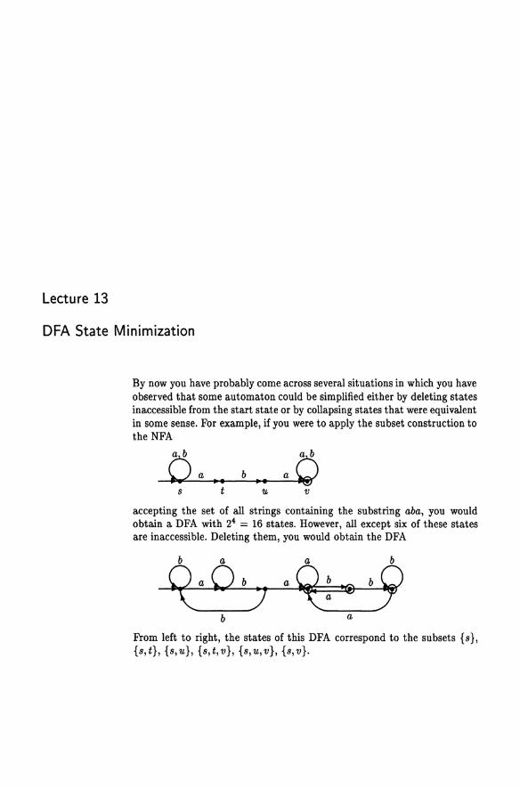
Lecture 13
DFA State Minimization
By now you have probably come across several situations in which you have observed that some automaton could be simplified either by deleting states inaccessible from the start state or by collapsing states that were equivalent in some sense. For example, if you were to apply the subset construction to the NFA
Xa ~ .. b ·0 • •
s t u v
accepting the set of all strings containing the substring aba, you would obtain a DFA with 24 = 16 states. However, all except six of these states are inaccessible. Deleting them, you would obtain the DFA
b a
From left to right, the states of this DFA correspond to the subsets {s}, {s,t}, {s,u}, {s,t,v}, {s,u,v}, {s,v}.
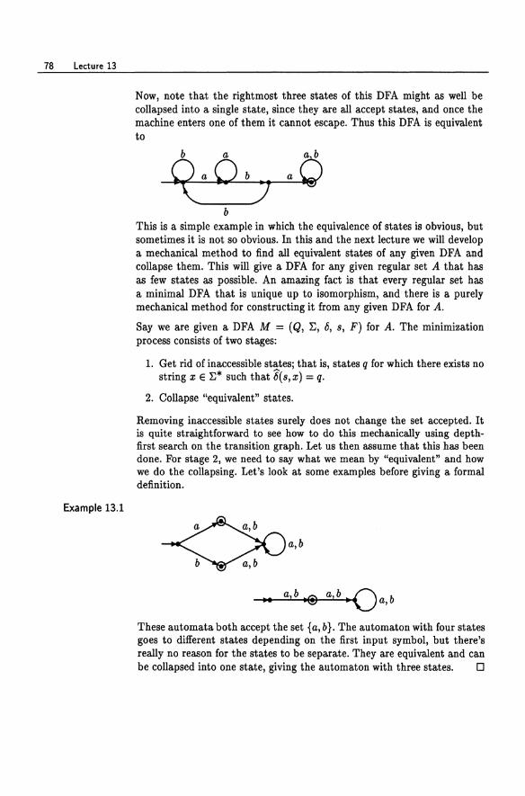
78 Lecture 13
Example 13.1
Now, note that the rightmost three states of this DFA might as well be collapsed into a single state, since they are all accept states, and once the machine enters one of them it cannot escape. Thus this DFA is equivalent to
7 .Q b
b This is a simple example in which the equivalence of states is obvious, but sometimes it is not so obvious. In this and the next lecture we will develop a mechanical method to find all equivalent states of any given DFA and collapse them. This will give a DFA for any given regular set A that has as few states as possible. An amazing fact is that every regular set has a minimal DFA that is unique up to isomorphism, and there is a purely mechanical method for constructing it from any given DFA for A.
Say we are given a DFA M = (Q, ~, 6, 8, F) for A. The minimization process consists of two stages:
1. Get rid of inaccessible states; that is, states q for which there exists no string x E ~* such that 6(s,x) = q.
2. Collapse "equivalent" states.
Removing inaccessible states surely does not change the set accepted. It is quite straightforward to see how to do this mechanically using depthfirst search on the transition graph. Let us then assume that this has been done. For stage 2, we need to say what we mean by "equivalent" and how we do the collapsing. Let's look at some examples before giving a formal definition.
a,b
u a,b ~@ a,b ~ Oa,b
These automata both accept the set {a, b}. The automaton with four states goes to different states depending on the first input symbol, but there's really no reason for the states to be separate. They are equivalent and can be collapsed into one state, giving the automaton with three states. 0
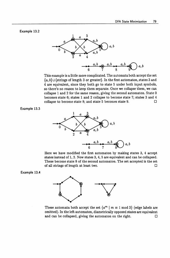
Example 13.2
Example 13.3
Example 13.4
DFA State Minimization 79
1 3
a,b
2
•• a,b.@ a,b... a,b .£"'"\ a,b 6 7 8 ;)LJ
This example is a little more complicated. The automata both accept the set {a, b} U {strings of length 3 or greater}. In the first automaton, states 3 and 4 are equivalent, since they both go to state 5 under both input symbols, so there's no reason to keep them separate. Once we collapse them, we can collapse 1 and 2 for the same reason, giving the second automaton. State 0 becomes state 6; states 1 and 2 collapse to become state 7; states 3 and 4 collapse to become state 8; and state 5 becomes state 9. 0
1 3
a,b
2 4
a,b a,b iO b •• •• ~ a, 6 7 8
Here we have modified the first automaton by making states 3, 4 accept states instead of 1,2. Now states 3,4,5 are equivalent and can be collapsed. These become state 8 of the second automaton. The set accepted is the set of all strings of length at least two. 0
These automata both accept the set {am 1m == 1 mod 3} (edge labels are omitted). In the left automaton, diametrically opposed states are equivalent and can be collapsed, giving the automaton on the right. 0
80 Lecture 13
The Quotient Construction
How do we know in general when two states can be collapsed safely without changing the set accepted? How do we do the collapsing formally? Is there a fast algorithm for doing it? How can we determine whether any further collapsing is possible?
Surely we never want to collapse an accept state p and a reject state q, because if p = 6(s, x) E F and q = 6(s,y) (j F, then x must be accepted and y must be rejected even after collapsing, so there is no way to declare the collapsed state to be an accept or reject state without error. Also, if we collapse p and q, then we had better also collapse 6 (p, a) and 6 (q, a) to maintain determinism. These two observations together imply inductively that we cannot collapse p and q if 6(p, x) E F and 6(q,x) (j F for some string x.
It turns out that this criterion is necessary and sufficient for deciding whether a pair of states call be collapsed. That is, if there exists a string x such that 6(p, x) E F and 6(q, x) (j F or vice versa, thenp and q cannot be safely collapsedj and if no such x exists, then they can.
Here's how we show this formally. We first define an equivalence relation ~ on Q by
p ~ q ~ 'Vx E E* (6(P, x) E F {:::::} 6(q, x) E F).
This definition is just a formal restatement of the collapsing criterion. It is not hard to argue that the relation ~ is indeed an equivalence relation: it is
• reflexive: p ~ p for all pj
• symmetric: if p ~ q, then q ~ pj and
• transitive: if p ~ q and q ~ r, then p ~ r.
As with all equivalence relations, ~ partitions the set on which it is defined into disjoint equivalence classes:
[Pl ~f {q I q ~ pl.
Every element p E Q is contained in exactly one equivalence class [Pl, and
p ~ q {:::::} IP] = [q].
We now define a DFA M/~ called the quotient automaton, whose states correspond to the equivalence classes of ~. This construction is called a quotient construction and is quite common in algebra. We will see a more general account of it in Supplementary Lectures C and D.
DFA State Minimization 81
There is one state of M/';:!, for each ';:!,-equivalence class. In fact, formally, the states of M/';:!, are the equivalence classes; this is the mathematical way of "collapsing" equivalent states.
Define
M/';:!, ~ (Q', E, 6', s', F'),
where
Q' d~ {IP)I P E Q},
6'(IP],a) ~ [6(p,a)], , deC [ ]
S = s,
F' ~ {IP]I p E F}.
(13.1)
There is a subtle but important point involving the definition of 6' in (13.1): we need to show that it is well-defined. Note that the action of 6' on the equivalence class IP] is defined in terms of p. It is conceivable that a different choice of representative of the class IP] (i.e., some q such that q ';:!, p) might lead to a different right-hand side in (13.1). Lemma 13.5 says exactly that this does not happen.
Lemma 13.5 If p ';:!, q, then 6(p,a) ';:!, 6(q,a). Equivalently, if IP] = [q], then [6(p,a)) = [6(q, a)].
Proof. Suppose p ';:!, q. Let a E E and y E E*.
6(6(p,a),y) E F <==} 6(p,ay) E F
<==} 6(q, ay) E F since p ';:!, q
<==} 6(6(q,a),y) E F.
Since y was arbitrary, 6(p, a) ';:!, 6(q, a) by definition of >:::.
Lemma 13.6 P E F <==} IP] E F'.
o
Proof. The direction =? is immediate from the definition of F'. For the direction ¢::, we need to show that if p ';:!, q and p E F, then q E F. In other words, every ';:!,-equivalence class is either a subset of F or disjoint from F. This follows immediately by taking x = € in the definition of p ';:!, q. 0
Lemma 13.7 For all x E E*, 6' (IP], x) = [8(p,x)].
Proof. By induction on Ixl.
82 Lecture 13
Basis
For x = f,
8' ([P], f) = [P] definition of 8'
= [8(p,f)] definition of 8.
Induction step
Assume 8'([P] , x) = [8(p,x)], and let a E~.
8'([P] , xa) = 6'(8'([P], x), a) definition of 8'
= 6' ([8 (p, x)], a) induction hypothesis
= [6(8(p, x), a)] definition of 6'
= [8(p,xa)]
Theorem 13.8 L(M/f!::!) = L(M).
definition of 8. o
Proof. For x E ~*,
x E L(M/ f!::!) {:=:} 8'(s',x) E F'
{:=:} 8' ([s], x) E F'
{:=:} [8(s,x)] E F'
{:=:} 6(s, x) E F
{:=:} x E L(M)
M/f!::! Cannot Be Collapsed Further
definition of acceptance
definition of s'
Lemma 13.7
Lemma 13.6
definition of acceptance. o
It is conceivable that after doing the quotient construction once, we might be able to collapse even further by doing it again. It turns out that once is enough. To see this, let's do the quotient construction a second time. Define
[P] '" [q] ~ "Ix E ~* (8'([P],x) E F' {:=:} 8'([q],x) E F').
This is exactly the same definition as f!::! above, only applied to the quotient automaton M/f!::!. We use the notation'" for the equivalence relation on Q' to distinguish it from the relation f!::! on Q. Now
[P] '" [q] => "Ix (8' ([P], x) E F' {:=:} 8' ([q], x) E F') definition of '"
=> "Ix ([8(p,x)] E F' {:=:} [8(q,x)] E F') Lemma 13.7
::::} 'l:/x (8(p,x) E F ¢:::::} 8(q, x) E F) ::::}pr:::!q
::::} lP] = [q].
DFA State Minimization 83
Lemma 13.6
definition of r:::!
Thus any two equivalent states of M /r:::! are in fact equal, and the collapsing relation'" on Q' is just the identity relation =.
Lecture 14
A Minimization Algorithm
Here is an algorithm for computing the collapsing relation ~ for a given DFA M with no inaccessible states. Our algorithm will mark (unordered) pairs of states {p,q}. A pair {p,q} will be marked as soon as a reason is discovered why p and q are not equivalent.
1. Write down a table of all pairs {p,q}, initially unmarked.
2. Mark {p,q} if p E F and q ¢ F or vice versa.
3. Repeat the following until no more changes occur: if there exists an unmarked pair {p,q} such that {6(p,a),6(q,a)} is marked for some a E~, then mark {p,q}.
4. When done, p ~ q iff {p,q} is not marked.
Here are some things to note about this algorithm:
• If {p,q} is marked in step 2, then p and q are surely not equivalent: take x = e in the definition of ~.
• We may have to look at the same pair {p, q} many times in step 3, since any change in the table may suddenly allow {p,q} to be marked. We stop only after we make an entire pass through the table with no new marks.
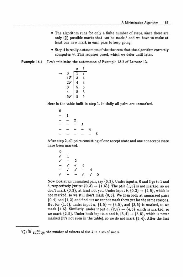
A Minimization Algorithm 85
• The algorithm runs for only a finite number of steps, since there are only (~) possible marks that can be made,l and we have to make at least one new mark in each pass to keep going.
• Step 4 is really a statement of the theorem that the algorithm correctly computes R:i. This requires proof, which we defer until later.
Example 14.1 Let's minimize the automaton of Example 13.2 of Lecture 13.
a b
-+ ° 1 2 IF 3 4 2F 4 3 3 5 5 4 5 5 5F 5 5
Here is the table built in step 1. Initially all pairs are unmarked.
° 1 2
3 4
5
After step 2, all pairs consisting of one accept state and one nonaccept state have been marked.
° ,f 1 ,f 2
,f
,f ,f
,f ,f 3
4 ,f ,f 5
Now look at an unmarked pair, say {O, 3}. Underinput a, ° and 3 go to 1 and 5, respectively (write: {O,3} -+ {l,5}). The pair {l,5} is not marked, so we don't mark {O, 3}, at least not yet. Under input b, {O,3} ..... {2, 5}, which is not marked, so we still don't mark {O,3}. We then look at unmarked pairs {O, 4} and {I, 2} and find out we cannot mark them yet for the same reasons. But for {1,5}, under input a, {1,5} -+ {3,5}, and {3,5} is marked, so we mark {1,5}. Similarly, under input a, {2,5} -+ {4,5} which is marked, so we mark {2,5}. Under both inputs a and b, {3,4} -+ {5,5}, which is never marked (it's not even in the table), so we do not mark {3, 4}. After the first
1(;:) cI£! .!(:~.)!, the number of subsets ofsize k in a set of size n.
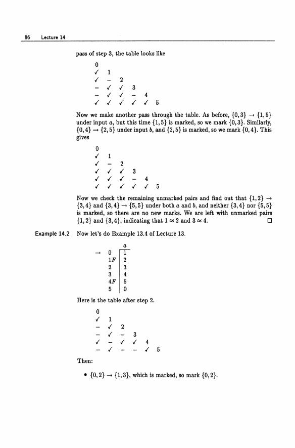
86 Lecture 14
pass of step 3, the table looks like
D ,f 1 ,f 2
,f ,f 3 ,f,f 4
,f,f,f,f,fS
Now we make another pass through the table. As before, {O,3} -+ {1,5} under input a, but this time {1, S} is marked, so we mark {O,3}. Similarly, {D,4} -+ {2, S} under input b, and {2, 5} is marked, so we mark {D, 4}. This gives
D ,f 1 ,f 2 ,f ,f ,f 3 ,f ,f ,f 4 ,f ,f ,f ,f ,f 5
Now we check the remaining unmarked pairs and find out that {1,2} -+
{3,4} and {3,4} -+ {5,5} under both a and b, and neither {3,4} nor {S,S} is marked, so there are no new marks. We are left with unmarked pairs {1,2} and {3, 4}, indicating that 1 ~ 2 and 3 ~ 4. 0
Example 14.2 Now let's do Example 13.4 of Lecture 13.
a -+ 0 1
1F 2 2 3 3 4 4F 5 5 0
Here is the table after step 2.
o ,f 1
,f 2 ,f 3
,f ,f ,f 4 ,f ,f 5
Then:
• {O,2} -+ {1,3}, which is marked, so mark {O,2}.
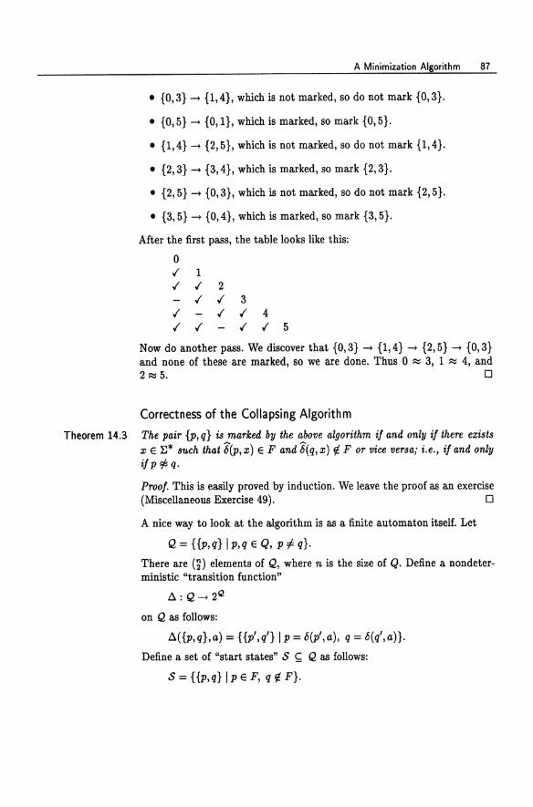
A Minimization Algorithm 87
• {O,3} ..... {I, 4}, which is not marked, so do not mark {O,3}.
• {O,5} ..... {O, I}, which is marked, so mark {O,5}.
• {1,4} ..... {2,5}, which is not marked, so do not mark {1,4}.
• {2,3} ..... {3, 4}, which is marked, so mark {2,3}.
• {2, 5} ..... {O, 3}, which is not marked, so do not mark {2, 5}.
• {3,5} ..... {O,4}, which is marked, so mark {3,5}.
After the first pass, the table looks like this:
° .f 1 .f .f 2
.f .f 3 .f .f .f 4 .f .f .f .f 5
Now do another pass. We discover that {O,3} ..... {1,4} ..... {2,5} ..... {O,3} and none of these are marked, so we are done. Thus ° ~ 3, 1 ~ 4, and 2 ~ 5. 0
Correctness of the Collapsing Algorithm
Theorem 14.3 The pair {p, q} is marked by the above algorithm if and only if there exists x E ~* such that 6(p, x) E F and 6( q, x) f/. F or vice versa; i. e., if and only ifp ~ q.
Proof. This is easily proved by induction. We leave the proof as an exercise (Miscellaneous Exercise 49). 0
A nice way to look at the algorithm is as a finite automaton itself. Let
Q = {{p,q} I p,q E Q, p;i: q}.
There are (~) elements of Q, where n is the size of Q. Define a nondeterministic "transition function"
t:. : Q ..... 2Q
on Q as follows:
t:.({p,q},a) = {{p',q'} I p = 8(p',a), q = 8(q',a)}.
Define a set of "start states" S ~ Q as follows:
S = {{p,q} I p E F, q f/. F}.
88 Lecture 14
(We don't need to write " ... or vice versa" because {p,q} is an unordered pair.) Step 2 of the algorithm marks the elements of S, and step 3 marks pairs in 8({p,q},a) when {p,q} is marked for any a e ~. In these terms, Theorem 14.3 says that p ¢ q iff {p,q} is accessible in this automaton.
Lecture 15
Myhill-Nerode Relations
Two deterministic finite automata
M = (QM, I:, OM, SM, FM),
N = (QN, I:, ON, SN, FN)
are said to be isomorphic (Greek for "same form") if there is a one-to-one and onto mapping I : Q M ---> Q N such that
• I(SM) = SN,
• l(oM(p,a)) = oN(f(p),a) for all p E QM, a E I:, and
• p E FM iff I(p) E FN.
That is, they are essentially the same automaton up to renaming of states. It is easily argued that isomorphic automata accept the same set.
In this lecture and the next we will show that if M and N are any two automata with no inaccessible states accepting the same set, then the quotient automata M/'/'>!, and N/'/'>!, obtained by the collapsing algorithm of Lecture 14 are isomorphic. Thus the DFA obtained by the collapsing algorithm is the minimal DFA for the set it accepts, and this automaton is unique up to isomorphism.
We will do this by exploiting a profound and beautiful correspondence between finite automata with input alphabet I: and certain equivalence
90 lecture 15
relations on E*. We will show that the unique minimal DFA for a regular set R can be defined in a natural way directly from R, and that any minimal automaton for R is isomorphic to this automaton.
Myhill-Nerode Relations
Let R ~ E* be a regular set, and let M = (Q, E, 0, s, F) be a DFA for R with no inaccessible states. The automaton M induces an equivalence relation =M on E* defined by
x =M Y ~ 6(s,x) = 6(s,y).
(Don't confuse this relation with the collapsing relation ~ of Lecture 13-that relation was defined on Q, whereas =M is defined on E*.)
One can easily show that the relation =M is an equivalence relation; that is, that it is reflexive, symmetric, and transitive. In addition, =M satisfies a few other useful properties:
(i) It is a right congruence: for any x, y E E* and a E E,
x ==M Y =? xa ==M ya.
To see this, assume that x =M y. Then
6(s,xa) = 0(6(s,x),a)
= 0(6(s,y),a) by assumption
= 6(s,ya).
(il) It refines R: for any x, y E E*,
X ==M Y =? (x E R ¢::::::} Y E R).
This is because 6(s, x) = 6(s, y), and this is either an accept or a reject state, so either both x and y are accepted or both are rejected. Another way to say this is that every ==M-class has either all its elements in R or none of its elements in R; in other words, R is a union of =M-classes.
(iii) It is of finite index; that is, it has only finitely many equivalence classes. This is because there is exactly one equivalence class
{x E E* I 6(s,x) = q}
corresponding to each state q of M.
Let us call an equivalence relation == on E* a Myhill-Nerode relation lor R if it satisfies properties (i), (ii), and (iii); that is, if it is a right congruence of finite index refining R.
Myhill-Nerode Relations 91
The interesting thing about this definition is that it characterizes exactly the relations on ~* that are ==M for some automaton M. In other words, we can reconstruct M from ==M using only the fact that ==M is Myhill-Nerode. To see this, we will show how to construct an automaton M=. for R from any given Myhill-Nerode relation == for R. We will show later that the two constructions
are inverses up to isomorphism of automata.
Let R S;; ~*, and let == be an arbitrary Myhill-Nerode relation for R. Right now we're not assuming that R is regular, only that the relation == satisfies (i), (ii), and (iii). The ==-class of the string x is
[x]~f{yly==x}.
Although there are infinitely many strings, there are only finitely many ==-classes, by property (iii).
Now define the DFA M=. = (Q, ~, 8, s, F), where
Q ~f {[xli x E ~*}, def [ j
S = €,
F d,g {[x] I x E R},
8([x],a) ~f [xa].
It follows from property (i) of Myhill-Nero de relations that 8 is well defined. In other words, we have defined the action of 8 on an equivalence class [x] in terms of an element x chosen from that class, and it is conceivable that we could have gotten something different had we chosen another y E [x] such that [xa] "1= [ya]. The property of right congruence says exactly that this cannot happen.
Finally, observe that
x E R {:::} [x] E F. (15.1)
The implication (:::}) is from the definition of F, and ({::) follows from the definition of F and property (ii) of Myhill-Nerode relations.
Now we are ready to prove that L(M=) = R.
Lemma 15.1 6([x],y) = [xyj.
Proof. Induction on Iyl.
92 Lecture 15
Basis
6([x] , E) = [x] = [XE].
Induction step
6([x],ya) = o(6([x],y),a) definition of6
= o ([xy] , a) induction hypothesis
= [xya] definition of o. o
Theorem 15.2 L(M=) = R.
Proof.
x E L(M=) {:::::} 6([E] , x) E F {:::::} [x] E F
{:::::} x E R
definition of acceptance
Lemma 15.1
property (15.1).
M 1-+ ==M and == 1-+ M= Are Inverses
o
We have described two natural constructions, one taking a given automaton M for R with no inaccessible states to a corresponding Myhill-Nerode relation ==M for R, and one taking a given Myhill-Nerode relation == for R to a DFA M= for R. We now wish to show that these two operations are inverses up to isomorphism.
Lemma 15.3 (i) If == is a Myhill-Nerode relation for R, and if we apply the construction == 1-+ M= and then apply the construction M 1-+ ==M to the result, the resulting relation ==Me is identical to ==.
(ii) If M is a DFA for R with no inaccessible states, and if we apply the construction M 1-+. ==M and then apply the construction == 1-+ M= to the result, the resulting DFA M=M is isomorphic to M.
Proof. (i) Let M= = (Q, ~, 0, 8, F) be the automaton constructed from == as described above. Then for any x, y E ~*,
X ==Me Y {:::::} 6(8, x) = 6(s, y)
{:::::} 6([E],X) = 6([E],Y) {:::::} [x] = [y] {:::::} x == y.
definition of ==Me
definition of s Lemma 15.1
Myhill-Nerode Relations 93
(ii) Let M = (Q, ~,o, s, F) and let M=M = (Q', ~, 0', s', F'). Recall from the construction that
[x] = {y I Y =M x} = {y 18(s,y) = 8(s,x)}, Q' = {[x] I x E ~*},
s' = If], F' = {[x] I x E R},
o'([x],a) = [xa].
We will show that M=M and M are isomorphic under the map
/: Q' -4 Q, /([x]) = 8( s, x).
By the definition of =M, [x] = [y] iff 8(s,x) = 8(s,y), so the map / is well defined on =M-classes and is one-to-one. Since M has no inaccessible states, / is onto.
To show that / is an isomorphism of automata, we need to show that / preserves all automata-theoretic structure: the start state, transition function, and final states. That is, we need to show
• /(s') = s, • /(o'([x],a)) = o(f([x]),a),
• [x] E F' <==> /([x]) E F.
These are argued as follows:
I(s') = 1([1:]) definition of s'
= 8( s, €) definition of /
= s definition of 8j
f(o'([x], a)) = f([xa]) definition of 0'
= 8( s, xa) definition of /
= 0(8(s,x),a) definition of8
= o(f([x]) , a) definition of /j
[x] E F' <==> x E R
<==> 8(s, x) E F
<==> f([x]) E F
definition of F and property (ii)
since L(M) = R definition of f. o
94 Lectu re 15
We have shown:
Theorem 15.4 Let:E be a finite alphabet. Up to isomorphism of automata, there is a oneto-one correspondence between deterministic finite automata over :E with no inaccessible states accepting Rand Myhill-Nerode relations for J!, on :E*.
Lecture 16
The Myhill-Nerode Theorem
Let R ~ E* be a regular set. Recall from Lecture 15 that a Myhill-NerQde relation for R is an equivalence relation == on E* satisfying the following three properties:
(i) == is a right congruence: for any x, y E E* and a E E,
x == y => xa == yaj
(ii) == refines R: for any x, y E E*,
x == Y => (x E R ¢:::} 11 E R)j
(iii) == is of finite index; that is, == has only finitely many equivalence classes.
We showed that there was a natural one-to-one correspondence (up to isomorphism of automata) between
• deterministic finite automata for R with input alphabet E and with no inaccessible states, and
• Myhill-Nerode relations for R on E*.
This is interesting, because it says we can deal with regular sets and finite automata in terms of a few simple, purely algebraic properties.
96 Lecture 16
In this lecture we will show that there exists a coarsest Myhill-Nerode relation =R for any given regular set Ri that is, one that every other MyhillN erode relation for R refines. The notions of coarsest and refinement will be defined below. The relation =R corresponds to the unique minimal DFA for R.
Recall from Lecture 15 the two constructions
• M H =M, which takes an arbitrary DFA M = (Q, E, 6, s, F) with no inaccessible states accepting R and produces a Myhill-Nerode relation =M for R:
x =M y ~ 6(s, x) = 6(s,y);
• = H M=, which takes an arbitrary Myhill-Nerode relation = on E* for R and produces a DFA M= = (Q, E, 6, s, F) accepting R:
[x] d~f {y I y = x},
Q dg {[x] I x E E*},
de! [ ] S = €,
6 ([x] , a) ~ [xa],
F ~ {[x] I x E R}.
We showed that these two constructions are inverses up to isomorphism.
Definition 16.1 A relation =1 is said to refine another relation =2 if =1 ~ =2, considered as sets of ordered pairs. In other words, =1 refines =2 if for all x and y, x =1 y implies x =2 y. For equivalence relations =1 and =2, this is the same as saying that for every x, the =l-class of x is included in the =2-class of ~ 0
For example, the equivalence relation x = y mod 6 on the integers refines the equivalence relation x = y mod 3. For another example, clause (ii) of the definition of Myhill-Nerode relations says that a Myhill-Nerode relation = for R refines the equivalence relation with equivalence classes Rand E* - R.
The relation of refinement between equivalence relations is a partial order: it is reflexive (every relation refines itself), transitive (if =1 refines =2 and =2 refines =3, then =1 refines =3), and antisymmetric (if =1 refines =2 and =2 refines =1, then =1 and =2 are the same relation).
If =1 refines =2, then =1 is the finer and =2 is the coarser of the two relations. There is always a finest and a coarsest equivalence relation on any set U, namely the identity relation {(x,x) I x E U} and the universal relation {(x,y) I X,y E U}, respectively.
The Myhill-Nerode Theorem 97
Now let R !; I:*, regular or not. We define an equivalence relation =R on I:* in terms of R as follows:
x =R Y ~ Vz e I:* (xz e R <=> yz e R). (16.1)
In other words, two strings are equivalent under =R if, whenever you append the same string to both of them, the resulting two strings are either both in R or both not in R. It is not hard to show that this is an equivalence relation for any R.
We show that for any set R, regular or not, the relation =R satisfies the first two properties (i) and (ti) of Myhill-Nerode relations and is the coarsest such relation on I:*. In case R is regular, this relation is also of finite index, therefore a Myhill-Nerode relation for R. In fact, it is the coarsest possible Myhill-Nerode relation for R and corresponds to the unique minimal finite automaton for R.
Lemma 16.2 Let R !; I:*, regular or not. The relation =R defined by (16.1) is a right congruence refining R and is the coarsest such relation on I:*.
Proof. To show that ==R is a right congruence, take z = aw in the definition of=R:
x =R y:::} Va e I: Vw e I:*(xaw e R <=> yaw e R)
:::} Va e I: (xa =R '00,).
To show that ==R refines R, take z = e in the definition of =R:
x =R y :::} (x e R <=> y e R).
Moreover, =R is the coarsest such relation, because any other equivalence relation = satisfying (i) and (ti) refines =R:
x=y :::} Vz (xz == yz) :::} Vz (xz e R <=> yz e R)
by induction on \z\, using property (i)
property (ii) definition of =R. o
At this point all the hard work is done. We can now state and prove the Myhill-Nerode theorem:
Theorem 16.3 (Myhill-Nero de theorem) Let R !; I:*. The following statements are equivalent:
(a) R is regular;
(b) there exists a Myhill-Nerode relation for R;
(c) the relation =R is of finite index.
98 Lecture 16
Proof. (a) => (b) Given a DFA M for R, the construction M H =M produces a Myhill-Nerode relation for R.
(b) => (c) By Lemma 16.2, any Myhill-Nerode relation for R is of finite index and refines =Rj therefore =R is of finite index.
(c) => (a) If =R is of finite index, then it is a Myhill-Nerode relation for R, and the construction = H M= produces a DFA for R. 0
Since =R is the unique coarsest Myhill-Nerode relation for a regular set R, it corresponds to the DFA for R with the fewest states among all DFAs for R.
The collapsing algorithm of Lecture 14 actually gives this automaton. Suppose M = (Q, E, 6, s, F) is a DFA for R that is already collapsedj that is, there are no inaccessible states, and the collapsing relation
p ~ q ~ 't/z E E* (6(p,x) E F {:::::} 6(q,x) E F)
is the identity relation on Q. Then the Myhill-Nerode relation =M corresponding to M is exactly =R:
X=RY
{:::::} 't/z E E* (zz E R {:::::} yz E R) definition of =R
{:::::} 't/z E E* (6(s,xz) E F {:::::} 6(s,yz) E F) definition of acceptance
{:::::} 't/z E E* (6(6(s,x),z) E F {:::::} 6(6(s,y),z) E F)
{:::::} 6(s,z) ~ 6(s,y)
{:::::} 6(s,z) = 6(s,y)
An Application
Homework 1, Exercise 3
definition of ~
since M is collapsed
definition of =M.
The Myhill-Nerode theorem can be used to determine whether a set R is regular or nonregular by determining the number of =R-classes. For example, consider the set
A = {anbn I n ~ O}.
If k =F m, then alt ~A am, since aloble E A but amble ¢ A. Therefore, there are infinitely many =A-classes, at least one for each a\ k ~ O. By the Myhill-Nerode theorem, A is not regular.
In fact, one can show that the =A-classes are exactly
GIt = {alt }, k ~ 0,
The Myhill-Nerode Theorem 99
Hie = {anHbn 11 :5 n}, k ~ 0,
E = 1:* - U Gle U Hie = 1:* - {ambn 10:5 n:5 m}. Ie?;O
For strings in GIe, all and only strings in {anbnH I n ~ O} can be appended to obtain a string in Aj for strings in Hie, only the string ble can be appended to obtain a string in Aj and no string can be appended to a string in E to obtain a string in A.
We will see another application of the Myhill-Nerode theorem involving two-way finite automata in Lectures 17 and 18.
Historical Notes
Minimization of DFAs was studied by Huffman [61], Moore [90], Nerode [94], and Hopcroft [59], among others. The Myhill-Nerode theorem is due independently to Myhill [91] and Nerode [94] in slightly different forms.
Supplementary Lecture B
Collapsing Nondeterministic Automata
With respect to minimization, the situation for nondeterministic automata is not as satisfactory as that for deterministic automata. For example, minimal NFAs are not necessarily unique up to isomorphism (Miscellaneous Exercise 60). However, part of the Myhill-Nerode theory developed in Lectures 13 through 16 does generalize to NFAs. The generalization is based on the notion of bisimulation, an important concept in the theory of concurrency [87]. In this lecture we briefly investigate this connection.
The version of bisimulation we consider here is called strong bisimulation in the concurrency literature. There are weaker forms that apply too. We show that bisimulation relations between nondeterministic automata and collapsing relations on deterministic automata are strongly related. The former generalize the latter in two significant ways: they work for nondeterministic automata, and they can relate two different automata.
Bisimulation
Let
M = (QM, ~, ~M, SU, Fu), N = (QN, ~, ~N' SN, FN)
be two NFAs. Recall that for NFAs, ~(p, a) is a set of states.
Collapsing Nondeterministic Automata 101
Let ~ be a binary relation relating states of M with states of Nj that is, ~ is a subset of QM x QN. For B ~ QN, define
C~(B) ~ {p E QM 13q E B p ~ q},
the set of all states of M that are related via ~ to some state in B. Similarly, for A ~ QM, define
C~(A) ~f {q E QN I 3p E A p ~ q}.
The relation ~ can be extended in a natural way to subsets of QM and QN: for A ~ Q M and B ~ Q N,
A ~ B ~ A ~ C~(B) and B ~ C~(A) (B.1) {=:} "Ip E A 3q E B p ~ q and "Iq E B 3p E A p ~ q.
Note that {p} ~ {q} iff p ~ q and that B ~ B' implies C~(B) ~ C~(B').
Definition B.1 The relation ~ is called a bisimulation if the following three conditions are met:
Lemma B.2
(ii) if P ~ q, then for all a E E, AM(p,a) ~ AN(q,a)j and
(iii) if p ~ q, then p E FM iff q E FN. o
Note the similarity of these conditions to the defining conditions of collapsing relations on DFAs from Lecture 13.
We say that M and N are bisimilar if there exists a bisimulation between them. The bisimilarity class of M is the family of all NFAs that are bisimilar to M. We will show that bisimilar automata accept the same set and that every bisimilarity class contains a unique minimal NFA that can be obtained by a collapsing construction.
First let's establish some basic consequences of Definition B.I.
(i) Bisimulation is symmetric: if ~ is a bisimulation between M and N, then its reverse
{(q,p) I p ~ q}
is a bisimulation between Nand M.
(ii) Bisimulation is transitive: if ~l is a bisimulation between M and N and ~2 is a bisimulation between Nand P, then their composition
102 Supplementary Lecture B
~1 0 ~2 ~ {(P, r) 13q p ~1 q and q ~2 r}
is a bisimulation between M and P.
(iii) The union of any nonempty family of bisimulations between M and N is a bisimulation between M and N.
Proof. All three properties follow quite easily from the definition of bisimulation. We argue (iii) explicitly.
Let {~il i E I} be a nonempty indexed set of bisimulations between M and N. Define
~ ~ U~i' iEI
Thus
p ~ q <=> 3i E I P ~i q.
Since I is nonempty, 8M ~i 8N for some i E I, therefore 8M ~ 8N • If P ~ q, then for some i E I, P ~i q. Therefore, ~(p,a) ~i ~(q,a) and ~(p,a) ~ ~(q,a). Finally, if p ~ q, then p ~i q for some i E I, whence p E FM iff q E FN. 0
Lern rna B.3 Let ~ be a bisimulation between M and N. If A ~ B, then for all x E I:*, LiM (A, x) ~ LiN(B, x).
Proof. Suppose A ~ B. For x = f,
LiM (A, f) = A ~ B = .6.M(B, f).
For x = a E I:, since A ~ CRj(B), if pEA then there exists q E B such that p ~ q. By Definition B.1(ii),
~M(p,a) ~ CRj(~N(q,a)) ~ CRj(LiN(B,a)).
Therefore,
LiM(A,a) = U ~M(p,a) ~ CRj(LiN(B, a)). pEA
By a symmetric argument, LiN(B,a) ~ CRj(LiM(A,a)). Therefore,
LiM(A,a) ~ LiN(B, a). (B.2)
Proceeding by induction, suppose that LiM(A,x) ~ .6.N(B,x). By (B.2) and Lemma 6.1,
LiM(A,xa) = LiM(LiM(A,x),a)
~ LiN(LiN(B, x), a)
= LiN(B,xa). o
Collapsing Nondeterministic Automata 103
Theorem B.4 Bisimilar automata accept the same set.
Proof. Suppose ~ is a bisimulation between M and N. By Definition B.I(i) * ~ ~ and Lemma B.3, for any:z: E ~ , dM(SM,:Z:) ~ dN(SN,:Z:). By Definition B.I(iii), LiM(SM,:Z:) n FM t= 0 iff LiN(SN,:Z:) n FN t= 0. By definition of acceptance for nondeterministic automata, :z: E L(M) iff :z: E L(N). Since :z: is arbitrary, L(M) = L(N). 0
In fact, one can show that if M and N are bisimilar, then (B.I) is a bisimulation between the deterministic automata obtained from M and N by the subset construction (Miscellaneous Exercise 64).
As with the deterministic theory, minimization involves elimination of inaccessible states and collapsing. Here's how we deal with accessibility. Let ~ be a bisimulation between M and N. The support of ~ in M is the set CRj ( Q N ), the set of states of M that are related by ~ to some state of N.
Lemma B.5 A state of M is in the support of all bisimulations involving M if and only if it is accessible.
Proof. Let ~ be an arbitrary bisimulation between M and another automaton. By Definition B.l(i), every start state of M is in the support of ~j and by Definition B.l(ii), if p is in the support of~, then every element of d(p,a) is in the support of ~ for every a E ~. It follows inductively that every accessible state of M is in the support of ~.
Conversely, it is not difficult to check that the relation
{ (p, p) I p is accessible} (B.3)
is a bisimulation between M and itself. If a state is in the support of all bisimulations, then it must be in the support of (B.3), therefore accessi~ 0
Autobisimulation
Definition B.6 An autobisimulation is a bisimulation between an automaton and itself. 0
Theorem B.7 Any nondeterministic automaton M has a coarsest autobisimulation =M .
. The relation =M is an equivalence relation.
Proof. Let B be the set of all autobisimulations on M. The set B is non empty, since it contains the identity relation at least. Let =M be the union of all the relations in B. By Lemma B.2(iii), =M is itself in Band is refined by every element of B. The relation =M is reflexive, since the identity relation is in B, and is symmetric and transitive by Lemma B.2(i) and (ii). 0
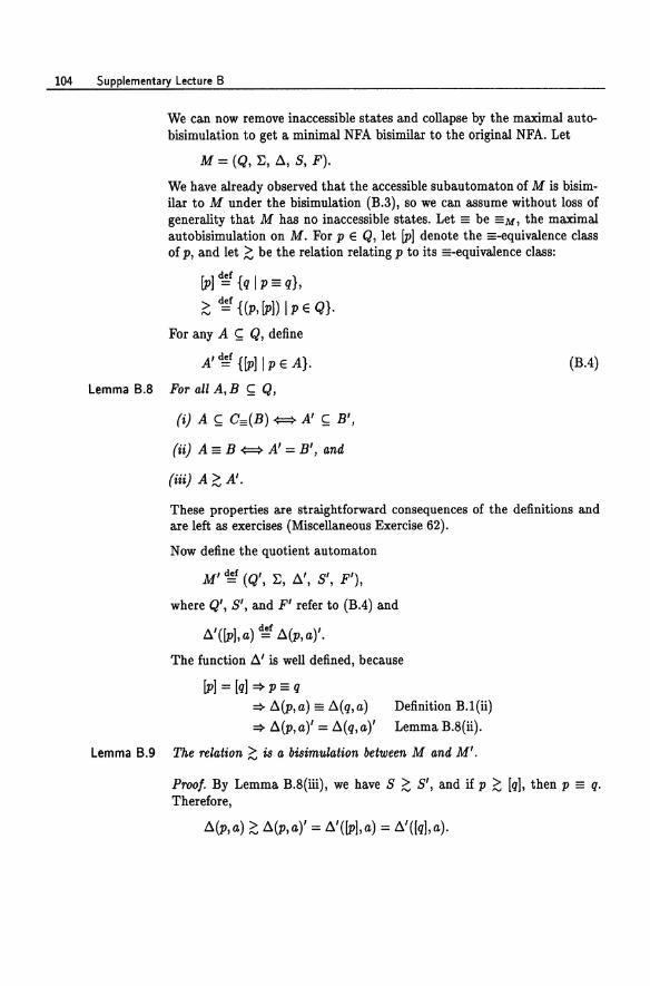
104 Supplementary Lecture B
We can now remove inaccessible states and collapse by the maximal autobisimulation to get a minimal NFA bisimilar to the original NFA. Let
M = (Q, E, A, 8, F).
We have already observed that the accessible subautomaton of M is bisimilar to M under the bisimulation (B.3), so we can assume without loss of generality that M has no inaccessible states. Let == be ==M, the maximal autobisimulation on M. For p E Q, let [PI denote the ==-equivalence class of p, and let ~ be the relation relating p to its ==-equivalence class:
[PI ~f {q I p == q},
~ ~f {(p, [P]) I p E Q}.
For any A ~ Q, define
A' ~f {[P]I PEA}.
Lemma B.8 For all A,B ~ Q,
(i) A ~ C=(B) <=> A' ~ B',
(ii) A == B <=> A' = B', and
( ''') A> A' U~ '" .
(BA)
These properties are straightforward consequences of the definitions and are left as exercises (Miscellaneous Exercise 62).
Now define the quotient automaton
M' ~ (Q', E, A', 8', F'),
where Q', 8', and F' refer to (BA) and
A'([p],a) ~f A(p, a)'.
The function A' is well defined, because
[PI = [q] ~ p == q ~ A(p,a) == A(q,a) ~ A(p,a)' = A(q, a)'
Definition B.l(ii)
Lemma B.8(ii).
Lemma B.9 The relation ~ is a bisimulation between M and M'.
Proof. By Lemma B.8(iii), we have 8 ~ 8', and if p ~ [q], then p == q. Therefore,
A(p, a) ~ A(p, a)' = A'([p],a) = A/([q],a).
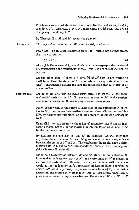
Collapsing Nondeterministic Automata 105
This takes care of start states and transitions. For the final states, if p E F, then [PI E F'. Conversely, if [PI E F', there exists q E [PI such that q E Fj then p == q, therefore p E F. 0
By Theorem BA, M and M' accept the same set.
Lemma B.lO The only autobisimulation on M' is the identity relation =.
Proof. Let'" be an autobisimulation on M'. If '" related two distinct states, then the composition
(B.5)
where ;S is the reverse of ~, would relate two non-==u-equivalent states of M, contradicting the maximality of ==u. Thus", is a subset of the identity relation.
On the other hand, if there is a state [PI of M' that is not related to itself by"', then the state p of M is not related to any state of M under (B.5), contradicting Lemma B.5 and the assumption that all states of M are accessible. 0
Theorem B.11 Let M be an NFA with no inaccessible states and let ==u be the maximal autobisimulation on M. The quotient automaton M' is the minimal automaton bisimilar to M and is unique up to isomorphism.
Proof. To show this, it will suffice to show that for any automaton N bisimilar to M, if we remove inaccessible states and then collapse the resulting NFA by its maximal autobisimulation, we obtain an automaton isomorphic toM'.
Using (B.3), we can assume without loss of generality that N has no inaccessible states. Let ==N be the maximal autobisimulation on N, and let N' be the quotient automaton.
By Lemmas B.2 and B.9, M' and N' are bisimilar. We will show that any bisimulation between M' and N' gives a one-to-one correspondence between the states of M' and N'. This establishes the result, since a bisimulation that is a one-to-one correspondence constitutes an isomorphism (Miscellaneous Exercise 63).
Let ~ be a bisimulation between M' and N'. Under~, every state of M' is related to at least one state of N', and every state of N' is related to at most one state of M'j otherwise the composition of ~ with its reverse would not be the identity on M', contradicting Lemma B.lO. Therefore, ~ embeds M' into N' injectively (i.e., in a one-to-one fashion). By a symmetric argument, the reverse of ~ embeds N' into M' injectively. Therefore, ~ gives a one-to-one correspondence between the states of M' and N'. 0
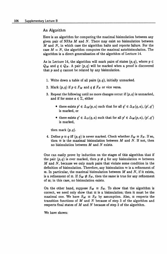
106 Supplementary Lecture B
An Algorithm
Here is an algorithm for computing the maximal bisimulation between any given pair of NFAs M and N. There may exist no bisimulation between M and N, in which case the algorithm halts and reports failure. For the case M = N, the algorithm computes the maximal autobisimulation. The algorithm is a direct generalization of the algorithm of Lecture 14.
As in Lecture 14, the algorithm will mark pairs of states (p, q), where p E QM and q E QN. A pair (p,q) will be marked when a proof is discovered that p and q cannot be related by any bisimulation.
1. Write down a table of all pairs (p,q), initially unmarked.
2. Mark (p,q) if p E FM and q ¢ FN or vice vttrsa.
3. Repeat the following until no more changes occur: if (p, q) is unmarked, and if for some a E I:, either
• there exists p' E ~M(p,a) such that for all q' E ~N(q,a), (p',q') is marked, or
• there exists q' E ~N(q,a) such that for allp' E ~M(p,a), (p',q') is marked,
then mark (p, q).
4. Define p == q iff (p, q) is never marked. Check whether 8M == 8 N. If so, then == is the maximal bisimulation between M and N. If not, then no bisimulation between M and N exists.
One can easily prove by induction on the stages of this algorithm that if the pair (p, q) is ever marked, then p rF q for any bisimulation ~ between M and N, because we only mark pairs that violate some condition in the definition of bisimulation. Therefore, any bisimulation ~ is a refinement of ==. In particular, the maximal bisimulation between M and N, if it exists, is a refinement of ==. If 8M ~ 8N , then the same is true for any refinement of ==j in this case, no bisimulation exists.
On the other hand, suppose 8M == 8N • To show that the algorithm is correct, we need only show that == is a bisimulationj then it must be the maximal one. We have 8M == 8N by assumption. Also, == respects the transition functions of M and N because of step 3 of the algorithm and respects final states of M and N because of step 2 of the algorithm.
We have shown:
Collapsing Nondeterministic Automata 107
Theorem B.12 The algorithm above correctly computes the maximal bisimulation between two NFAs if a bisimulation exists. If no bisimulation exists, the algorithm halts and reports failure. If both automata are the same, the algorithm computes the maximal autobisimulation.
Supplementary Lecture C
Automata on Terms
The theory of finite automata has many interesting and useful generalizations that allow more general types of inputs, such as infinite strings and finite and infinite trees. In this lecture and the next we will study one such generalization: finite automata on terms, also known as finite labeled trees. This generalization is quite natural and has a decidedly algebraic flavor. In particular, we will show that the entire Myhill-Nerode theory developed in Lectures 13 through 16 is really a consequence of basic results in universal algebra, a branch of algebra that deals with general algebraic concepts such as direct product, homomorphism, homomorphic image, and quotient algebra.
Signatures and Terms
A signature is an alphabet ~ consisting of various /unction and relation symbols in which each symbol is assigned a natural number, called its arity. An element of ~ is called constant, unary, binary, ternary, or n-ary if its arity is 0, 1,2,3, or n, respectively. We regard an n-ary function or relation symbol as denoting some (as yet unspecified) function or relation of n inputs on some (as yet unspecified) domain.
For example, the signature of monoids consists of two function symbols, a binary multiplication symbol . and a constant 1 for the multiplicative
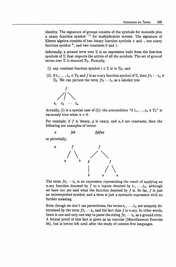
Automata on Terms 109
identity. The signature of groups consists of the symbols for monoids plus a unary function symbol -1 for multiplicative inverse. The signature of Kleene algebra consists of two binary function symbols + and ., one unary function symbol *, and two constants 0 and 1.
Informally, a ground term over E is an expression built from the function symbols of E that respects the arities of all the symbols. The set of ground terms over E is denoted TE • Formally,
(i) any constant function symbol C E E is in TEi and
(ii) if tl, ... ,t .. E TE and I is an n-ary function symbol of E, then It1 ... t .. E TIl. We can picture the term Itl ... t .. as a labeled tree
I
//"'" t1 t2 ... t ..
Actually, (i) is a special case of (ii): the precondition "if t1, . .. ,t .. E TE" is vacuously true when n = O.
For example, if I is binary, 9 is unary, and a, b are constants, then the following are examples of terms:
a lab Igblaa
or pictorially,
a I I
/\ /'" a b 9 I
/\ b a a
The term It1 ... t .. is an expression representing the result of applying an n-ary function denoted by I to n inputs denoted by t1, ... ,tn, although we have not yet said what the function denoted by I is. So far, I is just an uninterpreted symbol, and a. term is just a. syntactic expression with no further meaning.
Even though we don't use parentheses, the terms tl, ... ,tn are uniquely determined by the term Itl ... t .. and the fact that I is n-ary. In other words, there is one and only one way to parse the string It1 ... t .. as a ground term. A formal proof of this fact is given as an exercise (Miscellaneous Exercise 94), but is better left until after the study of context-free languages.
110 Supplementary Lecture C
Note that ifthere are no constants in E, then TI: is empty. If there are only finitely many constants and no other function symbols, then TI: is finite. In all other cases, TI: is infinite.
E-algebras
A E-algebra is a structure A consisting of a set A, called the carrier of A, along with a map that assigns a function IA or relation RA of the appropriate arity to each function symbol leE or relation symbol R e E. If I is an n-ary function symbol, then the function associated with I must be an n-ary function IA : An -+ A. If R is an n-ary relation symbol, then the relation RA must be an n-ary relation RA ~ An. Constant function symbols c are interpreted as O-ary functions (functions with no inputs), which are just elements cA of A. A unary relation is just a subset of A.
This interpretation of symbols of E extends in a natural way by induction to all ground terms. Each ground term t is naturally associated with an element tA e A, defined inductively as follows:
I A def IA( A A) tl ... tn = tl , ... ,tn .
This includes the base case: the interpretation of a constant c as an element cA e A is part of the specification of A.
Example C.1 Let r be a finite alphabet. The monoid r* is an algebra of signature .,1. The carrier of this algebra is the set r*, the binary function symbol . is interpreted as string concatenation, and the constant 1 is interpreted as the ~~qL 0
Example C2 The family of regular sets over an alphabet r is a Kleene algebra in which + is interpreted as set union, . as set concatenation, * as asterate, 0 as the null set, and 1 as the set {f}. 0
Example C.3 The family of binary relations on a set X is also a Kleene algebra in which + is interpreted as set union, . as relational composition, * as reflexive transitive closure, 0 as the null relation, and 1 as the identity relation. 0
Term Algebras
Example C4 Let E be an arbitrary signature. The set TI: of ground terms over E gives a family of E-algebras under the following natural interpretation: for n-ary I,
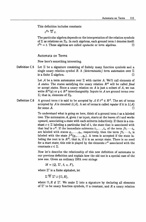
This definition includes constants
cTr. ~c.
Automata on Terms 111
The particular algebra depends on the interpretation of the relation symbols of ~ as relations on TE • In such algebras, each ground term t denotes itself: t7I: = t. These algebras are called syntactic or term algebras. 0
Automata on Terms
Now here's something interesting.
Definition C.S Let ~ be a signature consisting of finitely many function symbols and a single unary relation symbol R. A (deterministic) term automaton over ~ is a finite ~-algebra. 0
Let A be a term automaton over ~ with carrier A. We'll call elements of A states. The states satisfying the unary relation RA will be called final or accept states. Since a unary relation on A is just a subset of A, we can write RA(q) or q e RA interchangeably. Inputs to A are ground terms over ~j that is, elements of TE.
Definition C.6 A ground term t is said to be accepted by A if tA eRA. The set of terms accepted by A is denoted L(A). A set of terms is called regular if it is L(A) ~~A 0
To understand what is going on here, think of a ground term t as a labeled tree. The automaton A, given t as input, starts at the leaves of t and works upward, associating a state with each subterm inductively. If there is a constant c e ~ labeling a particular leaf of t, the state that is associated with that leaf is cA. If the immediate subterms tl, ... , tn of the term Itl ... tn are labeled with states qb'" , qn, respectively, then the term Itl ... tn is labeled with the state IA(ql, ... , qn). A term is accepted if the state labeling the root is in RAj that is, if it is an accept state. There is no need for a start statej this role is played by the elements cA associated with the constants c e ~.
Now let's describe the relationship of this new definition of automata to our previous definition and explain how the old one is a special case of the new one. Given an ordinary DFA over strings
M = (Q, ~/, 6, s, F),
where ~' is a finite alphabet, let
~ ~f ~/u {D,R},
where D,R f/. ~/. We make ~ into a signature by declaring all elements of ~' to be unary function symbols, 0 a constant, and R a unary relation
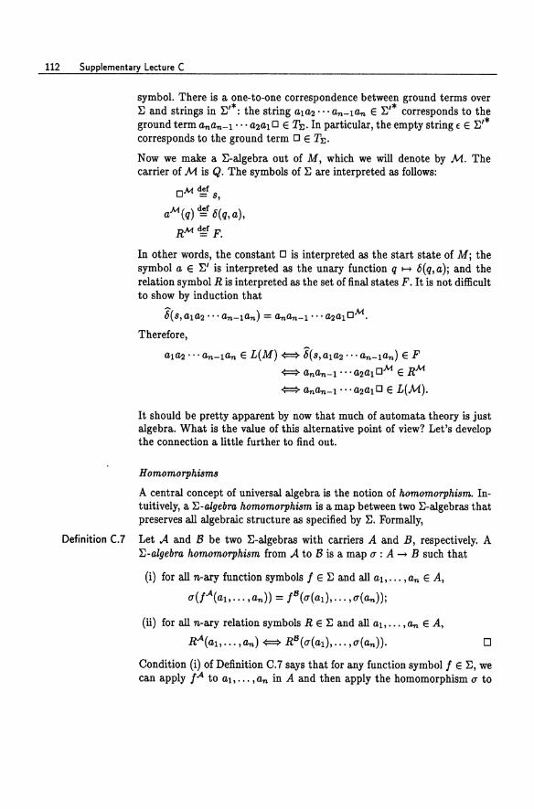
112 Supplementary Lecture C
symbol. There is a one-to-one correspondence between ground terms over E and strings in E/*: the string aIa2 ... an-Ian E E/* corresponds to the ground term anan-I ... a2aI 0 E TE. In particular, the empty string f E E/* corresponds to the ground term 0 E TE.
Now we make a E-algebra out of M, which we will denote by M. The carrier of M is Q. The symbols of E are interpreted as follows:
O M def = s, aM(q) ~f 8(q,a),
RM~F.
In other words, the constant 0 is interpreted as the start state of Mj the symbol a E E' is interpreted as the unary function q 1-+ 8(q,a)j and the relation symbol R is interpreted as the set of final states F. It is not difficult to show by induction that
~ M 8(s,ala2··· an-Ian) = anan-I··· a2aIO .
Therefore,
aIa2··· an-Ian E L(M) {:::=} 6(s,aIa2··· an-Ian) E F {:::=} anan-l ... a2aI OM E RM
{:::=} anan-l ... a2aI 0 E L(M).
It should be pretty apparent by now that much of automata theory is just algebra. What is the value of this alternative point of view? Let's develop the connection a little further to find out.
Homomorphisms
A central concept of universal algebra is the notion of homomorphism. Intuitively, a E-algebra homomorphism is a map between two E-algebras that preserves all algebraic structure as specified by E. Formally,
Definition C.7 Let A and B be two E-algebras with carriers A and B, respectively. A E-algebra homomorphism from A to B is a map (J : A --> B such that
(i) for all n-ary function symbols fEE and all aI, ... ,an E A,
(J(fA(al' ... ,an)) = f 8 (J(al), ... ,(J(an))j
(ii) for all n-ary relation symbols R E E and all al, ... ,an E A,
RA(al' ... ,an) {:::=} R8 (J(al), ... ,(J(an)). 0
Condition (i) of Definition C.7 says that for any function symbol fEE, we can apply fA to al, ... ,an in A and then apply the homomorphism (J to
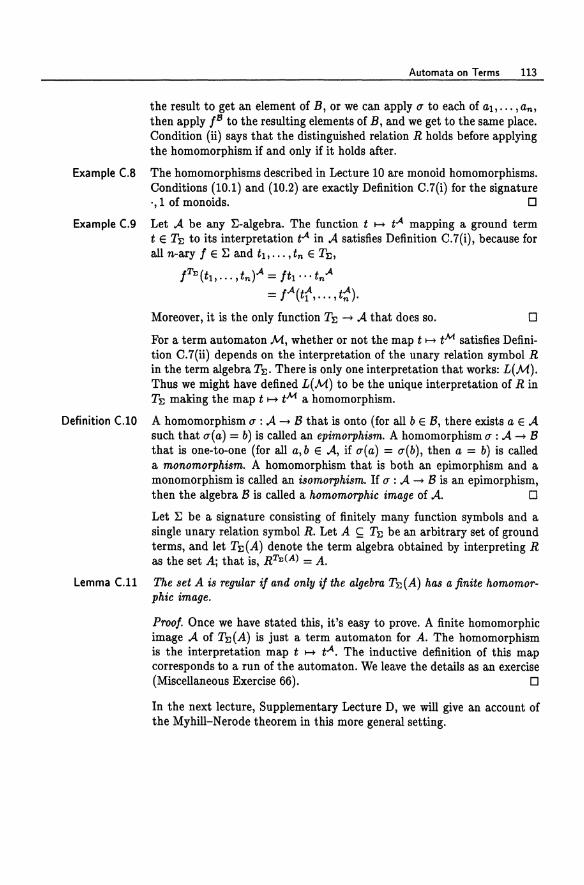
Automata on Terms 113
the result to get an element of B, or we can apply u to each of at, ... ,an, then apply fS to the resulting elements of B, and we get to the same place. Condition (ii) says that the distinguished relation R holds before applying the homomorphism if and only if it holds after.
Example e.8 The homomorphisms described in Lecture 10 are monoid homomorphisms. Conditions (10.1) and (10.2) are exactly Definition C.7(i) for the signature ,,1 of monoids. 0
Example e.g Let A be any 1::-algebra. The function t 1-+ tA mapping a ground term t e TI: to its interpretation tA in A satisfies Definition C.7(i), because for all n-ary f e 1:: and tl,"" tn e TI:,
fTr: (tt, ... ,tn),A = ftl ... tn,A = f,A(tf, ... ,t-:).
Moreover, it is the only function TI: -+ A that does so. o For a term automaton M, whether or not the map t H tM satisfies Definition C.7(ii) depends on the interpretation of the unary relation symbol R in the term algebra TI:. There is only one interpretation that works: L(M). Thus we might have defined L(M) to be the unique interpretation of R in TI: making the map t H tM a homomorphism.
Definition e.l0 A homomorphism u : A -+ B that is onto (for all b e B, there exists a e A such that u(a) = b) is called an epimorphism. A homomorphism u : A -+ B that is one-to-one (for all a, b e A, if u(a) = u(b), then a = b) is called a monomorphism. A homomorphism that is both an epimorphism and a monomorphism is called an isomorphism. If u : A -+ B is an epimorphism, then the algebra B is called a homomorphic image of A. 0
Let 1:: be a signature consisting of finitely many function symbols and a single unary relation symbol R. Let A ~ TI: be an arbitrary set of ground terms, and let TI:(A) denote the term algebra obtained by interpreting R as the set Aj that is, RTr:(A) = A.
Lemma C.ll The set A is regular if and only if the algebra TI:(A) has a finite homomorphic image.
Proof. Once we have stated this, it's easy to prove. A finite homomorphic image A of TI:(A) is just a term automaton for A. The homomorphism is the interpretation map t H tAo The inductive definition of this map corresponds to a run of the automaton. We leave the details as an exercise (Miscellaneous Exercise 66). 0
In the next lecture, Supplementary Lecture D, we will give an account of the Myhill-Nerode theorem in this more general setting.
Supplementary Lecture D
The Myhill-Nerode Theorem for Term Automata
In the last lecture we generalized DFAs on strings to term automata over a signature ~ and demonstrated that automata-theoretic concepts such as "final states" and "run" were really more general algebraic concepts in disguise. In this lecture we continue to develop this correspondence, leading finally to a fuller understanding of the Myhill-Nerode theorem.
Congruence
First we need to introduce the important algebraic concept of congruence. Congruences and homomorphisms go hand-in-hand. Recall from Supplementary Lecture C that a homomorphism between two 1:-algebras is a map that preserves all algebraic structure (Definition C.7). Every homomorphism cr : A ~ B induces a certain natural binary relation on A:
U =<T V ~ cr(u) = cr(v).
The relation =<T is called the kernel! of cr.
1If you have taken algebra, you may have seen the word kernel used differently: normal subgroups of groups, ideals of rings, null spaces of linear transformations. These concepts are closely allied and serve the same purpose. The definition of kernel as a binary relation is more broadly applicable.
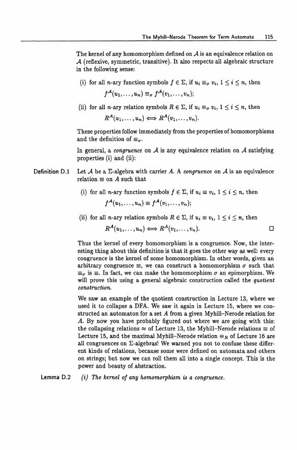
The Myhill-Nerode Theorem for Term Automata 115
The kernel of any homomorphism defined on A is an equivalence relation on A (reflexive, symmetric, transitive). It also respects all algebraic structure in the following sense:
(i) for all n-ary function symbols 1 E ~, if 'Ui =17 Vi, 1 :5 i :5 n, then
/"A('Ul' •.• ,'Un) =17/.A(Vl' .•• ,Vn)j
(ii) for all n-ary relation symbols R E ~, if 'Ui =17 Vi, 1 :5 i :5 n, then
R.A('Ul' .•• ,'Un) <=> R.A(Vl' ... ,Vn ).
These properties follow immediately from the properties of homomorphisms and the definition of =17. In general, a congruence on A is any equivalence relation on A satisfying properties (i) and (ii):
Definition D.1 Let A be a ~-algebra with carrier A. A congruence on A is an equivalence relation = on A such that
Lemma D.2
(i) for all n-ary function symbols 1 E ~, if 'U; = Vi, 1 :5 i :5 n, then
/",1.( 'U1, ••. ,'Un) = I.A( V1, • •• ,Vn)j
(ii) for all n-ary relation symbols R E ~, if 'Ui = Vi, 1 :5 i :5 n, then
R.A('Ul' .•• ,'Un) <=> R.A(v1, ..• ,Vn ). 0
Thus the kernel of every homomorphism is a congruence. Now, the interesting thing about this definition is that it goes the other way as well: every congruence is the kernel of some homomorphism. In other words, given an arbitrary congruence =, we can construct a homomorphism u such that =17 is =. In fact, we can make the homomorphism u an epimorphism. We will prove this using a general algebraic construction called the quotient construction.
We saw an example of the quotient construction in Lecture 13, where we used it to collapse a DFA. We saw it again in Lecture 15, where we constructed an automaton for a set A from a given Myhill-Nerode relation for A. By now you have probably figured out where we are going with this: the collapsing relations s::z of Lecture 13, the Myhill-Nerode relations = of Lecture 15, and the maximal Myhill-Nerode relation =n of Lecture 16 are all congruences on ~-algebras! We warned you not to confuse these different kinds of relations, because some were defined on automata and others on stringsj but now we can roll them all into a single concept. This is the power and beauty of abstraction.
(i) The kernel 01 any homomorphism is a congruence.
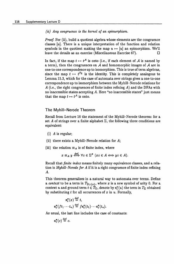
116 Supplementary Lecture 0
(ii) Any congruence is the kernel of an epimorphism.
Proof. For (ii), build a quotient algebra whose elements are the congruence classes [uJ. There is a unique interpretation of the function and relation symbols in the quotient making the map u H [uJ an epimorphism. We'll leave the details as an exercise (Miscellaneous Exercise 67). 0
In fact, if the map t H tA is onto (i.e., if each element of A is named by a term), then the congruences on A and homomorphic images of A are in one-to-one correspondence up to isomorphism. This is true of term algebras, since the map t H tTr. is the identity. This is completely analogous to Lemma 15.3, which for the case of automata over strings gives a one-to-one correspondence up to isomorphism between the Myhill-Nerode relations for A (i.e., the right congruences of finite index refining A) and the DFAs with no inaccessible states accepting A. Here "no inaccessible states" just means that the map t H tA is onto.
The Myhill-Nerode Theorem
Recall from Lecture 16 the statement of the Myhill-Nerode theorem: for a set A of strings over a finite alphabet E, the following three conditions are equivalent:
(i) A is regular;
(ii) there exists a Myhill-Nerode relation for A;
(iii) the relation =A is of finite index, where
x =A y ~ Vz E E* (xz E A {:::::} yz E A).
Recall that finite index means finitely many equivalence classes, and a relation is Myhill-Nerode for A if it is a right congruence of finite index refining A.
This theorem generalizes in a natural way to automata over terms. Define a context to be a term in TEU{",}, where x is a new symbol of arity O. For a context u and ground term t E TIl, denote by sf (u) the term in TIl obtained by substituting t for all occurrences of x in u. Formally,
"'( ) def t St x = , sHftl ... tn ) ~ fs:(tl)'" s:(tn ).
As usual, the last line includes the case of constants:
"'( ) def StC=C.
The Myhill-Nerode Theorem for Term Automata 117
Let ~ be a signature consisting of finitely many function symbols and a single unary relation symbol R. For a given A ~ TE and ground terms s, tETE, define
s ==A t ~ for all contexts u, s:(u) E A {=:} st(u) E A.
It is not difficult to argue that ==A is a congruence on TE(A) (Miscellaneous Exercise 68).
Theorem D.3 (Myhill-Nero de theorem for term automata) Let A ~ TE • Let TE(A) denote the term algebra over ~ in which R is interpreted as the unary relation A. The following statements are equivalent:
(i) A is regular;
(i') TE(A) has a finite homomorphic image;
(ii) there exists a congruence of finite index on TE(A);
(iii) the relation =A is of finite index.
Proof. We have already observed (Lemma C.11) that to say A is regular (i.e., accepted by a term automaton) is just another way of saying that TE(A) has a finite homomorphic image. Thus (i) and (i/) are equivalent.
(i /) => (ii) If TE(A) has a finite homomorphic image under epimorphism (T, then the kernel of (T is of finite index, since its congruence classes are in one-to-one correspondence with the elements of the homomorphic image.
(il) => (iii) Let == be any congruence on TE(A). We show that == refines ==Aj therefore, =A is of finite index if == is. Suppose s == t. It follows by a straightforward inductive argument using Definition D.l(i) that for any context u, s=(u) == s:(u)j then by Definition D.l(ii), s=(u) E A iff s:(u) E A. Since the context u was arbitrary,s ==A t.
(iii) => (i/) Since ==A is a congruence, it is the kernel of an epimorphism obtained by the quotient construction. Since ==A is of finite index, the quotient algebra is finite and therefore a finite homomorphic image of TE(A). 0
As in Lecture 16, the quotient of TE(A) by ==A gives the minimal homomorphic image of TE(A)j and for any other homomorphic image B, there is a unique homomorphism B --+ TE(A)/==A.
Historical Notes
Thatcher and Wright [119] generalized finite automata on strings to finite automata on terms and developed the algebraic connection. The more general version of the Myhill-Nerode theorem (Theorem D.3) is in some sense
118 Supplementary Lecture D
an inevitable consequence of Myhill and Nerode's work [91, 94] since according to Thatcher and Wright, "conventional finite automata theory goes through for the generalization-and it goes through quite neatly" [119]. The first explicit mention of the equivalence of the term analogs of (i) and (ii) in the statement of the Myhill-Nerode theorem seems to be by Brainerd [13, 14] and Eilenberg and Wright [34], although the latter claim that their paper "contains nothing that is essentially new, except perhaps for a point of view" [34]. A relation on terms analogous to =A was defined and clause (iii) added explicitly by Arbib and Give'on [5, Definition 2.13], although it is also essentially implicit in work of Brainerd [13, 14].
Good general references are Gccseg and Steinby [42] and Englefriet [35].
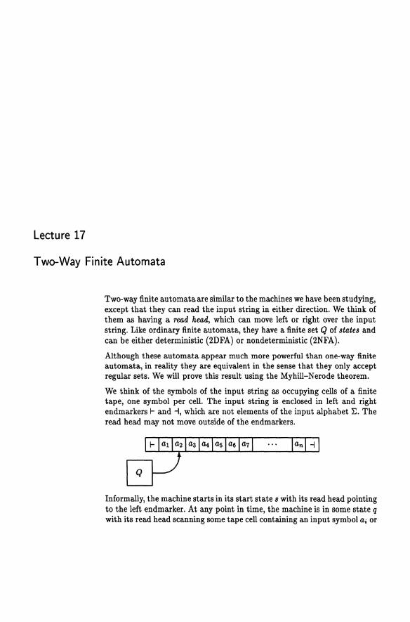
Lecture 17
Two-Way Finite Automata
Two-way finite automata are similar to the machines we have been studying, except that they can read the input string in either direction. We think of them as having a read head, which can move left or right over the input string. Like ordinary finite automata, they have a finite set Q of states and can be either deterministic (2DFA) or nondeterministic (2NFA).
Although these automata appear much more powerful than one-way finite automata, in reality they are equivalent in the sense that they only accept regular sets. We will prove this result using the Myhill-Nerode theorem.
We think of the symbols of the input string as occupying cells of a finite tape, one symbol per cell. The input string is enclosed in left and right endmarkers I- and -1, which are not elements of the input alphabet E. The read head may not move outside of the endmarkers.
Informally, the machine starts in its start state 8 with its read head pointing to the left endmarker. At any point in time, the machine is in some state q with its read head scanning some tape cell containing an input symbol ao or
120 Lecture 17
one of the endmarkers. Based on its current state and the symbol occupying the tape cell it is currently scanning, it moves its read head either left or right one cell and enters a new state. It accepts by entering a special accept state t and rejects by entering a special reject state r. The machine's action on a particular state and symbol is determined by a transition function 6 that is part of the specification of the machine.
Example 17.1 Here is an informal description of a 2DFA accepting the set
A = {x E {a,b}* I #a(x) is a multiple of 3 and #b(x) is even}.
The machine starts in its start state scanning the left endmarker. It scans left to right over the input, counting the number of a's mod 3 and ignoring the b's. When it reaches the right endmarker -I, if the number of a's it has seen is not a multiple of 3, it enters its reject state, thereby rejecting the input-the input string x is not in the set A, since the first condition is not satisfied. Otherwise it scans right to left over the input, counting the number of b's mod 2 and ignoring the a's. When it reaches the left endmarker f- again, if the number of b's it has seen is odd, it enters its reject state; otherwise, it enters its accept state. 0
Unlike ordinary finite automata, a 2DFA needs only a single accept state and a single reject state. We can think of it as halting immediately when it enters one of these two states, although formally it keeps running but remains in the accept or reject state. The machine need not read the entire input before accepting or rejecting. Indeed, it need not ever accept or reject at all, but may loop infinitely without ever entering its accept or reject state.
Formal Definition of 2DFA
Formally, a 2DFA is an octuple
M = (Q, ~, f-, -I, 6, s, t, r),
where
• Q is a finite set (the states),
• ~ is a finite set (the input alphabet),
• f- is the left endmarker, f- ¢ ~,
• -I is the right endmarker, -I ¢ ~,
• 6 : Q x (~ U {f-, -I}) ~ (Q x {L, R}) is the transition function (L, R stand for left and right, respectively),
• SEQ is the start state,
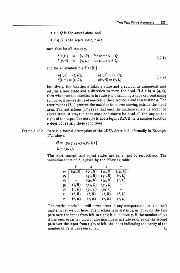
Two-Way Finite Automata 121
• t E Q is the accept state, and
• r E Q is the reject state, r "I- t,
such that for all states q,
b(q,r) b(q, -I)
= =
(u,R) (v, L)
for some u E Q, for some v E Q,
and for all symbols b E 1: u {r},
8(t, b) = (t,R), b(t, --I) = (t,L),
8(r, b) = (r,R), b(r, --I) = (r, L).
(17.1)
(17.2)
Intuitively, the function 15 takes a state and a symbol as arguments and returns a new state and a direction to move the head. If b(P,b) = (q,d), then whenever the machine is in state p and scanning a tape cell containing symbol b, it moves its head one cell in the direction d and enters state q. The restrictions (17.1) prevent the machine from ever moving outside the input area. The restrictions (17.2) say that once the machine enters its accept or reject state, it stays in that state and moves its head all the way to the right of the tape. The octuple is not a legal 2DFA if its transition function 15 does not satisfy these conditions.
Example 17.2 Here is a formal description of the 2DFA described informally in Example 17.1 above.
Q = {qO,ql,q2,PO,Pl,t,r}, 1: = {a, b}.
The start, accept, and reject states are qo, t, and r, respectively. The transition function 15 is given by the following table:
r qo ql q2 Po (t,R) Pl (r,R) t (t,R) r (r,R)
a ql,R
(q2, R) (qo, R) (Po, L) (pl,L) (t,R) (r,R)
b qo,R
(ql! R) (q2,R) (pl,L) (Po, L) (t, R) (r,R)
(t, L) (r, L)
The entries marked - will never occur in any computation, so it doesn't matter what we put here. The machine is in states qo, ql, or q2 on the first pass over the input from left to right; it is in state qi if the number of a's it has seen so far is i mod 3. The machine is in state Po or Pl on the second pass over the input from right to left, the index indicating the parity of the number of b's it has seen so far. 0
122 Lect u re 17
Configurations and Acceptance
Fix an input x E E*, say x = ala2 ... an. Let ao = I- and an+1 = -I. Then
aOala2'" anan+l = I- x -l .
A configuration of the machine on input x is a pair (q, i) such that q E Q and 0 :::; i :::; n + 1. Informally, the pair (q, i) gives a current state and current position ofthe read head. The start configuration is (s,O), meaning that the machine is in its start state s and scanning the left endmarker.
A binary relation +, the next configuration relation, is defined on configurations aB follows:
o(p,ai) = (q,L):::} (P,i) + (q,i -1),
o(p, ail = (q, R) :::} (p, i) + (q, i + 1).
The relation ~ describes one step of the machine on input x. We define .. the relations + inductively, n ~ 0:
• (p, i) + (p, i)j and
• if (p,i) + (q,j) and (q,j) + (u,k), then (p,i) ~ (u,k).
The relation ~ is J'ust the n-fold composition of ~. The relations .. .. + are functionsj that is, for any configuration (p, i), there is exactly one
configuration (q,j) such that (P,i) + (q,j). Now define
(p,i) 7 (q,j) ~ 3n ~ 0 (P,i) + (q,j).
Note that the definitions of these relations depend on the input x. The machine is said to accept the input x if
(s,O) 7 (t,i) for some i.
In other words, the machine enters its accept state at some point. The machine is said to reject the input x if
(s,O) 7 (r,i) for some i.
In other words, the machine enters its reject state at some point. It cannot both accept and reject input x by our aBsumption that t:f. r and by properties (17.2). The machine is said to halt on input x if it either accepts x or rejects x. Note that this is a purely mathematical definition-the machine doesn't really grind to a halt! It is possible that the machine neither accepts nor rejects x, in which CaBe it is said to loop on x. The set L(M) is defined to be the set of strings accepted by M.
Two-Way Finite Automata 123
Example 17.3 The 2DFA described in Example 17.2 goes through the following sequence of configurations on input aababbb, leading to acceptance:
(qQ,O), (qQ,1), (qlo 2), (q2,3), (q2,4), (qQ,5), (qQ,6), (qQ,7), (qQ,8), (PQ,7), (Plo6), (Po, 5), (Plo4), (plo3), (Po, 2), (Po,l), (Po, 0), (t,l).
It goes through the following sequence of configurations on input aababa, leading to rejection:
(qo,O), (qQ,l), (qlo 2), (q2,3), (q2,4), (qo,5), (qo,6), (qlo 7), (r,6).
It goes through the following sequence of configurations on input aababb, leading to rejection:
(qo,O), (qo,l), (ql,2), (q2,3), (q2,4), (qo,5), (qo,6), (qo,7), (Po, 6), (Pl,5), (Po, 4), (Po, 3), (Plo 2), (plo1), (PloO), (r,l). 0
Lecture 18
2DFAs and Regular Sets
In this lecture we show that 2DFAs are no more powerful than ordinary DFAs. Here is the idea. Consider a long input string broken up in an arbitrary place into two substrings xz. How much information about x can the machine carry across the boundary from x into z? Since the machine is two-way, it can cross the boundary between x and z several times. Each time it crosses the boundary moving from right to left, that is, from z into :1:, it does so in some state q. When it crosses the boundary again moving from left to right (if ever), it comes out of x in some state, say p. Now if it ever goes into x in the future in state q again, it will emerge again in state p, because its future action is completely determined by its current configuration (state and head position). Moreover, the state p depends only on q and :1:. We will write Too(q) = p to denote this relationship. We can keep track of all such information by means of a finite table
Too: (QU{.}) --+ (QU{1.}),
where Q is the set of states of the 2DFA M, and • and 1. are two other objects not in Q whose purpose is described below.
On input xz, the machine M starts in its start state scanning the left endmarker. As it computes, it moves its read head. The head may eventually cross the boundary moving left to right from :I: into z. The first time it does so (if ever), it is in some state, which we will call T,,(.) (this is the purpose of .). The machine may never emerge from Xj in this case we write T,,(.) = 1.
2DFAs and Regular Sets 125
(this is the purpose of .L). The state T,,( e) gives some information about x, but only a finite amount of information, since there are only finitely many possibilities for T,,(e). Note also that T,,(e) depends only on x and not on z: if the input were xw instead of xz, the first time the machine passed the boundary from x into w, it would also be in state T,,(e), because its action up to that point is determined only by xi it hasn't seen anything to the right of the boundary yet.
If T., (e) = .L, M must be in an infinite loop inside x and will never accept or reject, by our assumption about moving all the way to the right endmarker whenever it accepts or rejects.
Suppose that the machine does emerge from x into z. It may wander around in z for a while, then later may move back into x from right to left in state q. If this happens, then it will either
e eventually emerge from x again in some state p, in which case we define T.,(q) = Pi or
e never emerge, in which case we define T.,(q) = .L.
Again, note that T", (q) depends only on x and q and not on z. If the machine entered x from the right on input xw in state q, then it would emerge again in state T.,(q) (or never emerge, if T",(q) = .L), because M is deterministic, and its behavior while inside x is completely determined by x and the state it entered x in.
If we write down T., (q) for every state q along with T", ( e ), this gives all the information about x one could ever hope to carry across the boundary from x to z. One can imagine an agent sitting to the right of the boundary between x and z, trying to obtain information about x. All it is allowed to do is observe the state T., ( e) the first time the machine emerges from x (if ever) and later send probes into x in various states q to see what state T.,(q) the machine comes out in (if at all). If y is another string such that Til = T"" then x and y will be indistinguishable from the agent's point of view.
Now note that there are only finitely many possible tables
T: (Q U {e}) -+ (Q U {.L}),
namely (k + 1)10+1, where k is the size of Q. Thus there is only a finite amount of information about x that can be passed across the boundary to the right of x, and it is all encoded in the table T.,.
Note also that if T., = Til and M accepts xz, then M accepts yz. This is because the sequence of states the machine is in as it passes the boundary between x and z (or between y and z) in either direction is completely
126 Lecture 18
determined by the table T .. = T!I and z. To accept :z;z, the machine must at some point be scanning the right endmarker in its accept state t. Since the sequence of states along the boundary is the same and the action when the machine is scanning z is the same, this also must happen on input yz.
Now we can use the Myhill-Nerode theorem to show that L(M) is regular. We have just argued that
T", = T!I => Vz (M accepts :z;z <==> M accepts yz)
<==> Vz (:z;z E L(M) <==> yz E L(M))
<==> :z; ==L(M) y,
where ==L(M) is the relation first defined in Eq. (16.1) of Lecture 16. Thus if two strings have the same table, then they are equivalent under ==L(M)' Since there are only finitely many tables, the relation ==L(M) has only finitely many equivalence classes, at most one for each tablej therefore, ==L(M) is of finite index. By the Myhill-Nerode theorem, L(M) is a regular set.
Constructing a DFA
The argument above may be a bit unsatisfying, since it does not explicitly construct a DFA equivalent to a given 2DFA M. We can easily do so, however. Intuitively, we can build a DFA whose states correspond to the tables.
Formally,- define
:z;==y~T .. =T!I'
That is, call two strings in ~* equivalent if they have the same table. There are only finitely many equivalence classes, at most one for each tablej thus == is of finite index. We can also show the following:
(i) The table T .. a is uniquely determined by T .. and aj that is, if T .. = T!I' then T .. a = T!la' This says that == is a right congruence.
(ii) Whether or not :z; is accepted by M is completely determined by T .. j that is, if T", = T!I' then either both :z; and y are accepted by M or neither is. This says that == refines L(M).
These observations together say that == is a Myhill-Nerode relation for L(M). Using the construction == H M= described in Lecture 15, we can obtain a DFA for L(M) explicitly.
To show (i), we show how to construct T .. a from T .. and a.
2DFAs and Regular Sets 127
e If PO,Plo ... ,Pk,qo,qlo ... ,qk e Q such that 6(p"a) = (q"L) and T .. (q,) = PH1, 0 :::; i :::; k -1, and 6(p", a) = (q", R), then T .... (po) = q".
e IfPo,Plo ... ,P",qo,ql, ... ,q"-l e Q such that 6(p"a) = (q"L) and T .. (qi) = PH1! 0:::; i :::; k - 1, and Pic = Pi, i < k, then T .... (Po) = .L.
e If PO,Pl, ... ,p",qO,ql, ... ,q" e Q such that 6(p, , a) = (qi, L), 0 :::; i :::; k, T .. (q,) = PH1! 0 :::; i :::; k - 1, and T .. (q,,) = ol, then T .... (po) = .L.
e If T .. (e) =ol, then T .... (e) =ol.
e If T .. (e) = p, then T .... (e) = T .... (p).
For (li), suppose T .. = TTl and consider the sequence of states M is in as it crosses the boundary in either direction between the input string and the right endmarker -I. This sequence is the same on input x as it is on input y, since it is completely determined by the table. Both strings x and yare accepted iff this sequence contains the accept state t.
We have shown that the relation:::: is a Myhill-Nerode relation for L(M), where M is an arbitrary 2DFA. The construction:::: H ME of Lecture 15 gives a DFA equivalent to M. Recall that in that construction, the states of the DFA correspond in a one-to-one fashion with the ::::-classesi and here, each ::::-class [x] corresponds to a table T .. : (Q U {e}) --+ (Q U {ol}).
If we wanted to, we could build a DFA M' directly from the tables:
Q' ~ {T : (Q U {e }) --+ (Q U {ol} )}, I def T.
8 = ., 6'(T .. , a) ~ T .... ,
F' d,g {T .. I x e L(M)}.
The transition function 6' is well defined because of property (i), and T., e F' iff x e L(M) by property (li). As usual, one can prove by induction on Iyl that
then
6'(T."y) = T"Tli
x e L(M') {:::::> 6'(8/,X) e F'
¢::::} 6'(T.,x) e F' {:::::> T., e F'
{:::::> x e L(M).
Thus L(M') = L(M).
Another proof, due to Vardi [122], is given in Miscellaneous Exercise 61.
128 Lectu re 18
Historical Notes
Two-way finite automata were first studied by Rabin and Scott [1021 and Shepherdson [1141. Vardi [1221 gave a shorter proof of equivalence to DFAs (Miscellaneous Exercise 61).
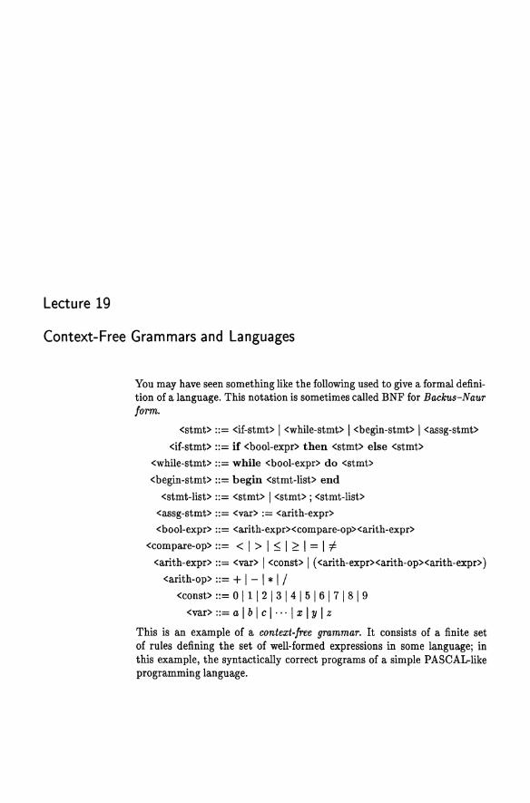
Lecture 19
Context-Free Grammars and Languages
You may have seen something like the following used to give a formal definition of a language. This notation is sometimes called BNF for Backus-Naur form.
<stmt> ::= <if-stmt> I <while-stmt> I <begin-stmt> I <assg-stmt>
<if-stmt> ::= if <bool-expr> then <stmt> else <stmt>
<while-stmt> ::= while <bool-expr> do <stmt>
<begin-stmt> ::= begin <stmt-list> end
<stmt-list> ::= <stmt> I <stmt> ; <stmt-list>
<assg-stmt> ::= <var> := <arith-expr>
<bool-expr> ::= <arith-expr><compare-op><arith-expr>
<compare-op> ::= < I> I ~ I ~ I = I i-<arith-expr> ::= <var> I <const> I «arith-expr><arith-op><arith-expr»
<arith-op> ::= + I - I * I / <const> ::= 0 11 I 2 I 3 I 4 I 5 I 6 I 7 I 8 I 9
<var> ::= a I b I c I ... I x I y I z
This is an example of a context-free grammar. It consists of a finite set of rules defining the set of well-formed expressions in some language; in this example, the syntactically correct programs of a simple PASCAL-like programming language.
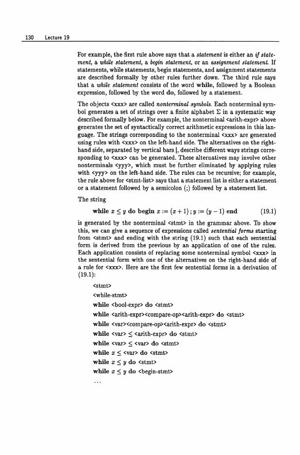
130 Lecture 19
For example, the first rule above says that a statement is either an i/statement, a while statement, a begin statement, or an assignment statement. If statements, while statements, begin statements, and assignment statements are described formally by other rules further down. The third rule says that a while statement consists of the word while, followed by a Boolean expression, followed by the word do, followed by a statement.
The objects <xxx> are called nonterminal symbols. Each nonterminal symbol generates a set of strings over a finite alphabet :E in a systematic way described formally below. For example, the nonterminal <arith-expr> above generates the set of syntactically correct arithmetic expressions in this language. The strings corresponding to the nonterminal <xxx> are generated using rules with <xxx> on the left-hand side. The alternatives on the righthand side, separated by vertical bars I, describe different ways strings corresponding to <xxx> can be generated. These alternatives may involve other nonterminals <yyy>, which must be further eliminated by applying rules with <yyy> on the left-hand side. The rules can be recursivej for example, the rule above for <stmt-list> says that a statement list is either a statement or a statement followed by a semicolon (j) followed by a statement list.
The string
while x $ y do begin x := (x + 1) j Y := (y -1) end (19.1)
is generated by the nonterminal <stmt> in the grammar above. To show this, we can give a sequence of expressions called sentential/orms starting from <stmt> and ending with the string (19.1) such that each sentential form is derived from the previous by an application of one of the rules. Each application consists of replacing some nonterminal symbol <xxx> in the sentential form with one of the alternatives on the right-hand side of a rule for <xxx>. Here are the first few sentential forms in a derivation of (19.1):
<stmt>
<while-stmt>
while <bool-expr> do <stmt>
while <arith-expr><compare-op><arith-expr> do <stmt>
while <var><compare-op><arith-expr> do <stmt>
while <var> $ <arith-expr> do <stmt>
while <var> $ <var> do <stmt>
while x $ <var> do <stmt>
.while x $ y do <stmt>
while x $ y do <begin-stmt>
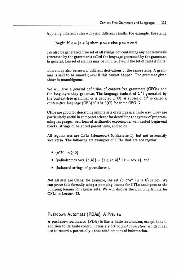
Context-Free Grammars and Languages 131
Applying different rules will yield different results. For example, the string
begin if z = (x + 3) then y := z else y := x end
can also be generated. The set of all strings not containing any nonterminals generated by the grammar is called the language generated by the grammar. In general, this set of strings may be infinite, even if the set of rules is finite.
There may also be several different derivations of the same string. A grammar is said to be unambiguous if this cannot happen. The grammar given above is unambiguous.
We will give a general definition of context-free grammars (CFGs) and the languages they generate. The language (subset of 'E*) generated by the context-free grammar G is denoted L( G). A subset of 'E* is called a context-free language (CFL) if it is L(G) for some CFG G.
CFLs are good for describing infinite sets of strings in a finite way. They are particularly useful in computer science for describing the syntax of programming languages, well-formed arithmetic expressions, well-nested begin-end blocks, strings of balanced parentheses, and so on.
All regular sets are CFLs (Homework 5, Exercise 1), but not necessarily vice versa. The following are examples of CFLs that are not regular:
• {anbn I n ~ O}j
• {palindromes over {a,b}} = {x E {a,b}* I x = rev x}; and
• {balanced strings of parentheses}.
Not all sets are CFLsj for example, the set {anbnan I n ~ O} is not. We can prove this formally using a pumping lemma for CFLs analogous to the pumping lemma for regular sets. We will discuss the pumping lemma for CFLs in Lecture 22.
Pushdown Automata (PDAs): A Preview
A pushdown automaton (PDA) is like a finite automaton, except that in addition to its finite control, it has a stack or pushdown store, which it can use to record a potentially unbounded amount of information.
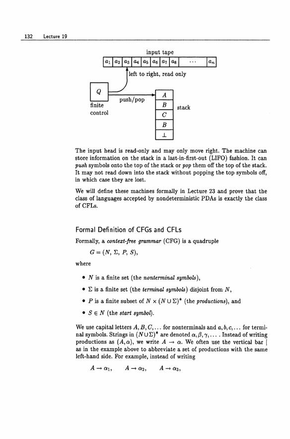
132 Lecture 19
finite control
B
C
B
.l
stack
The input head is read-only and may only move right. The machine can store information on the stack in a last-in-first-out (LIFO) fashion. It can push symbols onto the top of the stack or pop them off the top of the stack. It may not read down into the stack without popping the top symbols off, in which case they are lost.
We will define these machines formally in Lecture 23 and prove that the class of languages accepted by nondeterministic PDAs is exactly the class of CFLs.
Formal Definition of CFGs and CFLs
Formally, a contezt-free grammar (CFG) is a quadruple
G= (N,~, P, S),
where
• N is a finite set (the nonterminal symbols),
• ~ is a finite set (the terminal symbols) disjoint from- N,
• P is a finite subset of N x (N U ~)* (the productions), and
• SEN (the start symbon.
We use capital letters A, B, C, ... for nonterminals and a, b, c, ... for terminal symbols. Strings in (NU ~)* are denoted a,{3, 1, .... Instead of writing productions as (A, a), we write A --> a. We often use the vertical bar I as in the example above to abbreviate a set of productions with the same left-hand side. For example, instead of writing
Context-Free Grammars and Languages 133
we might write
A -+ 0:1 10:2 10:3.
If 0:, /3 E (N U ~)*, we say that /3 is derivable from 0: in one step and write
1 0: --+ /3
G
if /3 can be obtained from 0: by replacing some occurrence of a nonterminal A in 0: with 1, where A -+ 1 is in P; that is, if there exist 0:1. 0:2 E (NU~)* and production A -+ 1 such that
0: = 0:1 A0:2 and /3 = 0:110:2.
Let ~ be the reflexive transitive closure of the relation .2..; that is, G G
define
o • 0: --+ 0: for any 0:, G
• 0: ~ /3 if there exists 1 such that 0: ~ 1 and 1.2.. /3, and G G G
• 0: ~ /3 if 0: ~ /3 for some n > O. G G -
A string in (NU~)* derivable from the start symbol S is called a sentential form. A sentential form is called a sentence if it consists only of terminal symbols; that is, if it is in ~*. The language generated by G, denoted L( G), is the set of all sentences:
L(G) = {x E ~* IS + x}.
A subset B ~ ~* is a context-free language (CFL) if B = L(G) for some context-free grammar G.
Example 19.1 The nonregular set {anbn I n ~ O} is a CFL. It is generated by the grammar
S -+ aSb I f,
where f is the null string. More precisely, G = (N, ~, P, S), where
N = is}, ~ = {a,b}, P = {S -+ aSb, S -+ fl.
Here is a derivation of a3b3 in G: 1 1 1 1
S G aSb G aaSbb G aaaSbbb G aaabbb.
The first three steps apply the production S -+ aSb and the last applies the production S -+ f. Thus
S~aaabbb. G
134 Lecture 19
One can show by induction on n that
S n+l nbn --a a ,
so all strings of the form anbn are in L(G); conversely, the only strings in L( G) are of the form anbn, as can be shown by induction on the length of the derivation. 0
Example 19.2 The nonregular set
{palindromes over {a, b}*} = {:c E {a, b} * I :c = rev:c}
is a CFL generated by the grammar
S --+ aSa I bSb I a I b I e.
The first two productions generate any number of balanced a's or b's at the outer ends of the string, working from the outside in. The last three productions are used to finish the derivation. The productions S --+ a and S --+ b are used to generate an odd-length palindrome with an a or b, respectively, as the middle symbol; and the production S --+ e is used to generate an even-length palindrome. 0
Historical Notes
Context-free grammars and languages were introduced by Chomsky [17, 18, 201, although they were foreshadowed by the systems of Post [1001 and Markov [83]. Backus-Naur form was used to specify the syntax of programming languages by Backus [7] and Naur [93].
Lecture 20
Balanced Parentheses
Intuitively, a string of parentheses is balanced if each left parenthesis has a matching right parenthesis and the matched pairs are well nested. The set PAREN of balanced strings of parentheses [ ] is the prototypical contextfree language and plays a pivotal role in the theory of CFLs.
The set PAREN is generated by the grammar
S -+ [S] I SS I f. This is not obvious, so let's give a proof. First we need a formal characterization of balanced. To avoid confusing notation, we'll use
L(x) ~f #[(x) = the number of left parentheses in x,
R(x) ~f #] (x) = the number of right parentheses in x.
We will define a string x of parentheses to be balanced if and only if
(i) L(x) = R(x), and
(li) for all prefixes y of x, L(y) ~ R(y).
(Recall that a prefix of x is a string y such that x = yz for some z.) To see that this definition correctly captures the intuitive notion of balanced, note that property (i) says that there must be the same number of left
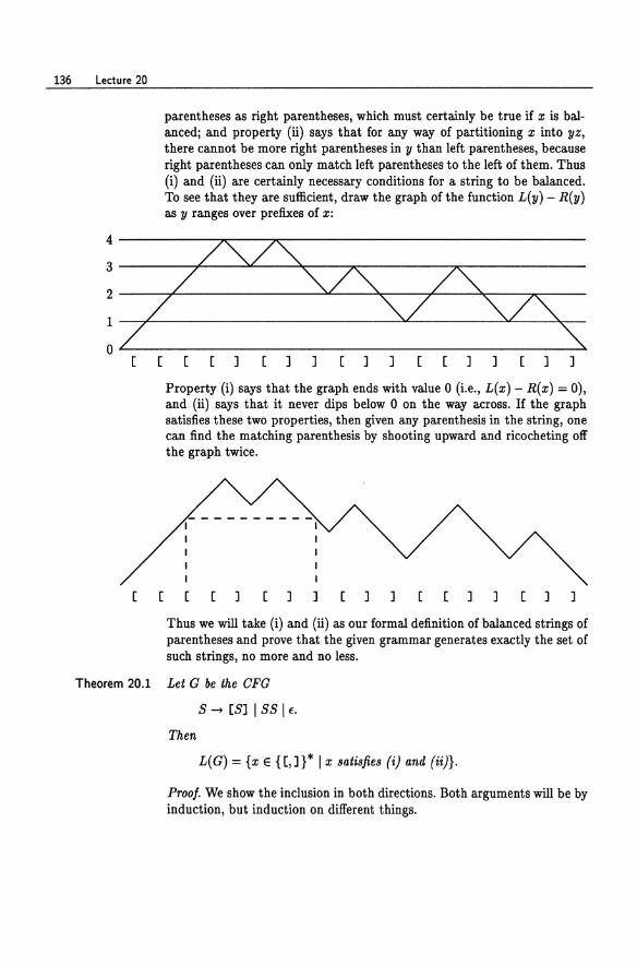
136 Lecture 20
parentheses as right parentheses, which must certainly be true if x is balanced; and property (ii) says that for any way of partitioning x into yz, there cannot be more right parentheses in y than left parentheses, because right parentheses can only match left parentheses to the left of them. Thus (i) and (ii) are certainly necessary conditions for a string to be balanced. To see that they are sufficient, draw the graph of the function L(y) - R(y) as y ranges over prefixes of x:
4----------~~--~----------------------------------
3--------~----~--~~--_,~--------~--------------
2 ----~r_----------------~----~----_r----~----~~----
1 ---r----------------------------~~----------~----~-
OL-------------------------------------------------~ [[ [[] []] []] [[]] ]]
[ [
Property (i) says that the graph ends with value 0 (Le., L(x) - R(x) = 0), and (ii) says that it never dips below 0 on the way across. H the graph satisfies these two properties, then given any parenthesis in the string, one can find the matching parenthesis by shooting upward and ricocheting off the graph twice.
[] []] []] [[] [ ] ]
Thus we will take (i) and (ii) as our formal definition of balanced strings of parentheses and prove that the given grammar generates exactly the set of such strings, no more and no less.
Theorem 20.1 Let G be the CPG
s -+ [S] I SS I f. Then
L( G) = {x E {[,]} * I x satisfies (i) and (ii)}.
Proof. We show the inclusion in both directions. Both arguments will be by induction, but induction on different things.
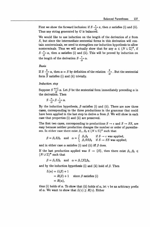
Balanced Parentheses 137
First we show the forward inclusion: if 8 ~ x, then x satisfies (i) and (ii). G
Thus any string generated by G is balanced.
We would like to use induction on the length of the derivation of x from 8, but since the intermediate sentential forms in this derivation will contain nonterminals, we need to strengthen our induction hypothesis to allow nonterminals. Thus we will actually show that for any Ct E (N U I:)*, if 8 ~ Ct, then Ct satisfies (i) and (ii). This will be proved by induction on
G
the length of the derivation 8 ~ o. G
Basis
If 8 ~ Ct, then Ct = 8 by definition of the relation ~. But the sentential G G
form 8 satisfies (i) and (ii) trivially.
Induction step
Suppose 8 ~ Ct. Let {3 be the sentential form immediately preceding Ct in G
the derivation. Then
8~{3~0. G G
By the induction hypothesis, {3 satisfies (i) and (ii). There are now three cases, corresponding to the three productions in the grammar that could have been applied in the last step to derive 0 from {3. We will show in each case that properties (i) and (ii) are preserved.
The first two cases, corresponding to productions 8 .... f and 8 .... 88, are easy because neither production changes the number or order of parentheses. In either case there exist {3l, {32 E (N U E)* such that
{ {3l{32 if 8 .... f was applied, {3 = {3l8{32 and 0 = {3l88{32 if 8 .... 88 was applied;
and in either case 0 satisfies (i) and (ii) iff {3 does.
If the last production applied was 8 .... [8], then there exist {31, {32 E (N U E)* such that
{3 = {31 8 {32 and 0 = {31 [8]{32,
and by the induction hypothesis (i) and (ii) hold of {3. Then
L(o) = L({3) + 1
= R({3) + 1 since {3 satisfies (i)
= R(o),
thus (i) holds of o. To show that (ii) holds of Ct, let, be an arbitrary prefix of o. We want to show that L(,) ~ R('Y). Either
138 Lectu re 20
• 'Y is a prefix of f3I, in which case 'Y is a prefix of f3, so (ii) holds for the prefix 'Y by the induction hypothesis; or
• 'Y is a prefix of f3I [8 but not of f3I, in which case
L( 'Y) = L(f3I) + 1
~ R(f3I) + 1 induction hypothesis, since f3I is a prefix of f3
> R(f3I) =R('Y); or
• 'Y = f3I [8]6, where 6 is a prefix of f32, in which case
L('Y) = L(f3I86) + 1
~ R(f3I86) + 1 induction hypothesis
= Rb)·
Thus in all cases L('Y) ~ Rb). Since 'Y was arbitrary, (ii) holds of 0:. This concludes the inductive proof that if 8 ~ x, then x is balanced.
G
Now we wish to show the other direction: if x is balanced, then 8 ~ x. G
This is done by induction on Ixl. Assume that x satisfies (i) and (ii).
Basis
If Ixl = 0, we have x = f and 8 ~ x in one step using the production G
8 -+ f.
Induction step
If Ixl > 0, we break the argument into two cases: either
(a) there exists a proper prefix y of x (one such that 0 < Iyl < Ixl) satisfying (i) and (ii), or
(b) no such prefix exists.
In case (a), we have x = yz for some z, 0 < Izl < lxi, and z satisfies (i) and (ii) as well:
L(z) = L(x) - L(y) = R(x) - R(y) = R(z),
and for any prefix w of z,
L(w) = L(yw) - L(y) ~ R(yw) - R(y) since yw is a prefix of x and L(y) = R(y)
= R(w).
Balanced Parentheses 139
By the induction hypothesis, 8 ~ V and 8 ~ z. Then we can derive x G G
by starting with the production 8 -+ 88, then deriving V from the first 8, then deriving z from the second 8:
1 • • 8 --+ 88 --+ V8 --+ vz = x.
G G G
In case (b), no such V exists. Then x = [z] for some z, and z satisfies (i) and (ti). It satisfies (i) since
L(z) = L(x) - 1 = R(x) - 1 = R(z),
and it satisfies (ii) since for all nonnull prefixes '1.£ of z,
L(u) - R(u) = L([u) -1- R([u) ~ 0
since L( ['1.£) - R( ['1.£) ~ 1 because we are in case (b). By the induction hypothesis, 8 ~ z. Combining this derivation with the production 8 -+
G [8], we get a derivation of x:
8~ [8] ~ [z] =x. G G
Thus every string satisfying (i) and (ii) can be derived. 0
Lecture 21
Normal Forms
For many applications, it is often helpful to assume that CFGs are in one or another special restricted form. Two of the most useful such forms are Chomsky normal form (CNF) and Greibach normal form (GNF).
Definition 21.1 A CFG is in Chomsky normal form (CNF) if all productions are of the form
A -+ BO or A -+ a,
where A, B, 0 E N and a E ~. A CFG is in Greibach normal form (GNF) if all productions are of the form
A -+ aB1B2 ••• B/c
for some k 2:: 0, where A, Bll ... ,B/c E N and a E ~. Note that k = 0 is allowed, giving productions of the form A -+ a. 0
For example, the two grammars
S -+ AB I AO ISS, 0 -+ SB,
S -+ [B I [SB I [BS I [SBS,
A-+ [,
B --+ J B -+ J, (21.1)
(21.2)
are grammars in Chomsky and Greibach normal form, respectively, for the set of all nonnull strings of balanced parentheses [ J .
No grammar in Chomsky or Greibach form can generate the null string €
(Why not?). Apart from this one exception, they are completely general:
Normal Forms 141
Theorem 21.2 Por any CPG G, there is a CPG G' in Chomsky normal form and a CPG G" in Greibach normal form such that
L(G") = L(G') = L(G) - {fl.
Getting Rid of f- and Unit Productions
To prove Theorem 21.2, we must first show how to get rid of all f-productions A --. f and unit productions A --. B. These productions are bothersome because they make it hard to determine whether applying a production makes any progress toward deriving a string of terminals. For instance, with unit productions, there can be loops in the derivation, and with f
productions, one can generate very long strings of nonterminals and then erase them all. Without f- or unit productions, every step in the derivation makes demonstrable progress toward the terminal string in the sense that either the sentential form gets strictly longer or a new terminal symbol appears.
We cannot simply throw out the f- and unit productions, because they may be needed to generate some strings in L(G)j so before we throw them out, we had better throw in some other productions we can use instead.
Lemma 21.3 Por any CPG G = (N, ~, P, S), there is a CPG G' with no f- or unit productions such that L( G') = L( G) - {f}.
Proof. Let P be the smallest set of productions containing P and closed under the two rules
(a) if A --. a.B/3 and B --. e are in P, then A --. a./3 is in Pj and
(b) if A --. B and B --. 'Yare in P, then A --. 'Y is in P.
We can construct P inductively from P by adding productions as required to satisfy (a) and (b). Note that only finitely many productions ever get added, sinc~ each new right-hand side is a substring of an old right-hand side. Thus P is still finite.
Now let G be the grammar
G = (N, ~, P, S).
Since P ~ P, every derivation of G is a derivation of Gj thus L( G) ~ L( G). But L(G) = L(G), since each new production that was thrown in because of rule (a) or (b) can be simulated in two steps by the two productions that caused it to be thrown in.
142 Lecture 21
N ow we show that for nonnull x E ~*, any derivation S ...;.. x of mini-G
mum length does not use any f- or unit productions. Thus the f- and unit productions are superfluous and can be deleted from G with impunity.
Let x =f. f and consider a minimum-length derivation S ...;.. x. Suppose for G
a contradiction that an f-production B -+ f is used at some point in the derivation, say
• f: 1 f:. S~'YBu ~'Yu ~x. G G G
One of 'Y, 0 is nonnuil, otherwise x would be null, contradicting the assumption that it isn't. Thus that occurrence of B must first have appeared earlier in the derivation when a production of the form A -+ OI.B/3 was applied:
S~~A9~~OI.B/39~'YBo~~~x G G G G G
for some m, n, k ~ O. But by rule (a), A -+ 01./3 is also in P, and this production could have been applied at that point instead, giving a strictly shorter derivation of x:
S ~ ~A9 ~ 1J0I./39 ~ 'Yo ~ x. G G G G
This contradicts our assumption that the derivation was of minimum length.
A similar argument shows that unit productions do not appear in minimumlength derivations in G. Let x =f: f and consider a derivation S ...;.. x of
G minimum length. Suppose a unit production A -+ B is used at some point, say
• A 1 /3. S~OI. /3~OI.B ~x. G G G
We must eventually dispose of that occurrence of B, say by applying a production B -+ 'Y later on.
mAl n 1 ilk S~OI. /3~OI.B/3~~B9~~'YIl~x.
G G G G G
But by rule (b), A -+ 'Y is also in P, and this could have been applied instead, giving a strictly shorter derivation of x:
S ~ OI.A/3 ~ 0I.'Y/3 ~ ~'Y9 ~ x. G G G G
Again, this contradicts the minimality of the length of the derivation.
Thus we do not need f-productions or unit productions to generate nonnull strings. If we discard them from G, we obtain a grammar G' generating L(G) - {fl. 0
Normal Forms 143
Chomsky Normal Form
Once we are rid of E- and unit productions, it is a simple matter to put the resulting grammar into Chomsky normal form. For each terminal a E E, introduce a new nonterminal Aa and production Aa -+ a, and replace all occurrences of a on the right-hand sides of old productions (except productions of the form B -+ a) with Aa. Then all productions are of the form
A -+ a or A -+ B1B2 ... Bk, k 2::: 2,
where the Bo are nonterminals. The set of terminal strings generated is not changed; it just takes one more step than before to generate a terminal symbol. For any production
A -+ B1B2··· Bk
with k 2::: 3, introduce a new nonterminal C and replace this production with the two productions
A -+ B1C and C -+ B2B3··· Bk.
Keep doing this until all right-hand sides are of length at most 2.
Example 21.4 Let's derive a CNF grammar for the set
{aRb" In 2::: O} - {E} = {anbn In 2::: I}.
Starting with the grammar
S -+ aSb I E
for {anbn I n 2::: O}, we remove the E-production as described in Lemma 21.3 to get
S -+ aSb lab,
which generates {anbn I n 2::: I}. Then we add nonterminals A, Band replace these productions with
S-+ ASB lAB, A-+a, B -+ b.
Finally, we add a nonterminal C and replace S -+ ASB with
S -+ AC and C -+ SB.
The final grammar in Chomsky form is
S-+AB lAC, C -+ SB, A-+ a, B -+ b. o Example 21.5 We derive a CNF grammar for the set of nonnull strings of balanced paren
theses [ ]. Start with the grammar
S -+ [S] I SS I E
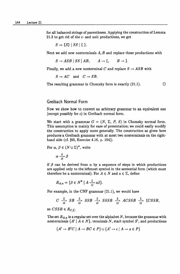
144 Lecture 21
for all balanced strings of parentheses. Applying the construction of Lemma 21.3 to get rid of the e- and unit productions, we get
S ~ [S] I SS I [].
Next we add new nonterminals A, B and replace these productions with
S ~ ASB I SS lAB, A~ [, B~].
Finally, we add a new nonterminal G and replace S ~ ASB with
S~AG and G~SB.
The resulting grammar in Chomsky form is exactly (21.1). o
Greibach Normal Form
Now we show how to convert an arbitrary grammar to an equivalent one (except possibly for e) in Greibach normal form.
We start with a grammar G = (N, ~, P, S) in Chomsky normal form. This assumption is mainly for ease of presentation; we could easily modify the construction to apply more generally. The construction as given here produces a Greibach grammar with at most two nonterminals on the righthand side (cf. [60, Exercise 4.16, p. 104)).
For 0:, f3 E (N U ~)*, write
L 0: --+ f3
G
if f3 can be derived from 0: by a sequence of steps in which productions are applied only to the leftmost symbol in the sentential form (which must therefore be a nonterminal). For A E N and a E ~, define
RA,1l = {f3 E N* I A 1: af3}.
For example, in the CNF grammar (21.1), we would have
G ~ SB ~ SSB G G
so GSSB E Ro,[.
~ SSSB G
~ AGSSB G
L --+ G
[CSSB,
The set RA,Il is a regular set over the alphabet N, because the grammar with nonterminals {A'l A E N}, terminals N, start symbol S', and productions
{A' ~ B'G I A ~ BG E P} U {A' ~ e I A ~ a E P}
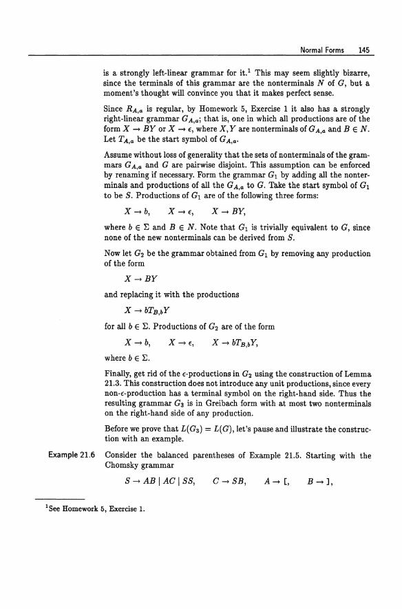
Normal Forms 145
is a strongly left-linear grammar for it.1 This may seem slightly bizarre, since the terminals of this grammar are the nonterminals N of G, but a moment's thought will convince you that it makes perfect sense.
Since RA,a is regular, by Homework 5, Exercise 1 it also has a strongly right-linear grammar G A,a; that is, one in which all productions are of the form X - BY or X - f, where X, Y are nonterminals of G A,a and BEN. Let T A,a be the start symbol of G A,a.
Assume without loss of generality that the sets of nonterminals of the grammars G A,a and G are pairwise disjoint. This assumption can be enforced by renaming if necessary. Form the grammar G1 by adding all the nonterminals and productions of all the G A,a to G. Take the start symbol of Gl to be S. Productions of G1 are of the following three forms:
X-b, X-f, X-BY,
where b E ~ and BEN. Note that G1 is trivially equivalent to G, since none of the new nonterminals can be derived from S.
Now let G2 be the grammar obtained from G1 by removing any production of the form
X-BY
and replacing it with the productions
X -bTB,bY
for all b E ~. Productions of G2 are of the form
X-b,
where b E~.
X-f,
Finally, get rid of the f-productions in G2 using the construction of Lemma 21.3. This construction does not introduce any unit productions, since every non-f-production has a terminal symbol on the right-hand side. Thus the resulting grammar Ga is in Greibach form with at most two nonterminals on the right-hand side of any production.
Before we prove that L(Ga) = L(G), let's pause and illustrate the construction with an example.
Example 21.6 Consider the balanced parentheses of Example 21.5. Starting with the Chomsky grammar
S - AB I AC ISS, C-SB, A- [, B-1,
1 See Homework 5, Exercise 1.
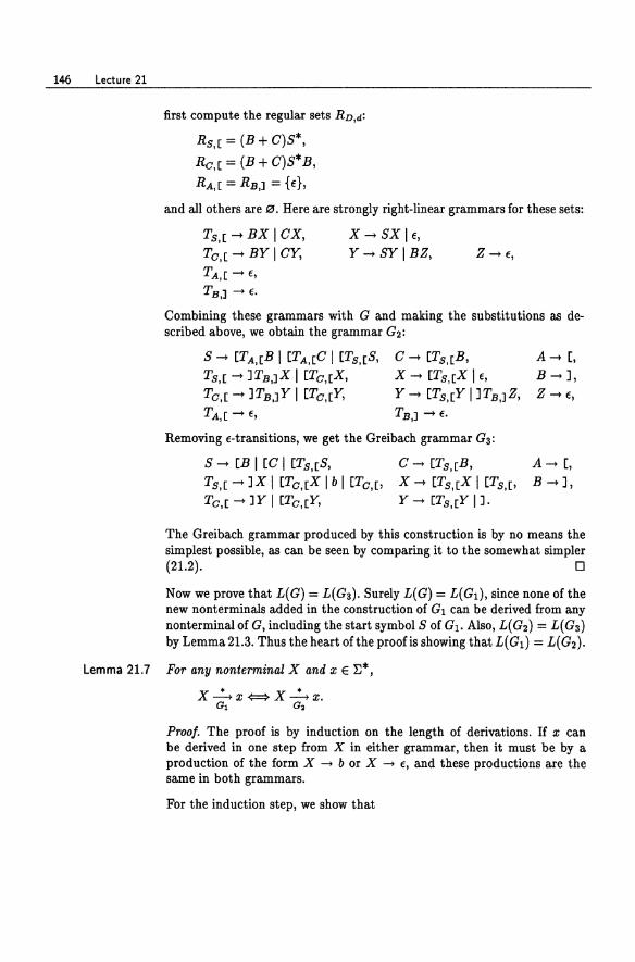
146 Lecture 21
first compute the regular sets RD,d:
Rs,[ = (B + O)S*,
Ro,[ = (B + O)S*B,
RA ,[ = RB ,] = {f}, and all others are 0. Here are strongly right-linear grammars for these sets:
Ts,[ - BX lOX, To,[ - BY I OY,
TA ,[ - f,
TB ,] - f.
X-SXIE, Y_SYIBZ, Z-E,
Combining these grammars with G and making the substitutions as described above, we obtain the grammar G2:
S - [TA,[B I [TA,[O I [Ts,[S, Ts,[ - ]TB,]X I [To, [X, To,[ - ]TB,]Y I [To,[Y,
TA ,[ - f,
0- [Ts,[B,
X - [Ts,[X I E,
Y - [Ts,[Y I ] TB,]Z,
TB,] - E.
Removing E-transitions, we get the Greibach grammar G3 :
S - [B I [C I [Ts,[S, Ts,[ -]X I [To,[X I b I [To,[, To,[ - lY I [To,[Y,
0-+ [Ts,[B, X -+ [Ts,[X I [TS ,[,
Y - [Ts,[Y I 1.
A- [, B-], Z-E,
A- [, B-J,
The Greibach grammar produced by this construction is by no means the simplest possible, as can be seen by comparing it to the somewhat simpler (21.2). 0
Now we prove that L(G) = L(Ga). Surely L(G) = L(Gl)' since none of the new nonterminals added in the construction of Gl can be derived from any nonterminal of G, including the start symbol S of GI • Also, L(G2) = L(G3)
by Lemma 21.3. Thus the heart of the proofis showing that L(Gt} = L(G2}.
Lemma 21.7 For any nonterminal X and x E E*,
X ~ x {:::} X ~ X. Gl G3
Proof. The proof is by induction on the length of derivations. If x can be derived in one step from X in either grammar, then it must be by a production of the form X - b or X - E, and these productions are the same in both grammars.
For the induction step, we show that
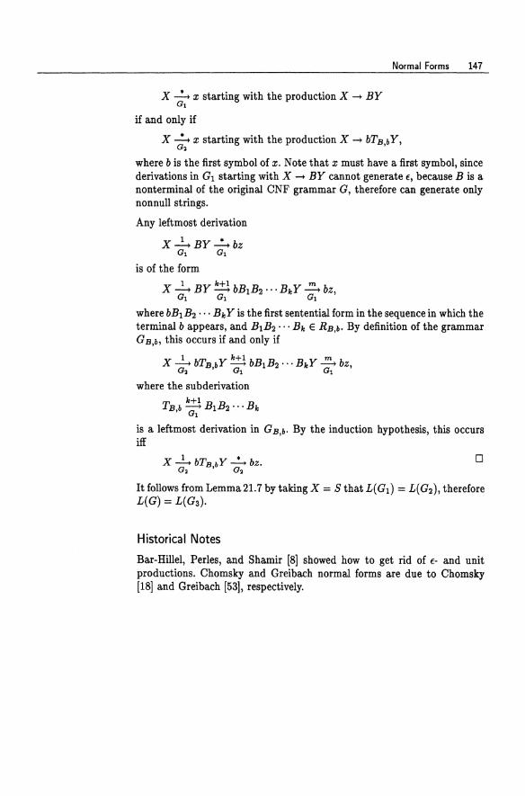
x ...!.... x starting with the production X -+ BY G,
if and only if
Normal Forms 147
X * x starting with the production X -+ bTB,bY,
where b is the first symbol of x. Note that x must have a first symbol, since derivations in G1 starting with X -+ BY cannot generate f, because B is a nonterminal of the original CNF grammar G, therefore can generate only nonnull strings.
Any leftmost derivation
X~BY...!....bz G, G,
is of the form 1 k+l m X ---+ BY ---+ bBIB2 ... BkY ---+ bz,
Gl Gl Gl
where bB1B2 ... BkY is the first sentential form in the sequence in which the terminal b appears, and BIB2 ... Bk E RB,b' By definition of the grammar G B,b, this occurs if and only if
1 k+l m X ---+ bTB bY ---+ bB1B2 ... B"Y ---+ bz,
G2 ' G, G,
where the subderivation
TBb ~BIB2···B" , G,
is a leftmost derivation in GB,b' By the induction hypothesis, this occurs iff
o
It follows from Lemma 21.7 by taking X = S that L(G1) = L(G2), therefore L(G) = L(Ga).
Historical Notes
Bar-Hillel, Perles, and Shamir [8] showed how to get rid of f- and unit productions. Chomsky and Greibach normal forms are due to Chomsky [18] and Greibach [53], respectively.
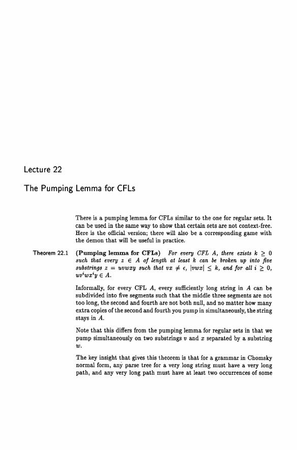
Lecture 22
The Pumping Lemma for CFLs
There is a pumping lemma for CFLs similar to the one for regular sets. It can be used in the same way to show that certain sets are not context-free. Here is the official version; there will also be a corresponding game with the demon that will be useful in practice.
Theorem 22.1 (Pwnping lemma for CFLs) For every CFL A, there exists k ;:: 0 such that every z e A of length at least k can be broken up into five substrings z = uvwxy such that vx :1= e, Ivwxl :5 k, and for all i ;:: 0, uv'wxiye A.
Informally, for every CFL A, every sufficiently long string in A can be subdivided into five segments such that the middle three segments are not too long, the second and fourth are not both null, and no matter how many extra copies of the second and fourth you pump in simultaneously, the string stays in A.
Note that this differs from the pumping lemma for regular sets in that we pump simultaneously on two substrings v and x separated by a substring w.
The key insight that gives this theorem is that for a grammar in Chomsky nor~al form, any parse tree for a very long string must have a very long path, and any very long path must have at least two occurrences of some
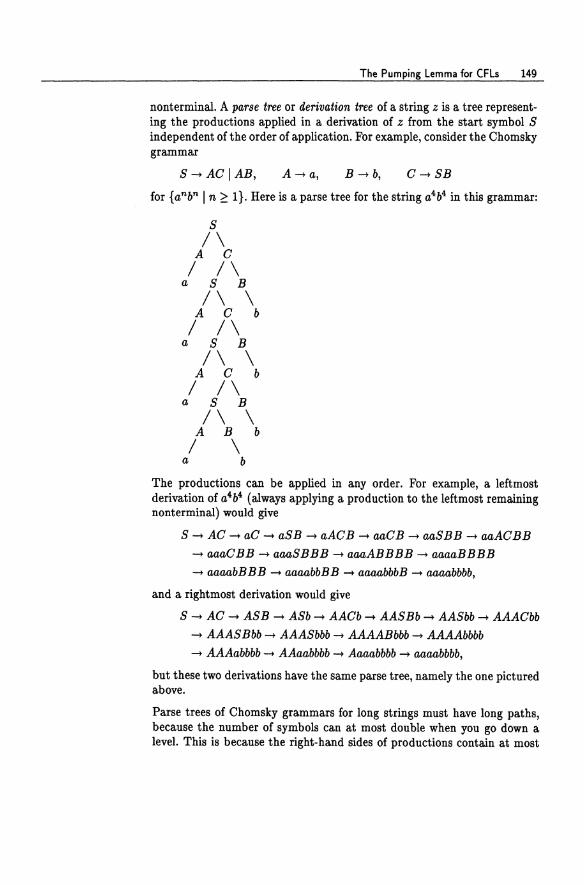
The Pumping Lemma for CFLs 149
nonterminal. A parse tree or derivation tree of a string z is a tree representing the productions applied in a derivation of z from the start symbol S independent of the order of application. For example, consider the Chomsky grammar
S~AGIAB, A~a, B~b, G~SB
for {anbn I n ~ 1}. Here is a parse tree for the string a4b4 in this grammar:
S
/\ A G
/ /\ a S B
/\ \ A G b
/ /\ a S B
/\ \ A G b
/ /\ a S B
/\ \ A B b
/ \ a b
The productions can be applied in any order. For example, a leftmost derivation of a4b4 (always applying a production to the leftmost remaining nonterminal) would give
S ~ AG ~ aG ~ aSB ~ aAGB ~ aaGB ~ aaSBB ~ aaAGBB
~ aaaGBB ~ aaaSBBB ~ aaaABBBB ~ aaaaBBBB
~ aaaabBBB ~ aaaabbBB ~ aaaabbbB ~ aaaabbbb,
and a rightmost derivation would give
S ~ AG ~ ASB ~ ASb ~ AAGb --> AASBb ~ AASbb ~ AAAGbb
~ AAASBbb ~ AAASbbb ~ AAAABbbb ~ AAAAbbbb
~ AAAabbbb ~ AAaabbbb ~ Aaaabbbb ~ aaaabbbb,
but these two derivations have the same parse tree, namely the one pictured above.
Parse trees of Chomsky grammars for long strings must have long paths, because the number of symbols can at most double when you go down a level. This is because the right-hand sides of productions contain at most
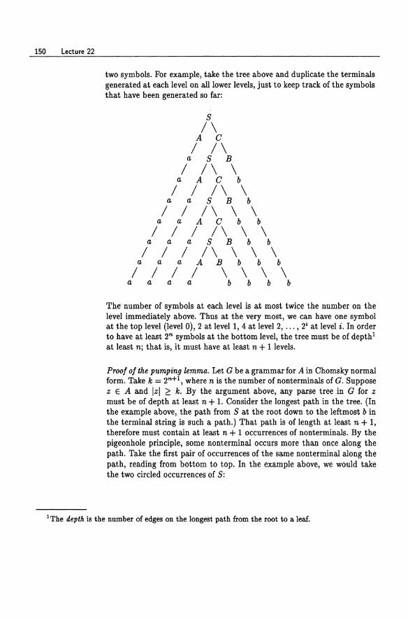
150 Lecture 22
two symbols. For example, take the tree above and duplicate the terminals generated at each level on all lower levels, just to keep track of the symbols that have been generated so far:
s /\
A c / /\
a S B
/ /\ \ a A C b
/ / /\ \ a a S B b
/ / /\ \ \ a a A C b b
/ / / /\ \ \ a a a S B b b
/ / / /\ \ \ \ a a a A B b b b
/ / / / \ \ \ \ a a a a b b b b
The' number of symbols at each level is at most twice the number on the level immediately above. Thus at the very most, we can have one symbol at the top level (level 0), 2 at levell, 4 at level 2, ... , 2' at level i. In order to have at least 2" symbols at the bottom level, the tree must be of depth 1
at least nj that is, it must have at least n + 1 levels.
Proof of the pumping lemma. Let G be a grammar for A in Chomsky normal form. Take k = 2"+1, where n is the number of nonterminals of G. Suppose z E A and Izl ;::: k. By the argument above, any parse tree in G for z must be of depth at least n + 1. Consider the longest path in the tree. (In the example above, the path from S at the root down to the leftmost b in the terminal string is such a path.) That path is of length at least n + 1, therefore must contain at least n + 1 occurrences of nonterminals. By the pigeonhole principle, some nonterminal occurs more than once along the path. Take the first pair of occurrences of the same nonterminal along the path, reading from bottom to top. In the example above, we would take the two circled occurrences of S:
IThe depth is the number of edges on the longest path from the root to a leaf.
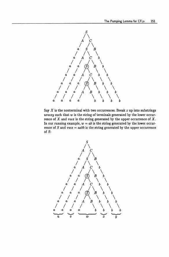
The Pumping Lemma for CFLs 151
s /\
A C / /\
a S B / /\ \
a A C b
/ / /\ \ / / ~ B\ \
a a A ebb / / / /\ \ \
/ / / ~ B\ \ \ a a a A B b b b
/ / / / \\\\ a a a a b b b b
Say X is the nonterminal with two occurrences. Break z up into substrings 1I.vw:cy such that w is the string of terminals generated by the lower occurrence of X and vwx is the string generated by the upper occurrence of X. In our running example, w = ab is the string generated by the lower occurrence of Sand vwx = aabb is the string generated by the upper occurrence of S:
S /\
A C
/ /\ a S B
/ /\ \ a A C b
/ / /\ \ / / ~ B\ \
a a A ebb / / / /\ \ \
/ / / ~ B\ \ \ a a a A B b b b
/ / / / \\\\ a a a a b b b b --..,....... --.,., ---.......-- --.,., --..,.......
1£ V W X Y
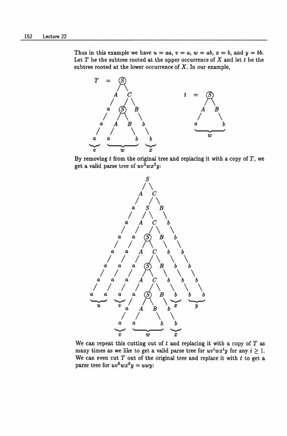
152 Lecture 22
Thus in this example we have u = aa, v = a, W = ab, x = b, and y = bb. Let T be the subtree rooted at the upper occurrence of X and let t be the subtree rooted at the lower occurrence of X. In our example,
T =1\ A 0 t =1\ / /\
/ 1\ B\ A B
/ \ a A B b a b
/ / \ \ '-----v----"' a a b b
W
---.,..,. '-----v----"' ---.,..,. v W x
By removing t from the original tree and replacing it with a copy of T, we get a valid parse tree of uv2wx2y:
s /\
A 0 / /\
a S B
/ /\ \ a A 0 b
/ / /\ \ a a ~ B b
/ / /\ \ \ a a A 0 b b
/ / / /\ \ \ / / / 1\ B\ \ \
a a a A 0 b b b
/ / / / /\ \ \ \ a a a a~B b b b --.,- ---.,..,. / /\ \ ---.,..,. --.,-
u v a A B b x y
/ / \ \ a a b b
---.,..,. '-----v----"' ---.,..,. v w x
We can repeat this cutting out of t and replacing it with a copy of T as many times as we like to get a valid parse tree for UViW:ciy for any i ;::: 1. We can even cut T out of the original tree and replace it with t to get a parse tree for uvOwxOy = uwy:
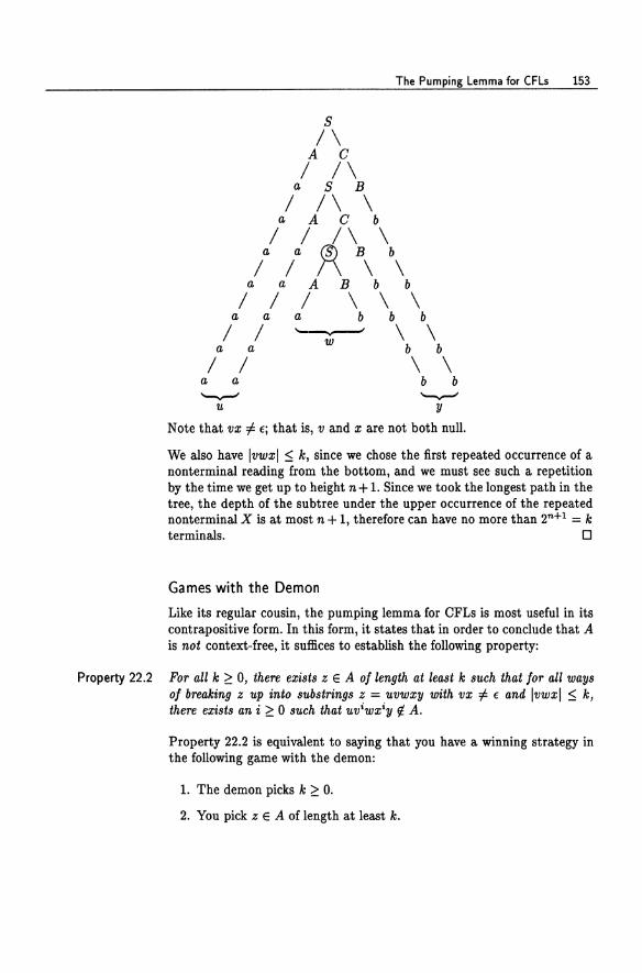
The Pumping Lemma for CFLs 153
s /\
A c / /\
a S B
/ /\ \ a A C b
/ / /\ \ a a 1\ B b
/ / \ \ a a A B b b
/ / / \ \ \ a a a b b b
/ / ~ \ \ w a a b b / / \ \
a a b b ~ ~
u y
Note that vx =f. €; that is, v and x are not both null.
We also have Ivwxl :5 k, since we chose the first repeated occurrence of a nonterminal reading from the bottom, and we must see such a repetition by the time we get up to height n + 1. Since we took the longest path in the tree, the depth of the subtree under the upper occurrence of the repeated nonterminal X is at most n + 1, therefore can have no more than 2n+1 = k terminals. 0
Games with the Demon
Like its regular cousin, the pumping lemma for CFLs is most useful in its contrapositive form. In this form, it states that in order to conclude that A is not context-free, it suffices to establish the following property:
Property 22.2 For all k ~ 0, there exists z E A of length at least k such that for all ways of breaking z up into substrings z = uvwxy with vx # f and Ivwxl :5 k, there exists an i ~ 0 such that uviwxiy ~ A.
Property 22.2 is equivalent to saying that you have a winning strategy in the following game with the demon:
1. The demon picks k ~ O.
2. You pick z E A of length at least k.
154 Lecture 22
3. The demon picks strings U,v,w,x,y such that z = uvwxy, Ivxl > 0, and Ivwxl :5 k.
4. You pick i ~ O. If uv'wx'y ¢ A, then you win.
If you want to show that a given set A is not context-free, it suffices to show that you have a winning strategy in this gamej that is, no matter what the demon does in steps 1 and 3, you have moves in steps 2 and 4 that can beat him.
Example 22.3 Let's use the pumping lemma to show that the set
A = {a"b"a" I n ~ O}
is not context-free. We'll do this by showing that we can always win the game with the demon.
Say the demon picks k in step 1. You have to argue that you can win no matter what k is. A good choice for you in step 2 is to pick z = alcbloalo . Then z E A and Izl = 3k ~ k. Then in step 3, say the demon picks u, v, w, x, Y such that z = uvwxy, vx '" to, and Ivwxl :5 k. You pick i = 2. In every case, you win: if the demon picked either v or x to contain at least one a and at least one b, then uv2wx2y is not of the form a*b*a*, hence certainly not in Aj if the demon picked v and x to contain only a's, then uv2wx2y has more than twice as many a's as b's, hence is not in Aj if the demon picked v and x to contain only b's, then uv2wx2y has fewer than twice as many a's as b's, hence is not in Aj and finally, if one of v or x contains only a's and the other contains only b's, then uv2wx2y cannot be of the form ambmam, hence is not in A. In all cases you can ensure uv2wx2y ¢ A, so you have a winning strategy. By the pumping lemma, A is not context-free. 0
Example 22.4 Let's use the pumping lemma to show that the set
A = {ww I we {a,b}*}
is not context-free. Since the family of CFLs is closed under intersection with regular sets (Homework 7, Exercise 2), it suffices to show that the set
A' = An L(a*b*a*b*)
= {a"bma"bm I m,n ~ O}
is not context-free.
Say the demon picks k. You pick z = alobkaloblo • Call each of the four substrings of the form ak or bk a block. Then zEA' and Izl ~ k. Say the demon picks u,v,w,x,y such that z = uvwxy, vx '" f, and Ivwxl < k. No matter what the demon does, you can win by picking i = 2:
The Pumping Lemma for CFLs 155
• If one of v or x contains both a's and b's (i.e., if one of v or x straddles a block boundary), then 'UV2wx2y is not of the form a*b*a*b*, thus is not in A'.
• If v and x are both from the same block, then 'Uv2wx2y has one block longer than the other three, therefore is not in A'.
• If v and x are in different blocks, then the blocks must be adjacentj otherwise Ivwxl would be greater than k. Thus one of the blocks containing v or x must be a block of a's and the other a block of b's. Then 'UV2wx2y has either two blocks of a's of different size (if vx contains an a) or two blocks of b's of different size (if vx contains a b) or both. In any case, 'Uv2wx2y is not of the form an bmanbm .
Since you can always ensure a win by playing this strategy, A' (and therefore A) is not a CFL by the pumping lemma.
Surprisingly, the complement of A, namely
{a,b}* - {ww I wE {a,b}*},
is a CFL. Here is a CFG for it:
S -+ AB I BA I A I B,
A-+ CACI a, B -+ CBC I b,
C -+ a lb. This grammar generates
(i) all strings of odd length (starting with productions S -+ A and S -+ B)j or
(ii) strings of the form xay'Ubv or 'Ubvxay, where X,y,'U,V E {a,b}*, Ixl = IYI, and 1'1£1 = Ivl·
The nonterminal A generates all strings of the form xay, Ixl = Iyl. The nonterminal B generates all strings of the form 'Ubv, 1'1£1 = Ivl. No string of the form (i) can be of the form ww, since ww is always of even length. No string of the form (ii) can be of the form ww, since there are occurrences of a and b separated by a distance of n/2, where n is the length of the string.
This example shows that the family of CFLs is not closed under complement. 0
Note that in both these examples, your choice of i = 2 in step 4 was independent of the demon's move in step 3. This may not always be possible! However, keep in mind that you have the freedom to pick i in step 4 after you have seen what the demon did in step 3.
156 Lecture 22
Historical Notes
The pumping lemma for CFLs is due to Bar-Hillel, Perles, and Shamir [8). A somewhat stronger version was given by Ogden [96).
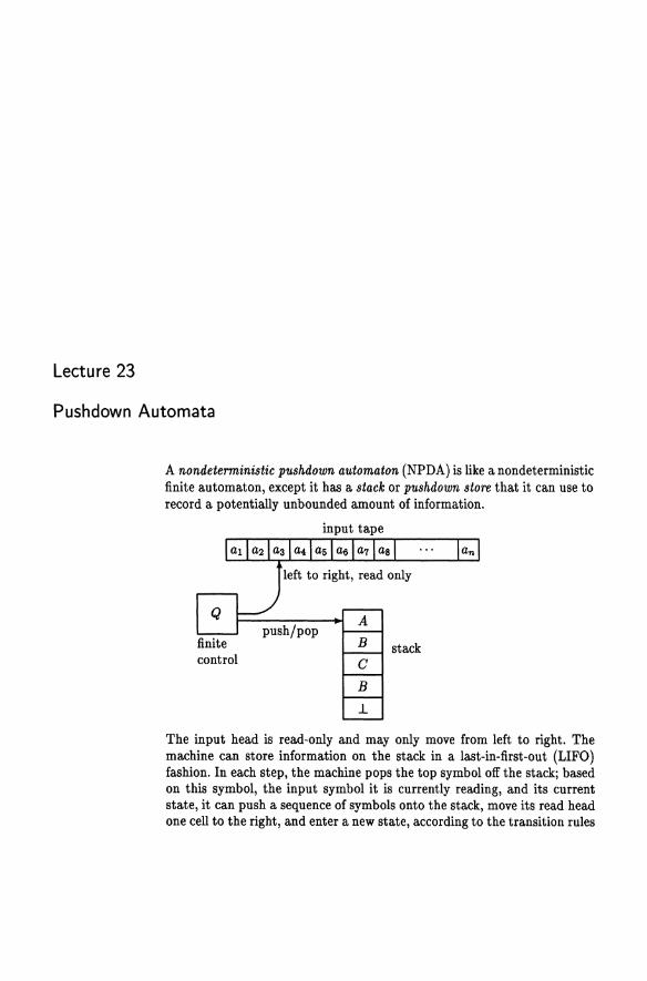
Lecture 23
Pushdown Automata
A nondeterministic pushdown automaton (NPDA) is like a nondeterministic finite automaton, except it has a stack or pushdown store that it can use to record a potentially unbounded amount of information.
finite control
B
C
B
1.
stack
The input head is read-only and may only move from left to right. The machine can store information on the stack in a last-in-first-out (LIFO) fashion. In each step, the machine pops the top symbol off the stack; based on this symbol, the input symbol it is currently reading, and its current state, it can push a sequence of symbols onto the stack, move its read head one cell to the right, and enter a new state, according to the transition rules
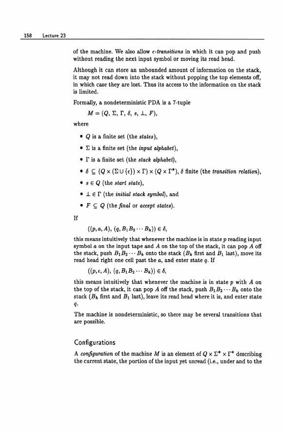
158 Lectu re 23
of the machine. We also allow E-transitions in which it can pop and push without reading the next input symbol or moving its read head.
Although it can store an unbounded amount of information on the stack, it may not read down into the stack without popping the top elements off, in which case they are lost. Thus its access to the information on the stack is limited.
Formally, a nondeterministic PDA is a 7-tuple
M = (Q, E, r, 0, s, .L, F),
where
• Q is a finite set (the states),
• E is a finite set (the input alphabet),
• r is a finite set (the stack alphabet),
• 6 l:;; (Q x (E U {E}) x r) x (Q x r*), 6 finite (the transition relation),
• seQ (the start state),
• .L e r (the initial stack symbo~, and
• F l:;; Q (the final or accept states).
If
«p,a,A), (q,B1B2···B,,)) e 0, this means intuitively that whenever the machine is in state p reading input symbol a on the input tape and A on the top of the stack, it can pop A off the stack, push BIB2 ... B" onto the stack (B" first and Bl last), move its read head right one cell past the a, and enter state q. If
(P,E,A), (q,B1B2'" B,,)) e 6,
this means intuitively that whenever the machine is in state p with A on the top of the stack, it can pop A off the stack, push B1B2'" B" onto the stack (B" first and Bl last), leave its read head where it is, and enter state q.
The machine is nondeterministic, so there may be several transitions that are possible.
Configu rations
A configuration of the machine M is an element of Q x E* x r* describing the current state, the portion of the input yet unread (Le., under and to the
Pushdown Automata 159
right of the read head), and the current stack contents. A configuration gives complete information about the global state of M at some point during a computation. For example, the configuration
(p, baaabba, ABAC.1)
might describe the situation
C
.1
The portion of the input to the left of the input head need not be represented in the configuration, because it cannot affect the computation from that point on. In general, the set of configurations is infinite.
The start configuration on input x is (s,x, .1). That is, the machine always starts in its start state s with its read head pointing to the leftmost input symbol and the stack containing only the symbol .L.
The next configuration relation ..2... describes how the machine can move M
from one configuration to another in one step. It is defined formally as follows: if
((p,a,A), (q,'Y)) e 6,
then for any y e 1:* and f3 e r* , 1
(p,ay,Af3) 7 (q,y,'Yf3);
and if
((P,E,A), (q,'Y)) e 6,
then for any y e 1:* and f3 e r*,
(p,y,Af3) -if (q,y,'Yf3).
(23.1)
(23.2)
In (23.1), the ay changed to y, indicating that the input symbol a was eaten; the Af3 changed to 'Yf3, indicating that the A was popped and 'Y was pushed; and the p changed to q, indicating the change of state. In (23.2),
160 Lectu re 23
everything is the same except that the y does not change, indicating that no input symbol was eaten. No two configurations are related by 2.... unless
M required by (23.1) or (23.2).
Define the relations ~ and M
C~D~C=D, M
• ---+ M
as follows:
C ~ D ~ :IE C ~ E and E 2.... D, M M M
C~D~:ln>OC~D. M - M
Then ~ is the reflexive transitive closure of 2..... In other words, C ~ D M M M
if the configuration D follows from the configuration C in zero or more steps of the next configuration relation 2.....
M
Acceptance
There are two alternative definitions of acceptance in common use: by empty stack and by final state. It turns out that it doesn't matter which definition we use, since each kind of machine can simulate the other.
Let's consider acceptance by final state first. Informally, the machine M is said to accept its input x by final state if it ever enters a state in F after scanning its entire input, starting in the start configuration on input x. Formally, M accepts x by final state if
(s,x,..L) ~ (q,€,'Y) M
for some q E F and 'Y E r*. In the right-hand configuration, € is the null string, signifying that the entire input has been read, and 'Y is junk left on the stack.
Informally, M is said to accept its input x by empty stack if it ever pops the last element off the stack without pushing anything back on after reading the entire input, starting in the start configuration on input x. Formally, M accepts x by empty stack if
(s,x,..L) 7 (q,f,f)
for some q E Q. In this definition, the q in the right-hand configuration can be any state whatsoever, and the € in the second and third positions indicate that the entire input has been read and the stack is empty, respectively. Note that F is irrelevant in the definition of acceptance by empty stack.
The two different forms of automata can simulate each other (see Lecture E)j thus it doesn't matter which one we work with.
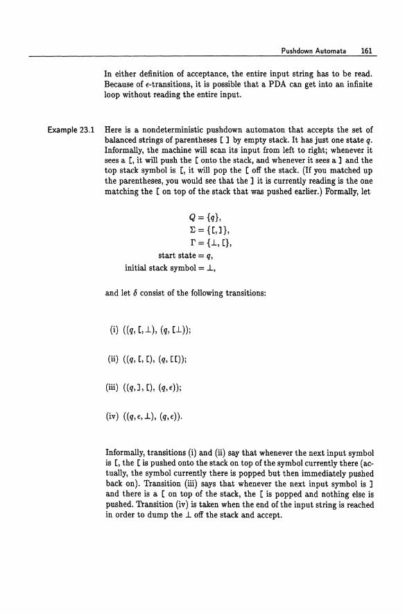
Pushdown Automata 161
In either definition of acceptance, the entire input string has to be read. Because of E-transitions, it is possible that a PDA can get into an infinite loop without reading the entire input.
Example 23.1 Here is a nondeterministic pushdown automaton that accepts the set of balanced strings of parentheses [ ] by empty stack. It has just one state q. Informally, the machine will scan its input from left to right; whenever it sees a [, it will push the [ onto the stack, and whenever it sees a] and the top stack symbol is [, it will pop the [ off the stack. (If you matched up the parentheses, you would see that the ] it is currently reading is the one matching the [ on top of the stack that was pushed earlier.) Formally, let
Q = {q}, ~={[,]},
r = {.1, [},
start state = q,
initial stack symbol = .1,
and let 6 consist of the following transitions:
(i) ((q, [, .i), (q, [.i));
(li) «q, [, E), (q, [[));
(iii) «q,], E), (q,En;
(iv) «q, 10, .i), (q, En.
Informally, transitions (i) and (ii) say that whenever the next input symbol is [, the [ is pushed onto the stack on top of the symbol currently there (actually, the symbol currently there is popped but then immediately pushed back on). Transition (iii) says that whenever the next input symbol is ] and there is a [ on top of the stack, the [ is popped and nothing else is pushed. Transition (iv) is taken when the end of the input string is reached in order to dump the .1 off the stack and accept.
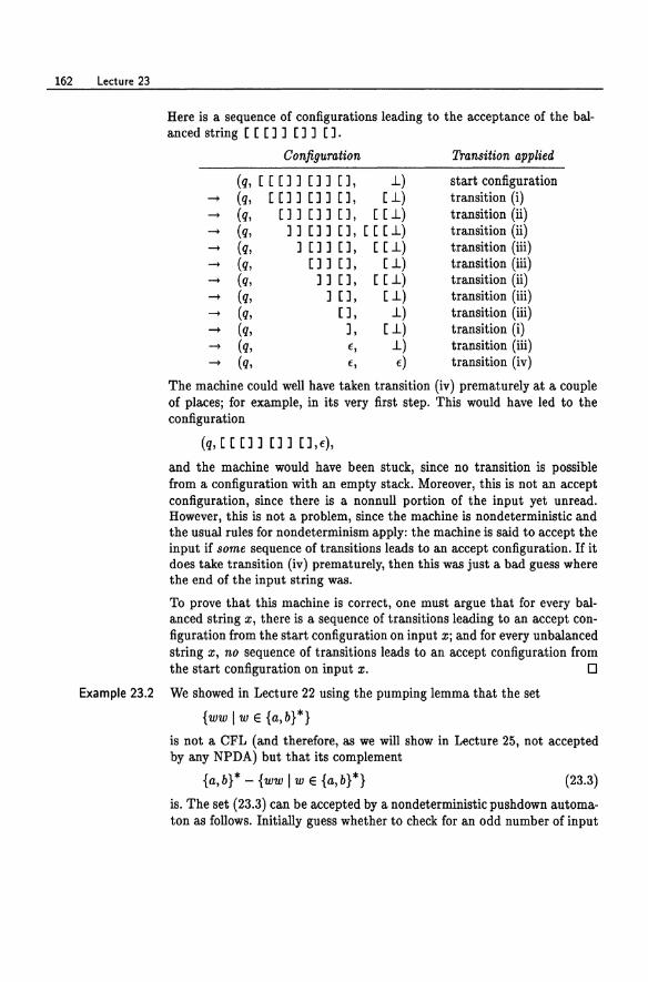
162 Lecture 23
Here is a sequence of configurations leading to the acceptance of the bal-anced string [ [ []] [] ] [].
Configuration Transition applied
(q, [[ []] []] [J, .L) start configuration -+ (q, [[]][]][], [ .L) transition (i) -+ (q, []] [] J [J, [ [.L) transition (ii) -+ (q, ]] [] ] [], [ [ [ 1.) transition (ii) -+ (q, J []J [J, [ [.L) transition (iii) -+ (q, []] [], [ .L) transition (iii) -+ (q, ] ] [], [ [1.) transition (ii) -+ (q, ] [], [ .L) transition (iii) -+ (q, [], .L) transition (iii) -+ (q, J, [ .L) transition (i) -+ (q, f, .L) transition (iii) -+ (q, f, f) transition (iv)
The machine could well have taken transition (iv) prematurely at a couple of placesj for example, in its very first step. This would have led to the configuration
(q, [[ []] [] J [],f),
and the machine would have been stuck, since no transition is possible from a configuration with an empty stack. Moreover, this is not an accept configuration, since there is a nonnull portion of the input yet unread. However, this is not a problem, since the machine is nondeterministic and the usual rules for nondeterminism apply: the machine is said to accept the input if some sequence of transitions leads to an accept configuration. If it does take transition (iv) prematurely, then this was just a bad guess where the end of the input string was.
To prove that this machine is correct, one must argue that for every balanced string x, there is a sequence of transitions leading to an accept configuration from the start configuration on input Xj and for every unbalanced string x, no sequence of transitions leads to an accept configuration from the start configuration on input x. 0
Example 23.2 We showed in Lecture 22 using the pumping lemma that the set
{ww I we {a,b}*}
is not a eFL (and therefore, as we will show in Lecture 25, not accepted by any NPDA) but that its complement
{a,b}* - {ww I we {a,b}*} (23.3)
is. The set (23.3) can be accepted by a nondeterministic pushdown automaton as follows. Initially guess whether to check for an odd number of input
Pushdown Automata 163
symbols or for an even number of the form xayubv or ubvxay with Ixl = Iyl and lui = 1'111. To check for the former condition, we do not need the stack at all-we can just count mod 2 with a finite automaton encoded in the finite control of the PDA. To check for the latter, we scan the input for a nondeterministically chosen length of time, pushing the input symbols onto the stack. We use the stack as an integer counter. At some nondeterministically chosen time, we remember the current input symbol in the finite control-this is the a or b that is guessed to be the symbol in the first half not matching the corresponding symbol in the second half-then continue to scan, popping one symbol off the stack for each input symbol read. When the initial stack symbol .l is on top of the stack, we start pushing symbols again. At some point we nondeterministically guess where the corresponding symbol in the second half is. If it is the same symbol as the one remembered from the first half, reject. Otherwise we scan the rest of the input, popping the stack as we go. If the stack contains only .l when the end of the input is reached, we accept by popping the .l, leaving an empty stack. 0
We close with a few technical remarks about NPDAs:
1. In deterministic PDAs (Supplementary Lecture F), we will need an endmarker on the input so that the machine knows when it is at the end of the input string. In NPDAs, the endmarker is unnecessary, since the machine can guess nondeterministically where the end of the string is. If it guesses wrong and empties its stack before scanning the entire input, then that was just a bad guess.
2. We distinguish the initial stack symbol .l only because we need it to define the start configuration. Other than that, it is treated like any other stack symbol and can be pushed and popped at any time. In particular, it need not stay on the bottom of the stack after the start configuration; it can be popped in the first move and something else pushed in its place if desired.
3. A transition ((p,a,A), (q,P)) or ((P,f,A), (q,P)) does not apply unless A is on top of the stack. In particular, no transition applies if the stack is empty. In that case the machine is stuck.
4. In acceptance by empty stack, the stack must be empty in a configumtion, that is, after applying a transition. In our intuitive description above, when a transition such as ((p,f,A), (q,BC)) is taken with only A on the stack, the stack is momentarily empty between the time A is popped and BC is pushed. This does not count in the definition of acceptance by empty stack. To accept by empty stack, everything must be popped and nothing pushed back on.
Supplementary Lecture E
Final State Versus Empty Stack
It doesn't matter whether we take NPDAs to accept by empty stack or by final state; the two methods of acceptance are equivalent in the sense that each type of machine can simulate the other. Given an arbitrary NPDA M that accepts by final state or empty stack, we will show how to construct an equivalent NPDA M' with a single accept state for which acceptance by empty stack and by final state coincide.
The construction of M' differs slightly, depending on whether M accepts by final state or by empty stack, but there is enough in common between the two constructions that we will do them together, pointing out where they differ.
We have not discussed deterministic PDAs yet-we will do so in Supplementary Lecture F-but for future reference, the construction we are about to give can be made to preserve determinism.
Let
M = (Q, E, r, 0,8,1., F)
be an NPDA that accepts by empty stack or by final state. Let 1£, t be two new states not in Q, and let JL be a new stack symbol not in r. Define
if M accepts by empty stack, if M accepts by final state;
Final State Versus Empty Stack 165
~ ~ { {JL} - rU{JL}
Consider the NPDA
if M accepts by empty stack, if M accepts by final state.
M' = (QU{u,t},~, rU{JL}, 6', '11., JL, {t}),
where 6' contains all the transitions of 6, as well as the transitions
«U,f,JL), (s,.1JL)), «q,e,A), (t,A)), qeG, Ae~,
«t,f,A), (t,f)), A e ru {JL}.
(E.1)
(E.2)
(E.3)
Thus the new automaton M' has a new start state'll., a new initial stack symbol JL, and a new single final state t. In the first step, by transition (E.1), it pushes the old initial stack symbol .1 on top of JL, then enters the old start state s. It can then run as M would, since it contains all the transitions of M. At some point it might enter state t according to (E.2). Once it enters state t, it can dump everything off its stack using transitions (E.3). Moreover, this is the only way it can empty its stack, since it cannot pop JL except in state t. Thus acceptance by empty stack and by final state coincide for M'.
Now we show that L(M') = L(M). Suppose first that M accepts by empty stack. If M accepts x, then
(s,x,.1) ~ (q,f,f) M
for some n. But then
('II., x, JL) -!,. (s,x,.1JL)..!!.r (q,e,JL) -!,. (t,f,JL) -!,. (t,f,f). M M M M
Now suppose M accepts by final state. If M accepts x, then
(s,x,.1) 7 (q,f,-y), q e F.
Then
(u,x,JL) it (s,x,.1JL) it (q,f,-yJL) it (t,f,-yJL) -/it (t,e,E).
Thus in either case, M' accepts x. Since x was arbitrary, L(M) S; L(M').
Conversely, suppose M' accepts x. Then
(u,x,JL) -!,. (s,x,.1JL)..!!.r (q,y,-yJL) -!,. (t,y,'YJL) ~ (t,E,E) M M M M
for some q E G. But Y = E, since M' cannot read any input symbols once it enters state tj therefore,
(s,x,.1) ~ (q,€,-y). M
(EA)
166 Supplementary Lecture E
Now let's consider the definitions of G and t::. and transitions (E.2) governing the first move into state t, and ask how the transition
(q, f, 'YlL) J7 (t, f, 'YlL)
could come about. If M accepts by empty stack, then we must have 'Y = f. On the other hand, if M accepts by final state, then we must have q E F. In either case, (E.4) says that M accepts x. Since x was arbitrary, L(M') ~ L(M).
Lecture 24
PDAs and CFGs
In this lecture and the next we will show that nondeterministic pushdown automata and context-free grammars are equivalent in expressive power: the languages accepted by NPDAs are exactly the context-free languages. In this lecture we will show how to convert a given CFG to an equivalent NPDA. We will do the other direction in Lecture 25.
Suppose we are given a CFG G = (N, E, P, S). We wish to construct an NPDA M such that L(M) = L(G). By a simple construction from Lecture 21, we can assume without loss of generality that all productions of G are of the form
A -- cB1B2 ... Bk,
where c E E U {f} and k ;::: o. We construct from G an equivalent NPDA M with only one state that accepts by empty stack. Let
M = ({q}, E, N, 0, q, S, 13),
where
• q is the only state,
• E, the set of terminals of G, is the input alphabet of M,
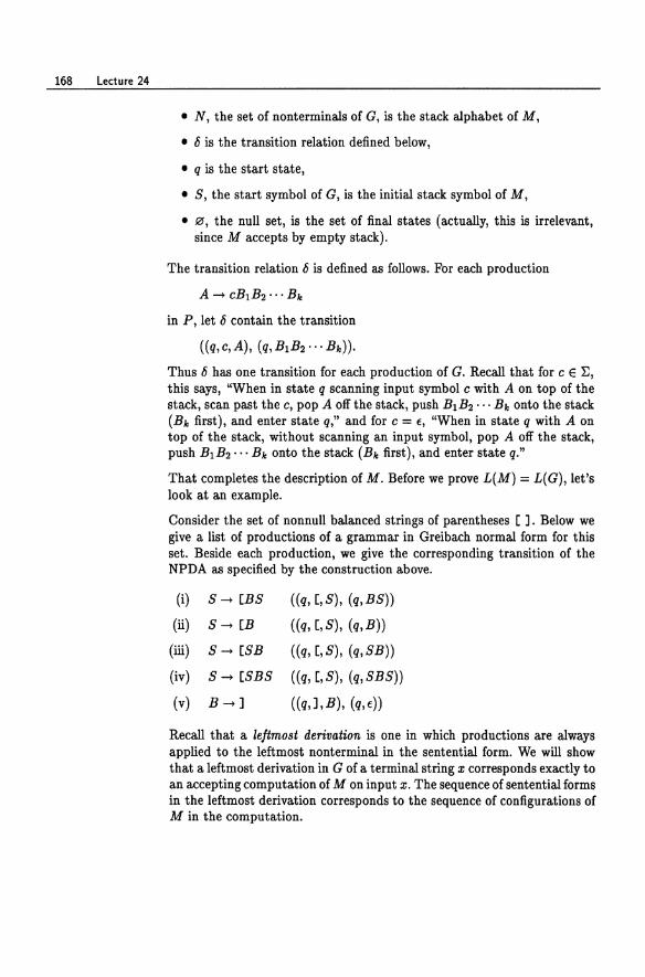
168 Lecture 24
• N, the set of nonterminals of G, is the stack alphabet of M,
• 6 is the transition relation defined below,
• q is the start state,
• S, the start symbol of G, is the initial stack symbol of M,
• 0, the null set, is the set of final states (actually, this is irrelevant, since M accepts by empty stack).
The transition relation 6 is defined as follows. For each production
A --+ CBlB2 ... Bk
in P, let 6 contain the transition
((q,c,A), (q,BlB2,,·Bk))'
Thus 6 has one transition for each production of G. Recall that for c E :E, this says, "When in state q scanning input symbol c with A on top of the stack, scan past the c, pop A off the stack, push Bl B2 ••• Bk onto the stack (Bk first), and enter state q," and for c = E, "When in state q with A on top of the stack, without scanning an input symbol, pop A off the stack, push BlB2'" Bk onto the stack (Bk first), and enter state q."
That completes the description of M. Before we prove L(M) = L(G), let's look at an example.
Consider the set of nonnull balanced strings of parentheses [ ]. Below we give a list of productions of a grammar in Greibach normal form for this set. Beside each production, we give the corresponding transition of the NPDA as specified by the construction above.
(i) S --+ [BS ((q, [,S), (q,BS))
(ii) S --+ [B ((q, [,S), (q,B))
(iii) S --+ [SB ((q, [,S), (q,SB))
(iv) S --+ [SBS ((q, [,S), (q,SBS))
(v) B --+] ((q,], B), (q, E))
Recall that a leftmost derivation is one in which productions are always applied to the leftmost nonterminal in the sentential form. We will show that a leftmost derivation in G of a terminal string x corresponds exactly to an accepting computation of M on input x. The sequence of sentential forms in the leftmost derivation corresponds to the sequence of configurations of M in the computation.
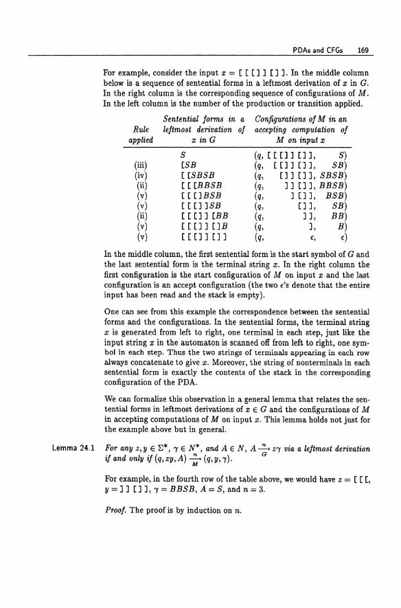
PDAs and CFGs 169
For example, consider the input x = [ [ [] ] [] ]. In the middle column below is a sequence of sentential forms in a leftmost derivation of x in G. In the right column is the corresponding sequence of configurations of M. In the left column is the number of the production or transition applied.
Sentential forms in a Configurations of M in an Rule leftmost derivation of accepting computation of
applied x in G M on input x
S (q, [[[]] [] ], S) (iii) [SB (q, [[]] []], SB) (iv) [[SBSB (q, []] []], SBSB) (ii) [[ [BBSB (q, ]] []], BBSB) (v) [[ [lBSB (q, ] [] ], BSB) (v) [[[]]SB (q, [ll, SB) (li) [ [[ll [BB (q, ] ], BB) (v) [[[]][]B (q, ] , B) (v) [[[]][]] (q, 40, f)
In the middle column, the first sentential form is the start symbol of G and the last sentential form is the terminal string x. In the right column the first configuration is the start configuration of M on input x and the last configuration is an accept configuration (the two 40'S denote that the entire input has been read and the stack is empty).
One can see from this example the correspondence between the sentential forms and the configurations. In the sentential forms, the terminal string x is generated from left to right, one terminal in each step, just like the input string x in the automaton is scanned off from left to right, one symbol in each step. Thus the two strings of terminals appearing in each row always concatenate to give x. Moreover, the string of nonterminals in each sentential form is exactly the contents of the stack in the corresponding configuration of the PDA.
We can formalize this observation in a general lemma that relates the sentential forms in leftmost derivations of x E G and the configurations of M in accepting computations of M on input x. This lemma holds not just for the example above but in general.
Lemma 24.1 For any z, y E E*, r E N*, and A E N, A ~ zr via a leftmost derivation if and only if (q, zy, A) ~ (q, y, r). G
M
For example, in the fourth row of the table above, we would have z = [ [ [, y = ] ] [] ], r = BBSB, A = S, and n = 3.
Proof. The proof is by induction on n.
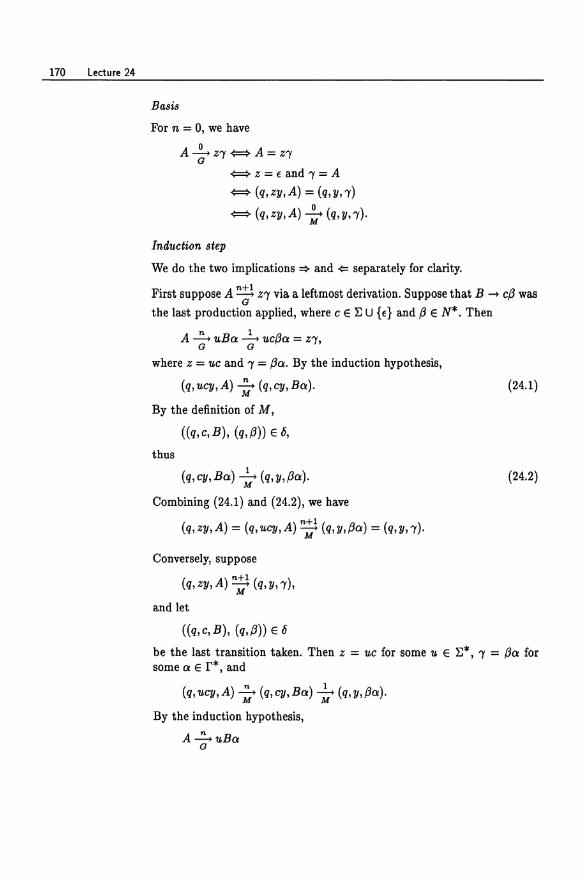
170 Lecture 24
Basis
For n = 0, we have
A ~ Z'Y ¢=} A = Z'Y G
¢=}z=fand'Y=A
¢=} (q,zy,A) = (q,y,'Y)
¢=} (q, zy, A) -l:; (q, y, '1).
Induction step
We do the two implications ~ and <= separately for clarity.
First suppose A ~ Z'Y via a leftmost derivation. Suppose that B -+ c{3 was G
the last production applied, where c E ~ U {f} and {3 E N*. Then
A ~ uBa. 2.. uc{3a. = Z'Y, G G
where z = uc and '1 = {3a.. By the induction hypothesis,
(q,ucy,A) ~ (q,cy,Ba.). M
By the definition of M,
((q,c,B), (q,{3)) EO,
thus
(q, cy, BOo) 2.. (q, y,{3a.). M
Combining (24.1) and (24.2), we have
(q,zy,A) = (q,ucy,A) '7 (q,y,{3a.) = (q,y,'Y).
Conversely, suppose
(q, zy, A) '7 (q, y, '1),
and let
((q,c,B), (q,{3)) E fJ
(24.1)
(24.2)
be the last transition taken. Then z = uc for some u E ~*, '1 = {3a. for some a. E r*, and
(q, ucy, A) 7 (q, cy, BOo) -i: (q, y,{3a.).
By the induction hypothesis,
A~uBa. G
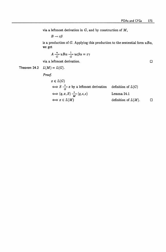
PDAs and CFGs 171
via a leftmost derivation in G, and by construction of M,
B -t c{3
is a production of G. Applying this production to the sentential form 'UBa, we get
A ~ 'UBa ~ 'Uc{3a = Z'Y G G
via a leftmost derivation.
Theorem 24.2 L(M) = L(G).
Proof.
x e L(G)
<==? S ~ x by a leftmost derivation definition of L( G) G
<==? (q,x,S) -if (q,€,€) Lemma 24.1
o
<==? x e L(M) definition of L(M). 0
Lecture 25
Simulating NPDAs by CFGs
We have shown that every CFL is accepted by some NPDA. Now we show conversely that NPDAs accept only CFLs. Thus NPDAs and CFGs are equivalent in expressive power. We will do this in two steps by showing that
(i) every NPDA can be simulated by an NPDA with one state; and
(ii) every NPDA with one state has an equivalent CFG.
Actually, step (ii) is the easier of the two, since we have already done all the work in Lecture 24. In that lecture, given a grammar in which all productions were of the form
A -+ CB1B2 ... B,.
for some k ~ 0 and c E ~ U {f}, we constructed an equivalent NPDA with one state. That construction is invertible. Suppose we have an NPDA with one state
M = ({q}, ~, r, 6, q, .L, 0)
that accepts by empty stack. Define the grammar
G = (r, ~, P, .L),
where P contains a production
A -+ cB1B2 ... Bk
for every transition
((q, c, A), (q, B1B2· .. Bk)) E 6,
Simulating NPDAs by CFGs 173
where C E }j U {fl. Then Lemma 24.1 and Theorem 24.2 apply verbatim, thus L(G) = L(M).
It remains to show how to simulate an arbitrary NPDA by an NPDA with one state. Essentially, we will maintain all state information on the stack. By the construction of Supplementary Lecture E, we can assume without loss of generality that M is of the form
M = (Q, }j, r, 6, s, ..l, {t});
that is, M has a single final state t, and M can empty its stack after it enters state t.
Let
f'~ Q xfx Q.
Elements of f' are written (p A q), where p, q E Q and A E f. We will construct a new NPDA
M' = ({*},}j, f', 6', *, (s..lt), 0)
with one state * that accepts by empty stack. The new machine M' will be able to scan a string x starting with only (p A q) on its stack and end up with an empty stack iff M can scan x starting in state p with only A on its stack and end up in state q with an empty stack.
The transition relation 6' of M' is defined as follows: for each transition
((p, c, A), (qO, B1B2· .. Bk)) E 6,
where C E }j U {f}, include in 6' the transitions
(( *, c, (p A qk)), (*, (qo Bl ql)(ql B2 q2) ... (qk-l Bk qk}))
for all possible choices of ql, q2,'" ,qk. For k = 0, this reduces to: if
((p,c,A), (qo,f)) E 6,
include in 6' the transition
((*,c,(pAqo)), (*,f)).
Intuitively, M' simulates M, guessing nondeterministically what states M will be in at certain future points in the computation, saving those guesses on the stack, and then verifying later that those guesses were correct.
174 Lecture 25
The following lemma formalizes the intuitive relationship between computations of M and M'.
Lemma 25.1 Let M' be the NPDA constructed from M as above. Then
(p, x, B1B2··· B,,) ~ (q, e, e) M
if and only if there exist qo, q1 , ... , q" such that p = qo, q = q", and
(*, x, (qo B1 q1)(q1 B2 q2) ... (q"-1 B" q,,») ~ (*, f, e). M
In particular,
(P,x,B) -i7 (q,e,e) {:::} (*,x, (PB q)) ~ (*,e,e).
Proof. By induction on n (What else?). For n = 0, both sides are equivalent to the assertion that p = q, x = e, and k = o. Now suppose that (P,X,B1B2···B,,) ~ (q,f,e). Let
M
((p,c,B1), (r,0102··· Om))
be the first transition applied, where c e ~ U {e} and m ;::: o. Then x = cy and
(p, x, B1B2··· B,,) -1:: (r, v, 0 10 2 ... OmB2··· B,,)
-i7 (q, e, e).
By the induction hypothesis, there exist ro, r1, ... , rm-I. ql, ... , qk-1, qk such that r = ro, q = qk, and
(*, V, (ro 01 r1)(r1 O2 r2)··· (rm-1 Om q1)(q1 B2 q2)··· (q"-1 B,. q,,»)
~ (*,e,e).
Also, by construction of M',
(( *, C, (p B1 q1»), (*, (rO 01 r1)(r1 02 r2)··· (rm-l Om q1)))
is a transition of M'. Combining these, we get
(*,x, (PB1 ql)(q1 B2 q2) ... (q"-l B" q,,»)
2,+ (*,V, (ro 0 1 r1)(r1 O2 r2)··· (rm-1 Om ql)(q1 B2 q2}··· (q"-1 B" q,,») M
~ (*,e,e).
Conversely, suppose
(*,x, (qo B1 q1)(q1 B2 q2) ... (q"-1 B" q,,») ~ (*,f,e). M
Let
Simulating NPDAs by CFGs 175
be the first transition applied, where C E :E U {€} and m ~ O. Then x = cy and
(*, x, (qO B1 q1}(q1 B2 q2)'" (qk-1 Bk qk))
~ (*, y, (ro C1 r1}(r1 C2 r2)'" (rm-1 Cm q1)(q1 B2 q2)'" (qk-1 Bk qk)) M
it (*,10,10).
By the induction hypothesis,
(ro, y, C1 C2··· CmB2'" Bk) ~ (qk, f, f). M
Also, by construction of M',
((qo, C, B1)' (ro, C1 C2 ••• Cm))
is a transition of M. Combining these, we get
(qo, x, B1B2··· Bk) 7 (ro, y, C1 c2··· CmB2 ... Bk)
~ (qk,f,f). M
Theorem 25.2 L(M') = L(M).
Proof. For all x E :E*,
x E L(M') -¢::::} (*,x, (8 1. t)) ~ (*,f,f) M
-¢::::} (8,X,J..) ~ (t,f,f) M
-¢::::} x E L(M).
Historical Notes
Lemma 25.1
D
D
Pushdown automata were introduced by Oettinger [95]. The equivalence of PDAs and CFGs was established by Chomsky [19], Schiitzenberger [112], and Evey [36].
Supplementary Lecture F
Deterministic Pushdown Automata
A deterministic pushdown automaton (DPDA) is an octuple
M = (Q, ~, r, 0, ..1., -I, s, F),
where everything is the same as with NPDAs, except:
(i) -I is a special symbol not in ~, called the right endmarker, and
o ~ (Qx(~U{-I}u{€})xr)x(Qxr*). (ii) 0 is deterministic in the sense that exactly one transition applies in
any given situation. This means that for any p E Q, a E ~ U {-I}, and A E r, 0 contains exactly one transition of the form ((p, a, A), (q, (3)) or ((P,€,A), (q,{3)).
(iii) 0 is restricted so that ..1. is always on the bottom of the stack. The machine may pop ..1. off momentarily, but must push it directly back on. In other words, all transitions involving ..1. must be of the form ((p,a,..1.), (q,{3..1.)).
The right endmarker -I delimits the input string and is a necessary addition. With NPDAs, we could guess where the end of the input string was, but with DPDAs we have no such luxury.
The restriction in (iii) is so that the machine never deadlocks by emptying its stack. This assumption is without loss of generality; even if the machine
Deterministic Pushdown Automata 177
did not obey it, we could make it do so by a construction involving a new stack symbol JL, as in Supplementary Lecture E. In that construction, we must modify the transitions (E.2) to read the symbol -I.
We consider only acceptance by final state. One can define acceptance by empty stack and prove that such machines are equivalent. The assumption (iii) would have to be modified accordingly.
The definitions of configurations and acceptance by final state are the same as with NPDAs. The start configuration on input x e E* is (s, x -I, .1), and x is accepted iff
(s,x -1,.1) -i:; (q,f,{3)
for some q e F and {3 e r*.
A language accepted by a DPDA is called a deterministic context-free language (DCFL). Surely every DCFL is a CFL, since every DPDA can be simulated by an NPDA. In this lecture we will show that the family of DCFLs is closed under complement. We know that there exist CFLs whose complements are not CFLsj for example,
{a,b}* - {ww I w e {a,b}*}.
These CFLs cannot be DCFLs. Thus, unlike finite automata, nondeterminism in PDAs gives strictly more power.
To show that the DCFLs are closed under complement, we will construct, given any DPDA M with input alphabet E, a new DPDA M' such that L(M') = E* - L(M).
We would like to build M' to simulate M and accept iff M does not accept. Unfortunately, we cannot just switch accept and nonaccept states like we did with DFAs. The main difficulty here is that unlike finite automata, DPDAs need not scan all of their inputj they may loop infinitely on inputs they do not accept without reading the entire input string. The machine M' will have to detect any such pathological behavior in M, since M' will have to scan the entire input and enter an accept state on all those inputs that are not accepted by M, including those inputs on which M loops prematurely.
We solve this problem by showing how to modify M to detect such spurious looping and deal with it gracefully. After each modification step, we will argue that the resulting machine still accepts the same set as M and is still deterministic.
178 Supplementary Lecture F
Checking for End of Input
It will be useful to include one bit of information in the finite control of M to remember whether or not M has seen the endmarker -i yet. Formally, we duplicate the finite control Q to get a new copy Q' = {q' I q E Q} disjoint from Q and add a new transition
((p',a,A), (q',,B))
for each transition ((p,a,A), (q,,B)) E 6. We remove any transition of the form ((P,-i,A), (q,,B)) and replace it with ((P,-i,A), (q',,B)). The primed states thus behave exactly like the unprimed original states, except that we jump from an unprimed state to a primed state when we scan the endmarker. The start state will still be s, but we will take as final states all primed states corresponding to final states in the old machine Mj that is, the new set of final states will be
F' = {q' I q E F}.
The new machine is still deterministic, since there is still exactly one transition that applies in any configuration. It accepts the same set, since if
(s,x -i,l.) -i7 (q,f,'Y), q E F
in the old machine, then there must be some intermediate transition that reads the -i:
(s, x -i, 1.) -it (p, -i, A,B) -if (r, E, a,B) -it (q, E, 1).
Then in the new machine,
(s, x -i, 1.) -it: (p, -i, A,B) -b (r', E, a,B) -it: (q', E, 1)·
Conversely, if
(s,x -i,l.) ~ (q',E,'Y), q' E F' M
in the new machine, then removing the primes gives a valid accepting computation sequence
(s,x -i,1.) ~ (q,E,'Y), q E F M
in the old machine.
Now we can tell from information in the sta.te whether we have seen -i or not. With this informa.tion, we can make the machine remain in an accept state if it has already scanned the -i and accepted. This is done by deleting every primed transition ((p',f,A), (q',,B)) with p' E F' and replacing it with ((P',E,A), (P',A)).
Deterministic Pushdown Automata 179
Getting Rid of Spurious Loops
We include two new nonaccept states r and r' and transitions
«r,a,A), (r,A)), «r, -I, A), (r/, A)), «r/,€,A), (r/,A)),
a e E, A e r, Aer, Aer.
We can think of r' as a reject state. If the machine is in state r, it will always scan to the end of the input and enter state r' , leaving the stack intact. Once the machine is in state r ' , it stays there. (So far there is no way for the machine to reach state r or r ' , but just wait ... )
We will now show how to modify the machine so that for all inputs, the machine scans the entire input and enters either an accept state or the state r'. Let x be any input. Because of determinism, there is a unique infinite sequence of configurations the machine goes through on input X. Let 'Yi denote the stack contents at time i e {O, 1, 2, ... }. There exists an infinite sequence of times io < i1 < i2 < ... such that for all i",
(F.1)
We can take io = 0, since 'Yo = 1. and hoi = 1, and the machine never empties its stack. Proceeding inductively, we can take ilc+l to be the earliest time after i" such that l'YiHll is minimum among alll'Yil, i > i".
Now we pick an infinite subsequence jo < iI < h < ... of io < il < i2 < ... such that the same transition, say «p,€,A), (q,P)), is applied at times jo,iI,h, ... . Such a subsequence exists by the pigeonhole principle: there are only finitely many transitions in 0, so at least one must be applied infinitely often. The states p, q can be primed or unprimed. The transition must be an €-transition, since it is applied infinitely often, and there are only finitely many input symbols to scan.
By (F.1), the machine never sees any stack symbol below the top symbol of 'Yj. after time j", and the top symbol is A. Thus the only stack symbols it sees after time j" are those it pushes after time j". Since the machine is deterministic, once it applies transition «(p, 10, A), (q, P)), it is in a loop and will go through the same periodic sequence of €-transitions repeated forever, since it sees nothing that can force it to do anything different. Moreover, this behavior is independent of the input. Thus if p is not an accept state, then the input is not accepted. We might as well remove the transition «p,€,A), (q,P)) from 0 and replace it with the transition «p,€,A), (r,A)) if p is an unprimed state or «p, 10, A), (r',A)) if p is a primed state. The language accepted by the automaton is not changed.
If this is done for all transitions «p,€,A), (q,P)) causing such spurious loops, we obtain a machine equivalent to M that on any input scans the
180 Supplementary lecture F
entire input string and the endmarker -j and enters either an accept state or the state r'. To get a machine M' accepting the complement of L(M), make r' the unique accept state of M'.
Historical Notes
Deterministic PDAs were first studied by Fischer [37], Schiitzenberger [112], Haines [54], and Ginsburg and Greibach [44].
Lecture 26
Parsing
One of the most important applications of context-free languages and pushdown automata is in compilers. The input to a PASCAL compiler is a PASCAL program, but it is presented to the compiler as a string of ASCII characters. Before it can do anything else, the compiler has to scan this string and determine the syntactic structure of the program. This process is called parsing.
The syntax of the programming language (or at least big parts of it) is often specified in terms of a context-free grammar. The process of parsing is essentially determining a parse tree or derivation tree of the program in that grammar. This tree provides the structure the compiler needs to know in order to generate code.
The subroutine of the compiler that parses the input is called the parser. Many parsers use a single stack and resemble deterministic PDAs. By now the theory of deterministic PDAs and parsing is so well developed that in many instances a parser for a given grammar can be generated automatically. This technology is used in what we call compiler compilers.
Example 26.1 Consider well-parenthesized expressions of propositional logic. There are propositional variables P, Q, R, ... , constants 1.., T (for false and true, respectively), binary operators 1\ (and), V (or), -+ (implication or if-then), and +-+ (if and only if or biconditional), and unary operator., (not), as well as parentheses. The following grammar generates the well-parenthesized
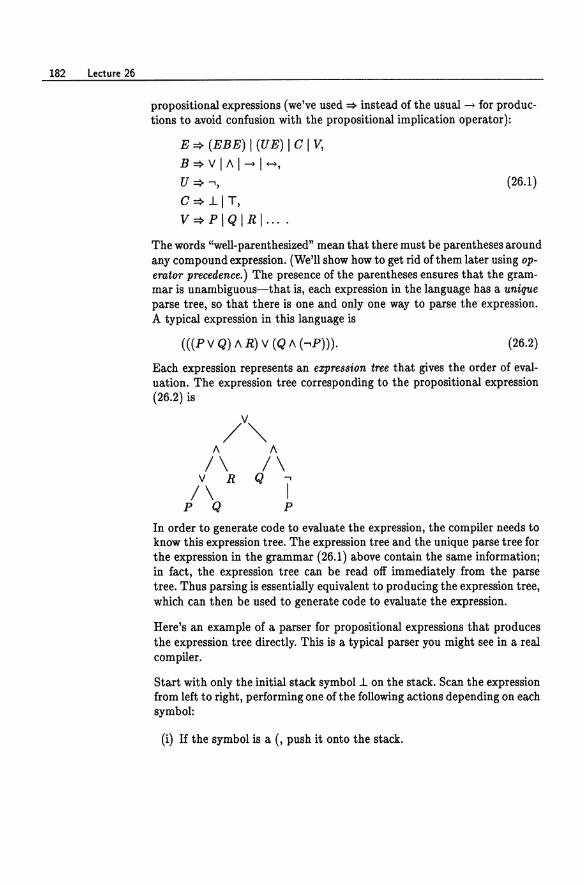
182 Lecture 26
propositional expressions (we've used '* instead of the usual -> for productions to avoid confusion with the propositional implication operator):
E,* (EBE) 1 (UE) 1 C 1 v, B '* V 1 A 1 -> 1 -,
U'* -', c'* .11 T,
V'*PIQIRI· ..
(26.1)
The words "well-parenthesized" mean that there must be parentheses around any compound expression. (We'll show how to get rid of them later using operator precedence.) The presence of the parentheses ensures that the grammar is unambiguous-that is, each expression in the language has a unique parse tree, so that there is one and only one way to parse the expression. A typical expression in this language is
(((P V Q) A R) V (Q A (-'P))). (26.2)
Each expression represents an expression tree that gives the order of evaluation. The expression tree corresponding to the propositional expression (26.2) is
/V"", A A
/\ /\ V R Q -, /\ I
P Q P In order to generate code to evaluate the expression, the compiler needs to know this expression tree. The expression tree and the unique parse tree for the expression in the grammar (26.1) above contain the same information; in fact, the expression tree can be read off immediately from the parse tree. Thus parsing is essentially equivalent to producing the expression tree, which can then be used to generate code to evaluate the expression.
Here's an example of a parser for propositional expressions that produces the expression tree directly. This is a typical parser you might see in a real compiler.
Start with only the initial stack symbol .1 on the stack. Scan the expression from left to right, performing one of the following actions depending on each symbol:
(i) If the symbol is a (, push it onto the stack.
Parsing 183
(ii) If the symbol is an operator, either unary or binary, push it onto the stack.
(iii) If the symbol is a constant, push a pointer to it onto the stack.
(iv) If the symbol is a variable, look it up in the symbol table and push a pointer to the symbol table entry onto the stack. The symbol table is a dictionary containing the name of every variable used in the program and a pointer to a memory location where its value will be stored. If the variable has never been seen before, a new symbol table entry is created.
(v) If the symbol is a ), do a reduce. This is where all the action takes place. A reduce step consists of the following sequence of actions:
(a) Allocate a block of storage for a new node in the expression tree. The block has space for the name of an operator and pointers to left and right operands.
(b) Pop the top object off the stack. It had better be a pointer to an operand (either a constant, variable, or node in the expression tree created previously). If not, give a syntax error. If so, save the pointer in the newly allocated node as the right operand.
(c) Pop the top object off the stack. It had better be an operator. If not, give a syntax error. If so, save the operator name in the newly allocated node. If the operator is unary, skip the next step (d) and go directly to (e).
(d) Pop the top object off the stacIe. It had better be a pointer to an operand. If not, give a syntax error. If so, save the pointer in the newly allocated node as the left operand.
(e) Pop the top object off the stack. It had better be a (. This is the left parenthesis matching the right parenthesis we just scanned. If not, give a syntax error.
(f) Push a pointer to the newly allocated node onto the stack.
Let's illustrate this algorithm on the input string
(((PV Q)" R) V (Q" (..,P))).
We start with the stack containing only an initial stack symbol .1. We scan the first three ('s and push them according to (i). We scan P and push a pointer to its symbol table entry according to (iv). We push the operator V according to (ii), then push a pointer to Q according to (iv). At this point the stack looks like
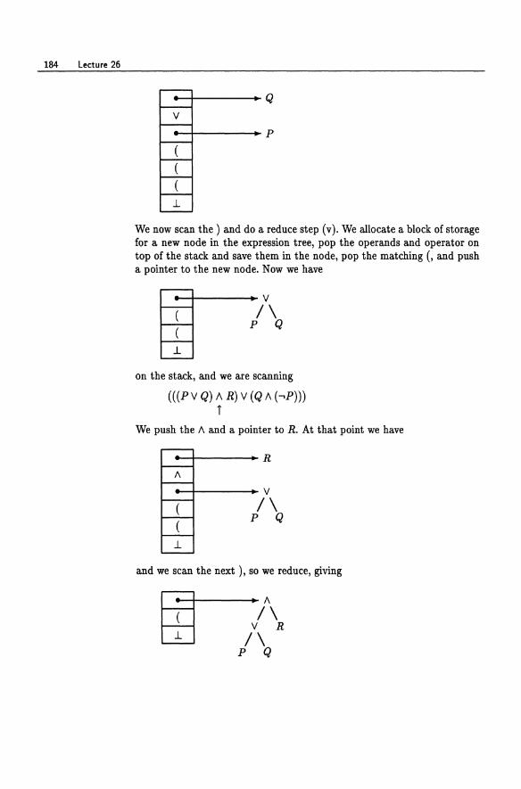
184 Lectu re 26
-+-----Q v -+-----P
..L
We now scan the) and do a reduce step (v). We allocate a block of storage for a new node in the expression tree, pop the operands and operator on top of the stack and save them in the node, pop the matching {, and push a pointer to the new node. Now we have
-+----... V
/\ P Q
..L
on the stack, and we are scanning
({{PV Q) A R) V (Q A (..,P))) T
We push the A and a pointer to R. At that point we have
-+----..... R
--+-----V /\
P Q
and we scan the next ), so we reduce, giving
§tI1\ V R
..L /\ P Q
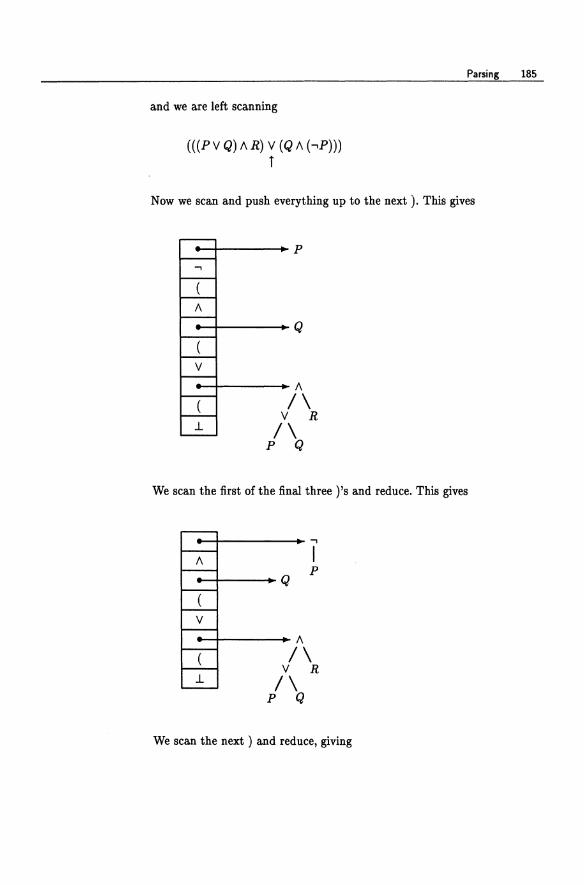
and we are left scanning
(((P V Q) /\ R) V (Q /\ (..,P))) i
Parsing 185
Now we scan and push everything up to the next ). This gives
--I-----P ..,
/\
........,I----_Q
V
--1-----/\ /\
V R .l /\
P Q
We scan the first of the final three )'s and reduce. This gives
--1-----... .., /\ I _-I---_Q P
V
--1----- /\ /\
V R .l /\
P Q
We scan the next) and reduce, giving
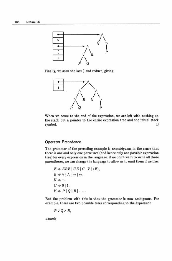
186 Lecture 26
~+--------------'A
v -+-------_ A
/\
/\ Q I
P V R /\
P Q
Finally, we scan the last) and reduce, giving
When we come to the end of the expression, we are left with nothing on the stack but a pointer to the entire expression tree and the initial stack symbol. 0
Operator Precedence
The grammar of the preceding example is unambiguous in the sense that there is one and only one parse tree (and hence only one possible expression tree) for every expression in the language. If we don't want to write all those parentheses, we can change the language to allow us to omit them if we like:
E:::} EBE I U E I C I V I (E),
B :::} V I A I -+ I -, U :::} ..."
C :::} 0 11, V:::}PIQIRI .. ·
But the problem with this is that the grammar is now ambiguous. For example, there are two possible trees corresponding to the expression
PVQAR,
namely
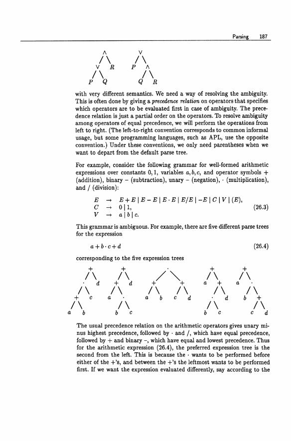
Parsing 187
A V
/\ /\ V R P A
/\ /\ p Q Q R
with very different semantics. We need a way of resolving the ambiguity. This is often done by giving a precedence relation on operators that specifies which operators are to be evaluated first in case of ambiguity. The precedence relation is just a partial order on the operators. To resolve ambiguity among operators of equal precedence, we will perform the operations from left to right. (The left-to-right convention corresponds to common informal usage, but some programming languages, such as APL, use the opposite convention.) Under these conventions, we only need parentheses when we want to depart from the default parse tree.
For example, consider the following grammar for well-formed arithmetic expressions over constants 0,1, variables a, b, c, and operator symbols + (addition), binary - (subtraction), unary - (negation), . (multiplication), and / (division):
E ...... C ...... V ......
E + E I E - E IE· E I E / E I - E I C I V I (E), 011, a I b I c.
(26.3)
This grammar is ambiguous. For example, there are five different parse trees for the expression
a+b·c+d (26.4)
corresponding to the five expression trees
+ +
+/""+
+ + /\ /\ /\ /\
d + d a + a
/\ /\ /\ /\ /\ /\ + c a a b c d d b + /\ /\ /\ /\
a b b c b c c d
The usual precedence relation on the arithmetic operators gives unary minus highest precedence, followed by . and /, which have equal precedence, followed by + and binary -, which have equal and lowest precedence. Thus for the arithmetic expression (26.4), the preferred expression tree is the second from the left. This is because the· wants to be performed before either of the +'s, and between the +'s the leftmost wants to be performed first. If we want the expression evaluated differently, say according to the
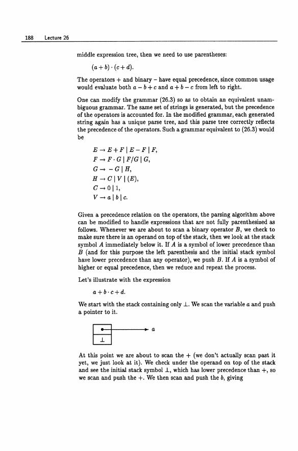
188 Lectu re 26
middle expression tree, then we need to use parentheses:
(a+b)· (c+d).
The operators + and binary - have equal precedence, since common usage would evaluate both a - b + c and a + b - c from left to right.
One can modify the grammar (26.3) so as to obtain an equivalent unambiguous grammar. The same set of strings is generated, but the precedence of the operators is accounted for. In the modified grammar, each generated string again has a unique parse tree, and this parse tree correctly reflects the precedence of the operators. Such a grammar equivalent to (26.3) would be
E ~ E + FIE - F I F,
F ~ F·G I FIG I G,
G~ -GIH,
H~CI V I (E), C~Oll,
V ~ a I b I c.
Given a precedence relation on the operators, the parsing algorithm above can be modified to handle expressions that are not fully parenthesized as follows. Whenever we are about to scan a binary operator B, we check to make sure there is an operand on top of the stack, then we look at the stack symbol A immediately below it. If A is a symbol of lower precedence than B (and for this purpose the left parenthesis and the initial stack symbol have lower precedence than any operator), we push B. If A is a symbol of higher or equal precedence, then we reduce and repeat the process.
Let's illustrate with the expression
a +b· c+d.
We start with the stack containing only .L We scan the variable a and push a pointer to it.
At this point we are about to scan the + (we don't actually scan past it yet, we just look at it). We check under the operand on top of the stack and see the initial stack symbol .1, which has lower precedence than +, so we scan and push the +. We then scan and push the b, giving
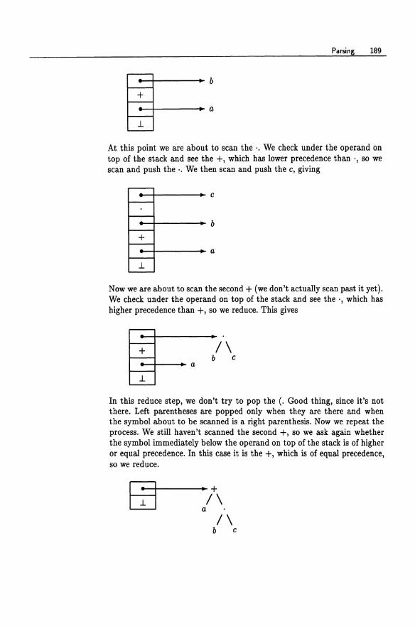
Parsing 189
-t-----b
+ e-+----_a
J.
At this point we are about to scan the .. We check under the operand on top of the stack and see the +, which has lower precedence than ., so we scan and push the .. We then scan and push the c, giving
e-+----_ c
-+----+-b
e--I----_ a
Now we are about to scan the second + (we don't actually scan past it yet). We check under the operand on top of the stack and see the ., which has higher precedence than +, so we reduce. This gives
+ /\ b c
1.
In this reduce step, we don't try to pop the (. Good thing, since it's not there. Left parentheses are popped only when they are there and when the symbol about to be scanned is a right parenthesis. Now we repeat the process. We still haven't scanned the second +, so we ask again whether the symbol immediately below the operand on top of the stack is of higher or equal precedence. In this case it is the +, which is of equal precedence, so we reduce.
Bj---:/+\ /\
b c
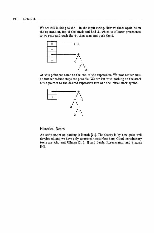
190 Lecture 26
We are still looking at the + in the input string. Now we check again below the operand on top of the stack and find .1, which is of lower precedence, so we scan and push the +, then scan and push the d.
-+----+d
+ -+----++ .1 /\
a
/\ b c
At this point we come to the end of the expression. We now reduce until no further reduce steps are possible. We are left with nothing on the stack but a pointer to the desired expression tree and the initial stack symbol.
/\ b c
Historical Notes
An early paper on parsing is Knuth [71]. The theory is by now quite well developed, and we have only scratched the surface here. Good introductory texts are Aho and Ullman [2, 3, 4] and Lewis, Rosenkrantz, and Stearns [80].
Lecture 27
The Cocke-Kasami-Younger Algorithm
Given a CFL A and a string x E E*, how do we tell whether x is in A? If A is a deterministic CFL and we are given a deterministic PDA for it, we can easily write a program to simulate the PDA. In fact, this is a good way to do it in practice and is done frequently in compilers; we saw an example of this in Lecture 26.
What if A is not a deterministic CFL, or even if it is but we are not given a deterministic PDA for it? If A is given by a CFG G, we can first convert G to Chomsky normal form (A -> Be or A -> a) so that each production either produces a terminal or increases the length of the sentential form, then try all derivations of length 21xl- 1 to see if any of them produce x. Unfortunately, there might be exponentially many such derivations, so this is rather inefficient. Alternatively, we might produce an equivalent NPDA and try all computation sequences, but again because of the nondeterminism there may be exponentially many to try.
Here is a cubic-time algorithm due to Cocke, Kasami, and Younger [65, 1251. It is an example of the technique of dynamic programming, a very useful technique in the design of efficient algorithms. It determines for each substring y of x the set of all nonterminals that generate y. This is done inductively on the length of y.

192 Lecture 27
For simplicity, we will assume that the given grammar G is in Chomsky normal form. One can give a more general version of the algorithm that works for grammars not in this form.
We illustrate the algorithm with an example. Consider the following grammar for the set of all nonnull strings with equally many a's and b's:
8 ~ AB I BA I 88 I AC I BD, A~a, B~b,
C~8B, D~8A.
We'll run the algorithm on the input string x = aabbab. Let n be the length of the string (here n = 6). Draw n + 1 vertical lines separating the letters of x and number them 0 to n:
lalalblblalbl 0123456
For 0::; i < j ::; n, let Xij denote the substring of x between lines i and j. In this example, X1,4 = abb and X2,6 = bbab. The whole string x is XO,n. Build a table T with (~) entries, one for each pair i,j such that 0 ::; i < j ::; n.
o 1
2 3
4 5
6
The i,jth entry of T, denoted Tij, refers to the substring Xij.
We will fill in each entry Tij of T with the set of nonterminals of G that generate the substring Xij of x. This information will be produced inductively, shorter substrings first.
We start with the substrings of length one. These are the substrings of x of the form Xi,H1 for 0 ::; i ::; n - 1 and correspond to the table entries along the top diagonal. For each such substring c = Xi,H1, if there is a production X ~ c E G, we write the nonterminal X in the table at location i, i + 1.
o A 1
A 2 B 3
B 4 A 5
B 6
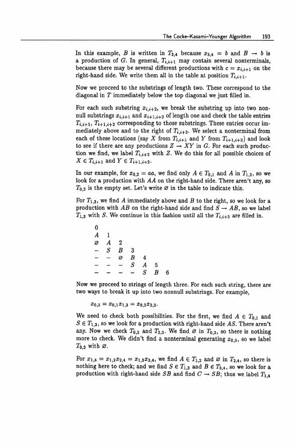
The Cocke-Kasami-Younger Algorithm 193
In this example, B is written in T 3,4 because X3,4 = b and B -+ b is a production of G. In general, T;,i+1 may contain several nonterminals, because there may be several different productions with c = Xi,i+1 on the right-hand side. We write them all in the table at position Ti,i+l'
Now we proceed to the substrings of length two. These correspond to the diagonal in T immediately below the top diagonal we just filled in.
For each such substring Xi,i+2, we break the substring up into two nonnull substrings Xi,i+1 and Xi+I,i+2 of length one and check the table entries Ti,i+l, Ti+l,i+2 corresponding to those substrings. These entries occur immediately above and to the right of Ti,i+2. We select a nonterminal from each of these locations (say X from Ti,i+1 and Y from Ti+I,i+2) and look to see if there are any productions Z -+ XY in G. For each such production we find, we label Ti,i+2 with Z. We do this for all possible choices of X E Ti,i+l and Y E Ti+l,i+2.
In our example, for XO,2 = aa, we find only A E TO,l and A in T l ,2, so we look for a production with AA on the right-hand side. There aren't any, so TO,2 is the empty set. Let's write 0 in the table to indicate this.
For TI,a, we find A immediately above and B to the right, so we look for a production with AB on the right-hand side and find S -+ AB, so we label Tl,a with S. We continue in this fashion until all the T i ,i+2 are filled in.
0 A 1 0 A 2
S B 3 0 B 4
S A 5 S B 6
Now we proceed to strings of length three. For each such string, there are two ways to break it up into two nonnull substrings. For example,
We need to check both possibilities. For the first, we find A E TO,l and S E TI,a, so we look for a production with right-hand side AS. There aren't any. Now we check TO,2 and T 2,a. We find 0 in TO,2, so there is nothing more to check. We didn't find a nonterminal generating XO,3, so we label TO,a with 0.
For Xl,4 = Xl,2X2,4 = Xl,aXa,4, we find A E T l ,2 and 0 in T2,4, so there is nothing here to checkj and we find S E Tl,a and B E Ta,4, so we look for a production with right-hand side SB and find C -+ SBj thus we label Tl,4
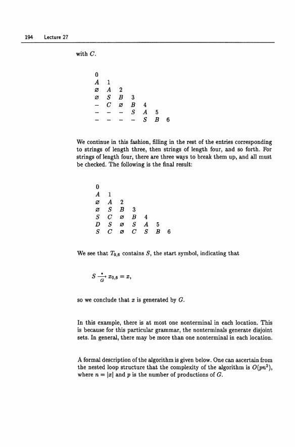
194 Lecture 27
with C.
0 A 1 0 A 2 0 S B 3
C 0 B 4 S A 5
S B 6
We continue in this fashion, filling in the rest of the entries corresponding to strings of length three, then strings of length four, and so forth. For strings of length four, there are three ways to break them up, and all must be checked. The following is the final result:
0 A 1 0 A 2 0 S B 3 S C 0 B 4 D S 0 S A 5 S C 0 C S B 6
We see that TO•6 contains S, the start symbol, indicating that
S~X06 =x, G •
so we conclude that x is generated by G.
In this example, there is at most one nonterminal in each location. This is because for this particular grammar, the nonterminals generate disjoint sets. In general, there may be more than one nonterminal in each location.
A formal description of the algorithm is given below. One can ascertain from the nested loop structure that the complexity of the algorithm is O(pn3), where n = Ixl and p is the number of productions of G.
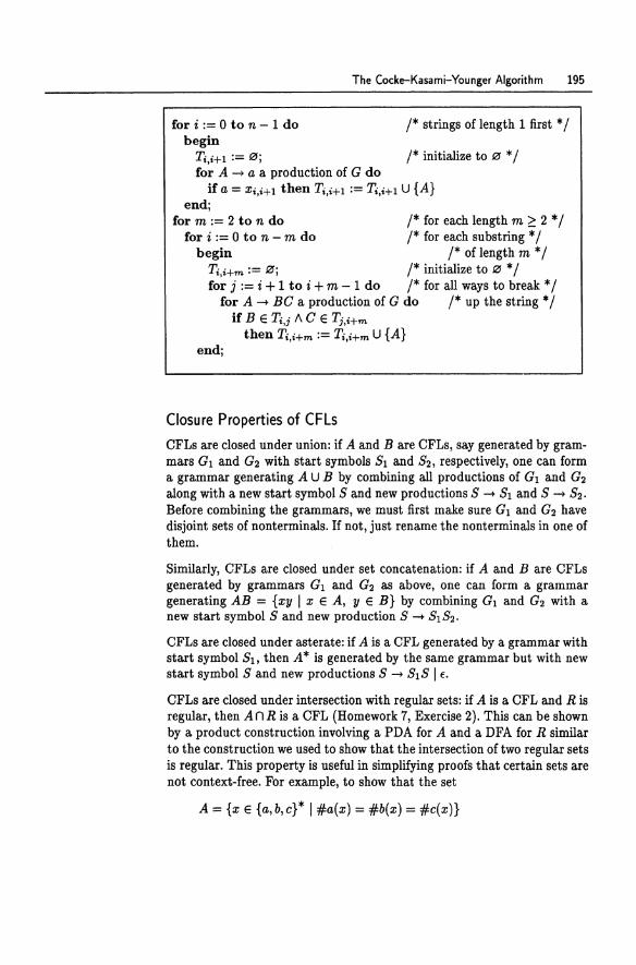
The Cocke-Kasami-Younger Algorithm 195
for i := 0 to n - 1 do begin
1* strings of length 1 first * /
Ti,Hl := 0; /* initialize to 0 * / for A --+ a a production of G do
if a = Xi,i+! then Ti,i+! := n,i+! U {A} end;
for m:= 2 to n do 1* for each length m ~ 2 */ for i := 0 to n - m do 1* for each substring * /
begin 1* of length m * / Ti,Hm := 0; /* initialize to 0 * / for j := i + 1 to i + m - 1 do /* for all ways to break * /
for A --+ BC a production of G do 1* up the string * / if B E Ti,; ACE T;,Hm
then Ti,Hm := Ti,Hm U {A} end;
Closure Properties of CFLs
eFLs are closed under union: if A and B are eFLs, say generated by grammars G1 and G2 with start symbols 81 and 82, respectively, one can form a grammar generating A U B by combining all productions of G1 and G2
along with a new start symbol 8 and new productions 8 --+ 81 and 8 --+ 82. Before combining the grammars, we must first make sure G1 and G2 have disjoint sets of nonterminals. If not, just rename the nonterminals in one of them.
Similarly, eFLs are closed under set concatenation: if A and Bare eFLs generated by grammars Gl and Ga as above, one can form a grammar generating AB = {xy I x E A, y E B} by combining G1 and Ga with a new start symbol 8 and new production 8 --+ 8182.
eFLs are closed under asterate: if A is a eFL generated by a grammar with start symbol 81. then A* is generated by the same grammar but with new start symbol 8 and new productions 8 --+ 818 I E.
eFLs are closed under intersection with regular sets: if A is a eFL and R is regular, then An R is a eFL (Homework 7, Exercise 2). This can be shown by a product construction involving a PDA for A and a DFA for R similar to the construction we used to show that the intersection of two regular sets is regular. This property is useful in simplifying proofs that certain sets are not context-free. For example, to show that the set
A = {x E {a,b,c}* I #a(x) = #b(x) = #c(x)}
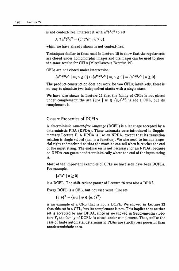
196 Lecture 27
is not context-free, intersect it with a*b*c* to get
An a*b*c* = {anbncn I n ~ O},
which we have already shown is not context-free.
Techniques similar to those used in Lecture 10 to show that the regular sets are closed under homomorphic images and preimages can be used to show the same results for CFLs (Miscellaneous Exercise 79).
CFLs are not closed under intersection:
{ambmcn I m,n ~ O} n {ambncn I m,n ~ O} = {anbncn I n ~ O}.
The product construction does not work for two CFLs; intuitively, there is no way to simulate two independent stacks with a single stack.
We have also shown in Lecture 22 that the family of CFLs is not closed under complement: the set {ww I w E {a, b} *} is not a CFL, but its complement is.
Closure Properties of DCFLs
A deterministic context-free language (DCFL) is a language accepted by a deterministic PDA (DPDA). These automata were introduced in Supplementary Lecture F. A DPDA is like an NPDA, except that its transition relation is single-valued (i.e., is a function). We also need to include a special right endmarker -1 so that the machine can tell when it reaches the end of the input string. The endmarker is not necessary for an NPDA, because an NPDA can guess nondeterministically where the end of the input string is.
Most of the important examples of CFLs we have seen have been DCFLs. For example,
{anbn I n ~ O}
is a DCFL. The shift-reduce parser of Lecture 26 was also a DPDA.
Every DCFL is a CFL, but not vice versa. The set
{a,b}* - {ww I wE {a,b}*}
is an example of a CFL that is not a DCFL. We showed in Lecture 22 that this set is a CFL, but its complement is not. This implies that neither set is accepted by any DPDA, since as we showed in Supplementary Lecture F, the family of DCFLs is closed under complement. Thus, unlike the case of finite automata, deterministic PDAs are strictly less powerful than nondeterministic ones.
The Cocke-Kasami-Younger Algorithm 197
DCFLs are not closed under union. For example, consider the union
{ambnck 1m i= n} U {ambnck In f:; k}.
Each set is a DCFL. The union is a CFL-an NPDA could guess nondeterministically which condition to check for-but it is not a DCFL. If it were, then its complement
""{ambnck Imi=n}n""{ambnck Inf:;k}
would be. But then intersecting with the regular set a*b*c* would give
{anbncn I n ~ O},
which is not even context-free.
Similarly, DCFLs are not closed under reversal, although proving this is a little harder. The set
{bambnck I m i= n} U {cambnck In f:; k}
over the alphabet {a, b, c} is an example of a DCFL whose reversal is not a DCFL (Miscellaneous Exercise 93).
Historical Notes
The CKY algorithm first appeared in print in Kasami [65] and Younger [125], although Hopcroft and Ullman [60] credit the original idea to John Cocke.
Closure properties of CFLs were studied by Scheinberg [110], Ginsburg and Rose [46, 48], Bar-Hillel, Perles, and Shamir [8], and Ginsburg and Spanier [49].
See p. 180 for the history of DPDAs and DCFLs.
Supplementary Lecture G
The Chomsky-Schiitzenberger Theorem
Let PARENn denote the language consisting of all balanced strings of parentheses of n distinct types. This language is generated by'the grammar
S-+ [S]\ [S]\"·\ [S]\SS\f. 1122 nn
The languages PARENn are sometimes called Dyck languages in the literature.
The following theorem shows that the parenthesis languages PARENn play a special role in the theory of context-free languages: every CFL is essentially a parenthesis language modified in some relatively simple way. In a sense, balanced parentheses capture the essential structure of CFLs that differentiates them from the regular sets.
Theorem G.1 (Chomsky-Schiitzenberger) E'lJery context-free language is a homomorphic image of the intersection of a parenthesis language and a regular set. In other words, for every CFL A, there is an n ~ 0, a regular set R, and a homomorphism h such that
A = h(PARENn n R).
Recall from Lecture 10 that a homomorphism is a map h : r* -+ ~* such that h(x1/) = h(x)h(1/) for all x,1/ E r*. It follows from this property that h(f) = 10 and that h is completely determined by its values on r. The
The Chomsky-Schiitzenberger Theorem 199
homomorphic image of a set B !; r* under h is the set {h(x) I x E B} !; E*, denoted h(B).
Proof. Let G = (N, E, P, S) be an arbitrary CFG in Chomsky normal form. Denote productions in P by 'If, p, (1', ••••
For 'If E P, define 1 12 2
{A --. [B ][C]
I W ww ~
'If = 1122 A--. [][]
1r 'JI"1I' W'
if 'If = A --. BC,
and define the grammar G' = (N, r, P', S) with 1 1 2 2 r = {[, ], [, ] I 'If E P}, 'Ir 1r 71" 11"
P' = {'If' I 'If E Pl. The idea here is that a balanced string of parentheses generated by G' encodes a corresponding string generated by G along with its parse tree.
Let PARENr be the parenthesis language over parentheses r. Surely L( G') !; PARENr, since the productions of G' generate parentheses in well-nested matched pairs. However, not all strings in PARENr are generated by G'. Here are some properties satisfied by strings in L( G') that are not satisfied by strings in PARENr in general:
1 2 (i) Every ] is immediately followed by a [.
w w
2 (ii) No ] is immediately followed by a left parenthesis.
w
1 1 (iii) If 'If = A --. BC, then every [ is immediately followed by [ for Bome
w 2 P pEP with left-hand side B, and every [ is immediately followed by 1 w [ for some q E P with left-hand side C. u
1 1 2 (iv) If 'If = A --. a, then every [ is immediately followed by ] and every [
w 2 W W
is immediately followed by ]. w
In addition, all strings x such that A -;. x satisfy the property G
1 (VA) The string x begins with [ for some 'If E P with left-hand side A.
W
Each of the properties (i) though (VA) can be described by a regular expression; thus the sets
RA = {x E r* I x satisfies (i) through (VA)}
200 Supplementary Lecture G
Lemma G.2
are regular. We claim
A~ x {::::::> x E PARENr nRA. G/
Proof. The direction (::}) is a straightforward proof by induction on the length of the derivation. For the direction ({:::), suppose x E PARENr nRA. We proceed by induction on the length of x. It follows from properties (i) through (v A) and the fact that x is a string of balanced parentheses that x is of the form
1 12 2 x= [y][z]
1(" 1r1r 1("
for some y, Z E r* and 11' with left-hand side A. If 11' = A -+ BC, then from property (iii), y satisfies (VB) and z satisfies (ve). Also, y and z satisfy (i) through (iv) and are balanced. Thus y E PARENr n RB and z E PARENr n Re. By the induction hypothesis, B ~ y and C ~ Zi
G/ G/ therefore,
1 1 12 2 • 1 12 2 A,.. [B][C],.. [y][z] =X.
G 7r 7r7r 1(" G 7r 7r1r 11'
If 11' = A -+ a, then from property (iv), y = z = €, and 1 1 12 2
A --+ [] [] = X. G' 7r 7r1l" 1['
o
It follows from Lemma G.2 that L(G') = PARENr n Rs. Now define the homomorphism h: r* -+ E* as follows. For 11' of the form A -+ BC, take
1 1 2 2 h([) = h(J) = h([) = h(]) = f.
?r 7r 7r 11"
For 11' of the form A -+ a, take 1 2 2
h( ]) = h( n = h(]) = €, ". ". ".
1 h( [) = a.
".
Applying h to the production 11" of P' gives the production 11' of Pi thus L(G) = h(L(G')) = h(PARENr n Rs). This completes the proof of the Chomsky-Schiitzenberger theorem. 0
Historical Notes
The pivotal importance of balanced parentheses in the theory of contextfree languages was recognized quite early on. The Chomsky-Schiitzenberger theorem is due to Chomsky and Schiitzenberger [19, 22].
Supplementary Lecture H
Parikh's Theorem
Here is a theorem that says a little more about the structure of CFLs. It says that for any CFL A, if we look only at the relative number of occurrences of terminal symbols in strings in A without regard to their order, then A is indistinguishable from a regular set.
Formally, let ~ = {al, ... ,ak}. The Parikh map is the function
'I/J: ~* --- Nk
defined by
'I/J(x) ~f (#al (x), #a2(x), . .. , #ak(x)).
That is, 'I/J(x) records the number of occurrences of each symbol in x. The structure ~* with binary operation· (concatenation) and constant 15 forms a monoid,l as does the structure Nk with binary operation + (componentwise addition) and identity 0 = (0, ... ,0), and 'I/J is a monoid homomorphism:
'I/J(xy) = 'I/J(x) + 'I/J(y) , 'I/J(I5) = o.
1 Recall from Lecture 2 that a monoid is an algebraic structure consisting of a set with an associative binary operation and an identity for that operation.
202 Supplementary Lecture H
The main difference between the monoids E* and Nlo is that the latter is commutative,2 whereas the former is not, except in the case k = 1. In fact, if :: is the smallest monoid congruence3 on E* such that a,aj :: aja, , 1 :5 i,j :5 k, then Nlo is isomorphic to the quotient4 E* /::. The monoid E* is sometimes called the free monoid on k generators, and Nlo is sometimes called the free commutative monoid on k generators. The word "free" refers to the fact that the structures do not satisfy any equations besides the logical consequences of the monoid or commutative monoid axioms, respectively.
The commutative image of a set A ~ E* is its image under 1/J:
1/J(A) ~ {1/J(x) I x E A}.
If '1.£1, ••• ,Urn E Nk, the su bmonoid of Nk generated by '1.£1, ••• ,Urn is denoted <'1.£1, ••• ,Urn>· This is the smallest subset of Nlo containing '1.£1, ••• ,Urn and the monoid identity 0 and closed under +. Equivalently,
<'1.£1, ••• ,urn> = {alul + ... +amurn I al,.·· ,arn E N} ~ Nlo.
A subset of Nlo is called linear if it is a coset of such a finitely generated submonoidj that is, if it is of the form
'1.£0 + <'1.£1, ... ,urn> = {uo + alUl + ... + amUrn I al, ... ,arn EN}.
A subset of Nlo is called semilinear if it is a union of finitely many linear sets. For example,
1/J({anbn I n ~ O}) = 1/J({x E {a,b}* I #a(x) = #b(x)}) = {(n,n) I n ~ O} = «1,1»
is a semilinear (in fact, linear) subset of N2, but {(n, n2 ) I n ~ O} is not.
Theorem H.1 (Parikh) For any context-free language A, 1/J(A) is semilinear.
The converse does not hold: the set {anbncn I n ~ O} is not context-free but has a semilinear image under 1/J. This is also the image of the CFL {(ab)ncn I n ~ O} and the regular set (abc)*.
2 A monoid is commutative if zy = y:Il for all z and y. 3 A monoid congruence is an equivalence relation == on the monoid that respects the monoid
structure in the sense that if z == z' and y == y', then zy == z'y'. 'The quotient of a monoid M by a congruence == is a monoid whose elements are the congruence
classes [:Il) ~ {y I y == z}, binary operation [z)· [y) ~ [zy), and constant [1), where 1 is the identity of M. See Supplementary Lectures C and D for more information on these concepts.
Parikh's Theorem 203
For every semilinear set S ~ Nk , it is not hard to construct a regular set R ~ 1:* such that 'I/J(R) = S. For example, {(n,n) I n ~ O} = 'I/J((ab)*). For this reason, Parikh's theorem is sometimes stated as follows:
Every context-free language is letter-equivalent to a regular 8et,
where letter-equivalence means the sets have the same commutative image.
In order to prove Parikh's theorem, we need some definitions. Let G = (N, 1:, P, S) be an arbitrary CFG in Chomsky normal form. Let s, t, ... denote parse trees of G with a nonterminal at the root, nonterminals labeling the internal nodes, and terminals or nonterminals labeling the leaves. Define
root(s) ~f the nonterminal at the root of s;
yield( s) ~f the string of terminals and nonterminals at the leaves of s, reading left to right;
depth(s) ~ the length of the longest path in 8 from a leaf up to the root (the length of a path is the number of edges, or the number of nodes less one);
N(s) ~f the set of nonterminals appearing in s.
Define a pump to be a parse tree 8 such that
(i) s contains at least two nodes; and
(li) yield(s) = x· root(8)' y for some x,y E 1:*; that is, all leaves are labeled with terminal symbols except one, and the nonterminallabeling that leaf is the same as the one labeling the root.
These objects arose in the proof of the pumping lemma for CFLs in Lecture 22: wherever a nonterminal A appears in a parse tree 8, the tree can be split apart at that point and a pump'll. with root( '11.) = A inserted to get a larger parse tree t.
For parse trees s, t, define 8 <I t if t can be obtained from 8 by splitting s at a node labeled with some nonterminal A and inserting a pump with root labeled A. The relation <I is not a partial order (it is not reflexive or transitive), but it is welliounded in the sense that there exists no infinite descending chain So I> 81 I> 82 I> ••. , because if 8 <I t, then s has strictly fewer nodes than t.
Define a pump t to be a ba8ic pump if it is <I-minimal among all pumps; that is, if it does not properly contain another pump that could be cut out. In other words, a pump t is a ba8ic pump if the only s such that 8 <I t is
204 Supplementary Lecture H
the trivial one-node parse tree labeled with the nonterminal root(t). Basic pumps cannot be too big:
Lemma H.2 If s is a basic pump, then depth(s) ::; 2n, where n is the number of nonterminals in N.
Proof. Let 7r denote the path in s from the unique leaf with label root( s) up to the root. The path 7r can be no longer than n, because if it were, it would have a repeated nonterminal and would therefore contain a pump that could be removed, contradicting the <l-minimality of s. For any other leaf, the path from that leaf up to the first node on the path 7r can be no longer than n + 1 for the same reason. Thus the total length of any path from a leaf to the root can be no longer than 2n. 0
It follows from Lemma H.2 and the fact that there are only finitely many productions in G that the number of basic pumps is finite, say p.
Lemma H.3 Every parse tree t with yield(t) E E* is either <l-minimal or contains a basic pump.
Proof. If t is not <l-minimal, then by definition it contains a pump s. Let s be <l-minimal among all pumps contained in t. Then s is a basic pump, because if it were not, then it would contain a smaller pump u, and u would be a smaller pump contained in t, contradicting the minimality of s. 0
Define s ::; t if t can be obtained from s by some finite sequence of insertions of basic pumps u such that N(u) ~ N(s). In other words, starting from s, we are allowed to choose any occurrence of a nonterminal A in s and insert a basic pump u with root(u) = A at that point, provided u contains no new nonterminals that are not already contained in s. If t can be obtained from s by a finite number of repetitions of this process, then s ::; t.
If 0: E (N U E)*, define 'IjJ(o:) = 'IjJ(x), where x is the string obtained from 0: by deleting all nonterminals. Let 'IjJ(t) abbreviate 'IjJ(yield(t)).
Lemma H.4 The set {'IjJ(t) Is::; t} is linear.
Proof.
{'IjJ(t) Is::; t} = 'IjJ(s) + <{'IjJ(u) I u is a basic pump with N(u) ~ N(s)}>.
o Lemma H.5 If s is ::;-minimal, then depth(s) ::; (p + 1)(n + 1), where p is the number
of distinct basic pumps and n is the size of N.
Proof. If s had a path longer than depth(s) ::; (p + 1)(n + 1), then that path could be broken up into p + 1 segments, each of length at least n + 1, and each segment would have a repeated nonterminal. Then there would be
Parikh's Theorem 205
p + 1 disjoint pumps. (Two pumps are considered disjoint if they have no nodes in common, or if the root of one is a leaf of the other.) Each of these p + 1 pumps either is basic or contains a basic pump by Lemma H.3j thus there would be p + 1 disjoint basic pumps. But there are only p distinct basic pumps in all, so by the pigeonhole principle there must be two disjoint occurrences of the same basic pump. But this contradicts the $-minimality of s, since one of these basic pumps could be deleted without changing the set of nonterminals contained in the tree. 0
Proof of Theorem H.l. Let
M = {s I s is $-minimal, root(s) = S, yield(s) E E*}.
We show that
'I/J(L(G)) = U {'I/J(t) Is $ t} . • EM
This set is semilinear by Lemma H.5, which implies that M is finite, and by Lemma H.4. Any t such that s $ t for some s E M has root( t) = Sand yield(t) E E*j thus yield(t) E L(G) and 'I/J(t) E 'I/J(L(G)). Conversely, any string x E L(G) has a parse tree t with root(t) = Sand yield(t) = x, and there must exist a $-minimal s $ t. Then s E M and
'I/J(x) E {'I/J(t) I s $ t}. o
Historical Notes
Parikh's theorem was first proved by Rohit Parikh [98]. Alternative proofs have been given by Goldstine [52), Harrison [55), and Kuich [75].
Lecture 28
Turing Machines and Effective Computability
In this lecture we introduce the most powerful of the automata we will study: Turing machines (TMs) , named after Alan Turing, who invented them in 1936. Turing machines can compute any function normally considered computable; in fact, it is quite reasonable to define computable to mean computable by aTM.
TMs were invented in the 1930s, long before real computers appeared. They came at a time when mathematicians were trying to come to grips with the notion of effective computation. They knew various algorithms for computing things effectively, but they weren't quite sure how to define "effectively computable" in a general way that would allow them to distinguish between the computable and the noncomputable. Several alternative formalisms evolved, each with its own peculiarities, in the attempt to nail down this notion:
• Turing machines (Alan Turing [120]);
• Post systems (Emil Post [99, 100]);
• ",-recursive functions (Kurt Godel [511, Jacques Herbrand);
• ~-calculus (Alonzo Church [231, Stephen C. Kleene [66]); and
• combinatory logic (Moses Schonfinkel [111], Haskell B. Curry [29]).
Turing Machines and Effective Computability 207
All of these systems embody the idea of effective computation in one form or another. They work on various types of data; for example, Turing machines manipulate strings over a finite alphabet, It-recursive functions manipulate the natural numbers, the A-calculus manipulates A-terms, and combinatory logic manipulates terms built from combinator symbols.
However, there are natural translations between all these different types of data. For example, there is a simple one-to-one correspondence between strings in {O,l}* and natural numbers N = {O, 1,2, ... } defined by
x 1-+ #(lx) - 1, (28.1)
where #y is the natural number represented by the binary string y. Conversely, it is easy to encode just about anything (natural numbers, A-terms, strings in {O, 1, 2, ... , 9} *, trees, graphs, ... ) as strings in {O, 1} *. Under these natural encodings of the data, it turns out that all the formalisms above can simulate one another, so despite their superficial differences they are all computationally equivalent.
Nowadays we can take unabashed advantage of our more modern perspective and add programming languages such as PASCAL or C (or idealized versions of them) to this list-a true luxury compared to what Church and GOdel had to struggle with.
Of the classical systems listed above, the one that most closely resembles a modern computer is the Turing machine. Besides the off-the-shelf model we will define below, there are also many custom variations (nondeterministic, multitape, multidimensional tape, two-way infinite tapes, and so on) that all turn out to be computationally equivalent in the sense that they can all simulate one another.
Church's Thesis
Because these vastly dissimilar formalisms are all computationally equivalent, the common notion of computability that they embody is extremely robust, which is to say that it is invariant under fairly radical perturbations in the model. All these mathematicians with their pet systems turned out to be looking at the same thing from different angles. This was too striking to be mere coincidence. They soon came to the realization that the commonality among all these systems must be the elusive notion of effective computability that they had sought for so long. Computability is not just Turing machines, nor the A-calculus, nor the j.£-recursive functions, nor the PASCAL programming language, but the common spirit embodied by them all.
Alonzo Church [25] gave voice to this thought, and it has since become known as Church's thesis (or the Church-Turing thesis). It is not a the-
208 Lecture 28
orem, but rather a declaration that all these formalisms capture precisely our intuition about what it means to be effectively computable in principle, no more and no less. Church's thesis may not seem like such a big deal in retrospect, since by now we are thoroughly familiar with the capabilities of modern computers; but keep in mind that at the time it was first formulated, computers and programming languages had yet to be invented. Coming to this realization was an enormous intellectual leap.
Probably the most compelling development leading to the acceptance of Church's thesis was the Turing machine. It was the first model that could be considered readily programmable. If someone laid one of the other systems out in front of you and declared, "This system captures exactly what we mean by effectively computable," you might harbor some skepticism. But it is hard to argue with Turing machines. One can rightly challenge Church's thesis on the grounds that there are aspects of computation that are not addressed by Turing machines (for example, randomized or interactive computation), but no one could dispute that the notion of effective computability as captured by Turing machines is robust and important.
Universality and Self-Reference
One of the most intriguing aspects of these systems, and a pervasive theme in our study of them, is the idea of programs as data. Each of these programming systems is powerful enough that programs can be written that understand and manipulate other programs that are encoded as data in some reasonable way. For example, in the A-calculus, A-terms act as both programs and data; combinator symbols in combinatory logic manipulate other combinator symbols; there is a so-called Godel numbering of the /1,recursive functions in which each function has a number that can be used as input to other p.-recursive functions; and Turing machines can interpret their input strings as descriptions of other Turing machines. It is not a far step from this idea to the notion of universal simulation, in which a universal program or machine U is constructed to take an encoded description of another program or machine M and a string x as input and perform a step-by-step simulation of M on input x. A modern-day example of this phenomenon would be a SCHEME interpreter written in SCHEME.
One far-reaching corollary of universality is the notion of self-reference. It is exactly this capability that led to the discovery of natural uncomputable problems. If you know some set theory, you can convince yourself that uncomputable problems must exist by a cardinality argument: there are uncountably many decision problems but only countably many Turing machines. However, self-reference allows us to construct very simple and natural examples of uncomputable problems. For example, there do not
Turing Machines and Effective Computability 209
exist general procedures that can determine whether a given block of code in a given PASCAL program is ever going to be executed, or whether a given PASCAL program will ever halt. These are important problems that compiler builders would like to solve; unfortunately, one can give a formal proof that they are unsolvable.
Perhaps the most striking example of the power of self-reference is the incompleteness theorem of Kurt Godel. Starting near the beginning of the twentieth century with Whitehead and Russell's Principia Mathematica [123], there was a movement to reduce all of mathematics to pure symbol manipulation, independent of semantics. This was in part to understand and avoid the set-theoretic paradoxes discovered by Russell and others. This movement was advocated by the mathematician David Hilbert and became known as the formalist program. It attracted a lot of followers and fed the development of formal logic as we know it today. Its proponents believed that all mathematical truths could be derived in some fixed formal system, just by starting with a few axioms and applying rules of inference in a purely mechanical way. This view of mathematical proof is highly computational. The formal deductive system most popular at the time for reasoning about the natural numbers, called Peano arithmetic (PA), was believed to be adequate for expressing and deriving mechanically all true statements of number theory. The incompleteness theorem showed that this was wrong: there exist even fairly simple statements of number theory that are true but not provable in PA. This holds not only for PA but for any reasonable extension of it. This revelation was a significant setback for the formalist program and sent shock waves throughout the mathematical world.
Godel proved the incompleteness theorem using self-reference. The basic observation needed here is that the language of number theory is expressive enough to talk about itself and about proofs in PA. For example, one can write down a number-theoretic statement that says that a certain other number-theoretic statement has a proof in PA, and one can reason about such statements using PA itself. Now, by a tricky argument involving substitutions, one can actually construct statements that talk about whether they themselves are provable. Godel actually constructed a sentence that said, "I am not provable.» This construction is presented in detail in Supplementary Lecture K.
The consequences of universality are not only philosophical but also practical. Universality was in a sense the germ of the idea that led to the development of computers as we know them today: the notion of a stored program, a piece of software that can be read and executed by hardware. This programmability is what makes computers so versatile. Although it was
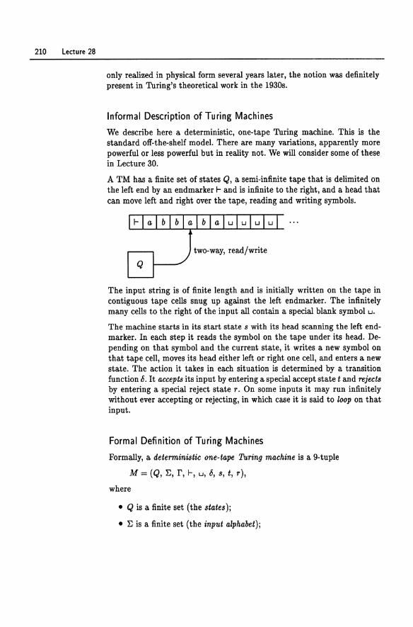
210 Lecture 28
only realized in physical form several years later, the notion was definitely present in Turing's theoretical work in the 1930s.
Informal Description of Turing Machines
We describe here a deterministic, one-tape Turing machine. This is the standard off-the-shelf model. There are many variations, apparently more powerful or less powerful but in reality not. We will consider some of these in Lecture 30.
A TM has a finite set of states Q, a semi-infinite tape that is delimited on the left end by an endmarker r and is infinite to the right, and a head that can move left and right over the tape, reading and writing symbols.
The input string is of finite length and is initially written on the tape in contiguous tape cells snug up against the left endmarker. The infinitely many cells to the right of the input all contain a special blank symbol w.
The machine starts in its start state s with its head scanning the left endmarker. In each step it reads the symbol on the tape under its head. Depending on that symbol and the current state, it writes a new symbol on that tape cell, moves its head either left or right one cell, and enters a new state. The action it takes in each situation is determined by a transition function o. It accepts its input by entering a special accept state t and rejects by entering a special reject state r. On some inputs it may run infinitely without ever accepting or rejecting, in which case it is said to loop on that input.
Formal Definition of Turing Machines
Formally, a deterministic one-tape Turing machine is a 9-tuple
M = (Q, ~, r, r, w, 0, s, t, r),
where
• Q is a finite set (the states);
• ~ is a finite set (the input alphabet);
Turing Machines and Effective Computability 211
• r is a finite set (the tape alphabet) containing ~ as a subset;
• wE r - ~, the blank symbol;
• r E r - ~, the left endmarker;
• 8: Q x r -+ Q x r x {L, R}, the transition function;
• SEQ, the start state;
• t E Q, the accept state; and
• r E Q, the reject state, r i- t.
Intuitively, 8(p,a) = (q,b,d) means, "When in state p scanning symbol a, write b on that tape cell, move the head in direction d, and enter state q." The symbols Land R stand for left and right, respectively.
We restrict TMs so that the left endmarker is never overwritten with another symbol and the machine never moves off the tape to the left of the endmarker; that is, we require that for all p E Q there exists q E Q such that
8(p,r) = (q,r,R). (28.2)
We also require that once the machine enters its accept state, it never leaves it, and similarly for its reject state; that is, for all b E r there exist c, c' E r and d, d' E {L, R} such that
8(t, b) 8(r,b)
= (t,c,d), (r, c', d'). (28.3)
We sometimes refer to the state set and transition function collectively as the finite control.
Example 28.1 Here is a TM that accepts the non-context-free set {anbncn In;::: O}. Informally, the machine starts in its start state s, then scans to the right over the input string, checking that it is of the form a*b*c*. It doesn't write anything on the way across (formally, it writes the same symbol it reads). When it sees the first blank symbol w, it overwrites it with a right endmarker ... 1. Now it scans left, erasing the first c it sees, then the first b it sees, then the first a it sees, until it comes to the f-. It then scans right, erasing one a, one b, and one c. It continues to sweep left and right over the input, erasing one occurrence of each letter in each pass. If on some pass it sees at least one occurrence of one of the letters and no occurrences of another, it rejects. Otherwise, it eventually erases all the letters and makes one pass between f- and -i seeing only blanks, at which point it accepts.
Formally, this machine has
Q = {s, ql, ... , ql0, t, r},
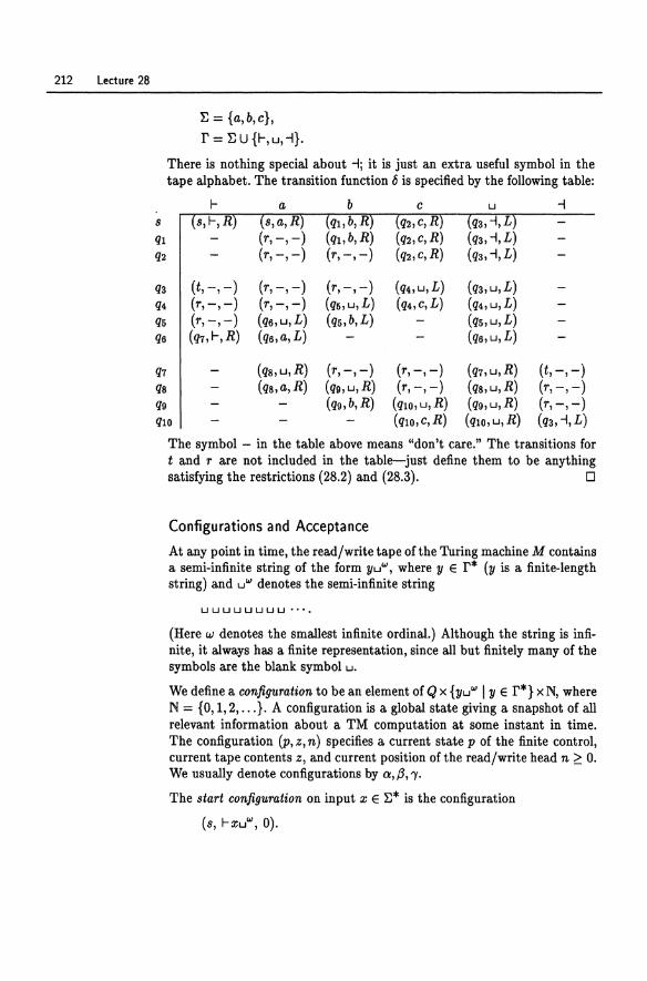
212 Lecture 28
8
ql q2
q3 q4 qs q6
q7 qs q9
~ = {a,b,c}, r = ~ U {f-,u, -I}.
There is nothing special about -Ij it is just an extra useful symbol in the tape alphabet. The transition function 0 is specified by the following table:
f- a b -I
(t,-,-) (r,-,-) (r,-,-) (q4,u,L) (q3, u, L) (r,-,-) (r, -,-) (qs,u,L) (q4,c,L) (q4,u,L) (r, -, -) (q6,u,L) (qS, b, L) (q5,u,L) (q7,f-,R) (q6,a,L) (q6,u,L)
(qs,u,R) (r,-,-) (r, -, -) (q7,u,R) (t,-,-) (qs,a,R) (q9, u, R) (r, -,-) (q8,u,R) (r, -,-)
(q9,b,R) (qlO,u,R) (q9, u, R) (r,-,-) qlO (qlO,c,R) (qlo,u,R) (q3, -I, L)
The symbol - in the table above means "don't care." The transitions for t and r are not included in the table-just define them to be anything satisfying the restrictions (28.2) and (28.3). 0
Configurations and Acceptance
At any point in time, the read/write tape of the Turing machine M contains a semi-infinite string of the form yu", where y E r* (y is a finite-length string) and u" denotes the semi-infinite string
uuuuuuuu· ...
(Here w denotes the smallest infinite ordinal.) Although the string is infinite, it always has a finite representation, since all but finitely many of the symbols are the blank symbol u.
We define a configuration to be an element of Q x {yu" lyE r*} x N, where N = {O, 1,2, ... }. A configuration is a global state giving a snapshot of all relevant information about a TM computation at some instant in time. The configuration (p, z, n) specifies a current state p of the finite control, current tape contents z, and current position of the read/write head n ~ O. We usually denote configurations by 0., /3, 'Y.
The start configuration on input x E ~* is the configuration
(8, f-xu", 0).
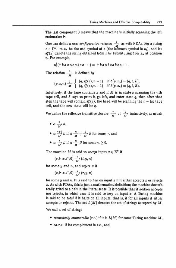
Turing Machines and Effective Computability 213
The last component 0 means that the machine is initially scanning the left endmarker 1-.
One can define a next configuration relation .2..... as with PDAs. For a string M
z E rw, let z .. be the nth symbol of z (the leftmost symbol is Zo), and let si,'(z) denote the string obtained from z by substituting b for Zn at position n. For example,
st (I- b a a a cab ca· .. ) = I- b a abc abc a ....
The relation .2..... is defined by M
(P ) 1 {(q,sb'(z),n -1) ,z,n M (q,sb'(z),n+ 1)
if 6(P,zn) = (q,b,L), if 6(P,z .. ) = (q,b,R).
Intuitively, if the tape contains z and if M is in state p scanning the nth tape cell, and 6 says to print b, go left, and enter state q, then after that step the tape will contain si,'(z), the head will be scanning the n -1st tape cell, and the new state will be q.
We define the reflexive transitive closure ~ of .2..... inductively, as usual: M M
o • aMa,
n+l. .. 1 • a --+ {3 If a --+ 1 --+ {3 for some 1, and
M M M
• a ~ {3 if a ~ {3 for some n > 0. M M -
The machine M is said to accept input x E ~* if
(s,1- XUW,O) -i7 (t,y,n)
for some y and n, and reject x if
(s,1- XUw , 0) ~ (r,y,n) M
for some y and n. It is said to halt on input x if it either accepts x or rejects x. As with PDAs, this is just a mathematical definition; the machine doesn't really grind to a halt in the literal sense. It is possible that it neither accepts nor rejects, in which case it is said to loop on input x. A Turing machine is said to be total if it halts on all inputs; that is, if for all inputs it either accepts or rejects. The set L(M) denotes the set of strings accepted by M.
We call a set of strings
• recursively enumerable (r.e.) if it is L(M) for some Turing machine M,
• co-r.e. if its complement is r.e., and
214 Lecture 28
• recursive if it is L(M) for some total Turing machine M.
In common parlance, the term "recursive" usually refers to an algorithm that calls itself. The definition above has nothing to do with this usage. As used here, it is just a name for a set accepted by a Turing machine that always halts.
We will see lots of examples next time.
Historical Notes
Church's thesis is often referred to as the Church-Turing thesis, although Alonzo Church was the first to formulate it explicitly [25]. The thesis was based on Church and Kleene's observation that the >.-calculus and the p.recursive functions of Godel and Herbrand were computationally equivalent [25]. Church was apparently unaware of Turing's work at the time of the writing of [25], or if he was, he failed to mention it. Turing, on the other hand, cited Church's paper [25] explicitly in [120], and apparently considered his machines to be a much more compelling definition of computability. In an appendix to [120], Turing outlined a proof of the computational equivalence of Turing machines and the >.-calculus.
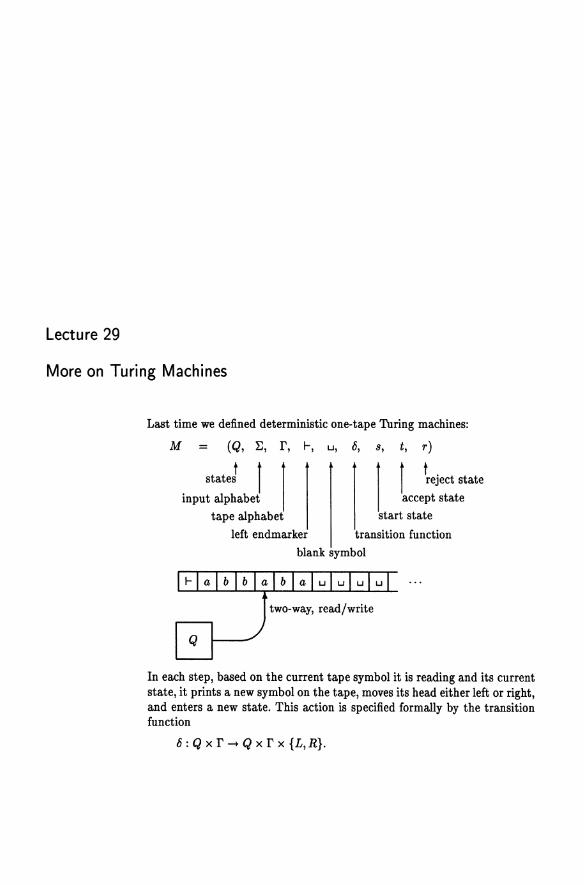
Lecture 29
More on Turing Machines
Last time we defined deterministic one-tape 'lUring machines:
M = (Q, E, r, 1-, u, 8,
t 1 1 states
input alphabet tape alphabet
s, t, r)
1 1 treject state
accept state
start state
left endmarker transition function
blank symbol
In each step, based on the current tape symbol it is reading and its current state, it prints a new symbol on the tape, moves its head either left or right, and enters a new state. This action is specified formally by the transition function
8: Q x r -> Q x r x {L,R}.
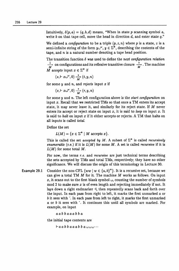
216 Lecture 29
Intuitively, 6(p,a) = (q,b,d) means, "When in state p scanning symbol a, write b on that tape cell, move the head in direction d, and enter state q."
We defined a configuration to be a triple (p, z, n) where p is a state, z is a semi-infinite string of the form yu", y E E*, describing the contents of the tape, and n is a natural number denoting a tape head position.
The transition function 6 was used to define the nezt configuration relation .2... on configurations and its reflexive transitive closure ~ . The machine M M
M accepts input x E E* if
(s,1- xu", 0) -it (t,y,n)
for some y and n, and rejects input x if
(s, I- xu", 0) -it (r,y,n)
for some y and n. The left configuration above is the start configuration on input x. Recall that we restricted TMs so that once a TM enters its accept state, it may never leave it, and similarly for its reject state. If M never enters its accept or reject state on input x, it is said to loop on input x. It is said to halt on input x if it either accepts or rejects. A TM that halts on all inputs is called total.
Define the set
L(M) = {x E E* I M accepts x}.
This is called the set accepted by M. A subset of E* is cal.led recursively enumerable (r.e.) if it is L(M) for some M. A set is called recursive if it is L(M) for some total M.
For now, the terms r.e. and recursive are just technical terms describing the sets accepted by TMs and total TMs, respectively; they have no other significance. We will discuss the origin of this terminology in Lecture 30.
Example 29.1 Consider the non-CFL {ww I w E {a, b} *}. It is a recursive set, because we can give a total TM M for it. The machine M works as follows. On input x, it scans out to the first blank symbol u, counting the number of symbols mod 2 to make sure x is of even length and rejecting immediately if not. It lays down a right endmarker -l, then repeatedly scans back a.nd forth over the input. In each pass from right to left, it marks the first unmarked a or b it sees with '. In each pass from left to right, it p1arks the first unmarked a or b it sees with '. It continues this until all symbols are marked. For example, on input
aabbaaabba
the initial tape contents are
I-aabbaaabbauuu···
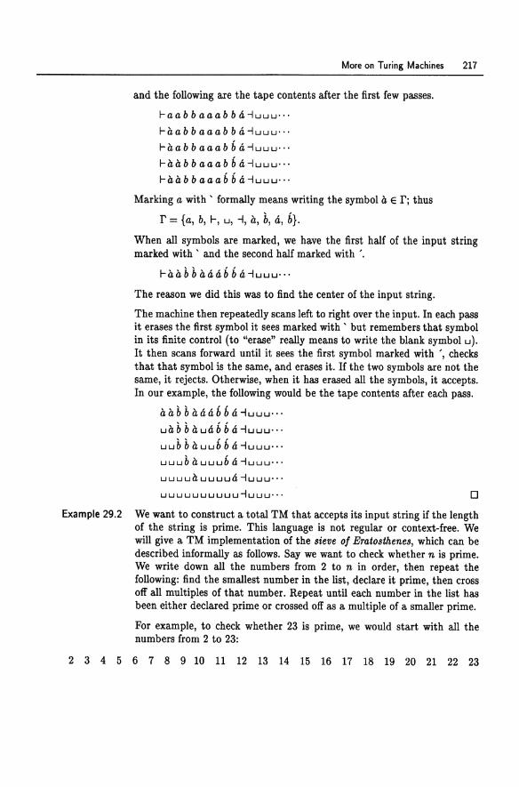
More on Turing Machines 217
and the following are the tape contents after the first few passes.
I-aabbaaabba-iuuu .. · Hub b aaab b a-iuuu'"
I-aabbaaabba-iuuu .. · I-aabbaaabba-iuuu .. · I-aabbaaabba-iuuu .. ·
Marking a with ' formally means writing the symbol a E r; thus
r = {a, b, 1-, u, -i, a, b, a, b}. When all symbols are marked, we have the first half of the input string marked with' and the second half marked with '.
I-aabb aaabb a-iuuu'"
The reason we did this was to find the center of the input string.
The machine then repeatedly scans left to right over the input. In each pass it erases the first symbol it sees marked with ' but remembers that symbol in its finite control (to "erase" really means to write the blank symbol u). It then scans forward until it sees the first symbol marked with " checks that that symbol is the same, and erases it. If the two symbols are not the same, it rejects. Otherwise, when it has erased all the symbols, it accepts. In our example, the following would be the tape contents after each pass.
aabbaaabba-iuuu'" uabbauabba-iuuu"· uubbauubba-iuuu'" uuub a uuub a -iuuu'"
uuuua uuuua -iuuu'"
uuuuuuuuuu-iuuu" . o Example 29.2 We want to construct a total TM that accepts its input string if the length
of the string is prime. This language is not regular or context-free. We will give a TM implementation of the sieve 0/ Eratosthenes, which can be described informally as follows. Say we want to check whether n is prime. We write down all the numbers from 2 to n in order, then repeat the following: find the smallest number in the list, declare it prime, then cross off all multiples of that number. Repeat until each number in the list has been either declared prime or crossed off as a multiple of a smaller prime.
For example, to check whether 23 is prime, we would start with all the numbers from 2 to 23:
2 3 4 5 6 7 8 9 10 11 12 13 14 15 16 17 18 19 20 21 22 23
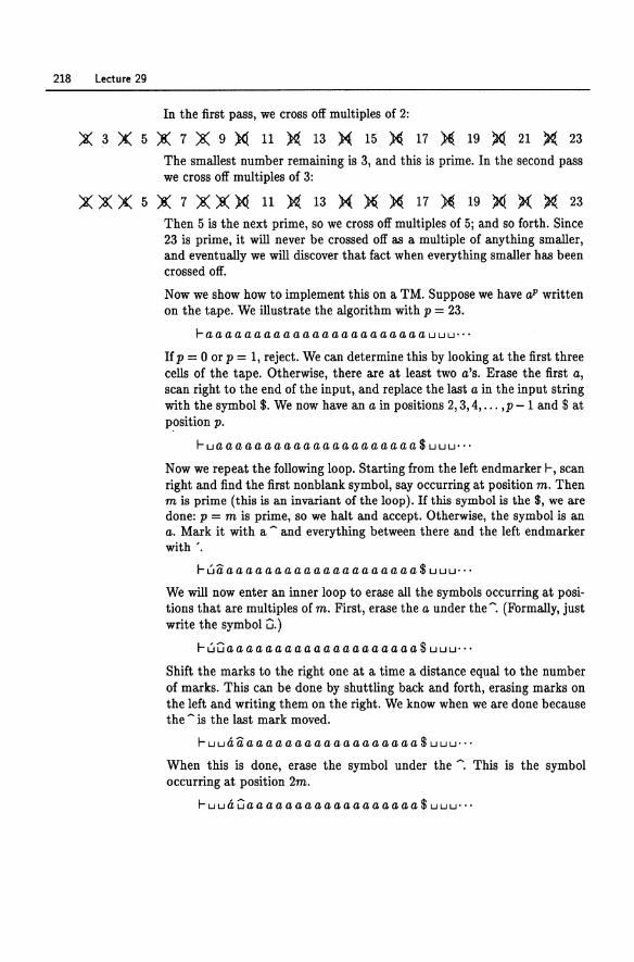
218 Lecture 29
In the first pass, we cross off multiples of 2:
)( 3 X 5 )( 7 )( 9 )Q 11 ~ 13 X 15 X 17 )«{ 19 }K( 21 ~ 23
The smallest number remaining is 3, and this is prime. In the second pass we cross off multiples of 3:
)( )( X 5 )( 7 )()()Q 11 ~ 13 X X X 17 )«{ 19 }K( )( ~ 23
Then 5 is the next prime, so we cross off multiples of 5; and so forth. Since 23 is prime, it will never be crossed off as a multiple of anything smaller, and eventually we will discover that fact when everything smaller has been crossed off.
Now we show how to implement this on a TM. Suppose we have oJ' written on the tape. We illustrate the algorithm with p = 23.
I-a a a a a a a a a aa a a aa aa a a a aa a uuu'"
If p = 0 or p = 1, reject. We can determine this by looking at the first three cells of the tape. Otherwise, there are at least two a's. Erase the first a, scan right to the end of the input, and replace the last a in the input string with the symbol $. We now have an a in positions 2,3,4, ... ,p - 1 and $ at position p.
I-ua aaaaaaaaaaaaaaaaaaaa $ uuu'"
Now we repeat the following loop. Starting from the left endmarker 1-, scan right and find the first nonblank symbol, say occurring at position m. Then m is prime (this is an invariant ofthe loop). If this symbol is the $, we are done: p = m is prime, so we halt and accept. Otherwise, the symbol is an a. Mark it with a ~ and everything between there and the left endmarker with '.
I-uaaa aa aaaaa aaaaaaaaaaa $ uuu'"
We will now enter an inner loop to erase all the symbols occurring at positions that are multiples of m. First, erase the a under the"'. (Formally, just write the symbol u.)
I-uuaaaa aaa aa aaaaaaaaaaa $ uuu'"
Shift the marks to the right one at a time a distance equal to the number of marks. This can be done by shuttling back and forth, erasing marks on the left and writing them on the right. We know when we are done because the ~ is the last mark moved.
I-uuaaaaaaaaa aaaaaaa aaaa $ uuu'"
When this is done, erase the symbol under the~. This is the symbol occurring at position 2m.
I-uua uaaaaa aaaaaaaaaaaaa $ uuu'"
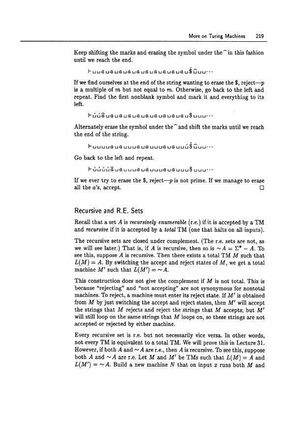
More on Turing Machines 219
Keep shifting the marks and erasing the symbol under the ~ in this fashion until we reach the end.
I-uua ua ua ua ua ua ua ua ua ua u$ uuu···
If we find ourselves at the end of the string wanting to erase the $, reject-p is a multiple of m but not equal to m. Otherwise, go back to the left and repeat. Find the first nonblank symbol and mark it and everything to its left.
I-uuaua ua ua ua ua ua ua ua ua u$ uuu···
Alternately erase the symbol under the ~ and shift the marks until we reach the end of the string.
I-uuuua ua uuua ua uuua ua uuu$ uuu···
Go back to the left and repeat.
I- uuuuaua uuua ua uuua ua uuu$ uuu···
If we ever try to erase the $, reject-p is not prime. If we manage to erase all the a's, accept. 0
Recursive and R.E. Sets
Recall that a set A is recursively enumerable (r.e.) if it is accepted by a TM and recursive if it is accepted by a total TM (one that halts on all inputs).
The recursive sets are closed under complement. (The r.e. sets are not, as we will see later.) That is, if A is recursive, then so is '" A = E* - A. To see this, suppose A is recursive. Then there exists a total TM M such that L(M) = A. By switching the accept and reject states of M, we get a total machine M' such that L(M') = "'A.
This construction does not give the complement if M is not total. This is because "rejecting" and "not accepting" are not synonymous for nontotal machines. To reject, a machine must enter its reject state. If M' is obtained from M by just switching the accept and reject states, then M' will accept the strings that M rejects and reject the strings that M accepts; but M' will still loop on the same strings that M loops on, so these strings are not accepted or rejected by either machine.
Every recursive set is r.e. but not necessarily vice versa. In other words, not every TM is equivalent to a total TM. We will prove this in Lecture 31. However, if both A and'" A are r.e., then A is recursive. To see this, suppose both A and'" A are r.e. Let M and M' be TMs such that L(M) = A and L(M') = '" A. Build a new machine N that on input x runs both M and
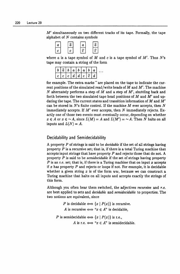
220 Lecture 29
M' simultaneously on two different tracks of its tape. Formally, the tape alphabet of N contains symbols
where a is a tape symbol of M and c is a tape symbol of M'. Thus N's tape may contain a string of the form
for example. The extra marks ~ are placed on the tape to indicate the current positions of the simulated read/write heads of M and M'. The machine N alternately performs a step of M and a step of M', shuttling back and forth between the two simulated tape head positions of M and M' and updating the tape. The current states and transition information of M and M' can be stored in N's finite control. If the machine M ever accepts, then N immediately accepts. If M' ever accepts, then N immediately rejects. Exactly one of those two events must eventually occur, depending on whether a; E A or a; E '" A, since L(M) = A and L(M') = '" A. Then N halts on all inputs and L(N) = A.
Decidability and Semidecidability A property P of strings is said to be decidable if the set of all strings having property P is a recursive set; that is, if there is a total Turing machine that accepts input strings that have property P and rejects those that do not. A property P is said to be semidecidable if the set of strings having property P is an r.e. set; that is, if there is a Turing machine that on input a; accepts if a; has property P and rejects or loops if not. For example, it is decidable whether a given string a; is of the form ww, because we can construct a Turing machine that halts on all inputs and accepts exactly the strings of this form.
Although you often hear them switched, the adjectives recursive and r.e. are best applied to sets and decidable and semidecidable to properties. The two notions are equivalent, since
P is decidable {::::} {a; I p(a;)} is recursive.
A is recursive {::::} "a; E A" is decidable,
Pis semidecidable {::::} {a; I p(a;)} is r.e.,
A is r.e. {::::} "a; E A" is semidecidable.
Lecture 30
Equivalent Models
As mentioned, the concept of computability is remarkably robust. As evidence of this, we will present several different flavors of Turing machines that at first glance appear to be significantly more or less powerful than the basic model defined in Lecture 29 but in fact are computationally equivalent.
Multiple Tapes
First, we show how to simulate mUltitape Turing machines with singletape Turing machines. Thus extra tapes don't add any power. A three-tape machine is similar to a one-tape TM except that it has three semi-infinite tapes and three independent read/write heads. Initially, the input occupies the first tape and the other two are blank. In each step, the machine reads the three symbols under its heads, and based on this information and the current state, it prints a symbol on each tape, moves the heads (they don't all have to move in the same direction), and enters a new state.
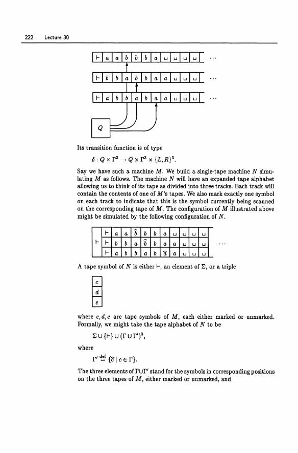
222 Lecture 30
Its transition function is of type
fJ: Q x r 3 ~ Q x r 3 x {L,R}3.
Say we have such a machine M. We build a single-tape machine N simulating M as follows. The machine N will have an expanded tape alphabet allowing us to think of its tape as divided into three tracks. Each track will contain the contents of one of M's tapes. We also mark exactly one symbol on each track to indicate that this is the symbol currently being scanned on the corresponding tape of M. The configuration of M illustrated above might be simulated by the following configuration of N.
I- a a b b b a u u u u
l- I- b b a b b a a u u u
I- a b b a b a a u u u
A tape symbol of N is either 1-, an element of :E, or a triple
where c, d, e are tape symbols of M, each either marked or unmarked. Formally, we might take the tape alphabet of N to be
:E U {I-} U (r U r')3,
where
r' ~ {c ICE r}.
The three elements of rur' stand for the symbols in corresponding positions on the three tapes of M, either marked or unmarked, and
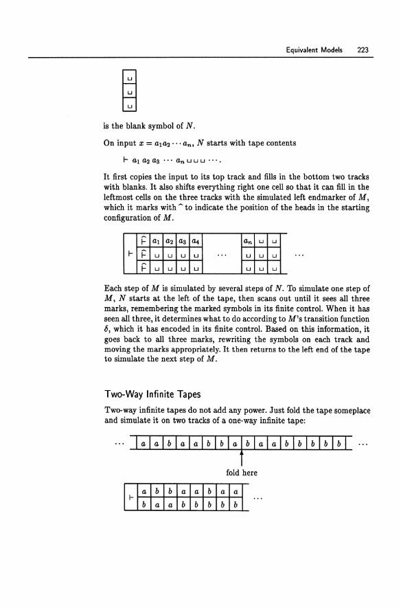
Equivalent Models 223
is the blank symbol of N.
On input x = ala2'" an, N starts with tape contents
It first copies the input to its top track and fills in the bottom two tracks with blanks. It also shifts everything right one cell so that it can fill in the leftmost cells on the three tracks with the simulated left endmarker of M, which it marks with ~ to indicate the position of the heads in the starting configuration of M.
~ al a2 a3 a4 an u u
I- ~ u u u u ... u u u
~ u u u u u u u
Each step of M is simulated by several steps of N. To simulate one step of M, N starts at the left of the tape, then scans out until it sees all three marks, remembering the marked symbols in its finite control. When it has seen all three, it determines what to do according to M's transition function 6, which it has encoded in its finite control. Based on this information, it goes back to all three marks, rewriting the symbols on each track and moving the marks appropriately. It then returns to the left end of the tape to simulate the next step of M.
Two-Way Infinite Tapes
Two-way infinite tapes do not add any power. Just fold the tape someplace and simulate it on two tracks of a one-way infinite tape:
I a I. I b I a I a I bib I at b I. I. I bib I bib I b I
fold here
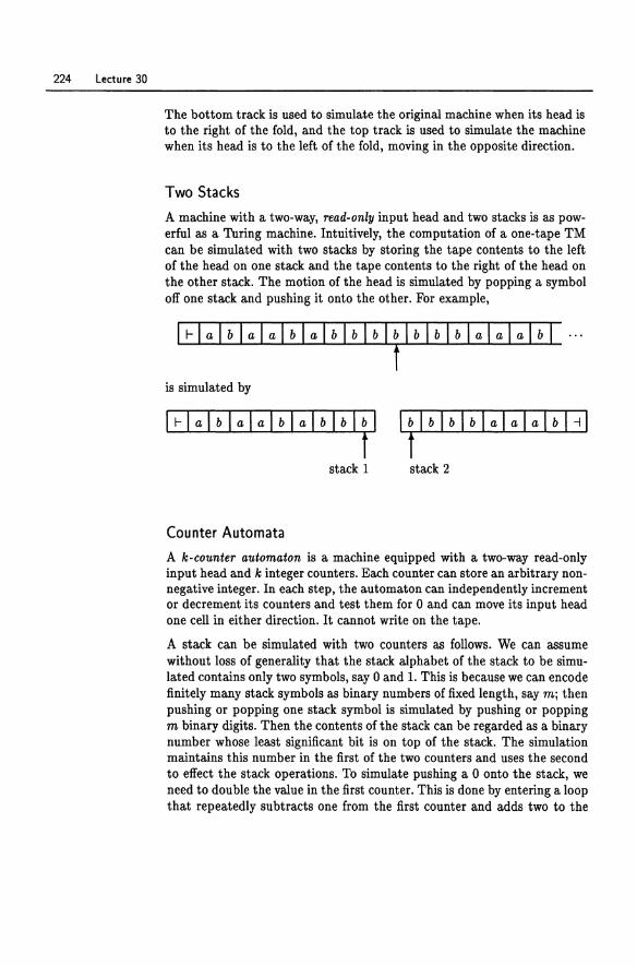
224 Lecture 30
The bottom track is used to simulate the original machine when its head is to the right of the fold, and the top track is used to simulate the machine when its head is to the left of the fold, moving in the opposite direction.
Two Stacks
A machine with a two-way, read-only input head and two stacks is as powerful as a Turing machine. Intuitively, the computation of a one-tape TM can be simulated with two stacks by storing the tape contents to the left of the head on one stack and the tape contents to the right of the head on the other stack. The motion of the head is simulated by popping a symbol off one stack and pushing it onto the other. For example,
Irlalblalalblalblblblblblblblalalalbl t
is simulated by
I r I a I b I a I a I b I a I bib I b I
t stack 1
Cou nter Automata
A k-counter automaton is a machine equipped with a two-way read-only input head and k integer counters. Each counter can store an arbitrary nonnegative integer. In each step, the automaton can independently increment or decrement its counters and test them for 0 and can move its input head one cell in either direction. It cannot write on the tape.
A stack can be simulated with two counters as follows. We can assume without loss of generality that the stack alphabet of the stack to be simulated contains only two symbols, say 0 and 1. This is because we can encode finitely many stack symbols as binary numbers of fixed length, say mj then pushing or popping one stack symbol is simulated by pushing or popping m binary digits. Then the contents of the stack can be regarded as a binary number whose least significant bit is on top of the stack. The simulation maintains this number in the first of the two counters and uses the second to effect the stack operations. To simulate pushing a 0 onto the stack, we need to double the value in the first counter. This is done by entering a loop that repeatedly subtracts one from the first counter and adds two to the
Equivalent Models 225
second until the first counter is O. The value in the second counter is then twice the original value in the first counter. We can then transfer that value back to the first counter, or just switch the roles of the two counters. To push 1, the operation is the same, except the value of the second counter is incremented once at the end. To simulate popping, we need to divide the counter value by two; this is done by decrementing one counter while incrementing the other counter every second step. Testing the parity of the original counter contents tells whether a simulated 1 or 0 was popped.
Since a two-stack machine can simulate an arbitrary TM, and since two counters can simulate a stack, it follows that a four-counter automaton can simulate an arbitrary TM.
However, we can do even better: a two-counter automaton can simulate a four-counter automaton. When the four-counter automaton has the values i,j, k, l in its counters, the two-counter automaton will have the value 2i 3i 5k7i in its first counter. It uses its second counter to effect the counter operations of the four-counter automaton. For example, if the four-counter automaton wanted to add one to k (the value of the third counter), then the two-counter automaton would have to multiply the value in its first counter by 5. This is done in the same way as above, adding 5 to the second counter for every 1 we subtract from the first counter. To simulate a test for zero, the two-counter automaton has to determine whether the value in its first counter is divisible by 2, 3, 5, or 7, respectively, depending on which counter of the four-counter automaton is being tested.
Combining these simulations, we see that two-counter automata are as powerful as arbitrary Turing machines. However, as you can imagine, it takes an enormous number of steps of the two-counter automaton to simulate one step of the Turing machine.
One-counter automata are not as powerful as arbitrary TMs, although they can accept non-CFLs. For example, the set {a"b"c" I n ~ O} can be accepted by a one-counter automaton.
Enumeration Machines
We defined the recursively enumerable (r.e.) sets to be those sets accepted by Turing machines. The term recursively enumerable comes from a different but equivalent formalism embodying the idea that the elements of an r.e. set can be enumerated one at a time in a mechanical fashion.
Define an enumeration machine as follows. It has a finite control and two tapes, a read/write work tape and a write-only output tape. The work tape head can move in either direction and can read and write any element of r. The output tape head moves right one cell when it writes a symbol, and
226 Lecture 30
it can only write symbols in E. There is no input and no accept or reject state. The machine starts in its start state with both tapes blank. It moves according to its transition function like a TM, occasionally writing symbols on the output tape as determined by the transition function. At some point it may enter a special enumeration state, which is just a distinguished state of its finite control. When that happens, the string currently written on the output tape is said to be enumerated. The output tape is then automatically erased and the output head moved back to the beginning of the tape (the work tape is left intact), and the machine continues from that point. The machine runs forever. The set L(E) is defined to be the set of all strings in E* that are ever enumerated by the enumeration machine E. The machine might never enter its enumeration state, in which case L(E) = 0, or it might enumerate infinitely many strings. The same string may be enumerated more than once.
Enumeration machines and 'lUring machines are equivalent in computational power:
Theorem 30.1 The family of sets enumerated by enumeration machines is exactly the family of r.e. sets. In other words, a set is L(E) for some enumeration machine E if and only if it is L(M) for some Turing machine M.
Proof. We show first that given an enumeration machine E, we can construct a 'lUring machine M such that L(M) = L(E). Let M on input x copy x to one of three tracks on its tape, then simulate E, using the other two tracks to record the contents of E's work tape and output tape. For every string enumerated by E, M compares this string to x and accepts if they match. Then M accepts its input x iff x is ever enumerated by E, so the set of strings accepted by M is exactly the set of strings enumerated by E.
Conversely, given a TM M, we can construct an enumeration machine E such that L(E) = L(M). We would like E somehow to simulate M on all possible strings in E* and enumerate those that are accepted.
Here is an approach that doesn't quite work. The enumeration machine E writes down the strings in E* one by one on the bottom track of its work tape in some order. For every input string x, it simulates M on input x, using the top track of its work tape to do the simulation. If M accepts x, E copies x to its output tape and enters its enumeration state. It then goes on to the next string.
The problem with this procedure is that M might not halt on some input x, and then E would be stuck simulating M on x forever and would never move on to strings later in the list (and it is impossible to determine in general whether M will ever halt on x, as we will see in Lecture 31). Thus E should not just list the strings in E* in some order and simulate M on
Equivalent Models 227
those inputs one at a time, waiting for each simulation to halt before going on to the next, because the simulation might never halt.
The solution to this problem is timesharing. Instead of simulating M on the input strings one at a time, the enumeration machine E should run several simulations at once, working a few steps on each simulation and then moving on to the next. The work tape of E can be divided into segments separated by a special marker # E r, with a simulation of M on a different input string running in each segment. Between passes, E can move way out to the right, create a new segment, and start up a new simulation in that segment on the next input string. For example, we might have E simulate M on the first input for one step, then the first and second inputs for one step each, then the first, second, and third inputs for one step each, and so on. If any simulation needs more space than initially allocated in its segment, the entire contents of the tape to its right can be shifted to the right one cell. In this way M is eventually simulated on all input strings, even if some of the simulations never halt. 0
Historical Notes
Turing machines were invented by Alan Turing [120]. Originally they were presented in the form of enumeration machines, since Turing was interested in enumerating the decimal expansions of computable real numbers and values of real-valued functions. Turing also introduced the concept of nondeterminism in his original paper, although he did not develop the idea.
The basic properties of the r.e. sets were developed by Kleene [68] and Post [100,101].
Counter automata were studied by Fischer [38], Fischer et al. [39], and Minsky [88].
Lecture 31
Universal Machines and Diagonalization
A Universal Turing Machine
Now we come to a crucial observation about the power of Turing machines: there exist Turing machines that can simulate other Turing machines whose descriptions are presented as part of the input. There is nothing mysterious about this; it is the same as writing a LISP interpreter in LISP.
First we need to fix a reasonable encoding scheme for Turing machines over the alphabet {D, I}. This encoding scheme should be simple enough that all the data associated with a machine M -the set of states, the transition function, the input and tape alphabets, the endmarker, the blank symbol, and the start, accept, and reject states-can be determined easily by another machine reading the encoded description of M. For example, if the string begins with the prefix
DnlOmlOklOslOtlOrlOuID"I,
this might indicate that the machine has n states represented by the numbers D to n - 1; it has m tape symbols represented by the numbers D to m - 1, of which the first k represent input symbols; the start, accept, and reject states are 8, t, and T, respectively; and the endmarker and blank symbol are u and v, respectively. The remainder of the string can consist
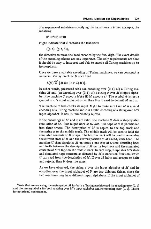
Universal Machines and Diagonalization 229
of a sequence of substrings specifying the transitions in O. For example, the substring
OPlOalOqlOblO
might indicate that 0 contains the transition
((p,a), (q,b,L)),
the direction to move the head encoded by the final digit. The exact details of the encoding scheme are not important. The only requirements are that it should be easy to interpret and able to encode all Turing machines up to isomorphism.
Once we have a suitable encoding of Turing machines, we can construct a universal Turing machine U such that
L(U) ~ {M#x I x E L(M)}.
In other words, presented with (an encoding over {O, I} of) a Turing machine M and (an encoding over {O, I} of) a string x over M's input alphabet, the machine U accepts M #x iff M accepts x.1 The symbol # is just a symbol in U's input alphabet other than 0 or 1 used to delimit M and x.
The machine U first checks its input M #x to make sure that M is a valid encoding of a Turing machine and x is a valid encoding of a string over M's input alphabet. If not, it immediately rejects.
If the encodings of M and x are valid, the machine U does a step-by-step simulation of M. This might work as follows. The tape of U is partitioned into three tracks. The description of M is copied to the top track and the string x to the middle track. The middle track will be used to hold the simulated contents of M's tape. The bottom track will be used to remember the current state of M and the current position of M's read/write head. The machine U then simulates M on input x one step at a time, shuttling back and forth between the description of M on its top track and the simulated contents of M's tape on the middle track. In each step, it updates M's state and simulated tape contents as dictated by M's transition function, which U can read from the description of M. If ever M halts and accepts or halts and rejects, then U does the same.
As we have observed, the string x over the input alphabet of M and its encoding over the input alphabet of U are two different things, since the two machines may have different input alphabets. If the input alphabet of
1 Note that we are using the metasymbol M for both a Turing machine and its encoding over {O, I} and the metasymbol x for both a string over M's input alphabet and its encoding over {O, I}. This is for notational convenience.
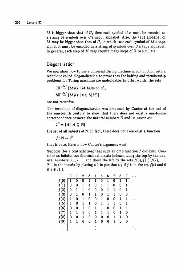
230 Lecture 31
M is bigger than that of U, then each symbol of x must be encoded as a string of symbols over U's input alphabet. Also, the tape alphabet of M may be bigger than that of U, in which CaBe each symbol of M's tape alphabet must be encoded aB a string of symbols over U's tape alphabet. In general, each step of M may require many steps of U to simulate.
Diagonalization
We now show how to use a universal Turing machine in conjunction with a technique called diagonalization to prove that the halting and membership problems for Turing machines are undecidable. In other words, the sets
HP ~ {M#x I M halts on x},
MP ~f {M#x I x E L(M)}
are not recursive.
The technique of diagonalization was first used by Cantor at the end of the nineteenth century to show that there does not exist a one-to-one correspondence between the natural numbers N and its power set
2M = {A I A S;; N},
the set of all subsets of N. In fact, there does not even exist a function
I:N-+2N that is onto. Here is how Cantor's argument went.
Suppose (for a contradiction) that such an onto function 1 did exist. Consider an infinite two-dimensional matrix indexed along the top by the natural numbers 0,1,2, ... and down the left by the sets 1(0),/(1),/(2), .... Fill in the matrix by placing a 1 in position i,j if j is in the set I(i) and 0 if j ¢ I(i).
0 1 2 3 4 5 6 7 8 9 1(0) 1 0 0 1 1 0 1 0 1 1 1(1) 0 0 1 1 0 1 1 0 0 1 1(2) 0 1 1 0 0 0 1 1 0 1 1(3) 0 1 0 1 1 0 1 1 0 0 1(4) 1 0 1 0 0 1 0 0 1 1 1(5) 1 0 1 1 0 1 1 1 0 1 1(6) 0 0 1 0 1 1 0 0 1 1 1(7) 1 1 1 0 1 1 1 0 1 0 1(8) 0 0 1 0 0 0 0 1 1 0 1(9) 1 1 0 0 1 0 0 1 0 0
Universal Machines and Diagonalization 231
The ith row of the matrix is a bit string describing the set I( i). For example, in the above picture, 1(0) = {O, 3, 4, 6, 8, 9, ... } and 1(1) = {2, 3, 5, 6, 9, ... }. By our (soon to be proved fallacious) assumption that 1 is onto, every subset of N appears as a row of this matrix.
But we can construct a new set that does not appear in the list by complementing the main diagonal of the matrix (hence the term diagonalization). Look at the infinite bit string down the main diagonal (in this example, 1011010010···) and take its Boolean complement (in this example, 0100101101 .. -). This new bit string represents a set B (in this example, B = {1, 4, 6, 7,9, ... } ). But the set B does not appear anywhere in the list down the left side of the matrix, since it differs from every I(i) on at least one element, namely i. This is a contradiction, since every subset of N was supposed to occur as a row of the matrix, by our assumption that 1 was onto.
This argument works not only for the natural numbers N, but for any set A whatsoever. Suppose (for a contradiction) there existed an onto function from A to its power set:
1 :A~ 2A.
Let
B = {x E A I x ¢ I(x)}
(this is the formal way of complementing the diagonal). Then B ~ A. Since 1 is onto, there must exist yEA such that I(y) = B. Now we ask whether y E I(Y) and discover a contradiction:
1/ E 1(1/) {::::} Y E B since B = I(Y) {::::} Y ¢ I(Y) definition of B.
Thus no such 1 can exist.
Undecidability of the Halting Problem
We have discussed how to encode descriptions of Turing machines as strings in {O, 1} * so that these descriptions can be read and simulated by a universal Turing machine U. The machine U takes as input an encoding of a Turing machine M and a string x and simulates M on input x, and
• halts and accepts if M halts and accepts x,
• halts and rejects if M halts and rejects x, and
• loops if M loops on x.
232 Lecture 31
The machine U doesn't do any fancy analysis on the machine M to try to determine whether or not it will halt. It just blindly simulates M step by step. If M doesn't halt on x, then U will just go on happily simulating M forever.
It is natural to ask whether we can do better than just a blind simulation. Might there be some way to analyze M to determine in advance, before doing the simulation, whether M would eventually halt on x? If U could say for sure in advance that M would not halt on x, then it could skip the simulation and save itself a lot of useless work. On the other hand, if U could ascertain that M would eventually halt on x, then it could go ahead with the simulation to determine whether M accepts or rejects. We could then build a machine U' that takes as input an encoding of a Turing machine M and a string x, and
• halts and accepts if M halts and accepts x,
• halts and rejects if M halts and rejects x, and
• halts and rejects if M loops on x.
This would say that L(U') = L(U) = MP is a recursive set.
Unfortunately, this is not possible in general. There are certainly machines for which it is possible to determine halting by some heuristic or other: machines for which the start state is the accept state, for example. However, there is no general method that gives the right answer for all machines.
We can prove this using Cantor's diagonalization technique. For x E {O, I} *, let Mz be the Turing machine with input alphabet {O, I} whose encoding over {O, I} * is x. (If x is not a legal description of a TM with input alphabet {O, I} * according to our encoding scheme, we take M., to be some arbitrary but fixed TM with input alphabet {O, I}, say a trivial TM with one state that immediately halts.) In this way we get a list
(31.1)
containing all possible Turing machines with input alphabet {O, I} indexed by strings in {O,I}*. We make sure that the encoding scheme is simple enough that a universal machine can determine M., from x for the purpose of simulation.
Now consider an infinite two-dimensional matrix indexed along the top by strings in {0,1}* and down the left by TMs in the list (31.1). The matrix
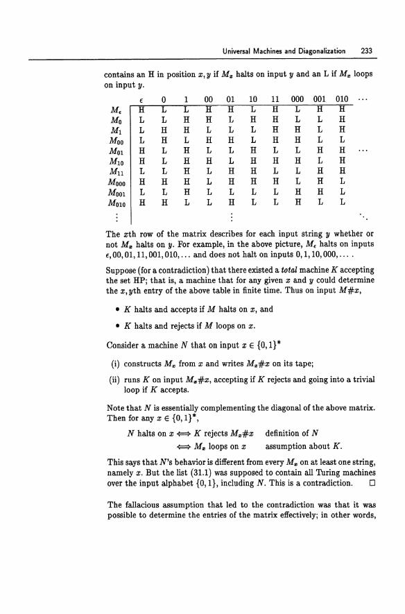
Universal Machines and Diagonalization 233
contains an H in position x, y if M", halts on input y and an L if M", loops on input y.
f a 1 00 01 10 11 000 001 010 M. H L L H H L H L H H Mo L L H H L H H L L H Ml L H H L L L H H L H Moo L H L H H L H H L L MOl H L H L L H L L H H M10 H L H H L H H H L H Mn L L H L H H L L H H Mooo H H H L H H H L H L MOOl L L H L L L L H H L M010 H H L L H L L H L L
The xth row of the matrix describes for each input string y whether or not M", halts on y. For example, in the above picture, M. halts on inputs f, 00, 01,11, 001, 010, ... and does not halt on inputs 0, 1, 10, 000, ....
Suppose (for a contradiction) that there existed a total machine K accepting the set HPj that is, a machine that for any given x and y could determine the x, yth entry of the above table in finite time. Thus on input M #x,
• K halts and accepts if M halts on x, and
• K halts and rejects if M loops on x.
Consider a machine N that on input x E {0,1}*
(i) constructs M", from x and writes M.,#x on its tapej
(ii) runs K on input M.,#x, accepting if K rejects and going into a trivial loop if K accepts.
Note that N is essentially complementing the diagonal of the above matrix. Then for any x E {0,1}*,
N halts on x {::=} K rejects M.,#x definition of N
{::=} M., loops on x assumption about K.
This says that N's behavior is different from every M., on at least one string, namely x. But the list (31.1) was supposed to contain all Turing machines over the input alphabet {a, I}, including N. This is a contradiction. 0
The fallacious assumption that led to the contradiction was that it was possible to determine the entries of the matrix effectivelYj in other words,
234 Lecture 31
that there existed a Turing machine K that given M and x could determine in a finite time whether or not M halts on x.
One can always simulate a given machine on a given input. If the machine ever halts, then we will know this eventually, and we can stop the simulation and say that it halted; but if not, there is no way in general to stop after a finite time and say for certain that it will never halt.
Undecidability of the Membership Problem
The membership problem is also undecidable. We can show this by reducing the halting problem to it. In other words, we show that if there were a way to decide membership in general, we could use this as a subroutine to decide halting in general. But we just showed above that halting is undecidable, so membership must be undecidable too.
Here is how we would use a total TM that decides membership as a subroutine to decide halting. Given a machine M and input x, suppose we wanted to find out whether M halts on x. Build a new machine N that is exactly like M, except that it accepts whenever M would either accept or reject. The machine N can be constructed from M simply by adding a new accept state and making the old accept and reject states transfer to this new accept state. Then for all x, N accepts x iff M halts on x. The membership problem for N and x (asking whether x E L(N)) is therefore the same as the halting problem for M and x (asking whether M halts on x). If the membership problem were decidable, then we could decide whether M halts on x by constructing N and asking whether x E L(N). But we have shown above that the halting problem is undecidable, therefore the membership problem must also be undecidable.
Lecture 32
Decidable and Undecidable Problems
Here are some examples of decision problems involving Turing machines. Is it decidable whether a given Turing machine
(a) has at least 481 states?
(b) takes more than 481 steps on input f?
(c) takes more than 481 steps on some input?
(d) takes more than 481 steps on all inputs?
(e) ever moves its head more than 481 tape cells away from the left endmarker on input f?
(f) accepts the null string E?
(g) accepts any string at all?
(h) accepts every string?
(i) accepts a finite set?
(j) accepts a regular set?
(k) accepts a CFL?
(1) accepts a recursive set?
236 Lecture 32
(m) is equivalent to a Turing machine with a shorter description?
Problems (a) through (e) are decidable and problems (f) through (m) are undecidable (proofs below). We will show that problems (f) through (1) are undecidable by showing that a decision procedure for one of these problems could be used to construct a decision procedure for the halting problem, which we know is impossible. Problem (m) is a little more difficult, and we will leave that as an exercise (Miscellaneous Exercise 131). Translated into modern terms, problem (m) is the same as determining whether there exists a shorter PASCAL program equivalent to a given one.
The best way to show that a problem is decidable is to give a total Turing machine that accepts exactly the "yes" instances. Because it must be total, it must also reject the "no" instances; in other words, it must not loop on any input.
Problem (a) is easily decidable, since the number of states of M can be read off from the encoding of M. We can build a Turing machine that, given the encoding of M written on its input tape, counts the number of states of M and accepts or rejects depending on whether the number is at least 481.
Problem (b) is decidable, since we can simulate M on input f with a universal machine for 481 steps (counting up to 481 on a separate track) and accept or reject depending on whether M has halted by that time.
Problem (c) is decidable: we can just simulate M on all inputs of length at most 481 for 481 steps. If M takes more than 481 steps on some input, then it will take more than 481 steps on some input of length at most 481, since in 481 steps it can read at most the first 481 symbols of the input.
The argument for problem (d) is similar. If M takes more than 481 steps on all inputs of length at most 481, then it will take more than 481 steps on all inputs.
For problem (e), if M never moves more than 481 tape cells away from the left endmarker, then it will either halt or loop in such a way that we can detect the looping after a finite time. This is because if M has k states and m tape symbols, and never moves more than 481 tape cells away from the left endmarker, then there are only 482km481 configurations it could possibly ever be in, one for each choice of head position, state, and tape contents that fit within 481 tape cells. If it runs for any longer than that without moving more than 481 tape cells away from the left endmarker, then it must be in a loop, because it must have repeated a configuration. This can be detected by a machine that simulates M, counting the number of steps M takes on a separate track and declaring M to be in a loop if the bound of 482km481 steps is ever exceeded.
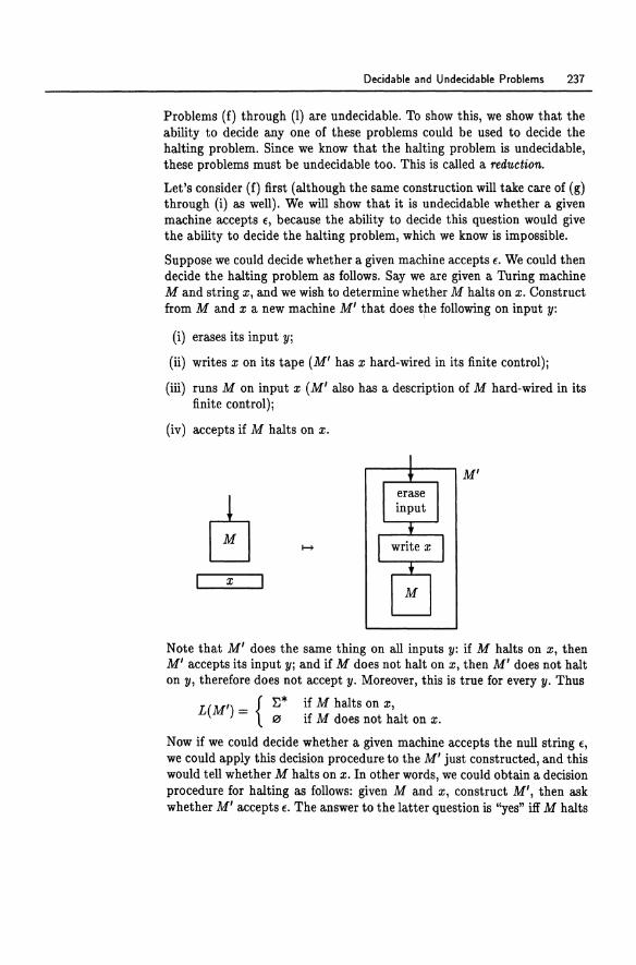
Decidable and Undecidable Problems 237
Problems (f) through (1) are undecidable. To show this, we show that the ability to decide anyone of these problems could be used to decide the halting problem. Since we know that the halting problem is undecidable, these problems must be undecidable too. This is called a reduction.
Let's consider (f) first (although the same construction will take care of (g) through (i) as well). We will show that it is undecidable whether a given machine accepts f, because the ability to decide this question would give the ability to decide the halting problem, which we know is impossible.
Suppose we could decide whether a given machine accepts f. We could then decide the halting problem as follows. Say we are given a Turing machine M and string x, and we wish to determine whether M halts on x. Construct from M and x a new machine M' that does the following on input y:
I
(i) erases its input Yj
(ii) writes x on its tape (M' has x hard-wired in its finite control)j
(iii) runs M on input x (M' also has a description of M hard-wired in its finite control)j
(iv) accepts if M halts on x.
M'
x M
Note that M' does the same thing on all inputs y: if M halts on x, then M' accepts its input Yj and if M does not halt on x, then M' does not halt on y, therefore does not accept y. Moreover, this is true for every y. Thus
L(M') _ {~* if M halts on x, - flJ if M does not halt on x.
Now if we could decide whether a given machine accepts the null string f,
we could apply this decision procedure to the M' just constructed, and this would tell whether M halts on x. In other words, we could obtain a decision procedure for halting as follows: given M and x, construct M', then ask whether M' accepts f. The answer to the latter question is "yes" iff M halts
238 Lectu re 32
on x. Since we know the halting problem is undecidable, it must also be undecidable whether a given machine accepts f.
Similarly, if we could decide whether a given machine accepts any string at all, or whether it accepts every string, or whether the set of strings it accepts is finite, we could apply any of these decision procedures to M' and this would tell whether M halts on x. Since we know that the halting problem is undecidable, all of these problems must be undecidable too.
To show that (j), (k), and (1) are undecidable, pick your favorite r.e. but nonrecursive set A (HP or MP will do) and modify the above construction as follows. Given M and x, build a new machine Mil that does the following on input y:
(i) saves y on a separate track of its tape;
(ii) writes x on a different track (x is hard-wired in the finite control of Mil);
(iii) runs M on input x (M is also hard-wired in the finite control of Mil);
(iv) if M halts on x, then Mil runs a machine accepting A on its original input y, and accepts if that machine accepts.
Either M does not halt on x, in which case the simulation in step (iii) never halts and Mil never accepts any string; or.M does halt on x, in which case Mil accepts its input y iff yEA. Thus
L(M") = {~ if M halts on x, IU if M does not halt on x.
Since A is neither recursive, CFL, nor regular, and 0 is all three of these things, if one could decide whether a given TM accepts a recursive, contextfree, or regular set, then one could apply this decision procedure to Mil and this would tell whether M halts on x.
Lecture 33
Reduction
There are two main techniques for showing that problems are undecidable: diagonalization and reduction. We saw examples of diagonalization in Lecture 31 and reduction in Lecture 32.
Once we have established that a problem such as HP is undecidable, we can show that another problem B is undecidable by reducing HP to B. Intuitively, this means we can manipulate instances of HP to make them look like instances of the problem B in such a way that ''yes'' instances of HP become "yes" instances of B and "no" instances of HP become "no" instances of B. Although we cannot tell effectively whether a given instance of HP is a "yes" instance, the manipulation preserves "yes"-ness and "no"ness. If there existed a decision procedure for B, then we could apply it to the disguised instances of HP to decide membership in HP. In other words, combining a decision procedure for B with the manipulation procedure would give a decision procedure for HP. Since we have already shown that no such decision procedure for HP can exist, we can conclude that no decision procedure for B can exist.
We can give an abstract definition of reduction and prove a general theorem that will save us a lot of work in undecidability proofs from now on.
Given sets A ~ ~* and B ~ ~*, a (many-one) reduction of A to B is a computable function
u: ~* -~*
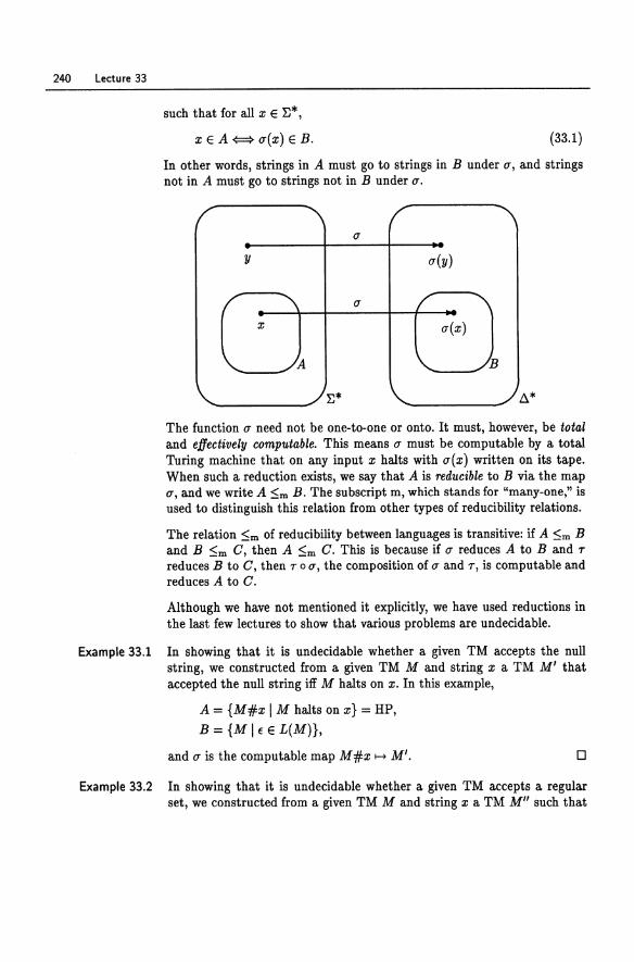
240 Lectu re 33
such that for all x E E*,
x E A -<==> O"(x) E B. (33.1)
In other words, strings in A must go to strings in B under 0", and strings not in A must go to strings not in B under 0".
y
B
E* ~*
The function 0" need not be one-to-one or onto. It must, however, be total and effectively computable. This means 0" must be computable by a total Turing machine that on any input x halts with O"(x) written on its tape. When such a reduction exists, we say that A is reducible to B via the map 0", and we write A :5m B. The subscript m, which stands for "many-one," is used to distinguish this relation from other types of reducibility relations.
The relation :5m of reducibility between languages is transitive: if A :5m B and B :5m C, then A :5m C. This is because if 0" reduces A to Band 7
reduces B to C, then 700", the composition of 0" and 7, is computable and reduces A to C.
Although we have not mentioned it explicitly, we have used reductions in the last few lectures to show that various problems are undecidable.
Example 33.1 In showing that it is undecidable whether a given TM accepts the null string, we constructed from a given TM M and string x a TM M' that accepted the null string iff M halts on x. In this example,
A = {M#x I M halts on x} = HP,
B = {M I f E L(M)},
and 0" is the computable map M#x f-+ M'. o
Example 33.2 In showing that it is undecidable whether a given TM accepts a regular set, we constructed from a given TM M and string x a TM Mil such that
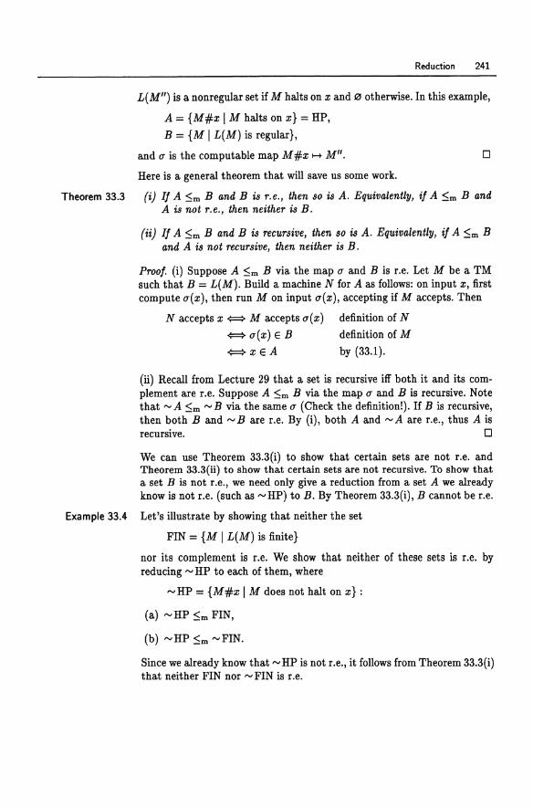
Reduction 241
L(M") is a nonregular set if M halts on x and 0 otherwise. In this example,
A = {M#x I M halts on x} = HP,
B = {M I L(M) is regular},
and q is the computable map M#x 1-+ Mil. o Here is a general theorem that will save us some work.
Theorem 33.3 (i) If A :'5m Band B is r.e., then so is A. Equivalently, if A :'5m Band A is not r.e., then neither is B.
(ii) If A :'5m Band B is recursive, then so is A. Equivalently, if A :'5m B and A is not recursive, then neither is B.
Proof. (i) Suppose A :'5m B via the map q and B is r.e. Let M be a TM such that B = L(M). Build a machine N for A as follows: on input x, first compute q(x), then run M on input q(x), accepting if M accepts. Then
N accepts x {::::::> M accepts u(x) definition of N
{::::::> u( x) E B definition of M
{::::::> x E A by (33.1).
(ii) Recall from Lecture 29 that a set is recursive iff both it and its complement are r.e. Suppose A :'5m B via the map 17 and B is recursive. Note that'" A :'5m '" B via the same 17 (Check the definition!). If B is recursive, then both Band'" Bare r.e. By (i), both A and'" A are r.e., thus A is recursive. 0
We can use Theorem 33.3(i) to show that certain sets are not r.e. and Theorem 33.3(ii) to show that certain sets are not recursive. To show that a set B is not r.e., we need only give a reduction from a set A we already know is not r.e. (such as '" HP) to B. By Theorem 33.3(i), B cannot be r.e.
Example 33.4 Let's illustrate by showing that neither the set
FIN = {M I L(M) is finite}
nor its complement is r.e. We show that neither of these sets is r.e. by reducing'" HP to each of them, where
"'HP = {M#x I M does not halt on x}:
(a) "'HP:'5m FIN,
(b) '" HP :'5m '" FIN.
Since we already know that'" HP is not r.e., it follows from Theorem 33.3(i) that neither FIN nor'" FIN is r.e.
242 Lecture 33
For (a), we want to give a computable map u such that
M#x E ..... HP {:::::::> u(M#x) E FIN.
In other words, from M #x we want to construct a Turing machine M' = u(M#x) such that
M does not halt on x {:::::::> L(M') is finite. (33.2)
Note that the description of M' can depend on M and x. In particular, M' can have a description of M and the string x hard-wired in its finite control if desired.
We have actually already given a construction satisfying (33.2). Given M#x, construct M' such that on all inputs y, M' takes the following actions:
(i) erases its input Yj
(ii) writes x on its tape (M' has x hard-wired in its finite control)j
(iii) runs M on input x (M' also has a description of M hard-wired in its finite control)j
(iv) accepts if M halts on x.
If M does not halt on input x, then the simulation in step (iii) never halts, and M' never reaches step (iv). In this case M' does not accept its input y. This happens the same way for all inputs y, therefore in this case, L(M) = 0. On the other hand, if M does halt on x, then the simulation in step (iii) halts, and y is accepted in step (iv). Moreover, this is true for all y. In this case, L(M) = ~*. Thus
M halts on x => L(M') = ~* M does not halt on x => L(M') = 0
=> L(M') is infinite, => L(M') is finite.
Thus (33.2) is satisfied. Note that this is all we have to do to show that FIN is not r.e.: we have given the reduction (a), so by Theorem 33.3(i) we are done.
There is a common pitfall here that we should be careful to avoid. It is important to observe that the computable map u that produces a description of M' from M and x does not need to execute the program (i) through (iv). It only produces the description of a machine M' that does so. The computation of u is quite simple-it does not involve the simulation of any other machines or anything complicated at all. It merely takes a description of a Turing machine M and string x and plugs them into a general description of a machine that executes (i) through (iv). This can be done quite easily by a total TM, so u is total and effectively computable.
Reduction 243
Now (b). By definition of reduction, a map reducing "'HP to "'FIN also reduces HP to FIN, so it suffices to give a computable map r such that
M#x e HP ~ r(M#x) e FIN.
In other words, from M and x we want to construct a Turing machine Mil = r(M#x) such that
M halts on x ~ L(M") is finite. (33.3)
Given M#x, construct a machine Mil that on input y
(i) saves y on a separate track;
(ii) writes x on the tape;
(iii) simulates M on x for Iyl steps (it erases one symbol of y for each step of M on x that it simulates);
(iv) accepts if M has not halted within that time, otherwise rejects.
Now if M never halts on x, then Mil halts and accepts y in step (iv) after Iyl steps of the simulation, and this is true for all y. In this case L(M") = ~*. On the other hand, if M does halt on x, then it does so after some finite number of steps, say n. Then Mil accepts y in (iv) if Iyl < n (since the simulation in (iii) has not finished by Iyl steps) and rejects y in (iv) if Iyl ~ n (since the simulation in (iii) does have time to complete). In this case M" accepts all strings of length less than n and rejects all strings of length n or greater, so L(M") is a finite set. Thus
M halts on x => L(M") = {y Ilyl < running time of M on x} => L( M") is finite,
M does not halt on x => L(M") = ~* => L(M") is infinite.
Then (33.3) is satisfied.
It is important that the functions u and r in these two reductions can be computed by Turing machines that always halt. 0
Historical Notes
The technique of diagonalization was first used by Cantor [161 to show that there were fewer real algebraic numbers than real numbers.

244 Lecture 33
Universal Turing machines and the application of Cantor's diagonalization technique to prove the undecidability of the halting problem appear in Turing's original paper [120].
Reducibility relations are discussed by Post [101]; see [106, 116].
Lecture 34
Rice's Theorem
Rice's theorem says that undecidability is the rule, not the exception. It is a very powerful theorem, subsuming many undecidability results that we have seen as special cases.
Theorem 34.1 (Rice's theorem) Every nontrivial property of the T.e. sets is undecidable.
Yes, you heard right: that's every nontrivial property of the r.e. sets. So as not to misinterpret this, let us clarify a few things.
First, fix a finite alphabet E. A property of the r.e. sets is a map
P: {r.e. subsets of E*} -. {T,J.},
where T and 1. represent truth and falsity, respectively. For example, the property of emptiness is represented by the map
P(A) = {T ~f A = .0, 1. If A #.0.
To ask whether such a property P is decidable, the set has to be presented in a finite form suitable for input to a TM. We assume that r.e. sets are presented by TMs that accept them. But keep in mind that the property is a property of sets, not of Turing machines; thus it must be true or false independent of the particular TM chosen to represent the set.
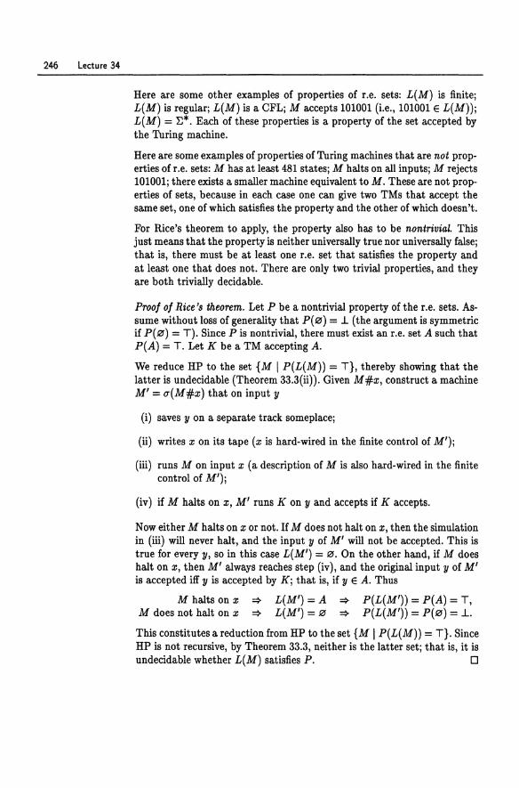
246 Lectu re 34
Here are some other examples of properties of r.e. sets: L(M) is finitej L(M) is regularj L(M) is a CFLj M accepts 101001 (Le., 101001 E L(M»j L( M) = ~*. Each of these properties is a property of the set accepted by the Turing machine.
Here are some examples of properties of Turing machines that are not properties of r.e. sets: M has at least 481 statesj M halts on all inputsj M rejects 101OO1j there exists a smaller machine equivalent to M. These are not properties of sets, because in each case one can give two TMs that accept the same set, one of which satisfies the property and the other of which doesn't.
For IDce's theorem to apply, the property also has to be nontrivial. This just means that the property is neither universally true nor universally falsej that is, there must be at least one r.e. set that satisfies the property and at least one that does not. There are only two trivial properties, and they are both trivially decidable.
Proof of Rice's theorem. Let P be a nontrivial property of the r.e. sets. Assume without loss of generality that P(0') = .L (the argument is symmetric if P(0') = T). Since P is nontrivial, there must exist an r.e. set A such that P(A) = T. Let K be a TM accepting A.
We reduce HP to the set {M I P(L(M» = T}, thereby showing that the latter is undecidable (Theorem 33.3(ii». Given M#x, construct a machine M' = u(M#x) that on input y
(i) saves y on a separate track someplacej
(ii) writes x on its tape (x is hard-wired in the finite control of M')j
(iii) runs M on input x (a description of M is also hard-wired in the finite control of M')j
(iv) if M halts on x, M' runs K on y and accepts if K accepts.
Now either M halts on x or not. If M does not halt on x, then the simulation in (iii) will never halt, and the input y of M' will not be accepted. This is true for every y, so in this case L(M') = 0'. On the other hand, if M does halt on x, then M' always reaches step (iv), and the original input y of M' is accepted iff y is accepted by Kj that is, if YEA. Thus
M halts on x :::} L(M') = A :::} P(L(M'» = P(A) = T, M does not halt on x :::} L(M') = 0' :::} P(L(M'» = P(0') = .L.
This constitutes a reduction from HP to the set {M I P(L(M» = T}. Since HP is not recursive, by Theorem 33.3, neither is the latter setj that is, it is undecidable whether L( M) satisfies P. 0
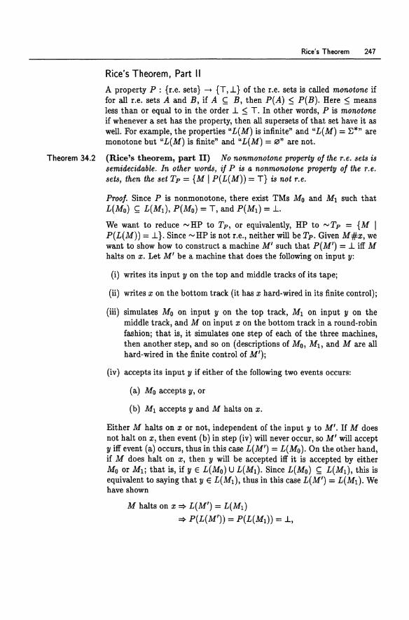
Rice's Theorem 247
Rice's Theorem, Part 1\
A property P : {r.e. sets} -+ {T,.l} of the r.e. sets is called monotone if for all r.e. sets A and B, if A ~ B, then P(A) ::; P(B). Here::; means less than or equal to in the order .l ::; T. In other words, P is monotone if whenever a set has the property, then all supersets of that set have it as well. For example, the properties "L(M) is infinite" and "L(M) = E*" are monotone but "L(M) is finite" and "L(M) = 0" are not.
Theorem 34.2 (Rice's theorem, part II) No nonmonotone property of the r.e. sets is semidecidable. In other words, if P is a nonmonotone property of the r.e. sets, then the set Tp = {M I P(L(M)) = T} is not r.e.
Proof. Since P is nonmonotone, there exist TMs Mo and Ml such that L(Mo) ~ L(M1), P(Mo) = T, and P(M1) = .l. We want to reduce ..... HP to Tp , or equivalently, HP to ..... Tp = {M I P(L(M)) = .l}. Since ..... HP is not r.e., neither will be Tp • Given M#x, we want to show how to construct a machine M' such that P(M') = .l iff M halts on x. Let M' be a machine that does the following on input y:
(i) writes its input y on the top and middle tracks of its tape;
(il) writes x on the bottom track (it has x hard-wired in its finite control);
(iii) simulates Mo on input y on the top track, Ml on input y on the middle track, and M on input x on the bottom track in a round-robin fashion; that is, it simulates one step of each of the three machines, then another step, and so on (descriptions of Mo, Mb and M are all hard-wired in the finite control of M');
(iv) accepts its input y if either of the following two events occurs:
(a) Mo accepts y, or
(b) Ml accepts y and M halts on x.
Either M halts on x or not, independent of the input y to M'. If M does not halt on x, then event (b) in step (iv) will never occur, so M' will accept y iff event (a) occurs, thus in this case L(M') = L(Mo). On the other hand, if M does halt on x, then y will be accepted iff it is accepted by either Mo or Ml; that is, if Y E L(Mo) U L(Ml). Since L(Mo) ~ L(M1), this is equivalent to saying that y E L(M1), thus in this case L(M') = L(Ml). We have shown
M halts on x => L(M') = L(Ml) => P(L(M')) = P(L(M1)) = .l,
248 Lecture 34
M does not halt on x => L(M') = L(Mo) => P(L(M')) = P(L(Mo)) = T.
The construction of M' from M and x constitutes a reduction from'" HP to the set Tp = {M I P(L(M)) = T}. By Theorem 33.3(i), the latter set is not r.e. 0
Historical Notes
Rice's theorem was proved by H. G. Rice [104, 1051.
Lecture 35
Undecidable Problems About CFLs
In this lecture we show that a very simple problem about CFLs is undecidable, namely the problem of deciding whether a given CFG generates all strings.
It is decidable whether a given CFG generates any string at all, since we know by the pumping lemma that a CFG G that generates any string at all must generate a short string; and we can determine for all short strings x whether x E L( G) by the CKY algorithm.
This decision procedure is rather inefficient. Here is a better one. Let G = (N, ~, P, S) be the given CFG. To decide whether L(G) is nonempty, we will execute an inductive procedure that marks a nonterminal when it is determined that that nonterminal generates some string in ~* -any string at all-and when we are done, ask whether the start symbol S is marked.
At stage 0, mark all the symbols of ~. At each successive stage, mark a nonterminal A E N if there is a production A -+ {3 E P and all symbols of {3 are marked. Quit when there are no more changes; that is, when for each production A -+ {3, either A is marked or there is an unmarked symbol of {3. This must happen after a finite time, since there are only finitely many symbols to mark.
It can be shown that A is marked by this procedure if and only if there is a string x E ~* such that A"':"" x. This can be proved by induction,
G
250 Lecture 35
the implication => by induction on the stage that A is marked, and the implication <= by induction on the length of the derivation A -iJ z.
Then L( G) is nonempty iff there exists an z E ~* such that S ~ z iff S G
is marked.
Believe it or not, this procedure can be implemented in linear time, so it is in fact quite easy to decide whether L(G) = 0. See also Miscellaneous Exercise 134 for another approach.
The finiteness problem for CFLs is also decidable (Miscellaneous Exercise 135).
Valid Computation Histories
In contrast to the efficient algorithm just given, it is impossible to decide in general for a given CFG G whether L( G) = ~*. We will show this by a reduction from the halting problem.
The reduction will involve the set VALCOMPS(M,z) of valid computation histories of a Turing machine M on input z, defined below. This set is also useful in showing the undecidability of other problems involving CFLs, such as whether the intersection of two given CFLs is nonempty or whether the complement of a given CFL is a CFL.
Recall that a configumtion a of a Turing machine M is a triple (q,y,n) where q is a state, y is a semi-infinite string describing the contents of the tape, and n is a nonnegative integer describing the head position.
We can encode configurations as finite strings over the alphabet
rx(Qu{-}),
where Q is the set of states of M, r is the tape alphabet of M, and - is a new symbol. A pair in r x (Q U { - }) is written vertically with the element of r on top. A typical configuration (q, y, k) might be encoded as the string
I- b1 ~ ba ... b" ... bm
---- ... q ... -
which shows the nonblank symbols of y on the top and indicates that the machine is in state q scanning the kth tape cell. Recall that the start configuration of M on input z is
I- al a2 ... an s - -
where s is the start state oiM and z = ala2 ... an.
Undecidable Problems About CFLs 251
A valid computation history of M on x is a list of such encodings of configurations of M separated by a special marker # I/. r x (Q U {-}); that is, a string
#0.0#0.1#0.2#'" #aN#
such that
• 0.0 is the start configuration of M on x;
• aN is a halting configuration; that is, the state appearing in aN is either the accept state t or the reject state r; and
• ai+1 follows in one step from ai according to the transition function fJ of M, for 0 $ i $ N - 1; that is,
1 ai A1 ai+1, 0 $ i $ N - 1,
where ~ is the next configuration relation of M. M
In other words, the valid computation history describes a halting computation of the machine M on input x, if M does indeed halt. If M does not halt on x, then no such valid computation history exists.
Let Ll = {#} U (r x (Q U { - } )). Then a valid computation history of M on x, if it exists, is a string in Ll *. Define
VALCOMPS(M,x) ~f {valid computation histories of M on x}.
Then VALCOMPS(M,x) ~ Ll*, and
VALCOMPS(M,x) = 0 <==> M does not halt on x.
Thus the complement ofVALCOMPS(M,x), namely
""VALCOMPS(M,x) = Ll* - VALCOMPS(M,x),
is equal to Ll * iff M does not halt on x.
(35.1)
The key claim now is that ""VALCOMPS(M,x) is a CFL. Moreover, without knowing whether or not M halts on x, we can construct a CFG G for ""VALCOMPS(M,x) from a description of M and x. By (35.1), we will have
L( G) = Ll * <==> M does not halt on x.
Since we can construct G effectively from M and x, this will constitute a reduction
",HP $m {G I G is a CFG and L(G) = Ll*}.
By Theorem 33.3(i), the latter set is not r.e., which is what we want to show.
252 Lecture 35
To show that "'YALCOMPS(M, x) is a CFL, let us carefully write down all the conditions for a string z E f)" * to be a valid computation history of Monx:
(1) z must begin and end with a #j that is, it must be of the form
#aO#al#··· #aN#,
where each ai is in (f)" - #)*j
(2) each ai is a string of symbols of the form
a or
a q
where exactly one symbol of ai has an element of Q on the bottom and the others have -, and only the leftmost has a f- on tOpj
(3) ao represents the start configuration of M on Xj
(4) a halt state, either t or r, appears somewhere in z (by our convention that Turing machines always remain in a halt state once they enter it, this is equivalent to saying that aN is a halt configuration)j and
(5) ai + ai+l for 0 :::; i :::; N - 1.
Let
Ai = {x E f)" * I x satisfies condition (i)}, 1:::; i :::; 5.
A string in f),,* is in YALCOMPS(M,x) iff it satisfies all five conditions listed abovej that is,
YALCOMPS(M,x) = n A;. l$i$S
A string is in "'YALCOMPS(M,x) iff it fails to satisfy at least one of conditions (1) through (5)j that is, if it is in at least one of the'" Ai, 1 :::; i :::; 5. We show that each of the sets '" Ai is a CFL and show how to obtain a CFG Gi for it. Then "'YALCOMPS(M,x) is the union of the '" Ai, and we know how to construct a grammar G for this union from the Gi.
The sets AI, A2 , Aa, and A4 are all regular sets, and we can easily construct right-linear CFGs for their complements from finite automata or regular expressions. The only difficult case will be As.
The set Al is the set of strings beginning and ending with a #. This is the regular set
#f),,*#.
Undecidable Problems About CFls 253
To check that a string is in A2, we need only check that between every two #'s there is exactly one symbol with a state q on the bottom, and I- occurs on the top immediately after each # (except the last) and nowhere else. This can easily be checked with a finite automaton.
The set As is the regular set
# I- al a2 an # D. * s - - ... -
To check that a string is in ~, we need only check that t or r appears someplace in the string. Again, this is easily checked by a finite automaton.
Finally, we are left with the task of showing that"" As is a CFL. Consider a substring· .. #a#{3# ... of a string in D. * satisfying conditions (1) through
(4). Note that if a ~ {3, then the two configurations must agree in most M
symbols except for a few near the position of the head; and the differences that can occur near the position of the head must be consistent with the action of 6. For example, the substring might look like
.. ·#l-abaababb#l-ababbabb# .. · ----q---- ---p-----
This would occur if 6(q, a) = (p, b, L). We can check that a ~ {3 by check-M
ing for all three-element substrings u of a that the corresponding three-element substring v of {3 differs from u in a way that is consistent with the operation of 6. Corresponding means occurring at the same distance from the closest # to its left. For example, the pair
a a b a b b -q- p--
occurring at a distance 4 from the closest # to their left in a and {3, respectively, are consistent with 6, since 6 (q, a) = (p, b, L). The pair
abb abb
occurring at distance 7 are consistent (any two identical length-three substrings are consistent, since this would occur if the tape head were far away). The pair
a b a a b a - - p
occurring at distance 2 are consistent, because there exists a transition moving left and entering state p.
We can write down all consistent pairs of strings of length three over D.. For any configurations a and {3, if a ~ {3, then all corresponding substrings
M
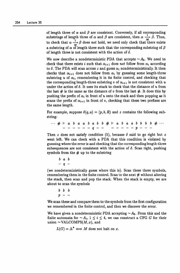
254 Lectu re 35
of length three of a and {3 are consistent. Conversely, if all corresponding substrings of length three of a and {3 are consistent, then a ..2.... {3. Thus,
1 M to check that a ---4 {3 does not hold, we need only check that there exists
M a substring of a of length three such that the corresponding substring of (3 oflength three is not consistent with the action of o. We now describe a nondeterministic PDA that accepts rv As. We need to check that there exists i such that ai+l does not follow from ai according to O. The PDA will scan across z and guess ai nondeterministically. It then checks that ai+l does not follow from ai by guessing some length-three substring u of ai, remembering it in its finite control, and checking that the corresponding length-three substring v of aiH is not consistent with u under the action of O. It uses its stack to check that the distance of u from the last # is the same as the distance of v from the last #. It does this by pushing the prefix of ai in front of u onto the stack and then popping as it scans the prefix of ai+l in front of v, checking that these two prefixes are the same length.
For example, suppose o(q,a) = (p,b,R) and z contains the following substring:
.. ·#I-a b a a bab b#l-a b aabb b b# .. · ------q-- -----p---
Then z does not satisfy condition (5), because 0 said to go right but z went left. We can check with a PDA that this condition is violated by guessing where the error is and checking that the corresponding length-three subsequences are not consistent with the action of O. Scan right, pushing symbols from the # up to the substring
b a b - q -
(we nondeterministically guess where this is). Scan these three symbols, remembering them in the finite control. Scan to the next # without altering the stack, then scan and pop the stack. When the stack is empty, we are about to scan the symbols
b b b p - -
We scan these and compare them to the symbols from the first configuration we remembered in the finite control, and then we discover the error.
We have given a nondeterministic PDA accepting rv As. From this and the finite automata for rv Ai, 1 ::; i ::; 4, we can construct a CFG G for their union rvVALCOMPS(M,x), and
L( G) = D. * ¢=> M does not halt on x.
Undecidable Problems About CFLs 255
If we could decide whether G generates all strings over its terminal alphabet, it would answer the question of whether M halts on x. We have thus reduced the halting problem to the question of whether a given grammar generates all strings. Since the halting problem is undecidable, we have shown:
Theorem 35.1 It is undecidable for a given CFG G whether or not L( G) = E*.
Many other simple problems involving CFLs are undecidable: whether a given CFL is a DCFL, whether the intersection of two given CFLs is a CFL, whether the complement of a given CFL is a CFL, and so on. These problems can all be shown to be undecidable using valid computation histories. We leave these as exercises (Miscellaneous Exercise 121).
Historical Notes
Undecidable properties of context-free languages were established by BarHillel et al. [8], Ginsburg and Rose [47], and Hartmanis and Hopcroft [56]. The idea of valid computation histories is essentially from Kleene [67, 68], where it is called the T -predicate.
Lecture 36
Other Formalisms
In this lecture and the next we take a brief look at some of the other traditional formalisms that are computationally equivalent to Turing machines. Each one of these formalisms embodies a notion of computation in one form or another, and each can simulate the others. In addition to Turing machines, we'll consider
• Post systems;
• type 0 grammars;
• I'-recursive functions (I' = "mu", Greek for m);
• >.-calculus (>. = "lambda", Greek for 1);
• combinatory logic; and
• while programs.
Post Systems By the 1920s, mathematicians had realized that much of formal logic was just symbol manipulation and strongly related to emerging notions of computability. Emil Post came up with a general formalism, now called Post systems, for talking about rearranging strings of symbols. A Post system
Other Formalisms 257
consists of disjoint finite sets N and ~ of nonterminal and terminal symbols, respectively, a special start symbol SEN, a set of variables Xo, Xl, ... ranging over (N U ~)*, and a finite set of productions of the form
XOXIXIX2X2Xa'" Xnxn .... YOYIYIY2Y2Ya'" YmYm,
where the Xi and Yj are strings in (N U ~)*, and each Y; is some Xi that occurs on the left-hand side. If a string in (N U ~)* matches the left-hand side for some assignment of strings to the variables Xi, then that string can be rewritten as specified by the right-hand side. A string X E ~* is generated by the system if x can be derived from S by a finite sequence of such rewriting steps.
Post systems and Turing machines are equivalent in computational power. Any Post system can be simulated by a TM that writes the start symbol on a track of its tape, then does the pattern matching and string rewriting according to the productions of the Post system in all possible ways, accepting if its input x is ever generated. Conversely, given any TM M, a Post system P can be designed that mimics the action of M. The sentential forms of P encode configurations of M.
One of Post's main theorems was that Post systems in which all productions are of the more restricted form
xX .... XY
are just as powerful as general Post systems. Productions of this form say, "Take the string x off the front of the sentential form if it's there, and put Y on the back." If you did Miscellaneous Exercise 99 on queue machines, you may have already recognized that this is essentially the same result.
Type 0 Grammars
Grammars are a restricted class of Post systems that arose in formal language theory. There is a natural hierarchy of grammars, called the Chomsky hierarchy, which classifies grammars into four types named 0, 1, 2, and 3. The type 2 and type 3 grammars are just the context-free and right-linear grammars, respectively, which we have already seen. A more general class of grammars, called the type 0 or unrestricted grammars, are much like CFGs, except that productions may be of the more general form
a .... (3, (36.1)
where a and (3 are any strings of terminals and nonterminals whatsoever. A type 0 grammar consists of a finite set of such productions. If the lefthand side of a production matches a substring of a sentential form, then the substring c,an be replaced by the right-hand side of the production. A
258 Lect u re 36
string x of terminal symbols is generated by G, that is, x E L( G), if x can be derived from the start symbol S by some finite number of such applications; in symbols, S -!.... x.
G
Type 0 grammars are a special case of Post systems: the grammar production (36.1) corresponds to the Post production
XaY -+ X{3y.
Type 0 grammars are the most powerful grammars in the Chomsky hierarchy of grammars and generate exactly the r.e. sets. One can easily build a Turing machine to simulate a. given type 0 grammar. The machine saves its input x on a track of its tape. It then writes the start symbol S of the grammar on another track and applies productions nondeterministic ally, accepting if its input string x is ever generated.
Conversely, type 0 grammars can simulate Turing machines. Intuitively, sentential forms of the grammar encode configurations of the machine, and the productions simulate 5 (Miscellaneous Exercise 104).
Type 1 grammars are the context-sensitive grammars (CSGs). These are like type 0 grammars with productions of the form (36.1), except that we impose the extra restriction that lal ~ 1{31. Context-sensitive grammars are equivalent (except for a trivial glitch involving the null string) to nondeterministic linear bounded automata (LBAs), which are TMs that cannot write on the blank portion of the tape to the right of the input string (see Exercise 2 of Homework 8 and Exercise 2 of Homework 12). The bound on the tape in LBAs translates to the restriction lal ~ 1!3I for CSGs.
The ",-Recursive Functions
GOdel defined a collection of number-theoretic functions Nlo -+ N that, according to his intuition, represented all the computa.ble functions. His definition was as follows:
(1) Successor. The function 8: N -+ N given by 8(X) = x+1 is computable.
(2) Zero. The function z : N' -+ N given by z( ) = 0 is computable.
(3) Projections. The functions 7I"i: : N" -+ N given by 7I"i:(X1, ••. ,xn ) = Xk, 1 ~ k ~ n, are computable.
(4) Composition. If I: Nk -+ N and 910 ... ,9k: N" -+ N are computable, then so is the function I 0 (gl, ... , gk) : N" -+ N that on in put x = Xl, ••• ,Xn gives
Example 36.1
Other Formalisms 259
(5) Primitive recursion. If hi : l'f'-l -> Nand gi : l'f'H -> N are computable, 1 ::; i ::; k, then so are the functions Ii : l'f' -> N, 1 ::; i ::; k, defined by mutual induction as follows:
MO, x) ~f hi(x),
Mx + 1,x) ~ gi(X,x,!1(x,x), ... , Ik(x,x)),
where x = X2, •.. ,xn .
(6) Unbounded minimization. If 9 : l'f'+l -> N is computable, then so is the function I : l'f' -> N that on input x = Xl, ... ,Xn gives the least y such that g(z, x) is defined for all z ::; y and g(y, x) = ° if such a y exists and is undefined otherwise. We denote this by
f(x) = p,y.(g(y, x) = 0).
The functions defined by (1) through (6) are called the p,-recursive functions. The functions defined by (1) through (5) only are called the primitive recursive functions .
• The constant functions constn ( ) = n are primitive recursive:
def constn = so··· 0 s oz. ~
n
• Addition is primitive recursive, since we can define
add(O,y) ~ y,
add(x + 1,y) ~ s(add(x,y)).
This is a bona fide definition by primitive recursion: in rule (5) above, take k = 1, n = 2, h = 7I"t, and 9 = s 071":. Then
add(O,y) = h(y) = y, add(x + 1, y) = g(x, y, add(x, y)) = s(add(x, y)).
• Multiplication is primitive recursive, since
( ) def mult O,y = 0,
mult(x+ 1,y) ~ add(y,mult(x,y)).
Note how we used the function add defined previously. We are allowed to build up primitive recursive functions inductively in this way.
• Exponentiation is primitive recursive, since
( ) def exp x,D = 1,
exp(x,y + 1) ~f mult(x, exp(x, y)).
260 Lecture 36
• The predecessor function
. 1 {X-1 x - = 0
is primitive recursive:
0.!.1 ~f 0,
(x + 1) .!. 1 d,g x.
• Proper subtraction
if x> 0, ifx=O
x.!.y= { ~-y if x ~ y, if x < y
is primitive recursive, and can be defined from predecessor in exactly the same way that addition is defined from successor.
• The sign function is primitive recursive:
sign(x) ~f 1 .!. (1 .!. x)
_ {1 if x> 0, - 0 if x = o.
• The relations <, :$, >, ~, =, and #, considered as (0,1)-valued functions, are all primitive recursive; for example,
compare::;(x,y) d,g 1.!. sign(x.!. y)
_ { 1 - 0
if x :$ y, if x> y.
• Functions can be defined by cases. For example,
{ x+ 1 g(x,y) = x
is primitive recursive:
if 2'" < y, if 2'" ~ y
g(x, y) ~f compared 2"', y) . (x + 1) + compare?: (2" , y) . x.
• Inverses of certain functions can be defined. For example, fiOg2 y 1 is primitive recursive:! fiog2yl = f(y,y), where
f(O,y) d~r 0,
f(x+ 1,y) ~f g(f(x,y),y),
1 r x 1 = least integer not less than Xj log2 = base 2 logarithm.
Other Formalisms 261
and g is from the previous example. The function f just continues to add 1 to its first argument x until the condition 2'" ~ Y is satisfied. This must happen for some x $ y. Inverses of other common functions, such as square root, can be defined similarly. 0
Observe that all the primitive recursive functions are total, whereas a p,recursive function may not be. There exist total computable functions that are not primitive recursive; one example is Ackermann's function:
A(O,y) ~ y + 1,
A(x+ 1,0) ~ A(x,l), (36.2)
A(x + 1, Y + 1) d~f A(x,A(x + 1,y)).
Lecture 37
The A-Calculus
The A-calculus (A = "lambda," Greek for 1) consists of a set of objects called A-term.s and some rules for manipulating them. It was originally designed to capture formally the notions of functional abstraction and functional application and their interaction.
The A-calculus has had a profound impact on computing. One can see the basic principles of the A-calculus at work in the functional programming language LISP and its more modern offspring SCHEME and DYLAN.
In mathematics, A-notation is commonly used to represent functions. The expression Ax.E(x) denotes a function that on input x computes E(x). To apply this function to an input, one substitutes the input for the variable x in the body E(x) and evaluates the resulting expression.
For example, the expression
AX.(X + 1)
might be used to denote the successor function on natural numbers. To apply this function to the input 7, we would substitute 7 for x in the body and evaluate:
(AX.(X + 1))7 ..... 7 + 1 = B.
In the programming language DYLAN, one would write
The A-Calculus 263
(method (x) (+ xl»
for the same thing. The keyword method is really A in disguise. If you typed
«method (x) (+ xl» 7)
at a DYLAN interpreter, it would print out 8.
For another example, the expression
AX./(gX)
denotes the composition of the functions / and gj that is, the function that on input x applies 9 to x, then applies / to the result. The expression
A/.Ag.AX./(gX) (37.1)
denotes the function that takes functions / and 9 as input and gives back their composition AX./(gX). In DYLAN one would write
(method (f)
(method (g)
(method (x) (f (g x»»)
To see how this works, let's apply (37.1) to the successor function twice. We use different variables in the successor functions below for clarity. The symbol --+ denotes one substitution step.
(A/.Ag.AX.(f(gX))) (Ay.(y + 1)) (AZ.(Z + 1)) --+ (Ag.AX.«Ay.(y + 1)) (gx))) (AZ.(Z+ 1)) --+ Ax.«Ay.(y + 1)) «AZ.(Z + 1))x)) --+ AX.«Ay.(y + 1)) (x + 1)) --+ AX.«X + 1) + 1)
substitute Ay.(y + 1) for /
substitute AZ.(Z + 1) for 9 substitute x for Z
substitute x + 1 for y
We could have substituted gx for y in the second step or (AZ.(Z + 1))x for y in the thirdj we would have arrived at the same final result.
Functions represented by A-terms have only one input. A function with two inputs x, y that returns a value M is modeled by a function with one input x that returns a function with one input y that returns a value M. The technical term for this trick is currying (after Haskell B. Curry).
The Pure A-Calculus
In the pure A-calculus, there are only variables {I, g, h, x, y, ... } and operators for A-abstraction and application. Syntactic objects called A-terms are built inductively from these:
264 Lecture 37
• any variable x is a 'x-term;
• if M and N are 'x-terms, then MN is a 'x-term (functional applicationthink of M as a function that is about to be applied to input N); and
• if M is a A-term and x is a variable, then Ax.M is a A-term (functional abstraction-think of Ax.M as the function that on input x computes M).
The operation of application is not associative, and unparenthesized expressions are conventionally associated to the left; thus, MNP should be parsed (MN)P.
In the pure 'x-calculus, ,X-terms serve as both functions and data. There is nothing like "+1" as we used it informally above, unless we encode it somehow. We'll show how to do this below.
The substitution rule described informally above is called {3-reduction. Formally, this works as follows. Whenever our 'x-term contains a subterm of the form ('xx.M)N, we can replace this subterm by the term s~(M), where s~(M) denotes the term obtained by
(i) renaming the bound variables of M (those y occurring in the scope of some ,Xy) as necessary so that neither x nor any variable of N occurs bound in M; and
(ii) substituting N for all occurrences of x in the resulting term.
Step (i) is necessary only to make sure that any free variables y of N will not be inadvertently captured by a AY occurring in M when the substitution is done in step (ii). This is the same problem that comes up in first-order logic. We can rename bound variables in A-terms anytime, since their behavior as functions is not changed. For example, we can rewrite ,Xy.xy as AZ.XZ;
intuitively, the function that on input y applies x to y is the same as the function that on input Z applies x to z. The process of renaming bound variables is officially called a-reduction.
We denote a- and {3-reduction by ~ and L, respectively. Thus
(Ax.M)N L sN(M).
Computation in the 'x-calculus is performed by {3-reducing subterms whenever possible and for as long as possible. The order of the reductions doesn't matter, since there is a theorem that says that if you can reduce M to Nl by some sequence of reduction steps and M to N2 by some other sequence of reduction steps, then there exists a term P such that both Nl and N2 reduce to P.
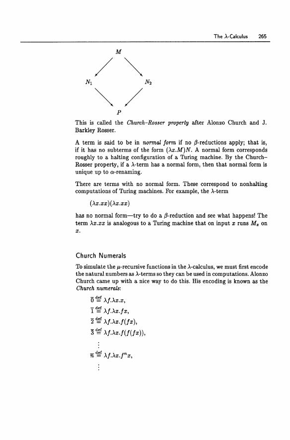
The A-Calculus 265
M
P
This is called the Church-Rosser property after Alonzo Church and J. Barkley Rosser.
A term is said to be in normal lorm if no .a-reductions applYi that is, if it has no subterms of the form (Ax.M)N. A normal form corresponds roughly to a halting configuration of a Turing machine. By the ChurchRosser property, if a A-term has a normal form, then that normal form is unique up to a-renaming.
There are terms with no normal form. These correspond to nonhalting computations of Turing machines. For example, the A-term
(AX.XX)(AX.XX)
has no normal form-try to do a .a-reduction and see what happens! The term Ax.xx is analogous to a Turing machine that on input x runs MOl on x.
Church Numerals
To simulate the JV"recursive functions in the A-calculus, we must first encode the natural numbers as A-terms so they can be used in computations. Alonzo Church came up with a nice way to do this. His encoding is known as the Church numerals:
- def 0= A/.Ax.x, -def 1 = A/.Ax.lx,
2~ A/.Ax.l(fx), - def ) 3 = >'1.Ax.I(f(fx ),
- def 'I' In n = A .AX. X,
266 Lecture 37
where rx is an abbreviation for the term
f(f(···(fx)···)). "---v--"
n
In other words, n represents a function that on input f returns the n-fold composition of f with itself. The n are all distinct and in normal form.
Using this representation of the natural numbers, the successor function can be defined as
de! s = >.m.>.f.>.x.f(mfx).
To see that this is correct, try applying it to any n: sn = (>.m.>.f.>.x.f(mfx)) (>.f.>.x.rx)
~ (.~m.>'g.>'y.g(mgy)) (>.f.>.x.rx)
L >.g.>.y.g«>.f.>.x.rx)gy)
L >.g.>.y.g«>.x.gnx)y)
L >.g.>.y.g(gny)
= >.g.>.y.gn+1 y ~ >.f·>.x·r+1x
= n+ 1.
One can likewise define addition, multiplication, and all the other It-recursive functions.
Combinatory Logic
Combinatory logic is a form of variable-free >.-calculus. It was first invented to study the mathematics of symbol manipulation, especially substitution. The system consists of terms called combinators that are manipulated using reduction rules.
There are two primitive combinators Sand K, which are just symbols, as well as a countable set of variables {X, Y, ... }. More complicated combinators are formed inductively: S, K, and variables are combinatorsj and if M and N are combinators, then so is MN. Here MN is just a term, a syntactic object, but we can think of M as a function and N as its inputj thus, MN represents the application of M to N. As with the >.-calculus, this operation is not associative, so we use parentheses to avoid ambiguity. By convention, a string of applications associates to the leftj thus, XYZ should be parsed (XY)Z and not X(YZ).
The ~-Calculus 267
Computation proceeds according to two reduction rules, one for S and one for K. For any terms M, N, and P,
SMNP -+ MP(NP),
KMN-+M.
Computation in this system consists of a sequence of reduction steps applied to subterms of a term.
Other combinators can be built from Sand K. For example, the combinator
I ~ SKK acts as the identity function: for any X,
IX = SKKX
-+ KX(KX) the S rule
-+ X the K rule.
Let B = SK. Whereas K picks out the first element of a pair, B picks out the second element:
BXY = SKXY -+ KY(XY) -+ Y.
One can construct fancy combinators from Sand K that can rearrange symbols in every conceivable way. For example, to take two inputs and apply the second to the first, use the combinator C = S(S(KS)B)K:
CXY = S(S(KS)B)KXY
-+ S(KS)BX(KX)Y
-+ KSX(BX)(KX)Y
-+ S(BX)(KX)Y -+ BXY(KXY)
-+ YX.
There is a theorem that says that no matter how you want to rearrange your inputs, there is a combinator built from Sand K only that can do it. In other words, for any term M built from Xl, ... ,Xn and the application operator, there is a combinator D built from Sand K only such that
DX1X 2 ••• Xn ~ M.
This theorem is called combinatorial completeness.
There is a paradoxical combinator SII(SII), which corresponds to the ~term (~x.xx)(~x.xx). Like its counterpart, it has no normal form.
Like the ~-calculus, combinatory logic is powerful enough to simulate Turing machines.
268 Lecture 37
Historical Notes
The late 19208 and 19308 were a hectic time. Turing machines (Turing [120)), Post systems (Post [99, 100)), p.-recursive functions (Godel [51), Herbrand, Kleene [67)), the A-calculus (Church [23, 24, 25, 26), Kleene [66), Rosser [107)), and combinatory logic (SchOnfinkel [111), Curry [29)) were all developed around this time.
The >.-calculus is a topic unto itself. Barendregt's book [9] is an indispensable reference.
The p.-recursive functions were formulated by Godel and presented in a series of lectures at Princeton in 1934. According to Church [25), GOdel acknowledged that he got the idea originally from Jacques Herbrand in conversation.
A proof of the equivalence of the p.-recursive functions and the A-calculus first appeared in Church [25), although Church attributes the proof chiefly to Kleene. The equivalence of TMs and the A-calculus was shown by Turing [120).
Various perspectives on this important period can be found in Kleene [69), Davis [31, 32), Rogers [106), Yasuhara [124), Jones [63), Brainerd and Landweber [15), Hennie [58), and Machtey and Young [81).
Chomsky [18) defined the Chomsky hierarchy and proved that the type 0 grammars generate exactly the r.e. sets.
The relationship between context-sensitive grammars and linear bounded automata was studied by Myhill [92), Landweber [78), and Kuroda [77).
Supplementary Lecture I
While Programs
We can relate the primitive and It-recursive functions of Godel to more modern concepts. Consider a simple programming language with variables Var = {x, y, ... } ranging over N containing the following constructs:
(i) simple assignments x := 0 x:= y + 1 x:= y
(ii) sequential composition p i q
(iii) conditional if x < y then p else q
(iv) lor loop for y do p
(v) while loop while x < y do p
In (iii) and (v), the relation < can be replaced by anyone of >, ;:::, ~, =, or #. In (ii) we can parenthesize using begin ... end if necessary.
Programs built inductively from these constructs are called while programs. Programs built without the while construct (v) are called for programs. We will show in Theorem 1.1 that while programs compute exactly the It-recursive functions and that for programs compute exactly the primitive recursive functions.
The intuitive operation of the for loop is as follows: upon entering the loop for y do p, the current value of variable y is determined, and the program
270 Supplementary Lecture I
p is executed that many times. Assignment to the variable y within the body of the loop does not change the number of times the loop is executed, nor does execution of the body of the loop alone decrement y or change its value in any way except by explicit assignment.
The intuitive operation of the while loop is as follows: upon entering the loop while x < y do p, the condition x < y is tested with the current values of the variables x, y. If the condition is false, then the body of the loop is not executed, and control passes through to the statement following the while loop. If the condition is true, then the body p of the loop is executed once, and then the procedure is repeated with the new values of x, y. Thus the while loop repeatedly tests the condition x < y, and if true, executes the body p. The first time that the condition x < y tests false (if ever), the body of the loop is not executed and control passes immediately to the statement following the loop. If the condition always tests true, then the while loop never halts, as for example with the program while x = x do x := x + 1.
In the presence of the while loop, the for loop is redundant: for y do p is simulated by the while program
z := 0 ; w := y ; while z < w do begin p ; z := z + 1 end
where z and w are variables not occurring in p. However, note that for programs always halt. Thus the only source of potential nontermination is the while loop.
Semantics of While Programs In order to prove the equivalence of while programs and the Jt-recursive functions, we must give formal semantics for while programs.
A state or environment (1 is an assignment of a nonnegative integer to each variable in Var; that is, (1 : Var -+ N. The set of all such environments is denoted Env. If a program is started in an initial environment (1, then in the course of execution, the values of variables will be changed, so that if and when the program halts, the final environment will in general be different from (1. We thus interpret programs p as partial functions [p~ : Env -+ Env. The value [p~ ((1) is the final environment after executing the program p with initial environment (1, provided p halts. If p does not halt when started in initial environment (1, then [P]((1) is undefined. Thus [P] : Env -+ Env is a partial function; its domain is the set of (1 causing p to halt. Note that whether or not p halts depends on the initial environment; for example, if (1(x) = 0, then the program while x > 0 do x := x + 1 halts on initial environment (1, whereas if (1(x) = 1, then it does not.
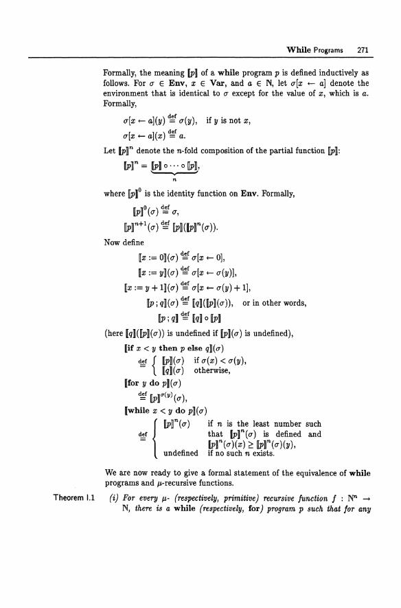
While Programs 271
Formally, the meaning [P] of a while program p is defined inductively as follows. For u e Env, x e Var, and a e N, let u[x +- a] denote the environment that is identical to u except for the value of x, which is a. Formally,
u[x +- a](y) rI,g u(y), if y is not x,
u[x +- a](x) rI,g a.
Let IPr denote the n-fold composition of the partial function [P]:
[p]n = [PI 0 ... 0 [P], '--v---"
n
where [Pt is the identity function on Env. Formally,
[P]o(u) rI,g u,
[pr+1(u) rI,g [p]((p]n(u)).
Now define
[x := O](u) rI,g u[x +- 0),
[x := y](u) rI,g u[x +- u(y)],
[x := y + 1](u) rI,g u[x +- u(y) + I], [p; qD(u) rI,g [qD([P](u)), or in other words,
[p ; qJ ~f [d 0 [P]
(here [q]([P](u)) is undefined if [P)(u) is undefined),
[if x < y then p else qD(u) ~ {[PD(u) if u(x) < u(y), - [q)(u) otherwise,
[for y do p](u)
rI,g [p]"(I/)(u),
[while x < y do p](u)
{ [pr(u)
def
= undefined
if n is the least number such that IPr(u) is defined an<i IPr(u)(x) ~ [pr(u)(y), if no such n exists.
We are now ready to give a formal statement of the equivalence of while programs and p.-recursive functions.
Theorem 1.1 (i) For every p.- (respectively, primitive) recursive function J : ~ -+
N, there is a while (respectively, for) program p such that Jor any
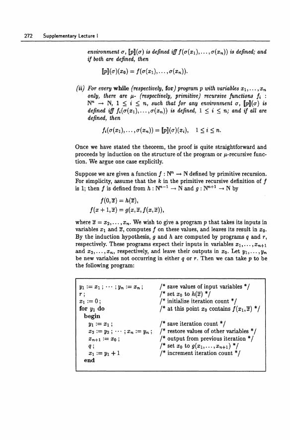
272 Supplementary Lecture I
environment u, [Pl(u) is defined iff l(u(x1), ... ,u(xn)) is defined; and il both are defined, then
[PHu)(xo) = l(u(x1), ... ,u(xn)).
(ii) For every while (respectively, for) program p with variables Xl, •.• ,xn only, there are p.- (respectively, primitive) recursive functions Ii : N" -+ N, 1 $ i $ n, such that lor any environment u, [P](u) is defined iff 1.(u(x1), ... , U(Xn)) is defined, 1 $ i $ nj and il all are defined, then
Once we have stated the theorem, the proof is quite straightforward and proceeds by induction on the structure of the program or p.-recursive function. We argue one case explicitly.
Suppose we are given a function I : N" -+ N defined by primitive recursion. For simplicity, assume that the k in the primitive recursive definition of 1 is 1; then I is defined from h : N"-1 -+ N and 9 : N"+1 -+ N by
1(0, x) = h(x), I(x + 1, x) = g(x, x, I(x, x)),
where x = X2,' •• ,Xn • We wish to give a program p that takes its inputs in variables Xl and x, computes I on these values, and leaves its result in Xo. By the induction hypothesis, 9 and h are computed by programs q and r, respectively. These programs expect their inputs in variables X1>' .. ,Xn+1 and X2, .. . ,Xn, respectively, and leave their outputs in Xo. Let Y1, ... ,Yn be new variables not occurring in either q or T. Then we can take p to be the following program:
Yl := Xl ; •.. ; Yn := Xn ; T; Xl:= 0; for Yl do
begin VI := Xl;
X2 := Y2 ; ... ; Xn := Vn ; Xn+1 := Xo; q; Xl := YI + 1
end
/* save values of input variables * / 1* set Xo to h(x) * / 1* initialize iteration count * / 1* at this point Xo contains I(xl, x) * /
/* save iteration count * / 1* restore values of other variables * / /* output from previous iteration * / 1* set Xo to g(X1>"" xn+d * / /* increment iteration count * /
While Programs 273
Historical Notes
Godel originally worked exclusively with the primitive recursive functions. Ackermann's [11 discovery of the non-primitive recursive yet intuitively computable total function (36.2) forced GOdel to rethink the foundations of his system and ultimately to include unbounded minimization, despite the fact that it led to partial functions. As we now know, this is inevitable: no r.e.list of total computable functions could contain all total computable functions, as can be shown by a straightforward diagonalization argument.
The relationship between the primitive recursive functions and for programs was observed by Meyer and Ritchie [86].
Supplementary Lecture J
Beyond Undecidability
Oracle Machines and Relative Computation
We know that virtually all interesting questions about Turing machineswhether a given TM halts on a given input, whether a given TM accepts a finite set, and so on-are undecidable. But are all these questions equally hard? For example, suppose by some magic we were given the power to decide the halting problem. Could we somehow use that power to decide if a given TM accepts a finite set? In other words, relative to the halting problem, is finiteness decidable?
Questions about relative computability can be formalized and studied using oracle Turing machines. Intuitively, an oracle TM is a TM equipped with an oracle, a set B to which the TM may pose membership questions and always receive correct answers after a finite time. The interesting thing about this definition is that it makes sense even if B is not recursive.
Formally, an oracle Turing machine is a TM that in addition to its ordinary read/write tape is equipped with a special one-way-infinite read-only input tape on which some infinite string is written. The extra tape is called the oracle tape, and the string written on it is called the oracle. The machine can move its oracle tape head one cell in either direction in each step and make decisions based on the symbols written on the oracle tape. Other than that, it behaves exactly like an ordinary Turing machine.
Beyond Undecidability 275
We usually think of the oracle as a specification of a set of strings. If the oracle is an infinite string over {O, I}, then we can regard it as the characteristic function of a set B ~ I'll, where the nth bit of the oracle string is 1 iff nEB. In that way we can study computation relative to the set B.
There is nothing mysterious about oracle TMs. They operate exactly like ordinary TMs, the only difference being the oracle. Ordinary TMs are equivalent to oracle TMs with the null oracle 0, whose characteristic function is 00000· .. ; for such machines, the oracle gives no extra information that the TM doesn't already have.
For A, B ~ E*, we say that A is recursively enumerable (r. e.) in B if there is an oracle TM M with oracle B such that A = L(M). In addition, if Mis total (Le., halts on all inputs), we write A ::;T B and say that A is recursive in B or that A Turing reduces to B.
For example, the halting problem is recursive in the membership problem, since halting is decidable in the presence of an oracle for membership. Here's how: given a TM M and input x, first ask the oracle whether M accepts x. If the answer is yes, then M certainly halts on x. If the answer is no, switch accept and reject states of M to get the machine M', then ask the oracle whether M' accepts x. If the answer is yes, then M rejects x, therefore halts on x. If the answer is still no, then M neither accepts or rejects x, therefore loops on x. In all cases we can say definitively after a finite time whether M halts on x.
Likewise, the membership problem is recursive in the halting problem, since we can determine membership in the presence of an oracle for halting. Given a TM M and input x, modify M so as never to reject by making the reject state r into a nonreject state. You can add a new dummy inaccessible reject state if you like. Call this modified machine M'. Now on any input, M' accepts iff it halts, and L(M) = L(M'), so we can determine whether M accepts x by asking the oracle whether the modified machine M' halts on x.
It is not hard to show that the relation ::;T is transitive; that is, if A is recursive in Band B is recursive in C, then A is recursive in C. Moreover, the relation ::;m refines ::;T; in other words, if A ::;m B, then A ::;T B (Miscellaneous Exercise 141).
The relation ::;T is strictly coarser than ::;m, since '" HP :tm HP but '" HP ::;T HP. In fact, any set A Turing reduces to its complement, since with an oracle for A, on input x one can simply ask the oracle whether x E A, accepting if not and rejecting if so.
276 Supplementary Lecture J
The Arithmetic Hierarchy
Once we have the notion of relative computation, we can define a hierarchy of classes as follows. Fix the alphabet {O, I} and identify strings in {O, I} * with the natural numbers according to the one-to-one correspondence (28.1). Define
~O def { } .£.11 = r.e. sets ,
~~ ~ {recursive sets},
~~+1 ~f {sets r.e. in some B E ~~},
~~+1 ~f {sets recursive in some B E ~~},
II~ ~ {complements of sets in ~~}.
Thus II~ is the class of co-r.e. sets. The classes ~~, II~, and ~~ comprise what is known as the arithmetic hierarchy.
Here is perhaps a more revealing characterization of the arithmetic hierarchy in terms of alternation of quantifiers. Recall from Exercise 1 of Homework 11 that a set A is r.e. iff there exists a decidable binary predicate R such that
A = {x 13y R(x,y)}.
For example,
HP = {M#x 13t M halts on x in t steps},
MP = {M#x 13t M accepts x in t steps}.
(J.1)
Note that the predicate "M halts on x" is not decidable, but the predicate "M halts on x in t steps" is, since we can just simulate M on input x with a universal machine for t steps and see if it halts within that time. Alternatively,
HP = {M#x 13v v is a halting computation history of M on x},
MP = {M#x 13v v is an accepting computation history of M on x}.
Thus the class ~~ is the family of all sets that can be expressed in the form (J.1).
Similarly, it follows from elementary logic that II~, the family of co-r.e. sets, is the class of all sets A for which there exists a decidable binary predicate R such that
A = {x I 'Vy R(x,y)}. (J.2)
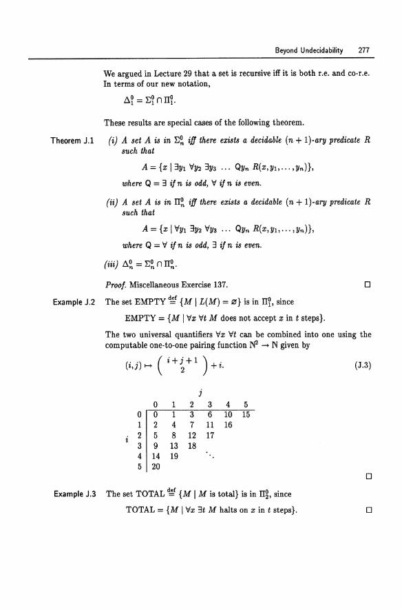
Beyond Undecidability 277
We argued in Lecture 29 that a set is recursive iff it is both r.e. and co-r.e. In terms of our new notation,
A.~ = ~~ n II~.
These results are special cases of the following theorem.
Theorem J.1 (i) A set A is in ~~ iff there exists a decidable (n + l)-ary predicate R such that
A = {x 13Yl 'i/Y2 3Y3 ... QYn R(x, Yl, .. ·, Yn)},
where Q = 3 if n is odd, 'i/ if n is even.
(ii) A set A is in II~ iff there exists a decidable (n + 1) -ary predicate R such that
A = {x I'i/Yl 3Y2 'i/Y3 ... QYn R(x, Yl, ... ,Yn)},
where Q = 'i/ if n is odd, 3 if n is even.
(iii) A.~ = ~~ n II~.
Proof. Miscellaneous Exercise 137.
Example J.2 The set EMPTY ~ {M I L(M) = 0} is in II~, since
EMPTY = {M I 'i/x 'i/t M does not accept x in t steps}.
o
The two universal quantifiers 'i/x 'i/t can be combined into one using the computable one-to-one pairing function ~ -+ N given by
(i,j) ...... (i+{+1 )+i. (J.3)
j
0 1 2 3 4 5 0 0 1 3 6 10 15 1 2 4 7 11 16 2 5 8 12 17 3 9 13 18 4 14 19 5 20
Example J.3 The set TOTAL ~ {M I M is total} is in IIg, since
TOTAL = {M I 'i/x 3t M halts on x in t steps}.
o
o
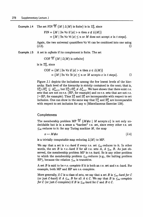
278 Supplementary Lecture J
Example J.4 The set FIN ~ {M I L(M) is finite} is in I;g, since
FIN = {M 13n 'TIx if Ixl > n then x ¢ L(M)} = {M 13n 'TIx 'TIt Ixl :::; n or M does not accept x in t steps}.
Again, the two universal quantifiers 'TIx 'TIt can be combined into one using ~~. 0
Example J.5 A set is cofinite if its complement is finite. The set
COF ~f {M I L(M) is cofinite}
is in I;g, since
COF = {M 13n 'TIx if Ixl > n then x E L(M)} = {M 13n 'TIx 3t Ixl :::; n or M accepts x in t steps}. 0
Figure J.1 depicts the inclusions among the few lowest levels of the hierarchy. Each level of the hierarchy is strictly contained in the next; that is, I;~ U II~ ~ 1l~+1' but I;~ U II~ f:. 1l~+1' We have shown that there exist r .e. sets that are not co-r.e. (HP, for example) and co-r.e. sets that are not r.e. ('" HP, for example). Thus I;~ and II~ are incomparable with respect to set inclusion. One can show in the same way that I;~ and II~ are incomparable with respect to set inclusion for any n (Miscellaneous Exercise 138).
Completeness
The membership problem MP ~f {M#x I M accepts x} is not only undecidable but is in a sense a "hardest" r.e. set, since every other r.e. set :::;m-reduces to it: for any Turing machine M, the map
x ...... M#x (JA)
is a trivially computable map reducing L(M) to MP.
We say that a set is r.e.-hard if every r.e. set :::;m-reduces to it. In other words, the set B is r.e.-hard if for all r.e. sets A, A :::;m B. As just observed, the membership problem MP is r.e.-hard. So is any other problem to which the membership problem :::;m-reduces (e.g., the halting problem HP), because the relation :::;m is transitive.
A set B is said to be r.e.-complete if it is both an r.e. set and r.e.-hard. For example, both MP and HP are r.e.-complete.
More generally, if C is a class of sets, we say that a set B is :::;m -hard for C (or just C-hard) if A :::;m B for all A E C. We say that B is :::;m-complete for C (or just C-complete) if B is :::;m-hard for C and B E C.
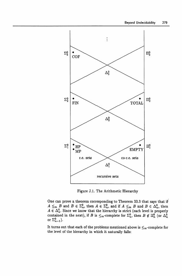
Beyond U ndecida bility 279
II~
recursive sets
Figure J.l. The Arithmetic Hierarchy
One can prove a theorem corresponding to Theorem 33.3 that says that if' A :::;m Band B E E~, then A E E~, and if A :::;m Band B E .1.~, then A E .1.~. Since we know that the hierarchy is strict (each level is properly contained in the next), if B is :::;m-complete for E~, then B f/. II~ (or ~~ or E~_l)'
It turns out that each of the problems mentioned above is $m-complete for the level of the hierarchy in which it naturally falls:
280 Supplementary Lecture J
(i) HP is ::S;m-complete for ~y,
(ii) MP is ::S;m-complete for ~~,
(iii) EMPTY is ::S;m-complete for m, (iv) TOTAL is ::S;m-complete for rrg, (v) FIN is ::S;m-complete for ~g, and
(vi) OOF is ::S;m-complete for ~g.
Since the hierarchy is strict, none of these problems is contained in any class lower in the hierarchy or ::S;T-reduces to any problem complete for any class lower in the hierarchy. If it did, then the hierarchy would collapse at that level. For example, EMPTY does not reduce to HP and OOF does not reduce to FIN.
We prove (v); the others we leave as exercises (Miscellaneous Exercise 142). We have already argued that FIN E ~g. To show that it is ::S;m-hard for ~g, we need to show that any set in ~g reduces to it. We use the characterization of Theorem J.1. Let
A = {x 13y "Iz R(x,y,z)}
be an arbitrary set in ~g, where R(x, y, z) is a decidable ternary predicate. Let M be a total machine that decides R. We need to construct a machine N effectively from a given x such that N E FIN iff x E Aj in other words, N accepts a finite set iff 3y "Iz R(x,y,z). Let N on input w
(i) write down all strings y of length at most Iwlj (ii) for each such y, try to find a z such that ...,R(x, y, z) (Le., such that
M rejects x#y#z), and accept if all these trials are successful. The machine N has x and a description of M hard-wired in its finite control.
In step (ii), for each y of length at most Iwl, N can just enumerate strings z in some order and run M on x#y#z until some z is found causing M to reject. Since M is total, N need not worry about timesharing. If no such z is ever found, N just goes on forever. Surely such an N can be built effectively from M and x.
Now if x E A, then there exists y such that for all z, R(x, y, z) (i.e., for all z, M accepts x#y#z)j thus step (ii) fails whenever Iwl ~ Iyl. In this case N accepts a finite set. On the other hand, if x ¢ A, then for all y there exists a z such that ...,R(x, y, z), and these are all found in step (ii). In this case, N accepts ~*.
Beyond Undecidability 281
We have shown that the machine N accepts a finite set iff x E A, therefore the map x H N constitutes a :5m-reduction from A to FIN. Since A was an arbitrary element of ~g, FIN is :5m-hard for ~g.
The Analytic Hierarchy and II}
The arithmetic hierarchy is defined in terms of first-order quantification, or quantification over natural numbers or strings. But it doesn't stop there: if we consider second-order quantification-quantification over functions and relations-we get the so-called analytic hierarchy consisting of classes ~~, il~, A~. The entire arithmetic hierarchy is strictly contained in Ai, the lowest class in the analytic hierarchy. Elements of Ai are called hyperarithmetic sets.
A remarkable theorem due to Kleene says that the sets of natural numbers definable by one universal second-order quantifier (i.e., the II} sets) are exactly the sets definable by first-order induction.
The class ill also has natural complete problems. For example, suppose we are given a recursive binary relation -< on N; that is, a recursive subset of Nl .. A natural question to ask is whether the relation is well founded; that is, whether there exists no infinite descending chain
no >- nl >- n2 >- .•..
This decision problem is :5m-complete for II}.
These results are getting a bit beyond our scope, so we'll stop here.
Historical Notes
Oracle Turing machines were first defined by Turing [121]. The arithmetic and analytic hierarchies were studied by Kleene [68]; see also Rogers [106], Shoenfield [115], Kleene [69], and Soare [116].
Modern-day complexity theory has its roots in the theory of recursive functions and effective computability. The :5T- and :5m-reducibility relations, the concepts of completeness and hardness, and the arithmetic hierarchy all have their subrecursive counterparts; see Karp [64], Cook [28], and Stockmeyer [118]. For an introduction to complexity theory, see Hartmanis and Stearns [57], Garey and Johnson [40], or Papadimitriou [97].
Lecture 38
Godel's Incompleteness Theorem
In 1931 Kurt GOdel [50, 51] proved a momentous theorem with far-reaching philosophical consequences: he showed that no reasonable formal proof system for number theory can prove all true sentences. This result set the logic community on its ear and left Hilbert's formalist program in shambles. This result is widely regarded as one of the greatest intellectual achievements of twentieth-century mathematics.
With our understanding of reductions and r.e. sets, we are in a position to understand this theorem and give a complete proof. It is thus a fitting note on which to end the course.
The Language of Number Theory
The first-order language of number theory L is a formal language for expressing properties of the natural numbers
N= {0,1,2, ... }.
The language is built from the following symbols:
• variables z, y, z, . .. ranging over Nj
• operator symbols + (addition) and . (multiplication)j
Godel's Incompleteness Theorem 283
• constant symbols 0 (additive identity) and 1 (multiplicative identity);
• relation symbol = (other relation symbols <, ::;, >, and ~ are definable);
• quantifiers'r/ (for all) and 3 (there exists);
• propositional operators V (or), 1\ (and), -, (not), -+ (if-then), and +-+
(if and only if); and
• parentheses.
Rather than give a formal definition of the well-formed formulas of this language (which we could easily do with a CFG), let's give some examples of formulas and their interpretations.
We can define other comparison relations besides =; for example,
def 3 x ::; y = z x + z = y,
x < y ~ 3z x + z = Y 1\ -,(z = 0).
Many useful number-theoretic concepts can be formalized in this language. For example:
• "q is the quotient and r the remainder obtained when dividing x by y using integer division":
INTDIV(x,y,q,r) ~ x = qy + r 1\ r < y
• "y divides x":
DIV(y,Z) ~ 3q INTOIV(X,y,q,O)
• "x is even":
EVEN(X) ~ DIv(2,x)
Here 2 is an abbreviation for 1+1.
• "x is odd":
ooo(x) ~ -,EVEN(X)
• "x is prime":
PRIME(X) ~ X ~ 2 1\ 'r/y (DIV(Y,X) -+ (y = 1 Vy = x))
• "x is a power of two" :
POWER2(X) ~ 'r/y (DIV(Y,X) 1\ PRIME(Y)) -+ Y = 2
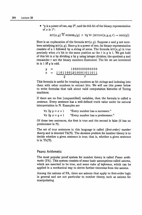
284 Lecture 38
• "y is a power of two, say 2k, and the kth bit of the binary representation of x is 1":
BIT(X,y) ~ POWER2(y) /\ \:Iq \:Ir (INTDIV(x,y,q,r) -+ ODD(q))
Here is an explanation of the formula BIT(X, V). Suppose x and yare numbers satisfying BIT(X, V). Since y is a power of two, its binary representation consists of a 1 followed by a string of zeros. The formula BIT(X,y) is true precisely when x's bit in the same position as the 1 in y is 1. We get hold of this bit in x by dividing x by y using integer division; the quotient q and remainder r are the binary numbers illustrated. The bit we are interested in is 1 iff q is odd.
y x
= =
1000000000000 J101}00~P1000~01101\
q r
This formula is useful for treating numbers as bit strings and indexing into them with other numbers to extract bits. We will use this power below to write formulas that talk about valid computation histories of Turing machines.
If there are no free (unquantified) variables, then the formula is called a sentence. Every sentence has a well-defined truth value under its natural interpretation in N. Examples are
\:Ix 3y y = x + 1 \:Ix 3y x = y+ 1
"Every number has a successor." "Every number has a predecessor."
Of these two sentences, the first is true and the second is false (0 has no predecessor in N).
The set of true sentences in this language is called (first-order) number theory and is denoted Th(N). The decision problem for number theory is to decide whether a given sentence is true; that is, whether a given sentence is in Th(N).
Peano Arithmetic
The most popular proof system for number theory is called Peano arithmetic (PA). This system consists of some basic assumptions called axioms, which are asserted to be true, and some rules of inference, which can be applied in a mechanical way to derive further theorems from the axioms.
Among the axioms of PA, there are axioms that apply to first-order logic in general and are not particular to number theory, such as axioms for manipulating
GOdel's Incompleteness Theorem 285
• propositional formulas, such as (rp A 'I/J) - rpj
• quantifiers, such as ('t/x rp(x)) - rp(17)j and
• equality, such as 't/x 't/y 't/z (x = yAy = z - x = z).
In addition, PA has the following axioms particular to number theory:
't/x .... (0 = x + 1) 't/x't/y (x + 1 = Y + 1- x = y)
't/x x +0 = x
't/x 't/y x + (y + 1) = (x + y) + 1
't/x x· 0 = 0
't/x't/y x . (y + 1) = (x· y) + x
(rp(O) A't/x (rp(x) - rp(x + 1))) - 't/x rp(x)
o is not a successor
successor is one-to-one
o is an identity for + + is associative
o is an annihilator for .
. distributes over + induction axiom
where rp(x) denotes any formula with one free variable x. The last axiom is called the induction axiom. It is actually an axiom scheme because it represents infinitely many axioms, one for each rp(x). It is really the induction principle on N as you know it: in words,
• if rp is true of 0 (basis), and
• if for any x, from the assumption that rp is true of x, it follows that rp is true of x + 1 (induction step),
then we can conclude that rp is true of all x.
There are also two rules of inference for deriving new theorems from old:
These two rules are called modv.s ponens and generalization, respectively.
A proof of rpn is a sequence rpo, rpl , rp2, ... ,rpn of formulas such that each rpi either is an axiom or follows from formulas occurring earlier in the list by a rule of inference. A sentence of the language is a theorem of the system if it has a proof.
A proof system is said to be sound if all theorems are truej that is, if it is not possible to prove a false sentence. This is a basic requirement of all reasonable proof systemsj a proof system wouldn't be much good if its theorems were false. The system PA is sound, as one can show by induction on the length of proofs: all the axioms are true, and any conclusion derived by a rule of inference from true premises is true. Soundness means that the following set inclusions hold:
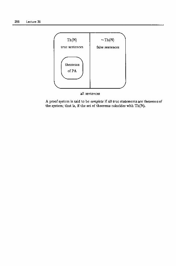
286 Lecture 38
Th(N) ---Th(N)
true sentences false sentences
all sentences
A proof system is said to be complete if all true statements are theorems of the system; that is, if the set of theorems coincides with Th(N).
Lecture 39
Proof of the Incompleteness Theorem
G6del proved the incompleteness theorem by constructing, for any reasonable proof system, a sentence of number theory <p that asserts its own un provability in that system:
<p is true {::=> <p is not provable. (39.1)
Any reasonable proof system, including PA, is sound; this means that for any sentence 'I/J,
'I/J is provable '* 'I/J is true (39.2)
(a proof system would not be worth much if some of its theorems were false). Then <p must be true, because otherwise
<p is false '* <p is provable by (39.1)
'* <p is true by (39.2),
a contradiction. Since <p is true, by (39.1) <p is not provable.
The construction of <p is quite interesting by itself, since it captures in no uncertain terms the notion of self-reference. The power that one needs to construct such a self-referential sentence is present in Turing machines and all modern programming languages. For example, the following is a C program that prints itself:
288 Lectu re 39
char *s="char *s=y.cy.sy.c;Y.cmainO{printf(s,34,s,34,10,10);}y'c"; main(){printf(s,34,s,34,10,10);}
Here 34 and 10 are the ASCII codes for double quote (") and newline, respectively. Although it's a mind-bender to try to figure out what this program does, it's worth the attempt, because once you understand this you have understood the main idea behind GOdel's construction.
We'll construct Godel's self-referential sentence in Supplementary Lecture K. For now we take a simpler approach that still retains the most important consequences. We will argue that in P A or any other reasonable proof system for number theory,
(i) the set of theorems (provable sentences) is r.e., but
(ii) the set Th(N) of true sentences is not,
therefore the two sets cannot be equal, and the proof system cannot be complete. This approach is due to Turing [1201.
The set of theorems of PA is certainly r.e.: one can enumerate the theorems by enumerating all the axioms and systematically applying the rules of inference in all possible ways, emitting every sentence that is ever derived. This is true for any reasonable proof system.
The crux then is to show:
Lemma 39.1 Th(N) i8 not r.e.
Proof. We prove this by a reduction "'HP :5m Th(N). The result will then follow from Theorem 33.3(i) and the fact that'" HP is not r.e. Recall that
HP = {M#x I M halts on input x}.
Given M#x, we show how to produce a sentence 'Y in the language of number theory such that
M#x E "'HP {::::::} 'Y E Th(N);
that is,
M does not halt on x {::::::} 'Y is true.
In other words, given M and x, we want to construct a sentence 'Y in the language of number theory that says, "M does not halt on x." This will be possible because the language of number theory is strong enough to talk about Turing machines and whether or not they halt.
Recall the formula BIT(1I, x) constructed in Lecture 38, which allows us to think of numbers as bit strings and extract bits from them. Using this as
Proof of the Incompleteness Theorem 289
a starting point, we will be able to construct a series of formulas culminating in a formula VALCOMPM,,,(Y) that says that y represents a valid computation history of M on input Xi that is, y represents a sequence of configurations ao, al, ... ,aN of M, encoded over some alphabet ~, such that
(i) ao is the start configuration of M on x,
(ii) ai+l follows from ai according to the transition function 8 of M, and
(iii) aN is a halt configuration.
These are the same valid computation histories we saw in Lecture 34. Once we have the formula VALCOMPM,,, (y), we can say that M does not halt on x by saying that there does not exist a valid computation history:
'Y ~f .,3y VALCOMPM,,,(Y).
This constitutes a reduction from'" HP to Th(N).
It remains only to provide the gory details of the construction of 'Y from M and x. Here they are. Assume that configurations of M are encoded over a finite alphabet ~ of size p, where p is prime. Every number has a unique p-ary representation. We use this representation instead of the binary representation for convenience.
Let the symbols of the start configuration of M on x = al a2 ... an be encoded by the p-ary digits ko, ... ,kn as shown:
I- al a2 a3 a4 an S -
ko kl k2 k3 k4 kn
Let the blank symbol u be encoded by the p-ary digit k.
Let C be the set of all sextuples (a, b, c, d, e, f) of p-ary digits such that if the three elements of ~ represented by a, b, and c occur consecutively in a configuration ai, and if d, e, and f occur in the corresponding locations in ai+l, then this would be consistent with the transition function 6. For example, if
6(q,a) = (p,b,R),
then the sextuple
a a b - q -
would be in C.
a b b -p
Now it's time to define some formulas.
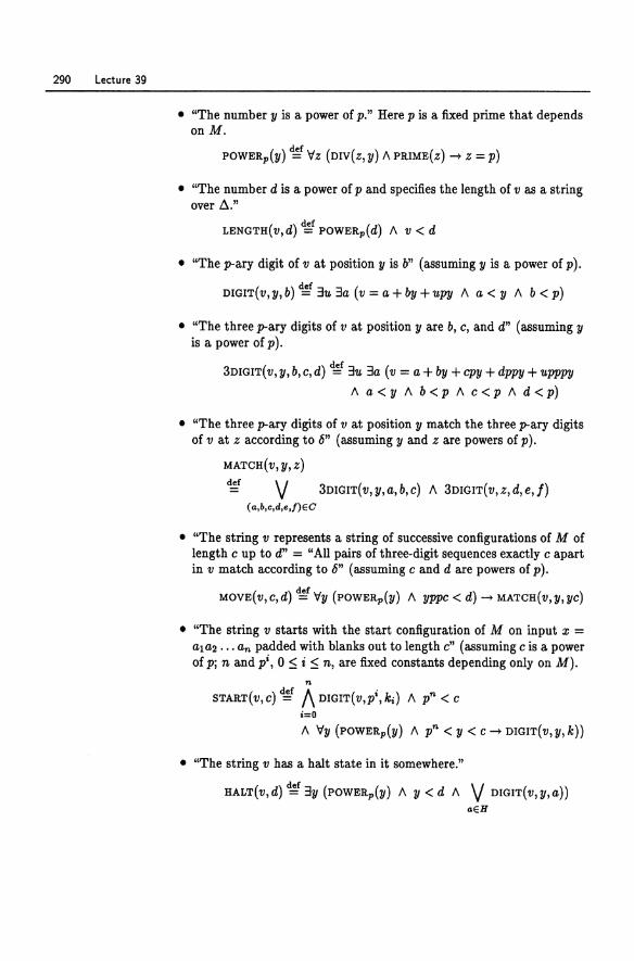
290 Lecture 39
• "The number '0 is a power of p." Here p is a fixed prime that depends onM.
POWERp('O) ~ Vz (DIV(Z, '0) " PRIME(Z) -+ Z = p)
• "The number d is a power of p and specifies the length of vasa string over 6."
LENGTH(V, d) ~ POWERp(d) " v < d
• "The p-ary digit of vat position '0 is b" (assuming '0 is a power of pl. def
DIGIT(V,'O,b) = 3u3a (v=a+by+uP'g" a<'O" b<p)
• "The three p-ary digits of v at position '0 are b, e, and d" (assuming '0 is a power of pl.
3DIGIT( v, '0, b, e, d) ~f 311. 3a (v = a + by + cpy + dppy + upppy
" a < '0 " b < p " e < p " d < p)
• "The three p-ary digits of v at position '0 match the three p-ary digits of vat Z according to 6" (assuming '0 and Z are powers of pl.
MATCH(V,'O,Z) def v 3DIGIT(v,'O,a,b,e) " 3DIGIT(v,z,d,e,j)
(a,b,c,d,e,f)EC
• "The string v represents a string of successive configurations of M of length e up to d" = "All pairs of three-digit sequences exactly e apart in v match according to 6" (assuming e and d are powers of pl.
MOVE(v,e,d) ~V'O (POWERp('O) " 'Oppe < d) -+ MATCH(v,'O,ye)
• "The string v starts with the start configuration of M on input x = ala2 ... an padded with blanks out to length e" (assuming e is a power of Pi n and Pi, 0 $ i $ n, are fixed constants depending only on M).
n def 1\ . START(v,e) = DIGIT(V,p',ki)" pn < e
i=O
" "1'0 (POWERp('O) " pn < '0 < C -+ DIGIT(V,'O, k))
• "The string v has a halt state in it somewhere."
HALT(V,d) ~ 3'0 (POWERp('O) " '0 < d" V DIGIT(v,'O,a)) aEH
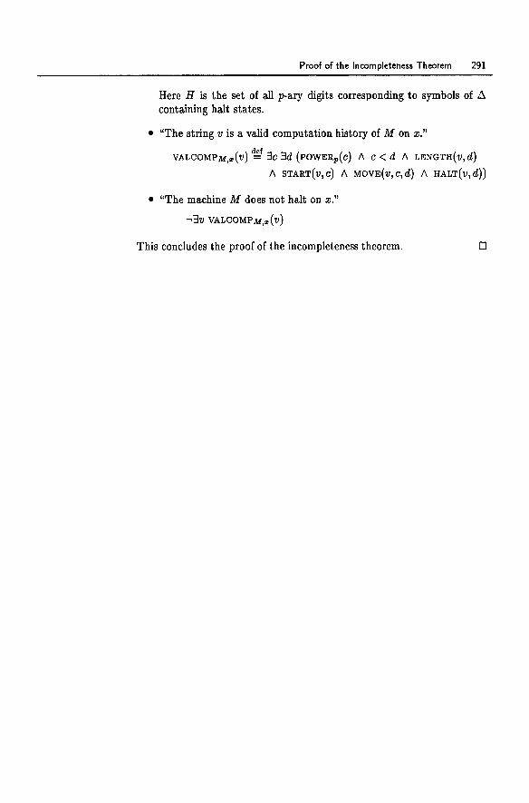
Proof of the Incompleteness Theorem 291
Here H is the set of all p-ary digits corresponding to symbols of !1 containing halt states.
• "The string v is a valid computation history of M on x."
VALCOMPM,.,(V) d~f 3c 3d (POWERp(C) 1\ C < d 1\ LENGTH(V,d)
1\ START(V,C) 1\ MOVE(V,c,d) 1\ HALT(V,d))
• "The machine M does not halt on x."
...,3v VALCOMPM,.,(V)
This concludes the proof of the incompleteness theorem. o

Supplementary Lecture K
Godel's Proof
GOdel proved the incompleteness theorem by constructing, for any reasonable proof system, a sentence of number theory that asserts its own unprovability. Here is the essence of Godel's construction.
We use the symbols I- and 1= for provability in Peano arithmetic (PA) and truth, respectively. That is,
1= cp ~ sentence cp is true in N,
I- cp ~ sentence cp is provable in PA.
To say that PA is sound says that every theorem of PA is true; in other words, for any sentence cp, if I- cp, then 1= cpo The soundness of PA can be established by induction on the length of proofs, using the fact that all axioms of PA are true and the induction rules preserve truth. (We haven't defined truth, but we'll come back to this later.)
Let formulas of number theory be coded as natural numbers in some reasonable way. Fix this coding and let r cp' denote the code of the formula cpo First we prove a lemma due to Godel that is a kind of fixpoint theorem.
Lemma K.l (Godel's fixpoint lemma) For any formula 1JI(x) with one free variable x, there exists a sentence T such that
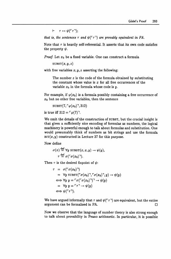
Godel's Proof 293
I- r +-+ tP(r r')j
that is, the sentences rand tP (r r') are provably equivalent in PA.
Note that r is heavily self-referential. It asserts that its own code satisfies the property tP.
Proof. Let Xo be a fixed variable. One can construct a formula
SUBST(X, y, z)
with free variables x, y, z asserting the following:
The number z is the code of the formula obtained by substituting the constant whose value is x for all free occurrences of the variable Xo in the formula whose code is y.
For example, if rp(xo) is a formula possibly containing a free occurrence of Xo but no other free variables, then the sentence
SUBST(7, rrp(xo)', 312)
is true iff 312 = rrp(7)'.
We omit the details of the construction of SUBST, but the crucial insight is that given a sufficiently nice encoding of formulas as numbers, the logical machinery is powerful enough to talk about formulas and substitution. One would presumably think of numbers as bit strings and use the formula BIT(X,y) constructed in Lecture 37 for this purpose.
Now define
O'(x) ~ 'fly SUBST(X,x,y) -+ tP(y),
r ~f O'(r O'(xo)').
Then r is the desired fixpoint of tP:
r = O'(rO'(xon
= 'fly SUBSTrO'(Xo)',rO'(xo)',y) -+ tP(y) {:::::} 'fly y = rO'{rO'{xon' -+ tP{y)
= 'fly y = rr' -+ tP(y) {:::::} tP(rr').
We have argued informally that r and tPrr') are equivalent, but the entire argument can be formalized in PA. 0
Now we observe that the language of number theory is also strong enough to talk about provability in Peano arithmetic. In particular, it is possible
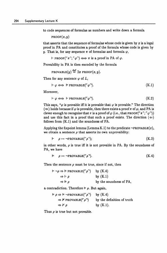
294 Supplementary Lecture K
to code sequences of formulas as numbers and write down a formula
PROOF(X,y)
that asserts that the sequence of formulas whose code is given by x is a legal proof in PA and constitutes a proof of the formula whose code is given by y. That is, for any sequence 11" of formulas and formula rp,
f- PROOF(r1l"',rrp') {:::::::} 11" is a proof in PA of rp.
Provability in PA is then encoded by the formula
PROVABLE(y) ~ 3x PROOF(X,y).
Then for any sentence rp of L,
f- rp {:::::::} 1= PROVABLE(r rp '). (K.l)
Moreover,
(K.2)
This says, "rp is provable iff it is provable that rp is provable." The direction (=> ) holds because if rp is provable, then there exists a proof 11" of rp, and PA is clever enough to recognize that 11" is a proof of rp (Le., that PROOF(r 11"', r rp')) and use this fact in a proof that such a proof exists. The direction ({:::) follows from (K.l) and the soundness of PA.
Applying the fixpoint lemma (LemmaK.l) to the predicate ...,PROVABLE(X),
we obtain a sentence p that asserts its own un provability:
(K.3)
in other words, p is true iff it is not provable in PA. By the soundness of PA, we have
Then the sentence p must be true, since if not, then
1= ""p => 1= PROVABLE(r p')
=> f- p
=> 1= p
by (KA) by (K.l)
by the soundness of P A,
a contradiction. Therefore 1= p. But again,
1= P => 1= ...,PROVABLE(r p')
=> ¥ PROVABLE(r p')
=>¥ P
Thus p is true but not provable.
by (KA) by the definition of truth
by (K.l).
(KA)
Godel's Proof 295
The Second Incompleteness Theorem
In the last section we constructed a sentence p such that
(i) p is true, but
(ii) p is not provable in PA.
Now in a weak moment, we might reason as follows. If PA is so all-powerful, why can't we just encode the whole argument of the previous section in PA as well? Then (i) and (ii) should be provable in PA. But this would say that p is provable in PA, yet provably not provable in PA. We would appear to have a paradox on our hands. Thinking about this is enough to make your head swim.
To sort this out, observe that there is logic going on at two levels here. The object of our study is a logical system, namely the language of number theory L and its deductive system PA; but we are reasoning about it using another logical system, which we will call the metasystem. The symbols 1-, 1=, =>, and {::::} that we used in the previous section are not symbols of L, but metasymbols, or symbols of the metasystem. The statements we made about truth and provability of sentences of L are metastatements.
For example, let ep be a sentence of L. The statement I- ep is not a sentence of L but a metastatement that says, "ep is provable in PA." Similarly, 1= ep is a metastatement that says, "ep is true."
Now certain metastatements about Land PA can be encoded in L using the coding scheme rep' and reasoned about in PA. For example, the metastatement I- tp is encoded as the sentence PROVABLE(r'"tp') of L. The metastatement (K.l) expresses the correctness of this encoding.
Other metastatements cannot be expressed in L. For example, the metastatement "ep is true" cannot be expressed in L. You might think that the sentence ep itself does this, but it doesn't, at least not in the way we want to use it: to encode meta-arguments in PA, we have to work with the code rep' of ep, so there would have to be a formula TRUE(X) of L such that for all sentences ep of L,
(K.S)
But it follows from the fixpoint lemma (Lemma K.l) that no such formula can exist. If it did, then there would exist a sentence u such that
1= u {::::} 1= ...,TRUE(r U ');
but by (K.5),
296 Supplementary Lecture K
1= (J' -¢=:> 1= TRUE(r (J' '),
a contradiction.
The language L is not powerful enough to express the truth of sentences of L or the soundness of PA (which refers to truth). These are external concepts, and we must deal with them in the metasystem. However, Land PA are powerful enough to express and reason about provability and consistency, which are the internal analogs of truth and soundness, respectively. Consistency just means that no contradiction can be derived; in other words, .L (falsity) is not a theorem. The consistency of PA is expressed in L as follows:
CONSIS ~f -,PROVABLE(r .L '}.
Meta-arguments involving only the concepts of provability and consistency can typically be mapped down into PA. For example, the argument we gave in the last section for (K.2) can be mapped down into PA, giving
I- PROVABLE(r <p'} +-+ PROVABLE(rpROVABLE(r <p '}'}. (K.6)
With this in mind, we can try to recreate the argument of the previous section without reference to truth or soundness. This leads to the following amazing consequence.
Theorem K.2 (G8del's second incOInpleteness theorem) No sufficiently powerful deductive system can prove its own consistency, unless it is inconsistent.
Of course, if the system is inconsistent (i.e., if it can prove .L), then it can prove anything, including its own consistency.
We prove the second incompleteness theorem for PA. But it actually holds for any sufficiently powerful deductive system, where "sufficiently powerful" just means strong enough to encode and reason about certain simple met astatements involving provability and consistency such as those discussed above.
Proof. Let p be the formula of (K.3). If I- p, then I- PROVABLE(r p'} by (K.2), but also I- -,PROVABLE(r p'} by (K.3), so PA would be inconsistent. Furthermore, this argument can be mapped down into PA using (K.6), giving
I- PROVABLE(r p'} - -,CONSIS,
or in contrapositive form,
(K.7)
Godel's Proof 297
Now suppose that consistency were provable; that is, I- CONSIS. By (K.7), we would have I- "'PROVABLE(r p'). Then by (K.3), we would have I- p. But we have just shown that this implies that PA is inconsistent.
Thus if PA is consistent, then,lt CONSIS. o
The Consistency of Mathematics
The metasystem we have been talking about so glibly is Zermelo-F'raenkel set theory (ZF), a modification of Cantor's original set theory that evolved after Russell discovered an inconsistency.
In Cantor's system one could form the set of all elements satisfying any given property. But consider the property x ¢ x. If you could form the set
b~f{xlx¢x},
then b E b iff b ¢ b, a contradiction. This is known as Russell's paradox. (Notice any similarities to anything in Lecture 3l?)
Over the years, mathematicians and logicians have come to fairly universal agreement that ZF forms a reasonable foundation for most of classical mathematics (type theory and intuitionism excluded). Pure ZF set theory is a first-order theory that deals with nothing but sets, sets of sets, sets of sets of sets, and so on. There is an "element of" relation E, a basic set 0,
and ways of constructing more complicated sets inductively. The natural numbers are defined inductively as certain sets:
0~0,
1 ~ {O},
2 ~f {O,l},
def { } 3 = 0,1,2,
and so on. There are axioms and proof rules for manipulating sets, and the Peano axioms for number theory can be derived from them.
In ZF one can give formal semantics for the language L of number theory, including a definition of truth. One can then prove that relative to that semantics, PA is sound, therefore consistent. But is ZF consistent? No one knows. And Godel's theorem says that no one can ever know, short of discovering an inconsistency. As far as we can tell, a new Russell's paradox could be discovered tomorrow, and much of the structure of mathematics that has been built over the last century would come crashing down.
GOdel's theorem says that we cannot prove the consistency of ZF in ZF any more than we can prove the consistency of PA in PA. In order to prove
298 Supplementary Lecture K
the consistency of ZF, we would have to go outside of ZF to an even larger metasystem. But then we would be faced with the same question about the consistency of that metasystem. At some point, we just have to stop and take consistency as a matter of faith. Most mathematicians would agree that ZF is just as good a place as any to do this. But the only assurance we have that the ice is solid under our feet is that no one has broken through yet-at least not since Cantor!
Exercises
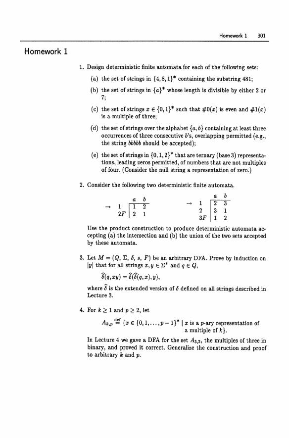
Homework 1
Homework 1 301
1. Design deterministic finite automata for each of the following sets:
(a) the set of strings in {4,8, 1}* containing the substring 481;
(b) the set of strings in {a} * whose length is divisible by either 2 or 7;
(c) the set of strings x E {O, 1}* such that #O(x) is even and #1(x) is a multiple of three;
(d) the set of strings over the alphabet {a, b} containing at least three occurrences of three consecutive b's, overlapping permitted (e.g., the string bbbbb should be accepted);
(e) the set of strings in {O, 1, 2} * that are ternary (base 3) representations, leading zeros permitted, of numbers that are not multiples of four. (Consider the null string a representation of zero.)
2. Consider the following two deterministic finite automata.
a b lr-r-r 2F I 2 1
a b
1 1IT3 2 3 1 3F 1 2
Use the product construction to produce deterministic automata accepting (a) the intersection and (b) the union of the two sets accepted by these automata.
3. Let M = (Q, E, h, s, F) be an arbitrary DFA. Prove by induction on Iyl that for all strings x, y E E* and q E Q,
6(q,xy) = 6(6(q,x),y),
where 6 is the extended version of h defined on all strings described in Lecture 3.
4. For k ~ 1 and p ~ 2, let
Ak,p ~ {x E {O, 1, ... ,p - I} * I x is a p-ary representation of a multiple of k}.
In Lecture 4 we gave a DFA for the set Aa,2, the multiples of three in binary, and proved it correct. Generalize the construction and proof to arbitrary k and p.
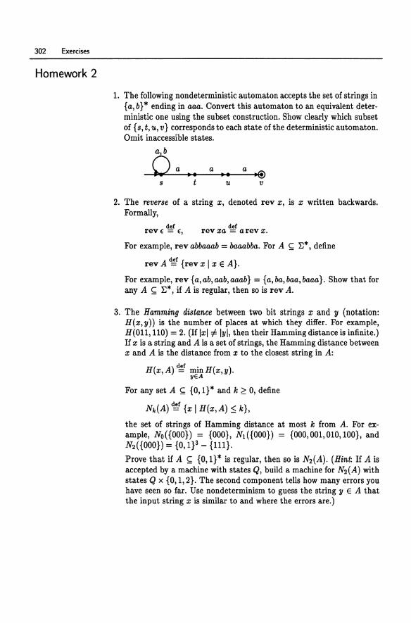
302 Exercises
Homework 2
1. The following nondeterministic automaton accepts the set of strings in { a, b} * ending in aaa. Convert this automaton to an equivalent deterministic one using the subset construction. Show clearly which subset of {s, t, 'It, v} corresponds to each state of the deterministic automaton. Omit inaccessible states.
a,b
Q a - .. a •• s t
2. The reverse of a string x, denoted rev x, is x written backwards. Formally,
def reVE = E,
def rev xa = a rev x.
For example, rev abbaaab = baaabba. For A ~ l:*, define
rev A ~ {rev x I x E A}.
For example, rev {a,ab,aab,aaab} = {a,ba,baa,baaa}. Show that for any A ~ l:*, if A is regular, then so is rev A.
3. The Hamming distance between two bit strings x and y (notation: H(x,'O)) is the number of places at which they differ. For example, H(Ol1, 110) = 2. (If Ixl ::f. 1'01, then their Hamming distance is infinite.) If x is a string and A is a set of strings, the Hamming distance between x and A is the distance from x to the closest string in A:
H(x,A) ~ minH(x,'O). ilEA
For any set A ~ {0,1}* and k ~ 0, define
Nk(A) ~ {x I H(x, A) 5 k},
the set of strings of Hamming distance at most k from A. For example, No({OOO}) = {OOO}, N1 ({000}) = {OOO,OOl,OlO,lOO}, and N2({000}) = {O, 1P - {111}.
Prove that if A ~ {0,1}* is regular, then so is N2(A). (Hint: If A is accepted by a machine with states Q, build a machine for N2(A) with states Q x {O, 1, 2}. The second component tells how many errors you have seen so far. Use nondeterminism to guess the string yEA that the input string x is similar to and where the errors are.)
Homework 3
Homework 3 303
1. Give regular expressions for each of the following subsets of {a, b} *. (a) {x I x contains an even number of a's}
(b) {x I x contains an odd number of b's}
(c) {x I x contains an even number of a's or an odd number of b's}
(d) {x I x contains an even number of a's and an odd number of b's}
Try to simplify the expressions as much as possible using the algebraic laws of Lecture 9. Recall that regular expressions over {a, b} may use E, ~, a, b, and operators +, *, and· only; the other pattern operators are not allowed.
2. Give deterministic finite automata accepting the sets of strings match-ing the following regular expressions.
(a) (000* + 111*)*
(b) (01 + 10)(01 + 10)(01 + 10)
(c) (0+ 1(01*0)*1)*
Try to simplify as much as possible.
3. For any set of strings A, define the set
MiddleThirds A = {y I 3x, z Ixl = Iyl = Izi and xyz E A}.
For example, MiddleThirds{ f, a, ab, bab, bbab, aabbab} = {f, a, bb}. Show that if A is regular, then so is MiddleThirds A.
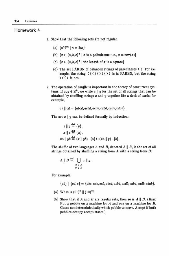
304 ~xercises
Homework 4
1. Show that the following sets are not regular.
(a) {anbm In = 2m}
(b) {x e {a, b, c}* I x is a palindrome; i.e., x = rev(x)}
( c) {x e {a, b, c} * I the length of x is a square}
(d) The set PAREN of balanced strings of parentheses ( ). For ex-ample, the string « ( ) ( ) ) ( » is in PAREN, but the string ) «) is not.
2. The operation of shuffle is important in the theory of concurrent systems. If x, y e ~*, we write x II y for the set of all strings that can be obtained by shuffling strings x and y together like a deck of cards; for example,
ab II cd = {abed, acbd, acdb, cabd, cadb, cdab}.
The set x II y can be defined formally by induction:
f II y~f {y},
xllf~{x},
xa II yb ~ (x II yb) . {a} U (xa II y) . {b}.
The shuffle of two languages A and B, denoted A II B, is the set of all strings obtained by shuffling a string from A with a string from B:
AIIB~ U x lIy·
For example,
zEA !lEB
{ab} II {cd, e} = {abe, aeb, eab, abed, acbd, acdb, cabd, cadb, edab}.
(a) What is (01)* II (1O)*?
(b) Show that if A and B are regular sets, then so is A II B. (Hint: Put a pebble on a machine for A and one on a machine for B. Guess nondeterministically which pebble to move. Accept if both pebbles occupy accept states.)
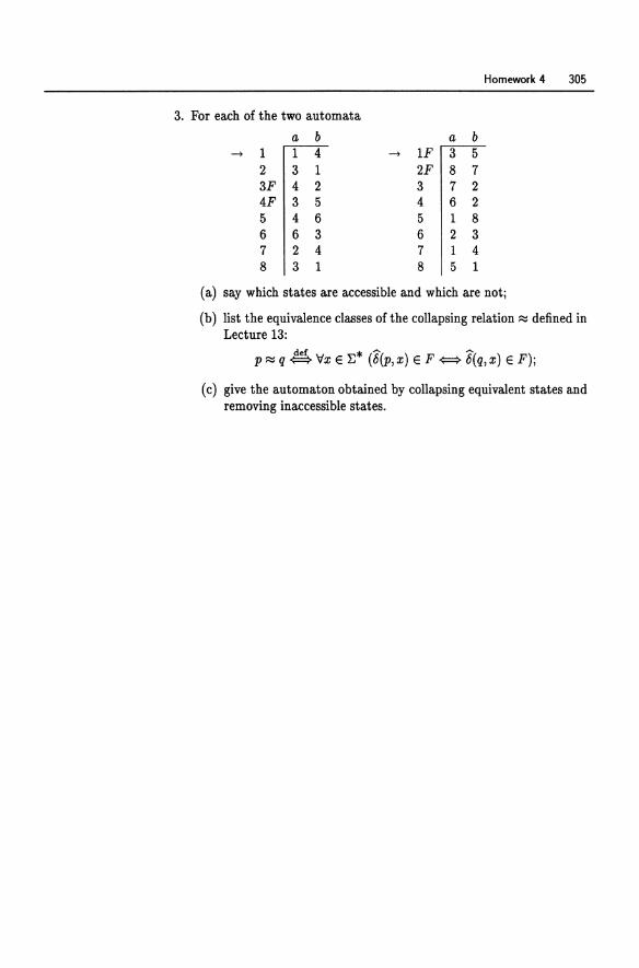
Homework 4 305
3. For each of the two automata
a b a b -+ 1 1 4 -+ IF 3 5
2 3 1 2F 8 7 3F 4 2 3 7 2 4F 3 5 4 6 2 5 4 6 5 1 8 6 6 3 6 2 3 7 2 4 7 1 4 8 3 1 8 5 1
(a) say which states are accessible and which are noti
(b) list the equivalence classes of the collapsing relation ~ defined in Lecture 13:
p ~ q ~ 'Vx E E* (6(P,x) E F {::::::> 6(q,x) E F)i
(c) give the automaton obtained by collapsing equivalent states and removing inaccessible states.
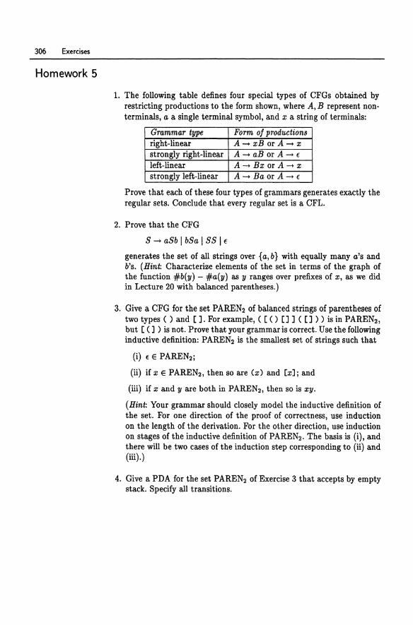
306 Exercises
Homework 5
1. The following table defines four special types of CFGs obtained by restricting productions to the form shown, where A, B represent nonterminals, a a single terminal symbol, and x a string of terminals:
Grammar type Form oj produ.ctions right-linear A-xB orA- x strongly right-linear A-aB orA- f left-linear A_ Bx orA- x strongly left-linear A- Baor A-f
Prove that each of these four types of grammars generates exactly the regular sets. Conclude that every regular set is a CFL.
2. Prove that the CFG
8 - a8b I b8a I 88 I f generates the set of all strings over {a, b} with equally many a's and b's. (Hint: Characterize elements of the set in terms of the graph of the function #b(y) - #a(y) as y ranges over prefixes of x, as we did in Lecture 20 with balanced parentheses.)
3. Give a CFG for the set PAREN2 of balanced strings of parentheses of two types ( ) and []. For example, ( [() []] ( []» is in PAREN2, but [(] ) is not. Prove that your grammar is correct. Use the following inductive definition: PAREN2 is the smallest set of strings such that
(i) f E PAREN2i
(ti) if x E PAREN2, then so are (x) and [xl i and
(iii) if x and y are both in PAREN2, then so is xy.
(Hint: Your grammar should closely model the inductive definition of the set. For one direction of the proof of correctness, use induction on the length of the derivation. For the other direction, use induction on stages of the inductive definition of PAREN2. The basis is (i), and there will be two cases of the induction step corresponding to (ii) and (iii).)
4. Give a PDA for the set PAREN2 of Exercise 3 that accepts by empty stack. Specify all transitions.
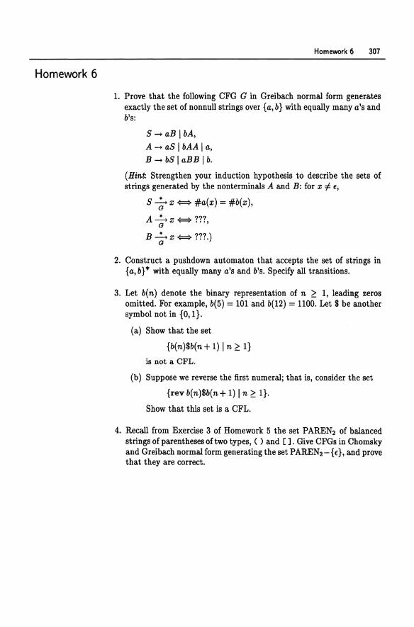
Homework 6
Homework 6 307
1. Prove that the following CFG G in Greibach normal form generates exactly the set of nonnull strings over {a, b} with equally many a's and b's:
S-aB IbA, A-aSlbAAla, B - bS I aBB I b.
(Hint: Strengthen your induction hypothesis to describe the sets of strings generated by the nonterminals A and B: for :z; :F E,
S +:z; ~ #a(:z;) = #b(:z;),
A • 111 G:Z;~···'
B~:z;~???) G
2. Construct a pushdown automaton that accepts the set of strings in { a, b} * with equally many a's and b's. Specify all transitions.
3. Let b(n) denote the binary representation of n ~ 1, leading zeros omitted. For example, b(5) = 101 and b(12) = 1100. Let $ be another symbol not in {a, I}.
(a) Show that the set
{b(n)$b(n+ 1) I n ~ I}
is not a CFL.
(b) Suppose we reverse the first numeral; that is, consider the set
{revb(n)$b(n+ 1) I n ~ I}.
Show that this set is a CFL.
4. Recall from Exercise 3 of Homework 5 the set PAREN2 of balanced strings of parentheses of two types, ( ) and []. Give CFGs in Chomsky and Greibach normal form generating the set PAREN 2 - { E }, and prove that they are correct.
308 Exercises
Homework 7
1. Describe a parser to parse regular expressions according to the precedence relation
* >. > + Here> means "has higher precedence than." The main differences you will have to account for between regular expressions and the arithmetic expressions discussed in Lecture 26 are: (i) the unary operator * comes after its operand, not before it as with unary minus; and (ii) the concatenation operator· can be omitted. lllustrate the action of your parser on the expression
(a + b)* + ab*a.
2. Prove that if A is a CFL and R is a regular set, then An R is a CFL. (Hint: Use a product construction.)
3. Recall the shuffle operator II from Homework 4. Show that the shuffle of two CFLs is not necessarily a CFL. (Hint: Use the previous exercise to simplify the argument.)
4. Let A be any regular set. Show that the set
{x 13y Iyl = 21.,1 and xy E A}
is regular.
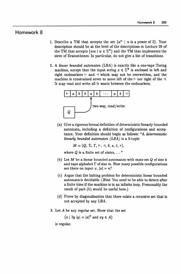
Homework 8
Homework 8 309
1. Describe a TM that accepts the set {an 1 n is a power of 2}. Your description should be at the level of the descriptions in Lecture 29 of the TM that accepts {ww 1 w E ~*} and the TM that implements the sieve of Eratosthenes. In particular, do not give a list of transitions.
2. A linear bounded automaton (LBA) is exactly like a one-tape Turing machine, except that the input string z E ~* is enclosed in left and right endmarkers I- and -l which may not be overwritten, and the machine is constrained never to move left of the I- nor right of the -l. It may read and write all it wants between the endmarkers.
(a) Give a rigorous formal definition of deterministic linearly bounded automata, including a definition of configurations and acceptance. Your definition should begin as follows: "A deterministic linearly bounded automaton (LEA) is a 9-tuple
M = (Q, ~, r, 1-, -l, 0, s, t, r),
where Q is a finite set of states, ... "
(b) Let M be a linear bounded automaton with state set Q of size k and tape alphabet r of size m. How many possible configurations are there on input z, Izl = n?
(c) Argue that the halting problem for deterministic linear bounded automata is decidable. (Hint: You need to be able to detect after a finite time if the machine is in an infinite loop. Presumably the result of part (b) would be useful here.)
(d) Prove by diagonaiization that there exists a recursive set that is not accepted by any LBA.
3. Let A be any regular set. Show that the set
{z 13y Iyl = IZl2 and zy E A}
is regular.
310 Exercises
Homework 9
1. Prove that the following question is undecidable. Given a Turing machine M and state q of M, does M ever enter state q on some input? (This problem is analogous to the problem of identifying dead code: given a PASCAL program containing a designated block of code, will that block of code ever be executed?)
2. Prove that it is undecidable whether two given Turing machines accept the same set. (This problem is analogous to determining whether two given PASCAL programs are equivalent.)
3. Prove that the emptiness problem for deterministic linearly bounded automata (Le., whether L(M) = 0) is undecidable. (Hint: Think VALCOMPS.)
4. Prove that an r.e. set is recursive iff there exists an enumeration machine that enumerates it in increasing order.
5. For A, B ~ ~*, define
AlB ~f {x 13y E B xy E A},
A - B ~ {x IVy E B xy E A}.
(a) Show that if A is regular and B is any set whatsoever, then AlB and A - B are regular.
(b) Show that even if we are given a finite automaton for A and a Turing machine for B, we cannot necessarily construct an automaton for AlB or A - B effectively.
Homework 10
1. Show that neither the set
TOTAL ~f {M I M halts on all inputs}
nor its complement is r.e.
Homework 10 311
2. Consider one-tape Turing machines that are constrained not to overwrite the input string. They may write all they want on the blank portion of the tape to the right of the input string.
(a) Show that these machines accept only regular sets. (If you're thinking, "Hey, why not just copy the input string out to the blank portion of the tape," think again ... )
(b) Show that, despite (a), it is impossible to construct an equivalent finite automaton effectively from such a machine.
3. Show that it is undecidable whether the intersection of two CFLs is nonempty. (Hint: Use a variant of VALCOMPS in which every other configuration is reversed:
ao#rev al #a2 #rev a3 # ... #an .
Express this set as the intersection of two CFLs.)
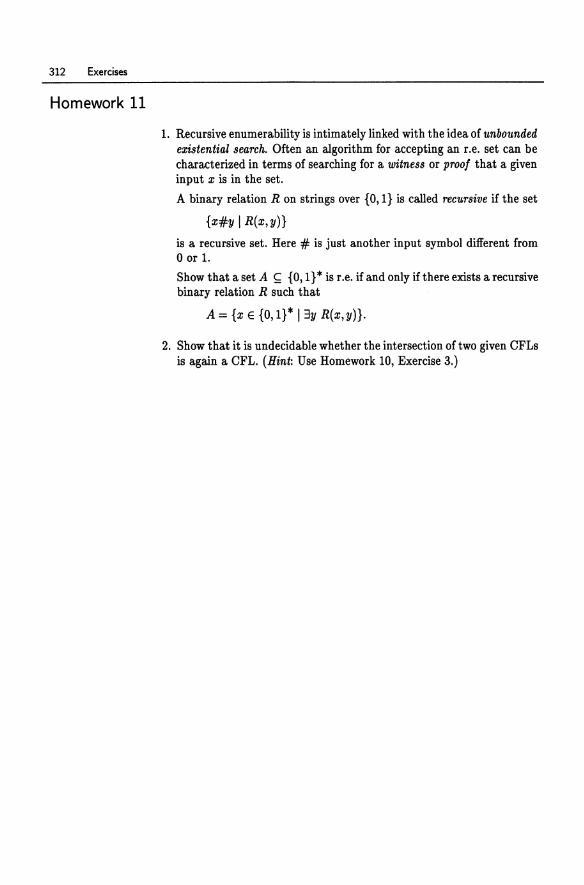
312 Exercises
Homework 11
1. Recursive enumerability is intimately linked with the idea of unbounded existential search. Often an algorithm for accepting an r.e. set can be characterized in terms of searching for a witness or prool that a given input x is in the set.
A binary relation R on strings over {O, I} is called recursive if the set
{x#y I R(x,y)}
is a recursive set. Here # is just another input symbol different from
° or 1. Show that a set A ~ {O, I} * is r .e. if and only if there exists a recursive binary relation R such that
A = {x E {O, 1}* 13y R(x,y)}.
2. Show that it is undecidable whether the intersection of two given CFLs is again a CFL. (Hint: Use Homework 10, Exercise 3.)
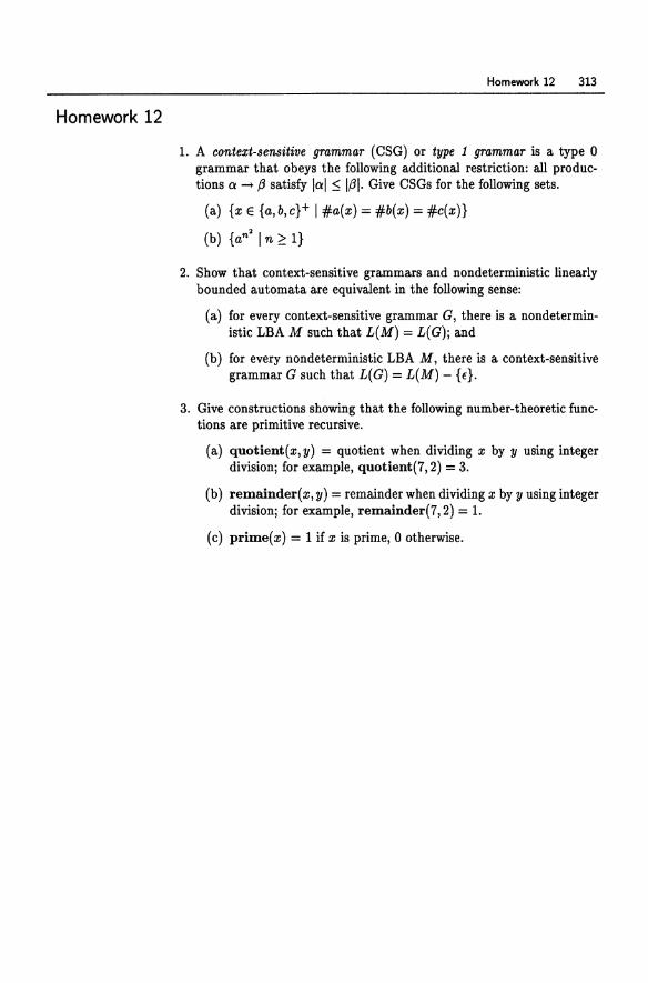
Homework 12
Homework 12 313
1. A context-sensitive grammar (CSG) or type 1 grammar is a type 0 grammar that obeys the following additional restriction: all productions a -4 f3 satisfy lal ~ 1f31. Give CSGs for the following sets.
(a) {x E {a,b,c}+ I #a(x) = #b(x) = #c(x)}
(b) {an'ln~l}
2. Show that context-sensitive grammars and nondeterministic linearly bounded automata are equivalent in the following sense:
(a) for every context-sensitive grammar G, there is a nondeterministic LBA M such that L(M) = L(G); and
(b) for every nondeterministic LBA M, there is a context-sensitive grammar G such that L(G) = L(M) - {f}.
3. Give constructions showing that the following number-theoretic functions are primitive recursive.
(a) quotient(x,y) = quotient when dividing x by y using integer division; for example, quotient (7, 2) = 3.
(b) remainder( x, y) = remainder when dividing x by y using integer division; for example, remainder(7,2) = 1.
(c) prime( x) = 1 if x is prime, 0 otherwise.
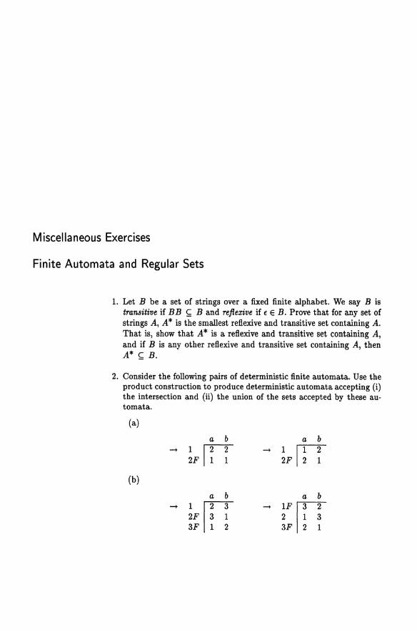
Miscellaneous Exercises
Finite Automata and Regular Sets
1. Let B be a set of strings over a fixed finite alphabet. We say B is transitive if BB ~ B and reflexive if fEB. Prove that for any set of strings A, A * is the smallest reflexive and transitive set containing A. That is, show that A * is a reflexive and transitive set containing A, and if B is any other reflexive and transitive set containing A, then A* ~ B.
2. Consider the following pairs of deterministic finite automata. Use the product construction to produce deterministic automata accepting (i) the intersection and (ii) the union of the sets accepted by these automata.
(a)
a b a b -+
1 Iii -+ 1m-2F 1 1 2F 2 1
(b)
a b a b -+ !fIT -+ !FIIT 2F 3 1 2 1 3
3F 1 2 3F 2 1
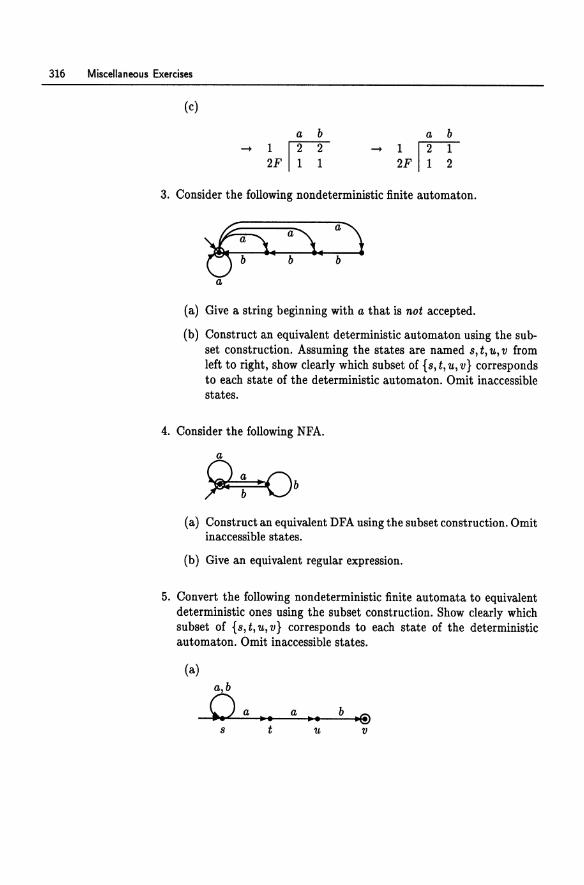
316 Miscellaneous Exercises
(c)
a b 1122 2F 11 1
a b 11""2"1 2F 11 2
3. Consider the following nondeterministic finite automaton.
(a) Give a string beginning with a that is not accepted.
(b) Construct an equivalent deterministic automaton using the subset construction. Assuming the states are named s, t, u, v from left to right, show clearly which subset of {s, t, u, v} corresponds to each state of the deterministic automaton. Omit inaccessible states.
4. Consider the following NFA.
(a) Construct an equivalent DFA using the subset construction. Omit inaccessible states.
(b) Give an equivalent regular expression.
5. Convert the following nondeterministic finite automata to equivalent deterministic ones using the subset construction. Show clearly which subset of {s, t, u, v} corresponds to each state of the deterministic automaton. Omit inaccessible states.
(a) a,b
Oa a b .® ... • • s t u v
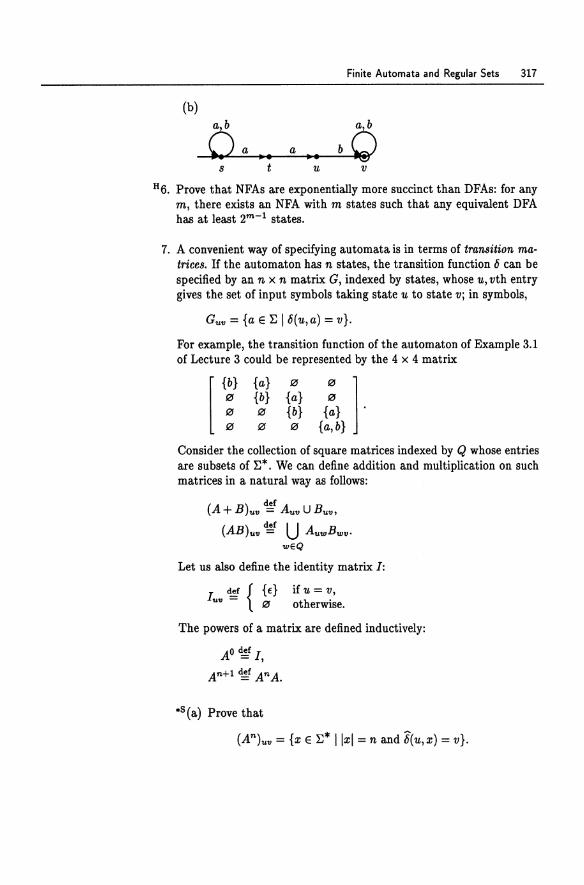
Finite Automata and Regular Sets 317
(b)
~a U ~. a • • s t u v
H6. Prove that NFAs are exponentially more succinct than DFAs: for any m, there exists an NFA with m states such that any equivalent DFA has at least 2m - 1 states.
7. A convenient way of specifying automata is in terms of transition matrices. If the automaton has n states, the transition function 6 can be specified by an n x n matrix G, indexed by states, whose u, vth entry gives the set of input symbols taking state u to state Vj in symbols,
Guv = {a E ~ 16(u,a) = v}.
For example, the transition function of the automaton of Example 3.1 of Lecture 3 could be represented by the 4 x 4 matrix
{a} {b} o o
o {a} {b} o
o 1 o {a} .
{a,b}
Consider the collection of square matrices indexed by Q whose entries are subsets of ~*. We can define addition and multiplication on such matrices in a natural way as follows:
(A + B)uv ~f Autl U Buv ,
(AB)uv ~ U AuwBwv. wEQ
Let us also define the identity matrix I:
Iutl ~f { ~} if u = v, otherwise.
The powers of a matrix are defined inductively:
AO ~f I,
An+1 ~ AnA .
• s ( a) Prove that
(An)utl = {x E ~* Ilxl = n and 8(u, x) = v}.
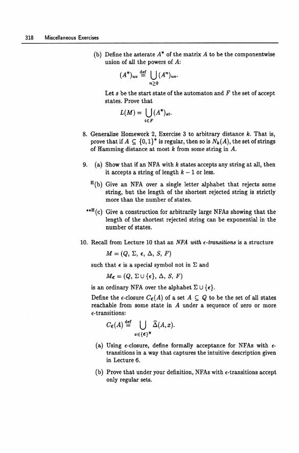
318 Miscellaneous Exercises
(b) Define the asterate A* ofthe matrix A to be the componentwise union of all the powers of A:
(A*)uv ~f U (An) .. v. n;:::O
Let s be the start state of the automaton and F the set of accept states. Prove that
L(M) = U (A*)st. tEF
8. Generalize Homework 2, Exercise 3 to arbitrary distance k. That is, prove that if A ~ {O, 1}* is regular, then so is N1c(A), the set ofstrings of Hamming distance at most k from some string in A.
9. (a) Show that if an NFA with k states accepts any string at all, then it accepts a string of length k - 1 or less.
H(b) Give an NFA over a single letter alphabet that rejects some string, but the length of the shortest rejected string is strictly more than the number of states .
.. H(C) Give a construction for arbitrarily large NFAs showing that the length of the shortest rejected string can be exponential in the number of states.
10. Recall from Lecture 10 that an NFA with e-tmnsitions is a structure
M = (Q, ~, E, ll, S, F)
such that E is a special symbol not in ~ and
ME = (Q, ~ U {E}, ll, S, F)
is an ordinary NFA over the alphabet ~ U {E}.
Define the e-closure GE(A) of a set A ~ Q to be the set of all states reachable from some state in A under a sequence of zero or more e-transitions:
Ge(A) d~ U A(A,x). "'E{E}*
(a) Using e-closure, define formally acceptance for NFAs with etransitions in a way that captures the intuitive description given in Lecture 6.
(b) Prove that under your definition, NFAs with e-transitions accept only regular sets.
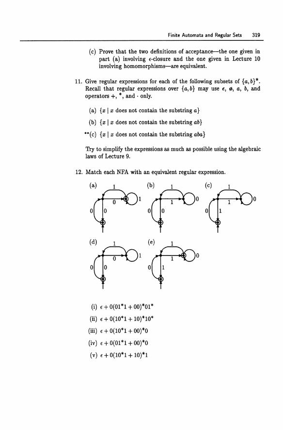
Finite Automata and Regular Sets 319
(c) Prove that the two definitions of acceptance-the one given in part (a) involving E-closure and the one given in Lecture 10 involving homomorphisms-are equivalent.
11. Give regular expressions for each of the following subsets of {a, b} *. Recall that regular expressions over {a, b} may use 1:, ~, a, b, and operators +, *, and· only.
(a) {x I x does not contain the substring a}
(b) {x I x does not contain the substring ab}
** (c) {x I x does not contain the substring aba}
Try to simplify the expressions as much as possible using the algebraic laws of Lecture 9.
12. Match each NFA with an equivalent regular expression.
(a) 1 (b) 1 (c) 1
1 0 0
o 0 0
(d) 1 (e) 1
1 0
o 0
(i) E + 0(01 *1 + 00)*01 *
(ii) E + 0(10*1 + 10)*10*
(iii) E + 0(10*1 + 00)*0
(iv) E + 0(01 *1 + 00)*0
(v) f + 0(10*1 + 10)*1
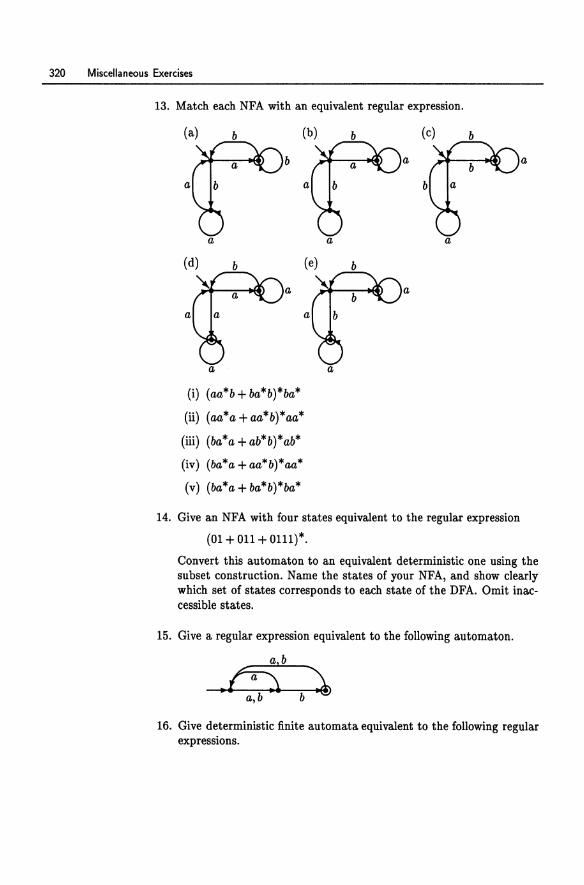
320 Miscellaneous Exercises
13. Match each NFA with an equivalent regular expression.
(a) (b) (c)
b a a
a a
a a
(d)
a a
a a
a a
(i) (aa*b + ba*b)*ba*
(li) (aa*a + aa*b)*aa*
(iii) (ba*a + ab*b)*ab*
(iv) (ba*a + aa*b) *aa*
(v) (ba*a + ba*b)*ba*
a
14. Give an NFA with four states equivalent to the regular expression
(01 + 011 + 0111)*.
Convert this automaton to an equivalent deterministic one using the subset construction. Name the states of your NFA, and show clearly which set of states corresponds to each state of the DFA. Omit inaccessible states.
15. Give a regular expression equivalent to the following automaton .
• ~b a,b b~
16. Give deterministic finite automata equivalent to the following regular expressions.
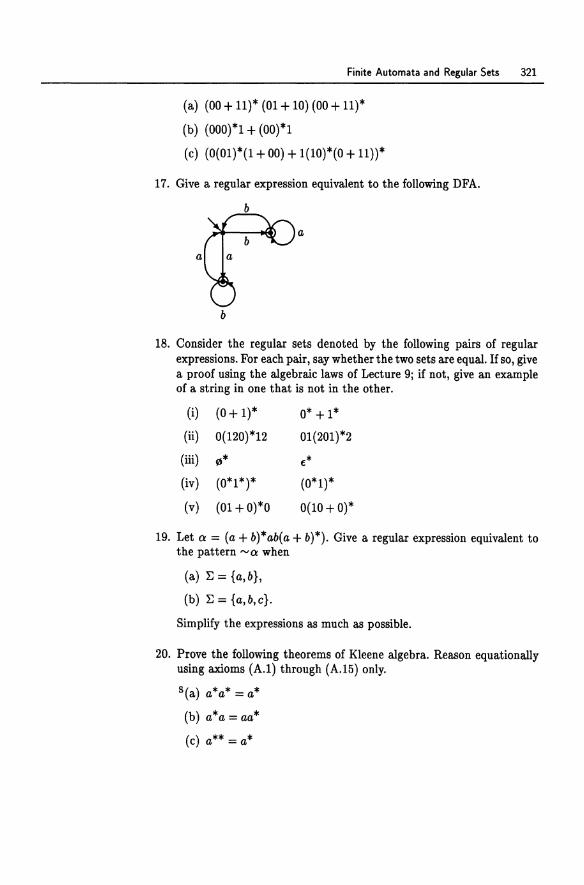
Finite Automata and Regular Sets 321
(a) (00 + 11)* (01 + 10) (00 + 11)*
(b) (000)*1 + (00)*1
(c) (0(01)*(1 + 00) + 1(10)*(0 + 11))*
17. Give a regular expression equivalent to the following DFA.
a
a
b
18. Consider the regular sets denoted by the following pairs of regular expressions. For each pair, say whether the two sets are equal. If so, give a proof using the algebraic laws of Lecture 9; if not, give an example of a string in one that is not in the other.
(i) (0 + 1)* 0* + 1*
(ii) 0(120)*12 01(201)*2
(iii) ~* E*
(iv) (0*1*)* (0*1)*
(v) (01 + 0)*0 0(10 + 0)*
19. Let 0: = (a + b)*ab(a + b)*). Give a regular expression equivalent to the pattern '" 0: when
(a) ~ = {a,b},
(b) ~ = {a,b,c}.
Simplify the expressions as much as possible.
20. Prove the following theorems of Kleene algebra. Reason equationally using axioms (A.1) through (A.15) only.
S(a) a*a* = a*
(b) a*a = aa*
(c) a** = a*
322 Miscellaneous Exercises
(d) (a*b)*a* = (a + b)*
(e) a(ba)* = (ab)*a
(f) a* = (aa)* + a(aa)*
21. Prove Lemma A.1.
·22. Prove that in the presence of Kleene algebra axioms (A.I) through (A.ll), axioms (A.12) and (A.14) are equivalent (and by symmetry, so are (A.13) and (A.15)).
·23. Here is a purely algebraic version of Miscellaneous Exercise 1. An element c of a Kleene algebra I( is said to be reflexive if I ::; c and transitive if cc ::; c. We say that c contains a if a ::; c. Prove that for any a E 1(,
(a) a* is reflexive and transitive and contains a; and
(b) a* is the least element of I( satisfying these properties. That is, if c is any element of I( that is reflexive and transitive and contains a, then a* ::; c.
This justifies the terminology reflexive transitive closure.
··24. Prove Lemma A.2: the family M(n, I() of n x n matrices over a Kleene algebra I( with the matrix operations defined as in Supplementary Lecture A again forms a Kleene algebra.
s25. Prove Theorem A.3.
HS26. For any set of strings A, define the set
FirstHalvesA = {x 13y Iyl = Ixl and xy E A}.
For example, FirstHalves {a, ab, bab, boob} = {a, bb}. Show that if A is regular, then so is FirstHalves A.
27. For any set of strings A, define the set
FirstThirds A = {x 13y Iyl = 21xl and xy E A}.
For example, FirstThirds {to, a, ab, bab, bbab} = {to, b}. Show that if A is regular, then so is FirstThirds A.
28. Given a set A ~ {O, I}*, let
A' = {xy I xly E A}.
Finite Automata and Regular Sets 323
That is, A' consists of all strings obtained from a string in A by deleting exactly one 1. Show that if A is regular, then so is A'.
29. For A a set of natural numbers, define
binary A = {binary representations of numbers in A} ~ (0 + 1) *,
unaryA={OnlnEA} ~ 0*.
For example, if A= {2,3,5}, then
binary A = {10, 11, 101},
unary A = {OO,OOO,OOOOO}.
Consider the following two propositions:
(i) For all A, if binary A is regular, then so is unary A.
(ii) For all A, if unary A is regular, then so is binary A.
One of (i) and (ii) is true and the other is false. Which is which? Give a proof and a counterexample.
·30. Let A be a regular set. Consider the two sets
{x 13n ;:: 0 3y E A y = xn}, {x 13n ;:: a 3y E A x = yn}.
One is necessarily regular and one is not. Which is which? Give a proof and a counterexample .
• H31. One of the following subsets of {a, b, $} * is regular and the other is not. Which is which? Give proofs.
{xy I x,y E {a,b}*, #a(x) = #b(y)} {x$y I x,y E {a,b}*, #a(x) = #b(y)}
••• H32. Two of the following three sets are always regular for any regular set A. Which are they? Give two proofs and a counterexample.
(a) {x I xl"l E A}
(b) {x 13y Iyl = 221 - 1 and xy E A}
(c) {x 13y Iyl = log Ixl and xy E A}
•• Hs33. Let p be any polynomial of degree d with nonnegative integer coefficients. Show that if A is a regular set, then so is the set
A' = {x 13y Iyl = p(lxl) and YEA}.
324 Miscellaneous Exercises
***34. (Seiferas and McNaughton [113]) Let!: N -+ N be a function. Call ! regularity preserving if the set
{x 13y Iyl = !(Ixl) and xy e A}
is regular whenever A is. Call ! weakly regularity preserving if the set
{x 13y Ivl = !(Ixl) and yeA}
is regular whenever A is. Prove that the following statements are equivalent:
(a) f is regularity preserving;
(b) f is weakly regularity preserving;
(c) for any ultimately periodic set U S;; N, the set
rl(U) = {m I f(m) e U}
is also ultimately periodic; and
(d) for any n e N, the set {m I f(m) = n} is ultimately periodic, and f is ultimately periodic mod p for any p ;?: 1 in the sense that
00
'Vp;?: 1 3q;?: 1 'V n J(n) == J(n + q) mod p.
00
Here 'V means "for almost all" or "for all but finitely many." Formally,
00 de! 'V n <p(n) <===> 3m ;?: 0 'Vn;?: m <p(n).
s35. Show that the set {ww I we {O, 1}*} is not regular.
536. Show that the set
PRIMES ~ {aP I p is prime}
is not regular.
37. Which of the following sets are regular and which are not? Give justification.
(a) {an b2m In;?: 0 and m ;?: O}
(b) {anbm In = 2m}
(c) {anbm In # m}
(d) {aP- 1 I p is prime}
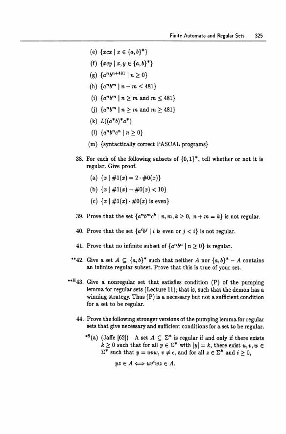
(e) {xcx I x e {a,b}*}
(f) {xcy I x,y e {a,b}*}
(g) {anbn+481 I n ~ O}
(h) {anbm In - m ~ 481}
Finite Automata and Regular Sets 325
(i) {anbm I n ~ m and m ~ 481}
(j) {anbm I n ~ m and m ~ 481}
(k) L«a*b)*a*)
(1) {anbncn I n ~ O}
(m) {syntactically correct PASCAL programs}
38. For each of the following subsets of {O, 1} *, tell whether or not it is regular. Give proof.
(a) {x I #1(x) = 2· #O(x)}
(b) {x I #1(x) - #O(x) < lO}
(c) {x I #1(x) . #O(x) is even}
39. Prove that the set {anbmck I n,m, k ~ 0, n + m = k} is not regular.
40. Prove that the set {aibi I i is even or j < i} is not regular.
41. Prove that no infinite subset of {anbn I n ~ O} is regular.
··42. Give a set A !; {a,b}* such that neither A nor {a,b}* - A contains an infinite regular subset. Prove that this is true of your set .
.. H43. Give a nonregular set that satisfies condition (P) of the pumping lemma for regular sets (Lecture 11); that is, such that the demon has a winning strategy. Thus (P) is a necessary but not a sufficient condition for a set to be regular.
44. Prove the following stronger versions of the pumping lemma for regular sets that give necessary and sufficient conditions for a set to be regular .
• 8(a) (Jaffe [62]) A set A I:;; E* is regular if and only if there exists k ~ 0 such that for all y e E* with Iyl = k, there exist u, v, w e E* such that y = uvw, v f:. E, and for all z e E* and i ~ 0,
yz e A -¢:::::} uviwz e A.
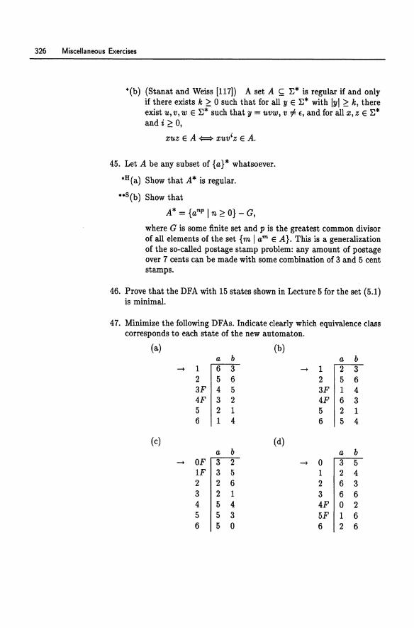
326 Miscellaneous Exercises
O(b) (Stanat and Weiss [117]) A set A ~ E* is regular if and only if there exists k ~ 0 such that for all y E E* with Iyl ~ k, there exist U,V,W E E* such that y = UVW, v =j:. €, and for all X,Z E E* and i ~ 0,
xuz E A¢::::} xuviz E A.
45. Let A be any subset of {a}* whatsoever.
oH(a) Show that A* is regular.
"S(b) Show that
A* = {anp I n ~ O} - G,
where G is some finite set and p is the greatest common divisor of all elements of the set {m I am E A}. This is a generalization of the so-called postage stamp problem: any amount of postage over 7 cents can be made with some combination of 3 and 5 cent stamps.
46. Prove that the DFA with 15 states shown in Lecture 5 for the set (5.1) is minimal.
47. Minimize the following DFAs. Indicate clearly which equivalence class corresponds to each state of the new automaton.
(a) (b) a b a b
-> 1 6 3 -> 1 2 3 2 5 6 2 5 6 3F 4 5 3F 1 4 4F 3 2 4F 6 3 5 2 1 5 2 1 6 1 4 6 5 4
(c) (d) a b a b
-> OF 3 2 -> 0 3 5 IF 3 5 1 2 4 2 2 6 2 6 3 3 2 1 3 6 6 4 5 4 4F 0 2 5 5 3 5F 1 6 6 5 0 6 2 6
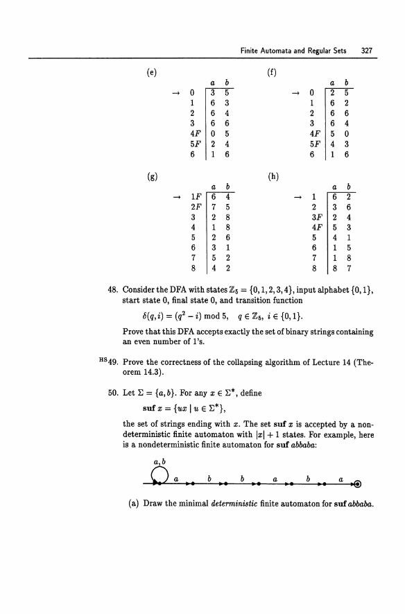
Finite Automata and Regular Sets 327
(e) (f) a b a b
-+ 0 3 5 -+ 0 2 5 1 6 3 1 6 2 2 6 4 2 6 6 3 6 6 3 6 4 4F 0 5 4F 5 0 5F 2 4 5F 4 3 6 1 6 6 1 6
(g) (h) a b a b
-+ 1F 6 4 -+ 1 6 2 2F 7 5 2 3 6 3 2 8 3F 2 4 4 1 8 4F 5 3 5 2 6 5 4 1 6 3 1 6 1 5 7 5 2 7 1 8 8 4 2 8 8 7
48. Consider the DFA with states Zs = {O, 1, 2, 3, 4}, input alphabet {O, 1}, start state 0, final state 0, and transition function
8(q,i) = (q2 - i) mod 5, q E Zs, i E {0,1}.
Prove that this DFA accepts exactly the set of binary strings containing an even number of l's.
HS49. Prove the correctness of the collapsing algorithm of Lecture 14 (Theorem 14.3).
50. Let E = {a, b}. For any x E E*, define
sufx = {ux I U E E*},
the set of strings ending with x. The set suf x is accepted by a nondeterministic finite automaton with Ixl + 1 states. For example, here is a nondeterministic finite automaton for suf abbaba:
b ... b a .. .. . b .. . (a) Draw the minimal deterministic finite automaton for suf abbaba.
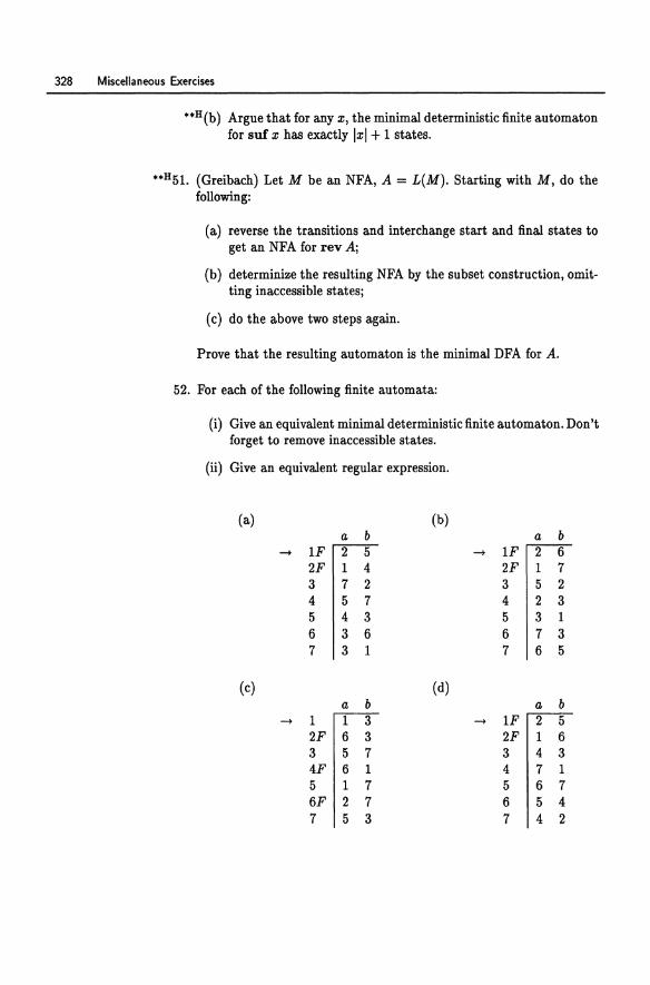
328 Miscellaneous Exercises
.. H (b) Argue that for any x, the minimal deterministic finite automaton for suf x has exactly Ixl + I states.
**H51. (Greibach) Let M be an NFA, A = L(M). Starting with M, do the following:
(a) reverse the transitions and interchange start and final states to get an NFA for rev A;
(b) determinize the resulting NFA by the subset construction, omitting inaccessible states;
(c) do the above two steps again.
Prove that the resulting automaton is the minimal DFA for A.
52. For each of the following finite automata:
(i) Give an equivalent minimal deterministic finite automaton. Don't forget to remove inaccessible states.
(ti) Give an equivalent regular expression.
(a) (b) a b a b
-+ IF 2 5 -+ IF 2 6 2F I 4 2F I 7 3 7 2 3 5 2 4 5 7 4 2 3 5 4 3 5 3 I 6 3 6 6 7 3 7 3 I 7 6 5
(c) (d) a b a b
-+ I I 3 -+ IF 2 5 2F 6 3 2F I 6 3 5 7 3 4 3 4F 6 1 4 7 1 5 I 7 5 6 7 6F 2 7 6 5 4 7 5 3 7 4 2
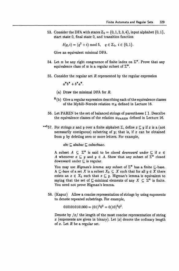
Finite Automata and Regular Sets 329
53. Consider the DFA with states 2:5 = {a, 1,2,3, 4}, input alphabet {O, I}, start state 0, final state 0, and transition function
t5(q, i) = (q2 + i) mod 5, q E 2:5, i E {O, I}.
Give an equivalent minimal DFA.
54. Let == be any right congruence of finite index on E*. Prove that any equivalence class of == is a regular subset of E* .
55. Consider the regular set R represented by the regular expression
a*b* + b*a*.
(a) Draw the minimal DFA for R.
H (b) Give a regular expression describing each of the equivalence classes of the Myhill-Nerode relation ==R defined in Lecture 16.
56. Let PAREN be the set of balanced strings of parentheses [ ]. Describe the equivalence classes of the relation ==PAREN defined in Lecture 16 .
.. s57. For strings x and y over a finite alphabet E, define x!; y if x is a (not necessarily contiguous) substring of Yi that is, if x can be obtained from Y by deleting zero or more letters. For example,
abc !; ababac !; cabacbaac.
A subset A C E* is said to be closed downward under C if x E A whenever z- !; y and yEA. Show' that any subset of £* closed downward under!; is regular.
You may use Higman's lemma: any subset of E* has a finite !;-base. A !;-base of a set X is a subset Xo ~ X such that for all y E X there exists an x E Xo such that x !; y. Higman's lemma is equivalent to saying that the set of !;-minimal elements of any X ~ E* is finite. You need not prove Higman's lemma.
58. (Kapur) Allow a concise representation of strings by using exponents to denote repeated substrings. For example,
Denote by / x/the length of the most concise representation of string x (exponents are given in binary). Let Ixl denote the ordinary length of x. Let R be a regular set.
330 Miscellaneous Exercises
·(a) Show that there exist constants c and d depending only on R such that for all x E R, there exists another string y E R such that Iyl-Ixl :5 d and /y/ :5 clog Iyl·
··(b) Answer the same question with the condition Iyl - Ixl :5 d replaced by the condition Iyl = Ixl .
... 859. Here is a generalization of nondeterminism. An alternating finite automaton (AFA) is a 5-tuple
M = (Q, ~, 0, F, 0:)
where Q is a finite set of states, ~ is a finite input alphabet, F : Q -+
{O, I} is the characteristic function of a set of final states, that is,
F( ) = {I if q is ~ final state, q ° othel"Wlse,
o is the transition function
0: (Q x~) -+ «Q -+ {O,l}) -+ {O,l}),
and 0: is the acceptance condition
0:: (Q -+ {O, I}) -+ {O, I}.
Intuitively, a computation of M generates a computation tree whose depth is the length of the input string. The function F gives a labeling of ° or 1 to the leaves of this computation tree. For all q E Q and a E ~, the Boolean function
o(q,a): (Q -+ {O,l}) -+ {O,l}
takes a Boolean labeling on states at level i and computes a new labeling at level i-I; this is used to pass Boolean labels ° or 1 back up the computation tree. The machine accepts if the labeling at level ° satisfies 0:. An NFA is just an AFA in which the Boolean functions 0:
and o(q, a) compute the Boolean "or" of some subset of the inputs.
Formally, the transition function 0 uniquely determines a map
6: (Q x ~*) -+ «Q -+ {O, I}) -+ {O, I}),
defined inductively as follows: for q E Q, a E ~, and x E ~*,
6(q,€)(u) = u(q),
6(q,ax)(u) = 0(q,a)(>.p.(6(p,x)(u))).
(Here ">.p ... " means "the function which on input p computes ... ;" see Lecture 37.) The machine is said to accept x E ~* if
0:(>.p.(6(P,x)(F))) = 1.
Finite Automata and Regular Sets 331
Prove that a set A ~ ~* is accepted by a k-state alternating finite automaton if and only if its reverse rev A is accepted by a 2k-state deterministic finite automaton.
H60. Show that minimal-state NFAs are not necessarily unique.
61. (Vardi [122]) In this exercise we show that two-way nondeterministic finite automata accept only regular sets. Let M be a 2NFA with states Q, start states S, accept state t, and transition function
t::.: Q x (~U {I-, -I}) -+ 2QX({L,R}).
Assume without loss of generality that whenever M accepts, it moves its head all the way to the right endmarker -I and enters its accept state t.
(a) Let x = aIa2· .. an E ~*, ai E~, 1:5 i:5 n. Let ao =1- and an+1 = -I. Argue that x is not accepted by M iff there exist sets Wi ~ Q, 0:5 i:5 n+ 1, such that
• S ~ Wo;
• ifu E Wi, 0:5 i:5 n, and (v,R) E t::.(u,ai), then v E Wi+1;
• ifu e Wi, 1 :5 i :5 n+1, and (v,L) e t::.(u,ai), then v E Wi-I; and
H(b) Using (a), show that "'L(M), hence L(M), is regular.
62. Prove Lemma B.S.
63. Prove that if a bisimulation between two NFAs is a one-to-one correspondence on the states, then it is an isomorphism.
64. Prove that if NFAs M and N are bisimilar, then the relation (B.1) of Supplementary Lecture B gives a bisimulation between the deterministic automata obtained from M and N by the subset construction.
65. Prove that two DFAs are bisimilar if and only if they accept the same set.
66. Prove Lemma C.1l.
67. Prove Lemma D.2.
332 Miscellaneous Exercises
68. Prove that the relation =A defined in the statement of the MyhillNerode theorem for term automata (Theorem D.3) is a congruence on the term algebra TIJ(A).
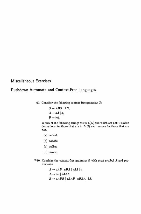
Miscellaneous Exercises
Pushdown Automata and Context-Free Languages
69. Consider the following context-free grammar G:
S --+ ABS lAB,
A --+ aA I a~ B --+ bA.
Which of the following strings are in L( G) and which are not? Provide derivations for those that are in L( G) and reasons for those that are not.
(a) aabaab
(b) aaaaba
(c) aabbaa
(d) abaaba
oH70. Consider the context-free grammar G with start symbol S and productions
S --+ aAB I aBA I bAA I E,
A --+ as I bAAA, B --+ aABB I aBAB I aBBA I bS.
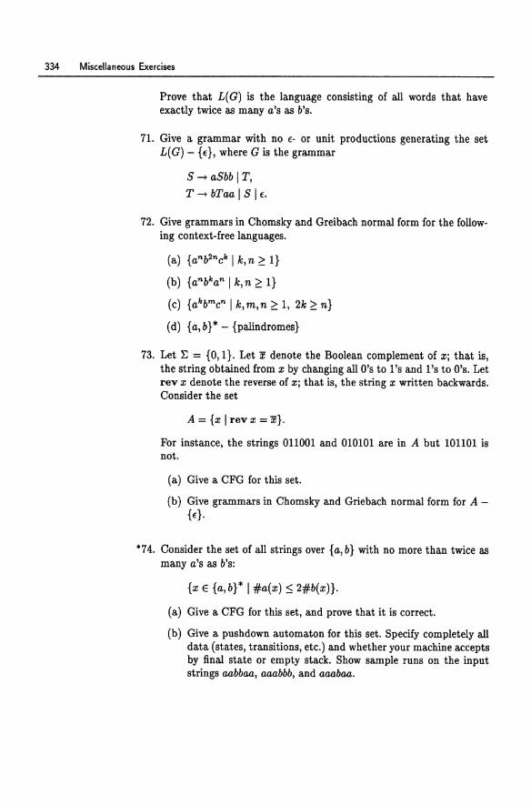
334 Miscellaneous Exercises
Prove that L( G) is the language consisting of all words that have exactly twice as many a's as b's.
71. Give a grammar with no f- or unit productions generating the set L(G) - {f}, where G is the grammar
S -+ aSbb I T,
T -+ bTaa I S I f.
72. Give grammars in Chomsky and Greibach normal form for the following context-free languages.
(a) {an b2nck I k,n ~ 1}
(b) {anbkan I k,n ~ 1}
(c) {akbmcn I k,m,n ~ 1, 2k ~ n}
( d) {a, b} * - {palindromes}
73. Let I; = {0,1}. Let x denote the Boolean complement of Xj that is, the string obtained from x by changing all O's to l's and l's to O's. Let rev x denote the reverse of Xj that is, the string x written backwards. Consider the set
A = {x I rev X =x}.
For instance, the strings 011001 and 010101 are in A but 101101 is not.
(a) Give a CFG for this set.
(b) Give grammars in Chomsky and Griebach normal form for A -{fl·
• 74. Consider the set of all strings over {a, b} with no more than twice as many a's as b's:
{x E {a,b}* I #a(x) :::; 2#b(x)}.
(a) Give a CFG for this set, and prove that it is correct.
(b) Give a pushdown automaton for this set. Specify completely all data (states, transitions, etc.) and whether your machine accepts by final state or empty stack. Show sample runs on the input strings aabbaa, aaabbb, and aaabaa.
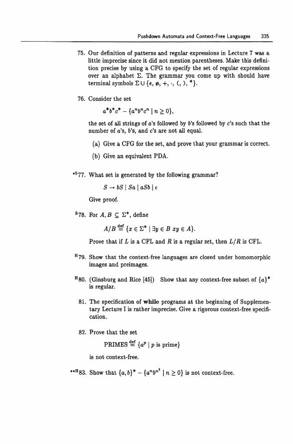
Pushdown Automata and Context-Free Languages 335
75. Our definition of patterns and regular expressions in Lecture 7 was a little imprecise since it did not mention parentheses. Make this definition precise by using a CFG to specify the set of regular expressions over an alphabet ~. The grammar you come up with should have terminal symbols ~ U {E, f), +, " (, ), *}.
76. Consider the set
a*b*c* - {anbncn I n ~ O},
the set of all strings of a's followed by b's followed by c's such that the number of a's, b's, and c's are not all equal.
(a) Give a CFG for the set, and prove that your grammar is correct.
(b) Give an equivalent PDA .
• 877. What set is generated by the following grammar?
S -+ bS I Sa I aSb I €
Give proof.
878. For A, B ~ ~*, define
AlB ~ {x E}J* 13y E B xy E A}.
Prove that if L is a CFL and R is a regular set, then LI R is CFL.
H79. Show that the context-free languages are closed under homomorphic images and preimages.
H80. (Ginsburg and Rice [45]) Show that any context-free subset of {a}* is regular.
81. The specification of while programs at the beginning of Supplementary Lecture I is rather imprecise. Give a rigorous context-free specification.
82. Prove that the set
PRIMES ~f {aP I p is prime}
is not context-free.
uH83. Show that {a,b}* - {anbn2 I n ~ O} is not context-free.
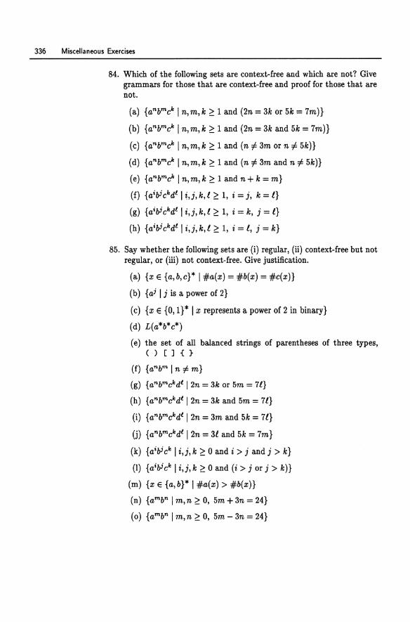
336 Miscellaneous Exercises
84. Which of the following sets are context-free and which are not? Give grammars for those that are context-free and proof for those that are not.
(a) {anbmc" I n,m,k ~ 1 and (2n = 3k or 5k = 7m)}
(b) {anbmc" I n,m,k ~ 1 and (2n = 3k and 5k = 7m)}
(c) {anbmc" In, m, k ~ 1 and (n -::f. 3m or n -::f. 5k)}
(d) {anbmc" I n,m,k ~ 1 and (n -::f. 3m and n -::f. 5k)}
(e) {anbmc"ln,m,k~landn+k=m}
(f) {a'lh"dl I i,j, k,l ~ 1, i = j, k = l}
(g) {a'bic"dll i,j,k,l ~ 1, i = k, j = l}
(h) {a'bic"dll i,j,k,l ~ 1, i = l, j = k}
85. Say whether the following sets are (i) regular, (ii) context-free but not regular, or (iii) not context-free. Give justification.
(a) {x E {a,b,c}* I #a(x) = #b(x) = #c(x)}
(b) {ai I j is a power of 2}
(c) {x E {O, I} * I x represents a power of 2 in binary}
(d) L(a*b*c*)
(e) the set of all balanced strings of parentheses of three types, ()[]{}
(f) {anbm In =fi m}
(g) {anbmc"dl 12n = 3k or 5m = 7l}
(h) {anbmc"dl 12n = 3k and 5m = 7l}
(i) {anbmc"dl 12n = 3m and 5k = 7l}
(j) {anbmc"dl I2n = 31 and 5k = 7m}
(k) {aibic" I i,j, k ~ 0 and i > j and j > k}
(1) {aibick I i,j, k ~ ° and (i > j or j > k)}
(m) {x E {a,b}* I #a(x) > #b(x)}
(n) {ambn I m,n ~ 0, 5m + 3n = 24}
(0) {ambn I m,n ~ 0, 5m - 3n = 24}
Pushdown Automata and Context-Free Languages 337
.. H86. Give a non-context-free set that satisfies the condition of the pumping lemma for CFLs given in Lecture 22; that is, such that the demon has a winning strategy.
87. Let :E be a finite alphabet. For a set A ~ :E*, define
cycle A = {yx I xy E A},
permute A = {y 13x E A Va E :E #a(x) = #a(y)}.
For example, if:E = {a,b,c} and A = {aaabe}, then
cycle A = {aaabc, aabca, abcaa, bcaaa, caaab} , permute A = {aaabe, aabca, abcaa, beaaa, eaaab,
aabae,abaea,baeaa,aeaab,eaaba, abaae,baaea,aaeab,aeaba,eabaa, baaac, aaaeb, aaeba, aebaa, ebaaa}.
Which of the following propositions are true and which are false? Give proof.
(a) For all A ~ :E*, if A is regular, then so is cycle A.
(b) For all A ~ :E*, if A is regular, then so is permute A .
.. H(C) For all A ~ :E*, if A is context-free, then so is cycleA.
(d) For all A ~ :E*, if A is context-free, then so is permute A.
88. Recall the shuflle operator II from Homework 4.
(a) Show that if L is context-free and R is regular, then L II R is context-free.
*(b) If L is a DCFL, is L II R necessarily a DCFL? Give proof.
* 89. For A, B ~ :E*, define
AlB ~ {x 13y E B xy E A}
A+- B ~f {x I Vy E B xy E A}.
Exactly one of the following two statements is true.
(a) If L is context-free, then so is LI:E*.
(b) If L is context-free, then so is L +- :E*.
Which is true? Give a proof and a counterexample.
90. Let :E = {a, b, e}. Exactly one of the following four statements is true.
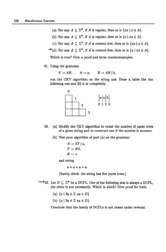
338 Miscellaneous Exercises
(a) For any A ~ ~*, if A is regular, then so is {xx I x E A}.
(b) For any A ~ ~*, if A is regular, then so is {x I xx E A}.
(c) For any A ~ ~*, if A is context-free, then so is {xx I x E A} .
• H(d) For any A ~ ~*, if A is context-free, then so is {x I xx E A}.
Which is true? Give a proof and three counterexamples.
91. Using the grammar
S -+ AB, A -+ a, B -+ AB I b,
run the CKY algorithm on the string aab. Draw a table like the following one and fill it in completely.
o
92. (a) Modify the CKY algorithm to count the number of parse trees of a given string and to construct one if the number is nonzero.
(b) Test your algorithm of part (a) on the grammar
S -+ ST I a, T-+ BS,
B-++
and string
a+a+a+a.
(Sanity check: the string has five parse trees.)
... 893. Let D ~ ~* be a DCFL. One of the following sets is always a DCFL, the other is not necessarily. Which is which? Give proof for both.
(a) {x 13a E ~ xa E D}
(b) {x 13a E ~ ax E D}
Conclude that the family of DCFLs is not closed under reversal.
Pushdown Automata and Context-Free Languages 339
94. Let I: be a fixed finite signature as described in Supplementary Lecture C. Give an unambiguous context-free grammar for the set of ground terms over I:. Unambiguous means that there is exactly one parse tree for each ground term. Prove that your grammar is correct and that it is unambiguous.
··95. The context-free language {anbn In;:: O} is the unique ~ -minimal solution of the equation
X=aXb+f.
In general, let I: be a finite alphabet. Consider finite systems of equations of the form
where the Xi are variables ranging over subsets of I:* and the Ei are regular expressions over Xl, ... ,Xn and I:.
(a) Argue that any such system has a unique minimal solution
You may want to use the Knaster-Tarski theorem: any monotone map on a complete partial order has a unique least fixpoint. A map 1 on a partially ordered set is monotone if x :5 Y -+ I(x) :5 I(Y). A partially ordered set is complete if every subset of that set has a least upper bound.
(b) For the Xl, ... ,Xn of part (a), show that Xl is a context-free language.
(c) Show that all context-free languages arise in this way.
Miscellaneous Exercises
Turing Machines and Effective Computability
96. Give a Turing machine with input alphabet {a} that on input am halts with am' written on its tape. Describe the operation of the machine both informally and formally. Be sure to specify all data.
97. The Euclidean algorithm com pu tes the greatest common divisor (GCD) of two nonnegative integers:
procedure gcd(m,n): if n = 0 then return(m)
else return(gcd(n,m mod n»
Give a Turing machine with input alphabet {a, #} that on input am#an halts with agcd(m,n) written on its tape. Describe the operation of the machine both informally and formally. Be sure to specify all data.
98. Prove that the class of r.e. sets is closed under union and intersection.
99. A queue machine is like a Turing machine, except that it has a queue instead of a tape. It has a finite queue alphabet r and a finite input alphabet I: ~ r. If x E I:* is the input, the machine starts in its start state s with x$ in the queue, where $ is a special symbol in r - I:. In each step, it removes a symbol from the front of the queue. Based on
Turing Machines and Effective Computability 341
that symbol and the current state, it pushes a string Z E r* onto the back of the queue and enters a new state according to the transition function o. It accepts by emptying its queue.
S(a) Give a rigorous formal definition of these machines, including a definition of configurations and acceptance. Your definition should begin as follows: "A queue machine is a sextuple
M = (Q, E, r, $, D, s),
where ... "
.. oHS(b) Prove that queue machines and Turing machines are equivalent in power.
100. A one-counter automaton is an automaton with a finite set of states Q, a two-way read-only input head, and a separate counter that can hold any nonnegative integer. The input x E E* is enclosed in endmarkers 1-, -1 f/. E, and the input head may not go outside the end markers. The machine starts in its start state s with its counter empty and with its input head pointing to the left endmarker 1-. In each step, it can test its counter for zero. Based on this information, its current state, and the symbol its input head is currently reading, it can either add one to its counter or subtract one, move its input head either left or right, and enter a new state. It accepts by entering a distinguished final state t.
(a) Give a rigorous formal definition of these machines, including a definition of acceptance. Your definition should begin as follows: "A one-counter automaton is a septuple
M = (Q, E, 1-, -1, s, t, D),
where ... "
O(b) Prove that the membership problem for deterministic one-counter automata is decidable: given M and x, does M accept x?
H(c) Prove that the emptiness problem is undecidable: given a onecounter automaton M, is L(M) = 0?
101. A ray automaton consists of an infinite number of deterministic finite automata Ao, AI, A 2 , ••• arranged in a line. The automata all have the same set of states Q, the same start state s, and the same transition function 0 except Ao, which has a different transition function Do since it has no left neighbor. They all start simultaneously in their initial state s and execute synchronously. In each step, each Ai moves to a new state, depending on its own current state and the current states of its
342 Miscellaneous Exercises
immediate left and right neighbors, according to its transition function. The ray automaton is said to halt if Ao ever enters a distinguished final state t. There is no input alphabet.
(a) Give a rigorous formal definition of ray automata, including a definition of execution and halting. Your definition should begin as follows: "A my automaton is a quintuple
A = (Q, s, t, 00, 0),
where Q is a finite set of states, ... "
(b) Prove that the halting problem for ray automata is undecidable.
(c) Is the halting problem for ray automata semidecidable? Why or why not?
102. A deterministic two-dimensional Thring machine is like a Turing machine except that instead of a one-dimensional tape it has a twodimensional tape that is like a chessboard, infinite in all directions. It has a finite input alphabet E and a finite tape alphabet r containing E as a subset. If x E E* is the input, ixi = n, the machine starts in its start state s with x written in tape cells (0, 1), (0, 2), ... , (0, n), the origin (0,0) containing a special symbol 0 E r - E, and all other cells (i,j) containing a special blank symbol u E r - E. It has a read/write head initially pointing to the origin. In each step, it reads the symbol of r currently occupying the cell it is scanning. Depending on that symbol and the current state of the finite control, it writes a symbol of r on that cell, moves one cell either north, south, east, or west, and enters a new state, according to its transition function 0.1t accepts its input by erasing the entire board; that is, filling all cells with u.
H(a) Give a rigorous formal definition of these machines, including a definition of configurations, the next configuration relation, and acceptance. Try to be as precise as possible. Your definition should begin as follows: "A two-dimensional Thring machine is a 7-tuple
M = (Q, E, r, u, 0, s, 0),
where Q is a finite set of states, ... "
(b) Argue that two-dimensional Turing machines and ordinary Turing machines are equivalent in the sense that each can simulate the other. Describe the simulations informally (Le., no transitions) but in sufficient detail that transitions implementing your description could readily be written down.
Turing Machines and Effective Computability 343
103. A nondeterministic Turing machine is one with a multiple-valued transition relation. Give a formal definition of these machines. Argue that every nondeterministic TM can be simulated by a deterministic TM.
104. Show that the type 0 grammars (see Lecture 36) generate exactly the r.e. sets.
105. For A, B ~ ~*, define
AlB ~f {x E}J* 13y E B xy E A}.
(a) Show that if A and Bare r.e., then so is AlB.
OH(b) Show that every r.e. set can be represented as AlB with A and B CFLs.
106. Is it decidable, given M #y, whether the Turing machine M ever writes a nonblank symbol on its tape on input y? Why or why not?
107. Is it decidable for TMs M whether L(M) = rev L(M)? Give proof.
108. Tell whether the following problems are decidable or undecidable. Give proof.
(a) Given a TM M and a string y, does M ever write the symbol # on its tape on input y?
(b) Given a CFG G, does G generate all strings except €?
(c) Given an LBA M, does M accept a string of even length?
(d) Given a TM M, are there infinitely many TMs equivalent to M?
109. Tell whether or not the following sets are r.e. Give proof.
(a) {(M,N) I M takes fewer steps than N on input €}
(b) {M I M takes fewer than 481481 steps on some input}
(c) {M I M takes fewer than 481481 steps on at least 481481
different inputs}
(d) {M I M takes fewer than 481481 steps on all inputs}
110. Show that the set {M I M accepts at least 481 strings} is r.e. but not co-r.e.
344 Miscellaneous Exercises
111. One of the following sets is r.e. and the other is not. Which is which? Give proof for both.
(a) {M I L(M) contains at least 481 elements}
(b) {M I L(M) contains at most 481 elements}
112. Show that the set
{M I M halts on all inputs of length less than 481}
is r.e., but its complement is not.
s 113. Let M range over Turing machine descriptions. Show that neither the set
REG ~ {M I L(M) is a regular set}
nor its complement is recursively enumerable.
114. Let IMI denote the length of the description of the Turing machine M. Are the following problems decidable? Give proof.
(a) Does a given Turing machine M take at least IMI steps on some input?
(b) ... on all inputs?
115. Tell whether the following problems are decidable or undecidable, and give proof:
(a) whether a given TM runs for at least 481481 steps on input a481 ;
(b) whether a given TM ever reenters its start state on any input;
*(c) whether a given Turing machine will ever move its head left more than ten times on input a481 ;
*(d) whether a given Turing machine will ever print more than 481 nonblank symbols on input a481 •
116. Think for two minutes about why the following problems are undecidable, but don't write anything down:
(a) whether two given C++ programs compute the same function;
(b) whether a given C++ program will ever get into an infinite loop on some input;
Turing Machines and Effective Computability 345
(c) whether a given Jt-recursive function is totalj
(d) whether a given 'x-term reduces to normal form.
117. Show that the following problems of pairs of Turing machines are undecidable:
(a) whether L(M) = L(N)j
(b) whether L(M) ~ L(N)j
(c) whether L(M) n L(N) = 0'j
(d) whether L(M) n L(N) is a recursive setj
(e) whether L(M) n L(N) is finite.
··118. Formalize and prove the following extension of Rice's theorem that has the results of Exercise 117 as special cases: every nontrivial property of pairs of r.e. sets is undecidable.
119. Let G and G' denote context-free grammars over {a,b}. Prove that the following problems are undecidable:
H(a) whether L(G) = L(G')j
(b) whether L(G) ~ L(G')j
·(c) whether L(G) = L(G)L(G).
120. One of the following problems is decidable and the other is not. Which is which? Give proof for both.
(a) Given a CFL L and a regular set R, is L ~ R?
(b) Given a CFL L and a regular set R, is R ~ L?
H121. Prove that the following problems are undecidable:
(a) whether a given CFL is a DCFLj
(b) whether the intersection of two given CFLs is a CFLj
(c) whether the complement of a given CFL is a CFLj
··(d) whether the union of two given DCFLs is a DCFL.
122. Prove that it is undecidable whether a given LBA halts on all inputs.
346 Miscellaneous Exercises
H123. Show that the finiteness problem for Turing machines reduces to the finiteness problem for LBAs.
124. Prove that it is undecidable whether a given LBA accepts a regular set.
125. Consider the following context-sensitive productions.
S -+ bSb,
S ...... AcA,
Ab -+ A,
Ab -+ b,
bA -+ b,
bA -+ A.
Let G be the grammar given by all the rules except for the last, and let Gt the grammar given by all the rules including the last. One of L( G) and L( Gt ) is regular, and the other is context-free but not regular. Which is which, and why?
126. Give a set over a single letter alphabet in each of the following classes, or explain why such a set does not exist:
(a) regular;
(b) DCFL but not regular;
(c) CFL but not DCFL;
(d) recursive but not CFL;
(e) r.e. but not recursive;
(f) not r.e.
127. Prove that every infinite regular set contains a non-r.e. subset.
*H128. Prove that every infinite r.e. set contains an infinite recursive subset.
*129. In this exercise we will prove a kind of fixpoint theorem for Turing machines known as the recursion theorem.
If M is a TM, let M(x) denote the contents of M's tape at the point that M halts on input x, provided M does indeed halt on input x. If M does not halt on input x, then M(x) is undefined.
Turing Machines and Effective Computability 347
A partial function u : E* -+ E* is said to be a computable function if u(x) = M(x) for some Turing machine M. In addition, u is a total computable function if M is total.
Let M., be the TM whose encoding over E* is x.
Theorem (Recursion theorem) Let u : E* -+ E* be any total computable function. Then there exists a string u such that
L(Mu) = L(Mu(u)).
(a) Let u : E* -+ E* be a given total computable function, say computable by a total TM K. Let N be a TM that on input x computes a description of a machine that does the following on input y:
• constructs M.,j
• runs M., on input Xj
• if it halts, runs K on M.,(x)j
• interprets the result of that computation, K(M,,(x)), as the description of a TM, and simulates that TM on the original input y, accepting or rejecting as that machine accepts or rejects, respectively.
Argue that N is total and that
L(MN (,,)) = L(Mu(Mz(zn)'
(b) Let v be a description of the machine Nj that is, N = Mv. Argue that N(v) is the desired fixpoint of u.
H130. Give a short proof of Rice's theorem using the recursion theorem (see Miscellaneous Exercise 129).
uH 131. A TM is minimal if it has the fewest states among all TMs that accept the same set. Prove that there does not exist an infinite r.e. set of minimal TMs.
132. H(a) Show that there does not exist an r.e. list of Turing machines such that every machine on the list is total (Le., halts on all inputs) and every recursive set is represented by some machine on the list .
.. H(b) Show that there exists an r.e. list of Turing machines such that every machine on the list accepts a recursive set and every recursive set is represented by some machine on the list.
348 Miscellaneous Exercises
··133. In addition to the usual constructs of while programs (simple assignment, conditional, while loop, sequential composition), add a print statement
print x and halt
that prints the current value of a variable and halts. Call two programs equivalent if for all initial values of the variables, one program halts iff the other does, and whenever they both halt, they print the same value.
One of the following problems is decidable and the other is undecidable. Which is which? Justify your answers.
(a) Given a program, does there exist an equivalent program with at most one while loop?
(b) Given a program, does there exist an equivalent program with no while loops?
134. This question is for those who know something about propositional logic. A propositional Horn clause is a disjunction of literals with at most one positive literal. The clause
-,Pl V -,P2 V··· V -'Pn V Q
is often written as
P1 A P2 A .•. A Pn ~ Q,
and the clause
can be written as
Pl A P2 A ... A Pn -+ .1,
where .1 denotes falsity. Any single positive literal Q is also a Horn clause.
(a) Show that the emptiness problem for context-free languages (i.e., given a context-free grammar G, deciding whether L(G) = 0) reduces to the satisfiability problem for finite conjunctions of Horn clauses, and vice versa.
(b) Since the satisfiability of propositional formulas is decidable, what can we conclude about the decidability of the emptiness problem for CFLs?
Turing Machines and Effective Computability 349
B135. Show that the finiteness problem for regular sets and context-free languages (Le., whether a given machine/grammar accepts/generates a finite set) is decidable.
136. Show that FIN :5T REG. In other words, suppose you are given an oracle that will always answer questions ofthe form "Is L(M) a regular set?" truthfully. Show how to use such an oracle to decide questions of the form "Is L(M) finite?"
**137. Prove Theorem J.1.
*B138. Let HPI ~ HP, and let HPn+1 be the halting problem for oracle Turing machines with oracle HPn , n ;:: Ii that is,
HP n+1 ~ {M #x I M is an oracle TM with oracle HP n,
M halts on input x}.
The oracle need not be represented in the description of the oracle machine M. Show that HPn E ~~ - II~.
139. Show that the integer square root function is primitive recursive. On input n, the function should return the greatest integer less than or equal to the square root of n.
B140. A language B is said to be computable in linear time if there exists a deterministic Turing machine M and a constant c > 0 such that L(M) = Band M always halts within en steps on inputs of length n. Show that there exists a recursive set that is not computable in linear time.
141. Show that the Turing reducibility relation :5T is reflexive and transitive and that :5m refines :5T.
142. Prove that the following sets are :5m-complete for the given classes:
(a) EMPTY is :5m-complete for II~i
*(b) TOTAL is :5m-complete for IIgi
U(c) COF is :5m-complete for ~~i
**(d) the set
REG ~f {M I L(M) is a regular set}
is :5m-complete for ~~.
350 Miscellaneous Exercises
*H143. Prove that there exists a total computable function f : N -+ N that is not provably total in Peano arithmetic.
Hints for Selected Miscellaneous Exercises
6. Look for a clue in Lecture 5.
9. (b) Build an NFA with seven states arranged in loops of length two and five. Assign start and final states so that the shortest rejected string is of length 9 = 2 . 5 - 1.
(c) The product of a set of distinct primes is exponential in their sum.
26. Given a DFA M for A, build an NFA M' for FirstHalvesA that implements the following idea: put a white pebble on the start state of M and green and blue pebbles on an arbitrary guessed state of M. Never move the green pebble. Move the white pebble forward in response to input symbols and move the blue pebble forward according to some nondeterministically guessed input symbol. Accept if the white and green pebbles occupy the same state and the blue pebble occupies an accept state when the input string is exhausted. Describe M' formally and prove that it accepts the set FirstHalves A. Presumably the set of states of M' will be the set Q x Q x Q encoding the positions of the three pebbles.
In general, you will see several problems of the form
show that if A is a regular set, then so is A',
352 Hints for Selected Miscellaneous Exercises
where A' is some set formed by massaging A in some way. Exercise 2 of Homework 2 about rev A and Exercise 3 of Homework 3 about MiddleThirds A are of this type. Most of these problems can be solved by applying the following five-step protocol:
Step 1 Assume we are given a deterministic finite automaton
M = (Q, ~, 0, s, F)
accepting A. We want to build a nondeterministic automaton
M' - (Q' ~ tl' 8' F') - " , , accepting A'. Come up with an intuitive design of M' in terms of moving pebbles around on the states of M. Think about the initial configuration of pebbles, how the pebbles should move in response to each input symbol, and what the accepting configurations should be.
Step 2 Write down a formal description of Q', ~, tl', 8', and pi that formally captures your intuition about moving the pebbles developed in step 1. The first thing to think about is what the states Q' should be. You need to figure out how to encode formally the information that the new machine needs to remember at each step. Make sure the types are right; for example, whatever you decide the set of states Q' should be, the start state should be an element of Q' and the set of accept states pi should be a subset of Q'. If you are designing a deterministic machine M', then 0' should be a function Q' x ~ -t Q'. If M' is to be nondeterministic, then you should have tl' : Q' x ~ -t 2Q'.
Step 3 In step 2, you defined a transition function /).' of M'. Most likely, /).' was defined in terms of the transition function 8 of M. State a lemma extending this relationship to a relationship between '8 and ii'.
Step 4 Prove the lemma stated in step 3 by induction on Ixl. The proof will most likely use the standard inductive definitions of '8 and ~', as well as the definition you gave in step 2 of tl' in terms of o.
Step 5 Prove that L( M') = A'. The proof will generally use the lemma proved in step 4 and the definitions of 8' and pi.
Step 1 is usually not much of a problem, since it is usually easy to see how to move the pebbles. Steps 2 and 3 typically give the most trouble. If the lemma in step 3 is formulated correctly, the proofs in 4 and 5 should be fairly routine.
An example of an application of this protocol is given in the solution to this exercise on p. 358.
31. One of the sets is {a,b}*.
Hints for Selected Miscellaneous Exercises 353
32. Use the matrix representation of Miscellaneous Exercise 7.
33. Use the fact that
d (")
p(n+l)= EP·.~n), i=O Z.
where p(i) denotes the ith derivative of p.
43. Try
U (a+ct(b+ct + (a + b + c)*cc(a + b+ c)* n;::O
with k = 3.
45. (a) By Theorem 12.3, it suffices to show that A* is ultimately periodic. You can take as period the length of the smallest nonnull element of A. This is not necessarily the smallest period, but it will do.
49. For the direction (=», use induction on the stages of the algorithm. For the direction (-¢=), use induction on Ixl.
50. (b) Consider the relation
y == z ~ overlap(y,x) = overlap(z,x),
where overlap(y, x) is the longest string that is both a suffix of y and a prefix of x. Use the Myhill-Nerode theorem.
51. Suppose that you start with a DFA for B with no inaccessible states, reverse the transitions and exchange the start and final states to get an NFA for rev B, then construct an equivalent DFA using the subset construction, omitting inaccessible states. Prove that the resulting automaton is the minimal DFA for rev B.
55. (b) Two of them are e and aa*.
60. aa* == a*a.
61. (b) Build an NFA whose states are subsets of Q. Let the machine guess the sets Wi.
354 Hints for Selected Miscellaneous Exercises
70. Prove inductively that
S ....!.... x<==> #a(x) = 2#b(x), G
A....!.... x<==> #a(x) = 2#b(x) + 1, G
B....!.... x<==> #a(x) = 2#b(x) - 2. G
Think about the graph of the function #a(y) - 2#b(y) for prefixes y of x.
79. Everything you need can be found in Lecture 10.
80. Use Parikh's theorem (Theorem H.1) and the theorem on ultimate periodicity (Theorem 12.3).
83. Use Parikh's theorem (Theorem H.1) and the fact that the complement of a semilinear subset of Nk is semilinear.
86. Show that the condition (P) of the pumping lemma for regular sets given in Lecture 11 implies the condition of the pumping lemma for context-free languages given in Lecture 22. Give a non-context-free set satisfying (P). A slightly modified version of the hint for Miscellaneous Exercise 43 should do.
87. (c) Build a PDA that pushes and pops antimatter.
90. (d) Consider the set
A = {anbncmambkck I n,m,k;::: 1}.
93. (a) Let
M = (Q, E, r, 6, J., -I, 8, .0)
be a DPDA for D that accepts by empty stack. Prove that for p, q E Q and a E E,
hE r* I (p,a,,},) -if (q,e,e)}
is a regular set.
(b) See the end of Lecture 27.
99. (b) Simulating a queue machine with a Turing machine is easy. The other direction is tricky. Make the queue of the queue machine contain a representation of the configuration of the Turing ma-
Hints for Selected Miscellaneous Exercises 355
chine. The hard part is simulating a left move of the Turing machine. You need to go all the way around the queue.
You might try breaking your solution into two steps:
(i) First invent a new kind of Turing machine, a one-way Turing machine. These machines can only move right on the tape. When they see the right endmarker, they magically jump back to the left endmarker. Show that one-way machines can simulate ordinary TMs. Simulate a left move of the ordinary TM by pushing a marker all the way around to the right.
(ii) Simulate one-way machines with queue machines.
100. (c) Think VALCOMPS.
102. (a) The infinite checkerboard should be Z x Z, where Z is the set of integers { ... , -2, -1,0, 1, 2,3, ... }. Tape contents should be modeled by functions J : Z x Z ~ r, which assign a tape symbol in r to each cell (i,j) E Z x Z.
105. (b) Think VALCOMPS.
119. (a) Take G to be S ~ as I bS I f.
121. Think VALCOMPS.
123. Think VALCOMPS.
128. Use Exercise 4 of Homework 9.
130. Let P be a nontrivial property of the r.e. sets. Then there exist TMs MT and MJ. such that P(L(MT)) = T and P(L(MJ.)) = 1.. Show that if it were decidable for TMs M whether P(L(M)) = T, then we could construct a total computable map (j with no fixpoint, contradicting the recursion theorem (see Miscellaneous Exercise 129).
131. Use the recursion theorem (see Miscellaneous Exercise 129).
132. (a) Diagonalize.
(b) Let::::; be an arbitrary computable linear order on the set of input strings. Given M, let M' be a machine that on input x simulates M on all y::::; x.
356 Hints for Selected Miscellaneous Exercises
135. Use the pumping lemma.
138. Diagonalize.
140. Construct a list of total Turing machines that run in linear time such that every set computable in linear time is accepted by some machine on the list. Build a machine that diagonalizes over this list.
143. Diagonalize.
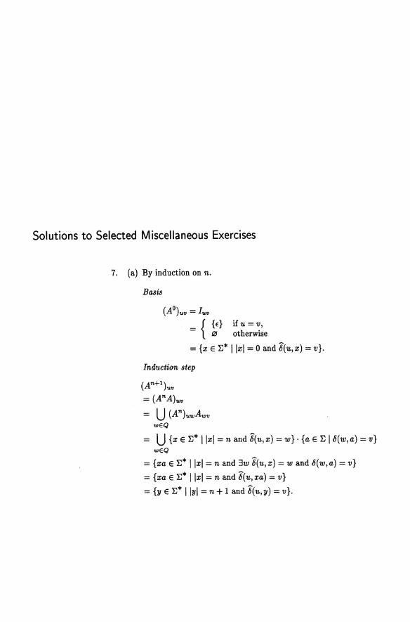
Solutions to Selected Miscellaneous Exercises
7. (a) By induction on n.
Basis
if u = v, otherwise
* ~ = {x E 1: Ilxl = 0 and 6(u,x) = v}.
Induction step
(An+l)uv
= (AnA)uv
= U (An)uwAwv wEQ
U * ~ = {XE1: Ilxl=nand6(u,x)=w}·{aEI:16(w,a)=v} wEQ
* ~ = {xa E 1: Ilxl = nand 3w 6(u,x) = wand 6(w,a) = v}
= {xa E 1:* Ilxl = nand 8(u,xa) = v}
= {y E 1:* Ilyl = n + 1 and 8( u, y) = v}.
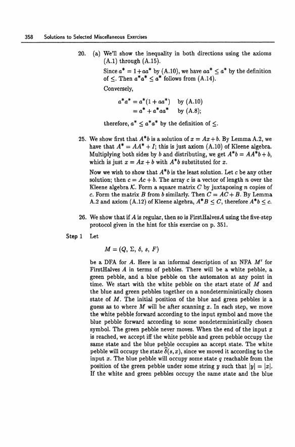
358 Solutions to Selected Miscellaneous Exercises
20. (a) We'll show the inequality in both directions using the axioms (A.l) through (A.l5).
Since a* = l+aa* by (A.lO), we have 00* :5 a* by the definition of :5. Then a*a* :5 a* follows from (A.l4).
Conversely,
a*a* = a*(l + oo*} by (A.lO)
= a* + a* aa* by (A.B);
therefore, a* :5 a*a* by the definition of :5.
25. We show first that A *b is a solution of x = Ax + b. By Lemma A.2, we have that A* = AA* + I; this is just axiom (A.lO) of Kleene algebra. Multiplying both sides by b and distributing, we get A*b = AA*b+ b, which is just x = Ax + b with A*b substituted for x.
Now we wish to show that A*b is the least solution. Let c be any other solution; then c = Ac + b. The array c is a vector of length n over the Kleene algebra /C. Form a square matrix C by juxtaposing n copies of c. Form the matrix B from b similarly. Then C = AC + B. By Lemma A.2 and axiom (A.12) of Kleene algebra, A* B :5 C, therefore A*b:5 c.
26. We show that if A is regular, then so is FirstHalvesA using the five-step protocol given in the hint for this exercise on p. 351.
Step 1 Let
M = (Q, ~, 0, s, F)
be a DFA for A. Here is an informal description of an NFA M' for FirstHalves A in terms of pebbles. There will be a white pebble, a green pebble, and a blue pebble on the automaton at any point in time. We start with the white pebble on the start state of M and the blue and green pebbles together on a nondeterministically chosen state of M. The initial position of the blue and green pebbles is a guess as to where M will be after scanning x. In each step, we move the white pebble forward according to the input symbol and move the blue pebble forward according to some nondeterministically chosen symbol. The green pebble never moves. When the end of the input x is reached, we accept iff the white pebble and green pebble occupy the same state and the blue pebble occupies an accept state. The white pebble will occupy the state c5( s, x), since we moved it according to the input x. The blue pebble will occupy some state q reachable from the position of the green pebble under some string y such that Iyl = Ixl. H the white and green pebbles occupy the same state and the blue
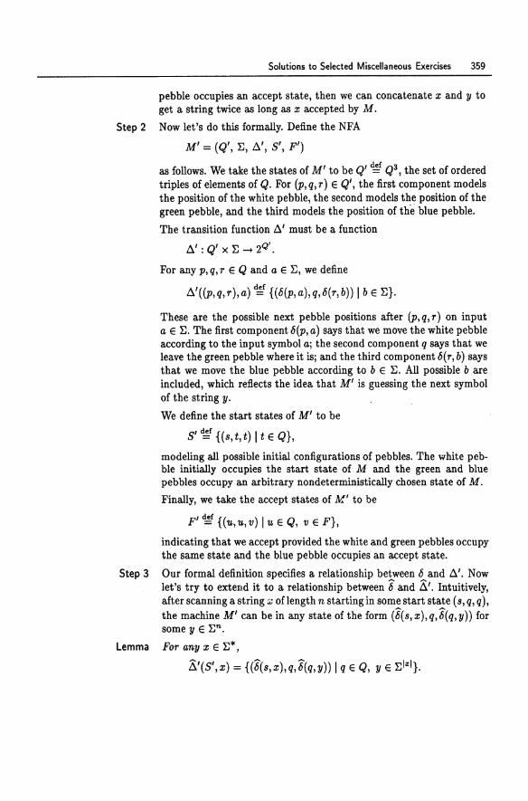
Solutions to Selected Miscellaneous Exercises 359
pebble occupies an accept state, then we can concatenate x and y to get a string twice as long as x accepted by M.
Step 2 Now let's do this formally. Define the NFA
M' = (Q', ~, !:J.', S', F')
as follows. We take the states of M' to be Q' ~f Q3, the set of ordered triples of elements of Q. For (p, q, r) E Q', the first component models the position of the white pebble, the second models the position of the green pebble, and the third models the position of th"e blue pebble.
The transition function !:J.' must be a function
!:J.':Q'x~->2Q'.
For any p,q,r E Q and a E ~, we define
!:J.'((p,q,r),a) ~ {(8(p,a),q,8(r, b)) I b E ~}.
These are the possible next pebble positions after (p, q, r) on input a E ~. The first component 8(p,a) says that we move the white pebble according to the input symbol aj the second component q says that we leave the green pebble where it iSj and the third component 8(r, b) says that we move the blue pebble according to b E ~. All possible bare included, which reflects the idea that M' is guessing the next symbol of the string y.
We define the start states of M' to be
S' ~f {(s,t,t) It E Q},
modeling all possible initial configurations of pebbles. The white pebble initially occupies the start state of M and the green and blue pebbles occupy an arbitrary nondeterministically chosen state of M.
Finally, we take the accept states of At' to be
F' ~ {(u,u,v) I'll. E Q, v E F},
indicating that we accept provided the white and green pebbles occupy the same state and the blue pebble occupies an accept state.
Step 3 Our formal definition specifies a relationship between 8 and !:J.'. Now let's try to extend it to a relationship between 8 and Li'. Intuitively, after scanning a string:;; oflength n starting in some start state (s, q, q), the machine M' can be in any state ofthe form (8(s,x),q,8(q,y)) for some y E ~n.
Lemma For any x E ~*,
Li'(s',x) = {(8(s,x),q,8(q,y)) I q E Q, y E ~I"'I}.
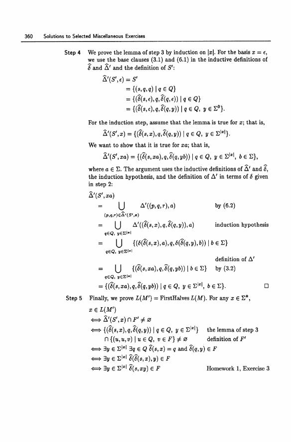
360 Solutions to Selected Miscellaneous Exercises
Step 4 We prove the lemma of step 3 by induction on Ixl. For the basis x = e, we use the base clauses (3.1) and (6.1) in the inductive definitions of 6 and Li' and the definition of 8':
Li'(8', e) = 8'
= {(s,q,q) I q E Q}
= {(6(s,e),q,6(q,e)) I q E Q}
= {(6(s,e),q,6(q,y)) I q E Q, y E ~O}.
For the induction step, assume that the lemma is true for Xj that is, ~, I ~ ~ II /1 (8 ,x) = {(6(s,x),q,6(q,y)) I q E Q, y E ~ z}.
We want to show that it is true for xaj that is, ~, , ~ ~ II /1 (8 ,xa) = {(6(s,xa),q,6(q,yb)) I q E Q, y E ~" , b E ~},
where a E ~. The argument uses the inductive definitions of Li' and 6, the induction hypothesis, and the definition of /1' in terms of 6 given in step 2:
Li'(8',xa)
= u /1'((p,q,r),a) by (6.2) (p,q,r)E;;;'(S' ,z)
U /1' ((6(s, x), q, 6(q, y)), a) induction hypothesis qEQ, lIEElzl
U {(6(6(s,x),a),q,6(6(q,y), b)) I b E~} qEQ, lIEE1-1
definition of /1'
= U {(6(s,xa),q,6(q,yb)) I b E~} by (3.2) qEQ, lIEEI-1
~ ~ II = {(6(s,xa),q,6(q,yb)) I q E Q, y E ~" , b E ~}.
Step 5 Finally, we prove L(M') = FirstHalves L(M). For any x E ~*,
x E L(M')
{:::::> Li'(8', x) n F' =I 0
{:::::> {(6(s,x),q,6(q,y)) I q E Q, y E ~I"I} the lemma of step 3
n {(u,u,v) I u E Q, v E F} =I 0 definition of F'
{:::::> 3y E ~I"I 3q E Q 6(s, x) = q and 6(q,y) E F
{:::::> 3y E ~I"'I 6(6(s,x),y) E F
o
{:::::> 3y E ~I"'I 6(s,xy) E F Homework 1, Exercise 3
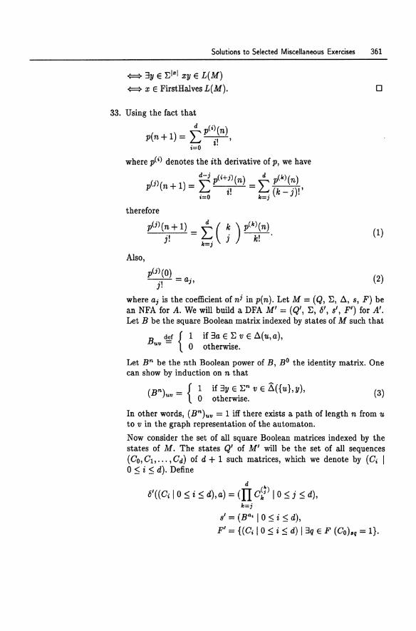
Solutions to Selected Miscellaneous Exercises 361
{:::::} 3y E Ei"'l xy E L(M)
{:::::} X E FirstHalves L(M).
33. Using the fact that
d pC;)(n) p(n+1)= 2:-,,-,
;=0 z.
where pCi) denotes the ith derivative of p, we have
(j) _ ~ pC;+j)(n) _ ~ pCk)(n) p (n + 1) - L...J i! - L....-. (k _ ')!'
;=0 k=) J
therefore
Also,
p(j)(n + 1) = ~ ( k ) pCk)(n) " L...J' k" J. k' J .
=)
pUleO) -.-,-=aj,
J.
o
(1)
(2)
where aj is the coefficient of n j in pen). Let M = (Q, E, ~, s, P) be an NFA for A. We will build a DFA M' = (Q', E, fl, s', P') for A'. Let B be the square Boolean matrix indexed by states of M such that
B ~ {1 if 3a E EvE ~(u,a), uv - 0 otherwise.
Let B n be the nth Boolean power of B, BO the identity matrix. One can show by induction on n that
(B n )",,= {1 if3YE.En V ELi({u},y), (3) o otherwIse.
In other words, (B n )"" = 1 iff there exists a path of length n from u to v in the graph representation of the automaton.
Now consider the set of all square Boolean matrices indexed by the states of M. The states Q' of M' will be the set of all sequences (CO,C1,00. ,Cd) of d + 1 such matrices, which we denote by (C; I 0::; i ::; d). Define
d k
8'((C; I 0 ::; i ::; d),a) = (II d j ) 10::; j ::; d), k=j
s' = (BB' I 0 ::; i ::; d), P' = {( Ci I 0 ::; i ::; d) I 3q E P (Co) sq = 1}.
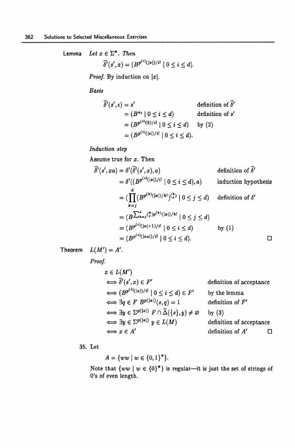
362 Solutions to Selected Miscellaneous Exercises
Lemma Let x e E*. Then
6\s',x) = (Bp(i)CI"I)/i! 10::::; i ::::; d).
Proof. By induction on Ixl.
Basis
6' (s', f) = s' definition of 6' = (B a• I 0 ::::; i ::::; d) definition of s'
= (W(')CO)/i! I 0 ::::; i ::::; d) by (2)
= (BP(')CIEI)/i! I 0 ::::; i ::::; d).
Induction step
Assume true for x. Then
6'(s',xa) = 6'(6'(s',x),a) definition of 6' = 6'«BP(')CI"i)/i! 10::::; i ::::; d),a) induction hypothesis
d
= (11 (BP(·)CI"i)/k!)C7) 10::::; j ::::; d) definition of 6' k=j
= (BL::=;C;)p(·)(I"I)/k! I 0 ::::; j ::::; d)
= (BP(')(I"I+l)/i! I 0 ::::; i ::::; d) by (1)
= (W(')(I"al)/i! I 0 ::::; i ::::; d). o Theorem L(M') = A'.
Proof.
x e L(M')
-¢::=::? 6' ( s' , x) E P'
-¢::=::? (W(')CI"I)/i! I 0 ::::; i ::::; d) e P'
-¢::=::? 3q e P WC1:z:1)(s,q) = 1
-¢::=::?3yeEP(I"I) pn~({S},Y):f0 -¢::=::? 3y E EP(I:z:1) y E L(M)
-¢::=::?xE A'
35. Let
A = {ww I w E {0,1}*}.
definition of acceptance
by the lemma
definition of P'
by (3) definition of acceptance
definition of A' 0
Note that {ww I w E {O} *} is regular-it is just the set of strings of O's of even length.
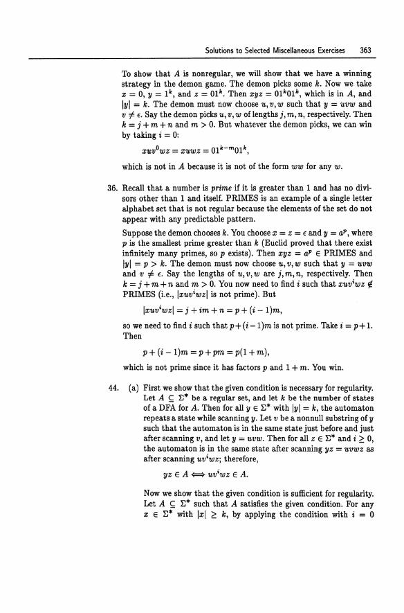
Solutions to Selected Miscellaneous Exercises 363
To show that A is nonregular, we will show that we have a winning strategy in the demon game. The demon picks some k. Now we take x = 0, y = 1", and z = 01". Then xyz = 01"'01", which is in A, and Iyl = k. The demon must now choose u,v,w such that y = uvw and v ::f:. f. Say the demon picks u, v,w of lengths i, m, n, respectively. Then k = i + m + n and m > O. But whatever the demon picks, we can win by taking i = 0:
xuvowz = xuwz = 01 k-m 01 Ie,
which is not in A because it is not of the form ww for any w.
36. Recall that a number is prime if it is greater than 1 and has no divisors other than 1 and itself. PRIMES is an example of a single letter alphabet set that is not regular because the elements of the set do not appear with any predictable pattern.
Suppose the demon chooses k. You choose x = Z = f and y = aP, where p is the smallest prime greater than k (Euclid proved that there exist infinitely many primes, so p exists). Then xyz = ol' E PRIMES and Iyl = p > k. The demon must now choose u, v, w such that y = uvw and v ::f:. f. Say the lengths of u, v, ware i, m, n, respectively. Then k = i + m + n and m > O. You now need to find i such that xuv'wz ¢ PRIMES (Le., Ixuv'wzl is not prime). But
IX'l£v'wzl = i +im+n = p+ (i -l)m,
so we need to find i such that p + (i - l)m is not prime. Take i = p + 1. Then
p+ (i -l)m = p+pm = p(l +m),
which is not prime since it has factors p and 1 + m. You win.
44. (a) First we show that the given condition is necessary for regularity. Let A s;; ~* be a regular set, and let k be the number of states of a DFA for A. Then for all y E ~* with Iyl = k, the automaton repeats a state while scanning y. Let v be a nonnull substring of y such that the automaton is in the same state just before and just after scanning v, and let y = uvw. Then for all z E ~* and i ;?: 0, the automaton is in the same state after scanning yz = uvwz as after scanning 'l£V'WZj therefore,
yz E A {::::::::} uv'wz EA.
Now we show that the given condition is sufficient for regularity. Let A ~ ~* such that A satisfies the given condition. For any x E ~* with Ixl ;?: k, by applying the condition with i = 0
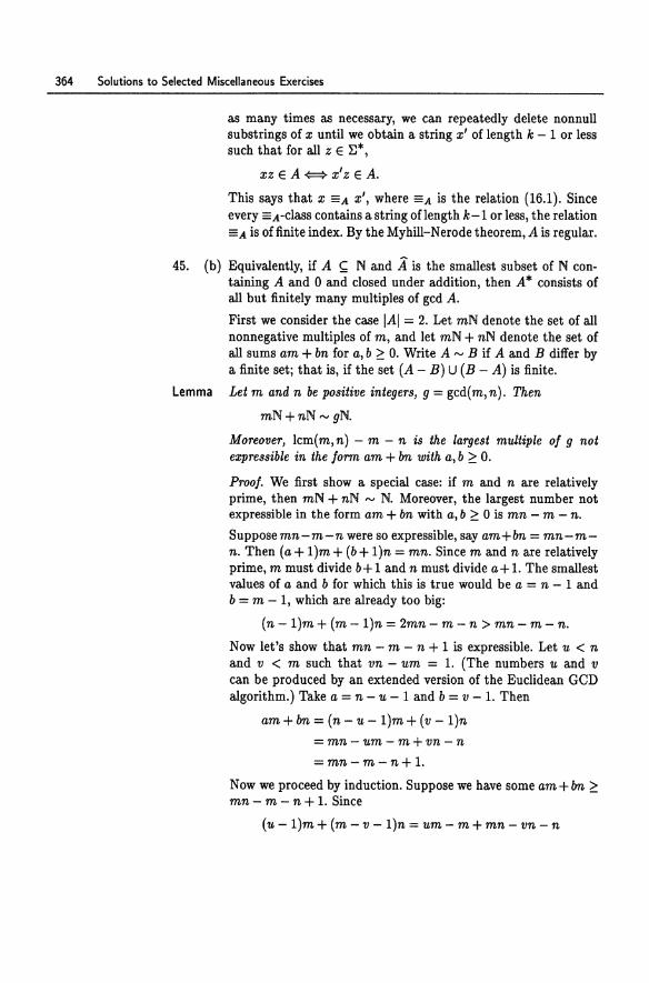
364 Solutions to Selected Miscellaneous Exercises
as many times as necessary, we can repeatedly delete nonnull substrings of x until we obtain a string x' of length k - 1 or less such that for all Z E ~*,
xz E A-¢::=} x'z E A.
This says that x =A x', where =A is the relation (16.1). Since every =A-class contains a string oflength k-1 or less, the relation =A is of finite index. By the Myhill-Nerode theorem, A is regular.
45. (b) Equivalently, if A ~ N and A is the smallest subset of N containing A and 0 and closed under addition, then A* consists of all but finitely many multiples of gcd A.
First we consider the case JAJ = 2. Let mN denote the set of all nonnegative multiples of m, and let mN + nN denote the set of all sums am + bn for a, b ~ O. Write A '" B if A and B differ by a finite set; that is, if the set (A - B) U (B - A) is finite.
Lemma Let m and n be positive integers, g = gcd( m, n). Then
mN + nN '" gN.
Moreover, lcm(m,n) - m - n is the largest multiple of g not expressible in the form am + bn with a, b ~ O.
Proof. We first show a special case: if m and n are relatively prime, then mN + nN '" N. Moreover, the largest number not expressible in the form am + bn with a, b ~ 0 is mn - m - n.
Suppose mn-m-n were so expressible, say am+bn = mn-mn. Then (a + 1)m + (b + 1)n = mn. Since m and n are relatively prime, m must divide b+ 1 and n must divide a + 1. The smallest values of a and b for which this is true would be a = n - 1 and b = m - 1, which are already too big:
(n -1)m + (m -1)n = 2mn - m - n > mn - m - n.
Now let's show that mn - m - n + 1 is expressible. Let u < n and v < m such that vn - um = 1. (The numbers u and v can be produced by an extended version of the Euclidean GCD algorithm.) Take a = n - u - 1 and b = v - 1. Then
am + bn = (n - u - 1)m + (v - 1)n
= mn - um - m + vn - n
= mn - m - n+ 1.
Now we proceed by induction. Suppose we have some am + bn ~ mn - m - n + 1. Since
(u - 1)m + (m - v - 1)n = um - m + mn - vn - n
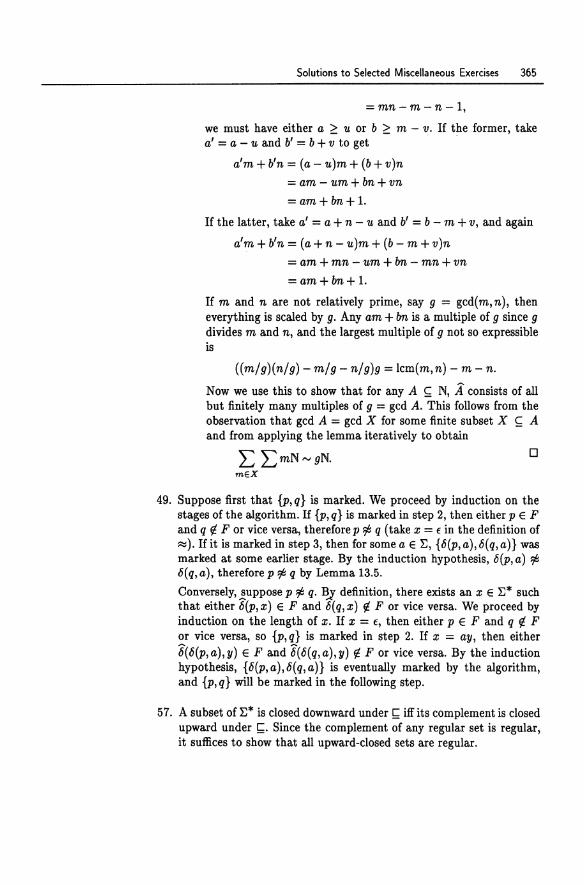
Solutions to Selected Miscellaneous Exercises 365
=mn-m -n -1,
we must have either a ~ u or b ~ m - v. If the former, take a' = a - u and b' = b + v to get .
a'm +b'n = (a - u)m+ (b+v)n
= am - um+bn+vn
= am+bn+ 1.
If the latter, take a' = a + n - u and b' = b - m + v, and again
a'm+b'n= (a+n-u)m+(b-m+v)n
= am + mn - um + bn - mn + vn
=am+bn+1.
If m and n are not relatively prime, say 9 = gcd(m,n), then everything is scaled by g. Any am + bn is a multiple of 9 since 9 divides m and n, and the largest multiple of 9 not so expressible is
«mjg)(njg) - mjg - njg)g = lcm(m,n) - m - n.
Now we use this to show that for any A ~ N, A consists of all but finitely many multiples of 9 = gcd A. This follows from the observation that gcd A = gcd X for some finite subset X ~ A and from applying the lemma iteratively to obtain
L LmN",gN. o mEX
49. Suppose first that {p,q} is marked. We proceed by induction on the stages of the algorithm. If {p, q} is marked in step 2, then either p E F and q f/. F or vice versa, therefore p ~ q (take z = E in the definition of ~). If it is marked in step 3, then for some a E I;, {6(p, a), 6(q, a)} was marked at some earlier stage. By the induction hypothesis, 6(p,a) ~ 6(q,a), therefore p ~ q by Lemma 13.5.
Conversely, !uppose p ~ q. B"'y definition, there exists an z E I;* such that either 6(P,z) E F and 6(q,z) f/. F or vice versa. We proceed by induction on the length of z. If z = E, then either p E F and q f/. F or vice versa, so {p,q} is marked in step 2. If z = ay, then either 6(6(p,a),y) E F and 6(6(q,a),y) f/. F or vice versa. By the induction hypothesis, {6(p,a),6(q,a)} is eventually marked by the algorithm, and {p,q} will be marked in the following step.
57. A subset of I;* is closed downward under [; iff its complement is closed upward under [;. Since the complement of any regular set is regular, it suffices to show that all upward-closed sets are regular.
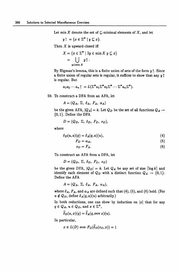
366 Solutions to Selected Miscellaneous Exercises
Let minX denote the set of ~-minimal elements of X, and let
111 ={xEI:*11I~x}.
Then X is upward-closed iff
X = {x E I:* I 311 E min X 11 ~ x}
= U 111· lIEminX
By Higman's lemma, this is a finite union of sets of the form 111. Since a finite union of regular sets is regular, it suffices to show that any 111 is regular. But
alaa'" an 1 = L(I:*a1 I:*a2E* ... E*anE*).
59. To construct a DFA from an AFA, let
A = (QA, E, 6A, FA, Q:A)
be the given AFA, IQAI = k. Let QD be the set of all functions QA -+ {O, I}. Define the DFA
D = (QD, E, 6D, FD, SD),
where
6D(u,a)(q) = 6A(q,a)(u), FD = Q:A,
SD = FA'
To construct an AFA from a DFA, let
D = (QD, E, 6D, FD, SD)
(4) (5) (6)
be the given DFA, IQDI = k. Let QA be any set of size [logkl and identify each element of QD with a distinct function QA -+ {O, I}. Define the AFA
A = (QA, I:, 6A, FA, Q:A),
where 6A, FA, and Q:A are defined such that (4), (5), and (6) hold. (For u ¢ QD, define 6A(q,a)(u) arbitrarily.)
In both reductions, one can show by induction on Ixl that for any q E QA, U E QD, and x E E*,
6D(U,X)(q) = ~(q,revx)(u). In particular,
x E L(D) {:::::} FD(6.0(SD,X)) = 1
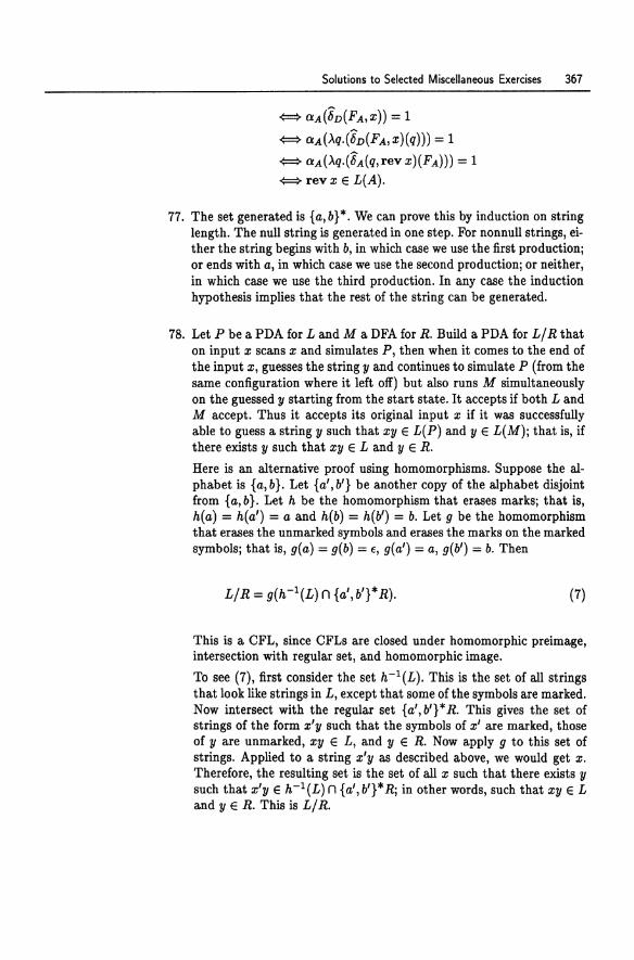
Solutions to Selected Miscellaneous Exercises 367
<==> aA(6D(FA,X)) = 1
<==> aA(Aq.(6D(FA,X)(q))) = 1
<==> aA(Aq.(6A(Q, rev X)(FA))) = 1
<==> rev x E L(A).
77. The set generated is {a,b}*. We can prove this by induction on string length. The null string is generated in one step. For nonnull strings, either the string begins with b, in which case we use the first production; or ends with a, in which case we use the second production; or neither, in which case we use the third production. In any case the induction hypothesis implies that the rest of the string can be generated.
78. Let P be a PDA for L and M a DFA for R. Build a PDA for L/ R that on input x scans x and simulates P, then when it comes to the end of the input x, guesses the string y and continues to simulate P (from the same configuration where it left off) but also runs M simultaneously on the guessed y starting from the start state. It accepts if both L and M accept. Thus it accepts its original input x if it was successfully able to guess a string y such that xy E L(P) and y E L(M); that is, if there exists y such that xy ELand y E R.
Here is an alternative proof using homomorphisms. Suppose the alphabet is {a, b}. Let {a', b'} be another copy of the alphabet disjoint from {a,b}. Let h be the homomorphism that erases marks; that is, h(a) = h(a') = a and h(b) = h(b') = b. Let 9 be the homomorphism that erases the unmarked symbols and erases the marks on the marked symbols; that is, g(a) = g(b) = e, g(a') = a, g(b') = b. Then
L/ R = g(h-l(L) n {a',b'}* R). (7)
This is a CFL, since CFLs are closed under homomorphic preimage, intersection with regular set, and homomorphic image.
To see (7), first consider the set h-1(L). This is the set of all strings that look like strings in L, except that some of the symbols are marked. Now intersect with the regular set {a', b'} * R. This gives the set of strings of the form x'y such that the symbols of x' are marked, those of yare unmarked, xy E L, and y E R. Now apply 9 to this set of strings. Applied to a string x'y as described above, we would get x. Therefore, the resulting set is the set of all x such that there exists y such that x'y E h-1(L) n {a', b'}* R; in other words, such that xy E L and y E R. This is L/ R.
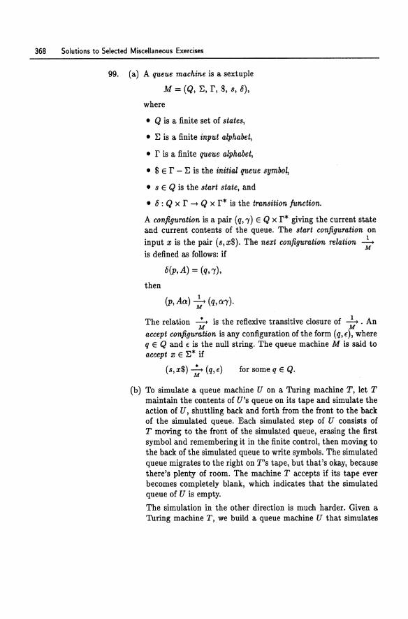
368 Solutions to Selected Miscellaneous Exercises
99. (a) A queue machine is a sextuple
M= (Q,~, r, $, s, 6),
where
• Q is a finite set of states,
• ~ is a finite input alphabet,
• r is a finite queue alphabet,
• $ E r - ~ is the initial queue symbol,
• 8 E Q is the start state, and
• 6: Q x r -+ Q x r* is the transition function.
A configuration is a pair (q, 'Y) E Q x r* giving the current state and current contents of the queue. The start configuration on
input x is the pair (s,x$). The next configuration relation ~ M
is defined as follows: if
6(p,A) = (q,'Y),
then
(p,Aa) ~ (q,a'Y). M
The relation -.!... is the reflexive transitive closure of ~. An M M
accept configuration is any configuration of the form (q, f), where q E Q and f is the null string. The queue machine M is said to accept x E ~* if
(8, x$) -.!... (q, €) M
for some q E Q.
(b) To simulate a queue machine U on a 'lUring machine T, let T maintain the contents of U's queue on its tape and simulate the action of U, shuttling back and forth from the front to the back of the simulated queue. Each simulated step of U consists of T moving to the front of the simulated queue, erasing the first symbol and remembering it in the finite control, then moving to the back of the simulated queue to write symbols. The simulated queue migrates to the right on T's tape, but that's okay, because there's plenty of room. The machine T accepts if its tape ever becomes completely blank, which indicates that the simulated queue of U is empty.
The simulation in the other direction is much harder. Given a 'lUring machine T, we build a queue machine U that simulates
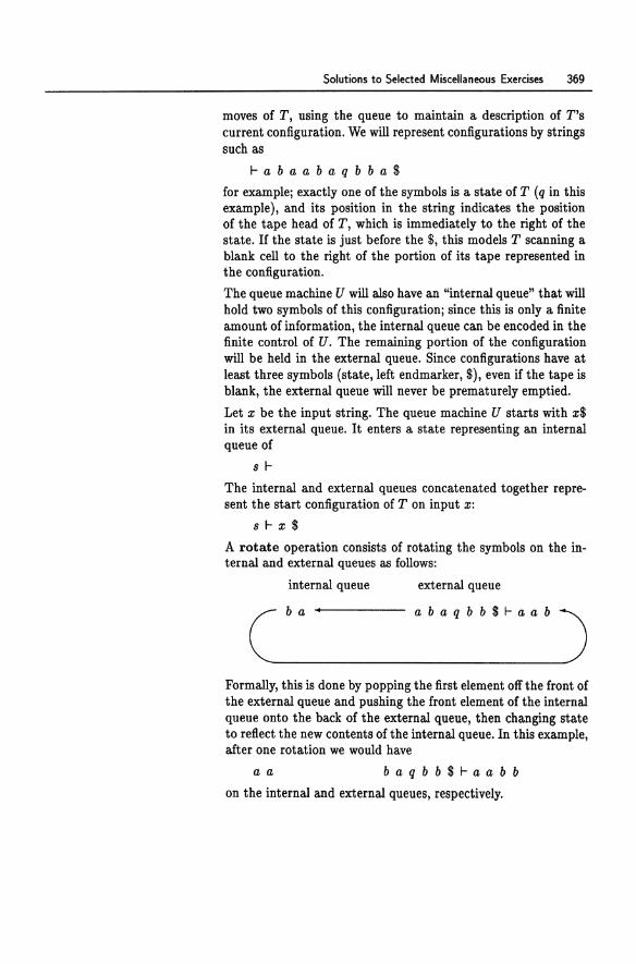
Solutions to Selected Miscellaneous Exercises 369
moves of T, using the queue to maintain a description of T's current configuration. We will represent configurations by strings such as
r a b a a b a q b b a $
for example; exactly one of the symbols is a state of T (q in this example), and its position in the string indicates the position of the tape head of T, which is immediately to the right of the state. If the state is just before the $, this models T scanning a blank cell to the right of the portion of its tape represented in the configuration.
The queue machine U will also have an "internal queue" that will hold two symbols of this configuration; since this is only a finite amount of information, the internal queue can be encoded in the finite control of U. The remaining portion of the configuration will be held in the external queue. Since configurations have at least three symbols (state, left endmarker, $), even if the tape is blank, the external queue will never be prematurely emptied.
Let x be the input string. The queue machine U starts with x$ in its external queue. It enters a state representing an internal queue of
s r The internal and external queues concatenated together represent the start configuration of T on input x:
s r x $
A rotate operation consists of rotating the symbols on the internal and external queues as follows:
internal queue external queue
C __ b _a_ -_'~~~~~~~~_a_b_a_q_b_b_$_r_a_a_b __ )
Formally, this is done by popping the first element off the front of the external queue and pushing the front element of the internal queue onto the back of the external queue, then changing state to reflect the new contents of the internal queue. In this example, after one rotation we would have
aa b a q b b $ r a a b b
on the internal and external queues, respectively.
370 Solutions to Selected Miscellaneous Exercises
113. Let
We simulate a step of T as follows. If the rightmost symbol of the internal queue is not a state of T, we rotate until this becomes true. In this example, after three more steps we would have
aq bb$l-aabbaab
Now we have the symbol that T is scanning (say b) at the head of the external queue and the current state of T (say q) rightmost on the internal queue. We read b at the head of the queue. If b is not $, we simulate a move of T as follows .
• If DT(q,b) = (P,c,R) and the leftmost symbol ofthe internal queue is d, we push d onto the back of the external queue and make (c p) the new internal queue.
• If DT (q, b) = (p, c, L) and the leftmost symbol of the internal queue is d, we push p onto the back of the external queue and make (d c) the new internal queue.
In the example above, this would give
ap b$l-aabbaaba
if DT(q,b) = (p,a,R), and
aa b$l-aabbaabq
if DT(q,b) = (p,a,L). If the symbol at the head of the external queue is $, then this indica.tes that the tape head of T is scanning a blank symbol to the right of the portion of the tape represented in the configuration. For example,
bq $I-aabbbaabab
In this case, when we pop $ we don't simulate a move of T immediately; first we insert an extra blank symbol u between the state and the $. We do this by pushing both symbols in the internal queue onto the back of the external queue and making the new internal queue (u $). In this example, the resulting queue contents would be
u $ I- a a b b b a a b a b b q
We continue to simulate moves of T. If T ever enters its accept state, then U goes into a little subroutine that just empties its external queue, thereby accepting.
REG = {M I L(M) is regular}.
Solutions to Selected Miscellaneous Exercises 371
A corollary of Rice's theorem for r.e. sets (Theorem 34.2) is that any semidecidable property of the r.e. sets is monotone. That is, if P is a property ofr.e. sets such that {M I P(L(M))} is r.e., A and Bare r.e. sets, A ~ B, and P(A), then P(B). Applying this corollary with P(C) = "C is regular," A = 0, and B = {anbn I n ~ O} gives immediately that REG is not r.e. Similarly, applying the corollary with P( C) = "C is not regular," A = {anbn I n ~ a}, and B = :E* gives immediately that REG is not co-r.e.
References
[1] W. ACKERMANN, Zum Hilbertschen Aufbau der reellen Zahlen, Math. Annalen, 99 (1928), pp. 118-133.
[2] A.V. AHO AND J.D. ULLMAN, The Theory of Paraing, Translation, and Compiling, Vol. I: Parsing, Prentice Hall, Englewood Clift's, NJ, 1972.
[3] --, The Theory of Parsing, Tranalation, and Compiling, Vol. II: Compiling, Prentice Hall, Englewood Clift's, NJ, 1973.
[4] --, Principles of Compiler Design, Addison-Wesley, Reading, MA, 1977.
[5] M.A. ARBIB AND Y. GIVE'ON, Algebra automata I: Parallel programming as a prolegomenon to the categorical approach, Information and Control, 12 (1968), pp. 331-345.
[6] R.C. BACKHOUSE, Cloaure Algorithma and the Star-Height Problem of Regular Languages, Ph.D. thesis, Imperial College, London, 1975.
[7] J. W. BACKUS, The syntax and semantics of the proposed international algebraic language of the Ziirich ACM-GAMM conference, in Proc. Intl. Conf. Information Processing, UNESCO, 1959, pp. 125-132.
[8] Y. BAR-HILLEL, M. PERLES, AND E. SHAMIR, On formal properties of simple phrase structure grammars, Z. Phonetik. Sprachwiaa. Kommunikationaforach., 14 (1961), pp. 143-172.
[9] H.P. BARENDREGT, The Lambda Calculua, North-Holland, Amsterdam, 1984.
[10] S.L. BLOOM AND Z. ESIK, Equational axioms for regular sets, Mathematical Structures in Computer Science, 3 (1993), pp. 1-24.
[11] M. BOFFA, Une remarque sur les systemes complets d'identites rationnelles, Informatique TMoretique et Applicationa/Theoretical Informatics and Applicationa, 24 (1990), pp. 419-423.
374 References
(12) --, Une condition impliquant toutes les identites rationnelles, Informatique TMoretique et Applications/Theoretical Informatics and Applications, 29 (1995), pp. 515-518.
(13) W.S. BRAINERD, Tree Generating Systems and Tree Automata, Ph.D. thesis, Purdue University, Indiana, 1967.
(14) --, The minimalization of tree automata, Information and Control, 13 (1968), pp. 484-491.
[15) W.S. BRAINERD AND L.H. LANDWEBER, Theory of Computation, John Wiley, New York, 1974.
[16) G. CANTOR, Uber eine Eigenschaft des InbegrifFes alIer reellen algebraischen Zahlen, J. fir die reine und angewandte Mathematik, 77 (1874), pp. 258-262. Reprinted in Georg Cantor Gesammelte Abhandlungen, Berlin, SpringerVerlag, 1932, pp. 115-118.
(17) N. CHOMSKY, Three models for the description of languages, IRE 7Tans. Information Theory, 2 (1956), pp. 113-124.
[18) --, On certain formal properties of grammars, Information and Control, 2 (1959), pp. 137-167.
[19) --, Context-free grammars and pushdown storage, Tech. Rep., MIT Research Lab. in Electronics, Cambridge, MA, 1962.
[20) --, Formal properties of grammars, Handbook of Math. Psych., 2 (1963), pp. 323-418.
[21) N. CHOMSKY AND G.A. MILLER, Finite state languages, Information and Control, 1 (1958), pp. 91-112.
[22) N. CHOMSKY AND M.P. SCHUTZ EN BERGER, The algebraic theory of context free languages, in Computer Programming and Formal Systems, P. Braffort and D. Hirschberg, eds., North-Holland, Amsterdam, 1963, pp. 118-161.
[23) A. CHURCH, A set of postulates for the foundation of logic, Ann. Math., 33-34 (1933), pp. 346-366,839-864.
[24) --, A note on the Entscheidungsproblem, J. Symbolic Logic, 58 (1936), pp. 345-363.
[25) --, An unsolvable problem of elementary number theory, Amer. J. Math., 58 (1936), pp. 345-363.
[26) --, The calculi oflambda-conversion, Ann. Math. Studies,6 (1941).
[27) J.H. CONWAY, Regular Algebra and Finite Machines, Chapman and Hall, London, 1971.
[28) S.A. COOK, The complexity of theorem proving procedures, in Proc. Third Symp. Theory of Computing, Assoc. Comput. Mach., New York, 1971, pp. 151-158.
[29) H.B. CURRY, An analysis of logical substitution, Amer. J. Math., 51 (1929), pp. 363-384.
[30) N.J. CUTLAND, Computability, Cambridge University, Cambridge, 1980.
References 375
[31) M. DAVIS, Computability and Unaolvability, McGraw-Hill, New York, 1958.
[32) --, The Undecidable, Raven Press, Hewlitt, NY, 1965.
[33) A. EHRENFEUCHT, R. PARIKH, AND G. RoZENBERG, Pumping lemmas and regular sets, SIAM J. Computing, 10 (1981), pp. 536-541.
[34) S. ElLENBERG AND J .B. WRIGHT, Automata in general algebra, Information and Control, 11 (1967), pp. 452-470.
[35) J. ENGELFRIET, Tree automata and tree grammars, Tech. Rep. DAIMI FN-10, Aarhus University, Aarhus, Denmark, 1975.
[36) J. EVEY, Application of pushdown store machines, in Proc. Fall Joint Computer Conf., AFIPS Press, Montvale, NJ, 1963, pp. 215-227.
[37) P .C. FISCHER, On computability by certain classes of restricted Turing machines, in Proc. Fourth Symp. Switching Circuit Theory and Logical Design, 1963, pp. 23-32.
[38) --, Turing machines with restricted memory access, Information and Control, 9 (1966), pp. 364-379.
[39) P .C. FISCHER, A.R. MEYER, AND A.L. RoSENBERG, Counter machines and counter languages, Math. SY"'tems Theory, 2 (1968), pp. 265-283.
[40) M.R. GAREY AND D.S. JOHNSON, Computer", and Intractibility: A Guide to the Theory of NP-Completeness, W.H. Freeman, New York, 1979.
[41) F. GtCSEG AND I. PEAK, Algebraic Theory of Automata, Akad6miai Kiad6, Budapest, 1972.
[42) F. GtCSEG AND M. STEIN BY, Tree Automata, Akademiai Kiad6, Budapest, 1984.
[43) S. GINSBURG, The Mathematical Theory of Contezt-Free Language"" McGrawHill, New York, 1966.
[44] S. GINSBURG AND S.A. GREIBACH, Deterministic context-free languages, Information and Control, 9 (1966), pp. 563-582.
[45) S. GINSBURG AND H. G. RICE, Two families of languages related to ALGOL, J. As",oc. Comput. Mach., 9 (1962), pp. 350-371.
[46) S. GINSBURG AND G.F. RoSE, Operations which preserve definability in languages, J. Assoc. Comput. Mach., 10 (1963), pp. 175-195.
[47) --, Some recursively unsolvable problems in ALGOL-like languages, J. Assoc. Comput. Mach., 10 (1963), pp. 29-47.
(48) --, Preservation of languages by transducers, Information and Contro~ 9 (1966), pp. 153-176.
(49) S. GINSBURG AND E.H. SPANIER, Quotients of context-free languages, J. Assoc. Comput. Mach., 10 (1963), pp. 487-492.
[50) K. GODEL, Uber formal unentscheidbare Sitze der Principia Mathematica und verwandter Systeme I, Monatshefte for Mathematik und Physik, 38 (1931), pp. 173-198.
376 References
[51) --, On undecidable propositions of formal mathematical systems, in The Undecidable, M. Davis, ed., Raven Press, Hewlitt, NY, 1965, pp. 5-38.
[52) J. GOLDSTINE, A simplified proof of Parikh's theorem, Discrete Math., 19 (1977), pp. 235-240.
[53) S.A. GREIBACH, A new normal form theorem for context-free phrase structure grammars, J. Assoc. Comput. Mach., 12 (1965), pp. 42-52.
[54] L. HAINES, Generation and recognition of formal languages, Ph.D. thesis, MIT, Cambridge, MA, 1965.
[55) M.A. HARRISON, Introduction to Formal Language Theory, Addison-Wesley, Reading, MA, 1978.
[56) J. HARTMANIS AND J .E. HOPCROFT, Structure of undecidable problems in automata theory, in Proc. Ninth Symp. Switching and Automata Theory, IEEE, 1968, pp. 327-333.
[57) J. HARTMANIS AND R.E. STEARNS, On the complexity of algorithms, Trans. Amer. Math. Soc., 117 (1965), pp. 285-306.
[58) F .C. HENNIE, Introduction to Computability, Addison-Wesley, Reading, MA, 1977.
[59) J.E. HOPCROFT, An nlogn algorithm for minimizing the states in a finite automaton, in The Theory of Machines and Computation, Z. Kohavi, ed., Academic Press, New York, 1971, pp. 189-196.
(60) J.E. HOPCROFT AND J.D. ULLMAN, Introduction to Automata Theory, Languages, and Computation, Addison-Wesley, Reading, MA, 1979.
(61) D.A. HUFFMAN, The synthesis of sequential switching circuits, J. Franklin Institute, 257 (1954), pp. 161-190,275-303.
(62) J. JAFFE, A necessary and sufficient pumping lemma for regular languages, SIGACT News, 10 (1978), pp. 48-49.
(63) N.D. JONES, Computability Theory: An Introduction, Academic Press, New York,1973.
(64) R.M. KARP, Reducibility among combinatorial problems, in Complexity of Computer Computations, R.E. Miller and J.W. Thatcher, eds., Plenum Press, New York, 1972, pp. 85-103.
[65] T. KASAMI, An efficient recognition and syntax algorithm for context-free languages, Tech. Rep. AFCRL-65-758, Air Force Cambridge Research Lab, Bedford, MA, 1965.
(66) S.C. KLEENE, A theory of positive integers in formal logic, Amer. J. Math., 57 (1935), pp. 153-173,219-244.
(67) --, General recursive functions of natural numbers, Math. Annalen, 112 (1936), pp. 727-742.
(68) --, Recursive predicates and quantifiers, Trans. Amer. Math. Soc., 53 (1943), pp. 41-74.
References 317
[69) --, Introduction to Metamathem~tic&, D. van Nostrand, Princeton, NJ, 1952.
[70) --, Representation of events in nerve nets and finite automata, in Au· tomato. Studies, C.E. Shannon and J. McCarthy, eds., Princeton University Press, Princeton, NJ, 1956, pp. 3-41.
[71) D.E. KNUTH, On the translation of languages from left to right, Information and Control, 8 (1965), pp. 607-639.
[72) D.C. KOZEN, The Design and Analysis of Algorithms, Springer-Verlag, New York, 1991.
[73) --, A completeness theorem for Kleene algebras and the algebra of regular events, Infor. and Comput., 110 (1994), pp. 366-390.
[74) D. I\ROB, A complete system of B-rational identities, Theoretical Computer Science, 89 (1991), pp. 207-343.
[75) W. KUICH, The Kleene and Parikh theorem in complete semirings, in Proc. 14th Colloq. Automata, Languages, and Programming, T. Ottmann, ed., vol. 267 of Lect. Notes in Comput. Sci., EATCS, Springer-Verlag, New York, 1987, pp. 212-225. .
[76) W. KUICH AND A. SALOMAA, Semirings, Automata, and Languages, Springer-Verlag, Berlin, 1986.
[77) S.Y. KURODA, Classes oflanguages and linear bounded automata, Information and Control, 7 (1964), pp. 207-223.
[78] P .S. LANDWEBER, Three theorems on phrase structure grammars of type 1, Information and Control, 6 (1963), pp. 131-136.
[79] H.R. LEWIS AND C.H. PAPADIMITRlOU, Elements of the Theory of Computation, Prentice Hall, Englewood Cliffs, NJ, 1981.
[80) P.M. LEWIS, D.J. ROSENKRANTZ, AND R.E. STEARNS, Compiler Design Theory, Addison-Wesley, Reading, MA, 1976.
[81) M. MACHTEY AND P. YOUNG, An Introduction to the General Theory of Algorithms, North-Holland, Amsterdam, 1978.
[82) Z. MANNA, Mathematical Theory of Computation, McGraw-Hill, New York, 1974.
(83) A.A. MARKOV, The Theory of Algorithms, vol. 42, Trudy Math. Steklov Inst., 1954. English translation, National Science Foundation, Washington, DC, 1961.
[84] W.S. MCCULLOCH AND W. PITTS, A logical calculus ofthe ideas immanent in neI'V()US activity, Bull. Math. Biophy&ics,5 (1943), pp. 115-143.
(85) R. McNAUGHTON AND H. YAMADA, Regular expressions and state graphs for automata, IEEE TraM. Electronic Computers, 9 (1960), pp. 39-47.
[86] A.R. MEYER AND D.M. RITCHIE, The complexityofloop programs, in Proc. ACM Natl. Meeting, 1967, pp. 465-469.
378 References
[87) R. MILNER, Operational and algebraic semantics of concurrent processes, in Handbook of Theoretical Computer Science, J. van Leeuwen, ed., vol. B, North-Holland, Amsterdam, 1990, pp. 1201-1242.
[88] M.L. MINSKY, Recursive unsolvability of Post's problem of 'tag' and other topics in the theory of Turing machines, Ann. Math., 74 (1961), pp. 437-455.
[89] M.L. MINSKY AND S. PAPERT, Unrecognizable sets of numbers, J. As"oc. Comput. Mach., 13 (1966), pp. 281-286.
[90) E.F. MOORE, Gedanken experiments on sequential machines, Automata Studie", (1956), pp. 129-153.
[91) J. MYHILL, Finite automata and the representation of events, Technical Note WADD 57-624, Wright Patterson AFB, Dayton, Ohio, 1957.
[92) --, Linear bounded automata, Technical Note WADD 60-165, Wright Patterson AFB, Dayton, Ohio, 1960.
(93) P. NAUR, Revised report on the algorithmic language ALGOL 60, Comm. Assoc. Comput. Mach., 6 (1963), pp. 1-17.
[94) A. NERODE, Linear automaton transformations, Proc. Amer. Math. Soc., 9 (1958), pp. 541-544.
(95) A.G. OETTINGER, Automatic syntactic analysis and the pushdown store, Proc. Symposia on Applied Math., 12 (1961).
[96) W. OGDEN, A helpful result for proving inherent ambiguity, Math. Systems Theory,2 (1968), pp. 191-194.
[97) C.H. PAPADIMITRIOU, Computational Complexity, Addison-Wesley, Reading, MA,1994.
[98) R. PARIKH, On context-free languages, J. Assoc. Comput. Mach., 13 (1966), pp. 570-581.
[99) E. POST, Finite combinatory processes-formulation, I, J. Symbolic Logic, 1 (1936), pp. 103-105.
[100) --, Formal reductions of the general combinatorial decision problem, Amer. J. Math., 65 (1943), pp. 197-215.
(101) --, Recursively enumerable sets of positive natural numbers and their decision problems, Bull. Amer. Math. Soc., 50 (1944), pp. 284-316.
[102) M.O. RABIN AND D.S. SCOTT, Finite automata and their decision problems, IBM J. Res. Develop., 3 (1959), pp. 115-125.
(103) V.N. REDKO, On defining relations for the algebra ofregular events, Ukrain. Mat. Z., 16 (1964), pp. 120-126. In Russian.
[104) H.G. RICE, Classes of recursively enumerable sets and their decision problems, Trans. Amer. Math. Soc., 89 (1953), pp. 25-59.
[105) --, On completely recursively enumerable classes and their key arrays, J. Symbolic Logic, 21 (1956), pp. 304-341.
[106) H. RoGERS, JR., Theory of Recursive Functions and Effective Computability, McGraw-Hill, New York, 1967.
References 379
[107) J.B. RoSSER, A mathematical logic without variables, Ann. Math., 36 (1935), pp. 127-150.
[108) A. SALOMAA, Two complete axiom systems for the algebra of regular events, J. Assoc. Comput. Mach., 13 (1966), pp. 158-169.
[109) A. SALOMAA AND M. SOITTOLA, Automata Theoretic Aspects of Formal Power Series, Springer-Verlag, New York, 1978.
[110) S. SCHEINBERG, Note on the Boolean properties of context-free languages, Information and Control, 3 (1960), pp. 372-375.
[111) M. SCHONFINKEL, Uber die Bausteine der mathematischen Logik, Math. Annalen, 92 (1924), pp. 305-316.
[112) M.P. SCRUTZENBERGER, On context-free languages and pushdown automata, Information and Control,6 (1963), pp. 246-264.
[113) J.I. SEIFERAS AND R. McNAUGHTON, Regularity-preserving relations, Theor. Comput. Sci., 2 (1976), pp. 147-154.
[114) J.C. SHEPHERDSON, The reduction of two-way automata to one-way automata, IBM J. Res. Develop., 3 (1959), pp. 198-200.
[115) J.R. SHOENFIELD, Degrees of Unsolvability, North-Holland, Amsterdam, 1971.
[116) R.I. SOARE, Recursively Enumemble Sets and Degrees, Springer-Verlag, Berlin, 1987.
[117) D. STANAT AND S. WEISS, A pumping theorem for regular languages, SIGACT News, 14 (1982), pp. 36-37.
[118) L.J. STOCKMEYER, The polynomial-time hierarchy, Theor. Comput. Sci., 3 (1976), pp. 1-22.
[119) J.W. THATCHER AND J.B. WRIGHT, Generalized finite automata theory with an application to a decision problem of second order logic, Math. Syst. Theory, 2 (1968), pp. 57-81.
[120) A.M. TURING, On computable numbers with an application to the Entscheidungsproblem, Proc. London Math. Soc., 42 (1936), pp. 230-265. Erratum: Ibid., 43 (1937), pp. 544-546.
[121) --, Systems of logic based on ordinals, Proc. London Math. Soc., 42 (1939), pp. 230-265.
[122) M.Y. VARDI, A note on the reduction of two-way automata to one-way automata, Information Processing Letter8, 30 (1989), pp. 261-264.
[123) A.N. WHITEHEAD AND B. RUSSELL, Principia Mathematica, Cambridge University Press, Cambridge, 1910-1913. Three volumes.
[124) A. YASUHARA, Recursive Fir£nction Theory and Logic, Academic Press, New York,1971.
[125) D.H. YOUNGER, Recognition and parsing of context-free languages in time n3 , Information and Control, 10 (1967), pp. 189-208.
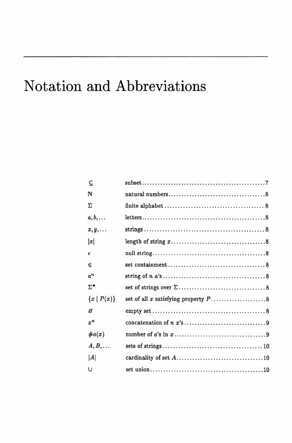
Notation and Abbreviations
!; subset ............................................... 7
N natural numbers ..................................... 8
~ finite alphabet ...................................... 8
a, b, . . . letters ............................................... 8
x, y,... strings .............................................. 8
Ix I length of string x . .....................•............. 8
E null string ........................................... 8
e set containment ..................................... 8
an string of n a's . ...................................... 8
~* set ofstrings over ~ ................................. 8
{x I P(x)} set of all x satisfying property P ...... ............... 8
o empty set ........................................... 8
xn concatenation of n x's ............................... 9
#a(x) number of a's in x ................................... 9
A, B,... sets of strings ................................. '" .. 10
IAI cardinality of set A ................................. 10
U set union ........................................... 10
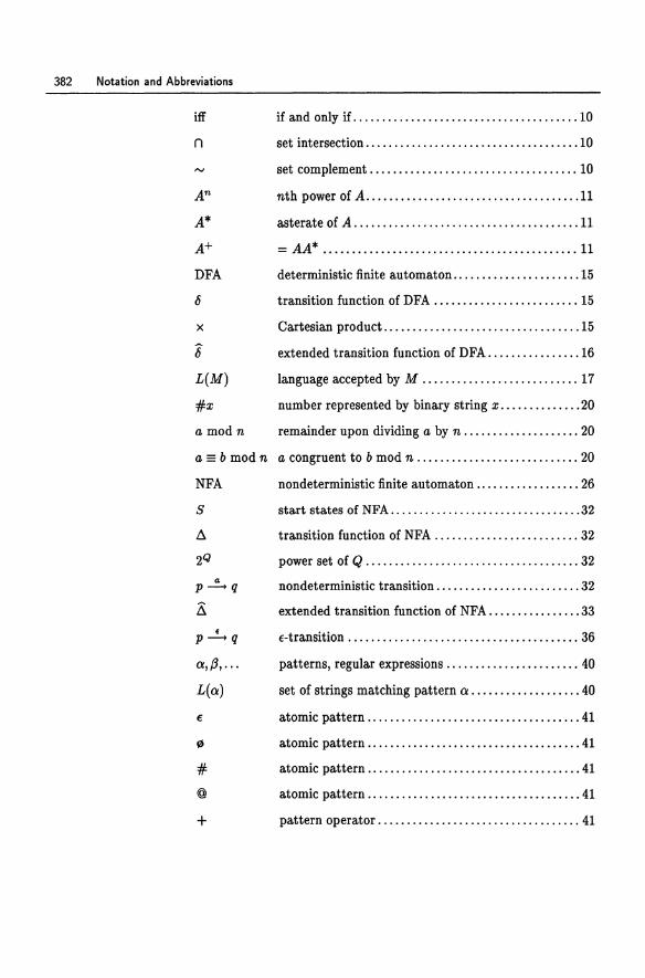
382 Notation and Abbreviations
iff
n
A*
A+
DFA
6
x
6 L(M)
#x amodn
if and only if ....................................... 10
set intersection ..................................... 10
set complement .................................... 10
nth power of A ..................................... 11
asterate of A ............. .......................... 11
= AA* ............................................ 11
deterministic finite automaton ...................... 15
transition function of DFA ......................... 15
Cartesian product .................................. 15
extended transition function of DFA ................ 16
language accepted by M ........................... 17
number represented by binary string x . ............. 20
remainder upon dividing a by n .................... 20
a == b mod n a congruent to b mod n ............................ 20
II P --+ q
~ E
P --+ q
01., (3, ...
L(a)
"
# @
+
nondeterministic finite automaton .................. 26
start states of NFA ................................. 32
transition function of NFA ......................... 32
power set of Q ..................................... 32
nondeterministic transition ......................... 32
extended transition function of NFA ................ 33
f-transition ........................................ 36
patterns, regular expressions ....................... 40
set of strings matching pattern a ................... 40
atomic pattern ..................................... 41
atomic pattern ..................................... 41
atomic pattern ..................................... 41
atomic pattern ..................................... 41
pattern operator ................................... 41
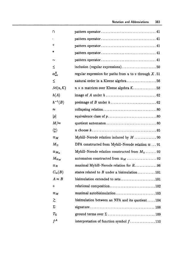
n
+
*
M(n,K)
h(A)
h-l(B)
a
> '"
Notation and Abbreviations 383
pattern operator ................................... 41
pattern operator ................................... 41
pattern operator ................................... 41
pattern operator ................................... 41
pattern operator ................................... 41
inclusion (regular expressions) ...................... 50
regular expression for paths from 'U to v through X. 51
natural order in a Kleene algebra ................... 56
n x n matrices over Kleene algebra K ............... 58
image of A under h ................................ 62
preimage of B under h ............................. 62
collapsing relation .................................. 80
equivalence class of p .. ............................. 80
quotient automaton ................................ 80
n choose k ......................................... 85
Myhill-Nerode relation induced by M .............. 90
DFA constructed from Myhill-Nerode relation == ... 91
Myhill-Nerode relation constructed from M= ....... 92
automaton constructed from ==M ••••••••••••••••••• 92
maximal Myhill-Nerode relation for R .............. 96
states related to B under a bisimulation ........... 101
bisimulation extended to sets ...................... 101
relational composition ............................. 102
maximal autobisimulation ......................... 103
bisimulation between an NFA and its quotient ..... 104
signature ......................................... 108
ground terms over ~ .............................. 109
interpretation of function symbol J ................ 110
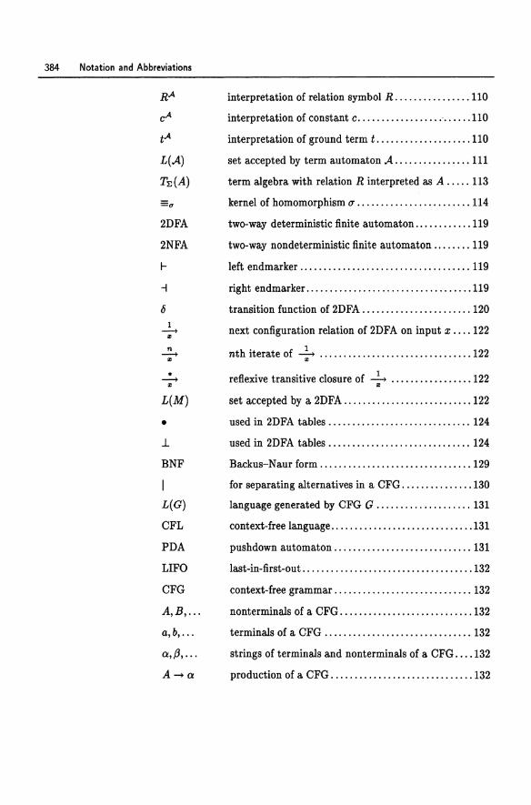
384 Notation and Abbreviations
2DFA
2NFA
f-
-I
o 1
---+ .. n
---+ or
• ---+ .. L(M)
• 1.
BNF
L(G) eFL
PDA
LIFO
eFG
A,B, ...
a,b, ...
a,{3, ...
A-+a
interpretation of relation symbol R . ............... 110
interpretation of constant c ................. . " ...... 110
interpretation of ground term t . ................... 110
set accepted by term automaton A ..... ....... ~ ... 111
term algebra with relation R interpreted as A ..... 113
kernel of homomorphism 0" •••••••••••••••••••••••• 114
two-way deterministic finite automaton ............ 119
two-way nondeterministic finite automaton ........ 119
left endmarker .................................... 119
right endmarker ................................... 119
transition function of 2DFA ....................... 120
next configuration relation of 2DFA on input x .... 122
nth iterate of + ................................ 122
reflexive transitive closure of + ................. 122
set accepted by a 2DFA ........................... 122
used in 2DFA tables .............................. 124
used in 2DFA tables .............................. 124
Backus-Naur form ................................ 129
for separating alternatives in a eFG ............... 130
language generated by eFG G .................... 131
context-free language .............................. 131
pushdown automaton ............................. 131
last-in-first-out .................................... 132
context-free grammar ............................. 132
nonterminals of a eFG ............................ 132
terminals of a eFG ............................... 132
strings of terminals and nontermina1s of a eFG .... 132
production of a eFG .............................. 132
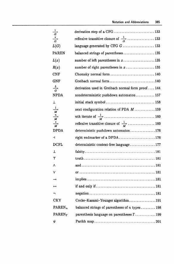
1 ---+
G • ---+ G
L(G) PAREN
L(x)
R(x)
CNF
GNF L
---+ G
NPDA
.1 1
---+ M n
---+ M • ---+ M
DPDA , DCFL
.1
T
" V
CKY
PARENn
PARENr
""
Notation and Abbreviations 385
derivation step of a CFG .......................... 133
reflexive transitive closure of + ................. 133
language generated by CFG G .................... 133
balanced strings of parentheses .................... 135
number ofleft parentheses in x .................... 135
number ofright parentheses in x .................. 135
Chomsky normal form ............................ 140
Greibach normal form ............................. 140
derivation used in Greibach normal form proof .... 144
nondeterministic pushdown automaton ............ 157
initial stack symbol ............................... 158
next configuration relation of PDA M ............. 159
nth iterate of .2.... ................................ 160 M
reflexive transitive closure of .2.... ................. 160 M
deterministic pushdown automaton ................ 176
right endmarker of a DPDA ....................... 176
deterministic context-free language ................ 177
falsity ............................................. 181
truth ............................................. 181
and ............................................... 181
or ................................................ 181
implies ............................................ 181
if and only if ...................................... 181
negation .......................................... 181
Cocke-Kasami-Younger algorithm ................. 191
balanced strings of parentheses of n types ......... 198
parenthesis language on parentheses r ............. 199
Parikh map ....................................... 201
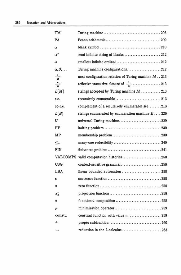
386 Notation and Abbreviations
TM
PA
u
u'"
w
a,p, ... 1
--+ M • --+ M
L(M)
r.e.
co-r.e.
L(E)
U
HP
MP
FIN
Turing machine ................................... 206
Peano arithmetic .................................. 209
blank symbol ..................................... 210
semi-infinite string of blanks ...................... 212
smallest infinite ordinal ........................... 212
Turing machine configurations ..................... 212
next configuration relation of Turing machine M .. 213
reflexive transitive closure of ~ ................. 213 M
strings accepted by Turing machine M ............ 213
recursively enumerable ............................ 213
complement of a recursively enumerable set ........ 213
strings enumerated by enumeration machine E .... 226
universal Turing machine .......................... 229
halting problem ................................... 230
membership problem .............................. 230
many-one reducibility ............................. 240
finiteness problem ................................. 241
VALCOMPS valid computation histories ........................ 250
CSG
LBA
s
z
o
canstn
.!.
context-sensitive grammar ......................... 258
linear bounded automaton ........................ 258
successor function ................................. 258
zero function ...................................... 258
projection function ................................ 258
functional composition ............................ 258
minimization operator ............................. 259
constant function with value n .................... 259
proper subtraction ................................ 260
reduction in the A-calculus ........................ 263
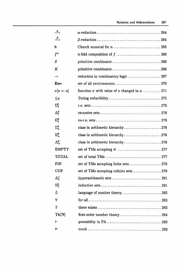
co --+
r s K
Env
u[x +- a]
:5T
~~
a~
II~
~~
II~
a~
EMPTY
TOTAL
FIN
COF
al III
L
V
3
Th(N)
r 1=
Notation and Abbreviations 387
a-reduction ....................................... 264
,a-reduction ....................................... 264
Church numeral for n ............................. 265
n-fold composition of f ........................... 266
primitive combinator .............................. 266
primitive combinator .............................. 266
reduction in combinatory logic .................... 267
set of all environments ............................ 270
function u with value of x changed to a ........... 271
Turing reducibility ................................ 275
r.e. sets ........................................... 276
recursive sets ..................................... 276
co-r.e. sets ........................................ 276
class in arithmetic hierarchy ....................... 276
class in arithmetic hierarchy ....................... 276
class in arithmetic hierarchy ....................... 276
set of TMs accepting {O ........................... 277
set of total TMs .................................. 277
set of TMs accepting finite sets .................... 278
set of TMs accepting cofinite sets .................. 278
hyperarithmetic sets .............................. 281
inductive sets ..................................... 281
language of number theory ........................ 282
for all ............................................. 283
there exists ....................................... 283
first-order number theory ......................... 284
provability in PA .................................. 292
truth ............................................. 292
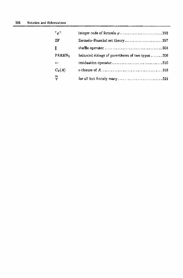
388 Notation and Abbreviations
integer code of formula rp ..•••••..•••••.•••••••.••• 292
ZF Zermelo-Fraenkel set theory ....................... 297
II shuffle operator ................................... 304
PAREN2 balanced strings of parentheses of two types ....... 306
residuation operator ............................... 310
Ge(A) e-closure of A ..................................... 318
00
\;/ for all but finitely many ........................... 324
Index
Abstraction, 5 functional, 263 >'-, 263
Acceptance, 17 2DFA, 120, 122 by empty stack, 160, 163, 164 by final state, 160, 164 DFA,16 DPDA,177 NFA, 26,33 NFA with €-transitions, 65, 318 term automaton, 111 Turing machine, 210, 213, 216
Accept state, 15, 111, 121, 158, 210, 211
Accessible, 29, 75, 77, 78, 84, 94, 95, 103,116
Ackermann, W., 273 Ackermann's function, 261, 273 Aho, A.V., 190 Algorithm
CKY, 191-195,249,338 Cocke-Kasami-Younger, see CKY collapsing, 84-88,106-107,327,365 Euclidean, 340, 364 maximal bisimulation, 106-107 minimization, see collapsing parsing, 181-190 primality, 217-219
recursive, 214 Alphabet, 8
single letter, 73, 74, 318, 326, 335, 346
stack, 158 a-reduction, 264 Alternating
finite automaton, 330, 366 quantifiers, see quantifier
Ambiguous, 131, 182, 186, 339 Analytic hierarchy, see hierarchy Annihilator, 12, 56 Antimatter, 354 Antisymmetry, 56, 96 Application operator, 267 Arbib, M.A., 118 Arithmetic hierarchy, see hierarchy Arity, 108 Assignment statement, 130 Associativity, 9, 11, 42, 45, 55, 264,
266, 285 Asterate, 11, 56
closure of CFLs under, 195 closure of regular sets under, 38
Atomic pattern, 40, 41 Autobisimulation, 103
maximal, 106 Automaton
counter, 224-225,227, 341
390 Index
Automaton (cont.) finite, 4, 14
deterministic, 15, 24, 54 nondeterministic, 26, 32, 39 two-way, 119-128,331 with e-transitions, 36-37, 65, 318
linear bounded, 4, 258, 268, 309, 313
product, 22 pushdown, 4, 131, 175
deterministic, 163,176-177,191, 196
nondeterministic, 157 one-state, 172
quotient, 80 term, 108-118 two-stack, 224
Axioms Kleene algebra, 55-56 Peano arithmetic, 284
Axiom scheme, 285
Backhouse, R.C., 60 Backus, J.W., 129, 134 Backus-Naur form, 129, 134 Balanced parentheses, 131, 135-140,
143, 145, 161, 198, 304, 306, 307, 329
Bar-Hillel, Y., 71, 147, 156, 197, 255 Basic pump, 203 Basis, 21 Begin statement, 130 ,B-reduction, 264 Biconditional, 181 Binary
relation, 110 representation, 19, 207, 224, 284,
301, 307, 323, 329 symbol,108
Bisimilar, 101 Bisimilarity class, 101 Bisimulation, 100, 101, 331
strong, 100 Blank symbol, 210, 211 Bloom, S.L., 60 BNF, 3ee Backus-Naur form Boffa, M., 60 Brainerd, W.S., 118, 268
Cantor, G., 230, 243, 297, 298 Capture of free variable, 264 Cardinality, 10, 208 Carrier, 110 Cell, 119, 157 CFL, 3ee context-free language Characteristic function, 275, 330 Chomsky
hierarchy, 4, 257, 268 normal form, 3ee normal form
Chomsky, N., 4, 54,134,147,175, 200, 268
Chomsky-Schiitzenberger theorem, 198-200
Church -Rosser property, 265 -Turing thesis, 8ee Church's thesis numerals, 265
Church, A., 4, 206, 207, 214, 265, 268 Church's thesis, 207-208, 214 CKY algorithm, 191-195, 197, 249,
338 Closure
properties of CFLs, 154, 155, 195-197,308,
335,367 of DCFLs, 177-180,196-197,338 of r .e. sets, 340 of regular sets, 21-24,37-39,47,
62,302 reflexive transitive, 56, 110, 160,
213, 315, 322 CNF, 8ee normal form Coarser, 96 Coarsest, 97 Cocke, J., 197 Cocke-Kasami-Younger algorithm,
8ee CKY algorithm Cofinite, 278 Collapsing, 77, 81
algorithm, 84-88, 98, 106-107,327, 365
DFA,77-99 NFA, 100-107 relation, 80, 84, 98, 100, 101
Combinator, 207, 266 Combinatorial completeness, 267
Combinatory logic, 4, 206, 207, 256, 266,268
Commutative image, 202 Commutativity, 12, 55, 202 Compiler compiler, 181 Complement, 10
CFLs not closed under, 155, 196 closure of DCFLs under, 177-180,
196 closure of recursive sets under, 219 closure of regular sets under, 23 r.e. sets not closed under, 219
Completeness for a class of decision problems,
278-281, 349 combinatorial, 267 deductive, 286
Complete partial order, 339 Complexity theory, 281 Composition
functional, 240, 258, 263, 271 relational, 57, 101, 110, 122 sequential, 269
Compound pattern, 40, 41 Computability, 5, 206, 207, 256 Computable
function, 347 total, 273, 347, 350
reduction, 240 Concatenation
closure of CFLs under, 195 closure of regular sets under, 37 set, 10, 37 string, 9
Concurrency, 100 Conditional, 269 Configuration
2DFA,122 DPDA,I77 PDA,158 queue machine, 368 start, 122, 159, 212, 216, 250 Turing machine, 212, 216, 250
Congruence, 114, 115, 117,202 class, 116 right, 90, 95, 97, 116
Consistency, 296, 297 Constant, 108
propositional, 181 Context, 116 Context-free
Index 391
grammar, 4, 129, 131, 132, 134 language, 4, 131, 133, 134
deterministic, 177, 191, 196 Context-sensitive
grammar, 4,258,268,313 language, 4
Contradiction, 68, 74 Contrapositive, 70, 153 Conway, J.H., 60 Cook, S.A., 281 Co-r.e., 213 Coset, 202 Counter, 163, 224
automaton, 224-225, 227, 341 Curry, 263 Curry, H.B., 4, 206, 263, 268 Cycle, 337
Davis, M., 268 DCFL, 8ee deterministic context-free
language Dead code, 310 Decidability, 220, 235-236 Decision problem, 7, 284 Demon game
for CFLs, 153-155 for regular sets, 71-73
De Morgan laws, 12, 24, 45 Denesting rule, 57 Depth, 150, 203, 330 Derivation
leftmost, 149, 168 rightmost, 149 tree, 8ee parse tree
Determinism, 176 Deterministic
context-free language, 177, 191, 196 finite automaton, 54 pushdown automaton, 163,
175-177,191,196 DFA, 8ee finite automaton Diagonalization, 230-234, 239, 243 Direct product, 108 Disjoint
pumps, 205
392 Index
Disjoint (cont.) union, 48
Distributivity, 12, 56, 285 DPDA, see deterministic pushdown
automaton Dyck language, see parenthesis
language DYLAN,262 Dynamic programming, 191
Effective, see computability Ehrenfeucht, A., 71 Eilenberg, S., 118 Emptiness problem
for CFLs, 249, 348 for LBAs, 310
Empty string, 8 Encoding, 207, 292
of configurations, 250 of natural numbers in the
,x-calculus, 265 of natural" numbers in ZF, 297
Endmarker, 120, 163, 176, 196, 211 Engelfriet, J., 118 Enumeration
machine, 225-227 state, 226
Environment, 270 Epimorphism, 113, 116 e-closure, 37, 65, 318 e-production, 141-142,145, 147, 334 e-transition, 36-37, 65, 158, 179, 318 Equational logic, 50 Equivalence
among variations of TMs, 221-227 class, 80 letter-, 203 of acceptance by final state and
empty stack, 164-166 of bisimilar automata, 103 of CSGs and LBAs, 258, 268 ofDFAs and
2DFAs,124-128 NFAs, 28-36 NFAs with e-transitions, 318 regular expressions, 46-54, 59 right-linear grammars, 54, 306
of ~-recursive functions and the ,x-calculus, 265
of NPDAs and CFGs, 167-175 one-state NPDAs, 172
of primitive recursive functions and for programs, 273
ofTMs and enumeration machines, 225-227 four-counter automata, 224-225 ,x-calculus, 268 Post systems, 257 two-counter automata, 225 two-stack automata, 224 type 0 grammars, 258, 268, 343
of while programs and ~-recursive functions, 271
problem, 310 relation, 49, 80, 90, 96
Erase, 217 Esik, Z., 60 Euclid,363 Euclidean algorithm, 340, 364 Evaluation, 262 Evey, J., 175 Exponentiation, 259 Expression
regular, see regular expression tree, 182
Final state, see accept state Finer, 96 Finite
automaton, 4, 14 alternating, 330, 366 deterministic, 15, 24, 54 nondeterministic, 32, 39 two-way, 119-128, 331 with e-transitions, 36-37, 65, 318
control, 211 index, 90, 95, 116-117 -state transition system, 14, 24
Finitely generated, 202 Finiteness problem
for CFLs, 250, 349 for regular sets, 349
Fischer, P.C., 180, 227 Fixpoint, 293, 339, 346, 347
lemma, 292 For
loop, 269 progrann, 269, 273
Formalist progrann, 5, 209, 282 Formal proof system, 282 Free
commutative monoid, 202 monoid,202 variable, 284, 293
Function Ackermann's, 261, 273 characteristic, 275, 330 computable, 347 monotone, 339 J'-recursive, 4, 206, 214, 256,
258-261,268,269,345 pairing, 277 partial, 270, 273, 347 primitive recursive, 259, 269, 273,
313 regularity preserving, 76, 324 transition, see transition function weakly regularity preserving, 324
Functional abstraction, 262-264 application, 262-264 composition, see composition
Garey, M., 281 GCD, see greatest common divisor Gecseg, F., 60, 118 Generalization, 285 Generate, 202, 257, 258 Ginsburg, S., 39, 180, 197, 255, 335 Give'on, Y., 118 GNF, see normal form G5del, K., 4, 5, 206, 207, 209,214,
258, 268, 269,273, 282, 287, 292
GOdel numbering, 208 GOdel's
fixpoint lemma, see fixpoint lemma incompleteness theorem, see
incompleteness theorem Goldstine, J., 205 Grammar, 4, 257
context-free, 4, 129, 132, 134
Index 393
context-sensitive, 4, 258, 268, 313 left-linear, 306 right-linear, 4, 54, 257, 306 strongly left-linear, 306 strongly right-linear, 306 type 0, 256, 257, 268 type 1, 257, 313 type 2, 257 type 3, 257
Greatest common divisor, 326,340, 364
Greibach, S.A., 147, 180,307,328 Greibach normal form, see normal
form Ground term, 109 Guess and verify, 26
Haines, L., 180 Halting
2DFA,122 configuration, 251 DPDA, 177, 179-180 LBA,309 problem, 230, 309
undecidability of, 231-234, 244 Turing machine, 213, 216
Hamming distance, 65, 302 Hardest r.e. set, 278 Hardness, 278 Harrison, M.A., 205 Hartmanis, J., 281 Head
read-only, 119, 157, 224 read/write, 210, 212, 220, 221 write-only, 225
Hennie, F.C., 268 Herbrand, J., 4, 206, 214, 268 Hierarchy
analytic, 281 arithmetic, 276-281 Chomsky, 4, 257, 268
Higman's lemma, 329, 365 Hilbert, D., 5, 209, 282 Historical notes, 24, 39, 54, 60, 71,
76,99,117,128,134,147,156, 175, 180, 190, 197, 200, 205, 214, 227, 243, 248, 255, 268, 273,281
394 Index
Homomorphic image, 62, 76, 108, 113, 117, 198, 199
closure of CFLs under, 196, 335, 367
closure ofregular sets under, 62 minimal, 117
Homomorphic preimage, 62 closure of CFLs under, 196, 335,
367 closure of regular sets under, 62
Homomorphism, 61-66, 74, 76, 108, 112, 114, 198, 319
~-algebra, 112 Hopcroft, J.E., 24,99,197 Horn clause, 348 Huffman, D.A., 99
Idempotence, 56 Idempotent semiring, 56 Identity
element, 9, 12, 56, 285 function, 267 relation, 96, 105, 110
If statement, 130 Image, 62 Implication, 181 Inaccessible, see accessible Incompleteness theorem, 5, 209,
282-298 Induction
axiom, 285 hypothesis, 20 step, 21 structural, 47
Infinite string, 108 Initial stack symbol, 158, 163 Input string, 16 Integer division, 283 Interactive computation, 208 Intersection, 10
CFLs not closed under, 196 closure of r.e. sets under, 340 closure of regular sets under, 22-23 of CFLs, 311, 312 of CFLs with regular sets, 195, 308,
367 Intuitionism, 297 Inverse, 260
Isomorphism, 78, 100, 105, 113, 229 of automata, 30, 89, 92-95
Jaffe, J., 71, 325 Johnson, D., 281 Jones, N.D., 268
Kapur, S., 329 Karp, R.M., 281 Kasami, T., 197 Kernel, 114, 115, 117 Kleene, S.C., 4, 24, 54, 55, 206, 214,
227,255,281 Kleene algebra, 49, 55-60, 110, 321,
322, 358 Knaster-Tarski theorem, 339 Knuth, D.E., 190 Kozen, D.C., 60 Krob, D., 60 Kuich, W., 60, 205 Kuroda, S.Y., 268
Labeled tree, 108, 109, 111 A-abstraction, 263 A-calculus, 4, 206, 214, 256, 262-268
pure, 263 A-notation, 262 A-term, 207, 262, 263,345 Landweber, L.H., 268 Landweber, P.S., 268 Language, 4
accepted by M, 17 context-free, 4, 131, 133, 134 context-sensitive, 4 deterministic context-free, 177, 191,
196 Dyck, see parenthesis language generated by G, 133 of number theory, 209, 282, 288,
293, 295, 297 parenthesis, 198
LBA, see linear bounded automaton Least upper bound, 56, 339 Leftmost derivation, 149, 168 Length, 8, 203 Letter, 8
-equivalence, 203 Level,149
Lewis, P.M., 190 LIFO,157 Linear
bounded automaton, 4, 258, 268, 309,313
equations, 59-60 order, 355 set, 202 time, 349, 356
LISP, 262 Logic, 256
combinatory, 4, 206, 207, 266, 268 equational, 50 first-order, 282, 297 propositional, 181 second-order, 281
Loop, 75 Looping
2DFA,122 DPDA, 177, 179-180 LBA,309 PDA,161 Turing machine, 210, 213, 216
Machtey, M., 268 Many-one reduction, 239 Markov, A.A., 134 Markov system, 134 Match, 40, 41 Matching parentheses, 136 Matrix, 322, 353, 357, 358, 361
over a Kleene algebra, 58-59 Maximal autobisimulation, 106 McCulloch, W.S., 24 McNaughton, R., 39, 54, 76, 324 Membership problem, 230, 278
undecidability of, 234 Metastatement, 295 Metasymbol, 229, 295 Metasystem, 295, 297 method,263 Meyer, A.R., 227,273 Miller, G.A., 54 Minimal
<J-, 203 ~-, 204 1;-, 366 derivation, 142
Index 395
DFA, 78, 89, 98 homomorphic image, 117 NFA, 100-101,104,331 Turing machine, 347
Minimization algorithm, see collapsing algorithm unbounded, 259, 273
Modus ponens, 285 Monoid, 9, 110, 201
free, 202 free commutative, 202
Monomorphism, 113 Monotone
function, 339 operator, 56 property, 247, 371
Moore, E.F., 99 Multiple
of k, 301 of three, 19
It-recursive function, 4, 206, 214, 256, 258-261,268,269,345
Myhill, J., 99, 118, 268 Myhill-Nerode
relation, 90-95, 116, 126, 127, 329 theorem, 95-99, 119, 126, 353, 364
for term automata, 116-118,332 theory, 100, 108
N-ary symbol, 108 Natural numbers, 207, 230, 282
encoding in the >.-calculus, 265 in ZF, 297
Naur, P., 129, 134 Nerode, A., 99, 118 Next configuration relation
2DFA,122 PDA,159 queue machine, 368 Turing machine, 213, 216
NFA, see nondeterministic finite automaton
Non-CFL,216 Nondeterminism, 25-26, 162, 177, 227 Nondeterministic
finite automaton, 26, 32, 39 pushdown automaton, 157
396 Index
Nondeterministic (cont.) one-state, 172
Turing machine, 207 Nonmonotone property, 247 Nonregular set, 67, 70, 72-74 Nonterminalsymbol
CFG, 130, 132 Post system, 257
Nontrivial property, 245, 246 Normal form
Chomsky, 140, 143-144, 147, 191, 192,199,203,334
Greibach, 140, 144--147,307,334 A-calculus, 265
NPDA, 8ee nondeterministic pushdown automaton
Null string, 8 Number theory, 209, 284
Oettinger, A.G., 175 Ogden, W., 156 One-way Turing machine, 355 Operand, 183 Operations
set, 10-13 string, 9-10
Operator application, 267 Kleene algebra, 55 A-calculus, 263 monotone, 56 number theory, 282 pattern, 40, 41 precedence, 45, 182, 186-190 propositional, 181, 283 regular expression, 45 shufile, 304, 308,337
Oracle, 274, 349 tape, 274 Turing machine, 274
Output tape, 225
P-ary representation, 289, 301 P = NP problem, 25 PA, 8ee Peano arithmetic Pairing function, 277 Palindromes, 131, 134 Papadimitriou, C.H., 281
Paradox, 295 Russell's, 209, 297
Paradoxical combinator, 267 Parentheses, see balanced parentheses Parenthesis language, 198 Parikh, R., 71, 201, 205 Parikh map, 201 Parikh's theorem, 201-205, 354 Parse tree, 148, 149, 181, 203 Parser, 181 Parsing, 181-190 Partial
function, 270, 273, 347 order, 56, 96, 187,203
complete, 339 Path, 148, 203 Pattern, 40
atomic, 40, 41 compound, 40, 41 matching, 40, 257 operator, 40, 41
PDA, 8ee automaton, pushdown Peak, I., 60 Peano arithmetic, 209, 284, 292, 297,
350 Period, 74 Periodic, 179 Perles, M., 71, 147, 156, 197, 255 Permutation, 337 Pigeonhole principle, 68, 69, 150, 179,
205 Pitts, W., 24 Polynomial, 323, 353, 361
time, 25 Pop, 132, 157 Post, E.L., 4, 134, 206, 227, 244, 256,
268 Postage stamp problem, 326 Post system, 4, 134, 206, 256-257, 268 Power
of a set, 11 of two, 283 set, 32, 231
ofN,230 Precedence
operator, 45, 182, 186-190 relation, 187, 308
Predecessor, 260
Prefix, 9, 135 proper, 10, 138
Prime, 7, 217, 283, 324,335,351,363 relatively, 364
Primitive recursion, 259 recursive function, 259, 2611, 273,
313 Principia Mathematica, 209 Product
automaton, 22 construction, 22-23, 74, 195, 301,
308,315 Production
CFG,132 €-, 141-142,147,334 Post system, 257 unit, 141-142, 147, 334
Program that prints itself, 287 Projection, 258 Proof,285 Proper
prefix, 10, 138 subtraction, 260
Property monotone, 247,371 nonmonotone, 247 nontrivial, 245, 246 of r .e. sets, 245
Propositional constant, 181 logic, 181 operator, 181, 283 variable, 181
Provability, 293, 296 Pump, 203
basic, 203 disjoint, 205
Pumping lemma for CFLs, 131, 148-156,203, 337,
354 for regular sets, 70-73,325, 354,
363 Push, 132, 157 Pushdown
automaton, see automaton store, 131, 157
Quantifier alternation, 71, 276 first-order, 281, 283 second-order, 281
Queue, 340
Index 397
machine, 257, 340, 354, 368-370 Quotient, 202
algebra, 108, 116 automaton, 80, 104 construction, 80-83, 115
Rabin, M.O., 39, 128 Randomized computation, 208 Ray automaton, 341 R.e., see recursively enumerable
-complete, 278 -hard, 278
Read head, 119, 157, 224 Read/write head, 210, 212, 220, 221 Recursion theorem, 346-347, 355 Recursive, 216, 219
algorithm, 214 in, 275 relation, 312 set, 214
Recursively enumerable, 213, 216, 219,225,227
in, 275 Redko, V.N., 60 Reduce, 183, 239 Reducibility relation, 240, 244 Reducible, 240 Reduction, 234, 237, 239
a-,264 f3-, 264 combinatory logic, 266, 267 many-one, 239, 275 Turing, 275, 349
Redundancy, 44, 45 Refinement, 90, 95-97, 275 Reflexive transitive closure, see
closure Reflexivity, 49, 56, 80, 96 Regular
expression, 4, 45, 54, 199 operator, 45
set, 17, 45, 198 set of terms, 111
398 Index
Regularity preserving function, 76, 324
Rejection, see acceptance Reject state, 121, 210, 211 Relation
collapsing, 80 equivalence, 49, 80 next configuration, see next
configuration relation precedence, 187 reducibility, 240, 244 transition, 158 well-founded, 281
Relational composition, see composition
Relative computation, 274-281 Relatively prime, 364 Renaming bound variables, 264 Reversal
closure of regular sets under, 302 DCFLs not closed under, 197,338
Reverse, 302, 353 Rice, H.G., 248,335 Rice's theorem, 245-248,345, 347,
355,371 Right
congruence, 90, 95, 97, 116 -linear grammar, see grammar
Rightmost derivation, 149 Ritchie, D.M., 273 Robust, 207 Rogers, H., 268, 281 Rose, G.F., 39, 197, 255 Rosenberg, A.L., 227 Rosenkrantz, D.J., 190 Rosser, J.B., 265,268 Rozenberg, G., 71 Rubik's cube, 14 Rule
denesting, 57 of inference, 284, 285 shifting, 57
Russell, B., 5, 209, 297 Russell's paradox, see paradox
Salomaa, A., 60 Scheinberg, S., 197 SCHEME,262
Schonfinkel, M., 4, 206, 268 Schiitzenberger, M.P., 175, 180, 200 Scott, D.S., 39, 128 Second incompleteness theorem,
295-297 Seiferas, J .1., 76, 324 Self-reference, 208, 287, 293 Semantics, 270 Semidecidability, 220 Semi-infinite, 212 Semilinear set, 202 Semiring, 56 Sentence, 133
of first-order logic, 284 Sentential form, 130, 133 Sequential composition, see
composition Set
accepted by M, 17 complement, see complement concatenation, see concatenation intersection, see intersection operations, 10-13 regular, see regular set theory
Cantor, 297 Zermelo-Fraenkel,297
union, see union Shamir, E., 71, 147, 156, 197, 255 Shepherdson, J .C., 128 Shifting rule, 57 Shift-reduce parser, 196 Shoenfield, J.R., 281 Shuffle operator, 304, 308, 337 Sieve of Eratosthenes, 217-219,309 l;-algebra, 110 Signature, 108, 339
group, 109 Kleene algebra, 109 monoid,108
Simple assignment, 269 Simplification rules for regular
expressions, 49 Single letter alphabet, see alphabet Singleton, 35, 42, 46 Soare, R.I., 281 Soittola, M., 60 Soundness, 285, 292, 294, 296
Spanier, E.H., 197 Square root, 261, 349 Stack, 131, 157
alphabet, 158 Stanat, D., 71, 326 Start
configuration, &ee configuration state, 15, 120, 158, 210, 211 symbol
CFG,132 Post system, 257
State, 14, 15, 111 accept, 15, 111, 121, 158, 210, 211 enumeration, 226 final, see accept minimization, see collapsing of a while program, 270 reject, 121, 210, 211 start, 15, 120, 158, 210, 211
Statement, 130 Stearns, R.E., 190, 281 Steinby, M., 118 Strategy, 71, 153 String, 8
concatenation, see concatenation empty, 8 infinite, 108 null,8 operations, 9-10
Subset construction, 28,35-37,39, 77,302,316,320,331,353
Substitution, 262, 264, 293 Successor, 258, 262, 266, 285 Succinctness, 317 Support, 103 Symbol, 8
table, 183 Symmetry, 49, 80, 101 Syntactic algebra, see term algebra Syntax, 181
Tape, 210 alphabet, 211 cell,213 output, 225
Term algebra, 111 automaton, 108-118
ground,109 ~-, 207,262,263,345
Terminal symbol CFG,132 Post system, 257
Ternary symbol, 108 Thatcher, J.W., 117 Theorem, 285 Timesharing, 227, 247 TM, see Turing machine Total,213
Index 399
computable function, 273, 347, 350 Turing machine, 216, 219
T-predicate, 255 llack,66, 220, 222 llansition,14
diagram, 15 function
2DFA,120 DFA,15 NFA,33 Turing machine, 210, 211, 215
matrix, 16, 317 relation
PDA,158 system, 14, 24 table, 15
llansitivity, 49, 56, 80, 96, 101 of reductions, 240
Irick,73 Iruth, 292, 296 Turing, A.M., 4, 206, 210, 214, 227,
244, 268, 281 Turing
machine, 4, 206, 207, 210, 214, 227, 268
deterministic one-tape, 210, 215 minimal,347 multidimensional tape, 207, 342 multitape, 207, 221 nondeterministic, 207 oracle, 274 two-way infinite tape, 207,223 universal, 228-231, 244
reduction, see reduction, Turing Two-stack automaton, 224 Two-way finite automaton, 119-128,
331

400 Index
2DFA, 3ee two-way finite automaton 2NFA, see two-way finite automaton Type
n grammar, see grammar theory, 297
Ullman, J.D., 24, 190, 197 Ultimate periodicity, 74-76, 324, 353,
354 Unambiguous, 131, 182, 186 Unary
relation, 110 representation, 323 symbol, 108
Unbounded minimization, 259, 273 Undecidability, 236-238
of the halting problem, 231-234, 244
of the membership problem, 234 Union, 10, 110
closure of CFLs under, 195 closure of r.e. sets under, 340 closure of regular sets under, 24 DCFLs not closed under, 197 disjoint, 48
Unit production, 141-142,147,334 Universal
algebra, 108 machine, 208 relation, 96 simulation, 208 Turing machine, 228-231, 244
UNIX, 40
V ALCOMPS, see valid computation history
valid computation history, 250, 255, 284,289,310,311
Vardi, M.Y., 128, 331 Variable
combinatory logic, 266 free, 284 Kleene algebra, 59 'x-calculus, 263 Post system, 257 programming language, 269 propositional, 181
Weiss, S., 71, 326 Well
-defined, 81 -founded, 203, 281 -parenthesized, 182
While loop, 269 program, 256, 269, 335, 348 statement, 130
Whitehead, A.N., 209 Winning strategy, 71, 153 Work tape, 225 Wright, J.B., 117, 118
Yamada, H., 39, 54 Yasuhara, A., 268 Young, P., 268 Younger, D.H., 197
Zermelo-Fraenkel set theory, 297 ZF, see Zermelo-Fraenkel set theory