Driving Spiral Arms in the Circumstellar Disks of HD 100546 and HD 141569A
Upload
khangminh22Category
view
0download
0
Dissertation
submitted to the
Combined Faculties of the Natural Sciences and
Mathematics
of the Ruperto-Carola-University of Heidelberg, Germany
for the degree of
Doctor of Natural Sciences
Put forward by
Master Phys. Ana Lucıa Uribe Uribe
born in: Bogota (Colombia)
Oral examination: February 1st, 2012
The migration of planets in protoplanetary disks
Referees: Prof. Dr. Thomas HenningProf. Dr. Andreas Quirrenbach
Zusammenfassung
Die Doktorarbeit prasentiert eine numerische Studie zur Wechselwirkung zwischen Planeten und zirkum-stellaren Scheiben. Wir benutzen den hydrodynamischen/magneto-hydrodynamischen Code PLUTO(Mignone et al., 2007) zur Simulation von zirkumstellaren Akkretionsscheiben. Ein Modul zur Beschrei-bung des Planeten wurde in den Code eingebaut. Wir untersuchen zwei entscheidende Aspekte in derTheorie der Planetenentstehung: die Migration von Planeten aufgrund des Gravitationstorque der Scheibeund die Akkretion von Gas der umliegenden Scheibe auf die Planeten. Zuerst untersuchen wir dieseGesichtspunkte fur massereiche Planeten (Mp ≈ MJup) in der Entwicklungsphase einer Gaslucke inder Scheibe. Sobald die Gaslucke erzeugt wird (Σgap < 0.1Σ0), findet man eine lineare Abhangigkeitzwischen der Oberflachendichte innerhalb der Gaslucke und der Migration und Gasakkretionsrate. DerTorque welcher auf den Planeten wirkt, hangt stark von dem Material innerhalb der Hill-Sphare ab sobalddie lokale Scheibenmasse die Planetenmasse ubersteigt. Die Entleerung der Hill-Sphare aufgrund einesakkretierenden Planeten kann die Migrationszeitskala aus der linearen Abschatzung bis zu einer Groenord-nung erhohen. Zweitens untersuchen wir die Migration und Gasakkretion in turbulenten Scheiben, gener-iert von der Magneto-Rotations Instabilitat (MRI). In schwach magnetisierten turbulenten Scheiben do-miniert die Migration von Planeten mit geringer Masse durch stochastische Dichtefluktuationen welchemithilfe einer gegebenen Amplitude und Korrelationszeit charakterisiert werden kann. Aufgrund derUngesattigtheit des Korotationstorque von der turbulenten Advektion und Diffusion des Gases in der”horseshoe” Region konnen schwerere Planeten eine langsamere oder sogar eine umgekehrte Migrationerfahren. Die magnetische Turbulenz ist im Falle von Riesenplaneten, welche eine Gaslucke offnen, starkunterdruckt. Zusatzlich akkretieren Planeten mit Jupitermasse in turbulenten Scheiben weniger als vomglobal-gemittelten internen Stress in der Scheibe erwartet wird. Unsere Ergebnisse konnen direkt in einPlaneten-Populations Model eingebaut werden um die Eigenschaften der beobachteten Populationen vonextrasolaren Planeten besser zu verstehen.
Abstract
This thesis presents a numerical study on the interaction between planets and circumstellar disks. Weuse the hydrodynamics/magnetohydrodynamics code PLUTO (Mignone et al., 2007) to simulate thecircumstellar accretion disk. A module to include embedded planets was incorporated into the code. Westudy two critical aspects for planet formation theory: the migration of planets due to gravitational disktorques and the accretion of gas onto planets from the surrounding disk. These two aspects are criticalin any planet formation model as they will determine the final mass and the orbital separation. We firstinvestigate these aspects for massive planets (Mp ≈ MJup) in the evolutionary phase when a gap hasbeen cleared in the disk. It is found that when a gap has been opened (Σgap < 0.1Σ0), the migrationand gas accretion rate is linearly dependent on the surface density inside the gap. The torques exertedon the planet depend strongly on the material inside the Hill sphere when the local disk mass exceedsthe planet mass. The depletion of the Hill sphere due to an accreting planet can increase migrationtimescales up to an order of magnitude of the linear estimate. Secondly, we investigate migration andgas accretion in turbulent disks, where the turbulence is generated by the magneto-rotational instability(MRI). In weakly magnetized and turbulent disks, low-mass planet migration is dominated by stochasticdensity perturbations that can be characterized with a given amplitude and correlation time. Moremassive planets can undergo slower or reversed migration due to the unsaturation of the corotationtorque by turbulent advection and diffusion of gas into the horseshoe region. Magnetic turbulence isgreatly suppressed by giant planets that open a gap in the disk. Additionally, Jupiter-mass planets inturbulent disks are found to accrete less than expected from the global-averaged internal stresses in thedisk. Our results can be directly implemented in planet population synthesis studies in order to betterunderstand the nature of the observed population of extrasolar planets.
iii

iv

Para mis padres.

ii
Contents
List of Figures vii
List of Tables xiii
1 Introduction 1
1.1 Context . . . . . . . . . . . . . . . . . . . . . . . . . . . . . . . . . . . . . 1
1.2 Planet formation and evolution: concepts, theory and simulations . . . . . 2
1.3 About this thesis . . . . . . . . . . . . . . . . . . . . . . . . . . . . . . . . 8
2 Planet-disk gravitational interactions 11
2.1 Migration Regimes . . . . . . . . . . . . . . . . . . . . . . . . . . . . . . . 12
2.1.1 Type I: Low-mass planet migration . . . . . . . . . . . . . . . . . . 12
2.1.2 Type II: Gap-opening planets . . . . . . . . . . . . . . . . . . . . . 13
2.1.3 Type III: Intermediate cases . . . . . . . . . . . . . . . . . . . . . . 14
2.2 Migration in non-isothermal disks . . . . . . . . . . . . . . . . . . . . . . . 14
2.3 Corotation Torques . . . . . . . . . . . . . . . . . . . . . . . . . . . . . . . 15
3 Type II migration and gas accretion onto planets in disks with uniform
constant mass accretion 17
3.1 Introduction . . . . . . . . . . . . . . . . . . . . . . . . . . . . . . . . . . . 18
3.2 Gap opening and type II migration . . . . . . . . . . . . . . . . . . . . . . 19
3.3 Description of the setup of the simulations . . . . . . . . . . . . . . . . . . 20
3.3.1 Disk profile and planet setup . . . . . . . . . . . . . . . . . . . . . . 21
3.3.1.1 Parameters of the simulations . . . . . . . . . . . . . . . . 22
3.3.2 Test of the viscous evolution of the disk . . . . . . . . . . . . . . . . 22
3.4 Results . . . . . . . . . . . . . . . . . . . . . . . . . . . . . . . . . . . . . . 22
3.4.1 Dependence of migration on surface density . . . . . . . . . . . . . 22
3.4.1.1 Fixed orbit planet . . . . . . . . . . . . . . . . . . . . . . 23
3.4.1.2 Free moving planet: Effect of the Hill sphere . . . . . . . . 24
3.4.2 Dependence of migration on the power law exponent . . . . . . . . 26
iii

CONTENTS
3.4.3 Dependence of migration on disk viscosity . . . . . . . . . . . . . . 27
3.4.4 Accretion of gas onto planets . . . . . . . . . . . . . . . . . . . . . 28
3.4.5 Mass flow through gaps . . . . . . . . . . . . . . . . . . . . . . . . 30
3.5 Discussion and conclusions . . . . . . . . . . . . . . . . . . . . . . . . . . . 32
4 3D MHD Simulations of Planet Migration in Turbulent Stratified Disks 37
4.1 Introduction . . . . . . . . . . . . . . . . . . . . . . . . . . . . . . . . . . . 38
4.2 Simulation Setup . . . . . . . . . . . . . . . . . . . . . . . . . . . . . . . . 40
4.2.1 Disk and Planet Models . . . . . . . . . . . . . . . . . . . . . . . . 41
4.2.2 Magnetic Field Configuration . . . . . . . . . . . . . . . . . . . . . 42
4.2.2.1 Zonal flows and pressure bumps . . . . . . . . . . . . . . . 43
4.3 Results . . . . . . . . . . . . . . . . . . . . . . . . . . . . . . . . . . . . . . 44
4.3.1 Disk torques and migration . . . . . . . . . . . . . . . . . . . . . . 44
4.3.1.1 Low Mass Planets (q = 5 × 10⁻⁶ and q = 1 × 10⁻⁵) . . . . 45
4.3.1.2 Intermediate Mass Planets (q = 5 × 10⁻⁵, q = 1 × 10⁻⁴
and q = 2 × 10⁻⁴) . . . . . . . . . . . . . . . . . . . . . . 47
4.3.1.3 Large Mass Planet (q = 10−3) . . . . . . . . . . . . . . . . 52
4.4 Discussion and conclusions . . . . . . . . . . . . . . . . . . . . . . . . . . . 54
4.5 Summary . . . . . . . . . . . . . . . . . . . . . . . . . . . . . . . . . . . . 60
5 Accretion of gas onto giant planets and envelope structure in magnetized
turbulent disks 63
5.1 Introduction . . . . . . . . . . . . . . . . . . . . . . . . . . . . . . . . . . . 64
5.1.1 Modeling planet accretion . . . . . . . . . . . . . . . . . . . . . . . 64
5.2 Computationl setup . . . . . . . . . . . . . . . . . . . . . . . . . . . . . . . 66
5.2.1 Boundary conditions . . . . . . . . . . . . . . . . . . . . . . . . . . 67
5.2.2 Initial conditions, gap opening and viscosity . . . . . . . . . . . . . 67
5.2.3 Accretion prescription . . . . . . . . . . . . . . . . . . . . . . . . . 67
5.3 Results . . . . . . . . . . . . . . . . . . . . . . . . . . . . . . . . . . . . . . 69
5.3.1 Structure of the envelope and mass inflow . . . . . . . . . . . . . . 69
5.3.2 Gas accretion rates . . . . . . . . . . . . . . . . . . . . . . . . . . . 69
5.3.3 Gas inflow and magnetic pressure . . . . . . . . . . . . . . . . . . . 72
5.4 Discussion and conclusions . . . . . . . . . . . . . . . . . . . . . . . . . . . 75
5.5 Summary . . . . . . . . . . . . . . . . . . . . . . . . . . . . . . . . . . . . 77
6 Conclusions 79
6.1 Future research . . . . . . . . . . . . . . . . . . . . . . . . . . . . . . . . . 81
A Stochastic gravitational torque on low-mass planets 83
iv

CONTENTS
Bibliography 87
v

CONTENTS
vi
List of Figures
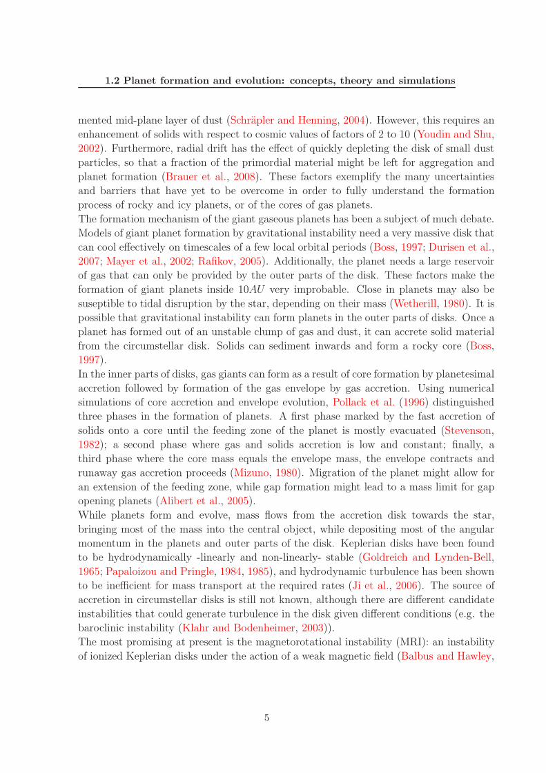
1.1 Minimum mass vs. orbital period of exoplanets. The color represents the
orbital eccentricity of the planets. [Figure produced with the exoplanets.org
plotter] . . . . . . . . . . . . . . . . . . . . . . . . . . . . . . . . . . . . . 3
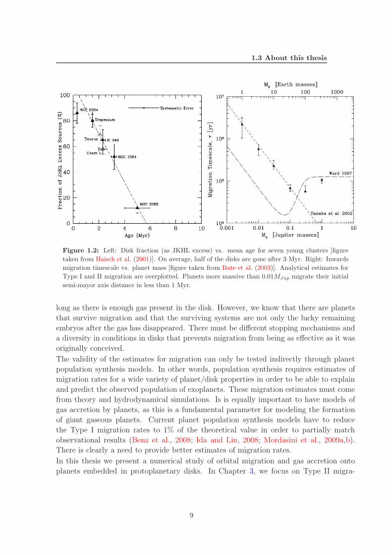
1.2 Left: Disk fraction (as JKHL excess) vs. mean age for seven young clusters
[figure taken from Haisch et al. (2001)]. On average, half of the disks are
gone after 3 Myr. Right: Inwards migration timescale vs. planet mass
[figure taken from Bate et al. (2003)]. Analytical estimates for Type I and
II migration are overplotted. Planets more massive than 0.01MJup migrate
their initial semi-mayor axis distance in less than 1 Myr. . . . . . . . . . . 9
3.1 Disk mass accretion rate measured in the simulations. The analytical esti-
mate M = −3πΣν is shown in the dashed line. . . . . . . . . . . . . . . . . 23
3.2 Cumulative average torques on the planet for varying surface density (where
Σ=Σ0) for ǫ = 0.3 (left) and ǫ = 0.06 (right). From dark to light curves,
Σ0 = 5×10⁻⁶, 1×10⁻⁵, 5×10⁻⁵, 1×10⁻⁴, 5×10⁻⁴, 1×10⁻³ and 3×10⁻³,
respectively. This corresponds to B = (πr2p)Σ/Mp = 0.017, 0.035, 0.17,
0.35, 1.76, 3.53 and 10.6. . . . . . . . . . . . . . . . . . . . . . . . . . . . . 24
3.3 Surface density after 500 orbits for ǫ = 0.3 (left) and ǫ = 0.06 (right).
Initial densities are Σ0 = 5 × 10⁻⁶, 1 × 10⁻⁵, 5 × 10⁻⁵, 1 × 10⁻⁴, 5 × 10⁻⁴,
1 × 10⁻³ and 3 × 10⁻³. . . . . . . . . . . . . . . . . . . . . . . . . . . . . 25
3.4 Density after 500 orbits for ǫ = 0.3 (left) and ǫ = 0.06 (right). The initial
density is Σ0 = 5 × 10⁻⁴ for both cases. . . . . . . . . . . . . . . . . . . . . 26
3.5 Dependence of the cumulative average torque on the B = (πr2pΣ)/Mp pa-
rameter (where Σ=Σ0) for ǫ = 0.3 (left) and ǫ = 0.06 (right). The dashed
line shows the analytical expression Γ = −(3/4)ν0Ωp (Eq. 3.4). The dash-
dotted line shows the analytical expression Γ = −(3/2π)ν0ΩpB (Eq. 3.6). . 27
vii

LIST OF FIGURES
3.6 Cumulative average torques on the planet for varying surface density, ex-
cluding (left) and including (right) the contribution of the Hill sphere on
the orbital evolution. From dark to light curves, Σ0 = 5 × 10⁻⁶, 1 × 10⁻⁵,
5 × 10⁻⁵, 1 × 10⁻⁴, 5 × 10⁻⁴, 1 × 10⁻³ and 3 × 10⁻³, respectively. This
corresponds to B = (πr2p)Σ/Mp = 0.017, 0.035, 0.17, 0.35, 1.76, 3.53 and
10.6. . . . . . . . . . . . . . . . . . . . . . . . . . . . . . . . . . . . . . . . 28
3.7 Planet position for varying surface density, excluding (left) and including
(right) the contribution of the Hill sphere on the orbital evolution. From
dark to light curves, Σ0 = 5× 10⁻⁶, 1× 10⁻⁵, 5× 10⁻⁵, 1× 10⁻⁴, 5× 10⁻⁴,
1×10⁻³ and 3×10⁻³, respectively. This corresponds to B = (πr2p)Σ/Mp =
0.017, 0.035, 0.17, 0.35, 1.76, 3.53 and 10.6. . . . . . . . . . . . . . . . . . . 29
3.8 Dependence of the cumulative average torque on the B = (πr2pΣ)/Mp pa-
rameter, excluding (left) and including (right) the contribution of the Hill
sphere on the orbital evolution. The dashed line shows the analytical ex-
pression Γ = −(3/4)ν0Ωp (Eq. 3.4). The dash-dotted line shows the ana-
lytical expression Γ = −(3/2π)ν0ΩpB (Eq. 3.6). . . . . . . . . . . . . . . . 30
3.9 Left: Dependence of the cumulative average torque (taking last value at
1500 orbital periods) on the surface density exponent a parameter (where
Σ=Σ0r−a and ν = ν0r
a), for two different values of the surface density
constant Σ0. Right: Surface density after 1500 orbital periods of the planet
for each profile. . . . . . . . . . . . . . . . . . . . . . . . . . . . . . . . . . 31
3.10 Left: Cumulative average torques on the planet for varying viscosity (ν =
1 × 10⁻⁶, 1 × 10⁻⁵, 1 × 10⁻⁴ and 1 × 10⁻³). Right: Torques vs kinematic
viscosity ν. . . . . . . . . . . . . . . . . . . . . . . . . . . . . . . . . . . . 32
3.11 Left: Accretion rate of gas onto the planet for different disk surface densi-
ties. Right: Cumulative mass accreted by the planet. From dark to light
curves, Σ0 = 5× 10⁻⁶, 1× 10⁻⁵, 5× 10⁻⁵, 1× 10⁻⁴, 5× 10⁻⁴, 1× 10⁻³ and
3 × 10⁻³, respectively. . . . . . . . . . . . . . . . . . . . . . . . . . . . . . 33
3.12 Accretion rates onto the planet as a function of surface density. . . . . . . 33
3.13 Left: Cumulative torques vs time for different densities. From dark to light
curves, Σ0 = 5 × 10⁻⁶, 1 × 10⁻⁵, 5 × 10⁻⁵, 1 × 10⁻⁴, 5 × 10⁻⁴, 1 × 10⁻³
and 3 × 10⁻³, respectively. Right: Dependence of the cumulative average
torque on the B = (πr2pΣ)/Mp parameter for an accreting planet. The
dashed line shows the analytical expression Γ = −(3/4)ν0Ωp (Eq. 3.4).
The dash-dotted line shows the analytical expression Γ = −(3/2π)ν0ΩpB
(Eq. 3.6). . . . . . . . . . . . . . . . . . . . . . . . . . . . . . . . . . . . . 34
viii
LIST OF FIGURES
3.14 Mass flux ρ(rp)vr(rp), averaged in time and in the azimuthal direction at
the position of the planet. The mass flux is shown for simulations with
a fixed orbit planet (stars), a free moving planet (diamonds) and a free
moving and accreting planet (crosses). The blue symbols denote positive
values of the mass flux. . . . . . . . . . . . . . . . . . . . . . . . . . . . . . 35
4.1 Initial radial distribution of the time, azimuthally and vertically averaged
stress parameter (before the addition of the potential of the planet). The
dashed and dashed-dot lines show the Reynolds TRey and Maxwell TMax
stresses respectively, normalized by the initial pressure. The solid line
shows the total effective α parameter. . . . . . . . . . . . . . . . . . . . . . 43
4.2 Time evolution of Bφ, B2/B20 and α for a run without a planet. The dashed
and dashed-dotted lines show the Reynolds TRey and Maxwell TMax stresses
respectively, normalized to the initial pressure. The solid line shows the
total effective α parameter. . . . . . . . . . . . . . . . . . . . . . . . . . . . 44
4.3 Top figure: Time-averaged thermal and magnetic pressure in the mid-plane
(black line) and one scale height above the mid-plane (red line). The profiles
have been normalized to take out the radial variation. Bottom figure:
Azimuthal velocity perturbation (with respect to Keplerian speed) in the
mid-plane (black line) and one scale height above the mid-plane (red line).
This is from a simulation with no planet included. . . . . . . . . . . . . . 45
4.4 Logarithm of the disk density in the mid plane (top row) and in an az-
imuthal cut at the position of the planet (bottom row) for runs R2 (left,
q = 10−5), R5 (middle, q = 10−4) and R9 (right, q = 10−3). . . . . . . . . . 47
4.5 Cumulative average torque for run R1 for q = 5 × 10⁻⁶. The red and blue
lines show the torque exerted by the inner and outer disk respectively. . . . 48
4.6 Cumulative average torque for runs R2 and R3, for q = 10−5,where the
planet is located at rp = 3.3 and rp = 5.0 respectively. The red and blue
lines show the torque exerted by the inner and outer disk, respectively. . . 48
4.7 Power spectrum of the surface density, averaged in time and azimuthally,
from MHD simulation (stars). We compare with the power spectrum that
results from the turbulent model of Baruteau and Lin (2010) used in HD
simulations, with (triangles) and without (crosses) the cutoff of the modes
with m > 6, and with effective α ∼ 10−3. . . . . . . . . . . . . . . . . . . . 49
4.8 Cumulative average torque for run R4 for q = 5 × 10⁻⁵. The red and blue
lines show the torque exerted by the inner and outer disk respectively. . . . 52
4.9 Cumulative average torque for runs R5 and R6, for q = 10−4, where the
planet is located at rp = 3.3 and rp = 5.0 respectively. The red and blue
lines show the torque exerted by the inner and outer disk, respectively. . . 53
ix

LIST OF FIGURES
4.10 Cumulative average torque for run R7 for q = 10−4, for the planet located
at rp = 4.0, initially at the right side of a pressure bump. The red and blue
lines show the torque exerted by the inner and outer disk respectively. . . . 54
4.11 Cumulative average torque for run R8 for q = 2 × 10⁻⁴. The red and blue
lines show the torque exerted by the inner and outer disk respectively. . . . 55
4.12 Surface density at different times in the simulation. Top, middle and bot-
tom plot show the surface density for runs R2, R5 and R9 respectively.
The vertical lines shows the position of the planet and the extent of the
Hill radius. . . . . . . . . . . . . . . . . . . . . . . . . . . . . . . . . . . . . 56
4.13 Time evolution of the stresses in a disk with an embedded planet. Top,
middle and bottom plot show the stresses for runs R2, R5 and R9, respec-
tively. The dashed and dashed-dotted lines show the Reynolds TRey and
Maxwell TMax stresses, respectively, normalized to the initial pressure. The
solid line shows the total effective α parameter. . . . . . . . . . . . . . . . 57
4.14 Cumulative average torque for run R9 for q = 10−3. The red and blue
lines show the torque exerted by the inner and outer disk respectively. The
torque coming from the Hill sphere has been excluded from the calculation. 58
4.15 Radial distribution of the time, azimuthally and vertically averaged stress
parameter for run R9. The dashed and dashed-dot lines show the Reynolds
TRey and Maxwell TMax stresses respectively, normalized by the initial pres-
sure. The solid line shows the total effective α parameter. . . . . . . . . . . 59
4.16 Gap comparison for run R9 (q = 10−3) and run 10, an equivalent HD
simulation with α = 2 × 10⁻³. . . . . . . . . . . . . . . . . . . . . . . . . . 60
4.17 Specific torque as a function of q = Mp/Ms. The black symbols correspond
to simulations R1, R2, R4, R5, R8 and R9, where the position of the planet
is rp = 5.0. The red symbols correspond to simulations R3 and R6, where
the position of the planet is rp = 3.3. In the q = 5 × 10⁻⁶ to q = 2 × 10⁻⁴
mass range, we overplot the analytical estimates for the torque, taking
into account only the Lindblad contribution Γtot = ΓLind (dotted line) and
both the Lindblad plus the unsaturated horseshoe drag Γtot = ΓLind + ΓHS
(dash-dotted line), for both positions (i.e. local surface density profiles) of
the planet, rp = 5.0 (black line) and rp = 3.3 (red line). For the analytical
expressions of the torque, we take the half-width of the horseshoe region
to be 5% larger than its analytical estimate. The dashed line corresponds
to the constant Type II migration rate, given by the viscous transport in
the disk, using α = 2 × 10⁻³. Error bars represent the standard deviation
of the torque time distribution. . . . . . . . . . . . . . . . . . . . . . . . . 61
x
LIST OF FIGURES
5.1 Initial conditions before the planet starts accreting for the laminar disk
simulations and the MHD simulation. The gap in the MHD simulation is
found to be wider as compared to all the viscous simulations. . . . . . . . 68
5.2 Density in the surface of the Hill sphere for the viscous laminar runs with
α = 2 × 10⁻³(left) and α = 2 × 10⁻⁴(right). The density is shown in units
of 2 × 10⁻¹⁰grcm−3. The center of the ellipse corresponds to the point in
the Hill sphere that is most distant from the star and points away in the
radial direction. . . . . . . . . . . . . . . . . . . . . . . . . . . . . . . . . . 70
5.3 Density in the surface of the Hill sphere for the viscous laminar run with
α = 2 × 10⁻⁵(left) and for the turbulent run(right). The density is shown
in units of 2 × 10⁻¹⁰grcm−3. The center of the ellipse corresponds to the
point in the Hill sphere that is most distant from the star and points away
in the radial direction. . . . . . . . . . . . . . . . . . . . . . . . . . . . . . 70
5.4 Mass flux through the surface of the Hill sphere for the viscous laminar
runs with α = 2 × 10⁻³(left) and α = 2 × 10⁻⁴(right). The mass flux is
given in units of MJyr−1S−1, where quantity S is the area of the grid cell
given by S = r2h∆θRH∆φRH . The center of the ellipse corresponds to the
point in the Hill sphere that is most distant from the star and points away
in the radial direction. . . . . . . . . . . . . . . . . . . . . . . . . . . . . . 71
5.5 Mass flux through the surface of the Hill sphere for α = 2× 10⁻⁵(left) and
for the turbulent run(right). The mass flux is given in units of MJyr−1S−1,
where quantity S is the area of the grid cell given by S = r2h∆θRH∆φRH .
The center of the ellipse corresponds to the point in the Hill sphere that is
most distant from the star and points away in the radial direction. . . . . . 71
5.6 Vertical structure of the mass inflow ρvinflow into the Hill sphere. The co-
ordinate θRH refers to the polar angle in the frame of the planet. The quan-
tity ρvinflow has been azimuthaly averaged (with respect to the Hill sphere).
The quantity S is the area of the grid cell given by S = r2h∆θRH∆φRH . . . 72
5.7 Mass accretion rate for the three viscous simulations and the magnetized
simulation. The red line corresponds to α = 2 × 10⁻⁵, green line to α =
2 × 10⁻⁴, and black line to α = 2 × 10⁻³. The yellow line shows the MHD
case. The colored dashed lines show the mean value of each simulation. . . 73
5.8 Cumulative mass accreted by the planet for the three viscous simulations
and the magnetized simulation. The solid line corresponds to α = 2×10⁻³,
dotted line to α = 2 × 10⁻⁴, and dashed line to α = 2 × 10⁻⁵. The dash-
dotted line shows the MHD case. . . . . . . . . . . . . . . . . . . . . . . . 74
5.9 Left: Radial mass flux for the different runs. Right: Pressure for the
different runs. The dashed line shows the magnetic pressure (multiplied by
a factor of 150) for the magnetized case. . . . . . . . . . . . . . . . . . . . 75
xi
LIST OF FIGURES
5.10 Left:Density (in units of 10−12grcm−3) in the mid-plane for the laminar
viscous simulation with α = 2 × 10⁻³. Right: Radial velocity (in units of
vk(1AU)) in the mid-plane for the same simulation. The overplotted vector
field shows the velocity field in the mid-plane. . . . . . . . . . . . . . . . . 75
5.11 Left:Density (in units of 10−12grcm−3) in the mid-plane for the MHD sim-
ulation. Right: Radial velocity (in units of vk(1AU)) in the mid-plane for
the MHD simulation. The overplotted vector field shows the velocity field
in the mid-plane. . . . . . . . . . . . . . . . . . . . . . . . . . . . . . . . . 76
5.12 Magnetic pressure in the mid-plane for the MHD simulation. The over-
plotted vector field shows the velocity field in the mid-plane. . . . . . . . 76
5.13 Mass accretion rates by the planet for different values of α(crosses) and the
turbulent run (square and dotted line). The diamond symbols show the
accretion rate M = 3πνΣ calculated using the unperturbed density, while
the triangle symbols show the accretion rate calculated using the mean
density inside the gap region. . . . . . . . . . . . . . . . . . . . . . . . . . 78
A.1 Left: Semi-mayor axis vs time for 50 massless particles (position signaled
by color). Right: Fractional change in semi-mayor axis vs time. Particles
undergo a diffusion process in small scales. . . . . . . . . . . . . . . . . . 85
A.2 Left: Cumulative torque on the 50 massless particles. Right: Histogram of
the cumulative torque at the end of the simulation (after 150 orbits). . . . 85
xii
List of Tables
3.1 Simulations parameters and measured gas accretion rates onto the planet. . 30
4.1 Simulation Parameters . . . . . . . . . . . . . . . . . . . . . . . . . . . . . 42
xiii

LIST OF TABLES
xiv
1
Introduction
1.1 Context
The natural history of the earth and the origin and formation of our solar system are two
of the most fundamental scientific questions of modern times. Tremendous progress and
understanding has been achieved in this field in the last century. Improbable and incorrect
theories of solar system formation have given way to a mature and comprehensive theory
of planet formation by accretion of solid material and eventually gas, in a circumstellar
disk of gas and dust revolving around an early accreting Sun.
The field of planet formation, which has had its main focus on the solar system, has become
much more exciting and complex, as hundreds of new planetary systems were discovered
in the last decade, and new ones are constantly being added to the list (see Figure 1.1).
Preconceived ideas were challenged with the great diversity of systems observed, with the
discovery of Jupiter mass planets closer to their parent star than Mercury is to the Sun, of
tightly packed multi-planet systems, of free-floating giant planets, of bloated giants and
super Earths. Focus shifted to a theory of planet formation that is capable of explaining
such diversity, and why the solar system is similar, or why it differs from other planetary
systems.
Any theory that attempts to explain the observed diversity in systems has to include
many different elements such as the possibility of gaseous planet formation by gravita-
tional instability in the outer parts of massive disks, or the excitation of eccentricity and
inclination of close-in planets in systems with an outer massive companion due to the
Kozai mechanism, or a history of planet migration that produces Jupiter-mass planets at
small separations. These elements might not have been all present in the formation of the
solar system, but they have become much more relevant in explaining a great number of
the observed extrasolar planets.
Ultimately, a comprehensive theory of planet formation must be linked to stellar formation
1
1. INTRODUCTION
history and must be able to explain features of individual systems as well as general
population characteristics, where diversity in outcome results from a diversity in initial
conditions.
While currently the general structure of such a theory is in place, focus has shifted from
the idea of a grand theory, to explaining and describing in detail the multiple processes in-
volved in the formation of planetary systems. There are many unresolved key issues along
the way, due to the complexity and scales involved. These include the centimeter and me-
ter barrier to planetesimal formation, the fast inwards migration of planets, the source of
accretion in disks, and the size distribution and composition of dust grains, among others.
It is not theoretically or computationally feasible to form a planetary system from begin-
ning to end, although methods like planet population synthesis are capable of gathering
a number of elements, and study the interplay of these and the evolution of planetary
systems during Gyrs timescales. Additionally, global three-dimensional numerical simula-
tions of protoplanetary disks have reached unprecedented resolutions, making it possible
to elucidate the nature of important non-linear processes and instabilities that might be
present in disks, such as the baroclinic instability, the well studied magneto-rotational
instability, or the nature of planet-disk interactions.
1.2 Planet formation and evolution: concepts, theory and sim-
ulations
Early theories of solar system formation considered many different scenarios. One branch
of early theories postulated a disjunct formation of the Sun and the planets (Jeans, 1931).
In this branch, the Sun was proposed to be formed and established in its current main se-
quence state before the formation of the planets (Lissauer, 1993; Ter Haar, 1967; Williams
and Cremin, 1968).
One possibility was the formation of the planets out of solid and gas material ejected from
the Sun as a result of a perturbation by a near-by passing star (Chamberlin, 1901; Jeans,
1931; Jeffreys and Moulton, 1929; Moulton, 1905). The ejected solid material was called
planetesimals and is the origin of the terminology used currently. Filaments of stellar
material would be tidally formed around the Sun, followed by the condensation of the
filaments into the planets at different separations from the Sun. This theory was later
discarded when it was demonstrated that the terrestial planets were not massive enough
to condense out of filament material, and the timescales for formation of the giant planets
were of the order the lifetime of the solar system, due to very large cooling timescales
(Lyttleton, 1940; Nolke, 1932; Spitzer, 1939).
Another possibility was the formation of the planets out of a captured interstellar cloud
by the Sun, that later condensed into planets (Berlage, 1968). The cloud was apriori
2

1.2 Planet formation and evolution: concepts, theory and simulations
Figure 1.1: Minimum mass vs. orbital period of exoplanets. The color represents the orbital
eccentricity of the planets. [Figure produced with the exoplanets.org plotter]
assumed to have the right angular momentum to match the solar system distribution and
it would form ringed structures as a result of dissipative processes, which would later
condense into planets. The rings were also predicted to be distributed according to the
Titus-Bode law. The difference in composition was attributed solely to the difference in
temperature in the nebula. In the inner hotter regions only non-volatile material could
condense, forming the terrestial planets (Ter Haar, 1948, 1950).
Theories of cloud capture were later abandoned as the problem of the angular momen-
tum distribution of the solar system remained unsolved. No mechanism was provided to
remove angular momentum from the Sun, and the angular momentum distribution was
always imposed as an initial condition in the cloud, rather than being a result of physical
evolution. Additionally, condensation timescales of the planets by gravitational instability
seemed comparable to the lifetime of the solar system.
Theories where the Sun co-formed with the planets effectively out of the same interstellar
material slowly gained more acceptance and popularity. Circumstellar disks were recog-
nized as natural by-products of the formation of stars out of the colapse of a rotating
molecular cloud and conservation of angular momentum (Cameron, 1962; Hoyle, 1960;
3
1. INTRODUCTION
Terebey et al., 1984). The excess of infrared luminosity in the spectra of low-mass stars
was attributed to heated circumstellar material (dust grains) emitting thermal reprocessed
stellar light (Geisel, 1970; Lada and Adams, 1992; Mendoza V., 1968). These young stel-
lar objects represented the first stages of star formation. In the circumstellar envelope
composed of gas and dust and arranged in a flattened disk structure, planetesimals and
planets could form out of the solid material.
Edgeworth (1949) already postulated an accretion disk around the Sun, where angular
momentum was carried away from the Sun by viscous processes, slowing down the rotation
of the Sun. The source of viscosity was the boundary layer between disk material and
the solar surface. However it was not clear if this provided enough viscosity to support
accretion and carry the necessary amount of angular momentum outwards (Edgeworth,
1962).
With the possibility of grain growth by coagulation and competitive accretion (Baines
and Williams, 1965; Donn and Sears, 1963), timescales for terrestial planet formation
decreased by orders of magnitude, as compared to the case where condensation from a
gas sub-cloud was assumed. The accretion of small particles and grains into a protoplanet
with an atmosphere also allowed for the possibility of energy release by interaction with
particles and of dispersal of light materials (McCrea and Williams, 1965).
The growth of dust particles into aggregates and macroscopic bodies, and their effect
on disk properties has been studied extensively (Alexander, 2008; Birnstiel et al., 2010,
2011; Dullemond and Monnier, 2010; Guttler et al., 2010; Juhasz et al., 2010; Williams
and Cieza, 2011). Dust grows by collisional sticking into larger aggregates, that then be-
come compactified (Dominik and Tielens, 1997). Evidence for grain growth in envelopes of
young stellar objects can be seen in the change in shape of the spectral energy distribution
at long wavelengths (millimeter and sub-millimeter) (Bouwman et al., 2008; Mannings and
Emerson, 1994; Sicilia-Aguilar et al., 2007; Throop et al., 2001). This change is usually
associated with an evolutionary sequence. However, other physical configurations in the
disk, such as a steady state of growth and fragmentation due to turbulent stirring, can
produce a constant supply of small and large grains in long timescales (millions of years)
(Dullemond and Dominik, 2005; Schrapler and Henning, 2004; Weidenschilling, 1984).
Turbulence and composition of the disk will critically affect the processing of heavy ele-
ments such as silicates, iron and PAHs, therefore affecting the optical properties in the
disk (Bouwman et al., 2008; Henning and Meeus, 2009; Henning and Stognienko, 1996;
Hughes and Armitage, 2010; Juhasz et al., 2009). Dust growth will depend on factors
such as sticking efficiency, relative velocities and electric charge. Growth is significantly
hindered for charged grains (Okuzumi, 2009). Additionally, turbulence creates high rel-
ative velocities which disrupts aggregates due to collisional fragmentation (Brauer et al.,
2008; Zsom et al., 2010).
Another possibility to form macroscopic bodies are gravitational instabilities of the sedi-
4
1.2 Planet formation and evolution: concepts, theory and simulations
mented mid-plane layer of dust (Schrapler and Henning, 2004). However, this requires an
enhancement of solids with respect to cosmic values of factors of 2 to 10 (Youdin and Shu,
2002). Furthermore, radial drift has the effect of quickly depleting the disk of small dust
particles, so that a fraction of the primordial material might be left for aggregation and
planet formation (Brauer et al., 2008). These factors exemplify the many uncertainties
and barriers that have yet to be overcome in order to fully understand the formation
process of rocky and icy planets, or of the cores of gas planets.
The formation mechanism of the giant gaseous planets has been a subject of much debate.
Models of giant planet formation by gravitational instability need a very massive disk that
can cool effectively on timescales of a few local orbital periods (Boss, 1997; Durisen et al.,
2007; Mayer et al., 2002; Rafikov, 2005). Additionally, the planet needs a large reservoir
of gas that can only be provided by the outer parts of the disk. These factors make the
formation of giant planets inside 10AU very improbable. Close in planets may also be
suseptible to tidal disruption by the star, depending on their mass (Wetherill, 1980). It is
possible that gravitational instability can form planets in the outer parts of disks. Once a
planet has formed out of an unstable clump of gas and dust, it can accrete solid material
from the circumstellar disk. Solids can sediment inwards and form a rocky core (Boss,
1997).
In the inner parts of disks, gas giants can form as a result of core formation by planetesimal
accretion followed by formation of the gas envelope by gas accretion. Using numerical
simulations of core accretion and envelope evolution, Pollack et al. (1996) distinguished
three phases in the formation of planets. A first phase marked by the fast accretion of
solids onto a core until the feeding zone of the planet is mostly evacuated (Stevenson,
1982); a second phase where gas and solids accretion is low and constant; finally, a
third phase where the core mass equals the envelope mass, the envelope contracts and
runaway gas accretion proceeds (Mizuno, 1980). Migration of the planet might allow for
an extension of the feeding zone, while gap formation might lead to a mass limit for gap
opening planets (Alibert et al., 2005).
While planets form and evolve, mass flows from the accretion disk towards the star,
bringing most of the mass into the central object, while depositing most of the angular
momentum in the planets and outer parts of the disk. Keplerian disks have been found
to be hydrodynamically -linearly and non-linearly- stable (Goldreich and Lynden-Bell,
1965; Papaloizou and Pringle, 1984, 1985), and hydrodynamic turbulence has been shown
to be inefficient for mass transport at the required rates (Ji et al., 2006). The source of
accretion in circumstellar disks is still not known, although there are different candidate
instabilities that could generate turbulence in the disk given different conditions (e.g. the
baroclinic instability (Klahr and Bodenheimer, 2003)).
The most promising at present is the magnetorotational instability (MRI): an instability
of ionized Keplerian disks under the action of a weak magnetic field (Balbus and Hawley,
5
1. INTRODUCTION
1991, 1998). The MRI is active when the field is well coupled to the gas, so it requires a
minimum degree of ionization. This makes the development of the instability dependent
on factors like the distance from the star and from the mid-plane, the temperature and
chemical composition, and external sources of ionization such as cosmic rays (Sano et al.,
2000; Turner and Sano, 2008; Turner et al., 2007). The characteristics of the MRI-dead
zone therefore depend on these factors. In general the upper layers and the outer parts of
the disk will be MRI-active, therefore turbulent, while the mid-plane will remain stable
(Dzyurkevich et al., 2010; Fleming and Stone, 2003; Machida et al., 2000).
The development of new numerical methods and codes (Mignone et al., 2007; Stone et al.,
2008; Stone and Norman, 1992), along with access to supercomputers, has allowed an
enormous amount of work to arise using numerical MHD simulations of magnetized disks.
In particular, the linear growth and saturation level of the instability have been studied
extensively (Davis et al., 2010; Fleming and Stone, 2003; Flock et al., 2011; Fromang and
Papaloizou, 2007; Fromang et al., 2007; Guan et al., 2009; Hawley et al., 1995, 1996; Sano
et al., 2004; Sharma et al., 2006; Stone et al., 1996; Stone and Pringle, 2001; Wardle,
1999), along with the characterization of the dead zone using resistive simulations that
calculate a self-consistent ionization profile (Sano et al., 2000; Turner and Sano, 2008).
Of particular interest to planet formation are the studies on dust stirring above the mid-
plane by turbulent eddies and high relative velocities that hinder coagulation (Johansen
and Klahr, 2005; Turner et al., 2010, 2007). Also relevant is dust trapping in the edge
of the dead zone that could provide a place for rapid particle accumulation (Dzyurkevich
et al., 2010; Kretke and Lin, 2007). MHD structures in an MRI-turbulent flow can also
increase the effectiveness of particle trapping in regions of over pressure (Johansen et al.,
2006, 2007, 2009)
As cores are formed in these turbulent accretion disks, there is a point where the mass
of the planet is large enough so that gravitational forces between the disk and the planet
become important. The theory of periodical perturbations in disks (such as the potential
of an orbiting planet) had been developed in the field of galaxy spiral arms long before
it had its application in planet-disk interactions (Goldreich and Tremaine, 1979; Lin and
Shu, 1966; Shu, 1970). The planet excites density waves in the disk that propagate away
from itself. Due to gravitational torques exerted on the planet by the gas, the planet can
move radially. The speed and direction of motion depend on the planet mass and on disk
properties like the surface density and viscosity (Bate et al., 2003; Papaloizou and Lin,
1984; Tanaka et al., 2002; Ward, 1997). For standard disk parameters, migration leads to
a fast reduction of the separation between planet and star (Tanaka et al., 2002). Planets
comparable to Earth or more massive migrate inwards in timescales that are comparable
to the disk lifetime (see Figure 1.2). However, many mechanisms have been put forward
to prevent or slow down rapid inwards migration (Masset, 2002; Masset et al., 2006b;
Paardekooper and Papaloizou, 2009a; Thommes and Murray, 2006).
6
1.2 Planet formation and evolution: concepts, theory and simulations
Models of planet formation processes were put to the test as hundreds of new extrasolar
planets were discovered in the last decade (see Figure 1.1). The radial velocity method
provided the first large population of discovered planets: close in massive giants that pro-
duce large RV signals in the spectra of the parent star, allowing for estimation of orbital
parameters and a minimum value of the planet mass (Marcy et al., 2005; Santos et al.,
2003; Udry and Santos, 2007). Giant planets were found to be common around stars with
higher metalicities (for solar type stars)(Udry and Santos, 2007; Vauclair, 2004), suggest-
ing a possible signature of a more efficient formation by core accretion (Johnson et al.,
2010). Massive planets were found to clump at short separations, with periods around 3
days, pointing to a history of inwards migration and a common stopping mechanism close
to the star, such as the stellar magnetosphere boundary or an inner cavity in the disk
(Cumming et al., 1999; Udry et al., 2003). However, in-situ formation of close in planets
has been found to be possible in some cases (Bodenheimer et al., 2000).
A big surprise was the large range of eccentricities in the population of exoplanets (see
Figure 1.1). Contrary to the solar system, exoplanets were found to have a almost a
full range of eccentricities, similar to the one found in stellar multiple systems (Shen and
Turner, 2008; Udry and Santos, 2007). Planet-planet scattering has been proposed to
explain highly eccentric planets, as it would dominate the dynamics after the gas is no
longer present (since the gas tends to damp eccentricity) and therefore shape the final
configuration of a system (Ford and Rasio, 2008). Small-period solid planets (rock plus
ice) in close-in orbits are predicted to have low eccentricities due to tidal circularization
(Juric and Tremaine, 2008; Nagasawa et al., 2008; Rasio and Ford, 1996).
Another detection technique, the transit method, brings the possibility of obtaining the
radius of the planet, by studying the dimming of the stellar brightness due to a planet
passing in front of the star through the line of sight (Borucki and Summers, 1984). To-
gether with the RV method, candidates can be confirmed and the mean density of the
planet can be obtained with the mass and radius information. Hundreds of candidates
have been found by the KEPLER (Koch et al., 1998) and COROT (Leger et al., 2009)
space missions, which include many Neptune analogs and super earths, possibly in the
habitable zone of their parent star (Batalha et al., 2011; Gilliland et al., 2010; Howard
et al., 2010).
The transit of planets provides the unique opportunity to study the absorption spectra
of the atmosphere of a planet or the presence of moons (Ballester et al., 2007; Charbon-
neau et al., 2005; Pont et al., 2008; Richardson et al., 2007). Additionally, the Rossiter-
MacLaughlin effect (the displacement of the stellar spectral lines due to stellar rotation
during a transit) makes it possible to obtain the inclination of the orbit of the transiting
planet, a parameter that provides much insight into the formation mechanism (Fabrycky
and Winn, 2009; Gaudi and Winn, 2007).
An interesting subset of the exoplanet population are the so called bloated giants, which
7
1. INTRODUCTION
are unusually high-up in the mass-radius diagram of planets; planet structure models
predict smaller radii for planets of equivalent masses (Howard et al., 2010). Tidal heating
has been proposed as the main inflating mechanism (Ibgui and Burrows, 2009; Miller
et al., 2009; Ogilvie and Lin, 2004), although tidal effects are not sufficient for explaining
the largest of the inflated planets (Leconte et al., 2010). Magnetic effects such as Ohmic
dissipation could account for a fraction of the necessary thermal energy to produce the
inflation in radius (Batygin and Stevenson, 2010).
Other planet detection methods like microlensing or direct imaging can detect planet
in previously unexplored parts of the planetary mass-separation diagram, although with
much lower yield compared to the RV or transit method. Microlensing is capable of finding
very low-mass planets, but follow up and characterization are not possible (Beaulieu et al.,
2006; Bennett and Rhie, 1996; Gould and Loeb, 1992; Mao and Paczynski, 1991). Direct
imaging can detect large period, young planets in the infrared thermal light, although
it is an extremely challenging method due to the typical contrast of over six orders of
magnitude between the star and the planet (Angel, 1994; Kalas et al., 2005; Lafreniere
et al., 2008; Thalmann et al., 2009). However, both of these methods provide interesting
testing grounds for formation models in the outer parts of the disk, specially of planets
formed by gravitational instability (Veras et al., 2009).
Making sense of the multitude of data of extrasolar planets and comparing to theoretical
models is a difficult task. Planet population synthesis models combine observational
constraints with theoretical elements to create synthetic populations of individual planets
forming and evolving in individual disks with diverse initial conditions (Mordasini et al.,
2009a). These simulations usually include disk evolution through evaporation, planet
accretion of planetesimals and gas, planet migration, and an adapted stellar structure
model for the planet core and atmosphere. Although planet population synthesis brings
together the uncertainties of each of its elements, it is a powerful tool to understand the
interplay of processes and timescales of formation. Population synthesis has been able to
reproduce key elements of the observed planet population like the metalicity relation and
the presence of close-in giants due to Type II migration. It has also shed light on runaway
accretion processes and their relation to clumps in the mass distribution of exoplanets
(Alibert et al., 2004; Benz et al., 2008; Ida and Lin, 2004; Mordasini et al., 2009b).
1.3 About this thesis
It can be inferred from the population of discovered exoplanets that many systems un-
derwent migration in their evolutionary history. The fact that migration timescales are in
general shorter or on the order of the disk mean lifetime presents a problem for the for-
mation of planetary systems; in theory planet embryos would fall into the central star as
8
1.3 About this thesis
Figure 1.2: Left: Disk fraction (as JKHL excess) vs. mean age for seven young clusters [figure
taken from Haisch et al. (2001)]. On average, half of the disks are gone after 3 Myr. Right: Inwards
migration timescale vs. planet mass [figure taken from Bate et al. (2003)]. Analytical estimates for
Type I and II migration are overplotted. Planets more massive than 0.01MJup migrate their initial
semi-mayor axis distance in less than 1 Myr.
long as there is enough gas present in the disk. However, we know that there are planets
that survive migration and that the surviving systems are not only the lucky remaining
embryos after the gas has disappeared. There must be different stopping mechanisms and
a diversity in conditions in disks that prevents migration from being as effective as it was
originally conceived.
The validity of the estimates for migration can only be tested indirectly through planet
population synthesis models. In other words, population synthesis requires estimates of
migration rates for a wide variety of planet/disk properties in order to be able to explain
and predict the observed population of exoplanets. These migration estimates must come
from theory and hydrodynamical simulations. Is is equally important to have models of
gas accretion by planets, as this is a fundamental parameter for modeling the formation
of giant gaseous planets. Current planet population synthesis models have to reduce
the Type I migration rates to 1% of the theoretical value in order to partially match
observational results (Benz et al., 2008; Ida and Lin, 2008; Mordasini et al., 2009a,b).
There is clearly a need to provide better estimates of migration rates.
In this thesis we present a numerical study of orbital migration and gas accretion onto
planets embedded in protoplanetary disks. In Chapter 3, we focus on Type II migra-
9
1. INTRODUCTION
tion of gap opening planets. Similar studies have been performed to study the migration
and gas accretion of gap opening planets. Edgar (2007) studied migration as a function
of surface density and viscosity. However, no comparison with analytical estimates was
done and they did not present the estimations of the torque as a function of the stud-
ied parameters. Additionally, their results overlap between the gap opening regime and
partial gap opening. Masset and Papaloizou (2003) concentrated on studying runaway
Type III migration, and covered a good range of the parameter space. We perform a
dedicated study of Type II migration as a function of a variety of parameters and provide
a comparison with analytical estimates. We also study the relation between migration
and accretion onto planets, which is critical to obtain the correct migration rates. Our
results are directly applicable to planet population synthesis models
In Chapters 4 and 5, we turn to the more complex problem of migration in turbulent
disks. In most previous numerical and analytical studies, the disk turbulence is included
as an effective viscosity. The disk, however, is technically laminar. One possibility that
has been explored is modeling of the turbulence itself using a perturbing potential. In
this case, the actual stochastic perturbations are reproduced in the density (Adams and
Bloch, 2009; Baruteau and Lin, 2010; Laughlin et al., 2004). Simulations of turbulent disks
where turbulence is generated by weak magnetic fields through the magneto-rotational
instability (MRI) have been performed, under the approximation of a local shear flow, or
a cylindrical geometry (Nelson and Papaloizou, 2003, 2004; Oishi et al., 2007; Papaloizou
and Nelson, 2003; Papaloizou et al., 2004).
We study migration in turbulent disks, with MRI-induced turbulence, in global stratified
disk simulations. This is useful for two reasons. It provies a check for the previous sim-
ulations that have been performed with other approximations, and it provies parameters
derived from ”real” MHD turbulence that can be used in populations synthesis models
and semi-analytical models. We also study the accretion of gas onto giant planets in
MRI-turbulent disks, which has never been studied in the literature before.
10

2
Planet-disk gravitational interactions
Young planets orbiting around a star and embedded in a circumstellar disk will interact
gravitationally with the gas and the dust present in the disk. The dust component is
typically a small fraction ( 0.01) of the gas component, therefore the dynamics of migration
can be understood in terms of the interaction between circumstellar gas and planet. The
effect of the gas on the planet will be to change its separation to the star at a certain rate
and direction, while the planet will modify the density in the disk linearly or non-linearly
depending on the planet mass.
This process will depend on a number of factors: the gravitational torque exerted on the
planet and the gas, the viscous diffusion in the disk, the thermal properties of the disk
and the disk density structure. These factors in turn introduce relevant timescales which
will determine the importance of each factor: the migration timescale τmig, the viscous
timescale τν , the cooling timescale τcool, the orbital timescale τorb and finally the libration
τlib and U-turn timescales τuturn associated with material near corotation 1.
The evolution of the gas under the action of the planet is given by (neglecting magnetic
fields and self-gravity and energy transport)
∂ρ
∂t−∇ · (ρv) = 0 (2.1)
∂v
∂t+ (v · ∇)v = −
1
ρ∇p −∇Φp −∇Φstar + fν (2.2)
(2.3)
where Φp and Φstar are the planet and stellar gravitational potential respectively and fνis the viscous stress tensor. The gas pressure relates to the density through an equation
of state p = p(ρ, T ). The stellar potential is given by Φstar(r) = −GMstar/r, while the
1All these being relevant within the gas disk lifetime
11
2. PLANET-DISK GRAVITATIONAL INTERACTIONS
planet potential is given by
Φp(r) = −GMp
|r − rp|. (2.4)
The torque exerted by the disk on the planet is determined at any moment in time by the
detailed structure of the density resulting from solving system Eq 2.2, and is given by
Γ(r) = GMp
∫
ρ(r)rp × r
|r− rp|3dV. (2.5)
Torque exerted on the planet leads to a change in angular momentum Γ = dL/dt. In
particular, vertical torque leads to a change in orbital angular momentum Γz = dLz/dt =
d(Mprpv′
p)/dt, where v′
p is the velocity of the planet in the orbital plane, equal to the
Keplerian speed v′
p = vKep =√
GMp/rp. Using this expression, the vertical torque Γz is
related to the change in separation rp by
Γz =Mpvk
2rp
. (2.6)
A natural timescale for migration is τm = rp/rp.
2.1 Migration Regimes
2.1.1 Type I: Low-mass planet migration
If a planet doesn’t significantly perturb the disk, the steady state density structure can
be estimated through linear perturbation analysis. Let v0 and p0 be the unperturbed
velocity and pressure. The orbiting planet introduces perturbations v1 and p1 such that
v1 << v0 and p1 << p0. It is possible to define the enthalpy perturbation as η = p1/ρ0.
The perturbed velocity, pressure, enthalpy and gravitational potential of the planet are
fourier-decomposed as
X = ΣmRe[Xmeim(φ−Ωp)], (2.7)
where spherical coordinates (r, θ, φ) are used. Solving Eqs. 2.2 and 2.3, for the fourier
amplitudes Xm of perturbed velocities and enthalpy results in a wave equation for ηm.
The amplitude of the enthalpy wave ηm is found to diverge for two cases: when 4BΩ −
m2(Ω − Ωp)2 = 0 and when Ω − Ωp = 0. The first case occurs at positions rm in the disk
where 4BΩ(rm) = m2(Ω(rm) − Ωp), where B is the Oort’s constant. These locations are
referred to as Lindblad resonances, and are located inside and outside the orbit of the
planet, moving asymptotically towards rp as m increases to infinity. The second divergent
case occurs at the position rc where Ω(rc) = Ωp, which is the corotation resonance. Due
to the pressure gradient, the corotation resonance is offset from the position of the planet
(Lin and Papaloizou, 1986; Tanaka et al., 2002; Ward, 1997).
12

2.1 Migration Regimes
The angular momentum flux carried by the waves, can be approximated as
Fw =
∫ 2π
0
∫
∞
−∞
dφdzr2ρ0v1,φv1,r, (2.8)
which by conservation of angular momentum, will be given to/by the planet in terms of
orbital angular momentum. The effective torque felt by the planet due to this angular
momentum flux is given by
ΓI = −(2.340 − 0.099a + 0.418b)
(
q
hp
)2
Σpr4pΩ2
p, . (2.9)
where q = Mp/Mstar and hp is the pressure scale height of the disk. This is the Type
I migration regime for low-mass planets (Tanaka et al., 2002). This is valid in locally
isothermal disks with power law density profiles, where Σ = Σ0r−a and b is the power law
exponent of the temperature profile.
2.1.2 Type II: Gap-opening planets
As the mass of the planet increases above a certain limit, the perturbations on the disk
density become highly non-linear. The planet opens a partial or full cavity in the disk
density around its orbit, pushing material away from corotation. The limiting mass for
gap opening can be expressed in terms of two criteria: the viscous and the pressure
criteria. In the first case, a condition for gap opening is that the angular momentum
transported by the waves Fw matches or exceeds the angular momentum transported by
viscous processes in the disk Fν . Taking a gaussian profile for the density in the vertical
direction, and writing the dynamic viscosity η in terms of the surface density Σ =∫
ρdz,
the viscous angular momentum flux is
Fν = 3πΣr2Ω. (2.10)
Letting q = Mp/Mstar, and equating Fw = Fv, results in a lower limit for the mass of the
planet given by
q >40ν
Ωr2. (2.11)
The viscosity can be modelled as a turbulent viscosity parameterized by α, where ν =
αΩkH2 and H = cs/Ωk. In this case, the viscous criteria can be expressed as the maximum
value of α that allowes for gap opening
α <q
40
( r
H
)2
. (2.12)
13

2. PLANET-DISK GRAVITATIONAL INTERACTIONS
As a second condition for the planet to open a gap, the Hill radius of the planet must
exceed the pressure scale height rh = (q/3)1/3 > H . This can be expressed as a condition
on the mass of the planet
q > 3
(
H
r
)3
. (2.13)
As opposed to the migration of low-mass planets, where the planet angular momentum
flux can never match the viscous flux in the disk, a large-mass planet that satisfies Eq
2.12 and Eq 2.13 can be in a position in the disk where the wave torque is cancelled out.
This means the planet is stationary in the frame moving radially with the disk at the
viscous rate. In this case, the effective torque on the planet is given by
ΓII = −2π
Mp
(
3
2r2pΩpνΣ
)
(2.14)
This is Type II migration regime for gap opening planets (Bryden et al., 1999; Crida et al.,
2006). The timescale for migration is then the viscous accretion timescale τν = (2r2)/(3ν).
2.1.3 Type III: Intermediate cases
An interesting migration case occurs for intermediate-mass planets (sub-Saturns to Jupiters)
that open a partial gap in the disk. If the disk is massive enough and the gas mass in the
coorbital region is comparable or larger to the mass of the planet, the planet can migrate
inwards in a runaway process. The torque coming from the corotation region can have
a negative contribution due to open streamlines that go from the inner disk to the outer
disk, passing the planet. This torque scales with the radial drift rate of the planet and is
proportional to the mass located in the corotation region (Masset and Papaloizou, 2003).
2.2 Migration in non-isothermal disks
In the case of adiabatic disks, or disks where the temperature structure is allowed to vary
according to the evolution of the density and the stellar flux, low-mass planets can migrate
outwards in certain conditions. A component of the corotation torque that scales with the
entropy gradient (which is not present in locally isothermal disks) can be present in cases
of high opacities or a fully adiabatic disk. This component is positive and can overcome the
negative wave torque, making the planet drift outwards. This effect will usually saturate
(i.e. the torque will go to zero in short timescales) as the entropy gradient is removed
by motions in the horseshoe region. Similar to the vortensity-related corotation torque
that can remain un-saturated due to viscosity, the entropy-related corotation torque can
remain un-saturated due to fast local cooling (Baruteau and Masset, 2008; Kley et al.,
2009).
14
2.3 Corotation Torques
2.3 Corotation Torques
From a frame of reference moving with the planet at an angular frequency Ωp, gas particles
within a certain distance of rp move on horseshoe orbits around the position of the planet.
These gas particles orbit in trajectories that follow equipotential surfaces defined by the
two body-problem, around Lagrangian points. On the side trailing the planet, particles
move radially inwards, while on the leading side they move radially outwards. Each
time a particle executes a U-turn as it makes its closest approach to the planet, its
angular momentum changes. The change in angular momentum with time will determine
the torque exerted on the planet due to particles in horseshow orbits Masset (2002);
Paardekooper and Papaloizou (2009a,b).
The corotation torque can be estimated by calculating the change in angular momentum
of gas particles that move from the outer(inner) disk to the inner(outer) disk , at the
trailing(leading) side of the planet. Assuming particles are matched symmetrically to
either part of the planet as they execute a U-turn, and the half-width xs to be the same
at each side, the total change in angular momentum can be given as a integral over the
half-width of the horseshoe region. For the trailing side, this is given by
∆Lt =
∫ rp
rp+xs
(f(2rp − r) − f(r))dr, (2.15)
while for the leading side this is given by
∆Ll =
∫ rp
rp−xs
(f(2rp − r) − f(r))dr. (2.16)
Here f(r) is the angular momentum of a gas particle at r, an is equal to f(r) = Σ(r)v(r)r.
The net change in angular momentum is then ∆Lt + ∆Ll. The torque can be shown to
scale with the gradient of the vortensity (d/dr)(Σ/w), where w is the vorticity. This effect
will usually saturate (i.e. the torque will go to zero in short timescales) as the vortensity
gradient is removed by motions in the horseshoe region, unless a sufficiently high viscosity
is present (Masset, 2002; Paardekooper and Papaloizou, 2009a,b)
15

2. PLANET-DISK GRAVITATIONAL INTERACTIONS
16

3
Type II migration and gas accretion
onto planets in disks with uniform
constant mass accretion
Using two-dimensional hydrodynamical simulations, we study the orbital migration
and gas accretion of a free-moving planet of mass Mp = 2MJup purely in the stage
where a gap has been cleared in the disk by the planet. The viscosity in the disk is
chosen to obtain a constant mass accretion rate through the entire disk, independent
of time and radial position. We study the effects of various parameters like the
surface density, density power-law exponent, gravitational softening and viscosity.
We find that the torque of the planet is best approximated by the expression Γ =
− 32q
r2νΩpΣ, for a wide range of disk densities. When the local disk mass is around
10 times the planet mass, we observe runaway migration and the planet migrates
inwards much faster than the analytical estimate. Only when the Hill sphere material
is not taken into account in the orbital evolution, or when the planet is accreting,
the migration of the planet is slowed down if it is in the regime where the local
disk mass is larger than the planet mass. The torques exerted on the planet do not
depend on the steepness of the density profile. We also study the accretion of gas
onto the planet, and find that the accretion rate measured in the simulations is a
fraction of the disk accretion rate, and is given by Mp = 3πνΣgap ≈ (0.1)3πνΣ0.
17
3. TYPE II MIGRATION AND GAS ACCRETION ONTO PLANETSIN DISKS WITH UNIFORM CONSTANT MASS ACCRETION
3.1 Introduction
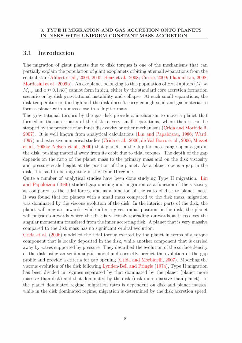
The migration of giant planets due to disk torques is one of the mechanisms that can
partially explain the population of giant exoplanets orbiting at small separations from the
central star (Alibert et al., 2004, 2005; Benz et al., 2008; Currie, 2009; Ida and Lin, 2008;
Mordasini et al., 2009b). An exoplanet belonging to this population of Hot Jupiters (Mp ≈
Mjup and a ≈ 0.1AU) cannot form in situ, either by the standard core accretion formation
scenario or by disk gravitational instability and collapse. At such small separations, the
disk temperature is too high and the disk doesn’t carry enough solid and gas material to
form a planet with a mass close to a Jupiter mass.
The gravitational torques by the gas disk provide a mechanism to move a planet that
formed in the outer parts of the disk to very small separations, where then it can be
stopped by the presence of an inner disk cavity or other mechanisms (Crida and Morbidelli,
2007). It is well known from analytical calculations (Lin and Papaloizou, 1986; Ward,
1997) and extensive numerical studies (Crida et al., 2006; de Val-Borro et al., 2006; Masset
et al., 2006a; Nelson et al., 2000) that planets in the Jupiter mass range open a gap in
the disk, pushing material away from its orbit due to tidal torques. The depth of the gap
depends on the ratio of the planet mass to the primary mass and on the disk viscosity
and pressure scale height at the position of the planet. As a planet opens a gap in the
disk, it is said to be migrating in the Type II regime.
Quite a number of analytical studies have been done studying Type II migration. Lin
and Papaloizou (1986) studied gap opening and migration as a function of the viscosity
as compared to the tidal forces, and as a function of the ratio of disk to planet mass.
It was found that for planets with a small mass compared to the disk mass, migration
was dominated by the viscous evolution of the disk. In the interior parts of the disk, the
planet will migrate inwards, while after a given radial position in the disk, the planet
will migrate outwards where the disk is viscously spreading outwards as it receives the
angular momentum transfered from the inner accreting disk. A planet that is very massive
compared to the disk mass has no significant orbital evolution.
Crida et al. (2006) modelled the tidal torque exerted by the planet in terms of a torque
component that is locally deposited in the disk, while another component that is carried
away by waves supported by pressure. They described the evolution of the surface density
of the disk using an semi-analytic model and correctly predict the evolution of the gap
profile and provide a criteria for gap opening (Crida and Morbidelli, 2007). Modeling the
viscous evolution of the disk following Lynden-Bell and Pringle (1974), Type II migration
has been divided in regimes separated by that dominated by the planet (planet more
massive than disk) and that dominated by the disk (disk more massive than planet). In
the planet dominated regime, migration rates is dependent on disk and planet masses,
while in the disk dominated regime, migration is determined by the disk accretion speed,
18

3.2 Gap opening and type II migration
which significantly slows down migration as compared to Type I rates or Type II in the
planet dominated regime (Armitage, 2007a,b; Syer and Clarke, 1995).
Three-dimensional hydrodynamics calculations have shown that the surface density of
the disk can be correctly modelled using two-dimensional simulations with proper gravi-
tational potential smoothing. The mass of the disk present inside the Roche lobe of the
planet is also critical for the torque determination and can in some cases reverse inwards
migration. Jupiter-mass planets have also been found to be able to accrete very efficiently
through gaps, as compared to the disk mass accretion, although this might depend on
the numerical algorithm used to model planet accretion in a grid numerical code. Addi-
tionally as the planet mass increases above a Jupiter-mass, accretion efficiency decreases.
(Bate et al., 2003; Bryden et al., 1999; Lubow et al., 1999).
Crida and Morbidelli (2007) performed two-dimensional hydrodynamical simulations of
Type II migration coupled with a one-dimensional simulation of a viscously spreading
disk, in order to correctly model the global viscous evolution of the disk. They observed
the effects of the corotation torque for planets that open a partial gap when the disk has
enough viscosity to mantain the torque corotation torque unsaturated. This effect can in
principle slow down or reverse the inwards migration of planets that open partial gaps
(D’Angelo et al., 2005). Edgar (2007) performed a study of migration as a function of disk
mass and viscosity and obtained interesting results on the discrepancy between analytical
estimates of migration in the Type II range and two-dimensional numerical simulations.
In this chapter we revisit the issue of the dependence of Type II migration rates on the
disk mass, and on the disk surface density gradient. We focus on how different numerical
set ups can yield very different results, and how migration rates derived from numerical
simulations compare with analytical models. We also provide estimates of migration rates
in the Type II regime, directly obtained from simulations, that can be used in planet
population synthesis models to more accurately estimate the migration of giant planets.
This chapter is organized as follows. In section 2, we summarize the analytical expressions
for the Type II torque. Section 3 describes the set up of the simulations, the parameters
used and the initial conditions. We also show a test of the numerical scheme to verify
the correct viscous evolution in the disk. In Section 4 we present our results for various
numerical set ups and parameters. Finally, the conclusions of the study are presented in
Section 5.
3.2 Gap opening and type II migration
Planets migrate in the Type II regime when they open a gap in the disk around their orbit.
In this case, the density perturbations induced by the planet can no longer be treated as
linear since the disk density is drastically modified in the gap region. The transition into
19
3. TYPE II MIGRATION AND GAS ACCRETION ONTO PLANETSIN DISKS WITH UNIFORM CONSTANT MASS ACCRETION
this regime is approximately given by the conditions that
(Mp/Ms)(1/(3h3p)) > 1, (3.1)
and
Mp/Ms > 40ν/r2pΩp, (3.2)
meaning that the planet has to be able to overcome both the pressure gradient and the
viscous transport at its given position in the disk (Crida and Morbidelli, 2007; Lin and
Papaloizou, 1986).
After the gap has opened, the torques on the planet cannot consistently move the planet
in the disk, since it can take an equilibrium position inside the gap where the total net
torque is zero instantaneously. This effectively means that the planet is stationary in a
frame moving with the disk, at the viscous rate. One can assume that the giant planet
now moves at the radial velocity given by the equations for the viscous evolution of the
disk, vr = −3ν/2r (Lynden-Bell and Pringle, 1974). This in turn can be integrated to
give the radius of the planet as a function of time
r(t) = (r20 − 3νt)1/2, (3.3)
where r0 is the initial position of the planet at t = 0. The torque felt by the planet at a
given location, Γ(r) = rvrΩp/2, is then given by
Γ = −3
4νΩp. (3.4)
However this expression is not correct for a broad range of disk to planet mass ratios. The
expression can be modified to take into account this variation. In this case, the radial
velocity of the planet is given by vr = −(Ms/Mp)3νΣr, which can be integrated to give
the position of the planet as a function of time
r(t) = r0e−3νΣt/q , (3.5)
which is valid for a = 0 only. Here q = Mp/Ms and r0 is the initial position of the planet.
The time-averaged torque exerted by the disk at a given radial position is then given by
Γ = −3
2qr2νΩpΣ. (3.6)
3.3 Description of the setup of the simulations
We performed the simulations using the Hydrodynamics module of the Godunov code
PLUTO (Mignone et al., 2007). In the code, time stepping is done using a second order
20

3.3 Description of the setup of the simulations
Runge Kutta integrator, while space interpolation is done is done with the second order
linear TVD approximation. For computing the fluxes through the cell interfaces, we use
the HLLC approximate Riemann solver. We work in polar geometry r = (r, φ), where
the computational domain is given by r ∈ [0.4, 4.0] and φ ∈ [0, 2π]. The resolution in the
radial and azimuthal direction is (Nr, Nφ) = (128, 256) and the grid is uniform.
3.3.1 Disk profile and planet setup
The initial surface density profile of the disk is given by
Σ = Σ0r−a. (3.7)
The equation of state of the disk is given by p = csΣ, where cs is the sound speed. The
disk is assumed to be locally isothermal, so that the temperature drops radially as T ∝ r−1
and is constant in time. Hence, the sound speed is given by cs = c0r−0.5 and the effective
pressure scale height of the disk is set to the standard value of cs = h = 0.05. The initial
azimuthal velocity is equal to the Keplerian value corrected by the pressure contribution
vφ =
√
GMs
r(1 − c2
s(a + 1)). (3.8)
The gravitational potential felt by the disk at a location r includes the stellar and plane-
tary contributions, and is given by
Φg(r) = −GMs
|r − rs|−
GMp
(|r − rp|2 + ǫ2)1/2, (3.9)
where r, rs and rp, are the positions of the gas, star and planet respectively, measured from
the center of mass of the star-planet system. Also, ǫ = krhill is the softening parameter
of the potential, to avoid divergent forces on the disk near the planet. The constant k
is less than one. The ratio between the planet mass and the stellar mass is given by
q = Mp/Ms = 2 × 10⁻³. The initial position of the planet is set to rp = 1.5. The planet
is free to migrate and its equations of motion are integrated using a leap frog integrator.
The simulations are run for 500 or 1500 periods of the planet.
The z component of the torque Γ exerted by the disk on the planet is given by
Γz = GMp
∫
Σ(r)(rp × r)z
(|r − rp|2 + ǫ2)3/2dA, (3.10)
where (rp×r)z = (rp×r)·ez , with ez being the cartesian unit vector in the z direction. The
torque is calculated for every timestep of the hydro code. We work in normalized units,
where GMs = 1 and positions and velocities are normalized to r0 = 1 and vk(r0) = 1. We
21
3. TYPE II MIGRATION AND GAS ACCRETION ONTO PLANETSIN DISKS WITH UNIFORM CONSTANT MASS ACCRETION
note that all torques in the following sections are negative quantities presented as absolute
values
The kinematic viscosity ν is in general radially varying with a power law and is given by
ν = ν0ra, where a is the radial exponent of the surface density in Equation 3.7. We take
this form of the viscosity so that for all of the simulations, the disk mass accretion rate
M ∼ 3πνΣ is radially constant.
3.3.1.1 Parameters of the simulations
We study migration rates both as a function of the radial exponent a of the surface density
(where ν = ν0ra ) and as a function of surface density and viscosity. In simulations that
vary the radial exponent, the surface density is constant Σ0 = 1 × 10⁻⁴. The radial
exponent is varied for the values a = 0.0, 0.5, 1.0 and 1.5. In simulations that vary
the surface density, we choose values in a large range, from local disk mass very small
compared to the planet mass, to local disk mass larger than planet mass. Here the
radial exponent is fixed to a = 0. The surface density constant is varied for the values
Σ0 = 5 × 10⁻⁶, 1 × 10⁻⁵, 5 × 10⁻⁵, 1 × 10⁻⁴, 5 × 10⁻⁴, 1 × 10⁻³ and 3 × 10⁻³.
3.3.2 Test of the viscous evolution of the disk
Since migration speeds of gap-opening planets are critically dependent on the disk viscous
evolution, it’s necessary to correctly model this evolution numerically. Figure 3.1 shows
the mass accretion rate measured in simulations with no planet included, for different
values of the surface density and a = 0. We have implemented boundary conditions that
set the velocity of the flow at each radial boundary to that determined by the analytical
expression for the constant mass accretion rate for each value of the surface density. This
ensures a constant flow of mass through the disks that matches well with the expected
value resulting from theory. The density profile is not modified up to more than a few
percent of its initial value (only close to the boundaries) and the disk achieves a steady
state.
3.4 Results
3.4.1 Dependence of migration on surface density
In this section, we study the Type II migration regime of giant planets for a range of
disks density. First we present the results for the case when the planet is not allowed to
migrate, and then the results in the case when the planet is allowed to move radially.
For a planet mass of q = Mp/Ms = 2 × 10⁻³, we followed the evolution of the orbital
elements and the torque experienced by the planet over 1500 orbits (or 500 orbits for a
22
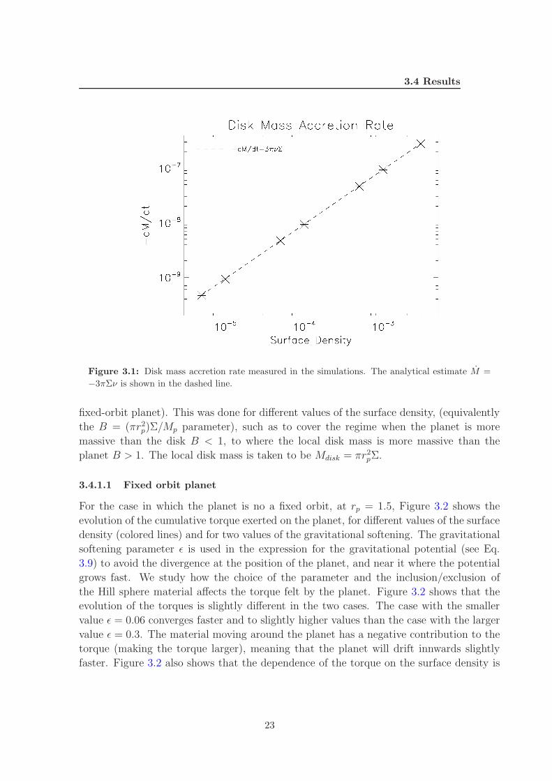
3.4 Results
Figure 3.1: Disk mass accretion rate measured in the simulations. The analytical estimate M =
−3πΣν is shown in the dashed line.
fixed-orbit planet). This was done for different values of the surface density, (equivalently
the B = (πr2p)Σ/Mp parameter), such as to cover the regime when the planet is more
massive than the disk B < 1, to where the local disk mass is more massive than the
planet B > 1. The local disk mass is taken to be Mdisk = πr2pΣ.
3.4.1.1 Fixed orbit planet
For the case in which the planet is no a fixed orbit, at rp = 1.5, Figure 3.2 shows the
evolution of the cumulative torque exerted on the planet, for different values of the surface
density (colored lines) and for two values of the gravitational softening. The gravitational
softening parameter ǫ is used in the expression for the gravitational potential (see Eq.
3.9) to avoid the divergence at the position of the planet, and near it where the potential
grows fast. We study how the choice of the parameter and the inclusion/exclusion of
the Hill sphere material affects the torque felt by the planet. Figure 3.2 shows that the
evolution of the torques is slightly different in the two cases. The case with the smaller
value ǫ = 0.06 converges faster and to slightly higher values than the case with the larger
value ǫ = 0.3. The material moving around the planet has a negative contribution to the
torque (making the torque larger), meaning that the planet will drift innwards slightly
faster. Figure 3.2 also shows that the dependence of the torque on the surface density is
23
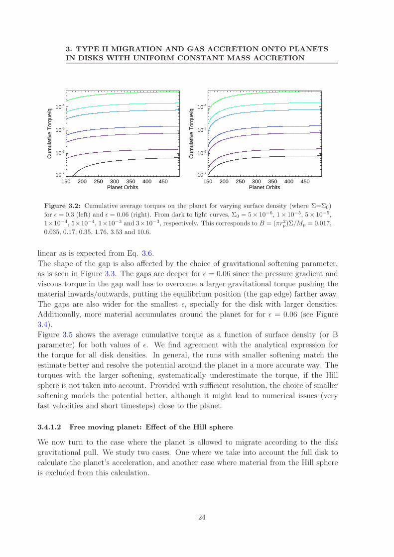
3. TYPE II MIGRATION AND GAS ACCRETION ONTO PLANETSIN DISKS WITH UNIFORM CONSTANT MASS ACCRETION
150 200 250 300 350 400 450Planet Orbits
10-7
10-6
10-5
10-4
Cum
ulat
ive
Tor
que/
q
150 200 250 300 350 400 450Planet Orbits
10-7
10-6
10-5
10-4
Cum
ulat
ive
Tor
que/
q
Figure 3.2: Cumulative average torques on the planet for varying surface density (where Σ=Σ0)
for ǫ = 0.3 (left) and ǫ = 0.06 (right). From dark to light curves, Σ0 = 5× 10⁻⁶, 1× 10⁻⁵, 5× 10⁻⁵,
1×10⁻⁴, 5×10⁻⁴, 1×10⁻³ and 3×10⁻³, respectively. This corresponds to B = (πr2
p)Σ/Mp = 0.017,
0.035, 0.17, 0.35, 1.76, 3.53 and 10.6.
linear as is expected from Eq. 3.6.
The shape of the gap is also affected by the choice of gravitational softening parameter,
as is seen in Figure 3.3. The gaps are deeper for ǫ = 0.06 since the pressure gradient and
viscous torque in the gap wall has to overcome a larger gravitational torque pushing the
material inwards/outwards, putting the equilibrium position (the gap edge) farther away.
The gaps are also wider for the smallest ǫ, specially for the disk with larger densities.
Additionally, more material accumulates around the planet for for ǫ = 0.06 (see Figure
3.4).
Figure 3.5 shows the average cumulative torque as a function of surface density (or B
parameter) for both values of ǫ. We find agreement with the analytical expression for
the torque for all disk densities. In general, the runs with smaller softening match the
estimate better and resolve the potential around the planet in a more accurate way. The
torques with the larger softening, systematically underestimate the torque, if the Hill
sphere is not taken into account. Provided with sufficient resolution, the choice of smaller
softening models the potential better, although it might lead to numerical issues (very
fast velocities and short timesteps) close to the planet.
3.4.1.2 Free moving planet: Effect of the Hill sphere
We now turn to the case where the planet is allowed to migrate according to the disk
gravitational pull. We study two cases. One where we take into account the full disk to
calculate the planet’s acceleration, and another case where material from the Hill sphere
is excluded from this calculation.
24
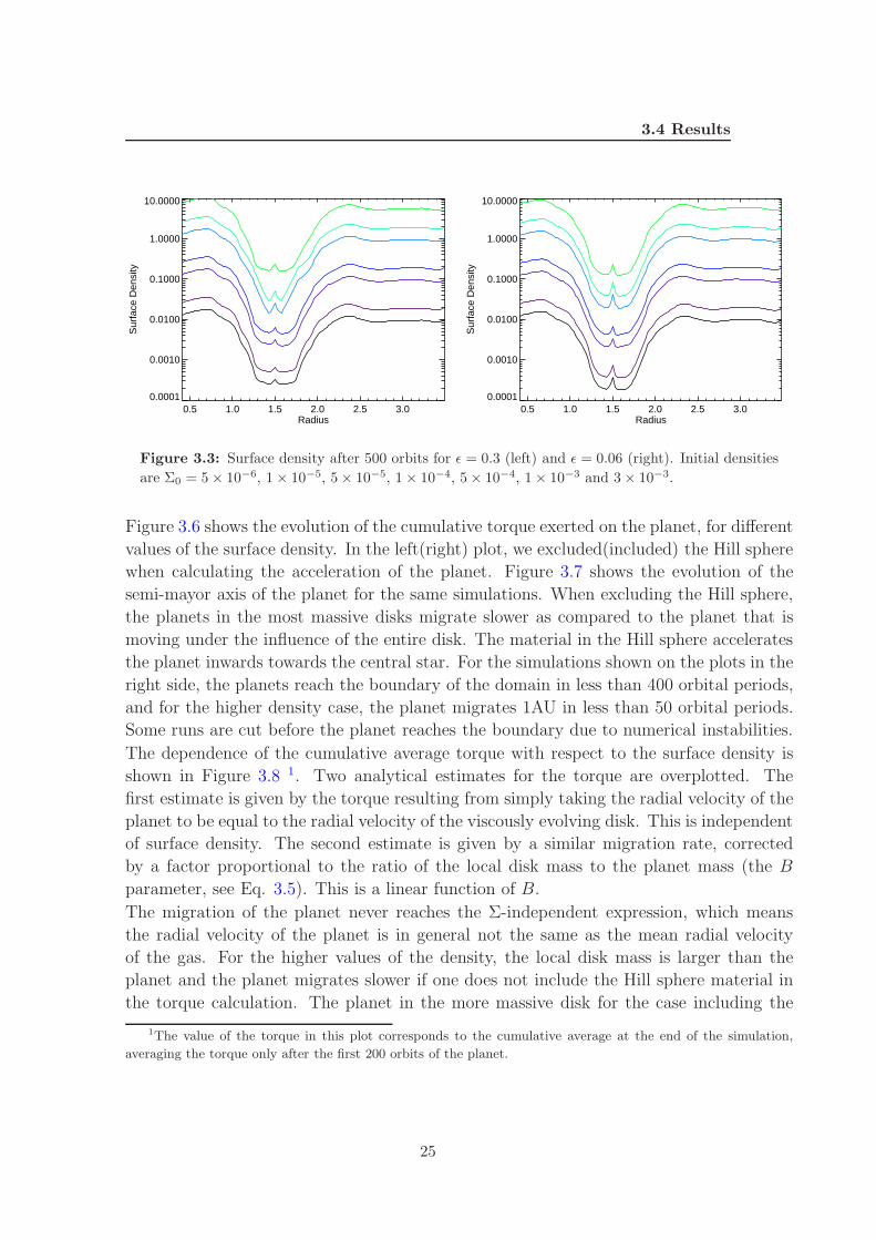
3.4 Results
0.5 1.0 1.5 2.0 2.5 3.0Radius
0.0001
0.0010
0.0100
0.1000
1.0000
10.0000
Sur
face
Den
sity
0.5 1.0 1.5 2.0 2.5 3.0Radius
0.0001
0.0010
0.0100
0.1000
1.0000
10.0000
Sur
face
Den
sity
Figure 3.3: Surface density after 500 orbits for ǫ = 0.3 (left) and ǫ = 0.06 (right). Initial densities
are Σ0 = 5 × 10⁻⁶, 1 × 10⁻⁵, 5 × 10⁻⁵, 1 × 10⁻⁴, 5 × 10⁻⁴, 1 × 10⁻³ and 3 × 10⁻³.
Figure 3.6 shows the evolution of the cumulative torque exerted on the planet, for different
values of the surface density. In the left(right) plot, we excluded(included) the Hill sphere
when calculating the acceleration of the planet. Figure 3.7 shows the evolution of the
semi-mayor axis of the planet for the same simulations. When excluding the Hill sphere,
the planets in the most massive disks migrate slower as compared to the planet that is
moving under the influence of the entire disk. The material in the Hill sphere accelerates
the planet inwards towards the central star. For the simulations shown on the plots in the
right side, the planets reach the boundary of the domain in less than 400 orbital periods,
and for the higher density case, the planet migrates 1AU in less than 50 orbital periods.
Some runs are cut before the planet reaches the boundary due to numerical instabilities.
The dependence of the cumulative average torque with respect to the surface density is
shown in Figure 3.8 1. Two analytical estimates for the torque are overplotted. The
first estimate is given by the torque resulting from simply taking the radial velocity of the
planet to be equal to the radial velocity of the viscously evolving disk. This is independent
of surface density. The second estimate is given by a similar migration rate, corrected
by a factor proportional to the ratio of the local disk mass to the planet mass (the B
parameter, see Eq. 3.5). This is a linear function of B.
The migration of the planet never reaches the Σ-independent expression, which means
the radial velocity of the planet is in general not the same as the mean radial velocity
of the gas. For the higher values of the density, the local disk mass is larger than the
planet and the planet migrates slower if one does not include the Hill sphere material in
the torque calculation. The planet in the more massive disk for the case including the
1The value of the torque in this plot corresponds to the cumulative average at the end of the simulation,
averaging the torque only after the first 200 orbits of the planet.
25

3. TYPE II MIGRATION AND GAS ACCRETION ONTO PLANETSIN DISKS WITH UNIFORM CONSTANT MASS ACCRETION
0.5 1.0 1.5 2.0 2.5 3.0r
0
1
2
3
4
5
6
Azi
mut
h
2.7394e-6
0.0002
0.0003
0.0005
0.0007
0.0009
0.0010
0.5 1.0 1.5 2.0 2.5 3.0r
0
1
2
3
4
5
6
Azi
mut
h
1.1227e-6
0.0002
0.0004
0.0005
0.0007
0.0009
0.0011
Figure 3.4: Density after 500 orbits for ǫ = 0.3 (left) and ǫ = 0.06 (right). The initial density is
Σ0 = 5 × 10⁻⁴ for both cases.
Hill sphere (Figure 3.8, right plot), migrates significantly faster that the rate given by the
viscous evolution of the disk Γ = − 32q
r2νΩpΣ.. The planet reaches the inner boundary of
the computational domain in the first 50 orbits.
3.4.2 Dependence of migration on the power law exponent
We performed simulations testing the dependence of the migration rates on the exponent
of the surface density Σ = Σ0r−a. In this case the viscosity profile was chosen to be
ν = ν0ra, (3.11)
so as to produce an approximately constant mass accretion rate through the disk. The
simulations were done for the surface density Σ0 = 1 × 10⁻⁴. The power law exponent a
was varied to take values of a = 0, 0.5, 1.0, and 1.5. Figure 3.9 shows the dependence
26

3.4 Results
-2.0 -1.5 -1.0 -0.5 0.0 0.5 1.0Log (π rp
2 Σ )/Mp
-3.0
-3.5
-4.0
-4.5
-5.0
-5.5
-6.0
-6.5
Log
Cum
ulat
ive
torq
ue/q
-(3/4)νΩp-(3/2π)νΩpB
-2.0 -1.5 -1.0 -0.5 0.0 0.5 1.0Log (π rp
2 Σ )/Mp
-3.0
-3.5
-4.0
-4.5
-5.0
-5.5
-6.0
-6.5
Log
Cum
ulat
ive
torq
ue/q
-(3/4)νΩp-(3/2π)νΩpB
Figure 3.5: Dependence of the cumulative average torque on the B = (πr2
pΣ)/Mp parameter
(where Σ=Σ0) for ǫ = 0.3 (left) and ǫ = 0.06 (right). The dashed line shows the analytical expression
Γ = −(3/4)ν0Ωp (Eq. 3.4). The dash-dotted line shows the analytical expression Γ = −(3/2π)ν0ΩpB
(Eq. 3.6).
of the cumulative average torque on a and the density profile after 1500 orbital periods
have elapsed.
We find that the torque is independent of the surface density profile. This is true even as
the planet migrates and changes position radially, thus in principle increasing the surface
density that it ”sees” locally. There was no measurable difference in the torque, either
due to the change in radius during the 1000 orbits evolution, or due to the planet moving
to parts of the disk where the density is higher (a > 0).
3.4.3 Dependence of migration on disk viscosity
To study the dependence of the torque exerted on the planet as a function of viscosity,
we run four different simulations with a flat density profile and different viscosities. The
kinematic viscosity is set to ν = 1×10⁻⁶, 1×10⁻⁵, 1×10⁻⁴ and 1×10⁻³. The cumulative
torque as a function of time, and viscosity is shown in Figure 3.10. We see that the
expression Γ = − 32q
r2νΩpΣ does not correctly match the simulated torque for different
viscosities. For the lowest viscosity ν = 1 × 10⁻⁶, the torque is found to be equal to
the case when ν = 1 × 10⁻⁵. This means that the code is not capable of handling such
lower viscosities and the limit of the numerical viscosity has been reached. For values
of the viscosity larger than ν = 1 × 10⁻⁵, the torques are considerably lower than the
analytical estimate. For ν = 1 × 10⁻³, the simulated torque is more than one order of
magnitude lower. In this case, the gap depth is only 10% of the initial density, and the
corotation torque is influenced by viscosity. In the case where ν = 1 × 10⁻⁴, almost a
full gap is opened, but migration is still slowed down due to the torque exerted by the
27
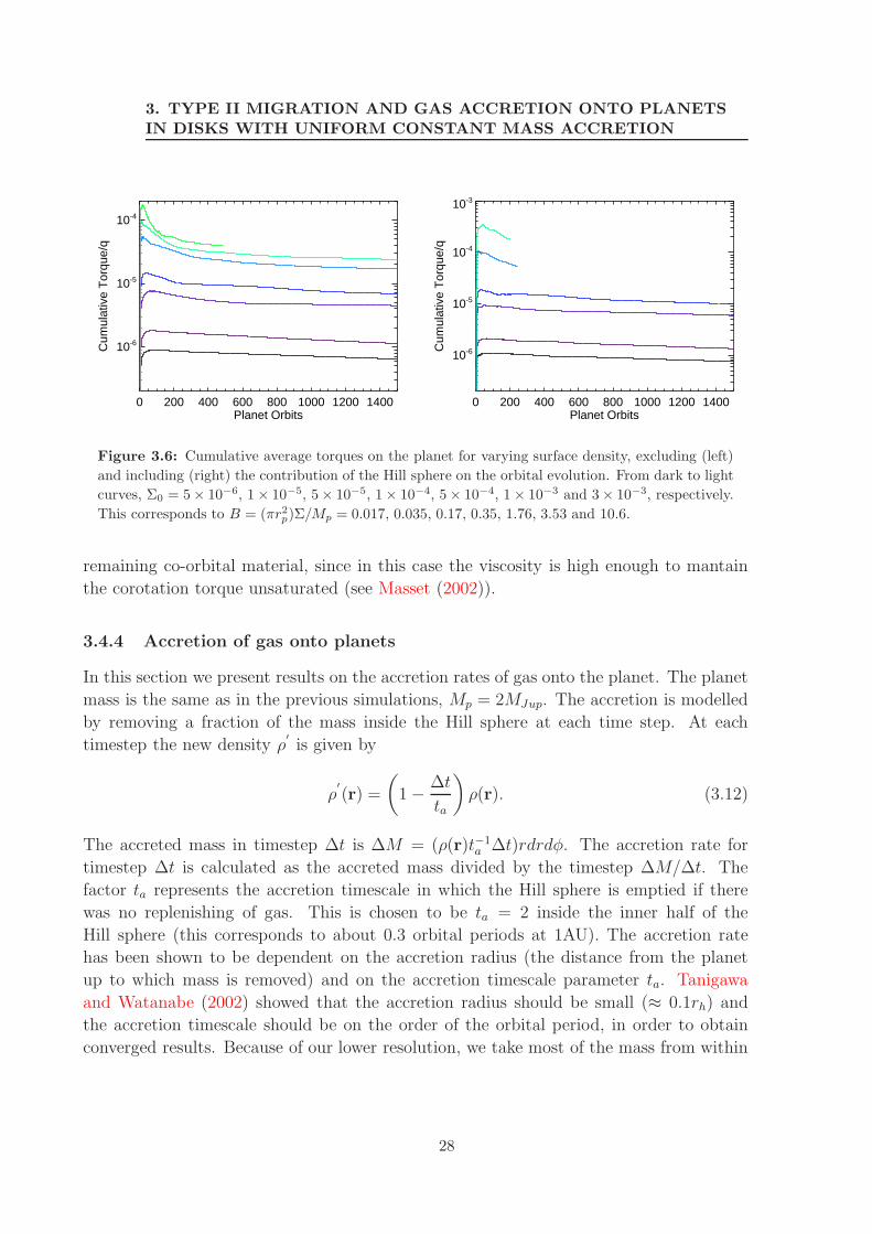
3. TYPE II MIGRATION AND GAS ACCRETION ONTO PLANETSIN DISKS WITH UNIFORM CONSTANT MASS ACCRETION
0 200 400 600 800 1000 1200 1400Planet Orbits
10-6
10-5
10-4
Cum
ulat
ive
Tor
que/
q
0 200 400 600 800 1000 1200 1400Planet Orbits
10-6
10-5
10-4
10-3
Cum
ulat
ive
Tor
que/
q
Figure 3.6: Cumulative average torques on the planet for varying surface density, excluding (left)
and including (right) the contribution of the Hill sphere on the orbital evolution. From dark to light
curves, Σ0 = 5 × 10⁻⁶, 1 × 10⁻⁵, 5 × 10⁻⁵, 1 × 10⁻⁴, 5 × 10⁻⁴, 1 × 10⁻³ and 3 × 10⁻³, respectively.
This corresponds to B = (πr2p)Σ/Mp = 0.017, 0.035, 0.17, 0.35, 1.76, 3.53 and 10.6.
remaining co-orbital material, since in this case the viscosity is high enough to mantain
the corotation torque unsaturated (see Masset (2002)).
3.4.4 Accretion of gas onto planets
In this section we present results on the accretion rates of gas onto the planet. The planet
mass is the same as in the previous simulations, Mp = 2MJup. The accretion is modelled
by removing a fraction of the mass inside the Hill sphere at each time step. At each
timestep the new density ρ′
is given by
ρ′
(r) =
(
1 −∆t
ta
)
ρ(r). (3.12)
The accreted mass in timestep ∆t is ∆M = (ρ(r)t−1a ∆t)rdrdφ. The accretion rate for
timestep ∆t is calculated as the accreted mass divided by the timestep ∆M/∆t. The
factor ta represents the accretion timescale in which the Hill sphere is emptied if there
was no replenishing of gas. This is chosen to be ta = 2 inside the inner half of the
Hill sphere (this corresponds to about 0.3 orbital periods at 1AU). The accretion rate
has been shown to be dependent on the accretion radius (the distance from the planet
up to which mass is removed) and on the accretion timescale parameter ta. Tanigawa
and Watanabe (2002) showed that the accretion radius should be small (≈ 0.1rh) and
the accretion timescale should be on the order of the orbital period, in order to obtain
converged results. Because of our lower resolution, we take most of the mass from within
28
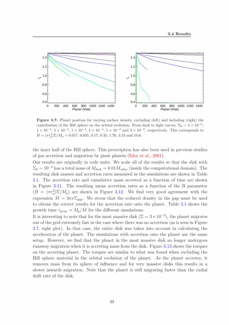
3.4 Results
0 200 400 600 800 1000 1200 1400Planet Orbits
0.4
0.6
0.8
1.0
1.2
1.4
r p
0 200 400 600 800 1000 1200 1400Planet Orbits
0.4
0.6
0.8
1.0
1.2
1.4
r p
Figure 3.7: Planet position for varying surface density, excluding (left) and including (right) the
contribution of the Hill sphere on the orbital evolution. From dark to light curves, Σ0 = 5 × 10⁻⁶,
1 × 10⁻⁵, 5 × 10⁻⁵, 1 × 10⁻⁴, 5 × 10⁻⁴, 1 × 10⁻³ and 3 × 10⁻³, respectively. This corresponds to
B = (πr2p)Σ/Mp = 0.017, 0.035, 0.17, 0.35, 1.76, 3.53 and 10.6.
the inner half of the Hill sphere. This prescription has also been used in previous studies
of gas accretion and migration by giant planets (Kley et al., 2001).
Our results are originally in code units. We scale all of the results so that the disk with
Σ0 = 10−4 has a total mass of Mdisk = 0.01Msolar (inside the computational domain). The
resulting disk masses and accretion rates measured in the simulations are shown in Table
3.1. The accretion rate and cumulative mass accreted as a function of time are shown
in Figure 3.11. The resulting mean accretion rates as a function of the B parameter
(B = (πr2p)Σ/Mp) are shown in Figure 3.12. We find very good agreement with the
expression M = 3πνΣgap. We stress that the reduced density in the gap must be used
to obtain the correct results for the accretion rate onto the planet. Table 3.1 shows the
growth time τgrow = Mp/M for the different simulations.
It is interesting to note that for the most massive disk (Σ = 3×10⁻³), the planet migrates
out of the grid extremely fast in the case where there was no accretion (as is seen in Figure
3.7, right plot). In that case, the entire disk was taken into account in calculating the
acceleration of the planet. The simulations with accretion onto the planet use the same
setup. However, we find that the planet in the most massive disk no longer undergoes
runaway migration when it is accreting mass from the disk. Figure 3.13 shows the torques
on the accreting planet. The torques are similar to what was found when excluding the
Hill sphere material in the orbital evolution of the planet. As the planet accretes, it
removes mass from its sphere of influence and for very massive disks this results in a
slower inwards migration. Note that the planet is still migrating faster than the radial
drift rate of the disk.
29

3. TYPE II MIGRATION AND GAS ACCRETION ONTO PLANETSIN DISKS WITH UNIFORM CONSTANT MASS ACCRETION
-2.0 -1.5 -1.0 -0.5 0.0 0.5 1.0Log (π rp
2 Σ )/Mp
-3.5
-4.0
-4.5
-5.0
-5.5
-6.0
-6.5
Log
Cum
ulat
ive
torq
ue/q
-(3/4)νΩp-(3/2π)νΩpB
-2.0 -1.5 -1.0 -0.5 0.0 0.5 1.0Log (π rp
2 Σ )/Mp
-3.5
-4.0
-4.5
-5.0
-5.5
-6.0
-6.5
Log
Cum
ulat
ive
torq
ue/q
-(3/4)νΩp-(3/2π)νΩpB
Figure 3.8: Dependence of the cumulative average torque on the B = (πr2
pΣ)/Mp parameter,
excluding (left) and including (right) the contribution of the Hill sphere on the orbital evolution.
The dashed line shows the analytical expression Γ = −(3/4)ν0Ωp (Eq. 3.4). The dash-dotted line
shows the analytical expression Γ = −(3/2π)ν0ΩpB (Eq. 3.6).
Σ0 5 × 10⁻⁶ 1 × 10⁻⁵ 5 × 10⁻⁵ 1 × 10⁻⁴ 5 × 10⁻⁴ 1 × 10⁻³ 3 × 10⁻³
Mdisk[code] 1.4 × 10⁻⁴ 2.8 × 10⁻⁴ 1.4 × 10⁻³ 2.8 × 10⁻³ 1.4 × 10⁻² 2.8 × 10⁻² 8.5 × 10⁻²
Mdisk[M⊙] 5 × 10⁻⁴ 1 × 10⁻³ 5 × 10⁻³ 1 × 10⁻² 5 × 10⁻² 1 × 10⁻¹ 3 × 10⁻¹
dM/dt[MJup/yr] 9.5 × 10⁻⁸ 1.9 × 10⁻⁷ 9.5 × 10⁻⁷ 1.8 × 10⁻⁶ 7.5 × 10⁻⁶ 3.3 × 10⁻⁵ 6.8 × 10⁻⁵
τgrow[yr] 2 × 10⁷ 1 × 10⁷ 2 × 10⁶ 1 × 10⁶ 2.6 × 10⁵ 6 × 10⁴ 3 × 10⁴
Table 3.1: Simulations parameters and measured gas accretion rates onto the planet.
3.4.5 Mass flow through gaps
An interesting question is that of how much gas is able to pass by the planet when there
is a gap present. We calculate this for three different sets of simulations: the case when
the planet is on a fixed orbit (presented in Section 3.4.1.1), the case when the planet is
allowed to migrate (presented in Section 3.4.1.2), and the case when the planet is allowed
to migrate and to accrete gas (presented in Section 3.4.4). For each case, the surface
density varies as before where Σ0 = 5 × 10⁻⁶, 1 × 10⁻⁵, 5 × 10⁻⁵, 1 × 10⁻⁴, 5 × 10⁻⁴,
1 × 10⁻³ and 3 × 10⁻³.
Figure 3.14 shows the mass flux, calculated as ρ(rp)vr(rp), and averaged in time and in
the azimuthal direction. This represents the mass per unit time that passes through the
orbit of the planet (i.e. per 2πrp). The density ρ has been multiplied by an additional
factor of hrp to compare to the analytical expression involving the surface density. The
blue symbols in Figure 3.14 denote positive values of the mass flux, which means flow of
gas from the inner to the outer disk.
For the fixed orbit case, the net mass flux is negative (radially inwards), and is exactly the
30
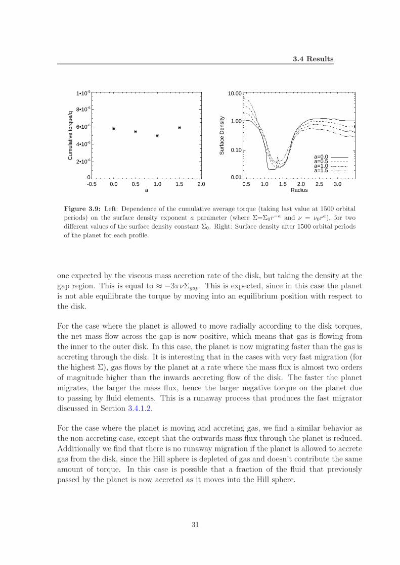
3.4 Results
-0.5 0.0 0.5 1.0 1.5 2.0a
0
2•10-6
4•10-6
6•10-6
8•10-6
1•10-5
Cum
ulat
ive
torq
ue/q
0.5 1.0 1.5 2.0 2.5 3.0Radius
0.01
0.10
1.00
10.00
Sur
face
Den
sity
a=1.5a=1.0a=0.5a=0.0
Figure 3.9: Left: Dependence of the cumulative average torque (taking last value at 1500 orbital
periods) on the surface density exponent a parameter (where Σ=Σ0r−a and ν = ν0r
a), for two
different values of the surface density constant Σ0. Right: Surface density after 1500 orbital periods
of the planet for each profile.
one expected by the viscous mass accretion rate of the disk, but taking the density at the
gap region. This is equal to ≈ −3πνΣgap. This is expected, since in this case the planet
is not able equilibrate the torque by moving into an equilibrium position with respect to
the disk.
For the case where the planet is allowed to move radially according to the disk torques,
the net mass flow across the gap is now positive, which means that gas is flowing from
the inner to the outer disk. In this case, the planet is now migrating faster than the gas is
accreting through the disk. It is interesting that in the cases with very fast migration (for
the highest Σ), gas flows by the planet at a rate where the mass flux is almost two orders
of magnitude higher than the inwards accreting flow of the disk. The faster the planet
migrates, the larger the mass flux, hence the larger negative torque on the planet due
to passing by fluid elements. This is a runaway process that produces the fast migrator
discussed in Section 3.4.1.2.
For the case where the planet is moving and accreting gas, we find a similar behavior as
the non-accreting case, except that the outwards mass flux through the planet is reduced.
Additionally we find that there is no runaway migration if the planet is allowed to accrete
gas from the disk, since the Hill sphere is depleted of gas and doesn’t contribute the same
amount of torque. In this case is possible that a fraction of the fluid that previously
passed by the planet is now accreted as it moves into the Hill sphere.
31
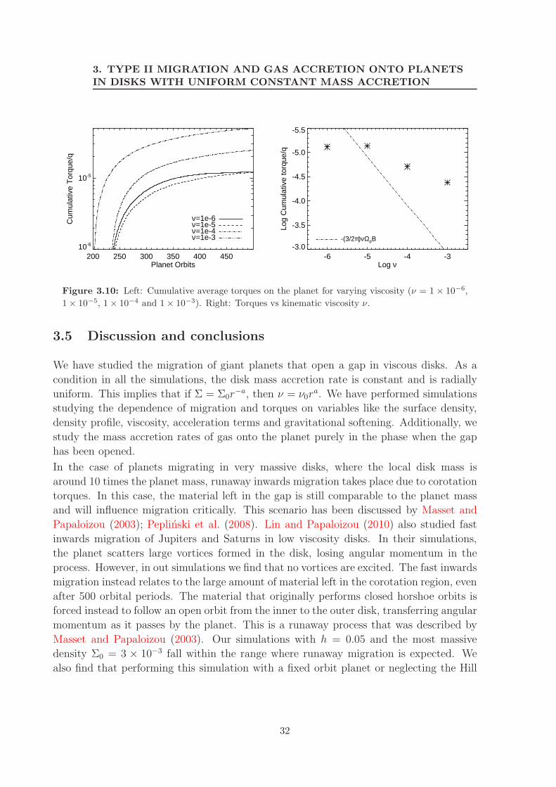
3. TYPE II MIGRATION AND GAS ACCRETION ONTO PLANETSIN DISKS WITH UNIFORM CONSTANT MASS ACCRETION
200 250 300 350 400 450Planet Orbits
10-6
10-5
Cum
ulat
ive
Tor
que/
q
ν=1e-3ν=1e-4ν=1e-5ν=1e-6
-6 -5 -4 -3Log ν
-3.0
-3.5
-4.0
-4.5
-5.0
-5.5
Log
Cum
ulat
ive
torq
ue/q
-(3/2π)νΩpB
Figure 3.10: Left: Cumulative average torques on the planet for varying viscosity (ν = 1 × 10⁻⁶,
1 × 10⁻⁵, 1 × 10⁻⁴ and 1 × 10⁻³). Right: Torques vs kinematic viscosity ν.
3.5 Discussion and conclusions
We have studied the migration of giant planets that open a gap in viscous disks. As a
condition in all the simulations, the disk mass accretion rate is constant and is radially
uniform. This implies that if Σ = Σ0r−a, then ν = ν0r
a. We have performed simulations
studying the dependence of migration and torques on variables like the surface density,
density profile, viscosity, acceleration terms and gravitational softening. Additionally, we
study the mass accretion rates of gas onto the planet purely in the phase when the gap
has been opened.
In the case of planets migrating in very massive disks, where the local disk mass is
around 10 times the planet mass, runaway inwards migration takes place due to corotation
torques. In this case, the material left in the gap is still comparable to the planet mass
and will influence migration critically. This scenario has been discussed by Masset and
Papaloizou (2003); Peplinski et al. (2008). Lin and Papaloizou (2010) also studied fast
inwards migration of Jupiters and Saturns in low viscosity disks. In their simulations,
the planet scatters large vortices formed in the disk, losing angular momentum in the
process. However, in out simulations we find that no vortices are excited. The fast inwards
migration instead relates to the large amount of material left in the corotation region, even
after 500 orbital periods. The material that originally performs closed horshoe orbits is
forced instead to follow an open orbit from the inner to the outer disk, transferring angular
momentum as it passes by the planet. This is a runaway process that was described by
Masset and Papaloizou (2003). Our simulations with h = 0.05 and the most massive
density Σ0 = 3 × 10⁻³ fall within the range where runaway migration is expected. We
also find that performing this simulation with a fixed orbit planet or neglecting the Hill
32
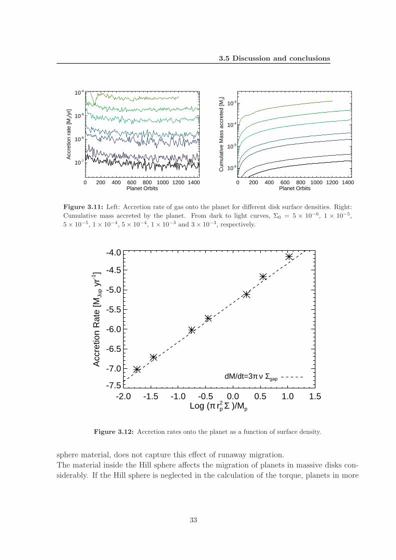
3.5 Discussion and conclusions
0 200 400 600 800 1000 1200 1400Planet Orbits
10-7
10-6
10-5
10-4
Acc
retio
n ra
te [M
J/yr
]
0 200 400 600 800 1000 1200 1400Planet Orbits
10-6
10-5
10-4
10-3
Cum
ulat
ive
Mas
s ac
cret
ed [M
J]
Figure 3.11: Left: Accretion rate of gas onto the planet for different disk surface densities. Right:
Cumulative mass accreted by the planet. From dark to light curves, Σ0 = 5 × 10⁻⁶, 1 × 10⁻⁵,
5 × 10⁻⁵, 1 × 10⁻⁴, 5 × 10⁻⁴, 1 × 10⁻³ and 3 × 10⁻³, respectively.
-2.0 -1.5 -1.0 -0.5 0.0 0.5 1.0 1.5Log (π rp
2 Σ )/Mp
-7.5
-7.0
-6.5
-6.0
-5.5
-5.0
-4.5
-4.0
Acc
retio
n R
ate
[MJu
p yr
-1]
dM/dt=3π ν Σgap
Figure 3.12: Accretion rates onto the planet as a function of surface density.
sphere material, does not capture this effect of runaway migration.
The material inside the Hill sphere affects the migration of planets in massive disks con-
siderably. If the Hill sphere is neglected in the calculation of the torque, planets in more
33

3. TYPE II MIGRATION AND GAS ACCRETION ONTO PLANETSIN DISKS WITH UNIFORM CONSTANT MASS ACCRETION
0 200 400 600 800 1000 1200 1400Planet Orbits
10-6
10-5
10-4
10-3
Cum
ulat
ive
Tor
que/
q
-2.0 -1.5 -1.0 -0.5 0.0 0.5 1.0Log (π rp
2 Σ )/Mp
-3.5
-4.0
-4.5
-5.0
-5.5
-6.0
-6.5
Log
Cum
ulat
ive
torq
ue/q
-(3/4)νΩp-(3/2π)νΩpB
Figure 3.13: Left: Cumulative torques vs time for different densities. From dark to light curves,
Σ0 = 5 × 10⁻⁶, 1 × 10⁻⁵, 5 × 10⁻⁵, 1 × 10⁻⁴, 5 × 10⁻⁴, 1 × 10⁻³ and 3 × 10⁻³, respectively. Right:
Dependence of the cumulative average torque on the B = (πr2
pΣ)/Mp parameter for an accreting
planet. The dashed line shows the analytical expression Γ = −(3/4)ν0Ωp (Eq. 3.4). The dash-dotted
line shows the analytical expression Γ = −(3/2π)ν0ΩpB (Eq. 3.6).
massive disks will migrate slower and the torques will be approximately independent of
Σ.
Migration rates are also independent of the density profile in the disk. The torques exerted
on the planet are constant as a function of surface density exponent up to a = 1.5. It is
not clear if this remains valid for very massive disks. The variation of the torque with
disk viscosity showed interesting behavior. For larger viscosities, the torque is no longer
given by the analytical estimate that is linear with respect to viscosity. The offset of the
simulated torque from the formula grows with larger viscosities. The slower migration in
highly viscous disks has been observed also by Crida and Morbidelli (2007). This can be
an effect of the corotation torque exerted by material left in the gap. At high viscosities,
the corotation torque can be unsaturated and the material orbiting in horseshoe orbits
around corotation exerts a positive torque on the planet, therefore slowing migration down
(Masset, 2002; Paardekooper and Papaloizou, 2009a).
During the gap phase of the evolution, planets accrete at a fraction of the viscous mass
accretion rate, corrected to take into account the density inside the gap. This is approx-
imately given by Mp = 3πνΣgap ≈ (0.1)3πνΣ0. It is interesting that for the accreting
planet in the most massive disk, we find no runway migration, as opposed to the case
where accretion is switched off.
The estimations of the Type II torque dependence on a wide range of parameters is usefull
in the modeling of synthetic planet populations that can explain and predict the observed
population of extrasolar planets, specially massive planets in the gap opening regime.
34

3.5 Discussion and conclusions
-2.0 -1.5 -1.0 -0.5 0.0 0.5 1.0Log (π rp
2 Σ )/Mp
-4
-6
-8
-10
-12
<ρ
v r>
AccretingFree Mov.Fixed Orb.
-3ν Bgap/π rp
Figure 3.14: Mass flux ρ(rp)vr(rp), averaged in time and in the azimuthal direction at the position
of the planet. The mass flux is shown for simulations with a fixed orbit planet (stars), a free moving
planet (diamonds) and a free moving and accreting planet (crosses). The blue symbols denote
positive values of the mass flux.
35
3. TYPE II MIGRATION AND GAS ACCRETION ONTO PLANETSIN DISKS WITH UNIFORM CONSTANT MASS ACCRETION
36
4
3D MHD Simulations of Planet
Migration in Turbulent Stratified
Disks
We performed 3D MHD simulations of planet migration in stratified disks using the
Godunov code PLUTO, where the disk is turbulent due to the magnetorotational
instability. We study the migration for planets with different planet-star mass ratios
q = Mp/Ms. In agreement with previous studies, for the low-mass planet cases
(q = 5 × 10⁻⁶ and 10−5), migration is dominated by random fluctuations in the
torque. For a Jupiter-mass planet (q = Mp/Ms = 10−3 for Ms = 1M⊙), we find
a reduction of the magnetic stress inside the orbit of the planet and around the
gap region. After an initial stage where the torque on the planet is positive, it
reverses and we recover migration rates similar to those found in disks where the
turbulent viscosity is modelled by an α viscosity. For the intermediate-mass planets
(q = 5 × 10⁻⁵, 10−4 and 2 × 10⁻⁴) we find a new and so far unexpected behavior.
In some cases they experience sustained and systematic outwards migration for the
entire duration of the simulation. For this case, the horseshoe region is resolved
and torques coming from the corotation region can remain unsaturated due to the
stresses in the disk. These stresses are generated directly by the magnetic field. The
magnitude of the horseshoe drag can overcome the negative Lindblad contribution
when the local surface density profile is flat or increasing outwards, which we see
in certain locations in our simulations due to the presence of a zonal flow. The
intermediate-mass planet is migrating radially outwards in locations where there is
a positive gradient of a pressure bump (zonal flow) a.
aA version of this chapter has been published in The Astrophysical Journal, 736, 85 (2011) (Uribe
et al., 2011).
37
4. 3D MHD SIMULATIONS OF PLANET MIGRATION INTURBULENT STRATIFIED DISKS
4.1 Introduction
Understanding why and how fast planets migrate is fundamental to explaining the ob-
served distribution of exoplanets and constraining planet formation timescales and ef-
ficiencies (Alibert et al., 2005). The basic principle behind the migration of planets in
protoplanetary disks is the transfer of angular momentum between the planet and its disk.
This transport process occurs at Lindblad resonances and, in a locally isothermal disk,
typically leads to fast inwards migration. (Goldreich and Tremaine, 1980; Papaloizou
and Lin, 1984; Tanaka et al., 2002; Ward, 1986). This is the standard type I migration
scenario which applies to low- to intermediate-mass planets where the specific torque is a
linear function of the planet mass (Ward, 1997).
If the planet is massive enough (the mass depending on the viscosity and the pressure scale
height), the tidal forces on the disk can eventually overcome the pressure gradient and the
viscous transport, causing gap opening around the planet orbit. This migration regime,
referred to as type II, in which the planet-disk interaction can no longer be described
by linear perturbation theory, is then conceptually very different from the type I regime.
Due to the gap opening, it is possible for the torques on the planet to cancel in such a
way that the evolution of the planet’s position is determined by the viscous transport of
gas in the disk, making the planet move with the disk on viscous timescales (Bate et al.,
2003; Ward, 1997).
Current numerical and analytical calculations estimate migration timescales to be a small
fraction of the expected disk lifetime, which creates a problem for the survival of planetary
cores. Gas planet cores need to reach a critical mass before the onset of runaway gas
accretion (Ida and Lin, 2008). It is well established that planet population synthesis
models together with giant planet formation models require a much less efficient type
I migration to reproduce the observed distribution of exoplanets (Alibert et al., 2005;
Benz et al., 2008; Ida and Lin, 2004, 2007; Mordasini et al., 2009b; Trilling et al., 2002).
Nevertheless, core survival mechanisms have also been proposed to solve the timescale
problem without resorting to an artificially reduced Type I migration rate (Fromang
et al., 2005; Terquem, 2003; Thommes and Murray, 2006).
Deviations from linear theory have been found in a number of three dimensional calcula-
tions. Masset (2002) and D’Angelo et al. (2003b) and later Masset et al. (2006a) found
that for intermediate-mass planets (around Mp = 1× 10⁻⁴Ms), the torques on the planet
can be significantly lower and even reverse sign when the local surface density profile of
the disk is flatter (Σ ∼ rα with α = 0 − 0.5) than in the usually assumed Minimum
Mass Solar Nebula (MMSN) model Σ ∼ r−1.5. This is found for a certain range of the
disk viscosity. In this case, the torques from the corotation region can become impor-
tant. The fluid elements that are librating (moving in horseshoe orbits in the corotation
region) orbit on a U-turn trajectory at trailing and leading sides of the planet. These
38

4.1 Introduction
fluid elements exert a torque on the planet at each U-turn, which is a symmetric effect
on both sides of the planet in an inviscid disk; therefore there is no net torque coming
from this region after a few librating periods. This is referred to as the ”saturation” of
the corotation torque. In the presence of viscosity, if the viscous crossing timescale across
the horseshoe region of accreting disk material is smaller than the libration timescale, the
torques exerted by fluid elements around the U-turn are not symmetric at each side of
the planet, creating a net positive torque that can be sustained. This is refereed to as
the ”unsaturated” corotation torque, and it can depend on the surface density and on the
width of the horseshoe region that in turn depends on the planet mass (Ward, 1992).
So far most numerical studies of migration and/or gap formation have concentrated on the
quasi-laminar disk case, where Navier-Stokes shear viscosity is included in order to model
the viscous stresses resulting from including turbulence in the disk (e.g. Bate et al. (2003);
Bryden et al. (1999); Crida et al. (2006); de Val-Borro et al. (2006); Nelson et al. (2000);
Papaloizou and Larwood (2000) and many more). There has been strong interest in sim-
ulating planet-disk interactions in turbulent disks, where the turbulence is magnetically
generated by the magneto-rotational instability (MRI) (Balbus and Hawley, 1991, 1998).
Only ideal MHD has been considered so far in global simulations. The disk is assumed to
be fully ionized and the magnetic diffusivity is negligible. Winters et al. (2003) looked at
gap formation by intermediate- and large-mass planets in turbulent unstratified disks and
the local internal stresses around the planet. In the MHD case, they found the gap to be
shallower and wider compared to the laminar HD case; the Maxwell stresses in the disk
dropped in the vicinity of the planet’s orbit. Papaloizou and Nelson (2003) performed
a comprehensive study of protoplanets embedded in MHD-turbulent unstratified disks.
They found that for low mass planets, Type I migration is no longer effective due to large
fluctuations in the torque. No convergence was reached due to fluctuations of the torque
on timescales longer than the orbital period and short simulation timescales. However,
the torques for planets more massive than 30M⊕ = 0.1MJup were found to converge to
the standard Type I migration torques after long-time averaging (Nelson and Papaloizou,
2003, 2004; Papaloizou et al., 2004). For low-mass protoplanets, Nelson (2005) studied the
long-term evolution of the orbital elements and particularly the excitation of eccentric-
ity by turbulent fluctuations. The evolution of the orbital elements of particles in MHD
turbulence has also been studied using shearing unstratified boxes (Yang et al., 2009)
and stratified boxes including a dead zone (Oishi et al., 2007). To avoid the expensive
MHD simulations, other approaches have been taken, such as modeling the turbulence as
a time and space varying forcing in a laminar disk model (Laughlin et al., 2004). In this
case, depending on the amplitude of the forcing, type I migration can be overcome by
the random fluctuations in the torque, and random walk motion will be superimposed on
the smooth inward migration. Baruteau and Lin (2010) used a similar turbulent forcing
model and studied the unsaturation of the corotation torque due to turbulence. Depend-
39

4. 3D MHD SIMULATIONS OF PLANET MIGRATION INTURBULENT STRATIFIED DISKS
ing on the amplitude of the turbulence, the corotation torque is found to be unsaturated
to a certain level, making the total torque increase accordingly (become less negative),
slowing down inwards migration. Other approaches include the analytical description of
stochastic migration of low-mass planets using a diffusion-advection equation (Adams and
Bloch, 2009; Johnson et al., 2006) and coupling N-body simulations with a random forcing
to study the accretion and formation of low-mass planets (Ogihara et al., 2007). Recently,
Nelson and Gressel (2010) examined the velocity dispersion of 1 m to 10 km planetesimals
embedded in a turbulent disk, using 3D MHD simulations and neglecting stratification,
and characterized the stochastic gravitational perturbations felt by planetesimals due to
MHD turbulence.
In this chapter, we study planet migration in stratified 3D MHD-turbulent disks for planet
masses in the Type I and II mass range. In Section 4.2 we describe the numerical setup of
our simulations, and the initial conditions for the disk and the magnetic field, before the
addition of a planet. In section 4.3 we present the results of our simulations and finally
in section 4.4 we discuss our results.
4.2 Simulation Setup
Simulations where performed using the finite volume fluid dynamics code PLUTO (Mignone
et al., 2007). In the code, time stepping is done using a second order Runge Kutta scheme,
while the spatial integration is performed using linear interpolation through the second
order TVD scheme. The Riemann fluxes are computed using the HLLC and HLLD
solvers for the HD and MHD cases, respectively. The code uses the Constrained Trans-
port method for preserving a divergence-free magnetic field (Gardiner and Stone, 2005).
The numerical setup for the MHD case follows the setup presented in (Flock et al., 2010).
The MHD equations in the isothermal approximation (no energy equation) are given by
∂ρ
∂t+ ∇ · (ρv) = 0 (4.1)
∂v
∂t+ (v · ∇)v +
1
ρB× (∇× B) = −
1
ρ∇P −∇Φg (4.2)
∂B
∂t+ B(∇ · v) − (B · ∇)v + (v · ∇)B = 0 (4.3)
The potential Φg includes contributions from the star and the planet. We work in spher-
ical coordinates (r, θ, φ), where the computational domain is given by r ∈ [1, 10], θ ∈
[π/2−0.3, π/2 + 0.3] and φ ∈ [0, 2π]. The grid resolution is (Nr, Nθ, Nφ) = (256, 128, 256)
and it is centered in the center of mass of the planet-star system. The boundary con-
ditions for the velocities and magnetic field are periodic in the vertical (θ boundary)
and azimuthal directions and reflective in the radial direction, except for the transverse
40
4.2 Simulation Setup
magnetic field component, which reverses its sign at the radial boundary. Buffer zones
are defined at the radial boundaries to avoid boundary effects, where for 1 < r < 2 the
magnetic resistivity is given by η = 2 × 10⁻⁴(2 − r) and for 9 < r < 10 the resistivity is
η = 1 × 10⁻⁴(r − 9).
4.2.1 Disk and Planet Models
As an initial condition we take a gas disk in sub-Keplerian rotation around a solar mass
star. The azimuthal velocity is given by
vφ =√
v2k − c2
s(a − 2b), (4.4)
where vk is the Keplerian velocity and a = 3/2 and b = 0.5 are the exponents of the radial
power law distribution of the density ρ ∝ r−a and sound speed cs = c0(r sin θ)−b. The
initial density distribution is given by
ρ(r, θ) = (r sin θ)−3/2 exp
(
sin θ − 1
c20
)
. (4.5)
The disk is described by a locally isothermal equation of state P = c2sρ. The ratio of the
pressure scale height h to the radial coordinate of the disk is taken to be a constant such
that h = H/(r sin θ) = 0.07.
The gravitational potential of the planet is given by a softened point-mass potential
Φp(r) = −GM
(|r − rp|2 + ǫ2)1/2(4.6)
where ǫ is the softening parameter, needed to avoid numerical divergence near the position
of the planet and
|rp − r|2 = r2p + r2 − 2rpr(sin θp sin θ cos(φp − φ) + cos θp cos θ) (4.7)
is the distance between the planet and a gas particle in the disk. For all the simulations
ǫ is set to be a fraction of the Hill radius ǫ = krp(Mp/3)1/3 with k < 0.5. Table 4.1 shows
the parameters of our simulations. Distances are given in units of r0 = 1AU , density
is given in units of ρ0 = 2.6 × 10⁻¹⁰gcm−3, and velocity is given in units of Keplerian
speed at 1AU , v0 = vk(1AU). The surface density have been scaled such that the total
disk mass is 0.01Mstar. Magnetic fields are given in units of B0 =√
4πρ0v20. In the cases
where the planet is not on a fixed orbit (runs see Table 4.1), the equations of motion are
integrated with a simple leap frog integrator. For the calculation of the torque, we include
41

4. 3D MHD SIMULATIONS OF PLANET MIGRATION INTURBULENT STRATIFIED DISKS
Name q = Mp/M⋆ ǫ(rh) rp Fixed orbit Run time (local orbits)
R0 Massless 0.3 3.3 Yes 130
R1 5 × 10⁻⁶ 0.3 5.0 No 85
R2 10−5 0.3 5.0 No 140
R3 10−5 0.1 3.3 Yes 89
R4 5 × 10⁻⁵ 0.3 5.0 No 90
R5 10−4 0.3 5.0 No 100
R6 10−4 0.1 3.3 Yes 135
R7 10−4 0.3 4.0 No 85
R8 2 × 10⁻⁴ 0.3 5.0 No 95
R9 10−3 0.3 5.0 No 100
R10 (HD) 10−3 0.3 5.0 No 100
Table 4.1: Simulation Parameters
the entire disk in the integration (without Hill sphere tapering, except for simulation R9).
The components of the torque vector in cartesian coordinates are given by
Γi = GMp
∫
ρ(r)(rp × r)i
(|r− rp|2 + ǫ2)3/2dV, (4.8)
where i ∈ x, y, z is any of the three cartesian indices and (rp × r)i = (rp × r) · ei,
with ei being the cartesian unit vectors. Of course, for studying migration, we are mostly
interested in the z component of the torque vector. Specific torques are given in units of
v2k(1AU).
4.2.2 Magnetic Field Configuration
Before introducing the planet in the simulations, a weak toroidal magnetic field is imposed
on the disk given by
(Br, Bθ, Bφ) = (0, 0, 2p/25), (4.9)
where p is the initial thermal pressure. This gives an initial azimuthal field with constant
plasma beta β = 25. The field is imposed in a subset of the full computational domain
given by 2 < r < 9 and π/2 − 0.07 < θ < π/2 + 0.07. The simulation is then followed
until turbulence generated by the MRI has reached a saturated state. After this stage, we
reset the density to the initial condition. This is the initial state in which the potential
of the planet is incorporated and where all our runs start. The azimuthally, vertically
and time averaged value of the effective α parameter is shown in Figure 4.1. However,
the α stress is not constant throughout the vertical dimension. The upper layers of the
disk are the most active. Figure 4.2 shows the time evolution of Bφ, B2/B20 and α for
42
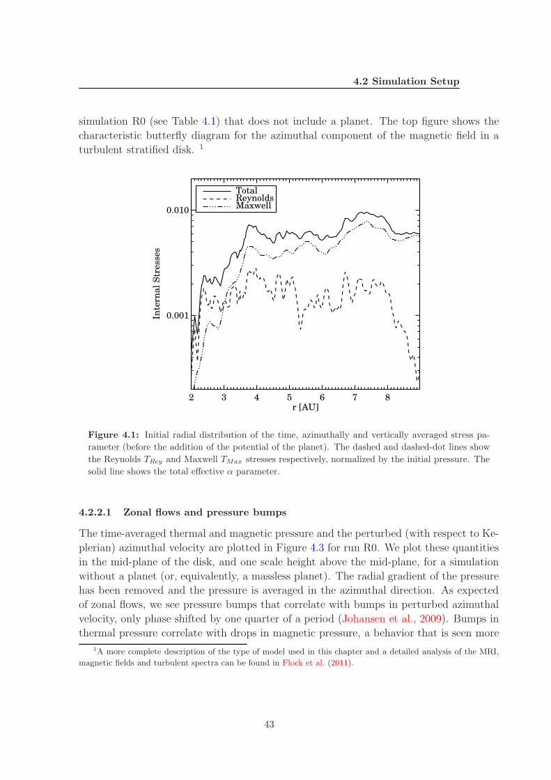
4.2 Simulation Setup
simulation R0 (see Table 4.1) that does not include a planet. The top figure shows the
characteristic butterfly diagram for the azimuthal component of the magnetic field in a
turbulent stratified disk. 1
2 3 4 5 6 7 8r [AU]
0.001
0.010
Inte
rna
l S
tress
es
TotalReynoldsMaxwell
Figure 4.1: Initial radial distribution of the time, azimuthally and vertically averaged stress pa-
rameter (before the addition of the potential of the planet). The dashed and dashed-dot lines show
the Reynolds TRey and Maxwell TMax stresses respectively, normalized by the initial pressure. The
solid line shows the total effective α parameter.
4.2.2.1 Zonal flows and pressure bumps
The time-averaged thermal and magnetic pressure and the perturbed (with respect to Ke-
plerian) azimuthal velocity are plotted in Figure 4.3 for run R0. We plot these quantities
in the mid-plane of the disk, and one scale height above the mid-plane, for a simulation
without a planet (or, equivalently, a massless planet). The radial gradient of the pressure
has been removed and the pressure is averaged in the azimuthal direction. As expected
of zonal flows, we see pressure bumps that correlate with bumps in perturbed azimuthal
velocity, only phase shifted by one quarter of a period (Johansen et al., 2009). Bumps in
thermal pressure correlate with drops in magnetic pressure, a behavior that is seen more
1A more complete description of the type of model used in this chapter and a detailed analysis of the MRI,
magnetic fields and turbulent spectra can be found in Flock et al. (2011).
43
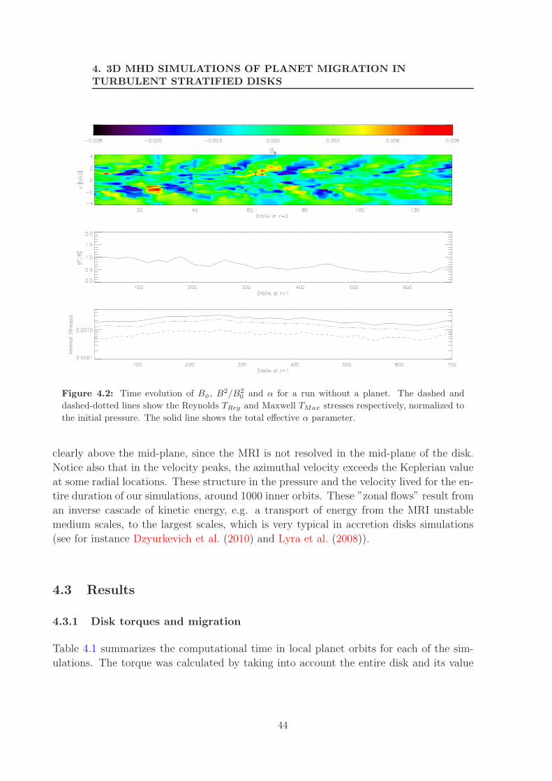
4. 3D MHD SIMULATIONS OF PLANET MIGRATION INTURBULENT STRATIFIED DISKS
Figure 4.2: Time evolution of Bφ, B2/B2
0 and α for a run without a planet. The dashed and
dashed-dotted lines show the Reynolds TRey and Maxwell TMax stresses respectively, normalized to
the initial pressure. The solid line shows the total effective α parameter.
clearly above the mid-plane, since the MRI is not resolved in the mid-plane of the disk.
Notice also that in the velocity peaks, the azimuthal velocity exceeds the Keplerian value
at some radial locations. These structure in the pressure and the velocity lived for the en-
tire duration of our simulations, around 1000 inner orbits. These ”zonal flows” result from
an inverse cascade of kinetic energy, e.g. a transport of energy from the MRI unstable
medium scales, to the largest scales, which is very typical in accretion disks simulations
(see for instance Dzyurkevich et al. (2010) and Lyra et al. (2008)).
4.3 Results
4.3.1 Disk torques and migration
Table 4.1 summarizes the computational time in local planet orbits for each of the sim-
ulations. The torque was calculated by taking into account the entire disk and its value
44
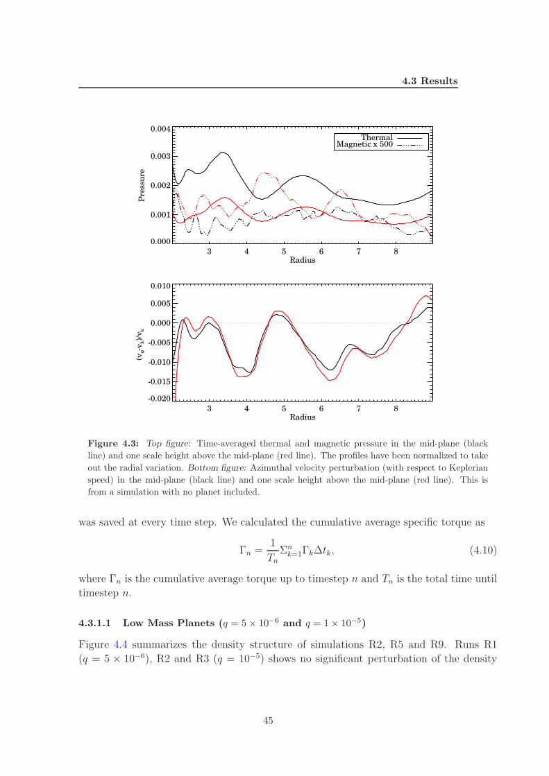
4.3 Results
3 4 5 6 7 8Radius
0.000
0.001
0.002
0.003
0.004
Pre
ssu
reThermal
Magnetic x 500
3 4 5 6 7 8Radius
-0.020
-0.015
-0.010
-0.005
0.000
0.005
0.010
(vφ-
vk)/
vk
Figure 4.3: Top figure: Time-averaged thermal and magnetic pressure in the mid-plane (black
line) and one scale height above the mid-plane (red line). The profiles have been normalized to take
out the radial variation. Bottom figure: Azimuthal velocity perturbation (with respect to Keplerian
speed) in the mid-plane (black line) and one scale height above the mid-plane (red line). This is
from a simulation with no planet included.
was saved at every time step. We calculated the cumulative average specific torque as
Γn =1
Tn
Σnk=1Γk∆tk, (4.10)
where Γn is the cumulative average torque up to timestep n and Tn is the total time until
timestep n.
4.3.1.1 Low Mass Planets (q = 5 × 10⁻⁶ and q = 1 × 10⁻⁵)
Figure 4.4 summarizes the density structure of simulations R2, R5 and R9. Runs R1
(q = 5 × 10⁻⁶), R2 and R3 (q = 10−5) shows no significant perturbation of the density
45
4. 3D MHD SIMULATIONS OF PLANET MIGRATION INTURBULENT STRATIFIED DISKS
by the planet, and no spiral arms are seen. The turbulent perturbations dominate in this
case. Figure 4.5 shows the torque cumulative average torque as a function of local orbits
for run R1. Figure 4.6 shows the torque for simulations R2 and R3. The fluctuations in
the torque created by the perturbations in the density can, in both cases, be larger than
the mean torque expected for standard Type I migration in a laminar disk. Comparing
the torque for the planet at different positions in the disk, we see that the local (in time)
evolution depends on the location of the planet. Random variations in the torque can
be an order of magnitude larger than torques coming from the Lindblad resonances, in
addition to the possibility that the spiral waves excited at Lindblad resonances are partly
or totally suppressed by density fluctuations coming from the turbulence, such that the
magnitude of this torque can be reduced. For the low-mass planet simulations, we find
no convergence of the torque on timescale of the runs. For a run with a massless planet
orbitting at rp = 3.3, a gaussian fit of the time distribution of the torque gives a standard
deviation of σ ≈ 1.5e − 5. We also calculate the auto-correlation function of the torque
and take the correlation time to be given by τc =∫ tmax
0ACF (τ)dτ . This gives τc ≈ 2
local orbits, while the first and second zero crossing of the torque ACF occur at 0.2 and
0.8 local orbits. 1 This is in agreement with results by Nelson (2005) and Fromang and
Nelson (2009) and with estimates used by Baruteau and Lin (2010) that are based in
previous MHD simulations of turbulent low-mass planet migration. We also calculate the
power spectrum of the mid-plane density (see Eq. 3 in Baruteau and Lin (2010)). This
is shown in Figure 4.7 and we compare our results from MHD simulations to Figure 1 of
Baruteau and Lin (2010), where the spectrum in the result of the forcing model for the
turbulence with α ∼ 10−3. This comparison is valuable, since ultimately, a more complete
parameter study migration and turbulence will have to be studied in models with forced
turbulence. For this α value, in our simulations we find that the larger scales carry more
power than in the random forcing model, while the two spectrum agree for smaller scales
for the case that includes the modes with m > 6. The higher power at larger scales can
result from the higher compressibility of stratified disks, especially at large scales, as a
vertically stratified disk can respond to compression with vertical expansion. However,
the overall shape of the spectrum of the MHD simulation agrees better with the HD
simulation without the m > 6 modes included. Therefore with the proper scaling of
the amplitude of the turbulence, and a cutoff of these modes, these simulations could
reproduce the MHD spectrum. Another possibility is that the power at the small scales
in the MHD simulation is lower due to lacking resolution at these scales. Ultimately,
there needs to be a physical motivation for the cutoff of the turbulent forcing potential
1The calculation of the torque standard deviation and the torque correlation time is done as an averaging over
a set of massless particles that sample the torque at different locations in the disk. This provides a characterization
of the stochastic torque in an unperturbed disk. A more detailed description of this topic is presented in Appendix
A
46
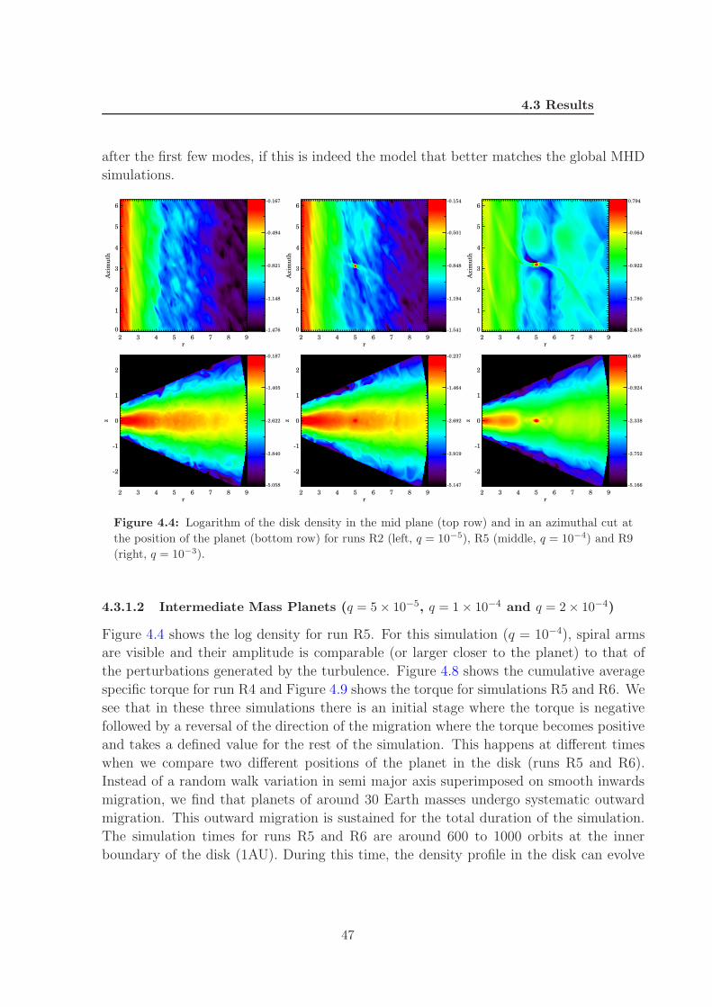
4.3 Results
after the first few modes, if this is indeed the model that better matches the global MHD
simulations.
2 3 4 5 6 7 8 9r
0
1
2
3
4
5
6
Azim
uth
-1.476
-1.148
-0.821
-0.494
-0.167
2 3 4 5 6 7 8 9r
0
1
2
3
4
5
6
Azim
uth
-1.541
-1.194
-0.848
-0.501
-0.154
2 3 4 5 6 7 8 9r
0
1
2
3
4
5
6
Azim
uth
-2.638
-1.780
-0.922
-0.064
0.794
2 3 4 5 6 7 8 9r
-2
-1
0
1
2
z
-5.058
-3.840
-2.622
-1.405
-0.187
2 3 4 5 6 7 8 9r
-2
-1
0
1
2
z
-5.147
-3.919
-2.692
-1.464
-0.237
2 3 4 5 6 7 8 9r
-2
-1
0
1
2
z
-5.166
-3.752
-2.338
-0.924
0.489
Figure 4.4: Logarithm of the disk density in the mid plane (top row) and in an azimuthal cut at
the position of the planet (bottom row) for runs R2 (left, q = 10−5), R5 (middle, q = 10−4) and R9
(right, q = 10−3).
4.3.1.2 Intermediate Mass Planets (q = 5 × 10⁻⁵, q = 1 × 10⁻⁴ and q = 2 × 10⁻⁴)
Figure 4.4 shows the log density for run R5. For this simulation (q = 10−4), spiral arms
are visible and their amplitude is comparable (or larger closer to the planet) to that of
the perturbations generated by the turbulence. Figure 4.8 shows the cumulative average
specific torque for run R4 and Figure 4.9 shows the torque for simulations R5 and R6. We
see that in these three simulations there is an initial stage where the torque is negative
followed by a reversal of the direction of the migration where the torque becomes positive
and takes a defined value for the rest of the simulation. This happens at different times
when we compare two different positions of the planet in the disk (runs R5 and R6).
Instead of a random walk variation in semi major axis superimposed on smooth inwards
migration, we find that planets of around 30 Earth masses undergo systematic outward
migration. This outward migration is sustained for the total duration of the simulation.
The simulation times for runs R5 and R6 are around 600 to 1000 orbits at the inner
boundary of the disk (1AU). During this time, the density profile in the disk can evolve
47
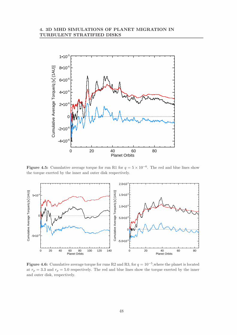
4. 3D MHD SIMULATIONS OF PLANET MIGRATION INTURBULENT STRATIFIED DISKS
0 20 40 60 80Planet Orbits
-4•10-6
-2•10-6
0
2•10-6
4•10-6
6•10-6
8•10-6
1•10-5C
umul
ativ
e A
vera
ge T
orqu
e/q
[vk2 (1
AU
)]
Figure 4.5: Cumulative average torque for run R1 for q = 5 × 10⁻⁶. The red and blue lines show
the torque exerted by the inner and outer disk respectively.
0 20 40 60 80 100 120 140Planet Orbits
-5•10-6
0
5•10-6
Cum
ulat
ive
Ave
rage
Tor
que/
q [v
k2 (1
AU
)]
0 20 40 60 80Planet Orbits
-5.0•10-6
0
5.0•10-6
1.0•10-5
1.5•10-5
2.0•10-5
Cum
ulat
ive
Ave
rage
Tor
que/
q [v
k2 (1
AU
)]
Figure 4.6: Cumulative average torque for runs R2 and R3, for q = 10−5,where the planet is located
at rp = 3.3 and rp = 5.0 respectively. The red and blue lines show the torque exerted by the inner
and outer disk, respectively.
48
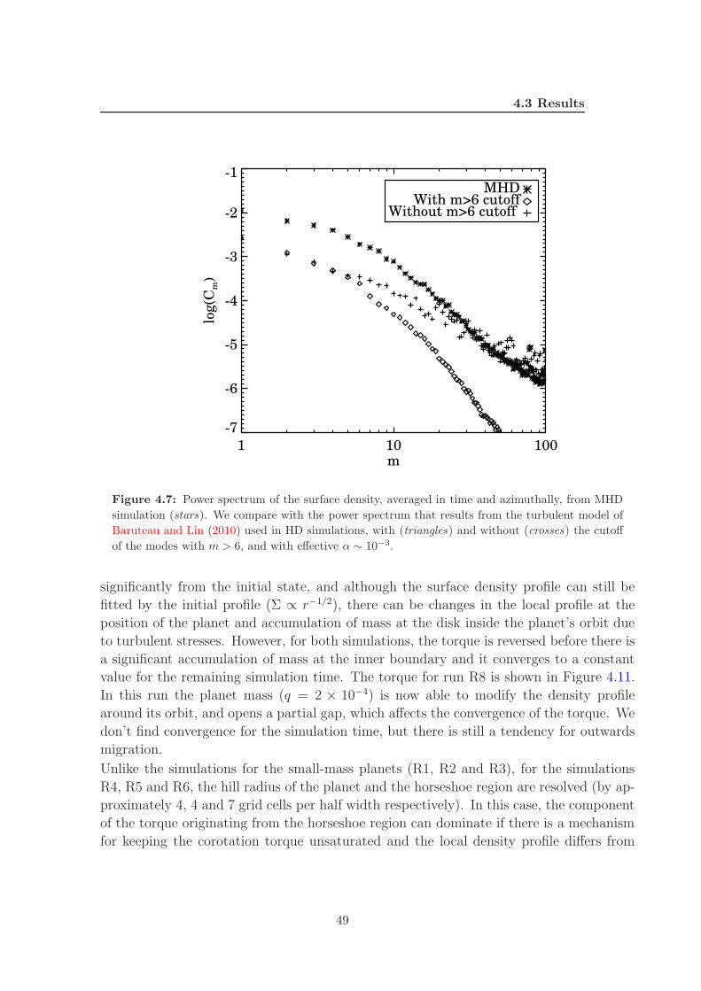
4.3 Results
1 10 100m
-7
-6
-5
-4
-3
-2
-1
log(C
m)
MHDWith m>6 cutoff
Without m>6 cutoff
Figure 4.7: Power spectrum of the surface density, averaged in time and azimuthally, from MHD
simulation (stars). We compare with the power spectrum that results from the turbulent model of
Baruteau and Lin (2010) used in HD simulations, with (triangles) and without (crosses) the cutoff
of the modes with m > 6, and with effective α ∼ 10−3.
significantly from the initial state, and although the surface density profile can still be
fitted by the initial profile (Σ ∝ r−1/2), there can be changes in the local profile at the
position of the planet and accumulation of mass at the disk inside the planet’s orbit due
to turbulent stresses. However, for both simulations, the torque is reversed before there is
a significant accumulation of mass at the inner boundary and it converges to a constant
value for the remaining simulation time. The torque for run R8 is shown in Figure 4.11.
In this run the planet mass (q = 2 × 10⁻⁴) is now able to modify the density profile
around its orbit, and opens a partial gap, which affects the convergence of the torque. We
don’t find convergence for the simulation time, but there is still a tendency for outwards
migration.
Unlike the simulations for the small-mass planets (R1, R2 and R3), for the simulations
R4, R5 and R6, the hill radius of the planet and the horseshoe region are resolved (by ap-
proximately 4, 4 and 7 grid cells per half width respectively). In this case, the component
of the torque originating from the horseshoe region can dominate if there is a mechanism
for keeping the corotation torque unsaturated and the local density profile differs from
49
4. 3D MHD SIMULATIONS OF PLANET MIGRATION INTURBULENT STRATIFIED DISKS
the global profile, possibly increasing outwards, such that the corotation torque can be
larger than the Lindblad torque, making the total torque positive. There are special lo-
cations in the disk where is possible for the surface density to increase outwards, due to
the appearance of zonal flows, as seen in Section 4.2.2.1.
Comparing the torque values of the simulations with analytical estimates by Paardekooper
and Papaloizou (2009a) or Masset et al. (2006a) is not straightforward. First, the un-
dergoing evolution of the disk can make the surface density profile at the position of the
planet and the effective stress resulting from turbulence vary in time, therefore one torque
estimate does not apply at all times. On the other hand, the value of the horseshoe drag
is very sensitive to the structure of the horseshoe region, and the estimate used in the
analytical calculations is based on a 2D model of the flow around the planet. In our case,
the horseshoe region is distorted, making the half-width difficult to define. Addition-
ally, the inclusion of magnetic fields can introduce new magnetic resonances that affect
the total torque, as seen by Terquem (2003) and Fromang et al. (2005) for a uniform
non-turbulent field. For the sake of the comparison and simplicity, we discard this type
of contribution. We attempt a comparison with the analytical estimates for the torque,
including a contribution of the horseshoe drag. We take the total torque to be composed
of the Lindblad torque in a 3D locally isothermal disk (Tanaka et al., 2002)
ΓLind = −(2.340 − 0.099a + 0.418b)
(
q
hp
)2
Σpr4pΩ2
p, (4.11)
plus the fully unsaturated non-linear horseshoe drag1 (Paardekooper and Papaloizou,
2009a)
ΓHS =3
4
(
3
2− a
)
x4sΣpr
4pΩ2
p. (4.12)
Here Ωp is the angular frequency of the planet and Σp is the surface density at the position
of the planet. The cumulative average torque at the end of the simulation for run R5
is 2.0 × 10⁻⁵ and we take the half width of the horseshoe region to be xs = 0.25, as
is measured in our simulations (calculated from the analytical expression, xs = 0.24).
Assuming the global surface density profile Σ ∝ r−d, with d = 0.5, will always give a
negative torque. However, the torque always becomes positive for d = 0.3 and matches
the simulation value for d = −1.5, which is comparable to the local profile observed in
the simulations (see middle plot in Figure 4.12). We should also note that already a
”close-to-flat” profile can significantly reduce the negative torque or change the sign of
the torque. For simulation R6, the cumulative average torque at the end of the simulation
1We take the expression for an isothermal disk, in the zero gravitational softening limit.
50
4.3 Results
is 3.7 × 10⁻⁶ and the measured half width of the horseshoe region is xs = 0.16. In this
case, a local profile of d = 0.1 is enough to obtain a positive torque, while a local profile
of d = −0.4 matches the value of the torque obtained in the simulation. However for this
simulation, we only observe a flatter profile (see Figure 4.12). This discrepancy can be due
to the fact that these values are very sensitive to the value of xs, since the horseshoe drag
scales as x4s, and we stress that the streamlines can be very distorted, therefore making
the estimation of xs difficult. This is a critical parameter, and we find that an increase
of 1% to 5% in the simulation value of xs with respect to the analytical estimation is
enough to reproduce the observed positive torques. Therefore, if one assumes that the
observed torque is composed of the wave torque plus the corotation torque and neglects
any additional effect, we see that the corotation torque is crucial and able to cancel out
or overcome the negative Lindblad contribution for standard disk parameters.
To further test the effect of the local density profile, we performed a simulation with
q = 10−4, for the planet located at rp = 4.0 (run R7, Figure 4.10), initially at the right
side of a pressure bump (where pressure and density decrease with radius). In this case,
the cumulative average torque does not clearly converge, and we do not see systematic
outwards migration, as the cumulative average torque approaches zero. However there is
still a significant reduction of the torque as compared to the Type I Lindblad torque, which
cannot be explained only in terms of a locally decreasing radial density profile. This result
suggest that even in the absence of a pressure bump, inwards migration can be significantly
slowed down for this planet mass. We note also that we used the expression for the
horseshoe drag valid for an isothermal disk, so that there is an additional contribution
due to the locally isothermal profile that we did not take into account.
To see if the transport of mass in the disk is enough to sustain the unsaturated torque,
we take the expression for the minimal α to mantain the unsaturated corotation torque
(Masset et al., 2006a)
αm = 0.035q3/2h−7/2, (4.13)
we obtain αm = 0.0003 for q = 10−4, which is always smaller than what we observe in our
simulations1 (comparing with the volume average α). For run R6 we also observed that
in comparison to a purely HD laminar run, in which the planet is able to open a partial
gap in the disk, the gap in this case is less deep that in the HD case, and also wider,
compared to the narrower gap seen in the laminar simulation. For run R5, there was no
gap opening neither in the laminar nor the turbulent runs as the gap opening criterion is
not satisfied. We also find that the stresses in the disk are affected by the presence of the
planet; the volume averaged stress decreases as the mass of the planet is increased (see
top and middle plots in Figure 4.13), which might be a result of numerical dissipation
1However, this expression for αm is derived using a 2D model of the HS region, which determines the viscous
crossing time across the region, the libration time and the U-turn time.
51

4. 3D MHD SIMULATIONS OF PLANET MIGRATION INTURBULENT STRATIFIED DISKS
due to the limited resolution.
0 20 40 60 80Planet Orbits
-4•10-5
-2•10-5
0
2•10-5
4•10-5
Cum
ulat
ive
Ave
rage
Tor
que/
q [v
k2 (1
AU
)]
Figure 4.8: Cumulative average torque for run R4 for q = 5 × 10⁻⁵. The red and blue lines show
the torque exerted by the inner and outer disk respectively.
4.3.1.3 Large Mass Planet (q = 10−3)
The density structure and spiral arms induced by the Jupiter mass planet in run R9
(q = 10−3) dominate over the turbulent perturbations and influences the entire disk.
Figure 4.14 shows the cumulative average torque. We have excluded the torques coming
from the Hill sphere for the calculation of the torque, to exclude material bound to
the planet which is not properly simulated at this resolution or without including other
relevant effects. For these simulations, initially we see the same trend as for runs R5
and R6, where the torque becomes positive, however this is not sustained for this planet
mass as torques coming from the corotation region are suppressed due to gap opening (see
bottom plot in Figure 4.12 and the right panels in Figure 4.4). Additionally, the planet
modifies the stresses in the disk, and therefore, the accretion behavior, as can be seen
in the bottom plot in Figure 4.13, that shows the evolution of the stresses for run R9.
In this case, the α stress is progressively suppressed and the Reynolds stress dominates
the total stress. The reduction of the Maxwell stress is seen mostly in the part of the
52
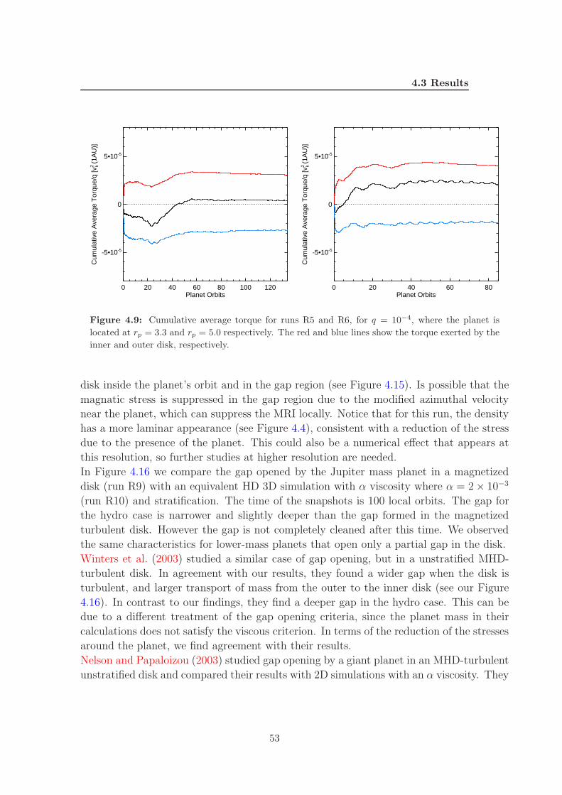
4.3 Results
0 20 40 60 80 100 120Planet Orbits
-5•10-5
0
5•10-5
Cum
ulat
ive
Ave
rage
Tor
que/
q [v
k2 (1
AU
)]
0 20 40 60 80Planet Orbits
-5•10-5
0
5•10-5
Cum
ulat
ive
Ave
rage
Tor
que/
q [v
k2 (1
AU
)]
Figure 4.9: Cumulative average torque for runs R5 and R6, for q = 10−4, where the planet is
located at rp = 3.3 and rp = 5.0 respectively. The red and blue lines show the torque exerted by the
inner and outer disk, respectively.
disk inside the planet’s orbit and in the gap region (see Figure 4.15). Is possible that the
magnatic stress is suppressed in the gap region due to the modified azimuthal velocity
near the planet, which can suppress the MRI locally. Notice that for this run, the density
has a more laminar appearance (see Figure 4.4), consistent with a reduction of the stress
due to the presence of the planet. This could also be a numerical effect that appears at
this resolution, so further studies at higher resolution are needed.
In Figure 4.16 we compare the gap opened by the Jupiter mass planet in a magnetized
disk (run R9) with an equivalent HD 3D simulation with α viscosity where α = 2 × 10⁻³
(run R10) and stratification. The time of the snapshots is 100 local orbits. The gap for
the hydro case is narrower and slightly deeper than the gap formed in the magnetized
turbulent disk. However the gap is not completely cleaned after this time. We observed
the same characteristics for lower-mass planets that open only a partial gap in the disk.
Winters et al. (2003) studied a similar case of gap opening, but in a unstratified MHD-
turbulent disk. In agreement with our results, they found a wider gap when the disk is
turbulent, and larger transport of mass from the outer to the inner disk (see our Figure
4.16). In contrast to our findings, they find a deeper gap in the hydro case. This can be
due to a different treatment of the gap opening criteria, since the planet mass in their
calculations does not satisfy the viscous criterion. In terms of the reduction of the stresses
around the planet, we find agreement with their results.
Nelson and Papaloizou (2003) studied gap opening by a giant planet in an MHD-turbulent
unstratified disk and compared their results with 2D simulations with an α viscosity. They
53

4. 3D MHD SIMULATIONS OF PLANET MIGRATION INTURBULENT STRATIFIED DISKS
0 20 40 60 80Planet Orbits
-4•10-5
-2•10-5
0
2•10-5
4•10-5
Cum
ulat
ive
Ave
rage
Tor
que/
q [v
k2 (1
AU
)]
Figure 4.10: Cumulative average torque for run R7 for q = 10−4, for the planet located at rp = 4.0,
initially at the right side of a pressure bump. The red and blue lines show the torque exerted by the
inner and outer disk respectively.
found that a run with an equivalent α stress to the turbulent run produced a shallower
gap. This is different to our own results where we found the same gap depth. However,
we should note they only studied how the turbulence affects an already formed gap and
did not observe the depletion of the outer disk. The difference to our simulation results
could also be due to our choice of α in the hydro run. We choose an α matching the
global average of the turbulent runs, but this is a quantity that varies vertically. In a
non-stratified disk simulation, this averaging is not necessary.
4.4 Discussion and conclusions
For simulations R1, R2 and R3, where q = 10−5, during the simulated time, migration was
dominated by random fluctuations in the torque, that can be orders of magnitude larger
that what is expected for the value of the Lindblad or corotation torques for this planet
mass. This is in agreement with simulations by Nelson (2005) of migration of low-mass
protoplanets in cylindrical disk models, where stratification is neglected. It is unclear if
after long term averaging (∼ 1000 orbits), the fluctuations will average out to zero while
54

4.4 Discussion and conclusions
0 20 40 60 80Planet Orbits
-1•10-4
-5•10-5
0
5•10-5
1•10-4
Cum
ulat
ive
Ave
rage
Tor
que/
q [v
k2 (1
AU
)]
Figure 4.11: Cumulative average torque for run R8 for q = 2× 10⁻⁴. The red and blue lines show
the torque exerted by the inner and outer disk respectively.
some component of the systematic torque will remain. Such a calculation is currently
too expensive. It will also be difficult to get a steady state without special prescriptions
for correcting the density, due to the accretion evolution of the disk, in addition to the
decrease in α stress for long simulation times due to the limited resolution. Another
interesting point for further studies is to investigate this type of migration with enough
resolution to resolve the corotation region, to see the impact of the corotation torque
in these cases. However, even if this torque is present and well resolved, its magnitude
would still be small compared to the amplitude of the fluctuations, since ultimately the
torque depends strongly on the width of the corotation region, which approaches zero as
the planet mass approaches zero.
As the planet mass is increased by one order of magnitude to q = 10−4, the hill radius is
now properly resolved and the systematic torque is now large enough to dominate over
the random component of the torque. Outwards migration in a locally isothermal disk
can occur due to the viscosity unsaturating the torque coming from the corotation region
(where the viscous timescale across the horseshoe region is smaller than the libration
timescale), as was found by Masset et al. (2006a) for planets in the intermediate-mass
55
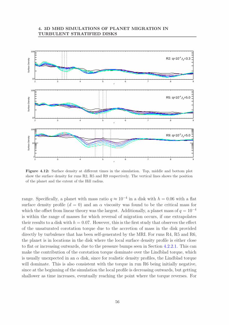
4. 3D MHD SIMULATIONS OF PLANET MIGRATION INTURBULENT STRATIFIED DISKS
2 3 4 5 6 7 8 9r
10
100
Sur
face
Den
sity R2: q=10-4,rp=3.3
2 3 4 5 6 7 8 9r
10
100
Sur
face
Den
sity R5: q=10-4,rp=5.0
2 3 4 5 6 7 8 9r
1
10
100
Sur
face
Den
sity R9: q=10-3,rp=5.0
Figure 4.12: Surface density at different times in the simulation. Top, middle and bottom plot
show the surface density for runs R2, R5 and R9 respectively. The vertical lines shows the position
of the planet and the extent of the Hill radius.
range. Specifically, a planet with mass ratio q ≈ 10−4 in a disk with h = 0.06 with a flat
surface density profile (d = 0) and an α viscosity was found to be the critical mass for
which the offset from linear theory was the largest. Additionally, a planet mass of q = 10−4
is within the range of masses for which reversal of migration occurs, if one extrapolates
their results to a disk with h = 0.07. However, this is the first study that observes the effect
of the unsaturated corotation torque due to the accretion of mass in the disk provided
directly by turbulence that has been self-generated by the MRI. For runs R4, R5 and R6,
the planet is in locations in the disk where the local surface density profile is either close
to flat or increasing outwards, due to the pressure bumps seen in Section 4.2.2.1. This can
make the contribution of the corotation torque dominate over the Lindblad torque, which
is usually unexpected in an α disk, since for realistic density profiles, the Lindblad torque
will dominate. This is also consistent with the torque in run R6 being initially negative,
since at the beginning of the simulation the local profile is decreasing outwards, but getting
shallower as time increases, eventually reaching the point where the torque reverses. For
56

4.4 Discussion and conclusions
0 20 40 60 80 100Planet Orbits
0.0001
0.0010
0.0100
Inte
rna
l S
tress
es
0 20 40 60 80 100Planet Orbits
0.0001
0.0010
0.0100
Inte
rna
l S
tress
es
0 20 40 60 80 100Planet Orbits
0.0001
0.0010
0.0100
Inte
rna
l S
tress
es
Figure 4.13: Time evolution of the stresses in a disk with an embedded planet. Top, middle and
bottom plot show the stresses for runs R2, R5 and R9, respectively. The dashed and dashed-dotted
lines show the Reynolds TRey and Maxwell TMax stresses, respectively, normalized to the initial
pressure. The solid line shows the total effective α parameter.
run R5, the slope is almost immediately increasing outwards due to the evolution of the
disk, which makes the torque positive from the beginning of the simulations. We can
only roughly compare our numerical results with analytical estimates, as was done in
the previous section, for the reasons described already there. Also in comparing with
previous estimates, we also discarded any possible additional contributions to the torque
that might arise because of the turbulent magnetic fields. The detailed structure of the
horseshoe region in the presence of turbulence and stratification deserves further study.
Our results are summarized on Figure 4.17, where the torque dependence on planet mass
is shown. For each simulation, we plot the last value of the cumulative average torque.
Note however that only for part of the simulations the torque converges to a well defined
value. It is possible to see a trend of the torque to reverse, corresponding to the addition
of the contribution of the fully unsaturated horseshoe drag (Γtot = ΓLind + ΓHS). For the
plot we assumed values for the width of the horseshoe region that are 5% larger than
the analytical estimate given by Paardekooper and Papaloizou (2009a) and we use the
57

4. 3D MHD SIMULATIONS OF PLANET MIGRATION INTURBULENT STRATIFIED DISKS
0 20 40 60 80 100Planet Orbits
-5•10-5
0
5•10-5
Cum
ulat
ive
Ave
rage
Tor
que/
q [v
k2 (1
AU
)]
Figure 4.14: Cumulative average torque for run R9 for q = 10−3. The red and blue lines show the
torque exerted by the inner and outer disk respectively. The torque coming from the Hill sphere has
been excluded from the calculation.
value of the local surface density profile for the calculation of the torque. We see that
the trend breaks down already for q = 2 × 10⁻⁴, where gap opening starts to become
important and there is a transition into the Type II regime. Error bars represent the
standard deviation of the time distribution of the torque. Note that since the raw torque
is a highly oscillating quantity, the standard deviation does not match directly to the
amplitude of the turbulent fluctuations, especially in the high-mass planet cases. For run
10, the standard deviation was found to be only 20% lower that in the turbulent run R9.
In the Type II range, we plot the torque corresponding to the viscous timescale of the
disk, taking α = 3 × 10⁻³. We find reasonable agreement with our simulation, taking
into account the short simulation time, and that the value of the torque is still decreasing
in the simulation after 100 orbits. Additionally we use the value of the initial, volume
averaged α, while the mid-plane value is smaller.
The question remains about the long term behavior of the torque, and whether this is
only a transient behavior lasting for the first few hundred orbits (assuming the same local
surface density profile), afterwards saturating and returning to standard negative Type I
values. This is still a transient behavior in the sense that the planet can migrate out of the
58

4.4 Discussion and conclusions
2 3 4 5 6 7 8r [AU]
0.0001
0.0010
0.0100In
tern
al
Str
ess
es
TotalReynoldsMaxwell
Figure 4.15: Radial distribution of the time, azimuthally and vertically averaged stress parameter
for run R9. The dashed and dashed-dot lines show the Reynolds TRey and Maxwell TMax stresses
respectively, normalized by the initial pressure. The solid line shows the total effective α parameter.
part of the disk where the local profile allows for outwards migration and enter a region
where migration proceeds inwards again. Additionally it is limited by the lifetime of the
pressure bumps, which we weren’t able to determine. We observe a stable pressure bump
through the duration of our simulations. If there are other mechanisms such as the ones
discussed in Masset et al. (2006b) that produces this type of locally increasing outwards
density profile, then, in the presence of turbulence, these density bumps can also act as
a protoplanet trap and halt, slow down or reverse inwards migration. Dzyurkevich et al.
(2010) performed non-ideal MHD simulations of accretion disks with spatially varying
resistivity. They also find zonal flows/pressure bumps not only at the snow line, e.g. a
region with a jump in resistivity, but also inside the more active region. They already
suggest that small planets should get trapped at those local pressure maxima (see also
Kretke and Lin (2007)).
59
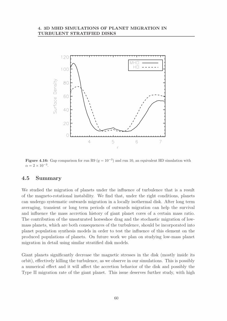
4. 3D MHD SIMULATIONS OF PLANET MIGRATION INTURBULENT STRATIFIED DISKS
Figure 4.16: Gap comparison for run R9 (q = 10−3) and run 10, an equivalent HD simulation with
α = 2 × 10⁻³.
4.5 Summary
We studied the migration of planets under the influence of turbulence that is a result
of the magneto-rotational instability. We find that, under the right conditions, planets
can undergo systematic outwards migration in a locally isothermal disk. After long term
averaging, transient or long term periods of outwards migration can help the survival
and influence the mass accretion history of giant planet cores of a certain mass ratio.
The contribution of the unsaturated horseshoe drag and the stochastic migration of low-
mass planets, which are both consequences of the turbulence, should be incorporated into
planet population synthesis models in order to test the influence of this element on the
produced populations of planets. On future work we plan on studying low-mass planet
migration in detail using similar stratified disk models.
Giant planets significantly decrease the magnetic stresses in the disk (mostly inside its
orbit), effectively killing the turbulence, as we observe in our simulations. This is possibly
a numerical effect and it will affect the accretion behavior of the disk and possibly the
Type II migration rate of the giant planet. This issue deserves further study, with high
60
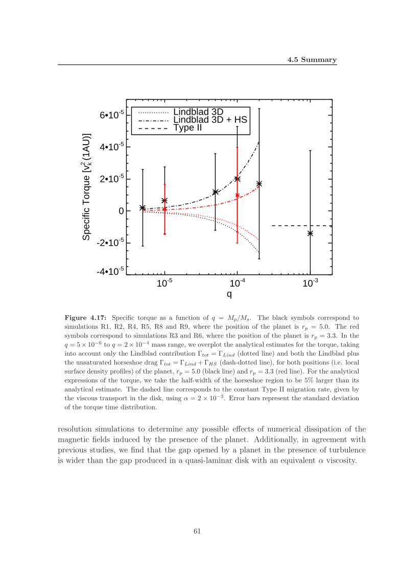
4.5 Summary
10-5 10-4 10-3
q
-4•10-5
-2•10-5
0
2•10-5
4•10-5
6•10-5
Spe
cific
Tor
que
[vk2 (1
AU
)]
Lindblad 3DLindblad 3D + HSType II
Figure 4.17: Specific torque as a function of q = Mp/Ms. The black symbols correspond to
simulations R1, R2, R4, R5, R8 and R9, where the position of the planet is rp = 5.0. The red
symbols correspond to simulations R3 and R6, where the position of the planet is rp = 3.3. In the
q = 5× 10⁻⁶ to q = 2× 10⁻⁴ mass range, we overplot the analytical estimates for the torque, taking
into account only the Lindblad contribution Γtot = ΓLind (dotted line) and both the Lindblad plus
the unsaturated horseshoe drag Γtot = ΓLind + ΓHS (dash-dotted line), for both positions (i.e. local
surface density profiles) of the planet, rp = 5.0 (black line) and rp = 3.3 (red line). For the analytical
expressions of the torque, we take the half-width of the horseshoe region to be 5% larger than its
analytical estimate. The dashed line corresponds to the constant Type II migration rate, given by
the viscous transport in the disk, using α = 2 × 10⁻³. Error bars represent the standard deviation
of the torque time distribution.
resolution simulations to determine any possible effects of numerical dissipation of the
magnetic fields induced by the presence of the planet. Additionally, in agreement with
previous studies, we find that the gap opened by a planet in the presence of turbulence
is wider than the gap produced in a quasi-laminar disk with an equivalent α viscosity.
61

4. 3D MHD SIMULATIONS OF PLANET MIGRATION INTURBULENT STRATIFIED DISKS
62

5
Accretion of gas onto giant planets
and envelope structure in
magnetized turbulent disks
We have performed three-dimensional magneto-hydrodynamical simulations of ac-
cretion disks, using the PLUTO code, and studied the accretion of gas onto a Jupiter-
mass planet after opening a gap in the disk. We compare our results with simulations
of laminar, yet viscous disks with different levels of an α viscosity. A jupiter mass
planet is known to reduce the magnetic stress in the disk to around 10% of the
unperturbed value. We find that this low levels of MRI-turbulence in protoplane-
tary disks do not enhance mass accretion onto the planet, and in fact might slightly
suppress accretion, as compared to the case of a laminar viscous disk with compa-
rable α parameter. In all cases, the accretion flow accross the surface of the Hill
sphere of the planet is not spherically or azimuthally symmetric, and is predomi-
nantly restricted to the mid-plane of the disk. Even in the turbulent case, we find
no vertical flow of mass into the Hill sphere. Accretion rates are best approximated
analytically by using the reduced density in the gap region. This means that the
gap-opening planet never reaches an accretion rate as high as the one given by the
unperturbed density of the disk. For a simulation of a magnetized turbulent disk,
where the global averaged alpha stress is αMHD = 1 × 10⁻³, we find the accretion
rate onto the planet to be M = 6 × 10⁻⁷MJyr−1.
63
5. ACCRETION OF GAS ONTO GIANT PLANETS AND ENVELOPESTRUCTURE IN MAGNETIZED TURBULENT DISKS
5.1 Introduction
Studying how planets accrete gas from circumstellar disks is necessary to estimate a limit
on the mass of giant gaseous planets depending on the disk properties such as density and
viscosity. It is also necessary to estimate the timescales for gas accretion (Alibert et al.,
2004). In general one should take into account the effects of migration, gap formation
and the viscous evolution of the disk.
In the inner parts of disks, gas giants can form as a result of core formation by plan-
etesimal accretion followed by formation of the gas envelope by gas accretion from the
circumstellar disk. Pollack et al. (1996) distinguished three phases in the formation using
numerical simulations of core accretion and envelope evolution. A first phase marked
by the fast accretion of solids unto a core until the feeding zone of the planet is mostly
evacuated (Stevenson, 1982). A second phase where gas and solids accretion is low and
constant. Finally, a third stage when the core mass equals the envelope mass, leading to
the contraction of the envelope and the onset of runaway gas accretion (Mizuno, 1980).
Migration of the planet might allow for an extension of the feeding zone, while gap for-
mation might lead to a mass limit for gap opening planets (Alibert et al., 2005). In the
outer parts of the disk, giant planets could form as a result of the collapse of a gravita-
tionally unstable disk clump. This mechanism requires a very massive disk that can cool
effectively on timescales of a few local orbital periods (Boss, 1997; Durisen et al., 2007;
Mayer et al., 2002; Rafikov, 2005).
Planet population synthesis models produce synthetic populations of extrasolar planets,
with a large diversity of initial conditions. These models have been successful in reproduc-
ing key features of the observed distribution of exoplanets(Benz et al., 2008; Ida and Lin,
2008; Mordasini et al., 2009a,b). The calculations usually include one-dimensional disk
evolution and core/envelope structure models. The accretion of planetesimals and gas
onto an already formed proto-core is included, using a given prescription for the accretion
rates of gas and rocky materials onto the planet (Alibert et al., 2004). For this reason,
an accurate estimation and parameterization of the accretion rates of gas onto planets
for a variety of conditions is necessary to correctly calculate the formation time and the
limiting mass of the giant planetary population.
5.1.1 Modeling planet accretion
The accretion of gas onto planets has been modelled using two different approaches. On
one side, one dimensional models have been used to calculate the radial structure of the
envelope and the accretion onto a rocky core. This models can include effects such as
the dust opacity of the envelope, the release of energy of infalling planetesimals into the
envelope and the thermal feedback of the planet (Hubickyj et al., 2005; Ikoma et al., 2000).
64

5.1 Introduction
These models can only include the disk evolution in a restricted way, and assume a certain
model of the outer envelope (as a boundary condition) that is spherically symmetric.
On the other hand, two/three-dimensional simulations of accretion disk with accreting
planets aim to estimate the structure of the flow around the planet and how much mass
is the disk capable of feeding to the planet. However, most of these simulations miss the
radiative feedback from the planet and a detailed model of the inner envelope. D’Angelo
et al. (2003a,b); Tanigawa and Watanabe (2002) used high resolution two-dimensional sim-
ulations to study the detailed flow pattern around the planet, and the circumplanetary
disk. They showed that inside the planets Roche lobe, accretion in the circumplanetary
disk is powered mainly by energy dissipation of circulating matter at the spiral shock.
Outside the Roche lobe, gas flows into the planet through ”accretion bands” located be-
tween the horseshoe flow and the passing-by flow (although the detailed structure depends
strongly on the sound speed). The accretion timescale
τacc =Mp
Mp
, (5.1)
has been measured to be around 104 − 105 yr, and the accretion rate of a Jupiter-mass
planet has been found to be on the order of 10−5MJ/yr on a disk with Md = 0.01M⊙
(Bate et al., 2003; Bryden et al., 1999; Kley et al., 2001; Lubow et al., 1999). Three-
dimensional simulations including radiation transfer have found similar accretion rates
and have shown the formation of a thick (H/r ≈ 0.5) circumplanetary disk (Klahr and
Kley, 2006).
In this chapter we take the second approach and study the accretion rate of gas onto
giant gap-opening planets in turbulent magnetized disks using three-dimensional global
disk simulations. The turbulence in the disk is generated by the magneto-rotational
instability (Balbus and Hawley, 1991). We compare the accretion rate of a planet in a
turbulent disk with that in a viscous laminar disk and we examine the accretion structure
and mass inflow into the Hill sphere of the planet, where material is assumed to be
gravitationally bound to the planet. The chapter is organized as follows. In Section 2, we
describe the computational setup, boundary and initial conditions, and the parameters
we use in our simulations. We also describe the prescription for the mass accretion onto
the planet. In Section 3.1, we present our results on the three-dimensional structure of the
accretion flow into the Hill sphere. Section 3.2 contains the results on the mass accretion
rates for the different simulations, while Section 3.3 shows the details of the accretion flow
around the planet. Finally, we discuss and sumarize our results in Sections 4 and 5.
65
5. ACCRETION OF GAS ONTO GIANT PLANETS AND ENVELOPESTRUCTURE IN MAGNETIZED TURBULENT DISKS
5.2 Computationl setup
Simulations were performed using the finite volume fluid dynamics code PLUTO (Mignone
et al., 2007). In the code, time stepping is done using a second order Runge Kutta
scheme, while the spatial integration is performed using linear interpolation through the
second order TVD scheme. The Riemann fluxes are computed using the HLLC and HLLD
solvers for the HD and MHD cases, respectively. The code uses the Constrained Transport
method for preserving a divergence-free magnetic field (Gardiner and Stone, 2005). The
numerical setup for the MHD case follows the setup presented in (Flock et al., 2010).
We use spherical coordinates (r, θ, φ) and the domain is given by r ∈ [1, 10], θ ∈ [π/2 −
0.3, π/2 + 0.3] and φ ∈ [0, 2π]. The grid resolution is (Nr, Nθ, Nφ) = (256, 128, 256) and
it is centered in the center of mass of the planet-star system.
The gas disk is initially in sub-Keplerian rotation around a solar mass star. The azimuthal
velocity is given by
vφ =√
v2k − c2
s(a − 2b), (5.2)
where vk is the Keplerian velocity and a = 3/2 and b = 0.5 are the exponents of the radial
power law distribution of the density ρ ∝ r−a and sound speed cs = c0(r sin θ)−b. The
initial density distribution is given by
ρ(r, θ) = (r sin θ)−3/2 exp
(
sin θ − 1
c20
)
. (5.3)
The disk is described by a locally isothermal equation of state P = c2sρ. The ratio of the
pressure scale height h to the radial coordinate of the disk is taken to be a constant such
that h = H/(r sin θ) = 0.07.
The gravitational potential of the planet is given by a softened point-mass potential
Φp(r) = −GM
(|r − rp|2 + ǫ2)1/2(5.4)
where ǫ is the softening parameter, needed to avoid numerical divergence near the position
of the planet. For all the simulations ǫ is set to be a fraction of the Hill radius ǫ =
krp(Mp/3)1/3 with k = 0.3. Distances are given in units of r0 = 1AU , density is given in
units of ρ0 = 1 × 10⁻¹²gcm−3, and velocity is given in units of Keplerian speed at 1AU ,
v0 = vk(1AU). The surface density have been scaled such that the total disk mass is
0.01Mstar. Magnetic fields are given in units of B0 =√
4πρ0v20. The equations of motion
of the planet are solved at each timestep with a leap frog integrator.
The components of the torque vector in cartesian coordinates are given by
Γi = GMp
∫
ρ(r)(rp × r)i
(|r− rp|2 + ǫ2)3/2dV, (5.5)
66
5.2 Computationl setup
where i ∈ x, y, z is any of the three cartesian indices and (~rp × ~r)i = (~rp × ~r) · ei, and
ei are the cartesian unit vectors. Specific torques are given in units of v2k(1AU).
5.2.1 Boundary conditions
The boundary conditions for the velocities and magnetic field are periodic in the vertical
(θ boundary) and azimuthal directions and reflective in the radial direction, except for
the transverse magnetic field component, which reverses its sign at the radial boundary.
Buffer zones are defined at the radial boundaries to avoid boundary effects, where for
1 < r < 2 the magnetic resistivity is given by η = 2 × 10⁻⁴(2 − r) and for 9 < r < 10 the
resistivity is η = 1 × 10⁻⁴(r − 9).
5.2.2 Initial conditions, gap opening and viscosity
The planet is allowed to accrete gas after only 100 orbital periods at 5AU have elapsed
(see Figure 5.1). At this stage, a gap has been cleared, and the density has been reduced
by more than 95%. We refer to Chapter 4 for a detailed description of the initial setup
and the study of the migration and the interaction between the planet and the magnetic
field. For the hydrodynamical simulations, viscosity is added explicitly as a source term
in the momentum equation. We use an α-type kinematic viscosity give by ν = αc2sH ,
where α takes values of 2 × 10⁻³, 2 × 10⁻⁴ and 2 × 10⁻⁵.
5.2.3 Accretion prescription
The accretion is modelled by removing a fraction of the mass inside the Hill sphere at
each time step. At each timestep the new density ρ′
is given by
ρ′
(r) =
(
1 −∆t
ta
)
ρ(r). (5.6)
The accreted mass in timestep ∆t is ∆M = (ρ(r)∆tt−1a )r2sin(θ)drdθdφ. The accretion
rate for timestep ∆t is calculated as the accreted mass divided by the timestep ∆M/∆t.
The factor ta represents the accretion timescale in which the Hill sphere is emptied if
there was no gas flowing in from the disk. This is chosen to be ta = 1Ω−11AU inside
the inner half of the Hill sphere and ta = 2Ω−11AU in the outer half of the Hill sphere
(where Ω−11AU is the keplerian angular frequency at 1AU). A density floor is applied to
the simulations with magnetic fields, where the density is not allowed to drop bellow
10−19grcm−3. Nevertheless, the density in the simulation never reaches this value. The
magnetic field is not modified as the density is reduced inside the Hill sphere in order to
preserve a divergence-free field. The accretion rate has been shown to be dependent on
the accretion radius (the distance from the planet up to which mass is removed) and on
67
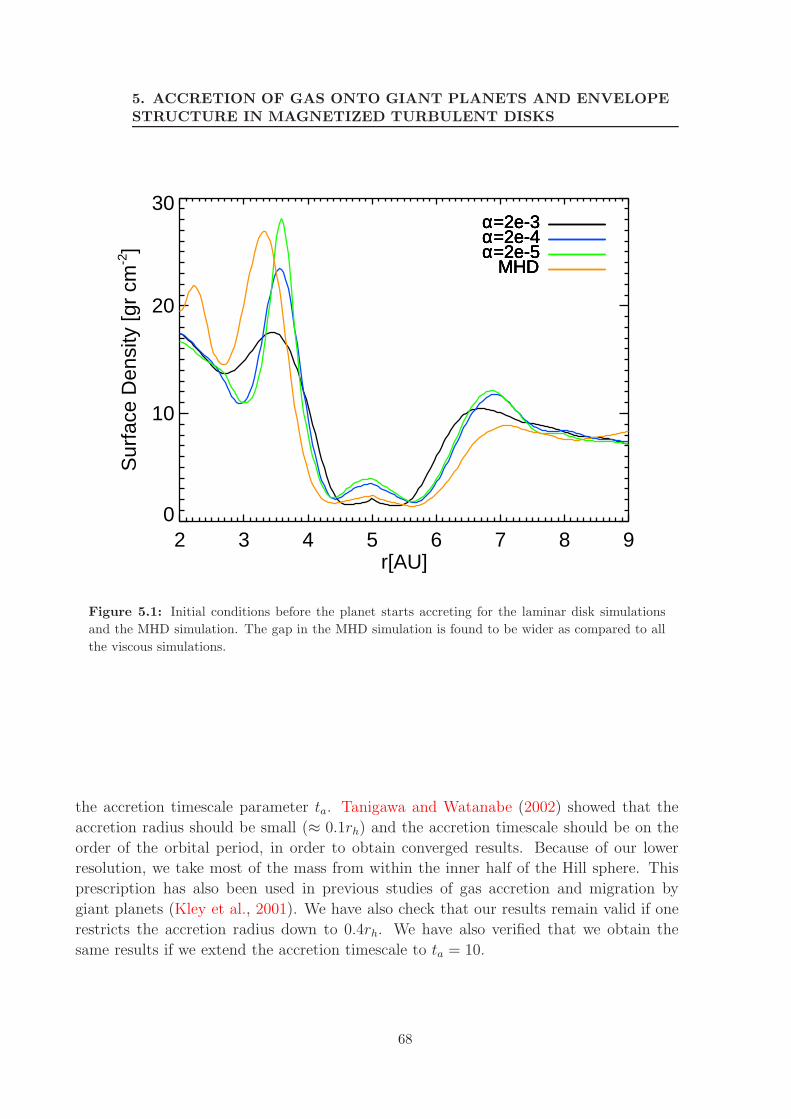
5. ACCRETION OF GAS ONTO GIANT PLANETS AND ENVELOPESTRUCTURE IN MAGNETIZED TURBULENT DISKS
2 3 4 5 6 7 8 9r[AU]
0
10
20
30
Sur
face
Den
sity
[gr
cm-2]
α=2e-3α=2e-4α=2e-5
MHD
α=2e-3α=2e-4α=2e-5
MHD
α=2e-3α=2e-4α=2e-5
MHD
α=2e-3α=2e-4α=2e-5
MHD
Figure 5.1: Initial conditions before the planet starts accreting for the laminar disk simulations
and the MHD simulation. The gap in the MHD simulation is found to be wider as compared to all
the viscous simulations.
the accretion timescale parameter ta. Tanigawa and Watanabe (2002) showed that the
accretion radius should be small (≈ 0.1rh) and the accretion timescale should be on the
order of the orbital period, in order to obtain converged results. Because of our lower
resolution, we take most of the mass from within the inner half of the Hill sphere. This
prescription has also been used in previous studies of gas accretion and migration by
giant planets (Kley et al., 2001). We have also check that our results remain valid if one
restricts the accretion radius down to 0.4rh. We have also verified that we obtain the
same results if we extend the accretion timescale to ta = 10.
68

5.3 Results
5.3 Results
5.3.1 Structure of the envelope and mass inflow
In this section we study the structure of the density and the inflow of mass in/into the
Hill sphere. We calculate the gas density and the mass flux through the surface of the Hill
sphere. The mass flux is given by ρvinflow = ρv·(∇F/|∇F |), where F (r) = (r−rp)2−r2h =
0 is the equation describing the surface of the Hill sphere. The density is plotted in Figures
5.2 and 5.3 for all four simulations. The mass flux is plotted in Figures 5.4 and 5.5 for
all simulations. These quantities have been averaged in time. We plot the surface of the
Hill sphere using an ellipsoidal projection where the three-dimensional structure can be
observed. The center of the ellipse corresponds to the point in the Hill sphere that is most
distant from the star.
The structure of the spiral arms can be seen in Figures 5.2 and 5.3 in the radial directions
(with respect to the star) pointing away from the planet. The arms go into the Hill sphere
radially from the inner and outer disk. However, comparing the density plots with the
mass flux as is seen in Figures 5.4 and 5.5, the accretion into the Hill sphere is not exactly
correlated to the spiral arms in general, meaning that the planet accretes from a more
extended region. The density and mass flux are much larger in the case with the higher
viscosity (α = 2 × 10⁻³), and are the lowest in the turbulent magnetized case. In the
first high viscosity case, most of the gas accreted is supplied by the disk from the outer
disk. In the low viscosity cases and the magnetized case, the mass flux is more extended
over the midplane surrounding the planet. In all cases, all the flux through the surface is
inflowing, and we see no significant amount gas entering the Hill sphere from the vertical
direction above and below the mid-plane. Figure 5.6 shows the vertical structure of the
mass flux averaged over the azimuthal direction. Once the gas enters the Hill sphere, we
assume it is bounded to the planet and it will be eventually accreted out of the domain.
5.3.2 Gas accretion rates
The cumulative mass accreted and the accretion rate are shown in Figures 5.8 and 5.7,
for the laminar viscous simulations and the magnetized simulation1. We will first discuss
the laminar simulations. The largest accretion rate is obtained for the viscous simulation
with α = 2 × 10⁻³, as it is expected since the disk accretion rate is proportional to the
viscosity. For the case where α = 2 × 10⁻⁴ and α = 2 × 10⁻⁵ the accretion rates are one
third lower than the rate for the higher viscosity, but with the α = 2×10⁻⁴ being slightly
lower than the lowest viscosity case. This means that the limit of the lowest viscosity that
the code is able to resolve above numerical dissipation effects is α ≈ 10−4. Additionaly,
1We will refer to αMHD to denote the alpha stress that is measured in the magnetized simulation, and to α
to denote the Shakura and Sunyaev (1973) viscosity parameter that is chosen for the viscous laminar simulations
69
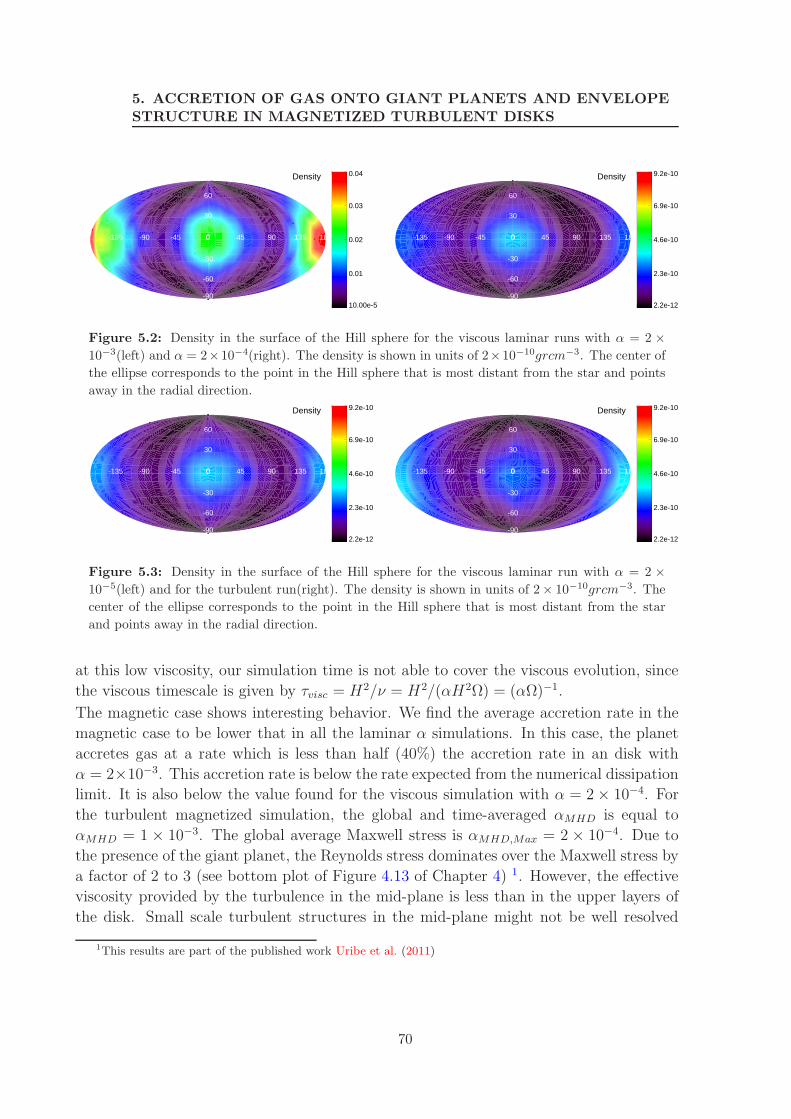
5. ACCRETION OF GAS ONTO GIANT PLANETS AND ENVELOPESTRUCTURE IN MAGNETIZED TURBULENT DISKS
-135 -90 -45 0 45 90 135 180
-90
-60
-30
0
30
60
90
10.00e-5
0.01
0.02
0.03
0.04Density
-135 -90 -45 0 45 90 135 180
-90
-60
-30
0
30
60
90
2.2e-12
2.3e-10
4.6e-10
6.9e-10
9.2e-10Density
Figure 5.2: Density in the surface of the Hill sphere for the viscous laminar runs with α = 2 ×
10−3(left) and α = 2×10⁻⁴(right). The density is shown in units of 2×10⁻¹⁰grcm−3. The center of
the ellipse corresponds to the point in the Hill sphere that is most distant from the star and points
away in the radial direction.
-135 -90 -45 0 45 90 135 180
-90
-60
-30
0
30
60
90
2.2e-12
2.3e-10
4.6e-10
6.9e-10
9.2e-10Density
-135 -90 -45 0 45 90 135 180
-90
-60
-30
0
30
60
90
2.2e-12
2.3e-10
4.6e-10
6.9e-10
9.2e-10Density
Figure 5.3: Density in the surface of the Hill sphere for the viscous laminar run with α = 2 ×
10−5(left) and for the turbulent run(right). The density is shown in units of 2× 10⁻¹⁰grcm−3. The
center of the ellipse corresponds to the point in the Hill sphere that is most distant from the star
and points away in the radial direction.
at this low viscosity, our simulation time is not able to cover the viscous evolution, since
the viscous timescale is given by τvisc = H2/ν = H2/(αH2Ω) = (αΩ)−1.
The magnetic case shows interesting behavior. We find the average accretion rate in the
magnetic case to be lower that in all the laminar α simulations. In this case, the planet
accretes gas at a rate which is less than half (40%) the accretion rate in an disk with
α = 2×10⁻³. This accretion rate is below the rate expected from the numerical dissipation
limit. It is also below the value found for the viscous simulation with α = 2 × 10⁻⁴. For
the turbulent magnetized simulation, the global and time-averaged αMHD is equal to
αMHD = 1 × 10⁻³. The global average Maxwell stress is αMHD,Max = 2 × 10⁻⁴. Due to
the presence of the giant planet, the Reynolds stress dominates over the Maxwell stress by
a factor of 2 to 3 (see bottom plot of Figure 4.13 of Chapter 4) 1. However, the effective
viscosity provided by the turbulence in the mid-plane is less than in the upper layers of
the disk. Small scale turbulent structures in the mid-plane might not be well resolved
1This results are part of the published work Uribe et al. (2011)
70

5.3 Results
-135 -90 -45 0 45 90 135 180
-90
-60
-30
0
30
60
90
2.70e-5
0.00
0.00
0.00
0.01Mass Flux
-135 -90 -45 0 45 90 135 180
-90
-60
-30
0
30
60
90
6.0e-13
3.7e-11
7.4e-11
1.1e-10
1.5e-10Mass Flux
Figure 5.4: Mass flux through the surface of the Hill sphere for the viscous laminar runs with
α = 2 × 10⁻³(left) and α = 2 × 10⁻⁴(right). The mass flux is given in units of MJyr−1S−1, where
quantity S is the area of the grid cell given by S = r2
h∆θRH∆φRH . The center of the ellipse
corresponds to the point in the Hill sphere that is most distant from the star and points away in the
radial direction.
-135 -90 -45 0 45 90 135 180
-90
-60
-30
0
30
60
90
6.0e-13
3.7e-11
7.4e-11
1.1e-10
1.5e-10Mass Flux
-135 -90 -45 0 45 90 135 180
-90
-60
-30
0
30
60
90
6.0e-13
3.7e-11
7.4e-11
1.1e-10
1.5e-10Mass Flux
Figure 5.5: Mass flux through the surface of the Hill sphere for α = 2 × 10⁻⁵(left) and for the
turbulent run(right). The mass flux is given in units of MJyr−1S−1, where quantity S is the area of
the grid cell given by S = r2
h∆θRH∆φRH . The center of the ellipse corresponds to the point in the
Hill sphere that is most distant from the star and points away in the radial direction.
and the α parameter measured for magnetic turbulence measures large scale transport.
Nevertheless, the effective viscosity in the mid-plane should be comparable (or higher) to
the one in the viscous laminar simulation with α = 2 × 10⁻⁵. Since the mean accretion
rate in the turbulent run is still lower than in the later case, this suggest an additional
effect hindering accretion in the magnetic case.
Figure 5.8 shows the total mass accreted by the planet starting from the time when the
accretion is switched on. There is an initial rapid raise due to the material that has
accumulated in the Hill sphere during the previous evolution of 100 orbital periods. After
this stage, the planet has consumed the ”excess” of material, and accretes at a rate in
which the disk can provide material. It can be seen in Figure 5.8 that even though
the initial conditions are slightly different (some simulations have more gas accumulation
around the planet depending on viscosity, as seen in Figure 5.1), after the initial phase is
passed, the accretion tends to relax to more or less steady state values.
Previously, Tanigawa and Watanabe (2002) and Lubow et al. (1999) found growth times of
71

5. ACCRETION OF GAS ONTO GIANT PLANETS AND ENVELOPESTRUCTURE IN MAGNETIZED TURBULENT DISKS
-1.0 -0.5 0.0 0.5 1.0θRH-π/2
0
2•10-11
4•10-11
6•10-11
8•10-11
ρ v i
nflo
w [M
J yr
-1 S
-1]
α=2e-3α=2e-4α=2e-5
MHD
α=2e-3α=2e-4α=2e-5
MHD
α=2e-3α=2e-4α=2e-5
MHD
α=2e-3α=2e-4α=2e-5
MHD
Figure 5.6: Vertical structure of the mass inflow ρvinflow into the Hill sphere. The coordinate
θRH refers to the polar angle in the frame of the planet. The quantity ρvinflow has been azimuthaly
averaged (with respect to the Hill sphere). The quantity S is the area of the grid cell given by
S = r2
h∆θRH∆φRH .
4×10⁴yr and 4×10⁴yr. Kley et al. (2001) found gas accretion rates of M = 6×10⁻⁵MJ/yr
for Jupiter mass planets, which indicates a growth time of 2 × 10⁴yr. We find a mass
accretion rate of M ≈ 10−6MJ/yr for the laminar viscous case with α = 2×10⁻³. For the
magnetized simulation we find M ≈ 6×10⁻⁷MJ/yr. These rates are measured only when
the planet has already cleared a gap around its orbit, contrary to the previous studies.
Therefore we obtain a growth time (after gap opening) one order of magnitude smaller
than growth times measured in the absence of a gap.
5.3.3 Gas inflow and magnetic pressure
Figure 5.9 shows the radial mass flux and the pressure (and magnetic pressure b2/(8π))
at a distance of ±2rh from the planet position. In the mid-plane, the thermal pressure
exceeds the magnetic pressure by a factor of the order of 102. There is radial inflow of
72

5.3 Results
0 5 10 15 20Planet Orbits
0
5.0•10-7
1.0•10-6
1.5•10-6
2.0•10-6
Acc
retio
n ra
te [M
J/yr
]
α=2e-3α=2e-4α=2e-5
MHD
Figure 5.7: Mass accretion rate for the three viscous simulations and the magnetized simulation.
The red line corresponds to α = 2 × 10⁻⁵, green line to α = 2 × 10⁻⁴, and black line to α =
2 × 10⁻³. The yellow line shows the MHD case. The colored dashed lines show the mean value of
each simulation.
gas coming from both sides of the planet, and this is dominant in the high viscosity case.
As the viscosity gets lower, the density and mass flux decrease. The magnetized case
shows radial mass inflow comparable to the two cases with the lower α viscosity. The
radial profile of the thermal pressure is similar for all cases, although the pressure across
the Hill sphere decreases with viscosity. At either side of the planet, following the spiral
arms, there are bumps of high magnetic pressure.
Figure 5.10 shows the density in the mid plane and the radial velocity for the laminar
viscous simulation with α = 2 × 10⁻³. Overplotted is the mid-plane vector field of the
velocity. Figure 5.11 shows the same quantities for the magnetized turbulent disk simu-
lation. The mid-plane magnetic pressure for this simulation is plotted in Figure 5.12. In
agreement with previous studies (Tanigawa and Watanabe, 2002), we find that the gas
accreting into the planet comes from a flow between the open pass-by flow and the gas
that is orbiting in horsshoe orbits at corotation. This comes from both sides of the planet,
73
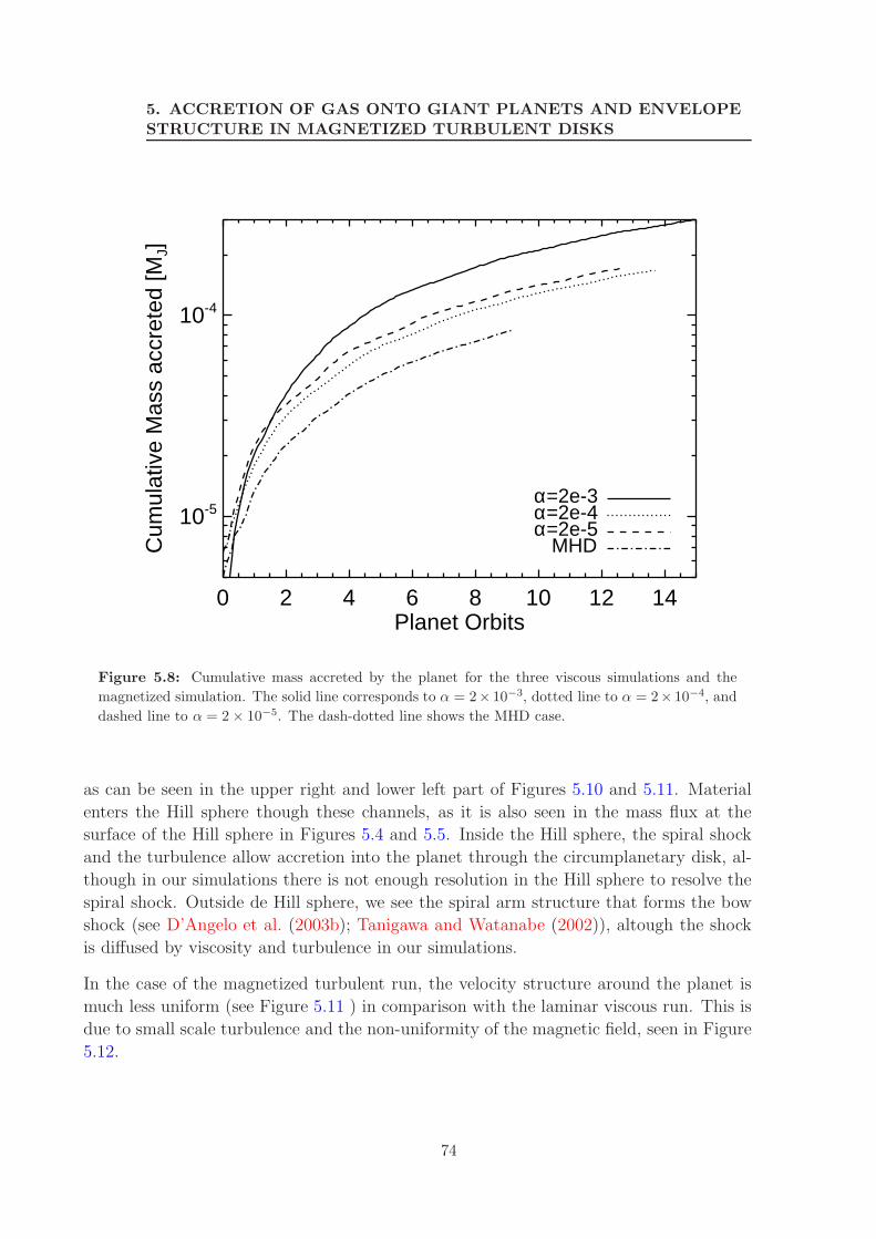
5. ACCRETION OF GAS ONTO GIANT PLANETS AND ENVELOPESTRUCTURE IN MAGNETIZED TURBULENT DISKS
0 2 4 6 8 10 12 14Planet Orbits
10-5
10-4
Cum
ulat
ive
Mas
s ac
cret
ed [M
J]
MHDα=2e-5α=2e-4α=2e-3
Figure 5.8: Cumulative mass accreted by the planet for the three viscous simulations and the
magnetized simulation. The solid line corresponds to α = 2× 10⁻³, dotted line to α = 2× 10⁻⁴, and
dashed line to α = 2 × 10⁻⁵. The dash-dotted line shows the MHD case.
as can be seen in the upper right and lower left part of Figures 5.10 and 5.11. Material
enters the Hill sphere though these channels, as it is also seen in the mass flux at the
surface of the Hill sphere in Figures 5.4 and 5.5. Inside the Hill sphere, the spiral shock
and the turbulence allow accretion into the planet through the circumplanetary disk, al-
though in our simulations there is not enough resolution in the Hill sphere to resolve the
spiral shock. Outside de Hill sphere, we see the spiral arm structure that forms the bow
shock (see D’Angelo et al. (2003b); Tanigawa and Watanabe (2002)), altough the shock
is diffused by viscosity and turbulence in our simulations.
In the case of the magnetized turbulent run, the velocity structure around the planet is
much less uniform (see Figure 5.11 ) in comparison with the laminar viscous run. This is
due to small scale turbulence and the non-uniformity of the magnetic field, seen in Figure
5.12.
74
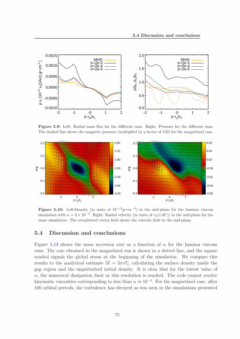
5.4 Discussion and conclusions
-2 -1 -0 1 2(r-rp)/rh
-0.0010
-0.0005
0.0000
0.0005
0.0010
0.0015
ρ v r
[10-1
2 vk(
1AU
) gr
cm
-3 ] MHD
α=2e-3α=2e-4α=2e-5
-2 -1 -0 1 2(r-rp)/rh
0.0
0.5
1.0
1.5
2.0
p/p 0
, pm/p
0
MHDα=2e-3α=2e-4α=2e-5
Figure 5.9: Left: Radial mass flux for the different runs. Right: Pressure for the different runs.
The dashed line shows the magnetic pressure (multiplied by a factor of 150) for the magnetized case.
-1 0 1(r-rp)/rh
-0.2
-0.1
0.0
0.1
0.2
φ-φ p
-3.20
-2.80
-2.40
-2.00
-1.60
-1.21
-0.81
-1 0 1(r-rp)/rh
-0.2
-0.1
0.0
0.1
0.2
φ-φ p
-0.05
-0.04
-0.02
-0.00
0.02
0.04
0.05
Figure 5.10: Left:Density (in units of 10−12grcm−3) in the mid-plane for the laminar viscous
simulation with α = 2× 10⁻³. Right: Radial velocity (in units of vk(1AU)) in the mid-plane for the
same simulation. The overplotted vector field shows the velocity field in the mid-plane.
5.4 Discussion and conclusions
Figure 5.13 shows the mass accretion rate as a function of α for the laminar viscous
runs. The rate obtained in the magnetized run is shown in a dotted line, and the square
symbol signals the global stress at the beginning of the simulation. We compare this
results to the analytical estimate M = 3πνΣ, calculating the surface density inside the
gap region and the unperturbed initial density. It is clear that for the lowest value of
α, the numerical dissipation limit at this resolution is reached. The code cannot resolve
kinematic viscosities corresponding to less than α ≈ 10−4. For the magnetized case, after
100 orbital periods, the turbulence has decayed as was seen in the simulations presented
75
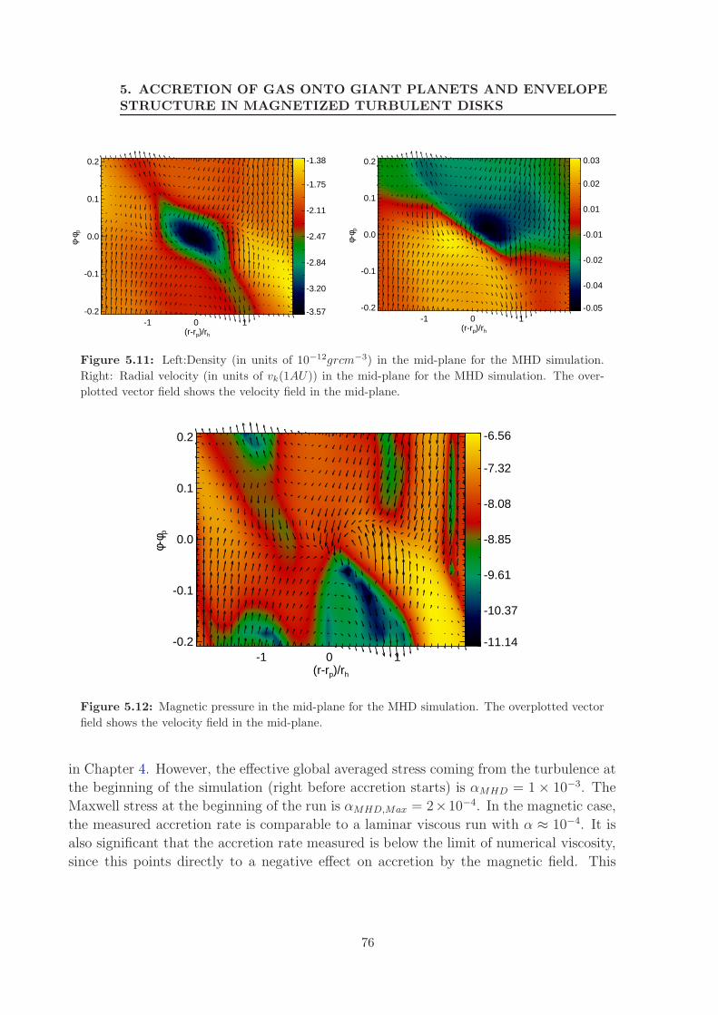
5. ACCRETION OF GAS ONTO GIANT PLANETS AND ENVELOPESTRUCTURE IN MAGNETIZED TURBULENT DISKS
-1 0 1(r-rp)/rh
-0.2
-0.1
0.0
0.1
0.2
φ-φ p
-3.57
-3.20
-2.84
-2.47
-2.11
-1.75
-1.38
-1 0 1(r-rp)/rh
-0.2
-0.1
0.0
0.1
0.2
φ-φ p
-0.05
-0.04
-0.02
-0.01
0.01
0.02
0.03
Figure 5.11: Left:Density (in units of 10−12grcm−3) in the mid-plane for the MHD simulation.
Right: Radial velocity (in units of vk(1AU)) in the mid-plane for the MHD simulation. The over-
plotted vector field shows the velocity field in the mid-plane.
-1 0 1(r-rp)/rh
-0.2
-0.1
0.0
0.1
0.2
φ-φ p
-11.14
-10.37
-9.61
-8.85
-8.08
-7.32
-6.56
Figure 5.12: Magnetic pressure in the mid-plane for the MHD simulation. The overplotted vector
field shows the velocity field in the mid-plane.
in Chapter 4. However, the effective global averaged stress coming from the turbulence at
the beginning of the simulation (right before accretion starts) is αMHD = 1 × 10⁻³. The
Maxwell stress at the beginning of the run is αMHD,Max = 2×10⁻⁴. In the magnetic case,
the measured accretion rate is comparable to a laminar viscous run with α ≈ 10−4. It is
also significant that the accretion rate measured is below the limit of numerical viscosity,
since this points directly to a negative effect on accretion by the magnetic field. This
76
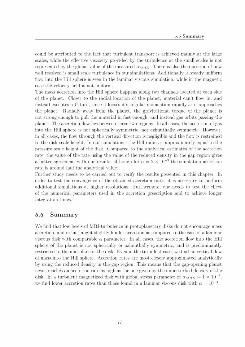
5.5 Summary
could be attributed to the fact that turbulent transport is achieved mainly at the large
scales, while the effective viscosity provided by the turbulence at the small scales is not
represented by the global value of the measured αMHD. There is also the question of how
well resolved is small scale turbulence in our simulations. Additionally, a steady uniform
flow into the Hill sphere is seen in the laminar viscous simulation, while in the magnetic
case the velocity field is not uniform.
The mass accretion into the Hill sphere happens along two channels located at each side
of the planet. Closer to the radial location of the planet, material can’t flow in, and
instead executes a U-turn, since it looses it’s angular momentum rapidly as it approaches
the planet. Radially away from the planet, the gravitational torque of the planet is
not strong enough to pull the material in fast enough, and instead gas orbits passing the
planet. The accretion flow lies between these two regions. In all cases, the accretion of gas
into the Hill sphere is not spherically symmetric, nor azimuthally symmetric. However,
in all cases, the flow through the vertical direction is negligible and the flow is restrained
to the disk scale height. In our simulations, the Hill radius is approximately equal to the
pressure scale height of the disk. Compared to the analytical estimates of the accretion
rate, the value of the rate using the value of the reduced density in the gap region gives
a better agreement with our results, although for α = 2 × 10⁻³ the simulation accretion
rate is around half the analytical value.
Further study needs to be carried out to verify the results presented in this chapter. In
order to test the convergence of the obtained accretion rates, it is necessary to perform
additional simulations at higher resolutions. Furthermore, one needs to test the effect
of the numerical parameters used in the accretion prescription and to achieve longer
integration times.
5.5 Summary
We find that low levels of MRI-turbulence in protoplanetary disks do not encourage mass
accretion, and in fact might slightly hinder accretion as compared to the case of a laminar
viscous disk with comparable α parameter. In all cases, the accretion flow into the Hill
sphere of the planet is not spherically or azimuthally symmetric, and is predominantly
restricted to the mid-plane of the disk. Even in the turbulent case, we find no vertical flow
of mass into the Hill sphere. Accretion rates are most closely approximated analytically
by using the reduced density in the gap region. This means that the gap-opening planet
never reaches an accretion rate as high as the one given by the unperturbed density of the
disk. In a turbulent magnetized disk with global stress parameter of αMHD = 1 × 10⁻³,
we find lower accretion rates than those found in a laminar viscous disk with α = 10−4.
77
5. ACCRETION OF GAS ONTO GIANT PLANETS AND ENVELOPESTRUCTURE IN MAGNETIZED TURBULENT DISKS
10-5 10-4 10-3
α
10-7
10-6
10-5
Acc
retio
n R
ate
[MJ/
yr]
MHD
dM/dt=3πνΣgapdM/dt=3πνΣ0Simulation
Figure 5.13: Mass accretion rates by the planet for different values of α(crosses) and the turbulent
run (square and dotted line). The diamond symbols show the accretion rate M = 3πνΣ calculated
using the unperturbed density, while the triangle symbols show the accretion rate calculated using
the mean density inside the gap region.
78

6
Conclusions
This thesis presents a study on different aspects of the interaction between a forming
planet and a circumstellar accretion disk of gas and dust. The focus points of this work
are the migration behavior of planets due to disk gravitational torques and the accretion
of gas onto giant planets. The accretion disk is modelled using hydro and magneto-
hydrodynamical simulations with the PLUTO code (Mignone et al., 2007). The planet
contribution and modeling was incorporated into the code. The planet module allows
for a free moving planet (using a simple leap frog integrator), accretion of gas onto the
planet (using the accretion prescription proposed by Kley et al. (2001)) and the presence
of multiple planets (which was used in this work as a particle integrator). The main
conclusions of this work are the following.
Chapter 3 deals with the migration and gas accretion of Jupiter mass planets in the
evolutionary phase when a gap has been opened in the disk. The dependence of the
torque was studied as a function of disk surface density, viscosity, steepness of density
profile and numerical parameters such as the gravitational softening. The accretion rate
onto planets was studied as a function of surface density. We improve over previous results
and include migration and accretion, and study the interplay between these two factors.
We find that migration is affected by accretion of gas by the planet and very fast inwards
migration is suppressed when the planet is accreting material from the disk. Our results
can be summarized in more detail as follows.• The linear estimate of the torque for Type II migration given by Eq. 3.6 is only fully
realized when the planet is artificially fixed on a given orbit at constant separation.
When the local disk mass is larger than the planet mass, the motion and accretion
of the planet affects the migration rate.
• When the local disk mass is larger than the planet mass, the migration rate is highly
dependent on the material inside the Hill sphere of the planet. If the Hill sphere is
not included in the motion of the planet, the mean cumulative torque is lower than
the analytical estimate. For Mdisk ≈ πr2pΣ = 10Mp, the mean cumulative torque is
79
6. CONCLUSIONS
lower by one order of magnitude. As a result, the migration timescale increases by
the same amount.
• When the local disk mass is larger than the planet mass, the mean cumulative torque
is lower than the analytical estimate when the planet is accreting gas from the disk
(due to the depletion of the Hill sphere). For Mdisk ≈ πr2pΣ = 10Mp, the mean
cumulative torque is lower by one order of magnitude. As a result, the migration
timescale increases by the same amount.
• When the local disk mass is about 10 times the planet mass, the planet undergoes
runaway (Type III) migration. Runaway migration is triggered by the initial fast
migration due to the Hill sphere material, but it is caused by gas passing by the planet
in open orbits from the inner to the outer disk. Runaway migration is completely
suppressed when the Hill sphere is depleted by planetary accretion.
• In a disk with uniform and constant mass accretion, there is no dependence of Type
II migration on the power law exponent of the surface density, so that a giant planet
will migrate equally fast in a disk with flat or rapidly decreasing density profile
The results of this chapter can be directly implemented in planet population synthesis
models, to better model the evolution of massive planets.
Chapter 4 deals with the migration of planets with masses from Mp = 3MEarth to
Mp = MJup in magnetized turbulent disks. We improve over previous studies that assume
an parametrized form of the turbulent viscosity or that use a forcing potential to simulate
turbulence. In our simulations, we study a global disk and turbulence is self-consistently
generated by magnetic fields. We find new migration behavior for intermediate-mass
planets (Neptunes and Saturns) that might reduce the effectiveness of fast Type I in-
wards migration. In this case, further study needs to be carried out to directly apply our
results in population synthesis simulations. Our results are summarized in more detail as
follows.
• For low-mass planets that don’t significantly perturb the disk, the stochastic torque
resulting from the density perturbations is characterized in terms of the density spec-
tra, the autocorrelation time of the torque and the torque standard deviation. These
quantities allow for modeling of the turbulent torque through a forcing potential or
as a diffusion process, that are tuned to match the characteristics of MRI turbulence.
The parameters found can be directly used in planet population synthesis modeling.
• Due to positive corotation torques, the migration of intermediate-mass planets (in
the Neptune/Saturn mass range) can be slowed down or even reverse in parts of the
disk where the density increases locally. These type of structures in the disk can
be a result of un-uniformities in the internal stresses (i.e the magnetic field). Zonal
flows are exited by the magnetic turbulence and have amplitudes of ≈ 20 − 25%
80
6.1 Future research
the unperturbed density value. Planets with mass ratios of around q = 10−4 can be
temporarily trapped in these locations in the disk.
• Jupiter mass planets strongly decrease the magnetic stress in the disk, and the
Reynolds stress dominates the angular momentum transport. This can potentially
have an impact on the overall mass accretion rate in the disk. The shape of the
gap is also influenced by turbulence, being wider in a magnetized turbulent disk as
compared to a viscous laminar disk.
Chapter 5 deals with the accretion rate of gas onto Jupiter-mass planets in a turbulent
magnetized disk. This is the first study to investigate how accretion is affected by turbu-
lence and turbulent magnetic fields. Our results suggest that accretion in turbulent mag-
netized disks cannot be directly modelled by assuming a laminar disk with a parametrized
form of the viscosity. We find that accretion rates are smaller than previously calculated.
Further work is required to understand the interplay between turbulence, magnetic fields
and accretion. Our results are summarized as follows.
• Accretion rates are lower in the presence of magnetic turbulence as compared to the
accretion rate in a viscous laminar disk that has an α = ν/HΩ equal to the global
average stress measured in the turbulent disk.
• The accretion flow structure is very similar to the one obtained in two-dimensional
simulations of laminar viscous disks. The accretion flow is constrained to specific re-
gions in the mid-plane of the disk and it is not azimuthally or spherically symmetric.
The mean vertical structure of the accretion flow is gaussian, following the density
distribution, and its vertical dimension is constained to one scale height of the disk.
The flow in the vertical direction is negligible as compared to the mid-plane flow, in
both the turbulent and the laminar cases.
• In general, the accretion rate of gas onto the planet is best approximated by M =
3πνΣgap. However we do not find an exact match for the high α = 10−2 case. This
could possibly be a result of the numerical parameters that we used for the accretion
prescription.
6.1 Future research
Many aspects that were not explored in this work pose interesting questions for future
investigations. One aspect that has not been explored in the literature is the migration of
planets in turbulent disks with thermal effects included. In all the simulations presented
in this work, the disk is locally isothermal, such that its temperature profile is constant.
This assumes an infinitely short cooling time. It is well known that including heating
and cooling effects or a full treatment of radiation transport affects the migration rates
observed in simulations (Klahr and Kley, 2006; Kley et al., 2009; Paardekooper et al.,
81

6. CONCLUSIONS
2010). This is due to contributions to the torque from the corotation region, that be-
have in a similar manner as the viscosity-induced corotation torques in isothermal disks.
Studing thermal effects in magnetized turbulent disks will provide a more complete and
comprehensive understanding of the impact of corotation torques and of the migration
rates of embedded planets. An interesting option to tackle this problem is to include
thermal effects in two-dimensional simulations with forced turbulence. This greatly sim-
plifies the numerical problem and makes the simulations practical. The forced turbulence
can be tuned to resemble MRI turbulence using the parameters found in this work. This
would allow a practical study of different parameters without the prohibiting limitations
of three-dimensional MHD simulations.
Another aspect that deserves attention is the numerical modeling of the gas accretion
by planets in hydrodynamical simulations. Improving the prescription for modeling the
gas accretion is necessary to understand the full formation process. A better model for
accretion must include physical elements that tie the disk modeling to the formation of
the planet and its envelope. One such element is the radiation feedback unto the disk
from the forming protoplanet, such that the contraction of the envelope can be followed.
Furthermore, it is necessary to implement a sub-grid model for the inner envelope of
the planet that provides a boundary condition for the disk simulations. The treatment
of the magnetic field when the planet is accreting also needs to be revised. In this
work, mass is removed from the grid to simulate accretion and the magnetic field is not
modified. As before, ultimately there needs to be a treatment of the magnetic field based
on physical arguments. The implementation of these elements will be possible as higher
resolution simulations become practical, and allow for the circumplanetary disk to be
properly resolved.
Higher resolution simulations are also required to establish the convergence of the results
with increasing resolution. Longer integration times are necessary to cover the longer
physical timescales associated with the viscous evolution of the disk, gap opening and the
evolution of zonal flow structures. Covering these timescales is not yet practically possible
for three-dimensional magneto-hydrodynamics simulations.
An important application of this work is related to observations of the dust in the outer
parts of protoplanetary disks at sub-milimeter and milimeter wavelengths. Telescopes like
ALMA will be able to probe and spatially resolve the outer regions of protoplanetary disks
at these wavelengths. A very interesting question is whether the structures in the disk
resulting from planet-disk interactions or from magnetic turbulence can be observed and
under what conditions. The results of this work can be incorporated into dust growth and
evolution models or radiative transfer codes in order to model observed disk structures
like gaps or density inhomogeneities.
82

Appendix A
Stochastic gravitational torque on
low-mass planets
In this Appendix we present results about the characterization of the turbulent torque
exerted on low mass planets in turbulent disks. This subject has been covered extensively
using two-dimensional hydrodynamical simulations of planet-disk interaction (Baruteau
and Lin, 2010; Laughlin et al., 2004; Ogihara et al., 2007), and using a semi-analytical
model to describe the migration (Adams and Bloch, 2009). In hydrodynamical simula-
tions, turbulence in the disk is not consistently generated by disk instabilities. Instead it
is modelled as a turbulent perturbation in the form of a potential that appears a source
term in the momentum equation. The potential is taken to be a sum over a certain
number of modes, each with a different amplitude and lifetime. Laughlin et al. (2004)
proposed the following form of the potential (for mode m)
Φm = ηmr−0.5e(r−rc)2/σ2
cos(mθ − φ − Ωct) sin
(
πt
∆t
)
. (A.1)
Here, ηm is the amplitude of mode m, (rc, φc) are parameters sampled from a uniform
distribution covering the computational domain, the mode m is sampled from a log-
random distribution, and the time t = t − tm,c, where tm,c is the starting time of mode
m. At any given time, a given number of modes are alive in the disk. The amplitude
and lifetime of the mode are tuned in order to obtain a density amplitudes spectrum that
resembles a turbulent disk spectrum with well characterized magnetic turbulence.
In order to have estimations the amplitude and lifetime of modes in the turbulent po-
tential, one needs to characterize the stochastic gravitational torque exerted by the disk
on test massless particles. We performed simulations of massless particles embedded in
a turbulent disk. The computational setup is identical to the one described in Chapter
4, except that instead of a planet orbiting the disk, we follow the orbital evolution of 50
massless particles at different positions in the disk. These particles have no feedback on
83
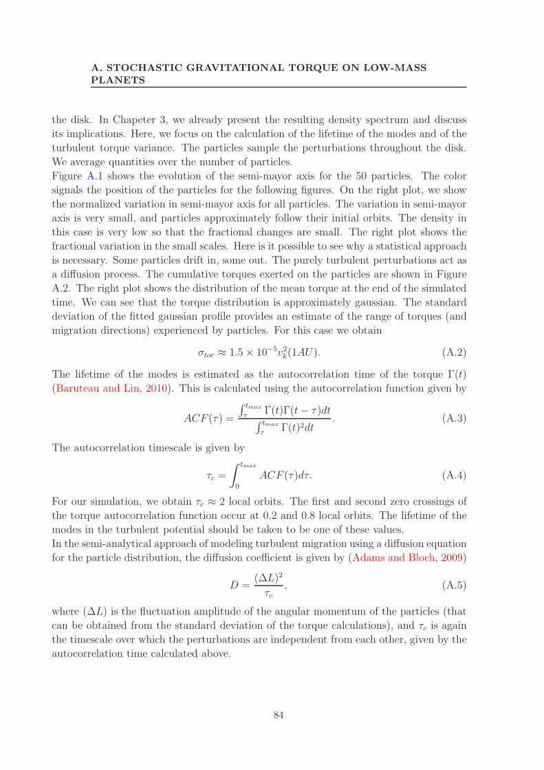
A. STOCHASTIC GRAVITATIONAL TORQUE ON LOW-MASSPLANETS
the disk. In Chapeter 3, we already present the resulting density spectrum and discuss
its implications. Here, we focus on the calculation of the lifetime of the modes and of the
turbulent torque variance. The particles sample the perturbations throughout the disk.
We average quantities over the number of particles.
Figure A.1 shows the evolution of the semi-mayor axis for the 50 particles. The color
signals the position of the particles for the following figures. On the right plot, we show
the normalized variation in semi-mayor axis for all particles. The variation in semi-mayor
axis is very small, and particles approximately follow their initial orbits. The density in
this case is very low so that the fractional changes are small. The right plot shows the
fractional variation in the small scales. Here is it possible to see why a statistical approach
is necessary. Some particles drift in, some out. The purely turbulent perturbations act as
a diffusion process. The cumulative torques exerted on the particles are shown in Figure
A.2. The right plot shows the distribution of the mean torque at the end of the simulated
time. We can see that the torque distribution is approximately gaussian. The standard
deviation of the fitted gaussian profile provides an estimate of the range of torques (and
migration directions) experienced by particles. For this case we obtain
σtor ≈ 1.5 × 10⁻⁵v2k(1AU). (A.2)
The lifetime of the modes is estimated as the autocorrelation time of the torque Γ(t)
(Baruteau and Lin, 2010). This is calculated using the autocorrelation function given by
ACF (τ) =
∫ tmax
τΓ(t)Γ(t − τ)dt
∫ tmax
τΓ(t)2dt
. (A.3)
The autocorrelation timescale is given by
τc =
∫ tmax
0
ACF (τ)dτ. (A.4)
For our simulation, we obtain τc ≈ 2 local orbits. The first and second zero crossings of
the torque autocorrelation function occur at 0.2 and 0.8 local orbits. The lifetime of the
modes in the turbulent potential should be taken to be one of these values.
In the semi-analytical approach of modeling turbulent migration using a diffusion equation
for the particle distribution, the diffusion coefficient is given by (Adams and Bloch, 2009)
D =(∆L)2
τc, (A.5)
where (∆L) is the fluctuation amplitude of the angular momentum of the particles (that
can be obtained from the standard deviation of the torque calculations), and τc is again
the timescale over which the perturbations are independent from each other, given by the
autocorrelation time calculated above.
84
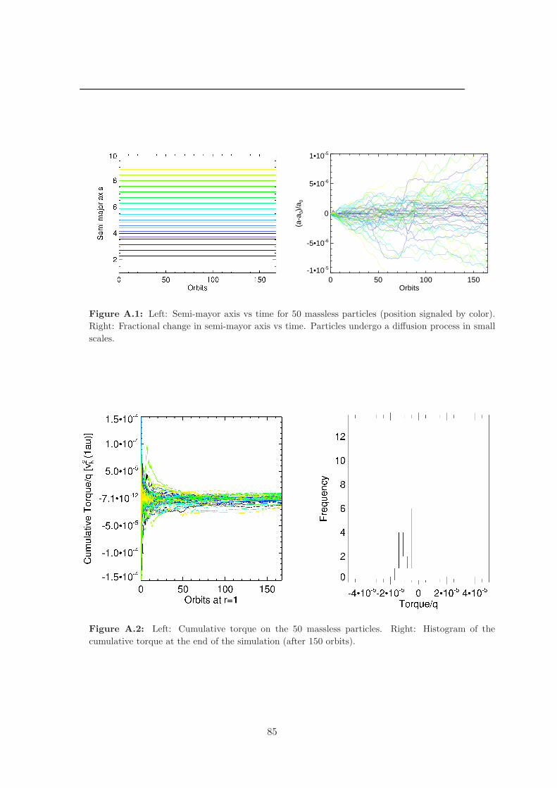
0 50 100 150Orbits
-1•10-5
-5•10-6
0
5•10-6
1•10-5
(a-a
0)/a
0
Figure A.1: Left: Semi-mayor axis vs time for 50 massless particles (position signaled by color).
Right: Fractional change in semi-mayor axis vs time. Particles undergo a diffusion process in small
scales.
Figure A.2: Left: Cumulative torque on the 50 massless particles. Right: Histogram of the
cumulative torque at the end of the simulation (after 150 orbits).
85

A. STOCHASTIC GRAVITATIONAL TORQUE ON LOW-MASSPLANETS
86
Bibliography
Adams, F. C. and Bloch, A. M.: 2009, ApJ 701, 1381 10, 40, 83, 84
Alexander, R.: 2008, New Astronomy Reviews 52, 60 4
Alibert, Y., Mordasini, C., and Benz, W.: 2004, A&A 417, L25 8, 18, 64
Alibert, Y., Mordasini, C., Benz, W., and Winisdoerffer, C.: 2005, A&A 434, 343 5, 18,
38, 64
Angel, J. R. P.: 1994, Nature 368, 203 8
Armitage, P. J.: 2007a, ArXiv Astrophysics e-prints 19
Armitage, P. J.: 2007b, ApJ 665, 1381 19
Baines, M. J. and Williams, I. P.: 1965, Nature 205, 59 4
Balbus, S. A. and Hawley, J. F.: 1991, ApJ 376, 214 5, 39, 65
Balbus, S. A. and Hawley, J. F.: 1998, Reviews of Modern Physics 70, 1 6, 39
Ballester, G. E., Sing, D. K., and Herbert, F.: 2007, Nature 445, 511 7
Baruteau, C. and Lin, D. N. C.: 2010, ApJ 709, 759 ix, 10, 39, 46, 49, 83, 84
Baruteau, C. and Masset, F.: 2008, ApJ 672, 1054 14
Batalha, N. M., Borucki, W. J., Bryson, S. T., Buchhave, L. A., Caldwell, D. A.,
Christensen-Dalsgaard, J., Ciardi, D., Dunham, E. W., Fressin, F., Gautier, III, T. N.,
Gilliland, R. L., Haas, M. R., Howell, S. B., Jenkins, J. M., Kjeldsen, H., Koch, D. G.,
Latham, D. W., Lissauer, J. J., Marcy, G. W., Rowe, J. F., Sasselov, D. D., Seager, S.,
Steffen, J. H., Torres, G., Basri, G. S., Brown, T. M., Charbonneau, D., Christiansen,
J., Clarke, B., Cochran, W. D., Dupree, A., Fabrycky, D. C., Fischer, D., Ford, E. B.,
Fortney, J., Girouard, F. R., Holman, M. J., Johnson, J., Isaacson, H., Klaus, T. C.,
Machalek, P., Moorehead, A. V., Morehead, R. C., Ragozzine, D., Tenenbaum, P.,
87

BIBLIOGRAPHY
Twicken, J., Quinn, S., VanCleve, J., Walkowicz, L. M., Welsh, W. F., Devore, E., and
Gould, A.: 2011, ApJ 729, 27 7
Bate, M. R., Lubow, S. H., Ogilvie, G. I., and Miller, K. A.: 2003, MNRAS 341, 213 vii,
6, 9, 19, 38, 39, 65
Batygin, K. and Stevenson, D. J.: 2010, ApJ 714, L238 8
Beaulieu, J.-P., Bennett, D. P., Fouque, P., Williams, A., Dominik, M., Jørgensen, U. G.,
Kubas, D., Cassan, A., Coutures, C., Greenhill, J., Hill, K., Menzies, J., Sackett, P. D.,
Albrow, M., Brillant, S., Caldwell, J. A. R., Calitz, J. J., Cook, K. H., Corrales, E.,
Desort, M., Dieters, S., Dominis, D., Donatowicz, J., Hoffman, M., Kane, S., Mar-
quette, J.-B., Martin, R., Meintjes, P., Pollard, K., Sahu, K., Vinter, C., Wambsganss,
J., Woller, K., Horne, K., Steele, I., Bramich, D. M., Burgdorf, M., Snodgrass, C.,
Bode, M., Udalski, A., Szymanski, M. K., Kubiak, M., Wieckowski, T., Pietrzynski,
G., Soszynski, I., Szewczyk, O., Wyrzykowski, L., Paczynski, B., Abe, F., Bond, I. A.,
Britton, T. R., Gilmore, A. C., Hearnshaw, J. B., Itow, Y., Kamiya, K., Kilmartin,
P. M., Korpela, A. V., Masuda, K., Matsubara, Y., Motomura, M., Muraki, Y., Naka-
mura, S., Okada, C., Ohnishi, K., Rattenbury, N. J., Sako, T., Sato, S., Sasaki, M.,
Sekiguchi, T., Sullivan, D. J., Tristram, P. J., Yock, P. C. M., and Yoshioka, T.: 2006,
Nature 439, 437 8
Bennett, D. P. and Rhie, S. H.: 1996, ApJ 472, 660 8
Benz, W., Mordasini, C., Alibert, Y., and Naef, D.: 2008, Physica Scripta Volume T
130(1), 014022 8, 9, 18, 38, 64
Berlage, H. P.: 1968, The origin of the solar system 2
Birnstiel, T., Dullemond, C. P., and Brauer, F.: 2010, A&A 513, A79+ 4
Birnstiel, T., Ormel, C. W., and Dullemond, C. P.: 2011, A&A 525, A11+ 4
Bodenheimer, P., Hubickyj, O., and Lissauer, J. J.: 2000, Icarus 143, 2 7
Borucki, W. J. and Summers, A. L.: 1984, Icarus 58, 121 7
Boss, A. P.: 1997, Science 276, 1836 5, 64
Bouwman, J., Henning, T., Hillenbrand, L. A., Meyer, M. R., Pascucci, I., Carpenter, J.,
Hines, D., Kim, J. S., Silverstone, M. D., Hollenbach, D., and Wolf, S.: 2008, ApJ 683,
479 4
Brauer, F., Dullemond, C. P., and Henning, T.: 2008, A&A 480, 859 4, 5
88

BIBLIOGRAPHY
Bryden, G., Chen, X., Lin, D. N. C., Nelson, R. P., and Papaloizou, J. C. B.: 1999, ApJ
514, 344 14, 19, 39, 65
Cameron, A. G. W.: 1962, Icarus 1, 13 3
Chamberlin, T. C.: 1901, ApJ 14, 17 2
Charbonneau, D., Allen, L. E., Megeath, S. T., Torres, G., Alonso, R., Brown, T. M.,
Gilliland, R. L., Latham, D. W., Mandushev, G., O’Donovan, F. T., and Sozzetti, A.:
2005, ApJ 626, 523 7
Crida, A. and Morbidelli, A.: 2007, MNRAS 377, 1324 18, 19, 20, 34
Crida, A., Morbidelli, A., and Masset, F.: 2006, Icarus 181, 587 14, 18, 39
Cumming, A., Marcy, G. W., and Butler, R. P.: 1999, ApJ 526, 890 7
Currie, T.: 2009, ApJ 694, L171 18
D’Angelo, G., Bate, M. R., and Lubow, S. H.: 2005, MNRAS 358, 316 19
D’Angelo, G., Kley, W., and Henning, T.: 2003a, in D. Deming & S. Seager (ed.),
Scientific Frontiers in Research on Extrasolar Planets, Vol. 294 of Astronomical Society
of the Pacific Conference Series, pp 323–326 65
D’Angelo, G., Kley, W., and Henning, T.: 2003b, ApJ 586, 540 38, 65, 74
Davis, S. W., Stone, J. M., and Pessah, M. E.: 2010, ApJ 713, 52 6
de Val-Borro, M., Edgar, R. G., Artymowicz, P., Ciecielag, P., Cresswell, P., D’Angelo,
G., Delgado-Donate, E. J., Dirksen, G., Fromang, S., Gawryszczak, A., Klahr, H., Kley,
W., Lyra, W., Masset, F., Mellema, G., Nelson, R. P., Paardekooper, S., Peplinski, A.,
Pierens, A., Plewa, T., Rice, K., Schafer, C., and Speith, R.: 2006, MNRAS 370, 529
18, 39
Dominik, C. and Tielens, A. G. G. M.: 1997, ApJ 480, 647 4
Donn, B. and Sears, G. W.: 1963, Science 140, 1208 4
Dullemond, C. P. and Dominik, C.: 2005, A&A 434, 971 4
Dullemond, C. P. and Monnier, J. D.: 2010, ARA&A 48, 205 4
Durisen, R. H., Boss, A. P., Mayer, L., Nelson, A. F., Quinn, T., and Rice, W. K. M.:
2007, Protostars and Planets V pp 607–622 5, 64
89

BIBLIOGRAPHY
Dzyurkevich, N., Flock, M., Turner, N. J., Klahr, H., and Henning, T.: 2010, A&A 515,
A70+ 6, 44, 59
Edgar, R. G.: 2007, ApJ 663, 1325 10, 19
Edgeworth, K. E.: 1949, MNRAS 109, 600 4
Edgeworth, K. E.: 1962, The Observatory 82, 219 4
Fabrycky, D. C. and Winn, J. N.: 2009, ApJ 696, 1230 7
Fleming, T. and Stone, J. M.: 2003, ApJ 585, 908 6
Flock, M., Dzyurkevich, N., Klahr, H., and Mignone, A.: 2010, A&A 516, A26+ 40, 66
Flock, M., Dzyurkevich, N., Klahr, H., Turner, N. J., and Henning, T.: 2011, ApJ 735,
122 6, 43
Ford, E. B. and Rasio, F. A.: 2008, ApJ 686, 621 7
Fromang, S. and Nelson, R. P.: 2009, A&A 496, 597 46
Fromang, S. and Papaloizou, J.: 2007, A&A 476, 1113 6
Fromang, S., Papaloizou, J., Lesur, G., and Heinemann, T.: 2007, A&A 476, 1123 6
Fromang, S., Terquem, C., and Nelson, R. P.: 2005, MNRAS 363, 943 38, 50
Gardiner, T. A. and Stone, J. M.: 2005, Journal of Computational Physics 205, 509 40,
66
Gaudi, B. S. and Winn, J. N.: 2007, ApJ 655, 550 7
Geisel, S. L.: 1970, ApJ 161, L105+ 4
Gilliland, R. L., Jenkins, J. M., Borucki, W. J., Bryson, S. T., Caldwell, D. A., Clarke,
B. D., Dotson, J. L., Haas, M. R., Hall, J., Klaus, T., Koch, D., McCauliff, S., Quintana,
E. V., Twicken, J. D., and van Cleve, J. E.: 2010, ApJ 713, L160 7
Goldreich, P. and Lynden-Bell, D.: 1965, MNRAS 130, 97 5
Goldreich, P. and Tremaine, S.: 1979, ApJ 233, 857 6
Goldreich, P. and Tremaine, S.: 1980, ApJ 241, 425 38
Gould, A. and Loeb, A.: 1992, ApJ 396, 104 8
Guan, X., Gammie, C. F., Simon, J. B., and Johnson, B. M.: 2009, ApJ 694, 1010 6
90
BIBLIOGRAPHY
Guttler, C., Blum, J., Zsom, A., Ormel, C. W., and Dullemond, C. P.: 2010, A&A 513,
A56+ 4
Haisch, Jr., K. E., Lada, E. A., and Lada, C. J.: 2001, ApJ 553, L153 vii, 9
Hawley, J. F., Gammie, C. F., and Balbus, S. A.: 1995, ApJ 440, 742 6
Hawley, J. F., Gammie, C. F., and Balbus, S. A.: 1996, ApJ 464, 690 6
Henning, T. and Meeus, G.: 2009, ArXiv e-prints 4
Henning, T. and Stognienko, R.: 1996, A&A 311, 291 4
Howard, A. W., Marcy, G. W., Johnson, J. A., Fischer, D. A., Wright, J. T., Isaacson,
H., Valenti, J. A., Anderson, J., Lin, D. N. C., and Ida, S.: 2010, Science 330, 653 7, 8
Hoyle, F.: 1960, QJRAS 1, 28 3
Hubickyj, O., Bodenheimer, P., and Lissauer, J. J.: 2005, Icarus 179, 415 64
Hughes, A. L. H. and Armitage, P. J.: 2010, ApJ 719, 1633 4
Ibgui, L. and Burrows, A.: 2009, ApJ 700, 1921 8
Ida, S. and Lin, D. N. C.: 2004, ApJ 604, 388 8, 38
Ida, S. and Lin, D. N. C.: 2007, ArXiv e-prints 38
Ida, S. and Lin, D. N. C.: 2008, in Y.-S. Sun, S. Ferraz-Mello, & J.-L. Zhou (ed.), IAU
Symposium, Vol. 249 of IAU Symposium, pp 223–232 9, 18, 38, 64
Ikoma, M., Nakazawa, K., and Emori, H.: 2000, ApJ 537, 1013 64
Jeans, J.: 1931, Nature 128, 432 2
Jeffreys, H. and Moulton, F. R.: 1929, Science 69, 245 2
Ji, H., Burin, M., Schartman, E., and Goodman, J.: 2006, Nature 444, 343 5
Johansen, A. and Klahr, H.: 2005, ApJ 634, 1353 6
Johansen, A., Klahr, H., and Henning, T.: 2006, ApJ 636, 1121 6
Johansen, A., Oishi, J. S., Mac Low, M.-M., Klahr, H., Henning, T., and Youdin, A.:
2007, Nature 448, 1022 6
Johansen, A., Youdin, A., and Klahr, H.: 2009, ApJ 697, 1269 6, 43
91
BIBLIOGRAPHY
Johnson, E. T., Goodman, J., and Menou, K.: 2006, ApJ 647, 1413 40
Johnson, J. A., Aller, K. M., Howard, A. W., and Crepp, J. R.: 2010, PASP 122, 905 7
Juhasz, A., Bouwman, J., Henning, T., Acke, B., van den Ancker, M. E., Meeus, G.,
Dominik, C., Min, M., Tielens, A. G. G. M., and Waters, L. B. F. M.: 2010, ApJ 721,
431 4
Juhasz, A., Henning, T., Bouwman, J., Dullemond, C. P., Pascucci, I., and Apai, D.:
2009, ApJ 695, 1024 4
Juric, M. and Tremaine, S.: 2008, ApJ 686, 603 7
Kalas, P., Graham, J. R., and Clampin, M.: 2005, Nature 435, 1067 8
Klahr, H. and Kley, W.: 2006, A&A 445, 747 65, 81
Klahr, H. H. and Bodenheimer, P.: 2003, ApJ 582, 869 5
Kley, W., Bitsch, B., and Klahr, H.: 2009, A&A 506, 971 14, 81
Kley, W., D’Angelo, G., and Henning, T.: 2001, ApJ 547, 457 29, 65, 68, 72, 79
Koch, D. G., Borucki, W., Webster, L., Dunham, E., Jenkins, J., Marriott, J., and
Reitsema, H. J.: 1998, in P. Y. Bely & J. B. Breckinridge (ed.), Society of Photo-
Optical Instrumentation Engineers (SPIE) Conference Series, Vol. 3356 of Society of
Photo-Optical Instrumentation Engineers (SPIE) Conference Series, pp 599–607 7
Kretke, K. A. and Lin, D. N. C.: 2007, ApJ 664, L55 6, 59
Lada, C. J. and Adams, F. C.: 1992, ApJ 393, 278 4
Lafreniere, D., Jayawardhana, R., and van Kerkwijk, M. H.: 2008, ApJ 689, L153 8
Laughlin, G., Steinacker, A., and Adams, F. C.: 2004, ApJ 608, 489 10, 39, 83
Leconte, J., Chabrier, G., Baraffe, I., and Levrard, B.: 2010, A&A 516, A64+ 8
Leger, A., Rouan, D., Schneider, J., Barge, P., Fridlund, M., Samuel, B., Ollivier, M.,
Guenther, E., Deleuil, M., Deeg, H. J., Auvergne, M., Alonso, R., Aigrain, S., Alapini,
A., Almenara, J. M., Baglin, A., Barbieri, M., Bruntt, H., Borde, P., Bouchy, F.,
Cabrera, J., Catala, C., Carone, L., Carpano, S., Csizmadia, S., Dvorak, R., Erikson,
A., Ferraz-Mello, S., Foing, B., Fressin, F., Gandolfi, D., Gillon, M., Gondoin, P.,
Grasset, O., Guillot, T., Hatzes, A., Hebrard, G., Jorda, L., Lammer, H., Llebaria, A.,
Loeillet, B., Mayor, M., Mazeh, T., Moutou, C., Patzold, M., Pont, F., Queloz, D.,
Rauer, H., Renner, S., Samadi, R., Shporer, A., Sotin, C., Tingley, B., Wuchterl, G.,
92
BIBLIOGRAPHY
Adda, M., Agogu, P., Appourchaux, T., Ballans, H., Baron, P., Beaufort, T., Bellenger,
R., Berlin, R., Bernardi, P., Blouin, D., Baudin, F., Bodin, P., Boisnard, L., Boit,
L., Bonneau, F., Borzeix, S., Briet, R., Buey, J.-T., Butler, B., Cailleau, D., Cautain,
R., Chabaud, P.-Y., Chaintreuil, S., Chiavassa, F., Costes, V., Cuna Parrho, V., de
Oliveira Fialho, F., Decaudin, M., Defise, J.-M., Djalal, S., Epstein, G., Exil, G.-E.,
Faure, C., Fenouillet, T., Gaboriaud, A., Gallic, A., Gamet, P., Gavalda, P., Grolleau,
E., Gruneisen, R., Gueguen, L., Guis, V., Guivarc’h, V., Guterman, P., Hallouard,
D., Hasiba, J., Heuripeau, F., Huntzinger, G., Hustaix, H., Imad, C., Imbert, C.,
Johlander, B., Jouret, M., Journoud, P., Karioty, F., Kerjean, L., Lafaille, V., Lafond,
L., Lam-Trong, T., Landiech, P., Lapeyrere, V., Larque, T., Laudet, P., Lautier, N.,
Lecann, H., Lefevre, L., Leruyet, B., Levacher, P., Magnan, A., Mazy, E., Mertens,
F., Mesnager, J.-M., Meunier, J.-C., Michel, J.-P., Monjoin, W., Naudet, D., Nguyen-
Kim, K., Orcesi, J.-L., Ottacher, H., Perez, R., Peter, G., Plasson, P., Plesseria, J.-Y.,
Pontet, B., Pradines, A., Quentin, C., Reynaud, J.-L., Rolland, G., Rollenhagen, F.,
Romagnan, R., Russ, N., Schmidt, R., Schwartz, N., Sebbag, I., Sedes, G., Smit, H.,
Steller, M. B., Sunter, W., Surace, C., Tello, M., Tiphene, D., Toulouse, P., Ulmer, B.,
Vandermarcq, O., Vergnault, E., Vuillemin, A., and Zanatta, P.: 2009, A&A 506, 287
7
Lin, C. C. and Shu, F. H.: 1966, Proceedings of the National Academy of Science 55, 229
6
Lin, D. N. C. and Papaloizou, J.: 1986, ApJ 309, 846 12, 18, 20
Lin, M.-K. and Papaloizou, J. C. B.: 2010, MNRAS 405, 1473 32
Lissauer, J. J.: 1993, ARA&A 31, 129 2
Lubow, S. H., Seibert, M., and Artymowicz, P.: 1999, ApJ 526, 1001 19, 65, 71
Lynden-Bell, D. and Pringle, J. E.: 1974, MNRAS 168, 603 18, 20
Lyra, W., Johansen, A., Klahr, H., and Piskunov, N.: 2008, A&A 479, 883 44
Lyttleton, R. A.: 1940, MNRAS 100, 546 2
Machida, M., Hayashi, M. R., and Matsumoto, R.: 2000, ApJ 532, L67 6
Mannings, V. and Emerson, J. P.: 1994, MNRAS 267, 361 4
Mao, S. and Paczynski, B.: 1991, ApJ 374, L37 8
Marcy, G., Butler, R. P., Fischer, D., Vogt, S., Wright, J. T., Tinney, C. G., and Jones,
H. R. A.: 2005, Progress of Theoretical Physics Supplement 158, 24 7
93

BIBLIOGRAPHY
Masset, F. S.: 2002, A&A 387, 605 6, 15, 28, 34, 38
Masset, F. S., D’Angelo, G., and Kley, W.: 2006a, ApJ 652, 730 18, 38, 50, 51, 55
Masset, F. S., Morbidelli, A., Crida, A., and Ferreira, J.: 2006b, ApJ 642, 478 6, 59
Masset, F. S. and Papaloizou, J. C. B.: 2003, ApJ 588, 494 10, 14, 32
Mayer, L., Quinn, T., Wadsley, J., and Stadel, J.: 2002, Science 298, 1756 5, 64
McCrea, W. H. and Williams, I. P.: 1965, Royal Society of London Proceedings Series A
287, 143 4
Mendoza V., E. E.: 1968, ApJ 151, 977 4
Mignone, A., Bodo, G., Massaglia, S., Matsakos, T., Tesileanu, O., Zanni, C., and Ferrari,
A.: 2007, ApJS 170, 228 iii, 6, 20, 40, 66, 79
Miller, N., Fortney, J. J., and Jackson, B.: 2009, ApJ 702, 1413 8
Mizuno, H.: 1980, Progress of Theoretical Physics 64, 544 5, 64
Mordasini, C., Alibert, Y., and Benz, W.: 2009a, A&A 501, 1139 8, 9, 64
Mordasini, C., Alibert, Y., Benz, W., and Naef, D.: 2009b, A&A 501, 1161 8, 9, 18, 38,
64
Moulton, F. R.: 1905, ApJ 22, 165 2
Nagasawa, M., Ida, S., and Bessho, T.: 2008, ApJ 678, 498 7
Nelson, R. P.: 2005, A&A 443, 1067 39, 46, 54
Nelson, R. P. and Gressel, O.: 2010, MNRAS 409, 639 40
Nelson, R. P. and Papaloizou, J. C. B.: 2003, MNRAS 339, 993 10, 39, 53
Nelson, R. P. and Papaloizou, J. C. B.: 2004, MNRAS 350, 849 10, 39
Nelson, R. P., Papaloizou, J. C. B., Masset, F., and Kley, W.: 2000, MNRAS 318, 18
18, 39
Nolke, F.: 1932, MNRAS 93, 159 2
Ogihara, M., Ida, S., and Morbidelli, A.: 2007, Icarus 188, 522 40, 83
Ogilvie, G. I. and Lin, D. N. C.: 2004, ApJ 610, 477 8
94
BIBLIOGRAPHY
Oishi, J. S., Mac Low, M., and Menou, K.: 2007, ApJ 670, 805 10, 39
Okuzumi, S.: 2009, ApJ 698, 1122 4
Paardekooper, S., Baruteau, C., Crida, A., and Kley, W.: 2010, MNRAS 401, 1950 81
Paardekooper, S. and Papaloizou, J. C. B.: 2009a, MNRAS 394, 2283 6, 15, 34, 50, 57
Paardekooper, S. and Papaloizou, J. C. B.: 2009b, MNRAS 394, 2297 15
Papaloizou, J. and Lin, D. N. C.: 1984, ApJ 285, 818 6, 38
Papaloizou, J. C. B. and Larwood, J. D.: 2000, MNRAS 315, 823 39
Papaloizou, J. C. B. and Nelson, R. P.: 2003, MNRAS 339, 983 10, 39
Papaloizou, J. C. B., Nelson, R. P., and Snellgrove, M. D.: 2004, MNRAS 350, 829 10,
39
Papaloizou, J. C. B. and Pringle, J. E.: 1984, MNRAS 208, 721 5
Papaloizou, J. C. B. and Pringle, J. E.: 1985, MNRAS 213, 799 5
Peplinski, A., Artymowicz, P., and Mellema, G.: 2008, MNRAS 386, 179 32
Pollack, J. B., Hubickyj, O., Bodenheimer, P., Lissauer, J. J., Podolak, M., and Green-
zweig, Y.: 1996, Icarus 124, 62 5, 64
Pont, F., Knutson, H., Gilliland, R. L., Moutou, C., and Charbonneau, D.: 2008, MNRAS
385, 109 7
Rafikov, R. R.: 2005, ApJ 621, L69 5, 64
Rasio, F. A. and Ford, E. B.: 1996, Science 274, 954 7
Richardson, L. J., Deming, D., Horning, K., Seager, S., and Harrington, J.: 2007, Nature
445, 892 7
Sano, T., Inutsuka, S.-i., Turner, N. J., and Stone, J. M.: 2004, ApJ 605, 321 6
Sano, T., Miyama, S. M., Umebayashi, T., and Nakano, T.: 2000, ApJ 543, 486 6
Santos, N. C., Israelian, G., Mayor, M., Rebolo, R., and Udry, S.: 2003, A&A 398, 363
7
Schrapler, R. and Henning, T.: 2004, ApJ 614, 960 4, 5
Shakura, N. I. and Sunyaev, R. A.: 1973, A&A 24, 337 69
95
BIBLIOGRAPHY
Sharma, P., Hammett, G. W., Quataert, E., and Stone, J. M.: 2006, ApJ 637, 952 6
Shen, Y. and Turner, E. L.: 2008, ApJ 685, 553 7
Shu, F. H.: 1970, ApJ 160, 99 6
Sicilia-Aguilar, A., Hartmann, L. W., Watson, D., Bohac, C., Henning, T., and Bouwman,
J.: 2007, ApJ 659, 1637 4
Spitzer, Jr., L.: 1939, ApJ 90, 675 2
Stevenson, D. J.: 1982, Planet. Space Sci. 30, 755 5, 64
Stone, J. M., Gardiner, T. A., Teuben, P., Hawley, J. F., and Simon, J. B.: 2008, ApJS
178, 137 6
Stone, J. M., Hawley, J. F., Gammie, C. F., and Balbus, S. A.: 1996, ApJ 463, 656 6
Stone, J. M. and Norman, M. L.: 1992, ApJS 80, 753 6
Stone, J. M. and Pringle, J. E.: 2001, MNRAS 322, 461 6
Syer, D. and Clarke, C. J.: 1995, MNRAS 277, 758 19
Tanaka, H., Takeuchi, T., and Ward, W. R.: 2002, ApJ 565, 1257 6, 12, 13, 38, 50
Tanigawa, T. and Watanabe, S.-i.: 2002, ApJ 580, 506 28, 65, 68, 71, 73, 74
Ter Haar, D.: 1948, Science 107, 405 3
Ter Haar, D.: 1950, ApJ 111, 179 3
Ter Haar, D.: 1967, ARA&A 5, 267 2
Terebey, S., Shu, F. H., and Cassen, P.: 1984, ApJ 286, 529 4
Terquem, C. E. J. M. L. J.: 2003, MNRAS 341, 1157 38, 50
Thalmann, C., Carson, J., Janson, M., Goto, M., McElwain, M., Egner, S., Feldt, M.,
Hashimoto, J., Hayano, Y., Henning, T., Hodapp, K. W., Kandori, R., Klahr, H., Kudo,
T., Kusakabe, N., Mordasini, C., Morino, J.-I., Suto, H., Suzuki, R., and Tamura, M.:
2009, ApJ 707, L123 8
Thommes, E. W. and Murray, N.: 2006, ApJ 644, 1214 6, 38
Throop, H. B., Bally, J., Esposito, L. W., and McCaughrean, M. J.: 2001, Science 292,
1686 4
96

BIBLIOGRAPHY
Trilling, D. E., Lunine, J. I., and Benz, W.: 2002, A&A 394, 241 38
Turner, N. J., Carballido, A., and Sano, T.: 2010, ApJ 708, 188 6
Turner, N. J. and Sano, T.: 2008, ApJ 679, L131 6
Turner, N. J., Sano, T., and Dziourkevitch, N.: 2007, ApJ 659, 729 6
Udry, S., Mayor, M., and Santos, N. C.: 2003, A&A 407, 369 7
Udry, S. and Santos, N. C.: 2007, ARA&A 45, 397 7
Uribe, A. L., Klahr, H., Flock, M., and Henning, T.: 2011, ApJ 736, 85 37, 70
Vauclair, S.: 2004, ApJ 605, 874 7
Veras, D., Crepp, J. R., and Ford, E. B.: 2009, ApJ 696, 1600 8
Ward, W. R.: 1986, Icarus 67, 164 38
Ward, W. R.: 1992, in S. F. Dermott, J. H. Hunter Jr., & R. E. Wilson (ed.), Astrophysical
Disks, Vol. 675 of Annals of the New York Academy of Sciences, pp 314–323 39
Ward, W. R.: 1997, Icarus 126, 261 6, 12, 18, 38
Wardle, M.: 1999, MNRAS 307, 849 6
Weidenschilling, S. J.: 1984, Icarus 60, 553 4
Wetherill, G. W.: 1980, ARA&A 18, 77 5
Williams, I. P. and Cremin, A. W.: 1968, QJRAS 9, 40 2
Williams, J. P. and Cieza, L. A.: 2011, ArXiv e-prints 4
Winters, W. F., Balbus, S. A., and Hawley, J. F.: 2003, ApJ 589, 543 39, 53
Yang, C., Mac Low, M., and Menou, K.: 2009, ApJ 707, 1233 39
Youdin, A. N. and Shu, F. H.: 2002, ApJ 580, 494 5
Zsom, A., Ormel, C. W., Guttler, C., Blum, J., and Dullemond, C. P.: 2010, A&A 513,
A57+ 4
97
Acknowledgements
Agradecimientos
Quiero agradecerle a mis amigos por mantenerme cuerda durante estos tres
anos. Gracias a Maxito por ser como eres, a Paolilla por ser tan loquita, y a
Carolina y Ulrich por ser tan hermosos. Gracias a mis amigos que estuvieron
lejos pero siempre en mi mente, Peter y Olga. A las personas con las que
comparti muchos buenos momentos durante este tiempo; Juan, Camila, Julio,
Natasha, Sareh, Somayeh, Dading, Matucci, Lavinia, Leonard. En especial, le
agradezco a mi amigo Mauricio por los infinitos cafes, las sesiones de quejas
y de nostalgia, por hacerme reir y sacarme la piedra de vez en cuando. Estos
tres anos no hubieran sido lo mismo sin el en Heidelberg.
Un agradecimiento especial a Mario por toda su ayuda al comienzo (y en la
mitad, y al final) del proyecto, fue muy bacano poder trabajar con el. Tambien
le quiero agradecer a mis supervisores, Hubert y Thomas, por todo su apoyo,
discusiones y consejos. Le agradezco a Hubert por su amabilidad constante y
por todas sus ideas y sugerencias que siempre mejoraron mi trabajo.
Mis queridos padres son los que han hecho posible que yo tenga esta oportu-
nidad en primer lugar. Gracias a mi mama por siempre estar ahi para mi y
por no dejarme olvidar todo lo que siempre estara ahi para mi. Gracias a mi
papa por su apoyo, su generosidad y sus locuras. Le agradezco tambien a mi
querida hermana Luisa, por sus correos de apoyo y de distraccion :P.
Finalmente, mis ultimas gracias son para Joe, el mejor descubrimiento que
pude haber hecho en este tiempo. Gracias por caminar este camino al lado
mio, por ser una persona tan increible y por hacerme feliz. Los momentos que
comparti contigo (y con Harper) durante este tiempo estaran siempre en mi
corazon.
English Version
I would like to thank my friends for keeping me sane during these three years.
Thanks to Maxito for being how you are, to Paolilla for being a crazy girl, and
to Carolina and Ulrich for being so beautiful people. Thanks to my friends who
were far away but were always on my mind, Peter and Olga. To the people
who shared this years with me at some point and with whom I spent many
good times; Juan, Camila, Julio, Natasha, Sareh, Somayeh, Dading, Matucci,
Lavinia, Leonard. Specially, I want to thank my friend Mauricio for the infinite
coffees, the complaining and nostalgia sessions, for always making me laugh and
very mad sometimes. These three years would not have been the same without
him in Heidelberg.
A special thanks to Mario for all his help in the early (and not so early) days
of the project, it was great to get to work with you. I also want to thank my
supervisors, Hubert and Thomas, for all their support, discussions and advice.
I thank Hubert for his constant kindness and for all his suggestions and ideas
that always improved my work.
My dear parents have made it possible for me to be here in the first place.
Thanks to my mom for being always there for me and for not letting me forget
all that was always there for me. Thanks to my dad for his constant support,
his generosity and his craziness. Thanks to my dear sister Luisa for her support
and distraction emails :P.
Finally, my last thanks are for Joe, the best discovery I could have made in
this time. Thank you for walking this path next to me, for being so wonderful
and for making me happy. The moments I spent with you (and Harper) during
this time will be forever in my heart.
Declaration
I herewith declare that I have produced this paper without the prohibited
assistance of third parties and without making use of aids other than those
specified; notions taken over directly or indirectly from other sources have been
identified as such. This paper has not previously been presented in identical
or similar form to any other German or foreign examination board.
The thesis work was conducted from 2008 to 2011 under the supervision of
Dr. Hubert Klahr and Prof. Dr. Thomas Henning at Max-Planck-Institute for
Astronomy (MPIA).
Heidelberg, November 21, 2011.
Copyright © 2022 FDOKUMEN