arX

iv:0

711.

3779

v1 [

mat

h-ph

] 2

3 N

ov 2

007

FRACALMO PRE-PRINT www.fracalmo.org

Journal of Computational and Applied Mathematics,Vol 207, No 2, pp. 245-257 (2007).

The role of the Fox-Wright functions

in fractional sub-diffusion of distributed order1

Francesco MAINARDI(1) and Gianni PAGNINI(2)

(1) Department of Physics, University of Bologna, and INFN,Via Irnerio 46, I-40126 Bologna, Italyfrancesco.mainardi@unibo.it

(2) National Agency for New Technologies, Energy and the Environment,ENEA, Centre ”E. Clementel”,

Via Martiri di Monte Sole 4, I-40129 Bologna, Italygianni.pagnini@bologna.enea.it

Abstract

The fundamental solution of the fractional diffusion equation ofdistributed order in time (usually adopted for modelling sub-diffusionprocesses) is obtained based on its Mellin-Barnes integral representation.Such solution is proved to be related via a Laplace-type integral to theFox-Wright functions. A series expansion is also provided in order topoint out the distribution of time-scales related to the distribution of thefractional orders. The results of the time fractional diffusion equation of asingle order are also recalled and then re-obtained from the general theory.

Keywords: Sub-diffusion, Fractional derivatives, Mellin-Barnes integrals,Mittag-Leffler functions, Fox-Wright functions, Integral Transforms.

MSC 2000: 26A33, 33E12, 33C40, 33C60, 44A10, 45K05,

1 Introduction

The Wright function is defined by the series representation, valid in the wholecomplex plane,

Wλ,µ(z) :=

∞∑

k=0

zk

k! Γ(λk + µ), λ > −1 , µ ∈ C , z ∈ C . (1.1)

It is an entire function of order 1/(1+λ), that has been known also as generalisedBessel function2.

1This paper is based on an invited talk given by Francesco Mainardi at the internationalconference Special Functions: Asymptotic Analysis and Computation, which took place inSantander (Spain) on 4-6 July, 2005. The conference was organized in honor of Nico M.Temme, who celebrated his 65-th birthday in 2005. Selected papers presented at the conferenceare published in this special issue of JCAM with the organizers as Guest Editors: AmparoGil, Javier Segura (Universidad de Cantabria, Santander) and Jose Luis Lopez (UniversidadPblica de Navarra, Pamplona).

2When λ = 1 the Wright function can be expressed in terms of the Bessel function of orderν = µ − 1. In fact we have Jµ−1(z) = (z/2)µ−1 W1,µ

`

−z2/4´

.

1

Originally, E.M. Wright introduced and investigated this function with therestriction λ ≥ 0 in a series of notes starting from 1933 in the framework of theasymptotic theory of partitions [55, 56, 57]. Only later, in 1940, he consideredthe case −1 < λ < 0 [58]. We note that in the handbook of the BatemanProject [15] (see Vol. 3, Ch. 18), presumably for a misprint, λ is restricted tobe non negative in spite of the fact that the 1940 Wright’s paper is cited.

For the cases λ > 0 and −1 < λ < 0 we agree to distinguish thecorresponding functions by calling them Wright functions of the first and secondtype, respectively. As a matter of fact the two types of functions exhibit a quitedifferent asymptotic behavior as it was shown more recently in two relevantpapers by Wong and Zaho [53, 54]. The case λ = 0 is trivial since it turns outfrom (1.1) W0,µ(z) = exp(z)/Γ(µ).

Following a former idea of Wright himself [57], the Wright functions can begeneralized as follows

pΨq(z) :=

∞∑

k=0

∏pi=1 Γ(ai + Aik)∏qj=1 Γ(bi + Bik)

zk

k!, (1.2)

where z ∈ C, {ai, bj} ∈ C, {Ai, Bj} ∈ R with Ai, Bj 6= 0 and i = 1, 2, . . . , p,j = 1, 2, . . . , q. An empty product, when it occurs, is taken to be 1. Thefollowing alternative notations are commonly used

pΨq

[(ai, Ai)1,p

(bj , Bj)1,q; z

]= pΨq

[(a1, A1), · · · , (ap, Ap)

(b1, B1), · · · , (bq, Bq); z

]. (1.3)

Then, the standard Wright function (1.1), being obtained from (1.2) when p = 0and q = 1 with B1 = λ > −1 , b1 = µ, reads

Wλ,µ(z) ≡ 0Ψ1

[ −−(µ, λ)

; z

]. (1.4)

All the above functions are known to belong to the more general class of theFox H functions introduced in 1961 by C.Fox [16]. For more information theinterested reader is referred to the specialized literature including the books[25, 28, 41, 45, 50], and the relevant articles [23, 24, 26, 51]. In particular, werecommend the article by Kilbas et al. [26] where the authors have establishedthe conditions for the existence of pΨq(z), see there §2, and provided itsrepresentations in terms of Mellin-Barnes integrals, §3, and Fox H functions,§4.

For the sake of reader’s convenience we devote the Appendix for a shortoutline of the H functions in order to understand the Fox representation of thestandard and generalized Wright functions of the first and second type that weshall introduce in the following. More appropriately, following [51, 13], we canrefer to the generalized Wright functions simply to as the Fox-Wright functions.

The Fox notation for the standard Wright functions depends on their typeand reads

Wλ,µ(z) :=

∞∑

k=0

zk

k! Γ(λk + µ)=

H1,00,2

[−z

∣∣∣∣− ; −(0, 1); (1 − µ, λ)

], λ > 0 ;

H1,01,1

[−z

∣∣∣∣−; (µ,−λ)

(0, 1);−

], −1 < λ < 0 .

(1.5)

2

Putting (b1, B1) = (µ, λ), we have for the generalized Wright function:

pΨq(z) =

∞∑

k=0

∏pj=1 Γ(aj + Ajk)

Γ(µ + λk)∏q

j=2 Γ(bj + Bjk)

zk

k!, (1.6)

pΨq(z) =

H1,pp,q+1

[−z

∣∣∣∣(1 − aj , Aj)1,p ; −(0, 1); (1 − µ, λ), (1 − bj , Bj)2,q

], λ > 0 ;

H1,pp+1,q

[−z

∣∣∣∣(1 − aj , Aj)1,p; (µ,−λ)

(0, 1); (1 − bj , Bj)2,q

], −1 < λ < 0 .

(1.7)

In this paper we shall show the key-role of the standard and generalized Wrightfunctions of the second type for finding the fundamental solutions of diffusion-like equations containing fractional derivatives in time of order β < 1. Inthe physical literature, such equations are in general referred to as fractionalsub-diffusion equations, since they are used as model equations for the kineticdescription of anomalous diffusion processes of slow type, characterized by asub-linear grow of the variance (the mean squared displacement) with time.For an easy introduction to anomalous diffusion and fractional kinetics see thepopular articles [29, 49].

In addition to the simplest case of a single time-fractional derivative, moregenerally we can have a weighted (discrete or continuous) spectrum of time-fractional derivatives of distributed order (less than 1): then we speak aboutfractional sub-diffusion of distributed order. We note that only from a few yearsthe fractional diffusion equations of distributed order have been investigated,over all to describe processes of super-slow diffusion. These processes arecharacterized by a variance growing as a power of the logarithm of time ratherthan as a linear combination of powers with exponent less than 1.

We shall devote Section 2 to the simplest case of the time-fractional diffusionequation of a single order: here we discuss how to obtain the fundamentalsolution that will be expressed in terms of a (standard) Wright function ofsecond type. In Section 3 we shall consider the equations of distributed order.Starting from a generic distribution of fractional derivatives, we provide somerepresentations of the fundamental solution involving Fox-Wright functionsof the second type. In Section 4, as a check of consistency, we derive thefundamental solution for the single order as a particular case of the generalrepresentations. Finally, the main conclusions are drawn in Section 5.

2 The time-fractional diffusion equation

of single order

It is well known that the fundamental solution (or Green function) of thestandard diffusion equation

∂

∂tu(x, t) =

∂2

∂x2u(x, t) , x ∈ R, t ≥ 0, (2.1)

3

i.e. the solution subjected to the initial condition u(x, 0) = δ(x) (the generalizedDirac function3), is the Gaussian probability density function (pdf)

u(x, t) =1

2√

πt−1/2 e−x2/(4t) , (2.2)

that evolves in time with second moment4 growing linearly with time,

µ2(t) :=

∫ +∞

−∞

x2 u(x, t) dx = 2t . (2.3)

We note the scaling property of the Green function, expressed by the equation

u(x, t) = t−1/2 U(x/t1/2) , with U(x) := u(x, 1) . (2.4)

The function U(x) depending on the single variable x turns out to be an evenfunction of x, that is U(x) = U(|x|), and is called the reduced Green function.The positive variable X := |x|/t1/2 is known as the similarity variable.

By replacing in the standard diffusion equation (2.1) the first-order timederivative by an integro-differential operator interpreted as a time fractionalderivative of order β ∈ (0, 1], we obtain a generalized diffusion equation, theparabolic character of which is preserved. We call it the time-fractional diffusionequation of order β and, consistently with (2.1), we write it as

∂β

∂tβu(x, t) =

∂2

∂x2u(x, t) , x ∈ R, t ≥ 0, 0 < β ≤ 1 , (2.5)

with u(x, 0) = δ(x).In (2.5) ∂β/∂tβ denotes the fractional derivative (of Caputo type) of order β,whose definition is more easily understood if given in terms of Laplace transform.Let f(t) be a sufficiently well-behaved (generalized) function on t ≥ 0 with

Laplace transform L {f(t); s} = f(s) =∫ ∞

0e−st f(t) dt. We have

L

{dβ

dtβf(t); s

}= sβ f(s) − sβ−1 f(0+) with 0 < β ≤ 1, (2.6)

if we define:

dβ

dtβf(t) :=

1

Γ(1 − β)

∫ t

0

df(τ)

dτ

dτ

(t − τ)βfor 0 < β < 1 ,

d

dtf(t) for β = 1 .

(2.7)

For 0 < β < 1 we can also write the fractional derivative (2.7) in each of thefollowing two forms,

dβ

dtβf(t) =

1

Γ(1 − β)

d

dt

[∫ t

0

f(τ) − f(0+)

(t − τ)βdτ

], (2.8)

3Remark: Through this paper we are working formally in that we assume a suitable space

of generalized functions where it is possible to deal at the same time with delta functions,integral transforms of Fourier, Laplace, Mellin type, and fractional integrals and derivatives.

4The centred second moment provides the variance usually denoted by σ2(t). It is ameasure for the spatial spread of u(x, t) with time of a random walking particle starting atthe origin x = 0, pertinent to the solution of the diffusion equation (2.1) with initial conditionu(x, 0) = δ(x). The asymptotic behaviour of the variance as t → ∞ is relevant to distinguishnormal diffusion (σ2(t)/t → c > 0) from anomalous processes of sub-diffusion (σ2(t)/t → 0)and of super-diffusion (σ2(t)/t → +∞).

4

dβ

dtβf(t) =

1

Γ(1 − β)

d

dt

[∫ t

0

f(τ)

(t − τ)βdτ

]− f(0+)

t−β

Γ(1 − β). (2.9)

We refer to the fractional derivative defined by (2.7) as the Caputo fractionalderivative, since it was formerly applied by Caputo in the late sixties formodelling dissipation effects in Linear Viscoelasticity, see e.g. [5, 6, 9, 33]. Thereader should observe that Caputo’s definition differs from the usual one namedafter Riemann and Liouville, which is given by the first term in the RHS of(2.7), see e.g. [4, 46]. For more details we refer e.g. to [21, 27, 44].

Returning to Eq. (2.5), its fundamental solution can be obtained by applyingin sequence the Fourier and Laplace transforms to the equation itself5.

Let f(x) be a sufficiently well-behaved (generalized) function on x ∈ R with

Fourier transform F {f(x); κ} = f(κ) =∫ +∞

−∞e iκx f(x) dx , κ ∈ R . We have

F

{d2

dx2f(x); κ

}= −κ2 f(κ) (2.10)

and for the Dirac generalized function δ(x) we have δ(κ) ≡ 1 . Then, in theFourier-Laplace domain our Cauchy problem (2.3) appears, after applying the

formulas (2.6), (2.10), in the form sβ u(κ, s) − sβ−1 = −κ2 u(κ, s) , from whichwe obtain

u(κ, s) =sβ−1

sβ + κ2, 0 < β ≤ 1 , ℜ(s) > 0 , κ ∈ R . (2.11)

To determine the Green function (that is expected to be symmetric in x) inthe space-time domain we can follow two alternative strategies related to thedifferent order in carrying out the inversion of the Fourier-Laplace transformsin (2.11).(S1) : invert the Fourier transform getting u(x, s) and then invert this Laplacetransform;(S2) : invert the Laplace transform getting u(κ, t) and then invert this Fouriertransform.

Strategy (S1): Recalling the Fourier transform pair,

a

b + κ2

F↔ a

2b1/2e−|x|b1/2

, b > 0 , (2.12)

and setting a = sβ−1 , b = sβ we get

u(x, s) =sβ/2−1

2e−|x|sβ/2

, 0 < β ≤ 1 . (2.13)

5The time-fractional diffusion equation was investigated by using Mellin transforms bySchneider & Wyss [47] in their pioneering 1989 paper where they adopted the equivalentintegral form

u(x, t) = u(x, 0) +1

Γ(β)

Z t

0

»

∂2

∂x2u(x, τ)

–

dτ

(t − τ)1−β.

The time-fractional diffusion equation with the Caputo derivative has been adopted andinvestigated by several authors. From the former contributors let us quote Mainardi, seee.g. [30, 31, 32, 33] (see also [19, 20, 22, 36] and references therein), who has expressed thefundamental solution in terms of a special function (of Wright type) of which he has studiedthe analytical properties and provided plots also for 1 < β < 2.

5

The strategy (S1) has been followed by Mainardi [30, 31, 32, 33] to obtain theGreen function in the form

u(x, t) = t−β/2 U(|x|/tβ/2

), −∞ < x < +∞ , t ≥ 0 , (2.14)

where the variable X := |x|/tβ/2 acts as similarity variable and the functionU(x) := u(x, 1) denotes the reduced Green function that is expressed in termsof a Wright function of the second type. Indeed we have

U(x) =1

2M β

2

(|x|) =1

2W

−β

2,1− β

2

(−|x|) , (2.15)

where the M function of order β/2 has been introduced and investigated in[30, 31, 32, 33], see also [44]. More generally, in the complex plain the functionM β

2

(z) is well defined for any β ∈ (0, 2) and ∀z ∈ C by a power series as

M β

2

(z) =

∞∑

k=0

(−z)k

k! Γ[−βk/2 + (1 − β/2)]

=1

π

∞∑

k=0

(−z)k

k!Γ[(β(k + 1)/2] sin[(πβ(k + 1)/2] .

(2.16)

By comparing the power series in (1.1) and (2.16) we recognize that the M β

2

function is indeed a special case of the Wright function of the second type withλ = −β/2 and µ = 1−β/2, so that it is an entire function of order 1/(1−β/2).Noteworthy special cases of this functions are

M 1

2

(z) =1√π

exp(− z2/4

), M 1

3

(z) = 32/3 Ai(z/31/3

), (2.17)

where Ai denotes the Airy function, see e.g. [1, 52].Strategy (S2): Recalling the Laplace transform pair, see e.g. [15, 21, 44],

sβ−1

sβ + c

L↔ Eβ(−ctβ) , c > 0 , (2.18)

and setting c = κ2 we get

u(κ, t) = Eβ(−κ2tβ) , 0 < β ≤ 1 , (2.19)

where Eβ denotes the Mittag-Leffler function6.The strategy (S2) has been followed by Gorenflo, Iskenderov & Luchko [17]

and by Mainardi, Luchko & Pagnini [35] to obtain the Green functions of the

6Let us recall that the Mittag-Leffler function Eβ(z) (β > 0) is an entire transcendentalfunction of order 1/β, defined in the complex plane by the power series

Eβ(z) :=∞

X

k=0

zk

Γ(β k + 1), β > 0 , z ∈ C .

Originally Mittag-Leffler introduced and investigated (in five notes from 1903 to 1905)this function as an instructive example of entire function that generalises the exponential(recovered for β = 1). For more details we refer e.g. to [14, 15, 18, 34, 44]. Here we like torecall that, for 0 < β < 1 and negative argument, Eβ preserves the complete monotonicity

of the exponential: indeed it is represented in terms of a real Laplace transform of a positive

6

more general space-time fractional diffusion equations in terms of Mellin-Barnesintegrals. For the time fractional diffusion equation the reduced Green function(2.15) now appears in the form:

U(x) =1

π

∫ ∞

0

cos (κx)Eβ

(−κ2

)dκ =

1

2x

1

2πi

∫ γ+i∞

γ−i∞

Γ(1 − s)

Γ(1 − βs/2)xs ds

(2.20)with 0 < γ < 1 and x > 0. We point out that from now on we restrict ourattention to x > 0 in view of the symmetry of the solution.

In conclusion, we may represent the solution U(x) given in (2.15) and in(2.20) using the general formalism of the Fox-Wright functions, that is in termsof a generalized Wright function pΨq [17], or in terms of a Fox H function [38],as follows

U(x) =1

20Ψ1

[ −−(1 − β

2 ,−β2 )

;−x

]=

1

2H1,0

1,1

[x

∣∣∣∣∣−− ; (1 − β

2 , β2 )

(0, 1) ; −−

]. (2.21)

As proven in [35] we recall that u(x, t) can interpreted as a symmetric spatialpdf evolving in time, with a stretched exponential decay. More precisely, wehave

U(x) =1

2M β

2

(|x|) ∼ Axa e−bxc, x → +∞ , (2.22)

with

A ={2π(2 − β) 2β/(2−β)β(2−2β)/(2−β)

}−1/2

, (2.23)

a =2β − 2

2(2 − β), b = (2 − β) 2−2/(2−β)ββ/(2−β) , c =

2

2 − β. (2.24)

Furthermore the moments (of even order) of u(x, t) are

µ2n(t) :=

∫ +∞

−∞

x2n u(x, t) dx =Γ(2n + 1)

Γ(βn + 1)tβn , n = 0, 1, 2, . . . , t ≥ 0 . (2.25)

Of particular interest is the evolution of the second moment: from (2.25) wehave

µ2(t) = 2tβ

Γ(β + 1), 0 < β ≤ 1 , (2.26)

so that that for β < 1 we note a sub-linear growing in time, consistently withan anomalous process of slow diffusion (alternatively called sub-diffusion), incontrast with the law (2.3) of normal diffusion. Such result can also be obtainedin a simpler way from the Fourier transform (2.19) noting that

µ2(t) = − ∂2

∂κ2u(κ = 0, t) . (2.27)

function,

Eβ(−tβ ) =sin (βπ)

π

Z

∞

0

e−σt σβ−1

σ2β + 2 σβ cos(βπ) + 1dσ , t ≥ 0 , 0 < β < 1 ,

but decreases at infinity as a power law with exponent −β: Eβ(−tβ) ∼ t−β/Γ(−β). Inparticular, if β = 1/2 we have, for t ≥ 0 and t → ∞,

E1/2(−√

t) = e t erfc(√

t) ∼ 1/(√

π t) ,

where erfc denotes the complementary error function, see e.g. [1, 52].

7

3 The time-fractional diffusion equation

of distributed order

The fractional diffusion equation (2.5) can be generalized by using the notion offractional derivative of distributed order in time7. We now consider the so-calledtime-fractional diffusion equation of distributed order

∫ 1

0

b(β)

[∂β

∂tβu(x, t)

]dβ =

∂2

∂x2u(x, t) , b(β) ≥ 0,

∫ 1

0

b(β) dβ = 1 , (3.1)

with x ∈ R, t ≥ 0. Clearly, some special conditions of regularity and behaviournear the boundaries will be required for the weight function b(β).

Time-fractional diffusion equations of distributed order have recently beendiscussed in [10, 11, 12, 48] and in [42]. As usual we consider the initial conditionu(x, 0) = δ(x) in order to keep the probability meaning. Indeed, already in thepaper [10] it was shown that the Green function is non-negative and normalized,so allowing interpretation as a density of the probability at time t of a diffusingparticle to be in the point x. The main interest of those authors was devoted tothe second moment of the Green function (the displacement variance or mean-square displacement) in order to show the sub-diffusive character of the relatedstochastic process by analysing some interesting cases of the weight functionb(β).

In this paper we are interested to a more general approach involving ageneric distribution b(β) in order to provide a general representation of thecorresponding fundamental solution. By applying in sequence the Fourier andLaplace transforms to Eq. (3,1) in analogy with the single-order case, see Eqs.(2.5) and (2.11), we obtain,

u(κ, s) =B(s)/s

B(s) + κ2, ℜ(s) > 0 , κ ∈ R , (3.2)

where

B(s) =

∫ 1

0

b(β) sβ dβ . (3.3)

Before of trying to get the solution in the space-time domain, it is worth tooutline the expression of its second moment as it can be derived from Eq. (3.2)using (2.27). We have

u(κ, s) =1

s

(1 − κ2

B(s)+ . . .

), so µ2(s) = − ∂2

∂κ2u(κ = 0, s) =

2

s B(s). (3.4)

Then, from (3.4) we are allowed to derive the asymptotic behaviours of µ2(t)for t → 0+ and t → +∞ from the asymptotic behaviours of B(s) for s → ∞and s → 0, respectively, in virtue of the Tauberian theorems.

The expected sub-linear growth with time is shown in the following specialcases of b(β) treated in [10, 11].

The first case is slow diffusion (power-law growth) where

b(β) = b1δ(β − β1) + b2δ(β − β2), 0 < β1 < β2 ≤ 1, b1 > 0, b2 > 0, b1 + b2 = 1.

7We find a former idea of fractional derivative of distributed order in time in the 1969 bookby Caputo [6], that was later developed by Caputo himself, see [7, 8] and by Bagley & Torvik,see [2].

8

In fact

µ2(s) =2

b1 sβ1+1 + b2 sβ2+1, so µ2(t) ∼

2

b2Γ(β2 + 1)tβ2 , t → 0,

2

b1Γ(β1 + 1)tβ1 , t → ∞.

(3.5)

In [10], see Eq. (16), the authors were able to provide the analytical expressionof µ2(t) in terms of a 2-parameter Mittag-Leffler function.

The second case is super-slow diffusion (logarithmic growth) where

b(β) = 1, 0 ≤ β ≤ 1 .

In fact

µ2(s) = 2log s

s(s − 1), so µ2(t) ∼

2t log(1/t), t → 0,

2 log(t), t → ∞.(3.6)

In [10], see Eqs. (23)-(26), the authors were able to provide the analyticalexpression of µ2(t) in terms of an exponential integral function.

Let us now return to Eq. (3.2). Inverting the Laplace transform, in virtueof the Titchmarsh theorem we obtain

u(κ, t) = − 1

π

∫ ∞

0

e−rt Im{

u(reiπ

)}dr , (3.7)

that requires the expression of −Im{B(s)/[s(B(s) + κ2]

}along the ray s = r eiπ

with r > 0 (the branch cut of the functions sβ and sβ−1). By writing

B(r e iπ

)= ρ cos(πγ) + iρ sin(πγ) ,

ρ = ρ(r) =∣∣B

(r eiπ

)∣∣ ,γ = γ(r) =

1

πarg

[B

(r eiπ

)],

(3.8)

after simple calculations we get

u(κ, t) =

∫ ∞

0

e−rt

rK(κ, r) dr , (3.9)

where

K(κ, r) =1

π

κ2ρ sin(πγ)

κ4 + 2κ2 ρ cos(πγ) + ρ2. (3.10)

Then, since u(x, t) is symmetric in x, the inversion formula for the Fouriertransform yields for x, t ≥ 0,

u(x, t) =1

π

∫ +∞

0

cos(κx)

{∫ ∞

0

e−rt

rK(r, κ) dr

}dκ . (3.11)

To carry out the above Fourier integral we use the method of the Mellintransform. Let

M{f(ξ); s} = f∗(s) =

∫ +∞

0

f(ξ) ξ s − 1 dξ, γ1 < ℜ(s) < γ2, (3.12)

9

be the Mellin transform of a sufficiently well-behaved function f(ξ) , and let

M−1 {f∗(s); ξ} = f(ξ) =1

2πi

∫ γ+i∞

γ−i∞

f∗(s) ξ−s ds , (3.13)

be the inverse Mellin transform, where ξ > 0 , γ = ℜ(s) , γ1 < γ < γ2 .

Denoting byM↔ the juxtaposition of a function f(ξ) with its Mellin transform

f∗(s) , the Mellin convolution implies

h(ξ) = f(ξ) ⊗ g(ξ) :=

∫ ∞

0

1

ηf(η) g(ξ/η) dη

M↔ h∗(s) = f∗(s) g∗(s) . (3.14)

Then, following [35] (pp. 160-161), we recognize that the Fourier integral in(3.11) can be interpreted as a Mellin convolution in κ , that is u(x, t) = f(κ, t)⊗g(κ, x), if we set (see (3.14) with ξ = 1/x, η = κ)

f(κ, t) :=

∫ ∞

0

e−rt

rK(κ, r)dr

M↔ f∗(s, t) , (3.15)

g(κ, x) :=1

π xκcos

(1

κ

)M↔ Γ(1 − s)

π xsin

(πs

2

):= g∗(s, x) , (3.16)

with 0 < ℜ(s) < 1. The next step thus consists in computing the Mellintransform f∗(s, t) of the function f(κ, t) and then inverting the productf∗(s, t) g∗(s, x) using (3.16) in the inversion Mellin formula, namely

u(x, t) =1

πx

1

2πi

∫ σ+i∞

σ−i∞

f∗(s, t) Γ(1 − s) sin(πs/2)xs ds

=1

x

1

2πi

∫ σ+i∞

σ−i∞

f∗(s, t)Γ(1 − s)

Γ(s/2)Γ(1 − s/2)xs ds .

(3.17)

The required Mellin transform f∗(s; t) is

f∗(s, t) =

∫ ∞

0

e−rt

r

{1

π

∫ ∞

0

κ2 ρ sin(πγ)

κ4 + 2ρ cos(πγ)κ2 + ρ2κs − 1 dκ

}dr . (3.18)

The term in braces can be computed by making the variable change κ2 → ρµand reads

ρs/2+1

2ρ

1

π

∫ ∞

0

sin(πγ)

µ2 + 2µ cos(πγ) + 1µ(s/2+1)−1 dµ

(3.19)

= −ρs/2

2

{Γ(s/2 + 1)Γ[1 − (s/2 + 1)]

Γ(γs/2) Γ(1 − γs/2)

},

where we have used a formula of the Handbook by Marichev, see [39] p. 156,Eq. 15 (1), under the condition 0 < ℜ(s/2 + 1) < 2, |γ| < 1. As a consequenceof (3.18)-(3.19) we finally get

f∗(s, t) = −∫ ∞

0

e−rt

r

ρs/2

2

{Γ(s/2 + 1)Γ[1 − (s/2 + 1)]

Γ(γs/2) Γ(1 − γs/2)

}dr , (3.20)

10

Now, using Eqs (3.17) and (3.20) we can finally write the solution as

u(x, t) =1

2πx

∫ ∞

0

e−rt

rF (ρ1/2x) dr , (3.21)

where F (ρ1/2x) is expressed in terms of Mellin-Barnes integrals:

F (ρ1/2x) =1

2πi

∫ σ+i∞

σ−i∞

πΓ(1 − s)

Γ(γs/2)Γ(1 − γs/2)(ρ1/2x)s ds =

1

2πi

∫ σ+i∞

σ−i∞

Γ(1 − s) sin(πγs/2)(ρ1/2x)s ds ,

(3.22)

and ρ = ρ(r), γ = γ(r), we remind it, are related to the distribution b(β)according to Eqs (3.3) and (3.8). By solving the Mellin-Barnes integrals by theresidue theorem we arrive at the series representations in powers of (ρ1/2x),

F (ρ1/2x) = πρ1/2x∞∑

k=0

(−ρ1/2x)k

k!Γ(γk/2 + γ/2)Γ(−γk/2 + 1 − γ/2)

= ρ1/2x

∞∑

k=0

(−ρ1/2x)k

k!sin(πγ(k + 1)/2) .

(3.23)

Then, in virtue of Eqs (1.2)-(1.3) we recognize

F (ρ1/2x) = πρ1/2x 0Ψ2

[ −−(1 − γ/2,−γ/2)(γ/2, γ/2)

;−ρ1/2x

], (3.24)

which implies that F (ρ1/2x) is a Fox-Wright function of the second type (beingγ > 0). The Fox representation of the function is

F (ρ1/2x) = πH1,01,2

[ρ1/2x

∣∣∣∣−− ; (1, γ/2)

(1, 1); (1, γ/2)

]. (3.25)

In conclusion, the fundamental solution admits the (equivalent) representations:

u(x, t) =1

2

∫ ∞

0

e−rt

rρ1/2

0Ψ2

[ −−(1 − γ/2,−γ/2)(γ/2, γ/2)

;−ρ1/2x

]dr , (3.26)

and

u(x, t) =1

2x

∫ ∞

0

e−rt

rH1,0

1,2

[ρ1/2x

∣∣∣∣−− ; (1, γ/2)

(1, 1); (1, γ/2)

]dr . (3.27)

If we exchange the order of integration and summation, we have an alternativeand interesting series representation of the fundamental solution:

u(x, t) =1

2π

∞∑

k=0

(−x)k

k!ϕk(t) , (3.28)

where

ϕk(t) =

∫ ∞

0

e−rt

rsin[πγ(k + 1)/2] ρ(k+1)/2 dr , (3.29)

with ρ = ρ(r), γ = γ(r).

11

4 The reduction to fractional sub-diffusion

of a single order ν

In order to check the consistency of the general analysis carried out in theprevious Section and to explore directions for future work, we find it instructiveto derive as particular cases the results of Section 2 concerning the fractionalsub-diffusion of a single order. We now agree to denote this (fixed) order byν to be distinguishes from β used in the distributed order case (as a variableorder). This means to consider in Eq (3.1) the particular case

b(β) = δ(β − ν) , 0 < ν < 1 , (4.1)

so that B(s) = sν and Eq, (3.8) yields

ρ = ρ(r) = rν , γ = const = ν . (4.2)

In this case the Eqs (3.9)-(3.10) reduce to

u(κ, t) =

∫ ∞

0

e−rt

rK(κ, r) dr , K(κ, r) =

1

π

κ2ρ sin(πν)

κ4 + 2κ2 ρ cos(πν) + ρ2, (4.3)

and hence, in virtue of (3.11),

u(x, t) =1

π

∫ ∞

0

cos(kx)

{sin(πν)

π

∫ ∞

0

κ2 rν−1 e−rt

κ4 + 2rν cos(πν)κ2 + r2νdr

}dκ .

(4.4)With the change of variable r = σκ2/ν the term in brace reads

sin(νπ)

π

∫ ∞

0

e−σκ2/νt σν−1

σ2ν + 2σν cos(νπ) + 1dσ , (4.5)

so that

u(x, t) =1

π

∫ ∞

0

cos(kx)Eν

(−κ2tν

)dκ , (4.6)

where Eν is the Mittag-Leffler function of order ν according to its integralrepresentation of footnote (6). We thus recognize that Eq. (4.6) is consistentwith Eq. (2.19), and, once applied the scaling relation for the Fourier transform,with Eqs. (2.14)-(2.15) and (2.20).

The consistency with the results expressed in terms of the general formalismof Fox-Wright function, that is the comparison between Eqs. (2.21) and (3.26)-(3.27), can be obtained in a less direct way because one is required to use thescaling relations and the Laplace transform rules of the Fox H functions availablein the specialized literature. We do not report on this tedious calculations. Ina more direct and instructive way the consistency with the single-order caseis shown by using the series representation of the fundamental solution (3.28)-(3.29). In this special case the functions ϕk(t) turn out to be

ϕk(t) = sin[πν(k + 1)/2]

∫ ∞

0

e−rt

rr ν(k + 1)/2 dr

= sin[πν(k + 1)/2]Γ[ν(k + 1)/2]

tν(k+1)/2.

(4.7)

12

As a consequence, the solution reads

u(x, t) =1

2t−ν/2 · 1

π

∞∑

k=0

(−x/tν/2)k

k!Γ[ν(k + 1)/2] sin[πν(k + 1)/2]

=1

2t−ν/2 M ν

2

( x

tν/2

),

(4.8)

in agreement with Eqs. (2.14)-(2.16). Of course, only in this special case it ispossible to single out a common time factor (t−ν/2) from all the functions ϕk(t)and get a self-similar solution. In general the set of functions ϕk(t) give raiseto a distribution of different time scales related in some way to the distributionof the orders of the fractional derivatives.

5 Conclusions

The diffusion-like equations containing fractional derivatives in time and/orin space are usually adopted to model phenomena of anomalous transport inphysics, so a detailed study of their solutions is required. Our attention in thispaper has been focused on the time fractional diffusion equations of distributedorder less than 1, which are known to be model equations for sub-diffusiveprocesses. Specifically, we have worked out how express their fundamentalsolutions in terms of Fox-Wright functions.

At first we have recalled the main results for the fundamental solution ofthe time fractional diffusion equation of a single order, which are obtained byapplying the Fourier-Laplace integral transforms. The required solution turnsout to be self similar (through a definite space-time scaling relationship), andexpressed in terms of a special function belonging to the simpler class of theWright functions. Then we were able to adapt the previous techniques forobtaining the fundamental solution in the general case of a distributed order.For such solution we have provided a representation in terms of a Laplace-typeintegral of a Fox-Wright function, that can be expanded in a series containingpowers of space and certain functions of time, responsible of the time-scaledistribution.

Among the various questions for future research on this topic, particularlyrelevant in our opinion is the possibility to use our analytical results forplotting the fundamental solutions in some noteworthy cases of fractional orderdistribution, as it was for the simplest case of a single order.

Acknowledgements

The authors are grateful to R. Gorenflo and the anonymous referees for usefulcomments and suggestions.

13

Appendix: The Fox H functions

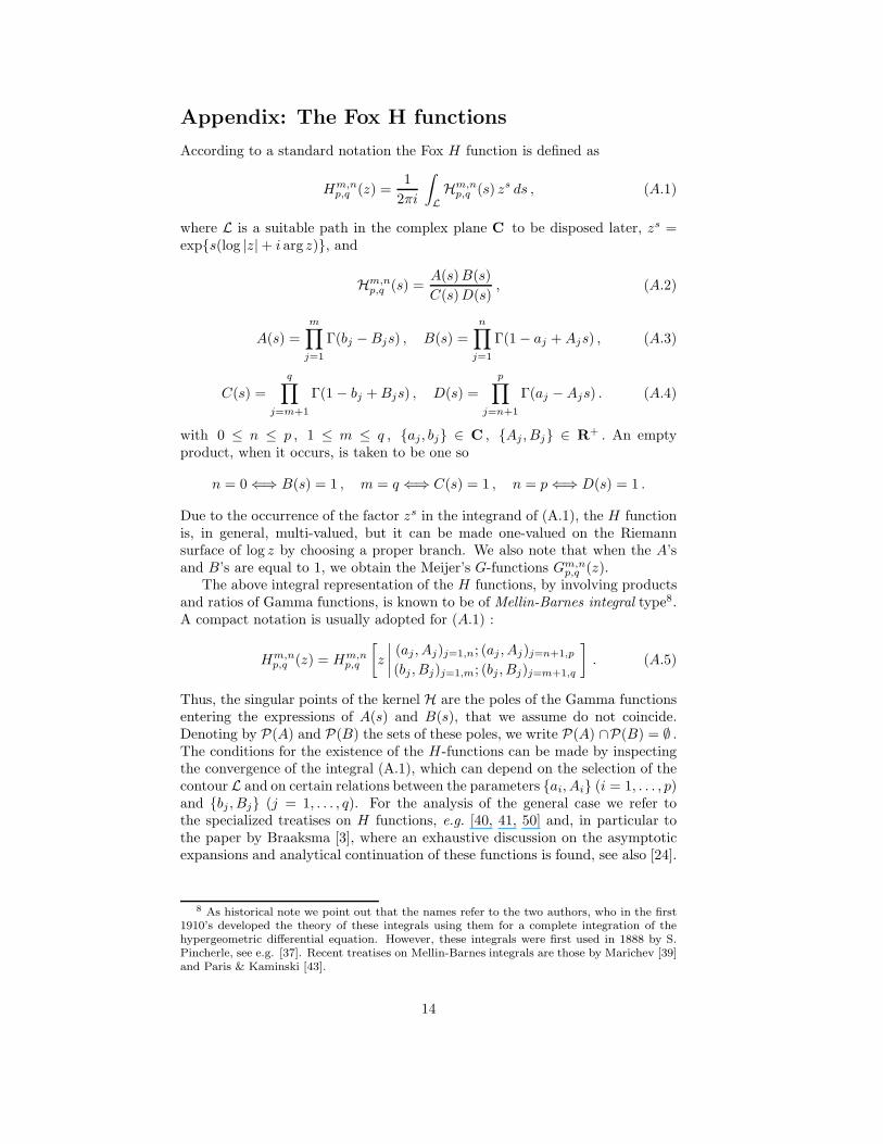
According to a standard notation the Fox H function is defined as

Hm,np,q (z) =

1

2πi

∫

L

Hm,np,q (s) zs ds , (A.1)

where L is a suitable path in the complex plane C to be disposed later, zs =exp{s(log |z|+ i arg z)}, and

Hm,np,q (s) =

A(s)B(s)

C(s)D(s), (A.2)

A(s) =

m∏

j=1

Γ(bj − Bjs) , B(s) =

n∏

j=1

Γ(1 − aj + Ajs) , (A.3)

C(s) =

q∏

j=m+1

Γ(1 − bj + Bjs) , D(s) =

p∏

j=n+1

Γ(aj − Ajs) . (A.4)

with 0 ≤ n ≤ p , 1 ≤ m ≤ q , {aj, bj} ∈ C , {Aj , Bj} ∈ R+ . An emptyproduct, when it occurs, is taken to be one so

n = 0 ⇐⇒ B(s) = 1 , m = q ⇐⇒ C(s) = 1 , n = p ⇐⇒ D(s) = 1 .

Due to the occurrence of the factor zs in the integrand of (A.1), the H functionis, in general, multi-valued, but it can be made one-valued on the Riemannsurface of log z by choosing a proper branch. We also note that when the A’sand B’s are equal to 1, we obtain the Meijer’s G-functions Gm,n

p,q (z).The above integral representation of the H functions, by involving products

and ratios of Gamma functions, is known to be of Mellin-Barnes integral type8.A compact notation is usually adopted for (A.1) :

Hm,np,q (z) = Hm,n

p,q

[z

∣∣∣∣(aj , Aj)j=1,n; (aj , Aj)j=n+1,p

(bj , Bj)j=1,m; (bj , Bj)j=m+1,q

]. (A.5)

Thus, the singular points of the kernel H are the poles of the Gamma functionsentering the expressions of A(s) and B(s), that we assume do not coincide.Denoting by P(A) and P(B) the sets of these poles, we write P(A) ∩P(B) = ∅ .The conditions for the existence of the H-functions can be made by inspectingthe convergence of the integral (A.1), which can depend on the selection of thecontour L and on certain relations between the parameters {ai, Ai} (i = 1, . . . , p)and {bj , Bj} (j = 1, . . . , q). For the analysis of the general case we refer tothe specialized treatises on H functions, e.g. [40, 41, 50] and, in particular tothe paper by Braaksma [3], where an exhaustive discussion on the asymptoticexpansions and analytical continuation of these functions is found, see also [24].

8 As historical note we point out that the names refer to the two authors, who in the first1910’s developed the theory of these integrals using them for a complete integration of thehypergeometric differential equation. However, these integrals were first used in 1888 by S.Pincherle, see e.g. [37]. Recent treatises on Mellin-Barnes integrals are those by Marichev [39]and Paris & Kaminski [43].

14

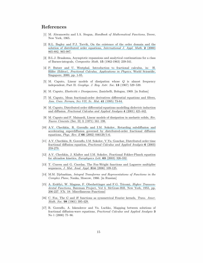
References

[1] M. Abramowitz and I.A. Stegun, Handbook of Mathematical Functions, Dover,New York, 1965.

[2] R.L. Bagley and P.J. Torvik, On the existence of the order domain and thesolution of distributed order equations, International J. Appl. Math. 2 (2000)865-882, 965-987.

[3] B.L.J. Braaksma, Asymptotic expansions and analytical continuations for a classof Barnes-integrals, Compositio Math. 15 (1962-1963) 239-341.

[4] P. Butzer and U. Westphal, Introduction to fractional calculus, in: H.Hilfer (Editor), Fractional Calculus, Applications in Physics, World Scientific,Singapore, 2000, pp. 1-85.

[5] M. Caputo, Linear models of dissipation whose Q is almost frequencyindependent, Part II. Geophys. J. Roy. Astr. Soc. 13 (1967) 529–539.

[6] M. Caputo, Elasticita e Dissipazione, Zanichelli, Bologna, 1969. [in Italian]

[7] M. Caputo, Mean fractional-order derivatives differential equations and filters,Ann. Univ. Ferrara, Sez VII, Sc. Mat. 41 (1995) 73-84.

[8] M. Caputo, Distributed order differential equations modelling dielectric inductionand diffusion. Fractional Calculus and Applied Analysis 4 (2001) 421-442.

[9] M. Caputo and F. Mainardi, Linear models of dissipation in anelastic solids, Riv.Nuovo Cimento (Ser. II) 1 (1971) 161–198.

[10] A.V. Chechkin, R. Gorenflo and I.M. Sokolov, Retarding subdiffusion andaccelerating superdiffusion governed by distributed-order fractional diffusionequations, Phys. Rev. E 66 (2002) 046129/1-6.

[11] A.V. Chechkin, R. Gorenflo, I.M. Sokolov, V.Yu. Gonchar, Distributed order timefractional diffusion equation, Fractional Calculus and Applied Analysis 6 (2003)259-279.

[12] A.V. Chechkin, J. Klafter and I.M. Sokolov, Fractional Fokker-Planck equationfor ultraslow kinetics, Europhysics Lett. 63 (2003) 326-332.

[13] T. Craven and G. Csordas, The Fox-Wright functions and Laguerre multipliersequences, J. Mat. Anal. Appl. 314 (2006) 109-125.

[14] M.M. Djrbashian, Integral Transforms and Representations of Functions in theComplex Plane, Nauka, Moscow, 1966. [in Russian]

[15] A. Erdelyi, W. Magnus, F. Oberhettinger and F.G. Tricomi, Higher Transcen-dental Functions, Bateman Project, Vol 3, McGraw-Hill, New York, 1955, pp.206-227. [Ch. 18: Miscellaneous Functions]

[16] C. Fox, The G and H functions as symmetrical Fourier kernels, Trans. Amer.Math. Soc. 98 (1961) 395-429.

[17] R. Gorenflo, A. Iskenderov and Yu. Luchko, Mapping between solutions offractional diffusion-wave equations, Fractional Calculus and Applied Analysis 3

No 1 (2000) 75–86.

15

[18] R. Gorenflo, J. Loutchko, Yu. Luchko, Computation of the Mittag-Leffler functionEα,β(z) and its derivatives, Fractional Calculus and Applied Analysis 5 No 4(2002) 491-518.

[19] R. Gorenflo, Yu. Luchko and F. Mainardi, Analytical properties and applicationsof the Wright function. Fractional Calculus and Applied Analysis 2 (1999) 383-414. [E-print http://arxiv.org/abs/math-ph/0701069]

[20] R. Gorenflo, Yu. Luchko and F. Mainardi, Wright functions as scale-invariantsolutions of the diffusion-wave equation, J. Comput. Appl. Math. 118 (2000)175-191.

[21] R. Gorenflo and F. Mainardi, Fractional calculus: integral and differentialequations of fractional order, in: A. Carpinteri and F. Mainardi (Editors),Fractals and Fractional Calculus in Continuum Mechanics, Springer Verlag,Wien, 1997, pp. 223–276. [Reprinted in http://www.fracalmo.org]

[22] R. Gorenflo, F. Mainardi and H.M. Srivastava, Special functions in fractionalrelaxation-oscillation and fractional diffusion-wave phenomena, in D. Bainov(Editor), Proceedings VIII International Colloquium on Differential Equations,Plovdiv 1997, VSP, Utrecht, 1998, pp. 195-202.

[23] A.A. Kilbas, Fractional calculus of the generalized Wright function, FractionalCalculus and Applied Analysis 8 (2005) 114-126.

[24] A.A. Kilbas and M. Saigo, On the H functions, J. Appl. Math. Stochastic Anal.12 (1999) 191-204.

[25] A.A. Kilbas and M. Saigo, H-transforms. Theory and Applications, CRC Press,Boca Raton, FL,2004.

[26] A.A Kilbas, M. Saigo, J.J. Trujillo, On the generalized Wright function,Fractional Calculus and Applied Analysis 5 (2002) 437-460.

[27] A.A. Kilbas, H.M. Srivastava and J.J. Trujillo, Theory and Applications ofFractional Differential Equations, Elsevier, Amsterdam, 2006.

[28] V. Kiryakova, Generalized Fractional Calculus and Applications, Longman,Harlow, U.K., 1994. [Pitman Research Notes in Mathematics, Vol. 301]

[29] J. Klafter and I.M. Sokolov, Anomalous diffusion spreads its wings, Physics World18 (2005), 29-32.

[30] F. Mainardi, On the initial value problem for the fractional diffusion-waveequation, in: S. Rionero and T. Ruggeri (Editors), Waves and Stability inContinuous Media, World Scientific, Singapore, 1994, pp. 246-251.

[31] F. Mainardi, The fundamental solutions for the fractional diffusion-waveequation, Appl. Math. Lett. 9 No 6 (1996) 23-28.

[32] F. Mainardi, Fractional relaxation-oscillation and fractional diffusion-wavephenomena, Chaos, Solitons and Fractals 7 (1996) 1461–1477.

[33] F. Mainardi, Fractional calculus: some basic problems in continuum andstatistical mechanics, in: A. Carpinteri and F. Mainardi (Editors), Fractals andFractional Calculus in Continuum Mechanics, Springer Verlag, Wien and New-York, 1997, pp. 291–348. [Reprinted in http://www.fracalmo.org]

16

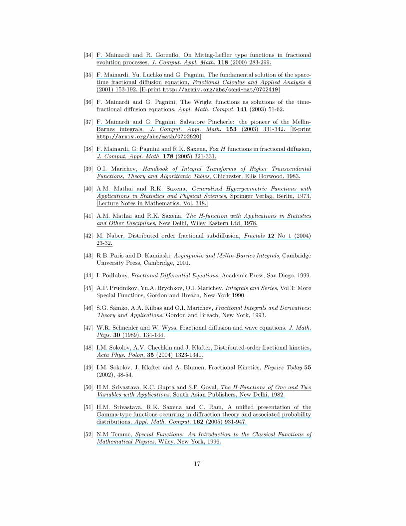
[34] F. Mainardi and R. Gorenflo, On Mittag-Leffler type functions in fractionalevolution processes, J. Comput. Appl. Math. 118 (2000) 283-299.

[35] F. Mainardi, Yu. Luchko and G. Pagnini, The fundamental solution of the space-time fractional diffusion equation, Fractional Calculus and Applied Analysis 4

(2001) 153-192. [E-print http://arxiv.org/abs/cond-mat/0702419]

[36] F. Mainardi and G. Pagnini, The Wright functions as solutions of the time-fractional diffusion equations, Appl. Math. Comput. 141 (2003) 51-62.

[37] F. Mainardi and G. Pagnini, Salvatore Pincherle: the pioneer of the Mellin-Barnes integrals, J. Comput. Appl. Math. 153 (2003) 331-342. [E-printhttp://arxiv.org/abs/math/0702520]

[38] F. Mainardi, G. Pagnini and R.K. Saxena, Fox H functions in fractional diffusion,J. Comput. Appl. Math. 178 (2005) 321-331.

[39] O.I. Marichev, Handbook of Integral Transforms of Higher TranscendentalFunctions, Theory and Algorithmic Tables, Chichester, Ellis Horwood, 1983.

[40] A.M. Mathai and R.K. Saxena, Generalized Hypergeometric Functions withApplications in Statistics and Physical Sciences, Springer Verlag, Berlin, 1973.[Lecture Notes in Mathematics, Vol. 348.]

[41] A.M. Mathai and R.K. Saxena, The H-function with Applications in Statisticsand Other Disciplines, New Delhi, Wiley Eastern Ltd, 1978.

[42] M. Naber, Distributed order fractional subdiffusion, Fractals 12 No 1 (2004)23-32.

[43] R.B. Paris and D. Kaminski, Asymptotic and Mellin-Barnes Integrals, CambridgeUniversity Press, Cambridge, 2001.

[44] I. Podlubny, Fractional Differential Equations, Academic Press, San Diego, 1999.

[45] A.P. Prudnikov, Yu.A. Brychkov, O.I. Marichev, Integrals and Series, Vol 3: MoreSpecial Functions, Gordon and Breach, New York 1990.

[46] S.G. Samko, A.A. Kilbas and O.I. Marichev, Fractional Integrals and Derivatives:Theory and Applications, Gordon and Breach, New York, 1993.

[47] W.R. Schneider and W. Wyss, Fractional diffusion and wave equations. J. Math.Phys. 30 (1989), 134-144.

[48] I.M. Sokolov, A.V. Chechkin and J. Klafter, Distributed-order fractional kinetics,Acta Phys. Polon. 35 (2004) 1323-1341.

[49] I.M. Sokolov, J. Klafter and A. Blumen, Fractional Kinetics, Physics Today 55

(2002), 48-54.

[50] H.M. Srivastava, K.C. Gupta and S.P. Goyal, The H-Functions of One and TwoVariables with Applications, South Asian Publishers, New Delhi, 1982.

[51] H.M. Srivastava, R.K. Saxena and C. Ram, A unified presentation of theGamma-type functions occurring in diffraction theory and associated probabilitydistributions, Appl. Math. Comput. 162 (2005) 931-947.

[52] N.M Temme, Special Functions: An Introduction to the Classical Functions ofMathematical Physics, Wiley, New York, 1996.

17

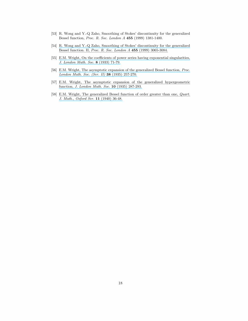
[53] R. Wong and Y.-Q Zaho, Smoothing of Stokes’ discontinuity for the generalizedBessel function, Proc. R. Soc. London A 455 (1999) 1381-1400.

[54] R. Wong and Y.-Q Zaho, Smoothing of Stokes’ discontinuity for the generalizedBessel function. II, Proc. R. Soc. London A 455 (1999) 3065-3084.

[55] E.M. Wright, On the coefficients of power series having exponential singularities,J. London Math. Soc. 8 (1933) 71-79.

[56] E.M. Wright, The asymptotic expansion of the generalized Bessel function, Proc.London Math. Soc. (Ser. II) 38 (1935) 257-270.

[57] E.M. Wright, The asymptotic expansion of the generalized hypergeometricfunction, J. London Math. Soc. 10 (1935) 287-293.

[58] E.M. Wright, The generalized Bessel function of order greater than one, Quart.J. Math., Oxford Ser. 11 (1940) 36-48.

18