1 Introduction

The scalar field model with potential U(φ) = m2

2φ2 + λ

4!φ4 + σ

6!φ6 is the simplest model

exhibiting a rich phase structure and for studying tricritical phenomena in both two and

three dimensional systems [see, e.g. Refs. [1] and [2]]. In terms of the phase diagram

for the model, a tricritical point can emerge whenever we have three phases coexisting

simultaneously. For the above potential, in the absence of corrections due to fluctuations,

one can have a second order transition in m when the scalar field mass vanishes and

λ > 0, σ > 0. A first order transition happens for the case of λ < 0, σ > 0. The tricritical

point occurs when the quartic coupling constant vanishes (with m = 0, σ > 0). A study

of the phase diagram for this model in 3D, at finite temperature, was recently done [3]

and it has been shown that there is a temperature β−1(m,λ, σ) for which the physical

thermal mass mβ and coupling constant λβ vanishes, thus characterizing the tricritical

point.

There are many possible applications associated with the model with potential U(φ)

with φ6 interaction. For instance, in D = 2, it is known [4] that the minimal conformal

quantum field theory, with central charge 7/10 (the tricritical Ising model) is in the

same universality class, in the scaling region near the tricritical point, of the Landau-

Ginzburg model with the above potential. This φ6 potential model can then be thought

of as the continuum realization of the Ising model with possible applications in, e.g.,

the description of adsorbed helium on krypton-plated graphite [5], in understanding the

statistical mechanics of binary mixtures, such as He3 − He4 [6], etc. These are just a

few examples of systems exhibiting tricritical phenomena in condensed matter physics.

In field theory in general, the φ6 model has been used in the study of polarons, or

solitonic like field configurations on systems of low dimensionality [1]. Also, a gauged

(SU(2)) version of the φ6 potential model in Euclidean 3D, has recently been used to study

a possible existence of a tricritical point in Higgs models at high temperatures [7]. In this

context the tricritical point is characterized by the ratio of the quartic coupling constant

and the gauge coupling constant of the effective three-dimensional theory, obtained from

the 3 + 1D high temperature, dimensionally reduced SU(2) Higgs model. This can be

particularly useful in the context of the study of the electroweak phase transition.

2

There are then many reasons that make the φ6 potential model an interesting model

to be studied. In this paper, we will be particularly interested in studying the regime of

parameters for which:

m2 > 0 , λ < 0 , σ > 0 and

(

λ

3!

)2

− 4m2 σ

5!

> 0 . (1)

In this case U(φ) has three relative minima φt± and φf (see Fig. 1). For these parameters

the system has metastable vacuum states and it may exhibit a first order phase transition.

The states of the classical field theory for which φ = φt± are the unique classical states

of lowest energy (true vacuum) and, at least in perturbation theory, they correspond to

the unique vacuum states of the quantum theory. The state of the classical field theory

for which φ = φf is a stable classical equilibrium state. However, it is rendered unstable

by quantum effects, i.e., barrier penetration (or over the barrier thermal fluctuations, at

finite temperatures). φf is the false vacuum (the metastable state).

We will compute the vacuum decay (tunneling) rate at both zero and finite temper-

ature. For calculation reasons we will restrict ourselves to the thin wall approximation

for the true vacuum bubble (or bounce solution). We then consider the energy-density

difference between the true and false vacuum as very small as compared with the height

of the barrier of the U(φ) potential [9, 13]. From this, we are able to give the explicit

expression for the bounce and also to qualitatively describe the eigensolutions for the

bounce configuration. The paper is organized as follows: In Sec. II we obtain the bounce

field configuration for the model and we compute the Euclidean action in the thin wall

approximation. In Sec. III we calculate the vacuum decay rate at zero temperature and

we discuss the eigenvalue equations obtained for the bounce configuration within the ap-

proximations we have taken for the bounce. In Sec. IV we compute the nucleation rate

at finite temperature, following the procedure given in [14]. In Sec. V the concluding

remarks are given. In this paper we use h = c = kb = 1.

3

2 The Vacuum Decay Rate and the Bounce Solution

Let us consider a scalar field model, in three-dimensional space-time, with Euclidean

action given by

SE(φ) =∫

d3xE

[

1

2(∂µφ)2 + U(φ)

]

, (2)

with

U(φ) =m2

2φ2 +

λ

4!φ4 +

σ

6!φ6 . (3)

As discussed in the introduction, we are interested in the regime for which the parameters

in (3) satisfies (1), such that the potential U(φ) exhibits non-degenerate local minima and

then metastable states. The picture we have in mind is that once the system is prepared

in the false vacuum state, it will evolve to the true vacuum state by tunneling (at zero

temperature) or by bubble nucleation, triggered by thermal fluctuations over the potential

barrier.

In the case of quantum field theory at zero temperature the study of the decay of

false vacuum was initiated by Voloshin, Kobsarev and Okun [8] and later by Callan and

Coleman [9, 10], who developed the so called bounce method for the theory of quantum

decay. In this context the decay rate per unit space-time volume V3 is given by

Γ

V3=(

∆SE

2π

)3/2[

det′ (−2E + U ′′(φb))

det (−2E + U ′′(φf))

]−1/2

e−∆SE (1 + O(h)) , (4)

where 2E = ∂2

∂τ2 + ∂2

∂x2 + ∂2

∂y2 , U′′(φ) = d2U(φ)

dφ2 and ∆SE = SE(φb) − SE(φf). SE(φb) is

the Euclidean action evaluated at its extreme (specifically a saddle point), φ = φb, where

φb is the bounce: a solution of the field equation of motion, δSE/δφ|φ=φb= 0, with the

appropriate boundary conditions. The prime in the determinantal prefactor in (4) means

that the three zero eigenvalues (the translational modes) of the [−2E + U ′′(φb)] operator

has been removed from it.

As it was shown by Coleman, Glaser and Martin [11], the solution that minimizes SE

is a spherical symmetric solution, r2 = τ 2 + x2 + y2 (in D dimensions the solution has

4

O(D) symmetry) and then φb can be written as the solution of the radial equation of

motion

d2φb

dr2+

2

r

dφb

dr= U ′(φb) , (5)

with the boundary conditions: limr→∞ φb(r) = φf and dφb

dr|r=0 = 0.

At finite temperature the calculation of the decay rate were first considered in [12]

in the context of quantum mechanics and later by Linde [13], for quantum field theory.

In [13], it is argued that temperature corrections to the nucleation rate are obtained

recalling that finite temperature field theory (at sufficiently high temperatures) in D =

d + 1 dimensions is equivalent to d-dimensional Euclidean quantum field theory with h

substituted by T . At finite temperature, the bounce, φB ≡ φB(ρ) (ρ = |r|), is a static

solution of the field equation of motion:

d2φB

dρ2+

1

ρ

dφB

dρ= U ′(φB) , (6)

with boundary conditions: limρ→∞ φB(ρ) = φf and dφB

dρ|ρ=0 = 0. The vacuum decay

rate, or bubble nucleation rate in this case, is proportional to e−∆E/T , where ∆E is the

nucleation barrier, given by (β = 1/T )

∆E

T= β

∫

d2x [LE(φB) − LE(φf)] , (7)

where LE is the Euclidean Lagrangian density.

The problem of the computation of the nucleation rate at finite temperature was

recently reconsidered by Gleiser, Marques and Ramos [14], who have used the early works

of Langer [15]. In this context the nucleation rate is given by

(Γ)β = −|E−|π

Im

[

det [−2E + U ′′(φB)]βdet [−2E + U ′′(φf)]β

]−1/2

e−∆E/T (1 + O(h)) , (8)

where E2− is the negative eigenvalue associated to the operator [−2E + U ′′(φB)].

To compute the vacuum decay rates, we need, therefore, to solve Eq. (5) for φb(r)

(at zero temperature), or Eq. (6) for φB(ρ) (at finite temperature). In the model studied

here, we can give an approximate analytical treatment for the bounce solution in the so

5

called thin-wall approximation, in which case the energy-density difference between the

false and true vacuum states can be considered very small, as compared to the height of

the potential barrier: ǫ0 = U(φf) − U(φt) ≪ U(φ2) (see Fig. 1). By interpreting φb as

a position and r as the time, Eq. (5) can be seen as a classical equation of motion for a

particle moving in a potential −U(φ) and subject to a viscous like damping force, with

stokes’s law coefficient inversely proportional to the time. The particle motion can then

be interpreted as it was released at rest, at time zero (because of the boundary conditiondφb

dr|r=0 = 0). From (5) it follows that

d

dr

1

2

(

dφb

dr

)2

− U(φb)

= −2

r

(

dφb

dr

)2

≤ 0 , (9)

meaning that the particle loses energy. Then, if the initial position of the particle is chosen

to be at the left of some value φ = φ1 (see Fig. 2), it will never reach the position φf .

Now, for φb(r) very close to φt, we can linearize Eq. (5) to obtain

[

d2

dr2+

2

r

d

dr− µ2

]

(φb − φt) = 0 , (10)

where µ2 = U(φt). The solution of (10) is

φb − φt = (φ(0) − φt)sinh(µr)

µr. (11)

Therefore, if we choose the position of the particle to be initially sufficiently close to φt, we

can arrange for it to stay arbitrarily close to φt for arbitrarily large r. But for sufficiently

large r, r = R, the viscous damping force can be neglected, since its coefficient is inversely

proportional to r. And if the viscous damping is neglected, the particle will reach the

position φf at a finite time R+∆R. Then, by continuity, there must be an initial position

between φt and φ1 for which the particle will come to rest at φf , after an infinity time.

From the above arguments, we can find a general expression for φb, valid for ǫ0 ≪ U(φ2).

In order to not lose too much energy, we must choose φb(0), the initial position of the

particle, very close to φt. The particle then stays close to φt until some very large time,

r = R. Near R (between R − ∆R and R + ∆R, ∆R ≪ R) the particle moves quickly

(according to Eq. (5), neglecting the viscous damping force), through the valley in Fig.

6

2 and it slowly comes to rest at φf , after an infinity time. Thus, we can write for the

bounce the following expression (φf = 0)

φb(r) =

φt 0 < r < R − ∆R

φwall(r −R) R − ∆R < r < R+ ∆R

φf R + ∆R < r <∞, (12)

where φwall satisfies the equation

d2φwall

dr2= U ′(φwall) . (13)

Eq. (12) is the thin-wall approximation for the bounce solution. From Eq. (13), we

obtain

∫ φwall

0

dφ√

2U(φ)= r . (14)

By rewriting U(φ) as

U(φ) =σ

6!φ2(

φ2 − φ20

)2 − γφ2

φ20

, (15)

with

φ20 = −1

2

6!

σ

λ

4!(16)

and

γ =φ2

0

4

6!

σ

(

λ

4!

)2

− 2m2

, (17)

then, by neglecting in (15) the term proportional to γ (valid in the thin-wall approxima-

tion), we obtain that

∫ φwall

0

dφ√

2 σ6!φ (φ2 − φ2

0)= r . (18)

The above integral is straightforward and the solution for φwall(r) can be written as

7

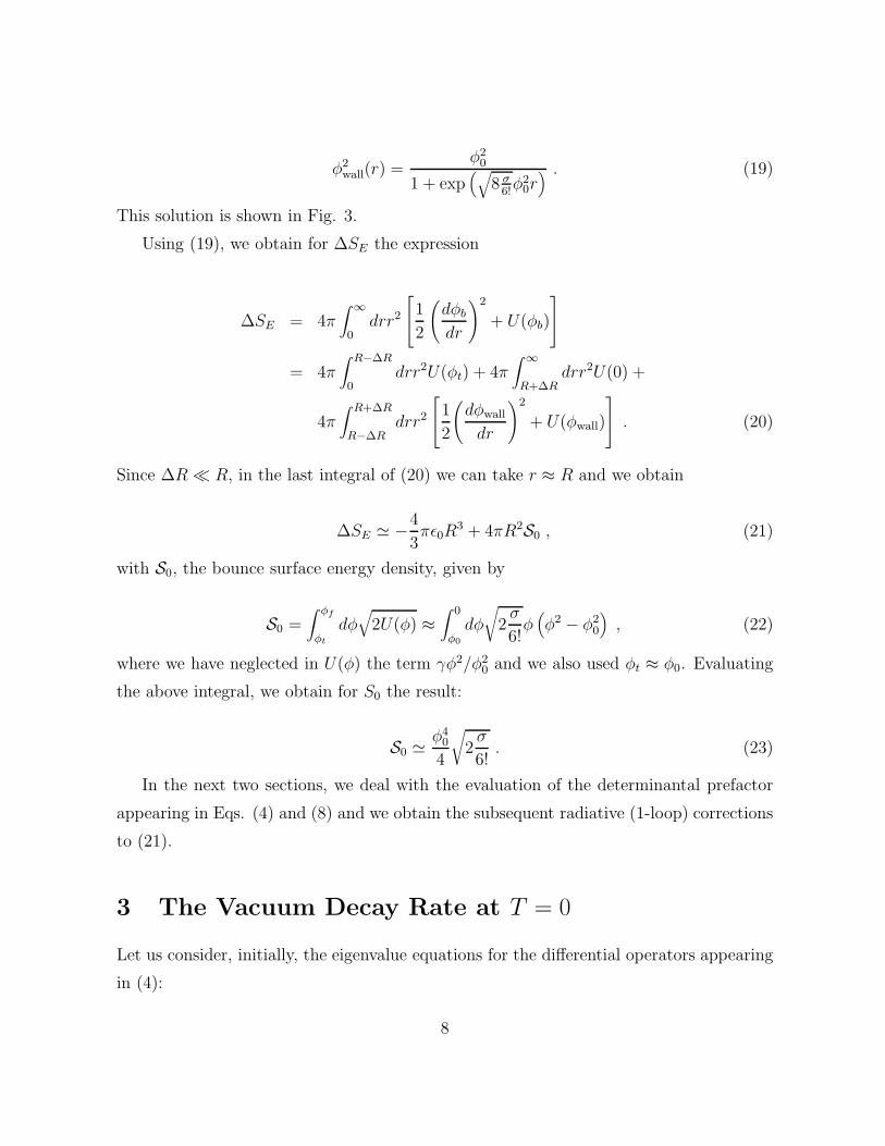
φ2wall(r) =

φ20

1 + exp(√

8 σ6!φ2

0r) . (19)

This solution is shown in Fig. 3.

Using (19), we obtain for ∆SE the expression

∆SE = 4π∫ ∞

0drr2

1

2

(

dφb

dr

)2

+ U(φb)

= 4π∫ R−∆R

0drr2U(φt) + 4π

∫ ∞

R+∆Rdrr2U(0) +

4π∫ R+∆R

R−∆Rdrr2

1

2

(

dφwall

dr

)2

+ U(φwall)

. (20)

Since ∆R ≪ R, in the last integral of (20) we can take r ≈ R and we obtain

∆SE ≃ −4

3πǫ0R

3 + 4πR2S0 , (21)

with S0, the bounce surface energy density, given by

S0 =∫ φf

φt

dφ√

2U(φ) ≈∫ 0

φ0

dφ

√

2σ

6!φ(

φ2 − φ20

)

, (22)

where we have neglected in U(φ) the term γφ2/φ20 and we also used φt ≈ φ0. Evaluating

the above integral, we obtain for S0 the result:

S0 ≃φ4

0

4

√

2σ

6!. (23)

In the next two sections, we deal with the evaluation of the determinantal prefactor

appearing in Eqs. (4) and (8) and we obtain the subsequent radiative (1-loop) corrections

to (21).

3 The Vacuum Decay Rate at T = 0

Let us consider, initially, the eigenvalue equations for the differential operators appearing

in (4):

8

[−2E + U ′′(φb)]ψb(i) = E2b (i)ψb(i) (24)

and

[−2E + U ′′(φf)]ψf (j) = E2f(j)ψf (j) . (25)

We then have for the determinantal prefactor of (4), the following

K =

[

det′ [−2E + U ′′(φb)]

det [−2E + U ′′(φf)]

]−1/2

= exp

{

−1

2ln

[

det′ [−2E + U ′′(φb)]

det [−2E + U ′′(φf)]

]}

= exp

{

−1

2ln

[

∏

i′E2

b (i)∏

j E2f(j)

]}

= exp

−1

2

∑

i

′ ln |E2b (i)| −

∑

j

lnE2f (j)

. (26)

Since the bounce can be approximated by a constant field configuration for r < (R−∆R) ≈ R, we can write for K, in the thin wall approximation, the expression:

K = exp

−1

2

4

3πR3

∫ d3p

(2π)3ln

[

E2t (p)

E2f (p)

]

+

∑

i

′ ln |E2wall(i)| −

∑

j

lnE2f (j)

, (27)

where E2t(f)(p) = p2 + U ′′(φt(f)). The integral in (27) can then be identified as the one

loop correction to the classical potential, while the remaining terms represent the quantum

corrections due to fluctuations around the bounce wall [16]. Then, by using Eqs. (21)

and (27) in Eq. (4) and following [9, 10], we obtain

Γ

V3≃ 2

(

∆SE

2π

)3/2

exp[

4

3πR3∆Ueff − 4πR2 (S0 + S1)

]

, (28)

where S1, is the term giving the 1-loop quantum corrections to fluctuations around the

bounce wall,

9

S1 =1

4πR2

∑

i

′ ln∣

∣

∣E2wall(i)

∣

∣

∣−∑

j

lnE2f(j)

, (29)

where E2wall(i) are the eigenvalues of −2E + U ′′(φwall(r − R). In (28) we have also that

∆Ueff = Ueff(φt) − Ueff(φf), where Ueff is the one loop effective potential, given by [17]

Ueff(φ) = U(φ) +1

2

∫

d3p

(2π)3ln

[

p2 + U ′′(φ)

p2 +m2

]

. (30)

The ultraviolet divergence in (30) can be handled in the usual way. Integrating over p0

and by using an ultraviolet cut-off, Λ, for the space-momentum, we obtain

Ueff(φ) = U(φ) − 1

12

(

p2 +m2)3/2 ∣

∣

∣

Λ

0−(

p2 +m2 +λ

2φ2 +

σ

4!φ4

)3/2∣

∣

∣

Λ

0

. (31)

Using that (1 + x)3/2 = 1 + 3/2x+ 3/8x2 + . . ., we obtain for Ueff the expression

Ueff(φ) = U(φ) − 1

12

(

m2 +λ

2φ2 +

σ

4!φ4

)3/2

−m3 − 3

2Y (Λ)

(

λ

2φ2 +

σ

4!φ4

)

+O (1/Λ) , (32)

where Y (Λ) = Λ2 + m2r. The divergent terms in (32) are proportional to φ2 and φ4 but

not to φ6. Then, only the mass m and λ need to be renormalized (σr = σ). From the

usual definition of renormalized mass mr and coupling constant λr,

m2r =

d2Ueff(φ)

dφ2

∣

∣

∣

φ=0(33)

and

λr =d4Ueff(φ)

dφ4

∣

∣

∣

φ=0(34)

and writing the unrenormalized parameters in terms of renormalized ones, we obtain for

the renormalized one loop effective potential, the following expression:

Ueff(φ) = Ur(φ) − 1

12

[

U ′′r (φ)3/2 −m3

r −3

4mrλrφ

2r −

3λ2r

32mrφ4 − 3mrσr

16φ4

]

, (35)

10

where Ur means the tree level potential expressed in terms of the renormalized quantities.

For convenience, from now on we drop the r subscript from the expressions and it is to

be understood that the parameters m,λ and σ are the renormalized ones, instead of the

bare ones. Then, ∆Ueff can be written as (since φf = 0)

∆Ueff = U(φt) −1

12

[

U ′′(φt)3/2 − 3

4mλφ2

t −3λ2

32mφ4

t −3mσ

16φ4

t

]

(36)

We now turn to the problem of evaluating the eigenvalues E2wall(i) of −2E+U ′′[φwall(r−

R)], which appears in (27). This is not an easy task. In fact, only in a very few examples

this has known analytical solutions, as, for example, for the kink solution in the (λφ4)D=2

model [18]. Unfortunately, for the model studied here, we can not find analytical solutions

for these differential operators. However, we can perform an approximate analysis, and, in

particular we can find explicitly the negatives and zero modes for the differential operator

for the bounce wall field configuration. By making use of the spherical symmetry of the

bounce solution, we can express the eigenvalue equation:

[−2E + U ′′(φwall(r − R))]Ψi(r, θ, ϕ) = E2wall(i)Ψi(r, θ, ϕ)

in the form

[

− d2

dr2− 2

r

d

dr+l(l + 1)

r2+m2 +

λ

2φ2

wall(r −R) +σ

4!φ4

wall(r − R)

]

ψi(r) = E2wall(i)ψi(r) ,

(37)

where l = 0, 1, 2, . . .. Making ψi(r) = χi(r)/r and z = r − R, we obtain

[

− d2

dz2+

l(l + 1)

(z +R)2+m2 +

λ

2φ2

wall(z) +σ

4!φ4

wall(z)

]

χn,l(z) = E2wall(n, l)χn,l(z) . (38)

Since ∆R ≪ R, we can take l(l + 1)/(z +R)2 ≈ l(l + 1)/R2 and then

[

− d2

dz2+λ

2φ2

wall(z) +σ

4!φ4

wall(z)

]

χn(z) = η2nχn(z) , (39)

where ηn is obtained from

11

E2wall(n, l) = η2

n +m2 +l(l + 1)

R2. (40)

We know that the −2E + U ′′(φb(r)) operator has three zero eigenvalues coming from

the bounce translational invariance. Then, for l = 1 and to the lowest value of ηn (which

can be chosen as η1), we will have E2wall(1, 1) = 0, with multiplicity three, as expected,

and η21 = −m2 − 2/R2. The lowest eigenvalue E2

wall (the negative eigenvalue) will be

E2wall(1, 0) = −2/R2, with multiplicity one, just what one would expect for the metastable

state, the existence of only one negative eigenvalue [16]. To evaluate the other eigenvalues,

we make the following change of variable w =√

σ6!φ2

0 z and use (19) in (40). We then get

− d2

dw2− 24

1 + e√

8w+

30(

1 + e√

8w)2

χn(w) = ν2nχn(w) , (41)

where ν2n = η2

n 6!/(σφ40). We can then express the eigenvalues of −2E + U ′′(φwall(r − R))

as

E2wall(n, l) = φ4

0

σ

6!ν2

n +m2 +l(l + 1)

R2. (42)

We were not able to find any analytical solution for Eq. (41), which it is even harder

to solve, due to the boundary conditions. We are currently working on the numerical

solution for the eigenvalues, whose results will be reported elsewhere.

4 The Nucleation Rate at Finite Temperature

At finite temperature, the bounce solution is a static solution of the field equation of

motion, δSE/δφ|φ=φB(ρ) = 0, where φB(ρ) is given as in (12), with bubble radius ρ and

thickness ∆ρ ≪ ρ. φwall = φwall(ρ) is still expressed as in (19). To calculate the determi-

nantal prefactor in (8), we consider the eigenvalue equations for the differential operators:

[−2E + U ′′(φB)]ψB(i) = µ2BψB(i) (43)

and

12

[−2E + U ′′(φf)]ψf (i) = µ2fψf (i) , (44)

where, in momentum space, µ2 = ω2n +E2, where ωn = 2πn

βare the Matsubara frequencies

(n = 0,±1,±2, . . .). Using (43) and (44) in (8), we obtain for K the expression:

Kβ =

[

det [−2E + U ′′(φB)]βdet [−2E + U ′′(φf)]β

]−1/2

= exp

{

−1

2ln

[

det [−2E + U ′′(φB)]βdet [−2E + U ′′(φf)]β

]}

= exp

−1

2ln

∏+∞n=−∞

∏

i [ω2n + E2

B(i)]∏+∞

n=−∞∏

j

[

ω2n + E2

f(j)]

= exp

−1

2ln

∏+∞n=−∞

(

ω2n + E2

−)

(ω2n + E2

0)2∏′

i [ω2n + E2

B(i)]∏+∞

n=−∞∏

j

[

ω2n + E2

f (j)]

, (45)

where we have separated the negative and zero eigenvalues in the numerator of Eq. (45),

with the prime meaning that the single negative eigenvalue, E2−, and the two zero eigen-

values, E20 (related to the now two-dimensional space), were excluded from the product.

The term for n = 0 in (ω2n + E2

0) can be handled using collective coordinates method, as

in [10, 18], resulting in the factor V2

[

∆E2πT

]

, where V2 is the “volume” of the two-space.

Separating the n = 0 modes from both the numerator and denominator of (45) and using

the identity

n=+∞∏

n=1

(

1 +a2

n2

)

=sinh(πa)

πa, (46)

we get

Kβ = V2

[

∆E

2πT

]

exp

{

− ln(E2−)

1

2 − ln

[

sin(β2|E−|)

β2|E−|

]

+ a+ b

}

, (47)

where

a =

−3 +∑

j

−∑

i

′

ln+∞∏

n=1

ω2n +

∑

i

′ −∑

j

ln β (48)

13

and

b =∑

j

[

β

2Ef (j) + ln

(

1 − e−βEf (j))

]

−∑

i

′[

β

2EB(i) + ln

(

1 − e−βEB(i))

]

. (49)

Since∑

i′ has three eigenvalues less than

∑

j and (E2−)1/2 = i|E−|, we obtain

Kβ = −i V2

[

∆E

2πT

]

[

2β2 sin

(

β

2|E−|

)]−1

eb . (50)

Using the above results in (8), we then obtain for the nucleation rate, per unit volume,

the expression:

Γβ

V2= 2QT 3 exp

[

−∆F (T )

T

]

, (51)

with

Q =(

∆E

2πT

) |E−|2T

π sin( |E−|2T

)(52)

and

∆F (T ) = ∆E−∑

j

[

1

2Ef (j) +

1

βln(

1 − e−βEf (j))

]

+∑

i

′[

1

2EB(i) +

1

βln(

1 − e−βEB(i))

]

.

(53)

In the thin-wall approximation (in an analogous way as was done in Sec. III) we can

write

∆F (T ) ≃ −πρ2 ∆Ueff(T ) + 2π(S0 + Sβ)ρ , (54)

where ∆Ueff(T ) is given by

∆Ueff(T ) = ǫ0 +∫

d2p

(2π)2

[

1

2

√

p2 + U ′′(φf) −1

2

√

p2 + U ′′(φt)]

+T∫

d2p

(2π)2ln[

1 − e−β√

p2+U ′′(φf )]

− T∫

d2p

(2π)2ln[

1 − e−β√

p2+U ′′(φt)]

(55)

14

and Sβ is the 1-loop finite temperature correction to the bubble surface energy density,

given by

Sβ =T

2πρ

∑

i

′[

β

2Ewall(i) + ln

(

1 − e−βEwall(i))

]

−∑

j

[

β

2Ef (j) + ln

(

1 − e−βEf (j))

]

,

(56)

where E2wall(i) are the eigenvalues of −∇2 + U ′′(φwall(ρ − ρ)). In (55), the first integral

is divergent but it can be handled just in the same way as in the previous section, by

the introduction of the appropriated counterterms of renormalization. The remaining

integrals in (55) are all finite and they can be reduced to integrals of the type

I(t) =∫ ∞

0dx[

x ln(

1 − e√

x2+t2)]

(57)

and it is evaluated in Appendix B. The result is:

I(t) = I(0) +t3

6+t2

4− t2

2ln t− 1

2

+∞∑

n=1

(−1)n+1ζ(2n)

n(n+ 1)(2π)2n

(

t2)n+1

, (58)

where ζ(n) is the Riemman Zeta function. Using (58) in (55), we obtain for (54) the

following expression

∆F (T ) = −πρ2 [ǫ0 + c(φf) − c(φt)] + 2πρ [S0 + Sβ ] , (59)

where (using t = βU ′′(φ)1/2)

c(φ) =1

2πβ3I (t) ≃ 1

2πβ3

(

I(0) +t3

6+t2

4− t2

2ln t− ζ(2)t4

16π2

)

. (60)

The critical radius for bubble nucleation, ρc, is obtained by minimizing (59),

δ∆F (T )/δρ|ρ=ρc= 0.

For the eigenvalues E2wall(i) of −∇2 +U ′′(φwall(ρ− ρ)), using the now cylindrical sym-

metry of φwall(ρ), the eigenvalue equation

[−∇2 + U ′′(φwall(ρ− ρ))]Ψi(ρ, ϕ) = E2wall(i)Ψi(ρ, ϕ)

can be written as

15

[

− d2

dρ2− 1

ρ

d

ρ+s2

ρ2+m2 +

λ

2φ2

wall(ρ− ρ) +σ

4!φ4

wall(ρ− ρ)

]

ψn,s(ρ) = E2wall(n, s)ψn,s(ρ) ,

(61)

where s = 0,±1,±2, . . .. Taking ψ(ρ) = χ(ρ)/ρ1/2, we obtain

[

− d2

dρ2+

4s2 − 1

4ρ2+m2 +

λ

2φ2

wall(ρ− ρ) +σ

4!φ4

wall(ρ− ρ)

]

χn,s(ρ) = E2wall(n, s)χn,s(ρ) .

(62)

As in the previous section, we make z = (ρ− ρ) and because ∆ρ≪ ρ, then

[

− d2

dz2+λ

2φ2

wall(z) +σ

4!φ4

wall(z)

]

χn(z) = η2nχn(ρ) , (63)

where η2n is now obtained from

E2wall(n, s) = η2

n +m2 +4s2 − 1

4ρ2. (64)

Analogously to the zero temperature case, the differential operator −∇2+U ′′(φB) has now

two zero eigenvalues (related to the translational modes in the two-dimensional space).

The multiplicity of (64) is two for all s 6= 0 and for s = 0 the multiplicity is one.

Then for s = 1 and lower ηn (we choose η1) we will have E2wall(1, 1) = 0 and then

η21 = −[m2 + 3/(4ρ2)]. For the negative eigenvalue we obtain E2

− = E2wall(1, 0) = −1/ρ2.

As in the previous section, by taking w =√

σ/6!φ20 z, we obtain for the eigenvalues,

E2wall(n, s) = φ4

0

σ

6!ν2

n +m2 +4s2 − 1

4ρ2, (65)

where νn is the same as in the previous section.

5 Conclusions

In this paper we have studied the evaluation of the vacuum decay rates, at both zero

temperature and at finite temperature, for the σφ6 model in D = 3, when the parameters

of the model satisfies the conditions given in (1). Our main results were the determi-

nation of the expression for the bounce solution, Eqs. (12) and (19), and also, despite

16

of the difficulties for finding the solutions for the bounce’s wall eigenvalue problem, by

taking consistent considerations for the field equations we have at hand (like the thin-wall

approximation), we were able to perform a detailed analysis of the bounce negative and

zero eigenvalues. We have also given a set of eigenvalue equations, which can be use-

ful in a more detailed analysis of this problem using, e.g. numerical methods. In [1] it

was analyzed the phase structure for the σφ6 model in D = 2 in the lattice and it was

also studied the possible production of topological and nontopological excitations in the

model. By remembering that at high temperatures our model in D = 3 resembles the

D = 2 model at zero temperature, it will be interesting to apply the method and results

we have obtained here to the problem studied in [1] for the regime of a first order phase

transition.

Acknowledgements

ROR and NFS are partially supported by Conselho Nacional de Desenvolvimento

Cientıfico e Tecnologico - CNPq (Brazil). GHF is supported by a grant from CAPES.

ROR would like also to thank ICTP-Trieste, for the kind hospitality, when during his

stay, this work was completed.

Appendix

We evaluate here the integral (57),

I(t) =∫ ∞

0dx[

x ln(

1 − e√

x2+t2)]

. (A.66)

Using that

∂I(t)

∂(t2)=∫ ∞

0dx

[

x∂

∂(t2)ln(

1 − e√

x2+t2)

]

=∫ ∞

0dx

[

x∂

∂(x2)ln(

1 − e√

x2+t2)

]

(A.67)

and integrating by parts, we obtain that

dI(t)

d(t2)=

1

2ln(

1 − e√

x2+t2) ∣

∣

∣

∞

0= −1

2ln(

1 − e−t)

. (A.68)

17

We can then write I(t) in the form:

I(t) = I(0) −∫ t

0dt[

t ln(

1 − e−t)]

= I(0) −∫ t

0dt

[

t ln sinh(

t

2

)

+ t ln 2 − t2

2

]

(A.69)

If one uses (46) and expanding the logarithm in the above equation, we are able to perform

the integral and we obtain the result shown in Sec. IV, Eq. (58).

References

[1] M.G. do Amaral, J. Phys. G24, 1061 (1998).

[2] M.A.Aguero Granados and A.A. Espinosa Garrido, Phys.Lett A 182, 294 (1993),

M.A.Aguero Granados, Phys.Lett 199, 185 (1995), W.Fa Lu, G.J.Ni and Z.G.Wang,

J.Phys.G 24, 673 (1998).

[3] G. N. J. Ananos and N. F. Svaiter, Physica A241, 627 (1997).

[4] A. B. Zamolodchikov, Sov. J. Nucl. Phys. 44, 529 (1986).

[5] I. D. Lawrye and S. Sarbach, in Phase transitions and Critical Phenomena, Eds. C.

Domb and J. Lebowitz, Vol. 9 (Academic Press, NY, 1983).

[6] R. B. Griffiths, Phys. Rev. B7, 545 (1973).

[7] P. Arnold and D. Wright, Phys. Rev. D55, 6274 (1997).

[8] M. B. Voloshin, I. Yu. Kobzarev, and L. B. Okun, Yad. Fiz. 20 1229 (1974) [Sov. J.

Nucl. Phys. 20, 644 (1975)].

[9] S. Coleman, Phys. Rev. D 15, 2929 (1977).

[10] C. Callan and S. Coleman, Phys. Rev D 16, 1762 (1977).

[11] S. Coleman, V Glaser, and A. Martin, Commun. Math. Phys. 58, 211 (1978).

[12] I. Affleck, Phys. Rev. Lett. 46, 388 (1981).

18

[13] A. Linde, Nucl.Phys. B216, 421 (1983).

[14] M. Gleiser, G. C. Marques and R. O. Ramos, Phys. Rev. D48, 1571 (1993).

[15] J. S. Langer, Ann. Phys, (N.Y) 41, 108 (1967), ibid. 54, 258 (1969).

[16] N. J. Gunther, D. A. Nicole and D. J. Wallace, J. Phys. A13, 1755 (1980).

[17] M. S. Swanson, Path Integrals and Quantum Processes (Academic Press, INC, Lon-

don, England 1992).

[18] R. Rajaraman, Solitons and Instantons. An Introduction to Solitons and Instantons

in Quantum Field Theory (North-Holland, Amsterdam, Netherlands 1982).

19

Figure Captions

Figure 1:The potential U(φ) for parameters m,λ, σ satisfying Eq. (1.1).

Figure 2:The inverted potential −U(φ).

Figure 3:The bubble field configuration φwall(r).

20

U(�)

�2 �t�fFigure 1

21

�U(�) �1 �t�f

Figure 2

22

Figure 3

�wall(r)

rR

23