The Leader–Follower Location Model

Netw Spat Econ (2007) 7:45–61DOI 10.1007/s11067-006-9007-2

The Leader–Follower Location Model

D. R. Santos-Peñate · R. Suárez-Vega ·P. Dorta-González

Published online: 6 December 2006© Springer Science + Business Media, LLC 2006

Abstract This paper summarizes some results for the leader–follower location modelon networks in several scenarios. Discretization results are considered and differ-ences derived from the inelastic and elastic demand assumptions, as well as fromthe customer’s choice rule, are emphasized. Finally, some issues for future lines ofinvestigation are suggested.

Keywords Competitive location · Leader–follower model · (r|Xp)-medianoid ·(r|p)-centroid

1 Introduction

Derived from the economic model by Stackelberg (1934), the leader–followerlocation problem consists of determining an optimal strategy for two competingfirms which make decisions sequentially. A firm FX , the leader, makes decisionsanticipating the actions of a competitor firm FY , the follower. Firm FX knows that,once its facility sites are recognized by the follower, it will open its facilities in thelocations that maximize its market share (or profit). The leader wants to determinethe strategy which maximizes its market share taking the follower’s reaction intoaccount. This leader–follower problem is a Stackelberg game, other Stackelbergmodels result from different objectives of the players. Thus, the (r|p)-centroidproblem formalized by Hakimi (1983) is the optimal strategy of the leader when

D. R. Santos-Peñate (B) · R. Suárez-Vega · P. Dorta-GonzálezDepartamento de Métodos Cuantitativos en Economía y Gestión,Universidad de Las Palmas de Gran Canaria, Las Palmas, Spaine-mail: [email protected]

R. Suárez-Vegae-mail: [email protected]

P. Dorta-Gonzáleze-mail: [email protected]

46 D. R. Santos-Peñate, R. Suarez-Vega, et al.

its objective is to minimize the maximum market share of the follower. The (r|Xp)-medianoid is the optimal solution to the follower’s problem whose objective is themaximization of its market share.

Usually, a Stackelberg solution is obtained by a recursive procedure. First thereaction function of the follower is calculated and then it is incorporated to theleader’s payoff which has to be optimized (see Eiselt and Laporte (1996) for a reviewof sequential location models). In this paper, we treat sequential location models onnetworks. We consider the leader–follower model in several scenarios, characterizedby the customer’s choice rule, the type of goods served by the firms, and the static ordynamic environment.

This paper is organized as follows. Section 2 contains the formulation of the staticleader–follower model assuming that distance is the only decision criterion. Section 3includes some discretization results. Section 4 describes the static model modified byintroducing attraction functions which incorporate facility attributes in addition todistance. Section 5 treats the dynamic leader–follower problem. Finally Section 6includes some concluding remarks.

2 The Static Model

Let F be the set of candidate sites for the facilities. For X, Y ⊂ F, W(X|Y) denotesthe demand captured by a firm with facilities located at points in set X, given acompetitor firm whose facilities are located at points in set Y. We formulate theleader–follower model as follows:

– The follower problemFirm FX operates in the market with p facilities located at points Xp ={x1, ..., xp} ⊂ F. Firm FY wants to enter the market by locating r facilities inthe set of points Yr = {xp+1, ..., xp+r} ⊂ F that maximizes its market share. Theproblem is to determine the set Y∗

r = {x∗p+1, ..., x∗

p+r} ⊂ F such that

W(Y∗r |Xp) = max

Yr⊂FW(Yr|Xp).

– The leader problemThere are no facilities in the market. Firm FX wants to enter the market bylocating p facilities in the set of points Xp = {x1, ..., xp} ⊂ F that maximizes itsmarket share, taking into account a competitor firm FY which will make decisionsas a follower. The problem of the leader is to find the set X∗

p = {x∗1, ..., x∗

p} ⊂ Fsuch that

W(X∗p|Y∗

r (X∗p)) = max

Xp⊂FW(Xp|Y∗

r (Xp))

where Y∗r (Xp) is the optimal solution to the follower problem given that the

competitor facilities are located at Xp.

The pair(

X∗p, Y∗

r (X∗p)

)is a leader–follower solution or Stackelberg solution.

If F is a network with node set V and edge set E, F = N(V, E), being Vthe set of demand points, we have the leader–follower model on networks. The(r|Xp)-medianoid and (r|p)-centroid problems formulated by Hakimi (1983, 1990)

The Leader–Follower Location Model 47

are closely connected with the leader–follower model above. The (r|Xp)-medianoidproblem is the follower problem on networks. Thus, the optimal strategy for thefollower is the (r|Xp)-medianoid. The (r|p)-centroid problem is to determine the setX∗

p = {x∗1, ..., x∗

p} ⊂ F such that

W(X∗p|Y∗

r (X∗p)) = min

Xp⊂FmaxYr⊂F

W(Yr|Xp).

Hakimi (1990) studied the (r|Xp)-medianoid and (r|p)-centroid problem in sixscenarios resulting from the combination of inelastic and elastic demand with threedifferent choice rules: binary, partially binary and proportional.

Inelastic and elastic demand refer to essential and unessential goods, respectively.In contrast to inelastic demand, for which the customers use all their buying power,for elastic demand the expenditure depends on the distance between the client andthe facilities. For inelastic demand the (r|p)-centroid and the leader problem areequivalent, that is, an optimal strategy for the leader in our leader–follower model isan (r|p)-centroid.

Under the binary rule, the customer patronizes the closest facility. If the distancefrom a demand point to the closest facility belonging to firm FX is the same as thedistance between this point and the closest facility belonging to firm FY , the demandat this point is captured by firm FX . As Hakimi pointed out, this is a questionableassumption and it may be more reasonable to assume that the buying power of thecustomer is shared, or the customer patronizes a new facility. The motivation for thisassumption was to avoid certain trivial cases such as those which occur if p = r = 1when the consumer is novelty oriented or the demand is equally shared.

Under the partially binary rule, the customer uses the closest facility from eachfirm. Under the proportional choice rule, the customer distributes the purchasingpower between the facilities operating in the market. In these cases, the portion ofpurchasing power at v spent at a facility at x depends on the distance from v to x.

If all products and facilities are homogeneous, the transport is difficult or the cus-tomer uses a facility solely for purchases of standardized goods such as a newspaper,the binary choice rule describes the behavior of a rational consumer (Drezner andEiselt, 2002). However, the interpretation of the partially binary rule is less evident.Suppose, for example, that the closest facility to a customer belongs to firm FX , andsome other facilities belonging to this firm are nearer to this customer than the closestfacility from firm FY . If no differentiation of products or facilities exist, there are notincentives to visit any facility belonging to firm FY . Why should a customer visit afacility from firm FY leaving out closer facilities from FX? The proportional rule ismore realistic.

We now consider the leader–follower model on networks. Let F = N(V, E) be aweighted network with node set V = {vi}n

i=1 and edge set E. The network N(V, E)

represents a market where the demand (or buying power) at node v is w(v) (≥ 0),and l(e)(≥ 0) is the unitary transportation cost along the edge e. A segment [x1, x2] ofthe edge [vi, v j] is the subset of points of [vi, v j] between x1 and x2 including x1 and x2.The open segment ]x1, x2[ is [x1, x2] \ {x1, x2}. For any x, y ∈ N(V, E), the distancebetween x and y, d(x, y), is the length of the shortest path connecting x and y.For any pair of finite sets X, Y ⊂ N(V, E), D(v, X) denotes the distance betweennode v and set X, given by D(v, X) = min{d(v, x) : x ∈ X}, and V(Y|X) denotes theset of nodes v such that the distance from v to Y is less than the distance from v toX, that is, V(Y|X) = {v ∈ V : D(v, Y) < D(v, X)}.


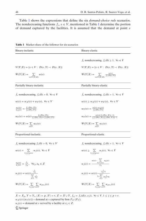
Table 1 shows the expressions that define the six demand-choice rule scenarios.The nondecreasing functions fv , v ∈ V, mentioned in Table 1 determine the portionof demand captured by the facilities. It is assumed that the demand at point v

Table 1 Market share of the follower for six scenarios

Binary-inelastic Binary-elastic

fv nondecreasing, fv(0) ≥ 1, ∀v ∈ V

V(Y|X) = {v ∈ V : D(v, Y) < D(v, X)} V(Y|X) = {v ∈ V : D(v, Y) < D(v, X)}

W(Y|X) = ∑v∈V(Y|X)

w(v) W(Y|X) = ∑v∈V(Y|X)

w(v)fv(D(v,Y))

Partially binary-inelastic Partially binary-elastic

fv nondecreasing, fv(0) > 0, ∀v ∈ V fv nondecreasing, fv(0) > 1, ∀v ∈ V

w(v) = wX (v) + wY (v), ∀v ∈ V w(v) ≥ wX (v) + wY (v), ∀v ∈ V

wY (v)wX (v)

= fv(D(v,X))

fv(D(v,Y))wY (v) = w(v)−wX (v)

fv(D(v,Y))

wY (v) = w(v)fv(D(v,X))

fv(D(v,X))+ fv(D(v,Y))wY (v) = w(v)( fv(D(v,X))−1)

[ fv(D(v,X)) fv(D(v,Y))]−1

W(Y|X) = ∑v∈V

wY (v) W(Y|X) = ∑v∈V

wY (v)

Proportional-inelastic Proportional-elastic

fv nondecreasing fv(0) > 0, ∀v ∈ V fv nondecreasing, fv(0) > 1, ∀v ∈ V

w(v) = ∑1≤ j≤p+r

w j(v), ∀v ∈ V w(v) ≥ ∑1≤ j≤p+r

w j(v), ∀v ∈ V

wk(v)w j(v)

= fv jfvk

, ∀x j, xk ∈ Z w j(v) =w(v)−

p+r∑k=1,k �= j

wk(v)

fv j

w j(v) = w(v)

1fv j

p+r∑k=1

1fvk

w j(v) = w(v)

1fv j−1

1+p+r∑k=1

1( fvk−1)

W(Y|X) = ∑1≤ j≤r

∑v∈V

wp+ j(v) W(Y|X) = ∑1≤ j≤r

∑v∈V

wp+ j(v)

X = Xp, Y = Yr , |X| = p, |Y| = r, Z = X ∪ Y, fv j = fv(d(v, x j)), ∀v ∈ V, 1 ≤ j ≤ p + r.wX (v) (wY (v)) = demand at v captured by firm FX (FY ).w j(v) = demand at v served by a facility at x j ∈ Z .


Fig. 1 The leader hasadvantage on the follower

captured by a facility is inversely proportional to fv(δ) where δ is the distancebetween v and the facility.

Example 1 Figures 1 and 2 show the solutions to the leader–follower problem on twodifferent networks for inelastic demand and the binary choice rule. For the networkof Fig. 1, the leader is located at node v3 (the median of the tree) and the followeropens a facility at v2 (or v4). The market share captured by the leader is three andthat of the follower is two units.

In Fig. 2 the leader captures node v1 in which the demand is one. Any point on]v2, v3[ is a (1|{v1})-medianoid. In particular the midpoint of the edge [v2, v3] is anoptimal location for the follower who captures v2 and v3, with a total demand oftwo. Observe that other Stackelberg solutions exist. Thus, a point within ]v2, v3[ is a(1|1)-centroid and the follower would be located at v2 or v3.

Moreover, the Stackelberg solution in Fig. 1 is a Nash equilibrium (for any firm,a unilateral movement to another location does not provide any additional captureddemand). In the network of Fig. 2, a Nash equilibrium does not exist.

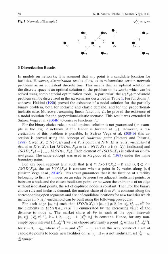
Example 2 Let r = p = 1. Figure 3 shows a network where the Stackelberg solutionsfor inelastic and elastic demand are different.

For inelastic demand, the optimal strategy of the leader is the node v3 and themaximum captured demand is six, the follower opens a facility at node v5 andcaptures five units of demand.

For elastic demand with fv(δ) = 1 + δ, the leader is located at v5 and the followeropens a facility at v3. The demand captured by the leader is 8

3 and the followercaptures 31

12 .

It is easy to prove that, for any scenario, the market share function W is submod-ular, nondecreasing and W(∅) = 0 (Santos Peñate and Suárez Vega, 2003). Theseresults are useful to build algorithms which solve the (r|Xp)-medianoid and (r|p)-centroid problems (Benati and Laporte, 1994; Benati, 1999; Berman and Krass, 1998;Nemhauser and Wolsey, 1978).

Fig. 2 The follower hasadvantage on the leader


Fig. 3 Network of Example 2

3 Discretization Results

In models on networks, it is assumed that any point is a candidate location forfacilities. However, discretization results allow us to reformulate certain networkproblems as an equivalent discrete one. This means that an optimal solution inthe discrete space is an optimal solution to the problem on networks which can besolved using combinatorial optimization tools. In particular, the (r|Xp)-medianoidproblem can be discretized in the six scenarios described in Table 1. For functions fvconcave, Hakimi (1990) proved the existence of a nodal solution for the partiallybinary problem, both for inelastic and elastic demand, and for the proportional-inelastic case. Moreover, assuming linear functions fv , he proved the existence ofa nodal solution for the proportional-elastic scenario. This result was extended inSuárez Vega et al. (2004b) to concave functions fv .

For the binary choice rule, a nodal optimal solution is not guaranteed (an exam-ple is the Fig. 2 network if the leader is located at v1). However, a dis-cretization of this problem is possible. In Suárez Vega et al. (2004b) this as-sertion is proved using the concept of isodistant point (Peeters and Plastria,1998). Given Xp ⊂ N(V, E) and v ∈ V, a point x ∈ N(V, E) is (v, Xp)-isodistant ifd(v, x) = D(v, Xp). Let ISOD(v, Xp) = {x ∈ N(V, E) : x is (v, Xp)-isodistant} andISOD(Xp) = ⋃

v∈V ISOD(v, Xp). Each element of ISOD(Xp) is called an isodis-tant point. The same concept was used in Megiddo et al. (1983) under the nameboundary point.

For any open segment ]s, t[ such that ]s, t[ ∩ ISOD(Xp) = ∅ and {s, t} ⊂ V ∪ISOD(Xp), the set V(Yr|Xp) is constant when a point in Yr varies along ]s, t[(Suárez Vega et al., 2004b). This result guarantees that if the location of a facilitybelonging to firm FY moves on an edge between two adjacent isodistant points, orbetween a node and the closest isodistant point, or between the endpoints of an edgewithout isodistant points, the set of captured nodes is constant. Then, for the binarychoice rule and inelastic demand, the market share of firm FY is constant along thecorresponding open segments and a set of candidate locations for new facilities whichincludes an (r|Xp)-medianoid can be built using the following procedure.

For each edge [vi, v j] such that ISOD(Xp) ∩ [vi, v j] �= ∅, let x1ij, x2

ij, ..., xqij

ij bethe elements in ISOD(Xp) ∩ [vi, v j] enumerated by the increasing value of thedistance to node vi. The market share of FY in each of the open intervals]vi, x1

ij[, ]xkij, xk+1

ij [, k = 1, 2, ..., qij − 1, ]xqij

ij , v j[, is constant. Hence, for any non-

empty open interval ]xkij, xk+1

ij [ we can choose arbitrarily a point ykij within ]xk

ij, xk+1ij [,

for k = 0, ..., qij, where x0ij = vi and x

qij+1ij = v j, and in this way construct a set of

candidate points to locate new facilities on [vi, v j]. If vi is not isodistant, set y0ij = vi.


Analogously, if v j is not isodistant, set yqij

ij =v j. If ISOD(Xp)∩[vi, v j]=∅ set qij = 0,

and y0ij = vi or y0

ij = v j. Let Cij ={

ykij

}qij

k=0. Then C = ⋃

i, j Cij contains an (r|Xp)-

medianoid (Suárez Vega et al., 2004b).

Example 3 Consider the (1|X1)-medianoid problem posed in Fig. 2 where X1 ={v1}. The sets of isodistant points are ISOD(v1, X1) = {v1}, ISOD(v2, X1) = {v1, v3}and ISOD(v3, X1) = {v1, v2}. At each edge, the isodistant points coincide with theendpoints and C can be defined as C = ⋃

Cij with Cij = {yij}i< j where yij is themidpoint of [vi, v j]. The market share captured by points y12 and y13 is one unit,while point y23 captures two units. In this case, Y1 = {y23} is a (1|X1)-medianoid.

For elastic demand, although the set of nodes covered by a facility is constantwithin the open segments without isodistant points, the buying power captured alongthese intervals depends on the distance between the facility and the demand nodes.As the distance from a node v to any point on the network is a concave function onany edge, if fv is concave for any node v, the market share function is convex alongany open segment without isodistant points. Therefore, there exists an ε-optimalsolution such that each location is a node or is close to an isodistant point. In otherwords, given Xp, there exists a set Z ∗

r = {z∗i }1≤i≤r where z∗

i is a node or an isodistantpoint, i = 1, ..., r, such that in any of its neighborhoods there exist ε-optimal solutions(Suárez Vega et al., 2004b). Example 4 illustrates this result.

Example 4 Consider the network in Fig. 4. If X1 = {v1}, the (v, X1)-isodistantpoints on [v2, v3], denoted by ISOD[v2,v3](v, X1), are ISOD[v2,v3](v1, X1) = ∅,ISOD[v2,v3](v2, X1) = {z2}, ISOD[v2,v3](v3, X1) = {z1}, and ISOD[v2,v3](v4, X1) ={z1, z2}. A point on ]v2, z1[ captures {v2, v4}, a point on ]z1, z2[ captures {v2, v3, v4}and a point on ]z2, v3[ captures {v3, v4}.

Figure 5 shows the market share captured along the edge [v2, v3] when fv(δ) =(1.1 + δ)

13 ,∀v ∈ V. Note that the optimum is not attained on the edge but there

exists an ε-optimal solution in z1. The market share when fv(δ) = 1.1 + δ13 , ∀v ∈ V,

is presented in Fig. 6. In this case, the optimum is reached at node v3.

Fig. 4 Network used inExample 4


0 0.5 1 1.5 2 2.5 3 3.5 41.2

1.3

1.4

1.5

1.6

1.7

1.8

1.9

2

Location on edge

De

ma

nd

ca

ptu

red

Fig. 5 Demand captured on edge [v2, v3] for fv(δ) = (1.1 + δ)13

0 0.5 1 1.5 2 2.5 3 3.5 40.7

0.8

0.9

1

1.1

1.2

1.3

1.4

Location on edge

De

ma

nd

ca

ptu

red

Fig. 6 Demand captured on edge [v2, v3] for fv(δ) = 1.1 + δ13


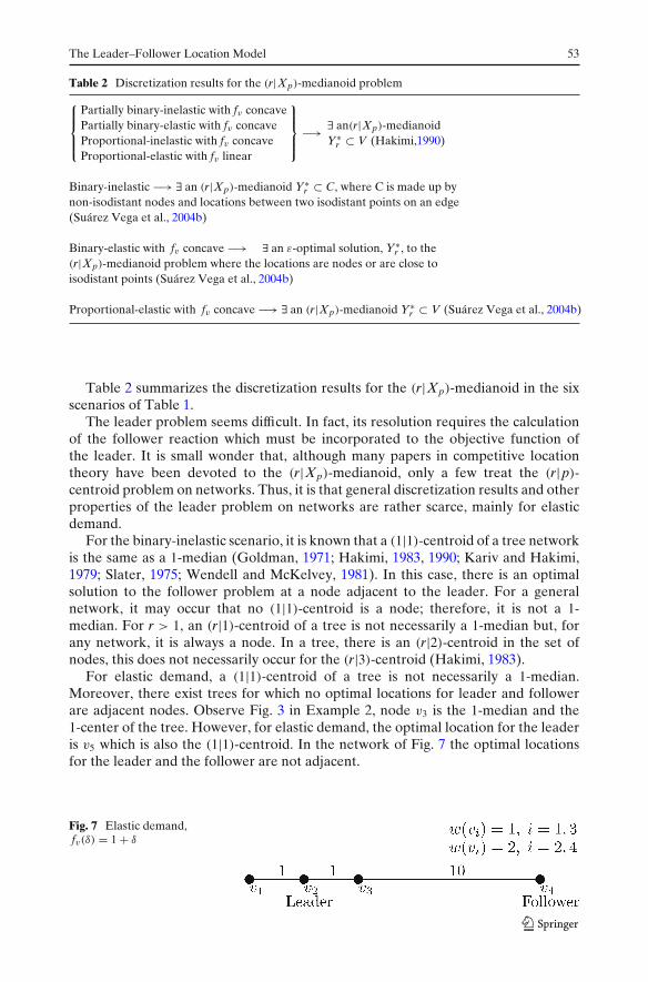
Table 2 Discretization results for the (r|Xp)-medianoid problem

⎧⎪⎪⎨⎪⎪⎩

Partially binary-inelastic with fv concavePartially binary-elastic with fv concaveProportional-inelastic with fv concaveProportional-elastic with fv linear

⎫⎪⎪⎬⎪⎪⎭

−→ ∃ an(r|Xp)-medianoidY∗

r ⊂ V (Hakimi,1990)

Binary-inelastic −→ ∃ an (r|Xp)-medianoid Y∗r ⊂ C, where C is made up by

non-isodistant nodes and locations between two isodistant points on an edge(Suárez Vega et al., 2004b)

Binary-elastic with fv concave −→ ∃ an ε-optimal solution, Y∗r , to the

(r|Xp)-medianoid problem where the locations are nodes or are close toisodistant points (Suárez Vega et al., 2004b)

Proportional-elastic with fv concave −→ ∃ an (r|Xp)-medianoid Y∗r ⊂ V (Suárez Vega et al., 2004b)

Table 2 summarizes the discretization results for the (r|Xp)-medianoid in the sixscenarios of Table 1.

The leader problem seems difficult. In fact, its resolution requires the calculationof the follower reaction which must be incorporated to the objective function ofthe leader. It is small wonder that, although many papers in competitive locationtheory have been devoted to the (r|Xp)-medianoid, only a few treat the (r|p)-centroid problem on networks. Thus, it is that general discretization results and otherproperties of the leader problem on networks are rather scarce, mainly for elasticdemand.

For the binary-inelastic scenario, it is known that a (1|1)-centroid of a tree networkis the same as a 1-median (Goldman, 1971; Hakimi, 1983, 1990; Kariv and Hakimi,1979; Slater, 1975; Wendell and McKelvey, 1981). In this case, there is an optimalsolution to the follower problem at a node adjacent to the leader. For a generalnetwork, it may occur that no (1|1)-centroid is a node; therefore, it is not a 1-median. For r > 1, an (r|1)-centroid of a tree is not necessarily a 1-median but, forany network, it is always a node. In a tree, there is an (r|2)-centroid in the set ofnodes, this does not necessarily occur for the (r|3)-centroid (Hakimi, 1983).

For elastic demand, a (1|1)-centroid of a tree is not necessarily a 1-median.Moreover, there exist trees for which no optimal locations for leader and followerare adjacent nodes. Observe Fig. 3 in Example 2, node v3 is the 1-median and the1-center of the tree. However, for elastic demand, the optimal location for the leaderis v5 which is also the (1|1)-centroid. In the network of Fig. 7 the optimal locationsfor the leader and the follower are not adjacent.

Fig. 7 Elastic demand,fv(δ) = 1 + δ


4 The Leader–Follower Attractiveness–Location Model

In the previous sections it was assumed that customers patronize facilities accordingto distance. However, normally they consider facility attributes such as prices,variety of products, environmental conditions, parking area, accessibility and certainexternality costs, in addition to distance. Attraction functions are introduced in orderto incorporate these attributes in the location model.

In Huff’s model (Huff, 1964), the attraction aij perceived by customers locatedat node vi towards a facility j, sited at x j, is directly proportional to the size ofthe facility and inversely proportional to a power of the distance between vi andx j. The probability of a customer at node vi travelling to facility j at x j is Pij = aij

p+r∑k=1

aik

and the expected demand captured from node vi by facility j at x j is Eij = w(vi)Pij.Table 3 shows different attraction functions used in competitive location models.

Table 3 Attraction functions

Multiplicative aij =s∏

k=1

fik(aijk)

aij = a j

dβ

ij

(Drezner, 1994b; Eiselt and Laporte, 1988a, 1998b;Eiselt and Laporte, 1989; Eiselt and Laporte, 1989,Huff, 1964; Plastria, 1997; Plastria andCarrizosa, 2003)

aij =s∏

k=1

aβkijk (Achabal et al., 1982; Berman and Krass, 1998,

2002; Nakanishi and Cooper, 1974)

aij = a j

f (dij)with f concave (Peeters and Plastria, 1998; Suárez Vega et al.,

2004a)

Additive aij =s∑

k=1

fik(aijk)

aij =s∑

k=1

βka jk − dij (Benati, 1999; Drezner, 1994a; Drezner andDrezner, 1996)

Exponential aij = e−βdij

s∏k=1

aβkijk

aij = aαj e−βdij (Hodgson, 1981)

dij = d(vi, x j).aijh = perception of customers at vi with respect to attribute h of facility j at x j


Henceforth, we consider the attraction function given by

aij = a j

fvi(d(vi, x j))

where a j denotes the attractiveness or quality level of facility j located at x j, and fvi ,vi ∈ V, are positive real functions. The following conditions are assumed.

Assumption 1 Function fv : �+0 → �+ is concave and nondecreasing, ∀v ∈ V.

Assumption 2 For any facility (new or existing), its attractiveness is on [L, U], where0 < L < U < ∞.

Assumption 3 There exists a fixed cost function depending on the attractiveness, F :�+

0 → �+, which is continuous and nondecreasing.

A reformulation of the leader–follower model on networks allows us to includethe attractiveness among the decision variables, in addition to location. The binary,partially binary and proportional choice rules are defined in a similar way to the rulesof Section 2, replacing distance d(vi, x j) by attraction aij. So, under the binary choicerule, customers patronize the most attractive facility and the proportional model isequivalent to the probabilistic model introduced in Huff (1964). It is assumed that

Ufv(0)

≤ 1 for the binary choice rule, and Ufv(0)

< 1 for both the partially binary andthe proportional ones. The expressions corresponding to each scenario result from

those shown in Table 1, replacing 1fv(D(v,Z ))

by G(v, Z , AZ ) = max1≤ j≤q

{b j

fv(D(v,z j))

}being

Z = {z j}qj=1 ⊂ F and AZ = {bj}q

j=1 ⊂ [L, U], Z = X, Y, for the binary and partiallybinary choice rules; for the proportional choice rule, 1

fv jand 1

fv j−1 are replaced by a j

fv j

and a j

fv j−a j, respectively.

The objective function is the profit. If firm FX has p facilities at Xp with attrac-tiveness AXp , the profit obtained by firm FY , owner of r facilities at Yr with attrac-tiveness AYr , is given by

W(Yr, AYr |Xp, AXp) = R(Yr, AYr ) −r∑

j=1

F(ap+ j)

where R(Yr, AYr ) is the net profit (excluding the fixed costs), defined as the demandcaptured multiplied by the net profit margin per unit of demand.

The follower problem is to determine the pair (Y∗r , AY∗

r) with Y∗

r = {x∗p+1, ..., x∗

p+r}and A∗

Y∗r

= {a∗p+1, ..., a∗

p+r}, being a∗j the attractiveness of facility at x∗

j , that maximizesthe profit of firm FY , given the locations Xp and the quality levels AXp for thefacilities belonging to firm FX , that is,

W(Y∗r , A∗

Y∗r) = max

Yr⊂F,AYr ⊂[L,U]W(Yr, AYr |Xp, AXp).

The pair (Y∗r , A∗

Y∗r) is an (r|Xp, AXp)-medianoid.

For simplicity, we consider that the net profit margin per unit of demand is 1. Inthis case R(Yr, AYr ) coincides with the demand captured by firm FY .


Example 5 Consider the market represented by the triangular network of Fig. 2in the inelastic-binary scenario with fv(δ) = 1 + δ for any node v. Suppose thatfirm FX has a facility at X1 = {v1} with attractiveness a1 = 1. Firm FY wants toenter the market with one facility with attractiveness a ∈ [0.1, 1] located at pointx. Then FY captures node vi if and only if a

1+d(vi,x)> 1

1+d(vi,v1). From this condition

it follows that, for any x and a, firm FY does not capture v1. If a > 12 and x = vi,

firm FY captures vi, i = 2, 3. Firm FY captures nodes v2 and v3 simultaneously ifand only if 2a > 1 + max{d(v2, x), d(v3, x)}; therefore, for a > 3

4 , any point withinthe open segment centered at the midpoint of [v2, v3] with radius equal to 2a − 3

2captures v2 and v3. In particular, if a = 1 this segment is the open edge ]v2, v3[.As, by Assumption 3, function F is nondecreasing, if 2 − F( 3

4 + ε) = max{2 − F( 34 +

ε), 1 − F( 12 + ε), F(0.1)} then any point within the open segment centered at the

midpoint with radius of 2ε and attractiveness a = 34 + ε is an ε-optimal solution to

the (1|X1, AX1)-medianoid problem. If 1 − F( 12 + ε) > max{2 − F( 3

4 + ε), F(0.1)}, v2

(or v3) with attractiveness a = 12 + ε is an ε-optimal solution. Otherwise, we conclude

that, the attraction level which allows the capture of demand has an excessive costwhich leads to negative profits. In this case, the optimal strategy for the follower isnot to open any facility.

Under Assumptions 1 to 3, some results hold (Suárez Vega, 2001; Suárez Vega etal., 2004a). It is proved that, for the partially binary and proportional choice rules,for inelastic and elastic demand, there exists an (r|Xp, AXp)-medianoid where thelocations are nodes. Under Assumptions 1 and 2, function R(Yr, AYr ) is nonde-creasing on [L, U]r, that is, R(a) ≤ R(b) for any a = (a1, ..., ar), b = (b 1, ..., br) ∈[L, U]r such that ai ≤ bi, where R(a) = R(Yr, AYr ) being AYr = {a1, ..., ar} for a =(a1, ..., ar) ∈ [L, U]r. For inelastic demand, if the choice rule is partially binary thenfunction R(Yr, AYr ) is quasiconcave with respect to a j ∈ [L, U] for any facility j.For the proportional choice rule, R(a) = R(Yr, AYr ) is strictly concave on [I, S]r

(Suárez Vega et al., 2004a). For elastic demand, if the choice rule is partially binary,function R(Yr, AYr ) is convex on [L, U]r. To prove this result, it is suffice to con-sider that wY(v) = w(v)hv(G(v, Yr, AYr )) where hv(x) = x(G(v,Xp,AXp )−1)

xG(v,Xp,AXp )−1 . FunctionG(v, Yr, AYr ) is nondecreasing and convex on [L, U]r. Moreover, for 0 < x < 1,hv(x) is increasing and strictly convex. Therefore wY(v) = hv ◦ Gv(v, Yr, AYr ) is anincreasing and convex function of a = (a1, ..., ar), and consequently R(Yr, AYr ) =∑v∈V

wY(v) also. For the proportional choice rule, R(Yr, AYr ) is convex with respect

to a j ∈ [L, U] for any facility j. This result follows from the convexity of w j(v) =a j

fv j−a j

1+p+r∑k=1

akfvk−ak

with respect to a j for any j.

If the choice rule is binary, a nodal solution is not guaranteed. In this case, theconcept of isoattractive point is defined in a similar way to the isodistance. Replacingisodistance by isoattractiveness, some results can be derived from those obtainedwhen distance is assumed to be the only decision criterion. Thus, given AYr , forthe binary-inelastic scenario, there exists a finite set of points that contains a set ofoptimal locations. For the binary-elastic model, there exists an ε-optimal solution inwhich the locations are nodes or sites close to isoattractive points. Moreover, for thebinary-inelastic scenario, given Yr, there exists an ε-optimal solution to the problemof obtaining the optimal attractiveness levels.


Except for some works developed in the plane (Plastria, 1997; Plastria andCarrizosa, 2003) or in discrete space (Achabal et al., 1982; Eiselt and Laporte,1988a), most papers that treat the (r|Xp)-medianoid model incorporating attractionfunctions, consider decisions either on locations or attractiveness, but not both. In(Suárez Vega et al., 2004a), locations and attractiveness levels are decision variablesand the location-attractiveness problem is solved via a global optimization approachcombined with combinatorial heuristic algorithms.

5 The Dynamic Leader–Follower Model

In the static leader–follower model formulated in Section 2, the relevant parametersin the location decision are assumed to be constant through the planning horizon.However, this static model is frequently unrealistic. In most cases the locationdecisions are long-term, daily or seasonal changes in demand can occur, new facilitiescan produce market expansion, new products can generate an increasing demand,and so on. The literature on location analysis contains a collection of papersdescribing implicitly or explicitly dynamic models (see Current et al. (1997); Owenand Daskin (1998) for a review). According to the definition given in (Current etal., 1997), implicitly dynamic models consider that parameters may change over timeand take into account these changes in the decision making process. However, thesemodels are static in the sense that facilities are to be opened at the beginning of theplanning period and remain in operation throughout (e.g., Drezner, 1995; Dreznerand Wesolowsky, 1991; Ghosh and Craig, 1983). Explicitly dynamic models (e.g.,Carrizosa et al., 2005; Current et al., 1997; Gunawardane, 1982; Rao and Rutenberg,1979; Suzuki et al., 1991; Wesolowsky and Truscott, 1975) provide a plan whichspecifies locations and instants for opening and/or closing facilities.

The follower location problem in a dynamic environment (without closing facili-ties) is the following:

Firm FX operates in the planning horizon [0, T] with p ≤ qX facilities located atpoints Xp = {x1, ..., xp} ⊂ F, such that facility at xi operates in [ti, T], i = 1, ..., p.Firm FY knows the plan of firm FX and wants to enter the market by locatingr ≤ qY facilities in the set of points Yr = {xp+1, ..., xp+r} ⊂ F, with facility at xp+i

operating in [tp+i, T], i = 1, ..., r, maximizing its profit. Denote XTp = (Xp, TXp)

and YTr = (Yr, TYr ) where TXp = {ti}1≤i≤p and TYr = {tp+i}1≤i≤r. The problem is todetermine the number r∗ of facilities, and the pair YT∗

r∗ = (Y∗r∗ , T∗

Y∗r), where Y∗

r∗ ={x∗

p+1, ..., x∗p+r∗ } ⊂ F and T∗

Y∗r

= {t∗p+1, ..., t∗p+r∗ } ⊂ [0, T], being x∗i and t∗i the location

and entry instant for facility i, i = p + 1, ..., p + r∗, such that

W(YT∗r∗ |XTp) = max

r ≤ qY , Yr ⊂ F, TYr ⊂ [0, T]W(YTr|XTp),

where W(YTr|XTp) denotes the profit obtained by firm FY with facilities locatedat Yr and opening instants TYr , when the competitor firm FX has facilities at Xp

entering the market at instants TXp .


The leader problem is to determine the strategy that maximizes its profit takinginto account a competitor firm FY which will make decisions as a follower. Theproblem of the leader is to find the number of facilities p∗ and the pair XT∗

p∗ =(X∗

p∗ , T∗p∗) with the locations X∗

p∗ = {x∗1, ..., x∗

p∗ } ⊂ F and the entry instants T∗p∗ =

{t∗1, ..., t∗p∗ } ⊂ [0, T] such that

W(XT∗p∗ |YT∗

r∗(XT∗p∗)) = max

p ≤ qX , Xp ⊂ F, TXp ⊂ [0, T]W(XTp|YT∗

r∗(XTp))

where YT∗r∗(XTp) is the optimal solution to the follower problem given the locations

and entry instants for the competitor facilities, XTp.Hereafter, we consider the particular case where any facility belonging to FX is

operating at the beginning of the planning period [0, T], that is, ti = 0, i = 1, ..., p.Explicitly dynamic models in competitive location are rather scarce, at least

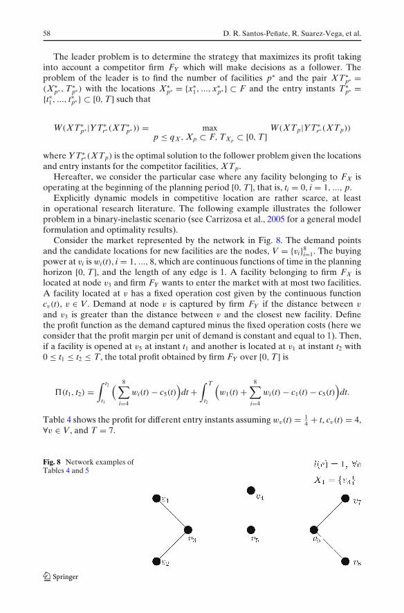
in operational research literature. The following example illustrates the followerproblem in a binary-inelastic scenario (see Carrizosa et al., 2005 for a general modelformulation and optimality results).

Consider the market represented by the network in Fig. 8. The demand pointsand the candidate locations for new facilities are the nodes, V = {vi}8

i=1. The buyingpower at vi is wi(t), i = 1, ..., 8, which are continuous functions of time in the planninghorizon [0, T], and the length of any edge is 1. A facility belonging to firm FX islocated at node v3 and firm FY wants to enter the market with at most two facilities.A facility located at v has a fixed operation cost given by the continuous functioncv(t), v ∈ V. Demand at node v is captured by firm FY if the distance between v

and v3 is greater than the distance between v and the closest new facility. Definethe profit function as the demand captured minus the fixed operation costs (here weconsider that the profit margin per unit of demand is constant and equal to 1). Then,if a facility is opened at v5 at instant t1 and another is located at v1 at instant t2 with0 ≤ t1 ≤ t2 ≤ T, the total profit obtained by firm FY over [0, T] is

�(t1, t2) =∫ t2

t1

( 8∑i=4

wi(t) − c5(t))

dt +∫ T

t2

(w1(t) +

8∑i=4

wi(t) − c1(t) − c5(t))

dt.

Table 4 shows the profit for different entry instants assuming wv(t) = 14 + t, cv(t) = 4,

∀v ∈ V, and T = 7.

Fig. 8 Network examples ofTables 4 and 5


Table 4 Profit for locationsx1 = v5 and x2 = v1 and entryinstants t1 and t2 in networkFig. 8

t1, t2 Profit

0, 0 101.501120 , 15

4 109.281312 , 13

12 105.021, 2 107.253, 3 94

As wi(t), ci(t), i = 1, ..., 8, are continuous functions on [0, T], for any set oflocations the problem max

0≤t1≤t2�(t1, t2) is well defined and an optimal solution exists.

Then, for any set of at most two locations, optimal instants can be derived from theKuhn–Tucker conditions. Since the set of candidate locations is finite, there exists anoptimal solution to the problem of finding the locations and instants that maximizethe profit.

From the optimality conditions, it follows that the optimal solution to the followerproblem for qY = 2 is to open facilities at nodes v5 and v1 at instants t1 = 11

20 andt2 = 15

4 , respectively. Two open facilities at these nodes at the beginning of the plan-ning horizon provide a profit of 109.28 − 101.5 = 7.78 units lower than the optimalsolution to the explicitly dynamic problem. The optimal solution to the implicitlydynamic model is to open only one facility at v5 which provides a profit of 103.25.This strategy coincides with the solution to the static problem of finding the bestr ≤ qY locations when demand wv(t) is approximated by a constant function w̄v , that

is, w̄v = 1T

∫ T0 wv(t)dt = 1

7

∫ 70

(14 + t

)dt = 15

4 .Table 5 shows the optimal strategy of the follower for any choice of the leader.

The results for v2, v7, and v8 coincide with those obtained for v1; the same occurs forv3 and v6. The optimal location for the leader is not unique, observe that v3 and v5

provide the maximum profit. However, the follower is not indifferent to these twolocations. If the leader’s aim is the most unfavorable location for the follower (the(2|1)-centroid), it will open a facility at v5.

Table 5 Optimal strategy of the follower for any location of the leader in network Fig. 8, for qX = 1,qY = 2, wv(t) = 1

4 + t, ∀v ∈ V, and T = 7

Leader Follower Profit

Leader Follower

v1 x1 = v3, t1 = 928 −1.75 156.11

v3 x1 = v5, x2 = v1, t1 = 1120 , t2 = 15

4 24.50 109.28v4 x1 = v5, t1 = 9

28 −1.75 156.11v5 x1 = v3, x2 = v6, t1 = t2 = 13

2 24.50 105.02


6 Concluding Remarks

Stackelberg games in location suggest a variety of research issues. The choice rulesthat represent the consumer’s behavior and the nature of the goods provided by thecompeting firms, lead to different scenarios where the leader–follower models canbe investigated. A considerable effort has been devoted to obtaining discretizationresults for the (r|Xp)-medianoid problem on networks, and to designing algorithmsthat solve the (r|Xp)-medianoid and the (r|p)-centroid problems in discrete spaces,mostly for inelastic demand.

Among other investigation lines, the research can be extended in the following di-rections: 1) study of competitive location models assuming elastic demand; 2) analysisof alternative customer’s choice rules such as the Pareto–Huff model (Peeters andPlastria, 1998) and others; 3) analysis of the choice rules that incorporate attributes ofthe facilities in addition to distance, and discussion of the quasiconcavity or concavityof the revenue function when demand is inelastic in contrast to the convexity of thisfunction in case of elastic demand; 4) study of explicitly dynamic competitive locationmodels and 5) design of algorithms to solve Stackelberg location models.

Acknowledgements Partially financed by the Ministerio de Educación y Ciencia (Spain) andFEDER (grant BFM2002-04525-C02-01 and MTM2005-09362-C03-03).

References

Achabal DD, Gorr WL, Mahajan V (1982) MULTILOC: a multiple store location decision model. JRetail 58(2):5–25

Benati S (1999) The maximum capture problem with heterogeneous customers. Comput Oper Res26:1351–1367

Benati S, Laporte G (1994) Tabu search algorithms for the (r|Xp)-medianoid and (r|p)-centroidproblems. Location Sci 2(4):193–204

Berman O, Krass D (1998) Flow intercepting spatial interaction model: a new approach to optimallocation of competitive facilities. Location Sci 6:41–65

Berman O, Krass D (2002) Locating multiple competitive facilities: spatial interaction models withvariable expenditures. Ann Oper Res 111(1):197–225

Carrizosa E, Gordillo J, Santos-Peñate, DR (2005) Locating competitive facilities via a VNS al-gorithm. Proceedings of the international workshop on global optimization. Universidad deAlmeria, Almeria. pp 61–66

Current J, Ratick S, Revelle C (1997) Dynamic facility location when the total number of facilities isuncertain: a decision analysis approach. Eur J Oper Res 110:597–609

Drezner T (1994a) Locating a single new facility among existing unequally attractive facilities. J RegSci 34(2):237–252

Drezner T (1994b) Optimal continuous location of a retail facility, facility attractiveness, and marketshare: an interactive model. J Retail 70(1):49–64

Drezner Z (1995) Dynamic facility location: the progressive p-median problem. Location Sci 3(1):1–7Drezner T, Drezner Z (1996) Competitive facilities: market share and location with random utility.

J Reg Sci 36(1):1–15Drezner T, Eiselt HA (2002) Comsumers in competitive location models. In: Drezner Z, Hamacher

HW (eds) Facility location: applications and theory. Springer, Berlin Heidelberg New York,pp 151–178

Drezner Z, Wesolowsky GO (1991) Facility location when demand is time dependent. Nav ResLogist 38:763–777

Eiselt HA, Laporte G (1988a) Location of a new facility in the presence of weights. Asia-Pac J OperRes 5:160–165

Eisel HA, Laporte G (1988b) Trading areas of facilities with different sizes. Rech Opér 22(1):33–44


Eiselt HA, Laporte G (1989) The maximum capture problem in a weighted network. J Reg Sci29(3):433–439

Eiselt HA, Laporte G (1996) Sequential location problems. Eur J Oper Res 96:217–231Eisel HA, Laporte G, Pederzoli, G (1989) Optimal sizes of facilities on a linear market. Math Comput

Model 12(1):97–103Ghosh A, Craig CS (1983) Formulating retail location strategy in a changing environment. J Mark

47:56–68Goldman AJ (1971) Optimal center location in simple networks. Transp Sci 5:212–221Gunawardane G (1982) Dynamic versions of set covering type public facility location problems. Eur

J Oper Res 10:190–195Hakimi SL (1983) On locating new facilities in a competitive environment. Eur J Oper Res 12:29–35Hakimi SL (1990) Location with spatial interactions: competitive locations and games. In:

Mirchandani PB, Francis RL (eds) Discrete location theory. Wiley, New York, pp 439–478Hodgson MJ (1981) A location–allocation model maximizing consumers’ welfare. Reg Stud

15(6):493–506Huff DL (1964) Defining and estimating a trading area. J Mark 28:34–38Kariv O, Hakimi L (1979) An algorithm approach to network location problems, part II: the

p-median. SIAM J Appl Math 37:539–560Megiddo N, Zemel E, Hakimi SL (1983) The maximum coverage location problem. SIAM J Algebr

Discrete Methods 4:253–261Nakanishi M, Cooper LG (1974) Parameter estimation for a multiplicative competitive interaction

model-least squares approach. J of Mark Res 11:303–311Nemhauser GL, Wolsey LA (1978) Best algorithms for approximating the maximum of a submodular

set function. Math Oper Res 3(3):177–188Owen SH, Daskin MS (1998) Strategic facility location: a review. Eur J Oper Res 111:423–447Peeters PH, Plastria F (1998) Discretization results for the Huff and Pareto–Huff competitive loca-

tion models on networks. Top 6(2):247–260Plastria F (1997) Profit maximising single competitive facility location in the plane. Stud Locat Anal

11:115–126Plastria F, Carrizosa E (2003) Locating and design of a competitive facility for profit maximisatition.

Optimization (Online), http://www.optimization-online.org/DB_HTML/2003/01/591.htmlRao RC, Rutenberg DP (1979) Preempting an alert rival: strategic timing of the first plant by analysis

of sophisticated rivalry. Bell J Econ 10:412–428Santos Peñate DR, Suárez Vega R (2003) Submodular capture functions in competitive location: the

(r|Xp)-medianoid and the (r|p)-centroid problems. 27 Congreso SEIO, Lérida, Spain.Slater PJ (1975) Maximim facility location. J Res Natl Bur Stand: B Math Sci 79:107–115Stackelberg H (1934) Markform and Gleichgewicht. Springer, Berlin Heidelberg New YorkSuárez Vega R (2001) El (r|Xp)-medianoide incorporando criterios de atracción. PhD thesis, Uni-

versidad de Las Palmas de G.C.Suárez Vega R, Santos Peñate DR, Dorta González P (2004a) Discretization and resolution of the

(r|Xp)-medianoid problem involving quality criteria. Top 12(1)Suárez Vega R, Santos Peñate DR, Dorta González P (2004b) Competitive multi-facility location on

networks: the (r|Xp)-medianoid problem. J Reg Sci, 44(3):569–588Suzuki T, Asami Y, Okabe, A. (1991) Sequential location-allocation of public facilities in one- and

two dimensional space: comparison of several policies. Math Program 52:125–146Wendell RE, McKelvey RD (1981) New perspectives in competitive location theory. Eur J Oper Res

6:174–182Wesolowsky GO, Truscott WG (1975) The multiperiod location-allocation problem with relocation

facilities. Manage Sci 22:57–65

http://www.optimization-online.org/DB_HTML/2003/01/591.html

The Leader–Follower Location Model

Documents

Transcript of The Leader–Follower Location Model