THE INFLUENCE OF COMMUNICATION CONTEXT ON POLITICAL

COGNITION IN PRESIDENTIAL CAMPAIGNS: A GEOSPATIAL ANALYSIS

DISSERTATION

Presented in Partial Fulfillment of the Requirements for the Degree Doctor of Philosophy

in the Graduate School of The Ohio State University

By

Yung-I Liu, M.A.

* * * * *

The Ohio State University

2008

Dissertation Committee:

Professor Gerald M. Kosicki, Adviser Approved by

Professor William P. Eveland, Jr.

Professor Osei Appiah ______________________________

Professor Prabu David Adviser Communication Graduate Program

i

Copyright by Yung-I Liu

2008

ii

ABSTRACT

Due to targeting strategies employed by contemporary political campaigns,

campaign intensity is not uniform across the whole country. People in different

geographical locations would be influenced by campaigns differently depending on

where they are. This study argues that political campaigns could shape a person’s total

communication context in which a person is conditioned, and accordingly both individual

and contextual factors within this context should form synergistic influences on this

person’s cognitive responses to the election. Therefore, this study attempts to investigate

how mass media and interpersonal communication factors at the individual level and the

campaign level within an individual’s communication context that is defined by some

geospatial characteristics created by campaigns would influence this individual’s political

knowledge.

Data for this study come from three separate studies conducted during the 2000

presidential election in the U.S. Owing to the geospatial mapping nature of the study,

these data files are combined and analyzed at the two geospatial units -- state and media

market.

The results from a series of multilevel modeling analyses reveal that there is some

evidence that political campaign practices, including televised political ads, candidate

appearances, and campaign contacts, do promote some learning about politics. There is

also evidence to support the information flow approach to contextual effects. More

iii

specifically, it is found that macro-level political ads, candidate appearances, and

campaign contacts influence people’s newspaper use in predicting their political

knowledge; and that macro-level political ads and candidate appearances influence

people’s political discussion in predicting their political knowledge. Finally, consistent

with literature, people who read newspapers, watch network and cable television news,

and engage in political discussion more frequently have more political knowledge. But,

people who watch more local TV news have less political knowledge.

These findings suggest that communication, including both mass media and

interpersonal communication, does play a significant role in informing people in political

campaigns. However, political learning is conditioned on many factors -- media, people,

stimuli, and place, all of which lead to different results. The present study not only

demonstrates that conditional communication effects also hinge on geospatial, contextual

factors but also helps to develop contextual theories in communication science that

specifically take into account contextual factors and addresses cross-level inference. The

present study, which assesses informing effects of communication in political campaigns

from a macro-contextual perspective, provides a good understanding of the role that

communication would play in a larger social, economic and political setting.

iv

ACKNOWLEDGMENTS

I would first like to thank my adviser, Dr. Gerald Kosicki, for his guidance in my

dissertation and throughout my life at OSU. He has always given me insightful advice

about my research, teaching, career, and even personal matters. He has been a very good

resource for solving my various problems. He has always encouraged me to be an

independent thinker and researcher. His thought leader-style scope and vision have

inspired me to continuously challenge myself and become a better scholar. I greatly

appreciate his continuous support, care, encouragement and earnest enlightenment. I am

grateful that he has spent a lot of time meeting with me, reviewing my work,

brainstorming with me, giving me feedback, and generously sharing his knowledge and

ideas. I certainly have learned a lot from him. Words cannot express my gratitude for

everything Dr. Kosicki has done for me. I feel very fortunate and honored to be his

advisee.

I would also like to thank both Dr. Osei Appiah and Dr. William "Chip" Eveland

for their guidance in my dissertation and other aspects of my academic career over the

past several years. Chip coached me and guided me through every step of completing my

first academic publication. He has stimulated my interest and built up my confidence in

social science research. I have also liked to seek his advice and guidance about my

research, statistical problems and career because his answers are always to the point,

profound, clear, and useful. I am very grateful for his time, patience and encouragement.

v

Chip is a respected researcher and educator, and I think he has set an excellent example

especially for young scholars. I appreciate very much the opportunities Chip has given

me to collaborate with him and learn from him.

My deepest gratitude also goes to Osei for his incessant support, care and

encouragement. He has taught me how to conduct experimental studies to examine ethnic

and cultural differences in advertising. I have learned a lot from working with him. He

has always been so generously shared with me his tangible and intangible resources. He

has always been patient and enthusiastic to answer my various questions whether they are

important or trivial. He has been good at boosting my morale. I have enjoyed every

moment I have spent with him. Because of him, I felt easier to get accustomed to the life

as a doctoral student, and find my graduate life more cheerful and memorable. I

appreciate very much the opportunities Osei has given me to collaborate with him and

learn from him.

I would also like to express my gratitude to Dr. Prabu David. He has always given

me constructive advice and comments as well as kind assistance whenever I need him. I

have benefited a lot from his knowledge of research methods and statistical analysis. I

have also learned how to be a better teacher from him.

I would also like to thank Dr. Daniel McDonald for his guidance and assistance at

the early years of my doctoral program. I would like to thank Dr. Andrew Hayes for

helping me develop an interest in quantitative methods and for providing guidance in my

vi

statistical questions. I also want to say thanks to Dr. Li Gong for giving me the

opportunity to collaborate with him on research projects.

I thank Aaron Smith, Robb Hagen, and Joe Szymczak for their assistance in

various contexts in the past years.

I want to thank all the dear friends I have met at OSU, particularly Mihye Seo,

Bethany Simunich, Bell O’Neil, Troy Elias, Mong-Shan Yang, Seong Jae Min, Tingting

Lu, Lindsay Hoffman, Shu-Fang Lin, Carrie Lynn Reinhard, Brian Horton, Tom German,

Tiffany Thomson, Jennifer Chakroff, Heather LaMarre, and Jingbo Meng.

Finally, I would like to acknowledge those who have stood by my side through

the years, Chieh-Ling, Yu Chang, Ping-Yen, Chyi-Shan, and Yi-Ping. They have

enriched my life and given me the strength to fulfill my dreams.

vii

VITA

March 1, 1972 ............................Born – Kaohsiung City, Taiwan

1994............................................B.A. English Language and Literature Soochow University 1995-1996 ..................................Flight Attendant, China Airlines

1996-1997 ..................................SouthEast Asia Group-Foreign Workers News Agency 1998............................................M.A. Journalism and Communication The Ohio State University 1999-2000 ..................................Employment & Internal Communication Specialist Siemens Telecommunication Systems Limited 2000-2003 ..................................Consultant Edelman Public Relations Worldwide Taiwan Branch 2004-2007 ..................................Graduate Research and Teaching Associate The Ohio State University

PUBLICATIONS

Liu, Y. I., & Eveland, W. P., Jr. (2005). Education, need for cognition, and campaign interest as moderators of news effects on political knowledge: An analysis of the knowledge gap. Journalism & Mass Communication Quarterly, 82(4), 910-929.

FIELDS OF STUDY

Major Field: Communication

Graduate Interdisciplinary Specialization in Survey Research

viii

TABLE OF CONTENTS

Page

Abstract ............................................................................................................................... ii

Acknowledgments.............................................................................................................. iv

Vita.................................................................................................................................... vii

List of Tables ..................................................................................................................... xi

List of Figures .................................................................................................................. xiii

Chapters:

1 Introduction...................................................................................................................1

1.1 Political Campaign Strategies .............................................................................2

1.1.1 Integrated Marketing Communications........................................................3

1.1.2 Targeting Strategies......................................................................................6

1.2 The Role of Campaigns in Elections.................................................................12

1.3 Presidential Campaign Finance .........................................................................16

1.4 The Geospatial Dimension in Political Campaigns...........................................19

1.5 The Purpose of the Present Study......................................................................23

2 Theoretical Framework...............................................................................................27

2.1 Overview of the Present Study..........................................................................27

2.2 Contextual Theories and Cross-level Inference ................................................32

2.2.1 The Importance of Contexts.......................................................................32

2.2.2 Conceptualizations of Contexts and Micro-Macro Linkages.....................34

2.2.3 Characteristics of the Micro Level and the Macro Level...........................36

2.2.4 The Information Flow Perspective on Contextual Effects .........................40

2.2.5 Multilevel Analysis ....................................................................................44

2.2.6 The Role of Sociopolitical Contexts in Communication Research............45

ix

2.3 Mass Media Use and Political Knowledge........................................................49

2.3.1 Hypotheses .................................................................................................57

2.4 Political Discussion and Political Knowledge...................................................57

2.4.1 Hypotheses .................................................................................................65

2.5 Hypotheses of Macro-level and Interaction Effects ..........................................65

3 Methods ......................................................................................................................73

3.1 Data Sources......................................................................................................73

3.1.1 Individual-level Data..................................................................................73

3.1.2 Televised Political Ads...............................................................................77

3.1.3 Candidate Appearances ..............................................................................78

3.1.4 Campaign Contacts ....................................................................................80

3.2 Merging Data Files............................................................................................80

3.3 Measures............................................................................................................83

3.3.1 Individual-level Independent Variables .....................................................84

3.3.2 Individual-level Control Variables.............................................................85

3.3.3 Individual-level Dependent Variable .........................................................85

3.3.4 Campaign-level Variables ..........................................................................86

3.3.4.1 Televised Political Ads .....................................................................86

3.3.4.2 Candidate Appearances.....................................................................96

3.3.4.3 Campaign Contacts. ..........................................................................99

3.4 Data Analysis ..................................................................................................104

4 Results.......................................................................................................................105

4.1 Descriptive Analysis........................................................................................105

4.2 The Issue of Sample Representativeness ........................................................109

4.3 Multilevel Analysis .........................................................................................113

4.3.1 One-way Random Effects ANOVA Model .............................................115

4.3.2 Random-coefficients Regression Model ..................................................118

x

4.3.3 Means-as-outcomes Regression Model....................................................123

4.3.4 Intercepts-as-outcomes Model .................................................................128

4.3.5 Intercepts-and-slopes-as-outcomes Model...............................................135

4.4 Summary of Major Findings ...........................................................................160

5 Discussion and Conclusion.......................................................................................165

5.1 Goal of Study and Major Findings ..................................................................165

5.2 The Importance of Geospatial Dimension in Campaigns ...............................166

5.3 Campaign’s Role in Democracy......................................................................177

5.4 Study Limitations and Future Research ..........................................................182

Appendix..........................................................................................................................187

List of References ............................................................................................................195

xi

LIST OF TABLES

Table Page

1.1 Contested electoral votes in the 2000 and the 2004 presidential campaigns (The figures of the electoral and the popular votes are from Federal Election Commission.). ............................................................................................................9 3.1 Descriptive statistics of the individual-level variables. .........................................103

3.2 Descriptive statistics of the campaign-level variables. ..........................................104

4.1 Descriptive statistics of the individual-level variables and state advertising frequencies. ............................................................................................................106 4.2 Descriptive statistics of the individual-level variables and state advertising expenditures. ..........................................................................................................106 4.3 Descriptive statistics of the individual-level variables and state candidate appearances. ...........................................................................................................107 4.4 Descriptive statistics of the individual-level variables and state campaign contacts. .................................................................................................................107 4.5 Descriptive statistics of the individual-level variables and media market advertising frequencies. .........................................................................................108 4.6 Descriptive statistics of the individual-level variables and media market advertising expenditures. .......................................................................................108 4.7 Descriptive statistics of the individual-level variables and media market candidate appearances............................................................................................109 4.8 Descriptive statistics of the individual-level variables and media market campaign contacts. .................................................................................................109 4.9 Descriptive statistics of the individual-level variables before and after merging with camping-level variables...................................................................110

xii

4.10 Results from the one-way random effects ANOVA models. ................................117

4.11 Results from the random-coefficients regression models. .....................................121

4.12 Results from the means-as-outcomes regression model. .......................................126

4.13 Results from the intercepts-as-outcomes model. ...................................................132

4.14 Results from the intercepts-and-slopes-as-outcomes model..................................145

4.15 Interaction of newspaper use and advertising spending predicting political knowledge (state). ..................................................................................................152 4.16 Interaction of newspaper use and candidate appearances predicting political knowledge (state). .................................................................................................153 4.17 Interaction of newspaper use and campaign contacts predicting political knowledge (state). ..................................................................................................155 4.18 Interaction of political discussion and advertising spending predicting political knowledge (media market). .....................................................................156 4.19 Interaction of political discussion and candidate appearances predicting political knowledge (media market). .....................................................................158 4.20 Interaction of newspaper use and campaign contacts predicting political knowledge (media market). ...................................................................................159 4.21 Summary of the data analysis results.....................................................................161

xiii

LIST OF FIGURES

Figure Page

1.1 The states highlighted in yellow are considered "battleground states" in the 2000 presidential election. The states in blue are either safe Republican states or safe Democratic states (source: CNN.com). ..........................................................8 1.2 Gray states are considered "battleground states" in the 2004 presidential election. Red states are safe Republican states and blue states are safe Democratic states (source: Time Inc.). ......................................................................9 2.1 The proposed conceptual model of the present study..............................................72

3.1 Designated Market Areas (DMAs) of Ohio (source: Polidata Demographic and Political Guides). .............................................................................................82 3.2 Designated Market Areas (DMAs) of Delaware (source: Polidata Demographic and Political Guides). ......................................................................82 3.3 Univariate map of advertising frequencies (state). ..................................................92

3.4 Bivariate map of advertising frequencies and political knowledge (state). .............92

3.5 Bivariate plot of advertising frequencies and political knowledge (state)...............93

3.6 Bivariate plot of advertising frequencies and political knowledge (DMA).............93

3.7 Univariate map of advertising expenditures (state). ................................................94

3.8 Bivariate map of advertising expenditures and political knowledge (state). ...........94

3.9 Bivariate plot of advertising expenditures and political knowledge (state).............95

3.10 Bivariate plot of advertising expenditures and political knowledge (DMA)...........95

3.11 Univariate map of candidate appearances (state).....................................................97

xiv

3.12 Bivariate map of candidate appearances and political knowledge (state). ..............97

3.13 Bivariate plot of candidate appearances and political knowledge (state). ...............98

3.14 Bivariate plot of candidate appearances and political knowledge (DMA). .............98

3.15 Univariate map of campaign contacts (states). ......................................................100

3.16 Bivariate map of campaign contacts and political knowledge (states). .................101

3.17 Bivariate plot of campaign contacts and political knowledge (states)...................101

3.18 Bivariate plot of campaign contacts and political knowledge (DMA). .................102

4.1 Interaction of newspaper use and advertising spending predicting political knowledge (state). ..................................................................................................140 4.2 Interaction of newspaper use and candidate appearances predicting political knowledge (state). .................................................................................................141 4.3 Interaction of newspaper use and campaign contacts predicting political knowledge (state). ..................................................................................................141 4.4 Interaction of political discussion and advertising spending predicting political knowledge (media market). .....................................................................143 4.5 Interaction of political discussion and candidate appearances predicting political knowledge (media market). .....................................................................144 4.6 Interaction of newspaper use and advertising spending predicting political knowledge (state). ..................................................................................................152 4.7 Interaction of newspaper use and candidate appearances predicting political knowledge (state). .................................................................................................154 4.8 Interaction of newspaper use and campaign contacts predicting political knowledge (state). ..................................................................................................155

xv

4.9 Interaction of political discussion and advertising spending predicting political knowledge (media market). .....................................................................157 4.10 Interaction of political discussion and candidate appearances predicting political knowledge (media market). .....................................................................158 4.11 Interaction of newspaper use and campaign contacts predicting political knowledge (media market). ...................................................................................160

1

CHAPTER 1

INTRODUCTION

Elections in the United States are largely driven by campaigns. Political

campaigns have grown very sophisticated. A variety of communications, considerations,

knowledge and tools, including advertising, press, public relations, grassroots efforts,

polling, and voter analysis are brought together in a political campaign. Generally

speaking, it is a strategic integration, coordination and orchestration between

paid/controlled media and earned/free media. In addition to candidates themselves, other

sources of political support and efforts, such as political parties, political action

committees (PACs), and independent groups like Swift Vets and POWs for Truth and

MoveOn.org in the 2004 presidential election also play important roles in political

campaigns. This study conducts a series of multilevel modeling analyses to untangle

some of the issues related to today’s multifaceted and interconnected political campaigns.

The study investigates how people’s surrounding communication contexts could

influence their political cognition in presidential campaigns. The following sections will

discuss major aspects of current political campaign practices, including strategies, finance

and geospatial dimensions.

2

Political Campaign Strategies

In political campaigns, candidates are the products. Both political and product

marketing try to present positive images and create a positive environment for the

product or the candidate. However, political campaigns are different – and more complex

-- than product campaigns. Two characteristics make political campaigns more

complicated and difficult to do and study than product campaigns. First, competing

brands are usually not mentioned in product campaigns, whereas opponents are

mentioned in political campaigns. In a political campaign, voters are presented with both

positive and negative messages regarding a candidate. Second, product marketers do not

have to coordinate the campaigns of two different products, e.g., computers and

perfumes, at the same time. However, political campaign practitioners usually have to

coordinate seemingly unrelated campaigns. Under the election law, different individuals

and groups could run campaigns that are either officially coordinated or officially

uncoordinated with the candidates’ campaigns. This is why compared with product

campaigns, political campaigns are obviously linked in some way, and may be officially

uncoordinated. For example, in the 2004 presidential election, anti-gay marriage

campaigns, which were created to engage the Republican base, particularly the religious

right, seemed to be unrelated to Bush’s presidential campaigns. However, the success of

one hinges on the success of the other. The issue campaigns can be used to hook and

mobilize people with special interests.

Generally speaking, two core concepts can help us understand today’s

increasingly sophisticated political campaigns – integrated marketing communications,

and targeting strategies.

3

Integrated Marketing Communications

In political campaigns, integrated marketing communications means strategic

integration and coordination of a variety of communications, knowledge and tools,

including advertising, news media, public relations, grassroots efforts, polling, and voter

analysis to seek maximum communication impacts on voters. The following section will

discuss the three major types of communication efforts in presidential campaigns --

advertising, news media, and grassroots efforts. These three types of communication

efforts coordinate with and complement each other.

The most prominent communication effort in presidential campaigns is paid or

controlled media, i.e., advertising. Getting its start in 1952, televised political ads have

accounted for the largest portion of campaign expenditures of major presidential

candidates, and about 60 percent of campaign budgets is allocated for advertisements

(West, 1999). In the two recent elections, television advertising continues to be the major

tool that candidates used to influence the voters. In the 2000 election, the two major

candidates and their party committees spent $127 million on televised ads between June 1

and the Election Day; and in the 2004 election, each of the two major candidates spent

about $125 million on ads (West, 2005). Clearly, television advertising has become the

primary tool that candidates use to communicate with voters (Abramowitz & Segal,

1992; Kaid, 2005; Perloff, 2002).

Advertising can be used to reach large audiences. In recent years, candidates have

tended to buy ads mainly in local channels of broadcast TV stations, not much in national

networks, mainly because they want to target voters in particular areas as part of their

strategy to win an electoral vote majority. They also buy specialized cable TV channels

4

to reach groups of people with specific profiles or to reach opinion leaders that are

attracted to the channels for their attention to high-end real-estate, expensive vacations,

cooking and golf, to name just a few. In addition, they also buy ads on radio, the Internet,

and even billboards. However, candidates do not have full control over advertising

because political parties, independent groups, and even individuals can also run ads

related to the election (West, 2005). The influence of independent groups has gained

more weight in recent presidential elections. Independent groups are viewed as one of the

three major types of organizations in an election: candidates’ campaign organizations,

political parties, and special interest groups (Foley, 1994). Independent groups became

more active in running ads in recent presidential elections than in previous presidential

elections (Kaid, 2005; West, 2005). According to West (2005), they spent about $10

million on television advertising in the 2000 presidential election.

The second major category of communication efforts in presidential campaigns is

so-called earned or free media. The public relations function is largely about the quest for

free media, i.e., stories in news media. News media are free media and can present a

candidate’s faces and messages in a more credible way to large audiences. To attract

local news media attention, candidates travel to place after place, and their surrogates

such as their spouses, friends, cabinet members, and celebrities also travel to place after

place to make appearances on behalf of the candidates. Candidates and their surrogates

make public appearances in town hall meetings, forums, rallies and other types of

gatherings to provide face-to-face opportunities for direct, personal contact and

interaction with voters. Candidates and parties spend significant resources on traveling

around for fundraising and mobilization. An important goal is to make some news to

5

attract free media coverage. They want to get their messages out on the local news.

National conventions and debates are other forms of free media in presidential

campaigns.

The third major category of communication efforts in presidential campaigns is

grassroots efforts. In today’s political campaigns, those grassroots efforts -- ground

operations -- are very sophisticated and organized. The goal is to turn out voters. The

major approach is get-out-the-vote activities, in which campaign practitioners contact

voters through various channels. Get-out-the-vote (GOTV) includes three techniques of

directly contacting voters: telephone, direct mail, and face-to-face (Tyson, 1999).

Political campaign workers contact registered voters from door to door in neighborhood

after neighborhood. The more sophisticated operations observe any political signs in the

yard or windows of the house, and use PDAs to mark down the information about

whether voters are home or not home; and whether they are Republicans, Democrats or

independents, and the like. If they find that a given household belongs to the opponent,

they won’t come back. If they find that this household is composed of persuadable,

undecided voters, they go back and revisit them – in some cases multiple times. For weak

supporters, they encourage them to vote. For strong supporters, they contact them to

encourage them to donate funds. The goal is to keep those voters active, and make sure

they will vote on the Election Day. This category of communication efforts can reach

relatively fewer people at a time compared with advertising and news media, although the

scope of these ground efforts in recent campaigns has been considerable – particularly in

the closely contested battleground states.

6

Targeting Strategies

The second core characteristic of today’s political campaigns is targeting

strategies. Product marketing uses targeting strategies to reach target audiences. Political

marketing also uses targeting strategies. Instead of reaching voters by broad demographic

and geographic characteristics, today’s political campaigns employ a strategy called

targeting that identifies and persuades particularly those voters who have great influences

on winning the election (Tyson, 1999). For example, Stuckey (2005) suggested that in

2004, though generally the two major parties’ candidates focused on the so-called swing

states, the Democrats put more efforts in persuading demographically characterized

voters, particularly undecided voters, whereas the Republicans put more efforts in

mobilizing ideologically characterized voters, particularly supporters and those leaning

toward Bush (also see Kenski & Kenski, 2005).

In presidential campaigns, a hotly contested battleground could be at the county

level and the national level. During primary elections, candidates use targeting strategies

based on demographic composition, partisanship, polling results, and other research to

reach certain counties within a state. In presidential campaigns at the national level,

targeting generally means targeting voters in swing states or so-called “battleground

states” – the places where the race is highly contested, and ignoring those places that are

already safely ahead or hopeless. The distinction between battleground states versus non-

battleground states is based on the perceived winnability or contestedness of the race

within a state based on polling. In swing states, a candidate can win just a little more than

the other candidates, whereas in non-battleground states, who would win the election is

7

clearer and there’s not much opportunity to change it, at least within the bounds of

available resources.

Because presidential campaigns have to work with the Electoral College system,

they are organized state by state. According to Kenski and Kenski (2005), for years

presidential candidates allocated tremendous campaign resources to those largest states

that have the most electoral votes. It should be noted that the notion of battleground states

versus non-battleground states is developed on the basis of not only the number of

electoral votes but also some characteristics of a state, including the number of popular

votes, history of winning the election, party identification, and recent poll data about

patterns of candidate support within a state. The goal of each campaign is to assemble a

majority of the electoral votes – 270 – because winning the presidency in the United

States is decided by winning a majority of the electoral votes. Each campaign begins with

a list of relatively safe states and a list of hopeless states. Building on the list of the safe

states, each campaign tries to figure out a strategy to win enough of the swing states to

obtain an Electoral College majority.

As indicated by The U.S. Department of State (2004, p. 4), “Battleground states

do not have to have a large number of Electoral College votes. The 2004 election is

expected to be close, so even a small state with a few Electoral College votes can give the

candidate the winning margin.” In recent presidential elections, about seventeen states

have been characterized as the so-called battleground states, and some of them do have a

small number of electoral votes. In the two most recent presidential elections, i.e., the

2000 election and the 2004 election, which states belong to battleground states or non-

battleground states should be almost the same. In the 2004 presidential election

8

campaign, the battleground states refer to about 17 states, such as Arkansas, Arizona,

Florida, Iowa, Maine, Michigan, Minnesota, Missouri, Nevada, New Hampshire, New

Mexico, Ohio, Oregon, Pennsylvania, Washington, West Virginia, and Wisconsin (2004

Wisconsin Advertising Project; Kathy & Page, 2004). Figure 1.1 highlights these so-

called battleground states in the 2000 presidential election. Figure 1.2 highlights the so-

called safe states in the 2004 presidential election. Following targeting strategies,

presidential candidates actually compete for only about 40% of the electoral votes which

are in the so-called battleground states. The contested electoral vote 35%~40% was

derived by dividing the total electoral votes of these 17 states by 538, or by inferring

from the safe electoral votes, which were calculated based on those safe Republican

states or safe Democratic states (see Table 1.1).

Figure 1.1: The states highlighted in yellow are considered "battleground states" in the

2000 presidential election. The states in blue are either safe Republican states or safe

Democratic states (source: CNN.com).

9

Figure 1.2: Gray states are considered "battleground states" in the 2004 presidential

election. Red states are safe Republican states and blue states are safe Democratic states

(source: Time Inc.).

2000 election 2004 election Bush Gore Bush Kerry Electoral vote 271 266 286 251 Popular vote 50,456,002 50,999,897 62,040,610 59,028,444 Safe electoral vote 30% 30% Contested electoral vote 35~40%

Table 1.1: Contested electoral votes in the 2000 and the 2004 presidential campaigns

(The figures of the electoral and the popular votes are from Federal Election

Commission.).

10

Both the 2000 and the 2004 presidential campaigns seemed to focus on winning

the electoral votes only, and did not care much about the popular votes. In these two most

recent presidential elections, owing to targeting strategies, candidates did not get

maximum popular votes they might have received. In the 2000 presidential election, Al

Gore got a popular-vote majority (won by about 0.5 million votes), whereas George W.

Bush won the electoral votes, but not the popular votes. In the 2004 election, John Kerry

did not get a popular-vote majority by about 3 million votes. If Democrats had structured

their 2004 campaigns in a different way, they likely could have received more popular

votes. If they would have put more efforts to get people to vote in some non-battleground

Democratic-safe states, such as California, New York, Massachusetts, and District of

Columbia, they would be more likely to win more popular votes nationwide. As a result,

they might have been in a stronger position to consider a recount for the controversial

race in Ohio, like Gore asked for a recount in Florida in 2000. The lack of popular votes

in the nation as a whole seemed to limit Kerry’s choices. Compared with Gore’s

campaign in 2000, Kerry’s 2004 campaign seemed to focus on even fewer states.

According to the Electoral College System used at the present time, the winner

takes all. Maine and Nebraska are the only two states that do no follow the winner-take-

all rule, but use a different method called the Congressional District Method – giving two

electoral votes to the statewide winner, and each of the remaining votes to the winner in

each congressional district (The Center for Voting and Democracy, 2006). However,

there are plans for reforming the winner-take-all system. For instance, Koza et al. (2006)

proposed that the current winner-take-all system should be replaced by the system that

winning the most popular votes nationwide gets the presidency. They argued that this

11

new system should make all states competitive, instead of only those so-called

battleground states, and every vote equally important (Koza et al., 2006). For example,

California has the greatest number of electoral votes, but for years presidential candidates

have not campaigned a lot in California because it’s not a battleground state, though they

do raise money there. To put it simply, in the Electoral College it doesn’t matter that

Democrats win by one vote or one million popular votes in California. On the contrary, it

matters very much whether they win Ohio or not no matter what the margin is. For the

2008 presidential election, California is filing a ballot initiative to change from the

winner-take-all system to the congressional district allocation method (Hertzberg, 2007).

The latest status of this reform effort is that it failed and the 2008 election will use the

current winner-take-all method in California.

Large campaign resource allocations are planned according to targeting strategies.

By adopting targeting strategies, candidates as well as other relevant campaign

organizations, such as political parties and independent groups, should allocate relatively

more resources, such as political advertising, candidates’ visits, campaign contacts and

other campaign efforts to reach certain clusters of voters according to demographics,

partisanship, psychographics, strategies for winning the Electoral College, and the like.

As far as general election campaigning is concerned, targeting battleground states

accounts for major part of the targeting efforts. For example, analyzing candidate

appearances in presidential campaigns from 1972 to 2000 at the county level, the media

market level, and the state level, Althaus and his colleagues (2002) found that over time

the number and the geographic coverage of candidate appearances have been increasing,

and over time appearances still have been concentrated in areas that are more populated,

12

more competitive, and consistently vote for the opponents. Accordingly, battleground

states should receive predominately more media attention than non-battleground states.

The indicators of campaign intensity should coincide with those battleground states. As

for the non-battleground states, generally speaking, the campaigns do not even ask people

in these places to vote or to vote for a certain candidate because who would win is very

clear and almost predetermined. As a result, in these places, a lot of people are likely to

stay at home on the Election Day because they don’t think their votes matter. Owing to

targeting strategies, campaign intensity and effects should not be uniform across the

whole country.

The Role of Campaigns in Elections

Integrated marketing communications and targeting strategies provide two

perspectives to understand today’s sophisticated political campaigns. Political campaigns

use a combination of communication tools to inform, mobilize and persuade target

audiences. In today’s political elections, it’s very difficult to disregard campaigns. Thus,

it is important to understand campaigns’ role in elections, especially the communication

function of political campaigns.

Political campaigns can help fulfill democratic ideals. Different from modern

democratic theory that focuses on democratic procedures and political representatives’

accountability, classical democratic theory views participation in democracy as an

educational opportunity for citizens to cultivate their reasoning ability with respect to the

common good (Lawrence, 1991; Pateman, 1970). Fournier (2006) argued that “classical

democratic theory expects campaigns to be a forum for debate about policies, ideas, and

leadership, a debate that exposes the electorate to the major alternatives competing for

13

government, that allows voters to learn about them, compare them, and deliberate on their

respective value” (p. 50). A general concern regarding campaigns is that campaigns could

manipulate voters. But, it seems that this concern should not exist in the context of the

U.S. presidential elections. Brady, Johnson, and Sides (2006) argued that several factors

could minimize campaigns’ manipulation; for example, people do not believe whatever is

told in campaigns; a candidate’s or a party’s claims may be challenged by other

candidates or parties; and mass media play a watchdog role.

According to Brady, Johnson, and Sides (2006), there are four major types of

campaign effects: persuasion, priming, informing and mobilizing voters, and changing

voters’ strategic thinking of candidates’ or parties’ chance of winning and allying with

partners (also see Perloff, 2002). Among these types of campaign effects, it is the third

type -- informing and mobilizing voters – that contains most fundamental democratic

values. However, it should be noted that persuasive effects, and informing and

mobilization effects are inseparable. Persuasive effects manifest themselves in such

dependent variables as vote choice, candidate perceptions and preferences. Holbrook and

McClurg (2005) argued that “independents need to be persuaded and mobilized, while

partisans mainly need to be mobilized” and “what are often interpreted as persuasive

effects may in fact be the product of mobilization” (p. 691). That is, persuasive effects

and mobilizing effects are closely related campaign products because voter turnout can be

resulted from persuasion as well. Thus, assessing campaign effects should not ignore the

interconnected nature of various types of effects.

The ideal format of representative democracy in the U.S. endows both elected

officials and citizens their own positions and functions in the system and requires them to

14

assume their respective responsibilities. The bridge between elected officials and citizens

in a democratic system lies in public opinion. Only when citizens have sufficient

information and knowledge as well as direct participation in political processes can

citizens produce informed opinions and make well-reasoned decisions and thereby,

realize the democratic ideal of achieving the common good. Communication can help

unfold campaigns’ multidimensional and multidirectional nature. The major role of

communication in political campaigns should be to inform, mobilize and persuade

citizens. In sum, political campaigns have democratic implications, and communication,

either mass communication or interpersonal communication, plays an essential role in

political campaigns. The present study focuses particularly on investigating informing

effects of communication in political campaigns.

Kenski and Kenski (2005) argued that campaigns could make a difference,

especially in close races. The 2000 and the 2004 presidential elections are examples of

highly contested races. Analyzing the survey data collected in the 1988, 1993, and 1997

Canadian federal elections, Fournier (2006) found that campaigns reduced individual

differences between voters with different levels of political information in their vote

intention or reported vote, but this reduction was not found in the aggregate-level. In

Fournier’s (2006) study, political information is operationalized by various indicators,

such as factual political knowledge, knowledge of parties and candidates, parties’ issue

stances, etc. That is, comparing the actual vote choices and the hypothetical informed

vote choices from imputation, campaigns was not found to decrease aggregate-level or

the entire electorate’s discrepancies, but decreased individual-level discrepancies

(Fournier, 2006). Fournier (2006) concluded that campaigns do make a difference, and

15

help voters make more enlightened vote choices. However, Alvarez and Shankster (2006)

argued that presidential elections are not suitable for investigating campaign effects

because compared with other types of elections, such as statewide congressional and

gubernatorial elections, the magnitude of their media coverage, campaign intensity,

advertising, candidate appearances, and major events like debates and conventions, do

not vary a lot between years, and there are relatively few presidential campaign cases

available up to now.

Zaller’s (1992) two-sided information flow hypothesis, which asserted that in a

one-sided information flow condition, news media that consistently provide biased one-

sided content are more likely to influence people’s political attitudes, whereas in a two-

sided information flow condition, news media that consistently provide two-sided content

are less likely to influence people’s political attitudes because the effects would cancel

each other out. De Vreese and Boomgaarden (2006) argued that this conditionality of

communication effects can occur at either the individual level or the aggregate level.

Moreover, De Vreese and Boomgaarden (2006) argued that “changes in public opinion

mostly do not imply the replacement of a crystallized belief by another but rather a

change in the balance of positive and negative considerations relating to a given issue”

(p. 21). This suggests that communication effects would vary spatiotemporally during the

course of the campaign. Sometimes the information flow may be one-sided, and

sometimes two-sided, and this fluctuation may be resulted from the interaction of many

situational, intuitional, and individual factors. This suggests that if communication effects

are summed up and evaluated just at the end of the campaign, it is likely to conclude that

communication has little influence on voters, given almost equal amount of resources

16

invested and information flows created by the two parties in running presidential

campaigns in a single presidential election.

Do campaigns have effects? Brady, Johnson, and Sides (2006) argued that

campaign effects should be treated “not as dichotomies that do or do not exist but as

variables or continua that depend on history, current circumstance, and the voters

themselves” (p. 13), and thereby, the more meaningful question to ask is when and how

campaign effects come into being. Brady, Johnson, and Sides (2006) still acknowledged

the influence of individual and structural factors, such as party identification, social

economic backgrounds, and broader social, economic and political conditions. But, they

argued that the question to ask is whether campaigns could also influence voters.

Presidential Campaign Finance

A tremendous amount of money is spent in presidential campaigns to promote

candidates, just like what product marketing does to build brand power. When all sources

trying to influence the presidential election are considered, it is estimated that slightly

less than $1 billion was spent in the 2000 campaign, and about $1.7 billion was spent in

the 2004 campaign (Preface, 2005). Thus, it would be helpful to first understand the

mechanism regarding how campaign fund is raised and spent when studying political

campaigns because the flow of money not only provides an overview of critical campaign

components but also suggests which components receive more weight. The current law

that regulates finance of federal election campaigns, including both contributing and

spending money, is Federal Election Campaign Act (FECA), and the Federal Election

Commission (FEC) is the governmental organization which enforces the law (Corrado,

2000). The law stipulates the limits of the amount that each of the four major sources of

17

campaign funds, including individuals, political action committees (PACs), party

committees, and candidates, could contribute (Corrado, 2000). According to King (1999),

there are five ways to raise funds: candidate-involved solicitation from individuals,

candidate-involved fund-raising events, supporters of the candidate using personal

connections, direct mail, and PAC contributions.

There are two major ways to spend campaign money: coordinated expenditures

and independent expenditures. Coordinated expenditures mean that political parties

coordinate with candidates to spend the money received from the money under the law’s

limits of contribution, whereas independent expenditures mean that individuals and

groups can spend unlimited amount of money from the money under the law’s limits of

contribution without having to coordinate with or contact a candidate, and they are

usually spent on television or radio ads, and direct mailings (Corrado, 2000; Zuckerman,

1999). The law allows political parties to spend unlimited amount of money on some

specific activities for the purpose of promoting citizens’ participation in elections

(Corrado, 2000). These expenditures include “voter registration,” “turnout drives,” “slate

cards, sample ballots, brochures, posters, buttons, and bumper stickers for use in

connection with volunteer campaign efforts,” but do not include media advertising

(Corrado, 2000, p. 21).

There are two types of financial activities that are not regulated by the FECA --

soft money and issue advocacy (Corrado, 2000). Unlike hard money, which refers to the

funds raised under the law’s contribution limits and given directly to candidates, soft

money can come from unlimited sources and be spent without the limit of amount

(Corrado, 2000; West, 2005). Soft money can be used for such activities as supporting a

18

party and promoting voter registration, but cannot be used to contribute to candidates, do

coordinated or independent expenditures, or simply speaking, do something related to

federal elections (Corrado, 2000). Issue advocacy refers to publicly communicating

information about candidates’ background, and about issues or policies (Corrado, 2000).

Issue advocacy cannot contain words like “vote for,” “elect,” “defeat,” “support,” etc.

that are expressively advocated for identifiable candidates (Corrado, 2000, p. 24;

Zuckerman, 1999). Any source, even including corporations and labor unions, can make

unlimited contributions to issue advocacy, and the information regarding how much and

where the money is received and spent does not have to be disclosed to the public

(Corrado, 2000). As for the sources of advertising funds, after the enactment of the 2002

Bipartisan Campaign Reform Act (BCRA), the current situation is that candidates can use

hard money and parties can use hard and soft money to run ads; and interest groups can

run issue ads with unlimited amount of money (West, 2005).

The transition from party-centered to candidate-centered campaigns has been

noticed by researchers in the field of electoral politics (Abramowitz & Segal, 1992;

Glynn et al., 1999). This trend implies that candidates’ own qualities, but not

partisanship, will increasingly become the key determinant of wining elections, and that

the money to be spent in campaign, especially for challengers, will become a more

important factor of winning elections (Abramowitz & Segal, 1992). The amount of

money needed for running a political campaign has kept growing, and media advertising,

especially television advertising, has been the main reason (Abramowitz & Segal, 1992;

Corrado, 2000).

19

The Geospatial Dimension in Political Campaigns

From the above discussion about current political campaign practices and the

situation of the recent presidential elections, it can be said that communication’s role in a

political campaign is multifaceted, multidirectional and intertwined with various

components of a campaign. Trent and Friedenberg (2004) described four stages of the

U.S. presidential campaigns: surfacing, primaries, national conventions, and general

elections. According to the regular timeline of a U.S. presidential election, the surfacing

stage usually starts one or two years ago before the election. At this initial stage,

candidates try to surface themselves and build up the momentum. The second stage –

presidential primary elections – usually takes place from February to June. The third

stage -- presidential nominating conventions -- usually takes place in summer. The two

major conventions are the Democratic National Convention and the Republican National

Convention. Finally, general elections are held in November. Most research on

communication effects in presidential campaigns centers around the general election.

At every stage, candidates make efforts to get more funds, media coverage, and

supporters. Brady, Johnson, and Sides (2006) argued that campaigns are “usually

characterized by heightened intensity” (p. 2), which includes three groups of indictors in

various respects among voters, candidates and parties, and mass media: voters’ attention

to campaign news, interest in campaigns, political discussion and knowledge, strength of

vote choice, etc.; candidates’ and parties’ effort, time and money invested in campaign

ads, conventions, debates, appearances, mobilizing voters, etc.; and media’s coverage of

campaigns.

20

Because of the highly focused targeting strategies used by contemporary political

campaigns, campaign intensity is not uniform across the whole country. People in

different geographical locations would be influenced by campaigns differently depending

on where they are. Owing to the interconnected nature of various forms of campaign

intensity, it is difficult to study communication effects in political campaigns without a

context. Different contexts would have different campaign intensity. As a result, how

campaign intensity could influence the frequency, the content and the modality of

communication would vary across contexts. In other words, it is important to understand

how sociopolitical contexts that are created by campaigns by some geospatial

characteristics resulted from targeting strategies would influence communication nature

and effects in political campaigns. Communication effects on an individual’s cognition,

affection and behaviors may implicate a collective nature depending on this individual’s

context. Assuming media and other aspects of campaign communication are the same

across all places in the country would miss the true nature of communication effects in

political campaigns. Thus, the concept of contextuality should be incorporated into

research on communication effects in political campaigns because contexts, especially

social and political contexts, can influence how people generate knowledge and attitudes

as well as how they behave in communication processes. According to Steinberg and

Steinberg (2006), there are a variety of spatial questions that can be studied, such as the

closeness, the adjacency, the distance, the directionality, and categorization of things. The

present study is concerned with one of the question types discussed by Steinberg and

Steinberg (2006) – the correspondence, which refers to “where items coincide in space

(e.g., occur together and possibly indicate cause and effect relationships)” (p. 20).

21

Communication scientists (e.g., Dervin, 2003c; McLeod & Blumler, 1987;

McLeod & Pan, 1989; McLeod, Kosicki, & McLeod, 2002; Pan & McLeod, 1991)

viewed contexts or macro theorizing as an essential part in communication research and

argued that contexts should not be disregarded when investigating various

communication effects. McLeod, Kosicki and McLeod (2002) argued that political

communication effects should be examined in specific sociopolitical environments from a

broader spatial and temporal perspective. Researchers have approached the concept of

context in different ways. Particularly, research has shown a close relationship between

an individual and his or her surrounding. For example, Lane (1959) argued that

ecological patterns of a community, i.e. the concentration of various social groups in

certain areas according to such social demographic variables as social classes and

ethnicity, could influence people’s political participation. Similarly, Huckfeldt and

Sprague (1995) argued that political campaigns function as a booster of a contextual

influence process that molds an individual’s political choices and preferences to be

correspondent with his or her sociopolitical surroundings.

The relationship between the individuals and the context is an important topic in

communication research, a.k.a the linkage between the micro level and the macro level

from a multilevel perspective. Przeworski and Teune (1970) advocated conducting

comparative research, referring to studies taking into consideration contexts, and

conducted in several contexts and at multiple levels. McLeod & Pan (1989) advocated

clearly-specified within-level or in their term, ontologically horizontal, communication

theories, and more importantly, cross-level or in their term, ontologically vertical, theory

construction in communication research. Similarly, Alexander and Giesen (1987) also

22

urged a linkage between micro and macro. Munch and Smelser (1987) argued that both

the micro level, in which the processes form the network of interactions in society, and

the macro level, whose frameworks produced by and also condition the micro-level

processes, are equally important and mutually interdependent.

Most existing studies in the field of communication science are single-level

studies, and a majority of them investigate phenomena at the individual level, as opposed

to the contextual level. As Slater, Snyder, and Hayes (2006) argued, communication

theories and studies rarely consist of multiple levels, though the call for developing

multilevel and cross-level theories and research is not something new at all. Up to now,

few studies deal with issues at both the micro and macro levels or use multilevel

modeling methods (exceptions e.g., Kim & Ball-Rokeach, 2006; Southwell, 2005).

In terms of studies of communication effects in presidential campaigns, most of

them have examined effects either only among individual-level variables or only among

contextual-level variables. That is, they can be generally divided into two groups. One

group of studies examined the relationships between individuals’ media use behaviors,

and political learning, participation and vote choice. The other group of studies focused

on differential distribution of campaign resources, especially advertising and candidate

appearances, between states or other macro-level units, and how this differential

distribution leads to differential voter turnout and vote choice between states or other

macro-level units. Macro-level studies, most of which are in the political science field,

treat communication variables, especially advertising, just as another factor along with

other non-communication factors in the analysis. The connections between individual-

level variables and contextual-level variables have not been fully explored in current

23

research on communication effects in political campaigns. To fully understand

communication effects on voters, contextual factors should be taken into consideration.

To truly understand communication effects in political campaigns, the focus should be on

the micro-macro linkage, i.e., the interplay of both individual-level variables and

contextual variables in communication processes.

The Purpose of the Present Study

The core thesis behind the present study is that political campaigns could shape a

person’s total communication context in which a person is conditioned, and accordingly

both individual and contextual factors within this context should form synergistic

influences on this person’s cognitive responses to the election. Studying communication

effects on individuals should never ignore the broader social and political contexts that

surround the individuals because different contexts may produce different ambient

information and thereby, different consequences. The present study attempts to

understand how differential allocation of campaign resources would result in differential

communication activities in different geospatial locations, and thereby, influence

people’s responses with respect to the election.

The dominant voting model -- the Michigan model of voting, which originates in

the pre-TV era in 1950s, when there were no political ads and the Internet, argues that

people’s early-learned predispositions, such as party identification, strongly bias people’s

perception of candidates’ personal characteristics and issue positions as well as the

evaluation of candidates’ performance, and accordingly, influence their voting decisions

(Lau & Redlawsk, 2006). According to this view, media play a minimal role and people

24

are not influenced by campaigns very much. Communication is relegated to a minor

factor of influence in elections.

However, studying elections in the 21st Century should not ignore the role

campaigns play in political processes, especially the communication function of political

campaigns. Given that communication technologies, media markets, consumer markets,

and campaign practices have become more complex, communication’s role in political

processes has likely become much more important and central than it was in early times.

As discussed in previous sections, major political campaigns in recent years have been

designed based on the concepts of integrated marketing communications and targeting

strategies. They constantly innovate and adopt new ways to reach voters. Unfortunately,

the dominant voting model has not accommodated the recent development of political

campaigns. Existing studies and people’s understanding have not yet kept up with this

change in current political campaign practices.

The goal of communication research is to build theories of communication

science and to make the theories more refined. McLeod and Pan (2005) defined theory as

“a set of organized propositions that provide an explanation for some recurrent

phenomena of research interest” (p. 32). They asserted that a theory should explain the

phenomena abstractly enough for them to recur; in other words, “conceptually similar”

phenomena occurred in other temporal and spatial dimensions should be observable by

the same theoretical explanations (McLeod & Pan, 2005). Therefore, a good theory can

well predict the conditions under which conceptually similar phenomena might take place

(McLeod & Pan, 2005). Presidential elections over the years have some commonalities.

However, each presidential election is also unique because the context is different and

25

thereby, all things within that particular context make each election unique. From the

standpoint of building general theories of communication, both generality and uniqueness

should be studied. Scientific studies should consider both general and unique factors in

order to make substantive contribution to the building of communication theories.

If commonality is what is sought after, studying the role of communication in just

one election campaign does not contribute to the building of communication theories as

much as studying this phenomenon in multiple election campaigns. Studying multiple

election campaigns can help build theories based on generalities, commonalities or

similarities, as opposed to specificities or differences, through aggregating knowledge

across a number of different election campaigns. Each election is also unique owing to its

unique context. The unique factors in elections may include the national mood at that

time, specific issues in that year, party identification change, historical circumstances,

media patterns, candidates, campaign strategies, and the like. All these things may evolve

and change year by year, and their meanings relative to other things change as well. As a

result, all these contextual attributes provide each election a unique context in terms of

time and space, and all the effects assessed in research should be explained within a

context. Studying many elections across general principles or studying unique factors in a

specific election year can be two different purposes of communication research with

conceptually and methodologically different approaches. Either type of research purpose

should be able to produce meaningful contribution to the building and refinement of

communication theories.

The present study is conducted within the context of the 2000 presidential election

in the U.S. The study aims to understand new trends of the nature and the character of

26

communication choices as well as the mechanisms of communication effects in political

campaigns by incorporating the concept of sociopolitical contexts defined by geospatial

characteristics. Particularly, this study focuses on linkages and interactions between

micro and macro factors. Geospace is a dimension that has not been fully taken into

account in existing studies of political campaigns. Given that many Americans are

apathetic about certain aspects of politics, this study aims to demonstrate that

communication is able to engage and influence people, either those mainstream members

of the parties, i.e., those with strong party identification, or those without strong party

identification, i.e, the independents, in political processes. More importantly, this study

hopes to help build communication theories by modeling the influence of contextual

factors rather than just explaining communication effects within a specific context.

27

CHAPTER 2

THEORETICAL FRAMEWORK

The theoretical framework for the present study involves theoretical models and

findings of political communication research related to communication effects in political

campaigns, the logic of geospatial inquiry and cross-level inference, and how these can

help illuminate the study of contemporary campaigns. This chapter also discusses the

details of the present study, and formulates relevant research hypotheses based on the

theoretical framework.

Overview of the Present Study

This study, which attempts to understand communication effects in political

campaigns, is designed from the perspective of a person’s total communication

environment. The study is concerned with how political campaigns could use geographic

variables to conceptually define sociopolitical parameters in which differential

communication effects take place. It is expected that both macro- and micro-level factors

surrounding a specific voter should form synergistic influences on this voter’s cognitive

responses with respect to the election. The study attempts to understand how presidential

campaigns could shape voters’ total communication environments, and accordingly,

influence their understanding of the candidates and the election. This is based on the

notion that an individual’s understanding of the election could be influenced not only by

28

his or her personal characteristics but also by contextual factors in the immediate

environment. More specifically, the study attempts to understand how mass

communication and interpersonal communication factors at both the micro and the macro

levels as well as their interconnected relationships within an individual’s communication

environment created by campaign practices could influence this individual’s political

knowledge.

Communication’s role in political campaigns can be more comprehensively

understood by taking into account as many important aspects as possible. This study will

simultaneously investigate the relationships among those essential factors in

communication processes during a presidential campaign. The variables to be considered

at the individual level include news media use and interpersonal political discussion. The

variables at the campaign level include three major campaign intensity indicators --

televised political ads, candidate appearances, and campaign-related contacts. This study

particularly incorporates the third form of campaign intensity. Although most campaign

practices focus on convincing voters what or whom to support, it is the direct-contact get-

out-the-vote efforts of a campaign that push voters to actually vote (Tyson, 1999).

Campaign-related contacts play an important role in presidential campaigns, though their

effect has not yet been assessed in existing studies. These three indicators -- televised

political ads, candidate appearances, and campaign-related contacts -- represent the

critical contextual influences of campaigns on voters in a presidential election.

Political campaigns could influence the frequency, the content and the modality of

people’s communicative acts as well as their responses to the election campaign, and

these influences would vary across contexts. This study speculates that voters who are

29

conditioned in the environment with more intensified campaign practices in various

respects should feel more receptive of, more interested in, and more targeted by election

campaigns because campaigns make them notice that the race is very competitive and

understand that their votes have important stakes. The flow of campaign-related cognitive

transactions is likely to be more dynamic and interactive among various relevant

participants, including voters, candidates, and mass media, in a highly intensified

communication environment than in a less intensified communication environment. In

those environments with more campaign-engineering, voters may be more likely to seek

election-related news from mass media and engage in more interpersonal conversations

and discussions about the election. These induced behaviors may accordingly influence

their learning about the campaigns. Thus, communication effects in terms of informing

voters should be more likely in some places than in other places. To capture differential

communication effects, this study investigates relationships among these essential

individual-level factors and campaign-level campaign intensity factors, including cross-

level interactions, in explaining voters’ learning about the election. Cross-level

interactions could help understand the relationships between individuals and their

surrounding sociopolitical mechanisms at work in communication processes.

Each respondent is nested within a certain communication context that is created

by campaigns by some geospatial characteristics resulted from targeting strategies.

Therefore, the present study assesses communication effects, i.e., communication’s role

in informing citizens, by partitioning these effects geographically into segments of

different sociopolitical contexts. That is, this study takes into consideration geospatial

factors and is context-focused. It emphasizes sociopolitical contexts or generally

30

speaking, communication contexts, defined by some geospatial characteristics created by

campaigns, and attempts to investigate the relationships among the macro- and micro-

level variables within particular sociopolitical contexts. Because campaign intensity

should vary from place to place, e.g., from state to state or from media market to media

market, this study geographically categorizes voters into different sociopolitical contexts

defined by such geospatial units as state and media market. That is, both states and media

markets are the contextual units in this study. These geospatial units should be correlated

with overall sociopolitical and communication contexts in which voters are conditioned.

Thus, voters’ knowledge about the election could be adequately assessed.

The O-S-O-R communication effects model (McLeod, Kosicki, & McLeod, 2002)

can be employed as the overarching theoretical framework for the present study, and

various strands of theories or theoretical models and issues related to each essential

concept of the present study could be accommodated within this paradigm. The O-S-O-R

communication effects model encompasses the following components. The first O

(organism) refers to the “structural, cultural, cognitive, and motivational characteristics”

that an individual has and could interfere or interact with the incoming stimulus or

message (S) (McLeod, Kosicki, & McLeod, 2002, p. 238). The second O refers to various

activities happening between receiving the stimuli (S) and the final responses or effects

(R). The second O could be various activities “at various levels ranging from short-term

psychological responses to more enduring complex behaviors” (McLeod, Kosicki, &

McLeod, 2002, p. 239).

The O-S-O-R model is viewed as a paradigm that addresses various

communication effects by the same linear process constituted of these O1, S, O2 and R

31

components. The original O-S-O-R communication effects model has been mostly

applied in theoretical models and studies taking a cognitive psychological perspective, for

instance, the extended cognitive mediation model (ECMM; Eveland, 2005). However,

given its broad nature, the O-S-O-R model can also be applied in the present study that

takes a macro perspective. Unlike the “level-friendly” first “O” (McLeod, Kosicki, &

McLeod, 2008), the second “O,” which is an intervening component between stimuli and

responses, and addresses individual characteristics, such as individuals’ various

information-processing strategies in the ECMM, is beyond of the scope of the present

study. Therefore, the present study is built upon a portion of the original O-S-O-R model,

i.e., the O-S-R framework. In the O-S-R framework, the “level-friendly” “O” (McLeod,

Kosicki, & McLeod, 2008) could refer to not only a person’s psychological

characteristics but also larger structural characteristics that connect with a person. That is

to say, the “O” accommodates the macro-level variables of the multilevel models

employed in the present study.

More specifically, in the O-S-R framework of the present study, the first O

includes two parts. The first part is individual characteristics, including some individual-

level demographic variables, such as age, gender, education, and income. The second part

is contextual factors, which condition individuals in specific communication

environments. Because the present study defines people’s contexts by the use of various

campaign intensity indicators, the first “O” also includes three campaign-level factors --

televised political ads, candidate visits, and campaign contacts. The S is represented by

individual-level news media use and political discussion. The R is represented by

individual-level political knowledge.

32

The present study asserts that different geospatial parameters would result in

different communication effects. A clear understanding of contextual theories and

geospatial dimensions should help assess all these relationships.

Contextual Theories and Cross-level Inference

The present study emphasizes geospatial dimensions, including micro-macro

linkage and cross-level inference. This section will discuss the importance of

incorporating the concept of context into communication research, conceptualizations of

contexts, relationships between individuals and contexts, characteristics of the micro

level and the macro level, the information flow perspective on contextual effects, and the

role of sociopolitical contexts in existing communication studies. Moreover, this section

will also indicate how the micro- and macro-level variables in the present study fit into

the multilevel framework, and how they will be analyzed.

The Importance of Contexts

Context has an important, yet controversial role in social science research. Dervin

(2003b) argued that universalist versus contextual theories is one of the antitheses in

communication research. Przeworski & Teune (1970) also argued that there are two

opposite views: one view is that social science observations can be generalized across

spatiotemporal parameters, whereas the other view is that observations are extremely

specific to where they are made and generalizations of social reality are limited. Dervin

(2003c) pointed out that researchers’ conceptualization of context is like a continuum – at

one end, context is treated as another factor and there are numerous contextual factors

because every possible attributes of other factors, such as person, structure, culture, etc.,

can be defined as context; and at the other end, context is embedded in every study and

33

therefore, generalization is impossible. These are the extreme views on the concept of

context. According to Przeworski and Teune (1970), the less extreme view, especially in

political science, asserts that “social science statements are relative to classes of nations

or “areas” that share syndromes of historical, cultural and social characteristics” (p. 7).

Although the concept of context is important, it seems that communication

research has not yet fully explored it. Dervin (2003a) argued that communication

research “attempts to predict and explain communication behavior based on across time-

space static conceptualizations of communication rather than time-space bound, dynamic,

situated conceptualizations” and assumes “the entity (e.g., culture or individual in

culture) moves from situation to situation in the same state condition” (p. 66). Thus, she

argued that communication, or in her term “communicating” should situate in four things

-- embedding in structures, occurring in specific time-space, fixing on a continuum of

time, and the use of historical sense; and thus, understandings of reality resulting from

communication should differ from situation to situation (Dervin, 2003a). The common

themes regarding the concept of context that are more relevant to communication

research along this line of thought identified by Dervin (2003c) include: meaning making

requires context; reality varies across time and space; and the research focus is on

process, as opposed to outcome.

Przeworski and Teune (1970) argued that the issue about whether historically

fixed observations should be treated as specific to the system in that particular time and

space or whether general theories without reference to a particular time and space should

be developed is not in such an extreme situation; rather, they argued that the issue here is

to define the conditions and the appropriate procedures for developing and testing general

34

theories. That is, by conducting comparative research in a way that is able to model

systemic or contextual factors, Przeworski and Teune (1970) believed that the

development of general theories is possible.

Conceptualizations of Contexts and Micro-Macro Linkages

Once the concept of context is incorporated into research, research should be

examined from a multilevel perspective, which usually consists of the micro level and the

macro level. Scholars use different terms to refer to the concept of micro and macro. The

micro level, the lower level, the individual level, members, and objects within systems

are used interchangeably; and the macro level, the higher level, the context level, the

aggregate level, the group, the collective, and systems are used interchangeably. For

example, Lazarsfeld (1959) defined a collective as “any element in a proposition

composed of members, i.e., constituent parts, which are regarded as comparable” (p.

118). In the most general sense, contexts refer to the macro level, and contextual

variables refer to variables at the macro level, as opposed to the micro-level variables

within a context. That is, the micro level refers to the objects within a context or a

system, and the macro level refers to the context or the system itself.

According to Dewey (1960), “Within a context there is a spatial and temporal

background which affects all thinking, and a selective interest or bias which conditions

the subject matter of thinking” (p. 88). Munch and Smelser (1987) defined micro and

macro in such a way that they see “the micro level as involving encounters and patterned

interaction among individuals (which would include communication, exchange,

cooperation, and conflict) and the macro level as referring to those structures in society

(groups, organizations, institutions, and cultural productions) that are sustained (however

35

imperfectly) by mechanisms of social control and that constitute both opportunities and

constraints on individual behavior and interactions” (p. 357). From this perspective,

contexts may generally refer to larger cultural contexts, social contexts, political contexts,

and the like.

The concept of system discussed by several scholars can help further understand

the concept of context. Przeworski and Teune (1970) argued that social phenomena are

“not only diverse but always occur in mutually interdependent and interacting structures,

possessing a spatiotemporal location” (p. 12), and if these patterns of interaction are

stable, they can be treated as systems, which is composed of various interacting

components. That is, social phenomena are handled as “components of systems”

(Przeworski & Teune, 1970, p. 12). McLeod and Blumler (1987) defined a system as “a

bounded set of interrelationships between units” (p. 275), and suggested several

characteristics of systems: systems are dynamic organizations; systems can be described

by their parts, processes, antecedents, and consequences. They also suggested that which

subsystems a specific unit belongs to depends on the conditions (McLeod & Blumler,

1987). According to Przeworski and Teune (1970), societies, nations, and cultures are

examples of systems, and individuals, groups, communities, institutions, or governments

are examples of interacting components within social systems. Comparative research is to

organize components of systems at multiple levels and assess interactions within these

systems across these multiple levels (Przeworski & Teune, 1970). Thus, it can be said

that contexts and systems are conceptually the same thing, and they usually constitute the

macro level.

36

Micro and macro are linked according to objects’ temporal dimension, referring to

the differentiation between short and long time frame, and spatial dimension, referring to

the differentiation between a single geometric spot and the unbounded universe (Gerstein,

1987). According to Przeworski and Teune (1970), the concept of “all historically located

social systems” or “all spatiotemporal parameters” (p. 25) defines the maximum extent

that any statements of scientific observations can be generalized. They argued that “this

concept defines the entire population of conditions within which observations of social

phenomena can be made, and any particular set of observations is a sample, random or

not, of this population” (Przeworski & Teune, 1970, p. 25).

Characteristics of the Micro Level and the Macro Level

According to Lazarsfeld (1959), there are four characteristics of individual

members of the collective: absolute properties, which can be directly found in individual

members without any extra information about the collective or other members; relational

properties, which is based on the relationships between a particular member and the rest

of the members; comparative properties, which is based on the comparison between a

particular member’s value and the collective’s value on some absolute or relational

property; and contextual properties, which characterize individual members with the

same value of a collective property. Contextual properties are obtained by a procedure

called disaggregation, meaning data of the units at the macro level are disaggregated into

data of the units at the micro level (Hox, 2002). For example, in the present study, the

micro-level independent variables, the control variables, and the dependent variable can

all be viewed as absolute properties. The macro-level campaign intensity variables can be

viewed as contextual properties.

37

Compared with micro-level properties, macro-level properties are more complex

because they usually have to involve the relationships with the micro level, i.e., the

linkage between the micro level and the macro level. Scholars have proposed a variety of

ways to look at relationships between the micro level and the macro level. For example,

Lazarsfeld (1959) proposed three properties about collectives, including analytical

properties, structural properties, and global properties. Przeworski and Teune (1970)

proposed three types of macro-level characteristics and they called them systemic factors,

including diffusion patterns, settings, and contexts.

Basically, there are three categories of conceptualization of the macro level or the

linkage between micro and macro. As discussed by Przeworski and Teune (1970), macro-

level factors in the first two categories are based on observations only at the macro level,

whereas macro-level factors in the third category are based on the aggregation at the

micro level.

According to Przeworski and Teune (1970), the first systemic factor is diffusion

patterns, which means individual behaviors resulting from the spread of some internal

cultural patterns within the system. This is similar to what Schegloff (1987) called

differences in micro phenomena between macros, such as cultures and societies, as a way

to relate the micro and macro levels.

According to Przeworski and Teune (1970), the second systemic factor is settings,

which is the same as what Lazarsfeld (1959) called global properties, meaning that they

cannot be directly observed among individual members. More specifically, Przeworski

and Teune (1970) argued that settings, which may include historical, institutional,

external, behavioral, and physical settings, are composed of characteristics that influence

38

individuals within the system. Munch and Smelser (1987) called this is a way to move

from the macro to the micro and called it “the macro as internalized,” meaning that

elements at the macro level penetrate and reign individuals at the micro level. This is

similar to the second way proposed by Schegloff’s (1987) to link micro and macro:

participants in micro processes such as interactions demonstrate differences in attributes

related to the macro level, such as class, ethnicity, and gender, etc. In the present study,

the two macro-level campaign intensity variables – televised political ads and candidate

appearances within each state or media market -- fall under this category. These two

variables are more like the behavioral settings proposed by Przeworski and Teune (1970),

meaning that the behaviors of a system may influence or be influenced by the behaviors

of the individuals within this system. As discussed in the first chapter, political campaign

practitioners use campaign resources, such as advertising and candidate appearances,

differentially in different states and media markets to reach voters, and in turn, voters

within each state and media market provide campaign strategists some information about

how to allocate campaign resources through opinion poll, for example. That is,

campaigns and voters reciprocally influence each other.

Finally, according to Przeworski and Teune (1970), the third systemic factor is

contexts, which is based on aggregates of characteristics at the individual level.

Przeworski and Teune (1970) argued the following:

Within each social system, individuals hold certain attitudes and interact both

with each other and with their physical environment. When the characteristics of

individuals – whether predispositional, behavioral, or relational – are aggregated,

the social system of which they are members acquires a parameter. (p. 56)

39

This definition of contexts argued by Przeworski and Teune (1970) is consistent with the

general conceptual meaning of the contexts discussed above. Przeworski and Teune

(1970) said that a good distinction among contextual factors is what R. B. Cattell called

structural and population variables. According to Przeworski and Teune (1970),

structural contexts, which are aggregates of relational properties at the individual level

and corresponds to what Lazarsfeld (1959) called structural properties, meaning that they

are obtained on the basis of the relations among members or among subunits, consisting

of individual members, within a larger unit; and population contexts, which are

aggregates of individual characteristics, and corresponds to what Lazarsfeld (1959) called

analytical properties, meaning that they are obtained on the basis of the property of each

member. This is also a way that Munch and Smelser (1987) discussed to move from the

micro to the macro and called it “aggregation,” meaning summing up the parts to get the

whole. In the present study, the macro-level campaign intensity variable – campaign

contacts within each state or media market -- falls under this category because this

variable comes from the aggregate of the data at the individual level.

The macro level can present in various specific and concrete forms. Schegloff

(1987) argued that contexts provide a way to link micro and macro levels, though his

conceptualization of contexts is slightly different from the above-mentioned

conceptualization of contexts. Schegloff (1987) argued that contexts, as a bridging

concept, serve as a mediator between micro and macro levels. According to Schegloff

(1987), some people have viewed contexts as “a scope intermediate between the largest

structures of a society and the details of interaction – ‘contexts of the middle range’” (p.

218), such as institutional or organizational contexts, contexts characterized by activities

40

to be done, and contexts characterized by relationships between participants. Similarly,

Rhodebeck (1995) argued that context “takes many forms, ranging from those quite near

the individual to those far removed” (p. 239), for instance, interpersonal interaction

versus broader social, economic and cultural environments. Books and Prysby (1995) and

Prysby and Books (1987) look at contexts from a geographical point of view. They

argued that contexts are defined by such areal terms as neighborhood, community,

county, city, state, etc. However, Books & Prysby (1988) also argued that it is valid to

view contexts as “nongeographical environments surrounding the individual, such as the

family, voluntary associations, and the workplace” (p. 214).

The macro level in the present study is defined based on campaign intensity,

which varies by two geospatial units -- state and media market. Thus, like Books and

Prysby, the present study also takes a geospatial approach to study the macro level, which

generally refers to “context” in the present study.

The Information Flow Perspective on Contextual Effects

McLeod (2001) argued that “contextual effects require evidence showing that

characteristics of the social unit account for variance after all individual-level effects

have been removed” (p. 222). Contextual effects refer to the phenomenon that individuals

within a context are influenced by some characteristics of this context. From a political

communication point of view, Books and Prysby (1991) defined contextual effects as the

effects of the characteristics, which vary across contextual units, of a local context on

individuals’ political attitudes and behaviors. Huckfeldt and Sprague (1995) differentiate

contextual effects from environmental effects. According to Huckfeldt and Sprague

(1995), environmental effects generally refer to any effects of individually extraneous

41

factors on individual behaviors. Contextual effects are more narrowly defined than

environmental effects. Contextual effects occur “when individual behavior depends upon

some individually external factor after all individual-level determinants have been taken

into account” (Huckfeldt & Sprague, 1995, p. 9). Contextual effects do not refer to any

effects resulted from variables outside the individuals, but only those effects resulted

from characteristics with contextual variation (Books & Prysby, 1988).

The variance of contextual units could be found either among the aggregates of

the individual units or among the attributes within each of the individual units (Pan &

McLeod, 1991). How the macro-level factors are obtained is an important issue in

multilevel research because it is related to whether or not contextual effects exist. It can

be found in some multilevel studies that macro-level variables are aggregates of data of

micro-level units when macro-level attributes cannot be found directly from micro-level

units. Pan and McLeod (1991) warned that it would be difficult to legitimate a level if all

its important concepts are aggregated from the units at the lower level. In the present

study, only one of the macro-level campaign intensity variables is of this kind.

Contextual processes or mechanisms explain how contextual effects take place.

Erbring and Young (1979) argued that contextual effects are “mediated through processes

that are somehow contingent upon the social structure in which the individual is

embedded” (p. 399). Contextual processes “spring from the social environment in which

the individual is located, rather than from the characteristics of the individual alone”

(Weatherford, 1983, p. 871). Literature suggests an information flow approach to

contextual effects (Books & Prysby, 1988; Books & Prysby, 1991; Books & Prysby,

1995; Orbell, 1970; Prysby & Books, 1987). This information flow approach can be used

42

to explain the mechanism of contextual effects in the present study, which examines how

communication in political campaigns would produce differential informing effects in

different geospatial units.

According to the information flow approach, contextual effects are brought about

by the variations in the nature of information flow structured by the sociopolitical

contexts, and conditioned by how people react to these localized variations, i.e., the

formation of people’s attitudes and behaviors based on the information from the context

in which they are embedded (Books & Prysby, 1991; also see Prysby & Books, 1987;

Books & Prysby, 1995). This information difference across contexts is the root of

contextual effects (Books & Prysby, 1995). Contexts influence the sources, amount,

content and tone of the information that flows to citizens and condition their reaction to

the information (Books & Prysby, 1991; Books & Prysby, 1995; Books & Prysby, 1999).

Contexts influence “the receptivity individuals have to information, reinforcing or

diluting responses they would otherwise make to it” (Books & Prysby, 1991, p. 77).

Contextual effects result from “the structuring of political information by the social

environment in such a way as to influence how people within those settings think and act

politically” (Burbank, 1997, p. 114). People obtain political information from their local

environments, which would bias the information that people receive (Burbank, 1997).

This information flow perspective is the broad form of contextual effects conceptualized

by Rhodebeck (1995), as opposed to the narrow form, which work through interpersonal

transmission.

Prysby and Books (1987) argued that contextual effects “can include not just

influences from the social/political composition of one’s context, but also from the

43

structured interactions and general characteristics of the area” (p. 226). According to this

information flow approach, there are four primary sources of information: personal

observation, social interaction, organizational involvement, and mass media (Books &

Prysby, 1988; Books & Prysby, 1991; Books & Prysby, 1995; Prysby & Books, 1987).

Personal observation means that people make direct observations about local contexts;

social interaction refers to informal interaction with other people in the context;

organizationally based interaction refers to interaction with other people via membership

in various organizations, such as church, union, etc.; and finally, mass media especially

refers to local media, as opposed to national media (Books & Prysby, 1991). Books and

Prysby (1991) also identified three attributes of the information flow that could influence

individuals, including the content, the volume, and the consistency of the information.

The major mechanism of contextual effects discussed most in literature is social

interaction, though its conceptualizations are not completely the same (see e.g., Books &

Prysby, 1991; Erbring & Young, 1979; Huckfeldt & Sprague, 1995; Przeworski & Teune,

1970). In this mechanism, the characteristics of the contextual unit influence an

individual’s political attitudes and behaviors by influencing the character of the social

interaction that this individual experiences (Books & Prysby, 1991). Huckfeldt and

Sprague (1995) argued that social interaction within specific environments produces

social contexts and contextual effects. Rhodebeck (1995) advocated that more research

takes a broader approach focusing on larger contexts, which “highlights the sorts of social

conditions and events that provide the raw material for discussions among friends,

family, neighbors and co-workers” (p. 250).

44

Determining appropriate geographical contextual units requires clear

understanding of the underlying informational mechanisms at work (Books & Prysby,

1995). In sum, the present study takes the information flow approach to examine

informing effects of both mass media and interpersonal communication in political

campaigns. In the present study, due to the multifaceted campaign practices, the

mechanism of contextual effects should contain multiple information sources, including

mass media, social interaction, organizational interaction, and even personal observation.

Moreover, the present study focuses on one of the attributes of the information flow, i.e.,

its volume or frequency.

Multilevel Analysis

Gerstein (1987) argued that micro and macro are relative concepts and objects

should not be treated as intrinsically micro or macro. How objects should be treated as

micro or macro also depends on the analytic purpose (Gerstein, 1987). One of the

features of contextual-effects models identified by Blalock (1984) is that the independent

variables contain at least one micro-level variable and one macro-level variable. A

contextual analysis refers to a cross-level analysis involving both individual-level and

contextual-level variables (Books & Prysby, 1988).

Boyd and Iversen (1979) argued that the two major purposes of multilevel

analysis are to explain individual-level behaviors by variables at both the individual level

and the macro level, and to explain macro-level relationships within a single macro-level

unit with information of individual-level behaviors. Hox (2002) argued that multilevel

modeling focuses on the models in which the dependent variables are at the micro level,

and models that assess micro-level influence on macro-level outcomes are rare.

45

Przeworski & Teune (1970) also discussed three types of multilevel study design and

analysis: First, all variables are observed and analyzed at a single level; second, variables

are observed at multiple levels, but treated and analyzed only at the macro level, i.e., the

cross-systemic level as called by Przeworski and Teune; and finally, variables are

observed and analyzed at multiple levels. In terms of causal relationships between micro

and macro, Gerstein (1987) argued that researchers should assume that they have

interactive potential, and directions of causality change in different conditions.

The present study focuses on assessing the effects of both micro- and macro-level

predictor variables on the micro-level outcome variable. More importantly, the present

study attempts to understand possible cross-level interaction effects among these

variables.

The Role of Sociopolitical Contexts in Communication Research

In light of the multilevel perspective discussed above, it would be interesting to

know how researchers have dealt with micro-macro or in other words, individual-context

lineage in communication studies. The concept of sociopolitical contexts in

communication processes has been taken into account in communication research, though

most existing studies do not really model contextual factors. Pan and McLeod (1991)

argued that there are four types of relationships in communication processes, including

macro to macro, macro to micro, micro to macro, and micro to micro, which are also the

routes linking individuals to broader social and political properties. Most existing

communication studies deal with micro-to-micro processes. They examine the

relationships among micro-level variables, such as the influence of an individual’s media

use on his or her cognitive, affective and behavioral responses like political learning,

46

candidate evaluation, vote choice, and political participation. These studies treat macro-

level variables more like a container for testing the relationships among micro-level

variables. That is, the implicit assumption is that micro-level variables reside within

broader social and political contexts.

A geospatial dimension can be easily detected in either the micro to macro route

or the macro to micro route. For example, in studies of the knowledge gap hypothesis

(e.g., Donohue, Tichenor, & Olien, 1975), the macro-level factors, including media

publicity of an issue as well as the extent of social conflict and personal relevance of this

issue within the community, influence micro-level mass media use or interpersonal

communication through enhanced interest in this issue, and then, result in the macro-level

narrowing of knowledge gaps through more learning of this issue among individuals.

These micro-macro linkages embed themselves in a social and political context. Similar

mechanism can be found in other knowledge gap studies (e.g., Holbrook, 2002; Jerit,

Barabas, & Bolsen, 2006; Moore, 1987) at the levels beyond communities.

Other studies that examined the relationships between micro-level variables and

macro-level variables by linking individual-level effects with media content within a

given social and political context through individual media use behaviors. Media content

here is concerned with how messages are produced and conveyed to the public. These

social and political contexts are communities, neighborhoods, and counties (e.g., Kosicki,

Becker, & Fredin, 1994; Viswanath, Kosicki, Fredin, & Park, 2000); media markets (e.g.,

Soontae, Jin, & Pfau, 2006); and the whole nation characterized by particular national

issues, such as in the studies of framing (e.g., Park & Kosicki, 1995; Pan & Kosicki,

2001) and priming (e.g., Pan & Kosicki, 1997). Studies of presidential elections could

47

also be viewed as being nested within a given social and political context at the national

level. In addition to mass media coverage, other studies (e.g., Huckfeldt & Sprague,

1991; Huckfeldt & Sprague, 1995; McLeod et al., 1996a; Sotirovic & McLeod, 2001)

examined the relationships between the nature of discussion network or social network

and individual-level effects, such as knowledge, participation and vote choice. Here, the

role of characteristics of social network is similar to the role of characteristics of news

media content. That is, these social network studies also connect macro-level factors in a

given social and political context with micro-level effects. It should be noted that these

studies follow the macro to micro route, not the micro to macro route. That is, it is the

influence of social, political and institutional products, e.g., media content or social

network, on individuals.

It is difficult to study micro-to-macro relationships that attribute macro-level

consequences to individual-level variables, such as individuals’ contribution to aggregate

public opinion or macro-level sociopolitical changes. There are two reasons. First, macro-

level consequences “are manifested through institutional policies, practices, and laws and

other outcomes that transcend individual judgments”; and second, they are “not reducible

to the simple aggregation of individual-level effects” (McLeod, Kosicki, & McLeod,

2002, p. 237). The studies of the knowledge gap hypothesis mentioned above are

examples that contain both the macro to micro route and the micro to macro route (also

see Pan & McLeod, 1991). Furthermore, there are only a few studies investigating the

relationships among macro-level variables and follow the macro-to-macro route, such as

mass media’s influence on other sociopolitical institutions or on macro-level

sociopolitical changes. For example, studies (Hill & McKee, 2005; Shaw, 1999a)

48

investigated the relationships among campaign strategies, campaign resource allocation,

and voter turnout between different states.

Finally, some studies investigate interaction effects between micro-level variables

and macro-level variables within a given sociopolitical context. For example, studies

examined interactions between contextual variables, which manifest in such community

or neighborhood characteristics as community stability and integration, institutional

confidence and connectedness, etc., and individual-level variables, such as media use, in

predicting individuals’ behaviors, such as civic participation (e.g., Kang & Kwak, 2003;

Paek, Yoon, & Shah, 2005; Shah, McLeod, & Yoon, 2001). The concept of context can

also be found in multilevel studies which test interaction effects between individual-level

variables and media characteristics as contextual variables (e.g., Eveland & Dylko, 2006;

Eveland & Liu, 2005).

Since communication plays such a crucial role in today’s political campaigns, it is

important to know whether communication has positive effects, negative effects or no

effect in informing voters. The following sections will discuss the theories or the

theoretical models and issues related to the important variables assessed in the present

study. Moreover, theoretical statements about the nature of the relationships among these

variables that the present study expects to find, i.e., the hypotheses, will be proposed

accordingly. Most existing studies in communication science examine relationships

among variables only at the individual level. Thus, most of the theories and the

theoretical models that will be discussed in the following sections are based on

relationships only among micro-level variables. However, relevant hypotheses beyond

the individual level will be proposed.

49

Mass Media Use and Political Knowledge

The function of mass media in campaigns should be to provide citizens relevant

information about candidates and policy issues, and to mobilize them to engage in

political processes as much as possible. Price (1999) defined political information as

factual knowledge in the political domain. Political knowledge or political learning is

usually measured by recognition of public officials’ names, candidates’ personal

background information, candidates’ issue positions, parties’ issue positions, and the like.

People’s information processing behaviors influence how they learn from news

content. There are three levels of these activities, from the lowest level of exposure, the

middle level of attention, and to the highest level of elaboration. Attention is the

allocation of cognitive focus to news or particular news stories (Eveland, Shah, & Kwak,

2003). Elaboration refers to cognitive processing of news content by connecting it to

prior knowledge or experience and deriving implications of news content (Eveland, 2001,

2005). Elaborative activities can increase learning because they increase the strength of

memory storage and increase recall by using more mental pathways (Eveland, 2001,

2005).

Research (Chaffee & Schleuder, 1986; Drew & Weaver, 1990; McLeod &

McDonald, 1985) indicated that exposure and attention are different constructs, and

examining the effects of media use on knowledge solely based on exposure without

considering attention would underestimate or misestimate true media effects. Drew and

Weaver (1990) argued that exposure is a necessary condition for attention, and people

can simply watch television without paying much attention. Eveland and his colleagues

(2002) argued that reading newspaper almost equals to engaging in attention activities.

50

Chaffee and Schleuder (1986) argued that attention requires more cognitive efforts than

exposure, and assessing knowledge gain by using attention measure in addition to

exposure measure will more accurately understand people’s media use behaviors. They

said that reading newspaper involves both exposure and attention, and thus, measuring

newspaper exposure means simultaneously measuring newspaper attention. However,

they said that people can watch television without investing much mental effort so

exposure to television may not necessarily involve attention. Therefore, including

measures of exposure and attention as well as elaboration if it’s possible can more

accurately assess the relationship between news media use and political knowledge.

There are differences in the nature of newspaper and television news that may

explain why the strength of their associations with knowledge is different. Graber (1994)

argued that headlines and anchors’ introduction in television news and newspaper’s

inverted pyramid format of news presentation, which presents the most important and the

most recent information first in the sequence order, all help people learn from news.

Newspapers have several unique attributes that help people learn. First, although

background and contextual information are put near the end of a news story, the

newspaper still contains more background and contextual information than television

(Eveland & Scheufele, 2000; Sotirovic & McLeod, 2004). Moreover, newspapers provide

more complete and detailed description of news events (Eveland, Seo, & Marton, 2002;

Walma Van Der Molen & Van Der Voort, 2000b). Compared with a regular television

newscast, a daily newspaper provides not only more news stories but also more

information in a single news story (Eveland, Seo, & Marton, 2002). Finally, newspapers

allow people to decide their own reading speed (Sotirovic & McLeod, 2004).

51

Television also has some unique attributes that help people learn. Graber (1990,

2001) argued that audiovisuals, as opposed to verbal stimuli, either spoken or written,

have their unique contribution to people’s learning from television news. From the

perspective of human beings’ basic learning capacity, Graber (2001) said that people

process information rich in audiovisual stimuli more “quickly, easily and accurately” (p.

24) than information without these kinds of stimuli. According to Graber (2001),

audiovisual information enhances memory and thus, increase recall and accuracy because

they are useful than verbal stimuli for serving as shortcuts for people to form impressions

on unfamiliar people and issues in news. Audiovisual information is more similar to real-

life or firsthand experience, which generally activates more sensory neurons, and thereby,

increases recall (Graber, 2001). Moreover, Neuman, Just and Crigler (1992) argued that

visuals in television news make television a more approachable medium because they

provide the kind of contextual information that cannot be found in newspaper, and this

merit makes television more effective in communicating abstract and distant issues.

Research on mass media’s role in informing people generally argues that both

newspaper use and television news use could contribute to political knowledge, and

newspaper use is consistently a stronger predictor than TV news use.

Early research (e.g., McLeod & McDonald, 1985) found that newspapers were a

more effective medium for news learning than television. Studies found that exposure to

newspapers (Drew & Weaver, 1990; McLeod & McDonald, 1985) and attention to

newspapers (Chaffee & Schleuder, 1986; McLeod & McDonald, 1985) are positively

associated with knowledge. Some studies argued that exposure to newspapers (Drew &

Weaver, 1990; Sotirovic & McLeod, 2004) and attention to newspapers (Sotirovic &

52

McLeod, 2004) are stronger predictors of political knowledge than television news use.

Sotirovic and McLeod (2004) found that either exposure and attention to television

national news or campaign programs or exposure and attention to newspapers have

positive associations with political knowledge, though newspaper’s effects are stronger

than television’s effects. More importantly, they found that attention to newspaper

campaign news is the strongest predictor. Druckman (2005) even found that newspaper

use, not television news use, leads to political learning.

Without discounting newspaper’s contribution, studies, especially more recent

ones, found that television news use could also contribute to political learning. Studies

(Neuman, Just, & Crigler, 1992; Walma Van Der Molen & Van Der Voort, 2000a,

2000b) argued that television may be an effective or more effective medium for learning

from news. Particularly, attention to television news (Chaffee & Schleuder, 1986;

Chaffee, Zhao, & Leshner, 1994; McLeod & McDonald, 1985) is a strong predictor of

knowledge. Drew and Weaver conducted a series of studies (1991, 1995, 1998, 2001,

2006) of the presidential elections from 1988 to 2004, and found that exposure (1995)

and attention to TV campaign news (2001) predict issue knowledge in one of the studies

respectively, but exposure and attention to newspaper do not predict issue knowledge in

any of the presidential election studies. Other studies (e.g., Norris & Sanders, 2003)

found that there is no difference in the amount of learning between television news use

and newspaper use.

Furthermore, some studies produced more complex findings regarding the

relationships between knowledge and news media use. For example, Chaffee, Zhao, and

Leshner (1994) found that both exposure to newspaper and exposure to television news

53

have positive relationships with three types of political knowledge: party’s issue stances,

candidate’s issue stances, and candidate personal knowledge. They found that although

both attention to newspaper and attention to television are positively associated with

candidate personal knowledge, attention to newspaper predicts knowledge of parties’

issue stances, and attention to television predicts knowledge of candidates’ issue stances.

More importantly, they found that attention to television campaign news is the strongest

predictor of knowledge of candidates’ issue stances. Thus, Chaffee, Zhao, and Leshner

(1994) suggested that overall television news use and other types of election-related

television programs positively influence voters’ knowledge gain about candidates’ issue

stances and their personal information, whereas newspaper seems to contribute more to

knowledge of issue stances between the two major parties. Similarly, Chaffee and

Kanihan (1997) argued that television is an information source of individual candidates,

whereas newspaper is an information source of parties’ differences in issue stances.

Among different types of television news, local TV news is controversial due to

its “softer” nature. It can be said that soft news is in the middle of a continuum in which

one extreme is hard news and the other is pure entertainment. Prior (2003) argued that

soft news refers to both the nature of news stories and news programs in which news

stories appear. Some studies use the former definition (e.g., McLeod et al, 1996a; Scott &

Gobetz, 1992), while other studies use the latter definition (e.g., Baum, 2003; Eveland,

2006; Moy, Xenos, & Hess, 2005; Prior, 2003).

From the perspective of the first definition, news stories can be categorized into

hard news or soft news. Patterson (2000) defined soft news as news that is not clearly

connected to public policy issues and is “typically more sensational, more personality-

54

centered, less time-bound, more practical, and more incident-based than other news” (p.

4). Soft news is presented as being more personal and familiar as well as less distant and

institutional (Patterson, 2000). Hard news focuses on current policy issues, public events,

or social issues, whereas soft news focuses on human interest topics, features or issues

unrelated to policies (Scott & Gobetz, 1992). More specifically, hard news is stories

about national, international, and local matters of government or urgent criminal issues

concerning the general public; and soft news is stories that are not so exigent, and are

about non-criminal narratives of ordinary people, lifestyles, and arts (Turow, 1983).

The second definition refers to the differences between traditional hard news

sources and nontraditional, new, softer news sources. Soft news in this sense refers to

those news formats that provide a mix of both information and entertainment (Prior,

2003). These “entertainment-oriented, quasi-news media outlets” are called soft news

media (Baum, 2002). Traditional news formats generally refer to newspaper, and local

and national television news; and nontraditional, soft news formats may include talk

shows, late-night comedies, and other infotainment programs (see e.g., McLeod et al.,

1996b; Moy, Xenos, & Hess, 2005; Prior, 2003).

Is local TV news hard news or soft news? Baum (2002) categorized local TV

news into hard news on the basis of his reliability statistical testing results. However,

Baum (2002) argued that the dividing line between soft and hard news media is not

always clear; and local TV news, for example, is a relatively obscure instance. Owing to

economic considerations, local news media have been criticized for focusing on trivial,

yet entertaining, aspects of important issues, events, and affairs in order to sell the news

to the regionwide audience and survive (Kaniss, 1991). Moreover, Prior (2003) found

55

that people who have a strong preference for entertainment, but not for news, like soft

news and local TV news, whereas people who have a strong preference for news, but not

for entertainment, like newspaper. National TV news is liked by those who have a

preference for news, but is not significantly associated with entertainment preference at

all (Prior, 2003). Therefore, it can be said that local TV news is between hard news and

soft news, and seems to be closer to soft news.

Whether soft news also informs citizens as hard news does is inconclusive. Some

studies (Baum, 2003; Prior, 2003) argued that generally speaking, there is limited

evidence that soft news contributes to learning about politics. Prior (2003) found that soft

news consumption has little consistent effects on knowledge about either soft news or

hard news. Baum (2003) argued that there is some, though limited, association between

soft news consumption and increase in knowledge of some political facts. However,

analyzing three surveys conducted in 2004, Eveland (2006) found that there are

consistent positive relationships between nontraditional media, including talk radio, talk

shows, late night comedies, and the Internet news, and political knowledge, which was

measured by public affairs and candidates’ issue stances.

Does local TV news inform citizens? Like soft news, the answer is inconclusive.

Prior (2003) found that a preference for local TV news has negative effects on knowledge

about hard news. Druckman (2005) conducted research on people’s local newspaper and

local television news use behaviors during the 2000 Minnesota Senate campaign, and

found that reading local newspapers, not watching the local television news, is associated

with the increase in knowledge of candidate issue stances. Moy, McCluskey, McCoy, and

Spratt (2004) found that attention to both local newspapers and local television news is

56

positively associated with political knowledge, but there is no significant difference

between newspapers and television news in the extent to which they contribute to

people’s political knowledge gain. However, in this study (Moy et al., 2004), the political

knowledge measure is respondents’ self-perceived or -assessed levels of knowledge about

local news and politics, and as Druckman (2005) pointed out, this measure does not

assess knowledge about election campaigns specifically.

Research on the effect of televised political ads on people’s political knowledge is

relatively mixed compared with traditional news sources. A series of survey studies of

election campaigns conducted by Drew and Weaver showed that effects of exposure and

attention to televised political ads on knowledge of candidates’ issue positions are found

only in the 1990 senatorial election (Weaver & Drew, 1993), but not in any of the studies

of presidential elections (Drew & Weaver, 1991; Drew & Weaver, 1998; Drew &

Weaver, 2006; Weaver & Drew, 1995; Weaver & Drew, 2001). Analyzing six

presidential and Senatorial campaign surveys from 1984 to 1992, Zhao and Chaffee

(1995) found that attention to television news is a consistent and stronger predictor of

knowledge of candidates’ issue positions than attention to televised ads. Although they

found that attention to ads predicts issue knowledge in some of the six races they

analyzed, Zhao and Chaffee (1995) concluded that “televised political advertising is not a

channel to which the enlightenment of the electorate can – or need – be entrusted” (p.

54).

On the other hand, analyzing the 1992 ANES survey data collected during the

presidential campaign, Brians and Wattenberg (1996) found that recall of televised ads is

a stronger predictor of knowledge of candidates’ issue positions and evaluation of

57

candidates based on issues than exposure and attention to newspaper and television news,

and recall of televised ads is still a strong predictor later in the campaign when both types

of news media use are not significant. Particularly, Brians and Wattenberg (1996) found

that recall of negative political ads is positively associated with issue knowledge and

issue-based candidate evaluation in the final stage of the campaign. They suggested that

political campaign advertising plays an important role in both voters’ political learning

and evaluation of candidates based on this learning. Ridout, Shah, Goldstein, and Franz

(2004) also found that people learn from political ads about candidates and their issue

positions above and beyond the sources of TV news and newspaper.

The majority of studies provide evidence that mass media, especially newspaper

and television news, contribute to people’s political knowledge gain. Most studies found

that televised political advertising is positively related to political knowledge more or

less, though its effect seems weaker and instable than other traditional news sources like

TV news and newspaper, Thus, it is predicted:

H1a: People who have more newspaper use will have more political knowledge

than people who have less newspaper use.

H1b: People who have more television news use will have more political

knowledge than people who have less television news use.

Political Discussion and Political Knowledge

Talk about politics is an essential component of the democratic process. Political

philosophers, such as John Dewey and Gabriel Trade, have emphasized the importance of

political discussion among citizens in a democracy. According to Dewey (1954), talk or

communication, association, interaction or intercourse among citizens is a critical

58

component of a democratic practice and plays an important role in democratic life. He

thought that the key to a better democratic public is “the improvement of the methods and

conditions of debate, discussion and persuasion” (Dewey, 1954, p. 208). Tarde (1898)

argued that before the coming of the press, only conversations among citizens function as

a check on governments.

The notion of political discussion can be traced back to the origin of public

spheres. A public sphere is a domain of social life in which public opinion can be formed

(Habermas, Lennox, & Lennox, 1974). A public sphere is the sphere of “public

discussion, public knowledge, and public opinion” (Starr, 2004, p. 5). A part of the public

sphere is formed in every conversation in which individual citizens, acting as a public

body, have the freedom to assemble and express their opinions about things concerning

general interest (Habermas, Lennox, & Lennox, 1974).

The relationship between talk about politics and the formation of public spheres

cannot be fully explained without taking into account the role of media information in

this process. The nature of interpersonal political discussion and public spheres fostered

by it has been greatly influenced by the development of information and communication

industry. Because of the lack of communication networks, including postal service and

regular flow of information like periodical press, public spheres did not come into being

among European societies before 1600 (Starr, 2004). Later, with the coming of

capitalism, coupled with printing revolution, the elite class implemented control of the

information and print industry through censorship and surveillance (Starr, 2004). Thus, it

can be said that public spheres in the early days were generally associated with talks

among social elites. However, conversation, discussion and debate among ordinary

59

citizens in salons, coffeehouses, clubs and other types of reading and learning groups

should not be ignored in this regard (Tarde, 1898; Zaret, 2000). The fact that public

spheres did not always develop inside the elite class was also exemplified in such events

as the English Revolution (Starr, 2004).

At the present time, making decisions based on opinions generated from well-

informed reasoning and deliberation is also emphasized in the constitutional design of the

American democratic system. The Founders of American democracy preferred a

representative democracy to a participatory democracy. The rationale behind this

preference is that a representative democracy provides a “constitutional space” between

citizens and the government (Pearson, 2004, p. 60), and this space provides elected

representatives time and detachment to deliberate and improve public opinions in order to

minimize demagoguery, which is more easily to occur in direct democratic systems

(Pearson, 2004). That is, what is emphasized here is public decision making based on

informed, reasoned and deliberated opinions, not based on temporary passion and

information. In sum, political discussion has played a critical role throughout the

historical development of democracy.

Political discussion is a multidimensional construct based on place or occasion,

content, and discussion partners (Scheufele, 2000). Researchers use various terms to

describe the notion of talking about politics, such as political discussion, political

conversation, political talk, political deliberation, and the like. Political discussion is

generally used to refer to similar notions that fall into this category of political behavior.

These notions can be placed in a continuum ranging from casual, extemporaneous

conversations to more formal, purposeful discussions.

60

According to Tarde (1898), conversation is defined as “any dialogue without

direct and immediate utility, in which one talks primarily to talk, for pleasure, as a game,

out of politeness” (p. 308). Kim, Wyatt, and Katz (1999) defined “political conversation”

as “all kinds of political talk, discussion, or argument as long as they are voluntarily

carried out by free citizens without any specific purpose or predetermined agenda” (p.

362). This perspective of political talk is also termed “ordinary political conversation” by

Wyatt, Katz, and Kim (2000; Wyatt, Kim, & Katz, 2000).

Some use the term “political discussion,” though their conceptualizations are not

different from aforementioned conceptualizations of political conversation. Conover,

Searing, and Crewe (2002) defined political discussion as “conversations that are

spontaneous, unstructured and without clear goals” (p. 24). Barabas (2004) defined

political discussion as discussing or chatting about politics with family members, friends,

neighbors, or co-workers informally. Nevertheless, some scholars think political

discussion is different from casual talk. Scheufele (2000) argued that political talk is

different from casual conversation because it is politics-centered and more oriented by

the goals of exchanging information, expressing one’s opinions and evaluating other

people’s opinions. However, those (e.g., Dewey, 1954; Tarde, 1898) who hold the view

that informal conversation among citizens plays an important role in democratic life seem

to suggest that citizens do not intentionally separate conversations about political issues

from talks about other issues.

A stricter form of political discussion is political deliberation. Deliberation is

defined as “a wide range of competing arguments is given careful consideration in small-

group, face-to-face discussion” (Fishkin, 1995, p. 34). It is “a request for a certain kind of

61

talk: rational, contained, and oriented to a shared problem” (Sanders, 1997, p. 370).

Dutwin (2003) argued that the two major characteristics of deliberation are equality,

meaning that all voices are equally heard, and rationality, meaning that reasoned

arguments are presented. Manin (1987) argued that the process of deliberation helps

individuals to figure out what they really want for themselves with respect to making

political decisions.

Judging from these definitions, casual political conversation is obviously different

from political deliberation. Some people think that conversation is very different from

other more serious, regulatory, purposeful forms of political discussion, such as

deliberation, which is widely acknowledged to be truly beneficial for a democracy. This

school of thought suggested that if conversation meets the standards of deliberation, it

could be beneficial to democracy. Schudson (1997) argued that public, norm-directed,

common end-oriented problem-solving conversations, but not spontaneous, free, non-

utilitarian, pleasure-oriented sociable talks, are desirable in a democracy. The former

notion is similar to deliberation. In Fishkin’s (1991) ideal model of democracy,

deliberation, along with political equality and nontyranny, are the three democratic

conditions that need to be satisfied. However, it should be noted that although political

deliberation is widely regarded as a primary way to revive and improve American

democracy, it hasn’t been fully realized yet and its feasibility is still doubted.

Is there any empirical evidence that conversation among ordinary citizens also

leads to something good for democracy? Some researchers (e.g., Wyatt, Katz, & Kim,

2000; Wyatt, Kim, & Katz, 2000) believed that informal conversation about politics

among citizens has important democratic implications and is meaningful for citizens’

62

democratic life. Thus, Wyatt, Katz, and Kim (2000) suggested that it should be

encouraged along with other types of political discourse, such as formal, purposeful

deliberation and debate. Dutwin (2003) suggested that political conversation prepares

citizens to participate in political deliberation.

In the present study, the conceptualization of political discussion excludes more

formal, goal-oriented political talk, such as deliberation, and focuses on how frequently

people engage in discussing politics with others in various occasions.

Judging from the historical development of public spheres, it can be concluded

that there is an inseparable relationship among media, information, talk about politics,

and formation of opinions. As discussed previously, political campaigns today take an

integrated marketing communications approach. Communication in campaigns consists

of various phases, including advertising, news, interpersonal involvement, and the like.

Campaign strategists and practitioners recognize that interpersonal contact is an

important communication tool for grassroots efforts so they visit and talk to voters,

especially opinion leaders. They also hope that these people whom they personally

contact can help them disseminate the messages.

Both political discussion and mass media could be people’s sources of learning

about politics. News media are generally regarded as the source of the content of political

discussion or as the stimulus or promoter of interpersonal discussion about politics. Tarde

(1898) argued that it is conversation that is “the most continuous and the most universal,

its invisible source, flowing everywhere and at all time in unequal waves” (p. 307), and

media is only one of the sources of opinion. The theory of two-step flow of

communication puts more emphasis on interpersonal discussion than on news media.

63

According to the theory of two-step flow of communication (Katz & Lazarsfeld, 2006),

in the first stage information of news media is transmitted to only those who are well-

informed, and in the second stage those who receive information from news media in the

first stage inform and interpret the messages to other people through interpersonal

discussion. A relevant notion is from the news diffusion research, asserting that some

segments of the public learn about a news story not from the major news diffusing source

-- mass media, but from interpersonal communication sources (Larsen & Hill, 1954;

Rogers, 2000). Delli Carpini and Williams (1994) found that people use information from

both mass media and interpersonal sources when they engage in conversations about

politics. In political campaigns, both mass communication and interpersonal

communication can be voters’ source of information about the election, and the interplay

of these two could also influence people’s knowledge, opinions, attitudes and behaviors

with regard to the election.

Research has showed that there is a close relationship between mass media use

and interpersonal political discussion, and both can lead to political knowledge gain.

Eveland and his colleagues (2005a) found that there are direct unidirectional causal

relationships from concurrent news media use, operationalized as television news use and

newspaper use, and concurrent interpersonal political discussion to concurrent political

knowledge as well as indirect unidirectional causal relationships from prior news media

use and prior political discussion to concurrent knowledge through concurrent

communication variables. As for the relationship between the two communication

variables, they found that there are direct causal relationships from either prior discussion

or concurrent discussion to concurrent news media use, and a slightly less strong causal

64

relationship from concurrent news media use to concurrent discussion (Eveland et al.,

2005b).

Empirical research generally asserts that the more frequently people discuss

politics or news, the more knowledgeable they are about politics (Bennett, Flickinger, &

Rhine, 2000; Eveland & Thomson, 2006; Holbert, Benoit, Hansen, & Wen, 2002;

Kennamer, 1990; Robinson & Levy, 1986; Scheufele, 2000; exceptions e.g., de Boer &

Velthuijsen, 2001). Conducting a survey during the 1988 presidential election, Kennamer

(1990) found that political conversations are positively related to learning about the

campaign. Bennett, Flickinger and Rhine (2000) analyzed multiple surveys conducted in

Britain and the U.S. across years, and concluded that political discussion is a predictor of

knowledge about government and public affairs. Robinson and Levy (1986) found that

more talking about the news, especially national and international news, results in better

understanding of the news. Eveland and Thomson (2006) found that political discussion

and political knowledge are positively associated. Scheufele (2000) found that discussing

politics and public affairs with others is positively related to factual political knowledge.

Holbert et al. (2002) found that political discussion is positively related to knowledge of

presidential candidates’ issue stances. Although the majority of studies support a positive

relationship between political discussion and political knowledge, de Boer and

Velthuijsen (2001) found that engaging in conversations about the news is not associated

with factual political knowledge.

Eveland (2004) showed that political discussion could help increase people’s

learning about political issues through an information processing mechanism called

elaboration. As mentioned previously, elaboration refers to cognitive processing of news

65

content by connecting it to prior knowledge or experience and deriving implications of

news content (Eveland, 2001, 2005). However, it should be noted that though

interpersonal political discussion could contribute to increase in political knowledge, the

problem of misinformation would result in reverse consequences. That is, uninformed

discussion partners would convey incorrect, ungrounded, and deceptive political

information, and thereby, hinder meaningful political learning (Eveland, 2004).

Based on the above discussion, it is predicted:

H2: People who have more political discussion will have more political

knowledge than people who have less political discussion.

Hypotheses of Macro-level and Interaction Effects

Communication variables in a person’s immediate environment would have some

overall influence on his or her learning about things. The information flow perspective

(see Books & Prysby, 1991 etc.) argued that variations in ambient information, which

may come from personal observation, social interaction, organizational involvement, and

mass media, produce contextual effects. Southwell (2005) argued that studies (e.g.,

Chaffee & Wilson, 1977) have suggested that “the sheer physical prevalence of

information in an environment should be predictive of individual likelihood of exposure

to that information” (p. 117). This proposition is held in the present study.

The campaign-level variables are indicators of campaign intensity, including

televised political advertising, candidate appearances, and contacts from campaigns.

These three variables, which constitute communication contexts in different geospatial

areas, would influence people’s learning about the campaign. Thus, the following

hypotheses are posed:

66

H3: The increase in televised political advertisements will be positively

associated with the increase in political knowledge.

H4: The increase in candidate appearances will be positively associated with the

increase in political knowledge.

H5: The increase in campaign contacts will be positively associated with the

increase in political knowledge.

In addition to examining the direct effects of the campaign-level variables, this

study attempts to understand possible cross-level interaction or moderation effects. The

information flow approach argued that contextual effects occur when the nature of

information flow structured by the context influences how people within the context react

to this locally varying information (see Books & Prysby, 1988; Books & Prysby, 1991;

Books & Prysby, 1995; Burbank, 1997; Erbring & Young, 1979; Huckfeldt & Sprague,

1995; McLeod, 2001; Prysby & Books, 1987), and the four primary sources of

information are personal observation, social interaction, organizational involvement, and

mass media (Books & Prysby, 1988; Books & Prysby, 1991; Books & Prysby, 1995;

Prysby & Books, 1987). According to the Pew survey in the 2000 election, the order of

people’s first four campaign information sources are newspapers, cable TV, network TV,

and local TV (Farnsworth & Lichter, 2007). Thus, in the study, people’s the information

sources include mass media, e.g., newspapers, network TV news, cable TV news, and

local TV news, and interpersonal political discussion. The theoretical logic here is that

newspapers, TV news, and political discussion carry information of televised political

ads, candidate appearances, and campaign contacts, which vary across contexts.

67

Assessing interaction effects can help understand the geospatial variation of informing

effects of communication.

In political campaigns, the same set of campaign messages would be conveyed

through both newspapers and televised ads. People in the places with more televised ads

are more likely to encounter the campaign messages in the ambient environment and be

more familiar with these massages than those in the places without the advertisement

information in the environment. Goldstein and Ridout (2004) categorized the Wisconsin

Advertising Project data, which was used in the present study, as one of the measures of

“the information environment of a particular campaign” (p. 215). Thus, reading the same

or relevant information on newspapers reinforces people’s memory of the information.

Having the foundation of the campaign messages makes the same or relevant messages in

the newspaper easier to comprehend. Repetition of message exposure makes people learn

more when reading newspaper. Thus, it is predicted:

H6a: The relationship between newspaper use and political knowledge will be

stronger in the places with more political advertising than in the places with less

political advertising.

According to a recent Gallup Poll research, the first four news sources that people

in the U.S. use daily are as follows: local television news (55%), local newspapers (44%),

the evening network news and cable news (34-35%; both are at the 3rd place); and only

about 7% of the respondents said they read national newspapers on a daily basis (Saad,

2007). The fact that more people watch local TV news than network and cable news, and

most people read local newspapers, not national newspapers helps manifest the

contextual differences of these information sources emphasized in the study. Candidates’

68

visits to town would definitely be covered by local media, such as local newspapers.

Thus, it is predicted:

H6b: The relationship between newspaper use and political knowledge will be

stronger in the places with more candidate appearances than in the places with

fewer candidate appearances.

In political campaigns, people would encounter the same set of campaign

messages from multiple channels, including brochures, pamphlets and flyer inserts in

newspapers as well as direct contact from the campaigns or other groups either face to

face on various occasions or on the phone. People in the places with more campaign-

related contacts are more likely to encounter the campaign messages in the ambient

environment and be more familiar with these massages than those in the places without

the information in the environment. Thus, based on the same logic of H6a, reading the

same or relevant information in newspapers reinforces people’s memory of the

information. Repetition of message exposure makes people learn more when reading

newspaper. So, it is predicted:

H6c: The relationship between newspaper use and political knowledge will be

stronger in the places with more campaign contacts than in the places with fewer

campaign contacts.

TV news can be the platform of both news content and televised political ads.

Goldstein and Freedman (2002b) argued that “political ads are most often aired on local

and national news broadcasts” (p. 731). Because political ads run on news, TV news

exposure can be the surrogate of exposure to televised political ads. TV news use,

including national network news, cable news, and local news, can serve as a proxy

69

measure of people’s advertising exposure magnitude at the individual level. Therefore, it

is predicted:

H7a: The relationship between TV news use and political knowledge will be

stronger in the places with more political advertising than in the places with less

political advertising.

Unlike serving as a proxy of ad exposure as in H7a, TV news content itself is an

information source for campaign messages. Candidates’ visits to town would definitely

be covered by local TV news. The volume of the coverage of candidate visits on local TV

news would reflect the volume of candidate visits locally. Information about candidates’

travel from place to place would also be broadcast on network and cable TV news.

Unlike the volume of this kind of coverage on local TV news that would vary from place

to place, the coverage of candidate appearances on network and cable TV news should be

the same across the nation. However, based on the campaign’s targeting strategies,

candidates would visit those battlegrounds more frequently than non-battlegrounds.

Accordingly, battlegrounds would be covered more heavily on network and cable TV

news than non-battlegrounds. In addition, there should be more campaign information

available in the ambient environment within those frequently visited places. When people

watch or hear their counties, cities or states in network and cable TV news, they would

become more attentive to the news about candidate visits and relevant campaign

messages, and thereby, increase their political knowledge. Thus, overall, in the places

with more candidate appearances, people would gain more political knowledge from

watching TV news. Thus, it is predicted:

70

H7b: The relationship between TV news use and political knowledge will be

stronger in the places with more candidate appearances than in the places with

fewer candidate appearances.

Based on the same logic of H6a and H6c, the same set of campaign messages

would be conveyed through multiple channels. People in the places with more campaign-

related contacts are more likely to encounter the campaign messages in the ambient

environment and be more familiar with these massages than those in the places with

fewer campaign contacts. Thus, when people are exposed to the same or relevant

campaign messages on TV news, their memory of the messages is reinforced. Repetition

of message exposure makes people learn more when watching TV news. Thus, it is

predicted:

H7c: The relationship between TV news and political knowledge will be stronger

in the places with more campaign contacts than in the places with fewer campaign

contacts.

Interpersonal political discussion is also an important information source of

campaign messages. The theory of two-step flow of communication (Katz & Lazarsfeld,

2006) and the news diffusion research (Larsen & Hill, 1954; Rogers, 2000) asserted that

some people rely on talking with other people to learn about news. In the context of

presidential campaigns, the content of interpersonal political discussion may include a

variety of campaign messages, such as candidates’ issue stances, candidates’ personal

characteristics, candidates’ visits, specific political ads, and the like. From the

information flow perspective (see Books & Prysby, 1991 etc.), the frequency and content

of political talk should reflect local campaign situations. Discussion content carries

71

campaign messages. People in the places with more campaign information in the ambient

environment are more likely to build the foundation of political knowledge. So, when

people in the places with more televised ads, candidate appearances, and campaign

contacts discuss politics with each other, they are more likely to increase their knowledge

of the election than people in the places with less campaigning. Thus, the following

hypotheses are posed:

H8a: The relationship between political discussion and political knowledge will

be stronger in the places with more political advertising than in the places with

less political advertising.

H8b: The relationship between political discussion and political knowledge will

be stronger in the places with more candidate appearances than in the places with

fewer candidate appearances.

H8c: The relationship between political discussion and political knowledge will

be stronger in the places with more campaign contacts than in the places with

fewer campaign contacts.

Figure 2.1 shows the proposed conceptual model of the present study, which

indicates the major independent and dependant variables, and the predicted relationships

between them.

72

Figure 2.1: The proposed conceptual model of the present study.

73

CHAPTER 3

METHODS

This chapter discusses the research design, the data files, the measurement of the

concepts, and the data analysis plan of the present study.

Data Sources

Data for this study came from three separate studies conducted during the 2000

presidential election in the U.S., including National Annenberg Election Survey (NAES),

Wisconsin Advertising Project, and a data file on candidate travel complied by Professor

Daron Shaw in the Department of Government at University of Texas at Austin. In the

present study, each respondent is nested within a certain communication context that is

created by some geospatial characteristics resulted from the campaign’s targeting

strategies. That is, communication contexts are created by campaign intensity, which

would vary in such geospatial units as state and media market. Therefore, there are two

levels in this study -- the individual level and the campaign level (the contextual level).

The variables at these two levels are from the following data files respectively.

Individual-level Data

For all the variables at the individual level, this study analyzed the data gathered

as part of National Annenberg Election Survey (NAES) during the 2000 presidential

election. The 2000 NAES was done by the Annenberg School for Communication and

74

the Annenberg Public Policy Center of the University of Pennsylvania. Princeton Survey

Research Associates and Schulman, Ronca & Bucuvalas Inc. directed some components

of this project like sampling, fieldwork, data processing, and so on. The 2000 NAES was

in the field for about fourteen months before and after the election. 79,458 adults in the

U.S. were interviewed, and a total of 100,626 interviews were conducted. All the

interviews were conducted by telephone. The 2000 NAES contains several sub-studies,

including the national rolling cross-section study; cross-section studies in important states

like Iowa, New Hampshire, Ohio, etc.; pre-post panel studies around such major events

as presidential primary elections, presidential nominating conventions, the Bush-Gore

debates, and the general election; multiple interview panel studies; and some other minor

studies. Each respondent was initially interviewed as part of one cross-section study, and

some of them were re-interviewed to form other types of sub-studies of the 2000 NAES

as indicated above. Cross-section interviews were conducted on a daily basis, and about

50 to 300 interviews on average were conducted each day. Each interview was about 30

minutes long on average, and was conducted in either English or Spanish. The 2000

NAES asked questions mainly about the 2000 presidential election as well as some

questions about general politics and voting in the elections of Senate and House of

Representative. The main study of the 2000 NAES -- the national rolling cross-section

study, which was conducted from December 14, 1999 to January 19, 2001, interviewed a

total of 58,373 respondents. The present study used the data file, which is part of the

national rolling cross-section study conducted between October 3 and November 6, 2000,

and contains a total of 10,825 interviews in 49 states and 199 media markets.

75

All the 2000 NAES cross-section studies, except some minor studies, used rolling

cross-section (RCS) samples. RCS, which is a special type of repeated cross-section

design, distributes a series of cross-sections by a predetermined equal time interval over a

period of time (Kenski, 2004a). In the case of the 2000 NAES, the time interval was day

because the NAES conducted a cross-section survey to collect data from a random

sample of the same population every day during the presidential campaign period. In

other words, a RCS design divides the sample, i.e., randomly selected members of the

population, into a number of “replicates” (Kenski, 2004b; Weisberg, 2005). In the 2000

NAES, each replicate consisted of fifty phone numbers (Kenski, 2004b). Both a phone

number’s chance of being selected from the population to be included in the initial

sample, and the number’s chance of being put into a specific replicate were random

(Kenski, 2004b). Each day a certain number of replicates, i.e., a new set of phone

numbers, were added to the pool of numbers to be calling, and how many replicates were

released to the filed was decided based on the number of interviews desired to be

completed that day (Kenski, 2004b). The 2000 NEAS suggested a ratio of six sampled

phone numbers to 1 completed interview (Kenski, 2004b). Each sampled phone number

was called by interviewers a maximum of 18 times over 14 days.

That is, the NAES intended to treat every selected phone number equally, and to

make the sample of any single day as representative as possible so on each day they

balanced the proportion of respondents who were called a few times and those who were

called many time before completing an interview (Kenski, 2004b; Waldman, 2004). A

RCS design attempts to make each cross-section sample truly random (Kenski, 2004a).

Thus, the NAES argued that “the day on which a respondent was interviewed may for

76

purposes of analysis be considered a random event” (Waldman, 2004, p. 14). Thus, it can

be said that in the RCS design, each of the cross-sections is conducted among randomly

selected samples from the same population (Kenski, 2004a; 2004b). However, it should

be noted that a RCS design may have analytical challenges owing to small sample size of

a single cross-section (Brady & Johnston, 2006). Moreover, a RCS design cannot be used

to assess individual-level changes over time because individuals sampled are different

from one cross-section to another (Kenski, 2004a). That is, there are two appropriate

types of unit of analysis in a RCS design – the individual at a single point in time or the

population over time (Kenski, 2004b).

There are two steps in the selection of the samples in the NAES cross-section

studies. First, all households were randomly sampled by randomly generated telephone

numbers. The first eight digits of a 10-digit telephone number, including the 3-digit area

code, the 3-digit exchange, and the 2-digit bank, “were randomly generated proportional

to telephone company estimates of the count of residential numbers in each combination

of area code, exchange, and bank” (Waldman, 2004, p. 13-14). As for the last 2-digits

suffixes, they were generated completely at random. Second, interviewers randomly

selected one of the adult residents aged 18 or older to interview at each sampled

household. Depending on the number of the adults in the household, different random

selection schemes were followed. Regarding other aspects of the fieldwork, interviews

were conducted between 10 a.m. and 11 p.m. of the respondent’s local time. The NAES

said that the response rate was 31%1.

1 The formula for calculating the overall response rate is: (completed interviews) / (total numbers sampled – ineligible households – e * indeterminate status). “e” is an estimated percentage of numbers of indeterminate status that are not eligible households.

77

Political campaign strategies are dynamic, which means that sometime during the

course of the campaign, a specific place may receive a lot of campaigning, and at other

times this same place may receive little campaigning. In addition, communication effects

can fluctuate and diffuse over the course of the campaign. Communication effects can be

either temporary or enduring because communication can either take effects

instantaneously or cumulate over extended period of time. The time when the data are

collected should not be a major issue in a one-shot study, such as the present study.

However, given the nature of communication effects in political campaigns, the time

frame of all the data files used in this study was made as comparable as possible.

Therefore, this study investigated communication effects around the general election and

used data collected during the time closest to the Election Day. The Election Day was

November 7, 2000.

There are three variables about campaign intensity at the campaign level. These

three variables come from three separate sources, and were incorporated into the NAES

data file.

Televised Political Ads

The first variable – televised political ads – comes from the Wisconsin

Advertising Project2 conducted during the 2000 U.S. presidential election by Department

of Political Science at University of Wisconsin – Madison (Goldstein, Franz, & Ridout,

2002). The data in this project were bought from Campaign Media Analysis Group

2 “The data were obtained from a joint project of the Brennan Center for Justice at New York

University School of Law and Professor Kenneth Goldstein of the University of Wisconsin-Madison, and includes media tracking data from the Campaign Media Analysis Group in Washington, D.C. The Brennan Center-Wisconsin project was sponsored by a grant from The Pew Charitable Trusts. The opinions expressed in this article are those of the author(s) and do not necessarily reflect the views of the Brennan Center, Professor Goldstein, or The Pew Charitable Trusts.” (direct quote from the code book)

78

(CMAG), which used information gathered especially by Competitive Media Reporting’s

Ad Detector technology, a satellite transmissions tracking system. They monitored

political advertising activities of the national network television stations, including ABC,

CBS, NBC, and Fox, 25 national cable networks such as CNN, ESPN, etc. as well as

local advertising in the largest 75 media markets (DMAs) in the U.S. They argued that

more than 80 percent of the U. S. population lives in these 75 media markets (Goldstein

& Freedman, 2002a).

The Wisconsin Advertising Project collected both quantitative, i.e., ad frequency

data, and qualitative information, i.e., storyboard (content), of televised political

advertisements. The frequency data contained each ad’s targeting information, such as

the date, the time, the length, the station, the program, the media market, the estimated

cost, and the like. The storyboards were coded to obtain such information as the sponsor,

the tone, the issues, the purpose, the race, and the like. Finally, the targeting information

and the coded content information were merged into a single data set, which contained

about 35 questions in total. According to Goldstein and Ridout (2004), these data can be

aggregated on a variety of variables, such as specific ads, media markets, types of ad, and

the like. On the basis of the high correlation between the CMAG tracking data regarding

broadcast information of the ads and billing invoices obtained from television stations,

they argued that the CMAG data is valid (Goldstein & Freedman, 2002a; Goldstein &

Ridout, 2004).

Candidate Appearances

The second variable about campaign intensity -- candidate appearances -- comes

from a data file compiled and provided by Professor Daron Shaw at University of Texas

79

at Austin. This data file is published in Professor Shaw’s book The Race to 270 (2006).

The number of appearances of both presidential candidates and vice presidential

candidates of the two major parties -- Bush, Gore, Cheney, and Lieberman – was

estimated based on the information provided by the Republican and the Democratic

campaigns, and validated with the information published in the Hotline and The New

York Times (Shaw, 2006). Shaw (2006) argued that the two campaigns are the primary

source of this appearance information because they are more likely to report any last-

minute update of the candidates’ schedules. Scheduled activities that do not actually

happen, of course, should not be included in the final data set.

The number of appearances made by each of the four candidates in public

occasions was recorded at the media market and the state levels, and multiple

appearances made in the same place on the same day were counted independently (Shaw,

2006). Shaw (2006) argued that the rationale behind this recording criterion is that free

media coverage that candidates’ public appearances may earn is what is desired to be

measured; therefore, each appearance incident has its own weight. Besides, the purposes

of the candidates’ appearances, including official duties, campaign-related events, and

fund raising, were indicated in the information provided by the campaigns (Shaw, 2006).

Fund-raising activities and vacation days were not recorded in order to decrease the

possibility that non-public events may take up a major portion in the analysis result

(Shaw, 2006). The data reflect the candidates’ travel situation between August 20 and

November 6, 2000.

80

Campaign Contacts

The third variable about campaign intensity -- campaign contacts -- also comes

from the data files gathered as part of National Annenberg Election Survey (NAES)

during the 2000 presidential election. The number of campaign contacts that each

individual respondent received was aggregated by media market and state to form the

campaign-level campaign contact variables.

Merging Data Files

In this study, the hypotheses are proposed based on communication contexts as

the theoretical unit of analysis. Communication contexts can be either state or media

market because campaign intensity would vary by these two kinds of geospatial units.

Both geospatial concepts, i.e., state and media market, can help demonstrate the

geographical mapping nature of this study. Thus, both state and media market were used

as the unit of analysis at the campaign level. That is, both state and media market were

used as the merging variables to combine the data file of the individual-level variables

and the data files of the campaign-level variables.

Goldstein and Freedman (2002b) argued that political ads are bought according to

media markets, and media markets in the same state are often treated very differently.

Defined at the county level, media markets are “the geographic definition of the

combined viewership for an area’s TV stations and the combined listenership for an

area’s radio stations” (Hutchens, 1999, p. 123). Which media market a county belongs to

is decided by which area’s TV or radio stations have the largest portion of combined

viewership and listenership from the residents (Hutchens, 1999). Thus, when budgeting

for political advertising, campaigns consider the geographic relationship between media

81

markets and political areas, such as congressional districts, statewide, and other

demarcation (Hutchens, 1999). However, media markets do not consider newspaper

readership. Hutchens (1999) argued that high-circulation daily newspapers are not a

major communication method used in political campaigns. One of the reasons is that it is

difficult to use newspaper ads to target voters with specific demographic profiles

(Edmonds, 1999; Hutchens, 1999). It can be said that because newspapers can reach

“diverse, mass audiences across a city, county, or even state” (Edmonds, 1999, p.156),

they are not usually considered as part of targeting strategies in political campaigns.

The purpose of using both state and media market as the campaign-level

geospatial unit in the present study is to understand whether they produce different

results. It is speculated that using media market as the unit of analysis should produce

more precise findings because larger states may contain multiple media markets, each

with different levels of campaign intensity, and a media market may cover a part of a

battleground state and a part of a non-battleground state. For example, Ohio is a

battleground state, and has twelve different media markets (see Figure 3.1). Ohio has four

media markets of its own, including Columbus, Cleveland, Lima, and Zanesville, and

eight media markets shared with other states. For instance, one of the media markets in

Ohio – Cincinnati – covers part of Indiana and part of Kentucky, which are not

characterized as battleground states in the recent U.S. presidential elections. On the

contrary, Delaware has no media markets of its own (see Figure 3.2), but is encompassed

by two media markets sharing with other states – Philadelphia (Pennsylvania and New

Jersey), and Salisbury (Maryland). Pennsylvania is viewed as a battleground state, but

Delaware, New Jersey, and Maryland are not.

82

Figure 3.1: Designated Market Areas (DMAs) of Ohio (source: Polidata Demographic

and Political Guides).

Figure 3.2: Designated Market Areas (DMAs) of Delaware (source: Polidata

Demographic and Political Guides).

83

Therefore, two merging variables – state and media market -- were used to merge

these data files, including National Annenberg Election Survey (NAES), Wisconsin

Advertising Project, the date file of candidate appearances, and the data file of campaign

contacts. The first merging variable -- state – is contained in all the existing data files

used in the present study except the Wisconsin Advertising Project. The second merging

variable – Designated Market Areas (DMAs) or media market – is contained in all these

data files. According to The Nielsen Company, there are a total of 211 media markets in

2000.

There were three major steps in the procedure for merging the individual-level

data file with the three campaign-level data files. The first step was to arrange the three

campaign-level data files by state and media market. Second, these three new files were

merged with the individual-level data file to generate a single data file. Finally, extensive

checking and validation were done after merging all the data files in order to make sure

they were merged accurately.

Measures

There are four individual-level independent variables, four individual-level

control variables, three campaign-level independent variables, and one individual-level

dependent variable in the present study. Table 3.1 shows the descriptive statistics of the

individual-level variables, which are all contained in the NAES data file. The Appendix

provides the question wording of the NAES items used to construct the individual-level

variables in the study.

84

Individual-level Independent Variables. The four predictors at the individual

level are newspaper use, network and cable television news use, local television news

use, and political discussion.

Newspaper use was constructed from one exposure item (days in the past week

reading a daily newspaper) and one attention item (attention to newspaper articles about

the presidential campaign). Because the cases of “don’t know” and “no answer”

responses were extremely few, they were treated as missing values. Because these two

items used different metrics, they were standardized before constructing the index (r =

.35; α = .52).

Network and cable television news use was constructed from two exposure items

(days in the past week watching national network news or cable news) and one attention

item (attention to stories about the presidential campaign on national network or cable

TV news). The two exposure items -- watching national network news and cable news –

were weighted by 1/2 to make exposure and attention measures have equivalent weight

for the additive index of network and cable television news use. Because the cases of

“don’t know” and “no answer” responses were extremely few, they were treated as

missing values. Because the exposure and attention items used different metrics, they

were standardized before constructing the index (r = .33; α = .49). Local television news

use was constructed from one exposure item (days in the past week watching local TV

news) and one attention item (attention to stories about the presidential campaign on local

TV news). Because the cases of “don’t know” and “no answer” responses were extremely

few, they were treated as missing values. Because the exposure and attention items used

different metrics, they were standardized before constructing the index (r = .32; α = .48).

85

The political discussion variable was constructed from two items: the number of

days in the past week respondents discussed politics with their family or friends, and

people at work or on the Web (r = .47; α = .63). Because the cases of “don’t know” and

“no answer” responses were extremely few, they were treated as missing values. The

wording of the second item is not good because people at work and people on the web are

very different. However, this study focuses on sheer frequencies of discussion activities.

Therefore, discussion partners’ characteristics, for instance, their relationships, and the

anonymity issue, are not variables of concern in the present study.

Individual-level Control Variables. Four demographic variables, including age,

gender, education, and income, were statistically controlled in the analysis. The age

measure ranged from 18 to 96 years old (M = 46.07, SD = 16.58). Gender was coded with

males as 1 (45.2%) and females as 0 (54.8%). Respondents were asked to give the last

grade or class they had completed in school. The education measure was an ordinal

variable with 9 categories ranging from grade eight or lower to graduate or professional

degree (median = 5 [some college, no degree]). Income was an ordinal variable with 9

categories ranging from less than $10,000 to $150,000 or more (median = 5 [$35,000 to

less than $50,000]).

Individual-level Dependent Variable. Political knowledge was constructed from

the twenty items asking respondents’ knowledge of candidates’ positions on thirteen

issues. In these items, respondents are asked whether or not Bush or Gore supports:

biggest tax cut, cutting taxes by using the Medicare surplus, paying the national debt,

biggest increase in social security spending, investing social security in the stock market,

paying senior citizens’ prescription drugs, providing health insurance for every child,

86

providing patients the right to sue health maintenance organizations, abortion, the sale of

RU-486, handgun licenses, owing concealed handguns, and selling oil reserve for the

winter heating demand (α = .84). If respondents place the two candidates in the correct

absolute position on an issue, they were given one point. “Don’t know” and “no answer”

were treated as incorrect answers and given no point. Respondents’ responses to the 20

items were tallied. The average of the points earned was calculated and then a percentage

index was constructed.

Campaign-level Variables. The three predictors at the campaign level are

televised political ads, candidate appearances, and campaign contacts.

Televised Political Ads. In the present study, this variable refers to the total

amount of televised political advertisements a state or a media market receives during the

presidential election campaign. The televised political ads variable included the ads

sponsored by candidates (Bush and Gore), parties (The Democratic Party and The

Republican Party/Grand Old Party or GOP), Republican National Committee,

Democratic National Committee, and independent groups supporting for Bush or Gore.

To make the time frame comparable with other campaign intensity variables as much as

possible and also conserve sufficient valid cases, the ads run between July 18 and

November 6, 2000 were analyzed.

Based on the Wisconsin Advertising Project data file, two types of measures of

political ads could be used: the number of spots aired and the estimated cost of ads in a

state or a media market. The value of either the total number of spots aired in each media

market or the total amount of estimated cost of ads in each media market was obtained

from aggregating the number of the ads aired or the amount of money spent in each

87

media market. Because the Wisconsin Advertising Project data file doesn’t indicate

which state an ad was aired, the value of either the total number of spots aired or the total

amount of estimated cost of ads in a state was calculated by a formula explained later in

this section. In addition to the number of spots aired and the estimated cost of ads,

another commonly used measure is gross rating points (GRPs). Southwell (2005) used

“media weight” of an advertisement to refer to the “sheer prevalence” of that ad (p. 117),

and they used GRPs to define media weight. However, there is no GRPs information in

the Wisconsin Advertising Project data file.

Gross Rating Point (GRP) is “a unit of measurement of audience size” and is used

to “measure the exposure to one or more programs or commercials, without regard to

multiple exposures of the same advertising to individuals” (Nielsen Media Research,

n.d.). It is calculated as follows: gross impressions (the sum of the audience size) divided

by the population size and then times 100 (Sissors & Baron, 2002). GRPs are “a measure

of the total gross weight delivered by a vehicle” or in other words “the sum of the ratings

for all of the individual announcements or programs” (Sissors & Baron, 2002, p. 409). In

short, GRPs, which is an estimate composed of both reach and frequency, measure the

chances of an audience group’s exposure to media messages (Southwell, 2005; Farris &

Parry, 1991). That is, GRPs figure is equal to frequency times reach (%) (Sissors &

Baron, 2002). Reach, as a measure of message dispersion, refers to how many different

people will see the ad at least once over a defined time frame, and frequency, as a

measure of message repetition, refers to the average number of times that the audience is

exposed to the same ad (Sissors & Baron, 2002). One hundred GRPs mean that

88

approximately 100% of people in a media market see an ad one time (Shaw, 1999a,

1999b).

In the Wisconsin Advertising Project data file, the cost of an ad was measured by

giving the average cost of an ad broadcast during that time, and this value was calculated

based on various market information (Goldstein & Freedman, 2002a). According to

Goldstein and Freedman (2002a), this variable “combines information on both the

number of times a spot was aired and the number of people who were likely to have seen

it” (p. 26). It can be said that the operationalization of this variable contains the two core

concepts associated with GRPs, though based on the information provided in the data

file, it seems that this variable doesn’t directly taken into account GRPs.

How much to pay to get an ad broadcast varies from media market to media

market because some places are more expensive than others. GRPs do not reflect these

cost discrepancies in their measures (Hill & McKee, 2005; Shaw, 1999a). GRPs

“equalize market-advertising cost discrepancies” (Hill & McKee, 2005, p. 709). Thus,

some studies (e.g., Hill & McKee, 2005) adjusted advertising spending with gross rating

points (GRPs) to obtain more accurate assessment of advertising magnitude in a place,

and to do comparison of advertising magnitude from place to place. Although Goldstein

and Ridout (2004) also argued that this method can “account for the differential cost of

air time” (p. 216), they pointed out the fact that the GRPs information is not readily

available for researchers. Owing to the difficulty of obtaining the GRPs information and

the estimated cost of ads variable in the data file seems to already take into account the

concepts of reach and frequency, the present study did not do any kinds of weighting to

this variable. Moreover, Goldstein and Freedman (2002a) argued that they are not so

89

confident in the estimated cost of ads variable in the data set because they think they may

underestimate how much were actually paid, particularly by political parties and interest

groups.

As for the other type of measure of political ads that was also used in the present

study, Goldstein and Freedman (2002a) argued that the number of spots aired is not a

perfect unit of analysis because there are different numbers of people exposed to the ads

aired in different times and media markets, and this measure doesn’t account for this

difference. By comparing the number of spot aired and GRPs, Goldstein and Freedman

(2002a) found that these two types of measures are correlated well with each other;

therefore, they concluded that these two types of measures are not different in terms of

understanding advertising buys at the media market level.

Goldstein and Freedman (2002a) argued that all these three types of measures --

the number of spots aired, advertising spending, and GRPs – do not actually measure

advertising exposure at the individual level, and suggested that a better approach is to

include individual viewers’ media use information, such as the show, the time, and the

like (also see Goldstein & Ridout, 2004). That is, though these three approaches are able

to reflect the fact that volume of advertising aired varies from place to place, they do not

take into account that individual respondents’ media use behaviors also vary.

As mentioned earlier, the individual-level data file and the data files of the other

two campaign intensity variables, i.e., candidate appearances and campaign contacts,

originally contain the information of both states and media markets. In these two data

files it is already known to which state a media market belongs. The values of either

candidate appearances or campaign contacts are already known in the data sets or can be

90

directly computed at either the state level or the media market level. However, the

Wisconsin Advertising Project data file doesn’t provide which state an ad was aired,

since media markets can include multiple states. As a result, regarding the state-level

political ads variable, i.e., the value of either the total number of spots aired or the total

amount of the estimated cost of ads in a state, needs to be calculated by a formula. This is

an important issue that should be considered when categorizing the media markets into

the fifty states.

As explained previously, a single state may contain more than one media market,

and a media market may cover an area across state lines. Thus, the proportion of

population in each media market within a state should be considered. The political ads of

a media market should be taken into account in all the states it covers. The present study

used the following formula to calculate the value of total political ads of a state with n

media markets.

A state’s total ads spending = (total spending in the 1st media market * proportion

of population in the 1st media market) + (total spending in the 2nd media market *

proportion of population in the 2nd media market) + …+ (total spending in the nth media

market * proportion of population in the nth media market)

The total spots aired and the total ad spending of the media markets that are not in

the Wisconsin Advertising Project data file were treated as missing values in this

equation. Similar formulas using different measures of advertisements that make

population adjustments can be found in other studies (e.g., Hill & McKee, 2005; Shaw,

1999a, 1999b). The information about population of residents in each media market was

obtained from Polidata Demographic and Political Guides. This formula can be applied

91

to the other political ads measure used in the present study -- the total spots aired. The

population adjustment reflects the fact that campaign efforts should be more cost

effective in more-populated areas than in less-populated areas. Therefore, the political

ads variable calculated based on the nature of media markets within a state could more

appropriately reflect statewide advertising intensity.

In the final data file, a total of 226,864 ads and a total of $152,131,615 ad

expenditure were grouped according to media market. The final data file contains the

information of advertising frequencies (M = 3,719.08, SD = 2,955.42) and expenditures

(M = 2,493,960.90, SD = 2,860,658.93) for 61 media markets. The values of these 61

media markets were used to obtain the values of advertising frequencies (M = 2,194.92,

SD = 2,329.85) and expenditures (M = 1,751,670.09, SD = 2,463,132.84) of the 45 states

by using the method described above. Figure 3.3 and 3.4 show the geospatial distribution

of state advertising frequencies and political knowledge. The states in blue are missing

values, and darker states get more ads. The yellow circles are political knowledge, and

larger circles indicate more political knowledge. Figure 3.7 and 3.8 show the geospatial

distribution of state advertising expenditures and political knowledge. Figure 3.5, 3.6, 3.9

and 3.10 suggest that political ads seem to be positively related to political knowledge.

Table 3.2 shows the descriptive statistics of the campaign-level variables.

92

Figure 3.3: Univariate map of advertising frequencies (state).

Figure 3.4: Bivariate map of advertising frequencies and political knowledge (state).

93

Figure 3.5: Bivariate plot of advertising frequencies and political knowledge (state).

Figure 3.6: Bivariate plot of advertising frequencies and political knowledge (DMA).

94

Figure 3.7: Univariate map of advertising expenditures (state).

Figure 3.8: Bivariate map of advertising expenditures and political knowledge (state).

95

Figure 3.9: Bivariate plot of advertising expenditures and political knowledge (state).

Figure 3.10: Bivariate plot of advertising expenditures and political knowledge (DMA).

96

Candidate Appearances. The variable of candidate appearances was constructed

from the information about the number of times that the two presidential candidates --

Bush and Gore -- and the two vice-presidential candidates -- Cheney and Lieberman --

visited certain places during the 2000 presidential election. In the original data file, the

number of appearances is tallied by media markets in each state, and shows the four

candidates’ travel between August 20 and November 6, 2000. The value of the total

candidate appearances in each state or in each media market was obtained from

aggregating candidate appearances in each state or media market. There are a total of 50

states and District of Columbia tallied in the original data file, and 24 of which have a

value of 0 (M = 8.61, SD = 12.67). Moreover, there are a total of 155 media markets in

the original data file, and 65 of which have a value of 0 (M = 2.83, SD = 3.95). Those

media markets that are not in the original data file of candidate appearances were treated

as missing values. Figure 3.11 and 3.12 show the geospatial distribution of candidate

appearances and political knowledge. Blue states are missing values, and darker states get

more candidate appearances. The yellow circles are political knowledge, and larger

circles indicate more political knowledge. It can be seen from the maps that these

variables vary across places. Figure 3.13 and 3.14 show that candidate appearances seem

to be positively related to political knowledge.

97

Figure 3.11: Univariate map of candidate appearances (state).

Figure 3.12: Bivariate map of candidate appearances and political knowledge (state).

98

Figure 3.13: Bivariate plot of candidate appearances and political knowledge (state).

Figure 3.14: Bivariate plot of candidate appearances and political knowledge (DMA).

99

Campaign Contacts. The variable of campaign-related contacts comes from three

items, including whether respondents are contacted by anyone from the campaigns in

person or on the phone about the presidential election; whether they are contacted by any

other groups about the presidential election; and whether they receive any brochures or

flyers about the presidential campaigns. To make the time frame comparable with the

other two campaign intensity variables and to obtain campaign contact information based

on sufficient valid cases, the four data files of the NAES studies conducted between July

18 and September 4, September 5 and October 2, October 3 and November 6, and

between November 8 and December 7, 2000 were used. A total of 8,129 responses of

having campaign contacts and 54,203 responses of having no campaign contacts were

categorized according to each state and media market.

The “yes” response to each of the three items in each of the four data files was

given one point, whereas “no” response was given zero point. “Don’t know” and “no

answer” were treated as missing values. The points obtained from the three items in the

four data files were aggregated according to states and media markets. As long as a “yes”

or “no” response was provided to any one of the three items among any one of the four

data files, the points were tallied for this specific state or media market. The total points

obtained in each state or each media market were divided by the total “yes” and “no”

responses in that state or media market to construct a percentage index, which represents

the intensity of campaign contacts. In the final data files, a total of 48 states and

Washington D.C. have valid values (M = 12.59, SD = 3.65), and a total of 204 media

markets have valid values (M = 11.97, SD = 6.02). Figure 3.15 and 3.16 show the

geospatial distribution of campaign contacts and political knowledge. Blue states are

100

missing values, and darker states get more campaign contacts. The yellow circles are

political knowledge, and larger circles indicate more political knowledge. Figure 3.17 and

3.18 suggest that there seems to be a positive relationship between campaign contacts and

political knowledge.

Figure 3.15: Univariate map of campaign contacts (states).

101

Figure 3.16: Bivariate map of campaign contacts and political knowledge (states).

Figure 3.17: Bivariate plot of campaign contacts and political knowledge (states).

102

Figure 3.18: Bivariate plot of campaign contacts and political knowledge (DMA).

103

Valid Cases

Mean S.D. Min. Max.

Political knowledge 5279 53.79 23.93 .00 100.00Biggest tax cut 5279 .63 .48 .00 1.00Cutting taxes by Medicare surplus 5279 .52 .50 .00 1.00Paying down national debt the most 5279 .52 .50 .00 1.00Biggest increase for social security 5279 .55 .50 .00 1.00Investing social security-Bush 5279 .65 .48 .00 1.00Investing social security-Gore 5279 .59 .49 .00 1.00Prescription drugs-Bush 5279 .37 .48 .00 1.00Prescription drugs-Gore 5279 .50 .50 .00 1.00Health insurance for children-Bush 5279 .38 .49 .00 1.00Health insurance for children-Gore 5279 .74 .44 .00 1.00The right to sue HMOs-Bush 5279 .36 .48 .00 1.00The right to sue HMOs-Gore 5279 .47 .50 .00 1.00Abortion-Bush 5279 .66 .47 .00 1.00Abortion-Gore 5279 .64 .48 .00 1.00The sale of RU-486 5279 .48 .50 .00 1.00License to buy a handgun-Bush 5279 .38 .48 .00 1.00License to buy a handgun-Gore 5279 .69 .46 .00 1.00Legislation for concealed handguns 5279 .55 .50 .00 1.00Selling oil reserve-Bush 5279 .48 .50 .00 1.00Selling oil reserve-Gore 5279 .61 .49 .00 1.00

Newspaper use 10790 -.15 .91 -1.37 1.24Newspaper exposure 10790 3.78 2.88 .00 7.00Newspaper attention 8330 2.69 .95 1.00 4.00

Network & cable television news use 10797 -.11 .88 -1.58 1.79Exposure to national network news 10752 3.22 2.69 .00 7.00Exposure to cable news 10759 2.68 2.77 .00 7.00Attention to network/cable TV news 9020 2.90 0.92 1.00 4.00

Local television news use 10753 -.14 .93 -1.57 1.24Exposure to local TV news 10753 4.22 2.69 .00 7.00Attention to local TV news 8806 2.71 .89 1.00 4.00

Political discussion 5410 2.09 1.93 .00 7.00Discus with family or friends 5400 2.92 2.50 .00 7.00Discuss at work or online 5402 1.25 1.96 .00 7.00

State 10825 49 statesMedia Market 10825 199 marketsAge 10728 46.07 16.58 18.00 96.00Male 10825 .45 .50 .00 1.00Education 10747 5.16 2.30 1.00 9.00Income 9615 4.94 2.07 1.00 9.00

Table 3.1: Descriptive statistics of the individual-level variables.

104

Valid Cases

Mean S.D. Min. Max.

State

Ad frequencies 45 2,194.92 2,329.85 .28 7,575.94Ad expenditures 45 1,751,670.09 2,463,132.84 64.82 11,858,164.80Candidate appearances

50 & DC

8.61 12.67 .00 47.00

Campaign contacts

48 & DC

12.59 3.65 6.41 23.41

Media market

Ad frequencies 61 3,719.08 2,955.42 1.00 8,799.00Ad expenditures 61 2,493,960.90 2,860,658.93 234.00 14,822,706.00Candidate appearances

155 2.83 3.95 .00 16.00

Campaign contacts

204 11.97 6.02 .00 35.71

Table 3.2: Descriptive statistics of the campaign-level variables.

Data Analysis

The present study employed one of the five forms of macro-to-micro multilevel

analysis illustrated by McLeod, Kosicki and McLeod (2008) – contextual analysis. A

series of multilevel modeling analyses (using HLM software) were conducted to assess

these effects. Various models were used to test the proposed hypotheses. The multilevel

modeling analysis followed the procedures outlined by Raudenbush and Bryk (2002)

(also see Luke, 2004; Park, Eveland, & Cudeck, 2008).

105

CHAPTER 4

RESULTS

This chapter presents the results of the data analyses. The first section provides

the results of the descriptive analyses, and the second section provides the results of the

multilevel analyses.

Descriptive Analysis

There were a total of eight campaign-level variables, including state advertising

frequencies, state advertising expenditures, state candidate appearances, state campaign

contacts, media market advertising frequencies, media market advertising expenditures,

media market candidate appearances, and media market campaign contacts. The

campaign-level variables were analyzed one at a time. Therefore, each campaign-level

variable was combined with the data file of the individual-level variables respectively by

either state or media market. During the process of combining the individual-level and

the campaign-level variables, listwise deletion was performed to delete the missing

values in the data files. Thus, there were a total of eight data files to be analyzed by the

multilevel modeling method. Tables 4.1-4.8 show the descriptive statistics of the

combined data sets.

106

Valid Cases

Mean S.D. Min. Max.

Political knowledge 2,281 54.59 23.90 .00 100.00Newspaper use 2,281 -.18 .90 -1.37 1.24Network/cable television news use

2,281 -.13 .86 -1.58 1.50

Local television news use 2,281 -.17 .92 -1.57 1.24Political discussion 2,281 2.06 1.89 .00 7.00Age 2,281 45.04 16.05 18.00 94.00Male 2,281 .46 .50 .00 1.00Education 2,281 5.18 2.29 1.00 9.00Income 2,281 4.93 2.04 1.00 9.00Advertising frequencies 45 2,194.92 2,329.85 .28 7,575.94

Table 4.1: Descriptive statistics of the individual-level variables and state advertising

frequencies.

Valid Cases

Mean S.D. Min. Max.

Political knowledge 2,281 54.59 23.90 .00 100.00Newspaper use 2,281 -.18 .90 -1.37 1.24Network/cable television news use

2,281 -.13 .86 -1.58 1.50

Local television news use 2,281 -.17 .92 -1.57 1.24Political discussion 2,281 2.06 1.89 .00 7.00Age 2,281 45.04 16.05 18.00 94.00Male 2,281 .46 .50 .00 1.00Education 2,281 5.18 2.29 1.00 9.00Income 2,281 4.93 2.04 1.00 9.00Advertising expenditures (unit: $1000)

45 1,751.67 2,463.13 .06 11,858.16

Table 4.2: Descriptive statistics of the individual-level variables and state advertising

expenditures.

107

Valid Cases

Mean S.D. Min. Max.

Political knowledge 2,322 54.62 23.90 .00 100.00Newspaper use 2,322 -.18 .90 -1.37 1.24Network/cable television news use

2,322 -.13 .86 -1.58 1.50

Local television news use 2,322 -.16 .92 -1.57 1.24Political discussion 2,322 2.06 1.89 .00 7.00Age 2,322 45.01 16.01 18.00 94.00Male 2,322 .46 .50 .00 1.00Education 2,322 5.18 2.29 1.00 9.00Income 2,322 4.93 2.04 1.00 9.00Candidate appearances 48 9.15 12.87 0 47

Table 4.3: Descriptive statistics of the individual-level variables and state candidate

appearances.

Valid

Cases Mean S.D. Min. Max.

Political knowledge 2,322 54.62 23.90 .00 100.00Newspaper use 2,322 -.18 .90 -1.37 1.24Network/cable television news use

2,322 -.13 .86 -1.58 1.50

Local television news use 2,322 -.16 .92 -1.57 1.24Political discussion 2,322 2.06 1.89 .00 7.00Age 2,322 45.01 16.01 18.00 94.00Male 2,322 .46 .50 .00 1.00Education 2,322 5.18 2.29 1.00 9.00Income 2,322 4.93 2.04 1.00 9.00Campaign contacts 47 &

DC12.66 3.66 6.41 23.41

Table 4.4: Descriptive statistics of the individual-level variables and state campaign

contacts.

108

Valid Cases

Mean S.D. Min. Max.

Political knowledge 1,440 55.47 24.02 .00 100.00Newspaper use 1,440 -.17 .91 -1.37 1.24Network/cable television news use

1,440 -.15 .86 -1.58 1.50

Local television news use 1,440 -.17 .93 -1.57 1.24Political discussion 1,440 2.06 1.88 .00 7.00Age 1,440 44.87 15.99 18.00 94.00Male 1,440 .46 .50 .00 1.00Education 1,440 5.32 2.31 1.00 9.00Income 1,440 5.12 2.07 1.00 9.00Advertising frequencies 61 3,719.08 2,955.42 1.00 8,799.00

Table 4.5: Descriptive statistics of the individual-level variables and media market

advertising frequencies.

Valid Cases

Mean S.D. Min. Max.

Political knowledge 1,440 55.47 24.02 .00 100.00Newspaper use 1,440 -.17 .91 -1.37 1.24Network/cable television news use

1,440 -.15 .86 -1.58 1.50

Local television news use 1,440 -.17 .93 -1.57 1.24Political discussion 1,440 2.06 1.88 .00 7.00Age 1,440 44.87 15.99 18.00 94.00Male 1,440 .46 .50 .00 1.00Education 1,440 5.32 2.31 1.00 9.00Income 1,440 5.12 2.07 1.00 9.00Advertising expenditures (unit: $1000)

61 2,493.96 2,860.66 .23 14,822.71

Table 4.6: Descriptive statistics of the individual-level variables and media market

advertising expenditures.

109

Valid Cases

Mean S.D. Min. Max.

Political knowledge 2,008 54.82 23.84 .00 100.00Newspaper use 2,008 -.18 .90 -1.37 1.24Network/cable television news use

2,008 -.15 .86 -1.58 1.50

Local television news use 2,008 -.17 .93 -1.57 1.24Political discussion 2,008 2.03 1.87 .00 7.00Age 2,008 44.93 16.11 18.00 94.00Male 2,008 .46 .50 .00 1.00Education 2,008 5.19 2.28 1.00 9.00Income 2,008 4.95 2.04 1.00 9.00Candidate appearances 142 3.05 4.05 0 16

Table 4.7: Descriptive statistics of the individual-level variables and media market

candidate appearances.

Valid

Cases Mean S.D. Min. Max.

Political knowledge 2,322 54.62 23.90 .00 100.00Newspaper use 2,322 -.18 .90 -1.37 1.24Network/cable television news use

2,322 -.13 .86 -1.58 1.50

Local television news use 2,322 -.16 .92 -1.57 1.24Political discussion 2,322 2.06 1.89 .00 7.00Age 2,322 45.01 16.01 18.00 94.00Male 2,322 .46 .50 .00 1.00Education 2,322 5.18 2.29 1.00 9.00Income 2,322 4.93 2.04 1.00 9.00Campaign contacts 185 12.14 5.84 .00 35.71

Table 4.8: Descriptive statistics of the individual-level variables and media market

campaign contacts.

The Issue of Sample Representativeness

Some efforts have been made to conserve cases, such as imputing missing values.

For example, respondents were included in the data file even if they provide responses

110

only to exposure or attention items when creating news use indexes. Table 4.9 presents

the descriptive statistics of the individual-level variables before and after combining with

the campaign-level variables. It seems that the margining procedure did not significantly

change the mean and variance very much. Although it looks like there’s no big

discrepancy, statistical tests were conducted to ascertain this conclusion. Two data files –

candidate appearances (state) and advertising spending (media market) were checked.

Valid Cases All cases before merging

2,322

1,440

Variables Mean S.D. Mean S.D. Mean S.D.

Political knowledge 53.79 23.93 54.62 23.90 55.47 24.02Newspaper use -.15 .91 -.18 .90 -.17 .91Network & cable television news use

-.11 .88 -.13 .86 -.15 .86

Local television news use -.14 .93 -.16 .92 -.17 .93Political discussion 2.09 1.93 2.06 1.89 2.06 1.88Age 46.07 16.58 45.01 16.01 44.87 15.99Male .45 .50 .46 .50 .46 .50Education 5.16 2.30 5.18 2.29 5.32 2.31Income 4.94 2.07 4.93 2.04 5.12 2.07

Table 4.9: Descriptive statistics of the individual-level variables before and after merging

with camping-level variables.

When categorizing the 10,825 respondents into the group with the candidate

appearance (state) variable and the group without this variable, there’s only one case that

doesn’t have this variable. It is obvious that the result from the independent groups t-test

indicate that there’s no significant difference between these two groups in terms of

political knowledge, news media use, political discussion, and all the demographic

111

variables. Then, the respondents in the group with the candidate appearances variable

were further excluded by deleting missing values listwise. When compare this final group

(N= 2322) and the rest of the respondents (N = 8503), the result from the independent

groups t-test indicate that this group is more knowledgeable, t(5277) = -2.24, p < .05

(two-tailed), has less newspaper use, t(10788) = 2.09, p < .05 (two-tailed), and is

younger, t(10726) = 3.48, p < .01 (two-tailed).

When categorizing the 10,825 respondents into the group with the advertising

spending (media market) variable (N= 6721) and the group without this variable (N=

4104), the result from the independent groups t-test shows that the former group is more

knowledgeable, t(5277) = -4.63, p < .001 (two-tailed), more educated, t(10745) = -8.12, p

< .001 (two-tailed), and wealthier, t(9613) = -11.87, p < .001 (two-tailed). Then, the

respondents in the group with the advertising spending variable were further excluded by

deleting missing values listwise. When compare this final group (N= 1440) and the rest

of the respondents (N = 9385), the result from the independent groups t-test indicate that

this group is more knowledgeable, t(5277) = -3.13, p < .01 (two-tailed), younger,

t(10726) = 2.97, p < .01 (two-tailed), more educated, t(10745) = -2.92, p < .01 (two-

tailed), wealthier, t(9613) = -3.59, p < .001 (two-tailed), and use less network and cable

TV news, t(10795) = 2.07, p < .05 (two-tailed).

The above findings suggest that most cases were dropped due to deleting missing

values listwise, and two major sources are the political knowledge and political

discussion variables because only half the sample was asked the items used to construct

these two variables. The third source is the income variable. Overall, relatively fewer

cases were dropped due to merging with the campaign-level variables. The eight final

112

data files used in the multilevel analysis cover most of the 50 states. The four data files

with state as the campaign-level unit have 45-48 states. But, not all the four data files

with media market as the campaign-level unit have 211 media markets. The candidate

appearances file and the campaign contacts file have 142 and 185 media markets

respectively. These six data files have the case number between 2000 and 2400. The

major concern is the political ads files, which have only 61 media markets and the

smallest case number (N= 1440) at the individual level.

The results from the independent groups t-test of the media market political ads

data set reveal that major discrepancies between the included group and the excluded

group exist in three variables – political knowledge, education, and income. These three

variables are closely related to one another. Higher education and income are two strong

predictors of higher level of political knowledge. Thus, it’s conceivable that when the

included group has more education and income than the excluded group, this group also

has more political knowledge.

Regarding the issue of the impact of smaller number of cases on the significance

of effects, no major difference was found between the data file with more cases and the

data file with fewer cases in terms of the effects of individual-level variables or cross-

level interaction effects based on the multilevel analysis results presented in the next

section in this chapter. All the campaign-level variables with different numbers of units (J

= 45, 48, and 48 states; J = 61, 142, and 185 media markets) have interaction effects with

specific individual-level communication variables. However, there’s a small difference

between the two political advertising data files with the smallest case number (N=1440,

J= 61 media markets) and the rest of the data files with more case number in terms of the

113

significant findings of the main effects of the campaign-level variables. The effect of

political advertising in media markets is a little weaker than media market candidate

appearances and campaign contacts. The main effect of state political advertising is even

weaker, and there are two types of measures of political advertising, which may

somewhat confound this finding.

In addition to the issue of item nonresponse, unit nonresponse is another issue in

the NAES. According to the 2000 NAES, the cooperation rate was 53% and the overall

response rate was 25-31% for the national RCS studies (Waldman, 2004; Winneg,

Kenski, & Adasiewicz, 2006). Response rates can be interpreted in two ways: A low

response rate means that the sample size is smaller than wanted; that nonreponse bias

may exist; and that the representativeness of the sample is doubtful (Weisberg, 2005). On

the other hand, response rates are a function of the time and effort put into call-backs,

refusal conversion and other telephone survey management tools. The NAES said that

their response rates are comparable to those of most telephone surveys at the present

time, and that their samples well reflected demographic parameters of the population,

except the education variable (Waldman, 2004). The education of the NAES sample is

higher than that of the population (Waldman, 2004).

Therefore, it can be concluded that overall the sample of the present study is not

perfectly representative of the population, especially in terms of social economic status,

and while there may be some biasing effects, these are likely to be small.

Multilevel Analysis

The following equations and their explanations were adapted from Raudenbush

and Bryk (2002) (also see Luke, 2004), and the analysis followed the procedures

114

suggested by Raudenbush and Bryk (2002) (also see Luke, 2004; Park, Eveland, &

Cudeck, 2008). All the independent and control variables at the individual level, and the

independent variables at the campaign level were grand-mean centered in the models.

T. Snijders and R. Bosker (as cited in Luke, 2004) argued that the differences

between full maximum likelihood estimation and restricted maximum likelihood

estimation are very small, especially when the number of level-2 units is large, i.e., 30 or

more. Thus, all the analyses were conducted by the use of full maximum likelihood

estimation because the numbers of the campaign-level units in all the eight data files are

over 30.

Moreover, all the results reported here are with robust standard errors because the

number of the campaign-level units is relatively large. Robust standard errors are

appropriate when the number of units at the higher level is large (Raudenbush & Bryk,

2002). Besides, in all the analyses, there was no significant discrepancy between model-

based standard errors and robust standard errors; therefore, it can be said that there is no

indication of model misspecification (Raudenbush & Bryk, 2002). Finally, the variable of

campaign contacts was obtained from aggregating the values at the individual level in

four NAES data files. In order to assess the effect of the aggregated variable at the higher

level, its counterpart at the lower level should be controlled in the model (see Park,

Eveland, & Cudeck, 2008; Raudenbush & Bryk, 2002). Because the responses from the

individual-level data set used in the present study account for only 26% of the total

responses used to construct the campaign contacts variable at the campaign level, the

individual-level campaign contacts were not controlled in the models.

115

Five types of hierarchical linear models were employed to test the hypotheses.

They are one-way random effects ANOVA model, random-coefficients regression model,

means-as-outcomes regression model, intercepts-as-outcomes model, and intercepts-and-

slopes-as-outcomes model.

(1) One-way Random Effects ANOVA Model

Analysis of the one-way random effects ANOVA model was conducted to

understand whether multilevel modeling analysis is appropriate for the present study. The

statistical model is as follows:

Level 1 model: Y ij = β0j + rij rij ~ N(0, σ2) Level 2 model: β0j = γ00 + u0j u0j ~ N(0, τ00)

Mixed-effects model: Yij = γ00 + u0j + rij where Yij: political knowledge of individual i in state or media market j. β0j: the mean score of political knowledge for state or media market j. rij: the residual variance (random effect or random error) for individual i in state or media market j, which is assumed to be normally distributed with a mean 0 and variance σ2. γ00: the grand mean of political knowledge, i.e. the average of the state or media market means. u0j: the residual variance (random effect or random error) of state or media market j in the intercept β0j (i.e., the deviation of state or media market j’s mean from the grand mean γ00), which is assumed to have a mean of 0 and variance τ00.

According to Table 4.10, the results suggest that the average initial status of

political knowledge is about 54~55 for all participants. σ2 captures the within-state or -

media market variability, whereas τ00 captures the between-state or -media market

variability. The intraclass correlation coefficient (ICC) ρ = τ00 /(τ00 + σ2) was calculated

to see if between-states or -media market variance accounts for a sufficient proportion of

the total variance in political knowledge. It is found that the ICCs were only about 1 or

2% across the models with different campaign-level variables and units (6.980 / [6.980 +

116

564.373] = 0.012; 6.660 / [6.660 + 564.643] = 0.012; 6.660 / [6.660 + 564.643] = 0.012;

7.514 / [7.514 + 569.610] = 0.013; 9.804 / [9.804 + 558.686] = 0.017; 10.261 / [10.261 +

561.084] = 0.018). That is, only about 1 or 2% of the total explainable variance in

political knowledge could be attributed to between-state or between-media market

differences. Variance in political knowledge largely comes from individual differences.

In other words, states or media markets accounted for only 1 or 2% of the variability of

political knowledge.

Some people would argue that the small ICCs suggest that it is not justifiable and

useful to conduct multilevel analysis. However, Kreft and de Leeuw (1998) claimed that

a small ICC can increase the alpha level (the assumed Type I error probability 0.05), and

this increase is significant particularly when the number of lower-level units within a

higher-level unit is large. That is, Kreft and de Leeuw (1998) suggested that multilevel

modeling should be used even in the condition of small ICCs. Similarly, Hayes (2006)

also argued that it is beneficial to use multilevel modeling “even when the ICC is near

zero” (p. 394). Moreover, the results of the random effect tests also indicate that there

remains statistically significant unexplained variance among states and among media

markets, χ2(44) = 74.16, p < .01; χ2 (47) = 76.10, p < .01; χ2 (47) = 76.10, p < .01; χ2 (60)

= 84.29, p < .05; χ2(141) = 184.83, p < .01; χ2 (184) = 234.16, p < .01. Thus, based on the

theoretical and the methodological justification as well as the statistical test results, the

present study continues to conduct multilevel analysis to investigate possible main effects

of the individual-level and the campaign-level variables as well as cross-level interaction

effects.

117

Level 2 variable: Political advertisements Fixed Effect Coefficient SE t-ratio p-value Intercept (average state mean), γ00 54.774 .685 79.906 .000 Random Effects Variance

Component df χ2 p-value

State mean, u0j (τ00) 6.980 44 74.164 .003 Level-1 residuals, rij ( σ2) 564.373 Model Fit Deviance Statistic Parameters 20,942.810 3 Level 2 variable: Candidate appearances Fixed Effect Coefficient SE t-ratio p-value Intercept (average state mean), γ00 54.805 .670 81.794 .000 Random Effects Variance

Component df χ2 p-value

State mean, u0j (τ00) 6.660 47 76.095 .005 Level-1 residuals, rij ( σ2) 564.643 Model Fit Deviance Statistic Parameters 21,321.629 3 Level 2 variable: Campaign contacts Fixed Effect Coefficient SE t-ratio p-value Intercept (average state mean), γ00 54.805 .670 81.794 .000 Random Effects Variance

Component df χ2 p-value

State mean, u0j (τ00) 6.660 47 76.095 .005 Level-1 residuals, rij ( σ2) 564.643 Model Fit Deviance Statistic Parameters 21,321.629 3 Level 2 variable: Political advertisements Fixed Effect Coefficient SE t-ratio p-value Intercept (average market mean), γ00 55.175 .759 72.679 .000 Random Effects Variance

Component df χ2 p-value

Media market mean, u0j (τ00) 7.514 60 84.288 .021 Level-1 residuals, rij ( σ2) 569.610 Model Fit Deviance Statistic Parameters 13,238.749 3 Level 2 variable: Candidate appearances Fixed Effect Coefficient SE t-ratio p-value Intercept (average market mean), γ00 54.384 .637 85.417 .000

Continued

Table 4.10: Results from the one-way random effects ANOVA models.

118

Table 4.10 continued Random Effects Variance

Component df χ2 p-value

Media market mean, u0j (τ00) 9.804 141 184.829 .008 Level-1 residuals, rij ( σ2) 558.686 Model Fit Deviance Statistic Parameters 18,428.852 3 Level 2 variables: Campaign contacts Fixed Effect Coefficient SE t-ratio p-value Intercept (average market mean), γ00 54.223 .589 91.991 .000 Random Effects Variance

Component df χ2 p-value

Media market mean, u0j (τ00) 10.261 184 234.158 .007 Level-1 residuals, rij ( σ2) 561.084 Model Fit Deviance Statistic Parameters 21,322.404 3

(2) Random-coefficients Regression Model

The random-coefficients regression model helps investigate the effects of

individual-level variables on political knowledge. The parameter of each individual-level

predictor, including newspaper use, network and cable TV news use, local TV news use,

and political discussion, was set to vary across states or media markets as a function of a

grand mean and a random error. On the other hand, the individual-level control variables,

including age, gender, education and income, were fixed to have a common effect for all

states and media markets. The statistical model is as follows:

Level 1 model: Y ij = β0j + β1j (NPUSE) ij + β2j (NE/CATV) ij + β3j (LOTV) ij + β4j (DISCU) ij + β5j (AGE)ij + β6j (MALE) ij + β7j (EDUCA) ij + β8j (INCOME) ij + rij

Level 2 model: β0j = γ00 + u0j β1j = γ10 + u1j β2j = γ20 + u2j β3j = γ30 + u3j β4j = γ40 + u4j β5j = γ50

119

β6j = γ60 β7j = γ70 β8j = γ80

Mixed-effects model: Y ij = γ00 + γ10 (NPUSE) ij + γ20 (NE/CATV) ij + γ30 (LOTV) ij + γ40

(DISCU) ij + γ50 (AGE)ij + γ60 (MALE) ij +γ70 (EDUCA) ij +γ80 (INCOME) ij + u0j + u1j (NPUSE) ij + u2j (NE/CATV) ij + u3j (LOTV) ij + u4j (DISCU) ij + rij where Yij: political knowledge of individual i in state or media market j. β0j: the mean score of political knowledge for state or media market j. β1j: the relationship between newspaper use and political knowledge for state or media market j. β2j: the relationship between network and cable television news use and political knowledge for state or media market j. β3j: the relationship between local television news use and political knowledge for state or media market j. β4j: the relationship between political discussion and political knowledge for state or media market j. rij: the residual variance (random effect or random error) for individual i in state or media market j after controlling for the individual-level predictors; rij is assumed to be normally distributed with a mean 0 and variance σ2. γ00: the grand mean of political knowledge, i.e. the average of the state or media market means or the average intercept across states or media markets. γ10: the average (mean value) newspaper use-political knowledge slope across states or media markets. γ20: the average (mean value) network and cable television news use-political knowledge slope across states or media markets. γ30: the average (mean value) local television news use-political knowledge slope across states or media markets. γ40: the average (mean value) political discussion-political knowledge slope across states or media markets. u0j: the residual variance (random effect or random error) of state or media market j in the intercept β0j (i.e., the deviation of state or media market j’s mean from the grand mean γ00), which is assumed to have a mean of 0 and variance τ00. u1j: the residual variance (random effect or random error) of state or media market j in the slope β1j. u2j: the residual variance (random effect or random error) of state or media market j in the slope β2j. u3j: the residual variance (random effect or random error) of state or media market j in the slope β3j. u4j: the residual variance (random effect or random error) of state or media market j in the slope β4j.

120

The results reported in Table 4.11 are the main effects of a specific predictor over

all values of the other predictors in the model. According to Table 4.11, people who read

newspaper more frequently had more political knowledge across all six data sets, t(44) =

10.22, p < .001; t(47) = 10.25, p < .001; t(47) = 10.25, p < .001; t(60) = 6.51, p < .001;

t(141) = 7.24, p < .001; t(184) = 7.30, p < .001. Therefore, H1a, which predicts that

people who have more newspaper use will have more political knowledge than people

who have less newspaper use, is supported.

People who watched network and cable television news more frequently had more

political knowledge across all six data sets, t(44) = 5.98, p < .001; t(47) = 6.01, p < .001;

t(47) = 6.01, p < .001; t(60) = 4.35, p < .001; t(141) = 5.68, p < .001; t(184) = 6.82, p <

.001. Unexpectedly, people who watched local television news more frequently had less

political knowledge in four data sets, t(44) = -2.32 , p < .05; t(47) = -2.26 , p < .05; t(47)

= -2.26, p < .05; t(184) = -2.03, p < .05. Therefore, H1b, which predicts that people who

have more television news use will have more political knowledge than people who have

less television news use, is partially supported.

The results also indicate that people who discussed politics more frequently had

more political knowledge across all six data sets, t(44) = 9.95, p < .001; t(47) = 10.17, p <

.001; t(47) = 10.17 , p < .001; t(60) = 9.14, p < .001; t(141) = 10.18, p < .001; t(184) =

11.02, p < .001. Therefore, H2, which predicts that people who have more political

discussion will have more political knowledge than people who have less political

discussion, is supported.

Moreover, the results of the first three data sets in Table 4.11 show that there

remains some statistically significant unexplained variability among the state means

121

(variance of individual-level intercepts) on political knowledge, χ2(43) = 80.90, p < .01;

χ2(45) = 81.02, p < .01; χ2(45) = 81.02, p < .01. The deviance statistics suggest that the

random-coefficients regression model has a better fit to the data than the one-way random

effects ANOVA model, χ2(22) = 857.71, p < .001; χ2(22) = 870.30, p < .001; χ2(22) =

870.30, p < .001; χ2(22) = 550.02, p < .001; χ2(22) = 715.86, p < .001; χ2(22) = 856.00, p

< .001.

Level 2 variable: Political advertisements Fixed Effect Coefficient SE t-ratio p-value Intercept (average state mean), γ00 54.891 .589 93.149 .000 Newspaper use, γ10 3.261 .319 10.220 .000 Ne/Ca television news use, γ20 4.341 .726 5.976 .000 Local television news use, γ30 -1.106 .477 -2.318 .025 Political discussion, γ40 2.710 .272 9.953 .000 Random Effects Variance

Component df χ2 p-value

State mean, u0j (τ00) 7.179 43 80.895 .001 Newspaper use, u1j (τ10) .062 43 29.403 >.500 Ne/Ca television news use, u2j (τ20) 5.965 43 57.174 .072 Local television news use, u3j (τ30) .239 43 33.934 >.500 Political discussion, u4j (τ40) .483 43 52.181 .159 Level-1 residuals, rij ( σ2) 383.222 Model Fit Deviance Statistic Parameters 20,085.101 25 Level 2 variable: Candidate appearances Fixed Effect Coefficient SE t-ratio p-value Intercept (average state mean), γ00 54.913 .575 95.476 .000 Newspaper use, γ10 3.259 .318 10.246 .000 Ne/Ca television news use, γ20 4.294 .714 6.014 .000 Local television news use, γ30 -1.074 .476 -2.256 .029 Political discussion, γ40 2.767 .272 10.171 .000 Random Effects Variance

Component df χ2 p-value

Continued

Table 4.11: Results from the random-coefficients regression models.

122

Table 4.11 continued State mean, u0j (τ00) 6.927 45 81.021 .001 Newspaper use, u1j (τ10) .051 45 31.001 >.500 Ne/Ca television news use, u2j (τ20) 5.922 45 58.819 .081 Local television news use, u3j (τ30) .301 45 34.251 >.500 Political discussion, u4j (τ40) .498 45 56.767 .112 Level-1 residuals, rij ( σ2) 383.824 Model Fit Deviance Statistic Parameters 20,451.325 25 Level 2 variable: Campaign contacts Fixed Effect Coefficient SE t-ratio p-value Intercept (average state mean), γ00 54.913 .575 95.476 .000 Newspaper use, γ10 3.259 .318 10.246 .000 Ne/Ca television news use, γ20 4.294 .714 6.014 .000 Local television news use, γ30 -1.074 .476 -2.256 .029 Political discussion, γ40 2.767 .272 10.171 .000 Random Effects Variance

Component df χ2 p-value

State mean, u0j (τ00) 6.927 45 81.021 .001 Newspaper use, u1j (τ10) .051 45 31.001 >.500 Ne/Ca television news use, u2j (τ20) 5.922 45 58.819 .081 Local television news use, u3j (τ30) .301 45 34.251 >.500 Political discussion, u4j (τ40) .498 45 56.767 .112 Level-1 residuals, rij ( σ2) 383.824 Model Fit Deviance Statistic Parameters 20,451.325 25 Level 2 variable: Political advertisements Fixed Effect Coefficient SE t-ratio p-value Intercept (average market mean), γ00 55.486 .581 95.503 .000 Newspaper use, γ10 3.323 .510 6.509 .000 Ne/Ca television news use, γ20 4.284 .985 4.351 .000 Local television news use, γ30 -1.206 .693 -1.740 .087 Political discussion, γ40 2.950 .323 9.141 .000 Random Effects Variance

Component df χ2 p-value

Media market mean, u0j (τ00) 4.545 58 69.924 .136 Newspaper use, u1j (τ10) 2.694 58 61.791 .342 Ne/Ca television news use, u2j (τ20) 13.873 58 79.819 .030 Local television news use, u3j (τ30) 3.005 58 49.614 >.500 Political discussion, u4j (τ40) 1.001 58 59.714 .413 Level-1 residuals, rij ( σ2) 380.038

Continued

123

Table 4.11 continued Model Fit Deviance Statistic Parameters 12,688.725 25 Level 2 variable: Candidate appearances Fixed Effect Coefficient SE t-ratio p-value Intercept (average market mean), γ00 54.834 .483 113.643 .000 Newspaper use, γ10 3.398 .469 7.241 .000 Ne/Ca television news use, γ20 4.360 .768 5.681 .000 Local television news use, γ30 -.981 .570 -1.722 .087 Political discussion, γ40 2.793 .274 10.183 .000 Random Effects Variance

Component df χ2 p-value

Media market mean, u0j (τ00) 4.058 102 115.491 .171 Newspaper use, u1j (τ10) 2.250 102 98.655 >.500 Ne/Ca television news use, u2j (τ20) 9.537 102 126.118 .053 Local television news use, u3j (τ30) 1.631 102 87.160 >.500 Political discussion, u4j (τ40) .703 102 95.476 >.500 Level-1 residuals, rij ( σ2) 385.658 Model Fit Deviance Statistic Parameters 17,712.995 25 Level 2 variables: Campaign contacts Fixed Effect Coefficient SE t-ratio p-value Intercept (average market mean), γ00 54.579 .444 122.840 .000 Newspaper use, γ10 3.213 .440 7.295 .000 Ne/Ca television news use, γ20 4.638 .680 6.822 .000 Local television news use, γ30 -1.063 .524 -2.030 .043 Political discussion, γ30 2.774 .252 11.019 .000 Random Effects Variance

Component df χ2 p-value

Media market mean, u0j (τ00) 3.845 124 139.799 .158 Newspaper use, u1j (τ10) 1.543 124 112.180 >.500 Ne/Ca television news use, u2j (τ20) 7.631 124 148.964 .063 Local television news use, u3j (τ30) .946 124 102.330 >.500 Political discussion, u4j (τ40) .768 124 119.426 >.500 Level-1 residuals, rij ( σ2) 383.758 Model Fit Deviance Statistic Parameters 20,466.408 25

(3) Means-as-outcomes Regression Model

The means-as-outcomes regression model helps investigate the effects of

campaign-level variables on political knowledge. In this model, the state or media market

124

mean (intercept β0j) was set to vary across states or media markets as a function of a

grand mean, the campaign-level predictor and a random error. The statistical model is as

follows:

Level 1 model: Y ij = β0j + rij

Level 2 model: β0j = γ00 + γ01 (CAMPAIGN)j + u0j

Mixed-effects model: Y ij = γ00 + γ01 (CAMPAIGN)j + u0j + rij

where Yij: political knowledge of individual i in state or media market j. β0j: the mean score of political knowledge for state or media market j. rij: the residual variance (random effect or random error) for individual i in state or media market j, which is assumed to be normally distributed with a mean 0 and variance σ2. γ00: the grand mean of political knowledge, i.e. the average of the state or media market means, after controlling for the campaign-level predictor, i.e., political ads, candidate appearances or campaign contacts. γ01: the effect of the campaign-level predictor, i.e., political ads, candidate appearances or campaign contacts, on β0 j. u0j: the residual variance (random effect or random error) of state or media market j in the intercept β0j after controlling for the campaign-level predictor, i.e., political ads, candidate appearances or campaign contacts; u0j is assumed to have a mean of 0 and variance τ00.

The results reported in Table 4.12 are the main effects of a specific predictor over

all values of other predictors in the model. According to Table 4.12, advertising

frequencies and expenditures were not significantly related to political knowledge in

states and media markets. Thus, H3, which predicts that the increase in televised political

advertisements will be positively associated with the increase in political knowledge, is

not supported.

The results indicate that in the media markets with more presidential candidate

appearances, the mean political knowledge score was higher, t(140) = 2.28, p < .05,

though this relationship was not found in states. Thus, H4, which predicts that the

125

increase in presidential candidate appearances will be positively associated with the

increase in political knowledge, is partially supported. As for campaign contacts, the

results show that the mean political knowledge score was higher in the states with more

campaign contacts, t(46) = 2.70, p < .05, and in the media markets with more campaign

contacts, t(183) = 2.10, p < .05. Therefore, H5, which predicts that the increase in

campaign contacts will be positively associated with the increase in political knowledge,

is supported.

Moreover, the results also indicate that there remains statistically significant

unexplained variance among the state means on political knowledge (variance of

individual-level intercepts), χ2(43) = 72.63, p < .01; χ2(43) = 73.33, p < .01; χ2(46) =

76.30, p < .01; χ2(46) = 69.92 , p < .05; and among the media market means on political

knowledge (variance of individual-level intercepts), χ2(59) = 83.72, p < .05; χ2(59) =

83.53, p < .05; χ2(140) = 180.26, p < .05; χ2(183) = 227.98, p < .05.

The deviance statistics suggest that the means-as-outcomes regression model has

a better fit to the data than the one-way random effects ANOVA model in the three data

sets, χ2(1) = 5.2, p < .05 (state campaign contacts); χ2(1) = 4.74, p < .05 (media market

candidate appearances); χ2(1) = 3.95, p < .05 (media market campaign contacts). This

was not found in the other five data sets, χ2(1) = 1.82, p > .05 (state ad frequencies); χ2(1)

= 1.09, p > .05 (state ad expenditures); χ2(1) = 0.03, p > .05 (state candidate

appearances); χ2(1) = 1.12, p > .05 (media market ad frequencies); χ2(1) = 1.29, p > .05

(media market ad expenditures).

126

Level 2 variable: Ad frequencies Fixed Effect Coefficient SE t-ratio p-value Intercept (average state mean), γ00 54.717 .677 80.822 .000 Ad frequencies, γ01 .0004 .0003 1.544 .130 Random Effects Variance

Component df χ2 p-value

State mean, u0j (τ00) 6.479 43 72.626 .003 Level-1 residuals, rij ( σ2) 564.179 Model Fit Deviance Statistic Parameters 20,940.986 4 Level 2 variable: Ad expenditures Fixed Effect Coefficient SE t-ratio p-value Intercept (average state mean), γ00 54.685 .695 78.628 .000 Ad expenditures, γ01 .0003 .0002 1.414 .165 Random Effects Variance

Component df χ2 p-value

State mean, u0j (τ00) 6.741 43 73.327 .003 Level-1 residuals, rij ( σ2) 564.224 Model Fit Deviance Statistic Parameters 20,941.720 4 Level 2 variable: Candidate appearances Fixed Effect Coefficient SE t-ratio p-value Intercept (average state mean), γ00 54.777 .700 78.221 .000 Candidate app., γ01 .007 .045 .165 .870 Random Effects Variance

Component df χ2 p-value

State mean, u0j (τ00) 6.704 46 76.299 .004 Level-1 residuals, rij ( σ2) 564.612 Model Fit Deviance Statistic Parameters 21,321.601 4 Level 2 variable: Campaign contacts Fixed Effect Coefficient SE t-ratio p-value Intercept (average state mean), γ00 54.658 .638 85.719 .000 Campaign con., γ01 .444 .165 2.699 .010 Random Effects Variance

Component df χ2 p-value

State mean, u0j (τ00) 5.284 46 69.918 .013 Level-1 residuals, rij ( σ2) 564.141 Model Fit Deviance Statistic Parameters 21,316.429 4

Continued

Table 4.12: Results from the means-as-outcomes regression model.

127

Table 4.12 continued Level 2 variable: Ad frequencies Fixed Effect Coefficient SE t-ratio p-value Intercept (average market mean), γ00 55.226 .763 72.351 .000 Ad frequencies, γ01 .0003 .0002 1.164 .249 Random Effects Variance

Component df χ2 p-value

Media market mean, u0j (τ00) 7.577 59 83.716 .019 Level-1 residuals, rij ( σ2) 569.125 Model Fit Deviance Statistic Parameters 13,237.634 4 Level 2 variable: Ad expenditures Fixed Effect Coefficient SE t-ratio p-value Intercept (average market mean), γ00 55.039 .779 70.649 .000 Ad expenditures, γ01 .0003 .0002 1.533 .130 Random Effects Variance

Component df χ2 p-value

Media market mean, u0j (τ00) 7.579 59 83.530 .019 Level-1 residuals, rij ( σ2) 569.055 Model Fit Deviance Statistic Parameters 13,237.463 4 Level 2 variable: Candidate appearances Fixed Effect Coefficient SE t-ratio p-value Intercept (average market mean), γ00 53.967 .658 82.025 .000 Candidate app., γ01 .277 .121 2.283 .024 Random Effects Variance

Component df χ2 p-value

Media market mean, u0j (τ00) 9.039 140 180.258 .012 Level-1 residuals, rij ( σ2) 557.889 Model Fit Deviance Statistic Parameters 18,424.109 4 Level 2 variables: Campaign contacts Fixed Effect Coefficient SE t-ratio p-value Intercept (average market mean), γ00 54.148 .580 93.342 .000 Campaign con., γ01 .241 .114 2.104 .036 Random Effects Variance

Component df χ2 p-value

Media market mean, u0j (τ00) 8.476 183 227.978 .013 Level-1 residuals, rij ( σ2) 561.443 Model Fit Deviance Statistic Parameters 21,318.458 4

128

(4) Intercepts-as-outcomes Model

The intercepts-as-outcomes model helps simultaneously investigate the effects of

both the individual-level variables and the campaign-level variables on political

knowledge. In this model, the state or media market mean (intercept β0j) was set to vary

across states or media markets as a function of a grand mean, the campaign-level

predictor and a random error. The parameter of each individual-level predictor, including

newspaper use (slope β1j), network and cable TV news use (slope β2j), local TV news use

(slope β3j), and political discussion (slope β4j), was set to vary across states or media

markets as a function of a grand mean and a random error. The individual-level control

variables, including age, gender, education and income, were fixed to have a common

effect for all states or media markets. The statistical model is as follows:

Level 1 model: Y ij = β0j + β1j (NPUSE) ij + β2j (NE/CATV) ij + β3j (LOTV) ij + β4j (DISCU) ij + β5j (AGE)ij + β6j (MALE) ij + β7j (EDUCA) ij + β8j (INCOME) ij + rij Level 2 model: β0j = γ00 + γ01 (CAMPAIGN)j + u0j β1j = γ10 + u1j β2j = γ20 + u2j β3j = γ30 + u3j β4j = γ40 + u4j β5j = γ50 β6j = γ60 β7j = γ70 β8j = γ80

Mixed-effects model: Y ij = γ00 + γ01 (CAMPAIGN)j + γ10 (NPUSE) ij + γ20 (NE/CATV) ij

+ γ30 (LOTV) ij + γ40 (DISCU) ij + γ50 (AGE)ij + γ60 (MALE) ij +γ70 (EDUCA) ij +γ80 (INCOME) ij + u0j + u1j (NPUSE) ij + u2j (NE/CATV) ij + u3j (LOTV) ij + u4j (DISCU) ij + rij Where Yij: political knowledge of individual i in state or media market j. β0j: the mean score of political knowledge for state or media market j. β1j: the relationship between newspaper use and political knowledge for state or media market j.

129

β2j: the relationship between network and cable television news use and political knowledge for state or media market j. β3j: the relationship between local television news use and political knowledge for state or media market j. β4j: the relationship between political discussion and political knowledge for state or media market j. rij: the residual variance (random effect or random error) for individual i in state or media market j after controlling for the individual-level predictors; rij is assumed to be normally distributed with a mean 0 and variance σ2. γ00: the grand mean of political knowledge, i.e. the average of the state or media market means, after controlling for the campaign-level predictor, i.e., political ads, candidate appearances or campaign contacts. γ01: the effect of the campaign-level predictor, i.e., political ads, candidate appearances or campaign contacts, on β0j. γ10: the average (mean value) newspaper use-political knowledge slope across states or media markets. γ20: the average (mean value) network and cable television news use-political knowledge slope across states or media markets. γ30: the average (mean value) local television news use-political knowledge slope across states or media markets. γ40: the average (mean value) political discussion-political knowledge slope across states or media markets. u0j: the residual variance (random effect or random error) of state or media market j in the intercept β0j after controlling for the campaign-level predictor, i.e., political ads, candidate appearances or campaign contacts; u0j is assumed to have a mean of 0 and variance τ00. u1j: the residual variance (random effect or random error) of state or media market j in the slope β1j. u2j: the residual variance (random effect or random error) of state or media market j in the slope β2j. u3j: the residual variance (random effect or random error) of state or media market j in the slope β3j. u4j: the residual variance (random effect or random error) of state or media market j in the slope β4j.

The results reported in Table 4.13 are the main effects of a specific predictor over

all values of the other predictors in the model. The results (see Table 4.13) indicate that

people who read newspaper more frequently had more political knowledge across all

eight data sets, t(44) = 10.15, p < .001; t(44) = 10.14, p < .001; t(47) = 10.24, p < .001;

t(47) = 10.13, p < .001; t(60) = 6.64, p < .001; t(60) = 6.49, p < .001; t(141) = 7.12, p <

130

.001; t(184) = 7.25, p < .001. Therefore, H1a, which predicts that people who have more

newspaper use will have more political knowledge than people who have less newspaper

use, is supported.

The results also show that people who watched network and cable television news

more frequently had more political knowledge across all eight data sets, t(44) = 6.02, p <

.001; t(44) = 5.98, p < .001; t(47) = 6.03, p < .001; t(47) = 6.07, p < .001; t(60) = 4.36, p

< .001; t(60) = 4.32, p < .001; t(141) = 5.72, p < .001; t(184) = 6.86, p < .001.

Unexpectedly, people who watched local television news more frequently had less

political knowledge in five data sets, t(44) = -2.37 , p < .05; t(44) = -2.35, p < .05; t(47) =

-2.26, p < .05; t(47) = -2.25, p < .05; t(184) = -2.00, p < .05. Therefore, H1b, which

predicts that people who have more television news use will have more political

knowledge than people who have less television news use, is partially supported.

Moreover, the results indicate that people who discussed politics more frequently

had more political knowledge across all eight data sets, t(44) = 9.96, p < .001; t(44) =

9.89, p < .001; t(47) = 10.14, p < .001; t(47) = 10.07, p < .001; t(60) = 9.17, p < .001;

t(60) = 9.23, p < .001; t(141) = 10.24, p < .001; t(184) = 11.00, p < .001. Therefore, H2,

which predicts that people who have more political discussion will have more political

knowledge than people who have less political discussion, is supported.

Regarding the main effects of the campaign-level variables, Table 4.13 shows that

there was a marginally significant relationship between advertising frequencies and

political knowledge in states, t(43) = 2.00, p = .051, and in media markets, t(59) = 1.68,

p = .098. There was a significant relationship between advertising expenditures and

political knowledge in media markets, t(59) = 2.88, p < .01. Thus, H3, which predicts that

131

the increase in televised political advertisements will be positively associated with the

increase in political knowledge, is partially supported.

The results indicate that in the media markets with more presidential candidate

appearances, the mean political knowledge score was higher, t(140) = 2.33, p < .05, but

this relationship was not found in states. Thus, H4, which predicts that the increase in

presidential candidate appearances will be positively associated with the increase in

political knowledge, is partially supported. As for campaign contacts, the results show

that the mean political knowledge score was higher in the states with more campaign

contacts, t(46) = 2.07, p < .05, but this relationship was not found in media markets.

Therefore, H5, which predicts that the increase in campaign contacts will be positively

associated with the increase in political knowledge, is partially supported.

Moreover, the results also indicate that there remains statistically significant

unexplained variance among the state means on political knowledge (variance of

individual-level intercepts), χ2(42) = 76.98, p < .01; χ2(42) = 79.72, p < .01; χ2(44) =

81.16, p < .01; χ2(44) = 79.38, p < .01. The deviance statistics suggest that the intercepts-

as-outcomes model has a better fit to the data than the random-coefficients regression

model in one data set, χ2(1) = 3.89, p < .05 (media market candidate appearances). This

was not found in other data sets, χ2(1) = 2.34 , p > .05 (state ad frequencies); χ2(1) = .58,

p > .05 (state ad expenditures); χ2(1) = .03, p > .05 (state candidate appearances); χ2(1) =

2.19, p > .05 (state campaign contacts); χ2(1) = 1.73, p > .05 (media market ad

frequencies); χ2(1) = 2.62, p > .05 (media market ad expenditures); χ2(1) = .74, p > .05

(media market campaign contacts).

132

Level 2 variable: Ad frequencies Fixed Effect Coefficient SE t-ratio p-value Intercept (average state mean), γ00 54.824 .574 95.482 .000 Ad frequencies, γ01 .0003 .0002 2.003 .051 Newspaper use, γ10 3.251 .320 10.147 .000 Ne/Ca television news use, γ20 4.365 .725 6.021 .000 Local television news use, γ30 -1.118 .472 -2.367 .023 Political discussion, γ40 2.711 .272 9.960 .000 Random Effects Variance

Component df χ2 p-value

State mean, u0j (τ00) 6.470 42 76.981 .001 Newspaper use, u1j (τ10) .078 43 29.401 >.500 Ne/Ca television news use, u2j (τ20) 5.436 43 57.139 .073 Local television news use, u3j (τ30) .242 43 33.958 >.500 Political discussion, u4j (τ40) .445 43 52.147 .160 Level-1 residuals, rij ( σ2) 383.241 Model Fit Deviance Statistic Parameters 20,082.761 26 Level 2 variable: Ad expenditures Fixed Effect Coefficient SE t-ratio p-value Intercept (average state mean), γ00 54.842 .592 92.704 .000 Ad expenditures, γ01 .0002 .0001 1.201 .237 Newspaper use, γ10 3.248 .320 10.141 .000 Ne/Ca television news use, γ20 4.341 .726 5.982 .000 Local television news use, γ30 -1.114 .474 -2.348 .023 Political discussion, γ40 2.702 .273 9.888 .000 Random Effects Variance

Component df χ2 p-value

State mean, u0j (τ00) 6.976 42 79.718 .001 Newspaper use, u1j (τ10) .080 43 29.398 >.500 Ne/Ca television news use, u2j (τ20) 5.733 43 57.176 .072 Local television news use, u3j (τ30) .218 43 33.959 >.500 Political discussion, u4j (τ40) .490 43 52.196 .159 Level-1 residuals, rij ( σ2) 383.201 Model Fit Deviance Statistic Parameters 20,084.519 26 Level 2 variable: Candidate appearances Fixed Effect Coefficient SE t-ratio p-value Intercept (average state mean), γ00 54.890 .585 93.807 .000 Candidate app., γ01 .006 .028 .223 .824

Continued

Table 4.13: Results from the intercepts-as-outcomes model.

133

Table 4.13 continued Newspaper use, γ10 3.256 .318 10.235 .000 Ne/Ca television news use, γ20 4.288 .711 6.029 .000 Local television news use, γ30 -1.076 .476 -2.260 .028 Political discussion, γ40 2.765 .273 10.143 .000 Random Effects Variance

Component df χ2 p-value

State mean, u0j (τ00) 6.925 44 81.158 .001 Newspaper use, u1j (τ10) .053 45 30.999 >.500 Ne/Ca television news use, u2j (τ20) 5.856 45 58.818 .081 Local television news use, u3j (τ30) .293 45 34.255 >.500 Political discussion, u4j (τ40) .500 45 56.770 .112 Level-1 residuals, rij ( σ2) 383.829 Model Fit Deviance Statistic Parameters 20,451.293 26 Level 2 variable: Campaign contacts Fixed Effect Coefficient SE t-ratio p-value Intercept (average state mean), γ00 54.853 .565 97.067 .000 Campaign con., γ01 .243 .118 2.068 .044 Newspaper use, γ10 3.225 .318 10.133 .000 Ne/Ca television news use, γ20 4.333 .714 6.071 .000 Local television news use, γ30 -1.066 .473 -2.254 .029 Political discussion, γ40 2.743 .272 10.068 .000 Random Effects Variance

Component df χ2 p-value

State mean, u0j (τ00) 6.683 44 79.383 .001 Newspaper use, u1j (τ10) .072 45 31.001 >.500 Ne/Ca television news use, u2j (τ20) 5.460 45 58.864 .080 Local television news use, u3j (τ30) .268 45 34.281 >.500 Political discussion, u4j (τ40) .525 45 56.896 .110 Level-1 residuals, rij ( σ2) 383.557 Model Fit Deviance Statistic Parameters 20,449.131 26 Level 2 variable: Ad frequencies Fixed Effect Coefficient SE t-ratio p-value Intercept (average market mean), γ00 55.564 .573 96.915 .000 Ad frequencies, γ01 .0003 .0002 1.678 .098 Newspaper use, γ10 3.347 .504 6.636 .000 Ne/Ca television news use, γ20 4.278 .980 4.364 .000 Local television news use, γ30 -1.226 .689 -1.779 .080

Continued

134

Table 4.13 continued Political discussion, γ40 2.952 .322 9.169 .000 Random Effects Variance

Component df χ2 p-value

Media market mean, u0j (τ00) 4.081 57 69.344 .127 Newspaper use, u1j (τ10) 2.605 58 61.682 .346 Ne/Ca television news use, u2j (τ20) 13.410 58 79.731 .031 Local television news use, u3j (τ30) 2.781 58 49.649 >.500 Political discussion, u4j (τ40) .958 58 59.702 .414 Level-1 residuals, rij ( σ2) 380.013 Model Fit Deviance Statistic Parameters 12,686.999 26 Level 2 variable: Ad expenditures Fixed Effect Coefficient SE t-ratio p-value Intercept (average market mean), γ00 55.360 .583 94.888 .000 Ad expenditures, γ01 .0003 .0001 2.879 .006 Newspaper use, γ10 3.279 .505 6.494 .000 Ne/Ca television news use, γ20 4.264 .987 4.322 .000 Local television news use, γ30 -1.219 .683 -1.785 .079 Political discussion, γ40 2.951 .320 9.231 .000 Random Effects Variance

Component df χ2 p-value

Media market mean, u0j (τ00) 5.148 57 71.582 .093 Newspaper use, u1j (τ10) 2.805 58 61.845 .340 Ne/Ca television news use, u2j (τ20) 14.015 58 79.996 .029 Local television news use, u3j (τ30) 3.049 58 49.769 >.500 Political discussion, u4j (τ40) .938 58 59.821 .409 Level-1 residuals, rij ( σ2) 379.087 Model Fit Deviance Statistic Parameters 12,686.107 26 Level 2 variable: Candidate appearances Fixed Effect Coefficient SE t-ratio p-value Intercept (average market mean), γ00 54.517 .524 104.047 .000 Candidate app., γ01 .202 .086 2.334 .021 Newspaper use, γ10 3.343 .469 7.123 .000 Ne/Ca television news use, γ20 4.351 .761 5.720 .000 Local television news use, γ30 -1.008 .562 -1.793 .075 Political discussion, γ40 2.791 .272 10.243 .000 Random Effects Variance

Component df χ2 p-value

Media market mean, u0j (τ00) 4.394 101 117.308 .128

Continued

135

Table 4.13 continued Newspaper use, u1j (τ10) 2.347 102 98.835 >.500 Ne/Ca television news use, u2j (τ20) 8.793 102 126.400 .051 Local television news use, u3j (τ30) 1.665 102 87.349 >.500 Political discussion, u4j (τ40) .728 102 95.612 >.500 Level-1 residuals, rij ( σ2) 384.840 Model Fit Deviance Statistic Parameters 17,709.108 26 Level 2 variables: Campaign contacts Fixed Effect Coefficient SE t-ratio p-value Intercept (average market mean), γ00 54.535 .445 122.506 .000 Campaign con., γ01 .083 .087 .953 .342 Newspaper use, γ10 3.187 .440 7.247 .000 Ne/Ca television news use, γ20 4.647 .678 6.857 .000 Local television news use, γ30 -1.049 .525 -1.999 .047 Political discussion, γ40 2.768 .252 11.003 .000 Random Effects Variance

Component df χ2 p-value

Media market mean, u0j (τ00) 3.836 123 139.904 .142 Newspaper use, u1j (τ10) 1.569 124 112.186 >.500 Ne/Ca television news use, u2j (τ20) 7.516 124 148.956 .063 Local television news use, u3j (τ30) .893 124 102.356 >.500 Political discussion, u3j (τ30) .743 124 119.419 >.500 Level-1 residuals, rij ( σ2) 383.740 Model Fit Deviance Statistic Parameters 20,465.665 26

(5) Intercepts-and-slopes-as-outcomes Model

In the intercepts-and-slopes-as-outcomes model, the interaction terms were added

to the intercepts-as-outcomes model. The intercepts-and-slopes-as-outcomes model helps

simultaneously investigate the main effects of both the individual-level variables and the

campaign-level variables on political knowledge as well as the cross-level interaction

effects between them. In this model, the state or media market mean (intercept β0j) and

the parameter of each individual-level predictor (slope β1j, β2j, β3j, and β4j) were set to

vary across states or media markets as a function of a grand mean, a campaign-level

136

predictor and a random error. The individual-level control variables, including age,

gender, education and income were fixed to have a common effect for all states or media

markets. The statistical model is as follows:

Level 1 model: Y ij = β0j + β1j (NPUSE) ij + β2j (NE/CATV) ij + β3j (LOTV) ij + β4j (DISCU) ij + β5j (AGE)ij + β6j (MALE) ij + β7j (EDUCA) ij + β8j (INCOME) ij + rij

Level 2 model: β0j = γ00 + γ01 (CAMPAIGN)j + u0j β1j = γ10 + γ11 (CAMPAIGN)j + u1j β2j = γ20 + γ21 (CAMPAIGN)j + u2j β3j = γ30 + γ31 (CAMPAIGN)j + u3j β4j = γ40 + γ41 (CAMPAIGN)j + u4j β5j = γ50 β6j = γ60 β7j = γ70 β8j = γ80

Mixed-effects model: Y ij = γ00 + γ01 (CAMPAIGN)j + γ10 (NPUSE) ij + γ11

(CAMPAIGN)j (NPUSE) ij + γ20 (NE/CATV) ij + γ21 (CAMPAIGN)j (NE/CATV)ij + γ30

(LOTV) ij + γ31 (CAMPAIGN)j (LOTV)ij + γ40 (DISCU) ij + γ41 (CAMPAIGN)j

(DISCU)ij +γ50 (AGE)ij + γ60 (MALE) ij + γ70 (EDUCA) ij + γ80 (INCOME) ij + u0j + u1j (NPUSE) ij + u2j (NE/CATV) ij + u3j (LOTV) ij + u4j (DISCU) ij + rij Where Yij: political knowledge of individual i in state or media market j. β0j: the mean score of political knowledge for state or media market j. β1j: the relationship between newspaper use and political knowledge for state or media market j. β2j: the relationship between network and cable television news use and political knowledge for state or media market j. β3j: the relationship between local television news use and political knowledge for state or media market j. β4j: the relationship between political discussion and political knowledge for state or media market j. rij: the residual variance (random effect or random error) for individual i in state or media market j after controlling for the individual-level predictors; rij is assumed to be normally distributed with a mean 0 and variance σ2. γ00: the grand mean of political knowledge, i.e. the average of the state or media market means, after controlling for the campaign-level predictor, i.e., political ads, candidate appearances or campaign contacts. γ01: the effect of the campaign-level predictor, i.e., political ads, candidate appearances or campaign contacts, on β0j.

137

γ10: the average (mean value) newspaper use-political knowledge slope across states or media markets after controlling for the campaign-level predictor, i.e., political ads, candidate appearances or campaign contacts. γ11: the effect of the campaign-level predictor, i.e., political ads, candidate appearances or campaign contacts, on β1j; also an indicator of cross-level interactions. γ20: the average (mean value) network and cable television news use-political knowledge slope across states or media markets after controlling for the campaign-level predictor, i.e., political ads, candidate appearances or campaign contacts. γ21: the effect of the campaign-level predictor, i.e., political ads, candidate appearances or campaign contacts, on β2j; also an indicator of cross-level interactions. γ30: the average (mean value) local television news use-political knowledge slope across states or media markets after controlling for the campaign-level predictor, i.e., political ads, candidate appearances or campaign contacts. γ31: the effect of the campaign-level predictor, i.e., political ads, candidate appearances or campaign contacts, on β3j; also an indicator of cross-level interactions. γ40: the average (mean value) political discussion-political knowledge slope across states or media markets after controlling for the campaign-level predictor, i.e., political ads, candidate appearances or campaign contacts. γ41: the effect of the campaign-level predictor, i.e., political ads, candidate appearances or campaign contacts, on β4j; also an indicator of cross-level interactions. u0j: the residual variance (random effect or random error) of state or media market j in the intercept β0j after controlling for the campaign-level predictor; u0j is assumed to have a mean of 0 and variance τ00. u1j: the residual variance (random effect or random error) of state or media market j in the slope β1j after controlling for the campaign-level predictor. u2j: the residual variance (random effect or random error) of state or media market j in the slope β2j after controlling for the campaign-level predictor. u3j: the residual variance (random effect or random error) of state or media market j in the slope β3j after controlling for the campaign-level predictor. u4j: the residual variance (random effect or random error) of state or media market j in the slope β4j after controlling for the campaign-level predictor.

Table 4.14 presents the main effects of a specific individual-level predictor,

including newspaper use, network and cable TV news use, local TV news use, and

political discussion, at the mean (due to grand-mean centering) of the campaign-level

variable, and over all values of the other variables in the model. It also indicates the main

effects of a specific campaign-level predictor, including advertising frequencies,

advertising expenditures, candidate appearances, and campaign contacts, at the mean

(due to grand-mean centering) of all the individual-level primary predictors, i.e.,

138

newspaper use, network and cable TV news use, local TV news use, and political

discussion, and over all values of the other variables in the model. These main effects are

conditional because interaction terms are included in the model. Table 4.14 also presents

the interaction effects between the individual-level variables and the campaign-level

variables.

The results indicate that people who read newspaper more frequently had more

political knowledge across all eight data sets, t(43) = 9.69, p < .001; t(43) = 8.36, p <

.001; t(46) = 7.53, p < .001; t(46) = 9.39, p < .001; t(59) = 6.80, p < .001; t(59) = 6.23, p

< .001; t(140) = 6.36, p < .001; t(183) = 6.97, p < .001. The results also show that people

who watched network and cable television news more frequently had more political

knowledge across all eight data sets, t(43) = 6.27, p < .001; t(43) = 6.49, p < .001; t(46) =

6.73, p < .001; t(46) = 6.40, p < .001; t(59) = 4.49, p < .001; t(59) = 4.43, p < .001; t(140)

= 6.11, p < .001; t(183) = 6.80, p < .001. People who watched local television news more

frequently had less political knowledge in the first four data sets, t(43) = -2.32 , p < .05;

t(43) = -2.20, p < .05; t(46) = -2.03, p < .05; t(46) = -2.12, p < .05. Moreover, the results

indicate that people who discussed politics more frequently had more political knowledge

across all eight data sets, t(43) = 10.11, p < .001; t(43) = 10.19, p < .001; t(46) = 9.99 , p

< .001; t(46) = 10.44, p < .001; t(59) = 9.04, p < .001; t(59) = 9.67, p < .001; t(140) =

9.40, p < .001; t(183) = 10.61, p < .001. These results are consistent with the results from

the random-coefficients regression model and the intercepts-as-outcomes model.

Regarding the campaign-level variables, Table 4.14 shows that there was a

marginally significant relationship between advertising frequencies and political

knowledge in states, t(43) = 1.95, p = .057, and in media markets, t(59) = 1.76, p = .083.

139

There was a marginally significant relationship between candidate appearances and

political knowledge in media markets, t(140) = 1.96, p = .051, but this relationship was

not found in states. There was a marginally significant relationship between campaign

contacts and political knowledge in states, t(46) = 1.68, p = .099, but this relationship was

not found in media markets. Like the results from the means-as-outcomes regression

model and the intercepts-as-outcomes model, the results from this model also indicate

that campaign practices are positively related to people’s political knowledge to some

extent.

Regarding the interaction effects, it is found that newspaper use interacted with

state advertising spending, t(43) = 2.77, p < .01, newspaper use interacted with state

candidate appearances, t(46) = 2.03, p < .05, and newspaper use interacted with state

campaign contacts, t(46) = 2.37, p < .05, in predicting political knowledge. These

findings support H6a, H6b and H6c, which predict that the relationship between

newspaper use and political knowledge will be stronger in the places with more political

ads, candidate appearances, or campaign contacts than in the places with fewer of these

campaign practices. This suggests that the relationship between newspaper use and

political knowledge “within” states varied significantly “between” states due to some

campaign-level factors. The difference between people with more newspaper use and less

newspaper use was greater in the states with more advertising spending, candidate

appearances or campaign contacts than in the states with less advertising spending,

candidate appearances or less campaign contacts. Figure 4.1 shows that the difference

increased about 63% from 4.25 to 6.92. Figure 4.2 shows that the difference increased

about 37% from 4.61 to 6.32. Figure 4.3 shows that the difference increased about 78%

140

from 4.08 to 7.24. This means that newspaper use had a greater impact on political

knowledge in the places with more advertising spending, candidate appearance, or

campaign contacts than in the places with fewer of these.

0

10

20

30

40

50

60

70

80

90

100

-1 SD NP +1 SD NP

Polit

ical

Kno

wle

dge

-1 SD Adsspe+1 SD Adsspe

Figure 4.1: Interaction of newspaper use and advertising spending predicting political

knowledge (state).

141

0

10

20

30

40

50

60

70

80

90

100

-1 SD NP +1 SD NP

Polit

ical

Kno

wle

dge

-1 SD APP+1 SD App

Figure 4.2: Interaction of newspaper use and candidate appearances predicting political

knowledge (state).

0

10

20

30

40

50

60

70

80

90

100

-1 SD NP +1 SD NP

Polit

ical

Kno

wle

dge

-1 SD Con+1 SD Con

Figure 4.3: Interaction of newspaper use and campaign contacts predicting political

knowledge (state).

142

Moreover, there are marginally significant interaction effects between network

and cable TV news use and state advertising spending, t(43) = -1.73, p = .09, and

between local TV news use and media market advertising frequencies, t(59) = 1.67, p =

1.00. These findings provide some evidence for H7a, which predicts that the relationship

between TV news use and political knowledge will be stronger in the places with more

political ads than in the places with fewer political ads.

Finally, it is also found that political discussion interacted with advertising

spending in media markets, t(59) = 3.01, p < .01, and that political discussion interacted

with candidate appearances in media markets, t(140) = 2.48, p < .05, in predicting

political knowledge. These findings support H8a, which predicts that the relationship

between political discussion and political knowledge will be stronger in the places with

more political ads than in the places with less political ads; and H8b, which predicts that

the relationship between political discussion and political knowledge will be stronger in

the places with more candidate appearances than in the places with less candidate

appearances. This suggests that the relationship between political discussion and political

knowledge “within” media markets varied significantly “between” media markets due to

some campaign-level factors. The difference between people with more political

discussion and less political discussion was greater in the media markets with more

advertising spending or candidate appearances than in the media markets with less

advertising spending or candidate appearances. Figure 4.4 shows that the difference

increased about 50% from 8.69 to 13.00. Figure 4.5 shows that the difference increased

about 43% from 8.02 to 11.50. This means that political discussion had a greater impact

143

on political knowledge in the places with more advertising spending or candidate

appearances than the places with fewer of these.

0

10

20

30

40

50

60

70

80

90

100

-1 SD Disc +1 SD Disc

Polit

ical

Kno

wle

dge

-1 SD Adsspe+1 SD Adsspe

Figure 4.4: Interaction of political discussion and advertising spending predicting

political knowledge (media market).

144

0

10

20

30

40

50

60

70

80

90

100

-1 SD Disc +1 SD Disc

Polit

ical

Kno

wle

dge

-1 SD App+1 SD App

Figure 4.5: Interaction of political discussion and candidate appearances predicting

political knowledge (media market).

The results also indicate that there remains statistically significant unexplained

variability among the state means on political knowledge (variance of individual-level

intercepts), χ2(42) = 77.19, p < .01; χ2(42) = 79.84, p < .01; χ2(44) = 81.76, p < .01;

χ2(44) = 79.34, p < .01. The deviance statistics suggest that the intercepts-and-slopes-as-

outcomes model did not have a better fit to the data than the intercepts-as-outcomes

model, χ2(4) = 3.08, p > .05; χ2(4) = 4.07, p > .05; χ2(4) = 2.91, p > .05; χ2(4) = 3.85, p

>.05; χ2(4) = 2.57, p > .05; χ2(4) = 4.21, p > .05; χ2(4) = 5.43, p > .05; χ2(4) = 3.11, p >

.05.

145

Level 2 variable: Ad frequencies Fixed Effect Coefficient SE t-ratio p-value Model for state means Intercept (average state mean), γ00 54.802 .570 96.128 .000 Ad frequencies, γ01 .0004 .0002 1.952 .057 Model for newspaper use slopes Intercept, γ10 3.243 .335 9.687 .000 Ad frequencies, γ11 .0002 .0001 1.414 .165 Model for ne/ca TV news use slopes Intercept, γ20 4.388 .700 6.269 .000 Ad frequencies, γ21 -.0003 .0003 -1.169 .249 Model for local TV news use slopes Intercept, γ30 -1.128 .486 -2.323 .025 Ad frequencies, γ31 .0002 .0002 .961 .342 Model for political discussion slopes Intercept, γ40 2.730 .270 10.107 .000 Ad frequencies, γ41 -.0001 .0001 -.984 .331 Random Effects Variance

Component df χ2 p-value

State mean, u0j (τ00) 6.439 42 77.194 .001 Newspaper use, u1j (τ10) .081 42 28.604 >.500 Ne/ca TV news use, u2j (τ20) 5.123 42 55.564 .078 Local TV news use, u3j (τ30) .305 42 33.187 >.500 Political discussion, u4j (τ40) .392 42 51.442 .151 Level-1 residuals, rij ( σ2) 382.872 Model Fit Deviance Statistic Parameters 20,079.684 30 Level 2 variable: Ad expenditures Fixed Effect Coefficient SE t-ratio p-value Model for state means Intercept (average state mean), γ00 54.818 .592 92.555 .000 Ad expenditures, γ01 .0002 .0002 1.265 .213 Model for newspaper use slopes Intercept, γ10 3.102 .371 8.359 .000 Ad expenditures, γ11 .0003 .0001 2.768 .009 Model for ne/ca TV news use slopes Intercept, γ20 4.428 .683 6.486 .000 Ad expenditures, γ21 -.0004 .0002 -1.731 .090 Model for local TV news use slopes Intercept, γ30 -1.077 .490 -2.196 .033 Ad expenditures, γ31 .00004 .0002 .157 .876

Continued

Table 4.14: Results from the intercepts-and-slopes-as-outcomes model.

146

Table 4.14 continued Model for political discussion slopes Intercept, γ40 2.694 .264 10.186 .000 Ad expenditures, γ41 .00009 .0001 .827 .413 Random Effects Variance

Component df χ2 p-value

State mean, u0j (τ00) 7.031 42 79.839 .001 Newspaper use, u1j (τ10) .058 42 27.018 >.500 Ne/ca TV news use, u2j (τ20) 5.011 42 54.086 .100 Local TV news use, u3j (τ30) .246 42 33.921 >.500 Political discussion, u4j (τ40) .430 42 51.603 .147 Level-1 residuals, rij ( σ2) 382.756 Model Fit Deviance Statistic Parameters 20,080.449 30 Level 2 variable: Candidate appearances Fixed Effect Coefficient SE t-ratio p-value Model for state means Intercept (average state mean), γ00 54.858 .580 94.504 .000

Candidate app., γ01 .017 .045 .379 .706 Model for newspaper use slopes Intercept, γ10 3.029 .402 7.529 .000 Candidate app., γ11 .037 .018 2.030 .048 Model for ne/ca TV news use slopes Intercept, γ20 4.508 .670 6.732 .000 Candidate app., γ21 -.052 .048 -1.066 .292 Model for local TV news use slopes Intercept, γ30 -1.044 .513 -2.034 .047 Candidate app., γ31 -.002 .031 -.050 .961 Model for political discussion slopes Intercept, γ40 2.713 .272 9.994 .000 Candidate app., γ41 .014 .017 .791 .433 Random Effects Variance

Component df χ2 p-value

State mean, u0j (τ00) 6.970 44 81.756 .001 Newspaper use, u1j (τ10) .034 44 29.229 >.500 Ne/ca TV news use, u2j (τ20) 5.318 44 57.990 .077 Local TV news use, u3j (τ30) .312 44 34.218 >.500 Political discussion, u4j (τ40) .391 44 56.111 .104 Level-1 residuals, rij ( σ2) 383.671

Continued

147

Table 4.14 continued Model Fit Deviance Statistic Parameters 20,448.382 30 Level 2 variable: Campaign contacts Fixed Effect Coefficient SE t-ratio p-value Model for state means Intercept (average state mean), γ00 54.797 .564 97.137 .000 Campaign con., γ01 .264 .157 1.682 .099 Model for newspaper use slopes Intercept, γ10 3.136 .334 9.393 .000 Campaign con., γ11 .240 .101 2.371 .022 Model for ne/ca TV news use slopes Intercept, γ20 4.325 .676 6.395 .000 Campaign con., γ21 -.257 .205 -1.249 .218 Model for local TV news use slopes Intercept, γ30 -1.004 .474 -2.116 .040 Campaign con., γ31 -.003 .145 -.020 .985 Model for political discussion slopes Intercept, γ40 2.739 .262 10.443 .000 Campaign con., γ41 .066 .080 .825 .414 Random Effects Variance

Component df χ2 p-value

State mean, u0j (τ00) 6.785 44 79.339 .001 Newspaper use, u1j (τ10) .041 44 27.941 >.500 Ne/ca TV news use, u2j (τ20) 5.014 44 57.773 .080 Local TV news use, u3j (τ30) .277 44 34.210 >.500 Political discussion, u4j (τ40) .397 44 56.415 .099 Level-1 residuals, rij ( σ2) 383.251 Model Fit Deviance Statistic Parameters 20,445.280 30 Level 2 variable: Ad frequencies Fixed Effect Coefficient SE t-ratio p-value Model for media market means Intercept (average market mean), γ00

55.534 .572 97.157 .000

Ad frequencies, γ01 .0003 .0002 1.763 .083 Model for newspaper use slopes Intercept, γ10 3.422 .503 6.798 .000 Ad frequencies, γ11 .000001 .0002 .006 .995

Continued

148

Table 4.14 continued Model for ne/ca TV news use slopes Intercept, γ20 4.239 .944 4.489 .000 Ad frequencies, γ21 -.0003 .0003 -1.154 .254 Model for local TV news use slopes Intercept, γ30 -1.125 .672 -1.674 .099 Ad frequencies, γ31 .0004 .0002 1.670 .100 Model for political discussion slopes Intercept, γ40 2.938 .325 9.039 .000 Ad frequencies, γ41 .00001 .0001 .097 .924 Random Effects Variance

Component df χ2 p-value

Media market mean, u0j (τ00) 3.975 57 69.692 .121 Newspaper use, u1j (τ10) 2.673 57 61.781 .309 Ne/ca TV news use, u2j (τ20) 11.439 57 78.003 .034 Local TV news use, u3j (τ30) 2.369 57 49.416 >.500 Political discussion, u4j (τ40) .948 57 59.666 .379 Level-1 residuals, rij ( σ2) 379.735 Model Fit Deviance Statistic Parameters 12,684.431 30 Level 2 variable: Ad expenditures Fixed Effect Coefficient SE t-ratio p-value Model for media market means Intercept (average market mean), γ00

55.389 .576 96.233 .000

Ad expenditures, γ01 .0002 .0001 1.657 .102 Model for newspaper use slopes Intercept, γ10 3.184 .511 6.226 .000 Ad expenditures, γ11 .0002 .0001 1.320 .192 Model for ne/ca TV news use slopes Intercept, γ20 4.373 .988 4.425 .000 Ad expenditures, γ21 -.0002 .0002 -1.078 .286 Model for local TV news use slopes Intercept, γ30 -1.190 .686 -1.734 .088 Ad expenditures, γ31 -.00005 .0002 -.266 .791 Model for political discussion slopes Intercept, γ40 2.883 .298 9.668 .000 Ad expenditures, γ41 .0002 .00006 3.014 .004

Continued

149

Table 4.14 continued Random Effects Variance

Component df χ2 p-value

Media market mean, u0j (τ00) 4.967 57 70.407 .109 Newspaper use, u1j (τ10) 2.443 57 60.723 .343 Ne/ca TV news use, u2j (τ20) 13.454 57 78.463 .031 Local TV news use, u3j (τ30) 2.893 57 49.393 >.500 Political discussion, u4j (τ40) .466 57 53.878 >.500 Level-1 residuals, rij ( σ2) 379.408 Model Fit Deviance Statistic Parameters 12,681.895 30 Level 2 variable: Candidate appearances Fixed Effect Coefficient SE t-ratio p-value Model for media market means Intercept (average market mean), γ00

54.528 .521 104.670 .000

Candidate app., γ01 .180 .092 1.964 .051 Model for newspaper use slopes Intercept, γ10 3.212 .505 6.357 .000 Candidate app., γ11 .082 .091 .903 .368 Model for ne/ca TV news use slopes Intercept, γ20 4.639 .759 6.111 .000 Candidate app., γ21 -.173 .173 -.997 .321 Model for local TV news use slopes Intercept, γ30 -.939 .589 -1.594 .113 Candidate app., γ31 -.056 .111 -.501 .616 Model for political discussion slopes Intercept, γ40 2.613 .278 9.396 .000 Candidate app., γ41 .115 .046 2.481 .015 Random Effects Variance

Component df χ2 p-value

Media market mean, u0j (τ00) 4.248 101 116.509 .139 Newspaper use, u1j (τ10) 1.968 101 98.161 >.500 Ne/ca TV news use, u2j (τ20) 7.060 101 124.333 .057 Local TV news use, u3j (τ30) 1.376 101 87.313 >.500 Political discussion, u4j (τ40) .362 101 90.146 >.500 Level-1 residuals, rij ( σ2) 385.579 Model Fit Deviance Statistic Parameters 17,703.678 30 Level 2 variables: Campaign contacts

Continued

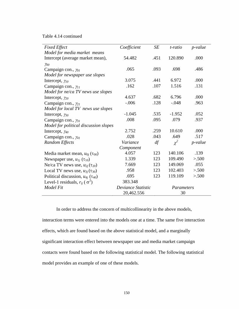
150

Table 4.14 continued Fixed Effect Coefficient SE t-ratio p-value Model for media market means Intercept (average market mean), γ00

54.482 .451 120.890 .000

Campaign con., γ01 .065 .093 .698 .486 Model for newspaper use slopes Intercept, γ10 3.075 .441 6.972 .000 Campaign con., γ11 .162 .107 1.516 .131 Model for ne/ca TV news use slopes Intercept, γ20 4.637 .682 6.796 .000 Campaign con., γ21 -.006 .128 -.048 .963 Model for local TV news use slopes Intercept, γ30 -1.045 .535 -1.952 .052 Campaign con., γ31 .008 .095 .079 .937 Model for political discussion slopes Intercept, γ40 2.752 .259 10.610 .000 Campaign con., γ41 .028 .043 .649 .517 Random Effects Variance

Component df χ2 p-value

Media market mean, u0j (τ00) 4.057 123 140.106 .139 Newspaper use, u1j (τ10) 1.339 123 109.490 >.500 Ne/ca TV news use, u2j (τ20) 7.669 123 149.069 .055 Local TV news use, u3j (τ30) .958 123 102.403 >.500 Political discussion, u4j (τ40) .695 123 119.109 >.500 Level-1 residuals, rij ( σ2) 383.348 Model Fit Deviance Statistic Parameters 20,462.556 30

In order to address the concern of multicollinearity in the above models,

interaction terms were entered into the models one at a time. The same five interaction

effects, which are found based on the above statistical model, and a marginally

significant interaction effect between newspaper use and media market campaign

contacts were found based on the following statistical model. The following statistical

model provides an example of one of these models.

151

Level 1 model: Y ij = β0j + β1j (NPUSE) ij + β2j (NE/CATV) ij + β3j (LOTV) ij + β4j (DISCU) ij + β5j (AGE)ij + β6j (MALE) ij + β7j (EDUCA) ij + β8j (INCOME) ij + rij

Level 2 model: β0j = γ00 + γ01 (CAMPAIGN)j + u0j β1j = γ10 + γ11 (CAMPAIGN)j + u1j β2j = γ20 + u2j β3j = γ30 + u3j β4j = γ40 + u4j β5j = γ50 β6j = γ60 β7j = γ70 β8j = γ80

Mixed-effects model: Y ij = γ00 + γ01 (CAMPAIGN)j + γ10 (NPUSE) ij + γ11

(CAMPAIGN)j (NPUSE) ij + γ20 (NE/CATV) ij + γ30 (LOTV) ij +γ40 (DISCU) ij + γ50

(AGE)ij + γ60 (MALE) ij + γ70 (EDUCA) ij + γ80 (INCOME) ij + u0j + u1j (NPUSE) ij + u2j (NE/CATV) ij + u3j (LOTV) ij + u4j (DISCU) ij + rij

Table 4.15 shows that newspaper use interacted with state advertising spending,

t(43) = 2.71, p = .01, in predicting political knowledge. Thus, H6a is supported. Figure

4.6 shows that the difference increased about 62% from 4.27 to 6.93. This means that the

difference between people with more newspaper use and less newspaper use was greater

in the states with more advertising spending than in the states with less advertising

spending. In other words, newspaper use had a greater impact on political knowledge in

the places with more advertising spending.

152

Level 2 variable: Ad expenditures Fixed Effect Coefficient SE t-ratio p-value Intercept (average state mean), γ00 54.834 .595 92.091 .000 Ad expenditures, γ01 .0001 .0002 .733 .467 Model for newspaper use slope Intercept, γ10 3.110 .352 8.836 .000 Ad expenditures, γ11 .0003 .0001 2.712 .010 Ne/Ca television news use, γ20 4.317 .718 6.009 .000 Local television news use, γ30 -1.070 .480 -2.228 .031 Political discussion, γ40 2.713 .273 9.940 .000 Random Effects Variance

Component df χ2 p-value

State mean, u0j (τ00) 7.088 42 79.867 .001 Newspaper use, u1j (τ10) .055 42 27.063 >.500 Ne/ca TV news use, u2j (τ20) 5.627 43 57.206 .072 Local TV news use, u3j (τ30) .212 43 33.887 >.500 Political discussion, u4j (τ40) .450 43 52.209 .159 Level-1 residuals, rij ( σ2) 382.941 Model Fit Deviance Statistic Parameters 20,082.587 27

Table 4.15: Interaction of newspaper use and advertising spending predicting political

knowledge (state).

0

10

20

30

40

50

60

70

80

90

100

-1 SD NP +1 SD NP

Polit

ical

Kno

wle

dge

-1 SD Adsspe+1 SD Adsspe

Figure 4.6: Interaction of newspaper use and advertising spending predicting political

knowledge (state).

153

Table 4.16 shows that newspaper use interacted with state candidate appearances,

t(46) = 2.01, p = .05, in predicting political knowledge. Thus, H6b is supported. Figure

4.7 shows that the difference increased about 32% from 4.74 to 6.27. This means that the

difference between people with more newspaper use and less newspaper use was greater

in the states with more candidate appearances than in the states with less candidate

appearances. In other words, newspaper use had a greater impact on political knowledge

in the places with more candidate appearances.

Level 2 variable: Candidate appearances Fixed Effect Coefficient SE t-ratio p-value Intercept (average state mean), γ00 54.894 .590 93.083 .000 Candidate app., γ01 -.002 .029 -.079 .937 Model for newspaper use slope Intercept, γ10 3.053 .392 7.797 .000 Candidate app., γ11 .033 .016 2.014 .050 Ne/Ca television news use, γ20 4.303 .706 6.099 .000 Local television news use, γ30 -1.054 .479 -2.201 .033 Political discussion, γ40 2.777 .274 10.143 .000 Random Effects Variance

Component df χ2 p-value

State mean, u0j (τ00) 7.062 44 80.915 .001 Newspaper use, u1j (τ10) .033 44 29.295 >.500 Ne/ca TV news use, u2j (τ20) 5.688 45 58.831 .081 Local TV news use, u3j (τ30) .308 45 34.233 >.500 Political discussion, u4j (τ40) .476 45 56.764 .112 Level-1 residuals, rij ( σ2) 383.672 Model Fit Deviance Statistic Parameters 20,450.052 27

Table 4.16: Interaction of newspaper use and candidate appearances predicting political

knowledge (state).

154

0

10

20

30

40

50

60

70

80

90

100

-1 SD NP +1 SD NP

Polit

ical

Kno

wle

dge

-1 SD App+1 SD App

Figure 4.7: Interaction of newspaper use and candidate appearances predicting political

knowledge (state).

Table 4.17 shows that newspaper use interacted with state campaign contacts,

t(46) = 2.09, p < .05, in predicting political knowledge. Thus, H6c is supported. Figure

4.8 shows that the difference increased about 69% from 4.21 to 7.12. This means that the

difference between people with more newspaper use and less newspaper use was greater

in the states with more campaign contacts than in the states with less campaign contacts.

In other words, newspaper use had a greater impact on political knowledge in the places

with more campaign contacts.

155

Level 2 variable: Campaign contacts Fixed Effect Coefficient SE t-ratio p-value Intercept (average state mean), γ00 54.830 .572 95.890 .000 Campaign con., γ01 .205 .130 1.576 .122 Model for newspaper use slopes Intercept, γ10 3.139 .325 9.656 .000 Campaign con., γ11 .221 .106 2.091 .042 Ne/Ca television news use, γ20 4.316 .705 6.123 .000 Local television news use, γ30 -1.028 .477 -2.153 .036 Political discussion, γ40 2.748 .275 9.981 .000 Random Effects Variance

Component df χ2 p-value

State mean, u0j (τ00) 6.859 44 79.132 .001 Newspaper use, u1j (τ10) .038 44 28.026 >.500 Ne/ca TV news use, u2j (τ20) 5.373 45 58.931 .079 Local TV news use, u3j (τ30) .299 45 34.260 >.500 Political discussion, u4j (τ40) .524 45 56.957 .109 Level-1 residuals, rij ( σ2) 383.188 Model Fit Deviance Statistic Parameters 20,446.975 27

Table 4.17: Interaction of newspaper use and campaign contacts predicting political

knowledge (state).

0

10

20

30

40

50

60

70

80

90

100

-1 SD NP +1 SD NP

Polit

ical

Kno

wle

dge

-1 SD Con+1 SD Con

Figure 4.8: Interaction of newspaper use and campaign contacts predicting political

knowledge (state).

156

Table 4.18 shows that political discussion interacted with media market

advertising expenditures, t(59) = 3.18, p < .01, in predicting political knowledge. Thus,

H8a is supported. Figure 4.9 shows that the difference increased about 22% from 9.80 to

11.95. The difference between people with more political discussion and less political

discussion was greater in the media markets with more advertising spending than in the

media markets with less advertising spending. In other words, political discussion had a

greater impact on political knowledge in the places with more advertising spending.

Level 2 variable: Ad expenditures Fixed Effect Coefficient SE t-ratio p-value Intercept (average market mean), γ00 55.376 .580 95.470 .000 Ad expenditures, γ01 .0002 .0001 2.102 .040 Newspaper use, γ10 3.286 .507 6.484 .000 Ne/Ca television news use, γ20 4.267 .991 4.306 .000 Local television news use, γ30 -1.238 .686 -1.805 .076 Model for political discussion slopes Intercept, γ40 2.891 .300 9.640 .000 Ad expenditures, γ41 .0001 .00005 3.180 .003 Random Effects Variance

Component df χ2 p-value

Media market mean, u0j (τ00) 5.028 57 70.472 .108 Newspaper use, u1j (τ10) 2.678 58 61.722 .344 Ne/ca TV news use, u2j (τ20) 14.397 58 79.866 .030 Local TV news use, u3j (τ30) 2.940 58 49.711 >.500 Political discussion, u4j (τ40) .514 57 54.432 >.500 Level-1 residuals, rij ( σ2) 379.285 Model Fit Deviance Statistic Parameters 12,683.518 27

Table 4.18: Interaction of political discussion and advertising spending predicting

political knowledge (media market).

157

0

10

20

30

40

50

60

70

80

90

100

-1 SD Disc +1 SD Disc

Polit

ical

Kno

wle

dge

-1 SD Adsspe+1 SD Adsspe

Figure 4.9: Interaction of political discussion and advertising spending predicting

political knowledge (media market).

Table 4.19 shows that political discussion interacted with media market candidate

appearances, t(140) = 2.15, p < .05, in predicting political knowledge. Thus, H8b is

supported. Figure 4.10 shows that the difference increased about 31% from 8.57 to 11.21.

The difference between people with more political discussion and less political

discussion was greater in the media markets with more candidate appearances than in the

media markets with less candidate appearances. In other words, political discussion had a

greater impact on political knowledge in the places with more candidate appearances.

158

Level 2 variable: Candidate appearances Fixed Effect Coefficient SE t-ratio p-value Intercept (average market mean), γ00 54.526 .522 104.555 .000 Candidate app., γ01 .175 .088 1.996 .048 Newspaper use, γ10 3.369 .471 7.150 .000 Ne/Ca television news use, γ20 4.386 .762 5.756 .000 Local television news use, γ30 -1.062 .569 -1.865 .064 Model for political discussion slopes Intercept, γ40 2.647 .277 9.544 .000 Candidate app., γ41 .087 .040 2.149 .033 Random Effects Variance

Component df χ2 p-value

Media market mean, u0j (τ00) 4.221 101 116.510 .139 Newspaper use, u1j (τ10) 2.228 102 98.755 >.500 Ne/ca TV news use, u2j (τ20) 8.765 102 126.332 .051 Local TV news use, u3j (τ30) 1.476 102 87.173 >.500 Political discussion, u4j (τ40) .441 101 90.787 >.500 Level-1 residuals, rij ( σ2) 385.065 Model Fit Deviance Statistic Parameters 17,706.402 27

Table 4.19: Interaction of political discussion and candidate appearances predicting

political knowledge (media market).

0

10

20

30

40

50

60

70

80

90

100

-1 SD Disc +1 SD Disc

Polit

ical

Kno

wle

dge

-1 SD App+1 SD App

Figure 4.10: Interaction of political discussion and candidate appearances predicting

political knowledge (media market).

159

Table 4.20 shows that there was a marginally significant interaction effect

between newspaper use and media market campaign contacts, t(183) = 1.87, p = .063, in

predicting political knowledge. This provides further evidence for H6c. Figure 4.11

shows that the difference increased about 102% from 3.66 to 7.39. The difference

between people with more newspaper use and less newspaper use was greater in the

media markets with more campaign contacts than in the media markets with less

campaign contacts. In other words, newspaper use had a greater impact on political

knowledge in the places with more campaign contacts.

Level 2 variables: Campaign contacts Fixed Effect Coefficient SE t-ratio p-value Intercept (average market mean), γ00 54.487 .449 121.433 .000 Campaign con., γ01 .066 .090 .737 .462 Model for newspaper use slopes Intercept, γ10 3.062 .436 7.015 .000 Campaign con., γ11 .177 .095 1.867 .063 Ne/Ca television news use, γ20 4.632 .678 6.833 .000 Local television news use, γ30 -1.030 .527 -1.954 .052 Political discussion, γ40 2.774 .253 10.956 .000 Random Effects Variance

Component df χ2 p-value

Media market mean, u0j (τ00) 3.987 123 140.106 .139 Newspaper use, u1j (τ10) 1.345 123 109.398 >.500 Ne/ca TV news use, u2j (τ20) 7.798 124 149.129 .062 Local TV news use, u3j (τ30) .950 124 102.482 >.500 Political discussion, u4j (τ40) .729 124 119.576 >.500 Level-1 residuals, rij ( σ2) 383.320 Model Fit Deviance Statistic Parameters 20,462.848 27

Table 4.20: Interaction of newspaper use and campaign contacts predicting political

knowledge (media market).

160

0

10

20

30

40

50

60

70

80

90

100

-1 SD NP +1 SD NP

Polit

ical

Kno

wle

dge

-1 SD Con+1 SD Con

Figure 4.11: Interaction of newspaper use and campaign contacts predicting political

knowledge (media market).

Summary of Major Findings

In conclusion, a positive relationship was found between newspaper use and

political knowledge across all the data files whether campaign-level variables were

controlled in the model. This supports H1a, which predicts people who have more

newspaper use will have more political knowledge than people who have less newspaper

use. A positive relationship was found between network and cable TV news use and

political knowledge across all the data files whether campaign-level variables were

controlled in the model. But, a negative relationship between local TV news use and

political knowledge was found among the majority of the data files whether campaign-

level variables were controlled in the model. Therefore, H1b, which predicts that people

who have more television news use will have more political knowledge than people who

have less television news use, is partially supported. A positive relationship was found

161

between political discussion and political knowledge across all the data files whether

campaign-level variables were controlled in the model. This supports H2, which predicts

that people who have more political discussion will have more political knowledge than

people who have less political discussion. Table 4.21 presents a summary of the data

analysis results.

Main effects

Ad frequencies

Ad expenditures

Candidate appearances

Campaign contacts

Main effects H3: 2/4 H3: 1/4 H4: 2/4 H5: 3/4

Newspaper use H1a: 14/14 H6a: NS H6a** H6b* H6c*

Network & cable TV use

H1b: 14/14 H7a: NS H7a# H7b: NS H7c: NS

Local TV news use

H1b: 9/14 H7a# H7a: NS H7b: NS H7c: NS

Political discussion

H2: 14/14 H8a: NS H8a** H8b* H8c: NS

Table 4.21: Summary of the data analysis results.

Note: (1) The findings of the main effects are from the random-coefficients regression model, means-as-outcomes regression model, and intercepts-as-outcomes model. The denominator means the number of all the models analyzed. The numerator means the number of the models that produce statistically significant relationships. (2) Interaction effects are from the intercepts-and-slopes-as-outcomes model. # p < .10; * p < .05; ** p < .01

Regarding the campaign-level variables, when the individual-level variables were

not controlled in the model, no significant relationship was found between the two

political advertising measures, i.e., advertising frequencies and expenditures, and political

knowledge in either states or media markets. However, when the individual-level

variables were controlled in the model, there was some evidence that political advertising

162

and political knowledge are positively associated. More specifically, a marginally

significant relationship was found between advertising frequencies and political

knowledge in both states and media markets, and a significant relationship was found

between advertising expenditures and political knowledge in media markets. Therefore,

H3, which predicts that the increase in televised political advertisements will be

positively associated with the increase in political knowledge, is partially supported.

Moreover, a positive relationship was found between candidate appearances and political

knowledge in media markets whether the individual-level variables were controlled in the

model. This provides some evidence for H4, which predicts the increase in presidential

candidate appearances will be positively associated with the increase in political

knowledge. A positive relationship was found between campaign contacts and political

knowledge in both states and media markets when the individual-level variables were not

controlled in the model. But, when the individual-level variables were controlled in the

model, this relationship existed only in states. This generally supports H5, which predicts

that the increase in campaign contacts will be positively associated with the increase in

political knowledge.

Finally, the findings of interaction effects are mixed. Whether all the interaction

terms between the major individual-level and campaign-level predictors were in the

model at the same time or the interaction terms between the major individual-level and

campaign-level predictors were in the model one at a time, the same five interaction

effects were found. More specifically, interaction effects were found between newspaper

use and advertising spending (state), between newspaper use and candidate appearances

(state), and between newspaper use and campaign contacts (state) in predicting political

163

knowledge. These findings support H6a, which predicts that the relationship between

newspaper use and political knowledge will be stronger in the places with more political

ads than in the places with less political ads; H6b, which predicts that the relationship

between newspaper use and political knowledge will be stronger in the places with more

candidate appearances than in the places with less candidate appearances; and H6c,

which predicts that the relationship between newspaper use and political knowledge will

be stronger in the places with more campaign contacts than in the places with less

campaign contacts.

Moreover, interaction effects were found between political discussion and

advertising spending (media market), and between political discussion and candidate

appearances (media market) in predicting political knowledge. These findings support

H8a, which predicts that the relationship between political discussion and political

knowledge will be stronger in the places with more political ads than in the places with

less political ads; and H8b, which predicts that the relationship between political

discussion and political knowledge will be stronger in the places with more candidate

appearances than in the places with less candidate appearances.

Finally, when the interaction terms between the major individual-level and

campaign-level predictors were in the model one at a time, a marginally significant

interaction effect was found between newspaper use and campaign contacts (media

market). This provides further evidence to support H6c. When all the interaction terms

between the major individual-level and campaign-level predictors were in the model at

the same time, marginally significant interaction effects were found between network and

cable TV news use and advertising spending (state), and between local TV news use and

164

advertising frequencies (media market). These findings provide some evidence for H7a,

which predicts that the relationship between TV news use and political knowledge will be

stronger in the places with more political ads than in the places with less political ads.

H7b (TV news use x candidate appearances), H7c (TV news x campaign contacts) and

H8c (political discussion x campaign contacts) are not supported.

165

CHAPTER 5

DISCUSSION AND CONCLUSION

This chapter discusses the major findings of the study as well as their theoretical

and practical implications. It also discusses some limitations of the study and proposes

the directions for future research.

Goal of Study and Major Findings

The present study is a multilevel study of strategic communication in the 2000

presidential campaign. It takes a multidimensional and multilevel perspective to look at

the communication function in today’s increasingly sophisticated and multifaceted

political campaigns. The purpose of the study is to investigate how people’s surrounding

communication contexts that are defined by some geospatial characteristics created by

campaign strategies could influence their political cognition in political campaigns. The

core idea behind this study is that political campaigns could shape a person’s

communication context in which this person is conditioned or nested, and accordingly

both individual-level and contextual-level factors within this context could form

synergistic influences on this person’s responses with respect to the election. That is, it

attempts to understand how differential allocation of campaign resources would result in

differential communication effects in different geospaces, and thereby, influence people’s

learning about the election.

166

According to the data analysis results, people who read newspaper, watch

network and cable TV news, and engage in political discussion more frequently have

more political knowledge. But, people who watch local TV news more frequently have

less political knowledge. There is some evidence that the three campaign intensity

indicators – televised political ads, candidate appearances, and campaign-related contacts

-- have positive relationships with political knowledge. More importantly, there are

contextual effects in the relationship between newspaper use and political knowledge

when it is conditioned on macro-level political ads, candidate appearances, and campaign

contacts; and in the relationship between political discussion and political knowledge

when it is conditioned on macro-level political ads and candidate appearances. This

means that people’s newspaper use and political discussion have greater impacts on their

political knowledge in the places with more campaign intensity than in the places with

less campaign intensity. There is also some relatively weak evidence for the contextual

effects in the relationship between TV news use and political knowledge when it is

conditioned on macro-level political ads.

The Importance of Geospatial Dimension in Campaigns

The present study expands existing literature and research with its innovative

research findings about geospatial, contextual effects in political campaigns. It employs a

somewhat different set of theoretical models and research methods to assess informing

effects of communication in political campaigns from a macro-contextual perspective and

focuses on cross-level connections. It contributes to the development and advancement of

cross-level theorizing in communication science, and also provides a good understanding

of the role that communication would play in a larger social, economic and political

167

setting. Although the O-S-O-R communication effects model suggests a macro-level

component in its first “O,” it is not quite clear how to accommodate contextual influences

in this model. Based on the O-S-O-R paradigm, the present study not only demonstrates

that conditional communication effects – the essence of the O-S-O-R model – also hinge

on geospatial, contextual factors but also helps to develop contextual theories of

communication that specifically take into account contextual factors and address cross-

level inference.

The findings of the study suggest that geography matters in political

communication. The three campaign intensity indicators -- televised political advertising,

candidate appearances, and campaign contacts – do create geospatially varying

communication contexts, which accordingly result in differential informing effects.

Overall, campaign contacts in a person’s context is the strongest predictor of his or her

political knowledge. Candidate appearances is the second strongest predictor, and

political advertising is the weakest predictor. But, the difference among the main effects

of these three campaign-level variables is moderate. There are two possible explanations

for the relatively weaker main effect of political ads. The first explanation is about the

data, which has only 61 media markets available for the data analysis, and for

constructing the state political advertising variable. The other two campaign-level

variables have more individual-level cases and campaign-level units. The second

explanation is about the method of assessing advertising effects. Research (Ridout, Shah,

Goldstein, & Franz, 2004) argued that total number of ads aired in a person’s media

market is a poor predictor of political knowledge. Generally speaking, the results of the

168

study provide evidence that political campaign practices do promote some learning about

politics.

These macro-level campaign practices are not the sole determinant of

communication effects. They provide contexts. The results of the present study show that

political learning is conditioned on many factors -- media, people, stimuli, and place, all

of which lead to different results. Different geospatial parameters created by campaign

strategies result in different informing effects of communication.

The present study provides evidence to support the information flow approach to

contextual effects. The information flow approach argued that contextual effects occur

when the nature of information flow structured by the context influences how people

react to this locally varying information (see Books & Prysby, 1988; Books & Prysby,

1991; Books & Prysby, 1995; Burbank, 1997; Erbring & Young, 1979; Huckfeldt &

Sprague, 1995; McLeod, 2001; Prysby & Books, 1987). It is found that the geospatial

variation of political ads, candidate appearances, and campaign contacts influences the

relationship between newspaper use and political knowledge, and that the geospatial

variation of political ads and candidate appearances influences the relationship between

political discussion and political knowledge.

People who are in the environment full of campaign messages are more likely to

build their knowledge base of these massages because they have more chance to

encounter these messages and practice making sense of them in that kind of environment.

In a political campaign, campaign massages are related to each other and conveyed

through various channels. Repetition of message exposure makes people easier to learn

the message. Accordingly, when they encounter the same or relevant information when

169

they read newspaper, their memory of the information is reinforced and they are more

likely to understand, retain and recall the information than those without this prior

knowledge base. This can explain whey people in the places with more political ads and

campaign contacts in the context are more likely to gain political knowledge from

reading newspaper than those in the places with less this information in the ambient

environment. The relationship between people’s newspaper use and political knowledge

is strengthened in those places.

Candidate appearances from the campaign can also imbue a place with campaign

messages. Residing in an environment full of campaign messages can help build a

knowledge base of these messages, which can assist learning about relevant information.

In addition, candidates’ travel would be covered by newspapers. Particularly, if the visit

is local, the visit and its relevant information would definitely be reported by local

newspapers. This can explain why people in the places visited by candidates more

frequently are more likely to gain political knowledge from reading newspaper than those

in the places visited less frequently. The relationship between newspaper use and political

knowledge is strengthened in the places with more information of candidate appearances

and relevant campaign messages in the environment.

The nature of information linking newspaper use and the three types of campaign

practices is a little different, though the mechanism that produces contextual effects is the

same. The linkage between newspaper use and either political ads or campaign contacts is

mainly about general campaign information. The linkage between newspaper use and

candidate appearances is both direct, specific messages about candidate visits and general

campaign information.

170

During a political campaign, interpersonal political discussion is also an important

information source of campaign messages. According to the theory of two-step flow of

communication (Katz & Lazarsfeld, 2006) and the news diffusion research (Larsen &

Hill, 1954; Rogers, 2000), talking with other people is an important information source

for some segments of the general public. From the information flow perspective (see

Books & Prysby, 1991 etc.), the frequency and content of political talk should reflect

local campaign situations. Political ads and candidate appearances conveyed from mass

media in the local context can become people’s discussion topics and content. Thus,

people in the places with more political ads and candidate appearances are more likely to

discuss election-relevant topics with other people, and build their knowledge base.

Accordingly, they are more likely to gain political knowledge from exchanging second-

hand campaign information with other people. This is why the relationship between

political discussion and political knowledge is strengthened in the place with more

televised ads and candidate visits than in the places with fewer ads and visits.

From the pattern of the above findings, generally speaking, people’s newspaper

use and political discussion are influenced by the geospatial variation of campaign

practices, but their television news use is almost not influenced by the campaign’s

geospatial variation. In other words, the relationships between TV news use, including

network, cable and local TV, and political knowledge are almost not influenced by where

people reside or what kinds of communication contexts they are conditioned.

There are weak interaction effects between televised political ads and network

and cable TV news use, and between televised political ads and local TV news use in

predicting political knowledge. Inconsistent with the hypothesis, the interaction effect

171

between political ads and network and cable TV news use in predicting political

knowledge is negative. The interaction effect between local TV news use and political

ads is positive as hypothesized. These findings suggest that geospatial variation of

political ads does have some influence on the relationship between TV news use and

political knowledge.

There are several explanations for the weak interaction effects between people’s

TV news use and campaign-level televised political ads in predicting political knowledge.

First, as discussed previously, compared with candidate appearances and campaign

contacts, political advertising in a person’s context is a weak predictor of his or her

political knowledge. Second, TV news use is used as a proxy measure of advertising

effects. Although a lot of ads are aired during news programs, a lot more ads are aired in

other parts of the day. Based on the 226,864 ads from the Wisconsin Advertising Project

analyzed in the present study, only about 24.1% of the ads were run during the 4:00 -

7:30 p.m. time slot, including 17% of them run during the news. About 23.2 % of the ads

were run during the early news (4:00-7:30 p.m.) and the late news (10:00 or 11:00 p.m.).

This means that about 80% of the ads appeared during non-news programs and in other

parts of the day. This means that adverting exposure is something broader than just TV

news use exposure. So, if the proxy measure is not adequate in capturing real effects of

advertising, it would not be a surprising finding. Theses findings are consistent with

pervious research (Ridout, Shah, Goldstein, & Franz, 2004) that found that the hours of

TV watching per day, total number of ads aired in a person’s media market, and the

combination of the former two measures are all poor predictors of political knowledge.

172

This study found that the relationships between TV news use and political

knowledge and between TV news use, including both network and cable TV news, and

local TV news, do not vary across communication contexts constituted by candidate

appearances. In other words, the relationship between TV news use and political

knowledge is not stronger in the places with more candidate appearances than in the

places with fewer candidate appearances. People in the places with more candidate

appearances do not gain more political knowledge from watching TV news.

In the case of network and cable TV news, the coverage of candidate appearances

should be the same across the nation. However, the heavily visited places should be the

frequently mentioned places in the news. The explanation for no interaction effect

between network and cable TV news use and candidate appearances may be that

campaign information in the context and in the news due to candidate visits does not

become people’s political knowledge through being more attentive to their own places

mentioned in the news. Compared with newspaper and discussion as people’s

information sources, network and cable TV news tend to be less locally and contextually

bound. Being attentive to news coverage of a person’s own town seems hard to reflect

contextual differences of candidate appearances as an information source.

In the case of local TV news, its relationship with political knowledge is found

not to be influenced by the geospatial variation of candidates’ visits, either. There’s no

interaction effect between local TV new use and candidate appearances. This may

suggest that when people in the places with more candidate appearances-related

campaign information in the news and in the ambient environment watch local TV news,

they do not benefit from residing in such a kind of environment. As indicated previously,

173

candidate appearances have some positive effects on political knowledge, whereas local

TV news use has negative effects on knowledge. So, that no interaction effect is found

should not be attributed to that candidate appearances do not have something to do with

political knowledge; rather, it should be attributed to that local TV news is not a good

medium for political learning.

The results of the study also show that campaign contacts do not interact with

network and cable TV news, local TV news, and political discussion in predicting

political knowledge. This means that the relationships between either TV news use or

political discussion and political knowledge are not strengthened due to more campaign

information resulted from campaign contacts in the context. People in the places with

more campaign-related contacts do not benefit from having higher chance of

encountering campaign messages in the ambient environment to build their knowledge

base, and thereby, being more likely to gain political knowledge when they watch TV

news or engage in political discussion. There are some explanations.

First, research indicates that most people in the U.S. read local newspapers (44%)

on a daily basis, as opposed to national newspapers (7%) (Saad, 2007). As discussed

previously, the geospatial variation of political ads and campaign contacts has effects on

the relationship between newspaper use and political knowledge because newspaper more

or less reflects the contextual differences of these information sources. Therefore, unlike

newspaper, it could be that network and cable TV news does not well reflect the

contextual variation of an information source like campaign contacts. Furthermore, like

local newspaper, local TV news should reflect the geospatial variation of information

sources. Local TV news would more or less carry the messages from the momentum built

174

by campaign contacts in the ambient environment. However, like the case of the

relationship between local TV news and candidate appearances, that no interaction effect

is found between local TV news use and campaign contacts could be attributed to that

local TV news is inherently not a strong and stable predictor of political knowledge.

Finally, why are there interaction effects between political discussion and political

ads, and political discussion and candidate appearances, but not between political

discussion and campaign contacts? According to the relevant theories, i.e., the theory of

two-step flow of communication and the news diffusion research, political discussion is

an information source for some people because those people rely on others for

transmitting information from mass media. Thus, a possible explanation is that unlike the

other two campaign-level information sources – political ads and candidate appearances,

which are mainly broadcast on mass media, campaign contact is more like mediated and

unmediated interpersonal communication. Because they are not mass communication,

they are less likely to be fad. The campaign messages conveyed through campaign

contacts or general campaign information in the ambient environment due to campaign

contacts are less likely to become a handy topic and materials for discussion. In other

words, discussion content does not well reflect differential availability of campaign

messages constructed by campaign contacts in the context. In other words, people’s

political discussion is not influenced by campaign contacts in the context. This may

explain why people in the places with more campaign contacts do not learn more from

discussing politics with other people.

Based on the above findings, this study helps build contextual theories of

communication by modeling effects of contextual factors and cross-level interactions.

175

Macro-level research is so underthought in communication science, though the advocacy

for developing contextual theories is not something new. Particularly, context or

geospace is an important, yet under-explored dimension in research on communication

effects in political campaigns. The findings of the present study suggest that political

campaigning is about geospace. In the communication field, the majority of studies are

concerned with individual-level variables and micro psychological processes. However,

many social, political and economic implications should not be reduced to psychology.

They should not be touched only by research with psychological views and methods.

McLeod and Blumler (1987) argued that “communication science without a macro

component would be impoverished and seriously incomplete” (p. 277). McLeod, Kosicki,

and McLeod (2008) also argued that “If our explanations remain solely at the individual

level, we are guilty of disciplinary reductionism and risk missing important social

influences, implicitly blaming individuals for problems whose remedies would be better

sought through institutions” (p. 16). Reducing broader social, economic, and political

problems into psychology is definitely not right for the advancement of the field.

The value of macro-level studies, such as the present study, is that they help build

theories at different levels, which can help really understand broader social, political and

economic problems that are not answered by psychology. McLeod and Blumler (1987)

argued that the macrosocial level research in communication science examines

communication systems or communication signification of social systems.

Acknowledging the importance of a macro perspective, the present study is designed

based on the idea that media work and people learn about political campaigns in the real-

world setting. It is a misconception that people would share the same information

176

baseline across the whole country. For example, there would be a very big difference

between the information environment in Ohio and that in Wyoming. That is to say, the

present study assesses how the population learns about politics, and looks at campaign

and communication effects from a larger real world viewpoint.

Particularly, the present study takes a geospatial approach to examine

communication effects in political campaigns. McLeod and Blumler (1987) argued that

the appropriate approach to macrosocial-level communication research is comparative

research, which is “based on the presumption that different system parameters (i.e.,

different manners in which systems are structured) will differentially encourage or

constrain communication roles and behaviors belonging to, organized by, or exposed to

them” (p. 308), because a system can only be understood by comparing with other

systems. The findings of the present study suggest that people in different geospatial units

are not in a uniform communication environment, and that immersing in different

communication environments produces different informing effects in political campaigns.

Finally, consistent with most literature, the results of the present study generally

suggest that news media, including newspapers and network and cable television news,

and political discussion, contribute to people’s political knowledge gain. Therefore, in

addition to help building contextual theories in communication science, this study also

demonstrate that communication, including both mass media use and interpersonal

communication, does play a significant role in informing people in political campaigns.

Inconsistent with the hypothesis that TV news use should be positively related to

political knowledge, the findings of local TV news use indicate that people who watch

local television news more frequently have less political knowledge. Unlike newspaper,

177

network and cable TV news, and political discussion, which are predictors of political

knowledge across all the data files tested in the present study, local TV news is either

negatively associated with political knowledge or not associated with political knowledge

at all. So, like existing studies, which reach different conclusions on the relationship

between local TV news and political knowledge, the finding of local TV news in the

present study is also somewhat mixed. Overall, this study suggests that informing effects

of local TV news is limited as far as national politics is concerned.

Content analyzed 8,095 stories of local TV news in 15 cities in 2000, Rosenstiel,

Gottlieb, and Brady (2000) found that “politics/government” is second to “crime/law” as

the most popular topic. The volume of “crime/law” coverage (18%) almost doubled that

of “politics/government” coverage (10%) in the study. This may help explain why the

present study found a negative relationship between local TV news use and political

knowledge. With respect to demographic characteristics of the audience of local TV

news, according to a recent Gallup Poll research, women, those 50 and older, and

Democrats are the major viewers (Saad, 2007). In sum, more studies should be conducted

to investigate whether local TV news does not have much to do with people’s political

knowledge. Future research would also investigate whether it is the content of local news

that does not help people gain political knowledge or the viewers of local TV news who

are less knowledgeable on average.

Campaign’s Role in Democracy

In addition to helping understand the latest trends and processes of political

campaigns, the findings of the study have implications for relevant public policies. They

suggest that there is a serious problem in current political campaign practices that may

178

impede civic engagement efforts. That is, although this study demonstrates that

communication is able to influence people, it also provides evidence that in political

campaigns not every citizen has an equal opportunity to learn about campaign messages,

to be influenced by campaigns, and to play a role in the political processes.

The use of targeting strategies is not wrong. However, targeting people in

democracy -- what does this imply? Does this kind of democratic system engage people

or foster apathy about politics? Is there equality of every vote? What efforts do

candidates put into those places that are already ahead or hopeless? Winning the

presidency in the United States is decided by winning the majority of the electoral vote.

Candidates’ focusing only on campaigning in the battleground states in order to win the

electoral vote has serious consequences.

First, as in the 2000 race, if a candidate wins the race because he or she wins the

electoral vote, but not the popular vote, does the candidate have any political legitimacy?

A successful president and government should have political legitimacy, which is

endowed by winning the popular vote, not the electoral vote. The electoral vote, which is

the aggregate of, not proportional to, the popular vote within a state, reflects only the

simple sum of people’s preference. If campaigns focus on winning the electoral vote

only, and do not care much about the popular vote, the elected officials does not truly

reflect citizen’s will. A president without legitimacy is very hard to govern the

constituencies.

Moreover, democracy is organized under the notion of equality of every vote.

Everybody's vote should count the same. When candidates pick some states to campaign

while ignoring others, this democratic ideal is compromised. Equality and freedom are

179

the two fundamental principles of democracy. According to Dahl (1989), there are two

essential assumptions of a democratic process – “the Principle of Equal Consideration of

Interests,” which suggests that the interests of every person should be equally considered,

and “the Presumption of Personal Autonomy,” which means that each person has the

right to judge a policy on the basis of his or her own best interest because no one else

knows what the best interest is better than the person himself or herself. According to

Dahl (1989), both assumptions serve as the premises of “the Strong Principle of

Equality,” meaning that “if the good or interests of everyone should be weighed equally,

and if each adult person is in general the best judge of his or her good or interests, then

every adult member of an association is sufficiently well qualified, taken all around, to

participate in making binding collective decisions that affect his or her good or interests,

that is, to be a full citizen of the demos” (p. 105). These assumptions of democracy are

labeled differently by different people, though the essence is the same. Simply put,

equality allows each citizen an equal opportunity to have some influence in the

democratic decision-making process, whereas autonomy (or freedom) allows citizens the

freedom and independence to express their own judgments in the process (Perez, 2004).

The findings of the present study suggest that citizens are in vastly different

information environment in current political campaigns. Campaigns do not treat every

citizen equally. Voice of each person is disparate. This conflicts with the distinctive

feature of democracy -- the democratic ideal “equality.” Although distribution of media

messages is not uniform because media resources are unevenly distributed across the

country, campaigns’ targeting strategies would exacerbate the inequalities in access to

campaign messages. Owing to the campaign’s targeting strategies, not every citizen is

180

worth the same amount of campaigning. People in some places are left out from the

campaigns. They may never be exposed to campaigns at all and asked for their vote. This

certainly is not healthy for a democratic system in the long term because it may lead to

marginalization of people in some parts of the country. People are not engaged and would

continue to be apathetic about politics.

These phenomena raise significant questions about the nature of American

democracy, and the meaning of campaigns for democracy. Campaigning in some specific

geospatial areas may be a very effective strategy to deliver an Electoral College majority.

However, the role and the function of communication campaigns in an election should

not be just for that purpose. Candidates have a mandate from citizens for some kind of

change. If just tiny portion of the population has been consulted, the usefulness of

campaigns in a democracy is doubtful.

However, when criticizing fairness of the current voting system from a person’s

standpoint, it should be noted that United States is a federal nation composed of

independent states and fairness should also be examined from the perspective of a state.

The presidential election in the U.S. is to elect somebody to be the head of the federal

government’s executive branch. The Electoral College system, which is a unique history

of American democracy, is rooted in the concept of federalism. Given this federal nature

of the U.S. voting system, big or small states should be represented at the federal level.

Under the current system, less populous states are overrepresented in the federal election

relative to their populations. More specifically, people in states with small populations

have a larger share of the electoral vote than those in states with big populations. For

example, in 2000, Wyoming, which has the population (493,782, Polidata Demographic

181

and Political Guides) and three electoral votes, has about 0.000006 Electoral College

representation per person. Ohio, which has the population (11,353,140, Polidata

Demographic and Political Guides) and 21 electoral votes, has less than 0.000002

Electoral College representation per person. This means that from this perspective, each

person’s vote in Wyoming has more power to influence the election than that in Ohio.

This suggests that the Electoral College system encourages candidates to pay

attention to small states in order to win as many electoral votes as possible. If candidates

just need to win popular votes to obtain the presidency, they would campaign mainly in

big cities, big markets, and big states that have a large population, and concentrate

particularly on mobilizing their base supporters. On the contrary, the Electoral College

system urges candidates to campaign more widely and broadly throughout the whole

nation. As the findings of the present study show, the major problem with the Electoral

College system is that candidates tend to focus on swing states.

Therefore, current system has its own merits, but owing to these serious

implications regarding the inequalities in political life, political campaigns shouldn’t

focus only on putting a lot of effort into those highly contested battlegrounds and just

want to win 270 Electoral College votes without caring much about winning the popular

vote. Without a doubt, like product campaigns, political campaigns also strive to reach

target audiences. However, unlike product campaigns, political campaigns, which bear

the responsibility for fulfilling democratic ideals, shouldn’t completely ignore those

people who are not part of the target audiences. An ideal and healthy democratic system

should be to engage as many people as possible in political processes and treat everyone

equally.

182

Study Limitations and Future Research

The present study is secondary research that analyzes existing data which are

collected for multiple purposes. The question items are certainly not the most ideal ones

for the present study. There are several limitations of the present study, and relevant

recommendations can be made.

First, the present study uses individuals’ TV news use as a proxy measure of their

exposure to televised political ads. This was done because the NAES data file used in the

present study doesn’t contain a direct measure of people’s exposure to advertising. That

is, in terms of the primary campaign practices – political advertising, the present study

only has macro-level advertising data, but no measure of advertising exposure at the

individual level. So, TV news use serves as a link with the macro-level televised ads

variable. Although this proxy measure is limited, it’s better than nothing because

individual differences should never be ignored. Some people do not care about elections

at all no matter how intense the campaign is. This is why the findings of the present study

indicate not only that variations of individuals’ news media use and interpersonal

communication significantly predict political knowledge but also that these variations at

the individual level interact with some campaign intensity variables in predicting political

knowledge. That is, individual differences can be amplified by some contextual factors.

This means that individual differences should always be taken into account. That said, the

effects could be more accurately assessed if the direct measure of people’s advertising

exposure is available in the individual-level data file, in this case, the NAES data. Future

research should use people’s exposure to televised political ads instead of their television

news use.

183

Some may be concerned about the alphas for the measures of communication

variables, including both news media use and political discussion. Some may think that

this means that the measures are not very reliable, and so do not really measure the

concepts as intended. However, alpha is in part a function of the number of items

included in the index, assuming they are equally reliable. When studying real populations

in field research and not experimental subjects in a laboratory, additional survey items are

very expensive. Survey designers, faced with the dilemma of whether to add largely

redundant items in the questionnaire to gain enhanced reliability or adding questions

tapping other subject areas often choose the latter. This reduces the number of similar

items that can be added together to form reliable multi-item indices. High reliability does

not imply validity so this not necessarily hurts the quality of the remaining items.

Another recommendation for the individual-level data could be to provide more

details of individual respondents’ TV watching information. For example, studies

(Freedman & Goldstein, 1999; Goldstein & Freedman, 2002b; Ridout, Shah, Goldstein,

& Franz, 2004) matched individual respondents’ television viewing information, such as

programs and dayparts, with advertising broadcast data in the respondents’ media market

to capture the effects of advertising. This approach seems to be a better and more refined

approach to assess effects of advertising, especially effects of specific types of ads on

individuals.

Another limitation of the present study is that the data file from Wisconsin

Advertising Project contains only 75 media markets, though they claimed that more than

80 percent of the U. S. population lives in these media markets. Although some places in

the country may not even have any campaigning, this information is still important.

184

Future research should include as many media markets as possible in order to cover more

of the country. Therefore, research findings could better reflect what’s going on in the

whole country. Moreover, in addition to information of the number of spots aired and the

estimated cost of each ad, researchers would hope that the data from the Wisconsin

Advertising Project also contain GRPs as another measure of advertising strength.

Several research topics can be extended from the present study. First, future

research could test other dependent variables such as political participation, likelihood to

vote, and vote choice to understand political campaigns’ mobilizing and persuasive

effects in addition to informing effects tested in the present study. Moreover, future

research could assess geospatial variations of these communication effects in other more

recent presidential campaigns, such as the 2004 and the 2008 elections.

In addition to understanding geospatial variations of communication effects by

examining cross-level interactions, future research can investigate the movements in

communication processes. From the geospatial perspective, it is not that some places

have campaigns and some places have no campaigns. It is that some places have high

campaign intensity, whereas other places have low campaign intensity. The influence of

communication in political campaigns on people in a specific context is like a natural

experiment because it provides people something in the beginning to get people involve

in the election. Thus, future research could test mediation in a multilevel context by using

multilevel structural equation modeling to understand whether campaign practices

promote news media use and political discussion, which will then lead to more political

knowledge and participation. It would also be interesting to investigate whether a

candidate’s campaign intensity influence people’s mass media use and political

185

discussion, which will then lead to discrepancies in issue positions between this candidate

and respondents as well as evaluations of this candidate’s traits, and finally, influence

vote choice. Testing mediation can help understand directions of causality among

variables at both levels. Multi-group multilevel SEM could also be conducted to

understand whether the flow of the effects vary across geospatial units.

Moreover, people’s mass media use and political discussion behaviors are likely

to correlate with or reciprocally reinforce each other more strongly in a communication

environment with more campaigning than they do in a one with less campaigning. Thus,

in addition to the effects of campaign practices on people’s communication behaviors,

future research could also investigate the relationship between people’s mass media use

and interpersonal political discussion. Is this relationship unidirectional, reverse or

reciprocal? Does it vary under different communication contexts?

Although the present study does not hypothesize causality and test causal effects,

it is based on the causal logic that it is the news content that leads to political knowledge.

It’s conventional and preponderant in communication science that testing the effects of

communication on knowledge. Future research could test reverse causality that

knowledge causes communication or media use. It is possible that people who have more

political knowledge or other characteristics, such as interest in politics, select certain

types of communication vehicles, not the content of communication that leads to

differential levels of political knowledge.

Finally, as the campaign progresses, communication effects could fluctuate,

diffuse, and cumulate. Future research could employ a longitudinal research design to

186

capture the dynamic nature of communication effects engendered over the course of a

campaign.

APPENDIX

QUESTION WORDING

187

Political Knowledge: [1] To the best of your knowledge, who {through 6 Nov 00: favors | starting 8 Nov 00: favored} the biggest tax cut, George W. Bush or Al Gore?

(1) Bush (2) Gore (3) No difference 998 Don’t know 999 No answer

[2] To the best of your knowledge, who {through 6 Nov 00: favors | starting 8 Nov 00: favored} using some of the Medicare surplus to cut taxes, George W. Bush or Al Gore?

(1) Bush (2) Gore (3) No difference 998 Don’t know 999 No answer

[3] To the best of your knowledge, who {through 6 Nov 00: favors | starting 8 Nov 00: favored} paying down the national debt the most, George W. Bush or Al Gore?

(1) Bush (2) Gore (3) No difference 998 Don’t know 999 No answer

[4] To the best of your knowledge, who {through 6 Nov 00: favors | starting 8 Nov 00: favored} the biggest increase in spending for Social Security, George W. Bush or Al

188

Gore? (1) Bush (2) Gore (3) No difference 998 Don’t know 999 No answer

[5] George W. Bush—do you think he {through 6 Nov 00: favors or opposes | starting 8 Nov 00: favored or opposed} allowing workers to invest some of their Social Security contributions in the stock market?

(1) Favor (2) Oppose 998 Don’t know 999 No answer

[5] Al Gore—do you think he {through 6 Nov 00: favors or opposes | starting 8 Nov 00: favored or opposed} allowing workers to invest some of their Social Security contributions in the stock market?

(1) Favor (2) Oppose 998 Don’t know 999 No answer

[6] On the issue of prescription drugs for senior citizens, to the best of your knowledge, what {through 6 Nov 00: does | starting 8 Nov 00: did} George W. Bush think? {Does | Did} George W. Bush think the federal government should not pay for senior citizens’ prescription drugs; the government should offer senior citizens a voucher to cover some of the cost of prescription drugs; or the federal government should cover prescription drugs through Medicare?

(1) Should not pay (2) Offer voucher to cover some costs (3) Cover through Medicare 998 Don’t know 999 No answer

[6] On the issue of prescription drugs for senior citizens, to the best of your knowledge, what {through 6 Nov 00: does | starting 8 Nov 00: did} Al Gore think? {Does | Did} Al Gore think the federal government should not pay for senior citizens’ prescription drugs; the government should offer senior citizens a voucher to cover some of the cost of prescription drugs; or the federal government should cover prescription drugs through Medicare?

(1) Should not pay

189

(2) Offer voucher to cover some costs (3) Cover through Medicare 998 Don’t know 999 No answer

[7] George W. Bush—do you think he {through 6 Nov 00: favors or opposes | starting 8 Nov 00: favored or opposed} using government funds to make sure that every child in the US is covered by health insurance?

(1) Favor (2) Oppose 998 Don’t know 999 No answer

[7] Al Gore—do you think he {through 6 Nov 00: favors or opposes | starting 8 Nov 00: favored or opposed} using government funds to make sure that every child in the US is covered by health insurance?

(1) Favor (2) Oppose 998 Don’t know 999 No answer

[8] George W. Bush—do you think he {through 6 Nov 00: favors or opposes | starting 8 Nov 00: favored or opposed} giving patients the right to sue their health maintenance organization or HMO?

(1) Favor (2) Oppose 998 Don’t know 999 No answer

[8] Al Gore—do you think he {through 6 Nov 00: favors or opposes | starting 8 Nov 00: favored or opposed} giving patients the right to sue their health maintenance organization or HMO?

(1) Favor (2) Oppose 998 Don’t know 999 No answer

[9] George W. Bush—do you think he {through 6 Nov 00: favors or opposes | starting 8 Nov 00: favored or opposed} making it harder for a woman to get an abortion?

(1) Favor (2) Oppose

190

998 Don’t know 999 No answer

[9] Al Gore—do you think he {through 6 Nov 00: favors or opposes | starting 8 Nov 00: favored or opposed} making it harder for a woman to get an abortion?

(1) Favor (2) Oppose 998 Don’t know 999 No answer

[10] To the best of your knowledge, who {through 6 Nov 00: opposes | starting 8 Nov 00: opposed} the sale of RU-486? George W. Bush, Al Gore, both or neither?

(1) Bush (2) Gore (3) Both (4) Neither 998 Don’t know 999 No answer

191

[11] George W. Bush—do you think he {through 6 Nov 00: favors or opposes | starting 8 Nov 00: favored or opposed} requiring a license for a person to buy a handgun?

(1) Favor (2) Oppose 998 Don’t know 999 No answer

[11] Al Gore—do you think he {through 6 Nov 00: favors or opposes | starting 8 Nov 00: favored or opposed} requiring a license for a person to buy a handgun?

(1) Favor (2) Oppose 998 Don’t know 999 No answer

[12] To the best of your knowledge, who supported legislation allowing people to carry concealed handguns? George W. Bush, Al Gore, both or neither?

(1) Bush (2) Gore (3) Both (4) Neither 998 Don’t know 999 No answer

[13] To the best of your knowledge, {through 6 Nov 00: does | starting 8 Nov 00: did} George W. Bush favor or oppose selling some of the oil reserve to increase the winter heating oil supply?

(1) Favor (2) Oppose 998 Don’t know 999 No answer

[13] To the best of your knowledge, {through 6 Nov 00: does | starting 8 Nov 00: did} Al Gore favor or oppose selling some of the oil reserve to increase the winter heating oil supply?

(1) Favor (2) Oppose 998 Don’t know 999 No answer

Newspaper Use: How many days in the past week did you read a daily newspaper?

Range 0-7 998 Don’t know 999 No answer

192

During the past week, how much attention did you pay to newspaper articles about the campaign for president? A great deal of attention, some, not too much or no attention at all?

(1) Great deal (2) Some (3) Not too much (4) None 998 Don’t know 999 No answer

Network and Cable Television News Use: How many days in the past week did you watch the national network news on TV—by national network news, I mean Peter Jennings on ABC, Dan Rather on CBS, Tom Brokaw on NBC, Fox News or UPN News?

Range 0-7 998 Don’t know 999 No answer

How many days in the past week did you watch cable news, such as CNN or MSNBC?

Range 0-7 998 Don’t know 999 No answer

During the past week, how much attention did you pay to stories on national network or cable TV news about the campaign for president? A great deal of attention, some, not too much or no attention at all?

(1) Great deal (2) Some (3) Not too much (4) None 998 Don’t know 999 No answer

Local Television News Use: How many days in the past week did you watch the local TV news—for example, “Eyewitness News” or “Action News”?

Range 0-7 998 Don’t know 999 No answer

193

During the past week, how much attention did you pay to stories on local TV news about the campaign for president? A great deal of attention, some, not too much or no attention at all?

(1) Great deal (2) Some (3) Not too much (4) None 998 Don’t know 999 No answer

Political Discussion: How many days in the past week did you discuss politics with your family or friends?

Range 0-7 998 Don’t know 999 No answer

How many days in the past week did you discuss politics with people at work or on the Internet?

Range 0-7 998 Don’t know 999 No answer

State: 49 states (except Alaska) Media Market: Nielsen media market (estimated from phone) Age: What is your age?

Range 18-97 998 Don’t know 999 No answer

Gender: Sex

(1) Male (2) Female 999 No answer

194

Education: What is the last grade or class you completed in school?

(1) Grade eight or lower (2) Some high school, no diploma (3) High school diploma or equivalent (4) Technical or vocational school after high school (5) Some college, no degree (6) Associate’s or two-year college degree (7) Four-year college degree (8) Graduate or professional school after college, no degree (9) Graduate or professional degree 998 Don’t know 999 No answer

Income: Last year, what was your total household income before taxes? Just stop me when I get to the right category. Less than $10,000; $10,000 to less than $15,000; $15,000 to less than $25,000; $25,000 to less than $35,000; $35,000 to less than $50,000; $50,000 to less than $75,000; $75,000 to less than $100,000; $100,000 to less than $150,000; or $150,000 or more?

(1) Less than $10,000 (2) $10,000 to less than $15,000 (3) $15,000 to less than $25,000 (4) $25,000 to less than $35,000 (5) $35,000 to less than $50,000 (6) $50,000 to less than $75,000 (7) $75,000 to less than $100,000 (8) $100,000 to less than $150,000 (9) $150,000 or more 998 Don’t know 999 No answer

195

References

Abramowitz, A. I., & Segal, J. A. (1992). Senate elections. Ann Arbor : University of Michigan Press.

Alexander, J. C., & Giesen, B. (1987). From reduction to linkage: The long view of the

micro-macro debate. In J. C. Alexander, B. Giesen, R. Munch, & N. J. Smelser (Eds.), The micro-macro link (pp. 1-42). Berkeley, CA: University of California Press.

Althaus, S. L., Nardulli, P. F., & Shaw, D. R. (2002). Candidate appearances in

presidential elections, 1972-2000. Political Communication, 19, 49-72. Alvarez, R. M., & Shankster, A. (2006). Studying statewide political campaigns. In H. E.

Brady & R. Johnson (Eds.), capturing campaign effects (pp. 307-335). Ann Arbor: The University of Michigan Press.

Barabas, J. (2004). How deliberation affects policy opinions. The American Political

Science Review, 98(4), 687-701. Baum, M. A. (2002). Sex, lies, and war: How soft news brings foreign policy to the

inattentive public. The American Political Science Review, 96(1), 91-109. Baum, M. A. (2003). Soft news and political knowledge: Evidence of absence or absence

of evidence? Political Communication, 20, 173-190. Bennett, S. E., Flickinger, R. S., & Rhine, S. L. (2000). Political talk over here, over

there, over time. British Journal of Political Science, 30(1), 99-119. Blalock, H. M. (1984). Contextual-effects models: Theoretical and methodological

issues. Annual Review of Sociology, 10, 353-372. Books, J. W., & Prysby, C. L. (1988). Studying contextual effects on political behavior:

A research inventory and agenda. American Politics Quarterly, 16(2), 211-238. Books, J. W., & Prysby, C. L. (1991). Political behavior and the local context. New

York: Praeger.

196

Books, J. W., & Prysby, C. L. (1995). On the future of contextual models of political behavior. In M. Eagles (Ed.), Spatial and contextual models in political research (pp. 255-273). Bristol, PA: Taylor & Francis.

Books, J., & Prysby, C. (1999). Contextual effects on retrospective economic

evaluations: The impact of the state and local economy. Political Behavior, 21(1), 1-16.

Boyd, L. H., Jr., & Iversen, G. R. (1979). Contextual analysis: Concepts and statistical

techniques. Belmont, CA: Wadsworth. Brady, H. E., & Johnston, R. (2006). The rolling cross-section and causal attribution. In

H. E. Brady & R. Johnston (Eds.), Capturing campaign effects (pp. 164-195). Ann Arbor: The University of Michigan Press.

Brady, H. E., Johnston, R., & Sides, J. (2006). The study of political campaigns. In H. E.

Brady & R. Johnston (Eds.), capturing campaign effects (pp. 1-26). Ann Arbor: The University of Michigan Press.

Brians, C. L., & Wattenberg, M. P. (1996). Campaign issue knowledge and salience:

Comparing reception from TV commercials, TV news and newspapers. American Journal of Political Science, 40 (1), 172-193.

Burbank, M. J. (1997). Explaining contextual effects on vote choice. Political Behavior,

19(2), 113-132. Cable News Network. (n.d.). Battleground states. Retrieved July 27, 2007, from

http://www.cnn.com/interactive/allpolitics/0010/battleground.states/battlegroundstates.html

Chaffee, S. H., & Kanihan, S. F. (1997). Learning about politics from mass media.

Political Communication, 14, 421-430. Chaffee, S. H., & Schleuder, J. (1986). Measurement and effects of attention to media

news. Human Communication Research, 13, 76-107. Chaffee, S. H., & Wilson, D. G. (1977). Media rich, media poor: Two studies of diversity

in agenda-holding. Journalism Quarterly, 54, 466-476. Chaffee, S. H., Zhao, X., & Leshner, G. (1994). Political knowledge and the campaign

media of 1992. Communication Research, 21, 305-324. Conover, P. J., Searing, D. D., & Crewe, I. M. (2002). The deliberative potential of

political discussion. British Journal of Political Science, 32(1), 21-62.

197

Corrado, A. (2000). Campaign finance reform: Beyond the basics. New York: The Century Foundation Press.

Dahl, R. A. (1989). Democracy and its critics. New Haven: Yale University Press. de Boer, C., & Velthuijsen, A. S. (2001). Participation in conversations about the news.

International Journal of Public Opinion Research, 13(2), 140-158. Delli Carpini, M. X., & Williams, B. A. (1994). Methods, metaphors, and media

research: The uses of television in political conversation. Communication Research, 21(6), 782-812.

Dervin, B. (2003a). Comparative theory reconceptualized: From entities and states to

processes and dynamics. In B. Dervin, L. Foreman-Wernet, & E. Lauterbach (Eds.), Sense-making methodology reader: selected writings of Brenda Dervin (pp. 61-71). Creskill, NJ: Hampton Press.

Dervin, B. (2003b). Verbing communication: Mandate for disciplinary invention. In B.

Dervin, L. Foreman-Wernet, & E. Lauterbach (Eds.), Sense-making methodology reader: selected writings of Brenda Dervin (pp. 101-109). Creskill, NJ: Hampton Press.

Dervin, B. (2003c). Given a context by any other name: Methodological tools for taming

the unruly beast. In B. Dervin, L. Foreman-Wernet, & E. Lauterbach (Eds.), Sense-making methodology reader: selected writings of Brenda Dervin (pp. 111-131). Creskill, NJ: Hampton Press.

De Vreese, C. H., & Boomgaarden, H. G. (2006). Media message flows and interpersonal

communication: The conditional nature of effects on public opinion. Communication Research, 33, 19-37.

Dewey, J. (1954). The public and its problems. Athens: Swallow Press. Dewey, J. (1960). Context and thought. In R. J. Bernstein (Ed.), On experience, nature,

and freedom (pp. 88-110). New York: Bobbs-Merrill. Donohue, G. A., Tichenor, P. J., & Olien, C. N. (1975). Mass media and the knowledge

gap: A hypothesis reconsidered. Communication Research, 2, 3-23. Drew, D., & Weaver, D. (1990). Media attention, media exposure, and media effects.

Journalism Quarterly, 67, 740-748. Drew, D., & Weaver, D. (1991). Voter learning in the 1988 presidential election: Did the

debates and the media matter? Journalism Quarterly, 68, 27-37.

198

Drew, D., & Weaver, D. (1998). Voter leaning in the 1996 presidential election: Did the media matter? Journalism & Mass Communication Quarterly, 75, 292-301.

Drew, D., & Weaver, D. (2006). Voter learning in the 2004 presidential election: Did the

media matter? Journalism & Mass Communication Quarterly, 83, 25-42. Druckman, J. N. (2005). Media matter: How newspapers and television news cover

campaigns and influence voters. Political Communication, 22, 463-481. Dutwin, D. (2003). The character of deliberation: Equality, argument, and the formation

of public opinion. International Journal of Public Opinion Research, 15(3), 239-264. Edmonds, T. N. (1999). Print ads. In D. D. Perlmutter (Ed.), The Manship School guide

to political communication (pp. 156-163). Baton Rouge: Louisiana State University Press.

Erbring, L., & Young, A. A. (1979). Individuals and social structure: Contextual effects

as endogenous feedback. Sociological Methods and Research, 7, 396-430. Eveland, W. P., Jr. (2001). The cognitive mediation model of learning from the news:

Evidence from nonelection, off-year election, and presidential election contexts. Communication Research, 28, 571-601.

Eveland, W. P., Jr. (2004). The effect of political discussion in producing informed

citizens: The roles of information, motivation, and elaboration. Political Communication, 21, 177-193.

Eveland, W. P., Jr. (2005). Information-processing strategies in mass communication

research. In S. Dunwoody, L. B. Becker, D. M. McLeod, & G. M. Kosicki (Eds.), The evolution of key mass communication concepts: Honoring Jack M. McLeod (pp. 217-248). Cresskill, NJ: Hampton Press.

Eveland, W. P., Jr. (2006, August). The benchwarmers hit a home run: Non-traditional

political communication effects in 2004. Paper presented at the annual meeting of the Association for Education in Jocularism and Mass Communication, San Francisco, CA.

Eveland, W. P., Jr., & Dylko, I. B. (2006, November). Questioning the assumption of

uniform effects of the news media: The moderating role of community and newspaper characteristics. Paper presented at the annual meeting of the Midwest Association for Public Opinion Research, Chicago, IL.

Eveland, W. P., Jr., Hayes, A. F., Shah, D. V., & Kwak, N. (2005a). Understanding the

relationship between communication and political knowledge: A model-comparison approach using panel data. Political Communication, 22, 423-446.

199

Eveland, W. P., Jr., Hayes, A. F., Shah, D. V., & Kwak, N. (2005b). Observations on estimation of communication effects on political knowledge and a test of intracommunication mediation. Political Communication, 22, 505-509.

Eveland, W. P., Jr., & Liu, Y. I. (2005, August). Multilevel models of the impact of news

use and news content characteristics on political knowledge and participation. Paper presented at the annual meeting of the Association for Education in Journalism & Mass Communication, San Antonio, TX.

Eveland, W. P., Jr., & Scheufele, D. A. (2000). Connecting news media use with gaps in

knowledge and participation. Political Communication, 17, 215-237. Eveland, W. P., Jr., Seo, M., & Marton, K. (2002). Learning from the news in campaign

2000: An experimental comparison of TV news, newspapers, and online news. Media Psychology, 4, 355-380.

Eveland, W. P., Jr., Shah, D. V., & Kwak, N. (2003). Assessing causality in the cognitive

mediation model: A panel study of motivations, information processing, and learning during campaign 2000. Communication Research, 30, 359-386.

Eveland, W. P., Jr., & Thomson, T. (2006). Is it talking, thinking, or both? A lagged

dependent variable model of discussion effects on political knowledge. Journal of Communication, 56, 523-542.

Farris, P. W., & Parry, M. E. (1991). Clarifying some ambiguities regarding GRP and

average frequency: A comment on “GRP: A case of mistaken identity.” Journal of Advertising Research, 31(6), 75-77.

Farnsworth, S. J., & Lichter, S. R. (2007). The nightly news nightmare: Television’s

coverage of U.S. presidential elections, 1988-2004 (2nd ed.). Lanham, MD: Rowman & Littlefield.

Fishkin, J. S. (1991). Democracy and deliberation: New directions for democratic

reform. New Haven, CT: Yale University Press. Fishkin, J. S. (1995). The voice of the people: Public opinion & democracy. New Haven,

CT: Yale University Press. Foley, E. B. (1994). Equal-dollar-per-voter: A constitutional principle of campaign

finance. Columbia Law Review, 94(4), 1204-1257. Fournier, P. (2006). The impact of campaigns on discrepancies, errors, and biases in

voting behavior. In H. E. Brady & R. Johnson (Eds.), capturing campaign effects (pp. 45-77). Ann Arbor: The University of Michigan Press.

200

Freedman, P., & Goldstein, K. (1999). Measuring media exposure and the effects of negative campaign ads. American Journal of Political Science, 43(4), 1189-1208.

Gerstein, D. R. (1987). To unpack micro and macro: Link small with large and part with

whole. In J. C. Alexander, B. Giesen, R. Munch, & N. J. Smelser (Eds.), The micro-macro link (pp. 86-111). Berkeley, CA: University of California Press.

Glynn, C.J., Herbst, S., O’Keefe, G.J., & Shapiro, R.Y. (1999). Public opinion. Boulder:

Westview Press. Goldstein, K., Franz, M., & Ridout, T. (2002). Political Advertising in 2000 [Data file].

Madison, WI: The Department of Political Science at The University of Wisconsin-Madison and The Brennan Center for Justice at New York University.

Goldstein, K., & Freedman, P. (2002a). Lessons learned: Campaign advertising in the

2000 elections. Political Communication, 19, 5-28. Goldstein, K., & Freedman, P. (2002b). Campaign advertising and voter turnout: New

evidence for a stimulation effect. The Journal of Politics, 64(3), 721-740. Goldstein, K., & Ridout, T. N. (2004). Measuring the effects of televised political

advertising in the United States. Annual Review of Political Science, 7, 205-226. Graber, D. A. (1990). Seeing is remembering: How visuals contribute to learning from

television news. Journal of Communication, 40(3), 134-155. Graber, D. A. (1994). Why voters fail information tests: Can the hurdles be overcome?

Political Communication, 11, 331-346. Graber, D. A. (2001). Political learning: How our brains process complex information

(pp. 11-42). In Processing politics: Learning from television in the Internet age. Chicago: University of Chicago Press.

Hayes, A. F. (2006). A primer on multilevel modeling. Human Communication Research,

32, 385-410. Habermas, J., Lennox, S., & Lennox, F. (1974). The public sphere: An encyclopedia

article (1964). New German Critique, 3, 49-55. Hertzberg, H. (2007, August 6). Votescam. The New Yorker. Retrieved August 3, 2007,

from http://www.newyorker.com/talk/comment/2007/08/06/070806taco_talk_hertzberg

Hill, D., & McKee, S. C. (2005). The electoral collage, mobilization, and turnout in the

2000 presidential election. American Politics Research, 33(5), 700-725.

201

Holbert, R. L., Benoit, W. L., Hansen, G. J., & Wen, W. C. (2002). The role of communication in the formation of an issue-based citizenry. Communication Monographs, 69(4), 296-310.

Holbrook, T. M. (2002). Presidential campaigns and the knowledge gap. Political

Communication, 19, 437-454. Holbrook, T. M., & McClurg, S. D. (2005). The mobilization of core supporters:

campaigns, turnout, and electoral composition in the United States presidential elections. American Journal of Political Science, 49(4), 689-703.

Hox, J. (2002). Multilevel analysis: Techniques and applications. Mahwah, NJ:

Lawrence Erlbaum Associates. Huckfeldt, R., & Sprague, J. (1991). Discussant effects on vote choice: Intimacy,

structure, and interdependence. Journal of Politics, 53(1), 122-158. Huckfeldt, R., & Sprague, J. (1995). Citizens, politics, and social communication:

Information and influence in an election campaign. Cambridge: Cambridge University Press.

Hutchens, J. M. (1999). Political media buying. In D. D. Perlmutter (Ed.), The Manship

School guide to political communication (pp. 122-130). Baton Rouge: Louisiana State University Press.

Jerit, J., Barabas, J., & Bolsen, T. (2006). Citizens, knowledge, and the information

environment. American Journal of Political Science, 50 (2), 266-282. Kaid, L. L. (2005). Videostyle in the 2004 presidential advertising. In R. E. Denton, Jr.

(Ed.), The 2004 presidential campaign: A communication perspective (pp. 283-299). Lanham, MD: Rowman & Littlefield.

Kang, N., & Kwak, N. (2003). A multilevel approach to civic participation: Individual

length of residence, neighborhood residential stability, and their interactive effects with media use. Communication Research, 30, 80-106.

Kaniss, P. (1991). Making local news. Chicago: The University of Chicago Press. Kathy, K., & Page, S. (2004, May 26). Solving 'jigsaw puzzle' key for presidential

hopefuls. USA Today. Retrieved December 17, 2006, from http://www.usatoday.com/news/politicselections/nation/president/2004-05-24-battleground-states_x.htm

Katz, E., & Lazarsfeld, P. F. (2006). Personal influence: The part played by people in the

flow of mass communications. New Brunswick, NJ: Transaction.

202

Kennamer, J. D. (1990). Political discussion and cognition: A 1988 look. Journalism Quarterly, 67(2), 348-352.

Kenski, K. (2004a). Research design concepts for the rolling cross-section approach. In

D. Romer, K. Kenski, P. Waldman, C. Adasiewicz, & K. H. Jamieson (Eds.), Capturing campaign dynamics: The National Annenberg Election Survey (pp. 34-55). New York: Oxford University Press.

Kenski, K. (2004b). The rolling cross-section design. In D. Romer, K. Kenski, P.

Waldman, C. Adasiewicz, & K. H. Jamieson (Eds.), Capturing campaign dynamics: The National Annenberg Election Survey (pp. 56-65). New York: Oxford University Press.

Kenski, H. C., & Kenski, K. M. (2005). Explaining the vote in a divided country: The

presidential election of 2004. In R. E. Denton, Jr. (Ed.), The 2004 presidential campaign: A communication perspective (pp. 301-342). Lanham, Maryland: Rowman & Littlefield.

Kim, Y. C., & Ball-Rokeach, S. J. (2006). Community storytelling network,

neighborhood context, and civic engagement: A multilevel approach. Human Communication Research, 32, 411-439.

Kim, J., Wyatt, R. O., & Katz, E. (1999). News, talk, opinion, participation: The part

played by conversation in deliberative democracy. Political Communication, 16, 361-385.

King, T. (1999). Candidates as fund-raisers. In D. D. Perlmutter (Ed.), The Manship

School guide to political communication (pp. 311-315). Baton Rouge: Louisiana State University Press.

Kosicki, G. M., Becker, L. B., & Fredin, E. S. (1994). Buses and ballots: The role of

media images in a local election. Journalism Quarterly, 71, 76-89. Koza, J. R., Fadem, B., Grueskin, M., Mandell, M. S., Richie, R., & Zimmerman, J. F.

(2006). Every vote equal: A state-based plan for electing the president by national popular vote. Los Altos, CA: National Popular Vote Press.

Kreft, I., & de Leeuw, J. (1998). Introducing multilevel modeling. Thousand Oaks, CA:

Sage. Lane, R. E. (1959). Political life: Why and how people get involved in politics. New

York: Free Press. Larsen, O. N., & Hill, R. J. (1954). Mass media and interpersonal communication in the

diffusion of a news event. American Sociological Review, 19, 426-433.

203

Lau, R. R., & Redlawsk, D. P. (2006). How voters decide: Information processing during election campaigns. Cambridge University Press: New York.

Lawrence, S. E. (1991). Justice, democracy, litigation, and political participation. Social

Science Quarterly, 72 (3), 464-477. Lazarsfeld, P. F. (1959). Evidence and inference in social research. In L. Daniel (Ed.),

Evidence and inference (pp. 107-138). Glencoe, IL: The Free Press. Luke, D. A. (2004). Multilevel modeling. Thousand Oaks, CA : Sage Publications. Manin, B. (1987). On legitimacy and political deliberation. Political Theory, 15(3), 338-

368. McLeod, J. M. (2001). Steven Chaffee and the future of political communication

research. Political Communication, 18, 215-224. McLeod, J. M., & Blumler, J. G. (1987). The macrosocial level of communication

science. In C. R. Berger & S. H. Chaffee (Eds.), Handbook of communication science (pp. 271-322). Newbury Park, CA: Sage Publications.

McLeod, J. M., Daily, K., Guo, Z., Eveland, W. P., Jr., Bayer, J., Yang, S., & Wang, H.

(1996a). Community integration, local media use, and democratic processes. Communication Research, 23(2), 179-209.

McLeod, J. M., Guo, Z., Daily, K., Steele, C. A., Huang, H., Horowitz, E., & Chen, H.

(1996b). The impact of traditional and nontraditional media forms in the 1992 presidential election. Journalism and Mass Communication Quarterly, 73(2), 401-416.

McLeod, D. M., Kosicki, G. M., & McLeod, J. M. (2002). Resurveying the boundaries of

political communications effects. In J. Bryant & D. Zillmann (Eds.), Media effects: Advances in theory and research 2nd Ed. (pp. 215-267). Mahwah, NJ: Erlbaum.

McLeod, J. M., Kosicki, G. M., & McLeod, D. M. (2008). Levels of analysis and

communication science. Unpublished manuscript. McLeod, J. M., & McDonald, D. G. (1985). Beyond simple exposure media orientations

and their impact on political processes. Communication Research, 12, 3-33. McLeod, J. M., & Pan, Z. (1989). Getting levels across and crossing levels. American

Behavioral Scientist, 33, 199-202. McLeod, J. M., & Pan, Z. (2005). Concept explication and theory construction. In S.

Dunwoody, L. B. Becker, D. M. McLeod, & G. M. Kosicki (Eds.), The evolution

204

of key mass communication concepts: Honoring Jack McLeod (pp. 13-76). Cresskill, NJ: Hampton Press.

Moore, D. W. (1987). Political campaigns and the knowledge-gap hypothesis. Public

Opinion Quarterly, 51, 186-200. Moy, P., McCluskey, M. R., McCoy, K., & Spratt, M. A. (2004). Political correlates of

local news media use. Journal of Communication, 54, 532-546. Moy, P., Xenos, M. A., & Hess, V. K. (2005). Communication and citizenship: Mapping

the political effects of infotainment. Mass Communication and Society, 8(2), 111-131.

Munch, R., & Smelser, N. J. (1987). Relating the micro and macro. In J. C. Alexander,

B. Giesen, R. Munch, & N. J. Smelser (Eds.), The micro-macro link (pp. 356-387). Berkeley, CA: University of California Press.

Neuman, W. R., Just, M. R., & Crigler, A. N. (1992). Media matter (pp. 78-95) and

Learning from the news (pp. 96-109). In Common knowledge: News and the construction of political meaning. Chicago: University of Chicago Press.

Nielsen Media Research. (n.d.). Glossary of media terms & acronyms. Retrieved August

7, 2007, from http://www.nielsenmedia.com/nc/portal/site/Public/ Norris, P., & Sanders, D. (2003). Message or medium? Campaign learning during the

2001 British general election. Political Communication, 20, 233-262. Orbell, J. M. (1970). An information-flow theory of community influence. The Journal of

Politics, 32(2), 322-338. Paek, H. J., Yoon, S. H., & Shah, D. V. (2005). Local news, social integration, and

community participation: Hierarchical linear modeling of contextual and cross-level effects. Journalism and Mass Communication Quarterly, 82, 587-606.

Pan, Z., & Kosicki, G. M. (1997). Priming and media impact on the evaluations of the

president’s performance. Communication Research, 24(1), 3-30. Pan, Z., & Kosicki, G. M. (2001). Framing as a strategic action in public deliberation. In

S. D. Reese, O. H. Gandy & A. E. Grant (Eds.), Framing public life: Perspectives on media and our understanding of the social world (pp. 35-65). Mahwah, NJ: Lawrence Erlbaum Associates.

Pan, Z., & McLeod, J. M. (1991). Multilevel analysis in mass communication research.

Communication Research, 18, 140-173.

205

Park, E., & Kosicki, G. M. (1995). Political support during the Iran-Contra affair: People’s reasoning process and media influence. Communication Research, 22, 207-236.

Park, H. S., Eveland, W. P., Jr., & Cudeck, R. (2008). Multilevel modeling: Studying

people in contexts. In A. F. Hayes, M. D. Slater, & L. B. Snyder (Eds.), The SAGE sourcebook of advanced data analysis methods for communication research (pp. 219-245). Thousand Oaks, CA: Sage.

Pateman, C. (1970). Participation and democratic theory. New York: Cambridge

University Press. Patterson, T. E. (2000). Doing well and doing good: How soft news and critical

journalism are shrinking the news audience and weakening democracy – And what news outlets can do about it (Faculty Research Working Paper Series, RWP01-001). Cambridge, MA: John F. Kennedy School of Government, Harvard University.

Pearson, Jr., S. A. (2004). Public opinion and the pulse of Democracy. Society, 42(1), pp.

57-71. Perez, O. (2004). Global governance and electronic democracy: E-politics as a

multidimensional experience. In P.M. Shane (Ed.), Democracy online: The prospects for political renewal through the Internet (pp. 83-94). New York: Taylor and Francis.

Perloff, R. M. (2002). Political campaign persuasion and its discontents: Perspectives

from the past and research prescriptions for the future. In J. P. Dillard and M. Pfau (Eds.), The persuasion handbook: Developments in theory and practice (pp. 605-632). Thousand Oaks, CA: Sage.

Polidata Demographic and Political Guides. (n.d.). Polidata region maps. Retrieved July

27, 2007, from http://www.polidata.us/books/default.htm Preface. (2005). In R. E. Denton, Jr. (Ed.), The 2004 presidential campaign: A

communication perspective (pp. ix-xvi). Lanham, Maryland: Rowman & Littlefield. Price, V. (1999). Political information. In J. P. Robinson, P. R. Shaver, & L. S.

Wrightsman (Eds.), Measures of political attitudes (pp. 591-639). San Diego: Academic Press.

Prior, M. (2003). Any good news in soft news? The impact of soft news preference on

political knowledge. Political Communication, 20, 149-171. Przeworski, A., & Teune, H. (1970). The logic of comparative social inquiry. Malabar,

FL: Krieger Publishing Company.

206

Prysby, C. L., & Books, J. W. (1987). Modeling contextual effects on political behavior: Static versus dynamic models. Political Behavior, 9(3), 225-245.

Raudenbush, S. W., & Bryk, A. S. (2002). Hierarchical linear models: Applications and

data analysis methods (2nd ed.). Thousand Oaks, CA : Sage Publications. Rhodebeck, L. A. (1995). Contextual determinants of reference group behavior. In M.

Eagles (Ed.), Spatial and contextual models in political research (pp. 235-254). Bristol, PA: Taylor & Francis.

Ridout, T. N., Shah, D. V., Goldstein, K. M., & Franz, M. M. (2004). Evaluating

measures of campaign advertising exposure on political learning. Political Behavior, 26(3), 201-225.

Robinson, J. P., & Levy, M. R. (1986). Interpersonal communication and news

comprehension. The Public Opinion Quarterly, 50, 160-175. Rogers, E. M. (2000). Reflections on news event diffusion research. Journalism and

Mass Communication Quarterly, 77(3), 561-576. Rosenstiel, T., Gottlieb, C., & Brady, L. A. (2000). Time of peril for TV news: Quality

sells, but commitment—and viewership—continue to erode. Columbia Journalism Review, 39 (4), 84-89.

Saad, L. (2007, January 5). Local TV is No. 1 source of news for Americans; network

and cable news viewership down. Gallup Poll News Service. Retrieved April 10, 2008, from LexisNexis Academic database.

Sanders, L. M. (1997). Against deliberation. Political Theory, 25, 347-376. Schegloff, E. A. (1987). Between micro and macro: Contexts and other connections. In J.

C. Alexander, B. Giesen, R. Munch, & N. J. Smelser (Eds.), The micro-macro link (pp. 207-234). Berkeley, CA: University of California Press.

Scheufele, D. A. (2000). Talk or conversation? Dimensions of interpersonal discussion

and their implications for participatory democracy. Journalism and Mass Communication Quarterly, 77, 727-743.

Schudson, M. (1997). Why conversation is not the soul of democracy. Critical Studies in

Mass Communication, 14, 297-309. Scott, D. K, & Gobetz, R. H. (1992). Hard news/soft news content of the national

broadcast networks, 1972-1987. Journalism Quarterly, 69(2), 406-412.

207

Shah, D., McLeod, J. M., Yoon, S. (2001). Communication, context, and community: An exploration of print, broadcast, and Internet influences. Communication Research, 28, 464-506.

Shaw, D. R. (1999a). The methods behind the madness: Presidential electoral college

strategies, 1988-1996. The Journal of Politics, 61(4), 893-913. Shaw, D. R. (1999b). The effect of TV ads and candidate appearances on statewide

presidential votes, 1988-96. The American Political Science Review, 93(2), 345-361.

Shaw, D. R. (2006). The race to 270: The Electoral College and the campaign strategies

of 2000 and 2004. Chicago: The University of Chicago Press. Sissors, J. Z., & Baron, R. B. (2002). Advertising media planning (6th ed.). New York:

McGraw-Hill. Slater, M. D., Snyder, L., & Hayes, A. F. (2006). Thinking and modeling at multiple

levels: The potential contribution of multilevel modeling to communication theory and research. Human Communication Research, 32, 375-384.

Soontae, A., Jin, H. S., & Pfau, M. (2006). The effects of issue advocacy advertising on

voters’ candidate issue knowledge and turnout. Journalism and Mass Communication Quarterly, 83(1), 7-24.

Sotirovic, M., & McLeod, J. M. (2001). Values, communication behavior, and political

participation. Political Communication, 18, 273-300. Sotirovic, M. & McLeod, J. M. (2004). Knowledge as understanding: The information

processing approach to political learning. In L. L. Kaid (Ed.), Handbook of Political Communication (pp. 357-394). Mahwah, NJ: Erlbaum.

Southwell, B. G. (2005). Between messages and people: A multilevel model of memory

for television content. Communication Research, 32(1). 112-140. Starr, P. (2004). The creation of the media: Political origins of modern communications.

New York: Basic Books. Steinberg, S. J., & Steinberg, S. L. (2006). Geographic information systems for the social

sciences: Investigating space and place. Thousand Oaks, CA: Sage Publications. Stuckey, M. E. (2005). Swinging the vote in the 2004 presidential election. In R. E.

Denton, Jr. (Ed.), The 2004 presidential campaign: A communication perspective (pp. 153-166). Lanham, Maryland: Rowman & Littlefield.

208

Tarde, G. (1898). Opinion and conversation. In Terry N. Clark (Ed.), Gabriel Tarde on communication and social influence: Selected papers (pp. 297-318). Chicago: University of Chicago Press.

The Center for Voting and Democracy. (2006, March 5). Maine and Nebraska. Retrieved

August 3, 2007, from http://www.fairvote.org/e_college/me_ne.htm The U.S. Department of State. (2004, October 19). The battleground states. Election

Focus 2004, 1(15), 4-6. Time Inc. (n.d.). The battleground states. Retrieved May 20, 2008, from

http://www.time.com/time/election2004/battleground/ Trent, J. S., & Friedenberg, R. V. (2004). Political campaign communication: Principles

and practices. Westport, CT: Praeger. Turow, J. (1983). Local television: Producing soft news. Journal of Communication, 33,

111-123. Tyson, G. S. (1999). GOTV: Get out the vote. In D. D. Perlmutter (Ed.), The Manship

School guide to political communication (pp. 131-136). Baton Rouge: Louisiana State University Press.

Viswanath, K., Kosicki, G. M., Fredin, E. S., & Park, E. (2000). Local community ties:

Community-boundedness, and local public affairs knowledge gaps. Communication Research, 27, 27-50.

Waldman, P. (2004). Survey procedures, content, and dataset overview. In D. Romer, K.

Kenski, P. Waldman, C. Adasiewicz, & K. H. Jamieson (Eds.), Capturing campaign dynamics: The National Annenberg Election Survey (pp. 12-33). New York: Oxford University Press.

Walma Van Der Molen, J. H., & Van Der Voort, T. H. A. (2000a). The impact of

television, print, and audio on children’s recall of the news: A study of three alternative explanations for the dual-coding hypothesis. Human Communication Research, 26(1), 3-26.

Walma Van Der Molen, J. H., & Van Der Voort, T. H. A. (2000b). Children’s and adults’

recall of television and print news in children’s and adult news formats. Communication Research, 27(2), 132-160.

Weatherford, M. S. (1983). Evaluating economic policy: A contextual model of the

opinion formation process. The Journal of Politics, 45, 866-888. Weaver, D., & Drew, D. (1993). Voter learning in the 1990 off-year election: Did the

media matter? Journalism Quarterly, 70, 356-368.

209

Weaver, D., & Drew, D. (1995). Voter learning in the 1992 presidential election: Did the

‘nontraditional’ media and debates matter? Journalism & Mass Communication Quarterly, 72, 7-17.

Weaver, D., & Drew, D. (2001). Voter learning and interest in the 2000 presidential

election: Did the media matter? Journalism & Mass Communication Quarterly, 78, 787-798.

Weisberg, H. F. (2005). The total survey error approach: A guide to the new science of

survey research. Chicago: The University of Chicago Press. West, D. M. (1999). A brief history of political advertising on television. In D. D.

Perlmutter (Ed.), The Manship School guide to political communication (pp. 27-32). Baton Rouge: Louisiana State University Press.

West, D. M. (2005). Air wars: Television advertising in election campaign, 1952-2004.

Washington, D.C: CQ Press. Winneg, K., Kenski, K., & Adasiewicz, C. (2006). NAES datasets, survey procedures,

and content. In D. Romer, K. Kenski, K. Winneg, C. Adasiewicz, & K. H. Jamieson (Eds.), Capturing campaign dynamics 2000 & 2004: The National Annenberg Election Survey (pp. 14-42). Philadelphia: University of Pennsylvania Press.

Federal Election Commission. (December 2001). 2000 presidential electoral and popular

vote. Retrieved May 17, 2008 from http://www.fec.gov/pubrec/fe2000/elecpop.htm

Federal Election Commission. (n.d.). 2004 election results. Retrieved May 17, 2008 from

http://www.fec.gov/pubrec/fe2004/tables.pdf 2004 Wisconsin Advertising Project. (n.d.). 2004 election panel study data. Retrieved

June 12, 2007, from http://csp.polisci.wisc.edu/BYU_UW/data.asp Wyatt, R. O., Katz, E., & Kim, J. (2000). Bridging the spheres: Political and personal

conversation in public and private spaces. Journal of Communication, 50, 71-92. Wyatt, R. O., Kim, J., & Katz, E. (2000). How feeling free to talk affects ordinary

political conversation, purposeful argumentation, and civic participation. Journalism and Mass Communication Quarterly, 77(1), 99-114.

Zaller, J. R. (1992). The nature and origins of mass opinion. New York: Cambridge

University Press.

210

Zaret, D. (2000). Origins of democratic culture: Printing, petitions, and the public sphere in early-modern England. Princeton, NJ: Princeton University Press.

Zhao, X., & Chaffee, S. H. (1995). Campaign advertisements versus television news as

sources of political issue information. The Public Opinion Quarterly, 59(1), 41-65.

Zuckerman, E. (1999). PACs and campaign finance. In D. D. Perlmutter (Ed.), The

Manship School guide to political communication (pp. 84-92). Baton Rouge: Louisiana State University Press.