The impact of driver and flow variability on capacity estimates of permissive movements 1 Funding...

THE IMPACT OF DRIVER AND FLOW VARIABILITY ON CAPACITYESTIMATES OF PERMISSIVE MOVEMENTS*

SHANE VELAN and MICHEL VAN AERDEDepartment of Civil Engineering, Queen's University, Kingston, Ontario, Canada K7L 3N6

(Received 12 December 1996; in revised form 12 January 1998)

AbstractÐThe following paper describes a stochastic extension to earlier research into a generalised deter-ministic model of driver gap acceptance. This gap acceptance model is applicable to tra�c ¯ow at both sig-nalised and unsignalised intersections. The proposed microscopic gap acceptance model has beenimplemented within the INTEGRATION tra�c simulation model and is therefore equally suitable for ana-lysis of a single isolated intersection approach for static conditions, as well as in a fully dynamic analysis ofnetworks consisting of hundreds of signalised and unsignalised intersections. Variability in both the supply ofgaps in the priority ¯ow and the demand for gaps from the non-priority vehicles is introduced. The analysisillustrates the impact on the overall relationship between priority ¯ow and the capacity of the non-priority¯ow. Cowan M3 and exponentially distributed gap supply models are considered, as are normal and log-normal gap±demand models which account for driver heterogeneity. The results are not only shown to belogical, but also consistent with several analytical capacity models, the Highway Capacity Manual and arecent National Cooperative Highway Research Program project on the same topic. # 1998 Elsevier ScienceLtd. All rights reserved

Keywords: gap acceptance, capacity, permissive movements.

1. INTRODUCTION

All gap acceptance models rely on a gap supply, which determines the variability of the gaps in thehigher priority tra�c stream, and a gap demand component, which gives an indication of theusefulness of the available gaps to the lower priority tra�c stream.

Most previous investigations of microscopic gap acceptance have included either a random gapsupply or a stochastic demand for gaps with drivers behaving consistently and/or homogeneously(Plank, 1982; Ashworth and Bottom, 1977; Blumenfeld and Weiss, 1978, 1979). However, usuallytheir combined impact is not quanti®ed adequately. These random and stochastic factors mustbe analysed individually and collectively, in order to better understand which of these factorshave the most signi®cant impact on the ultimate relationship between the priority ¯ow rate,and the capacity or delay of the non-priority ¯ow. Only after the individual impacts of each sto-chastic factor are understood in isolation, can their rather complex interaction e�ects be fullyunderstood.

The traditional terminology for describing con¯icting ¯ows has been developed for two-way-stop-controlled (TWSC) intersections, where the minor ¯ow on the minor street approach isopposed by the major ¯ow on the major street. However, the application of gap acceptancebeyond the TWSC intersection to, for example, yield-controlled intersections and merges, or per-mitted left turns and right-turns-on-red (RTOR) at signalised intersections, requires a more gen-eralised terminology. Several alternative terminologies have been used in the literature to describean opposed vehicle on the minor approach, including non-priority vehicle and subject vehicle.Similarly, the priority tra�c stream on the major road has been called the priority tra�c streamand the con¯icting tra�c stream. In this paper, a generalised terminology is employed in which apriority vehicle is considered to oppose a non-priority vehicle.

Transpn Res.-A, Vol. 32, No. 7, pp. 509±527, 1998# 1998 Elsevier Science Ltd. All rights reserved

Pergamon Printed in Great Britain

PII: S0965-8564(98)00013-5

0965-8564/98 $19.00+0.00

509

*Funding for this study was provided by the Natural Sciences and Engineering Research Council of Canada.yAuthor for correspondence. Fax: 001 514 481 7473; e-mail: [email protected]

This paper demonstrates the steps of implementing stochastic parameters into a uniform sup-ply±demand gap acceptance model (Velan and Van Aerde, 1996a,b). The impact of driver varia-bility on the capacity of a non-priority movement is quanti®ed for a range of priority ¯ow rates onthe priority approach. Three parameters are considered for uniform and stochastic conditions:

(a) the distribution of priority tra�c stream headways, which act as the supply of gaps;(b) the distribution of the critical gap of the non-priority vehicles, which is the minimum-length

time gap in the priority tra�c stream that a non-priority vehicle will accept; and(c) the distribution of the follow-up time of the non-priority vehicles, which is the time span

between the departure of one non-priority vehicle and the departure of the next queuednon-priority vehicle, when the priority ¯ow is 0 vph.

The follow-up time is equal to the saturation ¯ow headway of the non-priority approach.These three binary parameters yield a total of eight (23) possible combinations. As it is expected

that the distribution of the follow-up time plays a lesser role in determining the capacity of thenon-priority approach, the stochastic follow-up time is considered only after the stochastic criticalgap and the random headway in the priority tra�c stream have been implemented, as indicated inTable 1. The analysis begins with a simplistic scenario of homogeneous non-priority drivers withuniform critical gap and follow-up time, opposed by a uniform priority tra�c stream. For thisscenario, the capacity of the non-priority approach can be determined readily using analyticaltechniques. However, as random and stochastic parameters are implemented in the model, theanalytical calculations are shown to become increasingly complex and cumbersome. It shouldbe noted that Scenario 3, in which homogeneous and consistent non-priority drivers are opposedby a priority tra�c stream with randomly distributed headways, is similar to ch. 10 of the 1994Highway Capacity Manual (HCM) procedure for the estimation of capacity and delay at TWSCintersections.

2. BACKGROUND

Using gap acceptance is the most common and best documented approach for the analysis ofcapacity and delay at unsignalised intersections. Intersections without Tra�®c Signals (Brilon,1988) and Intersections without Tra�c Signals II (Brilon, 1991) contain a collection of papers fromworkshops held in Bochum, Germany. National Cooperative Highway Research Program(NCHR-P) Project 3-46, Vol. 1 (Kyte et al., 1996) provides recent information concerning theestimation of capacity and delay at unsignalised intersections using gap acceptance models.

2.1. Analytical models for estimating capacity of the non-priority approachAn analytical solution to the capacity of the non-priority approach can be formulated in a

general sense as indicated in eqn (1).

c � �p�1t�0

f t� �g t� �dt �1�

wherec � non-priority approach capacity (vph)vp � priority ¯ow rate (vph),f t� � � probability distribution of the available gaps, andg t� � � number of non-priority vehicles which accept a gap of size t seconds.

Table 1. Stages of development of the proposed gap acceptance model with random gap supply and stochastic gap demand

Scenario Opposing headway Critical gap Follow-up time

1 Uniform Deterministic Deterministic2 Uniform Stochastic Deterministic3 Random Deterministic Deterministic4 Random Stochastic Deterministic5 Random Stochastic Stochastic

510 Shane Velan and Michel Van Aerde

The gap demand function g t� � is controlled by two parameters, the critical gap tc� � and follow-up time tf

ÿ �. Unlike the follow-up time, the critical gap cannot be measured directly in the ®eld.

Many procedures have been developed for the estimation of the critical gap based on observationsof accepted and rejected gaps. Brilon (1995) used a simulation program to generate accepted andrejected gaps. He compared the estimated critical gaps from many estimation procedures to thosevalues that were used to generate the simulated data. Headways in the priority tra�c stream weregenerated according to the hyper-erlang distribution, and the critical gaps and follow-up timeswere generated according to a shifted-Erlang distribution with no decay of the critical gap. Twocases with di�erent speeds on the major approach were used to test the e�ectiveness of the criticalgap estimation procedures (1) speed 50 kph, mean critical gap 5.8 s, mean follow-up time 2.6 s and(2) speed 70 kph, mean critical gap 7.2 s, mean follow-up time 3.6 s. For both cases the coe�cientof variation (COV) of the critical gap was 0.308 and the COV of the follow-up time was 0.387. Ofthe estimation procedures tested, including the logit model and methods by Troutbeck (1992),Ashworth (1970), Ra� (1950), Harders (1976), Hewitt (1992) and Siegloch (1973), only the max-imum likelihood method by Troutbeck (1992) and the probit estimation by Hewitt (1992) gaverealistic estimates for the mean critical gap that were independent of the major street volume.

In order to determine recommended values for the critical gap and follow-up time, 59 video-taped periods of operation at 53 unsignalised intersections were recorded and compiled forNCHRP Project 3-46 (Kyte et al., 1996). Recommended values of the mean critical gap for pas-senger cars varied between 4.1 and 7.5 s, depending on the non-priority movement (left turn,through or right turn) and the number of lanes in the priority tra�c stream. The recommendedmean follow-up time for passenger cars ranged from 2.2 to 4.0 s, depending on the movement ofthe non-priority vehicle. Further analysis of the compiled data from NCHRP Project 3-46 (Tian etal., 1995) revealed that the COV of the critical gap varied from 0.29 to 0.41 and the COV of thefollow-up time varied from 0.23 to 0.39, depending on the movement of the non-priority vehicle.

Many parameters a�ect the demand for gaps, ranging from vehicle characteristics and the geo-metry of the intersection, to driver aggressiveness and familiarity with the intersection (Kyte et al.,1996). These variable parameters are ignored when drivers are assumed to behave homogeneouslyand consistently. Plank (1982) de®nes the assumptions of homogeneous and consistent drivers. Adeterministic critical gap in which all gaps greater than the critical gap are rejected and all gapssmaller than the critical gap are accepted would imply that a driver is consistent, and if all drivershave the same critical gap then they are homogeneous. Representing the critical gap with a sto-chastic distribution for a particular driver would imply inconsistent behaviour. If drivers havedi�erent values of the critical gap or di�erent stochastic distributions of the critical gap then theyare considered to be heterogeneous.

Althoughmostmodels assume homogeneous and consistent drivers, Ashworth and Bottom (1977)revealed that permitting inconsistent drivers was more realistic than permitting heterogeneity amonga group of drivers, since the major source of variability in gap acceptance is within drivers and notbetween them. Studies by Kittelson and Vandehey (1991) and Kyte et al. (1991), which describeddriver inconsistency, concluded that the critical gapmay be expected to decay as a non-priority driverwaits at the front of the queue. The error induced by assuming homogeneity was quanti®ed by Blu-menfelid and Weiss (1978, 1979), who have shown that assuming drivers are homogeneous leads toan over estimation of capacity, which is unlikely to exceed the true capacity by more than 15%.

When stochastically modelling the critical gap and the follow-up time, the distribution of thevariability must be taken into account. Kyte et al. (1996) intimated that a stochastic distributionfor the critical gap, which can be determined based on data of accepted and rejected gaps, shouldbe characterised by

1. a minimum value as the lower threshold which is greater than zero;2. an expectation of average critical gap (or mean critical gap);3. a standard deviation; and4. a skewness factor, expected to be positive, that assumes and accounts for a longer tail on the

right side of the distribution.

The NCHRP Project 3-46 recommendation of the maximum likelihood method (Troutbeck,1992) as the estimation procedure for the critical gap, which assumes a log-normal distribution, isconsistent with the above characteristics.

Driver gap acceptance 511

Historically, the ®rst analytical models for estimating the non-priority approach capacity requiredseveral simplifying assumptions, such as a uniform critical gap and follow-up time, and a constantpriority ¯ow rate. Harders (1968) and Drew (1968) made two further assumptions to generate theiranalytical estimation of the non-priority approach capacity (c), as indicated in eqn (2). Theirfourth assumption was that an exponential distribution could represent the headways of the prioritytra�c stream, while a ®fth assumption considered that a stepwise function could describe g t� �.

c � �peÿ�ptc

1ÿ eÿ�ptf�2�

Siegloch (1973) retained the ®rst four assumptions, but assumed a continuous linear function forg t� � instead of a stepwise function, to arrive at the alternative model that is presented in eqn (3):

c � 1

tfeÿ�pt0 �3�

where t0 � tc ÿ tf=2.The estimation of the capacity of the non-priority approach was further improved by Tanner(1967), Troutbeck (1986) and Cowan (1987) by assuming that the priority headways followed theCowan M3 distribution (Cowan, 1975). This assumption modi®es the exponential distribution ofheadways in the non-priority tra�c stream to account for bunching of the vehicles. The resultingcapacity estimates would follow a formula similar to eqn (4):

c � ��peÿl tcÿtm� �

1ÿ eÿltf�4�

wheretm � minimum inter-vehicle tracking headway of the priority vehicles (s),� � the proportion of priority vehicles travelling with headways greater than tm and

l � ��p=3600

1ÿ tm�p=3600� decay constant �5�

As part of NCHRP Project 3-46, extensive data collection was used to test the e�ectiveness ofmany analytical models and simulation tools. It was found that accurate delay estimation cannoteasily be attained without ®rst modelling capacity accurately. Harders' analytical model and the1994 HCM procedure for estimating capacity at TWSC intersections could predict the same levelof service for 50% of cases, and to within one level of service in 90% of cases. As a result,NCHRP Project 3-46 suggested using simulation for estimating the non-priority approach capa-city for complex scenarios. Of the simulation models tested, only KNOSIMO (Grossmann, 1988)accurately estimated the delay at American sites, but it was noted that the model does not capturethe e�ects of multiple lanes.

Given the above context, the remainder of this paper describes the gap acceptance modelpresent within the INTEGRATION tra�c simulation model and its relevant attributes.

3. DEVELOPMENT OF A STOCHASTIC GAP ACCEPTANCE MODEL

The INTEGRATION model (Van Aerde and Yagar, 1988a,b; Van Aerde, 1995; Van Aerde andHellinga, 1996) was used as the platform for the development of a ¯exible gap-acceptance modelbased on the following model features. Intersections can have up to seven legs, each of which canbe either uncontrolled, yield-controlled, stop-controlled or signalised. Each approach can have upto seven lanes, with striping that permits or prohibits left-turn, through or right-turn movementson each lane. Turning bays and channelisation can be added on any approach. The arrival pro®lesof all intersection approach ¯ows can be controlled by altering the departure rate, the degree of


randomness of the departure headways, and upstream controls to create platoons. Only after thebasic gap acceptance model has been validated, can the more complex model capabilities be usede�ectively.

For simple modeling of the con¯icting tra�c streams at an unsignalised intersection INTE-GRATION requires several user inputs. The ®rst component of input variables describes theroads, also called links. The jam density, ¯ow at capacity, free speed, speed-at-capacity, and speedvariability de®ne the macroscopic speed-¯ow relationship and the microscopic car-following logicfor each link. (See Scenario 3 for further discussion.) The link length and number of lanes will alsoa�ect the car-following logic. The downstream control (yield sign, stop sign or signal) must bespeci®ed to determine the priority, or hierarchy, of ¯ows at the downstream intersection. In addi-tion, the COV and mean base value of the critical gap, and the critical gap decay constant arespeci®ed either globally or for a particular link; adjustment factors are then automatically appliedto account for non-priority turning movements, the presence of a stop sign on the non-priorityapproach and multiple lanes in the priority tra�c stream, such that the mean critical gap is con-sistent with the 1994 HCM. (Further discussion of the critical gap and follow-up time is includedin Scenarios 1 and 2.) The second component of input variables speci®es each ¯ow demand as anorigin-destination pair. Each O±D pair is described by an average ¯ow rate in vehicles per hour(vph), simulation start and end times, a passenger car equivalency, and a proportion of randomdeparture headways. (The implications of these parameters on the departure and arrival headwaydistributions are discussed in Scenario 3.) Other input components are signal timings and inci-dents, which are not relevant to this study.

The complex model features and detailed input speci®cations, together with the dynamic andnetwork features, make the INTEGRATION tra�c simulation model an ideal platform forexploring the gap acceptance process of con¯icting ¯ows. In addition, the implementation andvalidation of a gap acceptance model within INTEGRATION improves the accuracy of largescale simulations of networks. The following ®ve sections describe the implementation and simu-lation results for each of the ®ve scenarios that were considered in the development of a gapacceptance model with random gap supply and stochastic gap demand.

4. SCENARIO 1: UNIFORM GAP SUPPLY AND DETERMINISTIC GAP DEMAND

A simple but fundamental starting point is a scenario in which the priority tra�c stream isdischarged with uniform headways, and where the demand for these gaps is considered to bedeterministic by assuming that the non-priority drivers behave consistently and homogeneously.Speci®cally, consistency is ensured by assigning a critical gap decay constant of 0.0, so that a non-priority driver always has the same critical gap while waiting at the front of the queue. To achievehomogeneity, all non-priority drivers are considered to have the same critical gap tc� � of 5.0 s andfollow-up time tf

ÿ �of 2.0 s. The follow-up time also implies an unopposed saturation ¯ow rate

of 1800 vph (3600 s hÿ1/2 s vehÿ1) on the non-priority approach. The values of the critical gapand follow-up time were chosen with two objectives: (a) to be within or close to the range ofvalues recommended by NCHRP Project 3-46 (Kyte et al., 1996) and (b) to simplify the analyticalcalculations.

4.1. Analytical modelGiven that the headways in the priority tra�c stream are uniform, the probability distribution

of the gap size is given by

f t� � � 1:0 for t � 3600=vp0:0 for t 6� 3600=�p

��6�

In this deterministic gap acceptance model, g t� � is a stepwise function with the form

g t� � � max 0; 1� inttÿ tctf

� �� 7�


where

int x� � � the nearest integer less than x, and

inttÿ tctf

� �� the number of follow-up vehicles for a gap of size t:

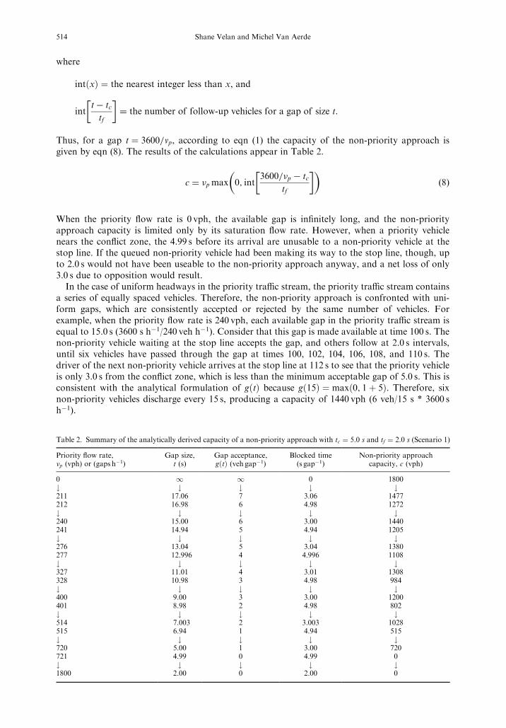
Thus, for a gap t � 3600=vp, according to eqn (1) the capacity of the non-priority approach isgiven by eqn (8). The results of the calculations appear in Table 2.

c � �p max 0; int3600=�p ÿ tc

tf

� �� 8�

When the priority ¯ow rate is 0 vph, the available gap is in®nitely long, and the non-priorityapproach capacity is limited only by its saturation ¯ow rate. However, when a priority vehiclenears the con¯ict zone, the 4.99 s before its arrival are unusable to a non-priority vehicle at thestop line. If the queued non-priority vehicle had been making its way to the stop line, though, upto 2.0 s would not have been useable to the non-priority approach anyway, and a net loss of only3.0 s due to opposition would result.

In the case of uniform headways in the priority tra�c stream, the priority tra�c stream containsa series of equally spaced vehicles. Therefore, the non-priority approach is confronted with uni-form gaps, which are consistently accepted or rejected by the same number of vehicles. Forexample, when the priority ¯ow rate is 240 vph, each available gap in the priority tra�c stream isequal to 15.0 s (3600 s hÿ1/240 veh hÿ1). Consider that this gap is made available at time 100 s. Thenon-priority vehicle waiting at the stop line accepts the gap, and others follow at 2.0 s intervals,until six vehicles have passed through the gap at times 100, 102, 104, 106, 108, and 110 s. Thedriver of the next non-priority vehicle arrives at the stop line at 112 s to see that the priority vehicleis only 3.0 s from the con¯ict zone, which is less than the minimum acceptable gap of 5.0 s. This isconsistent with the analytical formulation of g t� � because g 15� � � max 0; 1� 5� �. Therefore, sixnon-priority vehicles discharge every 15 s, producing a capacity of 1440 vph (6 veh/15 s * 3600 shÿ1).

Table 2. Summary of the analytically derived capacity of a non-priority approach with tc � 5:0 s and tf � 2:0 s (Scenario 1)

Priority ¯ow rate,�p (vph) or (gaps hÿ1)

Gap size,t (s)

Gap acceptance,g t� � (veh gapÿ1)

Blocked time(s gapÿ1)

Non-priority approachcapacity, c (vph)

0 1 1 0 1800# # # # #211 17.06 7 3.06 1477212 16.98 6 4.98 1272# # # # #240 15.00 6 3.00 1440241 14.94 5 4.94 1205# # # # #276 13.04 5 3.04 1380277 12.996 4 4.996 1108# # # # #327 11.01 4 3.01 1308328 10.98 3 4.98 984# # # # #400 9.00 3 3.00 1200401 8.98 2 4.98 802# # # # #514 7.003 2 3.003 1028515 6.94 1 4.94 515# # # # #720 5.00 1 3.00 720721 4.99 0 4.99 0# # # # #1800 2.00 0 2.00 0


Alternatively, the capacity can be derived by the transparency technique described by Plank(1982), in which the capacity is equal to the product of the transparency (the proportion of timethe priority tra�c stream is not blocking the non-priority approach) and the saturation ¯ow rateof the non-priority approach. Since 3.0 s are lost to the non-priority approach out of every 15 s, thenon-priority approach capacity is 1440 vph (12 s/15 s*1800 vph). This 3.0 s is referred to as theblocked time of the non-priority approach.

If one now considers a 1 vph increase to the priority ¯ow rate from 240 vph to 241 vph, each gapin the priority tra�c stream is now 14.94 s long (3600 s hÿ1/241 vph). As before, the non-priorityvehicle at the stop line accepts the gap which becomes available at time 100 s, and the next fournon-priority vehicles follow at intervals of 2 s. But, when the sixth non-priority vehicle arrivesat the stop line at time 110 s, only a 4.94 s lag is available, which must be rejected as it is lessthan the critical gap of 5.0 s. So only ®ve non-priority vehicles can accept each gap,g 14:94� � � max 0; 1� 4� �. Thus, with only a 1 vph increase to the priority ¯ow rate, the non-priority approach capacity has fallen abruptly from 1440 to 1205 vph, computed as either ®vevehicles accepting gaps every 14.94 s (5 veh/14.94 s*3600 s hÿ1), or 4.94 s of blocked time and 10 sof unblocked time every 14.94 s at the saturation ¯ow rate of 1800 vph(10 s/14.94 s*1800 vph).

As the priority ¯ow rate increases to 276 vph, the blocked time of the non-priority approachdecreases from 4.94 s to 3.04 s per available gap, allowing the non-priority approach capacityto increase. Although the gaps are smaller (13.04 versus 14.94 s), ®ve non-priority vehicles willstill be able to accept each gap, g 13:04� � � max 0; 1� 4� �. Since the gaps are arriving more fre-quently, the non-priority approach capacity increases linearly with the priority ¯ow rate, and theslope is equal to the number of vehicles accepting each gap in the priority tra�c stream. Even-tually, another drop in capacity will occur at a priority ¯ow rate of 277 vph, when only fourvehicles will be able to accept each 12.996 s gap, and the blocked time will increase to 4.996 s pergap.

This process of a gradual linear increase in the non-priority approach capacity, followed occa-sionally by abrupt decreases continues, until a priority ¯ow rate of 721 vph is reached. At thispoint each available gap is 4.99 s, which is too small for even a single non-priority vehicle to acceptit. The end points of these abrupt changes are listed in Table 2, and a graph of this discontinuousfunction is represented in Fig. 1.

4.2. Simulation resultsThe identical scenario to the one considered above was simulated using the gap acceptance

model imbedded in INTEGRATION. Results are presented in Fig. 1. It is clear that the simula-tion results of the non-priority approach capacity concur with the analytical calculations. It shouldbe noted that this graph was generated using 15min observations for each priority ¯ow rate.Caution should be exercised when interpolating between the sampled simulation results, since astraight line fails to capture the true stepwise nature of the function.

This scenario is most interesting from a theoretical standpoint, since the case of consistentand homogeneous drivers accepting uniform gaps is not realistic. However, this scenario doesserve as a good starting point to understand the fundamental operation of this supply±demandgap acceptance model. Given this base scenario, the implementation of stochastic demandfor gaps and/or random supply of gaps can now be considered, as is shown in subsequentsections.

5. SCENARIO 2: UNIFORM GAP SUPPLY AND PARTLY STOCHASTIC GAP DEMAND

The next step in the development of the model consisted of an analysis of the e�ect of a sto-chastic critical gap. Since the follow-up time remained uniform, the gap demand side of the modelcan only be considered partially stochastic.

5.1. ImplementationIn Scenario 2, non-priority drivers are still assumed to be consistent, but the homogeneity

assumption has been relaxed by modelling the critical gaps of all the non-priority drivers with alog-normal distribution, de®ned by the mean critical gap and COV. Each non-priority driver'scritical gap is assigned based on the driver's aggressiveness, with a more aggressive driver having a


smaller critical gap. Because the critical gap decay parameter is still 0.0, each driver's critical gapremains consistent for the entire duration of their front-of-queue position.

The log-normal distribution was selected to represent the probability density function of thecritical gap because it satis®es most of the characteristics as de®ned by Kyte et al., (1996).Although characteristic (1) is not satis®ed by the log-normal distribution since the minimum cri-tical gap is zero, the probability of very small critical gaps is relatively small. The log-normal dis-tribution is a good candidate for modelling the critical gap because it is mathematically simple andtractable.

In this scenario, the critical gaps of the non-priority vehicles were considered to ®t a log-normaldistribution with a speci®ed mean critical gap of 5.0 s and a COV which was varied from 0.0 to 0.5,which brackets the COVs that were found in the NCHRP Project 3-46 Working Paper no. 16(Tian et al., 1995).

5.2. Analytical modelThe probability distribution of the available gaps remained unchanged from Scenario 1, where

f t� � is de®ned by eqn (6). With stochastic gap-demand the front-of-queue non-priority driver willaccept an available gap of size t if his/her critical gap is smaller. Since the critical gap is log-nor-mally distributed among all drivers, the probability of the gap acceptance, i.e. P t > tc� �, can begiven by the cumulative distribution function of the log-normal distribution, H t� �. From Fig. 2 itcan be noted that as the critical gap COV increases, the distribution of H t� � becomes ¯atter andmore skewed.

If the front-of-queue vehicle does accept the available gap, then the next queued vehicle willadvance to the stop-line exactly 2.0 s later (tf � 2:0 s), and the probability of accepting the lag isH t� tfÿ �

. The probability of the nth queued vehicle accepting the lag is equal to H t� nÿ 1� �tfÿ �

,provided that all preceding vehicles do indeed accept the gap. Therefore, the number of vehiclesaccepting each gap can be given by

g t� � � H t� � �X1i�1

Yij�0

H t� j:tfÿ �" #

�9�

This formulation of g t� � assumes that each available gap can be treated as an independent event,an assumption that will be compared to the simulation results in the following section. FromFig. 3, it can be seen that the stepwise nature of g t� � is preserved for small critical gap COV, butg t� � becomes a smooth curve for COV greater than 0.3. Also, as the COV increases so does the

Fig. 1. Analytically derived and simulated non-priority approach capacity under uniform gap supply and deterministic gapdemand (Scenario 1: tc � 5:0 s; tf � 2:0 s).


likelihood of the occurrence that a preceding queued vehicle with a critical gap larger than the lagwill block all subsequent vehicles from accepting the lag. Consequently, the g t� � tends to decreasewith increasing critical gap COV.

Using eqn (1) the capacity can be analytically derived by substituting the functions f t� � and g t� �de®ned above. The curves in Fig. 4 show that the stepwise nature of the non-priority approachcapacity described in Scenario 1 is preserved for small critical gap COV; the curves becomesmooth for COV greater than 0.3. Also, the tails of the capacity curves for a priority ¯ow rateexceeding 720 vph (3600 s hÿ1/tc) correspond to the portion of g t� � where the available gap t issmaller than the critical gap, tc � 5:0 s. Finally, it should be noted that increases to the critical gapCOV result in increases to the non-priority approach capacity at high priority ¯ows and slightdecreases to the capacity at low priority ¯ows. The latter observation does not agree with Blu-menfeld and Weiss (1978, 1979), who found that relaxing the homogeneity assumption can result

Fig. 2. Probability of acceptance of the available gap t for the front-of-queue non-priority vehicle (Scenario 2:tc � 5:0 s; tf � 2:0 s).

Fig. 3. Mean number of non-priority vehicles that will accept an available gap t (Scenario 2: tc � 5:0 s; tf � 2:0 s).


in estimates of the non-priority approach capacity that are up to 15% smaller than the case ofhomogeneous drivers with deterministic critical gaps as in Scenario 1 (COV=0.0).

5.3. Simulation resultsFigure 5 shows 15 1-min observations of the non-priority approach for a series of priority ¯ow

rates. Non-priority drivers are assumed to be consistent and heterogeneous. The follow-up time is2.0 s, and the mean critical gap is 5.0 s with COV equal to 0.5.

When the priority tra�c stream is ¯owing uniformly, there is no variability in the priority ¯owrate from one 1-min observation to the next. Because vehicles are modelled discretely in thismicroscopic simulation, only an integer number of priority vehicles can be observed for a priority¯ow rate in any given time interval. For example, for a priority ¯ow rate of 400 vph, or 6.67vehicles per min, only 6 or 7 vehicles may be observed in any 1-min observation, corresponding to¯ows of 360 and 420 vph, respectively. So, in Fig. 5 there is no variability in the priority ¯ow rate(x-direction), although the 1-min priority ¯ow observations may appear in two columns since themeasurements were discrete.

If all of the non-priority vehicles reacted in the same way to the uniform available gap, thestepwise nature of Fig. 1 would be preserved. However, with a variable critical gap, non-priorityvehicles do not behave homogeneously, resulting in a variance in the non-priority approachcapacity from one 1-min observation to the next. In Fig. 5 with COV equal to 0. 5, variance aboutthe stepwise function was present in the y-direction, with the greatest variation for priority ¯owrates from 300 to 500 vph. This variation in the y-direction tends to smooth the stepwise functionseen in Fig. 1.

The non-priority approach has been modelled to operate under oversaturated conditions, so foreach priority ¯ow rate the average of the 15 1-min observations of non-priority ¯ow represents a15-min observation of the capacity. It is apparent from Fig. 4 that the 15-min, non-priorityapproach capacity is not the same as the analytically derived capacity. For priority ¯ow ratesgreater than 500 vph, the simulation capacity is smaller than the capacity derived by the analyticalprocedure because the simulation does not treat every available gap in the priority tra�c stream asan independent event. This discrepancy is zero for deterministic critical gaps (COV=0) andincreases with increasing COV.

In the analytical model, it is assumed that for each new gap in the priority tra�c stream anindependent critical gap is selected from the log-normal distribution. In the simulation, eachnon-priority driver must be served at the front of the queue before any subsequent non-priority

Fig. 4. Capacity for a non-priority approach facing a priority tra�c stream (Scenario 2: tc � 5:0 s; tf � 2:0 s).


vehicles can accept a gap. If a non-priority driver with a critical gap greater than the available gapreaches the front of the queue, that driver will act like a plug on the downstream end of the link,e�ectively blocking all ¯ow on the non-priority approach for the remainder of the 15-min simu-lation. This plug factor occurs when the front-of-queue driver has a critical gap that is larger thanthe available gap, which is more likely to occur when the priority ¯ow rate or the critical gap COVincrease.

The presence of the plug factor for the entire 15 min duration of the simulation accounted forthe non-priority approach capacity of 0 vph at priority ¯ow rates of 900 vph and greater (Fig. 4).In Fig. 5, for a priority ¯ow of 750 vph, six non-priority drivers accepted gaps during the®rst minute of simulation, producing data point (720 vph, 360 vph); 3 non-priority drivers acceptedgaps during the second 1-min observation, producing data point (780 vph, 180 vph); andno more gaps were accepted for the remainder of the simulation due to the plug factor. Thiscreated a 15-min observation of capacity equal to 36 vph, compared to the analytical estimate of487 vph.

The simulated values agree with Blumenfeld and Weiss (1978, 1979), except that the capacityreductions are often greater than 15% and they do not apply for all priority ¯ow rates. The impactof the plug factor would be reduced if the drivers behaved inconsistently, by modelling the criticalgap with decay. Then the front-of-queue vehicle would eventually discharge no matter how largethe initial critical gap was. To see the impact of the critical gap decay with strictly deterministiccritical gaps, see Velan and Van Aerde (1996a,b).

A second factor which causes non-priority approach capacity increases for small priority ¯owrates remains unexplained. It is clear that this factor has a greater impact on the non-priorityapproach capacity for increased critical gap COV. At the time of publication, the authors wereunable to explain the capacity increases, although there is a suspicion that the car-following logicis the cause of the discrepancy between the analytical estimates and simulation values.

6. SCENARIO 3: RANDOM GAP SUPPLY AND DETERMINISTIC GAP DEMAND

This third scenario considers all non-priority drivers to be consistent and homogeneous, butvariability is introduced into the headways of the priority tra�c stream. This scenario has beenmodelled extensively through analytical methods, and matches the assumptions of the 1994 HCM.The analytical capacity models discussed earlier by Harders (1976), Siegloch (1973) and Troutbeck(1986) are utilised in this section to verify the simulation results.

Fig. 5. Variability of the 15 1-min observations for gap acceptance with uniform gap supply and stochastic gap demand(Scenario 2: mean tc � 5:0 s, COV=0.5; tf � 2:0 s).


6.1. ImplementationThe INTEGRATION model permits the user to specify the level of randomness in the trip

departure headways from each trip origin as being from 0 to 100% random. If, for a ¯ow of900 vph, the randomness was speci®ed as 0%, the departure headways would all have a uniformlength of 4.0 s (3600 s hÿ1/900 vph). In contrast, if the model user requested 100% randomness, themean departure headway remains 4.0 s, but the standard deviation would be equal to the mean,according to the mathematical properties of the exponential distribution. For 50% randomness,each vehicle's departure headway consists of a constant portion equal to 2.0 s, plus a randomcomponent with a mean and standard deviation of 2.0 s.

As the priority vehicles with random headways travel along the priority approach from their triporigin, the distribution of headways may be a�ected by the prevailing microscopic car-followinglogic. This logic captures the relationship between each vehicle's speed with its individual headway(Van Aerde, 1995). During the simulation, each vehicle determines its speed based on the currentdistance headway each decisecond, according to the formula

hd � c1 � c2uf ÿ u

� c3u �10�

wherehd � distance headway (km)u � speed (km hÿ1)dimensionless constant, k � c1=c2 � 2uc ÿ uf

ÿ �= uf ÿ ucÿ �2

®rst variable distance headway constant km2 hÿ1ÿ �

; c2 � 1= dj k� 1=ufÿ �ÿ �

®xed distance headway constant (km), c1 � kc2second variable distance headway constant hÿ1

ÿ �; c3 � uÿ1c ÿc1 � uc=qc ÿ c2= uf ÿ uc

ÿ �ÿ �¯ow at capacity, qc � 1800 vphfree speed, uf � 60 km hÿ1

speed-at-capacity, uc � 55 km hÿ1

jam density, dj � 140 veh kmÿ1

The distinction between the randomness of the departure headways of the priority tra�c streamand a platooned priority tra�c stream may need clari®cation. Velan and Van Aerde (1996a) con-sidered platooned ¯ow due to upstream signals separately from randomness of the departureheadways of the priority tra�c stream.

6.2. Simulation resultsAs a result of the car-following logic, vehicles that start with larger than average headways at

the upstream end of the priority approach, travel at a somewhat greater speed, thereby reducingtheir headway relative to the preceding vehicle on the link. In contrast, vehicles that start their tripwith a smaller than average headway will initially reduce their speed, which in turn increases theirheadway relative to the preceding vehicle on the link. The impact of the former gap-shrinkinge�ect was minimised by specifying a speed-at-capacity (55 kmhÿ1) that was close to the free-speed(60 kmhÿ1) and by limiting the priority approach to 500m in length. The latter gap-expandinge�ect created a noticeable change in the proportion of small headways in the priority tra�cstream, as seen in Fig. 6.

For a priority ¯ow rate of 900 vph and 100% random departure headways, Fig. 6 displays (a)the cumulative departure headway distribution of the priority tra�c stream 500m upstream of theunsignalised intersection and (b) the cumulative arrival headway distribution of the priority tra�cstream at the unsignalised intersection, i.e. after the e�ects of car-following on the priorityapproach. Fig. 7 shows the same cumulative headway distributions for a ¯ow of 1740 vph and100% randomness, which is close to the priority approach capacity of 1800 vph.

The departure headways tend to follow the negative exponential distribution quite closely, witha mean headway of 4.0 s for priority ¯ow 900 vph (3600 s hÿ1/900 vph=4.0 s) and mean headway2.07 s for priority ¯ow 1740 vph (3600 s hÿ1/1740 vph=2.07 s). The car-following logic eliminatedall headways smaller than the minimum time headway of 2.0 s (1=qc), and increased the proportionof headways greater than 2.0 s.


The arrival headways tend to follow the Cowan M3 distribution, a dichotomised distribution inwhich a proportion of the vehicles travel in bunches and the remaining vehicles travel with freeheadways corresponding to a shifted negative exponential distribution. The probability distributionfunction f t� � and the cumulative distribution function F t� � for the Cowan M3 distribution are

f t� � �0 for t < tm1ÿ � for t � tm�leÿl tÿtm� � for t < tm

8<: �11�

F t� � � 0 for t < tm1ÿ �eÿl tÿtm� � for t5tm

��12�

where �; l and tm are as de®ned previously.

Fig. 6. Distribution of departure and arrival headways in the priority tra�c stream at a priority ¯ow rate of 900 vph.

Fig. 7. Distribution of departure and arrival headways in the priority tra�c stream at a priority ¯ow rate of 1800 vph.


The Cowan M3 distribution was calibrated to the simulation arrival headways by ®rst settingtm, the minimum inter-vehicle tracking headway of the priority vehicles, to the inverse of the ¯owat capacity (1=qc). Then �, the proportion of priority vehicles travelling with headways greaterthan tm, was adjusted until the Cowan M3 cumulative distribution function visually matched thesimulation cumulative arrival headways. The calibrated values of � were 0.45 for 900 vph and 0.07for 1740 vph, meaning that 55 and 93% of the priority vehicles were travelling at the minimumheadway, respectively.

As seen in Figs 6 and 7, the exponential distribution, which is used to re¯ect the headway dis-tribution in the Harders (1976) and Siegloch (1973) models, does not account for a minimum fol-lowing distance. Clearly, the simulated arrival headway distribution does not ®t the exponentialdistribution for any arrival headway smaller than 10 s. In the simulation, the minimum headwayactually has an associated variability which would cause the arrival headway distribution to better®t the more realistic Cowan M4 distribution (Cowan, 1975). Since all available gaps that aresmaller than the critical gap will be rejected by the non-priority vehicles, obtaining the correctdistribution for the very small headways in the priority tra�c stream is not crucial anyway.

Fig. 8 provides a series of curves which represent the capacity of the non-priority approach forvarying levels of randomness in the departure headways of the priority tra�c stream. It can benoted that an increase in the randomness of headways in the priority tra�c stream producedincreases in the capacity of the non-priority approach. Speci®cally, compared to uniform priority¯ow as was the case in Scenario 1 (0% randomness), on average the non-priority approach capa-city increased by 35 vph for 25% randomness, by 80 vph for 5% randomness, by 135 vph for 75%randomness, and by 175 vph for 100% randomness. While the capacity of the non-priorityapproach was reduced by the presence of smaller than average gaps, this reduction was more thano�set by the greater number of follow-up vehicles which would accept each large gap.

The Troutbeck (1986), Harders (1976) and Siegloch (1973) capacity models were used to esti-mate the non-priority approach capacity for the case of 100% random departure headways, thecase where the arrival headways will most closely match the exponential distribution. TheTroutbeck model assumes that the arrival headways of the priority tra�c stream, which are alsothe available gaps, can be represented by the Cowan M3 distribution, which must be calibrated forvarying priority ¯ow rates as was done above. Rather than calibrating a for all simulated priorityarrival headways, the value of � was estimated by linear interpolation between intercepts (0 vph,1.00) and (1800 vph, 0.00), and the previously calibrated points (900 vph, 0.55) and (1740 vph,0.07).

These results match the Troutbeck model more closely than the estimation of the capacity fromthe Harders and Siegloch models. Compared to 100% random ¯ow, on average the non-priority

Fig. 8. Impact of randomness in the departure headways in the priority tra�c stream on the non-priority approach capacitywith uniform gap demand (Scenario 3: tc � 5:0 s; tf � 2:0 s).


approach capacity was 30 vph di�erent from the Troutbeck model's estimation, whereas theHarders and Siegloch models had average discrepancies of 129 vph and 135 vph, respectively. Inthe Harders and Slegloch models, the use of the exponential distribution to represent the headwaydistribution of the priority tra�c stream permits impossibly small headways; consequently, largegaps in the priority tra�c stream become available to the non-priority vehicles, even at priority¯ow rates that exceed the priority approach's saturation ¯ow rate. This explains the asymptoticbehaviour of the Harders and Siegloch models along the positive x-axis.

The apparent variability in the 1-min observations should be addressed at this time. As ran-domness of the non-priority departure headways was increased, the variance of the priority arrivalrate increased for the sample of 15 1-min observations. In Fig. 9, one may note that data pointswith the same speci®ed non-priority ¯ow rate often have di�erent observed non-priority ¯ow rates,and hence have di�erent x-coordinates. As a result of the variability in headways of the prioritytra�c stream, both small and large gaps became available to the non-priority vehicles. The num-ber of non-priority vehicles, which accepted each particular gap, depended only on the size of theavailable gap, since the critical gap and follow-up time were held constant. The apparent varia-bility in the y-direction is somewhat misleading. If an observation was made for each availablegap, then all of the data points would fall exactly on the discontinuous function presented in Fig. 1.However, each data point is a 1-min aggregation, thereby creating the appearance of variability inthe y-direction in Fig. 9.

7. SCENARIO 4: RANDOM GAP SUPPLY AND PARTLY STOCHASTIC GAP DEMAND

During the following analysis, the level of randomness in departure headways in the prioritytra�c stream was ®xed at 100%, while the critical gap COV was varied from 0.0 to 1.0 (consistentand heterogeneous non-priority drivers). As discussed in Scenario 2, the plug factor tends todecrease the non-priority approach capacity, when a vehicle requiring a large critical gap reachesthe front of the queue. The increases in the non-priority approach capacity for low priority ¯owrates and large critical gap COV remain unexplained.

As shown on Fig. 10, an increased critical gap COV created a more pronounced S-shaped curve.The intercepts remained ®xed because the variability of the critical gap and the degree of ran-domness in the priority ¯ow have no impact on the non-priority approach capacity when thepriority ¯ow is 0 vph or if the available gaps are equal to the saturation ¯ow headway of 2 s(3600 s hÿ1/1800 vph) on the priority approach.

Fig. 9. Variability of 1-min observations of non-priority approach capacity for 100% random departure headways withuniform gap demand (Scenario 3: tc � 5:0 s; tf � 2:0 s).


One important di�erence between this Scenario 4 and Scenario 2 is that the x-intercept is muchlarger in Scenario 4. Potentially, with uniform priority ¯ow in Scenario 2, a plug could completelystop the ¯ow of the non-priority approach. However, with random headways in the priority tra�cstream it was found that eventually a large gap arrives, allowing the plug to become dislodged.

As discussed in Scenario 3, the random priority ¯ow creates variability in the x-direction for the1-min observations. As the critical gap COV increased in this scenario, the variability of the 1-minobservations of approach capacity also increased in the y-direction due to the plug factor, asexplained in Scenario 2. Finally, variability in both the x-direction and y-direction for COVgreater than 0.1 has su�ciently obscured the stepwise function such that interpolation between thedata points can be regarded as a valid estimate of the average approach capacity.

8. SCENARIO 5: RANDOM GAP SUPPLY AND STOCHASTIC GAP DEMAND

In this ®nal scenario, a truly random supply and stochastic demand gap acceptance model isformulated. In addition to random departure headways in the priority tra�c stream and log-nor-mally distributed critical gaps, a stochastic follow-up time tf

ÿ �is introduced.

8.1. ImplementationAfter a non-priority vehicle accepts a gap and crosses the stop line, the next vehicle in queue

proceeds to the stop line at the saturation ¯ow rate qc� �, speci®ed as 1800 vph. Before reaching thestop line, the driver is unable to accept gaps in the priority tra�c stream, e�ectively suspending thegap acceptance process. The time required for that vehicle to proceed to the stop line, commonlyreferred to as the follow-up time, is equal to the saturation ¯ow rate headway (1=qc) of 2.0 s.Alternatively, the same time duration may be thought of as the time required for a vehicle to travelthe distance of one jam density headway (1=dj) at the speed-at-capacity (uc) of the approach,tf � 1

qc� 1

dj�uc. Therefore, any variability in the jam density or the speed-at-capacity is re¯ectedindirectly in the follow-up time.

INTEGRATION permits the speci®cation of a vehicle speed variability factor, which results ina stochastic speed±headway relationship that dictates the car-following behaviour. The COV ofthe follow-up time is equal to the COV of the speed-at-capacity.

8.2. Simulation resultsThe results that are presented next have 100% random headways in the priority tra�c stream,

and critical gaps that are log-normally distributed, with a mean of 5.0 s and COV set equal to 0.3.

Fig. 10. Impact of the critical gap COV on the non-priority approach capacity with 100% random departure headways inthe priority tra�c stream (Scenario 4: mean tc � 5:0 s; tf � 2:0 s).


The vehicle speed variability was modelled using a COV set equal to 0.25 and 0.50, and both thenormal and log-normal distributions were considered. Data from NCHRP Project 3-46 (Tian etal., 1995) con®rm that these values and ranges are reasonable. The simulation results are presentedin Fig. 11.

Increases in the COV of the follow-up time were shown to have no appreciable impact on thenon-priority approach capacity for both the normal and log-normal distributions. Instead, it wasfound that when a vehicle with a large follow-up time becomes the front of the queue, it may notreach the stop line with enough time to accept a gap, whereas a vehicle with the mean follow-uptime may have been able to discharge. Likewise, a vehicle with a follow-up time smaller than themean may accept a gap that produces an increase in the non-priority approach capacity. However,unlike other pairs of asymmetric, o�setting factors in gap acceptance, these two factors appear toexactly balance each other. In e�ect, the gap acceptance process is suspended while the follow-uptime occurs. Whether these suspensions occur in equal units of 2.0 s, for example, or as variabletime lengths with an average of 2.0 s does not change the sum of the time intervals when gapacceptance is suspended.

Therefore, the reduction in the capacity of the non-priority approach (y-intercept of Fig. 11),which is attributable to the follow-up time, is considered to be dependent only on the mean followup time and not its distribution. Nevertheless, this feature should still be incorporated into this gapacceptance model since it captures a realistic part of the variability in driver behaviour. Also, thevariability of the follow-up time may become signi®cant as the interactions with other factors areconsidered.

9. CONCLUSIONS

Analysis of all ®ve scenarios in the development of the gap acceptance model with random gapsupply and stochastic gap demand yielded the following conclusions.

A gap acceptance model with uniform gap supply and deterministic gap demand (Scenario 1)has a stepwise relationship between non-priority approach capacity and priority ¯ow rate, with novariability from one 1-min observation to the next. A gap acceptance model with uniform gapsupply and partly stochastic gap demand (Scenario 2) has no variance in the priority ¯ow rate, butit does have variability in the non-priority approach capacity from one 1-min observation to thenext. In Scenario 2, the plug factor decreased the non-priority approach capacity, especially atlarge priority ¯ow rates, which is in agreement with Blumenfeld and Weiss (1978, 1979), exceptthat the capacity reductions are often greater than 15% and they do not apply for all priority ¯owrates.

Fig. 11. Impact of the distribution and variance of the follow-up time on the non-priority approach capacity with 100%random departure headways in the priority tra�c stream and stochastic critical gap (Scenario 5: mean tc � 5:0 s, COV=0.3;

mean tf � 2:0 s).


A gap acceptance model with random gap supply and deterministic gap demand (Scenario 3)has variability in the priority ¯ow rate. The deterministic critical gap and follow-up time result inthe same stepwise function g t� � for the number of vehicles accepting a gap of size t. Overall, thenon-priority approach capacity increases for increasing randomness in the headwaysÐas opposedto uniform headwaysÐof the priority tra�c stream. INTEGRATION's arrival headway dis-tribution was a better ®t to the Cowan M3 headway distribution than the exponential distribution;consequently, the non-priority approach capacity predicted by the simulation matched the Trout-beck model more closely than the Harders model or the Slegloch model.

A gap acceptance model with random gap supply and partly stochastic gap demand (Scenario 4)has variability in both the priority ¯ow rate and the non-priority approach capacity. The varia-bility is su�cient to produce a smooth curve of non-priority approach capacity vs priority ¯owrate. In Scenario 4, the plug factor decreased the non-priority approach capacity for priority ¯owsgreater than 600 vph, with more impact as the critical gap COV was increased. The addition of astochastic follow-up time (Scenario 5) had no impact on the mean non-priority approach capacity,but the variability which was introduced was more representative of driver behaviour. Analyticalmodels for Scenarios 4 and 5 were found to be cumbersome and impractical.

10. RECOMMENDATIONS

Most analytical models of non-priority approach capacity assume that the impacts of consider-ing drivers to be homogeneous and consistent are equal and o�setting. INTEGRATION's criticalgap decay feature can model inconsistent drivers. Capacity estimates with realistic headway dis-tributions of the priority tra�c stream and with various combinations of driver inconsistency andheterogeneity could be used to test the assumption made by the analytical models. Before this canbe done, the capacity increases (Scenarios 2 and 4) at small priority ¯ow rates for increasing cri-tical gap COV must be corrected or explained.

The simulation model should be tested to verify the non-priority approach capacity for a rangeof intersection control types and diverse geometric combinations. This simulation model should beapplied to scenarios that are di�cult to model analytically, for example intersections with twostage gap acceptance. Also, multiple con¯icting ¯ows should be considered to assess the resultingimpedance and compare those values to the HCM. The evaluation of capacity and estimates ofdelay should be compared directly to ®eld data to verify the accuracy of this gap acceptancemodel. This comparison will reveal the most critical calibration factors when this model is appliedin the ®eld.

Once the model has been more thoroughly veri®ed, validated and calibrated, it could be used toassess at which critical volumes each intersection control type operates best. From this assessment,which would be performed by one consistent tool, guidelines could be developed which indicatethe appropriate control type at a given intersection, and the associated implications on delay, fuelconsumption and vehicle emissions.

AcknowledgementsÐSpecial thanks to Bruce Robinson from Kittelson and Associates, Inc., as well as the anonymousreviewers of this paper for their comments.

REFERENCES

Ashworth, R. (1970) The analysis and interpretation of gap acceptance data. Transportation Research 4, 270±280.Ashworth, R. and Bottom, C. G. (1977) Some observations of driver gap-acceptance behavior at a priority intersection.

Tra�c Engineering and Control 18, 569±571.Blumen®eld, D. E. and Weiss, G. H. Weiss (1978) Statistics of delay for a driver population with step and distributed gap

acceptance functions. Transportation Research 12, 423±429.Blumen®eld, D. E. and Weiss, G. H. (1979) The e�ects of gap-acceptance criteria on merging delay and capacity at an

uncontrolled junction. Tra�c Engineering and Control 20, 16±20.Brilon, W. (ed.) (1988) Intersections Without Tra�c Signals, Proceedings of an International Workshop. Springer-Verlag,

Berlin.Brilon, W. (ed.) (1991) Intersections Without Tra�c Signals II, Proceedings of an International Workshop. Springer-Verlag,

Berlin.Brilon, W. (1995) Delays at oversaturated unsignalised intersections based on reserve capacities. Presented at the Trans-

portation Research Board 75th Annual Meeting, Paper no. 950013, Washington, DC.Cowan, R. J. (1975) Useful headway models. Transportation Research 9, 371±375.


Cowan, R. J. (1987) An extension of Tanner's results on uncontrolled intersections: clari®cation of some issues. QueuingSystems 1, 249±263.

Drew, D. R. (1968) Tra�c Flow Theory and Control. McGraw-Hill, New York.Grossmann, M. (1988) KNOSIMOÐA practical simulation model for unsignalised intersections. Intersections Without

Tra�c Signals, Proceedings of an International Workshop, pp. 263±273. Springer-Verlag, Berlin.Harders, J. (1968) The capacity of unsignalised urban intersections. Schriftenreihe Strassenbau and Strassenverkehrstechnik

76 (In German).Harders, J. (1976) Critical gaps and move up times as the basis of capacity calculations for rural roads. Strassenban and

Strassenverherstechnic 216 (In German).Hewitt, R. H. (1992) Using Probit Analysis with Gap Acceptance Data. Department of Civil Engineering of Glasgow.Kittelson, W. K. and Vandehey, M. A. (1991) Delay e�ects on driver gap acceptance characteristics at two-way stop-con-

trolled intersections. Transportation Research Record 1320, 154±159.Kyte, M., Clemow, C., Mahfood, N., Lall, B. K. and Khisty, C. J. (1991) Capacity and delay characteristics of two-way

stop-controlled intersections. Transportation Research Record 1320, 160±167.Kyte, M., Tian, Z., Mir, Z., Hameedmansoor, Z., Kittelson, W., Vandehey, M., Robinson, B., Brilon, W., Bondzio, L.,

Wu, N. and Troubeck, R. (1996) Capacity and Level of Service at Unsignalised Intersections. National CooperativeHighway Research Program Project 3-46. Transportation Research Board, National Research Council, Washington,DC.

Plank, A. W. (1982) The capacity of a priority intersection-two approaches. Tra�c Engineering and Control 23, 88±89.Ra�, M. S. (1950) A Volume Warrant for Urban Stop Signals. The Eno Foundation for Highway Tra�c Control, Sauga-

tuck, Connecticut.Siegloch, W. (1973) Capacity calculations for unsignalised intersections. Schriften-reihe Strassenbau and Strassenverkehr-

stechnik 76, Bonn, West Germany. (In German).Special Report 209: Highway Capacity Manual (1994) Transportation Research Board, National Research Council,

Washington, DC.Tanner, J. C. (1967) The capacity of an uncontrolled intersection. Biometrika 54, 657±658.Tian, Z. Troutbeck, R. Brilon, W. Robinson, B. and Kyte, M. (1995) Estimating critical gaps and follow-up times for

TWSC intersections. National Cooperative Highway Research Program Project 3-46, working paper 16, TransportationResearch Board, National Research Council, Washington, DC.

Troutbeck, R. J. (1986) Average delay at an unsignalised intersection with two major streams each having a dichotomisedheadway distribution. Transportation Science 20, 272±286.

Troutbeck, R. J. (1992) Estimating the critical acceptance gap from tra�c movements. Research report 92-5.Van Aerde, M. and Yagar, S. (1988) Dynamic integrated freeway/tra�c signal networks: problems and proposed solutions.

Transportation Research-A 22, 435±443.Van Aerde, M. and Yagar, S. (1988) Dynamic integrated freeway/tra�c signal networks: a routing-based modeling

approach. Transportation Research-A 22, 445±453.Van Aerde, M. (1995) A single regime speed-¯ow-density relationship for freeways and arterials. Transportation Research

Board 75th Annual Meeting, Washington, DC.Van Aerde, M. and Hellinga, B. (1996) INTEGRATION: overview of current simulation features. Transportation

Research Board 75th Annual Meeting. Paper no. 961082, Washington, DC.Velan, S. and Van Aerde, M. (1996a) Relative e�ects of opposing ¯ow and gap acceptance characteristics on approach

capacity at uncontrolled intersections. Transportation Research Board 75th Annual Meeting, Washington, DC.Velan, S. and Van Aerde, M. (1966) Gap acceptance and approach capacity at unsignalised intersections. ITE Journal 66(3),

40±45.


The impact of driver and flow variability on capacity estimates of permissive movements 1 Funding...

Documents

Transcript of The impact of driver and flow variability on capacity estimates of permissive movements 1 Funding...