1University of California, Berkeley and Santa Clara University, respectively. We thankPipat Luengnaruemitchai and Justin Jones for research assistance and Michael Bordo and CharlesGoodhart for comments.

2The classic account is of course Friedman and Schwartz (1963).

3We have in mind Temin (1976), although he clearly had predecessors in the 1940s and1950s.

4See for example Hamilton (1987) and Eichengreen (1988).

5An early example is Bernanke and James (1991).

1

The Great Depression as a Credit Boom Gone Wrong1

Barry Eichengreen and Kris MitchenerMay 2003

1. Introduction

The Great Depression is the macroeconomist�s Rorschach test. Every generation views

the Depression through the lens of its own particular (conscious or subconscious) concerns. In

the 1960s monetary economists, worried by mounting inflationary pressures and convinced that

mismanagement of the monetary aggregates could destabilize otherwise stable economies,

portrayed the Depression as a consequence of ill-advised central bank policies.2 In the 1970s

apostles of the neo-Keynesian synthesis, convinced that animal spirits were responsible for

cyclical fluctuations, rewrote the history of the Depression in terms of the instability of

consumption and investment spending.3 In the 1980s economists impressed by the growing

influence of international trade and investment again rewrote that history, this time in terms of

the instability of the international monetary and financial system.4 And, in the 1990s, a decade of

financial instability, they portrayed the Depression as one big banking crisis.5

In the aftermath of the credit boom and bust of the 1990s, there is thus a temptation to

6This may be labeled for present purposes as the BIS interpretation. See for exampleBorio and Lowe (2002), Borio, Fufine and Lowe (2001), and Vila (2002).

2

rewrite the history of the Great Depression as a credit boom gone wrong. The credit-boom

interpretation of macroeconomic cycles, as informed by the experience of the 1990s, goes

something like this.6 There is first an upswing in economic activity. As the economy expands,

banks and financial markets provide an expanding volume of credit to finance the growth of both

consumption and investment. Whether because the exchange rate is pegged or for other reasons

such as a positive supply shock, upward pressure on wholesale and retail prices is subdued.

Hence, the central bank has no obvious reason to tighten and stem the growth of money and

credit, leading to a further expansion of output and further increase in credit, which feeds on

itself.

Higher property and securities prices encourage investment activity, especially in interest-

rate-sensitive activities like construction. But, as lending expands, increasingly speculative

investments are underwritten, and the quality of bank loans declines. The demand for

speculative investments rises with the supply, since, in the prevailing environment of stable

prices, nominal interest rates and therefore yields on safe assets are low. In search of yield,

investors dabble increasingly in risky investments. Their appetite for risk is stronger still to the

extent that these trends coincide with the development of new technologies, in particular network

technologies of promising but uncertain commercial potential.

Eventually, all this construction and investment activity, together with the wealth effect

on consumption, produces signs of inflationary pressure, and the central bank begins to tighten.

The financial bubble is pricked and, as asset prices decline, the economy is left with an overhang

7That this is the right story and the right policy implication is, of course, not universallyagreed. On the controversy over the role of asset prices in the conduct of monetary policy, seeBullard and Schaling (2002), Bernanke and Gertler (1999), Cecchetti, Genberg, Lipsky andWadhwani (2000), Filardo (2000) and Goodhart (2000). This same debate figures prominently inthe literature on the Great Depression, as we describe momentarily.

3

of ill-designed, non-viable investment projects, distressed banks, and heavily indebted

households and firms, aggravating the subsequent downturn.

No single policy implication necessarily flows from this story, but some readers will

conclude that the monetary authorities should respond preemptively to the rise in asset prices.

Central banks should not be misled, in this view, by the disconnect between asset price inflation

and consumer price inflation. They should respond to the inflation of asset prices by reining in

credit and preventing the expansion from taking a form that ultimately renders subsequent

difficulties more severe.7

This tale from the 1990s has obvious appeal for historians of the 1920s. The 1920s was a

decade of expansion, reflecting recovery from World War I, new information and

communications technologies like radio, and new processes like the motor vehicle production

using assembly-line methods. In the United States, a feature of the expansion was abundant

supplies of credit, reflecting the ample gold reserves accumulated by the country during World

War I, the stance of Federal Reserve policies, and financial innovations ranging from the

development of the modern investment trust to consumer credit tied to purchases of durable

goods such as automobiles. Credit fueled a real estate boom in Florida in 1925, a Wall Street

boom in 1928-9, and a consumer durables spending spree spanning the second half of the 1920s.

That these booms developed under the fixed exchange rates of the gold standard meant that they

generated little inflationary pressure at home and that their effects were transmitted to the rest of

8This is only one conceivable implication in the sense that other authors who insist thatthe central bank should have focused exclusively on wholesale and retail price inflationcharacterize Fed policy as too tight rather than too loose in the late 1920s (see e.g. Meltzer 2003).

4

the world. Absent overt signs of inflation, the Fed had no reason to raise the official short-term

rate.

Over time, signs developed of a deterioration in the quality of projects � as in the Florida

land boom of the mid-1920s � and a growing prevalence of malfeasance and graft, evident in the

activities of Charles Ponzi in Florida, Clarence Hatry in London, and Ivar Kreuger in Stockholm.

This in turn created concern among central banks about the effects of asset-price inflation on the

economy, leading them eventually to tighten. Banks passed along the higher cost of additional

reserves to their borrowers, and, in the U.S. case, they further felt direct pressure to limit their

lending to securities market participants. Borrowers with highly leveraged positions, stock

market positions in particular, experienced financial strain, leading them to compress their

spending, and consumption and investment turned down. Ultimately, the resulting deflation

became sufficiently severe to threaten the stability of the financial system and the economy more

generally. One conceivable implication of this account is that the Fed should have prevented the

development of speculative excesses by maintaining a tighter policy stance, despite the absence

of overt signs of inflation.8 Doing so might have prevented or at least slowed the build-up of

speculative excesses that became sources of severe financial stress when the economy eventually

turned down. By limiting the extent of the credit boom in the late 1920s, this preemptive policy

would have reduced the severity of the Great Depression in the early 1930s.

This �new view� has at least two significant precursors in the literature on the interwar

period: the Austrian interpretation of the Great Depression, and the view that attributes the

9�At least� alludes to the fact that there is also the Liquidationist School in the UnitedStates (DeLong 1990, Meltzer 2003), which has much in common with the Austrian view, andthe French interpretation of the Depression (Moure 2002), which also echoes the Austrian view. And of course there is the Minsky (1986)-Kindleberger (1978) interpretation of booms, panicsand crashes, largely inspired by the experience of the Great Depression, in which the endogenousresponse of credit plays an integral role. We return to this below. In addition, to the extent thatthe credit boom of the �twenties manifested itself in rising property prices and unsustainableconstruction activity, there are also parallels with the earlier views of Henry George (1879). TheGeorgist view acknowledges the role of credit in fueling speculation and argues in particular that�speculative advances in land values� are central to causing business cycles. Rising rents inducespeculators to purchase land for capital gains rather than for current use, which in turn causes sitevalues to rise in dramatic fashion, setting off further rounds of speculation that eventually erodethe profits of firms by increasing mortgage costs and rents. Eventually, these burdens reducenew investment and aggregate demand, and bring forth a recession. In effect, the high price ofland acts to �lock out labor and capital by landowners� (George, 1879, p.270). Only as this cycleis unwound and land prices and rents fall does investment pick up again, allowing the economyto recover toward full employment. The Georgist view differs in terms of the timing of the riseof speculation and the decline of investment and economic activity; George and his followerssaw the latter as starting to decline even while the property boom was still underway (albeit in itslate states), where the views emphasized in the text see investment and demand generally asdeclining only after the bubble bursts.

10In this respect there are parallels between the Austrian model and Keynes� Treatise onMoney (1930), a fact appreciated by Keynes and emphasized by Laidler (1999). In addition,there are parallels between the Austrian view and the modern debate about whether central banksshould simply concentrate on commodity price inflation or also be concerned about asset priceinflation. We return to this below.

11Mises and Hayek did not typically distinguish between asset and commodity priceinflation, but when they did, they minimized the relevance of the distinction. Laidler (1999)argues that Hayek in particular saw the rate of interest (which affected the evolution of assetprices) as the key price (since it was what equilibrated or disequibrated saving and investment);by this interpretation, asset price inflation in fact mattered more than commodity price inflation.

5

Depression to the stock market boom and crash.9 The Austrian view, with roots in the work of

Ludwig von Mises (1924) and Friedrich von Hayek (1925), focused on the divergence between

the market rate of interest and the natural rate of interest.10 When the market rate fell below the

natural rate, Mises and Hayek argued, prices rose and investment boomed.11 The source of that

divergence, according to Mises, was the banking system, freed from the disciplining influence of

12Although Mises referred not to the build-up of indebtedness but to the inadequacy ofsaving, his point was essentially the same.

13In Hayek�s (1932, p.44) words, �any attempt to combat the crisis by credit expansionwill...not only be merely the treatment of symptoms as causes, but may also prolong thedepression by delaying the inevitable real adjustments.�

14The Austrian views of the early Robbins were kept alive by, inter alia, Rothbard (1975).

6

the classical gold standard. Excessive credit creation by banks, both central and commercial,

encouraged asset price inflation, fueling consumption and investment. The longer that asset-

price inflation was allowed to run, the greater were the depletion of the stock of sound

investment projects and the accumulated financial excesses.12 Moreover, the more severe

became the subsequent downturn. The credit boom thus contained the seeds of the subsequent

crisis. The policy implication was that countries should avoid monetary arrangements that

allowed significant divergences between the market and natural rates of interest (in particular, a

gold standard of the rigid prewar variety was preferable to the more malleable interwar vintage)

and that they should allow the downturn to proceed in order to purge unviable firms and

investment projects from the economy, thereby clearing the way for sustainable recovery.13

The definitive application of the Austrian model to the Great Depression was by Lionel

Robbins (1934) in a book largely responsible for popularizing the name now attached to this

episode.14 Robbins attributed the Depression of the 1930s to the unsustainable credit expansion

of the 1920s. Blame for that credit expansion he in turn laid at the doorstep of the Federal

Reserve System, which had kept interest rates below the natural rate for too long in the hope that

low rates might help Britain surmount its balance-of-payments problems and thereby solidify the

reconstructed gold exchange standard, and ultimately on the doorstep of the new gold standard

15As Robbins (1934, pp.41-2) put it, �Sooner or later the initial errors are discovered. And then starts a reverse rush for liquidity. The Stock Exchange collapses. There is a shortageof new issues. Production in the industries producing capital-goods slows down. The boom is atan end.�

16Robbins (1934), p.62.

17There is clear overlap between the Austrian view and the bubble interpretation; thus,Robbins points to the run-up in stock prices in the United States as a prominent consequence ofthe expansion of bank credit in the 1920s.

7

itself, which gave central banks more leeway to manipulate policy. This divergence between

market and natural rates stimulated the provision of bank credit, allowing the development of

financial excesses which, when revealed, led unavoidably to the downturn, the financial crisis,

and the Depression.15 Central banks were misled into inaction by the tendency for the credit

boom to stimulate not just aggregate demand but also aggregate supply (through increased

production of consumption goods and growing investment in capacity). But the quality of much

of that additional capacity was inferior. The credit boom had �the qualitative effect of providing

a favourable atmosphere for the fraudulent operations of sharks and swindlers,� which meant that

neither the expansion of supply nor the high level of asset prices was sustainable and only set the

stage for a disruptive crisis.16 Moving from diagnosis to prescription, Robbins recommended

against monetary and fiscal measures to counter the downward spiral, insisting that the economy

needed to be cleansed of financial and nonfinancial excesses to set the stage for a sustainable

recovery.

The other significant precursor blames the Great Depression on a bubble in the stock

market.17 Galbraith (1972) describes how what he characterizes as a bubble developed in

response to the combination of financial innovation and ample credit in an unregulated financial

18Eventually they also borrowed from corporations, as nonbank firms shifted funds intothe money market in response to rising demand.

19Estimates of asset returns are from Smiley and Keehn (1988).

20Santoni and Dwyer (1989) and Meltzer (2003) argue that this evidence is not necessarilyconsistent with the existence of a bubble. Meltzer, similarly, rejects the bubble interpretation onthe grounds that the rise in equity valuations in the late 1920s was not out of proportion to therise of earnings. From the present point of view, the issue is not simply whether earnings rose asrapidly as equity prices in these years but also whether the magnitude of capital gains createdexpectations of further capital gains which were less obviously justifiable by fundamentals.

8

environment. Investor enthusiasm was grounded in the promise of new information and

communications technologies; Radio Corporation of America (RCA) was the 1920s equivalent

of America On Line (AOL). (Figure 1, which superimposes the price of AOL shares in the 1990s

on the price of RCA shares in the 1920s, illustrates the parallel.) In addition, however, the

enthusiasm of investors was importantly fueled by financial innovation and ample supplies of

credit. The 1920s saw the spread from Britain to America of the investment trust, an entity that

had existed in England for half a century, but now in a variant that allowed the manager of the

trust to buy stocks on margin, raising the fund�s leverage. This anticipates a theme we develop

later in the paper � that the consequences of credit expansion and the extent of the boom thereby

induced may depend on the structure and regulation of the financial sector. Individual investors

were similarly permitted to purchase shares for 10 per cent down, borrowing from their brokers

who in turn borrowed from the banks.18 Capital gains on the representative portfolio of nearly 30

per cent in calendar year 1927 and more than 30 per cent in calendar year 1928 encouraged the

belief that stocks could only go up.19 Share prices and dividends had broadly moved in tandem

through the first quarter of 1928. They diverged thereafter, in response it has been suggested to

the Fed�s cut in interest rates late in the preceding year.20 (See Figure 2.)

21Others argued that the authorities should resist the temptation to stabilize commodityprices (which were now falling rapidly, doing considerable damage to the economy), much lessasset prices, for fear that this would only encourage the development of another, even largerbubble that would be followed by a still more devastating crash. Thus, Robbins (1934) drew thisconclusion, in advice he later came to regret.

9

There are any number of explanations for what happened next, from investment guru

Roger Babson�s warning at the National Business Conference that �sooner or later a crash is

coming,� to the credit squeeze, to the business deceleration, to protectionist rumblings in the

Congress. Whatever the cause, the Great Crash bequeathed a legacy of problems for banks,

corporations, and households, which had assumed heavy debt loads and packed their portfolios

full of speculative and now poorly performing assets. Some policy makers concluded from this

experience that central banks should take it upon themselves to deter excessive speculation.21

This paper takes these old literatures and gives them a modern cast. It asks how well

modern models and measures of the credit boom phenomenon can explain the uneven expansion

of the 1920s and the slump of the 1930s. In Sections 2 and 3 we consider quantitative indicators

of the development of the credit boom for sixteen countries and ask whether the height of the

boom was positively associated with the depth of the subsequent slump. In Section 4 we

complement this macroeconomic analysis with three sectoral studies that shed further light on the

explanatory power of the credit boom interpretation: the property market and construction

industry (where recent experience suggests that credit-boom dynamics should have been

particularly apparent), mass-production consumer goods industries (where the role of financial

innovation was particularly important), and high-tech industries (where authors like Perez 2002

suggest that the role of the credit boom should have been especially evident). Obviously, the

parallels with the 1990s are never far from our minds. Finally, in Section 5 we examine the

10

hypothesis, echoing Mises and Hayek and advanced recently by The Economist (2002), that

credit booms have become more of a problem as the world has moved from the fixed rates of the

gold standard to more discretionary and elastic monetary regimes. Section 6 summarizes our

findings and their implications for modern debates.

To anticipate, we find that the credit boom view provides a useful perspective on both the

boom of the 1920s and the subsequent slump. In particular, it directs the investigator�s attention

to the role played by the structure of the financial sector and the interaction of finance and

innovation. We will argue that adequately understanding this cyclical episode requires attending

to the roles of financial structure and the finance-innovation nexus. We would be prepared to

make the same argument about the macroeconomic cycle of the 1990s.

2. The 1920s as a Credit Boom

As explained in the preceding section, the literature on credit booms is concerned with

both the growth of credit and its effects. A significant expansion of the supply of credit is not

sufficient by itself to constitute a boom of the sort that was of concern to the Austrians or which

today attracts the attention of economists like Borio and Lowe (2002). What is critical is that the

growth of credit should be associated with a rise in asset prices and an acceleration in rates of

fixed investment relative to trend. In the view of these authors, it is this confluence of factors

that might be said to comprise the distinction between credit boom and credit growth. Whether

credit booms and credit growth have significantly different implications for the subsequent

development of the economy is of course what determines whether this distinction has

22And which presumably determines whether central banks should respond preemptivelyto the development of credit booms independent of their implications for inflation.

23The countries are, in alphabetical order: Argentina, Australia, Belgium, Canada,Denmark, Finland, France, Germany, Italy, Japan, the Netherlands, Norway, Spain, Sweden, theUK and the U.S.

11

substance.22

A particular difficulty for attempts to analyze credit booms in this period is that we have

only limited historical information on credit itself. Goldsmith (1985) provides estimates of total

private credit (the sum of loans by financial institutions, consumer credit, mortgages, corporate

stocks and bonds, trade credit and other private credit) for two benchmark years: 1913 and 1929,

for nine countries. We exclude claims against financial institutions (including currency and

deposits) and government debt, on which Goldsmith also includes data, from our aggregates,

which are shown in Table 1. These suggest very significant increases in credit supply, so

measured, over World War I and the 1920s in the United States, the United Kingdom, Japan, and

Norway. Comparable increases are not evident in Belgium, Denmark, France, Germany, or

Switzerland. That Germany is an outlier, with a sharp reduction in the stock of outstanding

credit over this period, is not surprising, given the massive destruction of credit wrought by the

1923 hyperinflation.

An alternative is to analyze information on money rather than credit. This variable has

the advantage of being available for a larger sample of countries and a continuous period of

years. In what follows we use data on this measure of credit for a standard sample of 16

countries at an annual periodicity starting in 1920.23

As emphasized by Brunner and Meltzer (1976), money and credit are not the same. Bank

12

money is not the only source of credit to households and firms; firms, for example, can also

obtain credit through securities markets. This is only one of several reasons why the two variable

are not the same, albeit perhaps the most important one. Fortunately, our period is one when

banks were more important, relatively speaking, as a source of credit -- securities markets in

most countries not having gained the depth and liquidity they were to acquire subsequently.

Thus, it may do relatively little violence to reality to use M2 (scaled by nominal GDP) as our

measure of credit. For the nine countries on which we have data on the growth of both money

and credit over the period 1913-1929, the M2/GDP and Credit/GDP ratios have a correlation of

0.70.

M2/GDP also has a variety of other labels: it is Cambridge k and the inverse of the

velocity of circulation. This observation has the merit of reminding us that the behavior of credit

alone (whether measured imperfectly, as here, or in more sophisticated fashion, as by Goldsmith

himself) cannot convincingly distinguish between credit-boom and monetary explanations for

cyclical fluctuations. The literature on velocity (e.g. Bordo and Jonung 1987) has shown that this

variable can trend downward (as it did in many countries before World War II) or upward (as it

did subsequently). Distinguishing a credit boom cum monetary expansion from secular

movements in velocity thus requires detrending the latter. We therefore fit a linear trend on data

through 1930 and focus on the residuals. As in Borio and Lowe, this allows us to analyze

cumulative processes � that is, the cumulative deviation of credit from its baseline or trend level

� as opposed to credit conditions in a particular year, which would be the focus if we simply

24We experimented with different filters and with filtering the data only through 1929without substantively changing the results.

25See Dominguez, Fair and Shapiro (1987), Hamilton (1992) and Cecchetti (1992). Wereturn to this point below.

13

considered its rate of growth in that year.24

The close parallels between arguments focusing on money and credit also direct our

attention to the problem of endogeneity. In what follows, we address it by lagging our credit

indicators when considering their association with subsequent business cycle movements. While

this procedure is subject to Tobin�s post hoc, ergo procter hoc critique, we are not convinced that

his critique is compelling in our context. In particular, we know of little evidence that

contemporaries expected the severe downturn that we now refer to as the Great Depression in

advance of the event (a few prescient Austrian-school forecasters to the contrary

notwithstanding).25 For those not convinced that timing provides identification, in Section 4 we

also relate the development of credit conditions to deeper institutional and structural features of

the economy (the monetary regime, the sectoral composition of activity, the structure of the

financial sector) that are clearly predetermined with respect to the credit-market developments of

the 1920s.

Figure 3 shows the individual country experiences. A contrast with the 1990s is the

downward trend of the M2/GNP ratio in the 1920s in half the countries, consistent with Bordo

and Jonung (1987). This trend may also be indicative of the intensifying deflationary pressure

exerted by the interwar gold standard, which constrained the growth of money and credit as

economies recovered from the World War I and expanded through the second half of the 1920s.

In a number of countries, M2/GNP ratios then rise relative to this earlier trend in the 1930s as

26This tendency is documented by Bernanke (2000) and commented on further by Cole,Ohanian and Leung (2002).

27The point is well known; it is at the center of Choudhri and Kochin (1980).

14

interest rates decline and the velocity of circulation falls.26

Exceptions to these generalizations include the United Kingdom, where there is a bulge in

the M2/GNP ratio in 1921-24, when the Bank of England was seeking to push down prices to

facilitate the restoration of the prewar parity but seems to have depressed nominal GNP more

than the money supply. While the M2 ratio trends upward in the United States, this is to a large

extent driven by the end points of the period over which the trend is estimated (1920-1 and 1929-

30). That the ratio otherwise shows little trend one way or the other is consistent with the

literature suggesting that the Fed sterilized the gold inflows it received in this period. Nor does

velocity trend downward in Germany in the second half of the 1920s, presumably reflecting the

slow return of confidence in financial assets following the end of the hyperinflation, a

phenomenon that is also evident in France. Spain, for its part, is an outlier by virtue of not

having been on the gold standard in the 1920s and 1930s; velocity and therefore M2/GNP

consequently display entirely different time profiles.27

Contemporaries focused on the impact of accommodating credit conditions on asset

prices, and equity valuations in particular. These are shown in Figure 4, normalized by the

overall level of prices, again relative to trend over the period through 1930. Equity valuations

rise relative to trend virtually everywhere in the late 1920s and collapse in the 1930s. Although

the U.S. boom is the best known, these data suggest that similar fluctuations occurred in a

number of other countries. By design, these figures encourage one to underestimate this aspect

28The U.S. CPI fell by a bit over three per cent cumulative over this period.

29Patat and Lutfalla (1990) observe that M2 continued increasing through the summer of1930, unusually for the period, as a result of these capital inflows. This sequence of events andtheir connection with investment are analyzed by Eichengreen and Wyplosz (1988).

15

of the credit boom, since the trend in the 1920s, from which deviations are calculated, was

strongly upward almost everywhere; in the United States, the classic case, the index of 421

common stocks rose from a base of 100 in 1926 to 130 by the end of 1927, 150 in 1928 and

almost 230 at the peak in September 1929, a period when the general price level was stable, even

falling.28

Contemporaries also saw the credit boom as stimulating investment, both directly, by

making external funding more freely available and reducing collateral constraints, and indirectly,

by raising Tobin�s q and the incentive to invest. Investment fluctuations are shown in Figure 5.

Although those movements are dominated by the collapse in the 1930s, as a result of which

fluctuations around trend in the second half of the 1920s hardly stand out, it is still evident that a

number of countries experienced surges in investment in the 1920s. There are a few exceptions

worth noting. For example, France experiences an investment boom in the late 1920s, which

extends through 1930, reflecting its relatively late postwar stabilization in 1926, and the surge of

investment initiated with the end of the post-stabilization recession in 1927 (sustained by the

large amounts of financial capital that flowed back to the country as the strong franc came to be

seen as a safe haven).29

In order to more systematically draw out the connections between equity valuations and

investment, Table 2 reports some simple investment equations, where the investment ratio is

regressed on log q (equity prices deflated by wholesale prices, contemporaneous or lagged),

30The regression is run in double-log form.

31In addition the collapse of stock market valuations could have worsened the Depressionby undermining bank balance sheets and leading to the bank failures that, observers widely agree,were a key engine of deflation in many countries (see e.g. Bernanke and James 1991). In fact,however, there is little correlation between q in 1928 and the incidence of banking crisesthereafter. A probit regression of the Bordo-Eichengreen banking crisis dummy on the deviationof q from its 1920s trend, with and without a variety of controls, never yields a coefficient thatdiffers from zero at standard confidence levels. On reflection this is not surprising. Consider,for example the contrast between the United States and Canada. Although both had exceptionalstock market booms in the 1920s, one had a banking crisis while the other did not. Evidently, theabsence of restrictions on branch banking in Canada and regulations limiting the ability ofCanadian banks to lend against real estate dominated the impact of changing asset valuations onbank solvency and stability. Or contrast Britain and Argentina. Neither country experienced apronounced credit boom or rapid stock market run-up in the 1920s, yet the latter had a seriousbanking crisis in the spring of 1931, while the former escaped the problem entirely. The reasonsare not hard to see: Argentina�s terms of trade deteriorated in the Depression, while Britain�simproved, and Argentina had been on the receiving as opposed to the sending end of capitalflows in the 1920s. The behavior of stock markets mattered for the subsequent evolution ofoutput and employment, and for the banking systems whose stability was an importantdeterminant of macroeconomic fluctuations, but they were not the only thing that mattered.

16

lagged output growth (the accelerator term), and a lagged dependent variable (investment tending

to be serially correlated because projects take time to complete and are less likely to be

abandoned once underway).30 A doubling of q like that which occurred between 1926 and 1929

in the United States results, according to these equations, in an 18 per cent increase in

investment, and the collapse in share prices that occurred subsequently would have had an even

larger negative effect.31

We can ask which of these dimensions of the credit boom phenomenon has the greatest

explanatory power for the output collapse that followed. Figure 6 juxtaposes the deviation of

each of these three variables relative to trend circa 1928 � which we take to be the peak of the

boom � with the subsequent collapse in GDP from 1929 through 1932. (To be clear, it is the fall

in output that is displayed on the vertical axis; the larger the fall, the greater the value.) Of these

32While the stock market boom as a factor in the depression is a staple of historytextbooks, it has not been much emphasized in the scholarly literature. In part, scholarlyskepticism reflects problems with the thesis in the case of the United States, the country wherethe rise in stock prices was evidently most pronounced. The economic downturn in the U.S.preceded the stock market crash; while the business cycle peak was reached in August 1929, theWall Street crash is conventionally dated as occurring in October. (The market reached its peakon September 3rd, 1929, but the big price drops associated in the popular mind with the GreatCrash were Black Thursday, October 24, and Black Tuesday, October 29, well after industrialproduction peaked.) Moreover, the Great Depression in the United States was clearlycompounded by the blunders of U.S. policy makers starting in 1930 � Hoover�s tax increases andthe failure of the Federal Reserve to stem the banking panics that ultimately forced a substantialfraction of all American banks to close their doors � as much as to any adverse consequencesflowing from the run-up of the stock market. We will have more to say about this below.

33This is not exactly the procedure utilized by Borio and Lowe, who search for the bestcombination of weights that minimize the signal-to-noise ratio of subsequent banking crisescorrectly and incorrectly predicted. Below we experiment with some sensitivity analysis alongthese lines.

17

three variables, only equity prices are strongly related to subsequent output movements. This

points up the difficulty of distinguishing the credit and stock-market boom interpretations of the

slump.32

3. A Composite Indicator

If we are prepared to be more courageous, we can combine these three dimensions of the

credit boom phenomenon into a composite indicator similar to that utilized by Borio and Lowe

(2002). The simplest approach is to weight the three components equally.33 The result is shown

in Figure 7, with the composite indicator averaged across countries. The idea is to capture not

just the availability of credit to the private sector but also its transmission to asset prices and

economic activity. The motivation is that the same increase in domestic credit may have

different effects depending on the structure of the economy that amplifies or muffles its impact.

34In Argentina and Australia, for example.

18

Such a composite indicator thus seeks to capture both the impulse and its amplification by

measuring not only the growth of credit but also its impact on asset prices and aggregate demand.

Whether the composite indicator has more explanatory power than simpler, more familiar

alternatives is an empirical question. To be clear, we are not necessarily advocating the utility of

this measure, but we are interested in exploring its explanatory power and implications.

Figure 7 highlights the credit boom of the immediate post-World War I period, when

interest rates were pegged at low levels but domestic demand was freed of wartime controls,

allowing the volume of credit to be essentially demand determined and setting off a wave of

merger-and-acquisitions activity and a surge of plant and equipment investment. This boom was

then reined in by interest rate hikes starting in 1920 (see Lewis 1949). Lax credit conditions

reemerged in the second half of the 1920s (as emphasized by Kindleberger 1973), peaking in

1928. Interestingly, the late-1920s boom does not appear particularly pronounced relative to that

at the beginning of the decade. The credit boom then gives way to a credit bust, which bottoms

out in 1932.

Figure 8 shows the composite indicator by country. Consistent with the interpretation of

the immediate postwar credit boom in terms of the difficulty of curtailing wartime budget deficits

and decontrolling interest rates, there is less evidence of the immediate postwar credit boom

outside the main theaters of the war.34 Turning to the second half of the 1920s, we see evidence

of France�s credit-induced recession in 1926, the year of the Poincaré stabilization. We observe

the relatively early end of the credit boom in Germany, reflecting the Reichsbank�s effort to

discourage foreign borrowing in 1926 (by, among other things, allowing the Reichsmark to

35Robbins (1934, pp.49-50) argues that the German credit boom persisted into 1928, ascapital flows from the United States �overbore� the Reichsbank�s efforts to institute tighterconditions. Our composite indicators suggest that the boom ended earlier in Germany than theU.S., although one can quibble about the dating.

36Schacht�s emphasis on the need to introduce an element of exchange risk into themarket in order to discourage what we would now refer to as the carry trade suggests that thepegged exchange rates of the interwar gold standard were a factor in the development of thecredit boom. It will remind readers of contemporary arguments (viz. Goldstein 1998) thatpegged rates can be an important source of investor moral hazard. We pursue these ideas inSection 5 below.

19

fluctuate more freely within the gold points, thereby introducing a foreign-investment-repelling

element of exchange risk into the market) and then to put a damper on stock market speculation

in the first half of 1927 (McNeill 1986, Voth 2002).35 Evidently, the pegged exchange rates of

the interwar gold standard, while transmitting credit conditions across countries, also left room

for distinctive national experiences.36

Figure 9 shows that the height of the credit boom, measured by the percentage deviation

of the composite indicator from trend in 1928, varied across countries, and that its height at that

date significantly predicts the severity of the subsequent downturn, here measured through 1932.

We see, qua Robbins (1934), that the credit boom of the late 1920s was led by the North

Americans � consistent with the U.S.-centered nature of the dominant interpretation of the

financial boom and bust � with France and Italy not far behind. The Fed cut interest rates in

1927, partly in response to the motor-vehicle induced slowdown in the U.S. economy, as Henry

Ford shut down his assembly lines to retool for the Model A (Kindleberger 1973), partly to

address the problems of Western farmers suffering the effects of chronically depressed

agricultural prices (Noyes 1938), and partly to relieve the pressure on sterling and other weak

37Other authors thus offer a more eclectic interpretation of the Fed�s motives thanRobbins (1934), who focuses on the weakness of the British balance of payments and the Fed�sconcern for the stability of the interwar gold standard. Note that the NBER placed the businesscycle peak in October 1926, and industrial production hit its low in the final quarter of thesubsequent year. The Fed�s interest rate cut was in the summer of 1927.

38The Florida land boom is a story in itself (we will have more to say about it below). Among other things it featured the involvement of no less than Charles Ponzi. Ponzi issuedcertificates of indebtedness promising a 200 per cent dividend in two months� time. He used thecapital thereby raised to purchase land for subdivision, planning 23 lots to the acre. Ponzi�sadvertising described the land in question as being �near Jacksonville,� where in fact it was 65miles west of the city and covered with a thick growth of palmetto and other weeds. When hewas unable to quickly sell the lots, Ponzi predictably found himself unable to meet his financialobligations, and was subsequently indicted for violating Florida statutes regarding trusts andfound guilty by jury. For details, see Vanderblue (1927a,b).

39Of course, other factors also contributed to the bias toward monetary ease, including thefact that the economy experienced a slowdown in 1923-4 and that the latter was an election year.On international motivations for 1924-5 interest rate policies, see Wicker (1966), Chapter 7.

20

European currencies (Clarke 1967).37

A more limited credit boom is also said to have developed in the United States in 1925

(Kindleberger 1973), although this is hardly evident in our calculations (see Figure 8). The

emphasis placed by these earlier authors on credit conditions in this period derives from the

upsurge in residential construction (mainly in Florida, but to a more limited extent in other parts

of the country).38 This earlier credit boom may have similarly had roots in interest rate cuts taken

by the Fed in 1924-5 to help Britain back onto the gold standard.39 Whatever the motivations for

the policy, there is little reason to doubt that monetary ease lay behind the property boom. In the

words Vanderblue (1927a, p.116), �[t]he relatively low yield on high-grade investments made it

possible to tempt investors into purchasing real estate bonds...secured by new structures located

in the boom territory.�

But the 1925 boom was relatively minor and short-lived compared to what came after;

40This was of course Temin�s (1976) objection to the older literature associated withauthors like Robert A. Gordon emphasizing the rise and fall of fixed investment as a primemover in the Depression.

41Rothbard (1975), Table 8.

42We elaborate the role of these factors in the sectoral studies of Section 5, below.

21

this comes out clearly from our Figure 8, if not from narrative accounts of the period. By 1927

investment in real structures had declined by six per cent from its 1925 peak. This, clearly, poses

difficulties for the credit-boom interpretation of the post-1928 slump. Even if credit fueled the

residential real estate boom in the United States, the timing of the latter is wrong for explaining

the onset of the Great Depression, unless one is prepared to argue that the fall in investment in

structures worked through to the rest of the economy with an unusually long lag.40

As investment in structures declined, the Fed cut rates. U.S. bank reserves grew faster in

the second half of 1927 than in any other semester of the 1920s.41 This supports the notion that

the ready availability of credit to the American economy was a factor shaping the expansion of

the later 1920s. Moreover, that expansion was heavily driven by spending on consumer durables

purchased on the installment plan (Olney 1990), using credit provided mainly by nonbank

lenders (finance companies, which had developed previously to finance purchases of income-

earning durable goods like sewing machines and pianos but acquired new importance on the

American scene when in the 1920s the major automobile producers established divisions and

subsidiaries designed to finance purchases of their own durable goods), and by speculative

purchases of financial assets, purchased using bank credit funneled to investors through their

brokers (White 1990b).42 The consequences showed up not just in the stock market, but in the

burgeoning automobile industry, the leading sector of the 1920s, and in the commercial property

43From 1920 to 1929, real private nonresidential construction spending in the UnitedStates rose by a cumulative 56 per cent. The peak years were 1926-29: annual nonresidential realestate spending exceeded $5 billion in each of these years (up from $3 billion in the immediatelypreceding period); construction activity was most intense in the central business districts of citieslike New York, Boston and Detroit. The value of commercial contracts awarded peaked in 1927-28, coincident with the peak in the composite credit boom indicator. Given the need for time tobuild, the process exhibited persistent: large commercial real estate projects like the Empire StateBuilding were only finalized in 1929. (The Empire State Building actually broke ground only inMarch 1930; by 1931 it was being referred to as the �Empty State Building.�) See Hoyt (1933)and Wendt (1953).

22

market, which boomed in virtually every American city. It is no coincidence, for example, that

the late 1920s was the occasion for the appearance of the modern high-rise, when the skylines of

many American cities were defined. While the Florida real estate boom attracted more attention,

given the sensational nature of some of the frauds and the colorful character of the individuals

involved, the urban building boom that followed later in the decade is temporally more consistent

with the evolution of the composite indicator.43

In France, another country where there is evidence of a credit boom, capital inflows

lubricated the operation of French capital markets starting in 1927, as the flight capital of the

prior period was repatriated following the Poincaré stabilization. In the second half of 1926, this

capital influx drove up the value of the franc. By the end of the year, the Bank of France and the

politicians grew worried that further real appreciation would create hardships for French industry,

and they pegged the currency (a policy given legal status in 1928 when gold convertibility was

officially reestablished at the new, lower value of the franc). Nominal interest rates came down,

and with the price level now stable (tied as it was to prices in the rest of the world), lower yields

encouraged a movement into riskier investments (Eichengreen and Wyplosz 1988). Thus, one of

the mechanisms that might have damped the subsequent investment boom, namely a real

44The classic reference is Toniolo (1980).

45We will have more to say about some of these countries, Australia in particular, below.

46See Johansen (1987). Denmark is not conventionally regarded as a country with chronicfinancial problems in the second half of the 1920s, although the analysis here suggests that it mayhave had more in common with Britain than commonly believed. Consistent with thisinterpretation, Denmark was quick to follow the UK off the gold standard in 1931 and thenjoined the sterling area.

23

appreciation, was effectively disabled.

Less has been written about the credit boom in Italy.44 Prior to the reintroduction of the

gold standard at the end of 1927, the big universal banks could already count on discount

window access at the Bank of Italy. Thereafter, capital inflows resulting from the placement of a

succession of foreign loans underwrote the continued expansion of credit. In addition, the central

bank continued to follow an accommodating policy in view of its concerns with the financial

condition of the three largest banks, something it could afford to do to the extent that it possessed

reserves in excess of those required to back currency in circulation (Fratianni and Spinelli 1997,

p.151).

The credit boom was less pronounced � though echoes were still audible � in Argentina,

Australia, Belgium, Canada, Germany, and Norway.45 It was all but absent in the United

Kingdom, where starting in 1927 the Bank of England was forced to maintain restrictive credit

conditions to support an increasingly overvalued currency, and in Denmark, another country that

brought its currency back to par, which traded heavily with Britain, and which was tightly

integrated into the London market.46

Boom turned to bust in 1929. The Fed, concerned that the high level of the stock market

was diverting resources from more productive uses and heightening financial fragility, began

47The large flow of capital and gold to France in this period affected the rest of the worldin the same manner, as observed in histories of the period (e.g. Johnson 1998).

24

raising its discount rate in 1928; higher U.S. rates in turn curtailed capital flows to Europe and

Latin America, forcing central banks there to tighten to prevent their currencies from

weakening.47

Overall, this analysis points to the existence of a short but sharp credit boom in the

second half of the 1920s, peaking in 1928 and most prominent in the United States. Countries

with close economic ties to the U.S., such as Canada, had the greatest tendency to share in these

conditions (Green and Sparks 1988). In contrast, countries with chronic exchange rate problems,

notably Britain, did not share the same conditions because they did not share the same policies,

their central banks being forced to put a damper on money and credit growth in order to defend

weak currencies. A few countries where economic conditions were special � France because of

the relatively late date of its postwar stabilization, Spain by virtue of never joining the interwar

gold standard � display different time profiles, which is itself evidence of the tendency for an

international financial system organized around the pegged exchange rates of the gold exchange

standard to transmit these lax credit conditions to the rest of the world.

Figure 9 also shows the bivariate regression line summarizing the relationship between

the height of the credit boom circa 1928 and the magnitude of the subsequent output collapse,

accompanied by regression coefficients and t-statistics. The relationship is significantly positive.

It retains its significance when we control for other national characteristics that also shape

countries� susceptibility of recessionary forces � for example, their openness, their trade

48For example, a regression of the change in real GNP per capita between 1928 and 1932on the absolute value of the trade balance relative to GNP in 1928 and the 1928 value of thecomposite indicator yields (with t-statistics in parentheses):

δ y = -97.95 -32.21 trade balance ratio + 54.83 credit boom (0.37) (0.94) (2.32) F = 3.54, R-squared = 0.37

49Green and Sparks (1988) contrast the Australian and Canadian recoveries and attributethe timing of the turnaround to the identity of their principal trading partners: Australia�s mainexport market, the UK, also began recovering at the end of 1931, whereas recovery in Canada�s

25

balances, and their dependence on international capital flows.48

The variation around the regression line reminds us that the magnitude of the credit

boom, so measured, was by no means the sole determinant of the severity of the subsequent

slump. The downturn in the United States was significantly more severe than the magnitude of

the credit boom alone would lead one to predict, particularly when the downturn is measured

through 1932. This plausibly reflects policy-related shocks: the ratcheting up of interest rates to

support the dollar after sterling�s depreciation in September 1931 and the country�s deepening

banking-sector distress. Canada, while an outlier in the same direction, does somewhat better

relative to the magnitude of its credit boom in the immediately preceding period. This may

reflect that its banking system was more widely branched and that the commercial banks had

been prevented from making mortgage loans in the 1920s (foreclosing one channel through

which the credit boom might eventually lead to financial distress). The contrast is all the more

striking given Canada�s dependence on wheat exports and the droughts that swept the Prairies.

On the other hand, the country was relatively slow to make up this lost ground in subsequent

years. Australia does poorly relative to expectations (that is to say, relative to the regression

line).49 Japan is an outlier in the other direction: having suffered a series of economic difficulties

principal export market, the U.S., was delayed until 1933.

50Note also that the R-squared of the regression (of the fall in output between 1929 andeither 1931 or 1932 on the one hand and the deviation from trend of the boom indicator in 1928)is higher when we use the deviation of share prices from trend than when we use the composite. One way of understanding this is that the impact of the stock market was felt partly insofar as itsalso affected the other components of the composite indicator. Although these linkages existed,they worked in opposite directions and were subject to variable lags. Table 2 above documentedthe positive association of equity valuations with investment. At the same time, however, thefluctuation of share prices affected the excess supply of money and credit in the other direction. The deviation of the domestic credit/GDP ratio from trend is designed to capture the availabilityof credit for speculative uses. A higher level of q which stimulated investment would have alsoraised the denominator of this ratio, other things equal. With the other two components of thecomposite indicator moving in opposite directions in response to the rise of share prices, butsubject to complex and variable lags, it is not entirely surprising that these other two componentsadded more noise than information content useful for forecasting output.

26

in the 1920s and not going back onto the gold standard until 1930, it did not have far to fall when

the Depression struck. Italy is also below the line. The Bank of Italy extended large amounts of

secret last-resort lending to the three large ailing universal banks under cover of disguised

exchange controls, supporting both the financial system and the economy.

These observations � and specifically the low value of the R-squared � give us an

opportunity to clarify what we are and are not prepared to claim for this analysis.50 We do not

wish to be misunderstood as arguing that the height scaled by the credit boom circa 1928

provides a complete explanation for the Great Depression, or that it provides a superior

explanation to popular alternatives like post-1929 policy mistakes or the constraints of the

international monetary system. Readers familiar with our own previous work on the role of the

gold standard and bank failures (respectively) in propagating the Depression will have

anticipated this point. Here the point is evident in the fact that the credit boom indicator explains

less than a third of the cross-country variation in the post-1929 slump in economic activity. In

27

addition, there is the fact, already emphasized, that the components of the composite indicator are

not really distinguishable from proxies that might be used to test the effects of alternatives like

the monetary, stock market bubble, and over-investment interpretations of the slump.

Thus, if we are going to convince the reader that the credit boom interpretation is a useful

supplement to these better known interpretations of the onset of the Great Depression, this simple

quantitative analysis will need to be supplemented with qualitative evidence pointing in the same

direction. We turn to this qualitative evidence in the next section.

We conducted a variety of sensitivity analyses to give these measures a run for their

money. For example, we considered only the fall in output through 1930 or 1931. Shortening

the period over which the dependent variable is measured from 1929-32 to 1929-31 has

essentially no effect; the t-statistic on the composite indicator changes from 2.36 to 2.49, and the

R-squared of the regression is now 0.31 instead of 0.28. When we shorten the period covered by

the dependent variable to 1929-30, however, the t-statistic on the composite indicator drops to

1.64 (just on the margin of significance at the 90 per cent level of confidence), and the R-squared

falls to 0.16. There is a sense in which supporters of the credit-boom interpretation can take

heart even from this negative result. Those who would emphasize the preeminence of policy

mistakes (failure to act as a lender of last result resulting in widespread bank failures, for

example) would presumably argue that even if the credit boom indicator had explanatory power

for the initial phase of the downturn, it can explain little of the subsequent cross-country

variation in its depth and duration, which is primarily attributable to these other factors. In fact,

we do not find that the shorter the period, the greater the explanatory power of the credit-boom

thesis; the actual story is more complex.

51Borio and Lowe (2002) do something along these lines. When this is done separately forcurrency and banking crises, it yields slightly different composite indicators for the two cases,although the prevalence of twin crises in the 1930s dictates that the differences in the twovariants are small. In practice, this means picking weights of 0.26, 0.40 and 0.34 on theM2/GDP, investment/GDP and equity price/CPI ratios for currency crises, and of 0.38, 0.32, and0.30, respectively, for banking crises. Banking and currency crisis dates are taken from Bordo,Eichengreen, Klingebiel and Martinez-Peria (2001). Conveniently, this is the same source asused by Borio and Lowe for the recent period.

28

We also experimented with a variety of alternative weighting schemes for the

components of the composite indicator. One possibility is to weight the three ratios by their

respective signal-to-noise ratios � that is, by the ratio of the share of subsequent crises

successfully predicted by data through 1928 to the share of false positives, where the signaling

threshold is set to maximize this ratio.51 We are suspicious of this procedure insofar as it uses

information on post-1928 developments (on whether a country had a banking or currency crisis),

which are plausibly correlated with the magnitude of the fall in output to derive the weights used

to construct the composite used for forecasting the fall in output. For what it is worth, this

variant of the composite actually performs less well; the t-statistics on the composite and the R-

squared of the regression are lower than when we use unweighted averages of the three

components, regardless of the period covered by the dependent variable.

We then looked to see whether there was any evidence of nonlinear effects of the credit

boom indicators. Borio and Lowe (2002) suggest that credit booms are likely to have larger

effects when the various indicators exceed typical levels by a relatively large margin (a �critical

threshold�), and when several components exceed those typical levels simultaneously (when a

high level of the composite indicator reflects substantial contributions from several components

and not just one). A first test simply added squared values of the composite indicator as a second

29

independent variable; these never entered with coefficients significantly different from zero or

significantly enhanced the overall explanatory power of the regressions. We obtained more

interesting results when we added to the regression equation displayed in Figure 9 interaction

terms involving the individual components, setting the value of those components to zero when

they were below trend. Thus, the interaction terms capture additional effects in above-trend

�credit boom periods� only. When we added two-way interactions of credit with equity prices

and credit with fixed investment, the coefficient on the composite remained essentially

unchanged (the slope coefficient fell slightly to 1.13, and the t-statistic fell marginally to 2.33).

In addition, the two-way interaction of credit and the stock market entered with a coefficient that

was significantly greater than zero at the 95 per cent confidence level, while the coefficient on

the two-way interaction of credit and investment entered with a coefficient that was significantly

less than zero at the 95 per cent level. This suggests that the credit expansion in the 1920s had

the largest impact on the slump of the 1930s in countries where it was mainly associated with a

stock market boom, while it had the smallest adverse effect where it was mainly associated with

fixed investment. Neither of these additional interaction effects was large enough to reverse the

dominance of the composite indicator in any of our sample countries. But the additional effects

do suggest that whether the credit expansion of the later �twenties was mainly associated with an

equity run-up or a fixed-investment surge did significantly shape its implications for the severity

of the subsequent downturn.

We then added the two other two interaction terms (the two way interaction of the stock

market and investment, and the interaction of all three components of the composite index), but

neither of the additional coefficients differed significantly from zero. The other effects were

52The significance levels declined, which is understandable given very limited degrees offreedom. The composite indicator was now significant at the 90 per cent confidence level, whilethe two-way interaction of credit and the stock market was significant at the 95 per cent level,and the two-way interaction of credit and investment just missed significance at the 90 per centlevel.

30

essentially changed.52

Some readers will worry about the combination of more and less developed countries in

our sample and question whether the experience of the less developed countries speaks to the

issues at hand. Eyeballing Figure 9 is sufficient to confirm that leaving out Argentina and the

low-income European countries (Spain, Italy) does not weaken the relationship between the

height of the credit boom circa 1928 and the magnitude of the output fall thereafter; if anything

the opposite is true. If we use weighted least squares (weighting the observations by per capita

income), to more systematically reduce the weight on low income countries, the results are in fact

strengthened; the fit of the equation is significantly improved. The same conclusion follows if

we instead leave out the non-European and North American countries (Australia and Japan).

4. Sectoral Evidence

Another way of adding substance to the credit boom interpretation is by looking more

closely at the behavior of credit-sensitive sectors.

A. The Construction Sector

As Figures 10 and 11 show, investment in structures, especially private residential fixed

investment, rose in the 1920s, not just in the United States but also in Canada, Finland, Sweden,

the Netherlands, and the UK. While indoor plumbing, electrification, and the diffusion of the

automobile all fueled the demand for new housing, the most important factor in the housing

31

boom was the end of World War I. The war destroyed thousands of structures and affected

demographic conditions in ways that stoked the demand for housing (it led to unusually high

family formation in the 1920s, for example). In turn, the cessation of the war stabilized the

investment environment (or at least set the stage for doing so).

But there were significant differences across countries in the size and timing of their

construction booms that cannot be explained by simply the cessation of hostilities or the damage

caused by the war. Australia, Canada, and the United States all experienced residential housing

booms of varying degrees of intensity but had suffered no direct damage from the war. This

points to the importance of credit market developments and in turn to differences in the structure

and operation of the financial sector. Countries differed in terms of the institutions that were

primarily used to finance mortgages (savings and loan associations and building societies in the

U.S. and UK; savings banks in Australia; private mortgage banks in Belgium, the Netherlands,

and Canada; the Credit Foncier in France; and cooperative mortgage societies in Scandinavia).

They also differed in the development of secondary markets, as shown in Table 3. One

conjecture based on Table 3 is that banks more aggressively financed investment in residential

housing in countries where the financial system was more intensely competitive. In the U.S.,

where banks and Savings & Loans were already failing at significant rates in the 1920s, financial

institutions competed aggressively for high-yielding construction loans. In Australia, in contrast,

where there had been prior consolidation of the financial industry, there was less of a tendency

for banks to gamble for survival, and the magnitude of the construction boom was less. Indeed,

Merrett (1991) criticizes the banks for the conservatism of their investment behavior in the

1920s.

53And partly of different macroeconomic policies after 1929, Australia being early toabandon the gold standard, the U.S. being relatively late.

32

These differences in behavior in the upswing had important implications for the

subsequent depression. The slump was severe in Australia and Canada, but in neither case was it

compounded by a U.S. style banking crisis. The relative health of the Australian banking system

enabled it to escape the 1930s with only three bank suspensions despite a sharp decline in output.

And, in Canada, the country�s 11 commercial banks remained in operation throughout the period.

This greater resilience of the banking sector in the slump is partly a reflection of more

conservative behavior during the upswing.53

In addition, there may have been a role for accumulated experience in these differences.

As noted above, Australia had experienced an earlier housing boom in the 1880s, fueled by rapid

increases in mortgage lending by savings banks. Bank credit as a share of GDP doubled between

1880 and 1890. The majority of the increase went into residential construction, the 1880s being

a period of rapid urbanization and population growth. In the early 1890s, when this boom turned

to bust, 13 of the country�s 23 banks failed or were forced to suspend operations. The U.S. also

had credit booms in the 19th century, but none as dramatic as this earlier Australian episode.

None of these 19th century cycles had resulted in the failure of more than half of the country�s

financial institutions.

This earlier experience is said to have rendered Australian savings banks more cautious

during the next credit boom, that of the 1920s. As Schedvin (1970, p.80) puts it, �Even after

nearly 40 years the effect of the events of �93 coloured in no small way the banks� reaction to the

depression.� In contrast to the 1890s, even as credit expanded rapidly at the end of the 1920s

33

(Figure 10), savings banks raised their capital ratios, limited their exposure to property, kept the

maturity of loans relatively short, and held a relatively high share of government securities (Kent

and D�Arcy, 2002). Meanwhile, in the U.S., S&Ls and other intermediaries fueled an orgy of

construction that left the landscape littered with vacant apartment buildings, and with

subdivisions that were prematurely divided and remained undeveloped for years (Field 1992).

Mortgage debt more than tripled from $8 billion in 1919 to $27 billion in 1929. Realtors and

developers often sat on the boards of S&Ls, influencing the operation and real estate lending of

these intermediaries. This conflict of interest may have led lenders to make loans of lower

quality and higher risk. Moreover, new and complementary sources of credit further fueled the

boom. In 1913, regulators removed restrictions on national banks which had previously

prevented the latter from holding real estate mortgages. And the growth of auto ownership

(made easier in part through installment plans offered by auto finance companies, described

below) accelerated the pace and extent of land subdivision and encouraged speculation on city

edges and recently converted farmland.

To be sure, credit was not the only conditioning factor. Governments also put in place

(positive and negative) incentives for residential housing construction by the private sector.

Most European countries imposed price caps on rental housing at the beginning of the war and

kept them in place for some years following the conclusion of hostilities. The speed with which

those controls were removed thus played a role in shaping the construction boom. In countries

where the removal of rent control was delayed, the incentive for the private sector to undertake

new construction projects was correspondingly less. Countries such as Belgium, Denmark,

Norway, and France that were slow to remove rent restrictions in the 1920s or only did so

34

partially (Table 3) experienced delayed growth or only modest growth in residential housing. In

contrast, Finland, Sweden, and the Netherlands abolished rent control altogether in the 1920s, the

UK began to phase out its laws in 1923, and Canada and the United States never adopted

comprehensive rent control at the national level. In these countries, prices were freer to respond

to the increase in demand for housing. The construction industry in turn responded to the market

signals, undertaking building activity that was fueled by ample credit from building societies,

mortgage banks, and insurance companies.

In addition, in many countries construction costs had risen faster than rents both during

and after the war, stifling the incentives for new housing projects. Even after the initial postwar

deflation, wage rates in the British building trades (circa 1923) remained 90 per cent above 1914

levels for craftsmen and fully 115 per cent for unskilled workers. Given the lag between price

and wage adjustment in the 1920s, how and when countries stabilized their currencies appears to

have mattered for the course of their subsequent housing booms. In particular, countries that

deflated in the effort to restore prewar parities often saddled construction with higher labor costs

that damped the response of the industry.

These considerations go some way toward explaining the precocious timing of the U.S.

construction boom. The country had no wartime depreciation to be reversed and no postwar

depreciation to be halted; continual maintenance of the gold standard encouraged long-term

financial commitments. It largely completed the necessary deflation in the initial postwar years,

avoiding extended disjunctures between prices and labor costs. Its competitive banking system

provided ample financing to the construction sector. While the story of the 1925 Florida land

boom would not be complete without references to the actions of Charles Ponzi et al, the broader

35

monetary and financial conditions that are the focus here seem to take us a considerable way

toward explaining the timing.

B. Consumer Durables

Consumer durables further illustrate how the structure of the financial sector shaped the

credit boom of the 1920s. As in the 1990s, the rise in expenditure was not limited to investment;

the period also featured rapid increases in consumer spending. To be sure, rising household

incomes supported the growth of consumption, but financial institutions aggressively competing

to supply households with credit allowed consumer spending to rise even faster than personal

income. The most prominent case is the United States, where consumer debt as a percentage of

personal income doubled from 4 ½ per cent in 1918-20 to more than 9 per cent in 1929 (Olney

1991). Not surprisingly, analysts of the U.S. economy have placed considerable weight on the

deterioration of household balance sheets a factor as depressing consumer spending in the

subsequent slump (Mishkin 1978).

Unfortunately, systematic information on consumer debt and installment credit in this

period is not available for countries other than the United States. That such information was only

gathered in the U.S. is consistent with the view that consumer credit was most prevalent there.

The only other country that appears to have come close is Canada, where proximity to the U.S.

market heightened the power of example and made it relatively easy for U.S. financial firms to

set up operations north of the border. By 1928 there were as many as 1,300 finance companies

operating in Canada (which is only slightly smaller than the comparable number for the United

States � see below).

Scattered evidence suggests that the rate of growth of the number of installment contracts

54This observation is not original with us. Crick (1929, p.103) argues that installmentcredit did more to amplify the business cycle upswing in the U.S. because it started from a higherbase and its use was more evenly spread over the population. In the UK, in contrast, �the netresult is a comparatively small expansion in the total volume of installment buying on the upwardphase of the business cycle.�

55The first instance of an installment credit plan in the United States of which we areaware was that introduced in 1807 by Cowperthwaite & Sons of New York, a furniture store. Scott (2003) argues that the phenomenon emerged in Britain in the second quarter of the century.

36

in the 1920s was also rapid in a number of our other sample countries. But in other countries the

process started from a lower base. Hence, consumer credit and household debt played a less

important role in the macroeconomic upswing and eventual collapse in these other countries.54

Recall that the credit boom as measured in Section 2 above was most pronounced in the U.S. and

Canada. That financial institutions providing consumer credit had penetrated these economies

extensively suggests that they played a role in amplifying the credit boom in both North

American countries.

None of these practices was entirely new. In both the United States and Britain they were

already widely commented upon in the first half of the 19th century.55 Singer had sold sewing

machines on credit in both the U.S. and Britain from the 1850s. Pianos, household furniture and

even books were financed using installment credit in subsequent decades.

But it was the advent of assembly-line methods for the production of automobiles and the

development a mass market in motor vehicles that resulted in the rapid growth of installment

credit. The General Motors Corporation established the General Motors Acceptance Corporation

(GMAC) in 1919 to finance sales of its cars. GMAC having demonstrated the advantages of this

mechanism, other producers followed suit, along with a large number of independent (non-

producer affiliated) finance companies. By 1925 there were more than 1,500 finance companies

56The National Association of Finance Companies was then formed with the object ofstandardizing the installment business. The NAFC laid down rules for, inter alia, deposits andmaturities, and in 1925 the American Rediscount Corporation was established to act as a kind ofproprietary reserve bank for finance companies. The history of the ARC is yet to be written.

57Bowden and Turner (1993), p.252.

58The first Canadian sales finance company, the Continental Guaranty CorporationCanada, was formed in 1916, coincident with the growth of motor vehicle purchases (Neufeld1972). A specialized company, the Fidelity Contract Corporation, had been established in 1904to discount piano paper, and it had been joined by several competitors by 1916.

59UMFC went public in 1928. In the UK the practice was known as hire purchase ratherthan installment purchase. Reflecting differences in legal convention, in the U.S. case ownershipof the goods passed to the consumer, the seller or finance company merely retaining a lien. Under hire purchase, in contrast, the consumer leased the good (whose title thus resided with thefinancier) with an option to buy.

37

operating in the United States.56 By 1927 nearly two-thirds of new cars in the U.S. were

purchased on installment terms.57 Olney (1991) shows that installment credit was of comparable

importance for purchases of a variety of household appliances.

While the growth of installment purchase was global, commentators were unanimous in

arguing that the phenomenon was most advanced in the United States. An indication of this fact

is the role of U.S. financial institutions in the development of analogous mechanisms in other

countries. Almost immediately following its establishment, GMAC branched into Canada,

where General Motors and other U.S. producers dominated the motor vehicle market.58 GMAC

was active in the UK in the 1920s, prompting the development of indigenous competitors such as

the United Motor Finance Corporation Ltd.59 GMAC similarly established branches in Antwerp,

Berlin, and Copenhagen (Crick, 1929, p.22). Inspired by this example, the Italian Automobile

Club attempted to establish a finance company to promote sales of cars.

Other American companies also participated in the development abroad of institutions of

38

consumer credit, reflecting the relatively advanced state of installment lending in the U.S. and the

country�s role as a capital exporter. An important step in the diffusion of installment credit in the

UK came in 1919 when Continental Guaranty of America created a British subsidiary, United

Dominions Trust, to handle credit sales for motor cars. In the 1920s, the Commercial Investment

Trust Company, the second largest American finance company, purchased subsidiaries in

Germany, France and Scandinavia while operating its own offices in Argentina, Brazil and Cuba.

Installment credit spread to the Netherlands partly through the creation of the N.V. Hollandsche

Disconteerings-Bank in 1925, formed with American capital participation. Other capital and

commodity exporters emulated the practice. Thus, once installment finance companies sprang up

in Switzerland in the 1920s, they quickly opened offices in Germany to finance purchases of

Swiss products.

Installment business similarly gained importance in Australia in the 1920s, especially in

financing purchases of imported goods, including motor vehicles. By 1928 at least 70 companies

were engaged in the business in the state of Victoria alone. Specialized finance companies

issued cash orders to be paid off in installments that were accepted at leading shops in payment

for virtually anything except food. (They were even used to pay for dental care on the

installment plan.) But the Australian authorities, their views still colored by the crisis of the

1890s (see Subsection 4A above), began to worry about the over-extension of credit as early as

the summer of 1927. In response they applied direct pressure to curtail the extension of

installment credit for the purchase of imported cars. In parallel with the conservative approach of

Australian banks to financing construction activity, this constrained the role of credit in fueling

the upswing, and in turn limited the extent of financial distress in the subsequent slump.

60The Board of Trade estimated that by the late 1930s, hire purchase agreements wereused in more than 70 per cent of sales for cars and bicycles, working class furniture, andelectrical household equipment (Hoovers, audio equipment), while trade estimates suggest that itaccounted for at least this proportion of pianos and sewing machines.

61Olney (1991), p.27.

62Olney (1991, Table 4.4) suggests that the share may have been only slightly lower thanthat for automobiles.

39

Elsewhere, the growth of installment credit was rapid. Scott (2003) shows that number of

hire-purchase agreements outstanding in Britain nearly tripled from 6 million in 1924 to 16

million between in 1928. Crick (1929, p.6) estimates that 80 per cent of pianos and

gramophones, 50 to 60 per cent of motor cars, 70 per cent of sewing machines and 50 per cent of

furniture sold in the UK in the 1920s were subject to installment agreements.60 He notes that

down-payment terms were lower than in the United States and that the terms on which

installment credit was extended grew increasingly liberal over the period, consistent with other

observations about financial behavior the late stages of a credit boom.

However, all this growth began from a much lower base than in the United States. Even

at the end of the 1920s, installment credit was still too small to significantly affect the

macroeconomic aggregates. Figures in Scott (2003) suggest that installment credit financed only

about 2 per cent of British retail sales in this period. Comparable ratios for other European

countries were almost surely lower. In the U.S., in contrast, nearly 9 per cent of consumer

spending in the 1920s was on durable goods.61 Of all spending on durables, 60 per cent was on

big-ticket items (major durable goods), and some 70 per cent of that in turn was financed with

consumer credit. In addition, a substantial fraction of minor durable goods were purchased under

the installment plan.62 We see here the higher base from which installment credit in the United

63Bowden and Turner (1993) find that income distribution was very important forexplaining the diffusion of motor vehicle ownership in the UK � that a more uneven incomedistribution than in the U.S. led to significantly slower diffusion.

40

States expanded in the 1920s and thus the more significant macroeconomic consequences of its

growth.

As in construction, part of the explanation for these exceptional features of U.S.

experience may have been the intensely competitive nature of the financial sector, including ease

of entry. By the late 1920s, 1,500 finance companies competed with commercial banks for a

toehold in the market. To be sure, other factors played a role as well; for example, relatively high

household incomes and an egalitarian distribution of income meant that there was a large pool of

households in a position to purchase big-ticket items like automobiles, vacuum cleaners, audio

equipment, and kitchen appliances. European motor-car producers continued to concentrate on

high-end vehicles, partly reflecting their slowness in adopting mass-production methods, but

partly because they perceived more limited working-class demand.63 Scott suggests that the

household equipment component of consumer spending was less important in the UK than the

U.S. because British husbands somehow failed to appreciate their wives� need for a Hoover!

More plausibly the explanation lies in lower living standards and greater income inequality.

Thus, the structure and response of the financial sector seems to have played an important

role in transmitting the credit boom of the 1920s, although financial structure was not the only

factor shaping the differential response of different countries.

C. High Tech

The end of World War I and the restoration of price stability restored investor as well as

consumer confidence. This in turn laid the groundwork for a rise in purchases of producer

64Ford switched over to the Model A in 1927, as noted above, not without consequencesfor the course of the boom.

41

durable equipment. Purchases of machinery and equipment rose most rapidly in Australia,

Canada, the U.S. and the UK, as shown in Figure 12. The most prominent aspect of this trend

was investor enthusiasm for the commercial potential and profitability of newly developed,

technologically sophisticated products and processes (including but not limited to consumer

durables). The most visible case in point was radio, as noted in Section 1 above. Radio was the

1920s analog to the Internet, right down to the use of the medium to trumpet the promise of

investment in that same medium. RCA was market leader into which investors scrambled in

anticipation of capital gains (the price of RCA stock rose from 1 ½ in 1921 to a high of 549 in

1929 � some 73 times earnings � despite the fact that the company paid no dividends anytime in

the period).

But while radio was the most dramatic case in point, technological dynamism was not

limited to this one sector. The 1920s was also the age of automobiles and mass production � the

years following Henry Ford�s development of the assembly line and the decade of the Model T.64

It featured technological breakthroughs in the use of electrical machinery and the production of

synthetic chemicals. Along with RCA, the high-tech stars of the period included Westinghouse,

General Electric, AT&T, and Montgomery Ward (the Walmart of the time, whose attractions to

investors resided in the innovative nature of its retail network). Field (2003) suggests that the

technological advances associated with the activities of these companies, had as a corollary, a

significant acceleration in the rate of total factor productivity growth, which stoked the

65Although, just as in the case of the second half of the 1990s, there remains dispute overthe precise magnitude of the acceleration and the sectors in which it was centered.

66The quarterly market capitalization index is based on 10 industries, using SIC-level datafrom CRISP. The market capitalization figures for the 10 industries are summed and thenindexed (1929:01 = 100).

42

enthusiasm of investors.65

Firms captured this investor enthusiasm in the form of rising stock prices. Our index of

�high tech� stocks in sectors such as communications, electrical equipment and appliances,

inorganic chemicals and transportation (i.e. Dupont, Maytag, General Electric, Westinghouse,

Chrysler and GM) rose by over 200% between 1926-29..66 (See Figures 13 and 14.) What these

technological advances did not uniformly translate into, however, was profitability, at least in the

short run. With benefit of hindsight, we now know that the enthusiasm of investors for the

commercial potential of these new technologies, above all radio, was premature, although not

wholly unwarranted. Networks require an installed base in order to be commercially viable, and

radio in particular required a significant installed base before the industry became profitable.

The number of U.S. households with radio sets rose rapidly but in 1928 was still less than a third

of 1939 levels. A profitable market for advertising presupposed the existence of broadcast

networks which only began to develop with the establishment of the National Broadcast

Company in 1926 (initially as a network of 19 stations). For all these reasons, commercial

viability took time. That investors overestimated the speed with which profitability would ensue

may not have been entirely unrelated to prevailing credit conditions: the low level of interest

rates prevailing in the United States and the ample availability of brokers loans, reflecting the

liquidity of the financial system, may have encouraged investors to reach for more speculative

67This, of course, is a familiar argument, also highlighted by, inter alia, Schumpeter(1939).

68Again, the argument has important precedents, such as Minsky (1986) and Kindleberger(1978).

43

investments.

Perez (2002) generalizes the point, arguing that the emergence of new network

technologies regularly causes stock markets to overreact. Securities markets typically respond to

the emergence of a new network technology with a boom and bust cycle which must be

completed before glimmers of profitability and commercial viability finally become visible. She

tells this same story of the canal boom of the 1820s, the railroad boom of the 1840s,

electrification in the 1890s, the age of radio, automobiles and mass production in the 1920s, and

the information and communications boom of the 1990s. Each of these innovations involved the

deployment of a network technology, necessarily implying a lag of uncertain length between

initial installation and eventual profitability. In each case, market participants overestimated the

speed of deployment and adaptation, causing securities markets to overshoot.

Importantly from the present point of view, Perez emphasizes the role of the financial

system, and of accommodating credit conditions in particular, in fueling speculative activity.67 In

each case, she argues, the availability of credit was enhanced by financial innovation, which

provided channels for liquidity to flow to technologically dynamic sectors. In the 1920s the

innovations in question included the new techniques for marketing securities to individual

investors and the spread of the investment trust. In Perez�s view, the infusion of liquidity into

the markets leads to easy capital gains, which in turn encourage �ethical softening� in the frenzy

phase, followed by the inevitable fall.68 The long-run productive potential of the economy is

44

enhanced by the investment consequences of all this speculative activity, but an extended period

of capital losses and consolidation still must intervene before a positive impact on profitability is

felt.

Can the behavior of the high-tech sectors in the 1920s help us to distinguish between the

credit-boom and bubble interpretations? That the run-up in the stock market was most

pronounced among high-tech firms and particularly evident in the United States, the seed bed of

the new industries, might seem like prima facie evidence for the bubble interpretation; as Perez

argues, bubbles seem to be associated with the early emergence of network technologies of great

promise but uncertain short-run profitability. However, accommodating credit conditions play an

important role in the response of the securities markets, even in Perez�s own story. It is not

technology but the interaction of technology with financial conditions that matters for her story.

The technological impulse propelling the stock market may have been exogenous from the

present point of view, but had credit market conditions been tighter, due to some combination of

a more restrictive monetary policy and a less dynamic financial structure, the response of

securities prices would have been less.

Thus, while this sectoral case study does not permit us to distinguish between the credit-

boom and bubble interpretations, it reinforces the emphasis we place elsewhere in this paper on

the role of financial structure and of the interaction of finance with innovation.

5. Credit Booms and the Gold Standard

How a pronounced credit boom could develop under the gold standard is not obvious. In

principle, the gold standard did not provide an elastic currency at the global level, which should

69To be sure, the inelasticity of the currency under the gold standard created otherproblems, such as pronounced fluctuations in money and credit over the cycle that could causefinancial stringency and distress in the banking system, including, in the worst case, financialcrises. It is revealing that the Federal Reserve System was established precisely in order toprovide �an elastic currency.�

70Mining and prospecting activity and the incentive to melt down jewelry for coinage inperiods of deflation lent some elasticity to global gold supplies, as emphasized by contemporaryobservers, but the magnitude of this response was limited at business cycle frequencies; seeRockoff (1984).

45

have worked to limit the amplitude of the credit boom.69 For the world as a whole, supplies of

money and credit should have been tied down by supplies of monetary gold that were inelastic in

the short run.70 Hence, when a credit boom got underway, it was not accommodated by increased

supplies of money and credit. Higher interest rates would tend to dampen investment and choke

off borrowing by stock-market speculators. The implication was that credit booms should have

been less pronounced under the gold standard. This was the contemporary conclusion of Mises

and Hayek, described in Section 1 above.

Today, in contrast, �the external constraint on credit imposed by the gold standard has

gone.� �Central banks now virtually ignore the pace of credit expansion so long as inflation is

under control. As a result, the �elasticity� of private credit creation has increased significantly�

(The Economist 2002, p.23).

How to characterize the 1920s from this point of view is not clear. There was a sharp rise

in the importance of foreign exchange reserves relative to gold, compared to the prewar era,

imparting more elasticity to global supplies of money and credit. During the boom period (1924-

28) the share of foreign exchange in the total reserves (gold plus foreign exchange) of the 24

central banks considered by Nurkse (1944) rose from 27 to 42 per cent (before falling back

46

slightly to 37 per cent in 1929). It then collapsed to 19 per cent in 1931 and 8 per cent in 1932.

This lent a procyclical elasticity to money and credit under the hybrid interwar gold-exchange

standard. It is one reason why the elasticity of credit creation could have been higher than

suggested by textbook models of the gold standard system.

Of course, this critique of the interwar gold standard may equally constitute a critique of

the prewar gold standard. Central banks also held foreign exchange reserves before 1913. But

the practice was not as widespread as in the 1920s. And we are aware of no other period in

which the share of foreign exchange reserves fell as sharply as in 1929-32, effectively destroying

a third of the global monetary base.

Before 1914, central banks holding excess gold reserves were also able to manipulate the

money multiplier by, inter alia, altering their discount rates. Bloomfield (1959) emphasized the

tendency for the rates of discount of the major central banks to move together over the cycle, as if

some such reaction was occurring on a global scale. Authors like Cairncross (1953) and Ford

(1962) suggest that changes in money and credit conditions occurring in response to investment

fluctuations were an important source of global business cycle fluctuations under the pre-1914

gold standard. Portraits of the consequences by authors like Kindleberger (1978) do not suggest

that credit booms were less pronounced in the gold-standard years than under subsequent

monetary regimes.

The preceding discussion focuses on the gold standard as a global monetary regime, an

appropriate view if the credit boom of the 1920s is seen as a global phenomenon. Alternatively,

we can consider the gold standard�s operation at the country level and ask whether it would have

worked to restrain or encourage a credit boom in a particular country.

71Recall our discussion of the French credit boom of the late 1920s, which is couched inexactly these terms.

47

We are not aware of much satisfactory theoretical analysis of the connections between the

exchange rate regime and endogenous credit dynamics. The Asian crisis and other recent

episodes in which pegged rates have collapsed have encouraged the view that pegged rates

encourage credit booms. Under pegged rates, animal spirits that drive up the stock market and

investment, in turn raising interest rates, will encourage capital inflows from abroad, augmenting

supplies of money and credit. When the exchange rate is pegged, there is little perceived

exchange risk to deter interest arbitrage and no tendency for the currency to appreciate and tamp

down the investment boom.71 Even if the supply of credit is fixed at the global level, it is elastic

from the point of view of the individual country. Thus, credit booms concentrated in individual

countries (or groups of countries) may be even more pronounced under fixed than flexible

exchange rates. This view is informed by the experience of Scandinavian countries in the late

1980s and by the experience of Asian countries in the 1990s, when large capital inflows

sustained pronounced credit booms, setting the stage for an even more painful subsequent fall

(McKinnon and Pill 1997, Goldstein 1998).

This view assumes that the boom does not originate in increases in domestic credit but

rather from other sources like irrational investor exuberance and that it is then accommodated by

capital inflows. If, on the other hand, the source of the boom is excessive domestic credit

creation, then this will lead to balance of payments deficits and capital outflows that, if left

uncorrected, may jeopardize the pegged exchange rate. In this situation, the pegged rate is a

restraint rather than a contributor to the credit boom. From this point of view, whether pegged

72We are missing data for the early part of the pre-1914 period for Canada, Denmark, Italyand Sweden (due to gaps in the stock market series).

48

rates in general and the gold standard in particular are part of the problem or part of this solution

will depend on the source of the boom � whether it is domestic credit as opposed to investment

or asset-price inflation � and whether it is a global or country-specific phenomenon. The answer

will also depend on how monetary policy is conducted, since even pegged rates provide some

room for discretion under certain circumstances.

Ultimately, then, whether credit booms were more or less pronounced under the gold

standard is an empirical question. We can analyze it by constructing analogous indicators of

credit booms using annual data for the period from 1880 up through 1997 and then calculating

whether the volatility of our measure is greater in times and places when the gold standard was

absent than when it was present. We have the necessary data for all or most of this period for

nine countries: Australia, Canada, Denmark, France, Germany, Italy, Sweden, the United

Kingdom and the United States.72 We detrended separately for the pre-1914, interwar, Bretton

Woods and post-Bretton Woods periods. We then computed the standard deviation of the

detrended composite, looking only at boom periods (observations for years when the composite

was above trend). Finally, we compared years when countries were on the gold standard with

years when they were not, and years when exchange rates were pegged to when they were

floating (on the grounds that the same arguments regarding the external constraint that apply to

the gold standard also apply, in principle, to other fixed-rate regimes).

From the results (Table 4), it would appear that the amplitude of credit booms as

measured by the standard deviation was greater in periods when exchange rates were pegged than

73This is also true when we use signal/noise ratios constructed on the basis of bankingcrises or currency crises.

74A variety of sensitivity analyses confirmed these results. Thus, we used differentdetrending schemes (for example, fitting log-linear rather than linear trends to the stock marketseries); the results were in all cases virtually identical. We weighted the components of thecomposite using signal/noise ratios, as explained above. We used different weights for the foursubperiods (1880-1913, 1919-1938, 1945-1971, and 1973-97); again, none of our results wasaffected. We computed the standard deviation of the entire series (rather than simply for thoseportions where the composite indicator was above trend), in which case we were able to detect nosignificant differences between the gold standard years and other periods.

49

when they were floating. The difference is significant at the 95 per cent level.73 In contrast,

when we compare when countries were on the gold standard than when they were not, we find no

differences in volatility under the two regimes.74 These comparisons thus lend little support to

the notion that credit booms were less of a problem under the gold standard. On the other hand,

they are consistent with the view that pegged rates � which limit inflationary pressures but allow

the demand for money to be endogenously determined, and which encourage policy makers to

focus on the stability of prices and exchange rates but not the evolution of credit conditions � are

conducive to credit booms, in individual countries or groups of countries at least, if not

necessarily in the world as a whole.

It could be that the interwar gold standard was special � that the credit boom of the 1920s

was an anomaly and that similar phenomena were absent, or at least more muted, prior to 1914.

This, after all, was the Mises/Hayek view. Hence, the final row of Table 4, instead of comparing

gold-standard and non-gold-standard observations, compares pre-1914 gold-standard

observations with non-gold-standard observations (that is, it eliminates the interwar gold

standard years). As before, we restrict the analysis to credit-boom episodes � that is, to periods

when the credit boom indicator is above trend. This change in periodization transforms the

75Note that any bias in the volatility of estimates of pre-1914 national income would workagainst this conclusion (authors like Romer arguing that conventional estimates of pre-1914 GNPmay be excessively volatile), which only reinforces our finding.

76Recall also that we find that the credit boom of the 1920s was heavily concentrated in ahandful of countries and that equity prices rather than the supply of domestic credit was the mostimportant contributing factor. Our preceding discussion suggests that these are precisely thecircumstances under which a pegged exchange rate would amplify such booms: as equity pricesrose, stimulating investment and increasing the demand for credit, capital would flow in toarbitrage interest differentials, rendering credit more elastic and deactivating one mechanism(scarcity of funds and higher interest rates) that would work to limit the boom. The question, ofcourse, is whether there was any difference in the factors initiating credit booms before and after1914. The popular view of pre-1914 expansions and recessions is that they were mainly drivenby investment and asset price booms and collapses, not by monetary policy (Summers 2000). Thus, it is not clear that this provides an explanation for the apparent contrast between the pre-1914 period and the 1920s evident in the data.

50

picture. The amplitude of credit-boom episodes appears to have been less before 1914 than in

the non-gold-standard years (starting in the 1930s).75 Any evidence that credit booms were more

pronounced under the gold standard than other monetary regimes, in other words, is attributable

to the 1920s experience that is the subject of this paper.76

Our overall conclusion is that the gold standard was neither the cause nor the solution to

the credit-boom problem; the effects depended importantly on how that gold standard was

structured and managed. Similarly, this analysis does not support the notion that pegged

exchange rates are either a fundamental cause or a solution to the credit-boom problem. Our

own view is that an exchange rate rule, which focuses monetary policy makers� attention on a

particular asset price rather than on the broader constellation of asset and commodity market

conditions, is not the optimal basis on which to formulate monetary policy. But the evidence of

this section suggests that, more than the putative monetary regime, what matters is how monetary

conditions are managed in practice.

51

6. Conclusion

The 1990s was a decade of ample liquidity and low and stable interest rates in many

countries. Accommodating credit fueled increases in property prices and facilitated increasing

consumer indebtedness, notably in the United States, while financing high investment rates. It

encouraged rapid increases in securities prices. These developments heightened the vulnerability

of financial systems and economies to a sudden reversal of sentiment, although the consequences

to date have taken the form less of a bang than a fizzle. To be sure, credit market conditions do

not provide the entire explanation for these developments. Investment and equity valuations

were also stimulated by accelerating productivity growth, although the magnitude of this new-

economy phenomenon remains a matter of dispute. But it is hard to dispute that credit market

conditions at a minimum played a supporting role.

Among the consequences of these developments has been renewed interest in the work of

Mises, Hayek, Robbins and Rothbard, who emphasized the role of credit dynamics in post-World

War I cyclical developments. For a combination of domestic and international reasons, the Fed

maintained a relatively accommodating stance for much of the 1920s. With inflation

stabilization, other countries found themselves on the receiving end of capital inflows. Financial

innovation magnified the impact of these accommodating credit conditions, and central banks did

little to preempt their effects. The consequences, as in the 1990s, included property booms,

increasing consumer debt, surging investment, and rising securities prices (particularly those of

high-tech firms). They included growing worries about the stability of financial institutions and

markets. They culminated in the wholesale collapse of financial markets and institutions and the

gravest macroeconomic crisis the modern world has ever seen.

52

This characterization of the Great Depression as a credit boom gone wrong has much to

recommend it, if not as a complete and rounded portrait of interwar macroeconomic

developments, then at least as a cautionary tale for contemporary policy makers. We wish not to

be misunderstood: as repeatedly emphasized above, we are not arguing that the credit-boom

interpretation is a superior alternative to analyses of the Depression emphasizing the roles of the

gold standard, the stock market boom, and monetary blunders. But a horse-race is not the best

context in which to assess theories of the Great Depression. The Depression was a complex and

multifaceted event. The perspective provided by the credit-boom view is a useful supplement to

these more conventional interpretations.

In particular, focusing on the credit boom of the 1920s directs attention to the role of the

interwar gold standard in setting the stage for the slump of the 1930s. Our analysis suggests that

equally pronounced credit booms were not a facet of the classical gold standard.

Notwithstanding the colorful accounts of Kindleberger et al., the amplitude of credit fluctuations

appears to have been less under the pre-1914 gold standard than under the more flexible

exchange rate regimes that followed. Evidently, however, the interwar gold standard was

different. Our conjecture is that the strongly procyclical behavior of the foreign exchange

component of global international reserves and the failure of domestic monetary authorities to

quickly install stable policy rules to guide the more discretionary approach to monetary

management that replaced the more rigid rules-based gold standard of the earlier era are

important for explaining the fragilities that set the stage for the Great Depression. Previous work

has tended to emphasize the role of the interwar gold standard in the post-1929 collapse of

foreign-exchange reserves and money supplies and in the international transmission of

77See Eichengreen (1992).

53

destabilizing impulses. That one of the present authors is associated with this literature should

remind the reader that we are by no means questioning the explanatory power of this view.77 But

the credit boom view suggests that the structure and operation of the interwar gold standard also

played a role in the expansion phase, when the endogenous response of the foreign exchange

component of global reserves allowed credit to expand more rapidly than would have been

possible under traditional gold standard arrangements. This is an important extension of the

conventional gold-standard-and-Great-Depression story.

In addition, focusing on the role of credit conditions in the expansion of the 1920s and

slump of the 1930s directs attention to two factors that warrant more attention than they have

received in the recent literature on the Great Depression: the structure of domestic financial

systems, and the interplay of finance and innovation. Financial structure and regulation have

featured in the comparative literature on the causes of banking crises in the 1930s (Grossman

1994), but other channels through which they could have shaped and accentuated the boom of the

1920s and the subsequent reaction may have not received their due. The interplay of finance and

innovation in stimulating the expansion and setting the stage for the crash has been the subject of

even less attention, with recent authors tending to focus exclusively on one or the other of these

two factors. It was of course precisely the experience of the 1920s and 1930s that provided the

backdrop for Schumpeter�s great work, Business Cycles, where he characterized capitalism, and

in particular its cyclical aspect, as �innovation financed by credit.� The experience of the 1990s

reminds us that the development and effects of credit conditions may play out in quite different

ways depending on the nature of the technological environment. It reminds us that the

54

interaction of credit with innovation warrants additional attention.

The implications for policy are less clear. One possible implication is that policy makers

should act preemptively to prevent the development of unsustainable credit booms that might

have seriously negative macroeconomic and financial consequences when they turn to bust. The

strong version is that central banks should concern themselves not just with commodity price

inflation but also with asset price inflation, especially in periods of technological dynamism

when asset market inflation has a particular tendency to overshoot. They should tighten when

they see credit expanding rapidly and asset-market conditions responding enthusiastically, and do

so even if commodity-price inflation remains subdued.

But most policy makers and analysts are reluctant to draw this conclusion. Central banks

have no reliable way of determining when asset prices lose touch with fundamentals. This was

as much a problem in the 1920s as the 1990s. It is only with benefit of hindsight that textbook

writers refer confidently to a bubble, and even now, not all observers agree. In any case,

monetary policy is a blunt instrument to deploy in response to increases in asset price valuations.

The collateral damage to the real economy can be severe, as Hjalmar Schacht learned in 1927 and

George Harrison learned in 1929.

A more appropriate conclusion, in our view, is that although financial market conditions

are important, they are first and foremost the responsibility of financial market regulators. In the

interwar period, regulators should have concerned themselves with conflicts of interest between

the underwriting and advising activities of the investment banks before as well as after the fact.

They should have engaged in closer supervision of financial institutions if they saw signs that

loan quality was deteriorating. They should have contemplated increases in capital and liquidity

55

requirements to prevent the credit boom from developing in ways that heightened the

vulnerability of the economy and the financial system to a subsequent downturn. This seems to

us the right lesson for policy to draw also from the experience of the 1990s. The problem, of

course, is that such lessons are always more evident after the fact.

56

References

Bernanke, Ben (2000), Essays on the Great Depression, Princeton: Princeton University Press.

Bernanke, Ben and Mark Gertler (1999), �Monetary Policy and Asset Volatility,� FederalReserve Bank of Kansas City Economic Review 84 (4th Q), pp.17-51.

Bernanke, Ben and Harold James (1991), �The Gold Standard, Deflation and Financial Crises inthe Great Depression: An International Comparison,� in R. Glenn Hubbard (ed.), FinancialMarkets and Financial Crises, Chicago: University of Chicago Press, pp.33-68.

Bloomfield, Arthur (1959), Monetary Policy Under the Gold Standard, New York: FederalReserve Bank of New York.

Bordo, Michael, Barry Eichengreen, Daniela Klingebiel and Soledad Maria Martinez Peria(2001), �Is the Crisis Problem Growing More Severe?� Economic Policy 32, pp.51-82.

Bordo, Michael and Lars Jonung (1987), The Long Run Behavior of the Velocity of Circulation:The International Evidence, New York: Cambridge University Press.

Borio, Claudio, Craig Furfine and Philip Lowe (2001), �Procyclicality of the Financial Systemand Financial Stability: Issues and Policy Options,� BIS Papers no. 1, Basel: BIS.

Borio, Claudio and Philip Lowe (2002), �Asset Prices, Financial and Monetary Stability:Exploring the Nexus,� unpublished manuscript, Bank for International Settlements (January).

Bowden, Sue and Paul Turner (1993), �The Demand for Consumer Durables in the UnitedKingdom in the Interwar Period,� Journal of Economic History 53, pp.244-258.

Bowden, Sue (1995), �The New Consumerism,� in Paul Johnson (ed.), Twentieth CenturyBritain: Economic, Social and Cultural Change, New York: Addison Wesley, pp.243-249.

Brunner, Karl and Allan H. Meltzer (1976), �An Aggregative Theory for a Closed Economy,� inJerome Stein (ed.), Monetarism, Amsterdam: North Holland, pp.69-103.

Bullard, James B. And Eric Schaling (2002), �Why the Fed Should Ignore the Stock Market,�Federal Reserve Bank of St. Louis Review 84 (March/April), pp.35-41.

Cairncross, Alec (1953), Home and Foreign Investment, Cambridge: Cambridge UniversityPress.

Cecchetti, Stephen (1992), �Prices During the Great Depression: Was the Deflation of 1930-1932Really Unanticipated?� American Economic Review 82, pp.141-156.

57

Cecchetti, Stephen, Hans Genberg, John Lipsky and Sushil Wadhwani (2000), �Asset Prices andCentral Bank Policy,� Geneva Reports on the World Economy 2, London: CEPR.

Choudhri, E. And Levis Kochin (1980), �The Exchange Rate and the International Transmissionof usiness Cycle Disturbances,� Journal of Money, Credit and Banking 12, pp.565-574.

Clarke, S.V.O. (1967), Central Bank Cooperation 1923-1931, New York: Federal Reserve Bankof New York.

Cole, Harold L., Lee E. Ohanian and Ron Leung (2002), �Deflation, Real Wages, and theInternational Great Depression: A Productivity Puzzle,� unpublished manuscript, FederalReserve Bank of Minneapolis.

Crick, W.F. (1929), The Economics of Instalment Trading and Hire-Purchase, London: Pitmanand Sons.

DeLong, J. Bradford (1990), �Liquidation Cycles: Old Fashioned Real Business Cycle Theoryand the Great Depression,� NBER Working Paper no.3546 (December).

Dominguez, Kathryn, Ray Fair and Matthew Shapiro (1988), �Forecasting the Great Depression:Harvard Versus Yale,� American Economic Review 78, pp.595-612.

Economist (2002), �The Unfinished Recession: A Survey of the World Economy,� 28 September(Supplement).

Eichengreen, Barry (1988), �Did International Economic Forces Cause the Great Depression?�Contemporary Policy Issues 6, pp.90-114.

Eichengreen, Barry and Charles Wyplosz (1988), �The Economic Consequences of the FrancPoincare,� in Elhanan Helpman et al. (eds), Economic Effects of Government Expenditure,Cambridge, Mass.: MIT Press.

Field, Alexander J. (1984), �A New Interpretation of the Onset of the Great Depression,� Journalof Economic History 44, pp.489-498.

Field, Alexander J. (1992), �Uncontrolled Land Development and the Duration of the Depressionin the United States,� Journal of Economic History 52, pp.785-805.

Field, Alexander J. (2003), �The Most Technologically Progressive Decade of the Century,�American Economic Review (forthcoming).

Filardo, Andrew (2000), �Monetary Policy and Asset Prices,� Federal Reserve Bank of KansasCity Economic Review 85 (3rd Q), pp.11-37.

58

Ford, Alec (1962), The Gold Standard: Britain and Argentina, Oxford: Clarendon Press.

Fratianni, Michele and Franco Spinelli (1997), A Monetary History of Italy, Cambridge:Cambridge University Press.

Friedman, Milton and Anna J. Schwartz (1963), A Monetary History of the United States, 1867-1960, Princeton: Princeton University Press.

Galbraith, John Kenneth (1972), The Great Crash, Boston: Houghton-Mifflin.

George, Henry (1879), Progress and Poverty, Reprint. New York: Robert SchalkenbachFoundation.

Goldsmith, Raymond (1985), Comparative National Balance Sheets: A Study of TwentyCountries, 1688-1978, Chicago: University of Chicago Press.

Goldstein, Morris (1998), The Asian Financial Crisis, Washington, D.C.: Institute forInternational Economics.

Goodhart, Charles (2000), �Asset Prices and the Conduct of Monetary Policy,� unpublishedmansucript, LSE.

Green, Alan G. And Gordon R. Sparks (1988), �A Macro Interpretation of Recovery: Australiaand Canada,� in R.G. Gregory and N.G. Butlin (eds.), Recovery from the Depression: Australiaand the World Economy in the 1930s, Cambridge: Cambridge University Press, pp.89-112.

Green, George (1971), �The Economic Impact of the Stock Market Boom and Crash of 1929,� inFederal Reserve Bank of Boston, Consumer Spending and Monetary Policy: The Linkages,Boston: Federal Reserve Bank of Boston, p.189-220.

Grossman, Richard (1994), �The Shoe That Didn�t Drop: Explaining Banking Stability Duringthe Great Depression,� Journal of Economic History 54, pp.654-682.

Hamilton, James (1987), �Monetary Factors in the Great Depression,� Journal of MonetaryEconomics 13, pp.1-25.

Hamilton, James D. (1992), �Was the Deflation of the Great Depression Anticipated? Evidencefrom the Commodity Futures Market,� American Economic Review 82, pp.157-178.

Hayek, Freidrich A. von (1925), �Die Wahrungspolitik der vereingten Staaten seit derUberwindung der Krise um 1920,� Zeitschrift fur Volkswirtschaft und Sozialpolitik N.S. 5,pp.25-65, 254-317.

59

Hayek, Freidrich A. von (1932), ��Reflections on the �Pure Theory of Money� of Mr. J.M.Keynes, Part II,� Economica 12, pp.22-44.

Hoyt, J. (1933), One Hundred Years of Land Values in Chicago, Chicago: University of ChicagoPress.

Johansen, Hans Christian (1987), The Danish Economy in the Twentieth Century, London:Croom Helm.

Johnson, H. Clark (1998), Gold, France and the Great Depression, 1919-1932, New Haven:Yale University Press.

Kent, Christopher and Patrick D�Arcy (2002), �Cyclical Prudence � Credit Cycles in Australia,�unpublished manuscript, Reserve Bank of Australia.

Keynes, John Maynard (1930), A Treatise on Money, London: Macmillan.

Kindleberger, Charles P. (1973), The World in Depression, 1929-1939, Berkeley: University ofCalifornia Press.

Kindleberger, Charles P. (1978), Manias, Panics and Crashes, New York: Basic Books.

Laidler, David (1999), Fabricating the Keynesian Revolution, Cambridge: Cambridge UniversityPress.

Lewis, W. Arthur (1949), Economic Survey 1919-1939, London: Allen & Unwin.

Meltzer, Allan N. (2003), A History of the Federal Reserve, Vol. 1: 1913-1951, Chicago:University of Chicago Press.

Minsky, Hyman (1986), Stabilizing an Unstable Economy, New Haven: Yale University Press.

Moure, Kenneth (2002), The Gold Standard Illusion: France, the Bank of France, and theInternational Gold Standard, 1914-1939, New York: Oxford University Press.

Noyes, Alexander Dana (1938), The Market Place, Boston: Little, Brown.

McKinnon, Ronald and Hew Pill (1997), �Credible Economic Liberalization andOverborrowing,� American Economic Review Papers and Proceedings 87, pp.189-193.

McNeill, William (1986), American Money and the Weimar Republic, New York: ColumbiaUniversity Press.

60

Merritt, D.T. (1991), �Financial Institutions Under Pressure: Are the Right Lessons Being learntfrom the 1890s?� Economic Papers 10, pp.1-10.

Mises, Ludwig von (1924), Theorie des Geldes und der Umlaufsmittel, 2nd edition, Munich,translated and reprinted as The Theory of Money and Credit, New Haven: Yale University Press(1953).

Mishkin, Frederic (1978), �The Household Balance Sheet and the Great Depression,� Journal ofEconomic History 38, pp.918-937.

Neufeld, E.P. ((1972), The Financial System of Canada, Toronto: Macmillan.

Nurkse, Ragnar (1944), International Currency Experience, Geneva: League of Nations.

Olney, Martha (1990), Buy Now, Pay Later: Advertizing, Credit and Consumer Durables in the1920s, Chapel Hill: University of North Carolina Press.

Patat, Jean-Pierre and Michel Lutfalla (1990), A Monetary History of France in the TwentiethCentury, New York: St. Martin�s Press.

Olney, Martha (1991), Buy Now, Pay Later: Advertizing, Credit and Consumer Durables in the1920s, Chapel Hill: University of North Carolina Press.

Perez, Carlita (2002), Technological Revolutions and Financial Capital, Cheltenham: EdwardElgar.

Robbins, Lionel (1934), The Great Depression, New York: Macmillan.

Rockoff, Hugh (1984), �Some Evidence on the Real Price of Gold, Its Costs of Production, andCommodity Prices,� in Michael D. Bordo and Anna J. Schwartz (eds), A Retrospective on theClassical Gold Standard, 1821-1931, pp.613-650.

Romer, Christina (1990), �The Great Crash and the Onset of the Great Depression,� QuarterlyJournal of Economics CV, pp.597-624.

Rothbard, Murray N. (1975), America�s Greatest Depression, Kansas City: Sheed and Ward(Third Edition).

Santoni, Gary and Gerald Dwyer (1990), �Bubbles or Fudamentals: Evidence from the Great BullMarkets,� in Eugene White (ed.), Crashes and Panics: The Lessons from History, New York:Dow Jones Irwin, pp.188-210.

Schedvin, C.B. (1970), Australia and the Great Depression, Sydney: Cambridge University

61

Press.

Schumpeter, Joseph (1939), Business Cycles, Philadelphia: Porcupine Press.

Scott, Peter (2003), �The Twilight World of Interwar British Hire Purchase,� Past and Present(forthcoming).

Smiley, Gene and Richard H. Keehn (1988), �Margin Purchases, Brokers� Loans, and the BullMarkt of the Twenties,� Business and Economic History 17, pp.129-142.

Temin, Peter (1976), Did Monetary Forces Cause the Great Depression? New York: Norton.

Toniolo, Gianni (1980), L�economia dell�Italia fascista, Bari: Laterza.

Vanderblue, Homer B. (1927a), �The Florida Land Boom: Part I,� Journal of Land and PublicUtility Economics III, pp.113-131.

Vanderblue, Homer B. (1927b), �The Florida Land Boom: Part II,� Journal of Land and PublicUtility Economics III, pp.252-269.

Villa, Anne (2001), �Asset Price Crises and Banking Crises: Some Empirical Evidence,�www.bis.org/pubs/confer08.pdf.

Voth, Hans-Joachim (2002), �With a Bang, Not a Whimper: Pricking Germany�s �Stock MarketBubble� in 1927 and the Slide into Depression,� unpublished manuscript, Pompeu FabraUniversity.

White, Eugene (1990a), �The Stock Market Boom and Crash of 1929 Revisited,� Journal ofEconomic Perspectives 4, pp.67-84.

White, Eugene (1990b), �When the Ticker Ran Late: The Stock Market Boom and Crash of1929,� in Eugene White (ed.), Crashes and Panics: The Lessons from History, New York: DowJones Irwin, pp.143-187.

Wicker, Elmus (1966), Federal Reserve Monetary Policy 1917-1933, New York: RandomHouse.

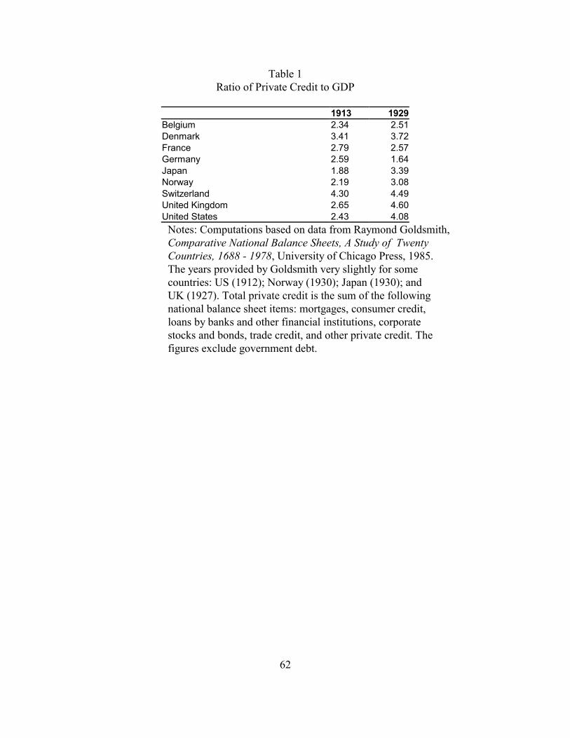
62

Table 1Ratio of Private Credit to GDP

1913 1929Belgium 2.34 2.51Denmark 3.41 3.72France 2.79 2.57Germany 2.59 1.64Japan 1.88 3.39Norway 2.19 3.08Switzerland 4.30 4.49United Kingdom 2.65 4.60United States 2.43 4.08

Notes: Computations based on data from Raymond Goldsmith,Comparative National Balance Sheets, A Study of Twenty Countries, 1688 - 1978, University of Chicago Press, 1985. The years provided by Goldsmith very slightly for some countries: US (1912); Norway (1930); Japan (1930); and UK (1927). Total private credit is the sum of the following national balance sheet items: mortgages, consumer credit, loans by banks and other financial institutions, corporate stocks and bonds, trade credit, and other private credit. The figures exclude government debt.

63

Table 2Tobin�s q and Investment

(Double log regression, with investment ratio as the dependant variable)

Pooled Country fixed effectsCountry & time

fixed effects Random effects

q 0.18 - 0.15 - 0.20 - 0.18 -(2.64) (2.25) (2.45) (2.64)

q-1-0.01 0.15 0.08 0.20 0.03 0.21 -0.01 0.15(0.06) (4.34) (1.12) (4.98) (0.43) (4.72) (0.06) (4.34)

(I/Y)-10.72 0.71 0.55 0.54 0.58 0.56 0.72 0.71

(21.25) (21.00) (13.42) (13.18) (13.04) (12.68) (21.25) (21.00)(GDP

growth)-1

0.01 0.01 0.01 0.01 0.01 0.01 0.01 0.01(2.70) (3.08) (2.58) (2.96) (0.24) (0.75) (2.70) (3.08)

Constant -1.33 -1.25 -1.88 -1.79 -1.71 -1.55 -1.33 -1.25(7.09) (6.78) (8.79) (8.57) (7.32) (6.42) (7.09) (6.78)

Numberof obs. 298 298 298 298 298 298 298 298

R2 0.67 0.49 0.66 0.66 0.73 0.72 0.72 0.71Note: t-statistics in parentheses.Source: See text.

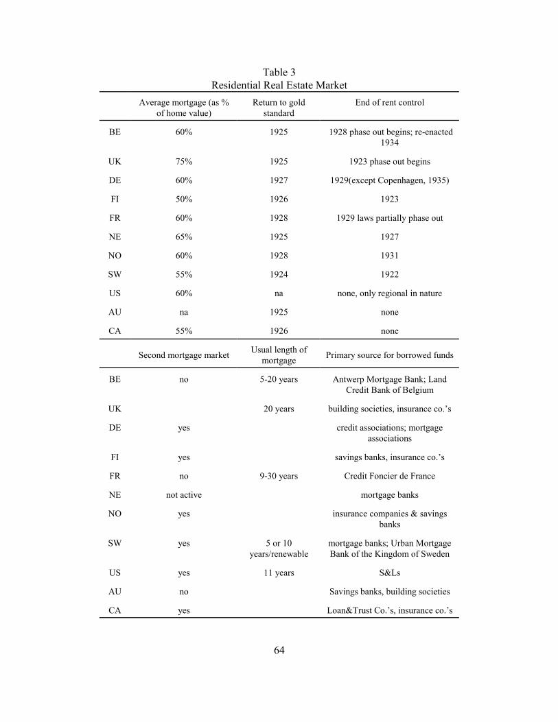
64

Table 3Residential Real Estate Market

Average mortgage (as %of home value)

Return to goldstandard

End of rent control

BE 60% 1925 1928 phase out begins; re-enacted1934

UK 75% 1925 1923 phase out begins

DE 60% 1927 1929(except Copenhagen, 1935)

FI 50% 1926 1923

FR 60% 1928 1929 laws partially phase out

NE 65% 1925 1927

NO 60% 1928 1931

SW 55% 1924 1922

US 60% na none, only regional in nature

AU na 1925 none

CA 55% 1926 none

Second mortgage market Usual length ofmortgage Primary source for borrowed funds

BE no 5-20 years Antwerp Mortgage Bank; LandCredit Bank of Belgium

UK 20 years building societies, insurance co.�s

DE yes credit associations; mortgageassociations

FI yes savings banks, insurance co.�s

FR no 9-30 years Credit Foncier de France

NE not active mortgage banks

NO yes insurance companies & savingsbanks

SW yes 5 or 10years/renewable

mortgage banks; Urban MortgageBank of the Kingdom of Sweden

US yes 11 years S&Ls

AU no Savings banks, building societies

CA yes Loan&Trust Co.�s, insurance co.�s

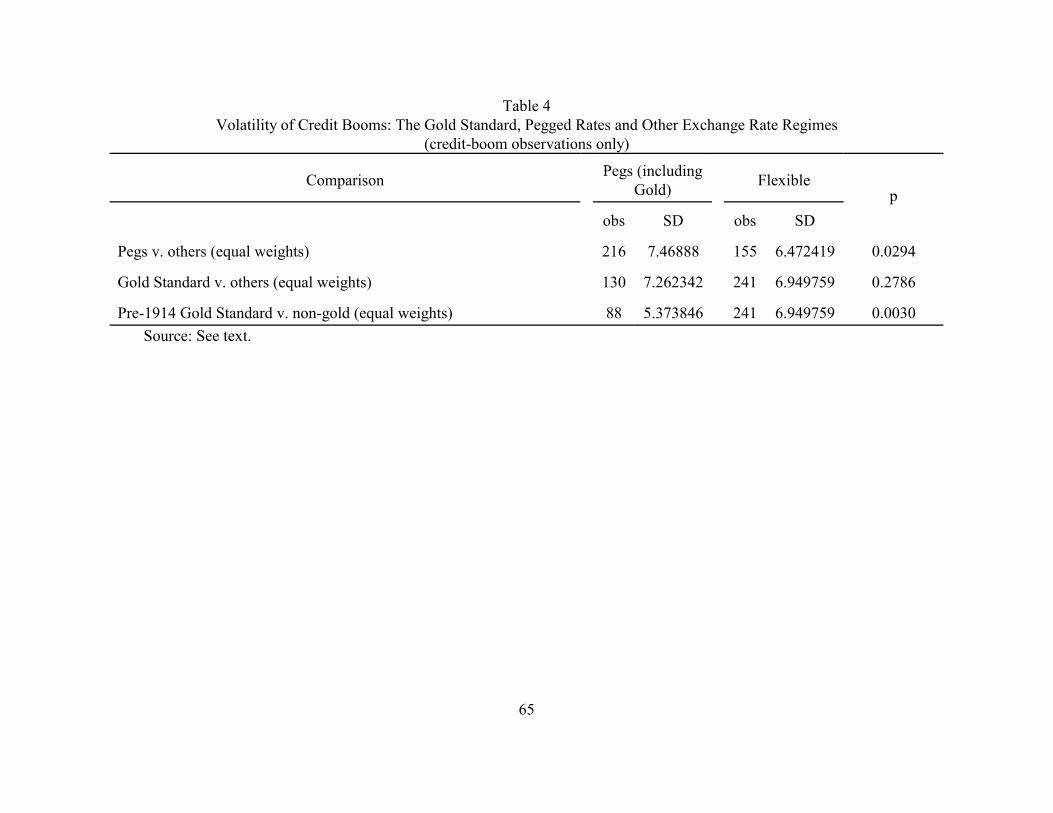
65

Table 4Volatility of Credit Booms: The Gold Standard, Pegged Rates and Other Exchange Rate Regimes

(credit-boom observations only)

Comparison Pegs (includingGold) Flexible

pobs SD obs SD

Pegs v. others (equal weights) 216 7.46888 155 6.472419 0.0294

Gold Standard v. others (equal weights) 130 7.262342 241 6.949759 0.2786

Pre-1914 Gold Standard v. non-gold (equal weights) 88 5.373846 241 6.949759 0.0030Source: See text.

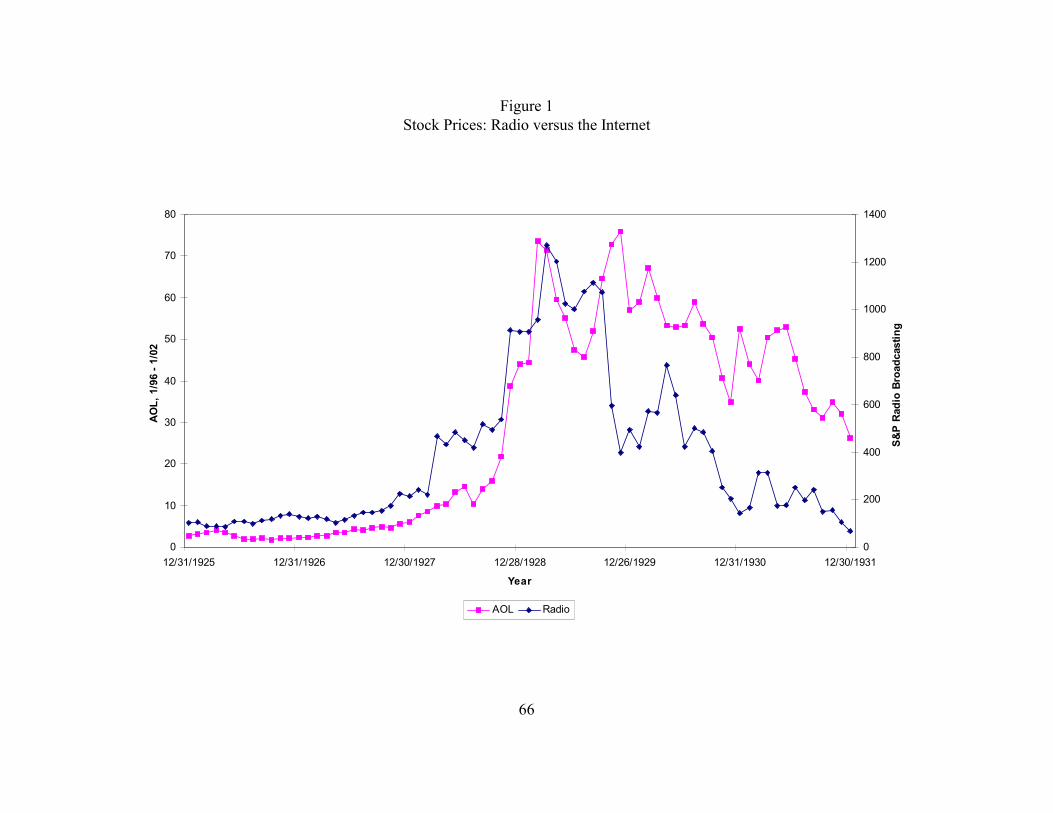
66

0

10

20

30

40

50

60

70

80

12/31/1925 12/31/1926 12/30/1927 12/28/1928 12/26/1929 12/31/1930 12/30/1931

Year

AO

L, 1

/96

- 1/0

2

0

200

400

600

800

1000

1200

1400

S&P

Rad

io B

road

cast

ing

AOL Radio

Figure 1Stock Prices: Radio versus the Internet

67

0

50

100

150

200

250

300

350

400

1920 1921 1922 1923 1924 1925 1926 1927 1928 1929 1930 1931 1932 1933 1934

Year

1920

= 1

00

Dow Jones Dividends Index

Dow Jones Industrial Stock Price Index

Figure 2Divergence in US Dividends & Stock Prices

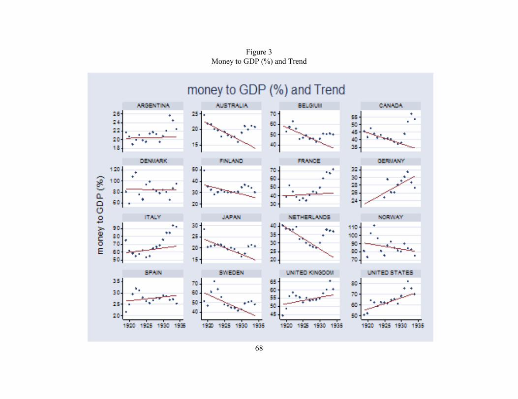
68

Figure 3Money to GDP (%) and Trend

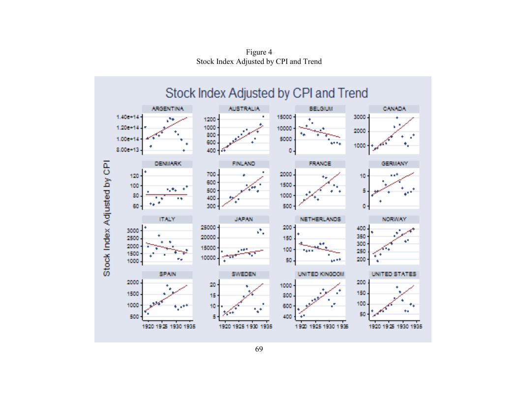
69

Figure 4Stock Index Adjusted by CPI and Trend

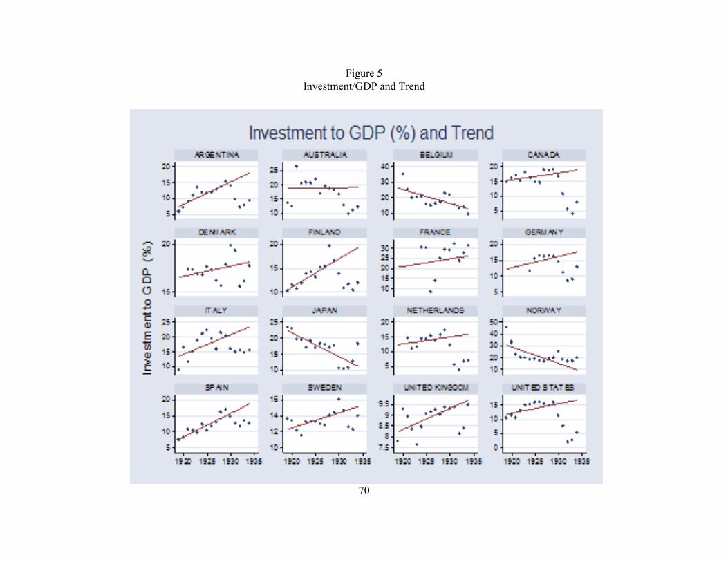
70

Figure 5Investment/GDP and Trend

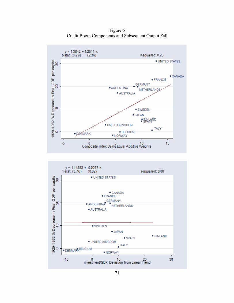
71

Figure 6Credit Boom Components and Subsequent Output Fall

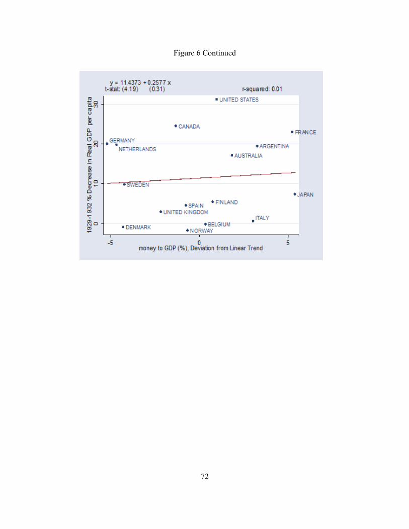
72

Figure 6 Continued

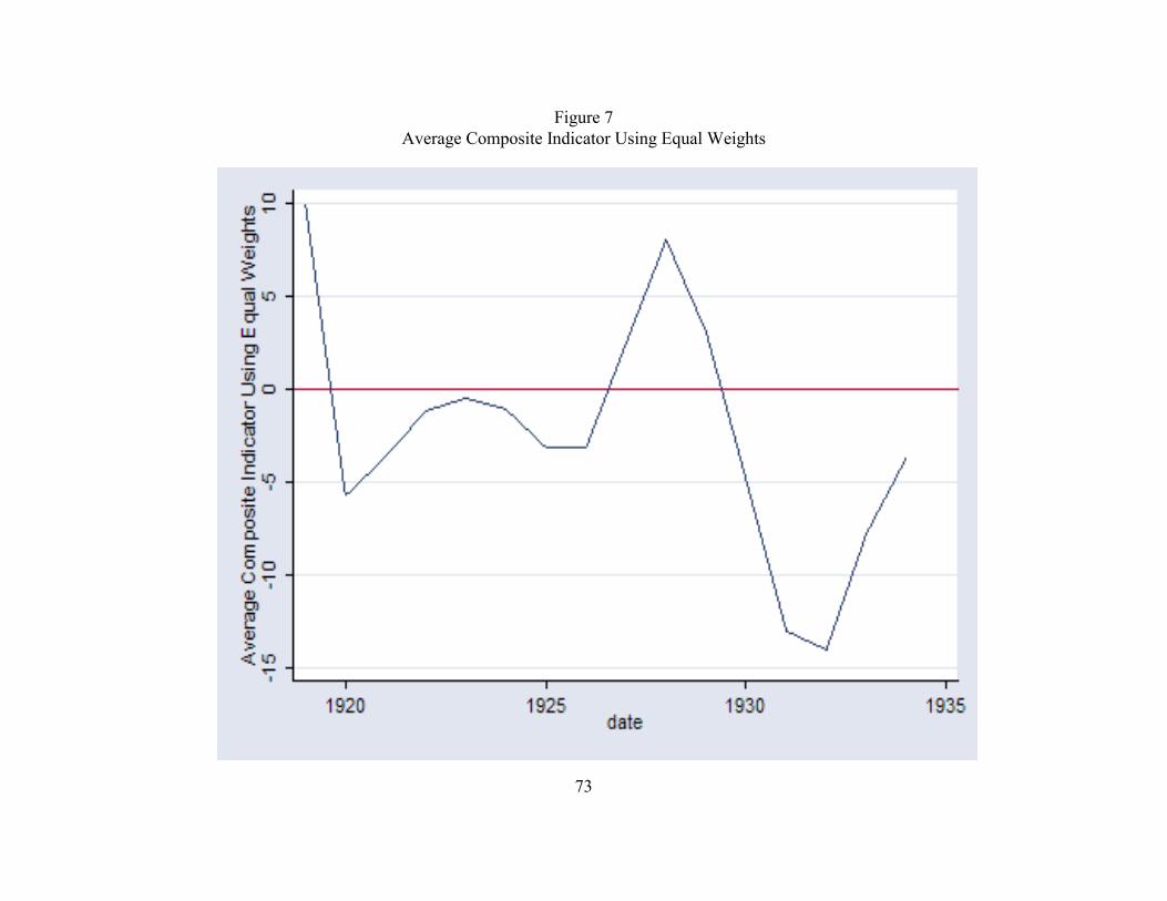
73

Figure 7Average Composite Indicator Using Equal Weights

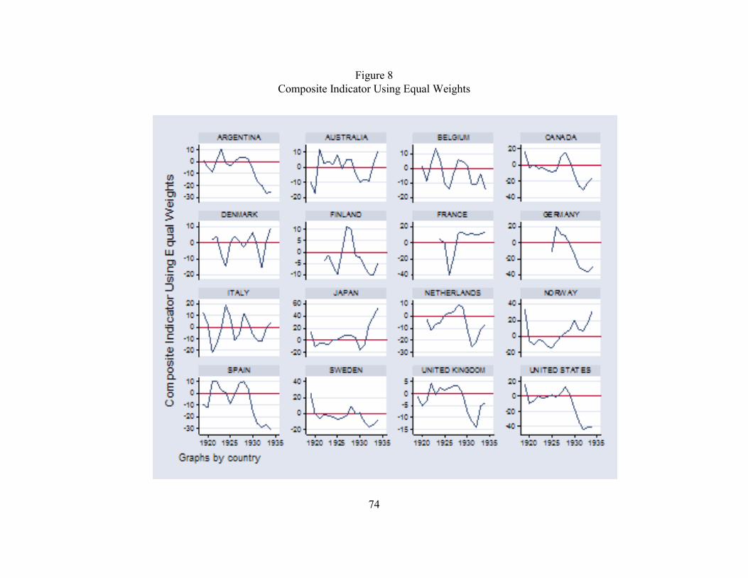
74

Figure 8Composite Indicator Using Equal Weights

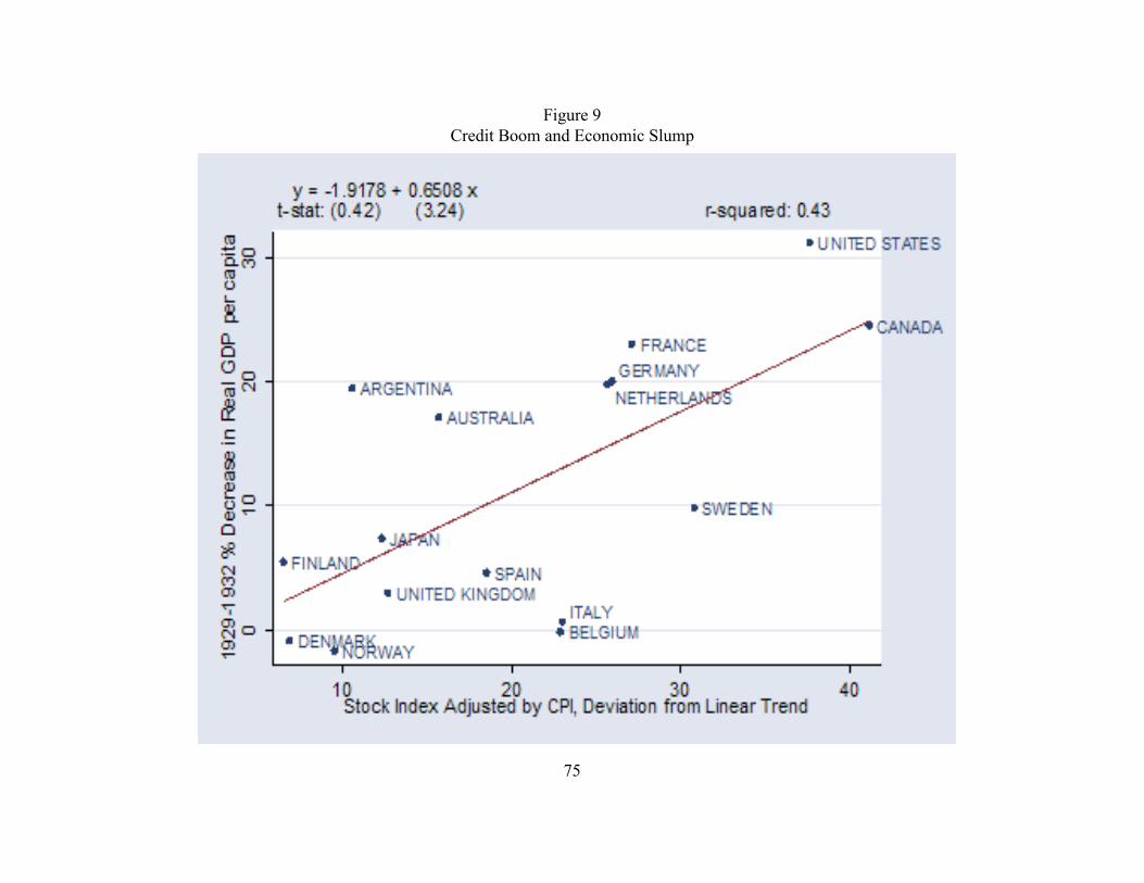
75

Figure 9Credit Boom and Economic Slump

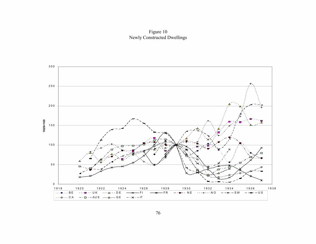
76

0

5 0

1 0 0

1 5 0

2 0 0

2 5 0

3 0 0

1 9 1 8 1 9 2 0 1 9 2 2 1 9 2 4 1 9 2 6 1 9 2 8 1 9 3 0 1 9 3 2 1 9 3 4 1 9 3 6 1 9 3 8

1929

=100

B E U K D E F I F R N E N O S W U S

C A AU S G E IT

Figure 10Newly Constructed Dwellings

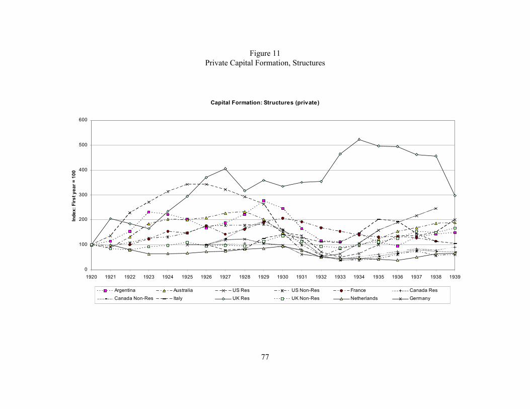
77

Capital Formation: Structures (private)

0

100

200

300

400

500

600

1920 1921 1922 1923 1924 1925 1926 1927 1928 1929 1930 1931 1932 1933 1934 1935 1936 1937 1938 1939

Inde

x: F

irst y

ear =

100

Argentina Australia US Res US Non-Res France Canada ResCanada Non-Res Italy UK Res UK Non-Res Netherlands Germany

Figure 11Private Capital Formation, Structures

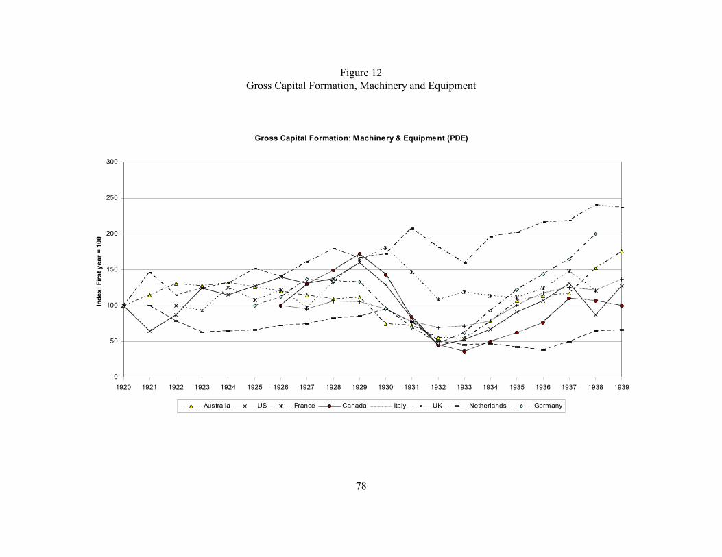
78

Gross Capital Formation: Machinery & Equipment (PDE)

0

50

100

150

200

250

300

1920 1921 1922 1923 1924 1925 1926 1927 1928 1929 1930 1931 1932 1933 1934 1935 1936 1937 1938 1939

Inde

x: F

irst y

ear =

100

Australia US France Canada Italy UK Netherlands Germany

Figure 12Gross Capital Formation, Machinery and Equipment

79

0

50

100

150

200

250

300

350

192601

192603

192606

192609

192612

192703

192706

192709

192712

192803

192806

192809

192812

192903

192906

192909

192912

193003

193006

193009

193012

193103

193106

193109

193112

193203

193206

193209

193212

193303

193306

193309

193312

193403

193406

193409

193412

193503

193506

193509

19351219

26:1

= 1

00

Based on data for 10 Technology Industries

Figure 13Market Capitalization for Aggregate Technology Index

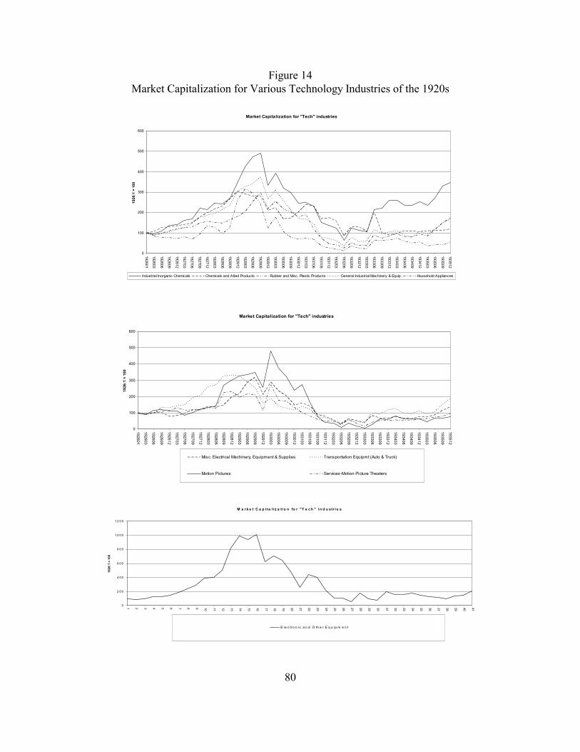
80

Market Capitalization for "Tech" industries

0

100

200

300

400

500

600

192601

192603

192606

192609

192612

192703

192706

192709

192712

192803

192806

192809

192812

192903

192906

192909

192912

193003

193006

193009

193012

193103

193106

193109

193112

193203

193206

193209

193212

193303

193306

193309

193312

193403

193406

193409

193412

193503

193506

193509

19351219

26:1

= 1

00

Industrial Inorganic Chemicals Chemicals and Allied Products Rubber and Misc. Plastic Products General Industrial Machinery & Equip. Household Appliances

Market Capitalization for "Tech" industries

0

100

200

300

400

500

600

192601

192603

192606

192609

192612

192703

192706

192709

192712

192803

192806

192809

192812

192903

192906

192909

192912

193003

193006

193009

193012

193103

193106

193109

193112

193203

193206

193209

193212

193303

193306

193309

193312

193403

193406

193409

193412

193503

193506

193509

19351219

26:1

= 1

00

Misc. Electrical Machinery, Equipment & Supplies Transportation Equipmt (Auto & Truck)

Motion Pictures Services-Motion Picture Theaters

M a r k e t C a p i ta l i z a ti o n fo r " T e c h " i n d u str i e s

0

2 0 0

4 0 0

6 0 0

8 0 0

1 0 0 0

1 2 0 0

1 2 3 4 5 6 7 8 9 10 11 12 13 14 15 16 17 18 19 20 21 22 23 24 25 26 27 28 29 30 31 32 33 34 35 36 37 38 39 40 4119

26:1

= 1

00

E le c tr o n ic a n d O th e r E q u ip m e n t

Figure 14Market Capitalization for Various Technology Industries of the 1920s