The family as producer of health — an extended grossman ...

Ž .Journal of Health Economics 19 2000 611–637www.elsevier.nlrlocatereconbase

The family as producer of health — an extendedgrossman model

Lena Jacobson)Departments of Community Medicine and Economics, Lund UniÕersity, MalmorLund, Sweden¨

Received 7 May 1998; received in revised form 24 February 1999; accepted 30 November 1999

Abstract

Deriving a model, where each family member is the producer of his own and otherfamily members’ health, shows that the family will not try to equalise marginal benefits andmarginal costs of health capital for each family member. They will rather invest in healthuntil the rate of marginal consumption benefits equals the rate of marginal net effectivecosts of health capital. The level of compensation in the social insurance system, theeffective price of care, health related information, and transfer payments will all affect theproduction possibility set, and therefore the optimal level and distribution of family health.q 2000 Elsevier Science B.V. All rights reserved.

JEL classification: I1; I12

Keywords: Health; Human capital; Family; Grossman model

1. Introduction

Ž .In his seminal work, Michael Grossman 1972a,b constructed and estimated adynamic model of the demand for the commodity ‘good health’. He argued that

) Pfizer AB, PO Box 501, SE-183 25 Taby, Sweden. Tel.: q46-8-519-064-05; fax: q46-8-519-062-¨12.

Ž .E-mail address: [email protected] L. Jacobson .

0167-6296r00r$ - see front matter q 2000 Elsevier Science B.V. All rights reserved.Ž .PII: S0167-6296 99 00041-7

( )L. JacobsonrJournal of Health Economics 19 2000 611–637612

such a model is important for two reasons. First, because the level of healthinfluences the amount and productivity of labour supplied to an economy. Second,what consumers demand when they purchase medical services are not theseservices per se but rather ‘good health’. Added to these, there are further reasons.The model will help explain individuals’ health related behaviour, e.g., why somepeople smoke and some not, and why different individuals have different health

Ž .and different health care utilisation Muurinen and Le Grand, 1985 . In order toevaluate and predict the effects of regulations, new technology, changes in socialinsurance schemes and government, and other programmes, knowledge about theeffects on individuals’ demand for health and health related behaviour is essential.These effects will not be confined just to the present distribution of health capitalŽ .direct effects , but they will change the individual’s lifetime health profileŽ .indirect effects . Hence, present and future total utilisation of health care re-sources and social insurance are to a large extent the result of aggregate previous,present and future health related behaviour. Therefore, increasing our knowledgeof what factors determine observed inequalities in health and the path of lifetimehealth has important policy implications.Fundamental to the demand for health model is the sharp distinction between

market goods and commodities. In this approach, consumers produce commoditiesŽ .with inputs of market goods and their own time Becker, 1965 . For example, they

use sporting equipment and their own time to produce recreation, travelling timeand transportation services to produce visits, and part of their Sundays and churchservices to produce ‘peace of mind’. Since goods and services are inputs into theproduction of commodities, the demand for these goods and services is a derived

Ž .demand Grossman, 1972a, p. xv .Further, the commodity good health is treated as a durable item, as one

component of human capital. Health is demanded by the consumer for tworeasons: as a consumption commodity, directly entering the individual’s utility

Ž .function i.e., sick days being a source of disutility ; and as an investmentcommodity, determining the total amount of time available for market andnonmarket activities. According to the model, the level of health is endogenous,

Ž .and depends at least in part on the resources allocated to its production. Theshadow price of health will depend on many variables besides the price of medicalcare, and the quantity of health demanded will be negatively correlated with itsshadow price.Though the model yields valuable contributions to explain individuals’ health

related behaviours and differences in health and health care utilisation, attempts toŽdevelop the theoretical model have been relatively few for a review, see Gross-

.man, 1982, 1998 , and they have all been based on the individual as producer ofhealth. This implies that both the original model, as well as the extended models,can only be used to analyse adult health, not children’s ‘demand’ for health and

( )L. JacobsonrJournal of Health Economics 19 2000 611–637 613

their health care utilisation.1 It also implies that the influence of other familymembers on the individual’s demand for health and demand for health care cannotbe considered.However, to analyse health issues from a family perspective is important for

several reasons. It has been suggested that events during fetal life and earlyŽchildhood are associated with disease and mortality in later life Barker, 1992,

.1994; Power et al., 1996; Wadsworth, 1996, 1997 . The pathway linking early lifewith adult disease is explained by the process of ‘biological programming’Ž .Barker, 1992, 1994 and the continuities in lifetime socio-economic circum-stances.2 This implies that a life course perspective is needed when searching forthe determinants of inequalities in health, and a demand for health model wherethe production of child health is included.Further reasons for a family perspective, i.e., to include the influence other

family members have on an individual’s health related behaviour, is supported byŽ .some empirical findings. Grossman 1975 found that an increase in wives’

schooling increased male health. Actually Grossman found the coefficient onŽwives’ schooling to exceed the coefficient of men’s own schooling however, not

. Ž .significantly higher . Currie and Gruber 1996 examined the effects of publichealth insurance on children’s health and utilisation of medical care. They foundthat parents with some college education are more likely to take their children tothe doctor, with a stronger effect for mothers than for fathers, and that utilisation ishigher both for first children and for children in smaller families. Further findingsare that, conditional on household income, children in households with no malehead have higher utilisation levels, and that visits seem to be normal goods while

Ž .hospitalisations appear to be inferior goods. Thomas et al. 1991 found that amother’s education has a large impact on child height in Northeast Brazil, and thatalmost all of this impact can be explained by indicators of her access to

Ž .information. Delaney 1995 reports on negative effects of parental divorce onchildren’s health. Parental divorce also seems to have long-term effects on

Ž .personality and longevity Tucker et al., 1997 .Furthermore, how resources are allocated into investments in formal schooling

and child health, as well as into investments in adult health and on-the-job

1 Ž .Previously, for example Grossman 1975; see also Leibowitz, 1974 has argued that the health andintelligence of children partly depend on genetic inheritance, but that in particular they depend on earlychildhood environmental factors, which are shaped to a large extent by parents. However, Grossman et

Ž .al. Becker, 1991; Cigno, 1991 view the increase in direct utility as the reason for parents’ investing inchild quality, i.e., that child quality is a consumption commodity. This paper argues that there exists amonetary incentive as well.

2 Ž .See Becker’s 1991, Chapter 6 model of family background and the opportunities of children,where he analyses the influence family expenditures and endowments have on the income of children.


training, are decisions made jointly within the family. Existing demand for healthmodels cannot explain and analyse such family and lifecycle related issues.Analysing health matters from a family perspective will be a step in the directionto a model in which the stocks of health and knowledge are simultaneouslydetermined.3This paper extends the Grossman model in that the family is seen as the

producer of health4. By the family as producer of health is meant that each familymember is the producer, not only of his own health, but also of the health of otherfamily members, and that not only his own income and wealth, but also theearnings of other family members, can be used in the production of health. Themodel will be derived assuming complete certainty. The implications of relaxingthis assumption will be briefly discussed in the closing section of the paper.According to Grossman, the individual receives both investment and consump-

tion benefits from investing in his own health. This paper argues that this is validalso for investments in other family members’ health. Investment benefits occur

Ž .because increased adult health or child health will decrease future time spent sickŽ .or time spent taking care of a sick child . Family time available for market workwill then increase, which may raise family income and increase consumption andinvestment possibilities for all family members. Consumption benefits may alsooccur, if family members derive utility not only from own health, but from thehealth of other members as well, i.e., the individual cares about the well-being ofhis or her child and spouse as he or she cares about his or her own well-being.Even though the individual may have incentives for producing health of other

Ž .family members both with and without partly altruistic preferences , it is notself-evident how the objective function should be treated. While there is only oneperson who maximises his or her lifetime utility in the traditional Grossmanindividual demand for health model, there are at least two persons with commonor non-common interests to consider, when formulating the optimisation problemin the family version of the model. In the model of the family as producer of

Žhealth developed in this paper, the family rather than the individuals making up.the family is the economic unit, and a common preference approach will be used

Ž .Becker, 1974, 1991 . The implications of relaxing this assumption will be brieflydiscussed in the final section of the paper.Viewing the family as producer of health will not only affect how the benefits

from investments in health are treated in the model, but also the household

3 ACurrently, we still lack comprehensive theoretical models in which the stocks of health andknowledge are determined simultaneously. I am somewhat disappointed that my 1982 plea for the

w Ž .x Ž .development of these models has gone unanswered Grossman 1982 .B Grossman, 1998, p. 5 .4 More exactly, parents are the producers of their own and their child’s health, while children are

assumed passive.


Ž .production function s and the amount of available resources. In Grossman’smodel, productivity is determined by the individual’s education. But seen from afamily perspective, productivity may be determined by other family members’education as well. Further, it may not be the individual’s education per se thatdetermines his or her productivity in producing health, but human capital specificto that activity.5 Resources available for health production are not only ownincome, but total family income. However, an important difference betweeninvesting in own health and investing in another person’s health is the difficulty toobserve when ‘enough’ investments have been made; being uncertain whetherenough has been done to restore the health of the other person. In contrast, forinvestments in own health, one knows when one prefers to use time and money toproduce other commodities than health.6To analyse an individual’s lifetime health and lifetime health care utilisation

profile, it is necessary to use a lifecycle approach. A lifecycle approach may alsobe essential in order to explain observed differences in health and medical careutilisation among individuals. The lifecycle model concerns individual investmentdecisions and deals with resource allocation over an individual’s lifetime rather

Žthan solely with decisions of the present time period see Polachek and SiebertŽ .1993 for a description of the lifecycle human capital model, and how the

.lifecycle approach can be used to explain earnings variations . While an individ-ual’s amount of education and on-the-job training determine the individual’slifetime earnings, health capital determines not only the individual’s productivitybut also his or her amount of healthy time. To tackle such a dynamic optimisationproblem, there are three major approaches: calculus of variations, dynamic pro-

Ž .gramming, and optimal control theory Chiang, 1992, pp. 17–22 . In this paper,optimal control theory will be used.The paper is organised as follows. In Section 2, a model of the family as

producer of health is derived in three steps. First, as a frame of reference, a modelof the single person family is derived. Then, a model for the husband–wife familyis derived and, eventually, a child is added to the family and a parents–childfamily model is presented. In Section 3, a graphic illustration of the family asproducer of health model follows, and the effects on family health of changes insome exogenous variables are analysed. The paper concludes by a discussion ofthe implications of relaxing the assumption of common preferences and insteadassumes allocation within the family to be the outcome of a cooperative Nashbargaining model, as well as a brief discussion of relaxing the assumption ofcomplete certainty. Section 4 also includes some remarks regarding family forma-

5 For example self-management programs, educational programs for parents with chronically illchildren, information about diet habits, etc.

6 I am grateful to Lars Soderstrom for this point.¨ ¨


tion, family size, and inter-sibling allocation, as well as a discussion of somepolicy implications.

2. The family as producer of health

In the following, a model of the family as producer of health will be developedsuccessively in three steps. As a frame of reference, a model of the single personfamily will be presented, then the husband and wife family, and finally the parentsand child family.7In all three models, the family is assumed to choose the amount of market

goods to consume in each time period in order to maximise family lifetime utility,given initial family wealth and each family member’s initial amount of healthcapital, and given the production functions and prices. The time path of familywealth and the paths of each family member’s health are then given by the optimalamounts of market goods chosen.

2.1. The single-person family

Ž .Similar to Grossman 1972a,b , the individual is assumed to derive utility fromown health, H , and from the consumption of other commodities8, Z . Thet tindividual has a strictly concave utility function, where utility in period t is

u su H ,Z . 1Ž . Ž .t t t

The individual’s stock of health will depreciate during his or her lifetime, butŽ .the individual can invest in health produce health capital to offset this deprecia-

tion in health capital. The individual’s stock of health will develop over timeaccording to

EHrEts I yd H , 2Ž .t t t t

7 The three versions of the family as producer of health model could be seen as tools for analysinghealth and health care utilisation during different stages in an individual’s life: as a child in a two

Žparents’ family; as a single adult person either prior to partnership, after a divorce, or at the end of.life ; as partners without children; and as partners with one child. The objective was not to analyse

transitions between stages — that would have required quite a different analytical framework — andthere are obviously many more possible stages to account for in real life. The objective was rather tomake a model that could provide important insights into family health behaviour, given the fact that thefamily exists.

8 Those ‘other commodities’ are produced and consumed in period t, i.e., they cannot be stored.


which is the equation of motion for the state variable health, and where d is thetrate of depreciation. The individual produces gross investments in health, I , andtother commodities, Z , according to the production functions:t

I s M ,h ;E 3Ž . Ž .t t t ,H t ,H

and

Z s X ,h ;E , 4Ž . Ž .t t t ,Z t ,Z

where M and X are market goods9, and h and h are own time used in thet t t,H t,Zproduction of health and other commodities, respectively, E and E aret,H t,Zefficiency parameters10, and the production functions are assumed homogenous ofdegree one in both goods and time inputs11.

Ž . Ž .Individual family stock of wealth W will develop over time according tot

EWrEtsrWqv H ,E h qB yp M yq X , 5Ž . Ž .t t t t t ,v t ,v t t t t t

the equation of motion for the state variable wealth, where r is the market interestrate, v is the wage rate, E is the level of education and on the job training,t t,vh is time in market work, B is transfers, and p and q are the prices oft,v t t t

Ž . Ž .medical care M and other goods X , respectively.t tHealth will affect market income in two ways: through its effect on the wage

rate; and through its effect on healthy time available for market work. AccordingŽ .to the formulation in Eq. 5 , an individual’s productivity in market work is

determined by his or her amount of health capital and level of education andŽ .on-the-job training, implying that v H ,E can be thought of as the ‘labourt t t,v

market earnings rate of return on human capital’.Ž .The available amount of healthy time in each time period is total time V less

Ž .time spent sick h , where time spent sick is determined by the individual’st,SŽ Ž .. 12 Ž .amount of health capital h sh H . Time spent in market work h , int,S t,S t t,v

Ž . Ž . Ž .producing health h and other commodities h , and time spent sick ht,H t,Z t,SŽ .have to sum up to total time available V , i.e.,

Vsh qh qh qh . 6Ž .t ,v t ,H t ,Z t ,S

9 Note that inputs in the production of health may not only be medical care services, but diet,Ž .exercise, housing, etc. See Grossman 1972a , for an analysis of joint production. Here, however, it

will be assumed that medical care services are the only inputs in the production of health.10 Ž .In Grossman 1972a,b the individual’s productivity is determined by his or her level of schooling.

Ž . ŽAs in Becker 1991 , individual productivity in producing different commodities may differ activity.specific human capital . The individual’s productivity in producing health may depend on information

and knowledge about health matters as well as the individual’s stock of health, while the individual’sŽproductivity in market work depends on his or her stock of educational capital formal education and

.on-the-job training .11 An assumption made by Grossman as well as his successors.12 Eh rEH -0, E2h rEH 2)0.t,S t t,S t


The individual’s problem is then to choose the time paths of the controlvariables M and Z that maximise lifetime utility. The problem can then bet twritten:

T yu tMax Us e u H ,ZŽ .H t tt

such that EHrEts I yd Ht t ,H t t

EWrEtsrWqv H ,E h qB yp M yq XŽ .t t t t t ,v t ,v t t t t t

Vsh qh qh qht ,v t ,H t ,Z t ,S

H 0 sH , W 0 sW , H andW givenŽ . Ž .0 0 0 0

H T sH FH , W T sW G0, WUl s0Ž . Ž .T min T T T ,W

T freew xand X ,M G0 for all tg 0,T 7Ž .t t

where U is the individual’s intertemporal utility function, i.e., the discounted valueof the individual’s lifetime utility, discounted by the individual’s rate of timepreference, u . EHrEt and EWrEt are the equations of motion for the statet tvariables H and W, respectively, and V the time restriction. H is theminindividual’s ‘death stock’ of health capital. The individual dies when health passes

Ž .below some level H , which determines T time of death . It should be observedminthat the individual is free to borrow and lend capital at each period, but the bequestŽ .W cannot be negative.T

Ž .The solution to this horizontal-terminal-line problem Chiang, 1992 gives thatthe individual invests in health until the marginal benefit of new health equals the

Ž .marginal cost of health see Appendix A :

eyu trl Eu rEH qh Ev rEH y w rl Eh rEHŽ .Ž .t ,W t t t ,v t t t t ,W t ,S t

sp d qry Ep rEt rp , 8Ž . Ž .t t t t

Ž .where l and l are costate variables, w is the lagrange multiplier for thet,W t,H ttime restriction, Eu rEH is marginal utility of health capital13, Ev rEH is thet t t tmarginal effect of health on wage14, Eh rEH is the marginal effect of health ont,S tthe amount of sick time and p is the effective price of medical care goods andt

Ž .services M .tŽ .The first order condition A10 in the Appendix A gives that l equalst,H

Ž .l p . Thus, in periods when the budget is binding l high or the effectivet,W t t,W

13 Eu rEH )0, E2u rEH 2-0.t t t t14 Ev rEH )0.t t


Ž .price of care p is high, l will be high, implying that the individual’s stock oft t,HŽ .health is low. Further, the first order condition A7 shows that:

El rEtsl d yl h Ev rEH qw Eh rEH y Eu rEH eyu t ,Ž . Ž . Ž .t ,H t ,H t t ,W t ,v t t t t ,S t t t

9Ž .

i.e., the time path of l will depend on, for example, the rate of depreciation int,HŽ .health d , the sensitivity in the individual’s wage rate to changed healtht

Ž . wEv rEH , and the individual’s valuation of time how binding the time restrictiont tŽ .xis w . An increased rate of depreciation will increase l , decreasing thet t,H

individual’s level of health. If the individual’s wage rate becomes more sensitiveŽ .to differences in health, the individual will invest more in health l decreases .t,H

Finally, the more restricting the time constraint is, the higher will the individual’sŽ .valuation of time be w , and the more will the individual invest in healtht

Ž .decreasing l .t,HNote that while Eu rEH is the increase in utility in period t if health capital int t

period t is increased by one unit, l is the increase in lifetime utility if health int,Hperiod t is increased by one unit of health capital.Looking at the time path of the costate variable l , the solution shows thatt,W

l decreases over time with a rate equal to the rate of interest, r. According tot,Wthe present formulation, the individual is free to borrow and lend capital at each

Ž .period of time EWrEt can take both positive and negative values , but W ist T

Fig. 1. An illustration of the paths of the control variable, c, and the state variable, y, in an optimalŽ . Ž .control problem. a Illustrates that the control path, c t , does not have to be continuous; it only has to

be piecewise continuous. For example, an individual’s medical care consumption can make jumps overŽ .time, i.e., be positive in some time periods and zero in some. The state path, y t , on the other hand,

w x Ž .has to be continuous throughout the time period 0,T as illustrated in b . However, the state path isallowed to have a finite number of sharp points, i.e., it needs to be piecewise differentiable. Thosesharp points will occur at the times when the control path makes a jump. For example, a jump in

Ž .medical care consumption, say at time t , may correspond to a sharp decrease in health, y t . To place1 1a state-space constraint on the maximisation problem can, for example, be to only allow for positive

Ž . Žvalues on y t , i.e., the permissible area of movement for y is the area above the horizontal axis for. Žexample, if y is monetary wealth, to allow for saving but not for borrowing . Source: Chiang 1992, p.

.163, Fig. 7.1 .


restricted to be non-negative, i.e., the bequest cannot be negative. If formulatingŽ .the problem as a state-space constraint problem Chiang, 1992, pp. 298–300 ,

EWrEt is forced to be non-negative in every period. l will then not bet t,WŽcontinuous, but make jumps in periods where this restriction is binding see Fig. 1

.for an illustration .The values of l and w may be interpreted as measures of stress, economict,W t

and time stress, respectively. If the wealth andror time constraint is binding forseveral periods, the values of l and w will be high and increasing.t,W t

2.2. The husband–wife family

Using a common preference model of family behaviour, the instantaneousŽ .family strictly concave utility function can be written as

usu H ,H ,Z , 10Ž . Ž .m f

where time subscripts are omitted in order to simplify the notations. u is familyŽ . Ž .utility in period t, H and H are husband male and wife female health,m f

respectively, and Z is a vector of commodities consumed. As in the single-personŽ . Ž .model, the depreciation in male d and female health d may be offset bym f

Ž . Ž .gross investments in male I and female I health, respectively, according tom fthe production functions:

I s I M ,h ,h ;E ,E 11Ž . Ž .m m m Hm ,m Hm ,f H ,m H ,f

and

I s I M ,h ,h ;E ,E , 12Ž . Ž .f f f H f ,m H f ,f H ,m H ,f

where the production functions are assumed homogenous of degree one in goodsand time inputs. M and M indicate market goods used in the production of malem fand female health, respectively. Time used in the production of health is indicatedby h , h , h , and h . The first subscript denotes what is produced;Hm,m Hm,f H f,m H f,f

Ž . Ž .male H or female H health, the second subscript denotes who is them fŽ . Ž .producer; the husband m or the wife f . E and E indicate male and femaleH ,m H ,f

productivity in health production. Similarly, net investments in health are

EH rEts I yd H 13Ž .m m m m

and

EH rEts I yd H . 14Ž .f f f f

The development of family wealth follows

EWrEtsrWqv H ,E h qv H ,E h qBŽ . Ž .m m v ,m v ,m f f v ,f v ,f

yp M qM yqX , 15Ž . Ž .m f


Ž . Ž . Žwhere v H ,E and v H ,E are the husband’s and wife’s wage rates orm m v ,m f f v ,f. Ž .labour market earnings rates of return on human capital , respectively. E Ev,m v ,f

Ž . Ž .is the husband’s wife’s level of education and on-the-job training, and h hv,m v ,fŽ .his her amount of time spent in market work.The time restrictions are

V sh qh qh qh qh ism,f. 16Ž .i v ,i Z ,i Hm ,i H f ,i S ,i

Ž .Total time for each spouse V is allocated between time spent in market workiŽ . Ž . Ž .h , in home production of health h qh and other commodities hv,i Hm,i H f,i Z,i

Ž .and time being sick h , where health determines the amount of sick timeS,iŽ Ž ..h sh H .S,i S,i iThe problem facing the family is to choose the time paths of the control

variables M , M , and Z, in order to maximise lifetime utility. The problem canm fŽ .then be written time subscripts still omitted for simplicity :T yu tMax Us e u H ,H ,ZŽ .H m ft

such that EH rEts I yd Hm m m m

EH rEts I yd Hf f f f

EWrEtsrWqv H ,E h qv H ,E hŽ . Ž .m m v ,m v ,m f f v ,f v ,f

qByp M qM yqXŽ .m f

V sh qh qh qh qh ism,fi v ,i Z ,i Hm ,i H f ,i S ,i

H 0 , H 0 ,W 0 givenŽ . Ž . Ž .m f

H T andror H T FHŽ . Ž .m f min

W T G0, WUlWs0Ž . T T

T freew xand X ,M ,M G0 for all tg 0,T 17Ž .m f

.T , in this case, is the ‘lifetime’ of the husband–wife family; the family ‘dies’when husband andror wife no longer has a health status greater than H . Themin

Žsolution to this maximisation problem gives the marginal condition see Appendix.A, condition A16 :

w xŽ . Ž . Ž .Ž .EurEH p d q ry Ep rEt rp y Ev rEH h y w rl Eh rEHŽ .m m m m m m m v ,m m W S ,m ms .w xŽ . Ž . Ž .Ž .EurEH p d q ry Ep rEt rp y Ev rEH h y w rl Eh rEHŽ .f f f f f f f v ,f f W S ,f f

18Ž .Ž .Thus, the optimal condition 8 , i.e., that the individual invests in health until

marginal benefits equal marginal costs, is not valid any more. In a two-personfamily with common preferences, husband and wife together invest in health until

Ž Ž ..the rate of marginal consumption benefits left hand side of Eq. 18 equals the


Ž .rate of marginal net effective cost of health capital right hand side . The neteffective cost of health capital equals the user cost of capital less the marginal

Ž . Ž Ž .investment benefit of health capital in brackets . A similar result see Eq. A10.in Appendix A can be derived for lifetime utility of health, i.e., that

l sl rp sl rp . 19Ž .W Hm m H f f

Ž .Condition 19 implies that family members will invest in health until the rate ofŽ .marginal lifetime utility of health to the effective price of health is equal for all

Ž .family members and equal to the marginal utility of wealth .

2.3. The parents–child family

Adding a child to the husband–wife family model gives the following instanta-Ž .neous strictly concave family utility function time subscripts omitted :

usu H ,H ,H ,Z , 20Ž . Ž .m f c

where H is child health, developing over time according to the equation ofcmotion,

EH rEts I yd H , 21Ž .c c c c

Ž .and produced by the child’s parents by use of market goods M and parentalcŽ .time h and h , respectively according to the production function:Hc,m Hc,f

I s I M ,h ,h ;E ,E . 22Ž . Ž .c c c Hc ,m Hc ,f H ,m H ,f

Ž .The time restriction for each parent husband and wife, respectively thenbecomes

V sh qh qh qh qh qh qh ism,f 23Ž .i v ,i Z ,i Hm ,i H f ,i Hc ,i S ,i Sc ,i

where h is time taking care of a sick child for parent i, and where Eh rEH -0Sc,i Sc,i cand E2h rEH 2)0.15 The family problem will now be extended to choose theSc,i cpaths of M , M , M , and Z in order tom f c

T yu tMax Us e u H ,H ,H ,ZŽ .H m f ct

such that EH rEts I yd H for jsm, f, cj j j j

EWrEtsrWqv H ,E h qv H ,E h qBŽ . Ž .m m v ,m v ,m f f v ,f v ,f

yp M qM qM yqXŽ .m f c

V sh qh qh qh qh qh qh for ism,fi v ,i Z ,i Hm ,i H f ,i Hc ,i S ,i Sc ,i

H 0 given for jsm,f,cŽ .j

15 Thus, it is assumed that the parents themselves are taking care of their sick child. In reality,however, they may have other options.


H T FH for at least one of jsm,f,cŽ .j minUW T G0, W T l T s0Ž . Ž . Ž .W

T freew xand X ,M G0 for all tg 0,T , jsm,f,c. 24Ž .j

As in the previous case, T is the ‘lifetime’ of the parents–child family.16Ž . ŽSolving the maximisation problem in Eq. 24 adds the marginal condition see

.Appendix A, condition A18 ,EurEHiEurEHc

w xp d q ry Ep rE t rp y Ev rEH h y w rl Eh rEHŽ . Ž . Ž .Ž .Ž .i i i i i i v , i i W S ,i is ism,fw xp d q ry Ep rE t rp y y w rl Eh rEH y w rl Eh rEHŽ . Ž .Ž . Ž .Ž .Ž .c c c c m W Sc ,m c f W Sc ,f c

25Ž .Ž .to the one in Eq. 18 . The net effective marginal cost of adult health capital is the

Ž .same as in condition 18 . Net effective marginal cost of child health is equal tothe user cost of child health capital less the marginal investment benefit of childhealth, which is the sum of the monetary value of the change in time taking care ofa sick child for father and mother, respectively, for a marginal change in child

Ž .health. Condition 19 is now extended to

l sl rp sl rp sl rp , 26Ž .W Hm m H f f Hc c

implying that the family invests in health until the rate of marginal utilities ofŽ .lifetime health to effective price of health for all family members is equal andequal to the marginal utility of wealth. The family will not try to equalise theamount of health capital between family members.

Ž .Rearranging condition 26 gives that l sl p , implying that poor familiesHc W cŽ .where the wealth restriction is binding value a marginal change in child healthhigher than rich families, and that families for who the wealth constraint is not

Ž .binding l s0 has a zero marginal utility of child health. Further, it implies thatWa child with unhealthy parents can be expected to have lower health comparedwith a child with healthy parents, because resources have to be spent on increasing

Ž .the health of the unhealthy parents to achieve condition 25 .

16 Even though not directly included in the models above, for simplicity, an individual’s lifetime maybe seen as consisting of three time periods. In the first time period, the individual is a child in aparents–child family; in the second period, he or she is a parent in the parents–child family; and in the

Ž .third period, he or she is a husband or wife in the husband–wife family. His her initial health in theŽ . Ž .first period is his her inherited amount of health capital. Initial health in the second period is his her

Ž . Žterminal amount of health in the first period and so on. This imply that his her health as old in the. Ž . Ž .third period is determined by inherited health, investments made by his her parents during his herŽ . Ž .childhood first period , and by own and spouse’s actions during adulthood second and third period ,

given the exogenous variables.


3. Graphic illustrations of the model

3.1. The optimal distribution of family health

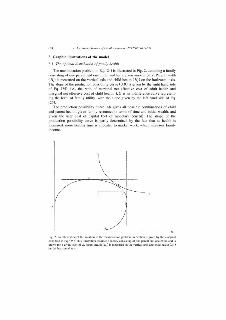
Ž .The maximisation problem in Eq. 24 is illustrated in Fig. 2, assuming a familyconsisting of one parent and one child, and for a given amount of Z. Parent healthŽ . Ž .H is measured on the vertical axis and child health H on the horizontal axis.i c

Ž .The slope of the production possibility curve AB is given by the right hand sideŽ .of Eq. 25 , i.e., the ratio of marginal net effective cost of adult health and

marginal net effective cost of child health. UU is an indifference curve represent-ing the level of family utility, with the slope given by the left hand side of Eq.Ž .25 .The production possibility curve AB gives all possible combinations of child

and parent health, given family resources in terms of time and initial wealth, andŽ .given the user cost of capital net of monetary benefit . The shape of the

production possibility curve is partly determined by the fact that as health isincreased, more healthy time is allocated to market work, which increases familyincome.

Fig. 2. An illustration of the solution to the maximisation problem in Section 2 given by the marginalŽ .condition in Eq. 25 . This illustration assumes a family consisting of one parent and one child, and is

Ž . Ž .drawn for a given level of Z. Parent health H is measured on the vertical axis and child health Hi con the horizontal axis.


If all time and wealth were allocated to the production of child health, thedistribution of health would be given by point B. Producing one amount of parenthealth using some of total family time and wealth would reduce adult sick timeand increase family income, allowing child health to increase as well. It would be

Žpossible to increase both child and adult health at the same time given time,.wealth and user cost of capital until health states defined by point D were

reached. Then, increased adult health would be so ‘expensive’ that child healthhad to be reduced to make additional investments in adult health possible. If childhealth was reduced enough to allow for the production of adult health given bypoint F, the parent would have to spend so much time taking care of the sick childthat income would no longer be enough to make gross investments compensatingfor the depreciation, and child and adult health would both fall.For completely selfish parents, child health per se would not enter the family

Žutility function, so indifference curves would be horizontal. Maximising utility for. Ž .given Z subject to the production possibility set budget constraint would thent

give point F in Fig. 2. This shows that even a selfish parent would invest in childŽhealth, but only because child health affects family income the investment aspect

.of child health . However, because of altruism, adult utility will increase as childhealth increases. For a completely altruistic parent, indifference curves would bevertical. Maximising family utility then implies that the parent would be willing toinvest in child health until point D is reached. Thus, altruism would be effectivealong the production possibility curve from F to D. The location of point P on theproduction possibility curve between F and D will depend on the parent’s degreeof altruism toward the child; ceteris paribus, a more altruistic parent would choosea point closer to D than a less altruistic parent.If point E represents the endowed amounts of health capital at the beginning of

period t, the adult would invest in both own and child health until point P wasreached. However, assume that adult health cannot be increased because of, forexample, lack of treatment. Then the adult would maximise utility by investing inchild health until point O is reached.If, at the beginning of time t, their endowed amounts of health capital were as

represented by point O, then the parent would invest in own health only and letchild health depreciate until point P was reached. It may then look as if the parentunderinvested in child health, but this would be a utility maximising behaviourgiven the restrictions he or she were faced with.Because the health of one of the individuals could be increased without

Ž .decreasing the health of the other, points on the segments AF and BD in Fig. 2do not represent stable situations. Health given by points on these positive slopingparts of the production possibility curve would only be stable if additional grossinvestments in health, to offset depreciation, could not be made because of, forexample, lack of treatment. In this paper, it is assumed that the individuals alwayshave this possibility, i.e., the analyses focus on the negatively sloping part of the

Ž .production possibility curve for a constant level of Z .


3.2. Effects of changes in exogenous Õariables on optimal family health

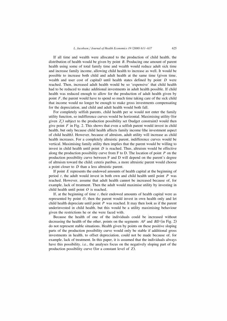
ŽAn increased rate of depreciation, d or an increased coinsurance rate in the.health insurance system, increased p that increases p would affect family health

by increasing the net cost of health capital. If both child and parent depreciationrates increased, but d increased more than d , the point indicating optimal healthc mwould move from P to PX in Fig. 3. The income effect would decrease both childand parent health, but the substitution effect would increase parent health whiledecreasing child health. The total effect would be a reduction in child health, whilethe effect on parent health would be ambiguous. Using Fig. 3 to analyse the effectof a reduction in the coinsurance rate for medical care utilisation by childrenŽ .aimed to increase child health , the effect on child health is positive but the effecton parent health is ambiguous. Because the cost of child health is reduced,resources previously used to produce child health can now partly be spent on adult

Žhealth production and partly on the production of other consumption commodi-.ties . Health related information will have a similar effect. Increased health related

Ž .Fig. 3. This figure illustrates the effects of changes in the costs of health capital. Parent health H isiŽ .given by the vertical axis and child health H by the horizontal axis. The initial production possibilityc

curve is given by AB; UU and U XU X are family indifference curves; and initial optimal health is givenby point P. An increased cost of health, where the cost of child health increases more than the cost ofparent health, will give the new production possibility curve AXBX, and a new equilibrium given by

X Žpoint P . The total effect on family health can be divided into an income effect the move from P toY . Ž Y X .P and a substitution effect the move from P to P .


information will make the parent more productive in producing new health. Thisincrease in E will decrease both p and p .H ,i i c

ŽIf the value of parent time is set equal to his or her wage rate i.e,. w rl sv ,i W i.ism,f and if some insurance exists, covering x% of losses due to taking care of

a sick child, the net cost of child health will be:

p d qry Ep rEt rpŽ .Ž .c c c c

y yv Eh rEH 1yx yv Eh rEH 1yx . 27Ž . Ž . Ž . Ž . Ž .m Sc ,m c f Sc ,f c

Ž .For x)0, the net cost of child health in Eq. 27 is higher than the net cost ofŽ . Ž .child health in Eq. 25 the denominator on the right hand side , implying a lower

optimal level of child health. Increasing x will decrease the monetary value ofŽ .investments in child health increasing the net cost of child health because an

increased rate of compensation will reduce the incentive to invest in child health.The effect on family health by an increase in x is shown in Fig. 4. Optimal health

Fig. 4. This figure illustrates the effects of an increase in the rate of compensation for income lossesŽ . Ž .due to taking care of a sick child x and an increase in transfer payment B , respectively. The

increase in the level of compensation will increase the slope of the production possibility curve fromX Ž . XAB to AB , increasing the net cost of child health H . Optimal health will move from point P to P .c

Ž .The effect on child health will be negative, while the effect on parent health H is ambiguous. Aniincrease in transfer payment will increase family resources available for family production of healthand other commodities, leaving the ratio of net cost of health capital unchanged. Family initialproduction possibilities are given by AB, and optimal health by point P. An increase in transferpayment will shift the production possibility curve to the right, and optimal health to PY.


will move from P to PX. The effect on child health is negative while the effect onparent health is ambiguous. The reason for this reduction in child health is that theparent cannot increase family income as much as before by investing in childhealth after x is increased. An increase in the compensation for losses due to ownŽ .parent illness will have a similar effect, but the reduction in H due to theiincrease in the level of compensation will now partly be offset by the reduction inthe wage rate caused by the parent’s reduced health.

Ž .An increase in transfer payment B has no effect on the marginal condition inŽ .Eq. 25 , but it will have an effect on family health. As shown in Fig. 4, an

increase in B will shift the production possibility curve to the right. As shown, anincrease in B will increase both parent and child health, i.e., the point of optimalhealth will move from P to PY. As Fig. 4 is drawn, the increase in B is assumedto have no effect on the slope of the production possibility curve. However, it maybe the case that an increase in B affects the parent’s time allocation decision, forexample decreasing the incentive for market work. Such a decrease in h willv,ithen lead to a flatter production possibility curve.

4. Discussion and concluding remarks

This paper has extended the individualistic demand for health model, theGrossman model, by deriving a model of the family as producer of health. This isan important extension because it makes it possible to analyse the influence thatother family members may have on an individual’s health related behaviour and toanalyse differences in health and health care utilisation between children.This section summarises the conclusions and discusses the implications of some

of the assumptions and simplifications made in the paper. It ends with a discussionof some policy implications of the model.

4.1. Conclusion

The purpose of this paper was to develop a demand for health model that takesinto account characteristics and behaviour of other family members’ on anindividual’s health and health care utilisation. This was done by treating eachfamily member as a producer of his own and other family members’ health.The extended model, the family-as-producer-of-health model, has several impli-

cations. The main finding is that the family will not try to equalise marginalbenefits and marginal costs of health capital for each family member. Instead, theywill invest in health until the rate of marginal consumption benefits equals the rateof marginal net effective costs of health capital, or, in other words, family

Ž .members will invest in health until the rate of marginal lifetime utility of health


Žto the effective price of health is equal for all family members and equal to the.marginal utility of wealth . The net effective cost of health capital equals the user

cost of capital less the marginal investment benefit of health capital. Variablessuch as the level of compensation in the social insurance system, the effectiveprice of care, health related information, and transfer payments will all affect thefamily production possibility set, and, therefore, the optimal level and distributionof family health.

Ž .Results related to individual health show a that an increased rate of deprecia-Ž .tion will decrease the individual’s level of health; b that when an individual’s

wage rate becomes more sensitive to differences in health, the individual willŽ .invest more in health; and c that the more restricting the time constraint is, the

higher the individual’s valuation of time will be and the more the individual investin health.

ŽRegarding child health, it is shown that poor families where the wealth.restriction is binding value child health higher than rich families and that families

where the wealth constraint is not binding have a zero marginal utility of childhealth. Further, a child with unhealthy parents can be expected to have lowerhealth compared with a child with healthy parents, because resources have to bespent on increasing the health of the unhealthy parents for the marginal conditionto be fullfilled. It is also shown that even a selfish parent will invest in child health

Ž .because child health affects family income the investment aspect of child health .By assuming that adult health cannot be increased because, for example, lack of

treatment, it is shown that the adult will maximise utility by ‘overinvesting’ inchild health. If, on the other hand, their endowed amounts of health capital weresuch that the child’s health was above and the parent’s health below what isregarded as optimal, the parent will invest only in own health and let child healthdepreciate until optimum is reached.The effects of changes in some exogenous variables on optimal family health

were also considered in the paper. An increased rate of depreciation, an increasedcoinsurance rate in the health insurance system, or an increase in health relatedinformation will affect family health by increasing the net cost of health capital.

4.2. Common preferences

The model derived in this paper is based on the assumption of commonŽ .preferences Becker, 1991 . As shown by recent empirical work, it may not be a

proper description to assume that spouses have common preferences and toassume that who has the control of resources has no impact on how theseresources are allocated. Empirical work shows, for example, that the distribution

Ž .of non-earned income does matter. Thomas 1990 found that unearned income inthe hands of a mother had a bigger effect on her family’s health than income under

Ž .the control of a father. Thomas 1994 also examined the relationship between


parental education and child height. He found that the education of the mother hada bigger effect on her daughters’ height, while paternal education had a biggerimpact on his sons’ height. He also found that as the woman’s power in thehousehold allocation process increased17, she became more able to assert herpreferences and direct more resources towards commodities she cares about.

Ž .Haddad and Hoddinott 1994 used a non-cooperative bargaining model to exam-ine the impact of the intrahousehold distribution of income on the anthropometric

Ž .status height-for-age of boys relative to girls. They found that an increase infemale share of household income seemed not to be gender neutral; boys wouldgain relative to girls.

ŽSeveral models of family behaviour have been suggested in the literature for.surveys, see Lundberg and Pollak, 1996 and Bergstrom, 1997 . McElroy and

Ž .Horney 1981; see also Manser and Brown, 1980 suggested a model where thedistribution of resources within the family is seen as the outcome of a cooperativeNash bargaining process. According to this bargaining model, the objective of thespouses is to maximise a utility–gain production function, defined as the productof the husband’s gain and the wife’s gain from marriage. These gains from

Ž .marriage will decrease when utility as single the threat point increases.Then, using a Nash bargaining model to describe family behaviour, the effect

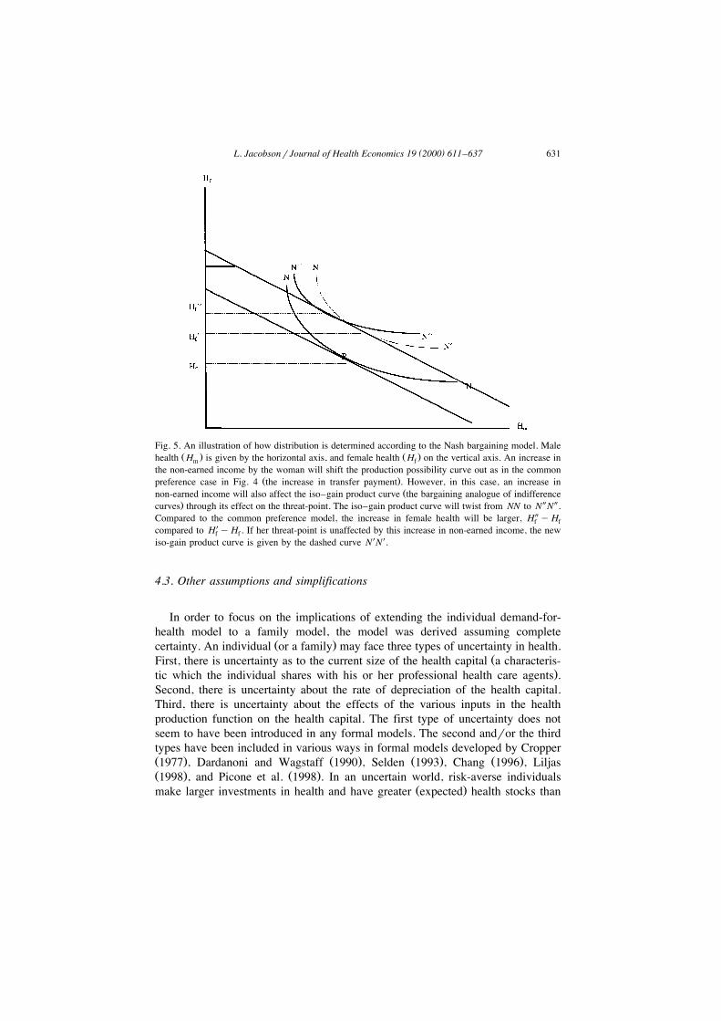
on family health of an increase in the non-earned income by the wife is illustratedŽ . Ž .in Fig. 5. Male health H is given by the horizontal axis, and female health Hm f

by the vertical axis. An increase in the non-earned income by the wife will shiftthe production possibility curve outwards as in the common preference case in Fig.4. However, in this case, an increase in non-earned income will also affect the

Ž .iso–gain product curve the bargaining analogue of indifference curves throughits effect on the threat-point. If utility as single is the actual threat-point, herbargaining power will increase, because the increase in her non-earned incomewill increase her utility as single. The iso–gain product curve will twist from NNto NYNY. Compared to the common preference model, the increase in femalehealth will be larger, HYyH compared to H XyH . The increase in the mother’sf f f fnon-earned income may also increase child health either because she cares moreabout child health than the father does, or because she prefers more healthy goodsthan he does. In the last case, not only child health will increase, but the health ofall family members. Thus, according to the Nash bargaining model, familydecisions are the outcome of some bargaining process and family demands willdepend not only on prices and total family income, but also on the determinants ofthe threat points18.

17 As indicators of power in the household allocation decisions the study used nonlabour income,opportunities outside the home, and relative educational status.18 Ž .A Nash bargaining family demand for health model is formally derived in Bolin et al., 1999b ,

which also contains some additional results.


Fig. 5. An illustration of how distribution is determined according to the Nash bargaining model. MaleŽ . Ž .health H is given by the horizontal axis, and female health H on the vertical axis. An increase inm f

the non-earned income by the woman will shift the production possibility curve out as in the commonŽ .preference case in Fig. 4 the increase in transfer payment . However, in this case, an increase in

Žnon-earned income will also affect the iso–gain product curve the bargaining analogue of indifference. Y Ycurves through its effect on the threat-point. The iso–gain product curve will twist from NN to N N .

Compared to the common preference model, the increase in female health will be larger, HYyHf fcompared to H XyH . If her threat-point is unaffected by this increase in non-earned income, the newf fiso-gain product curve is given by the dashed curve N XN X.

4.3. Other assumptions and simplifications

In order to focus on the implications of extending the individual demand-for-health model to a family model, the model was derived assuming complete

Ž .certainty. An individual or a family may face three types of uncertainty in health.ŽFirst, there is uncertainty as to the current size of the health capital a characteris-

.tic which the individual shares with his or her professional health care agents .Second, there is uncertainty about the rate of depreciation of the health capital.Third, there is uncertainty about the effects of the various inputs in the healthproduction function on the health capital. The first type of uncertainty does notseem to have been introduced in any formal models. The second andror the thirdtypes have been included in various ways in formal models developed by CropperŽ . Ž . Ž . Ž .1977 , Dardanoni and Wagstaff 1990 , Selden 1993 , Chang 1996 , LiljasŽ . Ž .1998 , and Picone et al. 1998 . In an uncertain world, risk-averse individuals

Ž .make larger investments in health and have greater expected health stocks than


they would in a perfectly certain world. This result is quite in accordance with theŽ .discussion in Grossman 1972a,b , even though it was not formally proved, since

the original Grossman model ruled out uncertainty for the sake of simplicity.19 AŽ .portfolio approach to health behaviour has been discussed by Dowie 1975 and,

Ž .more formally, by Horgby 1997 . Their basic message is that the individualshould diversify his or her health investment activities, if there is uncertainty aboutthe effects on health capital of various measures intended to improve health.Some implications of these results for the model developed in this paper seem

Ž .to be worth noticing. The expected total health capital of the family would belarger than in the certain case. With common preferences, the relative distribution

Ž .of expected health capital among family members would remain the same as inthe certain case. With non-common preferences, however, the relative distributionmay change, since family members may then have different attitudes towards riskand uncertainty. For the same reason, the optimal portfolio of health investmentsmay be quite different for different family members, not only because of thecharacteristics included in the certain case developed in this paper but alsodepending on diverging attitudes towards risk among family members. Thus, thisphenomenon may contribute to explaining differing morbidity and mortalityexpectations and experiences among family members.A further simplification made in the paper is that important family related

Ž .decisions such as family formation i.e., marriage or divorce , family size and intersibling allocation of resources were not considered. Those issus are discussed by

Ž . Ž . Ž .Becker 1991 , Becker and Lewis 1973 and Becker and Tomes 1976 , and giveŽrise to issues such as assortative marriage that equally healthy or wealthy

.individuals marry each other , the interaction between quantity and quality ofchildren, and whether the transfers of resources from parents to children are basedon efficiency or equity considerations.

4.4. Policy implications

The model presented in this paper has some important policy implications whendiscussing and analysing differences in health and health care utilisation amongindividuals and for a single individual over time. It was shown that variables suchas other family members’ health, preferences, education, income, etc., are impor-

Žtant for an individual’s stock of health and health care utilisation i.e., health.related behaviour . It was further shown that an individual’s present health and

health care utilisation is the result of investments made earlier in life by him orherself, and by his or her parents.

19 Grossman suggested that the simplest way to introduce uncertainty might be to let a givenŽ .consumer face a probability distribution of depreciation rates in every period Grossman 1972a,b .

However, none of the studies so far has employed such an approach.


Consequently, the individual’s family situation has to be considered whenformulating prevention, treatment, rehabilitation and educational health pro-grammes. But family variables also have to be included in the evaluation of suchprogrammes and in analyses of reasons to differences in health and health careutilisation.Naturally, the extended theoretical model also calls for new empirical estima-

tions, which can increase our knowledge about health behaviour both per se and inpolicy-relevant contexts. Some preliminary results are available in Bolin et al.Ž .1998a , who analyse the demand for health and health care in Sweden 1980r81and 1988r89, using a Swedish panel data set and considering both the dynamiccharacter of the Grossman model and the impact of the family structure.

Acknowledgements

I am grateful for the helpful comments and suggestions on earlier drafts fromBjorn Lindgren, Kristian Bolin, Inga Persson, participants at the seminar in¨political economy at the Department of Economics, Lund University, and tworeferees. This research was supported by grants from Vardalstiftelsen and from theSwedish National Institute of Public Health, which is gratefully acknowledged.

Appendix A

To solve the dynamic optimisation problem in Section 2, optimal control theoryŽ .is used Chiang, 1992 . The problem is formulated as an equality constraint

problem where time is binding in each period, but where the family is free toborrow and lend during the family lifetime. It contains given initial points, but avariable terminal point; i.e., a horizontal-terminal line problem. The Lagrangian

Ž .for solving this problem is Chiang, 1992, p. 276 :

Lsu H ,H ,H ,Z eyu tŽ .m f c

ql I M ,h ,h ;E ,E yd HŽ .Hm m m Hm ,m Hm ,f H ,m h ,f m m

ql I M ,h ,h ;E ,E yd HŽ .H f f f H f ,m H f ,f H ,m H ,f f f

ql I M ,h ,H ;E ,E yd HŽ .Hc c c Hc ,m Hc ,f H ,m H ,f c c

ql rWqv H ,E hŽ .W m m v ,m v ,m

qv H ,E h yp M qM qM yqXŽ . Ž .f f v ,f v ,f m f c

w xqw Vyh yh yh yh yh yh yhm v ,m Z ,m Hm ,m H f ,m Hc ,m S ,m Sc ,m

w xqw Vyh yh yh yh yh yh yh A1Ž .f v ,f Z ,f Hm ,f H f ,f Hc ,f S ,f Sc ,f


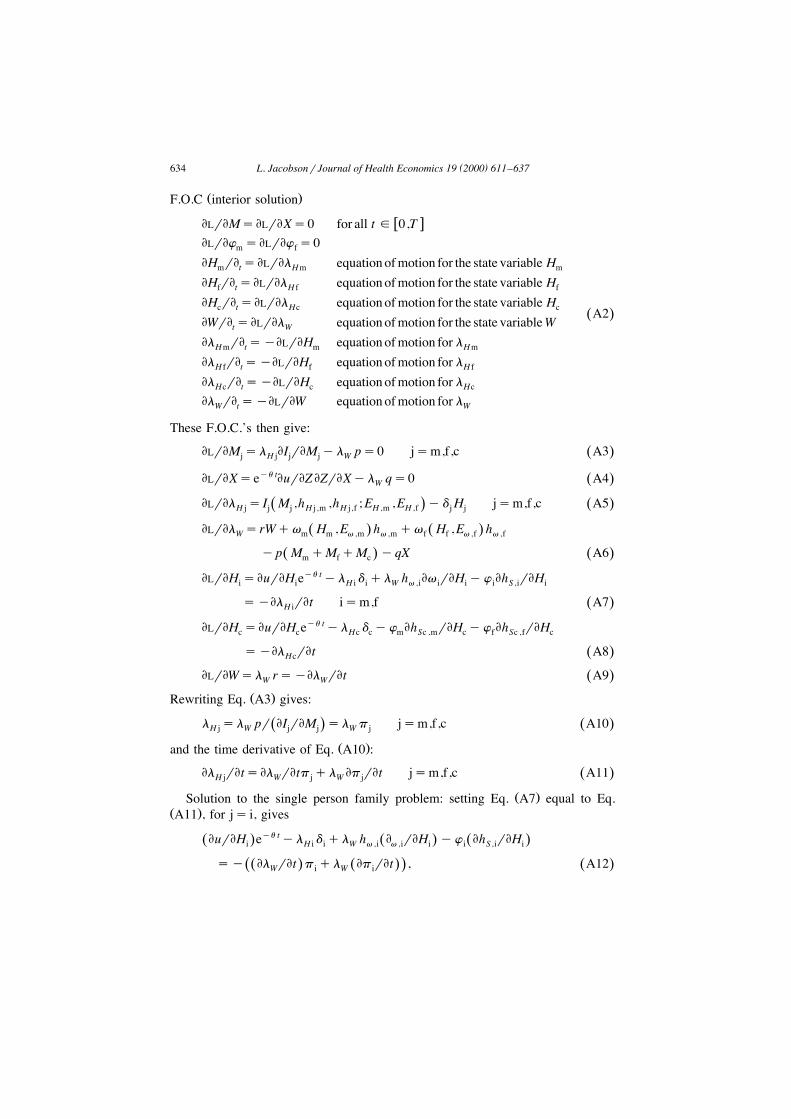
Ž .F.O.C interior solution

w xELrEMsELrEXs0 for all tg 0,TELrEw sELrEw s0m f

EH rE sELrEl equation ofmotion for the state variable Hm t Hm m

EH rE sELrEl equation ofmotion for the state variable Hf t H f f

EH rE sELrEl equation ofmotion for the state variable Hc t Hc c A2Ž .EWrE sELrEl equation ofmotion for the state variableWt W

El rE syELrEH equation ofmotion for lHm t m Hm

El rE syELrEH equation ofmotion for lH f t f H f

El rE syELrEH equation ofmotion for lHc t c Hc

El rE syELrEW equation ofmotion for lW t W

These F.O.C.’s then give:

ELrEM sl EI rEM yl ps0 jsm,f,c A3Ž .j H j j j W

ELrEXseyu tEurEZ EZrEXyl qs0 A4Ž .W

ELrEl s I M ,h ,h ;E ,E yd H jsm,f,c A5Ž .Ž .H j j j H j ,m H j ,f H ,m H ,f j j

ELrEl srWqv H ,E h qv H ,E hŽ . Ž .W m m v ,m v ,m f f v ,f v ,f

yp M qM qM yqX A6Ž . Ž .m f c

ELrEH sEurEH eyu tyl d ql h Ev rEH yw Eh rEHi i H i i W v ,i i i i S ,i i

syEl rEt ism,f A7Ž .H i

ELrEH sEurEH eyu tyl d yw Eh rEH yw Eh rEHc c Hc c m Sc ,m c f Sc ,f c

syEl rEt A8Ž .Hc

ELrEWsl rsyEl rEt A9Ž .W W

Ž .Rewriting Eq. A3 gives:

l sl pr EI rEM sl p jsm,f,c A10Ž .Ž .H j W j j W j

Ž .and the time derivative of Eq. A10 :

El rEtsEl rEtp ql Ep rEt jsm,f,c A11Ž .H j W j W j

Ž .Solution to the single person family problem: setting Eq. A7 equal to Eq.Ž .A11 , for js i, gives

EurEH eyu tyl d ql h E rEH yw Eh rEHŽ . Ž . Ž .i H i i W v ,i v ,i i i S ,i i

sy El rEt p ql Ep rEt , A12Ž . Ž . Ž .Ž .W i W i


Ž . Ž .and using Eqs. A10 and A9 to substitute for l and yEl rEt givesHm WŽ .subscript i omitted

EurEH eyu tyl pdql h EvrEH yw Eh rEHŽ . Ž . Ž .W W v S

sl rpyl EprEt A13Ž . Ž .W W

Ž .Re-arranging Eq. A13 and adding the time subscript gives the marginal conditionŽ .in Eq. 8 , i.e.,

eyu trl Eu rEH qh Ev rEH y w rl Eh rEHŽ .Ž .t ,W t t t ,v t t t t ,W t ,S t

sp d qry Ep rEt rp . A14Ž . Ž .t t t t

Ž . Ž .Solution to the husband–wife family problem: use Eqs. A9 – 11 to write Eq.Ž .A7 as

EurEH eyu tyl p d ql h Ev rEH yw Eh rEHŽ . Ž . Ž .i W i i W v ,i i i i S ,i i

sl rp yl Ep rEt , ism,f. A15Ž . Ž .W i W i

Set i equal to m and f, respectively, and divide the expression for m with the oneŽ .for f to obtain the marginal condition in Eq. 18 ,

w xŽ . Ž . Ž .Ž .EurEH p d q ry Ep rEt rp y Ev rEH h y w rl Eh rEHŽ .m m m m m m m v ,m m W S ,m ms .w xŽ . Ž . Ž .Ž .EurEH p d q ry Ep rEt rp y Ev rEH h y w rl Eh rEHŽ .f f f f f f f v ,f f W S ,f f

A16Ž .Ž . Ž .Solution to the parents–child family problem: use Eqs. A9 – 11 to write Eq.

Ž .A8 as:

EurEH eyu tyl p d yw Eh rEH yw Eh rEHŽ . Ž . Ž .c W c c m Sc ,m c f Sc ,f c

sl rp yl Ep rEt A17Ž . Ž .W c W c

Ž . Ž .The marginal condition in Eq. 25 is then obtained by dividing Eq. A15 forŽ .ism with Eq. A17 , i.e.,

EurEHmEurEHc

w xŽ . Ž . Ž .Ž .p d q ry Ep rEt rp y Ev rEH h y w rl Eh rEHŽ .m m m m m m v ,m m W S ,m ms .w xŽ . Ž .Ž . Ž .Ž .p d q ry Ep rEt rp y y w rl Eh rEH y w rl Eh rEHŽ .c c c c m W Sc ,m c f W Sc ,f c

A18Ž .

References

Ž .Barker, D.J.P. Ed. , 1992. Fetal and infant origins of adult disease. British Medical Journal, London.Barker, D.J.P., 1994. Mothers, babies, and disease in later life. British Medical Journal, London.Becker, G.S., 1965. A theory of the allocation of time. The Economic Journal 75, 493–517.

Ž .Becker, G.S., 1974. A theory of social interactions. Journal of Political Economy 82 6 , 1063–1094.


Becker, G.S., 1991. A Treatise on the Family. Harvard University Press, Cambridge, MA, enlargededition.

Becker, G.S., Lewis, H.G., 1973. On the interaction between the quantity and quality of children.Ž .Journal of Political Economy 81 2 , 279–288, Pt. 2.

Becker, G.S., Tomes, N., 1976. Child endowments and the quantity and quality of children. Journal ofŽ .Political Economy 84 4 , S143–S162, Pt. 2.

Ž .Bergstrom, T., 1997. A survey of theories of the family. In: Rosenzweig, M.R., Stark, O. Eds. ,Handbook of Population and Family Economics. North-Holland, Amsterdam.

Bolin, K., Jacobson, L., Lindgren, B., 1999. The demand for health and health care in Sweden1980r81 and 1988r89. Lund University, Departments of Economics and Community HealthŽ .mimeo .

Bolin, K., Jacobson, L., Lindgren, B., 1999. The family as the health producer — the case when familymembers are Nash-bargainers. Lund University, Departments of Economics and Community

Ž .Medicine mimeo .Chang, F.-R., 1996. Uncertainty and investment in health. Journal of Health Economics 15, 369–376.Chiang, A.C., 1992. Elements of Dynamic Optimization. McGraw-Hill, New York.Cigno, A., 1991. Economics of the Family. Oxford Univ. Press, Oxford.Cropper, M.L., 1977. Health, investment in health, and occupational choice. Journal of Political

Economy 85, 1273–1294.Currie, J., Gruber, J., 1996. Health insurance eligibility, utilisation of medical care, and child health.

Ž .The Quarterly Journal of Economics 111 2 , 431–466.Dardanoni, V., Wagstaff, A., 1990. Uncertainty and the demand for medical care. Journal of Health

Economics 9, 23–38.Delaney, S.E., 1995. Divorce mediation and children’s adjustment to parental divorce. Pediatric

Ž .Nursing 21 5 , 434–437.Dowie, J., 1975. The portfolio approach to health behaviour. Social of Science and Medicine 9,

619–631.Grossman, M., 1972a. The demand for health: a theoretical and empirical investigation. NBER

Occasional Paper 119, New York.Grossman, M., 1972b. On the concept of health capital and the demand for health. Journal of Political

Economy 80, 223–255.Ž .Grossman, M., 1975. The correlation between health and schooling. In: Terleckyj, N.E. Ed. ,

Household Production and Consumption. Columbia University Press for the National Bureau ofEconomic Research, New York.

Grossman, M., 1982. The demand for health after a decade. Journal of Health Economics 1, 1–3.Ž .Grossman, M., 1998. The human capital model. In: Culyer, A.J., Newhouse, J.P. Eds. , Handbook of

Ž .Health Economics. North-Holland, Amsterdam, Forthcoming .Haddad, L., Hoddinott, J., 1994. Women’s income and boy–girl anthropometric status in the Cote

Ž .d’Ivoire. World Development 22 4 , 543–553.Horgby, P.-J., 1997. Essays on sharing, management, and evaluation of health risks, Ekonomiska

studier utgivna av nationalekonomiska institutionen, Handelshogskolan vid Goteborgs Universitet¨ ¨no 68, Goteborg University, Dissertation.¨

Ž .Leibowitz, A., 1974. Home investments in children. Journal of Political Economy 82 2 .Liljas, B., 1998. The demand for health with uncertainty and insurance. Journal of Health Economics

17, 153–170.Lundberg, S., Pollak, R.A., 1996. Bargaining and distribution in marriage. Journal of Economic

Ž .Perspectives 10 4 , 139–158.Manser, M., Brown, M., 1980. Marriage and household decision making: a bargaining analysis.

Ž .International Economic Review 21 1 , 31–44.McElroy, M.B., Horney, M.J., 1981. Nash-bargained household decisions: toward a generalization of

Ž .the theory of demand. International Economic Review 22 2 , 333–349.


Muurinen, J.-M., Le Grand, J., 1985. The economic analysis of inequalities in health. Social ScienceŽ .and Medicine 20 10 , 1029–1035.

Picone, G., Uribe, M., Wilson, R.M., 1998. The effect of uncertainty on the demand for medical care,health capital, and wealth. Journal of Health Economics 17, 171–185.

Polachek, S.W., Siebert, W.S., 1993. The Economics of Earnings. Cambridge Univ. Press, Cambridge.Power, C., Bartley, M., Smith, G.D., Blane, D., 1996. Transmission of social and biological risk across

Ž .the life course. In: Blane, D., Brunner, E., Wilkinson, R. Eds. , Health and Social Organization.Towards a Health Policy for the 21st Century. Routledge, London.

Selden, T., 1993. Uncertainty and health care spending by the poor: the health capital model revisited.Journal of Health Economics 12, 109–115.

Thomas, D., 1990. Intra-household resource allocation: an inferential approach. Journal of HumanŽ .Resources 25 4 , 635–664.

Thomas, D., 1994. Like father, like son: like mother, like daughter: parental resources and child height.Ž .Journal of Human Resources 29 4 , 950–988.

Thomas, D., Strauss, J., Henriques, M.-H., 1991. How does mother’s education affect child height?Ž .Journal of Human Resources 26 2 , 183–211.

Tucker, J.S., Friedman, H.S., Schwartz, J.E., Criqui, M.H., Tomlinson-Keasey, C., Wingard, D.L.,Martin, L.R., 1997. Parental divorce: effects on individual behavior and longevity. Journal of

Ž .Personal and Social Psychology 73 2 , 381–391.Wadsworth, M.E., 1996. Family and education as determinants of health. In: Blane, D., Brunner, E.,

Ž .Wilkinson, R. Eds. , Health and Social Organization. Towards a Health Policy for the 21stCentury. Routledge, London.

Wadsworth, M.E., 1997. Health inequalities in the life course perspective. Social Science and MedicineŽ .44 6 , 859–869.

The family as producer of health — an extended grossman ...

Documents

Transcript of The family as producer of health — an extended grossman ...