The emergence of norms of cooperation in staghunt games with production

Lidia Bagnoli�, Giorgio Negroniy

February 6th, 2008

Abstract

In this paper we study a two agents asymmetric stag hunt game. Themodel has an in�nity of strict, Pareto rankable Nash equilibria. Theequilibrium selection problem is solved by appealing to the stochasticstability concept put forward by Young (1993). We prove two main results.When the action sets are numerable in�nite sets, then for any value of thedistributive parameter we can expect the emergence of a norm involvingless than maximal cooperation. When instead the action sets are �nitesets of a particular type (in the sense that each agent can choose hismaximum optimal e¤ort and fractions of this), then for some value of thedistributive parameter we can expect the emergence of a norm involvingmaximal cooperation.

keywords: asymmetric stag hunt game; stochastic stability; cooper-ation norms.

1 Introduction

According to Skyrms (2004), the stag hunt is a story that became a game. Thegame is a prototype of the social contract while the story is told by Rousseau.Consider two hunters who have to decide whether to cooperate to hunt a stag.Suppose that, in the case they succeed in hunting the stag, the catch is dividedequally. Hunting stags is demanding and it requires the cooperation of both.Suppose that, while waiting for the stag, a hare happens to pass within reachof one of them; hunting hares is much easier: it requires a minimum e¤ort andit can be done successfully without the cooperation of the other hunter. Letus assume that no binding agreement is possible for the two hunters. Althoughfor each of them half a stag is more valuable than a hare, they can not be surethat the other player will provide the required e¤ort. In other terms, althoughthe situation in which both hunt the stag is a Nash equilibrium which Paretodominates the other equilibrium in which both hunt the hare (the minimax

�Regione Emilia Romagna, Bologna.yBologna University and DARTT. E-mail: giorgio.negroni@unibo.it

1

solution), the former equilibrium may fail to be risk dominant. See Carlssonand Van Damme (1993).

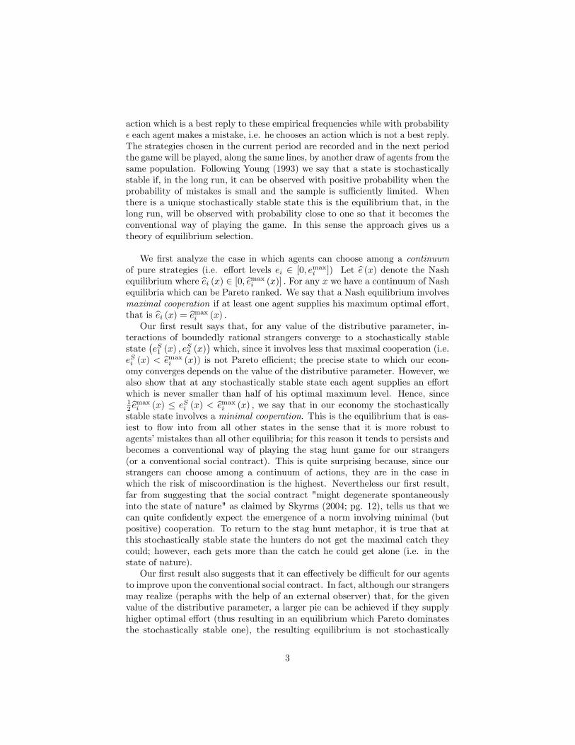
In this paper we follow Bryant (1983) and Cooper (1999) and use the staghunt game as a model of team production. We assume that agents�e¤ort arecomplementary inputs so that total output of the team is determined by the leaste¤ort. In terms of the stag hunt parable, this means that we focus on the totalcatch of the hunters rather than on the stag/hare alternative. It is a standardresult in games with strategic complementarities that, when the marginal bene�tfrom coordinated actions is greater than the marginal cost of e¤ort, then anycommon level of e¤ort is a strict Nash equilibrium; see Cooper and John (1988).Moreover, since all individuals prefer an equilibrium in which all players supplyhigher e¤ort, all these Nash equilibria can be Pareto ranked. We are thus ina situation in which since the Nash equilibrium concept neither prescribes norpredicts the outcome of the game, it needs to be supplemented with an adequatetheory of equilibrium selection. Any traditional re�nement would not help aslong as the play is simultaneous; of course if we consider a sequential game, thenthe only subgame perfect equilibrium is the Pareto optimum one. However,the evidence from experimental economics suggests that the Pareto dominantequilibrium is quite unlikely in the simultaneous stag hunt game; in this case,in fact, life can indeed be "inside the production possibility frontier" (Cooper(1999), pg. 151). See Van Huyck, Battalio and Beil (1990), Van Huyck, Cookand Battalio (1997) and the discussion in Crawford (1991, 1995).

We depart from Bryant (1983) in three respects. First we consider a twoagents economy with identical (separable) utility functions but di¤erent produc-tivities. Second, although the distributive parameter (x) regulating the distri-bution of the joint product among the two agents is �xed1 , we do not assumefrom the outset that the resulting distribution is egalitarian.2 Third, we assumethat our stag hunt game is played by boundedly rational, randomly matchedplayers, along the lines suggested by Young (1993, 1998). In a sense we areconsidering a stag hunt played by boundedly rational "strangers".3

Since our strangers are engaged in a strategic game, they need to form anexpectation on the behavior of their opponent. Following Young we considerthe case in which this expectation is shaped by the accumulation of antecedents,according to an inductive process. Suppose that each agent collects a sampleof size k from the last m past plays of the game, with k < m. Given k he thenextracts the empirical frequencies with which each (pure) strategy was playedin the past by other agents. With probability 1� � each agent then chooses an

1We assume that it is determined by the existing distributional rule (left unexplained)endorsed by the society.

2As pointed out by Cooper (1999), the coordination problems arising in Byant�s (1983)model is partly a consequence of the rule that distributes equally the fruits of the cooperationregardless of individual e¤ort levels. See also Bryant (1994).

3This last assumption makes our contribution departing also from Crawford�s (1991) evo-lutionary approach to the stag hunt as well as from Crawford�s (1995).

2

action which is a best reply to these empirical frequencies while with probability� each agent makes a mistake, i.e. he chooses an action which is not a best reply.The strategies chosen in the current period are recorded and in the next periodthe game will be played, along the same lines, by another draw of agents from thesame population. Following Young (1993) we say that a state is stochasticallystable if, in the long run, it can be observed with positive probability when theprobability of mistakes is small and the sample is su¢ ciently limited. Whenthere is a unique stochastically stable state this is the equilibrium that, in thelong run, will be observed with probability close to one so that it becomes theconventional way of playing the game. In this sense the approach gives us atheory of equilibrium selection.

We �rst analyze the case in which agents can choose among a continuumof pure strategies (i.e. e¤ort levels ei 2 [0; emaxi ]) Let be (x) denote the Nashequilibrium where bei (x) 2 [0; bemaxi (x)] : For any x we have a continuum of Nashequilibria which can be Pareto ranked. We say that a Nash equilibrium involvesmaximal cooperation if at least one agent supplies his maximum optimal e¤ort,that is bei (x) = bemaxi (x) :Our �rst result says that, for any value of the distributive parameter, in-

teractions of boundedly rational strangers converge to a stochastically stablestate

�eS1 (x) ; e

S2 (x)

�which, since it involves less that maximal cooperation (i.e.

eSi (x) < bemaxi (x)) is not Pareto e¢ cient; the precise state to which our econ-omy converges depends on the value of the distributive parameter. However, wealso show that at any stochastically stable state each agent supplies an e¤ortwhich is never smaller than half of his optimal maximum level. Hence, since12bemaxi (x) � eSi (x) < bemaxi (x) ; we say that in our economy the stochasticallystable state involves a minimal cooperation. This is the equilibrium that is eas-iest to �ow into from all other states in the sense that it is more robust toagents�mistakes than all other equilibria; for this reason it tends to persists andbecomes a conventional way of playing the stag hunt game for our strangers(or a conventional social contract). This is quite surprising because, since ourstrangers can choose among a continuum of actions, they are in the case inwhich the risk of miscoordination is the highest. Nevertheless our �rst result,far from suggesting that the social contract "might degenerate spontaneouslyinto the state of nature" as claimed by Skyrms (2004; pg. 12), tells us that wecan quite con�dently expect the emergence of a norm involving minimal (butpositive) cooperation. To return to the stag hunt metaphor, it is true that atthis stochastically stable state the hunters do not get the maximal catch theycould; however, each gets more than the catch he could get alone (i.e. in thestate of nature).Our �rst result also suggests that it can e¤ectively be di¢ cult for our agents

to improve upon the conventional social contract. In fact, although our strangersmay realize (peraphs with the help of an external observer) that, for the givenvalue of the distributive parameter, a larger pie can be achieved if they supplyhigher optimal e¤ort (thus resulting in an equilibrium which Pareto dominatesthe stochastically stable one), the resulting equilibrium is not stochastically

3

stable.4

We then analyze the interactions of boundedly rational strangers when eachcan choose among a �nite number of pure strategies. Our second result saysthat, although equilibria with minimal cooperation may still be stochasticallystable, now it is also possible to observe the emergence of a norm involvingmaximal cooperation. However the emergence of this norm is not due to anye¢ ciency considerations; in fact, we show that the stochastically stable equilib-rium involving maximal cooperation is Pareto e¢ cient for some values of thedistributive parameter only and provided that the number of strategies avail-able is not too big and agents have su¢ ciently di¤erent productivities. Lastlywe show that when each agent can choose more that two actions, the equilibriumwith maximal cooperation corresponding to the value of the distributive para-meter suggested by the utilitarian unweighted cooperative solution will never bestochastically stable. We remark that our results are not due to any incentiveproblem; see Legros and Mathews (1993), Vislie (1994) and Hvide (2001).

The remaining of the paper is organized as follow. In Section 2 we presenta variant of Bryant (1983) symmetric coordination problem. In Section 3 weintroduce our asymmetric coordination game. In Section 4 we brie�y summarizeYoung�s (1993) concept of stochastic stabile state. Section 5 then discusses thestochastic stability of our asymmetric coordination game �rst when agents havea continuum of strategies and then when agents can choose only among a �nitenumber of discrete strategies. Section 7 summarizes our results.

2 A symmetric coordination game

In this section we brie�y present a variant of Bryant�s (1983) coordination game.Consider two equally productive agents engaged in a joint project and let

Y = �min [e1; e2]

be the technology available, where ei 2 [1; emax]. Suppose that the outcome ofthe cooperation is divided according to the distributional parameter x so thatagent 1 gets Y1 = xY and agent 2 gets Y2 = (1� x)Y: Let us �rst suppose5x = 1=2: Denoting by Vi (Yi; ei) = Yi � bei the payo¤ of the generic agent i; weget

Vi =�2 min [e1; e2]� bei = amin [e1; e2]� bei;

4One possibility open to our strangers would be to agree on conditional contracts, whoseenforcement is ensured by an external observer, in which (a) they agree on a particular divisionof the fruits of social cooperation and (b) they supply their maximal optimal e¤ort, given thisvalue of the distributive parameter: However this alternative is not viable in our economy sincethere is no external observer. A still di¤erent alternative would be to consider self-enforcingsocial contracts, as in Binmore (1994). We leave the exploration of this alternative to futureresearch.

5As it can be veri�ed, x = 1=2 is also to the cooperative solution of the game. See Cooper(1999).

4

where we assume a > b: This is the game studied by Van Huyck et al. (1990).Because of the technological complementarity, and since e¤ort is costly, no agenthas the incentive to choose an e¤ort such that his contribution to the jointproject is larger than the contribution of the other agent. Let e2 = ee: Thepayo¤ of agent 1 is V1 (ee; ee) = (a� b) ee if e1 = ee and V1 (e1; ee) = (a� b) e1 ife1 < ee: Analogously for agent 2. Since V1 (ee; ee)� V1 (e1; ee) = (ee� e1) (a� b) ; itfollows that all the pro�les (e1; e2) = (e; e) with e � emax are Nash equilibria,being a > b:Suppose now that the distributive parameter is x: Then

V1 = �xmin [e1; e2]� be1

V2 = � (1� x)min [e1; e2]� be2:

Let e2 = ee: The payo¤ of agent 1 is V1 (ee; ee) = (�x� b) ee if e1 = ee andV1 (e1; ee) = (�x� b) e1 if e1 < ee:Hence V1 (ee; ee) � V1 (e1; ee) if (ee� e1) (�x� b) �0; that is if x � b=�: Consider now player 2 and let e1 = ee: Then V2 (ee; ee) =(� (1� x)� b) ee if e2 = ee and V2 (e2; ee) = (� (1� x)� b) e2 if e2 < ee: HenceV2 (ee; ee) � V2 (e2; ee) if (ee� e2) (� (1� x)� b) � 0; that is if x � (�� b) =�: Itturns out that all the pro�les (e1; e2) = (e; e) with e � emax are Nash equilib-ria if and only if b=� � x � (�� b) =�: In this case the game is a stag hunt.However if the distributive parameter does not satis�es this condition, then thegame admits only one Nash equilibrium in which (e1; e2) = (0; 0) :

3 An asymmetric coordination game

In this section we modify the basic model by allowing some form of heterogene-ity; speci�cally we assume (a) that individual e¤orts are not equally productiveand (b) that the distribution of the fruits of joint production is not a priori egali-tarian. Moreover, since we want to consider a game that maintains the structureof the stag hunt for any value of the distributive parameter, we modify the VanHuyck et al. (1990) model by considering a non linear e¤ort disutility. Inthe next section we shall use this model to study the problem of equilibriumselection by appealing to the inductive argument put forward by Young (1993).As in Cooper (1999), we consider an economy populated by two individuals

engaged in a joint project. The output produced is given by

Y = min [�e1; �e2] (1)

where e1 and e2 denote the e¤ort levels chosen by the two agents while � and� are two real numbers representing the (possibly) heterogeneous individuals�productivities. We suppose that there is an already established distributionalrule which determines how the output is shared by the two individuals; lettingx denote the share of the production going to agent 1, we get Y1 = xY andY2 = (1� x)Y: The output received by each individual is entirely consumed.

5

Let6

V1 = xmin [�e1; �e2]� e21

V2 = (1� x)min [�e1; �e2]� e22:(2)

denote the agents�payo¤s and let emax1 = �=2 and emax2 = �=2 be the maximumfeasible level of e¤orts for the two agents. Let G denote the game in which agentssimultaneously selects their e¤ort levels from the sets Si = [0; emaxi ] and receivea payo¤ given by (2) : Given the distributional parameter, and given agent�s 2e¤ort, the problem faced by agent 1 is to choose7 e1 to maximize x�e1 � e21subjected to �e1 � �e2: Let be1 be the solution of this problem, where:

be1 =8><>:

x�2 if e2 � x�2

2� ;

��e2 if e2 � x�

2

2� :

(3)

Analogously, the problem faced by agent 2 is to choose e2 to maximize(1� x)�e2� e22 subjected to �e2 � �e1: Let be2 be the solution of this problem,where:

be2 =8><>:(1� x) �2 if e1 � (1� x) �

2

2� ;

�� e1 if e1 � (1� x) �

2

2� :

(4)

We can state the following result.8

Proposition 1 For any x 2 [0; 1] there is an in�nity of strict, pure strategiesPareto rankable Nash equilibria. Let � � �

� : Then:

(a) the set of Nash equilibria is (be1; �be1) where be1 � min �bemax1 ; ��1bemax2

�=

min��x2 ;

(1�x)�22�

�;

(b) for any given x; the equilibrium in which at least one agent o¤ers hismaximum optimal e¤ort, i.e. be1 = bemax1 = xemax1 and be2 = bemax2 = (1� x) emax2 ;is Pareto dominant.

Proof. See the Appendix.

For each player we can write the payo¤ corresponding to any Nash equilib-rium as:

V1 (x) = be1 (x) (x�� be1 (x))V2 (x) = be1 (x) �(1� x)�� �2be1 (x)� (5)

6The quasi-linearity with respect to the consumption good is essential because in oureconomy the consumption good is the numeraire; cfr. Ray et al.(2006).

7We restrict our analysis to the case of pure strategies only.8 In a similar model, Anderson et al. (2001) argue that a change in e¤ort cost does not

a¤ect the Nash equilibria. This is not necessarily true in our model.

6

In this section we restrict our analysis to the case in which, for any valueof the distributive parameter, at least one agent chooses his maximum level ofoptimal e¤ort9 , i.e. bei = bemaxi :We say that the corresponding Nash equilibriuminvolves maximal cooperation: From (1) and Proposition 1 it follows that at anyNash equilibrium the level of production with maximal cooperation is

Y =

8><>:�bemax1 = x�

2

2 if x � x�;

�bemax2 = (1� x) �2

2 if x � x�;(6)

where x� � �2

�2+�2= 1

�2+1: Production attains its maximum level Y when

x = x�. The following table shows the income and the utility distributions asfunctions of x; corresponding to the Nash equilibrium with maximal cooperation.

x � x� x � x�

Y1 (x) x2 �2

2 x (1� x) �2

2

Y2 (x) x (1� x) �22 (1� x)2 �2

2

V1 (x) x2 �2

4 (1� x) �2

2

hx�1 + �2

2�2

�� �2

2�2

iV2 (x) x�

2

2

�1� x

��2

2�2+ 1��

(1� x)2 �2

4

(7)

The maximum optimal e¤ort is supplied by agent 1 when x � x� and byagent 2 when x � x�: Notice that x� corresponds to the unweighted utilitariancooperative solution of the model. The next Lemma establishes some relevantproperties of the equilibrium payo¤s functions V1 (x) and V2 (x).

Lemma 2 Consider the payo¤ functions V1 (x) and V2 (x) given by (5) : Then:a) V1 (x) = V2 (x) = 0 for x = 0 and x = 1: For any 0 < x � x�; V1 (x)

is an increasing and convex function while for any x � x�; V1 (x) is a concavefunction with a maximum V 1 at x = x1: For any 0 < x � x�; V2 (x) is aconcave function with a maximum V 2 at x = x2 while for any x � x�; V2 (x) isa decreasing and convex function. V1 (x) and V2 (x) are maximized respectivelywhen

x1 =�2 + �2

2�2 + �2; x2 =

�2

�2 + 2�2; (8)

where, for any (�; �) ; x2 < x� < x1 and x2 < 12 < x1.

9Notice that since Bryant (1983) considers only an egalitarian distribution, he �nds thatthere is only one Pareto dominant equilibrium. In our case instead, we have one Paretodominant equilibrium for any x:

7

b) Let � > �: Then V 1 < V 2: Moreover V2 (x) > V1 (x) for every x < x3and V2 (x) � V1 (x) for every x � x3 where

x3 ��2 + �2

3�2 + �2; (9)

and x2 < x� < x3:c) Let � < �: Then V 1 > V 2: Moreover V2 (x) > V1 (x) for every x < x4

and V2 (x) � V1 (x) for every x � x4 where

x4 �2�2

�2 + 3�2; (10)

and x4 < x� < x1:

Proof. Omitted since it relies on simple algebraic manipulations. �

The next Lemma shows that the game has two properties that will be usefulin the following analysis.

Lemma 3 The game G is acyclic and satis�es the bandwagon property. More-over, let L (e) denote the length of the shortest best reply path originated in thestrategy pro�le e; then L� = maxL (e) = 2:

Proof. See the Appendix.

Acyclicity means that the best reply graph contains no directed cycles, aproperty satis�ed by all coordination games. A su¢ cient condition for the(marginal) bandwagon property to hold for generic (i.e. not necessarily acyclic)symmetric games has been proved by Kandori and Rob (1998): A reformulationwhich holds for acyclic but not necessarily symmetric two players games is givenby Binmore, Samuelson and Young (2003). Let = (2; S1; S2; V1; V2) be a�nite acyclic game with two players and let SN denote the set of all strict Nashequilibria of the game. exhibits the bandwagon property if for each s 2 SNand s 2 S with si 6= si for any i = (1; 2) the following conditions is satis�ed

V1 (s1; s2)� V1 (s1; s2) � V1 (s1; s2)� V1 (s1; s2) ; (11)

with an analogous condition holding for agent 2. This essentially says that, forboth agents, deviations from the equilibrium strategy are more costly when theopponent plays his part of the equilibrium.

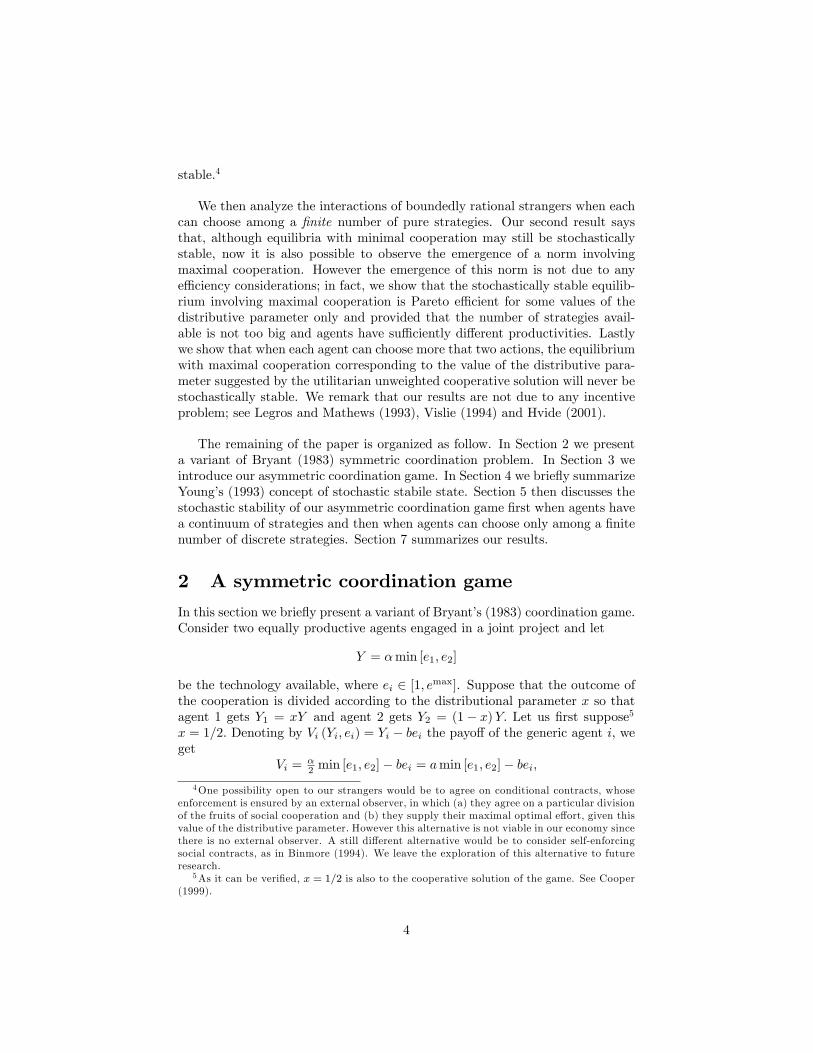
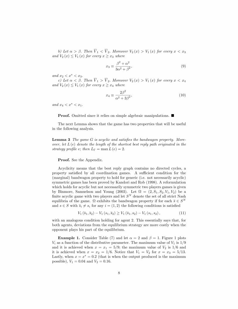
Example 1. Consider Table (7) and let � = 2 and � = 1: Figure 1 plotsVi as a function of the distributive parameter: The maximum value of V1 is 1=9and it is achieved when x = x1 = 5=9; the maximum value of V2 is 1=6 andit is achieved when x = x2 = 1=6: Notice that V1 = V2 for x = x3 = 5=13:Lastly, when x = x� = 0:2 (that is when the output produced is the maximumpossible), V1 = 0:04 and V2 = 0:16:

8

10.750.50.250

0.2

0.15

0.1

0.05

0

V1; V2V1; V2

Figure 1 - V1 and V2 as a function of x when � = 1 and � = 2. V1 dotted.

Lemma 3 can be used to establish the existence of two regions in which mu-tually advantageous agreements are possible; these are respectively the intervals[0; x2) and (x1; 1] : The interval [x2; x1] represents instead the set of e¢ cient dis-tributional norms: for any x belonging to this interval we can not increase theutility of one agent without decreasing the utility of the other one.

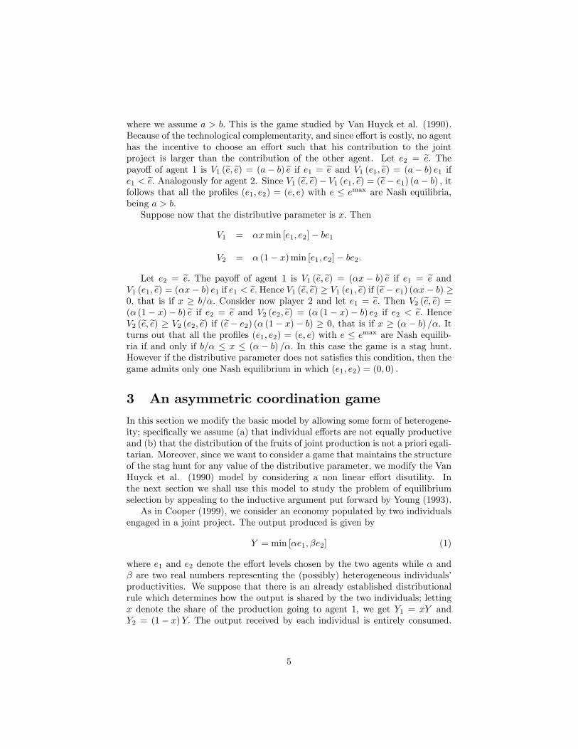
We now ask which is the maximum utility that both agents can reach at anyNash equilibrium with maximal cooperation. In order to derive this, we cannot rely on the utility possibility frontier (UPF) traditionally de�ned since thisis based on the assumption that the amount of good available for distributionis exogenously given. This is not true in our economy. As we have seen (seethe proof of Proposition 1), the utility that each agent derives at the Nashequilibrium is maximum when, for any value of the distributive parameter,at least one agent chooses his maximum optimal e¤ort. However, since thismaximum e¤ort depends on x; by changing the distributive parameter we changethe total output as well as the associated utility of each agent. This leads usto introduce the concept of utility distribution frontier (UDF) that we nowde�ne.10

De�nition 4 Consider the Nash equilibrium in which, for any given x; at leastone agent o¤ers his maximum optimal e¤ort. The Utility Distribution Frontier(UDF) describes how the corresponding utility pair (V1; V2) varies with x:

Since the UDF is derived under the assumption that at least one agent sup-plies his maximum optimal e¤orts, it represents the equilibria involving maximalcooperation. The UDF tells us: (a) the utility we can assure to one agent giventhe utility of the other one when the distributional parameter x changes, know-ing that (b) to any particular x there corresponds a particular level of output

10See Wasow (1980).

9

available for distribution. As a consequence, when we move along the UDF (thatis when x changes), output varies. There is however a precise relationship be-tween the two frontiers. To see this consider a given level of output and the UPFassociated. Except when the speci�ed level of output corresponds to maximumlevel, the UPF intersects the UDF in two points. These correspond to the twodistributions of utility (corresponding to two di¤erent values of the distributiveparameter) supporting the speci�ed level of output as an equilibrium.

0.40.30.20.10

0.4

0.3

0.2

0.1

0

V1

V2

V1

V2

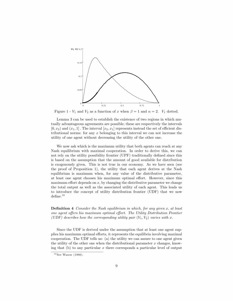
Figure 2 - UDF and equilibrium paths.

Figure 2 shows an example of the UDF (in which � = 2 and � = 1).11 Frominspection we see immediately that the UDF is asymmetric and not comprehen-sive. Since we consider an economy populated by agents with the same utilityfunctions, the asymmetry is entirely due to the di¤erence in e¤ort productivi-ties. The non-comprehensiveness derives from the existence of the two regionsin which mutually advantageous agreements are possible.12

Suppose now that x is given and consider the continuum of Nash equilibriaderived by progressively increasing the e¤ort levels, starting from the state ofnature of zero e¤ort. In the payo¤ space, this generates a path V2 (V1) startingfrom (0; 0) and ending in a point on the UDF in correspondence of which atleast one agent supply his maximum optimal e¤ort. As a consequence, alongthe path total production increases. Figure 2 shows three possible paths, eachderived for a speci�c value13 of x:

11Let V = (V1; V2) be a point on the UDF. Consider a clockwise change of V; starting fromthe origin, x = 0. Then output �rst increases; it reaches a maximum level when x = x� (whichcorresponds to a point V belonging to the decreasing harm of the UDF) and then declines,reaching again the origin when x = 1.12We may be tempted to conclude that free disposal could make the UDF comprehensive;

however, this is not true in our model since this would involve a series of utility pairs whichare not Nash equilibria.13Concerning Figure 2, the convex path on the left hand side is derived for x = 1

3; the

concave path on the right hand side is derived for x = 23; lastly the linear path in the middle

10

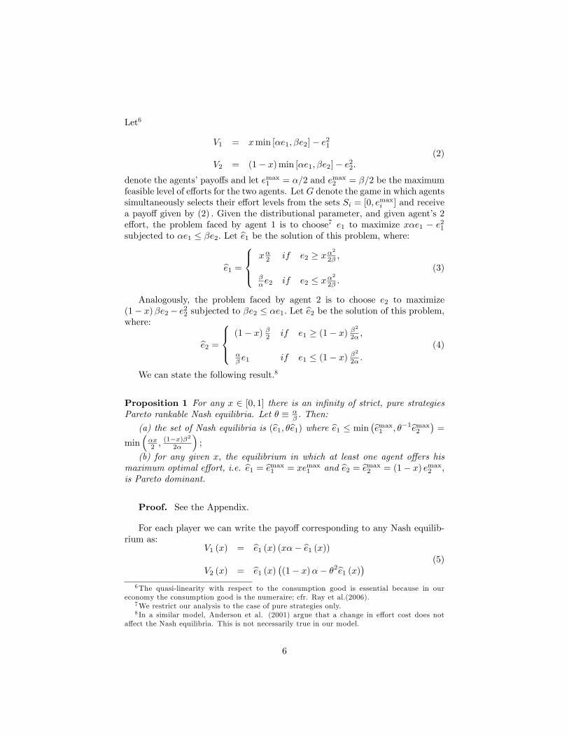
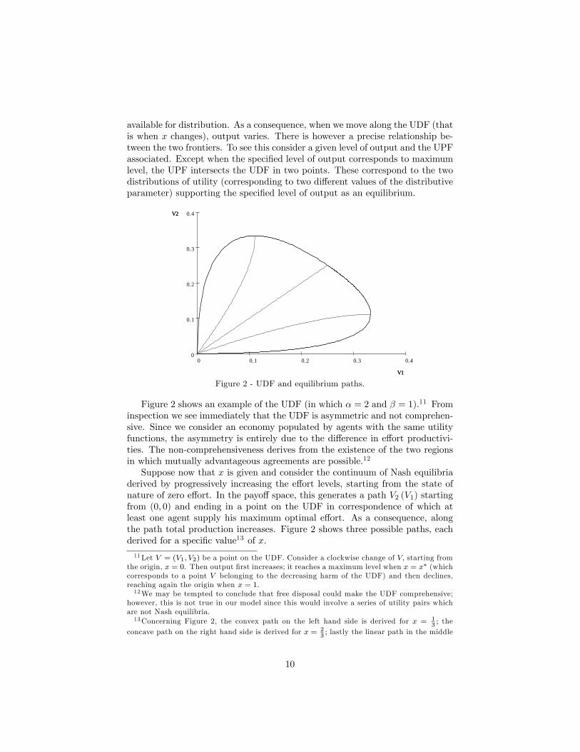
Lastly, we want to understand how the utility distribution frontier is a¤ectedby a change in the e¤ort productivities. Let us keep constant the productivityof one agent and increase the productivity of the other one. Few computationsshow that when x � x� we get @V1=@� > 0; @V2=@� > 0; @V1=@� = 0 and@V2=@� > 0; when instead x � x� we get @V1=@� > 0; @V2=@� > 0; @V1=@� >0 and @V2=@� = 0: This implies that the utility distribution frontier movesoutward, as shown in Figure 3. Notice that for x < x�; we have a multipliere¤ect (see Cooper and John (1988)) when the productivity of agent 1 increases;for x > x�; we have instead a multiplier e¤ect when the productivity of agent 2increases.

0.20.150.10.050

0.2

0.15

0.1

0.05

0

V1

V2

V1

V2

Figure 3 - E¤ect of a change of � on the UDF when � = 1; inner locus:� = 0:5; middle locus: � = 1; outer locus: � = 2:

4 Stochastic stability

In this Section we brie�y discuss the notion of stochastically stable state intro-duced by Young (1993).Let = (2; S1; S2; V1; V2) be a �nite game with two players and let SN

denote the set of all strict Nash equilibria of the game. Let t = 1; 2; ::: de-note successive time periods and consider a �xed (but large) population of Nplayers. Let N1 and N2 be the sub-populations of agents 1 and 2 respectively.In each period the �nite basic game G is played once by two agents randomlyselected from these sub-populations. When selected, each agent has to forman expectation on the behavior of his opponent. Let h (t) = (s (1) ; :::; s (t)) bethe history of plays at the end of period t; it consists of the past plays of thegame where each play denotes the pro�le of strategies played in that period,i.e.s (t) = (s1 (t) ; s2 (t)) : Since gathering information is costly, each agent bases

is derived for x = x�: In general any path with x < x� is convex in the (V1; V2) space whereasany path with x > x� is concave.

11

his current action not on the whole past plays available but rather on a sampleof k plays taken from the most recent m (with 1 � k < m) plays.14Thus at the beginning of period t + 1 (with t � m) each agent consults k

plays of the game and derives the empirical frequency with which each (pure)strategy was played in his sample; then he chooses his current action which isthe best reply to these empirical frequencies. Current actions are recorded15 andthe economy moves from the current state h to the successor state h0: Periodt+ 1 then closes.In the new period t + 2; the game is played again by two other randomly

selected agents. As before, each consults k plays of the game from the mostrecent m periods and chooses his current action which is the best reply to thenewly derived empirical frequencies. This moves the economy from the currentstate h0 to the successor state, h00 and so on: The transition from one state to itssuccessor is governed by the Markov process P 0 with transition function P 0hh0 :

Theorem 1 in Young (1993) shows that when the basic game is acyclic andthe sample is su¢ ciently limited, the adaptive process without mistakes selectsa state of the form h = (bs; :::; bs) where bs = (bs1; bs2) 2 SN is a pure strategiesstrict Nash equilibrium pro�le. In this state the same Nash equilibrium pro�lebs is played m times in succession so that we may call it a convention.16 Sincethe Markov process is reducible, the speci�c convention selected depends on theinitial conditions.

The assumption that agents always choose a best response given the avail-able information is clearly unrealistic. We can more realistically imagine thatwith probability � agent i chooses an action that is not a best reply to thederived empirical frequencies (i.e. he makes a mistake) while with probability1 � � he chooses an action which is a best reply to the derived empirical fre-quencies. In this case the transition from state h to state h0 is governed by theperturbed Markov process P � with transition function P �hh0 : If we assume thatall mistakes are possible and that the probability to make a mistake is time-independent, then the transition matrix associated with P �hh0 is strictly positiveand the Markov process is irreducible and aperiodic (ergodic). The process hasthus a unique stationary distribution ��: When the probability of mistakes issmall, the stationary distribution of the perturbed process P � coincides with oneof the stationary distributions of the unperturbed process P 0: Hence we say thata state h is stochastically stable relative to the process P � if lim�!0 �

� (h) > 0:When there is a unique stochastically stable state, this stationary distribution

14The fraction k=m can thus be seen as an index of the completeness of agents�information.15Since the memory size is �nite, the inclusion of the current period implies that agents

disregards the most distant play.16"This equilibrium then becomes the conventional way of playing the game, because for

as long as anyone can remember, the game has always been played in this way. Thereforesampling does not matter any more, because no matter what samples the agents take, theiroptimal responses will be to play the equilibrium that it already in place" (Young, (1993),66).

12

is concentrated around just one equilibrium; this is the state that, in the longrun, will be observed with probability close to one.

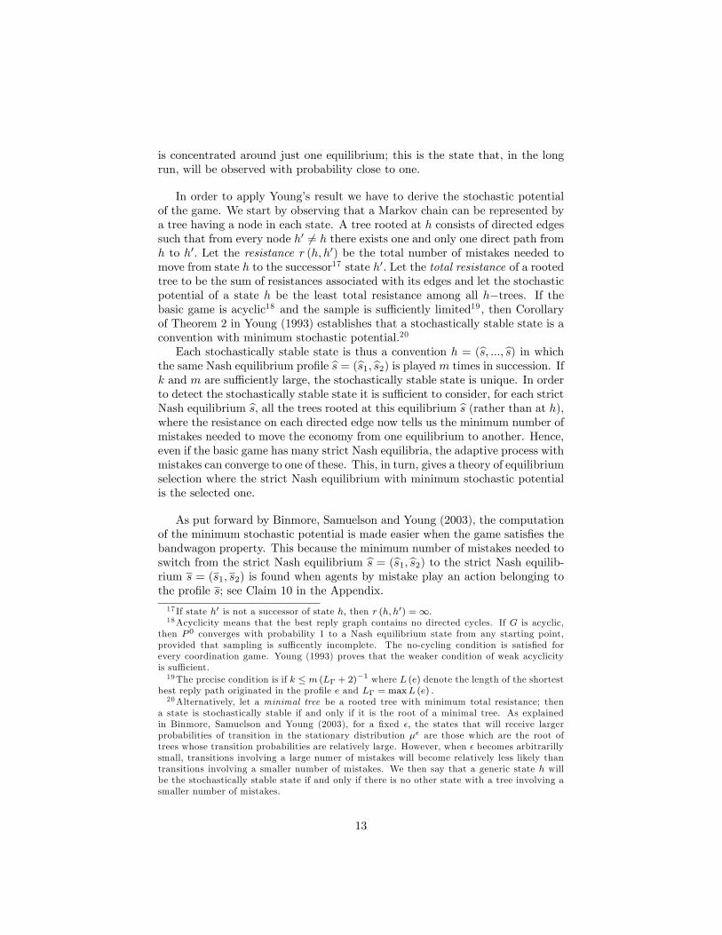
In order to apply Young�s result we have to derive the stochastic potentialof the game. We start by observing that a Markov chain can be represented bya tree having a node in each state. A tree rooted at h consists of directed edgessuch that from every node h0 6= h there exists one and only one direct path fromh to h0: Let the resistance r (h; h0) be the total number of mistakes needed tomove from state h to the successor17 state h0: Let the total resistance of a rootedtree to be the sum of resistances associated with its edges and let the stochasticpotential of a state h be the least total resistance among all h�trees. If thebasic game is acyclic18 and the sample is su¢ ciently limited19 , then Corollaryof Theorem 2 in Young (1993) establishes that a stochastically stable state is aconvention with minimum stochastic potential.20

Each stochastically stable state is thus a convention h = (bs; :::; bs) in whichthe same Nash equilibrium pro�le bs = (bs1; bs2) is playedm times in succession. Ifk and m are su¢ ciently large, the stochastically stable state is unique. In orderto detect the stochastically stable state it is su¢ cient to consider, for each strictNash equilibrium bs, all the trees rooted at this equilibrium bs (rather than at h),where the resistance on each directed edge now tells us the minimum number ofmistakes needed to move the economy from one equilibrium to another. Hence,even if the basic game has many strict Nash equilibria, the adaptive process withmistakes can converge to one of these. This, in turn, gives a theory of equilibriumselection where the strict Nash equilibrium with minimum stochastic potentialis the selected one.

As put forward by Binmore, Samuelson and Young (2003), the computationof the minimum stochastic potential is made easier when the game satis�es thebandwagon property. This because the minimum number of mistakes needed toswitch from the strict Nash equilibrium bs = (bs1; bs2) to the strict Nash equilib-rium s = (s1; s2) is found when agents by mistake play an action belonging tothe pro�le s; see Claim 10 in the Appendix.17 If state h0 is not a successor of state h; then r (h; h0) =1:18Acyclicity means that the best reply graph contains no directed cycles. If G is acyclic,

then P 0 converges with probability 1 to a Nash equilibrium state from any starting point,provided that sampling is su¢ cently incomplete. The no-cycling condition is satis�ed forevery coordination game. Young (1993) proves that the weaker condition of weak acyclicityis su¢ cient.19The precise condition is if k � m (L� + 2)�1 where L (e) denote the length of the shortest

best reply path originated in the pro�le e and L� = maxL (e) :20Alternatively, let a minimal tree be a rooted tree with minimum total resistance; then

a state is stochastically stable if and only if it is the root of a minimal tree. As explainedin Binmore, Samuelson and Young (2003), for a �xed �; the states that will receive largerprobabilities of transition in the stationary distribution �� are those which are the root oftrees whose transition probabilities are relatively large. However, when � becomes arbitrarillysmall, transitions involving a large numer of mistakes will become relatively less likely thantransitions involving a smaller number of mistakes. We then say that a generic state h willbe the stochastically stable state if and only if there is no other state with a tree involving asmaller number of mistakes.

13

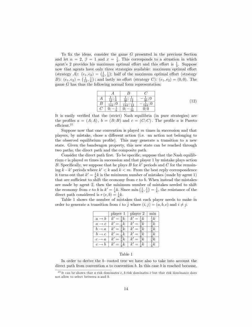
To �x the ideas, consider the game G presented in the previous Sectionand let � = 2, � = 1 and x = 1

3 : This corresponds to a situation in whichagent�s 2 provides his maximum optimal e¤ort and this e¤ort is 1

3 . Supposenow that agents have only three strategies available: maximum optimal e¤ort(strategy A): (e1; e2) =

�16 ;

13

�; half of the maximum optimal e¤ort (strategy

B): (e1; e2) =�112 ;

16

�; and lastly no e¤ort (strategy C): (e1; e2) = (0; 0). The

game G has thus the following normal form representation:

A B CA 1

12 ;19

136 ;

112 � 1

36 ; 0B 7

144 ; 07144 ;

112 � 1

144 ; 0C 0;� 19 0;� 1

36 0; 0

(12)

It is easily veri�ed that the (strict) Nash equilibria (in pure strategies) arethe pro�les a = (A;A) ; b = (B;B) and c = (C;C) : The pro�le a is Paretoe¢ cient.21

Suppose now that one convention is played m times in succession and thatplayers, by mistake, chose a di¤erent action (i.e. an action not belonging tothe observed equilibrium pro�le). This may generate a transition to a newstate. Given the bandwagon property, this new state can be reached throughtwo paths, the direct path and the composite path.Consider the direct path �rst. To be speci�c, suppose that the Nash equilib-

rium c is played m times in succession and that player 1 by mistake plays actionB: Speci�cally, we suppose that he plays B for k0 periods and C for the remain-ing k�k0 periods where k0 < k and k < m. From the best reply correspondenceit turns out that k0 = 1

8k is the minimum number of mistakes (made by agent 1)that are su¢ cient to shift the economy from c to b: When instead the mistakesare made by agent 2, then the minimum number of mistakes needed to shiftthe economy from c to b is k0 = 1

4k: Since min�18 ;

14

�= 1

8 ; the resistance of thedirect path considered is r (c; b) = 1

8k:Table 1 shows the number of mistakes that each player needs to make in

order to generate a transition from i to j where (i; j) = (a; b; c) and i 6= j:

player 1 player 2 mina! b k0 = 5

8k k0 = 14k

14k

a! c k0 = 78k k0 = 3

4k34k

b! a k0 = 38k k0 = 3

4k38k

b! c k0 = 78k k0 = 3

4k34k

c! a k0 = 38k k0 = 3

4k38k

c! b k0 = 18k k0 = 1

4k18k

Table 1

In order to derive the b�rooted tree we have also to take into account thedirect path from convention a to convention b: In this case b is reached because,21 It can be shown that a risk dominates c; b risk dominates c but that risk dominance does

not allow to select between a and b:

14

although agents observe that the Nash equilibrium a was played m times insuccession, some agent by mistake plays action B: The resistance of the directpath considered is r (a; b) = 1

4k: As shown in the second column of Table 2,when direct paths only are considered, the total resistance of the b�rooted treeis r (a; b) + r (c; b) = 3

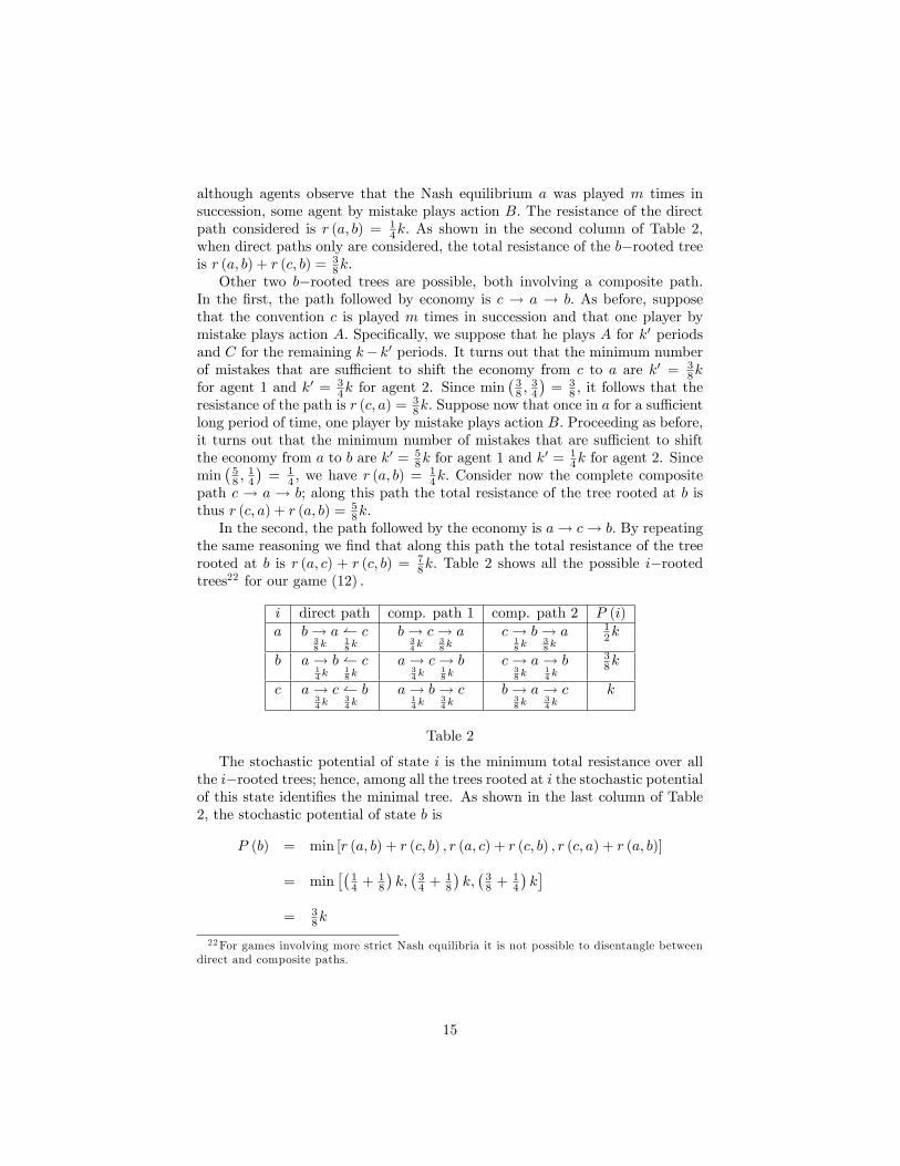
8k:Other two b�rooted trees are possible, both involving a composite path.

In the �rst, the path followed by economy is c ! a ! b: As before, supposethat the convention c is played m times in succession and that one player bymistake plays action A: Speci�cally, we suppose that he plays A for k0 periodsand C for the remaining k� k0 periods. It turns out that the minimum numberof mistakes that are su¢ cient to shift the economy from c to a are k0 = 3

8kfor agent 1 and k0 = 3

4k for agent 2. Since min�38 ;

34

�= 3

8 ; it follows that theresistance of the path is r (c; a) = 3

8k: Suppose now that once in a for a su¢ cientlong period of time, one player by mistake plays action B: Proceeding as before,it turns out that the minimum number of mistakes that are su¢ cient to shiftthe economy from a to b are k0 = 5

8k for agent 1 and k0 = 1

4k for agent 2. Sincemin

�58 ;

14

�= 1

4 ; we have r (a; b) =14k: Consider now the complete composite

path c ! a ! b; along this path the total resistance of the tree rooted at b isthus r (c; a) + r (a; b) = 5

8k:In the second, the path followed by the economy is a! c! b: By repeating

the same reasoning we �nd that along this path the total resistance of the treerooted at b is r (a; c) + r (c; b) = 7

8k: Table 2 shows all the possible i�rootedtrees22 for our game (12) :

i direct path comp. path 1 comp. path 2 P (i)a b!

38ka (

18kc b!

34kc!

38ka c!

18kb!

38ka 1

2k

b a!14kb (

18kc a!

34kc!

18kb c!

38ka!

14kb 3

8k

c a!34kc (

34kb a!

14kb!

34kc b!

38ka!

34kc k

Table 2

The stochastic potential of state i is the minimum total resistance over allthe i�rooted trees; hence, among all the trees rooted at i the stochastic potentialof this state identi�es the minimal tree. As shown in the last column of Table2, the stochastic potential of state b is

P (b) = min [r (a; b) + r (c; b) ; r (a; c) + r (c; b) ; r (c; a) + r (a; b)]

= min��14 +

18

�k;�34 +

18

�k;�38 +

14

�k�

= 38k

22For games involving more strict Nash equilibria it is not possible to disentangle betweendirect and composite paths.

15

The stochastically stable state is the state with minimum stochastic poten-tial. From inspection of the last column of Table 2 we conclude that

min [P (a) ; P (b) ; P (c)] = P (b)

so that the unique stochastically stable state of the above game is b; that isthe strict Nash equilibrium pro�le (B;B) in which each agent supply half of hisoptimal maximum e¤ort.23

5 Stochastically stable states in the stag-huntgame with production

In this Section we derive the stochastically stable states for the economy de-scribed in Section 3. Let assume that this economy is populated by N bound-edly rational agents and let N1 and N2 be the sub-populations of agents 1 and2 respectively; in each period, one agent is randomly selected from each sub-population to play the stage-game. Since agents are boundedly rational, theyare concerned with their stage-game strategies only. Since Young (1993) resultshold for a �nite game, in order to apply his approach we have to shift fromthe game G to a game G� (de�ned below) with a �nite strategy set. Here � isa real number su¢ ciently small and we interpret 1=� as a degree of precisionwith which we measure e¤ort. For smaller and smaller values of �; since we candiscriminate more �nely between e¤ort levels, the number of possible actions in-creases. In the limit as � ! 0, agents can choose their e¤ort from a continuumof values. We shall consider two cases: in the �rst e¤ort is a continuous variable(in the sense just speci�ed) while in the second e¤ort is a discrete variable.

5.1 Case 1: e¤ort is (in the limit) a continuous variable

Let x � x� and assume that agents can choose their equilibrium24 e¤ort levelsfrom the �nite and discrete sets S1 and S2 respectively25 where

S1 = f0; �; 2�; :::; bemax1 � �; bemax1 g [�eS1

S2 = f0; ��; 2��; :::; � (bemax1 � �) ; �bemax1 g [��eS1:

(13)

23A careful reader should have noticed that in our case there is no composite path withtotal resistance smaller than the total resistance of the direct path.24Notice that the original action set for the generic agent i is Si =

�0; :::; bemaxi ; :::; emaxi

:

However, since our game satis�es the bandwagon property, we can exclude all the e¤ort levelsgreater than the maximum optimal one; these actions will never be a Nash equilibrium anddo not alter the resistances of transition between states. Here eSi denotes the stochasticallystable e¤ort level; we include this in the set of feasible actions in order to derive exact results.See Binmore, Samuelson and Young (2003).25When instead x � x�; we have to consider the sets S01 and S02; where

S01 =�0; ��1�; :::; ��1

�bemax2 � ��; ��1bemax2

[���1eS2

S02 =

�0; �; :::; bemax2 � �; bemax2

[�eS2:

16

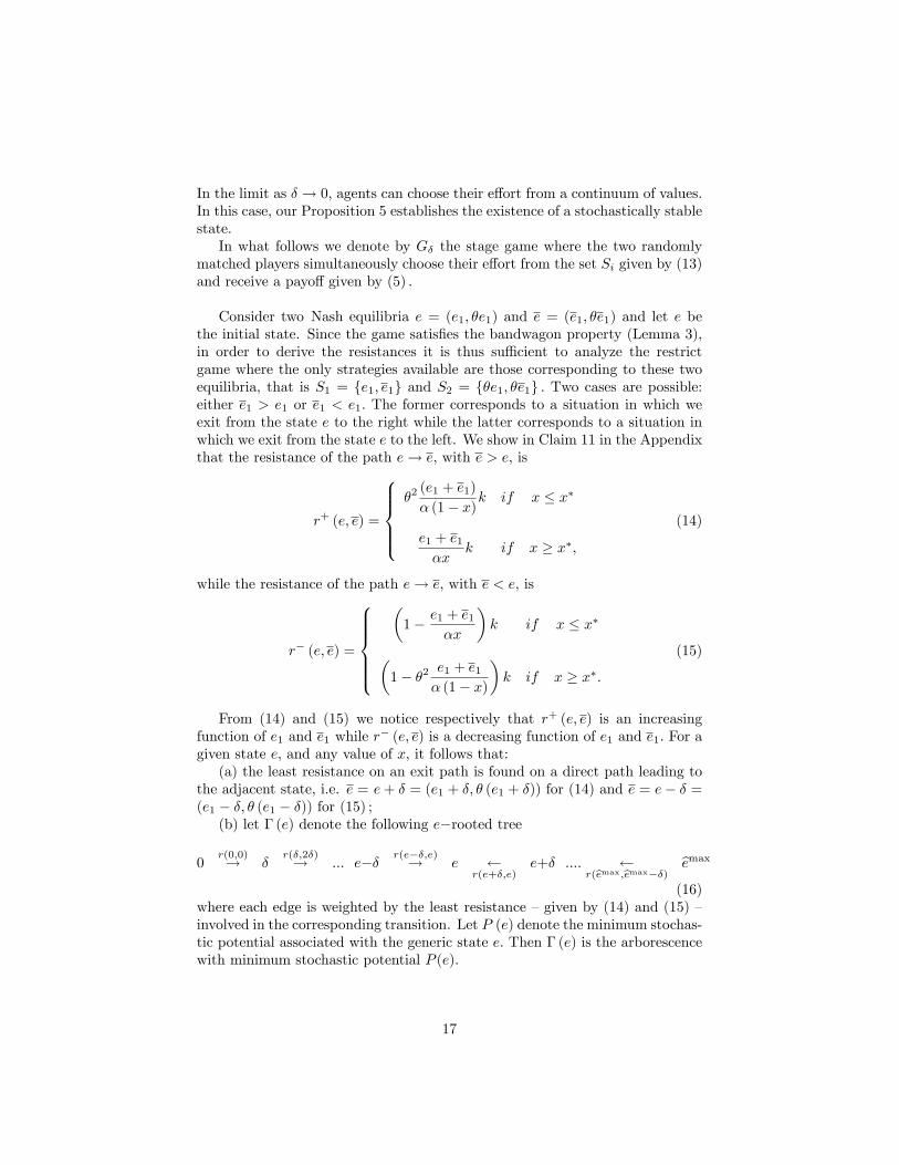
In the limit as � ! 0, agents can choose their e¤ort from a continuum of values.In this case, our Proposition 5 establishes the existence of a stochastically stablestate.In what follows we denote by G� the stage game where the two randomly

matched players simultaneously choose their e¤ort from the set Si given by (13)and receive a payo¤ given by (5) :

Consider two Nash equilibria e = (e1; �e1) and e = (e1; �e1) and let e bethe initial state. Since the game satis�es the bandwagon property (Lemma 3),in order to derive the resistances it is thus su¢ cient to analyze the restrictgame where the only strategies available are those corresponding to these twoequilibria, that is S1 = fe1; e1g and S2 = f�e1; �e1g : Two cases are possible:either e1 > e1 or e1 < e1: The former corresponds to a situation in which weexit from the state e to the right while the latter corresponds to a situation inwhich we exit from the state e to the left. We show in Claim 11 in the Appendixthat the resistance of the path e! e, with e > e; is

r+ (e; e) =

8>>><>>>:�2(e1 + e1)

� (1� x)k if x � x�

e1 + e1�x

k if x � x�;

(14)

while the resistance of the path e! e, with e < e; is

r� (e; e) =

8>>>><>>>>:

�1� e1 + e1

�x

�k if x � x�

�1� �2 e1 + e1

� (1� x)

�k if x � x�:

(15)

From (14) and (15) we notice respectively that r+ (e; e) is an increasingfunction of e1 and e1 while r� (e; e) is a decreasing function of e1 and e1: For agiven state e; and any value of x; it follows that:(a) the least resistance on an exit path is found on a direct path leading to

the adjacent state, i.e. e = e+ � = (e1 + �; � (e1 + �)) for (14) and e = e� � =(e1 � �; � (e1 � �)) for (15) ;(b) let � (e) denote the following e�rooted tree

0r(0;0)! �

r(�;2�)! ::: e�� r(e��;e)! e r(e+�;e)

e+� :::: r(bemax;bemax��) bemax

(16)where each edge is weighted by the least resistance �given by (14) and (15) �involved in the corresponding transition. Let P (e) denote the minimum stochas-tic potential associated with the generic state e: Then � (e) is the arborescencewith minimum stochastic potential P (e):

17

As shown in Claim 12 in the Appendix, we can write the stochastic potentialassociated with a generic state e as26

P (e) = P (e� �) + r (e� �; e)� r (e; e� �)

P (e) = P (e+ �) + r (e+ �; e)� r (e; e+ �)(17)

Since the game G� is acyclic, we know from Young (1993) that it has atleast one stochastically stable state, es� =

�eS1 ; e

S2

�: This is the state which

minimizes the stochastic potential over all the possible states, i.e. es� = argmineP (e) : Let27 0 < es� < bemax; then it must be P (es�) < P (es� + �) and P (es�) <P (es� � �) ; conditions satis�ed when288<: r (es� + �; e

s�)� r (es�; es� + �) < 0

r (es� � �; es�)� r (es�; es� � �) < 0:(18)

From (14) ; (15) and (18) it then follows that, for any value of the distributiveparameter, es� is a stochastically stable state if�����es� � �x2 1� x

1 + x��2 � 1

� ����� < �

2:

Therefore, as � ! 0 the stochastically stable state tends to the equilibrium

es =�eS1 (x) ; e

S2 (x)

�=

�x

2

(1� x)1 + x

��2 � 1

� ; �x2

� (1� x)1 + x

��2 � 1

�! :Notice that

eS1 =

8>><>>:bemax1

�1� x�2

1+x(�2�1)

�if x � x�

bemax2 ��1�1� 1�x

1+x(�2�1)

�if x � x�;

(19)

so that, for any x and for any �; bemaxi > eSi since

(1�x)1+x(�2�1) < 1 if x � x�

x�2

1+x(�2�1) < 1 if x � x�:

26From (14) and (15) we may also compute the resistances of the path e! e: When e > e;r� (e; e) = r (e+ �; e) ; when e < e; r+ (e; e) = r (e� �; e) :27The cases es� = bemax and es� = 0 will be considered below.28As shown above, for any value of x; the resistances r (e; e+ �) and r (e; e� �) are re-

spectively an increasing and a decreasing function of e: Then, if conditions (18) are satis�ed,it follows that P

�es� + (k � 1) �

�< P

�es� + k�

�and P

�es� � (k � 1) �

�< P

�es� � k�

�: This

ensures that the stochastic potential has a global minimum at es� .

18

From Point (b) of Proposition 1 it then follows that the stochastically stablestate es is not Pareto e¢ cient:

In previous analysis we assumed 0 < es� < bemax: We have now to verify thate¤ectively the lower and upper bound of the action set can not be stochasticallystable states. Suppose �rst that es� = bemax: Since a state involving an e¤ortgrater than the maximum optimal one can not be a Nash equilibrium, it followsthat bemax is stochastically stable only if P (bemax) < P (bemax � �) ; conditionsatis�ed when

r (bemax � �; bemax)� r (bemax; bemax � �) < 0: (20)

From (14) ; (15) we may write (20) as8><>:�x2 < �x

21�x

1+x(�2�1) +�2 if x � x�

(1�x)�22� < �x

21�x

1+x(�2�1) +�2 if x � x�

(21)

from which we conclude that bemax is stochastically stable when either � > �1and x � x� or � > �2 and x � x�; where

�1 � �x2�2

(�2x+(1�x))

�2 � �(1�x)2�2(�2x+(1�x)) :

(22)

Since these conditions can not be satis�ed as � ! 0; it follows that bemax cannot be a stochastically stable state.Suppose now that es� = 0: Since a state involving an e¤ort smaller that zero

is not feasible, it follows that zero e¤ort is a stochastically stable state only ifP (0) < P (�) ; condition satis�ed when

r (�; 0)� r (0; �) < 0: (23)

From (14) ; (15) ; since

r (�; 0)� r (0; �) =

8>><>>:1 + �

1�x(1+�2)2x(1�x) if x � x�

1 + ��1+x(1+�2)2x(1�x) if x � x�;

it follows that (23) is never satis�ed. We can summarize this discussion in thefollowing Proposition.

Proposition 5 Let G be the continuous game and let G� be a discrete approx-imation of G with precision 1=� where � < �1 for x � x� and � < �2 for x � x�:

19

Let x be given. As � ! 0; G� has a unique stochastically stable equilibrium givenby: �

eS1 (x) ; eS2 (x)

�=

�x

2

(1� x)1 + x

��2 � 1

� ; ��x2

(1� x)1 + x

��2 � 1

�! : (24)

The stochastically stable equilibrium is not Pareto e¢ cient.

Proposition 5 says that when � ! 0 and for any value of the distributiveparameter, the game played by boundedly rational strangers converges to astochastically stable but Pareto ine¢ cient state. The precise equilibrium towhich our economy converges depends on the value of the distributive parameter.When sampling is su¢ ciently large (although incomplete) and both k=m andthe probability of mistakes are su¢ ciently small, in the long run the equilibrium�eS1 ; e

S2

�will be observed with the highest positive probability so that it tends

to persist and becomes the conventional way of playing the stag hunt game.To get an idea of how much the stochastically stable levels of e¤ort di¤er from

the maximum optimal levels, consider (19) and notice that eS1 (x) =12bemax1 =

12bemax2 ��1 for x = x� while 12bemax1 < eS1 (x) < bemax1 when x < x� and 1

2bemax2 ��1 <

eS1 (x) < bemax2 ��1 when x > x�: Analogously for player 2. Therefore, for any x;the stochastically stable e¤ort is not smaller that half of the maximum optimale¤ort.29 Notice that when x � x�; the lower � (i.e. �=�), the lower the distancebetween the stochastically stable equilibrium and the equilibrium with maximale¤ort. The opposite obtains for x � x�:

Substituting (24) into (1) and (2) yields the production and the individualpayo¤s at the stochastically stable state:

Y S (x) = �2x2

(1�x)1+x(�2�1)

V S1 (x) = �2x2

4(1�x)

(1+x(�2�1))2�1� x+ 2x�2

�V S2 (x) = �2x

4(1�x)2

(1+x(�2�1))2�2 (1� x) + x�2

�(25)

Example 2. Let us reconsider now previous example 1. Let � = 2 and� = 1: The stochastically stable equilibrium is the strategy pro�le�

eS1 (x) ; eS2 (x)

�=

�x� x23x+ 1

;2x� 2x23x+ 1

�:

The associated level of production is Y S (x) = 2x 1�x3x+1 while agent�s payo¤s are�

V S1 ; VS2

�=

x2

1� x(3x+ 1)

2 (7x+ 1) ; x (1� x)2 2x+ 2

(3x+ 1)2

!:

29However, letting V S (x) =�V S1 (x) ; V S2 (x)

�and V (x) = (V1 (x) ; V2 (x)) ; this does not

mean that V S (x)� V (x) is maximum when x = x�:

20

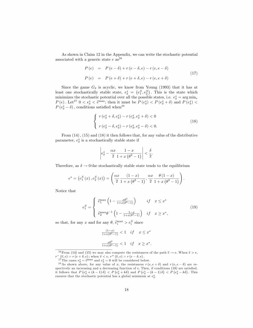
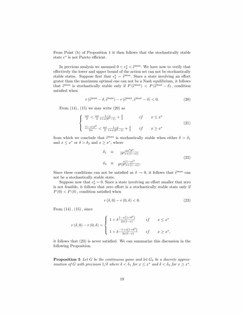
Figures 4 and 5 plot respectively the total production and the individual utilitycorresponding to the stochastically stable equilibrium (dotted curves). To fa-cilitate the comparison with previous Example 1, we have also plotted in theseFigures the total production and the individual payo¤s when agents supply theirmaximum optimal e¤ort.

10.750.50.250

0.5

0.375

0.25

0.125

0

YY

Figure 4 - Total production at the stochastically stable equilibria (dottedcurve).

10.750.50.250

0.2

0.15

0.1

0.05

0

V1; V2V1; V2

Figure 5 - V1 and V2 at the stochastically stable equilibria (dotted curves).

It is evident from (24) and (25) that the stochastically stable equilibriumdepends on the distributive parameter. By varying x we obtain a di¤erentstochastically stable equilibrium. We can then de�ne the set of stochasticallystable equilibria.

21

De�nition 6 Consider the stochastically stable Nash equilibria in which, forany given x; agents supply the e¤ort levels

�eS1 ; e

S2

�: The stochastically stable

Utility Distribution Frontier (S-UDF) describes how the corresponding utilitypair

�V S1 ; V

S2

�varies with x:

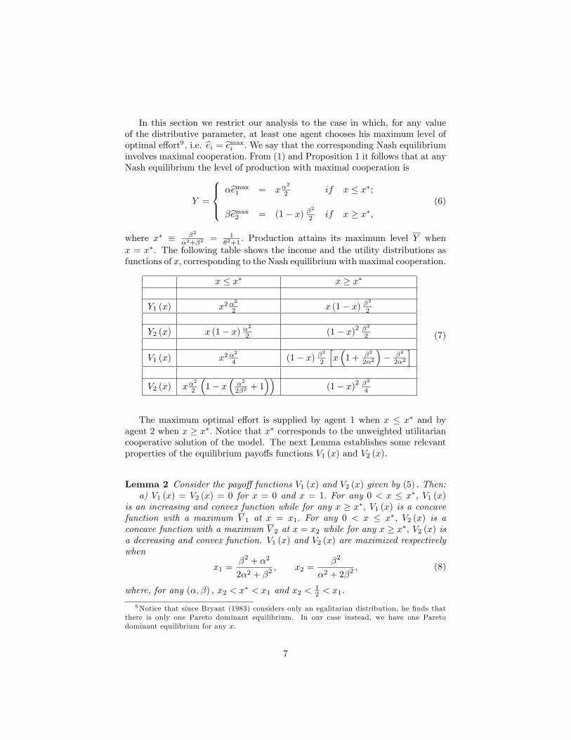
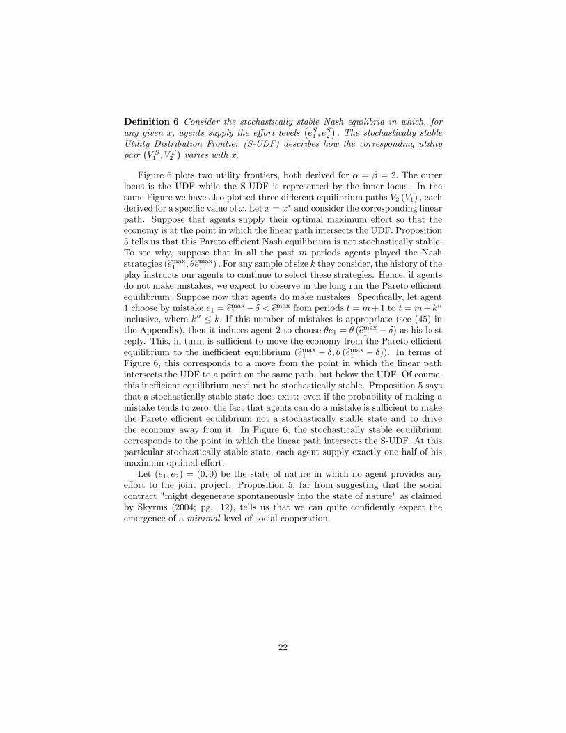
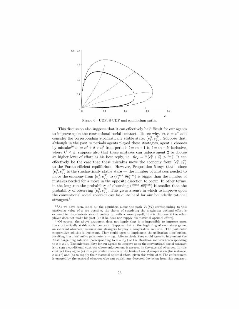
Figure 6 plots two utility frontiers, both derived for � = � = 2: The outerlocus is the UDF while the S-UDF is represented by the inner locus. In thesame Figure we have also plotted three di¤erent equilibrium paths V2 (V1) ; eachderived for a speci�c value of x: Let x = x� and consider the corresponding linearpath. Suppose that agents supply their optimal maximum e¤ort so that theeconomy is at the point in which the linear path intersects the UDF. Proposition5 tells us that this Pareto e¢ cient Nash equilibrium is not stochastically stable.To see why, suppose that in all the past m periods agents played the Nashstrategies (bemax1 ; �bemax1 ) : For any sample of size k they consider, the history of theplay instructs our agents to continue to select these strategies. Hence, if agentsdo not make mistakes, we expect to observe in the long run the Pareto e¢ cientequilibrium. Suppose now that agents do make mistakes. Speci�cally, let agent1 choose by mistake e1 = bemax1 � � < bemax1 from periods t = m+1 to t = m+k00

inclusive, where k00 � k: If this number of mistakes is appropriate (see (45) inthe Appendix), then it induces agent 2 to choose �e1 = � (bemax1 � �) as his bestreply. This, in turn, is su¢ cient to move the economy from the Pareto e¢ cientequilibrium to the ine¢ cient equilibrium (bemax1 � �; � (bemax1 � �)). In terms ofFigure 6, this corresponds to a move from the point in which the linear pathintersects the UDF to a point on the same path, but below the UDF. Of course,this ine¢ cient equilibrium need not be stochastically stable. Proposition 5 saysthat a stochastically stable state does exist: even if the probability of making amistake tends to zero, the fact that agents can do a mistake is su¢ cient to makethe Pareto e¢ cient equilibrium not a stochastically stable state and to drivethe economy away from it. In Figure 6, the stochastically stable equilibriumcorresponds to the point in which the linear path intersects the S-UDF. At thisparticular stochastically stable state, each agent supply exactly one half of hismaximum optimal e¤ort.Let (e1; e2) = (0; 0) be the state of nature in which no agent provides any

e¤ort to the joint project. Proposition 5, far from suggesting that the socialcontract "might degenerate spontaneously into the state of nature" as claimedby Skyrms (2004; pg. 12), tells us that we can quite con�dently expect theemergence of a minimal level of social cooperation.

22

0.40.30.20.10

0.4

0.3

0.2

0.1

0

V1

V2

V1

V2

Figure 6 - UDF, S-UDF and equilibrium paths.

This discussion also suggests that it can e¤ectively be di¢ cult for our agentsto improve upon the conventional social contract. To see why, let x = x� andconsider the corresponding stochastically stable state,

�eS1 ; e

S2

�. Suppose that,

although in the past m periods agents played these strategies, agent 1 choosesby mistake30 e1 = eS1 + � > e

S1 from periods t = m+ 1 to t = m+ k0 inclusive,

where k0 � k; suppose also that these mistakes can induce agent 2 to choosean higher level of e¤ort as his best reply, i.e. �e2 = �

�eS1 + �

�> �eS1 : It can

e¤ectively be the case that these mistakes move the economy from�eS1 ; e

S2

�to the Pareto e¢ cient equilibrium. However, Proposition 5 says that � since�eS1 ; e

S2

�is the stochastically stable state � the number of mistakes needed to

move the economy from�eS1 ; e

S2

�to (bemax1 ; �bemax1 ) is bigger than the number of

mistakes needed for a move in the opposite direction to occur. In other terms,in the long run the probability of observing (bemax1 ; �bemax1 ) is smaller than theprobability of observing

�eS1 ; e

S2

�: This gives a sense in which to improve upon

the conventional social contract can be quite hard for our boundedly rationalstrangers.31

30As we have seen, since all the equilibria along the path V2 (V1) corresponding to thisparticular value of x are possible, the choice of supplying the maximum optimal e¤ort isexposed to the strategic risk of ending up with a lower payo¤; this is the case if the otherplayer does not make his part (i.e if he does nor supply his maximal optimal e¤ort).31Of course, the above argument does not imply that it is impossible to improve upon

the stochastically stable social contract. Suppose that at the beginning of each stage game,an external observer instructs our strangers to play a cooperative solution. The particularcooperative solution is irrelevant. They could agree to implement the utilitarian distribution,resulting in a distributive parameter x = xU . Alternatively, they could agree to implement theNash bargaining solution (corresponding to x = xN ) or the Rawlsian solution (correspondingto x = xR). The only possiblity for our agents to improve upon the conventional social contractis to sign a conditional contract whose enforcement is assured by the external observer. In thiscontract they agree (a) on a particular division of the fruits of social cooperation (for instance,x = x�) and (b) to supply their maximal optimal e¤ort, given this value of x: The enforcementis ensured by the external observer who can punish any detected deviation from this contract.

23

Remark 1. We can use Theorem 2 in Ellison (2000) to show that oureconomy converges to the stochastically stable state in �nite time. Let theradius of the generic state e be the minimum number of mistakes needed to leavethis state; in our case R (e) = min (r (e; e+ �) ; r (e; e� �)) : Ellison introducesthe concept of modi�ed coradius in order to formalize the observation that alarge change will occur more rapidly if it involves a gradual change betweenconsecutive states. Let rT (e) denote the minimum total resistance over allpossible paths from e to es: De�ne the adjusted total resistance, r�T (e) ; bysubtracting from rT (e) the radius of the intermediate states through which thepath passes. In our model we have

r�T (e) =

8<: r (e; e+ �) if e < es

r (e; e� �) if e < es:

The adjusted coradius CR� of the stochastically stable equilibrium is the max-imum r�T (e) over all possible di¤erent states. In our model, r (e; e+ �) is in-creasing in e while r (e; e� �) is decreasing in e; then the maximum value ofr�T (e) is found when e = es � � for e < es and when e = es + � for e > es:Hence CR� (es) = max (r (es � �; es) ; r (es + �; es)) : When R (es�) > CR� (es�) ;Theorem 2 in Ellison (2000) gives some information on the speed of the adjust-ment. Since in our economy the conditions (18) are satis�ed, it then necessarilyfollows that R (es�) > CR� (es�) so that we can apply Ellison�s Theorem 2: LetW (e; es�; �) denote the expected wait until a state e

s is �rst reached from anydi¤erent state e in the ��perturbed model. Then from Theorem 2, point b) inEllison (2000) it follows that32

W (e; es�; �) = O���CR

�(es�)�

as �! 0: Since CR� (es) = r (es � �; es) ; we have

CR� (es) =

8<:�2 2es��

�(1�x) if x < x�

2es���x if x > x�:

(26)

From (24) and (26) we obtain

CR� (es) <

8<:�1 = �2 x

1�x+x�2 if x < x�

�2 = 1�x1�x+x�2 if x > x�

where �2 = 1 � �1: Then, for any x; since max �1 = max �2 =12 ; we get

CR� (es�) <12 : Hence there exists a positive constant � such that W (e; es�; �) <

�p�:

This solution, however, seems too demanding for our boundedly rational strangers. See alsoBinmore (1994) for a telling criticism.

32Following Ellison, we write f (z) = O (g (z)) for z ! z as a short-hand for "there exists aconstant C such that f (z) =g (z) = C as z ! z":

24

Remark 2. Let us consider the following potential function

� (e1; e2) = (1� x)xmin [�e1; �e2]��(1� x) e21 + xe22

�:

Since

V1 (e1; e2)� V1 (e�1; e2) = (1� x)�1 [� (e1; e2)� � (e�1; e2)]

V2 (e1; e2)� V2 (e1; e�2) = x�1 [� (e1; e2)� � (e1; e�2)]

it then follows from Mondered and Shapley (1996) that the game G is weightedpotential game. As suggested by these authors, the equilibrium selection pre-dicted by the maximization of the potential function � is the equilibrium that issupported by the experimental evidence provided by Van Huyck et al. (1990).In our case, few computations show that the Nash equilibrium which maximizesthe potential function � is the stochastically stable one.

5.2 Case 2: e¤ort is a discrete variable

We have seen in previous Section that, when e¤ort is a continuous variable,the stochastically stable state involves minimal cooperation. In this Section weshow that when e¤ort can take a �nite number of discrete values, it is possible toobtain a stochastically stable state involving maximal cooperation.33 Howeverthis does not necessarily means that our economy converges to a Pareto e¢ cientequilibrium. This occurs for particular values of the distributive parameter only;for other values of the distributive parameter, at the stochastically stable stateagents do provide their maximal optimal e¤orts; however both agents could bebetter o¤ by altering the value of the distributive parameter.For illustrative purposes, let us consider the most extreme case in which

agents can choose among two strategies (H;L) only, where H coincides with themaximum optimal e¤ort (e; with e = min

�bemax1 ; ��1bemax2

�), while L coincides

with zero e¤ort. Taking (2) into account, we obtain the following payo¤ matrixcorresponding to the traditional stag hunt game in which (H1;H2) and (L1; L2)are the two pure strategies Nash equilibria:

H2 L2H1 e (�x� e) ; e

�� (1� x)� �2e

��e2; 0

L1 0; ��2e2 0; 0

It can be shown that, for any distributional rule, the Pareto e¢ cient equilibriumis now stochastically stable and risk dominant. The reason is that we haveconsidered the case in which strategic uncertainty is the minimum conceivable.

33The experimantal literature showed that coordination failures can e¤ectively arise in asymmetric stag hunt game with a �nite number of discrete strategies. This led Cooper (1999)to notice that this type of games are not a mere technical curiosity.

25

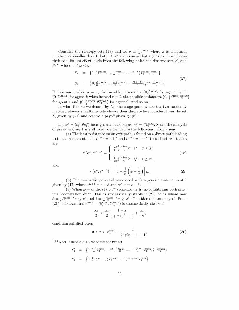
Consider the strategy sets (13) and let � � 1nbemaxi where n is a natural

number not smaller than 1: Let x � x� and assume that agents can now choosetheir equilibrium e¤ort levels from the following �nite and discrete sets S1 andS2

34 where 1 � ! � n :

S1 =�0; 1nbemax1 ; :::; !nbemax1 ; :::;

�n�1n

� bemax1 ; bemax1

S2 =

n0; �nbemax1 ; :::; !�n bemax1 ; :::; �(n�1)n bemax1 ; �bemax1

o (27)

For instance, when n = 1; the possible actions are (0; bemax1 ) for agent 1 and(0; �bemax1 ) for agent 2; when instead n = 2; the possible actions are

�0; 12bemax1 ; bemax1

�for agent 1 and

�0; �2bemax1 ; �bemax1

�for agent 2: And so on.

In what follows we denote by Gn the stage game where the two randomlymatched players simultaneously choose their discrete level of e¤ort from the setSi given by (27) and receive a payo¤ given by (5) :

Let e! = (e!1 ; �e!1 ) be a generic state where e

!1 =

!nbemax1 : Since the analysis

of previous Case 1 is still valid, we can derive the following informations.(a) The least resistance on an exit path is found on a direct path leading

to the adjacent state, i.e. e!+1 = e+ � and e!�1 = e� �; these least resistancesare

r�e!; e!+1

�=

8><>:x�2

1�x!+ 1

2

n k if x � x�

1�xx�2

!+ 12

n k if x � x�;(28)

and

r�e!; e!�1

�=

�1� 1

n

�! � 1

2

��k: (29)

(b) The stochastic potential associated with a generic state e! is stillgiven by (17) where e!+1 = e+ � and e!�1 = e� �:

(c) When ! = n; the state e! coincides with the equilibrium with max-imal cooperation bemax: This is stochastically stable if (21) holds where now� = 1

nbemax1 if x � x� and � = 1nbemax2 if x � x�. Consider the case x � x�: From

(21) it follows that bemax = (bemax1 ; �bemax1 ) is stochastically stable if

�x

2<�x

2

1� x1 + x

��2 � 1

� + �x4n;

condition satis�ed when

0 < x < xmaxn � 1

�2 (2n� 1) + 1; (30)

34When instead x � x�; we obtain the two set

S01 =n0; �

�1

nbemax2 ; :::; !�

�1

nbemax2 ; :::;

��1(n�1)n

bemax2 ; ��1bemax2

oS02 =

n0; 1

nbemax2 ; :::; !

nbemax2 ; :::;

(n�1)n

bemax2 ; bemax2

o:

26

where xmaxn � x� for n � 1: Consider now the case x � x�: From (21) it followsthat bemax = ���1bemax2 ; bemax2

�is stochastically stable if

(1� x)�2

2�<�x

2

1� x1 + x

��2 � 1

� + (1� x)�24�n

;

condition satis�ed when

2n� 1�2 + (2n� 1)

� xminn < x < 1; (31)

where xminn � x� for n � 1: We can summarize this result in the followingProposition.

Proposition 7 Let x be given and consider the game Gn: Let ! = n and con-sider the Nash equilibrium bemax in which agents supply their maximum optimale¤ort.(a) The Nash equilibrium (bemax1 ; �bemax1 ) is stochastically stable if x 2 (0; xmaxn ) ;

where xmaxn is given by (30) :(b) The Nash equilibrium

���1bemax2 ; bemax2

�is stochastically stable if x 2�

xminn ; 1�; where xminn is given by (31) :

Proposition 7 tells us that when agents can choose among a �nite numberof discrete strategies, then the Nash equilibrium with maximal cooperation canbe stochastically stable.35 Proposition 7 however does not tell whether the sto-chastically stable Nash equilibria with maximal cooperation are Pareto e¢ cientstates or not. In Corollary 8 below we show that this occurs only if the numberof strategies available is not too and agents have su¢ ciently di¤erent produc-tivities. When instead agents have identical or not too di¤erent productivities,

35When the distributive parameter does not belong to the speci�ed intervals the stochasti-cally stable state involves less than maximal cooperation. For a given n; the generic state e! ;with 0 < ! < n; is stochastically stable if8<: r

�e!+1; e!

�� r

�e! ; e!+1

�< 0

r�e!�1; e!

�� r

�e! ; e!�1

�< 0:

For x < x�; these conditions are satis�ed if x 2�xmin (!) ; xmax (!)

�where

xmin (!) � 2(n�!)�1�2(2!+1)+2(n�!)�1

xmax (!) � 2(n�!)+1�2(2!�1)+2(n�!)+1 :

It can easily be seen that xmax (!) = xmaxn when ! = n: Notice that xmax (! + 1) =xmin (!) : Consider now the state with cooperation immediately lower than the maximalone, i.e. e! = en�1 = n�1

nbemax: This is a stochastically stable state provided that

x 2 [xmaxn ; xmax (n� 1)] =�xmin (n� 1) ; xmax (n� 1)

�: Analogously considerations hold for

x > x�:

27

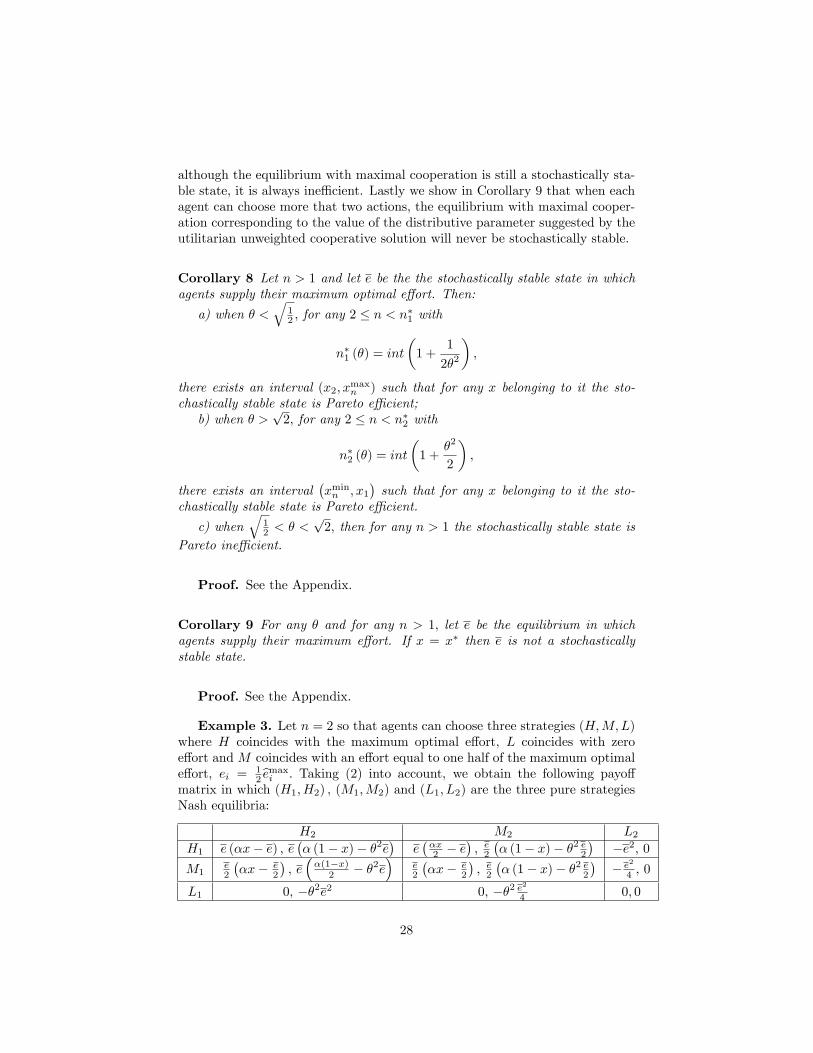
although the equilibrium with maximal cooperation is still a stochastically sta-ble state, it is always ine¢ cient. Lastly we show in Corollary 9 that when eachagent can choose more that two actions, the equilibrium with maximal cooper-ation corresponding to the value of the distributive parameter suggested by theutilitarian unweighted cooperative solution will never be stochastically stable.

Corollary 8 Let n > 1 and let e be the the stochastically stable state in whichagents supply their maximum optimal e¤ort. Then:

a) when � <q

12 ; for any 2 � n < n

�1 with

n�1 (�) = int

�1 +

1

2�2

�;

there exists an interval (x2; xmaxn ) such that for any x belonging to it the sto-chastically stable state is Pareto e¢ cient;b) when � >

p2; for any 2 � n < n�2 with

n�2 (�) = int

�1 +

�2

2

�;

there exists an interval�xminn ; x1

�such that for any x belonging to it the sto-

chastically stable state is Pareto e¢ cient.

c) whenq

12 < � <

p2; then for any n > 1 the stochastically stable state is

Pareto ine¢ cient.

Proof. See the Appendix.

Corollary 9 For any � and for any n > 1; let e be the equilibrium in whichagents supply their maximum e¤ort. If x = x� then e is not a stochasticallystable state.

Proof. See the Appendix.

Example 3. Let n = 2 so that agents can choose three strategies (H;M;L)where H coincides with the maximum optimal e¤ort, L coincides with zeroe¤ort and M coincides with an e¤ort equal to one half of the maximum optimale¤ort, ei = 1

2bemaxi : Taking (2) into account, we obtain the following payo¤matrix in which (H1;H2) ; (M1;M2) and (L1; L2) are the three pure strategiesNash equilibria:

H2 M2 L2H1 e (�x� e) ; e

�� (1� x)� �2e

�e��x2 � e

�; e2�� (1� x)� �2 e2

��e2; 0

M1e2

��x� e

2

�; e��(1�x)

2 � �2e�

e2

��x� e

2

�; e2�� (1� x)� �2 e2

�� e24 ; 0

L1 0; ��2e2 0; ��2 e24 0; 0

28

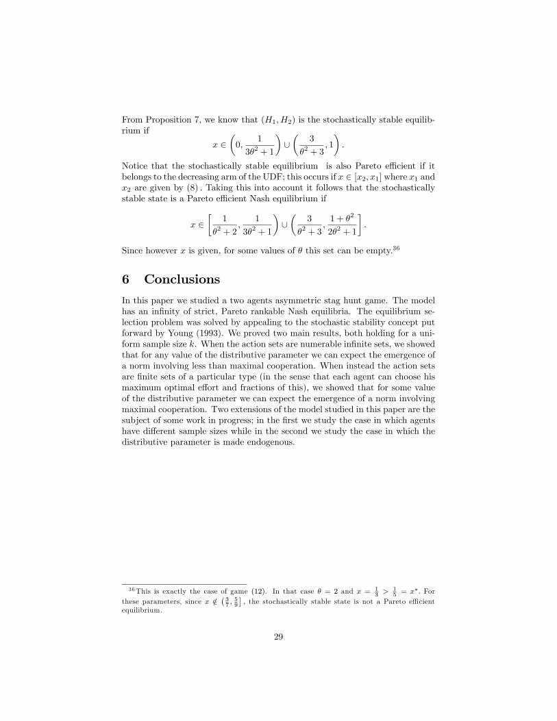
From Proposition 7, we know that (H1;H2) is the stochastically stable equilib-rium if

x 2�0;

1

3�2 + 1

�[�

3

�2 + 3; 1

�:

Notice that the stochastically stable equilibrium is also Pareto e¢ cient if itbelongs to the decreasing arm of the UDF; this occurs if x 2 [x2; x1] where x1 andx2 are given by (8) : Taking this into account it follows that the stochasticallystable state is a Pareto e¢ cient Nash equilibrium if

x 2�

1

�2 + 2;

1

3�2 + 1

�[�

3

�2 + 3;1 + �2

2�2 + 1

�:

Since however x is given, for some values of � this set can be empty.36

6 Conclusions

In this paper we studied a two agents asymmetric stag hunt game. The modelhas an in�nity of strict, Pareto rankable Nash equilibria. The equilibrium se-lection problem was solved by appealing to the stochastic stability concept putforward by Young (1993). We proved two main results, both holding for a uni-form sample size k. When the action sets are numerable in�nite sets, we showedthat for any value of the distributive parameter we can expect the emergence ofa norm involving less than maximal cooperation. When instead the action setsare �nite sets of a particular type (in the sense that each agent can choose hismaximum optimal e¤ort and fractions of this), we showed that for some valueof the distributive parameter we can expect the emergence of a norm involvingmaximal cooperation. Two extensions of the model studied in this paper are thesubject of some work in progress; in the �rst we study the case in which agentshave di¤erent sample sizes while in the second we study the case in which thedistributive parameter is made endogenous.

36This is exactly the case of game (12). In that case � = 2 and x = 13> 1

5= x�: For

these parameters, since x =2�37; 59

�; the stochastically stable state is not a Pareto e¢ cient

equilibrium.

29

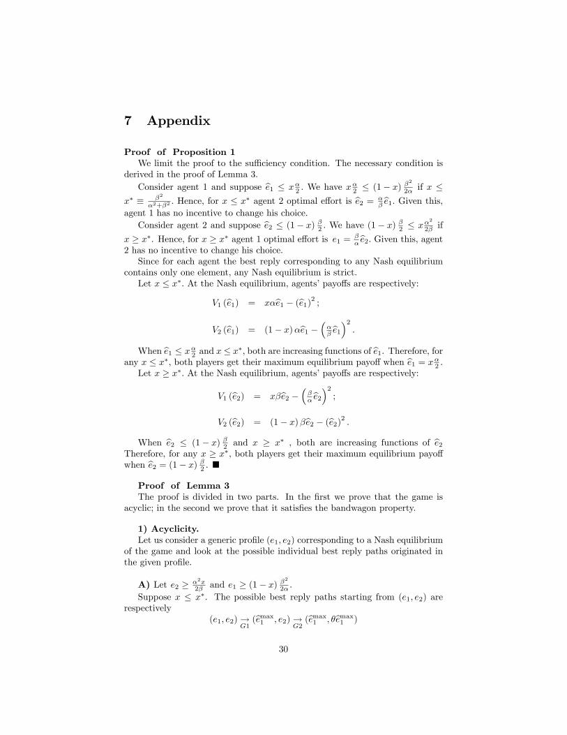
7 Appendix

Proof of Proposition 1We limit the proof to the su¢ ciency condition. The necessary condition is

derived in the proof of Lemma 3.Consider agent 1 and suppose be1 � x�2 : We have x�2 � (1� x) �22� if x �

x� � �2

�2+�2: Hence, for x � x� agent 2 optimal e¤ort is be2 = �

� be1: Given this,agent 1 has no incentive to change his choice.Consider agent 2 and suppose be2 � (1� x) �2 : We have (1� x) �2 � x�22� if

x � x�. Hence, for x � x� agent 1 optimal e¤ort is e1 = ��be2: Given this, agent

2 has no incentive to change his choice.Since for each agent the best reply corresponding to any Nash equilibrium

contains only one element, any Nash equilibrium is strict.Let x � x�: At the Nash equilibrium, agents�payo¤s are respectively:

V1 (be1) = x�be1 � (be1)2 ;V2 (be1) = (1� x)�be1 � ��� be1�2 :

When be1 � x�2 and x� x�; both are increasing functions of be1. Therefore, forany x � x�, both players get their maximum equilibrium payo¤ when be1 = x�2 .Let x � x�: At the Nash equilibrium, agents�payo¤s are respectively:

V1 (be2) = x�be2 � ���be2�2 ;V2 (be2) = (1� x)�be2 � (be2)2 :

When be2 � (1� x) �2 and x � x� , both are increasing functions of be2Therefore, for any x � x�, both players get their maximum equilibrium payo¤when be2 = (1� x) �2 . �Proof of Lemma 3The proof is divided in two parts. In the �rst we prove that the game is

acyclic; in the second we prove that it satis�es the bandwagon property.

1) Acyclicity.Let us consider a generic pro�le (e1; e2) corresponding to a Nash equilibrium

of the game and look at the possible individual best reply paths originated inthe given pro�le.

A) Let e2 � �2x2� and e1 � (1� x) �

2

2� :

Suppose x � x�. The possible best reply paths starting from (e1; e2) arerespectively

(e1; e2)!G1(bemax1 ; e2)!

G2(bemax1 ; �bemax1 )

30

for agent 1 and

(e1; e2)!G2(e1; bemax2 )!

G1(bemax1 ; bemax2 )!

G2(bemax1 ; bemax2 )

for agent 2. In order to understand these paths, let (e1; e2) be given and consideragent�s 1 best reply. This leads to the pro�le (bemax1 ; e2) ; where bemax1 = �x

2 .Given this new pro�le, and since x � x�; agent�s 2 best reply leads to the Nashequilibrium pro�le (bemax1 ; �bemax1 ). We have thus derived the �rst path. Let now(e1; e2) be given and consider agent�s 2 best reply. This leads to the pro�le(e1; bemax2 ) where bemax2 = (1� x) �2 . Given this new pro�le, agent�s 1 best replyleads to the pro�le (bemax1 ; bemax2 ). However, from this last pro�le, agent�s 2 bestreply leads to the Nash equilibrium pro�le (bemax1 ; bemax2 ) : We have thus derivedthe second path.

Suppose x � x� Proceeding as above, we can derive the possible best replypaths starting from (e1; e2) : These are respectively:

(e1; e2)!G1(bemax1 ; e2)!

G2(bemax1 ; bemax2 )!

G1

���1bemax2 ; bemax2

�for agent 1 and

(e1; e2)!G2(e1; bemax2 )!

G1

���1bemax2 ; bemax2

�for agent 2.

Let L (e) denote the length of the shortest path of best reply with origin ine: In the case just analyzed we have L (e) = 2:

B) Let e2 < �2x2� and e1 � (1� x) �

2

2�The best reply paths for agent 2 are as for previous case A. For player 1 the

possible best reply paths originated in (e1; e2) are respectively

(e1; e2)!G1

���1e2; e2

�= (be1; �be1)

when x � x� (with be1 � bemax1 ) and

(e1; e2)!G1

���1e2; e2

!(if e2 � bemax2 !

G2

���1e2; bemax2

�!G1

���1bemax2 ; bemax2

�if e2 � bemax2 !

G2

���1be2; be2�

when x � x�:

Notice that L (e) = 1:

C) Let e2 < �2x2� and e1 < (1� x) �

2

2�The best reply paths for agent 1 are as for previous case B. For player 2 the

possible best reply paths originated in (e1; e2) are respectively

31

(e1; e2)!G2(e1; �e1)!

(if e1 � bemax1 !

G1(bemax1 ; �e1) !

G2(bemax1 ; �bemax1 )

if e1 � bemax1 !G1(be1; �be1)

when x � x� and

(e1; e2)!G2(e1; �e1) =

���1be2; be2�

when x � x� (where e2 � bemax2 ).

Notice that L (e) = 1:

D) Let e2 � �2x2� and e1 < (1� x) �

2

2�The best reply paths for agent 1 are as for previous case A while those of

player 2 are as for previous case C. Notice that L (e) = 1: This ends the proofof the �rst part.

We observe that, since only a (pure strategy) Nash equilibrium pro�le can bea sink of the best reply graph, the proof of the acyclicity is equivalent to a proofof a necessary condition for the existence of (pure strategies) Nash equilibria.

2) Bandwagon property.Let (be1; �be1) be the set of Nash equilibria, where be1 � min��x2 ; (1�x)�22�

�.

Following Binmore, Samuelson and Young (2003), a su¢ cient condition for thegame to exhibit the bandwagon property is that:

1 (be; e) = V1 (be1; �be1)� V1 (e1; �be1)� V1 (be1; e2) + V1 (e1; e2) � 0

2 (be; e) = V2 (be1; �be1)� V2 (e1; �be1)� V2 (be1; e2) + V2 (e1; e2) � 0(32)

where be = (be1; �be1) is any Nash equilibrium of the game and e = (e1; e2) is anynon-equilibrium strategy pro�le. Recall that

V1 (be1; �be1) = �be1x� be21V2 (be1; �be1) = �be1 (1� x)� �2be21:

The following table give informations on the relevant payo¤s:

V1 (e1; �be1) V2 (e1; �be1)if e1 � be1 : �e1x� e21 �e1 (1� x)� �2be21if e1 � be1 : �be1x� e21 �be1 (1� x)� �2be21

V1 (be1; e2) V2 (be1; e2)if be1 � ��1e2 : �be1x� be21 �be1 (1� x)� e22if be1 � ��1e2 : �e2x� be21 �e2 (1� x)� e22

32

and lastly

V1 (e1; e2) V2 (e1; e2)

if e1 � ��1e2 : �e1x� e21 �e1 (1� x)� e22if e1 � ��1e2 : �e2x� e21 �e2 (1� x)� e22

Next table summarizes all the possible situations:

1 (be; e) 2 (be; e)��1e2 < e1 < be1 �x (be1 � e1) > 0 � (1� x) (be1 � e1) > 0e1 < �

�1e2 < be1 �x�be1 � ��1e2� ��1 > 0 � (1� x)

�be1 � ��1e1� > 0e1 < be1 < ��1e2 0 0

��1e2 < be1 < e1 0 0be1 < ��1e2 < e1 �x���1e2 � be1� > 0 � (1� x)

���1e2 � be1� > 0be1 < e1 < ��1e2 �x (e1 � be1) > 0 � (1� x) (e1 � be1) > 0

Since all the entries of this table are non negative, 1 (be; e) and 2 (be; e) arenon negative as well. This ends the proof.�

Claim 10 Consider an acyclic and �nite game with two players. Let bs =(bs1; bs2) be any strict Nash equilibrium of the game and let s = (s1; s2) be anydi¤erent strategy pro�le. Let the bandwagon property (32) be satis�ed for any(strict) Nash equilibrium pro�le bs and for any other pro�le s: Then the transitionfrom the (strict) Nash equilibrium bs to the (strict) Nash equilibrium s = (s1; s2)involves the minimum number of mistakes if the other player by mistakes choosesstrategy si.

Proof. Since the game is acyclic, we know from Young (1993) that thereexists a stochastically stable equilibrium and it coincides with a strict purestrategies Nash equilibrium. Let bs be an arbitrary Nash equilibrium. We wantto �nd the minimum number of mistakes that player 2 must make in order tomove the economy from bs = (bs1; bs2) to the other Nash equilibrium s = (s1; s2) :Analogous considerations holds when the mistakes are made by agent 1. Let mbe the memory size and k be the sample size used by both agents.

Suppose that the economy has been in the state bs for a long period of timeand consider �rst the case in which by mistake agent 2 chooses s2: Speci�callylet us suppose that agents 2 choose s2 by mistake from period t = m + 1 tot = m + k0 inclusive, where k0 � k: If agent 1 draws a sample that includesthese k0 choices of s2; as well as k � k0 choices of bs2; then agent 1 deduces thatthe probability that agent 2 plays bs2 is �2 = 1 � k0

k and that the probability

33

that agent 2 plays s2 is 1 � �2 = k0

k : It then follows that agent 1 is indi¤erentbetween bs1 and s1 if the number of mistakes s2 made by agent 2 is

k0 = A1k �V1 (bs1; bs2)� V1 (s1; bs2)

V1 (bs1; bs2)� V1 (s1; bs2) + V1 (s1; s2)� V1 (bs1; s2)k: (33)

Consider now the case in which by mistake agent 2 chooses s�2 6= s2: Asbefore, let us suppose that agents 2 choose s�2 by mistake from period t = m+1to t = m + k0 inclusive, where k0 � k: If agent 1 draws a sample that includesthese k0 choices of s�2; as well as k � k0 choices of bs2; then agent 1 deduces thatthe probability that agent 2 plays bs2 is �2 = 1 � k0

k and that the probabilitythat agent 2 plays s�2 is 1 � �2 = k0

k : It then follows that agent 1 is indi¤erentbetween bs1 and s1 if if the number of mistakes s�2 made by agent 2 is

k0 = B1k �V1 (bs1; bs2)� V1 (s1; bs2)

V1 (bs1; bs2)� V1 (s1; bs2) + V1 (s1; s�2)� V1 (bs1; s�2)k: (34)

The number of mistakes involving strategy s2 is the minimum if A1 < B1:Since bs is a strict Nash equilibrium, the numerators of A1 and B1 are strictlypositive. Suppose now that the bandwagon property (32) is satis�ed; whenreferred to player 1, this requires

1 (bs; s) = V1 (bs1; bs2)� V1 (s1; bs2)� V1 (bs1; s2) + V1 (s1; s2) � 0:In the case of A1 we have bs = (bs1; bs2) and s = (s1; s2) : In the case of B1 wehave bs = (bs1; bs2) and s = (s1; s�2) : Since also the denominator37 of A1 and B1are non negative, it then follows that A1 < B1 if

1 (s; s) = V1 (s1; s2)� V1 (bs1; s2)� V1 (s1; s�2) + V1 (bs1; s�2) � 0: (35)

Since s = (s1; s2) is a Nash equilibrium, this condition is satis�ed if the band-wagon property holds for s = (s1; s2) and s = (bs1; s�2) : �Claim 11 .Consider the game G� and let e = (e1; �e1) be an arbitrary initialNash equilibrium:(a) The path of exit from e to the right and involving the minimum number

of mistakes, is the path leading to the adjacent state e+ � = (e1 + �; � (e1 + �)) :The resistance of the path e! e+ � is

r (e; e+ �) =

8>>><>>>:�2(2e1 + �)

� (1� x)k if x � x�;

2e1 + �

�xk if x � x�:

(36)

37Since e and be are two strict Nash equilibria, it follows that the denominator of A1 isstrictly positive. If the denominator of B1 is zero, then the condition A1 < B1 is alwayssatis�ed. If instead the denominator of B1 is positive, the condition A1 < B1 is satis�ed if(35) holds.

34

(b) The path of exit from e to the left and involving the minimum numberof mistakes, is the path leading to the adjacent state e� � = (e1 � �; � (e1 � �)) :The resistance of the path e! e� � is

r (e; e� �) =

8>>>><>>>>:

�1� 2e1 � �

�x

�k if x � x�;

�1� �2 2e1 � �

� (1� x)

�k if x � x�:

(37)

Proof. Consider two Nash equilibria e = (e1; �e1) and e = (e1; �e1) and lete be the �xed initial state. Since the game satis�es the bandwagon property(Lemma 3), we know from Claim 10 in the Appendix that the path of leastresistance from e to e is the direct path. We now show e to e must be adjacentstates.Since the path of least resistance is a direct path, in order to derive the resis-

tance it is thus su¢ cient to analyze the restrict game where the only strategiesavailable are those corresponding to these two equilibria, that is S1 = fe1; e1gand S2 = f�e1; �e1g : Two cases are possible: either e1 > e1 or e1 < e1: Theformer corresponds to a situation in which we exit from the state e to the right(i.e. such that e1 > e1) while the latter corresponds to a situation in which weexit from the state e to the left (i.e. such that e1 < e1).

A) Let e1 > e1 and consider the following payo¤ matrix

�e1 �e1e1 e1 (�x� e1) ; e1

�� (1� x)� �2e1

�e1 (�x� e1) ; (1� x)�e1 � (�e1)2

e1 e1�x� e21; e1�� (1� x)� �2e1

�e1 (�x� e1) ; e1

�� (1� x)� �2e1

�(38)

Let (�1; �2) be a mixed strategy pro�le where �1 (resp. �2) is the probabilitythat agent 1 (resp. 2) plays e1 (resp. �e1). The best reply correspondence is

V1 (e1; �2) � V1 (e1; �2) () �2 � 1� e1 + e1�x

V2 (�1; �e1) � V2 (�1; �e1) () �1 � 1� �2 e1 + e1� (1� x)

(39)

Let m be the memory size and k be the sample size used by both agents.Suppose that in the past plays agents 2 choose �e1 by mistake from periodt = m + 1 to t = m + k0 inclusive, where k0 � k: If actual agent 1 draws asample that includes these k0 choices of �e1; as well as k�k0 choices of �e1; thenagent 1 deduce that �2 = 1� k0

k and 1� �2 =k0

k : It then follows from (39) thatthe minimum numbers of mistakes past agents 2 must make in order to induceactual agent 1 to choose e1 as best reply is

35

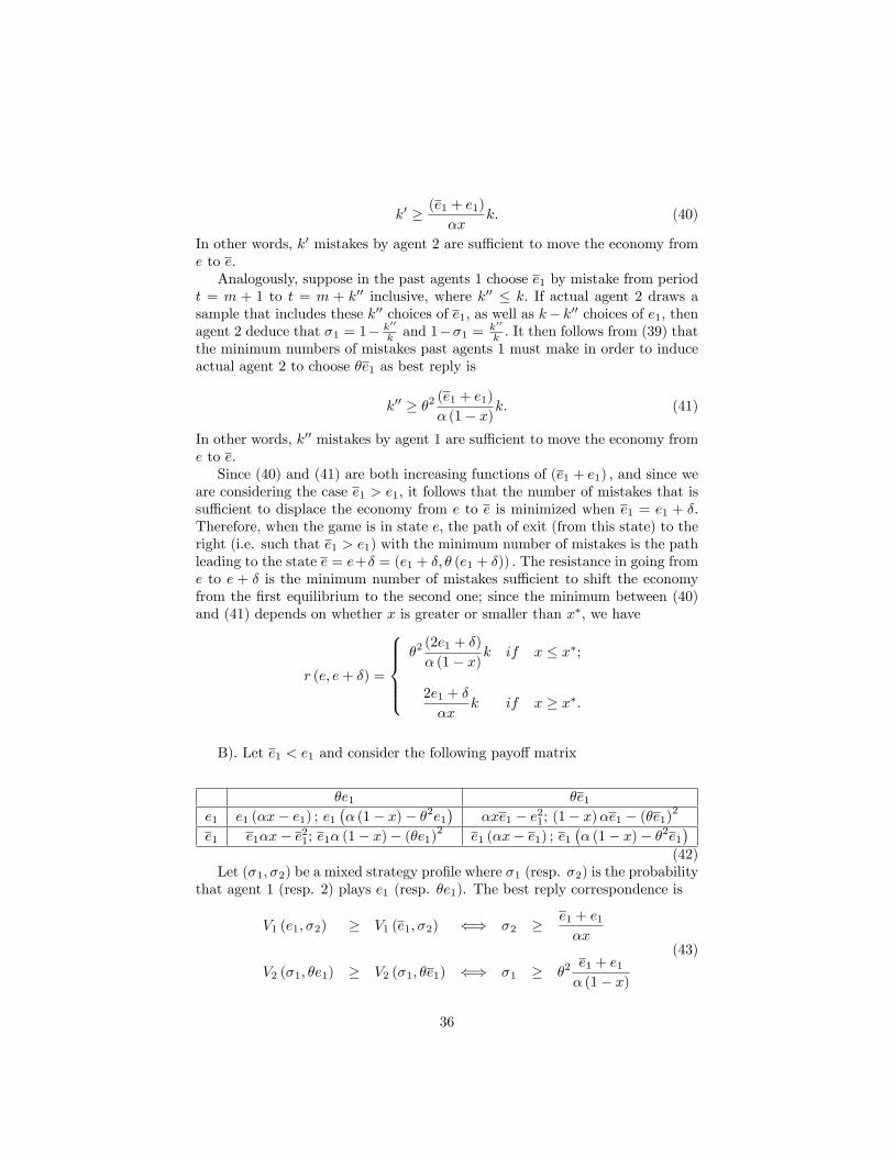
k0 � (e1 + e1)�x

k: (40)

In other words, k0 mistakes by agent 2 are su¢ cient to move the economy frome to e:Analogously, suppose in the past agents 1 choose e1 by mistake from period

t = m + 1 to t = m + k00 inclusive, where k00 � k: If actual agent 2 draws asample that includes these k00 choices of e1; as well as k� k00 choices of e1; thenagent 2 deduce that �1 = 1� k00

k and 1��1 = k00

k : It then follows from (39) thatthe minimum numbers of mistakes past agents 1 must make in order to induceactual agent 2 to choose �e1 as best reply is

k00 � �2 (e1 + e1)� (1� x)k: (41)

In other words, k00 mistakes by agent 1 are su¢ cient to move the economy frome to e:Since (40) and (41) are both increasing functions of (e1 + e1) ; and since we

are considering the case e1 > e1; it follows that the number of mistakes that issu¢ cient to displace the economy from e to e is minimized when e1 = e1 + �:Therefore, when the game is in state e; the path of exit (from this state) to theright (i.e. such that e1 > e1) with the minimum number of mistakes is the pathleading to the state e = e+� = (e1 + �; � (e1 + �)) : The resistance in going frome to e + � is the minimum number of mistakes su¢ cient to shift the economyfrom the �rst equilibrium to the second one; since the minimum between (40)and (41) depends on whether x is greater or smaller than x�; we have

r (e; e+ �) =

8>>><>>>:�2(2e1 + �)

� (1� x)k if x � x�;

2e1 + �

�xk if x � x�:

B). Let e1 < e1 and consider the following payo¤ matrix

�e1 �e1e1 e1 (�x� e1) ; e1

�� (1� x)� �2e1

��xe1 � e21; (1� x)�e1 � (�e1)

2

e1 e1�x� e21; e1� (1� x)� (�e1)2

e1 (�x� e1) ; e1�� (1� x)� �2e1

�(42)

Let (�1; �2) be a mixed strategy pro�le where �1 (resp. �2) is the probabilitythat agent 1 (resp. 2) plays e1 (resp. �e1). The best reply correspondence is

V1 (e1; �2) � V1 (e1; �2) () �2 � e1 + e1�x

V2 (�1; �e1) � V2 (�1; �e1) () �1 � �2e1 + e1� (1� x)

(43)

36

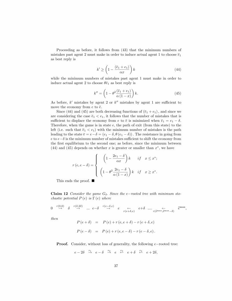
Proceeding as before, it follows from (43) that the minimum numbers ofmistakes past agent 2 must make in order to induce actual agent 1 to choose e1as best reply is

k0 ��1� (e1 + e1)

�x

�k (44)

while the minimum numbers of mistakes past agent 1 must make in order toinduce actual agent 2 to choose �e1 as best reply is

k00 =

�1� �2 (e1 + e1)

� (1� x)

�k: (45)

As before, k0 mistakes by agent 2 or k00 mistakes by agent 1 are su¢ cient tomove the economy from e to e:Since (44) and (45) are both decreasing functions of (e1 + e1) ; and since we

are considering the case e1 < e1; it follows that the number of mistakes that issu¢ cient to displace the economy from e to e is minimized when e1 = e1 � �:Therefore, when the game is in state e; the path of exit (from this state) to theleft (i.e. such that e1 < e1) with the minimum number of mistakes is the pathleading to the state e = e�� = (e1 � �; � (e1 � �)) : The resistance in going frome to e�� is the minimum number of mistakes su¢ cient to shift the economy fromthe �rst equilibrium to the second one; as before, since the minimum between(44) and (45) depends on whether x is greater or smaller than x�; we have

r (e; e� �) =

8>>>><>>>>:

�1� 2e1 � �

�x

�k if x � x�;

�1� �2 2e1 � �

� (1� x)

�k if x � x�:

This ends the proof. �

Claim 12 Consider the game G�: Since the e�rooted tree with minimum sto-chastic potential P (e) is � (e) where

0r(0;0)! �

r(�;2�)! ::: e�� r(e��;e)! e r(e+�;e)

e+� :::: r(bemax;bemax��) bemax;

thenP (e+ �) = P (e) + r (e; e+ �)� r (e+ �; e)

P (e� �) = P (e) + r (e; e� �)� r (e� �; e) :

Proof. Consider, without loss of generality, the following e�rooted tree:

e� 2� r1! e� � r2! er3 e+ �

r4 e+ 2�;

37

where r1 � r (e� 2�; e� �) ; r2 � r (e� �; e) ; r3 � r (e+ �; e) and r4 �r (e+ 2�; e+ �) : We have

P (e) = r1 + r2 + r3 + r4: (46)

Consider now the following (e+ �)�rooted tree:

e� 2� r1! e� � r2! er03! e+ �

r4 e+ 2�;

where r03 � r (e; e+ �) : We then have

P (e+ �) = r1 + r2 + r03 + r4: (47)

From (46) and (47) we have

P (e+ �) = r1 + r2 + r03 + r4 + r3 � r3

= P (e) + r03 � r3

= P (e) + r (e; e+ �)� r (e+ �; e) :

Lastly, consider the following (e� �)�rooted tree:

e� 2� r1! e� � r02 er3 e+ �

r4 e+ 2�;

where r02 � r (e; e� �) : We then have

P (e� �) = r1 + r02 + r3 + r4: (48)

From (46) and (48) we have

P (e� �) = r1 + r02 + r3 + r4 + r2 � r2

= P (e) + r02 � r2

= P (e) + r (e; e� �)� r (e� �; e) :

�

Proof of Corollary 8Recall that when x � x�; the UDF is an increasing function for 0 � x � x2

and a decreasing function for x2 < x � x�; when instead x � x�; the UDF is adecreasing function for x� < x � x1 and an increasing function for x1 < x � 1where x2 and x1 are both given in (8) :Let n > 1: Then e is the stochastically stable state when either x 2 (0; xmaxn ) �

(0; x�) or x 2�xminn ; 1

�� (x�; 1) : Notice that x2 < xmaxn when n < n�1 (�) while

xminn < x1 when n < n�2 (�) where

n�1 (�) = int�1 + 1

2�2

�n�2 (�) = int

�1 + �2

2

�:

38

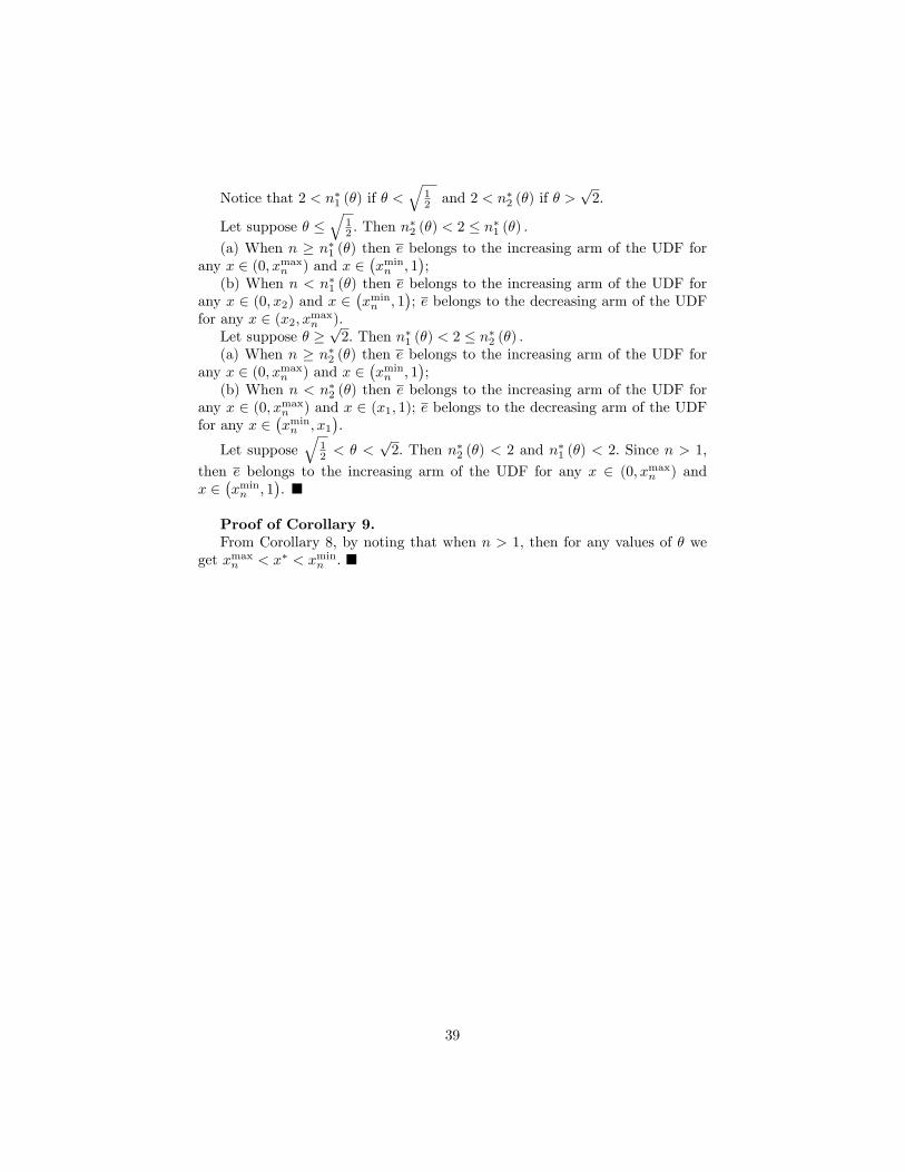
Notice that 2 < n�1 (�) if � <q

12 and 2 < n�2 (�) if � >

p2:

Let suppose � �q

12 : Then n

�2 (�) < 2 � n�1 (�) :

(a) When n � n�1 (�) then e belongs to the increasing arm of the UDF forany x 2 (0; xmaxn ) and x 2

�xminn ; 1

�;

(b) When n < n�1 (�) then e belongs to the increasing arm of the UDF forany x 2 (0; x2) and x 2

�xminn ; 1

�; e belongs to the decreasing arm of the UDF

for any x 2 (x2; xmaxn ).Let suppose � �

p2: Then n�1 (�) < 2 � n�2 (�) :

(a) When n � n�2 (�) then e belongs to the increasing arm of the UDF forany x 2 (0; xmaxn ) and x 2

�xminn ; 1

�;

(b) When n < n�2 (�) then e belongs to the increasing arm of the UDF forany x 2 (0; xmaxn ) and x 2 (x1; 1); e belongs to the decreasing arm of the UDFfor any x 2

�xminn ; x1

�.

Let supposeq

12 < � <

p2: Then n�2 (�) < 2 and n�1 (�) < 2: Since n > 1;

then e belongs to the increasing arm of the UDF for any x 2 (0; xmaxn ) andx 2

�xminn ; 1

�. �

Proof of Corollary 9.From Corollary 8, by noting that when n > 1; then for any values of � we

get xmaxn < x� < xminn : �

39

References

[1] Anderson S. P., J. K. Goeree and C. A. Holt, (2001), Minimum-e¤ort co-ordination games: stochastic potential and logic equilibrium, Games andEconomic Behavior, 34, 177-199.

[2] Binmore K., (1994), Game Theory and the Social Contract. Vol. 1, PlayingFair, MIT Press.

[3] Binmore K., L. Samuelson and P. Young, (2003), Equilibrium selection inbargaining games, Games and Economic Behavior, 45, 296-328.

[4] Bryant J., (1983), A simple rational expectations Keynes-type model, Quar-terly Journal of Economics, 525-528.

[5] Bryant J. (1994), Coordination theory, the stag hunt and macroeconomics.In J. W. Friedman (ed.), Problems of Coordination in Economic Activity,Kluwer Academic Press.

[6] Carlsson H. and E. Van Damme (1993), Equilibrium selection in stag huntgames. In Binmore K., A. Kirman and P. Tani (eds.), Frontiers of GameTheory, MIT Press.

[7] Cooper R. (1999), Coordination Games, Cambridge University Press.

[8] Cooper R. and A. John (1988), Coordinating coordination failures in Key-nesian models, Quarterly Journal of Economics, 103, 441-463.

[9] Crawford V., (1990), An "evolutionary" interpretation of Van Huyck, Bat-talio and Beil�s experimental results on coordination, Games and EconomicBehavior, 3, 25-59.

[10] Crawford V., (1995), Adaptive dynamics in coordination games, Econo-metrica, 63, 103-143.

[11] Ellison G., (2000), Basin of attraction, long-run stochastic stability, and thespeed of step-by-step evolution, Review of Economic Studies, 67, 17-45.

[12] Hvide H., (2001), Some comments on free-riding in Leontief partnerships,Economic Inquiry, 39, 467-473.

[13] Kandori M. and R. Rob (1998), Bandwagon e¤ects and long run technologychoice, Games and Economic Behavior, 22, 30-60.

[14] Legros P. and S. A. Mathews (1993), E¢ cient and nearly-e¢ cient partner-ship, Review of Economic Studies, 68, 599-611.

[15] Mondered D. and L. S. Shapley (1996), Potential games, Games and Eco-nomic Behavior, 14, 124-143.

[16] Ray D., J. M. Baland and O. Dagnelie (2006), Inequality and ine¢ ciencyin joint projects, mimeo.

40

[17] Skyrms B., (2004), The Stag Hunt and the Evolution of Social Structure,Cambridge University Press.

[18] Van Huyck J., R. Battalio and R. O. Beil (1990), Tacit coordination games,strategic uncertainty and coordination failures, American Economic Re-view, 80, 234-248.

[19] Van Huyck J., J. Cook and R. Battalio (1997), Adaptive behavior andcoordination failures, Journal of Economic Behavior and Organization, 32,483-503.

[20] Vislie J., (1994), E¢ ciency and equilibria in complementarity teams, Jour-nal of Economic Behavior and Organization, 23, 83-91.

[21] Wasow B., (1980), Optimal income distribution with variable factor sup-plies: a graphical exposition, The Manchester School, 1, 79-86.

[22] Young P., (1993), The evolution of conventions, Econometrica, 61, 57-84.

[23] Young P., (1998), Individual Strategies and Social Structure, PrincetonUniversity Press.

41