The Effect of Oxygen in Sweet Corrosion of Carbon Steel for ...

The Effect of Oxygen in Sweet Corrosion of Carbon Steel for Enhanced Oil Recovery

Applications

A dissertation presented to

the faculty of

the Russ College of Engineering and Technology of Ohio University

In partial fulfillment

of the requirements for the degree

Doctor of Philosophy

Nor Roslina Rosli

December 2015

© 2015 Nor Roslina Rosli. All Rights Reserved.

2

This dissertation titled


Applications

by

NOR ROSLINA ROSLI

has been approved for

the Department of Chemical and Biomolecular Engineering

and the Russ College of Engineering and Technology by

Srdjan Nesic

Professor of Chemical and Biomolecular Engineering

Dennis Irwin

Dean, Russ College of Engineering and Technology

3

ABSTRACT

ROSLI, NOR ROSLINA, Ph.D., December 2015, Chemical Engineering


Applications

Director of Dissertation: Srdjan Nesic

The primary objective of this work is to investigate the corrosion behavior of

carbon steel in simulated CO2-EOR environments when O2 is present in the CO2 supply.

A preliminary study was first conducted at low pressure to investigate the effect of O2 on

the protectiveness of iron carbonate (FeCO3) corrosion product layers in mild steel CO2

corrosion. Carbon steel (UNS G10180) samples were immersed in a CO2 saturated

1 wt.% NaCl electrolyte for 2 days to facilitate formation of a protective FeCO3 layer on

the steel surface. Temperature and pH were maintained at 80°C and 6.6, then 1 ppm O2

was introduced to the electrolyte. The impact of the oxidant(s) was studied after samples

were exposed for one week to test conditions. Electrochemical measurements indicated

increased corrosion rates over the first two days of O2 exposure, with a decrease in

corrosion rate thereafter due to corrosion product formation that conferred some degree

of protection to the steel surface. When O2 was introduced after carbonate formation, the

corrosion rate did not increase. Although the final corrosion rates of all tests were

relatively low (less than 0.2 mm/y), localized corrosion was observed. Surface analysis

showed attack of iron carbonate crystals and formation of iron (III) oxides. This

degradation of initially formed FeCO3 occurred concurrently with the development of

localized corrosion features as deep as 80 µm.

4

High pressure experiments were then conducted at CO2-EOR simulated downhole

conditions. The effect of O2 (4 vol. %) on the corrosion performance of mild steel (UNS

G10180) in CO2-saturated brine was investigated using a 4-liter autoclave at two different

temperatures (25 and 80°C) and pressures (40 and 90 bar). Experiments at 25°C are

categorized as ‘FeCO3-free’ while experiments at 80°C are termed ‘FeCO3-forming’. The

work included electrochemical measurements, weight loss determination, and

characterization of the corrosion products. Severe corrosion was observed on the steel

specimen after 48 hours of exposure to the corrosive environments. Tests at FeCO3-

forming conditions exhibited localized corrosion, while the FeCO3-free experiments

displayed severe general corrosion. Corrosion prediction using Multicorp© software was

performed and the output corrosion rate data were compared against experimental results.

Reasonable correlation was observed with the experimental data in anoxic conditions.

5

DEDICATION

Elmira, Eshal and Fatin, my patient and understanding little girls.

and

Zafri, for your constant love and support through thick and thin.

6

ACKNOWLEDGMENTS

I wish to express my sincere gratitude to my supervisors, Professor Srdjan Nesic,

Dr David Young, and Dr Yoon-Seok Choi, who have given support and encouragement

to a student like me, who is loaded with family commitments. I wish to acknowledge the

considerable contributions made by many of my colleagues at the Institute for Corrosion

and Multiphase Technology (ICMT). Among them are Steve Upton, Cody Shafer, and

Alexis Barxias who have spent substantial time and energy in helping me get my setup to

work in proper order because the autoclave is never an easy equipment to work with. I

humbly thank the Center for Electrochemical Engineering Research (CEER) for letting

me utilize their X-ray diffraction and Raman spectroscopy instrumentation for specimen

analyses. Special thanks have to go to my dissertation committee members Dr John

Staser, Dr Michael Jensen, and Dr Dina López for their invaluable technical advice.

Editoral help from Dr David Young, Dr Bert Pots and Dr Joseph Lee are much

appreciated, and essential to the completion of this dissertation. I am grateful to the

research team from PETRONAS, namely Muhammad Firdaus Suhor, Azmi Mohammed

Nor, and Ahmad Zaki Abbas, for their help and feedback relating to high pressure sweet

corrosion. Scholarship and financial support from the Ministry of Education, Malaysia

has made it possible for me to complete my studies. Finally, a thank you to all the other

members at the ICMT that are not mentioned, for all their feedback and support and

making my graduate school years an unforgettable experience.

7

TABLE OF CONTENTS

Page

Abstract ............................................................................................................................... 3

Dedication ........................................................................................................................... 5

Acknowledgments............................................................................................................... 6

List of Tables .................................................................................................................... 11

List of Figures ................................................................................................................... 12

Chapter 1: Introduction ..................................................................................................... 21

1.1 Background ....................................................................................................... 21

1.1.1 Cost of Corrosion in the Oil and Gas Industry ............................................. 21

1.1.2 Oxygen and Carbon Dioxide’s Role in Corrosion ........................................ 22

1.2 Layout of Dissertation....................................................................................... 23

Chapter 2: Literature Review ............................................................................................ 24

2.1 CO2-Enhanced Oil Recovery (CO2-EOR) ........................................................ 24

2.2 Carbon Capture and Storage (CCS) .................................................................. 27

2.3 CO2 Corrosion ................................................................................................... 30

2.3.1 Water Chemistry ........................................................................................... 31

2.3.2 Electrochemistry ........................................................................................... 33

2.3.3 Factors Affecting CO2 Corrosion Rate ......................................................... 34

8

2.3.4 Corrosion Product Prediction using Pourbaix Diagrams .............................. 36

2.3.5 CO2 Corrosion at EOR Conditions ............................................................... 38

2.4 Properties of CO2 – O2 Mixtures ...................................................................... 41

2.5 Oxygen Corrosion of Steel ................................................................................ 41

2.5.1 Iron Oxides.................................................................................................... 43

2.5.2 Effect of O2 on CO2 Corrosion ..................................................................... 44

2.6 Chapter Summary ............................................................................................. 46

Chapter 3: Objectives and Hypotheses ............................................................................. 47

3.1 Problem Statement and Research Gap .............................................................. 47

3.2 Objectives of the Study ..................................................................................... 47

3.3 Research Hypothesis ......................................................................................... 47

Chapter 4: Low Pressure Corrosion Experiments ............................................................. 51

4.1 Sample Material ................................................................................................ 52

4.2 Experimental Design ......................................................................................... 53

4.3 Electrochemical Measurements ........................................................................ 59

4.4 Results and Discussions: FeCO3-Free Experiments ......................................... 60

4.5 Results and Discussions: FeCO3-Forming Experiments................................... 63

4.5.1 Test A: Baseline CO2 Corrosion Experiment ............................................... 64

4.5.2 Test B: O2 Ingress from Day 2 ...................................................................... 70

9

4.5.3 Test C: O2 Ingress from Day 0 ...................................................................... 80

4.5.4 Results Summary .......................................................................................... 93

4.6 Proposed Corrosion Mechanism ....................................................................... 96

4.7 Chapter Summary ........................................................................................... 101

Chapter 5: High Pressure Corrosion Tests ...................................................................... 102

5.1 Introduction ..................................................................................................... 102

5.2 Sample Material and Preparation .................................................................... 104

5.3 Experimental Set-up and Instrumentation ...................................................... 105

5.4 Measurements and Test Matrix ....................................................................... 108

5.5 Results and Discussion ................................................................................... 110

5.5.1 Experiment 1: 25°C, 40 bar pCO2, with and without 4% O2. ..................... 110




5.6 The Proposed Corrosion Mechanism .............................................................. 136

5.7 The Effect of Flow .......................................................................................... 139

5.8 Chapter Summary and Conclusions ................................................................ 149

Chapter 6: Modeling ....................................................................................................... 151

6.1 Simulation at Low Pressure ............................................................................ 151

10

6.2 Simulation at High Pressure............................................................................ 154

6.2.1 Multicorp© High Pressure Simulation for Tests at 25°C ........................... 155

6.2.2 Multicorp© High Pressure Simulation for Tests at 80°C ........................... 161

6.2.3 Multicorp© Simulation on the Effect of Flow ............................................ 164

6.3 Chapter Summary ........................................................................................... 168

Chapter 7: Conclusion and Recommendations ............................................................... 169

7.1 Overall Summary/Conclusion ......................................................................... 169

7.2 Future Work/Recommendations ..................................................................... 170

References ....................................................................................................................... 173

Appendix A: AES Analysis of Steel Specimen .............................................................. 183

Appendix B: Calculation of O2 Content in Water from Orbisphere Data ...................... 184

Appendix C: Clarke Solution Treatment (ASTM G1-03) .............................................. 187

Appendix D: Sample Calculation of Corrosion Rate from Weight Loss ........................ 188

Appendix E: Sample Calculation of Corrosion Rate from Polarisation Resistance ....... 189

Appendix F: Predicted O2 Solubility in Water ............................................................... 191

Appendix G: Sample calculation for Pitting Ratio Determination ................................. 196

Appendix H: Determination of O2 Consumption from Weight Loss of Steel ................ 197

11

LIST OF TABLES

Page

Table 1: Composition of CO2 from Different Capture Processes [26]. ............................ 29

Table 2: Estimated CO2-O2 Mixture Critical Properties from REFPROP9 Database ...... 42

Table 3: Iron Oxides and their Characteristics [79]. ......................................................... 44

Table 4: Overview of O2-CO2 Corrosion Tests in the Literature. ..................................... 45

Table 5: Composition of Steel (Balance Fe). .................................................................... 53

Table 6: Test Matrix for Low Pressure Corrosion Test. ................................................... 56

Table 7: Summary of Corrosion Rate Results. ................................................................. 94

Table 8: Test Matrix for High Pressure Corrosion Test. ................................................ 110

Table 9: Results Summary of High Pressure Corrosion Experiments ............................ 149

12

LIST OF FIGURES

Page

Figure 1. Schematic of CO2-EOR with alternating water injection. ................................. 25

Figure 2. Typical CO2 and water injection well [5] .......................................................... 26

Figure 3. CO2 capture options in the electric power industry. .......................................... 28

Figure 4. Pourbaix diagram for Fe-O2-H2O system at 25°C ............................................. 37

Figure 5. Pourbaix diagram of CO2-O2-H2O system generated using OLIAnalyzer 3.2. . 38

Figure 6. Carbon dioxide phase diagram .......................................................................... 39

Figure 7. Schematic for hypothesis at low pressure ......................................................... 49

Figure 8. Schematic of hypothesis at high pressure .......................................................... 49

Figure 9. Steel specimens for glass cell tests .................................................................... 52

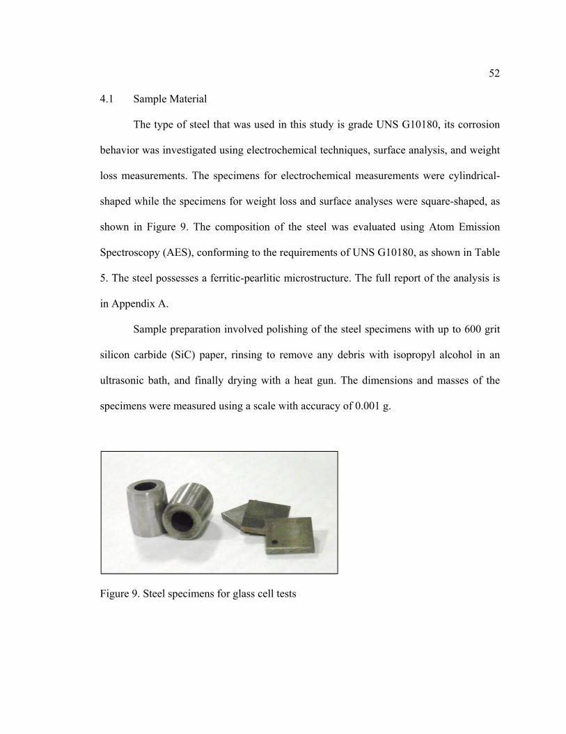
Figure 10. Glass cell setup (Courtesy of Cody Shafer, ICMT) ........................................ 54

Figure 11. Oxygen meter, Orbisphere 410........................................................................ 55

Figure 12. Different tests for FeCO3-forming experiments. ............................................. 57

Figure 13. Effect of O2 on corrosion rates at FeCO3-free condition (pH 4, 25°C) ........... 61

Figure 14. Nyquist plots relative to the reference electrode (pH 4, 25°C) ....................... 62

Figure 15. Polarization curves versus Ag/AgCl reference electrode (pH 4, 25°C) .......... 63

Figure 16. LPR mean corrosion rates for Test A (Baseline CO2 Corrosion, 80°C, pH 6.6,

0 ppm O2, 50 ppm initial Fe2+ concentration). .................................................................. 65

Figure 17. Mean corrosion potential for Test A (Baseline CO2 Corrosion, 80°C, pH 6.6,

0 ppm O2, 50 ppm initial Fe2+ concentration). .................................................................. 65

13

Figure 18. Solution pH for Test A, (80°C, pH 6.6, 0 ppm O2, 50 ppm initial Fe2+

concentration). .................................................................................................................. 66

Figure 19. Total iron ion concentration in the solution for Test A (80°C, pH 6.6, 0 ppm

O2, 50 ppm initial Fe2+ concentration). ............................................................................. 67

Figure 20. SEM image and EDS spectra of sample for Test A (80°C, pH 6.6, 0 ppm O2,

50 ppm initial Fe2+ concentration) .................................................................................... 68

Figure 21. SEM image of steel surface for Test A after corrosion product removal ........ 69

Figure 22. Cross-section view of steel specimen for Test A ............................................ 69

Figure 23. LPR mean corrosion rate for Test B (O2 introduced on Day 2). ..................... 71

Figure 24. Mean corrosion potential for Test B (O2 introduced on Day 2). ..................... 71

Figure 25. Solution pH for Test B (O2 introduced on Day 2). .......................................... 72

Figure 26. FeCO3 crystals on steel surface at 24 h in Test B. ........................................... 73

Figure 27. FeCO3 crystals on steel surface at 48 h before O2 introduction in Test B. ...... 74

Figure 28. Oxide clusters on FeCO3 layer at 168 h in Test B ........................................... 74

Figure 29. SEM image and EDS spectra of sample at the end of Test B ......................... 75

Figure 30. Cross-section of the sample from Test B ........................................................ 76

Figure 31. X-ray diffraction of the specimen after 7 day immersion for Test B. ............. 77

Figure 32. SEM image of the bare steel surface from Test B ........................................... 78

Figure 33. Surface profile of pits on specimen from Test B. ............................................ 79

Figure 34. Initial electrolyte color change from colorless to yellow to black in Test C ... 80

Figure 35. Reddish brown precipitate at the bottom of the glass cell. .............................. 81

Figure 36. LPR mean corrosion rate for Test C ................................................................ 82

14

Figure 37. Mean corrosion potential for Test C ................................................................ 83

Figure 38. Bulk solution pH for Test C. ........................................................................... 84

Figure 39. Total iron concentration in solution of Test C. ................................................ 84

Figure 40. Steel surface at the end of Day 2 in Test C. .................................................... 85




Figure 44. SEM image and EDS spectra of sample recovered after 8 days in Test C ...... 88

Figure 45. Imperfectly formed FeCO3 crystals covered with iron oxides ........................ 88

Figure 46. X-ray diffraction of the specimen recovered after 7 days in Test C. .............. 89

Figure 47. Raman spectra of specimen recovered after 7 days in Test C. ........................ 90

Figure 48. Cross-section of specimen recovered after 7 days of Test C ........................... 90

Figure 49. Schematic of a tubercle based on a study described by Herro [68]. ................ 91

Figure 50. SEM image of steel surface for Test C after corrosion product removal ........ 92

Figure 51. Pit depth analysis of specimen recovered at the end of Test C. ...................... 93

Figure 52. Corrosion rates comparison of Tests A, B and C. ........................................... 94

Figure 53. Corrosion potential of test A, B and C. ........................................................... 95

Figure 54. Comparison of test solution pH for Tests A, B and C. .................................... 96

Figure 55. Proposed tuberculation mechanism in CO2 corrosion with O2 intrusion. ....... 97

Figure 56. Cylindrical and flat steel specimens for high pressure experiments. ............ 104

Figure 57. Dimensions of steel specimens used in the high pressure tests. .................... 105

Figure 58. 4-L stainless steel autoclave diagram (Courtesy of Cody Shafer, ICMT) .... 106

15

Figure 59. The 4-L autoclave in ICMT ........................................................................... 107

Figure 60. Piping and instrumentation diagram of the autoclave setup .......................... 107

Figure 61. Boundary conditions of experiment in the CO2 phase diagram .................... 109

Figure 62. LPR corrosion rate with time for experiments at 25°C, 40 bar pCO2, with and

without 4% O2. ................................................................................................................ 111

Figure 63. Weight loss corrosion rates compared to LPR time-integrated corrosion rates

for experiments at 25°C, 40 bar pCO2, with and without 4% O2. .................................. 111

Figure 64. Corrosion potential for experiments at 25°C, 40 bar pCO2, with and without

4% O2. ............................................................................................................................. 112

Figure 65. Bluish-green corrosion product on a recovered steel specimen for experiment

at 25°C, 40 bar pCO2, with 4% O2 .................................................................................. 113

Figure 66. SEM and EDS analysis of steel surface at the end of 25°C, 40 bar pCO2, with

and without 4% O2 experiments. .................................................................................... 113

Figure 67. Steel cross-sections at 25°C, 40 bar pCO2, with and without 4% O2 ............ 114

Figure 68. XRD analysis for specimen at 25°C, 40 bar pCO2, with 4% O2 for 48 h. .... 115

Figure 69. Profilometry of specimen at 25°C, 40 bar pCO2, with 4% O2 after 48 h. ..... 115

Figure 70. LPR corrosion rate with time for experiments at 25°C, 90 bar pCO2, with and

without 4% O2. ................................................................................................................ 116

Figure 71. Weight loss corrosion rates compared to LPR time-integrated corrosion rates

for experiments at 25°C, 90 bar pCO2, with and without 4% O2. .................................. 117

Figure 72. Corrosion potential with time for experiments at 25°C, 90 bar pCO2, with and

without 4% O2. ................................................................................................................ 118

16

Figure 73. SEM micrographs and EDS analysis of steel surface at the end of 25°C, 90 bar

pCO2, with and without 4% O2 experiments. ................................................................. 119

Figure 74. Steel cross-sections at the end of 25°C, 90 bar pCO2, with and without 4% O2

tests. ................................................................................................................................ 120

Figure 75. XRD analysis for specimen at 25°C, 90 bar pCO2, with 4% O2, 48h. .......... 120

Figure 76. Profilometry of steel specimen at at 25°C, 90 bar pCO2, with 4% O2, 48h .. 121

Figure 77. Corrosion rates of steel at 80°C and 40 bar CO2 with and without O2. ......... 122

Figure 78. Corrosion potential of steel at 80°C and 40 bar CO2 with and without O2. .. 123

Figure 79. Corrosion rates measured using weight loss technique compared with

integrated LPR results for conditions with and without O2 at 80°C, 40 bar CO2 after 2

days of test. ..................................................................................................................... 124

Figure 80. Steel surface after being exposed to 80°C, 40 bar CO2, 4% O2 in solution for

48 hours. .......................................................................................................................... 125

Figure 81. Cross-sectional view of steel specimen for tests conditions at (a) 80°C, 40 bar

pCO2, 1.7 bar O2 and (b) 80°C, 40 bar pCO2. ................................................................. 126

Figure 82. XRD analysis for specimen at the end of 80°C, 40 bar pCO2, with 4% O2

experiment....................................................................................................................... 127

Figure 83. Raman spectra at two different locations on the steel specimen (785 nm laser

excitation energy at 50 mW laser power, 20 s integration time). ................................... 127

Figure 84. Surface profilometry of bare steel for test conditions 80°C, 40 bar pCO2,

1.7 bar O2 ........................................................................................................................ 129

Figure 85. Corrosion rates of steel at 80°C and 90 bar CO2 with and without O2. ......... 130

17

Figure 86. Corrosion rates measured using weight loss technique compared with

integrated LPR results for conditions with and without O2 at 80°C, 90 bar CO2 after 2

days of test. ..................................................................................................................... 131

Figure 87. Corrosion potential of steel at 80°C and 90 bar CO2 with and without O2 ... 132

Figure 88. Steel samples after 2 days of immersion without (left) and with O2 (right). . 132

Figure 89. Micrograph of steel surface at 80°C, 90 bar CO2 in 1 wt% NaCl solution for

48 with and without the presence of 4% O2. ................................................................... 133

Figure 90. Cross-section of steel at 80°C, 90 bar CO2 in 1 wt% NaCl solution for 48 with

and without the presence of 4% O2. ................................................................................ 134

Figure 91. Analysis of steel surface using XRD for the specimen recovered at the end of

the 80°C, 90 bar pCO2, with 4% O2 experiment. ............................................................ 134

Figure 92. Hematite peaks detected using Raman spectroscopy with 532 nm laser

excitation energy at 2 mW laser power, 20 s integration time. ....................................... 135

Figure 93. Surface profilometry of bare steel for test conditions 80°C, 90 bar pCO2,

1.7 bar O2. ....................................................................................................................... 135

Figure 94. Localized corrosion on steel surface as seen under SEM. ............................. 136

Figure 95. Proposed corrosion mechanism at low temperature and high pCO2 with O2

ingress in a closed system. .............................................................................................. 137

Figure 96. Proposed corrosion mechanism at high temperature and high pCO2 with O2

ingress in a closed system. .............................................................................................. 138

Figure 97. Effect of 1000 rpm flow rotational speed on the corrosion rates in equivalent

CO2 systems. ................................................................................................................... 140

18

Figure 98. Effect of 1000 rpm flow on the corrosion rates in equivalent CO2/O2 systems.

......................................................................................................................................... 140

Figure 99. Effect of flow and O2 on weight loss corrosion rate. .................................... 141

Figure 100. Steel specimens at 80°C 90 bar CO2, 4% O2, and 1000 rpm speed. ........... 142

Figure 101. SEM of steel surface at 80°C 90 bar CO2, 4% O2, and 1000 rpm speed. .... 142

Figure 102. EDS of steel surface at 80°C, 90 bar CO2, 4% O2, and 1000 rpm rotational

speed. .............................................................................................................................. 143

Figure 103. SEM of steel surface at 80°C 90 bar CO2, and 1000 rpm rotational speed. 144

Figure 104. EDS analysis of two points on the steel as labeled in the previous Figure. 144

Figure 105. Cross-sectional views of coupon comparing the effect of flow at 80°C and

90 bar CO2....................................................................................................................... 145

Figure 106. Cross-sectional views of coupon comparing the effect of flow in CO2-O2

system at 80°C, 90 bar CO2 and 4% O2. ......................................................................... 145

Figure 107. Surface profilometry of steel for experiment at 80°C, 90 bar CO2, 2 days,

1000 rpm ......................................................................................................................... 146

Figure 108. Surface profilometry of steel for experiment at 80°C, 90 bar CO2, 2 days, 4%

O2, 1000 rpm ................................................................................................................... 147

Figure 109. Surface profilometry of another specimen for experiment at 80°C, 90 bar

CO2, 2 days, 4% O2, 1000 rpm ....................................................................................... 148

Figure 110. Comparison of corrosion rates between Freecorp© and experimental data at

25°C, 1 bar, pH 4.0, with and without 3 ppm O2 ............................................................ 152

19

Figure 111. The effect of 3 ppm O2 in CO2 system at 25°C, 1 bar shown in Tafel plots

using Freecorp© .............................................................................................................. 152

Figure 112. Comparison of corrosion rates between Multicorp© and experimental data of

test at 80°C, pH 6.6 and 0.5 bar CO2, with and without O2 ............................................ 154

Figure 113. Simulated surface pH and porosity at 80°C, pH 6.6, and 0.5 bar CO2 ........ 154

Figure 114. Comparison of simulated corrosion rate with experimental results for

experiment at 40 bar CO2, 25°C, autogenous pH for 48 hours ....................................... 156

Figure 115. Comparison of simulated corrosion rate with experimental results for

experiment at 90 bar CO2, 25°C, autogenous pH for 48 hours ....................................... 156

Figure 116. Predicted corrosion rates using Multicorp© at varying pressures at 25°C,

autogenous pH for 2 days ............................................................................................... 157


autogenous pH for 60 days ............................................................................................. 158

Figure 118. Simulated surface porosity at 25°C and autogenous pH for 60 days .......... 159

Figure 119. Predicted surface pH at 25°C and autogenous solution pH for 60 days ...... 160

Figure 120. Predicted bulk and surface pH at 25°C........................................................ 160


autogenous pH ................................................................................................................ 161

Figure 122. Simulated surface porosity at 80°C and autogenous pH for 30 days .......... 162

Figure 123. Predicted surface pH at 80°C and autogenous solution pH for 30 days ...... 163

Figure 124. Predicted bulk and surface pH using Multicorp© ....................................... 163

20

Figure 125. Simulated corrosion rate at varying flow velocities for non-FeCO3 forming

condition (25°C, 90 bar CO2, autogenous pH, 60 days) ................................................. 165

Figure 126. Simulated corrosion rate at varying flow velocities for FeCO3 forming

condition (80°C, 90 bar CO2, autogenous pH, 30 days) ................................................. 165

Figure 127. Evolution of simulated corrosion rate at varying flow velocities and non-

FeCO3 forming condition (25°C, 90 bar CO2, autogenous pH, 60 days) ....................... 166

Figure 128. Simulated surface porosity at various flow velocities at 25°C, 90 bar CO2,


Figure 129. Simulated surface pH at various flow velocities at 25°C, 90 bar CO2 and


Figure 130. Predicted corrosion rate at various flow velocity at 80°C, 90 bar CO2, for 2

days at autogenous pH .................................................................................................... 168

21

CHAPTER 1: INTRODUCTION

1.1 Background

Steel has been used since ancient times due to its durability and, as smelting

methods developed, availability. Over time, metallurgical processes have also evolved,

resulting in the production of steels with enhanced hardness, strength, ductility, and

resistance to corrosion (stainless steel). Today, steel remains a material of choice in many

industries, and is used in various physically and chemically harsh environments.

Economic factors do often limit the use of high-end corrosion resistant alloy (CRA) steels

in such environments. Therefore, carbon steel is generally the preferred and economic

choice, but only feasible for aggressive environments if used in conjunction with

appropriate mitigation strategies. This applies in particular to the oil and gas industry

where massive amounts of steels are required for both downhole and surface facilities.

1.1.1 Cost of Corrosion in the Oil and Gas Industry

In 2002, a study undertaken by NACE, and backed by the U.S. Federal Highway

Administration, estimated the total cost of corrosion associated with oil and gas

exploration and production in the United States to be $1.4 billion annually. The cost of

corrosion in gas and liquid transmission pipelines was determined to be much higher at

$7 billion [1]. Corrosion accounts for about 25% of the infrastructure failures in the oil

and gas industry [2].

22

1.1.2 Oxygen and Carbon Dioxide’s Role in Corrosion

Oxygen, O2, the gas that is vital to life, is the main culprit for material failure by

its reaction with steel in the presence of moisture, producing rust as corrosion product.

Carbon dioxide, CO2, generally accepted as the culprit behind global warming, also plays

a major role in corrosion of carbon steel. CO2 is generally co-produced with oil and gas,

or injected for enhanced oil recovery, causing internal corrosion in tubulars, pipelines,

and other equipment. When CO2 gas dissolves in water, it produces an acidic solution

that drives a type of corrosion called ‘sweet corrosion’. Its corrosion product may provide

a degree of protection against further deterioration of the steel, depending on, among

other controlling factors, temperature and water chemistry. A mixture of O2 and CO2

dissolved in water may cause relatively severe corrosion due to a mixture of reactions and

mechanisms; this is discussed in detail in the next chapter.

Since each case of corrosion has the potential to be unique, extensive and

systematic investigations are essential. The mechanisms have to be fully understood in

order to prevent and find mitigation strategies that act against the hazards of corrosion.

Presently, there is limited understanding of corrosion that involves the mixture of two

different corrosive gases, such as when O2 is a contaminant in a CO2-containing

environment. Addressing this gap is the key objective of the research described in this

dissertation.

23

1.2 Layout of Dissertation

The work presented in this dissertation covers the investigation of CO2 corrosion

of steel with O2 ingress for high pressure downhole conditions. The following chapters

present the different aspects of this research work:

Chapter 2: Literature review. This chapter provides a detailed review of topics

relevant to this research including CO2-EOR, CCS technology, CO2 corrosion, and

corrosion caused by O2.

Chapter 3: Hypotheses and Objectives. The goals and the proposed hypotheses of

the effect of O2 on CO2 corrosion at CO2-EOR conditions are presented separately.

Chapter 4: Low Pressure Corrosion Tests. The details of the preliminary corrosion

experiments that were conducted at atmospheric pressure conditions are discussed.

Chapter 5: High Pressure Corrosion Test. Experiments were conducted in a high

pressure stainless steel vessel to simulate downhole conditions of an EOR field.

Chapter 6: Modeling. Results from experiments are compared to output from

available in-house simulation software.

Chapter 7: Summary and Conclusion. The overall conclusions and

recommendations of prospective work are presented.

24

CHAPTER 2: LITERATURE REVIEW

This chapter addresses the connection between carbon dioxide (CO2) corrosion in

the oil and gas industry relating to enhanced oil recovery (EOR) and carbon capture and

storage (CCS). It is organized into several subtopics. The first part of the chapter provides

an overview of CO2 enhanced oil recovery (CO2-EOR). This is then followed by a

section that describes related technology that is used to lessen global warming effects,

i.e., CCS. In each case, there is a risk of corrosion by CO2 and oxygen (O2) particularly

when anthropogenic sources of CO2 are injected downhole. Theoretical descriptions of

corrosion in such systems are then presented and discussed.

2.1 CO2-Enhanced Oil Recovery (CO2-EOR)

Since the 1940s, an increasing number of oil reservoirs around the world have

been abandoned upon their depletion. A depleted, or matured, reservoir is a term coined

for a reservoir that has typically undergone extensive oil production via conventional

primary and secondary extraction techniques. Nevertheless, these matured reservoirs are

not fully exhausted as they still contain as much as 50% of the original oil in place

(OOIP), trapped within the host geologic formation [3]. The remaining trapped oil can be

recovered by means of tertiary methods such as injection of high pressure carbon dioxide

(CO2) into the reservoir, thereby extending field life. The technology referred to as CO2-

EOR has been a method of choice since the 1970s. When the trapped oil in the reservoir

rocks comes into contact with the injected high pressure CO2, it becomes less viscous and

swells up, enabling it to permeate through the rocks into the oil wells. This method of oil

re

pr

C

st

w

a

su

fr

F

tu

en

ph

ecovery, wh

rices soared

Committee (

tarted its ope

water-floodin

tertiary mo

upplied from

rom McElmo

igure 1. Sch

The u

ubing of inje

nvironment

henomenon

hich was onc

d. A notable

SACROC) u

erations in 1

ng, a seconda

ode of oil re

m the Val V

o Dome in C

hematic of CO

use of CO2 in

ection wells.

that can cau

is called CO

ce considere

CO2-EOR e

unit in Kell

948 using ga

ary recovery

ecovery, CO

erde Basin g

Colorado [7]

O2-EOR wit

njection, how

CO2, in com

use damage

O2 corrosion

ed uneconom

example is t

ly Snyder F

as drive as it

y technique,

O2 injection

gas field, an

, [8].

th alternating

wever, pose

mbination w

and failure

or ‘sweet co

mic, became

the Scurry A

Field, Scurry

ts primary re

in 1954. In

[4]–[6]. Its

nd later to a

g water injec

es a new cor

with any aqu

to the tubin

orrosion’.

e increasingl

Area Canyon

y County, T

ecovery met

1972, opera

source of C

more consi

ction.

rrosion risk t

ueous phase,

ng and casin

ly feasible a

n Reef Oper

Texas. The

thod, followe

ations switch

CO2 was ini

stent CO2 su

to the casing

creates an a

ng material.

25

as oil

rators

e unit

ed by

hed to

itially

upply

g and

acidic

This

o

ea

w

st

al

to

C

u

(W

co

F(RreA

Like h

f injection w

asily shaped

walls can be

teel a more

lloys (CRAs

o be consiste

CO2 and wate

sual scheme

WAG) proce

ontact with C

igure 2. TypReproduced eserved. L.E

Advanced CO

hydrocarbon

wells are typ

d, and can w

thinner, thu

economical

s) and stainle

ently treated

er as shown

e in CO2-E

ess. The wa

CO2 [12].

pical CO2 anwith permis

E. Newton, SO2 Corrosion

n transmissio

pically cons

withstand hig

us reducing c

choice com

ess steels [9

d with corros

n in Figure 2

EOR sites. T

ater aids in

nd water injecssion from NACROC CO

n, 1985. © N

on pipelines,

structed from

gh pressures

construction

mpared to oth

]–[11]. Carb

sion inhibitor

2. Alternatin

This techniq

moving the

ction well [5NACE InternO2 project - CNACE Intern

, the well ca

m carbon ste

s. Due to its

n costs treme

her material

bon steel in C

r due to con

ng cycles of

que is calle

e oil that wa

5] national, HouCorrosion prnational 1985

asings and p

eel. Carbon

s strength, tu

endously. Th

ls such as co

CO2-EOR ap

nstant sequen

CO2 and wa

ed the water

as previousl

uston. TX. Aroblems and 5.)

production tu

steel is dur

ubing and c

his makes ca

orrosion res

pplications n

ntial exposur

ater injection

r alternating

ly swollen b

All rights solutions, in

26

ubing

rable,

casing

arbon

istant

needs

res to

n is a

g gas

by its

n:

27

2.2 Carbon Capture and Storage (CCS)

Emission of CO2 into the atmosphere primarily stems from human activities,

potentially causing climate change and contributing to global warming. Carbon Capture

and Storage (CCS) involves a combination of technologies to combat this threat. CCS

involves capturing CO2 from large-scale industrial processes and injecting it into

subterranean geologic formations either for sequestration or further utilization. Captured

CO2 could potentially be used to stimulate oil production from matured reservoirs, thus

adding a revenue source to, for example, power plants. An example of a major CO2-EOR

project is the IEA GHG Weyburn-Midale CO2 Monitoring and Storage Project which is

located in Saskatchewan, Canada [13], [14]. The CO2 is supplied from a coal gasification

plant in North Dakota and transported by over 300 miles of pipeline across the US-

Canadian border. The project started in the year 2000 and is currently the world’s largest

CO2-EOR/CCS project. The Boundary Dam integrated CCS project, which was

commissioned in October 2014, similarly supplies CO2 to the Weyburn-Midale field but

from a post-combustion CO2 capture process.

The capture of CO2 from power plants can be done either before or after the fuel

combustion process via three different processes: pre-combustion, post-combustion or

oxyfuel; these are illustrated in Figure 3. The CO2 product from all three processes can

contain impurities such as oxygen (O2), hydrogen sulfide (H2S), sulfur dioxide (SO2) and

water. A review of the impurities in CO2 supplies from a range of CCS technologies

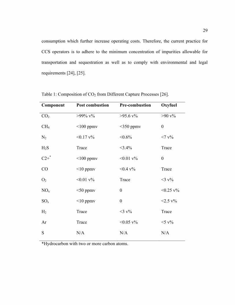
indicated that the concentration of O2 can be as high as 3 vol.%, as Table 1 shows. This

has the potential to lead to severe corrosion of steel pipes [15]–[17]. It has been reported

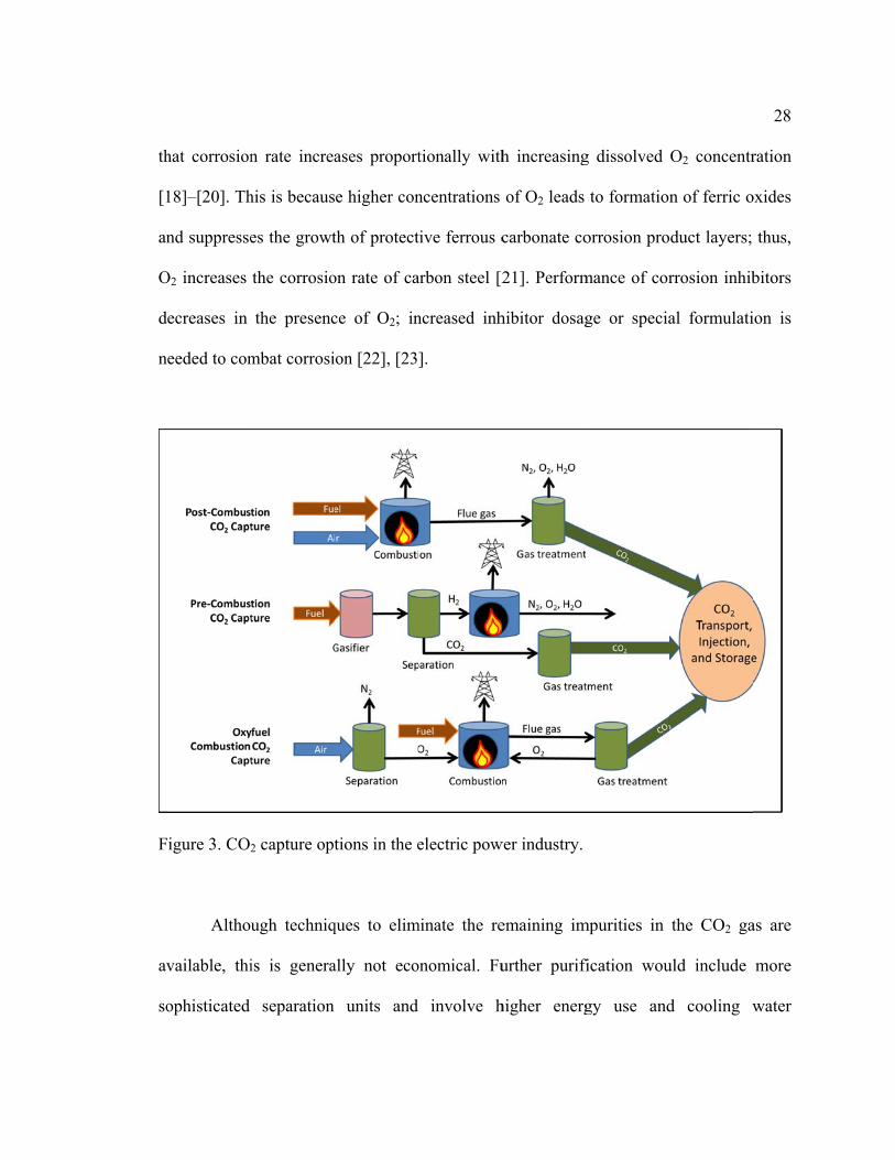
th

[1

an

O

d

n

F

av

so

hat corrosion

18]–[20]. Th

nd suppresse

O2 increases

ecreases in

eeded to com

igure 3. CO2

Althou

vailable, thi

ophisticated

n rate increa

his is becaus

es the growt

the corrosio

the presenc

mbat corrosi

2 capture opt

ugh techniq

is is genera

separation

ases proport

e higher con

th of protect

on rate of ca

ce of O2; in

on [22], [23

tions in the e

ques to elim

ally not eco

units and

tionally with

ncentrations

tive ferrous c

arbon steel [2

ncreased inh

].

electric pow

minate the re

onomical. Fu

involve h

h increasing

of O2 leads

carbonate co

21]. Perform

hibitor dosag

wer industry.

emaining im

urther purifi

higher energ

g dissolved

to formation

orrosion pro

mance of cor

ge or specia

mpurities in

fication wou

gy use and

O2 concentr

n of ferric o

duct layers;

rrosion inhib

al formulati

the CO2 ga

uld include

d cooling w

28

ration

oxides

thus,

bitors

ion is

as are

more

water

29

consumption which further increase operating costs. Therefore, the current practice for

CCS operators is to adhere to the minimum concentration of impurities allowable for

transportation and sequestration as well as to comply with environmental and legal

requirements [24], [25].

Table 1: Composition of CO2 from Different Capture Processes [26].

Component Post combustion Pre-combustion Oxyfuel

CO2 >99% v% >95.6 v% >90 v%

CH4 <100 ppmv <350 ppmv 0

N2 <0.17 v% <0.6% <7 v%

H2S Trace <3.4% Trace

C2+* <100 ppmv <0.01 v% 0

CO <10 ppmv <0.4 v% Trace

O2 <0.01 v% Trace <3 v%

NOx <50 ppmv 0 <0.25 v%

SOx <10 ppmv 0 <2.5 v%

H2 Trace <3 v% Trace

Ar Trace <0.05 v% <5 v%

S N/A N/A N/A

*Hydrocarbon with two or more carbon atoms.

30

Transportation of CO2 from its sources to geological storage or EOR injection wells

is typically done via miles of carbon steel pipeline at operating conditions between 75

and 200 bar CO2 and temperatures up to 30°C [27]. CO2 well casing and tubing, also

consisting of steel elements, can be exposed to operating conditions up to 500 bar CO2

and temperatures up to 150°C [27]. The extreme conditions make corrosion of steel by

CO2 inevitable and it is important to understand the mechanism of the corrosion process.

2.3 CO2 Corrosion

Dry CO2, whether in gaseous, liquid or solid phase, is harmless to steel. However,

when water is present, CO2 dissolves therein to create a weak acidic solution called

carbonic acid which is corrosive to steel. The overall reactive phenomenon between CO2,

water, and steel is referred to as CO2 corrosion.

An acid’s ability to lose a hydrogen ion (H+), or proton, defines the strength of the

acid. Strong acids, such as hydrochloric acid (HCl), completely dissociate in water, while

weak acids such as carbonic acid (H2CO3) dissociate incompletely in water. Carbonic

acid constantly provides a reservoir of hydrogen ions, which leads to a higher corrosion

rate than strong acid solutions under the same pH condition. In other words, corrosion

rates at the same pH conditions is higher due to the increased accessibility of hydrogen

ions to the active steel surface [28].

31

2.3.1 Water Chemistry

The water chemistry of CO2 corrosion can be described from the following

reaction equations:

( ) ( ) (1)

(aq) + (l) ( ) (2)

( ) ( ) + ( ) (3)

( ) ( ) + ( ) (4)

Reaction (1) is CO2 dissolution in water, followed by hydration to form carbonic acid (2).

Carbonic acid dissociates to form hydrogen ions and bicarbonate (3). The bicarbonate

further dissociates to form carbonate ions and more hydrogen ions (4). When the carbonic

acid reacts with steel, primarily Fe, it forms a thin layer of crystals called iron carbonate

(FeCO3) on the steel surface, provided that the ion concentrations are saturated. The

overall reaction can be expressed as follows:

( ) + (aq) + (l) ( ) + ( ) (5)

Incorporating electrochemical and precipitation processes, this is the overall reaction

involving CO2, water and steel in CO2 corrosion. The electrochemical reactions

themselves are discussed in the next section.

32

The layer of FeCO3, also known as siderite, forms on the steel surface and confers

some protection by slowing down the corrosion process as a result of mass transfer

resistance set by the layer, blocking the steel surface and making it unavailable for

corrosion. This has been studied by many researchers since the 1970’s [29]–[34]. Solid

FeCO3 forms when the concentrations of Fe2+ and CO32- exceed the solubility limit

according to the following reaction [35]:

( ) + ( ) ( ) (6)

The precipitation of FeCO3 also depends on its saturation, which is defined by:

= (7)

FeCO3 will not form if the saturation value is less than 1. The solubility product constant,

Ksp, is a function of temperature, Tk, and ionic strength, I, and can be calculated by [36]:

log = −59.3498 − 0.41377 − . + 24.5724 log +2.518 . − 0.657 (8)

The degree of protection that the FeCO3 layer provides has been investigated in

terms of its shear stress, adhesion properties, dissolution in flowing conditions, and other

parameters [11], [37]–[39]. However, limited research has been done on the integrity of

this film with respect to O2 exposure especially at high pressure.

33

2.3.2 Electrochemistry

In an electrochemical reaction, there is a transfer of electrons at anodic and

cathodic sites on the steel surface. In a mild steel corrosion process, iron loses two of its

electrons when it is oxidized in the anodic reaction.

( ) → ( ) + 2 (9)

Ferrous ions, Fe2+, migrates into the solution that is adjacent to the steel surface. In an

acidic solution, hydrogen ions (H+) diffuse to the steel surface to receive the electrons

released by the iron via the following reduction reaction:

2 ( ) + 2 → ( ) (10)

This reduction results in hydrogen gas evolution. Other reduction reactions involving

carbonates have been proposed, called the ‘direct’ reduction of carbonic acid and

bicarbonate ion, respectively [29], [40]:

2 ( ) + 2 → ( ) + 2 ( ) (11) 2 ( ) + 2 → ( ) + 2 ( ) (12)

34

This mechanism was later dismissed by others as to not actually take place [41]. The

observed dominant cathodic reaction was the reduction of H+ that was provided by the

dissociation of carbonic acid. This is referred to as the ‘buffering effect’.

Another cathodic reaction can occur due to the direct reduction of water.

2 ( ) + 2 → ( ) + 2 ( ) (13)

This reaction is purely charge transfer controlled because water is present in abundance at

the steel surface [42]. The reaction is too slow and occurs at potentials below -1000 mV

[40], which is well below the typical corrosion potential seen in CO2 corrosion.

In this discussion of the electrochemistry of CO2 corrosion, water is assumed to

be oxygen-free. In the occasion that O2 is present in the system, an additional O2

reduction reaction will occur; this is discussed later in this chapter.

2.3.3 Factors Affecting CO2 Corrosion Rate

Many factors affect the rate of CO2 corrosion, which include, but are not limited

to, temperature, pH, pressure, impurities, and salinity. Temperature affects gas solubility,

reaction kinetics, and equilibrium constants. As temperature increases, the solubility of

O2 and CO2 decreases, thus reducing their concentrations in solution. Nevertheless,

corrosion rates generally increase with temperature as reaction rates increase more

strongly with temperature than the solubility decreases [18], [43]. The phase identity and

morphology of corrosion products also changes with temperatures [44]. At elevated

35

temperature, the corrosion product layer may become protective and reduce corrosion

rates, depending on flow, pH, and ferrous iron concentration [35], [45], [46].

At low pH, say around pH 4, corrosion rate increases as temperature increases and

protection by corrosion products will be less than for a higher pH; this is due to the nature

of the corrosion product, which is generally porous and loose and does not offer any

protection to the steel surface. Previous researchers indicated that corrosion rates at pH 4

increase rapidly from 25 to 90°C but increase at a slower rate between 90 and 125°C due

to changes in the iron oxidation reaction [42]. At higher pH, the corrosion rate will

generally drop at higher temperature due to the formation of a dense and compact

corrosion product that can be very adherent to the steel surface and thus provides a form

of self-mitigation against further corrosion. This physical barrier restricts the diffusion of

aggressive species as well as prevents further dissolution of steel and leads to blocking of

the steel surface, impeding iron dissolution [29], [46], [47].

Corrosion rate may increase slightly as salt concentration is increased up to 3 wt%

due to a higher electrical conductivity of the solution. Further increase in the salt

concentration would limit the solubility of gases such as O2, which then lowers the

corrosion rate [18], [43]. Retarded anodic and cathodic reactions have been reported at

25 wt% NaCl concentration as well [48].

The increase in the partial pressure of CO2 generally increases the overall

corrosion rate of steel for conditions without a protective corrosion product layer; this is

due to the increased carbonic acid concentration in the solution. Several different factors

36

influence the corrosion behavior at high pressure conditions, which will be discussed in

detail later in this chapter.

The above factors not only affect the corrosion rate, but also determine the type of

corrosion product that would evolve. Knowledge of chemical equilibria for the involved

species and electrochemistry can be combined in the form of a plot called a Pourbaix

diagram, and can be applied to predict the thermodynamically stable species, including

the corrosion products.

2.3.4 Corrosion Product Prediction using Pourbaix Diagrams

A Pourbaix diagram, or a potential-pH diagram, is a map that can be created by

plotting equilibrium relationships in a plot of potential versus pH. The diagram can be

used to predict the type of corrosion products that form at different pH values and

potentials. The use of the Pourbaix diagram is the key in assisting in experimental design

and interpretation of results. Electrochemical equilibrium transition lines follow from the

Nernst equation, while chemical reaction transitions follow from chemical equilibria,

(K values). The Pourbaix diagram for Fe-O2-H2O is given in Figure 4. The lines represent

the equilibrium conditions when the activities of species are equal across the line.

Various computer software options exist to produce such diagrams, an example is shown

in Figure 5. Based on these two diagrams, iron will not corrode and stays in the form of

Fe when the potential is very low due to the high availability of electrons. Increase in

potential would lead to dissolution of iron into Fe2+ at low pH values, or precipitate as

oxides of iron at higher pH values. The driving force for the evolution of a stable species

b

ea

F

ecomes enha

ach equilibri

igure 4. Pou

anced as the

ium line.

urbaix diagra

e combined p

am for Fe-O2

pH and pote

2-H2O system

ential conditi

m at 25°C

ions move fufurther away

37

from

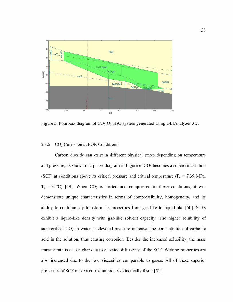
38

Figure 5. Pourbaix diagram of CO2-O2-H2O system generated using OLIAnalyzer 3.2.

2.3.5 CO2 Corrosion at EOR Conditions

Carbon dioxide can exist in different physical states depending on temperature

and pressure, as shown in a phase diagram in Figure 6. CO2 becomes a supercritical fluid

(SCF) at conditions above its critical pressure and critical temperature (Pc = 7.39 MPa,

Tc = 31°C) [49]. When CO2 is heated and compressed to these conditions, it will

demonstrate unique characteristics in terms of compressibility, homogeneity, and its

ability to continuously transform its properties from gas-like to liquid-like [50]. SCFs

exhibit a liquid-like density with gas-like solvent capacity. The higher solubility of

supercritical CO2 in water at elevated pressure increases the concentration of carbonic

acid in the solution, thus causing corrosion. Besides the increased solubility, the mass

transfer rate is also higher due to elevated diffusivity of the SCF. Wetting properties are

also increased due to the low viscosities comparable to gases. All of these superior

properties of SCF make a corrosion process kinetically faster [51].

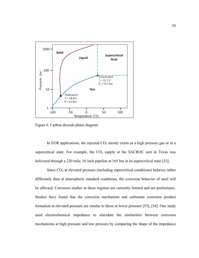
39

Figure 6. Carbon dioxide phase diagram

In EOR applications, the injected CO2 mostly exists as a high pressure gas or in a

supercritical state. For example, the CO2 supply at the SACROC unit in Texas was

delivered through a 220 mile, 16 inch pipeline at 165 bar in its supercritical state [52].

Since CO2 at elevated pressure (including supercritical conditions) behaves rather

differently than at atmospheric standard conditions, the corrosion behavior of steel will

be affected. Corrosion studies in these regimes are currently limited and are preliminary.

Studies have found that the corrosion mechanism and carbonate corrosion product

formation at elevated pressure are similar to those at lower pressure [53], [54]. One study

used electrochemical impedance to elucidate the similarities between corrosion

mechanisms at high pressure and low pressure by comparing the shape of the impedance

40

loop [54]. Various magnitudes of corrosion rates at high pressure have been reported by

research scholars with corrosion rates as high as 40 mm per year [55]–[57].

In ‘scale-free’ CO2 corrosion, the corrosion rate of steel is proportional to the

partial pressure of CO2 up to about 10 bars. This is explained by the increased

concentration of carbonic acid in the solution that leads to the increase in cathodic

reactions in the system. This pattern changes as the CO2 partial pressure increases beyond

10 bars, especially in a more alkaline environment when the corrosion rate starts to

decline due to the formation of a protective FeCO3 layer on the steel surface. At this

condition, the increase in concentration of bicarbonate and carbonate ions causes

supersaturation and precipitation to occur, thus forming a layer of FeCO3 that provides

protection against corrosion [31], [58]. Most corrosion prediction models are designed for

low pressure applications. For partial pressures of CO2 above say 10 bar, over prediction

of the corrosion rate is to be expected. This is because these models do not take some

factors into consideration such as the effect of water wetting and protectiveness of the

corrosion product layer. Modifications can be done to these models by introducing

particular factors, such as the fugacity coefficients, as well as using equilibrium constants

that are valid at elevated pressures [59].

One study reported that UNS G10180 carbon steel experiences corrosive attack

due to its exposure to water-saturated supercritical CO2 [60]. In another study, it was

reported that there existed a layer of cementite (iron carbide) with intergrown siderite

(iron carbonate) at 80 bar CO2 (supercritical) [59]. Researchers also observed that the

41

coverage of iron carbonate was more thorough with supercritical CO2 than for liquid CO2,

which also causes a significant reduction in corrosion rate of X65 steel [61].

While the physical and chemical properties of the corrosion product layer

continue to be studied, the effect of external factors, such as O2 intrusion on the corrosion

product layer, has been given less attention.

2.4 Properties of CO2 – O2 Mixtures

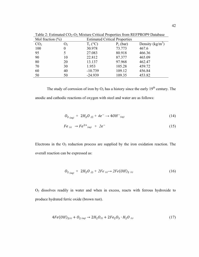
The physical properties of mixtures differ from pure substances. Table 2 shows

the changes in mixture properties at different ratios of CO2 and O2 relating to

supercriticality. Note that the critical point changes and mixtures are less dense at the

critical point as the O2 concentration increases. Physical property data of CO2-O2

mixtures such as molar volume, viscosity, and diffusion coefficients is limited, especially

at pressures above 1 bar [27], [62]. Phase diagrams of CO2 mixtures relevant to CCS

have been published where it has been observed that boiling and condensing behavior

will change due to impurities. [63]. Vapor-liquid equilibria of CO2 mixtures have been

published in articles since the 1970s [64]–[66], however, the temperature and pressure

range is still limited.

2.5 Oxygen Corrosion of Steel

When iron is in contact with air and moisture, it oxidizes into what is generally

known as rust. Iron and O2 react with each other to form different oxides and

oxyhydroxides, turning the metal surface brittle and resulting in spallation.

42

Table 2: Estimated CO2-O2 Mixture Critical Properties from REFPROP9 Database Mol fraction (%) Estimated Critical Properties CO2 O2 Tc (°C) Pc (bar) Density (kg/m3) 100 0 30.978 73.773 467.6 95 5 27.083 80.918 466.36 90 10 22.812 87.377 465.09 80 20 13.137 97.968 462.47 70 30 1.953 105.28 459.72 60 40 -10.739 109.12 456.84 50 50 -24.939 109.35 453.82

The study of corrosion of iron by O2 has a history since the early 19th century. The

anodic and cathodic reactions of oxygen with steel and water are as follows:

(aq) + 2 (l) + 4 → 4 (aq) (14) (s) → (aq) + 2 (15)

Electrons in the O2 reduction process are supplied by the iron oxidation reaction. The

overall reaction can be expressed as:

(aq) + 2 (l) + 2Fe (s)→ 2Fe( ) (s) (16)

O2 dissolves readily in water and when in excess, reacts with ferrous hydroxide to

produce hydrated ferric oxide (brown rust).

4 ( ) (s) + (aq) → 2 (l) + 2 ∙ (s) (17)

43

The presence of O2 also causes other reactions to occur, forming various types of iron

oxides.

The corrosion rate of iron generally increases as the concentration of dissolved O2

in water increases. Localized corrosion occurs when poor mass transport exists under

deposits and crevices [67]. Tubercles are the typical morphology of the corrosion product

observed on steel surfaces in the form of small, rounded, hollow protrusions [68]–[72].

Other factors such as water velocity, temperature, pH, and dissolved minerals affect the

corrosion process [73].

2.5.1 Iron Oxides

Iron can commonly occur in ferrous (+2 oxidation state) or ferric (+3) forms. The

ferric form generally has very low solubility [74]. Under oxidizing conditions, iron

precipitates as ferric hydroxide. Typically, iron oxides have an octahedral structural unit

in which Fe atoms are surrounded by six oxide (O2-) and/or hydroxide (OH-) anions. The

O2 and OH ions are arranged in layers that are either in a α-phase or γ-phase. The α-

phase arrangement is hexagonally close-packed (hcp), whereas the γ-phase is cubic close-

packed (ccp). For example, goethite (α-FeOOH) and hematite (α-Fe2O3) are in hcp form,

while lepidocrocite (γ-FeOOH) and maghemite (γ-Fe2O3) are in ccp form [75]. There are

16 different iron oxide or oxyhydroxide phases that have been reported to exist in nature.

Nine of the oxides have been reported to be detected on corrosion products of steel,

namely goethite, hematite, lepidocrocite, maghemite, iron (II) hydroxide (Fe(OH)2), iron

(III) hydroxide (Fe(OH)3), akaganeite (β-FeOOH), feroxyhite (δ-FeOOH), and magnetite

44

(Fe3O4) [76]. The mechanism of iron oxide and oxyhydroxide formation on low alloy

steel in aqueous solution has been studied by previous researchers [77], [78].

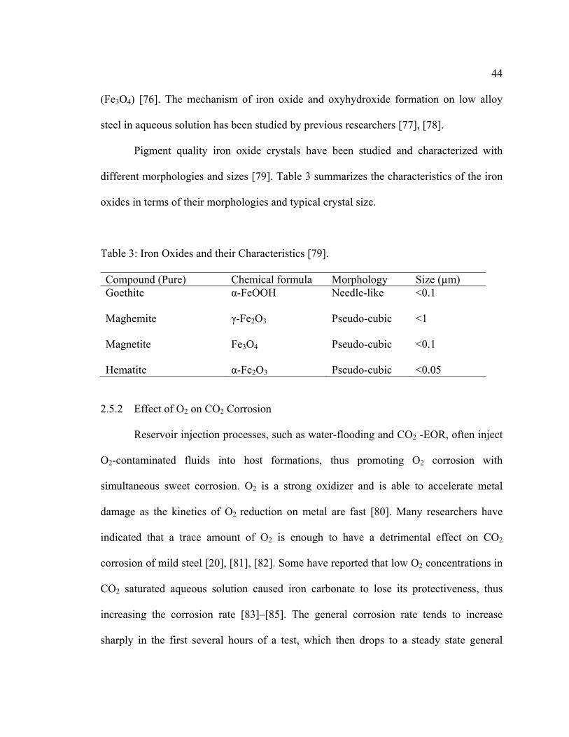
Pigment quality iron oxide crystals have been studied and characterized with

different morphologies and sizes [79]. Table 3 summarizes the characteristics of the iron

oxides in terms of their morphologies and typical crystal size.

Table 3: Iron Oxides and their Characteristics [79].

Compound (Pure) Chemical formula Morphology Size (µm) Goethite α-FeOOH Needle-like <0.1 Maghemite γ-Fe2O3 Pseudo-cubic <1 Magnetite Fe3O4 Pseudo-cubic <0.1 Hematite α-Fe2O3 Pseudo-cubic <0.05

2.5.2 Effect of O2 on CO2 Corrosion

Reservoir injection processes, such as water-flooding and CO2 -EOR, often inject

O2-contaminated fluids into host formations, thus promoting O2 corrosion with

simultaneous sweet corrosion. O2 is a strong oxidizer and is able to accelerate metal

damage as the kinetics of O2 reduction on metal are fast [80]. Many researchers have

indicated that a trace amount of O2 is enough to have a detrimental effect on CO2

corrosion of mild steel [20], [81], [82]. Some have reported that low O2 concentrations in

CO2 saturated aqueous solution caused iron carbonate to lose its protectiveness, thus

increasing the corrosion rate [83]–[85]. The general corrosion rate tends to increase

sharply in the first several hours of a test, which then drops to a steady state general

45

corrosion rate after about 20 hours of test time [81]. O2 intrusion also accelerates

corrosion in sour (H2S) systems [23]. CO2 corrosion with O2 intrusion is controlled by

both mass and charge transfer, as demonstrated by the higher corrosion rate in highly

turbulent systems than in a stagnant system [81]. Pits were observed in both stagnant and

turbulent O2-CO2 systems under a layer of red, loose, and porous iron oxide [69], [81]. It

was further reported that deeper pits occurred in correlation with increasing O2

concentration [81].

Table 4: Overview of O2-CO2 Corrosion Tests in the Literature.

No. pCO2, MPa

T, °C

H2O content

O2 content Steel type

Time, hours

Flow, rpm

CR, mm/y

Ref.

1 1 25 0.2 ppm 0.4 ppm 0.6 ppm 0.8 ppm 1.4 ppm

1018 24 0 0.86 0.99 1.14 1.45 2.06

[23]

2 8 35 100 g 3 vol% 304L 316L X42, X60

120 100 0.031 0.028 0.32 0.26

[20]

3 10 50 100 g 3 vol% 304L 316L X42 X60

120 100 0.032 0.042 0.99 0.93

[20]

4 8 50 sat 4 vol% X65, 13Cr

24 120

0 19.3 14.1

[86], [87]

5 2.5 120 sat 0.5 MPa N80 120 1 m/s 4.47 [88] 6 1 90 sat 0.05 MPa N80 72 0 1.43 [82] 7 1 90 sat 0.05 MPa N80 72 2 m/s 3.36 [82] 8 0.92 60 sat 5 vol% 3Cr 120 0 1.36 [89] 9 0.05 80 sat 1 ppm 1018 168 0 1.07 [90] 10 7.58 40 1000

ppmv 100 ppm 1010 5 0 2.3 [91]

46

In corrosion control, inhibitors lose their efficiency with increases in O2

concentration in CO2 environments [92]. Almost all corrosion inhibitors do not work well

when O2 is present. Observed corrosion products were reported to be porous and non-

protective. Still, limited investigations have been conducted to study the effect of O2 on

sweet corrosion of steel at elevated pressure, including conditions where supercritical

CO2 is present. Awareness and quantification of the amount of O2 ingress in a CO2-H2O

system is key to prevent potential catastrophic corrosion failures.

2.6 Chapter Summary

The discussion in this chapter covered the connection between O2 ingress in CO2

corrosion related to the oil and gas industry and carbon capture technology; CO2-EOR

was described. Discussion of CO2 corrosion covered the related electrochemical and

chemical reactions, thermodynamics, and the effect of high pressure. Mechanisms

relating to O2 corrosion were discussed, which included the different types of oxides that

can form during the corrosion process. The effect of O2 ingress on CO2 corrosion was

also discussed. Limited work has been done to investigate mechanisms relating to O2

ingress in high pressure CO2 corrosion. The intention of this dissertation is to expand

knowledge within this research area. High pressure CO2 will simulate the conditions of

CO2-EOR fields. The presence of O2 will act as the impurity in the CO2 supply. The

following chapters elaborate the methodology and research strategy that was applied to

explore how O2 affects CO2 corrosion in high pressure systems.

47

CHAPTER 3: OBJECTIVES AND HYPOTHESES

3.1 Problem Statement and Research Gap

Limited studies have thus far been conducted relating to establishing the

mechanism of CO2-O2 corrosion in both low and high pressure systems. In particular,

how tuberculation and blistering of the corrosion product layer occurs is poorly

understood. The research reported in this dissertation seeks to contribute to knowledge in

this area.

3.2 Objectives of the Study

This project aims to investigate the corrosion behavior of carbon steel in

CO2/O2/brine mixtures at ambient and simulated EOR conditions. A qualitative

mechanistic model of the corrosion process will be described. This study is expected to

provide knowledge and useful information beneficial for the future development of

corrosion control in CO2/O2/brine systems at elevated pressure, particularly in the oil and

gas industry.

The scope of this work includes electrochemical measurements, as well as surface

analysis of corrosion products in order to characterize their morphologies, phase

identities, and chemical properties.

3.3 Research Hypothesis

Dissolved O2 in water is highly reactive and readily converts Fe2+ to Fe3+ ions,

adversely impeding the formation of a protective layer of iron carbonate, FeCO3. Full

48

coverage of FeCO3 on a steel surface will be absent, thus exposing selective areas to

corrosive species. Dissolution of already formed FeCO3 crystals may also occur,

weakening the protective layer, leading to localized corrosion at crystal boundaries. This

is illustrated in Figure 7, which shows a thin layer of FeCO3 in CO2-saturated solution

that is damaged and/or dissolved in the presence of O2. Researchers [69], [81] have

reported that O2 causes localized corrosion and have also reported morphologies

corresponding to tubercles in their ambient pressure glass cell tests.

Iron carbonate layers on steel were reported to be thicker at high CO2 partial

pressures [61]. It is speculated that the thickness of this layer will decrease in the

presence of O2 since it oxidizes Fe2+ into Fe3+ ions, thereby impeding the formation of

FeCO3. Produced Fe3+ will result in formation of loose iron oxide, FexOy, particles. This

is illustrated in Figure 8 where the thicker layer of FeCO3 is also dissolved in the

presence of O2. The dissolution of FeCO3 weakens the protective layer, especially at its

crystal grain boundaries resulting in penetration of FexOy deeper into the steel in

association with creation of deeper pits.

F

F

co

un

igure 7. Sch

igure 8. Sch

Althou

orrosion, att

nanswered.

hematic for h

hematic of hy

ugh previou

tempts to de

The followin

hypothesis at

ypothesis at

us research

escribe its m

ng questions

t low pressur

high pressur

hers have in

mechanism a

s were addre

re

re

nvestigated

are limited.

essed in this

the effect

Many quest

research:

of O2 on

tions are stil

49

CO2

ll left

50

1. What iron oxides form in an O2/CO2 environment?

2. Do different kinds of oxides form at elevated pressure?

3. What is the solubility of O2 in various phases of CO2?

4. How severe is the corrosion?

5. Do the phenomena agree with generated Pourbaix diagrams?

6. Does O2 cause pitting corrosion?

7. What causes tuberculation and blistering on the corrosion product layer?

51

CHAPTER 4: LOW PRESSURE CORROSION EXPERIMENTS

This chapter describes the experiments that were conducted at atmospheric

pressure. Four different types of experiment are discussed. The first is a preliminary

experiment that was conducted to determine the effect of O2 on CO2 corrosion of steel at

a condition that does not promote growth of a protective iron carbonate layer on the steel

surface. This condition will be referred to as ‘FeCO3-free’. Other experiments were then

conducted for multiple sets of ‘FeCO3-forming’ conditions.

The experimental methodology is discussed first, followed by the results and their

discussion. Corrosion mechanisms for mild steel with oxygen (O2) intrusion in different

scenarios are then elaborated.

The objective of this study is to investigate the corrosion mechanism and the

stability of iron carbonate (FeCO3) on mild steel with simulated ingress of ppm levels of

O2 at 1 bar total pressure as a prelude to conducting experiments that simulate high

pressure environments.

Parts of this chapter have been presented at an international conference,

CORROSION 2014, in San Antonio, Texas [90]. (Reproduced with permission from

NACE International, Houston. TX. All rights reserved. N.R. Rosli, Y.-S. Choi, D. Young,

Paper Number C2014-4299 presented at CORROSION/2014, San Antonio, TX. ©

NACE International 2014.)

52

4.1 Sample Material

The type of steel that was used in this study is grade UNS G10180, its corrosion

behavior was investigated using electrochemical techniques, surface analysis, and weight

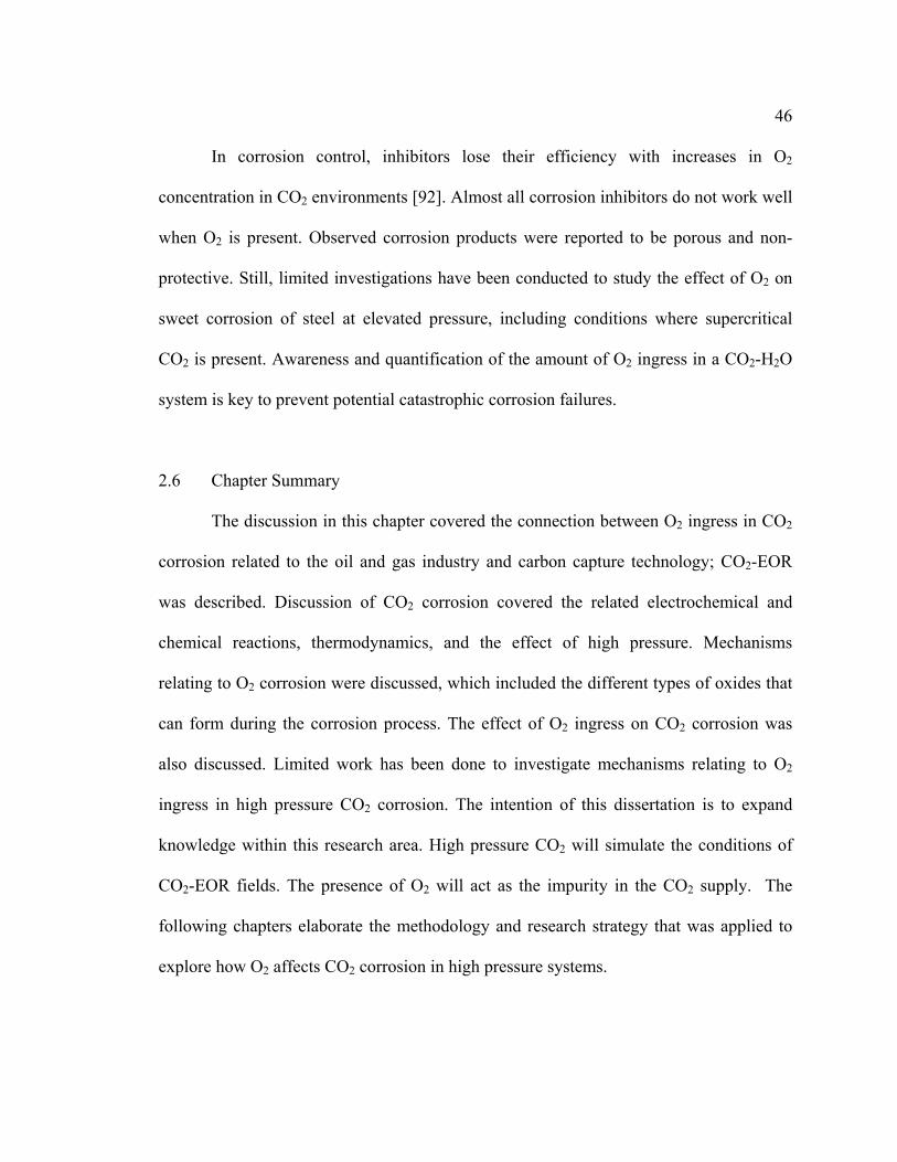
loss measurements. The specimens for electrochemical measurements were cylindrical-

shaped while the specimens for weight loss and surface analyses were square-shaped, as

shown in Figure 9. The composition of the steel was evaluated using Atom Emission

Spectroscopy (AES), conforming to the requirements of UNS G10180, as shown in Table

5. The steel possesses a ferritic-pearlitic microstructure. The full report of the analysis is

in Appendix A.

Sample preparation involved polishing of the steel specimens with up to 600 grit

silicon carbide (SiC) paper, rinsing to remove any debris with isopropyl alcohol in an

ultrasonic bath, and finally drying with a heat gun. The dimensions and masses of the

specimens were measured using a scale with accuracy of 0.001 g.

Figure 9. Steel specimens for glass cell tests

53

Table 5: Composition of Steel (Balance Fe).

Element Wt. %

Al 0.008 As 0.006 C 0.18 Co 0.003 Cr 0.12 Cu 0.18 Mn 0.75 Mo 0.02 Nb 0.002 Ni 0.065 P 0.011 S 0.021 Sb 0.009 Si 0.16 Sn 0.009 Ta 0.028 Ti 0.002 V 0.003 W 0.014 Zn 0.004 Zr 0.003

4.2 Experimental Design

A three-electrode glass cell setup, as shown in Figure 10, was utilized to conduct

the low-pressure corrosion tests described in this chapter. A TeflonTM lid was fabricated

with slots to hold multiple electrodes in place, as labeled in the diagram in Figure 10.

These include the pH electrode, thermocouple, gas inlet and outlet, reference electrode,

counter electrode, and holders for the working electrode and weight loss steel samples.

The electrolyte that was used for the system was 2 liters of 1 wt.% NaCl solution.

Before the start of each experiment, CO2 or a CO2 and O2 mixture was sparged through

th

T

sa

se

T

ce

th

(2

F

he solution f

The sparger w

aturating the

ensor, an Or

This value w

ell at the set

hat was CO2

25°C). Gas w

igure 10. Gl

for at least

was used to

e solution w

rbisphere 41

as then reca

t temperatur

2-saturated r

was continuo

lass cell setu

1 hour until

o reduce the

with gas. The

0, which giv

alculated to d

re. A sample

recorded a r

ously bubble

up (Courtesy

the desired

size of the

e O2 concen

ves the O2 c

determine th

e calculation

reading of le

ed into the sy

of Cody Sh

d stable conc

gas bubbles

ntration was

concentration

he actual con

n is included

ess than 10

ystem for the

hafer, ICMT)

centration o

s to speed u

monitored

n in the wate

ncentration o

d in Append

ppb of O2

e duration of

)

f O2 is achi

up the proce

using an ox

er phase at 2

of O2 in the

dix B. A sol

in the gas p

f the tests.

54

eved.

ess of

xygen

25°C.

glass

lution

phase

55

Figure 11. Oxygen meter, Orbisphere 410.

The desired temperature was maintained using a hotplate, controlled with a

thermocouple immersed into the solution. Once the solution temperature stabilized, its

pH was adjusted by adding deoxygenated reagent grade NaHCO3 or HCl. Deoxygenated

ferrous chloride (FeCl2·4H2O) solution was added to provide additional Fe2+ ions in order

to achieve a high initial FeCO3 saturation value; this accelerated the formation of a

protective layer, thus reduced the experiment time. The test matrix for the FeCO3-free

and FeCO3-forming experiments is shown in Table 6.

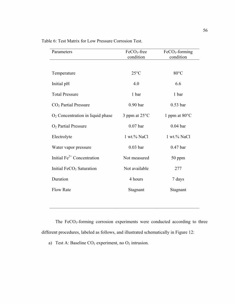
56

Table 6: Test Matrix for Low Pressure Corrosion Test.

Parameters FeCO3-free condition

FeCO3-forming condition

Temperature

25°C

80°C

Initial pH 4.0 6.6

Total Pressure 1 bar 1 bar

CO2 Partial Pressure 0.90 bar 0.53 bar

O2 Concentration in liquid phase 3 ppm at 25°C 1 ppm at 80°C

O2 Partial Pressure 0.07 bar 0.04 bar

Electrolyte 1 wt.% NaCl 1 wt.% NaCl

Water vapor pressure 0.03 bar 0.47 bar

Initial Fe2+ Concentration Not measured 50 ppm

Initial FeCO3 Saturation Not available 277

Duration 4 hours 7 days

Flow Rate Stagnant Stagnant

The FeCO3-forming corrosion experiments were conducted according to three

different procedures, labeled as follows, and illustrated schematically in Figure 12:

a) Test A: Baseline CO2 experiment, no O2 intrusion.

F

p

ex

ex

co

m

(X

b) Test B

of the

the eff

c) Test C

condu

withou

igure 12. Di

Electr

otentiostat

xplanation o

The te

xperiments,

orrosion pro

microscopy (

XRD) and R

B: O2 was ad

e FeCO3 laye

ffect of O2 in

C: CO2-O2 m

ucted to inv

ut any pre-c

ifferent tests

rochemical m

to determin

of this techni

est specimen

rinsed with

ocesses. The

(SEM), ene

Raman spectr

dded into the

er on the ste

ntrusion on th

mixture from

vestigate the

orrosion.

for FeCO3-f

measuremen

ne the cor

ique is descr

ns were prom

h isopropyl

e test specim

ergy dispers

roscopy.

e system afte

eel surface. T

he FeCO3 la

m the beginn

e effect of O

forming exp

nts were con

rrosion para

ribed in the n

mptly remov

alcohol, and

mens were

sive X-ray

er 2 days of

The objectiv

ayer.

nning of the

O2 impurity

periments.

nducted usin

ameters of

next sub-topi

ved from the

d dried to p

then analyz

spectroscop

CO2 corrosi

ve of this tes

experiment

y on CO2 co

ng a GAMRY

the experi

ic.

e electrolyte

prevent the

zed using s

py (EDS), X

on and form

st is to deter

. This study

orrosion of

Y Reference

iments. Det

at the end o

onset of fu

scanning ele

X-ray diffra

57

mation

rmine

y was

steel

e 600

tailed

of the

urther

ectron

action

58

Besides electrochemical measurements, the corrosion rate of the steel was also

determined by measuring the weight loss at the end of the experiments. The weight loss

of the steel is measured by completely removing the corrosion product from the steel

surface in order to determine the difference in weight. The layers of corrosion product on

the steel surface were removed using Clarke solution (ASTM G1-03). The Clarke

solution consists of a mixture of hydrochloric acid (HCl), antimony trioxide (Sb2O3), and

stannous chloride (SnCl2). The HCl removes the rust, Sb2O3 works as an inhibitor to

prevent HCl attack on the steel, while SnCl2 is a reducing agent to convert ferric chloride

to ferrous ions to avoid further reaction between ferric ions and fresh steel. A sample plot

of weight change during the treatment using Clarke solution is provided in Appendix C.

Weight loss from the specimens in all tests were recorded and translated into

corrosion rate using the following formula:

= ∙ ∙ (18)

The letter W represents the weight loss in grams, D is the density of the steel specimen in

units of g/cm3, A is the area of the specimen in cm2, and T is the experimental time in

seconds. The corrosion rate in cm/s was converted into units of mm/y with appropriate

unit conversion. Treated specimens were also characterized by profilometry, using a 3D

microscope, to determine the surface profile of the corroded steel surface. The

penetration rate was calculated from observable areas showing a pitting attack. A sample

59

calculation of a corrosion rate from a weight loss measurement is provided in

Appendix D.

4.3 Electrochemical Measurements

The working electrode was polarized at ±5 mV versus the open circuit potential

(OCP) at a scan rate of 0.125 mV/s. The value of the polarization resistance obtained

from this technique is the total polarization resistance, Rp,total, which includes the solution

resistance, Rs. To calculate the corrosion rate, the true polarization resistance, Rp, was

determined by subtracting the solution resistance from the total polarization resistance

that was obtained from linear polarization resistance (LPR) measurements.

= , − (19)

The solution resistance was obtained by conducting Electrical Impedance

Spectroscopy (EIS) on the specimen. The corrosion current, i, was then calculated using

the Stern-Geary equation:

= = ×. × ×( ) (20)

Where βa and βc are the anodic and cathodic Tafel slopes, set to a value of 0.12 V/decade

each, resulting in a Stern-Geary constant, B, value of 0.026 V. This value corresponds to

a corrosion rate that was controlled by both charge transfer and mass transfer.

60

The corrosion current density, icorr, in units of A/m2, is obtained by dividing the

current with the surface area of the steel specimen that is exposed to the solution.

= (21)

The corrosion rate is then calculated using the equation [46]:

= ∙ = ∙ 1.16 (22)

Where Mw is molar mass of the iron (Fe) in g/mol, ρ is the density in g/m3, n is the

number of charges per mol of iron loss, and F is the Faraday’s constant, 96,485 C/mol.

For every kmol of iron lost, 2 kmol of electrons are released, hence the number of charge,

n, is 2. A sample calculation of corrosion rate from polarization resistance value is given

in Appendix E.

4.4 Results and Discussions: FeCO3-Free Experiments

CO2 corrosion tests at total pressure of 1 bar have already been conducted by

previous researchers with reports of increased corrosion rate of carbon steel with the

intrusion of O2 [69], [81], [84]. This set of short term tests was conducted to understand

the effect of O2 on CO2 corrosion of bare steel.

As expected, the corrosion rate increased with O2 ingress. Figure 13 compares the

corrosion rate of steel as measured using LPR. The chart indicates that O2 ingress

61

increased the corrosion rate by 40% when measured at the end of a 4-hour experiment.

Simulation of results using Freecorp© indicated that 3 ppm O2 lead to about 30%

increase in the corrosion rate; this is discussed separately in Chapter 6.

Figure 13. Effect of O2 on corrosion rates at FeCO3-free condition (pH 4, 25°C)

The Nyquist plot, shown in Figure 14, which was obtained from EIS

measurements, showed lower polarization resistance, Rp, when O2 was present in the

system, which implies to a higher corrosion rate. The solution resistance, Rs, did not show

any significant difference in values.

1.1

1.5

0

0.5

1

1.5

2

CO2 only CO2 + 3 ppm O2

Corrosion rate, m

m/year

62

Rp, Ω Rs, Ω

CO2 53.4 3.45

CO2 + O2 38.2 4.08

Figure 14. Nyquist plots relative to the reference electrode (pH 4, 25°C)

Potentiodynamic sweeps were carried out to analyze the behavior of the anodic

and cathodic reactions of the corrosion process. The sweeps were conducted towards the

end of experiments due to their destructive effect to the specimens. The steel specimen

was first polarized negatively from 0 to -500 mV with respect to the Eoc. The OCP was

later monitored until it returned to its original OCP before the polarization. The specimen

was then positively polarized from 0 to 300 mV. The resulting polarization curves, shown

in Figure 15, exhibited higher corrosion current density in the presence of O2; this

translates to a higher corrosion rate. This is because the cathodic curve for the O2-CO2

system slightly shifted to the right. The overall shape of the curves did not change in the

presence of O2, showing a mixed mass transfer and charge transfer mechanism. Previous

researcher had found the cathodic curve shifted further when O2 concentration in

CO2-saturated solution was increased from 40 ppb to 3 ppm [81]. The potentiodynamic

0

5

10

15

20

25

0 10 20 30 40 50 60

‐Zim

age, Ω

Zreal, Ω

CO2 only

CO2 + 3 ppm O2

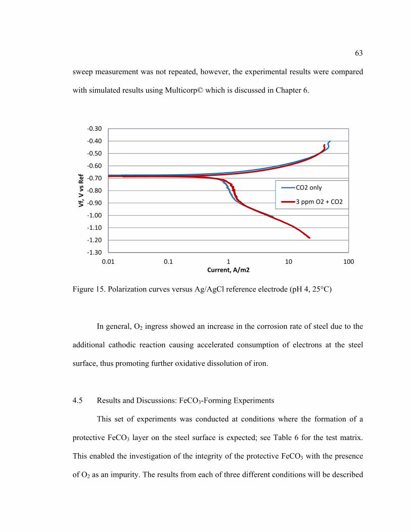
63

sweep measurement was not repeated, however, the experimental results were compared

with simulated results using Multicorp© which is discussed in Chapter 6.

Figure 15. Polarization curves versus Ag/AgCl reference electrode (pH 4, 25°C)

In general, O2 ingress showed an increase in the corrosion rate of steel due to the

additional cathodic reaction causing accelerated consumption of electrons at the steel

surface, thus promoting further oxidative dissolution of iron.

4.5 Results and Discussions: FeCO3-Forming Experiments

This set of experiments was conducted at conditions where the formation of a

protective FeCO3 layer on the steel surface is expected; see Table 6 for the test matrix.

This enabled the investigation of the integrity of the protective FeCO3 with the presence

of O2 as an impurity. The results from each of three different conditions will be described

‐1.30

‐1.20

‐1.10

‐1.00

‐0.90

‐0.80

‐0.70

‐0.60

‐0.50

‐0.40

‐0.30

0.01 0.1 1 10 100

Vf, V vs Ref

Current, A/m2

CO2 only

3 ppm O2 + CO2

64

separately in dedicated sub-sections. The electrochemical measurements, and generated

surface analysis results provide a basis for the proposed corrosion mechanism at the end

of this chapter.

4.5.1 Test A: Baseline CO2 Corrosion Experiment

The plot shown on Figure 16 shows that the corrosion rate for the baseline CO2

corrosion test kept on decreasing monotonously until the end of the 8-day experiment to

ca. 0.1 mm/y. These average values are based on two repeated tests, with error bars

indicating minimum and maximum values. The time-integrated corrosion rate value

corresponds to 0.26 mm/year while the weight loss corrosion rate value was 0.11

mm/year. Theoretically, the drop of the corrosion rate was due to coverage by FeCO3 on

the steel surface that slowed the corrosion process. The corrosion potential, shown in

Figure 17 as the mean values out of two repeats, was relatively stable at around -0.7 mV.

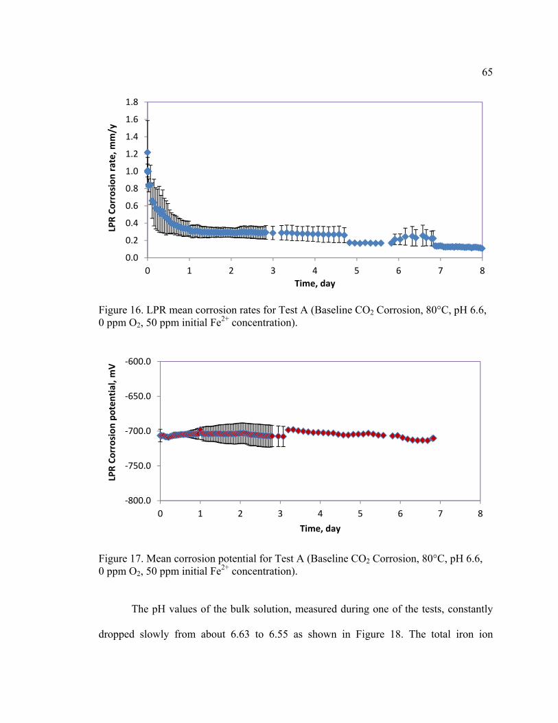
65

Figure 16. LPR mean corrosion rates for Test A (Baseline CO2 Corrosion, 80°C, pH 6.6, 0 ppm O2, 50 ppm initial Fe2+ concentration).

Figure 17. Mean corrosion potential for Test A (Baseline CO2 Corrosion, 80°C, pH 6.6, 0 ppm O2, 50 ppm initial Fe2+ concentration).

The pH values of the bulk solution, measured during one of the tests, constantly

dropped slowly from about 6.63 to 6.55 as shown in Figure 18. The total iron ion

0.0

0.2

0.4

0.6

0.8

1.0

1.2

1.4

1.6

1.8

0 1 2 3 4 5 6 7 8

LPR Corrosion rate, m

m/y

Time, day

‐800.0

‐750.0

‐700.0

‐650.0

‐600.0

0 1 2 3 4 5 6 7 8

LPR Corrosion potential, m

V

Time, day

66

concentration (Fe2+ and Fe3+) in the solution, measured using a spectrophotometer,

showed a decline from the initial 50 mg/L to 2.8 mg/L at the end of the experiment as

shown in Figure 19. The gradual decline in the iron concentration in this baseline test was

due to the continuous consumption of the initially added 50 mg/L of Fe2+ ions to form

FeCO3. The layer of protective FeCO3 slowed down the release of more Fe2+ into the

solution.

Figure 18. Solution pH for Test A, (80°C, pH 6.6, 0 ppm O2, 50 ppm initial Fe2+ concentration).

6.52

6.54

6.56

6.58

6.60

6.62

6.64

0 1 2 3 4 5 6 7

Solution pH

Time, day

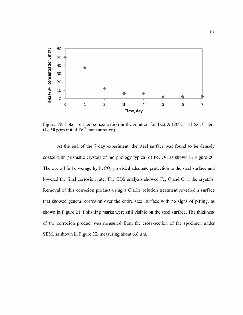
67

Figure 19. Total iron ion concentration in the solution for Test A (80°C, pH 6.6, 0 ppm O2, 50 ppm initial Fe2+ concentration).

At the end of the 7-day experiment, the steel surface was found to be densely

coated with prismatic crystals of morphology typical of FeCO3, as shown in Figure 20.

The overall full coverage by FeCO3 provided adequate protection to the steel surface and

lowered the final corrosion rate. The EDS analysis showed Fe, C and O in the crystals.

Removal of this corrosion product using a Clarke solution treatment revealed a surface

that showed general corrosion over the entire steel surface with no signs of pitting, as

shown in Figure 21. Polishing marks were still visible on the steel surface. The thickness

of the corrosion product was measured from the cross-section of the specimen under

SEM, as shown in Figure 22, measuring about 6.6 µm.

0

10

20

30

40

50

60

0 1 2 3 4 5 6 7

[Fe2+/3+] concentration, mg/L

Time, day

68

Figure 20. SEM image and EDS spectra of sample for Test A (80°C, pH 6.6, 0 ppm O2, 50 ppm initial Fe2+ concentration)

69

Figure 21. SEM image of steel surface for Test A after corrosion product removal

Figure 22. Cross-section view of steel specimen for Test A

70

4.5.2 Test B: O2 Ingress from Day 2

When O2 was introduced into the glass cell on Day 2, the clear, colorless solution

turned colored and murky due to the conversion of the available Fe2+ ions in the solution

into insoluble ferric precipitates that were suspended in the electrolyte. Figure 23 shows

that the introduction of 1 ppm O2 to the pre-corroded specimen caused the corrosion rate

to instantly spike and then settled at a relatively constant value of around 0.5 mm/year. It

is noteworthy that there was a greater scatter of corrosion rate values after the addition of

O2. Similar observations of instant increase in corrosion rate with higher degree of scatter

have been reported by previous researchers [69], [84].

The calculated time-averaged value from the corrosion rate measurement was

0.33 mm/year. There was also an immediate shift in the potential as O2 was added to the

system, shown in Figure 24, similar to the findings observed by another researcher [69].

The error bars shown in the plot represent the maximum and minimum recorded values.

The weight loss measurements recorded a corrosion rate of 0.77 mm/year, this is a value

that is higher than what was observed in Test A.

Figure 25 shows the variation in the solution pH that was measured during one the

tests at this condition. The pH dropped slightly in the beginning before the introduction

of O2, consistent with the pH in the baseline experiment, Test A. The pH then gradually

increased once the system became oxic with a recorded final pH of about 6.6.

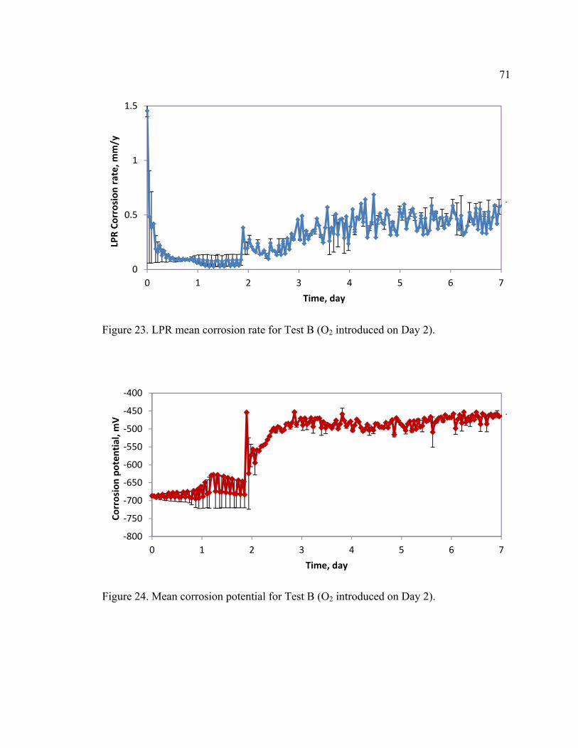
71

Figure 23. LPR mean corrosion rate for Test B (O2 introduced on Day 2).

Figure 24. Mean corrosion potential for Test B (O2 introduced on Day 2).

0

0.5

1

1.5

0 1 2 3 4 5 6 7


m/y

Time, day

‐800

‐750

‐700

‐650

‐600

‐550

‐500

‐450

‐400

0 1 2 3 4 5 6 7

Corrosion potential, m

V

Time, day

72

Figure 25. Solution pH for Test B (O2 introduced on Day 2).

Figure 26 shows the surface of the steel that was partially covered by prismatic

FeCO3 crystals that had formed after 24 hours of test duration. Figure 27 shows dense

coverage by FeCO3 crystals across almost the entire steel surface, right before the

addition of O2. The formation of FeCO3 in this first two days of the test provided some

protection to the steel surface, hence the drop in the corrosion rate as demonstrated in the

electrochemical measurements shown in Figure 24.

The FeCO3 layer was then perturbed by iron oxide formation on Day 2, which

caused the increase in the general corrosion rate after O2 was introduced to the system.

By the end of the test on Day 7, features such as tubercles and mounds of deposits were

observed on the steel surface. Small globular-shaped pseudo-cubic crystals were found

deposited in clusters on top of the prismatic FeCO3 crystals. These clusters of crystals

tend to accumulate and form mounds and craters as demonstrated in Figure 28 and Figure

29. The EDS analysis, shown in Figure 29, of the smaller pseudo-cubic crystals showed a

6.57

6.58

6.59

6.6

6.61

6.62

6.63

6.64

6.65

0 1 2 3 4 5 6 7

pH

Time, day

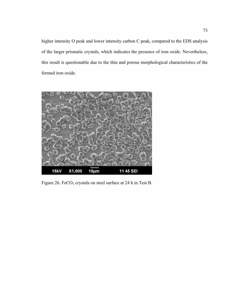
73

higher intensity O peak and lower intensity carbon C peak, compared to the EDS analysis

of the larger prismatic crystals, which indicates the presence of iron oxide. Nevertheless,

this result is questionable due to the thin and porous morphological characteristics of the

formed iron oxide.

Figure 26. FeCO3 crystals on steel surface at 24 h in Test B.

74

Figure 27. FeCO3 crystals on steel surface at 48 h before O2 introduction in Test B.

Figure 28. Oxide clusters on FeCO3 layer at 168 h in Test B

F

F

gr

co

el

b

ob

ap

su

o

in

li

igure 29. SE

The c

igure 30 dem

rey shown in

orrosion pro

lements, hen

etween the a

bserved in S

ppeared blac

urface const

f Fe, is a

ntermediate

ight grey.

EM image an

cross-section

monstrates a

n the SEM b

oduct layer.

nce the appe

atomic numb

SEM images

ck on the im

tituted from

light gray.

shading. A t

nd EDS spec

nal view of t

a dome-like

backscatter im

Heavy elem

arance of lig

bers of the

[93], [94]. T

mage due to

light elemen

Iron oxide

thin oxide la

ctra of sampl

the corrosion

hollow tube

mage are ind

ments scatte

ghter shades

elements pre

The epoxy th

the lesser am

nts (C, H, O

e and iron

ayer is notice

le at the end

n product o

ercular struc

dicative of c

er electrons

of gray. Th

esent and th

hat was used

mount of ba

O). The steel

carbonate c

eable on top

d of Test B

on the steel s

cture. The di

compositiona

more effec

herefore, ther

he contrastin

d to impregn

ackscattered

l, consisting

corrosion p

of the tuber

surface show

ifferent shad

al variation i

ctively than

re is a correl

ng shades of

nate the spec

electrons fr

g overwhelm

products wer

rcular structu

75

wn in

des of

in the

light

lation

f gray

cimen

rom a

mingly

re of

ure in

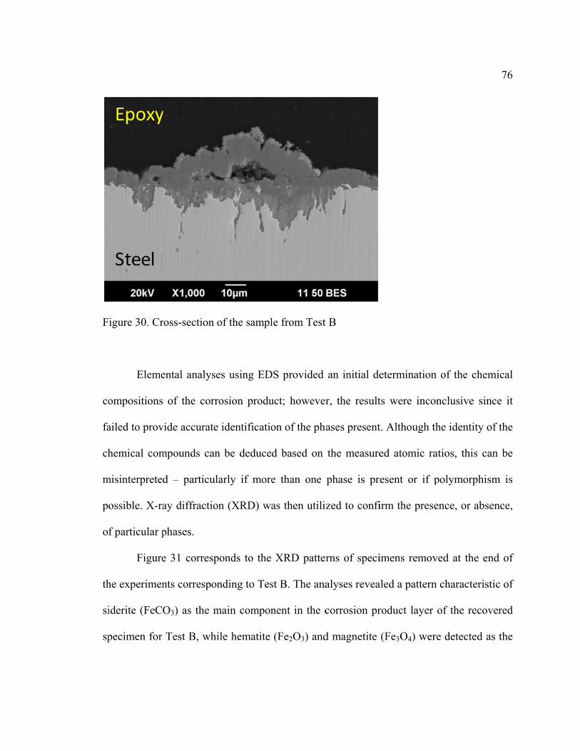
F

co

fa

ch

m

p

o

th

si

sp

igure 30. Cr

Eleme

ompositions

ailed to prov

hemical com

misinterprete

ossible. X-ra

f particular p

Figure

he experimen

iderite (FeC

pecimen for

ross-section

ental analyse

of the corr

vide accurate

mpounds can

d – particul

ay diffractio

phases.

e 31 corresp

nts correspon

O3) as the m

Test B, whi

of the sampl

es using ED

rosion produ

e identificatio

n be deduce

larly if more

on (XRD) w

ponds to the

nding to Tes

main compon

ile hematite

le from Test

DS provided

uct; however

on of the ph

d based on

e than one

as then utili

XRD patter

st B. The ana

nent in the c

(Fe2O3) and

t B

an initial de

r, the result

ases present

the measure

phase is pre

zed to confi

rns of speci

alyses revea

corrosion pr

d magnetite

etermination

ts were inco

t. Although t

ed atomic ra

esent or if p

irm the pres

imens remov

aled a pattern

roduct layer

(Fe3O4) wer

n of the chem

onclusive sin

the identity o

atios, this ca

polymorphis

ence, or abs

ved at the en

n characteris

of the recov

re detected a

76

mical

nce it

of the

an be

sm is

sence,

nd of

stic of

vered

as the

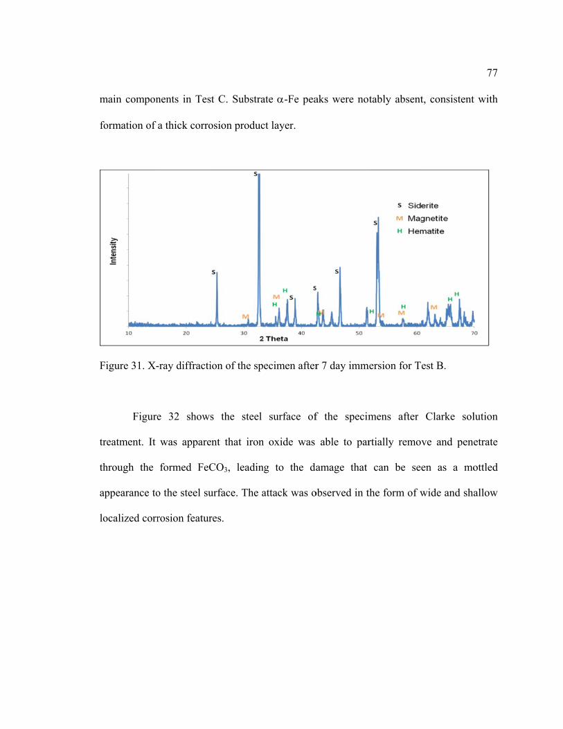
m

fo

F

tr

th

ap

lo

main compon

ormation of

igure 31. X-

Figure

reatment. It

hrough the

ppearance to

ocalized corr

nents in Tes

a thick corro

-ray diffracti

e 32 shows

was appare

formed FeC

o the steel su

rosion featur

st C. Substra

osion produc

ion of the sp

s the steel

ent that iron

CO3, leadin

urface. The a

res.

ate -Fe pea

ct layer.

ecimen after

surface of

n oxide was

ng to the da

attack was o

aks were no

r 7 day imm

f the specim

able to par

amage that

observed in t

tably absent

mersion for T

mens after

rtially remo

can be see

the form of w

t, consistent

est B.

Clarke sol

ve and pene

en as a mo

wide and sha

77

t with

lution

etrate

ottled

allow

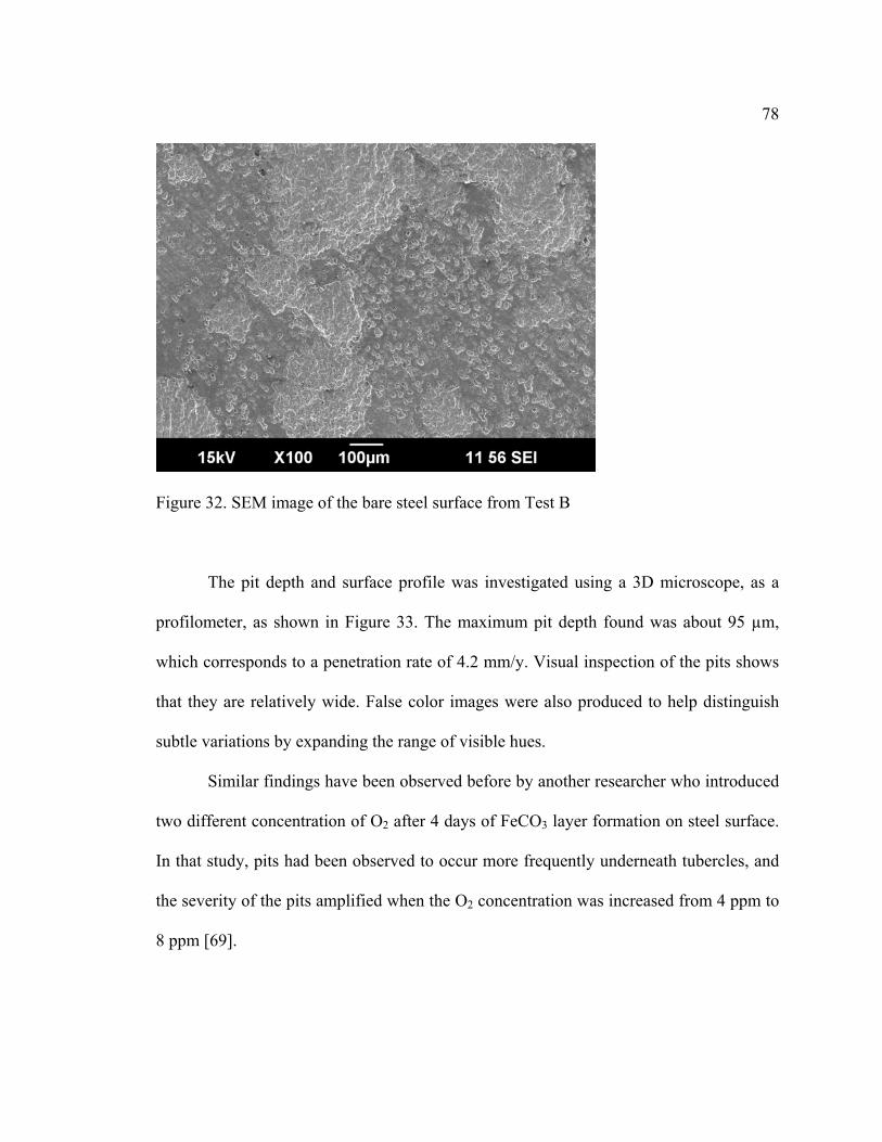
78

Figure 32. SEM image of the bare steel surface from Test B

The pit depth and surface profile was investigated using a 3D microscope, as a

profilometer, as shown in Figure 33. The maximum pit depth found was about 95 µm,

which corresponds to a penetration rate of 4.2 mm/y. Visual inspection of the pits shows

that they are relatively wide. False color images were also produced to help distinguish

subtle variations by expanding the range of visible hues.

Similar findings have been observed before by another researcher who introduced

two different concentration of O2 after 4 days of FeCO3 layer formation on steel surface.

In that study, pits had been observed to occur more frequently underneath tubercles, and

the severity of the pits amplified when the O2 concentration was increased from 4 ppm to

8 ppm [69].

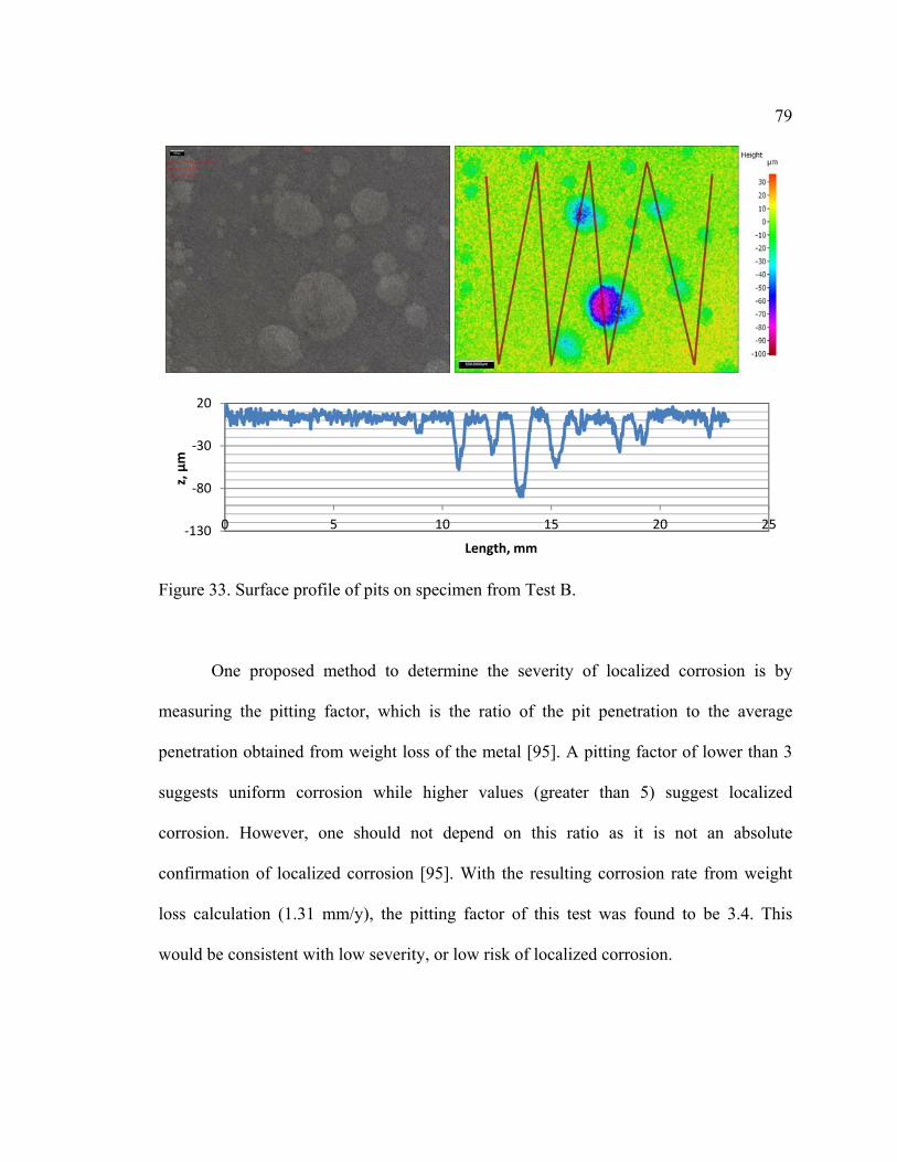
79

Figure 33. Surface profile of pits on specimen from Test B.

One proposed method to determine the severity of localized corrosion is by

measuring the pitting factor, which is the ratio of the pit penetration to the average

penetration obtained from weight loss of the metal [95]. A pitting factor of lower than 3

suggests uniform corrosion while higher values (greater than 5) suggest localized

corrosion. However, one should not depend on this ratio as it is not an absolute

confirmation of localized corrosion [95]. With the resulting corrosion rate from weight

loss calculation (1.31 mm/y), the pitting factor of this test was found to be 3.4. This

would be consistent with low severity, or low risk of localized corrosion.

‐130

‐80

‐30

20

0 5 10 15 20 25

z, µm

Length, mm

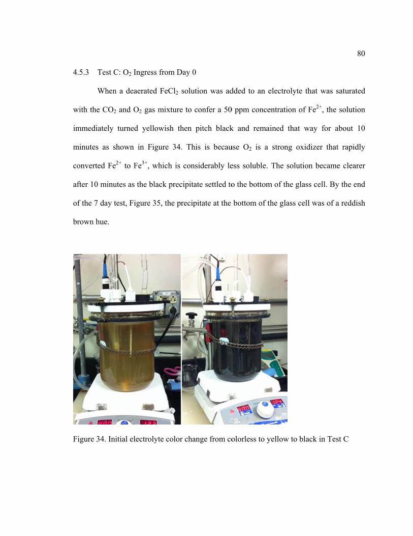
4

w

im

m

co

af

o

br

F

.5.3 Test C

When

with the CO2

mmediately

minutes as s

onverted Fe

fter 10 minu

f the 7 day t

rown hue.

igure 34. Ini

C: O2 Ingress

n a deaerated

2 and O2 gas

turned yell

hown in Fi

2+ to Fe3+, w

utes as the bl

test, Figure 3

itial electroly

s from Day 0

d FeCl2 solu

s mixture to

owish then

gure 34. Th

which is con

lack precipit

35, the precip

yte color cha

0

ution was ad

confer a 50

pitch black

his is becau

nsiderably le

tate settled to

pitate at the

ange from co

dded to an e

0 ppm conce

k and remai

use O2 is a

ess soluble.

o the bottom

bottom of th

olorless to y

electrolyte th

entration of F

ined that w

strong oxid

The solution

m of the glass

he glass cell

yellow to bla

hat was satu

Fe2+, the sol

way for abou

dizer that ra

n became cl

s cell. By th

l was of a re

ack in Test C

80

urated

lution

ut 10

apidly

learer

e end

ddish

C

81

Figure 35. Reddish brown precipitate at the bottom of the glass cell.

Corrosion rates, measured using LPR, are shown in Figure 36. Similar to Test A

and Test B, the corrosion rate showed a rapid decrease over the first few hours. However,

the decrease was less pronounced for Test C, with the corrosion rate holding relatively

steady at an average of around 0.8 mm/y until Day 4. Interestingly, the corrosion rate

then significantly decreased between Day 4 and Day 5 to a mean value of 0.2 mm/year,

where it remained relatively constant until the end of the experiment. Based on these

observations, it was concluded that the presence of O2 delayed the formation of a

protective layer on the steel surface.

The weight loss and time-averaged corrosion rates were 1.07 mm/year and

0.63 mm/year respectively. Both values were high compared to those for Test A and

Test B.

82

Figure 36. LPR mean corrosion rate for Test C

The change in the open circuit potential was insignificant in the initial part of the

experiment but exhibited an abrupt shift between Day 4 and Day 5, shown in Figure 37,

concurrent with the dip in the corrosion rate shown in Figure 36. The abrupt shift to more

positive potential from ca. -690 mV to ca. -475 mV is indicative of alterations in the

nature of the corrosion product on the steel surface.

0.0

0.2

0.4

0.6

0.8

1.0

1.2

1.4

1.6

1.8

2.0

0 1 2 3 4 5 6 7 8

Corrosion rate, m

m/year

Time, day

83

Figure 37. Mean corrosion potential for Test C

The pH of the solution remained relatively constant throughout the duration of the

experiment, see Figure 38. The final pH was similar to that measured in Test B.

The total dissolved iron ion concentration recorded a drastic drop from 50 ppm to

a very low value, as shown in Figure 39, consistent with the rapid conversion of ferrous

ions to insoluble ferric precipitates. It should be noted that these low values represent the

combined Fe2+ and Fe3+concentrations in the bulk solution is opposed to their

concentrations at, or in the proximity of, the actively corroding steel surface.

‐750

‐700

‐650

‐600

‐550

‐500

‐450

‐400

0 1 2 3 4 5 6 7 8


V

Time, day

84

Figure 38. Bulk solution pH for Test C.

Figure 39. Total iron concentration in solution of Test C.

The presence of 1 ppm O2 did not completely impede the formation of FeCO3

crystals on the steel surface, as can be seen in Figure 40 through Figure 43. However,

coverage by the FeCO3 crystals was incomplete, as observed on the steel specimen that

6.40

6.45

6.50

6.55

6.60

6.65

6.70

0 1 2 3 4 5 6 7 8

pH

Time, day

0

10

20

30

40

50

60

0 1 2 3 4 5 6 7 8

Total Fe concentration, mg/l

Time, day

85

was retrieved at the end of Day 2, as shown in Figure 40. The surface was instead

covered by a combination of prismatic and smaller sized plate-like crystals. The iron

oxide crystals obstructed the formation of FeCO3 and resulted in partial coverage by

FeCO3 of the steel surface. The attack by O2 was more rapid than the formation of FeCO3

as a corrosion product. A denser coverage of corrosion product was observed on the

specimen that was retrieved on Day 4, which consists of a mixture of prismatic FeCO3

crystals and smaller globular-shaped crystals, shown in Figure 41. Tubercular features

were non-existent at this stage. Between Day 6 and Day 8 oxide encrusted tubercules

were observed to develop on the steel specimens, as shown in Figure 42 and Figure 43.

Figure 40. Steel surface at the end of Day 2 in Test C.

86



87


EDS spectra shown in Figure 44 provided a good indication of the presence of

iron oxides on the steel surface. When the two different morphologies were analyzed, the

smaller crystals exhibited a lower content of C (carbon) as compared to the larger

prismatic crystals, indicative of possible formation of iron oxides.

Further investigation of the corrosion product layer showed the obstructive nature

of iron oxide towards FeCO3 crystals. The FeCO3 prisms also appeared imperfectly

formed, as shown in Figure 45. Iron oxides, such as Fe2O3 and Fe3O4, were hypothesized

to grow simultaneously with FeCO3 resulting in mixed crystal constituents within the

corrosion product layer.

F

F

p

w

igure 44. SE

igure 45. Im

Post a

eaks consist

weaker peaks

EM image an

mperfectly fo

analysis of th

tent with th

s of siderite (

nd EDS spec

rmed FeCO3

he specimen

he presence

(FeCO3), and

ctra of sampl

3 crystals co

n using XRD

of hematite

d goethite (α

le recovered

overed with i

D, Figure 46

e (α–Fe2O3)

α–FeO(OH))

d after 8 days

iron oxides

6, revealed in

and magne

).

s in Test C

ntense diffra

tite (Fe3O4)

88

action

, and

F

h

th

pr

R

ox

igure 46. X-

Rama

ematite, ma

he absence o

resence of c

Raman data

xide (Fe2O3)

-ray diffracti

an spectrosc

gnetite, goe

of a strong v

carbonate (C

would be co

) overlying t

ion of the sp

copy was u

thite and sid

vibrational m

CO32). Take

onsistent wi

the formed ir

ecimen reco

utilized to c

derite were

mode at ca.

en in conjun

ith the prese

ron carbonat

overed after 7

complement

identified, a

1086 cm1,

nction with

ence of a pr

te (FeCO3).

7 days in Te

the XRD

as shown in

, which is d

the XRD da

rimarily hem

est C.

data. Peak

Figure 47.

diagnostic fo

ata, the coll

matite-type

89

ks for

Note

or the

lected

ferric

F

w

co

co

ox

F

igure 47. Ra

A cro

was character

ompositiona

ontrasting sh

xide-encrust

igure 48. Cr

aman spectra

oss-section o

rized by SE

al difference

hades produ

ted corrosion

ross-section

a of specime

of the specim

M using bac

e of the cor

uced by the

n product tub

of specimen

en recovered

men recover

ck-scattered

rrosion prod

SEM back

bercle on top

n recovered a

d after 7 days

red at the c

electrons to

duct layer, a

kscattered im

p of a wide p

after 7 days o

s in Test C.

onclusion o

o provide in

as shown in

mage shows

pit.

of Test C

of the experi

nformation o

n Figure 48.

formation o

90

iment

on the

. The

of an

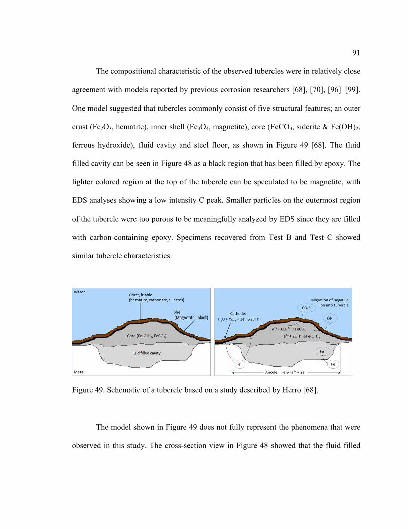
91

The compositional characteristic of the observed tubercles were in relatively close

agreement with models reported by previous corrosion researchers [68], [70], [96]–[99].

One model suggested that tubercles commonly consist of five structural features; an outer

crust (Fe2O3, hematite), inner shell (Fe3O4, magnetite), core (FeCO3, siderite & Fe(OH)2,

ferrous hydroxide), fluid cavity and steel floor, as shown in Figure 49 [68]. The fluid

filled cavity can be seen in Figure 48 as a black region that has been filled by epoxy. The

lighter colored region at the top of the tubercle can be speculated to be magnetite, with

EDS analyses showing a low intensity C peak. Smaller particles on the outermost region

of the tubercle were too porous to be meaningfully analyzed by EDS since they are filled

with carbon-containing epoxy. Specimens recovered from Test B and Test C showed

similar tubercle characteristics.

Figure 49. Schematic of a tubercle based on a study described by Herro [68].

The model shown in Figure 49 does not fully represent the phenomena that were

observed in this study. The cross-section view in Figure 48 showed that the fluid filled

92

cavity was not in direct contact with steel floor, but was separated by another layer of

corrosion product.

The entire steel surface underneath the corrosion product layer was severely

damaged, as shown in Figure 50 for the specimen recovered at the conclusion of the test

and treated with Clarke solution. Polish marks could no longer be seen on the surface of

this specimen. The surface profile showed penetration depths approaching 100 µm, as

shown in Figure 51. The true depth of penetration was unable to be confirmed due to the

unidentified original height of the surface.

Figure 50. SEM image of steel surface for Test C after corrosion product removal

93

Figure 51. Pit depth analysis of specimen recovered at the end of Test C.

4.5.4 Results Summary

The results from Test A, B and C can be analyzed by making comparisons

between them for each condition. Figure 52 shows that the presence of O2 caused the

final corrosion rate to be higher than the baseline, CO2 only, condition. This effect was

also supported by the recorded corrosion rate based on the weight loss of the specimens

as presented in Table 7. The corresponding corrosion rates of the specimens in Test B and

Test C (oxic conditions) were one order of magnitude greater than for Test A (anoxic).

Test C recorded the highest corrosion rate due to the longer exposure to O2, while Test B

had some form of protection against corrosion before the introduction of O2 into the

system.

‐100

‐80

‐60

‐40

‐20

0

20

0 2 4 6 8 10 12

z, µm

length, mm

94

Figure 52. Corrosion rates comparison of Tests A, B and C.

Table 7: Summary of Corrosion Rate Results.

Experiment Time-averaged corrosion rate from

LPR, mm/y Weight loss corrosion

rate, mm/y Test A 0.26 0.11 Test B 0.33 0.77 Test C 0.63 1.07

The corrosion potential in both Tests B and C ended in the same range of less

negative values as compared to the potential in the baseline condition, shown in Figure

53. Although both oxic conditions showed sudden shift in potential, the shift occurred at

different times of the experiments. The shift in potential that occurred in Test B was due

to the sudden introduction of O2 into the system, while the shift in Test C could be due to

the change in the solution water chemistry and the compositional change on the steel

surface due to corrosion products.

0

0.2

0.4

0.6

0.8

1

1.2

1.4

1.6

1.8

0 1 2 3 4 5 6 7 8

Corrosion rate, m

m/y

Time, days

Test A

Test B

Test C

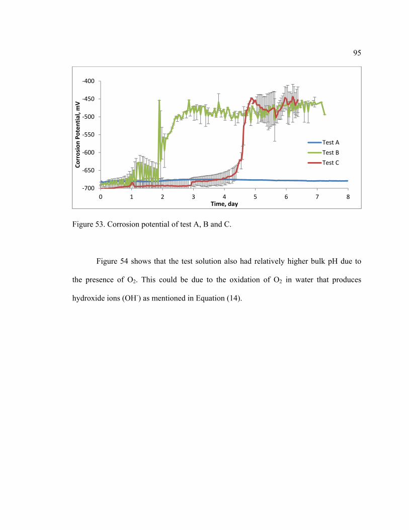
95

Figure 53. Corrosion potential of test A, B and C.

Figure 54 shows that the test solution also had relatively higher bulk pH due to

the presence of O2. This could be due to the oxidation of O2 in water that produces

hydroxide ions (OH-) as mentioned in Equation (14).

‐700

‐650

‐600

‐550

‐500

‐450

‐400

0 1 2 3 4 5 6 7 8

Corrosion Potential, m

V

Time, day

Test A

Test B

Test C

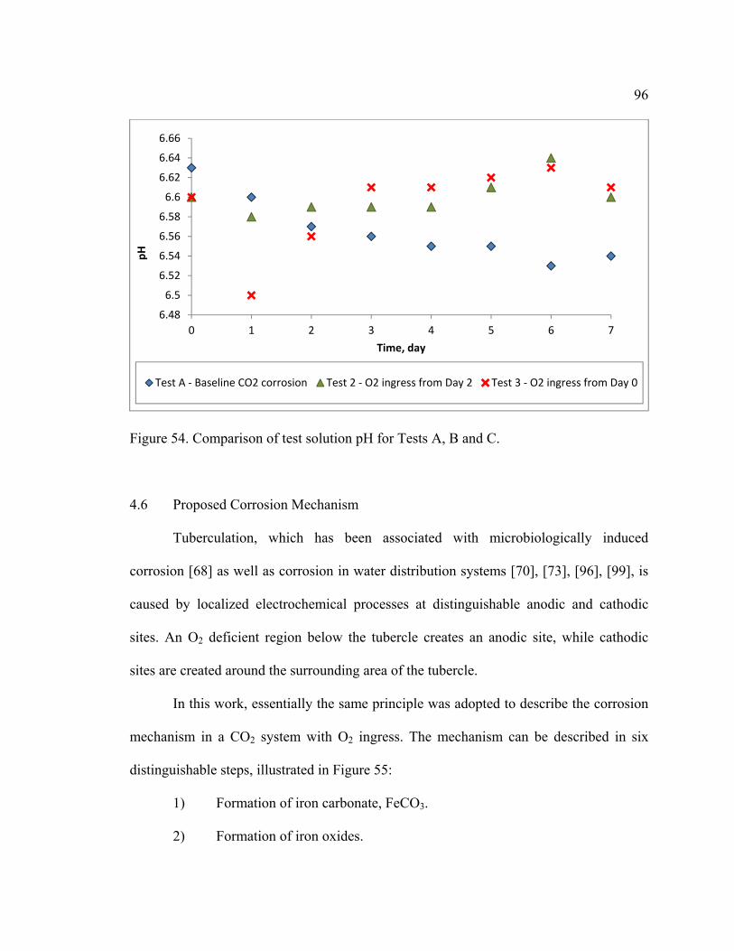
96

Figure 54. Comparison of test solution pH for Tests A, B and C.

4.6 Proposed Corrosion Mechanism

Tuberculation, which has been associated with microbiologically induced

corrosion [68] as well as corrosion in water distribution systems [70], [73], [96], [99], is

caused by localized electrochemical processes at distinguishable anodic and cathodic

sites. An O2 deficient region below the tubercle creates an anodic site, while cathodic

sites are created around the surrounding area of the tubercle.

In this work, essentially the same principle was adopted to describe the corrosion

mechanism in a CO2 system with O2 ingress. The mechanism can be described in six

distinguishable steps, illustrated in Figure 55:

1) Formation of iron carbonate, FeCO3.

2) Formation of iron oxides.

6.48

6.5

6.52

6.54

6.56

6.58

6.6

6.62

6.64

6.66

0 1 2 3 4 5 6 7

pH

Time, day

Test A ‐ Baseline CO2 corrosion Test 2 ‐ O2 ingress from Day 2 Test 3 ‐ O2 ingress from Day 0

F

o

3)

4)

5)

6)

igure 55. Pro

In an

f steel by el

Volume re

Pressure b

Rupture of

Underdepo

oposed tuber

ideally anox

ectrochemic

eduction of s

build-up in v

f top shell.

osit pitting c

rculation me

xic and CO2

cal and chem

solid materia

oid spaces fo

caused by a g

echanism in

2-saturated s

mical reactio

al.

forming dom

galvanic effe

CO2 corrosi

solution, FeC

ns (Figure 5

me-like struct

ect

ion with O2 i

CO3 will for

55(a)) in acc

tures.

intrusion.

rm on the su

cordance wit

97

urface

th the

98

following steps. CO2 gas dissolves in water and is hydrated into carbonic acid (H2CO3),

which then dissociates into a bicarbonate ion (HCO3-), which itself further dissociates

into a carbonate ion (CO32-). Associated generated hydrogen ions (H+) undergo reduction

concurrently with oxidation of iron, evolving H2 gas. As the concentration of Fe2+ and

CO32- exceeds the solubility limit, a FeCO3 layer is formed on the steel surface, see

reaction (6) in Chapter 2, sub-section 2.3.1.

The ingress of O2 adds an additional cathodic reaction, reduction of oxygen, see

reaction (14) in section 2.5. With this additional cathodic reaction, the rate of anodic

reaction will increase to compensate for the additional consumption of electrons.

The available O2 also causes the precipitation of highly insoluble iron oxides and

oxyhydroxides, which then grows/settles on the FeCO3 layer (Figure 55 (b)). Ferrous ions

in the solution rapidly convert to ferric ions due to the oxidizing power of O2, which then

precipitates into insoluble, loose, and porous Fe2O3, known as hematite.

2 ( ) + ( ) → 2 ( ) + ( ) (23)

( ) + 3 ( ) → 2 ( ) ( ) + 3 ( ) (24) 2 ( ) ( ) → ( )( ) + ( ) (25) 2 ( )( ) → ( ) + ( ) (26)

The author found evidence of FeCO3 dissolution by O2 from observing oxide crystals on

the faces of the FeCO3 crystals, which was reported earlier in this chapter. The

degradation of FeCO3 crystals is expressed in the following reaction:

99

4 ( ) + ( ) → 2 ( ) + 4 ( ) (27)

On a molar basis, the volume change from the conversion of 2 moles FeCO3 into 1 mole

Fe2O3 was determined. About 48.8% volume reduction of the occupied solid takes place

during the conversion. It can be hypothesized that this volume change creates void spaces

in between the FeCO3 crystals with a micro-environment that is lower in pH than in the

bulk solution (Figure 55(c)). The lower pH value in the confined space is due to iron ion

aquation and subsequent dissociation reactions that produce hydrogen ions. The creation

of the aqua acids, hexaaquairon (II) ([Fe(H2O)6]2+) and hexaaquairon (III) ([Fe(H2O)6]

3+),

contributes to the lowering of the pH value. The iron (III) aqua ion has a pKa value of 2.2,

and is more acidic than the iron (II) ion (pKa value of 8.3) [100] due to the greater

positive charge of the central metal ion in the complex.

( ) ( ) + ( ) ( ) ( ) ( ) + ( ) (28) ( ) ( ) + ( ) ( ) ( ) ( ) + ( ) (29)

The acidic micro-environment promotes the dissolution of FeCO3 and releases CO2 gas.

Hydrogen ions are also cathodically converted to H2 gas in this void space. The corrosion

product layer above the cavity impedes the migration of the gases into the bulk solution,

causing pressure build-up in the cavity, creating a dome-like structure (Figure 55(d)).

100

Localized regions of metal loss are capped with accumulated corrosion products and

deposits of precipitates.

The cathodic reaction continues to consume the O2 that is confined in the cavity

underneath the tubercle and becomes depleted with O2, which results in a differential

aeration cell. The area underneath the tubercle with the lower O2 concentration becomes

the anode while the larger surface area of the steel that is directly exposed to the aerated

bulk solution becomes the cathode. Anodic reaction increases the concentration of ferrous

ions, Fe2+ and further decreases the pH of the micro-environment. The low pH

accelerates the dissolution of metal and promotes crevice or localized corrosion. The

FeCO3 layer becomes thicker under the deposit due to the saturation of Fe2+ and CO32-

ions in the confined space.

As the pressure inside the cavity continues to rise, the thin top shell of the dome

loses its integrity and ruptures, releasing the trapped gases and ions into the bulk solution

(Figure 55(e)). The system now has a galvanic effect between the damaged tubercle and

the rest of the metal surface. FeCO3 forms downwards into the actively corroding steel,

creating the broad depression that was observed underneath the tubercles (Figure 55(f)).

The rupture of the tubercle’s top shell may also be caused by stress at the crystal

boundaries, which is a consequence of the previously discussed volume reduction.

All of these hypothesized corrosion mechanisms will require further investigation

to confirm their validity. Amongst the phenomena that can be explored are hydrogen

gas evolution, surface/pit pH changes, galvanic effects, and tubercle integrity.

101

4.7 Chapter Summary

The above described sequence of corrosion process steps provides a basis for

comparison with investigation of O2 ingress in sweet corrosion environments at high

pressure conditions, simulating the conditions in a CO2-EOR field. The observed

influence of O2 on sweet corrosion at low pressure was profound and must be seriously

considered when selecting materials and performing corrosion control of mild steel.

Localized corrosion was observed although the corrosion rates at the conclusion of all

tests were relatively low. Surface analysis showed degradation of FeCO3 crystals and

formation of iron oxides. This degradation of initially formed FeCO3 occurred

concurrently with the development of localized corrosion features as deep as 100 µm.

XRD and Raman confirm the formation of magnetite (Fe3O4), hematite (α-Fe2O3), and

goethite (α-FeOOH) along with siderite (FeCO3) in corrosion products.

102

CHAPTER 5: HIGH PRESSURE CORROSION TESTS

This chapter describes and discusses high pressure CO2 corrosion experiments in

the presence and absence of O2. Similar to the previous chapter, experimental

methodologies and design are initially described, followed by discussion of results and a

mechanistic description.

The set of experiments described herein investigates the corrosion behavior of

carbon steel in simulated CO2-EOR environments with the presence of O2 as an impurity

in the CO2 supply. The contaminant corresponds to the amount of O2 that can be present

in CO2 from an oxyfuel combustion flue gas, in particular.

5.1 Introduction

The CO2 utilized in CO2-EOR can be derived from natural or anthropogenic

sources, for example, CO2-rich geologic reservoirs or byproduct gas from an industrial

process. The SACROC unit of the Kelly-Snyder field in Texas receives its CO2 supply

from natural gas fields in southwest Texas [101], whilst the Weyburn-Midale fields in

Saskatchewan, Canada receive CO2 from a coal gasification plant in North Dakota [102].

However, unlike the above example, CO2 sourced from power plants may contain

significant levels of impurities, such as oxygen (O2), that pose a higher risk of corrosion

to injection/production wells and related infrastructure. O2 concentration in a CO2 stream

from the oxyfuel process can be as high as 3 vol.% [16] and further purification of the gas

to eliminate the O2 is considered unfeasible.

103

Previous studies have found that the existence of O2 in sweet corrosion systems

accelerated the corrosion rate of steel [20], [23], [55], [86], [87], [103] and caused pitting

corrosion [82], [88]–[90]. The effect of O2 on the corrosion mechanisms, especially at

high CO2 partial pressure, has not been thoroughly investigated.

The casing and tubing of injection wells are normally constructed out of carbon

steel due to its high strength, durability in high pressure environments, low cost, ease of

use in fabrication, and range of available corrosion mitigation strategies (e.g., inhibitors).

This makes carbon steel the preferred choice of material as compared to other materials

such as corrosion resistant alloys (CRAs) [9]. Carbon steel grades J-55 and N-80 are

typical examples of tubing/casing materials used in CO2 injection [104], [105]. However,

Kapusta and Canter [105] documented that corrosion was observed at Shell’s CO2-EOR

field in Mississippi after only 10 months of production. Their laboratory experiments

conducted on J-55 and N-80 grade tubing from the CO2-EOR field showed high

corrosion rates in their flow-through system (50 mm/year) and static system

(13 mm/year).

In this work, the effect of O2 (4 vol.%) on the corrosion performance of mild steel

(UNS G10180) in CO2-saturated brine was investigated using a 4-liter autoclave in

experiments of 48 hours duration. Experiments were conducted at temperature and

pressure combinations that correspond to subcritical-supercritical conditions.

104

5.2 Sample Material and Preparation

Carbon steel UNS G10180 was again used to represent casing and tubing

material, and has a ferritic/pearlitic microstructure that is similar to J-55 steel.

Cylindrical steel specimens were utilized in the corrosion study using

electrochemical methods, while rectangular steel specimens were utilized for weight loss

measurement and surface analysis, as shown in Figure 56. The dimensions of the steel

samples are shown in Figure 57. The specimens were polished with a 600 grit silicon

carbide (SiC) paper, cleaned with isopropanol in an ultrasonic bath, and dried using a

heat gun prior to the experiments. Following the cleaning process, the mass and the

dimensions of the specimens were measured and recorded.

Figure 56. Cylindrical and flat steel specimens for high pressure experiments.

F

5

st

a

a

g

T

w

in

igure 57. Di

.3 Exper

All hi

tainless steel

Pt-coated N

high pressu

lass pH elec

The electrode

with CO2 for

nto the seale

imensions of

rimental Set-

igh pressure

l autoclave a

Nb counter el

ure high tem

ctrode that w

es were imm

r at least 2 h

d autoclave

f steel specim

-up and Instr

e tests in th

as illustrated

lectrode, a s

mperature (H

were all inse

mersed in 3

hours before

until the des

mens used in

rumentation

his set of ex

d in Figure 5

shaft for the

HPHT) Ag/A

erted through

liters of sol

e the start of

sired partial

n the high pr

xperiments

58 and Figur

steel specim

AgCl refere

h the stainle

lution (1 wt

f each exper

pressure wa

ressure tests.

were condu

re 59. The se

men as the w

ence electrod

ess steel lid

t.% NaCl) th

riment. O2 w

as achieved.

.

ucted in a 4

et-up consist

working elect

de, and a H

of the autoc

hat was satu

was then bub

The O2 gas

105

4-liter

ted of

trode,

HPHT

clave.

urated

bbled

input

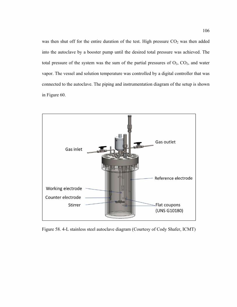
w

in

to

v

co

in

F

was then shu

nto the autoc

otal pressure

apor. The ve

onnected to

n Figure 60.

igure 58. 4-L

ut off for the

clave by a b

e of the syst

essel and sol

the autoclav

L stainless s

e entire dura

booster pump

tem was the

lution tempe

ve. The pipin

teel autoclav

ation of the t

p until the d

sum of the

erature was c

ng and instru

ve diagram (

test. High p

desired total

partial pres

controlled by

umentation d

(Courtesy of

pressure CO2

l pressure w

ssures of O2

y a digital co

diagram of th

f Cody Shafe

2 was then a

was achieved

, CO2, and w

ontroller tha

he setup is sh

er, ICMT)

106

added

d. The

water

at was

hown

107

Figure 59. The 4-L autoclave in ICMT

Figure 60. Piping and instrumentation diagram of the autoclave setup

108

5.4 Measurements and Test Matrix

Experiments were conducted at two different temperatures (25°C and 80°C) and

two different CO2 partial pressures (40 and 90 bar). These temperature and pressure

combinations encompass three different phases of CO2, illustrated as the corner points for

the shaded region in the CO2 phase diagram in Figure 61. The test matrix is shown in

Table 8. All tests were compared with a baseline condition without the presence of O2.

The presence of 4% O2 only slightly shifts the critical points of the CO2/O2 mixture,

maintaining the same three phases of CO2 in the different experiments.

Corrosion rates were measured continuously using the linear polarization

resistance (LPR) method. A Gamry Reference 600 potentiostat was utilized for this

purpose. The OCP was monitored throughout the experiment to ensure a stable condition

for accurate electrochemical measurements. The potential was polarized at ±5 mV with

respect to the OCP at a 0.125 mV/s scan rate, as mentioned in Chapter 4. The Stern-

Geary coefficient, B value, used in the calculation of corrosion rates in this work was

26 mV. Previous high pressure corrosion tests performed using this value had corrosion

rates that corresponded to the weight loss corrosion rates [106]. Electrochemical

impedance spectroscopy (EIS) was conducted to determine the value of the solution

resistance in order to correct the polarization resistance values obtained from LPR

measurements. Besides LPR, the average corrosion rates were also determined via weight

loss at the end of the 48-hour tests. Steel specimens were removed from the autoclave at

the completion of the high-pressure tests, rinsed with isopropanol, placed in individual

nitrogen-purged bags, and stored in a dry cabinet. Post-test analyses of the specimens

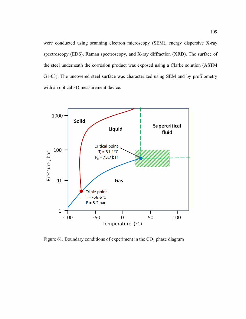
109

were conducted using scanning electron microscopy (SEM), energy dispersive X-ray

spectroscopy (EDS), Raman spectroscopy, and X-ray diffraction (XRD). The surface of

the steel underneath the corrosion product was exposed using a Clarke solution (ASTM

G1-03). The uncovered steel surface was characterized using SEM and by profilometry

with an optical 3D measurement device.

Figure 61. Boundary conditions of experiment in the CO2 phase diagram

110

Table 8: Test Matrix for High Pressure Corrosion Test.

Expt. No. T (°C) pCO2 (bar) pO2 (bar) CO2 Phase

1 25 40 0 & 1.7 Gas

2 25 90 0 & 3.75 Liquid

3 80 40 0 & 1.7 Gas

4 80 90 0 & 3.75 Supercritical

5.5 Results and Discussion

5.5.1 Experiment 1: 25°C, 40 bar pCO2, with and without 4% O2.

In this experiment, the CO2 is in its gaseous state. Figure 62 shows the variation

of the mean corrosion rate with time for the cases with and without O2 at 40 bar CO2 and

25°C, as measured using LPR. Error bars on the plot indicate maximum and minimum

recorded values. The presence of O2 in the system showed an increase in the overall

corrosion rate of the steel sample. These values were integrated over time and were

comparable to the weight loss corrosion rate that was measured at the end of the 48-hour

experiments, as shown in Figure 63. The corrosion potential of both oxic and anoxic

systems, however, did not show a significant difference between each set of experiments,

see Figure 64.

111

Figure 62. LPR corrosion rate with time for experiments at 25°C, 40 bar pCO2, with and without 4% O2.

Figure 63. Weight loss corrosion rates compared to LPR time-integrated corrosion rates for experiments at 25°C, 40 bar pCO2, with and without 4% O2.

0.0

2.0

4.0

6.0

8.0

10.0

12.0

14.0

16.0

18.0

0 10 20 30 40 50


m/y

Time, hour

25°C, 40 bar CO2, 4% O225°C, 40 bar CO2

9.5

6.3

9.3

8.0

0

2

4

6

8

10

12

With 4% O2 Without O2

Corrosion rate, m

m/year

Experimental conditions

Weight loss CR

Integrated LPR

112

Figure 64. Corrosion potential for experiments at 25°C, 40 bar pCO2, with and without 4% O2.

By visual inspection, the steel sample that was exposed to the anoxic environment

for 48 hours appeared clear of any obvious corrosion products on its surface, as can be

seen by the absence of any crystalline features on the surface of the specimens shown in

Figure 66. On the other hand, the steel sample from the CO2/O2 experiments appeared to

have a thin layer of bluish-green corrosion products that turned yellowish after about 20

to 30 minutes post-recovery. Elemental analysis using EDS, shown in Figure 66, revealed

a higher percentage of oxygen, O, that can be due to the presence of a thin iron oxide film

on the steel surface. Alloying elements such as molybdenum, manganese, and copper

were also detected on the steel surface. Using a 3D optical microscope, the surface profile

of the bare steel surface was measured, and exhibited uniform corrosion across the whole

steel surface.

‐680

‐660

‐640

‐620

‐600

‐580

0 10 20 30 40 50


V

Time, hour

25°C, 40 bar CO2, 4% O2

25°C, 40 bar CO2

Fat

Fan

su

igure 65. Blt 25°C, 40 b

igure 66. SEnd without 4

Cross

urface havin

uish-green car pCO2, wit

EM and EDS4% O2 exper

-sectional an

ng morpholo

corrosion proth 4% O2

S analysis of riments.

nalysis of th

gical feature

oduct on a re

f steel surfac

he steel samp

es that were

ecovered ste

e at the end

ples exhibite

loose and fr

eel specimen

of 25°C, 40

ed a layer on

ragile, typica

n for experim

bar pCO2, w

n top of the

al of skeleta

113

ment

with

steel

l iron

ca

an

so

in

ap

el

h

lo

sh

X

F

arbide. The

n expected t

ome amount

n the O2 ex

pproximate

lement resid

ave been los

oss for the ex

hown in the

XRD analysis

igure 67. Ste

thickness of

thickness of

t of iron carb

xperiment, b

52 µm thick

due observed

st or spalled

xperiment w

e cross-secti

s, as shown i

eel cross-sec

f the corrosio

f residual ca

bide was pro

based on th

kness, as com

d under SEM

off from the

without O2 w

on. The pre

in Figure 68

ctions at 25°

on product,

arbide on the

obably lost d

he weight lo

mpared to th

M. This sugg

e steel surfac

as 34 µm, w

esence of th

8.

C, 40 bar pC

as seen in F

e steel surfa

during the te

oss corrosio

he 15 µm th

gests that so

ce due to its

which corresp

his iron carb

CO2, with an

Figure 67, di

ace. Due to i

ests. The am

on rate, cor

hick layer of

ome of the i

fragility. Th

ponds to the

bide layer w

nd without 4%

id not confor

its fragile na

mount of iron

rresponded t

f carbide/allo

ron carbide

he calculated

e 40 µm thick

was confirme

% O2

114

rm to

ature,

n loss

to an

oying

must

d iron

kness

ed by

F

o

su

F

igure 68. XR

Althou

f pits or loca

urface was u

igure 69. Pro

RD analysis

ugh the pres

alized corros

uniformly co

ofilometry o

for specime

sence of O2

sion were no

orroded and t

of specimen

en at 25°C, 4

caused the c

ot detected,

the polishing

at 25°C, 40

40 bar pCO2,

corrosion rat

as shown in

g lines were

bar pCO2, w

, with 4% O2

te to increas

n Figure 69.

no longer vi

with 4% O2 a

2 for 48 h.

e, the occurr

The overall

isible.

after 48 h.

115

rence

l steel

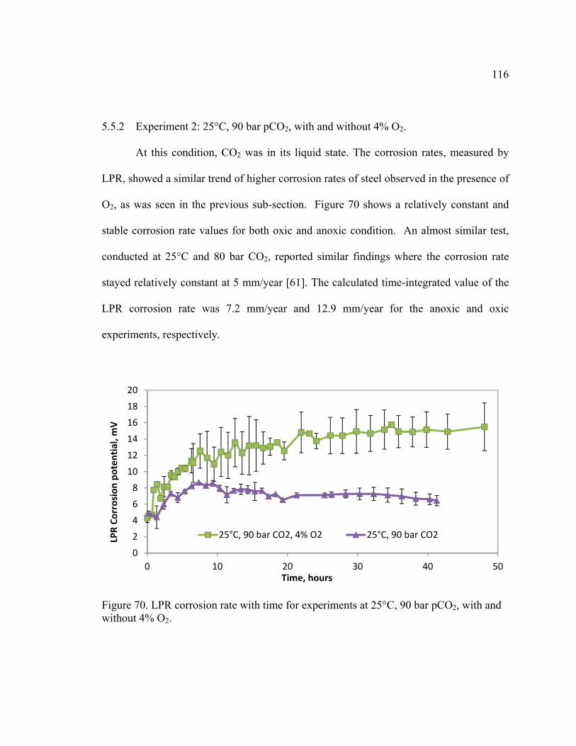
116

5.5.2 Experiment 2: 25°C, 90 bar pCO2, with and without 4% O2.

At this condition, CO2 was in its liquid state. The corrosion rates, measured by

LPR, showed a similar trend of higher corrosion rates of steel observed in the presence of

O2, as was seen in the previous sub-section. Figure 70 shows a relatively constant and

stable corrosion rate values for both oxic and anoxic condition. An almost similar test,

conducted at 25°C and 80 bar CO2, reported similar findings where the corrosion rate

stayed relatively constant at 5 mm/year [61]. The calculated time-integrated value of the

LPR corrosion rate was 7.2 mm/year and 12.9 mm/year for the anoxic and oxic

experiments, respectively.

Figure 70. LPR corrosion rate with time for experiments at 25°C, 90 bar pCO2, with and without 4% O2.

0

2

4

6

8

10

12

14

16

18

20

0 10 20 30 40 50

LPR Corrosion potential, m

V

Time, hours

25°C, 90 bar CO2, 4% O2 25°C, 90 bar CO2

117

The time-integrated values were compared with the weight lost corrosion rate,

shown in Figure 71, showing that the presence of O2 resulted in higher corrosion rates. In

an almost similar test, conducted at 25°C, 80 bar pCO2 , it reported a maximum LPR

corrosion rate of 7 mm/year [106], comparable with the time-integrated corrosion rate of

the anoxic experiment at a slightly higher CO2 partial pressure. There is a high

discrepancy between the weight loss corrosion rate for the experiment without O2 with

the corrosion rate measured using LPR. However, the repeatability of this particular

condition was high, and observed in three separate repeat experiments. This deviation in

value could be due to technical error during preparation and handling of the test

specimen.

Figure 71. Weight loss corrosion rates compared to LPR time-integrated corrosion rates for experiments at 25°C, 90 bar pCO2, with and without 4% O2.

15.1

1.8

12.9

7.2

0

2

4

6

8

10

12

14

16

18


Corrosion rate, m

m/year


Weight loss CRIntegrated LPR

118

The presence of O2 did not significantly affect the corrosion potential, as shown in

Figure 72. Similar behavior was discussed in the previous sub-section for the experiments

at 40 bar CO2.

Figure 72. Corrosion potential with time for experiments at 25°C, 90 bar pCO2, with and without 4% O2.

The condition of each steel surface at the end of the experiments was similar to

what was observed at 40 bar CO2. No obvious crystalline features or precipitate

accumulation were found when observed using SEM, as can be seen in Figure 73. EDS

indicated that O was more abundant on the specimen that was exposed to oxic conditions.

Higher percentages of the alloying elements copper, molybdenum, and nickel were also

detected on the steel surface.

‐635

‐630

‐625

‐620

‐615

‐610

‐605

‐600

‐595

‐590

0 10 20 30 40 50


V

Time, hours

25°C, 90 bar CO2, 4% O2 25°C, 90 bar CO2

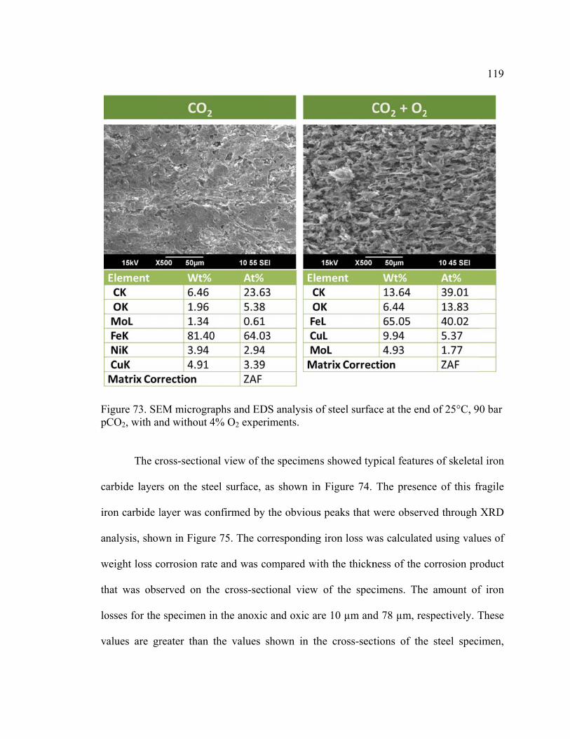
Fp

ca

ir

an

w

th

lo

v

igure 73. SECO2, with an

The cr

arbide layer

ron carbide l

nalysis, show

weight loss c

hat was obs

osses for the

alues are gr

EM microgrand without 4

ross-section

s on the ste

layer was co

wn in Figure

orrosion rate

erved on th

e specimen in

reater than t

aphs and ED4% O2 exper

al view of th

eel surface, a

onfirmed by

e 75. The co

e and was co

he cross-sect

n the anoxic

the values s

DS analysis oriments.

he specimen

as shown in

the obvious

orresponding

ompared wit

tional view

c and oxic ar

shown in th

of steel surfa

s showed typ

n Figure 74.

s peaks that

g iron loss w

th the thickn

of the spec

re 10 µm and

he cross-sec

ace at the end

ypical feature

The presen

were observ

was calculate

ness of the c

cimens. The

d 78 µm, res

tions of the

d of 25°C, 90

es of skeleta

nce of this fr

ved through

d using valu

corrosion pro

e amount of

spectively. T

e steel speci

119

0 bar

al iron

ragile

XRD

ues of

oduct

f iron

These

imen,

p

co

Fte

F

ossibly due

ourse of the

igure 74. Steests.

igure 75. XR

to the fragile

experiments

eel cross-sec

RD analysis

e nature of ir

s.

ctions at the

for specime

ron carbide

end of 25°C

en at 25°C, 9

that could h

C, 90 bar pCO

90 bar pCO2,

have been rem

O2, with and

, with 4% O2

moved durin

d without 4%

2, 48h.

120

ng the

% O2

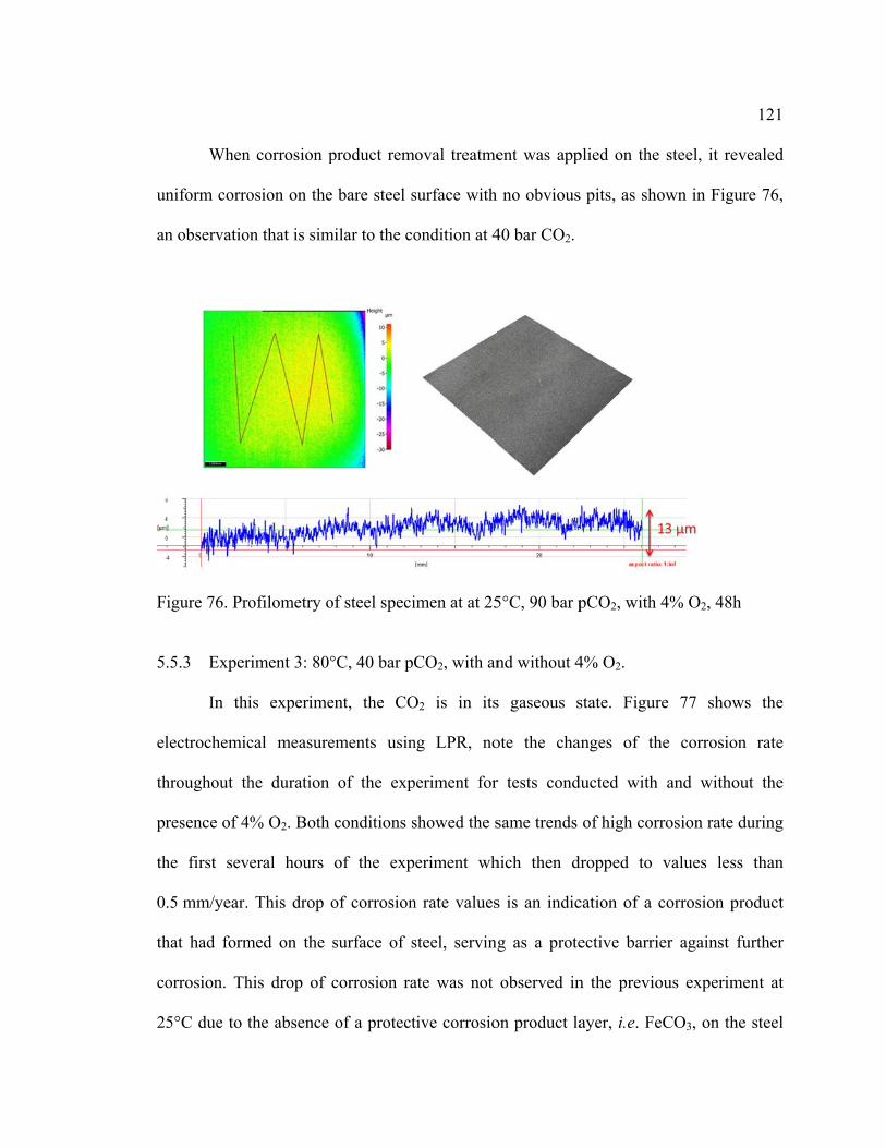
un

an

F

5

el

th

pr

th

0

th

co

2

When

niform corro

n observatio

igure 76. Pro

.5.3 Exper

In thi

lectrochemic

hroughout th

resence of 4

he first sev

.5 mm/year.

hat had form

orrosion. Th

5°C due to t

n corrosion p

osion on the

on that is sim

ofilometry o

riment 3: 80°

is experime

cal measure

he duration

4% O2. Both

veral hours

This drop o

med on the

his drop of

the absence

product rem

e bare steel s

milar to the co

of steel speci

°C, 40 bar pC

ent, the CO

ements usin

of the exp

conditions s

of the exp

of corrosion

surface of s

corrosion ra

of a protect

moval treatme

surface with

ondition at 4

imen at at 25

CO2, with an

O2 is in its

ng LPR, no

periment for

showed the s

eriment wh

n rate values

steel, serving

ate was not

tive corrosio

ent was app

h no obvious

40 bar CO2.

5°C, 90 bar p

nd without 4

s gaseous s

ote the cha

r tests cond

same trends

hich then d

s is an indic

g as a prote

observed in

on product la

plied on the

s pits, as sho

pCO2, with 4

4% O2.

state. Figure

anges of the

ducted with

of high corr

dropped to v

cation of a c

ective barrie

n the previo

ayer, i.e. FeC

steel, it rev

own in Figur

4% O2, 48h

e 77 shows

e corrosion

and withou

rosion rate d

values less

corrosion pro

er against fu

us experime

CO3, on the

121

vealed

re 76,

s the

n rate

ut the

during

than

oduct

urther

ent at

steel

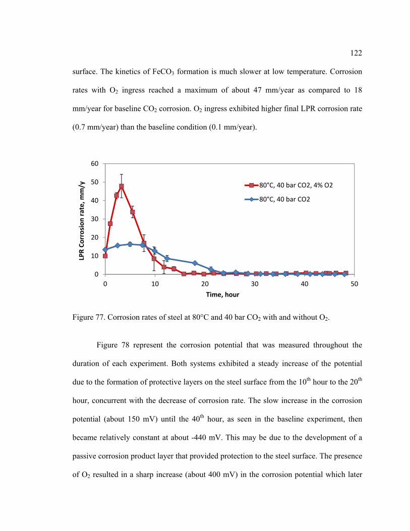
122

surface. The kinetics of FeCO3 formation is much slower at low temperature. Corrosion

rates with O2 ingress reached a maximum of about 47 mm/year as compared to 18

mm/year for baseline CO2 corrosion. O2 ingress exhibited higher final LPR corrosion rate

(0.7 mm/year) than the baseline condition (0.1 mm/year).

Figure 77. Corrosion rates of steel at 80°C and 40 bar CO2 with and without O2.

Figure 78 represent the corrosion potential that was measured throughout the

duration of each experiment. Both systems exhibited a steady increase of the potential

due to the formation of protective layers on the steel surface from the 10th hour to the 20th

hour, concurrent with the decrease of corrosion rate. The slow increase in the corrosion

potential (about 150 mV) until the 40th hour, as seen in the baseline experiment, then

became relatively constant at about -440 mV. This may be due to the development of a

passive corrosion product layer that provided protection to the steel surface. The presence

of O2 resulted in a sharp increase (about 400 mV) in the corrosion potential which later

0

10

20

30

40

50

60

0 10 20 30 40 50


m/y

Time, hour

80°C, 40 bar CO2, 4% O2

80°C, 40 bar CO2

123

dropped after the 20th hour and then became constant at about -420 mV around the 40th

hour. Based on the potential change, the formation of a corrosion product layer with the

presence of O2 is more rapid due to the increase in oxidizer concentration in the system

that produces excessive amounts of precipitation and corrosion products.

Figure 78. Corrosion potential of steel at 80°C and 40 bar CO2 with and without O2.

Corrosion rate was also measured by weight loss method, which was then

compared with the integrated values of corrosion rates from the LPR measurements. The

weight loss method represented the value of the overall corrosion rate during the 48-hour

period whereas the LPR corrosion rates were measured continuously throughout the test

duration. The comparison, which can be seen in Figure 79, showed that the weight loss

corrosion rates were comparable with the LPR corrosion rates. The presence of O2 in this

experiment resulted in a higher CO2 corrosion rate.

‐750

‐650

‐550

‐450

‐350

‐250

0 10 20 30 40 50


V

Time, hour

80°C, 40 bar CO2, 4% O2 80°C, 40 bar CO2

124

Figure 79. Corrosion rates measured using weight loss technique compared with integrated LPR results for conditions with and without O2 at 80°C, 40 bar CO2 after 2 days of test.

At the end of the oxic experiment, the steel specimens were covered with loose

red products that were easily dislodged when rinsed with isopropyl alcohol. This is a

preliminary indication that iron oxides were produced during the test. The reddish layer

was loose, porous, and prone to dislodge, exposing the grayish inner corrosion product

layer. Further observations of the specimen surface using scanning electron microscopy

(SEM) revealed two different kinds of crystal morphologies (Figure 80). The non-

adherent top layer consists of globular crystals that are typical of iron oxides while the

features underneath the top layer were of prism-like crystals of a morphology

characteristic of FeCO3.

9.2

7.0

8.4

5.5

0

2

4

6

8

10

12


Corrosion rate, m

m/year


Weight loss CR

Integrated LPR

125

Figure 80. Steel surface after being exposed to 80°C, 40 bar CO2, 4% O2 in solution for 48 hours.

The thickness and compositional characteristics of the corrosion product were

determined by preparing a cross-section of the specimen which was then analyzed under

SEM using backscattered electrons as shown in Figure 81. The thickness of the corrosion

product derived from the CO2/O2 environment was relatively thinner (43 µm) than the

corrosion product that was not subjected to O2 (78 µm). The amount of iron lost,

calculated from weight loss, was 50 µm and 38 µm for the conditions with O2 and

without O2, respectively. Most of the iron lost from the oxic experiment was probably

converted into loose iron oxide and had spalled off of the steel surface.

The backscatter image in Figure 81(a) suggests different compositions and layers

of the corrosion product based on the different shades of gray. The lighter shade of gray

at the top layer indicates a heavier compound than the layer next to the steel surface. This

is a good indication that the top layer consists of oxides, FexOy, while the layer closest to

126

the steel surface is iron carbonate, FeCO3. The bottom-most layer was observed to be

more coherent and compact than the top-most layer, providing a good protection to the

steel surface.

Figure 81. Cross-sectional view of steel specimen for tests conditions at (a) 80°C, 40 bar pCO2, 1.7 bar O2 and (b) 80°C, 40 bar pCO2.

X-ray diffraction (XRD) was utilized to determine the type of corrosion product

that was formed on the steel surface. The diffraction pattern in Figure 82 indicated

intense peaks of FeCO3, which confirmed the coherent layer of compact corrosion

product that was observed in the backscatter micrograph in Figure 81(a). Iron oxides and

hydroxide were also detected on the steel surface. However, the intensities of the

magnetite and hematite peaks were low and difficult to distinguish between each another.

Raman spectroscopy was later utilized to investigate the corrosion product crystals.

Analysis was conducted on different locations on the steel sample using 785 nm laser

excitation energy at 50 mW laser power and 20 s integration time. The reddish-colored

top layer picked up peaks that are characteristic of hematite (Fe2O3), while the grey-

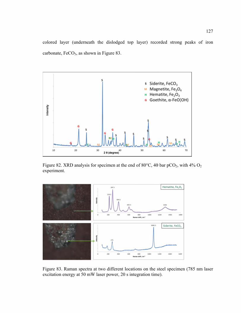
co

ca

Fex

Fex

olored layer

arbonate, Fe

igure 82. XRxperiment.

igure 83. Raxcitation ene

r (undernea

eCO3, as sho

RD analysis

aman spectraergy at 50 m

ath the disl

wn in Figure

for specime

a at two diffmW laser pow

lodged top

e 83.

en at the end

ferent locatiwer, 20 s inte

layer) reco

of 80°C, 40

ons on the segration time

orded strong

0 bar pCO2, w

steel specime).

g peaks of

with 4% O2

men (785 nm

127

f iron

laser

128

Further investigations were carried out to observe the surface profile of the steel

underneath the corrosion product after exposure to experimental conditions with O2

present. After carefully chemically removing the corrosion product, the bare steel surface

was analyzed using optical 3D profilometry. Localized corrosion was observed on the

bare steel surface and the surface profile, Figure 84, showed a pit depth up to 386 µm.

This maximum pit depth value converts to about 70 mm/year of penetration rate. The

occurrence of localized corrosion could be due to the heterogeneity of the corrosion

product layer on the steel surface, which could create highly localized environment for

initiation of pits.

Localized corrosion was quantified by calculating the pitting ratio (PR) using the

following method [95]:

= = . = 7.6 (33)

According to the definition, if the PR value is greater than 5, it is a sign of localized

corrosion. If the PR value is lower than 3 this implies no localized corrosion. If the PR

value falls between 3 and 5, there is a probability for localized corrosion to occur [95]. In

this case, the PR value indicates the existence of localized corrosion.

F1

d

th

m

so

5

ra

m

9

d

o

ra

m

co

igure 84. S.7 bar O2

To su

etrimental to

he experime

material failu

ome protecti

.5.4 Exper

In this

ates measure

maximum an

0 bar CO2 s

iscussed in t

f experimen

ates with O

maximum of

orrosion rate

urface profi

ummarize the

o steel integ

ent, severe l

ure, although

ion to the ste

riment 4: 80°

s experiment

ed by LPR

d minimum

showed sligh

the previous

nt for the ox

O2 ingress r

f about 30 m

e occurred e

ilometry of

e results, the

rity. Even th

localized co

h the coheren

eel, thus low

°C, 90 bar pC

t CO2 is in th

for 48 hour

values of co

htly similar b

s section. Hi

xygenated sy

eached a m

mm/year for

earlier in the

bare steel f

e presence o

hough low c

orrosion was

nt and comp

wering the un

CO2, with an

he supercriti

rs at 90 bar

orrosion rate

behavior as

gher corrosi

ystem as com

maximum of

the baseline

e presence o

for test con

of 4% O2 in

corrosion rat

s observed a

pact layer of

niform corros

nd without 4

ical phase. F

CO2 and 80

es. The beha

the experim

ion rate was

mpared to th

f over 50 m

e CO2 exper

of O2 and th

nditions 80°C

n 40 bar CO

te was recor

and can con

f FeCO3 on t

sion rate.

4% O2.

Figure 85 sho

0oC; the err

avior of the c

ments done a

observed in

he anoxic sy

mm/year as

riment. How

herefore resu

C, 40 bar p

O2 at 80°C ca

rded at the e

nsequently c

the steel pro

ows the corr

or bars mar

corrosion ra

at 40 bar CO

n the first 5 h

ystem. Corr

opposed to

wever, the dr

ulting in a m

129

pCO2,

an be

nd of

cause

ovides

rosion

rk the

ates at

O2, as

hours

osion

o the

rop in

much

130

lower time-integrated corrosion rate value as shown in Figure 86. The weight loss

corrosion rate also showed lower corrosion rate when O2 is present in supercritical CO2.

This differing observation could be caused by the complex nature of supercritical CO2

which affects the overall chemistry of the solution.

Figure 85. Corrosion rates of steel at 80°C and 90 bar CO2 with and without O2.

0

10

20

30

40

50

60

0 10 20 30 40 50

Corrosion rate, m

m/y

Time, hour

80°C, 90 bar CO2, 4% O2

80°C, 90 bar CO2

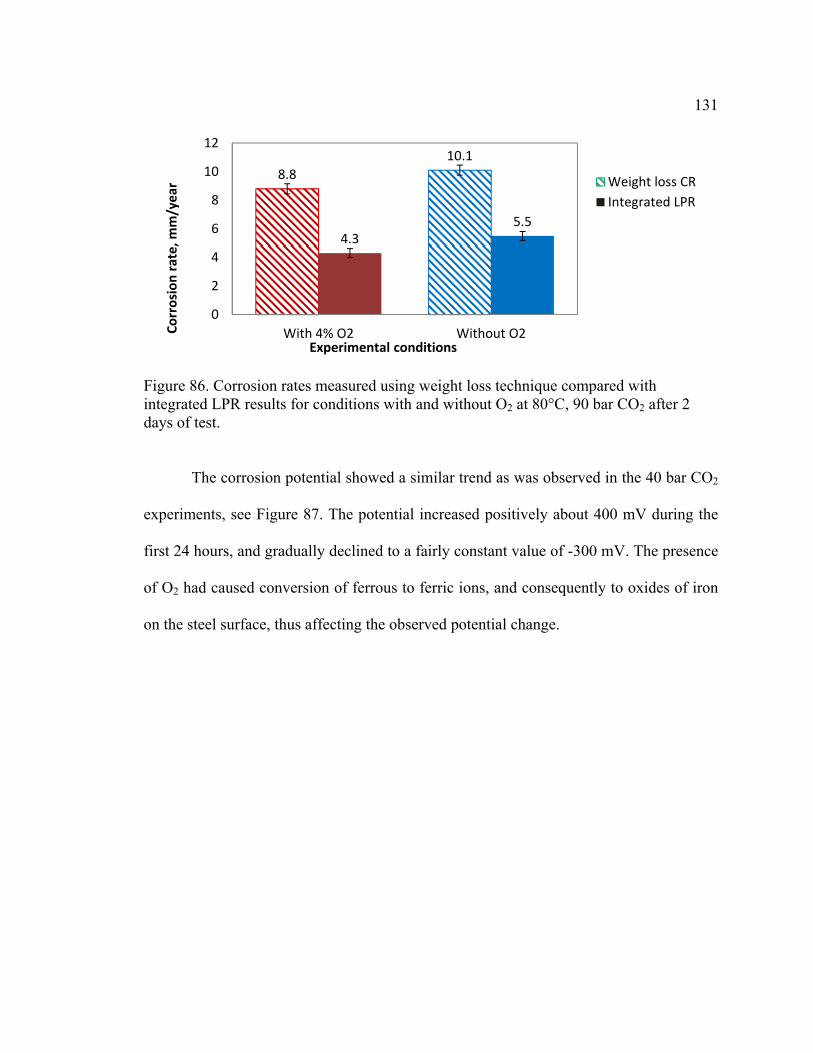
131

Figure 86. Corrosion rates measured using weight loss technique compared with integrated LPR results for conditions with and without O2 at 80°C, 90 bar CO2 after 2 days of test.

The corrosion potential showed a similar trend as was observed in the 40 bar CO2

experiments, see Figure 87. The potential increased positively about 400 mV during the

first 24 hours, and gradually declined to a fairly constant value of -300 mV. The presence

of O2 had caused conversion of ferrous to ferric ions, and consequently to oxides of iron

on the steel surface, thus affecting the observed potential change.

8.8

10.1

4.35.5

0

2

4

6

8

10

12

With 4% O2 Without O2Corrosion rate, m

m/year


Weight loss CR

Integrated LPR

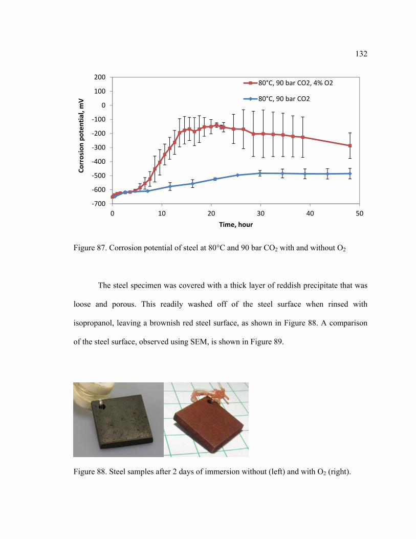
132

Figure 87. Corrosion potential of steel at 80°C and 90 bar CO2 with and without O2

The steel specimen was covered with a thick layer of reddish precipitate that was

loose and porous. This readily washed off of the steel surface when rinsed with

isopropanol, leaving a brownish red steel surface, as shown in Figure 88. A comparison

of the steel surface, observed using SEM, is shown in Figure 89.

Figure 88. Steel samples after 2 days of immersion without (left) and with O2 (right).

‐700

‐600

‐500

‐400

‐300

‐200

‐100

0

100

200

0 10 20 30 40 50


V

Time, hour

80°C, 90 bar CO2, 4% O2

80°C, 90 bar CO2

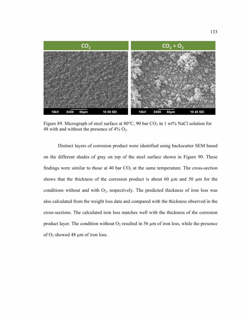
F4

on

fi

sh

co

al

cr

pr

o

igure 89. Mi8 with and w

Distin

n the differe

indings were

hows that th

onditions w

lso calculate

ross-sections

roduct layer

f O2 showed

icrograph ofwithout the p

nct layers of

ent shades o

e similar to

he thickness

ithout and w

ed from the w

s. The calcu

r. The condit

d 48 µm of ir

f steel surfacpresence of 4

f corrosion p

of gray on t

those at 40

s of the corr

with O2, resp

weight loss d

ulated iron lo

tion without

ron loss.

ce at 80°C, 94% O2.

roduct were

top of the s

bar CO2 at

rosion produ

pectively. T

data and com

oss matches

O2 resulted

90 bar CO2 in

e identified u

steel surface

the same tem

uct is about

The predicted

mpared with

well with th

in 56 µm of

n 1 wt% NaC

using backsc

e shown in F

mperature. T

t 60 µm an

d thickness

the thicknes

he thickness

f iron loss, w

Cl solution f

catter SEM b

Figure 90. T

The cross-se

d 50 µm fo

of iron loss

ss observed i

s of the corr

while the pres

133

for

based

These

ection

or the

s was

in the

osion

sence

Fan

R

w

Fth

igure 90. Crnd without th

The id

Raman spectr

was the only

igure 91. Anhe 80°C, 90 b

ross-section he presence

dentity of th

roscopy (Fig

compound th

nalysis of stebar pCO2, w

of steel at 80of 4% O2.

he corrosion

gure 92). Du

hat was dete

eel surface uwith 4% O2 e

0°C, 90 bar C

n product w

ue to the th

ected by Ram

using XRD foexperiment.

CO2 in 1 wt%

was confirme

hickness of t

man spectros

for the specim

% NaCl solu

ed by XRD

the top oxid

scopy.

men recover

ution for 48

(Figure 91)

de layer, hem

red at the end

134

with

) and

matite

d of

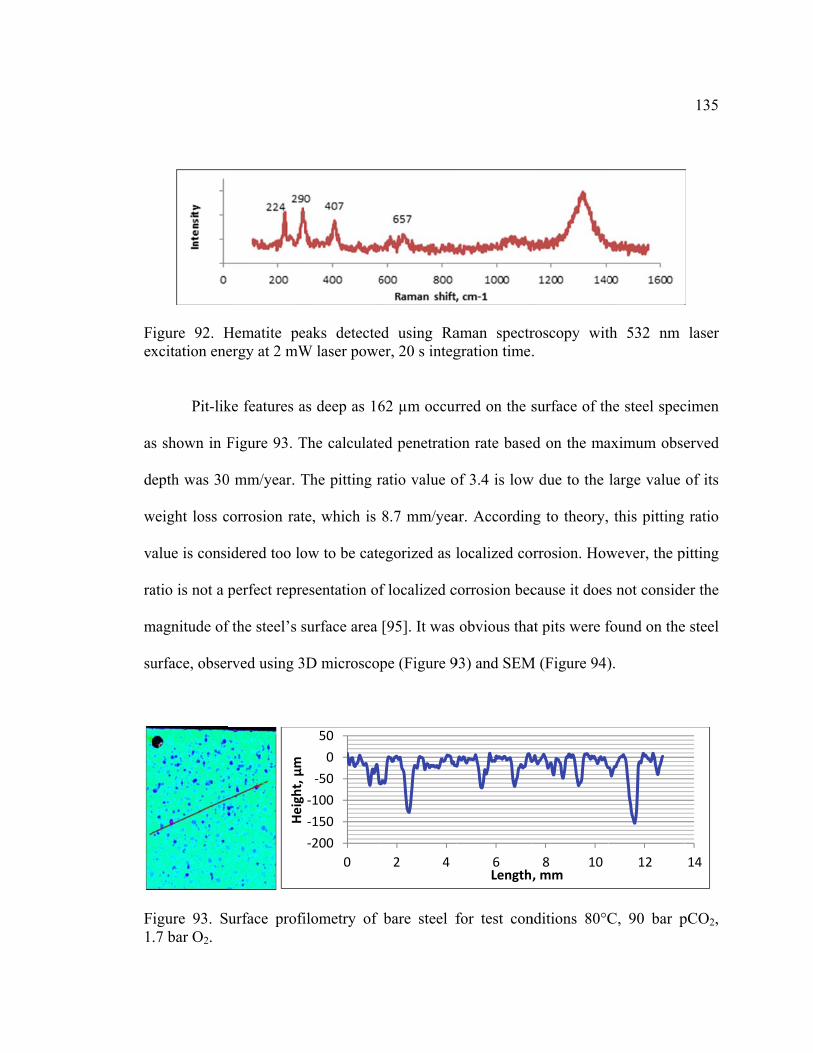
Fex

as

d

w

v

ra

m

su

F1

igure 92. Hxcitation ene

Pit-lik

s shown in F

epth was 30

weight loss c

alue is consi

atio is not a p

magnitude of

urface, obser

igure 93. S.7 bar O2.

Hematite peergy at 2 mW

ke features a

Figure 93. T

0 mm/year. T

corrosion rat

idered too lo

perfect repre

f the steel’s s

rved using 3

urface profi

Height, µm

eaks detecteW laser powe

as deep as 16

The calculate

The pitting r

te, which is

ow to be cate

esentation of

surface area

3D microscop

ilometry of

‐200

‐150

‐100

‐50

0

50

0

ed using Raer, 20 s integ

62 µm occur

ed penetratio

ratio value o

8.7 mm/yea

egorized as l

f localized c

[95]. It was

pe (Figure 9

bare steel f

2 4

aman spectrgration time.

rred on the s

on rate base

of 3.4 is low

ar. Accordin

localized co

corrosion bec

obvious tha

93) and SEM

for test con

6Length,

roscopy wit.

surface of th

d on the ma

w due to the

ng to theory,

orrosion. How

cause it does

at pits were f

M (Figure 94)

nditions 80°C

8 10, mm

th 532 nm

he steel spec

aximum obse

large value

this pitting

wever, the p

s not conside

found on the

).

C, 90 bar p

12

135

laser

cimen

erved

of its

ratio

pitting

er the

e steel

pCO2,

14

136

Figure 94. Localized corrosion on steel surface as seen under SEM.

5.6 The Proposed Corrosion Mechanism

The ingress of O2 in high CO2 partial pressure systems causes a more complex

electrochemistry of CO2 corrosion. The additional cathodic reaction (O2 reduction

reaction (14)) that takes place, results in an increased rate of anodic reaction to provide

more electrons for the cathodic reactions. The dissolution of iron into ferrous ions is

increased, which explains the overall higher corrosion rate. Previous researchers have

suggested that the FeCO3 is very vulnerable to O2 and is easily damaged or dissolved by

its presence [88], [107].

At low temperature, in this case 25°C, the temperature is too low for FeCO3 or

Fe2O3 to form effectively. Therefore, neither FeCO3 nor Fe2O3, was found on the steel

surface. However, for the oxic environment at room temperature, in the presence of

carbonate ions, formation of goethite, α-FeO(OH), [108] was observed as the greenish

la

sy

in

ac

re

b

an

Fin

an

o

co

as

h

ayer that turn

ystem leads

n the solutio

ct as oxidan

esidual iron

ecomes exp

nalyses). Fig

igure 95. Prongress in a cl

At hig

nd kineticall

f O2 interfe

oncentration

s iron oxid

eterogeneity

ned yellowis

to the incre

on. The exce

nts, causing d

n carbide, d

posed (as ev

gure 95 illust

oposed corrolosed system

gh temperatu

ly favored a

feres with t

n in solution

des, and are

y of the depo

sh with air o

ease of hydro

ess hydrogen

dissolution o

derived from

videnced by

trates this co

osion mecham.

ure, the form

as the precip

the formatio

n. The ferrou

e deposited

osition provi

xidation. Th

ogen, bicarb

n ion and bic

of iron to for

m pearlite a

the previou

orrosion mec

anism at low

mation of Fe

pitation rate

on of FeCO

us ions are o

loosely and

des for local

he high CO2

bonate, and

carbonate m

rm ferrous i

and, enrich

usly shown

chanism.

w temperature

eCO3 and ox

of these spe

O3 due to

oxidized to f

d randomly

lized environ

partial press

carbonate io

migrate to th

ions (Fe2+). C

hed with all

SEM micro

e and high p

xides are the

ecies increas

the diminis

ferric ions, w

y on the ste

nments with

sure in the c

on concentra

e steel surfa

Consequentl

loying elem

ographs and

pCO2 with O

ermodynami

ses. The pres

shed ferrous

which precip

eel surface.

h the steel su

137

closed

ations

ace to

ly the

ments,

EDS

2

ically

sence

s ion

pitate

The

urface

w

T

is

d

In

la

b

hy

bu

Fin

co

fo

which is cove

This may lead

s possible th

epleted, crea

n that theory

arger surfac

ecomes the

ypothesized

ut it appears

igure 96. Prongress in a cl

Furthe

onditions ca

ormed at hig

ered by FeC

d to formati

hat the O2 tha

ating a differ

y, the local a

e area of th

cathode. Su

to promote

s to be less p

oposed corrolosed system

er tests that

an be condu

gh CO2 part

CO3is protect

on of galvan

at is trapped

rential aerat

rea undernea

he steel tha

upersaturatio

the formati

protective tha

osion mecham.

are specific

ucted to con

ial pressure

ted, whereas

nic cells, eve

d in the conf

ion cell, as t

ath the iron

at is directly

on of Fe2+

ion of FeCO

an the FeCO

anism at high

c to studying

nfirm their v

might offer

s the steel su

en if the exa

fined space g

typically see

oxide layer

y exposed t

and CO32-

O3 in the pit

O3 formed els

h temperatur

g the corros

validity. Inv

r some answ

urface under

act mechanis

gets consum

en in crevice

becomes the

to the aerat

in the local

ts as illustrat

sewhere.

re and high p

sion mechan

vestigation o

wers about th

r the oxide is

sm is not cle

med, and bec

e corrosion [

e anode whil

ed bulk sol

l environme

ted in Figur

pCO2 with O

nisms under

of galvanic

he mechanis

138

s not.

ear. It

comes

[109].

le the

lution

ent is

re 96,

O2

these

cells

sm of

139

localized corrosion. Electrochemical impedance spectroscopy (EIS) may be utilized to

study the corrosion mechanism at high CO2 partial pressure in the presence of O2.

5.7 The Effect of Flow

An impeller, fitted to the autoclave, with a rotational speed set at 1000 rpm

conferred a flow field in the solution, corresponding to a peripheral velocity of about

1 m/s. The flow regime corresponds to a turbulent flow with a Reynolds number greater

than 200. Figure 97 shows that the initial corrosion rate almost doubled due to the

addition of flow in a CO2 system. It then slowly decreased to about 0.2 mm/year after

over 30 hours of test as compared to the lesser amount of time taken by the stagnant

system. Figure 98 illustrates the same effect of flow on a CO2/O2 system. This delayed

behavior in the drop of corrosion rate shows that the mechanisms of both CO2 and

CO2/O2 corrosion are influenced by mass transport of species to and from the metal

surface. The highest recorded corrosion rate was over 60 mm/year in the oxic and

turbulent environment. The lowered corrosion rate values are indicative of a protective

barrier that had formed on the steel surface in spite of the presence of turbulent flow.

140

Figure 97. Effect of 1000 rpm flow rotational speed on the corrosion rates in equivalent CO2 systems.

Figure 98. Effect of 1000 rpm flow on the corrosion rates in equivalent CO2/O2 systems.

0

10

20

30

40

50

0 10 20 30 40 50

Corrosion rate, m

m/y

Time, hour

80°C, 90 bar CO2 with flow

80°C, 90 bar CO2

0

10

20

30

40

50

60

70

0 10 20 30 40 50

Corrosion rate, m

m/y

Time, hour

80°C, 90 bar CO2, 4% O2

80°C, 90 bar CO2, 4% O2 with flow

141

The effect of flow was also significant in the corrosion rate values that were

measured by weight loss. Figure 99 illustrates that both CO2 and CO2/O2 flow systems

recorded high corrosion rates as compared to their rates in the stagnant condition.

Combination of high pressure CO2 with O2 and flow recorded the highest of over

35 mm/year.

Figure 99. Effect of flow and O2 on weight loss corrosion rate.

The surface of the steel specimen after 48 hours of exposure in the CO2/O2

environment at 80°C, 90 bar CO2, and 1000 rpm rotational speed showed layers of

corrosion product that were flaky and non-adherent, as shown in Figure 100.

Observations under SEM, as shown in Figure 101, indicated the appearance of typical

dense plate-like iron oxide crystals, with a high percentage of O in the EDS analysis

shown in Figure 102. Crystals of FeCO3 could not be seen on the sample.

10.1

24.4

8.8

35.2

0

5

10

15

20

25

30

35

40

0 rpm 1000 rpm

Weight loss corrosion rate,

mm/year

Flow conditions

CO2

CO2/O2

142

Figure 100. Steel specimens at 80°C 90 bar CO2, 4% O2, and 1000 rpm speed.

Figure 101. SEM of steel surface at 80°C 90 bar CO2, 4% O2, and 1000 rpm speed.

Fsp

in

ap

F

m

an

co

su

fi

in

igure 102. Epeed.

The sp

n an anoxic

ppeared sev

igure 104.

micrograph, w

nalysis on th

omposition o

uch as copp

indings of th

n solution wi

EDS of steel

pecimen from

CO2 enviro

verely corrod

Analysis o

was indicati

he flat non-cr

of the corrod

per, molybd

he alloying e

ith a pH valu

surface at 80

m the oxic C

onment. The

ded, as show

of a prisma

ive of FeCO

rystalline pa

ded steel sub

enum, mang

elements in

ue of 6.0 and

0°C, 90 bar

CO2/O2 expe

e steel spec

wn in Figur

atic crystal,

O3 by the de

art of the spe

bstrate with

ganese and

steel grade X

d at temperat

CO2, 4% O2

eriment was

cimen from

re 103. The

indicated

etection of e

ecimen, labe

high concen

nickel asso

X65 have be

tures 40, 60,

2, and 1000 r

compared w

the anoxic

e EDS analy

by point ‘

elements Fe

lled as point

ntrations of a

ciated with

een reported

, and 80°C [

rpm rotation

with the spec

flow experi

ysis is show

1’ on the

e, C and O.

t ‘2’, reveale

alloying elem

carbide. Si

d when imm

110]

143

nal

cimen

iment

wn in

SEM

EDS

ed the

ments

imilar

mersed

F

F

b

la

w

m

un

igure 103. S

igure 104. E

Figure

oth flow an

ayer in Figu

which could b

more obvious

nderlying Fe

SEM of steel

EDS analysis

e 105 and F

d stagnant c

ure 105(a) sh

be due to the

s in Figure 1

eCO3.

surface at 8

s of two poin

Figure 106 s

conditions fo

howed the p

e interferenc

106(a) wher

80°C 90 bar C

nts on the ste

show the cro

or CO2 and

presence of

ce of flow on

re the oxide

CO2, and 10

eel as labeled

oss-sectional

CO2/O2 sys

voids in be

n FeCO3 for

layer was fl

000 rpm rotat

d in the prev

l view of st

stems. The c

etween the c

rmation. The

flaky and non

tional speed

vious Figure

teel specime

corrosion pro

corrosion pro

e voids were

n-adherent t

144

d.

.

ens in

oduct

oduct

even

to the

F9

Fsy

th

su

m

igure 105. C0 bar CO2.

igure 106. Cystem at 80°

The c

he surface of

urface in bot

maximum pit

Cross-section

Cross-sectio°C, 90 bar CO

corrosion pro

f the bare ste

th CO2 and C

t depth obse

nal views o

onal views oO2 and 4% O

oduct was re

eel. Turbulen

CO2/O2 syst

erved was 9

f coupon co

of coupon cO2.

emoved usin

nt flow had c

tems as illust

93 µm for th

omparing the

omparing th

ng a Clarke

caused the a

trated in Fig

he anoxic sy

e effect of f

he effect of

solution in

appearance o

gure 107 and

ystem while

flow at 80°C

f flow in CO

order to ob

of pits on the

d Figure 108

e the oxic sy

145

C and

O2-O2

bserve

e steel

8. The

ystem

pr

n

F

F1

roved to be

ot exhibit p

igure 109. T

igure 107. S000 rpm

more aggres

pit-like featu

The deepest p

Surface prof

ssive with p

ures but inst

penetration w

filometry of

pit depth up

tead appeare

was recorded

f steel for ex

to 377 µm.

ed very seve

d to be abou

xperiment at

One specim

erely corrod

ut 380 µm.

t 80°C, 90 b

men, however

ded, as show

bar CO2, 2

146

r, did

wn in

days,

FO

igure 108. SO2, 1000 rpm

Surface profim

ilometry of s

steel for expeeriment at 800°C, 90 bar CO2, 2 days

147

s, 4%

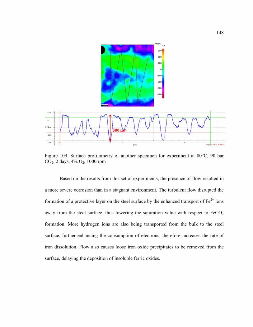
FC

a

fo

aw

fo

su

ir

su

igure 109. SCO2, 2 days,

Based

more severe

ormation of

way from th

ormation. M

urface, furth

ron dissoluti

urface, delay

Surface prof4% O2, 1000

d on the resu

e corrosion t

a protective

he steel surf

More hydrog

her enhancin

ion. Flow al

ying the depo

filometry of0 rpm

ults from this

than in a sta

layer on the

face, thus lo

gen ions are

ng the consu

so causes lo

osition of in

f another sp

s set of expe

agnant enviro

e steel surfac

owering the

also being

umption of e

oose iron ox

soluble ferri

pecimen for

eriments, the

onment. The

ce by the enh

saturation v

transported

electrons, th

xide precipit

ic oxides.

experiment

e presence of

e turbulent fl

hanced trans

value with r

d from the b

herefore incr

ates to be re

at 80°C, 9

f flow result

flow disrupte

sport of Fe2+

respect to F

bulk to the

reases the ra

emoved from

148

0 bar

ted in

ed the

+ ions

eCO3

steel

ate of

m the

149

5.8 Chapter Summary and Conclusions

Table 9 summarizes the results that were drawn from the current work on the

effect of O2 in high pressure conditions.

Table 9: Results Summary of High Pressure Corrosion Experiments T (°C)

pCO2 (bar)

pO2 (bar)

Flow condition, rpm

Final LPR corrosion rate (mm/year)

Weight loss Corrosion rate

Localized corrosion?

25 40 0 0 9.7 6.3 No

25 40 1.7 0 13.6 9.5 No

25 90 0 0 6.4 1.8 No

25 90 3.75 0 15.5 15.1 No

80 40 0 0 0.1 7.0 NA

80 40 1.7 0 0.7 9.2 Yes

80 90 0 0 1.3 10.1 NA

80 90 3.75 0 0.2 8.8 Yes

80 90 0 1000 0.2 24.4 Yes

80 90 3.75 1000 NA 35.2 Yes

The presence of O2 was particularly detrimental to steel integrity. The

experiments that were conducted at the 25°C caused severe uniform corrosion, devoid of

any protective corrosion product layer on the steel surface. The final corrosion rates,

based on the final Rp value measured by LPR, are considered to be high and regarded as

unacceptable by the oil and gas industry. Experiments that were conducted at 80°C

150

showed possible initiation of localized corrosion on steel. The formation of thick and

coherent corrosion products on the steel surface provided some defense from further

active corrosion of the steel. Although the final corrosion rates were low (0.7 and

0.2 mm/year), they were still considered as unacceptable values for oil and gas

applications which have been defined as a maximum of 0.1 mm/year [107], [111]. The

highest corrosion rate observed was in the flow experiments.

The overall results showed that the corrosion rates were magnitudes higher than

the corrosion rates observed at low pressure as discussed in Chapter 4. This is associated

with elevated CO2 partial pressures causing an increase in the carbonic acid

concentration.

151

CHAPTER 6: MODELING

In-house corrosion prediction tools called Freecorp©, and Multicorp© were

utilized for comparison of simulated corrosion rates to results.

6.1 Simulation at Low Pressure

Freecorp© is a simulation software that was developed by a team of research

scientists and programmers at the Institute for Corrosion and Multiphase Technology

(ICMT) to perform predictions of carbon steel corrosion at corrosion product layer-free

conditions. The software was utilized to simulate corrosion, and related data for the

FeCO3-free low pressure condition. Figure 110 shows that the corrosion rates presented

in Chapter 4 are in agreement with the simulated results. The polarization curve shown in

Figure 111 effectively describes the corrosion behavior change when O2 is present in the

system. The corrosion current increased due to the additional O2 reduction reaction,

reflected by the green vertical line, which shifted the total cathodic curve to the right. The

other lines are labeled as different colors: orange (H+ reduction), purple (H2O reduction),

light blue (H2CO3 reduction), red (total cathodic curve and Fe dissolution), and dark blue

(sweep curve).

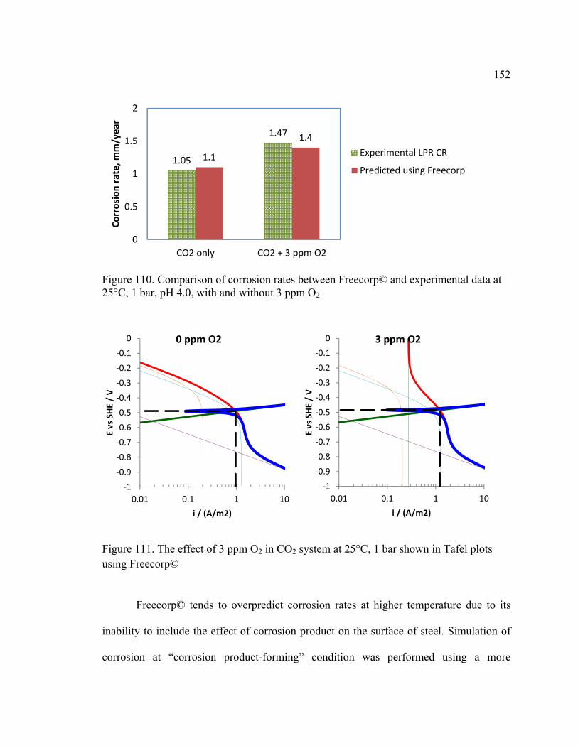
152

Figure 110. Comparison of corrosion rates between Freecorp© and experimental data at 25°C, 1 bar, pH 4.0, with and without 3 ppm O2

Figure 111. The effect of 3 ppm O2 in CO2 system at 25°C, 1 bar shown in Tafel plots using Freecorp©

Freecorp© tends to overpredict corrosion rates at higher temperature due to its

inability to include the effect of corrosion product on the surface of steel. Simulation of

corrosion at “corrosion product-forming” condition was performed using a more

1.05

1.47

1.1

1.4

0

0.5

1

1.5

2

CO2 only CO2 + 3 ppm O2

Corrosion rate, m

m/year

Experimental LPR CR

Predicted using Freecorp

‐1

‐0.9

‐0.8

‐0.7

‐0.6

‐0.5

‐0.4

‐0.3

‐0.2

‐0.1

0

0.01 0.1 1 10

E vs SHE / V

i / (A/m2)

0 ppm O2

‐1

‐0.9

‐0.8

‐0.7

‐0.6

‐0.5

‐0.4

‐0.3

‐0.2

‐0.1

0

0.01 0.1 1 10

E vs SHE / V

i / (A/m2)

3 ppm O2

153

advanced in-house proprietary model called Multicorp©. This corrosion prediction model

was designed for use in pipelines in the oil and gas industry, therefore, it is unable to

simulate the corrosion rate at a completely stagnant condition. All simulations using

Multicorp© were set at the lowest allowable superficial water velocity, which is 0.01 m/s.

Figure 112 compares the results between experimental (red squares) and

simulated data (blue line) for a 7-day experiment at 80°C, 0.5 bar CO2 and pH value of

6.6. The simulated data showed a slightly lower corrosion rate than the experimental data.

The immediate drop in both experimental and simulated corrosion rate is caused by the

formation of corrosion product on the steel surface, which was observed and discussed

earlier in Chapter 4. The drop in the corrosion rate corresponds to the drop in the surface

porosity, which is shown in Figure 113. The presence of O2 (denoted by the triangular

plots) resulted in a much higher corrosion rate for the first 5 days of the test due to the

additional O2 reduction reaction in the system. The formation and accumulation of oxide

precipitates on the steel surface partially mitigated further corrosion of the steel by

limiting the area of the steel surface that is directly exposed to the corrosive environment.

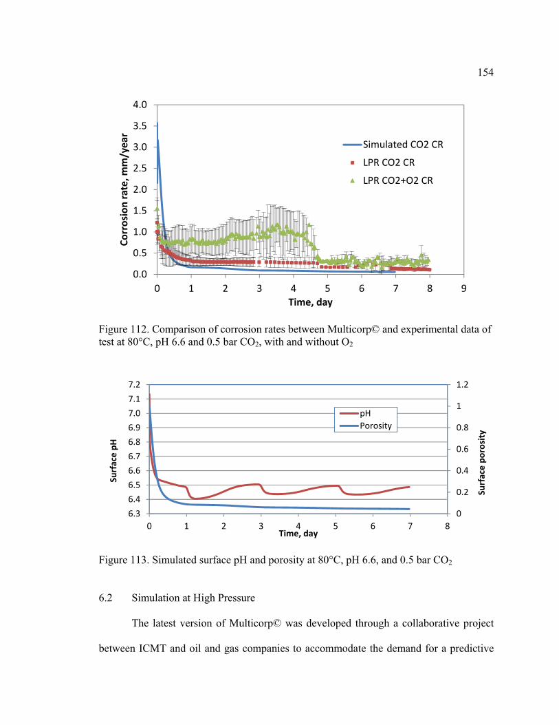
154

Figure 112. Comparison of corrosion rates between Multicorp© and experimental data of test at 80°C, pH 6.6 and 0.5 bar CO2, with and without O2

Figure 113. Simulated surface pH and porosity at 80°C, pH 6.6, and 0.5 bar CO2

6.2 Simulation at High Pressure

The latest version of Multicorp© was developed through a collaborative project

between ICMT and oil and gas companies to accommodate the demand for a predictive

0.0

0.5

1.0

1.5

2.0

2.5

3.0

3.5

4.0

0 1 2 3 4 5 6 7 8 9

Corrosion rate, m

m/year

Time, day

Simulated CO2 CR

LPR CO2 CR

LPR CO2+O2 CR

0

0.2

0.4

0.6

0.8

1

1.2

6.3

6.4

6.5

6.6

6.7

6.8

6.9

7.0

7.1

7.2

0 1 2 3 4 5 6 7 8

Surface porosity

Surface pH

Time, day

pH

Porosity

155

tool in near-critical and supercritical CO2 conditions for steel pipelines in the oil and gas

industry. This newest version of the software enables prediction of corrosion for

pressures up to 200 bar.

6.2.1 Multicorp© High Pressure Simulation for Tests at 25°C

Experimental results at CO2 partial pressures of 40 bar and 90 bar that was

presented in Chapter 5 were compared with simulated results using Multicorp©, shown

in Figure 114 and Figure 115. Both figures exhibited a fairly constant corrosion rate for

48 hours. The absence of a protective FeCO3 layer on the steel that was observed in the

laboratory experiment explains the constantly high corrosion rates. Multicorp© predicted

a slightly higher corrosion rate due to the inability of the model to simulate corrosion

behavior at stagnant conditions. The superficial fluid velocity was set at 0.01 m/s to

simulate a near stagnant environment. The presence of O2 affects the corrosion rate even

at high pressure, as shown in the two figures. The increase in the corrosion rate at 90 bar

is more significant than the increase at 40 bar CO2.

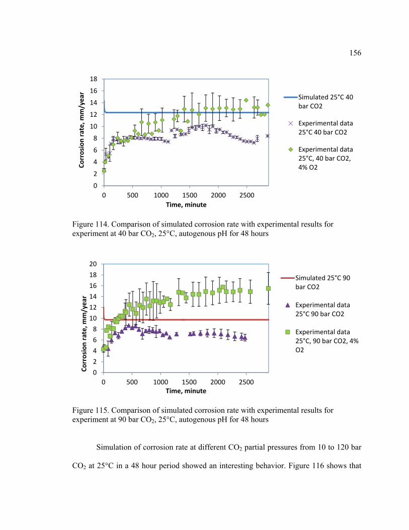
156

Figure 114. Comparison of simulated corrosion rate with experimental results for experiment at 40 bar CO2, 25°C, autogenous pH for 48 hours

Figure 115. Comparison of simulated corrosion rate with experimental results for experiment at 90 bar CO2, 25°C, autogenous pH for 48 hours

Simulation of corrosion rate at different CO2 partial pressures from 10 to 120 bar

CO2 at 25°C in a 48 hour period showed an interesting behavior. Figure 116 shows that

0

2

4

6

8

10

12

14

16

18

0 500 1000 1500 2000 2500

Corrosion rate, m

m/year

Time, minute

Simulated 25°C 40bar CO2

Experimental data25°C 40 bar CO2

Experimental data25°C, 40 bar CO2,4% O2

0

2

4

6

8

10

12

14

16

18

20

0 500 1000 1500 2000 2500

Corrosion rate, m

m/year

Time, minute

Simulated 25°C 90bar CO2

Experimental data25°C 90 bar CO2

Experimental data25°C, 90 bar CO2, 4%O2

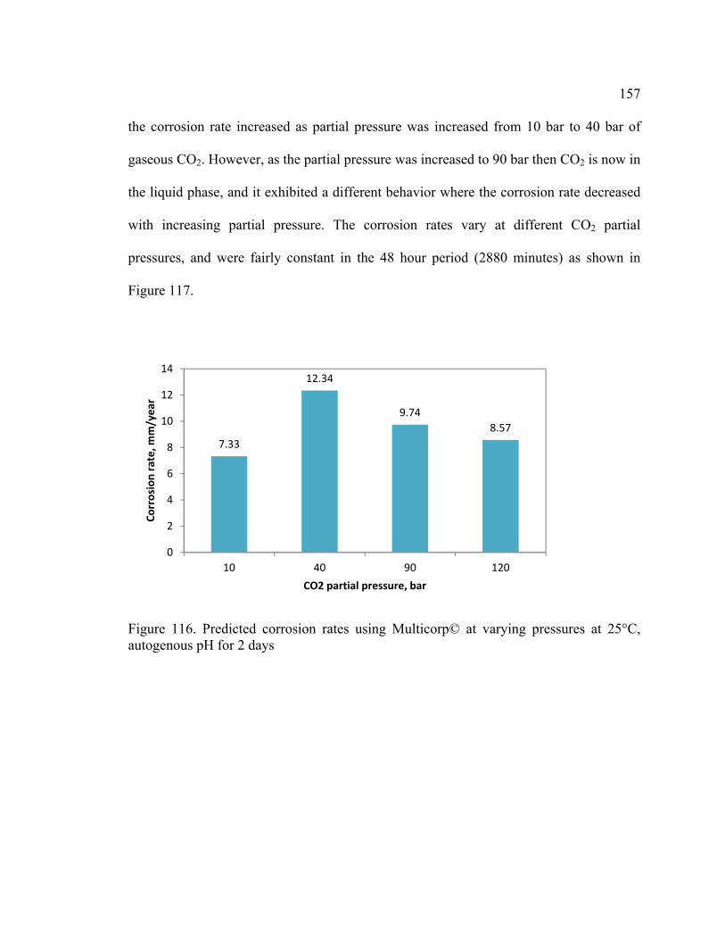
157

the corrosion rate increased as partial pressure was increased from 10 bar to 40 bar of

gaseous CO2. However, as the partial pressure was increased to 90 bar then CO2 is now in

the liquid phase, and it exhibited a different behavior where the corrosion rate decreased

with increasing partial pressure. The corrosion rates vary at different CO2 partial

pressures, and were fairly constant in the 48 hour period (2880 minutes) as shown in

Figure 117.

Figure 116. Predicted corrosion rates using Multicorp© at varying pressures at 25°C, autogenous pH for 2 days

7.33

12.34

9.74

8.57

0

2

4

6

8

10

12

14

10 40 90 120

Corrosion rate, m

m/year

CO2 partial pressure, bar

158

Figure 117. Predicted corrosion rates using Multicorp© at varying pressures at 25°C, autogenous pH for 60 days

Figure 117 shows that further simulation of corrosion rate at 25°C up to 60 days

demonstrates that the corrosion rates eventually drop towards much lower values. The

plot of the predicted porosity at the steel surface matches with the drop in corrosion rate,

indicative of some form of corrosion product layer forming thereon, as shown in Figure

118. The increase in CO2 partial pressure from 10 bar to 120 bar caused a delay in the

formation of a corrosion product layer, as seen in the drop in the surface porosity. This is

due to the increased concentration of carbonic acid that made the iron dissolution rate

increase to a greater value than the precipitation rate at 25°C. This can be explained by

the term Surface Scaling Tendency (SST) [112]:

= , , (30)

0

2

4

6

8

10

12

14

0 20000 40000 60000 80000 100000

Corrosion rate, m

m/year

Time, minute

25C 150 bar

25C 120 bar

25C 90 bar

25C 40 bar

25C 10 bar

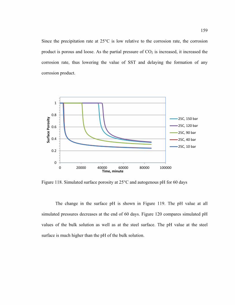
159

Since the precipitation rate at 25°C is low relative to the corrosion rate, the corrosion

product is porous and loose. As the partial pressure of CO2 is increased, it increased the

corrosion rate, thus lowering the value of SST and delaying the formation of any

corrosion product.

Figure 118. Simulated surface porosity at 25°C and autogenous pH for 60 days

The change in the surface pH is shown in Figure 119. The pH value at all

simulated pressures decreases at the end of 60 days. Figure 120 compares simulated pH

values of the bulk solution as well as at the steel surface. The pH value at the steel

surface is much higher than the pH of the bulk solution.

0

0.2

0.4

0.6

0.8

1

0 20000 40000 60000 80000 100000

Surface Porosity

Time, minute

25C, 150 bar

25C, 120 bar

25C, 90 bar

25C, 40 bar

25C, 10 bar

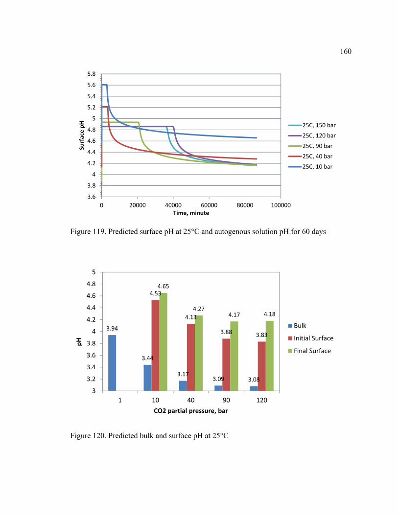
160

Figure 119. Predicted surface pH at 25°C and autogenous solution pH for 60 days

Figure 120. Predicted bulk and surface pH at 25°C

3.6

3.8

4

4.2

4.4

4.6

4.8

5

5.2

5.4

5.6

5.8

0 20000 40000 60000 80000 100000

Surface pH

Time, minute

25C, 150 bar

25C, 120 bar

25C, 90 bar

25C, 40 bar

25C, 10 bar

3.94

3.44

3.173.09 3.08

4.53

4.13

3.88 3.83

4.65

4.274.17 4.18

3

3.2

3.4

3.6

3.8

4

4.2

4.4

4.6

4.8

5

1 10 40 90 120

pH


Bulk

Initial Surface

Final Surface

161

6.2.2 Multicorp© High Pressure Simulation for Tests at 80°C

Simulation of corrosion at 80°C resulted in a very high initial corrosion rate

which then dropped rapidly within the first few hours of the corrosion process and

gradually decreases afterwards, as shown in Figure 121. However, the corrosion rate after

48 hours was still considered unacceptably high. The poor correlation of the corrosion

rate values is due to a number of possible factors. The simulated values were computed at

the lowest allowable superficial fluid velocity of 0.01 m/s, therefore it does not truly

represent corrosion rate values at stagnant condition. The simulation is also based on an

infinite amount of solution which affects the supersaturation of species involved in the

formation of FeCO3 or any other corrosion products.

Figure 121. Predicted corrosion rates using Multicorp© at varying pressures at 80°C, autogenous pH

0.1

1

10

100

1000

0 1 2

Corrosion rate, m

m/year

Time, day

80°C 120 bar

80°C 90 bar

80°C 40 bar

80°C 10 bar

Experimental data 80°C 40 bar

Experimental data 80°C 90 bar

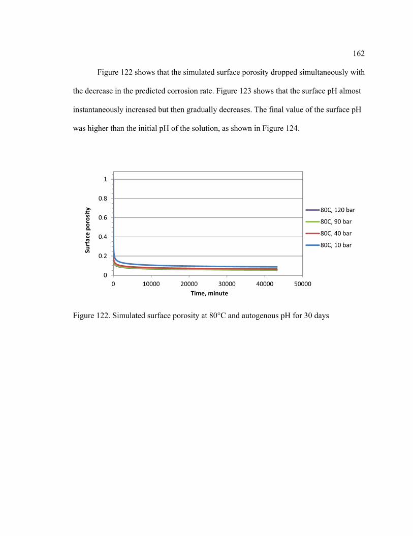
162

Figure 122 shows that the simulated surface porosity dropped simultaneously with

the decrease in the predicted corrosion rate. Figure 123 shows that the surface pH almost

instantaneously increased but then gradually decreases. The final value of the surface pH

was higher than the initial pH of the solution, as shown in Figure 124.

Figure 122. Simulated surface porosity at 80°C and autogenous pH for 30 days

0

0.2

0.4

0.6

0.8

1

0 10000 20000 30000 40000 50000

Surface porosity

Time, minute

80C, 120 bar

80C, 90 bar

80C, 40 bar

80C, 10 bar

163

Figure 123. Predicted surface pH at 80°C and autogenous solution pH for 30 days

Figure 124. Predicted bulk and surface pH using Multicorp©

4

4.2

4.4

4.6

4.8

5

5.2

5.4

5.6

5.8

6

0 10000 20000 30000 40000 50000

Surface pH

Time, minute

80C, 120 bar

80C, 90 bar

80C, 40 bar

80C, 10 bar

4.27

3.62

3.333.19 3.15

4.474.34 4.28 4.27

4.68

4.344.18 4.14

3

3.2

3.4

3.6

3.8

4

4.2

4.4

4.6

4.8

5

1 10 40 90 120

pH


Bulk

Initial Surface

Final Surface

164

6.2.3 Multicorp© Simulation on the Effect of Flow

The effect of solution velocity on the corrosion rate of steel depends on several

factors such as the passivity of the metal, salinity, O2 concentration, and corrosion

product or inhibitor film. For an active steel such as mild steel, its corrosion rate is

affected by flow velocity only when it is diffusion-controlled, and the effect is only

limited to low solution velocities [109]. The corrosion rate of an active steel will increase

with increasing solution velocity but levels off as the velocity gets higher [18], [113]. The

corrosion rate of an active-passive metal (stainless steel) is independent of flow at high

solution velocity due to its passivity [18]. The increase in corrosion rate when velocity is

increased is due to the O2 reduction process. Hydrogen ions that are close to the steel

surface are swept away by turbulent flow, enhancing the mass transport of O2 towards the

steel surface. Therefore, the effect of flow in the absence of O2 is unseen [43]. Salinity of

solution, i.e., concentration of Cl- in the solution, also plays a role in the effect of flow on

corrosion rate by interrupting passivation of steel. High salinity water, such as seawater,

would exhibit increased corrosion rate with increasing solution velocity while this

behavior is not exhibited in natural waters [43]. The effect of flow is less significant in

the presence of an inhibitor film or a protective FeCO3 layer on the steel surface,

however, it can cause the initiation of pits [113].

The Multicorp© model is able to simulate for superficial water velocity up to

10 m/s. Simulation of corrosion was done at various velocities from 0.01 m/s to 10 m/s.

Figure 125 and Figure 126 shows the effect of flow on the corrosion rate at 25°C and

80°C, respectively. Both figures show that the corrosion rate increases significantly as the

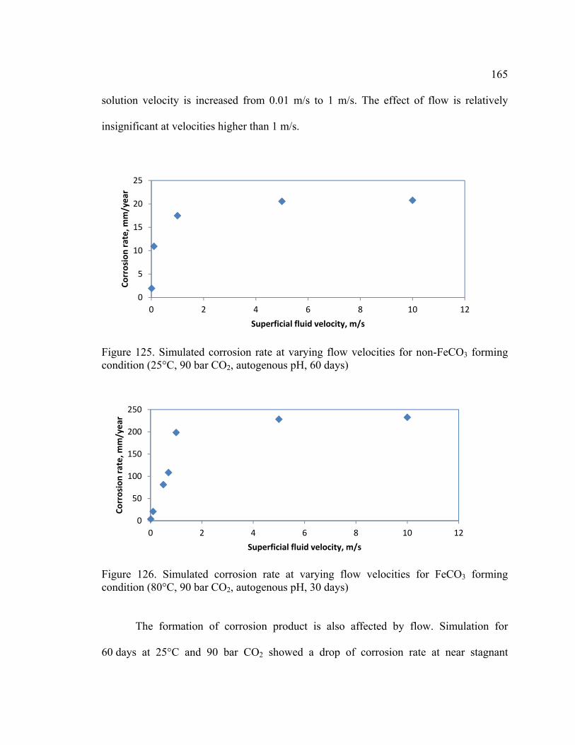
165

solution velocity is increased from 0.01 m/s to 1 m/s. The effect of flow is relatively

insignificant at velocities higher than 1 m/s.

Figure 125. Simulated corrosion rate at varying flow velocities for non-FeCO3 forming condition (25°C, 90 bar CO2, autogenous pH, 60 days)

Figure 126. Simulated corrosion rate at varying flow velocities for FeCO3 forming condition (80°C, 90 bar CO2, autogenous pH, 30 days)

The formation of corrosion product is also affected by flow. Simulation for

60 days at 25°C and 90 bar CO2 showed a drop of corrosion rate at near stagnant

0

5

10

15

20

25

0 2 4 6 8 10 12

Corrosion rate, m

m/year

Superficial fluid velocity, m/s

0

50

100

150

200

250

0 2 4 6 8 10 12

Corrosion rate, m

m/year

Superficial fluid velocity, m/s

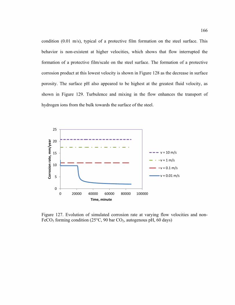
166

condition (0.01 m/s), typical of a protective film formation on the steel surface. This

behavior is non-existent at higher velocities, which shows that flow interrupted the

formation of a protective film/scale on the steel surface. The formation of a protective

corrosion product at this lowest velocity is shown in Figure 128 as the decrease in surface

porosity. The surface pH also appeared to be highest at the greatest fluid velocity, as

shown in Figure 129. Turbulence and mixing in the flow enhances the transport of

hydrogen ions from the bulk towards the surface of the steel.

Figure 127. Evolution of simulated corrosion rate at varying flow velocities and non-FeCO3 forming condition (25°C, 90 bar CO2, autogenous pH, 60 days)

0

5

10

15

20

25

0 20000 40000 60000 80000 100000

Corrosion rate, m

m/year

Time, minute

v = 10 m/s

v = 1 m/s

v = 0.1 m/s

v = 0.01 m/s

167

Figure 128. Simulated surface porosity at various flow velocities at 25°C, 90 bar CO2, autogenous pH for 60 days

Figure 129. Simulated surface pH at various flow velocities at 25°C, 90 bar CO2 and autogenous pH for 60 days

Prediction of corrosion rate at 80°C was compared with experimental data, as

shown in Figure 130. The experimental data for the stagnant test is in closest agreement

with the simulated corrosion rate at the lowest possible fluid velocity, 0.01 m/s.

0

0.2

0.4

0.6

0.8

1

1.2

0 20000 40000 60000 80000 100000

Surface porosity

Time, minute

v = 0.01 m/s

v = 0.1 m/s

v = 1 m/s

2

2.5

3

3.5

4

4.5

5

5.5

0 20000 40000 60000 80000 100000

Surface pH

Time, minute

v = 10 m/s

v = 1 m/s

v = 0.1 m/s

v = 0.01 m/s

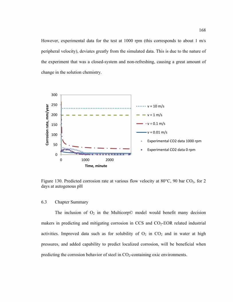
168

However, experimental data for the test at 1000 rpm (this corresponds to about 1 m/s

peripheral velocity), deviates greatly from the simulated data. This is due to the nature of

the experiment that was a closed-system and non-refreshing, causing a great amount of

change in the solution chemistry.

Figure 130. Predicted corrosion rate at various flow velocity at 80°C, 90 bar CO2, for 2 days at autogenous pH

6.3 Chapter Summary

The inclusion of O2 in the Multicorp© model would benefit many decision

makers in predicting and mitigating corrosion in CCS and CO2-EOR related industrial

activities. Improved data such as for solubility of O2 in CO2 and in water at high

pressures, and added capability to predict localized corrosion, will be beneficial when

predicting the corrosion behavior of steel in CO2-containing oxic environments.

0

50

100

150

200

250

300

0 1000 2000

Corrosion rate, m

m/year

Time, minute

v = 10 m/s

v = 1 m/s

v = 0.1 m/s

v = 0.01 m/s

Experimental CO2 data 1000 rpm

Experimental CO2 data 0 rpm

169

CHAPTER 7: CONCLUSION AND RECOMMENDATIONS

The work in this dissertation has covered the study of carbon steel corrosion at

supercritical and subcritical CO2 relevant to the CCS and CO2-EOR sector in which O2 is

present as an aggressive contaminant in CO2. Observations from the experiments at

gaseous and liquid CO2 can be beneficial in terms of corrosion in CO2 transmission line

in the CCS network where the conditions are up to 30°C and 200 bar CO2. Results from

experiments at supercritical CO2 will be much more relevant to downhole condition

(150°C and 500 bar CO2).

7.1 Overall Summary/Conclusion

While FeCO3 was found to be advantageous in providing some form of protection

to the steel surface, O2 was destructive to it, see Chapter 4. O2 was observed to cause

degeneration of FeCO3 crystals. The accumulation of iron oxides on the steel surface

caused the occurrence of tubercles as occluded regions on the steel surface, creating a

phenomenon similar to crevice corrosion that initiates the formation of pits. Oxides such

as magnetite (Fe3O4), hematite (α-Fe2O3), and goethite (α-FeOOH) along with siderite

(FeCO3) were the components of the tubercles.

Discussion in Chapter 5 has shown that the ingress of O2 in high pressure CO2

environment increased the overall corrosion rate of steel by suppressing the formation of

FeCO3 layer on the steel surface. Oxides similar to that in the low pressure tests were

observed in the high pressure experiments at 80°C. Even though the presence of tubercles

was not seen in high pressure experiments, pits were observed on the steel specimens in

170

the 80°C tests. XRD analyses detected iron carbide as the only significant corrosion

product that was observed in the 25°C experiment, while EDS detected the presence of

residual alloying elements such as Cu, Ni, Mn, and Mo on the steel surface. General

uniform corrosion was observed at this low temperature.

The presence of flow heightened the severity of corrosion by disrupting the

formation of a protective FeCO3 layer on the steel surface. This is due to the enhanced

mass transport of species to/away from the steel surface, which decreased the saturation

of ions with respect to FeCO3 formation. The combination of flow and O2 dramatically

increased the overall general and localized corrosion rate.

Simulation of corrosion at high pressure and low pressure using in-house

prediction models was beneficial. However, the models are not perfect. Predicted values

of corrosion at low pressure using Multicorp© has shown almost perfect matching with

experimental results. Simulation using Multicorp© for the high temperature low pressure

conditions resulted in acceptable values as well. However, Multicorp© lacks in the

calculation of the effect of O2 on CO2 corrosion. Prediction of corrosion rate at high

pressure high temperature (HPHT) conditions showed the poorest correlation with

experimental data.

7.2 Future Work/Recommendations

Based on the EDS analysis that was done on steel specimens shown in Chapter 5,

the alloying elements and their enrichment has aroused a degree of curiosity. Future study

on the effect of these alloying elements in steel can be conducted to understand their role

171

in corrosion of steel. The role of carbide as the skeletal remnants from corrosion of steel

should also be further investigated. Other kinds of steels, such as 3Cr, 13Cr and other

CRAs should also be tested to investigate their performance in oxic CO2 corrosion

environments.

The effect of O2 may also differ in different kinds of brine, depending on the

composition of the brine. Besides Na+ and Cl-, the brine that is used at oil fields typically

consist of other ions such as Ca2+, Mg2+, K+, and SO42-.

Based on the observations and high corrosion rate values in both low and high

pressure situations, it is vital that corrosion inhibitor be employed in O2/CO2 environment

since it is universally accepted that corrosion rate should not exceed 0.1 mm/year.

Mitigation of corrosion will help extend the life of equipment in CO2-EOR units.

Investigation of the inhibition strategy for corrosion at high pressure with the ingress of

O2 should be conducted, especially in combatting the onset of localized corrosion

underneath the thick corrosion product.

Prediction of corrosion using Multicorp© implies that the corrosion behavior of

steel at low temperature potentially reaches its steady state at about 60 days. Therefore,

longer tests can be conducted in order to give a better representation of the true corrosion

behavior.

The overall setup design can also be improved. The change in the solution water

chemistry should also be well-controlled either by using an ion-exchange unit, or simply

using larger volume vessels. Quantification of the amount of O2 and iron content

throughout the duration of the experiment would be beneficial in determining the actual

172

kinetics of the corrosion product formation. A stable pH measurement device would be a

valuable asset in future tests.

173

REFERENCES

[1] G. H. Koch, M. P. H. Brongers, N. G. Thompson, Y. P. Virmani, and J. H. Payer, “Corrosion Cost and Preventive Strategies in the United States.,” Federal Highway Administration, McLean, VA, Technical Report FHWA-RD-01-156, 2002.

[2] M. B. Kermani and D. Harrop, “The impact of corrosion on oil and gas industry,” SPE Prod. Facil., vol. 11, no. 3, pp. 186–190, 1996.

[3] I. Herrera and G. F. Pinder, “Enhanced Oil Recovery,” in Mathematical Modeling in Science and Engineering, John Wiley & Sons, Inc., 2012, pp. 149–164.

[4] S. R. Reeves, “Demonstration of a novel, integrated, multi-scale procedure for high-resolution 3D reservoir characterization and improved CO2-EOR/sequestration management, SACROC Unit.,” U.S. Department of Energy, DE-FC26-04NT15514, Mar. 2008.

[5] L. E. Newton, “SACROC CO2 project - Corrosion problems and solutions,” in Advances in CO2 Corrosion, vol. 2, Houston, TX: NACE International, 1985, pp. 235–249.

[6] W. S. Han, B. J. McPherson, P. C. Lichtner, and F. P. Wang, “Evaluation of trapping mechanisms in geologic CO2 sequestration: Case study of SACROC northern platform, a 35-year CO2 injection site,” Am. J. Sci., vol. 310, no. 4, pp. 282–324, Apr. 2010.

[7] R. F. Weeter and L. N. Halstead, “Production of CO2 from a reservoir - a new concept,” J. Pet. Technol., vol. 34, no. 09, pp. 2144–2148, Sep. 1982.

[8] T. D. Crameik and J. A. Plassey, “Carbon dioxide injection project SACROC Unit, Scurry County, Texas,” in Annual Meeting Papers, Division of Production, Houston, TX, 1972, pp. 72–D001.

[9] M. B. Kermani and A. Morshed, “Carbon dioxide corrosion in oil and gas production - A compendium,” Corrosion, vol. 59, no. 8, pp. 659–683, 2003.

[10] M. E. Parker, J. P. Meyer, and S. R. Meadows, “Carbon dioxide enhanced oil recovery injection operations technologies (Poster Presentation),” Energy Procedia, vol. 1, no. 1, pp. 3141–3148, Feb. 2009.

[11] E. Akeer, B. Brown, and S. Nesic, “The influence of mild steel metallurgy on the initiation of localized CO2 corrosion in flowing conditions,” in CORROSION/2013, Orlando, FL, 2013, p. 2383.

[12] J. Rogers and R. Grigg, “A literature analysis of the WAG injectivity abnormalities in the CO2 process,” SPE Reserv. Eval. Eng., vol. 4, no. 5, Oct. 2001.

174

[13] C. Preston, M. Monea, W. Jazrawi, K. Brown, S. Whittaker, D. White, D. Law, R. Chalaturnyk, and B. Rostron, “IEA GHG Weyburn CO2 monitoring and storage project,” Fuel Process. Technol., vol. 86, no. 14–15, pp. 1547–1568, Oct. 2005.

[14] S. Whittaker, B. Rostron, C. Hawkes, C. Gardner, D. White, J. Johnson, R. Chalaturnyk, and D. Seeburger, “A decade of CO2 injection into depleting oil fields: Monitoring and research activities of the IEA GHG Weyburn-Midale CO2 Monitoring and Storage Project,” Energy Procedia, vol. 4, pp. 6069–6076, 2011.

[15] B. M. Sass, H. Farzan, R. Prabhakar, J. Gerst, J. Sminchak, M. Bhargava, B. Nestleroth, and J. Figueroa, “Considerations for treating impurities in oxy-combustion flue gas prior to sequestration,” Energy Procedia, vol. 1, no. 1, pp. 535–542, 2009.

[16] A. Oosterkamp and J. Ramsen, “State of the art overview of CO2 pipeline transportation with relevance to offshore pipelines,” POLYTEC, Haugesund, Norway, POL-0-2007-138-A, 2008.

[17] V. White, L. Torrente-Murciano, D. Sturgeon, and D. Chadwick, “Purification of oxyfuel-derived CO2,” Energy Procedia, vol. 1, no. 1, pp. 399–406, 2009.

[18] D. A. Jones, Principles and Prevention of Corrosion, 2nd ed. Upper Saddle River, NJ: Prentice Hall, 1996.

[19] H. H. Uhlig, H. H. Triadis, and M. Stern, “Effect of oxygen, chlorides, and calcium ion on corrosion inhibition of iron by polyphosphates,” J Electrochem Soc, vol. 102, pp. 59–66, 1955.

[20] J. Collier, S. Papavinasam, J. Li, C. Shi, P. Liu, and J.-P. Gravel, “Effect of impurities on the corrosion performance of steels in supercritical carbon dioxide: Optimization of experimental procedure,” in CORROSION/2013, Orlando, FL, 2013, p. 2357.

[21] Y.-S. Choi, S. Nesic, and D. Young, “Effect of impurities on the corrosion behavior of CO2 transmission pipeline steel in supercritical CO2-water environments,” Environ. Sci. Technol. Env. Sci Technol, vol. 44, no. 23, pp. 9233–9238, 2010.

[22] E. Gulbrandsen, J. Kvarekval, and H. Miland, “Effect of Oxygen Contamination on the Inhibition Studies of Carbon Dioxide Corrosion,” CORROSION, vol. 61, no. 11, pp. 1086–1097, 2005.

[23] R. L. Martin, “Corrosion consequences of oxygen entry into oilfield brines,” in CORROSION/2002, Denver, CO, 2002, p. 02270.

175

[24] G. Pipitone and O. Bolland, “Power generation with CO2 capture: Technology for CO2 purification,” Int. J. Greenh. Gas Control, vol. 3, no. 5, pp. 528–534, Sep. 2009.

[25] F. Yang, G.-B. Zhao, H. Adidharma, B. Towler, and M. Radosz, “Effect of oxygen on minimum miscibility pressure in carbon dioxide flooding,” Ind. Eng. Chem. Res., vol. 46, no. 4, pp. 1396–1401, 2007.

[26] A. Oosterkamp and J. Ramsen, “State-of-the-Art Overview of CO2 Pipeline Transport with relevance to offshore pipelines,” POLYTEC, POL-O-2007-138-A, 2008.

[27] H. Li, J. P. Jakobsen, Ø. Wilhelmsen, and J. Yan, “PVTxy properties of CO2 mixtures relevant for CO2 capture, transport and storage: Review of available experimental data and theoretical models,” Appl. Energy, vol. 88, no. 11, pp. 3567–3579, Nov. 2011.

[28] S. Nesic, “Carbon dioxide corrosion of mild steel,” in Uhlig’s Corrosion Handbook, 3rd ed., Hoboken, New Jersey: John Wiley & Sons, Inc., 2011, pp. 229–246.

[29] C. deWaard and D. E. Milliams, “Carbonic acid corrosion of steel,” Corrosion, vol. 31, no. 5, pp. 177–181, 1975.

[30] C. deWaard and U. Lotz, “Prediction of CO2 corrosion of carbon steel,” in CORROSION/93, 1993, p. 69.

[31] S. Nesic and W. Sun, “2.25 - Corrosion in Acid Gas Solutions,” E.-C. T. J. A. Richardson, Ed. Oxford: Elsevier, 2010, pp. 1270–1298.

[32] S. Nesic, J. Postlethwaite, and S. Olsen, “An electrochemical model for prediction of corrosion of mild steel in aqueous carbon dioxide solutions,” Corrosion, vol. 52, no. 4, pp. 280–294, 1996.

[33] W. Sun and S. Nešić, “Kinetics of corrosion layer formation: Part 1—Iron carbonate layers in carbon dioxide corrosion,” Corrosion, vol. 64, no. 4, pp. 334–346, 2008.

[34] A. Dugstad, “The importance of FeCO3 supersaturation on the CO2 corrosion of carbon steels,” in CORROSION/92, 1992, p. 14.

[35] S. Nešic and K.-L. Lee, “A mechanistic model for carbon dioxide corrosion of mild steel in the presence of protective iron carbonate films-Part 3: Film growth model,” Corrosion, vol. 59, no. 7, pp. 616–628, 2003.

176

[36] W. Sun, S. Nešić, and R. C. Woollam, “The effect of temperature and ionic strength on iron carbonate (FeCO3) solubility limit,” Corros. Sci., vol. 51, no. 6, pp. 1273–1276, 2009.

[37] W. Li, Y. Xiong, B. Brown, K. E. Kee, and S. Nesic, “Measurement of wall shear stress in multiphase flow and its effect on protective FeCO3 corrosion product layer removal,” in CORROSION/2015, Dallas, TX, 2015, p. 5922.

[38] F. Farelas, B. Brown, and S. Nesic, “Iron Carbide and its Influence on the Formation of Protective Iron Carbonate in CO2 Corrosion of Mild Steel,” in CORROSION/2013, Orlando, FL, 2013, p. 2291.

[39] V. Fajardo, B. Brown, D. Young, and S. Nešić, “Study of the solubility of iron carbonate in the presence of acetic acid using an EQCM,” in CORROSION/2013, Orlando, FL, 2013, p. 2452.

[40] L. G. S. Gray, B. G. Anderson, M. J. Danysh, and P. R. Tremaine, “Mechanism of Carbon Steel Corrosion in Brines Containing Dissolved Carbon Dioxide at pH 4,” in CORROSION/1989, New Orleans, LA, 1989.

[41] T. Tran, B. Brown, and S. Nesic, “Corrosion of Mild Steel in an Aqueous CO2 Environment – Basic Electrochemical Mechanisms Revisited,” in CORROSION/2015, Dallas, TX.

[42] L. G. S. Gray, B. G. Anderson, M. J. Danysh, and P. R. Tremaine, “Effect of pH and temperature on the mechanism of carbon steel corrosion by aqueous carbon dioxide,” in CORROSION/90, Houston, TX, 1990, p. 40.

[43] H. H. Uhlig and R. W. Revie, Corrosion and corrosion control: an introduction to corrosion science and engineering, 2nd ed. New York: John Wiley & Sons, 1985.

[44] T. Tanupabrungsun, “Thermodynamics and kinetics of CO2 corrosion of mild steel at elevated temperatures,” Ohio University, Athens, OH, 2013.

[45] Z. F. Yin, Y. R. Feng, W. Z. Zhao, Z. Q. Bai, and G. F. Lin, “Effect of temperature on CO2 corrosion of carbon steel,” Surf. Interface Anal., vol. 41, no. 6, pp. 517–523, 2009.

[46] S. Nesic and W. Sun, “Corrosion in acid gas solutions,” in Shreir’s Corrosion, 4th ed., vol. 2, 4 vols., T. J. A. Richardson, B. Cottis, R. Lindsay, S. Lyon, D. Scantlebury, H. Stott, and M. Graham, Eds. Amsterdam: Elsevier, 2010, pp. 1270–1298.

[47] F. D. de Moraes, J. R. Shadley, J. Chen, and E. F. Rybicki, “Characterization of CO2 Corrosion Product Scales related to Environmental Conditions,” in CORROSION/2000, 2000, p. 30.

177

[48] H. Fang, B. Brown, and S. Nesic, “High Salt Concentration Effects On CO2 Corrosion And H2S Corrosion,” in CORROSION/2010, San Antonio, TX, 2010, p. 10276.

[49] S. S. H. Rizvi, Z. R. Yu, A. R. Bhaskar, and C. B. C. Raj, “Fundamentals of Processing with Supercritical Fluids,” S. S. H. Rizvi, Ed. Bishopbriggs, Glasgow: Chapman & Hall, 1994, pp. 1–26.

[50] A. A. Clifford and J. R. Williams, “Introduction to Supercritical Fluids and Their Applications,” vol. 13, J. R. Williams and A. A. Clifford, Eds. 2000, pp. 1–16.

[51] W. A. Propp, T. E. Carleson, C. M. Wai, P. R. Taylor, K. W. Daehling, S. Huang, and M. Abdel-Latif, “Corrosion in Supercritical Fluids,” US Department of Energy, DE96014006, 1996.

[52] H. V. Poollen, Fundamentals of enhanced oil recovery. Tulsa, OK: PennWell Publishing Co., 1980.

[53] Y. Zhang, X. Pang, S. Qu, X. Li, and K. Gao, “Discussion of the CO2 corrosion mechanism between low partial pressure and supercritical condition,” Corros. Sci., vol. 59, pp. 186–197, 2012.

[54] S. Wang, K. George, and S. Nesic, “High pressure CO2 corrosion electrochemistry and the effect of acetic acid,” in CORROSION/2004, New Orleans, LA, 2004, p. 04375.

[55] Y.-S. Choi and S. Nešić, “Corrosion behavior of carbon steel in supercritical CO2-water environments,” in CORROSION/2009, Atlanta, GA, 2009, p. 09256.

[56] K. O. Kongshaug and M. Seiersten, “Baseline experiments for the modelling of corrosion at high CO2 pressure,” in CORROSION/2004, New Orleans, LA, 2004, p. 04630.

[57] S. M. Hesjevik, S. Olsen, and M. Seiersten, “Corrosion at High CO2 Pressure,” in CORROSION/2003, San Diego, CA, 2003, p. 3345.

[58] S. Nesic, M. Nordsveen, R. Nyborg, and A. Stangeland, “A mechanistic model for carbon dioxide corrosion of mild steel in the presence of protective iron carbonate films - Part 2: A numerical experiment,” Corrosion, vol. 59, no. 6, pp. 489–497, 2003.

[59] A. M. Nor, M. F. Suhor, M. F. Mohamed, M. Singer, and S. Nesic, “Corrosion of Carbon Steel in High CO2 Containing Environments - the Effect of High Flow Rate,” in CORROSION/2012, Salt Lake City, UT, 2012, p. 1683.

178

[60] E. M. Russick, G. A. Poulter, C. L. J. Adkins, and N. R. Sorensen, “Corrosive effects of supercritical carbon dioxide and cosolvents on metals,” J. Supercrit. Fluids, vol. 9, no. 1, pp. 43–50, 1996.

[61] M. F. Suhor, M. F. Mohamed, A. M. Nor, M. Singer, and S. Nesic, “Corrosion of mild steel in high CO2 environment: effect of the FeCO3 layer,” in CORROSION/2012, Salt Lake City, Utah, 2012, p. 1434.

[62] H. Li, Ø. Wilhelmsen, Y. Lv, W. Wang, and J. Yan, “Viscosities, thermal conductivities and diffusion coefficients of CO2 mixtures: Review of experimental data and theoretical models,” Int. J. Greenh. Gas Control, vol. 5, no. 5, pp. 1119–1139, 2011.

[63] H. Li, J. Yan, J. Yan, and M. Anheden, “Impurity impacts on the purification process in oxy-fuel combustion based CO2 capture and storage system,” Appl. Energy, vol. 86, no. 2, pp. 202–213, Feb. 2009.

[64] J. Stoll, J. Vrabec, and H. Hasse, “Vapor–liquid equilibria of mixtures containing nitrogen, oxygen, carbon dioxide, and ethane,” AIChE J., vol. 49, no. 8, pp. 2187–2198, 2003.

[65] A. Fredenslund and G. A. Sather, “Gas-liquid equilibrium of the oxygen-carbon dioxide system,” J. Chem. Eng. Data, vol. 15, no. 1, pp. 17–22, Jan. 1970.

[66] A. Fredenslund, J. Mollerup, and O. Persson, “Gas-liquid equilibrium of oxygen-carbon dioxide system,” J. Chem. Eng. Data, vol. 17, no. 4, pp. 440–443, 1972.

[67] L. Garverick, Corrosion in the Petrochemical Industry. ASM International, 1994.

[68] H. M. Herro, “MIC myths - Does pitting cause MIC?,” in CORROSION/98, San Diego, 1998, p. 278.

[69] X. Gao, “Localized corrosion initiation by O2 in CO2 environment,” Institute for Corrosion and Multiphase Technology, Athens OH, CCJIP, Mar. 2013.

[70] J. R. Baylis, “Factors other than dissolved oxygen influencing the corrosion of iron pipes,” Ind. Eng. Chem., vol. 18, no. 4, pp. 370–380, 1926.

[71] R. I. Ray, J. S. Lee, B. J. Little, and T. L. Gerke, “The anatomy of tubercles: A corrosion study in a fresh water estuary,” Mater. Corros., vol. 61, no. 12, pp. 993–999, Dec. 2010.

[72] P. Sarin, V. L. Snoeyink, J. Bebee, W. M. Kriven, and J. A. Clement, “Physico-chemical characteristics of corrosion scales in old iron pipes,” Water Res., vol. 35, no. 12, pp. 2961–2969, 2001.

179

[73] L. McNeill and M. Edwards, “Iron pipe corrosion in water distribution systems,” Am. Water Works Assoc., vol. 93, no. 7, pp. 88–100, Jan. 2001.

[74] U. Schwertmann, “Solubility and dissolution of iron oxides,” Plant Soil, vol. 130, no. 1–2, pp. 1–25, Jan. 1991.

[75] U. Schwertmann and R. M. Cornell, Iron oxides in the laboratory. Preparation and characterization. Wiley-VCH, Weinheim, Germany, 2000.

[76] S. J. Oh, D. C. Cook, and H. E. Townsend, “Characterization of iron oxides commonly formed as corrosion products on steel,” Hyperfine Interact., vol. 112, no. 1–4, pp. 59–66, 01 1998.

[77] T. Misawa, K. Asami, K. Hashimoto, and S. Shimodaira, “The mechanism of atmospheric rusting and the protective amorphous rust on low alloy steel,” Corros. Sci., vol. 14, no. 4, pp. 279–289, 1974.

[78] T. Misawa, K. Hashimoto, and S. Shimodaira, “The mechanism of formation of iron oxide and oxyhydroxides in aqueous solutions at room temperature,” Corros. Sci., vol. 14, no. 2, pp. 131–149, 1974.

[79] M. A. Legodi and D. de Waal, “The preparation of magnetite, goethite, hematite and maghemite of pigment quality from mill scale iron waste,” Dyes Pigments, vol. 74, pp. 161–168, 2007.

[80] G. T. Skaperdas and H. H. Uhlig, “Corrosion of steel by dissolved carbon dioxide and oxygen,” Ind. Eng. Chem., vol. 34, no. 6, pp. 748–754, 1942.

[81] S. Wang, “Effect of oxygen on CO2 corrosion of mild steel,” Russ College of Engineering and Technology, Ohio University, Athens OH, 2009.

[82] W. Liu, S. Dong, J. Zhang, X. Lin, J. He, and M. Lu, “Effect of oxygen on corrosion and erosion-corrosion behavior of N80 steel under high temperature and high pressure,” in CORROSION/2014, San Antonio, TX, 2014, p. 4198.

[83] X. Gao, “Mechanisms of localized corrosion initiation in CO2 and H2S environments,” ICMT, CCJIP Report, 2010.

[84] X. Jiang, “Effect of oxygen contamination on CO2 corrosion in presence of FeCO3 film,” ICMT, CCJIP Report, 2008.

[85] D. John, B. Kinsella, S. Bailey, and R. D. Marco, “Flow dependence of carbon dioxide corrosion rates and the interference of trace dissolved oxygen,” in CORROSION/2007, Nashville, TN, 2007, p. 07315.

180

[86] Y.-S. Choi and S. Nesic, “Effect of impurities on the corrosion behavior of carbon steel in supercritical CO2 - water environments,” in CORROSION/2010, San Antonio, TX, 2010, p. 10196.

[87] Y.-S. Choi, S. Nešić, and D. Young, “Effect of impurities on the corrosion behavior of CO2 transmission pipeline steel in supercritical CO2−water environments,” Environ. Sci. Technol., vol. 44, no. 23, pp. 9233–9238, Dec. 2010.

[88] J. Zhang, X. Lin, S. Lu, T. Wang, W. Liu, S. Dong, C. Yang, and M. Lu, “Corrosion behavior and mechanism of N80 steel under high temperature and high pressure CO2-O2 coexisting condition,” in CORROSION/2013, Orlando, FL, 2013, p. 2479.

[89] X. Lin, W. Liu, F. Wu, C. Xu, J. Dou, and M. Lu, “Effect of O2 on corrosion of 3Cr steel in high temperature and high pressure CO2–O2 environment,” Appl. Surf. Sci., vol. 329, pp. 104–115, Feb. 2015.

[90] N. R. Rosli, Y.-S. Choi, and D. Young, “Impact of oxygen ingress in CO2 corrosion of mild steel,” in CORROSION/2014, San Antonio, TX, 2014, p. 4299.

[91] F. Ayello, K. Evans, R. Thodla, and N. Sridhar, “Effect of impurities on corrosion of steel in supercritical CO2,” in CORROSION/2010, San Antonio, TX, 2010, p. 10193.

[92] R. L. Martin, “Corrosion consequences of oxygen entry into sweet oilfield fluids,” in SPE Permian Basin Oil and Gas Recovery Conference, Midland, TX, 2001, p. SPE 70029.

[93] A. T. Laudate, The JEOL Institute Scanning Electron Microscope Operations Course. 2008.

[94] S. Richter, “Advanced use of the SEM: a seminar,” presented at the Institute for Corrosion and Multiphase Technology, Ohio University, Athens OH, 2013.

[95] B. Brown, “The likelihood of localized corrosion in an H2S/CO2 environment,” in CORROSION/2015, Dallas TX, 2015, p. 5855.

[96] T. L. Gerke, J. B. Maynard, M. R. Schock, and D. L. Lytle, “Physiochemical characterization of five iron tubercles from a single drinking water distribution system: Possible new insights on their formation and growth,” Corros. Sci., vol. 50, no. 7, pp. 2030–2039, 2008.

[97] R. I. Ray, J. S. Lee, B. J. Little, and T. L. Gerke, “The anatomy of tubercles: A corrosion study in a fresh water estuary,” Mater. Corros., vol. 61, no. 12, pp. 993–999, 2010.

181

[98] P. Sarin, V. L. Snoeyink, J. Bebee, W. M. Kriven, and J. A. Clement, “Physico-chemical characteristics of corrosion scales in old iron pipes,” Water Res., vol. 35, no. 12, pp. 2961–2969, Aug. 2001.

[99] P. Sarin, V. Snoeyink, D. Lytle, and W. Kriven, “Iron Corrosion Scales: Model for Scale Growth, Iron Release, and Colored Water Formation,” J. Environ. Eng., vol. 130, no. 4, pp. 364–373, 2004.

[100] G. L. Miessler and D. A. Tarr, Inorganic Chemistry, 4th ed. Upper Saddle River, NJ: Pearson Prentice Hall, 2004.

[101] H. K. Van Poollen and Associates, Fundamentals of enhanced oil recovery. PennWell Books, 1980.

[102] Y.-S. Choi, D. Young, S. Nešić, and L. G. S. Gray, “Wellbore integrity and corrosion of carbon steel in CO2 geologic storage environments: A literature review,” Int. J. Greenh. Gas Control, vol. 16, Supplement 1, pp. S70–S77, Jun. 2013.

[103] A. Dugstad and M. Halseid, “Internal corrosion in dense phase CO2 transport pipelines - State of the art and the need for further R&D,” in CORROSION/2012, Salt Lake City, UT, 2012.

[104] D. W. DeBerry and W. S. Clark, “Corrosion due to use of carbon dioxide for enhanced oil recovery. Final Report. Sumx No. 78-003,” SumX Corp., Austin, TX (USA), DOE/MC/08442-1, Sep. 1979.

[105] S. D. Kapusta and S. C. Canter, “Corrosion control in CO2 enhanced oil recovery,” in CORROSION/94, Baltimore, MD, 1994.

[106] A. Mohammed Nor, “The Effect of Turbulent Flow on Corrosion of Mild Steel in High Partial CO2 Environments,” Ohio University, 2013.

[107] A. Dugstad, L. Børvik, S. Palencsar, and P. A. Eikrem, “Corrosion testing of steel armour wires in flexible pipes - a parametric study,” in CORROSION/2015, Dallas, TX, 2015, p. 5829.

[108] R. M. Cornell and U. Schwertmann, The iron oxides: structure, properties, reactions, occurrences and uses. Wiley-vch, 2003.

[109] M. G. Fontana and N. D. Greene, Corrosion engineering. McGraw-Hill, 1967.

[110] A. A. Al-Asadi, “Iron Carbide Development and its Effect on Inhibitor Performance,” Ohio University, 2014.

182

[111] A. Pfennig and R. Bäßler, “Effect of CO2 on the stability of steels with 1% and 13% Cr in saline water,” Corros. Sci., vol. 51, no. 4, pp. 931–940, Apr. 2009.

[112] Y. Zheng, J. Ning, B. Brown, D. Young, and S. Nesic, “Mechanistic Study of the Effect of Iron Sulfide Layers on Hydrogen Sulfide Corrosion of Carbon Steel,” in CORROSION/2015, Dallas, TX, 2015, p. 5933.

[113] S. Nešić, “Key issues related to modelling of internal corrosion of oil and gas pipelines – A review,” Corros. Sci., vol. 49, no. 12, pp. 4308–4338, Dec. 2007.

[114] D. Tromans, “Temperature and pressure dependent solubility of oxygen in water: a thermodynamic analysis,” Hydrometallurgy, vol. 48, no. 3, pp. 327–342, 1998.

183

APPENDIX A: AES ANALYSIS OF STEEL SPECIMEN

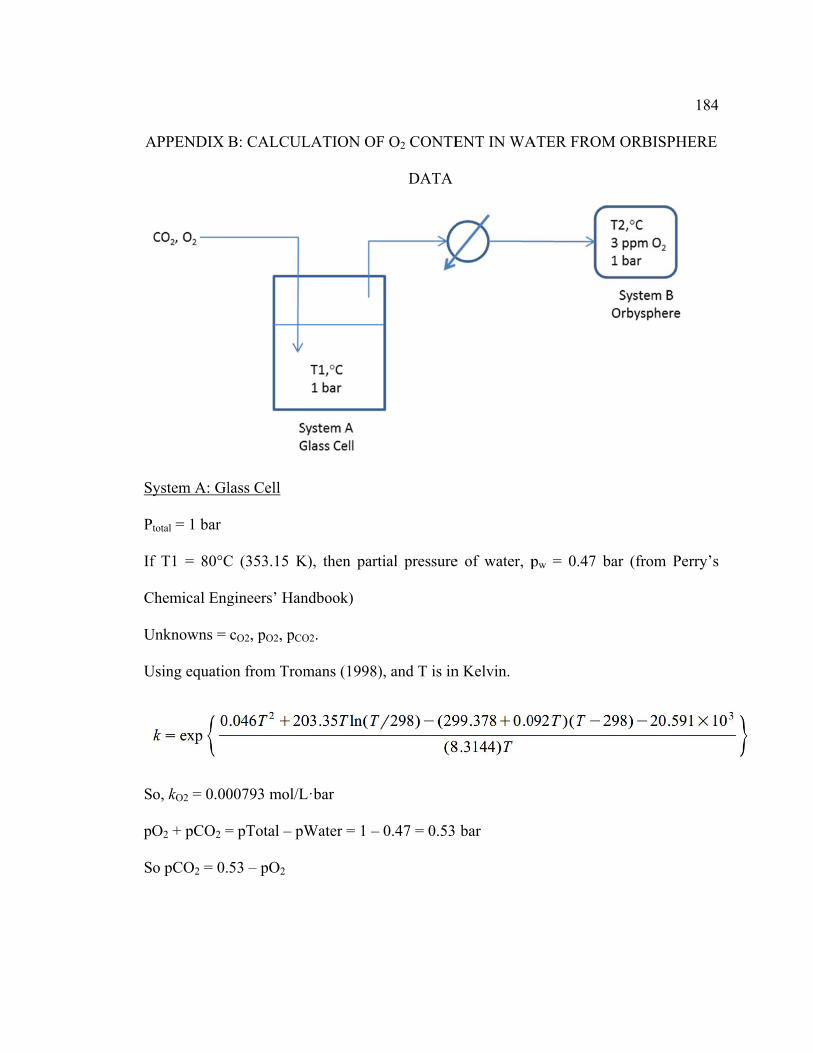
A

S

P

If

C

U

U

S

p

S

APPENDIX

ystem A: Gl

total = 1 bar

f T1 = 80°C

Chemical Eng

Unknowns =

Using equatio

o, kO2 = 0.00

O2 + pCO2 =

o pCO2 = 0.

B: CALCUL

lass Cell

C (353.15 K

gineers’ Han

cO2, pO2, pCO

on from Trom

00793 mol/L

= pTotal – pW

53 – pO2

LATION OF

K), then part

ndbook)

O2.

mans (1998)

L·bar

Water = 1 –

F O2 CONTE

DATA

tial pressure

), and T is in

0.47 = 0.53

ENT IN WA

e of water, p

n Kelvin.

bar

ATER FROM

pw = 0.47 b

M ORBISPH

bar (from Pe

184

HERE

erry’s

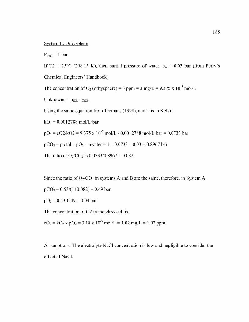
185

System B: Orbysphere

Ptotal = 1 bar

If T2 = 25°C (298.15 K), then partial pressure of water, pw = 0.03 bar (from Perry’s

Chemical Engineers’ Handbook)

The concentration of O2 (orbysphere) = 3 ppm = 3 mg/L = 9.375 x 10-5 mol/L

Unknowns = pO2, pCO2.

Using the same equation from Tromans (1998), and T is in Kelvin.

kO2 = 0.0012788 mol/L·bar

pO2 = cO2/kO2 = 9.375 x 10-5 mol/L / 0.0012788 mol/L·bar = 0.0733 bar

pCO2 = ptotal – pO2 – pwater = 1 – 0.0733 – 0.03 = 0.8967 bar

The ratio of O2/CO2 is 0.0733/0.8967 = 0.082

Since the ratio of O2/CO2 in systems A and B are the same, therefore, in System A,

pCO2 = 0.53/(1+0.082) = 0.49 bar

pO2 = 0.53-0.49 = 0.04 bar

The concentration of O2 in the glass cell is,

cO2 = kO2 x pO2 = 3.18 x 10-5 mol/L = 1.02 mg/L = 1.02 ppm

Assumptions: The electrolyte NaCl concentration is low and negligible to consider the

effect of NaCl.

186

Data from Perry's Handbook T Water Vapor Pressure °C mmHg bar 25 23.756 0.0317 30 31.824 0.0424 35 42.175 0.0562 40 55.324 0.0738 50 92.510 0.1233 60 149.38 0.1992 70 233.70 0.3116 80 355.10 0.4735 90 525.76 0.7010

100 760.00 1.0133

187

APPENDIX C: CLARKE SOLUTION TREATMENT (ASTM G1-03)

The Clarke solution for removal of corrosion product on steel consists of the following:

1) 100 mL hydrochloric acid, HCl

2) 2 g Antimony trioxide, Sb2O3

3) 5 g Stannous chloride, SnCl2

Clarke solution is a light brown formulation. The solution is corrosive; therefore

the procedure was conducted in a fume hood. Details of the procedure are provided in

ASTM G1-03 Standard Practice for Preparing, Cleaning, and Evaluating Corrosion Test

Specimens. Measurements of weight loss was done at every cycle of Clarke treatment

until the change in the mass was only in the 4th decimal point, as shown in the plot below.

6.3000

6.4000

6.5000

6.6000

0.0000

0.0200

0.0400

0.0600

0.0800

0.1000

0.1200

0.1400

0.1600

0 1 2 3 4 5 6 7 8 9 10

Mass of specimen, g

Mass loss, g

No. of treatment

Clarke solution treatment mass change

Mass loss

Specimen mass

188

APPENDIX D: SAMPLE CALCULATION OF CORROSION RATE FROM WEIGHT

LOSS

In this example, the weight of a specimen, retrieved from an experiment at 80°C

and 90 bar CO2, was determined using a digital balance during Clarke solution treatment,

accurate up to 4 decimal points. The surface area of the specimen was determined prior to

the start of the experiment by measuring the dimensions of the flat steel specimen. The

following equation was used to determine the corrosion rate in the mm/y.

The mass of the specimen before the start of the experiment, Wbefore = 6.6112 g

The mass of the retrieved specimen after Clarke solution treatment, Wafter = 6.3529 g

The weight loss, W = 6.6112 – 6.3529 = 0.2583 g

The density of the steel, D = 7.87 g/cm3 = 0.00787 g/mm3

The surface area, A = 585.7705 mm2

The time of exposure, T = 48 h = 0.0056 y

Inserting all these values into the equation will result in a corrosion rate value of

10.23 mm/y.

DAT

WCR

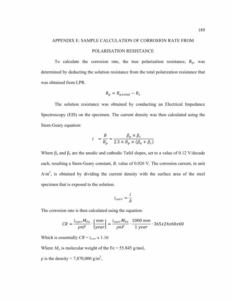
189

APPENDIX E: SAMPLE CALCULATION OF CORROSION RATE FROM

POLARISATION RESISTANCE

To calculate the corrosion rate, the true polarization resistance, Rp, was

determined by deducting the solution resistance from the total polarization resistance that

was obtained from LPR. = , −

The solution resistance was obtained by conducting an Electrical Impedance

Spectroscopy (EIS) on the specimen. The current density was then calculated using the

Stern-Geary equation:

= = ×2.3 × × ( + ) Where βa and βc are the anodic and cathodic Tafel slopes, set to a value of 0.12 V/decade

each, resulting a Stern-Geary constant, B, value of 0.026 V. The corrosion current, in unit

A/m2, is obtained by dividing the current density with the surface area of the steel

specimen that is exposed to the solution.

=

The corrosion rate is then calculated using the equation:

= ∙ = ∙ 10001 ∙ 365 24 60 60

Which is essentially CR = icorr x 1.16

Where Mw is molecular weight of the Fe = 55.845 g/mol,

ρ is the density = 7,870,000 g/m3,

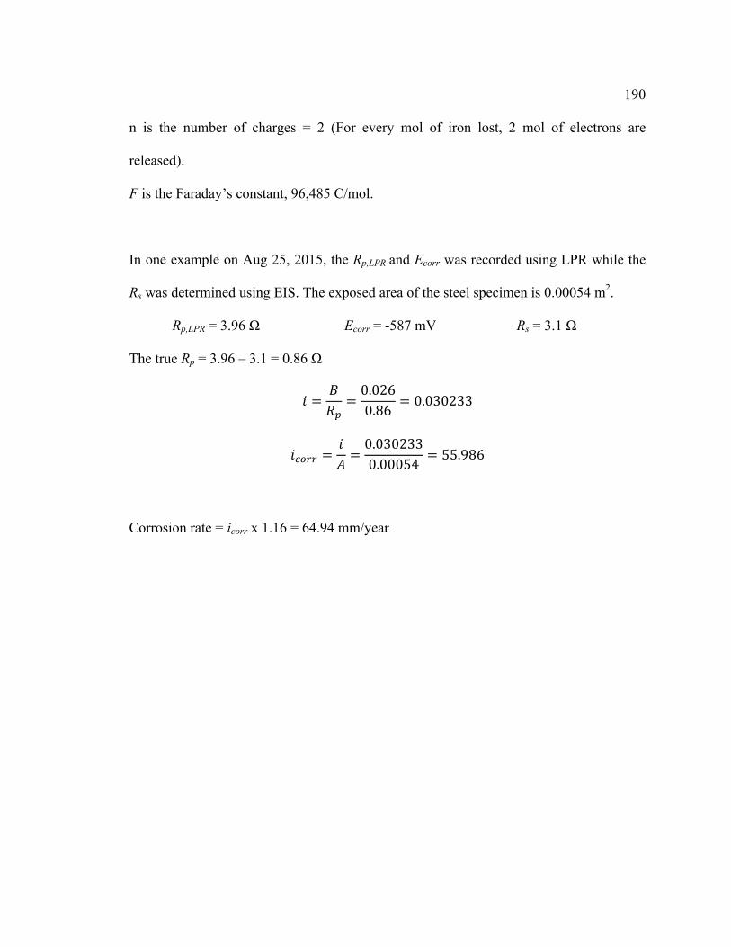
190

n is the number of charges = 2 (For every mol of iron lost, 2 mol of electrons are

released).

F is the Faraday’s constant, 96,485 C/mol.

In one example on Aug 25, 2015, the Rp,LPR and Ecorr was recorded using LPR while the

Rs was determined using EIS. The exposed area of the steel specimen is 0.00054 m2.

Rp,LPR = 3.96 Ω Ecorr = -587 mV Rs = 3.1 Ω

The true Rp = 3.96 – 3.1 = 0.86 Ω

= = 0.0260.86 = 0.030233

= = 0.0302330.00054 = 55.986

Corrosion rate = icorr x 1.16 = 64.94 mm/year

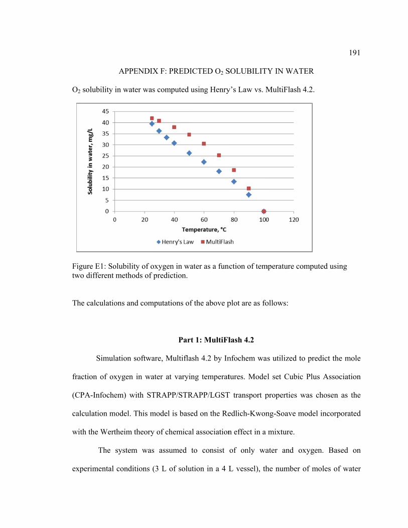
O

Ftw

T

fr

(C

ca

w

ex

O2 solubility

igure E1: Sowo different

The calculatio

Simul

raction of ox

CPA-Infoche

alculation m

with the Wert

The

xperimental

APPENDIX

in water was

olubility of omethods of

ons and com

lation softwa

xygen in wa

em) with ST

model. This m

theim theory

system was

conditions

X F: PREDI

s computed u

oxygen in waprediction.

mputations of

Par

are, Multifla

ater at varyi

TRAPP/STR

model is base

y of chemica

s assumed

(3 L of solu

ICTED O2 S

using Henry

ater as a fun

f the above p

t 1: MultiFl

ash 4.2 by In

ng temperat

RAPP/LGST

ed on the Re

al association

to consist

ution in a 4 L

SOLUBILITY

y’s Law vs. M

ction of tem

plot are as fo

lash 4.2

nfochem wa

tures. Mode

T transport p

edlich-Kwon

n effect in a

of only wa

L vessel), th

Y IN WATE

MultiFlash 4

mperature com

ollows:

s utilized to

l set Cubic

properties w

ng-Soave mo

mixture.

ater and ox

he number o

ER

4.2.

mputed using

predict the

Plus Associ

was chosen a

odel incorpo

xygen. Base

of moles of w

191

g

mole

iation

as the

orated

ed on

water

192

and oxygen was calculated. The number of moles of oxygen, calculated using the Ideal

Gas Law, is 0.16 moles. The number of moles in 3 L of water is 166.5 moles.

The software computes the mole fraction of each species in the water phase. The

mol fraction was then converted into units of solubility, grams per mole. The results are

shown in the following table.

Table E1: Results of computation using MultiFlash 4.2

Part 2: Henry’s Law

According to Henry’s Law, the partial pressure of a gas above a liquid is directly

proportional to the amount of gas that dissolves in the liquid at constant temperature. =

In this equation, the partial pressure of the gas above the liquid, and the

concentration of the dissolved gas in the solution are denoted as p and c, respectively.

The Henry’s Law coefficient, kH, is a value that depends on the solute, the solvent, and

temperature.

Total ρWater V water O2 conc

K C xO2 xH2O mol nO2 nWater mO2 mWater (kg/m 3 ) L gram/L

298.15 25 2.36E‐05 0.999976 166.499 3.93E‐03 166.495 1.26E‐01 2996.91 996.95 3.006079 0.042

303.15 30 2.30E‐05 0.999977 166.497 3.83E‐03 166.4932 1.23E‐01 2996.877 995.7 3.009819 0.041

313.15 40 2.15E‐05 0.999978 166.491 3.59E‐03 166.4873 1.15E‐01 2996.772 992.2 3.020331 0.038

323.15 50 1.97E‐05 0.99998 166.481 3.28E‐03 166.4777 1.05E‐01 2996.598 988.1 3.032687 0.035

333.15 60 1.74E‐05 0.999983 166.463 2.90E‐03 166.4602 9.27E‐02 2996.283 983.2 3.047481 0.030

343.15 70 1.45E‐05 0.999986 166.43 2.41E‐03 166.4277 7.72E‐02 2995.698 977.8 3.063712 0.025

353.15 80 1.08E‐05 0.999989 166.356 1.79E‐03 166.3542 5.74E‐02 2994.375 971.8 3.081267 0.019

363.15 90 5.98E‐06 0.999994 166.119 9.93E‐04 166.118 3.18E‐02 2990.124 965.3 3.097611 0.010

373.15 100 0.00E+00 0 0 0 0 0 0 958.4 0 0.000

mol frac in water No. of moles Mass, gramTemperature

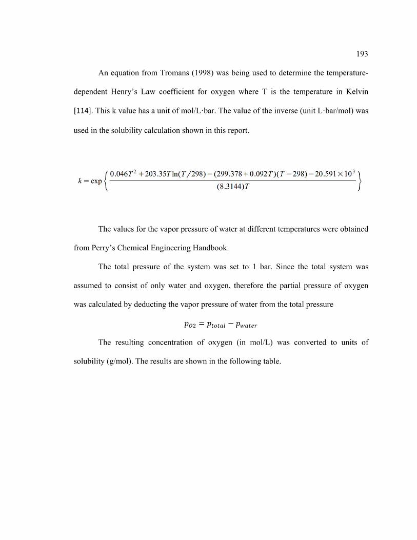
193

An equation from Tromans (1998) was being used to determine the temperature-

dependent Henry’s Law coefficient for oxygen where T is the temperature in Kelvin

[114]. This k value has a unit of mol/L·bar. The value of the inverse (unit L·bar/mol) was

used in the solubility calculation shown in this report.

The values for the vapor pressure of water at different temperatures were obtained

from Perry’s Chemical Engineering Handbook.

The total pressure of the system was set to 1 bar. Since the total system was

assumed to consist of only water and oxygen, therefore the partial pressure of oxygen

was calculated by deducting the vapor pressure of water from the total pressure = −

The resulting concentration of oxygen (in mol/L) was converted to units of

solubility (g/mol). The results are shown in the following table.

194

Table E2: Results of solubility calculation using Henry’s Law.

Discussion and Summary

Predicted value of oxygen solubility in water using two different methods was presented

in this report. Both methods have given comparable values of solubility. The solubility of

1 bar pure oxygen in water at 25°C is 40 mg/L. Values of oxygen solubility that are

commonly published are for water that is in contact with air. Since air is consist of 20%

oxygen, therefore 40 mg/L multiplied by 0.2 will result in oxygen solubility of 8 mg/L of

water.

pWater pO2 kH (T) O2

°C K bar bar L.bar/mol mol/L mg/L

25 298.15 0.031675 0.968325 783.9223 0.001235 39.52592

30 303.15 0.042432 0.957568 847.0861 0.00113 36.17227

35 308.15 0.056233 0.943767 907.898 0.00104 33.26299

40 313.15 0.073765 0.926235 965.6433 0.000959 30.6929

50 323.15 0.123347 0.876653 1069.483 0.00082 26.22936

60 333.15 0.199173 0.800827 1154.63 0.000694 22.19369

70 343.15 0.3116 0.6884 1218.654 0.000565 18.07566

80 353.15 0.473467 0.526533 1260.623 0.000418 13.36517

90 363.15 0.701013 0.298987 1280.914 0.000233 7.469054

100 373.15 1.013333 0 1280.948 0 0

Temperature O2 conc

Figuure E2. Sour

rce: engineerringtoolbox.

com [2]

195

196

APPENDIX G: SAMPLE CALCULATION FOR PITTING RATIO DETERMINATION

Example: At 80°C, 90 bar CO2, 48 hours, 1000 rpm

Weight loss corrosion rate, WL CR = 23.5 mm/year

Maximum pit depth (via profilometry) = 93 µm

Pit penetration rate, PPR,

= 0.09348ℎ × 24ℎ1 × 3651 = 17 /

Piting ratio, PR,

= = 1723.5 = 0.7

Therefore it is not prone to localized corrosion.

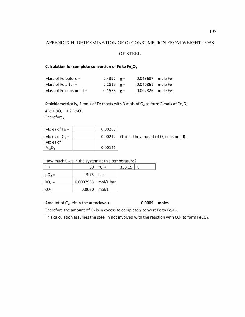
197

APPENDIX H: DETERMINATION OF O2 CONSUMPTION FROM WEIGHT LOSS

OF STEEL

Calculation for complete conversion of Fe to Fe2O3

Mass of Fe before = 2.4397 g = 0.043687 mole Fe

Mass of Fe after = 2.2819 g = 0.040861 mole Fe

Mass of Fe consumed = 0.1578 g = 0.002826 mole Fe

Stoichiometrically, 4 mols of Fe reacts with 3 mols of O2 to form 2 mols of Fe2O3

4Fe + 3O2 ‐‐> 2 Fe2O3

Therefore,

Moles of Fe = 0.00283

Moles of O2 = 0.00212 (This is the amount of O2 consumed).

Moles of Fe2O3 0.00141

How much O2 is in the system at this temperature?

T = 80 °C = 353.15 K

pO2 = 3.75 bar

kO2 = 0.0007933 mol/L.bar

cO2 = 0.0030 mol/L

Amount of O2 left in the autoclave = 0.0009 moles

Therefore the amount of O2 is in excess to completely convert Fe to Fe2O3.

This calculation assumes the steel in not involved with the reaction with CO2 to form FeCO3.

!!!!!!!!!!!!!!!!!!!!!!!!!!!!!!!!!!!!!!!

!!

Thesis and Dissertation Services

The Effect of Oxygen in Sweet Corrosion of Carbon Steel for ...

Documents

Transcript of The Effect of Oxygen in Sweet Corrosion of Carbon Steel for ...