
Structured Systems Evolution: Employing dynamic, executable ...
Upload
khangminh22Category
view
0download
0
Copyright is owned by the Author of the thesis. Permission is given for a copy to be downloaded by an individual for the purpose of research and private study only. The thesis may not be reproduced elsewhere without the pennission of the Author.

SAME Structured Analysis Modelling Environment
The Design of an Executable Data Flow Diagram and Dictionary System
A dissertation presented
in partial fulfillment of the requirements
for the degree of
Doctor of Philosophy in Computer Science
at Massey University
Thomas William George Docker
1989

The research reported in this thesis has been an investigation into the use of data
flow diagrams as a prototyping tool for use during the analysis of a system. Data flow
diagrams are one of the three main tools of structured systems analysis (the other two
are a data dictionary, and some means for representing process' logic, such as
minispecs).
The motivation for the research is a perceived need for better tools with which
analysts and end-users can communicate during the requirements gathering process.
Prototyping has been identified by many researchers and practitioners as such a tool.
However, the output from the requirements analysis phase is the specification, which is
a document that should provide the framework for all future developments of the
proposed system (and should evolve with the system). Such a document should be
provably correct. However this is seen as an ideal, and the most that can be hoped for
is a document which contains within it a mixture of formality.
Executable data flow diagrams are considered to provide an environment which
serves both as a means for communication between analysts and end-users (as they are
considered relatively easy to understand by end-users), and as a method for providing a
rigorous component of a specification. The rigour comes from the fact that, as
demonstrated in this thesis, data flow diagrams can be given strict operational semantics
based on low level ('fine-grain') data flow systems. This dual focus of executable data
flow diagrams is considered significant.
Given the approach adopted in the research, executable data flow diagrams are
able to provide an informal, flexible framework, with considerable abstraction
capabilities, that can be used to develop executable models of a system. The number of
concepts involved in providing this framework can be small. Apart from data flow
diagrams themselves, the only other component proposed in the research is a system
dictionary in which the definitions of data objects are stored. Procedural details are de
emphasised by treating the definition of data objects as statements in a single
assignment programming language during the execution of a model.
To support many of the ideas proposed in the research, a prototype
implementation (of the prototype tool) has been carried out in Prolog on an Apple
Macintosh. This system has been used to produce results that are included in this
thesis, which demonstrate the general soundness of the research.
ii

I would like to thank Professor Graham Tate, my chief supervisor, who has
provided useful guidance and support over the time taken to carry out and report on the
research discussed here. I would also like to thank Professor Mark Apperley, who as
my second supervisor, provided assistance at a critical time in the production of this
thesis. As well as these, thanks go to Dr John Hudson and Chris Phillips for reading
various portions of this tome. Last, but not least, the support provided by all the
Dockers is much appreciated.
ill

List of figures and tables xi
Chapter 1: Introduction 3 1.1 Motivation for the research . . . . . . . . . . . . . . . . . . . . . . . . . . . . . . . . . . . . . . . . . . . . . . . . . . . . . . . . . . 3
1.1.1 Methods, methodologies, tools, and techniques....................... 6
1.1.2 Formal specifications, and formal methods . . . . . . . . . . . . . . . . . . . . . . . . . . . . 6
1.1.3 Informal, semi-formal, and formal...................................... 7
1. 1 .4 Semi-formal techniques in the specification of requirements......... 8
1.1.5 Software development environments . . . . . . . . . . . . . . . . . . . . . . . . . . . . . . . . . . . 9
1. 1. 6 The software development process and the software life cycle . . . . . . 10
1.1. 7 Models, executable models, and prototypes . . . . . . . . . . . . . . . . . . . . . . . . . . . 12
Prototypes, and prototyping . . . . . . . . . . . . . . . . . . . . . . . . . . . . . . . . . . . . . . . . . . . . . 13
1.2 Objectives of the research............................................................ 14
1. 3 The approach. . . . . . . . . . . . . . . . . . . . . . . . . . . . . . . . . . . . . . . . . . . . . . . . . . . . . . . . . . . . . . . . . . . . . . . . . . 14
1.4 Structure of the dissertation......................................................... 16
Chapter 2: Structured systems analysis 1 7 2.1 Introduction . . . . . . . . . . . . . . . . . . . . . . . . . . . . . . . . . . . . . . . . . . . . . . . . . . . . . . . . . . . . . . . . . . . . . . . . . . . 17
2.2 Component tools of SSA............................................................ 18
2. 3 Data flow diagrams................................................................... 18
2.3.1 An application hierarchy of data flow diagrams....................... 20
2.4 Data dictionary........................................................................ 23
iv

CONTENTS V
2.4.1 Defming data objects...................................................... 24
Data structures and abstractions . . . . . . . . . . . . . . . . . . . . . . . . . . . . . . . . . . . . . . . . . 24
2.5 Process transformations............................................................. 26
2.5.1 Structured English......................................................... 26
2.5.2 Decision tables............................................................. 28
2.5.3 Decision trees.............................................................. 28
2.6 Combining the tools.................................................................. 30
2. 7 Using SSA in specifying requirements............................................ 31
2. 7 .1 The positive features of data flow diagrams for use in specifying requirements . . . . . . . . . . . . . . . . . . . . . . . . . . . . . . . . . . . . . . 31
2. 7 .2 Common ways of misusing data flow diagrams....................... 32
A voiding procedural details in data flow diagrams.................... 35
Avoiding control and physical details in data flow diagrams......... 36
2.8 A dictionary as a general resource.................................................. 36
2.9 Executable data flow diagrams...................................................... 38
2.10 Summary . . . . . . . . . . . . . . . . . . . . . . . . . . . . . . . . . . . . . . . . . . . . . . . . . . . . . . . . . . . . . . . . . . . . . . . . . . . . . . 39
Chapter 3: Data flow systems 4 0 3. 1 Introduction . . . . . . . . . . . . . . . . . . . . . . . . . . . . . . . . . . . . . . . . . . . . . . . . . . . . . . . . . . . . . . . . . . . . . . . . . . . 40
3 .1.1 An initial classification, and some definitions.......................... 41
3.2 Data-driven systems.................................................................. 42
3.2.1 Conditionals and loops .. . . . . . . . . . . . . . . . . . . . . . . .. . . . . . . . . . . . . . . .. . . .. . . . . . 45
3.2.2 Karp and Miller- a reference data-driven model...................... 51
3.2.3 Fine-grain data-driven architecture features............................ 52
Direct communication..................................................... 53
Packet communication.................................................... 53
Static and dynamic architectures......................................... 55
Enabling conditions and output conditions............................. 60
Summary of fine-grain data-driven systems........................... 61
3. 3 Demand-driven systems . . . . . . . . . . . . . .. . . . . . . . . . .. . . .. . . .. . . . . . . . . . . . . . .. . . .. . . . . . . . . 63
3.3.1 String reduction............................................................ 64
3.3.2 Graph reduction........................................................... 65
3.3.3 Demand-driven systems and functional languages.................... 67
3.4 Data flow systems and data flow diagrams........................................ 68
3 .4.1 Fine-grain data flow semantics applied to data flow diagrams....... 68
3.4.2 Input to output set transformations...................................... 72
3.4.3 Treating data flow diagrams and transformations independently...................................... 73
3.5 Summary.............................................................................. 74

CONTENTS ~
Chapter 4: The data-driven model in SAME 7 9 4.1 Introduction . . . . . . . . . . . . . . . . . . . . . . . . . . . . . . . . . . . . . . . . . . . . . . . . . . . . . . . . . . . . . . . . . . . . . . . . . . . 79
4.2 The operational semantics of a simple data flow diagram model(DFDMl), and its comparison with the Karp and Miller data-driven model....................................... 81
4.2.1 External entities and data stores.......................................... 84
External entities............................................................ 84
Data stores.................................................................. 86
4.3 The operational semantics of DFDM2.............................................. 87
4.3.1 Limited import and export sets........................................... 88
Limited import sets........................................................ 88
Conditional generation of data flows and limited export sets........ 90
4.3.2 Composition and decomposition of group objects.................... 93
4.4 Structural completeness of data flow diagrams................................... 95
4.4.1 Structurally complete data flow diagrams . . . . . . . . . . . . . . . . . . . . . . . . . . . . . . 97
4.4.2 Structurally incomplete data flow diagrams............................ 98
4.4.3 Invalid data flow diagrams............................................... 100
4.5 Levels of refinement.................................................................. 100
4.5.1 Hierarchy of data flow diagrams........................................ 101
4.5.2 Process sets................................................................ 102
4.6 Applications in the top level model................................................. 103
4. 7 Parallelism in the top level model................................................... 105
4.8 Deadlocks.............................................................................. 106
4.9 Summary.............................................................................. 107
Chapter S: The demand-driven model in SAME 108 5 .1 Introduction . . . . . . . . . . . . . . . . . . . . . . . . . . . . . . . . . . . . . . . . . . . . . . . . . . . . . . . . . . . . . . . . . . . . . . . . . . . 108
5.2 The lEgis language................................................................... 109
5.2.1 Options, conditionals and repeats....................................... 112
Options . . . . . . . . . . . . . . . . . . . . . . . . . . . . . . . . . . . . . . . . . . . . . . . . . . . . . . . . . . . . . . . . . . . . . 112
Conditionals ................................................................ 112
Repeats..................................................................... 113
5.3 Demand-driven interpretation of lEgis definitions................................ 116
5. 3 .1 Constructors . . . . . . . . . . . . . . . . . . . . . . . . . . . . . . . . . . . . . . . . . . . . . . . . . . . . . . . . . . . . . . . 117
Tuple constructors......................................................... 118
Stream constructors . . . . . . . . . . . . . . . . . . . . . . . . . . . . . . . . . . . . . . . . . . . . . . . . . . . . . . . 119
Basic type constructors................................................... 120
"Don't care" and empty values........................................... 121
5.3.2 Operations.................................................................. 122

CONTENTS vii
5.4 Naming and binding.................................................................. 123
5.4.1 Naming ..................................................................... 123
Environment, program, and working variables........................ 123
Version control and naming.............................................. 124
Naming of objects within SAME........................................ 124
5.4.2 Binding..................................................................... 126
5.5 Other characteristics of .tEgis and the demand-driven executable environment.................................. 128
5.5.1 Referential transparency.................................................. 128
5.5.2 Call-by-need and lazy evaluation........................................ 128
5.5.3 Typing and polymorphism............................................... 129
Strong, static, and dynamic typing...................................... 130
Polymorphism ............................................................. 131
5.6 Language design principles and .tEgis... .. . . .. . . .. . . .. . . .. . . . .. . . . . . . .. . .. . . . .. . . . . . 134
5.6.1 Procedural abstraction.................................................... 135
5.6.2 Data type completeness................................................... 135
5.6.3 Declaration correspondence.............................................. 135
5.7 Summary .............................................................................. 136
Chapter 6: The complete architecture of SAME 137 6.1 Introduction........................................................................... 137
6.2 A conceptual architecture for SAME............................................... 137
6.2.1 SID ......................................................................... 139
The structure of the dictionary, and the bindings between objects........................................ 140
Data flow diagrams as views onto data objects in the dictionary............................ 141
6.2.2 SYP ......................................................................... 146
Static definition facilities.................................................. 146
The external entity interface.............................................. 147
Data flow management (DFM)........................................... 148
Multiprocessing and the scheduling of processors.................... 148
6.3 Specifications and executions....................................................... 149
6.3.1 Specification of application environments, applications, data flow diagrams, and data objects.................... 149
6.3.2 The execution of an application.......................................... 149
Starvation................................................................... 150
Missing data objects....................................................... 150
Type conflicts.............................................................. 151
Inconsistencies, and their interpretation................................ 152
CONTENTS viii
Semantic errors............................................................ 152
6.4 Data stores in SAME .................................................................. 152
6. 4 .1 Methods of access. . . . . . . . . . . . . . . . . . . . . . . . . . . . . . . . . . . . . . . . . . . . . . . . . . . . . . . . . 154
6.4.2 Operations.................................................................. 155
6.4.3 Exceptions handling....................................................... 156
6.4.4 Name mappings . . . . . . . . . .. . . . . . . . . . . . . . . . . . .. . . . . . .. . .. . . . . . . .. . .. . . . .. . . . 156
6.4.5 Conceptual view of a data store.......................................... 159
6.4.6 A data flow view of data stores.......................................... 160
Referential transparency . . . . . . . . . . . . . . . . . . . . . . . . . . . . . . . . . . . . . . . . . . . . . . . . . . 161
6.5 Summary.............................................................................. 162
Chapter 7: An implementation 163 7 .1 Introduction . . . . . . . . . . . . . . . . . . . . . . . . . . . . . . . . . . . . . . . . . . . . . . . . . . . . . . . . . . . . . . . . . . . . . . . . . . . 163
7. 1.1 Main features of the implementation . . . . . . . . . . . . . . . . . . . . . . . . . . . . . . . . . . . . 164
7 .1.2 major features of the full SAME system that have not been implemented.......................................... 164
7 .2 An introduction to the definition subsystem through a simple example - finding the real roots of a quadratic equation............... 165
7.2.1 Creating a new application, and drawing a data flow diagram....... 165
7 .2.2 Defining data objects...................................................... 167
7 .2.3 Displaying data objects, their types, and their dependencies......... 168
7. 3 Building and running an executable model . . . . . . . . . . . . . . . . . . . . . . . . . . . . . . . . . . . . . . . . 172
7. 3 .1 Defining an executable process set...................................... 172
7. 3 .2 Running the model . . . . . . . . . . . . . . . . . . . . . . . . . . . . . . . . . . . . . . . . . . . . . . . . . . . . . . . . 173
7. 3. 3 Controlling the execution process . . . . . . . . . . . . . . . . . . . . . . . . . . . . . . . . . . . . . . . 17 6
7 .3.4 Tracing the exercising of a model . . . . . . . . . . . . . . . . . . . . . . . . . . . . . . . . . . . . . . . 177
7.3.5 Exporting to external entities ............................................. 178
7. 3. 6 Execution time exceptions.. . . . . . . . . . . . . . . . . . . . . . . . . . . . . . . . . . . . . . . . . . . . . . . 179
7. 3. 7 Exercising processes.. . . . . . . . . . . . . . . . . . . . . . . . . . . . . . . . . . . . . . . . . . . . . . . . . . . . . 180
The context of a process.................................................. 181
The fundamental algorithm for creating object instances............. 182
7 .4 Applications with multiple levels of data flow diagrams......................... 182
7.4.1 Refining (exploding) data flow diagrams ............................... 183
7.4.2 'Scope' of objects ......................................................... 184
7.4.3 Building an executable model............................................ 184
7.4.4 Hook composed data flow instances .................................... 185
7. 5 More error examples . . . . . . . . . . . . . . . . . . . . . . . . . . . . . . . . . . . . . . . . . . . . . . . . . . . . . . . . . . . . . . . . . 186
7. 5 .1 Missing data object definition............................................ 186
7 .5.2 No importers for a data flow............................................. 187

CONTENTS ix
7. 6 Limited import sets, conditional exports, and loops.............................. 188
7.7 Prolog as the implementation language............................................ 191
7 .8 Summary.............................................................................. 192
Chapter 8: An example analysis 193 8.1 introduction............................................................................ 193
8.2 A SAME model of the order processing example................................. 194
8.2.1 The application data flow diagram hierarchy........................... 194
8.2.2 The data object definitions for the application.......................... 196
8.3 The frrst prototype.................................................................... 201
8.3.1 The data stores contents .................................................. 202
8. 3 .2 Selected details from the development of the frrst prototype . . . . . . . . . 202
8. 4 The second prototype . . . . . . . . . . . . . . . . . . . . . . . . . . . . . . . . . . . . . . . . . . . . . . . . . . . . . . . . . . . . . . . . 211
8.5 Summary .............................................................................. 216
Chapter 9: Alternative architectures 219 9. 1 Introduction ............................................................................. 219
9.2 Other executable coarse-grain data flow schemes ................................... 220
9.2.1 The LGDF approach ofBabb .............................................. 220
9 .2.2 The Ada information management system prototyping environment of Burns and Kirkham ........................ 222
9.2.3 The DataLink environment of Strong ..................................... 223
9.3 Structured Analysis Simulated Environment (SASE) .............................. 224
9.3.1 META ......................................................................... 225
9. 3 .2 The SASE process sub-system ............................................ 226
9.3.3 SASE as a means for building implementation models ................. 227
9. 4 Comparative summary ................................................................. 227
9.5 Networks of von Neumann systems ................................................. 229
9. 6 Summary ................................................................................ 231
Chapter 10: Conclusions and further research 232 10.1 Summary and conclusions ............................................................. 232
10.1.1 Objectives of the research ................................................. 233
10.1.2 That the executable model be rigorous enough to form part of the specification ...................... 233
10.1.3 That the tool should have a small number of (simple) concepts ..................................... 234
10.1.4 That procedural details should be de-emphasised ...................... 234
10.1.5 That the tool should incorporate high levels of abstraction in a relatively simple manner ................ 234

CONTENTS X
10.1.6 That the tool should make effective use of graphics .................... 235
10.1.7 That the tool should provide 'soft' recovery from errors .............. 235
10.1.8 That the tool should be able to execute 'incomplete' models .......... 236
10.1.9 Primary objective ........................................................... 237
10.2 Further research ......................................................................... 237
Glossary 239
Bibliography 257

Figures 1.1 The waterfall model of the software life cycle,
showing the overlapping of stages................................................. 12
2.1 Comparison of the Gane and Sarson, and De Marco data flow diagram notations ........................................ 18
2.2 Context, or Level 0, data flow diagram for an order processing system..................................................... 20
2.3 Level 1 refinement of process ORDER PROCESSING ................................. 21
2.4 Level 2 refinement of process PRODUCE INVOICE................................... 22
2.5 The hierarchy of processes for the order processing application modelled in Figures 2.2 to 2.4 . . . . . . . . . . . . . . . . . . . . . . . . . . . . . . . . . . . . . . . . 22
2. 6 A possible data structure hierarchy of the INVOICE data flow shown in Figures 2.2 to 2.4... ................. ...... .... .......... .. ... 24
2. 7 A structured English minispec for calculating the status of a customer.................................................................. 27
2. 8 A decision table for calculating the status of a customer......................... 28
2.9 A decision tree for calculating the status of a customer .......................... 29
2.10 An integrated view of three tools described in Section 2.5, showing how they combine to form a logical model of an application . . . . . . . . . . . . . . . . . . . . . . . . . . . . . . . . . . . . . . . . . . . . . . . . . . . . . . . . . . . . . . . . . . . . . . 30
2.11 Excerpt from a 'loose' data flow diagram in Wasserman et al. [WPS86] ...................................................... 33
2.12 Excerpt from a 'loose' data flow diagram in Booch [Bo86] . . . . . . . . . . . . . . . . . . . . 34
xi
FIGURES AND TABLES xii
3 .1 Data dependency graph for finding the (real) roots of a quadratic .......................................................................... 43
3.2 Data flow graph for finding the (real) roots of a quadratic .......................................................................... 44
3.3 A data-driven program for finding the (real)
roots of a quadratic................................................................... 45
3 .4 A data flow graph for the conditional if x > y then a : = v1 else a := v2 ................................................ 46
3. 5 A cyclic data flow graph for calculating the factorial of N. . . . . . . . . . . . . . . . . . . . . . . 4 7
3.6 The general structure of a 'safe' while-loop in a data flow graph.................................................................. 48
3. 7 The occurrence of deadlock in a data-driven program graph.................... 49
3. 8 The occurrence of a race condition . . . . . . . . . . . . . . . . . . . . . . . . . . . . . . . . . . . . . . . . . . . . . . . . . 50
3. 9 The functional structure of a processing element in a token storing data-driven system.............................................. 54
3 .10 The functional structure of a processing element in a token matching data-driven system............................................ 55
3 .11 A conceptual snapshot of an Id data flow program showing the token <U.c.s.i, 4> on the arc connected to input port 2 of the instruction (activity) s ....................................... 57
3 .12 A data flow graph for the processing of the loop by the U-interpreter ...................................................................... 59
3 .13 A categorisation of data-driven machines. The machines discussed in this chapter are shown in the rectangles ............................ 61
3 .14 A demand-driven program for finding the (real) roots of a quadratic. . . . . . . . . . . . . . . . . . . . . . . . . . . . . . . . . . . . . . . . . . . . . . . . . . . . . . . . . . . . . . . . . . . 63
3 .15 A string reduction execution sequence for the part of the program in Figure 3.14 which finds the first root.. .......................... 64
3 .16 A graph reduction program corresponding to Figure 3 .14 . . . . . . . . . . . . . . . . . . . . . . 66
3 .17 The program graph of Figure 3.16 with reverse pointers . . . . . . . . . . . . . . . . . . . . . . . 67
3 .18 Level 1 data flow diagram, and data dictionary definitions for finding the (real) roots of a quadratic equation . . . . . . . . . . . . . . . . . . . . . . . . . . . . . . . 69
3 .19 Level 1_ data ~ow. diagram for finding the (real) roots of a quadranc applicanon . . . . . . . . . . . . . . . . . . . . . . . . . . . . . . . . . . . . . . . . . . . . . . . . . . . . . . . . . . . . . . . . . 70
3.20 Accessing the data store CUSTOMERS using cusT_# as the key ................... 71
3.21 Processing one COURSE_CODE against multiple STUDENT_# tokens .............. 71
4.1 Level 0 data flow diagram for the order processing example . . . . . . . . . . . . . . . . . . . 80
4.2 Level 1 data flow diagram ........................................................... 80
4.3 Level 2 data flow diagram for process PRODUCEINVOICE ••.••••••..•.•••••••••••• 80
4.4 Data flow diagram hierarchy for the order processing application, showing the leaf processes shaded . . . . . . . . . . . . . . . . . . . . . . . . . . . . . . . . . . 80
4.5 External entity e1, CUSTOMER, as the set {INVOICE, ORDER_DETAILS,UNFILLABLE_ORDER} of phantom nodes ................ 86
4.6 An example which shows the decomposition and

FIGURES AND TABLES xiii
composition of data flows in data flow diagrams................................. 93
4. 7 A structurally incomplete form of Figure 4.2 ..................................... 100
4. 8 Possible different data flow process explosion trees created during the analysis of an application ...................................... 101
4. 9 Virtual leaf process data flow diagram, Cop, for the order processing application ........................................................ 104
4.10 A snapshot of order processing transaction histories ............................ 105
5 .1 Dictionary definitions relating to INVOICE ••..........•••••••..•..........••.•••••.• 110
5. 2 Example invoice ...................................................................... 114
5. 3 Dependencies graph for INVOICE •••••••••••.......•..••••••••.....•••..•••••••.••••• 117
5. 5 The identity function id implemented in four languages that support parametric polymorphism .................................................. 132
6.1 A conceptual architecture for SAME ............................................... 138
6.2 Dictionary definitions relating to the objects in process 3, PRODUCE_INVOICE ......................................................... 139
6.3 An example invoice corresponding to the definitions in Figure 6.2 .......................................................................... 140
6. 4 Data object dependencies in process 3, PRODUCE INVOICE .••.••••••.•••••••..•.•• 142
6.5 Data object dependencies in the refinement to process 3, PRODUCE INVOICE •••••••••••••••.••.•••.•.•••••..••••••..•••••••••••••• 143
6,6 Using an example to show the associations (bindings) between objects in SYD ............................................................. 145
6. 7 Accessing the data store CUSTOMERS using cusT_# as the key ................... 154
6.8 Adding a 'control' dimension to a data flow diagram in which the keys for accessing data store tuples (among other things) can be specified ............................................. 155
6.9 Part of a data flow diagram implicitly showing multiple data flows referencing the same data store object (not necessarily the same instance) ................................................. 158
6.10 A conceptual view of a SAME data store .......................................... 160
7.1 Naming an application ............................................................... 165
7. 2 A Level 0 data flow diagram in the manner of Figure 3 .18 ..................... 166
7. 3 The structural details of the data flow diagram in Figure 7 .2 ................... 167
7.4 Defining the data object coefficients to be the tuple (a, b, c) ............ 167
7. 5 A dialogue containing a menu for selecting the data objects to display ................................................ 169
7. 6 Display of all data objects currently in the dictionary ............................ 169
7. 7 The internal representation of data object definitions for the roots example ................................................................. 169
7 .8 Redundant rhs facts which are used extensively in displaying data object dependencies ............................... 170
7. 9 A listing of data objects showing their (inferred) types .......................... 170
7 .10 A request to display the dependency graph, to the selected depth, of the data objects depended on by data flow

FIGURES AND TABLES xiv
roots in process findRootsOfQuadratic .................................................... 171
7 .11 Data dependency graph for data flow roots in process f indRoot sOfQuadra t ic ................................................................................ 172
7 .12 Specifying the executable model process set ...................................... 173
7 .13 Request for user to supply external entity generated data flow instances ................................................................... 173
7 .14 Sequence of requests for sub-object values for an instance of data flow coefficients ....................................... 176
7 .15 An ex amp le full trace ................................................................. 177
7 .16 The executable model representation of external entity an a 1 y st ........................................................... 177
7 .17 An example error display prompt generated by SAME during the creation of an instance of the data object root 1. Particularly, a request to find the square root of -15 has been trapped. (The user has supplied a further invalid value. See Figure 7 .18.) .............. 178
7 .18 Following the user supplying an invalid value (as shown in Figure 7 .17), SAME displays an error message. The user must supply a positive number before SAME will continue ...................... 179
7 .19 Messages generated under full trace which relate to the two attempts to find the square root of a negative number ............................ 179
7 .20 The data flow reduction graph for data flow roots evaluated in the context of process findRootsOfQuadratic ..................................... 181
7 .21 A particular refinement of the process findRootsOfQuadratic into the two processes computeRoot 1 and computeRoot2 ..................... 183
7 .22 A particular refinement of the process findRootsOfQuadratic into the two processes computeRootl and computeRoot2 ..................... 184
7 .23 A request to form an application model from the leaf level processes that are descendants of the process findRootsOfQuadratic (namely the two processes computeRootl and computeRoot2) ................ 185
7 .24 An instance of the data flow roots exported to the external entity analyst by the hook roots ................................... 185
7 .25 Amendments to data object definitions for the roots application, with an omission in the definition of the object sqr ...................................................... 186
7 .26 An error dialogue of the same general format as Figure 7 .17, which indicates that no value could be found nor generated for data object sqr .................................................................... 187
7 .27 Following the declaration of the data object sqr as sqr<=sqrt(bsq - fourAC), the object dependencies will be as shown .................. 187
7 .28 A different refinement of process f indRoot sOfQuadratic .................... 188
7 .29 An error dialogue stating that no importers exist for data flow n 1. ................................................ 188
7 .30 A data flow diagrn,.'11 which contains a loop ....................................... 189

FIGURES AND TABLES xv
7 .31 Data object definitions for the looping application; and an execution trace ................................................................ 190
7 .32 Prompt to the user to define the action to take when a currency mismatch occurs, in the case where the automatic flushing of instances has been turned off .......................................... 191
8. 1 Level O data flow diagram for the revised order processing application ........................................................ 194
8.2 Level 1 refinement of check:AndFill0rder ...................................... 195
8.3 Level 1 refinement of produceinvoice ........................................... 196
8.4 Data object definitions ............................................................... 200
8.5 Data dependency graph for data object invoice ................................. 200
8. 6 Data object definitions which differ from those given in Figure 8.4 .............................................. 201
8. 7 Data store tuples used in the first prototype ....................................... 202
8. 8 Data store access details for constructing instances of data flow customer_details ....................................... 204
8. 9 The objects to be mapped between the data flow adjusted credit and the customer data store tuple component cust_available_credit .................. 208
8.10 The generation of an invalid instance of cust_available_credit ........... 210
8.11 The instance of rejected order, which correctly identifies the customer's lack of available credit ............... 211
8.12 Revised form of Figure 8.1, with the data store parts replaced by the external entity parts ...................... 212
8.13 An instance of data object updated_part_details which contains multiple parts_remaininginstances .......................... 215
8.14 An instance of data object invoice which contains multiple line item instances ....................................... 216
9 .1 Executable META minispec for process p3, PRODUCE INVOICE •.•••.••...••.•.•••••••.••••.•.••••••..•••••..•••••••••• 225
9.2 A conceptual structure for a coarse-grain processing element ................... 230
Tables I Important properties of requirements and
design specifications, as identified by Howden [Ho82a]........................ 4
II The data dictionary language notation of De Marco . . . . . . . . . . . . . . . . . . . . . . . . . . . . . . 25
III A comparison of some reported date-driven architectures....................... 62
N Example tuple instances for specific definitions .................................. 118
V Example tuple instances for group object definitions ............................ 121
VI Example tuple instances using basic type constructors .......................... 121
VII The possible bindings between dictionary objects ................................ 144
VIII A comparison of some coarse-grain data flow schemes ......................... 228

Part I contains the background material to the research reported in the
dissertation.
In Chapter 1 the motivation for the research is described, along with a statement
of the objectives. The principle objective has been to investigate the use of executable
data flow diagrams as a prototyping tool for use during the analysis phase of the
software life cycle. The approach adopted to achieve this objective is also given.
Chapters 2 and 3 contain discussions of the more important support material. In
Chapter 2 structured systems analysis, which is the method that has data flow diagrams
as a component tool, is discussed. Both advantages and disadvantages in the use of
structured systems analysis, and data flow diagrams in particular, are enumerated.
In Chapter 3 low level ('fine-grain') data flow schemes are discussed, and
characteristics which are particularly useful to a high level ('coarse-grain') data flow
system are identified.
2

1.1 Motivation for the research In the design of a software system, the output from a requirements capturing
exercise is the specification, which is a document that contains an abstract computer
orientated representation of the set of end-user requirements.1
Producing a correct specification is seen to be the key to the successful, cost
effective development of software systems [Bo76]. There are, however, problems in
knowing when a specification is correct, and even when it is complete; not least
because of the problems of adequately specifying what is required in the first place. In
the context of the specification of requirements, Howden has stated that ([Ho82a],
p. 72):
'The principle idea in the analysis of requirements specifications is to make sure
that they have certain necessary properties.'
Howden tabulates some of the more important of these properties, included here
as Table I.
Some of the properties, notably completeness, must be viewed as ideals which
cannot be achieved in many software development projects.
1 Terms in bold type are included in the Glossary. In general, the term 'end-user(s)' will refer to the potential users of the system being analysed, who are considered not to be software developers. The terms 'user' and 'analyst' are used to refer to the person(s) carrying out the analysis. The term 'user' generally appears when the application of an analysis technique, or tool, is being discussed.
3

CHAPTER 1 - INTRODUCTION
Property Comments
Consistency Specifications information must be internally consistent. If the information is duplicated in different documents, consistency between copies must be maintained.
Completeness Specifications must be examined for missing or incomplete requirements and design information. All specification functions must be described, including important properties of data.
Necessity Each part of the specified system should be necessary and not redundant.
Feasibility The specified system should be feasible with existing hardware and technology.
Correctness In some cases, it is possible to compare part of the specification with an external source for correctness.
Table I: Important properties of requirements and design specifications, as identified by Howden [Ho82a].
4
Parnas and Clements enumerated various problems in the area of software
design [PC85]. Some of particular interest, are couched below in requirements
specification terms:
• In most cases the end-users do not know exactly what they want and are unable to
state what they do know.
• Even if the initial requirements were known, other requirements usually surface as
progress is made in the development of the software.
• Even if all of the relevant facts had been elicited and included in the specification,
experience shows that human beings are unable to fully comprehend the plethora of
details that must be taken into account in order to progress into the design and
building of a correct system.
• Even if all of the detail needed could be mastered, all but the most trivial projects are
subject to change for external reasons. Some of those changes may invalidate
previous requirements.
• Human errors can only be avoided if one can avoid the use of humans. No matter
how rational the requirements specification process, no matter how well the relevant
facts have been collected and organised, errors will be made.

CHAPTER 1 - INTRODUCTION 5
These problems suggest that as requirements are likely to change during
analysis, flexibility should exist in the methods and tools used to capture requirements.
As well, consistency needs to be maintained. In fact, checking for consistency is seen
to be the property in Table I which is the most achievable using computer tools. Given
the right tools, computers are particularly good at this type of task.
The correct specification of requirements is seen as the key to the successful,
cost-effective development of software systems [Bo76]. It is also generally agreed that
to be able to validate requirements, they must be rigorously specified. As Davis
succinctly puts it ([Da88], p. 1100):
'Use a formal technique when you cannot afford to have the requirement
misunderstood.'
In an attempt to improve both the capturing of requirements, and the production
of a specification document that can be effectively used throughout the software
development process, considerable effort is being expended on developing formal
specification methods (see, for example, [GT79a, BO85, Wa85, He86, Jo86, ZS86]).
However, most, if not all, of the techniques proposed use formal methods and
languages which require a reasonably sophisticated level of mathematical maturity to be
fully understood. This tends to make them unsuitable as communications media
between analysts and most end users; which is unfortunate, as a further major
perceived parameter in the requirements capturing process is the active involvement of
end users (see, for example, [Al84, BW79, CM83, De78, Ea82, 1084, MC83, Ri86,
SP88]).
Speaking specifically about understanding software requirements specifications,
Davis has observed that ([Da88], p. 1112):
'understandability appears to be inversely proportional to the level of
complexity and formality present.'
There can be seen to be a tension between the need on the one hand for an
unambiguous, succinct, specification of requirements as the output from the analysis
process, and (at the least) the need to validate those requirements with end users.
Part of the purpose of the research reported herein has been an attempt to
address some aspects of this tension by adding formality, in the shape of a strict syntax
and operational semantics, to the data flow diagrams of structured systems
analysis (SSA), a semi-formal technique, to produce a computer-assisted
software engineering (CASE) prototyping tool. Data flow diagrams are considered
relatively easy to understand [De78, Ri86, YBC88], yet they have the potential to be
viewed more formally as high level data flow program graphs [Ch79].
The subsequent sections of this introduction more fully develop some of the
background to the research.

CHAPTER 1 - INTRODUCTION 6
1.1.1 Methods, methodologies, tools, and techniques Quite often confusion exists in the use of the words 'method' and
'methodology'. The sense in which they are used in this thesis is as follows
(Fr80, MM85]:
Definition: A method consists of prescriptions for carrying out a certain type
of work process; that is, it is a way of doing something. •
Definition: A methodology is a collection of methods and tools, along with
the management and human-factors procedures necessary to their
application. •
Also 'tool' is used with a particular meaning (Fr80, MM85]:
Definition: A tool is an aid, such as a program, a language, or documentation
forms, that helps in the use of a method. •
Frequently, in this dissertation, the term 'technique' appears. It is used informally
as an abstraction. For example, a set of objects may be described as 'techniques' when,
say, some of them are 'methods' and the rest are (parts of) 'methodologies'.
1.1.2 Formal specifications, and formal methods The application of formal methods is viewed by many as being necessary for
the correct and unambiguous specification of objects (see, for example, (AP87, GM86,
Jo86, LZ77]). Consequently considerable effort is being spent on research in this area.
'Formal methods' and 'formal specifications' are widely used terms that imply the use
of strict syntax and semantics in the description of objects; whether the objects are
statements, programs, requirements, or something else.
The following definitions make clear what is meant by 'formal specification'
and the related term 'formal method':
Definition: A formal specification is a specification which has been
defined completely in a language that is mathematically precise in
both syntax and semantics. •
Definition: A formal method is a method with a rigorous mathematical
basis. •

CHAPTER 1 - INTRODUCTION 7
The extent to which formal methods can be successfully used is unknown.
Although some formal methods have been used to specify significant applications
[Su82, STE82], the correctness of the specifications has not been proved, and, in some
cases, has been shown to be incorrect [Na82]. As discussed in the next section, it
appears that the most that can be hoped for in practical situations is a specification in
which amenable parts of the requirements have been formally specified [Na82]. Any
specification which is not a formal specification will be described simply as a
'specification'. The integration of formal and informal specifications is considered
necessary. As Gehani and McGettrick have put it ([GM86], p. vii):
'Formal specifications do not render informal specifications obsolete or
irrelevant; although they [formal specifications] can be checked to some degree
for completeness, redundancy and ambiguity, and can be used in program
verification, they are often hard to read and understand. Consequently, informal
specifications are still necessary as an aid to the understanding of the system
being designed; informal and formal specifications complement each other.'
1.1.3 Informal, semi-formal, and formal The problems with proving the correctness and general applicability of formal
methods has led to the view that formal methods cannot be used without recourse to
informal techniques for specifying requirements (nor even for specifying programs)
[MM85, Na82, Fe88]. Naur has suggested that 'formality' should be viewed as an
extension of 'informality' [Na82]. He states that
'the meaning of any expression informal mode depends entirely on a context
which can only be described informally, the meaning of the formal mode having
been introduced by means of informal statements.'
Naur, himself, quotes from Zemanek discussing software development [Ze80]:
'No formalism makes any sense in itself; no formal structure has a meaning
unless it is related to an informal environment[ ... ] the beginning and the end of
every task in the real world is informal.'
The view of Naur is supported by Mathiassen and Munk-Madsen, who have
taken Naur's arguments, which were directed at program development, and applied
them to the more general area of systems development [MM85]. Both the views of
Naur, and Mathiassen and Munk-Madsen, are supported here. As a consequence, the
following are offered as definitions for 'informal' and 'formal' in the context of
describing some object:
Definition: The informal description of an object is a description that is done
without recourse to formal methods. •

CHAPTER 1 - INTRODUCTION 8
Definition: The formal description of an object is a description that is done
with recourse to formal methods. •
Note that a 'formal' description could include 'informal' descriptions within it,
as it is 'with recourse to' rather than 'solely with'. The counter-argument does not
apply: an 'informal' description contains no 'formal' descriptions within it.
It is possible to perceive of a spectrum of descriptions, going from informal at
one end, to totally formal at the other end. This is in keeping with Naur's proposals
[Na82].
The term 'semi-formal' is used loosely to describe any technique that is formal,
but with distinctly informal components. An example would be the structure charts
of structured design when interpreted using the algebraic approach(es) of Tse [St81,
Ts85, Ts85a, Ts86, Ts87, YC79].
1.1.4 Semi-formal techniques in the specification of requirements
Techniques of an informal nature for specifying requirements abound. The most
widely used is narrative text, but this frequently results in large, ambiguous, and
incomplete specifications that lead to communications problems between analysts and
end users; particularly when attempts are made to validate requirements [De78, Da88].
Starting in the early 1970's, semi-formal structured techniques have been
developed over the years in an attempt to improve both the approach to analysis, and to
place the emphasis more on the graphical presentation of information as a better method
of communications. Included in the structured approaches for the capturing and
specification of requirements are, Structured Analysis and Design Technique (SADT)
[Co85, Ro77, RS77, Di78, Th78], Information Systems work and Analysis of
Changes (ISAC) [BH84, LGN81, Lu82], Software Requirements Engineering
Methodology (SREM) [Al77, Al78, AD81, BBD77] which is more suited to embedded
real-time systems, and the class of techniques called 'structured systems analysis'
(SSA) [CB82, De78, GS79, We80].
All of these have quite powerful abstraction capabilities which allow, for
example, objects in diagrams to be exploded into lower level diagrams in a top-down
fashion.
SSA techniques are the most widely publicised and used techniques, and are
based on data flow diagrams, which show the system in terms of data precedences: a
data-orientated approach. The SSA techniques also happen to be the most informal
of those mentioned. It is impossible to say whether their popularity is due to their
relative simplicity, although some statistical evidence does exist to suggest that this may

CHAPTER 1 - INTRODUCTION 9
be the case: in comparing the use of data flow diagrams and IDEFo (the graphically
based function modelling part ofIDEF, a component of SADT), Yadav et al. concluded
that data flow diagrams appear slightly easier to use [YBC88].
Though the graphical features of the SSA techniques are seen to aid
communications between analysts and end users, they lack the necessary level of rigour
to satisfactorily facilitate the validation of requirements [Fr80, Ri86]. The lack of rigour
in these techniques stems from their generally free interpretation, which is due more to
a lack of strict semantics than a lack of syntax. Unfortunately, this lack of rigour invites
misuse [Do87]. It also leads to the possibility of incorrect, and ambiguous
specifications. Consequently, as a specification technique, SSA suffers from many of
the problems of narrative text. This is not surprising, because SSA still places a
reasonably heavy reliance on the use of textual data, although its syntax is generally,
but not completely, more formal than narrative text.
Some of the weaknesses of SSA are discussed in more detail in Chapter 2. At
this time it should be noted that they exist, and that an attempt to add formality to SSA
can be usefully applied to minimising the dependence on purely textual data. The means
used to achieve this minimisation is sketched out in Section 1.3, while the details form
the subject matter of Part II of this dissertation.
SSA has three major component tools which are of particular relevance in the
dissertation. These are:
• Data flow diagrams - An application is modelled by a hierarchy of data flow
diagrams which show how data flows through the application.
• Data dictionary - The description of data objects, and the transformations carried out
on them (by processes), are maintained in a data dictionary.
• Process specifications - For each bottom level (leaf) process, its process
specification (the process logic) describes how the data which flows into the
process is transformed into the data which flows out of the process.
These and the other component tools will be discussed more fully in Chapter 2.
1.1.5 Software development environments In looking to define any tool for the capturing of requirements, consideration
should be given to the environment in which that tool will be focussed. The current
approach in software engineering is to develop tools within a framework known as
a software development environment (SDE). SDEs are also known as
software engineering environments (SEEs), and integrated project (or
program) support environments (IPSEs).

CHAPTER 1 - INTRODUCTION 10
The fundamental purpose of a SDE is to provide a computer-based set of
methods and tools - a methodology to support the software (development)
process. The existence of a cohesive methodology is fundamental, as this
encapsulates the process model used in software development. In Dowson's words
([D086], p. 6),
'We take the position that an unstructured "bag of tools" does not qualify as a
software development environment.'
Attempts have been made to define environments made up from existing
methods and tools. Howden discusses the architecture for four possible SDEs, each
based on the waterfall model of the software process [Ho82]. The differences between
the environments is the number and sophistication of the methods and tools included.
What is apparent is the large number of 'discontinuities' which exist between the
different tools in each proposed environment. These discontinuities have to be bridged
generally by manual means, which makes them error-prone and unsatisfactory for the
development of other than small software projects.
The following definition emphasises the need for integration ([WD86], p. 5):
Definition: A software development environment is a coordinated
collection of software tools organised to support some approach to
software development or conform to some software process
model. •
It is argued that the real value of a SDE comes from the integration between the
various methods and tools that it uses. This integration is provided by a specialised
data base environment. Conceptually, these specialised data bases have much in
common with the more recent of the data dictionary systems, which also aim to
provide an integrated view, and control, of (all) the objects in some context (whether,
say, the context is an enterprise, or some division or department of that enterprise).
1.1.6 The software development process and the software life cycle
The underlying structure of a SDE is the particular software process
development model adopted by the architects of the SDE. The purpose of this section is
to determine what a process development model is, and whether a standard model and,
hence, SDE exists into which the proposed tool could be usefully placed.
The software development process (also called the software life cycle) is
frequently shown as consisting of a number of stages, such as requirements, design,

CHAPTER 1 - INTRODUCTION 11
implementation, testing, and operation and maintenance [So85].2 The activities carried
out in each of these stages is described by Sommerville as ([So85], p. 3):
• Requirements analysis and definition -The system's services, constraints and goals
are established by consultation with system end-users. Once they have been agreed,
they must be defined in a manner which is understandable by both end-users and
development staff.
• System and software design - Using the requirements definition as a base, the
requirements are partitioned to either hardware or software systems. This process is
termed systems design. Software design is the process of representing the functions
of each software system in a manner which may be readily transformed to one or
more computer programs.
• Implementation and unit testing - During this stage, the software design is realised
as a set of programs or program units which are written in some executable
programming language. Unit testing involves verifying that each unit meets its
specification.
• System testing - The individual program units or programs are integrated and tested
as a complete system to ensure that the software requirements have been met. After
testing, the software system is delivered to the customer.
• Operation and maintenance - Normally (although not necessarily) this is the longest
life cycle phase. The system is installed and put into practical use. The activity of
maintenance involves correcting errors which were not discovered in earlier stages of
the life cycle, improving the implementation of system units and enhancing the
system's services as new requirements are perceived.
Figure 1.1 shows the waterfall model view of this process, including:
• The overlap between the stages - There are no 'clean' division points between the
activities across stages.
• The feedback (and feed-forward) between the pre-operational development stages
The next stage in the process is dependent on work carried out in the previous
stage(s) (feed-forward). Identifying errors, or accounting for changes, etc., require
changes to previous stages (feedback).
• The feedback from the operational and maintenance stages - Once an application
becomes live, errors may surface, or changes be required over time, which lead to a
feedback to earlier stages.
2 It is possible to define 'software development process' and 'software life cycle' to have significantly different meanings. Compare, for example, the definition for 'software (development) process' in the Glossary with the following definition for 'life cycle' ([MRY86], p. 83): 'The system life cycle is the period of time from the initial perception of need for a software version to when it is removed from service'.

CHAPTER 1 - INTRODUCTION
requirements
design operations
and
testing t-11----l maintenance
Figure 1.1: The waterfall model of the software life cycle, showing the overlapping of stages
(based on Sommerville [So85], Figs 1.1 and 1.2).
12
The end points of the stages in the waterfall model are generally seen to coincide
with major documentation and review points. They also tend to correspond with points
at which major changes occur in the techniques and or environments used for the
development, such as at the interface between (structured) design and implementation,
where a switch is made from using two-dimensional structure charts to using a one
dimensional programming language [YC79].
The model in Figure 1. 1 is extremely abstract, and a number of important
features have been omitted, including:
• An indication of parallel activities within phases - Invariably, on other than the
smallest projects, developers work in tandem. This is certainly true of the
implementation phase, when a number of programmers will likely be concurrently
developing modules.
• An indication of whether or not prototyping is supported, and if so, where.
• An explicit indication of where verification and validation take place.
Figure 1.1 highlights a current major problem in the description of the software
process: the lack of a definitive process metamodel with which software process
models can be described, and checked for correctness and completeness [PC85,
WD86]. However, as this is a major research topic in itself, it will not be pursued
further here. Instead, the waterfall model of Figure 1.1 is accepted as adequate for the
purposes of the research reported herein.
1.1. 7 Models, executable models, and prototypes The use of models in analysis is now seen as fundamental. According to Quade
([Qu80], p. 31):
'Analysis without some sort of model, explicit or otherwise, is impossible.'

CHAPTER 1 INTRODUCTION 13
The following defines what a 'model' is understood to be:
Definition: A model of an object is a representation which specifies some but
not all of the attributes of the object. •
In the development of computer software, models are seen to be most useful if
they are executable [Ri86].
Definition: A dynamic model of an object is a model which can be made to
carry out a set of operations, possibly in some specified
sequence. •
An 'executable model' is merely a dynamic model, which in the context of
software development specifies a software model that can be exercised on a computer.
Prototypes, and prototyping As Carey and Mason have observed (CM83, p. 177), in computing:
'there appears to be little if any agreement on what a prototype is.'
The following simple definition is considered adequate:
Definition: A prototype is a model. •
A prototype is either an abstraction of the object it is modelling, a 'mock-up', or
it is a detailed representation of part of the object. SSA provides good facilities for
modelling parts of systems, as described in Chapter 2.
By implication, the medium used to construct a prototype need not be the same
as that used for the final object. A prototype of a menu system, for example, could be
constructed using the transition diagram interpreter (TDI) part of RAPID/USE
[WPS86], and then the real system could be constructed as part of a larger integrated
project using a language such as PL/I.
Definition: Prototyping is a method for building and evaluating prototypes. •
The purpose of prototyping, as it is seen here, is the same as that stated by
Carey and Mason ([CM83], p. 180):
'Our focus in this paper is on improving the final information system product
through use of prototypes to illuminate more clearly the [end-]user's real
needs.'

CHAPTER 1 - INTRODUCTION 14
This view of prototyping, as a productive way for analysts and end-users to
interact, is commonly held throughout the literature (see, for example, [AHN82, Al84,
BW79, CM83, Ea82, IH87, JS85, KS85, MC83, NJ82, SP88]). No other purpose
for prototyping is stressed here, although claims have been made for it as a replacement
for the 'classical' sofware development process [NJ82]. See, for example, the
discussion and references in Carey and Mason [CM83].
Different approaches to prototyping in computing have been enumerated [IH87,
JS85]. Ince and Hekrnatpour, provide the following taxonomy ([IH87], p. 9):
• Throw-it-away' prototyping - Which involves the production of an early version of
a software system during requirements analysis. This is then used as a learning
medium between the analyst and the end-user during the process of requirements
elicitation and specification.
• Incremental prototyping - Where a system is developed one section at a time, but
within a single overall software design.
• Evolutionary prototyping - Where a system is developed gradually to allow it to
adapt to the inevitable changes that take place within an enterprise.
1.2 Objectives of the research The principal objective of the research, has been to investigate the use of
executable data flow diagrams as a prototyping tool during the analysis phase of the
software life cycle.
Implicit in this objective are the following further objectives:
• That the executable model, which is a significant output of a prototyping exercise, be
rigorous enough to form part of the specification, if required.
• That to serve as an adequate communications medium between analysts and end-
users, the tool should:
have a small number of (simple) concepts;
de-emphasise procedural details;
incorporate high levels of abstraction in a relatively simple manner;
make effective use of graphics.
• To be an effective prototyping tool at the analysis stage, as well as the list of features
just given, the tool should:
- provide 'soft' recovery from errors;
- be able to exercise 'incomplete' models.
1.3 The approach In arriving at the objective(s) given in Section 1.2, the following five factors
were identified as of particular importance to the successful capturing of requirements:

CHAPTER 1 - INTRODUCTION 15
• Active user involvement - This is a long-held view in information systems
development. De Brabander and Thiers cite a paper written in 1959 which proposes
such an activity [DT84]. Active user involvement generally implies the need for
informal and semi-formal methods and tools.
• The use of graphical techniques in place of textual descriptions, wherever
appropriate Graphic techniques abound in commerce: PERT charts, pie charts,
histograms, and graphs, are notable examples. At the same time, purely textual
descriptions have been much criticised [Da88, De78].
• The use of executable models - Particularly in the form of prototypes, as a means to
illuminate clearly the needs of end-users [Al84, BW79, CM83, Ea82, MC83, Ri86,
SP88]. A model should be viewed (at the least) as a form of documentation.
• Powerful abstraction capabilities -Analysis is a creative process which has to map
complex real world problems into the specification of solutions [We81].
• A specification should be unambiguous - This implies the existence of strict
semantics in the specification method(s), and ways of avoiding or checking for
contradictions [AP87, Da88, GM86, Ho82a, Jo86, Ri86].
It was proposed that these factors can be addressed, to a significant degree, by
adding formality to SSA.
Following an initial study into using the three SSA tools mentioned in
Section 1.1.4, the approach adopted has been to specify the architecture for a tool
based on two of those components - data flow diagrams, and the data dictionary - plus
the development of a prototype ( of the prototype system) to test out many of the ideas
put forward.
The formality added to the data flow diagrams has three components:
• A formal syntaxfor specifying data flow diagrams-To ensure that only a consistent
data flow hierarchy can be created, with valid data flow connections.
• An operational semantics for data flow diagrams - These define how a data flow
diagram can be executed.
• A consistent means of transforming data flows - This is achieved by treating the
definitions of data objects in the dictionary as programming language statements,
when executing data flow diagram processes.
The tool is described as 'semi-formal'. Work to provide a completely formal
'back-end' is being undertaken separately from the research reported here.
Given the discussion in Section 1.1, the tool has not been fixed to any specific
methodology or, by implication, to any specific SDE or software development process
model. As a consequence of this, the tool can possibly have use beyond the
requirements specification phase. However, this is not argued in the dissertation, but is
suggested, in Chapter 10, as a possible topic for future research.

CHAPTER 1 - INTRODUCTION 16
The tool is not considered a panacea for all the ills bedevelling the specifying of
requirements. Again referring back to the discussions in previous sections, of necessity
it is seen as one of a collection of informal to formal tools for use during analysis.
1.4 Structure of the dissertation The thesis is structured in three parts. Part I contains this introductory chapter,
and two further chapters which survey material relevant to the tool described in Part II.
Part II proposes a design for an executable data flow diagram tool in Chapters 4
to 6. Following this, in Chapter 7, a prototype implementation of the tool is discussed.
Many of the ideas incorporated in the architecture of the executable data flow diagram
environment have been incorporated into this prototype, which has been written in
Prolog. It should be realised that no attempt was made to develop a complete
commercial implementation. Having said this, the prototype source is over 400 Kbytes
in size.
The final chapter in Part II contains a detailed example application developed on
the system described in Chapter 7.
Part III contains two chapters. The first, Chapter 9, discusses other approaches
to the execution of data flow diagrams. Included there is an outline description of a
system that was also developed as part of this research, and is the precursor to the
system described in Part II. Finally Chapter 10 discusses the findings of the research,
and suggests further avenues of investigation.

2.1 Introduction As it is discussed here, structured systems analysis (SSA) is the technique
exemplified by Gane and Sarson [GS79], and De Marco [De78]. These two approaches
are conceptually similar, but there are differences in notation, terminology, and rules.
In general, the differences between the two approaches will not be discussed. If
needed, a comprehensive discussion and comparison of the two can be found in Tucker
[Tu88].
The rest of this chapter begins with an identification of the three major tools in
SSA. After this each tool is discussed in detail, followed by a section which provides
an integrated view of the tools. The application of SSA to the specification of
requirements is then discussed, with most emphasis being given to the way that data
flow diagrams, in particular, can be misused when specifying systems.
One of the component tools of SSA is the data dictionary. In a later section, a
discussion on dictionaries takes them beyond their role in analysis, and focusses on
their role as general purpose tools. Following this, the two options that were pursued in
the research to develop a prototyping tool based on data flow diagrams are given.
Finally, a summary of the chapter is provided.
17

CHAPTER 2- STRUCTURED SYSTEMS ANALYSIS 18
2.2 Component tools of SSA Data flow diagrams are the main notational tool of SSA [De78, GS79, GS80].
Following on the success of structured design, SSA methodologies began to appear a
decade ago. Although much progress has been made in the understanding and the
refinement of these methodologies, as well as the development of new ones [CB82,
LB82], they suffer from a general lack of integration and lack of ease of validation,
which may in part be due to the fact that SSA is made up of a mixture of techniques.
The set of tools and techniques of SSA is based on relatively few primitive concepts
and building blocks. The major tools are
• data flow diagrams;
• a data dictionary;
• a representation of the procedural logic, such as minispecs, decision tables, or
decision trees.
2.3 Data flow diagrams The data flow diagrams of SSA use only four symbols (see Figure 2.1), namely
labelled arrows for data flows, annotated lozenges or bubbles for processes (or
transforms), squares for external entities (sources or sinks of data), and narrow open
ended rectangles, or straight (parallel) lines, for data stores. The two most used
notations are those shown in Figure 2.1.
Gane and Sarson De Marco notation notation
External Source Entity or
Sink
r "
8 Process
'- ,)
I Data Store File
Data Flow_ Data Flow.., r--
Figure 2.1: Comparison of the Gane and Sarson, and De Marco data flow diagram notations.

CHAPTER 2- STRUCTURED SYSTEMS ANALYSIS 19
A number of computer packages have been implemented based on the notation
of Gane and Sarson (for a sample, see [CTL87, IT84, Jo86a]), while others have been
based on De Marco's notation (see, for example, [CT86, DMK82, Yo86]). Some
packages support both, and allow the user to choose between them (an example is the
Visible Analyst Workbench [Pe87a]). The notation used in this dissertation is
essentially that of Gane and Sarson, which is considered to be neater than that of
De Marco's. The essentially rectangular shape of the boxes in the Gane and Sarson
scheme, and the regular shapes of the data flow arcs as straight-lined segments joined at
right-angles, makes the notation particularly suited to implementation on computers.
The prototype system in Chapter 7 implements a slightly modified form of Gane and
Sarson's notation, based on the MacCadd system [Jo86a].
Of the four symbols, external entities and data stores are arguably of lesser
importance. External entities are simply named parts of the application environment,
and data stores are conceptually only required in update situations (such as where a
process transforms an old instance of a data flow into a new, updated, instance), or in
future reference (read only) situations. Together, they provide the interface to the
surrounding environment.
The arrows and lozenges of the data flows and processes, respectively, are the
core of the data flow diagram notation and their generality enables them to be used with
a number of somewhat different emphases. For example, the practice of writing short
imperative statements in the lozenges, together with the top-down refinement of
data flow diagrams, gives rise to a functional decomposition view of systems. On the
other hand, the view of output data flows from transforms depending functionally on
input data flows, gives the fundamental data dependence view common to all data flow
systems. From an end-user system specification view, functional decomposition is
natural. From the point of view of an executable application model, the data
dependencies specified between the leaf processes in the data flow diagrams of the
explosion tree are central.1 Note that these two views are not at all incompatible,
unless, as often happens, the more fundamental data precedence properties are de
emphasised.
One major purpose served by data flow diagrams is the provision of logical
views, at increasing levels of refinement, of the system being analysed. During this
logical analysis, no physical considerations should intrude, not even in terms of time.
In general, data flow diagrams support this requirement well in that the details of how
the data flows are to be processed are 'hidden away' in the processes. Also,
conceptually, data does not have to flow instantaneously, nor need the capacity of a
1 The explosion tree (hierarchy) is discussed in Section 2.3.1.

CHAPTER 2- STRUCTURED SYSTEMS ANALYSIS 20
data flow conduit be limited, which means that the data flows can be viewed as pipes
along which instances of the data flows pass (in the direction of the arrows) to form
first-in, first-out (FIFO) queues at the importing processes. Exported data flows which
are imported by more than one process can be considered to generate extra copies at the
'T' junctions where the data flows fork (see, for example, data flow PART_DETAILS in
Figure 2.3). As soon as a complete set of data flows is available, the data flows can be
'consumed' by the importing process.
2.3.1 An application hierarchy of data flow diagrams In data flow diagram terms, an application is represented by a hierarchy of
diagrams. The standard approach is to first represent the application by a single data
flow diagram that defines the domain of the system. This is called a context ( data
flow) diagram, and it is also identified here as a Level O (data flow) diagram.2
Except for small applications, the few processes and data flows that are included in this
diagram represent functions and data flows, respectively, at a high level of abstraction.
The data flow diagram in Figure 2.2 serves as an example.
CUSTOHEIL 0 POST AL_DET AILS
INVOICE ICUST Ol1ERS
ORDEILDETAILS CUST Ol1EILDETAILS
CUSTOHER ORDER UNFILLABLE ORDER PROCESSING PARLDETAILS
.!PARTS UPDATE DJ ARLDETAILS
Figure 2.2: Context, or Level 0, data flow diagram for an order processing system.
The single process, named ORDER PROCESSING, represents the activities which
transform an order (generated by a CUSTOMER as the data flow ORDER_DETAILS), into
either: an order that cannot be filled (the data flow UNFILLABLE_ORDER); or an order that
is filled, which (finally) leads to the generation of an invoice (the data flow INVOICE).
Although this is a reasonable summation of Figure 2.2, from the diagram alone,
there is no way of knowing whether this is the correct interpretation without recourse to
supporting data or knowledge. The diagram itself does not contain information to this
level of detail.
2 De Marco distinguishes between these two, although he concedes that the context diagram should be part of the (hierarchy) set of data flow diagrams ([De78], p. 75). He describes the Level O diagram as the refinement of the context diagram. They are considered the same here to enable the context diagram, which forms the root in an application's data flow diagram hierarchy, to be described as being at level O of the hierarchy, without causing undue confusion. Also a context diagram could contain more than one process.

CHAPTER 2 - STRUCTURED SYSTEMS ANALYSIS 21
Accepting the above interpretation as correct, the following are worth noting:
• Much of the semantic information contained in the diagram, is carried in the assigned
names of the objects - Names such as ORDER PROCESSING, ORDER_DETAILS, and
PART_DETAILS, lend considerable weight to the understanding of the diagram.
• No guarantee can be given that the relationships between data flows can be fully
identified from the data flow diagram - There is no way of telling that INVOICE
depends on ORDER_DETAILS (what else does it depend on?). Nor that either one or
other, but not both, of INVOICE and UNFILLABLE_ORDER is generated for each
ORDER_DETAILS.3
One way of providing further detail, is to refine process ORDER PROCESSING to
create a new data flow diagram. Only processes can be selected to be refined into new
diagrams. However, once a process is being refined, it is possible, within the same
diagram, to refine the data flows which are input to and output from that process into
their component objects. Examples of how this can be done are given in Figures 3 .18
and 3.19 in Chapter 3, and the examples in Section 7.4 and Chapter 8.
One possible refinement (or 'explosion') of process ORDER PROCESSING is given
in Figure 2.3. Three new processes have been introduced in this diagram. Even though
more information is contained in the diagram, there is still a lot that is unclear. Why, for
example, is data store PARTS 'updated' by process FILL ORDER and not by CHECK ORDER?
What then is CHECK ORDER checking? If CHECK ORDER is checking the availability of parts
to fill an order, why doesn't it 'update' data store PARTS if the order can be filled?
UNFILLABL ORD
INVOICE ( 3 CUST011ER PRODUCE
INVOICE CUST011EIL
ORDEILDET AILS POST AL-DETAILS CUST011ERS
E_ tUST011EIL ER DETAILS
1 VALID ORDER .,
CHECK ORDER l
UPDATED_ PART_DETAILS P ART_DETAILS
-'--PARTS
BASI CJILLED_ ILDETAILS ORDE
2 FILL
ORDER
Figure 2.3: Level 1 refinement of process ORDER PROCESSING.
Two possible answers to these questions (among many) are the following:
• The data flow diagram is modelling a part-manual, part-computerised system, in
3 Because of their relatively free interpretation, there is no way of knowing whether only one ORDER_DETAILS is required to produce an INVOICE, or whether more than one is; and vice versa.

CHAPTER 2- STRUCTURED SYSTEMS ANALYSIS 22
which the process CHECK ORDER is done manually against some printed list, and the
process FILL ORDER is computerised.
• The data flow diagram is in error.
Within the classification of the second answer, is the possibility that the first
applies, but the diagram also contains errors. An obvious one, in this case, is that
PART_DETAILS should be two different data flows from two different data stores. The
first data store, called PARTS LIST say, would model the printed list, while the second
store could model a computer-held inventory of parts in the data store PARTS.
Whether this is the right approach is unclear, as the diagram does not contain
enough information to be able to draw the above conclusions.
Further refinements can be carried out, as necessary. Figure 2.4 shows the
refinement, in the context of the refined process, of PRODUCE INVOICE. This style of
drawing data flow diagrams is consistent with Gane and Sarson. De Marco, on the
other hand, tends to minimise on the amount of detail contained in diagrams.
PROCESS 3 - PRODUCE INVOICE
( 3.5 ' EXTENDEDJ'ILLED_ ( 3.1 '\ :BASIC_ INVOICE 1 FORH I ORDEILDETAILS ~COHPUTE l FILLED_
CUSTOHE:: EXTENSION) ORDEIL lINVOICE./
DETAILS TO_pAJ
( 3.4 ' r 3.2 , COHPUTEITOTAL lco:trPUTEJ
TO PAY J l TOTAL
( 3.3 ,
LESS lco:trPUTEJ l LESS
CUSTOHEILPOSTALDETAILS
ICUSTOHERS
Figure 2.4: Level 2 refinement of process PRODUCE INVOICE.
Level 0
Level 1
Level 2
Figure 2.5: The hierarchy of processes for the order processing application modelled in Figures 2.2 to 2.4.

CHAPTER 2- STRUCTURED SYSTEMS ANALYSIS 23
Taken together, these diagrams form a rather simple hierarchy, or explosion
tree. The preferred way, within this dissertation, of viewing an application in data flow
diagrams terms, is as a hierarchy of processes. A process hierarchy for the
application is given in Figure 2.5. The shaded processes are called the leaf
processes, as they come at the tips of the branches in the inverted tree which forms
the hierarchy.
2.4 Data dictionary As demonstrated in Section 2.3, data flow diagrams tell only part of a 'story'.
De Marco has said ([De78], p. 126) that, without a data dictionary, they
'are just pretty pictures that give some idea of what is going on in a system. It is
only when each and every element of the DFD has been rigorously defined that
the whole can constitute a "specification".'
The definitions of data flow diagram objects are contained in the data dictionary.
The inclusion of the word 'data' in the term 'data dictionary' is somewhat misleading,
as the dictionary contains details on process logic as well. The use of the term is
historical, as pointed out in Section 2.8.
The data dictionary contains definitions of any objects of interest. The main
classes of objects of interest here, and their definitional details are:4
• Data objects - For each data object, including data flows and data store tuples,
details on the component objects which it comprises, or its 'basic' type, or edit
details. (See Section 2.4.1.)
• Data flows- For each data flow, details of its single exporter and, possibly, multiple
importers.
• Data stores - For each data store, the data flows that are input to or output from the
store.
• Processes - For each process, the data flows that are input to or output from the
process. As well, details on whether the process is further refined or, if not, a
process logic summary specifying how the input data flows are transformed into the
output flows.
• External entities - For each external entity, the data flows that are input to or output
from the entity.
As listed above, there appears to be significant redundancy of information. For
instance, a data flow has details on its exporter, yet each object which exports a data
flow, has details on that data flow. Whether this redundancy is real, or just apparent,
4 There are no hard and fast rules on what level of detail, or what quantity of information, should be kept on objects. Some methods, such as SSADM [Ea86], have stricter rules than others [De78, GS79].

CHAPTER 2 - STRUCTURED SYSTEMS ANALYSIS 24
depends on how the data dictionary is maintained. If it is a manual system of cards,
say, then there are benefits in keeping as much information as possible in one place.
Not only does this lead to redundancy, it also invites inconsistencies caused by only
some of the affected cards being amended when a change is made. Computerised
systems, utilising data bases, can minimise on redundancy and any inconsistencies
which could result.
2.4.1 Defining data objects The discussion in this section will concentrate on defining data objects. The
definition of data flow diagram objects, such as processes and external entities, will not
be addressed. It can be assumed that the dictionary is either able to store the diagrams
themselves, or a textual representation of them. Whichever way, all the details within a
diagram are assumed to be able to be captured within a dictionary. Similarly, process
logic is also assumed to be held in the dictionary in a suitable form.
Data structures and abstractions In a similar way to a process being an abstraction of its refined descendant
processes, data can often be viewed as an abstraction of its component structures. The
INVOICE data flow in Figure 2.4, as an example, is likely to be a data object with a
structure that includes: details on the customer receiving the order; details of the parts
and quantities ordered, the cost of each quantity of parts ordered; the total cost of the
order; and so on. This structure could be represented in the form of a tree along the
lines of Figure 2.6.
INVOICE
INVOICE_# CUST_# CUST_DETAILS (EXTENDED_LINE_ITEM) TOTAL TO_pAY LESS
~ CUST_NAME (ADDRESS_LINE)
PART_# PART_DESCR QUANTIIY UNIT_PRICE EXTENSION
Figure 2.6: A possible data structure hierarchy of the INVOICE data flow shown in Figures 2.2 to 2.4.5
5 The curly braces signify that the enclosed object may be repeated a number of times.

CHAPTER 2 - STRUCTURED SYSTEMS ANALYSIS 25
In Figure 2.4, the component data objects TOTAL, LESS, and TO_PAY, themselves
appear as data flows. This similarity in concept between the refining of processes and
data flows (or, more generally, data objects), is one of the fundamental motivations
behind the adopted architecture given in Part II of this thesis.
A useful language for defining data objects is given in De Marco. Using this
language, certain of the invoice details of Figure 2.6 could be defined as follows:
INVOICE
CUST_DETAILS = EXTENDED_LINE_ITEM = INVOICE_#
INVOICE_#+ CUST_# + CUST_DETAILS + l(EXTENDED_LINE_ITEM} +TOTAL+TO_PAY +LESS. CUST_NAME + 1 (ADDRESS_LINE}3. PART_#+ PART_DESCR +QUANTITY+ UNIT_PRICE + EXTENSION. 5(DIGIT}5.
PART_DESCR QUANITIY EXTENSION
1 (CHARACTER} 14. = INTEGER.
REAL.
The complete notation is given here as Table II ([De78], p. 133).
Symbol Meaning
= 'is equivalent to', 'is composed of, or 'is defined as'
+ 'and', or 'with'
[] 'either-or'; that is, select one of the objects in the square brackets. The objects can be separated by 'I', a vertical bar standing for 'or'.
{ } 'iterations of the enclosed object(s)
() the enclosed object(s) is 'optional'
Table II: The data dictionary language notation of De Marco.
De Marco provides examples using the language, particularly in Chapter 12 of
Structured Analysis and System Specification [De78]. Weinberg also uses a slightly
extended form of this language [We80].
An object is defined only once in the dictionary, although a number of
alternative structures can be given for the object using square brackets. The object
BANK_TRANSACTION, for example, could be defined as
BANK_TRANSACTION [ CURRENT_ACCOUNT_TRANSACTION I SA VINGS_ACCOUNT_TRANSACTION ].
where the data format of these transactions could be totally different.

CHAPTER 2- STRUCTURED SYSTEMS ANALYSIS 26
De Marco does allow further information to be associated with a definition. For
example, if BANK_TRANS was a synonym (or alias) for BANK_TRANSACTION, the
definitions could be stored in the dictionary as:
BANK_TRANSACTION [ CURRENf_ACCOUNT_TRANSACTION I SA VINGS_ACCOUNT_TRANSACTION]
BANK_TRANS. BANK_TRANS = BANK_TRANSACTION.
IfBANK_TRANS had itself been defined in terms of some other objects, this set of
definitions would be inconsistent. Identifying BANK_TRANS as a synonym for
BANK_ TRANSACTION in the first definition has introduced the possibility for
inconsistencies to occur. An inconsistency is able to happen because there is
redundancy in defining the existence of one set of synonyms twice. It may be
convenient, and therefore justifiable, to do so, but it increases the possibility of errors
occurring.
Good practices to follow, and pitfalls to avoid, when organising a data
dictionary are given in De Marco, Gane and Sarson, and Peters [Pe88].
2.5 Process transformations Various methods are used for specifying the logic of processes. The three most
often mentioned are:
• Structured English
• Decision tables
• Decision trees
2.5.1 Structured English Probably the most used method for specifying process logic, structured
English is a form of pseudocode. Such languages are an amalgam of English and
the constructs of structured programming. Importantly, details on the structure and
initialisation of objects is abstracted out of process logic specified in structured English.
A possible specification of the process logic for PRODUCE INVOICE in Figure 2.3 is the
following:
FOR EACH PART#, ASSIGN QUANTITY * UNIT PRICE TO EXTENSION. ADD EXTENSION TO TOT AL.
IF TOT AL IS GREATER THAN $500, ASSIGN 10% TO DISCOUNT. ASSIGN TOTAL * DISCOUNT TO LESS.
OTHERWISE, IF TOTAL IS GREATER THAN $250,
ASSIGN 5% TO DISCOUNT. ASSIGN TOT AL * DISCOUNT TO LESS.
ASSIGN TOTAL - LESS TO TO_PAY.

CHAPTER 2 - STRUCTURED SYSTEMS ANALYSIS 27
This is essentially one of the syntaxes given in De Marco ([De78], p. 209). It is
reasonably informal and relies, for example, on indentation to define the scope of
conditional expressions.6 A structured English version of the process logic which is
closer to pseudocode is shown below:
PROCESS P3 FOR EACH PART# DO -
ASSIGN QUANTITY * UNIT PRICE TO EXTENSION ADD EXTENSION TO TOT AL
END DO IF TOT AL > $500
THEN ASSIGN 10% TO DISCOUNT ASSIGN TOT AL * DISCOUNT TO LESS
ELSEIF TOT AL > $250 THEN ASSIGN 5% TO DISCOUNT ASSIGN TOT AL * DISCOUNT TO LESS
END IF ASSIGN TOTAL - LESS TO TO PAY PROCESS END -
In this variant, the scope of expressions is fully resolved by the use of
constructs such as DO - END_DO. Although apparently less ambiguous, end-users
may find such a specification harder to understand.
Note that in both versions, no mention is made of the need to initialise TOT AL
to zero. Also, the types of the objects can only be inferred from the process logic. No
definitions are contained in the structured English.
To facilitate comparison with the other process logic methods to be discussed,
the structured English in Figure 2.7 describes how to identify whether a customer of a
particular enterprise should be treated as a priority customer, or as a normal customer.
Hopefully, the details are reasonably easy to understand. The example and notation
used are taken from Gane and Sarson ([GS79], p. 81).
IF customer does more than $10,000 business and-IF customer has good payment history
THEN priority treatment ELSE (bad payment history)
so-IF customer has been purchasing for more than 20 years
THEN priority treatment ELSE (20 years or less)
SO normal treatment ELSE (customer does $10,000 or less)
SO normal treatment
Figure 2.7: A structured English rninispec for calculating the status of a customer.
6 The functional language Miranda [Tu86] is an implemented language which uses layout to define scope.

CHAPTER 2- STRUCTURED SYSTEMS ANALYSIS 28
2.5.2 Decision tables A decision table is a two-dimensional matrix partitioned into four areas. They
have been used widely in United States Government institutions for a number of years,
and have had reasonable use elsewhere. Decision tables provide a concise means for
specifying what action to take when a relatively large number of conditions apply.
Details on their use can, for example, be found in Gildersleeve [Gi70], and McDaniel
[Mc78]. A decision table for the customer status example is shown in Figure 2.8
([GS79], p. 83). The columns numbered 1 to 8 are the rules that identify which
combination of conditions apply. A 'Y' signifies that the condition in the row in which
the 'Y' appears applies, and an 'N', signifies that it does not. Where an 'X' appears in
a column, this signifies that the action to be taken is that which is in the same row as the
'X'. A customer, for example, who purchases more than $10,000 of goods a year (cl
= Y), is a bad payer (c2 = N) , but has been trading with the company for more than
twenty years (c3 = Y), satisfies rule 3, and is given priority treatment (al).
1 2 3 4 5 6 7 8
cl: More than $10,000 a year? y y y y N N N N
c2: Good payment history ? y y N N y y N N
c3: With company > 20 years ? y N y N y N y N
al: Priority treatment X X X X X
a2: Normal treatment X X X
Figure 2.8: A decision table for calculating the status of a customer.
2.5.3 Decision trees Decision trees provide a graphical method for describing process logic. A
decision tree for the customer status example is shown in Figure 2.9. The decision tree
in Figure 2.9 is conveniently in the form of a binary tree, but quite often more than two
branches emanate from a decision node (see, for example, [De78, We80]).
De Marco considers decision trees as no more than a graphical representation of
decision tables. According to de Marco, end-users are more likely to understand
decision trees as they appear more familiar (like family trees, for example).

CHAPTER 2- STRUCTURED SYSTEMS ANALYSIS 29
This better acceptance and understanding of decision trees over decision tables
seems to apply equally as well to 'computer-literates'. In a design experiment carried
out by Vessey and Weber involving one hundred and twenty-four information systems
and computer science students from three tertiary establishments, all of whom had used
structured tools and the Cobol language, decision trees 'outperformed' decision tables
for the task of determining the set of conditional truth values that led to a particular set
of actions in the problem being solved [VW86]. Decision trees also 'outperformed'
decision tables when translating from them into Cobol.
More than $10,000 business
$10,000< or less
Good payment history
Priority
Customer more ---- Priority
Bad < than 20 years payment history
20 years or less ---- Normal
Good payment ----------- Priority history
Bad payment ----------- Normal history
Figure 2.9: A decision tree for calculating the status of a customer.
Three measures of performance were used in the experiments: time taken to
perform the experiment; the number of syntactic errors made; and the number of
semantic errors made.
Included in the experiment was the use of structured English. The results
showed that structured English also 'outperformed' decision tables on both tasks.
Given that one application coded by the participants was reasonably complex - having
six conditions, seven actions, and five levels of nesting when translated into Cobol -
this is an interesting finding.
When decision trees were compared with structured English, decision trees
were a better tool for enumerating the conditional expressions, and were as good as
structured English for converting into Cobol. This second finding would suggest that
the associated processing performed for each condition is relatively small, or highly
abstracted. If this is the case, this is not considered to devalue the findings, as one
would expect the amount of processing modelled by a minispec to be relatively small.

CHAPTER 2 - STRUCTURED SYSTEMS ANALYSIS 30
2.6 Combining the tools The way in which the three tools described in Section 2.5 are integrated is
described in Figure 2.10, which is based on Fig. 2.12 in Gane and Sarson ([GS79]).
I I
I
II' I-____ ,.-•~--\ ,-~-t.__, -I I \ ' '
\
\
I I \ ' I I \ '
I I \ ' I \ '
\
\
' ' '
Level O data flow diagram
Level 1 data flow diagram
Data dictionary Process logic tools
Figure 2.10: An integrated view of three tools described in Section 2.5, showing how they combine to form a logical model of an application.
To interpret this diagram, it is useful to consider how a particular data flow can
be validated. Part of this validation is likely to be a consideration of how the flow is
constructed, and it is this particular activity that will be considered here.
One approach is the following: The data flow diagrams can be used to identify
where the flow is created; that is, what process, external entity, or data store exports it.
If created by a process, then, from the representation of the process logic, information
can be obtained on which data objects are required to produce that object. By referring
back to the diagram(s), it may be possible to identify these data objects as import flows.
If not, the dictionary must be consulted to check that the data objects are component
objects of the import set of data flows, or (from the process logic and dictionary)
derivable from them. The dictionary will then be needed to check that the imported
objects are type compatible with the required export flow, and that the operations
carried out on the import objects are type-permissible operations for those objects.
The above procedure is not necessarily difficult, but it is relatively easy to make
errors. Given the significant number of data objects and processes that are likely to be

CHAPTER 2- STRUCTURED SYSTEMS ANALYSIS 31
in an application model, the probability of producing a consistent, correct model is
considered small. Procedures for correcting errors and performing modifications would
need to be exact, otherwise (further) inconsistencies are likely to arise.
Computerised dictionaries and data flow diagram draughting tools are
invaluable for maintaining consistency both within and between the diagrams and
dictionary. However, these provide only syntactic checks. A problem area is still the
maintaining of consistency with the minispecs (say), and the dictionary and diagrams.
This is due to the minispecs being textual descriptions of the process logic.
2. 7 Using SSA in specifying requirements The flexibility provided by SSA, particularly data flow diagrams, is important
to the creative approach needed in analysis. However, because SSA is currently mainly
descriptive, and relies heavily on textual descriptions, it is difficult to validate the
results of an analysis exercise. As DeMaagd has stated ([De82], p. 82):
'A [ ... ]problem with structured analysis techniques is that graphic analysis is
still an abstract representation. As such, data flow diagrams suffer from many
of the same problems communicating with non-data processing personnel as
conventional flowcharts do.'
Some statistical support for data flow diagrams not being more or less superior
to certain other techniques (narrative text, HIPO charts, and Warnier-Orr diagrams) is
provided by Nisek and Schwartz [NS88]. However, the usefulness of the findings are
questioned here, if only because the 'end-user' evaluated the specification in isolation,
and for a relatively short time period of one hour. It is unrealistic to expect that
specifications can be evaluated by end-users in vacuo. At the very least, a presentation
by the analyst to the end-user(s) should take place, which would be followed by an
evaluation of the specification by a small group of end-users.
Because of the pivotal role that data flow diagrams play in the success or
otherwise of SSA specifications, discussion will concentrate on identifying their
positive features for capturing requirements, and on identifying common ways in which
they can be misused. Understanding some of the ways they can be used incorrectly
should help in attempts to strengthen the techniques in which they are used.
2. 7 .1 The positive features of data flow diagrams for use in specifying requirements
The following are considered the most important features of data flow diagrams
for the elicitation and documentation of requirements:
• A graphical language- Important for discussions between the analyst and end-users.
• Good abstraction capabilities - A complete sub-system can be defined as a single

CHAPTER 2- STRUCTURED SYSTEMS ANALYSIS 32
process (for example, 'ORDER PROCESSING') and then expanded into lower level data
flow diagrams when required. Similarly, data flows can be 'bundled' (for example, 1BASIC-FILLED_ORDER_DETAII.,S
1) and split up later [De78, GS79, Ha88].
• Both a functional and data flow interpretation - It is possible to view a single data
flow diagram functionally, by concentrating on the process lozenges, or in terms of
the data precedences, by concentrating on the input and output data flow sets
associated with each process. This also helps in bridging between analysis and
design [De78, GS79, LGN81, Pa80, St81, YC79].
Collectively these features have the potential to provide an extremely flexible
tool. However, this flexibility has led to the misuse of data flow diagrams.
2.7.2 Common ways of misusing data flow diagrams Data flow diagrams have been misused in at least the following ways:
• Structurally inaccurate data flow diagrams - Included here are 'simplified data flow
diagrams' in which, for example, external entities (sources and sinks) communicate
directly with data stores, or where there are no external entities to provide an
interface with the outside world.
• Being 'prematurely physical' - This term was first used by Gane and Sarson
([GS79], p. 5):
'There is a great temptation to sketch a physical design of the new system
before one has a full understanding of all the logical requirements; this is
what is meant by being ''prematurely physical".'
This shows up most frequently as an overuse of data stores during the logical
analysis phase(s). An example would be a data store for the holding of transactions
which are subsequently processed sequentially.
• 'Functionalising' - By regarding data flow diagrams solely as a functional
decomposition tool.
• Textual glueing - Where 'difficult' parts of the system are described textually (in the
data dictionary or, more commonly, in minispecs).
• Over-abstraction - Where the analysis of a system is finished at too high a level of
abstraction.
Two examples will be given from the literature which demonstrate a 'loose'
interpretation of data flow diagrams. The first is an excerpt, shown in Figure 2.11,
taken from a Level O diagram constructed using De Marco's notation in Wasserman et
al. ([WPS86], Fig. 4, p. 329). It contains an external entity, called librarian, which is
connected directly through the data flow book query, to the data store book. Similarly,
the same external entity is connected through the flow loan query to the store loans.

CHAPTER 2 - STRUCTURED SYSTEMS ANALYSIS 33
book loans
~ book t loan bookinfo, query
cpno query
addition,
~-- deletion --- librarian slips
Figure 2.11: Excerpt from a 'loose' data flow diagram in Wasserman et al. [WPS86].
Only the data flow book query will be discussed, along with its associated
operation(s). All the points to be made apply equally in principle to data flow loan
query and its implied operation(s).
The application being modelled is a simple library system. The relevant
transactions which come under the term 'book query' are given as ([WPS86], p. 328):
• Get a list of titles of books in the library by a particular author.
• Find out what books are currently checked out by a particular borrower.
• Find out what borrower last checked out a particular copy of a book.
These three transaction types are included within the data flow book query. In
order not to make too lengthy the discussion, the concerns about this chosen abstraction
will be listed below:
1 Transactions are operations, and must be modelled by processes, whereas data
stores are 'data at rest' [GS79]. In the example, the data store book is expected to be
able to transform a transaction request into a response data flow (which has not
been shown - see 3 below). In detail, the data store has to parse each transaction to
identify the transaction type, and respond accordingly.
2 The import into and the export from the process bubble are sets of distinct
transactions, and should either be abstracted to a higher level flow, or be distinct
data flows. A data flow is a conduit which carries one, known, type of data. It can
be inferred from the diagram, and supporting documentation, that one of possibly
three different flows may be placed on the data flow at any time.
3 If the direction of the data flow arc is indicating nett flow, it should be going from
the data store to the external entity. The responses to these queries are seen to be
more important than the queries themselves.

CHAPTER 2- STRUCTURED SYSTEMS ANALYSIS 34
Supporting details for concern 2 in the list are:
• The data flow named (badly) as 'addition, deletion slips' is at least two distinct
types of data flow, for additions and deletions, respectively.7 From the supporting
narrative text, an addition data flow contains more details than deletion flows.
• The data flow named (again, badly) as 'bkid, bookinfo, cpno' will:
only consist of the data object bkid if the deletion is for all copies of the book
identified by bkid;
only consist of the data objects bkid and cpno if the deletion is for the copy
identified by cpno of the book identified by bkid;
consist of bkid, title, authors, publishers, and year, but not cpno, if a book is
being added. Nowhere in the supporting text does it state that bookinfo contains
title, authors, publishers, and year; this must be inferred.
The 'looseness' in this data flow diagram excerpt is a mixture of freely interpreting
both the syntax (connecting external entities directly via data flows to data stores), and the
semantics (assuming, for example, that data stores can 'process' transactions).
Pulse Clock
' ' ' I
I I Wind Air Water
Location
• Spa:id Temp Temp Sensor Sensors Sensors Sensors
Value Value Value Value
~ 1
r "I r 'I r 'I r 'I
Calculate Calculate Calculate Calculate Average Average Average Location
\. .J '- ~ '- ,/ '- ~
Average Average Average Value value value value
•--- Sensor Data Base
Figure 2.12: Excerpt from a 'loose' data flow diagram in Booch [Bo86].
7 There are two types of deletion: one copy of a book, or all copies of the book. Depending on the format of the data specifying a deletion, there could be two distinct types of deletion flow, making three types of transaction in all.

CHAPTER 2 - STRUCTURED SYSTEMS ANALYSIS 35
The second example, excerpted from Booch ([Bo86], Fig. 8, p. 218), is 'loose'
in at least the following ways:
• An external entity is connected via data flows directly to other external entities.
• A number of data flows have the same name. Similarly for a number of processes.
• Data flows have been merged. This implies some transforming of data through a
process is required. 8
No further analysis of this example will be given, although a number of
possible semantic ambiguities exist.
A detailed study of both systems will identify a considerable dependency on
narrative text, and the 'correct' interpretation and interpolation of that text.
A voiding procedural details in data flow diagrams A more specific issue with data flow diagrams, is the extent to which procedural
details should be included. The extension of the use of data flow diagrams to real-time
systems has led to the addition of control information to the diagrams [Wa86]. In many
ways this is not a problem, as control information is invariably kept distinct from the
normal flows and processes, etc; mostly by using dotted boxes and arcs for control
details and/or using separate diagrams [Ha85a, Wa86].
Of more concern is the existence of procedural details in the data flow diagrams
for business applications. Some users, for example, incorporate an exclusive-OR (EB)
symbol in their diagrams when only one of two input (or output flows) is required (or
produced). They also use an AND (*) symbol, to signify that both flows are needed.9
The use of these symbols is not considered good practice, for the principal reason that it
takes procedural details outside the processes [De78]. In the case of input data flows,
the interpretation of Ee is:
if data_flow_ 1_exists then do_something_with_data_flow_ 1 else if data_flow_2_exists then do_something_with_data_flow_2 else if both_exist then error.
Where both do_something_with_data_flow_ 1 and do_something_with_data_flow_2
are operations detailed in the process.
8 There are cases, when dealing with the imports and exports of refined processes, where instances of component data flows can usefully be collected together to form an instance of the more abstract flow. In which case a new type of object needs to be introduced to perform this function (as was done in the prototype system in Chapter 7). However, within the 'interior' of a refined data flow diagram, no merging of data flows should occur.
9 For an example, see the first data flow diagram in section 4.3.1, Limited import sets. See, also, their use in Weinberg [W e80].

CHAPTER 2 - STRUCTURED SYSTEMS ANALYSIS 36
If both data flows exist, this signifies an error, as both the operations could
legitimately be carried out. Note that 'both data flows existing' signifies that some
matching scheme exists. Exactly what the semantics of this scheme are, is generally
only defined in an informal manner [De78, GS79], and relies on a common sense
approach by the creators and interpreters of the diagrams. It also relies on the careful
description of how the processes transform (operate on) the input data flows to produce
the output flows (see Section 2.5).
For output data flows, the interpretation of EB is:
if some_condition_ 1 then produce_export_data_flow_ 1 else if some_condition_2 then produce_export_data_flow_2.
The nett effect of using the exclusive-OR and AND symbols, is to split the
semantics of the operations between the data flow diagram and the process logic. Some
of the details are now expressed in syntactic terms, using the symbols; while the rest of
the details must be contained within the process logic, most likely using one of the
techniques discussed in Section 2.4.
In conclusion, no procedural detail should be included in data flow diagrams
used to model commercial applications.
A voiding control and physical details in data flow diagrams Similarly, representing control and timing details as data flows should also be
avoided [De78]. A data flow called 1LAST_FRIDA Y_OF _THE_MONTH' is an example of such
a flow. These types of flows merely serve as triggers for invoking some activity, and
have nothing to say about the transformations between data flows (other than when
they occur).
A further temporal consideration that often appears in data flow diagrams, is the
use of a data store as a time delay. An analyst may have a preconceived view that a data
flow exported by a particular process will be transformed at a later date by its importing
process. Consequently the analyst defines a data store for holding the instances of the
flow. It may be, however, that the instances of the flow are imported by the second
process in the same order that they were exported by the first, in which case a simple
data flow arc between the processes would be the correct representation of the logical
relationship between the processes.
2.8 A dictionary as a general resource Before going on to outline some of the ways that SSA tools can be incorporated
into prototyping systems, the use of a dictionary as a general resource will be briefly
reviewed. This has relevance to the next section, where dictionaries are seen as the core
of an executable data flow diagram prototyping tool.

CHAPTER 2- STRUCTURED SYSTEMS ANALYSIS 37
The fact that the data in an enterprise is as much a resource as, say, the financial
and physical assets of the enterprise, has been recognised for many years.
Historically, as the amount of data that an enterprise kept grew, methods were
sought for not only organising the data, but for documenting what data existed, and
where it was held. The facility developed to perform this documentation role has come
to be known as a data dictionary. A relatively early description was given by Lefkovits
([Le77], p. 1-1):
'Basically, the use of a data dictionary is an attempt to capture and store in a
central location, all definitions of data within an enterprise and some of their
attributes, for the purpose of controlling how data is used and created and to
improve the documentation of the total collection of data on which an enterprise
depends.'
The data in a data dictionary describes the data of an enterprise, and
consequently is known as metadata ('data that describes data').
Early data dictionary systems were no more than inventories of data items,
along with their definitions. A major advance occurred with the development of
integrated data bases. Not only did these further endorse the need for the unambiguous
description of data, and the minimising of redundancy, but data bases in themselves
provided a good medium in which to implement data dictionaries. Consequently,
commercially developed dictionaries are now specialised data bases which contain
metadata [CD81, Le77, LHP82, Lo77].
A development made reasonably early on was to include details on computer
programs in the dictionary, both in terms of the data used or produced by the program,
and in terms of which software subsystems were needed. Again, the main functions
performed by these systems were cross-reference listings and usage analysis. The
'processing' of the metadata occurred in isolation from the processing of the data which
it described; as a result the systems discussed so far have become known as passive (data) dictionaries.
A further development occurred, when the descriptions of data objects
contained in the dictionary were used to automatically produce schemas and sub
schemas for data bases, as well as data definitions for mainly Cobol and PL/I
programs. Because of this more active role, dictionaries which provided these facilities
came to be known as active (data) dictionaries.
Another class of dictionary was identified by Docker and Tate [DT86], called
executable dictionaries. This class is characterised by being able to execute the
metadata in a similar way to (interpretable) programming language code. The word
'data' has been dropped from this category, in recognition of the fact that the data in the
dictionary is much more than the classical enterprise data of the early data dictionaries.

CHAPTER 2- STRUCTURED SYSTEMS ANALYSIS 38
Executable dictionaries exist in principle in many fourth generation languages,
and in some of the more developed mainframe dictionary systems (see, for example,
[As84, BR86, Co87, ICL84]).
To make clear the differences between the various types of dictionary, the
following classification is adopted:
• Passive A dictionary which provides, through metadata, only a documentation
facility for the description of a system (its processes and data) is called a passive
dictionary [LHP82, Za84a]. This type of dictionary can be manually based.
• Active If a dictionary is involved in providing metadata during the editing,
compilation and/or linking of a program, then it is an active dictionary with
respect to that program. There are degrees of activeness, and a fully active
dictionary is one in which all processes are fully dependent on the dictionary
[LHP82, Za84a]. An active dictionary must be computer-based to provide the
necessary interaction with the compilers, link editors, text editors, etc.
• Executable - This class of dictionary is a superset of the previous two. In addition to
the facilities provided by an active dictionary, an executable dictionary contains
metadata which is itself executable, in a somewhat similar way to (interpretable)
programming language code. An executable dictionary ideally assumes the activities
of the software components of current systems, but in a more integrated and
consistent way. A system dictionary processor is associated with an executable
dictionary in much the same way that an operating system is involved with a filing
system. However, the possible domain of an executable dictionary and its associated
processor is much wider, encompassing data communications, data bases and their
management (ideally implemented as persistent store with the associated
management being subsumed by the system dictionary processor [ABC83]), etc.
The dictionary is fully involved during the running of an application, including:
maintaining instances of data objects, checking the typing of objects and even,
possibly, checking that an instance of an object is a legal value (within a certain
range, etc.).
'System dictionary' is used within this thesis as a synonym for 'executable
dictionary', and is meant to convey the idea that the dictionary is a fundamental
component of the operating environment. It is suggested that a system dictionary could
provide the point of convergence between dictionaries and the specialised data bases of
SDEs in a unified software development, operational environment.
2.9 Executable data flow diagrams Following the investigation of SSA which provided the foundation for this
chapter, the initial approach adopted to providing a prototyping tool, was to design a

CHAPTER 2- STRUCTURED SYSTEMS ANALYSIS 39
system which incorporated the three major tools: data flow diagrams, a data dictionary,
and a method for specifying process logic (in a dialect of structured English named
META). This processing logic was to be executable so that the transformations between
import data flows and export flows could be validated operationally.
The system was named SASE, for Structured Analysis Simulated Environment,
and an overview of it is given in Section 9.3. Tate and Docker [TD85] provide greater
detail on the overall architecture, and the component systems.
During the design and development of the system, it became clear that the
dictionary was performing a considerable amount of the processing of data. As a result,
an investigation was begun into the feasibility of replacing the executable META
minispecs with an extended dictionary language. The purpose in doing this was to
minimise on both the number of component tools and, hence, the number of interfaces
in the system.
The result of this investigation was the development of the .tEgis language,
described in Chapter 5 and Appendix 1, as a substitute for the original dictionary and
META languages. The revised system is named SAME, for Structured Analysis
Modelling Environment, and has the architecture shown in Figure 6.1.
2.10 Summary This chapter has discussed SSA in terms of a mixture of the methods used by
De Marco [De78], and Gane and Sarson [GS79]. Benefits were outlined for using
SSA, particularly data flow diagrams, in the elicitation of requirements. Also discussed
was the potential misuse which could arise from this same flexibility, as this reduces
the confidence that can be placed in the outcome of an analysis exercise that is based on
SSA. The main weakness in SSA for specifying requirements was identified to be the
purely descriptive representation of the process logic. An outline was given of the two
architectures considered in the research to address this weakness (among others).
Chapter 3, the last introductory chapter, surveys fine-grain data flow systems to
identify suitable methods for executing data flow diagrams.

3.1 Introduction Data flow systems are being developed as an alternative to von Neumann
systems in an attempt to move away from both the centralised control inherent in the
use of a program counter, and the imperative style of programming suited to the
von Neumann architecture [Gu84, TBH82]. Whether data flow systems provide an
adequate solution is a matter of open research; even though a reasonable number of data
flow architectures have been proposed over the last decade, only about a dozen systems
have been constructed, and these are still in the early days of evaluation.1 As these data
flow systems operate at approximately the level of instructions in von Neumann
machines, they have been described as fine-grain data flow systems [Ve86].
What is of importance for the discussion here is not so much the potential for
data flow systems to support future computing needs in a more satisfactory manner
than von Neumann systems (although this is a subject worthy of debate; see, for
example, Gajski et al. [GPK82]), but rather the philosophy underpinning data flow
systems. In the context of SSA, the principal aspect of this philosophy is the emphasis
on data rather than operations. This is consistent with the mainly data-orientated view
of SSA [CB82, De78, GS79, LGN81, We80].
1 See Table 1 in Veen [Ve86].
40

CHAPTER 3-DATA FLOW SYSTEMS 41
The emphasis in this chapter is on identifying features of fine-grain data flow
systems which have particular relevance to SSA data flow diagrams, and which can
usefully be employed in an executable SSA data flow environment. To this end the
survey material presented here is limited in scope.
3.1.1 An initial classification, and some definitions In fine-grain data flow systems, no requirement exists for the programmer to
explicitly specify control information within a program. The translator of the language
used builds associations between the programming statement that produces a data object
and the statements which make use of that object.
There are various ways that the associations between programming statements
can be made, but each falls within one of two classes depending on the type of data
flow architecture used:2
• Data-driven systems, in which an operation (instruction) is executed when the data
required by that operation becomes available. Information on the instructions that
depend on the result of a particular instruction are associated with the 'supplier'
instruction (see Section 3.2).
• Demand-driven systems, where the data required by an operation is demanded by
that operation. This often requires the execution of one or more other operations to
produce the required data, which in their tum require the execution of further
instructions, and so on, until available or user-supplied data is referenced.
Information on the instructions which provide data to a particular instruction are
carried with the 'demanding' instruction (see Section 3.3).
These two classes of architecture are discussed in the next two sections.
However, prior to discussing the architectures it is useful to define a number of terms.
Definition: An algorithm specifies a sequence of steps which must be
carried out to solve a certain problem. •
Definition: A program specifies a set of operations (essentially unordered)
which must be carried out (in an appropriate order if need be), on
a set of input data, in order to produce the desired set of output
data. •
2 The term 'data flow' is frequently restricted to data-driven systems only, as this was the context in which it was first used [Gu84, Sh85]. The use here will encompass both data-driven and demand-driven systems.

CHAPTER 3-DATA FLOW SYSTEMS 42
The above definitions, taken from Sharp, separate the notion of an algorithm
from that of a program [Sh85]. An algorithm includes an explicit sequencing of
operations, and is thus suited to von Neumann systems, whereas a program can have
an ordering placed on it if necessary, but need not. The notion of a program (and a
computation) can be specialised to data flow systems in the following way [Sh85]:
Definition: A data flow program is one in which the ordering of operations
is not explicitly specified by the programmer, but is that implied
by the data interdependencies. •
Definition: A data flow computation is one in which operations are
executed in an order determined by the data interdependencies and
the availability of resources. •
Note that these definitions apply equally to data-driven and demand-driven systems.
The next section looks at fine-grain data-driven systems, which are an attempt
to optimise on the inherent parallelism of a program down to the sub-instruction level.
Then in the following section, demand-driven systems are discussed. This class of
system is closely associated with functional systems. Coming after these discussions
on fine-grain systems, a possible relationship between data flow systems and the data
flow diagrams of SSA is investigated. Finally, Section 3.5 summarises the chapter.
3.2 Data-driven systems Data-driven programs are often represented as directed graphs, where the nodes
of the graph describe operations (see, for example, [De74, DK82, Gu84, Ru77]). The
data dependencies involved in finding the real roots of a quadratic equation can be
defined graphically as in Figure 3.1. A data flow graph representation of a slightly
different version of this problem, based on Sharp [Sh85], is given in Figure 3.2.
The directed arcs of Figure 3.2 define the data dependencies. Each circle node
defines the operation to be carried out on the two input data values. One data value will
flow down each arc leading into the node. For asymmetrical operators, like '/'
(division), the spatial ordering of the arcs is important; the left-most arc is always the
first operand.
A textual representation of the data flow graph is given in Figure 3.3 using the
notation given in Treleaven et al. [TBH82]. The relationship between the two
representations is made clearer by observing that each node in Figure 3.2 has been
labelled with the corresponding instruction identifier from Figure 3.3.

CHAPTER3-DATAFLOW SYSTEMS 43
In Figure 3.3 each instruction consists of an operator and two operands. Each
operand is either a literal or an 'unknown' value represented by a pair of empty
parentheses, viz. ' ( ) '. Following the operands is a list of references; each reference has
the structure ix/y, where ix is an instruction identifier and y is the operand position
within ix where the result of applying the operator to the operands is to be placed. Each
instruction can be viewed as a template into which generated data values are slotted.
Assuming values of 1 for object a and 3 for object c, a possible sequence for the
execution of instruction i2 (to produce 2 *a* c) is the following:
i2: ( * () () i3/2 ) • i2: ( * () 3 i3/2 ) • i2: ( * 2 3 i3/2 ) • i2: ( 6 i3/2 )
where data object c is shown as being available before the result of instruction i 1 is
(2 * 1 = 2). A value of a data object is called a token.
b C a
~ ~ ~
-b b•b 4•a 2•a
/ 4•a•c ~ ~
✓( • ) b • b - 4 • a • c
~~
-It--..... -b + ✓( b • b - 4 ' a • c) -b - ✓( b • b - 4 • a• c)
~ ( -b + ✓ ( b • b - 4 • a • c ) ) / ( 2 • a ) ( -b - ✓( b • b - 4 • a • c ) ) / ( 2 • a )
root1 root2
Figure 3.1: Data dependency graph for finding the (real) roots of a quadratic.
Tokens (operands) are passed from instruction to instruction, and there is no
requirement to explicitly name the (intermediate) data objects. As well as this, the
operands of an instruction are 'consumed' by that instruction, and are not available to
any other instruction.

CHAPTER 3 - DATA FLOW SYSTEMS 44
If two or more instructions require a particular token, they must each be given a
copy. Creating duplicates is the function of the duplicate, or copy, operator, shown as a
triangle in Figure 3.2. In practical systems like the Manchester prototype data flow
computer [GKW85], the duplicate function only produces two values. Under this type
of regime, a further two duplicate nodes would be required in Figure 3.2.
b a 2 C
root1 root2
Figure 3.2: Data flow graph for finding the (real) roots of a quadratic.
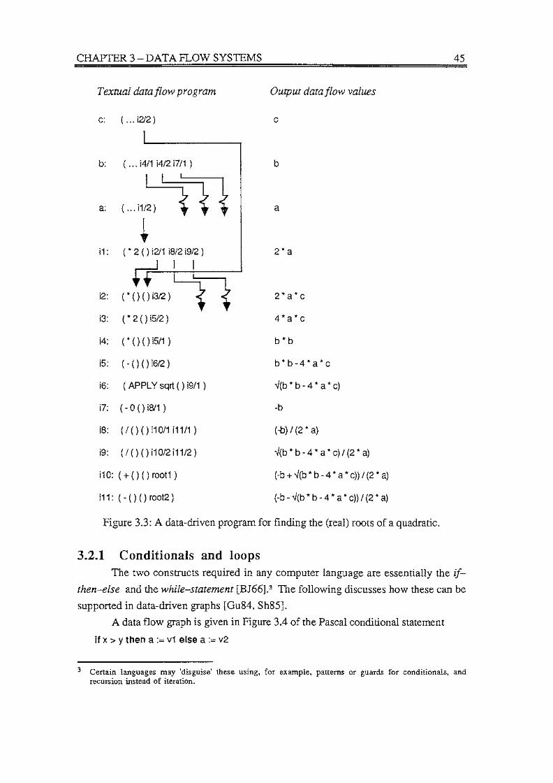
CHAPTER3-DATAFLOWSYSTEMS 45
Textual data flow program Output data flow values
c:
b:
a:
i1:
i2:
i3:
i4:
i5:
i6:
( ... i2/2)
( ... i4/1 i4/2 i?/1 )
(.i1/~
i ( * 2 () i2/1 i8/2 i9/2 ) di I
(·ooi3/2J ~7 ( * 2 () iS/2)
( * () () iS/1 )
( - () () i6/2 )
( APPLY sqrt ( ) i9/1 )
i?: ( - 0 () i8/1 )
i8: (/ () () i10/1 i11/1 )
i9: (/ () () i10/2 i11/2)
i10: ( + () () root1)
i11: ( - () () root2)
C
b
a
2*a
2*a*c
4*a*c
b*b
b*b-4*a*c
✓(b * b - 4 * a* c)
-b
(-b) / (2 * a)
✓(b * b - 4 * a* c) / (2 * a)
(-b + ✓(b * b-4 *a* c)) /(2 * a)
(-b - ✓(b * b- 4 *a* c)) / (2 * a)
Figure 3.3: A data-driven program for finding the (real) roots of a quadratic.
3.2.1 Conditionals and loops The two constructs required in any computer language are essentially the if
then-else and the while-statement [BJ66].3 The following discusses how these can be
supported in data-driven graphs [Gu84, Sh85].
A data flow graph is given in Figure 3.4 of the Pascal conditional statement
if x > y then a := v1 else a := v2
3 Certain languages may 'disguise' these using, for example, patterns or guards for conditionals, and recursion instead of iteration.

CHAPTER 3 - DATA FLOW SYSTEMS 46
v1 v2 X
X>Y
v1 v2
Figure 3.4: A data flow graph for the conditional if x > y then a := v1 else a := v2.
Two new nodes have been introduced in the data flow graph. The diamond
shape is a switch ( or branch). If the value of the conditional entering the diamond from
the right is true, the data token entering from the top is output through the port marked
'T'. Otherwise the value is output through the port marked 'F'. A token which flows
down an arc which ends with '.l' is destroyed without being used
As well as being used for the copy function, a triangle is also used for the
merge function.4 As a value appears on either of the input ports to the merge, it is
selected and placed on the single output port. If a value appears on both input ports,
non-determinism results as each input token has an equal chance of being selected (see
footnote 10). The correct application of a merge used in isolation would be the
responsibility of the programmer.
Loops (or cycles) are a natural phenomenon in programming. Their existence in
data-driven programs is indicated by the presence of cycles within the program graph.
4 If a copy function directly follows a merge in a graph, they will be combined (as in Figure 3.5).

CHAPTER 3-DATA FLOW SYSTEMS 47
In Figure 3.5, a data-driven graph equivalent is given of the following Pascal program
segment which calculates the factorial of N:
i :=N;
nfact := 1;
while i > O
do
nfact := nfact * i;
i := i -1
end; (* while *)
Nfact := nfact
Nfact
Figure 3.5: A cyclic data flow graph for calculating the factorial of N.

CHAPTER 3-DATA FLOW SYSTEMS 48
Although there is only one loop in the Pascal program segment, the data flow
graph contains two; one for each left-hand side object (i and nfact). In Figure 3.5, the
loop for i is shown shaded. Only two arcs cross this border, and the tokens that these
arcs carry need to be synchronised with those generated by the nfact loop.
In a system where multiple tokens on an arc are supported but where only one
instance of a data flow graph is allowed, this synchronisation can be achieved easily by
making the arcs FIFO queues. However, this seriously restricts the level of
concurrency that can be achieved. Methods do exist for gaining higher levels of
concurrency, but at the cost of greater complexity. The most common methods are code
copying and tagging, which are discussed in detail later (see section Static and
dynamic architectures). The extra complexity is a direct consequence of allowing
for both cyclic graphs and multiple tokens, for each data object.
The general structure of a 'safe' while-loop in a graph is shown in Figure 3.6.
initial input
result
Figure 3.6: The general structure of a 'safe' while-loop in a data flow graph.

CHAPTER 3- DATA FLOW SYSTEMS 49
As well as the added complexity required to achieve realistic levels of
concurrency, cyclic graphs introduce two potential problems: deadlock (deadly
embrace) and race conditions. The simplest case of a deadlock is described in
Figure 3.7, where operators P1 and P2 each depends on the other for one of its two
input tokens. As neither can fire until the required token is provided, the result is a
'deadlock'. However, by the careful use and matching of switches and merges,
deadlocks can be avoided.
c = P1(a, P2(c, b)) d = P2(P1 (a, d), b)
Figure 3.7: The occurrence of deadlock in a data-driven program graph.
In a data flow system, the simplest race condition occurs when two token
instances of the same data object get out of sequence as the result of taking two
different computational paths. An example of how this can happen is shown in the
sequence of diagrams (a) to (f) in Figure 3.8. Both G1 and G2 are segments of the
program data flow graph. The time for the data token t1 to be 'transformed' into the
token G1(t1) is much greater than the time required to transform t2 into G2(t2). The
result is that, on entry to the G3 program graph segment, G2(t2) will be erroneously
matched against t1 *, and G1 (t1) against t2*.
Unlike the avoidance of deadlocks, race conditions cannot be combatted
structurally in data flow graphs. Fortunately, the methods required to support safe
looping also ensure that no mismatching results from the occurrence of a race
condition.5
5 In the case of code copying, a race condition cannot arise where only one set of tokens is allowed through a copy of the graph at any one time.

CHAPTER 3- DATA FLOW SYSTEMS
rx•:•:•:•:•xs-•-,.;,;,,..,-,.;-,;•mx•:❖mmx•:<•,>,>;,.wmm,mm,x ....... ..,,
1
I ,._e:;._ >'I~·::::::- I
(a) (b)
::•!.:,u .. -..">!'6.-....,Y..~,~-....,,Y..:-,Y..:,!,~ .. -.t.:..-.t.:&Y.-:,:,:.:~.:.: .. -.:-:-:~-~?-!>!.:.:-:❖'.<:❖:.:❖:-! .. ">!•!i~«<!
I ,..______ I r,.,,.,.,.,.,.,_,_,,_,_,_,,.,,,,.,,.,.,,.<,.,,.""''--""'·~"'''·'""·"""·""·""'1
i ~
I ::_-_-:::_-, .. ~--~~~~--~ I I 12· l I t1 * I
I ..... _,...._., I L.,,,.,wm;-,m:-.w,m»:<->>»w.-,:«<•:•:•:•:->»:•m,m:->:->x««·-j
(d) (e)
50
(c)
r,,,,W,WU❖>C•"•~•'"'-'"•'•""•~W<❖S,<E.,•,,.,s"""'""'"'°'"'"•"•'•'•"•'•"••••>•':i
~ :,
! G1 ..___,_._ I
I ,_ __ ....,...... l I ..... _,...._, I I G3(G2(t2), t1 *) ii
t,.m:•mm» ... .... ·····''·""·'···"--«««->>:•-❖:•:•:•:•:•:•J (f)
Figure 3.8: The occurrence of a race condition.

CHAPTER 3-DATA FLOW SYSTEMS 51
3.2.2 Karp and Miller - a reference data-driven model The semantics of data-driven systems vary almost from system to system. To
explain the more important alternatives, a reference model will be used in a way similar
to that employed by Oxley et al. [OSC84]. The reference model in question is that of
Karp and Miller, which was originally introduced as 'a graph-theoretic model for the
description and analysis of parallel computations. Within the model, computation steps
correspond to nodes of a graph, and dependency between computation steps is
represented by branches with which queues of data are associated' [KM66].
The main operational characteristics of the Karp and Miller model (KM-model)
can be stated as:
• Directed arcs carry tokens between operational nodes.
• Firing rules (when nodes can execute, or 'fire'):
Kl: All arcs between nodes are FIFO queues.
K2: A node becomes eligible for execution when each of its input arcs contains a
number of tokens equal to the threshold for that arc.
K3: When a node executes, it reads and removes a specified number of tokens
from each input arc and performs its operation.
K4: The node completes execution by placing some number of result tokens on its
output arcs.
This model is essentially a graph of processors, and contains no means by
which data values can be input to or output from the graph representing an application.
Nor are data files supported.
Apart from these omissions, which are serious omissions as far as practical
systems are concerned, the KM-model does provide the most general model for FIFO
input only data flow systems. The general exception to FIFO input occurs in systems
which support iteration, where values for different levels of iteration can become
intermixed; a requirement then exists for matching up tokens at the same level of
iteration. A simple example application where this can arise is the multiplying of two
matrices together. A conceptually simple method for identifying which level of iteration
a token belongs to, is to include within each token its iteration level. This is frequently
called colouring or tagging (see, for example, [De74, Ro81, Ve86]).
Although each iteration is represented graphically in data flow systems by a
cycle in the data flow graph, it is possible to unfold the resulting cyclic graph of an
application for each specific set of input data to form an acyclic graph with a FIFO
queue on each arc; thus satisfying rule K 1 above.
The KM-model supports any number of inputs to a node, and any number of
outputs from a node. Rules K2 to K4 are quite general as the number of tokens on a
particular arc can be zero or any positive integer. Having zero tokens was not explicitly

CHAPTER 3 - DATA FLOW SYSTEMS 52
excluded by Karp and Miller, although allowing for it in their model is equivalent in a
functional system to having an unused parameter in a function on input, or no result
being produced from a function invocation on output. It is included here, because most
data-driven systems have at least one node type (the conditional) which can have at least
one empty output arc, and also because it has relevance to the SAME model discussed
in Part II.
3.2.3 Fine-grain data-driven architecture features There are many ways of classifying data-driven systems [Sr86, TBH82, Ve86].
The approach adopted here primarily reflects the potential for each highlighted
characteristic to be used in an executable data flow diagram system (see Section 3.4).
The KM-model rules given above describe particular operational semantics for
data flow systems. The following list, based on Treleaven and Hopkins [TH81],
describes a set of characteristics for a general data-driven computational model:
• The execution of an instruction uses up the data tokens which appear as operands in
that instruction. These tokens are not then available to this or any other instruction.
• There is no concept of shared data storage as exemplified by variables in imperative
languages.
• The value of a token cannot be changed, as no form of destructive assignment exists.
That is, the model incorporates a single-assignment language.
• Sequencing constraints are defined by the flow of data. Put another way, control
flow and data flow coincide.
• The resulting token of one instruction is passed directly to those instructions which
require that token as an operand. Each destination instruction has its own copy of the
token.
• A constant value may be embedded in an instruction as an 'optimisation' of the token
mechanism.
In fine-grain systems, a data flow program instruction can be viewed as a
template into which data values (tokens) can be 'slotted'. Figure 3.3 presents a
relatively simple template structure consisting of an operation, two token operands (one
of which possibly contains a literal), and a variable list of instruction addresses which
require as an input operand the resulting token created by the instruction [TBH82].6
An important characteristic of a data flow architecture is how the results of the
execution of a node are communicated to the directly dependent nodes. In a data-driven
system, the two main methods are direct communication and pack et
communication.
6 All operators have been shown as dyadic, which need not be the case in practical systems.
CHAPTER 3 - DATA FLOW SYSTEMS 53
Direct communication In direct communication architectures, processing elements are 'hard-wired'
together in some suitable way. In the Data-Driven Machine #1 (DDMl), for example,
the processing elements are organised as a hierarchy (tree) of processor-memory pairs
[Da78]. Each processing element is connected to one superior element (except for the
root) and up to eight inferior elements. The part of the (tree-structured) data flow
program allocated to a processing element can be further divided and allocated to
inferior elements.
Other examples of direct communication systems [Ve86] are Micro, a 'paper'
system [MM83], and the Data-Driven Processor Array (DDPA) [TA83].
A major problem with such systems is the need to find a suitable way of
mapping a program onto the topology of the system. Applications which have a similar
structure to the machine, usually ensure the best allocation of the physical resources and
the minimum level of overhead. DDPA, for example, is designed specifically for large
scale scientific calculations involving sets of equations, and is organised as a two
dimensional grid of processing elements.
Packet communication The most promising classes of data-driven architecture for generalised
processing are those based on packet communication. A data-driven system based on
packets is a specialised data communications network, with at least one implemented
system utilising a local area ring network topology [GKW85]. The network paths in
a data-driven architecture are the equivalent of the instruction and data busses of the
von Neumann system. However, the overheads are usually much greater in data
driven systems, and a reasonably high level of parallelism is required to compensate for
these costs.
In general, the more flexible a data-driven system is, the more complex
becomes its communication mechanisms. This manifests itself as either a relatively
large set of different packet types, or as more complex packets with a higher ratio of
status bits to data bits. The second alternative is the most common.
No detailed analysis of packet structures will be carried out here as it is felt little
of value to this thesis will result. What is considered worth discussing, and provides
one major characterisation of packet-based data-driven systems, is the method used for
'filling' an instance of an instruction template with its token operands. The two
principal techniques used are token storage and token matching.
In a token storage system, each token is stored in its destination instruction.
Consider that the program in Figure 3.3 is executed on a token storage computer, and
that an invocation of instruction i1 ('2 * a') produces a token with value 2. If no
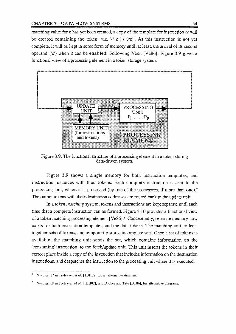
CHAPTER 3 - DATA FLOW SYSTEMS 54
matching value for c has yet been created, a copy of the template for instruction i2 will
be created containing the token; viz. '(* 2 ( ) i3/2)'. As this instruction is not yet
complete, it will be kept in some form of memory until, at least, the arrival of its second
operand ('c') when it can be enabled. Following Veen [Ve86], Figure 3.9 gives a
functional view of a processing element in a token storage system.
Figure 3.9: The functional structure of a processing element in a token storing data-driven system.
Figure 3.9 shows a single memory for both instruction templates, and
instruction instances with their tokens. Each complete instruction is sent to the
processing unit, where it is processed (by one of the processors, if more than one).7
The output tokens with their destination addresses are routed back to the update unit.
In a token matching system, tokens and instructions are kept separate until such
time that a complete instruction can be formed. Figure 3.10 provides a functional view
of a token matching processing element [Ve86].8 Conceptually, separate memory now
exists for both instruction templates, and the data tokens. The matching unit collects
together sets of tokens, and temporarily stores incomplete sets. Once a set of tokens is
available, the matching unit sends the set, which contains information on the
'consuming' instruction, to the fetch/update unit. This unit inserts the tokens in their
correct place inside a copy of the instruction that includes information on the destination
instructions, and despatches the instruction to the processing unit where it is executed.
7 See Fig. 17 in Treleaven et al. [TBH82] for an alternative diagram.
8 See Fig. 18 in Treleaven et al. [TBH82], and Docker and Tate [DT86], for alternative diagrams.

CHAPTER 3 - DATA FLOW SYSTEMS
Figure 3 .10: The functional structure of a processing element in a token matching data-driven system.
55
Systems which employ token matching effectively support re-entrant programs.
However, without special measures being taken to correctly match sets of tokens
(usually involving tags), re-entrant programs can lead to non-determinate behaviour.9
Various schemes exist for connecting processing elements together into a
complete data flow machine architecture. The more notable options are discussed in
Veen [Ve86].10 Although these options are of some interest, an architecture formed
from a single processing element, with multiple processors, is adequate for the research
reported here.
Static and dynamic architectures A different categorisation of data-driven systems relates to whether or not a
system supports the concurrent execution of more than one instance of the same node in
a data flow graph. Systems which do not are described as static. In such systems the
program graph need only be loaded once, which can be done statically before the
computation begins. Two methods have been used to ensure that only one instance of a
node is executing at a time [Ve86]:
• A lock is somehow placed on an executing node. This could simply be an associated
busy flag.
9 Veen (Section 2.4) provides a good example of a re-entrant graph which could result in non-determinancy [Ve86].
lO See, in particular, Fig. 14 and the associated text.

CHAPTER 3- DATA FLOW SYSTEMS 56
• A destination node somehow acknowledges to the generating node the receipt of a
token. A simple method used by Dennis and Misunas [DM74, De79a] is to require
that each output arc be empty before a node can be enabled; this means that only one
token can be on each arc at any time.
Example systems are the MIT static architecture of Dennis and Misunas
[DM74], and the system that has been designed as part of the Mandala project [Bu81]
which is based on the design principles put forward by Dennis et al. [DBL80].
Architectures which do support the firing of several copies of a data flow graph
node are described as dynamic. The most general scheme is where an instance of a
node is created 'on-demand' at execution time.
The two basic techniques that have been used for supporting the firing of
multiple instances of nodes, are code-copying and tagging.
As its name suggests, in a code-copying scheme, the need for a new instance of
a node results in a copy of the node being created, and a set of tokens being associated
with that node. Code-copying systems invariably duplicate at the level of a procedure or
block for greater efficiency. As most tokens will be required by instructions within the
creating procedure or block, the concept of locality arises [De84, Sp77]. The DDMl
computer is a good example of a code-copying system [Da78]. The hierarchical
structure of the system supports locality, as a sub-tree of processors can be assigned a
part of a data flow graph. As well as this, each processing element in the tree has (up
to) eight inferior processors to facilitate the execution of parts of the sub-tree in parallel.
Dynamic tagged architectures form the largest class of data flow systems. The
major work on tagged systems has been carried out by Arvind et al., initially at
Irvine[AG78] but subsequently at MIT [AK81, AG82], and by Watson et al. at the
University of Manchester [WG79, GKW85, WSW87]. Other tagged architectures can
be viewed as derivatives of the systems produced by these two groups. Although the
architectures of the Id machine (Arvind et al.) and the Manchester data flow computer
have significant differences, there is much similarity in principle in the way that tags are
used. Consequently, the discussion here will be restricted to the tagging scheme used in
the Id machine. 11
Tagging in the Id machine is under the control of the CT-interpreter [AG82],
which uncovers parallelism during the execution of a program and assigns a tag to each
parallel computational activity as it is created. The CT-interpreter is a generalised
scheme, and the Id machine has been described as a particular hardware implementation
[AK81].
11 Sometimes called 'Id' after the name of the language that the machine is designed to support (see, for example, Veen [Ve86]; also see Srini [Sr86]). 'Id' is an acronym for 'Irvine data flow' [AG78].

CHAPTER 3-DATA FLOW SYSTEMS 57
Every computation (single execution of an operator or node) is called an
activity. The U-interpreter allocates a unique name to each activity generated during
the execution of a program, and each token carries the name of its destination activity.
An activity name comprises four fields:
• u - the context field; this identifies the environment (bindings, etc.) in which the
activity is being evaluated. A context field is itself an activity name, so nested
contexts are supported.
• c - the code block name assigned by the Id compiler to the loop or procedure that
contains this activity.
• s - the instruction number within the code block.
• i - the initiation number; this identifies the loop iteration within which this activity
occurs. If the activity occurs outside a loop, the field has a value of 1. Nested loops
are provided for through nested contexts.
A token in the Id machine is the 2-tuple
(u.c.s.i, data_value)p
where p identifies one of the possible two import ports of the destination activity.
Together, c, sand p specify that the token is travelling along an arc that is connected to
the input port p of instruction s in code block c. The overall context in which this is
occurring is defined by u. If the activity is within a loop, i denotes the level of iteration.
A conceptual snapshot diagram is given in Figure 3.11 for a token with an activity
name 'u.c.s.i', a data value of 4, on input port p2 of operations.
Figure 3.11: A conceptual snapshot of an Id data flow program showing the token (u.c.s.i, 4) on the arc connected to input port 2 of the instruction (activity) s.

CHAPTER 3 - DATA FLOW SYSTEMS 58
The data flow program graph constructed by the Id compiler has two different
classes of node. The first class is that exemplified in Figure 3.2, and contains the
operations which can be carried out on the data. The second class of node consists of
operations to create and amend activity names. 12 There are also implicit operations on
activity names associated with the first class of operation. For instance, given that
instruction s in Figure 3.11 outputs the product of its two input values to instruction t
(on port p1), the input and output token sets for instructions could be
input token set = ( (u.c.s.i, 90)p1, (u.c.s.i, 4)p2}
output token set = ( (u.c.t.i, 360)p1 }
where the relative instruction number of the activity that will consume the output token
is t. Implicit operations on activity names only affect the instruction number field, s.
The full set of explicit operations on activity names will not be discussed here.
Instead, the general principles can be obtained from the following discussion on the
handling of loops.
In Figure 3.12 a data flow graph is shown for the Id expression [AG82]
(while p(x) do
new x ~ f(x)
return x)
Each activity name operator has been labelled, and the import and export sets ('pre-'
and 'post-conditions') of each node have been included. The types of activity name
operators used in a loop are o, 0-1, L, and L-1 • The output token of the O operator is
the same as the input token except that the initiation number has been incremented by 1.
The 0-1 operator resets an initiation number to 1. The L operator creates a new context,
u', for each instantiation of a loop. The value of this new context is the previous activity
name (u.c.s.i). The L-1 operator resets the context and initiation values to what they
were on entry to the loop (u and i, respectively).
The adding by the Id compiler of the necessary activity name operators to the
data flow program graph during compilation, means that the control of activity names
can be distributed to the processors that are responsible for executing the individual
block invocations. Thus, no centralised tag control, with the possibility of being a
bottleneck, is required.
The Id machine that Arvind and his group are constructing is actually a
combined code copying and dynamic tagging system. The reasons for this relate
specifically to physical machine considerations, and will be briefly discussed here
through the simple loop example given above (and in Figure 3.12). Consider that the
loop code block is allocated a pool of processing elements on which it will execute.
12 For lack of evidence, it is assumed that an activity name is trivially deleted when no longer required.

CHAPTER 3-DATA FLOW SYSTEMS 59
X {<U.C.S.i, X>}
s L
{<U'.c'.t'.1, X>} t
t
{ I I t ' <U .C .. J, X>
D {<U'.C'.t.j+1, X>}
p(x)
{<u'.c'.w.n, X>}
w D -1
X {<U'.c'.w'.1, X>}
new x
X {<U.c.s'.i, X>} :j:
t u' = u.c.s.i
+ c.s' is the successor of instruction c' .w' ( which is the L -1 instruction)
Figure 3.12: A data flow graph for the processing of the loop by the U-interpreter.

CHAPTER 3-DATA FLOW SYSTEMS 60
Two schemes suggest themselves for allocating activities to processors. In the
first scheme a (preferably contiguous) number of instructions are allocated to each
processor, such that instruction s will always execute on processor Pk· In the second
scheme, each processor is allocated a copy of the code block program graph. In either
scheme, the number of activities per processor is likely to result in the interleaved
execution of iterations, so tags are still required but can be less complex. 13
To support both code copying and tagging, the Id machine pays a price by
employing a centralised software scheduler to allocate pools of processors (physical
domains [AK81]) to program code blocks. The scheduler is called when a code block is
invoked, and it selects a physical domain depending on a number of criteria that
includes: the code block size; whether the code block already exists in some other
physical domain; how much data has to be moved between the new code block and the
code block which invoked it [AK81].
In Section 3.4, tagging is mentioned again in terms of SSA data flow diagrams.
The important concepts to be taken through to that section from the current discussion
are:
• Tags can be composite structures, with specialised operators acting on each part of
the structure.
• A distributed control scheme for tags should be relatively easy to implement.
• During execution, the size of a tag can be made a function of the 'complexity' of the
activity. That is, an instruction which is nested within procedure invocations and
loops can dynamically be given a more detailed tag than an instruction in 'top-level',
straight-line code.
In summary, static architectures tend to be simpler than dynamic architectures,
as they do not require a mechanism for creating copies of program sub-graphs, nor do
they need to maintain tags for differentiating between different tokens of the same
'named' object. Against this must be weighed the fact that they achieve lower levels of
parallelism.
Enabling conditions and output conditions A further categorisation is concerned with the conditions under which a node
becomes enabled, and under which a node outputs values. Although these are
essentially separate issues, there are two cases of interest for each. A node becomes
enabled either when at least one input token is available, or when all input tokens
become available. The DDDP can begin executing a node as soon as one operand is
13 If a complete code block is executed on a single processor, there is no need to maintain the u and c components during the execution of the code block program graph.

CHAPTER3-DATAFLOW SYSTEMS 61
available, but most systems require both operands [KYK83]. Similarly, a value can be
output either before the node finishes executing, or after the node completes execution.
The Manchester data flow computer exports output tokens before the completion of an
operation [GKW85].
Some improvement in performance may be gained by enabling or outputting,
respectively, as soon as possible, although there appears to be no reported significant
performance measurements to support this. The potential performance improvements
may be much greater in coarse-grain systems.
Summary of fine-grain data-driven systems The data-driven systems described here generally differ from the KM-model in
the following ways:
• The KM-model has no conditional or merge nodes which can lead to non
deterministic behaviour, so there is no requirement in that model to distinguish
between sets of inputs by the use of tags, for example. FIFO queues are adequate.
• The systems considered here invariably input just one token from each arc during the
invocation of a node. The KM-model allows for any number from each arc.
Similarly for output.
The various classifications, except for the enabling and output conditions, are
presented graphically in Figure 3.13 [Ve86].
Micro DDMl DDPA
DDP lAU MIT Multi
CODE COPYING
Figure 3.13: A categorisation of data-driven machines. The machines discussed in this chapter are shown in the rectangles. 14
14 The mMBO machine is a mixed control-flow, data-driven machine. See, also, Veen [Ve86], Fig. 15.

CHAPTER 3-DATA FLOW SYSTEMS 62
Table III provides a summary of a number of the reported architectures. Most of
which have been implemented, or emulated.
Research project Machine organisation Tokens on Tokens on each input arc each output arc
Utah DDMl [Da78] Direct communication; m n token storage; dynamic
Toulouse LAU [CH79] 15 Packet communications; m n token storage; static
MIT [De79a] Packet communication; 1 0 token storage; static
Multi [Bu81]16 Packet communication; 1 0 token storage; static
TI DDP [Co79]17 Packet communication; 1 0 token storage; static
Irvine/MIT [AK81] Packet communication; m n token matching; dynamic
Manchester [GKW85] Packet communication; m n token matching; dynamic
Tokyo DDDP [KYK83] Packet communications; m n token matching; dynamic
Newcastle JUMBO [THR82] Packet communication m n token matching; dynamic
Table ill: A comparison of some reported date-driven architectures.
15 Although a data-driven computer, the LAU system has a control flow program organisation. However, the control graph of a program coincides with its data graph [TBH82].
16 Veen [Ve86] advisedly describes Multi as a dynamic system, whereas it is firmly a static system. The confusion may arise because, conceptually, the system is designed to allow multiple applications to execute concurrently in an attempt to achieve higher levels of resource utilisation. However, each of these graphs executes statically in its own virtual machine.
17 The compiler may create multiple copies of part of a data flow graph to increase the concurrency, but this is done in a static manner at compile-time.

CHAPTER3 DATAFLOWSYSTEMS 63
3.3 Demand-driven systems In a demand-driven system, it is a request for a data item which leads to its
creation. In data flow graph terms this is realised as a request for the output token of an
operational node, which in turn leads to a demand for the input tokens of that node.
These input tokens are generally the output tokens of other operations, and so the
request for tokens propagates back up the graph. Taking the data flow graph of
Figure 3.1 as an example, a demand for a token of root1 will lead to a demand for two
further tokens, one of whose value is 2 * a. To satisfy the request for the '2 * a' token, a
token of the data object a is required.
A demand-driven program equivalent to Figure 3.3 is given in Figure 3.14.
Textual data flow program Output data flow values
a: a
b: b
c: C
i1: ( * 2 a) 2*a
i2: ( * i1 C) 2*a*c
i3: ( * 2 i2) 4*a*c
i4: ( * b b) b*b
i5: ( - i4 i3) b*b-4*a*c
i6: ( APPLY sqrt i5 ) ✓(b * b - 4 * a * c)
i?: ( - 0 b) -b
i8: ( / i? i1 ) (-b) / (2 * a)
i9: ( / i6 i1 ) ✓(b * b - 4 * a* c) / (2 * a)
i10:(+i8i9) (-b + ✓(b * b - 4 *a* c)) / (2 * a)
i11: ( - i8 i9 ) (-b- ✓(b * b- 4 *a* c)) / (2 * a)
Figure 3.14: A demand-driven program for finding the (real) roots of a quadratic.

CHAPTER 3-DATA FLOW SYSTEMS 64
The major differences between the programs in Figures 3.3 and 3.14 are:
• the absence of 'holes' in the demand-driven program instructions for input tokens;
• the absence of forward references in the demand-driven program (instead, backward
references exist).18
The two principal techniques that exist for executing the program in Figure 3 .14 are
string reduction and graph reduction. These are discussed in the next two
sections, but before doing so it is worth mentioning here that each instruction in the
program in Figure 3.14 can be viewed as a definition with syntax name: expression.
3.3.1 String reduction String reduction is essentially a rewrite scheme in which a demand for a data
object leads to the name of that object being replaced by its expression. at the point of
demand. Once a complete expression has been constructed for the original object being
demanded, the expression is evaluated (reduced) to its value. 19
(+ 18 19)
(+ (/ 17 11) (/ i6 11))
(+ (/ .(:_Q_Ql (* 2 a)) (/ (APPLY sqrt i5) (* 2 a)))
(+ (/ (- 0 .(:fil) (* 2 1)) (/ (APPLY sqrt (- i4 13)) (* 2 1)))
(+ (/ (- 0 (-5)) (* 2 1)) (/ (APPLY sqrt (- (* b b) (* 2 12))) (* 2 1)))
(+ (/ (- 0 (-5)) (* 2 1)) (/ (APPLY sqrt (- (* .(:fil .(:fil) (* 2 (* 11 c)))) (* 2 1)))
(+ (/ (- 0 (-5)) (* 2 1 )) (/ (APPLY sqrt (- (* (-5) (-5)) (* 2 (* r,__2__fil .6)))) (* 2 1)))
(+ (/ (- 0 (-5)) (* 2 1)} (/ (APPLY sqrt (- (* (-5) (-5)) (* 2 (* (* 2 1) 6)))) (* 2 1 )))
(+ (/ 5 2J (/ (APPLY sqrt (- 25 (* 2 (* 2 6)))) 2))
(+ 2.5 (/ (APPLY sqrt (- 25 (* 2 12))) 2))
(+ 2.5 (/ (APPLY sqrt (- 25 24)) 2))
(+ 2.5 (/ (APPLY sqrt 1) 2))
(+ 2.5 (/ 1 2))
(+ 2.5 0.5)
3
Figure 3.15: A string reduction execution sequence for the part of the program in Figure 3.14 which finds the first root.
18 However, see the discussion on graph reduction in Section 3.3.2.
19 This provides the most naYve method of evaluation.

CHAPTER 3 - DATA FLOW SYSTEMS 65
A set of string reduction evaluation steps for generating a token of root1 are
shown in Figure 3.15. The expressions above the line contain rewrites, where object
names to be replaced at the next step are shown in bold type and where each expression
which replaces a name is shown underlined. The expressions below the line show a
possible sequence of reductions which maximises on the inherent parallelism. The
reduced values at each step are shown in italic type. The coefficient token values used
in the example are a = 1, b = -5 and c = 6.
String reduction systems use code copying at a low level of granularity. A
consequence of code copying is that common objects, such as i1 in Figure 3.15, are
replaced by their expression at each point that they appear in the demanding
expression(s). Consequently, an object may have its value calculated a number of
times. On the plus side is the relative simplicitly of the technique.
Systems which use string reduction include the cellular-tree-based system of
Mago [Ma79, Ma80] which executes FFP programs [Ba78], the GMD reduction
machine, which supports a language based on the lambda calculus [HS79, Kl79,
KS80], and the Newcastle reduction machine which has been designed to support
multiple reduction languages [TM80].
3.3.2 Graph reduction Graph reduction differs from string reduction by 'replacing' a name with a
reference to the definition of the named object, rather than by the expression itself. In
this way a graph is built of the total expression to be evaluated. Taking the function
f x = (x + 1) * (x - 2) + 3
as an example. A call of the function of the form 'f 3' could lead to the following
sequence of graph reductions:
+
/ " ;*\ 3
+ -/\ ;,
X 1 X 2
+ -/\ ;,
3 1 3 2
• +
/ " • 7
4 3
In Figure 3.16 a graph is given for the evaluation of rootl using the demand
driven program of Figure 3.14. The overall spatial ordering of the objects in
Figure 3.16 is consistent with Figures 3.1 and 3.2.
One technique used to set up 'return addresses' for the generated tokens is to
reverse the pointers during the construction (execution) of the graph. Each node would
point to the first higher-level node that demands the lower level node's value. Later

CHAPTER 3-DATA FLOW SYSTEMS 66
demands for that value will make use of the already calculated value when their pointers
are eventually reversed. Figure 3.17 shows reversed pointers early in the evaluation of
the program graph of Figure 3.16.
b: (-5) c: (6)
i~ f2~) i5: (- i4 i3)
~ i\ ~ \p~y ~· i5)
i8:(/ i7 i1) i9:(/ i6 i1)
~i i10: (+ i8 i9)
Figure 3.16: A graph reduction program corresponding to Figure 3.14.
A concrete representation of the reverse pointers would be to store a single
'reverse address' in each token [TBH82].
Execution of the program graph in Figure 3.17 essentially leads to the pruning
of the tree from the leaves down, until only the root of the tree is left in the form of a
token value of the required (reduced) type.
Examples of graph reduction machines are: the AMPS system of Keller et al.
which uses a dialect of Lisp for its machine language [KPL78, KLP79]; the SKIM
reduction machine of Clarke et al. [CGM80], which is based on combinators; and the
ALICE reduction machine of Darlington et al. [DRS 1, HR], which is designed to
support functional languages like Hope [Ba85a] and ML [Ha85].

CHAPTER 3 DATA FLOW SYSTEMS 67
b: (-5) a: (1) c: (6)
~
~
i1 O: (+ i8 i9)
Figure 3.17: The program graph of Figure 3.16 with reverse pointers.
3.3.3 Demand-driven systems and functional languages As indicated above, there is a close association between demand-driven systems
and functional languages. The demand-driven program of Figure 3.14, particularly in
its string reduction form of Figure 3.15, can be viewed as the composition of
functions. This close relationship with functional systems has seen an increase in
interest in the development of demand-driven systems over the last few years [GKS87,
HR, PCS87, TM80, Tr85, WSW87]. Graph reductions have a parallel in functional
language systems, both through the representation of functional composition as graphs
[GKS87, HR, PCS87, Tr85, WSW87], and through the combinators of Schonfinkel
[Sc24], with their realisation in the SK reduction machine of Turner [Tu79a, Tu79b,
Tu87] and the SKW reduction machine of Clarke et al. [CGM80].
The definition of functions in functional languages are also essentially of the
form name : expression. In Miranda, for example, the function to calculate Fibonacci
numbers can be written as

CHAPTER 3-DATA FLOW SYSTEMS
fib n = 1,
1 '
n=O
n = 1
fib(n-1) + fib(n-2), otherwise
68
A particular benefit claimed of functional languages is that their underlying
semantics are simpler than those of imperative languages and, hence, the validity of
functional programs should be easier to prove. However, there is much still to be done
regarding the use of functional languages in the implementation of complex business
applications, in particular, before the above claim can be accepted with any confidence.
Other features of functional languages - such as their powerful abstraction
mechanisms, their conciseness, and their support of referential transparency - make
them good potential candidates for use as specification languages [Tu84]. With this
potential in mind, it is demonstrated in Chapter 5 that the data dictionary languages of
SSA can also be given a functional interpretation. The definition of a data object will be
shown to satisfy the form name : expression, followed by the suggestion that the
process logic in a data flow diagram can be represented by a set of such definitions in
the form of a reduction graph.
3.4 Data flow systems and data flow diagrams The quadratic equation example of Section 3.2 will be used here to demonstrate
one relationship between fine-grain data flow systems and SSA data flow diagrams.
The discussion will be extended to include the definition of data objects and the
transformation of input data flows to output data flows. In SSA terms these are
supported by the data dictionary and (for example) minispecs, respectively.
3.4.1 Fine-grain data flow semantics applied to data flow diagrams
Finding the roots of a quadratic can be specified in a Level O data flow diagram
as shown in Figure 3.18(a). Suitable dictionary definitions for the data flows are
shown in Figure 3.18(b).
Although unlikely in practice, the Level O diagram could be refined to the
Level 1 data flow diagram shown in Figure 3.19. The data flow definitions in
Figure 3.18(b) apply equally as well to the expanded diagram, except that COEFFICIENTS
and ROOTS are now redundant as the data flows, as well as the process, have been
refined.
Considering a data flow diagram as a data flow program graph, it is possible to
apply both a data-driven and a demand-driven interpretation to the diagram. In terms of
the example in Figures 3.18 and 3.19, a demand-driven interpretation would be one
where the roots of a quadratic would be demanded by an analyst, and this would finally
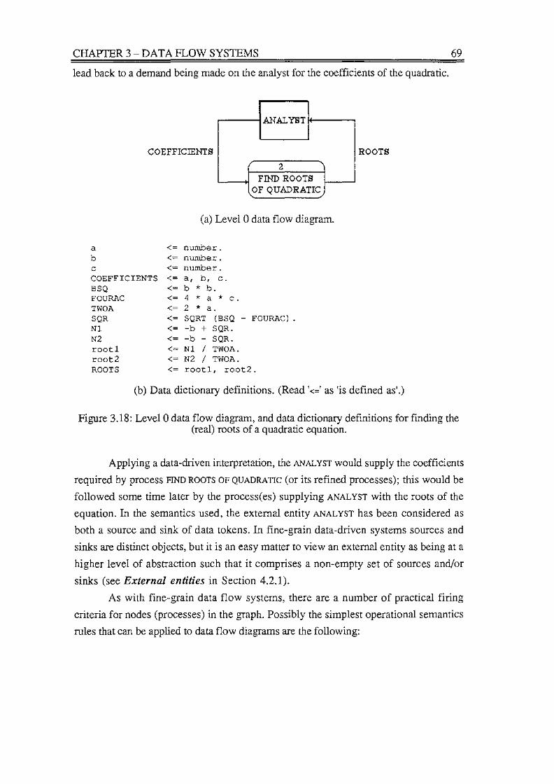
CHAPTER 3-DATA FLOW SYSTEMS 69
lead back to a demand being made on the analyst for the coefficients of the quadratic.
ANALYST"
COEFFICIENTS ROOTS
2 " FilID ROOTS
OF QUADRATIC '- ~
(a) Level O data flow diagram.
a <= number. b <= number. C <= number. COEFFICIENTS <= a, b, c. BSQ <= b * b. FOURAC <= 4 * a * c. TWOA <= 2 * a. SQR <= SQRT (BSQ - FOURAC). Nl <= -b + SQR. N2 <= -b - SQR. rootl <= Nl I TWOA. root2 <= N2 I TWOA. ROOTS <= root 1, root2.
(b) Data dictionary definitions. (Read'<=' as 'is defined as'.)
Figure 3.18: Level O data flow diagram, and data dictionary definitions for finding the (real) roots of a quadratic equation.
Applying a data-driven interpretation, the ANALYST would supply the coefficients
required by process FIND ROOTS OF QUADRATIC (or its refined processes); this would be
followed some time later by the process(es) supplying ANALYST with the roots of the
equation. In the semantics used, the external entity ANALYST has been considered as
both a source and sink of data tokens. In fine-grain data-driven systems sources and
sinks are distinct objects, but it is an easy matter to view an external entity as being at a
higher level of abstraction such that it comprises a non-empty set of sources and/or
sinks (see External entities in Section 4.2.1).
As with fine-grain data flow systems, there are a number of practical firing
criteria for nodes (processes) in the graph. Possibly the simplest operational semantics
rules that can be applied to data flow diagrams are the following:

CHAPTER 3 - DATA FLOW SYSTEMS 70
• A process becomes enabled, or executable, when all its input tokens are available.
This ensures that a process is deadlocked the first time it is executed, or nor at all. In
Figure 3.19, for instance, process COMPUTE FOURAC would become enabled when
matching tokens for a and c exist.
• A process executes as an indivisible object.
• The output tokens produced by a process are distributed, or exported, to the
importing objects (processes, external entities, and data stores) when the process
completes execution.
• The input tokens are consumed by the process.
b -
C -a -
FIND ROOTS OF QUADRATIC
~ ~ COH:UTE
r ? N1 . rootl C011PUTE 1 N1 --+ rootl
'-
4 C011PUTE - BSQ BSQ 3 ~r 5 N2 8
roo12 ........ C011PUTE C011PUTE C011PUTE ~
SQR so'a N2 H roo12
2 \. ) \.. ./ ~
C011PUTE _ FOURAC TWOA r FOURAC r 6
C011PUTE TWOA
\..
Figure 3.19: Level 1 data flow diagram for finding the (real) roots of a quadratic application.
The second and third rules together provide a 'safe' division point in that,
should an error occur during the execution of a process, any data produced by that
process during that invocation would not have found its way 'out' to other processes,
external entities, or data stores.
The semantics usually attached to SSA data flow diagrams are invariably much
looser than those given above: data flow tokens are considered available when required;
any number of tokens can be matched together, depending on the process logic; data
stores can be read and written to any number of times during the invocation of a
process, including reading the value of an object 'updated' during the same invocation.
Specifically, the two areas in which the above operational semantics rules do
not adequately reflect data flow diagrams, are where data stores are involved and where
one token of a particular data flow may want to be processed against a multiple number
of one or more other data flows.

CHAPTER3-DATAFLOW SYSTEMS 71
In the case of data stores, a token to be input by a process from a data store is
usually selected using (part of) at least one other input token as a key. Figure 3.20
provides an example where a CUST _# token is used as the key for accessing
CUSTOMER_DETAILS. Note the data flow identifying the key leading from the process to
the data store. The triangle symbol denotes this as a key, rather than as a 'normal' data
flow. Such 'data' flows do not have to be shown explicitly in data flow diagrams, as
the data dictionary should contain the necessary information.
OfHER_DATA
CUST_#
CUST_#
V
EXPORTED_DATA
CUSTOMER_DEf AILS
CUSTOMERS
Figure 3.20: Accessing the data store CUSTOMERS using CUST_# as the key.
Without employing a reasonably sophisticated system mechanism for extracting
the wanted data store token before enabling a process, the operational rule of requiring
all tokens to be available prior to the execution of a process cannot be satisfied for input
tokens supplied by data stores. It is possible, however, to obtain equivalent semantics
by allowing a process to become enabled when all non-data-store tokens are available;
provided that in the case of a data store token not being available when required during
the execution of the process, the enabling can be 'undone'. The undoing of a process is
not difficult to achieve if the operational rule is adhered to, that all output tokens are
(only) exported once a process has completed. Any process that is 'blocked' through
the lack of an available data store token would be considered not to have completed.
The second area where the operational semantics are not adequate, concerns the
matching of a single token on one data flow with multiple tokens on other data flows.
An example of when this could be required is described in Figure 3.21, where a token
of the data flow COURSE_CODE is being processed against a group of STUDENT_# tokens.
COURSE_CODE
, , r 'I
STUDENT_# COURSE_CLASS_LIST ,._
Figure 3.21: Processing one couRSE_CODE token against multiple STUDENT_# tokens.

CHAPTER 3- DATA FLOW SYSTEMS 72
To be able to support this operationally, some means must be defined for
processing elements of a group in order, and for identifying the limits of each group.
This is equivalent to interpreting a group data flow as a stream [ASS85] With this
interpretation, the process along with data flow COURSE_CODE in Figure 3.21 can be
viewed as a filter acting on the stream of STUDENT _#s. What suggests itself is some form
of colouring to identify each group object instance, with an implicit indexing of tokens
within the group. The techniques of the U-interpreter, discussed in Section 3.2.3 can
usefully be applied here [AK81].
It should be noted that nothing in Figure 3.21 suggests that one COURSE_CODE is
being processed against multiple STUDENT_# tokens. In Section 4.3.2 one method of
showing this explicitly is given, using double arrow heads for decomposed data flows.
If the operational semantics were amended in the ways suggested, to support
the processing of data stores and the processing of decomposed group objects, the
effects of errors can still be reasonably well defined.
3.4.2 Input to output set transformations Other research that has an operational interpretation of data flow diagrams
represent the process logic in imperative programming code [Ba82, Ba84, Ba85,
BK86, St87]. This is considered appropriate if the use of data flow diagrams is
extended to the design phase of software development. However, as an analysis tool
which should be easily understandable to the end-users of the system being analysed, it
provides too low a level of abstraction.
Three ways of specifying the transformations from input data flow sets to
output sets will be considered, namely:
• Program modules
• Executable minispecs
• Executable dictionary statements
For the reason given above, modules written in an imperative programming
language are considered unsuitable for the analysis phase. It may be possible, using
sub-programs, to present a higher level of abstraction for much of the logic.
Alternatively, a functional language could be used to define the logic of a process,
although these tend to require some understanding of the use of recursion.
Much of the concern with the use of existing programming languages for
specifying process logic, stems from the need to include the definition and initialisation
of variables, the need for loop control variables, etc. By employing an active
dictionary, much of this requirement can be dispensed with: details on the type and
initial value of a variable (possibly within a particular process) can be abstracted out of
the logic of a process and be stored in the dictionary instead. Having taken this step, it

CHAPTER 3 - DATA FLOW SYSTEMS 73
is possible to abstract out loop control variables as well. The result could be a language
whose syntax is essentially that of the structured English used by De Marco and others
[De78, GS79, We80], so that the processing logic could be represented by executable
rninispecs.
The SASE (Structured Analysis Simulated Environment), described briefly in
Chapter 9 [DT85, TD85], was an application of this reasoning. The dictionary
supporting the executable rninispecs contained full definitions of all data objects.
However, it was noted that much of the process logic was 'repeated' in these
definitions, albeit in an apparently unstructured way. This led to the dictionary
definitions of data objects themselves being interpreted as instructions. In such a
scheme, transformations on input data flows to output data flows are viewed as
operations on data structures. The definitions in Figure 3.18(b) can be considered in
this way, although they define rather simple data structures.20
One concern with using the dictionary definitions is their apparently monolithic
form. Consequently, some mechanism is required to structure the object definitions,
either explicitly or implicitly. Another concern is how these definitions can be tied
together to be executed. If a data object can only have one definition in the dictionary,
which seems a sensible restriction, the dictionary object definition language can be
viewed as a single-assignment language [Ac82, AG78, Mc82, MSA83, PCG76,
TE68, WA85]. This class of language has a data flow interpretation, and yields
particularly to a demand-driven, or reduction, mode of execution. This implies that the
language is essentially functional in nature.
3.4.3 Treating data flow diagrams and transformations independently
The above discussion suggests that there may be some independence between
the method of executing data flow diagrams, and the method of carrying out
transformations on input data flow sets to produce output sets. This is particularly the
case when the processing logic is carried out by dictionary-based executable minispecs
or by executable dictionary definitions.
In Part II of this thesis, SAME (Structured Analysis Modelling Environment) is
described. SAME contains two sub-models: a computational sub-model for the
execution of data flow diagrams (which was also used in the SASE system), and a
computational sub-model for executing the dictionary definitions of data objects.
Chapter 4 develops the data flow diagram sub-model, while in Chapter 5, the
20 A more comprehensive example is provided in Figure 6.3.

CHAPTER 3-DATA FLOW SYSTEMS 74
executable dictionary definition language named lEgis is developed. These are brought
together into the combined SAME computational model in Chapter 6.
3.5 Summary This chapter has discussed a number of alternative data flow systems. No
attempt has been made to be exhaustive, either in terms of the types of systems
discussed, or in terms of the example systems mentioned within each type. As well as
the cited original research documents, the excellent survey material in Treleaven et al.
[TBH82], Vegdahl [Ve84], Srini [Sr86], and Veen [Ve86], together provide a
considerable body of information, should further details be sought.21
Attention in this chapter has primarily been focussed on data flow architectures
(both data-driven and demand-driven), and various categorisations of data flow
systems have been provided. In general, the classification of systems has been directed
towards identifying types of systems or characteristics which support the notion of
executable SSA data flow diagrams. The fine-grain data-driven systems have a natural
relationship to data flow diagrams, and many of the concerns in fine-grain systems to
do with handling iteration, recursion and data structures, and avoiding deadlocks, have
parallels in (coarse-grained) data flow diagrams. Some of the features which are
considered particularly relevant to executable data flow diagrams are:
• The method used to match tokens (data flows) with operations (data stores, external
entities, and processes).
• The conditions under which operations can begin execution (the number of input
tokens required), and also when they can release their output token (frequently two
or more different data flows are created by a data flow diagram).
• The scheduling of operations, or code blocks, (processes) to processors.
• Removing the possibility of race conditions occurring by, for example, using tags.
• A method for safely handling loops (if they are to be allowed in data flow diagrams;
else banning them altogether).
A coarse-grained architecture for supporting executable data flow diagrams
forms the subject matter of Part II, when iteration, and data structures will be discussed
within that context.22 The realisation of such an architecture does not depend on
concrete fine-grain data flow architectures, but could be equally suited to a network of
von Neumann machines. This topic is discussed in Chapter 9 within Part III.
21 Much of the survey material in this chapter is based on Treleaven et al. [TBH82], Vegdahl [Ve84], Srini [Sr86], imd Veen [Ve86]. Wherever possible the original references for systems were also used, but some remained elusive.
22 Iteration md recursion are discussed further in Appendix 3.

CHAPTER 3-DATA FLOW SYSTEMS 75
The discussion on demand-driven, or reduction, systems has little to do with
data flow diagrams per se, but has much to do with the executable system dictionary
language called JEgis, which is the topic of Chapter 5. }Egis is a single assignment
language based on the data dictionary language(s) of De Marco [De78] and Weinberg
[We80], and is suitable for execution in a demand-driven fashion.
Within Part II, a particular data flow computational model, called SAME
(Structured Analysis Modelling Environment), is discussed. SAME itself consists of
two distinct sub-models.
At the top level is a data-driven sub-model of data flow diagrams. This is based
on the fine-grain data-driven systems of Chapter 3, but also reflects the data view of
data flow diagrams within the SSA methodologies. Two candidate sub-models are
discussed in Chapter 4. Their differences can be summarised in terms of the number of
SSA data flow diagram facilities that they provide. The simpler model, called DFDMl,
is deterministic. However, certain 'desirable' features, in the SSA sense, are missing,
such as allowing a process to execute against only a proper subset of a data flow import
set (called a 'limited import set'). Allowing 'limited' import sets enables loops to be
supported as well. The more complex model, called DFDM2, provides for limited
import sets, loops, limited export sets, and recursion. DFDMl is essentially contained
within DFDM2.
The bottom level sub-model employs a demand-driven (reduction) scheme to
map the input data flow set of a process to its output data flow set. As much as
possible, the bottom level sub-model is discussed independently of data flow diagrams
in Chapter 5.
In Chapter 6 the two sub-models are brought together to form the overall SAME
model. The generai operational rules of the combined model are as follows : When
created, instances of data flows are made available to their importing processes by the
top level sub-model. Once a process has available a full set of non-data-store-generated
input data flows, that process can be executed. (Data store generated data flows are
77

PART II 78
treated differently, but in a semantically-equivalent manner.) A process that is executing
produces each of its output data flows within the bottom level model, and does this
using a reduction technique by working backwards from each output to the set of input
data flow instances.
Chapter 7 discusses an implementation of SAME carried out in Prolog on the
Apple Macintosh. Restrictions in the implementation are also discussed.
In Chapter 8 the order processing application introduced in Chapter 2, and used
for illustration throughout Part II, is completely analysed using SAME.
The discussion of the components of SAME given in Chapters 4, 5 and 6, refer
to the full system and are purely descriptive. Only in Chapters 7 and 8 are examples
given of applications exercised on the SAME prototype described in Chapter 7.

4.1 Introduction The top level model in SAME supports a data-driven scheme which reflects the
data orientated role of data flow diagrams in SSA. A data flow diagram process can be
viewed as an operational node in a data flow graph, and the data flows as the arcs along
which data tokens flow. Very little is said here about how the operational nodes
transform sets of input tokens to sets of output tokens; that is the subject matter of
Chapter 5. Rather, attention is focussed on the characteristics of the top level model.1
In Chapter 2, it was shown that the data flow diagrams for an application form a
tree, or hierarchy. This can be seen in Figures 4.1 to 4.4, which were first given in
Chapter 2 as Figures 2.2 to 2.5 respectively.
Given a hierarchy of processes, most attention is directed to the set of leaf
processes. In moving from the analysis to the design phase, for example, only the leaf
processes are generally involved in the transformation into a structured design [Pa80].
In Figure 4.4, the set {p1, p2, p3.1, p3.2, p3.3, p3.4, p3.5} of shaded processes
identifies the leaf processes of Figures 4.1 to 4.3.
1 However, Section 5.2 can usefully be read at this point to gain some familiarity with the .tEgis language used to carry out transformations, as some examples in this chapter contain .tEgis statements.
79

CHAPTER 4- THE DATA-DRIVEN MODEL IN SAME
CUSTOl1EIL
0 POSTAL DETAILS INVOICE ICUSTOl1ERS
ORDEILDETAILS CUST Ol1EILDET AILS
CUSTOl1ER ORDER UNFILLABLE ORDER PROCESSING PARLDETAILS
I PARTS UP DATE DJ ARLDETAILS
INVOICE ( 3 ' CUSTO11ER jPRODUCE] INVOICE
CUSTO11EIL ORDEILDET AILS P OSTALDETAILS
CUST011ERS BASIG_.FILLED_
UNFILLABLE_ tUST011ElL ORDELDETAILS
ORDER DETAILS
I 1 \ VALID ORDER 2 I CHECK FILL
l ORDER ORDER
UPDATED_ PART _DETAILS PART-DETAILS
[illIT s
PROCESS 3 - PRODUCE INVOICE
I 3.5 ' EXTENDED...FILLED I 3.1 ' BASIC_
CUSTOJ:!E:: INVOICE I FORH I ORDER..DETAILS ~ COHPUTE I FILLED_
EXTENSION)' l INVOICE} ORDER_ DETAILS
TO__l>AY ( 3.4 ' I 3.2 ' COHPUTEITOTAL lcoHPUTEJ
TO PAY J l TOTAL
I 3.3 ' LESS lcoHPUTEI l LESS J
CUST OHER..P OST AL-DETAILS
ICUSTOHERS
Level 0
Level 1
Level 2
80
Figure 4.1: Level 0 data flow diagram for the order processing example.
Figure 4.2: Level 1 data flow diagram.
Figure 4.3: Level 2 data flow diagram for process PRODUCE INVOICE.
Figure 4.4: Data flow diagram hierarchy for the order processing application, showing the leaf processes shaded.

CHAPTER 4- THE DATA-DRIVEN MODEL IN SAME 81
During analysis the set of leaf processes will change as refinements occur. It is
even possible to envisage trees of processes growing and shrinking as alternative
application models are investigated and discarded. SAME allows any set of disjoint
processes in an application data flow diagram hierarchy to be specified as the 'leaf
nodes. In this way, already developed parts of an application can be abstracted to a
small number of processes while detailed modelling is being carried out on a related
part of the application. Processes p 1 and p2 in Figure 4.2 may have been refined, but
during the refinement of process p3 processes p 1 and p2 can be treated as leaf nodes,
in the manner suggested in Figure 4.4.
The overall impression is of a tree of application processes growing and being
'virtually pruned'. This notion is discussed further in Section 4.5 and Chapter 6.
In Section 4.2 the operational semantics for a relatively simple data-driven data
flow diagram model, called DFDMl, are proposed. The operational semantics of
DFDMl are such that a process which 'fails' to process a set of input (or import) data
flows will not leave the system in an unsafe, or inconsistent, condition. These
semantics are then compared with the reference model of Karp and Miller discussed in
Chapter 3 [KM66]. Following on a more complex, but less secure, model called
DFDM2 is specified. The rationale for developing DFDM2 is that the model includes
important SSA data flow diagram features not available in DFDMl.
Having defined the two models, a start is made to providing a formal basis for
SAME by giving rules on how data flow diagrams are allowed to be structured. The
concept of process sets is then introduced as an alternative to data flow diagram or
process trees for describing an application at the top level. Process sets will be used in
Appendix 2. An application at the top level is then defined in terms of a 5-tuple
(following the discussion of the low level model in Chapter 5, an extended form of this
definition will be developed in Appendix 2). The implicit parallelism in DFDMl and
DFDM2 is then discussed, and finally a summary of the chapter is provided.
4. 2 The operational semantics of a sim pie data flow diagram model (DFDMl), and its comparison with the Karp and Miller data-driven model
The operational data-driven semantics of DFDMl are essentially those
suggested in Section 3.4.1 as the simplest (safe) semantics for data flow diagrams. The
operational semantics are such that a process which 'fails' to complete execution will
leave the system in a safe and consistent condition.
In Chapter 3, following Oxley et al. [OSC84], the main operational
characteristics of the Karp and Miller model were given as:

CHAPTER 4- THE DATA-DRIVEN MODEL IN SAME 82
• Directed arcs carry tokens between operational nodes.
• Firing rules:
Kl: All arcs between nodes are FIFO queues.
K2: A node becomes eligible for execution when each of its input arcs contains a
number of tokens equal to the threshold for that arc.
K3: When a node executes, it reads and removes a specified number of tokens
from each input arc and performs its operation.
K4: The node completes execution by placing some number ofresult tokens on its
output arcs.
A useful way of comparing DFDMl with the above is to give equivalent
specifications. However, in so doing, a slightly different terminology is used. This is
not meant to confuse, but merely to draw a distinction between the fine-grain models of
Chapter 3 and the coarse-grain models discussed in this chapter.
The data-driven semantics for DFDMl are:
• Data flows (directed arcs) carry data flow instances (token sets) between operational
nodes. 2
• Firing rules:
2
Fl: Under normal operational conditions all data flows are, or in the case of data
store produced instances can be viewed as, FIFO queues.
F2: A process (node) is eligible for executing when a complete set of import
instances is available.
F3: When a process executes, one instance is read from each import flow.
Following successful execution of the process, the read data flow instances
are removed from the data flows.
F4: At the end of the successful execution of a process, each of the created
instances (possibly EMPTY3) is exported. If more than one importer exists for
an exported data flow, a copy of the instance is exported to each of the
importers. 4
F5: A data flow instance imported from a data store is created when first
referenced in the executing process, unless it has already been created.5
In general 'data flow arcs' are described as 'data flows', or just 'flows', and 'data flow instances' as 'instances'.
3 EMPTY is a polymorphic null value (see Sections 4.3.1 and 5.3.2).
4 For example, in the case of Figure 4.3, following completion of process p3.3 an instance (copy) of LESS will be exported to each of processes p3.4 and p3.5.
5 A data store created instance would already exist if another process which imports the data flow has already done so. In the case of data flow PART_DETAILS in Figure 4.3, for example, process CHECK ORDER will always cause the creation of an instance of this data flow. Process FILL ORDER will then have this instance available before execution, as with a normal data flow.

CHAPTER 4- THE DATA-DRIVEN MODEL IN SAME 83
F6: The ordering of the creation of external entity generated instances is decided
by the user.
Rules F 1 to F4 are the DFDMl equivalents to rules Kl to K4 respectively of
Karp and Miller. Rules F5 and F6 have no direct parallels in the Karp and Miller
model, as that model does not support the creation and availability of data values to this
level of detail.
In terms of F 1 and Kl, the only significant difference between the rules is that
data stores are handled differently from other data flows. However, as we shall see in
Section 4.2.1 (and later in more detail in Section 6.4), accesses to data stores can be
given the same FIFO interpretation as other flows within DFDMl. To a large degree,
this is a consequence of not allowing data store structures to be amended until a process
has completed (see rule F4). Also race conditions are avoided by tagging instances (see
Section 3.2.3).
In rule F2, a complete set of import instances is available to a process when (at
least) one instance exists for each required data flow in the import set of that process.
Implicit in this is that the instances are related in some way, such as being components
of the same order. SAME makes the relationship explicit by allocating a 'currency' (that
is, a tag) to each instance of each data flow when it is created. A related import set is
then characterised by each member instance having the same currency.
The use of the word 'required' in the previous paragraph is meant to indicate
that not all data flows in an import set necessarily need to have an instance available
before the associated process can be executed. The exception in DFDMl is any process
that imports one or more data store generated data flows. Instances for data store flows
are always assumed to exist. If during the execution of a process a required data store
instance is not available, the execution of the process can be abandoned without any
change to its pre-execution status and without it having exported any data flow
instances (see F4). This is discussed further in Sections 4.2.1 and 6.4.
The major difference between F2 and K2, is that the latter is a more general rule
that allows for a single token on one arc being matched to many tokens on another arc.
An example would be where a node operates as a filter on a stream of tokens. In
DFDMl, such a stream would need to be packaged up as a repeat group to form a
single data flow instance.6 The means for doing this are discussed in Section 5.3.1.
The interpretation of rule F3 is that only following successful execution of a
process is the set of import instances consumed. Successful execution is characterised
6 This means that infinitary objects could not be supported in DFDMl. However, these are not considered to be a factor in commercial applications; although it is certainly true that infinitary objects facilitate the use of pure functional (applicative) languages and data flow computing for such applications. (See Section 5.2.1, Repeats, for further discussion of infinitary objects in SAME.)

CHAPTER 4- THE DATA-DRIVEN MODEL IN SAME 84
by the generation of the set of associated export instances. Unsuccessful execution can
occur, for example, when a data store instance is unavailable. Elaboration on this is
given in Section 4.2.1.
Rule F4 states that export instances are only made available to the importers
once a process has completed execution. If conditional generation is involved in the
creation of a data flow, its exported value may be EMPTY (see Section 4.3.1), or
missing (in which case no data flow instance is created). An EMPTY instance has an
interpretation as a synchronisation object, as it has an associated currency.
Consequently, race conditions cannot occur in DFDMl.
FS specifies when data store import instances are created. Implicit to this is the
notion that data stores operate as specialised processes. The SSA view of data stores as
passive objects is considered to be too simplistic, and fundamentally in error. In SAME
they are more realistically viewed as abstract data types (ADTs) with local storage.
Given a key, the dictionary definition of the required data flow, and an operation, a data
store returns an instance of the required data flow and a status indicator. The
interpretation of the data flow instance depends on the value of the status indicator in
relationship to the operation carried out, as discussed in Section 6.4.3 and Appendix 1.
F6 is concerned with external entities. An external entity export instance is
created under the direction of the user, including the choice of which data flow is to
have an instance created.
4.2.1 External entities and data stores Two major differences between the Karp and Miller model and DFDMI are:
• External entities
• Data stores
External entities External entities and data stores both relate specifically to rules FS and F6, and
the fact that the Karp and Miller model is without comparable rules. The latter model
omits any detailed discussion of the interface to the 'outside world' or to stored data.
Communicating with the 'outside world' is satisfied in SAME in the standard SSA
way: mainly by the use of external entities, but also by data stores. Stored data ('data at
rest') is satisfied primarily by the use of data stores, although external entities (through
references to manual files, for example) can conceivably serve this purpose as well. In
this section external entities only are considered, while data stores are looked at in the
next section.
External entities provide the major interface with the environment that exists
outside the application being studied. Customers, for example, are viewed as objects on

CHAPTER 4- THE DATA-DRIVEN MODEL IN SAME 85
the boundary of the order processing example. For whatever reason(s) a decision has
been made that they do not (sensibly) form part of the application.
Within SAME, external entities serve as both sources and sinks of data. In
terms of Figure 4.2, it can be seen that a CUSTOMER acts as a source when placing an
ORDER, and as a sink when receiving an INVOICE. External entities can also be used as an
abstraction for as yet unrefined parts of a system.
The closest representation to external entities in low level data flow schemes is
the phantom node of Davis and Keller [DK82]. Like an external entity, a phantom
node sits on the periphery of the application being studied. The suggestion made by
Davis and Keller is that a phantom node provides a gateway to another part of the
system (possibly not yet studied). Within SSA, external entities (and even some data
stores) can be seen as serving this role. Thus both external entities and phantom nodes
provide, in the words of Davis and Keller, 'points at which the program [or
application] communicates with its environment by either receiving data or sending data
to it.'
At first sight, a major difference exists between external entities and phantom
nodes in that nowhere do Davis and Keller show a phantom node having more than one
import or export (to conserve functionality), and certainly not both an import and an
export. Whereas with an external entity, in the general case, both multiple imports and
exports can exist. The fundamental difference between the two is that each phantom
node is the name of the token being produced or consumed, as its arc is unnamed; an
external entity, on the other hand, can be used to name the object generating or
consuming an instance as the arc (data flow) itself is named. External entities can be
seen to provide a level of abstraction above that provided by phantom nodes. This extra
level of abstraction can be viewed as a means for identifying sets of phantom nodes,
based on some criteria of interest. Further, in terms of the data-driven model, the
importing (or exporting) of a particular external entity data flow can be viewed as an
independent operation from other data flows in the set, which is consistent with the
SSA interpretation. The external entity e1, CUSTOMER, in Figure 4.1 can be represented
as the set e1 = {INVOICE, ORDER_DETAILS, UNFILLABLE_ORDER} of phantom nodes in the
way described in Figure 4.5.
How, and in what order, an external entity produces data flow instances is
considered to be outside the control of SAME. On the other hand, an external entity is
considered to consume an instance the moment it is exported from a process. In many
cases an external entity export and an import could conceivably form 'message pairs';
SAME makes no special allowance for this. Potentially an exporting phantom node and
an importing phantom node have the ability to both be 'active' at the same time.

CHAPTER 4- THE DATA-DRNEN MODEL IN SAME 86
e1 !INVOICE!~
IUNFILLABLE_ORDERI
Al
I ORDER_DETAil.SI
H
Figure 4.5: External entity e1, CUSTOMER, as the set { INVOICE, ORDER_DET AILS, UNFILLABLE_ORDER} of phantom nodes.
Within SAME, to be consistent with SSA, the higher level abstraction of
external entities is used to name interface points with the external environment.
Data stores Data stores provide the biggest problem in the pure data flow interpretation of
data flow diagrams. A data store essentially contains related updateable structures
which can be accessed in a random fashion. A full discussion on data stores forms the
subject matter of Section 6.4; the discussion is limited here to providing a data flow
interpretation of data store accessing.
Concerning exporting to a data store, rule F4 given earlier states that within
DFDMl a data store structure can only be physically updated once a process has
completed execution. This means that within an invocation of a single process, the
ordering of data store imports ('reads'), and the values of the imported instances,
cannot be influenced by exports from that execution of the process. To stop other
processes affecting the values of instances, it is stated informally here that within
DFDMl no process can access a data store structure that could be updated by another
executing process (including a second invocation of the same process) during the
execution of that process. A scheme for checking when such an access clash could
potentially occur is described in Section 6.4.6.
Data store operations in SAME are conceptual in nature. The two types of
operation are import and export, where either a key or some sequencing is used to
identify the data store structure instance, and an operation details the activity to be
carried out. For example, it is possible to specify that an import is only to be carried
out if an instance of the data structure with the supplied key exists (see Section 6.4.3
for the details).
Concerning importing from a data store, the creation of an import instance
actually occurs during the execution of the process. This is at variance with the true data

CHAPTER 4- THE DATA-DRIVEN MODEL IN SAME 87
flow model where all data flows must be available before the execution of a process can
begin. Although the 'letter' of the data flow model is broken, the 'spirit' is not for the
following reasons:
• All data store accesses lead to the importing of a data flow instance. At the best, this
will be the required data structure. At worst the 'instance' will be an error message
saying no such instance exists, where one was expected. If necessary in this worst
case the system can 'roll back' the importing process to the position it was in before
execution began, as no exporting would have yet taken place.
• Multiple accesses within a single invocation of a process to a specific data store
instance, only leads to the importing of that instance once, at the first reference.
Consistent with the general re-use rule for imported instances, subsequent accesses
employ the already imported value.
• The importing of a single data store flow by more than one process leads to the same
instance being imported by each. The first process to import the flow causes the
creation of the instance, which is then exported to the other importing processes.
• Updating of a data store takes place when a process completes.
As within DFDMl the importing of data flow instances cannot be affected by
export amendments to the data store structures involved in the imports, the ordering of
imports from a data store is immaterial. In fact, during a single invocation of a process,
the importing of multiple instances of a single data flow with different keys can be
viewed as a repeat group - a single stream of instances. This stream would be the only
(macro) instance on the data flow arc and could be viewed as a normal data flow.
4.3 The operational semantics of DFDM2 Although a reasonably powerful model, DFDMl lacks some of the 'desirable'
features found in the SSA data flow diagrams. Most notably, the model does not allow
for a process to operate on different limited sets of its import data flows at different
invocations. Being able to do this would allow for the processing of loops at the data
flow diagram level (given a conditional construct in the transformation scheme).
Another restriction placed by DFDMl is that, on importing, only a single
instance of a data flow is matched with the single instances of the other import data
flows. Similarly when exporting, only a single instance can be exported down each
export arc following the completion of a process invocation. As a consequence, group
objects would have to be formed from what are, at a particular level of refinement,
naturally separate instances (in data flow terms). An example of the processing of a
single instance against several instances of another data flow was given in Figure 3.21,
where a single COURSE_CODE instance was being processed against a stream of
STUDENT_# instances.

CHAPTER 4- THE DATA-DRIVEN MODEL IN SAME 88
The example in Figure 3.21 shows a single export instance, named
COURSE_CLASS_LIST, which is most naturally interpreted as a group object. This
suggests that a need exists to compose group objects. It is also possible to identify a
need to decompose group objects into a number of separate objects. A reasonable
working analogy is being able to treat an array as a single object, or as a stream of
separate objects consisting of the array elements.
The changes to DFDMl to formulate DFDM2 will be discussed in terms of the
topics outlined above, namely:
• Limited import and export sets
• Composition and decomposition of group objects
4.3.1 Limited import and export sets In data flow diagrams, not all data flows in an import set are necessarily
required for a process to successfully execute. Similarly, a successfully executing
process may not produce instances for all the data flows in the export set of the
process. In an attempt to keep the model simple, this data dependent generation of
instances is not allowed for in DFDMl.
Limited import sets Limiting the required set of imports or exports to a proper subset of the import
set or export set, respectively, is considered to be a constraint on the execution of a
process.7 In some SSA methods this restriction is shown explicitly [We80], as in the
following diagram, which describes a banking application where each transaction is
processed as either a debit or a credit.
DEBIT_TRANS
cusroMER TRANSACITON IDENTIFY 1:f.' TRANS W
CREDIT _TRANS
DEBIT ACXX)UNT
AC_STATUS
Aa::oUNIS
CREDIT ACXX)UNT
DB_STA1US
ADVISE TRANS STATUS STA1US CUSTOMER
CR_STA1US
7 In a comparable way to constraints limiting the values an object can take in a data model [TL82], or the use of subranges in Pascal [JW78].

CHAPTER 4- THE DATA-DRIVEN MODEL IN SAME 89
If TRANSACTION is of type debit, an instance of DEBIT_TRANS is generated by
process IDENTIFY TRANS, otherwise an instance of CREDIT_TRANS is generated. Similarly,
process ADVISE STATUS requires an instance of DB_STATUS or one of CR_STATUS, but not
both, to produce an instance of TRANS_STATUS. The symbol 'EB' is correctly read as
'oR', and represents the disjunction of data flows (i.e., is an exclusive-OR).
Most methodologies do not explicitly show this type of restriction in the data
flow diagrams [CB82, De78, GS79, LB82]. In fact, there are strong arguments against
doing so [De78]; the most important being the fact that these details are procedural in
nature and should not be considered at the data flow diagram level. 8
In DFDM2, the following two cases are distinguished between in deciding
whether a process is executable at the top level model:
• A full import set of data flow instances is required.
• One of a number of proper subsets of the full import set is required.
The assumption with both of these is that any data store instances are accessed during
the execution of a process.
The first of these cases, which requires a full import set of instances to be
available, is described as the normal case. The second of these, which is called the
limited (import set) case, has the import set replaced by a set of import sets. The
following rule defines a valid set of import sets:
!SJ: No import set can be a subset of another import set - as this could lead to non
determinism. That is, depending on the order of availability of imports, either the
smaller set will be satisfied first, or both sets will be satisfied together. If, in an
attempt to guarantee determinancy, a policy was adopted to always satisfy the
smallest set first, the larger set would never be used as an executable set.
During the analysis of an application, it is possible for only a single subset to be
defined (as an interim measure). The effect is to reduce the required set of imports to
this limited set for all invocations of the process.
Within the execution of an application, if a set of imports9 is created for a
process that has limited import sets, such that the available set is a superset of (at least)
one of the limited import sets, an error is deemed to have occurred. This is a semantic
error that signifies that more data than was required has been generated. A procedure
that has available a set of instances corresponding to a limited import set, must have all
other import instances with that currency missing.
If such 'errors' were permitted to occur, unchecked, logistical problems could
result. Consider the following diagram, where process Pl has the import set {A, B, c}.
8 See the section A voiding procedural details in data flow diagrams, pp. 35-36.
9 That is, a set of instances with the same currency.

CHAPTER 4- THE DATA-DRIVEN MODEL IN SAME 90
]..____D •
Suppose that the set I = { { A, B}, { A, c} } of limited import sets exists. Should
instances of A, B and c all become available with the same currency, then both of the
sets { A, B} and { A, c} can be satisfied. If non-determinancy is to be avoided, the need
exists for a priority ordering on the limited import sets to be applied so that a preferred
set is chosen. Not only is this against the spirit of data flow computing, but it is also
dragging more 'procedural' details outside of the processes. As well as this, the model
would require the use of synchronisation 'instances' for missing values, as a full set of
instances would be needed to decide whether or not to apply the priority ordering.
The semantics of the model are such, that nothing is said on exactly when an
error of the type above can be identified as having occurred in relationship to the
execution of the process involved. The only way that an error for the import sets {A, B}
and { A, c} can be 'trapped' before the execution of process Pl is if matching instances
for B and c were available before the matching instance of A. An implementation
method which will ensure that this type of error can always be 'trapped' before the
execution of a process, is the one alluded to above that substitutes synchronisation
instances for missing ones (see the discussion in the following section).
Conditional generation of data flows and limited export sets It is relatively easy to find meaningful applications where not all data flows in
the export set of a process need have an instance generated during each invocation of
the process. This occurs where a data flow instance is created under some condition,
but not under another. For example, anticipating the discussion on conditionals in
Chapter 5, the following definition could exist:
REJECTED_AMOUNT <= ("Negative amount: ", AMOUNT) IF AMOUNT< 0.
If REJECTED_AMOUNT was exported by a process, then an instance for this object
would only be created when the object AMOUNT was less than zero. Where conditional
generation is involved in the creation of a data flow, SAME (using DFDM2) permits
two types of value to be generated in those cases where a 'normal' value is not going to
be created. The exported value may be either EMPTY, or missing (non-existent). The
difference between these can be stated as follows: A data flow with a value of EMPTY is
an object instance with a currency. It is a I-tuple, in the terminology of Chapter 5, and
can be a component of a larger object (tuple). A missing value, on the other hand, is

CHAPTER 4- THE DATA-DRIVEN MODEL IN SAME 91
considered to be a 0-tuple; that is, non-existent. The only operation possible on a 0-
tuple is a check for availability. For example, the following defines Das the result of the
operation 'A* B' if an instance of Bis available, or as 'A* c' otherwise.
D<= A*B IF(AVAILABLE(B))I A * C OTIIERWISE.
Note how the function Av AILABLE is applied to a possibly non-existent value.
The result is that each data object instance can take on one of the following two
classes of value:
• a 'concrete' value (such as 12, "Discount rate: " or EMPTY)
• missing
An example should help clarify the difference in the use of EMPTY and missing.
In the following, DISCOUNT is defined as 5 if TOT AL is more than 250 or EMPTY otherwise:
DISCOUNT<= 5 IF (TOTAL> 250) I EMPTY OTHERWISE.
Whereas the following defines DISCOUNT as 5 if TOT AL is greater than 250 or missing
otherwise:
DISCOUNT<= 5 IF (TOT AL> 250).
The generation of a concrete value for each data flow exported by a process,
guarantees the creation of a full export set, whereas the generation of (at least) one
missing value results in the creation of a limited export set.
]As it stands, the banking application given earlier includes the use of EMPTY
values for objects DEBIT_TRANS and CREDIT_TRANS. This can be identified from the fact
that both the processes DEBIT ACCOUNT and CREDIT ACCOUNT import data flow AC_STATUS.
To explain this further, consider the following set of object definitions which support
the use of missing values:10
TRANSACTION <= TRANS_TYPE <= ACCOUNT_# <= AMOUNT <= DEBIT_TRANS <= CREDIT_TRANS <= AC_STATUS <= NEW _BALANCE <= DR_AMENDMENT <=
CR_AMENDMENT <= DB_STATUS <=
CR_STATUS <= TRANS_STATUS <=
TRANS_TYPE, ACCOUNT_#, AMOUNT. STRING. NUMBER. NUMBER. (ACCOUNT_#, AMOUNT) IF (fRANS_TYPE = "DB"). (ACCOUNT_#, AMOUNT) IF (TRANS_TYPE = "CR"). CURRENT_AMOUNT, OVERDRAFT_LIMIT. CURRENT_AMOUNT + AMOUNT. (ACCOUNT_#, AMOUNT, NEW _BALANCE)
IF (NEW _BALANCE< OVERDRAFT_LIMIT). ACCOUNT_#, AMOUNT, NEW _BALANCE. ('TRANSACTION REFUSED", AMOUNT)
IF (NEW _BALANCE> OVERDRAFT_LIMIT) I ('TRANSACTION_ACCEPTED", NEW _BALANCE) OTIIERWISE. '1'HANK YOU", NEW _BALANCE. DB_STATUS IF (AV AILABLE(DB_STATUS)) I CR_STATUS OTIIERWISE.
lO Refer to Section 5.2 and/or Appendix 1 if the meaning is not clear.

CHAPTER 4- THE DATA-DRIVEN MODEL IN SAME 92
The definitions that explicitly relate to missing values are DEBIT_TRANS,
CREDIT_TRANS and TRANS_STATUS.
Using angled brackets to delimit instance values (tuples), consider that the
TRANSACTION instance ("CR", 1234, -120.94) is available to process IDENTIFY TRANS.
Following execution of this process, the instance (1234, -120.94) will be exported to
process CREDIT ACCOUNT. No DEBIT_TRANS instance value will be exported to DEBIT
ACCOUNT as the value is missing. During the execution of process CREDIT ACCOUNT, the
data flow AC_STATUS will be requested from data store ACCOUNT. This same instance of
AC_STATUS will be exported to DEBIT ACCOUNT. As there will be no matching DEBIT_TRANS
instance, this is an error.
Two solutions to the above problem exist. Either the importing from data store
ACCOUNTS by processes DEBIT ACCOUNT and CREDIT ACCOUNT must be considered
separate data flows, and named accordingly; or else the definitions for DEBIT_TRANS,
CREDIT_TRANS and TRANS_STATUS must be amended to the following:
DEBIT_TRANS
CREDIT_TRANS
TRANS_STATUS
<= (ACCOUNT_#, AMOUNT) EMPfY
<= (ACCOUNT_#, AMOUNT) EMPfY
IF (TRANS_TYPE = "DB") I OTHERWISE. IF (TRANS_TYPE = "CR") I OTHERWISE.
<= DB_STATUS CR_STATUS
IF (DB_STATUS,;; EMPTY) I O'IHERWISE.
It may be considered that the difference between the two cases is too small to
warrant such careful attention on the part of the user. However, it is contended that
allowing (slightly) different semantic interpretations of data flow diagrams is one of the
fundamental problems in their use. This is probably why some analysts prefer to
explicitly show limited import (and export) sets.
Note that DFDM2 is asymmetric in that it requires limited import sets to be
defined explicitly, but not limited export sets. As has been seen with the exports
DEBIT_TRANS and CREDIT_TRANS of process IDENTIFY TRANS, export sets are specified
within the 'procedural' logic of the process. Ideally, as mentioned above, limited
import sets would be similarly defined, but the model is unable to support this.
Compared to a model which only supported full import (and export) sets,
allowing limited import (and export) sets tends to both weaken the model and to make it
more complex. As was seen above, the time at which an error in an import set can be
identified may follow the execution of the importing process, unless explicit
synchronisation 'instances' are used. However, limited sets are seen to be a necessary
requirement for the adequate modelling of applications using SSA.

CHAPTER 4- THE DATA-DRIVEN MODEL IN SAME 93
4.3.2 Composition and decomposition of group objects Allowing for the composition and decomposition of group objects within data
flow diagrams means that semantic differences would exist between refined
(decomposed) and non-refined data flows. As there is no reason why decomposition
and composition should not be 'nested' to match the nesting of group objects, a data
flow diagram could contain data flows at many levels of refinement.
An example section of a diagram which contains a decomposed data flow was
given in Figure 3.21. Unfortunately, the diagram does not explicitly convey the
semantic difference between the data flow STUDENT_#, and the flows COURSE_CODE and
COURSE_CLASS_LIST. A relatively simple method for showing one level of decomposition
is shown in Figure 4.6(a), which is a more complete example of Figure 3.21. The six
decomposed flows in Figure 4.6(a) are shown with double arrow heads on the arcs.
Included as Figure 4.6(b) are suitable .tEgis definitions for the diagram.
COURSE_CODE
RETECTED_ENROLMENT
STUDENT_# ---.. ACCEPTED_STUDENT_#
COURSE_CLASS_LlST
UST STUDENT_N
COURSE_NAME
STUDENTS
(a) Part of a data flow diagram showing the use of a double-headed arc to signify the existence of a decomposed data flow.
STUDENTS STUDENT STUDENT_# STUDENT_NAME COURSES COURSE COURSE_CODE REJECTED_ENROLMENT
ACCEPTED_STUDENT_#
<= 1 {STUDENT}INF. <= STUDENT_#, STUDENT_NAME, OTHER_STUDENT_DEfAILS. <= NUMBER. <= STRING. <= 1 {COURSE}INF. <= COURSE_CODE,COURSE_NAME,COURSE_DEfAILS. <= STRING. <= ("Course full", COURSE_CODE,STUDENT_#)
IF CURRENT_ENROLMENT = COURSE_LIMIT. <= STUDENT_#
IF (CURRENT _ENROLMENT+ 1) < COURSE_LIMIT. COURSE_DEfAILS <= COURSE_LIMIT, CURRENT_ENROLMENT.
NUMBER. CURRENr_ENROLMENf <= NEW _CURRENT_ENROLMENT <= CURRENT-ENROLMENT+ 1
COURSE_CLASS_LIST
NUMBER_ENROU.,ED
IF (CURRENT_ENROLMENT + 1) < COURSE_LIMIT. <= COURSE_NAME,1 {ACCEPTED_STUDENT_#}INF,
NUMBER_ENROU.,ED. <= COUNT_OF(ACCEPTED_STUDENT_#).
(b) Supporting .tEgis definitions for the data flows in (a).
Figure 4.6: An example which shows the decomposition and composition of data flows in data flow diagrams.

CHAPTER 4- THE DATA-DRIVEN MODEL IN SAME 94
The scheme for representing decomposed data flows could be extended so that a
decomposed data flow would be represented by a triple headed arc, and so on. An
alternative scheme, and one more suited to numerous levels of nested decompositions,
would be to attach a nesting level to each decomposed data flow arc. For example,
describes a 'level 6' decomposed data flow, the equivalent of six arrow heads.
However, it is suggested that multiple levels of decomposition in data flow
diagrams are best handled by using refined data flow diagrams themselves for some of
the levels. This is not unreasonable as sets of decompositions, with their 'matching'
compositions, often form a refinement of data objects and the associated processing
carried out on those objects.
The semantics associated with ENROL STUDENT and PRODUCE ENROLMENTS UST in
Figure 4.6(a) are as follows.
Process ENROL STUDENT initially becomes runnable when both an instance of
COURSE_CODE and an instance of STUDENT_# are available. Assuming that both an
instance of STUDENT_NAME and an instance of COURSE_DETAILS are available, an instance
of REJECT _ENROLMENT, or an instance each of ACCEPTED_STUDENT _# and
NEW_CURRENT_ENROLMENT will be exported. Further invocations of process ENROL
STUDENT will make use of the same COURSE_CODE instance until all the matching
STUDENT_# instances have been imported.
Matching instances are signified by both the COURSE_CODE instance and
STUDENT_# instances having the same currency. In fact, in a similar way to the
elaboration of activity names carried out by the CT-interpreter (see Section 3.2.3), the
currency for each STUDENT_# instance will differ from that of each COURSE_CODE instance
by having an extra indexing suffix. Given that the currency of a COURSE_CODE instance
is c, the currency for a matching STUDENT_# instance would be (c,i), where i is an
implicit index which denotes the relative position of the STUDENT_# instance in the group
of matching STUDENT_# instances. The suffix i is ignored when comparing the
currencies of a decomposed and non-decomposed (at this level) data flow instances.
Adding an extra suffix for each level of decomposition is a relatively simple
general scheme for ensuring correct matching, and can be loosely compared to the
technique of subscripting in multi-dimensional arrays.
The last instance in a group of decomposed instances has a currency which is
augmented with an 'end-of group' indicator.
Moving on to the second process, there would be as many executions of
PRODUCE ENROLMENTS UST as there are instances of ACCEPTED_STUDENT_#. However, only
CHAPTER 4- TIIB DATA-DRIVEN MODEL IN SAME 95
one instance of COURSE_CLASS_LIST will be exported, and this will occur following the
processing of the last ACCEPTED_STUDENT_# instance. The construction of the repeat
group l{ACCEPTED_STUDENT_#}INF in the COURSE_CLASS_LIST data flow takes place
incrementally during the invocations of the process, and in between invocations the
'current state' of the process environment is retained.
The NUMBER_ENROLLED element of the COURSE_CLASS_LIST data flow makes use
of the COUNT_OF system function which counts the number of instances of a specified
decomposed data flow (see Section Al.5, in Appendix 1). It should be noted that the
number of enrolled students could not be obtained by importing the (NEW_)
CURRENT_ENROLMENT from the COURSES data store, as it is the final value that is required.
One possible concern with the above is what happens in the case where, say, no
ACCEPTED_STUDENT_# instances are created. What will be matched to the COURSE_CODE
instance in process PRODUCE ENROLMENTS LIST? The answer is that the 'end-of group'
indicator is 'broadcast' to all processes importing decomposed exports. In the case of
the example, the 'end-of group' indicator would be sent to PRODUCE ENROLMENTS LIST
and the importer(s) of the REJECTED_ENROLMENT data flow.
4. 4 Structural completeness of data flow diagrams
An important feature of SAME is its the ability to operate with incomplete
specifications. At the data-driven model level this takes the form of structurally
incomplete data flow diagrams. To understand what is meant by 'structurally
incomplete data flow diagrams', 'structural completeness' will be defined first
following the definition of some terms.
Definition: A process Pi is a descendant of a process Pj (or Pj is an
ancestor of Pi) if Pi is in the refinement of Pj•
This is written Pi L Pj- •
The relation descendant (ancestor) is transitive. Given that p 1 L P2, P2 L p3,
... , Pn-1 L Pn, then p J L Pn• Referring to Figures 4.1 to 4.4, the following can be
identified: p1 L. pO, p2 L pO, p3 L pO, p3.1 L p3, p3.2 L p3, p3.3 L p3, p3.4 L
p3, p3.5 L p3, p3.1 L pO, p3.2 L pO, p3.3 L pO, p3.4 L pO, and p3.5 L pO.
If Pi is not a descendant of Pj, this is written as Pi k Pj• For example, pO 1: p 1 .
It is useful to define the data object equivalent to process refinement so that the
refinement of data flows in data flow diagrams can be handled in a structural way. This
anticipates material presented in Chapter 5.

CHAPTER 4- THE DATA-DRIVEN MODEL IN SAME
Definition: A named data object di is contained in a named data object dj ( or
dj contains di) if di is either a sub-object of dj or di and dj are the
same object.
This is written di :s; dj, •
96
The relation contained in (contains) is also transitive. Taking examples from
Figure 4.6, the following are some of the possible contained in relationships that
exist: STUDENT::;;; STUDENT, STUDENT :s; STUDENTS, STUDENT_#::;;; ACCEPTED_STUDENT_#,
COURSE_LIMIT :s; COURSE_DETAILS, COURSE_LIMIT :s; COURSES.
If di is not contained in dj, this is written as di :1 dj, For example,
COURSE_DETAILS :t CO URS E_LIMIT. Objects that appear in conditionals (see
Section 5.2.1) may not necessarily be contained in the object being defined. In the
definition for NEW _CURRENT_ENROLMENT, the object COURSE_LIMIT is not part of the tuple
being defined, consequently COURSE_LIMIT :t NEW _CURRENT_ENROLMENT. The data
object CURRENT _ENROLMENT, does appear in the tuple body expression 1CURRENT_ENROLMENT+l
1 SO that CURRENT_ENROLMENT :s; NEW_CURRENT_ENROLMENT.
When refining data flow diagram processes, the import and export data flow
sets of the process provide an interface to the refining data flow diagram (see
Figure 4.3). To be able to satisfactorily specify structural completeness, this interface
dependency between a process and its refining data flow diagram needs to be
formalised. This will now be done.
Definition: Given a process p, which is refined to a data flow diagram
containing descendant processes, each data flow d in the import
set of p is called an import inherited data flow in the refining
data flow diagram, or any descendant process refining data flow
diagram in which it appears.
In a similar way, each data flow in the export set of p is called an
export inherited data flow in the refining diagram(s). •
In Figure 4.3, BASIC_FILLED_ORDER_DETAILS is an import inherited data flow
from process p3, and INVOICE is an export inherited flow. Collectively, they are called
inherited data flows.
The data flows INVOICE and CUSTOMER_POSTAL_DETAILS in Figure 4.3 were
inherited from process p3 in Figure 4.2. In their turn, these same two flows in
Figure 4.2 where inherited from the Level O process pO in Figure 4.1.

CHAPTER 4- THE DATA-DRIVEN MODEL IN SAME 97
As part of the refinement process, it is often convenient to specify inherited data
flows in terms of distinct component objects. The quadratic roots data flow diagram in
Figure 3.19 is a refinement of the process FIND ROOTS OF QUADRATIC in Figure 3.18(a).
In Figure 3.19 the inherited data flows have been specified as a, b, c, rootl, and root2,
instead of COEFFICENTS and ROOTS. Each of a, b, and C is contained in COEFFICIENTS, as
can be observed from Figure 3.18(b). Similarly for rootl and root2 with ROOTS.
Using the concept of an inherited data flow, and the contained in relation, the
interface data flows in refining data flow diagrams can be defined as follows:
Definition: Given a process p, which is refined to a data flow diagram
containing descendant processes, and given that the import data
flow set of p is/, and the export set is E: Each data flow din the
refining data flow diagram in which d ~ h, where h e /, is an
import interface data flow.
In a similar way, each data flow d in the refining data flow
diagram in which d ~ h, where he E, is an export interface data flow. •
The import interface data flows in Figure 3.19 are a, b, and c. The export
interface data flows are rootl and root2. Collectively they are called interface data
flows.
4.4.1 Structurally complete data flow diagrams A data flow diagram which satisfies the following rules is defined as a
structurally complete data flow diagram: 11
SJ: Each object in a data flow diagram must be of type t E O, where
0 = { data flow, process, external entity, data store}.
S2: An object of type data flow must have exactly one exporter. In the case of a
Level n diagram, n > 0, no exporter should be specified for an import interface
data flow.
S3: An object of type data flow must have one or more importers. In the case of a
Level n diagram, n > 0, no importer(s) should be specified for an export
interface data flow.
S4: A single object of type data flow cannot be imported more than once by a
specific importer.
11 A rule that has an alternative for each model has the model name in parentheses before its option.

CHAPTER 4- THE DATA-DRIVEN MODEL IN SAME 98
S5: An exporter of an object of type data flow is of type t, where t E o- and
o- = { process, external entity, data store}. S6: An importer of an object of type data flow is of type t, where t E o-. S7: As a minimum, either the exporter or each of the importers of a data flow must
be of type process. SB: Each object of type t E o- has both an export set containing the names of the
objects of type data flow that it exports (which is possibly empty), and an
import set containing the names of the objects of type data flow that it imports
(which is possibly empty).
S9: A process must have both a non-empty import set and a non-empty export set.
SJO: Each object of type t E o-- = {external entity, data store} must have at
least a non-empty import set or a non-empty export set.
SJ I: (DFDMl.) No cycles are permitted within a group of objects of type process. (DFDM2.) No object of type t E o- can directly import one of its own exports.
S12: The data flow diagram must have a non-empty set of objects of type process.
S13: A Level O diagram must have a non-empty set of objects of type external
entity.
S14: At least one object of type external entity must have a non-empty export set.
S15: A process can only exist within one data flow diagram.
S 16: Each object in a data flow diagram must have a name.
S17: The name of a data flow diagram object must be unique for its type within the
application, except in the case of an interface data flow, which can take the
name of the data flow that it is refining.
The minimal Level O data flow diagram is:
Applying the above rules, the data flow diagrams in Figures 4.1 to 4.3 can be
seen to be structurally complete.
4.4.2 Structurally incomplete data flow diagrams A data flow diagram is described as structurally incomplete if it satisfies the
following rules: 12
12 See footnote 11.

CHAPTER 4- TIIB DATA-DRIVEN MODEL IN SAME 99
SJ': Each object in a data flow diagram must be of type t E 0, where O = { data
flow, process, external entity, data store, unknown}.
S2 ': An object of type data flow must have at most one exporter. In the case of a
Level n diagram, n > 0, no exporter should be specified for an import interface
data flow.
S3': An object of type data flow can have zero or more importers. In the case of a
Level n diagram, n > 0, no importer(s) should be specified for an export
interface data flow.
S4': A single object of type data flow cannot be imported more than once by a
specific importer.
S5': An exporter of an object of type data flow is of type t, where t E o- and
o- = (process, external entity, data store, unknown}. S6': An importer of an object of type data flow is of type t, where t E o-. S7': As a minimum, either the exporter or each of the importers of a data flow must
be of type process or unknown. S8': Each object of type t E o- has both an export set containing the names of the
objects of type data flow that it exports (which is possibly empty), and an
import set containing the names of the objects of type data flow that it imports
(which is possibly empty).
S9': (DFDMl.) No cycles are permitted within a group made up only of objects
from the set ( process, unknown}. (DFDM2.) No object of type t e o- can directly import one of its own exports.
S10': A process can only exist within one data flow diagram.
S 11 ': Each object in a data flow diagram must have a name.
S 12 ': The name of a data flow diagram object must be unique for its type within the
application, except in the case of an interface data flow, which can take the
name of the data flow that it is refining.
The differences in the two sets of rules can be summarised as follows:
• Structurally incomplete data flows have the extra object type unknown. If an object
of this type only has an export data flow set, then the object is treated as a pseudo
external entity source for the generation of instances. If the object has only an import
set, it is treated as a pseudo external entity sink. Otherwise, the object is viewed as a
pseudo process that requires the user to specify the transformations from import set
to export set (see Figure 4.7).
• In a structurally incomplete data flow diagram, objects of type t e O can exist in
isolation (awaiting connection).
C 1- ' ,MAS::,EY Ui~l\ U \;:) \,
LIBRARY

CHAPTER 4- THE DATA-DRIVEN MODEL IN SAME 100
An example of a structurally incomplete data flow diagram is shown in Figure
4. 7, which can be viewed as a modified form of Figure 4.2. A shaded cut off lozenge
has been used to denote the unknown object (or subsystem), u1.
~iii~·; iiiii; ~ INVOICE
ICUST 011:EIL POSTAL-DETAILS
I CUST 011:ERS
VALID_ORDER
UPDATED-PART _DETAILS PART-DETAILS ...
IPARTS
3 PRODUCE
~\.INVOICE
. . . '-
-~ BASI CJ'ILLED_ ILDETAILS ORDE
2
FILL ORDER ~
Figure 4.7: A structurally incomplete form of Figure 4.2.
4.4.3 Invalid data flow diagrams A data flow diagram which is neither structurally complete nor structurally
incomplete is defined to be an invalid data flow diagram.
Structurally complete, structurally incomplete and invalid data flow diagrams
can be extended to the level of an application. This is done in Section 4.7.
4.5 Levels of refinement The refining of a process to a new data flow diagram is viewed as a reduction in
the level of abstraction. This reduction for a particular process can also be seen to
reduce the level of abstraction of the complete application of which it is a component.
The aim of any SSA exercise can be considered to be the reduction of abstraction to the
level at which an application can optimally be taken into the (structured) design phase of
the software development process. Unfortunately, no firm rules exist to say when this
point is reached, either in general or for a particular application. A much quoted rule of
thumb, is to stop refining a process when its logic can be specified on a single A4 page
as a minispec using structured English [Ke83, De78, De79]. Without constructing each
minispec during the production of a data flow diagram, it is impossible to say exactly
when this point is reached, although it is expected that an experienced analyst would be
able to make an educated guess. Whether all applications can be satisfactorily treated in
this way is debatable. Each case would again need to depend on the experience of the
analyst and her/his understanding of the application area. Also, specifying a maximum
size for a minispec can be viewed as imposing 'premature decisions in analysis which
should come about as part of detailed design and programming' [Fl].

CHAPTER 4- TI-IE DATA-DRIVEN MODEL IN SAME 101
An approach used by some analysts, and one that does provide a foundation for
formal treatment, is to refine data flow diagrams until each process has a single input
data flow and a single output data flow [De78]. Unfortunately, as in the case of a
merge, this may not be possible and some processes will have to have m > 1 imports
and/or n > 1 exports. A satisfactory relaxation of the one-import-one-export
requirement, proposed here and pursued in Appendix 2, is to ensure that each export be
fully functionally dependent on each import (see Section A2.4.8). That is, each import
data flow must appear in the defining_details of each export data flow, either directly by
name, or by use of all the component objects of the import flow (see Section 5.2).
4.5.1 Hierarchy of data flow diagrams The usually top-down refinement process of producing more and more detailed
data flow diagrams can be described as the generation of a data flow diagram
explosion tree. A more useful view, and one that is more in sympathy with SSA, is
to consider processes rather than diagrams. The term 'explosion tree' can just as
usefully be applied to processes. Figure 4.8 shows two possible process explosion
trees for the order processing system. The solidly shaded nodes identify the leaf
processes, which are those processes that are considered to be fully refined.
p1
p1.1 p1.2 p1.3 p3.1 p3.2 p3.3
(a) (b)
Figure 4.8: Possible different data flow process explosion trees created during the analysis of an application.
During the development of an application, it is reasonable to expect that a
number of explosion trees will be used. Figure 4.8, for example, may describe two
chronological stages in the analysis stage of an application, as follows: (a) shows the
refinement of process p 1 ; at a later time (b) shows the explosion of process p 3
ignoring any previous refinement of processes p 1 , p2 and p3 that may have occurred.
It is suggested that the flexible abstraction scenarios of the type just briefly outlined are
not uncommon and should be supported within software development environments.

CHAPTER 4- THE DATA-DRIVEN MODEL IN SAME 102
4.5.2 Process sets In Appendix 2 set theory will be used to suggest a basis for the formal
description of SAME; consequently, a set alternative to a process explosion tree will
now be given.
Definition: An application process set, P, is the set of processes in the
process explosion tree of the application. •
The process set, P, for the two explosion trees in Figure 4.8 is, respectively:
(a) {pO, p1, p1 .1, p1 .2, p1 .3, p2, p3};
(b) {pO, p1, p2, p3, p3.1, p3.2, p3.3}.
The leaf process set, PL, can also usefully be defined as follows.
Definition: An application leaf process set, PL, is the set of leaf processes
in the process explosion tree of the application.
The leaf process set, PL, for the two trees in Figure 4.8 is, respectively:
(a) {p1.1, p1.2, p1.3, p2, p3};
(b) {p1, p2, p3.1, p3.2, p3.3}.
The following diagram describes the sets P and PL for Figure 4.8(b):
•
One possible, time-independent, view of an application at the top level is as a
family of process sets, although details on data stores and external entities would be
missing.

CHAPTER 4- THE DATA-DRIVEN MODEL IN SAME 103
4.6 Applications in the top level model SAME executes applications, where at the top level an application can usefully
be described as the 5-tuple
A= (E, S, P, U, F)
such that E is the application set of external entities, S is the application set of data
stores, P is the application process set, U is the set of unknown objects in the
application, and F is the set of data flows that appear in the data flow diagram hierarchy
for the application. Each of the sets includes all the objects of its type that exist in the
application.
An application can be classified as structurally complete, structurally
incomplete, or invalid in a similar way that data flow diagrams were classified in
Section 4.4.
A structurally complete application is an application
Ac= (E, S, P, 0, F)
that satisfies the structurally complete data flow diagram rules of Section 4.4.1.
The following describes the structurally complete application specified in
Figures 4.1 to 4.3:
( {CUSTOMER}, {CUSTOMERS, PARTS } ,
{pO, p1, p2, p3, p3.1, p3.2, p3.3, p3.4, p3.5}, {},
(ORDER_DETAILS,UNFILLABLE_ORDER,CUSTOMER_DETAILS,PART_DETAILS,
V ALID_ORDER, UPDATED_PART_DETAILS, BASIC_FILLED_ORDER_DETAILS,
CUSTOMER_POSTAL_DETAILS, INVOICE, EXTENDED_FILLED_ORDER_DET AILS,
TOTAL, LESS, TO_PAY})
A structurally incomplete application is an application
A1 = (E, S, P, U, F)
that satisfies the structurally incomplete data flow diagram rules of Section 4.4.2.
The following describes the structurally incomplete application specified in
Figure 4.7 and a suitably modified Figure 4.1:
({}, {CUSTOMERS, PARTS}, {pQ, p2, p3}, {Ul},
{VALID_ORDER, PART_DETAILS, UPDATED_PART_DETAILS,
BASIC_FILLED _ORDER_DET AILS, CUSTOMER_POST AL_DETAILS, INVOICE})
A structurally invalid application is an application
Ax= (E, S, P, U, F)
that is neither structurally complete nor structurally incomplete.

CHAPTER 4- THE DATA-DRIVEN MODEL IN SAME 104
Having focussed on a data flow process rather than data flow diagram view of
an application, it is now worth looking at one particular virtual data flow diagram that
will be useful in the next section and in later chapters. In so doing, it is important to
realise that the diagram to be discussed will not generally exist within a hierarchy of
data flow diagrams.13 To be able to 'construct' the diagram, FL, the data flow set
equivalent to the leaf process set, PL, is required.
Definition: An application leaf data flow set, FL, is the set of application
data flows that appear in the import set or export set of any
process that is in the set PL. •
Let the data flow diagram made up of all the objects in the sets E, S, PL and FL
be called 8. For the order processing example, 8 (named 00 p) is given in Figure 4.9.
3 - PRODUCE INVOICE
3.5 ~EXTENDFD HLLED ORDER DETAILS 3.1
CUSfOMER - INVOICE FORM - COMPIJIB
INVOICE - EXT'l'NSION
,-. " ..... ~
ORDER_DETAILS TO_pAY , 3.4 3.2
- COMPIJIB ~ TOTAL
COMPIJIB TO_PAY 1UfAL
~
,,. 3.3
LESS COMPIJIB 'Al LESS
CUSTOMER_POSTAL_DETAILS
1 dl !CUSTOMERS
BASIC_Flll.FD_ORDER_DETAILS IB_ CUSfOMER_DETAILS UNFILLAB
ORD ER ,,,. 1 VAUD_ORDER
GIECK ~
ORDER
PART_DETAILS
d2 PARTS
~ 2 -~ Flll. -
ORDER UPDATFD_PART _DETAILS
Figure 4.9: Virtual leaf process data flow diagram, Cop, for the order processing application.
13 Except in the case where the application is being executed at Level O only.

CHAPTER 4- THE DATA-DRIVEN MODEL IN SAME 105
The above specifications are useful as intuitive descriptions of an application. In
Appendix 2 a more formal approach to describing application models is discussed.
4. 7 Parallelism in the top level model Parallelism is an inherent part of data flow systems, and is one of the strongest
justifications for their use as an alternative to imperative programs running on
von Neumann machines. It is possible to identify parallelism at a number of levels in
most systems. At the very lowest level, pipeline processors in von Neumann machines
allow for the staggered parallel execution of instructions, while data flow machines
support the parallel evaluation of sub-expressions. Above this low level, parallelism
can be identified at many levels within an application. Many mechanisms have been
suggested for exploiting parallelism in applications running on von Neumann
machines, but in most cases these have required the use of explicit control details.
A good example of inherent parallelism is a transaction orientated application.14
The order processing system can be viewed as the processing of a number of distinct,
parallel, orders. Given suitable data object instances, an 'instance' of Oop in Figure 4.9
is taken to be the life history of the associated order, so that, at any one time, a number
of instances of Oop, could be coexisting at various stages of completion. Such a
snapshot is provided in Figure 4.10.
I I
I
-
~.:!,o~.__ ______ ...... concurr~~t "
transactions
Figure 4.10: A snapshot of order processing transaction histories.
This transaction history is similar in concept to the (executable) model view
of the Jackson System Development (JSD) method [Ca86] and the entity life history of
the LBMS method [LB82], and is considered to be a most useful interpretation of SSA
data flow diagrams.
14 Transaction processing monitors on a number of the larger mainframes support this view by providing a virtual machine at the transaction level (or even lower).

CHAPTER 4- THE DATA-DRJVEN MODEL IN SAME 106
An alternative to the transaction history view is one in which the data flow
diagram 00 p forms an application network. Each process in the network has a
(FIFO) queue at which data flows await consumption, so that, conceptually, each
transaction is characterised by a status structure which provides a snapshot for that
transaction of its current state in the application network. This is possible, because all
the data flow instances of a transaction would carry a common identification tag.
There is similarity in this view to both open queueing networks [K.175] and Petri
Nets [Pe81], and is essentially the same as the Karp and Miller model described earlier.
SAME also corresponds to this model, but because of the restrictions placed on the top
level model in SAME, and the use of identification tags (currencies), the transaction
history view can also be applied.
The application network interpretation of a data flow diagram can also be
viewed as a lower level of parallelism within the transaction history interpretation. That
is, it provides an application level equivalent of the parallel processing of sub
expressions in low level data flow machines. How far such parallelism should be taken
is an interesting topic for discussion, but is not pursued further here.
4.8 Deadlocks In Section 3.2, as part of the discussion on conditionals and loops in fine-grain
data flow systems, deadlocks were discussed. Figure 3.7 provides an example of a data
flow graph with two deadlocked processes.
Structurally, a similar diagram could be created in both DFDMl and DFDM2,
although such structures do not generally arise in the types of applications modelled by
data flow diagrams. The firing rules for both DFDMl and DFDM2 require that a full set
of (non-data-store created) import flows be available before a process can be invoked.
Thus, any attempt to execute a model containing such a structure will lead to a deadlock
occurring with the first set(s) of import data flows.
Conditional imports and exports, manifested as limited import and export sets
respectively, will either cause the same effect, or will lead to no deadlocking as at least
one of the 'errant' processes will be able to be invoked using a limited import set (any
number of times).
If loops exist in an application modelled using DFDM2, the above arguments
apply as follows. A deadlock will occur if all its imports are required by each process in
the loop; this deadlock will occur with the first set of import data. If limited import sets
are correctly defined in the loop, no deadlocking will occur.

CHAPTER 4- THE DATA-DRIVEN MODEL IN SAME 107
4.9 Summary The discussion in this chapter has been concerned with a data-driven
interpretation of SSA data flow diagrams. A relatively simple model, named DFDMl,
has been proposed which has many similarities to the general model of Karp and Miller
[KM66]. The main differences between the models relate to the interfacing with the
'outside world' and the storing and accessing of persistent data. The Karp and Miller
model essentially ignores such considerations. The DFDMl model provides a non
deadlocking data-driven environment with fail-safe characteristics, which guarantee
that, in data flow terms, the system will always be left in a consistent state.
In SSA terms, DFDMl is excessively restrictive; such as requiring an instance
for each data flow in the full import set to successfully execute a process, and
producing an instance for all the data flows in the full export set. To provide a system
closer to SSA data flow diagrams, a second model, named DFDM2 has also been
proposed. The cost of the additional features in DFDM2 is the potential for SAME to be
left in a non-consistent state as the result of data store 'updates' being made without the
proper termination of the execution of a process (but techniques could be designed to
avoid this). This only applies when decomposed data flow exporting to data stores is
involved, and it can be argued that, at the level of processing an element within a group
object, consistency is maintained. Like DFDMl, DFDM2 is deadlock-free if no loops
exist in the data flow diagrams. If loops do exist, checking for deadlocks can be done
structurally.

5.1 Introduction For each data flow diagram process, the bottom level model in SAME provides
transformations from its set of import data flow instances to its set of export instances.
A demand-driven, or reduction, technique is used to carry out the transformations.
The chapter looks at this level of SAME, mostly independently of data flow
diagrams, and the unqualified use of the term 'model' will refer to the reduction
system.
This chapter continues with an overview of JEgis, the definitional language
supported in the model (while a more rigorous specification can be found in
Appendix 1). The stress in Section 5.2 is on the use of JEgis as a (static) definitional
language. The emphasis is changed in the following section where the demand-driven
method of executing JEgis definitions is explained; this is followed by a discussion of
the naming and execution-time binding of defined objects. At this point, the notion of
'binding distance' between data objects is introduced in anticipation of its use in
Appendix 2. In Section 5.5 further interesting features of JEgis and the execution
environment are discussed, while in the following section certain language design
principles are considered. Finally Section 5.7 summarises the chapter.
108

CHAPTER 5 - THE DEMAND-DRIVEN MODEL IN SAME 109
5.2 The 1Egis language JEgis has its origins in the data dictionary languages of SSA as exemplified by
De Marco [De78] and Weinberg [We80]. These languages in themselves are consistent
in philosophy with the languages found in stand-alone1 data dictionaries, but are much
more restricted [ICL84, LHP82, Ma84].
Dictionary languages are essentially description languages in which objects and
their inter-relationships are described, where the term 'object' is used in a general sense
to describe anything of interest. Because of the limited purpose as a SSA dictionary
language, JEgis can most usefully be described in dictionary terms as a definitional
language [WA85]. This follows from the fact that each JEgis 'statement' defines an
object, where each definition is often given in terms of other objects, many of which
are themselves defined elsewhere.2 However, during execution, as JEgis also provides
the sole means of translating between import and export sets of data flow instances, it is
also a single assignment programming language [Ac82, AG78, Mc82, MSA83,
PCG76, TE68, WA85].
In this section discussion focusses on the use of JEgis as a definitional
(dictionary) language.
The main syntactic unit in the language is the definition which has the form3
object_being_defined '<=' defining_details '.'
where '<=' should be read as 'is defined as' and'.' delimits the definition.
In its simplest form, object_being_defined is a name, such as AGE. The only
other form for object_being_defined is afunction_name, an example of which is
MAX(A, B), where the ordered parameter tuple '(A, B)' forms part of the name.4
The simplest defining_ details is one of:
• a basic type ( one of NUMBER, STRING, BOOLEAN)
• a constant (one of Boolean _constant, number _constant or string_constant)
• EMPTY (a special polymorphic null value)
• ? (a special polymorphic "don't care" value)
• a name
1 The term 'stand-alone' is used in the sense that the data dictionary is not part of a SSA methodology. The data dictionary could well be tied in with a data base management system, e.g., and be (partially) active in the sense described in Section 2.8.
2 The reason why some objects do not need to be explicitly defined will be discussed shortly.
3 See Appendix 1 for details on the metalanguage used for specifying the syntax of .tEgis.
4 In some ways this is similar to A-names (without the expression) in the A-notation [Pe77], in that the two names 0
MAX(A, B)' and 'MAX(C, D)' are interpreted as the same name. A different name would be 'MAX(A, B, c)'.

CHAPTER 5 - THE DEMAND-DRIVEN MODEL IN SAME
Examples of each of these are included in the following:
AGE<= NUMBER. EMPIDYEE_AGE <= AGE. NOTHING <=EMPfY. CAREFREE<=?. OK<=TRUE. BASIC_HOURLY_RATE <= 6.24. INVALlD_ORDER_MESSAGE <="**INVALID ORDER".
basic_type name null "Don't care" Boolean constant number constant string_ constant
110
The more general form of a definition has a tuple as the defining_details. In
fact, each of the simple examples given above is also a tuple made up of a single object;
a 1-tuple. Having all defined objects as tuples helps to make the semantics of the
language consistent and easier to understand.
In Figure 5.1 several definitions are given, each with a tuple as the
defining_ details.
INVOICE_# CUST_# DISCOUNT PART_# PART_DESCR UNIT_PRICE QUANITIY EXTENSION EXTENDED_LlNE_ITEM
EXTENDED_LlNE_ITEM_GROUP TOTAL LESS TO_PAY INVOICE
<= <= <= <= <= <= <= <= <=
<= <= <= <= <=
NUMBER. NUMBER. 5. NUMBER. ?. NUMBER. NUMBER. QUANTITY* UNIT_PRICE. PART_#, PART_DESCR, QUANTITY, UNIT_PRICE,
EXTENSION. 1 {EXTENDED_LlNE_ITEM} INF. SUM(l (EXTENSION} INF). TOTAL* (DISCOUNT/ 100). TOT AL - LESS. INVOICE_#, CUST _#,
EXTENDED_LINE_ITEM_GROUP, TO_PA Y.
Figure 5.1: Dictionary definitions relating to INVOICE.
The following provides explanation of some of the objects in Figure 5 .1:
• 1?
1 is the special "don't care", parameterless, polymorphic function (which is
discussed in more detail shortly).
• 'QUANTITY * UNIT _FRICE' is a tuple with a single object consisting of the arithmetic
product of QUANTITY and UNIT_PRICE. (Other arithmetic expressions appear in the
right-hand side of TOTAL, LESS and TO_PAY.)
• '1 (EXTENSION}INF' is a repeat _group of one or more EXTENSIONs. The actual number of
EXTENSIONs for a particular invoice is obtained at execution time when the user
specifies the line item instances.
• SUM( ... ) is a (pre-defined system) function that sums the values of the repeating group
of NUMBERS, 1l(EXTENSION}INF1, which is its single parameter.

CHAPTER 5 - THE DEMAND-DRIVEN MODEL IN SAME 111
'QUANTITY* UNIT_PRICE' and 1l(EXTENSION}INF1 given above are examples of
unnamed objects, as neither of them appears as the object being defined (left-hand - -side) in a definition. In fact, they cannot appear as an object_being_defined because
they do not fit the syntactic requirements (see Appendix 1).
Tuples can be formed in two ways. Implicitly, all objects between the
metasymbols '<=' and'.' of a definition are components of a definition-level tuple,
where any two objects are separated by a comma. Explicitly, a tuple can be formed by
enclosing one or more objects in parentheses, again separating any two objects by a
comma. The following examples are meant to provide some clarification:
(I) EXTENSION<= QUANTITY* UNIT _PRICE.
EXTENSION is a 1-tuple containing the object which is the product of
QUANTITY and UNIT_PRICE.
(II) NESTED_EXTENSION <=(QUANTITY* UNIT_pRICE).
NESTED_EXTENSION is a 1-tuple object which itself is the 1-tuple result of
multiplying QUANTITY by UNIT_PRICE. That is, using the definition of EXTENSION
in (I), NESTED _EXTENSION<= (EXTENSION).
(III) EXTENDED_LINE_ITEM <= PART_#, PART_DESCR, QUANTITY, UNIT_PRICE, EXTENSION.
EXTENDED_LINE_ITEM is the 5-tuple containing the objects PART_#,
PART_DESCR, QUANTITY, UNIT_PRICE and EXTENSION.
(IV) EXTENDED_LINE_ITEM <= (PART_#, PART_DESCR, QUANTITY, UNIT_pRICE), EXTENSION.
EXTENDED_LINE_ITEM is the 2-tuple containing the objects '(PART_#,
PART_DESCR, QUANTITY, UNIT_PRICE)' and EXTENSION. The first object is an
unnamed 4-tuple.
An example of a language that supports tuples, including empty tuples, but not
1-tuples, is the functional language Miranda [Tu86]. One reason why 1-tuples are not
supported is that parentheses, which are used to enclose tuples, are also used to group
expressions. Any expression enclosed in parentheses is taken to be a simple
expression. The single interpretation of parentheses in SAME, as tuple delimiters, is
considered more satisfactory than their 'overloaded' use in Miranda. In SAME, even an
arithmetic expression such as '((A+ B) * (C + D))' is viewed as an unnamed object
containing nested unnamed objects, each of which is a 1-tuple.
The objects defined in Figure 5.1 can be viewed as an initial attempt at defining
an invoice for the order processing example of Chapters 2 and 4. As yet not all the
required objects have been defined; for example, no customer name-and-address details
exist. Also, some objects may have been described in a more general form than that
finally required: CUST_# for example, may need to be limited to a fixed number of digits.
Defining PART_DESCR as'?', which should be read as "don't care", signifies that
currently there is no interest to define this object further.

CHAPTER 5 - THE DEMAND-DRIVEN MODEL IN SAME 112
5.2.1 Options, conditionals and repeats .iEgis has facilities for: selecting one of a number of options; the creation of an
object depending on some condition; and the creation of an object that consists of an
indexed set of tuples (which is called a stream). The last two, respectively, correspond
to the conditional statement and the loop construct in many imperative languages. Each
of these three facilities has the potential to affect the structure of a tuple instance at
execution time, and they will now be described.
Options An object in the defining_details of a definition can be described by an option,
as in the case ofTAX_DIFFERENCE in:
TAX_DIFFERENCE <=REFUND++ OWING.
where the symbol '++' stands for 'exclusive-OR', such that an instance of
TAX_DIFFERENCE can take on the value of a REFUND or an OWING instance, but not both.
There is no requirement for an explicit optional to allow for zero or one
occurrences of an object, as the object can be given a value of EMPTY, which is
equivalent to a non-existent value.
An option can be specified in terms of objects of different types. In
NUM_OR_STRING <=NUMBER++ STRING.
for example, the object NUM_OR_STRING has the union type NUMBER V STRING.
According to Harland this is true polymorphism, and provides a powerful abstraction
mechanism in languages [Ha84]. This is discussed further in Section 5.5.3.
Conditionals An object in the defining_details of a definition can be described by a
conditional, as in the case of DISCOUNT in the following.
LESS <= TOTAL* (DISCOUNT I 100). DISCOUNT <= 1 0 IF (TOTAL> 500) I
5 IF (TOTAL> 250) 0 OTIIERWISE.
The two general forms of a conditional are
if conditional term { 'I' if conditional term } [ 'I' othervvise term ] - - - - -
where each if_conditional_term is
tuple 'IF' '<' conditional expression ')'
and the optional othervvise _term is
tuple 'OTHERWISE'

CHAPTER 5 - THE DEMAND-DRIVEN MODEL IN SAME 113
An otherwise _term is usually required where limited import sets are not being
used (see Section 4.3.1), although its tuple can be assigned the special (polymorphic)
value of EMPTY.
A conditional is an unnamed object and can appear anywhere within the
defining_ details of a named object, even nested within other objects. For example, the
occurrence of DISCOUNT in the definition of LESS could be replaced by its
defining_ details to obtain
LESS <=TOTAL* ((lOIF (fOTAL> 500) 15 IF (fOTAL> 250) IO OTHERWISE)/ 100).
Note that the conditional has been parenthesised. This is only strictly necessary
where the tuples in a conditional have two or more components, and ambiguity in the
interpretation of commas could arise.
A conditional is interpreted in the same way that guarded commands are
evaluated [Di75]: starting with the conditional expression in the initial
if_ conditional _term, the first conditional _expression to evaluate to TRUE results in the
associated tuple being constructed. In the case of the conditional in the defining_ details
of LESS, if TOTAL has an instance value of 350 a 1-tuple with value 5 will be created. The
major difference between conditionals in .tEgis and guarded commands is that a
conditional which does not have an otherwise term is allowed to have all the
conditional_expressions evaluate to FALSE, whereas a guarded command in which all
the guards evaluate to false is considered to be in error.
The relationships between import sets and limited import sets, and the two
general forms of a conditional, were discussed in Section 4.3.1, and will be further
discussed, using an example application, in Section 7 .6.
Repeats It is also possible for a right-hand-side object to be a repeat _object. The adopted
view of a repeat object is as a related group of similar data objects, consequently the
more favoured way of referring to a repeat_object is as a group (data) object.
Group objects are generally specified by placing them in braces and assigning lower
and upper bounds, as in the following definition of EXTENDED_LINE_ITEM_GROUP.5
EXTENDED_LINE_ITEM_GROUP <= 1 {EXTENDED_LINE_ITEM}INF.
In words, this says that an (instance of an) EXTENDED_LINE_ITEM_GROUP consists
of one or more EXTENDED_LINE_ITEMS. That is, an EXTENDED_LINE_ITEM_GROUP instance
must be a non-empty stream of EXTENDED_LINE_ITEMs. The upper limit of INF (infinity)
5 Group objects can also be defined recursively in functions, see Section 5.3.2 for examples, or be completely specified (see end of current section).

CHAPTER 5 - THE DEMAND-DRIVEN MODEL IN SAME 114
merely says that no constraint is placed on the number of EXTENDED_LlNE_ITEMs that can
appear in an EXTENDED_LINE_ITEM_GROUP. The fact that JEgis can support definitions that
depend on infinitary objects lends support for its possible use in the formal
specification of systems. This is not pursued further here, but was allowed for in the
design of the language.
Group definitions can appear within any n-tuples, where n ~ l. For example,
INVOICE_DEf AILS could be defined as
INVOICE_DEfAILS <= CUSTOMER_POSTAL_DETAILS, INVOICE_#, CUST_#, CUST_REF, DATE, SALESMAN_#, DISCOUNT, l{EXTENDED_LlNE_ITEM}INF, TOTAL, LESS, TO_pAY.
An invoice instance which satisfies this definition is given in Figure 5.2.6
GROT INDUSTRIES RUBBISH OUTLETS LTD •~"7@•~~ I INVOICE_• j 061151 123 COMPOST DRIVE SMALL TOWN OVERSEAS CUST_• CUST-REF I SALESMAN_• DISCOUNT DATE
11308 5926 I 024 5~ 07 I 03 I 87
PART a PART -DESCR UNIT....PRICE QUANTITY EXTENSION 83004 RUSTY NAILS 1.46 12 17.52 35108 BLUNT KNIFE 12.95 25 323.75
TOTAL 341.27 LESS 17.06
TO....PAY 324.21
Figure 5 .2: Example invoice.
Group data objects can be nested to an arbitrary depth. An m row by n column
table can be represented by a stream of streams, in the following way:
TABLE<= l(l(TABLE_CELL)N}M.
The definition of TABLE introduces one interesting concept, namely the use of
objects as limits, to potentially produce different sized structures between different
instances of the same object. Both the lower and upper limits of a group object can be
defined by other objects. Once a group object instance has been created, it cannot be
altered as JEgis does not support the concept of a variable. However, it is possible to
create a smaller table, say, with a definition such as
6 An instance of INVOICE_DETAILS with more than four EXTENDED_LINE_ITEMs would likely lead to continuation invoice sheets being produced. However, this is a question of formatting data flow instances, and does not concern the data flows themselves. Also, the order of items in the definitions and templates can differ as named items are matched by name. Unnamed objects would be identified by their relative position within the most immediately nesting named object.

CHAPTER 5 - THE DEMAND-DRIVEN MODEL IN SAME 115
SMALLER_TABLE<= l{l{TABLE_CELL}L}K.
where Kand L are judiciously kept smaller than Mand N, respectively.7 The effect
would be that each 'row' in SMALLER_TABLE would contain the first L cells of the
corresponding 'row' in TABLE. No cells from the (K+l)th to the Mth 'row' of TABLE will
appear in SMALLER_TABLE.
For the above definition of TABLE to be valid, both M and N must have (a
derived8) type NUMBER. There is no restriction on when an instance of a bound object,
such as M, need be created, other than it must be able to be constructed at the time the
group object which depends on it is to be created (assuming that the bound object is not
previously available).
Each object instance within a group object instance has an implicit subscript
tuple associated with it. In the case of an instance of EXTENDED_LINE_ITEM within an
instance of EXTENDED_LINE_ITEM_GR0UP, the subscript list has a single value in the
inclusive range of 1 to INF. TABLE_CELL, on the other hand, has an ordered tuple of two
values (i , j), where 1 :::;; i :::;; m and 1 :::;; j :::;; n . In the following examples, FIRST and
LAST are defined as the first and lastTABLE_CELL 'entries' in TABLE, respectively.9
FIRST <= TABLEA(l, l]. LAST <= TABLEA[M, N].
The abstracting out of control details in repeats has some similarities to iterators
in the language CLU [LAB81].
A group object can also be created explicitly by providing all the components.
The group object is viewed as a group of tuples, where each pair of tuples is separated
by a pair of semicolons. Any tuple can be supplied as an object in the construction of a
group object, as the following example definitions show. 10
NAME <= STRING. AGE <= NUMBER. A_GR0UP _OF _NUMBERS <= (8 * 4;; 16 + 3.2 / 12;; (5 * (3 + 4));; AGE}. NAMES_AND_AGES <= {NAME, AGE;; "W. H. AUDEN", 94;; "SIEGFRIED SASSOON", 93).
This method of specifying group objects is similar to one used by Albano et al. for
specifying sequences [ACO85].
7 The system can check that K < M and L < N when creating an instance of SMALLER_TABLE.
8 The object limits could be indirectly defined by arithmetic expressions. (Note that other than numeric bounds can be defined. See Table V and Appendix 1.)
9The constructor '"', with the square brackets, allows an element of a stream to be indexed. Nested uses of the constructor can be simplified to a single instance of the constructor followed by a list of subscripts, as in the examples for FIRST and LAST. (See Appendix 1.)
IO The constructors'{}' and';;' are used to define elaborated tuples. (See Table V, and Appendix 1.)

CHAPTER 5 - THE DEMAND-DRIVEN MODEL IN SAME
5. 3 Demand-driven interpretation of /Egis definitions
116
Within Chapter 2, it was mentioned that SAME has an executable dictionary. In
the bottom level model this is realised by making JEgis definitions executable so that,
within a particular execution model, each of the definitions given in Figure 5.1 has an
execution-time interpretation. The execution model of relevance here is the combined
model to be discussed in Chapter 6, but at this point it is possible to discuss aspects
which are peculiar to the bottom level model alone which, fortunately, includes most of
the important features of the JEgis language. The method of execution of bottom level
programs is also discussed, and is used as the starting point.
In Section 5.2 it was stated that the simplest right-hand side for a definition was
one of a basic type, a constant, EMPTY,?, or a name. The first four of these can be
viewed as fully resolved objects; they are terminal objects of the language. A name, on
the other hand, is unresolved, by which is meant that it is necessary to (textually)
replace the name by some more detailed description. As an example, 'LESS' in the right
hand side of TO_PAY in Figure 5.1 could be replaced by 'TOTAL* (DISCOUNT/ 100)', which
is the defining_details of LESS. It is possible to go further and substitute for 'TOTAL' and
'DISCOUNT' as well.
In an executable environment, the preferred viewpoint is one of 'function
calling' rather than 'textual replacement', where a name can be interpreted as a function
with zero parameters. The major implication of this is that a name corresponds to an
object with a definition in the dictionary, such that the body of the function is taken to
be the de.fining_ details in the definition. The interpretation to be placed on an unnamed
object would be similar to that of a A-expression in the functional language Hope,
which is viewed as an anonymous function [Ba85a].
This functional interpretation for the definitions in Figure 5.1 can be seen in
Figure 5.3, where it has been shown how the data object INVOICE can be derived in
terms of its defining_details objects, and they by theirs. The dependencies graph in
Figure 5.3 can be viewed as an application of nested function calls (function
composition) in the construction of an instance of the tuple INVOICE.
Each object in Figure 5.3 will have an instance created 'on-demand'; that is,
apart from INVOICE, when the instance is required to form part of a larger object.
The order in which the objects in a tuple are constructed is not defined. As there
is no possibility of side-effects occurring during the evaluation of an object, the order
of evaluation can make no impact on the value that the tuple finally takes. In addition,
because a named object instance is available for re-use (within the context of a data flow
diagram process) once it has been evaluated, any need to optimise the evaluation of
objects by the imposition of an evaluation sequence is removed.

CHAPTER 5 - THE DEMAND-DRIVEN MODEL IN SAME 117
In terms of the example in Figure 5.3, TOTAL could be constructed before the
unnamed object '1 (EXTENDED_LINE_ITEM}INF', which could itself be constructed before
DISCOUNT' and so on.
INVOICE
INVOICE_# CUST _# TO_PAY
~csks NUMBER NUMBER TOTAL
I DISCOUNT
I 5
NUMBER ?
QUANTITY UNIT_FRICE
NUMBER NUMBER
Figure 5.3: Dependencies graph for INVOICE.
5.3.1 Constructors When an application is executing, the metasymbols and many of the built-in
operators (functions) used to define objects have a separate interpretation as
constructors. As an example, the simple definition
AGE<= NUMBER.
has an execution-time interpretation of 'generate an instance of object AGE of basic type
NUMBER'. The more complicated definition
EXTENDED_LINE_ITEM <= PART_#, PART_DESCR, QUANTITY, UNIT_PRICE, EXTENSION.
would be interpreted at execution-time as 'generate an instance of EXTENDED_LINE_ITEM
consisting of the tuple (PART_#, PART_DESCR, QUANTITY, UNIT_PRICE, EXTENSION)'. Each
object within the tuple could require the generation of further nested tuples to an
arbitrary depth. The type of the resulting tuple depends on the component objects.

CHAPTER 5 - THE DEMAND-DRIVEN MODEL IN SAME 118
The following three classes of constructors exist:
• Tuple constructors
• Stream constructors
• Basic type constructors
Tuple constructors The general form of a definition is
object_being_defined '<=' object { ',' object } '.'
At execution time, the delimiters'<=', ',' (comma), and'.' (full-stop) are collectively
used to create a tuple instance of the named object_being_defined. The size of the tuple
is equal to the number of comma delimiters plus one. So that in the case of no commas,
a I-tuple instance is created.
Table IV gives a number of example definitions and possible tuple instances
corresponding to the definitions. A named tuple instance has been shown in Table IV as
the ordered 2-tuple
(object_name, object_value)
while an unnamed tuple instance has been shown as the I-tuple
(object _value)
Definition Example tuple instance
A <= NUMBER. (A, (12))
B <= 2 * A. (B, (24))
C <= A,B. (C, ((A, (12)), (B, (24))))
D <= EMPTY. (D, ())
E <= ?. (E, (?))
Nl <= ''THOMAS". (Nl, ("THOMAS"))
N2 <= "STEARNS". (N2, ("STEARNS"))
FN <= "ELIOT". (FN, ("ELIOT"))
N <= Nl, N2, FN. (N, ((Nl, ("THOMAS")),
(N2, ("STEARNS")),
(FN, ("ELIOT"))))
Al <= A. (Al, (12))
Table IV: Example tuple instances for specific definitions.
An object_value is a tuple of tuples made up of defining_details object instances
(rhs_object_value). The general format for the ordered 2-tuple is the same as for the
object_ being_ defined:
(rhs_object_name, rhs_object_value).

CHAPTER 5 - THE DEMAND-DRIVEN MODEL IN SAME 119
Placing a pair of parentheses around a group of defining_details objects has the
effect of creating a nested tuple; that is, in the notation of Table IV, of surrounding the
group of corresponding instances with '< ... )', where the ellipses denote the group of
instances.
The evaluation of any expression produces an unnamed I-tuple, as in the
instance of Bin Table IV. The difference between the instances of s1 and s2 in Table VI
are worth studying in this respect. s 1 defines a 2-tuple (if L is FALSE), while
s2 defines a I-tuple containing a string expression (under the same condition). Note that
EMPTY and ? are treated as expressions.
Also worthy of special mention in Table IV, is the final definition of Al as the
tuple consisting of the single object A. The shown instance of Al is seen to have no
reference to A. This is because an object defined in terms of a single named object, in
this way, is effectively taken to be a synonym of the defining_details object. The
converse is not true as, to avoid complete circularity, the definition for the
defining_details named object should not contain a reference to the object being
defined.
Stream constructors The major stream constructor is the repeat, which was discussed in
Section 5 .2.1. The general structure of the repeat is
first_bound '{' object { , object } '}' second_bound
where the semantic rules on bounds require only that both first_bound and
second bound be of the same type, and that some ordering can be placed on them.
In Section 5.2.1, it was mentioned that a repeat is usually described as a 'group
object'. This will be continued here. In the case where more than one object is in the
tuple making up the 'body' of the group object, the order in which the objects are
constructed within each tuple is not specified. As well as this, however, no ordering is
defined for the generation of the subscripted tuples. The tuple with subscript m for
example, where m > l, could be created before the tuple with subscript m-1, and so on.
However, the subscripts provide an ordering through indexing such that an operation
performed over two streams will pair objects with equal subscript values, unless an
explicit, different, index matching is specified. In the case of a process operating on a
decomposed repeat group, it is important that the order in which the group objects
'arrive' at the process is the correct subscript value order.
Table V gives a number of examples, including a two-dimensional 'table' T.
Instances that result, directly or indirectly, from operations on group objects are
augmented with subscript details. Also, the dimensions of the repeat group are stored.

CHAPTER 5 - THE DEMAND-DRIVEN MODEL IN SAME 120
The augmented structure is
(rhs_object_name, repeat_bounds, rhs_object_value).
Particular elements of a group object, or nested group objects, can be selected
by specifying a subscript tuple. In Table V, for example, object G is defined as the first
element in the group of elements that form F. Both G and v are treated as 'synonyms' of
their respective defining_details named object, and so no reference to
the defining_details objects appear in the resulting instances. In a similar way, U"[3] is
viewed as a 'synonym' of AGE, and so AGE does not appear in the instance of u.
Definition Example tuple instance
F <= "B"(NUMBER, 31l}"A". (F, (2), ((["B"], ((254), (311))), (["A"], ((255), (311)))))
G <= FA["B"]. (G, ((254), (311)))
T <= l(l(TC)2)3. (T, (3, 2), (([1], (([1], (TC, (11))), ([2], (TC, (12))))),
([2], (([l], (TC, (21))), ([2], (TC, (22))))),
([3], (([1], (TC, (31))), ([2], (TC, (32)))))))
u <= (2 * 3; 3 +4;; AGE). (U, (3), (([1], ((6))), ([2], ((7))),((3], ((21)))))
V <= UA[2]. (V, (7))
Table V: Example tuple instances for group object definitions.
Four further tuple operators exist, for use in functions. These are: '«' which is
an infix, non-commutative, binary function that creates a new stream from an object
and a stream; 'REST' is a function that creates a new stream which is a copy of the given
string except that the first item has been removed; '»' forms a new stream by
appending a second stream to a first stream; and 'FIRST' is a function which selects the
first object in a given stream of objects. Examples involving the use of stream functions
are given in Section 5.3.2 and in Appendix 1.
Basic type constructors The basic types were identified in Section 5.2 as NUMBER, STRING, and BOOLEAN.
Associated with each of these basic types is a set of constructor functions. With objects
of type NUMBER, the usual arithmetic operators are available as constructors (see
Appendix 1). Parenthesising an arithmetic expression has the effect of nesting tuples,
which may affect the binding of operators to operands in the same way that parentheses
form sub-expressions in 'standard' arithmetic. Any nesting of tuples is 'collapsed'
during the creation of the result tuple, again in a way that is comparable to the general
treatment of parentheses in arithmetic (see Table VI).

CHAPTER 5 - THE DEMAND-DRIVEN MODEL IN SAME 121
The standard Boolean operators are also supported as constructors which
operate on I-tuples of type BOOLEAN (see Appendix 1). Using parentheses in Boolean
expressions has the same general effect as their use in arithmetic expressions.
The constructors for objects of type STRING are '::' (string concatenation), 1SUBSTR1 (substring), 1REPLSTR1 (replace string), and 'LENGTH' (for finding the length of
a string). Details on these are given in Appendix 1.
Definition Example tuple instance
D <= SQRT (B * B -4 * A * C) (D, (3)) Rl <= (-B+D)/(2*A) (Rl, (1)) R2 <= (-B-D)/(2*A) (R2, (-2)) Bl <= Rl >R2 (Bl, (TRUE)) B2 <= Bl AND (R2 EQ 0) (B2, (FALSE)) Ml<= (D, Rl) IF (NOT L) I (Ml, ((D, (3)), (Rl, (1))))
"LIS TRUE" OTHERWISE. N <= SUBSTR(Nl, 1, 1) :: ". " :: (N, ("T. S. ELIOT"))
SUBSTR(N2, 1, 1) :: ". ":: FN. L <= N2="". (L, (FALSE)) Sl <= ("MIDDLE NAME: ", N2) IF (NOT L) I (Sl, (("MIDDLE NAME:"),
EMPTY OTHERWISE. (N2, ("STEARNS")))) S2 <= "MIDDLE NAME: " :: N2 IF (NOT L) I (S2, ("MIDDLE NAME: STEARNS"))
EMPTY OTHERWISE.
Table VI: Example tuple instances using basic type constructors.II
"Don't care" and empty values Not shown in the above is the use of the polymorphic values 1?1 ("don't care")
and EMPTY, which can appear in an expression anywhere that an object can appear.
Each of the following are valid uses of'?' and EMPTY:
• SQRT(?)
• SUBSTR (1, 1, EMPTY)
• ("MIDDLE NAME: ", N2) IF(?)
• B*B-?*A*EMPTY
Permitting the occurrence of EMPTY within the last arithmetic expression may be
viewed with some concern. However, this is only making explicit what could happen
implicitly during the execution of an application: the corresponding object named c in
the definition of Din Table VI could feasibly have an instance value of EMPTY. In a case
11 The definition of Sl is an exception to this and involves the more general tuple constructor. It is included here to provide a comparison with the construction of the single string instance for S2.

CHAPTER 5 - Tiffi DEMAND-DRIVEN MODEL IN SAME 122
where EMPTY is met during the evaluation of an expression, SAME requires the user to
substitute a value of the required type.
With a "don't care" value'?', the system automatically substitutes a value of the
correct basic type to satisfy the expression. A possible implication of this is discussed
in Section 5.5.3.
Table VI gives a number of examples using basic type constructors. Observe
that in each case the instance created by an expression is a I-tuple. The definition for
object Ml provides an example of an object that can take on more than one type, at
different times.
5.3.2 Operations A number of pre-defined functions are available in .tEgis. Some of these have
already been used in the examples, generally without explanation. The full set of
functions is described in Appendix 1.
As well as the pre-defined functions, the language supports the definition of
functions by the user. The differences between the definition of a function object and a
'normal' named object can be summarised as follows:
• A function name (object_being_defined) is followed by a parenthesised tuple of zero
or more formal parameters.
• The defining details can be specified with a richer functional language, as well as that
used for defining 'normal' named objects.
The syntax for a function name is
name parenthesised _yarameter _ tuple
where a name has the same structure as a 'normal' object name, and a
parenthesised _yarameter _tuple is an ordered list of zero or more formal parameters.
Requiring an empty tuple, 'o', to be specified in the case of a function with no
parameters, allows the name string that precedes the tuple to be used as a 'normal'
object name, as well as a function name.
The following example provides a user-defined equivalent of the system
defined function SUM, which operates on a stream (repeat group) of objects of type
NUMBER:
SUM (S) <= IFS IS EMPTY THEN 0
ELSE FIRST (S) + SUM (REST (S)).
A function that doubles each object in a stream of objects of type NUMBER is:
DOUBLE(S) <= IFS IS EMPTY THEN EMPTY ELSE 2 * FIRST (S) « DOUBLE (REST (S)).
Further examples of user-defined functions are contained in Appendix 1.

CHAPTER 5 - THE DEMAND-DRIVEN MODEL IN SAME 123
5.4 Naming and binding The naming and binding of objects are inextricably interwoven in computer
languages. However, in the following two sub-sections an attempt is made to provide
some independent discussion of each.
5.4.1 Naming The naming of objects in computing systems has usually been handled in an
ad hoc fashion, which can best be described as 'ripple-naming'. That is, an object is
named inside a module, then if that module is used in the building of larger software
systems, the scope of that object may ripple outwards to larger and larger encapsulating
pieces of software. One effect of this in many commercial organisations is the creation
of homonyms and synonyms. Interestingly, the ability to handle these can be
viewed as a significant justification for the use of data dictionaries.
In systems which take a more object-based view of software development, the
above method of working can have catastrophic effects. The expectation is that any
useful object-based information space is likely to require the creation and maintenance
of a large number of named objects, with the added requirement of gaining timely
access to each of the objects via its name [AMP86, GR83, ZW85].
Environment, program, and working variables In terms of many current programming languages and software development
paradigms, the following three, not necessarily distinct, kinds of variables or objects to
be named prevail:
• Environment variables which are used to name data objects in data files and data
bases.
• Program variables which name objects of interest within programs and/or modules
(subroutines, procedures, etc.).
• Working variables that are used as loop controls, or to hold temporary values, etc.
To distinguish environment variables from program variables (although
environment variables can be used within programs as well), a data object can be
viewed as the ordered pair [ACO85]
(object_name, object_value)
Environment variables are so named because they transcend invocations of a
program, and have as minimum scope the environment in which they are created. With
most current programming languages, environment variables are often mapped onto
different named (program) variables.
Program variables can be simply partitioned into:
• Local variables, each of whose scope is the module or block in which it is declared.

CHAPTER 5 - THE DEMAND-DRIVEN MODEL IN SAME 124
• Global variables, whose scope is wider than a single module or block, except where
the module or block is the program, in which case the scope is equal to it.
Conflicting requirements can be identified with regard to naming. As an
example, the ability to use the same name in different procedures to represent different
variables is generally considered desirable, otherwise the .need to dream up unique
names, for working variables say, becomes a major task [RD87]. Against this is the
desire to remove the possibility of ambiguity in large information spaces, which could
be caused by being able to access more than one object with the same name.
In specific systems this conflict may be able to be satisfactorily resolved. An
example would be where all objects at the 'procedure' level and higher that are visible
must be uniquely named, while every other object need only be uniquely named within
its own limited environment. Thus the name of an object is essentially weighted
depending on its level of (system) visibility. Whether such a scheme provides a general
solution is open to debate. It is suggested that apparent artificial divisions of this form
have plagued computing for many years, and should be avoided.
Version control and naming Before considering the way that SAME handles the naming of objects, it is
worth mentioning a different problem associated with naming, but one which is
extremely important in the context of dictionary-based systems, or any large managed
object space: version control.
The software process can be viewed as a continuum of models in which each
model constitutes a (major or minor) version [Le81] At any time, a number of the
models along a spectrum may be in use, either as operational systems or as systems
under development. Methods for handling multiple versions is an active area of
research within software configuration management [Fe79, Be84, LM85].
Naming of objects within SAME SAME supports an executable dictionary which contains a number of
application environments, where an application environment is the widest scope
for naming and binding. An application environment can be viewed as a set of related
applications that a user wishes to group together (for example, order processing,
inventory control, etc.). Application environments can be created from other application
environments through environment definitions. Consider that a new version of
each of the applications ORDER_PROCESSING and INVENTORY _CONTROL is to be developed
containing minor differences from the current version. A new application environment
named OP _&_IC_ENV can be created containing a copy of the existing applications by
using the following environment definitions:

CHAPTER 5 - THE DEMAND-DRIVEN MODEL IN SAME
OP _&_IC_ENV ENV ORDER_pROCESSING INV _CONTROL
<= ENVIRONMENT (ENV). <= CONTAINS ( ( ORDER_PROCESSING, INV_ CONTROL}). <= COPY (OPERATIONAL_ENV, ORDER_PROCESSING). <= COPY (OPERATIONAL_ENV, INVENTORY _CONTROL).
125
where CONTAINS operates on a stream of applications as its single parameter and COPY
has two parameters, the first of which is an application environment name and the
second is the name of an existing application in that application environment.
Further details on environment definitions are contained in Appendix 1.
The concepts involved in the building of application environments in SAME is
similar to the way that environments are handled in the language Galileo [ACO85]. The
rationale for their use in SAME is based on the philosophy mentioned above, that the
software process can be viewed as the development of a family of related models. In
the case of many of these models, each is considered to differ only a relatively small
amount from the previous model (where there was one).12
The purpose in naming an object in JEgis is to provide the object with a unique
label by which it can be unambiguously referenced within an application environment.
This means, for example, that within a single application environment only one object
named CUST_# can be defined. This is rather a strong requirement, but does avoid the
ambiguity frequently found in commercial installations arising from the existence of
homonyms, and is considered to be a desirable aim of dictionary systems.
In the bottom level model of SAME, all named objects are implicitly global
within a single application environment. However, in the manner to be discussed in
Chapter 6, the scope of an object in each application is constrained by the data flow
diagrams of that application. It is possible for a single object definition to be used in
different processes, in which case different instances (possibly with equal value) will
be generated. In this sense, object definitions can be global. Object instances, however,
cannot be global. The only way that a specific object instance can be shared between
processes is by that object being imported by each of the processes as a data flow, or as
a component of a data flow. In this sense, data flows can be viewed as a parameter
passing mechanism.
With many, if not all, current commercial systems some variables will be global
and have the same name and meaning in different programs. These particular variables
are easily handled in SAME by being included in the total set of definitions within each
application. However, if the operations on these variables differ from application to
application, they would have to be named differently. This can be considered too
restrictive as there is merit in being able to use the same name for slightly different
12 What suggests itself here, is the creation of a base model in which only the changes to that model are stored.

CHAPTER 5 - THE DEMAND-DRIVEN MODEL IN SAME 126
variables within different programs, particularly where that name conveys a reasonable
semantic message within the context of each program. An example may be DATE in a
diary program, to signify "today's date", and DATE in an order processing program to
represent 'the date that an order was placed'. It is argued, however, that these are
different objects and should be seen as such. Further, as the name of an object should
be important, it should carry as much semantic information as possible (without the
need to resort to excessively long names); for example, TODAY'S_DATE and ORDER_DATE.
The lEgis equivalent to a working variable is identified in Chapter 6, as its
interpretation is within the context of a data flow diagram process.
5.4.2 Binding Bindings involving data objects in SAME occur at two levels. A named data
object binds to a data flow of the same name (a top level binding). At the bottom level,
bindings are defined in lEgis definitions: an object_being_defined is directly bound
to each of the named objects in its defining_ details. 13
Definition: Given that object 'P appears in the defining_details of object 3,
then the (asymmetrical) direct binding 3 • 'P is said to
exist. •
It is said that '3 binds to 'P', or ''P is bound to by 3 '.
In the following definition, EXTENSION is directly bound to QUANfITY and directly
bound to UNIT _PRICE:
EXTENSION<= QUANfITY * UNIT _PRICE.
Graphically,
EXTENSION
~ QUANfITY UNIT_PRICE
Each of these bindings is shown as follows:
• EXTENSION • QUANTIIT
• EXTENSION • UNIT_PRICE
The use of the single-headed arrow is significant and indicates, in the case of
EXTENSION • QUANTITY for example, an asymmetrical binding from EXTENSION to
QUANTITY. In Figure 5.3, each connection (line) describes an asymmetrical binding such
13 See Section A2.4.1 for why only named objects appear in bindings.

CHAPTER 5 - TI1E DEMAND-DRIVEN MODEL IN SAME 127
that the object spatially higher in the graph is at the 'tail' of the binding. For instance,
the following direct bindings involving INVOICE exist:
• INVOICE • INVOICE_#
• INVOICE • CUST_#
• INVOICE • EX'TENDED_LINE_ITEM
• INVOICE • TOTAL
• INVOICE • TO_PAY
A binding can also be transitive:
Definition: Given that 3 • 'P and 'P • II then the (asymmetrical)
transitive binding 3 • II exists. Transitivity applies to any
level of nesting, or indirection: given the bindings 3 • a 1, a 1
• a2, .•. , aµ • II, then 3 • II. •
A binding between two objects 3 and II is generally described in terms of the
set of all bindings that 'connect' the two objects.
Definition: Given the bindings 3 • a 1, a 1 • a2, ... , aµ • II, then the
binding set {3 • a 1, a 1 • ~, ... , aµ • II} describes a
binding of 3 • II. •
More than one binding set may exist between two objects. In the case of
EXTENDED_LINE_ITEM and QUANTITY in Figure 5.3, the following binding sets exist:
• {EX1ENDED_LINE_ITEM • QUANTITY}
• {EX1ENDED_LINE_ITEM • EXTENSION, EXTENSION • QUANTITY}
A binding is resolved at execution time, and occurs when an instance of the
referencing object (for example, 3) is being created. The feeling may be that the two
binding sets between EXTENDED_LINE_ITEM and QUANTITY result in references to different
instances of QUANTITY. This is not the case as, within the context of a single data flow
diagram process, an object instance is available for re-use once it has been created.
The operational limits of binding at execution time are dependent on the family
of data flow diagrams that define the application being executed. Put simply, bindings
only occur within the context of a process, and the limits on the objects participating in
bindings are provided by the export and import sets of the process.
The binding distance between any two objects is equal to the cardinality of
the set of bindings. In the case of there being more than one set for a pair of objects, as
with EXTENDED_LINE_ITEM and QUANTITY above, more than one binding distance may
exist. Where no set of bindings exists between two objects the cardinality is zero.
CHAPTER 5 - THE DEMAND-DRIVEN MODEL IN SAME
5. 5 Other characteristics of lEgis and the demand-driven executable environment
128
The previous sections, particularly Sections 5.2 and 5.3, have been mainly
concerned with how fEgis can be used. In this section a number of desirable language
features are discussed. These features have been included in fEgis because of their
ability to support abstraction during both the definition and execution phases.
The features to be briefly discussed are:
• Referential transparency
• Call-by-need and lazy evaluation
• Typing and polymorphism
Within fEgis, these features are particularly relevant at execution time, so they will be
discussed in this context.
5.5.1 Referential transparency In fEgis, consistent with data flow languages in general, there is no concept of
updateable objects to produce side effects, which means that the language falls within
the category of applicative languages [Sh85, Te76]. 14 A named data object depends
solely on the definitions of the objects which form its defining_details. At execution
time, the defining_details can be viewed as an 'expression' to be evaluated whose result
is an instance of the named object (object_being_defined). This instance is the 'value'
of the expression and it is this value that is semantically important. It has already been
demonstrated in Sections 5.2 and 5.3 that a defining_details object can be replaced by
an equivalent 'expression' without changing the overall 'value' of the instance. This
property of the language is called referential transparency [Qu60, Te7 6].
An important implication of referential transparency within SAME is that
amendments to an object's definition need not require changes to objects which
indirectly make use of that definition. This is true whether the amendment is made
'statically' or during execution of the application.
5.5.2 Call-by-need and lazy evaluation In SAME, object instances are evaluated on-demand; once evaluated an
instance is available for multiple use by the objects which bind to that object. The
process of delaying the creation of an object instance until actually required and making
it available for re-use is described as call-by-need [GHT84, He80]. Call-by-need
combines the benefits of both the call-by-name and call-by-value parameter
14 See, however, Smoliar [Sm85], who limits the term 'applicative' to those functional languages, such as pure-Lisp, whose structure is based on A-calculus. The use here of 'applicative' is consistent with the more general use which signifies that a language is referentially transparent [GHT84, Sh85].

CHAPTER 5 - THE DEMAND-DRIVEN MODEL IN SAME 129
passing mechanisms, but without the need to accommodate the deficiencies of either.
With call-by-name, an object is not actually evaluated until referenced.
However, if an object is referenced more than once, that object is evaluated each time it
is referenced. With call-by-value, each parameter is evaluated prior to the body of the
procedure being entered. Then, within the procedure body, a parameter can be
referenced any number of times without the need to re-evaluate it. If a parameter is not
referenced it will have been needlessly evaluated. Further, the major problem with call
by-value is when a parameter that is not required in the body during the invocation of a
procedure causes an error to occur. An example would be an attempt to evaluate a
parameter which includes division by zero.
Call-by-need employs the call-by-name technique of only evaluating a parameter
when needed, and the call-by-value technique of re-using evaluated parameter values.
Lazy evaluation is an extended form of call-by-need [GHT84, He80]. The
difference between the two can be identified when a group object is involved. With call
by-need, a group object is created in its entirety once a reference to the group object is
made. With lazy evaluation, each element of the repeat group is only created when a
reference to that element is made. If we view a repeat group as a list of elements in
LISP, call-by-need puts a delay on the evaluation of the complete list until a reference to
(an element of) the list is made. Lazy evaluation, on the other hand, puts a delay on the
cons function as well, which means that the evaluation of the tail of the list is delayed
until a reference is made to an element in the tail. The list is then only evaluated up to
and including that element [FW76, He80].
Both call-by-need and lazy evaluation fit in extremely well with reduction
computing by ensuring that no exponential explosion needlessly takes place in the
evaluation of data objects, which could occur if call-by-value alone was used. Lazy
evaluation can be seen to provide more flexibility than call-by-need.
In principle, ...Egis supports the use of lazy evaluation by allowing infinitary
objects to be declared. SAME on the other hand, consistent with the normal techniques
used in data processing, is designed to work with finite, but possibly large, objects.
Consequently, lazy evaluation is not supported but call-by-need is.
The major advantage of using call-by-need in SAME, is that only the objects
required in the construction of referenced objects need themselves be constructed.
However, objects that are potentially in error will only be discovered to be incorrect if
they are referenced.
5.5.3 Typing and polymorphism The typing of objects in programming languages has been a major area of
research for a number of years (see, for example, [Ca84, Ca86a, CW85, DD84,
CHAPTER 5 - THE DEMAND-DRIVEN MODEL IN SAME 130
0077, Mi78, Re74, Sc76, SW77]), and has more recently, particularly through the
notion of persistence [ACO85, AMP86, OR83, ZW85], been widened to data
environments (for example, data bases, persistent stores, object stores, etc.).
To provide the levels of abstraction considered desirable in software
development, polymorphism is being incorporated into many of the newer languages
(see, for example, [Ba 85, CW85, Ha84, Ha85, MCD87, Tu86]).
Strong, static, and dynamic typing In computing, typing and flexibility in abstraction generally go hand-in-hand.
The ability to be able to provide a succinct abstraction of an object (in the general sense)
within a particular programming language, depends on the richness of the set of basic
types supported in that language and the operations allowed on those types to create
new types (and operations). However, as well as the desire for powerful and flexible
means of abstraction, some mechanism is generally also required for limiting the values
that each object can take. Taking one extreme, an untyped language may well provide
complete flexibility, but the cost is that operations can be attempted (and possibly
succeed) on objects of the wrong type, such as attempting to add a person's name to
their hours worked in a payroll application. 15
What is considered to be a minimum requirement within SAME is strong
typing, such that the type system can allow for the creation of arbitrarily complex
tuples in which the type of any component can be checked at any time, but without
imposing the type 'strait-jacket' of many current languages. A language is strongly
typed if 'all expressions are type consistent' and if 'its compiler can guarantee that the
programs it accepts will execute without type errors' [CW85].
Most strongly typed languages use static type checking, where the type of
an object can be derived at compilation time (see, for example, [Ba85a, Ha85, MCD87,
ML86, PS85, Tu86]). In most languages, this is done by explicitly declaring each
object to be of a particular type. Some languages however, notably ML and Miranda,
are able to infer the type of an object statically from the operations defined on the object
[Ha85, Tu86]. These languages allocate the most general type possible for the
operations involved.
Static type checking allows most type errors to be discovered relatively cheaply
at translation (compilation) time, and leads to relatively efficient execution. With a
language in which all type checking is done dynamically, the cost incurred is the need
to type check each object every time an operation is carried out on it. The main
advantage of dynamic type checking is that it can provide increased flexibility and
15 A less severe example, but one that would raise a type exception in very few current computer languages, is adding a person's age to their hours worked.

CHAPTER 5 - THE DEMAND-DRIVEN MODEL IN SAME 131
increased expressive power over a purely statically typed language [CW85].
To provide the flexibility sought after for SAME, .iE.gis requires that the type of
an object need only be known at the time an operation is carried out on that object. This
means that dynamic typing must be supported, unless potentially large numbers of
object definitions are going to be checked each time an object is defined or re-defined. 16
If static type checking was supported, and in the case of an object being re-defined, any
existing instances of that object would also need to be amended to reflect the new
definition at the time of the re-definition.
With the dynamic type checking system of .iE.gis, consider that the definition of
an existing object is amended at execution time. Following such a change, it may be
some time before all the previously created instances of that object are consumed.
However, this is not a problem, as any data flow instance used after the change must
reflect the new structure. In a manner to be described in Section 6.3.2, the user would
be prompted for any new object instance needed as a result of the amendment, as
SAME would halt due to a missing or inconsistently typed data object. Also, any
unwanted existing object instances which were contained within a larger object
instance, would be discarded when the larger instance was consumed.
Polymorphism Most of the extensively used languages have a monomorphic type system,
where each object can only take on values of a single type. Many of the newer
languages do allow (some) objects to take on more than one type [DD79, Ba85a, Ha84,
Ha85, MCD87, Tu86]. These languages are said to be polymorphic.
The most widely used form is parametric polymorphism where, depending
on the language, each function has either an implicit or explicit type parameter.
Figure 5.5 contains an implementation of the identity function in various languages.
ML, Hope and Miranda are interactive functional languages and the system
responses have been shown in italics. Napier is an imperative language and 'system
responses' have been simulated using comments.
Certain other languages have some polymorphic facilities. It has been argued by
Harland [Ha84], that both the variant record of Pascal and the union type of Algol 68
are deliberate attempts at providing limited polymorphism. Ada has a more recognisable
form of parametric polymorphism, but this has to be resolved statically. The effect is of
a template which is filled in during compilation, followed by the instantiation of one of
a family of monomorphic functions [CW85].
16 The potential exists for a significant amount of static type checking to be carried out. This is an implementation issue, and is not discussed further here.

CHAPTER 5 - THE DEMAND-DRIVEN MODEL IN SAME 132
In one way, by allowing different structure patterns within the same type, the
variant record in Pascal is more general than the polymorphic languages so far cited.
Parametric polymorphism implies homogeneity, where each object, in a list say, has the
same type as the other objects. True polymorphism is where an object, such as a list
element, can take on one of a number of types [Ha84]. The type of the object would be
the union of the allowed types. Some languages do off er type unions, such as Algol 68
(although it is considered difficult to use [Ha84]). Miranda, for example, offers labelled
union types which are essentially equivalent to the Pascal variant records.
fun Id x = x; val Id= tn : 'a -> ~ Id 1; 1 : int Id "a"; "a": string Id [[1, 2], [3, 41]; [[1, 2], [3, 4]]: (int list) list
(a) Standard ML [Ha85]. (Type parameter is 'a.)
idX=X II Next command finds type of Id. id:: * * -> id 1 1 id "a" a id [[1, 2], [3, 4]] [[1, 2], [3, 4]]
(c) Miranda [Tu86].17 (Type parameter is *.)
dee Id : alpha -> alpha; -- Id x <= x; Id 1; 1 :num ld'a'; 'a' :char Id [[1, 2], [3, 4]]; [[1, 2], [3, 4]]: list (list (num))
(b) Hope [Ba85a]. (Type parameter is alpha.)
let Id= proc [t: type] (x: t -> t); x v1 := id [int] (1) ! v1 = 1 v2 := id [string] ("a") !v2= "a" v3 := id (int.list (1, pointer.to.rest)) ! v3 = int.list (1, pointer.to.rest)
(d) Napier [MCD87].18
(Type parameter is t.)
Figure 5.5: The identity function Id implemented in four languages that support parametric polymorphism.
JEgis implicitly supports polymorphism. To fully understand this statement, it
is necessary to place a third interpretation on an JEgis definition. Consider the definition
EXTENDED_LINE_ITEM <= PART_#, PART_DESCR, QUANTITY, UNIT_PRICE, EXTENSION.
17 The line beginning with 'II' is a comment.
18 The lines beginning with an exclamation mark are comments.

CHAPTER 5 - THE DEMAND-DRIVEN MODEL IN SAME 133
It was stated in Section 5.2 that this defines an EXTENDED_LINE_ITEM to be the 5-tuple
which contains the objects PART_#, PART_DESCR, QUANTITY, UNIT_FRICE and EXTENSION.
Following this, in Section 5.3, an execution-time interpretation was placed on the
definition, as follows: 'generate an instance of EXTENDED_LINE_ITEM consisting of the
tuple (PART_#, PART_DESCR, QUANTITY, UNIT_PRICE, EXTENSION)'.
The third interpretation to be placed on the definition is: 'The type of
EXTENDED_LINE_ITEM is the Cartesian cross-product of the types of PART_#, PART_DESCR,
QUANTITY, UNIT_FRICE and EXTENSION'.
Replacing each defining_ details object by its own definition, or its resulting
type if it is an unnamed expression or constant, the type of an object can usually be
reduced to a type 'expression' containing only the basic types of the language. The
exception is where one or more "don't care" values are involved, as in the case of
PART_DESCR in Figure 5.3. However, a "don't care" value is always replaced during
execution by a suitable basic type value, and is therefore constrained to be a value taken
from the union of the basic types, thus guaranteeing type closure.
The following type can be inferred at execution time for INVOICE in Figure 5.3:19
(INVOICE, (INVOICE_#, NUMBER) x (CUST_#, NUMBER) x (DISCOUNT, NUMBER) x (#,1 ((PART_#, NUMBER) x
(PART_DESCR, NUMBER u STRING u BOOLEAN) x (QUANTITY, NUMBER) x (UNIT_PRICE, NUMBER) x (EXTENSION, NUMBER) }INF) x
(TOTAL, NUMBER))
As PART_DESCR has been defined as a "don't care" object, its type is given by
'NUMBER u STRING u BOOLEAN', which is the union of the basic types. During execution,
if PART_DESCR was imported by two different processes, it is possible that the same
instance could be coerced to two different values. For example, if the definitions
USE_PD_l <= 2 * PART_DESCR. USE_PD_2 <= "Part description is: ":: PART_DESCR.
existed and object USE_PD_l was referenced in the first process, PART_DESCR would be
coerced to a NUMBER value. Further, if USE_PD_2 was referenced in the second process,
that copy of PART_DESCR would be coerced to a STRING. This chameleon attribute of'?'
may be disconcerting, but it should be remembered that the sole purpose in using
"don't care" values is where the user is stating no (current) preference in the value taken
by the associated object, even to the point described above. Obviously, at some stage,
one or both of the definitions USE_PD_l and USE_PD_2 must be amended.
19 '#' appearing on its own as a name denotes an unnamed object.

CHAPTER 5 - THE DEMAND-DRIVEN MODEL IN SAME 134
Revising the definition of any object in Figure 5.3 such that its type changes,
leads at execution time to a change in the type of all objects that are (transitively) at the
'tail' of bindings with that object.
Objects in lEgis can take on values of different types, which is true
polymorphism in the sense described by Harland [Ha84]. The following definitions
provide an example of this. 20
A
B C
<= NUMBER. <= NUMBER. <= A/B
("ATTEMPTED DMSIONBYZERO: ", A, B) IF (B ¢ 0) I OTHERWISE.
The type of C is (#,NUMBER) u ((#,STRING) X (A.NUMBER) X (B,NUMBER)), where
again the parentheses have been used for punctuation. If the further definition
D <=4 * C.
existed, a type error will result in the cases where B has an instance value of zero. A
more suitable definition is
D <= 4 * C IF (TYPE (C) = NUMBER) I C OTHERWISE.
or
D <= 4 * C IF (B ¢ 0) I C OTHERWISE.
The pre-defined function TYPE returns the type of the object supplied as its
parameter. lEgis compares the types of two structures using structural equivalence.
That is, a spatial pair-wise matching of objects within the two structures is performed.
5.6 Language design principles and lEgis In an attempt to provide a framework for the development of programming
languages, a number of design principles have been proposed. The most important of
these are procedural abstraction, data type completeness, and declaration
correspondence. No detailed discussion of these will be given here, as they have
been well-documented elsewhere [Te81, CM82, Ha84]. The intention is merely to
identify if and how lEgis satisfies each of these principles.
20 See also the example in Section 5.2.1, Options.

CHAPTER 5 - THE DEMAND-DRIVEN MODEL IN SAME 135
5.6.1 Procedural abstraction The principle of procedural abstraction requires that any piece of in-line code
can be abstracted over to form an abstraction body (a procedure) which can be invoked
whenever required [Ha84]. This abstraction should be carried out without the need to
significantly alter the code forming the abstracted body.
In .tEgis, the equivalent to in-line code is a tuple or tuple element. As a tuple
element can be either a named or unnamed expression, procedural abstraction is simply
replacing an unnamed expression (the 'in-line code') by a name (the 'value procedure
call'). The abstracted body is the defining_ details in the definition of the named object,
and is exactly the unnamed expression.
As an example, in the following definition of TOTAL
TOT AL<= QUANTITY* UNIT _PRICE.
the 'in-line code', 'QUANTITY* UNIT_PRICE', can be abstracted over to form the following
pair of definitions
TOTAL <= EXTENSION. EXTENSION <= QUANTITY* UNIT _PRICE.
5.6.2 Data type completeness The principle of data type completeness, due to Reynolds [Re70], requires that
all values be (see [Ha84]):
• passable as parameters;
• assignable;
• able to form components of data structures;
• able to be returned from functions.
A frequently quoted example of incompleteness is sets in Pascal, which cannot
contain sets as members.
In .tEgis, every instance of a data object is a tuple, and every expression
evaluates to a (component of a) tuple. No restrictions exist on what the components of a
tuple can be, so .tEgis supports the principle of data type completeness.
5.6.3 Declaration correspondence The principle of declaration correspondence requires that anything that can be
declared in-line must be able to be declared as a parameter. An example where this
cannot be done is the declaration of a constant in Pascal; although this can be done in
line, there is no parametric equivalent.
.tEgis has the single (monolithic) form of declaring named objects. Formal
parameters in function definitions are only place holders and contain no definition

CHAPTER 5 - THE DEMAND-DRIVEN MODEL IN SAME 136
details. An actual parameter is either a named object or unnamed expression, whose
evaluation is carried out on demand in the standard way. As a consequence, the
principle of declaration correspondence is supported.
5.7 Summary In this chapter, the bottom level model in SAME has been discussed. This
model is realised using the dictionary language lEgis. Each definition in /Egis has three
interpretations:
• Statically, each definition has a standard dictionary interpretation as metadata
describing an object of interest.
• At execution time, the definition of each referenced data object is interpreted as a
statement in a single-assignment language in which the metasymbols in the definition
are viewed as constructors in the creation of a tuple instance. Data flow diagram
objects also have a specialised interpretation, which allows for the execution of the
data flow diagrams.
• At execution time, and within the context of a data flow diagram process, sets of
definitions are bound together. At such a time, the types of data objects can be
resolved by treating the definition of each involved data object as a type declaration.
The number of features in lEgis are relatively few, and hopefully easy to
understand. Instances of objects are restricted to be tuples, and complex tuples can be
built from a few basic types.
An important consideration in designing the language is that it remain relatively
simple. As van Wijngaarden said more than twenty years ago [Wi63]
'In order that a language be powerful and elegant it should not contain many
concepts.'
Another primary consideration was that lEgis should provide powerful
abstraction capabilities to support a perceived need at the analysis phase of software
development.

6.1 Introduction In Chapters 4 and 5 the two component models of SAME were discussed,
generally independently of each other. The current chapter describes how these models
combine to provide an executable structured analysis prototyping environment.
In the next section a conceptual architecture for SAME is explained in terms of
its main structural components. Following on, the architecture is discussed further, but
the emphasis is changed to the modes of use available within SAME. An abstract data
type interpretation of data stores is then developed, which views data stores as active
objects. Finally, a summary of the chapter is given.
6.2 A conceptual architecture for SAME A conceptual architecture for SAME is given in Figure 6.1. The two primary
components are the system dictionary and the system dictionary processor.
The system dictionary (SYD) contains:
• Definitions of application environments, applications, data flow diagrams and data
objects. This includes the layout of data at the external entity interface.
• Instances of data flow diagrams and data objects created during the execution of
applications.
137

CHAPTER 6 - THE COMPLETE ARCHITECTURE OF SAME
a
DFDand data object definition interface
b
USER
d
External entity
interface
Data flow management
f
CUST _# <= NUMBER. DISCOUNT<= 10 IF (TOTAL> 500) I
5 IF (TOTAL> 250) I 0 OTHERWISE.
PART_#<=NUMBER. PART_DESCR <= S1RING. UNIT_PRICE <= NUMBER. QUANTITY<= NUMBER. EXTENSION<=
QUANTITY* UNIT_pRICE TOTAL<= SUM (1 {EXIENSION}INF).
SYSTEM DICTIONARY PROCESSOR (SYP)
g • Process scheduler
SYSTEM DICTIONARY (SYD)
Figure 6.1: A conceptual architecture for SAME.
138

CHAPTER 6 - THE COMPLETE ARCIDTECTURE OF SAME 139
The system dictionary processor (SYP) contains:
• An interface for defining application environments, applications, data flow diagrams
and data objects.
• An external entity interface.
• Data flow management.
• A pool of processors.
• A scheduler for assigning processors to processes.
6.2.1 SYD All objects that are described in the system are contained in SYD, including
application environments, applications, data flow diagrams and data objects.
Considered of most general interest is an application, which is viewed as a hierarchy of
data flow diagrams and the data objects associated with those diagrams. With regard to
the order processing example, Figures 4.1 to 4.4 describe one possible set of data flow
diagrams, and the hierarchy into which they fit. In terms of the data objects, and using
process PRODUCE_INVOICE in Figure 4.2 as an example, a suitable set of definitions is
given in Figure 6.2.
INVOICE <= CUSTOMER_POSTAL_DETAILS, EXTENDED_FILLED_ORDER-DETAILS, TOTAL, LESS, TO_PAY.
EXTENDED_FILLED_ <= INVOICE_#, CUST_#, CUST_REF, DATE, SALESMAN_#, DISCOUNT, 1 {EXTENDED_LINE_ITEM}INF. ORDER_DETAILS
BASIC_FILLED_ ORDER_DETAILS
<= INVOICE_#, CUST_#, CUST_REF, DATE, SALESMAN_#, DISCOUNT,
TO_pAY <= LESS <= 'IDTAL <= EXTENDED_LINE_ITEM <= BASIC_LINE-ITEM <= EXTENSION <= QUANITIY <= UNIT_PRICE <= DISCOUNr <=
1 {BASIC_LINE_ITEM} INF. TOTAL-LESS. TOTAL* (DISCOUNT/ 100). SUM (l{EXTENSION}INF). BASIC_LINE_ITEM, EXTENSION. PART_#, PART_DESCR, QUANTITY, UNIT_PRICE. QUANTITY* UNIT_PRICE. 1..9999. REAL. 10 IF(TOTAL>250)1 5 IF(TOTAL>250)1 0 OTHERWISE.
PART_DESCR <= 0{CHARACTER}l4. PART_# DAIB SALESMAN_# CUST_REF CUST_#
<= 1..99999. <= DAY, MONTH, YEAR. <= 1..999. <= 0(CHARACTER}lO. <= 1..99999. <= 1..99999. INVOICE_#
CUSTOMER_POSTAL_ DETAILS CUSTOMER_FOSTAL_ <= NAME CUSTOMER_POSTAL_ <= ADDRESS
<= CUSTOMER_POSTAL_NAME, CUSTOMER_POSTAL_ADDRESS.
1 (CHARACTER)20.
1 (ADDRESS_LINE}3.
ADDRESS_LINE <= l(CHARACTER)20.
Figure 6.2: Dictionary definitions relating to the objects in process 3, PRODUCE INVOICE.

CHAPTER 6 TIIE COMPLETE ARCHITECTURE OF SAME 140
In Figure 6.3 an instance of an invoice is given which satisfies the definitions
contained in Figure 6.2. The definitions allow for an 'infinite' number of line items on
the invoice, whereas the invoice itself only allows for four. The mapping from the
logical invoice structure to the physical structure would be defined at the external entity
interface by a suitable template. 1 This would be required to take into account the need
for continuation sheets, as well as the positioning of the physical representation of
objects on the form.
GROT INDUSTRIES RUBBISH OUTLETS LTD D~\"l'@•~rn I INVOICE_· 1 061151 123 COMPOST DRIVE SMALL TOWN OVERSEAS CUST_• CUST-REF SALESMAN_• DISCOUNT DATE
11308 5926 024 5~ 07 I 03 187
PART• PART-DESCR UNIT-PRICE QUANTITY EXTENSION 83004 RUSTY NAILS 1.46 12 17.52 35108 BLUNT KNIFE 12.95 25 323.75
TOTAL 341.27 LESS 17.06
TO.J>AV 324.21
Figure 6.3: An example invoice corresponding to the definitions in Figure 6.2.
The structure of the dictionary, and the bindings between objects
The minimal SAME system has an empty dictionary.
Applications, data flow diagrams and data objects can only be set up within the
context of an application environment. This means that at least one, named, application
environment must be the first object created by the user. To be able to specify a data
flow diagram, an application must also exist which will contain that diagram within its
data flow diagram hierarchy.
Once an application environment (and application) exists, dictionary objects can
be created in any order. Having this flexibility suggests that some means must exist to
bind objects to each other, especially bearing in mind that objects must be uniquely
named within a single application environment. The following describes the various
means for binding objects within the dictionary.
A data object is bound to another data object by appearing in the
defining_details of that data object (or vice versa), as described in Chapter 5. This
binding is usually 'realised' as an asymmetrical binding during execution, but tacitly a
two-way binding can be considered to exist for cross-referencing purposes (to support
1 Templates are explained in Section 6.2.2 when discussing the external entity interface.

CHAPTER 6- THE COMPLETE ARCHITECTURE OF SAME 141
the asking of questions such as "Which objects include DISCOUNT in their definition?").
There are three major types of binding associated with data flow diagrams:
• Between data flow diagram objects (external entities, data flows, data stores and
processes; also objects of type unknown).
• Between data flow diagrams in the application hierarchy ( each child to its parent).
• Between a hierarchy of data flow diagrams and an application.
The first of these has been discussed in detail in Chapter 4. What is important
for the discussion here, is that a particular (named) data flow object can appear in more
than one application. In terms of external entities and data stores, this is reasonably
obvious as these types of objects provide the interfaces to other applications (manual or
computerised). A shared data flow is one whose definition is used by at least two
applications. ORDER, for example, could be used by the applications ORDER PROCESSING
and INVENTORY CONTROL.
The binding between data flow diagram objects in a hierarchy of diagrams is
based on the ability to refine a data flow process in terms of a set of subordinate
processes. These child processes are consistently referred to as (process) refinements
within this document. Checking the structural and semantic correctness of such
refinements is a very useful feature of most, if not all, of the commercially available
data flow diagram drafting packages. These packages appear to carry out this binding
through the user applying a top-down refinement method. SAME provides greater
flexibility than this, by additionally allowing a set of existing processes to be grouped
together under a new, more abstract, process; this activity is called aggregating.
A data flow diagram can only be created in the context of an application. The
major characteristic of an application within SAME is its hierarchy of data flow
diagrams that provides the top level model view of the application. This hierarchy
identifies the set of data object definitions pertaining to the application. No other
mechanism exists within SAME for binding applications to data objects.
Data flow diagrams as views onto data objects in the dictionary
The set of data object definitions pertaining to an application, can be viewed as a
minimally structured space of named and unnamed objects of equal significance.
Abstracting over such a space requires features not available within the data object
definition facilities of the JEgis language, such as limiting the number of objects of
interest at any particular time. Facilities for doing this could be incorporated into the
language or its environment. However, within the context of SAME, many of the
desired facilities can be realised through data flow diagrams. Other features, which are
more in the area of data modelling, are not addressed here [BMS84, SS77].

CHAPTER 6 - THE COMPLETE ARCHITECTIJRE OF SAME 142
The data flow diagrams of an application can be interpreted as a mechanism for
restricting the view(s) taken of data objects; in a similar way that sub-schemas can
restrict the views provided of a data base. In particular, each application data flow
diagram2 can be considered to be a window onto a subset of the data objects in the
dictionary, such that no other data object in the dictionary is (currently) of interest
within the context of that application model. Figures 6.4 and 6.5 serve as examples of
the restricted views provided by examples, as do Figures 7.11, 7.22, 7.25, and 7.27.
At any one time, the dictionary will contain a set of data object definitions for
each application. As an application can be executed at any level for which an application
data flow diagram can be created, the largest window is always provided by the Level 0
diagram, which implicitly includes the data objects of refined diagrams. This carries
through to any level. A Level 1 process, for example, that has a Level 2 refinement,
'covers' the data objects referenced by the refining processes.
Consider the execution of the order processing example at the level of
abstraction described by Figure 4.2. The derivation of an invoice in the Level 1 process
PRODUCE INVOICE, is shown in Figure 6.4, given that values for the two imported data
flows BASIC_FILLED_ORDER_DETAILS and CUSTOMER_POSTAL_DETAILS are available.
INVOICE
'IUI'AL
/ EXTENDED_FILLED_ORDER_DETAILS
\7~0N BASIC_FILLED_ORDER_DETAILS
Figure 6.4: Data object dependencies in process 3, PRODUCE INVOICE.
2 An 'application data flow diagram' is the 'application virtual leaf data flow diagram', o, of Section 4.6 (see especially Figure 4.9). An 'application virtual leaf data flow diagram' will be referred to as an 'application data flow diagram' from this point onwards.

CHAPTER 6 - THE COMPLETE ARCI-IlTECTURE OF SAME 143
EXTENDED_FILLED_ORDER_DETAILS
TOTAL
EXTENSION
I EXTENDED_FILLED_ORDER_DETAILS
BASIC_FILLED _ORDER_DET AILS
(a) Process 3.1, COMPUTE EXTENSION (b) Process 3.2, COMPUTE TOTAL
LESS TO_PAY
BASIC_FILLED _ORDER_DET AILS WfAL TOTAL LESS
(c) Process 3.3, COMPUTE LESS (d) Process 3.4, COMPUTE TO PAY
INVOICE
EXTENDED_FILLED_ CUSTOMER] OSTAL_DETAILS TOTAL LESS TO_FAY ORDER_DETAILS
(e) Process 3.5, FORM INVOICE
Figure 6.5: Data object dependencies in the refinement to process 3, PRODUCE INVOICE.
If the application was executed at a level of abstraction which included the
Level 2 refinements to process PRODUCE INVOICE shown in Figure 4.3, the derivation of
the various data objects would be as described in Figure 6.5. Note that no changes need
to be made to the definitions of Figure 6.2 to facilitate this increase in level of

CHAPTER 6 - Tiffi COMPLETE ARCHITECTURE OF SAME 144
refinement. If any data object definition changes had occurred, these would have led to
implicit changes at both Levels 1 and 0.
The fact that no amendments need to be made to the definitions of the data
objects, tends to suggest that some level of independence exists between the two. The
degree of independence, however, depends on where the relationship is viewed from.
The .tEgis data object definitions can quite easily be interpreted independently of the
data flow diagrams, except that some problems do exist in identifying the boundaries
between applications.
The data flow diagrams, on the other hand, provide an incomplete view when
interpreted in isolation, as no details are provided on the mappings from data flow
import sets to the export sets. This asymmetrical relationship is made clearer by noting
that each application data flow diagram maps to a single set of data object definitions;
whereas for the general case, and up to renaming, each set of data objects can map to
more than one application data flow diagram. Figures 4.1, 4.2, and 4.9 together
provide one group of different data flow diagrams that are able to use a common set of
object definitions.
First object • Dictionary Application Application DFD Data objects environment
Second object J,
Dictionary I - - -
Application M I - - -environment
Application [M] M I - -
DFD [M] [M] H H -
Data objects [M] M [M] M, [M] M, [M]
Key: • "H" = The first object binds to an hierarchy of the second object. • "I" = Identical (the same object). • "M" = The first object binds to zero or more of the second object. • "[M]" = The first object indirectly binds to zero or more of the second object.
Table VII: The possible bindings between dictionary objects.

CHAPTER 6 - THE COMPLETE ARCHITECTURE OF SAME 145
INVOICE<= FORMAT (INVOICE_DETAILS) USING_TEMPlA TE (INVOICE_TEMPlA TE).
ADDRESS_LINE <= 1 {CHARACTER}20.
The SAME dictionary containing the two disjoint application environments ENVJ and ENV2.
Application environment ENVJ contains the following three applications: Al, A2 and ORDER_PROCESSING. Applications A2 and ORDER_PROCESSING share some objects.
The order processing application and its
fa associated hierarchy of data flow diagrams. (See Figures 4.1 to 4.4, and Figure 4.9.)
The set of data objects mapped onto by the application data flow diagrams in the box above. (See Figure 6.2.)
Figure 6.6: Using an example to show the associations (bindings) between objects in SYD.

CHAPTER 6- THE COMPLETE ARCHITECTURE OF SAME 146
The different bindings which can exist within SAME are described via an
example in Figure 6.6 and summarised in Table VII. To be able to create a data flow
diagram, at least one application environment must exist, containing an application. To
create a data object, only requires the existence of an application environment.
Intermediate objects such as EXTENDED_FILLED_ORDER_DETAILS and EXTENSION in
Figure 6.4 are the SAME equivalent of working variables. Their scope is restricted to
the process in which they are referenced, and, like any named data object, an instance
of an intermediate object can be used more than once within a process.
6.2.2 SYP The system dictionary processor, SYP, contains facilities for the static
definition of objects, and an execution-time environment for exercising application
models. Objects can also be defined or amended during the execution of an application.
The overall facilities provided for the static definition of objects has been
implicitly stated in Chapters 4 and 5. Further elaboration was also provided in
Section 6.2.1, while Chapter 7 provides useful details in the context of the
implemented system. As a consequence very little will be said here on this particular
aspect of the SAME architecture. Rather, following a brief discussion of the static
definition facilities, most effort will go on the description of the execution-time facilities
under the following headings:
• The external entity interface
• Data flow management (DFM)
• Multiprocessing and the scheduling of processors
Static definition facilities The static definition facilities provide the interface for defining application
environments, applications, hierarchies of data flow diagrams, and data objects.
Definitions are made within levels,3 as follows (see Figure 6.6):
• The highest level is the dictionary. No object definition can be made outside the
dictionary. The objects which can be 'defined' at the dictionary level are the naming
of the dictionary, and the setting up of application environments.
• The second level is the application environment, within which applications and data
objects can be specified.
• The third level is the application, at which data flow diagram hierarchies and data
objects can be defined.
• Finally, the fourth level is the data flow diagram, where data flow diagrams and data
objects can be specified.
3 Not to be confused with the levels of refinement within data flow diagrams.

CHAPTER 6- THE COMPLETE ARCHITECTURE OF SAME 147
The external entity interface Within data flow diagrams, interfaces to objects on the boundary of interest are
generally shown as external entities (otherwise as data stores). In Figure 4.2, for
example, there was no desire to represent a customer (enterprise) in detail and so the
object CUSTOMER was defined as an external entity. Other, less concrete, objects which
are on the boundary of the system being analysed and other computerised or manual
systems within the enterprise, can just as easily be defined as external entities. 4 Usually
'people' are modelled as external entities within SSA, and the combination of an
external entity with an editing process, as in the case of CUSTOMER and process CHECK
ORDER in Figure 4.2, is a common technique for modelling the human-computer
interface.
The SSA methodologies are at their best in modelling non-interactive parts of
systems and the complex interfaces required in present day interactive systems quite
often result in messy or incomplete data flow diagrams. (Menu systems, for example,
are better represented by finite state transition diagrams [CD84, Ja83, Pa69, Wa85].) In
addition, the representation of the handling of errors in interactive, particularly
transaction processing, systems is often also messy in data flow diagrams. Sensibly,
the handling of errors is usually relegated to lower level diagrams. The contention here
is that the screen-painting/report-layout facilities that are now available in fourth
generation systems, and which have data validation at run time, provide a good
environment for the modelling of external entities and the human-computer interface
within an executable data flow diagram environment [Co87]. In this way, clean
input/output can be assured. However, there may also be a desire on the part of the user
to model an application which includes the explicit validation or editing of data on
input, and so this should be allowed for. Consequently, in SAME, the principle
component of the external entity interface is a screen painting/report layout facility
which allows different levels of validation to be imposed on each data object.
The second major component of the external entity interface is concerned with
the frequency and ordering of the specification of external entities. In Section 4.2.1 it
was pointed out that an external entity data flow import is 'consumed' as soon as it is
exported from a process. Consumption of a data flow instance by an external entity
results in that value being displayed in the format specified by a template. An abstract
language for defining templates is assumed, as is some method for associating a
template with a set of data flows. The functionality of the template language is seen to
include the association of named objects with spatial positions. As well as this, the
language would support the generation of page numbers, date, etc., on reports. A good
4 This need not be done in the case of data stores, as by their nature they can persist beyond the invocation of an application.

CHAPTER 6- THE COMPLETE ARCHITECTURE OF SAME 148
example of a language which has the functionality sought in the template language is
Advanced Revelation [Co87].
The frequency and order in which external entity generated instances are created
is decided by the user, and the overall system is driven by the availability of these
instances.
Data flow management (DFM) The management of data flows is the central function within SYP. This is made
more apparent in Section 6.3, where the conceptual execution of an application is
described in some detail.
Data flow management (DFM) is concerned with the matching and allocation of
flows. When a process completes execution, DFM is responsible for the following:
• The possible explicit decomposition, or explicit composition, of group data flows
exported by the process. This occurs when the user has requested the corresponding
activity in the top level model. (See Composition and decomposition of
group objects in Section 4.2.2, and the section Composition and
decomposition of group objects at the end of Section 6.3.2.)
• The duplication of each export data flow that has multiple importers.
• The allocation of the export data flow instances to the importer(s) of those instances.
• Marking as 'runnable' each process whose import set is completed by instances from
the newly created export set.
• Consuming of the set of data flows imported by the process. In the case of one ( or
more) of the import set being a decomposed data flow, only the decomposed data
flow instance is consumed. (See Composition and decomposition of group
objects in Section 4.2.2, and the section Composition and decomposition of
group objects at the end of Section 6.3.2.)
Multiprocessing and the scheduling of processors The level of parallelism 'actively' supported in SAME is that of a data flow
diagram process. Although it is possible to define a process as a single arithmetic
operation, the expected level of refinement is seen to be a module which has strong
internal cohesion, and 'minimal' coupling with other modules (processes) [YC79].
Conceptually any number of processes, including multiple instances of the same
process, could be executing at the same time. As with the implemented fine-grain
systems of Chapter 3, limitations would be placed on the level of concurrency realisable
in a concrete system. The techniques used for allocating processes to processors in the
fine-grain systems apply equally to SAME.

CHAPTER 6- THE COMPLETE ARCHITECTURE OF SAME 149
6.3 Specifications and executions An alternative view of the architecture in Figure 6.1 is provided by considering
the modes of use within SAME: specification and execution.
6. 3 .1 Specification of application environments, applications, data flow diagrams, and data objects
The two-way flows a and b in Figure 6.1 provide the path through which
objects are added to the system dictionary, or through which queries about such objects
can be made and resolved. Two levels of structural completeness can also be tested in
this mode: at the first level, the structure of an application data flow diagram5 can be
checked to see that no object is isolated, and that all objects are structurally correctly
connected; at the second level, the data flow diagram structure checking is augmented
by a check on bindings between data flow export sets to data flow import sets. This
includes checks on intermediate objects to make sure that each object is in the derivation
graph of at least one export data flow (see Figure 5.3 for an example graph), and that
each object has been defined.
Most specification activities will be concerned with defining and redefining data
flow diagrams and data objects, rather than creating application environments and
setting up applications.
6.3.2 The execution of an application If a 'correct' application is executed, in that no structural errors exist in the
application data flow diagram and no binding errors occur when resolving the
mappings from export to import data flow sets, the flows d to i inclusive in Figure 6.1
are relevant.
An external entity data flow instance is supplied by the user along path d • e •
f. Once an import set of data flows exists for a process, that process can be scheduled
to run on a vacant processor. This is path f • g • h. (f is involved because the details
of the process are contained in the dictionary.) During the execution of the process,
import data flow instances and intermediate object values are made available to the
process via DFM along the two-way path i H f. At the completion of the process, the
export set of data flow instances is allocated to the importing processes by DFM along
path i • f. If, as a consequence, one or more processes has a full set of import data
flows available, the process(es) can be scheduled. If not, DFM requests import flows
from external entities. As can be seen, DFM plays a central role during execution.
In the case of an application being run which contains structural or binding
errors, two choices are available to the user (when an error occurs):
5 See Figure 4.9 for an example application data flow diagram.

CHAPTER 6- THE COMPLETE ARCHITECTURE OF SAME 150
• The execution can be stopped, while retaining its current execution state, and the
user can carry out modifications within the standard specification mode described in
Section 6.3.1.
• The user can remain in the executable mode, but gain temporary access to the
specification mode using the link c. Any modifications made by the user will likely
involve b as well as a and c.
The three major types of execution error that can occur are:
• Starvation - Where, during the period of execution, only missing data flow
instances are available to a specific process for a particular data flow when other
values were required. This means that the process will become blocked due to the
unavailability of data flow instances.
• Missing data object - Where, during the running of a process, an instance of a data
object is required which is not derivable from the set of available import data flow
instances. This is due to either the incorrect specification of one or more data objects,
or to one or more data flows having been omitted, or to both.
• Type conflict - Where an operation is being carried out on an object of the wrong
type. Such as attempting to form the sub-string of a NUMBER.
Starvation In the case of starvation, there is a requirement for the user to notice that
something is wrong. In general, this should not be too difficult as the system is likely
to grind to a halt, or some data flow arcs will have a relatively large number of
instances queued. In the implementation described in Chapter 7, a reporting level can be
individually set for each data flow in an application. If the number of instances of a data
flow that are waiting to be consumed exceeds its reporting level, SAME advises the
user of the fact. The user can halt the execution, or ignore the report (even, perhaps,
increasing the level at which reporting is to take place). If the transaction orientated
view of Section 4.7 is adopted, each reporting level should be viewed as an indicator of
the number of transactions which has an instance of a particular data flow available.
The reporting level can then be viewed as a trigger which signals when a threshold of
such transactions has been reached.
Missing data objects In the case of a missing data object, the system will halt and request an instance
value for the object (path a • c). At such times, the user can change the definition of
the data flow diagram, data objects, or both (path a • b). Following such a change, it
may be some time before all the previously created instances are consumed. However,
this is not a problem, as any data flow instance used after the change must reflect the

CHAPTER 6- THE COMPLETE ARCIIlTECTURE OF SAME 151
new structure. The user is prompted for any new object instance needed as a result of
the amendment (path a~ c), as the system will halt due to a missing data object. Also,
any unwanted existing object instances which are contained within a larger data flow
instance, would be discarded when the larger instance is consumed. If the object
definition of a data flow is deleted during the amendment of the application, all
instances of that data flow are automatically deleted at that time. Similarly, if a process
is deleted, all data flow instances queued at that process are also automatically deleted.
When a change is made to the definition of a data store, it may be a considerable
time (if ever) before all the data store tuples satisfy the new definition. In fact there may
be many different tuple structures within a single data store as the result of a number of
definition changes. Apart from the tedium of having to provide missing object values,
this is not a problem to the user as all object instances are held as an ordered pair of the
form (name, value), where name is the object name, and value can be a simple value or
a tuple of nested pairs. DFM does not use the definitions to locate an object instance
within a larger object instance; instead, it searches the larger instance for a matching
name. If an instance of the required object is in the larger tuple, the search will succeed.
Type conflicts As all type checking is carried out dynamically, type conflicts may occur. A
simple example is provided by the following set of definitions:
ERN ERS NUM STR
<= <= <= <=
NUM*STR. NUM::STR. NUMBER. STRING.
Any attempt to generate an instance of ERN, will result in a type conflict when
'reducing' the object STR to a value of type NUMBER. Similarly~ an attempt to create an
instance of ERS will lead to a type conflict, this time with reference to the object NUM.
As mentioned previously, the general effect of a type conflict occurring is a
request for the user to enter a value of the required type. The full list of options
available to the user at this time is:
• Supply the missing value - The user can explicitly provide a value, or request an
EMPTY or? value. In the case of specifying an EMPTY value, the user is likely to be
prompted again, (almost) immediately, for a non-null value. Supplying a value of the
wrong type will result in a repeated request for a value of the correct type.
• Amend definitions - The user can, through the link c in Figure 6.1, carry out
amendments to object definitions. Following which, one of the actions in this list
will have to be carried out.

CHAPTER 6-THE COMPLETE ARCHITECTURE OF SAME 152
• Stop execution - The execution can be 'abandoned' at the current point. The user is
then able to continue execution at a later time, if so desired, starting with the re
execution of the currently executing process(es).
Inconsistencies, and their interpretation As the user is able to change the definition of objects associated with an
application during the execution phase, it is possible that two instances of the same
named data object could have different types. These type inconsistencies can persist
until one of three activities occurs:
• An operation is attempted on an inconsistent object value which results in a type
conflict in the manner described in the previous section.
• An attempt is made to export (part of) the inconsistent object value to a data store.
The value to be stored must be type consistent with the definition of the data store
objects, and the user will be prompted accordingly.
• An attempt is made to export (part of) the inconsistent object value to an external
entity. All data objects are checked with their current definition when exporting to an
external entity. In the case of no template being used, the user is able to accept the
inconsistent object, or amend it. If a template is involved, and correctly formatted
output is required, this will force the user to provide a value of the correct type in a
similar way to the previous cases above. Where the user does not wish to provide
'corrected data', it is permissible for a template to be 'incorrectly filled'.
Semantic errors As well as structural errors, semantic errors can occur. For example, an
obligatory employee number may be EMPTY or missing when a salary cheque is
'produced'. SAME will prompt the user for a replacement object for an EMPTY value,
and will, when exporting to an external entity or data store, do the same for missing
values. In general, however, the onus is on the user to spot errors in this class. As with
structural errors, the user is free to amend the application during execution following
the discovery of a semantic error.
6.4 Data stores in SAME Data stores in SSA are described as 'data at rest' [GS79]. The reason for
describing them as such is an attempt to differentiate them from data flows, which are
seen as carrying continuously moving data around a data flow diagram.
Data stores fit uneasily into the pure data flow view of data flow diagrams.
Because of this, they are open both to misuse and misinterpretation. A common
misuse, in a batch-orientated system, is using a data store to hold transactions that will

CHAPTER 6 -THE COMPLETE ARCHITECTURE OF SAME 153
be processed later, whereas in a logical data flow diagram, these transactions should be
'queued' on a data flow arc. More serious misuses than this occur, all of which are the
result of a relatively free interpretation of data flow diagrams in general, and data stores
in particular (refer to the examples in Section 2.7.2). A more cynical view, and one that
is hard to justify, is that data stores with their associated processing are used to handle
the 'difficult' parts of the modelling of an application. To a large degree this is
considered to be as much a function of the 'textual' processing of data (using, for
example, minispecs).
The major characteristics of a data store are the ability to:
• contain data which persists beyond the execution time of an application;
• allow multiple access to a data object (across processes, and across invocations of
the same process(es));
• randomly access a data object using a set of keys;
• update (change) the value of any data object.
It has been argued that the persistence of data should not require the splitting of
data into categories, such as 'variables' and 'files', or 'data flows' and 'data stores'
[ABC83]. This argument is supported here, and the notion of a persistent store is
considered necessary in the context of the system dictionary; if only to retain
unconsumed data flow instances across executions of an application, so that an
application can be interrupted and resumed at a later time or date.
The second characteristic of being able to access a data object a number of times
is already supported in SAME, for normal data flows, within the context of a single
process. Different processes can gain access to the same object by each process
importing that object as a data flow, or as a sub-object within a 'shared' data flow.
PART_DETAILS in Figure 4.2, or any of its sub-objects, serves as an example.
The characteristics demonstrate that a data store can be viewed as a conceptual
file or data base. The ability to retain and update values suggests the existence of a
store, in the von Neumann machine sense. This is against the spirit of data flow
systems, but is important enough to have been accommodated in some low-level data
flow systems, including the Manchester data flow computer [GKW85].
A major failing of SSA is felt to be the view it takes of data stores as 'passive'
objects. In point of fact, they are active objects that are more realistically modelled as
abstract data types (ADTs). This can probably best be seen by considering an example.
Figure 6.7 shows part of a data flow diagram, given earlier as Figure 3.20. cusT_#, which is an import data flow of the process, is used as the key for accessing the
CUSTOMER_DET AILS data flow imported by the process from data store CUSTOMERS. 6
6 There is nothing in the diagram which explicitly states the relationship between these two 'flows'. If more flows existed between the process and the store, the implied relationship may not be so clear.

CHAPTER 6- THE COMPLETE ARCHITECTURE OF SAME 154
An interaction is being modelled between the process and the data store. It is
suggested that the most natural view of this interaction is that the process, in supplying
a cusT_# to the data store, is passing a request for a particular CUSTOMER_DETAILS
instance. The data store will be required to recognise the request, construct the needed
data flow instance, and make the instance available to the process. This interaction can
hardly be viewed as a passive activity.
OTHER_DATA
CUST_#
CUST_#
V
EXPORTED_DATA
CUSTOMER_DET AILS
CUSTOMERS
Figure 6.7: Accessing the data store CUSTOMERS using CUST_# as the key.
The preferred interpretation of data stores in SAME is as ADTs. Through a
fixed set of requests on a data store, the store can make available certain (parts) of the
data structures that it is maintaining. No process is able to access the data maintained by
the data store except through the defined interface.
6.4.1 Methods of access The defined interface in SAME is the two 'messages' (or meta-operations)
import and export. Conveniently, these can be shown as normal data flow arcs in
data flow diagrams. The data flow CUSTOMER_DETAILS in Figure 6.7 would then have
the textual interpretation 'import CUSTOMER_DETAILS'. If the data store is to be able to
supply the right instance of this data flow, it requires details on how the instance is to
be constructed.
At the JEgis level, this can be done in exactly the same way as for any other data
flow. The following set of definitions adequately describes both the CUSTOMERS data
store and the CUSTOMER_DETAILS data object.
CUSTOMERS <= 1 {CUSTOMER}oo. CUSTOMER <= CUST_#, CUSTOMER_NAME, CUSTOMER_ADDRESS,
CUST_BAlANCE, OTHER_DETAILS. CUSTOMER_DETAILS <= CUSTOMER_NAME, CUSTOMER_ADDRESS, CUST _BALANCE.
What is not described by the definitions is that the key used to create the
instance is the data object CUST_#. This could be solved by making cusT_# a (possibly
specialised) data flow as shown in Figure 6.7, but this is not done for two reasons:
• It is not considered to be a data flow in the strict sense.

CHAPTER 6 - THE COMPLETE ARCHITECTURE OF SAME 155
• The CUST_# indexing data flow and the CUSTOMER_DETAILS data flow would need to
be matched up somehow, as more than one data flow may be being imported by a
process from a single data store.
The second of these can be adequately 'solved' for by putting two labels on a
data flow; one the index and the other the data object name. However, the preferred
approach is to provide a third dimension to the data flow diagram for 'control'
information (which includes data store keys). This means that associated with each data
flow is its method of access, but that this is not explicitly shown on the standard data
flow diagram plane. Figure 6.8 suggests a possible conceptual view.
Textually, we can augment the definitions with details on the access method as
follows: 'import CUSTOMER_DETAILS using CUST_#', where the key details following
'using' can be any tuple of named objects that appear in the data store tuples.
'Control' plane
f$_• r•ta flow plane
Figure 6.8: Adding a 'control' dimension to a data flow diagram in which the keys for accessing data store tuples (among other things) can be specified.
As well as keyed access, SAME also supports sequential accessing of data store
tuples. As with keyed accessing, sequential accessing is applied at the data flow level,
so that textually the sequential accessing of CUSTOMER_DETAILS could be specified as
'import CUSTOMER_DETAILS sequentially'. Sequential processing only has meaning
where there is an implied ordering on the data store tuples. This ordering can be defined
separately for each data flow, so that one view of a data store is as a collection of
tuples, with an accessing scheme per data flow on those tuples.
6.4.2 Operations The meta-operations import and export do not fully specify the operations on
data store tuples usually allowed for in SSA. Although a relational system could
usefully be supported (see Strong [St87]), SAME currently provides the more common
file operations of reading, deleting, adding, and updating 'records'.

CHAPTER 6- THE COMPLETE ARCHITECTURE OF SAME 156
Implicitly associated with importing from a data store is the notion of reading
a tuple. To allow for the re-use of data, the importing of a data store data flow is
effectively a 'non-destructive read'.
When exporting to a data store, the operations that can be carried out on each
tuple instance are:
• deleting - where an existing tuple can be deleted. Only a full 'record', such as an
instance of CUSTOMER, can be deleted.7
• adding - which is the execution time mechanism for adding new 'record' tuples to
the data store.
• updating - which allows part, or all, of an existing data store tuple instance to be
amended.
6.4.3 Exceptions handling In scheduling a process to run, the assumption is that any data store 'accesses'
caused by that process will succeed. This may not, in reality, be the case. For example,
an imported data flow may not be able to be created, or a data store object instance that
is to be updated may not exist.
Associated with each operation is a set of exception activities, any one of which
can be chosen for each data flow. As an example, the following is the list of exception
activities which can apply when updating.
If a required data object to be updated is missing, one of the following can be
chosen for all instances of the data flow being used to update the data store instances:
• Abort process execution (without consuming any imports from the import set).
• Prompt the user for a value of the required type.
• Create a new object with the updated value. (Only applies if a tuple exists into which
the object can be placed, or the object is a complete 'record'.)
• Create a new object with a constant user-supplied value of a user-specified type.
(Only applies if a tuple exists into which the object can be placed, or the object is a
complete 'record'.)
The full details of the activities for each operation are given in Appendix 1.
6.4.4 Name mappings The ability to update named objects is a characteristic of imperative systems,
and does not strictly exist in data flow systems. However, when processing loops,
there is frequently a requirement to refer to different instances of the same named object
within a single pass through the loop. A common method employed to facilitate this in
7 Objects within a tuple can only be given the value EMPTY, and this must be done through the normal object evaluation method within an executing process.

CHAPTER 6 - THE COMPLETE ARCHITECTURE OF SAME 157
data flow languages (see for example, [Ac82, AG78, AW77, Mc83, WA85]) can be
demonstrated using the high-level, single-assignment language, SISAL [Mc83]:8
export Integrate function Integrate (returns real) for initial
int .- 0.0; y .- 0.0; X .- 0.02 while x < 1.0 repeat
int .- 0.01 * (old y + y); y .- old x * old x; x := old x + 0.02
returns value of sum int end for end function
The above program contains a loop in which two instances of the objects x and
y from successive iterations appear in the assignment statements. As each object can
only be given a single value, the two instances of each object must be made distinct.
SISAL uses the keyword 'old' to distinguish the previous from the current instance.
(An alternative found in some languages is to use 'new' to do the opposite.)
Each language that employs this technique implicitly incorporates renaming
semantics in which new_ name becomes old_ name when the next loop iteration occurs.
In SAME, the same type of situation arises when (part of) an export data flow is
an 'updated' (part of an) import data flow. Trivially, as an example, a data flow
diagram could include
with the associated definition
x <= old_x + 0.02.
old_x X
The use of 'old' in the SISAL program above can be viewed as a form of name
qualification which makes the object unique (unambiguous). As SAME requires object
names to be unique, this is achieved in the data flow diagram example above by the use
of different names for the import and export data flows. However, a major difference
exists between the two examples in that the SISAL program includes an implicit 'name
coercion', where the object 'x' is coerced to 'old x'.9
8 The example, taken from Gurd et al. [GKW85], computes the area under the curve y = x2 between x = 0.0 and x = I .0 using a trapezoidal approximation with constant x intervals of 0.02.
9 Strictly, this is not a name coercion, but is considered such for the sake of discussion. The 'coercing' is temporal in nature.

CHAPTER 6- THE COMPLETE ARCHITECTURE OF SAME 158
A case in SAME where the same object can usefully be 'name coerced' is when
data flows are imported and/or exported to data stores. Consider the section of data
flow diagram given in Figure 6.9(a), and the associated definitions in Figure 6.9(b).
TRANSACTION_DETAILS
CURRENT_BALANCE
CURRENT_BALANCE DAY_END_BALANCE REVISED_BALANCE TRANSACTION_DETAILS
CUSTOMERS
DAY_END_BALANCE
(a) Data flow diagram segment.
<= CUST_BALANCE. <= CUST_BALANCE. <= CURRENT_BALANCE + TRANSACTION_AMOUNTS. <= CUST_#, TRANSACTION_AMOUNT.
(b) Associated A3gis definitions.
Figure 6.9: Part of a data flow diagram implicitly showing multiple data flows referencing the same data store object (not necessarily the same instance).
Suggested in this example is that each of the three data flows 'accessing' the
CUSTOMERS data store is referencing the same object, CUST_BALANCE, within the
CUSTOMER tuple, although not necessarily the same instance. In the case of
CURRENT_BALANCE and DAY_END_BALANCE, the reference to the same object is explicit in
the definitions, and in such cases the defining of 'synonyms' in this way has an
execution time interpretation as a 'name coercion'.
With REVISED_BALANCE, there is no explicit association with CUST_BALANCE. To
make the relationship explicit, SAME provides a mechanism for mapping names
between data flows exported to a data store and the data store tuples. This mechanism is
kept separate from the A3gis object definitions themselves for two reasons:
• As a general philosophy, an attempt is made to keep the data flow diagrams distinct
from the object definitions.
• A data flow imported by a data store may also be imported by one or more processes
and/or external entities, and so any added details would not apply to these importers.
REVISED_BALANCE is such a data flow.

CHAPTER 6 - THE COMPLETE ARCHITECTIJRE OF SAME 159
Textually, the proposed mechanism can be represented by the construct
'map dataJlow _objects_tuple to data_store_objects_tuple in data_store'. For data
flow REVISED_BALANCE, the specification would be 'map REVISED_BALANCE to
CUST_BALANCE in CUSTOMER'.
In the general case, the ordering of objects within the tuples is significant, and a
single object (defined as a tuple) can be mapped against a tuple of objects, as long as
the basic types of the 'leaf level' objects match. For example, given the definitions
A <= NUMBER. B <= STRING. C <= BOOLEAN. D <= NUMBER. E <= STRING. F <= BOOLEAN. G <= STRING. H <= Hl, H2. H1 <= NUMBER. H2 <= STRING. TUPLE <= D,E,F,G. TUPLES<= 1 (TUPLE)INF.
both the following mappings are valid:
map (A. B, C) to (D, E, F) in TUPLE.
map (H, C) to (D, E, F) in TUPLE.
It should be noted that keys may need to be mapped as well.
6.4.5 Conceptual view of a data store The combined features of SAME data stores discussed in Sections 6.4.1 to
6.4.4 can be relatively easily incorporated into a conceptual ADT. A feature of such an
ADT is a membrane which encloses the data and the internal operations on the data. A
suitable membrane fitted around a data store is shown in Figure 6.10. The particular
box shape used is the data store symbol from the MacCadd package [Jo86a], and is the
one adopted in the SAME implementation described in Chapter 7.
For each data flow, the interface to the data store ADT consists of the four
classes of activities described in Sections 6.4.1 to 6.4.4, namely:
• The import and export of data flows at execution time.
• The static specification of an access operation for each data flow exported to a data
store.
• The static specification of the procedure to be used for handling exceptions at
execution time.
• The static specification of the name mappings for data flows exported to a data store.
At execution time access through the membrane is via the meta-operations
import and export. The data store tuple to be referenced is identified by the access
method specified in the import or export meta-operation. If a 'correct' data flow

CHAPTER 6 - TIIB COMPLETE ARCHITECTURE OF SAME 160
instance cannot be created by or absorbed into the data store, the exception is dealt with
in the way statically specified by the user.
CUSTOMERS
data store
using key sequentially
CUST_BALANCE
CltEJf_BALANC
+MEMBRANE
Figure 6.10: A conceptual view of a SAME data store.
Conceptually, as named objects pass through the membrane, they are coerced to
different named objects. In the case of an import data flow, the coercion is specified
by a standard .tEgis 'synonym' definition. With an export, the coercion is specified in
a map statement.
6.4.6 A data flow view of data stores The order in which data store generated data flows are processed is either
defined by the ordering of keys within normal data flows, or by some sequential
ordering which matches the ordering of normal data flows. Consequently, no
distinction needs to be made between data store generated flows and normal flows in
this way. A possible difference is to do with the availability of data store generated
flows. Normal data flows are guaranteed to be available before a process is made
runnable, but any data store generated flows are not. However, consistency with
normal flows is maintained by either:
• ensuring that a value is generated;
• 'rolling back' the process to the state it was in prior to its current invocation.

CHAPTER 6- THE COMPLETE ARCHITECTURE OF SAME 161
The first of these has a parallel in normal data flows, where a user-supplied value is
requested for a required component object that is missing from an instance of a data
flow (possibly due to the associated data flow data object being redefined).
The second alternative can be supported due to the requirement that no export
data flow instances can be exported until the process has generated a full set of export
instances.
Referential transparency A feature of data flow systems, and applicative systems in general, is referential
transparency (see Section 5.5.1). A data store appears to lack referential transparency
because of its ability to contain updateable objects. Certainly viewed over a specific
time frame, which can be quite small, most data stores are not referentially transparent.
However, within the context of a single process activation inside SAME, any accessing
to a data store is referentially transparent. This is guaranteed in two ways:
• Within one activation of a single process, multiple use of a data store flow will result
in an initial data store 'access' to that flow, followed by references to the created
value. Within a single activation of a set of processes (not necessarily overlapping in
time but co-ordinated by currencies or keys), where it is desired that they refer to the
same data flow instance, this is achieved by making all the processes in the set
import the same named data flow. In data flow diagram terms, this is shown as a
single flow emanating from the store, then splitting into multiple arcs, with one arc
per importing process. When first 'accessed' the data flow instance is generated, and
at that time is exported to the complete set of importing processes (rule FS in Section
4.2). For those processes that are not currently executing, the instance will be
queued on the data flow in the same way as for normal data flows.
• Any updating of a data flow can only occur at the end of the activation of the
exporting process (rule F4 in Section 4.2).
Inconsistencies in data store tuples could occur in the classic case when more
than one process both imports the same data flow and exports that flow. If, say, two
processes imported cusT_BALANCE, then each process carried out a transaction against
the balance, followed by a suitably named export to cusT_BALANCE, the resulting value
for CUST_BALANCE would be incorrect.
The onus for ensuring that such inconsistencies do not arise rests with the user,
however having SAME test for the possibility of such inconsistencies is relatively
straightforward. A structural analysis of a data flow diagram can be used to identify any
processes that are both importing the same data flow from a data store and then
exporting to the same store. This is very much a 'first cut' effort, as it will not identify
whether the exporting is to the same tuple object.

CHAPTER 6- THE COMPLETE ARCIIlTECTURE OF SAME 162
A second cut can be made by analysing the lEgis definitions for the data flow
objects, as well as the mappings. Let:
• Pl to Pn be the n processes which are importing a particular data store flow;
• I be the set of 'leaf level' data store tuple objects referenced through the shared
import data flow;
• e 1 to en be the sets of 'leaf level' data store tuple objects referenced through the
export data flow of processes Pl to Pn respectively;
• E = { ei n ej I i -:I:- j} be the set of commonly referenced export objects paired over sets
of 'leaf level' data store tuple objects.
If Z =In Eis non-empty, the possibility exists for the creation of inconsistent
tuple object instances (namely instances for those objects in Z).
The possibility also exists for inconsistencies to occur when more than one data
flow is imported, but with the same conditions for exporting as given previously. This
can happen when the same data flow tuple object is coerced to different data flow
names (possibly through poor analysis). As no ordering on the accessing of these
different data flows can be assumed, the same instance may be imported under the
different names.
Handling multiple imports only requires the intersection set of the import
referenced data store objects. This can be obtained in an analogous fashion to that used
to produce the set E. The set Z resulting from the exercise is more general than that
derived under the previous conditions, as nothing can be said on whether or not a non
empty intersection of the import sets will ever have an execution time equivalent of a set
of common object values.
6.5 Summary The two component models of SAME discussed in Chapters 4 and 5
respectively have been unified into a single model within this chapter. The major
components of this single model are a system dictionary processor (SYP) and a system
dictionary (SYD). The combined model supports multiple real processors to take
advantage of the parallelism inherent in many data processing applications. The model
also supports multiple application environments to facilitate, for example, the parallel
development of different versions of an application.
Included in the chapter was a discussion of data stores, and their interpretation
in SAME as abstract data types. The interpretation of data stores as active objects is
considered to be more realistic than the passive view generally adopted in SSA.

7.1 Introduction In this chapter, a prototype implementation of SAME is described, which has
been carried out in LP A Prolog on an Apple Macintosh SE [LP A85]. Knowledge of the
Prolog language is assumed, particularly the Edinburgh syntax [Br86, CM84].
In this chapter, the term 'SAME' will be used to refer to the implementation,
while the full system will be referred to as 'the full SAME system'.
In the rest of this section, the main features of the full SAME system that have
been included in the implementation are identified, as are the main omissions. In the
following sections some of the more important features of SAME are described, mainly
through example applications. Other important features are included in the example
given in Chapter 8.
The preferred method of working adopted in the examples, is to build a Level 0
data flow diagram, followed by the defining of data objects. Consistent with the general
philosophy of SAME, no ordering need generally be imposed on the definition of
objects, so these activities could be carried out in reverse order, or even in tandem
(there is an option available to define a data object when the associated data flow is
defined).
Section 7. 7 discusses the choice of Pro log as the implementation language, and
this is followed by a summary of the chapter.
163

CHAPTER 7 -AN IMPLEMENf A TION 164
7 .1.1 Main features of the implementation The implementation has been designed to be relatively user-friendly, and
employs as much as possible the standard Macintosh interface. The main features of the
implementation are:
• The use of windows, menus, and dialogue boxes.
• The graphical specification of data flow diagrams. Each data flow diagram is created
within its own window. A tool box is provided in each window for creating,
moving, and deleting objects.
• Special objects called hooks are included in other than Level O data flow diagrams.
There will be a hook for each data flow imported or exported by the process being
refined. Hooks provide a means for checking the consistent use of data flows across
different levels of data flow diagrams. (At execution time hooks serve as specialised
processes which split or merge data flow components.)
• Loops within data flow diagrams are supported.
• Limited import sets, and the conditional generation of export data flows. (See
Section 4.3.1.)
• An executable model can be formed from any set of processes within an application,
as long as no process is a dependant of any other process in the set (that is, the
'overlapping' of processes is not allowed). The user is even allowed to specify an
incomplete executable model, if so desired.
• Typing of objects is by type inference.
• Extensive error handling is provided. If an incomplete executable model is specified,
the effect at execution time is a 'soft' error. In most cases, such as a missing data
object definition or an incorrectly typed object, the user is prompted for a 'correct'
value. In other cases, such as no importer for a data flow, the system displays details
of the error that has occurred and then generally attempts to continue.
• All the features of the .tEgis language have been implemented, with the exception of
those listed in Section 7 .1.2.
• A restricted data store interface is provided. Data flows which do not contain group
objects are supported.
Most of the features given above are discussed in terms of examples within
Sections 7.2 to 7.6.
7.1.2 Major features of the full SAME system that have not been implemented
The following are the major features of the full SAME system that have not
been included in the implementation. These have been omitted to keep the
implementation (and the project) to a manageable size.

CHAPTER 7 - AN IMPLEMENTATION 165
• Decomposed data flows.
• Recursion (which implies the support of 'overlapping' processes within an
executable model).
• The following JEgis language features:
User-defined functions. (See Section 5.3.2.)
Data flow objects of type unknown. (See Section 4.4.2.)
Other than numeric bounds in a repeat. (See Table V.)
The explicit listing of a repeat using the constructor';;'. (See Table V.)
Qualified types. (See Section Al.3.)
Environment statements. These are not required as only a single environment is
supported in the implementation. (See Section 5.1.)
Templates for specifying input and output screens.
7. 2 An introduction to the definition subsystem through a simple example - finding the real roots of a quadratic equation In this section, the basic features of the definition subsystem are introduced
through an example: finding the two real roots of a quadratic equation.
7. 2 .1 Creating a new application, and drawing a data flow diagram
On entry to SAME, the user has the choice to create a new application, or to
work on an existing model (see Appendix 4). If the choice is to create a new
application, the dialogue shown in Figure 7 .1 is presented to the user.
t FIie Edit Windows -••1.:.1a
Enter o nome for the opplicotion
Nome
I roots
Description
When supplied with the three coefficients or o quodn1t1c, roots finds the two reol roots of the equation.
Creoted: 10th July 88 - t 2.58pm
( Concel ]
Figure 7.1: Naming an application.
CHAPTER 7 - AN IMPLEMENTATION 166
Suitable details for an application to find the two real roots of a quadratic
equation have been specified. The name details must be specified, while the description
is optional, and is purely documentation.
When presented with a valid name, SAME responds by asserting the fact1
type (ApplicationName, app) into the Prolog data base, and also creates a graphics
window with the name of the application. In Figure 7 .2, the user has 'drawn' a Level 0
data flow diagram for the application in the manner of Figure 3.18.
s File Edit Windows SAME Objects Show
:• roots
CJI co.fficie.nt• root.
: y fin.U..ot,OfQuadntic }- I Jilill
0 -!:.:11-:c-,""""""""""""'""'"""""""""""""""'"""""""'""'"""""""""""'"""""""""'"'"""""'""''""""'"""""""""""""""""""""""""=rl;::;-il fO 1::::1:•~·:·:·:·:::·:;:·:·~·:;:1:•:;:::.:::·:·:1:·:::·:·:;~.:i::~.:::·:·:·~;:i:::::::;~.~1:1:::::::•::1 1:::::;:·~·1·:·:·:·::'.1:•:·:::·:·:·:::::1:•:·:·:::;:::::1:::·:·:::·:::·:::;:·:::.:::.:·:·:·:·:·~·::~:m o C2J
Figure 7 .2: A Level O data flow diagram in the manner of Figure 3.18.
The following three predicate types are used for storing the structural (syntactic)
details of a data flow diagram:2
• type(ObjectName,ObjectType,GraphicReference).
Each data flow diagram object has a single type fact asserted containing the user
defined name of the object, its type, and a reference to facts containing the graphical
details of the object (including which window it is in, and its location within the
graphics window). The full type predicates for the application are shown in
Figure 7.3. The graphical details add little to the discussion and so the third
parameter should be ignored.
The ObjectName must be unique within the dictionary for its type. The Object Type
is one of ds, ee, or pr, for data store, external entity, or process, respectively.
• exporter(ExportingObj,ExportingObjType,DataFlowBeingExported,DFD).
Only one exporter fact can exist for each data flow. The exporter details for the
1 An initial upper case letter denotes a 'variable'.
2 See footnote 1.

CHAPTER 7 - AN IMPLEMENTATION 167
application are included in Figure 7 .3. The DFD parameter specifies which diagram
(window) the object is defined in.
• importer(DataFlowBeingimported,ImportingObj,ImportingObjType,DFD).
One importer fact is asserted for each importer (see Figure 7.3).3
type(roots,app). % Names the application. type(analyst,ee,ee0). type(findRootsOfQuadratic,pr,pr0). type(coefficients,df,df3). type(roots,df,df7).
exporter(analyst,ee,coefficients,roots). exporter(findRootsOfQuadratic,pr,roots,roots).
importer(coefficients,findRootsOfQuadratic,pr,roots). importer(roots,analyst,ee,roots).
Figure 7. 3: The structural details of the data flow diagram in Figure 7 .2. 4
7 .2.2 Defining data objects Having chosen to create the data flow diagram first, the user now defines the
data objects. Figure 7.4 shows the data object coefficients being defined as the tuple
(a, b, c) , and is the equivalent of the lEgis definition coefficients <= a, b, c.
s File Edit Windows SAME .. , , '-'•~- Show
-[ Object Creotion time: 10th July 88 - 1.12pm
~ [
I coefficients I Description
0:
-- Dota flow definition ..
1····· I
-(Number) ( String ] ( Booleon ) ( Don't core ) ( Empty ]
( Ok~] [ Concel )
Figure 7.4: Defining the data object coefficients to be the tuple (a, b, c).
3 The different ordering of the parameters in the exporter and importer predicates is to maximise on the efficiency of searching the Prolog data base during execution.
4 '% any string' is a comment.

CHAPTER 7 - AN IMPLEMENTATION 168
The syntax of a definition is checked when it is entered, and if found to be
incorrect, the user is prompted with the same dialogue for a valid definition.
The leftmost three of the top row of buttons in Figure 7.4 can be used to define
basic type objects. Alternatively, buttons exist which allow a user to define an object as
either a "don't care" value, or an EMP1Y (null) value.
7 .2.3 Displaying data objects, their types, and their dependencies
Two main methods are available for displaying the details of objects. The first is
by selecting menu options (mainly within the Show menu), while the second is through
the use of tools in graphic windows. In this section, both means are used to display
data objects, and the dependencies between them.
If the user selects option Display data objects in the Show menu, a dialogue
will be displayed that includes a menu listed in collating sequence of all the data objects
in the dictionary, as shown in Figure 7.5. The user can select any number of objects
from the menu, or by clicking on the Select all button, all the objects will be listed (see
Figure 7.6).
The internal format for storing data objects is
defn(ObjectName,InternalFormOfRHS).
where the internal form of an object is a Prolog data structure. The defn facts for the
roots example are shown in Figure 7. 7.
To both check the syntactic correctness of a data object definition, and to
produce the intermediate form of the definition, the goal
parse ( SourceDefnRHS, InternalFormOfRHS) is set with SourceDefnRHS suitably
instantiated. This goal will fail if the source definition is syntactically invalid, or
succeed with InternalFormOfRHS instantiated. The internal form is the only form that
data objects are stored in. When data objects are displayed, the same predicate is used
to regenerate the .tEgis definition by again setting the goal
parse (SourceDefnRHS, InternalFormOfRHS), but this time InternalFormOfRHS is
the initially instantiated parameter, and SourceDefnRHS is the 'returned value'.
With only a single representation for a data object no inconsistencies can arise
from having different source and intermediate versions for the data object.
Following a successful parse of a definition, other facts than the definition are
inserted into the data base. The extra facts are a set of predicates of the form
rhs(RHSObj,LHSObj).
The LHSObj is the data object being defined, and the RHSObj is a named object that
appears in the defining details. One rhs fact will be asserted for each named object in
the defining details. The relevant facts for the roots example are shown in Figure 7 .8.

CHAPTER 7 - AN IMPLEMENTATION 169
• File Edit Windows SAME Objects-., 1111.-
Select object(s) to disploy ~ B Q
I b C
coefficients root I root2 roots
lo
D Show types for selected objects
( Ok ) ( Select Bil ~ ) ( Concel l
Figure 7.5: A dialogue containing a menu for selecting the data objects to display .
• File Edit Windows SAME Objects Show Disploy
roots DlsplB!-1 e:i;;;
0 r----1-l~•f *** dO *** ~ --------------• OBJECT DEFINITIONS :
-------------------------------a:
CJ! oo•ffioienu root• numller b:
numller - y fincl).oot•OfQ<J-dnda
~ c:
numller - coefficients: .. (a, b, c)
root1: (- b+sqrt(b*b-4*a*c))/(2*a)
root2: II.- (- b-sqrt(b*b-4*a*c))/(2*a)
roots: (root1, root2)
i =====--============
Figure 7.6: Display of all data objects currently in the dictionary.
defn(a,type(num)). defn(b,type(num)). defn(c,type(num)). defn(coefficients, (a,b,c)). defn (rootl,
div(add(neg(b),func(sqrt,1, [sub(mul(b,b),mul(mul(4,a),c))])), mul ( 2, a) ) ) .
defn(root2, div (sub (neg (b), func (sqrt, 1, [sub (mul (b, b) ,mul (mul ( 4, a), c))])),
mul(2,a))). defn (roots, (rootl, root2)).
Figure 7.7: The internal representation of data object definitions for the roots example.

CHAPTER 7 - AN IMPLEMENTATION
rhs(a,coefficients). rhs(b,coefficients). rhs(c,coefficients). rhs(a,rootl). rhs(b,rootl). rhs(c,rootl). rhs(sqrt(l),rootl). rhs(a,root2). rhs (b, root2) . rhs (c, root2) . rhs(sqrt(l),root2). rhs(rootl,roots). rhs(root2,roots).
Figure 7.8: Redundant rhs facts which are used extensively in displaying data object dependencies.
170
The rhs facts are used extensively when reporting on the interdependencies of
objects. For example, to find all the definitions which contain a as a defining details
object, the following goal is set:
findall(LHSObj,rhs(a,LHSObj),LHSObjs).
This goal will always succeed, and results in LHSObj s being instantiated to a list of the
left-hand side object names which are defined in terms of a. For the roots example, this
list is [coefficients, rootl, root2].
The rhs facts are essentially redundant, as the right-hand side object names can
be extracted from the defn facts, but this would be a relatively slow process.
a:
b:
c:
S file Edit Windows SAME Objects Show Oispl11y
Display
number
number
number
coefficients: a : number b : number c : number
root1: (- b+sqrt(b*b-4*a*c))/(Z*a) : number
rootZ: (- b-sqrt(b*b-4*a*c))/(Z*a) : number
roots: root1 : number rootZ : number
I
Figure 7 .9: A listing of data objects showing their (inferred) types.

CHAPTER 7 - AN IMPLEMENTATION 171
If the check box, Show types for selected objects, in Figure 7.5 is
marked, data objects are displayed with their types in the manner described in
Figure 7.9. Typing for displays is resolved up to the types of the top level objects
within the defining details of an object.
No details are maintained in the dictionary (data base) on the type of a data
object. Rather, the type is inferred from its defining details objects when required,
which often means finding the types of these objects as well, as with roots in
Figure 7 .9. Consequently, if an object is redefined, no action needs to be taken to
amend typing information for that object, or any objects which depend on it. This is
consistent with the general policy adopted within SAME of resolving bindings as late as
possible.
A graphical means exists for displaying the dependencies of specific data
objects.
With the process box tool selected in the tool-pane of the graphics window
roots, and by holding down the option and 3€ keys while clicking on the process
findRootsOfQuadratic, the user asks the system to provide a menu in the form
shown in Figure 7 .10 of all the data flows used by the process. The user is able to
select objects from the menu and have the chosen activity or activities performed for
each of the selected objects. The two possible activities, are a display of the data object
definitions for the chosen objects, in the format described in Figure 7 .5, and the
generation of an object dependency graph.
e FIie Edit Windows SAME Objects Show
Process findAootsOfQuadrntic data objects flJ coefficients IO I.I It.,.
5 O Show definitions for selected objects
l2l;l Show dependency graphs for selected objects to o moHimum depth of III!JI
( Ok~ ( Select all l [ Cancel ]
Figure 7.10: A request to display the dependency graph, to the selected depth, of the data objects depended on by data flow roots in process findRootsOfQuadratic.
The effect from clicking the Ok button in Figure 7.10 is shown in Figure 7.11,
where a graph has been created of all data objects that the data flow roots depends on.

CHAPTER 7 -AN IMPLEMENTATION
s File Edit llJindOWS SAME Objects Show
ll• iii Object dependencies grnph iii0lil
0
• root•
l'J
A
'---------------1 fl
I
Figure 7 .11: Data dependency graph for data flow roots in process findRootsOfQuadratic.
(Ringed nodes denote objects elaborated elsewhere in the graph.)
7 .3 Building and running an executable model There are two stages to executing an application:
172
• Defining an executable process set - as not all the processes defined in an application
need be included in an executable model.
• Running the model - by providing external entity generated data flow instances.
7.3.1 Defining an executable process set The first time a request to build an executable model is made, by selecting
E1-1ecute in the SAME menu, the application hierarchy of processes is displayed along
with a menu of all the process names, as shown in Figure 7.12.
Generally, any set of processes can be chosen to form an executable model. If
the check box Find leaf processes from selected is marked, each process is
represented in the model by its child processes, if it has any, and they by theirs, etc.
The net effect is to create an application data flow diagram made up of all the leaf
processes which are descendants of the selected processes. If the Level 0 diagram
process( es) are chosen, the full application data flow diagram model will be created.
If the check box is not marked, the executable application model created
consists solely of the selected processes. By creating a model this way, it is possible to
generate a model that has 'hanging' data flow connections. That is, a data flow which
has an exporter but no importers, or vice versa.

CHAPTER 7 -AN IMPLEMENTATION
s File Edit Windows Objects Show
Rpplication hierarchy
~.findl\ootsOfQ11&dr•tic roots Select the processes to be
In the e11ecutable application • findRootsOfQuadratic, :'!1
D Find leaf processes from selected
~ ( Select all j [ Cancel )
Figure 7.12: Specifying the executable model process set.
173
When the model has been constructed, the user is requested to name the
executable application. A system-supplied default name of exec can be used.
7 .3.2 Running the model Selecting Continue in the SRME menu leads to the exercising of the model.
If an application model has just been built, selecting Continue will lead to a
menu being displayed of all the external entity generated data flows, as in Figure 7 .13.
ti File Edit Windows Objects Show Trace
Select import dato flows
coefficients :'!1
D More Instances to specify
Select oll [ Cancel j
Figure 7.13: Request for user to supply external entity generated data flow instances.
The user is then able to choose those flows which are to be specified. Marking
the check box More instances to specify allows the user to specify more than one

CHAPTER 7 - AN IMPLEMENTATION 174
instance for particular external entity generated data flows. This has not been done in
Figure 7.13, so the user will be prompted for a single instance of coefficients.5
When each external entity generated instance is fully created, the instance is
distributed to its importers. Once the user has specified all the desired instances for that
interaction, SAME will check to see if any processes have full import sets. Each
process that does have a full import set is added to a runnable list. Once this list is
formed, SAME works through the list, executing each process in turn.
During the processing of the runnable list, data flow instances are going to be
generated which may make more processes runnable. These new runnable processes
are in their turn added to the end of the runnable list.
When the complete list has been processed, SAME displays the message 'No
processes to execute.', and then waits on the user to specify the next activity. If
the user again selects Continue in the SAME menu, the above 'cycle' will be repeated.
Concentrating on the roots application, once the user has selected
coefficients, as in Figure 7.13, SAME will ask the user to supply a suitable instance
value for the data flow. The implementation only prompts users for basic type values,
so the user is asked in turn for a value for a, b, and c respectively. This sequence is
shown in Figure 7.14(a) to Figure 7.14(c).
Associated with all data flow instances is a currency. Figure 7.14(d) shows the
currency generated for the instance of coefficients. The user is able to change the
system supplied value if so desired. In general this is not expected to be done.
a: File Edit Windows SAME Objects Show Trace
*II* tO *ii*
Executi
Trnce
· Number
Object: a
Don't care
ConteHt
[ Empty ]
[ Cancel ]
Starting application exec
(a) Request for a value of a of type number.
Figure 7.14: (Continued ... )
5 This provides a way of (artificially) queueing instances on particular flows.

CHAPTER 7 -AN IMPLEMENTATION
s File Edit Windows SAME Objects Show Trace
Trace
***to*** Executi Object: b
1-3 Don't care
OiiJ
ConteHt
( Empty ]
[ Cancel ]
Starting application exec
(b) Request for a value of b of type number.
s File Edit Windows SAME Objects Show Trace
***to*** Executi
Trace ------Numb_e_r_, ____ _
Object: C
Don't care
ConteHt
( Empty ]
( Cancel ]
Starting application exec
(c) Request for a value of c of type number.
Figure 7.14: (Continued ... )
175

CHAPTER 7 - AN IMPLEMENTATION 176
s File Edit Windows SAME Objects Show Trace
Trnce
*'*to*** : Cun-encg for complete::"data·flow2 •
Executi Dato flow coefficients
Currency of IDII [ Cancel ]
ConteHt Starting application exec
(d) Prompt for currency of coefficients.
Figure 7.14: Sequence of requests for sub-object values for an instance of data flow coefficients.
7.3.3 Controlling the execution process The normal mode of execution, outlined in the previous section, is to execute all
runnable processes that exist using a fair scheduling algorithm. A facility also exists
under the SAME menu, called Single step mode, which causes the execution to pause
following the exercising of each process. This allows the user to, amongst other things,
look at data flow instances queued on data flow arcs, and amend them if necessary.
The examples discussed in this chapter do not make use of this feature.
7 .3.4 Tracing the exercising of a model Three levels of tracing are supported within the implementation: low, medium,
and full. All the examples in this chapter have been executed with full trace. Example
executions which use the medium tracing level are included in Chapter 8.
Figure 7.15 contains the trace produced from running the roots example with
the data of Figure 7.14. The right-pointing arrow'->' indicates an import data flow
instance, and '<-' signifies an export instance. Each data flow has all its component
objects listed in the trace, which means that traces can get large relatively quickly if
large data structures are moved between a number of processes. There are two possible
ways to restrict the trace without reverting to a lower trace level.
First, a facility exists to have the data flows displayed in a condensed form as a
list of tuples. This is primarily a formatting change, which reduces on the amount of
'white space' output.

CHAPTER 7 - AN IMPLEMENTATION 177
Second, A 'single step' facility is available which causes the system to halt after
the completion of each process invocation. At these points, the tracing level can be
changed.
s File Edit Windows SAME Objects Show
Trace
*** to *** •a•---•••-•--•-•--••
Execution sub-system [0.1] ==--=--============
STARTING: findRootsOfQuadratic (1) -> coefticients:
a: 1 b: -3 c: 2
<- roots: root1: 2 root2: 1
ENDING: tindRootsOfQuadratic (1) >-
ConteHt E!]~ ENDING: findRootsOfQuadratic Q (1) No processes to execute.
; ~ -
Figure 7.15: An example full trace.
7 .3.5 Exporting to external entities Each external entity in the application is represented by a data window in the
executable model. Figure 7.16 shows the instance of data flow roots, exported to the
external entity analyst, which corresponds to the coefficients instance of
Figure 7.14.
s File Edit Windows SAME Objects Show
EE: anBlllSt ~r *II* tO *II* ------------ Q
--------------------- Data tlov roots Execution sub-system [0.1] From process findRootsOfQuadratic
•= (currency 1) ----------------------------
STARTING: findRootsOfQuadratic ( root1: 2 -> coefficients: root2: 1
a: 1 b: -3 c: 2
<- roots: root1: 2 root2: 1
ENDING: findRootsOfQuadratic (1)
Conte Ht ENDING: findRootsOfQuadratic (1) No processes to execute. I
- i Figure 7.16: The executable model representation of external entity analyst.

CHAPTER 7 - AN IMPLEMENTATION 178
Each external entity window is a simple display window, and as each instance
is exported to the external entity the details of the instance are added to the window at
the current cursor position. As different data flows (as well as instances) may be
exported to the same external entity, each instance exported to an entity has a header
generated in the external entity window stating the name of the data flow, the name of
the exporting process, and the currency of the data flow instance, as in Figure 7 .16.
7 .3.6 Execution time exceptions During the analysis process it is likely that a user will make a number of errors.
In attempting to provide a flexible and forgiving environment, SAME must be able to
cope with both structural (syntactic) errors and semantic errors.
Syntactic errors can arise when an executable process set is chosen such that at
least one data flow has either no exporter, or is missing an importer. An example is
Given in Section 7.4.2.
A possible semantic error is where the user specifies coefficients for the roots
application which, when evaluating rootl and/or root2, lead to an attempt to find the
square root of a negative number. Figure 7 .17 describes SAME' s response when
attempting to evaluate root 1. The format of the dialogue in Figure 7 .17 is standard for
all errors that occur during the resolving of an object value. The text bar describes the
type of error, while the next three fields provide context information on where the error
occurred. The last field is an edit box in which the user can enter a value of the
specified type. In Figure 7 .17, the user has entered a negative value in response to the
prompt, which has led to SAME responding in the manner shown in Figure 7.18.
• File Edit Windows SAME Objects Show Troce
->
<-
ST ->
ST fi
- .. Rttempting to find the-square root of-a negatil.1e•1•alue •
Point error occurred: root I
Ualue supplied: -15
Within eHpression: (- b+sqrt(b'"b-4'"11'"c))/(2*11)
Type required: number
-2
[ Don't care ] [ Empty ] [ Cnnt:el ]
Figure 7 .17: An example error display prompt generated by SAME during the creation of an instance of the data object root 1. Particularly, a request to find the square root of -15 has been trapped. (The user has supplied a further invalid value. See Figure 7.18.)

CHAPTER 7 - AN IMPLEMENTATION 179
s File Edit Windows SAME Objects Show Trace -
"sT Attempting to find the square root of a negatiue ualue ,-.,-
-> = Point error occurred: root I
Ualue supplied: -15 <-
Within eHpression: (- b+sqrt(b"b-4"a*c))/(2*a) ENi ST ->
Type required: number -"""" -.... ,_.,
I
'sT ti e Incorrect type or ualue: Enter 8 ualue20 of
type number [ Continue ) t(-
'- -Figure 7.18: Following the user supplying an invalid value (as shown in Figure 7.17),
SAME displays an error message. The user must supply a positive number before SAME will continue.
Depending on the current level of tracing, details on the trapping of errors are
included in the trace window. Figure 7.19 shows the messages output for the above
error when full tracing is in operation. Note that a message has been generated for each
of rootl and root2, as an error dialogue would have been generated for each object.
root2: 1 ENDING: findRootsOfQuadratic (1) STARTING: findRootsOfQuadratic (2) -> coefficients:
a: 2 b: 1 c: 2
** sqrt function: root1: Negative parameter has been set to 4
** sqrt function: root2: Negative parameter has been set to 4
<- roots: root1: 0.25 root2: -0.75
ENDING: findRootsOfQuadratic (2) I ConteHt
ENDING: findRootsOfQuadratic (2) No processes to execute.
111111
Ill
Figure 7 .19: Messages generated under full trace which relate to the two attempts to find the square root of a negative number.
7.3.7 Exercising processes The fundamental unit of execution is an executable model leaf process. A
process is executable (or 'runnable') when an adequate set of import data flow

CHAPTER 7 - AN IMPLEMENTATION 180
instances is available. What constitutes an adequate import set was discussed in general
in Chapter 4, and can be summarised as follows:
• Where a process has limited import sets, an adequate set of imports exists when
instances are available which satisfy one (and only one) of the limited import sets.
• Where a process imports data store generated instances, an adequate set of imports
exists when all non-data-store generated flows have an instance each available.
• Where a process only has 'normal' (that is, not data store generated) data flows in the
import set, and no limited import sets, an adequate import set exists when an
instance is available for each data flow in the set.
Note that a process can have limited import sets, and also import data store
generated flows.
The context of a process Each process executes within its own context. At the time a process begins
execution, this context is defined by the pair (N, D). The possibly empty set D, contains
the names of the data store generated flows imported by the process for which an
instance does not already exist.6 The non-empty set N contains the existing data flow
instances that (at least) form the adequate set of imports. Each element in the set N is a
2-tuple (DataFlowName, DataFlowinstanceValue). A possible initial context for
process COMPUTE TO PAY in Figure 4.3 is
( {(total, 341.27),(less, 17.06)}, {})
while one for process CHECK ORDER in Figure 4.2 could be
( {(order_details, ParticularOrderDetails)},
{customer_details, part_details})
where ParticularOrderDetails is used here to represent the actual value in the
instance.
The Prolog facts which collectively represent this context state are
inst(order_details, Currency, computeToPay,
ParticularOrderDetails).
dsinst(customer_details, Currency, computeToPay).
dsinst(part_details, Currency, computeToPay).
where all parameters are fully instantiated, and Currency is the same value in each fact.
A process executes by finding out the names of all the data flows that it exports,
and then creates an instance for each of them by treating the object definition of the data
flow as a statement in a single assignment language. The general effect is the creation of
6 An instance will exist for a data store generated flow, only if that flow is imported by (at least) one other process, and the prior execution of that process has already led to the creation of the instance.

CHAPTER 7 - AN IMPLEMENTATION 181
a data flow reduction graph. The graph for data flow roots, evaluated in the context of
process find.RootsOfQuadratic from Section 7.3, is given in Figure 7.20.
:T -----.,. ( -b + ✓ (b*b - 4*a*c) ) / ( 2*a ( -b - ✓ (b*b - 4*c) ) / ( 2*a
t t t -b + ✓( b*b - 4*a*c 2*a -b - ✓( b*b - 4*a*c
t 2*a
__ t __ / t ✓( b * b - 4 *a* c) ✓( b * b - 4 *a* c)
t t t t ✓(• b*b-4*a*c ✓(• b - 4 * a * C
t t b * b * C 4 *
Figure 7 .20: The data flow reduction graph for data flow roots evaluated in the context of process find.RootsOfQuadratic.
The nodes in the reduction graph which correspond to named objects are shown
shaded in Figure 7.20. As each of these named nodes is resolved (evaluated), the set N
in the context is extended by the 2-tuple (DataObjectName, DataObjectValue)
corresponding to that object. The way the context is extended, is to assert a fact of the
form
met(DataObjectName, DataObjectValue).
into the dictionary. This is called its 'met value'. As only a single processor is

CHAPTER 7 - AN IMPLEMENTATION 182
supported in the implementation, and this executes each process to completion, there is
no need for a third parameter to identify the executing process.
Unnamed objects, which are expressions such as 'b * b' in Figure 7.20, are
resolved each time they are met. Consequently, in the example a number of expressions
are calculated twice, once for each root. It would have been possible to treat an
expression as a special type of name, leading to the creation of tuples like
(' b * b', 9). This was not done, as the probability of an expression being re-used
was not considered high enough to warrant the cost of maintaining larger contexts,
especially when these contexts could grow at an exponential rate.
When a process includes the importing of data store generated instances, the
creation of the instance occurs, at the latest, when the first reference is made to that data
flow or to one of its component objects. When a data store generated instance is
created, an inst (instance) fact is added into the dictionary, and the corresponding
cts Inst fact is deleted. Once all data store generated instances have been created, the set
D for a process will be empty.
As export data flow instances cannot be used by the process which creates
them, these instances are kept separate from the context. Once a set of export data flows
has been created by a process, the context is deleted.
The fundamental algorithm for creating object instances The fundamental algorithm used to create named object instances is:
Step 1:
Step 2:
Step 3:
Step 4:
Step 5:
Step 6:
If named object has already been created, use the met value.
If object is an imported data flow use its value.
If object is within an imported data flow, create a met value and use it.
If object is an as yet unresolved data store generated data flow,
create the data flow instance.
If object is within an as yet unresolved data store generated data
flow, create the data flow instance and create a met value.
Create an instance of the object using its definition and applying the
fundamental algorithm, then create a met value.
7.4 Applications with multiple levels of data flow diagrams
Most applications would involve the refining of data flow diagrams to at least
two levels, and quite often more. SAME supports the refining of data flow diagrams,
and the creation of executable models at differing (and mixed) levels of abstraction.

CHAPTER 7 - AN IMPLEMENTATION 183
7.4.1 Refining (exploding) data flow diagrams With the process tool in the tool pane of a diagram window selected, a user can
refine a process in the diagram by clicking on the process while holding down the
control key. If this was done for process findRootsOfQuadratic, the result would
be the creation of a graphics window of the same name. In the window would be two
objects, called hooks, which correspond to the two data flows coefficients and
roots respectively. These can be seen in Figure 7.21. The import data flow
coefficients is represented by a box shaded with horizontal lines, while the export
flow roots is represented by one with vertical lines. These hooks can be dragged
anywhere within the window.
Figure 7.21 describes a refinement of the process findRootsOfQuadratic in
terms of the two processes computeRootl and computeRoot2. In the case of the
export data flow roots, the refining diagram shows the two component flows rootl
and root2 being 'exported' to the hook named roots. The interpretation to be made is
that roots is a two tuple with components rootl and root2. As these two objects
appear in the object definition of roots as component objects (see Figure 7.6), SAME
accepts this refinement. However, if the user had attempted to 'export' a data flow to
roots with any other name, SAME would have queried the user on whether this was
or was not acceptable.
Ii File Edit Windows SAME Objects Show Processes
D
•
Figure 7.21: A particular refinement of the process findRootsOfQuadratic into the two processes computeRootl and computeRoot2.
The import data flow coefficients could have been similarly refined in terms
of its components a, b, and c. Except that in this case, the hook coefficients would
be carrying out the exporting to the two processes.

CHAPTER 7 - AN IMPLEMENTATION 184
Hooks also play an important part during the execution of a model, as explained
in Section 7.4.4.
7.4.2 'Scope' of objects Data flow diagrams provide windows onto the essentially monolithic set of data
object definitions. As an example, Figure 7.11 shows a dependency graph for the
export object roots created within the context of the process findRootsOfQuadratic,
and shows all the objects referenced within the process. Figure 7 .22 shows the
equivalent diagram for the export rootl within process computeRootl.
s File Edit Windows SAME Objects ShOW
D
•
-
D
--root2
Figure 7 .22: A particular refinement of the process f indRootsOfQuadra tic into the two processes computeRootl and computeRoot2.
It can be seen from the object dependencies graph in Figure 7 .22, that
computeRoot2 provides a more restricted view than findRootsOfQuadratic onto the
data objects in the dictionary.
7.4.3 Building an executable model Two possible 'sensible' execution models can now be built for the roots
application. The first is the previously described application consisting of the Level 0
process findRootsOfQuadratic. The second contains the two child processes
computeRootl and computeRoot2. In Figure 7.23 the second model is being created.
The difference between this request and that shown in Figure 7 .12, is that the
box Find leaf processes from selected has been checked, which means that each
process is replaced by any child processes that it may have. The result is an application
consisting solely of leaf processes.

CHAPTER 7 - AN IMPLEMENTATION
c File Edit Windows
roots
Objects Show
Application hierarchy
Select the processes to be In the eHecutable 11pplic11tion • findRootsOfQuadratic:;0 - 52 omputeRoot 1
computeRoot2
[8:1 Find leaf processes from selected
~ ( Select all ) [ Cancel )
185
Figure 7.23: A request to form an application model from the leaf level processes that are descendants of the process findRootsOfQuadratic (namely the two processes
computeRootl and computeRoot2).
7.4.4 Hook composed data flow instances During the execution of a model, hooks act as specialised processes. A hook
that coincides with a flow which is imported into the exploded process, splits an
instance of the flow into an instance each of its component flows. If the hook coincides
with an export flow, it constructs an instance of the refined flow from the an instance of
each component flow.
e FIie Edit Windows SAME Objects Show
EE: analllSt
STARTING: com.puteRoot1 (1) ----------------~ -> coefficients: Data flow roots a: 1 Froa hook roots (currency 1) b: -3 ----------------------------c: 2 root1: 2
<- root1: 2 root2: 1 ENDING: com.puteRoot1 (1) STARTING: com.puteRoot2 (1) -> coefficients:
a: 1 b: -3 c: 2
<- root2: 1 ENDING: com.puteRoot2 (1)
ConteHt 0;;; ENDING: com.puteRoot2 (1) IQ No processes to execute.
~
~ -
Figure 7.24: An instance of the data flow roots exported to the external entity analyst by the hook roots.

CHAPTER 7 - AN IMPLEMENTATION 186
Running the application with the data specified in Figure 7 .14 leads to the
instance of roots shown in Figure 7 .24 being exported to the external entity analyst.
The exporter of the instance is shown to be the hook roots, which took as 'imports'
the instances of the flows rootl and root2 (see Figure 7.21).
7 .5 More error examples Two more error examples will now be described. The first deals with the case
where a required data object has not been defined, while the second is concerned with
the specification of a structurally incomplete executable model (see Section 4.4.2).
7.5.1 Missing data object definition Consider that the user has amended the data object definitions from those
shown in Figure 7.6 to include those shown in Figure 7.25. In making the changes, the
user has omitted to define the data object sqr, as indicated in the graph in Figure 7.25.
s file Edit Windows SAME Objects Show = Olspla number
bsq: b*b
c: number
coefficients: (a. b. c)
tourAC: 4*a*c
n1:
n2: - b+sqr
- b-sqr root1:
n1/twoA root2:
n2/twoA roots:
(root1. root2) ...
twoA: I .,, __ _ 2*a __________ Q]
r11ph
Figure 7.25: Amendments to data object definitions for the roots application, with an omission in the definition of the object sqr.
An attempt to run this application will result in the error dialogue shown in
Figure 7 .26 being produced. Note that the error occurred while attempting to generate a
value for nl, whose defining details are '-b+sqr'.
Invariably the text bar heading 'Missing object ualue' refers to the fact that
no data object definition exists for the offending object.
Adding the definition
sqr <= sqrt(bsq - fourAC).

CHAPTER 7 - AN IMPLEMENTATION 187
at a suitable time will resolve the error, and produce the dependency graph shown in
Figure 7 .27.
s FIie Edit Windows SAME Objects Show Troce -
lllfDI I • • ,. illll•
*II =- Point error occurred: sqr ~ - Ualue supplied:
ST Within eHpression: nl ,- b+sqr ->
Type required: number '-
i....
111 I ....
'sT
( Ole~ ( Don't care l ( Empty J [ Cnncel )
H '--
Figure 7 .26: An error dialogue of the same general format as Figure 7 .17, which indicates that no value could be found nor generated for data object sqr.
It FIie Edit Windows SAME Objects Show
D
• co•fticzi•nU ..
111111
-111 nwn
l!l!l!
Figure 7 .27: Following the declaration of the data object sqr as sqr <= sqrt(bsq - fourAC), the object dependencies will be as shown.
7.5.2 No importers for a data flow Figure 7 .28 shows a more elaborate refinement of process
findRootsOfQuadratic than that given in Figure 7.21. To demonstrate the effect of
creating an incomplete executable model, consider that the user creates a model of all
the refined processes except for computeRootl.

CHAPTER 7 - AN IMPLEMENTATION 188
An attempt to execute this model will produce the error dialogue in Figure 7.29.
Edit Windows SAME Objects Show Processes
flndRootso rouadratic
-
Ill
Figure 7.28: A different refinement of process findRootsOfQuadratic .
• File Edit Windows SAME Objects Show
-& No importers for dete flow • EHporter: computeN I
[ Type: process
Dete flow: n 1
... Data flow currency: 1
-- Ualue: 4 -"s
( Continue ~] ( Stop )
Figure 7.29: An error dialogue stating that no importers exist for data flow nl.
7 .6 Limited import sets, conditional exports, and loops
Loops in data flow diagrams can only be correctly specified when limited
import sets and conditional exports are used, so these features will be discussed
together.
The example application that will be used to describe the features is one that
calculates total = a * n + init using successive addition; that is, total = sum( 1, n, a) +
init.

CHAPTER 7 - AN IMPLEMENTATION 189
A general solution at the data flow diagram level is possible, by incorporating a
loop in the manner described in Figure 7 .30.
e File Edit Windows SAME Objects Show
loop ll• il Ob ect dependencies
0 """" to•t.l ml
• ~ c:::JI initAN
i,oI.rl \ --+ pl :ill'of•r p2 ~
A .. :i;
Figure 7.30: A data flow diagram which contains a loop.
The definitions for the supporting data objects are shown in Figure 7 .31 (a). Of
particular interest are the definitions for nl and sum, which check for the existence of an
instance, and n2, soFarl, suml, and total, each of which only produces an instance
when its conditional is satisfied.
A trace of the execution of the model for input init = 4, a = 2, and n = 1 is
given as Figure 7.31(b). Where a conditionally generated export data flow has no
instance generated for it, this is shown as 'missing'. It is important to distinguish this
from a value of empty, which is a concrete nil instance. An empty value could be
created if, say, the definition of total was 'sum if nl~O or empty otherwise'.
If more than one set of export entity generated instances are specified, the
implementation defaults to flushing out other than the first set when looping back to
process p 1. The user is able to stop this happening by specifying under
Preferences ... in the SAME menu that automatic flushing is not to take place. The
result of doing this is a dialogue prompt to the user in the format of Figure 7 .32. By the
user setting the check boxes as shown in Figure 7 .32, the system will carry out an
interleaved execution of the sets of instances without further prompting. (See
Figure A3.2.)

CHAPTER 7 -AN IMPLEMENTATION
a : number
init: number
initAN: (init, a, n)
n : number
nl
n2
n if available(n) or n2 otherwise
nl-1 if nl>O soFar:
(sum, a, nl)
soFarl: (suml, a, n2) if nl>O
sum suml if available(n2) or init otherwise
suml : sum+a if nl>O
total : sum if n1:s;o
(a) Data object definitions
STARTING: pl (1) -> initAN:
init: 4 a: 2 n: 1
<- soFar: sum: 4 a: 2 nl: 1
ENDING: pl (1) STARTING: p2 (1) -> soFar:
sum: 4 a: 2 nl: 1
<- soFarl: suml: 6 a: 2 n2: 0
<- total: missing ENDING: p2 (1) STARTING: pl (1) -> soFarl:
suml: 6 a: 2 n2: 0
<- soFar: sum: 6 a: 2 nl: 0
ENDING: pl (1) STARTING: p2 (1) -> soFar:
sum: 6 a: 2 nl: 0
<- soFarl: missing <- total: 6 ENDING: p2 (1)
(b) Execution trace
190
Figure 7 .31: Data object definitions for the looping application; and an execution trace.

CHAPTER 7 - AN IMPLEMENTATION
s File Edit Windows SAME Objects Show Trace
Instances to be flushed Data flow: sofarl Process: pl
currency• I
[8:1 Coerce process currency
D Display instances D Delete instances
Cancel
191
Q
Figure 7 .32: Prompt to the user to define the action to take when a currency mismatch occurs, in the case where the automatic flushing of instances has been turned off.
7. 7 Prolog as the implementation language The initial implementation attempted was the SASE system described in
Chapter 9. This was carried out mainly in PL/I-G on a multi-user microcomputer. In
that system, the transformations to be carried out by processes were represented by
executable structured English statements. Once the research progressed to the stage of
treating the dictionary language as a single assignment language in which the
transformations could be performed, the suitability of PL/I-Gas the implementation
medium became questionable. As a consequence, experiments were carried out into the
suitability of using Prolog. These experiments were carried out on an ICL 2900
mainframe, and proved very promising.
Possible alternatives to Prolog were Lisp, and functional languages. The
facilities in Prolog proved rich and complete enough that Lisp could be viewed as a
'lower level' language, whose greater flexibility was not required. The functional
languages were considered too experimental; also, building and maintaining the
dictionary requires facilities not freely available in functional languages.
The facilities in Prolog that have proved most valuable are the following:
• Prolog provides the essentials of a persistent store/database, which is the central
component of SAME.
• The declarative style of the language, with its strong pattern matching capabilities,
mirrors the demand-driven dictionary language in SAME.
• Specifying and checking the structural characteristics of data flow diagrams is
relatively straightforward. (This is partly due to the fact that SAME allows loops in
data flow diagrams.)

CHAPTER 7 - AN IMPLEMENTATION 192
Following the experimentation on the ICL system, development of the current
prototype began on a Macintosh Plus using a pre-release version of LP A MacProlog,
which, amongst other things, had no graphics. Following the introduction of graphics,
a major rewrite and extension to the implementation has been carried out. Although
LPA MacProlog is now evolving into a comprehensive product [LPA85], considerable
time and effort has been spent on getting over 'quirks' of the system. The graphics add
considerably to the size of the implementation, which is approximately 450 Kbytes of
Prolog source, and about the same size in object format.
Including the MacProlog environment, the implementation requires at least
2.5 Mbytes of main memory to run in. The screen on a Mac Plus or Mac SE is really
too small to be useful. Working with the standard Mac II screen is abou·t the minimum
usable size.
7.8 Summary This chapter has provided some insight into a prototype version of SAME
written in Prolog on an Apple Macintosh. Not all the features of the system have been
described. Some of the omitted features, such as repeats and data stores, are considered
in Chapter 8.
A brief discussion has been included on choosing Prolog as the implementation
language. The persistent environment, and the pattern matching capabilities provided by
Prolog are two particular features which add support to its use.

8.1 Introduction In Chapter 2, a data flow diagram hierarchy was given for an order processing
application. This application has then been used in Part II as the main example for
describing various features of SAME.
In this chapter, a SAME specification will be developed for the application. This
model has significant differences from that given in Chapter 2, and referenced in
previous chapters. It may be remembered that as part of the discussion on the Level I
data flow diagram for the application (Figure 2.3), concern was voiced about the
correctness of the diagram in terms of the data flow PART_DETAILS (p. 22).
Consequently, the application will be developed in a way that combines the two
processes CHECK ORDER and FILL ORDER into a single process.
In Section 8.2, a specification is given consisting of a hierarchy of three data
flow diagrams and a set of data object definitions. This specification was constructed
by developing two models within the implementation discussed in the previous chapter.
These two models are described in Section 8.3 and 8.4, respectively. The need for two
models was brought about by the fact that the prototype implementation cannot yet
support the mapping of repeat groups to data store tuples, and vice versa. As a result,
the first model, developed in Section 8.3, supports the use of data stores in the
processing of orders, but only allows for a single line item in each order. This model is
called the 'first prototype'.
193

CHAPTER 8 -AN EXAMPLE ANALYSIS 194
The second model, developed in Section 8.4, allows multiple line items to be
specified. However, to achieve this, the data store PARTS was replaced with an external
entity of the same name, through which data store accessing with group objects could
be simulated. This model is called the 'second prototype' or model.
Together, the data flow diagram hierarchy of the first prototype and the data
object definitions of the second prototype form the specification of the application given
in the next section.
As in Chapter 7, the term 'SAME' will be used to denote the prototype
implementation described there. Any reference to the complete SAME system will use
the term 'the full SAME system'. All the diagrams and output shown in this chapter
have been produced using SAME.
8.2 A SAME model of the order processing example
The order processing model to be discussed in this section has two components:
the data flow diagram hierarchy developed in the first prototype, and the data object
definitions developed in the second prototype.
8.2.1 The application data flow diagram hierarchy The context diagram for the application is shown in Figure 8.1. This bears
many similarities to the Level 1 diagram shown earlier in Figure 2.2. The main
difference is that the processes CHECK ORDER and FILL ORDER have been combined into
the process, checkAnd.FillOrder, to simplify the checking for availability of parts.
invoice - produce-customer .. custorner_postal_ details Invoice
L .,
•• customers adjusted_credit I .. "
customer -details ,.
order I checkAnd-
FillOrder rejected_order basic filled order details - - -
-... part_details updated_part_ details
-pan:s
Figure 8.1: Level O data flow diagram for the revised order processing application.

CHAPTER 8 - AN EXAMPLE ANALYSIS 195
The refinement of process checkAndFillOrder is shown in Figure 8.2. This
carries out two classes of checking.1
The first class checks customer details to make sure that the order is for a valid
customer who has the necessary credit available. A valid customer is one for whom a
tuple exists in the data store customers which is 'matched' using cust_num as the key.
If the customer is valid, customer_details will be generated, and the credit
worthiness of the customer can be checked. If no suitable tuple exists, or the customer
is not credit-worthy, the order will be rejected.
custorner_details
customer details
cust nurn
validateCustomer
checkParts._ __ or_d_e_r~_o_a_r_t __ d_e_t_ai_· 1_s_._ Availability
vetted customer details basic filled - -order
__ .-_....,.details
validate-Order
vetted_parts_details
part_details updated_part_details rejected_order
part_details
Figure 8.2: Level 1 refinement of checkAndFillOrder.
The second class checks that each of the parts ordered has a tuple in the data
store parts. If one or more of the ordered parts does not have a tuple, the order is
rejected. If all parts have tuples, each part is checked to make sure that there are enough
units in stock to fill the order. Any shortfall will lead to the order being rejected.
The refinement of process forminvoice shown in Figure 8.3 is essentially that
shown in Figure 2.3. The only difference is the inclusion of data flow
adjusted credit, which adjusts the credit available to a customer once the cost of an
order has been calculated in process forminvoice.
1 The details of the operations carried out are contained in the data object definitions given m Section 8.2.2.

CHAPTER 8 - AN EXAMPLE ANALYSIS
basic filled order details - - -
basic_filled_order_details
computeExtension
extended filled order details - - -
compute- total Total
compute- less
adjusted_credit
adjusted_credit
to_pay
computeToPay
invoice
Less ____ .._ ___ __,
customer postal_ details
customer_postal_details
Figure 8.3: Level 1 refinement of produceinvoice.
8.2.2 The data object definitions for the application
196
The data object definitions which support the application data flow diagram
hierarchy given above, are those developed in the second prototype. These are given
here as Figure 8.4. To provide an overview of the structure of data object invoice, its
data dependency graph is given in Figure 8.5.
Some details relevant to the development of the model given in this section will
be discussed in the next two sections.
OBJECT DEFINITIONS:
adjusted_credit:
cust available credit - to_pay
basic filled order details:
(cust_nurn,
{l, inf, [basic_line_itern]}) if cust OK & parts_OK
basic line item:
(part_nurn,
part_descr,
unit_price,
order_quantity)
Figure 8.4: Data object definitions (continued ... ).

CHAPTER 8 - AN EXAMPLE ANALYSIS
customer:
(cust_num,
cust_name,
cust_address,
cust available_credit)
customers:
{l, inf, [customer]}
customer details:
(cust_name,
cust available_credit)
customer_postal_details:
(cust_name,
cust_address,
cust available_credit)
cust address:
string
cust available credit:
number
cust_message:
"Missing customer details" if customer_details=empty or
"Insufficient funds" if cust available creditS0 or
("Customer details OK",
cust_num,
cust available_credit) otherwise
cust name:
string
cust num:
number
cust OK:
not (customer_details=empty # cust_available_creditS0)
discount:
10 if total>S00 or
5 if total>250 or
0 otherwise
Figure 8.4: Data object definitions (continued ... ).
197

CHAPTER 8 - AN EXAMPLE ANALYSIS
extended filled order details:
(cust_num,
{1, inf, [part_num, part_descr, order_quantity, unit_price,
extension] } )
extension:
order_quantity*unit_price
invoice:
(cust_num,
customer_postal_details,
extended_filled_order_details,
discount,
total,
less,
to_pay)
less:
total*discount/100
missing_cust_details:
(missing_cust_mess,
missing_cust_status)
missing_part:
thereExists(part_detail, part_detail=empty)
order:
(cust_num,
order_date,
order_part_details)
order date:
date()
order_part_details:
{1, inf, [part_num, order_quantity]}
order_quantity:
number
part:
(part_num,
part_descr,
unit_price,
quantity_on_hand)
Figure 8.4: Data object definitions (continued ... ).
198

CHAPTER 8 - AN EXAMPLE ANALYSIS
parts:
{ 1, inf, [part] }
parts_message:
"Non-existent part" if missing_part or
"Parts shortage" if shortfall or
("Parts available",
{1, inf, [part_num, part_descr, unit_price, order_quantity] })
otherwise
parts_OK:
not (missing_part # shortfall)
parts_remaining:
quantity_on_hand - order_quantity
part_descr:
string
part_detail:
(part_ des er,
unit_price,
quantity_on_hand)
part_details:
{1, inf, [part_detail]}
part_num:
number
quantity_on_hand:
number
rejected_order:
(cust_message,
parts_message) if not (cust_OK & parts_OK)
shortfall:
thereExists({l,inf, [parts remaining]}, parts_remaining,
parts_remaining<0)
total:
sum({l,inf, [extension]})
to_pay:
total - less
unit_price:
number
Figure 8.4: Data object definitions (continued ... ).
199

CHAPTER 8 - AN EXAMPLE ANALYSIS
updated_part_details:
{l,inf, [parts_remaining]} if cust OK & parts_OK
vetted customer details:
(cust_message,
cust_OK)
vetted_parts_details:
(parts_message,
parts_OK)
Figure 8.4: Data object definitions.
cust num
num
Figure 8.5: Data dependency graph for data object invoice.
200

CHAPTER 8 - AN EXAMPLE ANALYSIS 201
8. 3 The first prototype Development of this first prototype included the construction of the diagrams in
Figures 8.1 to 8.3. Definitions are given in Figure 8.6 for all those data objects whose
details differ from the ones given in Figure 8.4. Also, the three objects missing_part,
parts_remaining, and shortfall, were not included in the first prototype.
basic filled order details:
(cust_num,
basic line_item) if cust_OK & parts_OK
extended filled order details:
(cust_num,
part_num,
part_descr,
order_quantity,
unit_price,
extension)
order_part_details:
(part_num,
order_quantity)
parts_message:
"Non-existent part" if part_details=empty or
"Parts shortage" if quantity_on_hand<order_quantity or
("Parts available",
part_num,
part_ descr,
unit_price,
order_quantity) otherwise
parts_OK:
not (part_details=empty # quantity_on_hand<order_quantity)
part_details:
(part_descr,
unit_price,
quantity_on_hand)
total:
extension
updated_part_details:
quantity_on_hand - order_quantity if cust_OK & parts_OK
Figure 8.6: Data object definitions which differ from those given in Figure 8.4.

CHAPTER 8 - AN EXAMPLE ANALYSIS 202
Before going on to discuss some of the details of the experimentation which
produced the model, brief details are given in the next section on the data store tuples
used in the experiments.
8. 3 .1 The data stores contents The two data stores customers and parts used in the model had a small
number of tuples set up using standard menu-driven facilities available in SAME. The
actual tuples used are listed in Figure 8.7.2
The general method of operation was to load the data store tuples prior to
carrying out a set of experiments. The amended tuples were generally discarded at the
end of an experiment set, and the original set was 'reloaded' when the next set of
experiments was performed. At times, the data stores were saved, partly processed,
between orders, and then recovered following the processing of an order. SAME
provides the facilities to do these operations simply and quickly.
Data store customers
1:
2:
3:
cust num: 101 cust - name: "Bennetts Bookshop" cust-address: "Broadway, Palmerston North" cust=available_credit: 1200
cust num: 102 cust name: 11 DIC 0
cust-address: "The Square, Palmerston North" cust=available_credit: 104
cust_num: 103 cust name: 11 Better Books" cust-address: "High Street, Wellington" cust-available credit: -12.45 - -
(a) Data store customers.
Data store parts
1:
2:
3:
4:
part num: 201 part-descr: "lm shelf" unit-price: 46.5 quantity_on_hand: 14
part num: 202 part-descr: "2m support" unit-price: 34.8 quantity_on_hand: 32
part_num: 203 part descr: "bracket" unit-price: 16.2 quantity_on_hand: 32
part num: 204 part-descr: "bolt" unit-price: 0.34 quantity_on_hand: 145
(b) Data store parts.
Figure 8.7: Data store tuples used in the first prototype.
8.3.2 Selected details from the development of the first prototype
In this section a brief discussion is given of selected events during the
development of the first prototype. To start with, details will be given of the execution
of the model with the following order details:3
2 The relative position of the first tuple in each data store is indicated in the listing by '1: ', and so on.
3 These details are entered through system generated prompts (see Figure 7.14). They are shown here in italics to distinguish them from the output produced by the implementation.

CHAPTER 8 - AN EXAMPLE ANALYSIS
order: cust num = 101 order_date = system generated value order_part_details:
part_num = 201 order_quantity = 12
203
The details of the experiment will be provided by an execution trace. There are
three levels of tracing in SAME: low, medium, and high. The trace that will be analysed
first was produced at the high trace level. Because the trace contains much detail, it will
be broken down into manageable segments.
The executable model used in the experiment was made up of the complete set
of leaf level processes in the application model, namely validateCustorner,
checkPartsAvailability,validateOrder,cornputeExtension,cornputeTotal,
cornputeLess, cornputeToPay, and forminvoice.
Once the above specified order data flow instance was exported by external
entity customer to the process validateCustomer, the processes validatecustomer
and checkPartsAvailability could both be executed. The first to be scheduled by
SAME was validateCustomer.4
STARTING: validateCustomer (1) -> cust num: 101 -> customer details:
cust name: "Bennetts Bookshop" cust-available credit: 1200
<- vetted customer details: cust message:
#-; "Customer details OK" cust num: 101 cust available credit: 1200
cust OK: true ENDING: validateCustomer (1)
The above trace segment shows that the process had imported('->') the two
flows cust num and customer_details, and produced the export ('<-') flow
vetted customer details.
The data flow cust_num was made available to the process by the hook order
(in Figure 8.2), while the flow customer_details was accessed using cust_num as
the key. The details on how the data flow customer_details was to be exported by
the data store were specified by the user, again through the menu interface. The actual
access details are shown in the dialogue box in Figure 8.8.
As a customer tuple existed for this customer, and the customer had adequate
credit (1200), a suitable instance of cust_message was created and the Boolean
4 The string ' ( 1 >' after the process' name indicates that the process' currency is 1. Also, '•' denotes an unnamed tuple.

CHAPTER 8 -AN EXAMPLE ANALYSIS 204
cust _ OK evaluated to true. These are the component objects of the exported data flow
vetted customer details.
Note that the data object cust_message contained the data objects cust_num
and cust_available_credit. Strictly these should not have appeared in a flow with
this name; in fact, the flow should have been renamed. However, to keep the
discussion here simple, this was not done.5
Doto flow access details for:
customer_detoils
Operation: E11ported by data store
Recess method: Keyed occess using: cusLnum
E11ceptions octiuity: Substitute on Empty uotue
Figure 8.8: Data store access details for constructing instances of data flow customer details.
Following the completion of process validateCustomer, the only process
which can be executed is checkPartsAvailability. The following is its execution
trace:
STARTING: checkPartsAvailability (1) -> order_part_details:
part_num: 201 order_quantity: 12
-> part_details: part_descr: "lm shelf" unit_price: 46.5 quantity_on_hand: 14
<- updated_part_details: 2 <- vetted_parts_details:
parts_message: #: "Parts available" part_num: 201 part_descr: "lm shelf" unit_price: 46.5 order_quantity: 12
parts_OK: true ENDING: checkPartsAvailability (1)
5 There are a number of questionable data object definitions, etc.; these exist because no attempt has been made to produce a 'definitive' solution. Rather, the models demonstrate that procedures and standards are needed as much, if not more, when prototyping as for any other phase of the life cycle.

CHAPTER 8 - AN EXAMPLE ANALYSIS 205
The above shows the importing of the two flows order_part_details and
part_details. In a similar way to the processing of validatecustomer, hook order
provides the instance of order_part_details, and the component object part_num is
used by the data store parts as the key to construct the instance of part_details.
The flow updated_part_details was obtained by subtracting
order_quantity from quantity_on_hand. This value was mapped to object
quantity_on_hand in the data store parts. The way a mapping was specifed is
discussed shortly with reference to the data object adjusted_credit (see Figure 8.9).
Once the instance of the flow vetted_parts_details had been created, the
process validateorder had a full set of import flows:
STARTING: validateOrder (1) -> vetted customer details:
cust_message: #: "Customer details OK" cust num: 101 cust available credit: 1200
cust OK: true -> vetted_parts_details:
parts message: #:-"Parts available" part_num: 201 part_descr: "lm shelf" unit_price: 46. 5 order_quantity: 12
parts OK: true <- basic filled order details: - - -
cust num: 101 basic line item: - -
part_num: 201 part_descr: "lm shelf" unit_price: 4 6. 5 order quantity: 12
<- rejected_order: missing ENDING: validateOrder (1)
The trace of the execution of process validateOrder shows that, as the two
import flows were 'OK' messages, the order could be filled. As a consequence the
shown instance of basic_filled_order_details was exported (through the hook of
the same name) to process computeExtension.
As the order was not rejected, no instance of rejected_order was created.
This is represented in the trace by an instance 'value' of missing.
Process computeExtension only required the one non-data-store-generated
flow to execute, so it was scheduled:

CHAPTER 8 - AN EXAMPLE ANALYSIS
STARTING: cornputeExtension (1) -> basic filled order details:
cust nurn: 101 basic line item: - -
part_nurn: 201 part descr: "lrn shelf" unityrice: 46.5 order_quantity: 12
<- extended filled order details: cust nurn: 101 part_nurn: 201 part_descr: "lrn shelf" order_quantity: 12 unit_price: 46.5 extension: 558
ENDING: cornputeExtension (1)
206
As the first prototype did not support multiple line items on an order, the
processing done by cornputeExtension was trivial. The single extension on the line
item was obtained by multiplying order_quantity by unit_price.
Similarly, the calculation performed by cornputeTotal was also trivial, as this
process summed all the extensions on an order.
STARTING: cornputeTotal (1) -> extended filled order details: - -
cust nurn: 101 part_nurn: 201 part_descr: "lrn shelf" order_quantity: 12 unit_price: 46.5 extension: 558
<- total: 558 ENDING: cornputeTotal (1)
Processes cornputeLess and cornputeToPay both performed simple tasks. As
the total on the order was greater than 5 o o, the discount rate applied was 1 o % • The final
amount that the customer needed to pay was 502. 2 monetary units.
STARTING: cornputeLess (1) -> total: 558 <- less: 55.8 ENDING: cornputeLess (1) STARTING: cornputeToPay (1) -> total: 558 -> less: 55.8 <- to_pay: 502.2 ENDING: cornputeToPay (1)
The final process executed for this order was forrninvoice. This required four
non-data-store-generated import flows, and the custorner_postal_details data store
generated flow.

CHAPTER 8 -AN EXAMPLE ANALYSIS
STARTING: forminvoice (1) -> extended filled order details:
cust num: 101 part_num: 201 part descr: "lm shelf" orde~ quantity: 12 unit_price: 46.5 extension: 558
-> total: 558 -> less: 55.8 -> to_pay: 502.2 -> customer_postal_details:
cust_name: "Bennetts Bookshop" cust address: "Broadway, Palmerston North" cust-available credit: 1200
<- invoice: cust num: 101 customer_postal_details:
cust_name: "Bennetts Bookshop" cust_address: "Broadway, Palmerston North" cust available credit: 1200 - -
extended filled order details: - -cust num: 101 part_num: 201 part_descr: "lm shelf" order_quantity: 12 unit_price: 46.5 extension: 558
discount: 10 total: 558 less: 55.8 to_pay: 502.2
<- adjusted_credit: 697.8 ENDING: forminvoice (1)
207
The above trace of this process shows that the data object cust_num appeared
twice in the data structure invoice. Also the import flow customer_postal_details
contains cust_available_credit, which is certainly not part of the customer's
address. Sensibly, this would need to be made available to the process as a separate
data flow.
One export from this process is the data flow adjusted_credit, which had to
be matched to the data store tuple component object cust_available_credit. The
mapping between these objects would have been specified by the user using a graphical
facility available in SAME. The essential part of this facility, showing the two matched
objects, is given in Figure 8.9.
Matching was carried out by clicking on the small rectangle containing the
object name. Only objects of like type could be matched.

CHAPTER 8 - AN EXAMPLE ANALYSIS 208
%~1\~i·til c usto me rs !@fitWM customer [Num]
[ Str l [Str]
Figure 8.9: The objects to be mapped between the data flow adjusted_credit and the customer data store tuple component cust_available_credit.
The effect of the importing of data flow adjusted_credit on data store
customers is shown in the following 'before' and 'after' snapshots of the relevant
tuple:
Data store customers
1: cust num: 101 cust_name: "Bennetts Bookshop" cust_address: "Broadway, Palmerston North" cust available credit: 1200
Data store customers
1: cust num: 101 cust_name: "Bennetts Bookshop" cust_address: "Broadway, Palmerston North" cust available credit: 697.8
The major output from the processing of the order was the invoice data object,
which was exported to external entity customer (represented by a text window). The
details of the exported instance are:

CHAPTER 8 - AN EXAMPLE ANALYSIS
Data flow invoice From process forminvoice (currency 1)
cust num: 101 customer_postal_details:
cust_name: "Bennetts Bookshop" cust address: "Broadway, Palmerston North"
extended filled order details: cust num: 101 part_num: 201 part descr: "lm shelf" order_quantity: 12 unit_price: 46.5 extension: 558
discount: 10 total: 558 less: 55.8 to_pay: 502.2
209
Quite often during the development of a model it proves more convenient to
work with a medium trace, as this makes it easier to identify where SAME has trapped
inconsistencies. The following is an example of this level of tracing. It shows the
execution history of an order in which two required data objects were not available in
process computeExtension, and one in process forminvoice. In each case, the user
has been prompted for the required value. Each of these inconsistencies was due to the
incorrect definition of data objects.
Execution sub-system [0.1]
STARTING: validateCustomer (1)
ENDING: validateCustomer (1)
STARTING: checkPartsAvailability (1)
ENDING: checkPartsAvailability (1)
STARTING: validateOrder (1)
ENDING: validateOrder (1)
STARTING: computeExtension (1)
** locating object part_descr:
Missing value filled by str(lm shelf)
** locating object unit_price:
Missing value filled by 46.5
ENDING: computeExtension (1)

CHAPTER 8 - AN EXAMPLE ANALYSIS
STARTING: computeTotal (1)
ENDING: computeTotal (1)
STARTING: computeLess (1)
ENDING: computeLess (1)
STARTING: computeToPay (1)
ENDING: computeToPay (1)
STARTING: forminvoice (1)
** locating object cust available credit:
Missing value filled by 1200
ENDING: forminvoice (1)
210
A semantic error which surfaced during the testing of exception conditions was
the incorrect checking for whether or not a customer had sufficient credit available for
the order to be filled (cust_available_credit > O). The invoice given in
Figure 8.10 shows that cust_available_credit was negative, and must have been
when the order was made. The 'must have been' rests on the fact that only one order
was flowing around the system at the time. The statement could not necessarily have
been made if a previous order for the same customer was in the system for some
overlapping period of time. This is because the later order may have reached the stage
of having customer_details imported into process checkAndFillOrder, which
includes cust_available_credit, before the earlier order made the value of
cust_available_credit negative through data flow adjusted_credit.
Data flow invoice From process forminvoice (currency 3)
cust num: 102 customer__postal_details:
cust name: "DIC" cust_address: "The Square, Palmerston North" cust available credit: -35.2
extended filled o~der details: cust num: 102 part_num: 203 part_descr: "bracket" order_quantity: 4 unit__price: 16.2 extension: 6 4. 8
discount: 0 total: 64. 8 less: 0 to__pay: 64.8
Figure 8.10: The generation of an invalid instance of cust_available_credit.

CHAPTER 8 - AN EXAMPLE ANALYSIS 211
The cause of the error was that basic filled order details had been
defined to be unconditionally generated (see Figure 8.6, for the correct definition). This
meant that, even though a rejected message was exported to the customer
(Figure 8.11), the processing of the order continued to the point of generating the
invoice in Figure 8.10. If quantified types had been implemented in SAME, this could
have been trapped.6
Following correction of data object basic_filled_order_details, repeating
the previous order resulted only in the production of the instance of rejected_order
shown in Figure 8.11, as required.7
Data flow rejected_order From process validateOrder (currency 4)
cust_message: "Insufficient funds" parts_message:
#: "Parts available" part_num: 203 part descr: "bracket" unityrice: 16.2 order_quantity: 4
Figure 8.11: The instance of rejected_order, which correctly identifies the customer's lack of available credit.
8. 4 The second prototype In this prototype, the data store parts was replaced by an external entity with
the same name, as shown in Figure 8.12.
The model supported the processing of repeat groups by having the parts data
store import and export flows consumed and generated, respectively, by the external
entity parts. In this model, the processing of an order required two export entity
generated flows: order and part_details. If the order could be filled, the model also
produced two flows for consumption by external entities: invoice by entity customer,
and updated_part_details by entity parts. Otherwise only an instance for the
single rejected_order flow was exported to external entity customer.
To show the effect of executing this model, the amount of trace details produced
was reduced by specifying an execution model which comprised only of the top level
processes, checkAndFillOrder and produce Invoice. That is, the executable model
was the same as Figure 8.12.
6 The intention in the full SAME system is that definition details given as a quantified type would be used at execution time to check that the instances of that object are within range, or whatever.
7 Note that cust_nurn could be usefully included in cust_rnessaqe.

CHAPTER 8 - AN EXAMPLE ANALYSIS 212
Although this model was at a higher level of abstraction than one made up of the
leaf level processes, the same set of data object definitions required by the leaf level
model could be used in the more abstract model. This relates back to the discussion in
Chapter 6, to do with the views that data flow diagrams provide onto data objects in the
dictionary. 8
1.nvo1.ce customer 111-:--------------------lproduce
customer_postal_details Invoice
... customers adjusted_credit •
customer -details
, .. .__0 _rd_e_r __ -tlll, checkAnd,
FillOrder
I
•
I
rejected_order basic filled order details
part_details
.,..
- - -
updated_part_details
IP
parts
Figure 8.12: Revised form of Figure 8.1, with the data store parts replaced by the external entity parts.
...
A high level trace output from one experiment will now be presented. In
producing the trace, the user has indicated a preference that the implicit subscripts
associated with group object elements be explicitly displayed. In the full SAME system,
the subscript operator '" 1 is a constructor.
To begin the experiment, the user entered the following external entity generated
data flow instances. From external entity customer:
order: cust num = 101 order_date = system generated value order_part_details:
part_num = 201 order_quantity 6 part_num = 202 order_quantity 12
8 Section Data flow diagrams as views onto data objects in the dictionary, which begins in p. 140.

CHAPTER 8 - AN EXAMPLE ANALYSIS
and, from external entity parts:
part_details: part_detail"' [1]:
part_descr"' [l] = "lm shelf" unit_price"'[l] = 46.5 quantity_on_hand"'[l] = 14
part_detail"'[2]: part_descr"' [2] = "2m support" unit_price"'[2] = 34.8 quantity_on_hand"'[2] = 32
213
As checkAndFillOrder now had a full set of import flows available, it was
scheduled for execution:
STARTING: checkAndFillOrder (1) -> order:
cust num: 101 order date: 28th Dec. 88 order_part_details:
part_numA[l]: 201 order_quantityA[l]: 6 part_numA[2]: 202 order_quantityA[2]: 12
-> part_details: part detail A [ 1] :
part_descrA[l]: "lm shelf" unit_priceA[l]: 46.5 quantity_on_handA[l]: 14
part detailA[2]: part_descrA[2]: "2m support" unit_priceA[2]: 34.8 quantity_on_handA[2]: 32
-> customer details: cust_name: "Bennetts Bookshop" cust available credit: 1200
<- updatedyart_details: parts remainingA[l]: 8 parts=remainingA[2]: 20
<- rejected order: missing <- basic filled order details: - -
cust num: 101 #:
basic_line_itemA[l]: part numA[l]: 201 part_descrA[l]: "lm shelf" unit_priceA[l]: 46.5 order quantityA[l]: 6
basic_line_itemA[2]: part numA[2]: 202 part_descrA[2]: "2m support" unit_priceA[2]: 34.8 order_quantityA[2]: 12
ENDING: checkAndFillOrder (1)
The trace segment given above shows that the order was able to be filled,
consequently no instance of data flow rejected_order was produced. The instance of

CHAPTER 8 -AN EXAMPLE ANALYSIS 214
basic_filled_order_details exported by checkAndFillOrder is the only non
data-store-generated import of process produceinvoice, consequently this process
was scheduled.
STARTING: produceinvoice (1) -> basic filled order details: - -
cust num: 101 #:
basic_line itemA[l]: part numA[l]: 201 part_descrA[l]: "lm shelf" unit_priceA[l]: 46.5 order_quantityA[l]: 6
basic_line_itemA[2]: part_numA[2]: 202 part_descrA[2]: "2m support" unit_priceA[2]: 34.8 order_quantityA[2]: 12
-> customer_postal_details: cust_name: "Bennetts Bookshop" cust_address: "Broadway, Palmerston North" cust available credit: 1200
<- invoice: cust num: 101 customer_postal_details:
cust_name: "Bennetts Bookshop" cust_address: "Broadway, Palmerston North" cust available credit: 1200
extended filled o~der details: cust num: 101 #:
part_numA[l]: 201 part_descrA[l]: "lm shelf" order_quantityA[l]: 6 unit_priceA[l]': 46.5 extensionA[l]: 279 part_num"[2]: 202 part_descr"[2]: "2m support" order_quantity"[2]: 12 unit_price"[2]: 34.8 extension"[2]: 417.6
discount: 10 total: 696.6 less: 69.66 to_pay: 626. 94
<- adjusted credit: 573.06 ENDING: produceinvoice (1)
A major difference between this prototype and that given in Section 8.3, is in
the checking of part details. This prototype makes use of the function thereExists,
which has two forms.
In the first form, the function has two parameters: the first identifies which
group object is to be the existential object, one of whose instances (elements) might
satisfy the binary condition given as the second parameter. In particular, given that the
defining details for missing_part are

CHAPTER 8 AN EXAMPLE ANALYSIS 215
thereExists(part_detail, part_detail=empty)
missing_part evaluates to true if there is a part_detail created by the 'data store'
parts which is empty.9
This form of thereExists is most used when there is a possibility that the
object being tested does not exist at all (in which case the result is unconditionally
false). In the case of part_detail, the existence of instances of this object could be
guaranteed, as the user had specified that where no matching part_detail existed in
the data store part, an instance would be generated by the store with a value of empty.
In the second form, the function has three parameters. The first is a tuple which
is evaluated before the binary condition is applied. This version of the function is useful
when it is known that the existential object will exist at some time within the context of
the process, but due to the fact that no guarantee can be given on the evaluation
sequence, its creation may not have occurred before the invocation of thereExists.
Consequently the evaluation of its group instances can be forced by a suitable
specification of the first parameter. With shortfall for example, which is defined as
thereExists({l, inf, [parts_remaining]}, parts_remaining,
parts_remaining<0).
the repeat will ensure that the subscripted instances of parts_remaining will be
generated before attempting to do the comparison for each instance. This second
version of the function is best viewed as the evaluation of the tuple forming the first
parameter, followed by a call to the two-parameter version of
thereExists(original_second_parameter, original_third_parameter).
Another function that was introduced in this model was sum. In its method of
use in the model, the function summed all the elements in the unnamed group object
supplied as its parameter.
The two data flow instances exported to external entities are shown as
Figures 8.13 and 8.14.
Data flow updated_part_details From process checkAndFillOrder (currency 1)
parts remainingA[l]: 8 parts=remainingA[2]: 20
Figure 8.13: An instance of data object updated_part_details which contains multiple parts_remaining instances.
9 Note that in this model, as the data store parts is modelled by an external entity, the generation of an empty value could only be achieved by respecifying part_detail to be a basic type object. As the external entity interface is set up, SAME prompts for basic type objects; as part_detail is a composite object, an
instance of each of its component objects is asked for.

CHAPTER 8 - AN EXAMPLE ANALYSIS
Data flow invoice From process produceinvoice (currency 1)
cust num: 101 customer_postal_details:
cust_name: "Bennetts Bookshop" cust address: "Broadway, Palmerston North" cust-available credit: 1200
extended filled o~der details: cust num: 101 #:
part_numA[l]: 201 part descrA[l]: "lm shelf" orde~_quantityA[l]: 6 unit_priceA[l]: 46.5 extensionA[l]: 279 part_numA[2]: 202 part descrA[2]: "2m support" orde~_quantityA[2]: 12 unit_priceA[2]: 34.8 extensionA[2]: 417.6
discount: 10 total: 696.6 less: 69.66 to_pay: 626.94
Figure 8.14: An instance of data object invoice which contains multiple line item instances.
8.5 Summary
216
In this chapter, a specification was given for an order processing system made
up of a hierarchy of data flow diagrams and a set of data object definitions. The
specification was developed from two complementary models, both of which were
evaluated using test data. Some discussion took place of the experimentation which
produced the executable models, restricted mainly to the consideration of traces. It is
impossible to convey here an adequate feel for the highly interactive environment
provided by SAME.
If the specification was to form part of a detailed requirements specification
document, further details on the experiments performed would need to be included,
such as showing what test data was used and the results produced from applying that
data.

Part III contains two chapters.
The first discusses three coarse-grain data flow systems that have been
proposed for developing business systems by other researchers, and have been
implemented to at least some degree. All of these systems are considered here to be
more suitable for systems design and implementation than for use during analysis. As
well, SASE (Structured Analysis Simulated Environment) the precursor to SAME, is
briefly described. SASE, as a tool, is viewed as being ideally positioned in the software
development process somewhere between SAME and the three other coarse-grained
systems.
The final discussion in the chapter is the specification of a conceptual
architecture for a coarse-grain data flow system, based on a network of von Neumann
machines.
Chapter 10 provides a summary of the research, and draws conclusions. Each
objective enumerated in Section 1.2 is considered in terms of how successful the
research has been in meeting that objective. Finally, some possible avenues for further
research are identified.
218

9.1 Introduction The data flow schemes of Babb [Ba82, Ba84, Ba85], Burns and Kirkham
[BK86], and Strong [St87, St88], are approaches other than SAME which come within
the coarse-grain category. There are major similarities between these three schemes:
such as their use of third generation languages for defining the process transformations,
and using modules (or macros) for carrying out data flow activities. The importance of
these schemes, and the reason for their inclusion here, is that they explicitly extend the
use of data flow diagrams to the design and implementation stages. This suggests the
possibility of using data flow diagrams throughout the software process.
Following a discussion of the main features of each of the three schemes in
Section 9.2, SASE, the precursor to SAME, is briefly described in Section 9.3. SASE
lies somewhere between SAME and the above schemes in terms of the level of
abstraction used to describe transformations. The structured English language in SASE
is considered adequate for specifying 'implementation models' (that is, 'release'
software) when supported by a system dictionary. Section 9.4 compares the schemes.
All of the systems discussed here emphasise the concurrency implicit in
applications. Section 9.5 briefly reviews a hardware architecture for realising this
concurrency. Finally, Section 9.6 summarises the chapter.
219

CHAPTER 9- ALTERNATIVE ARCHITECTURES
9.2 Other executable coarse-grain data flow schemes
220
The three schemes to be discussed here focus more on the use of data flow
diagrams at the design and implementation stages, rather than at the requirements stage
of the software process.
Two further executable modelling schemes, based on data flow diagrams, that
are currently being developed are those of Tse and Pong [TP86], and Chua et al.
[CTL87]. These are particularly concerned with the formal specification of data flow
diagrams, with Petri nets as their executable models. As these approaches are more
relevant to the discussion in Appendix 2, they are considered there.
9.2.1 The LGDF approach of Babb Babb coined the phrase 'large-grain' when he referred to his approach as 'large
grain data flow', or LGDF [Ba84].1 Babb describes the LGDF as a 'compromise
between the data flow and traditional [imperative] approaches'. In principle, the
approach is very much data-driven; but a noticeable difference is the potential for a
specified set of programs to share memory, although access contention to this memory
is resolved in a data-flow-like manner.
In LGDF, a data flow diagram process is represented either by a program in
some chosen target language or a system, where a system corresponds to a data flow
diagram of processes (programs and data flows).
Macros are used to specify the data flow (communication) operations. The
expanded body of the macros would depend on the source language used to program
the application.
When Fortran is being used for the application implementation language, a data
flow arc is represented by a named common block. This means that only a single
instance can be queued on a flow, which is a general LGDF requirement.2
Babb describes the steps involved in modelling and implementing a Fortran
program using LGDF as [Ba84]:3
• Draw data flow diagrams - Create a hierarchical, consistent set of data flow
diagrams that express the logical data dependencies of the program fragments
modelled.
• Create wirelist - Encode the data flow dependencies of the set of data flow diagrams
using macro calls.
1 'Coarse-grain' is a generalised synonym for 'large-grain'.
2 See Table III for fine-grain architectural equivalents: MIT, Multi, and TI DDP.
3 In principle, the procedure is the same for other third generation languages (for example, COBOL, PL/I, C, and Pascal).

CHAPTER 9 - AL TERNATNE ARCHITECTURES 221
• Package data declarations- Identify the Fortran data declarations corresponding to
each data link in the data flow diagrams. (These become a set of labelled COMMON
blocks in the generated programs.)
• Add data flow control to program fragments - Embed standard data flow control
macro calls in the Fortran code.
• Expand data flow macros - Expand the wirelist, packaged data declarations, and
program fragments to produce compilable Fortran tailored for a particular computer
environment.
• Compile and execute - Include, if desired, optimisation steps before and/or after
compiling.
Elaboration on these steps can be found in Babb [Ba84].
Two points particularly worth noting on the above procedure are: the obvious
emphasis on program development (only the first step is independent of this); the
relatively long feedback loop if amendments to data flow diagrams are required to be
made as a consequence of testing.
The data flow diagram semantics for LGDF are given in Babb [Ba82]. With
reference to the enabling and output conditions, LGDF is the same as, for example, the
MIT fine-grain system of Dennis [De79a] (see Table III). A process (program) is not
enabled unless all its imports are available, and all its export flows are empty.
The setting and clearing of data flow arcs are performed by the exporter and
importers, respectively, of a data flow. These control details are added into the process'
programs as macro calls. For example, a process which imports a data flow named
dOS can clear the arc by using the macro call aclear_ (dOS). This then allows the
exporter to execute if this was the only data flow on which it was blocked.
Each program process can be in one of three states:
• Executing - When it can read (write) on any data flow arc that is readable
(writeable).
• Suspended - Temporarily blocked while, for example, waiting for a previous export
to be used by its importer.
• Terminated- Permanently blocked, possibly due to a fatal system error.
As the data flow diagrams are acyclic graphs, the processing of loops must
either be carried out within a single process program, or by using explicit unfolding
through specifying multiple invocations of a process.
Data stores are not explicitly represented in LGDF, and the processing of a data
store (as a file) is viewed as a side-effect.
The macro calls to control concurrency and data sharing have to be incorporated
by hand, which has its problems. For example, multiple invocations of processes
(programs) are allowed, possibly resulting in simultaneous parallel updates of data

CHAPTER 9 - ALTERNATIVE ARCHITECTURES 222
structures. Unless care is taken to include the right macros in the correct position(s)
within all the involved programs, nondeterminism may result.
The need for synchronisation macros, etc., suggests analogies with P-V
semaphores [Di65]. Even in the most capable hands P-V semaphores are easily
misused (notably mis-matched), which is why more secure constructs such as monitors
have been developed [Ho74]. In the same way, the view is taken here that some sort of
enveloping (monitor-like) structure should be generated by the LGDF environment in
which a program can be placed. This envelope would then be responsible for the
sharing, etc., of the data imported or exported by the process, and could incorporate
similar constructs to the existing macros. Shared data should also be accessed through
the enveloping structure.
9.2.2 The Ada information management system prototyping environment of Burns and Kirkham
Burns and Kirkham describe their approach as being suited to creating
prototypes of information management systems [BK86].4 A prototype is constructed as
a single Ada program using:
• packages for data definitions;
• tasks for data flow arcs, and for processes;
• exceptions for error handling.
The interface with the user is a VDU terminal, and the following restrictions
apply:
• All external entities are modelled by this terminal.
• All data stores are implemented as random access files.
The user interface is essentially a general-purpose system [RB85], which
interfaces to the application through a single user control task. The flexible interface can . support format controls, multi-dialogue levels, help facilities, backtracking, and
graphics.
Each data store is modelled as an Ada task which controls access to the
associated file.
Each data flow arc is modelled as an ADT: a circular buff er task, of a specif ed
size, which operates on a data structure of type record. Burns and Kirkham point out
that it is straightforward to construct a generic package which can act as a template for
all data flows.
The environment has a data dictionary in which all data items are defined, and
the data definitions package is constructed from the dictionary.
4 To maintain consistency, the term 'application' is used in the discussion which follows in place of the phrase 'information management system'.

CHAPTER 9 - ALTERNATIVE ARCHITECTURES 223
Burns and Kirkham describe the procedure to be followed in any prototyping
exercise as:
• Construct a data definitions package from the data dictionary.
• Code the user control task where possible make use of the dialogue development
aids [RB85].
• Instantiate or construct all file control tasks.
• Construct a top level task for all application processes.
• Construct and test the appropriate transformations for each process.
The description as a prototyping method appears to rest on three features:
• The flexible user interface.
• The use of ADTs to provide abstract objects (such as data flow arcs), and to provide
the potential for software re-use. These can be viewed as building blocks for the
rapid creation of application models.
• The separate compilation and run-time loading of Ada procedures.
Burns and Kirkham suggest that the production of prototypes can be largely
'automated' using the generic and exception handling features in Ada. Presently, work
is being carried out towards the production of program generators.
9.2.3 The DataLink environment of Strong The primary objective of Strong's approach is to 'implement a system directly
from the data flow diagrams, removing the need for the transform analysis stage'
[St88]. The approach is seen here as an attempt to shorten the software process.
Strong's system is a software development package called DataLink. A
prototype has been constructed consisting of an applications generator, and a set of
library modules. The prototype has been implemented in Modula-2 and Pascal, and the
target language is Modula-2.
DataLink includes a specification language for defining the connections between
data flow diagram objects. This is needed as no graphical facility exists.
Unlike the previous two systems, DataLink is demand-driven. Initially a request
is made for one of the data flows exported to external entities, and this leads to the
system 'firing up' in a ripple fashion as demands are made on processes to produce
their export flows, and so on, back to demands for external entity generated flows.
The representation of data flow diagrams is as follows:
• Each process is a procedure written in some high level language (currently only
Modula-2), where input and output requests are to data streams (implemented as
special input-output modules in Modula-2).
• Data stores are views of a relational data base. Data store accessing is via a restricted
set of relational algebra statements onto a single data base.

CHAPTER 9 - ALTERNATIVE ARCI-IlTECTURES 224
• External entities are modelled as windows, although, unlike SAME, the user must
write a routine to make use of windowing primitives to manage each window. Also
menus can be set up to facilitate movement between the windows.
• Data flow arcs are modelled as ADTs containing a single text line buffer. Each arc
has one exporter, and only one importer. The exporter and importer communicate
through the data flow arc, and not directly.
DataLink provides the minimal constraints on the running of a process. Each
process is able to execute when only one specified import arc has data available and
only one specified export arc is empty. Which arcs are specified is decided by the user
in the code of the process.
A major problem with this scheduling approach is the possibility of deadlocks
occurring. In the prototype of DataLink, there is no way to guarantee that deadlocks
cannot arise. In fact, Strong gives guidelines on how to check for deadlocks, but does
not address the problem in any detail.
As with Babb's approach, the onus is very much on the user to ensure the
correct matching of synchronisation data flow (input-output) primitives.
The suggested method for developing a DataLink application is :
• Draw the data flow diagrams.
• Translate the diagrams into a DataLink specification.
• Run the specification through the applications generator. The output is a 'driver
program' in Modula-2.
• Write the procedures which implement the tasks performed at each process node in
the application. Suitable existing procedures can be used.
• Compile and link the procedures together to form an executable Modula-2 program.
In writing the procedures, the user is able to incorporate calls on the system
primitives for accessing data stores (that is, the relational data base), and external
entities (through windows, and menus for navigating between windows).
9. 3 Structured Analysis Simulated Environment (SASE) SASE was the precursor of SAME. The main difference between the two
systems, is the method used for specifying the transformations between data flow
import and export sets. In this section, the method used in SASE will be described.
The most common methods used in SSA methodologies for specifying the
transformations are decision tables, decision trees, Jackson structure diagrams [Ja75],
Warnier-Orr diagrams [Or77, Wa76] and minispecs (structured English). As SASE
was an attempt at implementing an executable environment using PL/I-G on a non
graphics microcomputer, minispecs was the technique chosen.

CHAPTER 9- ALTERNATIVE ARCHITECTURES 225
The system was only partially implemented, but the design was relatively
complete. The discussion here will describe the system as it was expected to function.
SASE had the following components:
• The top-level data flow diagram model of Chapter 4, except that the semantics were
not so fully defined.
• An active data dictionary, essentially using the language in De Marco [De78], which
has many similarities to .iEgis in SAME.
• An executable structured English language for defining the transformations from data
flow import sets to export sets in leaf level processes. This language was named
META.
The conceptual differences between the architecture for SASE and that shown in
Figure 6.1 for SAME were:
• The data object definitions in the system dictionary, SYD, were not executable.
• SYD also contained the META procedures corresponding to data flow diagram leaf
level processes.
• The object definition interface was more complex (see Section 9.3.2).
• No link c existed between the definition and execution subsystems.
9.3.1 META MET A was similar to the structured English type languages found in many of
the SSA texts, including Gane and Sarson [GS79], De Marco [De78], and Weinberg
[We80]. Figure 9 .1 is an example MET A mini spec for process PRODUCE INVOICE in
Figure 4.2.
PROCESS P3 FOR EACH BASIC LINE ITEM DO - -
MATCH BASIC LINE ITEM TO EXTENDED LINE ITEM ASSIGN QUANTITY *- UNIT PRICE TO EXTENSION ADD EXTENSION TO TOT AL
END DO IF TOT AL > 500 THEN ASSIGN 10 TO DISCOUNT ELSEIF TOTAL > 250 THEN ASSIGN 5 TO DISCOUNT ELSE ASSIGN O TO DISCOUNT END IF ASSIGN (TOT AL * DISCOUNT) / 100 TO LESS ASSIGN TOTAL - LESS TO TO PAY MATCH CUSTOMER POST AL DETAILS FORM INVOICE USING INVOfCE TEMPLATE PROCESS END -
Figure 9 .1: Executable MET A minispec for process p3, PRODUCE INVOICE.

CHAPTER 9- ALTERNATIVE ARCHITECTURES 226
There are a number of points which should be mentioned.
• Typing-The types of data objects were contained in the system dictionary, so there
was no need for explicit type declarations in processes. The dictionary processor
was actively involved in resolving the types of data instances between processes.
• Initialisation of data objects - Each data object was automatically initialised by the
system dictionary according to its type. For example, for the minispec m
Figure 9.1, TOTAL would have been initialised too before it was used.
• Object details - The details of all objects were contained in the dictionary.
• Importing/exporting interfaces - The system provided two interfaces to processes,
one for importing and the other for exporting. The import interface made all of a data
flow, or parts of a data flow in the case of structures, available to process statements
without the need for explicit import requests.
• Explicit matching of data objects - Imported data objects that did not appear on the
right-hand side of assignments within a process, but which needed to be mapped to
exported data flows, had to be explicitly mapped using the MATCH function. For
example, MATCH copied objects with the same label, such as PART_#, from the
BASIC_LINE_ITEM to an EXTENDED_LINE_ITEM. (EXTENDED_LINE_ITEM
was part of a matching group item, so an EXTENDED_LINE_ITEM was created for
each BASIC_LINE_ITEM.)
• Applicativity - In SASE, a process was viewed as an indivisible object, just as in
SAME. Consequently a process was treated as a pure function which exhibited no
side effects.
Following completion of the execution of a process, the export interface
checked that all export instances were complete or null. The management of data flows
was handled by a special process.
9.3.2 The SASE process sub-system The process sub-system was where META processes would have been
specified and translated into executable interpretive code (I-code). The two components
of the sub-system were to be a META-language editor and a translator. Neither of these
components were built on the target system. However, a META-language editor was
set up on a Prime minicomputer using a language-independent, syntax-directed editor
called GED, which was developed by Moretti [ML86a].
The syntax of the META language was input in extended-BNP, along with
'pretty printing' details. The output from this process was a screen-based editor. An
important feature of this editor, was that only syntactically correct processes could be
specified. Further, editing could be stopped before all non-terminal symbols were
resolved, with the incomplete state of the process being noted.

CHAPTER 9-AL TERNA TIVE ARCHITECTURES 227
9.3.3 SASE as a means for building implementation 1nodels MET A had the essential features of imperative languages like Pascal and
Modula-2, except that no program or procedure headings involving parameter lists were
defined. The object names used in the META processes were directly mapped through
SYD to the object qefinitions, and the import and export data flow sets. This effectively
precluded software re-use at the process level. However, the META language did
include a comprehensive sub-program feature, which supported the setting up of re
usable software at this level.
In a similar way to its use in SAME, SYP, the system dictionary processor,
was responsible for extracting import data flow objects required by the META
statements in a process, and was also responsible for composing export data flows
from the data objects created by the process.
If required, these operations could have been made explicit by an 'intelligent'
translator, and incorporated into (compiled) executable target code, in a language such
as Ada. Also, the object definitions maintained in the system dictionary could have been
used to generate data definitions in a way similar to that done by the commercially
available active dictionaries. The envisaged result would have been an operational
model in a language which supports concurrent processes.
9.4 Comparative summary The three systems discussed in Sections 9 .2.1 to 9 .2.3 can all be considered as
attempts to combine data flow diagrams with procedural languages.
The approach of Burns and Kirkham has taken advantage of the language
features in Ada for separately compiling procedures, packaging data, and concurrently
executing processes. Data flows are created as ADTs, and it is feasible that a generic
data flow ADT could be specified. Given the flexible interface tool component, and the
modular features of Ada which support the construction of ADTs, the scheme does
provide a reasonable prototyping tool in the hands of an analyst with programming
skills.
In a similar way, Strong makes use of modules for implementing data flow
diagram objects, including data flows as ADTs. He also employs the quasi-concurrency
available in Modula-2 to model the concurrency in the data flow diagrams. The major
failing of Strong's system is considered to be the low-level synchronisation
mechanisms, which, when taken together with the flexible operational semantics, can
lead to deadlocks.
Babb does not limit his approach to one specific target language, although the
published work only shows the use of Fortran in any detail. The macros used to handle

CHAPTER 9 - ALTERNATIVE ARCHITECTURES
Babb's Strong's Burns & SASE LGDF DataLink Kirkham
Suitable as a No No (1) Yes requirements tool
Suitable for use Yes Yes Yes Yes in design/ implementation
DFD graphics No No No No
DF system Macros Modula-2 Ada Trans-management ADTs ADTs parent
Software (3) Yes Yes (4) reusability
Target languages (6) Modula-2 Ada META supported
Data stores Files Restricted Random (7) representation RDB files
Environment Macros, DataLink, Data die., SYD, contains libraries, libraries, libraries, SYP, (9) compilers RDBMS, compiler editor,
compiler interpreter
Notes: (1) Depends on the availability of libraries of suitable ADTs, etc., and on the
sophistication of the user interface. (2) Only if functions are used is SAME considered usable for detailed design. (3) Depends on the target language, but generally yes.
SAME
Yes
(2)
Yes
Trans-parent
(5)
LEgis
(8)
SYD, SYP
(4) Yes, through sub-programs, but not comprehensively designed into the language. (5) Using functions. (6) Languages such as Fortran, Cobol, C, and Pascal have been mentioned. (7) Data flow management and files. (8) Conceptual ADTs. (9) Identifies the main facilities. 'Environment' is used informally.
Table VIII: A comparison of some coarse-grain data flow schemes.
228

CHAPTER 9 - ALTERNATIVE ARCHITECTIJRES 229
inter-process communication through data flow management, are essentially similar to
the modules used in the other systems. Like Strong's, Babb's system is susceptible to
deadlocks, although he makes no mention of the problem, or its possible occurrence, in
the literature.
All three systems lack a graphical interface. Third generation programs are not
considered a good medium for communicating with end-users, consequently all three
systems are considered more suitable for providing information at the 'back end' of the
analysis process, at the earliest. They are seen as particularly useful during design
where they can be used to model the implicit concurrency in an application.
Babb's scheme is designed for use with a number of languages to support the
production of implementation modules. The other two approaches can also be used in
this way if their respective single language is the target language.
SASE is considered a more useful scheme for undertaking analysis for the
following reasons:
• Unnecessary details (at the analysis stage) on the declaring and initialisation of
variables are abstracted out.
• The syntax of the META language is closer to English than the other languages.
• Interpreting operations provides better run time control of errors, and the reporting
of errors, but at the cost of slower execution.
Table VIII compares the discussed schemes in terms of some of the more
important features. SAME is also included, to provide further comparison.
9.5 Networks of von Neumann systems The topic of networks of von Neumann machines is extremely large, and there
is no intention to discuss the topic here other than with a narrow focus.
Data flow diagrams can be related reasonably easily both to fine-grain data
driven systems, and to networks of von Neumann machines. In fact, the relationship
of data flow diagrams to certain types of von Neumann computer networks, provides a
coarse-grain analogy to the relationship between fine-grain data flow program graphs
and the machines on which they are executed.
A suitable physical architecture for supporting executable diagrams could be a
local area network of von Neumann machines. One or more minispecs could be
mapped to each processor, in much the same way that Id code blocks are mapped to
physical domains in the Id machine [AK81]. Ideally there would be a high level of
interconnectivity between the processor nodes of the network, such as that found in the
ALICE reduction machine [CDF87], but it could be that a ring or Ethernet-type network
would be adequate for most purposes.

CHAPTER 9- ALTERNATIVE ARCHITECTURES 230
Each node, or processing element (PE), would need to carry out some data flow
management activities to alleviate bottlenecks. These are, at a minimum:
• Checking for adequate import sets.
• Extracting of objects from import data flows.
• Constructing export data flows from created component objects.
• Transferring exported data flows to the network data flow manager.
A possible conceptual structure for a PE is given in Figure 9.2, and contains:
processors and memory to handle input buffering (IB), output buffering (OB), data
flow management (DFM), process execution (processing unit, PU); local memory
(local memory unit, LMU), and cache storage (cache unit, CU). Although only one of
each component has been shown, more than one may be desirable for some to produce
a more balanced system. If the unit of execution is a MET A process, for example,
multiple PU s with associated CU s would be sensible.
Interconnection network
Figure 9.2: A conceptual structure for a coarse-grain processing element.
The scheduling of processes to PEs, and the management of data flows, should
be transparent to the user, and should not need to be programmed. This provides
considerable flexibility in such things as the number of PEs in the network, and the
topology of the network. Given that the network can be viewed as a local area network
operating with layered protocols, the DFM would add one level of protocol.

CHAPTER 9 - AL TERNA TNE ARCHITECTURES 231
9.6 Summary This chapter has looked at four other proposed coarse-grain approaches, while
two more are mentioned in Appendix 2. Three of the schemes are identified as being
more suited to the design and implementation phases of the software process. The
fourth is SASE, which was the precursor to SAME. As only a very limited part of the
system was implemented, emphasis was placed on describing the basic concepts behind
SASE. It was viewed as coming somewhere between the three other discussed systems
and SAME.
It was suggested in the chapter that a network of von Neumann systems could
provide a good environment for coarse-grain processing. A conceptual architecture for
a processing node in such a network was put forward in Section 9.5.
10.1 Summary and conclusions The research reported in this dissertation has explored the use of executable data
flow diagrams in the specification of software systems. Data flow diagrams are a
component of SSA, and are considered to be relatively easily understandable to end
users.
Two fundamental benefits were considered to arise from being able to execute
data flow diagrams. The first was the potential to provide a prototyping tool which can
serve as a focus between analysts and users in the capturing of requirements. The
second was the imposition of strict (operational) semantics on the interpretation of data
flow diagrams. In general, data flow diagrams are used in an informal manner, which
frequently leads to their misuse.
It was considered important that the prototyping tool have certain desirable
properties, which will be enumerated shortly and expanded on in the following sub
sections. Essentially, the needs were seen to exist to keep the tool both simple in terms
of the number of concepts that it incorporated, and flexible in terms of its ability to
model systems at various levels of abstraction and completeness.
A system has been produced which is considered to satisfy these two aims. A
prototype of this system has been developed, and this has been used to demonstrate the
general efficacy of the system.
232

CHAPTER 10- CONCLUSIONS AND FURTHER RESEARCH 233
10.1.1 Objectives of the research The primary objective of this research, has been to investigate the use of
executable data flow diagrams as a prototyping tool during the analysis phase of the
software life cycle.
Implicit in this objective were the following further objectives:
• That the executable model, which is a significant output of a prototyping exercise, be
rigorous enough to form part of the specification, if required.
• That to serve as an adequate communications medium between analysts and end-
users, the tool should:
have a small number of (simple) concepts;
de-emphasise procedural details;
incorporate high levels of abstraction in a relatively simple manner;
make effective use of graphics.
• To be an effective prototyping tool at the analysis stage, as well as the list of features
just given, the tool should:
- provide 'soft' recovery from errors;
- be able to exercise 'incomplete' models.
The extent to which each of these objectives has been achieved will now be
considered.
10 .1. 2 That the executable model be rigorous enough to form part of the specification
This objective has been achieved by incorporating strict operational semantics
into both the data flow diagrams and the underlying data object definitions used by an
application. The integration between the two is achieved by a binding between data
flow names in the diagrams and data object names in the object definitions, where a
data flow is bound to the data object with the same name (if it exists).
For each application model created, at least the following information is
obtainable from an analysis exercise for inclusion in a requirements specification:
• The application model - Consisting of:
- the application hierarchy of data flow diagrams;
- the set of all data object definitions used in the application;
the category the model falls in within the categorisation given in Section A2.5.
• A set of executable models - For each model:
the virtual leaf process data flow diagram, o; execution traces from exercises carried out with given data;
the category the executable model falls in within the categorisation given in
Section A2.5.

CHAPTER 10- CONCLUSIONS AND FURTHER RESEARCH 234
10 .1. 3 That the tool should have a small number of (simple) concepts
SAME has only two components for modelling applications: the data flow
diagram hierarchy, and the associated data object definitions. This is less than the
current SSA methods, which have three major components that also includes some
representation of the process logic (such as minispecs), as well as the previous two.
The two components in SAME are kept as distinct from each other as possible,
as data object definitions can be shared between applications. Integration is provided by
an implicit binding between each data-flow-data-object pair that have a common name.
10.1.4 That procedural details should be de-emphasised Each of the three coarse-grain data flow systems discussed in Chapter 9, of
Babb [Ba82, Ba84, Ba85], Burns and Kirkham [BK86], and Strong [St87, St88],
respectively, use procedural languages for performing the transformations between
data flow import and export sets.
SAME does not require the explicit specification of procedural details using
modules in this way. Instead the procedural details are distributed throughout the data
object definitions, and are viewed, statically, as providing the semantics of the objects.
The fact, for example, that an object B is described as having 'four times the value of A'
(B <= 4 * A), is considered a more useful definition than 'B is a NUMBER' (B <= NUMBER),
with the procedural details given elsewhere.
The de-emphasising of procedural detail is helped by the fact that the demand
driven program graphs constructed during execution, are automatically generated by
SAME. As a program graph is a straightforward evaluation of data object definitions,
treated as single-assignment language statements, the structure of the graph for a
particular object is essentially the same as its data dependency graph. This means that
an ( end-)user can view the creation of an instance of an object, as a navigation ( or
execution) of its dependency graph for a specific set of dependent object values.
10.1.5 That the tool should incorporate high levels of abstraction in a relatively simple manner
Data flow diagrams provide a powerful abstraction method at both the process
and data flow level. A single process can be an abstraction of a complete data flow
diagram, or hierarchy of diagrams. Similarly, a data flow could be a complex data
object which is partitioned into its component objects within refining data flow
diagrams.
Both of these abstraction mechanisms are supported in SAME. In the case of
data flows, the refinement of flows in the import and export sets of exploded
processes, has been provided for by the introduction of the 'hook' data flow diagram

CHAPTER 10- CONCLUSIONS AND FURTHER RESEARCH 235
object. An instance of a hook bears the name of its associated abstracted data flow.
Component data flows are then constructed between the hook and the relevant
process(es).
Further support for abstracting out unwanted details is provided in SAME
through the use of 'unknown' objects in data flow diagrams, and "don't care"
definitions and values for data objects.
10.1.6 That the tool should make effective use of graphics The interpretation to be made of this objective, is not one of psychological tests
of usage patterns, and usability, but a much simpler measure of the general extent to
which graphics have been used.
SAME is based on the concept of data flow diagrams providing the main focus
of an application model. The diagrams, principally through the processes, provide
windows through which relevant parts of the dictionary can be viewed, conceptually in
a similar way to subschemas providing views onto data bases. This emphasis on the
data flow diagrams as the primary interface has been incorporated into the prototype of
SAME, described in Chapter 7. As an example, Figures 7 .11 and 7 .22 contain different
views onto the same dictionary. The larger view provided by Figure 7 .11 is due to the
fact that the process through which the viewing is taking place is at a higher level of
abstraction than the process in Figure 7 .22.
The views through processes onto the dictionary can be in the form of
dependency graphs, a further graphical facility within SAME. As well as these, the
process hierarchy can be viewed graphically for both the application model and any
executable application model.
As graphics are provided for the two main facilities in SAME, the data flow
diagrams, and data objects (dependencies), the objective is felt to have been achieved.
10 .1. 7 That the tool should provide 'soft' recovery from errors
The general philosophy in SAME, is to provide 'soft' traps for all errors. This
implies that if an error occurs, it can be recovered from without the system crashing.
Obviously the trapping of all errors cannot be guaranteed, but in an attempt to identify
the most likely classes of errors, the following taxonomy was developed.
• Statically - When objects are being defined:
- During the creation of data flow diagrams - Illegal operations are trapped when
they occur during the creation of data flow diagrams. For example, SAME will
not allow a data flow to connect an external entity to a data store. Nor will it allow
two objects of the same type and name to be created in a diagram, and so on.

CHAPTER 10- CONCLUSIONS AND FURTHER RESEARCH 236
During the defining of data objects - Attempts to create an already existing data
object and syntax errors are trapped during the creation of the object, as are
certain other errors.
• Dynamically - When executing an application model:
The specified executable application model is structurally incomplete or invalid -
Attempts to execute the model may, for example, result in the creation of data
flow instances for which no importers exist. When such an error is trapped, the
user can stop the execution, amend the model, and continue from where the pause
was made.
Errors exist in the data objects - The most obvious of these are: missing data
object definitions; required data objects not being available in the context of a
process; data objects being of the wrong type for the specified operation; and
instance values being invalid for the required operation (such as zero for the
divisor in an arithmetic expression). SAME is meant to trap these errors, and in
each case request a suitable value from the user.
Comprehensive error trapping facilities have been included in the prototype of
SAME described in Chapter 7, and examples of error trapping in this system were
given in Sections 7.3.6 and 7.5. The provision of details on where and how the errors
arose was felt to be important to the trapping of errors, and an attempt has been made to
include such details in the prototype.
10.1.8 That the tool should be able to execute 'incomplete' models
An 'incomplete' executable model is any of the following:
• One which contains 'unknown' objects or "don't care" definitions.
• The executable application data flow diagram has structural errors.
• The data object definitions contain errors, such as missing definitions, or incorrect
typing.
• A mixture of the above two.
Apart from unknown objects and "don't care" definitions, possible omissions in
the incomplete models coincide with the dynamic errors identified in the previous
section. This is not a coincidence as it is important that incomplete models can be
exercised without the system crashing.
'Unknown' objects and "don't care" values produce 'guaranteed' behaviour
during the exercising of a model.

CHAPTER 10- CONCLUSIONS AND FURTHER RESEARCH 237
10.1.9 Primary objective As well as achieving the supporting objectives discussed in the earlier sections
of this chapter, meeting the primary objective required an evaluation of SSA and the
development of a strict interpretation of the component methods. The resulting rigorous
interpretation is considered to be consistent with the aims of SSA, and has been
obtained without the need to distort the underlying methods.
10.2 Further research During the carrying out of the research, a number of possible areas for further
research were identified. Those which relate most closely to SAME, and which can
generally be viewed as extensions to the system, are listed below:
• The addition of a further abstraction facility to allow user-defined types, and
operations specific to those types, to be declared. This facility is commonly found in
functional languages [Ba85a, Ha 85, Tu86].
• The 'correctness' of an executable model is checked by running the model against
selected sets of (test) data. If a more general statement of the validity of the model is
to be made, this would require the use of formal methods. Currently work is being
carried out by France to provide a formal basis for validating executable data flow
diagram models [FDP87, FD88, FD88a, Fr88]. It is expected that SAME will be
one of the supported systems.
• The execution of data flow diagrams at mixed levels of refinement to support
recursion.
• An investigation of the use of data flow diagrams throughout the software
development process.
• Little has been said on the interface provided by SAME to the user, either in terms of
the method for building templates, or more general facilities. Work could usefully be
done in both of these areas.
• The development of a suitable extension to .tEgis for storing the details of screen and
report templates.


A number of sources have been used in compiling this glossary. The major
ones have been McDonald et al., De Marco, and Gane and Sarson [MRY86, De78,
GS79].
!Egis. The single-assignment, system dictionary language in SAME.
Abstract (data) type (ADT). A user-defined type.
Abstraction. The process of separating the inherent characteristics of a concept or physical object from the concept or object (alternatively, the result of this process).
Active dictionary. A dictionary which provides metadata during the editing, compiling, and linking of programs; also supplies data for defining schemas and subschemas.
Activity. A computation in the U-interpreter.
Activity name. A 4-tuple which specifies an activity in the U-interpreter.
Acyclic graph. A (data flow) graph which contains no cycles (loops).
Adequate (set of import data flows instances). A set of data flow instances required to execute a process. (See Section 7.3.7.)
ADT. See abstract data type.
Aggregate type. A token type. consisting of two or more component parts.
Aggregating. The activity by which data flow diagram processes can be grouped together to form a single process.
Algorithm. A procedure that leads to a guaranteed result.
239

GLOSSARY 240
Alias. 1. See synonym. 2. A name or symbol which stands for something and is not its proper name.
Analysis. The study of a business area prior to implementing a new set of (possibly automated) procedures.
Analyst The person, group or organisation which performs the analysis of a system.
Ancestor. In SAME, process A is an ancestor of process B, if B is a transitive refinement of A.
Application. Any part of an end-user required software system which can be viewed in isolation; the part of a software system that is being, or is a candidate for being, analysed; a program; a cohesive suite of programs for use in a single enterprise activity or area.
Application data flow diagram. The (virtual) data flow diagram made up of the following objects in an application data flow diagram hierarchy: all the external entities; all the data stores; all the leaf level processes; all the data flows that are connected to leaf level processes (and to external entities and data stores, if the diagram is structurally invalid).
Application environment. In the system dictionary in SAME, the largest environment in which objects have to be uniquely named; a system dictionary contains one or more application environments.
Application network. An application virtual leaf data flow diagram, 8, viewed as a network of shared processes with the data flows being first-in, first-out (FIFO) queues.
Application virtual leaf data flow diagram (8). See application data flow diagram.
Application's binding distance. See definition in Section A2.5.
Asymmetrical direct binding. See direct binding.
Asymmetrical transitive binding. See transitive binding.
Attribute. A data element which holds information about an entity.
Automated software environment. See computer-assisted software engineering and software development environment.
Balancing. The relationship that exists between parent and child diagrams in a properly levelled data flow diagram hierarchy; specifically the equivalence of import and export data flows portrayed at a given lozenge on the parent diagram and the net import and export data flows on the associated child diagram.
Binding. A measure of the strength of the interconnection of one object to a second object.
Binding distance. The cardinality of the set of bindings between two data objects.
Call-by-name. The technique whereby a reference to a parameter is passed to a subprogram.

GLOSSARY 241
Call-by-need. The technique whereby the value of an object (parameter) is not calculated until the value is first required. Once calculated the value is available for use within the scope of the object. Quite often described as a parameter passing technique in subprograms. (See, also, on-demand.)
Call-by-name. The technique whereby the value of an object (parameter) is passed to a subprogram.
CASE. See computer-assisted software engineering.
Coarse-grain (data flow systems). A data flow system in which the level of operation is a module.
Code block name. Used in the U-interpreter to name the block in which a loop or procedure occurs (assigned by the Id compiler).
Code-copying (data flow systems). Data flow systems where multiple instances of nodes can be created by copying the node segment.
Coding. The phase in the life cycle during which data or a software version is represented in a symbolic form that can be accepted by a processor.
Cohesion. Measure of the strength of association of the elements within a module.
Colouring. Matching data flow instances by giving them like 'markings' (colours).
Computer-aided software engineering. See computer-assisted software engineering.
Computer-assisted software engineering (CASE). An umbrella term for computerised methods and tools which are focussed on helping the software engineer in the development of applications.
Conception. The point in time at which there is an initial perception of need for a software version.
Conservation of data. A principle in which a process cannot create data not dependent on its import flows, nor consume data without using that data to produce one or more export flows.
Constructor. In SAME, a special type of function used in creating instances of data objects.
Contained in. In SAME, a data object B is contained in a data object A, if B is a subobject of A, or Bis A.
Context. See definition in Section A2.4.1.
Context (data flow) diagram. Top level (Level 0) diagram of a data flow diagram hierarchy; the data flow diagram that portrays all the net imports and exports of the system, but shows no decomposition.
Context field. Used in the U-interpreter to define the environment in which an operation is carried out.
Corrective maintenance. Maintenance performed to overcome identified faults.

GLOSSARY 242
Coupling. Measure of the interdependence of modules in a design structure; the amount of information shared between two modules.
Currency. Within SAME, a cardinal valued tag added to each data flow instance. Data flows within the same import (or export) set will have the same currency.
Cyclic graph. A (data flow) graph which contains, or can contain, cycles (loops).
Data administrator (data base administrator). A person (or group) responsible for the control and integrity of a set of files (data bases).
Data aggregate. A named collection of data items (data elements) within a record. (See also group.)
Data base. 1. A collection of interrelated data stored together with controlled redundancy to serve one or more applications; the data are stored so that they are independent of programs which use the data; a common and controlled approach is used in adding new data and in modifying and in retrieving existing data within a data base. 2. Data store that is accessed in more than one way, and that can be modified in format without affecting the programs that access it.
Data dictionary. 1. A data base that describes the nature of each piece of data used in a system, often including process descriptions, glossary entries, and other items. 2. Set of definitions of data objects, data flows, data stores, external entities, and processes referred to in a data flow diagram hierarchy. 3. See dictionary.
Data dictionary processor. Program that affects a set of data dictionary procedures; specifically a program that allows definition control, and produces listings portraying definitions and relationships among definitions.(See, also, system dictionary processor.)
Data directory. A data base, usually machine-readable, that tells where each piece of data is stored in a system.
Data-driven. When an operation in a data flow system is enabled by the availability of its input data.
Data element. Primitive data object, one that is not decomposed to subordinate objects.
Data flow. 1. A pipeline along which information of known composition is passed. 2. Object type in a data flow diagram.
Data flow computation. Where operations are executed in an order determined by the data interdependencies and the availability of resources.
Data flow diagram (DFD). A network of related functions showing all interfaces between components; a partitioning of a system and component parts; A dataorientated graphical view of an application, usually with the following four types of object: data flows, data stores, external entities, and processes
Data flow program. Is one in which the the ordering of operations is defined by the data interdependencies.

GLOSSARY 243
Data flow (program) graph. A two-dimensional data flow program in which the nodes are operations and the arcs define the paths taken by data tokens.
Data immediate-access diagram (DIAD). A picture of the immediate-access paths into a data store showing what the users require to retrieve from the data store without searching or sorting it.(See, also, data structure diagram.)
Data item. See data element.
Data object. A data flow; a component of a data flow; a data store tuple; or a component of a data store tuple.
Data-orientated. Where emphasis is placed on the interdependencies between data objects, rather than on functional details.
Data preserving. See definition in Section A2.4.7.
Data store. 1. Repository of data; a time-delayed data flow; a file. 2. Object type in a data flow diagram.
Data structure. One or more data elements in a particular relationship, usually used to describe some entity.
Data structure diagram (DSD). A graphical tool to portray relationships between data elements in a file structure. (See, also, data immediate-access diagram.)
Data type completeness. A language design principle, whereby all objects in a program should be: passable as parameters; assignable; able to form components of data structures; and able to be returned from functions.
Deadlock. Where two (or more) operations are blocked because of mutual dependencies on data, such that no operation can have its data requirements satisfied to supply the other dependent operation(s).
Deadly embrace. See deadlock.
Decision table. A tabular chart showing the logic relating various combinations of conditions to a set of actions. Usually all possible combinations of conditions are dealt with in the table.
Decision tree. A branching chart showing the actions that follow from various combinations of conditions.
Declaration correspondence. A language design principle, whereby any object that can be declared within the body of a program, should be able to be declared as a parameter to a procedure.
Definition. The description of an object. Possibly in some formal notation.
Degree (of normalised relation). The number of domains making up the relation. (If there are seven domains, the relation is 7-ary or of degree 7 .)
Delivery. The point in a life cycle at which a software version is released for integration into the automated system of which it is a part.
Demand-driven. Where the data required by an operation in a data flow system is demanded by that operation.

GLOSSARY 244 Definition. Syntactic unit in .!Egis; used principally to define data objects and
functions.
Definitional language. Where instructions are represented, or have an interpretation as, definitions of objects.
Descendant. In SAME, process B is an descendant of process A, if B is a transitive refinement of A.
Design. 1. The (iterative) process of taking a logical model of a system, together with a strongly stated set of objectives for that system, and producing the specification of a physical system that will meet those objectives. 2. The phase in a life cycle during which the preliminary design is refined and expanded to contain more detailed descriptions of the processing logic, data structures, and data definitions, to the extent that the design is sufficiently complete to be implemented.
Detailed design. See design.
Development. The process by which user needs are transformed into a software version that can be delivered.
DFD. See data flow diagram.
DIAD See data immediate-access diagram.
Dictionary. An organised repository for metadata, and possibly other objects of interest.
Direct communication. A data flow architecture in which processing elements appear to be permanently connected together.
Direct binding. See definition in Section 5.4.2.
Directed graph. G = (V, E), where Vis the set of nodes and Eis the set of arcs such that all elements of E are distinct.
Directly bound.In the .!Egis definition, A<= B, c, for example, A is directly bound to B, and is directly bound to c, but to no other objects.
Discrete data element. One which takes up only a limited number of values, each of which usually has a meaning. See also continuous data element.
Domain. The set of all values of a data element that is part of a relation. Effectively equivalent to a field or data element.
DSD. See data structure diagram.
Dynamic (data flow systems). Data flow systems in which nodes can be copied.
Dynamic model. A model which can be made to carry out a set of operations, possibly in some specified sequence.
Dynamic type checking. Where the type of an object is derived during the execution of the program in which it appears.
EE. See external entity.

GLOSSARY 245
Enabled. In a data flow system, the point when an operation has a full set of input tokens, and is able to execute.
End-user. The person, group, or enterprise, who will be the user(s) of a proposed system.
Enterprise. Any organisation, or company, etc.
Entity. 1. External entity: a source or destination of data on a data flow diagram. 2. Something about which information is stored in a data store; e.g., customer, employees.
Environment definition. In SAME, a system dictionary definition which operates on application environments.
Executable dictionary. An active dictionary in which the metadata is executable.
Execution. I. A mode of use in SAME, when an executable application model is exercised. 2. The running of a computer program.
Exploded (process). See refined (process).
Explosion tree. A hierarchy of data flow diagrams (or processes).
Export. I. A data flow output by an external entity, data store, or process. 2. A meta-operation in SAME, which is used in data stores.
Export inherited. In SAME, a data flow D, which is exported by process A, is export inherited if it is also exported by process B, such that B is a descendant of A.
Export interface. See definition in Section 4.4.
External entity (EE). I. An object on the periphery of the system being analysed; part of a system which is not being considered in detail in the analysis .. 2. Object type in a data flow diagram.
Factored. A function or logical module is factored when it is decomposed into subfunctions or submodules
File. Data store.
Fine-grain (data flow systems). A data flow architecture at the level of primitive functions, such as ADD, MULTIPLY, and DIVIDE. Equivalent level to von Neumann machines in control flow computing.
First normal form (INF). A relation without repeating groups (a normalised relation but not meeting the stiff er tests for second or third normal form.
Formal. A formal description of an object is a description that is done with recourse to formal methods.
Formal method. A method with a rigorous mathematical basis.
Formal specification. A specification which has been defined completely in a language that is mathematically precise in both syntax and semantics.

GLOSSARY
Full export data preserving. See definition in Section A2.4.6.
Full functional completeness. See definition in Section A2.4.5. Full functional dependence. See definition in Section A2.4.8.
Full functional independence. A process which is not fully functionally dependent.
Full functional incompleteness. A process which is not fully functionally complete.
Full import data preserving. See definition in Section A2.4.4.
246
Fully active dictionary. An active dictionary which provides facilities for all the software of the enterprise.
Functional. 1. Functional cohesion: used to describe a module all of whose components contribute toward the performance of a single function. 2. Functional dependence: a data object A is functionally dependent on another data element B if given the value of B, the corresponding value of A is determined.
Functional completeness. See definition in Section A2.4.3.
Functional primitive. Lowest-level component of a data flow diagram; a process that is not further decomposed to a subsequent level.
Functional specification. Classical product of analysis; description of a system to be implemented.
Graph reduction. A demand-driven scheme in which the names of objects are replaced by references, thus forming a graph of references.
Group (item). A data structure composed of a small number of data elements, with a name, referred to as a whole. (See also data aggregate.)
Group (data) object. A structure containing a multiple number of a tuple of objects.
Heuristic. A procedure that often leads to an expected result, but makes no guarantee to do so.
Homonym. An object which has the same name as a different object.
Immediate access. Retrieval of a piece of data from a data store faster than it is possible to read through the whole data store searching for the piece of data or to sort the data store.
Implementation. 1. See coding. 2. Executable version of an application.
Import. 1. An input data flow to an external entity, data store, or process. 2. A meta-operation in SAME, which is used in data stores.
Import inherited. In SAME, a data flow D, which is imported by process A, is import inherited if it is also imported by process B, such that B is a descendant of A.

GLOSSARY 247
Incremental model. Model of a portion of a system; model of a portion of a system as it is proposed in an associated change request; description of a proposed modification to a structured specification.
Import Interface. See definition in Section 4.4.
Index. See key.
Informal. An informal description of an object is a description that is done without recourse to formal methods.
Information sink. Net receiver of system information.
Information Systems work and Analysis of Changes (ISAC). A methodology developed in Scandinavia, in which information systems being analysed are specified at three levels: change analysis; activity studies; and information analysis.
Initiation number. Used by the CT-interpreter to identify the loop in which an operation occurs.
Instruction number. Identifies an instruction within a U-interpreter activity.
Integrated programming support environment (IPSE). A software development environment restricted to part of the software life-cycle.
Integrated project support environment (IPSE). See software development environment.
Invalid data flow diagrams. In SAME, a data flow diagram that is neither structurally complete nor structurally incomplete.
IPSE. See integrated programming support environment and integrated project support environment.
ISAC. See Information Systems work and Analysis of Changes.
Key. A data element (or group of data elements) used to find or identify a record (tuple).
Lazy evaluation. An extended form of call-by-need, where the individual elements in a group object (stream) are only evaluated when that particular element is required. (In call-by-need, the complete group object would be evaluated when a reference was made to any component of it.)
Level O (data flow) diagram. See context (data flow) diagram and Level n (data flow) diagram.
Level n (data flow) diagram. 1. Indication of the position of a data flow diagram (process) in the application hierarchy of data flow diagram (processes) in SSA. 2. Indication of the level of a definition within the system dictionary in SAME.
Levelled. Portrayed in a hierarchical fashion such that the relationships among elements are presented as a tree structure.
Levels. See Level n ( data flow) diagram.
Leaf data flow set. See definition in Section 4.6.

GLOSSARY
Leaf process. A process in a data flow diagram that is not refined.
Leaf process set. See definition in Section 4.5.2.
Life cycle. I. See software development process.
248
2. The period of time from the initial perception of need for a software version to its retirement.
Logical. I. Implementation-independent; pertaining to the underlying policy rather than to any way of effecting that policy. 2. Nonphysical (of an entity, statement, or chart): capable of being implemented in more than one way, expressing the underlying nature of the system referred to. 3. Logical cohesion: used to describe a module which carries out a number of similar but slightly different functions - a poor module strength.
Maintenance. Modification of a software version after delivery to correct faults, improve performance or other attributes, or meet new requirements.
MET A. Pseudocode, or structured English, type language for specifying minispecs in SASE.
Metadata. The data in a dictionary which describes the data, programs, etc., of an enterprise; data which describes data.
Method. A set of rules, guidelines, and techniques for carrying out a process.
Methodology. A general philosophy for carrying out a process; comprised of procedures, principles, and practices.
Minispec. Transform description; statement of the policy governing transformation of input data flow(s) into output data flow(s) at a given functional primitive.
Missing. In SAME, the non-existent value of an export data flow that has no instance generated during the invocation of its exporting process.
Model. I. A representation which specifies some but not all of the attributes of an object. 2. Representation of a system using data flow diagrams, data dictionary, data structure diagrams,etc.
Modular programming. A programming discipline in which a program is constructed from a number of smaller units or modules.
Module. I. A logical module: a function or set of functions referred to by name. 2. A physical module: a contiguous sequence of program statements bounded by a boundary element and referred to by name.
Morphology. The study of an object's structure and form without concern for its function.
Mutual recursion. See recursion (2).
Narrative text. Free-form text. Natural language text.
Natural language. Language spoken by people, as opposed to a formal language, a language used by computers, or a metalanguage (a limited facility for rigorous description of a given logic).

GLOSSARY 249
Nodes. A module which has associated firing or enabling conditions that specify the input and output requirements for its activation.
Normalised (relation). A relation (file), without repeating groups, such that the values of the data elements (domains) could be represented as a twodimensional table.
Null (null). A special polymorphic empty value.
Object. An encapsulation of data and/or processing activity which reflects some entity in the software or its operational environment.
Object-oriented methodology. A methodology that represents the organisation of a piece of software as a layering of successively more detailed objects.
On-demand. When a data object first has its value calculated is when that object is first met in any expression. Once its value has been calculated, that value is available within the scope of the variable.
On-line. Connected directly to the computer so that input, output, data access, and computation can take place without further human intervention.
Operation. Use of a version in its operational environment.
Operation and maintenance. Use of a software system in its operational environment; involves monitoring for satisfactory performance and modification as necessary to correct problems or respond to changed requirements.
Orthogonal. Property of a representational technique or descriptive method in which the functions of the various tools used do not overlap each other.
Packet communication. A data flow architecture based on the use of packets for transferring tokens around the system.
Parametric polymorphism. A language in which a generic function can be defined with a type parameter. Given an implicit or explicit typed object, the function replaces the type parameter with the type of that object..
Passive dictionary. A dictionary which provides a documentation facility for the description of a system.
Perfective maintenance. Maintenance performed to improve performance, maintainability, or other software attributes.
Persistence. The concept, or phenomenon, where an object (value) exists for as long as it is needed, without the need to explicitly save the object in a file or data base.
Persistent store. A one-level store in which data persists as long as it is needed. (See Persistence.)
Petri networks (Petri nets). A network of related functions in a business operation in which people are portrayed as nodes, and documents as connections between nodes.
Phantom node. An interface object to the outside environment, found in a fine-grain scheme of Davis and Keller [DK82]. Similar in principle to an external entity.

GLOSSARY
Phase. A period of time during a life cycle.
Physical. 1. Implementation-dependent.
250
2. To do with the particular way data or logic is represented or implemented at a particular time. A physical statement cannot be assigned more than one realworld implementation. (See also logical.)
Polymorphic (language). A language, like JEgis, where an object can take on values of any one of a chosen set of types.
Preliminary design. The phase in a life cycle during which alternatives are analysed and the general architecture of a software version is defined; typically includes definition and structuring of modules and data, definition of interfaces, and preparation of timing and sizing estimates.
Primary key. A key which uniquely identifies a record (tuple).
Primitive function. An JEgis system function which has access to the execution state of an application.
Procedural abstraction. A language design principle, which requires that any piece of code within the same program block in a program can be encapsulated in a procedure.
Process (transform, transformation). 1. Transformation of input data flow(s) into output data flow(s). 2. A set of operations transforming data, logically or physically according to some process logic. 3. An object type in a data flow diagram.
Process' binding distance. See definition in Section A2.4.10.
Process description. Minispec; statement of the policy governing transformation of input data flow(s) at a given functional primitive.
Process hierarchy. The hierarchy made up of data flow processes and their refining processes.
Process logic. Description of how input (import) data flows are mapped to output (export) data flows in data flow diagram processes.
Process metamodel. A model (language) used to describe software process models.
Process set. See definition in Section 4.5.2.
Product. Results created by a process.
Program. Specifies a set of operations, essentially unordered, which must be carried out, in an appropriate order if need be, on a set of input data, in order to produce the desired set of output data.
Prototype. 1. An instance of a software version that does not exhibit all the properties of the final system; usually lacking in terms of functional or performance attributes. 2. See model.
Prototyping. A method that organises the creation and evolution of a software version as a series of prototypes. (Can also be a methodology.)

GLOSSARY 251
Pseudocode. A tool for specifying program logic in English-like-readable form without conforming to the syntactical rules of any particular programming language.
Race condition. Where sequenced data in a system can become out of sequence by data overtaking other data through following a quicker path (of operations) through the system.
Recursion. I. Where an object is defined, or evaluated, in terms of itself. 2. See mutual recursion.
Referential completeness. See definition in Section A2.4.2.
Referential transparency. A property of a programming language, and its execution environment, whereby an object can be replaced by any expression of the same value, anywhere that the object appears in a program, without changing the results of the execution of the program.
Refine. The process of refinement ('to refine').
Refined (process). A data flow diagram process which is refined into a (new) data flow diagram.
Refinement. A more detailed description of an object.
Refining (data flow diagram). A data flow diagram which is the refinement of a process; any Level n data flow diagram, where n ;;:: I.
Relation. A file represented in normalised form as a two-dimensional table of data elements.
Release. A software version that is delivered for integration into an automated system.
Relational data base. A data base constructed out of normalised relations only.
Requirements definition. The phase in the life cycle during which the requirements, such as the functional and performance capabilities, are defined.
Requirements specification. 1. See requirements definition. 2. See software requirements specification.
Retirement. The point in a life cycle at which a software version is removed from service.
Ring network. Form of local area data communications network in which the topology is in the shape of a ring.
SADT. See structured analysis design technique.
SAME. See Structured Analysis Modelling Environment.
SASE. See Structured Analysis Simulated Environment.
Schema. Set of relationships among data elements in a complex file structure.
Second normal form (2NF). A normalised relation in which all of the non-key domains are fully functionally dependent on the primary key.

GLOSSARY 252
Secondary index. An index to a data store based on some attribute other than the primary key.
Selection. Picking a methodology, or set of alternative methodologies, for use on a specific project.
Semantics. The model (including properties and operations on that model), plus the denotations to designated real world things and actions.
Side effect. The lowering of a module's cohesion due to its doing some subfunctions which are "on the side," not part of the main function of the module.
Single-assignment (programming) language. A language in which each identifier in a program can only have one value assigned to it during a single invocation of the program.
Software. The executable code, all of its associated documentation and documents that trace the history of its creation and evolution.
Software development environment (SDE). An integrated set of tools and methods in which software can be developed.
Software (development) process. The collection of related activities involved in the production of a software system.
Software engineer. A computer professional involved in the development of software using engineering concepts. More usually applied to developers (designers and programmers) than analysts.
Software engineering. An umbrella term for an engineering approach to the development of software.
Software engineering environment (SEE). See software development environment.
Software requirements specification. The point in time at which a version is described in a document that defines, in a relatively complete, precise, and verifiable manner, the requirements of a software version.
Software life cycle. See life cycle.
Software system. A component of an automated system that is realised as executable code.
Specification. J. See software requirements specification. 2. A mode of use in SAME, when objects are defined.
Specification increment. Description of a proposed change of requirement in a format (data flow diagrams, data dictionary, structured English, data structure diagrams, etc.) that facilitates integration into the structured specification; also specification increment document(SID).
SSA. See structured systems analysis.
Static (data flow systems). Data flow systems in which nodes cannot be copied.
Static type checking. Where the type of an object can be derived at compilation time.
GLOSSARY 253
Step-wise refinement. The decomposition, ideally in parallel, of the functional and data elements of a problem or program.
Stream. A sequence of like objects.
String reduction. A demand-driven scheme in which the names of objects are replaced by expressions at the point of demand; essentially a rewrite scheme.
Strong typing. A language in which all objects are type consistent, and in which the translator (compiler or interpreter) can guarantee that the programs it receives can execute without type errors.
Structurally complete (data flow diagram). A data flow diagram which satisfies the rules in Section 4.4.1.
Structurally complete application. An application in which all the data flow diagrams satisfy the structurally complete data flow diagram rules of Section 4.4.1.
Structurally incomplete (data flow diagram). A data flow diagram which satisfies the rules in Section 4.4.2.
Structurally incomplete application. An application with at least one data flow diagram that does not satisfy the structurally complete rules of Section 4.4.1, but which satisfies the structurally incomplete rules of Section 4.4.2.
Structurally invalid (data flow diagram). A data flow diagram which is neither structurally complete nor structurally incomplete.
Structurally invalid application. An application which is neither structurally complete nor structurally incomplete.
Structure chart. Graphic technique for portraying a hierarchy of modules and the relationships among them (specifically their connections and coupling).
Structured. Limited in such a way as to increase orthogonality; arranged in a topdown hierarchy.
Structured Analysis Design Technique (SADT). A proprietary data-flowing convention of SofTech Inc, Waltham, Massachusetts.
Structured Analysis Modelling Environment (SAME). An analysis prototyping tool based on executable data flow diagrams, and executable data object definitions resident in a system dictionary.
Structured Analysis Simulated Environment (SASE). An analysis prototyping tool based on executable data flow diagrams, executable MET A minispecs, and an active/executable system dictionary.
Structured design. Design technique that involves hierarchical partitioning of a modular structure in a top-down fashion, with emphasis on reduced coupling and strong cohesion.
Structured English. 1. A subset of the English language with limited syntax, limited vocabulary, and an indentation convention to call attention to logical blocking; a metalanguage for process specification. 2. A tool for representing policies and procedures in a precise form of English using the logical structures of structured coding. (See also pseudocode.)

GLOSSARY 254
Structured programming (coding). The construction of programs using a small number of logical constructs, each one-entry, one-exit, in a nested hierarchy.
Structured Specification. End-product of structured analysis; a target document (description of a new system of automated and manual procedures) made up of data flow diagrams, data dictionary, structured English process descriptions, data structure diagrams, and minimal overhead.
Structured systems analysis (SSA). A collection of techniques for performing analysis based on structured techniques and tools, including data flow diagrams, a data dictionary, and process specifications (using, for example, rninispecs).
Structured techniques. Those techniques of the genre of structured systems analysis and structured design.
Subschema. Portion of a schema; description of a private model of a file structure as conceived by a single user.
Synonym. A different name for an existing data dictionary data object.
SYD. See system dictionary (2).
SYP. See System dictionary processor.
System. Connected set of procedures (automated procedures, manual procedures, or both).
System dictionary. 1. See executable dictionary. 2. (SYD) One of the two primary components of SAME.
System dictionary processor. 1. A (data) dictionary processor which also executes the metadata as programming statements. 2. One of the two primary components within SAME (SYP).
System model. Representation of a system using data flow diagrams, data dictionary, data structure diagrams, etc.
Tagging. See colouring.
Target document. The end-product of analysis; description of a system to be implemented - in order to be characterised a target document, the description should include all of the criteria for project success.
Technique. An abstraction for a methodology, method, approach, tool, or mixture of these. Used when there is no desire to be more specific.
Technology. Collection of techniques and knowledge underlying some process.
Template. A specification of a screen or report format in lEgis.
Test and integration. The phase in a life cycle during which the conformance of the version to its requirements is assessed and the version is integrated into the larger (software or automated) system of which it is a part.
Third normal form (3NF). A normalised relation in which all of the non-key domains are fully functionally dependent on the primary key and all the non-key domains are mutually independent.

GLOSSARY 255
Tight English. A tool for representing policies and procedures with the least possible ambiguity. (See also structured English.)
Token. A data object value transmitted between operation nodes along a connecting arc.
Token matching. A data flow machine in which tokens are kept in a token store until a full set of tokens is available to create an instruction.
Token storage. A data flow machine in which each token is stored with its destination instruction.
Tool. Software or documentation method which assists in carrying out a task or activity.
Top-down (development). A development strategy whereby the executive control modules of a system are coded and tested first, to form a 'skeleton' version of the system; and when the system interfaces have been proven to work, the lower-level modules are coded and tested.
Top-down programming. An approach to programming in which the resulting program is hierarchically structured as a result of successive refinements.
Top-down refinement. See top-down ( development) and top-down programming.
Transaction analysis. A design strategy for original derivation of a modular structure from a data flow diagram describing the policy; a design strategy that is applicable to portions of the data flow diagram where there is parallel flow of similar data items by type.
Transaction history. An application virtual leaf data flow diagram, o, viewed as the history of a transaction. The data flow diagram defines all the possible operations in the history of the transaction.
Transform. See process.
Transformation. See process.
Transform analysis. A design strategy for original derivation of a modular structure from a data flow diagram describing the policy; a strategy that is applicable for the transform portions that correspond to the shell of the structure chart (input legs, output legs, and location of the president module).
Transform description. Statement describing the logical policy that governs transformation of input data flow(s) into output data flow(s) at a given functional primitive.
Transitive binding. See definition in Section 5.4.2.
Transitive refinement. See definition in Section 5.4.2.
Tuple. 1 Specific sets of values for the domains making up a relation. The "relational" term for a record. (See also segment.) 2. A data object in lEgis.
Type. An attribute of an object which define its structure and the operations which can be carried out with or on the object.

GLOSSARY 256
Undefined. An object in SAME for which no definition exists.
Unknown. In SAME a type of object in data flow diagrams which has an interpretation as either an external entity or a process, depending on the requirements of the user, and its importing and exporting characteristics. An object of this type explicitly signifies that the application data flow diagram is incomplete.
User. The person, group or enterprise which uses an analysis tool. See analyst. See, also, end-user.
User type, Where the type of an object is the (set) union of at least two other types.
Validation. 1. Analysing a version to assure that it meets user needs. 2. The establishment of the fitness or worth of an object for its operational mission.
Verification. 1. Analysing a version to assure that it meets its requirements. 2. To establish the truth of the correspondence between an object and its specification.
Version. Any instance of a software system.
Volatility. A measure of the rate at which a file's contents change, especially in terms of addition of new records and deletion of old.
Waterfall model. A particular model of the software process attributed to Royce [Ro70]. (See Figure 1.1, p. 11.)
Well-formed context. See definition in Section A2.4.1.

[AAO82] T. Ajisaka, K. Agusa & Y. Ohno, 'Integral Software Development through a Functional Language', in [Oh82], 1982, 33-38.
[ABC83] M. P. Atkinson, P. J. Bailey, K. J. Chisholm, W. P. Cockshott & R. Morrison, 'An Approach to Persistent Programming', Computer Journal, 26(4), 1983, 360-365.
[Ac82] W. B. Ackerman, 'Data Flow Languages', Computer, 15(2), February 1982, 15-25.
[ACO85] A. Albano, L. Cardelli & R. Orsini, 'Galileo: A Strongly-Typed, Interactive Conceptual Language', ACM Transactions on Database Systems, 10(2), June 1985, 230-260.
[Ad88] M. Adler, 'An Algebra for data Flow Diagram Process Decomposition', IEEE Transactions on Software Engineering, SE-14(2), February 1988, 169-183.
[AD81] M. W. Alford & C. G. Davis, 'Experience with the Software Development System', in [Hti81], 1981, 295-303.
[AG78] Arvind & K. P. Gostelow, The Id Report: An Asynchronous Language and Computing Machine, TR-114, Department of Computer and Information Science, University of California at Irvine, California, September 1978.
[AG82] Arvind & K. P. Gostelow, 'The U-Interpreter', Computer, 15(2), February 1982, 42-49.
[AHN82] N. Ahituv, M. Hadass & S. Neumann, 'A Flexible Approach to Information System Development', MIS Quarterly, June 1984, 69-78.
[AK81] Arvind & V. Kathail, 'A Multiple Processor Data Flow Machine that Supports Generalized Procedures', Proceedings of the 8th Annual International Symposium on Computer Architecture, 12-14 May 1981, Minneapolis, Minnesota, SIGARCH, 9(3), 1981, 291-302.
[Al77] M. W. Alford, 'A Requirements Engineering Methodology for Real-Time Processing Requirements', IEEE Transactions on Software Engineering, SE-3(2), February 1977, 60-69.
[Al78] M. W. Alford, 'Software Requirements Engineering Methodology (SREM) at the Age of Two', Proceedings of the 2nd International Computer Software and Applications Conference, IEEE Computer Society
257

BIBLIOGRAPHY 258
[Al84]
[Al86]
[ALM82]
[AMP86]
[ANS83]
[Ao87]
[AP87]
[As84]
[ASS85]
[Ba78]
[Ba82]
[Ba84]
[Ba85]
[Ba85a] [BB86]
[BBD77]
[BCS77]
[Be84]
[BG81]
[BGS84]
[BGW78]
[Bh86]
Press, New York, 1978, 332-339. M. Alavi, 'An Assessment of the Prototyping Approach to Information Systems Development', Communications of the ACM, 27(6), June 1984, 556-563. G. L. Alexander, An Algebra for Structured Systems Analysis, Honours Project, Department of Computer Science, Massey University, 1986. F. W. Allen, M. E. S. Loomis & M. V. Mannino, 'The Integrated Dictionary/Directory System', Computing Surveys, 14(2), June 1982, 245-286. M. P. Atkinson, R. Morrison & G. D. Pratten, 'A Persistent Information Space Architecture', 10th IFIP World Congress, Dublin, September 1986. The Programming Language Ada Reference Manual, American National Standards Institute, ANSIJMIL-STD-1815A-1983, Springer-Verlag, New York, 1983. M. Aoyarna, 'Concurrent Development of Software Systems: A New Development Paradigm', SIGSOFT, Software Engineering Notes, 12(3), July 1987, 20-23. 'Case Study: The Use of Formal Specification and Rapid Prototyping to Establish Product feasibility', Information and Software Technology, 29(7), September 1987, 388-394. Y. Asscher, 'Describing Businesses with Data Dictionaries', Data Processing, 26(6), July/August 1984, 17-19. H. Abelson, G. J. Sussman & J. Sussman, Structure and Interpretation of Computer Programs, The MIT Press, Cambridge, Massachusetts, 1985. J. Backus, 'Can Programming Be Liberated From the von Neumann Style? A Functional Style and its Algebra of Programs', ACM Turing Award Lecture, Communications of the ACM, 21(8), August 1978, 613-641. R. G. Babb II, 'Data-Driven Implementation of Data Flow Diagrams', Proceedings Sixth International Conference on Software Engineering, September 1982, 309-318. R. G. Babb II, 'Parallel Processing with Large-Grain Data Flow Techniques', Computer, 17(7), July 1984, 55-61. R. G. Babb II, 'A Data Flow Approach to Unifying Software Specification, Design and Implementation', Proceedings Third International Workshop on Software Specification and Design, London, 26-27 August 1985, IEEE, 9-13. R. Bailey, 'A Hope Tutorial', Datamation, 10(8), August 1985, 235-258. Software Engineering 86, Eds D. Barnes & P. Brown, Peter Peregrinus, London, 1986. T. E. Bell, D. C. Bixler & M. E. Dyer, 'An Extendable Approach to Computer-Aided Software Requirements Engineering', IEEE Transactions on Software Engineering, SE-3(2), February 1977, 49-60. 'The British Computer Society Data Dictionary Systems Working Party Report', Data Base, 9(2), Fall 1977, 2-24. E. H. Bersoff, 'Elements of Software Configuration Management', IEEE Transactions on Software Engineering, SE-10(1), January 1984, 79-87. R.M.Burstall & J. A. Goguen, 'An Informal Introduction to Specifications Using Clear', The Correctness Problem in Computer Science, Eds R. S. Boyer & J. Strother Moore, Academic Press, 1981, 185-213. B. W. Boehm, T. E. Gray & T. Seewaldt, 'Prototyping Versus Specifying: A Multi project Experiment', IEEE Transactions on Software Engineering, SE-10(3), May 1984, 290-302. R. Balzer, N. Goldman & D. Wile, 'Informality in Program Specifications', IEEE Transactions on Software Engineering, SE-4(2), February 1978, 94-103. L. Bhabuta, 'Standards and System Development', Data Processing, 28(7), September 1986, 344-350.
BIBLIOGRAPHY 259
[BH84] S. B0dker & J. Hammerskov, ISAC - A Case Study of Systems Description Tools, DAIMI PB-172, Computer Science Department, Aarhus University, April 1984.
[BHP84] F. W. Beichter, 0. Herzog & H. Petzsch, 'SLAN-4- A Software Specification and Design Language', IEEE Transactions on Software Engineering, SE-10(2), February 1984, 155-162.
[BJ66] C. Bohm & G. Jacopini, 'Flow Diagrams, Turing Machines and Languages With Only Two Formation Rules', Communications of the ACM, 9(5), May 1966, 366-371.
[BK86] A. Burns & J. A. Kirkham 'The Construction of Information Management System Prototypes in Ada', Software-Practice and Experience, 16(4), April 1986, 341-350.
[BKM84] Approaches to Prototyping, Eds R. Budde, K. Kuhlenkamp, L. Mathiassen & H. Zi.illighoven, Proceedings of the Working Conference on Prototyping, Namur, October 1983, Springer-Verlag, Berlin, 1984.
[Bl84] C. R. Black, 'LINC - A Fresh Perspective on Information Systems Development', Joint International Symposium on Information Systems, 9-11 April, Sydney, 1984.
[BJK86] W. Bruyn, R. Jensen, D. Keskar & P. Ward, 'ESML: An Extended Systems Modeling Language Based on the Data Flow Diagram', in [WD86], 1986, 58-67.
[BL72] L.A. Belady & M. M. Lehman, 'An Introduction to Growth Dynamics', Proceedings of the Conference on Statistical Computer Performance Evaluation, Brown University, 1971, in Statistical Computer Performance Evaluation, Academic Press, New York, 503-512.
[BMS84] On Conceptual Modelling, Eds M. L. Brodie, J. Mylopoulos & J. W. Schmidt, Springer-Verlag, New York, 1984.
[Bo75] B. W. Boehm, 'Some Experience with Automated Aids to the Design of Large Scale Reliable Software', IEEE Transactions on Software Engineering, SE-1(1), January 1975, 125-133.
[Bo76] B. W. Boehm, 'Software Engineering', IEEE Transactions on Computers, C-25(12), December 1976, 1226-1241.
[Bo79] B. W. Boehm, 'Guidelines for Verifying and Validating Software Requirements and Design Specifications', EURO !PIP 79, Ed. P.A. Samet, North-Holland, IFIP, 1979, 711-719.
[B085] N. D. Birrell & M. A. Ould, A Practical Handbook for Software Development, Cambridge University Press, 1985.
[Bo86] G. Booch, 'Object-Oriented Development', IEEE Transactions on Software Engineering, SE-12(2), February 1986, 211-221.
[Bo86a] B. W. Boehm, 'A Spiral Model of Software Development and Enhancement', in [WD86], 1986, 14-24.
[Bo87] P. 0. Bobbie, 'Productivity through Automated Tools', SIGSOFT, Software Engineering Notes, 12(2), April 1987, 30-31.
[BOI86] J. J. Baroudi, M. H. Olson & B. Ives, 'An Empirical Study of the Impact of User Involvement on System Usage and Information Satisfaction', Communications of the ACM, 29(3), March 1986.
[BOT85] D. Bolton, P. Osmon & P. Thomson, 'A Data Flow Methodology for System Development', Proceedings Third International Workshop on Software Specification and Design, London, 26-27 August 1985, IEEE, 22-24.
[Br77] P. Brinch Hansen, The Architecture of Concurrent Programs, Prentice-Hall, New Jersey, 1977.
[Br86] I. Bratko, Prolog Programming for Artificial Intelligence, Addison-Wesley, Wokingham, 1986.
[BR86] K. Behan & D. Ruscoe, Understanding Pick, The Ultimate Corporation, Melbourne, 1986.
[BS81] Method of Defining Syntactic Metalanguage, British Standards Institution, BS 6154, 1981.

BIBLIOGRAPHY 260
[BS84] M. H. Brown & R. Sedgewick, 'A System for Algorithm Animation', Technical Report No. CS-84-1, Department of Computer Science, Brown University, Providence, Rhode Island 02912, 1984.
[Bu81] F. J. Burkowski, 'A Multi-User Data-Flow Architecture', Proceedings of the 8th Annual International Symposium on Computer Architecture, 12-14 May 1981, Minneapolis, Minnesota, SIGARCH, 9(3), 1981, 327-340.
[BW79] T. Berrisford & J. Wetherbe, 'Heuristic Development: A Redesign of Systems Design', MIS Quarterly, March 1979, 11-19.
[BWW88] J. Billington, G. R. Wheeler & M. C. Wilbur-Ham, 'PROTEAN: A High-Level Petri Net Tool for the Specification and Verification of Communication Protocols', IEEE Transactions on Software Engineering, SE-14(3), March 1988, 301-316.
[Ca84] L. Cardelli, Basic Polymorphic Typechecking, AT&T Bell Laboratories, Computing Science Technical Report No. 112, Murray Hill, New Jersey, September 1984.
[Ca86] J. R. Cameron, 'An Overview of JSD', IEEE Transactions on Software Engineering, SE-12(2), February 1986, 222-240.
[Ca86a] L. Cardelli, A Polymorphic A-calculus with Type: Type, Digital Systems Research Center, Palo Alto, California, May 1986.
[CB82] G. Collins & G. Blay, Structured Systems Development Techniques: Strategic Planning to System Testing, Pitman, London, 1982.
[CCA86] V. E. Church, D. N. Card, W.W. Agresti & Q. L. Jordan, 'An Approach for Assessing Software Prototypes', SIGSOFT, Software Engineering Notes, 11(3), July 1986, 65-76.
[CCE81] Systems Analysis and Design: A Foundation for the 1980's, Eds W. Cotterman, J. D. Couger, N. L. Enger & F. Haroki, Elsevier, Amsterdam, 1981.
[CCK82] J. D. Couger, M. A. Colter & R. W. Knapp, Advanced System Development/Feasibility Techniques, John Wiley & Sons, New York, 1982.
[CD81] R. M. Curtice & E. M. Dieckmann, 'A Survey of Data Dictionaries', Datamation, March 1981, 135-158.
[CD84] B. E. Casey & B. Dasarathy, 'Modelling and Validating the Man-Machine Interface', Software-Practice and Experience, 12(6), June 1982, 557-569.
[CDF87] M. D. Cripps, J. Darlington, A. J. Field, P. G. Harrison and M. J. Reeve, 'The Design and Implementation of ALICE: A Parallel Graph Reduction Machine, May 1987. (To appear in Dataflow and Reduction Architectures, Ed. S.S. Thakkar, IEEE Press.)
[CDJ84] F. B. Chambers, D. A. Duce & G. P. Jones, Distributed Computing, Academic Press, 1984.
[CGM80] T. J. W. Clarke, P. J. S. Gladstone, C. D. Maclean & A. C. Norman, 'SKIM - The S, K, I Reduction Machine', Proceedings LISP-80 Conference, August 1980, Stanford, California, IEEE Press, 1980, 128-135.
[Ch79] N. Chapin, 'Some Structured Analysis Techniques', Data Base, 11(3), ACM SIGBDP, Winter 1979, 16-23.
[Ch81] N. Chapin, 'Structured Analysis and Structured Design: An Overview', in [CCE81], 1981, 199-211.
[Ch8la] N. Chapin, 'Graphic Tools in the Design of Information Systems', in [CCE81], 1981, 121-162.
[Ch88] G. Chroust, 'Models and Instances', SIGSOFT, Software Engineering Notes, 13(3), July 1988, 41-42.
[CH79] D. Comte & N. Hifdi, 'LAU Multiprocessor: Microfunctional Description and Technological Choices', Proceedings First European Conference on

BIBLIOGRAPHY 261
[CM82]
[CM83]
[CM84]
[Co68]
[Co73]
[Co79]
[Co81]
[Co85]
[Co87] [CPM86]
[CT86]
[CTL87]
[CTL87a]
[CW85]
[Da78]
[Da82]
[Da82a]
[Da82b]
[Da88]
[DBL80]
[DD79]
[DD84]
Parallel and Distributed Processing, Toulouse, February 1979, 8-15. A. J. Cole & R. Morrison, An Introduction to Programming with S-algol, Cambridge University Press, Cambridge, 1982. T. T. Carey & R. E. A. Mason, 'Information System Prototyping: Techniques, Tools, and Methodologies', INFOR, 21(3), August 1983, 177-191. W. F. Clocksin & C. S. Mellish, Programming in Prolog, second edition, Springer-Verlag, Berlin, 1984. L. L. Constantine, 'Control of Sequence and Parallelism in Modular Programs', Spring Joint Computer Conference, Atlantic City, New Jersey, 30 April-2 May 1968, AFIPS Press, 1968, 409--414. J. D. Couger, 'Evolution of Business System Analysis Techniques', Computing Surveys, 5(3), December 1985, 167-198. M. Cornish, 'The TI Data Flow Architectures: The Power of Concurrency for Avionics', Proceedings Third Conference on Digital Avionics Systems, Fort Worth, Texas, November 1979, IEEE, 1979, 19-25. M. F. Connor, 'Structured Analysis and Design Technique', in [CCE81], 1981, 213-234. 'Douglas Ross Talks About Structured Analysis', Computer, 18(7), July 1985, 80-88. Advanced Revelation - Tutorial, COSMOS Inc, June 1987. B. H. Cherrie, C. Potts, R. I. Maclean & A. J. Bartlett, 'The Role of Validation in Software Development', in [WD86], 1986, 47--48. Teamwork/SA®, Cadre Technologies Incorporated, 222 Richmond Street, Providence, RI 02903, 1986. T. S. Chua, K. P. Tan & P. T. Lee, 'AUTO-DFD: An Intelligent Data Flow Processor', Discs Publication Number TRD8/87, Department of Information Systems and Computer Science, National University of Singapore, Kent Ridge, Singapore 0511, August 1987. T. S. Chua, K. P. Tan & P. T. Lee, 'EXT-DFD: A Visual Language for Extended DFD', Discs Publication, Department of Information Systems and Computer Science, National University of Singapore, Kent Ridge, Singapore 0511, 1987. L. Cardelli & P. Wegner, 'On Understanding Types, Data Abstraction, and Polymorphism', Computing Surveys, 17(4), December 1985, 471-522. A. L. Davis, 'The Architecture and System Method of DDMl: A Recursively Structured Data Driven Machine', Proceedings 5th Annual Symposium on Computer Architecture, SIGARCH, 6(3), 3-5 April 1978, Palo Alto, California, 210-215. G. B. Davis, 'Strategies for Information Requirements Determination', IBM System Journal, 21(1), 1982, 4-30. A. Davis, 'The Design of a Family of Applications-Oriented Requirements Languages', Computer, 15(5), May 1982, 21-28. A. Davis, 'Rapid Prototyping Using Executable Requirements Specifications', SIGSOFT, Software Engineering Notes, 7(5), December 1982, 39--44. A. M. Davis, 'A Comparison of Techniques for the Specification of External System Behavior', Communications of the ACM, 31(9), September 1988, 1098-1115. J. B. Dennis, G. A. Boughton & C. K. C. Leung, 'Building Blocks for Data Flow Prototypes', Proceedings 7th Annual Symposium on Computer Architecture, SIGARCH, 8(3), 6-8 May 1980, La Baule, France, 1-8. A. Demers & J. Donohue, Revised Report on Russell, TR79-389, Computer Science Department, Cornell University, Ithaca, New York, 1979. J. Donahue & A. Demers, Data Types Are Values, Xerox Corporation, Palo Alto Research Center, California, March 1984.

BIBLIOGRAPHY 262
[De74] J.B. Dennis, 'First Version of a Data Flow Procedure Language', in Programming Symposium, Proceedings Colloque sur la Programmation, 9-11 April 1974, Paris, Lecture Notes in Computer Science, Vol. 19, Springer-Verlag, Berlin, 1974, 362-376.
[De78] T. DeMarco, Structured Analysis and System Specification, Prentice-Hall, New Jersey, 1978.
[De79] T. DeMarco, Concise Notes on Software Engineering, Yourdon, New York, 1979.
[De79a] J.B. Dennis, 'The Varieties of Data Flow Computers', Proceedings First International Conference on Distributed Computer Systems, Tolouse, October 1979, 430-439.
[De80] J.B. Dennis, 'Data Flow Supercomputers', Computer, 13(11), November 1980, 48-56.
[De82] G. R. DeMaagd, 'Limitations of Structured Analysis', Journal of Systems Management, September 1982, 26-27.
[De84] H. M. Deitel, An Introduction to Operating Systems, revised first edition, Addison-Wesley, 1984.
[DF87] D. A. Duce & E. V. C. Fielding, 'Formal Specification-A Comparison of Two Techniques', The Computer Journal, 30(4), August 1987, 316-327.
[DF88] T. W. G. Docker & R. B. France, 'Flexibility and Rigour in Structured Analysis', Submitted to IFIP Congress '89, 1988.
[DGG87] J. Dahler, P. Gerber, H.-P. Gisiger & A. Ki.indig, 'A Graphical Tool for the Design and Prototyping of Distributed Systems', SIGSOFT, Software Engineering Notes, 12(3), July 1987, 25-36.
[DHT82] Functional Programming and its Applications, Eds J. Darlington, P. Henderson and D. A. Turner, Cambridge University Press, Cambridge, 1982.
[Di65] E.W. Dijkstra, Cooperating Sequential Processes, Technological University, Eindhoven, 1965. (Reprinted in Programming Languages, Ed. F. Genuys, Academic Press, New York, 1968.)
[Di75] E.W. Dijkstra, 'Guarded Commands, Nondeterminancy, and Formal Derivation of Programs', Communications of the ACM, 18(8), August 1975, 453-457.
[Di78] M. E. Dickover, C. L. McGowan & D. T. Ross, 'Software Design Using SADT', in Vol. 2 of [In78], 1978, 99-114.
[Di85] J. Dietz, 'Towards an Information System Development Environment', in [TD85a], 1985, (with discussion) 27-34.
[DK82] A. L. Davis & R. M. Keller, 'Data Flow Program Graphs', Computer, 15(2), February 1982, 26-41.
[DM74] J. B. Dennis & D. P. Misunas, 'A Preliminary Architecture for a Basic Data Flow Processor', Proceedings of the 2nd Annual International Symposium on Computer Architecture, 20-22 January 1975, University of Houston, Houston, Texas, SIGARCH, 3(4), December 1974, 126-132.
[DM83] P.A. Dearnley & P. J. Mayhew, 'In Favour of System Prototypes and their Integration into the Systems Development Cycle', The Computer Journal, 26(1), February 1983, 36-42.
[DMK82] N. M. Delisle, D. E. Menicosy & N. L. Kerth, 'Tools for Supporting Structured Analysis', in [SW82], 1982, 11-20.
[Do86] M. Dowson, 'The Structure of the Software Process', in [WD86], 1986, 6-8.
[Do87] T. W. G. Docker, 'A Flexible Software Analysis Tool', Information and Software Technology, 29(1), January/February 1987, 21-26.
[Do88] T. W. G. Docker, 'SAME - A Structured Analysis Tool and its Implementation in Prolog', Logic Programming, Eds R. A. Kowalski & K. A. Bowen, Proceedings of the Fifth International Conference and Symposium, Seattle, Washington, 15-19 August 1988, MIT Press, 82-95.

BIBLIOGRAPHY 263
[DR81] J. Darlington & M. Reeve, 'Alice: A Multiprocessing Reduction Machine for the Parallel Evaluation of Applicative Languages', Proceedings of the International Symposium on Functional Programming Languages and
[DR84]
[DT84]
[DT85]
[DT86]
[DT87]
[Ea82]
Computer Architecture, June 1981, Goteborg, IEEE, 32-62. A. D'Cunha & T. Radhakrishnan, 'DASS: A Data Administration Support System', The Journal of Systems and Software, Vol. 4, 1984, 175-184. B. De Brabander & G Thiers, 'Successful Information System Development in Relation to Situational Factors Which Affect Effective Communication Between MIS-Users and EDP-Specialists', Management Science, 30(2), February 1984, 137-155. T. W. G. Docker & G. Tate, 'A High Level Data Flow Environment', Department of Computer Science Report 85/2, Massey University, February 1985. T. W. G. Docker & G. Tate, 'Executable Data Flow Diagrams', in [BB86], 1986, 352-370. T. W. G. Docker & G. Tate, 'Flexibility in Executable Specifications', Proceeedings 10th New Zealand Computer Conference ('Putting Computers to Work'), New Zealand Computer Society, 26-28 August 1987, Christchurch, 0155-0167. M. J. Earl, 'Prototype Systems for Accounting, Information and Control', Data Base, 13(2&3), ACM SIGBDP, Winter-Spring 1982, 39-46.
[EFN85] Formal Methods and Software Development, Eds H. Ehrig, C. Floyd,
[En81]
[Er86]
M. Nivat & J. Thatcher, Vol. 2, Colloquium on Software Engineering, Lecture Notes in Computer Science, Vol. 186, Springer-Verlag, Berlin, March 1985. N. L. Enger, 'Classical and Structured Systems Life Cycle Phases and Documentation', in [CCE81], 1981, 1-24. M. C. Er, 'Classical Tools of Systems Analysis - Why They Have Failed', Data Processing, 28(10), December 1986, 512-513.
[FDP87] R. B. France, T. W. G. Docker & C. H. E. Phillips, 'Towards the Integration of Formal and Informal Techniques in Software Development Environments', Proceeedings 10th New Zealand Computer Conference ('Putting Computers to Work'), New Zealand Computer Society,
[FD88] 26-28 August 1987, Christchurch, R57-R74. R. B. France & T. W. G. Docker, 'A Formal Basis for Structured Analysis', Software Engineering 88, Second IEE/BCS Conference, 11-15 July 1988, Liverpool, Institution of Electrical Engineers, Conference Publication No. 290, London, 191-195.
[FD88a] R. B. France & T. W. G. Docker, 'The Picture Level: A Theory of
[Fe79]
[Fe88]
[Fi84]
[Fl]
[Fr81] [Fr80]
[Fr88]
[FW76]
Hierarchical Data Flow Diagrams', forthcoming paper. S. I. Feldman, 'MAKE - A Program for Maintaining Computer Programs', Software-Practice and Experience, Vol. 9(4), April 1979, 255-65. J. H. Fetzer, 'Program Verification: The Very Idea', Communications of the ACM, 31(9), September 1988, 1048-1063. D. W. Fife, 'The Dictionary Becomes a Tool for System Management', in Advances in Data Base Management, Vol. 2, Eds E. A. Unger, P. S. Fisher & J. Slonim, Wiley Heyden, 1984, 101-117. C. Floyd, A Comparative Evaluation of System Development Methods, Technische Universitat Berlin, Institut fi.ir Angewandte Informatik, FranklinstraBe 28/29, Sekr. 5-6, D-1000 Berlin 10, Undated (1983 or later). P. Freeman, 'Why Johnny Can't Analyze', in [CCE81], 1981, 321-329. P. Freeman, 'A Perspective on Requirements Analysis and Specification', in [FW80], 1980, 86-96. R. B. France, 'The Specification Level: Deriving Formal Specifications from Hierarchical Data Flow Diagrams', forthcoming paper. D. P. Friedman & D.S. Wise, 'Cons Should Not Evaluate its Arguments', Automata, Languages and Programming, Third International Colloquium,

BIBLIOGRAPHY 264
[FW80]
[Ga85]
[Ga86]
[GG77]
[GHT84]
[Gi70]
[Gi84]
[GKS87]
[GKW85]
[GM86]
[Go84]
[GPK82]
[GR83]
[GS79]
[GS80]
[GT79]
[GT79a]
[GT80]
[Gu81]
[Gu84] [Ha80]
[Ha82]
[Ha84]
[Ha85]
[Ha85a]
Eds S. Michaelson & R. Milner, Edinburgh University, 20-23 July 1976, Edinburgh University Press, 1976, 257-284. Tutorial on Software Design Techniques, Third Edition, Eds P. Freeman & A. I. Wasserman, IEEE, New York, 1980, J. L. Gaudiot, 'Methods for Handling Structures in Data-Flow Systems', Proceedings of the 12th Annual International Symposium on Computer Architecture, 17-19 June, 1985, Boston, Massachusetts, SIGARCH, 13(3), 352-358. J. L. Gaudiot, 'Structure Handling in Data-Flow Systems', IEEE Transactions on Computers, C-35(6), June 1986, 489-502. D. Gries & N. Gehani, 'Some Ideas on Data Types in High-Level Languages', Communications of the ACM, 20(6), June 1977, 414-420. H. Glaser, C. Hankin & D. Till, Principles of Functional Programming, Prentice-Hall, London, 1984. T. R. Gildersleeve, Decision Tables and Their Practical Application in Data Processing, Prentice-Hall, Englewood Cliffs, New Jersey, 1970. R. V. Giddings, 'Accommodating Uncertainty in Software Design', Communications of the ACM, 27(5), May 1984, 428-434. J. R. W. Glauert, J. R. Kennaway & M. R. Sleep, 'Dactl: A Computational Model and Compiler Target Language Based on Graph Reduction', !CL Technical Journal, 5(3), May 1987, 509-537. J. R. Gurd, C. C. Kirkham & I. Watson, 'The Manchester Dataflow Computer', Communications of the ACM, 28(1), January 1985, 34-52. Software Specification Techniques, Eds N. Gehani & A. D. McGettrick, Addison-Wesley, Wokingham, 1986. H. Gomaa, 'A Software Design Method for Real-Time Systems', Communications of the ACM, 27(9), September 1984, 938-949. D. D. Gajski, D. A. Padua & D. J. Kuck, 'A Second Opinion on Data Flow Machines and Languages', Computer, 15(2), February 1982, 58-69. A. Goldberg & D. Robson, Smalltalk-80 The Language and its Implementation, Addison-Wesley. Massachusetts, 1983. C. Gane & T. Sarson, Structured Systems Analysis: Tools and Techniques, Prentice-Hall, New Jersey, 1979. C. Gane & T. Sarson, 'Structured Methodology: What Have We Learned?', Computer World/EXTRA, Vol. XIV, No. 38, 17 September 1980, 52-57. (Reprinted in [CCK82], 122-134.) K. P. Gostelow & R. E. Thomas, 'A View of Dataflow', Proceedings National Computer Conference, Vol. 48, AFIPS Press, New York, 4-7 June 1979, 629-636. J. A.Goguen & J. J. Tardo, 'An Introduction to OBJ: A Language for Writing and Testing Formal Algebraic Program Specifications', Specification of Reliable Software, IEEE, 1979, 170-189. K. P. Gostelow & R. E. Thomas, 'Performance of a Simulated Dataflow Computer', IEEE Transactions on Computers, C-29(10), October 1980, 905-919. D. A. Gustafson, 'Control Flow, Data Flow & Data Independence', SIGPLAN, 16(10), October 1981, 13-19. J. R. Gurd, 'Fundamentals of Dataflow', Chapter 1 in [CDJ84], 3-19. New Approaches to Systems Analysis and Design, Ed. P. Hammersley, British Computer Society/Heyden, London, 1980. (Reprinted from The Computer Journal, 23(1), February 1980.) T. Hayashi, 'A Requirements Definition Method Based on Flow-Net Model', in [Oh82], 1982, 41-49. D. M. Harland, Polymorphic Programming Languages, Ellis Horwood, Chichester, 1984. R. Harper, Introduction to Standard ML, Department of Computer Science, Edinburgh University, 1985. D. J. Hartley, A Structured Analysis Method for Real-Time Systems, A

BIBLIOGRAPHY 265
[Ha88]
[He80]
[He86]
[HG81]
[HHK77]
[HMM86]
[HMR85]
[HI86]
[HI86a]
[Ho74]
[Ho82]
[Ho82a]
[HS79]
[HR]
[Hi.i81]
[IBM83]
[ICL77]
[ICL84]
[IH87]
[In78]
[In86]
[1084]
[IT84] [Ja75]
[Ja83]
Seminar for the Fall DECUS U.S. Symposium, December 1985. I. T. Hawryszkiewycz, Introduction to Systems Analysis and Design, Prentice-Hall, Sydney, 1988. P. Henderson, Functional Programming Application and Implementation, Prentice-Hall, London, 1980. P. Henderson, 'Functional Programming, Formal Specification, and Rapid Prototyping', IEEE Transactions on Software Engineering, SE-12(2), February 1986, 241-250. C. L. Hankin & H. W. Glaser, 'The Data Flow Programming Language CAJOLE- An Informal Introduction', SIGPLAN, 16(7), July 1981, 35-44. M. Hammer, W. G. Howe, V. J. Kruskal & I. Wladawsky, 'A Very High Level Programming Language for Data Processing Applications', Communications of the ACM, 20(11), November 1977, 832-840. R. Harper, D. MacQueen & R. Milner, Standard ML, ECS-LFCS-86-2, Department of Computer Science, Edinburgh University, March 1986. P. Henderson, C. Minkowitz & J. S. Rowles, me too Reference Manual, International Computers Limited, London, 1985. S. Hekmatpour & D. C. Ince, 'Rapid Software Prototyping', Report 86/4, Mathematics Faculty, Open University, Walton Hall, Milton Keynes, MK7 6AA, 28 February 1986. S. Hekmatpour & D. C. Ince, 'Forms as a Language Facility', SIGPLAN Notices, 21(9), September 1986, 42-48. C. A. R. Hoare, 'Monitors: An Operating System Structuring Concept', Communications of the ACM, 17(10), October 1974, 549-557. (Corrigendum, Communications of the ACM, 18(2), February 1975, 95.) W. E. Howden, 'Contemporary Software Development Environments', Communications of the ACM, 25(5), May 1982, 318-329. W. E. Howden, 'Life-Cycle Software Validation', Computer, 15(2), February 1982, 71-78. F. Hommes & H. Schlutter, Reduction Machine System User's Guide, Technical Report ISP-Report 79, Gesellschaft filr Mathematik und Datenverarbeitung, MBH Bonn, December 1979. P. G. Harrison & M. J. Reeve, The Parallel Graph Reduction Machine, Alice, Imperial College, Undated preprint (1986 or later). Software Engineering Environments, Ed. H. Hilnke, Proceedings of the Symposium in Software Engineering Environments, 16-20 June 1980, Lahnstein, North-Holland, 1981. OS/VS! DB/DC Data Dictionary General Information Manual, GH20-9104-5, IBM, San Jose, California, 1983. Data Dictionary System, Technical Publication 6504, International Computers Limited, London, 1977. Data Dictionary System Summary (DDS.700), International Computers Limited, London, 1984. D. C. Ince & S. Hekmatpour, ' Software Prototyping - Progress and Prospects', Information and Software Technology, 29(1), January/February 1987, 8-14. Infotech State-of-the-Art Report on Structured Analysis and Design, Infotech, Maidenhead, Two volumes, 1978. Software Engineering The Decade of Change, Ed. D. Ince, Peter Peregrinus, London, 1986. B. Ives & M. Olson, 'User Involvement and MIS Success: A Review of Research', Management Science, 30(5), May 1984, 586-603. Excelerator™, Index Technology Corporation, 1984. M. A. Jackson, Principles of Program Design, Academic Press, London, 1975. R. J. K. Jacob, 'Using Formal Specifications in the Design of a Human-Computer Interface', Communications of the ACM, 20(4), April

BIBLIOGRAPHY 266
1983, 259-264. [Jo85] K. D. Jones, The Application of a Formal Development Method to a
Parallel Machine Environment, Ph.D. thesis, The University of Manchester, 1985.
[Jo86] C. B. Jones, 'Systematic Software Development Using VDM', Prentice-Hall, 1986.
[Jo86a] J. Jones, 'MacCadd, An Enabling Software Method Support Tool', People and Computers: Designing for Usability, Eds M. D. Harrison & A. F. Monk, Proceedings of the Second Conference of the British Computer Society Human Computer Interaction Specialist Group, 23-26 September 1986, University of York, Cambridge University Press, 1986, 132-154.
[JS85] M.A. Janson & L. D. Smith, 'Prototyping for Systems Development: A Critical Appraisal', MIS Quarterly, December 1985, 305-315.
[JW78] K. Jensen & N. Wirth, Pascal User Manual and Report, Second Edition, Springer-Verlag, New York, 1978.
[Ke77] J. L. W. Kessels, 'A Conceptual Framework for a Nonprocedural Programming Language', Communications of the ACM, 20(12), December 1977, 906-913.
[Ke80] P. G. W. Keen, 'Adaptive design for Decision Support Systems', Data Base, 12(1&2), ACM SIGBDP, Fall 1980, 15-25.
[Ke83] R. Keller, The Practice of Structured Analysis, Yourdon, New York, 1983.
[Kl75] L. Kleinrock, Queueing Systems, Volume 1: Theory, Wiley, New York, 1975.
[Kl79] W. E. Kluge, The Architecture of a Reduction Language Machine Hardware Model, Technical Report !SF-Report 79.03, Gesellschaft ftir Mathematik und Datenverarbeitung, MBH Bonn, August 1979.
[KL83] B. K. Kahn & E. W. Lumsden, 'A User-Oriented Framework for Data Dictionary Systems', Data Base, 15(1), ACM SIGBDP, Fall 1983, 28-36.
[KLP79] R. M. Keller, G. Lindstrom & S. Patil, 'A Loosely Coupled Applicative Multiprocessing System', Proceedings National Computer Conference, 4-7 June 1979, New York, AFIPS Press, Arlington, Virginia, Vol. 48, 1979, 613-622.
[KM66] R. M. Karp & R. E. Miller, 'Properties of a Model for Parallel Computations: Determinacy, Termination, Queueing', SIAM Journal of Applied Mathematics, 14(6), November 1966, 1390-1411.
[KNP87] J. Kramer, K. Ng, C. Potts & K. Whitehead, 'Tool Support for Requirements Analysis', Submitted to the IEEE 9th International Conference on Software Engineering, Monterey, 1987.
[Ko84] R. Kowalski, 'Software Engineering and Artificial Intelligence in New Generation Computing', FGCS (Fifth Generation Computer Systems), North-Holland, 1984, 39-49.
[KPL78] R. M. Keller, S. Patil & G. Lindstrom, An Architecture for a Loosely Coupled Parallel Processor, Technical Report UUCS-78-105, Department of Computer Science, University of Utah, October 1978.
[KS80] W. E. Kluge & H. Schlutter, 'An Architecture for the Direct Execution of Reduction Languages, Proceedings of the International Workshop HighLevel Language Computer Architecture, May 1980, Fort Lauderdale, Florida, University of Maryland and Office of Naval Research, 1980, 174-180.
[KS85] J. M. Kraushaar & L. E. Shirland, 'A Prototyping Method for Applications Development by End Users and Information Systems Specialists', MIS Quarterly, Vol. 9, September 1985, 189-197.
[LAB81] B. Liskov, R. Atkinson, T. Bloom, E. Moss, J.C. Schaffert, R. Scheifler & A. Snyder, CLU Reference Manual, Lecture Notes in Computer Science, Vol. 114, Springer-Verlag, Berlin, 1981.
[LB82] LBMS System Development Methodology Handbook, Learrnonth and

BIBLIOGRAPHY 267
[Le77] [Le81]
[Le85]
[Le86]
[Le86a]
[LGN81]
[LHP82]
[LL85]
[LM85]
[Lo77] [LPA85]
[LST84]
[Lu82]
[LZ77]
[Ma79]
[Ma80]
[Ma82]
[Ma84]
[Ma84a]
[Ma85]
[Ma85a]
Burchett Management Systems (LBMS), London, 1982. H. Lefkovits, Data Dictionary Systems, QED Information Sciences, 1977. M. M. Lehman, 'The Environment of Program Development and Maintenance- Programs, Programming and Programming Support', Proceedings, 1981 International Computing Symposium, IPC Business Press Ltd, 1981, 1-12. M. M. Lehman, 'Program Evolution', in [TD85a], 1985, (with discussion) 3-25. B. Lennartsson, Programming Environments and Paradigms - Some Reflections, Report No. LITH-IDA-R-86-32, Department of Computer and Information Science, Linkoping University, 1986. M. M. Lehman, 'Approach to a Disciplined Development Process -The IS TAR Integrated Project Support Environment', in [WD86], 1986, 28-33. M. Lundeberg, G. Goldkuhl & A. Nilsson, Information Systems Development A Systematic Approach, Prentice-Hall, Englewood Cliffs, 1981. B. W. Leong-Hong & B. K. Plagman, Data Dictionary/Directory Systems: Administration, Implementation and Usage, Wiley-Interscience, New York, 1982. K. R. Laughery, Jr, & K. R. Laughery, Sr, 'Human Factors in Software Engineering: A Review of the Literature', The Journal of Systems and Software, Vol. 5, 1985, 3-14. D. B. Leblang & G. McLean, 'DSEE: Overview and Configuration Management', in Integrated Project Support Environments, Ed. J. McDermid, Proceedings of the conference on Integrated Project Support Environments (IPSEs), University of York, 10-12 April 1985, Peter Peregrinus, 1985, 10-31. J. D. Lomax, Data Dictionary Systems, NCC Publications, 1977. LPA MacProlog User Manual, Logic Programming Associates Limited (LPA), London, 1985. M. M. Lehman, V. Stenning & W. M. Turski, 'Another Look at Software Design Methodology', SIGSOFT, Software Engineering Notes, 9(2), April 1984, 38-53. M. Lundeberg, 'The ISAC Approach to Specification of Information Systems and its Application to the Organization of an IFIP Working Conference', in [OSV82], 1982, 173-234. B. Liskov & S. Zilles, 'An Introduction to Formal Specifications of Data Abstractions', Chapter 1 of Current Trends in Programming Methodology, Vol. 1, Ed. R. T. Yeh, Prentice-Hall, Englewood Ciffs, New Jersey, 1977, 1-32. G. A. Mag6, 'A Network of Microprocessors to Execute Reduction Languages, Part I', International Journal of Computer and Information Sciences, 8(5), 1979, 349-385. G. A. Mag6, 'A Cellular Computer Architecture for Functional Programming', COMPCON, Spring 1980, IEEE Computer Society, 1980, 179-187. J. Martin, Application Development without Programmers, Prentice-Hall, Englewood Cliffs, New Jersey, 1982. A. Mayne, Data Dictionary Systems A Technical Review, NCC Publications, Manchester, 1984. R. W. Marti, 'Integrating Database and Program Descriptions Using an ER-Data Dictionary', The Journal of Systems and Software, Vol. 4, 1984, 185-195. M. Maiocchi, 'The Use of Petri Nets in Requirements and Functional Specification', in [TD85a], 1985, 253-274. J. Mason, 'From Analysis to Design', Datamation, 15 September 1985, 129-130, 132, 135.

BIBLIOGRAPHY 268
[Ma87] P. V. Mannino, 'A Presentation and Comparison of Four Information Systems Development Methodologies', SIGSOFT, Software Engineering Notes, 12(2), April 1987, 26-29.
[Mc78] H. McDaniel, An Introduction to Decision Logic Tables, Petrocelli Charter, New York, 1978.
[Mc81] D. D. McCracken, 'A Maverick Approach to Systems Analysis and Design', in [CCE81], 1981, 446-451.
[Mc82] J. R. McGraw, 'The VAL Language: Description and Analysis', ACM Transactions on Programming Languages and Systems, 4(2), January 1982, 44-82.
[Mc83] J. R. McGraw, S. Skedzielewski, S. Allen, D. Grit, R. Oldehoeft, J. R. W. Glauert, I. Dobes & P. Hohensee, SISAL - Streams and Iteration in a Single Assignment Language. Language Reference Manual (Version 1.0), Lawrence Livermore National Laboratory, Livermore, California, July, 1983.
[MC83] R. E. A. Mason & T. T. Carey, 'Prototyping Interactive Information Systems', Communications of the ACM, 26(5), May 1983, 347-354.
[Mc85] Integrated Project Support Environments, Ed. J. McDermid, Proceedings of the Conference on Integrated Project Support Environments, 10-12 April 1985, York, Peter Peregrinus, London, 1985.
[MCD87] R. Morrison, A. Brown, R. Connor & A. Dearle, Polymorphism, Persistence and Software Reuse in Strongly Typed Object Oriented Languages, Submitted for publication, 1987.
[Mi76] H. D. Mills, 'Software Development', IEEE Transactions on Software Engineering, SE-2(4), December 1976, 265-273.
[Mi78] R. Milner, 'A Theory of Type Polymorphism in Programming', Journal of Computer and System Sciences, Vol. 17, 1978, 348-375.
[Mi81] R. E. Michelsen, A Data-Driven Software Development Language and the Kernel of an Associated Development Methodology, Ph.D. thesis, University of Southwestern Louisiana, August 1981. (Reprint available from University Microfilms International, 300 N. Zeeb Road, Ann Arbor, MI 48106, USA.)
[Mi82] H. D. ~ills, 'The Intellectual Control of Computers', in [Oh82], 1982, XV-XXL
[ML86] M. Marcotty & H.F. Ledgard, Programming Language Landscape, second edition, SRA, Chicago, 1986.
[ML86a] Moretti, G. S. & Lyons, P. J., 'An Overview of GED, A Language-Independent Syntax-Directed Editor', The Australian Computer Journal, 18(2), May 1986, 61-66.
[MM83] R. W. Marczynski & J. Milewski, 'A Data Driven System Based on a Microprogrammed Processor Module', Proceedings of the 10th Annual International Symposium on Computer Architecture, 13-17 June, 1983, Stockholm, SIGARCH, 11(3), 98-106.
[MM85] L. Mathiassen & A. Munk-Madsen,' Formalization in Systems Development', in [EFN85], 101-116.
[MRY86] C. W. McDonald, W. Riddle & C. Yongblut, 'STARS Methodology Area Summary - Volume II: Preliminary Views on the Software Life Cycle and Methodology Selection', SIGSOFT, Software Engineering Notes, 11(2), April 1986, 58-85.
[MS85] T. J. McCabe & C. G. Schulmeyer, 'System Testing Aided by Structured Analysis: A Practical Experience', IEEE Transactions on Software Engineering, SE-11(9), September 1985, 917-921.
[Na82] P. Naur, 'Formalization in Program Development', BIT, Vol. 22, 1982, 437-453.
[No80] J. D. Noe, 'Abstractions of Net Models', Net Theory and Applications, Ed. W. Brauer, Lecture Notes in Computer Science, Vol. 84, Springer-Verlag, Berlin, 1980, 369-388.
[NJ82] J. D. Naumann & A. M. Jenkins, 'Prototyping: The New Paradigm for

BIBLIOGRAPHY 269
Systems Development', MIS Quarterly, September 1982, 29-44. [NK81] J. F. Nunamaker & B. Konsynski, 'Formal and Automated Techniques of
Systems Analysis and Design', in [CCE81], 1981, 291-319. [NS88] J. T. Nosek & R. B. Schwartz, 'User Validation ofinformation System
Requirements: Some Empirical Results', IEEE Transactions on Software Engineering, SE-14(9), September 1988, 1372-1375.
[Oh82] Requirements Engineering Environments, Ed. Y. Ohno, OHMSHA, North-Holland, 1982.
[OP81] V. A. Owles & M. J. Powers, 'Structured Systems Analysis Tutorial', Proceedings ACM '81, 9-11 November 1981, 11-21.
[Or77] Orr, J. T., Structured System Development, Yourdon Press, New York, 1977.
[OSC84] D. Oxley, W. Sauber & M. Cornish, 'Software Development for Data-Flow Machines', Chapter 29 in Handbook of Software Engineering, Eds C.R. Vick & C. V. Ramamoorthy, Van Nostrand Reinhold, New York, 1984, 640-655.
[OSV82] Information Systems Design Methodologies: A Comparative Review, Eds T. W. Olle, H. G. Sol & A. A. Verrijn-Stuart, IFIP, North-Holland, 1982.
[Pa69] D. L. Parnas, 'On the Use of Transition Diagrams in the Design of a User Interface for an Interactive Computer System', Proceedings 24th National ACM Conference, 26-28 August 1969, 379-385.
[Pa80] M. Page-Jones, The Practical Guide to Structured Systems Design, Y ourdon Press, New York, 1980.
[PC85] D. L. Parnas & P. C. Clements, 'A Rational Design Process: How and Why to Fake It', in [EFN85], 1985, 80-100.
[PCG76] A. Plas, D. Comte, 0. Gelly & J.C. Syre, 'LAU System Architecture: A Parallel Data Driven Processor Based on Single Assignment', Proceedings 1976 International Conference on Parallel Processing, Ed. P.H. Enslow, August 1976, 293-303.
[PCS87] S. L. Peyton Jones, C. Clack & J. Salkild,' GRIP: A Parallel Graph Reduction Machine', !CL Technical Journal, 5(3), May 1987, 595-599.
[Pe81] J. L. Peterson, Petri Net Theory and the Modeling of Systems, Prentice-Hall, Englewood Cliffs, New Jersey, 1981.
[Pe87] S. L. Peyton Jones, The Implementation of Functional Programming Languages, Prentice-Hall, Englewood Cliffs, New Jersey, 1987.
[Pe87a] G. Perrone, 'Low-Cost CASE: Tomorrow's Promise Emerging Today', Computer, 20(11), November 1987, 104-110.
[PFA86] C. Potts, A. Finkelstein, M. Aslett & J. Booth, 'Formalizing Requirements (Systematically)', pre-published paper, 1986.
[PS85] PS-algol Reference Manual, Second Edition, Persistent Programming Research Group, Persistent Programming Research Report 12, Department of Computational Science, University of St Andrews, North Haugh, St Andrews, 1985.
[PST86a] L. B. Protsko, P. G. Soerenson & J. P. Tremblay, SPSL/SPSA Version 2.0 Primer, Research Report 86-10, Department of Computational Science, University of Saskatchewan, Saskatoon, September 1986.
[PST86b] L.B. Protsko, P. G. Soerenson & J.P. Tremblay, DEVIEW Project Overview, Department of Computational Science, University of Saskatchewan, Saskatoon, October 1986.
[Qu60] W. V. Quine, Word and Object, Technology Press, Cambridge, Massachusetts, and Wiley, New York, 1960.
[Qu80] E. S. Quade, 'Pitfalls in Formulation and Modeling', in Pitfalls in Analysis, Eds G. Majone & E. S. Quade, John Wiley & Sons, Chichester, 1980, 23-43.
[RB85] J. Robinson & A. Burns, 'A Dialogue Development System for the Design and Implementation of User Interfaces in Ada, The Computer Journal, 28(1), February 1985, 22-28.
BIBLIOGRAPHY 270
[RD87] W. Ryder & T. W. G. Docker, 'One Approach to Implementing Objects in
[Re70]
[Re74]
[Re83]
[RH86]
[Ri86]
[Ro70]
[Ro77]
[Ro81]
[RS77]
[Ru77]
[SB82]
[Sc24]
[Sc76]
[Sc82]
PS-algol', To appear as a technical report, Massey University, 1987. J.C. Reynolds, 'GEDANKEN: A Simple Typeless Language Based on the Principles of Completeness and the Reference Concept', Communications of the ACM, 13(5), May 1970, 308-319. J. C. Reynolds, 'Towards a Theory of Type Structure', 9-11 April 1974, Paris, Lecture Notes in Computer Science, Vol. 19, Springer-Verlag, Berlin, 1974, 408-425. S. P. Reiss, 'PECAN: Program Development Systems that Support Multiple Views', Technical Report No. CS-83-29, Department of Computer Science, Brown University, Providence, Rhode Island 02912, 1983. S. Rotenstreich & W. E. Howden, 'Twer-Dimensional Program Design', IEEE Transactions on Software Engineering, SE-12(3), March 1986, 377-384. C. A. Richter, 'An Assessment of Structured Analysis and Structured Design', in [WD86], 1986, 41-45. W. W. Royce, 'Managing the Development of Large Software Systems: Concepts and Techniques', Proceedings WESCON, August 1970. D. T. Ross, 'Structured Analysis (SA): A Language for Communicating Ideas', IEEE Transactions on Software Engineering, SE-3(1), January 1977, 16-34. (Reprinted in [CCK82], 135-163.) J. D. Roberts, 'Naming by Colours: A Graph Theoretic Approach to Ditributed Structure', in Algorithmic Languages, Eds J. W. de Bakker & J.C. van Vliet, IFIP, North-Holland, 1981, 59-76. D. T. Ross & K. E. Scheman, Jr, 'Structured Analysis for Requirements Definition', IEEE Transactions on Software Engineering, SE-3(1), January 1977, 6-15. J. Rumbaugh, 'A Data Flow Multiprocessor', IEEE Transactions on Computers, C-26(2), February 1977, 138-146. J. G. Sakamoto & F. W. Ball, 'Supporting Business Systems Planning Studies with the DB/DC Data Dictionary', IBM System Journal, 21(1), 1982, 54-80. M. Schonfinkel, 'Uber die Bausteine der mathematischen Logik', Mathematical Annals, Vol. 92, 1924. D. Scott, 'Data Types as Lattices', SIAM Journal on Computing, Vol. 5, 1976, 522-587. B. Schneiderman, 'The Future of Interactive Systems and the Emergence of Direct Manipulation', Report No. TR-1156, Department of Computer Science, University of Maryland, College Park, MD 20742, 1982.
[SCB85] R. Saracco, L. Cerchio & P. Bagnoli, 'Specification and Design Methodologies: Problems in Their Introduction in Research and Industrial Environments', in [TD85a], 1985, 35-44.
[SCH77] J. C. Syre, D. Comte & N. Hifdi, 'Pipelining, Parallelism and Asynchronism in the LAU System', Proceedings 1977 International Conference on Parallel Processing, August, 1977, 87-92.
[SFS77] R. J. Swan, S. H. Fuller & D. P. Siewiorek, 'Cm* - A Modular Multimicroprocessor', Proceedings of AFIPS National Computer Conference, 13-16 June 1977, Dallas, Texas, Vol. 46, June 1977,
[Sh80]
[Sh85] [Sh88]
[Sm85]
637-644. J. A. Sharp, 'Some Thoughts on Data Flow Architectures', SIGARCH, 8(4), June 1980, 11-21. J. A. Sharp, Data Flow Computing, Ellis Horwood, London, 1985. P. Shoval, 'ADDISSA: Architectural Design of Information Systems Based on Structured Analysis', Information Systems, 13(2), 1988, 193-210. S. W. Smoliar, 'Applicative and Functional Programming', Chapter 26 in Handbook of Software Engineering, Eds C.R. Vick &

BIBLIOGRAPHY
C. V. Ramamoorthy, Van Nostrand Reinhold, New York, 1984, 565-597.
271
[So85] I. Sommerville, Software Engineering, second edition, Addison-Wesley, Wokingham, 1985.
[So86] Software Engineering Environments, Ed. I. Sommerville, Proceedings of Conference on Software Engineering Environments, 2-4 April 1986, Lancaster, Peter Peregrinus, London, 1986.
[Sp77] J. R. Spirn, Program Behavior: Models and Measurement, Elsevier, New York, 1977.
[SP88] P. Shoval & N. Pliskin, 'Structured Prototyping: Integrating Prototyping into Structured System Development', Information & Management, Vol. 14, 1988, 19-30.
[Sr86] V. P. Srini, 'An Architecture for Extended Abstract Data Flow', Proceedings of the 8th Annual International Symposium on Computer Architecture, 12-14 May 1981, Minneapolis, Minnesota, SIGARCH, 9(3), 1981, 303-325.
[Sr86] V. P. Srini, 'An Architectural Comparison of Dataflow Systems', Computer, 19(3), March 1986, 68-87.
[SS77] J. M. Smith & D. C. P. Smith, 'Database Abstractions: Aggregation and Generalization', ACM Transactions on Database Systems, 2(2), June 1977, 105-133.
[St81] W. P. Stevens, Using Structured Design, John Wiley & Sons, New York, 1981.
[St87] D. Strong, 'DataLink - Running Data Flow Diagrams', Proceeedings 10th New Zealand Computer Conference ('Putting Computers to Work'), New Zealand Computer Society, 26-28 August 1987, Christchurch, R87-R100.
[St88] D. Strong, A Data Flow Oriented Programming System, M.Sc. thesis, University of Otago, Dunedin, February 1988.
[STE82] C. A. Sunshine, D. H. Thompson, R. W. Erickson, S. L. Gerhart & D. Schwabe, 'Specification and Verification of Communication Protocols in AFFIRM Using State Transition Models', IEEE Transactions on Software Engineering, SE-8(5), September 1982, 460-489. (An abridged version is reprinted in [GM86], 303-339.)
[Su82] B. Sufrin, 'Formal Specification of a Display-Oriented Text Editor', Science of Computer Programming, Vol. 1, 1982, 157-202. (An abridged version is reprinted in [GM86], 223-267.)
[SW77] A. Shamir & W.W. Wadge, 'Data Types as Objects', Automata, Lcmguages and Programming, Fourth International Colloquium, Eds A. Salomaa & M. Steinby, University of Turku, 18-22 July 1977, Springer-Verlag, Lecture Notes in Computer Science, Vol. 52, Springer-Verlag, Berlin, 1977, 465-479.
[SW82] Automated Tools for Information Systems Design, Eds H.-J. Schneider & A. I. Wasserman, IFIP, North-Holland, 1982.
[TA83] N. Takahashi & M. Amamiya, 'A Data Flow Processor Array System: Design and Analysis', Proceedings of the 10th Annual International Symposium on Computer Architecture, 13-17 June, 1983, Stockholm, SIGARCH, 11 (3), 243-250.
[TBH82] P. C. Treleaven, D. B. Brownbridge & R. P. Hopkins, 'Data-Driven and Demand-Driven Computer Architecture', Computing Surveys, 14(1), March 1982, 93-143.
[TC85] R. B. Terwilliger & R.H. Campbell, PLEASE: Predicate Logic Based Executable Specifications, Report No. UIUCDCS-R-85-1231, Department of Computer Science, University of illinois at Urbana-Champaign, October 1985.
[TD85] G. Tate & T. W. G. Docker, 'A Rapid Prototyping System Based on Data Flow Principles', SIGSOFT, Software Engineering Notes, 10(2), April

BIBLIOGRAPHY 272
1985, 28-34. [1D85a] System Description Methodologies, Eds D. Teichroew & G. David, IFIP,
[TE68]
[Te76]
[Te81]
[Th78]
[Th87]
[TH77]
[TH81]
North-Holland, 1985. L. G. Tesler & H.J. Enea, 'A Language Design for Concurrent Processes', SJCC, Vol.32, AFIPS Press, 1968, 403-408. R. D. Tennent, 'The Denotational Semantics of Programming Languages', Communications of the ACM, 19(8), August 1976, 437-453. R. D. Tennent, Principles of Programming Languages, Prentice-Hall, 1981. M. Thomas, 'Functional Decomposition: SADT', in Vol. 2 of [In78], 1978, 335-354. R. J. Thomas, 'GRAPHITI and Structure Systems Methodologies', CASE Conference, Ann Arbor, Michigan, May 1987. D. Teichroew & E. A. Hershey, III, 'PSL/PSA: A Computer-Aided Technique for Structured Documentation and Analysis of Information Processing Systems', IEEE Transactions on Software Engineering, SE-3(1), January 1977, 41-48. P. C. Treleaven & R. P. Hopkins, 'Decentralized Computation', Proceedings of the 8th Annual International Symposium on Computer Architecture, 12-14 May 1981, Minneapolis, Minnesota, SIGARCH, 9(3), 1981, 279-290.
[THR82] P. C. Treleaven, R. P. Hopkins & P. W. Rautenbach, 'Combining Data
[TK85]
[TL82] [TM80]
[TP86]
Flow and Control Flow Computing', The Computer Journal, 25(2), May 1982, 207-217. R. J. Thomas & J. A. Kirkham, 'Micro-PSL and the Teaching of Systems Analysis and Design', in [1D85a], 1985, 45-58. D. C. Tsichritzis & F. H. Lochovsky, Data Models, Prentice-Hall, 1982. P. C. Treleaven & G. F. Mole, 'A Multi-Processor Reduction Machine for User-Defined Reduction Languages', Proceedings of the 7th Annual International Symposium on Computer Architecture, May 6-8, 1980, La Baule, SIGARCH, 8(3), 121-130. T. H. Tse & L. Pong, 'A Review of System Development Systems', Australian Computer Journal, 14(3), August 1982, 99-109.
[TP86a] T. H. Tse & L. Pong, 'An Examination of System Requirements Specification Languages', Computer Studies Publication TR-A4-86, Centre of Computer Studies and Applications, University of Hong Kong, 1986.
[TP86b] T. H. Tse & L. Pong, 'Towards a Formal Foundation for De Marco Data Flow Diagrams', Computer Studies Publication TR-A6-86, Centre of Computer Studies and Applications, University of Hong Kong, June 1986.
[TP86c] T. H. Tse & L. Pong, 'An Application of Petri Nets in Structured
[Tr82]
[Tr83]
[Tr84]
[Tr85]
[Ts85]
Analysis', SIGSOFT, Software Engineering Notes, 11(5), October 1986, 53-56. P. C. Treleaven, 'Computer Architecture for Functional Programming', in [DHT82], 1982, 281-306. P. C. Treleaven, 'The New Generation of Computer Architecture', Proceedings of the 10th Annual International Symposium on Computer Architecture, June 17-19, 1985, Boston, Massachusetts, SIGARCH, 13(3), 333-341. P. C. Treleaven, 'Decentralised Computer Architecture', Chapter 1 in New Computer Architectures, Ed. J. Tiberghien, Academic Press, 1984, 1-58. K. R. Traub, 'An Abstract Parallel Graph Reduction Machine', Proceedings of the 12th Annual International Symposium on Computer Architecture, 13-17 June 13-17, 1983, Stockholm, SIGARCH, 11(3), 402-409. T. H. Tse, An Algebraic F ormulationfor Structured Analysis and Design,

BIBLIOGRAPHY 273
[Ts85a]
[Ts86]
[Ts87]
[Tu79a]
[Tu79b]
[Tu84]
[Tu86]
[Tu88]
[Ur82]
[Va84]
[Ve84]
[Ve86]
[Vui74]
[VW86]
[Wa76]
[Wa82]
[Wa85]
[WA85]
[Wa86]
[WB72]
[WD86]
[We80]
Computer Studies Publication TR-A2-85, Centre of Computer Studies and Applications, University of Hong Kong, 1985. T. H. Tse, Towards a Unified Algebraic View of the Structured Analysis and Design Models, Computer Studies Publication TR-A6-85, Centre of Computer Studies and Applications, University of Hong Kong, 1985. T. H. Tse, 'Integrating the Structured Analysis and Design Models: An Initial Algebra Approach', The Australian Computer Journal, 18(3), August 1986, 121-127. T. H. Tse, 'Integrating the Structured Analysis and Design Models: A Category-Theoretic Approach', The Australian Computer Journal, 19(1), February 1987, 25-31. D. A. Turner, 'A New Implementation Technique for Applicative Languages', Software- Practice and Experience, 9(1), January 1979, 31-49. D. A. Turner, 'Another Algorithm for Bracket Abstraction', Journal of Symbolic Logic, 44(2), June 1979, 267-270. D. A. Turner, 'Functional Programs as Executable Specifications', Philosophical Transactions of the Royal Society, A 312, 1984, (page numbers include a discussion of the paper) 363-88. D. A. Turner, 'An Overview of Miranda', SIGPLAN Notices, 21(12), December 1986, 158-166. J. Tucker, The Analysis and Design of an Automated Tool to Support Structured Systems Analysis, M.Sc. thesis, Massey University, 1987. J.E. Urban, 'Software Development with Executable Functional Specifications', Proceedings 6th International Conference on Software Engineering, IEEE, 1982, 418-419. J. Van Duyn, 'Data Dictionaries as a Tool to Greater Productivity', Data Processing, 26(6), July/August 1984, 14-16. S. R. Vegdahl, 'A Survey of Proposed Architectures for the Execution of Functional Languages', IEEE Transactions on Computers, C-33(12), December 1984, 1050-1071. A.H. Veen, 'Dataflow Machine Architecture', Computing Surveys, 18(4), December 1986, 365-396. J. Vuillemin, 'Correct and Optimal Implementation of Recursion in a Simple Programming Language,' Journal Of Computer and System Sciences, Vol. 9, 1974, 332-354. I. Vessey and R. Weber, 'Structural Tools and Conditional Logic: An Empirical Investigation', Communications of the ACM, 29(1), January 1986, 1090-1097. Warnier, J. D., The Logical Construction of Programs, third edition, Translated by B. M. Flanagan, Van Nostrand Reinhold, 1976. A. I. Wasserman, 'The Future of Programming', Communications of the ACM, 25(3), March 1982, 196-206. A. I. Wasserman, 'Extending State Transition Diagrams for the Specification of Human-Computer Interaction', IEEE Transactions on Software Engineering, SE-11(8), August 1985, 699-713. W.W. Wadge & E. A. Ashcroft, Lucid, the Dataflow Programming Language, Academic Press, London, 1985. P. T. Ward, 'The Transformation Schema: An Extension of the Data Flow Diagram to Represent Control and Timing', IEEE Transactions on Software Engineering, SE-12(2), February 1986, 198-210. W. A. Wulf & C. G. Bell, 'C.mmp-A Multi-Mini-Processor', Proceedings of AFIPS FJCC, Vol. 41, September 1972, 765-777. 'Proceedings of an International Workshop on the Software Process and Software Environments', Eds J.C. Wileden & M. Dowson, Coto de caza, California, 27-29 March 1985, SIGSOFT, Software Engineering Notes, 11(4), August 1986. V. Weinberg, Structured Analysis, Prentice-Hall, New Jersey, 1980.

BIBLIOGRAPHY 27 4
[We81] G. M. Weinberg, 'General Systems Thinking and its Relevance to Systems Analysis and Design', in [CCE81], 1981,498-513.
[We82] C. S. Wetherall, 'Error Data Values in the Data-Flow Language VAL', ACM Transactions on Programming Languages and Systems, 4(2), April 1982, 226-238.
[We85] J.-L. Weldon, 'The Case for Active Data Dictionaries: Lessons from the Microcomputer World', Journal of Information Systems Management, Summer 1985, 42-45.
[WG79] I. Watson & J. Gurd, 'A Prototype Data Flow Computer with Token Labelling', Proceedings National Computer Conference, 4--7 June, 1979, New York, Vol. 48, AFIPS Press, 623-628
[Wi63] A. vanWijngaarden,'Generalised Algol', Annual Review in Automatic Programming, Pergamon Press, Oxford, 1963, 17-26.
[Wi77] N. Wirth, 'Modula: A Language for Modular Multiprogramming', Software -Practice and Experience, 7(1), January/February, 1977, 3-35.
[WPS86] A. I. Wasserman, P.A. Pircher, D. T. Shewmake & M. L. Kersten, 'Developing Interactive Information Systems with the User Software Engineering Methodology', IEEE Transactions on Software Engineering, SE-12(2), February 1986, 326-345.
[WSW87] I. Watson, J. Sargeant, P. Watson & V. Woods, 'Flagship Computational Models and Machine Architecture', !CL Technical Journal, 5(3), May 1987, 555-57 4.
[YBC88] S. B. Yadav, R.R. Bravoco, A. T. Chatfield & T. M. Rajkumar, 'Comparison of Analysis Techniques for Information Requirement Determination', Communications of the ACM, 31(9), September 1988, 1090-1097.
[YC79] E. Yourdon & L. L. Constantine, Structured Design, Yourdon, New York, 1979.
[YC83] S.S. Yau & M. U. Caglayan, 'Distributed Software System Design Representation Using Modified Petri Nets', IEEE Transactions on Software Engineering, SE-9(6), November 1983, 733-745.
[Yo86] The Yourdon Analyst/Designer Toolkit™, Yourdon Incorporated, 1501 Broadway, New York, NY 10036, 1986.
[Za83] P. Zave, 'Operational Specification Languages', ACM Annual Conference, 1983, 214--222.
[Za84] P. Zave, 'The Operational Versus the Conventional Approach to Software Development', Communications of the ACM, 27(2), February 1984, 104--118.
[Za84a] E. S. A. Z. Zahran, Concepts and Architectures for a New Generation of Data Dictionary Systems, Ph.D. thesis, London School of Economics, University of London, 1984.
[Za88] R. A. Zahniser, 'The Perils of Top-Down Design', SIGSOFT, Software Engineering Notes, 13(2), April 1988, 22-24.
[Zd77] M. M. Zloof & S. P. de Jong, 'The System for Business Automation (SBA): Programming Language', Communications of the ACM, 20(6), June 1977, 385-396.
[Ze80] H. Zemanek, 'Abstract Architecture', in Abstract Software Specifications, Ed. D. Bj~rner, Lecture Notes in Computer Science, Vol.86, Springer-Verlag, Berlin, 1980, 1-42.
[ZS86] P. Zave & W. Schell, 'Salient Features of an Executable Specification Language and its Environment', IEEE Transactions on Software Engineering, SE-12(2), February 1986, 312-325.
[ZW85] S. B. Zdonik & P. Wegner, Language and Methodology for ObjectOrientedDatabase Environments, Technical Report CS-85-19, Department of Computer Science, Brown University, Providence, Rhode Island, November 1985.

A 1.1 Introduction ........................................................................... 27 8
Al.2 Concrete syntax ....................................................................... 278
A 1.2.1 System dictionary ......................................................... 279
Al.2.2 Status information, and descriptors ..................................... 279
A 1.2.2.1 Status information ............................................. 279
Al.2.2.2 Descriptors ...................................................... 280
Al.2.3 System dictionary body .................................................. 280
A 1. 2. 3 .1 Environment statements ....................................... 280
Al.2.3.2 Static objects .................................................... 281
A 1.2.3.2.1 Data object definition ............................... 281
Al.2.3.2.2 Tuple ................................................. 281
Al.2.3.2.3 The type of an object ............................... 281
A 1.2.3.2.4 Component object .................................. 282
Al.2.3.2.5 Repeat object ........................................ 282
Al.2.3.2.6 Conditional object .................................. 282
Al.2.3.2.7 'One of .............................................. 283
Al.2.3.2.8 Expression ........................................... 283
Al.2.3.2.8.1 Arithmetic expression ................... 283
Al.2.3.2.8.2 Boolean expression ..................... 283
Al.2.3.2.8.3 String expression ........................ 284
Al.2.3.2.9 Functions ............................................ 284
Al.2.3.2.9.1 User functions definition ............... 284
276

APPENDIX 1 - .tEGIS 277
Al.2.3.2.9.2 System functions definition ............ 285
Al.2.3.2.9.3 Function call ............................. 285
Al.2.3.2.10 Typing .............................................. 286
Al.2.3.2.11 Constant ............................................ 286
Al.2.3.2.12 "Don't care" ........................................ 286
Al.2.3.2.13 Empty ............................................... 287
Al.2.3.2.14 Missing ............................................. 287
Al.2.3.2.15 High value .......................................... 287
Al.2.3.2.16 Inhibit synonyms .................................. 287
Al.2.3.2.17 Inhibit subscripting ................................ 287
A 1.2.3.2.18 Unique application details ........................ 287
Al.2.3.2.18.1 Data flow diagram hierarchy .......... 288
Al.2.3.2.18.1.1 Basic data flow diagram objects ........................ 288
Al.2.3.2.18.1.2 Exporting and importing ... 288
Al.2.3.2.18.1.3 Process, and data flow refinement. ................... 288
A 1.2.3 .2.18 .1.4 Control details ............... 288
Al.2.3.3 Execution time objects ......................................... 289
Al.2.3.3.1 Executable applications ............................ 289
Al.2.3.3.2 Process' status ...................................... 289
Al.2.3.3.3 Execution application process set ................. 289
Al.2.3.3.4 Instances ............................................. 290
Al.2.3.3.4.1 Data flow instance ....................... 290
A 1.2.3.3.4.2 Met value ................................. 290
Al.2.4 Name ....................................................................... 290
Al.2.5 Basic type objects ......................................................... 291
Al.2.5.1 Number ......................................................... 291
Al.2.5.2 Boolean ......................................................... 291
Al.2.5.3 String ............................................................ 291
Al.2.6 Date and time .............................................................. 291
Al.2.6.1 Date .............................................................. 291
Al.2.6.2 Time ............................................................. 292
Al.3 Further .tEgis language features ..................................................... 292
Al.3.1 Numeric operations ....................................................... 292
Al.3.2 String operations .......................................................... 292
Al.3.3 Stream operations ......................................................... 293
Al.3.4 System-dependent (primitive) operations .............................. 294
Al.5 System functions ..................................................................... 296

APPENDIX 1 - JEGIS 278
Al.6 Data store activities ................................................................... 298
Al.6.1 Exporting from a data store .............................................. 298
Al.6.2 Importing into a data store ............................................... 298
Al.I Introduction This appendix contains details on the /Egis language. Section A 1.2, gives the
concrete syntax; Section Al.3 has examples of constructs not described in the body of
the dissertation; and Section A 1.4 details the legal data store operations. A list of
system functions is contained in Section Al.5. Chapter 5, particularly Section 5.2, also
contains details of the language.
Al.2 Concrete syntax This section contains the concrete syntax for /Egis. The metalanguage used to
describe the syntax is that specified by the British Standards Institution [BS81].
It is expected that implementations of SAME could incorporate certain notational
differences from the language defined here and in the body of the dissertation. The
system described in Chapter 7, for example, does not make use of the 'is defined as'
symbol'<='. With this in mind, the language described in this appendix is considered to
form a major component of an interchange language. The only extra information
required to fully describe a SAME dictionary and its contents, are details on the
graphical structure and location of objects in data flow diagrams.
The following briefly describes the metasymbols used in this section:
• = : Defining symbol. The non-terminal appearing to the left of the equality symbol is
defined in terms of what appears on the right of the equality symbol.
• ; : Definition separator. Placed at the end of each definition.
• {} : Repeat symbols. Anything enclosed within matching curly braces are repeated
zero or more times.
• [] : Option symbols. Anything between matching square brackets are optional.
• () : Group symbols. Anything which appears between matching parentheses forms a
single group of symbols. Used in a similar way to parentheses in arithmetic
expressions.
• I : Definition separator. Divides the different definition options for an object.
• - : Except symbol. Can be used to exclude symbols. For example, in the definition
<actual-parameter> = <Object> - ( <basic-type> I <missing> )
an <actual-parameter> is defined as any <object> except <basic-type> or <missing> objects.

APPENDIX 1 - .tEGIS 279
• ' : All terminal symbols appear in single quotes to distinguish them from
metasymbols. (When a single quote appears as a terminal symbol, it appears in
double quotes:"'·.)
• (* *): Comment delimiters. Any string appearing between the symbols 1(*
1 and 1*)1 is
treated as a comment.
Al.2.1 System dictionary A (system) dictionary is defined as:
<system-dictionary> = <dictionary-name> <system-dictionary-body>
<dictionary-name>= ( 'DICTIONARY' I 'DIC') '(' <name> ')' '.'
Al.2.2 Status information, and descriptors
(* See Section A 1.2.4. *)
Each object has associated with it status information, and an optional textual
description.
Al.2.2.1 Status information
Status information, detailing the creation and last amendment dates, is
maintained by the system dictionary for all objects whose types are given in
<object-type> in Section Al.2.2.2. The structure of this information is as follows:
<Object-status-information> = <Object-creation-details> <Object-last-amendment-details>
<Object-creation-details> = ( 'CREATION_DETAILS' I 'CD')'(' <object-name> ',' <object-type> ','
<Creation-date> ',' <creation-time> ')' '.'
<Object-name> = <name>
<Creation-date> = <date>
<Creation-time> = <time>
<Object-last-amendment-details> =
(* See Section A 1.2.4. *)
(* See Section A 1.2.6.1. *) ;
(* See Section A 1.2.6.2. *)
( 'AMENDMENT_DETAILS' I 'AD') '(' <Object-name>',' <Object-type>',' <last-amendment-date> ',' <last-amendment-time> ')' '.'
<last-amendment-date>= <date>
<last-amendment-time> = <time>
Restriction:
<last-amendment-date> ~ <creation-date>.
(* See Section A 1.2.6.1. *)
(* See Section A 1.2.6.2. *) ;
If <last-amendment-date> = <Creation-date> then <last-amendment-time>> <Creation-time>

APPENDIX 1 - !EGIS 280
Al.2.2.2 Descriptors Optionally associated with each object in the dictionary is a descriptor. This is
not shown in the various definitions as a descriptor can be added at any time, even
before the object itself is defined.
<descriptor> = ( 'DESCRIPTOR' I 'DESC' ) '(' <Object-name> ',' <Object-type> ',' <description> ')' '.'
<Object-name> = <name>
<Object-type> = 'EE' I 'PR' I 'DS' I 'DF I 'UN' I 'OBJ' I 'APP'I 'EX' I 'DIC' I 'ENV'
<description> = <String>
Al.2.3 System dictionary body
(* See Section A 1.2.4. *)
( * DFD objects, including unknown. *) (* A data object. *) (* A (static) application. *) (* An executable application. *) (* A dictionary. *) (* An environment. *)
(* See Section A 1.2.5.3. *)
The major part of the dictionary is a disjoint set of environments.
Al.2.3.1 Environment statements
Environments can be manipulated as an entities using environment statements.
The second option in <copy-environment>, creates an environment by copying another
environment except for those applications listed in the stream following the difference
('--') operator. The names of the applications copied will remain the same as in the
copied environment.
<environment-statement> = { <environment-name> I <environment-contains> I <copy-environment> I <rename-application> }
<environment-name> = ( 'ENVIRONMENT' I 'ENV' ) '(' <name> ')' '.'
<environment-contains> =
(* See Section A 1.2.4. *)
<env-name> '<=''CONTAINS''(''(' <appl-name> { ',' <appl-name>} '}' ')' '.';
<Copy-environment> = ( <new-appl-name> '<=''COPY''(' <name-of-environment-to be copied from> ',' <appl-name> ')' ·:) I ( <name-of-environment-to be copied from>'--''(' <appl-name> { ',' <appl-name>} ')'
<rename-application>= 'RENAME''(' <env-name> ',' <Old-appl-name> ',' <new-appl-name> ')' '.'
<appl-name> = <name>
<env-name> = <name>
<name-of-environment-to be copied from> = <name>
(* See Section A 1.2.4. *)
(* See Section A 1.2.4. *)
(* See Section A 1.2.4. *)
Each environment can be viewed in terms of 'static' and 'execution time'
objects. Static objects are: data object definitions; user-defined functions; (pre-defined)
system functions; and application data flow diagram hierarchies (one hierarchy per
application).

APPENDIX 1 - JEGIS 281
<system-dictionary-body> = { { <environment-statement> }, <environment> }
<environment> = { <Static-object> I <execution-time-object> }
<environment-name> = ( 'ENVIRONMENT' I 'ENV' ) '(' <name> ')' '.' (* See Section A 1.2.4. *)
Al.2.3.2 Static objects
These collectively provide the total descriptive view of applications and data
objects.
<Static-object> = <data-object-definition> I <User-function-definition> I <system-function-definition> I <application-dfd-hierarchy>
Al.2.3.2.1 Data object definition
Every named data object in the dictionary is defined using the following
construct:
<data-object-definition> = <name> '<=' <tuple> '.' (* See Section A 1.2.4. *)
Al.2.3.2.2 Tuple
The structure of every data object is a tuple. A tuple is generally characterised
by the number of objects it contains. The minimum tuple is a 0-tuple (zero-tuple),
which is denoted by the terminal symbol MISSING (see Section Al.2.3.2.14). No
conceptual limit exists on the size of a tuple. A tuple which is greater than a 1-tuple is a
tuple of tuples.
The following defines all permissible data object tuples, other than those which
can appear in functions (See Section Al.2.3.2.9):
<tuple>= <type-definition> I <object-tuple>
<Object-tuple> = <Object> { ','<Object>}
Al.2.3.2.3 The type of an object
The typing of objects is carried out implicitly. However, the type of a data
object can be found explicitly as follows. This is useful in the case of a polymorphic
data object, to check the type of a particular instance of that object.
<type-definition> = TYPE''(' <tuple> ')' I <basic_type_expression>

APPENDIX 1 - JEGIS 282
Al.2.3.2.4 Component object
A tuple contains zero or more component objects. The forms an object can take
are:
<Object> = <repeat-object> I <conditional-object> I <One-ob I <name> I <expression> I <missing> I <inhibit-synonym> I <inhibit-subscripting>
Al.2.3.2.5 Repeat object
(* See Section A 1.2.4. *)
(* See Section A 1.2.1.14. *) (* See Section A 1.2.1.16. *) (* See Section A 1.2.1.17. *)
A repeat defines a tuple of tuples. In the case where bounds are given, the tuple
has a fixed number of elements (although the types may differ between different
instances of the same element). In a fully elaborated repeat, the tuple types may be
totally different:
<repeat-object> = <bounded-repeat-object> I <elaborated-repeat-object>
<bounded-repeat-object> = <first-bound> '{' <Object-tuple> '}' <Second-bound>
<first-bound> = <expression>
<Second-bound> = <expression> I <high-value>
<elaborated-repeat-object>= '{' <Object> { ';;' <Object>} '}'
Restriction:
TYPE(dirst-bound>) = TYPE(<second-bound>), and is a basic type. Fully elaborated repeats are allocated numeric bounds with <first-bound> = 1.
Al.2.3.2.6 Conditional object
A conditional object is used to conditionally define a tuple. During execution,
the <if-conditional-term>S are evaluated in order, from the first specified. The object-tuple
produced is that associated with the first <if-conditional-term> to evaluate to TRUE. If no
conditional evaluates to TRUE, and where an 'OTHERWISE' clause exists, the object-tuple
associated with the 'OTHERWISE' is produced.
<Conditional-object> = <if-conditional-term> { 'I' <if-conditional-term> } [ T <Otherwise-term> ]
<if-conditional-term> = <Object-tuple> 'IF' <conditional>
<Otherwise-term> = <Object-tuple> 'OTHERWISE'
<conditional> = <boolean-expression>

APPENDIX 1 - JEGIS 283
Al.2.3.2.7 'One of'
'One of is a binary operator which specifies that one of two <expression>S
should apply. If the first expression leads to the creation of a tuple, this is the value of
the object, else the second expression should apply. If neither applies, this is an error.
The operator can be used a number of times in a single definition. The order of
evaluation of <expression>S is left-to-right.
<one-ob= <expression>'++' <expression> {'++'<expression>}
Al.2.3.2.8 Expression
An expression is an object which at execution time evaluates to a basic type
value. An expression may have component objects within it. For example, in the
arithmetic expression 'A* B', A and B are component objects (tuples), and the
expression 'A* B' is also an object (tuple). Valid expressions are:
<expression>= <arithmetic-expression> I <boolean-expression> I <string-expression>
Al.2.3.2.8.1 Arithmetic expression
<arithmetic-expression> = <arithmetic-expression> <arith-op> <arithmetic-expression> I '-' <arithmetic-expression> I <name> I <number> I <number-function-call> I '(' <arithmetic-expression> ')'
<arith-Op> = '+' I '-' I '*' I ·r I 'DN' I 'REM'
Operator precedence:
See table in Section A 1.2.3.2.8.3.
Al.2.3.2.8.2 Boolean expression
(* See Section A 1.2.4. *) (* See Section A 1.2.5.1. *)
<boolean-expression> = <boolean-expression> <bool-op> <boolean-expression> I <expression> <Comp-op> <expression> I
<bool-op> = '&' I '#'
'NOT' <boolean-expression> I <name> I <boolean> I <boolean-function-call> I '(' <boolean-expression> ')'
<comp-op> = '<' I ':;;' I '=' I •~• I ~· I '>'
Operator precedence:
See table in Section A 1.2.3.2.8.3.
(* See Section A 1.2.4. *) (* See Section A 1.2.5.2. *)
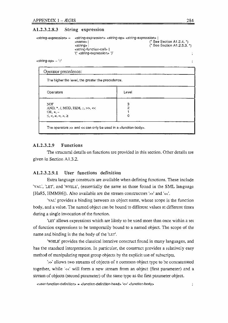
APPENDIX 1-.tEGIS 284
Al.2.3.2.8.3 String expression
<String-expression> = <string-expression> <string-op> <String-expression> I <name> I (* See Section A 1.2.4. *) <String> I (* See Section A 1.2.5.3. *) <String-function-call> I '(' <String-expression> ')'
<String-op> = '::'
Operator precedence:
The higher the level, the greater the precedence.
Operators Level
NOT 3 AND, *, /, MOD, REM, ::, >>, << 2 OR,+,- 1 ~, <, ;c, =, >, ~ 0
The operators >> and << can only be used in a <function-body>.
Al.2.3.2.9 Functions
The structural details on functions are provided in this section. Other details are
given in Section Al.3.2.
Al.2.3.2.9.1 User functions definition
Extra language constructs are available when defining functions. These include
'VAL', 'LET', and 'WHILE', (essentially the same as those found in the SML language
[Ha85, HMM86]). Also available are the stream constructors'»' and'«'.
'VAL' provides a binding between an object name, whose scope is the function
body, and a value. The named object can be bound to different values at different times
during a single invocation of the function.
'LET' allows expressions which are likely to be used more than once within a set
of function expressions to be temporarily bound to a named object. The scope of the
name and binding is the the body of the 'LET'.
'WHILE' provides the classical iterative construct found in many languages, and
has the standard interpretation. In particular, the construct provides a relatively easy
method of manipulating repeat group objects by the explicit use of subscripts.
'»' allows two streams of objects of a common object type to be concatenated
together, while '«' will form a new stream from an object (first parameter) and a
stream of objects (second parameter) of the same type as the first parameter object.
<User-function-definition> = <function-definition-head> '<=' <function-body>

APPENDIX 1 - JEGIS
<function-definition-head> = <function-name> '(' [ dermal-parameter-list> ] ')'
<function-name> = <name> (* See Section A 1.2.4. *)
Restriction:
<function-definition-head> is unique within the dictionary in terms of the combination of <function-name> with its arity (number of parameters).
dermal-parameter-list> = <name-list>
<function-body> = <function-expression> { ';' dunction_expression> }
<function-expression> = <Object-tuple> I <function-only-tuple>
<function-only-tuple> = <let> I <While> I <Val> I < function-stream-expression>
<val> = 'VAL' <name> '=' <object-tuple>
det> = 'LET' <Vais> 'IN' <let-body> ( 'ENDLET' I 'ENDL' )
<Vais> = <Val> { ':' <Val> }
<let-body> = <function-expression> { ';' dunction_expression> }
(* See Section A 1.2.4. *)
<While>= 'WHILE' <boolean_expression> 'DO' <While-body> ( 'ENDWHILE' I 'ENDW')
<While-body> = <function-expression> { ';' dunction_expression> }
<function-stream-expression> = <tuple-object> '«' ( <repeat-object> I <name> ) I
Restriction:
( <repeat-object> I <name> ) '»' <tuple-object> I <stream-function-call> I '(' <function-stream-expression> ')'
TYPE(<name>) must be a repeat object.
Al.2.3.2.9.2 System functions definition
285
Certain system functions, such as 'AVAILABLE' with a single parameter, test
system states, and are better described as primitive functions (see Sections Al.3.4
and Al.5). The implementation of these functions is system specific. All other system
functions are specified in the same manner as user-defined functions. A list of system
functions is given in Section Al.5.
Al.2.3.2.9.3 Function call
<boolean-function-call> = <function-call>
<number-function-call> = <function-call>
<String-function-call> = <function-call>

APPENDIX 1 - JEGIS
Restriction:
The value 'returned' by a <number-function-call> is of type NUMBER, etc.
<function-call> = <function-name> '(' [ <actual-parameter-list>] ')'
<actual-parameter-list> = <actual-parameter> { ',' <actual-parameter> }
<actual-parameter> = <Object> - <missing>
Al.2.3.2.10 Typing
<basic-type-expression> = <basic-type> I <qualified-type>
<qualified-type> = <Sub-type> I <basic-type-expression> <type-op> <basic-type-expression>
<basic-type> = 'BOOLEAN' I 'NUMBER' I 'STRING'
<type-op> = 'AND' I 'OR'
<SUb-type> = <repeat-range> I <range>
<repeat-range>= <first-bound>'{' ( 'DIGIT' I { 'CHAR' I 'CHARACTER'))')' <Second-bound>
Restrictions:
<Second-bound>~ <first-bound>. <first-bound> ~ 0. TYPE{dirst-bound>) = TYPE{<second-bound>) = NUMBER. <Second-bound> ~ <first-bound>.
<range> = <first-basic-type-value> ' . .' <Second-basic-type-value>
<first-basic-type-value> = <constant-object> I '-' <high-value>
<second-basic-type-value> = <Constant-object> I <high-value>
Restrictions:
<Second-basic-type-value> ~ <first-basic-type-value> in the collating sequence. TYPE{ <first-basic-type-value>) = TYPE{ <second-basic-type-value>). In each <range>, at least one of the <first-basic-type-value> and the <Second-basic-type-value> must be a <Constant-object>. " '-' <high-value> " means any value s; <Second-basic-type-value> is accepted.
Al.2.3.2.11 Constant
286
<Constant-object> = <number> I <String> I <boolean> {* See Section A 1.2.5. *)
Al.2.3.2.12 "Don't care"
<don't-care> = '?'

APPENDIX 1 - JEGIS
Al.2.3.2.13 Empty
<empty> = 'EMPTY'
Al.2.3.2.14 Missing
<missing> = 'MISSING'
Al.2.3.2.15 High value
287
(* No value. *)
INF is a polymorphic object which is used to signify a potentially high value.
The use of INF is restricted to repeats, and to qualified type expressions.
<high-value> has meaning for all types. In the case of numbers, <high-value> is a
high integer value. With strings, <high-value> is a long string made up of the highest
collating sequence characters. The <high-value> for Booleans is TRUE.
<high-value> = 'INF'
Al.2.3.2.16 Inhibit synonyms
If the defining details of an object is a single <name>, then at execution time the
defining object is treated as a synonym for the defined object, and when creating an
instance of the defined object, the defining object name is removed from the instance.
If the intention is that the name should be retained, synonym inhibiting can be
invoked using the operator'-'.
<inhibit-synonym> = •-• <name> (* See Section A 1.2.4. *)
Al.2.3.2.17 Inhibit subscripting
An object which appears in within a group object has an implicit subscript
created for it during execution, which means that any referenced object in a group
object is expected to be a subscripted object. If there is a need to reference a non
subscripted object (or one with a fixed subscript value), this can be done by inhibiting
subscripting on that object using the '@' operator.
<inhibit-subscripting> = '@' <name>
Al.2.3.2.18 Unique application details
Each application is fully identified by its name.
<application> = <application-name> <application-status-information> <application-dfds>
<application-name>= ( 'APPLICATION' I 'APPL')'(' <appl-name> ')'
<application-dfds> = { <dfd> I <Control-details> }
(* See Section A 1.2.4. *)

APPENDIX 1 - .tEGIS
Al.2.3.2.18.1 Data flow diagram hierarchy
<dfd> = { <external-entity> I <process> I <Unknown> I <data store> I <data flow> I <exporter> I <importer> I <refinement>}
Al.2.3.2.18.1.1 Basic data flow diagram objects
<external-entity> = ( 'EXTERNAL_ENI'ITY' I 'EE' ) '(' <name> ',' <appl-name> ')'
<process> = ( 'PROCESS' I 'PR' ) '(' <name> ',' <appl-name> ')'
<Unknown> = ( 'UNKNOWN' I 'UN ) '(' <name> ',' <Unknown-qualifier> ',' <appl-name> ')'
<Unknown-qualifier> = 'EE' I 'PR'
<data store>= ( 'DATA_STORE' I 'DS') '('<name>',' <appl-name> ')'
<data-flow>= ( 'DATA_FLOW I 'DF) '('<name>',' <appl-name> ')'
Al.2.3.2.18.1.2 Exporting and importing
288
(* See Section A 1.2.4. *)
(* See Section A 1.2.4. *)
(* See Section A 1.2.4. *)
(* See Section A 1.2.4. *)
<exporter>= 'EXP''(' <name>',' <non-df-dfd-object-type> ',' <appl-name> ')'
<importer> = 'IMP' '(' <name> ',' <non-df-dfd-object-type> ',' <appl-name> ')'
<non-df-dfd-object-type> = 'EE' I 'PR' I 'UN I 'DS'
Al.2.3.2.18.1.3 Process, and data flow refinement
<refinement>= ( 'REFINEMENT' I 'REF)'(' <refined-object> ',' <refined-object-type> ',' <refining-object> ',' <appl-name> ')'
<refined-object> = <name>
<refined-object-type>= 'PR' I 'DF
<refining-object> = <name>
Al.2.3.2.18.1.4 Control details
<Control-details> = { <import-set> I <data-store-action> }
(* See Section A 1.2.4. *)
(* See Section A 1.2.4. *)
<import-set>= ( 'IMPORT_SET' I 'IS')'(' <process>',' <name-list>',' <appl-name> ')'
Restriction:
The type of each <name> in the <name-list> must be DF.
<data-store-action>= { <access-method> I <Operation> I <exception>}

APPENDIX 1 - .tEGIS 289
<access-method>= ( ('KEYED_USING' I 'KU')'(' <df-name> ','<name-list>',' <appl-name> ')') I ( ( 'SEQUENTIAL' I 'SEQ' ) ) '(' <df-name> ',' <appl-name> ')' )
<Operation> = ( 'DELETING' I 'DEL' ) '(' <df-name> ',' <appl-name> ')' I ( ( ( 'ADDING' I 'ADD') I ('UPDATING' I 'UPD')) '(' <df-name> ',' <appl-name> ')'
'MAP' '(' <name-tuple> ')' 'TO' '(' <name-tuple> ')' )
<df-name> = <name> (* See Section A 1.2.4. *)
Restriction:
The type of <df-name> must be DF.
<exception> = ( 'EXCEPTION' I 'EXC' ) '(' <df-name> ',' <exception-activity> ',' <appl-name> ')'
<exception-activity> = <roll-back> I <prompt> I <default> I <empty> I <don't-care> I <missing>
Restrictions:
<exception activity> details, and the restrictions on their use, are described in Section A 1.4.
Al.2.3.3 Execution time objects The execution time objects are: executable applications, made up of instances of
data objects, executable application process sets, and process status' objects. None of
these can exist outside the context of the executable application model whose name they
include.
<executable-application> = <execution-application-name> <executable-application-process-set> <process'-status> { <instance> }
Al.2.3.3.1 Executable applications
Each executable application is fully identified by its name.
<exececution-application-name> = ( 'EXECUTABLE_APPLICATION I 'EA')'(' <exec-appl-name> ',' <appl-name> ')'
<exec-appl-name> = <name> (* See Section A 1.2.4. *)
Al.2.3.3.2 Process' status
Each executable process is in one of three states.
<process'-status> = ( 'BLOCKED' I 'RUNNABLE' I 'EXECUTING' ) '(' <process-name> ',' <exec-appl-name> ')'
Al.2.3.3.3 Execution application process set
These are the set of processes which are in.a particular executable model.
<execution-application-process-set>= ( <execution-process> )
<execution-process> = ( 'EXECUTION_PROCESS' I 'EP' ) '(' <name>, <exec-appl-name> ')'

APPENDIX 1 - £GIS 290
Al.2.3.3.4 Instances
An object instance can be either a data flow instance, or a met value (which is
the value of an intermediate object generated within the context of a process).
<instance> = <data-flow-instance> I <met-value>
Al.2.3.3.4.1 Data flow instance
<data-flow-instance> = 'INSTANCE''(' <df-name> ',' <importer-name> ',' <importer-type> ',' <exec-appl-name> ',' <Value-tuples> ')'
<importer-name> = <name> (* See Section A 1.2.4. *)
<importer-type> = <non-df-dfd-object-type>
<Value-tuples> = '(' <Value-tuple> { ','<value-tuple> } ')'
<Value-tuple> = '(' ( <name> ) <Value-tuples> ')' I <constant-object>
Al.2.3.3.4.2 Met value
<met-value> = 'MET '(' <data-object-name> ',' <process-name> ',' <exec-appl-name> ',' <Value-tuples> ')'
<data-object-name> = <name>
<process-name> = <name>
Al.2.4 Name
<name> = <simple-name> I <Subscripted-name>
Restriction:
(* See Section A 1.2.4. *) (* See Section A 1.2.3.2.11. *)
(* See Section A 1.2.4. *)
(* See Section A 1.2.4. *)
<name> must be unique for the object type within the dictionary.
<simple-name> = <single-quoted-string> I <restricted-unquoted-string>
<Single-quoted-string> = " ' " dull-unquoted-string> " ' ".
dull-unquoted-string> = Any sequence of characters in the character set.
Restriction:
If the dull-unquoted-string> appears within single quotes, any instance of a single quote in the dull-unquoted-string> is represented by two adjacent single quotes. If the dull-unquoted-string> appears within double quotes, any instance of a double quote in the dull-unquoted-string> is represented by two adjacent double quotes {see Section A 1.2.5.3).
<restricted-unquoted-symbol> = Any sequence of characters not including terminal symbols.
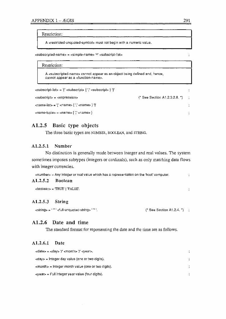
APPENDIX 1 - IEGIS
Restriction:
A <restricted-unquoted-symbol> must not begin with a numeric value.
<Subscripted-name> = <simple-name> "" <subscript-list>
Restriction:
A <Subscripted-name> cannot appear as an object being defined and, hence, cannot appear as a <function-name>.
<subscript-list> = '[' <Subscript> { ',' <subscript> } ']'
<Subscript> = <expression>
<name-list> = '[' <name> { ',' <name> } ']'
<name-tuple> = <name> { ',' <name>}
Al.2.5 Basic type objects
(* See Section A 1.2.3.2.8. *)
The three basic types are NUMBER, BOOLEAN, and STRING.
Al.2.5.1 Number
291
No distinction is generally made between integer and real values. The system
sometimes imposes subtypes (integers or cardinals), such as only matching data flows
with integer currencies.
<number> = Any integer or real value which has a representation on the 'host' computer.
Al.2.5.2 Boolean
<boolean>= TRUE' I 'FALSE'.
Al.2.5.3 String
<String> = ' " ' dull-unquoted-string> ' " '. (* See Section A 1.2.4. *)
Al.2.6 Date and time The standard format for representing the date and the time are as follows.
Al.2.6.1 Date
<date> = <day> '( <month> •r <Year>.
<day> = Integer day value (one or two digits).
<month> = Integer month value (one or two digits).
<year> = Full integer year value (four digits).

APPENDIX 1-.tEGIS
Al.2.6.2 Time
<time> = <hour> '.' <minutes> '.' <Seconds>.
<hour> = Integer twenty-four hour clock value (in range 0 .. 23).
<minutes> = Integer value (in range 0 .. 59).
<seconds> = Integer value (in range 0 .. 59).
Al.3 Further lEgis language features
292
Details on .tEgis language features not described in Chapter 5 are given in the
following subsections.
Al.3.1 Numeric operations • 'SUM' forms the total of all the component objects in its stream of objects. The
general form of the function is
SUM (GROUP _OBJECT)
For example, when the component instances of the repeat group are, respectively,
([l], (EXTENSION, (17.52))) and ([2], (EXTENSION, (323.75))),
SUM ( (1, INF, [EXTENSION]})
leads to the construction of the tuple
(341.27).
A fully elaborated repeat group can be given as the parameter for SUM.
Al.3.2 String operations The following extra functions are available for operating on 1-tuples of type
S1RING:
• 'sUBSTR' constructs a new string by selecting a contiguous range of characters from a
given string. The general form of the function is
SUBSTR (SOURCE_STR, FIRST_CHAR_FOSIDON, NUMBER_OF _CHARS_TO_SELECT)
For example,
SUBSTR (''THIS STRING rs TOO LONG", 16, 8)
leads to the construction of the tuple
('TOO LONG").
• 1REPLSTR
1 leads to the creation of a new string in which each occurrence, up to a
specified maximum number, of a given string of characters in a 'source' string is
replaced by a second string of characters. The general format is
REPLSTR(SOURCE_STR,STR_TO_REPLACE,STR_TO_REPLACE_WITH,
MAXIMUM_NUMBER_OF _TIMES_TO_PERFORM_THE_REPLACEMENT,
FIRST_CHARACTER_IN_SOURCE_STR_TO_BEGIN_REPLACEMENT_SEARCH).

APPENDIX 1-JEGIS
The example
REPLSTR ("MISS JONES", "MISS", "MS", 1, 1)
results in the creation of the tuple
("MS JONES").
293
• 'LENGTH' creates a I-tuple of type NUMBER that denotes the length in characters of a
given string. For example,
LENGTH ("HOW LONG IS THIS STRING?")
results in the creation of the tuple
(24).
Al.3.3 Stream operations Four tuple operators exist for use in functions. These are:
• '«' which is an infix, non-commutative, binary function that creates a new stream
from an object and a stream. For example, if ss has the associated stream value
((3), (([l], ("EIGHT")), ([2], ("NINE")), ([3], ("TEN"))))
then
"SEVEN" « SS
leads to the creation of the stream
((4), (([l], ("SEVEN")), ([2], ("EIGHT")), ([3], ("NINE")), ([4], ("TEN")))).
• 'REST' is a function that creates a new stream which is a copy of the given string
except that ·the first item has been removed. For example,
REST(SS)
leads to the creation of the stream
((2), (([l], ("NINE")), ([2], ("TEN")))).
• '»' forms a new stream by appending a second stream to a first stream. For
example, if ss1 and ss2 have the following respective values
((2), (([l], ("SEVEN")), ([2], ("EIGHT"))))
((2), ([l], ("NINE")), ([2], ("TEN"))))
then
SSl » SS2
leads to the creation of the stream
((4), (([l], ("SEVEN")), ([2], ("EIGHT")), ([3], ("NINE")), ([4], ("TEN")))).
• 'FIRST' is a function which selects the first object in a given stream of objects. For
example,
FIRST(SS)
extracts the object "EIGHT". Note that the relationship 's = FIRST (S) « REST (S)' holds.

APPENDIX 1 - JEGIS 294
Al.3.4 System-dependent (primitive) operations The implementation of the following functions is system-dependent, as they test
the execution state of processes, and data object instances.
• 'AV AILABLE(DATA_OBJECT)' which evaluates to TRUE if the data object (name) which is
its parameter has an instance in the context of the executing process. The instance
has to exist at the time the call on Av AILABLE is made.
• 1CURRENCY(DATA_FLOW _OR_PROCESS_OBJECT)
1 returns the currency of the object if its
type is DATA_FLOW or PROCESS.
• 1NEW(DATA_OBJECT)
1 is a function that performs a name coercion on a newly created
object. It is used in data flow diagrams which contain (tight) loops, so that the
imported (old) instance of a data object can be distinguished from the new instance
of that object, created during the current process invocation. For example,
NEW(OBJ)
leads to the creation of an instance of 'NEW(OBJ)' of the form
('NEW(OBJ)', (value of the object)).
When, or if, the object is exported, its name is automatically coerced (back) to 'OBJ'
by the system.
• 1THERE_EXISTS(DATA_OBJECT, CONDITION)', where CONDITION is one of the following
two forms: 1DATA_OBJECT binary_op expression'
'/unction (DATA_OBJECT, expression)'
'Boolean_ unary Junction DAT A_OBJECT1
'Boolean Junction (DATA_OBJECT)'
DATA_OBJECT must be a group object element; that is, it must be an implicitly
subscripted object. For example, given that the group object 1(1, INF, [EXTENSION]}'
has been imported by the executing process, the function call
THERE_EXISTS(EXTENSION, EXTENSION< 0)
will lead to the following two actions:
A check will be made that (at least) one instance of EXTENSION exists within the
context. If not, the function evaluates to FALSE.
For each instance of EXTENSION that exists, it is checked to see whether its value is
negative. If an instance is found which satisfies the conditional, the function
evaluates to TRUE, without the need to evaluate further. If no instance(s) satisfies
the conditional, the function evaluates to FALSE.
• 1THERE_EXISTS(EXPRESSION, DATA_OBJECT, CONDITION)', where the second and third
parameters are as given for the previous function. The first parameter is any valid
expression. The function is executed by first evaluating the expression given as the
first parameter, following which a call of the previous function is made, of the form

APPENDIX 1 - JEGIS 295
THERE_EXISTS(DATA_OBJECT, CONDIDON).
This function is used when it is known that the data object to be tested will have
subscripted instances created within the context of the process, but because there is
no general guarantee on the order of evaluating objects, at the time the function is
evaluated, the object may not have yet had its instances created. The first parameter
can be used to force this evaluation (if it has not already been carried out).
The example given for the previous function is relevant here. If the values of
EXTENSION had not been imported into the process, the current function should be
used with a call such as
THERE_EXISTS((l, INF, [EXTENSION]), EXTENSION, EXTENSION< 0) .
• 'FOR_ALL(DATA_OBJECT, CONDITION)', where CONDITION is as defined above in 1THERE_EXISTS(DATA_OBJECT, CONDITION)'. For the function to evaluate to TRUE, all
instances of the data object must satisfy the condition. If no instance of the
subscripted data object exists, the function evaluates to FALSE.
• 'FOR_ALL(EXPRESSION, DATA_OBJECT, CONDIDON)', where CONDIDON is as defined above
in 1THERE_EXISTS(DATA_OBJECT, CONDIDON)'. For the function to evaluate to TRUE, all
instances of the data object must satisfy the condition. The expression can be used to
ensure that the data object instances are created prior to the condition testing.
• 'EXPRESSION_l ++ EXPRESSION_2'.
If all the needed data object instances are available to evaluate EXPRESSION_l, then it is
evaluated. Otherwise an attempt is made to evaluate EXPRESSION_l. On of the options
must be able to be evaluated, otherwise an error condition is raised. '++'s can be
combined. For example,
'EXPRESSION_l ++ EXPRESSION_2 ++ EXPRESSION_3 ++ EXPRESSION_ 41
will result in an attempt to evaluate EXPRESSION_l first, then EXPRESSION_2, then
EXPRESSION_3, and finally EXPRESSION_ 4.
• '@ OBJ'. The unary operator'@' stops the implicit subscripting of an object in a
repeat group. In the definition
A<= ( 1, 2, [B, @ C"[ 6], D])
the instance created for object A will have two component tuples. In the first
component, an instance of B with subscript [ll will appear, and similarly for D. The
instance of c which will appear is that with an (implicit) subscript of [6]. In the
second component, an instance of B and D with subscript [2] will appear. The
instance of c will once again be that with an (implicit) subscript of [6].
• '~ OBJ'. The unary operator'~' stops the implicit interpretation of a simple definition
as the definition of a synonym. In
A<=~B
the instance created for object A will have the component tuple <B, value_ of _B) ••

APPENDIX 1 - JEGIS 296
Al.5 System functions The following lists the system-defined functions available in SAME. All but
those marked with a dagger ('t') been included in the implementation of Chapter 7.
Those marked with an asterisk ('*') are primitive functions, which require a system
specific implementation.
• AV AIIABLE(DATA_OBJECT) - If an instance of DATA_OBJECT exists,
the value is TRUE, otherwise it is FALSE. (*)
• COUNT_OF(DF _OR_PROCESS_OBJECT, OBJECT_TYPE) - In the context of a currently
running executable model, returns a count of, in the case of a specified data flow, the
number of instances that have been created of that data flow; or, in the case of a
specified process, the number of times that process has been executed. (*)
• CURRENCY(DF _OR_PROCESS_OBJECT, OBJECT_TYPE) - Returns the currency of a data
flow or process in a currently running executable model. (*)
• DATE() - Returns the date. (*)
• A DIV B Infix binary operator which returns the quotient
from dividing the (integer) number A by the (integer) number B.
• FIRST(OBJECT_STREAM) - Returns a copy of the first object in the stream. The object
can be any tuple. (t)
• FOR_ALL(DATA_OBJECT, CONDITION) - Used to see whether a condition applies to all
component objects in a data object stream.
• FOR_ALL(EXPRESSION, DATA_OBJECT, CONDIDON)- After first evaluating the expression,
checks to see whether a condition applies to all component objects in a data object
stream.
• LENGTH(STRING_OBJECT)- Returns the length of a string.
• MAX(TUPLE) - Returns the maximum collating sequence, basic typed,
valued object in TUPLE. This function works down through the
tuple structure locating each leaf object.
• MAX_ALL(fUPLE) - Returns the maximum collating sequence,
structure valued object in TUPLE. This function only operates on the
'top level' components of TUPLE, which can be of any type.
• MIN(fUPLE) - Returns the minimum collating sequence, basic typed,
valued object in TUPLE. This function works down through the
tuple structure locating each leaf object.
• MIN_ALL(fUPLE) - Returns the minimum collating sequence,
structure valued object in TUPLE. This function only operates on the
'top level' components of TUPLE, which can be of any type.
• NEW(NAME) - Coerces NAME to 'NEW(NAME)' for the instance of
a data object created within the currently executing context of a process.

APPENDIX 1 - JEGIS
Allows the previous (now imported) instance of the object to be
distinguished from the new (just created) instance of the same named
object within the single process context.
• POWER(MANTISSA_OBJECT, EXPONENT _OBJECT) - Given two objects of type
NUMBER, returns the result of calculating MANTISSA_OBJEcrEXPONENT_OBJECT.
• A REM B Infix binary operator which returns the remainder
from dividing the (integer) number A by the (integer) number B.
• REPLSTR (SOURCE_STR, STR_TO_REPLACE, STR_TO_REPLACE_WITH,
MAXIMUM_NUMBER_OF _TIMES_TO_PERFORM_THE_REPLACEMENT,
FIRST_CHARACTER_IN_SOURCE_STR_TO_BEGIN_REPLACEMENT_SEARCH)
Returns a string in which a specified string in the original string has
been replaced by a different string. The number of times the replacement
is to occur is also specified, as is the position in the source string
from which matching is to begin taking place.
297
(*)
• REST(OBJECT_STREAM)- Returns a copy of the given object stream, except for the first
item in the original stream. (t)
• SQRT(OBJECT_OF_TYPE_NUMBER)- Returns the square root of a number~ 0.
• SUBSTR(SOURCE_STRING, FROM, LENGTH) - Returns the substring of
SOURCE_STRING which begins at character position FROM, and is of
(maximum) size LENGTH.
• SUM(STREAM_OF_OBJECTS_OF_TYPE_NUMBER)- Used with a repeat group
object. Sums the components of the stream .
• THERE_EXISTS(DATA_OBJECT, CONDffiON)- Used to see whether a condition applies to
at least one component object in a data object stream .
• THERE_EXISTS(EXPRESSION, DATA_OBJECT, CONDffiON) - After first evaluating the
expression, checks to see whether a condition applies to at least one component
object in a data object stream.
• TIME() Returns the time.
• TYPE(I'UPLE) - Returns the type of the tuple.
• :: - Infix binary string concatenation operator.
• +, -, *, f - Standard infix binary arithmetic operators C-' also unary prefix).
• ::;;, <, =, ¢, >, ~ - Standard infix binary comparative operators.
• NOT, & ('AND'),# ('OR'), - Standard Boolean operators
('&' and'#' binary infix; 'NOT' unary prefix).
• «, » - Infix binary stream operators.
(*)
Ct)

APPENDIX 1 - .tEGIS 298
Al.6 Data store activities The details in this section relate closely to material presented in Section 6.4.
Each data flow that is imported into or exported from a data store has a set of
attributes associated with it. In the case of a data flow exported by a data store, the first
two in the following list are the associated attributes. For flows imported into the data
store, all the following are in the attributes set:
• The method of access (viewed from the data store).
• The method for handling exceptions.
• The operation carried out on the associated data store tuple.
• The name mapping which occurs between the data flow and the data store tuple.
The two methods of access are import the data flow into the data store, and
export the data flow from the data store. The other attributes will be discussed under
these access methods.
Al.6.1 Exporting from a data store There are two methods for exporting from a data store: sequential and keyed.
With sequential exporting, the 'next' tuple in the data store is accessed, and the
exported tuple is extracted from that tuple. With a keyed access, the tuple identified by
the key is accessed, and the data flow instance is formed from that tuple.
The only other attribute for a data flow exported from a data store, is the action
that is to be taken if the export instance is unable to be created from the data store
contents. The options are:
• Abort the process execution ('roll back') - No import data flows are consumed by
the process.
• Substitute a previously specified default value.
• Prompt the user for the data flow instance.
• Substitute a "don't care" value.
• Substitute an EMPTY value.
• Substitute a missing (MISSING) value.
Al.6.2 Importing into a data store A data flow that is imported into a data store is also matched to the data store
tuple either sequentially or using a key.
The operation caused by the importing is one of the following:
• Delete the matching data tuple from the data store.
• Add a new data tuple to the data store.
• update (amend) the matching data tuple in the data store.

APPENDIX 1 - JEGIS 299
The first two operations only work on full tuples, whereas an update can result
in only part of an existing data store tuple being changed.
The exceptions activities possible when importing are the following:
• Ignore the operation- Such as when deleting a non-existent tuple.
• Abort the process execution ('roll back') - No import data flows are consumed by
the process.
• Substitute a previously specified default value.
• Create a new object with the updated value. (Only applies if a tuple exists into which
the object can be placed, or the object is a complete 'record'.)
• Create a new object with a constant user-supplied value of a user-specified type.
(Only applies if a tuple exists into which the object can be placed, or the object is a
complete 'record'.)
The final operation that must be specified for data store imported flows, is the
mapping of the data flow object name(s), to the data store tuple name(s). This mapping
is done using the structure of the objects and their type(s) as the method of mapping, so
care needs to be exercised in the way that data objects are defined. For example, from
the following definitions data objects A and B have the same type, but A and c do not
(because of the ordering of the elements in the tuples).
A<=D, E,F. B<=G,E,H. C<=H,E,G. D<=NUMBER. E <= BOOLEAN. F<=STRING. G<=NUMBER. H<=STRING.

A2.1 Introduction ........................................................................... 301
A2.2 Formal specification of the structure of data flow diagrams ..................... 302
A2.2.1 PL specification of the roots of a quadratic application ............... 303
A2.2.2 Extensions required to the PL to fully support SAME ................ 304
A2.2.3 Acknowledgment. ......................................................... 305
A2.3 Execution states, and transformations between them ............................ 305
A2. 3 .1 Bi, the set of blocked processes ......................................... 307
A2. 3 .2 Ri, the set of runnable processes ........................................ 308
A2.3.3 Ei, the set of executable processes ...................................... 308
A2.4 Data object transformations ......................................................... 308
A2.4.1 Contexts .................................................................... 309
A2.4.2 Referential completeness ................................................. 311
A2.4.3 Functional completeness ................................................. 311
A2.4.4 Full import data preserving .............................................. 312
A2.4.5 Full functional completeness ............................................. 312
A2.4.6 Full export data preserving ............................................... 313
A2.4. 7 Data preserving ............................................................ 313
A2.4.8 Full functional dependence ............................................... 313
A2.4.9 Summary of the classification ........................................... 314
300

APPENDIX 2 - THE BASIS FOR A RIGOROUS INTERPR'N OF SAME 301
A2.4.10 The inclusion of binding distance ....................................... 314
A2.5 A final categorisation of applications ............................................... 315
A2.1 Introduction An application is represented in SAME by an executable model. The exercising
of this model is a simulation against which test data is processed. The limitations on
this approach relate both to the suitability of the model as an adequate representation of
the application, and to the representation of the test data. As a consequence, it is felt that
a need can be seen for the generation of a formal specification of the model generated in
SAME. To be able to produce such a document requires that both SAME itself be
formally specified, and that a suitable toolset exists for the generation of the formal
application specifications.
The production of a formal specification for a data flow system is a major task
and has formed the subject matter of at least one doctoral dissertation [Jo85], while also
being the active doctoral research area of France [FDP87, FD88a, FD88b, Fr88]. Work
undertaken by France and Docker to do with the formal specification of data flow
diagrams is relevant to SAME and is discussed in Section A2.2. Currently this work is
concerned with the use of algebras to define the syntax of the diagrams modelling an
application [FDP87, FD88a, FD88b]. France is extending this work to incorporate
semantics as well [Fr88], but this has not reached a stage where it can be applied to
SAME.
The work undertaken by France and Docker does not consider the relationships
between import and export sets of data flows, as these are dependent on the particular
method(s) used in the specification of the relationships. In SAME, the relationships are
defined by bindings between objects (see Section 5.4.2) which have a pictorial
representation as data dependency graphs, such as those given in Figure 6.5.
Section A2.4, provides a more formal interpretation of the transformations than that
given in the body of the dissertation.
Before discussing the work of France and Docker, two other research groups
working on the formalisation of data flow diagrams are worthy of special mention.
These are Tse and Pong [Tse85, Tse86a, Tse86b, Tse86c, Tse86d, TP86], and Chua
et al. [CTL87].
There are similarities in the work carried out by Tse's group and that of Chua.
Both have an underlying Petri net model for checking the consistency of a data flow
diagram and for providing executable models. The use of Petri nets is an obvious

APPENDIX 2 - THE BASIS FOR A RIGOROUS INTERPR'N OF SAME 302
approach, and has on a number of occassions been proposed as a formalisation tool for
specification and for software design, where most uses have been concerned with the
inherent concurrency within applications (see [YC83] and [Ma85], for examples).
These previous uses have close associations with the data dependency view of data
flow diagrams, and some work on the relationship of Petri nets to SSA data flow
diagrams was undertaken by Alexander at Massey University [A186]. A point of
concern highlighted by the work of Alexander was the representation of data stores in
Petri nets. The inference to be drawn is that data stores need to be modelled at a higher
level of abstraction than that found in simple transitions-places networks.
It is interesting to note that none of the cited references for Tse's or Chua's
group discuss the detailed handling of data stores. In Tse's case the work appears to be
restricted to processes and data flows only, while Chua seems to only note syntactic
differences between data stores and other data flow diagram objects.
The use of Petri nets as an underlying formalism has some value with reference
to testing the 'reachability' of flows. However, even here it is limited as the instances
of flows are treated as simple tokens with little or no semantics, so that, for example,
the conditional generation of a flow cannot be easily modelled. To adequately model the
semantics is likely to lead to an exponential explosion in the complexity of the nets, and
is therefore considered to have little value.
An alternative approach is a scheme which uses typed tokens, along with
predicates associated with the value of tokens to specify places in Petri nets. Two
particular examples of this approach are Pro-Nets [No80] and PROTEAN [BWW88],
but neither of these has been applied to data flow diagrams.
Work is being carried out by other people on limited aspects of data flow
diagrams. One such case is the work of Adler, which is concerned with an algebra to
support the decomposition of processes within data flow diagrams [Ad88].
A2.2 Formal specification of the structure of data flow diagrams
Work carried out principally by France takes Tse's work as a starting point. A
formal algebraic system has been developed consisting of a language and an inference
component from which algebraic specifications can be derived. The semantic model
used for the algebraic specification is the initial word algebra [BG81, FD88b].
By way of example, the following defines the theory which supports the
specification of a process: 1
1 The 'pl' in lower or upper case letters identifies this as a Picture Level (PL) theory, which is concerned with the syntactic details of a data flow diagram. A second level, called the Specification Level (SL), deals with the semantics of the data flow diagram components (see [Fr88]). The discussion here is limited to the PL.

APPENDIX 2 - THE BASIS FOR A RIGOROUS INTERPR'N OF SAME 303
THEORY PLprocess using Set(Plflow), Procnames Signature:
sorts = {plprocess }
constructors mkplprocess: procname, set(plflow), set(plflow) • plprocess -- creates a plprocess with name of type procname, and import and
export sets of plflows ---
obse rvat ion functions getpimports, getpexports : plprocess • set(plflow) --- generates the import and export sets, respectively, of a plprocess ---
ok predicate okproc : plprocess • boolean
Laws: \:::/ in, out E set(plflow); e E plprocess ; n E procname
PR1. getpimports(mkplprocess(n, in, out)) = in
PR2. getpexports(mkplprocess(n, in, out)) = out
PR3. isempty(intersect(getpimports(e), getpexports(e))), ~isempty(getpexports(e)), ~isempty(getpimports(e)) ~ okproc(e) -- a plprocess, e, is constructed correctly iff its import and export sets are
non-empty and disjoint ---
EN DTH E ORY Plprocess
The above theory, and the other theories required to formally describe the
structure of data flow diagrams, are given in France and Docker [FD88a].
A2.2.1 PL specification of the roots of a quadratic application
To demonstrate the use of the PL theories, the roots of a quadratic example
given in Section 3.4.1 will be defined. The Level O diagram given in Figure 3.18(a) has
the specification
RootsOfAQuadratic = mkplapplic('ROOTS OF A QUADRATIC', {mkplprocess('FIND ROOTS OF QUADRATIC', {COEFFICIENTS}, {ROOTS})}, {}, {mkplentity(ANALYST, {ROOTS}, {COEFFICIENTS})})
Figure 3.19 shows a Level 1 refinement of the process FIND ROOTS OF
QUADRATIC, and its specification is
'ROOTS OF A QUADRATIC' = primstruct(
mkplprocess('FIND ROOTS OF QUADRATIC', {COEFFICIENTS}, {ROOTS}), {mkplprocess('COMPUTE BSQ', {b}, {BSQ}), mkplprocess('COMPUTE FOURAC', {a, c}, {FOURAC}), mkplprocess('COMPUTE SOR', {BSQ, FOURAC}, {SOR}),

APPENDIX 2 - THE BASIS FOR A RIGOROUS INTERPR'N OF SAME 304
mkplprocess('COMPUTE N1', {b, SOR}, {N1}), mkplprocess('COMPUTE N2', {b, SOR}, {N2}), mkplprocess('COMPUTE TWOA', {a}, {TWOA}), mkplprocess('COM PUTE root1 ', {N1}, {root1 }) , mkplprocess('COMPUTE root2', {N2}, {root2})}
The above is possible because primstruct is a suitable operator in a theory that
specifies process refinements [FD88a]. Within the theory is a law
okrefinement(p, sp) <:=> okprocstruct(primstruct(p,sp))
which is valid if, and only if, sp is a refinement of p. The laws that determine this are
part of the theory.
All invalid data flow diagram hierarchies reduce to the value errapplic. It is
possible to parameterise errapplic, so that the (first met) reason why an hierarchy is
invalid can be identified. This can be done easily. For example, if plprocess •
plprocess, defined only on errplprocess, picks up an error from constructing a
plprocess. Thus if mkplprocess(n, in, out)= errplprocess then errapplic(mkplprocess(•)).
A2.2.2 Extensions required to the PL to fully support SAME The theories so far developed for the PL do not fully support the flexibility
found in SAME. For example, there are no theories associated with objects of type
unknown, nor with limited import and export sets. Also, the various classifications of
applications as structurally complete, incomplete, and invalid are not fully represented.
The extensions required to support these features are not considered significant.
An unknown object, for example is essentially viewed as either an external entity or a
process depending on the wishes of the user. In PL terms, no distinction need be made
between them as no details on transformations from data flow import sets to export sets
are specified.
France separates out syntactic from semantic details, and prefers to specify
limited import sets at the Specification Level (SL), which accounts for their omission
from the PL theories. The specification of theories at the SL to encapsulate the
semantics of data flow diagrams is currently being addressed [Fr88].
Amendments to the theories of the PL to support undefined (unknown) objects
and incomplete applications is being developed by France. An undefined object will
result in an incomplete specification, and is analogous to A1 in Section 4.6.

APPENDIX 2 - THE BASIS FOR A RIGOROUS INTERPR'N OF SAME 305
A2.2.3 Acknowledgment Section 2.2 owes much to the work of France, and has been included in this
thesis because of its particular relevance to SAME through the joint research of France
and Docker.
The rest of this appendix details work carried out independently of France.
A2.3 Execution states, and transformations between them
Rules describing the operational semantics of the data-driven DFDMl model
were given in Section 4.2, and are as follows:
• Data flows (directed arcs) carry instances (token sets) between operational nodes.
• Firing rules:
Fl: Under normal operational conditions all data flows are, or in the case of data
store produced instances can be viewed as, FIFO queues.
F2: A process (node) is eligible for executing when a complete set of import
instances is available.
F3: When a process executes, one instance is read from each import flow.
Following successful execution of the process, the read data flow instances
are removed from the data flows.
F4: At the end of the successful execution of a process, each of the created
instances (possibly EMPTY) is exported. If more than one importer exists for
an exported data flow, a copy of the instance is exported to each of the
importers.
FS: A data flow instance imported from a data store is created when first
referenced in the executing process, unless it has already been created.
F6: The ordering of the creation of external entity generated instances is decided
by the user.
The above rules do not provide details on when processes are executed. Rule
F2, for example, only states under what conditions a process becomes eligible for
execution. Details on exactly when a process is executed can be left as an
implementation issue. However, using Figure 6.1 as the specification of an abstract
'SAME machine', such details can be specified in terms of this machine. This is now
done, by viewing the execution state of SAME in terms of the allowable states that
processes can be in.
At any particular time during the exercising of an application model, a
component process can be in one of three states: blocked, runnable, or executing.
One condition under which a process is blocked is if an adequate set of data flow
instances is not available, where an adequate set is defined as follows:

APPENDIX 2 - THE BASIS FOR A RIGOROUS INTERPR'N OF SAME 306
Definition: An adequate set of data flows instances for an executable
process p exists if one of the following conditions is true:
• where import sets exist for process p, an import set of instances
is available;
• where import sets do not exist for p, a matching instance exists
for each of the data flows in the full import set, excepting those
generated by data stores.2 •
The other condition under which a process can be blocked, is where the
execution of the process was abandoned (rolled back) due to an unsuccessful data store
access.
The underlying architecture of the 'SAME machine' includes the set
{ c1, c2, ... , ck, c1, ... , cp} of processors, where p :2:: 1.
The execution of an application is defined as the sequence of state changes
[S0, S1, S2, ... , Sa], a> 0. The application completes at time ta.
Initially the system is in state S0 at time t0 = 0. A state transition Si-l • Si
occurs at time;, such that ti> ti-l• where i E N, the set of natural numbers. A change
in state from Si-l to Si occurs when one or more currently running processes
completes, or when external entity generated data flows become available. That is, the
execution of a process is considered an atomic activity, as is the supplying of external
entity generated data flow instances.
At state i, i E N0 (Nu { 0} ), the set of executable application leaf processes PL
can be divided into the sets
• Bi, the set of blocked processes;
• Ri, the set of runnable processes;
• Ei, the set of executing processes.
That is,
iPL=B· UR u E· 1 1 I'
s.t. Bin~ n Ei = 0, and where the superscript on PL is meant to signify that the sets
Bi, Ri, and Ei are state dependent. (PL never changes.)
At state S0 (t = 0),
OpL = PL U 0 U 0;
that is, B0 = PL, Ri = 0 and Ei = 0.
A diagram showing the possible state transitions is given as Figure A2. l.
2 Data store generated data flows are not specified in import sets, so need not be explicitly excluded.

APPENDIX 2 - THE BASIS FOR A RIGOROUS INTERPR'N OF SAME 307
[E3], [E4]
Figure A2. l: State transition diagram for the execution of processes within an application.
The conditions under which transitions occur are elaborated in the following
three sub-sections. The Boolean functions used in the conditions have the following
interpretation:
• import_set_available(pj, i) - This is true if process Pj has an adequate set of data
flows available at transition Si-l • Si.
• completed(pj, c1, i) - This is true if process Pj executing on real processor c1 finishes
execution at transition Si-l • Si.
• scheduled(pj, ck, i) - This is true if process Pj is allocated to real processor ck at
transition Si-l • Si.
• rolled_back(pj, c1, i) - This is true if process Pj is abandoned (rolled back) due to the
unavailability of a data store access at transition Si-l • Si. Such a process remains
blocked for one state transition to provide time for another process to produce the
required data store tuple. There is no guarantee that the tuple will be created in this
time, in which case the rolled back process will be rolled back again at a later
transition (Si+l • Si+2 at the earliest).
A2.3.1 Bi, the set of blocked processes The set Bi of blocked processes is defined by
Bi= {pj I [Bl] v [B2] v [B3]}

APPENDIX 2 - THE BASIS FOR A RIGOROUS INTERPR'N OF SAME 308
where:
• [Bl]= (pj E Bi-l A ~import_set_available(pj, i)).
• [B2] = (Pj E Ei-l A (completed(pj, c1, i) A ~import_set_available(pj, i)).
• [B3] = (Pj E Ei-1 A rolled_back(pj, C1, i)).
A2.3.2 Ri, the set of runnable processes The set Ri of runnable processes is defined by
Ri = {pj I [Rl] v [R2] v [R3]}
where:
• [Rl] = (pj E Bi-l A (import_set_available(pj, i) A ~scheduled(pj, ck, i)).
• [R2] = (Pj E Ri-l A ~scheduled(pj, ck, i)).
• [R3] = (pj E Ei-l A (completed(pj, c1, i) A import_set_available(pj, i)
A ~scheduled(pj, ck, i)).
A2.3.3 Ei, the set of executable processes The set Ei of executable processes is defined by
Ei = {pj I [El] v [E2] v [E3] v [E4]}
where:
• [El] = (pj E Bi-l A (import_set_available(pj, i) A scheduled(pj, ck, i))
• [E2] = (pj E Ri-l A scheduled(pj, ck, i))
• [E3] = (Pj E Ei-l A ~completed(pj, c1, i)).
• [E4] = (pj E Ei-l A (completed(pj, c1, i)
A import_set_available(pj, i)
A scheduled(pj, ck, i))).
A2.4 Data object transformations The transformations that occur in process' invocations from import sets to
export sets are not covered by the algebraic theories in Section A2.2. A major reason
for wanting to formally reason about the relationship between import and export data
flows is the principle of the conservation of data [GS79, Ha88]. Stated simply, if
conservation of data is to apply:
• a process cannot create data not dependent on the import flows;
• a process cannot consume data without using that data to produce one or more export
flows.
In providing a flexible environment, with powerful abstraction capabilities,
SAME allows for the violation of this principle. However, SAME also allows data
conservation to be checked for by providing a categorisation scheme for
transformations which is similar in principle to the categorisation for data flow

APPENDIX 2 - THE BASIS FOR A RIGOROUS INTERPR'N OF SAME 309
diagrams given in Section 4.4, and that for applications at the top level model given in
Section 4.6.
In the following much use is made of the generic phrase 'an object in [the data
flow] x'. Where used, this phrase should be interpreted as including the data flow x
itself as a candidate object.
A2.4.1 Contexts To begin with, the concept of a context will be developed. Contexts are defined
in terms of bindings and binding sets, which were discussed in Section 5.4.2. As well,
the existence of a function to map a data flow name to the (same) data object name is
assumed. If an object definition does not exist for the named object, the operation is
undefined.
Definition: The context CP' for a process p, is the tuple C = (I, D, E), where
I is the import set of data flows for process p, E is the set of
export data flows for process p, and Dis the set of all the named
objects which appear in any of the binding sets between the
objects in E and, at most, the objects in I. This excludes the
objects in E themselves, unless they appear in a loop. •
The set D contains the maximum number of objects that can be referenced in the
invocation of process p. The situations in which less objects will be referenced coincide
with the existence of limited import and/or export sets, and/or the existence of
conditionals.
The phrase 'at most' in the definition is in recognition of the fact that an export
data flow may (erroneously) not depend, partially or fully, on any of the import data
flows. Such a case is demonstrated in Figure A2.2, where D, through D2, depends on
data object F, which is not available in the import set of data flows.
Given the data flow process Pl in Figure A2.2(a), and the associated definitions
in Figure A2.2(b), the following bindings exist (for the stated derivation paths):
• D • D1 • Al defines binding set {D => Dl, Dl =>Al}.
• D • Dl • Bl defines binding set {D=>Dl,Dl=>Bl}.
• D • D2 • F defines binding set { D => D2, D2 => F} .
• D • D3 defines binding set {D => D3}.
• A • Al defines binding set {A=>Al}.
• A • A2 defines binding set {A=> A2}.
• B • Bl defines binding set {B => Bl}.
• B • B2 defines binding set {B => B2}.

APPENDIX 2 - THE BASIS FOR A RIGOROUS INTERPR'N OF SAME 310
A
B D Pl
C
(a) A data flow diagram process.
D <= Dl, D2, D3. Dl <= Al, Bl. D2 <= F. D3 <= 12. F <= 24. A <= Al, A2. B <= Bl, B2. C <= Cl, C2.
(b) Associated definitions.
Figure A2.2: Example used to demonstrate binding sets.
The context for Pl is
Cp1 = ( {A, B, C}, {A, Al, A2, B, ABl, B2, Dl, D2, D3, F}, {D} ).
The following are worth noting about the bindings:
• The constant values 12 and 24, which D3 and F are respectively defined as, do not
appear in any binding sets, as bindings to constant values are considered to have no
effect on the conservation of data. It is certainly true, that constants can be used to
generate data, but each constant is viewed as being globally available; in that its
representation, such as '12' for the number 'twelve', is taken to be its global name.
• The data objects A and B do not appear in the binding sets from D, although
component objects do.
Also worth noting is that the import data flow c is not used in producing D. This
will be referred to again in the next few sections.
A graphical representation of a binding set between two objects a and b, where
a • b, is the path in the dependency graph from a to b.3
If a loop exists within a context, this signifies the existence of a (potentially)
non-terminating dependency path, or paths (see Appendix 3). This can be used to
determine the status of an application model, so a well-formed context is defined as:
Definition: A well-formed context CP' for a process p, is a context that
contains no loops. •
3 See Figure 5.3 and the related example binding sets in Section 5.4.2.

APPENDIX 2 - THE BASIS FOR A RIGOROUS INTERPR'N OF SAME 311
For a given import set and export set, a context is unique. This follows from the
requirement that each data object can only be defined once within a single dictionary
application environment. (See The structure of the dictionary, and the
bindings between objects in Section 6.2.1.)
During execution, the context of a process defines the scope for the reusability
of objects. The export set is excluded from a well-formed context, as a reference within
the process to an export data flow implies the need for a further process.
A2.4.2 Referential completeness In SAME, the binding sets for a particular export from a process may possibly
not include any import set (nested) objects, in which case the export does not depend
on the import set. This would be the case, if the definition of Din Figure A2.2(b) was
D<=D2, D3.
To see whether a process has any exports which are independent of the import
set, the notion of referential completeness is defined as follows:
Definition: Given the import set of process p is I = {i 1, .. , i m}, and the
export set is E = {e1, •. , en}, the process pis referentially
complete if for each ek e E there exists at least one object in ek
which binds to at least one object in at least one data flow ij e /.
•
Referential completeness describes the most tenuous link possible between the
import set and the export set of a process. It guarantees that each export depends on (at
least) one member of the import set. This dependency need only occur in terms of a
single nested object within each data flow. In the case where the export data flow Dis
defined only in terms of D2 and D3, above, process Pl is not referentially complete.
Such a process is defined as referentially incomplete.
A2.4.3 Functional completeness A stronger relationship is one where each export set flow depends on each of
the import set data flows. This relationship is couched in process terms as:
Definition: Given the import set of process p is I= {i1 , .. , im}, and the
export set is E = { e 1 , •• , en}, then process p is defined as
functionally complete if for each combination of import set
export set pairs (ek, i), where ek e E and ij e I, a binding set
exists between an object in ek and an object in it •

APPENDIX 2 - THE BASIS FOR A RIGOROUS INTERPR'N OF SAME 312
Conceptually each export data flow is now a function of the complete import
data flow set. As a minimum, the dependence on each import data flow need be in
terms of a single nested object only.
Given the specification in Figure A2.2, the process Pl is not functionally
complete as there is no binding set between D and (a component of) c. Such a process
is defined as functionally incomplete.4
A2.4.4 Full import data preserving A process in which the export data flow set is defined in terms of the full data
flows in the import set, is defined to be fully import data preserving:
Definition: Given the import set of process p is / = {i 1 , •. , i m}, and the
export set is E = { e 1, .• , en}, then process p is defined as (fully)
import data preserving if\:::/ ij E /, then as a minimum either
the import ij is bound to by an object in at least one ek E E, or each
named object in ij is independently bound to by at least one object
in at least one ek E E. •
Conceptually each import flow is now fully needed to produce the export set for
the process. Pl would be fully import data preserving if the definition of 01, say, was
Dl <=A,B, C.
or the definitions for Dl and D3, say, were
D1 <= Al, Bl, CL D3 <= A2, B2, C2.
It should be noted that 02 is still binding to F, which is not (a component) in the
import set of data flows.
A2.4.5 Full functional completeness A process in which each export data flow is defined in terms of the full data
flows in the import set, is said to be fully functionally complete:
Definition: Given the import set of process p is/= {i1 , .. , im}, and the
export set is E = { e 1, .. , en}, then process p is defined as fully
functionally complete if for each combination of import set
export set pairs (e k• i), where e k E E and ij E /, then as a
4 A function which is referentially incomplete is also functionally incomplete. This concept of a weaker incomplete state being contained in a stronger incomplete state is discussed in Section A2.4.9.

APPENDIX 2 - THE BASIS FOR A RIGOROUS INTERPR'N OF SAME 313
minimum either the import ij is bound to by an object in ek, or
each named object in ij is bound to by one or more objects in ek.
•
Conceptually each export data flow is now a function of the complete import
data flow set. As a minimum, the dependency on each import data flow can be in terms
of a single nested object within the export data flow. As given in Figure A2.2, process
Pl is not fully functionally complete, and so it is defined as fully functionally
incomplete.
In the Figure A2.2 example, where only one export data flow exists, the cases
under which process Pl will be fully functionally complete coincide with those where it
is fully import data preserving (see Section A2.4.4).
A2.4.6 Full export data preserving A process in which each export data flow is defined only (indirectly) in terms of
the import data flow set, is defined to be fully export data preserving:
Definition: Given the import set of process p is/= (i1, .. , im}, and the
export set is E = {e1, .. , en}, then process pis defined as (fully)
export data preserving if "i/ ek E E, there is no object ekl in ek
(including ek itself) for which a binding ekl • oi exists such that
oi does not appear in at least one binding between eld and some ijk
in the set of import flows. •
Process Pl in Figure A2.2 would be fully export data preserving if F was
(contained in) a data flow in the import set. Note that this is the case even when an
object in c is not bound to. That is, unreferenced import data objects can exist.
A2.4. 7 Data preserving A process which is data preserving satisfies the following definition:
Definition: A process which is both import data preserving and export data
preserving is defined as (fully) data preserving. •
This corresponds to the use of the term in Hawryszkiewycz [Ha88].
A2.4.8 Full functional dependence The final category provides a stronger functional statement of data preservation.
A process in which each export data flow is defined completely in terms of the full data
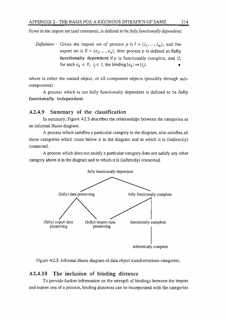
APPENDIX 2-THE BASIS FOR A RIGOROUS INTERPR'N OF SAME 314
flows in the import set (and constants), is defined to be fully functionally dependent:
Definition: Given the import set of process p is I = (i 1 , .. , i m}, and the
export set is E = {e1, .. , en}, then process pis defined as fully
functionally dependent if p is functionally complete, and if,
for each ek E E, ij E /, the binding LekJ • Lii •
where is either the named object, or all component objects (possibly through sub
components).
A process which is not fully functionally dependent is defined to be fully
functionally independent.
A2.4.9 Summary of the classification In summary, Figure A2.3 describes the relationships between the categories as
an informal Hasse diagram.
A process which satisfies a particular category in the diagram, also satisfies all
those categories which come below it in the diagram and to which it is (indirectly)
connected.
A process which does not satisfy a particular category does not satisfy any other
category above it in the diagram and to which it is (indirectly) connected.
fully functionally dependent
(fully) data preserving
(fully) export data preserving
(fully) import data preserving
fully functionally complete
functionally complete
referentially complete
Figure A2.3: Informal Hasse diagram of data object transformations categories.
A2.4.10 The inclusion of binding distance To provide further information on the strength of bindings between the import
and export sets of a process, binding distances can be incorporated with the categories

APPENDIX 2 - THE BASIS FOR A RIGOROUS INTERPR'N OF SAME 315
given above. Binding distance between two objects was defined, in Section 5.4.2, as
being equal to the Cardinality of the set of bindings between the objects.
Considered to be the most useful binding distance measure, is the maximum
level of binding which exists between objects in the context set D of a process (see
Section A2.4.1). For the example in Figure A2.2, the maximum binding level for Pl is
2, which occurs three times; once each for the sets {D • Dl, D1 • Al}, {D • D1, Dl •
Bl}, and {D • D2, D2 • F}. This is defined as the process' binding distance, as
follows:
Definition: The process' binding distance for process p is the maximum
of all the binding distances that exist between any of the objects in
the set D within the context of p. •
The strongest possible binding (between the import and export sets) in a
process is where the process is fully functionally dependent, and the process binding
distance is 1.
A2.5 A final categorisation of applications In Section 4.4.6 applications at the top level model were described as the 5-
tuple
A= (E, S, P, U, F)
such that E is the application set of external entities, S is the application set of data
stores, P is the application process set, U is the set of unknown objects in the
application, and F is the set of data flows that appear in the data flow diagram hierarchy
for the application. Each of the sets includes all the objects of its type that exist in the
application.
This description will now be extended to take account of the bottom level model
which describes the transformations between data flow sets. In doing so, a single
framework will be developed for describing both static and executable application
models.
The static model of an application includes all the objects of relevance to that
application, and is generally larger than any of the executable models for the
application.
An application in SAME is described as the 6-tuple
A= (E, S, P, U, F, C)
such that
• E is the application set of external entities, where each external entity e in E is
described by (name, I, E), such that name is the name of the entity, and I and E are

APPENDIX 2-THE BASIS FOR A RIGOROUS INTERPR'N OF SAME 316
respectively the import and export sets of the entity.
• S is the application set of data stores, where each data store s in S is described by
(name, I, E), such that name is the name of the store, and I and E are respectively the
import and export sets of the store.
• Pis the application process set, where each process p in Pis described by (name,
where_contained, C, IS), such that: name is the name of the process;
where contained is the name of the parent process, if there is one, or the name of the
application otherwise; C is the context for the process (see Section A2.4.1 ); and IS is
the (possibly empty) set of import sets for the process.
• U is the set of unknown objects in the application, where each unknown object u in
U is described by (name, where _contained, option), such that: name is the name of
the unknown object; where _contained is the name of the process in whose
refinement the unknown object appears, if there is one, or the name of the
application otherwise; and option is either process(C, IS), or entity(C, IS),
depending on whether the unknown object is to be interpreted as a process or an
external entity, respectively.
• F is the set of data flows that appear in the data flow diagram hierarchy for the
application, where each flow fin Fis described by (name, where_contained), such
that name is the name of the flow, and where _contained is the name of the process in
whose refinement the data flow appears, if there is one, or the name of the
application otherwise.
The classification of an application model, whether it is the static or an
executable model, is two-tiered. At the higher level, the application is defined as:
• structurally complete - if it satisfies the data flow diagram rules of Section 4.4.1;
• structurally incomplete - if it satisfies the data flow diagram rules of Section 4.4.2;
• structurally invalid - otherwise.
Those applications which are either structurally complete or incomplete, a lower
level classification applies in terms of the bindings of import sets to export sets. An
application, at the lower level, is defined as:
• referentially complete - if one process in the application is referentially complete, and
all other processes are at least referentially complete.5
• functionally complete - if one process in the application is functionally complete, and
all other processes are at least functionally complete.
• fully functionally complete - if one process in the application is fully functionally
complete, and all other processes are at least fully functionally complete.
5 The use of the term 'process' in this set of definitions extends to objects of type unknown which are to be treated like processes. Also, the phrase 'at least x' refers to the position of a category in the Hasse diagram of Figure A2.3.

APPENDIX 2 - THE BASIS FOR A RIGOROUS INTERPR'N OF SAME 317
• fully functionally dependent - if all processes in the application are fully functionally
dependent.
• (fully) data conserving - if all processes in the application are data conserving.
The lower level classification can be augmented with the application's binding
distance, which is defined as follows:
Definition: The application's binding distance is the maximum of all the
process' binding distances which exist in the application. •

A3.1 Introduction ........................................................................... 318
A3.2 Iteration ................................................................................ 319
A3.2.1 Iteration in the standard SAME model.. ................................ 319
A3.2.2 Iteration with renaming semantics ....................................... 322
A3.3 Recursion .............................................................................. 324
A3.1 Introduction Iteration, in the form of loops, at the data flow diagram level in SSA, is
generally discouraged. De Marco makes the following comment ([De78], p.40):
'[ ... ], you almost never see a loop in a Data Flow Diagram. A loop is
something that the data are unaware of; each datum typically goes through it
once, and so from its point of view it is not a loop at all. Loops and decisions
are control considerations and do not appear in Data Flow Diagrams.'
Other authors express stronger views. Hawryszkiewycz [Ha88], for example,
describes them as an illegal construct.
318

APPENDIX 3 - ITERATION AND RECURSION IN DFDS 319
The general mechanism for providing repetition in SAME is the group object,
which has an implicit index. The control activities required to construct group objects in
SAME, are made transparent in the execution models DFDMl and DFDM2. Although it
would be possible to pass an index as a data flow, this is not needed, and is considered
bad practice within SSA [Ha88, De78, GS79, We80]. Recursion can most naturally be
handled within functions.
Having said this, there are arguments to do with providing flexibility which
suggest that both repetition and recursion should be able to be specified within data
flow diagrams. An important application which is naturally recursive is bill of
materials, where part assemblies can be constructed from sub-assemblies, and so on.
A3.2 Iteration In SAME, renaming semantics are not part of the standard model(s), so the
direct importing of a data flow by the exporting process is not allowed. In Section
A3.2.1, the standard method for accommodating loops in SAME is described in terms
of a small example. In Section A3.2.2, the same example is modelled by an extended
version of SAME which (experimentally) supports renaming semantics. It should be
stressed that the ability to have two 'generations' of the same named object in the
context of a process is not considered desirable.
A3.2.1 Iteration in the standard SAME model A simple example of an application with looping is calculating total = n * a +
init using successive addition; that is, an application to find sum(O,n,a)+ init.
A data flow diagram for the application is shown in Figure A3.l(a), with the
object definitions in Figure A3.l(b). (See also Section 7.6.) The effect of executing this
application is the unfolding of the loop into a sequence of n instances of processes pl
and p2, as can be seen in the trace of Figures 7.31 and A3.2.
An important point to note is that the data flow diagram and the JEgis object
definitions still remain essentially independent from each other. The diagram has an
iterative structure while the data objects appear recursive. The data object definitions
taken on their own contain a cycle which will result in an infinite, mutually recursive,
path being generated if a demand-driven evaluation is attempted outside the context of
the data flow diagram. This can be seen in the dependency graph in Figure A3. l.
However, within the context of the data flow diagram, the evaluation is well bounded
as the execution is driven by the availability of the initial values, and the limited set of
data objects used in each process includes no recursion.

APPENDIX 3 - ITERATION AND RECURSION IN DFDS
s File Edit Windows SAME Objects Show
loop ~□~ Object dependencies gm ~e:rn
0 user total
• c::JJ initAN
soI•rl
- pl !fo!er p2
..
(a) A data flow diagram with a loop formed by flows soFar and soFarl.
s File Edit Windows SAME Objects Show Display
Display em Object dependencies gm a:
number init:
nu.m.ber initAN:
init,a,n n:
n1:
n2:
nu.m.ber
n if available(n) or n2 otherwise
n1-1 if n1>0 :ioFar:
:itua,a,n1 :ioFar1:
(:itua1,a,n2) if n1>0 :itua:
stua1 if available(n2) or init otherwise
stuai: :,um.+a if n1>0
total: Stua it n1::s;O
Def
111111
mm
(b) Object definitions.
n2
nl
Figure A3.l: An application containing a processing loop within the data flow diagram.
The impact on SAME of allowing loops at the diagram level is three-fold:
320
• The matching currency for data flows and processes is kept constant within the
execution of the loop. An instance of soFarl, for example, when produced will
have the same currency as the imported instance of s oF a r. As this instance of
soFarl becomes the available import set for process pl, the currency for this
process is coerced to the currency of the data flow soFarl. This scheme supports
the interleaving of sets of input data to the application, as shown in Figure A3.2.

APPENDIX 3 - ITERATION AND RECURSION IN DFDS
STARTING: pl (1) -> initAN:
init: 2 a: 3 n: 1
<- soFar: sum: 2 a: 3 nl: 1
ENDING: pl (1) STARTING: p2 (1) -> soFar:
sum: 2 a: 3 nl: 1
<- soFarl: suml: 5 a: 3 n2: 0
<- total: missing ENDING: p2 (1) STARTING: pl (2) -> initAN:
init: 4 a: 5 n: 1
-> soFarl (** 1 **): suml: 5 a: 3 n2: 0
** Process pl ** Currency changed from 1 to 2 <- soFar:
sum: 4 a: 5 nl: 1
ENDING: pl (2) STARTING: p2 (2) -> soFar:
sum: 4 a: 5 nl: 1
<- soFarl: suml: 9 a: 5 n2: 0
<- total: missing ENDING: p2 (2) STARTING: pl (1) -> soFarl:
suml: 5 a: 3 n2: 0
<- soFar: sum: 5 a: 3 nl: 0
ENDING: pl (1) STARTING: p2 (1) -> soFar:
sum: 5 a: 3 nl: 0
<- soFarl: missing <- total: 5 ENDING: p2 (1) STARTING: pl (2) -> soFarl:
suml: 9 a: 5 n2: 0
<- soFar: sum: 9 a: 5 nl: 0
ENDING: pl (2) STARTING: p2 (2) -> soFar:
sum: 9 a: 5 nl: 0
<- soFarl: missing <- total: 9 ENDING: p2 (2)
Figure A3.2: The trace for the loop example, where different import sets of data have been interleaved. 1
321
• The most abstract executable model must contain the loop diagram. For instance,
Figure A3.1 (a) cannot usefully be abstacted to an executable model containing just a
single process (see following paragraph). If an application contains nested loops, the
most abstract executable model is at the level of the innermost loop.
• As the object definitions must now allow for the indirect definition of an object in
1 In the implementation described in Chapter 7, automatic flushing of data flows must be turned off under Preferences ... in the SAME menu to produce the trace in Figure A3.2.

APPENDIX 3 - ITERATION AND RECURSION IN DFDS 322
terms of itself, it is possible that an object instance will not be able to be generated
from the definitions where an object definitions loop falls within the context of a
single process.
The last of these will lead to the user being advised of the existence of a cycle.
A3.2.2 Iteration with renaming semantics The extension to SAME to let a process directly import its own exports is
achieved by use of the function NEW, which has as its single parameter the name of a
data object. If, for example, the tuple element NEW(OBJ) was being evaluated, two
possible situations can occur:
• If a value exists for an object named 1NEW(OBJ)
1, this value is used.
• If no such value exists, a value is generated using the definition of OBJ. This value is
then bound to the object named 1NEW(OBJ)
1•
The example given in the previous section can be specified in the new scheme in
the manner described in Figure A3.3
The object dependency graphs for soFar and total are given in Figures A3.4
and A3.5, respectively. (The graph for total is too big to be viewed in its entirety on
the Macintosh SE screen.) Observe that new is shown as a function in the graphs. The
generated names 'new (sum)' and 'new (nl)' are internal to the invocation of the
process, and are transparent to the user.
An execution trace of the model is given in Figure A3.6 for the shown input
data. Note how 'new (sum)' becomes 'sum' on the next iteration. The renaming from
'new< sum)' to 'sum' takes place when creating the exports, so that instances of
'new (sum)' are inserted into the export data flow instances with the object name 'sum'.
• File Edit Windows SAME Objects Show Oisploy
0
I • c:n
-- l •
loop2 Displ8ll
um F initAH
pl r: a:
number init:
number initAN:
(init, a, n)
n: number
ni: n-1++(n1-1)
soFar: (new(sum), a, new(n1)) if new(n1)>0
sum:
0
I
I 11111!
mm init if available(n)&n=O or init+a if available(n)&n>O or
totaf~+a if new(n1)>0 II init if available(n)&n=O or ill sum.+a if new(n1)=0 Q
------------------------ Q]
Figure A3.3: The summation example using renaming semantics.
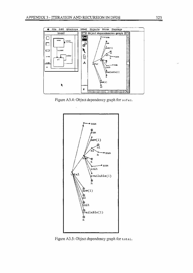
APPENDIX 3 - TIERA TION AND RECURSION IN DFDS
ct File Edit Windows SAME Objects Show Disploys
loop2 ~□~ Object dependencies grnph §'§0l\l
i.nitAN
pl
YI J'i'
' ~ A
n1llll llllll
nl
Figure A3.4: Object dependency graph for soFar.
II.
Figure A3.5: Object dependency graph for total.
323

APPENDIX 3 - ITERATION AND RECURSION IN DFDS
is file Edit Windows SAME Objects Show
Trace ~r EE: user *#*to*#* o ---=------==•-•==•=-===•=------- ~ ==--=-----------------------Execution sub-system (0.1]
STARTING: p1 (1) -> initAN:
init: 2 a: 3 n: 2
<- soFe.r: sum: 5 e.: 3 n1: 1
<- total: missing ENDING: p1 (1) STARTING: p1 (1) -> soFe.r:
sum: 5 a: 3 n1: 1
<- soFe.r: missing <- total: 8 ENDING: p1 (1)
Data flow total From process p1 (currency 1)
111111
8
m111
111111
11111!
illlli
~ ~ -
Figure A3.6: A trace of the model which contains renaming semantics.
A3.3 Recursion
324
Although recursion can be handled within data flow diagrams, the effects in
SAME are to:
• remove the independence between the diagrams and the iEgis object definitions;
• require the execution of a process and its descendant processes within the same
model;
• require the use of overlapping limited import sets.
These effects can be seen by considering the data flow diagram modelling of an
application to find the factorial of n.
Using a function, the factorial problem can be specified simply as
FACT(N) <= N * FACT(N-1) 1 (''NEGATIVE VALUE SPECIFIED FOR N OF", N)
IFN> 11 IF (N = 0 ORN= 1) I OTHERWISE.
A model for the application which does not use an explicit function is given in
Figure A3.7.
The refinement for process FACT includes an instance of itself. The availability
of an instance of N_MINUS_l will make the nested FACT process runnable. This would
lead to an expansion of process FACT into its three descendant processes, and the
allocation of the imported N_MINUS_l instance to processes CHECK FOR END and MULT.
The data flow instance for N_MINUS_l would have been name coerced to N by the
RECURSION operator. When the inner invocation of FACT completes, the export data flow
N_FACT is name coerced to N_MINUS_l_FACT also by the RECURSION operator.

APPENDIX 3 - ITERATION AND RECURSION IN DFDS 325
FACT
N N FACT
N_Mil\'US_l_FACT
(a) A data flow diagram with recursion.
N_FACT <= N * N_MINUS_l_FACT IF (N > 1) I BOUNDARY_VAL IF(N=0ORN= 1).
N_MINUS_l <= N - 1 IF (N > 1). BOUNDARY_VAL <= 1 IF(N=0ORN=l). N_MINUS_l_FACT <= RECURSION(N_FACT, (N_MINUS_l = N)). N <= 0 .. INF.
(b) Object definitions.
Figure A3.7: Finding the factorial of N using recursion in the data flow diagram.
The data flow BOUNDARY_ v AL supplies the value of the base equation of a
recursive definition. The invocation of nested instances of the process F~CT cease when
the value of N is less than or equal to 1, as no instance of N_MINUS_l will be generated.
Process MULT has the two limited import sets {N, BOUNDARY_ VAL} and {N,
N_MINUS_l_FACT}. The intersection of these sets is not disjoint, although it is reasonably
easy to demonstrate that non-determinism will not occur.
It is possible to circumvent using overlapping import sets, by distributing the
object N through the other flows, BOUNDARY_ VAL, N_MINUS_l and N_MINUS_l_FACT, but
this can be viewed as 'inelegant'.
As a second example, Figure A3.8 contains a structure diagram for finding the
components of parts within a bill of materials application. COMPONENTS(PART_#) is a
procedure for displaying the details of the part referenced by PART_#. As can be seen in
the diagram, this application is naturally recursive where parts can be composed from
other parts.
A data flow solution to this application is given in Figure A3.9. Figure A3.9(b)
contains the explosion of process PL MINOR_PARTS is the decomposed data flow labelled
MINOR_PART_NUM, which means that the nested process Pl will be invoked for each
MINOR_PART_NUM. One export instance of data flow MINOR_COMPONENTS will be
generated for each MINOR_PART_NUM.

APPENDIX 3 - ITERATION AND RECURSION IN DFDS 326
Note that the import sets for process Pl and the nested version of Pl do not
completely match. The difference is in terms of the data store generated data flows.
Figure A3.9(a) shows process Pl importing the two data flows PART_# and
PART_DETAILS, while the nested Pl in Figure A3.9(b) is only shown importing
MINOR]ART_NUM (that is, PART_#). A solution to this lack of symmetry is to allow data
stores to be specified within recursive processes, in which case PARTS would appear
within the confines of the larger box in Figure A3.9(b), as well as outside it. Figure
A3.10 contains the details of a specification based on this concept which is equivalent
to that given in Figure A3.9.
As with iteration, the execution time effect of recursion is an unfolding of
processes. The main difference between the handling of iteration and recursion at the
data flow diagram level in SAME, is the need to include data flow diagram process
details in the object definitions for an application using recursion.
It was argued earlier that the independence in iterative models between the data
flow diagrams and the object definitions is more apparent than real. This follows from
the fact that the object definitions now contain loops, so that the demand-driven
generation of an object instance could terminate within the context of the execution of a
data flow diagram process, but not if the generation is attempted outside a process.
GETPART_DETAILS USING PART_#
COMPONENTS(PART _#)
FIND TIIE COMPONENTS OF PART WHOSE KEY IS PART_#
OUTPUT PART_DESCR
LOOPWHILE MINOR_pART_#
EXISTS
COMPONENTS(MINOR_pART_#)
Figure A3.8: A structure diagram for the part components application, showing the recursive nature of the application.
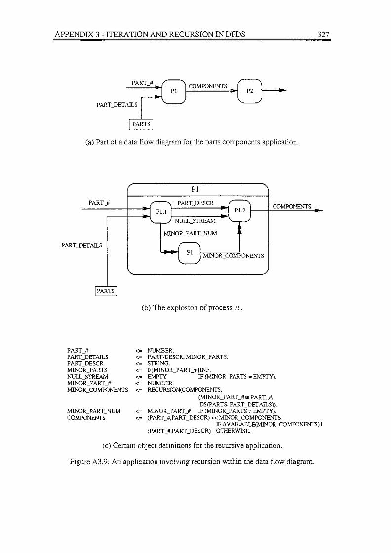
APPENDIX 3 - ITERATION AND RECURSION IN DFDS
PART_# COMPONENTS P2
PART_DETAILS
PARTS
(a) Part of a data flow diagram for the parts components application.
PART_#
PART_DEfAILS
PARTS
PART_# PART_DEfAILS PART_DESCR MINOR_PARTS NUU,_STREAM MINOR_FART_# MINOR_COMPONENTS
MINOR_FART_NUM COMPONENfS
Pl
PART_DESCR COMPONENTS
MINOR_COMPONENTS
(b) The explosion of process Pl.
<= <= <= <= <= <= <=
<= <=
NUMBER. PART-DESCR, MINOR_FARTS. STRING. 0(MINOR_PART_#)INF. EMPTY IF (MINOR_FARTS = EMPTY). NUMBER. RECURSION(COMPONENTS,
(MINOR_PART_#= PART_#, DS(PARTS, PART_DEfAILS)).
MINOR_PART_# IF (MINOR_FARTS * EMPTY). (PART _#,PART _DESCR) « MINOR_COMPONENTS
327
IF AV AII.ABLE(MINOR_COMPONENTS) I (PART_#,PART_DESCR) OTHERWISE.
(c) Certain object definitions for the recursive application.
Figure A3.9: An application involving recursion within the data flow diagram.

APPENDIX 3 - ITERATION AND RECURSION IN DFDS
PART_# COMPONENTS
PART_DETAILS
PARTS
(a) The same data flow diagram segment as Figure A3.6(a) can be used.
PART_#
PART_DETAILS
PARTS
Pl
PART_DESCR
NULL_STREAM
MINOR_p ART _NUM
MINOR_COMPONENTS
MINOR_pART_DETAILS
PARTS
COMPONENTS
(b) The data flow diagram in which PARTS appears within the exploded view of process Pl.
PART_# PART_DETAILS PART_DESCR MINOR_pARTS NULL_STREAM MINOR_PART_DETAILS MINOR_PART_# MINOR_COMPONENTS
MINOR_PART_NUM COMPONENTS
<= <= <= <= <= <= <= <=
<= <=
NUMBER. PART-DESCR, MINOR_PARTS. STRING. 0(MINOR_FART_#}INF. EMPTY IF (MINOR_PARTS = EMPTY). PART-DESCR, MINOR_pARTS. NUMBER. RECURSION(COMPONENTS,
(MINOR_PART_#= PART_#, MINOR_pART_DETAILS=PART_DETAJLS)).
MINOR_FART_# IF (MINOR_PARTS"' EMPTY). (PART _#,PART _DESCR) « MINOR_COMPONENTS
328
IF AV AIIABLE(MINOR_COMPONENTS) I (PART_#,PART_DESCR) OTHERWISE.
(c) Definitions including MINOR_PART_DETAILS, and an amendedMINOR_COMPONENTS.
Figure A3.10: The recursive application shown in Figure A3.6, but with the explicit representation of the minor part details data flow.
A4. l Introduction ........................................................................... 330
A4.2 Starting and ending a modelling session ........................................... 330
A4.2.1 Starting a SAME session ................................................. 330
Loading an existing application model .................. ................ 331
Creating an application model .......................................... . 333
A4.2.2 Ending a SAME session .................................................. 334
A4.3 SAME files ............................................................................ 335
A4.3. l SAME system files ........................................................ 335
A4.3.2 Application models files .................................................. 335
A4.4 Windows .............................................................................. 336
A4.4.1 Data flow diagram (DFD) windows .................................... 337
DFD windows tools ...................................................... 339
A4.4.2 Object dependencies graph window .................................... 344
Object dependencies graph window tools ............................. . 344
A4.4.3 Application hierarchy window ........................................... 345
Application hierarchy window tools ................................... . 345
A4.4.4 Data store mapping window ............................................. 347
Data store mapping window tools ...................................... .348
A4.5 Menus .................................................................................. 349
329

APPENDIX 4 - OUTLINE SAME USER MANUAL 330
A4.5.1 SAME ...................................................................... 349
A4.5.2 Objects ...................................................................... 352
A4.5.3 Show ....................................................................... 353
A4.5.4 Window .................................................................... 353
A4.5.5 Display ..................................................................... 354
A4.5.6 Trace ........................................................................ 354
A4.5.7 External entities ............................................................ 355
A4.5.8 Processes ................................................................... 355
A4.5.9 Data stores ................................................................. 356
A4.5.10 Data flows .................................................................. 357
A4.5.11 Next. ........................................................................ 357
A4.6 Help .................................................................................... 358
A4.1 Introduction This appendix describes some of the features of the prototype implementation of
SAME described in Chapter 7. In general, features described in Chapter 7 are not
elaborated here.
SAME has a comprehensive on-line help facility, access to which is described
in Section A4.6.
A4.2 Starting and ending a modelling session A4.2.1 Starting a SAME session
The system is loaded by clicking on the SAME application icon, shown in the
window below.
gO~SAME~0g 5 it•m• 547K in disk 238K •v
~ SAME
Warning: Do not attempt to load any other file directly.

APPENDIX 4 - OUTLINE SAME USER MANUAL
Once the application has been loaded, the following dialogue is displayed.
Structured Analysis Modelling Eriuironment
Uersion 1.0 - 22 January, 1989
© T llJ G Docker
[ Continue] ~
331
If Help is selected, brief details of the SAME system are given. Selecting Stop
will end the SAME session.
Clicking on Continue results in the menu bar being reduced to the format
shown in the diagram below.
c File Edit SAME
The 41 menu is that available under the LPA Prolog application, while the File,
and Edit menus are generated by LPA Prolog.
Warning: Unless prompted to do so, do not select any item in the File menu.
The two main options under the SAME menu are creating a new application
model, and loading an existing model from disk.
Loading an existing application model If an existing model is to be loaded, the load sequence is as follows: 1
1 Read Section A4.3.2 before continuing with the load sequence discussion.

APPENDIX 4 - OUTLINE SAME USER MANUAL 332
• Select the DFDs file - SAME prompts for the file which contains the non-data
objects details of the application model.
la bank e.g. I 1111,l'i dl'<lllllSI ~
[) bank Objs ~ I ( Ok l i ( [j1~i:1 l
! ( Cancel ) I ( OrilH/ )
0 = SAME applications
Conte Ht LOADING APPLICATION DFD HIERARCHY. Select the file from which the application hierarchy of data flow diagrams is to be loaded.
When the file has been selected, the system checks that the file is of the right
type. If it is, a dialogue of the following form is displayed, so that the user can check
the correct application is being loaded. If the file is of the wrong type, an exception
message is displayed, and the load sequence is halted.
Data flow diagram hierarchy fAMEj
Name: bank
Date saued: 27th April 89
Time saued: 3.49pm
Don't load
• Select the Data Objects file - The above sequence of activities is repeated, but
this time for the file which contains the data object definitions.
• Data stores reminder - Once the data object definitions have been loaded, the
following dialogue is displayed.
~ ~
Remember to load data store tuples, If required [ Continue J
tt

APPENDIX 4 - OUTLINE SAME USER MANUAL 333
If the application model includes data stores, the user must load the data store
tuple instances separately (see Section A4.5.9, menu item Load tuples ... ). This can
be done any time following the last item in the loading sequence (display of
application details).
• Display of application details - Finally, SAME displays the following
dialogue, giving the application details.
bank
Description
Created: Last amended:
19th April 89 - 12.56pm
(Cancel)
Creating an application model If a new application model is to be created, the following sequence of
operations occurs:
• Naming the application - A dialogue of the following form is displayed, and
this is filled in by the user. A name must be supplied for the application. The
description is optional and can be added at a later stage (see Section A4.5.1, menu
item Application ... ).
Enter a name for the application
Name
I roots
Description
Giuen the coefficients a, b, and c, finds the two real roots of a quadratic.
Created: 2nd Mey 89 - 5.02pm
( Cancel )

APPENDIX 4 - OUTLINE SAME USER MANUAL 334
• Creation of Level O data flow diagram - The system creates a DFD window
in which the user should create the Level O data flow diagram. The window is given
the name of the application.
The system applies a hidden grid when positioning objects of the types data
store, external entity, and process. The user is prompted for the size of this grid,
using the following dialogue. A suggested size of 20 is provided by the system as a
default value.
Reuise suggested grid size, ~AMEi os required, for window roots
A4.2.2 Ending a SAME session A modelling session is terminated by selecting Quit (3€0) in the SAME menu
(see Section A4.5.1). When quitting, the following exit sequence is followed through:
• Check on quitting - the user is prompted on whether or not an exit should be made
from the SAME system:
& Do you reolly want to quit SAME ~~
• Check on saving the application model(s) - if an exit from the SAME system is
required, the user is asked whether the application model(s) should be saved:
/4\ Do you wish to soue the application (ves] Ll.1 before eHitlng
If the answer is yes, the standard save sequence is followed (see item Sau e ... in
Section A4.5.1).

APPENDIX 4 - OUTLINE SAME USER MANUAL 335
A4.3 SAME files Apart from the LP A Prolog system, two types of files can be identified in the
SAME system: system files, and application models files.
A4.3.1 SAME system files The five files shown in the following window constitute the SAME system
files.
-• SAME 0= Sitems 547K in disk 238K •v•il•blt
kid :Q
SAME
~ ~ ~ D SAME d,fault •nvironment SAME Synt•x Htlp SAME Help SAMErts01
0 CJI IQ Q:]
The purpose of each file is:
• SAME-The SAME program (an LPA Prolog object file).
• SAME default environment - A file containing default details common to all
application models. Details from this file are automatically loaded on entry to SAME.
No user access is provided to this file.
• SAME Syntax Help - Contains help text on the structure of iEgis constructs, and
on the purpose of system defined functions. Access to the help details is provided
within SAME.
• SAME Help - Contains help details on all SAME menu items and graphic tools.
Access to the help details is provided within SAME.
• SAMEres0l - Details on the resources (cursors, buttons, etc.) used within SAME
are contained within this file. No user access is provided to this file.
A4.3.2 Application models files An application model created within SAME can be saved for use in later
sessions, either by selecting Saue ... in the SAME menu (see Section A4.5.1), or at the
time of quitting from SAME (see Section A4.2.2).
Each model is saved to two files:
• DFDs file - All details about the model which are in the system dictionary,
excluding the definition of data objects, are saved to a DFD file. This includes details
on any current executable model.
• Data Objects file - The definitions of the data objects in the system dictionary are
saved to a file of this type.

APPENDIX 4 - OUTLINE SAME USER MANUAL 336
The reason for storing the data objects in a separate file is to allow them to be
used by more than one application, and also to allow a single application to be exercised
against different sets of object definitions.
A4.4 Windows SAME maintains the following four classes of windows:
• DFDs - Each window contains a single data flow diagram in the application
hierarchy. At the top of the hierarchy is the Level O ( or context) diagram. Each other
diagram is a refinement of a single process. (A DFD window is also a graphics
window. See the last item.)
• EEs- Each external entity in the (executable) application model which imports one
or more data flows has a window created for it. All data flows exported to the
external entity are written to that window. (An external entity window is also a text
window. See the next item.)
• TEXT-As its name suggests, a text window is used to contain textual details. Apart
from EEs, three special text windows are used by the system:
ConteHt - This is used to display messages on the current state of the system.
Used mostly during the execution of a model.
Display - A display request either leads to a dialogue being shown on the screen,
or details being written to the Display window. A dialogue display is an
immediate display that is lost when the dialogue is completed. A display written to
the Display window can be kept for as long as desired, and can even be cut and
placed into other windows or documents via the Clipboard or Scrapbook.
Trace - If medium or full trace is on, details on the tracing of an executable model
are written to the Trace window. Details written to the Trace window can be kept
for as long as desired, and can even be cut and placed into other windows or
documents via the Clipboard or Scrapbook.
Note: Text windows quickly consume main memory, and lead to slow
processing speed as working memory is reduced. Periodically delete
text window details. It is better to delete medium to large chunks of
text, otherwise store fragmentation can occur.
• GRAPHICS - As its name suggests, a graphics window is used to contain
diagrams. Apart from DFDs, three special graphics windows are used by the system:
Object dependencies graph - This is used to display the structure of a data
object as a graph of its dependent objects.
Application hierarchy-The structure of both the application process hierarchy,
and the executable model process hierarchy, can be displayed in this window.
Data store mapping - This window is only created if one or more mappings

APPENDIX 4 - OUTLINE SAME USER MANUAL 337
has been carried out between data flows and data stores. The window will contain
a pictorial representation of the data flow and data store object structures, by
which the mappings can be specified.
In general, a graphics window has the structure of the DFD windows shown
in Section A4.4.1. The usual facilities associated with Macintosh windows, such as
'go-away' and resizing boxes, are present.
Note: Having graphic windows displayed slows down processing, as
the system refreshes the windows following dialogue displays, etc.
The following dialogue shows the windows from three of the above classes for
a simple application.
Select windows
------------- OF Os ------------- IQ processTronsaction bank ITTTTi
;r~~~;:ome, ::, --1 ----------- GRAPHICS -----------IO
Ok (Cancel)
A4.4.1 Data flow diagram (DFD) windows Each DFD window has the following basic structure:
tool pane __ _,.~
scrollable viewing pane
\ ~ Ill
ndl--1,;d.-- cursor (in the shape
1'"!
viewer ----11• of the process tool)
• Split line - which is the vertical line that splits the window into the two main areas:
the tool pane, and the viewing pane. The split bar can be moved by holding the
cursor down over the line, and dragging to left or right. Dragging to the left

APPENDIX 4 - OUTLINE SAME USER MANUAL 338
increases the viewing pane, and reduces the size of the tool pane and the viewer.
Dragging to the right has the opposite effect (see following diagram).
• Tool pane - to the left of the split line, which contains the various tools that can be
selected to operate in the window. The tool pane is fixed and cannot be scrolled. The
currently selected tool (if any) is shown in reverse video.
• Viewing pane - to the right of the split line, which provides a viewpoint onto the
large drawing area of the window. By using the scroll bars (or manipulating in the
viewer- see be~ow), the section of the drawing pane visible in the viewing area can
be changed.
• Viewer - this is below the tool pane and displays a reduced overview of the complete
drawing area, and the objects in the area. The currently visible area is shown in a
grey outlined (dotted) rectangle. Clicking in the viewer will centre the viewing pane
on the relative click point. A similar effect can be obtained by dragging the grey
rectangle in the viewer.
The DFD shown above contains a Level 0 (context) data flow diagram. The
name of the application is bank, which is the name assigned to the DFD window by the
system.
The selected tool is the process, which is reflected by the cursor taking on the
shape of a process box. Clicking in the viewing pane will result in the creation of a
process box that is centred on the cursor position, except for an adjustment to align the
box to the nearest (invisible) grid point.
process tool (the only visible tool)
full graphics window extent is represented by this area
process box in the visible window
roots
c>li:1W!tRoots I
0
dashed box describes the relative size and location of the viewing pane within the complete DFD window

APPENDIX 4 - OUTLINE SAME USER MANUAL 339
In the second DFD above, the split line has been dragged to the right so that
only the (selected) process tool is visible in the tool box. Note the increased size of the
viewer, and its various components.
The following DFD contains the refinement of process processTransaction
in the bank DFD. Two things worth noting are the reduced toolbox (neither the external
entity nor data store tool is available), and the two hooks. These hooks were created by
the system, and provide the only interface points to the bank DFD.
impo;t hook export hook
process Tm n soc t lo n
innlidlIHTrllntt
reduced -tool set ----1•Ji, tr~cti•n
'\ ~
-
cMclllH Vt11idlIH pe:rfox11t-Trt1n• 'r.rlMUI
min
111111
o li!ii!
DFD windows tools The tools available in DFD windows will now be described. Only the Level 0
DFD window has the full set of tools. The other windows do not have the external
entity nor the data stores tool. Double-clicking on any tool results in the display of a
help dialogue.
Process tool
• No modifiers. A fixed size process box is centred on the click point (but aligned to grid). A text box is inside the process box, and an unique process name must be typed into the box. The details on the process are saved into the dictionary when the mouse is clicked anywhere in the DFD, but outside of the text box.
Note: The mouse button is 'live' when so, unless a new process is to be following naming, use an unused combination; else click in the tool pane.
clicking, created
tool-key
Control key. If the object clicked on is a process, then a DFD window is created with the name of the process. Import and export hooks are created as necessary.
Where a refined DFD already exists for the process, the effect is to make that DFD the selected front window.

APPENDIX 4 - OUTLINE SAME USER MANUAL 340
Data store tool
D
If the object clicked on is not a process, and the DFD is a refinement of a process, the parent DFD window is made the front selected window.
Option key. Drag a marqui (rectangle) of the required width. A process box is then created (aligned to grid) of the specified width and standard depth.
Use this if a long process name is to be specified, or the process has a significant number of import and export data flows to be connected.
00 key. A dialogue is entered to allow the optional text description of the object to be specified; or, in the case where it already exists, amended.
Shift key. Displays details of the object clicked on, regardless of the object's type.
Control and Option keys. Displays a hierarchy of all the processes in the application, regardless of where the mouse is clicked within the viewing pane.
00 and Option keys. Displays a menu of the import and export data flow sets of the process clicked on. Data object definitions can be chosen for display, and/or data dependency graphs can be displayed.
00, Control, and Option keys. If an executable model exists, the processes in the executable model will be displayed as a graph.
No modifiers. A fixed size data store box is centred on the click point (but aligned to grid). A text box is inside the data store box, and an unique data store name must be typed into the box. The details on the data store are saved into the dictionary when the mouse is clicked anywhere in the DFD, but outside of the text box.
Note: The mouse button is 'live' when clicking, so, unless a new data store is to be created following naming, use an unused tool-key combination; else click in the tool pane.
Control key. A menu is displayed of all the data objects that are in the tuple of the data store that was clicked on.
Select from the menu to display the definitions of the data objects.
Option key. Drag a marqui (rectangle) of the required width. A data store box is then created (aligned to grid) of the specified width and standard depth.

APPENDIX 4 - OUTLINE SAME USER MANUAL 341
External entity tool
•
Data flow tool
Use this if a long data store name is to be specified, or the data store has a significant number of import and export data flows to be connected.
00 key. A dialogue is entered to allow the optional text description of the object to be specified; or, in the case where it already exists, amended.
Shift key. Displays details of the object clicked on, regardless of the object's type.
00 and Option keys. Displays a graph of the data object dependencies within the data store tuple.
No modifiers. A fixed size external entity box is centred on the click point (but aligned to grid). A text box is inside the external entity box, and an unique external entity name must be typed into the box. The details on the external entity are saved into the dictionary when the mouse is clicked anywhere in the DFD, but outside of the text box.
Note: The mouse button is 'live' when clicking, so, unless a new external entity is to be created following naming, use an unused tool-key combination; else click in the tool pane.
Option key. Drag a marqui (rectangle) of the required width. An external entity box is then created (aligned to grid) of the specified width and standard depth.
Use this if a long external entity name is to be specified, or the external entity has a significant number of import and export data flows to be connected.
00 key. A dialogue is entered to allow the optional text description of the object to be specified; or, in the case where it already exists, amended.
Shift key. Displays details of the object clicked on, regardless of the object's type.
No modifiers. A straight line arc segment is constructed between each contiguous pair of click points. The very first and last points must be inside boxes of the other data flow diagram object types. The first object clicked in is the exporter of the data flow, while the second is an importer.
A data flow arc can consist of any number of line segments. These line segments are 'straightened' automatically, and the angles between segments are multiples of 90 degrees.

APPENDIX 4 - OUTLINE SAME USER MANUAL 342
Further line segments can be drawn to other importers, when creating a data flow, by clicking at any point 'close' to an existing line segment, and then clicking new line segment points until an importer is reached. This process can be repeated for other importers.
Once all the arc segments for the data flow have been created, including those to multiple importers, the data flow must be named using the Control-key option described below.
Note: Do not make consecutive clicks too quickly when creating line segments. The Prolog system can lose events, which results in the construction of a 'stunted' arc. If this occurs, complete the naming process, then delete the data flow using the eraser tool, and re-draw.
Control key. Drag a marqui (rectangle) where the data flow name is to be placed, then enter the name in the text box described by the marqui. When this has been done, click outside the text box.
If the marqui is dragged from one of the left corners, the name will be left-justified. If dragged from one of the right corners it will be right justified.
If the name does not fit properly in the (invisible) name box, a new box can be constructed using the Option key.
Note: The mouse button is 'live' when clicking, so, unless a new data flow is to be created following naming, use a tool-key combination which has no specified action; else click in the tool pane.
Option key. Drag a marqui (rectangle) at the new position and of the desired size for the data flow name box. Then click on the data flow name to be moved.
As with the standard naming procedure, the name will be left-justified if the marqui is dragged from one of the left comers, and right justified otherwise.
00 key. A dialogue is entered to allow the optional text description of the object to be specified; or, in the case where it already exists, amended.
Amendments can also be made to the definition of the data object of the same name, if it exists. In the case where no definition currently exists, one can be specified.
Shift key. Displays details of the object clicked on, regardless of the object's type.

APPENDIX 4 - OUTLINE SAME USER MANUAL 343
Select tool No modifier. Clicking over an object makes that object the
Drag tool
_10] ~·
Eraser tool
selected object.
Note: Most objects are composite objects made up of ( at least) a graphic object and a text box. To select all the object, Drag a marqui (rectangle) around the object. Hooks are the only object type which has a single component. However, to select a hook, the click must occur in the shaded area of the hook, and not in the text area.
Shift key. Clicking on, or drawing a marqui round, an object, adds the object to the number of selected objects.
No modifier. All the currently selected objects can be dragged by clicking the mouse over one of the objects and dragging the mouse.
By clicking on any non-selected object, all previous selections are deselected, and the new object becomes selected and can be dragged.
Note: Most objects are composite objects made up of ( at least) a graphic object and a text box. To select all the object using the select tool, drag a marqui (rectangle) around the object. Hooks are the only object type which has a single component. However, to select a hook, the click must occur in the shaded area of the hook, and not in the text area.
Shift key. Clicking on a object extends the selected objects. Dragging will include both the previously selected and the newly selected objects.
Option key. Only the object clicked on is dragged, but any previously selected objects remain selected.
No modifier. Clicking on an object will result in a prompt from the system to query the requested erasure. If required, the object is then deleted.
If an object of type external entity, process, or data store is deleted, all the data flows imported and/or exported by that object are also deleted. In the case where that object is one of a number of importers of a data flow, details on the exporter and other importers of that flow are written to the Display window. These details can be used when redrawing the data flow.
Control key. Used when all objects in a window are to be deleted. Clicking anywhere in the DFD window will result in a prompt asking whether on not all objects should be deleted.

APPENDIX 4 - OUTLINE SAME USER MANUAL 344
Text tool
A No modifier. Text can be added anywhere within a DFD window by selecting this tool.
A single line of text can be entered by first clicking at the point where the left-most character of the text is to be placed, then typing in the text. The text is completed by clicking outside of the text line.
A block of text can be entered by dragging a marqui of the required size, then typing in the text. The text is completed by clicking outside of the text box.
The font, font size, and other details, can be specified using the Fonts menu.
Note: The mouse button is 'live' when clicking, so, unless a new text string is to be created immediately following the creation of the current string, use a tool-key combination which has no specified action; else click in the tool pane.
A4.4.2 Object dependencies graph window The object dependency graph window is used by the system to display the
graphs of the dependencies between chosen data objects, and has the same basic
structure as a DFD window.
Object dependencies graph window tools The tools available in the object dependencies graph window will now be
described. Double-clicking on any tool results in the display of a help dialogue.
Definition tool
Def
Select tool
Drag tool
_I{] ~·
No modifiers. Clicking anywhere in the viewing pane will result in a menu being displayed of all the data objects which appear in the dependency graph. Selecting objects from this menu will result in a display of their definitions.
No modifier. Clicking over the graph selects it. The graph can then be copied onto the Clipboard or Scrapbook.
No modifier. All the currently selected objects can be dragged by clicking the mouse over one of the objects and dragging the mouse. (More than one object - graph - will be in the window if the user has pasted other graphs from the Clipboard or Scrapbook.)
By clicking on any non-selected object, all previous selections are deselected, and the new object becomes selected and can be dragged.

APPENDIX 4 - OUTLINE SAME USER MANUAL 345
Eraser tool
Text tool
A
Note: Each graph is a single object, but where other objects have been pasted into the window, some may be composites made up of ( at least) a graphic object and a text box. To select one of these object, drag a marqui (rectangle) around the object. Hooks, like graphs, are single objects. However, to select a hook, the click must occur in the shaded area of the hook.
Shift key. Clicking on a object extends the selected objects. Dragging will include both the previously selected and the newly selected objects.
Option key. Only the object clicked on is dragged, but any previously selected objects remain selected.
No modifier. Clicking on the graph will result in it being deleted from the window.
No modifier. Text can be added anywhere within the window by selecting this tool.
A single line of text can be entered by first clicking at the point where the left-most character of the text is to be placed, then typing in the text. The text is completed by clicking outside of the text line.
A block of text can be entered by dragging a marqui of the required size, then typing in the text. The text is completed by clicking outside of the text box.
The font, font size, and other details, can be specified using the Fonts menu.
Note: The mouse button is 'live' when clicking, so, unless a new text string is to be created immediately following the creation of the current string, use a tool-key combination which has no specified action; else click in the tool pane.
A4.4.3 Application hierarchy window The application hierarchy window is used by the system to display the process
hierarchy in the static application model, and (separately) the flat hierarchy of an
existing executable model.
Application hierarchy window tools The tools available in the application hierarchy window will now be described.
Double-clicking on any tool results in the display of a help dialogue.

APPENDIX 4 - OUTLINE SAME USER MANUAL 346
Definition tool
Def
Select tool
Drag tool
_IO] ~·
Eraser tool
Text tool
A
No modifiers. Clicking anywhere in the viewing pane will result in a menu being displayed of all the data objects which appear in the dependency graph. Selecting objects from this menu will result in a display of their definitions.
No modifier. Clicking over the graph selects it. The graph can then be copied onto the Clipboard or Scrapbook.
No modifier. All the currently selected objects can be dragged by clicking the mouse over one of the objects and dragging the mouse. (More than one object will be in the window if the user has pasted other objects from the Clipboard or Scrapbook.)
By clicking on any non-selected object, all previous selections are deselected, and the new object becomes selected and can be dragged.
Note: Each graph is a single object, but where other objects have been pasted into the window, some may be composite objects. To select one of these object, drag a marqui (rectangle) around the object. Hooks, like graphs, are single objects. However, to select a hook, the click must occur in the shaded area of the hook.
Shift key. Clicking on a object extends the selected objects. Dragging will include both the previously selected and the newly selected objects.
Option key. Only the object clicked on is dragged, but any previously selected objects remain selected.
No modifier. Clicking on the graph will result in it being deleted from the window.
No modifier. Text can be added anywhere within the window by selecting this tool.
A single line of text can be entered by first clicking at the point where the left-most character of the text is to be placed, then typing in the text. The text is completed by clicking outside of the text line.
No modifier. Text can be added anywhere within the window by selecting this tool.

APPENDIX 4 - OUTLINE SAME USER MANUAL 347
A single line of text can be entered by first clicking at the point where the left-most character of the text is to be placed, then typing in the text. The text is completed by clicking outside of the text line.
A block of text can be entered by dragging a marqui of the required size, then typing in the text. The text is completed by clicking outside of the text box.
The font, font size, and other details, can be specified using the Fonts menu.
Note: The mouse button is 'live' when clicking, so, unless a new text string is to be created immediately following creation of the current string, use a tool-key combination which has no specified action; else click in the tool pane.
A4.4.4 Data store mapping window Data flows exported by a process to a data store must have the name of the data
flow (component objects) mapped to the data store tuple name, or to the names of
components of that tuple. This mapping is specified graphically using the data store
mapping window.
The following diagram shows the case where a data flow dfl is being exported
by a process to the data store dsl. Data flow dfl contains the basic type objects al (a
number), a21 (a string), and a22 (a boolean); a21 and a22 are components of the
object a2, and al and a2 are components of a. Similarly, the data store dsl contains
instances of the tuple dsTuple, and the components of dsTuple are dl (a string), and
d2 (a number).
In the diagram, al and d2 are shown in reverse video, which means that they
have been selected so that al will map to d2. The mapping is committed when the data
store tool is selected from the tool pane.
Select matching groups of objects from the data floy and data store. Each set of mate hi ng objects should be validated by selecting the data store icon in the graphics tool box.
I

APPENDIX 4 - OUTLINE SAME USER MANUAL 348
Objects are selected using the select tool. Clicking on a, for example, will select
all the basic type objects that are components of a (namely al, a21, and a22).
Any number of mappings between objects can be specified. The system checks
that each mapping takes place between objects of the same type and structure. Only
valid mappings are accepted by the system.
Data store mapping window tools The tools available in the data store mapping window will now be described.
Double-clicking on any tool results in the display of a help dialogue.
Select tool
Commit tool
D
No modifier. Clicking on a rectangle in either the data flow or data store structures has one of two effects. If the object is a composite object (such as a in the data flow structure dfl in the diagram above), all the component basic type objects are selected (that is, al, a21, and a22, in the case of selecting a). If the selected object is a basic type object, only that object is selected.
In the above diagram, al has been selected in the data flow df 1, and ct2 has been selected in the data store tuple dsTuple.
Clicking on an item that is already selected, deselects it.
00 key. In the diagrammatic representation of structures, each data object is represented by a rectangle of a constant width. This may mean that the name of the object is too wide for the rectangle, in which case it will not all be displayed by default. However, by depressing the 00 key when clicking on an object, the object's full name will be displayed in an extended rectangle.
Option key. Extended rectangles, created with the 00 key, which show the full names of objects, can only be removed by refreshing the window. This is done using the Option key and clicking anywhere in the viewing pane of the window.
No modifiers. To commit a selected matching of data flow data objects and data store tuple objects, click anywhere in the viewing pane.
If the match is invalid, because of an attempt to match objects of different types or structures, the commit will not occur, and a suitable error message will be raised.

APPENDIX 4 - OUTLINE SAME USER MANUAL 349
A4.5 Menus The various menus supported by the SAME system are described in this
section. The menus not described here are supported by LP A Prolog.
A4.5.1 SAME When an application model is to be loaded, the SAME menu bar contains four
items, as shown in the first menu below. Following selection of New application ...
or [Histing application ... (that is, once an application exists), the menu is changed to
the second format.
New application... N [Histing application ... E
Help
Quit
EHecute .. . Continue .. .
Set trace .. . Trace objects ... Un-trace objects ... Single step mode Binding leuel ... Grid size ... Preferences ...
Application ... Saue ... Reinitialise ...
H
Q
[
G
T
Help H fEgis syntaH help ...
Delete file ...
Quit Q
App Ii cation ... Displays the name, textual description, creation date, and last amendment date, of the currently loaded application model. The textual description of the application can be amended when it is displayed.
fEgis syntaH help ... The syntax of any of the .tEgis constructs can be displayed, as can the purpose of any system-defined function.
Binding leuel. .. In an executable model, each process has a depth specified, initially by SAME, to which data object instances will be searched to locate a referenced data object instance. The purpose for this is, for example, to stop lengthy, unsuccessful, searches occurring when a required object is not a component of any of the data objects available within the process.
The user can define the maximum level of search using this item.
Continue ... The exerc1smg of an ex1stmg executable model can be resumed by selecting this item.
If no existing executable model exists, the result of selecting this item is the same as choosing EH e cute ... and asking for the creation of a new model.
Delete file ... SAME application model files can be deleted by selecting this item. Each deletion request is queried by the system.
APPENDIX 4 - OUTLINE SAME USER MANUAL 350
EH e cute ... Selecting this item has one of two effects: if no current executable model exists, one is created; if an executable model does exist, the user is prompted to select one of the following four options: • Continue - Resume exercising the existing
executable model from the point it was halted. • Restart - Execute the current model, after
resetting the model to its initial state. • Modify - Create a modified executable model,
but retain all existing data object instances. (Most used when a small structural error is to be corrected in a model.)
• Rebuild - Construct a new executable model, and place the model in its initial state.
When an executable model is in its initial state, all the process and data flow currencies are set to 1, and no data object instances exist.
[Histing application ... An existing application model can be loaded by selecting this item. There are two major steps to the load process: loading the application data flow diagrams and existing executable model (if there is one); loading the data object definitions.
Grid size ... Each data flow diagram window uses an invisible grid to align objects by. This grid is used when creating an external entity, data store, or process. It is not used to align data flows.
If this item is chosen when a data flow window is the currently selected front window, the grid of that window is displayed. If desired, a new grid size can be selected at the time of the display and, optionally, the current objects aligned to this new grid.
If no data flow diagram window is the selected window when this item is chosen, the default grid size is displayed. This is the size that the system defaults to if the user does not wish to specify a grid size for a new diagram. If desired, a new default grid size can be selected at the time of the display.
Help ... If this item is ticked (selected), each time a menu item is selected, a help dialogue is displayed on that item. This only applies to the SAME system menus and not the LP A Prolog menus.
The item must be selected a second time to turn help off.

APPENDIX 4 - OUTLINE SAME USER MANUAL 351
Help for the graphic tools can be obtained by double clicking on the tool in the tool box. (Help does not need to be ticked to do this.)
New application ... Select this item when a new application model is to be created.
Preferences ... The system makes use of a number of user-settable variables. A number of these variables have their own menu items (see, e.g., Grid size ... ), while others can only be set by selecting the Preferences ... menu item.
Ou it... To end a modelling session, the user selects this item. If an application model is currently loaded, the user is given the option to save it before leaving the system.
Rein it i a Ii s e ... When an application model is loaded, a different model can be created or loaded by selecting this item. The currently loaded model is deleted, after the user has been given the opportunity to save it.
Sau e ... Used to save the currently loaded application model, and executable model (if one exists), to disk.
Set trace ... The execution sequence details of running an executable model can be written to the Trace window by specifying a suitable tracing level using this menu item.
The three trace levels available are: • Low - No trace details are written to the Trace
window. • Medium - An indication of the beginning and
ending of each process invocation is written to the Trace window, as are all status messages (warnings, errors, etc.).
• High-As well as all the medium trace details, import and export data flow instances are also written to the Trace window. These details can either be displayed in a 'pretty' format, or a compressed format to save on space.
Single step mode ... Ticking this item will lead to the running of an executable model being halted following each process invocation. At such times, tracing can be switched on or off, and unconsumed data flow instances can be displayed.
Trace objects ... One or more individual data objects (not just data flows) can be traced by selecting this item.

APPENDIX 4 - OUTLINE SAME USER MANUAL 352
A4.5.2 Objects
New data object... N Modify data object... M Rename data object... R Delete data object... D
Load data objects... L
Define data objects Check object deletion
Un-trace objects ... The tracing of data objects selected under Trace objects ... can be stopped using this item. Traces can be limited to specific periods of activity in a similar way to full tracing (see Single step mode ... ).
Check object deletion When this item is ticked, each time the user deletes a data flow from a data flow diagram, a prompt is issued where an associated data object definition exists. The prompt asks the user whether or not the associated definition should be deleted.
Define data objects If a data flow is being created when this item is ticked, the user is prompted with the New data object ... dialogue for the definition of the associated data object. (If the data object definition already exists, it is displayed in a dialogue box.)
Delete data object ... Any existing data object can be deleted using this item.
Load data objects ... Existing data object definitions can be loaded from a saved application using this item.
This is most used when a new data flow diagram hierarchy is to be bound to an existing set of definitions.
Modify data object ... Allows the definition of an existing data object to be changed.
Note: This item cannot be used to rename a data object. Use Rename data o b j e c t... to do this.
New data object ... Used to create the definition for a data object that is not yet in the dictionary.
Rename data object ... The name of a data object can be changed using this item.
The user is advised of all data objects which have the renamed object as a component object. The user is then able to amend these definitions, under system control, to include the new name.

APPENDIX 4 - OUTLINE SAME USER MANUAL 353
A4.5.3 Show
Where? ... I
Objects... O Instances... I
EHternal entities ... Data flows ... Data stores ... Processes ...
A4.5.4 Window
Hide Hide all
w
Select... S Select all
Fonts
Data flows ... Selecting this item, leads to the menu Data flows being added to the menu bar.
Data stores ... Selecting this item, results in the menu Data stores being added to the menu bar.
EHternal entities ... Selecting this item, results in the [Hternal entities menu being added to the menu bar.
Instances ... As yet unconsumed data flows can be displayed using this item.
Objects ... The definitions of selected data objects can be displayed using this item, as can their dependency graphs.
Processes... Selecting this item, results in the menu Processes being added to the menu bar.
Where? ... The definitions in which a selected data object appears as a component object can be displayed using this item.
Hide The currently selected window is hidden, and the next visible window is made the selected window.
Hide all All the currently displayed windows are hidden.
Select ... A menu of all windows, arranged by type, is displayed. Selecting one or more windows will lead to their being made visible.
Select all All the windows are made visible.
Fon ts Selecting this item will result in a menu named Fonts being added to the menu bar. The name of this menu item is changed to Hide fonts.
This menu can be used to set the font, and its style, in the currently selected window. If it is a text window, all the text is changed to the selected font and style. If it is a graphic window, only subsequently created textual descriptions will appear in the chosen font and style.

APPENDIX 4 - OUTLINE SAME USER MANUAL 354
A4.5.5 Display
Find display ... Cut display ... Copy display .. . Clear display .. .
Print display .. .
Clear & Quit Quit
A4.5.6 Trace
llllllfi • N:.JIII
Find trace .. . Cut trace .. . Copy trace .. . Clear trace .. .
Print trace .. .
Clear & Quit Quit
Hide fonts Selecting this item will lead to the removal of the Fonts menu from the menu bar, and the renaming of this item to Fonts.
Clear & Quit Delete all details in the Display window, hide the window, and remove the Display menu from the menu bar.
Clear display ... Clear a specific display from the Display window.
Copy display ... Copy a specific display from the Display window onto the Clipboard.
Cut dis p I a y . . . Cut a specific display from the Display window and place it on the Clipboard.
Find display ... Locate a specific display in the Display window.
Print display ... Print a specific display in the Display window on the attached printer.
Quit Hide the Display window, and remove the Display menu from the menu bar.
Clear & Quit Delete all details in the Trace window, hide the window, and remove the Trace menu from the menu bar.
Clear trace ... Clear a specific trace from the Tm ce window.
Copy trace... Copy a specific trace from the Trace window onto the Clipboard.
Cut trace ... Cut a specific trace from the Trace window and place it on the Clipboard.
Find trace ... Locate a specific trace in the Trace window.
Print trace ... Print a specific trace in the Trace window on the attached printer.

APPENDIX 4 - OUTLINE SAME USER MANUAL 355
A4.5. 7 External entities
Display ...
Quit Q
A4.5.8 Processes
; Processes: Display ...
Display import sets .. . Create import sets .. . Delete import sets .. .
Search depth .. . Set currency .. .
Quit Q
Quit Hide the Trace window, and remove the Trace menu from the menu bar.
Display ... Used to display details on the external entities in the application model.
Quit Removes the EHternal entities menu from the menu bar.
Create import sets ... Used to specify new import sets within the application model.
Delete import sets ... Used to delete one or more existing import sets from the application model.
Dis p I a y ... Used to display details on the processes in the application model.
Display import sets ... Used to display details on any import sets which exist in the application model.
Quit Removes the Processes menu from the menu bar.
Search depth ... The depth to which data objects are searched during execution to find a required data object can be specified using this item.
Each process can have its own depth level defined by the user, otherwise a system (usersettable) value is applied.
Restricting the depth of search stops long searches taking place when an object has been erroneously specified, or has not been specified.
Set currency ... The currency of one or more processes can be individually altered by selecting this item.

APPENDIX 4 - OUTLINE SAME USER MANUAL 356
A4.5.9 Data stores
Display data flows ... Display tuples .. .
Create tuples .. . Amend tuples .. . Delete tuples .. .
Load tuples .. . Saue tuples .. .
Access method ... EHceptions ... Mapping .. . Operation .. .
Quit Q
Access method ... Used to define the method, during execution, by which a data store is to be accessed for a specified data flow (i.e., keyed or sequential).
Amend tuples ... Tuple instances in a data store can have their value changed statically using this item.
Create tuples ... Tuple instances in a data store can be created statically using this item.
Delete tuples ... Selected tuple instances can be deleted statically from a data store using this item.
Display data flows ... Used to display details on the data flows imported and exported by selected data stores.
Display tuples ... Selected tuples in a data store can be displayed using this item.
EHceptions ... Used to define the activity to be followed during execution, by a data store, when an exception occurs during the creation of an instance for a specified data flow.
Load tuples ... Tuples from a data file can be loaded into the dictionary using this item. In the case where matching tuples are already loaded, the system prompts the user on whether tuples already in the dictionary should be kept or deleted prior to the loading.
Mapping ... Used to define the mapping between a data flow imported by a data store and the store tuple. The mapping is in terms of data object names, and the objects must be type compatible.
Operation . .. Used to define the operation to be carried out by a data store, during execution, for a specified data flow. The options for data flows imported by the data store are adding, deleting, and updating. For data flows exported by the data store, the operations are a destructive-read (deletion), and a non-destructive-read.
Quit Removes the Data stores menu from the menu bar.
Saue tuples ... Tuples for a chosen data store can be saved to a data file using this item.

APPENDIX 4 - OUTLINE SAME USER MANUAL 357
A4.5.10 Data flows
Display ...
Recess method ... EHceptions ... Mapping .. . Operation .. .
Set currency ...
Quit
A4.5.11 Next
Q
Recess method ... Used to define the method, during execution, by which a data store is to be accessed for a specified data flow (i.e., keyed or sequential).
Dis p I a y . . . Used to display details of selected data flows which exist in the application.
EHceptions ... Used to define the activity to be followed during execution, by a data store, when an exception occurs during the creation of an instance for a specified data flow.
Mapping ... Used to define the mapping between a specified data flow imported by a data store and the data store tuple. The mapping is in terms of data object names, but the objects must be type compatible.
Operation ... Used to define the operation to be carried out by a data store, during execution, for a specified data flow. The options for data flows imported by the data store are adding, deleting, and updating. For data flows exported by the data store, the operations are a destructive-read (deletion), and a non-destructive-read.
Quit Removes the Data flows menu from the menu bar.
Set currency ... The currency of one or more data flows can be individually altered by selecting this item.
Ne Ht When the displaying of a number of objects has been requested, and where these objects are displayed sequentially, the NeHt menu is added to the menu bar. Following the displaying of one object, the next object is displayed by selecting this item.
Following the displaying of all the selected objects (or, in some cases, the cancelling of the display request), this menu is automatically removed from the menu bar.

APPENDIX 4 - OUTLINE SAME USER MANUAL 358
A4.6 Help Two classes of help are available within the SAME system: general help, and
.tEgis constructs syntax help.
General help is available on each of the SAME menu items. To obtain help,
select the SAME menu item Help. This will lead to the display of a help dialogue
describing the help system. Each help dialogue is made up of one or more frames. The
diagram below is the first of six frames which describe the purpose of the Set trace ...
item in the SAME menu.
SAME
Set trace ...
Det11lls of the e11ecution history of 11n 11ppllc11tlon c11n be written to the displ11y window "Trnce" by selecting this menu item.
More ...
I of 6
NeHt ;J l'n~IJitlUS )
( Fir~ t trnnu~ ]
( Go to frnme ]
• Quit help
Help is turned off by selecting the Help item for a second time .
.tEgis syntax help can either be obtained by selecting item f£gis syntcrn help ...
in the SAME menu, or by choosing the syntaH help button in the data object definition
dialogue (see following diagram).
Object Cre11tlon time: 19th M11y 89 - 5.07pm
II
Description
D11t11 object definition
[Number] [ String ) Boole11n ) ( Don't care [ Empty )
Ok ~Efij ( Cancel ] '\
The effect of either of these is the displaying of a menu which contains the
names of all the constructs in the .tEgis language, and all the available functions (see
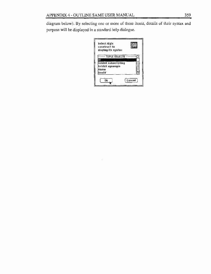
APPENDIX 4 - OUTLINE SAME USER MANUAL 359
diagram below). By selecting one or more of these items, details of their syntax and
purpose will be displayed in a standard help dialogue.
Select l£gis construct to display its synta11
----- TUPLE OBJECTS -------b'.)
~~6~~J! :~~~~~~ting 1!1i!i
Oneor ~-
~ (cancel)
Copyright © 2022 FDOKUMEN