The Complexity of Model Checking for Belief Revision and Update

Belief Revision and Update: Complexity of Model

Checking

Paolo Liberatore

Dipartimento di Informatica e Sistemistica

Universita di Roma “La Sapienza”

Via Salaria 113 – 00198 Roma, Italy

Email: [email protected]

WWW: http://www.dis.uniroma1.it/~liberato

Marco Schaerf





WWW: http://www.dis.uniroma1.it/~schaerf

1

Proposed running head:

Belief Revision: Complexity of Model Checking

Send proofs to:Marco Schaerf




Tel. ++39 06 4991 8332

Fax. ++39 06 8530 0849

Note: the ’0’ after ++39 MUST be dialed


2

Abstract

One of the main challenges in the formal modeling of common-sense reasoning is

the ability to cope with the dynamic nature of the world. Among the approaches put

forward to address this problem are belief revision and update. Given a knowledge base

T , representing our knowledge of the “state of affairs” of the world of interest, it is

possible that we are lead to trust another piece of information P , possibly inconsistent

with the old one T . The aim of revision and update operators is to characterize

the revised knowledge base T ′ that incorporates the new formula P into the old one

T while preserving consistency and, at the same time, avoiding the loss of too much

information. In this paper we study the computational complexity, in the propositional

case, of one of the main reasoning problems of belief revision and update: deciding if

an interpretation M is a model of the revised knowledge base.

3

1 Introduction

Recently, many formalisms have been proposed in the AI literature to model common-sense

reasoning. Particular emphasis has been put on the formal modeling of a distinct feature of

common-sense reasoning, that is, its dynamic nature. The AI goal of providing a logic model

of a human agent’s ability to reason in the presence of incomplete and changing information

has proven to be a very hard one. Nevertheless, many important formalisms have been put

forward in the literature.

Given a knowledge base T , representing our knowledge of the “state of affairs” of the

world of interest, it is possible that we are lead to trust another piece of information P ,

possibly inconsistent with the old one T . The aim of revision operators is to incorporate the

new formula P into the old one while preserving consistency and, at the same time, avoiding

the loss of too much information. This process has been called belief revision and the result

of revising T with P is denoted as T ∗ P .

This “minimal change assumption” was followed by the introduction of a large number

of specific revision operators. Among others, we mention Fagin, Ullman and Vardi [6],

Ginsberg [9], and Dalal [4]. A general framework for belief revision has been proposed by

Alchourron, Gardenfors, and Makinson [1, 8]. A close variant of revision is update. The

general framework for update has been studied by Katsuno and Mendelzon [12, 13] and

specific operators have been proposed, among the others, by Winslett [19] and Forbus [7].

The difference between revision and update is described in Section 2.1.

While most of the early work aimed at defining the appropriate semantics for revision and

4

update, recently, researchers have investigated the computational complexity of reasoning

with the operators introduced in the literature. To date, the most complete complexity

analysis has been done by Eiter and Gottlob [5]. More precisely, in the paper the authors

address the problem of characterizing the complexity, in a finite propositional language, of

the following problem:

Given a knowledge base T , a new formula P and a query Q (represented as

propositional formulas), decide whether Q is a logical consequence of T ∗ P , the

revised knowledge base.

In this paper we consider a distinct computational problem of belief revision and update.

Consider a knowledge base represented by a set of propositional formulae T . Any such

knowledge base can be equivalently represented by the set of its models, denoted as M(T ) =

M1, . . . ,Mn. We say that a model M is supported by a knowledge base T if and only if

M ∈M(T ), or equivalently M |= T .

The problem we address in this paper is to decide whether a model is supported by a

revised knowledge base:

Given a knowledge base T , a new piece of information P (represented as propo-

sitional formulas) and a model M , decide whether M ∈M(T ∗ P ).

This problem is known as model checking. The importance of model checking in AI

and related fields has been convincingly advocated by Halpern and Vardi in [10], where

model-based representations are considered a viable alternative to the standard approach

5

of representing knowledge in terms of formulae. In model-based representations the basic

computational task is model checking, not inference. In this setting it is also very important

to study the computational complexity of model checking.

While the computational complexity of inference and model checking are related, there

is no way to automatically derive the results for model checking from those already known

for inference. In fact, as our results show, there are operators that have the same complexity

w.r.t. query inference but with different complexity w.r.t. model checking.

The paper is structured as follows: in Section 2 we recall some key definitions and results

for belief revision. In Section 3 we briefly present all the results and discuss their relevance,

while in Section 4 we prove the complexity results for the general case and in Section 5 we

prove the results for the Horn case (i.e., when all the formulae involved in the revision are

in the Horn form). Finally, in Section 6 we draw some conclusions.

2 Preliminaries

In this section we (very briefly) present the background and terminology needed to un-

derstand the results presented later in the paper. Throughout this paper we restrict our

attention to a (finite) propositional language.

The alphabet of a propositional formula is the set of all propositional atoms occurring

in it. Formulae are built over a finite alphabet of propositional letters using the usual

connectives ¬ (not), ∨ (or) and ∧ (and). Additional connectives are used as shorthands,

α → β denotes ¬α ∨ β, α ≡ β is a shorthand for (α ∧ β) ∨ (¬α ∧ ¬β) and α 6≡ β denotes

6

¬(α ≡ β). A valuation of an alphabet X is truth assignment to all the propositional letters

in X. We will frequently denote a valuation of an alphabet X with the subset of letters in

X that are mapped into true.

An interpretation of a formula is a truth assignment to the atoms of its alphabet. A model

M of a formula F is an interpretation that satisfies F (written M |= F ). Interpretations and

models of propositional formulae will be denoted as sets of atoms (those which are mapped

into true). A theory T is a set of formulae. An interpretation is a model of a theory if it

is a model of every formula of the theory. Given a theory T and a formula F we say that

T entails F , written T |= F , if F is satisfied by every model of T . Given a propositional

formula or a theory T , we denote with M(T ) the set of its models. We say that a knowledge

base T supports a model M if M ∈ M(T ), or equivalently M |= T . A knowledge base T is

consistent, written T 6|= ⊥, if M(T ) is non-empty. Moreover, we denote with F the inverse

operator of M, that is, given a set of models A, F(A) denotes one of the formulae that have

exactly A as its set of models.

In order to make formulae more compact and easier to understand, we introduce a number

of notations that we use in the rest of the paper.

The notation F [x/y] denotes the formula F where every occurrence of the letter x is

replaced by the formula y. This notation is generalized to ordered sets: F [X/Y ] denotes the

formula F where all occurrences of letters in X are replaced by the corresponding elements

in Y , where X is an ordered set of letters and Y is an ordered set of formulae with the same

cardinality. That is, F [X/Y ] = F [x1/y1, · · · , xk/yk]. For example, let T = (x1 ∧ (¬x3 ∨x2)),

X = x1, x2, x3, and Y = y1, y2, y3. Then the formula T [X/Y ] is (y1 ∧ (¬y3 ∨ y2)).

7

In order to make the formulae more compact and readable, we overload the boolean

connectives to apply to sets of letters. For example, given three disjoint sets of letters W ,

S and R with the same number of elements k, we use the notation (¬S) as a shorthand for

the formula∧¬si|si ∈ S, (S ≡ R) to denote

∧si ≡ ri|1 ≤ i ≤ k, (S ≡ ¬R) to denote

∧si ≡ ¬ri|1 ≤ i ≤ k and (W ≡ (S ≡ ¬R)) for∧wi ≡ (si ≡ ¬ri)|1 ≤ i ≤ k. For

example, the formula

T ∧ (W ≡ (X ≡ ¬Y )

where T = (x1 ∧ (¬x3 ∨ x2)) is a shorthand for:

x1 ∧ (¬x3 ∨ x2) ∧ [w1 ≡ (x1 ≡ ¬y1)] ∧ [w2 ≡ (x2 ≡ ¬y2)] ∧ [w3 ≡ (x3 ≡ ¬y3)]

2.1 Belief Revision and Update

Belief revision is concerned with the modeling of accommodating a new piece of information

(the revising formula) into an existing body of knowledge (the knowledge base), where they

might contradict each other. A slightly different perspective is taken by knowledge update.

For an interesting discussion on the differences between belief revision and update we refer

the reader to the work of Katsuno and Mendelzon [13]. We assume that both the revising

formula and the knowledge base can be either a single formula or a theory.

We now recall the different approaches to revision and update, classifying them into

formula-based and model-based ones [12]. We use the following conventions: the expression

card(S) denotes the cardinality of a set S; the symmetric difference between two sets S1,

8

S2 is denoted by S1∆S2; and the set difference is denoted by S1 \ S2. If S is a set of sets,

∩S denotes the set formed intersecting all sets of S, and analogously ∪S for union; min⊆S

denotes the subset of S containing only the minimal (w.r.t. set inclusion) sets in S.

Formula-based approaches

They operate on the formulae syntactically appearing in the knowledge base T . Let W (T, P )

be the set of maximal subsets of T which are consistent with the revising formula P :

W (T, P ) = T ′ ⊆ T | T ′ ∪ P 6|= ⊥,¬∃U : T ′ ⊂ U ⊆ T, U ∪ P 6|= ⊥

The set W (T, P ) contains all the plausible subsets of T that we may retain when inserting

P .

Ginsberg. Fagin, Ullman, and Vardi [6] and, independently, Ginsberg [9] define the

revised knowledge base as a set of theories: T ∗G P = T ′ ∪ P | T ′ ∈ W (T, P ). This set

of theories must be interpreted as a disjunction of its members. In other words, the result

of revising T is the disjunction of all elements of the set composed of all maximal subsets of

T consistent with P , plus P . Logical consequence in the revised knowledge base is defined

as logical consequence in each of the theories, i.e., T ∗G P |= Q iff for all T ′ ∈ W (T, P ),

T ′ ∪P |= Q. In other words, Ginsberg considers all sets in W (T, P ) equally plausible and

inference is defined skeptically, i.e., Q must be a consequence of each set. Model checking is

defined in a similar way: M |= T ∗G P if and only if M is a model of at least one theory in

W (T, P ).

A more general framework has been defined by Nebel [14]. Here we do not analyze his

9

definitions.

WIDTIO. Since there may be exponentially many theories in T ∗G P , a simpler (but

somewhat drastical) approach is the so-called WIDTIO (When In Doubt Throw It Out [18]),

which is defined as T ∗Wid P = (∩W (T, P )) ∪ P.

Note that formula-based approaches are sensitive to the syntactic form of the theory.

That is, the revision with the same formula P of two logically equivalent theories T1 and T2

may yield different results, depending on the syntactic form of T1 and T2. We illustrate this

fact through an example.

Example. Consider T1 = a, b, T2 = a, a → b and P = ¬b. Clearly, T1 is equivalent

to T2. The only maximal subset of T1 consistent with P is a, while there are two maximal

consistent subsets of T2, that are a and a → b.

Thus, T1 ∗G P = a,¬b while T2 ∗G P = a ∨ (a → b),¬b = ¬b. The WIDTIO

revision gives the same results.

Model-based approaches

These operators select the models of P on the basis of some notion of proximity to the models

of T . Model-based approaches assume T to be a single formula; if T is a set of formulae it

is implicitly interpreted as the conjunction of all its elements. Many notions of proximity

have been defined in the literature. We distinguish them between pointwise proximity and

global proximity.

We first recall approaches in which proximity between models of P and models of T is

computed pointwise w.r.t. each model of T . That is, they select models of T one-by-one

10

and for each one they choose the closest models of P . These approaches are considered as

more suitable for knowledge update [13]. Let M be a model, we define µ(M, P ) as the set

containing the minimal differences (w.r.t. set inclusion) between each model of P and the

given M ; more formally:

µ(M,P ) = min⊆M∆N | N ∈M(P )

Winslett. Winslett [19] defines the models of the updated knowledge base as M(T ∗W

P ) = N ∈ M(P ) | ∃M ∈ M(T ) : M∆N ∈ µ(M, P ). In other words, for each model of T

it chooses the closest (w.r.t. set-containment) models of P .

Borgida. Borgida’s operator ∗B [2] coincides with Winslett’s one, except in the case

when P is consistent with T , in which case the revised theory is simply T ∧ P .

Forbus. This approach [7] takes into account cardinality: Let kM,P be the minimum

cardinality of sets in µ(M,P ). The models of Forbus’ updated theory are M(T ∗F P ) =

N ∈ M(P ) | ∃M ∈ M(T ) : card(M∆N) = kM,P. Note that, by means of cardinality,

Forbus’ update can compare (and discard) models which are incomparable in Winslett’s

approach.

We now recall approaches where proximity between models of P and models of T is

defined considering globally all models of T . In other words, these approaches consider at

the same time all pairs of models M ∈M(T ) and N ∈M(P ) and find all the closest pairs.

Let δ(T, P ) be defined as follows:

δ(T, P ) = min⊆⋃

M∈M(T )

µ(M, P )

11

Satoh. The models of the revised knowledge base are defined as M(T ∗S P ) = N ∈

M(P ) | ∃M ∈ M(T ) : N∆M ∈ δ(T, P ). That is, Satoh selects all closest pairs (by

set-containment of the difference set) and then projects on the models of P [15].

Dalal. This approach is similar to Forbus’, but global. Let kT,P be the minimum

cardinality of sets in δ(T, P ); Dalal [4] defines the models of a revised theory as M(T ∗D P ) =

N ∈ M(P ) | ∃M ∈ M(T ) : card(N∆M) = kT,P. That is, Dalal selects all closest pairs

(by cardinality of the difference set) and then projects on the models of P .

Wrong Variables Revisions

These two revision operators are model based and are based upon the hypothesis that the

interpretation of a subset of the variables, denoted with Ω, was wrong in the old knowledge

base T . The difference between them is based on a different definition of Ω. In Hegner’s

revision, Ω is the set of the variables of P . The underlying idea is that the original knowledge

base T was completely inaccurate w.r.t. everything mentioned in P .

Hegner. Let Ω be the variables of P . The models of Hegner’s revised theory [18] are

defined as M(T ∗H P ) = N ∈M(P ) | ∃M ∈M(T ) : N∆M ⊆ Ω.

Weber’s revision [17] is slightly less drastic. It assumes that the letters whose interpre-

tation was wrong are a subset of the letters of P , i.e., only those occurring in a minimal

difference between models of T and P .

Weber. Same definition with Ω = ∪δ(T, P ).

12

2.2 Computational Complexity

We assume that the reader is familiar with the basic concepts of computational complexity.

We use the standard notation of complexity classes [11]. Namely, the class P denotes the

set of problems whose solution can be found in polynomial time by a deterministic Turing

machine, while NP denotes the class of problems that can be solved in polynomial time by

a non-deterministic Turing machine. The class coNP denotes the set of decision problems

whose complement is in NP. We call NP-hard a problem G if any instance of a generic

problem NP can be reduced to an instance of G by means of a polynomial-time (many-one)

transformation (the same for coNP-hard).

Clearly, P ⊆ NP and P ⊆ coNP. We assume, following the prevailing assumptions of

computational complexity, that these containments are strict, that is P 6= NP and P 6= coNP.

Therefore, we call a problem that is in P tractable, and a problem that is NP-hard or coNP-

hard intractable (in the sense that any algorithm solving it would require a superpolynomial

amount of time in the worst case).

We also use higher complexity classes defined using oracles. In particular PA (NPA)

corresponds to the class of decision problems that are solved in polynomial time by deter-

ministic (nondeterministic) Turing machines using an oracle for A in polynomial time (for

a much more detailed presentation we refer the reader to [11]). All the problems we analyze

reside in the polynomial hierarchy, introduced by Stockmeyer [16], that is the analog of the

Kleene arithmetic hierarchy. The classes Σpk, Πp

k and ∆pk of the polynomial hierarchy are

defined by

13

Σp0 = Πp

0 = ∆p0 = P

and for k ≥ 0,

Σpk+1 = NPΣp

k , Πpk+1 = coΣp

k+1, ∆pk+1 = PΣp

k .

Notice that ∆p1 = P, Σp

1 = NP and Πp1 = coNP. Moreover, Σp

2= NPNP, that is the class of

problems solvable in nondeterministic polynomial time on a Turing machine that uses for

free an oracle for NP. The class PNP[O(log n)], often mentioned in the paper, is the class of

problems solvable in polynomial time using a logarithmic number of calls to an NP oracle.

The prototypical Σp2-complete problem is deciding the truth of the expression ∃X∀Y.F ,

where F is a propositional formula using the letters of the two alphabets X and Y . This

expression is valid if and only if there exists a truth assignment X1 to the letters of X such

that for all truth assignments to the letters of Y the formula F is true. In the paper we also

use a more restricted version, that is deciding the truth of ∃X∀Y.¬Π, where Π is a set of

3CNF clauses (i.e., , all clauses are composed of three literals). It is immediate to show that

deciding the truth of this quantified boolean formula is also a Σp2-complete problem.

3 Overview and discussion of the results

The complexity results are presented in Table 1. The table contains five columns. The

second and third show the complexity of model checking when T is a general propositional

formula, while the fourth and fifth show the Horn case. In the Horn case we assume that P

14

and all formulae in T are conjunctions of (possibly negative) Horn clauses. In both cases,

we consider two sub-cases: the second and fourth columns refer to the case in which no

constraint is assumed on the size of P (“generic”), while the third and fifth columns contain

the complexity result in the case the size of P is assumed to be bounded by a constant

(“bounded”).

In order to better appreciate the results we report in Table 2 the results on the complexity

of deciding T ∗ P |= Q obtained by Eiter and Gottlob [5]. The first thing to notice is that

the computational complexity of model checking for almost all operators is at the second

level of the polynomial hierarchy. This means that model checking for belief revision is much

harder than model checking for propositional logic (feasible in polynomial time).

We now give an intuitive idea why these problems are all in Σp2. For simplicity we

only consider the model-based approaches but this applies to the other systems as well. In

model-based approaches we have that M is a model of T ∗ P if and only if:

1. M |= P and

2. There exists a model N of T that is “close” to M .

The first step is obviously feasible in polynomial time, while the second one requires a

nondeterministic choice of N and for each choice checking the “closeness” of M and N . This

check can be performed with a new nondeterministic choice.

There are three exceptions to this rule: Dalal’s operator is complete for PNP[O(log n)],

while Hegner’s approach is NP-complete, and Ginsberg’s one is coNP-complete. The most

surprising result is the complexity of model checking for Ginsberg’s operator: as shown

15

in Table 2, inference for ∗G is as difficult as inference for ∗F , ∗W , ∗B and ∗S, while model

checking turns out to be significantly simpler.

Restricting the size of the revising formula P has a dramatic effect on the complexity

of model checking for ∗F and ∗W . In fact, the complexity goes down two levels. This

phenomenon does not arise for query inference.

While restricting to Horn form generally reduces the complexity by one level there are

two exceptions: ∗D and ∗F . The intuitive explanation is that these two operators use a

cardinality-based measure of minimality that cannot be expressed as a Horn formula. On

the other side, set-containment based minimality can be expressed with a Horn formula.

There are some problems that we have been unable to completely characterize. For

Weber’s revision we do not have the exact complexity for the general case with P bounded

and the Horn case with P generic. However, in our opinion, the most important open

problem is the complexity of WIDTIO revision in the Horn case. We know that the problem

is in NP and that the two cases with P generic and P bounded have exactly the same

complexity. We conjecture that this problem is NP-complete, but we have been unable to

prove it.

4 General Case

As said above, in this section we study the complexity of deciding whether M |= T ∗ P ,

given T , P and M as input.

For Ginsberg’s revision, model checking is easier than query answering. Namely, it is one

16

level down in the polynomial hierarchy. The significance of this result is that model checking

for Ginsberg’s operator is only a coNP problem, while its query answering problem has the

same complexity of the other operators (Πp2-complete).

Theorem 1 Deciding whether M |= T ∗G P is a coNP-complete problem.

Proof. Given a model M , we first decide if M |= P . This can be done in polynomial

time, and if this is not the case, the model is not supported by T ∗G P . Now, we have that

M |= T ∗G P if and only if M satisfies at least one element of W (T, P ). Let T ′ be the set of

the formulae in T that are satisfied by M . This is a consistent set, since it has at least one

model (M). To show that T ′ is in W (T, P ) we have to prove that given any other formula

f of T \ T ′, the set T ′ ∪ f ∪ P is inconsistent. Thus, we have the following algorithm to

decide whether M |= T ∗G P .

1. Check if M |= P (if not return false).

2. Compute T ′ = f ∈ T | M |= f

3. Decide, for any f ∈ T \ T ′, if the set T ′ ∪ f ∪ P is inconsistent.

The first two steps only require polynomial time, while the third one is a set of (at most

n) unsatisfiability problems that can be solved by a single call of a coNP algorithm. This

proves that the problem is in coNP.

Hardness follows by reduction from unsat. Given a propositional formula Π, built over

an alphabet X, we define:

17

T = r ∧ Π

P = s

M = X ∪ s

where r and s are new letters not contained in X. Notice that T only contains one formula.

We show that M |= T ∗G P if and only if Π is unsatisfiable.

Suppose Π is satisfiable: we have that T is consistent with P , thus T ∗G P = T ∧ P =

s, r, Π. Since M does not include r we have that M 6|= T ∗G P .

Now assume Π is unsatisfiable. We have that T is inconsistent, thus T ∗G P = P = s.

As a consequence M |= T ∗G P .

Even though Ginsberg’s and WIDTIO revision are very similar, the complexity results

we obtain are different.

Theorem 2 Deciding M |= T ∗Wid P is Σp2-complete.

Proof. First of all, let us prove membership. By definition, a formula fi ∈ T does not

belong to T ∗Wid P if and only if there is a maximal T ′ ⊆ T that is consistent with P but

fi 6∈ T ′.

Thus, to decide if M is a model of the revised base, we have to check that the formulae

of T not supporting M are ruled out by at least one maximal consistent subset T ′ of T . This

can be done using the following algorithm.

1. Verify M |= P .

18

2. For any f ∈ T such that M 6|= f , check if there exists a T ′ ⊆ T such that

(a) T ′ ∪ P is consistent.

(b) T ′ ∪ f, P is inconsistent.

Indeed, if such a T ′ exists, then it can be completed with elements of T in such a way

to obtain a maximal consistent subset of T not containing f . On the converse, if such a set

does not exist for a formula f , then this formula is in the revised base, and then M is not a

model of T ′. This is a Σp2 algorithm since it requires a nondeterministic choice of T ′ and, for

any such choice, a consistency and an inconsistency check (doable in polynomial time using

an NP oracle).

In order to prove Σp2-hardness we show a reduction from the prototypical Σp

2-complete

problem of deciding ∃X∀Y.F , where F is a propositional formula on the alphabet X ∪ Y .

Let T , P and M be defined as:

T = X ∪X ∪ ¬F ∧ r

P = true

M = X

where X = ¬x|x ∈ X, and r is a new propositional variable not appearing in X ∪ Y . We

show that M |= T ∗Wid P if and only if ∃X∀Y.F .

First of all, for any valuation of X, there is at least one maximal consistent subset of T .

Suppose X1 ⊆ X represents a valuation of X: then T ′ = X1 ∪ ¬xi | xi 6∈ X1 is consistent.

19

Hence, xi 6∈ T ∗Wid P : just consider T ′ = ¬xi∪xj | i 6= j. This is a consistent subset

of T , and it does not contain xi. Thus, either T ′ or T ′ ∪ ¬F ∧ r is a maximal consistent

subset of T , and it does not contain xi. Therefore, all atoms xi ∈ X and ¬xi ∈ X do not

belong to T ∗Wid P .

Now, it can be either T ∗Wid P = ¬F ∧ r, or T ∗Wid P = true. In the first case

M 6|= T ∗Wid P , while in the latter one M |= T ∗Wid P .

Suppose that there exists a valuation X1 ⊆ X such that F is valid for any Y . We have

that T ′ = X1 ∪ ¬xi | xi 6∈ X1 is consistent, but T ′ ∪ ¬F ∧ r is not. Since T ′ does not

contain ¬F ∧ r, we have that this formula is not in the revised base, hence T ∗Wid P = true.

As a result, M |= T ∗Wid P .

Suppose that for any X1 the formula F is not valid: T ′ is still consistent, but so is

T ′ ∪ ¬F ∧ r. As a result, any maximal consistent subset of T contains ¬F ∧ r, and

T ∗Wid P = ¬F ∧ r. Hence, M 6|= T ∗Wid P .

We now turn our attention to the model-based operators. All the model-based operators are

based on the principle that a model M |= P satisfies the result of a revision M |= T ∗ P if

and only if there is a model I |= T such that I and M are sufficiently close to each other.

It is not surprising that these methods have almost the same complexity (exception made

for Dalal’s that is a bit easier). However, although for query answering the complexity could

be proved with a single proof, for the model checking problem each operator requires its own

proof.

20

Theorem 3 Deciding M |= T ∗ P is in Σp2, where ∗ ∈ ∗F , ∗W , ∗S, ∗B.

Proof. Given M , T and P , let R = ¬F(M). Note that M |= T ∗ P if and only if

T ∗ P 6|= R. Since the inference problem of deciding whether T ∗ P 6|= R is in Πp2 for all the

model-based operators (cf. Table 2), we have that model checking is in the complementary

class Σp2.

Theorem 4 Deciding M |= T ∗ P is Σp2-complete, where ∗ ∈ ∗W , ∗B.

Proof. We will prove the Σp2-hardness of Winslett’s operator. The proof for Borgida’s

is similar. Let F be a propositional formula on the alphabet X ∪ Y . We consider the

Σp2-complete problem of deciding the validity of ∃X∀Y.F . Let

T = (X ≡ Z) ∧ Y ∧ w ∧ r

P = (Z ∧ ¬X ∧ ¬Y ∧ r ∧ ¬w) ∨ [(X ≡ Z) ∧ (w ≡ r) ∧ (w ≡ ¬F )]

M = Z ∪ r

notice that (Z ∧ ¬X ∧ ¬Y ∧ r ∧ ¬w) = F(M). We prove that ∃X∀Y.F if and only if

M |= T ∗W P .

First of all, we recall that, by definition, M(T ∗W P ) = ∪I∈M(T )F(I) ∗W P .

Suppose ∃X∀Y.F valid. Let X1 be the valuation of X that makes F valid. Now I =

X1 ∪ Z1 ∪ Y ∪ w, r (with Z1 = zi | xi ∈ X1) is a model of T . Consider the set

F(I) ∗W P . Since F is valid for any Y , the formula P has two kinds of models (apart

from M): the models with X = X1 and both w and r false, and the models with a

21

different valuation of X. Note that none of these models can exclude M from being a

model of the result of the revision F(I) ∗W P . The models with a different evaluation

of X are not less distant from I than M ; Indeed, let J be that model: if I contains

both xi and zi, but J contains none of these literals, then J is not closer of I than M ,

since the latter contains zi but not xi. The same argument holds if I contains none of

xi and zi but J contains both. The models with the same evaluation of X, but that

map w and r into false, are more distant from I than M , since M and I agree on w

and r while the other models disagree.

Suppose ∃X∀Y.F not valid. Then, for all the possible valuations of X, there exists a

valuation of Y that falsifies F . Now let I be the generic model of T . For any valuation

X1 of the variable X we can prove that M is never a model of F(I)∗W P . Consider that

for any X1 we have in P the model M ′ = X1∪Z1∪Y1∪w, r, where Z1 = zi | xi ∈ X1

and Y1 is the evaluation of Y that falsifies F . This model is closer to I than M , thus

M is not in the revised base.

The same proof can be used to prove the complexity of Borgida’s operator.

Theorem 5 Deciding M |= T ∗S P is Σp2-complete.

Proof. Given a propositional formula F , we prove that ∃X∀Y.F is valid if and only if

M |= T ∗S P , where

T = (X 6≡ Z) ∧ [(Y ∧ ¬w ∧ s ∧ r) ∨ (¬r ∧ (w ≡ s) ∧ (s ≡ F ))]

22

P = ¬X ∧ ¬Z ∧ ¬Y ∧ ¬w ∧ ¬s

M = r

Assume that there exists a subset X1 of X such that X1 ∪ Y1 |= F holds for any set

Y1 ⊆ Y . In this case, T contains two kinds of models:

I = X1 ∪ Z1 ∪ Y ∪ s, r

J = X1 ∪ Z1 ∪ Y1 ∪ w, s

where Z1 = zi | xi ∈ X1.

The differences between models are represented in the following table.

M M ′

I X1 ∪ Z1 ∪ Y ∪ s X1 ∪ Z1 ∪ Y ∪ s, r

J X1 ∪ Z1 ∪ Y1 ∪ w, s, r X1 ∪ Z1 ∪ Y1 ∪ w, s

The distance between I and M is incomparable with the other ones, thus M is a model

of the result. Notice that the models of T with a different valuation for the variables X do

not affect this result: given a model L = X2 ∪ Z2 ∪ . . . of T , if X2 ⊂ X1 then Z2 ⊃ Z1, thus

X2 ∪ Z2 6⊂ X1 ∪ Z1, which implies L∆M ′ 6⊂ I∆M .

Suppose now that for any set X1 ⊆ X there exists a set Y2 ⊆ Y such that X1 ∪ Y2 6|= F .

This implies that T has a new kind of models, at least one for each subset X1 of X:

K = X1 ∪ Z1 ∪ Y2

where Z1 = zi | xi 6∈ X1.

23

Adding this model to the table of the differences leads to

M M ′

I X1 ∪ Z1 ∪ Y ∪ s X1 ∪ Z1 ∪ Y ∪ s, r

J X1 ∪ Z1 ∪ Y1 ∪ w, s, r X1 ∪ Z1 ∪ Y1 ∪ w, s

K X1 ∪ Z1 ∪ Y2 ∪ r X1 ∪ Z1 ∪ Y2

In this new table, the distances between M and any model of T are not minimal. As a

result, M is not a model of T ∗S P .

Theorem 6 Deciding M |= T ∗F P is Σp2-complete.

Proof. We prove hardness by reduction from ∃∀QBF . Let Π be a set of propositional

clauses using variables X ∪ Y . We assume, without loss of generality, that |X| = |Y | = n.

We prove that ∃X∀Y.¬Π if and only if M |= T ∗F P , where

T = (X ≡ Z) ∧ ¬Y ∧ ¬W ∧ ¬r

P = (X ∧ ¬Z ∧ ¬Y ∧ ¬W ∧ r) ∨ [(X ≡ Z) ∧ (Y 6≡ W ) ∧ ¬r ∧ Π]

M = X ∪ r

Let us assume that there exists a subset X1 of X such that X1 ∪ Y1 6|= Π holds for any

set Y1 ⊆ Y . Consider the following model of T :

I = X1 ∪ Z1

where Z1 = zi | xi ∈ X1. We prove that M |= F(I) ∗F P . The distance between I and M

is

|I∆M | = |X\X1|+ |Z1|+ 1 = n + 1

24

Now, consider a model N of (X ≡ Z) ∧ (Y 6≡ W ) ∧ ¬r ∧ Π. Since Π is false for each

model extending X1, a model of the latter formula must contain a different subset of X.

Thus, N must be a model of the kind:

N = X2 ∪ Z2 ∪ Y2 ∪W2

where Y2 is such that X2 ∪ Y2 |= Π and W2 = wi | yi 6∈ Y2. The difference between I and

N is

|I∆N | = |X1∆X2|+ |Z1∆Z2|+ |Y2|+ |W2| = |X1∆X2|+ |Z1∆Z2|+ n > n + 1

This is because X1 and X2 differ for at least one literal, and the same holds for Z1 and Z2. The

update P has two kind of models, namely M and the models of (X ≡ Z)∧(Y 6≡ W )∧¬r∧Π.

Since the models of the latter are not closer to I than M , it follows that M is a model of

F(I) ∗F P , thus it is a model of T ∗F P .

Now, let us assume that there is no truth valuation X1 such that all the models extending

X1 over X ∪Y falsifies Π. Thus, for each X1 there exists a Y1 such that Π is satisfied by the

model X1 ∪ Y1. Consider an arbitrary model I of T :

I = X1 ∪ Z1

where Z1 = zi | xi ∈ X1. We prove that M is not a model of F(I)∗F P (for any I ∈M(T )),

thus proving that M is not a model of T ∗F P . The distance between I and M is

|I∆M | = |X\X1|+ |Z1|+ 1 = n + 1

25

Since for each X1 there is a model X1 ∪ Y1 of Π, the formula P contains the following

model

N = X1 ∪ Z1 ∪ Y1 ∪W1

where W1 = wi | yi 6∈ Y1. Consider the distance between I and N

|I∆N | = |Y1|+ |W1| = n

As a result, M is not a model of F(I)∗F P , and this holds for any I ∈M(T ). Therefore,

M is not a model of T ∗F P .

Model checking for Dalal’s revision operator turns out to be computationally simpler.

Theorem 7 Deciding whether M |= T ∗D P is PNP[O(log n)]-complete.

Proof. Membership follows from complexity of inference: verifying whether M |= T ∗D P

amounts to check T ∗D P 6|= ¬F(M), which is PNP[O(log n)].

Hardness is proved by reduction from the problem uocsat: given a set of clauses Π =

γ1, . . . , γm over an alphabet X, decide whether its (cardinality) maximal consistent subset

is unique. Let X ′, Y and Y ′ be new alphabets one-to-one with X, while C and C ′ are two

alphabets of m letters each, one-to-one with the clauses of Π. We show that Π has a unique

(cardinality) maximal consistent subset if and only if M 6|= T ∗D P , where

T =∧

γi∈Π

(ci → γi) ∧∧

γi∈Π

(c′i → γi[xi/yi]) ∧ [d ≡ (C ≡ C ′)] ∧ (X 6≡ X ′) ∧ (Y 6≡ Y ′)

P = C ∧ C ′ ∧ ¬X ∧ ¬X ′ ∧ ¬Y ∧ ¬Y ′

M = C ∪ C ′

26

First of all, notice that the condition X 6≡ X ′, together with the fact P |= ¬X ∧ ¬X ′,

implies that the valuation of X in a model of T does not affect its distance from P . The

same holds for Y . Evaluating the distance between models of T and models of P amounts

to evaluate their assignments to the variables C ∪ C ′ ∪ d.

Second, P has only two models, namely M and M ′ = M ∪ d. The only difference is

the valuation of d. Suppose that the maximal consistent subset of Π is unique, and calculate

the distance between T and M . Let Π′ ⊆ Π be this set. Consider C1 = ci | γi ∈ Π′ and

C ′1 = c′i | γi ∈ Π′.

Clearly, C1 ∪ C ′1 ∪ d can be extended with a suitable subset of X ∪ X ′ ∪ Y ∪ Y ′ to

obtain a model of T . The distance between this model and M ′ is 2(m− |Π′|). We are able

to prove that the distance between any model of T and M is at least 2(m− |Π′|) + 1. The

above model of T is 2(m− |Π′|) + 1 far from M because of the different valuation of d. For

any other model of T with d false there must be at least an i such that ci 6= c′i. Since the

valuation of C corresponds to a consistent subset of Π (the same for C ′), this implies that

the number of true ci is less than |Π′| (the same may be for c′i instead.) As a result, this

model assigns true to |Π′|+ |Π′|+ v variables, with v > 0. Hence, the difference between it

and M is (m−|Π′|)+(m−|Π′|+v) = 2(m−|Π|)+v, with v > 0. This implies M 6|= T ∗D P .

On the converse, suppose that Π has two (or more) maximal consistent subsets Π′ and

Π′′. One can build a model N of T assigning true to 2|Π′| variables among C ∪C ′, such that

d is false in N . The distance between N and M is now 2(m− |Π′|), thus M |= T ∗D P .

We now establish the complexity of the operator that use a set of variables Ω whose

27

observation is considered wrong, that is, Weber’s and Hegner’s ones.

Theorem 8 Deciding whether M |= T ∗H P is NP-complete.

Proof. To prove membership to NP, note that M |= T ∗H P is equivalent to the following

statements:

1. M |= P and

2. ∃I ∈ M(T ) such that the variables that differ between I and M are a subset of the

variables of P .

Since the first step can be accomplished in polynomial time and the second one is feasible

with an NP machine, this problem is in NP.

In order to prove hardness, consider the NP-complete problem of deciding the satisfia-

bility of a formula Π on the alphabet X. Given

T = Π ∨ (¬r ∧ ¬X)

P = X

M = X ∪ r

we can prove that Π is satisfiable if and only if M |= T ∗H P .

Suppose Π satisfiable: T contains a model I containing r. Hence the difference between

M and I is a subset of X, so M is in the revised knowledge base.

Suppose Π unsatisfiable: now T = ¬r ∧ ¬X, thus the revised base is ¬r ∧X that does

not support M .

28

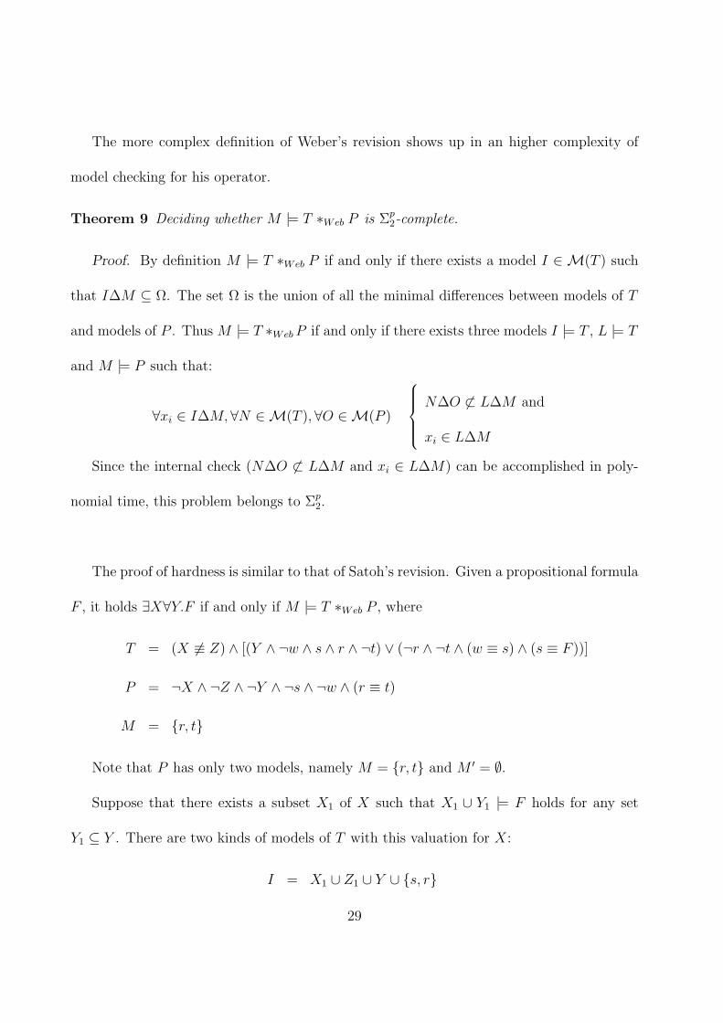
The more complex definition of Weber’s revision shows up in an higher complexity of

model checking for his operator.

Theorem 9 Deciding whether M |= T ∗Web P is Σp2-complete.

Proof. By definition M |= T ∗Web P if and only if there exists a model I ∈ M(T ) such

that I∆M ⊆ Ω. The set Ω is the union of all the minimal differences between models of T

and models of P . Thus M |= T ∗Web P if and only if there exists three models I |= T , L |= T

and M |= P such that:

∀xi ∈ I∆M, ∀N ∈M(T ),∀O ∈M(P )

N∆O 6⊂ L∆M and

xi ∈ L∆M

Since the internal check (N∆O 6⊂ L∆M and xi ∈ L∆M) can be accomplished in poly-

nomial time, this problem belongs to Σp2.

The proof of hardness is similar to that of Satoh’s revision. Given a propositional formula

F , it holds ∃X∀Y.F if and only if M |= T ∗Web P , where

T = (X 6≡ Z) ∧ [(Y ∧ ¬w ∧ s ∧ r ∧ ¬t) ∨ (¬r ∧ ¬t ∧ (w ≡ s) ∧ (s ≡ F ))]

P = ¬X ∧ ¬Z ∧ ¬Y ∧ ¬s ∧ ¬w ∧ (r ≡ t)

M = r, t

Note that P has only two models, namely M = r, t and M ′ = ∅.

Suppose that there exists a subset X1 of X such that X1 ∪ Y1 |= F holds for any set

Y1 ⊆ Y . There are two kinds of models of T with this valuation for X:

I = X1 ∪ Z1 ∪ Y ∪ s, r

29

J = X1 ∪ Z1 ∪ Y1 ∪ w, s

where Z1 = zi | xi ∈ X1. The differences between models of T and models of P are in the

following table.

M = r, t M ′ = ∅

I X1 ∪ Z1 ∪ Y ∪ s, t X1 ∪ Z1 ∪ Y ∪ s, r

J X1 ∪ Z1 ∪ Y1 ∪ w, s, r, t X1 ∪ Z1 ∪ Y1 ∪ w, s

As a result, the pair 〈I, M〉 is one of those with a minimal difference among these. Note

that a model L of T with a different valuation for X must have L∆M ′ incomparable with

I∆M (see the discussion for Satoh’s revision). Thus I∆M ⊆ Ω, which implies that M is a

model of T ∗Web P .

Suppose now that for any set X1 ⊆ X there exists a set Y2 ⊆ Y such that X1 ∪ Y2 6|= F .

This implies that T supports a new kind of models, at least one for each subset of X:

K = X1 ∪ Z1 ∪ Y2

which leads to a new row in the table of differences

M = r, t M ′ = ∅

I X1 ∪ Z1 ∪ Y ∪ s, t X1 ∪ Z1 ∪ Y ∪ s, r

J X1 ∪ Z1 ∪ Y1 ∪ w, s, r, t X1 ∪ Z1 ∪ Y1 ∪ w, s

K X1 ∪ Z1 ∪ Y2 ∪ r, t X1 ∪ Z1 ∪ Y2

where Z1 = zi | xi ∈ X1. Clearly, K∆M ′ is always contained in I∆M , and this happens

for any subset of X. Furthermore, J∆M ′ is always contained in J∆M . As a result, there is

30

no difference between a model of T and a model of P that is minimal and contains t. As a

result, t 6∈ Ω, and M is not a model of the result of the revision.

4.1 Bounded Case

In the previous section we investigated the complexity of evaluating model checking on the

revised knowledge bases. As it turned out, for most of the operators this complexity is at

the second level of the polynomial hierarchy. From an analysis of the proofs, it turns out

that this behavior depends on the new formula P being very complex.

However, in applications, it may be reasonable to assume that the size of the new formula

is very small w.r.t. the size of the knowledge base. This means that changes to the knowledge

base are incremental, since the revising formula can only contain a bounded number of

propositional variables. In this section we investigate the impact of this assumption on the

complexity of model checking. In particular, throughout this section we assume that the

size of the new formula P is bounded by a constant (k in the sequel). Notice that this

assumption can (in general) be substituted by the weaker assumption that the size of P is

bounded by a logarithm of the size of T . Under this assumption, we obtain the following

results.

Theorem 10 If |P | ≤ k, the complexity of deciding whether M |= T ∗ P is polynomial,

where ∗ ∈ ∗F , ∗W , ∗H.

Proof. The polynomiality of Hegner revision can be easily proved from the NP-membership

31

proof of the general case. We remind that M |= T ∗H P is equivalent to the following state-

ments:

1. M |= P and


variables of P .

When the size of P is bounded by a constant k, the number of its variables is also

bounded. As a result, the set of variables for which M and I can differ is also bounded

by k. The guessing of I can be replaced by an exhaustive verification over all models that

differ from I only for a subset of the variables of P . Since the cardinality of such a set is

bounded by 2k, that is a constant, the number of possible models to verify is also bounded

by a constant.

For Winslett’s and Forbus’ operators, we can prove the polynomiality with the same

proof. Consider for example Winslett’s revision. A model M of P is in the revision of T

with P if and only if there exists a model I in T such that M is its closest model. Consider

that, given a model I, its closest model has exactly the same valuation of I for the variables

that are not in P . Hence, the double quantification of the definition (M |= T ∗F P iff there

exists a I ∈M(T ) such that for all M ′ ∈M(P ) it holds I∆M ′ 6⊂ I∆M) is over a constant

set of variables, thus the models we have to consider (those of I and M ′ that agree with M

on the variables that are not in P ) are a constant number. For Forbus’ operator we have a

similar motivation.

32

Theorem 11 If |P | ≤ k, the complexity of deciding whether M |= T ∗ P is coNP-hard,

where ∗ ∈ ∗G, ∗B, ∗S, ∗D.

Proof. We show that if an operator ∗ satisfies the following three properties then the

problem of deciding whether M |= T ∗ P is coNP-hard.

1. If P is consistent then T ∗ P is consistent;

2. T ∗ P = T ∧ P whenever T ∧ P is consistent;

3. if T = f, where f is a formula equivalent to ¬r, then T ∗ r = r.

Notice that the first two properties above are postulates 3 and 4 of the AGM postulates

[1] and that all operators in ∗G, ∗B, ∗S, ∗D satisfy these two postulates, plus the third

property.

Given a formula Π on the alphabet X, we show that Π is unsatisfiable if and only if

M |= T ∗ P , where

T = r → (s ∧ Π)

P = r

M = X ∪ r

Suppose Π satisfiable. Then T ∧ P is consistent, thus T ∗ P = T ∧ P = r ∧ s ∧Π, which

does not support the model M , since M |= ¬s.

33

Suppose Π unsatisfiable. Then T = f, where f is equivalent to ¬r, thus T ∗ P =

f ∗ r = r, which supports the model M .

Proving membership in coNP for all the above revision operators is quite simple, with

the only exception of ∗Web.

Theorem 12 If |P | ≤ k, the complexity of deciding whether M |= T ∗ P is coNP-complete,

where ∗ ∈ ∗G, ∗B, ∗S, ∗D.

Proof. Hardness for all these operators follows from the previous lemma. Membership to

coNP for ∗G follows from the fact that this operator is in coNP even in the general case. For

∗B, since the only difference from ∗W is the check of unsatisfiability of T ∧ P , membership

to coNP easily follows.

For ∗S and ∗D, by definition M |= T ∗ P if and only if there exists a model I ∈ M(T )

such that, for any pair of models J ∈ M(T ) and N ∈ M(P ), the distance between J and

N is not smaller than the distance between I and M (the distance may be the difference or

its cardinality, depending on whether we use ∗S or ∗D). It is also easy to see that we can

restrict I to models of T that coincide with M for the variables not in P . As a result, the

check “for all models I” is indeed polynomial, as there are at most a polynomial number of

models I that coincide with M for the variables not in P . As a result, model checking can

be expressed as a check “for any pair of models J and N”, and is thus in coNP.

Theorem 13 If |P | ≤ k, the complexity of deciding whether M |= T ∗Web P is coNP-hard,

in PNP[O(1)].

34

Proof. Hardness follows from the previous lemma. Membership to PNP[O(1)] immediately

follows from the result of membership of inference with the same assumption of the size of

P [5].

On the other hand, WIDTIO semantics is not affected by the bound imposed on the size

of P .

Theorem 14 Even if |P | ≤ k, the complexity of deciding whether M |= T ∗Wid P is Σp2-

complete.

Proof. The problem with P unbounded is in Σp2, thus the same holds for P bounded.

From the proof of hardness of the general case, one can note that the P used in the reduction

is actually P = true, thus bounded.

5 Horn Case

So far, we have considered revision of arbitrary knowledge bases. However, it is also of inter-

est to consider the complexity for the case in which both the knowledge base T and the new

information P are in Horn form (i.e., they are conjunctions of Horn clauses). Furthermore,

it is also interesting to find the complexity in the case in which both the Horn limitation

and |P | ≤ k hold. In order to simplify the formulae, we use the following notation: given

a set of propositional clauses Π over an alphabet X, we denote with Πneg the set of clauses

obtained from Π where each positive literal xi is replaced by ¬x′i. Notice that Πneg only

contains negative literals on the alphabet X ∪ X ′ and is, therefore, in Horn form. This

35

transformation is often applied after a change of alphabet. In order to make our reductions

readable an example is in order. Let T = (x1 ∨ ¬x2) ∧ (¬x1 ∨ x2). T [X/Y ]neg denotes the

following formula:

T [X/Y ]neg = (¬y′1 ∨ ¬y2) ∧ (¬y1 ∨ ¬y′2)

We now turn our attention to the complexity analysis. First of all, the cardinality-based

revisions have the same complexity of the general (non-Horn) case.

Theorem 15 If T and P are Horn formulae, the model checking problem for ∗D is PNP[O(log n)]-

complete.

Proof. The membership is implied by the PNP[O(log n)] membership of the model checking

in the general case.

The hardness is proved by reduction from the problem of model checking for Dalal’s

revision in the general case. Let T and P be a theory and a formula, respectively, and

M a model. We prove that, if T and P are consistent, then M |= T ∗D P if and only if

M ′ |= T ′ ∗D P ′, where

T ′ = T [X/Y ]neg ∪ ¬Y ∨ ¬Y ′ ∪ Y ≡ Y1 ≡ · · · ≡ Yn ∪ Y ′ ≡ Y ′1 ≡ · · · ≡ Y ′

n ∪

P [X/Z]neg ∪ ¬Z ∨ ¬Z ′ ∪ Z ≡ Z1 ≡ · · · ≡ Zn ∪ Z ′ ≡ Z ′1 ≡ · · · ≡ Z ′

n ∪

W → (Y ≡ Z) ∪ X ≡ Z

P ′ = Y ∧ Y1 ∧ · · · ∧ Z ′n ∧W

M ′ = M ∪ Y ∪ Y1 ∪ · · · ∪ Z ′n ∪W

36

where Y, Y1, . . . , Yn, Y′, Y ′

1 , . . . , Y′n, Z, Z1, . . . , Zn, Z ′, Z ′

1, . . . , Z′n,W are new alphabets all one-

to-one with X. The reduction works as follows: let I be a model of T ′. This model can be

splitted in three parts, one that reflects a model of T [X/Y ]neg, one that reflects the value of

P [X/Z]neg, and the part regarding the comparison between them. Intuitively, the variables

Y are used to represent a model of T , while the variables Z are used for P . The formulas

¬Y ∨¬Y ′, together with the fact that P contains Y ∧Y ′, implies that the models of T ′ that

are closest to P ′ are those for which I ∩ Y is a model of T . This way, we are able to express

the models of a non-Horn theory (i.e., T ) with the Horn set T [X/Y ]neg. The same for P

and P [X/Y ]neg.

Moreover, T ′ contains W → (Z ≡ Y ), and since P ′ has W , the model I of T ′ must have

the maximum possible number of variables Y equal to Z. Finally, since T ′ has X ≡ Z and

P ′ has no constraint on X, the closest models of P ′ must have X setted to the same value

of the Z in the model of T ′, which is a model of P that is closest to T .

Let now formally prove the claim. Let I and J be a pair of models of T ′ and P ′ respec-

tively, such that their symmetric difference is minimal. We prove that J ∩ X = M , where

M is one of the models of T ∗D P . The converse also holds, that is, each model M of T ∗D P

can be extended to form a model J that is a model of T ′ ∗D P ′.

We prove the following facts

1. The value of Y ′ in I is exactly the opposite of the value of Y . The same holds for Z ′

and Z.

2. As a consequence, I ∩ Y is a model of T [X/Y ], and I ∩ Z of P [X/Z]. The converse

37

also holds: for each pair of models of T and P , there is a model of T ′.

3. The models I∩Y and I∩Z correspond to a pair of models of T and P whose difference

is minimal.

4. The model J corresponds to a model of T ∗D P .

Proof of 1. First, we prove that the value of Y ′ in I is exactly the opposite of the value of

Y . Since T is satisfiable, there exist a model Y1 of T [X/Y ]neg over Y ∪Y ′ such that yi ∈ Y1 if

and only if y′i 6∈ Y1. The same holds for Z and Z ′. Extending these models to form a model

I1 of T ′, we have that the distance between I1 and P is 2n(n + 1), which is the part due to

the yi’s and zi’s, plus the difference over the wi’s, which is at most n. Thus, the minimal

distance between T ′ and P ′ is at most 2n(n + 1) + n.

Let now prove that the value of Y in I is the opposite of the value of Y ′. Since T contains

¬yi ∨ ¬y′i, if this is not true, then there exists an index i such that neither yi not y′i is in

I. Now, consider the difference between I and P ′. Since yi and y′i are “replicated” n times,

the fact that yi, y′i 6∈ I is amplified, thus the difference is at least 2n(n + 1) + n + 1. Since

there are models of T that differ only 2n(n + 1) + n from P , this would imply that I is not

minimal. Since I is minimal by hypothesis, we conclude that I ∩Y ′ is the opposite of I ∩Y .

Proof of 2. This is easy to prove: since Y ′ is the opposite of Y , we have that xi | yi ∈ Y

is a model of T .

Proof of 3. Since P ′ contains W , the model J contains also W . As a result, the difference

between I and J is given by the value 2n(n + 1), which is due to the variable Y, . . . , Z ′n,

plus the number of wi’s that are not in I. The first part of the difference is fixed, thus the

38

difference is indeed the number of wi not in I. Since wi ∈ I implies yi = zi, this implies that

the difference is equal to the number of variables for which I ∩ Y and I ∩ Z differ. Since

I ∩ Y and I ∩ Z correspond to models of T and P , respectively, the model I is indeed the

union of a pair of models of T and P that are sufficiently close each other.

Proof of 4. The value of Z in T , and consequently the value of X, must coincide with the

value of one of the models of P that are closest to T .

Now, consider the formula P ′. This formula does not contain the variables in X. Thus,

for the pair I and J to be close enough, the model J must have the value of X equal to the

value of X in I. As a result, the value of X in the models of P ′ that are closest to T ′ is

indeed a model of P that is closest to T . This proves that M ′ is a model of T ′ ∗D P ′ if and

only if M is a model of T ∗D P .

Theorem 16 If T and P are Horn formulae, the model checking problem for ∗F is Σp2-

complete.

Proof. Membership is implied by the Σp2 membership of model checking in the general

case.

Hardness is proved by a reduction from the Σp2-complete problem ∃∀QBF. Let Π be a

set of clauses. We prove that ∃X∀Y ¬Π is valid if and only if M |= T ∗F P , where

T = r1 ∪R1 ∪ r2 ∪R2 ∪ X ≡ X ′ ∪ Y ∪ Y ′ ∪ z

39

P = (¬r1 ∨ ¬r2) ∧ (r1 ≡ R1) ∧ (r2 ≡ R2) ∧ (r1 → (X ∧ ¬X ′ ∧ ¬z)) ∧ (r2 → P ′)

P ′ = (X ≡ X ′) ∧ (¬Y ∨ ¬Y ′) ∧ Π[X/Y ]neg

M = r1 ∪R1 ∪X ∪ Y ∪ Y ′

where R1 and R2 are sets of 7n− 1 variables.

First of all, there is exactly a model I of T for each evaluation of the variables in X.

Let X1 ⊆ X be an interpretation over X, and let IX1 be the corresponding model of T . We

prove that F(IX1) ∗F P has M as a model if and only

Π ∧ xi | xi ∈ X1 ∧ ¬xi | xi 6∈ X1

is false for each possible evaluation of the variables in Y .

Let IX1 be the model of T associated to X1, and J be a model of P . The difference

between IX1 and M is

|IX1∆M | = |r2 ∪R2|+ |X\X1|+ |X1|+ |z| = 8n + 1

If J does not contain neither r1 nor r2, the distance between IX1 and J is at least 14n,

while IX1 and M differ for 8n+1 variables. As a result, the models of P that do not contain

neither r1 nor r2 are not minimal.

Let us consider a model J with r1 but not r2. The model M is a model of this kind.

Furthermore, M is the closest model to IX1 having r1 but not r2.

There are two kind of models with r2. First assume that there is an index i such that

their evaluation of the X is different from X1. Let X2 be the value of J over X. The distance

40

between IX1 and J is:

|IX1∆J | = |r1 ∪R2|+ |X1∆X2|+ |Y | = 8n + |X1∆X2| ≥ 8n + 1

As a result, J is not closer to IX1 than M .

Now consider the models J which have X1 = J ∩ X. These models depend on the

satisfiability of Π. Let us assume Π satisfiable. Then it is possible to assign Y ′ and Y to the

opposite values, thus is is possible to have a model J whose difference to IX1 is

|IX1∆J | = |r1 ∪R1|+ |Y | = 8n

As a result, if Π is satisfiable when X is forced to be X1, then M is not a model of T ∗F P .

Assume Π unsatisfiable. In this case, it is impossible to assign to Y and Y ′ opposite

evaluations. As a result, there is at least an index i such that both yi and y′i are false, thus

the difference between IX1 and J is

|IX1∆J | ≥ |r1 ∪R1|+ |Y |+ 1 = 8n + 1

This implies that M is a model of T ∗F P .

Summarizing, we have proved that, given an evaluation X1 over X, the model M is a

model of IX1 ∗F P if and only if the set Π is valid once assigned the X to have the value X1.

This is true for all the possible X1. As a result, M is a model of T ∗F P if and only if there

exists a value X1 such that IX1 ∗F P contains M , which is equivalent to say that there exists

a X1 such that for all Y the set of clauses Π is false.

For Ginsberg’s and Hegner’s revisions, the complexity decreases: they become tractable.

41

Theorem 17 If T and P are Horn formulae, the model checking problem for ∗G is polyno-

mial.

Proof. The algorithm given in the proof of Theorem 1 is polynomial if T and P are

Horn formulas. Indeed, the only non-polynomial steps were the checks of inconsistency of

T ′ ∪ f ∪ P. Since this is a Horn formula, this check can be done in polynomial time.

Theorem 18 If T and P are Horn formulae, the model checking problem for ∗H is polyno-

mial.

Proof. We recall that M |= T ∗H P is equivalent to the following statements:

1. M |= P and


variables of P .

Let X be the alphabet of T , Y the alphabet of P and Z = X ∪ Y . We construct a new

formula

T ′ = T ∧∧zi|zi ∈ (M \ Y ) ∧∧¬zi|zi ∈ (Z \M), zi ∈ (Z \ Y )

Notice that any model N of T ′ satisfies statement (2) above. Therefore, since satisfiability

checking of a Horn formula is polynomial, model checking can be performed in polynomial

time.

For the revision operators of Satoh, Winslett and Borgida, the complexity decreases of

one level.

42

Theorem 19 If T and P are Horn formulae, the model checking problem for ∗W and ∗B is

NP-complete.

Proof. We start with ∗W . The check M |= T ∗W P can be done by guessing a model

I ∈ M(T ) such that there is no model J ∈ M(P ) such that I∆J ⊂ I∆M . Given I, this

check is polynomial. Indeed, it is equivalent to the consistency of the Horn formula

P ∧ ∧

xi∈I,xi∈M

xi ∧∧

xi 6∈I,xi 6∈M

¬xi ∧( ∨

xi∈I,xi 6∈M

xi ∨∨

xi 6∈I,xi∈M

¬xi

)

This formula has a model J if and only if J is a model of P , and if I and M coincide on

the variable xi, then J has the same value on that variable. Furthermore, there must be an

xi such that I and M differ on it, while I and J agree.

As a result, model checking is in NP, since it amounts to check whether M ∈ M(P ),

and to guess a model I such that the above formula is unsatisfiable. Since that formula is

Horn, this check is polynomial.

The hardness of Winslett’s update is proved by reduction from the NP-complete problem

3sat. Let Π = γ1, . . . , γm be a set of clauses over X. We prove that Π is satisfiable if and

only if M |= T ∗W P , where

T = Πneg

P = (X = X ′)

M = X ∪X ′

Let us assume Π satisfiable and let G be a model of Π. Then

I = G ∪ x′i | xi 6∈ G

43

is a model of T . We prove that M is one its closest models of P . First of all, the symmetric

difference between them has the following property: for each i, either xi or x′i is in I∆M ,

but not both. This is because in I the value of xi and x′i are different, while in M they

coincide. Consider any other model J of P . According to the same argumentation, either

xi or x′i is in I∆J , for each i. As a result, I∆J 6⊂ I∆M .

Let us assume Π unsatisfiable. Let I be an arbitrary model of T . Since T contains

¬X∨¬X ′, we have that for any i either xi or x′i is not in I. Moreover, since Π is unsatisfiable,

there is at least an index k such that both xk and x′k are false. Now, consider the symmetric

difference between I and M . This set contains either xi or x′i, for each i. Moreover, for the

index k it holds xk, x′k ⊂ I∆M . Now, consider the model J of P :

J = M\xk, x′k

We have

I∆J = (I∆M)\xk, x′k

As a result, I∆J ⊂ I∆M . Thus, the model M is not one of the models of P closest to I.

Since this proof holds for any I ∈M(T ), the interpretation M is not a model of T ∗W P .

Let now turn to Borgida’s revision. The only difference between it and Winslett’s oper-

ator being the check of consistency of T ∪ P, which is polynomial for Horn formulas, we

obtain that M |= T ∗B P is in NP.

The proof of hardness of ∗W can be rewritten for ∗B as well. Just consider T ′ = T ∧ w,

P ′ = P ∧ ¬w. Since T ∪ P is inconsistent, the result T ′ ∗B P ′ is identical to T ∗W P . As

44

a result, M |= T ′ ∗B P ′ if and only if M |= T ∗W P , which is equivalent to the satisfiability

of the set of clauses Π.

Theorem 20 If T and P are Horn formulae, the model checking problem for ∗S is NP-

complete.

Proof. Membership is proved in a manner similar to the previous theorem. Indeed,

M |= T ∗S P if and only if there exists a model I of T such that does not exist a pair J , M ′

such that J∆M ′ ⊂ I∆M . The test “does not exist a pair J , M ′ such that J∆M ′ ⊂ I∆M”

can be done in polynomial time, if T and P are Horn formulas. Indeed, given M and I, the

above test is equivalent to verifying unsatisfiability of the Horn set

T [X/Y ] ∧ P ∧ ∧

xi 6∈I∆M

(yi = xi) ∧∨

xi∈I∆M

(yi = xi)

Indeed, the above formula is satisfiable if and only if there exists a model of T and a model

of P such that their difference is strictly contained in I∆M .

NP-hardness is proved by reduction from the NP-complete problem sat. Let Π be a set

of clauses. We prove that Π is satisfiable if and only if M |= T ∗S P , where

T = Πneg ∪ ¬X ∨ ¬X ′ ∪ X ∨X ′ → Z ∪ (∧ zi) → r ∪ r = u

P = X ∧X ′ ∧ ¬Z ∧ ¬r

M = X ∪X ′ ∪ u

Note that G ⊆ X is a model of Π if and only if G ∪ x′i | xi 6∈ G is a model of⋃

γj∈Π γnegj .

45

Assume that Π is satisfiable, and let G ⊆ X be a model of Π. The following interpretation

is a model of T :

I = G ∪ x′i | xi 6∈ G ∪ Z ∪ r, u

The symmetric difference between I and M is

I∆M = X\G ∪ x′i | xi ∈ X ∪ Z ∪ r

We prove that the difference between I and M is a minimal one, i.e., there do not exist

two other models J and N , of T and P respectively, such that J∆N ⊂ I∆M . We assume

J∆N ⊆ I∆M , and prove that this implies I∆M ⊆ J∆N .

Let X1 = J ∩X and X ′1 = J ∩X ′. Since X ∪X ′ ⊆ N , it follows that

(J∆N) ∩ (X ∪X ′) = X\X1 ∪X ′\X ′1

Since J∆N ∩ X ⊆ I∆M ∩ X, we obtain X\X1 ⊆ X\G, which implies G ⊆ X1. Since

X1∪X ′1 is a model of each ¬xi∨¬x′i, we have that X ′

1 ⊆ x′i | xi 6∈ G, which in turn implies

X ′\x′i | xi 6∈ G ⊆ X ′\X ′1. Since X ′\x′i | xi 6∈ G = J∆N ∩X ′, and X ′\X ′

1 = I∆M ∩X ′,

we have that X ′1 = x′i | xi 6∈ G, and thus X1 = G. This implies J ∩ Z = I ∩ Z = Z,

which implies r, u ⊆ J . Thus J = I. Now, the model of P that is closest to I is M , thus

I∆M ⊆ J∆N .

Assume Π unsatisfiable. We consider an arbitrary model I of T that is one of the closest

to M , and then prove that I∆M is never a minimal difference (i.e., there is always another

pair of models J and N whose difference is lesser). Let I be a model of T , X1 = I ∩X, and

X ′1 = I∩X ′. Since Π is unsatisfiable, Πneg cannot have models X1∪X ′

1 if X ′1 = x′i | xi 6∈ X1.

46

Since ¬xi ∨ ¬x′i is satisfied by I, there must be at least an index i such that xi 6∈ X1 and

x′i 6∈ X ′1.

If either xi or x′i is true in a model of T , then zi must also be true in that model. However,

in the model I, neither xi nor x′i is true, thus zi can be true or false. Suppose, without loss

of generality, that the condition xi 6∈ x′i and x′i 6∈ X ′1 holds exactly for one value of i. If zi is

true in the model I, r and u must also be true in I. This is the first possible form of I:

I1 = X1 ∪X ′1 ∪ Z ∪ r, u

However, zi can very well be false. In this case r can be true or false, and u has the same

value. Thus, we have two possibilities:

I2 = X1 ∪X ′1 ∪ Z\zi ∪ r, u

I3 = X1 ∪X ′1 ∪ Z\zi

Let now consider the differences between these models and M . Since I2∆M ⊂ I1∆M ,

we need not consider I1 any more. About I2 and I3 we have

I2∆M = X\X1 ∪X ′\X ′1 ∪ Z\zi ∪ r

I2∆M = X\X1 ∪X ′\X ′1 ∪ Z\zi ∪ u

Now, consider the model N = X ∪X ′. This is a model of P . Moreover, I2∆N is strictly

contained in I2∆M , and I3∆N is strictly contained in I3∆M . As a result, there is no model

I of T such that I∆M is minimal. Thus M is not a model of T ∗S P .

Finally, for Weber’s revision the complexity decreases “almost” one level.

47

Theorem 21 If T and P are Horn formulae, the model checking problem for ∗Web is NP-

complete.

Proof. Membership: M |= T ∗Web P holds if and only if there exists a model I ∈M(T )

such that, for each xi ∈ I∆M , there exists a pair of models J ∈ M(T ) and N ∈ M(P ),

such that xi ∈ J∆N and for each pair of models J ′ ∈M(T ) and N ′ ∈M(P ), does not hold

J ′∆N ′ ⊂ J∆N . The test “for each pair of models J ′ and N ′...” is polynomial since T and

P are Horn. Moreover, since there are only a linear number of variables, the test “for each

xi ∈ J∆N” can be rewritten as an and of n formulas.

In short: to test whether M |= T ∗Web P , guess a model I of T , and n pairs of models

〈Ji, Ni〉 such that if xi ∈ I∆M , then xi ∈ Ji∆Ni and the Horn formula

T [X/Y ] ∧ P ∧ ∧

xi 6∈Ji∆Ni

(yi = xi) ∧∨

xi∈Ji∆Ni

(yi = xi)

is unsatisfiable. This formula has a model if and only if there is a pair of models that are

close each other more than Ji and Ni are.

Hardness: let Π be a set of clauses. We prove that Π is is satisfiable if and only if

M |= T ∗Web P , where

T = Πneg ∪ ¬X ∨ ¬X ′ ∪ X ∨X ′ → Z ∪ (∧ zi) → r ∪ r → u ∧ ¬w ∪ u ∨ ¬w

P = X ∧X ′ ∧ ¬Z ∧ ¬r ∧ (¬u ∨ w)

M = X ∪X ′ ∪ w

The proof is similar to that of Satoh. Let I and J be a pair of models of T and P , respectively,

such that their difference is minimal. Let us suppose Π unsatisfiable. We prove that neither

48

u nor w are in I∆J , thus proving that they are not in Ω, either.

Since Π is unsatisfiable, there exists an index i such that neither xi nor x′i are in I. As

a result, the value of zi and r can be either true or false. Now, consider the case

I ∩ zi, r, u, w = ∅

J ∩ zi, r, u, w = ∅

This is possible, according to our definition of T and P . In this case, we have that I∆J ∩

zi, r, u, w = ∅. This proves that it is always possible to extend I in such a way the difference

between I and J does not contain the variables in zi, r, u, w. As a result, neither u nor w

are in Ω.

The interpretation M is not a model of T ∗Web P , since it has w but not u, and no model

of T has this property. Since neither u nor w are in Ω, the models of T ∗Web P must have

on u and w the value of a model of T . As a result, M is not a model of the revised base.

Let us suppose Π satisfiable. In this case, as proved in the proof of hardness for Satoh’s

revision, there exist a pair of models I and J whose difference is minimal, such that r ∈ I.

This happens because no model without r can have a so small distance to P over X ∪X ′.

As a result, we have u ∈ I and w 6∈ I. No model of P has both these properties. There are

models with the first but not the second, and vice versa. For the first ones it holds u ∈ I∆J ,

and for the second ones it holds w 6∈ I∆J . As a result, u,w ∈ Ω. There is no model of T

having the same evaluation of u,w of M , but since u,w ∈ Ω, these variables are not counted

as “different”. Thus, M ∈ T ∗Web P .

Theorem 22 If T and P are Horn formulae, the model checking problem for ∗Wid is in NP.

49

Proof. Let T be a set of Horn clauses and P a Horn formula. The problem of model

checking for ∗Wid can be determined by an oracle-powered machine as follows: to prove that

J |= T ∗Wid P , consider each f ∈ T such that J 6∈ M(f). If there exists a set T ′ ⊆ T such

that f 6∈ T ′, T ′ ∪ P is consistent, and T ′ ∪ g ∪ P is inconsistent for each g ∈ T\T ′, then

J |= T ∗Wid P . All the consistency checks are polynomial since the involved formulas are

Horn. As a result, the whole problem requires a single guessing, thus is in NP.

If we also assume that the size of P is bounded by a constant k we obtain that model

checking becomes tractable for all operators (except ∗Wid).

Theorem 23 If T and P are Horn formulae and |P | ≤ k, the model checking problem for

∗G, ∗F , ∗W , ∗B, ∗S, ∗D, ∗H and ∗Web is polynomial.

Proof. The model checking problem M |= T ∗P can be rewritten as the query answering

problem T ∗ P 6|= F(M). Since F(M) is a Horn formula, and the above query answering

problem has been proved to be polynomial [5], we conclude that the model checking problem

is also polynomial, for all the revisions considered in the statement of the theorem.

6 Conclusions

In this paper we have investigated a key issue of belief revision systems: their computa-

tional feasibility. Namely, we have studied, in a propositional language, the problem of

deciding whether a model is supported by a revised knowledge base. As it turns out, model

checking for belief revision and update is far more complex than model checking for classic

50

propositional logic.

Some questions are left open by this work. First, the complexity of model checking has

not been exactly determined in all cases: for Weber’s semantics, in the bounded case, we

have only been able to prove that model checking can be done with a constant number of

calls to an NP oracle, and that the problem is coNP-hard.

An entire line of related research, not investigated in this work, is the investigation of

belief revision operators w.r.t. their relative space efficiency. In the framework of space

efficiency [3], knowledge representation formalisms are compared in terms of their ability to

represent knowledge in little space. Since knowledge bases are used to represent models, it

makes sense to investigate how good different revision operators are with respect to their

ability to represent the set of model of the revised knowledge base in little space.

References

1. C. E. Alchourron, P. Gardenfors, and D. Makinson. On the logic of theory change:

Partial meet contraction and revision functions. Journal of Symbolic Logic, 50:510–530,

1985.

2. A. Borgida. Language features for flexible handling of exceptions in information systems.

ACM Transactions on Database Systems, 10:563–603, 1985.

3. M. Cadoli, F. Donini, P. Liberatore, and M. Schaerf. Comparing space efficiency of

propositional knowledge representation formalisms. In Proceedings of the Fifth In-

51

ternational Conference on the Principles of Knowledge Representation and Reasoning

(KR’96), pages 364–373, 1996.

4. M. Dalal. Investigations into a theory of knowledge base revision: Preliminary report.

In Proceedings of the Seventh National Conference on Artificial Intelligence (AAAI’88),

pages 475–479, 1988.

5. T. Eiter and G. Gottlob. On the complexity of propositional knowledge base revision,

updates and counterfactuals. Artificial Intelligence, 57:227–270, 1992.

6. R. Fagin, J. D. Ullman, and M. Y. Vardi. On the semantics of updates in databases.

In Proceedings of the Second ACM SIGACT SIGMOD Symposium on Principles of

Database Systems (PODS’83), pages 352–365, 1983.

7. K. D. Forbus. Introducing actions into qualitative simulation. In Proceedings of the

Eleventh International Joint Conference on Artificial Intelligence (IJCAI’89), pages

1273–1278, 1989.

8. P. Gardenfors. Knowledge in Flux: Modeling the Dynamics of Epistemic States. Bradford

Books, MIT Press, Cambridge, MA, 1988.

9. M. L. Ginsberg. Conterfactuals. Artificial Intelligence, 30:35–79, 1986.

10. J. Y. Halpern and M. Y. Vardi. Model checking vs. theorem proving: A manifesto. In

Proceedings of the Second International Conference on the Principles of Knowledge Rep-

resentation and Reasoning (KR’91), 1991. Also in Lifshitz V. Artificial Intelligence and

52

Mathematical Theory of Computation. Papers in Honor of John McCarthy, Academic

Press, San Diego, 1991.

11. D. S. Johnson. A catalog of complexity classes. In J. van Leeuwen, editor, Handbook of

Theoretical Computer Science, volume A, chapter 2. Elsevier Science Publishers (North-

Holland), Amsterdam, 1990.

12. H. Katsuno and A. O. Mendelzon. A unified view of propositional knowledge base

updates. In Proceedings of the Eleventh International Joint Conference on Artificial

Intelligence (IJCAI’89), pages 1413–1419, 1989.

13. H. Katsuno and A. O. Mendelzon. On the difference between updating a knowledge base

and revising it. In Proceedings of the Second International Conference on the Principles

of Knowledge Representation and Reasoning (KR’91), pages 387–394, 1991.

14. B. Nebel. Belief revision and default reasoning: Syntax-based approaches. In Proceedings

of the Second International Conference on the Principles of Knowledge Representation

and Reasoning (KR’91), pages 417–428, 1991.

15. K. Satoh. Nonmonotonic reasoning by minimal belief revision. In Proceedings of the

International Conference on Fifth Generation Computer Systems (FGCS’88), pages 455–

462, 1988.

16. L. J. Stockmeyer. The polynomial-time hierarchy. Theoretical Computer Science, 3:1–22,

1976.

53

17. A. Weber. Updating propositional formulas. In Proc. of First Conf. on Expert Database

Systems, pages 487–500, 1986.

18. M. Winslett. Sometimes updates are circumscription. In Proceedings of the Eleventh In-

ternational Joint Conference on Artificial Intelligence (IJCAI’89), pages 859–863, 1989.

19. M. Winslett. Updating Logical Databases. Cambridge University Press, 1990.

54

General case Horn case

P generic P bounded P generic P bounded

Ginsberg coNP-complete coNP-complete P P

∗G Th. 1 Th. 12 Th. 17 Th. 17

Forbus Σp2-complete P Σp

2-complete P

∗F Th. 3 Th. 10 Th. 16 Th. 23

Winslett Σp2-complete P NP-complete P

∗W Th. 3 Th. 10 Th. 19 Th. 23

Borgida Σp2-complete coNP-complete NP-complete P

∗B Th. 3 Th. 12 Th. 19 Th. 23

Satoh Σp2-complete coNP-complete NP-complete P

∗S Th. 3 Th. 12 Th. 20 Th. 23

Dalal PNP[O(log n)]-complete coNP-complete PNP[O(log n)]-complete P

∗D Th. 7 Th. 12 Th. 15 Th. 23

Hegner NP-complete P P P

∗H Th. 8 Th. 10 Th. 18 Th. 18

Weber Σp2-complete coNP-hard in PNP[O(1)] NP-complete P

∗Web Th. 9 Th. 12 Th. 21 Th. 23

WIDTIO Σp2-complete Σp

2-complete NP NP

∗Wid Th. 2 Th. 14 Th. 22 Th. 22

Table 1: The complexity of deciding whether M |= T ∗ P .

57

General case Horn case

P generic P bounded P generic P bounded

Ginsberg Πp2-complete Πp

2-complete coNP-complete coNP-complete

Forbus Πp2-complete coNP-complete Πp

2-complete P

Winslett Πp2-complete coNP-complete coNP-complete P

Borgida Πp2-complete NP-hard and coNP-hard coNP-complete P

in PNP[2]

Satoh Πp2-complete NP-hard and coNP-hard coNP-complete P

in PNP[O(1)]

Dalal PNP[O(log n)]-complete NP-hard and coNP-hard PNP[O(log n)]-complete P

in PNP[O(1)]

Weber Πp2-hard NP-hard and coNP-hard NP-hard P

in PΣp2[O(log n)] in PNP[O(1)] in PNP[O(log n)]

WIDTIO Πp2-hard Πp

2-hard coNP-hard coNP-hard

in PΣp2[O(log n)] in PΣp

2[O(log n)] in PNP[O(log n)] in PNP[O(log n)]

Table 2: The complexity of deciding whether T ∗ P |= Q [5].

58

The Complexity of Model Checking for Belief Revision and Update

Documents

Transcript of The Complexity of Model Checking for Belief Revision and Update