The comparison of the tool Parsifal with two mid-term planning ...

Degree project in

The comparison of the tool Parsifal with two mid-term planning tools for the

electric production of isolated systems

BORIS DADVISARD

Stockholm, Sweden 2012

XR-EE-ES 2012:009

Electric Power SystemsSecond Level,

1

Acknowledgements

This work was conducted as part of a Master’s Degree Project in the Department OSIRIS at EDF R&D,

in order to obtain the diploma of engineer of KTH, the Scientific and Technical University of

Stockholm.

The OSIRIS department (Optimisation SImulations Risk and Statistics for the energy markets) is

responsible at EDF R&D for developing tools and methods for an optimal management of the assets

portfolio of EDF. In this context, I joined a group responsible for studies concerning the isolated

energetic systems and I was under the tutorship of Sébastien FINET.

I would like to show my gratitude to the group R35 of OSIRIS that made this project possible. I had a

number of very interesting conversations within the group about stochastic dynamic programming

among other topics. A particular thank goes to my tutor Sébastien FINET for its precious advice and

sharing of knowledge and also to Aurélien BOUTIN and Elsa CLAUDET for their friendly support.

Finally, I am thankful to my supervisor and my examiner at KTH, Yelena VARDANYAN and Lennart SÖDER who accepted to supervise and review my master thesis at KTH.

2

________________________________________

Comparison of the tool Parsifal with two mid-term planning tools for the electrical production of isolated systems

Abstract

The tool Parsifal is a middle-term planning tool developed by the R&D department and the Operation

Center. It is used operationally by various isolated systems at EDF, in particular EDF Land. It meets a

need for optimization of the electrical power (thermal, hydraulic, markets) over a period of one year

or two. Parsifal allows a precise modeling of the hydraulic system, taking into account the

hydrological coupling between units lying in the same valley. The algorithm of stochastic dynamic

programming of Parsifal handles uncertainty on the availability of the units, on the demand and on

the hydrological inflows. However, this powerful – but old – tool is being challenged by new tools

which are under study in this project.

The aim of this work is to analyze the features of such tools for a potential replacement of Parsifal,

that is considered as the reference tool since it has been used operationally for a couple of decades.

The comparison has to be done based on the simulation results and on the user interface of the tools

that are considered. The goal is to determine if the tool under study is able to provide results

consistent with Parsifal and operationally usable by EDF in its production context. The production

context that lies within the scope of this project is limited to isolated systems.

This work should help OSIRIS to make its mind about the replacement of Parsifal by Tick-Tack, a

middle-term optimization tool developed internally by EDF, or by SDDP, a Brazilian tool developed by

the company PSR.

According to the results of this study both tools get an operation policy that turns more expensive

than Parsifal. This cost difference is due to the water management of the hydro resource that is less

optimal in the tools compared with Parsifal. In Tick-Tack as in SDDP, the main reason for this

difference is the handling of spillage in the case of wet inflow scenarios. However, both Tick-Tack and

SDDP benefit from a user-friendly interface and a smaller calculation time than Parsifal. As a general

result of this project, the tool Parsifal cannot be operationally replaced either by Tick-Tack or by

SDDP. Indeed, although Tick-Tack and SDDP offer interesting features in terms of calculation time

and graphical interface, they have not been designed in order to meet the specific needs of the

operational production of isolated systems like Parsifal has. Consequently, Parsifal will remain the

tool that is used for the electrical production middle-term planning of isolated systems in France.

However, this study will be used as a basis for future studies that will go into deeper details. These

studies may consider several unavailability scenarios instead of only one and add a spillage penalty

that prevents the tools from unnecessary spillage.

3

________________________________________


Contents

ACKNOWLEDGEMENTS ................................................................................................................. 2

ABSTRACT .................................................................................................................................... 3

TABLE OF CONTENTS .................................................................................................................... 4

LIST OF TABLES ............................................................................................................................. 6

LIST OF FIGURES ........................................................................................................................... 7

UNITS, NOTATIONS AND ACRONYMS ............................................................................................ 8

INTRODUCTION………………………………………………………………………………………………………………………….…10

I. MIDDLE-TERM OPTIMIZATION…………………………………………………………………………………………………...11

1. Optimisation in deterministic context……………………………………………………………………………………………………..…11

2. Optimisation in stochastic context: dynamic stochastic programming…….…………………………………………….….12

2.1 Definition of the state of a system .……………………………………..………………………………………………………………...12

2.2 Stochastic dynamic programming..…….…………………………………………………………………………………………………..13

3. Description of the three middle-term planning tools under study..…………………………………………….................14

3.1 Parsifal……………………………………………………………………………………………………………..…………………………………….14

3.2 Tick-Tack………………………………………………………………………………………………………….……………………………………..14

3.3 SDDP……………………………………………………………………………………………………….………………………………………………16

II. STUDY OF ISLAND ON TICK-TACK………………………………………………………………………………………………..17

1. Description of the electrical system of Island…………………………………………………………………………………………….17

2. Study of the parameter « Head Effect In Optimization » on Tick-Tack ………………………………………………………18

2.1 Description of the problem………………………………………………………………………………………………………………….…18

2.2 Deterministic model, without imposed reservoir content ……………………………………………………………………..20

2.3 Stochastic model, with imposed reservoir content…………………………………………………………………………………21

3. Comparison Tick-Tack – Parsifal…………………………………………………………………………………………………………….…22

3.1 Stochastic model, without imposed reservoir content……………………………………………………………………………23

3.2 Stochastic model, with imposed reservoir content ……………………………………………………………………………..…24

III. STUDY OF LAND ON TICK-TACK……………………………………………………………………………………………………........27

1. Description of the hydro electrical system of Land………………………………………………………………………….…........28

2. Simple model of Land on Tick-Tack………………………..……………………………………………………………………………….…28

2.1 Description of the model……………………....……………………………………………………………………………………………….28

2.1.1 Demand ……………………………………………………………………………………………………………………………………………….28

2.1.2 Hydraulic model……………………………………………………………………………………………………………………………………30

2.1.3 Thermal model…………………………………………………………………………………………………………………………………..…32

4

________________________________________


2.1.4 Study parameters of the simple model of Land…………………………………………………………………………………...33

2.2 Analysis of the simulation results……………………………………………………………………………………………………….…..34

2.2.1 Qualitative analysis………………………………………………………………………………………..…….……………………………...34

2.2.2 Quantitative analysis……………………………………………………………………………………..………………………………….…36

2.3 Discussion over the results of the simple model and conclusions…….………………..………………………………..….39

2.3.1 Internal management differences…………………………………………………………………..……………………………….…..39

2.3.2 Model differences……………………………………………………………………………………………………………………………..…39

3. Detailed model of Land on Tick-Tack……………………..……………………………………………………………………………….…40

3.1 Description of the detailed model of Land ……………………………………………………………………………………………..40

3.1.1 Demand ………………………………………………………………………………..………………………………………………………….…40

3.1.2 Hydraulic model…………………………………………………………………………………………………………………………..….....40

3.1.3 Thermal model and renewable energies………………………………………………………………………………………….....41

3.1.4 Uncertainty scenarios………………………………………………………………………………………………………………………....42

3.2 Analysis of the simulation results ……………………………………………………….…..……………………………………………..43

3.2.1 Qualitative analysis …………………………………………..……………………………………………………….…..…………………..43

3.2.2 Quantitative analysis…………………………………………… ……………………………………………………….…..……………....46

3.3 Discussion over the results of the detailed model and conclusions.……………………………………………………….49

IV. STUDY OF LAND ON SDDP………………………………………………………………………………………………….......50

1. Description of the model on SDDP…….…………………………………………………………………………………................50

2. Analysis of the results of the model.…………………………………………………………………………………..……………….51

3. Conclusion……………………………………………………………………………………………………………………………..……………53

DISCUSSION ON RESULTS ........................................................................................................... ..54

CONCLUSION .............................................................................................................................. 55

APPENDIX .................................................................................................................................. 56

A. Transition matrix of the two-state Markov chain of a power plant……………………………………….56 B. Economical value of the water content gap at the end of the studied period

Case study: Island , stochastic model, without imposed reservoir content)………………………….57

C. Diagrams of the weekly energy produced per unit.

Case study: Land, simple model………………………………………………..............................................59

D. Merit order costs and efficiency using the interpolation method …….…………………………........64

REFERENCES ............................................................................................................................... 66

5

________________________________________


List of tables

Table 2.1 : Electrical system of Island…………………………………………………………………………………………….…17

Table 2.2 : Description of the two models dealing with the head effect in optimization…………………..19

Table 2.3 : Generated energy and total costs of Island, stochastic model, with imposed reservoir content…..………………………………………………………………………………………………………...................................21

Table 2.4 : Generated power and total costs, comparison Tick-Tack- Parsifal on Island………………….…23

Table 2.5 : Generated power and total costs, comparison Tick-Tack- Parsifal on Island…………………...25

Table 3.0 : Positions repartition over one week……………………………………………………………………………..…29

Table 3.1 : Hydraulic system of Land on Tick-Tack………………………………………………………………………….…32

Table 3.2 : Thermal system of Land on Tick-Tack………………………………………………………………………………33

Table 3.3 : Generated power……………………………………………………………………………………………………….……34

Table 3.4 : Costs of thermal power……………………………………………………………………………………………………35

Table 3.5 : Total spillage……………………………………………………………………………………………………………………36

Table 3.6 : Utilization rate week 10 and week 11 position 1…………………………………………………………..…36

Table 3.7 : Utilization rate week 19 positions 4 to 7……………………………………………………………………….…38

Table 3.8 : Utilization rate week 20 position 7 (peak hours) ………………………………………………………….…38

Table 3.9 : Characteristics of the power plants of the system of Land, Tick-Tack………………………………41

Table 3.10 : Total generation over the 2-year period, Land, Tick-Tack………………………………………………43

Table 3.11 : Total cost over the 2-year period, Land, Tick-Tack…………………………………………………………44

Table 3.12 : Total spillage, Land, Tick-Tack………………………………………………………………………………………..45

Table 4.1 : Aggregation of the load positions from Parsifal on SDDP…………………………………………………50

Table 4.2 : Spillage, SDDP- Parsifal……………………………………………………….………………………………………..…52

Table 4.3 : Total generation over the 2-year period, SDDP-Parsifal………………………………………………..…52

Table 4.4 : Total cost over the 2-year period, SDDP-Parsifal………………………………………………………….....53

Table 5.1 : Synthesis of the capabilities of the three tools……………………………………………………………..…54

6

________________________________________


List of figures

Figure 1.1 : Decision process for hydrothermal systems…………………………………………………………………..12

Figure 2.1 : Hydro production means in Island……………………………………………………………………………….…17

Figure 2.2 : Head height on a hydro plant with reservoir……………………………………………………………….…18

Figure 2.3 : Efficiencies in function of the reservoir content on Tick-Tack………………………………………..19

Figure 2.4 : Reservoir content in a deterministic model without imposed content on Tick-Tack……...20

Figure 2.5 : Two-state Markov chain…………………………………………………………………………………………………20

Figure 2.6 : Mean reservoir content of Island, stochastic model, with imposed reservoir content…..21

Figure 2.7 : Comparison results Tick-Tack – Parsifal, Island, stochastic model, without imposed reservoir content…………………………………………………………………………………………………………………………..…23

Figure 2.8 : Comparison results Tick-Tack – Parsifal, Island, stochastic model with imposed

Reservoir content…………………………………………………………………………………………………………………..……..…25

Figure 3.1 : Overview of the hydro system of Land…………………………………………………………………………..28

Figure 3.2 : Weekly Load Duration Curve of Land…………………………………………………………………………..…29

Figure 3.3 : Aggregation of the power-discharge curves within Valley 1……………………………………….....30

Figure 3.4 : Aggregation of the power-discharge curves within Valley 2 ……………………………………….…31

Figure 3.5 : Aggregated overview of Land’s hydro system………………………………………………………………..32

Figure 3.5.1 : Hydro inflow scenarios of reservoir Alpha………………………………………………………………..…33

Figure 3.6 : Reservoir content per week……………………………………………………………………………………………35

Figure 3.7 : Increasing weekly demand for Land on Parsifal……………………………………………………………..40

Figure 3.8 : Mean reservoir content, Land, Tick-Tack………………………………………………………………..........45

Figure 3.9 : Energy over weeks 1 and 2, Land, Tick-Tack…………………………………………………………………..48

Figure 4.1 : Mean reservoir content, Land, SDDP………………………………………………………………………………51

Figure 6.1 : Weekly power generation, Land, Tick-Tack…………………………………………………………………….59

7

________________________________________


Units, notations and acronyms

Set of indices:

t : position index

k : stage index

i : reservoir index

g : thermal unit index

j : turbine index of a hydro unit or a thermal unit

: scenario index

: discretization index of the state variable

Parameters:

: duration of a position (hours)

T : number of positions within a stage (t [1,…, T])

K : number of stages in the studied period (k [1,…, K])

G : number of thermal production plants

I : number of hydro power production plants

L : number of stochastic scenarios

: number of discretization states of the state variable

X : number of state variables in the system

: installed power capacity of a hydro power plant (MW)

: minimum generated power of a hydro power plant (MW)

: installed power capacity of a thermal power plant (MW)

: minimum generated power of a thermal power plant (MW)

: maximum discharge of a hydro power plant (m3/s)

: minimum discharge of a hydro power plant (m3/s)

: installed storage capacity of a hydro power unit (hm3)

: minimum storage content of a hydro power unit (hm3)

: variable cost of the thermal power plant g (€/MWh)

: instant cost of a power system at stage k (k€)

: production coefficient (also called efficiency) of a hydro turbine (kWh/m3)

Ag : period of maintenance for unit g (hours)

8

________________________________________


Ωup,i : hydro stations directly upstreams station i

Variables:

: water value in reservoir i at the end of position t (€/m3)

Mi,t : water content of reservoir i at the end of position t (hm3)

Pi,t : generated power of hydro unit i during position t (MW)

Pg,t : generated power of thermal unit g during position t (MW)

Qi,t : water discharge of reservoir i during position t (m3/s)

Si,t : spilled water of reservoir i during position t (m3/s)

Wi,t : total water outflow of reservoir i during position t (m3/s)

: change in the storage content of reservoir i during position t (hm3)

: binary variable representing the unit commitment of plant g during position t

: decision taken at stage k

: random variable modeling a perturbation of the state of the system obtained at stage k+1

taking its values within ; …;

; … ;

: lateral hydro inflows at reservoir i during position t (m3/s)

: demand of the system during position t (MW)

: utilization rate of a hydro production unit i during position t (%)

: utilization rate of a thermal production unit g during position t (%)

: merit order cost of production unit i at the end of position t (€/MWh)

: optimal cumulated system cost at stage k, also called Bellman value (k€)

: mean down time of a power plant i (hours)

: unavailability ratio of a power plant i (%)

ρ(A) : probability of the system to be in state A

ρ(A→B) : probability of the system to move from state A to state B at next step

F : objective function in linear optimization

Matrices:

P : transition matrix of a Markov system

xt : state vector of a standard form linear optimization problem at position t

A : coefficient matrix of a standard form linear optimization problem

b : requirement vector of a standard form linear optimization problem

c : cost vector of a standard form linear optimization problem

9

________________________________________


Introduction

The general aim of a power systems planning tool is to schedule the operation of each unit of an

electrical system along time. The three tools that are considered in this report, that is Parsifal, Tick-

Tack and SDDP, are used to solve linear optimization problems of hydrothermal electrical systems at

the middle-term scale. They are capable of determining the least-cost operation schedule from one

week to several years in advance. Parsifal and Tick-Tack are used operationally in France whereas

SDDP is used mostly in Latin America countries, but in France as well. Those tools use stochastic

programming to handle uncertainty about hydrology, demand and random unavailability of the

power units. In addition, the immediate management decision for the stored water in the reservoirs

depends on the future management of the system. For these two reasons, the tools have the generic

name: Stochastic Dynamic Programming tools. As explained previously, the objective of this report is

to compare the functionalities of Parsifal with the tools mentioned above.

Tick-Tack is a mid-term generation dispatch tool that takes into account different random scenarios:

random unavailability of the units, uncertainty on the demand, random inflow scenarios. Tick-Tack

has a lighter calculation processor associated with a simpler hydraulic modeling than Parsifal. It might

be interesting to launch such a tool at a greater frequency compared with Parsifal in order to obtain

the seasonal variations of the quantities of interest such as the reservoir content of the lakes, the

electrical generation of each unit or the amount of deficit power.

SDDP is a stochastic generation dispatch tool used for middle-term studies. Unlike Parsifal, it is able

to represent the electrical transmission network and the natural gas system. The model calculates

the least-cost stochastic operating policy of a hydrothermal system, taking into account hydrological

uncertainty, load scenarios and availability of the units.

Generally speaking, this report was written based on three main kinds of literature references. First

of all, the features of the tools are mostly taken from their respective user manuals. Second, the

theory about optimization problems was both written thanks to the Introduction to Linear

Optimization by BERTISMAS and the EDF internal book called Biblos, as the main scientific literature

references. Lastly, an extra literature selection, including mathematical articles and paper excerpts

from scientific reviews, was needed to complete the knowledge on which this report is based.

10

________________________________________


I. Middle-term optimization

1. Optimization in deterministic context

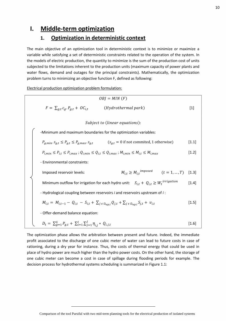
The main objective of an optimization tool in deterministic context is to minimize or maximize a

variable while satisfying a set of deterministic constraints related to the operation of the system. In

the models of electric production, the quantity to minimize is the sum of the production cost of units

subjected to the limitations inherent to the production units (maximum capacity of power plants and

water flows, demand and outages for the principal constraints). Mathematically, the optimization

problem turns to minimizing an objective function F, defined as following:

Electrical production optimization problem formulation:

( )

∑ ( ) [1]

( )

-Minimum and maximum boundaries for the optimization variables:

( ) [1.1]

; ; [1.2]

- Environmental constraints:

Imposed reservoir levels: ( ) [1.3]

Minimum outflow for irrigation for each hydro unit: [1.4]

- Hydrological coupling between reservoirs i and reservoirs upstream of i :

∑ ∑

[1.5]

- Offer-demand balance equation:

∑ ∑ ∑

[1.6]

The optimization phase allows the arbitration between present and future. Indeed, the immediate

profit associated to the discharge of one cubic meter of water can lead to future costs in case of

rationing, during a dry year for instance. Thus, the costs of thermal energy that could be used in

place of hydro power are much higher than the hydro power costs. On the other hand, the storage of

one cubic meter can become a cost in case of spillage during flooding periods for example. The

decision process for hydrothermal systems scheduling is summarized in Figure 1.1:

11

________________________________________


Figure 1.1. Decision process for hydrothermal systems

The output data of the optimization phase is the matrix of the water values of each reservoir:

[

]

A water value is defined as the expected value of the future profit associated with the discharge of

one cubic meter of stored water, and expressed in € /m3. Thus, the matrix of the water values

represents the least-cost strategy of water management in function of the reservoir content and

time.

2. Optimization in stochastic context: stochastic programming

As in deterministic programming, the aim of stochastic programming is to minimize the value of an

objective function (or cost function) while satisfying a number of linear constraints. However,

stochastic programming is a linear optimization technique that takes into account uncertainty

scenarios associated to the behavior of the system. These uncertainties are divided into three

categories. The first one corresponds to the uncertainties on natural phenomenon such as

temperature, hydrology, wind etc. The second category is represented by the mechanical

uncertainties (unavailability of production units, price variability on the markets etc.) and the third

one by the uncertainty concerning the demand. First, this section provides a definition of the state of

a system as a basic knowledge for the understanding of the concept of stochastic dynamic

programming, which is described in the second part of this section.

2.1. Definition of the state of a system.

All the study takes place within a finite and discrete time frame. The dynamics of the system is

described over K stages indexed by k. At stage k, the state of the system is hence characterized by a

state vector , which dimension is equal to X, where X is the number of state variables in the

system. In the optimization problem of a power system at stage k, the state vector is a column

12

________________________________________


composed of the generated power of each thermal power plant and the water content change in

each reservoir . Thus, X, the size of , is equal to (G+I).

[

]

[2.1]

Moreover, the state of the system is dynamically affected by the decision and the stochastic

perturbations at each stage k of the studied period, according to equation [2.2]:

( ) [2.2]i

2.2. Stochastic dynamic programming

It should be kept in mind that the state of the system is consequently dynamically evolving at each

stage k, depending on the perturbations and on the optimization policy. The dynamic programming is

based on the Bellman’s optimality principle, which is the fundament of the graph theory. This

principle stipulates that every sub-decision of an optimal decision is

optimal, for each time index k within . The algorithm of stochastic dynamic programming

that is under focus in this report applies this principle. For each initial state , the optimal cost is

noted ( ). It is possible to calculate this function by following the stages below, which are called

under the name ‘Backward Recursion Algorithm’ in the literature:

- for the initialization, ( ) is arbitrarily defined for the final possible

states for each variable of the system at stage k+1,

- then, for the optimal cumulated costs are calculated according to:

( ) [ ( ) ( ( ))] [3]i

Mathematically, the water values are obtained by taking the derivative of the cumulated cost of the

system according to the water content. Generally speaking, one will optimize the expectation value

of the cumulated cost of the system over the entire set of random realizations of , that is ;

…; ; … ;

, where L is the number of stochastic scenarios in the model. Note that using the

expectation value means that the uncertainty scenarios are considered to have the same outcome

probability. However, more realistic ways of handling the uncertainties are developed in variants of

the stochastic programming.

In the case of a power system, one can assess the instant cost of the system at stage k from the

state variables and :

∑ ∑

[4]i

13

________________________________________


Furthermore, according to the theory of optimization that is developed in Introduction to Linear

Optimization by BERTISMASii, the stochastic linear optimization problem represented by equation [3]

and [4] can be reduced to its standard form for each stage in the following way:

[5]ii

[6]ii

The dimension of the coefficient matrix A is equal to X times the number of constraints in the system.

The dimension of the requirement vector b and of the cost vector c is X as well.

As a result of the optimization phase, the matrix of the water values of each reservoir is calculated.

Then, in the simulation phase, the algorithm simulates the behavior of the system using the water

values as an input data, according to the perturbations that affect the system at each stage.

3. Description of three mid-term planning tools under study

Middle-term optimization tools lying within the scope of this project operate on two successive

phases: the optimization phase and the simulation phase. In the optimization phase the water value

of all stored water is calculated recursively on the studied period thanks to a backward optimization

algorithm. Then in the simulation phase, the water values are used to determine the most cost-

efficient production schedule of the hydrothermal system.

3.1 Parsifal

According to the User Guide of Parsifaliii, the optimizer of Parsifal solves a backward Stochastic

Dynamic Programming algorithm. The term “stochastic” means that Parsifal takes into account

uncertainty related to the demand, to the availability and generation capacity of power plants and to

hydro inflows. For calculation time reasons, Parsifal optimization phase is limited to dimension 2. This

means that maximum two reservoirs can have their water value optimized at the same time. At each

time stage and for each reservoir (1 or 2), the water values are calculated as a function of the first

reservoir content and the second reservoir content (if existing). Parsifal can deal with a two-

dimension optimization problem, namely the water values of one reservoir on one hand depend on

time and on its own storage level and, on the other hand, on the storage level of the other existing

reservoir. This is a fundamental characteristic of the optimization algorithm of Parsifal.

To obtain the valuation of a transition to the next time step, the optimizer solves a linear

deterministic optimization program at a time scale that is inferior to the stage unit and called

"position". In other words, there are several positions within a single stage.

The water values that were computed in the optimization phase are used as input of the simulator.

It simulates the contribution (or dispatch) of each production unit by solving a deterministic Linear

Optimization Program.

Moreover, the generation reserve and the deficit power must be modeled by fictitious thermal units

because Parsifal does not handle reserve and deficit powers. These fictitious units must be set with a

variable cost that is larger than all the other units of the system in order to be dispatched only at last.

14

________________________________________


3.2 Tick-Tack

As Tick-Tack is a tool developed within the OSIRIS department I worked at, the knowledge about this

tool is scattered between the researchers, some internal documents and the C++ computer code of

the tool. From this knowledge is summarized the main features about Tick-Tack. In terms of

optimization, the main difference with Parsifal is that Tick-Tack only does a one-dimension backward

Stochastic Dynamic Programming. This means that the water values of one reservoir only depend on

time and on its own storage level. Moreover, the algorithm carries out the backward optimization at

the hourly scale without performing any deterministic Linear Programming at the scale of a stage.

This is the second major difference. Last but not least, the calculation unit called ‘stage’ is equal to

one hour on Tick-Tack. There is no lower level (such as positions) as in Parsifal. Thus, the optimization

is more powerful but slower on Parsifal.

In the simulation phase, Tick-Tack piles the production means according to its costs considering the

water values of each reservoir.

In terms of hydraulic modeling, Tick-Tack is less detailed than Parsifal. Indeed, Parsifal considers the

hydraulic coupling between units belonging to the same valley, and can even take into account the

delay time of water from a unit to another. Tick-Tack does not take into account the hydrological

coupling at all.

Thus, Tick-Tack has a solver that is lighter and faster than Parsifal. Moreover, there is no limitation in

the number of reservoirs, whereas Parsifal handles only two reservoirs with optimization of the

water values. This limitation is due to the calculation time that increases exponentially with the

complexity of the problem.

The tool Tick-Tack takes into account a number of constraints and parameters in its models:

- The thermal units principal features are: variable cost in €/MWh, minimal and maximal

capacity of the unit (or nominal or installed capacity) in MW;

- The hydro units are represented by a storage reservoir and a generation plant. The reservoir

maximal storage capacity is expressed in hm3 and called “STOCK”. The plant is equipped with

turbines whose generation efficiency coefficient in kWh/m3 depends on the storage level.

Tick-Tack does consider constraints on hydro units such as a maximal capacity droop over

time, an efficiency droop and a variable relationship between storage level and head height.

(See section II.2.1 p.18 for precisions about the head height).

- The so-called “imposed reservoir content” system penalizes a STOCK unit if its storage

trajectory diverges from the targeted level at a given date. An imposed reservoir content can

be a single point at a single stage or a whole curve at each stage of the studied period. The

economical value of this penalty is given by the “toughness” parameter, in €/MWh;

- Tick-Tack takes into account the planned unit unavailability through a chronicle of

unavailability;

- It is also possible to add a random unavailability rate in % of the maximal generation capacity

to each unit. The user sets the mean down time in hours and Tick-Tack random generator

generates a chronicle of unavailability.

Finally, the generation reserve is not modeled in Tick-Tack, like in Parsifal. One must create a

fictitious thermal unit with a high variable cost to ensure that it would be dispatched at last. The

15

________________________________________


deficit power is accounted through its variable cost parameter in €/MWh. The set value must be

greater than all the other variables costs within the system.

3.3 SDDP

The main features of SDDP are summarized from the User Manual of SDDPiv in the following section.

The algorithm SDDP corresponds to a variant of the classical Stochastic Dynamic Programming. Its

approach is based on the analytical representation of the water values, called Stochastic Dual

Dynamic Programming. Its principal advantage is that the computational effort is not increased with

the augmentation of the size of the system. As a result, SDDP is able to deal with a great number

(until 200) of reservoirs with one-dimension optimization. However, the optimization algorithm only

furnishes an approximation of the real water value function. This real function is approached by an

upper and a lower bound that converge after a number of recursions. This parameter can be

modified according to the level of accuracy that is required.

On SDDP, the time scale goes over monthly or weekly bases and the load is exclusively represented

by its load duration curve over 1 to 5 positions (or blocks). The duration of the positions is a variable

parameter.

The tool SDDP takes into account a number of parameters and constraints in its models. It is capable

of representing the electrical transmission network with or without circuit losses, energy transfers on

the abroad markets and also the gas network. In addition, the uncertainty on the demand, the

hydrological inflows and the availability of the units are also considered in the model.

The description of the hydro units comprises several parameters such as the head, the tailwater

elevation, filtration and evaporation coefficients of the lakes. These parameters are filled in the

interface. Two types of hydro unit are available: « Reservoir », a hydro unit with regulation of the

water values over the whole planning period; “Sluiceway”, a unit having a regulation ability that

allows water to be stored only from an off-peak position to a peak position during the same stage.

The thermal system is described in a way similar to Parsifal, with a few differences: the variable cost

of thermal units takes into account the transportation cost of fuels and the Operation and

Maintenance cost as well as the cost of a unit of fuel. SDDP handles plants participating in Combined

Cycle schemes.

On SDDP, the generation reserve is modeled for both hydro and thermal plants. The deficit power is

a specific parameter that can be associated with a financial penalty in €/MWh. Generally speaking, it

is possible to economically penalize (or valorize) the whole set of constraints provided that they are

violated in order to avoid (or foster) precise behaviors of the system (carbon legislation, irrigation,

minimal or maximal storage level, controlled downstream outflow, network stability constraints…).

Furthermore, SDDP is equipped with a constraints generator module that can apply a minimal or a

maximal value to the sum of the generated power of hydro or thermal units. A complete statistics

module is also integrated to SDDP in order to get synthetic statistical data on the hydrological inflow

scenarios. In addition, SDDP includes a generator of random unavailability that neglects the time

correlation between the state of a power unit at t and its state at t+1. Indeed, the Monte-Carlo

algorithm that is used only considers the probability for a power plant to fail but ignores the mean

down timev.

16

________________________________________


II. Study of Island on Tick-Tack

1. Description of the electrical system of Island

Figure 2.1. Hydro production means in Island

Table 2.1. Electrical system of Island

Unit Technology Type (MW) Variable cost (€/MWh)

R.O.R Hydro Run-of -river 0 0

Reservoir Hydro Reservoir 0 0

Biomass Thermal Non-dispatchable 0 0

Diesel Thermal Classical 0,9 Low

Oil1 Thermal Classical 0,2 High

Oil2 Thermal Classical 0,1 Very high

Deficit Fictitious - 0 Extremely high

From an electrical point of view, Island is an isolated energy system, whose consumption is about

100 MW on average. The electrical production system consists exclusively of one system, which is

composed of the following elements:

- a run-of-river turbine (called R.O.R) that is located upstream of Reservoir and that turbines the

totality of the hydrological inflows;

- a storage reservoir, Reservoir, with a very high capacity;

- the generation station equipped with 4 turbines (G1 to G4), located downstream of the reservoir;

17

________________________________________


- an additional fictitious turbine is added to model the hydro primary reserve. Indeed, Parsifal does

not take the primary reserve into account in its model.

The thermal system is based on four groups presented according to increasing operation cost:

Biomass, Diesel, Oil1, Oil2. The Biomass thermal unit is represented as a “non-dispatchable” unit

because of its null variable cost and its low generation capacity. Indeed, this plant is going to produce

permanently its installed capacity. In addition, a seventh unit represents the deficit power (power

not served).

2. Study of the parameter « HeadEffectInOptimization » on

Tick-Tack

In the model of Tick-Tack, a Boolean parameter allows the head effect to be considered or not in the

optimization phase. It was necessary to test both possibilities of considering this parameter and

compare them to the results given by Parsifal in order to determine how Parsifal handles this

parameter in its own model. Indeed, there was no indication in the user guide of Parsifal about the

way the head effect was taken into account.

2.1 Description of the problem

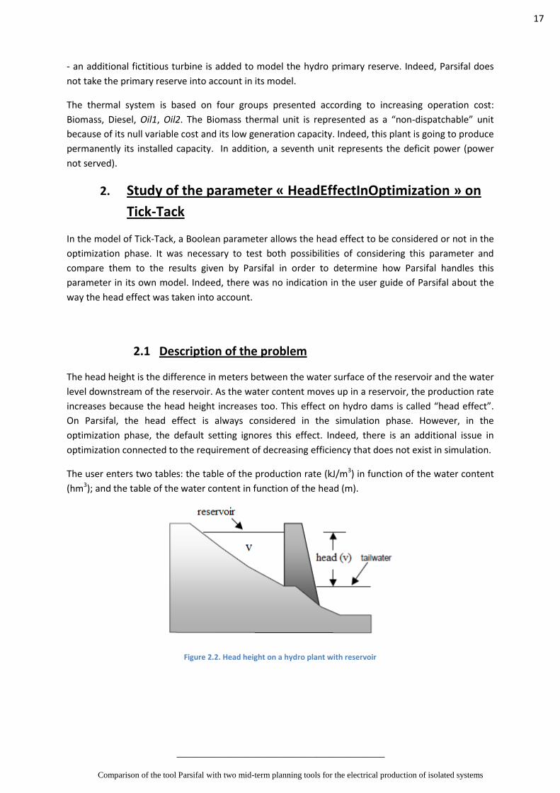
The head height is the difference in meters between the water surface of the reservoir and the water

level downstream of the reservoir. As the water content moves up in a reservoir, the production rate

increases because the head height increases too. This effect on hydro dams is called “head effect”.

On Parsifal, the head effect is always considered in the simulation phase. However, in the

optimization phase, the default setting ignores this effect. Indeed, there is an additional issue in

optimization connected to the requirement of decreasing efficiency that does not exist in simulation.

The user enters two tables: the table of the production rate (kJ/m3) in function of the water content

(hm3); and the table of the water content in function of the head (m).

Figure 2.2. Head height on a hydro plant with reservoir

18

________________________________________


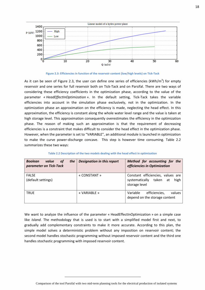
Figure 2.3: Efficiencies in function of the reservoir content (low/high levels) on Tick-Tack

As it can be seen of Figure 2.3, the user can define one series of efficiencies (kWh/m3) for empty

reservoir and one series for full reservoir both on Tick-Tack and on Parsifal. There are two ways of

considering these efficiency coefficients in the optimization phase, according to the value of the

parameter « HeadEffectInOptimization ». In the default setting, Tick-Tack takes the variable

efficiencies into account in the simulation phase exclusively, not in the optimization. In the

optimization phase an approximation on the efficiency is made, neglecting the head effect. In this

approximation, the efficiency is constant along the whole water level range and the value is taken at

high storage level. This approximation consequently overestimates the efficiency in the optimization

phase. The reason of making such an approximation is that the requirement of decreasing

efficiencies is a constraint that makes difficult to consider the head effect in the optimization phase.

However, when the parameter is set to “VARIABLE”, an additional module is launched in optimization

to make the curve power-discharge concave. This step is however time consuming. Table 2.2

summarizes these two ways:

Table 2.2 Description of the two models dealing with the head effect in optimization

Boolean value of the parameter on Tick-Tack

Designation in this report Method for accounting for the efficiencies in Optimization

FALSE (default settings)

« CONSTANT » Constant efficiencies, values are systematically taken at high storage level

TRUE « VARIABLE » Variable efficiencies, values depend on the storage content

We want to analyze the influence of the parameter « HeadEffectInOptimization » on a simple case

like Island. The methodology that is used is to start with a simplified model first and next, to

gradually add complementary constraints to make it more accurate. According to this plan, the

simple model solves a deterministic problem without any imposition on reservoir content; the

second model handles stochastic programming without imposed reservoir content and the third one

handles stochastic programming with imposed reservoir content.

19

________________________________________


2.2 Deterministic model, without imposed reservoir content

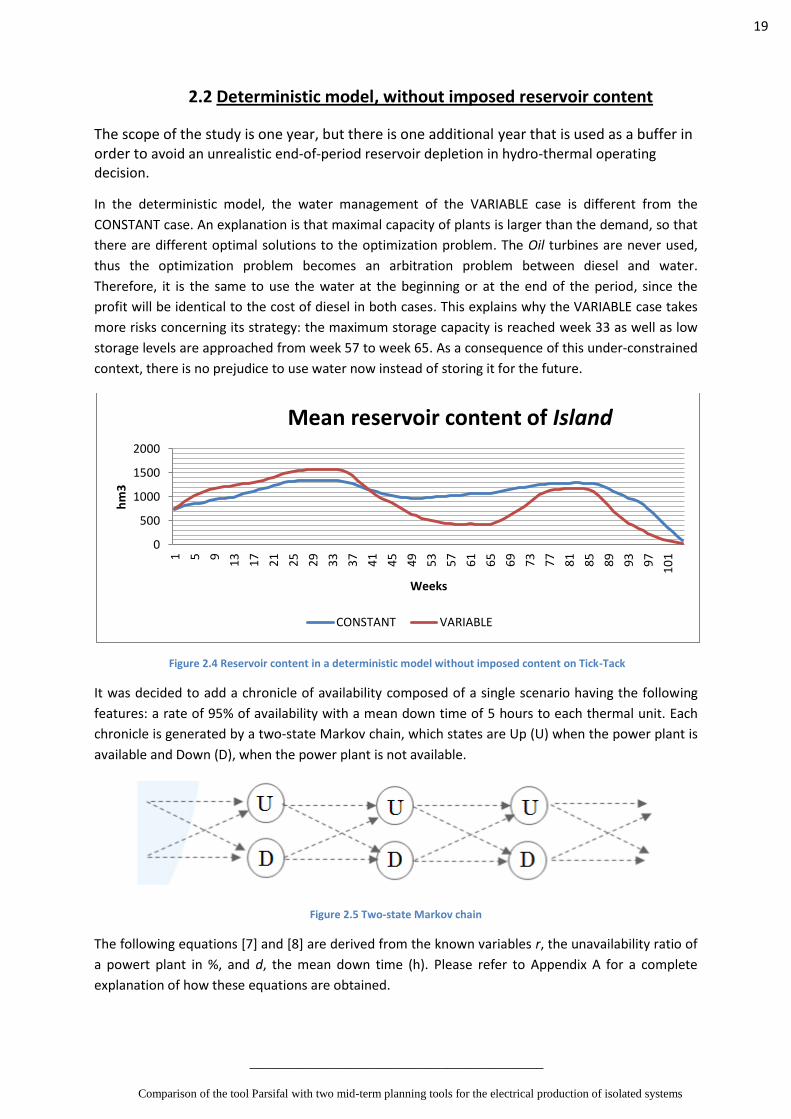
The scope of the study is one year, but there is one additional year that is used as a buffer in order to avoid an unrealistic end-of-period reservoir depletion in hydro-thermal operating decision.

In the deterministic model, the water management of the VARIABLE case is different from the

CONSTANT case. An explanation is that maximal capacity of plants is larger than the demand, so that

there are different optimal solutions to the optimization problem. The Oil turbines are never used,

thus the optimization problem becomes an arbitration problem between diesel and water.

Therefore, it is the same to use the water at the beginning or at the end of the period, since the

profit will be identical to the cost of diesel in both cases. This explains why the VARIABLE case takes

more risks concerning its strategy: the maximum storage capacity is reached week 33 as well as low

storage levels are approached from week 57 to week 65. As a consequence of this under-constrained

context, there is no prejudice to use water now instead of storing it for the future.

Figure 2.4 Reservoir content in a deterministic model without imposed content on Tick-Tack

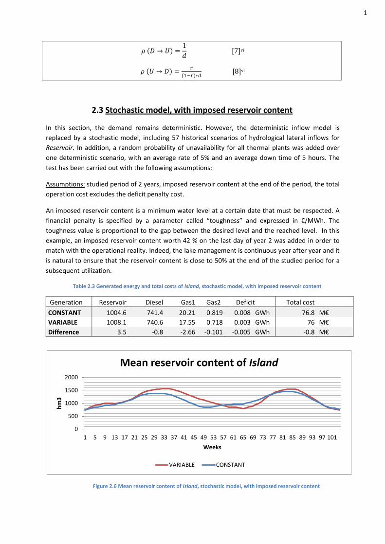
It was decided to add a chronicle of availability composed of a single scenario having the following

features: a rate of 95% of availability with a mean down time of 5 hours to each thermal unit. Each

chronicle is generated by a two-state Markov chain, which states are Up (U) when the power plant is

available and Down (D), when the power plant is not available.

Figure 2.5 Two-state Markov chain

The following equations [7] and [8] are derived from the known variables r, the unavailability ratio of

a powert plant in %, and d, the mean down time (h). Please refer to Appendix A for a complete

explanation of how these equations are obtained.

0

500

1000

1500

2000

1 5 9

13

17

21

25

29

33

37

41

45

49

53

57

61

65

69

73

77

81

85

89

93

97

10

1

hm

3

Weeks

Mean reservoir content of Island

CONSTANT VARIABLE

1

( )

vi

( )

( ) [8]vi

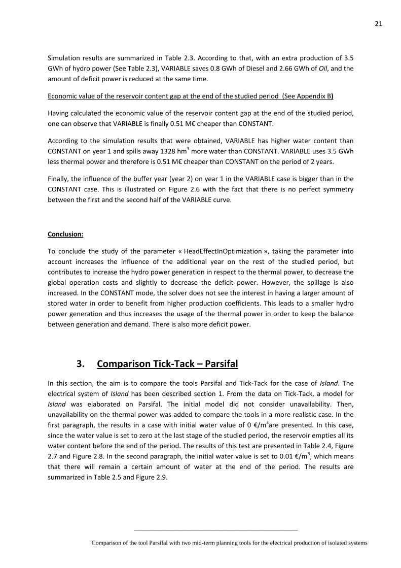
2.3 Stochastic model, with imposed reservoir content

In this section, the demand remains deterministic. However, the deterministic inflow model is

replaced by a stochastic model, including 57 historical scenarios of hydrological lateral inflows for

Reservoir. In addition, a random probability of unavailability for all thermal plants was added over

one deterministic scenario, with an average rate of 5% and an average down time of 5 hours. The

test has been carried out with the following assumptions:

Assumptions: studied period of 2 years, imposed reservoir content at the end of the period, the total

operation cost excludes the deficit penalty cost.

An imposed reservoir content is a minimum water level at a certain date that must be respected. A

financial penalty is specified by a parameter called “toughness” and expressed in €/MWh. The

toughness value is proportional to the gap between the desired level and the reached level. In this

example, an imposed reservoir content worth 42 % on the last day of year 2 was added in order to

match with the operational reality. Indeed, the lake management is continuous year after year and it

is natural to ensure that the reservoir content is close to 50% at the end of the studied period for a

subsequent utilization.

Table 2.3 Generated energy and total costs of Island, stochastic model, with imposed reservoir content

Generation Reservoir Diesel Gas1 Gas2 Deficit

Total cost

CONSTANT 1004.6 741.4 20.21 0.819 0.008 GWh 76.8 M€

VARIABLE 1008.1 740.6 17.55 0.718 0.003 GWh 76 M€

Difference 3.5 -0.8 -2.66 -0.101 -0.005 GWh -0.8 M€

Figure 2.6 Mean reservoir content of Island, stochastic model, with imposed reservoir content

0

500

1000

1500

2000

1 5 9 13 17 21 25 29 33 37 41 45 49 53 57 61 65 69 73 77 81 85 89 93 97 101

hm

3

Weeks


VARIABLE CONSTANT

21

____________________________________________


Simulation results are summarized in Table 2.3. According to that, with an extra production of 3.5

GWh of hydro power (See Table 2.3), VARIABLE saves 0.8 GWh of Diesel and 2.66 GWh of Oil, and the

amount of deficit power is reduced at the same time.

Economic value of the reservoir content gap at the end of the studied period (See Appendix B)

Having calculated the economic value of the reservoir content gap at the end of the studied period,

one can observe that VARIABLE is finally 0.51 M€ cheaper than CONSTANT.

According to the simulation results that were obtained, VARIABLE has higher water content than

CONSTANT on year 1 and spills away 1328 hm3 more water than CONSTANT. VARIABLE uses 3.5 GWh

less thermal power and therefore is 0.51 M€ cheaper than CONSTANT on the period of 2 years.

Finally, the influence of the buffer year (year 2) on year 1 in the VARIABLE case is bigger than in the

CONSTANT case. This is illustrated on Figure 2.6 with the fact that there is no perfect symmetry

between the first and the second half of the VARIABLE curve.

Conclusion:

To conclude the study of the parameter « HeadEffectInOptimization », taking the parameter into

account increases the influence of the additional year on the rest of the studied period, but

contributes to increase the hydro power generation in respect to the thermal power, to decrease the

global operation costs and slightly to decrease the deficit power. However, the spillage is also

increased. In the CONSTANT mode, the solver does not see the interest in having a larger amount of

stored water in order to benefit from higher production coefficients. This leads to a smaller hydro

power generation and thus increases the usage of the thermal power in order to keep the balance

between generation and demand. There is also more deficit power.

3. Comparison Tick-Tack – Parsifal

In this section, the aim is to compare the tools Parsifal and Tick-Tack for the case of Island. The

electrical system of Island has been described section 1. From the data on Tick-Tack, a model for

Island was elaborated on Parsifal. The initial model did not consider unavailability. Then,

unavailability on the thermal power was added to compare the tools in a more realistic case. In the

first paragraph, the results in a case with initial water value of 0 €/m3are presented. In this case,

since the water value is set to zero at the last stage of the studied period, the reservoir empties all its

water content before the end of the period. The results of this test are presented in Table 2.4, Figure

2.7 and Figure 2.8. In the second paragraph, the initial water value is set to 0.01 €/m3, which means

that there will remain a certain amount of water at the end of the period. The results are

summarized in Table 2.5 and Figure 2.9.

22

____________________________________________


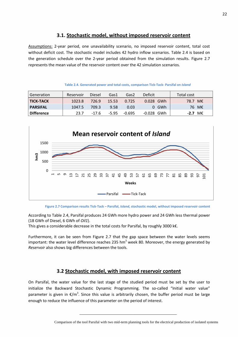
3.1. Stochastic model, without imposed reservoir content

Assumptions: 2-year period, one unavailability scenario, no imposed reservoir content, total cost

without deficit cost. The stochastic model includes 42 hydro inflow scenarios. Table 2.4 is based on

the generation schedule over the 2-year period obtained from the simulation results. Figure 2.7

represents the mean value of the reservoir content over the 42 simulation scenarios.

Table 2.4. Generated power and total costs, comparison Tick-Tack- Parsifal on Island

Generation Reservoir Diesel Gas1 Gas2 Deficit Total cost

TICK-TACK 1023.8 726.9 15.53 0.725 0.028 GWh 78.7 M€

PARSIFAL 1047.5 709.3 9.58 0.03 0 GWh 76 M€

Difference 23.7 -17.6 -5.95 -0.695 -0.028 GWh -2.7 M€

Figure 2.7 Comparison results Tick-Tack – Parsifal, Island, stochastic model, without imposed reservoir content

According to Table 2.4, Parsifal produces 24 GWh more hydro power and 24 GWh less thermal power (18 GWh of Diesel, 6 GWh of Oil1). This gives a considerable decrease in the total costs for Parsifal, by roughly 3000 k€. Furthermore, it can be seen from Figure 2.7 that the gap space between the water levels seems important: the water level difference reaches 235 hm3 week 80. Moreover, the energy generated by Reservoir also shows big differences between the tools.

3.2 Stochastic model, with imposed reservoir content

On Parsifal, the water value for the last stage of the studied period must be set by the user to

initialize the Backward Stochastic Dynamic Programming. The so-called “Initial water value”

parameter is given in €/m3. Since this value is arbitrarily chosen, the buffer period must be large

enough to reduce the influence of this parameter on the period of interest.

0

500

1000

1500

1 5 9

13

17

21

25

29

33

37

41

45

49

53

57

61

65

69

73

77

81

85

89

93

97

10

1

hm

3

Weeks


Parsifal Tick-Tack

23

____________________________________________


The value of 0 €/m3 chosen previously had been calculated according to the following formula, taken

from the User Guide of Parsifal: it is the product of the lowest thermal cost by the sum of all

efficiencies of the turbines within a same valley.

€

€ [9]ii

Through this constraint, an effect similar to Tick-Tack with imposed reservoir content is obtained.

Indeed, giving a strictly positive value to the water at the end of the studied period contributes to

obtain a final reservoir content that is strictly positive.

However, there is a need to have a sufficient water level at the end of the studied period, that is why

the initial water value was set to the value of 0.01€ , which gives a final reservoir content of

approximately 60 % of the total capacity of the lake. Then, this final level value was reported as an

imposed reservoir content on Tick-Tack in order to reach the same level at the end of the studied

period for both tools. The final water levels are actually very close: . The economic

value of this small water level gap is negligible compared to the total cost difference. This assertion is

illustrated by the Table 2.5.

Assumptions: 2-year period, one unavailability scenario, imposed reservoir content, total cost

without deficit cost. The stochastic model includes 42 hydro inflow scenarios. Table 2.5 is based on

the generation schedule over the 2-year period obtained from the simulation results. Figure 2.9

represents the mean value of the reservoir content over the 42 simulation scenarios.

Table 2.5. Generated power and total costs, comparison Tick-Tack- Parsifal on Island

Generation Reservoir Diesel Gas1 Gas2 Deficit Total cost

TICK-TACK 990.4 751.7 24 0.988 0.006 GWh 78.7 M€

PARSIFAL 995.6 761.6 9.15 0.037 0 GWh 76 M€

Difference 5.2 9.9 -14.85 -0.951 -0.006 GWh -2.7 M€

24

____________________________________________


Figure 2.8 Comparison results Tick-Tack – Parsifal, Island, stochastic model with imposed reservoir content

Figure 2.9 shows that the water levels through the weeks are significantly closer than in the previous

case.

On one hand, Tick-Tack spills away 74 hm3 more water compared to Parsifal. The energy associated

to the 74-hm3 spillage difference corresponds to 5.5 GWh approximately.

On the other hand, at the end of the period, that is on the last day, the reservoir content of Tick-Tack

is 28 hm3 higher than Parsifal. The energy associated to the 28-hm3 final amount of water content

difference corresponds to 1.5 GWh.

In total, Tick-Tack should generate 5.5 + 1.5 = 7 GWh less hydro power than Parsifal, due to spilled

water and final stored water. However, Tick-Tack benefits from higher values of the efficiency

because of a higher water level. This phenomenon is called head height effect and gives that the

generation efficiency of the turbines increases with the head height. As a result, the hydro energy

difference is only 5 GWh, as Table 2.4 shows. So the increase in efficiency contributes to an

additional hydro power of 2 GWh on Tick-Tack.

More globally, 5 GWh of hydro power and 10 GWh of Diesel on Parsifal replaces 15 GWh of Oil1 on

Tick-Tack. This allows Parsifal save 2.28 M€ after calculating the economical value of the storage

content differences.

Conclusion :

The energy generated by Reservoir over time is similar between the tools, but that is not exactly

identical. The generation of Oil1 is 15 GWh larger on Tick-Tack (essentially concentrated at the end of

the buffer year), so the operation costs are increased by 2.28 M€. Although this difference is not

negligible, Tick-Tack is capable of giving a precise idea of the evolution of the water level and of the

generated energy over the studied period. Tick-Tack also furnishes an estimation of the costs that is

similar to Parsifal, in the case of Island.

0

500

1000

1500

20001 5 9

13

17

21

25

29

33

37

41

45

49

53

57

61

65

69

73

77

81

85

89

93

97

10

1

hm

3

Weeks


TT Defaut Jal AN 2 comme Parsi 0,01 Parsi VMS 0,01Tick-Tack Parsifal

25

____________________________________________


To go further in a future work, it could be interesting to add several chronicles of unavailability. Then,

one would have to determine if the spillage is concentrated on one specific scenario with a small

probability to happen or if the difference would stem globally from all scenarios. This would provide

useful information for the management policy of Reservoir’s reservoir content.

26

____________________________________________


III. Study of Land on Tick-Tack

INTRODUCTION:

The aim of this study is to determine if Tick-Tack is capable of providing consistent results concerning

the optimization of the production capacities of Land. To do that, the simulation results obtained with

Parsifal are taken as reference because this tool has a smarter solver, which is consequently slower.

Since Tick-Tack is faster, it seems interesting to run Tick-Tack every month whereas Parsifal is yearly run.

This would give an estimation of the seasonal variations of the costs, of the fuel supply of the thermal

units and of the reservoir content of the lakes, with a view to the budget and purchase projections and

the management of the constraints on reservoir contents.

27

____________________________________________


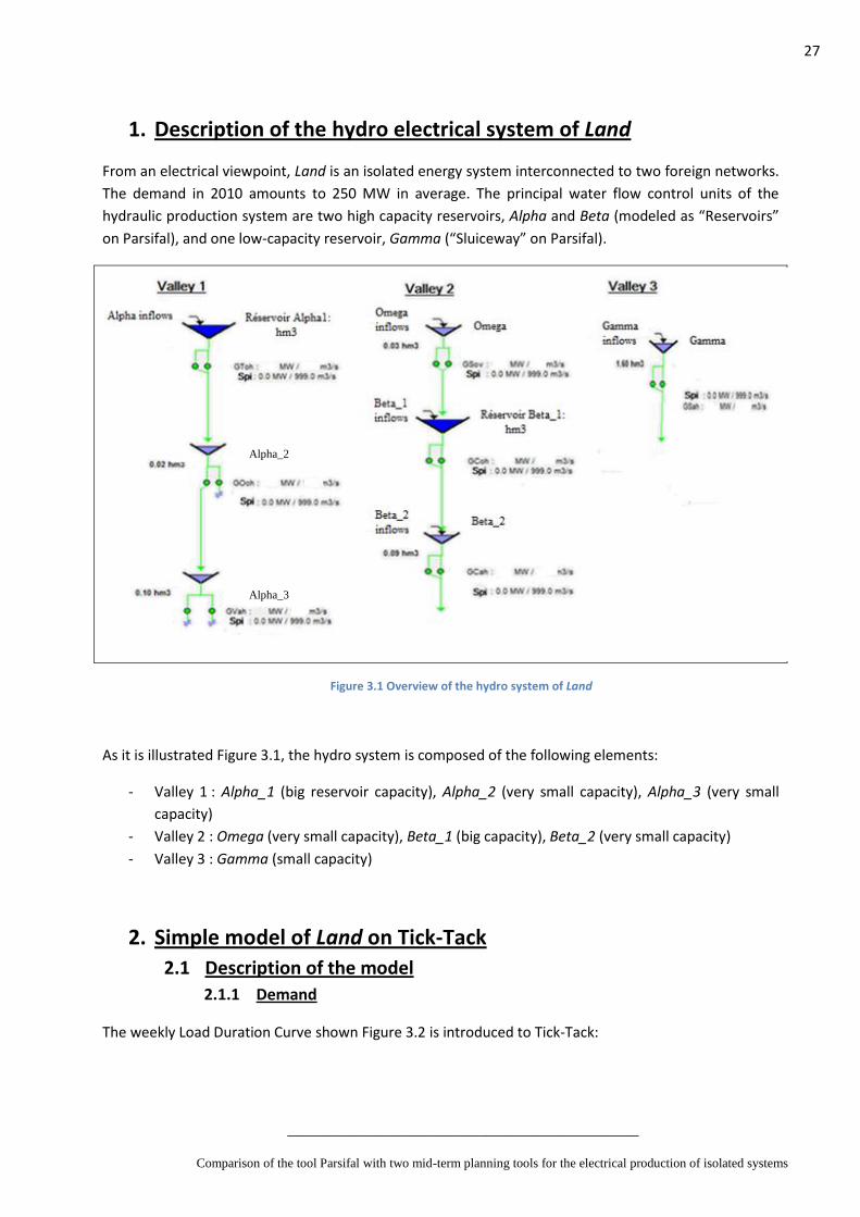
1. Description of the hydro electrical system of Land

From an electrical viewpoint, Land is an isolated energy system interconnected to two foreign networks.

The demand in 2010 amounts to 250 MW in average. The principal water flow control units of the

hydraulic production system are two high capacity reservoirs, Alpha and Beta (modeled as “Reservoirs”

on Parsifal), and one low-capacity reservoir, Gamma (“Sluiceway” on Parsifal).

Figure 3.1 Overview of the hydro system of Land

As it is illustrated Figure 3.1, the hydro system is composed of the following elements:

- Valley 1 : Alpha_1 (big reservoir capacity), Alpha_2 (very small capacity), Alpha_3 (very small

capacity)

- Valley 2 : Omega (very small capacity), Beta_1 (big capacity), Beta_2 (very small capacity)

- Valley 3 : Gamma (small capacity)

2. Simple model of Land on Tick-Tack

2.1 Description of the model

2.1.1 Demand

The weekly Load Duration Curve shown Figure 3.2 is introduced to Tick-Tack:

Alpha_2

Alpha_3

28

____________________________________________


Figure 3.2 Weekly Load Duration Curve of Land

According to Figure 3.2, the load is decreasing over one week. The 7 positions are distributed over the 168

hours in one week according to Table 3.0:

Table 3.0 Positions repartition over one week

Number of the position Position Duration (hours)

1 Extreme peak hours 3

2 Peak hours 10

3, 4, 5, 6 Four intermediate load levels 33 – 33 – 33 – 33

7 Off-peak hours 26

0

100000

200000

300000

400000

500000

6000001

26

6

53

1

79

6

10

61

13

26

15

91

18

56

21

21

23

86

26

51

29

16

31

81

34

46

37

11

39

76

42

41

45

06

47

71

50

36

53

01

55

66

58

31

60

96

63

61

66

26

68

91

71

56

74

21

76

86

79

51

82

16

84

81

Demand 2010 (kW)

Demande Tick-Tack Time (hours) Tick-Tack demand

P (kW)

200

300

400

500

1 6

11

16

21

26

31

36

41

46

51

56

61

66

71

76

81

86

91

96

10

1

10

6

11

1

11

6

12

1

12

6

13

1

13

6

14

1

14

6

15

1

15

6

16

1

16

6

Decreasing LDC over 1 week

Semaine1

P (MW)

Week 1 Time (hours)

29

____________________________________________


2.1.2 Hydraulic model

To model the hydraulic system of Land on Tick-Tack, the following assumptions were made:

- The six low capacity reservoirs are neglected. Only the reservoirs with a significant capacity are

considered: Alpha_1, Beta_1 and Gamma. The two-dimension optimization policy in Parsifal is

calculated for the reservoirs Alpha and Beta only.

- Valley 1: according to the coupling effect between units which belong to the same valley, the water

in the upper reservoir is generated with the efficiency of that unit and with the efficiency of all units

that are located downstream. Consequently, the efficiency of the equivalent unit of units Alpha_1,

Alpha_2 and Alpha_3 laid in series in Valley 1 is calculated by the sum of their respective efficiency.

The power-discharge characteristic curve of Alpha_Equivalent comes consequently from the sum of

the P-Q curves of Alpha_1, Alpha_2 and Alpha_3:

[10]

On should note that the production efficiency coefficients depend on the reservoir content. Both

Tick-Tack and Parsifal can be set with two series of coefficients: one at empty reservoir storage, and

the other one at full storage.

Figure 3.3 Aggregation of the power-discharge curves within Valley 1

Po

wer

(M

W)

Discharge m3/s

Valley 1 _ EMPTY

TOLLA OCANA Pont-Vanna

Po

wer

(M

W)

Discharge m3/s

Valley 1 _FULL

TOLLA OCANA Pont-Vanna

Po

wer

(M

W)

Discharge m3/s

Alpha_EQ_EMPTY

Po

wer

(M

W)

Discharge m3/s

Alpha_EQ_FULL

30

____________________________________________


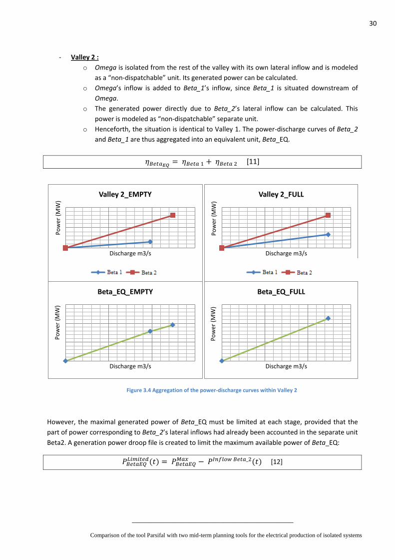
- Valley 2 :

o Omega is isolated from the rest of the valley with its own lateral inflow and is modeled

as a “non-dispatchable” unit. Its generated power can be calculated.

o Omega’s inflow is added to Beta_1’s inflow, since Beta_1 is situated downstream of

Omega.

o The generated power directly due to Beta_2’s lateral inflow can be calculated. This

power is modeled as “non-dispatchable” separate unit.

o Henceforth, the situation is identical to Valley 1. The power-discharge curves of Beta_2

and Beta_1 are thus aggregated into an equivalent unit, Beta_EQ.

[11]

Figure 3.4 Aggregation of the power-discharge curves within Valley 2

However, the maximal generated power of Beta_EQ must be limited at each stage, provided that the

part of power corresponding to Beta_2’s lateral inflows had already been accounted in the separate unit

Beta2. A generation power droop file is created to limit the maximum available power of Beta_EQ:

( )

( ) [12]

Po

wer

(M

W)

Discharge m3/s

Valley 2_EMPTY

CALA CORSCIA

Po

wer

(M

W)

Discharge m3/s

Valley 2_FULL

CALA CORSCIA

Po

wer

(M

W)

Discharge m3/s

Beta_EQ_EMPTY

Po

wer

(M

W)

Discharge m3/s

Beta_EQ_FULL

31

____________________________________________


As it is impossible to enter two different droop files (one for empty reservoir and one for full storage),

the maximum efficiency was used for the calculation of , that is efficiency at full storage.

Figure 3.5 Aggregated overview of Land’s hydro system

Consequently, the hydraulic system is represented as follows on Tick-Tack:

Table 3.1 Hydraulic system of Land on Tick-Tack

Unit Technology Type Cost

€/MWh Inflows

Alpha_EQ (Valley 1) Hydro Reservoir 0 Alpha

Omega Hydro Non-dispatchable 0 Omega

Beta_EQ Hydro Reservoir 0 Omega + Beta1

Beta_2 Hydro Non-dispatchable 0 Beta2

Gamma (Valley 3) Hydro Reservoir 0 Gamma

2.1.3 Thermal model

As Land imports power from abroad, the interconnection lines are modeled in the system. In order to

match to the reference data set in Parsifal the interconnection lines from Land to abroad called INTERCO

are modeled as a single fictive thermal unit. Its cost in €/MWh is also a fictive data. It is set to model the

fact that usually, the interconnection units produce their maximal capacity, that is to say the high

voltage lines are not oversized for power transmission. Consequently, the variable cost must be low, in

order for the fictive unit INTERCO to be used permanently as base power.

32

____________________________________________


Moreover, there are also 3 standard thermal units represented as « CLASSICAL » on Tick-Tack. Two of

them are run of Diesel (Diesel1 and Diesel2) and one is run of Oil. The deficit power is modeled as a

fictitious unit having a variable cost superior to all the other units’ cost.

The thermal units belonging to the system of Land are presented in Table 3.2.

Table 3.2 Thermal system of Land on Tick-Tack

THERMAL Unit Technology Type Variable cost (€/MWh)

Interco Thermal Classical Low

Diesel1 Thermal Classical Intermediate-low

Diesel2 Thermal Classical Intermediate-high

Oil Thermal Classical High

Deficit Fictitious - Extremely high

2.1.4 Study parameters of the simple model of Land

The simple model of Land includes the following parameters and constraints: the stochastic hydrological inflows comprise 57 scenarios. This is illustrated with the hydro inflow series of Alpha in Figure 3.5.1.

Figure 3.5.1 Hydro inflow scenarios of reservoir Alpha

0

10

20

30

40

50

1 3 5 7 9 11 13 15 17 19 21 23 25 27 29 31 33 35 37 39 41 43 45 47 49 51

m3

/s

Weeks

Hydro inflow scenarios of reservoir Alpha

Series1 Series2 Series3 Series4 Series5 Series6Series7 Series8 Series9 Series10 Series11 Series12Series13 Series14 Series15 Series16 Series17 Series18Series19 Series20 Series21 Series22 Series23 Series24Series25 Series26 Series27 Series28 Series29 Series30Series31 Series32 Series33 Series34 Series35 Series36Series37 Series38 Series39 Series40 Series41 Series42Series43 Series44 Series45 Series46 Series47 Series48Series49 Series50 Series51 Series52 Series53 Series54Series55 Series56 Series57

33

____________________________________________


However, the demand is deterministic, in other words there is only one scenario for the demand. See paragraph 2.1.1 of this section. Both reservoirs Alpha and Beta have an imposed reservoir level at the end of the planning period for operational reasons. The value of the imposed level is identical to the initial level at the beginning of the period. In the following paragraph the results that were obtained according to the simple model of Land are presented. A weekly analysis is shown in a first part, and gives qualitative results about the behavior of the system. In a second part, a deeper analysis is exposed, based on the results per position.

2.2 Analysis of the simulation results

2.2.1 Qualitative analysis

Based on the simple model of Land, the qualitative analysis gives general tendencies of the behavior of

the system, such as the cumulated generated energy of each power plant over the planning period, the

total cost over the period or the mean value among the 57 scenarios of the water content in the

reservoirs.

In the results of Table 3.3, the last column shows the generation difference between Tick-Tack and

Parsifal for each unit. One can see that the hydro system of Tick-Tack produces 1 GWh less power and

the thermal power 1 GWh more.

Table 3.3 : Generated power

Mean energy over the studied period

GWh Tick-Tack Parsifal Δ generation (Tick-Tack - Parsifal)

Interco 1109.5 1115.8 -6.3 GWh

Diesel1 294.6 293.6 1 GWh

Diesel2 206.3 198.9 7.4 GWh

Oil 6.5 7.6 -1.1 GWh

TOT THERMAL POWER 1616.9 1615.9 1 GWh

Valley 1 185 186.4 -1.4 GWh

Valley 2 310.1 308.6 1.5 GWh

Valley 3 91.9 93.1 -1.1 GWh

TOT HYDRO POWER 587 588 -1 GWh

Deficit 0 0 0 GWh

TOTAL 2203.9 2203.9 0 GWh

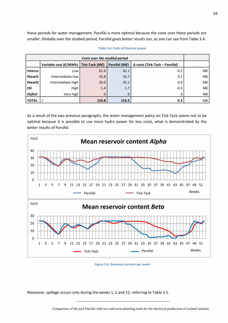
According to Table 3.4, the costs difference over the studied period amounts to 0.3 M€ over 124.5 M€ in

total. This is principally due to a difference in the utilization of the units INTERCO and Diesel2.

In addition, between Tick-Tack and Parsifal, the reservoir content trajectories are divergent over 2

periods: weeks 10 to 22 and weeks 27 to 43, according to Figure3.6. It is necessary to calculate the

economical value of the reservoir content gaps, Tick-Tack turns approximately 166 k€ more expensive

over the first period and 135 k€ over the second one. Thus, the tools give 2 different solutions over

34

____________________________________________


these periods for water management. Parsifal is more optimal because the costs over these periods are

smaller. Globally over the studied period, Parsifal gives better results too, as one can see from Table 3.4.

Table 3.4: Costs of thermal power

Costs over the studied period

Variable cost (€/MWh) Tick-Tack (M€) Parsifal (M€) Δ costs (Tick-Tack – Parsifal)

Interco Low 61.6 62.1 -0.5 M€

Diesel1 Intermediate-low 35.8 35.7 0.1 M€

Diesel2 Intermediate-high 26.0 25.1 0.9 M€

Oil High 1.4 1.7 -0.3 M€

Deficit Very high 0 0 0 M€

TOTAL / 124.8 124.5 0.3 M€

As a result of the two previous paragraphs, the water management policy on Tick-Tack seems not to be

optimal because it is possible to use more hydro power for less costs, what is demonstrated by the

better results of Parsifal.

Figure 3.6: Reservoir content per week

Moreover, spillage occurs only during the weeks 1, 2 and 52, referring to Table 3.5.

0

10

20

30

40

1 3 5 7 9 11 13 15 17 19 21 23 25 27 29 31 33 35 37 39 41 43 45 47 49 51

Mean reservoir content Alpha

Toll en fin de pas (hm3): TOLLA_H (Tick-Tack) Weeks Tick-Tack Parsifal

hm3

0

10

20

30

1 3 5 7 9 11 13 15 17 19 21 23 25 27 29 31 33 35 37 39 41 43 45 47 49 51

Mean reservoir content Beta

CALACUCCIA_H (Tick-Tack) Cala en fin de pas (hm3): Weeks Tick-Tack Parsifal

hm3

35

____________________________________________


Table 3.5. Total spillage

Total spillage Tick-Tack Parsifal

Alpha 36.288 hm3 34.872 hm3

Beta 20.496 hm3 12.276 hm3

This can be interpreted as a problem of toughness in the definition of imposed reservoir levels at the

beginning and at end of the period. The toughness that was used was worth 400 000 €/MWh, which was

probably far too much compared to the thermal costs. This may have contributed to increase

significantly the amount of spillage water during the first and the last weeks because of the “tough”

penalty.

2.2.2 Quantitative analysis

In the quantitative analysis, the periods that show major differences between Tick-Tack and Parsifal in

terms of energy generation are put under closer study. The periods that are not mentioned show only

small gaps and are excluded from the quantitative analysis. As a result, weeks 10, 11, 19, 20 and 27 to

33 have been chosen for the quantitative analysis.

Production results during weeks 10 and 11.

During weeks 10 and 11, the Oil turbines of Tick-Tack produces less than Parsifal.

Table 3.6. : Hydro power utilization rate week 10 and week 11 position 1

Week Position Tick-Tack Parsifal

Utilization Alpha_EQ

Utilization Beta_EQ

Utilization Alpha Utilization Beta

PTick-Tack - PParsifal

10 1 99 % 98 % 99 % 99 % 41 MW

10 2 99 % 98 % 99 % 99 % 32 MW

10 3 99 % 98 % 99 % 99 % 20 MW

10 4 99 % 98 % 99 % 99 % 0 MW

10 5 99 % 98 % 99 % 99 % - 9 MW

10 6 99 % 98 % 99 % 99 % - 19 MW

10 7 47.6 % 98 % 99 % 78.6 % - 22 MW

11 1 99 % 98 % 99 % 99 % 28 MW

The demand during these 2 weeks of March is close to the maximal demand of 2010 (See Figure 3.2). The hydro units together with the base thermal units are not sufficient to meet the demand so that the expensive Oil turbines become necessary to use. That is why Alpha and Beta produce their maximal power both on Tick-Tack and Parsifal during the positions 1 to 6, although Alpha is more expensive on Tick-Tack, considering the merit order for Tick-Tack .

At the positions 1 to 6, Tick-Tack and Parsifal actually see a different available hydro power. Indeed, the water management of Gamma is different in the tools because Gamma is modeled in different ways: Gamma is a sluiceway with no regulation on Parsifal and it is a reservoir with regulation of the water

36

____________________________________________


values on Tick-Tack. On Parsifal, a sluiceway is managed at the weekly scale whereas a reservoir is regulated at the scale of the entire period on Tick-Tack.

Week 10, position 1 (same observations for all positions until the 6-th position)

Position 1, Tick-Tack sees an available hydro power that is 41 MW bigger than Parsifal. This is due to the difference of models for Gamma, like previously. According to the results, Gamma produces 45 MW more on Tick-Tack than on Parsifal. This leads to a 45 MW-decrease in the production of the most expensive unit: the Oil unit.

Indeed, on Parsifal, the sluiceways are small-capacity reservoirs managed at the scale of a week with a specific filling constraint. The way the model for sluiceways is implemented in Parsifal obliges the sluiceways to be empty at the end of each week. This does not leave enough water to meet the high load at the beginning of the following week. For this reason we can observe an increasing gap between Gamma’s generation and the demand. In order to be consistent between the tools, we should have chosen an increasing load duration curve on Parsifal. In addition, on Tick-Tack, Gamma is modeled as a water-regulated unit with optimization of the water value, which is inexistent on Parsifal.

Week 10, position 7 :

According to the results, Alpha produces 22 MW less power on Tick-Tack than on Parsifal because Diesel1 turns cheaper than the merit order cost of the water stored in reservoir Alpha. Diesel1 has thus to produce the missing 22 MW.

Moreover, one can wonder why the utilization rate of Beta on Parsifal is not 99% but 78.6 % at position 7. At this time, the load is at low level and the reservoir in Beta_2 is full. Considering that Beta_2’s inflows are 2.65 m3/s, the maximal water flow that Beta_2 can handle without spilling any water away is: 12.4 – 2.65 = 9.75 m3/s that is precisely 78.6% of the maximum outflow capacity. Consequently for an optimal management, such a reduction is necessary in order not to spill away water at Beta_2 that had been discharged upstream.

Week 11, position 1

According to the results for week 11, the hydro production gap essentially comes from a higher usage of Gamma on Tick-Tack (+ 35 MW) due to the different models chosen for this unit that is a sluiceway on Parsifal and a regulated reservoir on Tick-Tack.

Production results during week 19.

According to the results for week 19, INTERCO produces less on Tick-Tack than on Parsifal during week 19.

Peak hours :

During the first three positions, Parsifal and Tick-Tack produce roughly the same at any time. The order cost of Beta is situated in the same cost section in both Parsifal and Tick-Tack. Another observation drawn from the simulation results is that the cost of Alpha is smaller than the cost of INTERCO in Tick-Tack and bigger in Parsifal. According to this observation, Alpha should produce more power in Tick-Tack and less in Parsifal. However, the whole hydro power associated with the INTERCO imports cannot meet the demand at peak period. These units are consequently all used at their maximal capacity.

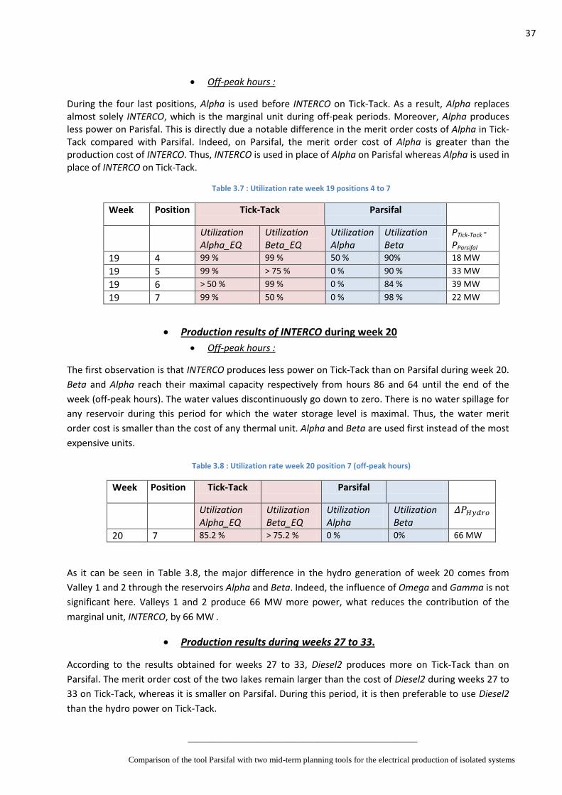
37

____________________________________________


Off-peak hours :

During the four last positions, Alpha is used before INTERCO on Tick-Tack. As a result, Alpha replaces almost solely INTERCO, which is the marginal unit during off-peak periods. Moreover, Alpha produces less power on Parisfal. This is directly due a notable difference in the merit order costs of Alpha in Tick-Tack compared with Parsifal. Indeed, on Parsifal, the merit order cost of Alpha is greater than the production cost of INTERCO. Thus, INTERCO is used in place of Alpha on Parisfal whereas Alpha is used in place of INTERCO on Tick-Tack.

Table 3.7 : Utilization rate week 19 positions 4 to 7



Utilization Beta_EQ

Utilization Alpha

Utilization Beta

PTick-Tack - PParsifal

19 4 99 % 99 % 50 % 90% 18 MW

19 5 99 % > 75 % 0 % 90 % 33 MW

19 6 > 50 % 99 % 0 % 84 % 39 MW

19 7 99 % 50 % 0 % 98 % 22 MW

Production results of INTERCO during week 20

Off-peak hours :

The first observation is that INTERCO produces less power on Tick-Tack than on Parsifal during week 20.

Beta and Alpha reach their maximal capacity respectively from hours 86 and 64 until the end of the

week (off-peak hours). The water values discontinuously go down to zero. There is no water spillage for

any reservoir during this period for which the water storage level is maximal. Thus, the water merit

order cost is smaller than the cost of any thermal unit. Alpha and Beta are used first instead of the most

expensive units.

Table 3.8 : Utilization rate week 20 position 7 (off-peak hours)



Utilization Beta_EQ

Utilization Alpha

Utilization Beta

20 7 85.2 % > 75.2 % 0 % 0% 66 MW

As it can be seen in Table 3.8, the major difference in the hydro generation of week 20 comes from

Valley 1 and 2 through the reservoirs Alpha and Beta. Indeed, the influence of Omega and Gamma is not

significant here. Valleys 1 and 2 produce 66 MW more power, what reduces the contribution of the

marginal unit, INTERCO, by 66 MW .

Production results during weeks 27 to 33.

According to the results obtained for weeks 27 to 33, Diesel2 produces more on Tick-Tack than on

Parsifal. The merit order cost of the two lakes remain larger than the cost of Diesel2 during weeks 27 to

33 on Tick-Tack, whereas it is smaller on Parsifal. During this period, it is then preferable to use Diesel2

than the hydro power on Tick-Tack.

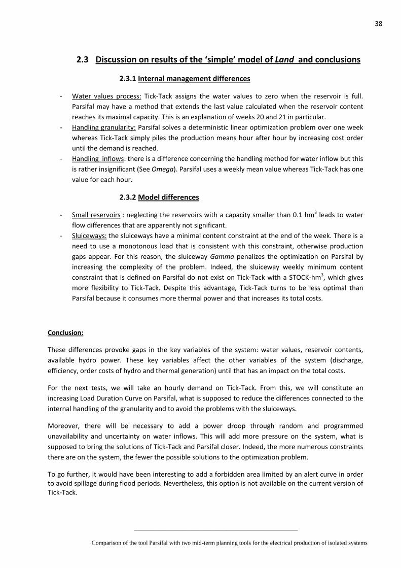
38

____________________________________________


2.3 Discussion on results of the ‘simple’ model of Land and conclusions

2.3.1 Internal management differences

- Water values process: Tick-Tack assigns the water values to zero when the reservoir is full.

Parsifal may have a method that extends the last value calculated when the reservoir content

reaches its maximal capacity. This is an explanation of weeks 20 and 21 in particular.

- Handling granularity: Parsifal solves a deterministic linear optimization problem over one week

whereas Tick-Tack simply piles the production means hour after hour by increasing cost order

until the demand is reached.

- Handling inflows: there is a difference concerning the handling method for water inflow but this

is rather insignificant (See Omega). Parsifal uses a weekly mean value whereas Tick-Tack has one

value for each hour.

2.3.2 Model differences

- Small reservoirs : neglecting the reservoirs with a capacity smaller than 0.1 hm3 leads to water

flow differences that are apparently not significant.

- Sluiceways: the sluiceways have a minimal content constraint at the end of the week. There is a

need to use a monotonous load that is consistent with this constraint, otherwise production

gaps appear. For this reason, the sluiceway Gamma penalizes the optimization on Parsifal by

increasing the complexity of the problem. Indeed, the sluiceway weekly minimum content

constraint that is defined on Parsifal do not exist on Tick-Tack with a STOCK-hm3, which gives

more flexibility to Tick-Tack. Despite this advantage, Tick-Tack turns to be less optimal than

Parsifal because it consumes more thermal power and that increases its total costs.

Conclusion:

These differences provoke gaps in the key variables of the system: water values, reservoir contents,

available hydro power. These key variables affect the other variables of the system (discharge,

efficiency, order costs of hydro and thermal generation) until that has an impact on the total costs.

For the next tests, we will take an hourly demand on Tick-Tack. From this, we will constitute an

increasing Load Duration Curve on Parsifal, what is supposed to reduce the differences connected to the

internal handling of the granularity and to avoid the problems with the sluiceways.

Moreover, there will be necessary to add a power droop through random and programmed

unavailability and uncertainty on water inflows. This will add more pressure on the system, what is

supposed to bring the solutions of Tick-Tack and Parsifal closer. Indeed, the more numerous constraints

there are on the system, the fewer the possible solutions to the optimization problem.

To go further, it would have been interesting to add a forbidden area limited by an alert curve in order to avoid spillage during flood periods. Nevertheless, this option is not available on the current version of Tick-Tack.

39

____________________________________________


3. Detailed model of the electrical system of Land

As it was mentioned in the discussion on the simple model, the simple model needs to be improved in

order to avoid the differences observed in the simulation results that come from an inappropriate

modeling. That is why a second model for Land has been designed, taking not only into account the

improvements of the simple model, but also new parameters such as the unavailability of the thermal

units. This model is called ‘detailed’ model and is described in the following section.

3.1 Description of the detailed model of Land

3.1.1 Demand

On Tick-Tack, the demand is an hourly chronicle over 2011 and 2012. This one is made monotonous

thanks to the Load Duration Curve process in order to improve the calculation time. Indeed, Parsifal is

not capable of handling an hourly demand in its models. The demand that is obtained is a weekly

increasing chronicle:

Figure 3.7 Increasing weekly demand for Land on Parsifal

Duration of the positions: 26h-33h-33h-33h-33h-7h sorted according to increasing demand over each week.

3.1.2 Hydro model

Alpha (Valley 1) and Gamma (Valley 3) are modeled as previously in the simple model, whereas Beta (Valley

2) is slightly modified. The water discharge Q, the efficiencies and the inflows v of Beta_EQ are

aggregated in the following way this time:

( ) [13]

[14]

0

100

200

300

400

500

1

24

47

70

93

11

6

13

9

16

2

18

5

20

8

23

1

25

4

27

7

30

0

32

3

34

6

36

9

39

2

41

5

43

8

46

1

48

4

50

7

53

0

55

3

57

6

59

9

62

2

64

5

66

8

69

1

71

4

MW

Positions

Demand - Parsifal

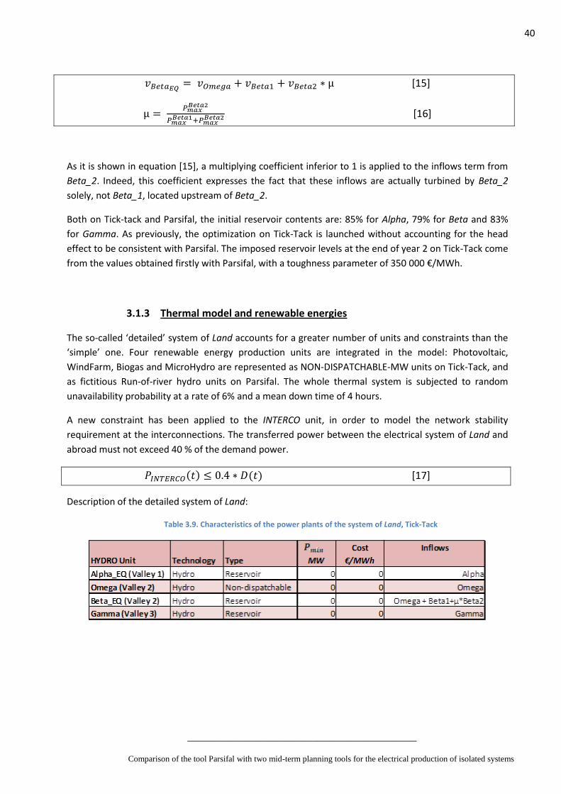
40

____________________________________________


[15]

[16]

As it is shown in equation [15], a multiplying coefficient inferior to 1 is applied to the inflows term from

Beta_2. Indeed, this coefficient expresses the fact that these inflows are actually turbined by Beta_2

solely, not Beta_1, located upstream of Beta_2.

Both on Tick-tack and Parsifal, the initial reservoir contents are: 85% for Alpha, 79% for Beta and 83%

for Gamma. As previously, the optimization on Tick-Tack is launched without accounting for the head

effect to be consistent with Parsifal. The imposed reservoir levels at the end of year 2 on Tick-Tack come

from the values obtained firstly with Parsifal, with a toughness parameter of 350 000 €/MWh.

3.1.3 Thermal model and renewable energies

The so-called ‘detailed’ system of Land accounts for a greater number of units and constraints than the

‘simple’ one. Four renewable energy production units are integrated in the model: Photovoltaic,

WindFarm, Biogas and MicroHydro are represented as NON-DISPATCHABLE-MW units on Tick-Tack, and

as fictitious Run-of-river hydro units on Parsifal. The whole thermal system is subjected to random

unavailability probability at a rate of 6% and a mean down time of 4 hours.

A new constraint has been applied to the INTERCO unit, in order to model the network stability

requirement at the interconnections. The transferred power between the electrical system of Land and

abroad must not exceed 40 % of the demand power.

( ) ( ) [17]

Description of the detailed system of Land:

Table 3.9. Characteristics of the power plants of the system of Land, Tick-Tack

41

____________________________________________


On Parsifal the number of lakes, where water values can be optimized is restricted to 2. That is why

Gamma is modeled as a “Sluiceway”. Gamma is modeled as a STOCK on Tick-Tack, with a small reservoir

capacity.

3.1.4 Uncertainty scenarios

First of all, the study scope lasts 2 years. Second, the models assume that the unavailability of the power

plant is a known data. There is only one scenario of unavailability for each thermal plant. This

unavailability scenario is generated by a Markov chain for each thermal unit. Moreover, the stochastic

hydro inflows contain 57 historical scenarios. The stochastic photovoltaic power has 20 historical

scenarios in MW. The optimization program combines these power, inflow and unavailability series into

114 scenarios that are made in this way:

- the demand scenario is considered in the 114 scenarios;

- the input power sceanrio for Windfarm, the one for Biogas and the one for MicroHydro are considered

in the 114 scenarios;

- the unavailability chronicle for each thermal unit is considered in the 114 scenarios;

- there are 57 hydro inflow scenarios for the hydro units Alpha, Omega, Beta 1, Beta 2 and Gamma. Each

one is considered twice in the 114 scenarios;

- there are 20 photovoltaic power scenarios that are considered at least 5 times (100 scenarios in total).

The 14 first are considered 6 times in order to be distributed in the whole 114 scenarios.

42

____________________________________________


3.2 Analysis of the simulation results

The simulations results are obtained according to the detailed model of Land.

3.2.1 Qualitative analysis

The qualitative analysis is a weekly study of the four outputs of interest: total generated power, total

costs, mean water content and total spillage.

Table 3.10: Total generation over the 2-year period, Land, Tick-Tack

Color chart: In red are shown significant negative energy differences; in green are shown significant positive energy differences.

Energy over the studied period (2 years) GWhTICK-TACK PARSIFAL Δ Energy TT-Parsi (GWh)

1 PV 58.22 58.38 -0.16

2 Windfarm 53.54 53.79 -0.26

3 MicroHydro 103.19 103.79 -0.61

4 Biogas 17.37 17.49 -0.12

5 Alpha 288.92 301.25 -12.33

6 Beta 390.62 400.67 -10.05

7 Omega 74.51 75.65 -1.14

8 Gamma 122.38 125.40 -3.01

9 Interco 1785.86 1786.10 -0.25

10 Diesel1 761.39 785.23 -23.84

11 Diesel2 838.24 786.68 51.55

12 Oil 0.401 0.29 0.11

13 Deficit 0 0 0

TOTAL Energy 4494.626 4494.626 -0.11 GWh

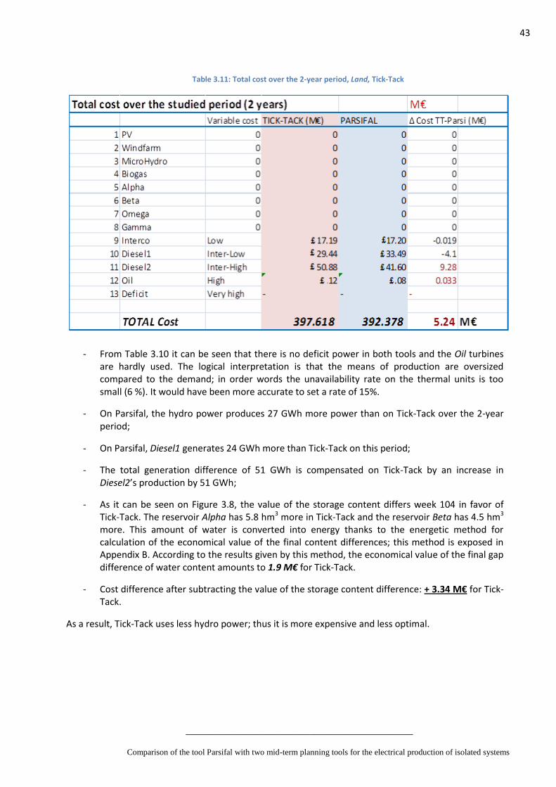
43

____________________________________________


Table 3.11: Total cost over the 2-year period, Land, Tick-Tack

- From Table 3.10 it can be seen that there is no deficit power in both tools and the Oil turbines are hardly used. The logical interpretation is that the means of production are oversized compared to the demand; in order words the unavailability rate on the thermal units is too small (6 %). It would have been more accurate to set a rate of 15%.

- On Parsifal, the hydro power produces 27 GWh more power than on Tick-Tack over the 2-year period;

- On Parsifal, Diesel1 generates 24 GWh more than Tick-Tack on this period;

- The total generation difference of 51 GWh is compensated on Tick-Tack by an increase in Diesel2’s production by 51 GWh;

- As it can be seen on Figure 3.8, the value of the storage content differs week 104 in favor of Tick-Tack. The reservoir Alpha has 5.8 hm3 more in Tick-Tack and the reservoir Beta has 4.5 hm3 more. This amount of water is converted into energy thanks to the energetic method for calculation of the economical value of the final content differences; this method is exposed in Appendix B. According to the results given by this method, the economical value of the final gap difference of water content amounts to 1.9 M€ for Tick-Tack.

- Cost difference after subtracting the value of the storage content difference: + 3.34 M€ for Tick-Tack.

As a result, Tick-Tack uses less hydro power; thus it is more expensive and less optimal.

44

____________________________________________


Figure 3.8. Mean reservoir content, Land, Tick-Tack

Table 3.12. Total spillage, Land, Tick-Tack

Total spillage Tick-Tack hm3

Parsifal hm3

Δ Spillage hm3

Alpha 17,6 8,65 8,94

Beta 33,6 15,5 18,1

Gamma 12,8 6,18 6,63

0

5

10

15

20

25

30

35

1 4 7

10

13

16

19

22

25

28

31

34

37

40

43

46

49

52

55

58

61

64

67

70

73

76

79

82

85

88

91

94

97

10

0

10

3

hm

3

Mean reservoir content ALPHA

Tolla Parsi en fin de pas Tolla_HTick-Tack Parsifal

0

5

10

15

20

25

1 4 7

10

13

16

19

22

25

28

31

34

37

40

43

46

49

52

55

58

61

64

67

70

73

76

79

82

85

88

91

94

97

10

0

10

3

hm

3

Weeks

Mean reservoir content BETA

Calacuccia Parsi en fin de pas Calacuccia_HTick-Tack Parsifal

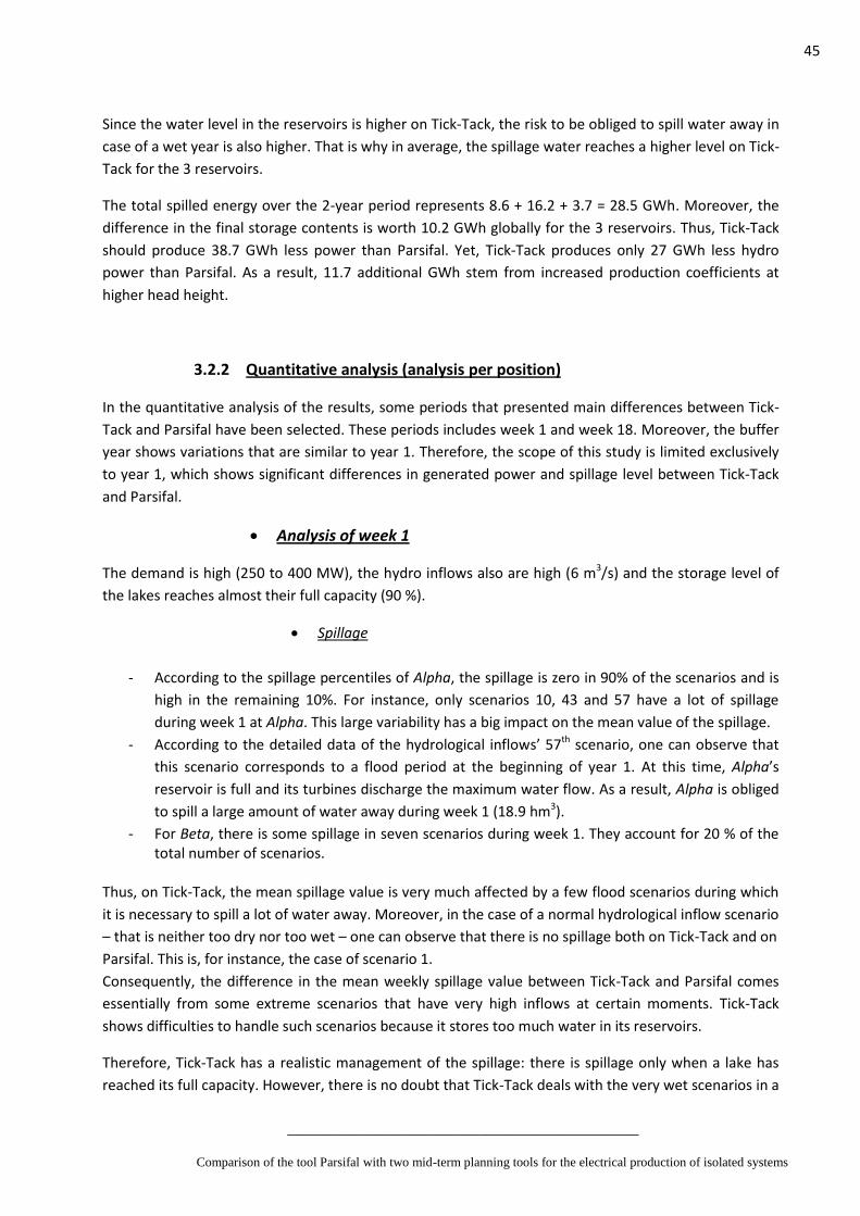
45

____________________________________________


Since the water level in the reservoirs is higher on Tick-Tack, the risk to be obliged to spill water away in

case of a wet year is also higher. That is why in average, the spillage water reaches a higher level on Tick-

Tack for the 3 reservoirs.

The total spilled energy over the 2-year period represents 8.6 + 16.2 + 3.7 = 28.5 GWh. Moreover, the

difference in the final storage contents is worth 10.2 GWh globally for the 3 reservoirs. Thus, Tick-Tack

should produce 38.7 GWh less power than Parsifal. Yet, Tick-Tack produces only 27 GWh less hydro

power than Parsifal. As a result, 11.7 additional GWh stem from increased production coefficients at

higher head height.

3.2.2 Quantitative analysis (analysis per position)

In the quantitative analysis of the results, some periods that presented main differences between Tick-

Tack and Parsifal have been selected. These periods includes week 1 and week 18. Moreover, the buffer

year shows variations that are similar to year 1. Therefore, the scope of this study is limited exclusively

to year 1, which shows significant differences in generated power and spillage level between Tick-Tack

and Parsifal.

Analysis of week 1

The demand is high (250 to 400 MW), the hydro inflows also are high (6 m3/s) and the storage level of

the lakes reaches almost their full capacity (90 %).

Spillage

- According to the spillage percentiles of Alpha, the spillage is zero in 90% of the scenarios and is

high in the remaining 10%. For instance, only scenarios 10, 43 and 57 have a lot of spillage

during week 1 at Alpha. This large variability has a big impact on the mean value of the spillage.

- According to the detailed data of the hydrological inflows’ 57th scenario, one can observe that

this scenario corresponds to a flood period at the beginning of year 1. At this time, Alpha’s

reservoir is full and its turbines discharge the maximum water flow. As a result, Alpha is obliged

to spill a large amount of water away during week 1 (18.9 hm3).

- For Beta, there is some spillage in seven scenarios during week 1. They account for 20 % of the total number of scenarios.

Thus, on Tick-Tack, the mean spillage value is very much affected by a few flood scenarios during which

it is necessary to spill a lot of water away. Moreover, in the case of a normal hydrological inflow scenario

– that is neither too dry nor too wet – one can observe that there is no spillage both on Tick-Tack and on

Parsifal. This is, for instance, the case of scenario 1.

Consequently, the difference in the mean weekly spillage value between Tick-Tack and Parsifal comes

essentially from some extreme scenarios that have very high inflows at certain moments. Tick-Tack

shows difficulties to handle such scenarios because it stores too much water in its reservoirs.

Therefore, Tick-Tack has a realistic management of the spillage: there is spillage only when a lake has

reached its full capacity. However, there is no doubt that Tick-Tack deals with the very wet scenarios in a

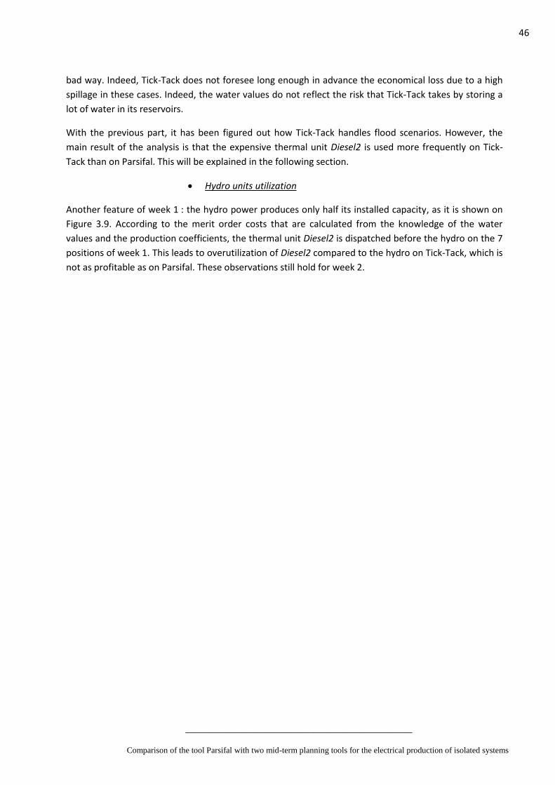
46

____________________________________________


bad way. Indeed, Tick-Tack does not foresee long enough in advance the economical loss due to a high

spillage in these cases. Indeed, the water values do not reflect the risk that Tick-Tack takes by storing a

lot of water in its reservoirs.

With the previous part, it has been figured out how Tick-Tack handles flood scenarios. However, the

main result of the analysis is that the expensive thermal unit Diesel2 is used more frequently on Tick-

Tack than on Parsifal. This will be explained in the following section.

Hydro units utilization

Another feature of week 1 : the hydro power produces only half its installed capacity, as it is shown on

Figure 3.9. According to the merit order costs that are calculated from the knowledge of the water

values and the production coefficients, the thermal unit Diesel2 is dispatched before the hydro on the 7

positions of week 1. This leads to overutilization of Diesel2 compared to the hydro on Tick-Tack, which is

not as profitable as on Parsifal. These observations still hold for week 2.

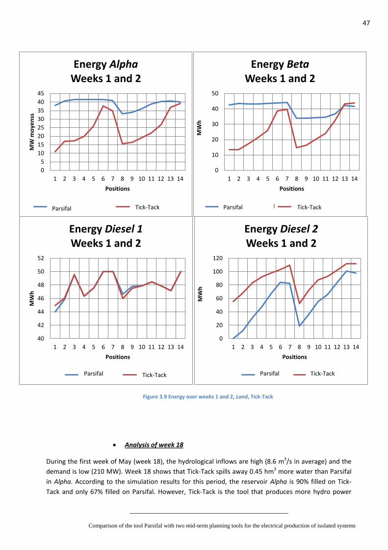
47

____________________________________________


Figure 3.9 Energy over weeks 1 and 2, Land, Tick-Tack

Analysis of week 18

During the first week of May (week 18), the hydrological inflows are high (8.6 m3/s in average) and the

demand is low (210 MW). Week 18 shows that Tick-Tack spills away 0.45 hm3 more water than Parsifal

in Alpha. According to the simulation results for this period, the reservoir Alpha is 90% filled on Tick-

Tack and only 67% filled on Parsifal. However, Tick-Tack is the tool that produces more hydro power

0

5

10

15

20

25

30

35

40

45

1 2 3 4 5 6 7 8 9 10 11 12 13 14

MW

mo

yen

ss

Positions

Energy Alpha Weeks 1 and 2

Tolla Parsifal (VALLEE 1) Tolla_EQ Tick-TackTick-Tack Parsifal

0

10

20

30

40

50

1 2 3 4 5 6 7 8 9 10 11 12 13 14

MW

h

Positions

Energy Beta Weeks 1 and 2

CALA_EQUIV Parsifal Calacuccia_EQ Tick-TackTick-Tack Parsifal

40

42

44

46

48

50

52

1 2 3 4 5 6 7 8 9 10 11 12 13 14

MW

h

Positions

Energy Diesel 1 Weeks 1 and 2

Lucciana Parsi LuccParsifal Tick-Tack

0

20

40

60

80

100

120

1 2 3 4 5 6 7 8 9 10 11 12 13 14

MW

h

Positions

Energy Diesel 2 Weeks 1 and 2

Vazzio Parsi #REF!Tick-Tack Tick-Tack Parsifal

48

____________________________________________


from Alpha during this week: 4.26 GWh against 2.37 for Parsifal. Finally, Tick-Tack spills more water

away but produces more hydro power.

During week 18, only 3 scenarios spill away a significant amount of water, and there is one scenario that

spills more water away than all the others: the scenario number 6. During week 18 of this flood

scenario, Alpha reaches its maximum storage capacity in only 24 hours. Alpha is then forced to spill

10.56 hm3 of water away.Tick-Tack will stay at maximum storage level during weeks 19, 20 and 21

before going down because the inflows only reach again their mean value during week 22.

Having all these results in mind, one can assert that Tick-Tack’s security margin against spring floods is

too small in terms of reservoir storage capacity. In other words, Tick-Tack is not as well prepared to face

random extreme scenarios as Parsifal.

In order to improve the behavior of Tick-Tack, it could have been interesting to add an alert curve on the

hydro reserve management in order to penalize Tick-Tack if it enters the forbidden area.

3.3 Discussion on the results of the ‘detailed’ model of Land and

conclusions

With default settings, Tick-Tack handles spillage in a way that is less optimal than Parsifal. Tick-Tack’s

reservoir contents are set too high in the simulation phase and that is due to overestimated water

values in the optimization phase. Since the 3 reservoirs are optimized in the previous model, it has been

decided to make a complementary test to check if the number of optimized reservoirs affects the

results. In this test, the generated power in Valley 1 and Valley 3 of Parsifal is set as an input data in Tick-

Tack. Therefore, only Beta_EQ of Valley 2 is optimized in Tick-Tack for this test.

Model of the complementary test: the generated power of Valley 1 and Valley 3 in Tick-Tack are taken

identical to the generation obtained with Parsifal. Only the reservoir Beta in Valley 2 is regulated by

optimization of the water values.

Results of the complementary test: the mean reservoir content of Beta is very close to the 3-reservoir

case. There is no major difference in the spillage either: 33.6 hm3 in the previous case and 30.9 hm3 in

this case instead of 15.5 hm3 on Parsifal. The total cost difference with Parsifal reaches 2 M€. The final

storage level difference of Beta is 0.7 M€. Thus, the total net cost difference is equal to 1.3 M€.

According to the results of the complementary test with one optimized reservoir, one can conclude that

Parsifal does offer a more complete optimization. Parsifal takes into account the inflow scenarios that lie

far from the average value, like for instance scenarios reflecting important spring flood periods.

Optimizing with one reservoir instead of three absolutely confirms this tendency.

49

____________________________________________


IV. SDDP : Land

1. Model of Land on SDDP

The major model difference with Parsifal lies in the number of positions that represent the demand.

Indeed, the load duration curve corresponding to the real chronological demand can contain maximum

5 positions on SDDP. These 5 positions were created on SDDP from the 7 positions of Parsifal by

aggregating together the 33-hour intermediate load level positions: the two first and two last were

merged together in order to obtain two 66-hour positions instead of four 33-hour positions. Table

explains the process of this aggregation.

Table 4.1 Aggregation of the load positions from Parsifal on SDDP

Positions on Parsifal Duration (hours) Positions on SDDP Duration (hours)

1 26 1 26

2, 3, 4, 5 33 – 33 – 33 – 33 2, 3 66 - 66

6 10 4 10

7 3 5 3

Many parameters of the model could be transposed identically from Parsifal to SDDP: 2-year studied

period, 57 hydro inflow scenarios and 20 photovoltaic scenarios, 1 unavailability scenario on the thermal

units (unavailability rate of 6%, mean down time of 4 hours), network stability constraint for the

interconnection. Furthermore, on SDDP the hydro system is described in a detailed way, similar to

Parsifal. As a consequence, it was possible to take into account each of the 7 hydro units without

aggregating those belonging to the same valley, like with Tick-Tack. Finally, an imposed reservoir level

was added to SDDP with the same values as the final storage level on Parsifal. The penalty associated to

it was set to a value lying between the higher cost of the thermal power (cost of Oil) and the deficit cost.

On the other hand, prior to the optimization phase, SDDP processes the chronicles of historic hydro

inflows with an auto-regressive model called ARP. The exact description of this model is not under the

scope of this study but it is necessary to mention it in this paragraph. However, in the simulation phase,

the historical inflows are not processed, they are used directly. Moreover, the ‘Head effect in

Optimization’ parameter was set to a constant value, equal to the efficiencies at full storage. By this

means, Parsifal and SDDP had the same behavior about this head effect parameter.

Finally, an arbitrary choice was made about the number of iterations of SDDP’s algorithm, which was set

to 5. This number could have probably been optimized in order to give estimated water values close to

the real solution in a minimum calculation time. However, this parameter was not optimized in the

study.

The results obtained with these model elements are presented in the following section.

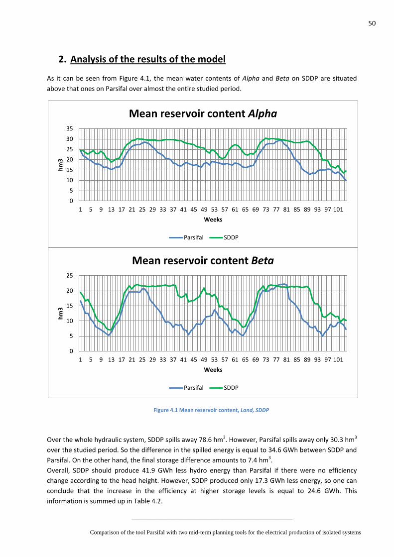
50

____________________________________________


2. Analysis of the results of the model

As it can be seen from Figure 4.1, the mean water contents of Alpha and Beta on SDDP are situated

above that ones on Parsifal over almost the entire studied period.

Figure 4.1 Mean reservoir content, Land, SDDP

Over the whole hydraulic system, SDDP spills away 78.6 hm3. However, Parsifal spills away only 30.3 hm3

over the studied period. So the difference in the spilled energy is equal to 34.6 GWh between SDDP and

Parsifal. On the other hand, the final storage difference amounts to 7.4 hm3.

Overall, SDDP should produce 41.9 GWh less hydro energy than Parsifal if there were no efficiency

change according to the head height. However, SDDP produced only 17.3 GWh less energy, so one can

conclude that the increase in the efficiency at higher storage levels is equal to 24.6 GWh. This

information is summed up in Table 4.2.

0

5

10

15

20

25

30

35

1 5 9 13 17 21 25 29 33 37 41 45 49 53 57 61 65 69 73 77 81 85 89 93 97 101

hm

3

Weeks

Mean reservoir content Alpha

Parsifal SDDP

0

5

10

15

20

25

1 5 9 13 17 21 25 29 33 37 41 45 49 53 57 61 65 69 73 77 81 85 89 93 97 101

hm

3

Weeks

Mean reservoir content Beta

Parsifal SDDP

51

____________________________________________


Table 4.2 Spillage, SDDP- Parsifal

Valley 1 Valley 2 Valley 3 Total

Spillage (hm3) SDDP 23.5 48.91 6.13 78.5 hm3

Parsifal 8.65 15.5 6.2 30.4 hm3

Difference SDDP - Parsifal

Spillage 14.85 33.41 -0.07 48.2 hm3

Table 4.3 Total generation over the 2-year period, SDDP-Parsifal

Energy over the studied period (2 years) GWhSDDP PARSIFAL Δ Energy SDDP-Parsi (GWh)

1 PV 58.4 58.4 0

2 Windfarm 53.8 53.8 0

3 MicroHydro 103.8 103.8 0

4 Biogas 17.36 17.49 -0.13

5 Alpha 294 301.2 -7.28

6 Beta 390.6 400.67 -10.07

7 Omega 75.7 75.65 0.04

8 Gamma 125.4 125.4 0.01

9 Interco 1786.91 1786.1 0.80

10 Diesel1 779 785.23 -6.20

11 Diesel2 809.36 786.68 22.68

12 Oil 0.324 0.29 0.03

13 Deficit 0 0 0

TOTAL Energy 4494.62 4494.73 -0.11 GWh

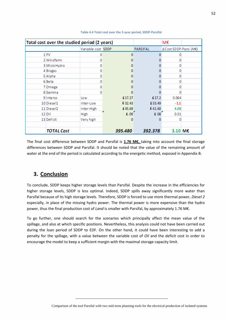
52

____________________________________________


Table 4.4 Total cost over the 2-year period, SDDP-Parsifal

The final cost difference between SDDP and Parsifal is 1.76 M€, taking into account the final storage

differences between SDDP and Parsifal. It should be noted that the value of the remaining amount of

water at the end of the period is calculated according to the energetic method, exposed in Appendix B.

3. Conclusion

To conclude, SDDP keeps higher storage levels than Parsifal. Despite the increase in the efficiencies for

higher storage levels, SDDP is less optimal. Indeed, SDDP spills away significantly more water than

Parsifal because of its high storage levels. Therefore, SDDP is forced to use more thermal power, Diesel 2

especially, in place of the missing hydro power. The thermal power is more expensive than the hydro

power, thus the final production cost of Land is smaller with Parsifal, by approximately 1.76 M€.

To go further, one should search for the scenarios which principally affect the mean value of the

spillage, and also at which specific positions. Nevertheless, this analysis could not have been carried out

during the loan period of SDDP to EDF. On the other hand, it could have been interesting to add a

penalty for the spillage, with a value between the variable cost of Oil and the deficit cost in order to

encourage the model to keep a sufficient margin with the maximal storage capacity limit.

53

____________________________________________


Discussion on results During the study of Tick-Tack and SDDP in comparison to Parsifal, almost all the important similarities

and differences between the tools have been described. It is time to add to the previously evocated

features, some new ones, like the calculation time and the ergonomics of the graphical interface, that

are crucial criterion in the operational field. So, Table 5.1 presents in a summarized way these key

indicators. Note that the results were obtained based on basic models and tests; the present study does

not aim to draw general conclusions about the tools from those basic tests but only to give tendencies

that are observed in the context of this study. Moreover, all the tests carried out in this analysis have

been run on a Windows Vista computer, equipped with a single core processor.

Table 5.1 Synthesis of the capabilities of the three tools

Tick-Tack benefits from a smaller calculation time in optimization. Parsifal and SDDP are slower; SDDP’s

calculation effort in optimization increases considerably with the number of iterations of the algorithm.

However, in the simulation phase, SDDP is the faster tool, but Tick-Tack is also fast. Parsifal has a high

simulation time compared to the other tools. These results seem to be consistent with the idea that

Parsifal’s optimization and simulation phases are based on more sophisticated algorithms, including the

real Stochastic Dynamic Programming. The quality of the water management policy is thus very sensitive

to this difference in the conception of the algorithms. Consequently, the solution to the optimization

problem of Land that offers Parsifal remains the more efficient way of dispatching the production means

over the middle-term period, provided that there are no alert curves defined on Tick-Tack or on SDDP.

The overall criticism that can be made in conclusion of this study is that both Tick-Tack and SDDP show

troubles to anticipate the flood periods during wet scenarios. For this reason, Parsifal offers a cheaper

and more optimal solution to the optimization problem of isolated systems.

On the other hand, the graphical interface of Parsifal has the advantage to be relatively simple to use,

provided that there is a small number of options in comparison with SDDP for instance. Indeed, SDDP

has a large diversity of options and parameters to model specific phenomenon of hydrothermal

systems. This aspect turned out to be a drawback for EDF since a tool needs to be clearly and entirely

understood from its basic aspects to its most specific functionalities. This is for instance the case of

Parsifal, which has been developed by the R&D departments in collaboration with the Production

Center. Last but not least, SDDP’s graphical interface has the advantage of being modern and user-

friendly, which is also the case of Tick-Tack.

Parameter or model data Parsifal Tick-Tack SDDP

Calculation time in optimization 24 min 14 min 1 iteration: 21 min

5 iterations : 1h 50 min

Calculation time in simuation 17 min 5 min 1 iteration: 2 min

5 iterations : 2 min

Optimality of the water management policy Good Sub-optimal Sub-optimal

Spillage control and reactivity towards flood

inflow scenarios

Good Medium Medium

Cost difference with Parsifal over 2 years 0 3.34 M€ 1.79 M€

Ergonomics of the graphical interface Old, simple to use User friendly, simple to use User friendly, dense

54

____________________________________________


Conclusion

In the course of this project, Tick-Tack was the first middle-term planning tool that has been under

study, and to compare with Parsifal. Tick-Tack is an optimization tool with a simple hydraulic model for

describing the hydro electrical production system. Its study revealed that Tick-Tack has a water

management strategy that is not as optimal as Parsifal, since Tick-Tack utilizes more thermal energy.

This difference comes essentially from the way Tick-Tack handles flood scenarios. In such a context,

represented by a few number of scenarios, Tick-Tack spills away a considerable amount of water, what

impacts directly the mean production costs. The simulation algorithm of Tick-Tack, based on an hourly

deterministic recursion, is the cause of such a behavior. Indeed, in comparison to Parsifal, Tick-Tack does

not have a view of the perturbations on the system over the whole week to come, but only over one

hour. This short deterministic vision of the “future” is the main explanation for the spillage difference.

On the other hand, Tick-Tack benefits from several advantages in its utilization: its graphical interface is

simple to use and modern and its calculation algorithm is soft and quick.

In the last part of the study, SDDP was compared with Parsifal. SDDP is based on a variant of the

Stochastic Dynamic Programming that is called SDDP too. SDDP stands for Stochastic Dual Dynamic

Programming, and performs an estimation of the real water value function. This turns out to be the first

major difference with Parsifal’s algorithm, which calculates the real water values function. In addition,

its principal limitation comes from the maximal number of positions both in optimization and simulation

that is available, that is maximum 5 positions. The major drawback of SDDP is that the optimization

problem solution is not as optimal as Parsifal because of troubles in handling the spillage in case of flood

periods. Like Tick-Tack, SDDP does not anticipate enough the large amount of water inflows in such a

case, and is obliged to spill water away. Moreover, the calculation time get much higher than Parsifal if

several iterations of the algorithm is selected in the options.

On the other hand, there are several similarities between SDDP and Parisfal. SDDP has a detailed model

of the hydro systems, like Parsifal. The hydro system description is even more detailed on SDDP.

Another positive point is that SDDP offers a large number of models and options to describe precisely

almost all energetic systems (thermo electrical and gas interconnected systems). Its interface is modern,

clear and organized. This makes that SDDP is very suitable as a study tool, but Parsifal is more

appropriate for the real operation of the French isolated systems.

To go further in the direction of this study, it could be considered to design a new tool inspired by the

ergonomics of Tick-Tack and SDDP and processing Parsifal’s algorithms in order to obtain optimal

solutions with a more intuitive tool.

55

____________________________________________


Appendix

A. Transition matrix of a two-state Markov power plant

Let’s consider the discrete two-state Markov Chain representing the availability and unavailability states

of a power plant. The availability state is called Up and represented by the letter U. The unavailability

state is the Down state, represented by D. Based on the article entitled Markov ChainV, the transition

matrix P of such a Markov chain is the following:

[ ( ) ( ) ( ) ( )

] [18]

The aim of this appendix is to derive the terms of the transition matrix P from the two known data that

are the unavailability ratio a power plant (r) and the mean down time (d).

From the mean down time d the term ( ) can be easily determined:

( ) [19]

Since the sum of all the probabilities of transition from one state should be equal to 1, we have:

( ) ( ) [20]

( ) ( ) [21]

With equations [19] and [21], one can deduce that:

( ) [22]

On the other hand, since the unavailability ratio of a power plant (r) is a given data, one can explicitly

derive ( ) from r:

( ) [23]

In addition, the term ( ) can be deduced from equation [23] since the system is either in state U or D:

( ) [24]

The probabilistic term ( ) can be derived using the conditional probabilities associated to the two

possible states of the system, U or D:

56

____________________________________________


( ) ( ) ( ) ( ) ( ) [25]

According to equations [19] and [22], one can get the following equation having ( ) as the only

unknown variable:

( ) ( ) (

) [26]

Therefore,

( )

( ) [27]

Consequently, the P transition matrix can be calculated thanks to equation [28]:

[

( )

( )

] [28]

In particular, the cross transition probabilities ( ) and ( ) are used in the definition of the

unavailability scenario generation for the thermal power plants.

B. Economical value of the water content gap at the end of the studied period

(Case study: Island , stochastic model, without imposed reservoir content)

o Method 1: via the water valuesi.

In order to compare the operation costs, one must determine the economical value of the water

content gap at the end of the studied period (December 30, 2012). In the case of Island, CONSTANT is 78

hm3 higher than VARIABLE. Let us choose a maximal valuation, that is a valuation maximizing the value

of the remaining water: the highest hourly water value over December 30, 2012, is used, with the

highest efficiency of Reservoir at low water level (empty reservoir). Indeed, on December 30, 2012 at

23h, the water level is only about 4.6 % for CONSTANT: it is thus necessary to take the values of the

efficiency at low level.

Results :

Profit for the water level gap in favor of CONSTANT: 114,2 k€;

Gross cost difference in favor of VARIABLE: 1553,3 k€

Net cost difference in favor of VARIABLE: 1439,1 k€

As a result, the profit associated with the water level gap does not compensate the cost difference in

favor of VARIABLE.

This method has however a significant drawbacks. On one hand, it takes into account the water value at

the end of the period, which is affected by the arbitrary choice of the initial water value. On the other

57

____________________________________________


hand, the water value varies quite much from one hour to another and that can influence the results

depending on which hour was considered. This method is thus too much approximate.

In order to solve this problem, another method consists in determining the hydrological energy in MWh

associated with the remaining water volume thanks to the knowledge of the efficiency, and then

subtracting this energy to the thermal production of the most expensive thermal unit. This second

method is called energy method for valuation of the final water level difference. It is explained in the

following section.

o Method 2: energy methodi.

ΔMfinal = 78 hm3 in favor of CONSTANT (CONSTANT has a water level that is 78 hm3 higher than

VARIABLE);

Mfinal = 4.6 % (low water level);

Mean efficiency at low level = µ kWh/ m3;

Energy = 78 000 000* µ = £ MWh = £ GWh

This energy would completely replace Oil2 and also a part of Oil1 of CONSTANT and would contribute to

a 948 k€ decrease in the operation costs.

Gross cost difference in favor of VARIABLE: 1553,3 k€

Profit of the water level gap in favor of CONSTANT : 948 k€

Net cost difference in favor of VARIABLE : 605 k€

o Conclusion on the methods of valuation

Between both methods of valuation, (method via the water value at the end of the period and method

via the energy), the net costs difference of the water level gap comes essentially from the arbitrary

choice of the initial water value, what affects the results significantly. This parameter is sensitive since

its value is close to the order costs of the thermal units. The arbitration between hydro and thermal

power is therefore quite sensitive to the initial water value.

However, both methods indicate that the cost difference is in favor of VARIABLE, which is consequently

cheaper.

Since there is a significant uncertainty on the water value at the end of the period, the first method is

left aside in this report. Consequently, the energy method will be used to obtain the economical value of

the final water level difference every time it will be necessary.

58

____________________________________________


C. Diagrams of the weekly energy produced per unit (Case study: Land, simple model)

0

1000

2000

3000

4000

5000

6000

7000

8000

1 3 5 7 9 11 13 15 17 19 21 23 25 27 29 31 33 35 37 39 41 43 45 47 49 51

Energy Valley 1 MWh

1 3 5 7 9 11 13 15 17 19 21 23 25 27 29 31 33 35 37 39 41 43 45 47 49 51

Energy Omega

Parsifal Tick-Tack

MWh

1 3 5 7 9 11 13 15 17 19 21 23 25 27 29 31 33 35 37 39 41 43 45 47 49 51

Time (weeks)

Energy Beta_EQ

Parsifal Tick-Tack

MWh

59

____________________________________________


1 3 5 7 9 11 13 15 17 19 21 23 25 27 29 31 33 35 37 39 41 43 45 47 49 51

Energy Gamma MWh

1 3 5 7 9 11 13 15 17 19 21 23 25 27 29 31 33 35 37 39 41 43 45 47 49 51

Energy INTERCO MWh

1 3 5 7 9 11 13 15 17 19 21 23 25 27 29 31 33 35 37 39 41 43 45 47 49 51

Time (weeks)

Energy Diesel 1

Parsifal Tick-Tack

MWh

60

____________________________________________


Figure 6.1: Weekly power generation, Land, Tick-Tack.

1 3 5 7 9 11 13 15 17 19 21 23 25 27 29 31 33 35 37 39 41 43 45 47 49 51

Energy Diesel 2 MWh

1 3 5 7 9 11 13 15 17 19 21 23 25 27 29 31 33 35 37 39 41 43 45 47 49 51

Energy Oil1 (MWh) MWh

1 3 5 7 9 11 13 15 17 19 21 23 25 27 29 31 33 35 37 39 41 43 45 47 49 51

Time (weeks)

Energy Oil2 (MWh)

Parsifal Tick-Tack

MWh

61

____________________________________________


D. Merit order costs and efficiency using the interpolation method

In order to be consistent with the model implemented in both tools, it is needed to calculate the efficiency using an interpolation between the empty reservoir value and the full reservoir value in function of the reservoir content at each time step.

From the value of 1 m3 of water in reservoir i, one can determine the merit order cost dividing by the sum of the efficiencies of the units directly downstream unit i.

∑ ( ) [29]i

With:

ηDOWN(i): efficiency for all power plants downstream of reservoir i (including i itself)

The merit order costs of a reservoir can then be compared to the different merit order costs of the thermal units to determine the dispatch order of the units for an optimal strategy. This is the aim of the linear programming of the simulation phase.

References

i Département OSIRIS, EDF R&D, Biblos : Processus et Méthodes pour la gestion d’un portefeuille d’actifs dans les marches de l’électricité, France, 2005. ii BERTISMAS D., TSITSIKLIS J.N., Introduction to Linear Optimization, Massachussets Institute of Technology, USA, 1997. iii LEVEQUE F., EDF, Parsifal User Guide, France, 1990. iv PSR, SDDP User Manual, Brazil, 2011. v PSR, SDDP Methodology Manual, Brazil, 2011. vi GEBALI F., Markov Chains, in “Analysis of Computer and Communication Network”, USA, 2008, p.71.

COLLOGNAT G., Introduction à la gestion prévisionnelle de la production, CNES / Département Production, France, 1994. BIRGE J. R., LOUVEAUX F., Introduction to Stochastic Programming, Springer, USA, 1997. PEREIRA M. V. F., Optimal Stochastic Operations Scheduling of Large Hydroelectric Systems, p.161-169, CEPEL - Centro de Pesquisas de Energia Eletrica, Brazil, 1989. PEREIRA M. V. F., OLIVEIRA G. C., COSTA C. C. G. and KELMAN J., Stochastic Streamflow Models for Hydroelectric System, p.379-390, CEPEL, Centro de Pesquisas de Energia Elétrica, Brazil, 1984.

http://www.springerlink.com/content/p60m000x36744111/

http://www.springerlink.com/content/978-0-387-74436-0/

The comparison of the tool Parsifal with two mid-term planning ...

Documents

Transcript of The comparison of the tool Parsifal with two mid-term planning ...