THE CAPM, THE APT AND A CONTINGENT CLAIMS MODEL OF A SECURITIES HOUSE

Journal of Business Finance ti? Accounting, 22(8), December 1995, 0306-686X

THE CAPM, THE APT AND A CONTINGENT CLAIMS MODEL OF A SECURITIES HOUSE

ANDREW CLARE*

INTRODUCTION

There have been increasing efforts on the part of governments and regulators to coordinate financial market regulations. The most notable result of this drive for internationally recognised regulations so far has been the BIS proposals in 1988 for common capital adequacy standards for commercial banks. All the major regulators agreed to these proposals, which subsequently took effect in 1992.’ The same drive and rationale is now being applied to Securities houses, or Investment banks. A number of different approaches are currently in operation. The two polar cases being: the UK’s rules (SIB, 1987) which are firmly based in portfolio theory, where the riskiness of the firm’s balance sheet is estimated explicity; and the German rules which simply require that securities houses maintain a flat rate capital to asset ratio of 8% (see the Banking Act of the Federal Republic of Germany, 1986) where no explicit recognition of balance sheet quality is made. New EC rules (EC Directive, 93/6/EEC, 1993), which are due to come into force by 1996, are similar in spirit to the SIB rules, where explicit judgements have been made by regulators about the risk inherent in particular financial instruments and positions.

The most efficient approach to the regulation of securities house capital is a risk based one, where the amount of capital required is designed to be an increasing function of the riskiness of the securities house’s balance sheet, this is the razson d’&e behind the SIB rules and the new EC rules. However, essential for such risk assessment are objective measures of how balance sheet changes can affect the probability of securities house failure. For example, how do changes in leverage, or asset quality affect this probability? Although many models of commercial bank behaviour have been developed (see Baltensperger, 1980; and Santomero, 1984) little attention has been given so far to modelling securities houses.

In this paper we develop a model particularly suited to capturing the essential features of a securities house. We argue that the capital and liquidity requirements for a securities house, normally modelled as separate for

The author is from the Department of Economics, University of Reading. He is indebted to George McKenzie and to the anonymous referee for comments on earlier drafts of this paper. The financial support for this research from the ESRC is gratefully acknowledged. (Paper received May 1992, revised and accepted July 1994)

Address for correspondence: Andrew Clare. The ISMA Centre, Department of Economics, Reading University, Reading RG6 2AA, UK.

@ Blackwell Publishers Ltd. 1995. 108 Cowley Road. Oxford OX4 IJF. UK and 1147 238 Main Street, Cambridge, MA 20142, USA.

1148 CLARE

commercial banks in the banking literature (see Baltensperger, 1980), are one and the same for securities houses. This characteristic of securities houses is recognised in the regulations governing these firms in both the UK and the US.

Furthermore, unlike portfolio models of financial intermediaries (see for example Miles and Hall, 1988) the model presented in this paper recognises the limited liability aspect of equity ownership. The consequences of ignoring this feature when calculating the probability of failure is to allow the value of firm equity to be less than zero, with the implication that bankruptcy cannot occur. Thus a contingent claims securities house model is developed here based upon the work of Black and Scholes (1972), Merton (1974), Smith (1976), and others. In addition, the model differs from the usual contingent claims models where the underlying asset is assumed to follow a random walk. Here a multi- factor return generating process is specified for the assets of the securities house’. The model can therefore incorporate the systematic risks of the macroeconomic environment.

The model provides a framework for assessing the influence of firm leverage and asset quality on the probability that a securities house might fail. This should be useful information for regulators attempting to impose risk based capital adequacy standards upon these firms. To this end, a simple securities house balance sheet is constructed to test whether the model is sensitive to balance sheet changes. Simple simulation experiments are conducted with this balance sheet to show how the model might be used to gain objective measures of the risk profile of a securities house as its balance sheet changes character.

The rest of this paper is organised as follows; in the next section we outline the different intermediation process undertaken by commercial banks and securities houses; in the third section the proposed model is formally developed; in the fourth section the data and procedures used to estimate both the CAPM and APT versions of the model are presented and the results are discussed; the final section concludes the paper.

THE DIFFERENCES BETWEEN BANKS AND SECURITIES HOUSES

The traditional business of a commercial bank involves raising highly liquid liabilities from the general public, usually in the form of sight, or very short- term deposit accounts, and lending these funds over much longer periods directly in primary credit markets. Commercial bank loans are normally held to maturity and the funds have traditionally not been invested directly in marketable securities.* Being highly illiquid, the asset structure of a commercial bank changes relatively slowly over time; the presence of non-performing loans made in the 1970s to less developed countries on the balance sheets of many of the world’s major commercial banks today is testimony to this fact.

In contrast to this, securities houses traditionally act as intermediaries for relatively short periods. As underwriters of new issues they are exposed to risk

0 Blackwell Publishers Ltd. 1995

THE CAPM, THE APT AND SECURITIES HOUSES 1149

in the primary credit market for only as long as it takes to place any new issue with investors. In their market making activities securities houses are exposed to risks as a result of having to hold inventories of assets to accommodate customers. As brokers, trading on their own behalf, securities houses invoke risk which simply reflects the speculative nature of trading in various securities markets. The maturity structure of a securities house’s balance sheet is usually highly liquid.

The differences in the maturity structure of the balance sheets of commercial banks and securities houses is reflected in the present regulatory system (see Haberman, 1987, for a summary of the SEC approach in the US). For commercial banks, capital standards are generally based upon the historic book values of assets. This is inevitable since many of the assets do not have a secondary market price. However, in both the UK and US rules’ for securities house^,^ position risk is taken into account explicitly. Regulators on both sides of the Atlantic use capital rules which reflect the likelihood of marketable assets declining in value and marketable liabilities (e. g. short positions) increasing in value in the event of forced sales to cover losses over very short periods of time.4 The emphasis is placed upon marking positions to market and not historic book values of positions. More importantly, liquidity and capital requirements for securities houses’ in the UK and the US are considered to be one and the same; the same is not true for commercial banks where separate liquidity and capital requirements are imposed by regulators.

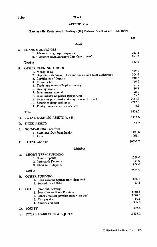
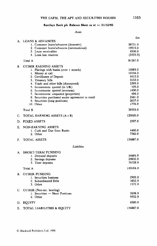
As an example of the differences between commercial banks and securities houses consider the balance sheets of Barclays Bank plc and Barclays De Zoete Wedd (see Appendix A for a fuller description). At the end of 1990 customer loans and advances by Barclays Bank made up 60.3 % of total assets, of which 72.1 % were to UK citizens and 27.9% were international advances. In contrast to this the ratio of Barclays De Zoete Wedd customer loans to total assets was 8.7 % , where 18.4% of these loans were under one year. The illiquid proportion of BZW’s assets if we include all loans and advances to customers, property and fixed assets is 9.7 % . The equivalent figure for Barclays is approximately 62 ’36. The asset struture is clearly different, the commercial bank being in a far more illiquid position than the securities house. Furthermore, the vast majority (approximately 90%) of BZW’s assets could be marked to market and indeed are currently marked to market under existing SIB regulations.

Now consider the liabilities of the two firms. In contrast to the asset side of its balance sheet Barclays Bank’s liabilities are highly liquid with short-term funding, short positions and securities business together making up almost 86 % of its total liabilities. For BZW short-term funding, short positions and securities business make up approximately 76% of its total liabilities. Barclays Bank then, like most commercial banks, has highly illiquid assets funded by relatively liquid liabilities, a fact which has caused regulators to impose both liquidity and capital requirements on commercial banks. The maturity structure of BZW’s assets and liabilities however, is relatively similar. The liquid nature of both the assets


1150 CLARE

and liabilities of securities houses has led to the combined approach to liquidity and capital requirements which is now in operation in both the UK and the US.

Traditionally much attention has been given to modelling commercial banks. Some authors highlight the banks’ decision to allocate the public’s deposits between income earning assets and reserves, while others have developed liability management models (see Baltensperger, 1980; for a review of such models). The discussion above indicated that a securities house performs an intermediation role essentially different from the role performed by a commercial bank. In this paper we develop an alternative model which we feel is more appropriate for the activities of a securities house. Traditional banking models which tend to emphasise either the liquidity aspect of the bank, or the capital structure, or try to model both aspects, are unnecessarily elaborate for modelling a securities house. Given the current regulatory environment, a model where capital and liquidity requirements are considered to be one and the same would seem to be more appropriate.

We also reject the traditional framework for the practical reasons that it is not clear how one could easily generate from these more traditional models a measure of the probability of bankruptcy.

A possible alternative however, would be to use the model developed by Miles and Hall (1988), where the market is assumed to know the ‘overall’ risk profile of the commercial bank. This portfolio model of bank failure however, ignores the fact that the holders of equity enjoy limited liability, i.e. the minimum value of their equity stake is zero. The effect of ignoring this feature of equity ownership when deriving a measure of the probability of failure is to allow the value of firm equity to be less than zero, with the implication that bankruptcy cannot, or at least is very unlikely to occur. Miles and Hall’s estimates of the probability of failure of the UK’s four major commercial banks are observationally equivalent to zero. Using a similar portfolio framework, Clare (1995) estimates that the probability of failure of five UK securities houses’ is also virtually zero.

The model presented in the next section offers an alternative way to model a securities house where - (a) capital and liquidity requirements are not modelled separately and (b) the limited liability of equity holders is modelled explicitly.

THE MODEL

The Contingent Claims Framework

Since the minimum value of any equity holding can never be less than zero, equation (1) gives the boundary condition for securities house capital:

K = MAX (A-L,O) (1)

where K is the value of securities house equity, A represents the assets of the



securities house and L represents its liabilities. During any given period the value of the firm’s capital will be the difference between its assets (A) and its liabilities (L). Insolvency occurs when A - L<O, but because equity holders are only liable to the maximum of their equity stake, the value of capital cannot be less than zero.

Equity can be viewed as a contingent claim on the underlying assets of the firm, a point originally noted by Black and Scholes (1972). The firm’s creditors are in the position of the writer of a call option on common stock, while equity holders can be viewed as the holders of that call option. If the value of the firm’s assets is greater than the value of its liabilities the equity owners have the right to exercise the contract, paying off the firms debts leaving themselves with the difference between A and L. Alternatively, if the value of the firm’s assets is less than the value of its liabilities (i.e. firm failure occurs) then equity holders will not exercise their ownership option, since it has a value of zero to them and they will relinquish control of the firm to its creditors.

The best known contingent claims model is the Black-Scholes stock option pricing model (Black and Scholes, 1972). In this model the stock price is assumed to be generated by a stochastic process known as geometric Brownian motion. The original model employed a number of fairly restrictive assumptions, however, work by Merton (1973), Cox and Ross (1976) and many others has shown that in general no single assumption is crucial to the model. Merton extended the analysis and used this basic framework to price both corporate debt (Merton, 1974) and bank deposit insurance (Merton, 1977). With regard to the Merton model, the most important extension of the model presented here is the specification of the process generating the return on the firm’s portfolio of assets (where the portfolio is net of traded short positions). Recent empirical work on the APT has revealed that macro economic variables are priced in equity market^.^ In response to this the return on the portfolio of assets held by the securities house will be assumed to be determined by the proportionate change through time of a number of factors, these factors representing systematic sources of risk.

In this paper we assume that at the beginning of each period the managers of the securities house know the firm’s end of period liabilities with certainty. The period we choose in the empirical part of this paper is one month. Both the SIB and the SEC require securities houses to monitor and report positions on a monthly basis. The assumption allows us to solve the model, it is not intended to imply that the choice of liabilities has no bearing on the conditional probability of bankruptcy. It is possible to imagine cases where the house’s funding is known with a fair degree of certainty for periods of one month. For example, the liability structure of the firm might comprise of fured interest bank loans (fixed for the monitoring period of one month) and short security positions where these positions are hedged using swaps, options contracts, etc., or hedged by long positions on the asset side of the firm’s balance sheet.

We could allow the liabilities of the securities house’ to evolve over time as


1152 CLARE

a Weiner process (i.e. removing the condition that the end period value of the liabilities are known with certainty) similar to the process which will be specified for the factors driving the value of the firm’s assets (see equation (2) below), however this would require solving the model as a compound option (see Geske, 1979). A compound option is an option written on an option. So far researchers have not been able to find a closed form solution for a compound option model which incorporates systematic risk. Since one of the main purposes of this paper is to introduce systematic risk into the model in the form of the APT and the CAPM, through the specification of the process driving asset prices, the compound option model is unsuitable for this purpose. The model presented in this section provides a framework for quantifying the impact of changes in leverage and in asset quality on the probability of failure. Such information may be useful to regulators who refer specifically to these issues in the rules for securities houses in both the US and the UK.

The end period value of capital and the probability of failure (or success), is thus determined by the process driving the asset’s of the securities house over this period. The assets are assumed here to be driven by the following multi-factor model:

A; = A;(Z , 5, t )

where Ai is asset i; Z; is a Weiner process specific to asset i, where Zi- N(0, dt); 5 is a vector of weiner processes specific to the j th factor driving the firm’s assets, where 3- N(0, Jt); and t is the time period under consideration. Ai represents the netted asset position of the firm, i.e. not including those assets which have been hedged using swap, or options contracts, etc., or hedged by for example, positions on the liability side of the balance sheet. In defining Aj in this way a certain proportion of liabilities are taken into consideration. This is a convenient way to represent the firm’s assets since current UK rules for securities houses apply to the unhedged asset position of the securities house.6

The instantaneous return on the ith asset is assumed to be a function of K common factors (or systematic components):

- - Ui - aidt + (&[:]) + a,&; Ai j - I (3)

where a; is the expected excess return on asset i: /3;j is the sensitivity of asset i to common factorj; is the j th common factor; and u; is the instantaneous standard deviation of asset i. Equation (3) is the continuous time equivalent of the k factor processes in Ross’s APT (Ross, 1976). If only one factor is driving asset returns and this factor is the exess return on the market then (3) becomes the continuous time equivalent of the CAPM.

The firm’s assets do not follow a random walk in this model, however they are systematically related to the instantaneous returns on the common factors, via their respective /3s which do develop as geometric random walks. This is



shown in equation (4) below:

where pj is the instantaneous expected return on the j th factor; and oj is the instantaneous standard deviation of factor j . Substituting (4) into (3) gives:

- - d l - aldt + (Pij(pJdt + aJ&, 1 ) + a&;. A; j - I

(5)

Utilising Ito's lemma it can be shown that the solution to (5) is given by:

k c psujq + aiz;. j- I

The expected value, p , and variance, S?, of the return on asset i can now be written as:

The closed form solution for the expectation of firm capital is given by the following (see Smith, 1976):

E ( K ) = d"A;N(hl) - L N(h2) (9) log(A;/L) + (pi + (6:/2)t)

where: hl = SiJt

log(Ai/L] + (pi - (6?/2)t) SiJt

h2 =

N( .) = the cumulative normal distribution.

The conditional probability of firm failure (i.e. when K-L<O), can now be written as prob (1 -h2) . Equation (9) can be used to assess the riskiness of a securities house' balance sheet.

In summary, the model presented in this section incorporates three important features. Firstly, the capital and liquidity requirements of the securities house are considered to be one and the same. Traditional models of banks tend to emphasise either the capital structure or the liquidity aspect of the bank, these models are unnecessarily elaborate for modelling a securities house. In addition, it is not obvious how one would derive a measure of the probability of


1154 CLARE

bankruptcy from these models. Secondly, portfolio models like the one presented in Miles and Hall (1988) may underestimate the probability of failure by not taking into account the limited liability aspect of equity ownership; the conditional probability of failure derived from the model in this paper does not ignore this aspect. Finally, the model incorporates systematic external influences upon the balance sheet through the APT and the CAPM.’

SIMULATION RESULTS

The Data and Synthetic Balance Sheets

In this section a number of simulations are undertaken. One of the purposes of the paper is to develop a framework which regulators could adopt to simulate for example, leverage changes of real securities houses to ascertain objective measures of how the risk profile of the securities houses balance sheet changes with changing leverage. To give some simple examples of how the model might be used, five hypothetical firms are constructed with differing degrees of leverage and asset quality. These synthetic firms allow us to gauge the sensitivity of the estimates of the probability of firm failure to changes in the composition of the balance sheet. Such simulations represent an important preliminary stage in the development of this model. Under the SIB rules (SIB, 1987) securities firms are required to make all the current prices on their positions available to regulators, so for regulators wishing to conduct their own simulation experiments the relevant data is already available.

In principle the approach could be used for banks, but without large scale securitisation of commercial bank assets the model would probably only be appropriate for assessing the quality of the bank’s securities activities, where the trading book is capitalised separately from traditional commercial banking activities. Appendix A shows that almost 90% of BZW’s assets in 1990 had a secondary market price, whereas 62% of Barclays Bank plc’s assets in 1990 could not be easily marked to market.

The Synthetic Finns

In Table 1 the composition of the balance sheets of the five securities firms are presented. Each balance sheet differs from the others in terms of either its assets, or its leverage. Firstly, for simplicity it is assumed that the securities house afin netting (see previous section headed The Model) is only long in a small equally weighted portfolio of UK quoted common stock. The portfolio consists of either: 20 randomly chosen stocks listed in the FT30; 20 randomly chosen stocks listed in the FTSE, but not in the FT30; or 20 randomly chosen stocks not quoted in either the FT30, or the FTSE. Hence, the differing portfolios of assets represent differing asset quality and should therefore, ceterus



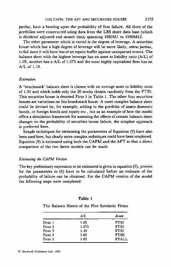
paribus, have a bearing upon the probability of firm failure. All three of the portfolios were constructed using data from the LBS share data base (which is dividend adjusted end month data) spanning 1980M1 to 1990M12.

The other parameter which is varied is the degree of leverage. A securities house which has a high degree of leverage will be more likely, c c t m paribus, to fail since it will have less of an equity buffer against unexpected events. The balance sheet with the highest leverage has an asset to liability ratio (A/L) of 1.05, another has a A/L of 1.075 and the most highly capitalised firm has an A/L of 1.10.

Estimation

A ‘benchmark’ balance sheet is chosen with an average asset to liability ratio of 1.05 and which holds only the 20 stocks chosen randomly from the FT30. This securities house is denoted Firm 1 in Table 1. The other four securities houses are variations on this benchmark house. A more complex balance sheet could be devised by, for example, adding to the portfolio of assets domestic bonds, or foreign bonds and equity etc., but as an example of how the model offers a simulation framework for assessing the effects of certain balance sheet changes on the probability of securities house failure, the simplest approach is preferred here.

Simple techniques for estimating the parameters of Equation (9) have also been used here, but clearly more complex techniques could have been employed. Equation (9) is estimated using both the CAPM and the AFT so that a direct comparison of the two factor models can be made.

Estimating the CAPM Version

The key preliminary expression to be estimated is given in equation (6)) proxies for the parameters in (6) have to be calculated before an estimate of the probability of failure can be obtained. For the CAPM version of the model the following steps were completed:

Table 1

The Balance Sheets of the Five Synthetic Firms

AIL Assets

Firm 1 Firm 2 Firm 3 Firm 4 Firm 5

1.05 1.075 1.10 1.05 1.05

FT30 FT30 FT30 FTSE FTALL


1156 CLARE

(1) Firstly, for the period 1980M1 to 1989M12 regression (10) was estimated:

where R, is the return on either of the three portfolios of assets shown in Table 1; bo and b, are OLS coefficients; R , is the return on the FT- ALL share index; R, is the risk free rate, proxied by the UK government three month T-Bill rate; and ex is a white noise error term.

(2) The fitted value of (lo), k,, was used as the expected return on portfolio x and by subtracting the risk free rate from this estimate a proxy for the expected excess return of the firm’s assets (ai in equation (6)) is obtained. Similarly 6, is used as an estimate of & (where j = 1).

(3) The proxy for 4 was taken to be e:, while the actual variance of the market over the period 1980M1 to 1989M12 was used as the proxy for 4, although clearly it would be possible to use a GARCH model to estimate this second parameter.

(4) To estimate the expected return on the market, pj, a simple average of past returns over the period 1980M1 to 1989M12 was calculated. An alternative might have been to use a simple AR model.

(5) Having obtained suitable proxies for the parameters of (9) the probability of firm failure was calculated for each of the five firms for 1990M1. Regulators could estimate all the parameters above easily at the beginning of each month to give the conditional probability that the firm would fail by the end of the month.

(6) Finally, Steps (1) to (5) were repeated moving each of the relevant data periods forward by one month to give the probability of failure for each of the firms on a rolling basis for each month of 1990.

Estimating the APT Version

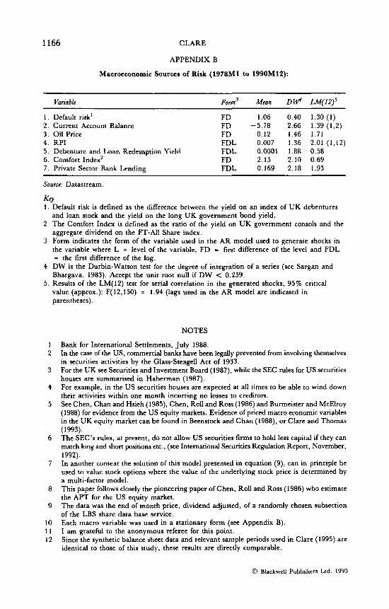
Before the estimation of the APT version can begin the factors making up the k factor generation process must be specified. The underlying macro economic variables used here were found by Clare and Thomas (1994)* to have been priced in the UK stock market over the period 1978M1 to 1990M12. The authors used the two step Fama and MacBeth technique (Fama and Macbeth, 1973) to estimate the risk premia of the macro factors driving the returns on 840 UK quoted common stock^.^ The priced macro economic variables are listed below and some basic descriptive statistics of the seven variables are presented in Appendix B.

The Macro Variables are:

(a) The dollar price of oil. (b) The redemption yield on a portfolio of UK debenture and loan stock. (c) An indicator of corporate default risk.

@ Rlackwell Publishers Ltd. 1995


(d) The spread between the yield on UK government consols and the aggregate market dividend yield.

(e) The retail price index. (0 UK private sector bank lending to UK residents. (g) The UK Current Account Balance.

The procedure used to estimate the APT version using the seven macro economic factors listed above was as follows:

(1) For the period 1980M1 to 1989M12 the following regression was estimated:

k

R,I = + C + vXl (11) J ' I

where a. is a constant; is the sensitivity of portfolio of assets x to the j th common factor; S, is the innovation (see step (4) below) in factor j ; and u, is a white noise error term specific to portfolio x .

(2) From equation (1 l), f i x is used as the expected value of portfolio x and by subtracting the risk free rate of interest from this estimate, a proxy for the expected excess return can be obtained. Also, the ag?s are used as the estimates of the &'s.

(3) The specific variance of the portfolio (d in (6)) is proxied by u,'. (4) The innovations in the macro factor series' were generated using the

residuals from an AR( 12) model (which was simplified where appropriate by deleting insignificant lags) of the form:

12 ..

Mjl = do + C 4MjI-i + S,! i- I

where Mj represents macro factor j; do is a constant; d . is an OLS coefficient; and S, is the innovation in macro variable 4;" The basic criterion was that the residuals should not be auto correlated and could therefore be regarded as innovations, a test for serial correlation in the residuals is presented in Appendix B. These generated regressors were used as the shocks (,!$'s in (1 l)) , while the fitted values of these AR models were taken as the conditional expected return of each factor respectively, pj.

(5) Since the actual variable used in (10) is a shock, the square of S, was taken to represent the conditional variance of the factor, 4.

(6) The information thus assembled was then used to estimate equation (9) and the probability of failure for each of the synthetic firms for 1990M1.

(7) Steps 1-6 were repeated on a rolling basis to give an estimate of the probability of failure for the seven firms from 1990M1 to 1990M12.


1158 CLARE

The Appropriateness of OLS to Estimnte Equation (6)

Equations (10) and (1 1) represent the usual way in which the parameters of the CAPM and APT are estimated respectively. Researchers use discrete time series data on the factors and the asset, or portfolio of interest. For the purposes of this model using OLS to estimate the parameters for equation (9) will produce unbiased estimates of the sensitivities of the portfolios to either the market, or the macro factors. However, the constant in these two regressions, bo and no respectively, represent the following:

1 1 2 bo = CY; - - @f$m - - ~ i , (CAPM) 2 2

where fli, is just the usual CAPM beta coefficient and u: is the variance of the market. It can be seen from (13a) and (13b) that the estimate of the constant will be biased. Unless flim, or equivalently Pil t3 f l ,k are equal to zero, where the asset or portfolio has no systematic component of risk. The extent of the bias will depend upon the relative magnitudes of and ~ in the case of (13a), and the relative magnitudes of ujs and u' in the case of (13b).

Another problem with using OLS to estimate the parameters of the model is that although we have correctly identified the fact that using a more conventional portfolio model of a securities house (as Miles and Hall, 1988 do) ignores the limited liability feature of equity ownership, the usual OLS estimates of the APT and the CAPM also ignore the limited liability feature of equity ownership." Although this is clearly an unsatisfactory way of estimating such models it is the conventional way of estimating them (for example see Ronn and Verma, 1986, or 1989). However, since the purpose of this exercise is to give an example of how simulation exercises may be conducted within this framework, OLS estimates of equation (6) should suffice.

Results

The estimates of the probability of firm failure for each of the five synthetic securities houses using both the single factor and multi factor versions of the model presented above, are plotted in Figures 1 to 5.

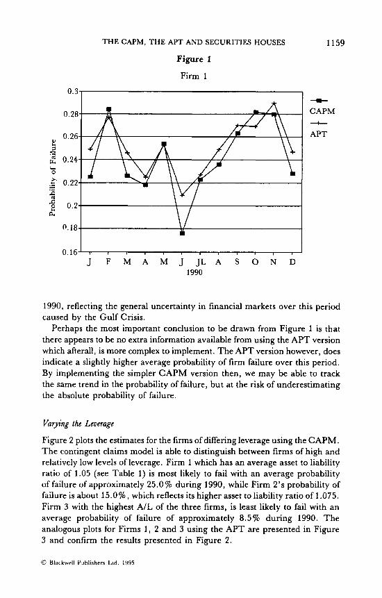
Figure 1 plots the estimated porbability of failure for the control firm, Firm 1, using both factor models. Clearly the differences between the two estimates are very small. Both models track the same trend in the estimates and are almost identical in magnitude. For Firm 1 then, the probability of failure is approximately 25 76, which would be well above the level which one would wish to see in financial markets, however since this is a sensitivity exercise the absolute value has little meaning. It is interesting to note that both models track a steady increase in the probability of failure between July and November of


THE CAPM, THE APT AND SECURITIES HOUSES

Figure 1

Firm 1

1159

-.- I --c CAPM + APT

0.16’ I I J F M A M J J L A S 0 N D

1990

1990, reflecting the general uncertainty in financial markets over this period caused by the Gulf Crisis.

Perhaps the most important conclusion to be drawn from Figure 1 is that there appears to be no extra information available from using the APT version which afterall, is more complex to implement. The APT version however, does indicate a slightly higher average probability of firm failure over this period. By implementing the simpler CAPM version then, we may be able to track the same trend in the probability of failure, but at the risk of underestimating the absolute probability of failure.

Varying the Leverage

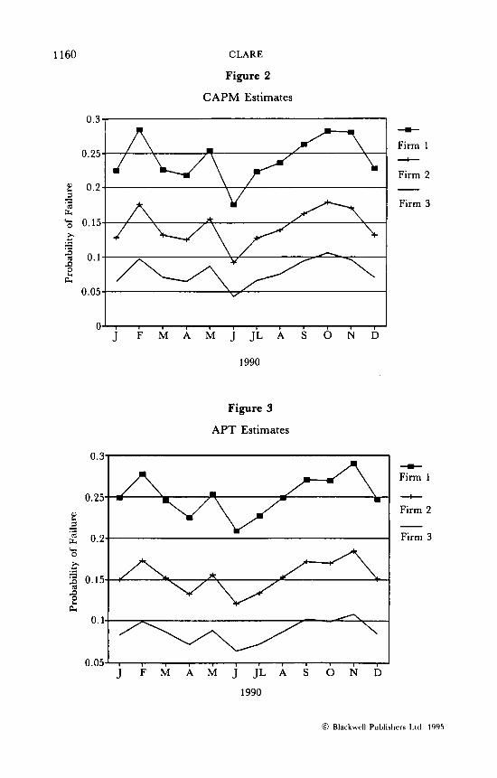
Figure 2 plots the estimates for the firms of differing leverage using the CAPM. The contingent claims model is able to distinguish between firms of high and relatively low levels of leverage. Firm 1 which has an average asset to liability ratio of 1.05 (see Table 1) is most likely to fail with an average probability of failure of approximately 25.0% during 1990, while Firm 2 ’ s probability of failure is about 15.096, which reflects its higher asset to liability ratio of 1.075. Firm 3 with the highest A/L of the three firms, is least likely to fail with an average probability of failure of approximately 8.5% during 1990. The analogous plots for Firms 1, 2 and 3 using the APT are presented in Figure 3 and confirm the results presented in Figure 2.

0 Blackwell Publishers I d . l Y Y 5

1160 CLARE

Figure 2

CAPM Estimates

0.3-

0.25-

8 0 .2 - 1

F4

- .-

% 0.15- x c) .- - 2 0.1- P

a e 0.05- V

0' I 1

J F M A M J J L A S O N D

1990

Figure 3

APT Estimates

0.25-

- 5 .4 2 0.2- LI

a 0.1-

-m-

Firm 1 + Firm 2

Firm 3

--c Firm 1

+ Firm 2

Firm 3

0 . 0 5 ' , I I J F M A M J JL A S 0 N D

1990

@ Rlackwell Publishers Ltcl. 1995


Varying Asset Quality

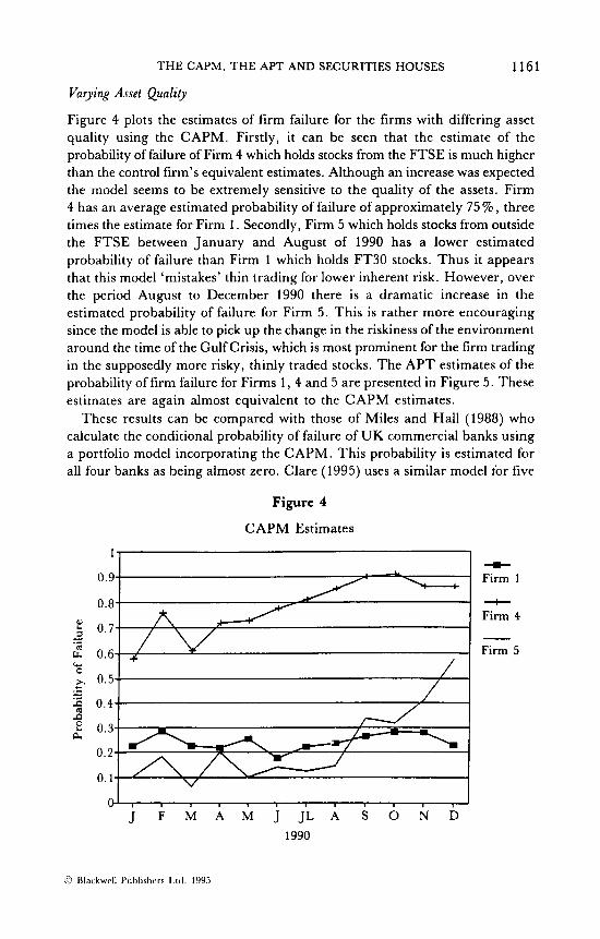
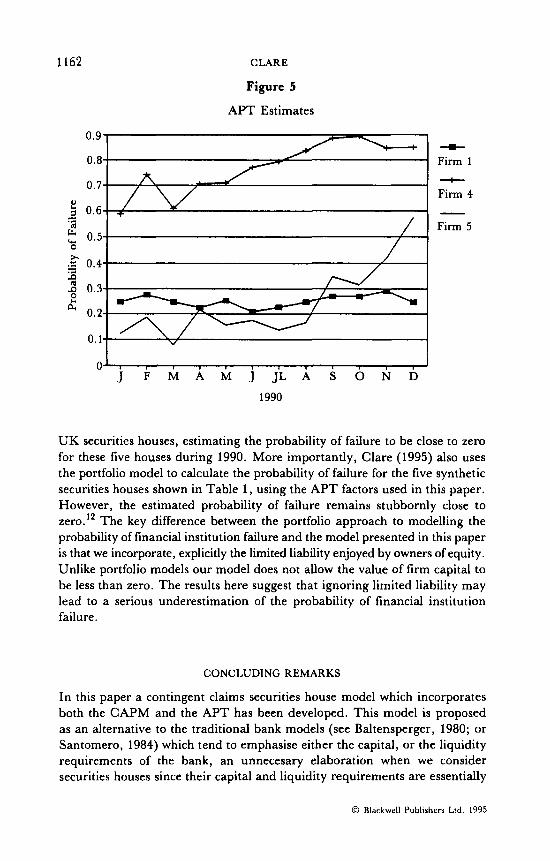
Figure 4 plots the estimates of firm failure for the firms with differing asset quality using the CAPM. Firstly, it can be seen that the estimate of the probability of failure of Firm 4 which holds stocks from the FTSE is much higher than the control firm's equivalent estimates. Although an increase was expected the model seems to be extremely sensitive to the quality of the assets. Firm 4 has an average estimated probability of failure of approximately 75 %I, three times the estimate for Firm 1. Secondly, Firm 5 which holds stocks from outside the FTSE between January and August of 1990 has a lower estimated probability of failure than Firm 1 which holds FT30 stocks. Thus it appears that this model 'mistakes' thin trading for lower inherent risk. However, over the period August to December 1990 there is a dramatic increase in the estimated probability of failure for Firm 5. This is rather more encouraging since the model is able to pick up the change in the riskiness of the environment around the time of the Gulf Crisis, which is most prominent for the firm trading in the supposedly more risky, thinly traded stocks. The APT estimates of the probability of firm failure for Firms 1, 4 and 5 are presented in Figure 5. These estimates are again almost equivalent to the CAPM estimates.

These results can be compared with those of Miles and Hall (1988) who calculate the conditional probability of failure of UK commercial banks using a portfolio model incorporating the CAPM. This probability is estimated for all four banks as being almost zero. Clare (1995) uses a similar model ior five

Figure 4

CAPM Estimates

". 1

x

v

0.5- / I

--Ir Firm 1

+ Firm 4

Firm 5

0 Blackwrll Publlshcrs Ltd. 1995

1162 CLARE

Figure 5

APT Estimates

0.9

0.8

0.7

5 0.6

2 0.5

.z 0.4

8 0.3 e

- .d

0 x r;l P

a 0.2

0.1

0 J F M A M J JL A S 0 N D

1990

- Firm 1 + Firm 4

Firm 5

UK securities houses, estimating the probability of failure to be close to zero for these five houses during 1990. More importantly, Clare (1995) also uses the portfolio model to calculate the probability of failure for the five synthetic securities houses shown in Table 1, using the APT factors used in this paper. However, the estimated probability of failure remains stubbornly close to zero. l2 The key difference between the portfolio approach to modelling the probability of financial institution failure and the model presented in this paper is that we incorporate, explicitly the limited liability enjoyed by owners of equity. Unlike portfolio models our model does not allow the value of firm capital to be less than zero. The results here suggest that ignoring limited liability may lead to a serious underestimation of the probability of financial institution failure.

CONCLUDING REMARKS

In this paper a contingent claims securities house model which incorporates both the CAPM and the APT has been developed. This model is proposed as an alternative to the traditional bank models (see Baltensperger, 1980; or Santomero, 1984) which tend to emphasise either the capital, or the liquidity requirements of the bank, an unnecesary elaboration when we consider securities houses since their capital and liquidity requirements are essentially

0 Blarkwrll Publishers Ltd. 1995


one and the same. We also propose this model as an alternative to portfolio based models of financial institutions since these ignore the limited liability aspect of equity ownership (see Miles and Hall, 1988; or Clare, 1995). Since regulators in the UK and the US are currently implementing a risk based regulatory system for securities houses, the model presented in this paper offers a framework which might enable regulators and perhaps securities house’ managers themselves, to gauge the effect which changes in asset quality and leverage may have on the probability of the firm’s failure.

The main conclusions of the paper are as follows:

1. The model, was found to be sensitive to changes in the leverage and asset quality of a synthetic securities house. For example, ceterurparibus, decreasing leverage from 1.075 to 1.1 reduces the probability of failure by a factor of almost 2. It therefore may be of use to regulators in designing more appropriate risk based capital adequacy rules for securities house’ capital. Of crucial importance is the comparative performances of the CAPM and APT versions of the model, previously unexplored in a contingent claims context. The two versions of the model revealed similar trends in the conditional probability of failure. Since the CAPM version does not require the prior identification of the macro factors, as the APT version does, its application is far simpler and therefore it must be preferred to the APT version. However, the cost of employing the simpler approach may lead to an underestimation of the probability of failure.

2,

Future research could include expanding the composition of the firm’s assets and/or respecifying the model so that the firm’s liabilities also develop as a geometric random walk, i.e. modelling the firm as a compound option (for example see Geske, 1979).


1164 CLARE

APPENDIX A

Barclayi De Zoete Wedd Holding8 (C.) Balance Sheet a8 at - 31/12/90

Assets

A. LOANS & ADVANCES 1. Advances to group companies 2. Customer loans/advances (less than 1 year)

Total A

B. OTHER EARNING ASSETS 1. Money at call 2. Deposits with banks, Discount houses and local authorities 3. Certificates of Deposit 4. Treasury bills 5. Trade and other bills (discounted) 6. Dealing assets 7. Investments: quoted 8. Investments: unquoted (properties) 9. Securities purchased under agreement to resell

10. Securities (long positions) 11. Equity investments in associates

Total B

C. TOTAL EARNING ASSETS (A + B)

D. FIXED ASSETS

E. NON-EARNING ASSETS 1. Cash and Due from Banks 2. Other

F. TOTAL ASSETS

Liabilities

A. SHORT-TERM FUNDING 1. Time Deposits 2. Interbank Deposits 3. Short term deposits

Total A

B. OTHER FUNDING 1. Loan secured against stock deposited 2. Subordinated Debt

C. OTHER (Non-int. bearing) 1. Securities - Short Positions 2. Other creditors payable (securities bus) 3. Tax payable 4. Sundry creditors

D. EQUITY

E. TOTAL LIABILITIES & EQUITY

f m

767.2 165.7

932.9

192.7 704.6 240.3

16.5 121.7

10.4 28.9 55.5

2441.5 2712.3

0.3

6524.7

7457.6

42.9

1190.6 1962.1

10653.2

1221.0 359.9 974.0

2554.9

808.8 51.8

4758.3 1796.5

14.5 335.6

332.8

10653.2


T H E CAPM, T H E APT AND SECURITIES HOUSES 1165

Barclays Bank plc Balance Sheet as a t - 31/12/90

Assets

A. LOANS & ADVANCES 1. Customer loans/advances (domestic) 2. Customer loans/advances (international) 3. Lease receivables 4. Loan loss reserves

Total A

B OTHER EARNING ASSETS 1. Placings with banks (over 1 month) 1. Money at call 2. Certificates of Deposit 3. Treasury bills 4. Trade and other bills (discounted) 5. Investments: quoted (in UK) 6. Investments: quoted (overseas) 7. Investments: unquoted (properties) 8. Securities purchased under agreement to resell 9. Securities (long positions)

10. Other

Total B

C. TOTAL EARNING ASSETS (A + B)

D. FIXED ASSETS

E. NON-EARNING ASSETS 1. Cash and Due from Banks 2. Other

F. TOTAL ASSETS

Liabilities

A. SHORT-TERM FUNDING 1. Demand deposits 2. Savings deposits 3. Time deposits

Total A

B. OTHER FUNDING 1. Securities business 2. Subordinated Debt 3. Other

C . OTHER (Non-int. bearing) 1. Securities - Short Positions 2. Other

D. EQUITY

E. TOTAL LIABILITIES & EQUITY

Em

58731.0 1991 5 .O 4956.0

(2335.0)

81 267 .O

10883.0 10554.0 4012.0 3552.0 2393.0

105.0 1000.0 494.0

2441 .O 2637.0 1776.0

39353.0

120620.0

2507.0

4400.0 7360.0

134887.0

14604.0 20832.0 74728.0

110164.0

2929.0 1652.0 1572.0

2638.0 9352.0

6580.0

134887.0


1166 CLARE

APPENDIX B

Macroeconomic Sources of Risk (1978M1 to 1990Ml2):

Variable Form3 Mean OW' LM(I2)'

1 . Default risk' FD 1.06 0.40 1.30 (1) 2. Current Account Balance FD -5.78 2.66 1.39 (1,2) 3 . Oil Price FD 0.12 1.46 1.71 4. RPI FDL 0.007 1.36 2.01 (1,12) 5 . Debenture and Loan Redemption Yield FDL 0.0001 1.88 0.58 6. Comfort Index' FD 2.15 2.10 0.69 7. Private Sector Bank Lending FDL 0.169 2.18 1.93

Source: Datastream.

KCY I . Default risk is defined as the difference between the yield on an index of UK debentures

and loan stock and the yield on the long UK government bond yield. 2 The Comfort Index is defined as the ratio of the yield on U K government consols and the

aggregate dividend on the FT-All Share index. 3 Form indicates the form of the variable used in the AR model used to generate shocks in

the variable where L = level of the variable, FD - first difference of the level and FDL = the first difference of the log.

Bhargava, 1983). Accept the unit root null if DW < 0.259.

value (approx.): F(12,150) = 1.94 (lags used in the AR model are indicated in parentheses).

4 DW is the Durbin-Watson test for the degree of integration of a series (see Sargan and

5. Results of the LM(12) test for serial correlation in the generated shocks, 95% critical

1 2

3

4

5

6

7

8

9

10 11 12

NOTES

Bank for International Settlements, July 1988. In the case of the US, commercial banks have been legally prevented from involving themselves in securities activities by the Glass-Steagell Act of 1933. For the UK see Securities and Investment Board (1987), while the SEC rules for US securities houses are summarised in Haberman (1987). For example, in the US securities houses are expected at all times to be able to wind down their activities within one month incurring no losses to creditors. See Chen, Chan and Hsieh (1985), Chen, Roll and Ross (1986) and Burmeister and McElroy (1988) for evidence from the US equity markets. Evidence of priced macro economic variables in the UK equity market can be found in Beenstock and Chan (1988), or Clare and Thomas (1993). The SEC's rules, at present, do not allow US securities firms to hold less capital if they can match long and short positions etc., (see International Securities Regulation Report, November, 1992). In another context the solution of this model presented in equation (9), can in principle be used to value stock options where the value of the underlying stock price is determined by a multi-factor model. This paper follows closely the pioneering paper of Chen, Roll and Ross (1986) who estimate the APT for the US equity market. The data was the end of month price, dividend adjusted, of a randomly chosen subsection of the LBS share data base service. Each macro variable was used in a stationary form (see Appendix B). I am grateful to the anonymous referee for this point. Since the synthetic balance sheet data and relevant sample periods used in Clare (1995) are identical to those of this study, these results are directly comparable.



REFERENCES

Baltensperger, E. (1979), ‘Alternative Theories of the Banking Firm’, Journal ofMonchry Economic$,

The Bank for International Settlements (1988), Znfemafional Convergence of Capifal Measurement and

Beenstock, M. and K.C. Chan (1988), ‘Economic Forces in the London Stockmarket’, O$ordBullCtin

Berger, A.N., K.A. Kuester and J.M. O’Brien (1989), Banking S y s h Risk: Charting a New Course

Black, F. and M. Scholes (1972), ‘The Valuation of Option Contracts and a Test of Market

Burmeister, E. and M.B. McElmy (1988), ‘Joint Estimation of Factor Sensitivities and Risk Premia

Chan, K.C., N. Chen and D.A. Hsieh (1985), ‘An Exploratory Investigation of the Firm Size

Chen, N., R. Roll and S.A. Ross (1986), ‘Economic Forces and the Stockmarket’, JoumalofBuriws,

Clare, A.D. (1995), ‘Using the APT to Calculate the Probability of Financial Institution Failure’,

-and S.H. Thomas (1994), ‘Macroeconomic Factors, the APT and the UK Stockmarket’,

-, G.W. McKenzie and S.H. Thomas (1991). ‘The Regulation of Securities Firms: Some

Cox, J.C. and S.A. Ross (1976), ‘The Valuation of Options for Alternative Stochastic Processes’,

Deutsche Bundesbank (1986), ‘The Banking Act of the Federal Republic of Germany’, Deutsche

Economisf, The (1992), ‘Accounting for Banks’ (May 9th-15th). pp. 20 and 106. European Community (1993), ‘On the Capital Adequacy of Investment Firms and Credit

Institutions’, The Oficial Journal of fhe European Communifies, Council Directive, 93/6/EEC (March).

Fama, E.F. and J.D. MacBeth (1973), ‘Risk, Return and Equilibrium: Empirical Tests’, Journal of Political Economy, Vol. 38, pp. 607-36.

Geske, R. (1979), ‘The Valuation of Compound Options’, Journal ofFinancia1 Economics, Vol. 7, pp. 63-81.

Haberman, G. (1987), ‘Capital Requirements of Commercial and Investment Banks: Contrasts in Regulation’, Federal Reserue Board ofNew York Quarfer(y Review (Autumn) pp. 1-10,

International Securities Regulation Report (1992), US Europe Splif on Capital Adequacy Standards. Vol. 5 (Buraff Publications, Washington DC), No. 23.

Lintner, J. (1965) ‘The Valuation of Risky Assets and the Selection of Risky Investments in Stock Portfolios and Capital Budgets’, Review of Economics and Statistics, Vol. 47, pp. 13-37.

Merton, R. (1973), ‘Theory of Rational Option Pricing’, Bell Journal ofEconomics and Management Science, Vol. 4, pp. 141-183. - (1974) ‘On the Pricing of Corporate Debt: The Risk Structure of Interest Rates’, Journal

of Finance, Vol. 29, pp. 449-470. - (1977). ‘An Analytic Derivation of the Cost of Deposit Insurance and Loan Guarantees:

An Application of Modern Option Pricing Theory’, Journal OfEanking and Finance, Vol. 1, pp. 3-1 1.

Miles D. and S. Hall (1988), ‘Measuring the Risk of Financial Institutions Portfolios: Some Suggestions for Alternative Techniques Using Stock Prices’, LSE Financial Markets Group Discussion Paper Series, No. 0029.

Ronn, E. and A. Verma (1986), ‘Pricing Risk-Adjusted Deposit Insurance: An Option Based Model’, Journal ofFinance, Vol. 41, pp. 871-895. - - (1989). ‘Risk Based Capital Adequacy for a Sample of 43 Major Banks’, Journal

OfBanking and Finance, Vol. 13, pp. 21-29. Ross, S.A. (1976), ‘The Arbitrage Theory of Capital Asset Pricing’, Journal $Economic Theory,

Vol. 13, pp. 341-60.

Vol. 6, pp. 1-37.

Capital Sfandords (Committee on Banking Regulations and Supervisory Practices).

of Economics and Statisfics, Vol. 50, pp. 27-39.

(Federal Reserve Board of Chicago), pp. 515-546.

Efficiency’, Journal of Finance, Vol. 27, pp. 399-417.

for the Arbitrage Pricing Theory’, Journal of Finance, Vol. 3, pp. 721-35.

Effect’, Journal of Financial Economics, Vol. 14, pp. 451-71.

Vol. 59, pp. 383-403.

The Journal of Money, Credif and Banking,Vol. 27, pp. 200-204.

Journal of Business Finance &Accounting, Vol. 21, No. 3 (April), pp. 309-330.

Kpy Issues’, Revisfa Intemazionale d i Scienze Sociali (JanuaryIMarch).

Journal of Financial Economics, Vol. 3, pp. 145-66.

Bundesbank Special Series, No. 2.

0 Blkckwell Publishers Ltd. 1995

1168 CLARE

Santomero, A.M. (1984), ‘Modeling the Banking Firm: A Survey’, Journal OfMonty Crcdif and

Sharpe, W.F. (1964), ‘Capital Asset Prices: A Theory of Market Equilibrium Under Conditions

SIB, Securities and Investments Board (1987), Financial Regulations (London). Smith, C.W. Jr. (1976), ‘Option Pricing: A Review’,JoumolofFiMntiolEconomics, Vol. 3, pp. 3-51.

Banking, Vol. 16, pp. 576-604.

of Risk’, Journal of Finance, Vol. 19, pp. 425-42.

@ Blackwell Publishers Ltd. 1995

THE CAPM, THE APT AND A CONTINGENT CLAIMS MODEL OF A SECURITIES HOUSE

Documents

Transcript of THE CAPM, THE APT AND A CONTINGENT CLAIMS MODEL OF A SECURITIES HOUSE